Time-resolved X-ray diffraction with accelerator- and laser-plasma-based

X-ray sources

Von der Fakultät für Physik der Universität Duisburg-Essen genehmigte

Dissertation

zur Erlangung des akademischen Grades eines Doktors der Naturwissenschaften (Dr. rer. nat.)

von

Matthieu Nicoul

aus Rennes (Frankreich) Referent: Prof. Em. Dr. Dietrich von der Linde Korreferent: Prof. Dr. Uwe Bovensiepen Vorsitzender des Prüfungsausschusses: Prof. Dr. Dietrich Wolf Tag der mündlichen Prüfung: 01. September 2010

ii

iii

A Esther, Sophie et Annabelle

iv

Acknowledgments

It would not have been possible to present the work of this thesis without the help,

assistance and support of a lot of persons.

I would like to thank first my supervisor Prof. Dr. Dietrich von der Linde and Dr.

Klaus Sokolowski-Tinten, for providing me the great opportunity to work on the exciting field

of time-resolved X-ray diffraction at the University Duisburg-Essen, but also to discover new

horizons by sending me at the SPPS.

I also want to thank Dr. Alexander Tarasevitch for his support and for always

answering my question concerning the laser system. Without his 10-Hz laser system, this

work would have never been made. I also want to thank Dr. Ping Zhou which has also always

answered my questions.

A very special thank also to Kay Eibl, for helping me with the administration issues

and for improving my English (which sounds always too much like French).

I also want to thank the technical staff, Michael Bieske for all the mechanical parts

required, Bernd Prof and Doris Steeger for their help in computer programming and

electronics, and Roland Kohn for all the computer related difficulties.

I want to thank especially Dr Uladzimir Shymanovich, for all the nights we spend in

the lab measuring, and for all your advices to improve my survival skills in Germany. You are

a dear friend.

I also want to thank all the others PhD students, starting with Wei Lu, Nikola

Stojanovic, Ivan Rajkovic, Manuel Ligges, Stephan Kähle, Konstantin Lobov, Oliver Heinz

and Jan Göhre, for all our exchanges.

I am grateful to Prof. Dr. Uwe Bovensiepen and Prof. Dr. Dietrich E. Wolf for their

agreement to review my thesis.

v

I finally want to thanks my parents and brothers, and my wife Esther for having

always stand behind me.

vi

Table of contents Acknowledgements . . . . . . . . . . . . . . . . . . . . . . . . . . . . . . . . . . . iv Table of contents . . . . . . . . . . . . . . . . . . . . . . . . . . . . . . . . . . . . . vi 1. Introduction . . . . . . . . . . . . . . . . . . . . . . . . . . . . . . . . . . . . . . . 1

1.1. Background . . . . . . . . . . . . . . . . . . . . . . . . . . . . . . . . . . . . . . . . . . . . . . . . . . . . 1 1.2. Motivation . . . . . . . . . . . . . . . . . . . . . . . . . . . . . . . . . . . . . . . . . . . . . . . . . . . . . 2 1.3. Structure of the thesis . . . . . . . . . . . . . . . . . . . . . . . . . . . . . . . . . . . . . . . . . . . . 3

2. Production of ultrafast X-ray pulses . . . . . . . . . . . . . . . . . . . . 5

2.1. Sources based on characteristic line emission . . . . . . . . . . . . . . . . . . . . . . . . . 5 2.1.1. Laser driven X-ray diode . . . . . . . . . . . . . . . . . . . . . . . . . . . . . . . . . . . . . 5 2.1.2. Laser-plasma source . . . . . . . . . . . . . . . . . . . . . . . . . . . . . . . . . . . . . . . . . 6

2.2. Sources based on electron accelerator . . . . . . . . . . . . . . . . . . . . . . . . . . . . . . . 7 2.2.1. Laboratory-sized source . . . . . . . . . . . . . . . . . . . . . . . . . . . . . . . . . . . . . . 8 2.2.2. Accelerator-sized source . . . . . . . . . . . . . . . . . . . . . . . . . . . . . . . . . . . . . . 9

2.2.2.1. Synchrotron 3rd generation . . . . . . . . . . . . . . . . . . . . . . . . . . . . . . . . 9 2.2.2.2. Modified Synchrotron 3rd generation sources . . . . . . . . . . . . . . . . . 10

2.2.2.2.1. The orbit deflection bunch method . . . . . . . . . . . . . . . . . . . . . . 10 2.2.2.2.2. The slicing source . . . . . . . . . . . . . . . . . . . . . . . . . . . . . . . . . . . 10

2.2.2.3. X-ray sources of the fourth generation . . . . . . . . . . . . . . . . . . . . . . . 11 2.2.2.3.1. Linac-based X-ray source . . . . . . . . . . . . . . . . . . . . . . . . . . . . . 11 2.2.2.3.2. The X-ray Free Electron Laser . . . . . . . . . . . . . . . . . . . . . . . . . 12

2.3. Comparison of the sources . . . . . . . . . . . . . . . . . . . . . . . . . . . . . . . . . . . . . . . . 13 2.4. Perspectives . . . . . . . . . . . . . . . . . . . . . . . . . . . . . . . . . . . . . . . . . . . . . . . . . . . . 13

3. Laser-plasma based sources, new setups . . . . . . . . . . . . . . . . 14

3.1. Principle and important parameters of a laser-plasma based X-ray source . . . 14 3.2. Laser system . . . . . . . . . . . . . . . . . . . . . . . . . . . . . . . . . . . . . . . . . . . . . . . . . . . 16 3.3. Laser-plasma X-ray sources . . . . . . . . . . . . . . . . . . . . . . . . . . . . . . . . . . . . . . . 18

3.3.1. X-ray mirrors . . . . . . . . . . . . . . . . . . . . . . . . . . . . . . . . . . . . . . . . . . . . . . . 18 3.3.1.1. Bent crystal mirror . . . . . . . . . . . . . . . . . . . . . . . . . . . . . . . . . . . . . . . 18 3.3.1.2. Multilayer X-ray mirror . . . . . . . . . . . . . . . . . . . . . . . . . . . . . . . . . . . 20 3.3.1.3. Other X-ray mirrors . . . . . . . . . . . . . . . . . . . . . . . . . . . . . . . . . . . . . . 24

vii

3.3.1.4. Comparison of the bent and multilayer mirrors . . . . . . . . . . . . . . . . 25 3.3.2. Modular setup for time resolved X-ray diffraction . . . . . . . . . . . . . . . . . . 26

3.3.2.1. “Big” in-vacuum set-up. . . . . . . . . . . . . . . . . . . . . . . . . . . . . . . . . . . 27 3.3.2.2. The modular setups . . . . . . . . . . . . . . . . . . . . . . . . . . . . . . . . . . . . . . 29

3.3.2.2.1. The wire-based modular setup . . . . . . . . . . . . . . . . . . . . . . . . . . 29 3.3.2.2.2. The tape target setup . . . . . . . . . . . . . . . . . . . . . . . . . . . .. . . . . . 32

3.3.3. The sample holder . . . . . . . . . . . . . . . . . . . . . . . . . . . . . . . . . . . . . . . . . . . 36 3.3.4. The detectors . . . . . . . . . . . . . . . . . . . . . . . . . . . . . . . . . . . . . . . . . . . . . . . 37

3.3.4.1. Direct detection camera . . . . . . . . . . . . . . . . . . . . . . . . . . . . . . . . . . . 38 3.3.4.2. Indirect detection camera . . . . . . . . . . . . . . . . . . . . . . . . . . . . . . . . . 39 3.3.4.3. Avalanche Photodiode (APD) . . . . . . . . . . . . . . . . . . . . . . . . . . . . . . 40

3.3.5. Air absorption . . . . . . . . . . . . . . . . . . . . . . . . . . . . . . . . . . . . . . . . . . . . . . 40 3.3.6. Optical beam paths in the setups . . . . . . . . . . . . . . . . . . . . . . . . . . . . . . . . 40

3.3.6.1. Pre-pulse . . . . . . . . . . . . . . . . . . . . . . . . . . . . . . . . . . . . . . . . . . . . . . 41 3.3.6.2. Pump beam . . . . . . . . . . . . . . . . . . . . . . . . . . . . . . . . . . . . . . . . . . . . 41 3.3.6.3. Probe pulse . . . . . . . . . . . . . . . . . . . . . . . . . . . . . . . . . . . . . . . . . . . . 41

3.3.7. X-ray output from the multilayer optic . . . . . . . . . . . . . . . . . . . . . . . . . . . 42 3.3.8. Adjustment of the modular setups . . . . . . . . . . . . . . . . . . . . . . . . . . . . . . . 45

3.3.9. Normalization and stability of the tape-target setup . . . . . . . . . . . . . . . . . . . 50 3.4 Summary and Outlook . . . . . . . . . . . . . . . . . . . . . . . . . . . . . . . . . . . . . . . . . . . . 52

4. Transient acoustic response in femtosecond optically excited materials . . . . . . . . . . . . . . . . . . . . . . . . . . . . . . . . . . . . . . . . . . . 53

4.1. Physical response following femtosecond optical excitation . . . . . . . . . . . . . . 53 4.1.1. Semiconductors . . . . . . . . . . . . . . . . . . . . . . . . . . . . . . . . . . . . . . . . . . . . . 54 4.1.2. Metals . . . . . . . . . . . . . . . . . . . . . . . . . . . . . . . . . . . . . . . . . . . . . . . . . . . . 55

4.2. Acoustic waves in fs-optically excited gallium arsenide . . . . . . . . . . . .. . . . . . 56 4.2.1. Previous work . . . . . . . . . . . . . . . . . . . . . . . . . . . . . . . . . . . . . . . . . . . . . . 57 4.2.2. Laser-generated acoustic waves in gallium arsenide . . . . . . . . . . . . . . . . 60

4.2.2.1. Experimental setup and data analysis . . . . . . . . . . . . . . . . . . . . . . . . 60 4.2.2.2. Experimental data . . . . . . . . . . . . . . . . . . . . . . . . . . . . . . . . . . . . . . . 62 4.2.2.3. Modeling of the acoustic response . . . . . . . . . . . . . . . . . . . . . . . . . . 65 4.2.2.4. Acoustic pulse speed . . . . . . . . . . . . . . . . . . . . . . . . . . . . . . . . . . . . . 71

4.2.3. Summary and discussion of the measurement on gallium arsenide . . . . . 76 4.3. Picosecond acoustic response of a laser-excited gold-film . . . . . . . . . . . . . . . . 78

4.3.1. Description of the experimental setup . . . . . . . . . . . . . . . . . . . . . . . . . . . . 78 4.3.2. Experimental data, analysis and discussion . . . . . . . . . . . . . . . . . . . . . . . 80 4.3.3. Modeling and interpretation of the experimental data . . . . . . . . . . . . . . . 86

4.3.3.1. Ratio γe / γi = 1 . . . . . . . . . . . . . . . . . . . . . . . . . . . . . . . . . . . . . . . . . 89 4.3.3.2. Ratio γe / γi ≠ 1 . . . . . . . . . . . . . . . . . . . . . . . . . . . . . . . . . . . . . . . . . 90

4.3.4. Summary and discussion of the measurements on gold . . . . . . . . . . . . . . 94

5. The Sub-Picosecond Pulse Source . . . . . . . . . . . . . . . . . . . . . 95

5.1. Presentation of the SPPS . . . . . . . . . . . . . . . . . . . . . . . . . . . . . . . . . . . . . . . . . . 95 5.1.1. General overview . . . . . . . . . . . . . . . . . . . . . . . . . . . . . . . . . . . . . . . . . . . 96 5.1.2. Temporal resolution of the SPPS beamline . . . . . . . . . . . . . . . . . . . . . . . 98

viii

5.1.2.1. The crossed-beam geometry . . . . . . . . . . . . . . . . . . . . . . . . . . . . . . . 98 5.1.2.2. The Electro-Optic technique . . . . . . . . . . . . . . . . . . . . . . . . . . . . . . . 99

5.2. Presentation of the scientific work performed at the SPPS . . . . . . . . . . . . . . . 102 5.2.1. Optical phonons in bismuth . . . . . . . . . . . . . . . . . . . . . . . . . . . . . . . . . . . 102

5.2.1.1. Presentation . . . . . . . . . . . . . . . . . . . . . . . . . . . . . . . . . . . . . . . . . . . . 102 5.2.1.2. Experimental setup and methodology . . . . . . . . . . . . . . . . . . . . . . . . 105 5.2.1.3. Measurements with high temporal resolution - results and

discussion . . . . . . . . . . . . . . . . . . . . . . . . . . . . . . . . . . . . . . . . . . . . . . 108 5.2.1.4. Conclusion and perspective . . . . . . . . . . . . . . . . . . . . . . . . . . . . . . . . 112

5.2.2. Liquid phase dynamics after ultrafast melting in indium antimonide . . . . 113 5.2.2.1. Presentation . . . . . . . . . . . . . . . . . . . . . . . . . . . . . . . . . . . . . . . . . . . . 113 5.2.2.2. Experimental setup and methodology . . . . . . . . . . . . . . . . . . . . . . . . 115 5.2.2.3. Result and discussion . . . . . . . . . . . . . . . . . . . . . . . . . . . . . . . . . . . . 117 5.2.2.4. Conclusion . . . . . . . . . . . . . . . . . . . . . . . . . . . . . . . . . . . . . . . . . . . . . 125

5.3. Conclusion and perspectives . . . . . . . . . . . . . . . . . . . . . . . . . . . . . . . . . . . . . . . 125

6. Conclusion and outlook . . . . . . . . . . . . . . . . . . . . . . . . . . . . . 127

6.1 Summary . . . . . . . . . . . . . . . . . . . . . . . . . . . . . . . . . . . . . . . . . . . . . . . . . . . . . . 127 6.2 Outlook . . . . . . . . . . . . . . . . . . . . . . . . . . . . . . . . . . . . . . . . . . . . . . . . . . . . . . . 129

Annexes . . . . . . . . . . . . . . . . . . . . . . . . . . . . . . . . . . . . . . . . . . . 132

A. Bi(111) intensity versus equilibrium atomic position . . . . . . . . . . . . . . . . . . . . . 133 B. Sample material properties . . . . . . . . . . . . . . . . . . . . . . . . . . . . . . . . . . . . . . . . . 136

B.1. Gallium arsenide: GaAs . . . . . . . . . . . . . . . . . . . . . . . . . . . . . . . . . . . . . . . 136 B.2. Indium antimonide: InSb . . . . . . . . . . . . . . . . . . . . . . . . . . . . . . . . . . . . . . . 136 B.3. Thin film gold on substrate . . . . . . . . . . . . . . . . . . . . . . . . . . . . . . . . . . . . . 137

B.3.1. Gold: Au . . . . . . . . . . . . . . . . . . . . . . . . . . . . . . . . . . . . . . . . . . . . . . . 137 B.3.2. Mica muscovite . . . . . . . . . . . . . . . . . . . . . . . . . . . . . . . . . . . . . . . . . . 138

Bibliography . . . . . . . . . . . . . . . . . . . . . . . . . . . . . . . . . . . . . . . . 139

1

1. Introduction

The first chapter is organized as follows. In the first section the importance of

ultrashort X-ray pulses is discussed. The second section presents possible experiments which

can be performed using this kind of short X-ray pulses and the motivation of the work

presented in this thesis. The last section describes in detail the structure and the content of the

thesis.

1.1. Background

The aim of the work presented in this thesis is to study the structural dynamics of

matter driven out of equilibrium by a femtosecond optical pulse. For that purpose the

experimental setup must have atomic spatial resolution and a temporal resolution high enough

to observe the transient phenomena under investigation.

The atomic spatial resolution is achieved by using a short wavelength X-ray probe.

People realized immediately that the discovery of X-rays by William Conrad Roentgen in

1895 [1] would play a very important role in medicine and in the determination of the structure

of matter. This importance has been demonstrated by the fact that a large number of Nobel

Prizes were awarded for scientific work performed with X-rays. The first Nobel Prize for the

discovery of the X-rays was given to W. C. Roentgen in 1901; for the observation of X-ray

diffraction from crystals by von Laue in 1914 [2]; for the development of X-ray spectrometers

by Bragg father and son in 1915 [3]; for the discovery of the characteristic X-ray radiation by

Barkla in 1917; for the discoveries and research in the field of X-ray spectroscopy by

Siegbahn in 1924 [4]. For the discovery of the helix structure of the DNA using the X-ray

diffraction method, Watson, Crick and Wilkins received the Nobel Prize in Physiology or

Medicine in 1962 [5].

The determination of the atomic structure of matter is possible due to the small

wavelength of the X-rays. It is comparable to typical interatomic distances in matter, i.e.

2

several Angstroms. Using a suitable scattering technique the atomic structure can be resolved

with a spatial resolution of milliångstrom (10-13 m).

The required temporal resolution depends on the mechanism to be observed. Typical

time-scales for atomic vibrations, atomic motion and bond breaking are hundreds of

femtoseconds, to tens of picoseconds for the build up of acoustic waves and their propagation

into the material. Such short time scales are not accessible with common X-ray detectors (e.g.

photo diodes). For such high time-resolution the appropriate technique is a stroboscopic

measurement, also called the pump-probe technique. This technique uses two ultrashort

pulses. One is used to excite or “pump” the sample, i.e. to initiate the process under

investigation. The second pulse is used to “probe” the sample at a given delay time after

excitation.

Until the late 1980s, it was not possible to produce X-ray pulses shorter than hundreds

of ps. Very much shorter pulses became available with the development of femtosecond laser

technology [6, 7]. A few years later, using an intense laser pulse, it became possible to generate

the first sub-picosecond laser plasma-based X-ray sources [8 - 10]. The pulse duration of these

sources is comparable to the pulse duration of the driving laser source. A more detailed

description will be provided in Sections 2.1.2 and 3.3. The first femtosecond time-resolved X-

ray diffraction experiment was performed in 1997 by Rischel et al. [11].

In the last years, another way to produce X-ray pulses of sub-picosecond duration

became available from accelerator-based sources. Several time-resolved experiments were

performed using these sources. However, it should be mentioned that these two methods of X-

ray pulse production are on a totally different scale: the laser-plasma based sources can be

produced in a laboratory with a table-top femtosecond laser-system, whereas the accelerator

ones need a large accelerator center, like DESY in Hamburg, Germany, or SLAC in Stanford,

California, USA.

1.2. Motivation

The number of reports about ultrafast phenomena studied with ultrashort X-ray pulses

has rapidly increased. Several studies of ultrafast phenomena have already been performed

and are reviewed in the following publications [12, 13]. Theses studies cover the following

areas:

3

- Phase transition in an organic charged transfer crystals corresponding to the transfer

of one electron between a donor and an acceptor molecule [14].

- Ultrafast melting caused by an ultrashort intense laser pulse. The induced change of

the electron distribution modifies drastically the interatomic potential landscape and leads to a

loss of the crystalline structure on a sub-picosecond time scale. This phenomenon has already

been investigated by time-resolved methods, using ultrashort:

- Optical pulses [15 - 18],

- Electron pulses [19, 20],

- X-ray pulses [21 - 27].

- Coherent optical phonons: In this case, the intensity of the exciting laser pulse is less

than the melting threshold. The electronic excitation weakens the interatomic forces and

initiates the coherent excitation of optical phonons. The coherent phonons can be monitored

by observing the change of the geometrical structure factor of the sample [28, 29]. Similar

experiments can be performed with nano-layered material [30 - 32].

- Coherent excitation of acoustic phonons: The material under study is excited with an

ultrashort laser pulse. The impulsive stress caused by the excitation of carriers and fast heating

of the material relaxes by generating coherent acoustic waves, as described by Thomsen et al.

in [33, 34]. The coherent acoustic strain can be monitor by measuring the changes in the

diffraction profile of the Bragg peaks. Some recent experiments on this topic can be found in [35 - 45].

The work presented in this thesis is focused on the energy relaxation and the lattice

destabilization in a semiconductor optically excited by an intense femtosecond pulse. The

field covered by the topic includes ultrafast melting, coherent excitation of optical phonons

and coherent excitation of acoustic phonons.

1.3. Structure of the thesis

The thesis is organized as follows:

Chapter 2 presents the different methods of generating ultrashort X-ray pulses suitable

for performing time-resolved experiments. This chapter deals with the type of sources

produced using a laboratory femtosecond laser and the sources based on an electron

accelerator.

4

Chapter 3 presents the experimental setups used at the University Duisburg-Essen and

details the new modular setups developed during this thesis.

Chapter 4 discusses the transient acoustic response of femtosecond optically excited

materials (semiconductors or metals). The aim of the presented measurements was to

investigate the relative magnitude of the electronic and thermal pressures contribution. As

main result, it appeared that with a bulk sample (here of gallium arsenide) it was not possible

to retrieve this information, whereas thin films (here of gold) allowed to obtain quantitative

information.

Chapter 5 presents a detailed description of the Sub-Picosecond Pulse Source (SPPS)

at Stanford. The SPPS has been used for two scientific studies within the framework of this

thesis. The first study concerned the excitation of coherent optical phonons in Bismuth. The

relationship of the phonon mode parameters versus the excitation strength was investigated.

The second set of experiments addressed the non-thermal melting of indium antimonide,

where it became possible to follow the transient states of the newly formed liquid phase and to

obtain qualitative information from them.

The last chapter summarizes the main results presented in this thesis. An outlook is

also provided.

5

2. Production of ultrashort X-ray pulses

The chapter is split into two main sections. The first describes the sources based on

characteristic line emission, and the second presents the sources based on the synchrotron

radiation of accelerated electrons. This chapter will also be divided into the laboratory-sized

and accelerator-sized sources.

2.1. Sources based on characteristic line emission

The first sources presented in this section produce X-ray emission based on the

characteristic X-ray line emission. This emission is the result of the radiative recombination

that takes place in an excited atom: an inner empty electron level is filled by an electron from

an upper electronic shell. For example, the transition of an electron from the L and M shells to

the K shell creates a Kα- and Kβ-emission, respectively. The energy of photons produced by

the different possible transitions is well-known [46]. To excite atoms, one can use an energetic

electron beam, e.g. electrons accelerated up to tens of keV and sent onto the target. The

electron beam ionizes the atoms and generates Bremstrahlung and X-ray characteristic line

emission.

The X-ray tube was the first apparatus able to produce X-rays in this way. They are

used today in a lot of laboratories for X-ray structural analysis. They produce their electron

beam with a continuously heated cathode and an anode placed in a vacuum tube with an

electrostatic potential difference in the order of tens of keV. The cathode emits electrons

which are accelerated and strike the anode, producing the X-ray emission.

The method to produce an ultrashort X-ray pulse from an X-ray tube is to replace the

continuous electron injection by a pulsed one. Sources described in sections 2.1.1 and 2.1.2

differ in the production of the pulsed ballistic electron beam needed for X-ray emission.

2.1.1. Laser driven X-ray diode

The laser driven X-ray diode is basically a normal X-ray tube with appropriate

modifications. The replacement of the continuous electron injection by a pulsed one within

6

the X-ray tube is achieved by the use of a pulsed femtosecond laser. The femtosecond pulse is

focused onto the cathode of the X-ray tube. During the very short time when the femtosecond

laser pulse is present, the emission of photoelectrons takes place [47 - 50]. It results in the

generation of a femtosecond electron bunch. This bunch is then accelerated by the electric

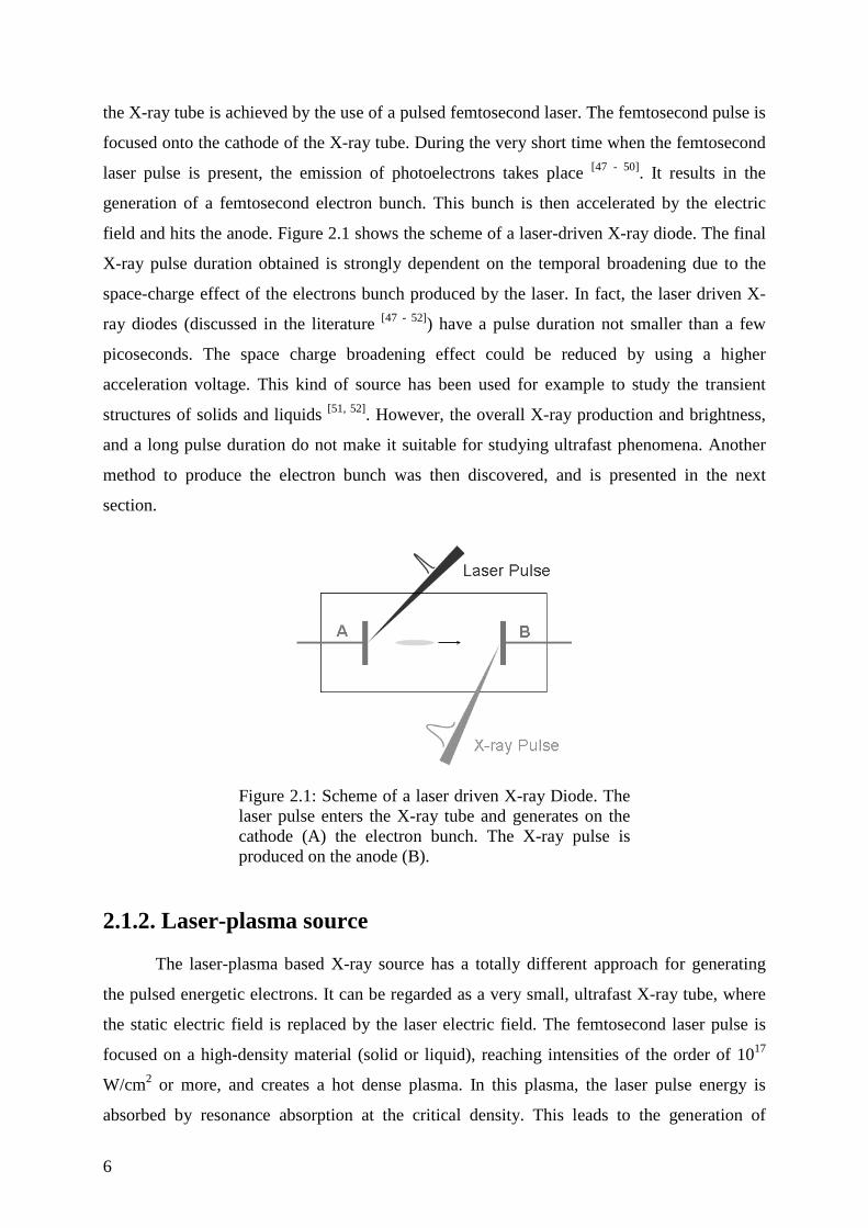
field and hits the anode. Figure 2.1 shows the scheme of a laser-driven X-ray diode. The final

X-ray pulse duration obtained is strongly dependent on the temporal broadening due to the

space-charge effect of the electrons bunch produced by the laser. In fact, the laser driven X-

ray diodes (discussed in the literature [47 - 52]) have a pulse duration not smaller than a few

picoseconds. The space charge broadening effect could be reduced by using a higher

acceleration voltage. This kind of source has been used for example to study the transient

structures of solids and liquids [51, 52]. However, the overall X-ray production and brightness,

and a long pulse duration do not make it suitable for studying ultrafast phenomena. Another

method to produce the electron bunch was then discovered, and is presented in the next

section.

Figure 2.1: Scheme of a laser driven X-ray Diode. The

laser pulse enters the X-ray tube and generates on the cathode (A) the electron bunch. The X-ray pulse is produced on the anode (B).

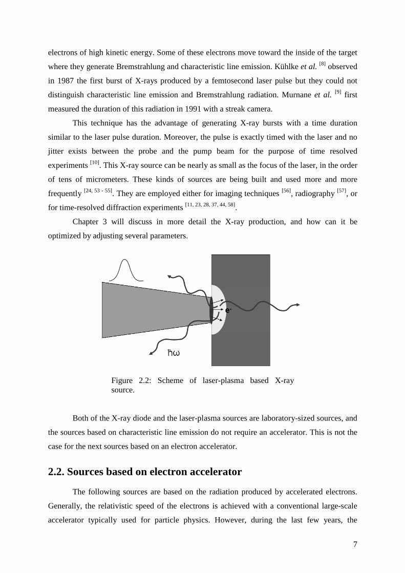
2.1.2. Laser-plasma source

The laser-plasma based X-ray source has a totally different approach for generating

the pulsed energetic electrons. It can be regarded as a very small, ultrafast X-ray tube, where

the static electric field is replaced by the laser electric field. The femtosecond laser pulse is

focused on a high-density material (solid or liquid), reaching intensities of the order of 1017

W/cm2 or more, and creates a hot dense plasma. In this plasma, the laser pulse energy is

absorbed by resonance absorption at the critical density. This leads to the generation of

7

electrons of high kinetic energy. Some of these electrons move toward the inside of the target

where they generate Bremstrahlung and characteristic line emission. Kühlke et al. [8] observed

in 1987 the first burst of X-rays produced by a femtosecond laser pulse but they could not

distinguish characteristic line emission and Bremstrahlung radiation. Murnane et al. [9] first

measured the duration of this radiation in 1991 with a streak camera.

This technique has the advantage of generating X-ray bursts with a time duration

similar to the laser pulse duration. Moreover, the pulse is exactly timed with the laser and no

jitter exists between the probe and the pump beam for the purpose of time resolved

experiments [10]. This X-ray source can be nearly as small as the focus of the laser, in the order

of tens of micrometers. These kinds of sources are being built and used more and more

frequently [24, 53 - 55]. They are employed either for imaging techniques [56], radiography [57], or

for time-resolved diffraction experiments [11, 23, 28, 37, 44, 58].

Chapter 3 will discuss in more detail the X-ray production, and how can it be

optimized by adjusting several parameters.

Figure 2.2: Scheme of laser-plasma based X-ray

source.

Both of the X-ray diode and the laser-plasma sources are laboratory-sized sources, and

the sources based on characteristic line emission do not require an accelerator. This is not the

case for the next sources based on an electron accelerator.

2.2. Sources based on electron accelerator

The following sources are based on the radiation produced by accelerated electrons.

Generally, the relativistic speed of the electrons is achieved with a conventional large-scale

accelerator typically used for particle physics. However, during the last few years, the

8

development of laboratory-sized sources using the laser field for the acceleration has been

under investigation. This section starts with a brief discussion of these new laboratory-sized

possibilities, which will be followed by a presentation of the large-scale accelerator-based

sources.

2.2.1. Laboratory-sized source

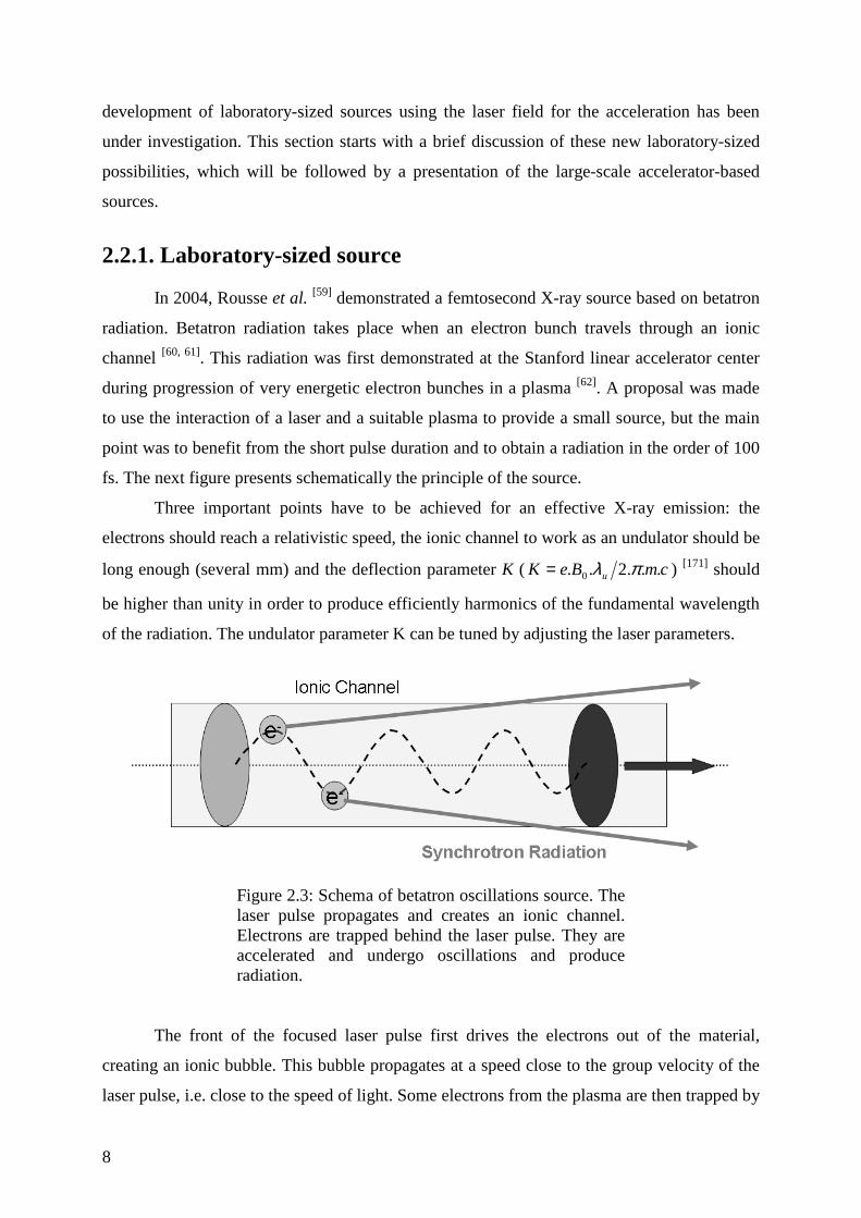
In 2004, Rousse et al. [59] demonstrated a femtosecond X-ray source based on betatron

radiation. Betatron radiation takes place when an electron bunch travels through an ionic

channel [60, 61]. This radiation was first demonstrated at the Stanford linear accelerator center

during progression of very energetic electron bunches in a plasma [62]. A proposal was made

to use the interaction of a laser and a suitable plasma to provide a small source, but the main

point was to benefit from the short pulse duration and to obtain a radiation in the order of 100

fs. The next figure presents schematically the principle of the source.

Three important points have to be achieved for an effective X-ray emission: the

electrons should reach a relativistic speed, the ionic channel to work as an undulator should be

long enough (several mm) and the deflection parameter K ( cmBeK u ...2.. 0 πλ= ) [171] should

be higher than unity in order to produce efficiently harmonics of the fundamental wavelength

of the radiation. The undulator parameter K can be tuned by adjusting the laser parameters.

Figure 2.3: Schema of betatron oscillations source. The

laser pulse propagates and creates an ionic channel. Electrons are trapped behind the laser pulse. They are accelerated and undergo oscillations and produce radiation.

The front of the focused laser pulse first drives the electrons out of the material,

creating an ionic bubble. This bubble propagates at a speed close to the group velocity of the

laser pulse, i.e. close to the speed of light. Some electrons from the plasma are then trapped by

9

the ionic bubble and are accelerated as they travel with the bubble. They can reach energies of

several hundreds of MeV. Displacement of these electrons was studied by Ta Phuoc et al. [63,

64]. Because of a strong radial electrostatic field, these trapped electrons undergo betatron

oscillations and emit synchrotron-like X-ray radiation. The final emission is highly

collimated.

Up to now only a proof-of-principle experiment has been performed with this source

which indicates a pulse duration of less than 1 picosecond [172]. However this kind of source is

promising, since it should allow to generate a very well collimated ultrashort X-ray pulse,

leading to a significant improvement of the brightness of the source, compared to laser-plasma

based X-ray sources.

2.2.2. Accelerator-sized source

As mentioned already, the required relativistic electron bunches are provided by

accelerators, for example from a synchrotron storage ring or from a linear accelerator. The

following sections describe the different ways to get an ultrashort X-ray pulse.

2.2.2.1. Synchrotron 3rd generation

The very easiest way to get an ultrashort X-ray pulse is to take the already available

pulse from synchrotrons. However, from their design and working condition, the duration of

these pulses are tens to hundred of picoseconds and therefore are only suitable for relatively

slow phenomena. Generally one needs a chopper to reduce the repetition rate (generally of

MHz) to typically 1 kHz, a measure that reduces drastically the brightness.

Several sources are using this scheme. The ID09B beam-line at ESRF [65] is working

with a chopper of ~ 1 kHz, the new beamline I19 at Diamond [66] and the beamline CRISTAL

at the SOLEIL [67] also based on this chopper technique. These sources benefit from the high

beam quality of synchrotron, i.e. well collimated beams tunable over a wide range of photon

energy up to tens of keV, which is suitable for structure analysis. As an example, Collet et al.

used the ID09B beamline to measure the picosecond neutral to ionic transition of the TTF-CA [14].

The next section presents interesting new schemes to produce femtosecond pulses

from ordinary long pulse synchrotrons.

10

2.2.2.2. Modified Synchrotron 3rd generation sources

Two working techniques have been developed for producing femtosecond pulses from

an existing synchrotron.

2.2.2.2.1. The orbit deflection bunch method

A method to produce ultrashort X-ray pulses with a synchrotron has been proposed by

Zholents et al. in 1999 [68]. This concept is based on a transverse deflecting radio frequency

(RF) cavity that produces a vertical displacement of the electrons correlated with their

longitudinal position (a “chirp”). A first cavity initiates the chirp while a second cavity placed

downstream is there to cancel the chirp. An insertion device is introduced between the two RF

cavities. The X-ray pulse produced in this insertion device by the chirped electron bunch

possesses a vertical tilted wavefront. It is possible to either slice the pulse vertically to remain

with a X-ray pulse of approximately 1 ps duration, or to use an asymmetrically cut crystal to

recompress the whole pulse down to approximately 1 ps also. Borland [69] have checked the

validity of this schema for the Advanced Photon Source and it was proposed to be

implemented at the MHATT-CAT beamline [70].

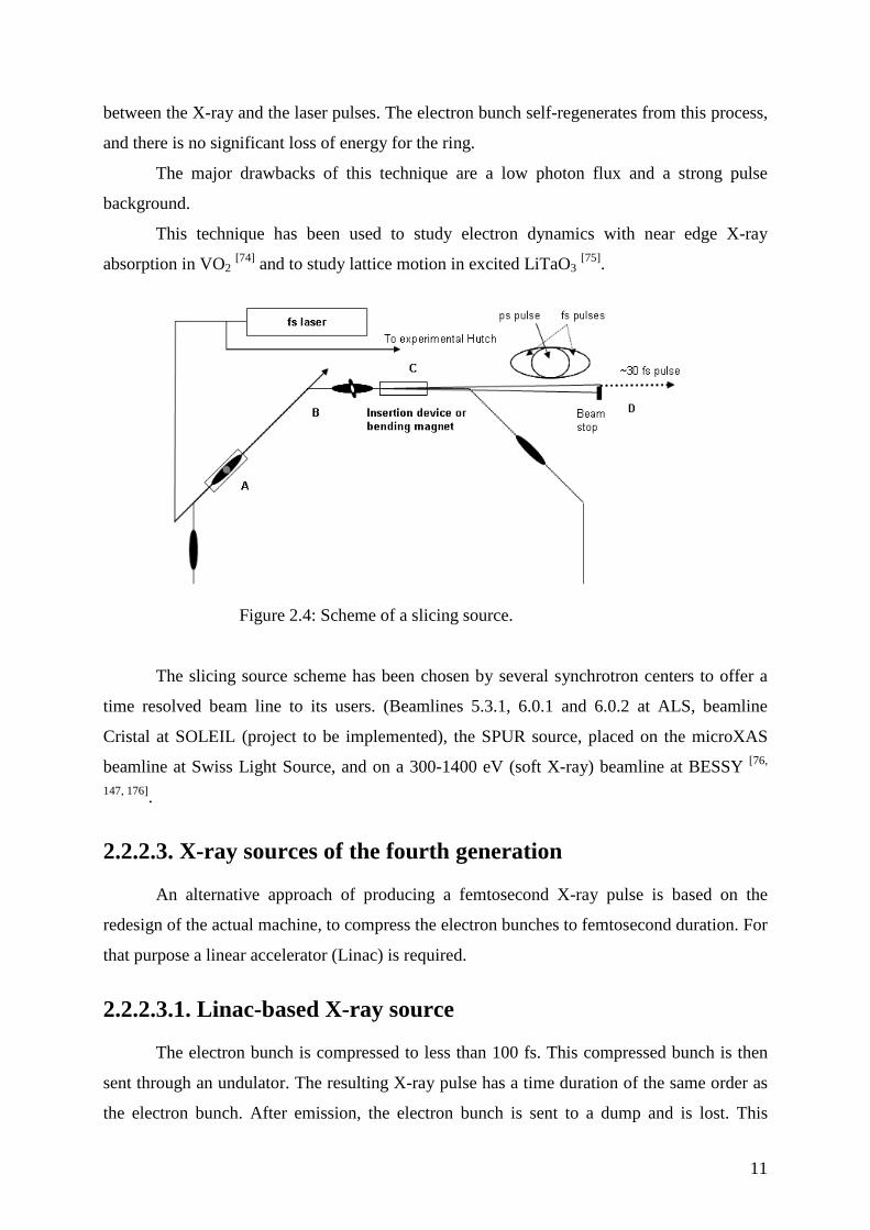
2.2.2.2.2. The slicing source

The other device is the slicing source [71]. It was demonstrated by Schoenlein et al. in

2000 at the Advance Light Source (ALS) in Berkeley, California [72, 73]. The basic idea is the

following: An energy modulation is created with a femtosecond laser within the electron

bunch during the co-propagation of the laser and the electrons in a wiggler. (This is step A in

Figure 2.4).

If the energy spread of the modulated electrons is big enough, they can be spatially

separated from the non-modulated parts of the pulse when passing a bending magnet. (Step

B1).

The electron bunch consists now of the main electron bunch (tens of picoseconds)

with a “hole” (of hundreds of femtoseconds) and two satellites (of hundreds of femtoseconds)

on both sides of the electron bunch. When this electron bunch passes in the next bending

magnets, the produced radiation possesses a similar time structure. It is then possible to select

one of the emitted fs X-ray pulses from the satellites using slits. This fs X-ray pulse is exactly

synchronized with the laser that had created the energy modulation, that is, there is no jitter

11

between the X-ray and the laser pulses. The electron bunch self-regenerates from this process,

and there is no significant loss of energy for the ring.

The major drawbacks of this technique are a low photon flux and a strong pulse

background.

This technique has been used to study electron dynamics with near edge X-ray

absorption in VO2 [74] and to study lattice motion in excited LiTaO3

[75].

Figure 2.4: Scheme of a slicing source.

The slicing source scheme has been chosen by several synchrotron centers to offer a

time resolved beam line to its users. (Beamlines 5.3.1, 6.0.1 and 6.0.2 at ALS, beamline

Cristal at SOLEIL (project to be implemented), the SPUR source, placed on the microXAS

beamline at Swiss Light Source, and on a 300-1400 eV (soft X-ray) beamline at BESSY [76,

147, 176].

2.2.2.3. X-ray sources of the fourth generation

An alternative approach of producing a femtosecond X-ray pulse is based on the

redesign of the actual machine, to compress the electron bunches to femtosecond duration. For

that purpose a linear accelerator (Linac) is required.

2.2.2.3.1. Linac-based X-ray source

The electron bunch is compressed to less than 100 fs. This compressed bunch is then

sent through an undulator. The resulting X-ray pulse has a time duration of the same order as

the electron bunch. After emission, the electron bunch is sent to a dump and is lost. This

12

source can deliver a collimated beam with spatial properties similar to a beamline from a

synchrotron. The source will have higher peak brilliance since there is a huge gain due to

decrease of pulse duration. But this source has a quite significant drawback in the presence of

a jitter between the accelerator and the laser used for experiment. This principle was used by

the SPPS at SLAC and a proposal for Max-4 in MAX Lab in Lund has been made to build a

similar source which could run in a non-disturbing way at the same time as the new facility

storage rings.

.

2.2.2.3.2. The X-ray Free Electron Laser

A free electron laser (FEL) is a light source where electrons from a relativistic electron

bunch radiate in phase in an undulator. Originally, it was designed only for the IR, visible and

ultraviolet spectrum, as it needs mirrors. The electrons can be seen as a gain medium, and

mirrors at the ends of the insertion device form a resonator cavity as in a laser. This resonator

insures that the electron motion in the insertion device is in phase with the field of the light. A

lot of FEL are currently in use worldwide, and some more are planned, because of their

properties.

However, because suitable X-ray mirrors are not readily available to be able to create

an X-ray FEL based on a similar design, other methods need to be employed to produce X-

rays and they are described next.

A SASE FEL uses the Self-Amplified Spontaneous Emission (SASE) to produce an

X-ray pulse. This process occurs in a very long undulator. Normally, in a common insertion

device, the electrons radiate randomly, and the X-ray production is just a linear response from

the number of electrons. If the size of undulator is long enough, e.g. 300 meters, the electron

bunch co-propagates with the emitted X-rays and the interaction with the electric field of X-

ray light becomes significant. As a result, the electrons start to spatially organize themselves

in micro-bunches separated by the X-ray wavelength. The radiation emitted from a micro-

bunch interferes constructively with the radiation produced by the other micro-bunches. As a

result, the X-ray flux increases with the square of the number of electrons and the intensity

increases.

The SASE effect was demonstrated first at the TTF (Tesla Test Facility) in Hamburg [77 - 79]. Currently, the FLASH (Free Electron Laser in Hamburg) is working with this scheme,

in the VUV and soft X-ray regime.

13

Two sources for working in the hard X-ray spectrum are relevant. These are the LCLS

at SLAC [80], which actually started to operate recently in 2009, and the X-FEL in Hamburg,

which is still under construction.

2.3. Comparison of the sources

An absolute comparison of theses different sources is really difficult, because they

differ in characteristics, such as the photon energy, the repetition rate, the pulse duration, and

the size or the cost of the installation. Moreover, they are appropriate for different

experiments. In the absolute, the SASE X-ray FEL will represent the best available X-ray

sources (LCLS have started in 2009, and X-FEL should start in 2013), because of their

unprecedented brightness. However, their construction and running costs are extremely high,

and beam time access will be very limited. On the other hand, it is relatively “easy” to set-up

an X-ray plasma source in a laboratory. Of course, the brightness is much lower, but it is then

accessible 24 hours a day. In fact, both kinds of sources are complementary. One design is

suitable for experiments requiring a huge number of photons, and the other is suitable for

preparatory experiments, or experiments requiring fewer photons.

2.4. Perspectives

The previous sections have described the possible ways to produce femtosecond X-ray

pulses. Their usage will become more and more predominant in the next years in various

research fields. A method to reach the sub-femtosecond time scale has been proposed by

Zholents et al. This method could lead to the production of a single attosecond hard X-ray

pulse from a few femtosecond X-ray pulse duration, based on multiple cascade seeding. Of

course, the contrast between the attosecond part and the femtosecond one should be large

enough to distinguish them [81, 82].

14

3. Laser-plasma based sources, new setups

The previous chapter described and compared the existing ultrashort X-ray pulse

sources available and the X-ray free electron lasers that will be available in the future. It

appears that the most promising sources in term of brightness and other important properties

are the so-called future 4th generation sources: the X-FEL and the LCLS. However, even if

they have a much lower brightness, the laser-plasma based X-ray sources still provide a very

good technical solution for generating ultrashort X-ray pulses for the purpose of time-resolved

experiments performed with an optical pump beam and an X-ray probe. This is due to their

small size, their low construction costs and their availability, i.e. they can run on demand in a

laboratory.

This chapter describes two new laser-plasma based X-ray sources set up during the

work on this thesis. The principle of a laser-plasma based X-ray source and its important

parameters are presented, followed by a description of the new experimental setups and a

discussion of their parameters.

3.1. Principle and important parameters of a laser-plasma based X-ray source

This section describes in more detail the laser-plasma based X-ray source already

presented in chapter 2.1.2. The important parameters required to optimize the X-ray

production will be discussed.

Kulhke et al. have investigated X-ray production versus the energy of the laser pulse

[8]. Stearns et al. have investigated the same effect with a picosecond laser to generate an X-

ray pulse [83]. Feurer et al. used a feedback loop control to optimize X-ray production [53].

Murnane et al. observed the effect of ASE on the X-ray pulse duration [84]. In 1995, Teubner

et al. investigated the role of the angle of incidence, the intensity and the polarization of the

laser pulses [85].

15

First of all, a figure-of-merit parameter for the optimization of an ultrafast laser-

plasma X-ray source is needed. In a lot of cases, the conversion efficiency, i.e. the number of

X-ray photons produced versus the number of incoming laser photons, is a useful parameter.

It can also be defined as the ratio of the X-ray energy divided by the energy of the laser pulse.

The conversation efficiency η is defined in the following way:

photonsphotons

KK

laser

K

N

N

E

E

ωωη ααα

h

h

*

*== , Eq. 2.1

where Ekα and Elaser are the energy of the pulses, Nkα and Nphotons are the numbers of photons.

The parameters which affect the conversion efficiency are as follows: the laser

intensity, the angle of incidence onto the target, the polarization of the laser and the size of the

plasma where the energy is absorbed.

To produce X-rays the target must be excited with a laser pulse of high intensity,

typically 1016-1017 W/cm2. High energy electrons are produced by the so called resonance

absorption at the critical density [86]. This process can be optimized by varying the plasma

scale length, i.e. the thickness of the plasma surface layer. This can be controlled by using a

suitable pre-pulse to create the plasma.

A fraction of high energy electrons propagate into the target material generating

Bremstrahlung and ionizing the core of some atoms. The subsequent electron recombination

within these ionized atoms produces the desired characteristic X-rays. This radiation consists

of the characteristic X-ray lines of the target material. The first ultrafast X-ray source was

demonstrated in 1987 by Kulhke et al. [8] and the subpicosecond pulse duration was measured

for the first time in 1991 by Murnane et al. [9] with a high speed streak camera.

This technique offers the advantage of generating X-ray bursts with a time duration

similar to that of the laser pulse, i.e. of a few hundred femtoseconds. Moreover, the pulse is

exactly timed with the laser and no jitter exists between the laser pump and the X-ray probe

pulse for a time-resolved pump-probe experiment. The photon energy can be selected through

the choice of target material, e.g. 4.51 keV for titanium and 8.02 keV for copper. The

repetition rate of the source is the same as that of the laser system, although it could be limited

by the capability to refresh the target to always present a fresh surface for the laser pulse.

16

To produce an efficient source, one needs to produce electrons with the appropriate

average kinetic energy to optimally ionize the target material. Feurer et al. found that the

average electron energy follows a power law as a function of the laser intensity times the

wavelength squared [54], i.e. Eavg ~ (Iλ2)1/3, which is in agreement with particle-in-cell (PIC)

simulations according to Gibbon et al. [87]. From the conventional X-ray tube, it is well known

that the electron energy should be approximately three times the material Kα energy. This

means that for the sources presented in this work the optimum energies are: Eopt Ti = 13.5 keV

and Eopt Cu = 24 keV. The corresponding optimum laser intensities are: Iopt Ti = 2.1 * 1016

W/cm2 and Iopt Cu = 3.8 * 1016 W/cm2.

These values should be compared with those obtained by Reich et al. These authors

have shown analytically and numerically that the optimum intensity to produce a femtosecond

X-ray pulse is Iopt = 7.3 * 109 Z4.4 [88]. It is, respectively, for ZTi = 22 and ZCu = 29, Iopt Ti = 5.6

* 1015 W/cm2 and Iopt Cu = 2.0 * 1016 W/cm2. These values are comparable in order of

magnitude with the previous ones.

The work presented in this thesis was done using several different setups, and their

parameters will be discussed in the respective sections.

3.2. Laser system

This section describes the laser system used to run the ultrafast X-ray sources.

The laser system was based on chirped pulsed amplification (CPA) [6, 7, 89] and worked

at a 10 Hz repetition rate. The CPA is a technique which allows the production of a high

intensity laser pulse. The principle is the following: A femtosecond pulse of low energy

passes through an optical assembly called a “stretcher”. The stretcher increases the pulse

duration by a factor of one thousand or more and in this way the peak intensity of the pulse

while keeping its energy constant. The stretched pulse can now pass through the several

amplification stages without damaging the amplifier medium, and also minimizing the non-

linear effects. After the amplification the pulse passes another optical assembly called a

“compressor”, and the laser pulse is recompressed to its original duration, but with a gain in

peak intensity corresponding to the energy gain.

The heart of the 10 Hz system is a mode-locked titanium-sapphire oscillator pumped

with a Verdi® laser (Diode-Pumped Solid-State, CW laser, λ=532 nm, P=5 W). The oscillator

17

produces a train of femtosecond laser pulses of 45 fs duration with a central wavelength at

800 nm and with a spectral bandwidth of 21 nm full width half maximum (FWHM). The

repetition rate is 80 MHz and the energy of a single pulse is approximately 1 nJ.

Before the pulses reach the amplification stages of the laser system, the repetition rate

must be cut down to 10 Hz. The decrease of the repetition rate is achieved with two Pockels

cells as an optical switch. The Pockels cell switch allows the precise selection and separation

of one single pulse from the 80 MHz train of pulses from the oscillator.

The amplifiers consist of two separate units, both using Ti:Sapphire as an

amplification medium, pumped by nanosecond Nd:YAG lasers (@532 nm).

The first amplifier is a so-called multipass amplifier. The beam makes eight passes

through the same amplifying medium. This first stage increases the pulse energy up to 1 mJ,

thus realizing an amplification of approximately 100000 times. The pumping laser used is an

INDI® laser. The second amplifier is also a multipass but with a larger cross section. After

four passes in the second crystal, the energy of the pulse increases up to approximately 200

mJ. The second crystal is pumped from both sides to obtain homogeneous pumping of the

amplification medium.

Then, the amplified pulse enters a compressor, an optical assembly using two

diffraction gratings to recompress the pulse. In fact, the laser system possesses two

compressors, which work differently depending on the beam properties required. Both can

recompress the pulse down to 45 femtoseconds. The first compressor operates in high vacuum

in order to prevent the laser pulse from suffering from self-modulation in air during its

propagation. The second compressor works in air (flushed with nitrogen to keep the

compressor dust-free) and is adjusted to achieve only 120 femtoseconds pulse duration. The

maximum energy per pulse is 150 mJ. This longer pulse duration allows the beam to reach the

experiment without having to suffer from non-linear effects in air. The laser peak power is

1.25 TW.

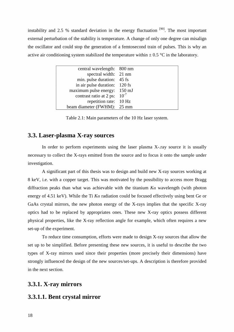
The main parameters of the laser system are summarized in the table 2.1.

The stability of the laser plays a very important role in the X-ray pulse generation, and

several types of measurements were performed to control the stability. The angular and

energy fluctuations were recorded on a shot-to-shot basis. These two parameters show a good

stability under normal working conditions, i.e. less than 100 µrad shot-to-shot pointing

18

instability and 2.5 % standard deviation in the energy fluctuation [90]. The most important

external perturbation of the stability is temperature. A change of only one degree can misalign

the oscillator and could stop the generation of a femtosecond train of pulses. This is why an

active air conditioning system stabilized the temperature within ± 0.5 °C in the laboratory.

central wavelength: 800 nm spectral width: 21 nm min. pulse duration: 45 fs in air pulse duration: 120 fs maximum pulse energy: 150 mJ contrast ratio at 2 ps: 10-7 repetition rate: 10 Hz beam diameter (FWHM): 25 mm Table 2.1: Main parameters of the 10 Hz laser system.

3.3. Laser-plasma X-ray sources

In order to perform experiments using the laser plasma X-.ray source it is usually

necessary to collect the X-rays emitted from the source and to focus it onto the sample under

investigation.

A significant part of this thesis was to design and build new X-ray sources working at

8 keV, i.e. with a copper target. This was motivated by the possibility to access more Bragg

diffraction peaks than what was achievable with the titanium Kα wavelength (with photon

energy of 4.51 keV). While the Ti Kα radiation could be focused effectively using bent Ge or

GaAs crystal mirrors, the new photon energy of the X-rays implies that the specific X-ray

optics had to be replaced by appropriates ones. These new X-ray optics possess different

physical properties, like the X-ray reflection angle for example, which often requires a new

set-up of the experiment.

To reduce time consumption, efforts were made to design X-ray sources that allow the

set up to be simplified. Before presenting these new sources, it is useful to describe the two

types of X-ray mirrors used since their properties (more precisely their dimensions) have

strongly influenced the design of the new sources/set-ups. A description is therefore provided

in the next section.

3.3.1. X-ray mirrors

3.3.1.1. Bent crystal mirror

19

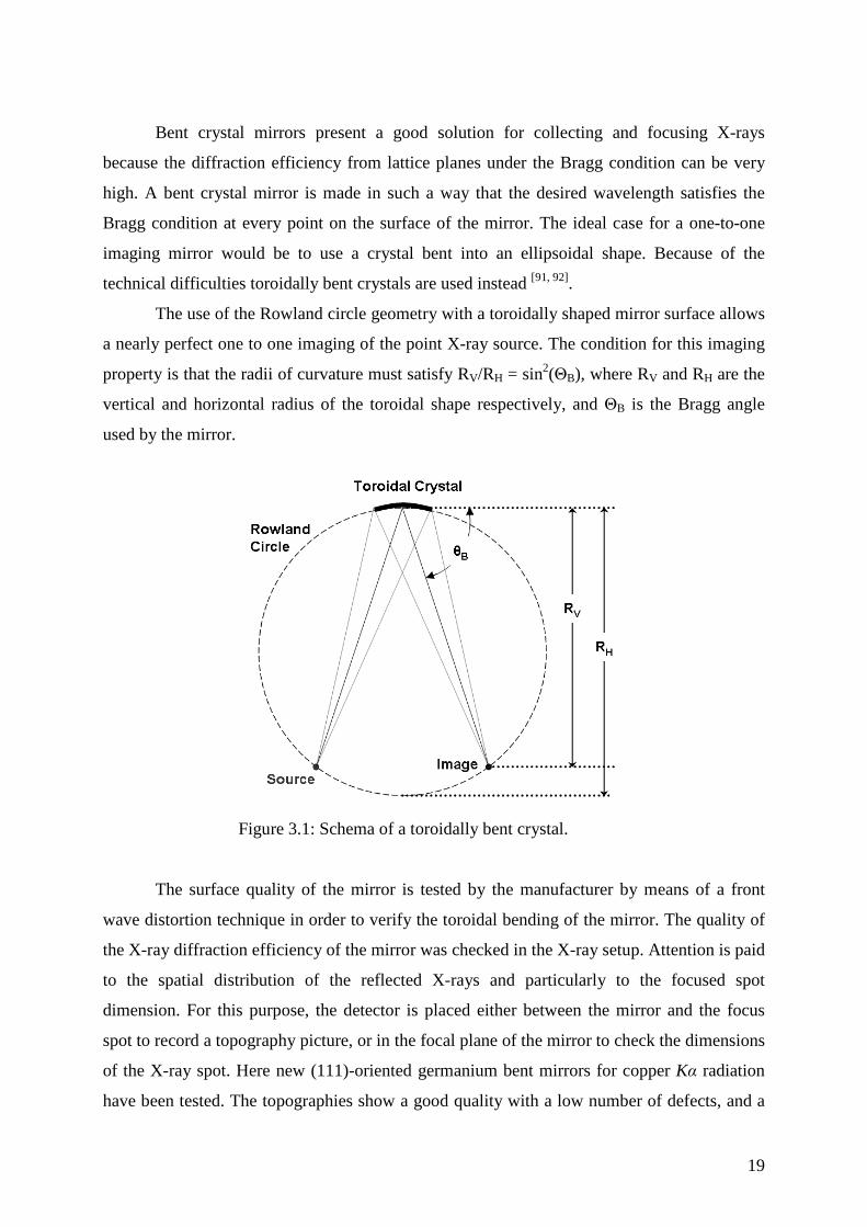
Bent crystal mirrors present a good solution for collecting and focusing X-rays

because the diffraction efficiency from lattice planes under the Bragg condition can be very

high. A bent crystal mirror is made in such a way that the desired wavelength satisfies the

Bragg condition at every point on the surface of the mirror. The ideal case for a one-to-one

imaging mirror would be to use a crystal bent into an ellipsoidal shape. Because of the

technical difficulties toroidally bent crystals are used instead [91, 92].

The use of the Rowland circle geometry with a toroidally shaped mirror surface allows

a nearly perfect one to one imaging of the point X-ray source. The condition for this imaging

property is that the radii of curvature must satisfy RV/RH = sin2(ΘB), where RV and RH are the

vertical and horizontal radius of the toroidal shape respectively, and ΘB is the Bragg angle

used by the mirror.

Figure 3.1: Schema of a toroidally bent crystal.

The surface quality of the mirror is tested by the manufacturer by means of a front

wave distortion technique in order to verify the toroidal bending of the mirror. The quality of

the X-ray diffraction efficiency of the mirror was checked in the X-ray setup. Attention is paid

to the spatial distribution of the reflected X-rays and particularly to the focused spot

dimension. For this purpose, the detector is placed either between the mirror and the focus

spot to record a topography picture, or in the focal plane of the mirror to check the dimensions

of the X-ray spot. Here new (111)-oriented germanium bent mirrors for copper Kα radiation

have been tested. The topographies show a good quality with a low number of defects, and a

20

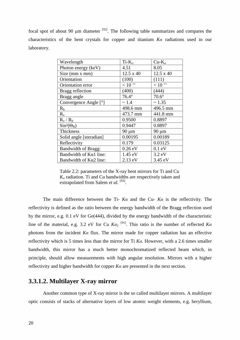
focal spot of about 90 µm diameter [92]. The following table summarizes and compares the

characteristics of the bent crystals for copper and titanium Kα radiations used in our

laboratory.

Wavelength Ti-Kα Cu-Kα Photon energy (keV) 4.51 8.05 Size (mm x mm) 12.5 x 40 12.5 x 40 Orientation (100) (111) Orientation error < 10 ’’ < 10 ’’ Bragg reflection (400) (444) Bragg angle 76.4° 70.6° Convergence Angle [°] ~ 1.4 ~ 1.35 Rh 498.6 mm 496.5 mm Rv 473.7 mm 441.8 mm Rv / Rh 0.9500 0.8897 Sin²(ΘB) 0.9447 0.8897 Thickness 90 µm 90 µm Solid angle [steradian] 0.00195 0.00189 Reflectivity 0.179 0.03125 Bandwidth of Bragg: 0.26 eV 0.1 eV Bandwidth of Kα1 line:

Bandwidth of Kα2 line: 1.45 eV 2.13 eV

3.2 eV 3.45 eV

Table 2.2: parameters of the X-ray bent mirrors for Ti and Cu

Kα radiation. Ti and Cu bandwidths are respectively taken and extrapolated from Salem et al. [93].

The main difference between the Ti- Kα and the Cu- Kα is the reflectivity. The

reflectivity is defined as the ratio between the energy bandwidth of the Bragg reflection used

by the mirror, e.g. 0.1 eV for Ge(444), divided by the energy bandwidth of the characteristic

line of the material, e.g. 3.2 eV for Cu Kα1 [91]. This ratio is the number of reflected Kα

photons from the incident Kα flux. The mirror made for copper radiation has an effective

reflectivity which is 5 times less than the mirror for Ti Kα. However, with a 2.6 times smaller

bandwidth, this mirror has a much better monochromatized reflected beam which, in

principle, should allow measurements with high angular resolution. Mirrors with a higher

reflectivity and higher bandwidth for copper Kα are presented in the next section.

3.3.1.2. Multilayer X-ray mirror

Another common type of X-ray mirror is the so called multilayer mirrors. A multilayer

optic consists of stacks of alternative layers of low atomic weight elements, e.g. beryllium,

21

and layers of heavy atomic weight, e.g. molybdenum. The thickness of each layer is in the

order of a few nm. Such layered material can be seen as an artificial crystal having a lattice

with interspacing distance d corresponding to the sum of the thickness of one layer of the light

element plus one layer of the heavy element.

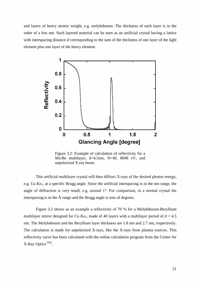
Figure 3.2: Example of calculation of reflectivity for a

Mo/Be multilayer, d=4.5nm, N=40, 8048 eV, and unpolarized X-ray beam.

This artificial multilayer crystal will then diffract X-rays of the desired photon energy,

e.g. Cu Kα1, at a specific Bragg angle. Since the artificial interspacing is in the nm range, the

angle of diffraction is very small, e.g. around 1°. For comparison, in a normal crystal the

interspacing is in the Å range and the Bragg angle is tens of degrees.

Figure 3.2 shows as an example a reflectivity of 70 % for a Molybdenum-Beryllium

multilayer mirror designed for Cu Kα1, made of 40 layers with a multilayer period of d = 4.5

nm. The Molybdenum and the Beryllium layer thickness are 1.8 nm and 2.7 nm, respectively.

The calculation is made for unpolarized X-rays, like the X-rays from plasma sources. This

reflectivity curve has been calculated with the online calculation program from the Centre for

X-Ray Optics [94].

22

An X-ray multilayer mirror can be designed with several different shapes or mounting

geometries, e.g. Montel-Helios, Kirkpatrick-Baez (description is provided later in the section).

Within the work of this thesis, three multilayer mirrors have been tested in order to decide

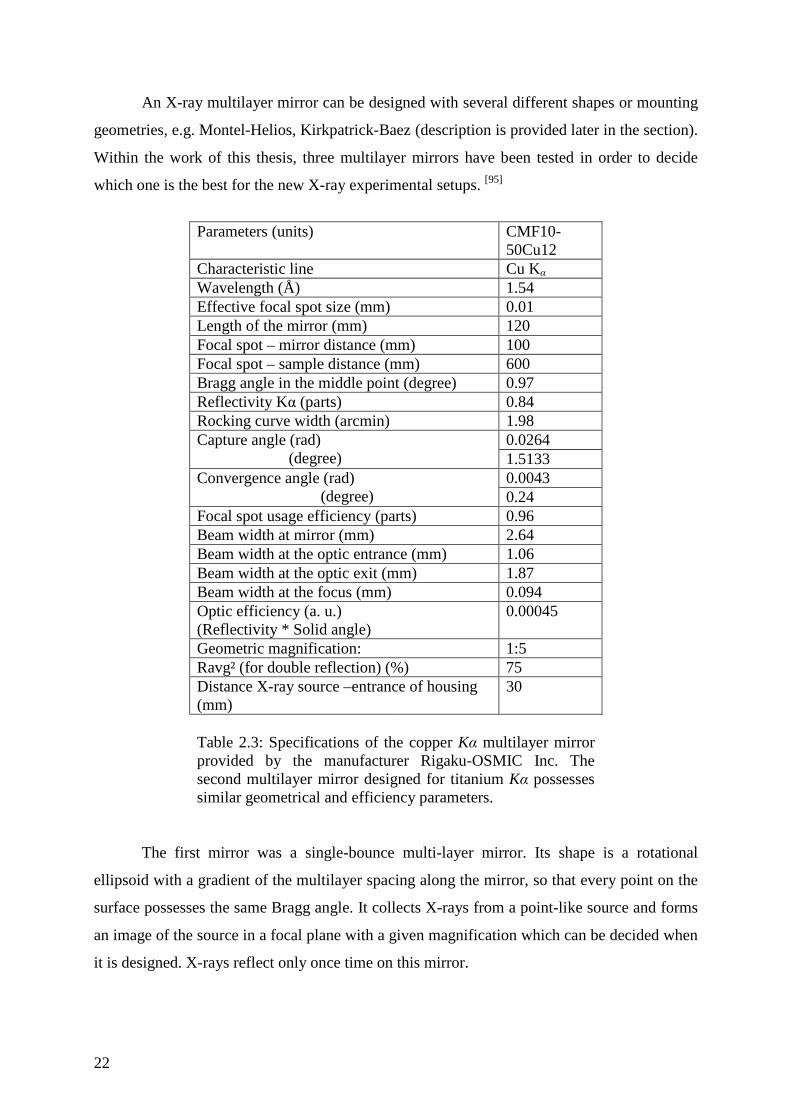
which one is the best for the new X-ray experimental setups. [95]

Parameters (units) CMF10-

50Cu12

Characteristic line Cu Kα Wavelength (Å) 1.54 Effective focal spot size (mm) 0.01 Length of the mirror (mm) 120 Focal spot – mirror distance (mm) 100 Focal spot – sample distance (mm) 600 Bragg angle in the middle point (degree) 0.97 Reflectivity Kα (parts) 0.84 Rocking curve width (arcmin) 1.98 0.0264

Capture angle (rad) (degree) 1.5133

0.0043

Convergence angle (rad) (degree) 0.24

Focal spot usage efficiency (parts) 0.96 Beam width at mirror (mm) 2.64 Beam width at the optic entrance (mm) 1.06 Beam width at the optic exit (mm) 1.87 Beam width at the focus (mm) 0.094 Optic efficiency (a. u.)

(Reflectivity * Solid angle) 0.00045

Geometric magnification: 1:5 Ravg² (for double reflection) (%) 75 Distance X-ray source –entrance of housing

(mm) 30

Table 2.3: Specifications of the copper Kα multilayer mirror

provided by the manufacturer Rigaku-OSMIC Inc. The second multilayer mirror designed for titanium Kα possesses similar geometrical and efficiency parameters.

The first mirror was a single-bounce multi-layer mirror. Its shape is a rotational

ellipsoid with a gradient of the multilayer spacing along the mirror, so that every point on the

surface possesses the same Bragg angle. It collects X-rays from a point-like source and forms

an image of the source in a focal plane with a given magnification which can be decided when

it is designed. X-rays reflect only once time on this mirror.

23

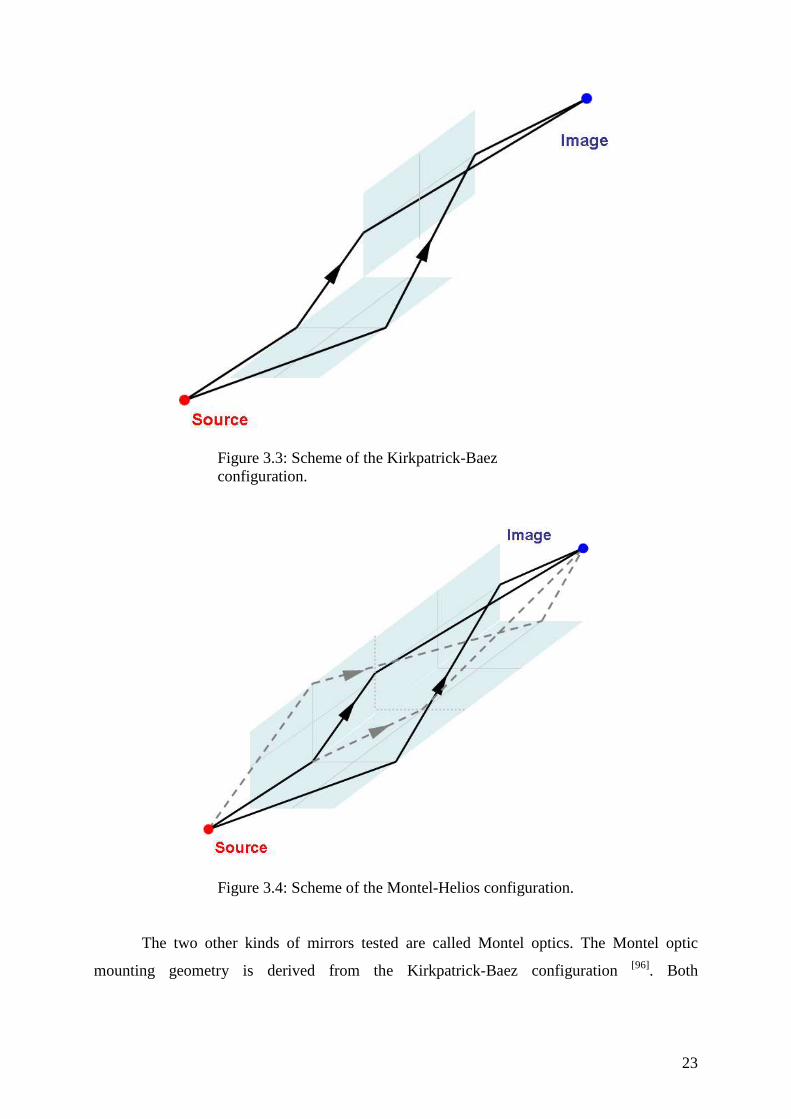
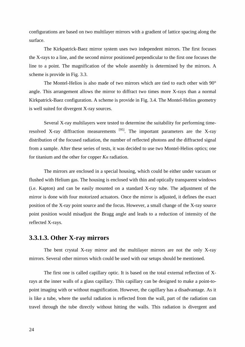
Figure 3.3: Scheme of the Kirkpatrick-Baez

configuration.

Figure 3.4: Scheme of the Montel-Helios configuration.

The two other kinds of mirrors tested are called Montel optics. The Montel optic

mounting geometry is derived from the Kirkpatrick-Baez configuration [96]. Both

24

configurations are based on two multilayer mirrors with a gradient of lattice spacing along the

surface.

The Kirkpatrick-Baez mirror system uses two independent mirrors. The first focuses

the X-rays to a line, and the second mirror positioned perpendicular to the first one focuses the

line to a point. The magnification of the whole assembly is determined by the mirrors. A

scheme is provide in Fig. 3.3.

The Montel-Helios is also made of two mirrors which are tied to each other with 90°

angle. This arrangement allows the mirror to diffract two times more X-rays than a normal

Kirkpatrick-Baez configuration. A scheme is provide in Fig. 3.4. The Montel-Helios geometry

is well suited for divergent X-ray sources.

Several X-ray multilayers were tested to determine the suitability for performing time-

resolved X-ray diffraction measurements [95]. The important parameters are the X-ray

distribution of the focused radiation, the number of reflected photons and the diffracted signal

from a sample. After these series of tests, it was decided to use two Montel-Helios optics; one

for titanium and the other for copper Kα radiation.

The mirrors are enclosed in a special housing, which could be either under vacuum or

flushed with Helium gas. The housing is enclosed with thin and optically transparent windows

(i.e. Kapton) and can be easily mounted on a standard X-ray tube. The adjustment of the

mirror is done with four motorized actuators. Once the mirror is adjusted, it defines the exact

position of the X-ray point source and the focus. However, a small change of the X-ray source

point position would misadjust the Bragg angle and leads to a reduction of intensity of the

reflected X-rays.

3.3.1.3. Other X-ray mirrors

The bent crystal X-ray mirror and the multilayer mirrors are not the only X-ray

mirrors. Several other mirrors which could be used with our setups should be mentioned.

The first one is called capillary optic. It is based on the total external reflection of X-

rays at the inner walls of a glass capillary. This capillary can be designed to make a point-to-

point imaging with or without magnification. However, the capillary has a disadvantage. As it

is like a tube, where the useful radiation is reflected from the wall, part of the radiation can

travel through the tube directly without hitting the walls. This radiation is divergent and

25

polychromatic and superimposed on the focused X-ray beam. Moreover, the reflected X-ray

beam has the shape of a hollow cone. Such a shape (i.e. a ring) is not the most appropriate for

the study of a monocrystalline sample; it would be more suitable for powder diffraction.

These kinds of mirrors were described by Bargheer et al. [97] and by Shymanovich et al. [98].

3.3.1.4. Comparison of the bent and multilayer mirrors

For the design of the new X-ray plasma sources and the set-up of the experiments,

three new Cu Kα mirrors (two bent and one multilayer) but also Ti Kα mirrors (two old bent

and one new multilayer) were taken into consideration. Knowing the technical properties of

these mirrors, it is possible to make an estimation of the expected X-ray reflected photons

after the mirror. This section focuses on the comparison between a bent crystal mirror and a

multilayer mirror for Cu Kα wavelength.

Assuming the X-ray yield per pulse to be 1.25 * 109 (taken arbitrarily) into 4π solid

angle for the new Cu Kα X-ray sources, the bent mirrors would then reflect approximately

3900 photons extremely well monochromatized (∆E = 0.1eV at E = 8048eV) and the

multilayer mirror would reflects 45000 photons consisting of approximately 30000 Kα1 and

15000 Kα2 photons.

The absolute number of photons from the multilayer mirror is one order of magnitude

greater than from a bent crystal. Even if the capturing solid angle of the multilayer mirror is

2.7 times smaller, its reflectivity is 24 times more efficient. Another advantage of the

magnifying multilayer mirror is that the effective photon flux per angle is higher due to a

convergence angle approximately 5.5 times smaller than for a bent mirror (i.e. 0.24° against

1.35° respectively). Finally, the incident beams possess different shapes due to the respective

design of the mirrors. It is a vertical rectangle for the bent mirror and a “diamond” shape, i.e.

a square rotated 45°, for the multilayer mirror. A topography picture of the multilayer can be

found section 3.3.7 describing the experimentally obtained X-ray probe beam.

This does not make the multilayer mirror the best choice when following transient

change of the Bragg angle, because the detected Bragg peak is a convolution of the rocking

curve of the particular Bragg-reflection with the shape of the mirror. A direct cross section of

the measured signal gives a signal intensity strongly dependent on the angular position. This

is shown on the left part of Figure 3.5.

26

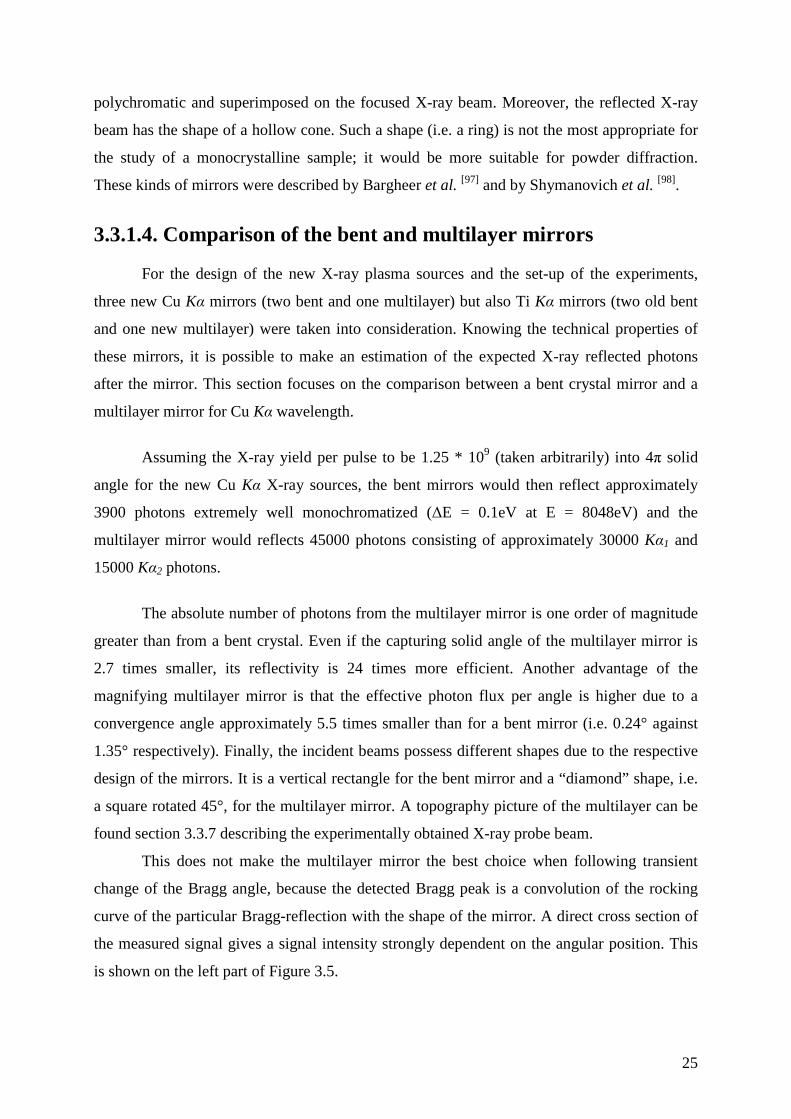
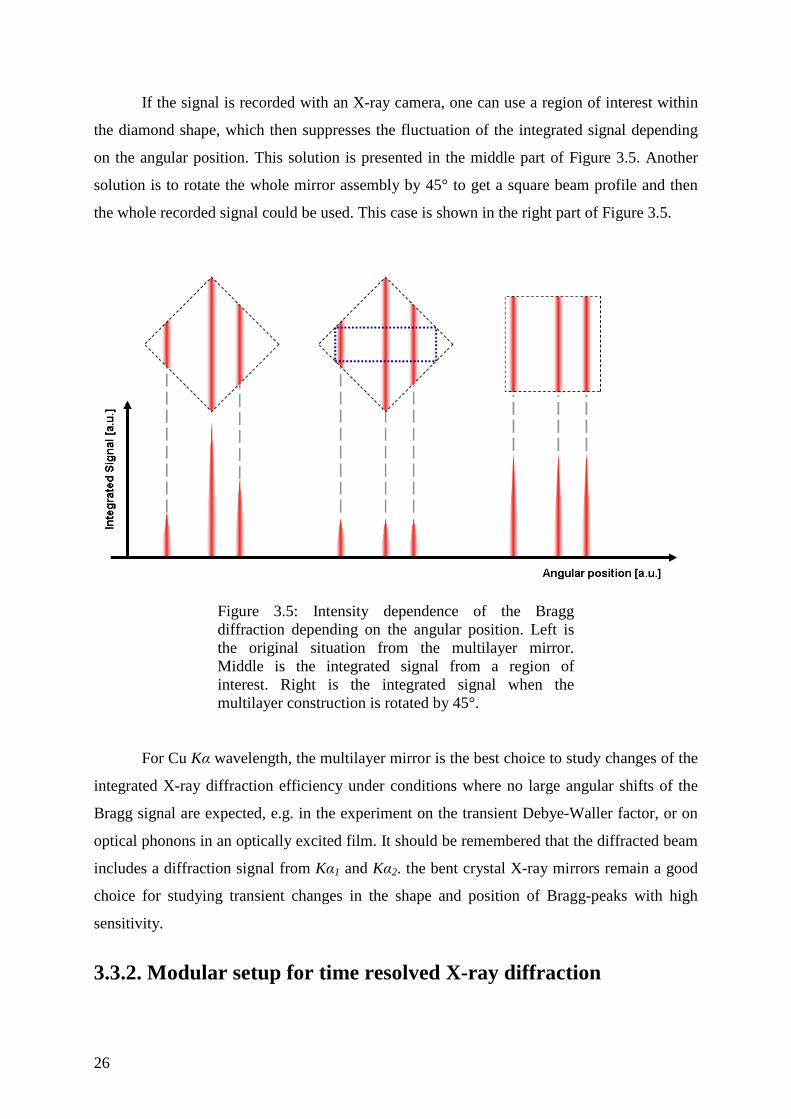
If the signal is recorded with an X-ray camera, one can use a region of interest within

the diamond shape, which then suppresses the fluctuation of the integrated signal depending

on the angular position. This solution is presented in the middle part of Figure 3.5. Another

solution is to rotate the whole mirror assembly by 45° to get a square beam profile and then

the whole recorded signal could be used. This case is shown in the right part of Figure 3.5.

Figure 3.5: Intensity dependence of the Bragg

diffraction depending on the angular position. Left is the original situation from the multilayer mirror. Middle is the integrated signal from a region of interest. Right is the integrated signal when the multilayer construction is rotated by 45°.

For Cu Kα wavelength, the multilayer mirror is the best choice to study changes of the

integrated X-ray diffraction efficiency under conditions where no large angular shifts of the

Bragg signal are expected, e.g. in the experiment on the transient Debye-Waller factor, or on

optical phonons in an optically excited film. It should be remembered that the diffracted beam

includes a diffraction signal from Kα1 and Kα2. the bent crystal X-ray mirrors remain a good

choice for studying transient changes in the shape and position of Bragg-peaks with high

sensitivity.

3.3.2. Modular setup for time resolved X-ray diffraction

27

The following section describes the X-ray setups for time resolved X-ray diffraction

experiments including the sample holder, detectors, pre-pulse beam, pump beam and probe

beam.

In all the setups the X-ray target must be placed in vacuum. If not, the laser pulse

would create a breakdown in air and would not be able to reach the target.

Due to this technical restriction, the original X-ray diffraction setups used in our

laboratory were placed entirely under vacuum [28, 90]. It is useful to start with a description of

this original setup to underline its advantages and weaknesses which in fact required the

construction of a new X-ray setup to overcome them.

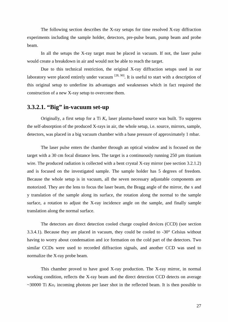
3.3.2.1. “Big” in-vacuum set-up

Originally, a first setup for a Ti Kα laser plasma-based source was built. To suppress

the self-absorption of the produced X-rays in air, the whole setup, i.e. source, mirrors, sample,

detectors, was placed in a big vacuum chamber with a base pressure of approximately 1 mbar.

The laser pulse enters the chamber through an optical window and is focused on the

target with a 30 cm focal distance lens. The target is a continuously running 250 µm titanium

wire. The produced radiation is collected with a bent crystal X-ray mirror (see section 3.2.1.2)

and is focused on the investigated sample. The sample holder has 5 degrees of freedom.

Because the whole setup is in vacuum, all the seven necessary adjustable components are

motorized. They are the lens to focus the laser beam, the Bragg angle of the mirror, the x and

y translation of the sample along its surface, the rotation along the normal to the sample

surface, a rotation to adjust the X-ray incidence angle on the sample, and finally sample

translation along the normal surface.

The detectors are direct detection cooled charge coupled devices (CCD) (see section

3.3.4.1). Because they are placed in vacuum, they could be cooled to -30° Celsius without

having to worry about condensation and ice formation on the cold part of the detectors. Two

similar CCDs were used to recorded diffraction signals, and another CCD was used to

normalize the X-ray probe beam.

This chamber proved to have good X-ray production. The X-ray mirror, in normal

working condition, reflects the X-ray beam and the direct detection CCD detects on average

~30000 Ti Kα1 incoming photons per laser shot in the reflected beam. It is then possible to

28

recalculate from this value the absolute X-ray production of the source. The quantum

efficiency of the detector is 0.55 for this wavelength, so the incident number of Kα1 photons is

~55000. Taking into account the reflectivity of the mirror (0.179), the fact that Kα–emission

consists of 66% Kα1 and 33% Kα2, and a capturing solid angle of 0.00195 steradian, the total

X-ray yield of the source is 3 * 109 Ti Kα photon per pulse into 4 π solid angle. (50000

detected = 4.9 * 109 produced). This setup was also used to measure the Cu Kα production

from a copper wire and was found to be 3.3 * 109 Cu Kα photons per pulse into 4π solid

angle. [90]

The optical pump beam is prepared outside the chamber. The pump wavelength is 800

nm, or 400 nm produced using a second harmonic generation crystal. The energy per pulse is

checked just before the sample with an energy meter. The beam is focused onto the sample

with a 1.5 meter focal length lens. The size of the focus is adjusted outside the chamber by

observing the focal distribution in a reference plane (equivalent to the sample position inside

the vacuum chamber) on a small CCD. The angle between the X-ray pulse and the optical

pulse is set to be as small as possible, i.e. approximately 10°.

A more complete and precise description of this setup can be found in the work from

Shymanovich [90].

Figure 3.6: Scheme of the original setup.

29

Nevertheless, the original setup has some obvious drawbacks. First, the size of the

chamber fixes the geometrical possibilities for experiments, e.g. the angular resolution on the

spatial detector is limited by the maximal distance between the sample and the detector, and

the wall of the chamber limits the maximum distance possible. The second drawback is that

when it is necessary to make an intervention on the setup during an experiment, e.g. to replace

the wire or adjust the setup for a new X-ray Bragg reflection at another angle which might

require moving the detector, the vacuum needs to be broken. This operation requires the

detectors to be warmed up before venting the chamber. Breaking the vacuum can take more

than 30 minutes. To overcome these drawbacks, the decision was made to create a modular

setup which would not be affected, or at least only minimally, by these problems.

3.3.2.2. The modular setups

Within the work of this thesis, I have designed two different modular setups with

significant differences. The main reason is that they were especially designed for either one of

the two different types of X-ray mirrors discussed above (bent crystal or multilayer). Both

setups can work either with a copper target or a titanium target, using the appropriate X-ray

mirror. This change can be made only by exchanging the target, replacing the X-ray mirror

and eventually repositioning the sample holder.

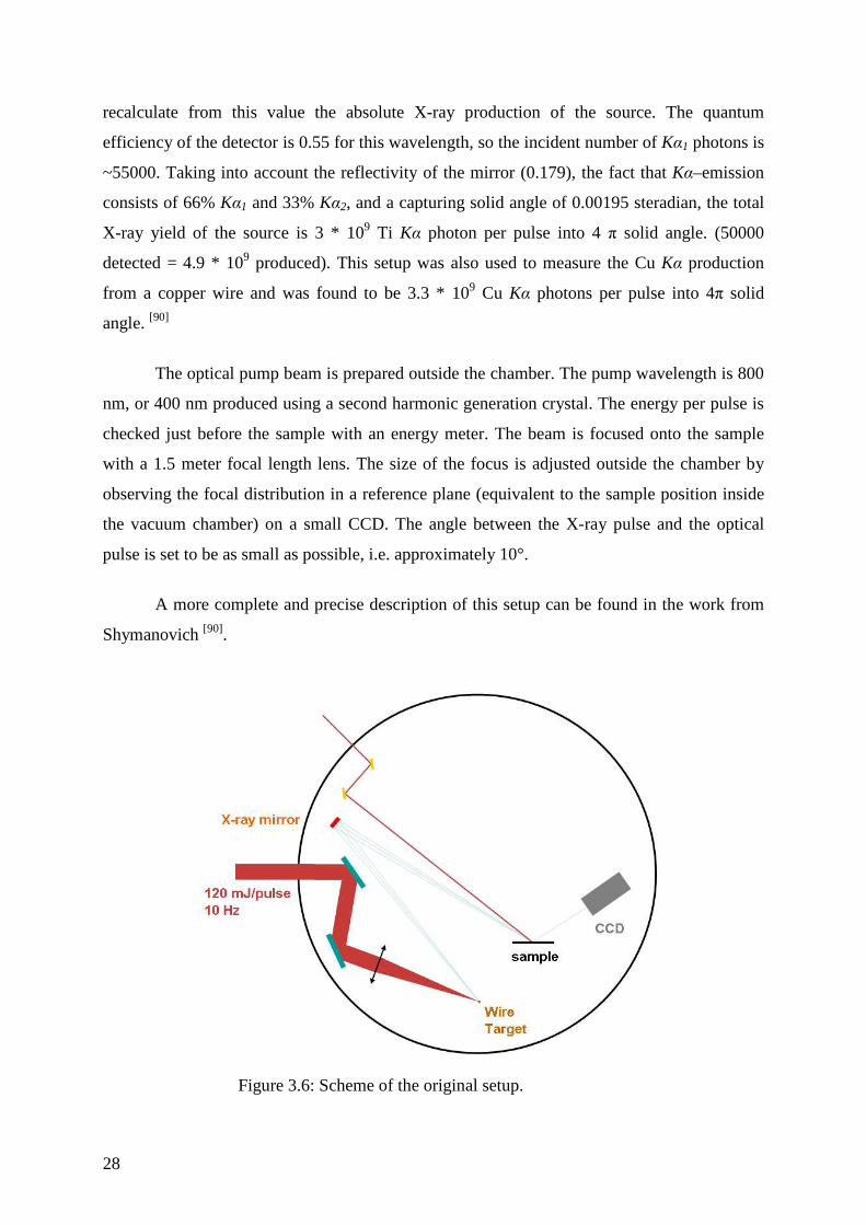
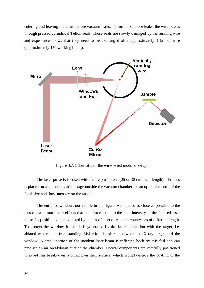
3.3.2.2.1. The wire-based modular setup

In this setup, a moving titanium or copper wire is used as an X-ray target. The wire

target modular setup uses the same target construction as the original vacuum setup. This

choice was made because the wire target system has proven good stability. The chamber is

primarily designed to use bent crystal mirrors. The chamber possesses three optional X-ray

outputs, one for the X-ray beam and others for purposes such as normalization of the X-ray

flux. The small volume of the target chamber, i.e. ~ 4000 cm3, allows a fast pump-down, e.g.

only one minute is required to reach 1 mbar.

Figure 3.7 shows a schematic of the wire-based modular setup without the optical

time-delay line for the sample excitation.

The titanium or copper wires are pulled with a motorized pulling system, located

outside of the chamber (not shown in the figure). The wire speed is set to approximately 2 mm

per second in order to present a fresh wire surface for every laser shot. The feedthroughs for

30

entering and leaving the chamber are vacuum leaks. To minimize these leaks, the wire passes

through pressed cylindrical Teflon seals. These seals are slowly damaged by the running wire

and experience shows that they need to be exchanged after approximately 1 km of wire

(approximately 150 working hours).

Figure 3.7: Schematic of the wire-based modular setup.

The laser pulse is focused with the help of a lens (25 or 30 cm focal length). The lens

is placed on a short translation stage outside the vacuum chamber for an optimal control of the

focal size and thus intensity on the target.

The entrance window, not visible in the figure, was placed as close as possible to the

lens to avoid non linear effects that could occur due to the high intensity of the focused laser

pulse. Its position can be adjusted by means of a set of vacuum connectors of different length.

To protect the window from debris generated by the laser interaction with the target, i.e.

ablated material, a free standing Mylar-foil is placed between the X-ray target and the

window. A small portion of the incident laser beam is reflected back by this foil and can

produce an air breakdown outside the chamber. Optical components are carefully positioned

to avoid this breakdown occurring on their surface, which would destroy the coating of the

31

mirrors. This breakdown has no effect on the laser beam properties because it occurs after the

laser pulse has passed, and the perturbations in air vanish before the next laser pulse. Debris

produced from a copper target sticks onto this free standing foil (in contrast to the debris from

a titanium target). As a consequence, the transmission of the foil slowly decreases with time

when the source is running. The rate of deposition can be minimized if the foil is placed as far

away as possible from the source. For this reason the 30 cm focal lens was mainly used and

the foil itself was placed 2 mm behind the optical window. The foil needs to be exchanged on

a regular basis (every 2-3 days) which takes less than five minutes.

The X-ray exit window is made in a flange with a clear surface of approximately

~1cm² in order to cover the whole solid angle of the X-ray bent mirror, standing ~50 cm from

the source. The vacuum is kept with a glued 6 µm Kapton foil. Debris is also deposited on the

exit foil but the effect on the X-ray transmission is negligible. Nevertheless, the exit foil is

also replaced on a weekly basis. The Kapton foil holds the vacuum well and does not cause a

vacuum leakage.

The vacuum chamber consists of an ISO-K T-flange made of stainless steel, on which

flanges are welded for the optical input and the X-ray output. The wall thickness is 4.5 mm or

less, which is normally enough to absorb all produced radiation, except very high energy

photons. To ensure secure radiation level, the source is enclosed in a lead housing with holes

only for the incoming laser and the three possible X-ray outputs.

The X-ray production of the wire-based chamber is measured using a Cu Kα bent

mirror and a direct detection CCD, the Roper Scientific camera (see section 3.3.4.1). The

CCD is placed between the X-ray mirror and the X-ray focus spot in order to measure the X-

ray flux from the mirror.

With a laser energy of 65mJ per pulse at the compressor output and no pre-pulse

system to optimize the X-ray production (see section 3.3.6.1), on average 183 Cu Kα1 photons

per pulse have been detected. Taking into account the quantum efficiency (QE = 0.18) of the

CCD, the absorption in air (total path in air is 68.5 cm, so the transmission is T = 0.463), and

the absorption in 100 µm Be and 30 µm Al foils used as windows to keep vacuum in the CCD

(see 2.4.1) and to attenuate the X-ray flux, respectively T = 0.982 and T = 0.685, one has on

average 3260 incident Cu Kα1 photons per pulse from the mirror. From this value, the X-ray

production of the source is finally estimated, taking into account the reflectivity (R = 0.036),

32

the solid angle of the bent mirror (0.00189 sr) and the ratio between Kα1 and Kα2. The

production of the wire-based setup is 0.9 * 109 Cu Kα photons per pulse into 4π steradian.

The same measurement has been done with a laser pulse energy of 90mJ and without

pre-pulse. The X-ray production in this case was 1.5 * 109 Cu Kα photons per pulse into 4π.

This value is slightly lower than what was measured using the in-vacuum setup but it is a

reasonable value allowing to perform time-resolved X-ray diffraction experiments. However

the real incident number of photons from the bent mirror is low and would require a long

acquisition time during an experiment. This source, due to the design of the chamber, could

not work with the multilayer X-ray mirrors, and another chamber had to be designed which is

presented in the next section.

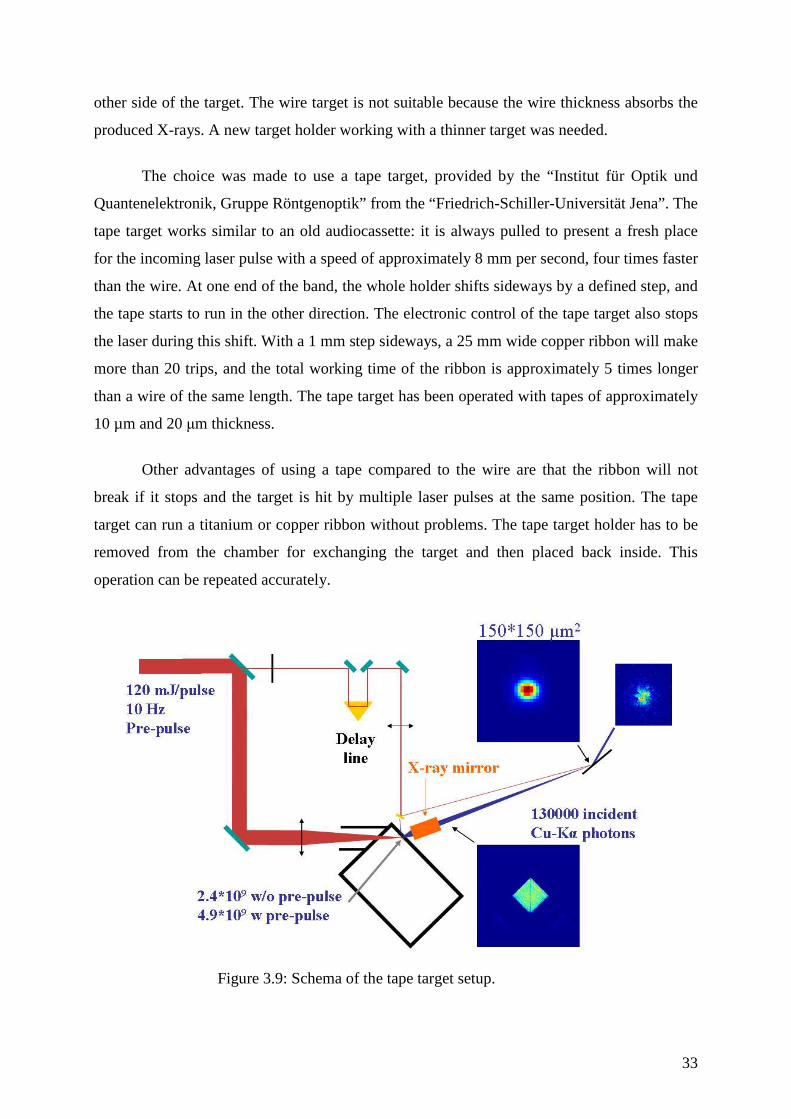
3.3.2.2.2. The tape target setup

As stressed in the previous section, the total X-ray flux one could get using a bent

crystal is approximately one order of magnitude less than with a multilayer mirror. The wire

modular setup can not integrate a multilayer mirror due to the design of the chamber: the

multilayer X-ray mirror needs to be placed at 3 cm from the source but the shortest distance

achievable with the chamber described above was ~9 cm. The geometry of the source has to

be radically different for these new mirrors which need to collect the X-rays produced on the

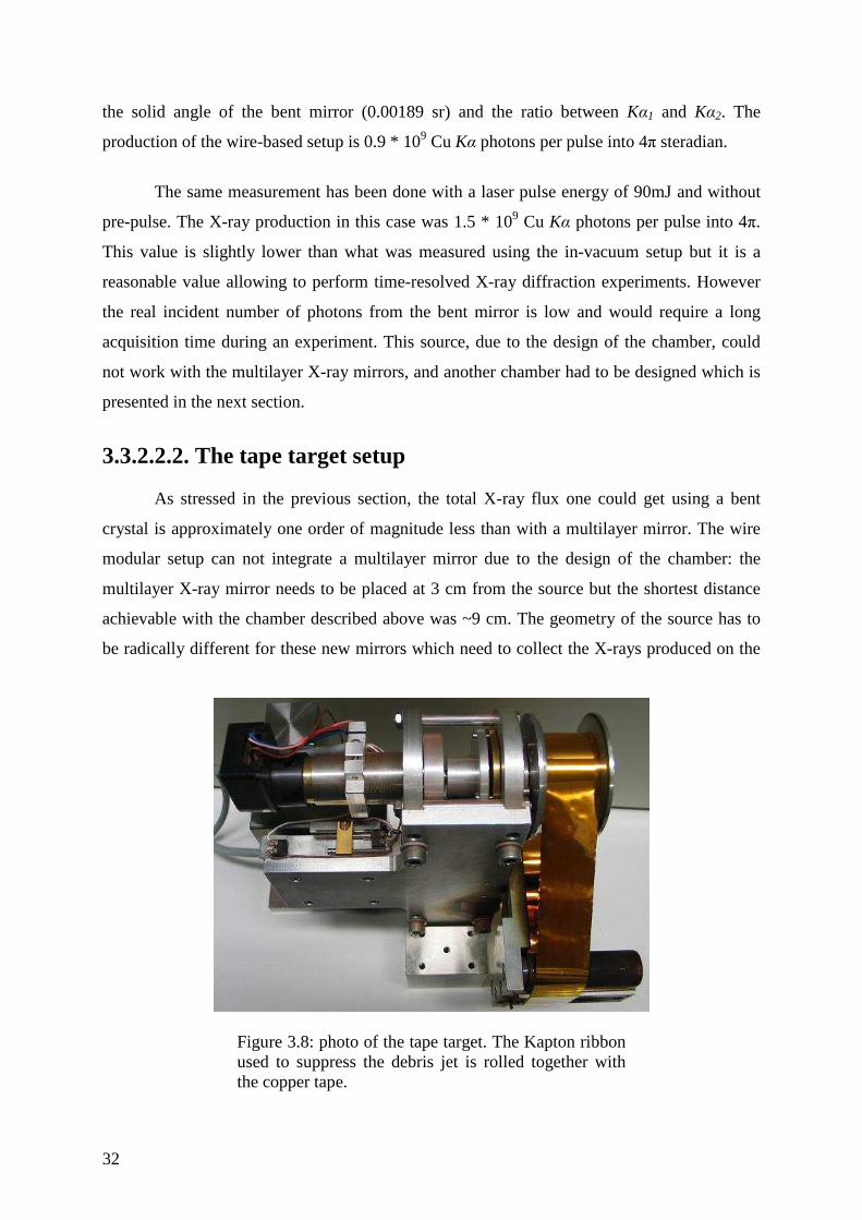
Figure 3.8: photo of the tape target. The Kapton ribbon

used to suppress the debris jet is rolled together with the copper tape.

33

other side of the target. The wire target is not suitable because the wire thickness absorbs the

produced X-rays. A new target holder working with a thinner target was needed.

The choice was made to use a tape target, provided by the “Institut für Optik und

Quantenelektronik, Gruppe Röntgenoptik” from the “Friedrich-Schiller-Universität Jena”. The

tape target works similar to an old audiocassette: it is always pulled to present a fresh place

for the incoming laser pulse with a speed of approximately 8 mm per second, four times faster

than the wire. At one end of the band, the whole holder shifts sideways by a defined step, and

the tape starts to run in the other direction. The electronic control of the tape target also stops

the laser during this shift. With a 1 mm step sideways, a 25 mm wide copper ribbon will make

more than 20 trips, and the total working time of the ribbon is approximately 5 times longer

than a wire of the same length. The tape target has been operated with tapes of approximately

10 µm and 20 µm thickness.

Other advantages of using a tape compared to the wire are that the ribbon will not

break if it stops and the target is hit by multiple laser pulses at the same position. The tape

target can run a titanium or copper ribbon without problems. The tape target holder has to be

removed from the chamber for exchanging the target and then placed back inside. This

operation can be repeated accurately.

Figure 3.9: Schema of the tape target setup.

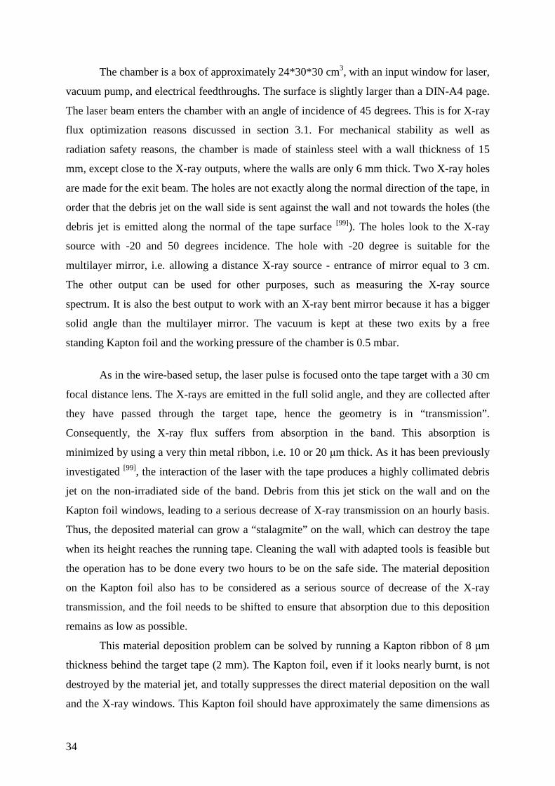
34

The chamber is a box of approximately 24*30*30 cm3, with an input window for laser,

vacuum pump, and electrical feedthroughs. The surface is slightly larger than a DIN-A4 page.

The laser beam enters the chamber with an angle of incidence of 45 degrees. This is for X-ray

flux optimization reasons discussed in section 3.1. For mechanical stability as well as

radiation safety reasons, the chamber is made of stainless steel with a wall thickness of 15

mm, except close to the X-ray outputs, where the walls are only 6 mm thick. Two X-ray holes

are made for the exit beam. The holes are not exactly along the normal direction of the tape, in

order that the debris jet on the wall side is sent against the wall and not towards the holes (the

debris jet is emitted along the normal of the tape surface [99]). The holes look to the X-ray

source with -20 and 50 degrees incidence. The hole with -20 degree is suitable for the

multilayer mirror, i.e. allowing a distance X-ray source - entrance of mirror equal to 3 cm.

The other output can be used for other purposes, such as measuring the X-ray source

spectrum. It is also the best output to work with an X-ray bent mirror because it has a bigger

solid angle than the multilayer mirror. The vacuum is kept at these two exits by a free

standing Kapton foil and the working pressure of the chamber is 0.5 mbar.

As in the wire-based setup, the laser pulse is focused onto the tape target with a 30 cm

focal distance lens. The X-rays are emitted in the full solid angle, and they are collected after

they have passed through the target tape, hence the geometry is in “transmission”.

Consequently, the X-ray flux suffers from absorption in the band. This absorption is

minimized by using a very thin metal ribbon, i.e. 10 or 20 µm thick. As it has been previously

investigated [99], the interaction of the laser with the tape produces a highly collimated debris

jet on the non-irradiated side of the band. Debris from this jet stick on the wall and on the

Kapton foil windows, leading to a serious decrease of X-ray transmission on an hourly basis.

Thus, the deposited material can grow a “stalagmite” on the wall, which can destroy the tape

when its height reaches the running tape. Cleaning the wall with adapted tools is feasible but

the operation has to be done every two hours to be on the safe side. The material deposition

on the Kapton foil also has to be considered as a serious source of decrease of the X-ray

transmission, and the foil needs to be shifted to ensure that absorption due to this deposition

remains as low as possible.

This material deposition problem can be solved by running a Kapton ribbon of 8 µm

thickness behind the target tape (2 mm). The Kapton foil, even if it looks nearly burnt, is not

destroyed by the material jet, and totally suppresses the direct material deposition on the wall

and the X-ray windows. This Kapton foil should have approximately the same dimensions as

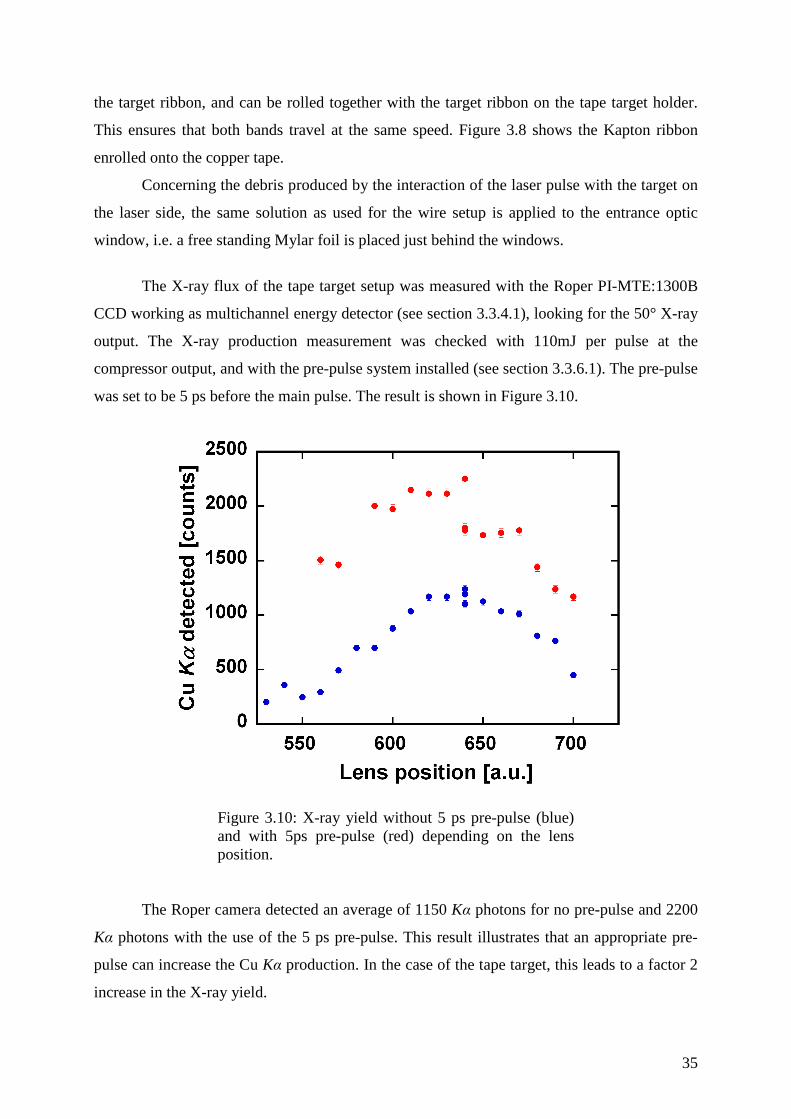
35

the target ribbon, and can be rolled together with the target ribbon on the tape target holder.

This ensures that both bands travel at the same speed. Figure 3.8 shows the Kapton ribbon

enrolled onto the copper tape.

Concerning the debris produced by the interaction of the laser pulse with the target on

the laser side, the same solution as used for the wire setup is applied to the entrance optic

window, i.e. a free standing Mylar foil is placed just behind the windows.

The X-ray flux of the tape target setup was measured with the Roper PI-MTE:1300B

CCD working as multichannel energy detector (see section 3.3.4.1), looking for the 50° X-ray

output. The X-ray production measurement was checked with 110mJ per pulse at the

compressor output, and with the pre-pulse system installed (see section 3.3.6.1). The pre-pulse

was set to be 5 ps before the main pulse. The result is shown in Figure 3.10.

Figure 3.10: X-ray yield without 5 ps pre-pulse (blue)

and with 5ps pre-pulse (red) depending on the lens position.

The Roper camera detected an average of 1150 Kα photons for no pre-pulse and 2200

Kα photons with the use of the 5 ps pre-pulse. This result illustrates that an appropriate pre-

pulse can increase the Cu Kα production. In the case of the tape target, this leads to a factor 2

increase in the X-ray yield.

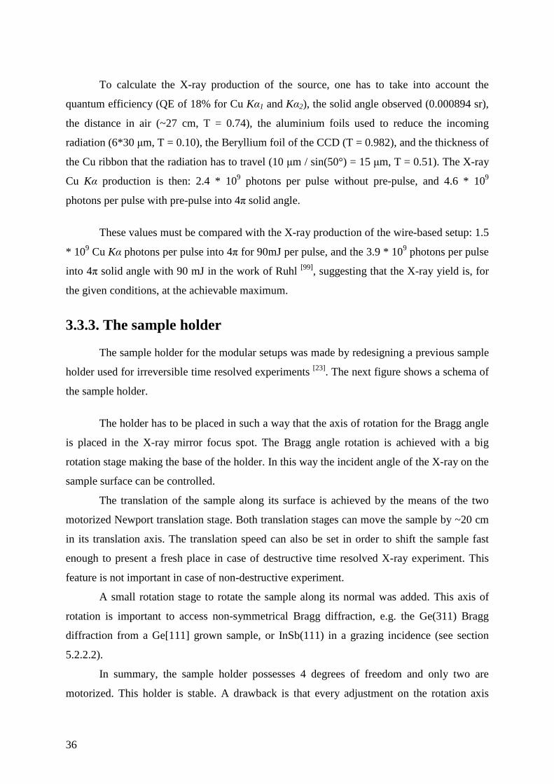
36

To calculate the X-ray production of the source, one has to take into account the

quantum efficiency (QE of 18% for Cu Kα1 and Kα2), the solid angle observed (0.000894 sr),

the distance in air (~27 cm, T = 0.74), the aluminium foils used to reduce the incoming

radiation (6*30 µm, T = 0.10), the Beryllium foil of the CCD (T = 0.982), and the thickness of

the Cu ribbon that the radiation has to travel (10 µm / sin(50°) = 15 µm, T = 0.51). The X-ray

Cu Kα production is then: 2.4 * 109 photons per pulse without pre-pulse, and 4.6 * 109

photons per pulse with pre-pulse into 4π solid angle.

These values must be compared with the X-ray production of the wire-based setup: 1.5

* 109 Cu Kα photons per pulse into 4π for 90mJ per pulse, and the 3.9 * 109 photons per pulse

into 4π solid angle with 90 mJ in the work of Ruhl [99], suggesting that the X-ray yield is, for

the given conditions, at the achievable maximum.

3.3.3. The sample holder

The sample holder for the modular setups was made by redesigning a previous sample

holder used for irreversible time resolved experiments [23]. The next figure shows a schema of

the sample holder.

The holder has to be placed in such a way that the axis of rotation for the Bragg angle

is placed in the X-ray mirror focus spot. The Bragg angle rotation is achieved with a big

rotation stage making the base of the holder. In this way the incident angle of the X-ray on the

sample surface can be controlled.

The translation of the sample along its surface is achieved by the means of the two

motorized Newport translation stage. Both translation stages can move the sample by ~20 cm

in its translation axis. The translation speed can also be set in order to shift the sample fast

enough to present a fresh place in case of destructive time resolved X-ray experiment. This

feature is not important in case of non-destructive experiment.

A small rotation stage to rotate the sample along its normal was added. This axis of

rotation is important to access non-symmetrical Bragg diffraction, e.g. the Ge(311) Bragg

diffraction from a Ge[111] grown sample, or InSb(111) in a grazing incidence (see section

5.2.2.2).

In summary, the sample holder possesses 4 degrees of freedom and only two are

motorized. This holder is stable. A drawback is that every adjustment on the rotation axis

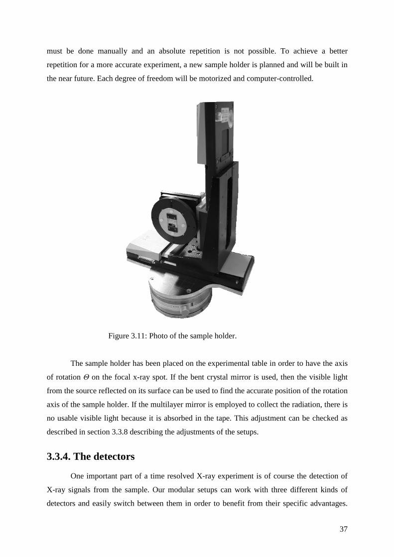
37

must be done manually and an absolute repetition is not possible. To achieve a better

repetition for a more accurate experiment, a new sample holder is planned and will be built in

the near future. Each degree of freedom will be motorized and computer-controlled.

Figure 3.11: Photo of the sample holder.

The sample holder has been placed on the experimental table in order to have the axis

of rotation Θ on the focal x-ray spot. If the bent crystal mirror is used, then the visible light

from the source reflected on its surface can be used to find the accurate position of the rotation

axis of the sample holder. If the multilayer mirror is employed to collect the radiation, there is

no usable visible light because it is absorbed in the tape. This adjustment can be checked as

described in section 3.3.8 describing the adjustments of the setups.

3.3.4. The detectors

One important part of a time resolved X-ray experiment is of course the detection of

X-ray signals from the sample. Our modular setups can work with three different kinds of

detectors and easily switch between them in order to benefit from their specific advantages.

38

The following detectors are presented in the next sections: a direct detection CCD-camera, an

indirect detection CCD-camera, and an avalanche photodiode.

3.3.4.1. Direct detection camera

The Roper Scientific PI-MTE:1300B camera is thinned back-illuminated Si-CCD and

used for direct detection. Technical data can be found on the Roper Scientific website [100].

This camera is very suitable for hard X-ray radiation in the few-keV-range due to its good

quantum efficiency, i.e. 55% for Ti Kα and 18% for Cu Kα. The quantum efficiency depends

only on the thickness of the active area of the CCD and its X-ray absorption at a given

wavelength.

Another interesting point is that the camera can be used as a multichannel energy

detector (mentioned in section 3.3.2.2.2). Provided that a pixel is hit by a single photon, the

signal will scale linearly with the incident phonon energy because the number of created

electron-hole pairs is proportional to the incident photon energy [101]. This is strictly valid if

the created electron-hole pair cloud does not spread over many pixels, but even in this case,

the total signal is just shared by several adjacent pixels. For example, for the camera system

used in our laboratory a 4.51 keV (Ti Kα1) photon will give a signal of ~589 AD-units

(“counts”), and an 8.04 keV photon (Cu Kα1) a signal of ~1050AD-units. For this reason a

signal histogram of the camera signal provides the source spectrum [101] and the absolute

number of detected photons can be also deduced.

During the acquisition of an image, a charged coupled device (CCD) will accumulate

not only the signal from incident radiation but also a signal due to the dark current. The dark

current depends strongly on the temperature of the detector. To reduce it, the easiest way is to

cool the detector. In our setups, the CCD is cooled to -30° Celsius. This is possible thanks to

an integrated Peltier cooler under the chip. Due to this low temperature, one has to protect the

CCD from condensation of contaminants (i.e. water) on the cooled parts. This is achieved by

maintaining the CCD chip under vacuum. However, this can be a technical challenge if the

camera is not in a vacuum chamber.

Cooling is easy to achieve in the big chamber. For the modular setups, the camera

which is now “in air” needs a special vacuum nose which isolates only the CCD. The nose

needs to be continuously pumped to insure the required vacuum. This nose has an input

Beryllium window of approximately 1 cm2, which limits the maximal exposure size on the

CCD (which is approximately 4 cm2).

39

The second major drawback of this detector is that the readout of the CCD chip is

rather slow. If one is interested in the full chip information, one needs 17 seconds to read the

chip. The readout time can be reduced for smaller regions of interest but it always remains

higher than 100 ms, and because of this, the Roper camera can not be used at the 10 Hz

repetition rate of the laser system.

3.3.4.2. Indirect detection camera

The indirect detection camera (Model Gemstar from Photonic Science) uses a

scintillator as the primary X-ray detecting element. Characteristics are given on the Photonic

Science website [102]. The main idea of the indirect X-ray detection is to transform the

incoming signal into an optical signal which is then detected and recorded by an “ordinary”

CCD-camera. This permits to achieve high quantum efficiency even for X-rays of higher

photon energy and, in fact, the performance can be optimized by using an appropriate

scintillator material and thickness. The scintillator of the camera used here is made of

polycrystalline layer of Gadolinium Oxysulphide. For the given thickness of 12 µm, this

material has a quantum efficiency of 85% for Cu Kα radiation. When an incident photon is

absorbed, the scintillator re-emits photons in the visible range. Part of them are collected by a

fiber optic and guided to a MCP-based image intensifier. The intensified image on the output

phosphor of the image intensifier is then collected by a demagnifying fiber optic (“fiber

taper”) and sent onto a cooled CCD chip. Since the CCD is not a slow-scan device the whole

camera system can work with 10 Hz repetition rate using 2*2 binning or by reducing the size

of the area on the CCD which is read and digitized. Therefore, this camera can run in a mode

where sequences of images are recorded with the signal of only one X-ray pulse per image.

A major drawback is that this camera can not give any information about the energy of

the incoming X-ray photons due to the several conversion processes, and unlike a direct

detection camera it can not be used for obtaining the energy spectrum from a signal

histogram. This type of camera is useful when the incoming photons are monochromatic, as is

the case here for the diffraction signals (after an X-ray mirror and a sample). In this case, the

average signal from the chip can be correlated with the average number of incoming photons.

The Gemstar camera was triggered by the laser system to start data acquisition. The

Gemstar camera also had an option to gate the MCP of the image intensifier. This allows to

reduce dark signal form the intensifier at high gain settings and to accumulate the signal of

multiple pulses on the CCD-chip.

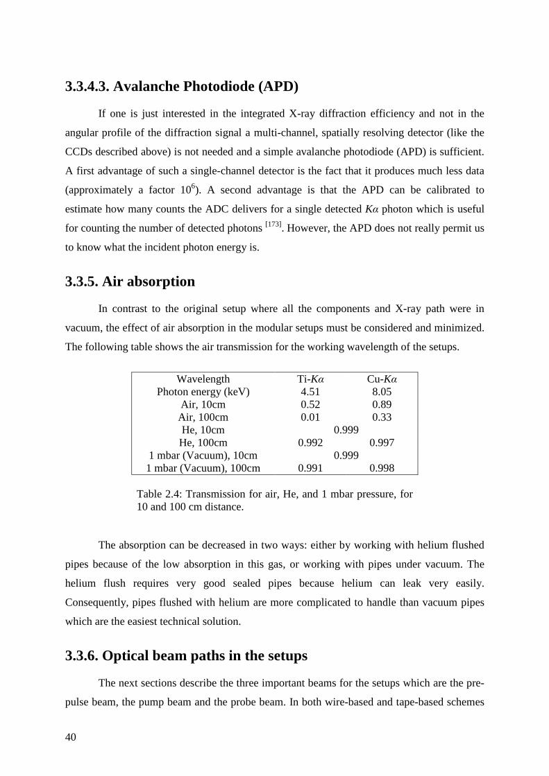
40

3.3.4.3. Avalanche Photodiode (APD)

If one is just interested in the integrated X-ray diffraction efficiency and not in the

angular profile of the diffraction signal a multi-channel, spatially resolving detector (like the

CCDs described above) is not needed and a simple avalanche photodiode (APD) is sufficient.

A first advantage of such a single-channel detector is the fact that it produces much less data

(approximately a factor 106). A second advantage is that the APD can be calibrated to

estimate how many counts the ADC delivers for a single detected Kα photon which is useful

for counting the number of detected photons [173]. However, the APD does not really permit us

to know what the incident photon energy is.

3.3.5. Air absorption

In contrast to the original setup where all the components and X-ray path were in

vacuum, the effect of air absorption in the modular setups must be considered and minimized.

The following table shows the air transmission for the working wavelength of the setups.

Wavelength Ti-Kα Cu-Kα Photon energy (keV) 4.51 8.05 Air, 10cm 0.52 0.89 Air, 100cm 0.01 0.33 He, 10cm 0.999 He, 100cm 0.992 0.997 1 mbar (Vacuum), 10cm 0.999 1 mbar (Vacuum), 100cm 0.991 0.998 Table 2.4: Transmission for air, He, and 1 mbar pressure, for

10 and 100 cm distance.

The absorption can be decreased in two ways: either by working with helium flushed

pipes because of the low absorption in this gas, or working with pipes under vacuum. The

helium flush requires very good sealed pipes because helium can leak very easily.

Consequently, pipes flushed with helium are more complicated to handle than vacuum pipes

which are the easiest technical solution.

3.3.6. Optical beam paths in the setups

The next sections describe the three important beams for the setups which are the pre-

pulse beam, the pump beam and the probe beam. In both wire-based and tape-based schemes

41

the beams lines were constructed in a similar way. After the air compressor, the laser delivers

pulses with an average energy of 120 mJ, pulse duration of 120 fs and at a wavelength of 800

nm.

3.3.6.1. Pre-pulse

The pre-pulse is generated using a pre-pulse generation stage. The central part of the

main pulse with full diameter of 7 mm is separated by a splitting mirror to create the pre-

pulse. The pre-pulse passes through a delay line and is then sent back collinearly with the

main part. With this operation, one can precisely change the arrival time of the pre-pulse with

respect to the main part of the beam. Thus the pre-pulse could also be suppressed. The

adjustment of the pre-pulse generation stage is done in such a way that the focal spot of the

main pulse is located in the middle of the larger focal spot of the pre-pulse.

3.3.6.2. Pump beam

The pump beam is generated with a splitting mirror, which possesses a hole at 45

degrees with respect to the normal and 1 cm offset from the middle of the mirror. The part of

the pulse which passes through the hole is now used for the sample excitation. First, the

energy per pulse can be adjusted with a half-wave-plate in conjunction with a polarizer. The

beam is then time-shifted with respect to the main beam with a delay stage consisting of a

gold-coated retro-reflector fixed onto a stepper motor driven translation stage. The size of the

pump beam on the sample is adjusted with a diaphragm, and the beam is focused with the help

of a 1 meter focal distance lens. A flipping mirror which can be inserted in the path sends the

beam to a CCD camera in order to check the size and the shape of the focus.

3.3.6.3. Probe pulse

The resulting main laser pulse has an average energy of 100 mJ per pulse before the

chamber after propagating in the pre-pulse delay stage and being reflected by the splitting

mirror. The pulse is focused with a 300 mm focal distance lens onto the target, with 45 degree

incidence, and generates the X-ray burst. The distance lens-target can be adjusted with a

translation stage controlled with a micrometric screw. Careful attention was paid to ensure

that the focus spot of the beam does not shift in the focal plane while shifting the lens. The

focal shape and size of the beam were measured to be 25 µm. The X-ray spot produced by the

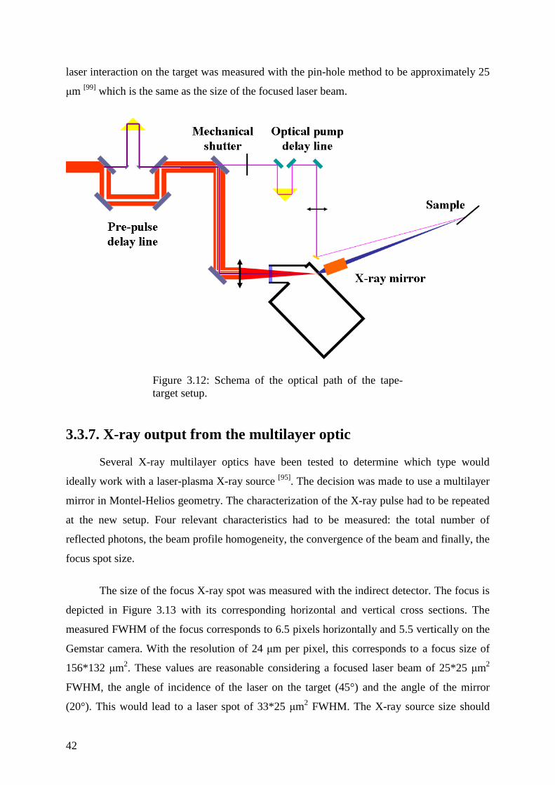
42

laser interaction on the target was measured with the pin-hole method to be approximately 25

µm [99] which is the same as the size of the focused laser beam.

Figure 3.12: Schema of the optical path of the tape-

target setup.

3.3.7. X-ray output from the multilayer optic

Several X-ray multilayer optics have been tested to determine which type would

ideally work with a laser-plasma X-ray source [95]. The decision was made to use a multilayer

mirror in Montel-Helios geometry. The characterization of the X-ray pulse had to be repeated

at the new setup. Four relevant characteristics had to be measured: the total number of

reflected photons, the beam profile homogeneity, the convergence of the beam and finally, the

focus spot size.

The size of the focus X-ray spot was measured with the indirect detector. The focus is

depicted in Figure 3.13 with its corresponding horizontal and vertical cross sections. The

measured FWHM of the focus corresponds to 6.5 pixels horizontally and 5.5 vertically on the

Gemstar camera. With the resolution of 24 µm per pixel, this corresponds to a focus size of

156*132 µm2. These values are reasonable considering a focused laser beam of 25*25 µm2

FWHM, the angle of incidence of the laser on the target (45°) and the angle of the mirror

(20°). This would lead to a laser spot of 33*25 µm2 FWHM. The X-ray source size should

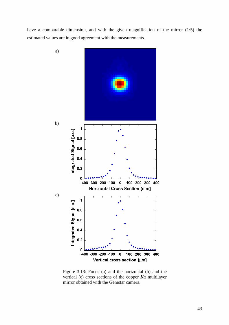
43

have a comparable dimension, and with the given magnification of the mirror (1:5) the

estimated values are in good agreement with the measurements.

a)

b)

c)

Figure 3.13: Focus (a) and the horizontal (b) and the

vertical (c) cross sections of the copper Kα multilayer mirror obtained with the Gemstar camera.

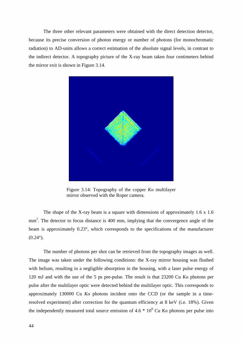
44

The three other relevant parameters were obtained with the direct detection detector,

because its precise conversion of photon energy or number of photons (for monochromatic

radiation) to AD-units allows a correct estimation of the absolute signal levels, in contrast to

the indirect detector. A topography picture of the X-ray beam taken four centimeters behind

the mirror exit is shown in Figure 3.14.

Figure 3.14: Topography of the copper Kα multilayer

mirror observed with the Roper camera.

The shape of the X-ray beam is a square with dimensions of approximately 1.6 x 1.6

mm2. The detector to focus distance is 400 mm, implying that the convergence angle of the

beam is approximately 0.23°, which corresponds to the specifications of the manufacturer

(0.24°).

The number of photons per shot can be retrieved from the topography images as well.

The image was taken under the following conditions: the X-ray mirror housing was flushed

with helium, resulting in a negligible absorption in the housing, with a laser pulse energy of

120 mJ and with the use of the 5 ps pre-pulse. The result is that 23200 Cu Kα photons per

pulse after the multilayer optic were detected behind the multilayer optic. This corresponds to

approximately 130000 Cu Kα photons incident onto the CCD (or the sample in a time-

resolved experiment) after correction for the quantum efficiency at 8 keV (i.e. 18%). Given

the independently measured total source emission of 4.6 * 109 Cu Kα photons per pulse into

45

4π(and taking into account the self absorption of the 10 µm copper ribbon) a total mirror

efficiency of 5.5 * 10-4 is obtained, which compare well (within the errors of the

measurements) with the design value of 4.5 * 10-4, provided by the manufacturer. Under

normal day-to-day working conditions the total number of reflected Cu Kα photons from the

mirror per pulse was between 110000 and 120000.

A comment must be made again concerning the shape of the beam. As already

mentioned in section 3.3.1.4, the “diamond” shape of the mirror does not make it the most

suitable optic if the Bragg angle or the shape of the rocking curve changes with delay time.

Such shifts can not be directly recognized with a single-channel detector but can lead to

apparent changes of integrated diffraction signal. Therefore, the combination of the

magnifying multilayer optic with a single-channel X-ray detector should only be used under

conditions where no shifts of the rocking curve can occur.

3.3.8. Adjustment of the modular setups

A very important challenge for the modular setups is to find temporal and spatial

overlap between the X-ray beam and the pump beam. Thanks to their modularity, this is very

easy to accomplish.

The first step is to find the position of the X-ray beam on the sample surface. After

having positioned the sample holder, i.e. its rotation stage at the X-ray focus, it is necessary to

look for a symmetrical Bragg diffraction from the sample, e.g. 50 nm Bi(111) oriented on a Si

substrate. This work is done with the Gemstar camera close to the sample, and the Bragg

angle is tuned until the desired Bragg peak is found. Afterwards the camera is moved slightly

away from the sample and the X-ray position is found and marked with a metal diaphragm.

The second step can be done only in case of symmetrical Bragg diffractions, but is not

always necessary. The X-ray camera can be removed. Then one adjusts a HeNe beam which

passes through the diaphragm, is reflected on the surface of the sample and passes through the

multilayer X-ray mirror. This allows us to find an approximate position of the X-rays on the

sample surface. A small CCD-camera is then installed to observe on a monitor the area on the

sample where the HeNe beam is reflected. This camera will be used to find the approximate

overlap between the X-ray beam and the pump beam, and also to monitor the sample during

experiments.

46

The third step is to find the exact position of the X-rays. For this purpose, the use of a

thin film is the best solution. Generally, the small camera allows to detect the separation limit

between the substrate and the coated film. The sample is moved with the translation stage in

order to see the disappearance, or the appearance of the X-ray diffraction signal, which marks

the border. With this, a region on the monitor where the X-ray spot could be present can be

drawn. To reduce this area, this operation has to be repeated on another border of the sample.

With 3 to 4 iterations in total, it is possible to precisely define the position of the X-ray beam

on the sample surface. To finally verify the correct overlap the fluence of the pump beam is

increased to a level that the film gets damaged and ablated. If the diffraction signal exhibits a

significant decrease (up to 100%), the overlap is correct.

The fourth step is to find time zero and to adjust the optical pump delay line so that the

time window covers from negative to positive times. A thin film is still the most suitable

choice, due to the acoustic wave developing in the film after excitation (see chapter 4 for more

details).To start, one should delay the pump beam to its maximum (the optical path is then the

longest possible), e.g. few hundreds of picoseconds, or its minimum (shorter optical path,

where negatives times are expected), and to see if a shift of the Bragg peak can be observed

(using one of the CCD-detectors). If no shift is observed at the largest delay time, the path of

the pump beam is too short. If a shift is observed even at the earliest possible delay time, the

optical pump beam path is too long. In both cases, the retro-reflector translation stage needs to

be shifted th to increase (or decrease) the optical path length. Once the delay translation stage

is correctly positioned, the overlap between the X-ray beam and pump beam on the surface

can be optimized by slightly scanning the pump beam over the surface, and looking for the

strongest signal change (i.e. largest shift of the Bragg peak), corresponding to the optimal

overlap.

Once these steps have been taken, the next task is to make a so-called time scan.

Figure 3.15 presents the temporal angular shift of the Bragg reflection, represented by the

center of gravity of the rocking curve, done with a Bismuth thin film (50 nm) and with a

fluence of 5 mJ/cm2.

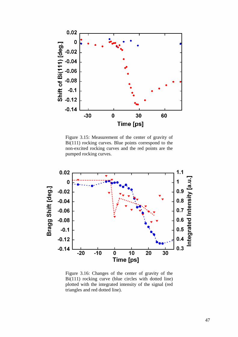
47

Figure 3.15: Measurement of the center of gravity of

Bi(111) rocking curves. Blue points correspond to the non-excited rocking curves and the red points are the pumped rocking curves.

Figure 3.16: Changes of the center of gravity of the

Bi(111) rocking curve (blue circles with dotted line) plotted with the integrated intensity of the signal (red triangles and red dotted line).

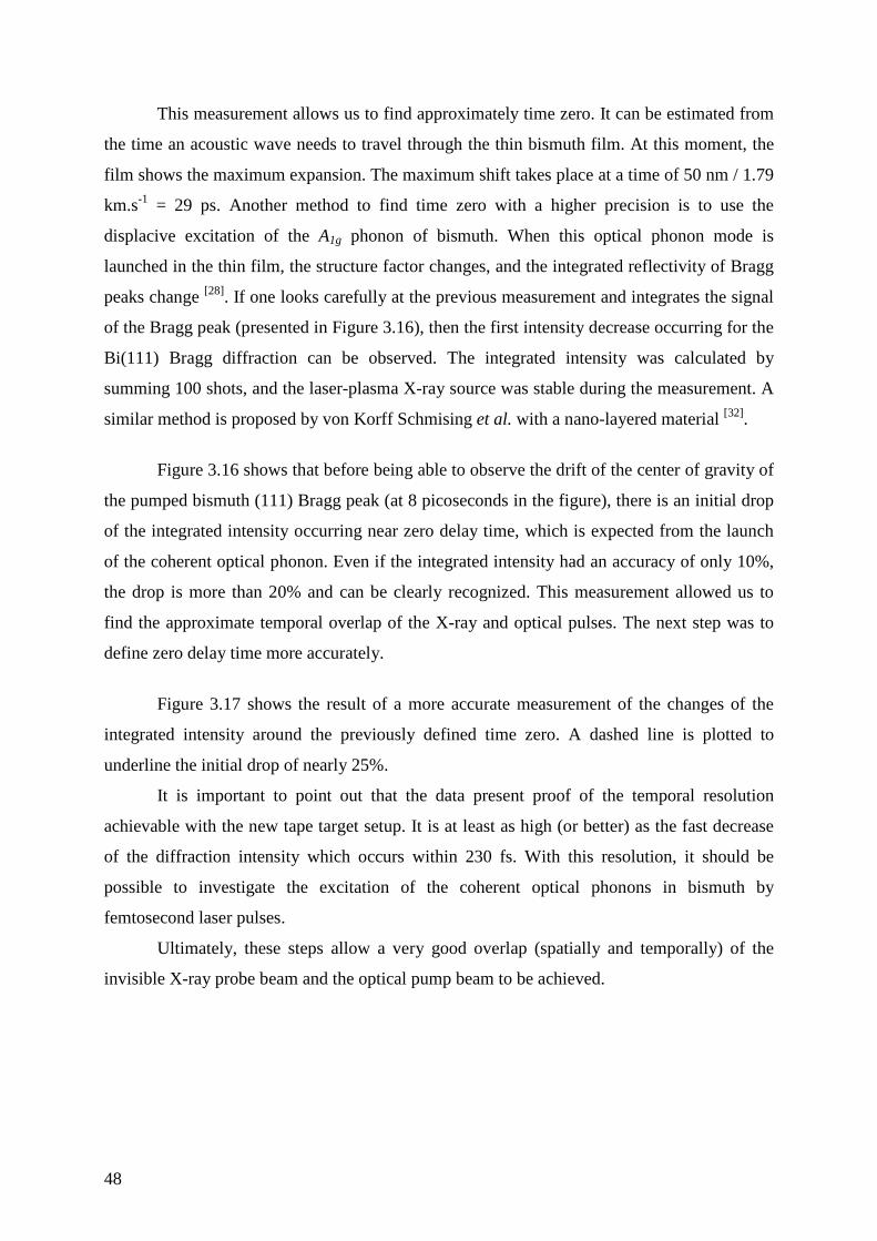
48

This measurement allows us to find approximately time zero. It can be estimated from

the time an acoustic wave needs to travel through the thin bismuth film. At this moment, the

film shows the maximum expansion. The maximum shift takes place at a time of 50 nm / 1.79

km.s-1 = 29 ps. Another method to find time zero with a higher precision is to use the

displacive excitation of the A1g phonon of bismuth. When this optical phonon mode is

launched in the thin film, the structure factor changes, and the integrated reflectivity of Bragg

peaks change [28]. If one looks carefully at the previous measurement and integrates the signal

of the Bragg peak (presented in Figure 3.16), then the first intensity decrease occurring for the

Bi(111) Bragg diffraction can be observed. The integrated intensity was calculated by

summing 100 shots, and the laser-plasma X-ray source was stable during the measurement. A

similar method is proposed by von Korff Schmising et al. with a nano-layered material [32].

Figure 3.16 shows that before being able to observe the drift of the center of gravity of

the pumped bismuth (111) Bragg peak (at 8 picoseconds in the figure), there is an initial drop

of the integrated intensity occurring near zero delay time, which is expected from the launch

of the coherent optical phonon. Even if the integrated intensity had an accuracy of only 10%,

the drop is more than 20% and can be clearly recognized. This measurement allowed us to

find the approximate temporal overlap of the X-ray and optical pulses. The next step was to

define zero delay time more accurately.

Figure 3.17 shows the result of a more accurate measurement of the changes of the

integrated intensity around the previously defined time zero. A dashed line is plotted to

underline the initial drop of nearly 25%.

It is important to point out that the data present proof of the temporal resolution

achievable with the new tape target setup. It is at least as high (or better) as the fast decrease

of the diffraction intensity which occurs within 230 fs. With this resolution, it should be

possible to investigate the excitation of the coherent optical phonons in bismuth by

femtosecond laser pulses.

Ultimately, these steps allow a very good overlap (spatially and temporally) of the

invisible X-ray probe beam and the optical pump beam to be achieved.

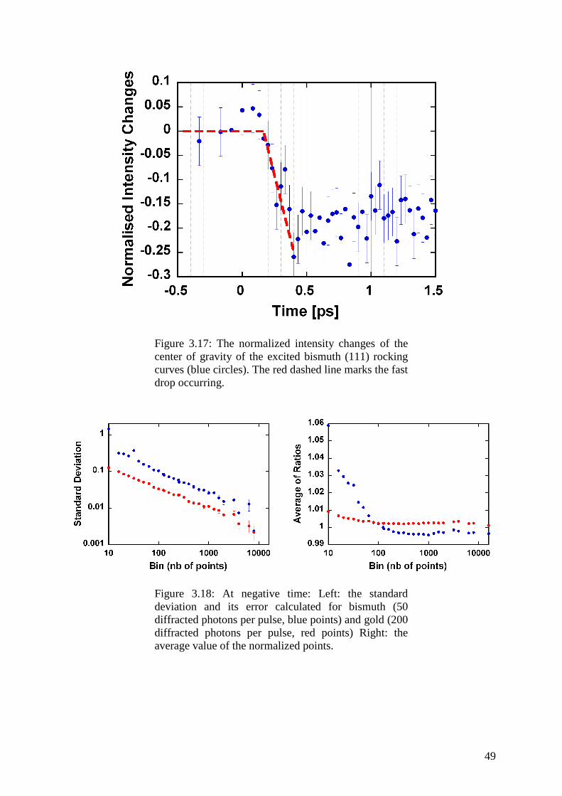
49

Figure 3.17: The normalized intensity changes of the

center of gravity of the excited bismuth (111) rocking curves (blue circles). The red dashed line marks the fast drop occurring.

Figure 3.18: At negative time: Left: the standard

deviation and its error calculated for bismuth (50 diffracted photons per pulse, blue points) and gold (200 diffracted photons per pulse, red points) Right: the average value of the normalized points.

50

3.3.9. Normalization and stability of the tape-target setup

Two laser parameters are extremely important for the magnitude of the diffracted X-

ray signal: the energy per pulse and the pointing (particularly the angular shift) of the laser

beam.

The energy per pulse fluctuations affect the total X-ray yield and the normalization

procedure is the same for the big chamber and the two new modular setups. The easiest

normalization procedure to suppress the effect of the pulse-to-pulse energy fluctuations in the

X-ray flux is to use a separate detector to monitor the total X-ray production directly from the

source. Indeed, the ratio of the X-ray photons reflected by the X-ray optic divided by the

number of photons produced is a constant. Both setups allow such normalization to be

performed. In the big vacuum chamber, this is done by recording on a second CCD-detector

the (400)-Bragg peak from an unpumped gallium arsenide as a reference signal (see section

3.3.2.1, and for more details [90]). The two modular X-ray sources were both designed with a

secondary X-ray output for this purpose. This normalization procedure proved that it can work

perfectly for the energy per pulse fluctuations [90].

The pointing stability of the laser beam affects the spatial drift of the focus beam in the

focal plane of the lens. These drifts affect the different setups differently, depending on the

geometry of the target and the X-ray optic employed. The multilayer X-ray optic is extremely

sensitive to small shifts of the X-ray source point, much more than the toroidally bent X-ray

crystal mirror. This is mainly due to the much shorter source-to-mirror distance. For the same

“shift”, the angular change is more pronounced with the multilayer mirror and can be seen as

misalignment of the mirror. In the case of a spatial shift of the focused laser beam onto the

target and depending on its shape i.e. spherical for the wire-target or a plane for the tape-

target, the X-ray production is affected in different ways. For the tape-target the angle of

incidence stays approximately the same and does not affect the X-ray production, whereas in

the case of the wire target, the incidence angle can vary from 0 to 90°, which will have a huge

effect on the X-ray production. Moreover, in the horizontal plane, the X-ray production can be

done “only” over the wire diameter, whereas even bigger shifts one the tape will still produce

X-rays.

In conclusion, shifts occurring in the tape-target leave the X-ray production almost

unaffected, whereas the flux behind the multilayer optic is very sensitive to these shifts. As

these sifts make the normalization procedure described above unsuitable, another

normalization method had to be found.

51

Few groups in the world also work with a femtosecond X-ray source based on a tape

target. It can be useful to review the method they use to normalize their signal. Bargheer et al.

and von Korff Schmising et al. [30, 103, 104] performed the normalization of the diffraction signal

using a divergent, i.e. a non focused, X-ray beam by recording a diffraction pattern which

contains information on excited and non-excited regions on the surface of the sample. Braun

et al. in their experiment on dipole solvation [105] worked with a multilayer mirror. They

normalized their signal by measuring the transmitted beam together with the diffracted one on

the same spatial detector. These methods are not generally applicable and only useful under

very special experimental conditions, i.e. the experiment has to be performed with a totally

divergent beam in the first case and the sample needs to be transparent enough for the X-rays.

In our setup, the thickness of the sample does not allow the recording of a transmitted beam,

and our measurement requires a focused beam to reach a suitable X-ray flux. These

normalization procedures could not be used therefore.

The final decision on how to perform the normalization to overcome the X-ray

fluctuations in our setup was the following: The measurement procedure is to record a long

sequence of X-ray iamges with the Gemstar camera or with the X-ray APD. This sequence

contains alternately, 5 consecutive X-ray images of the pumped sample and 5 consecutive

images with a non excited sample. This is performed by adding a fast (1 ms opening and

closing time) shutter in the optical pump beam path. The shutter is directly controlled with

one of the laser triggers, i.e. a 1 Hz trigger. After receiving the trigger signal, the shutter opens

long enough to let five consecutive laser pulses pass and then closes to block the next 5 laser

pulses. In the whole sequence images are labeled as “pumped” or “unpumped” by correlating

them to the signal of a diode measuring the optical pump energy after the shutter.

The number of points used in a sequence directly influences the accuracy of the

obtained data. This accuracy also depends on the laser stability, and was experimentally

checked for the tape-target under normal, day-to-day operating conditions. For this purpose,

the diffracted signal from two different samples (50 nm bismuth (111) and 200 nm gold

(111)) was recorded for a negative delay time setting, and a “meta-file” was produced

corresponding to approximately one hour of data collection. This meta-file was analyzed with

a “Matlab” routine which artificially used binning of different sizes, i.e. the number of points

used to produce one normalized transient point. Each specific binning produced a different

number of points, as the number of produced points times the bin size equals a fixed value (in

the next result, arbitrarily taken as 32000). This routine calculates the average of the

52

normalized signal and the standard deviation. The figure 3.18 presents the results for bismuth

(111) and gold (111) diffraction.

Experimentally, the average number of diffracted X-ray photons per pulse from the

different samples was already known to be 400 in the case of gold, and 50 in the case of

bismuth. This measurement helps to define the required acquisition time for a desired

accuracy. It shows that acquisition times smaller than 10 seconds (100 points sequence) are

not really suitable.

However, this normalization procedure is not the best. In the ideal case one should be

able to measure for each single pulse the total number of photons incident onto the sample.

This could be done by introducing an ionization chamber (also called gas-diode) just after the

X-ray optic, which would provide a signal proportional to the X-ray intensity reflected by the

mirror. This kind of detector is commonly in used at synchrotron facilities and was also used

successfully at the SPPS (see section 5.2.1.2). This proposal to use a gas-filled ionization-

chamber for normalization was actually implemented and successfully applied by W. Lu et al. [106, 168].

3.4 Summary and Outlook

This chapter described the three existing laser plasma-based X-ray sources of the 10

Hz laboratory of the University Duisburg-Essen. The big chamber wire-target source was used

mainly for the experimental work presented in the following chapter.

The newest tape-target plasma source has almost totally replaced the small wire-target

modular setup chamber, thanks to its advantages. It also possesses the defined parameters that

where required. The chamber is smaller, easier to handle, and physical intervention can be

performed in a very short time. The running plastic foil makes the source debris-free on the X-

ray extraction side. The X-ray wavelength is easily changeable by selecting the appropriate

target material and exchanging the X-ray optics. Adjustment of the optics and the setup can be

done faster than in the vacuum chamber and finally, the stability of the source has also been

demonstrated.

After completion of the laboratory work for this thesis, the new source and setup have

been intensively used by Lu et al. [106] for the study of coherent phonon excitation in bismuth

for high fluences up to the melting threshold (see Chapter 5.2.1.4 (end of chapter)). With this

work, the setup built in the frame of this thesis has successfully proved its usefulness.

53

4. Transient acoustic response in femtosecond optically excited materials

As will be discussed in more detail in the following section, the transient acoustic

response in femtosecond optically excited materials has been extensively studied for more

than two decades. While the general characteristics of the acoustic waves can be qualitatively

understood within the phenomenological model of Thomsen et al. [33, 34], there are significant

quantitative discrepancies among different studies, in particular with respect to the role of the

electronic and thermal contributions of the pressure driving the acoustic response. Recently,

Shymanovich et al. [90, 107] reported detailed investigations of transient acoustic waves in

femtosecond optically excited germanium using time-resolved X-ray diffraction. These

studies enabled quantitative conclusions to be made on the relative magnitude of the different

pressure contributions.

The aim of the experiments presented in this chapter was to perform similar

investigations of the electronic and thermal pressure contribution on other materials. The

experiments where performed on semiconductors (here a bulk sample of gallium arsenide

since no thin crystalline film was available) and also on metals (here a thin film of gold).

The chapter is structured as follows: Section 4.1 provides a short introduction to the

topic and, based on the approach of Thomsen et al. [34], the commonly used expressions for

the driving pressure are presented for semiconductors and metals. Sections 4.2 and 4.3 discuss

in detail the experiments on gallium arsenide and gold, respectively.

4.1. Physical response following femtosecond optical excitation

Upon optical excitation of a solid material by a femtosecond laser pulse, a significant

amount of energy is deposited within a very short time. The material response takes place via

several processes. The particular topic of this chapter is the generation and evolution of

acoustic waves (for excitation densities below the melting threshold) produced by the increase

of stress within the impulsively excited material [33, 34]. Such acoustic waves have been

54

observed in several experiments using different materials and different experimental

techniques [30, 35 - 41, 43 - 45, 103, 108 - 116].

The optical excitation of a material by a femtosecond pulse modifies the electron and

phonon distribution functions ne(k) and np(k) by δne(k) and δnp(k), respectively. These changes

produce stress σ (i.e. pressure) according to the following equations taken from [34]:

∑∑ ∂∂+

∂∂=

k

kp

k

ke kn

Ekn

ηωδ

ηδσ h

)()( , Eq. 4.1.

Where Ek and ωk are the energy of an electron and the frequency of a phonon of wave

vector k, respectively. η is the strain. The first term in Eq. 4.1 is an electronic contribution to

the stress associated with the deformation potential ∂Ek/∂η. The second term is the thermal

contribution.

thel σσσ += , Eq. 4.2.

In these equations the total stress is considered as a superposition of electronic (σel)

and thermal (σth) contributions.

4.1.1. Semiconductors

In semiconductors, the optical excitation produces electrons and holes. These electrons

and holes relax to the band edge within a short time (~ 1 ps) and thereby emit phonons.

Recombination occurs on a much longer time scale (typically tens of picoseconds up to one

nanosecond). Under these conditions, the electronic contribution to the total stress in Eq. 4.1

can be rewritten as follows [34]:

eg

eg

el ndP

dEBn

Eδδ

ησ −=

∂∂

= , Eq. 4.3.

Here, δne is the total number of excited electrons (and equal to the number of holes),

Eg is the band gap energy, P denotes pressure, B is the bulk modulus, and the assumption that

the solid is elastically isotropic is made.

For each photon of energy E which is absorbed, phonons of total energy (E - Eg) are

produced. Assuming that these phonons have a thermal distribution, their contribution to the

stress is:

55

( ) egth nEEC

B δβσ −−= 3, Eq. 4.4.

Here β is the coefficient of linear expansion and C the specific heat.

As β is usually positive, the phonons produce a negative stress (i.e. positive pressure).

On the other hand, dEg/dP may be positive or negative and so the electronic stress may add to

or subtract from the thermal pressure.

The initial ratio of the electronic over thermal pressure can be calculated for a given

δne to be:

( )g

g

th

el

EE

C

dP

dE

−=

βσσ

3, Eq. 4.5.

For semiconductors, Eq. 4.5 predicts that initially the electronic pressure should

dominate. However, the electronic contribution is strongly time dependent on the relevant

acoustic time-scales (approximately a few tens of picoseconds) because of the electron-hole

recombination.

The spatial dependence of δne and hence of σel can also vary on the relevant acoustic

time-scale due to carrier diffusion. On the other hand, temporal changes of the thermal

pressure σth (after the initial fast rise during electron-lattice equilibration) due to the cooling

induced by heat conduction are often neglected.

4.1.2. Metals

In metals, the dominant effect of laser excitation is the heating of conduction band

electrons. Thus the main change is a modification of the distribution function around the

Fermi level. Under such conditions, Wright et al. discussed stress generation in laser-excited

metals using the so-called Grüneisen parameters for electrons (γe) and phonons (γi) [116]. The

Grüneisen coefficients are defined respectively in the following way [116]:

( ) kke EE ηγ ∂∂−= , Eq. 4.6.

( ) kki ωηωγ ∂∂−= , Eq. 4.7.

Inserting these definitions into Eq. 4.1, the following equations for the electronic and

thermal stress are derived:

56

∑−=k

ekeel knE )(δγσ , Eq. 4.8.

∑−=k

ikith kn )(δωγσ h , Eq. 4.9.

A solution in the general case requires a knowledge of the temporal and spatial

evolution of ne(k) and ni(k), but assuming that electron-electron and phonon-phonon coupling

maintain the electron and phonon distribution in separate pseudo-equilibrium states (Fermi-

Dirac, and Bose-Einstein respectively), it is possible to write Eq. 4.1 as:

iiieee TCTC δγδγσ −−= , Eq. 4.10.

( ) ( ) ( )tTCtTCtP iiieee δγδγ += , Eq. 4.11.

Here δTE(t) and δTL(t) are the transient temperatures of the electrons and the lattice

and CE and CL are the specific heat of the electrons and the lattice respectively. Due to energy

conservation the deposited energy Eo can be written as:

( ) ( )tTCtTCE iieeo δδ += , Eq. 4.12.

After complete equilibration (when δTe and δTi become equal), the electronic

contribution to the total energy can be neglected because Ce<<Ci. Assuming further that the

electron-lattice energy exchange (which cools the electrons and heats the lattice) can be

described by a simple exponential function, Eq. 4.11 can be finally put into the following

form (with P0 ≈ γi Ci δTmax the maximum thermal pressure):

( )

−

−+= τ

γγ

tPtPi

e exp*11)( 0 , Eq. 4.13.

Therefore, the temporal dependence of pressure generated in an optically excited metal

can be expressed in terms of the ratio of the Grüneisen parameters and the electron-lattice

energy relaxation time τ.

4.2. Acoustic waves in fs-optically excited gallium arsenide

One of the main conclusions of the work on germanium by Shymanovich [90] was that

for this particular material a time-dependent, electronic pressure contribution needs to be

taken into account to properly describe the acoustic response after femtosecond laser

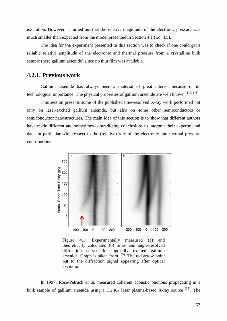
57

excitation. However, it turned out that the relative magnitude of the electronic pressure was

much smaller than expected from the model presented in Section 4.1 (Eq. 4.5).

The idea for the experiment presented in this section was to check if one could get a

reliable relative amplitude of the electronic and thermal pressure from a crystalline bulk

sample (here gallium arsenide) since no thin film was available.

4.2.1. Previous work

Gallium arsenide has always been a material of great interest because of its

technological importance. The physical properties of gallium arsenide are well known [117, 118].

This section presents some of the published time-resolved X-ray work performed not

only on laser-excited gallium arsenide, but also on some other semiconductors or

semiconductor nanostructures. The main idea of this section is to show that different authors

have made different and sometimes contradicting conclusions to interpret their experimental

data, in particular with respect to the (relative) role of the electronic and thermal pressure

contributions.

Figure 4.1: Experimentally measured (a) and

theoretically calculated (b) time- and angle-resolved diffraction curves for optically excited gallium arsenide. Graph is taken from [35]. The red arrow point out to the diffraction signal appearing after optical excitation.

In 1997, Rose-Petruck et al. measured coherent acoustic phonons propagating in a

bulk sample of gallium arsenide using a Cu Kα laser plasma-based X-ray source [35]. The

58

source was used without monochromatizing optics. Therefore, the gallium arsenide bulk

crystal diffracted both Cu Kα1 and Cu Kα2 at their specific Bragg angles. The diffraction

pattern was recorded on an imaging CCD. The sample was excited with 800 nm laser pulses

of 59 mJ/cm2 fluence and 30 fs pulse duration. The GaAs(111) Bragg-reflection was

observed. The result of this measurement is presented in Figure 4.1.

This measurement showed that the diffraction pattern is composed of the superposition

of the rocking curve of Kα1 and Kα2 since no X-ray optic was used. Fig. 4.1 shows: (i) the

signal from the unperturbed depth a bulk sample and (ii) after optical excitation, a new

diffraction contribution at a smaller angle appears, revealing the presence of expended

material at the surface. This secondary Bragg diffraction induced by the optical pump will be

referred as “satellite” later in the section. Sometimes, when one can observe several peaks, the

closest peak to the unperturbed signal is generally labeled as “first”. The average angle of this

satellite decreased with time. Due to the fast electron-lattice energy exchange and the large

Auger recombination coefficient of gallium arsenide, the assumption was made that after a

few ps the main contribution to the pressure was the thermal one. Therefore, the authors used

the model described by Thomsen et al. [34] with only the thermal contribution to fit their data.

Under these assumptions only three parameters are relevant: the velocity of sound and the

peak strain and the absorption depth, which were taken as fitting parameters.

This fit gave an effective deposition/absorption depth of 275 nm, which is much

smaller than the 740 nm linear absorption depth [117, 119]. This behavior was explained by the

important role of two-photon absorption. The authors did also include the thermal diffusion in

the elastic equation to calculate the strain, but the angular resolution of the measured rocking

curves was not sufficient to detect the expected changes. The angular resolution was the

limiting factor of the experiment.

In 2001 extended work was published on gallium arsenide and germanium crystals by

Cavalleri et al. [38]. The authors again used 800 nm femtosecond laser pulses to excite gallium

arsenide close to the melting threshold. In their model, the authors included linear and two-

photon absorption, intraband and Auger relaxation, the carrier diffusion into the bulk and the

cooling of the lattice by heat diffusion. They fitted their measurements with the corresponding

calculated rocking curves obtained from dynamical X-ray diffraction theory.

As a result, they found differences in the behaviors between germanium and gallium

arsenide. They confirmed the importance of non linear absorption in gallium arsenide and

59

found that the coefficient of two-photon absorption estimated from the fitting parameters to be

in agreement with literature values. In contrast, in germanium almost the opposite behavior

was observed. While two-photon absorption played only a minor role, the acoustic response

was mainly determined by strong ambipolar electron-hole diffusion leading to effective

deposition depths significantly larger than the linear absorption depth.

However, since the same set-up as that in the work of Rose-Petruck et al.

(polychromatic X-rays) was used, the experiments did not allow the observation of small

changes of the rocking curves.

In 2005, Lee et al. investigated, using a synchrotron source, a heterostructure

consisting of a single 1.5 µm (100)-Al0.3Ga0.7As layer grown on a (100)-GaAs substrate [43].

The Al0.3Ga0.7As layer is transparent at 800 nm. Therefore, the energy of the pump beam is

absorbed in the gallium arsenide substrate underneath. Because of the band gap of the alloy,

the carriers generated in gallium arsenide cannot diffuse into the film. However, the acoustic

wave developing in gallium arsenide is partly transferred into the film. Lee et al. monitored

the changes of integrated reflectivity at three different Bragg angles to observe the evolution

of this acoustic wave. The authors also used the Thomsen model to calculate rocking curves in

order to fit their measurement.

In 2004, Bargheer et al. had already used a similar alloy. The sample was a nano-

layered structure of AlxGa(1-x)As / GaAs. The superlattice reduced the Brillouin zone and

artificially transformed the acoustic phonon into an optical phonon for the superlattice. Using

a totally divergent Cu Kα X-ray source, Bargheer et al. measured the change of reflectivity of

weak superlattice reflections to monitor the coherent atomic motion within the structure [30].

They explained the phonon generation by only taking into account the electronic pressure and

totally neglected any thermal contribution over the small time range they investigated.

The last work of interest to be considered here was published by Morak et al. in 2006

[44]. The authors studied the acoustic waves developing in a heavier III-IV semiconductor,

namely indium antimonide. They performed their study using a Si Kα laser plasma-based

ultrafast X-ray source. They used a toroidally-bent crystal mirror to collect the radiation and

to focus it onto the sample. This X-ray optic provides a very monochromatic X-ray pulse able

to probe an extended angular range with high resolution.

60

To discuss their data the authors took both electronic and thermal contributions into

account. In particular, they compared different approaches (only thermal pressure, electronic

and thermal pressure with/without diffusion and recombination) to calculate the strain profile

at a given time to fit the rocking curves. The rocking curves were calculated using dynamical

diffraction theory, i.e. by solving Takagi-Taupin equations. However, only the first (strongest)

satellite diffraction peak in the transient diffraction pattern was used for the fit.

Morak et al. showed that carrier diffusion and recombination processes are required to

explain the observed time dependent changes of the rocking curves. They explicitly concluded

that the initial stress created by the electronic pressure can not be neglected. The authors used

only one satellite (generally the strongest one) to validate their model.

In summarizing this discussion it must be concluded that different authors have made

quite different and somehow contradicting assumptions about the (relative) role of the

electronic and thermal pressure contributions. Sometimes it appears that an apparently good

fit is only possible due to a low resolution measurement which does not allow to capture more

subtle (but, as will be shown later, important) changes of the rocking curves. This refers to a

low angular resolution (i.e. by using a non-monochromatic beam) as well as to a limited

dynamic range (i.e. intensity resolution).

In this thesis, high angular resolution and high dynamic range measurements of the

transient changes of rocking curves in laser-excited gallium arsenide caused by acoustic

waves were performed. The use of different excitation wavelengths (800 nm and 400 nm)

allowed variation of the excitation conditions (i.e. effective deposition depth).

4.2.2. Laser-generated acoustic waves in gallium arsenide

4.2.2.1. Experimental setup and data analysis

The measurements to be discussed here were performed using the “big” in-vacuum

chamber with titanium as the target material. The emitted X-rays were collected and focused

onto the sample using a toroidally bent crystal mirror, adjusted to reflect photons of 4.51 keV

(Ti Kα1). The size of the mirror and the geometry of the setup resulted in a 1.4° cone of X-

rays incident onto the sample, allowing the observation of a wide angular range around the

Bragg peak for a given delay time. A complete description of the setup was given Chapter

3.3.2.1.

61

The sample was a 350 µm thick wafer of single-crystalline gallium arsenide (much

thicker than the X-ray probe/extinction depth of approx. 1.6 µm) cut normal to the [100]

direction. The Bragg diffraction investigated was the GaAs(400), with a Bragg angle of

76.551°. Great care was taken to position the sample exactly in the focus of the X-ray mirror

in order to avoid the “acoustic artifact” [120]. This Bragg angle allowed a sample-to-detector

distance of 400 mm, which resulted in a resolution of 0.05 mrad per pixel of the detector.

The sample was excited with two different wavelengths, i.e. 800 nm and 400 nm. The

laser pump fluences on the sample were adjusted so that the threshold for cumulative damage

(which is below the melting threshold) was not reached. At 800 nm, a fluence of 32 mJ/cm2,

i.e. approximately 50% of the melting threshold, was used. At 400 nm, the pumping fluence

was 25 mJ/cm2, again, below the cumulative damage and the melting threshold (which have

been not explicitly determined). The absence of cumulative damage was monitored by

observing scattered pump light from the sample surface with a small CCD camera. Indeed,

when damage occurs, the scattering strongly increases. The two different pump wavelengths

produce different strain profiles because the absorption length in the semiconductor is shorter

for 400 nm, and consequently, the X-ray diffraction profiles will be different.

The rocking curves were obtained from cross sections of measured raw images

recorded on the CCD using a “Matlab” routine (a slightly modified version of the routine

described in [121]). First, the bent diffraction lines (shown in the left part of Fig. 4.2) were

unbent and then integrated along the direction normal to the dispersion direction. A reference

signal, in order to normalize the total (integrated) diffraction signal, was obtained from the

diffraction of a (non-excited) GaAs crystal placed close to the plasma source, which was

recorded simultaneously on a second CCD-detector. To reduce noise and in order to increase

the dynamic range (approximately 103) the measured rocking curves were smoothed with a

1:2:1 filter.

The right part of Figure 4.2 presents, as red and blue curves, the rocking curves of the

sample measured at negative delay times for 800 nm and 400 nm pumping, respectively.

These curves represent the diffraction profile of the unperturbed sample. They overlap

perfectly, indicating that the two sets of measurements, performed with an interval of a few

months between them, were fully reproducible. The green curve is a calculated rocking curve

of the (400) reflection of GaAs using dynamical diffraction theory (see 4.2.2.3). As can be

seen, the measured rocking curves are broadened by a factor of 1.4 approximately (from 0.33

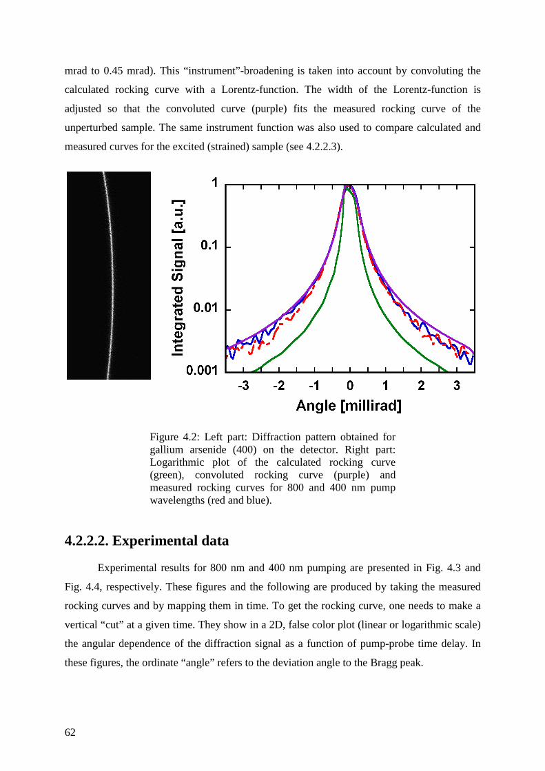
62

mrad to 0.45 mrad). This “instrument”-broadening is taken into account by convoluting the

calculated rocking curve with a Lorentz-function. The width of the Lorentz-function is

adjusted so that the convoluted curve (purple) fits the measured rocking curve of the

unperturbed sample. The same instrument function was also used to compare calculated and

measured curves for the excited (strained) sample (see 4.2.2.3).

Figure 4.2: Left part: Diffraction pattern obtained for

gallium arsenide (400) on the detector. Right part: Logarithmic plot of the calculated rocking curve (green), convoluted rocking curve (purple) and measured rocking curves for 800 and 400 nm pump wavelengths (red and blue).

4.2.2.2. Experimental data

Experimental results for 800 nm and 400 nm pumping are presented in Fig. 4.3 and

Fig. 4.4, respectively. These figures and the following are produced by taking the measured

rocking curves and by mapping them in time. To get the rocking curve, one needs to make a

vertical “cut” at a given time. They show in a 2D, false color plot (linear or logarithmic scale)

the angular dependence of the diffraction signal as a function of pump-probe time delay. In

these figures, the ordinate “angle” refers to the deviation angle to the Bragg peak.

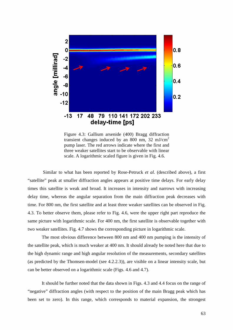
63

Figure 4.3: Gallium arsenide (400) Bragg diffraction

transient changes induced by an 800 nm, 32 mJ/cm2 pump laser. The red arrows indicate where the first and three weaker satellites start to be observable with linear scale. A logarithmic scaled figure is given in Fig. 4.6.

Similar to what has been reported by Rose-Petruck et al. (described above), a first

“satellite” peak at smaller diffraction angles appears at positive time delays. For early delay

times this satellite is weak and broad. It increases in intensity and narrows with increasing

delay time, whereas the angular separation from the main diffraction peak decreases with

time. For 800 nm, the first satellite and at least three weaker satellites can be observed in Fig.

4.3. To better observe them, please refer to Fig. 4.6, were the upper right part reproduce the

same picture with logarithmic scale. For 400 nm, the first satellite is observable together with

two weaker satellites. Fig. 4.7 shows the corresponding picture in logarithmic scale.

The most obvious difference between 800 nm and 400 nm pumping is the intensity of

the satellite peak, which is much weaker at 400 nm. It should already be noted here that due to

the high dynamic range and high angular resolution of the measurements, secondary satellites

(as predicted by the Thomsen-model (see 4.2.2.3)), are visible on a linear intensity scale, but

can be better observed on a logarithmic scale (Figs. 4.6 and 4.7).

It should be further noted that the data shown in Figs. 4.3 and 4.4 focus on the range of

“negative” diffraction angles (with respect to the position of the main Bragg peak which has

been set to zero). In this range, which corresponds to material expansion, the strongest

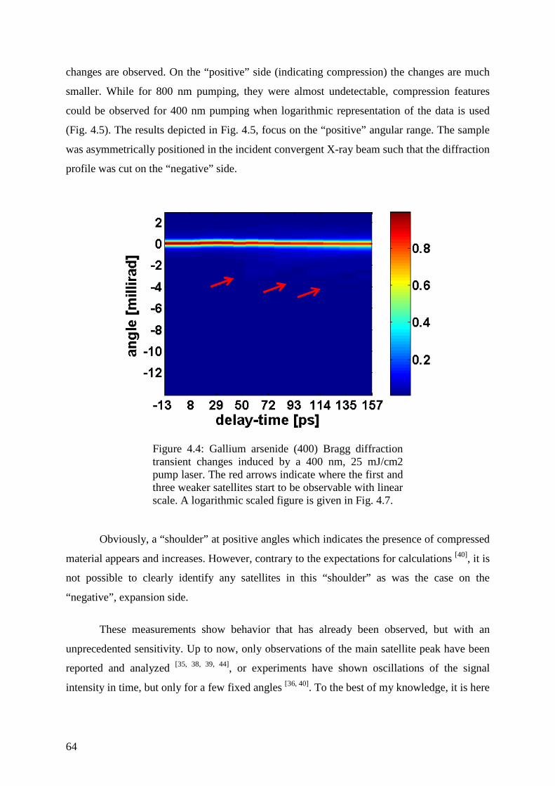
64

changes are observed. On the “positive” side (indicating compression) the changes are much

smaller. While for 800 nm pumping, they were almost undetectable, compression features

could be observed for 400 nm pumping when logarithmic representation of the data is used

(Fig. 4.5). The results depicted in Fig. 4.5, focus on the “positive” angular range. The sample

was asymmetrically positioned in the incident convergent X-ray beam such that the diffraction

profile was cut on the “negative” side.

Figure 4.4: Gallium arsenide (400) Bragg diffraction

transient changes induced by a 400 nm, 25 mJ/cm2 pump laser. The red arrows indicate where the first and three weaker satellites start to be observable with linear scale. A logarithmic scaled figure is given in Fig. 4.7.

Obviously, a “shoulder” at positive angles which indicates the presence of compressed

material appears and increases. However, contrary to the expectations for calculations [40], it is

not possible to clearly identify any satellites in this “shoulder” as was the case on the

“negative”, expansion side.

These measurements show behavior that has already been observed, but with an

unprecedented sensitivity. Up to now, only observations of the main satellite peak have been

reported and analyzed [35, 38, 39, 44], or experiments have shown oscillations of the signal

intensity in time, but only for a few fixed angles [36, 40]. To the best of my knowledge, it is here

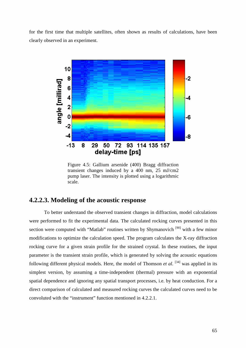
65

for the first time that multiple satellites, often shown as results of calculations, have been

clearly observed in an experiment.

Figure 4.5: Gallium arsenide (400) Bragg diffraction

transient changes induced by a 400 nm, 25 mJ/cm2 pump laser. The intensity is plotted using a logarithmic scale.

4.2.2.3. Modeling of the acoustic response

To better understand the observed transient changes in diffraction, model calculations

were performed to fit the experimental data. The calculated rocking curves presented in this

section were computed with “Matlab” routines written by Shymanovich [90] with a few minor

modifications to optimize the calculation speed. The program calculates the X-ray diffraction

rocking curve for a given strain profile for the strained crystal. In these routines, the input

parameter is the transient strain profile, which is generated by solving the acoustic equations

following different physical models. Here, the model of Thomson et al. [34] was applied in its

simplest version, by assuming a time-independent (thermal) pressure with an exponential

spatial dependence and ignoring any spatial transport processes, i.e. by heat conduction. For a

direct comparison of calculated and measured rocking curves the calculated curves need to be

convoluted with the “instrument” function mentioned in 4.2.2.1.

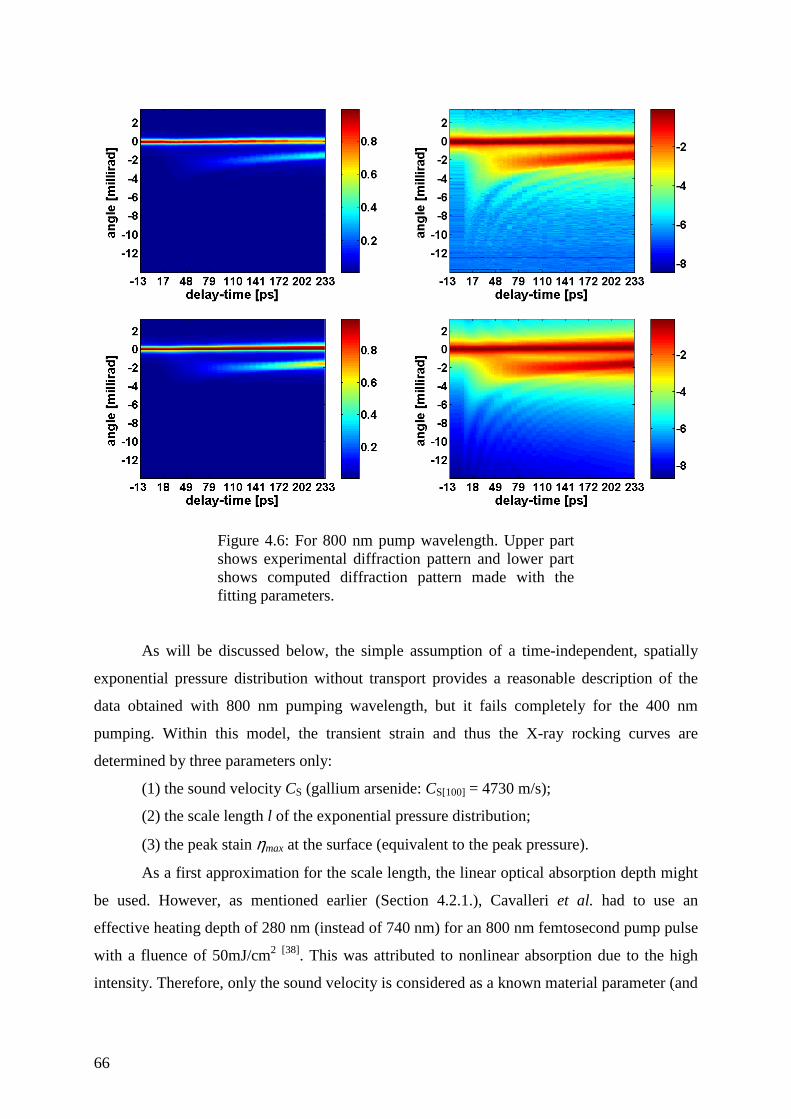
66

Figure 4.6: For 800 nm pump wavelength. Upper part

shows experimental diffraction pattern and lower part shows computed diffraction pattern made with the fitting parameters.

As will be discussed below, the simple assumption of a time-independent, spatially

exponential pressure distribution without transport provides a reasonable description of the

data obtained with 800 nm pumping wavelength, but it fails completely for the 400 nm

pumping. Within this model, the transient strain and thus the X-ray rocking curves are

determined by three parameters only:

(1) the sound velocity CS (gallium arsenide: CS[100] = 4730 m/s);

(2) the scale length l of the exponential pressure distribution;

(3) the peak stain ηmax at the surface (equivalent to the peak pressure).

As a first approximation for the scale length, the linear optical absorption depth might

be used. However, as mentioned earlier (Section 4.2.1.), Cavalleri et al. had to use an

effective heating depth of 280 nm (instead of 740 nm) for an 800 nm femtosecond pump pulse

with a fluence of 50mJ/cm2 [38]. This was attributed to nonlinear absorption due to the high

intensity. Therefore, only the sound velocity is considered as a known material parameter (and

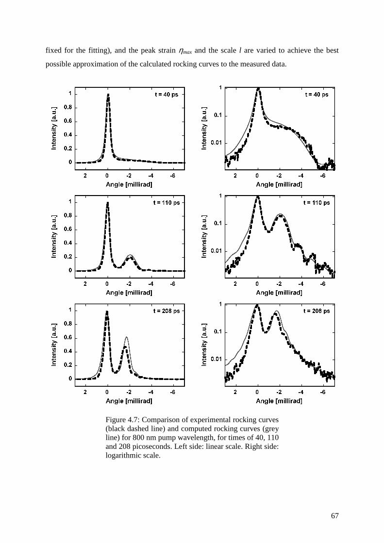
67

fixed for the fitting), and the peak strain ηmax and the scale l are varied to achieve the best

possible approximation of the calculated rocking curves to the measured data.

Figure 4.7: Comparison of experimental rocking curves

(black dashed line) and computed rocking curves (grey line) for 800 nm pump wavelength, for times of 40, 110 and 208 picoseconds. Left side: linear scale. Right side: logarithmic scale.

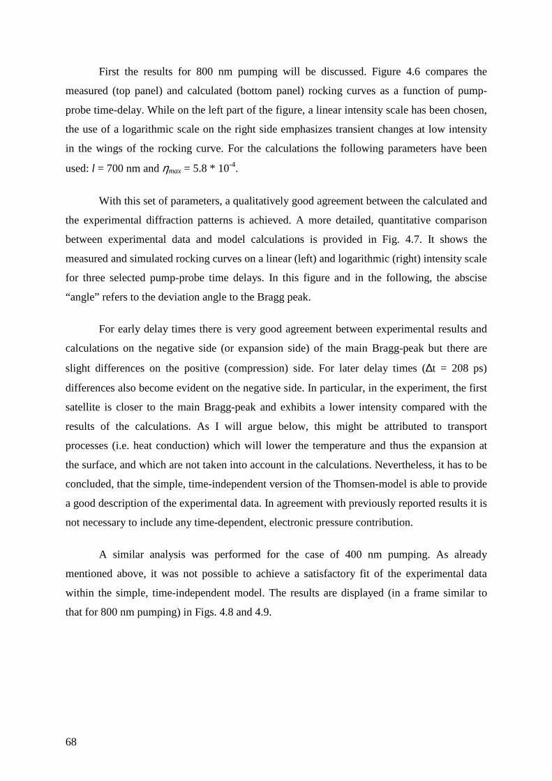
68

First the results for 800 nm pumping will be discussed. Figure 4.6 compares the

measured (top panel) and calculated (bottom panel) rocking curves as a function of pump-

probe time-delay. While on the left part of the figure, a linear intensity scale has been chosen,

the use of a logarithmic scale on the right side emphasizes transient changes at low intensity

in the wings of the rocking curve. For the calculations the following parameters have been

used: l = 700 nm and ηmax = 5.8 * 10-4.

With this set of parameters, a qualitatively good agreement between the calculated and

the experimental diffraction patterns is achieved. A more detailed, quantitative comparison

between experimental data and model calculations is provided in Fig. 4.7. It shows the

measured and simulated rocking curves on a linear (left) and logarithmic (right) intensity scale

for three selected pump-probe time delays. In this figure and in the following, the abscise

“angle” refers to the deviation angle to the Bragg peak.

For early delay times there is very good agreement between experimental results and

calculations on the negative side (or expansion side) of the main Bragg-peak but there are

slight differences on the positive (compression) side. For later delay times (∆t = 208 ps)

differences also become evident on the negative side. In particular, in the experiment, the first

satellite is closer to the main Bragg-peak and exhibits a lower intensity compared with the

results of the calculations. As I will argue below, this might be attributed to transport

processes (i.e. heat conduction) which will lower the temperature and thus the expansion at

the surface, and which are not taken into account in the calculations. Nevertheless, it has to be

concluded, that the simple, time-independent version of the Thomsen-model is able to provide

a good description of the experimental data. In agreement with previously reported results it is

not necessary to include any time-dependent, electronic pressure contribution.

A similar analysis was performed for the case of 400 nm pumping. As already

mentioned above, it was not possible to achieve a satisfactory fit of the experimental data

within the simple, time-independent model. The results are displayed (in a frame similar to

that for 800 nm pumping) in Figs. 4.8 and 4.9.

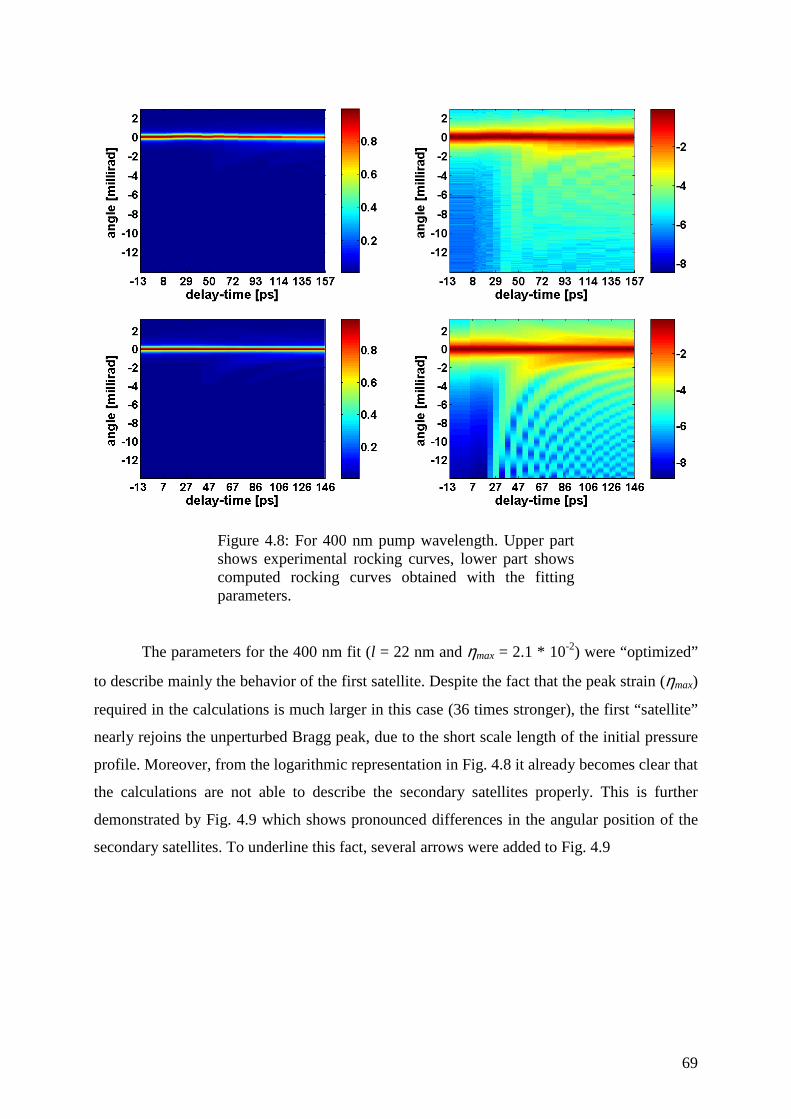
69

Figure 4.8: For 400 nm pump wavelength. Upper part

shows experimental rocking curves, lower part shows computed rocking curves obtained with the fitting parameters.

The parameters for the 400 nm fit (l = 22 nm and ηmax = 2.1 * 10-2) were “optimized”

to describe mainly the behavior of the first satellite. Despite the fact that the peak strain (ηmax)

required in the calculations is much larger in this case (36 times stronger), the first “satellite”

nearly rejoins the unperturbed Bragg peak, due to the short scale length of the initial pressure

profile. Moreover, from the logarithmic representation in Fig. 4.8 it already becomes clear that

the calculations are not able to describe the secondary satellites properly. This is further

demonstrated by Fig. 4.9 which shows pronounced differences in the angular position of the

secondary satellites. To underline this fact, several arrows were added to Fig. 4.9

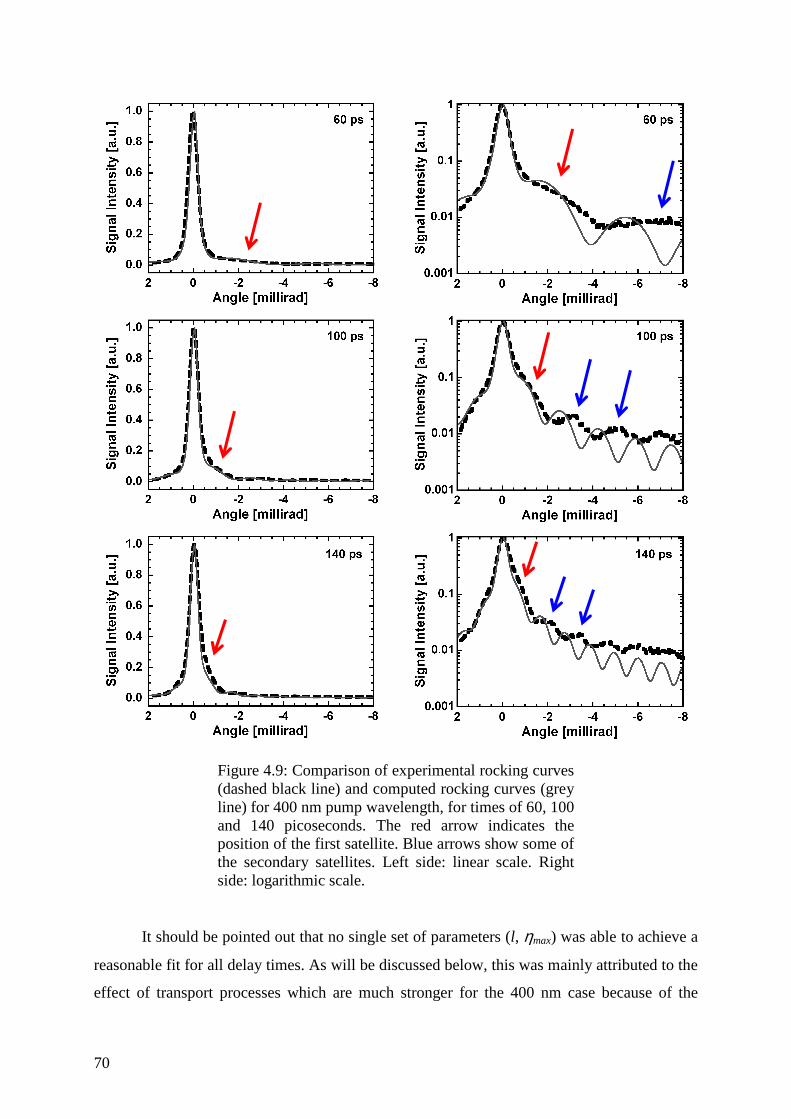
70

Figure 4.9: Comparison of experimental rocking curves (dashed black line) and computed rocking curves (grey line) for 400 nm pump wavelength, for times of 60, 100 and 140 picoseconds. The red arrow indicates the position of the first satellite. Blue arrows show some of the secondary satellites. Left side: linear scale. Right side: logarithmic scale.

It should be pointed out that no single set of parameters (l, ηmax) was able to achieve a

reasonable fit for all delay times. As will be discussed below, this was mainly attributed to the

effect of transport processes which are much stronger for the 400 nm case because of the

71

much larger gradients for 400 nm pumping than for 800 nm pumping. These effects change

the shape of the acoustic pulse as well as the temperature (and strain) of the heated (and

expanded) surface layer. However, no attempt was made to include such processes in the

model for the following reason: A more complete theoretical description (as was applied for

example by Morak et al. [44]) needs to include not only spatial transport processes but also the

detailed dynamics of the electronic and lattice excitation (energy relaxation, carrier diffusion,

electron-hole recombination) and the electronic pressure contribution. As a consequence many

additional material parameters, which are not precisely known for the conditions of strong

electronic excitation, will influence the strain evolution and the shape of the transient rocking

curves. Under such conditions, it cannot be expected to obtain a fit with a unique, physically

meaningful set of parameters.

4.2.2.4. Acoustic pulse speed

Using the Thomsen model for interpreting their measurement in indium antimonide

after femtosecond optical excitation, Lindenberg et al. in 2000 [36] and Larsson et al. in 2002 [40] have also statue than the propagating acoustic pulse with vector q induce an extra time-

dependent periodicity to the lattice. This gives rise to sidebands centered on the Bragg peak

(see Refs. [36] and [40], and references within).

As it has been discussed in these papers, the observed temporal oscillations of the

diffraction intensity are connected to the speed of the propagating acoustic pulse induced by

the optical excitation, i.e. the sound speed cS of the material. In the case of a symmetrical

Bragg-reflection, the following equation can be derived:

Gcs

)tan(Θ⋅∆Θ

= ω, Eq. 4.14

In both references, the authors applied this formula to their measurement performed

with synchrotron sources. Larsson et al. also checked the validity of the formula with the

computed diffraction pattern. However, these authors only got few experimental points.

In contrary, the experimental data obtained for the 400 nm and 800 nm were already

available and were of good quality, which have permitted afterwards to apply this formula

here.

Temporal dependencies of the diffraction intensity for different ∆Θ are obtained from

horizontal cross-sections of the 2D-representations shown in Figs. 4.6 and 4.8.

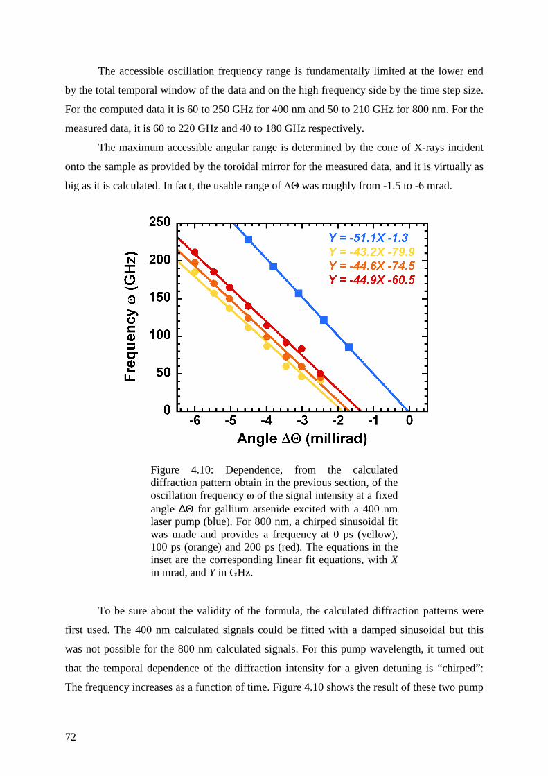
72

The accessible oscillation frequency range is fundamentally limited at the lower end

by the total temporal window of the data and on the high frequency side by the time step size.

For the computed data it is 60 to 250 GHz for 400 nm and 50 to 210 GHz for 800 nm. For the

measured data, it is 60 to 220 GHz and 40 to 180 GHz respectively.

The maximum accessible angular range is determined by the cone of X-rays incident

onto the sample as provided by the toroidal mirror for the measured data, and it is virtually as

big as it is calculated. In fact, the usable range of ∆Θ was roughly from -1.5 to -6 mrad.

Figure 4.10: Dependence, from the calculated diffraction pattern obtain in the previous section, of the oscillation frequency ω of the signal intensity at a fixed angle ∆Θ for gallium arsenide excited with a 400 nm laser pump (blue). For 800 nm, a chirped sinusoidal fit was made and provides a frequency at 0 ps (yellow), 100 ps (orange) and 200 ps (red). The equations in the inset are the corresponding linear fit equations, with X in mrad, and Y in GHz.

To be sure about the validity of the formula, the calculated diffraction patterns were

first used. The 400 nm calculated signals could be fitted with a damped sinusoidal but this

was not possible for the 800 nm calculated signals. For this pump wavelength, it turned out

that the temporal dependence of the diffraction intensity for a given detuning is “chirped”:

The frequency increases as a function of time. Figure 4.10 shows the result of these two pump

73

wavelengths: For the 400 nm data, the (unique) frequency of the fitting function is plotted

with blue squares. For the 800 nm data, three “instantaneous” frequencies for three different

times were obtained and plotted. Frequency at 0 ps, 100 ps and 200 ps are plotted in yellow,

orange and red, respectively.

All dependencies show a linear behavior, but it is obvious that their slope is different,

and already in disagreement with the theory. For the 400 nm calculated data, the linear fit

(blue line) passes through the origin, with a slope of ∆ω/∆Θ = -51.1 GHz/mrad. The slopes

from the 800 nm calculated data do not pass through the origin, but have all the same slope

(44.3 ± 1.8) GHz/mrad.

Using for the formula (Eq. 4.14) the following parameters: θB = 76.551°, tan(θB) =

4.184, d400 = 1.413 * 10-10 m, and G400 = 2π.d400-1 = 4.446 * 1010 m-1, the sound speed are the

following:

For 400 nm: cs[100] = (4807 ± 40) m/s.

For 800 nm: cs[100] = (4170 ± 170) m/s.

This result is of interest, because the obtained velocity for the 400 nm case

corresponds to the value reported in literature, i.e. (cs[100] = 4730 m/s), but surprisingly is

wrong using the 800 nm computed data. This suggests that this formula should be used with

great care, and is not working in all situations.

As the formula worked for the 400 nm calculated pump wavelength, similar analysis

was also performed on the 400 nm and 800 nm measured data. The figure 4.11 shows time-

dependencies of the X-ray diffraction intensity from the 400 nm experimental data (blue data

points) for a number of different ∆Θ, and their corresponding fitting function (red line).

Similar analysis was performed for the corresponding 800 nm data set. The result of

these two fits is depicted in Fig. 4.12.

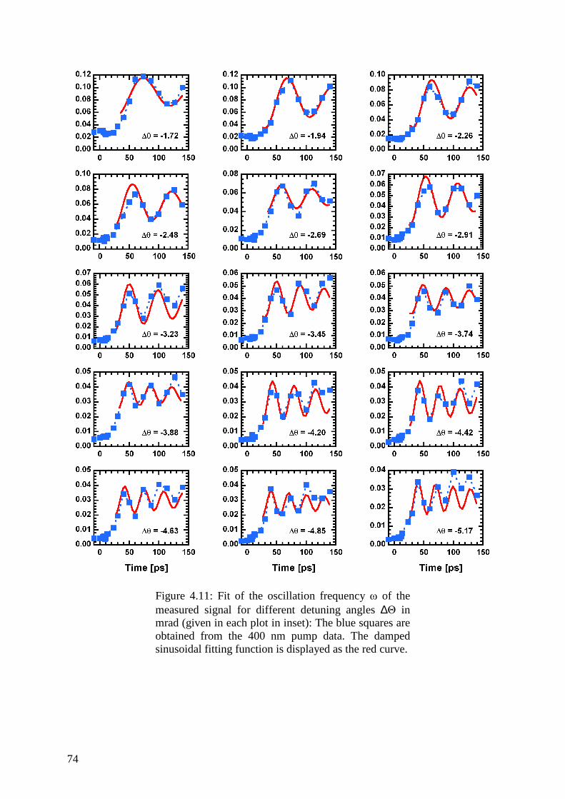
74

Figure 4.11: Fit of the oscillation frequency ω of the

measured signal for different detuning angles ∆Θ in mrad (given in each plot in inset): The blue squares are obtained from the 400 nm pump data. The damped sinusoidal fitting function is displayed as the red curve.

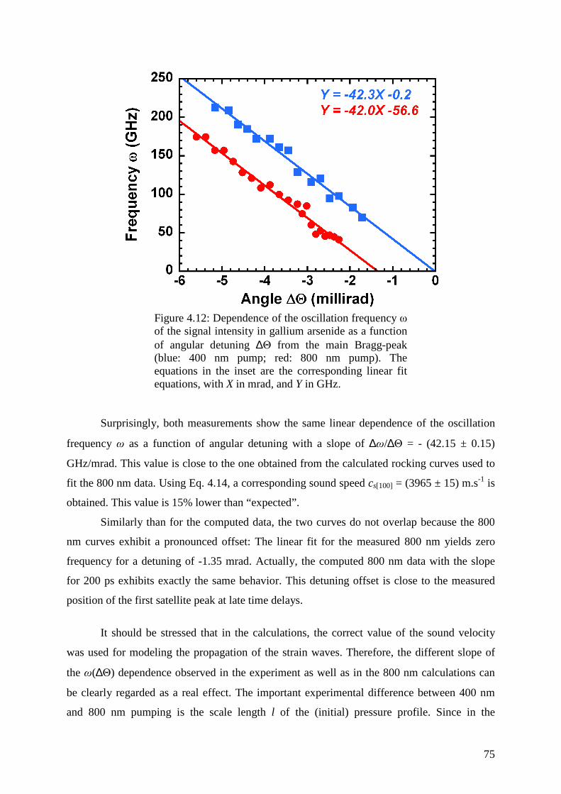
75

Figure 4.12: Dependence of the oscillation frequency ω

of the signal intensity in gallium arsenide as a function of angular detuning ∆Θ from the main Bragg-peak (blue: 400 nm pump; red: 800 nm pump). The equations in the inset are the corresponding linear fit equations, with X in mrad, and Y in GHz.

Surprisingly, both measurements show the same linear dependence of the oscillation

frequency ω as a function of angular detuning with a slope of ∆ω/∆Θ = - (42.15 ± 0.15)

GHz/mrad. This value is close to the one obtained from the calculated rocking curves used to

fit the 800 nm data. Using Eq. 4.14, a corresponding sound speed cs[100] = (3965 ± 15) m.s-1 is

obtained. This value is 15% lower than “expected”.

Similarly than for the computed data, the two curves do not overlap because the 800

nm curves exhibit a pronounced offset: The linear fit for the measured 800 nm yields zero

frequency for a detuning of -1.35 mrad. Actually, the computed 800 nm data with the slope

for 200 ps exhibits exactly the same behavior. This detuning offset is close to the measured

position of the first satellite peak at late time delays.

It should be stressed that in the calculations, the correct value of the sound velocity

was used for modeling the propagation of the strain waves. Therefore, the different slope of

the ω(∆Θ) dependence observed in the experiment as well as in the 800 nm calculations can

be clearly regarded as a real effect. The important experimental difference between 400 nm

and 800 nm pumping is the scale length l of the (initial) pressure profile. Since in the

76

calculations, the profile does not change because no transport is considered, the acoustic pulse

detaches much earlier from the “static” laser-excited region in the 400 nm case than in the 800

nm case. Assuming that the pulse must propagate roughly 7 times (at least) the scale length l

to completely detach, this time can be estimated as td ≈ 7 * l / cs, which is approximately 30 ps

at 400 nm, but more than one nanosecond at 800 nm.

Whether this is related to the deviation of the derived sound velocity from the “real”

value, and why there is in some cases an offset in the ω(∆Θ) dependence (in the case of a

“long” scale length) has not been further investigated. However, it must be concluded, that the

procedure described in [36, 40] must be used with great care, and that an agreement (or

disagreement) with the “real” sound velocity does not represent any kind of consistency-

check. The results discussed in this section with respect to the sound velocity also underline

the fact that the applied modeling provides a reasonable description of the 800 nm data, but

fails at 400 nm.

4.2.3. Summary and discussion of the measurement on gallium arsenide

Time-resolved X-ray diffraction experiments have been performed on single-

crystalline bulk samples of gallium arsenide, excited with femtosecond laser pulses at 800 nm

and 400 nm. The high angular resolution and large dynamic range of the measurements

allowed the recording of small/weak changes in the X-ray rocking curves. In particular, the

evolution of “side-bands” in the rocking curves caused by propagating strain/acoustic waves

could be clearly followed with high sensitivity.

The experimental data have been compared with model calculations based on the

approach introduced by Thomsen et al. [34]. This model has been used in its simplest version

by assuming a time-independent, spatially exponentially decaying pressure and ignoring any

transport processes. It was found that this simple approach provides a rather good description

of the experimental data obtained with 800 nm pumping, but for the 400 nm case, although it

shows qualitatively a comparable behavior (appearance of satellite diffraction peaks which

move towards the non-perturbed diffraction peak in time), fails completely to match the

position of these satellites.

In the following paragraphs, I will argue that this fact is most likely due to the

different role and importance of transport processes (i.e. heat conduction and, possibly, carrier

diffusion) for the different pumping conditions. While with a pump wavelength of 800 nm the

77

scale length l of the initial pressure profile is 700 nm, l is only 20 nm for a 400 nm pumping

wavelength. Due to this large difference, transport processes will be important for the latter

case, but can be essentially neglected at 800 nm.

Thomsen et al. [34] already discussed the effect of heat conduction on the strain pulse

traveling into the crystal. Whether this effect is important or not is determined by the typical

time scale for heat diffusion, which can be estimated as theat ≈ l2/D, where D is the thermal

diffusivity (for GaAs: D = 31 nm2.ps-1). theat needs to be compared with the range of delay

times over which the strain evolution is monitored in the experiments (approximately 200 ps).

For pumping with 800 nm, with l = 700 nm, one gets a theat of approximately 16 ns. In

contrast, for 400 nm pumping, with l = 20 nm, one gets a value of only 13 ps! This means that

heat diffusion can be neglected at a pump wavelength of 800 nm but that it definitely

influences the strain profile and the shape of the acoustic pulse at 400 nm. However, as

explained above, a model including transport processes was not tried because of the ambiguity

introduced by a number of additional parameters that would enter the calculations and which

are not accurately known under the conditions of the experiment (i.e. strong electronic

excitation).

Despite the unimportance of transport effects, it is nevertheless noteworthy that the

800 nm data are so well described by the simple, time-independent model. As has been

pointed out in the introduction to this chapter, it is expected that the time-dependent electronic

pressure should play an important role (see Eq. 4.5). However, the importance of the

electronic pressure is not only determined by the initial magnitude but also by its (limited)

“lifetime” tEP, due to electron-hole recombination. In gallium arsenide, Auger-recombination

determines the lifetime of electron-hole plasma at higher carrier densities. tEP can be estimated

as tEP ≈ 1 / (γ · ne-h2) ≈ 1 ps, with the Auger-recombination coefficient γ ≈ 10-30 cm6.s-1 and the

excited carrier density ne-h which is approximately ne-h ≈ (1 - R)·F / (l·ħω) ≈ 1021 cm-3 (with a

reflectivity of: R = 35 %; a pump fluence of: F = 32 mJ/cm2; a photon energy of: ħω = 1.5

eV). This one picosecond for the lifetime of the electronic pressure needs to be compared with

the typical acoustic time-scale of the experiment (at 800 nm pumping) tac ≈ l / cs ≈ 150 ps.

Since tEP is much shorter than tac, it is not surprising that the time-independent model works

well here. The electronic pressure might play some role in the 400 nm experiment because

under these conditions, tac ≈ 4 ps, and it is comparable with the carrier lifetime. However,

these effects are most likely masked by transport processes, as discussed above.

In conclusion, the presented measurement shows that it is not possible to get reliable

information concerning the electronic and thermal contributions to the acoustic response in

78

laser-excited gallium arsenide. I believe this is due to the fact that I used a bulk sample

because in this case the acoustic response and the strain evolution depend on too many

unknown parameters. To get reliable information, the use of a thin film of gallium arsenide

(and in general for all semiconductors) is required.

4.3. Picosecond acoustic response of a laser-excited gold-film

This section discusses time-resolved diffraction experiments on the transient acoustic

response of a thin (approx. 90 nm) gold film after femtosecond optical excitation. In contrast

to the experiments on bulk semiconductors, which have been discussed in the previous

section, the use of a thin film lead to well-defined excitation conditions and allowed to obtain

information about the processes that determine the dynamics of the acoustic waves in this

material. This experiment was mainly motivated by earlier results from Shymanovich who

had to vary the initial ratio of electronic and thermal pressure in order to fit his measurement

on a thin germanium crystalline film [90]. This experiment was done in order to compare the

behavior of a semiconductor and a metal under similar excitation conditions.

4.3.1. Description of the experimental setup

This measurement was performed with the in-vacuum setup described in section

3.3.2.1 using Ti Kα1 radiation. Because the reflectivity of gold at 800 nm is very high (R =

95%), 400 nm wavelength pump pulses (R = 30%) were used.

The gold sample was an Au(111) thin film epitaxially grown using RF magnetron

sputtering on freshly cleaved, (001)-oriented, high quality mica muscovite [122]. The relevant

material parameters are provided in Appendix B.3. The Bragg angle for the (111) reflection of

Au at 4.51 keV is 35.70°; the closest reflection of the mica-substrate is the (008)-reflection at

33.32°. Figure 4.13 shows the typical diffraction signal obtained for the gold thin film (on the

left side) and its substrate (on the right side), artificially put together in one image. The

distance sample – CCD is 160 mm.

The exposure time for the mica(800) and the Au(111) diffraction was 90 seconds, i.e.

900 laser pulses. From Figure 4.13 it is obvious that the Au(111) diffraction peak is much

broader than the mica(008) peak. The measured full width at half maximum of the rocking

curves are 0.365° for the Au(111) and 0.023° for the mica(008). Using the program XOP [123],

the theoretically calculated rocking curve widths are found to be 0.10° FWHM for the (111)-

reflection of a 90 nm thick crystalline gold film, and 0.0015° for a bulk mica sample. The

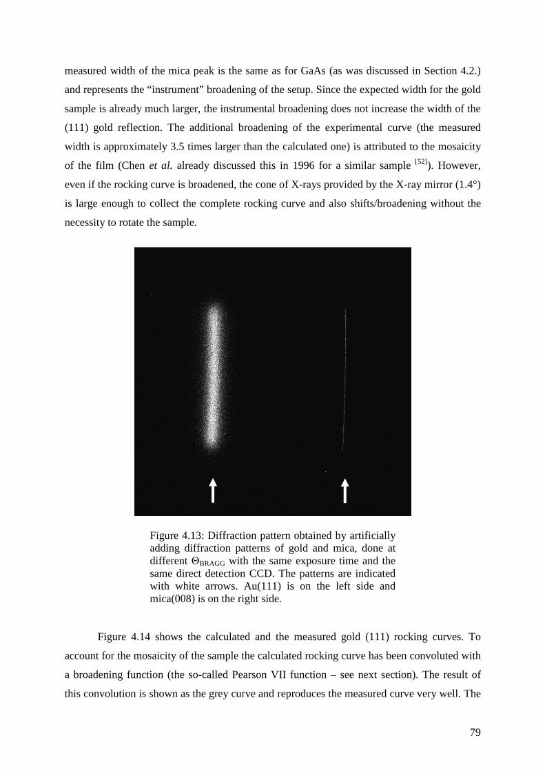
79

measured width of the mica peak is the same as for GaAs (as was discussed in Section 4.2.)

and represents the “instrument” broadening of the setup. Since the expected width for the gold

sample is already much larger, the instrumental broadening does not increase the width of the

(111) gold reflection. The additional broadening of the experimental curve (the measured

width is approximately 3.5 times larger than the calculated one) is attributed to the mosaicity

of the film (Chen et al. already discussed this in 1996 for a similar sample [52]). However,

even if the rocking curve is broadened, the cone of X-rays provided by the X-ray mirror (1.4°)

is large enough to collect the complete rocking curve and also shifts/broadening without the

necessity to rotate the sample.

Figure 4.13: Diffraction pattern obtained by artificially

adding diffraction patterns of gold and mica, done at different ΘBRAGG with the same exposure time and the same direct detection CCD. The patterns are indicated with white arrows. Au(111) is on the left side and mica(008) is on the right side.

Figure 4.14 shows the calculated and the measured gold (111) rocking curves. To

account for the mosaicity of the sample the calculated rocking curve has been convoluted with

a broadening function (the so-called Pearson VII function – see next section). The result of

this convolution is shown as the grey curve and reproduces the measured curve very well. The

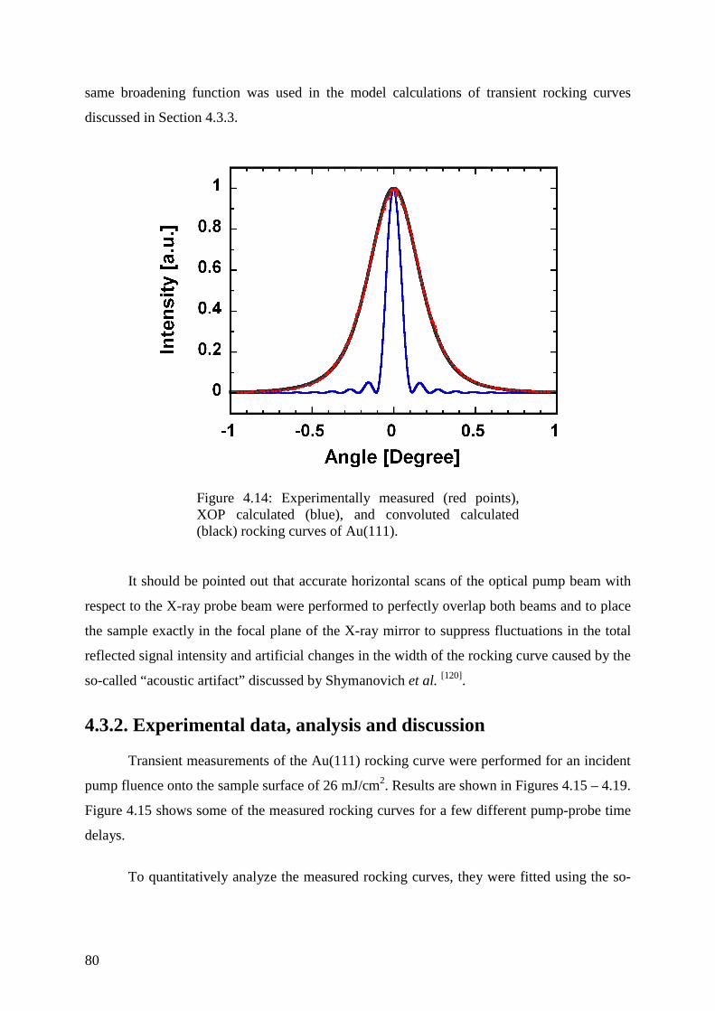
80

same broadening function was used in the model calculations of transient rocking curves

discussed in Section 4.3.3.

Figure 4.14: Experimentally measured (red points),

XOP calculated (blue), and convoluted calculated (black) rocking curves of Au(111).

It should be pointed out that accurate horizontal scans of the optical pump beam with

respect to the X-ray probe beam were performed to perfectly overlap both beams and to place

the sample exactly in the focal plane of the X-ray mirror to suppress fluctuations in the total

reflected signal intensity and artificial changes in the width of the rocking curve caused by the

so-called “acoustic artifact” discussed by Shymanovich et al. [120].

4.3.2. Experimental data, analysis and discussion

Transient measurements of the Au(111) rocking curve were performed for an incident

pump fluence onto the sample surface of 26 mJ/cm2. Results are shown in Figures 4.15 – 4.19.

Figure 4.15 shows some of the measured rocking curves for a few different pump-probe time

delays.

To quantitatively analyze the measured rocking curves, they were fitted using the so-

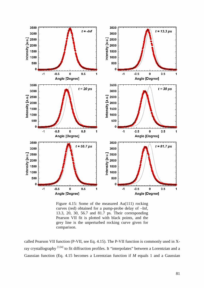
81

Figure 4.15: Some of the measured Au(111) rocking

curves (red) obtained for a pump-probe delay of –Inf, 13.3, 20, 30, 56.7 and 81.7 ps. Their corresponding Pearson VII fit is plotted with black points, and the grey line is the unperturbed rocking curve given for comparison.

called Pearson VII function (P-VII, see Eq. 4.15). The P-VII function is commonly used in X-

ray crystallography [124] to fit diffraction profiles. It “interpolates” between a Lorentzian and a

Gaussian function (Eq. 4.15 becomes a Lorentzian function if M equals 1 and a Gaussian

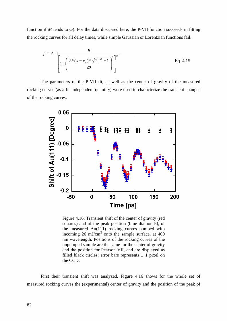
82

function if M tends to ∞). For the data discussed here, the P-VII function succeeds in fitting

the rocking curves for all delay times, while simple Gaussian or Lorentzian functions fail.

M

Moxx

BAf

−−+

+=−

2

12*)(*21

ω

Eq. 4.15

The parameters of the P-VII fit, as well as the center of gravity of the measured

rocking curves (as a fit-independent quantity) were used to characterize the transient changes

of the rocking curves.

Figure 4.16: Transient shift of the center of gravity (red

squares) and of the peak position (blue diamonds), of the measured Au(111) rocking curves pumped with incoming 26 mJ/cm2 onto the sample surface, at 400 nm wavelength. Positions of the rocking curves of the unpumped sample are the same for the center of gravity and the position for Pearson VII, and are displayed as filled black circles; error bars represents ± 1 pixel on the CCD.

First their transient shift was analyzed. Figure 4.16 shows for the whole set of

measured rocking curves the (experimental) center of gravity and the position of the peak of

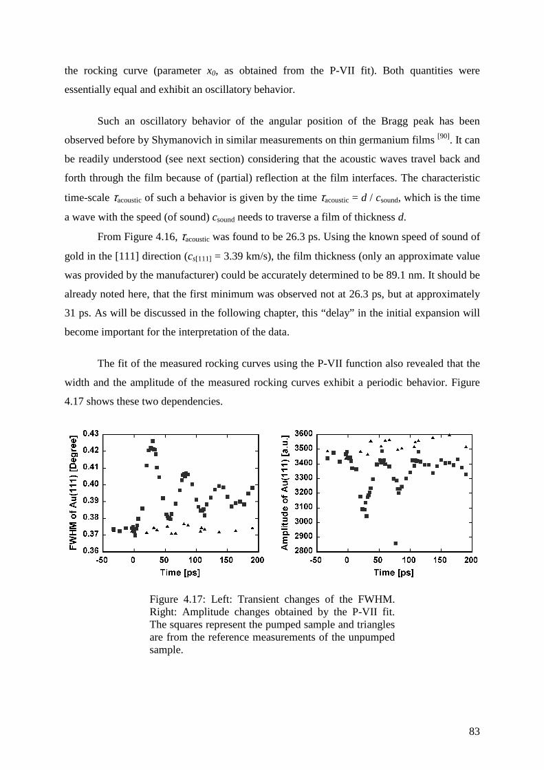
83

the rocking curve (parameter x0, as obtained from the P-VII fit). Both quantities were

essentially equal and exhibit an oscillatory behavior.

Such an oscillatory behavior of the angular position of the Bragg peak has been

observed before by Shymanovich in similar measurements on thin germanium films [90]. It can

be readily understood (see next section) considering that the acoustic waves travel back and

forth through the film because of (partial) reflection at the film interfaces. The characteristic

time-scale τacoustic of such a behavior is given by the time τacoustic = d / csound, which is the time

a wave with the speed (of sound) csound needs to traverse a film of thickness d.

From Figure 4.16, τacoustic was found to be 26.3 ps. Using the known speed of sound of

gold in the [111] direction (cs[111] = 3.39 km/s), the film thickness (only an approximate value

was provided by the manufacturer) could be accurately determined to be 89.1 nm. It should be

already noted here, that the first minimum was observed not at 26.3 ps, but at approximately

31 ps. As will be discussed in the following chapter, this “delay” in the initial expansion will

become important for the interpretation of the data.

The fit of the measured rocking curves using the P-VII function also revealed that the

width and the amplitude of the measured rocking curves exhibit a periodic behavior. Figure

4.17 shows these two dependencies.

Figure 4.17: Left: Transient changes of the FWHM. Right: Amplitude changes obtained by the P-VII fit. The squares represent the pumped sample and triangles are from the reference measurements of the unpumped sample.

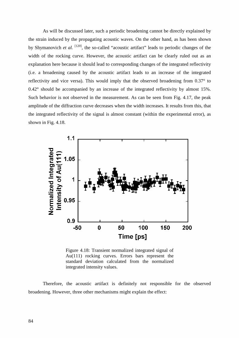
84

As will be discussed later, such a periodic broadening cannot be directly explained by

the strain induced by the propagating acoustic waves. On the other hand, as has been shown

by Shymanovich et al. [120], the so-called “acoustic artifact” leads to periodic changes of the

width of the rocking curve. However, the acoustic artifact can be clearly ruled out as an

explanation here because it should lead to corresponding changes of the integrated reflectivity

(i.e. a broadening caused by the acoustic artifact leads to an increase of the integrated

reflectivity and vice versa). This would imply that the observed broadening from 0.37° to

0.42° should be accompanied by an increase of the integrated reflectivity by almost 15%.

Such behavior is not observed in the measurement. As can be seen from Fig. 4.17, the peak

amplitude of the diffraction curve decreases when the width increases. It results from this, that

the integrated reflectivity of the signal is almost constant (within the experimental error), as

shown in Fig. 4.18.

Figure 4.18: Transient normalized integrated signal of

Au(111) rocking curves. Errors bars represent the standard deviation calculated from the normalized integrated intensity values.

Therefore, the acoustic artifact is definitely not responsible for the observed

broadening. However, three other mechanisms might explain the effect:

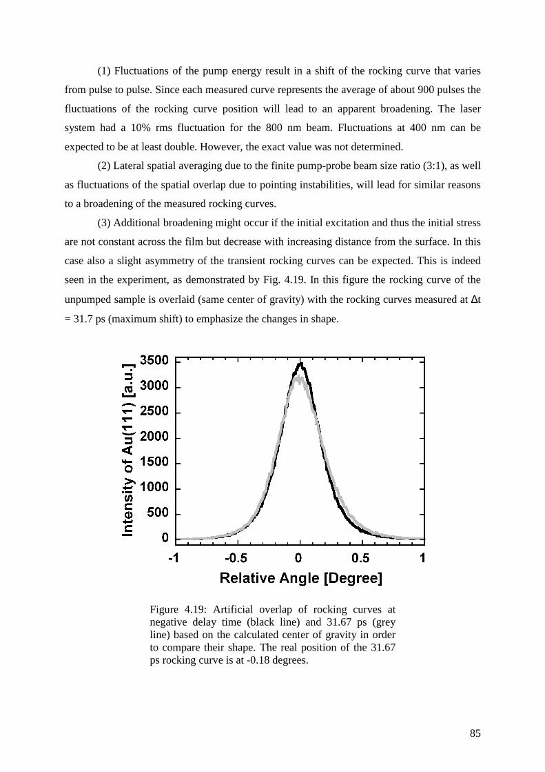
85

(1) Fluctuations of the pump energy result in a shift of the rocking curve that varies

from pulse to pulse. Since each measured curve represents the average of about 900 pulses the

fluctuations of the rocking curve position will lead to an apparent broadening. The laser

system had a 10% rms fluctuation for the 800 nm beam. Fluctuations at 400 nm can be

expected to be at least double. However, the exact value was not determined.

(2) Lateral spatial averaging due to the finite pump-probe beam size ratio (3:1), as well

as fluctuations of the spatial overlap due to pointing instabilities, will lead for similar reasons

to a broadening of the measured rocking curves.

(3) Additional broadening might occur if the initial excitation and thus the initial stress

are not constant across the film but decrease with increasing distance from the surface. In this

case also a slight asymmetry of the transient rocking curves can be expected. This is indeed

seen in the experiment, as demonstrated by Fig. 4.19. In this figure the rocking curve of the

unpumped sample is overlaid (same center of gravity) with the rocking curves measured at ∆t

= 31.7 ps (maximum shift) to emphasize the changes in shape.

Figure 4.19: Artificial overlap of rocking curves at

negative delay time (black line) and 31.67 ps (grey line) based on the calculated center of gravity in order to compare their shape. The real position of the 31.67 ps rocking curve is at -0.18 degrees.

86

With reference to Fig. 4.18 it should be also noted that for the given experimental

conditions no detectable decrease of the integrated reflectivity due to the Debye-Waller effect

is expected. Interpreting the shift of the (111) Bragg peak at long delay times (-0.11°

approximately) as thermal expansion, and assuming one dimensional expansion (i.e. under the

experimental conditions, the film can only expand along its normal direction) [121], a

temperature increase of 63 K is derived. The corresponding decrease of the signal intensity

due to the Debye-Waller effect would be approximately 1 % which is below the accuracy of

the measurement.

4.3.3. Modeling and interpretation of the experimental data

Compared to a bulk sample, the use of a thin film allows us to establish rather well

defined excitation conditions. Although the absorption depth at 400 nm is only 15 nm, fast

ballistic transport of the optically excited electrons distributes the deposited energy in less

than one picosecond, over depths of more than 100 nm [125]. Therefore, an almost

homogeneous excitation of the film, and negligible excitation of the substrate can be assumed.

As a consequence, the important parameter determining the induced pressure and the

subsequent acoustic waves is the total deposited energy. Moreover, any influence of transport

processes across the film-substrate interface on the propagation of the acoustic waves can be

neglected. This greatly simplifies the acoustic problem and the interpretation of the

experimental data.

The case of a step-like increasing, non-decaying pressure illustrates the main features

of the acoustic response in the best way. For these conditions, the strain waves have a simple

rectangular shape, as schematically shown in Fig. 4.20. Two rarefaction waves are launched

from the film-vacuum and film-substrate interfaces, respectively, into the pressurized film,

while the non-excited substrate is compressed. The acoustic waves travel back and forth

through the film because of (partial) reflection at the film interfaces. Their relative magnitude

as well as their decay is determined by the acoustic impedances of the film and the substrate,

respectively. As already mentioned above, the characteristic time-scale of the wave

propagation is given by the time T = d / cs, the time needed for acoustic waves to traverse the

film thickness d with the speed of sound cs.

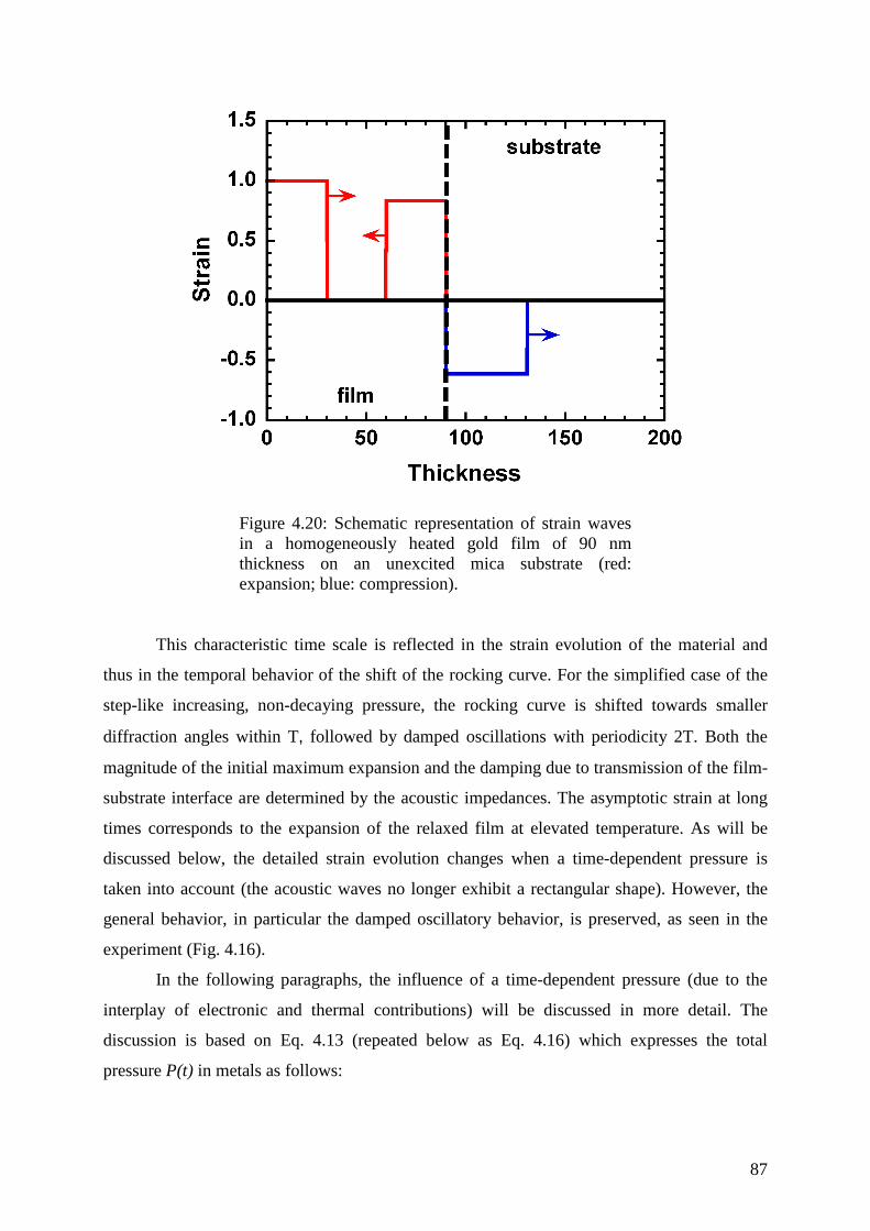
87

Figure 4.20: Schematic representation of strain waves

in a homogeneously heated gold film of 90 nm thickness on an unexcited mica substrate (red: expansion; blue: compression).

This characteristic time scale is reflected in the strain evolution of the material and

thus in the temporal behavior of the shift of the rocking curve. For the simplified case of the

step-like increasing, non-decaying pressure, the rocking curve is shifted towards smaller

diffraction angles within T, followed by damped oscillations with periodicity 2T. Both the

magnitude of the initial maximum expansion and the damping due to transmission of the film-

substrate interface are determined by the acoustic impedances. The asymptotic strain at long

times corresponds to the expansion of the relaxed film at elevated temperature. As will be

discussed below, the detailed strain evolution changes when a time-dependent pressure is

taken into account (the acoustic waves no longer exhibit a rectangular shape). However, the

general behavior, in particular the damped oscillatory behavior, is preserved, as seen in the

experiment (Fig. 4.16).

In the following paragraphs, the influence of a time-dependent pressure (due to the

interplay of electronic and thermal contributions) will be discussed in more detail. The

discussion is based on Eq. 4.13 (repeated below as Eq. 4.16) which expresses the total

pressure P(t) in metals as follows:

88

( )

−

−+= τ

γγ

tPtPi

e exp*11)( 0 , Eq. 4.16

While the maximum thermal pressure P0 in the film is determined by the deposited

energy, the time dependence of the pressure is a function of the γe / γi ratio and the time

constant τ for the electron-to-lattice energy transfer only. Depending on the γe / γi ratio,

different situations need to be considered, as displayed in Figure 4.21 (the time and pressure

scales have been normalized to τ and P0, respectively).

Figure 4.21: Evolution of the total pressure normalized

to the final pressure (P0) depending on the γe / γi Grüneisen ratio (for a ratio of 0, 0.5, 1 and 1.5), and normalized to the time constant τ.

When the γe / γi ratio is larger than one, then the pressure is maximal just after

excitation and decays with the time constant τ towards the asymptotic value P0; when γe / γi is

smaller than one the pressure increases with time also towards P0. For γe / γi = 1, the total

pressure is constant.

As mentioned above, the actual shape of the acoustic waves and thus also the shift of

the rocking curves depends on the temporal dependence of the total pressure. The different

situations sketched in Fig. 4.21 will be discussed below and compared to the experimental

data. For this purpose, the acoustic equations have been solved for the different P(t)-

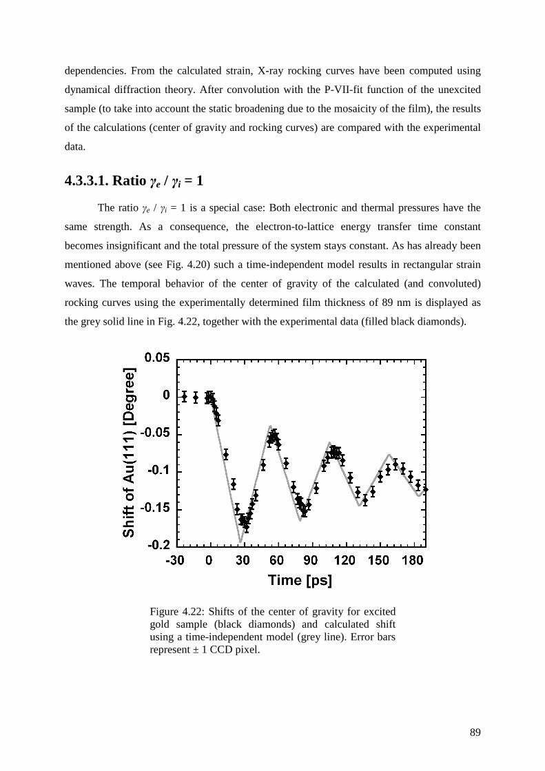
89

dependencies. From the calculated strain, X-ray rocking curves have been computed using

dynamical diffraction theory. After convolution with the P-VII-fit function of the unexcited

sample (to take into account the static broadening due to the mosaicity of the film), the results

of the calculations (center of gravity and rocking curves) are compared with the experimental

data.

4.3.3.1. Ratio γe / γi = 1

The ratio γe / γi = 1 is a special case: Both electronic and thermal pressures have the

same strength. As a consequence, the electron-to-lattice energy transfer time constant

becomes insignificant and the total pressure of the system stays constant. As has already been

mentioned above (see Fig. 4.20) such a time-independent model results in rectangular strain

waves. The temporal behavior of the center of gravity of the calculated (and convoluted)

rocking curves using the experimentally determined film thickness of 89 nm is displayed as

the grey solid line in Fig. 4.22, together with the experimental data (filled black diamonds).

Figure 4.22: Shifts of the center of gravity for excited

gold sample (black diamonds) and calculated shift using a time-independent model (grey line). Error bars represent ± 1 CCD pixel.

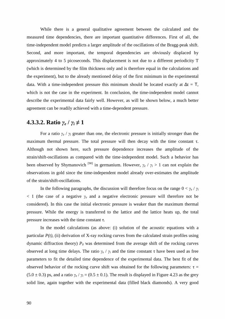
90

While there is a general qualitative agreement between the calculated and the

measured time dependencies, there are important quantitative differences. First of all, the

time-independent model predicts a larger amplitude of the oscillations of the Bragg-peak shift.

Second, and more important, the temporal dependencies are obviously displaced by

approximately 4 to 5 picoseconds. This displacement is not due to a different periodicity T

(which is determined by the film thickness only and is therefore equal in the calculations and

the experiment), but to the already mentioned delay of the first minimum in the experimental

data. With a time-independent pressure this minimum should be located exactly at ∆t = Τ,

which is not the case in the experiment. In conclusion, the time-independent model cannot

describe the experimental data fairly well. However, as will be shown below, a much better

agreement can be readily achieved with a time-dependent pressure.

4.3.3.2. Ratio γe / γi ≠ 1

For a ratio γe / γi greater than one, the electronic pressure is initially stronger than the

maximum thermal pressure. The total pressure will then decay with the time constant τ.

Although not shown here, such pressure dependence increases the amplitude of the

strain/shift-oscillations as compared with the time-independent model. Such a behavior has

been observed by Shymanovich [90] in germanium. However, γe / γi > 1 can not explain the

observations in gold since the time-independent model already over-estimates the amplitude

of the strain/shift-oscillations.

In the following paragraphs, the discussion will therefore focus on the range 0 < γe / γi

< 1 (the case of a negative γe and a negative electronic pressure will therefore not be

considered). In this case the initial electronic pressure is weaker than the maximum thermal

pressure. While the energy is transferred to the lattice and the lattice heats up, the total

pressure increases with the time constant τ.

In the model calculations (as above: (i) solution of the acoustic equations with a

particular P(t), (ii) derivation of X-ray rocking curves from the calculated strain profiles using

dynamic diffraction theory) P0 was determined from the average shift of the rocking curves

observed at long time delays. The ratio γe / γi and the time constant τ have been used as free

parameters to fit the detailed time dependence of the experimental data. The best fit of the

observed behavior of the rocking curve shift was obtained for the following parameters: τ =

(5.0 ± 0.3) ps, and a ratio γe / γi = (0.5 ± 0.1). The result is displayed in Figure 4.23 as the grey

solid line, again together with the experimental data (filled black diamonds). A very good

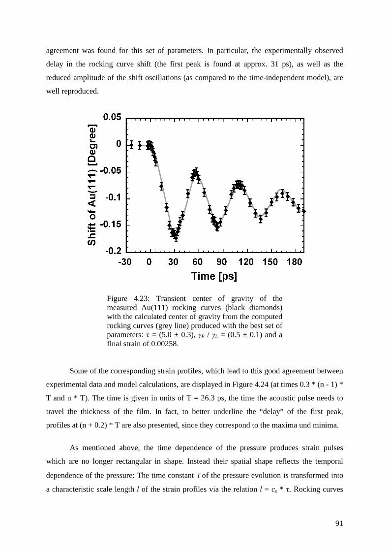
91

agreement was found for this set of parameters. In particular, the experimentally observed

delay in the rocking curve shift (the first peak is found at approx. 31 ps), as well as the

reduced amplitude of the shift oscillations (as compared to the time-independent model), are

well reproduced.

Figure 4.23: Transient center of gravity of the

measured Au(111) rocking curves (black diamonds) with the calculated center of gravity from the computed rocking curves (grey line) produced with the best set of parameters: τ = (5.0 ± 0.3), γE / γL = (0.5 ± 0.1) and a final strain of 0.00258.

Some of the corresponding strain profiles, which lead to this good agreement between

experimental data and model calculations, are displayed in Figure 4.24 (at times 0.3 * (n - 1) *

T and n * T). The time is given in units of T = 26.3 ps, the time the acoustic pulse needs to

travel the thickness of the film. In fact, to better underline the “delay” of the first peak,

profiles at (n + 0.2) * T are also presented, since they correspond to the maxima und minima.

As mentioned above, the time dependence of the pressure produces strain pulses

which are no longer rectangular in shape. Instead their spatial shape reflects the temporal

dependence of the pressure: The time constant τ of the pressure evolution is transformed into

a characteristic scale length l of the strain profiles via the relation l = cs * τ. Rocking curves

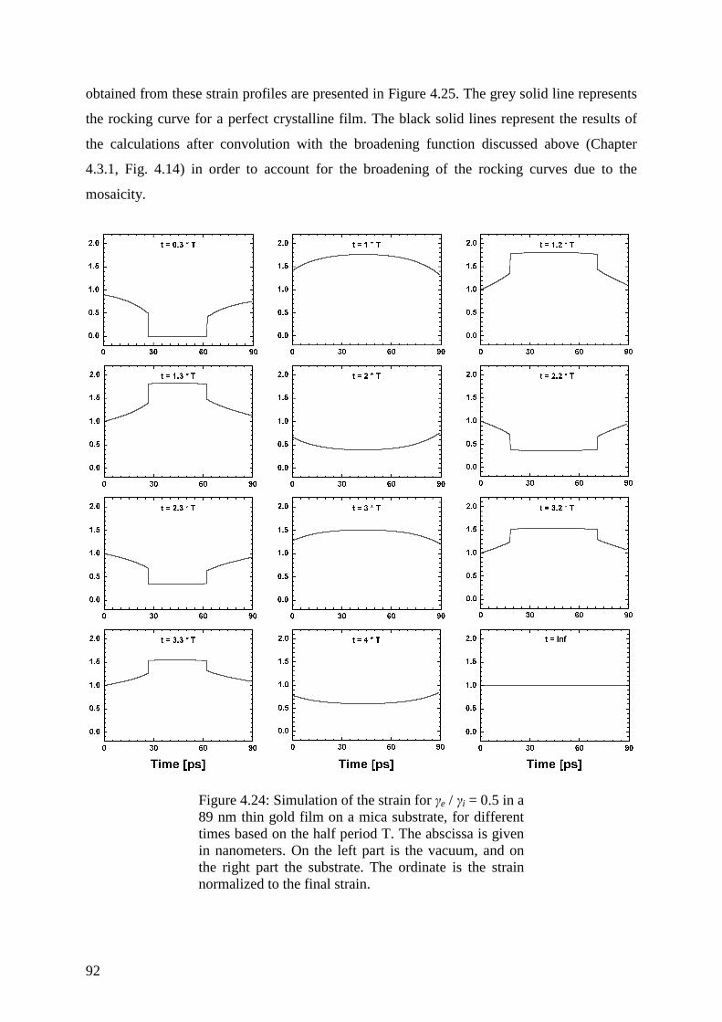
92

obtained from these strain profiles are presented in Figure 4.25. The grey solid line represents

the rocking curve for a perfect crystalline film. The black solid lines represent the results of

the calculations after convolution with the broadening function discussed above (Chapter

4.3.1, Fig. 4.14) in order to account for the broadening of the rocking curves due to the

mosaicity.

Figure 4.24: Simulation of the strain for γe / γi = 0.5 in a

89 nm thin gold film on a mica substrate, for different times based on the half period T. The abscissa is given in nanometers. On the left part is the vacuum, and on the right part the substrate. The ordinate is the strain normalized to the final strain.

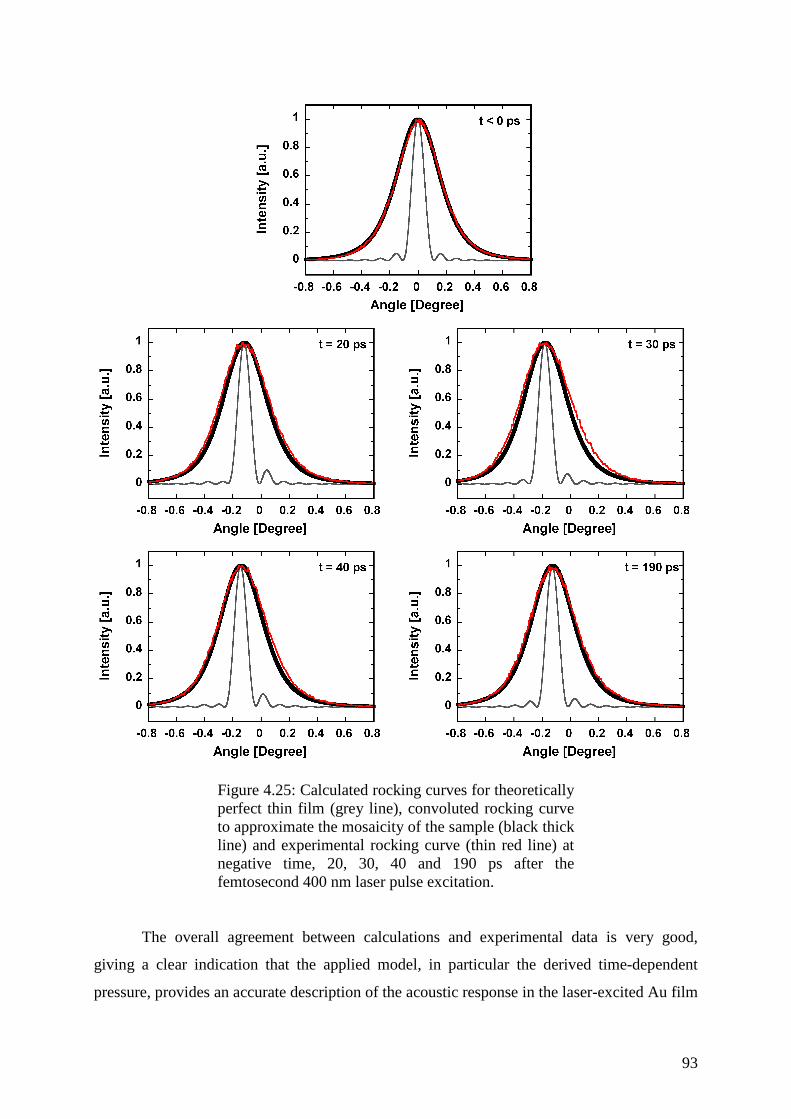
93

Figure 4.25: Calculated rocking curves for theoretically

perfect thin film (grey line), convoluted rocking curve to approximate the mosaicity of the sample (black thick line) and experimental rocking curve (thin red line) at negative time, 20, 30, 40 and 190 ps after the femtosecond 400 nm laser pulse excitation.

The overall agreement between calculations and experimental data is very good,

giving a clear indication that the applied model, in particular the derived time-dependent

pressure, provides an accurate description of the acoustic response in the laser-excited Au film

94

(possible reasons for the slight, asymmetric broadening of the experimental rocking curves

have already been discussed above).

4.3.4. Summary and discussion of the measurements on gold

Using time-resolved X-ray diffraction, it was possible to measure the evolution of the

transient rocking curve of a gold thin film excited with a 400 nm femtosecond pulse. To

interpret these measurements, the two-temperature model was used to fit the data. It was

found that the electron to lattice energy transfer time constant in gold is (5.0 ± 0.3)

picoseconds. This value was compared with the latest time-resolved electron diffraction

measurements performed by Ligges et al. [126, 127]. These authors used a femtosecond electron

source to measure the time constant for energy transfer in a thin gold film and found a time

constant of (4.7 ± 0.6) picoseconds which is in good agreement with the value obtained in this

thesis.

The second important piece of information obtained here concerns the ratio of the

Grüneisen parameters γe / γi which is found to be equals to (0.5 ± 0.1). From the literature,

these coefficients are known to be γe = (1.6 ± 0.5) and γi = (2.96 ± 0.04) [128, 129] which gives a

ratio of 0.54. Although γi is known accurately, γe is not known with great accuracy. With this

X-ray time-resolved diffraction measurement and using the known γi, an experimental γe of

(1.48 ± 0.3) was found, which is similar to the value given by McLean et al., but with a better

confidence interval.

With the relaxation of electrons, the electronic pressure decreases while thermal

pressure builds up two times stronger. The launched acoustic pulse travels with the sound

speed the film thickness in 26.3 ps, but the exponential front of the acoustic pulse causes a

delay of 4 ps of the strain maximum. The final temperature increase was calculated to be

approximately 63 K.

95

5. The Sub-Picosecond Pulse Source

This chapter presents the work carried out within the scope of this thesis at the Sub-

Picosecond Pulse Source (SPPS). The first part describes the SPPS and its properties, the

second and third parts discuss the results of time-resolved diffraction experiments carried out

at the SPPS. The first set of experiments investigated coherent optical phonons in optically

excited bismuth and the underlying changes in the interatomic forces. The second set of

measurements represents the first ultrafast diffuse X-ray scattering experiment used to observe

the formation of the liquid phase during ultrafast laser-induced melting in the covalent

semiconductor indium antimonide.

5.1. The Sub-Picosecond Pulse Source

The Sub-Picosecond Pulse Source (SPPS) was a source of ultrafast electrons and X-

ray pulses, and was located at the former Stanford linear accelerator center (SLAC) now

called “SLAC National Accelerator Laboratory”. SLAC was established in 1962 in Menlo

Park, California with the main goal to construct and to operate electron and particle

accelerators and related experimental facilities for use in high-energy physics and synchrotron

radiation research [130].

Based on the existing infrastructure at SLAC, in particular its large linear accelerator,

the decision was made to build here the first hard X-ray free electron laser named the Linac

Coherent Light Source (LCLS). At the beginning of the new century the decision was also

made to use the time before the construction of the LCLS could start to build a research and

development beamline to gain knowledge on important technical challenges related to the

LCLS, in particular the generation and handling of ultrashort GeV electron pulses. This R&D

beamline was named the Sub-Picosecond Pulse Source, and it operated from 2003 to 2006

when the construction of the LCLS started.

It should be underlined that the SPPS had a provisional character, both in its design

and the way it was operated (for example it had to run in a parasitic and non disturbing way

with respect to the other SLAC facilities).

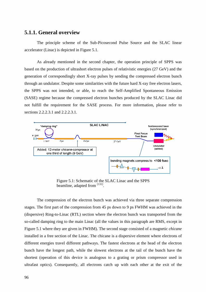
96

5.1.1. General overview

The principle scheme of the Sub-Picosecond Pulse Source and the SLAC linear

accelerator (Linac) is depicted in Figure 5.1.

As already mentioned in the second chapter, the operation principle of SPPS was

based on the production of ultrashort electron pulses of relativistic energies (27 GeV) and the

generation of correspondingly short X-ray pulses by sending the compressed electron bunch

through an undulator. Despite some similarities with the future hard X-ray free electron lasers,

the SPPS was not intended, or able, to reach the Self-Amplified Spontaneous Emission

(SASE) regime because the compressed electron bunches produced by the SLAC Linac did

not fulfill the requirement for the SASE process. For more information, please refer to

sections 2.2.2.3.1 and 2.2.2.3.1.

Figure 5.1: Schematic of the SLAC Linac and the SPPS

beamline, adapted from [131].

The compression of the electron bunch was achieved via three separate compression

stages. The first part of the compression from 45 ps down to 9 ps FWHM was achieved in the

(dispersive) Ring-to-Linac (RTL) section where the electron bunch was transported from the

so-called damping ring to the main Linac (all the values in this paragraph are RMS, except in

Figure 5.1 where they are given in FWHM). The second stage consisted of a magnetic chicane

installed in a free section of the Linac. The chicane is a dispersive element where electrons of

different energies travel different pathways. The fastest electrons at the head of the electron

bunch have the longest path, while the slowest electrons at the tail of the bunch have the

shortest (operation of this device is analogous to a grating or prism compressor used in

ultrafast optics). Consequently, all electrons catch up with each other at the exit of the

97

chicane, which compresses the bunch down to 400 fs FWHM. The final compression stage

consisted of two bending magnets located behind the Linac (here the electrons have reached

their full energy of 27 GeV) at the so-called Final Focus Test Beam (FFTB) station. The

FFTB was used as a diagnostic station to characterize the electron beam as long as the Linac

was used for particle physics experiments. After the compression in the FFTB, the bunch

duration was reduced to 35 fs RMS, corresponding to approximately 80 fs FWHM. These

values were obtained with dedicated measurement devices of the Linac and are in good

agreement with the particle tracking code used to predict the 80 fs bunches. Measurements by

interferometric autocorrelation of the coherent radiation from the electron bunches are also

consistent with this short bunch duration.

This ultrashort electron bunch then propagated through a 2.5 meter long undulator

which was also installed in the FFTB. As a result, ultrashort X-ray pulses with the same pulse

duration as the electron bunch, i.e. 80 fs, were produced. The electron bunches were dumped

after the insertion device. The undulator was adjusted to provide photons in the tuneable

energy range from 8 to 10 keV. The total number of emitted photons per pulse per 0.1%

bandwidth was up to 2 * 107. After the undulator, the X-ray pulse was monochromatized by a

set of multilayer mirrors to approximately 1% bandwidth and then transported 50 metres

further down to the experimental hutch. Beryllium lenses [132] could be inserted after the

monochromator to achieve one- or two-dimensional focusing. With the 2D-Lens system,

pulses with a few times 106 photons could be delivered to the experimental hutch in a

200*300 µm2 focus with a divergence of the order of few µrad. Under normal conditions, the

repetition rate of the SPPS was 10 Hz.

To be able to perform time-resolved experiments, a femtosecond laser system was

installed in the SPPS experimental area. This system was synchronized to the electron pulses

of the Linac via the radio frequency (RF) used to drive the accelerating RF-cavities of the

accelerator. However, this synchronization could only be achieved with a finite accuracy

resulting in a pulse-to-jitter of about 1 picosecond in the relative arrival time of laser- and X-

ray pulses. The next section will discuss in more detail specific measures to overcome the

jitter problem and to improve the temporal resolution down to the pulse duration limit.

A more complete and detailed description of the SPPS construction is provided in a

SLAC internal report by Cornacchia et al. [131].

98

5.1.2. Temporal resolution of the SPPS beamline

This section will discuss the temporal resolution that could be achieved in time-

resolved experiments at the SPPS beamline. The pulse duration of a single X-ray pulse from

the SPPS was about 80 fs, which was the shortest pulse length for hard X-ray pulses

worldwide. Such a short pulse duration allowed the SPPS, in principle, to achieve an

unprecedented time resolution.

However, the synchronization between the laser and the X-ray pulses suffered from

jitter, which, if no special measures had been taken, would have limited the achievable time

resolution to about one picosecond. At the SPPS the two most important sources for the jitter

were phase-noise in the driving RF-signal and, more important, fluctuations of the electrons

energy distribution of the electron bunch. These energy fluctuations lead to fluctuations in the

total travel time of the electrons down the Linac, and consequently to pulse-to-pulse variations

of the arrival time of the X-ray pulses produced in the undulator. To utilize the full potential

of the SPPS with respect to temporal resolution it therefore became an important challenge to

overcome the jitter problem. Since the future hard X-ray free electron laser will have to face

similar jitter problems, the solutions developed at the SPPS are also of primary importance for

these future facilities.

Two completely different methods to achieve a temporal resolution of about 100 fs at

the SPPS are described in the following subsections. Only the second one, i.e. the electro-

optic cross-correlation has been employed for the experiments discussed in this thesis.

5.1.2.1. Crossed-beam configuration

A very simple method to overcome the jitter problem is the so-called crossed-beam

configuration. This method was for example proposed for carrying out femtosecond time-

resolved X-ray diffraction experiments with a synchrotron pulse by Neutze et al. in 1997 [133].

It has been demonstrated in all-optical pump-probe [134] as well as optical pump – X-ray probe

experiments [135]. In this experimental configuration, the pump beam and the X-ray beam

impinge onto the sample surface under investigation with a largely different angle of

incidence. Figure 5.2 gives a schematic of the set-up. This produces a sweep in the actual

delay time between laser- and X-ray pulses across the sample surface because the relative

arrival time depends on the spatial position on the sample. If, for example, the surface of the

sample is excited simultaneously by a normal incident pump pulse, an obliquely incident (X-

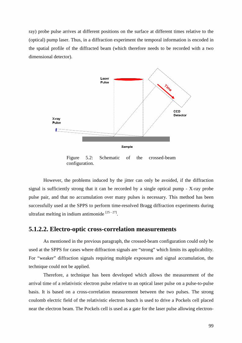
99

ray) probe pulse arrives at different positions on the surface at different times relative to the

(optical) pump laser. Thus, in a diffraction experiment the temporal information is encoded in

the spatial profile of the diffracted beam (which therefore needs to be recorded with a two

dimensional detector).

Figure 5.2: Schematic of the crossed-beam

configuration.

However, the problems induced by the jitter can only be avoided, if the diffraction

signal is sufficiently strong that it can be recorded by a single optical pump - X-ray probe

pulse pair, and that no accumulation over many pulses is necessary. This method has been

successfully used at the SPPS to perform time-resolved Bragg diffraction experiments during

ultrafast melting in indium antimonide [25 - 27].

5.1.2.2. Electro-optic cross-correlation measurements

As mentioned in the previous paragraph, the crossed-beam configuration could only be

used at the SPPS for cases where diffraction signals are “strong” which limits its applicability.

For “weaker” diffraction signals requiring multiple exposures and signal accumulation, the

technique could not be applied.

Therefore, a technique has been developed which allows the measurement of the

arrival time of a relativistic electron pulse relative to an optical laser pulse on a pulse-to-pulse

basis. It is based on a cross-correlation measurement between the two pulses. The strong

coulomb electric field of the relativistic electron bunch is used to drive a Pockels cell placed

near the electron beam. The Pockels cell is used as a gate for the laser pulse allowing electron-

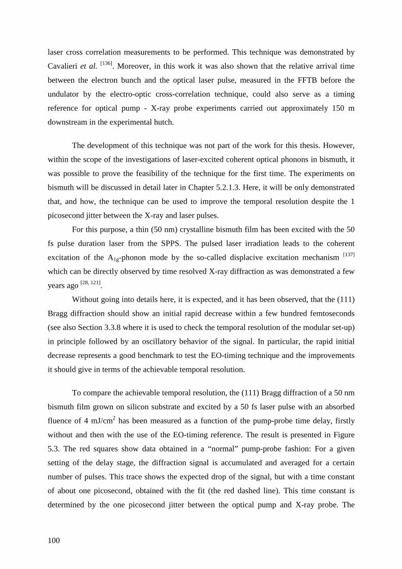
100

laser cross correlation measurements to be performed. This technique was demonstrated by

Cavalieri et al. [136]. Moreover, in this work it was also shown that the relative arrival time

between the electron bunch and the optical laser pulse, measured in the FFTB before the

undulator by the electro-optic cross-correlation technique, could also serve as a timing

reference for optical pump - X-ray probe experiments carried out approximately 150 m

downstream in the experimental hutch.

The development of this technique was not part of the work for this thesis. However,

within the scope of the investigations of laser-excited coherent optical phonons in bismuth, it

was possible to prove the feasibility of the technique for the first time. The experiments on

bismuth will be discussed in detail later in Chapter 5.2.1.3. Here, it will be only demonstrated

that, and how, the technique can be used to improve the temporal resolution despite the 1

picosecond jitter between the X-ray and laser pulses.

For this purpose, a thin (50 nm) crystalline bismuth film has been excited with the 50

fs pulse duration laser from the SPPS. The pulsed laser irradiation leads to the coherent

excitation of the A1g-phonon mode by the so-called displacive excitation mechanism [137]

which can be directly observed by time resolved X-ray diffraction as was demonstrated a few

years ago [28, 121].

Without going into details here, it is expected, and it has been observed, that the (111)

Bragg diffraction should show an initial rapid decrease within a few hundred femtoseconds

(see also Section 3.3.8 where it is used to check the temporal resolution of the modular set-up)

in principle followed by an oscillatory behavior of the signal. In particular, the rapid initial

decrease represents a good benchmark to test the EO-timing technique and the improvements

it should give in terms of the achievable temporal resolution.

To compare the achievable temporal resolution, the (111) Bragg diffraction of a 50 nm

bismuth film grown on silicon substrate and excited by a 50 fs laser pulse with an absorbed

fluence of 4 mJ/cm2 has been measured as a function of the pump-probe time delay, firstly

without and then with the use of the EO-timing reference. The result is presented in Figure

5.3. The red squares show data obtained in a “normal” pump-probe fashion: For a given

setting of the delay stage, the diffraction signal is accumulated and averaged for a certain

number of pulses. This trace shows the expected drop of the signal, but with a time constant

of about one picosecond, obtained with the fit (the red dashed line). This time constant is

determined by the one picosecond jitter between the optical pump and X-ray probe. The

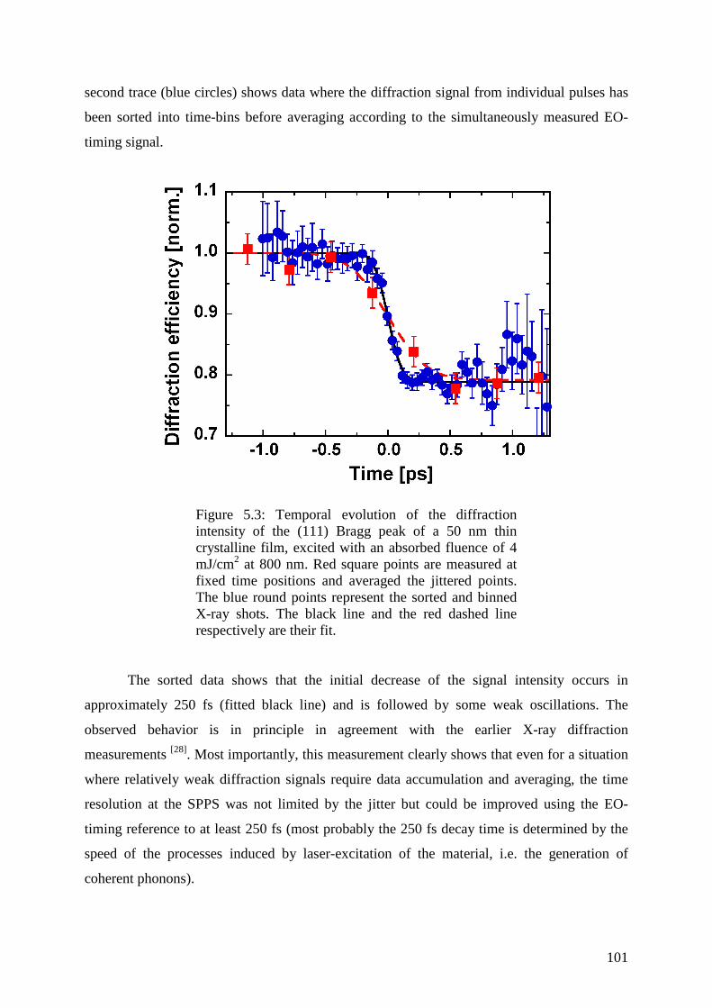
101

second trace (blue circles) shows data where the diffraction signal from individual pulses has

been sorted into time-bins before averaging according to the simultaneously measured EO-

timing signal.

Figure 5.3: Temporal evolution of the diffraction

intensity of the (111) Bragg peak of a 50 nm thin crystalline film, excited with an absorbed fluence of 4 mJ/cm2 at 800 nm. Red square points are measured at fixed time positions and averaged the jittered points. The blue round points represent the sorted and binned X-ray shots. The black line and the red dashed line respectively are their fit.

The sorted data shows that the initial decrease of the signal intensity occurs in

approximately 250 fs (fitted black line) and is followed by some weak oscillations. The

observed behavior is in principle in agreement with the earlier X-ray diffraction

measurements [28]. Most importantly, this measurement clearly shows that even for a situation

where relatively weak diffraction signals require data accumulation and averaging, the time

resolution at the SPPS was not limited by the jitter but could be improved using the EO-

timing reference to at least 250 fs (most probably the 250 fs decay time is determined by the

speed of the processes induced by laser-excitation of the material, i.e. the generation of

coherent phonons).

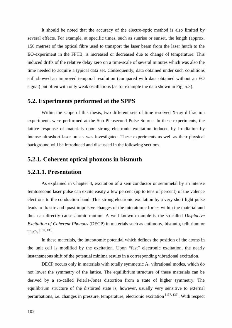
102

It should be noted that the accuracy of the electro-optic method is also limited by

several effects. For example, at specific times, such as sunrise or sunset, the length (approx.

150 metres) of the optical fibre used to transport the laser beam from the laser hutch to the

EO-experiment in the FFTB, is increased or decreased due to change of temperature. This

induced drifts of the relative delay zero on a time-scale of several minutes which was also the

time needed to acquire a typical data set. Consequently, data obtained under such conditions

still showed an improved temporal resolution (compared with data obtained without an EO

signal) but often with only weak oscillations (as for example the data shown in Fig. 5.3).

5.2. Experiments performed at the SPPS

Within the scope of this thesis, two different sets of time resolved X-ray diffraction

experiments were performed at the Sub-Picosecond Pulse Source. In these experiments, the

lattice response of materials upon strong electronic excitation induced by irradiation by

intense ultrashort laser pulses was investigated. These experiments as well as their physical

background will be introduced and discussed in the following sections.

5.2.1. Coherent optical phonons in bismuth

5.2.1.1. Presentation

As explained in Chapter 4, excitation of a semiconductor or semimetal by an intense

femtosecond laser pulse can excite easily a few percent (up to tens of percent) of the valence

electrons to the conduction band. This strong electronic excitation by a very short light pulse

leads to drastic and quasi impulsive changes of the interatomic forces within the material and

thus can directly cause atomic motion. A well-known example is the so-called Displacive

Excitation of Coherent Phonons (DECP) in materials such as antimony, bismuth, tellurium or

Ti2O3 [137, 138].

In these materials, the interatomic potential which defines the position of the atoms in

the unit cell is modified by the excitation. Upon “fast” electronic excitation, the nearly

instantaneous shift of the potential minima results in a corresponding vibrational excitation.

DECP occurs only in materials with totally symmetric A1 vibrational modes, which do

not lower the symmetry of the lattice. The equilibrium structure of these materials can be

derived by a so-called Peierls-Jones distortion from a state of higher symmetry. The

equilibrium structure of the distorted state is, however, usually very sensitive to external

perturbations, i.e. changes in pressure, temperature, electronic excitation [137, 139]. With respect

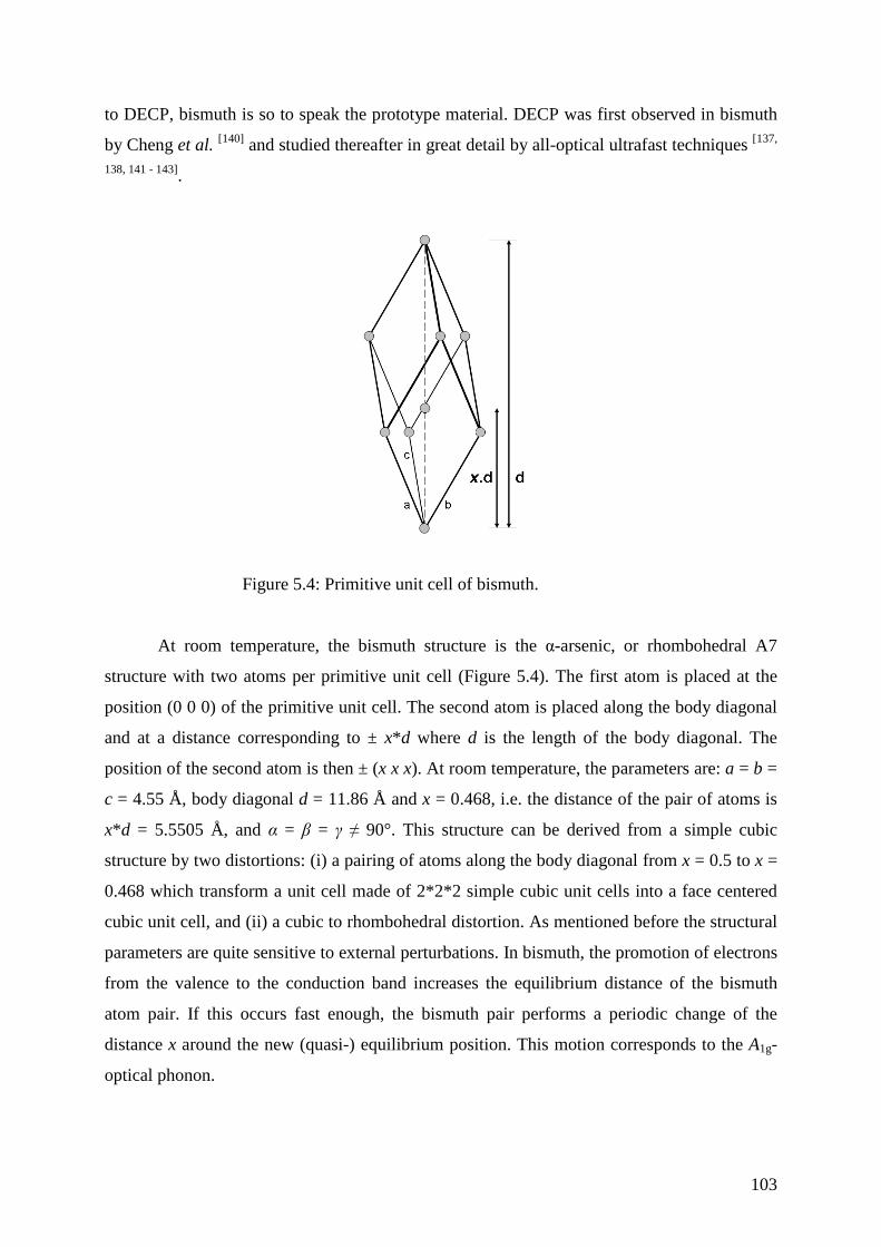
103

to DECP, bismuth is so to speak the prototype material. DECP was first observed in bismuth

by Cheng et al. [140] and studied thereafter in great detail by all-optical ultrafast techniques [137,

138, 141 - 143].

Figure 5.4: Primitive unit cell of bismuth.

At room temperature, the bismuth structure is the α-arsenic, or rhombohedral A7

structure with two atoms per primitive unit cell (Figure 5.4). The first atom is placed at the

position (0 0 0) of the primitive unit cell. The second atom is placed along the body diagonal

and at a distance corresponding to ± x*d where d is the length of the body diagonal. The

position of the second atom is then ± (x x x). At room temperature, the parameters are: a = b =

c = 4.55 Å, body diagonal d = 11.86 Å and x = 0.468, i.e. the distance of the pair of atoms is

x*d = 5.5505 Å, and α = β = γ ≠ 90°. This structure can be derived from a simple cubic

structure by two distortions: (i) a pairing of atoms along the body diagonal from x = 0.5 to x =

0.468 which transform a unit cell made of 2*2*2 simple cubic unit cells into a face centered

cubic unit cell, and (ii) a cubic to rhombohedral distortion. As mentioned before the structural

parameters are quite sensitive to external perturbations. In bismuth, the promotion of electrons

from the valence to the conduction band increases the equilibrium distance of the bismuth

atom pair. If this occurs fast enough, the bismuth pair performs a periodic change of the

distance x around the new (quasi-) equilibrium position. This motion corresponds to the A1g-

optical phonon.

104

In previous work, time-resolved optical techniques, i.e. reflectivity measurements,

have been used to study this process [137, 138, 141 - 143]. Due to their high temporal resolution and

the ability to detect very small signal changes with high accuracy, optical techniques are

powerful to retrieve information about the frequency of the excited phonon and its decay

dynamics (all derived from the oscillating part of the transient reflectivity response).

However, the optical techniques can provide only indirect information about the magnitude of

the atomic motion and its non-periodic components. Time resolved X-ray techniques can

provide direct information about the atomic motion (and its oscillatory and non oscillatory

components) induced by optical excitation.

The first successful experiment where time-resolved X-ray diffraction was used to

follow the atomic motion in photo-excited bismuth was performed by Sokolowski-Tinten et

al. [28, 121]. In this work, the evolution of two Bragg diffraction peaks of a 50 nm thin bismuth

film, i.e. the (111) and (222) of the primitive unit cell, were measured over a time range of

several picoseconds. These two Bragg peaks are directly sensitive to the excited A1g mode

because the atomic motion is along the 111 direction. For the (111) Bragg signal, they

observed a decrease of the overall signal intensity followed by periodic oscillations. In the

case of the (222) Bragg signal an initial increase of the signal intensity, followed by periodic

oscillations was observed.

These transient changes can be directly related to the change of the geometrical

structure factor induced by the changes of the Bi-Bi distance. Indeed, working with a thin

crystalline film allows describing X-ray diffraction in the kinematic limit. The kinematic X-

ray diffraction considers that the scattered radiation does not diffract again. This hypothesis is

true only when the diffracted intensity is weak compared to the incident intensity. This is the

case for X-ray diffraction from small crystals or samples with a thickness substantially thinner

than the extinction depth of the X-rays, whereas for bulk diffraction, the dynamic theory of X-

ray diffraction is used [121, 144].

Sokolowski-Tinten et al. excited the 50 nm thin film with a 800 nm laser pulse with an

incidence fluence of about 6 mJ/cm2. The relative position of the two bismuth atoms could be

retrieved through the changes of the structure factor of the lattice cell, yielding large atomic

displacements of about 0.2 Å, a few percent (3.6%) of the Bi-Bi interatomic distance. The

frequency of the A1g mode was found to be only 2.12 THz, substantially smaller compared to

the frequency of 2.92 THz measured in non-excited bismuth (i.e. by Raman-spectroscopy.

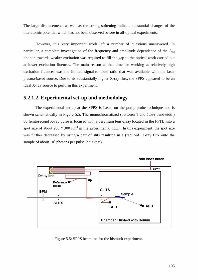
105

The large displacements as well as the strong softening indicate substantial changes of the

interatomic potential which has not been observed before in all-optical experiments.

However, this very important work left a number of questions unanswered. In

particular, a complete investigation of the frequency and amplitude dependence of the A1g

phonon towards weaker excitation was required to fill the gap to the optical work carried out

at lower excitation fluences. The main reason at that time for working at relatively high

excitation fluences was the limited signal-to-noise ratio that was available with the laser

plasma-based source. Due to its substantially higher X-ray flux, the SPPS appeared to be an

ideal X-ray source to perform this experiment.

5.2.1.2. Experimental set-up and methodology

The experimental set-up at the SPPS is based on the pump-probe technique and is

shown schematically in Figure 5.5. The monochromatized (between 1 and 1.5% bandwidth)

80 femtosecond X-ray pulse is focused with a beryllium lens-array located in the FFTB into a

spot size of about 200 * 300 µm2 in the experimental hutch. In this experiment, the spot size

was further decreased by using a pair of slits resulting in a (reduced) X-ray flux onto the

sample of about 106 photons per pulse (at 9 keV).

Figure 5.5: SPPS beamline for the bismuth experiment.

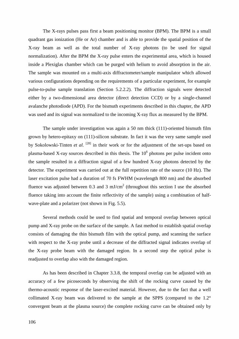
106

The X-rays pulses pass first a beam positioning monitor (BPM). The BPM is a small

quadrant gas ionization (He or Ar) chamber and is able to provide the spatial position of the

X-ray beam as well as the total number of X-ray photons (to be used for signal

normalization). After the BPM the X-ray pulse enters the experimental area, which is housed

inside a Plexiglas chamber which can be purged with helium to avoid absorption in the air.

The sample was mounted on a multi-axis diffractometer/sample manipulator which allowed

various configurations depending on the requirements of a particular experiment, for example

pulse-to-pulse sample translation (Section 5.2.2.2). The diffraction signals were detected

either by a two-dimensional area detector (direct detection CCD) or by a single-channel

avalanche photodiode (APD). For the bismuth experiments described in this chapter, the APD

was used and its signal was normalized to the incoming X-ray flux as measured by the BPM.

The sample under investigation was again a 50 nm thick (111)-oriented bismuth film

grown by hetero-epitaxy on (111)-silicon substrate. In fact it was the very same sample used

by Sokolowski-Tinten et al. [28] in their work or for the adjustment of the set-ups based on

plasma-based X-ray sources described in this thesis. The 106 photons per pulse incident onto

the sample resulted in a diffraction signal of a few hundred X-ray photons detected by the

detector. The experiment was carried out at the full repetition rate of the source (10 Hz). The

laser excitation pulse had a duration of 70 fs FWHM (wavelength 800 nm) and the absorbed

fluence was adjusted between 0.3 and 3 mJ/cm2 (throughout this section I use the absorbed

fluence taking into account the finite reflectivity of the sample) using a combination of half-

wave-plate and a polarizer (not shown in Fig. 5.5).

Several methods could be used to find spatial and temporal overlap between optical

pump and X-ray probe on the surface of the sample. A fast method to establish spatial overlap

consists of damaging the thin bismuth film with the optical pump, and scanning the surface

with respect to the X-ray probe until a decrease of the diffracted signal indicates overlap of

the X-ray probe beam with the damaged region. In a second step the optical pulse is

readjusted to overlap also with the damaged region.

As has been described in Chapter 3.3.8, the temporal overlap can be adjusted with an

accuracy of a few picoseconds by observing the shift of the rocking curve caused by the

thermo-acoustic response of the laser-excited material. However, due to the fact that a well

collimated X-ray beam was delivered to the sample at the SPPS (compared to the 1.2°

convergent beam at the plasma source) the complete rocking curve can be obtained only by

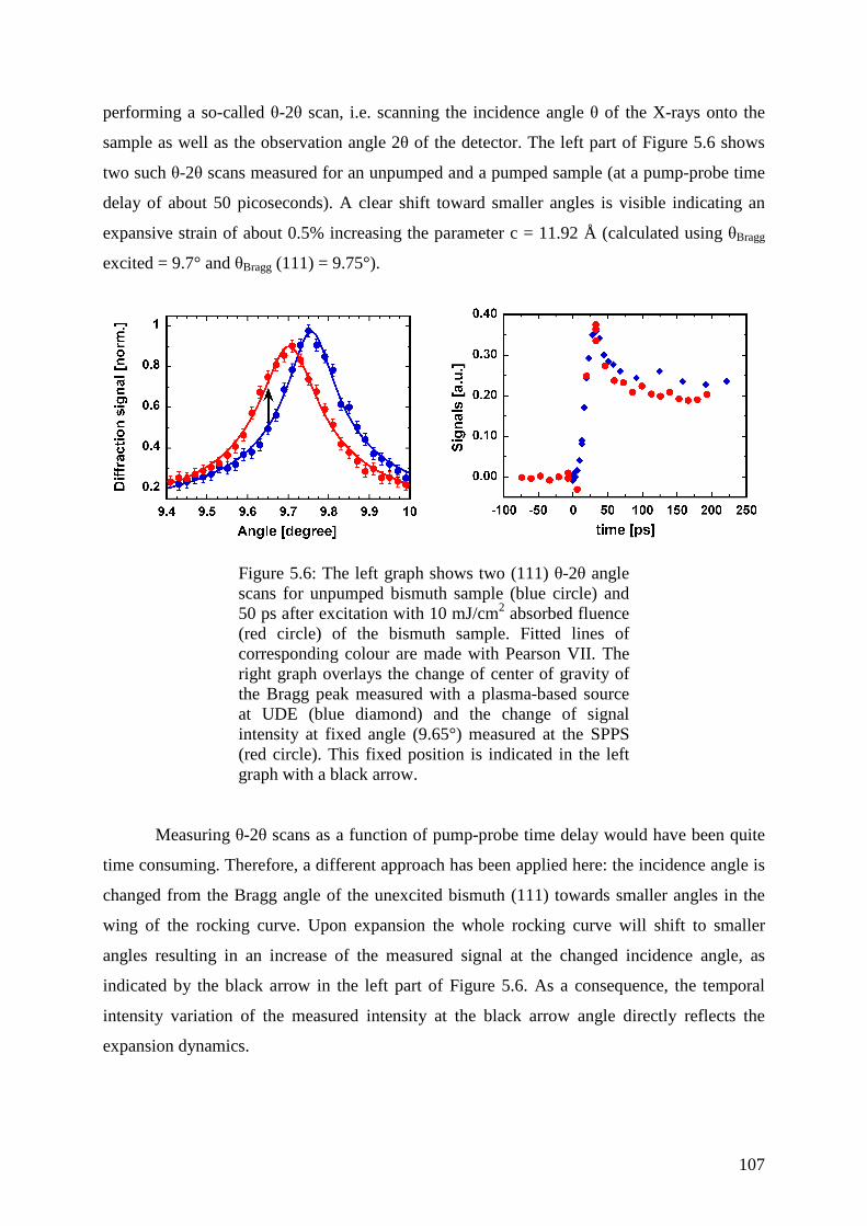
107

performing a so-called θ-2θ scan, i.e. scanning the incidence angle θ of the X-rays onto the

sample as well as the observation angle 2θ of the detector. The left part of Figure 5.6 shows

two such θ-2θ scans measured for an unpumped and a pumped sample (at a pump-probe time

delay of about 50 picoseconds). A clear shift toward smaller angles is visible indicating an

expansive strain of about 0.5% increasing the parameter c = 11.92 Å (calculated using θBragg

excited = 9.7° and θBragg (111) = 9.75°).

Figure 5.6: The left graph shows two (111) θ-2θ angle

scans for unpumped bismuth sample (blue circle) and 50 ps after excitation with 10 mJ/cm2 absorbed fluence (red circle) of the bismuth sample. Fitted lines of corresponding colour are made with Pearson VII. The right graph overlays the change of center of gravity of the Bragg peak measured with a plasma-based source at UDE (blue diamond) and the change of signal intensity at fixed angle (9.65°) measured at the SPPS (red circle). This fixed position is indicated in the left graph with a black arrow.

Measuring θ-2θ scans as a function of pump-probe time delay would have been quite

time consuming. Therefore, a different approach has been applied here: the incidence angle is

changed from the Bragg angle of the unexcited bismuth (111) towards smaller angles in the

wing of the rocking curve. Upon expansion the whole rocking curve will shift to smaller

angles resulting in an increase of the measured signal at the changed incidence angle, as

indicated by the black arrow in the left part of Figure 5.6. As a consequence, the temporal

intensity variation of the measured intensity at the black arrow angle directly reflects the

expansion dynamics.

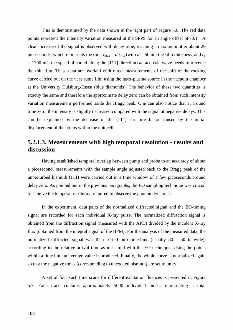
108

This is demonstrated by the data shown in the right part of Figure 5.6. The red data

points represent the intensity variation measured at the SPPS for an angle offset of -0.1°. A

clear increase of the signal is observed with delay time, reaching a maximum after about 29

picoseconds, which represents the time τmax = d / cs (with d = 50 nm the film thickness, and cs

= 1790 m/s the speed of sound along the [111] direction) an acoustic wave needs to traverse

the thin film. These data are overlaid with direct measurements of the shift of the rocking

curve carried out on the very same film using the laser-plasma source in the vacuum chamber

at the University Duisburg-Essen (blue diamonds). The behavior of these two quantities is

exactly the same and therefore the approximate delay zero can be obtained from such intensity

variation measurement performed aside the Bragg peak. One can also notice that at around

time zero, the intensity is slightly decreased compared with the signal at negative delays. This

can be explained by the decrease of the (111) structure factor caused by the initial

displacement of the atoms within the unit cell.

5.2.1.3. Measurements with high temporal resolution - results and discussion

Having established temporal overlap between pump and probe to an accuracy of about

a picosecond, measurements with the sample angle adjusted back to the Bragg peak of the

unperturbed bismuth (111) were carried out in a time window of a few picoseconds around

delay zero. As pointed out in the previous paragraphs, the EO sampling technique was crucial

to achieve the temporal resolution required to observe the phonon dynamics.

In the experiment, data pairs of the normalized diffracted signal and the EO-timing

signal are recorded for each individual X-ray pulse. The normalized diffraction signal is

obtained from the diffraction signal (measured with the APD) divided by the incident X-ray

flux (obtained from the integral signal of the BPM). For the analysis of the measured data, the

normalized diffracted signal was then sorted into time-bins (usually 30 – 50 fs wide),

according to the relative arrival time as measured with the EO-technique. Using the points

within a time bin, an average value is produced. Finally, the whole curve is normalized again

so that the negative times (corresponding to unexcited bismuth) are set to unity.

A set of four such time scans for different excitation fluences is presented in Figure

5.7. Each trace contains approximately 5000 individual pulses representing a total

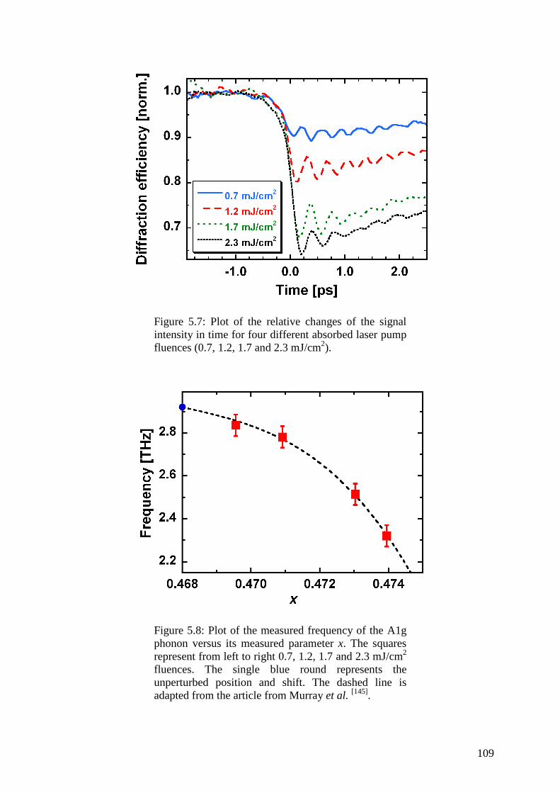
109

Figure 5.7: Plot of the relative changes of the signal

intensity in time for four different absorbed laser pump fluences (0.7, 1.2, 1.7 and 2.3 mJ/cm2).

Figure 5.8: Plot of the measured frequency of the A1g

phonon versus its measured parameter x. The squares represent from left to right 0.7, 1.2, 1.7 and 2.3 mJ/cm2 fluences. The single blue round represents the unperturbed position and shift. The dashed line is adapted from the article from Murray et al. [145].

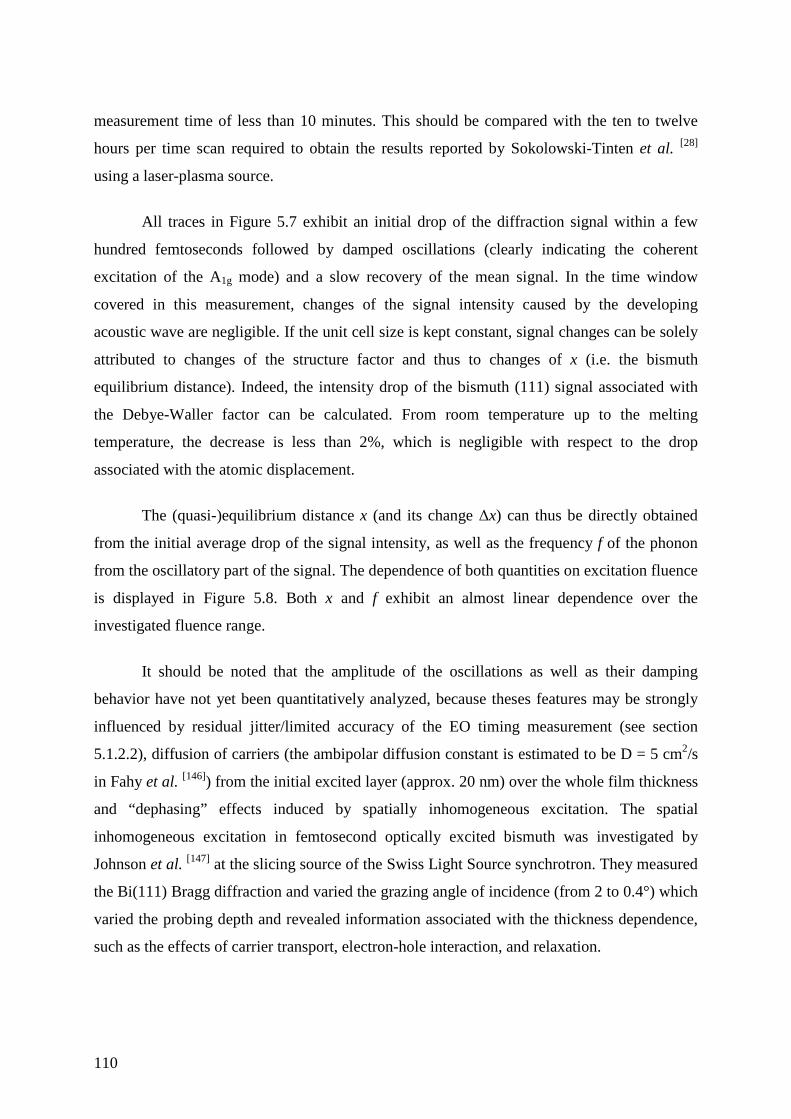
110

measurement time of less than 10 minutes. This should be compared with the ten to twelve

hours per time scan required to obtain the results reported by Sokolowski-Tinten et al. [28]

using a laser-plasma source.

All traces in Figure 5.7 exhibit an initial drop of the diffraction signal within a few

hundred femtoseconds followed by damped oscillations (clearly indicating the coherent

excitation of the A1g mode) and a slow recovery of the mean signal. In the time window

covered in this measurement, changes of the signal intensity caused by the developing

acoustic wave are negligible. If the unit cell size is kept constant, signal changes can be solely

attributed to changes of the structure factor and thus to changes of x (i.e. the bismuth

equilibrium distance). Indeed, the intensity drop of the bismuth (111) signal associated with

the Debye-Waller factor can be calculated. From room temperature up to the melting

temperature, the decrease is less than 2%, which is negligible with respect to the drop

associated with the atomic displacement.

The (quasi-)equilibrium distance x (and its change ∆x) can thus be directly obtained

from the initial average drop of the signal intensity, as well as the frequency f of the phonon

from the oscillatory part of the signal. The dependence of both quantities on excitation fluence

is displayed in Figure 5.8. Both x and f exhibit an almost linear dependence over the

investigated fluence range.

It should be noted that the amplitude of the oscillations as well as their damping

behavior have not yet been quantitatively analyzed, because theses features may be strongly

influenced by residual jitter/limited accuracy of the EO timing measurement (see section

5.1.2.2), diffusion of carriers (the ambipolar diffusion constant is estimated to be D = 5 cm2/s

in Fahy et al. [146]) from the initial excited layer (approx. 20 nm) over the whole film thickness

and “dephasing” effects induced by spatially inhomogeneous excitation. The spatial

inhomogeneous excitation in femtosecond optically excited bismuth was investigated by

Johnson et al. [147] at the slicing source of the Swiss Light Source synchrotron. They measured

the Bi(111) Bragg diffraction and varied the grazing angle of incidence (from 2 to 0.4°) which

varied the probing depth and revealed information associated with the thickness dependence,

such as the effects of carrier transport, electron-hole interaction, and relaxation.

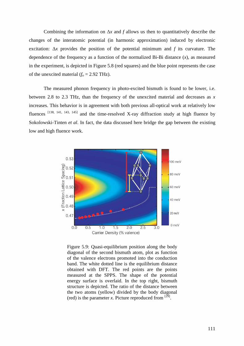
111

Combining the information on ∆x and f allows us then to quantitatively describe the

changes of the interatomic potential (in harmonic approximation) induced by electronic

excitation: ∆x provides the position of the potential minimum and f its curvature. The

dependence of the frequency as a function of the normalized Bi-Bi distance (x), as measured

in the experiment, is depicted in Figure 5.8 (red squares) and the blue point represents the case

of the unexcited material (fo = 2.92 THz).

The measured phonon frequency in photo-excited bismuth is found to be lower, i.e.

between 2.8 to 2.3 THz, than the frequency of the unexcited material and decreases as x

increases. This behavior is in agreement with both previous all-optical work at relatively low

fluences [138, 141, 143, 145] and the time-resolved X-ray diffraction study at high fluence by

Sokolowski-Tinten et al. In fact, the data discussed here bridge the gap between the existing

low and high fluence work.

Figure 5.9: Quasi-equilibrium position along the body

diagonal of the second bismuth atom, plot as function of the valence electrons promoted into the conduction band. The white dotted line is the equilibrium distance obtained with DFT. The red points are the points measured at the SPPS. The shape of the potential energy surface is overlaid. In the top right, bismuth structure is depicted. The ratio of the distance between the two atoms (yellow) divided by the body diagonal (red) is the parameter x. Picture reproduced from [29].

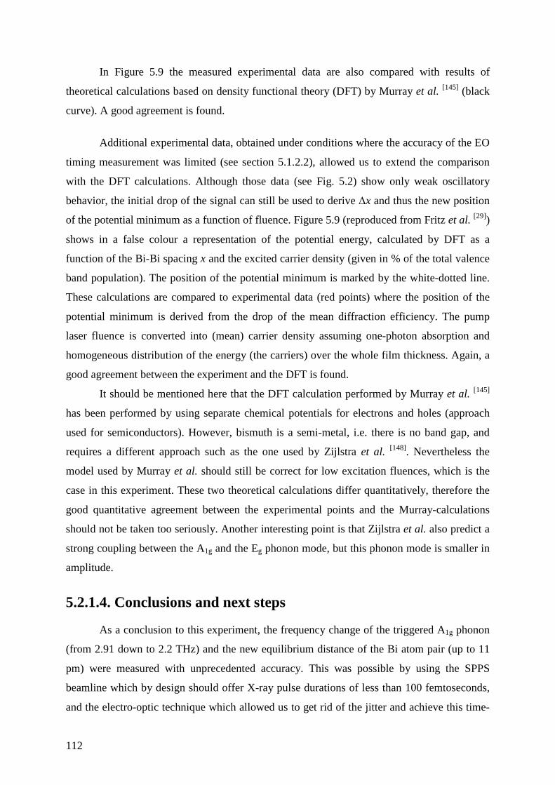
112

In Figure 5.9 the measured experimental data are also compared with results of

theoretical calculations based on density functional theory (DFT) by Murray et al. [145] (black

curve). A good agreement is found.

Additional experimental data, obtained under conditions where the accuracy of the EO

timing measurement was limited (see section 5.1.2.2), allowed us to extend the comparison

with the DFT calculations. Although those data (see Fig. 5.2) show only weak oscillatory

behavior, the initial drop of the signal can still be used to derive ∆x and thus the new position

of the potential minimum as a function of fluence. Figure 5.9 (reproduced from Fritz et al. [29])

shows in a false colour a representation of the potential energy, calculated by DFT as a

function of the Bi-Bi spacing x and the excited carrier density (given in % of the total valence

band population). The position of the potential minimum is marked by the white-dotted line.

These calculations are compared to experimental data (red points) where the position of the

potential minimum is derived from the drop of the mean diffraction efficiency. The pump

laser fluence is converted into (mean) carrier density assuming one-photon absorption and

homogeneous distribution of the energy (the carriers) over the whole film thickness. Again, a

good agreement between the experiment and the DFT is found.

It should be mentioned here that the DFT calculation performed by Murray et al. [145]

has been performed by using separate chemical potentials for electrons and holes (approach

used for semiconductors). However, bismuth is a semi-metal, i.e. there is no band gap, and

requires a different approach such as the one used by Zijlstra et al. [148]. Nevertheless the

model used by Murray et al. should still be correct for low excitation fluences, which is the

case in this experiment. These two theoretical calculations differ quantitatively, therefore the

good quantitative agreement between the experimental points and the Murray-calculations

should not be taken too seriously. Another interesting point is that Zijlstra et al. also predict a

strong coupling between the A1g and the Eg phonon mode, but this phonon mode is smaller in

amplitude.

5.2.1.4. Conclusions and next steps

As a conclusion to this experiment, the frequency change of the triggered A1g phonon

(from 2.91 down to 2.2 THz) and the new equilibrium distance of the Bi atom pair (up to 11

pm) were measured with unprecedented accuracy. This was possible by using the SPPS

beamline which by design should offer X-ray pulse durations of less than 100 femtoseconds,

and the electro-optic technique which allowed us to get rid of the jitter and achieve this time-

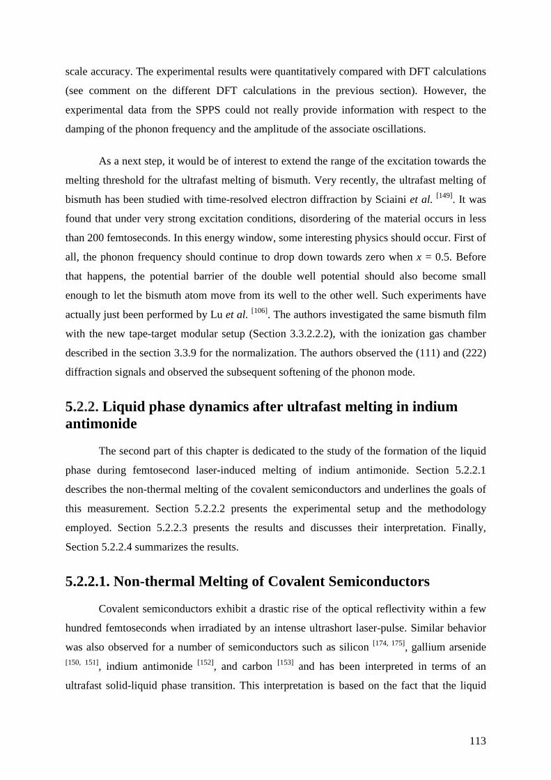
113

scale accuracy. The experimental results were quantitatively compared with DFT calculations

(see comment on the different DFT calculations in the previous section). However, the

experimental data from the SPPS could not really provide information with respect to the

damping of the phonon frequency and the amplitude of the associate oscillations.

As a next step, it would be of interest to extend the range of the excitation towards the

melting threshold for the ultrafast melting of bismuth. Very recently, the ultrafast melting of

bismuth has been studied with time-resolved electron diffraction by Sciaini et al. [149]. It was

found that under very strong excitation conditions, disordering of the material occurs in less

than 200 femtoseconds. In this energy window, some interesting physics should occur. First of

all, the phonon frequency should continue to drop down towards zero when x = 0.5. Before

that happens, the potential barrier of the double well potential should also become small

enough to let the bismuth atom move from its well to the other well. Such experiments have

actually just been performed by Lu et al. [106]. The authors investigated the same bismuth film

with the new tape-target modular setup (Section 3.3.2.2.2), with the ionization gas chamber

described in the section 3.3.9 for the normalization. The authors observed the (111) and (222)

diffraction signals and observed the subsequent softening of the phonon mode.

5.2.2. Liquid phase dynamics after ultrafast melting in indium antimonide

The second part of this chapter is dedicated to the study of the formation of the liquid

phase during femtosecond laser-induced melting of indium antimonide. Section 5.2.2.1

describes the non-thermal melting of the covalent semiconductors and underlines the goals of

this measurement. Section 5.2.2.2 presents the experimental setup and the methodology

employed. Section 5.2.2.3 presents the results and discusses their interpretation. Finally,

Section 5.2.2.4 summarizes the results.

5.2.2.1. Non-thermal Melting of Covalent Semiconductors

Covalent semiconductors exhibit a drastic rise of the optical reflectivity within a few

hundred femtoseconds when irradiated by an intense ultrashort laser-pulse. Similar behavior

was also observed for a number of semiconductors such as silicon [174, 175], gallium arsenide [150, 151], indium antimonide [152], and carbon [153] and has been interpreted in terms of an

ultrafast solid-liquid phase transition. This interpretation is based on the fact that the liquid

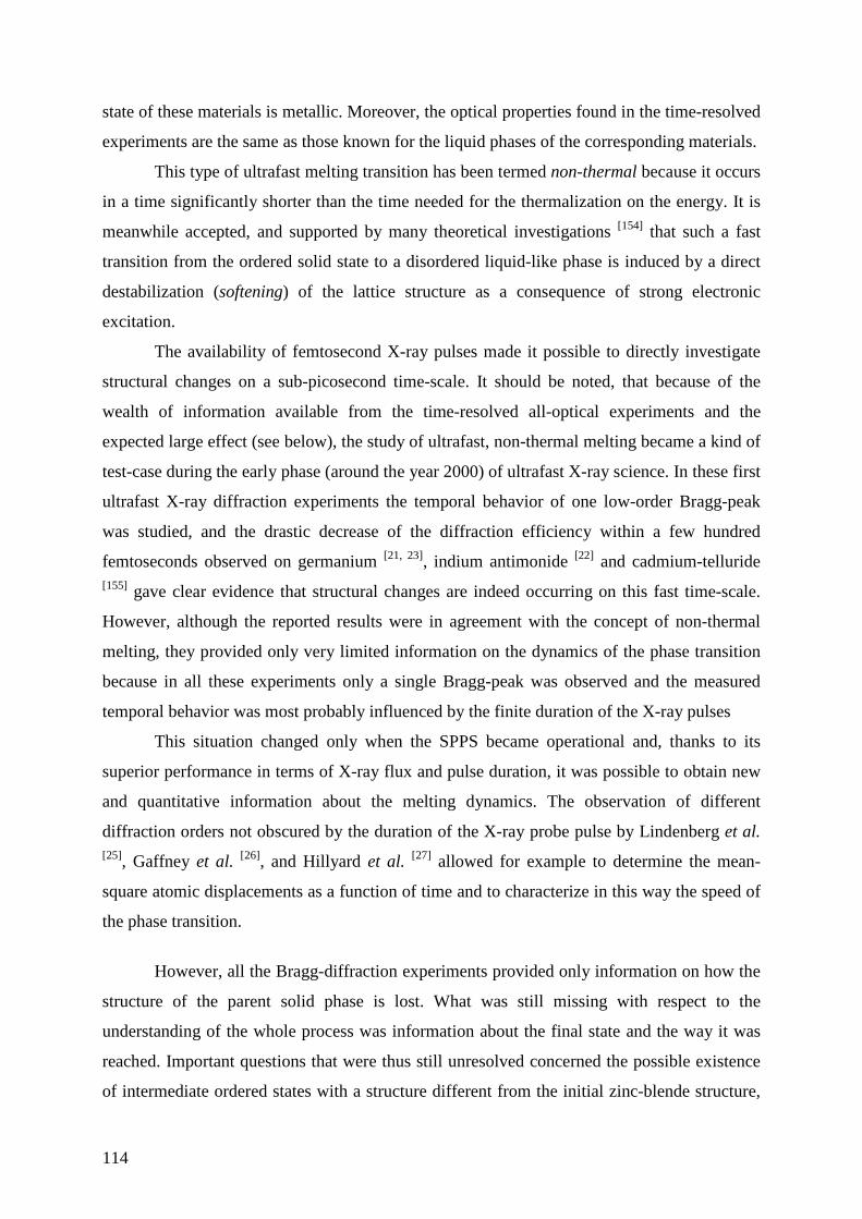
114

state of these materials is metallic. Moreover, the optical properties found in the time-resolved

experiments are the same as those known for the liquid phases of the corresponding materials.

This type of ultrafast melting transition has been termed non-thermal because it occurs

in a time significantly shorter than the time needed for the thermalization on the energy. It is

meanwhile accepted, and supported by many theoretical investigations [154] that such a fast

transition from the ordered solid state to a disordered liquid-like phase is induced by a direct

destabilization (softening) of the lattice structure as a consequence of strong electronic

excitation.

The availability of femtosecond X-ray pulses made it possible to directly investigate

structural changes on a sub-picosecond time-scale. It should be noted, that because of the

wealth of information available from the time-resolved all-optical experiments and the

expected large effect (see below), the study of ultrafast, non-thermal melting became a kind of

test-case during the early phase (around the year 2000) of ultrafast X-ray science. In these first

ultrafast X-ray diffraction experiments the temporal behavior of one low-order Bragg-peak

was studied, and the drastic decrease of the diffraction efficiency within a few hundred

femtoseconds observed on germanium [21, 23], indium antimonide [22] and cadmium-telluride [155] gave clear evidence that structural changes are indeed occurring on this fast time-scale.

However, although the reported results were in agreement with the concept of non-thermal

melting, they provided only very limited information on the dynamics of the phase transition

because in all these experiments only a single Bragg-peak was observed and the measured

temporal behavior was most probably influenced by the finite duration of the X-ray pulses

This situation changed only when the SPPS became operational and, thanks to its

superior performance in terms of X-ray flux and pulse duration, it was possible to obtain new

and quantitative information about the melting dynamics. The observation of different

diffraction orders not obscured by the duration of the X-ray probe pulse by Lindenberg et al. [25], Gaffney et al. [26], and Hillyard et al. [27] allowed for example to determine the mean-

square atomic displacements as a function of time and to characterize in this way the speed of

the phase transition.

However, all the Bragg-diffraction experiments provided only information on how the

structure of the parent solid phase is lost. What was still missing with respect to the

understanding of the whole process was information about the final state and the way it was

reached. Important questions that were thus still unresolved concerned the possible existence

of intermediate ordered states with a structure different from the initial zinc-blende structure,

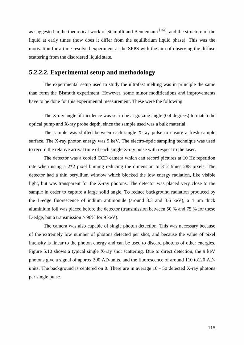
115

as suggested in the theoretical work of Stampfli and Bennemann [154], and the structure of the

liquid at early times (how does it differ from the equilibrium liquid phase). This was the

motivation for a time-resolved experiment at the SPPS with the aim of observing the diffuse

scattering from the disordered liquid state.

5.2.2.2. Experimental setup and methodology

The experimental setup used to study the ultrafast melting was in principle the same

than form the Bismuth experiment. However, some minor modifications and improvements

have to be done for this experimental measurement. These were the following:

The X-ray angle of incidence was set to be at grazing angle (0.4 degrees) to match the

optical pump and X-ray probe depth, since the sample used was a bulk material.

The sample was shifted between each single X-ray pulse to ensure a fresh sample

surface. The X-ray photon energy was 9 keV. The electro-optic sampling technique was used

to record the relative arrival time of each single X-ray pulse with respect to the laser.

The detector was a cooled CCD camera which can record pictures at 10 Hz repetition

rate when using a 2*2 pixel binning reducing the dimension to 312 times 288 pixels. The

detector had a thin beryllium window which blocked the low energy radiation, like visible

light, but was transparent for the X-ray photons. The detector was placed very close to the

sample in order to capture a large solid angle. To reduce background radiation produced by

the L-edge fluorescence of indium antimonide (around 3.3 and 3.6 keV), a 4 µm thick

aluminium foil was placed before the detector (transmission between 50 % and 75 % for these

L-edge, but a transmission > 96% for 9 keV).

The camera was also capable of single photon detection. This was necessary because

of the extremely low number of photons detected per shot, and because the value of pixel

intensity is linear to the photon energy and can be used to discard photons of other energies.

Figure 5.10 shows a typical single X-ray shot scattering. Due to direct detection, the 9 keV

photons give a signal of approx 300 AD-units, and the fluorescence of around 110 to120 AD-

units. The background is centered on 0. There are in average 10 - 50 detected X-ray photons

per single pulse.

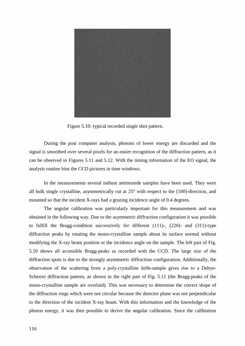
116

Figure 5.10: typical recorded single shot pattern.

During the post computer analysis, photons of lower energy are discarded and the

signal is smoothed over several pixels for an easier recognition of the diffraction pattern, as it

can be observed in Figures 5.11 and 5.12. With the timing information of the EO signal, the

analysis routine bins the CCD pictures in time windows.

In the measurements several indium antimonide samples have been used. They were

all bulk single crystalline, asymmetrically cut at 25° with respect to the [100]-direction, and

mounted so that the incident X-rays had a grazing incidence angle of 0.4 degrees.

The angular calibration was particularly important for this measurement and was

obtained in the following way. Due to the asymmetric diffraction configuration it was possible

to fulfill the Bragg-condition successively for different (111)-, (220)- and (311)-type

diffraction peaks by rotating the mono-crystalline sample about its surface normal without

modifying the X-ray beam position or the incidence angle on the sample. The left part of Fig.

5.10 shows all accessible Bragg-peaks as recorded with the CCD. The large size of the

diffraction spots is due to the strongly asymmetric diffraction configuration. Additionally, the

observation of the scattering from a poly-crystalline InSb-sample gives rise to a Debye-

Scherrer diffraction pattern, as shown in the right part of Fig. 5.11 (the Bragg-peaks of the

mono-crystalline sample are overlaid). This was necessary to determine the correct shape of

the diffraction rings which were not circular because the detector plane was not perpendicular

to the direction of the incident X-ray beam. With this information and the knowledge of the

photon energy, it was then possible to derive the angular calibration. Since the calibration

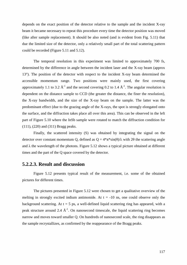
117

depends on the exact position of the detector relative to the sample and the incident X-ray

beam it became necessary to repeat this procedure every time the detector position was moved

(like after sample replacement). It should be also noted (and is evident from Fig. 5.11) that

due the limited size of the detector, only a relatively small part of the total scattering pattern

could be recorded (Figure 5.11 and 5.12).

The temporal resolution in this experiment was limited to approximately 700 fs,

determined by the difference in angle between the incident laser and the X-ray beam (approx

13°). The position of the detector with respect to the incident X-ray beam determined the

accessible momentum range. Two positions were mainly used, the first covering

approximately 1.1 to 3.2 Å-1 and the second covering 0.2 to 1.4 Å-1. The angular resolution is

dependent on the distance sample to CCD (the greater the distance, the finer the resolution),

the X-ray bandwidth, and the size of the X-ray beam on the sample. The latter was the

predominant effect (due to the grazing angle of the X-rays, the spot is strongly elongated onto

the surface, and the diffraction takes place all over this area). This can be observed in the left

part of Figure 5.10 where the InSb sample were rotated to match the diffraction condition for

(111), (220) and (311) Bragg peaks.

Finally, the scattered intensity (S) was obtained by integrating the signal on the

detector over constant momentum Q, defined as Q = 4*π*sin(θ)/λ with 2θ the scattering angle

and λ the wavelength of the photons. Figure 5.12 shows a typical picture obtained at different

times and the part of the Q space covered by the detector.

5.2.2.3. Result and discussion

Figure 5.12 presents typical result of the measurement, i.e. some of the obtained

pictures for different times.

The pictures presented in Figure 5.12 were chosen to get a qualitative overview of the

melting in strongly excited indium antimonide. At t = -10 ns, one could observe only the

background scattering. At t = 5 ps, a well-defined liquid scattering ring has appeared, with a

peak structure around 2.4 Å-1. On nanosecond timescale, the liquid scattering ring becomes

narrow and moves toward smaller Q. On hundreds of nanosecond scale, the ring disappears as

the sample recrystallizes, as confirmed by the reappearance of the Bragg peaks.

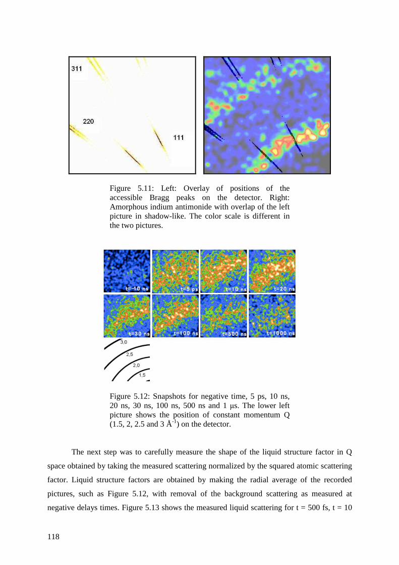
118

Figure 5.11: Left: Overlay of positions of the

accessible Bragg peaks on the detector. Right: Amorphous indium antimonide with overlap of the left picture in shadow-like. The color scale is different in the two pictures.

Figure 5.12: Snapshots for negative time, 5 ps, 10 ns,

20 ns, 30 ns, 100 ns, 500 ns and 1 µs. The lower left picture shows the position of constant momentum Q (1.5, 2, 2.5 and 3 Å-1) on the detector.

The next step was to carefully measure the shape of the liquid structure factor in Q

space obtained by taking the measured scattering normalized by the squared atomic scattering

factor. Liquid structure factors are obtained by making the radial average of the recorded

pictures, such as Figure 5.12, with removal of the background scattering as measured at

negative delays times. Figure 5.13 shows the measured liquid scattering for t = 500 fs, t = 10

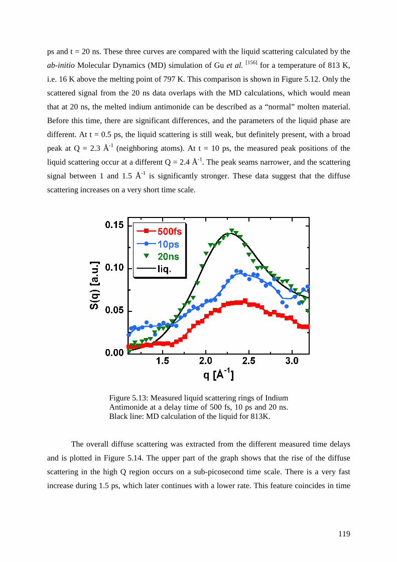
119

ps and t = 20 ns. These three curves are compared with the liquid scattering calculated by the

ab-initio Molecular Dynamics (MD) simulation of Gu et al. [156] for a temperature of 813 K,

i.e. 16 K above the melting point of 797 K. This comparison is shown in Figure 5.12. Only the

scattered signal from the 20 ns data overlaps with the MD calculations, which would mean

that at 20 ns, the melted indium antimonide can be described as a “normal” molten material.

Before this time, there are significant differences, and the parameters of the liquid phase are

different. At t = 0.5 ps, the liquid scattering is still weak, but definitely present, with a broad

peak at Q = 2.3 Å-1 (neighboring atoms). At t = 10 ps, the measured peak positions of the

liquid scattering occur at a different Q = 2.4 Å-1. The peak seams narrower, and the scattering

signal between 1 and 1.5 Å-1 is significantly stronger. These data suggest that the diffuse

scattering increases on a very short time scale.

Figure 5.13: Measured liquid scattering rings of Indium

Antimonide at a delay time of 500 fs, 10 ps and 20 ns. Black line: MD calculation of the liquid for 813K.

The overall diffuse scattering was extracted from the different measured time delays

and is plotted in Figure 5.14. The upper part of the graph shows that the rise of the diffuse

scattering in the high Q region occurs on a sub-picosecond time scale. There is a very fast

increase during 1.5 ps, which later continues with a lower rate. This feature coincides in time

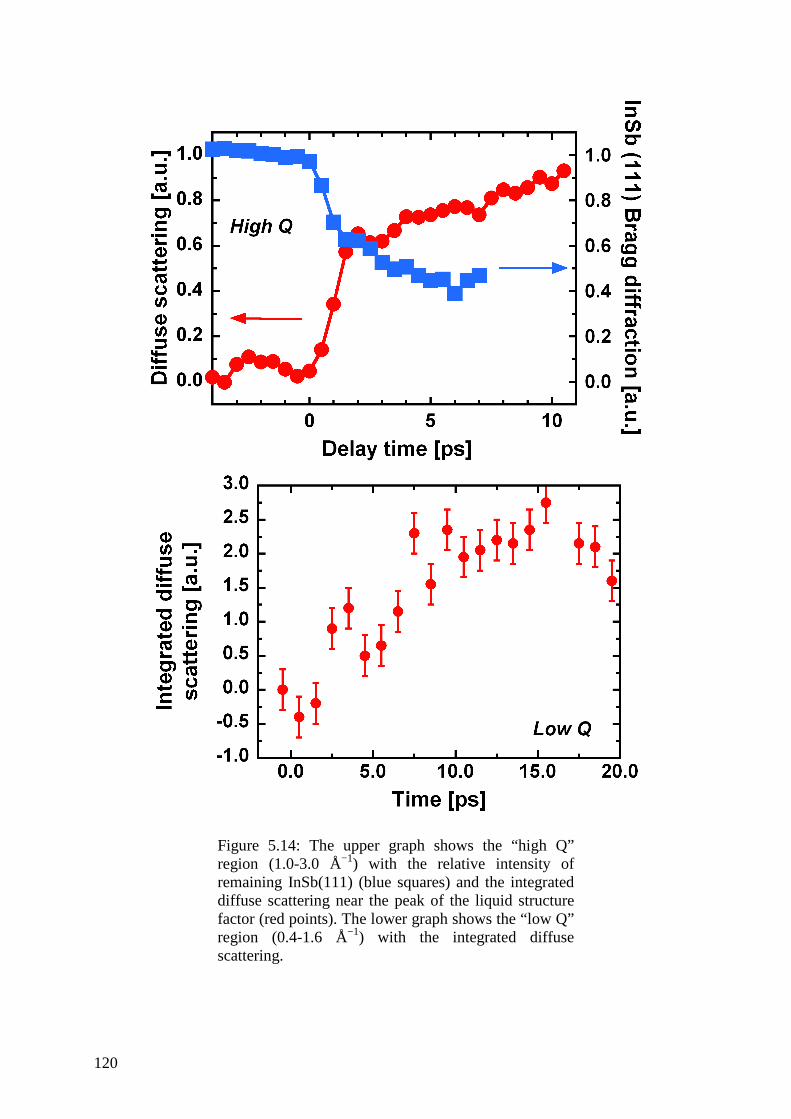
120

Figure 5.14: The upper graph shows the “high Q”

region (1.0-3.0 Å−1) with the relative intensity of remaining InSb(111) (blue squares) and the integrated diffuse scattering near the peak of the liquid structure factor (red points). The lower graph shows the “low Q” region (0.4-1.6 Å−1) with the integrated diffuse scattering.

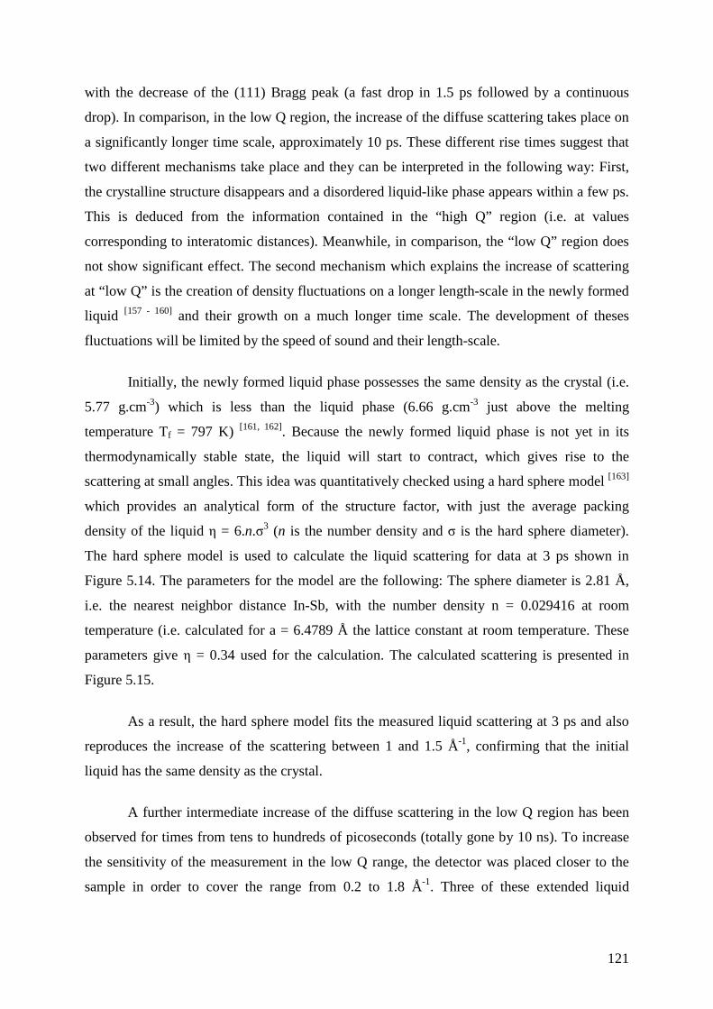
121

with the decrease of the (111) Bragg peak (a fast drop in 1.5 ps followed by a continuous

drop). In comparison, in the low Q region, the increase of the diffuse scattering takes place on

a significantly longer time scale, approximately 10 ps. These different rise times suggest that

two different mechanisms take place and they can be interpreted in the following way: First,

the crystalline structure disappears and a disordered liquid-like phase appears within a few ps.

This is deduced from the information contained in the “high Q” region (i.e. at values

corresponding to interatomic distances). Meanwhile, in comparison, the “low Q” region does

not show significant effect. The second mechanism which explains the increase of scattering

at “low Q” is the creation of density fluctuations on a longer length-scale in the newly formed

liquid [157 - 160] and their growth on a much longer time scale. The development of theses

fluctuations will be limited by the speed of sound and their length-scale.

Initially, the newly formed liquid phase possesses the same density as the crystal (i.e.

5.77 g.cm-3) which is less than the liquid phase (6.66 g.cm-3 just above the melting

temperature Tf = 797 K) [161, 162]. Because the newly formed liquid phase is not yet in its

thermodynamically stable state, the liquid will start to contract, which gives rise to the

scattering at small angles. This idea was quantitatively checked using a hard sphere model [163]

which provides an analytical form of the structure factor, with just the average packing

density of the liquid η = 6.n.σ3 (n is the number density and σ is the hard sphere diameter).

The hard sphere model is used to calculate the liquid scattering for data at 3 ps shown in

Figure 5.14. The parameters for the model are the following: The sphere diameter is 2.81 Å,

i.e. the nearest neighbor distance In-Sb, with the number density n = 0.029416 at room

temperature (i.e. calculated for a = 6.4789 Å the lattice constant at room temperature. These

parameters give η = 0.34 used for the calculation. The calculated scattering is presented in

Figure 5.15.

As a result, the hard sphere model fits the measured liquid scattering at 3 ps and also

reproduces the increase of the scattering between 1 and 1.5 Å-1, confirming that the initial

liquid has the same density as the crystal.

A further intermediate increase of the diffuse scattering in the low Q region has been

observed for times from tens to hundreds of picoseconds (totally gone by 10 ns). To increase

the sensitivity of the measurement in the low Q range, the detector was placed closer to the

sample in order to cover the range from 0.2 to 1.8 Å-1. Three of these extended liquid

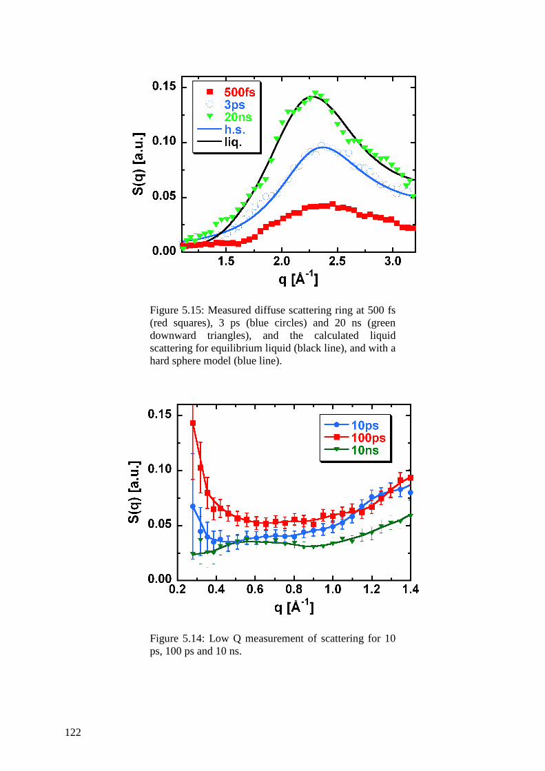
122

Figure 5.15: Measured diffuse scattering ring at 500 fs

(red squares), 3 ps (blue circles) and 20 ns (green downward triangles), and the calculated liquid scattering for equilibrium liquid (black line), and with a hard sphere model (blue line).

Figure 5.14: Low Q measurement of scattering for 10

ps, 100 ps and 10 ns.

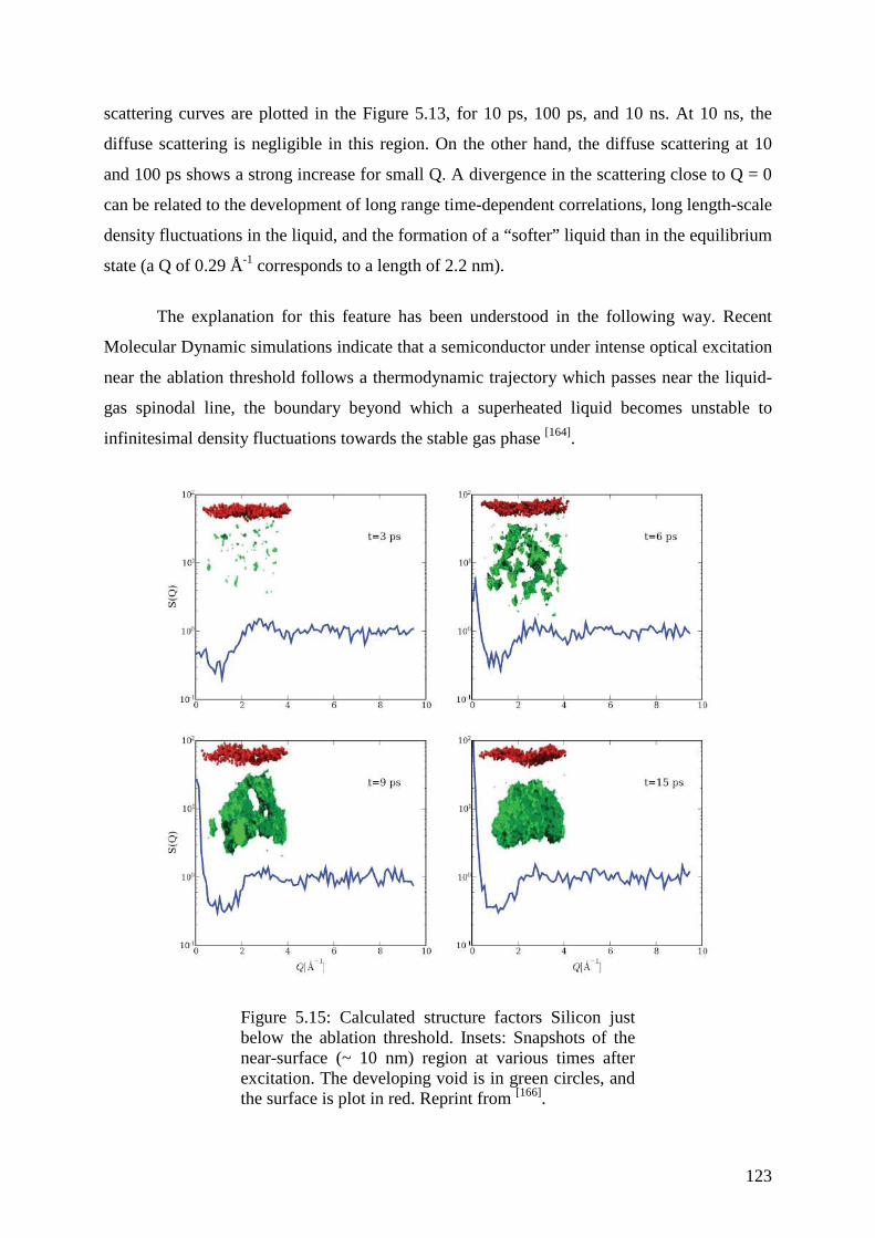
123

scattering curves are plotted in the Figure 5.13, for 10 ps, 100 ps, and 10 ns. At 10 ns, the

diffuse scattering is negligible in this region. On the other hand, the diffuse scattering at 10

and 100 ps shows a strong increase for small Q. A divergence in the scattering close to Q = 0

can be related to the development of long range time-dependent correlations, long length-scale

density fluctuations in the liquid, and the formation of a “softer” liquid than in the equilibrium

state (a Q of 0.29 Å-1 corresponds to a length of 2.2 nm).

The explanation for this feature has been understood in the following way. Recent

Molecular Dynamic simulations indicate that a semiconductor under intense optical excitation

near the ablation threshold follows a thermodynamic trajectory which passes near the liquid-

gas spinodal line, the boundary beyond which a superheated liquid becomes unstable to

infinitesimal density fluctuations towards the stable gas phase [164].

Figure 5.15: Calculated structure factors Silicon just

below the ablation threshold. Insets: Snapshots of the near-surface (~ 10 nm) region at various times after excitation. The developing void is in green circles, and the surface is plot in red. Reprint from [166].

124

In order to qualitatively understand the size and the structure of these long range

correlation, MD calculations were performed by our SPPS collaborators and used to calculate

the time-dependant structure factor S(Q,t). The calculations were based on previous

calculations done for the case of silicon [164, 165], as Si and InSb are quite similar in structure,

bonding and phase diagram.

The following assumptions were made for these simulations. Carriers are described by

Monte Carlo techniques and atom dynamics by Molecular Dynamics techniques. An incoming

absorbed photon creates an electron-hole pair assumed to follow Drude dynamics. The heating

of the material occurs through carrier-phonon scattering, which is simulated by transferring a

quantum of energy of tens of meV to the neighboring atoms by adding an appropriate

component to their velocity in a random direction. The atoms follow Newtonian dynamics and

interact via an empirical Stillinger-Weber potential (first classical model of a semiconductor)

which provides a satisfactory description of both the crystalline and liquid phases of silicon.

The structure factor was then directly calculated for various thermodynamic trajectories as a

function of time and for various laser fluences. The resulting X-ray structure factors obtained

for four different times, and a laser fluence just below the ablation threshold are plotted in

Figure 5.15.

The inset represents the calculated local structure near the surface for the given time. It

is observed that on a picosecond time-scale, localized voids form spontaneously, grow and

then fuse into a single void, and grown up to tens of nanometre in size [167]. The corresponding

calculated structure factors show a transient divergence at small Q, similar to what the

experimental data show. However, in indium antimonide, the optical penetration depth is

greater than the size of the simulation cell of the MD-calculations, which would slow down

the dynamics of this process over a time scale of hundreds of picosecond, as observed in the

experiment. These simulations provide a qualitative description of the fluctuating nature of the

liquid in agreement with the experimental data.

The experimental data indicates that following the optical excitation in indium

antimonide, the non thermal melting occurs first, to leave a liquid having the same density

than the crystal. After that, the liquid shrink and voids appear and start to grow inside the

liquid. Below the ablation threshold, the voids are too small (“sub-critical”) and eventually

dissolve in the liquid.

125

5.2.2.4. Conclusion for the non-thermal melting experiment

With an optical pulse, an ultrafast solid to liquid phase transition in indium antimonide

was launched, and it was characterized by following the transient evolution of the X-ray liquid

scattering. The formation of a metastable state of the liquid phase and the formation and

subsequent disappearance of voids within the sample were followed. This was possible by the

observation of X-ray scattering at small angles.

Within the frame of the thesis, novel data were obtained which have helped to define

the solid to liquid phase transition and the liquid dynamics occurring. To obtain a more

complete understanding of the dynamics happening during the ultrafast melting, the extension

of these experiments towards larger, as well as towards smaller angles is needed. The future

X-ray FELs will be able to fulfill these requirements with their short pulse duration, their

accessible wavelength range, and, in particular, their high flux..

Parallel to the X-ray sources, the femtosecond electron sources also achieved to get

direct information about the ultrafast melting. The pioneering work was made by Siwick et al. [19, 20] in a thin Aluminium poly-crystalline film. The authors have observed the disappearance

of the diffraction rings from the crystalline phase, and the appearance of the liquid scattering

rings.

5.3. Summary and perspectives

The SPPS has permitted to perform really important scientific work.

In Bismuth, a careful measurement of the change of the equilibrium position and the

change of the A1g phonon frequency was performed with different laser excitation. The initial

work was performed by Sokolowski-Tinten et al. [28] with a femtosecond plasma-based X-ray

source, but the measurement presented here have allowed measurements with much higher

accuracy over an extended fluence range.

The non-thermal melting experiment in indium antimonide has revealed the formation

and development of the liquid phase for excitation conditions close to the ablation threshold.

These two results were possible thanks to the unprecedented combination of a short X-

ray pulse duration and brightness at the SPPS. This has permitted to reduce by more than two

orders of magnitude the acquisition time in the case of the bismuth experiment, and to

perform the first diffuse X-ray scattering experiment with sub-ps temporal resolution.

126

Unfortunately, the SPPS was shut down in February 2006 to give room to the

construction of the LCLS. This new X-ray free electron laser has actually started in April

2009, and user can access it since November 2009. Hopefully, the European X-FEL will start

in 2014.

127

6. Summary and outlook

6.1. Summary

The work in my thesis was dedicated to the design and build up of a new table top

femtosecond plasma-based X-ray pulse source, and to time resolved experiments on

femtosecond to picosecond time-scales, using a plasma- and an accelerator-based X-ray pulse

source.

The short second chapter gives an introduction to the different types of ultrashort

pulsed X-ray sources that are either currently available, or are being developed or built. This

chapter underlines that the laboratory-sized, plasma-based X-ray sources still have the

potential to successfully perform ultrafast time-resolved experiments, and that they are

complementary to the accelerator-based sources.

The third chapter deals with the design, build-up and testing of new femtosecond

plasma-based X-ray pulse sources at the University of Duisburg-Essen. The chapter describes

the principle of the plasma-based sources, giving a description of the laser system and the

original “in-vacuum” chamber source, and discussing its “limitations”, which had to be

overcome with the X-ray sources I had to build. To underline the technical solutions used for

the new X-ray setups, the chapter discusses the X-ray optics geometry and efficiency in order

to optimize the X-ray flux onto the sample under study.

Two new sources were designed to overcome some of the limitations of the original

“in-vacuum” setup. One was based on a wire target and the other was based on a tape target.

Their performances were measured and discussed. The tape target chamber presented more

advantages, and was subsequently used to set up an experimental apparatus for ultrafast time

resolved X-ray diffraction. The chapter then focuses on this new X-ray source, providing a

description of the detectors used, the optical beam passes and the X-ray beam properties.

Finally, it discusses stability issues and normalization procedures. To due time constraints this

source was not used for the time resolved measurements presented in my thesis in Chapters 4

and 5. However, the source has been used intensively to study the softening of the A1g phonon

128

in Bismuth at high pump fluences by W. Lu et al. [106] and for novel time-resolved Debye-

Scherrer diffraction experiments in polycrystalline materials [168].

The fourth chapter focuses on two experiments performed in the laboratory of the

University of Duisburg-Essen. The driving idea of these investigations was to study the

interplay of the electronic and thermal pressure contributions for different femtosecond

optically excited materials (i.e. semiconductors and metals). These investigations arose from

the work and results of Shymanovich [90]. The first part of the chapter describes the physical

response for both kinds of materials, in particular the generation of stress/pressure.

The second part of the chapter deals with measurements on gallium arsenide. The

main conclusion is that for a bulk material no reliable information concerning the electronic

and thermal contributions to the acoustic response could be obtained, because the temporal

evolution of the strain in the sample depends on too many unknown parameters and a

meaningful comparison of the experimental data to model calculations became impossible.

The third part of the chapter deals with experiments on a thin crystalline gold film.

The experiment was successfully modeled and interpreted using the classic two-temperature

model. The relaxation time constant of the electron to lattice energy was found to be (5.0 ±

0.3) picoseconds, which is similar to the value recently obtained with femtosecond time-

resolved electron diffraction [126, 127]. The second important piece of information obtained is

the ratio of the Grüneisen parameters γe / γi = (0.5 ± 0.1). Only γi = (2.96 ± 0.04) is known in

the literature with good accuracy. γe is not known with such precision (γe = (1.6 ± 0.5)). Using

the measurement presented here, a more accurate value of γe = (1.48 ± 0.3) was obtained. The

measurement demonstrated that in contrast to semiconductors, the “established” model for the

electronic and thermal pressure is able to give the correct estimations of their relative

contributions.

The fifth chapter is dedicated to the Sub-Picosecond Pulse Source which existed at the

SLAC national accelerator laboratory and to two experiments performed using this

accelerator-based X-ray pulse source. The first part describes this source in detail.

The second part presents the work performed using this source. The first measurement

addressed the generation of coherent optical phonons in femtosecond optically-excited

bismuth and their dependence on laser pump fluence. The main result was that it was possible

to map the transient changes of the relevant potential energy surface (in harmonic

129

approximation) by measuring the softening of the phonon frequency (from 2.92 to 2.2 THz),

and the change of the equilibrium distance of the bismuth atoms pair (up to 11 pm increase).

The second measurement concerned the ultrafast non-thermal melting of a

semiconductor (here indium antimonide). The SPPS enabled us to follow the loss of the

crystalline order and appearance of the disordered liquid phase, and subsequently the transient

changes occurring within this newly formed liquid phase. In particular, the contraction of the

liquid phase, and the growth of voids in the liquid phase during the initial stage of ablation

could be observed.

Such results were possible due to the unprecedented combination of short pulse

duration and a high number of photons within each delivered X-ray pulse.

6.2. Outlook

As has previously been underlined, plasma based X-ray sources are still of great

interest for performing time-resolved X-ray diffraction experiments, due to their availability

and low cost (compared with the synchrotron slicing sources or the 4th generation X-ray

sources). This is why development, improvement and maintenance of the set-up and the X-ray

source should be pursued. Work can be done to improve the overall stability of the X-ray

source (by using for example a computer controlled beam stabilizer to reduce spatial drifts of

the X-ray source), or to reduce the self absorption of the X-rays in the target material by using

a more appropriate tape (such as a thinner metallic band). The proposal to use a gas-filled

ionization-chamber (described in Section 3.9) for normalization was actually implemented

and successfully applied by W. Lu et al. [106, 168].

The experiments performed to investigate the interplay of the electronic and thermal

pressure contributions showed that bulk samples do not provide reliable information. To carry

out further work and to be able to obtain the required pieces of information, the use of thin

crystalline films seems to be mandatory. However, it is not always possible to obtain such

crystalline thin films.

The investigation of the electronic and thermal pressure contribution dependence was

only achieved in germanium by Shymanovich [90]. However, in principle, if suitable thin film

samples become available, further investigations could be made.

A more accurate determination of the Grüneisen parameter γE of metals using the

transient changes of the diffraction signal, was up to now only achieved in aluminium using

femtosecond electron diffraction [109, 169]. The work done in this thesis could be continued by

130

trying to determine the Grüneisen parameters γe for other metals, and could be extended for

example to many magnetic metals such as rare earth elements with low Curie temperatures [169].

The study of non-reversible dynamics, such as the liquid phase dynamics in non-

thermally molten semiconductors or during ablation, can not be optimally carried out using a

plasma source due to the low number of photons. However, new sources such as the recently

started LCLS, and later the XFEL, will be able to perform these non reversible experiments.

Due to their extremely high brightness the required information can be obtained essentially

with just a few pulses or even with a single pulse.

131

132

Annexes

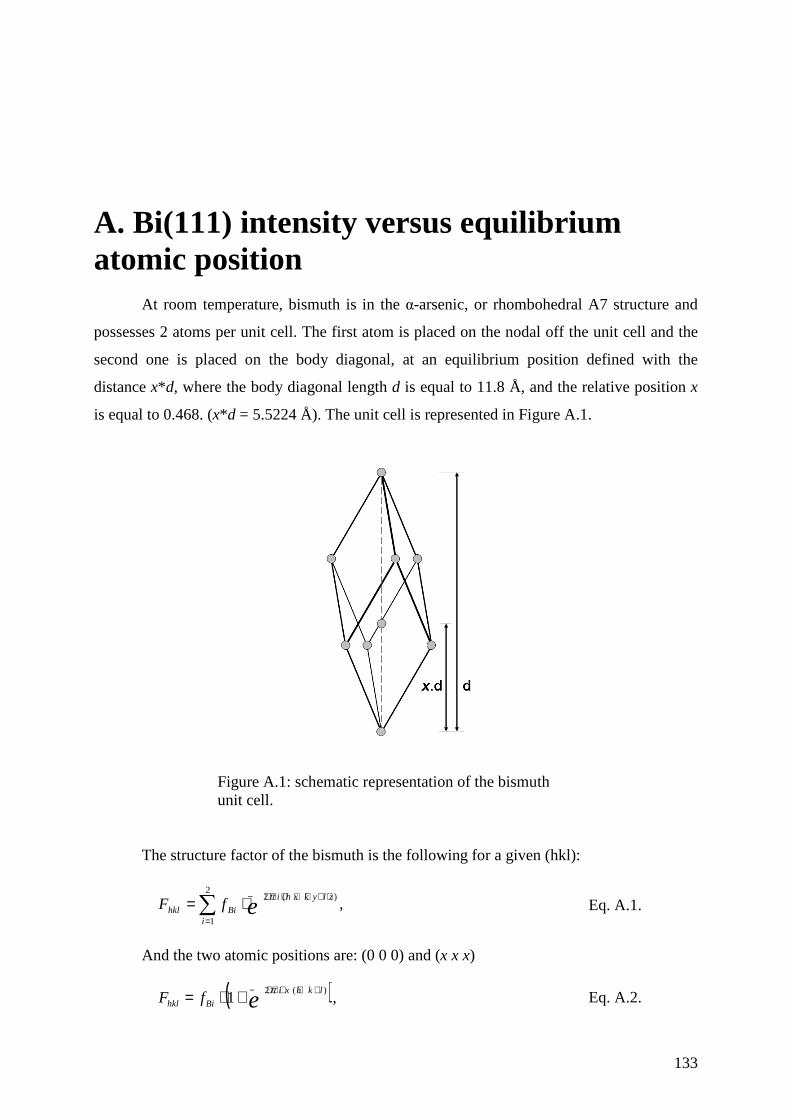
133

A. Bi(111) intensity versus equilibrium atomic position

At room temperature, bismuth is in the α-arsenic, or rhombohedral A7 structure and

possesses 2 atoms per unit cell. The first atom is placed on the nodal off the unit cell and the

second one is placed on the body diagonal, at an equilibrium position defined with the

distance x*d, where the body diagonal length d is equal to 11.8 Å, and the relative position x

is equal to 0.468. (x*d = 5.5224 Å). The unit cell is represented in Figure A.1.

Figure A.1: schematic representation of the bismuth

unit cell.

The structure factor of the bismuth is the following for a given (hkl):

∑=

⋅+⋅+⋅⋅⋅−⋅=2

1

)(2

i

zlykxhi

Bihkl efFπ

, Eq. A.1.

And the two atomic positions are: (0 0 0) and (x x x)

( )elkhxi

Bihkl fF)(2

1++⋅⋅⋅−+⋅= π

, Eq. A.2.

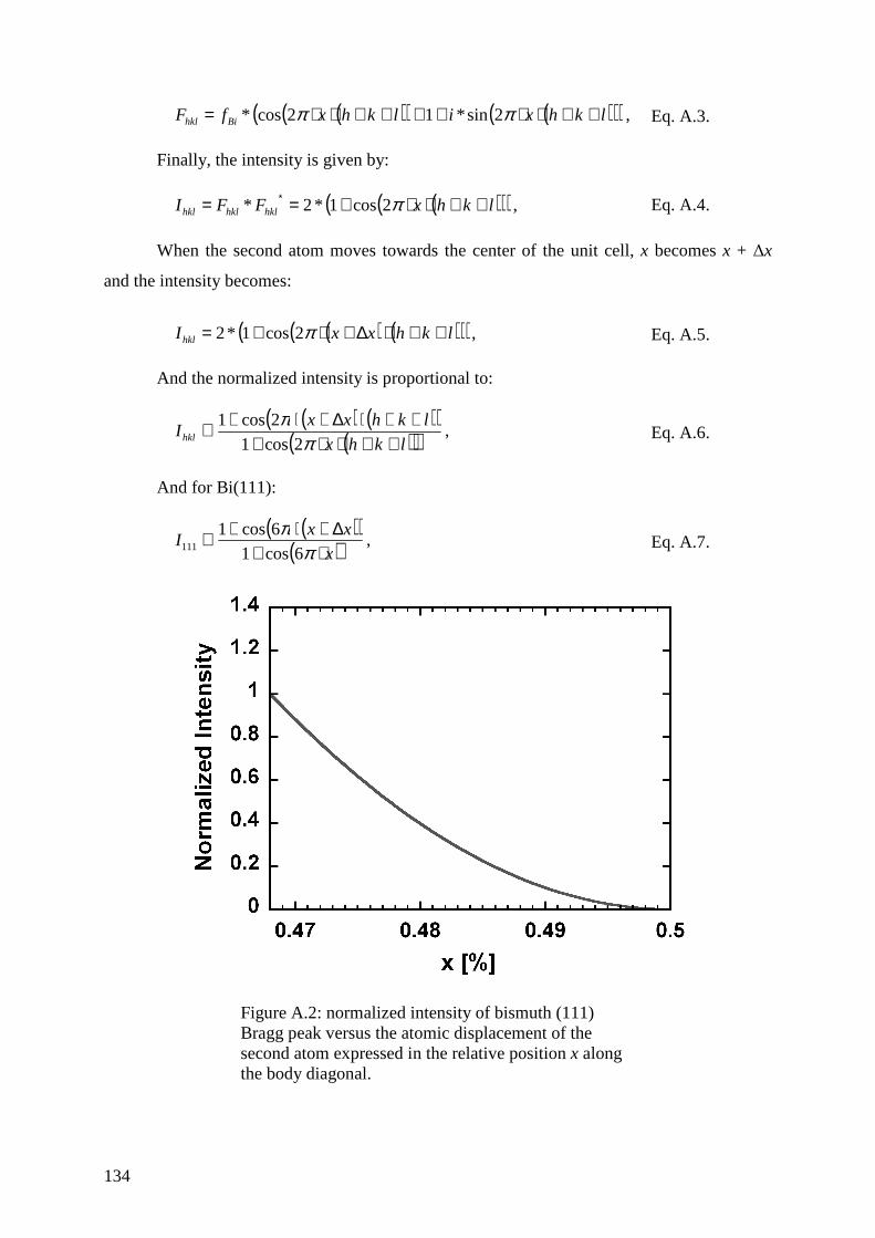
134

( )( ) ( )( )( )lkhxilkhxfF Bihkl ++⋅⋅++++⋅⋅= ππ 2sin*12cos* , Eq. A.3.

Finally, the intensity is given by:

( )( )( )lkhxFFI hklhklhkl ++⋅⋅+== ∗ π2cos1*2* , Eq. A.4.

When the second atom moves towards the center of the unit cell, x becomes x + ∆x

and the intensity becomes:

( ) ( )( )( )lkhxxI hkl ++⋅∆+⋅+= π2cos1*2 , Eq. A.5.

And the normalized intensity is proportional to:

( ) ( )( )

( )( )lkhx

lkhxxI hkl ++⋅⋅+

++⋅∆+⋅+∝π

π2cos1

2cos1, Eq. A.6.

And for Bi(111):

( )( )

( )x

xxI

⋅+∆+⋅+∝

ππ

6cos1

6cos1111 , Eq. A.7.

Figure A.2: normalized intensity of bismuth (111)

Bragg peak versus the atomic displacement of the second atom expressed in the relative position x along the body diagonal.

135

Figure A.2 shows the evolution of the normalized intensity for a given new relative

position of the second atom. When the diatomic distance of the atoms pair increases, the (111)

signal intensity will drop. Ultimately, if the parameter x becomes 0.5, the signal vanishes

completely. This would correspond to a forbidden reflection.

Measuring the signal intensity change of the (111) Bragg peak allows knowing the

new atomic position of the second bismuth atom. This method is used to establish the A1g

optical phonon frequencies of bismuth in the section 5.2.1. Indirectly, temporal overlap of

optical pump and X-ray probe can be found using the initial displacement of the bismuth

atoms, like shown in section 3.3.8.

136

B. Sample material properties

The following relevant parameters for this thesis (for the annexes B.1. and B.2.) are

taken from the web site of the Ioffe Physical Technical Institute [118] which has for goals to

propose a much possible complete set of parameters for all the important semiconductors.

B.1. gallium arsenide: GaAs Basic Parameters at 300 K: Crystal structure: Zinc Blende. Lattice constant: a = 5.65325 Å. Density: 5.317 g.cm-3. Auger coefficient: ~10-30cm6/s. Thermal properties: Bulk modulus: 7.53·* 1011 dyn.cm-2. Melting point: 1240 °C. Specific heat: 0.33 J.g-1.°C-1. Thermal conductivity: 0.55 W.cm-1.°C-1. Thermal diffusivity: 0.31 cm2.s-1. Thermal expansion, linear: 5.73·* 10-6 °C-1. Elastic constants:

C11 = 11.90·* 1011 dyn/cm2. C12 = 5.34·* 1011 dyn/cm2. C44 = 5.96·* 1011 dyn/cm2.

Longitudinal sound speed:

Cs[100] = ρ11C

= 4.73 * 103 m/s.

B.2. indium antimonide: InSb Basic Parameters at 300 K: Crystal structure: Zinc Blende. Lattice constant: a = 6.479 Å.

137

Density: 5.77 g.cm-3. Thermal properties: Bulk modulus: 4.66·* 1011 dyn.cm-2. Melting point: 527 °C. Specific heat: 0.2 J.g-1.°C-1. Thermal conductivity: 0.18 W.cm-1.°C-1. Thermal diffusivity: 0.16 cm2.s-1. Thermal expansion, linear: 5.37 *·10-6 °C-1. Elastic constants:

C11 = 6.67·* 1011 dyn/cm2. C12 = 3.65·* 1011 dyn/cm2. C44 = 3.02·* 1011 dyn/cm2.

B.3. gold on substrate X-rays (Ti Kα1): 4510.8 eV, λ = 2.748607 * 10-10 m. Acoustic reflectivity at the interface: -0.663. Relative amplitude wave interface / wave surface: 0.832. Sample area: 1*1 cm2.

B.3.1. gold: Au Film Thickness: 89 nm. Basic Parameters at 300 K: Crystal Structure: Cubic Face Centered. Lattice constant: a = 4.0782 Å. Θ(111) = 35.7098°. Density: 19.4 g/cm3. Thermal properties: Bulk modulus: 220 GPa. Melting point: 1337.33 K. Specific heat: 0.129 J.g-1.°C-1. Thermal conductivity: 0.18 W.cm-1.°C-1. Thermal diffusivity: 0.16 cm2.s-1. Thermal expansion, linear: 14.2·* 10-6 °C-1. Elastic constants:

C11 = 19.6 *·1011 dyn/cm2. C12 = 16.45·* 1011 dyn/cm2. C44 = 4.2·* 1011 dyn/cm2.

Longitudinal sound speed:

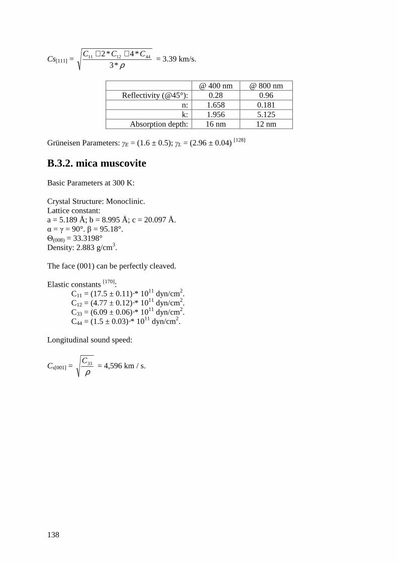
138

Cs[111] = ρ*3

*4*2 441211 CCC ++ = 3.39 km/s.

@ 400 nm @ 800 nm Reflectivity (@45°): 0.28 0.96 n: 1.658 0.181 k: 1.956 5.125 Absorption depth: 16 nm 12 nm Grüneisen Parameters: γE = (1.6 ± 0.5); γL = (2.96 ± 0.04) [128]

B.3.2. mica muscovite Basic Parameters at 300 K: Crystal Structure: Monoclinic. Lattice constant: a = 5.189 Å; b = 8.995 Å; c = 20.097 Å. α = γ = 90°. β = 95.18°. Θ(008) = 33.3198° Density: 2.883 g/cm3. The face (001) can be perfectly cleaved. Elastic constants [170]:

C11 = (17.5 ± 0.11)·* 1011 dyn/cm2. C12 = (4.77 ± 0.12)·* 1011 dyn/cm2. C33 = (6.09 ± 0.06)·* 1011 dyn/cm2. C44 = (1.5 ± 0.03)·* 1011 dyn/cm2.

Longitudinal sound speed:

Cs[001] = ρ33C

= 4,596 km / s.

139

Bibliography

[1] W. C. Röntgen, “On a new kind of Ray”, Nature 53, 274-277 (1896), translated by A. Stanton from, W. C. Röntgen, “Über eine neue Art von Strahlen”, Sitz. ber. an die med.-phys. Gesellschaft Würzburg, (1895)

[2] M. von Laue, Friedrich and Knipping “Eine quantitative Prüfrung der Theorie für die Interferenz-Erscheinungen bei Röntgenstrahlen”, Sitz. ber. der Kgl. Bayer. Akad. Wiss. 363, 73 (1912)

[3] W. H. Bragg and W. L. Bragg, “The reflection of X-rays by crystals”, Proc. Roy Soc. London A 88, 249 (1913)

[4] M. Siegbahn and E. Friman, Phys. Zeits. 17, 17;61;176 (1916); M. Siegbahn and E. Friman, “Uber die Hochfrequenzspektra (Z-reihe) der elemente Ta bis Bi”, Ann. d. Phys. 49, 623 (1916)

[5] J. D. Watson & F. H. C. Crick, “Molecular Structure of Nucleic Acids: A Structure for Deoxyribose Nucleic Acid”, Nature 171, 737-738 (1953)

[6] D. Strickland and G. Mourou, “Compression of Amplified Chirped Optical Pulses”, Optics Communications 55, 447-449 (1985)

[7] D. Strickland and G. Mourou, “Compression of Amplified Chirped Optical Pulses *”, Optics Communications 56, 219-221 (1985)

[8] D. Kühlke, U. Herpes, D. von der Linde, “Soft x-ray emission from subpicosend laser-produced plasma”, Appl. Phys. Lett. 50, 1785-1787 (1987)

[9] M. M. Murnane, H. C. Kapteyn, M. D. Rosen, R. W. Falcone, “Ultrafast X-ray Pulses from Laser-Produced Plasmas”, Science 251, 531-536 (1991)

[10] A. Rousse, P. Audebert, J. P. Geindre, F. Fall, and J. C. Gauthier, “Efficient Kα X-ray source from femtosecond laser-produced plasmas”, Phys. Rev. E 50, 2200-2207 (1994)

[11] C. Rischel, A. Rousse, I. Uschmann, P. A. Albouy, J. P. Geindre, P. Audebert, J. C. Gauthier, E. Förster, J. L. Martin, and A. Antonetti, “Femtosecond time-resolved X-ray diffraction from laser heated organic films”, Nature 390, 490-492 (1997)

[12] T. Pfeifer, C. Spielmann and G. Gerber, “Femtosecond X-ray science”, Rep. Prog. Phys. 96, 443-505 (2006)

[13] M. Bargheer, N. Zhavoronkon, M. Woerner, and T. Elsaesser, “Recent progress in ultrafast X-ray diffraction”, ChemPhysChem 7, 783-792 (2006)

[14] E. Collet, M. H. Lemée-Cailleau, M. Buron-Le Cointe, H. Cailleau, M. Wulff, T. Luty, S. Y. Koshihara, M. Meyer, Loic Toupet, Philippe Rabiller, Simone Techert, “Laser-Induced Ferroelectric Structural Order in an Organic Charge-Transfer Crystal”, Science 300, 612-615 (2003)

[15] K. Sokolowski-Tinten, H. Schulz, J. Bialkowski, and D. von der Linde, “Two Distinct Transitions in Ultrafast Solid-Liquid Phase Transformations of GaAs”, Appl. Phys. A 53, 227 (1991)

[16] K. Sokolowski-Tinten, J. Bialkowski, and D. von der Linde, “Ultrafast Laser-Induced Order-Disorder Transitions in Semiconductors”, Phys. Rev. B 51, 14186 (1995)

140

[17] K. Sokolowski-Tinten, J. Solis, J. Bialkowski, J. Siegel, C. N. Afonso, and D. von der Linde, “Dynamics of Ultrafast Phase Changes in Amorphous GeSb Films”, Phys. Rev. Lett. 81, 3679-3682 (1998)

[18] K. Sokolowski-Tinten, J. Bialkowski, M. Boing, A. Cavalleri, and D. von der Linde, “Thermal and Non-Thermal Melting of Gallium Arsenide after Femtosecond Laser Excitation”, Phys. Rev. B 58, R18805-R18808 (1998)

[19] B. J. Siwick, J. R. Dwyer, R. E. Jordan, and R. J. Dwayne Miller, “An Atomic-Level View of Melting Using Femtosecond Electron Diffraction”, Science 302, 1382-1385 (2003)

[20] B.J. Siwick, J.R. Dwyer, R.E. Jordan, and R.J.D. Miller, “Femtosecond Electron Diffraction Studies of Strongly Driven Structural Phase Transitions,” Chem. Phys. 299, 285-305 (2004)

[21] C. W. Siders, A. Cavalleri, K. Sokolowski-Tinten, C. Toth, T. Guo, M. Kammler, M. Horn-von Hoegen, K. R. Wilson, D. von der Linde and C. P. J. Barty, “Detection of nonthermal melting by ultrafast X-ray diffraction”, Science 286, 1340-1342 (1999)

[22] A. Rousse, C. Rischel, S. Fourmaux, I. Uschmann, S. Sebban, G. Grillon, P. Balcou, E. Förster, J. P. Geindre, P. Audebert, J. C. Gauthier, and D. Hulin, “Non-thermal melting in semiconductors measured at femtosecond resolution”, Nature 410, 65-68 (2001)

[23] K. Sokolowski-Tinten, C. Blome, C. Dietrich, A. Tarasevitch,M. Horn-von Hoegen, D. von der Linde, A. Cavalleri, J. Squier, and M. Kammler, “Femtosecond X-ray measurement of ultrafast melting and large acoustic transients”, Phys. Rev. Lett. 87, 225701 (2001)

[24] T. Feurer, A. Morak, I. Uschmann, C. Ziener, H. Schwoerer, C. Reich, P. Gibbon, E. Förster, R. Sauerbrey, K. Ortner and C. R. Becker, “Femtosecond silicon Kα pulses from laser-produced plasmas”, Phys. Rev. E 65, 016412 (2001)

[25] A. M. Lindenberg, et al., “Atomic scale visualization of inertial dynamics”, Science 308, 392-395 (2005)

[26] K. J. Gaffney, et al., “Observation of structural anisotropy and the onset of liquidlike motion during the nonthermal melting of InSb”, Phys. Rev. Lett. 95, 125701 (2005)

[27] P. B. Hillyard, et al., “Carrier-density-dependent lattice stability in InSb”, Phys. Rev. Lett. 98, 125501 (2007)

[28] K. Sokolowski-Tinten, C. Blome, J. Blums, A. Cavalleri, C. Dietrich, A. Tarasevitch, I. Uschmann, E. Förster, M. Kammler, M. Horn-von Hoegen and D. von der Linde, “Femtosecond X-ray measurement of coherent lattice vibrations near the Lindemann stability limit”, Nature 422, 287-289 (2003)

[29] D. M. Fritz, et al., “Ultrafast bond softening in Bismuth: Mapping a solid's interatomic potential with X-rays”, Science 315, 633-636 (2007)

[30] M. Bargheer, N. Zhavoronkov, Y. Gritsai, J. C. Woo, D. S. Kim, M. Woerner and T. Elsaesser, “Coherent atomic motions in a nanostructure studied by femtosecond X-ray diffraction”, Science 306, 1771- 1773 (2004)

[31] M. Bargheer, N. Zhavoronkov, J. C. Woo, D. S. Kim, M. Woerner, and T. Elsaesser, “Excitation mechanisms of coherent phonons unravelled by femtosecond X-ray diffraction”, Phys. Stat. Sol. (b) 243, 2389- 2396 (2006)

[32] C. von Korff Schmising, M. Bargheer, M. Kiel, N. Zhavoronkov, M. Woerner, T. Elsaesser, I. Vrejoiu, D. Hesse, and M. Alexe, “Accurate time delay determination for femtosecond X-ray diffraction experiments” Appl. Phys. B 88, 1-4 (2007)

141

[33] C. Thomsen, J. Strait, Z. Vardeny, H. J. Mark. J. Tauc, and J. Hauser,“Coherent phonon generation and detection by picosecond light pulses”, Phys. Rev. Lett., 53, 989-992 (1984)

[34] C. Thomsen, H. T. Grahn, H. J. Maris, and J. Tauc, “Surface generation and detection of phonons by picosecond light pulses”, Phys. Rev. B 34, 4129-4138 (1986)

[35] C. Rose-Petruck, R. Jimenez, T. Guo, A. Cavalleri, C. W. Siders, F. Raksi, J. A. Squier, B. C. Walker, K. R. Wilson, and C. P. J. Barty, “Picosecond-milliangström lattice dynamics measured by ultrafast X-ray diffraction”, Nature 398, 310-312 (1999)

[36] A. M. Lindenberg, I. Kang, S. L. Johnson, T. Missalla, P. A. Heimann, Z. Chang, J. Larsson, P. H. Bucksbaum, H. C. Kapteyn, H. A. Padmore, R. W. Lee, J. S. Wark and R. W. Falcone, “Time-resolved X-ray diffraction from coherent phonons during a laser-induced phase transition”, Phys. Rev. Lett. 84, 111 (2000)

[37] A. Cavalleri, C.W. Siders, F. L. H. Brown, D. M. Leitner, C. Tóth, J. A. Squier, C. P. J. Barty, K. R. Wilson, K. Sokolowski-Tinten, M. Horn-von Hoegen, D. von der Linde and M. Kammler, “Anharmonic lattice dynamics in germanium measured with ultrafast X-ray diffraction”, Phys. Rev. Lett. 85, 586-589 (2000)

[38] A. Cavalleri, C. W. Siders, C. Rose-Petruck, R. Jimenez, C. Tóth, J. A. Squier, C. P. J. Barty, K. R. Wilson, K. Sokolowski-Tinten, M. Horn-von Hoegen and D. von der Linde, “Ultrafast x-ray measurement of laser heating in semiconductors: Parameters determining the melting threshold”, Phys. Rev. B 63, 193306 (2001)

[39] D. A. Reis, M. F. DeCamp, P. H. Bucksbaum, R. Clarke, E. Dufresne, M. Hertlein, R. Merlin, R. Falcone, H. Kapteyn, M. M. Murnane, J. Larsson, Th. Missalla and J. S. Wark, “Probing impulsive strain propagation with X-Ray pulses”, Phys. Rev. Lett. 86, 3072-3075 (2001)

[40] J. Larsson, A. Allen, P. H. Bucksbaum, R. W. Falcone, A. Lindenberg, G. Naylor, T. Missalla, D. A. Reis, K. Scheidt, A. Sjögren, P. Sondhauss, M. Wulff and J. S.Wark, “Picosecond X-ray diffraction studies of laser-excited acoustic phonons in InSb”, Appl. Phys. A 75, 467 (2002)

[41] M. F. DeCamp, D. A. Reis, A. Cavalieri, P. H. Bucksbaum, R. Clarke, R. Merlin, E.M. Dufresne, D. A. Arms, A. M. Lindenberg, A.G. MacPhee, Z. Chang, B. Lings, J. S.Wark and S. Fahy, “Transient strain driven by a dense electron-hole plasma”, Phys. Rev. Lett. 91, 165502 (2003)

[42] M. F. DeCamp, D. A. Reis, D. M. Fritz, P. H. Bucksbaum, E. M. Dufresneb, and Roy Clarke, “X-ray synchrotron studies of ultrafast crystalline dynamics”, J. Synchrotron Rad. 12, 177–192 (2005)

[43] S. H. Lee, A. L. Cavalieri, D. M. Fritz, M. C. Swan, R. S. Hegde, M. Reason, R. S. Goldman and D. A. Reis, “Generation and propagation of a picosecond acoustic pulse at a buried interface: Time-resolved X-ray diffraction measurements”, Phys. Rev. Lett. 95, 246104 (2005)

[44] A. Morak, T. Kämpfer, I. Uschmann, A. Lübcke, E. Förster, and R. Sauerbrey, “Acoustic phonons in InSb probed by time-resolved x-ray diffraction”, Phys. Stat. Sol. b 243, 2728-2744 (2006)

[45] H. Enquist, H. Navirian, T. N. Hansen, A. M. Lindenberg, P. Sondhauss, O. Synnergren, J. S.Wark, and J. Larsson, “Large Acoustic Transients Induced by Nonthermal Melting of InSb”, Phys. Rev. Lett. 98, 225502 (2007)

[46] J. A. Bearden, “X-ray Wavelengths”, Rev. of Mod. Phys. 39, 78-124 (1967)

142

[47] T. Anderson, I. V. Tomov, and P. M. Rentzepis, “A high repetition rate, picosecond hard x-ray system, and its application to time-resolved x-ray diffraction”, J. Chem. Phys. 99, 869-875 (1993)

[48] A. Egbert, B. N. Chichkov and A. Ostendorf, “Ultrashort X-ray source driven by femtosecond laser pulses”, Europhys. Lett. 56, 228–233 (2001)

[49] A. Egbert, B. Mader, B. Tkachenko, C. Fallnich, B. N. Chichkov, H. Stiel and P. V. Nickles, “High-repetition rate femtosecond laser-driven hard-x-ray source”, Appl. Phys. Lett. 81, 2328-2330 (2002)

[50] U. Hinze, A. Egbert, B. Chichkov, and K. Eidmann, “Generation of picosecond hard-x-ray pulses in a femtosecond-laser-driven x-ray diode”, Optics Letters 29, 2079-2081 (2004)

[51] I. V. Tomov, D. A. Oulianov, P. Chen, and P. M. Rentzepis, “Ultrafast Time-Resolved Transient Structures of Solids and Liquids Studied by Means of X-ray Diffraction and EXAFS”, J. Phys. Chem. B 103, 7081-7091 (1999)

[52] P. Chen, I. V. Tomov, and P. M. Rentzepis, “Time resolved heat propagation in a gold crystal by means of picosecond x-ray diffraction”, J. Chem. Phys. 104, 10001-10007 (1996)

[53] T. Feurer, “Feedback-controlled optimization of soft-X-ray radiation from femtosecond laser-produced plasmas”, Appl. Phys. B 68, 55–60 (1999)

[54] T. Feuer, A. Morak, I. Uschmann, C. Ziener, H. Schwoerer, E. Förster and R. Sauerbrey, “An incoherent sub-picosecond X-ray source for time-resolved X-ray-diffracion experiments”, Appl. Phys. B 72, 15-20, (2001)

[55] H. Witte, M. Silies, T. Haarlammert, J. Hüve, J. Kutzner, and H. Zacharias, “Multi-kilohertz, ultrafast hard X-ray Kα source”, Appl. Phys. B 90, 11–14 (2008)

[56] A. Sjögren, M. Harbst, C. G. Wahlström, S. Svanberg, and C. Olsson, “High-repetition-rate, hard x-ray radiation from a laser-produced plasma: Photon yield and application considerations”, Rev. Sci. Instrum. 74, 2300-2311 (2003)

[57] H.-S. Park, et al., “High-energy Kα radiography using high-intensity, short-pulse lasers”, Phys. Plasmas 13, 056309 (2006)

[58] A. Cavalleri, C. Tóth, C. W. Siders, J. A. Squier, P. Forget and J. C. Kieffer, “Femtosecond Structural Dynamics in VO2 during an Ultrafast Solid-Solid Phase Transition”, Phys. Rev. Lett. 87, 237401 (2001)

[59] A. Rousse, K. Ta Phuoc, R. Shah, A. Pukhov, E. Lefebvre, V. Malka, S. Kiselev, F. Burgy, J. P. Rousseau, D. Umstadter, and D. Hulin, “Production of a keV X-Ray Beam from Synchrotron Radiation in Relativistic Laser-Plasma Interaction”, Phys. Rev. Lett. 93, 135005 (2004)

[60] A. Pukhov and J. Meyer-ter-Vehn, “Laser wake field acceleration: the highly non-linear broken-wave regime”, Appl. Phys. B 74, 355–361 (2002)

[61] E. Esarey, B. A. Shadwick, P. Catravas, and W. P. Leemans, “Synchrotron radiation from electron beams in plasma-focusing channels”, Phys. Rev. E 65, 056505 (2002)

[62] S. Wang, C. E. Clayton, B. E. Blue, E. S. Dodd, K. A. Marsh, W. B. Mori, C. Joshi, S. Lee, P. Muggli, T. Katsouleas, F. J. Decker, M. J. Hogan, R. H. Iverson, P. Raimondi, D. Walz, R. Siemann, and R. Assmann, “X-Ray Emission from Betatron Motion in a Plasma Wiggler”, Phys. Rev. Lett. 88, 135004 (2002)

[63] K. Ta Phuoc, F. Burgy, J. P. Rousseau, V. Malka, A. Rousse, R. Shah, D. Umstadter, A. Pukhov and S. Kiselev, “Laser based synchrotron radiation”, Phys. Plasmas 12, 023101 (2005)

[64] K. Ta Phuoc, S. Corde, R. Shah, F. Albert, R. Fitour, J. P. Rousseau, F. Burgy, B. Mercier, and A.e Rousse, “Imaging Electron Trajectories in a Laser-Wakefield Cavity Using Betatron X-Ray Radiation”, Phys. Rev. Lett. 97, 225002 (2006)

143

[65] http://www.esrf.eu/UsersAndScience/Experiments/MaterialsScience/ID09B [66] http://www.diamond.ac.uk/Beamlines/Beamlineplan/I19/Beamlinedescription.html [67] http://www.synchrotron-soleil.fr/portal/page/portal/Recherche/LignesLumiere/

CRISTAL [68] A. Zholents, P. Heimann, M. Zolotorev, and J. Byrd, “Generation of subpicosecond

X-ray pulses using RF orbit deflection”, Nuclear Instruments and Methods in Physics Research A 425, 385-389 (1999)

[69] M. Borland, “Simulation and analysis of using deflecting cavities to produce short x-ray pulses with the Advanced Photon Source”, Phys. Rev. STAB 8, 074001 (2005)

[70] http://www.aps.anl.gov/Sectors/Sector7/ [71] A. A. Zholents and M. S. Zolotorev, “Femtosecond X-Ray Pulses of Synchrotron

Radiation”, Phys. Rev. Lett. 76, 912-915 (1996) [72] R. W. Schoenlein, S. Chattopadhyay, H. H. W. Chong, T. E. Glover, P. A. Heimann,

C. V. Shank, A. A. Zholents, and M. S. Zolotorev, “Generation of Femtosecond Pulses of Synchrotron Radiation”, Science 287, 2237-2240 (2000)

[73] R. W. Schoenlein, S. Chattopadhyay, H. H. W. Chong, T. E. Glover, P.A. Heimann, W. P. Leemans, C. V. Shank, A. Zholents, M. Zolotorev, “Generation of femtosecond X-ray pulses via laser–electron beam interaction”, Appl. Phys. B 71, 1-10 (2000)

[74] A. Cavalleri, M. Rini, H. H. W. Chong, S. Fourmaux, T. E. Glover, P. A. Heimann, J. C. Kieffer, and R. W. Schoenlein, “Band-selective measurements of electron dynamics in VO2 using femtosecond near-edge X-ray absorption”, Phys. Rev. Lett. 95, 67405 (2005)

[75] A. Cavalleri1, S. Wall, C. Simpson, E. Statz, D. W. Ward, K. A. Nelson, M. Rini and R. W. Schoenlein, “Tracking the motion of charges in a terahertz light field by femtosecond X-ray diffraction”, Nature 442, 664-666 (2006)

[76] S. Khan, K. Holldack, T. Kachel, R. Mitzner, and T. Quast, “Femtosecond Undulator Radiation from Sliced Electron Bunches”, Phys. Rev. Lett. 97, 074801 (2006)

[77] J. Andruszkow, et al., “First Observation of Self-Amplified Spontaneous Emission in a Free-Electron Laser at 109 nm Wavelength”, Phys. Rev. Lett. 85, 3825-3829 (2000)

[78] V. Ayvazyan, “A new powerful source for coherent VUV radiation: Demonstration of exponential growth and saturation at the TTF free-electron laser”, Eur. Phys. J. D 20, 149-156 (2002)

[79] S. V. Milton, et al., “Exponential Gain and Saturation of a Self-Amplified Spontaneous Emission Free-Electron Laser”, Science 292, 2037-2041 (2001)

[80] L. F. DiMauro, J. Arthur, N. Berrah, J. Bozek, J. N. Galayda and J. Hastings, “Progress Report on the LCLS XFEL at SLAC”, Journal of Physics: Conference Series 88, 012058 (2007)

[81] A. A. Zholents and W. M. Fawley, “Proposal for Intense Attosecond Radiation from an X-Ray Free-Electron Laser”, Phys. Rev. Lett. 92, 224801 (2004)

[82] A. A. Zholents, “Laser assisted electron beam conditioning for free electron lasers”, Phys. Rev. STAB 8, 050701 (2005)

[83] D.G. Atearns, O.L. Landen, E.M. Campbell, and J.H. Scofield, “Generation of ultrashort x-ray pulses”, Phys. Rev. A 37, 1684-1690 (1988)

[84] M.M. Murnane, H.C. Kapteyn, and R.W. Falcone, “High-Density Plasmas Produced by Ultrafast Laser Pulses”, Phys. Rev. Lett. 62, 155-158 (1989)

144

[85] U. Teubner, C. Wiilker, W. Theobald, and E. Fijrster,“X-ray spectra from high-intensity subpicosecond laser produced plasmas”, Phys. Plasmas 2, 972-981 (1995)

[86] P. Gibbon, Short Pulse Laser Interactions with Matter: An Introduction , Imperial College Press/World Scientific, London/Singapore, (September 2005)

[87] P. Gibbon and E. Förster, “Short-pulse laser–plasma interactions”, Plasma Phys. Control. Fusion 38, 769–793 (1996)

[88] C. Reich, P. Gibbon, I. Uschmann and E. Förster, “Yield optimization and time structure of femtosecond laser plasma Kα sources”, Phys. Rev. Lett. 84, 4846-4849 (2000)

[89] S. Backus, C. G. Durfee, M. M. Murnane, and H. C. Kapteyn, “High power ultrafast lasers”, Rev. Sci. Instrum. 69, 1207-1223 (1998)

[90] U. Shymanovich, “Direct observation of ultrafast atomic motion using time-resolved X-ray diffraction”, Dissertation (2007)

[91] T. Missalla, I. Uschmann, E. Förster, G. Jenke, and D. von der Linde, “Monochromatic focusing of subpicosecond X-ray pulses in the KeV range”, Rev. Sci. Instrum. 70, 1288-1299 (1999)

[92] M. Nicoul, U. Shymanovich, S. Kähle, T. Caughey, D. Sampat, K. Sokolowski-Tinten, and D. von der Linde, “Bent Crystal X-Ray Mirrors for Time-Resolved Experiments with Femtosecond Laser-Produced X-ray Pulses”, Journal of Physics: Conference Series 21, 207–210 (2005)

[93] S. I. Salem and P. L. Lee, “Experimental Widths of K and L X-Ray Lines”, Atomic Data and Nuclear Data Tables 18, 233-241 (1976)

[94] www-cxro.lbl.gov [95] U. Shymanovich, M. Nicoul, K. Sokolowski-Tinten, A. Tarasevitch, C. Michaelsen,

and D. von der Linde, “Characterization and comparison of X-ray focusing optics for ultrafast X-ray diffraction experiments”, Applied Physics B 92, 493-499 (2008)

[96] P. Kirkpatrick and A. V. Baez, “Formation of Optical Images by X-Rays”, Journal of the optical society of America 38, 766-774 (1948)

[97] M. Bargheer, N. Zhavoronkov, R. Bruch, H. Legall, H. Stiel, M. Woerner, and T. Elsaesser, “Comparison of focusing optics for femtosecond X-ray diffraction”, Appl. Phys. B 00, 1–6 (2005)

[98] U. Shymanovich, M. Nicoul, W. Lu, S. Kähle, A. Tarasevitch, K. Sokolowski-Tinten, and D. von der Linde, “Towards ultrafast time-resolved Debye-Scherrer X-ray diffraction using a laser-plasma source”, Rev. Sci. Instrum. 80, 083102 (2009)

[99] A. Ruhl, “Erzeugung intensiver Röntgenimpulse mit einem Bandtarget”, (2006) [100] http://www.roperscientific.de/datasheets/

Princeton_Instruments_PI-MTE_1300B_RevA0.pdf [101] F. Zamponi, T. Kämpfer, A. Morak, I. Uschmann, and E. Förster, “Characterization

of a deep depletion, back-illuminated charge-coupled device in the x-ray range”, Rev. Sci. Instrum. 76, 116101 (2005)

[102] http://www.photonic-science.co.uk/products/PDF/X-ray_Gemstar_rev2.pdf [103] C. v. Korff Schmising, M. Bargheer, M. Kiel, N. Zhavoronkov, M. Woerner, T.

Elsaesser, I. Vrejoiu, D. Hesse, and M. Alexe, “Strain propagation in nanolayered perovskites probed by ultrafast x-ray diffraction”, Phys. Rev. B 73, 212202 (2006)

[104] C. v. Korff Schmising, M. Bargheer, M. Kiel, N. Zhavoronkov, M. Woerner, T. Elsaesser, I. Vrejoiu, D. Hesse, and M. Alexe, “Coupled Ultrafast Lattice and Polarization Dynamics in Ferroelectric Nanolayers”, Phys. Rev. Lett. 98, 257601 (2007)

145

[105] M. Braun, C. v. Korff Schmising, M. Kiel, N. Zhavoronkov, J. Dreyer, M. Bargheer, T. Elsaesser, C. Root, T. E. Schrader, P. Gilch, W. Zinth, and M. Woerner, “Ultrafast Changes of Molecular Crystal Structure Induced by Dipole Solvation”, Phys. Rev. Lett. 98, 248301 (2007)

[106] W. Lu, M. Nicoul, U. Shymanovich, A. Tarasevitch, M. Kammler, M. Horn von Hoegen, D. von der Linde, K. Sokolowski-Tinten, “Extreme phonon softening in laser-excited Bismuth – towards an inverse Peierls-transition”, proceedings MRS fall meeting 2009.

[107] U. Shymanovich, M. Nicoul, S. Kähle, W. Lu, A. Tarasevitch, K. Sokolowski-Tinten and D. von der Linde, “Interplay of thermal and electronic forces in the picosecond acoustic response of femtosecond-laser-excited Germanium”, under preparation.

[108] Y. Hayashi, Y. Tanaka, T. Kirimura, N. Tsukuda, E. Kuramoto and T. Ishikawa, “Acoustic Pulse Echoes Probed with Time-Resolved X-Ray Triple-Crystal Diffractometry”, Phys. Rev. Lett. 96, 115505 (1996)

[109] H. Park, X. Wang, S. Nie, R. Clinite, and J. Cao, “Mechanism of coherent acoustic phonon generation under nonequilibrium conditions”, Phys. Rev. B 72, 100301R (2005)

[110] J. J. Baumberg, D. A. Williams and K. Köhler, “Ultrafast Acoustic Phonon Ballistics in Semiconductor Heterostructures”, Phys. Rev. Lett. 78, 3358-3361 (1997)

[111] O. Matsuda, O. B. Wright, D. H. Hurley, V. Gusev and K. Shimizu, “Coherent shear phonon generation and detection with picosecond laser acoustics”, Phys. Rev. B 77, 224110 (2008)

[112] O. B. Wright, B. Perrin, O. Matsuda, and V. E. Gusev, “Ultrafast carrier diffusion in gallium arsenide probed with picosecond acoustic pulses”, Phys Rev. B 64, 081202 (2001)

[113] A. H. Chin, R.W. Schoenlein, T. E. Glover, P. Balling, W. P. Leemans and C. V. Shank, “Ultrafast Structural Dynamics in InSb Probed by Time-Resolved X-Ray Diffraction”, Phys. Rev. Lett. 83, 336-339 (1999)

[114] N. V. Chigarev, D. Yu. Paraschuk, X. Y. Pan and V. E. Gusev, “Coherent phonon emission in the supersonic expansion of photoexcited electron-hole plasma in Ge”, Phys. Rev. B 61, 15837-15840 (2000)

[115] G. Tas and H. J. Maris, “Picosecond ultrasonic study of phonon reflection from solid-liquid interfaces”, Phys. Rev. B 55, 1852-1857 (1997)

[116] O. B. Wright, “Ultrafast nonequilibrium stress generation in gold and silver”, Phys. Rev. B 49, 9985-9988 (1994)

[117] J. S. Blackmore, “Semiconducting and other major properties of gallium arsenide”, J. Appl. Phys. 55, 123-181 (1982)

[118] http://www.ioffe.ru/SVA/NSM/ [119] Handbook of Optical Constants in Solids, edited by E. D. Palik [120] U. Shymanovich, M. Nicoul, J. Blums, K. Sokolowski-Tinten, A. Tarasevitch, T.

Wietler, M. Horn-von Hoegen, and D. von der Linde, “Diffraction of strongly convergent X-rays from picosecond acoustic transients”, Appl. Phys. A 87, 7–11 (2007)

[121] C. Blome, “Untersuchung schneller Strukturänderungen mit Hilfe ultrakurzer Röntgenimpulse”, Dissertation (2003)

[122] http://www.phasis.ch/ [123] http://www.esrf.eu/UsersAndScience/Experiments/TBS/SciSoft/xop2.3/

146

[124] M.M. Hall, The Approximation of Symmetric X-Ray Peaks by Pearson Type VII Distributions, J. Apl. Cryst., Vol. 10, 66 (1977)

[125] J. Hohlfeld, J.G. Müller, S.-S.Wellershoff and E. Matthias, “Time-resolved thermoreflectivity of thin gold films and its dependence on film thickness”, Appl. Phys. B 64, 387–390 (1997)

[126] M. Ligges, I. Rajkovic, P. Zhou, O. Posth, C. Hassel, G. Dumpich and D. von der Linde, “ Observation of ultrafast lattice heating using time resolved electron diffraction”, Appl. Phys. Lett. 94, 101910 (2009)

[127] R. Ernstorfer et al., “Atomic view of the photoinduced collapse of gold and bismuth”, Springer Series in Chemical Physics 92 (in print, 2009)

[128] K. O. McLean, C. A. Swenson and C. R. Case, “Thermal Expansion of Copper, Silver, and Gold Below 30 K*”, J. of Low Temp. Phys. 7, 77-98 (1972)

[129] T. H. K. Barron, J. G. Collins and G. K. White, “Thermal expansion of solids at low temperatures”, Advances in Physics 29, 609-730 (1980)

[130] http://www.slac.stanford.edu [131] M. Cornacchia, J. Arthur, L. Bentson, R. Carr, P. Emma, J. Galayda, P. Krejcik, I.

Lindau, J. Safranek, J. Schmerge, J. Stohr, R. Tatchyn, and A. Wootton, “A Sub-Picosecond Photon Pulse Facility for SLAC”, SLAC-PUB-8950, (2001)

[132] A. Snigirev, V. Kohn, I. Snigireva, and B. Lengeler, “A compound refractive lens for focusing high-energy X-rays”, Nature 384, 49-51 (1996)

[133] R. Neutze and J. Hajdu, “Femtosecond time resolution in x-ray diffraction experiments”, Proc. Natl. Acad. Sci. USA 94, 5651-5655 (1997)

[134] K. Sokolowski-Tinten, A. Cavalleri and D. von der Linde, “Single-pulse time- and fluence-resolved optical measurements at femtosecond excited surfaces”, Appl. Phys. A 69, 577–579 (1999)

[135] O. Synnergren, M. Harbst, T. Missalla, J. Larsson, G. Katona, R. Neutze and R. Wouts, “Projecting picosecond lattice dynamics through x-ray topography”, Appl. Phys. Lett. 80, 3727-3729 (2002)

[136] A. L. Cavalieri et al., “Clocking Femtosecond X Rays”, Phys. Rev. Lett. 94, 114801 (2005)

[137] H. J. Zeiger, J. Vidal, T. K. Cheng, E. P. Ippen, G. Dresselhauss, and M. S. Dresselhaus, “Theory for displacive excitation of coherent phonons”, Phys. Rev. B 45, 768-778 (1992)

[138] T. K. Cheng, J. Vidal, H. J. Zeiger, G. Dresselhaus, M. S. Dresselhaus, and E. P. Ippen, “Mechanism for displacive excitation of coherent phonons in Sb, Bi, Te, and Ti2O3”, Appl. Phys. Lett. 59, 1923-1295 (1991)

[139] A. B. Shick, J. B. Ketterson, D. L. Novikov and A. J. Freeman, “Electronic structure, phase stability, and semimetal-semiconductor transitions in Bi”, Phys. Rev. B 60, 15484–15487 (1999)

[140] T. K. Cheng, S. D. Brorson, A. S. Kazeroonian, J. S. Moodera, G. Dresselhaus, M. S. Dresselhaus and E. P. Ippen, “Impulsive excitation of coherent phonons observed in reflection in bismuth and antimony”, Appl. Phys. Lett. 57, 1004-1006 (1990)

[141] M. Hase, K. Mizoguchi, H. Harima, S. Nakashima, M. Tani, K. Sakai, and M. Hangyo, “Optical control of coherent optical phonons in bismuth films”, Appl. Phys. Lett. 69, 2474-2476 (1996)

[142] M. F. DeCamp, D. A. Reis, P. H. Bucksbaum, and R. Merlin, “Dynamics and coherent control of high-amplitude optical phonons in bismuth”, Phys. Rev. B 64, 092301 (2001)

147

[143] M. Hase, M. Kitajima, S.-i. Nakashima, and K. Mizoguchi, “Dynamics of Coherent Anharmonic Phonons in Bismuth Using High Density Photoexcitation”, Phys. Rev. Lett. 88, 067401 (2002)

[144] W. H. Zachariasen, Theory of X-ray diffraction in crystals, New York: Dover Classics of Science and Mathematics, (1994)

[145] E. D. Murray, D. M. Fritz, J. K. Wahlstrand, S. Fahy, and D. A. Reis, “Effect of Lattice Anharmonicity in Bismuth High-amplitude Phonon Dynamics”, Phys. Rev. B 72, 060301 (2005)

[146] S. Fahy and D. A. Reis, “Coherent Phonons: Electronic Softening or Anharmonicity?”, Phys. Rev. Lett. 93, 109701 (2004)

[147] S. L. Johnson et al., “Nanoscale Depth-Resolved Coherent Femtosecond Motion in Laser-Excited Bismuth”, Phys. Rev. Lett. 100, 155501 (2008) S. L. Johnson et al., Directly Observing Squeezed Phonon States with Femtosecond X-Ray Diffraction”, Phys. Rev. Lett. 102, 175503 (2009)

[148] E. S. Zijlstra, L. L. Tatarinova and M. E. Garcia, “Laser-induced phonon-phonon interactions in bismuth”, Phys. Rev. B 74, 220301 (2006)

[149] G. Sciaini et al., “Electronic acceleration of atomic motions and disordering in bismuth”, Nature 458, 56-60 (2009)

[150] P. Saeta, J.-K. Wang, Y. Siegal, N. Bloembergen, and E. Mazur, “Ultrafast electronic disordering during femtosecond laser melting of GaAs”, Phys. Rev. Lett. 67, 1023-1026 (1991)

[151] K. Sokolowski-Tinten, J. Bialkowski, M. Boing, A. Cavalleri, and D. von der Linde, “Thermal and nonthermal melting of gallium arsenide after femtosecond laser excitation”, Phys. Rev. B 58, R11805-R11808 (1998)

[152] I. L. Shumay and U. Höfer, “Phase transformations of an InSb surface induced by strong femtosecond laser pulses”, Phys. Rev. B 53, 15878-15884 (1996)

[153] H. Reitze, H. Ahn, and M. C. Downer, “Optical properties of liquid carbon measured by femtosecond spectroscopy”, Phys. Rev. B 45, 2677 (1992)

[154] P. Stampfli, K. Bennemann, “Time dependence of the laser-induced femtosecond lattice instability in Si and GaAs: Role of longitudinal optical distortions”, Phys. Rev. B 49, 7299-7305 (1994)

[155] K. G. Nakamura et al., “Femtosecond time-resolved x-ray diffraction from optical coherent phonons in CdTe(111) crystal”, Appl. Phys. Lett. 93, 061905 (2008)

[156] T. Gu, X. Bian, J. Qin, and C. Xu, “Ab initio molecular-dynamics simulations of liquid GaSb and InSb”, Phys. Rev. B 71, 104206 (2005)

[157] H. Bale, B. Dobbs, J. Lin, and P. Schmidt, “X-ray scattering studies of critical opalescence in argon at constant density”, Phys. Rev. Lett. 25, 1556 (1970)

[158] L. Bosio, J. Teixeira, and H. Stanley, “Enhanced density fluctuations in supercooled H2O, D2O, and ethanol-water solutions: Evidence from small-angle x-ray scattering”, Phys. Rev. Lett. 46, 597 (1981)

[159] A. Pan, T. Rappl, D. Chandler, and N. Balsara, “Neutron scattering and monte carlo determination of the variation of the critical nucleus size with quench depth”, J. Phys. Chem B 110, 3692 (2006)

[160] P. Debenedetti, “When a phase is born”, Nature 441, 168 (2006) [161] S.V. Stankus, R.A. Khairulin and P.V. Tyagelsky, “Density of indium antimonide at

high temperatures”, Thermophysics and Aeromechanics 14, 161-164 (2007) [162] X. Chen, Q. Wang and K. Lu, “Temperature and time dependence of the density of

molten indium antimonide measured by an improved Archimedean method”, J. Phys.: Cond. Matt. 11,10335–10341 (1999)

148

[163] N. Ashcroft and J. Lekner, “Structure and resistivty of liquid metals”, Phys. Rev. 145, 83 (1966)

[164] P. Lorazo, L. J. Lewis, and M. Meunier, “Thermodynamic pathways to melting, ablation, and solidification in absorbing solids under pulsed laser irradiation”, Phys. Rev. B 73, 134108 (2006)

[165] P. Lorazo, L. J. Lewis, and M. Meunier, “Short-pulse laser ablation of solids: From phase explosion to fragmentation”, Phys. Rev. Lett. 91, 225502 (2003)

[166] A. M. Lindenberg et al., “X-Ray Diffuse Scattering Measurements of Nucleation Dynamics at Femtosecond Resolution”, Phys. Rev. Lett. 100, 135502 (2008)

[167] D. Zahn, “How does water boil?”, Phys. Rev. Lett. 93, 227801 (2004) [168] W. Lu, Dissertation (to be submitted) [169] S. Nie, X. Wang, H. Park, R. Clinite, and J. Cao, “Measurement of the Electronic

Grüneisen Constant Using Femtosecond Electron Diffraction”, Phys. Rev. Lett. 96, 025901 (2006)

[170] L. E. McNeil and M. Grimsditch, “Elastic moduli of muscovite mica”, J. Phys: Condens. Matter 5, 1681-1690 (1993)

[171] A. Thompson et al., “X-ray data booklet”, Section 2.1, “Characteristics of synchrotron radiation”

[172] K. Ta Phuoc et al., “Demonstration of the ultrafast nature of laser produced betatron radiation”, Physics of Plasmas 14, 080701 (2007)

[173] M. Moszyński, M. Kapusta, M. Balcerzyk, M. Szawlowski, D. Wolski, “Large Area Avalanche Photodiodes in X-rays and scintillation detection*”, Nucl. Instrum. Methods Phys. Res. A 442, 230-237 (2000)

[174] C. V. Shank, R. Yen and C. Hirlimann, “Time-Resolved Reflectivity Measurements of Femtosecond-Optical-Pulse-Induced Phase Transitions in Silicon”, Phys. Rev. Lett. 50, 454-457 (1983)

[175] C. V. Shank, R. Yen and C. Hirlimann, “Femtosecond-Time-Resolved Surface Structural Dynamics of Optically Excited Silicon”, Phys. Rev. Lett. 51, 900-902 (1983)

[176] T. Kachel, N. Pontius, C. Stamm, M. Wietstruk, E. F. Aziz, H. A. Dürr, W. Eberhardt, and F. M. F. de Groot, “Transient electronic and magnetic structures of nickel heated by ultrafast laser pulses”, Phys. Rev. B 80, 092404 (2009)