Embed Size (px)
Citation preview
-Zentrum für Entwicklungsforschung-
Rheinische Friedrich-Wilhelms-Universität Bonn
ANALYSIS OF WATER USE AND CROP ALLOCATION FOR THE
KHOREZM REGION IN UZBEKISTAN USING AN INTEGRATED
HYDROLOGIC-ECONOMIC MODEL
Inaugural-Dissertation
zur Erlangung des Grades
Doktor der Agrarwissenschaften
(Dr. Agr.)
der Hohen Landwirtschaftlichen Fakultät
der Rheinischen Friedrich-Wilhelms-Universität
zu Bonn
vorgelegt am 19.11.2010
von
Tina-Maria Schieder
aus Bonn (Deutschland)
Referent: PD Dr. P. Wehrheim
Korreferent: Prof. Dr. B. Diekkrüger
Tag der mündlichen Prüfung: 16.03.2011
Erscheinungsjahr: 2011
Diese Dissertation wird auf dem Hochschulschriftenserver der ULB Bonn http://hss.ulb.uni.bonn.de/diss_online elektronisch publiziert. D98
Abstract Sustainable and efficient water management is of central importance for the dominant
agricultural sector and thus for the population and the environment of the Khorezm region. Khorezm is situated in the lower Amu Darya river basin in the Central Asian Republic of Uzbekistan and the delta region of the Aral Sea. Recently, Khorezm has experienced an increase in ecological, economic and social problems. The deterioration of the ecology is a result of the vast expansion of the agricultural area (which began in the Soviet period in Uzbekistan), the utilization of marginal land and a very intensive production of cotton on a significant share of arable land. Supplying food for an increasing population and overcoming with the arid climate in Khorezm require intensive irrigation. However, the water distribution system is outdated. Current irrigation strategies are not flexible enough to cope with water supply and crop water demand, as both are becoming more variable. The political system, with its stringent crop quotas for cotton and wheat, nepotism, missing property rights and lack of incentives to save water, has promoted unsustainable water use rather than preventing it.
The focus of this study is an analysis of more economical and eco-efficient water management and crop allocation. The effects of political incentives as well as modified technological, environmental and institutional conditions, such as the reform of the cotton sector, the introduction of water prices and the improvement of the irrigation system, are evaluated regarding regional water distribution, crop allocation and economical outcomes. As a result, the basic hydrological and agronomical balances and characteristics in the Khorezm region are highly important and need to be identified. To adequately analyze these underlying conditions, an integrated water management model was chosen. The novelty of this study is the combination of interdisciplinary aspects in a theoretically consistent modeling framework. Essential hydrologic, climatologic, agronomic, institutional and economic relationships are integrated into one coherent optimization model for the Khorezm region. The capacity of the model to consider canal water and groundwater is of special importance. Furthermore, the water balance approach (accounting for water input and output) has an advantage over the static norm approach when used to determine irrigation requirements.
Simulations with the model indicate that a modification of the regional water supply, either politically or anthropogenically induced, has a large influence on the total irrigation, groundwater and drainage-system as well as the soil water budget in Khorezm. The model simulations suggest that low water supply causes a shift in the crop allocation to less water-demanding crops such as vegetables, wheat, alfalfa and fruits, which also have a higher value added in economic terms. When higher water supply is available, the cultivation of water-demanding rice, a crop that is favored by the local population, would become more advantageous due to higher gross margins. Simulations on an improvement of water distribution and irrigation systems indicate that infiltration losses could be diminished, especially at the field level. Furthermore, this would lead to an increase in additional available crop water supply, with positive impacts on crop yields. The simulation results further indicate that a complete liberalization of the cotton sector would lead to a fundamental restructuring of the crop allocation to less water-demanding crops and higher economically valued crops. This reform of the cotton sector would also lead to a general reduction of acreage with full compensation for the losses caused by the abolition of cotton subsidies and quota system. Marginal land could be reduced. However, the abolition of subsidies and secured crop sales prices by the government would increase the risk for farmers. Finally, the modeling results indicate that the introduction of water pricing could be an important instrument to induce environmental consumer awareness, which could lead to resource conservation. As a result of the extremely low gross crop profit margins in Khorezm, only a water price on a very low level could feasibly be implemented in this region.
Zusammenfassung Nachhaltige und effiziente Wasserbewirtschaftung sind von besonderer Bedeutung für
den dominanten Agrarsektor und damit für die Bevölkerung und Umwelt in Khorezm. Die Region Khorezm befindet sich im Unterlauf des Amu-Darya Flusseinzuggebietes in der zentralasiatischen Republik Usbekistan und in der Delta-Region des Aral Sees. Khorezm´s jetzige Situation ist gekennzeichnet durch ökologische, ökonomische und soziale Probleme. Die Schädigung der Ökologie ist im Wesentlichen durch die gewaltige Ausdehnung der landwirtschaftlichen Nutzfläche (mit ihrem Beginn während der Sowjetperiode in Usbekistan) und der steigenden Nutzung von Grenzertragsböden verursacht. Des Weiteren trägt der sehr intensive und ausgedehnte Baumwollanbau zu einer Verschärfung der Situation bei. Die Nahrungsmittelversorgung einer stark wachsenden Bevölkerung und das sehr aride Klima in Khorezm erfordern eine intensive Bewässerungslandwirtschaft. Das Wasserverteilungssystem ist allerdings überaltert und der Hauptgrund für steigende Ineffizienzen. Heutige Bewässerungsstrategien sind nicht flexibel genug, dem immer unbeständiger werdenden Wasserangebot und der sich variierenden Pflanzenwassernachfrage gerecht zu werden. Das politische System mit Subventionen und Anbauquoten für Baumwolle und Weizen, Vetternwirtschaft und fehlenden Eigentumsrechten tragen zusätzlich zu einer steigenden Wassernutzung und fehlender Nachhaltigkeit bei.
Die Analyse einer ökologisch und ökonomisch effizienteren Pflanzen- und Wasserbewirtschaftung bildet den Schwerpunkt dieser Arbeit. Die Effekte modifizierter technologischer-, umweltrelevanter- und institutioneller Rahmenbedingungen sollen hierbei bestimmt und ausgewertet werden. Die Liberalisierung des Baumwollsektors, die Einführung von Wasserpreisen oder die Verbesserung des Bewässerungssystems beispielsweise werden auf ihre Auswirkungen hinsichtlich regionaler Wasserverteilung, landwirtschaftlicher Anbaustruktur und ihrem ökonomischen Nutzen untersucht. Zu diesem Zwecke müssen im Vorfeld die wesentlichen hydrologischen und agronomischen Interaktionen und Eigenschaften der Region Khorezm identifiziert werden. Um diese zu Grunde liegenden Konditionen angemessen analysieren zu können, wurde ein integriertes Wasser-Management-Modell aufgebaut. Die Kombination von interdisziplinären Aspekten in einen theoretisch konsistenten Modellierungsrahmen stellt ein Novum in dieser Arbeit dar. Wesentliche klimatologische, hydrologische, agronomische, institutionelle und ökonomische Eigenschaften und Beziehungen sind in einem kohärenten Optimierungsmodell für die Region Khorezm integriert. Der große Vorteil dieser Modellierung liegt unter anderem auch in der Berücksichtigung von Kanal- und Grundwasser, die gerade in Bewässerungssystem von Khorezm von besonderer Wichtigkeit sind. Einen weiteren Nutzen des Modells und der darauf aufbauenden Forschungsarbeit bietet die Verwendung einer Wasser-Bilanzierungs-Methode. Im Gegensatz zu dem häufig verwendeten statischen Ansatz unter Nutzung von starren Bewässerungsnormen können durch die Bilanzierung von „Wassereinnahmen“ und „Wasserausgaben“ wesentliche Prozesse in größerer Genauigkeit dargestellt werden.
Die Modellsimulationen zeigen, dass eine (beispielsweise politisch induzierte oder anthropogen verursachte) Modifizierung des Wasserangebotes in Khorezm großen Einfluss auf das gesamte Bewässerungs-, Grundwasser und Entwässerungssystem und den Bodenwasserhaushalt hat. Vor allem in Situationen mit geringem Wasserangebot deuten die Simulationen darauf hin, dass sich der Anbau hin zu weniger wasserverbrauchenden Pflanzen und zu Feldfrüchten mit höherer Wertschöpfung (wie Gemüse, Luzerne, Weizen und Früchten) verschieben würde. In Situationen mit hohem Wasserangebot ist ein Anbau von Reis durch die hohen Gewinnmargen auf einigen Flächen durchaus möglich. Die Verbesserung des Bewässerungssystems, v.a. auf Feldebene, würde zu einer Verringerung der
Versickerung und damit einer zusätzlichen Wasserangebotsmenge für die Pflanzen führen. Das hätte positive Effekte auf die Erträge.
Außerdem zeigen die Simulationen, dass eine komplette Liberalisierung des Baumwollsektors zu einer drastisch veränderten landwirtschaftlichen Anbaustruktur führen würde. Die Verluste durch den Abbau von Subventionen und die Abkehr vom Quoten-System würden vollständig ausgeglichen werden durch den Anbau von Pflanzen mit geringerem Wasserbedarf aber wesentlich höherem ökonomischen Mehrwert. Auch die Gesamtanbaufläche würde sich reduzieren und Grenzertragsstandorte würden aus der Produktion ausscheiden. Die Abkehr vom jetzigen System mit gesicherten Verkaufspreisen würde auf der anderen Seite allerdings zu einer Erhöhung des Absatzrisikos der Landwirte führen. Die Einführung von Wasserpreisen in Khorezm wäre ein weiteres sinnvolles und wichtiges Werkzeug für Ressourcenschonung und ökologischer Bewusstseinsbildung der Konsumenten und Landwirte. Dies ist allerdings, so zeigen die Modellergebnisse, nur auf einem sehr niedrigen Preisniveau möglich. Die sehr geringe Gewinnspanne der Anbauprodukte lässt eine höhere Summe nicht zu.

I
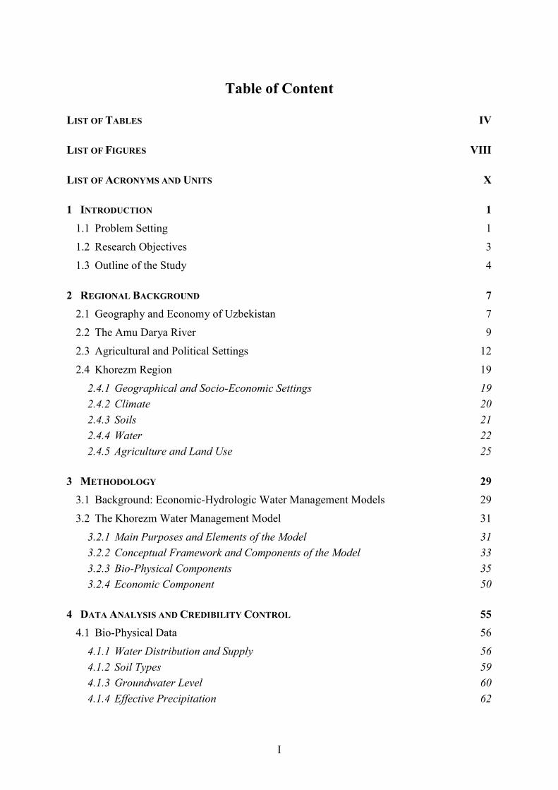
Table of Content
LIST OF TABLES IV
LIST OF FIGURES VIII
LIST OF ACRONYMS AND UNITS X
1 INTRODUCTION 1
1.1 Problem Setting 1
1.2 Research Objectives 3
1.3 Outline of the Study 4
2 REGIONAL BACKGROUND 7
2.1 Geography and Economy of Uzbekistan 7
2.2 The Amu Darya River 9
2.3 Agricultural and Political Settings 12
2.4 Khorezm Region 19
2.4.1 Geographical and Socio-Economic Settings 19
2.4.2 Climate 20
2.4.3 Soils 21
2.4.4 Water 22
2.4.5 Agriculture and Land Use 25
3 METHODOLOGY 29
3.1 Background: Economic-Hydrologic Water Management Models 29
3.2 The Khorezm Water Management Model 31
3.2.1 Main Purposes and Elements of the Model 31
3.2.2 Conceptual Framework and Components of the Model 33
3.2.3 Bio-Physical Components 35
3.2.4 Economic Component 50
4 DATA ANALYSIS AND CREDIBILITY CONTROL 55
4.1 Bio-Physical Data 56
4.1.1 Water Distribution and Supply 56
4.1.2 Soil Types 59
4.1.3 Groundwater Level 60
4.1.4 Effective Precipitation 62
II
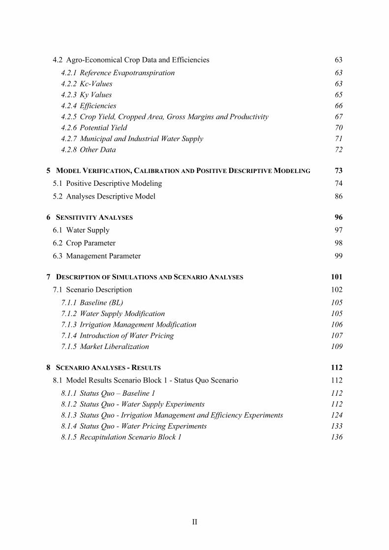
4.2 Agro-Economical Crop Data and Efficiencies 63
4.2.1 Reference Evapotranspiration 63
4.2.2 Kc-Values 63
4.2.3 Ky Values 65
4.2.4 Efficiencies 66
4.2.5 Crop Yield, Cropped Area, Gross Margins and Productivity 67
4.2.6 Potential Yield 70
4.2.7 Municipal and Industrial Water Supply 71
4.2.8 Other Data 72
5 MODEL VERIFICATION, CALIBRATION AND POSITIVE DESCRIPTIVE MODELING 73
5.1 Positive Descriptive Modeling 74
5.2 Analyses Descriptive Model 86
6 SENSITIVITY ANALYSES 96
6.1 Water Supply 97
6.2 Crop Parameter 98
6.3 Management Parameter 99
7 DESCRIPTION OF SIMULATIONS AND SCENARIO ANALYSES 101
7.1 Scenario Description 102
7.1.1 Baseline (BL) 105
7.1.2 Water Supply Modification 105
7.1.3 Irrigation Management Modification 106
7.1.4 Introduction of Water Pricing 107
7.1.5 Market Liberalization 109
8 SCENARIO ANALYSES - RESULTS 112
8.1 Model Results Scenario Block 1 - Status Quo Scenario 112
8.1.1 Status Quo – Baseline 1 112
8.1.2 Status Quo - Water Supply Experiments 112
8.1.3 Status Quo - Irrigation Management and Efficiency Experiments 124
8.1.4 Status Quo - Water Pricing Experiments 133
8.1.5 Recapitulation Scenario Block 1 136
III
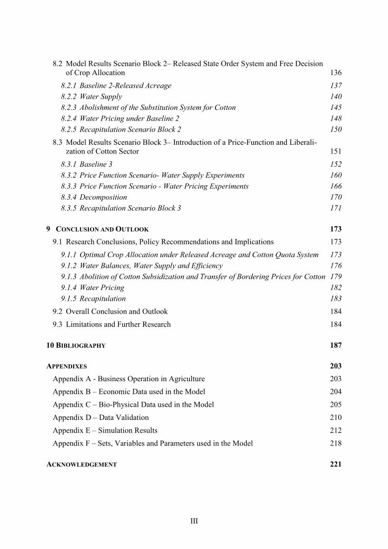
8.2 Model Results Scenario Block 2– Released State Order System and Free Decision of Crop Allocation 136
8.2.1 Baseline 2-Released Acreage 137
8.2.2 Water Supply 140
8.2.3 Abolishment of the Substitution System for Cotton 145
8.2.4 Water Pricing under Baseline 2 148
8.2.5 Recapitulation Scenario Block 2 150
8.3 Model Results Scenario Block 3– Introduction of a Price-Function and Liberali- zation of Cotton Sector 151
8.3.1 Baseline 3 152
8.3.2 Price Function Scenario- Water Supply Experiments 160
8.3.3 Price Function Scenario - Water Pricing Experiments 166
8.3.4 Decomposition 170
8.3.5 Recapitulation Scenario Block 3 171
9 CONCLUSION AND OUTLOOK 173
9.1 Research Conclusions, Policy Recommendations and Implications 173
9.1.1 Optimal Crop Allocation under Released Acreage and Cotton Quota System 173
9.1.2 Water Balances, Water Supply and Efficiency 176
9.1.3 Abolition of Cotton Subsidization and Transfer of Bordering Prices for Cotton 179
9.1.4 Water Pricing 182
9.1.5 Recapitulation 183
9.2 Overall Conclusion and Outlook 184
9.3 Limitations and Further Research 184
10 BIBLIOGRAPHY 187
APPENDIXES 203
Appendix A - Business Operation in Agriculture 203
Appendix B – Economic Data used in the Model 204
Appendix C – Bio-Physical Data used in the Model 205
Appendix D – Data Validation 210
Appendix E – Simulation Results 212
Appendix F – Sets, Variables and Parameters used in the Model 218
ACKNOWLEDGEMENT 221
IV
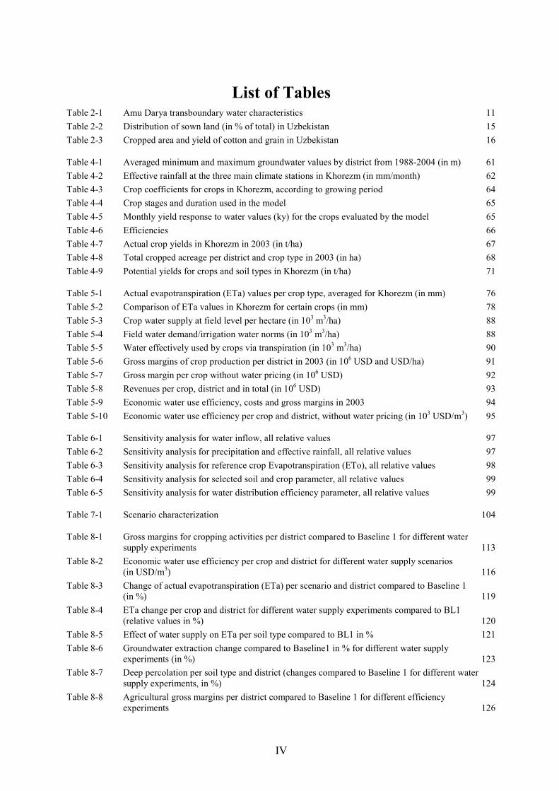
List of Tables
Table 2-1 Amu Darya transboundary water characteristics 11
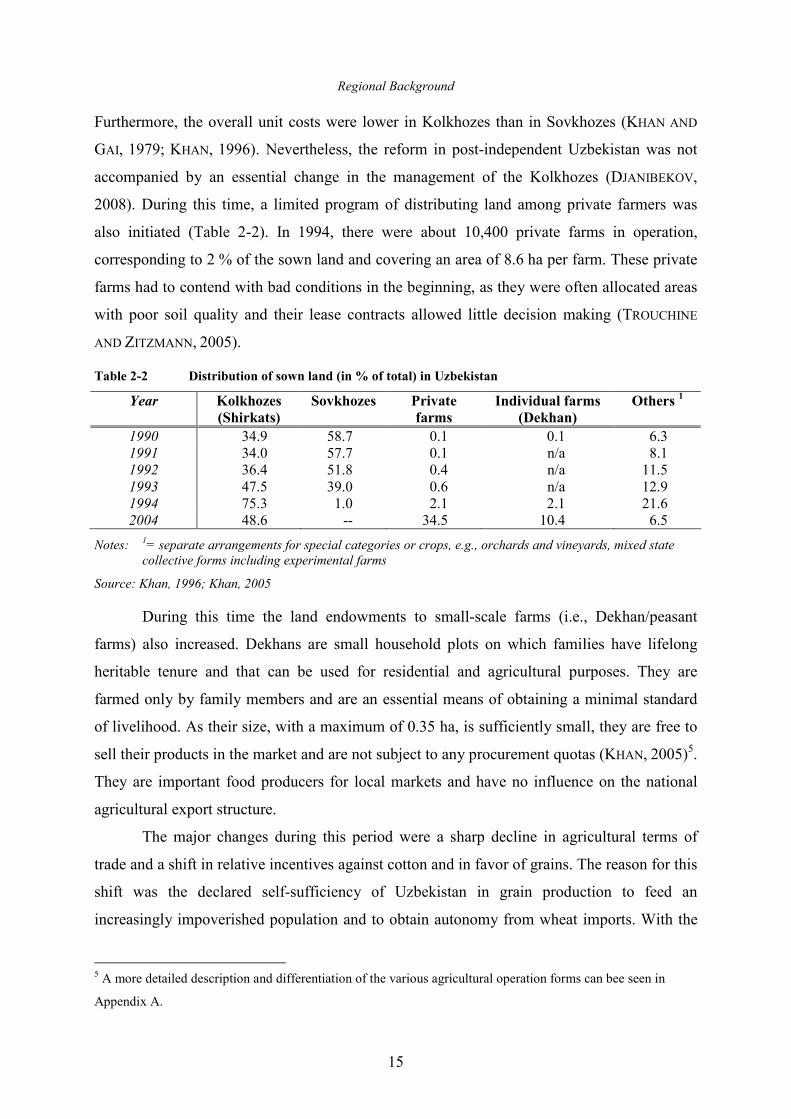
Table 2-2 Distribution of sown land (in % of total) in Uzbekistan 15
Table 2-3 Cropped area and yield of cotton and grain in Uzbekistan 16
Table 4-1 Averaged minimum and maximum groundwater values by district from 1988-2004 (in m) 61
Table 4-2 Effective rainfall at the three main climate stations in Khorezm (in mm/month) 62
Table 4-3 Crop coefficients for crops in Khorezm, according to growing period 64
Table 4-4 Crop stages and duration used in the model 65
Table 4-5 Monthly yield response to water values (ky) for the crops evaluated by the model 65
Table 4-6 Efficiencies 66
Table 4-7 Actual crop yields in Khorezm in 2003 (in t/ha) 67
Table 4-8 Total cropped acreage per district and crop type in 2003 (in ha) 68
Table 4-9 Potential yields for crops and soil types in Khorezm (in t/ha) 71
Table 5-1 Actual evapotranspiration (ETa) values per crop type, averaged for Khorezm (in mm) 76
Table 5-2 Comparison of ETa values in Khorezm for certain crops (in mm) 78
Table 5-3 Crop water supply at field level per hectare (in 103 m3/ha) 88
Table 5-4 Field water demand/irrigation water norms (in 103 m3/ha) 88
Table 5-5 Water effectively used by crops via transpiration (in 103 m3/ha) 90
Table 5-6 Gross margins of crop production per district in 2003 (in 106 USD and USD/ha) 91
Table 5-7 Gross margin per crop without water pricing (in 106 USD) 92
Table 5-8 Revenues per crop, district and in total (in 106 USD) 93
Table 5-9 Economic water use efficiency, costs and gross margins in 2003 94
Table 5-10 Economic water use efficiency per crop and district, without water pricing (in 103 USD/m3) 95
Table 6-1 Sensitivity analysis for water inflow, all relative values 97
Table 6-2 Sensitivity analysis for precipitation and effective rainfall, all relative values 97
Table 6-3 Sensitivity analysis for reference crop Evapotranspiration (ETo), all relative values 98
Table 6-4 Sensitivity analysis for selected soil and crop parameter, all relative values 99
Table 6-5 Sensitivity analysis for water distribution efficiency parameter, all relative values 99
Table 7-1 Scenario characterization 104
Table 8-1 Gross margins for cropping activities per district compared to Baseline 1 for different water supply experiments 113
Table 8-2 Economic water use efficiency per crop and district for different water supply scenarios (in USD/m3) 116
Table 8-3 Change of actual evapotranspiration (ETa) per scenario and district compared to Baseline 1 (in %) 119
Table 8-4 ETa change per crop and district for different water supply experiments compared to BL1 (relative values in %) 120
Table 8-5 Effect of water supply on ETa per soil type compared to BL1 in % 121
Table 8-6 Groundwater extraction change compared to Baseline1 in % for different water supply experiments (in %) 123
Table 8-7 Deep percolation per soil type and district (changes compared to Baseline 1 for different water supply experiments, in %) 124
Table 8-8 Agricultural gross margins per district compared to Baseline 1 for different efficiency experiments 126
V
Table 8-9 Economic water use efficiency per crop and district for different efficiency experiments (in USD/m3) 128
Table 8-10 Actual evapotranspiration for different efficiency experiments compared to Baseline 1 (in %) 129
Table 8-11 Yield per district, change compared to Baseline 1 for different efficiency experiments (in %) 129
Table 8-12 Yield change per crop compared to Baseline 1 for different efficiency experiments (in %) 130
Table 8-13 Water application at field level for whole Khorezm region for different efficiency scenarios (absolute [106 m3] and in %) 130
Table 8-14 Surface drainage from demand sites for different efficiency experiments compared to Baseline 1 [106 USD] (in %) 132
Table 8-15 Groundwater (GW) extraction change compared to Baseline 1 for different efficiency experiments, per soil type and per district (in %) 132
Table 8-16 Monthly groundwater extraction change compared to Baseline 1 for different efficiency experiments (in %) 133
Table 8-17 Gross margin, costs and revenues for experiments with different levels of water pricing under status quo scenario block 1 (in 106 USD) 134
Table 8-18 Water price level per district in which gross margins became zero (in USD/1000 m3) 135
Table 8-19 Water cost-covering water price level per district and in total (in USD/1000 m3) 135
Table 8-20 Gross margin, costs and revenues for Baseline 2 (in 106 USD), and changes to Baseline 1 (in %) 137
Table 8-21 Gross margin per crop for all Khorezm districts (in 106 USD) 139
Table 8-22 Acreage per district for Baseline 1 and Baseline 2 scenarios (in ha) 139
Table 8-23 Acreage per crop for Khorezm, Baseline 1 and Baseline 2 140
Table 8-24 Cropped area per district compared of Baseline 2 with experiments of modified water supply 141
Table 8-25 Crop allocation and share of crop area relative to total area for experiments with modified water supply under scenario block 2 for Khorezm (in ha and %) 141
Table 8-26 Revenues per crop and district for modified water supply (in 106 USD) and comparison to Baseline 2 (in %) 143
Table 8-27 Variable cost per crop and district for modified water supply (in 106 USD) and comparison to Baseline 2 (in %) 144
Table 8-28 Gross margin per crop and district for modified water supply (in 106 US Dollar) and comparison to Baseline 2 (in %) 145
Table 8-29 Irrigated area per district compared to Baseline 2 with experiments under liberalization of cotton sector 146
Table 8-30 Crop allocation, share of crop area to total area and comparison with Baseline 2 for cotton sector liberalization under scenario block 2 for Khorezm (in ha and %) 147
Table 8-31 Gross margin, revenue, and variable cost per crop for cotton market liberalization experiments under scenario block 2 (in 106 USD) and compared to Baseline 2 (in %) 148
Table 8-32 Gross margin, costs and revenues for experiments with different levels of water pricing under scenario block 2 with liberalization of the cotton sector (in 106 USD) 149
Table 8-33 Water price level per district in which gross margins became zero (in USD/1000 m3) 150
Table 8-34 Comparison of absolute and relative changes in acreage per district and crop between Baseline 1 and Baseline 3 scenarios 153
Table 8-35 Comparison of absolute and relative changes in acreage per soil type between the Baseline 1 scenario and the Baseline 3 scenario 155
Table 8-36 Comparison of absolute prices (in USD/t) and relative changes in crop prices per district between Baseline 1 and Baseline 3 scenarios 155
Table 8-37 Gross margins (absolute values and absolute changes in 106 USD) for Baseline 1 scenario and Baseline 3 scenario 157
Table 8-38 Revenues and production costs of the Baseline 3 scenario, and comparison of revenue and production costs between the Baseline 1 scenario and Baseline 3 scenario (in 106 USD and %) 158
VI
Table 8-39 Crop Area, comparison between Baseline 3 scenario and experiments with modified water supply 161
Table 8-40 Total cropped area per district and crop in ha for experiments with water supply +50% and -50% 161
Table 8-41 Crop sales prices for experiments with water supply +50% and -50%; total per crop (in USD/t and in %) compared to Baseline 3 162
Table 8-42 Changes in revenue per district and crop with water supply +50 % and water supply-50 % compared to Baseline 3 scenario (in %) 164
Table 8-43 Gross margins, total per district in 106 USD and change per district and crop between experiments with water supply +50% and water supply -50% compared to Baseline 3 scenario (in %) 165
Table 8-44 Gross margin changes per crop compared to Baseline 3 (in % and 106 USD) 165
Table 8-45 Water pricing experiments under liberalization and price function (parameter description) 167
Table 8-46 Water costs for different water pricing scenarios under liberalization per district (106 USD) 168
Table 8-47 Water price level per district and scenario block in which gross margins became zero (in USD/1000 m3) 169
Table C-1 Distribution of soil types in each rayon in Khorezm region according to hydromodule zones 205
Table C-2 Reference evapotranspiration (ETo), based on Cropwat FAO Penman-Monteith method (in mm/month) 205
Table C-3 Precipitation of districts in Khorezm (in mm/month) 205
Table C-4 Total irrigated area in hectare per soil for 2003 (in ha) 206
Table C-5 Municipal and industrial water uses (in 106 m3) 206
Table C-6 Ky(s) coefficient, seasonal crop response coefficients 206
Table C-7 Groundwater table depth in 2003, averaged 5-days values (in cm) 207
Table C-8 Aquifer specific parameter: groundwater pumping capacity (in 106 m3) (pump_cp); initial aquifer depth to the base level (in m) (hg00); aquifer specific yield coefficient (sy) 207
Table C-9 Initial root depth (in cm) 207
Table C-10 Soil related parameter: soils pore connectivity index (cc); soil connectivity and turtuosity parameter (mm); effective saturated hydraulic conductivity (khs) 208
Table C-11 Saturated soil moisture at field capacity, pF 2; soil moisture at wilting point, pf 4.2; initial soil moisture, z0 208
Table C-12 Crop price (in USD/t) (cpp) and variable crop planting cost (in USD/ha) (otc) 208
Table C-13 Salinity coefficients; salinity effecting coefficient-slope and threshold of electrical conductivity 208
Table C-14 Water supply to demand site by month (in 106 m3) 209
Table D-1 Comparison of monthly and daily ETa values (in mm) 210
Table D-2 Daily Eta values in mm per crop type (in mm) 210
Table E-1 Yield per crop und soil type, status quo scenario with modified water supply, comparison to Baseline1 (in %) 212
Table E-2 Change of deep percolation per hectare, district and crop type compared to BL1 for different water supply scenarios (in %) 214
Table E-3 Economic water use efficiency per crop and district for different efficiency experiments under status quo scenario (in USD/m3) 214
Table E-4 Acreage per crop and district, comparison Baseline3 to Baseline2, absolute values (in ha) 216
Table E-5 Variable production costs per district for Baseline3 scenario and experiments with modified water supply of +50 and -50, total values (in 106 USD) 216
Table E-6 Change of variable production costs per district and per crop for Baseline3 scenario and experiments with modified water supply of +50 and -50, total values (in 106 USD) 217
VII
Table F-1 Indices of the model 218
Table F-2 Sets of the model 218
Table F-3 Variables of the model 218
Table F-4 Parameters of the model 219
VIII
List of Figures Figure 2-1 Map of Uzbekistan within Central Asia, including the study site Khorezm 8
Figure 2-2 Watershed of the Amu Darya River 10
Figure 2-3 Distribution of Gross Agricultural Output (GAO) by types of farms (in %) 18
Figure 2-4 Structure of sown areas (%) and structure of grain production in 2006, in % of total gross harvest 19
Figure 2-5 The Khorezm province in Uzbekistan and its districts 20
Figure 2-6 Climatic conditions in Khorezm 21
Figure 2-7 Irrigation system in Khorezm 23
Figure 2-8 Drainage system in Khorezm 24
Figure 2-9 Irrigated area in Khorezm aiming at 275.000 ha in 2000 26
Figure 2-10 Land quality in Khorezm according to the bonitet-index 27
Figure 3-1 Execution and modeling steps of the study 33
Figure 3-2 Schematic representation of the water distribution process in the Khorezm Water Management Model 34
Figure 3-3 Surface water distribution 36
Figure 3-4 Schematic showing the surface and sub-surface water flows and soil water balance used in the model 38
Figure 3-5 Groundwater balance 41
Figure 3-6 Procedure for calculating reference and crop-specific evapotranspiration under standard conditions 44
Figure 3-7 Salt tolerance of grain crops 46
Figure 3-8 Relationship between relative yield and relative evapotranspiration for total growth period 49
Figure 3-9 Relationship between relative yield and relative evapotranspiration for individual growth periods 49
Figure 4-1 Water supply to Khorezm by year from 1988-2003 (109m3 (=km3)) 57
Figure 4-2 Total monthly water supply for selected Khorezm districts in 2003 (103 m3) 58
Figure 4-3 Irrigation water supply per hectare in 2003 at the district border (m3/ha) 59
Figure 4-4 Soil areas under irrigation in Khorezm (103 ha) 60
Figure 4-5 Groundwater table in Khorezm for selected districts in 2003 (m) 61
Figure 4-6 Reference evapotranspiration at the main climate stations in Khorezm (mm/month) 63
Figure 4-7 Acreage of main crops per district in 2003, cumulative share (in %) 68
Figure 4-8 Gross margins in irrigated agriculture per hectare for districts in Khorezm, basis year 2003 (in USD/ha) 69
Figure 4-9 Economic water use efficiency (e-WUE) ranking for districts in Khorezm 70
Figure 4-10 Monthly municipal and industrial water consumption in 2003 (in 106 m3) 71
Figure 5-1 Calculated monthly Eta for the Gurlan district with medium soils (sandy-loamy) for different crop types (in mm) 77
Figure 5-2 Calculated monthly ETa in the Gurlan district, for cotton, wheat and rice, for different soil types (in mm) 77
Figure 5-3 Groundwater simulation and verification 79
Figure 5-4 Total amount of drainage in Khorezm (in 106 m3) 80
Figure 5-5 Total irrigation water input and drainage output (in 106 m3) and ratio between drainage disposal and water supply (in %) 81
IX
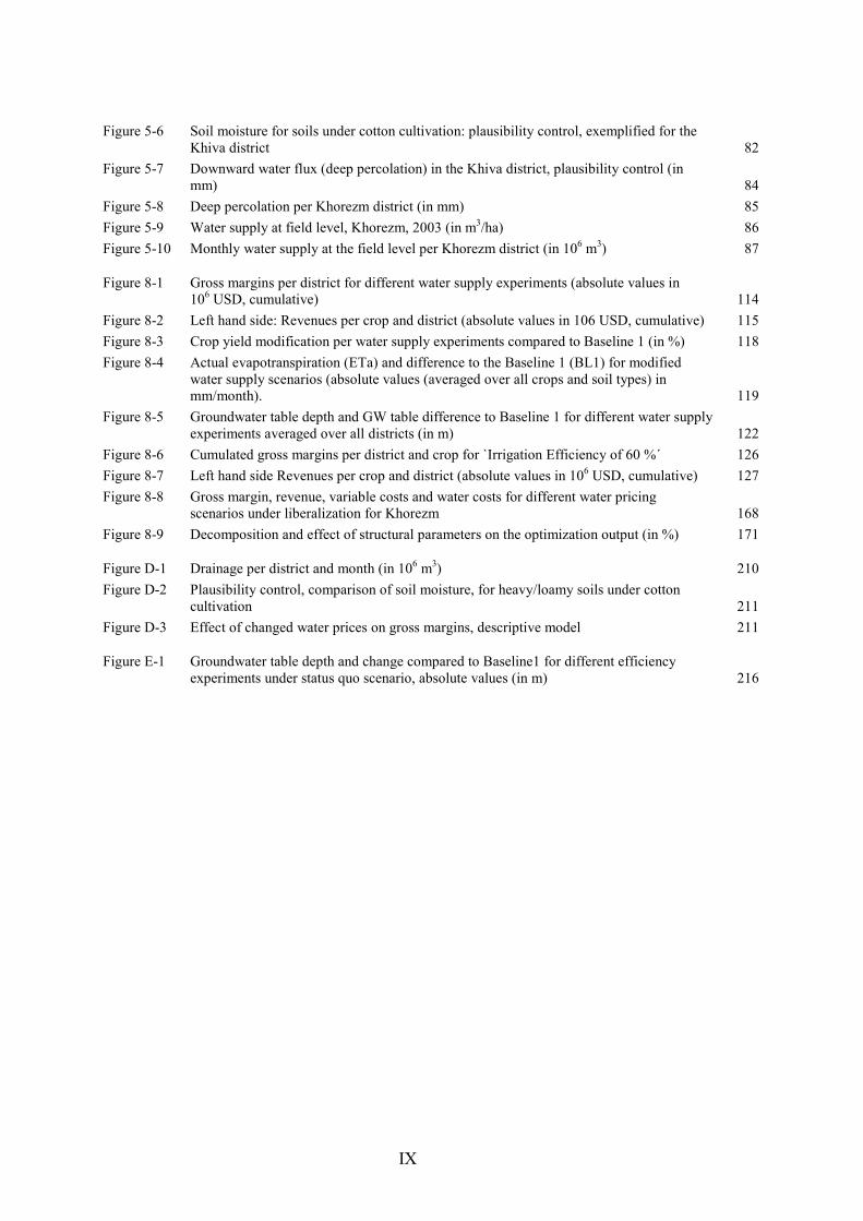
Figure 5-6 Soil moisture for soils under cotton cultivation: plausibility control, exemplified for the Khiva district 82
Figure 5-7 Downward water flux (deep percolation) in the Khiva district, plausibility control (in mm) 84
Figure 5-8 Deep percolation per Khorezm district (in mm) 85
Figure 5-9 Water supply at field level, Khorezm, 2003 (in m3/ha) 86
Figure 5-10 Monthly water supply at the field level per Khorezm district (in 106 m3) 87
Figure 8-1 Gross margins per district for different water supply experiments (absolute values in 106 USD, cumulative) 114
Figure 8-2 Left hand side: Revenues per crop and district (absolute values in 106 USD, cumulative) 115
Figure 8-3 Crop yield modification per water supply experiments compared to Baseline 1 (in %) 118
Figure 8-4 Actual evapotranspiration (ETa) and difference to the Baseline 1 (BL1) for modified water supply scenarios (absolute values (averaged over all crops and soil types) in mm/month). 119
Figure 8-5 Groundwater table depth and GW table difference to Baseline 1 for different water supply experiments averaged over all districts (in m) 122
Figure 8-6 Cumulated gross margins per district and crop for `Irrigation Efficiency of 60 %´ 126
Figure 8-7 Left hand side Revenues per crop and district (absolute values in 106 USD, cumulative) 127
Figure 8-8 Gross margin, revenue, variable costs and water costs for different water pricing scenarios under liberalization for Khorezm 168
Figure 8-9 Decomposition and effect of structural parameters on the optimization output (in %) 171
Figure D-1 Drainage per district and month (in 106 m3) 210
Figure D-2 Plausibility control, comparison of soil moisture, for heavy/loamy soils under cotton cultivation 211
Figure D-3 Effect of changed water prices on gross margins, descriptive model 211
Figure E-1 Groundwater table depth and change compared to Baseline1 for different efficiency experiments under status quo scenario, absolute values (in m) 216
X
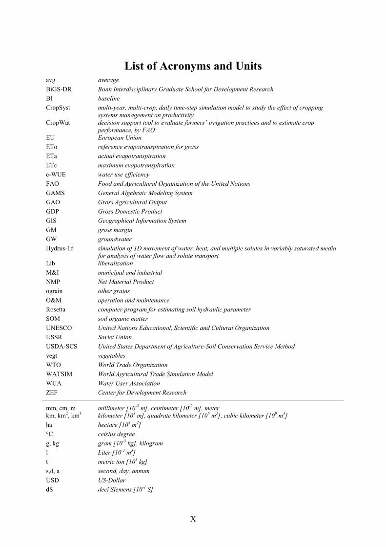
List of Acronyms and Units avg average
BiGS-DR Bonn Interdisciplinary Graduate School for Development Research
Bl baseline
CropSyst multi-year, multi-crop, daily time-step simulation model to study the effect of cropping systems management on productivity
CropWat decision support tool to evaluate farmers’ irrigation practices and to estimate crop performance, by FAO
EU European Union
ETo reference evapotranspiration for grass
ETa actual evapotranspiration
ETc maximum evapotranspiration
e-WUE water use efficiency
FAO Food and Agricultural Organization of the United Nations
GAMS General Algebraic Modeling System
GAO Gross Agricultural Output
GDP Gross Domestic Product
GIS Geographical Information System
GM gross margin
GW groundwater
Hydrus-1d simulation of 1D movement of water, heat, and multiple solutes in variably saturated media for analysis of water flow and solute transport
Lib liberalization
M&I municipal and industrial
NMP Net Material Product
ograin other grains
O&M operation and maintenance
Rosetta computer program for estimating soil hydraulic parameter
SOM soil organic matter
UNESCO United Nations Educational, Scientific and Cultural Organization
USSR Soviet Union
USDA-SCS United States Department of Agriculture-Soil Conservation Service Method
vegt vegetables
WTO World Trade Organization
WATSIM World Agricultural Trade Simulation Model
WUA Water User Association
ZEF Center for Development Research
mm, cm, m millimeter [10-3 m], centimeter [10-2 m], meter km, km2, km3 kilometer [103 m], quadrate kilometer [106 m2], cubic kilometer [109 m3]
ha hectare [104 m2]
°C celsius degree
g, kg gram [10-3 kg], kilogram
l Liter [10-3 m3]
t metric ton [103 kg]
s,d, a second, day, annum
USD US-Dollar
dS deci Siemens [10-1 S]
1
1 Introduction
1.1 Problem Setting
The problem of water scarcity is growing as water demand continues to increase.
Water needs are rising throughout the world as a result of population growth, urbanization,
agriculture and industrialization. Discussions related to water use problems increasingly focus
on the competition among water use sectors such as agriculture, forestry, industry,
hydropower, environment, and municipal use. Furthermore, mismanagement and unfavorable
climatic conditions in many regions of the world cause water demands to exceed water
supply, which negatively impacts the environment, economy and society at large.
Uzbekistan is an example of a country where water withdrawals exceed renewable
water resources. This deficit was most notable in water-scarce years such as 2000, 2001, and
2008. In Uzbekistan irrigation agriculture is the major water user and is characterized by large
amounts of wasted water combined with low water-use efficiency. Currently irrigation water
is provided at no charge.
The Khorezm region, which was used for this study, is in the Central Asian Republic
of Uzbekistan and the delta region of the Aral Sea. This region is one of many examples of
irrevocable, inefficient water consumption and water management. The agrarian economic
tendency, based on irrigated agricultural development and the cultivation of highly water-
consuming crops such as cotton and rice, has historically resulted in drastic ecological, social,
and economical problems and continues to cause problems today.
The past and present water deficiencies in Khorezm and the Aral Sea basin have had a
negative impact on people, the environment and the economy. During the Soviet period, the
Aral Sea basin turned into the world’s third largest producer of cotton (MICKLIN, 2000),
leading to an expansion of the irrigation systems in the area. Giant reservoirs along the river
catchments were created and caused increased evaporative losses. The expansion of the
irrigation area, mainly for cotton but also for rice and wheat, resulted in increasing water
consumption for crop-growing processes and soil leaching and, due to insufficient irrigation
canal system and mismanagement, to water wastage (LÉTOLLE AND MAINGUET, 1996).
Introduction
2
Enormous water consumption has been observed in Khorezm, the Aral Sea basin and almost
everywhere along the two main rivers in Central Asia, Amu Darya and Syr Darya; and it has
resulted in water shortages to downstream users combined with the dramatic shrinking of the
Aral Sea. The known as Aral Sea Syndrome has several negative effects, including local
climate changes in the areas surrounding the former lake, the destruction of the ecological
equilibrium, increasing water and soil salinity, dust storms, diarrheal and cancerous diseases,
declining crop yields, rising groundwater levels (GIESE ET AL., 1998), the creation of the new
Aralkum desert and the total collapse of the fishery sector.
The national and international community has become conscious of the Aral Sea
Syndrome over the past decades. Numerous conferences, projects and studies have been
completed since the independence of Uzbekistan in 1991. However, despite intensive efforts
within the last years, no significant changes in the region have been observed.
Throughout history, the population in the Aral Sea delta region has been dependent on
agriculture and irrigation. Due to population growth (1.4 % annually; SCS, 2008), acreage
extension and increasing pressure on land, adequate economical and eco-efficient instruments
must be located to feed and employ the existing population in the area. In times of water
shortages, such as 2000/2001 and 2008, it is difficult to obtain enough water for irrigation,
especially in the lower reaches of the Amu and Syr Darya River. Furthermore, increasing
water consumption by upstream water users will increase the pressure on water resources,
especially for the Aral Sea delta and the Khorezm region. Afghanistan is just one example of
an upstream user, as the country will need large amounts of water for agriculture and
hydropower in the near future.
Against this background the Khorezm region is faced with the following water-related
problems:
• Low and declining levels of water availability and supply in Khorezm.
• Insufficient and inequitable water distribution within the various districts of
Khorezm.
• Unfavorable crop allocation according to soil type and water supply, mainly
caused by the state order system with stringent crop orders for cotton and
wheat.
• Low irrigation and drainage efficiencies combined with insufficient irrigation
water management, resulting in water waste.
Introduction
3
• The sharp rise of acreage and the large amount of unfavorable and marginal
soils used for agricultural purposes and the problems arising as a result,
including salinity increase and a reduction in crop yields.
The situation in Khorezm requires an investigation into more efficient water use,
alternative crops and crop rotation, water conservation and distribution to feed the population
and to impede Uzbekistan’s disconnection from the world market. Interdisciplinary,
interdependent, practicable measures and the participation of local inhabitants and
government are necessary to be successful.
1.2 Research Objectives
One promising approach to reducing the unsustainable and negative effects of water
use on the local and national ecosystem and on the population is a more efficient water and
crop allocation and water use combined with a more efficient, sustainable water resources
management. This study is part of the project “Economic and Ecological Restructuring of
Water and Land Use in the Region Khorezm (Uzbekistan), a Pilot Project in Development
Research”1 at the Center for Development Research at the University of Bonn, Germany. It
was initialized to take a holistic economic and environmental approach to improving the
current situation. The goal is to develop effective and ecologically sustainable concepts for
landscape and water use restructuring focusing on the Khorezm region and the involvement of
the population, including farmers and scientists (VLEK ET AL., 2001; ZEF, 2003).
The Khorezm region is situated on one of the main rivers in Central Asia, the Amu
Darya, and is within the delta region of the Aral Sea. In this study, a regional analysis for
different spatial patterns of water use and crop allocation is carried out for this region.
The main objectives of the study are the detection and determination of water supply
as well as crop and irrigation water demand. As a result, water availability, water use patterns
and socio-economic aspects of water management in the region will be analyzed. The
correlation between economic outcomes of the agricultural production system and the
hydrologic system is based on physical and agronomical principles. These principles are
integrated using an interlinked and interactive model approach. Water balances for
1 in collaboration with: State Al-Khorezmi University, Urgench, Uzbekistan; United Nations Educational,
Scientific and Cultural Organization; German Remote Sensing Data Center; Institute for Atmospheric
Environmental Research, Germany
Introduction
4
groundwater, surface water, drainage water, and soil water are to be established. This will
provide a basis for analyses of water supply and demand for crops, yields and cropping
patterns. An optimization model will maximize economic and ecological benefits according to
yields, acreage, cultivation costs and sales prices and will result in a more effective crop
allocation in terms of water consumption and economic cost/benefit ratios. The objective is to
develop an integrated, adaptive tool with respect to the interdependencies of the hydrological
regime and the economic and ecological situation and with respect to the effects and
consequences of alternative water management strategies.
The following scenario-analyses on various hydrologic conditions and socio-economic
policies will be considered:
• Modification of the district-wide river/reservoir water supply.
• Introduction of water prices.
• Improvement of the irrigation and drainage system.
• Liberalization/reform of the cotton market and the farmer’s free choice of
what, where and how much to crop.
The consequences of these policies and their effects on soil and water balances, crop
allocation and gross margins, revenues, water values and production cost will be the major
outcome of the research.
Strategies and recommendations for a more effective water use, alternative water
management and allocation strategies and their effects and possibilities of implementation
will complete the study.
1.3 Outline of the Study
The second part of this study provides an overview of the hydrological system of the
Khorezm region and the main river flowing to this region, the Amu Darya. The discussion of
the economic situation, geographic settings and land use system for Uzbekistan and the
Khorezm region will complete the second chapter. It will afford background information on
the study area and explain why inefficiencies and mismanagement continue to exist under the
given agricultural and political system and the prevailing conditions of water supply and
water shortages.
The third part of this study describes the methodology and general water management
models, with an emphasis on integrated economic-hydrologic and optimization models. This
Introduction
5
description will provide the theoretical background for the integrated hydrologic-economic
management model. It will be followed by a detailed description of the Water Management
Model that has been developed for the agronomic, hydrologic and socio-economic system of
the Khorezm region. The framework, components, formulations and assumptions of this
model will be explained. The structure of an integrated hydrologic-economic management
and planning model for the Khorezm region will also be described. Furthermore, the specific
hydrologic, economic and agronomic parameters, processes, inter-connections and formulas
will be shown.
The fourth part of the study is focused on data, data reliability, assumptions, and data
availability.
Parts five and six of the study cover the model validation and verification, calibration
and sensitivity analysis. The validation testing consists of measuring how well a model serves
its intended purposes and can thus be used as a plausibility control of the model. The
validation testing also measures the model formulation and underlying parameter and data to
assess the accuracy of the model. As a result, a descriptive model is introduced for model
validation and calibration. A descriptive model analyzes “what is”, as compared to normative
models that analyze “what should be”. For the descriptive model, actual data observations
from 2003 are used for all relevant input parameters of water supply, cropping areas and
yields. This method will be used to illustrate whether the outcomes of the model formulation
and data for water balances and crop production processes are within a realistic range.
The validation is followed by a sensitivity analysis of essential hydrologic and
economic parameters to test the strength and quality of the empirical specifications of the
model. The sensitivity analysis is important to determine the influence and interactions of
input-factors to certain output variables (SALTELLI, 2008).
The normative optimization solutions are described and analyzed in parts seven and
eight. The various scenario analyses and experiments and their underlying policies and
modified parameters will be explained in chapter 7. The final results of the scenarios and the
associated experiments on water supply changes, the liberalization of the cotton sector, the
improvement of the water management system and the introduction of water pricing and its
effects on the hydrologic-agronomic-economic system in Khorezm will be presented and
discussed in chapter 8.
The last chapter presents the conclusions from the analyses as well as policy
recommendations. This chapter will also discuss the feasibility of the implementation of each

Introduction
6
of the suggested policies. Overall conclusions of the research, the perspectives and limitations
of the model and future work will conclude the study.
7
2 Regional Background
The following chapter is an overview on the geographic conditions and socio-
economic situation in Uzbekistan and Khorezm, the case-study region. Historical
circumstances, political settings, land use reforms and hydrologic-economic conditions of the
region will be described to get a better understanding of the current water use patterns and the
production and cropping system. This background information is necessary to understand why
this research is carried out within this specific area and it underscores the need for the
modeling approach. Furthermore, the information is essential for the understanding of the
parameters determined in the model.
2.1 Geography and Economy of Uzbekistan
The case study area, Khorezm, is situated within the Republic of Uzbekistan.
Uzbekistan is part of Central Asia (see Figure 2-1) and was a constituent republic of the
former Soviet Union from 1920 until the U.S.S.R. collapsed in 1991. At that time Uzbekistan
became an independent republic, along with the neighboring states of Tajikistan,
Turkmenistan, Kazakhstan, and Kyrgyzstan. Uzbekistan is completely landlocked and shares
borders with Kazakhstan to the west and to the north, Kyrgyzstan and Tajikistan to the east,
and Afghanistan and Turkmenistan to the south. It shares the Aral Sea and all its associated
environmental problems (which will be described later) with Kazakhstan in the northwest.
Uzbekistan is divided into 12 provinces (one of them is Khorezm), one autonomous republic
(Karakalpakstan), and one independent city (Tashkent city). Uzbekistan’s population is
estimated at 28 million, with a growth rate of 1.7 % in 2010, and 63 % of the population is
living in rural areas (SCS, 2010; WORLD BANK, 2010). The country is blessed with significant
natural resources including gold, several minerals and energy reserves, such as natural gases
and oil. The main exports of the country include cotton, energy, food, metal, and chemical
products. Uzbekistan is currently the world's fourth-largest cotton exporter (U.S.
DEPARTMENT OF STATE, 2010). The economy of Uzbekistan is primarily based on agriculture
and an increasing share of the industrial sector. The agricultural output accounts for 26 % of
Regional Background
8
the GDP and 28 % of the employment (SCS, 2009). The unemployment rate in agriculture is
considered to be very high, mainly due to seasonal and part-time jobs. However, reliable
figures are not available as no labor census is conducted in Uzbekistan. The main agricultural
products are cotton, vegetables, fruits, grain and livestock. The industrial sector is primarily
based on the processing of agricultural products, including cotton harvesters, textile
machinery, and food processing, as well as on energy production, including gasoline, diesel,
and electricity. The industrial GDP is approximately 32 % of the total GDP (SCS, 2010). The
GDP growth rate was estimated to be 8.1 % in 2009 (ADB, 2010; IMF, 2010).
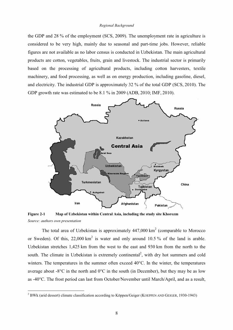
Figure 2-1 Map of Uzbekistan within Central Asia, including the study site Khorezm
Source: authors own presentation
The total area of Uzbekistan is approximately 447,000 km2 (comparable to Morocco
or Sweden). Of this, 22,000 km2 is water and only around 10.5 % of the land is arable.
Uzbekistan stretches 1,425 km from the west to the east and 930 km from the north to the
south. The climate in Uzbekistan is extremely continental2, with dry hot summers and cold
winters. The temperatures in the summer often exceed 40°C. In the winter, the temperatures
average about -8°C in the north and 0°C in the south (in December), but they may be as low
as -40°C. The frost period can last from October/November until March/April, and as a result,
2 BWk (arid dessert) climate classification according to Köppen/Geiger (KOEPPEN AND GEIGER, 1930-1943)
Regional Background
9
most areas of the country are not suitable for double cropping, except for favorable years
when a few vegetables with a short growing period can be double cropped (FAO, 1997a). The
majority of the country is arid, with sparse annual precipitation of less than 200 mm per year.
The majority of the precipitation occurs during winter and springtime, and the summer season
is very dry (GINTZBURGER ET AL., 2003). As a result, most of the agricultural area must be
irrigated with water from the main rivers passing through Uzbekistan.
The water resources in Uzbekistan are unevenly distributed. The vast plains that occupy more
than two-thirds of Uzbekistan have little access to water and only a small number of lakes.
The largest rivers in Uzbekistan and in Central Asia are Amu Darya and Syr Darya (Figure
2-1) and its tributaries, which originate in the mountains of Tajikistan and Kyrgyzstan,
respectively. Due to the extension of the broad artificial canal and irrigation network during
the Soviet period, arable land was expanded to the river valleys and marginal land was used
for arable agriculture. Because the Amu Darya is the main source of water for irrigation in
Khorezm (Figure 2-2), a brief overview of its significant characteristics and problems will be
provided in the following section.
2.2 The Amu Darya River
The Amu Darya, known in ancient times as the Oxus, is the largest river in Central
Asia. It extends approximately 2,550 km from its headwaters or 1,437 km up to the junction
(SAMAJLOV, 1956), compared with the 1,320 km of the Rhine. The Amu Darya River is
formed by the junction of the Vakhsh (Tadjikistan) and Panj (Afghanistan) rivers, which rise
in the Pamir Mountains of Central Asia. The river basin includes the territories of
Afghanistan, Tadjikistan, Uzbekistan and Turkmenistan (Table 2-1). Its upper course and
source starts off in the high Pamir Mountains of Central Asia (Afghanistan and Tajikistan),
marking much of the northern border of Afghanistan with Tajikistan, flowing through the
Karakum desert of Turkmenistan and Uzbekistan, and entering the southern Aral Sea through
a delta (Figure 2-2). The discharge is mainly generated by snowmelt and, to an increasing
degree, by melting from the glaciers in spring and summer time. Because the course of the
river is extremely long and many water users and irrigated areas are located within the basin,
less water is arriving in the downstream area and the Aral Sea.
The river flows generally northwest. The total water catchment area of the Amu Darya
basin is 227,000 km2 (ICWC CENTRAL ASIA, 2009), compared with the 185,000 km2 of the
Rhine. The average annual sum of discharge of the Amu Darya is approximately 75 km3. The
Regional Background
10
main tributaries of the Amu-Darya basin are the Zeravshan, Surkhan, Kashka and Sherabad
rivers, which flow into the river within the first 180 km. Based on the hydrographic indicators
the Zaravshan and Kashka rivers belong to the Amu Darya basin. The water from these two
rivers no longer reaches the river due to withdrawals for irrigation purpose and can be
considered independent rivers. Furthermore, there are no other inflows within a span of more
than 1,200 km flowing into the Aral Sea (Figure 2-2).
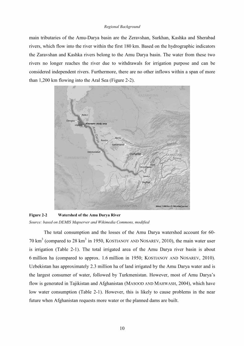
Figure 2-2 Watershed of the Amu Darya River
Source: based on DEMIS Mapserver and Wikimedia Commons, modified
The total consumption and the losses of the Amu Darya watershed account for 60-
70 km3 (compared to 28 km3 in 1950, KOSTIANOY AND NOSAREV, 2010), the main water user
is irrigation (Table 2-1). The total irrigated area of the Amu Darya river basin is about
6 million ha (compared to approx. 1.6 million in 1950; KOSTIANOY AND NOSAREV, 2010).
Uzbekistan has approximately 2.3 million ha of land irrigated by the Amu Darya water and is
the largest consumer of water, followed by Turkmenistan. However, most of Amu Darya’s
flow is generated in Tajikistan and Afghanistan (MASOOD AND MAHWASH, 2004), which have
low water consumption (Table 2-1). However, this is likely to cause problems in the near
future when Afghanistan requests more water or the planned dams are built.
Regional Background
11
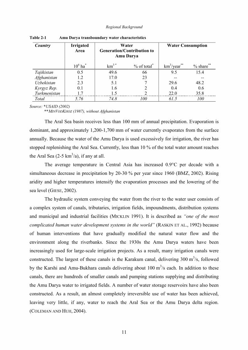
Table 2-1 Amu Darya transboundary water characteristics
Water
Generation/Contribution to
Amu Darya
Water Consumption Country Irrigated
Area
106 ha*
km3 * % of total* km3/year** % share** Tajikistan 0.5 49.6 66 9.5 15.4 Afghanistan 1.2 17.0 23 -- -- Uzbekistan 2.3 5.1 7 29.6 48.2 Kyrgyz Rep. 0.1 1.6 2 0.4 0.6 Turkmenistan 1.7 1.5 2 22.0 35.8 Total 5.76 74.8 100 61.5 100
Source: *USAID (2002) **MINVODKHOZ (1987), without Afghanistan
The Aral Sea basin receives less than 100 mm of annual precipitation. Evaporation is
dominant, and approximately 1,200-1,700 mm of water currently evaporates from the surface
annually. Because the water of the Amu Darya is used excessively for irrigation, the river has
stopped replenishing the Aral Sea. Currently, less than 10 % of the total water amount reaches
the Aral Sea (2-5 km3/a), if any at all.
The average temperature in Central Asia has increased 0.9°C per decade with a
simultaneous decrease in precipitation by 20-30 % per year since 1960 (BMZ, 2002). Rising
aridity and higher temperatures intensify the evaporation processes and the lowering of the
sea level (GIESE, 2002).
The hydraulic system conveying the water from the river to the water user consists of
a complex system of canals, tributaries, irrigation fields, impoundments, distribution systems
and municipal and industrial facilities (MICKLIN 1991). It is described as “one of the most
complicated human water development systems in the world” (RASKIN ET AL., 1992) because
of human interventions that have gradually modified the natural water flow and the
environment along the riverbanks. Since the 1930s the Amu Darya waters have been
increasingly used for large-scale irrigation projects. As a result, many irrigation canals were
constructed. The largest of these canals is the Karakum canal, delivering 300 m3/s, followed
by the Karshi and Amu-Bukhara canals delivering about 100 m3/s each. In addition to these
canals, there are hundreds of smaller canals and pumping stations supplying and distributing
the Amu Darya water to irrigated fields. A number of water storage reservoirs have also been
constructed. As a result, an almost completely irreversible use of water has been achieved,
leaving very little, if any, water to reach the Aral Sea or the Amu Darya delta region.
(COLEMAN AND HUH, 2004).
Regional Background
12
The water is not supplied based on demand and is wasted by poor water management
practices that result in the use of excessive quantities whenever water is available. Thus, the
construction of a water distribution and management model could help balance demand and
supply.
The drainage and irrigation systems are in poor condition, largely because of age and
the lack of recent maintenance (MASOOD AND MAHWASH, 2004). The drainage systems are
generally designed in such a way that most of the effluents are directly discharged back into
the river (UN, 2005) and thus gradually aggravate the downstream water quality. The
situation in Khorezm is different from this general situation because most of the drainage
water from Khorezm is discharged to the Sary Kamish depression. Water salinity in the delta
region has increased from 0.5-0.8 g/l to more than 2 g/l. As a result, water and soil salinity has
become a major problem, mainly in the downstream area. Approximately 30 % of the
irrigated areas suffer from moderate to high salinity levels (MURRAY-RUST ET AL., 2003).
The diversions of the Amu Darya for irrigation purposes and the change in its
chemistry have led to large-scale changes in the Aral Sea’s ecology and economy. The
decrease in the fish population already dramatically reduced and eliminated the fish industry
in the 1980s. The reduction of the Aral Sea also affects the regional climate. Due to the
reduction of the Aral Sea and, thus, the exposure of the seabed, strong winds have caused
thousands of tons of sand and soil to enter the air, negatively affecting its quality. This further
reduces crop yields because heavily salt-laden particles fall on arable land. Respiratory
illnesses, typhoid, and morbidity have also increased (HORSMAN, 2001). All of these factors
are contributing to the Aral Sea Syndrome (UNESCO, 2000).
2.3 Agricultural and Political Settings
During the Soviet era the production of cotton was politically enforced and intensified.
Uzbekistan was the largest cotton producer in the U.S.S.R. and became a raw material
supplier for the rest of the Soviet Union, mainly due to the expansion of the canal network
system on Syr Darya and Amu Darya during this time. It was assumed that soil and water
resources had infinite availability and usability, and sustainability criteria did not play any
role for policy and the local population. The environmental management during the Soviet era
brought decades of poor water management and a lack of water or sewage treatment facilities.
The heavy use of pesticides, herbicides and fertilizers in the fields, as well as the construction
of industrial enterprises with little regard to the negative effects on humans or the
Regional Background
13
environment, was also common during this time. The large-scale use of chemicals for cotton
cultivation, inefficient irrigation systems and poor drainage systems are examples of the
conditions that led to a high volume of saline and contaminated water entering the soil
(CURTIS, 2004) and into the groundwater. As a result, the quality of the groundwater and
surface water, which are the main sources of drinking water, is reduced. Furthermore, the
drainage water is deteriorated and causes many problems when drainage water is released
directly into the river. The mineralization of the groundwater in downstream areas of the Amu
Darya River can reach 5-20 g/l compared to values of 1-3 g/l in upstream areas (CROSA ET
AL., 2006A and 2006B). The direct causes for the ecological crisis in the downstream rivers
and delta regions, with the most prominent example being the “Aral Sea Syndrome”, are the
following:
• The dramatic expansion of irrigation areas and associated increasing water
usage for irrigation.
• The extension of cotton cultivation (mainly in monoculture) with large-scale
application of fertilizers and pesticides, resulting in the contamination of
drinking and irrigation water (GIESE, 1998).
After its independence in 1991, Uzbekistan has retained many elements of Soviet
economic planning, including central planning, subsidies, and the implementation of
production quotas and price settings (MÜLLER, 2006; DJANIBEKOV, 2008). Major economic
issues continue to be determined by the state. The government only allows limited direct
foreign investment, and little true privatization has occurred other than the foundation of
small enterprises (CURTIS, 2004). Intended structural changes, which will be described in the
following paragraphs, are occurring slowly because the state still continues to have a
dominating influence on the economy and, thus, on the environment.
Agrarian reform in Uzbekistan
In the last decades of the Soviet era, Uzbekistan's agriculture was dominated by
collective farms, mainly state farms (Kolkhozes, Sovkhozes). These farms had an average
size of more than 24,000 ha and an average of more than 1,100 farm workers in 1990/91.
Although only about 10 % of the country's land area was cultivated, about 40 % of its Net
Regional Background
14
Material Product (NMP3) was in agriculture. Throughout the 1980s, agricultural investments
and the agricultural area steadily increased. In contrast, net losses increased at an even faster
rate as a result of heavy salinization, erosion, and waterlogging of agricultural soils, which
inevitably place limits on the land's productivity. Nevertheless, during these decades,
Uzbekistan remained the major cotton-growing region of the Soviet Union, accounting for
61 % of the total Soviet production. Roughly 40 % of the total workforce and more than half
of the total irrigated land in Uzbekistan were devoted to cotton production in 1987 (CURTIS
1997). According to BLOCH (2002), the Soviet agricultural system had the following
characteristics:
� A dominance of large collective and state farms.
� Cotton monoculture.
� Crop farming dominating the structure of agriculture, with very little livestock.
� Heavy reliance on intensive use of land, water and chemicals.
� A lack of self sufficiency in food products, including wheat, milk, potatoes and
meat.
Since its independence Uzbekistan has initiated “step-by-step” economic reforms with
price liberalization and agrarian reform under strict governmental control. The agricultural
sector was exposed to a sequence of reforms that had several significant effects on the
organizational structure of the sector. However, the degree of independent decision making by
the farmers was limited by the government. The reform is most visible in the abolition of
Sovkhozes and their conversion into cooperative enterprises (Kolkhozes), which were later
restructured into Shirkats during the first phase of agricultural restructuring (POMFRET,
2000)4. The main difference between the two forms of ownership is that a Sovkhoz is like a
state enterprise in which the workers are employed at fixed wages, whereas a Kolkhoz pays
its workers from its own residual earnings (KHAN, 1996). The main reason for shifting to
Kolkhozes was the practical consideration of relieving the state budget to finance the wage
payments to the large Sovkhozy work force. Another reason for the shift was practical
efficiency considerations, as the output per unit of land was higher in Kolkhozes. 3 NMP was the main macroeconomic indicator during the Soviet era. In its concept, it is equivalent to GDP but is
calculated for the material production sector and excludes most of the services sector and the foreign trade
balance (CARSON, 1990).
4 The first phase of reform was implemented between 1989-1997/1998 according to KHAN 2005, CER 2004 or
TROUCHINE AND ZITZMANN, 2005
Regional Background
15
Furthermore, the overall unit costs were lower in Kolkhozes than in Sovkhozes (KHAN AND
GAI, 1979; KHAN, 1996). Nevertheless, the reform in post-independent Uzbekistan was not
accompanied by an essential change in the management of the Kolkhozes (DJANIBEKOV,
2008). During this time, a limited program of distributing land among private farmers was
also initiated (Table 2-2). In 1994, there were about 10,400 private farms in operation,
corresponding to 2 % of the sown land and covering an area of 8.6 ha per farm. These private
farms had to contend with bad conditions in the beginning, as they were often allocated areas
with poor soil quality and their lease contracts allowed little decision making (TROUCHINE
AND ZITZMANN, 2005).
Table 2-2 Distribution of sown land (in % of total) in Uzbekistan
Year Kolkhozes
(Shirkats)
Sovkhozes Private
farms
Individual farms
(Dekhan)
Others 1
1990 34.9 58.7 0.1 0.1 6.3 1991 34.0 57.7 0.1 n/a 8.1 1992 36.4 51.8 0.4 n/a 11.5 1993 47.5 39.0 0.6 n/a 12.9 1994 75.3 1.0 2.1 2.1 21.6 2004 48.6 -- 34.5 10.4 6.5
Notes: 1= separate arrangements for special categories or crops, e.g., orchards and vineyards, mixed state collective forms including experimental farms
Source: Khan, 1996; Khan, 2005
During this time the land endowments to small-scale farms (i.e., Dekhan/peasant
farms) also increased. Dekhans are small household plots on which families have lifelong
heritable tenure and that can be used for residential and agricultural purposes. They are
farmed only by family members and are an essential means of obtaining a minimal standard
of livelihood. As their size, with a maximum of 0.35 ha, is sufficiently small, they are free to
sell their products in the market and are not subject to any procurement quotas (KHAN, 2005)5.
They are important food producers for local markets and have no influence on the national
agricultural export structure.
The major changes during this period were a sharp decline in agricultural terms of
trade and a shift in relative incentives against cotton and in favor of grains. The reason for this
shift was the declared self-sufficiency of Uzbekistan in grain production to feed an
increasingly impoverished population and to obtain autonomy from wheat imports. With the
5 A more detailed description and differentiation of the various agricultural operation forms can bee seen in
Appendix A.
Regional Background
16
estimated production of 3.7 million tons of wheat in 1998, which was six times the level of
1991, Uzbekistan has largely achieved the goal of drastically reducing grain imports since its
independence (KANDIYOTI, 2002). According to TRUSHIN (1998) the area of cotton fields and
forage decreased from 1990 to 1996. The area of cotton fields decreased from 44 % to 35 %
while the area of forage decreased from 25 % to 13 %. During the same time the arable land
allocated to cereals increased from 24 % to 41 %. These changes have not only resulted in a
reduction of the area under cotton cultivation, but also a reduction of yield per ha. This is
because at that time the productivity of Kolkhozes and Sovkhozes, which were the main
producers of cotton, was still declining due to insufficient management and unfavorable land
conditions. The total cotton yield decreased 15 % between 1991 and 1994, and has decreased
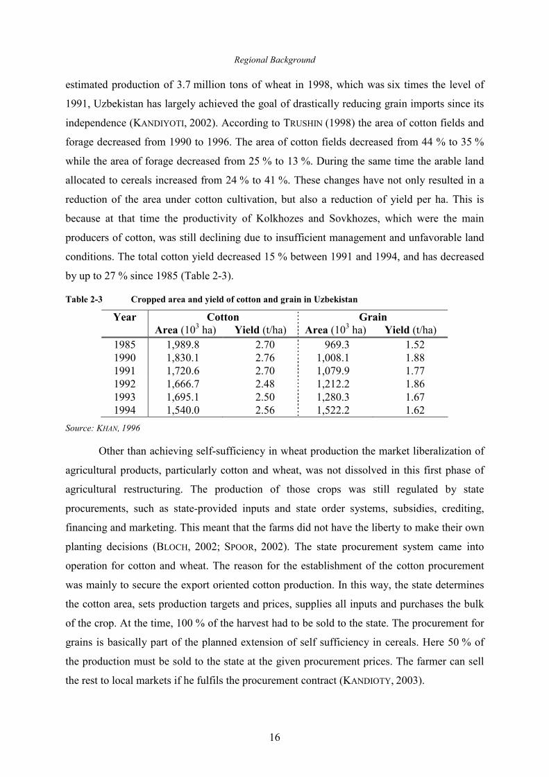
by up to 27 % since 1985 (Table 2-3).
Table 2-3 Cropped area and yield of cotton and grain in Uzbekistan
Year Cotton Grain
Area (103 ha) Yield (t/ha) Area (103 ha) Yield (t/ha) 1985 1,989.8 2.70 969.3 1.52 1990 1,830.1 2.76 1,008.1 1.88 1991 1,720.6 2.70 1,079.9 1.77 1992 1,666.7 2.48 1,212.2 1.86 1993 1,695.1 2.50 1,280.3 1.67 1994 1,540.0 2.56 1,522.2 1.62
Source: KHAN, 1996
Other than achieving self-sufficiency in wheat production the market liberalization of
agricultural products, particularly cotton and wheat, was not dissolved in this first phase of
agricultural restructuring. The production of those crops was still regulated by state
procurements, such as state-provided inputs and state order systems, subsidies, crediting,
financing and marketing. This meant that the farms did not have the liberty to make their own
planting decisions (BLOCH, 2002; SPOOR, 2002). The state procurement system came into
operation for cotton and wheat. The reason for the establishment of the cotton procurement
was mainly to secure the export oriented cotton production. In this way, the state determines
the cotton area, sets production targets and prices, supplies all inputs and purchases the bulk
of the crop. At the time, 100 % of the harvest had to be sold to the state. The procurement for
grains is basically part of the planned extension of self sufficiency in cereals. Here 50 % of
the production must be sold to the state at the given procurement prices. The farmer can sell
the rest to local markets if he fulfils the procurement contract (KANDIOTY, 2003).
Regional Background
17
The second phase, which lasted from 1997/98 through 2003, was characterized by the
legal admission and promotion of private farms distinct from Dekhan farms. This phase
strengthened Dekhan farming as it became evident that the productivity of Dekhan farms
increased by more than 35 % in comparison to the huge farm enterprises (Kolkhozes) that saw
a decline in productivity (USAID, 2005). Several new laws, giving more independence to
individual farms, went into effect during this phase, beginning in 19976. Occasionally the
distinction between smallholders (Dekhans) and individual farmers was indicated by granting
them independent juridical status as well as the right to hold own bank accounts and to
transact with buyers of crops and suppliers (KANDYOTI, 2002). However, they remain subject
to state-determined procurement prices to this day (TROUCHINE AND ZITZMANN, 2005).
Simultaneously, the former collective farms, the kolkhozes, were being transformed
into Shirkats, starting with more profitable collectives. In 2002 more than 90 % of the former
collectives were transformed into Shirkats. Those that failed to be retransformed into
profitable Shirkats were converted into private farms (KHAN, 2005). The state is still
interested in the control of the agrarian sector, and as a result, basic conditions of production
remain in this phase. Despite the efforts made toward self-sufficiency, Uzbekistan is still one
of the largest importers of food in Central Asia (BLOCH, 2002).
Furthermore, during this time, Water User Associations (WUAs) were promoted and
established, mainly in inefficient state and collective farms. These associations were tested by
the Uzbek government and were responsible for the entire operation and management of the
irrigation and drainage infrastructure within their territory (WEGERICH, 2001).
The third phase of transformation began in 2004 and is characterized by a further
conversion of poorly performing Shirkats into private farms. This was a result of many
Shirkats being confronted with financial problems and showing little improvement in
productivity (CER, 2004). The foundation for this decision was a Presidential Decree from
October 2003 that made private farms the principal agricultural enterprises in the future by
distributing the land of the Shirkats to private commercial farms. This process was nearly
completed in 2007; with 217,100 private farms operating in 2007. The total area of land
allotted to private farms was 5,787,800 ha, with an average of 26.7 ha per farm (SCS, 2007).
During this period the WUAs increased as well, and in Khorezm 113 had been established by
6 Law of the Republic of Uzbekistan (1998): On the Agricultural Cooperative, Tashkent, Uzbekistan.
Law of the Republic of Uzbekistan (1998): On the Farmer Enterprise, Tashkent, Uzbekistan.
Law of the Republic of Uzbekistan (1998): On the Dekhkan Farm, Tashkent, Uzbekistan.
Regional Background
18
2006. Each WUA had an average territory of about 2200 ha and 134 farms (RWUA, 2006
cited in BOBOJONOV, 2008).
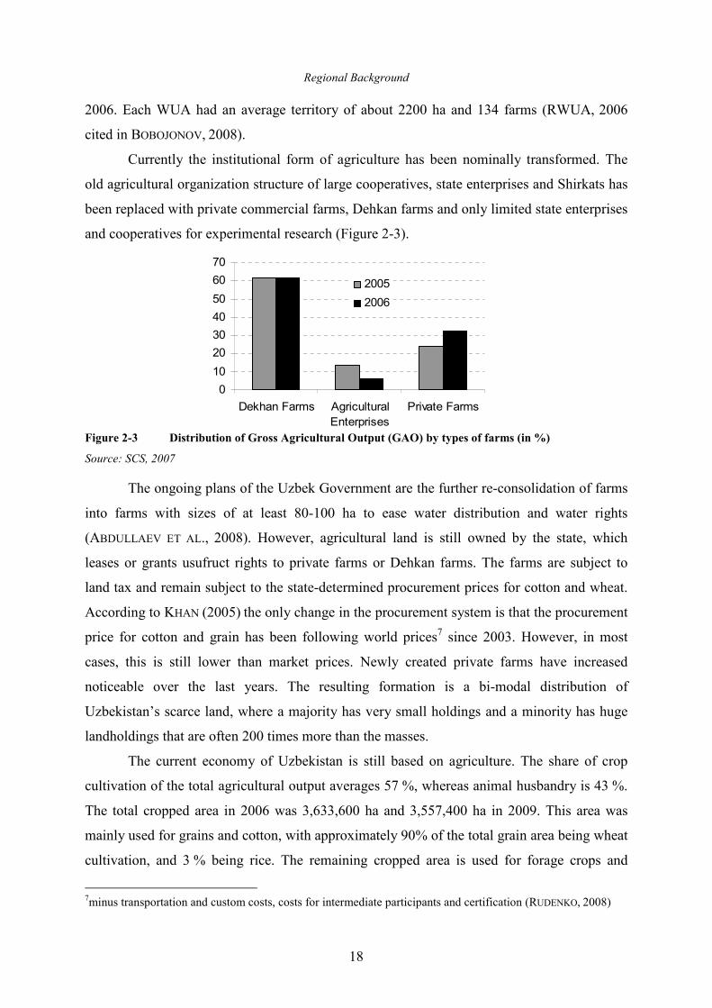
Currently the institutional form of agriculture has been nominally transformed. The
old agricultural organization structure of large cooperatives, state enterprises and Shirkats has
been replaced with private commercial farms, Dehkan farms and only limited state enterprises
and cooperatives for experimental research (Figure 2-3).
0
10
20
30
40
50
60
70
Dekhan Farms Agricultural
Enterprises
Private Farms
2005
2006
Figure 2-3 Distribution of Gross Agricultural Output (GAO) by types of farms (in %)
Source: SCS, 2007
The ongoing plans of the Uzbek Government are the further re-consolidation of farms
into farms with sizes of at least 80-100 ha to ease water distribution and water rights
(ABDULLAEV ET AL., 2008). However, agricultural land is still owned by the state, which
leases or grants usufruct rights to private farms or Dehkan farms. The farms are subject to
land tax and remain subject to the state-determined procurement prices for cotton and wheat.
According to KHAN (2005) the only change in the procurement system is that the procurement
price for cotton and grain has been following world prices7 since 2003. However, in most
cases, this is still lower than market prices. Newly created private farms have increased
noticeable over the last years. The resulting formation is a bi-modal distribution of
Uzbekistan’s scarce land, where a majority has very small holdings and a minority has huge
landholdings that are often 200 times more than the masses.
The current economy of Uzbekistan is still based on agriculture. The share of crop
cultivation of the total agricultural output averages 57 %, whereas animal husbandry is 43 %.
The total cropped area in 2006 was 3,633,600 ha and 3,557,400 ha in 2009. This area was
mainly used for grains and cotton, with approximately 90% of the total grain area being wheat
cultivation, and 3 % being rice. The remaining cropped area is used for forage crops and
7minus transportation and custom costs, costs for intermediate participants and certification (RUDENKO, 2008)
Regional Background
19
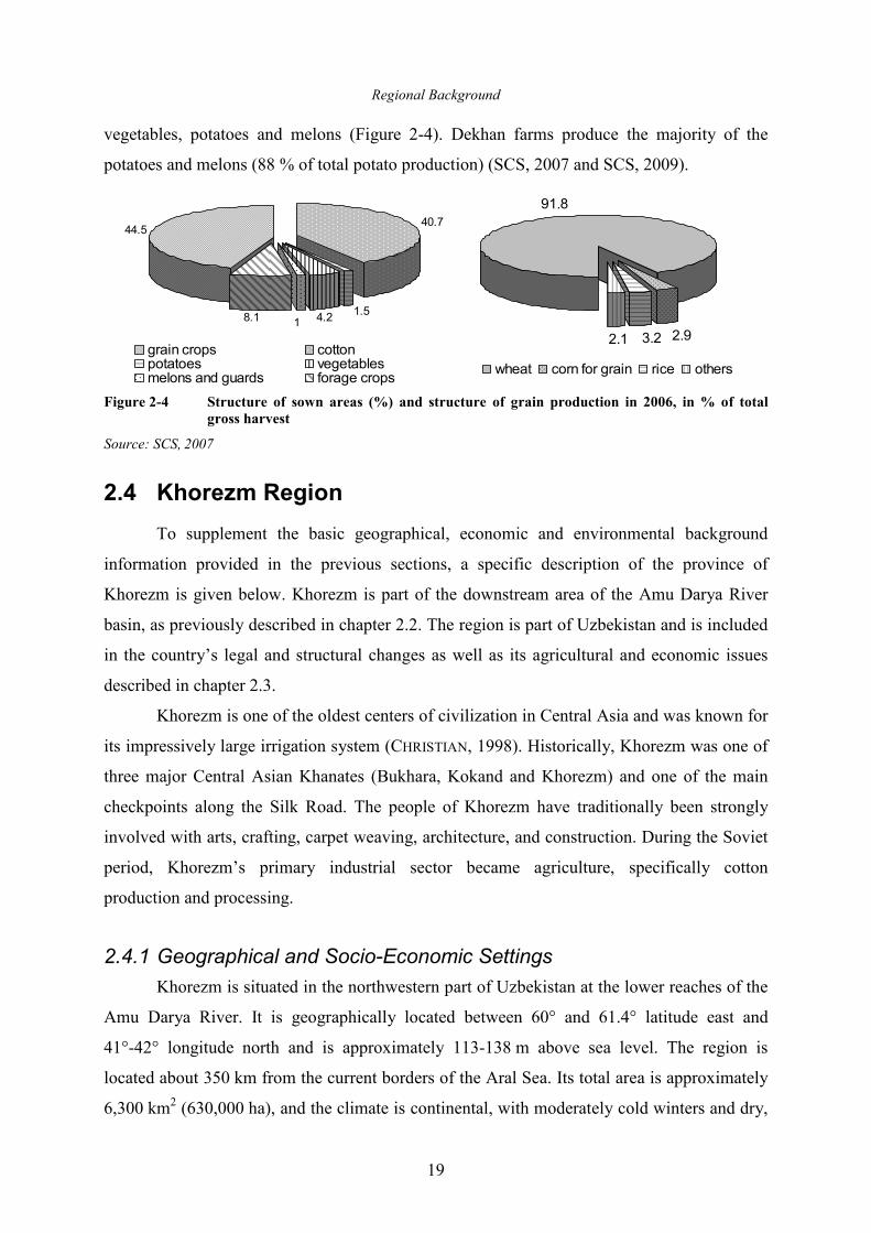
vegetables, potatoes and melons (Figure 2-4). Dekhan farms produce the majority of the
potatoes and melons (88 % of total potato production) (SCS, 2007 and SCS, 2009).
40.7
8.1 1 4.21.5
44.5
grain crops cottonpotatoes vegetablesmelons and guards forage crops
91.8
2.93.22.1
wheat corn for grain rice others
Figure 2-4 Structure of sown areas (%) and structure of grain production in 2006, in % of total
gross harvest
Source: SCS, 2007
2.4 Khorezm Region
To supplement the basic geographical, economic and environmental background
information provided in the previous sections, a specific description of the province of
Khorezm is given below. Khorezm is part of the downstream area of the Amu Darya River
basin, as previously described in chapter 2.2. The region is part of Uzbekistan and is included
in the country’s legal and structural changes as well as its agricultural and economic issues
described in chapter 2.3.
Khorezm is one of the oldest centers of civilization in Central Asia and was known for
its impressively large irrigation system (CHRISTIAN, 1998). Historically, Khorezm was one of
three major Central Asian Khanates (Bukhara, Kokand and Khorezm) and one of the main
checkpoints along the Silk Road. The people of Khorezm have traditionally been strongly
involved with arts, crafting, carpet weaving, architecture, and construction. During the Soviet
period, Khorezm’s primary industrial sector became agriculture, specifically cotton
production and processing.
2.4.1 Geographical and Socio-Economic Settings
Khorezm is situated in the northwestern part of Uzbekistan at the lower reaches of the
Amu Darya River. It is geographically located between 60° and 61.4° latitude east and
41°-42° longitude north and is approximately 113-138 m above sea level. The region is
located about 350 km from the current borders of the Aral Sea. Its total area is approximately
6,300 km2 (630,000 ha), and the climate is continental, with moderately cold winters and dry,
Regional Background
20
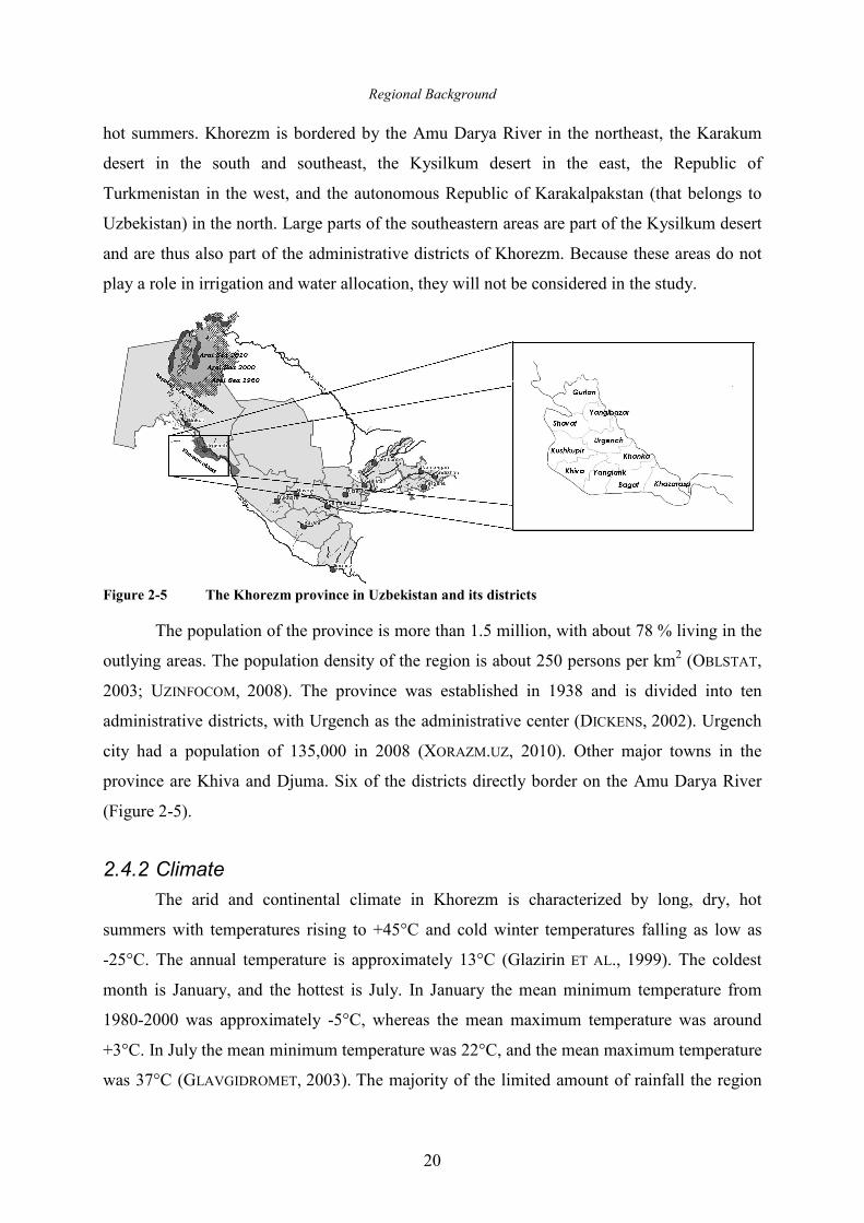
hot summers. Khorezm is bordered by the Amu Darya River in the northeast, the Karakum
desert in the south and southeast, the Kysilkum desert in the east, the Republic of
Turkmenistan in the west, and the autonomous Republic of Karakalpakstan (that belongs to
Uzbekistan) in the north. Large parts of the southeastern areas are part of the Kysilkum desert
and are thus also part of the administrative districts of Khorezm. Because these areas do not
play a role in irrigation and water allocation, they will not be considered in the study.
Figure 2-5 The Khorezm province in Uzbekistan and its districts
The population of the province is more than 1.5 million, with about 78 % living in the
outlying areas. The population density of the region is about 250 persons per km2 (OBLSTAT,
2003; UZINFOCOM, 2008). The province was established in 1938 and is divided into ten
administrative districts, with Urgench as the administrative center (DICKENS, 2002). Urgench
city had a population of 135,000 in 2008 (XORAZM.UZ, 2010). Other major towns in the
province are Khiva and Djuma. Six of the districts directly border on the Amu Darya River
(Figure 2-5).
2.4.2 Climate
The arid and continental climate in Khorezm is characterized by long, dry, hot
summers with temperatures rising to +45°C and cold winter temperatures falling as low as
-25°C. The annual temperature is approximately 13°C (Glazirin ET AL., 1999). The coldest
month is January, and the hottest is July. In January the mean minimum temperature from
1980-2000 was approximately -5°C, whereas the mean maximum temperature was around
+3°C. In July the mean minimum temperature was 22°C, and the mean maximum temperature
was 37°C (GLAVGIDROMET, 2003). The majority of the limited amount of rainfall the region
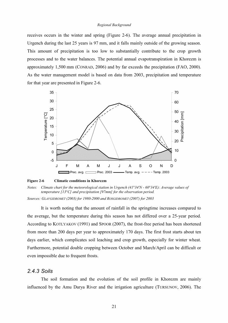
Regional Background
21
receives occurs in the winter and spring (Figure 2-6). The average annual precipitation in
Urgench during the last 25 years is 97 mm, and it falls mainly outside of the growing season.
This amount of precipitation is too low to substantially contribute to the crop growth
processes and to the water balances. The potential annual evapotranspiration in Khorezm is
approximately 1,500 mm (CONRAD, 2006) and by far exceeds the precipitation (FAO, 2000).
As the water management model is based on data from 2003, precipitation and temperature
for that year are presented in Figure 2-6.
-5
0
5
10
15
20
25
30
35
J F M A M J J A S O N D
Temperature [°C]
0
10
20
30
40
50
60
70
Precipitation [mm]
Prec. avg. Prec. 2003 Temp. avg. Temp. 2003
Figure 2-6 Climatic conditions in Khorezm
Notes: Climate chart for the meteorological station in Urgench (41°34'N - 60°34'E): Average values of temperature [13°C] and precipitation [97mm] for the observation period.
Sources: GLAVGIDROMET (2003) for 1980-2000 and ROSGIDROMET (2007) for 2003
It is worth noting that the amount of rainfall in the springtime increases compared to
the average, but the temperature during this season has not differed over a 25-year period.
According to KOTLYAKOV (1991) and SPOOR (2007), the frost-free period has been shortened
from more than 200 days per year to approximately 170 days. The first frost starts about ten
days earlier, which complicates soil leaching and crop growth, especially for winter wheat.
Furthermore, potential double cropping between October and March/April can be difficult or
even impossible due to frequent frosts.
2.4.3 Soils
The soil formation and the evolution of the soil profile in Khorezm are mainly
influenced by the Amu Darya River and the irrigation agriculture (TURSUNOV, 2006). The
Regional Background
22
soils of the Amu Darya delta consist of alluvial deposits from the river containing light,
medium and heavy loams and rarely consisting of loamy sands (SCHÄFER ET.AL, 2001).
However, the soils situated directly at the river bed consist of sand and loamy sand. Soils and
soil texture in Khorezm are very heterogeneous. Until the 1970s the soils of the major
irrigated area were very fertile and high in humus, nitrogen and carbonate content, resulting in
a high agricultural potential (TUSURNOV 1984, cited in SCHÄFER ET AL., 2001). Seventy
percent of the area was classified as meadow-alluvial loamy soils (Xerosols, Fluviosols) with
very few sand fractions, while the remaining is desert sandy soils consisting of more than
90 % sandy fractions. Furthermore buggy-meadow, takyr-meadow, boggy, grey-brown and
takyr soils can be found in Khorezm (KIENZLER, 2010; IBRAKHIMOV, 2007).
The intensification of irrigation caused a degradation of the soils as they became arid,
which resulted in increasing salinity, a loss of humus content (by 20 %) and a loss of fertility.
Due to this aridity, the hydromorphic meadow soils began transitioning into alkaline
automorphic soils (STULINA AND SEKTIMENKO, 2004). The overall productivity decreased
approximately 30-40 % (UN, 2001; ECOINFORMPROGNOZ, 2001). According to IBRAGIMOV
(2007) and RISKIEVA (1989) (both cited in KIENZLER, 2010), the soils in Khorezm are now
characterized by a very low soil organic matter content (SOM; 0.33-0.6 %) and a high
carbonate rock content. Because the natural fertility of the soils is low, crops require
additional chemical fertilizers (KHAMZINA, 2006). In periods of drought, the soils are crusted
(takyric soils according to FAO classification; SCHEFFER AND SCHACHTSCHABEL, 1998).
These soils could potentially evolve into pure takyr, solontschak (silty and salty) or desert
sandy soils. Most of the soils can be subclassified as phreatic and salic soils, as a shallow
groundwater level above 5 m influences soil, and salinity accumulation often occurs within
the soils.
2.4.4 Water
Given the arid climate in Uzbekistan and especially in the Khorezm region, irrigation
water from the Amu Darya River and the Tuyamuyun reservior is essential for agricultural
production. The fundamental importance of water for Uzbek and the Khorezmian agriculture
became increasingly evident in the years 2000, 2001 and 2008, when the overall water supply
was dramatically decreased due to droughts. Food shortages arose as a result of a decline in
production, particularly in those regions that were at the tail end of the river, such as the
Khorezm province. The local inhabitants fear that the number of drought years will increase.
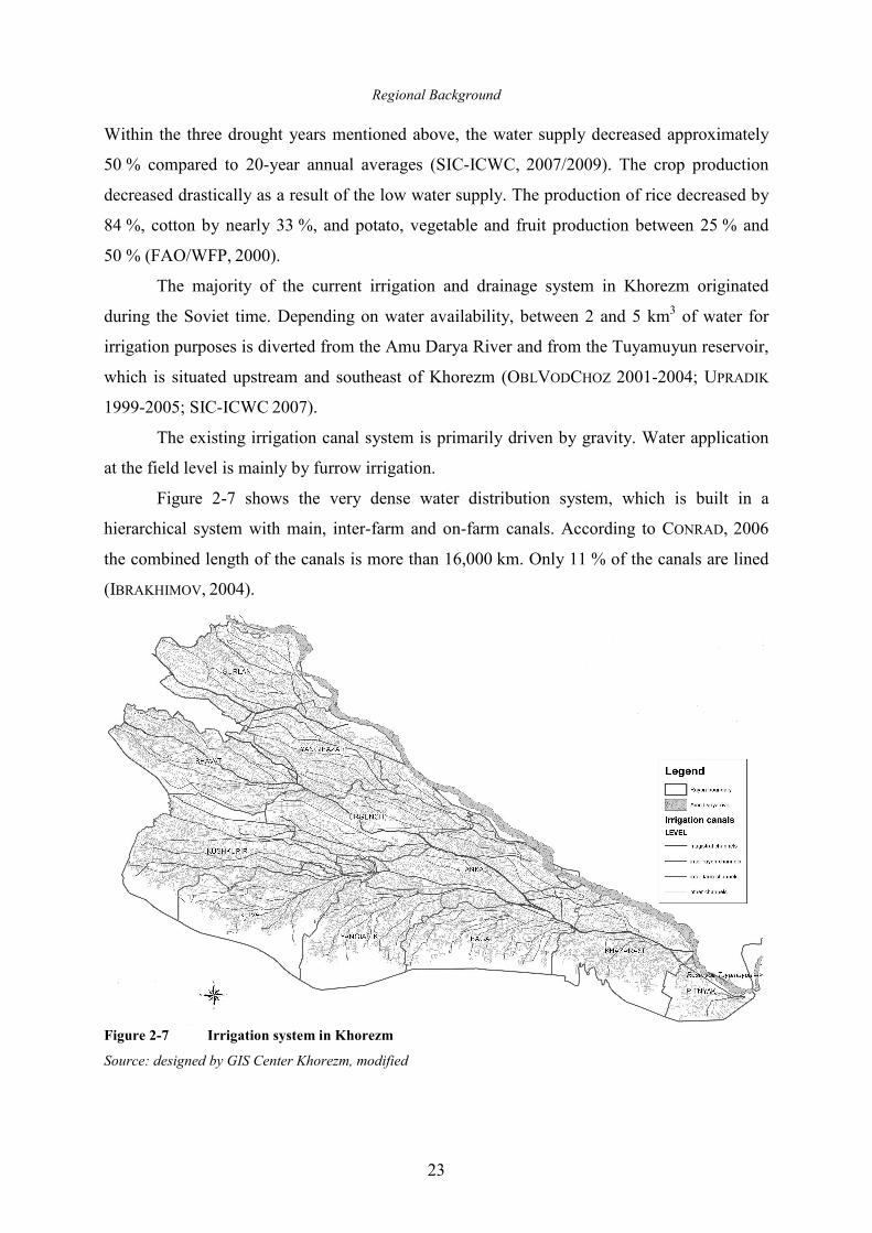
Regional Background
23
Within the three drought years mentioned above, the water supply decreased approximately
50 % compared to 20-year annual averages (SIC-ICWC, 2007/2009). The crop production
decreased drastically as a result of the low water supply. The production of rice decreased by
84 %, cotton by nearly 33 %, and potato, vegetable and fruit production between 25 % and
50 % (FAO/WFP, 2000).
The majority of the current irrigation and drainage system in Khorezm originated
during the Soviet time. Depending on water availability, between 2 and 5 km3 of water for
irrigation purposes is diverted from the Amu Darya River and from the Tuyamuyun reservoir,
which is situated upstream and southeast of Khorezm (OBLVODCHOZ 2001-2004; UPRADIK
1999-2005; SIC-ICWC 2007).
The existing irrigation canal system is primarily driven by gravity. Water application
at the field level is mainly by furrow irrigation.
Figure 2-7 shows the very dense water distribution system, which is built in a
hierarchical system with main, inter-farm and on-farm canals. According to CONRAD, 2006
the combined length of the canals is more than 16,000 km. Only 11 % of the canals are lined
(IBRAKHIMOV, 2004).
Figure 2-7 Irrigation system in Khorezm
Source: designed by GIS Center Khorezm, modified
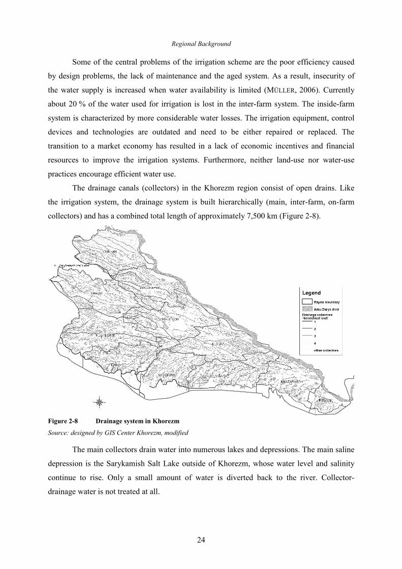
Regional Background
24
Some of the central problems of the irrigation scheme are the poor efficiency caused
by design problems, the lack of maintenance and the aged system. As a result, insecurity of
the water supply is increased when water availability is limited (MÜLLER, 2006). Currently
about 20 % of the water used for irrigation is lost in the inter-farm system. The inside-farm
system is characterized by more considerable water losses. The irrigation equipment, control
devices and technologies are outdated and need to be either repaired or replaced. The
transition to a market economy has resulted in a lack of economic incentives and financial
resources to improve the irrigation systems. Furthermore, neither land-use nor water-use
practices encourage efficient water use.
The drainage canals (collectors) in the Khorezm region consist of open drains. Like
the irrigation system, the drainage system is built hierarchically (main, inter-farm, on-farm
collectors) and has a combined total length of approximately 7,500 km (Figure 2-8).
Figure 2-8 Drainage system in Khorezm
Source: designed by GIS Center Khorezm, modified
The main collectors drain water into numerous lakes and depressions. The main saline
depression is the Sarykamish Salt Lake outside of Khorezm, whose water level and salinity
continue to rise. Only a small amount of water is diverted back to the river. Collector-
drainage water is not treated at all.
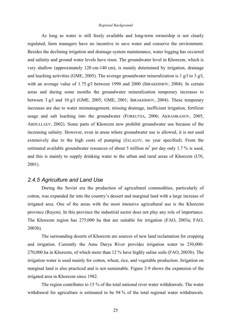
Regional Background
25
As long as water is still freely available and long-term ownership is not clearly
regulated, farm managers have no incentive to save water and conserve the environment.
Besides the declining irrigation and drainage system maintenance, water logging has occurred
and salinity and ground water levels have risen. The groundwater level in Khorezm, which is
very shallow (approximately 120 cm-140 cm), is mainly determined by irrigation, drainage
and leaching activities (GME, 2005). The average groundwater mineralization is 1 g/l to 3 g/l,
with an average value of 1.75 g/l between 1990 and 2000 (IBRAKHIMOV, 2004). In certain
areas and during some months the groundwater mineralization temporary increases to
between 3 g/l and 10 g/l (GME, 2005; GME, 2001; IBRAKHIMOV, 2004). These temporary
increases are due to water mismanagement, missing drainage, inefficient irrigation, fertilizer
usage and salt leaching into the groundwater (FORKUTSA, 2006; AKRAMKANOV, 2005,
ABDULLAEV, 2002). Some parts of Khorezm now prohibit groundwater use because of the
increasing salinity. However, even in areas where groundwater use is allowed, it is not used
extensively due to the high costs of pumping (JALALOV, no year specified). From the
estimated available groundwater resources of about 5 million m3 per day only 1.7 % is used,
and this is mainly to supply drinking water to the urban and rural areas of Khorezm (UN,
2001).
2.4.5 Agriculture and Land Use
During the Soviet era the production of agricultural commodities, particularly of
cotton, was expanded far into the country’s dessert and marginal land with a large increase of
irrigated area. One of the areas with the most intensive agricultural use is the Khorezm
province (Rayon). In this province the industrial sector does not play any role of importance.
The Khorezm region has 275,000 ha that are suitable for irrigation (FAO, 2003a; FAO,
2003b).
The surrounding deserts of Khorezm are sources of new land reclamation for cropping
and irrigation. Currently the Amu Darya River provides irrigation water to 230,000-
270,000 ha in Khorezm, of which more than 12 % have highly saline soils (FAO, 2003b). The
irrigation water is used mainly for cotton, wheat, rice, and vegetable production. Irrigation on
marginal land is also practiced and is not sustainable. Figure 2-9 shows the expansion of the
irrigated area in Khorezm since 1982.
The region contributes to 15 % of the total national river water withdrawals. The water
withdrawal for agriculture is estimated to be 94 % of the total regional water withdrawals.
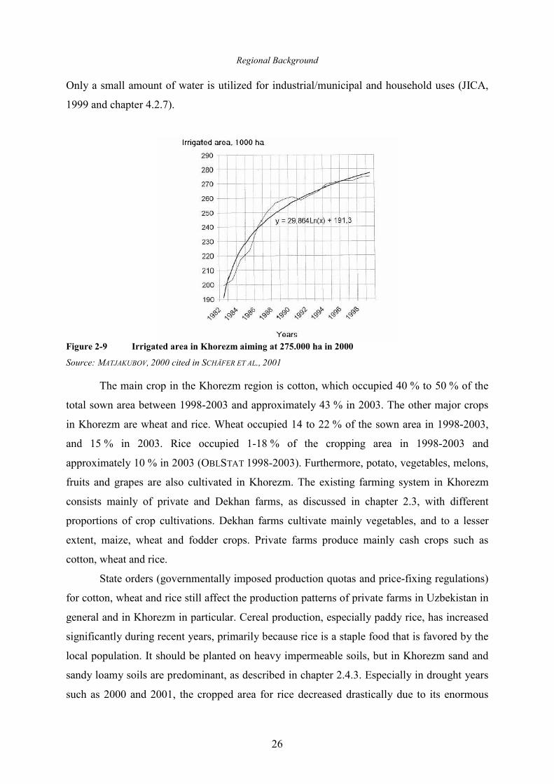
Regional Background
26
Only a small amount of water is utilized for industrial/municipal and household uses (JICA,
1999 and chapter 4.2.7).
Figure 2-9 Irrigated area in Khorezm aiming at 275.000 ha in 2000
Source: MATJAKUBOV, 2000 cited in SCHÄFER ET AL., 2001
The main crop in the Khorezm region is cotton, which occupied 40 % to 50 % of the
total sown area between 1998-2003 and approximately 43 % in 2003. The other major crops
in Khorezm are wheat and rice. Wheat occupied 14 to 22 % of the sown area in 1998-2003,
and 15 % in 2003. Rice occupied 1-18 % of the cropping area in 1998-2003 and
approximately 10 % in 2003 (OBLSTAT 1998-2003). Furthermore, potato, vegetables, melons,
fruits and grapes are also cultivated in Khorezm. The existing farming system in Khorezm
consists mainly of private and Dekhan farms, as discussed in chapter 2.3, with different
proportions of crop cultivations. Dekhan farms cultivate mainly vegetables, and to a lesser
extent, maize, wheat and fodder crops. Private farms produce mainly cash crops such as
cotton, wheat and rice.
State orders (governmentally imposed production quotas and price-fixing regulations)
for cotton, wheat and rice still affect the production patterns of private farms in Uzbekistan in
general and in Khorezm in particular. Cereal production, especially paddy rice, has increased
significantly during recent years, primarily because rice is a staple food that is favored by the
local population. It should be planted on heavy impermeable soils, but in Khorezm sand and
sandy loamy soils are predominant, as described in chapter 2.4.3. Especially in drought years
such as 2000 and 2001, the cropped area for rice decreased drastically due to its enormous
Regional Background
27
irrigation requirements (MÜLLER, 2006). Winter wheat was introduced in Khorezm after its
independence as a part of promoting self-sufficiency in grain production. The expansion of
the relatively salt-sensitive crop winter wheat, which is basically cropped after cotton, took
place mainly at the expense of alfalfa, which had negative effects on the formerly handled
crop rotation of alfalfa-cotton, causing a higher supply of nitrogen and humus content in the
soil (UN, 2001; SCHÄFER ET AL, 2001).
The soil quality and land capability are determined on a 100-degree scale for irrigated
land and is called ‘bonitet’. This index can be used to conduct a comparative assessment of
land quality and productivity. One point on this index is equal to a yielding capacity of 0.04
t/ha of cotton. This means that for the soils with the highest scores and, thus, the highest soil
fertility, it is possible to gain 4 t/ha of cotton (FAO, 2003c).
0
5
10
15
20
25
30
35
40
45
I II III IV, V
Quality of land suitable for irrigation
%
Figure 2-10 Land quality in Khorezm according to the bonitet-index
Notes: The categories are defined as: I Very good land, capable of producing 81-100 % of the potential yield II Good land, capable of producing 61-80 % of the potential yield III Moderate quality land, capable of producing 41-60 % of the potential yield IV+V Poor land, capable of producing 40 % of the potential yield
Source: FAO, 2003b; EU, 1996
Figure 2-10 gives the quality of land suitability for cotton growth in the Khorezm
region. The average bonitet-level for soils in Khorezm was 54 in the 1990s. This is equal to a
cotton production of 2.16 t/ha. In 1972 this value was 79 points, which is equal to 3.16 t/ha of
cotton. GIESE ET AL., 1998 stated that a yield reduction from more than 4 t/ha in the 1980s to
less than 3 t/ha towards the end of the 1990s was noticeable. Furthermore, we collected data
on cotton yield for 1998-2005, and these data confirm the general tendency of a strong
reduction in yield to less than 2.5-3 t/ha. In chapter 4.2.5 the actual cotton yields for 2003,
which were only 1.5-1.9 t/ha, are discussed. This decrease in yield reduction is caused by the
Regional Background
28
additional expansion of marginal land, but it is mainly a result of productivity losses due to
the increasing salinity of the soils (SCHÄFER ET AL., 2001).
Khorezm has the highest rate of secondary or human-induced salinization on irrigated
fields compared to all the provinces in Uzbekistan, and the rate is increasing (FAO, 2003b).
The proportion of slight, moderate and high salinization of soils to the total salt affected area
is 46.8 %, 41.1 % and 12.1 %, respectively. Water salinity is also increasing in Khorezm due
to the intensified use of irrigation water by the upstream users and their return flows.
Furthermore, the salt accumulation in the groundwater has increased (IBRAKHIMOV, 2007) due
to soil leaching and saline irrigation water reaching the groundwater. Additionally, the
groundwater table is rising, which intensifies the interaction between the groundwater, the
root zone and the soil. This leads to increased salt accumulation in soils and eventually in the
crops as well. The majority of the cultivated crops are very sensitive to increasing soil and
water salinity. The result is that the crop yield is reduced, which in turn leads to declining
revenues.
29
3 Methodology
The structure of agriculture and irrigation and the environmental and economic
consequences that they have in Uzbekistan and Khorezm are pivotal problems. The efficiency
of crops and water allocation are analyzed in this study in terms of agronomic, economic and
hydrologic aspects and processes. These issues determine the composition and methodology
of the hydrologic-agronomic-economic model described in detail in the following chapter. An
overview of the general background of water management models and hydrologic-economic
models currently in use and their main characteristics will be given. Finally, a detailed
description of the Khorezmian water management model that includes basic formulas,
features and interactions will be discussed.
3.1 Background: Economic-Hydrologic Water Management Models
A wide range of models are available to study water resources. In general, they are
dominated by hydrologic studies of flood/system control and water resource and quality
management. However, many different models for reservoir operation, groundwater
management, irrigation and drainage management, as well as the use of both surface and
groundwater in conjunction, can be found. These water management models consider the
quantity and quality of water, salt and soil. On the other hand, economic studies have focused
on cost-benefit analyses for profit maximization or the optimization of irrigation, industrial,
domestic net benefits, demand pattern and pricing or trading of water (MCKINNEY ET AL.,
1999).
This means that either the hydrologic or the economic component dominates the
model, depending on the objectives and on the specific problems of the analysis. However,
the sustainable and efficient management of water resources requires an interdisciplinary
approach. Interdependencies between physical, economic, agronomic, sociologic and
institutional aspects must be considered and incorporated into a holistic model. Thus, a
combined economic and hydrologic study at the river basin level and its sublevels seems to be
most appropriate to assess water management and policy issues (YOUNG, 1996). These
Methodology
30
economic-hydrologic models integrate water resource behavior and economic components
within a single numerical programming model. They consist of a hydrologic and an economic
system. The economic components are driven by the hydrologic and agronomic system,
which is based on physical parameters and principles. The hydrologic components and their
operation, on the other hand, are driven by socio-economic, political and environmental
objectives.
The two primary types of combined hydrologic-economic modeling techniques are
simulation and optimization. Simulation models simulate water resource behavior using
predefined sets of rules governing water allocations and infrastructure operations.
Optimization models optimize and select allocations and infrastructure based on objective
functions and accompanying constraints (MCKINNEY ET AL., 1999). It is possible to assess
water system responses using simulation models by changing demand patterns or population
growth or by including extreme events such as droughts, floods, or climate change.
Simulation models can also identify system failure components. Optimization models are
generally based on an objective function that can be driven by hydrology-inferred or
economic criteria such as optimal water allocation. In most cases these models also contain a
simulation component to characterize the hydrologic system.
Other major differences in modeling water resources management are short-term and
long-term models. Short-term models have modeling periods of one year or a single irrigation
season, whereas long-term models use extended periods are mainly used to analyze long-term
effects on quality and environmental patterns such as salt accumulation, groundwater or
surface flow changes.
Furthermore, a differentiation between loose and tight-coupled models in integrated
economic-hydrologic models is distinguished. In loose or even non-coupled models (also
called the compartment approach) the connection between the economy and hydrology is very
weak and only output data are transferred externally between the components. In tight- or
strong-coupled models (also called holistic approaches) the components are directly
connected into one single model based on the same unit of interaction (MCKINNEY ET AL.,
1999). These models are based on information transfer and on the interrelationship between
the components that are calculated endogenously within the model. The different components
of the system are interlinked and allow feedback between each other.
Furthermore, many integrated models for water resource management exist due to the
different approaches described. These models vary in their spatial scale (basin wide, district,
Methodology
31
field level etc.), included components (drainage, groundwater, surface flows, salinity,
institutional rules and incentives, water markets, benefits, etc.) or applied software. Recently,
water resource management modelers have started to integrate decision support systems based
on Geographical Information Systems (GIS) with a spatial representation of integrated
economic, agronomic, institutional and hydrologic components.
The Water Management Model for Khorezm, described below, is characterized as an
integrated hydrologic-agronomic-economic combined simulation-optimization model at the
district level. It is a tightly coupled short-term model with a one-year time horizon coded in
GAMS (General Algebraic Modeling System) and solved by a so-called piece-by-piece
approach. The characteristics of the model and the modeling framework were chosen as they
best fit the research objective of analyzing and improving water and crop allocation based on
hydrologic, agronomic and economic systems. Furthermore, linking other risk and uncertainty
management models in irrigated agriculture in Khorezm (BOBOJONOV, 2008), micro-
economic analyses of farm restructuring in Khorezm (DJANIBEKOV, 2008) or land and water
use reforms in Uzbekistan using a general equilibrium approach (MÜLLER, 2006) are possible,
because all of these methods are based on the same modeling system (GAMS) and were
applied to the Khorezm region within the “Economic and Ecological Restructuring of Water
and Land Use in the Region Khorezm (Uzbekistan), a Pilot Project in Development Research”
project. Additionally, a successful modeling framework for sustainable water resource
management for different water basins, such as Mekong and Syr Darya (CAI, 1999), already
existed that could serve as the basis for the Khorezm water management model.
3.2 The Khorezm Water Management Model
3.2.1 Main Purposes and Elements of the Model
The main questions of the study to be answered by the model are as follows:
• the identification of strategies and policies of efficient water and crop allocation
among users, agricultural development and water resource demand management in
Khorezm,
• the detection and determination of water supply and demand and the water availability
and water use patterns in the region of Khorezm,
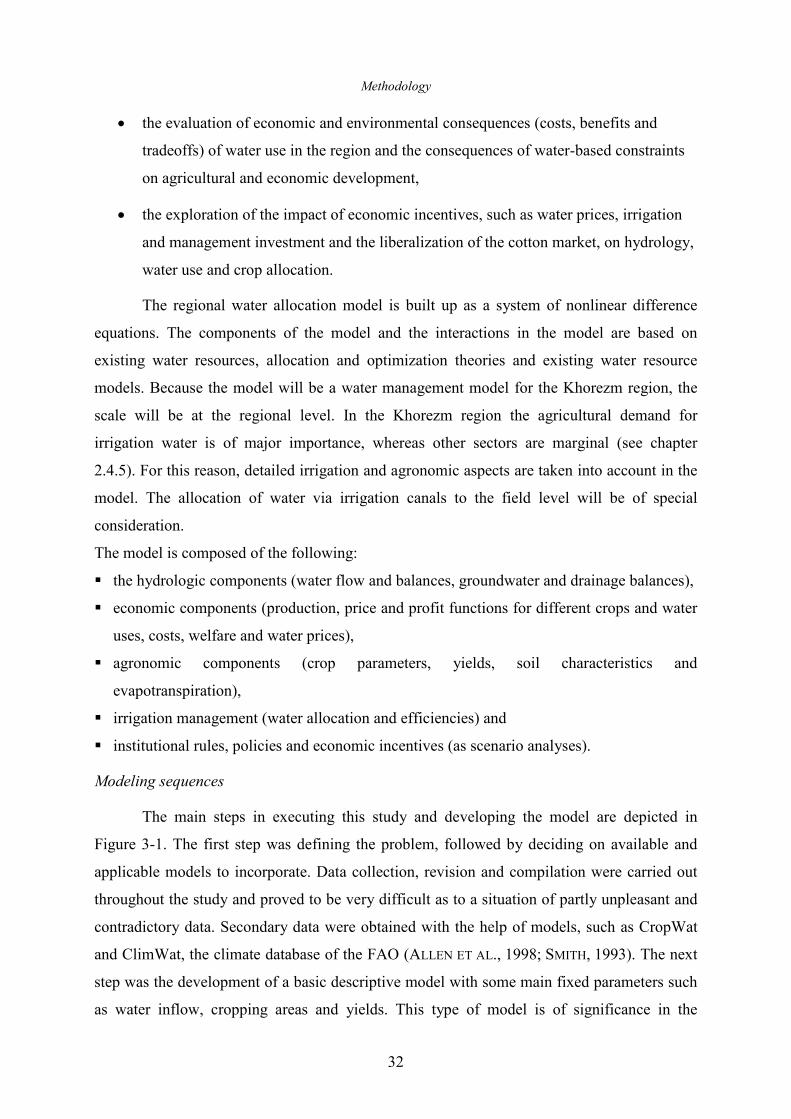
Methodology
32
• the evaluation of economic and environmental consequences (costs, benefits and
tradeoffs) of water use in the region and the consequences of water-based constraints
on agricultural and economic development,
• the exploration of the impact of economic incentives, such as water prices, irrigation
and management investment and the liberalization of the cotton market, on hydrology,
water use and crop allocation.
The regional water allocation model is built up as a system of nonlinear difference
equations. The components of the model and the interactions in the model are based on
existing water resources, allocation and optimization theories and existing water resource
models. Because the model will be a water management model for the Khorezm region, the
scale will be at the regional level. In the Khorezm region the agricultural demand for
irrigation water is of major importance, whereas other sectors are marginal (see chapter
2.4.5). For this reason, detailed irrigation and agronomic aspects are taken into account in the
model. The allocation of water via irrigation canals to the field level will be of special
consideration.
The model is composed of the following:
� the hydrologic components (water flow and balances, groundwater and drainage balances),
� economic components (production, price and profit functions for different crops and water
uses, costs, welfare and water prices),
� agronomic components (crop parameters, yields, soil characteristics and
evapotranspiration),
� irrigation management (water allocation and efficiencies) and
� institutional rules, policies and economic incentives (as scenario analyses).
Modeling sequences
The main steps in executing this study and developing the model are depicted in
Figure 3-1. The first step was defining the problem, followed by deciding on available and
applicable models to incorporate. Data collection, revision and compilation were carried out
throughout the study and proved to be very difficult as to a situation of partly unpleasant and
contradictory data. Secondary data were obtained with the help of models, such as CropWat
and ClimWat, the climate database of the FAO (ALLEN ET AL., 1998; SMITH, 1993). The next
step was the development of a basic descriptive model with some main fixed parameters such
as water inflow, cropping areas and yields. This type of model is of significance in the
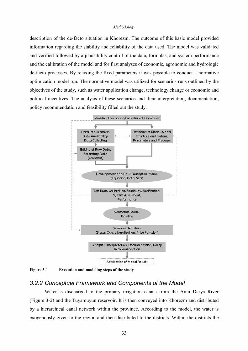
Methodology
33
description of the de-facto situation in Khorezm. The outcome of this basic model provided
information regarding the stability and reliability of the data used. The model was validated
and verified followed by a plausibility control of the data, formulas, and system performance
and the calibration of the model and for first analyses of economic, agronomic and hydrologic
de-facto processes. By relaxing the fixed parameters it was possible to conduct a normative
optimization model run. The normative model was utilized for scenarios runs outlined by the
objectives of the study, such as water application change, technology change or economic and
political incentives. The analysis of these scenarios and their interpretation, documentation,
policy recommendation and feasibility filled out the study.
Figure 3-1 Execution and modeling steps of the study
3.2.2 Conceptual Framework and Components of the Model
Water is discharged to the primary irrigation canals from the Amu Darya River
(Figure 3-2) and the Tuyamuyun reservoir. It is then conveyed into Khorezm and distributed
by a hierarchical canal network within the province. According to the model, the water is
exogenously given to the region and then distributed to the districts. Within the districts the
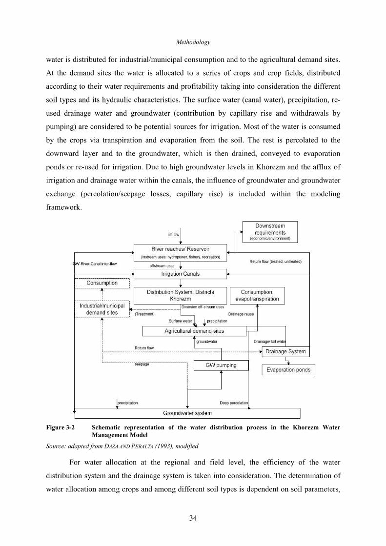
Methodology
34
water is distributed for industrial/municipal consumption and to the agricultural demand sites.
At the demand sites the water is allocated to a series of crops and crop fields, distributed
according to their water requirements and profitability taking into consideration the different
soil types and its hydraulic characteristics. The surface water (canal water), precipitation, re-
used drainage water and groundwater (contribution by capillary rise and withdrawals by
pumping) are considered to be potential sources for irrigation. Most of the water is consumed
by the crops via transpiration and evaporation from the soil. The rest is percolated to the
downward layer and to the groundwater, which is then drained, conveyed to evaporation
ponds or re-used for irrigation. Due to high groundwater levels in Khorezm and the afflux of
irrigation and drainage water within the canals, the influence of groundwater and groundwater
exchange (percolation/seepage losses, capillary rise) is included within the modeling
framework.
Figure 3-2 Schematic representation of the water distribution process in the Khorezm Water
Management Model
Source: adapted from DAZA AND PERALTA (1993), modified
For water allocation at the regional and field level, the efficiency of the water
distribution system and the drainage system is taken into consideration. The determination of
water allocation among crops and among different soil types is dependent on soil parameters,
Methodology
35
cropping pattern and crop characteristics. Water demand is determined endogenously within
the model using empirically determined agronomic parameters for the production function.
The water supply in the region, including the irrigated crop fields at each of the irrigation
demand sites, is determined through hydrologic water balances (surface water, groundwater
balance, drainage water and soil water).
Water supply and demand are integrated into an endogenous system. The valuation of
production and water use costs, revenues and yields are determined in an economic objective
function, which is constrained by hydrologic, agronomic, and institutional relations. Water
allocation to districts and crops is determined by maximizing profits, which considers
economic water use efficiency (e-WUE). Water-related policies and future programs will then
be modeled as different scenarios.
The model consists of ten districts. It is assumed that every district consists of an
evaporation pond and a groundwater reservoir. The model considers eight different crops
(cotton, wheat, rice, other grain, alfalfa, vegetables, fruits, potatoes) and three main soil types
(light, medium, heavy soils).
The model is written in the General Algebraic Modeling System (GAMS) (BROOKE ET
AL., 1988) language, which is a system for programming mathematical problems. GAMS
allows for linkages with other models, which are developed within the project. The model
covers a one-year time span and is subdivided into twelve monthly modeling periods.
3.2.3 Bio-Physical Components
The bio-physical components of the model are subdivided into hydrologic and crop
and soil-water-related agronomic interactions. Hydrologic processes in the model include
flows and balances of surface water, groundwater, drainage water and water within the root
zone (soil water).
Water Allocation
The following paragraph describes the water allocation within a demand site and the
water allocation among crops. The water that is discharged from canals, rivers and the
reservoir is allocated to different districts in Khorezm. Depending on the distribution
efficiency, the water is then allocated for non-irrigation (municipal and industrial uses,
NIWD) and irrigation purposes (WCP). The canal water for irrigation (and leaching), together
with the groundwater pumping, accounts for the water that is available for a crop field
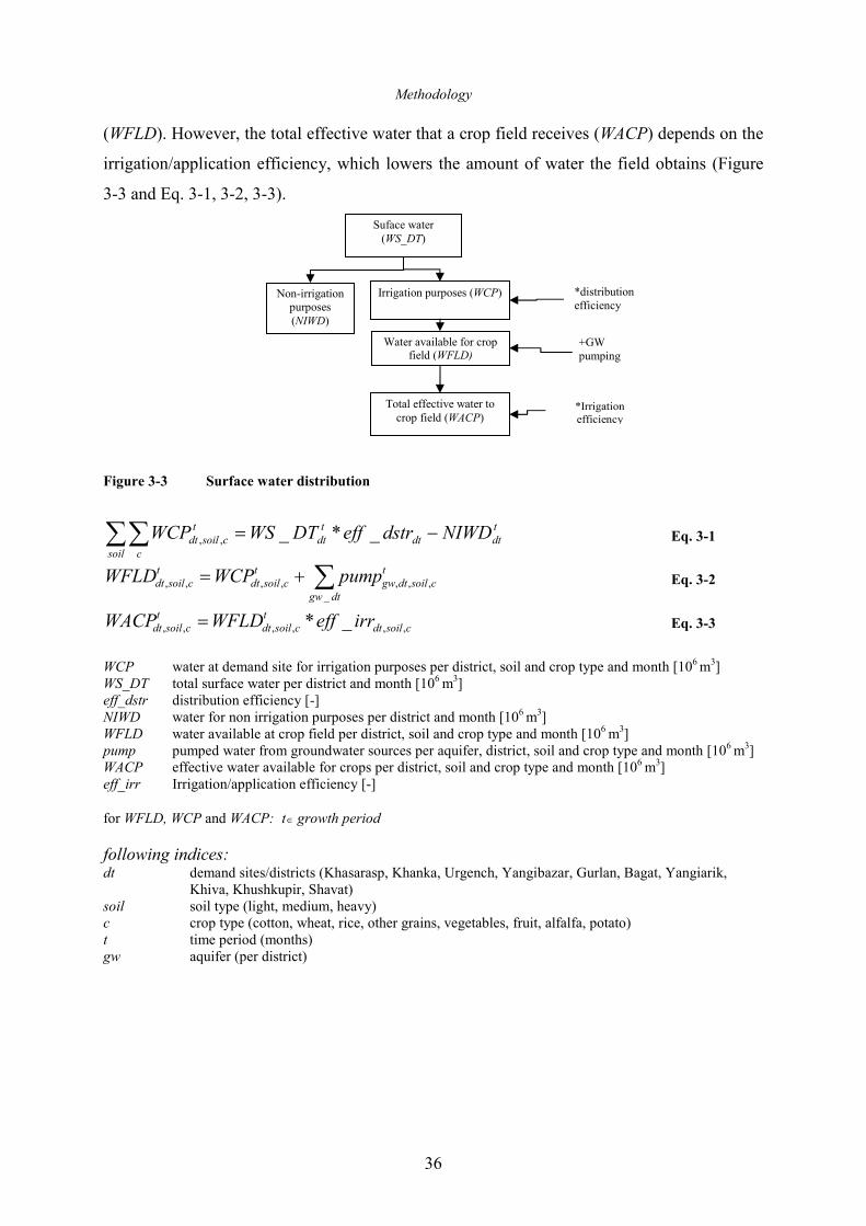
Methodology
36
(WFLD). However, the total effective water that a crop field receives (WACP) depends on the
irrigation/application efficiency, which lowers the amount of water the field obtains (Figure
3-3 and Eq. 3-1, 3-2, 3-3).
Figure 3-3 Surface water distribution
tdtdt
tdt
soil c
tcsoildt NIWDdstreffDTWSWCP −=∑∑ _*_,, Eq. 3-1
∑+=dtgw
tcsoildtgw
tcsoildt
tcsoildt pumpWCPWFLD
_,,,,,,, Eq. 3-2
csoildtt
csoildtt
csoildt irreffWFLDWACP ,,,,,, _*= Eq. 3-3
WCP water at demand site for irrigation purposes per district, soil and crop type and month [106 m3] WS_DT total surface water per district and month [106 m3] eff_dstr distribution efficiency [-] NIWD water for non irrigation purposes per district and month [106 m3] WFLD water available at crop field per district, soil and crop type and month [106 m3] pump pumped water from groundwater sources per aquifer, district, soil and crop type and month [106 m3] WACP effective water available for crops per district, soil and crop type and month [106 m3] eff_irr Irrigation/application efficiency [-]
for WFLD, WCP and WACP: t∈ growth period
following indices: dt demand sites/districts (Khasarasp, Khanka, Urgench, Yangibazar, Gurlan, Bagat, Yangiarik,
Khiva, Khushkupir, Shavat) soil soil type (light, medium, heavy) c crop type (cotton, wheat, rice, other grains, vegetables, fruit, alfalfa, potato) t time period (months) gw aquifer (per district)
Suface water (WS_DT)
Non-irrigation purposes (NIWD)
Irrigation purposes (WCP)
+GW pumping
Total effective water to crop field (WACP)
*Irrigation efficiency
Water available for crop field (WFLD)
*distribution efficiency
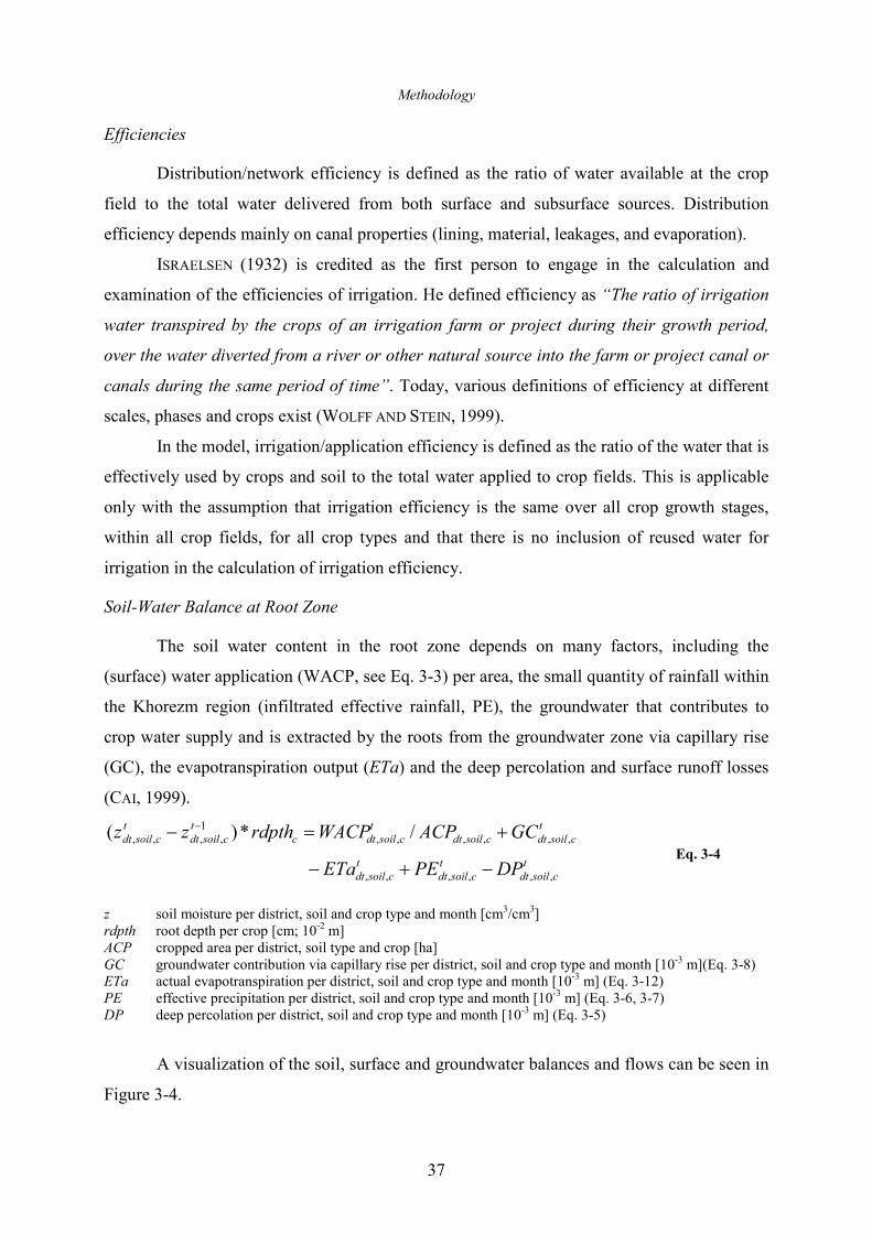
Methodology
37
Efficiencies
Distribution/network efficiency is defined as the ratio of water available at the crop
field to the total water delivered from both surface and subsurface sources. Distribution
efficiency depends mainly on canal properties (lining, material, leakages, and evaporation).
ISRAELSEN (1932) is credited as the first person to engage in the calculation and
examination of the efficiencies of irrigation. He defined efficiency as “The ratio of irrigation
water transpired by the crops of an irrigation farm or project during their growth period,
over the water diverted from a river or other natural source into the farm or project canal or
canals during the same period of time”. Today, various definitions of efficiency at different
scales, phases and crops exist (WOLFF AND STEIN, 1999).
In the model, irrigation/application efficiency is defined as the ratio of the water that is
effectively used by crops and soil to the total water applied to crop fields. This is applicable
only with the assumption that irrigation efficiency is the same over all crop growth stages,
within all crop fields, for all crop types and that there is no inclusion of reused water for
irrigation in the calculation of irrigation efficiency.
Soil-Water Balance at Root Zone
The soil water content in the root zone depends on many factors, including the
(surface) water application (WACP, see Eq. 3-3) per area, the small quantity of rainfall within
the Khorezm region (infiltrated effective rainfall, PE), the groundwater that contributes to
crop water supply and is extracted by the roots from the groundwater zone via capillary rise
(GC), the evapotranspiration output (ETa) and the deep percolation and surface runoff losses
(CAI, 1999).
tcsoildt
tcsoildt
tcsoildt
tcsoildtcsoildt
tcsoildtc
tcsoildt
tcsoildt
DPPEETa
GCACPWACPrdpthzz
,,,,,,
,,,,,,1
,,,, /*)(
−+−
+=− −
Eq. 3-4
z soil moisture per district, soil and crop type and month [cm3/cm3] rdpth root depth per crop [cm; 10-2 m] ACP cropped area per district, soil type and crop [ha] GC groundwater contribution via capillary rise per district, soil and crop type and month [10-3 m](Eq. 3-8) ETa actual evapotranspiration per district, soil and crop type and month [10-3 m] (Eq. 3-12) PE effective precipitation per district, soil and crop type and month [10-3 m] (Eq. 3-6, 3-7) DP deep percolation per district, soil and crop type and month [10-3 m] (Eq. 3-5)
A visualization of the soil, surface and groundwater balances and flows can be seen in
Figure 3-4.
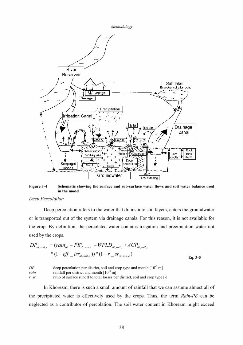
Methodology
38
Figure 3-4 Schematic showing the surface and sub-surface water flows and soil water balance used
in the model
Deep Percolation
Deep percolation refers to the water that drains into soil layers, enters the groundwater
or is transported out of the system via drainage canals. For this reason, it is not available for
the crop. By definition, the percolated water contains irrigation and precipitation water not
used by the crops.
)_1(*))_1(*
/(
,,,,
,,,,,,,,
csoildtcsoildt
csoildtt
csoildtt
csoildttdt
tcsoildt
srrirreff
ACPWFLDPErainDP
−−
+−=
Eq. 3-5 DP deep percolation per district, soil and crop type and month [10-3 m] rain rainfall per district and month [10-3 m] r_sr ratio of surface runoff to total losses per district, soil and crop type [-]
In Khorezm, there is such a small amount of rainfall that we can assume almost all of
the precipitated water is effectively used by the crops. Thus, the term Rain-PE can be
neglected as a contributor of percolation. The soil water content in Khorezm might exceed
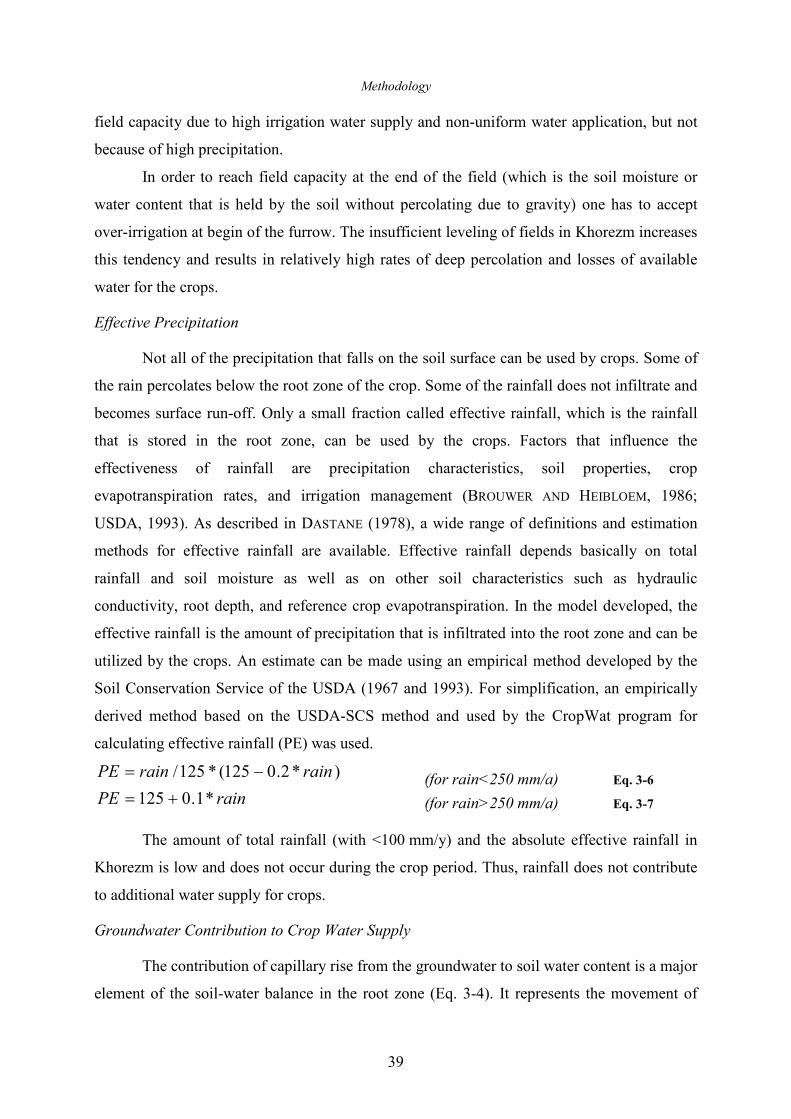
Methodology
39
field capacity due to high irrigation water supply and non-uniform water application, but not
because of high precipitation.
In order to reach field capacity at the end of the field (which is the soil moisture or
water content that is held by the soil without percolating due to gravity) one has to accept
over-irrigation at begin of the furrow. The insufficient leveling of fields in Khorezm increases
this tendency and results in relatively high rates of deep percolation and losses of available
water for the crops.
Effective Precipitation
Not all of the precipitation that falls on the soil surface can be used by crops. Some of
the rain percolates below the root zone of the crop. Some of the rainfall does not infiltrate and
becomes surface run-off. Only a small fraction called effective rainfall, which is the rainfall
that is stored in the root zone, can be used by the crops. Factors that influence the
effectiveness of rainfall are precipitation characteristics, soil properties, crop
evapotranspiration rates, and irrigation management (BROUWER AND HEIBLOEM, 1986;
USDA, 1993). As described in DASTANE (1978), a wide range of definitions and estimation
methods for effective rainfall are available. Effective rainfall depends basically on total
rainfall and soil moisture as well as on other soil characteristics such as hydraulic
conductivity, root depth, and reference crop evapotranspiration. In the model developed, the
effective rainfall is the amount of precipitation that is infiltrated into the root zone and can be
utilized by the crops. An estimate can be made using an empirical method developed by the
Soil Conservation Service of the USDA (1967 and 1993). For simplification, an empirically
derived method based on the USDA-SCS method and used by the CropWat program for
calculating effective rainfall (PE) was used.
)*2.0125(*125/ rainrainPE −= (for rain<250 mm/a) Eq. 3-6 rainPE *1.0125 += (for rain>250 mm/a) Eq. 3-7
The amount of total rainfall (with <100 mm/y) and the absolute effective rainfall in
Khorezm is low and does not occur during the crop period. Thus, rainfall does not contribute
to additional water supply for crops.
Groundwater Contribution to Crop Water Supply
The contribution of capillary rise from the groundwater to soil water content is a major
element of the soil-water balance in the root zone (Eq. 3-4). It represents the movement of
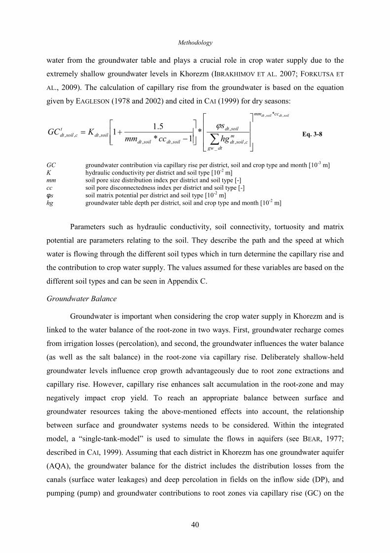
Methodology
40
water from the groundwater table and plays a crucial role in crop water supply due to the
extremely shallow groundwater levels in Khorezm (IBRAKHIMOV ET AL. 2007; FORKUTSA ET
AL., 2009). The calculation of capillary rise from the groundwater is based on the equation
given by EAGLESON (1978 and 2002) and cited in CAI (1999) for dry seasons:
soildtsoildt ccmm
dtgw
mcsoildt
soildt
soildtsoildt
soildtt
csoildthg
s
ccmmKGC
,, *
_,,
,
,,,,, *
1*
5.11
−+=
∑ϕ
Eq. 3-8
GC groundwater contribution via capillary rise per district, soil and crop type and month [10-3 m] K hydraulic conductivity per district and soil type [10-2 m] mm soil pore size distribution index per district and soil type [-] cc soil pore disconnectedness index per district and soil type [-] φs soil matrix potential per district and soil type [10-2 m] hg groundwater table depth per district, soil and crop type and month [10-2 m]
Parameters such as hydraulic conductivity, soil connectivity, tortuosity and matrix
potential are parameters relating to the soil. They describe the path and the speed at which
water is flowing through the different soil types which in turn determine the capillary rise and
the contribution to crop water supply. The values assumed for these variables are based on the
different soil types and can be seen in Appendix C.
Groundwater Balance
Groundwater is important when considering the crop water supply in Khorezm and is
linked to the water balance of the root-zone in two ways. First, groundwater recharge comes
from irrigation losses (percolation), and second, the groundwater influences the water balance
(as well as the salt balance) in the root-zone via capillary rise. Deliberately shallow-held
groundwater levels influence crop growth advantageously due to root zone extractions and
capillary rise. However, capillary rise enhances salt accumulation in the root-zone and may
negatively impact crop yield. To reach an appropriate balance between surface and
groundwater resources taking the above-mentioned effects into account, the relationship
between surface and groundwater systems needs to be considered. Within the integrated
model, a “single-tank-model” is used to simulate the flows in aquifers (see BEAR, 1977;
described in CAI, 1999). Assuming that each district in Khorezm has one groundwater aquifer
(AQA), the groundwater balance for the district includes the distribution losses from the
canals (surface water leakages) and deep percolation in fields on the inflow side (DP), and
pumping (pump) and groundwater contributions to root zones via capillary rise (GC) on the
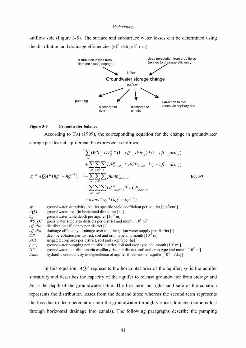
Methodology
41
outflow side (Figure 3-5). The surface and subsurface water losses can be determined using
the distribution and drainage efficiencies (eff_dstr, eff_drn).
Figure 3-5 Groundwater balance
According to CAI (1999), the corresponding equation for the change in groundwater
storage per district aquifer can be expressed as follows:
−−
−
−
−+
−−
=−
−
−
∑∑∑
∑∑∑
∑∑∑
∑
)(**
*
)_1(**
)_1(*)_1(*_(
)(**
1
,,,,
,,
,,,,
1
tt
dt soil ccsoildt
tcsoildt
dt soil c
tcsoildt
dt soil cdtcsoildt
tcsoildt
dtdtdt
tdt
tt
hghgsytrans
ACPGC
pump
drneffACPDP
drneffdstreffDTWS
hghgAQAsy Eq. 3-9
sy groundwater storativity, aquifer specific yield coefficient per aquifer [cm3/cm3] AQA groundwater area (in horizontal direction) [ha] hg groundwater table depth per aquifer [10-2 m] WS_DT gross water supply to districts per district and month [106 m3] eff_dstr distribution efficiency per district [-] eff_drn drainage efficiency, drainage over total irrigation water supply per district [-] DP deep percolation per district, soil and crop type and month [10-3 m] ACP irrigated crop area per district, soil and crop type [ha] pump groundwater pumping per aquifer, district, soil and crop type and month [106 m3] GC groundwater contribution via capillary rise per district, soil and crop type and month [10-3 m] trans hydraulic conductivity in dependence of aquifer thickness per aquifer [10-2 m/day]
In this equation, AQA represents the horizontal area of the aquifer, sy is the aquifer
storativity and describes the capacity of the aquifer to release groundwater from storage and
hg is the depth of the groundwater table. The first term on right-hand side of the equation
represents the distribution losses from the demand sites; whereas the second term represents
the loss due to deep percolation into the groundwater through vertical drainage (some is lost
through horizontal drainage into canals). The following paragraphs describe the pumping
Groundwater storage change
distribution losses from demand sites (seepage)
deep percolation from crop fields (related to drainage efficiency)
inflow
pumping
discharge to river
extraction to root zones via capillary rise
outflow
discharge to canals
Methodology
42
losses out of the aquifer, the groundwater contribution to crops by capillary rise and the
discharge from the aquifer to the surface water system. The coefficient trans describes the
dependency of hydraulic conductivity on the aquifer thickness.
Evapotranspiration
To determine the amount of crop water use and crop water productivity (the crop
production function), several calculations are necessary. Accounting for the actual
evapotranspiration (ETa) is the most relevant factor but also the most difficult to determine
(RAPPOLD, 2004). Evapotranspiration is the combination of the terms evaporation, which is
the amount of water that is evaporated by the soil surface to the atmosphere, and transpiration,
which is the amount of water that is transpired by crops and animals. To estimate the actual
evapotranspiration, the concept of a reference crop evapotranspiration (ETo) was introduced
by DOORENBROS AND PRUIT (1975).
Reference crop evapotranspiration (ETo)
ETo is the evapotranspiration from a reference crop with the specific characteristics of
grass, fully covering the soil and not deprived of water. It represents the evaporative demand
of the atmosphere at a specific location and time of the year and is independent of crop type,
crop development, management practices and soil factors. The value of ETo refers to the
hypothetical evapotranspiration that can be achieved by a reference crop (grass) under given
regional and climatologic conditions with no water shortages. The only factors that affect ETo
are climatic parameters such as pressure, wind speed, temperature, solar radiation, and hours
of daylight. This means that ETo is a climatic parameter and can be computed from weather
data (KASSAM AND SMITH, 2001).
The FAO Penman-Monteith method is widely used to calculate ETo (via the FAO
CropWat program8). The climatic factors of the Khorezm region, including amongst others
temperature, humidity, wind speed, and solar radiation, are incorporated into the calculation
of the reference evapotranspiration (ALLEN ET AL., 1998).
8 CropWat is a water balance-based computer program to calculate crop water requirements and irrigation water
requirements from climatic and crop data. It is also used in the development of irrigation schedules for different
management conditions and the calculation of water supply schemes for varying cropping patterns.
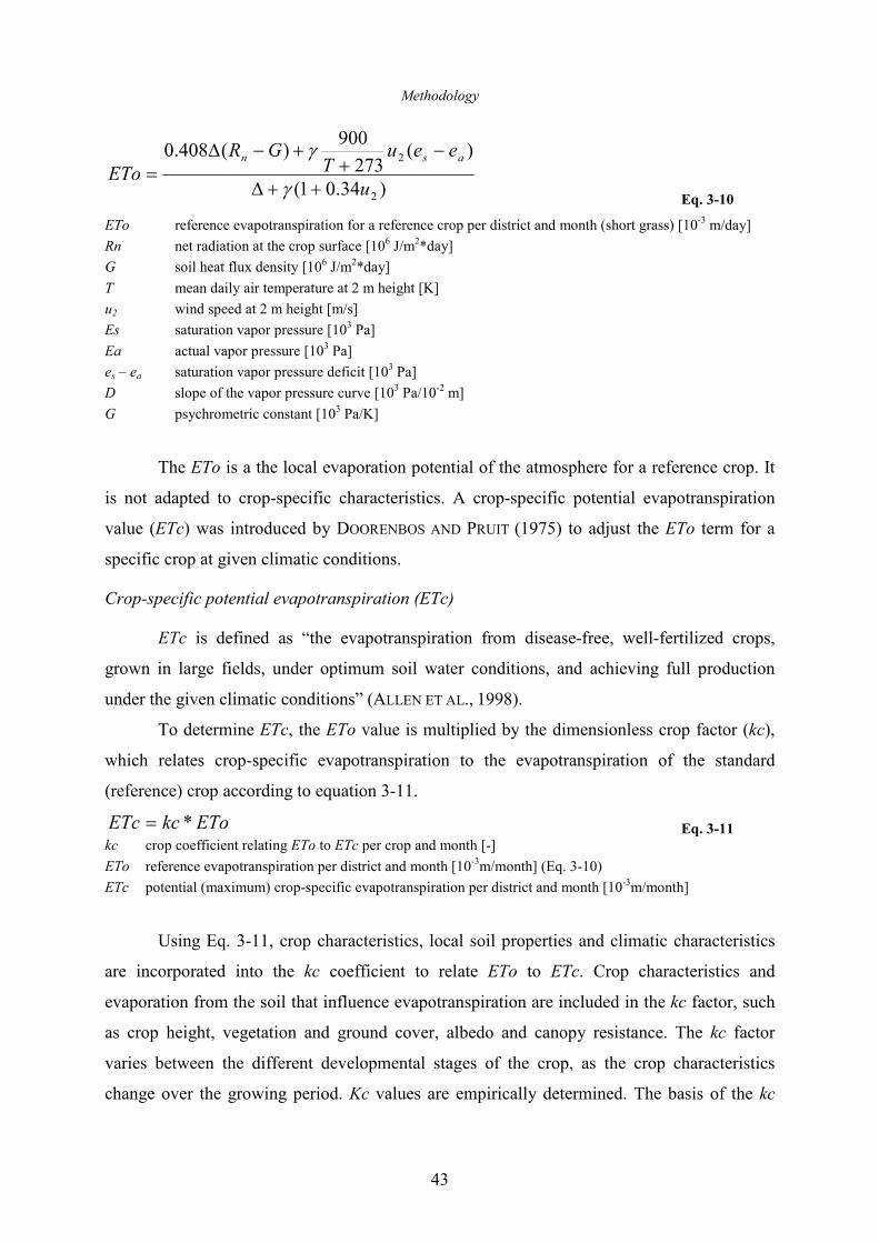
Methodology
43
)34.01(
)(273
900)(408.0
2
2
u
eeuT
GRETo
asn
++∆
−+
+−∆=
γ
γ
Eq. 3-10
ETo reference evapotranspiration for a reference crop per district and month (short grass) [10-3 m/day]
Rn net radiation at the crop surface [106 J/m2*day]
G soil heat flux density [106 J/m2*day]
T mean daily air temperature at 2 m height [K]
u2 wind speed at 2 m height [m/s]
Es saturation vapor pressure [103 Pa]
Ea actual vapor pressure [103 Pa]
es – ea saturation vapor pressure deficit [103 Pa]
D slope of the vapor pressure curve [103 Pa/10-2 m]
G psychrometric constant [103 Pa/K]
The ETo is a the local evaporation potential of the atmosphere for a reference crop. It
is not adapted to crop-specific characteristics. A crop-specific potential evapotranspiration
value (ETc) was introduced by DOORENBOS AND PRUIT (1975) to adjust the ETo term for a
specific crop at given climatic conditions.
Crop-specific potential evapotranspiration (ETc)
ETc is defined as “the evapotranspiration from disease-free, well-fertilized crops,
grown in large fields, under optimum soil water conditions, and achieving full production
under the given climatic conditions” (ALLEN ET AL., 1998).
To determine ETc, the ETo value is multiplied by the dimensionless crop factor (kc),
which relates crop-specific evapotranspiration to the evapotranspiration of the standard
(reference) crop according to equation 3-11.
ETokcETc *= Eq. 3-11 kc crop coefficient relating ETo to ETc per crop and month [-]
ETo reference evapotranspiration per district and month [10-3m/month] (Eq. 3-10)
ETc potential (maximum) crop-specific evapotranspiration per district and month [10-3m/month]
Using Eq. 3-11, crop characteristics, local soil properties and climatic characteristics
are incorporated into the kc coefficient to relate ETo to ETc. Crop characteristics and
evaporation from the soil that influence evapotranspiration are included in the kc factor, such
as crop height, vegetation and ground cover, albedo and canopy resistance. The kc factor
varies between the different developmental stages of the crop, as the crop characteristics
change over the growing period. Kc values are empirically determined. The basis of the kc
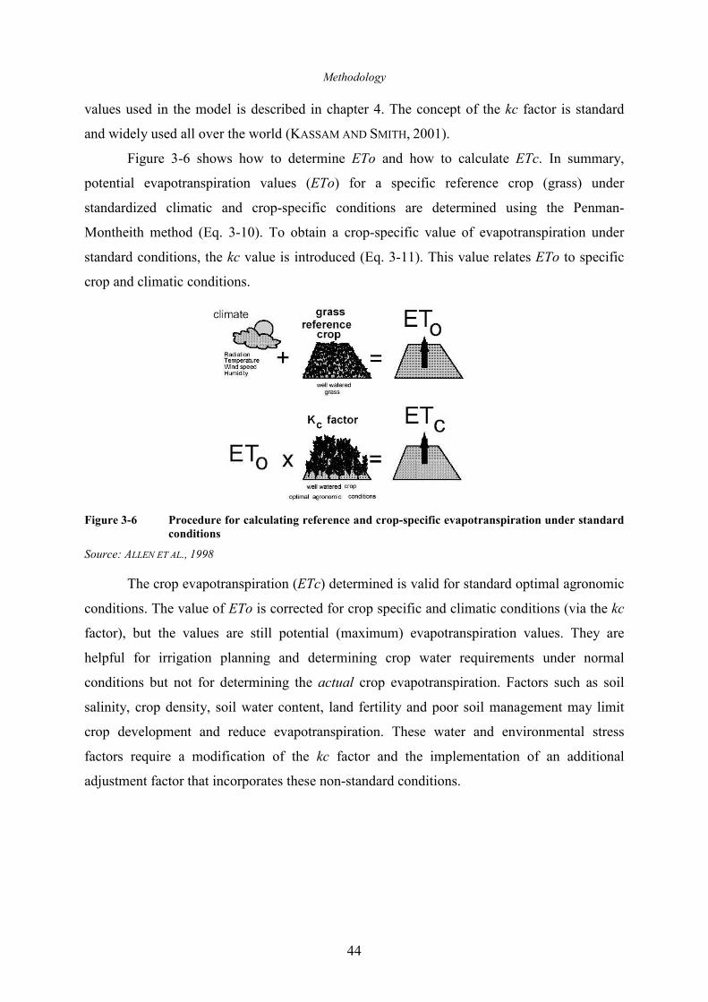
Methodology
44
values used in the model is described in chapter 4. The concept of the kc factor is standard
and widely used all over the world (KASSAM AND SMITH, 2001).
Figure 3-6 shows how to determine ETo and how to calculate ETc. In summary,
potential evapotranspiration values (ETo) for a specific reference crop (grass) under
standardized climatic and crop-specific conditions are determined using the Penman-
Montheith method (Eq. 3-10). To obtain a crop-specific value of evapotranspiration under
standard conditions, the kc value is introduced (Eq. 3-11). This value relates ETo to specific
crop and climatic conditions.
Figure 3-6 Procedure for calculating reference and crop-specific evapotranspiration under standard
conditions
Source: ALLEN ET AL., 1998
The crop evapotranspiration (ETc) determined is valid for standard optimal agronomic
conditions. The value of ETo is corrected for crop specific and climatic conditions (via the kc
factor), but the values are still potential (maximum) evapotranspiration values. They are
helpful for irrigation planning and determining crop water requirements under normal
conditions but not for determining the actual crop evapotranspiration. Factors such as soil
salinity, crop density, soil water content, land fertility and poor soil management may limit
crop development and reduce evapotranspiration. These water and environmental stress
factors require a modification of the kc factor and the implementation of an additional
adjustment factor that incorporates these non-standard conditions.
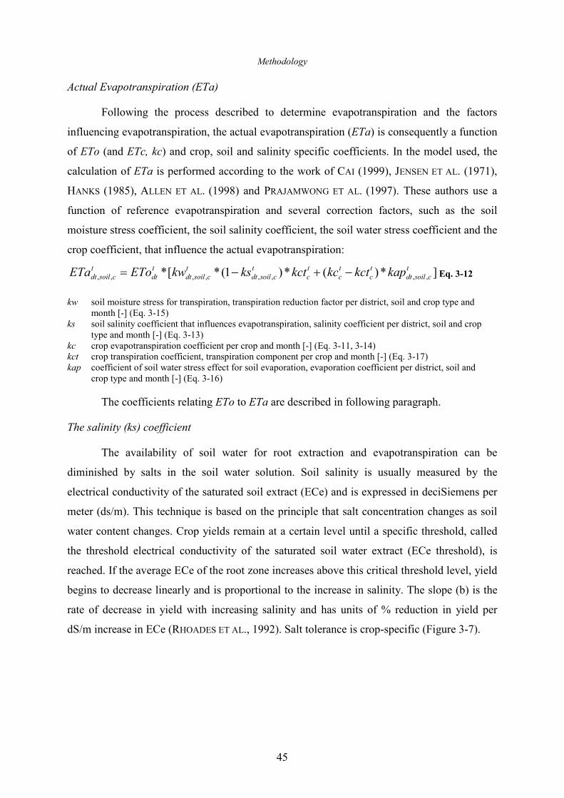
Methodology
45
Actual Evapotranspiration (ETa)
Following the process described to determine evapotranspiration and the factors
influencing evapotranspiration, the actual evapotranspiration (ETa) is consequently a function
of ETo (and ETc, kc) and crop, soil and salinity specific coefficients. In the model used, the
calculation of ETa is performed according to the work of CAI (1999), JENSEN ET AL. (1971),
HANKS (1985), ALLEN ET AL. (1998) and PRAJAMWONG ET AL. (1997). These authors use a
function of reference evapotranspiration and several correction factors, such as the soil
moisture stress coefficient, the soil salinity coefficient, the soil water stress coefficient and the
crop coefficient, that influence the actual evapotranspiration:
]*)(*)1(*[* ,,,,,,,,t
csoildttc
tc
tc
tcsoildt
tcsoildt
tdt
tcsoildt kapkctkckctkskwEToETa −+−= Eq. 3-12
kw soil moisture stress for transpiration, transpiration reduction factor per district, soil and crop type and
month [-] (Eq. 3-15) ks soil salinity coefficient that influences evapotranspiration, salinity coefficient per district, soil and crop
type and month [-] (Eq. 3-13) kc crop evapotranspiration coefficient per crop and month [-] (Eq. 3-11, 3-14) kct crop transpiration coefficient, transpiration component per crop and month [-] (Eq. 3-17) kap coefficient of soil water stress effect for soil evaporation, evaporation coefficient per district, soil and
crop type and month [-] (Eq. 3-16)
The coefficients relating ETo to ETa are described in following paragraph.
The salinity (ks) coefficient
The availability of soil water for root extraction and evapotranspiration can be
diminished by salts in the soil water solution. Soil salinity is usually measured by the
electrical conductivity of the saturated soil extract (ECe) and is expressed in deciSiemens per
meter (ds/m). This technique is based on the principle that salt concentration changes as soil
water content changes. Crop yields remain at a certain level until a specific threshold, called
the threshold electrical conductivity of the saturated soil water extract (ECe threshold), is
reached. If the average ECe of the root zone increases above this critical threshold level, yield
begins to decrease linearly and is proportional to the increase in salinity. The slope (b) is the
rate of decrease in yield with increasing salinity and has units of % reduction in yield per
dS/m increase in ECe (RHOADES ET AL., 1992). Salt tolerance is crop-specific (Figure 3-7).
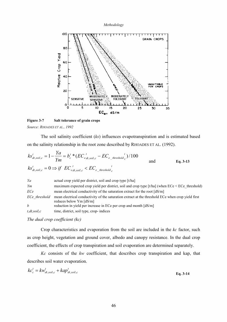
Methodology
46
Figure 3-7 Salt tolerance of grain crops
Source: RHOADES ET AL., 1992
The soil salinity coefficient (ks) influences evapotranspiration and is estimated based
on the salinity relationship in the root zone described by RHOADES ET AL. (1992).
100/)(*1 _,,,,t
cthresholde
t
csoildtetc
tcsoildt ECECb
Ym
Yaks −=−=
and Eq. 3-13
t
cthresholde
t
csoildtet
csoildt ECECifks _,,,, 0 <⇒=
Ya actual crop yield per district, soil and crop type [t/ha]
Ym maximum expected crop yield per district, soil and crop type [t/ha] (when ECe < ECe_threshold)
ECe mean electrical conductivity of the saturation extract for the root [dS/m]
ECe_threshold mean electrical conductivity of the saturation extract at the threshold ECe when crop yield first reduces below Ym [dS/m]
b reduction in yield per increase in ECe per crop and month [dS/m]
t,dt,soil,c time, district, soil type, crop- indices
The dual crop coefficient (kc)
Crop characteristics and evaporation from the soil are included in the kc factor, such
as crop height, vegetation and ground cover, albedo and canopy resistance. In the dual crop
coefficient, the effects of crop transpiration and soil evaporation are determined separately.
Kc consists of the kw coefficient, that describes crop transpiration and kap, that
describes soil water evaporation.
tcsoildt
tcsoildt
tc kapkwkc ,,,, +=
Eq. 3-14
Methodology
47
The kw coefficient
The coefficient that accounts for soil moisture stress as a result of reduction in crop
transpiration consists of an empirically derived soil moisture relationship between field
capacity and wilting point and is described in CAI (1999), who cited the work of JENSEN ET
AL. (1971) with the assumption that kw is “proportional to the logarithm of the percentage of
the remaining available soil moisture” (JENSEN ET AL., 1971).
)101ln(/1*100ln ,,,,
+
−
−=
soilsoil
soilt
csoildttcsoildt
zwzs
zwzkw Eq. 3-15
zw soil moisture at wilting point per district and soil type [cm3/cm3] zs soil moisture at field capacity per district and soil type [cm3/cm3]
The kap coefficient
The water stress coefficient that accounts for soil evaporation is described in
PRAJAMWONG ET AL. (1997) and is empirically derived.
5.0
,,,, *5.0
*5.0
−
−=
soilsoil
soilt
csoildttcsoildt
zwzs
zwzkap
Eq. 3-16
Both, kw and kap are valid for: soilt
csoildtsoilt
csoildt zszandzwz ≤≥ ,,,,
The kct coefficient
The coefficient kct accounts for the change of the crop coefficient in dependency of
the growing season. The coefficient was described by HANKS (1985).
Before crop emergence: 0=kct ,
and after crop emergence 9.0*kckct = Eq. 3-17
Crop-Water Production Function
Water stress for crops can be quantified using a relation between actual (ETa) and
maximum evapotranspiration (ETc). In cases when crop water requirements are fully met
from the available water supply, ETa=ETc. When the water supply for crops is insufficient,
ETa<ETc. When this occurs, crop yields are reduced.
The relationship between crop water supply and crop yield is described by a
correlation that was developed by the FAO (DOORENBOS AND KASSAM, 1979). The FAO
approach considers the relative crop yield loss (actual yield to maximum yield) as a linear
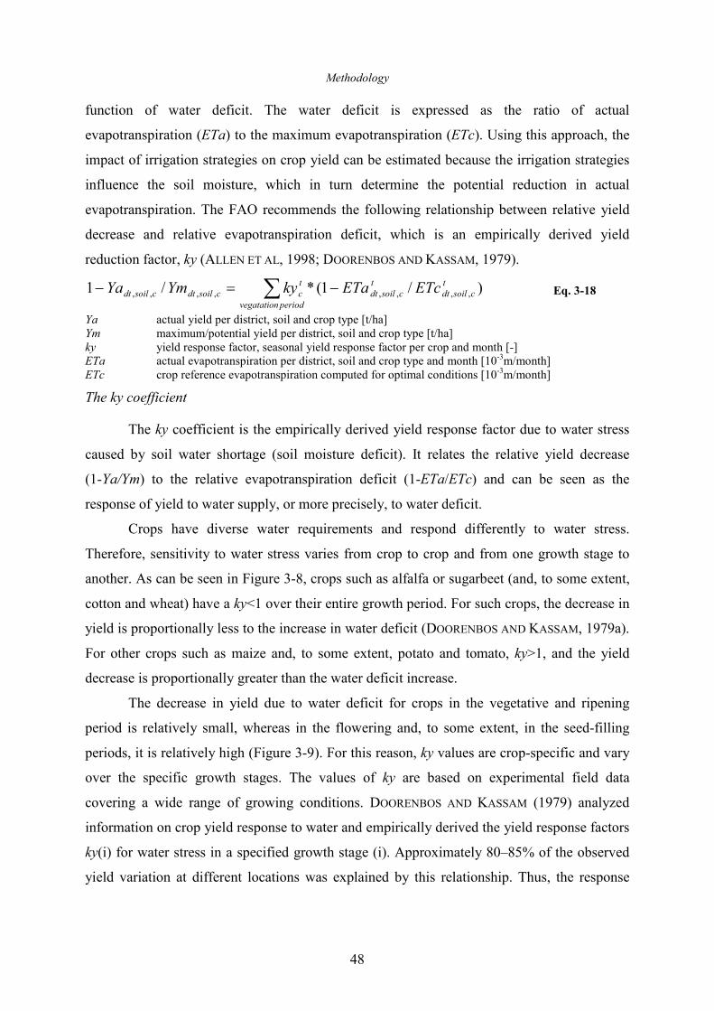
Methodology
48
function of water deficit. The water deficit is expressed as the ratio of actual
evapotranspiration (ETa) to the maximum evapotranspiration (ETc). Using this approach, the
impact of irrigation strategies on crop yield can be estimated because the irrigation strategies
influence the soil moisture, which in turn determine the potential reduction in actual
evapotranspiration. The FAO recommends the following relationship between relative yield
decrease and relative evapotranspiration deficit, which is an empirically derived yield
reduction factor, ky (ALLEN ET AL, 1998; DOORENBOS AND KASSAM, 1979).
∑ −=−periodvegatation
tcsoildt
tcsoildt
tccsoildtcsoildt ETcETakyYmYa )/1(*/1 ,,,,,,,, Eq. 3-18
Ya actual yield per district, soil and crop type [t/ha] Ym maximum/potential yield per district, soil and crop type [t/ha] ky yield response factor, seasonal yield response factor per crop and month [-] ETa actual evapotranspiration per district, soil and crop type and month [10-3m/month] ETc crop reference evapotranspiration computed for optimal conditions [10-3m/month]
The ky coefficient
The ky coefficient is the empirically derived yield response factor due to water stress
caused by soil water shortage (soil moisture deficit). It relates the relative yield decrease
(1-Ya/Ym) to the relative evapotranspiration deficit (1-ETa/ETc) and can be seen as the
response of yield to water supply, or more precisely, to water deficit.
Crops have diverse water requirements and respond differently to water stress.
Therefore, sensitivity to water stress varies from crop to crop and from one growth stage to
another. As can be seen in Figure 3-8, crops such as alfalfa or sugarbeet (and, to some extent,
cotton and wheat) have a ky<1 over their entire growth period. For such crops, the decrease in
yield is proportionally less to the increase in water deficit (DOORENBOS AND KASSAM, 1979a).
For other crops such as maize and, to some extent, potato and tomato, ky>1, and the yield
decrease is proportionally greater than the water deficit increase.
The decrease in yield due to water deficit for crops in the vegetative and ripening
period is relatively small, whereas in the flowering and, to some extent, in the seed-filling
periods, it is relatively high (Figure 3-9). For this reason, ky values are crop-specific and vary
over the specific growth stages. The values of ky are based on experimental field data
covering a wide range of growing conditions. DOORENBOS AND KASSAM (1979) analyzed
information on crop yield response to water and empirically derived the yield response factors
ky(i) for water stress in a specified growth stage (i). Approximately 80–85% of the observed
yield variation at different locations was explained by this relationship. Thus, the response
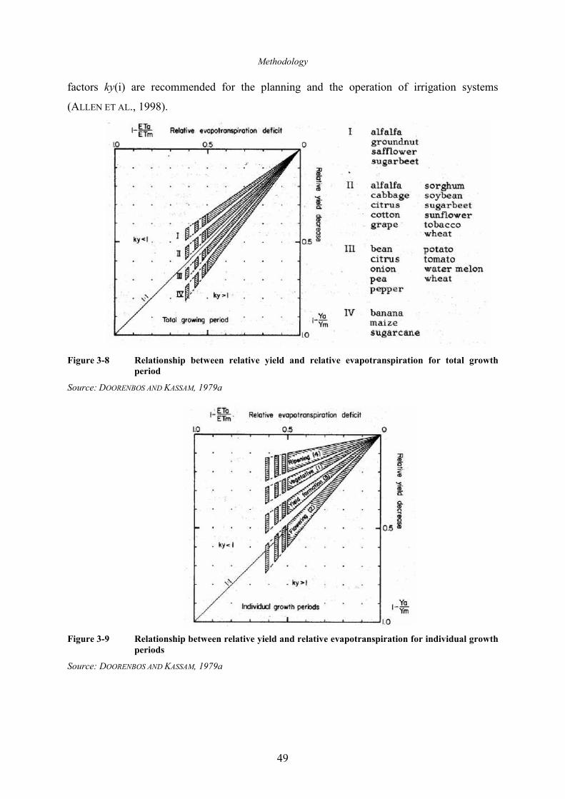
Methodology
49
factors ky(i) are recommended for the planning and the operation of irrigation systems
(ALLEN ET AL., 1998).
Figure 3-8 Relationship between relative yield and relative evapotranspiration for total growth
period
Source: DOORENBOS AND KASSAM, 1979a
Figure 3-9 Relationship between relative yield and relative evapotranspiration for individual growth
periods
Source: DOORENBOS AND KASSAM, 1979a
Methodology
50
3.2.4 Economic Component
The operation of hydrologic-agronomic systems in integrated hydrologic-economic
models is driven by socio-economic objectives, whereas the economic incentives are linked to
the physical system. The objective of this model is to maximize the gross margins in irrigated
agriculture specifically for the ten districts using physical, institutional and agro-political
constraints. The objective function is expressed as follows:
Eq. 3-19
Gross Margins and Water Costs
The total gross margin from agricultural demand sites (Aprft) is equal to crop revenue
(see Eq. 3-27) minus the fixed variable cropping costs (otc), groundwater pumping costs (gct)
and surface water supply costs (sct).
∑∑ ∑
−
−
−=
soil cp
dtdt
mdtmcpsoildtgw
cpdtcpsoildt
cpsoildtcpsoildtcpsoildtcpdt
dt
swdsct
gctpump
otcacp
cppACPmryldy
Aprft
)*(
)*(
)*(
)***max(
,,,,
,,,
,,,,,,,
Eq. 3-20
obj objective function [USD] otc other costs for crop cultivation [USD/ha]
Aprft agricultural gross margin [USD] pump groundwater pumping [m3]
ymax max yield [t/ha] gct groundwater pumping costs per unit [USD/m3]
mryld min relative yield [-] swd surface water diversion to districts [m3]
acp irrigated crop area [ha] sct surface water price per unit [USD/m3]
cpp crop price [USD/t]
Gross margins per crop, gross water costs and gross water application for a single
crop/crop field and for all the districts is calculated as follows:
cdts
csoildtcdtcdtcdt otcacpcWCcRvcGM ,,,,,, *___ ∑−−= Eq. 3-21
Whereas the total gross margins are the sum of all the per crop gross margins:
∑=c
cdtdt cGMallGM ,__ Eq. 3-22
∑=dt
dtAprftobj )(max
Methodology
51
Total water costs and water costs per crop are a function of the surface and pumping
water applied to the field and their supply costs:
dtcdtdtcdtcdt gctcPWsctcSWcWC *_*__ ,,, += Eq. 3-23
dtdtdtdtdt gctallPWsctallSWallWC *_*__ += Eq. 3-24
The amount of surface water application depends on the water applied to the crop field
and the distribution losses in the system:
∑∑ +=t s
tcsoildtcdt leachdstreffWCPcSW )1(*_/_ ,,, Eq. 3-25
∑=t
tdtdt DTWSallSW __ Eq. 3-26
The following terms are used in these equations:
GM_c, GM_all gross margins for crops and districts [USD]
SW_c, SW_all
surface water applied to crops and districts [m3]
Rv_c, Rv_all revenue for crops and districts [USD]
PW_c, PW_all
pumped water applied to crops and districts [m3]
WC_c, WC_all water costs for crops and districts [USD]
sct surface water price (costs) [USD/m3]
WV_c, WV_all value of water for crops and districts [-]
WCP surface water applied to fields [m3]
otc other variable crop cultivation costs [USD/ha]
acp cropped area [ha]
gct groundwater pumping costs [USD/m3]
eff_dstr distribution efficiency [-]
WS_DT gross water supply to districts [m3] dt,soil,c district, soil type, crop-indices
leach leaching fraction of water application [-]
Revenues
Crop revenues are determined by calculating actual yields per calculated cropped area
and the associated market prices (Eq. 3-27). Finally, the actual yields are a product of the
maximum potential yields per crop and the relative yields, which is an endogenously derived
variable that includes the actual evapotranspiration (see Eq. 3-12) and yield response to water
and crop coefficients for all crops in dependency of soil, climatic and crop characteristics.
Thus, the main connection between agronomy and economy is found in this relationship, as
actual evapotranspiration depends on climatic and soil moisture conditions, which in turn
depend on hydrology and water management strategies.
Methodology
52
cdtcsoildtcsoildtsoil
cdtcdt cppacpYmryldcRv ,,,,,,, ***_ ∑= ,
∑=c
cdtdt cRvallRv ,__ Eq. 3-27
ryld relative cop yield per district, soil and crop type and month [-]
Ym maximum potential yield per district, soil and crop type [t/ha]
cpp cop selling prices per district and crop [USD/t]
Relative yield (ryld) is attained by conversion of the crop production function (Eq.
3-18):
csoildt
csoildt
periodvegetationtdt
tc
tcsoildtt
ct
csoildtYm
Ya
ETokc
ETakyryld
,,
,,,,,, )
*1(*1 =−−= ∑ Eq. 3-28
Economic Water Use Efficiency
The economic water use efficiency (e-WUE) according to ZAFFARONI AND SCHNEITER
(1998) and COPELAND ET AL. (1993) is defined as the economic outcome (gross margin in
irrigated agriculture) over the total water applied and not mistakable with the water use
efficiency term used in bio-physics. Here the water use efficiency is a function of biomass
yield over total water application. The e-WUE already includes this factor, as gross margin is
a function of the crop yields. Furthermore, the crop prices and the productivity and cost
effectiveness of the crop planted are implemented (see Eq. 3-20, 3-21, 3-27). The e-WUE is
an important indicator of the profitability of a crop in terms of water use and will be examined
in more detail for single crops and districts in chapter 5.
cdtcdtcdt cTWcGMcWUEe ,,, _/__ =− Eq. 3-29
dtdtdt allTWallGMallWUEe _/__ =− Eq. 3-30
TW_c, TW_all
total water applied to crops and districts [m3]
e-WUE_c e-Wue_all
economic water use efficiency for single crops and for total Khorezm [-]
The total water applied to districts and crops is composed of surface water (SW_c,
SW_all, see Eq. 3-25 and 3-26) and a small amount of groundwater pumped (pump):
cdtcdtcdt pumpcSWcTW ,,, __ += Eq. 3-31
An important aim of this study is to apply economic incentives (such as subventions,
cost calculations, prices and liberalization of the cotton sector) to find alternatives for efficient
Methodology
53
water and crop allocation. To determine whether these alternatives have an effect on the
current system, the main economic task will be the analysis of economic incentives and their
influences on benefits and costs, the hydrologic system operation, crop allocation and the
water use in each scenario analysis.
Price-Function
Thus far, sales prices for agricultural products have been exogenously provided to the
model using fixed parameters according to actual surveyed market price data (see Appendix
C). For scenarios with liberalized cotton and wheat markets or the introduction of water
pricing mechanisms and released crop areas, it is important to implement an endogenous crop
price function to analyze the effect of modified supply to the demand for agricultural products
in an acreage-dependent manner (see chapter 8.3). Otherwise, corner solutions with high
acreages of water-cost/price-efficient crops will arise that under consideration of optimal
ecological water allocation seem reasonable. However, these solutions are not realistic
because farmers strive to diversify their products and reduce the risk of decreasing prices for
over-supplied crops. For this reason, the crop selling price will be endogenously calculated
using a relationship between supplied goods and people’s demand, and, related to that
willingness and ability to pay for such goods. Supply is determined by the market. If farmers
increase their production (and, thus, supply) the price will decrease. Thus, farmers will grow
fewer crops, reduce the size the cropland or diversify crop cultivation until an equilibrium
supply and demand is attained.
The price-function is implemented in the agricultural profit function (see Eq. 3-20).
Crop demand is a function of price and is characterized as follows:
csoildtcdt PBaPD ,,, *)( −= and Eq. 3-32
cdtcsoildt DBB
aP ,,, *
1−=
and Eq. 3-33
1,,
1,*
−
−
=t
csoildt
tcdt
P
DB η
Eq. 3-34 D/Dt-1 P/Pt-1
crop demand/demand last year crop price/price last year
a B
constant (y-intercept) constant (slope)
η price-elasticity
Methodology
54
Price elasticity η (of demand) is defined as the relative change in quantity of goods to
a relative change in the price of those goods (GRAF, 2002). Price elasticity was calculated for
some agricultural products in Khorezm by DJANIBEKOV (2008). The constant a can be derived
from the production level in Khorezm in 2003 (see Appendix B).
55
4 Data Analysis and Credibility Control
The availability, quality and credibility of input data are major factors determining the
quality and significance of a model. Various data were used for the integrated hydrologic-
economic model presented. These data build a foundation for further model-relevant
calculations, outcomes and analyses. For this reason it is necessary to monitor the credibility
of all relevant data. The methods used to monitor data credibility are described below.
The modeling framework required multidisciplinary data on local hydrology,
climatology, agronomy, economy, sociology, and crop and soil parameters. In addition to
experimental data from the project, this study also used data from other studies and projects,
secondary statistical data, empirically determined data, data from the literature and internet,
official governmental scientific databases, and expert knowledge. A range of data types were
used, including time series and single measurements, spatial and non-spatial data, country-
level, district-level, and field-level data with high or low resolution, and qualitative and
quantitative data. The basis year is 2003, but data collected between 1990 till 2004 were used
when available, for example, in climatologic and groundwater analyses.
Large data sets are necessary to conduct such an integrated study. The data collections
and measurements used and/or processed in this study were taken from studies within the
Khorezm-Project, databases of the project and other institutions involved in agronomic-
hydrologic-climatologic-economic investigations in Khorezm and Uzbekistan. Data on soil
moisture, matrix potential, plant characteristics, precipitation, humidity, sunlight duration,
groundwater table, aquifer yield coefficient, cropped areas, yields, prices and planting costs,
irrigation efficiencies and salinity were included. The FAO CropWat program was used to
determine the effective rainfall and reference evapotranspiration. The broad GIS-database of
the project and the so-called hydromodule zones (MAWR, 1987) were used to obtain soil
types in each district. The Russias Meteo Data Server (SMIS, 2003) contained climate data for
the Meteo-Stations in the Khiva and Urgench districts. From the JICA-study (JICA, 1996), it
was possible to calculate municipal and industrial (M&I) water use. The MAWR (2002)
provided detailed measurements of groundwater level, groundwater salinity and drainage
areas and SOKOLOV (1999) for groundwater pumping capacities. The Rosetta program
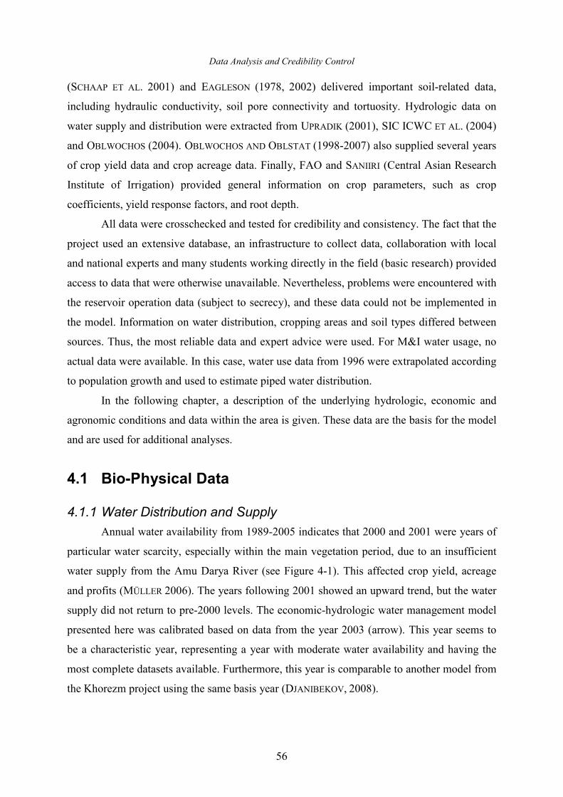
Data Analysis and Credibility Control
56
(SCHAAP ET AL. 2001) and EAGLESON (1978, 2002) delivered important soil-related data,
including hydraulic conductivity, soil pore connectivity and tortuosity. Hydrologic data on
water supply and distribution were extracted from UPRADIK (2001), SIC ICWC ET AL. (2004)
and OBLWOCHOS (2004). OBLWOCHOS AND OBLSTAT (1998-2007) also supplied several years
of crop yield data and crop acreage data. Finally, FAO and SANIIRI (Central Asian Research
Institute of Irrigation) provided general information on crop parameters, such as crop
coefficients, yield response factors, and root depth.
All data were crosschecked and tested for credibility and consistency. The fact that the
project used an extensive database, an infrastructure to collect data, collaboration with local
and national experts and many students working directly in the field (basic research) provided
access to data that were otherwise unavailable. Nevertheless, problems were encountered with
the reservoir operation data (subject to secrecy), and these data could not be implemented in
the model. Information on water distribution, cropping areas and soil types differed between
sources. Thus, the most reliable data and expert advice were used. For M&I water usage, no
actual data were available. In this case, water use data from 1996 were extrapolated according
to population growth and used to estimate piped water distribution.
In the following chapter, a description of the underlying hydrologic, economic and
agronomic conditions and data within the area is given. These data are the basis for the model
and are used for additional analyses.
4.1 Bio-Physical Data
4.1.1 Water Distribution and Supply
Annual water availability from 1989-2005 indicates that 2000 and 2001 were years of
particular water scarcity, especially within the main vegetation period, due to an insufficient
water supply from the Amu Darya River (see Figure 4-1). This affected crop yield, acreage
and profits (MÜLLER 2006). The years following 2001 showed an upward trend, but the water
supply did not return to pre-2000 levels. The economic-hydrologic water management model
presented here was calibrated based on data from the year 2003 (arrow). This year seems to
be a characteristic year, representing a year with moderate water availability and having the
most complete datasets available. Furthermore, this year is comparable to another model from
the Khorezm project using the same basis year (DJANIBEKOV, 2008).
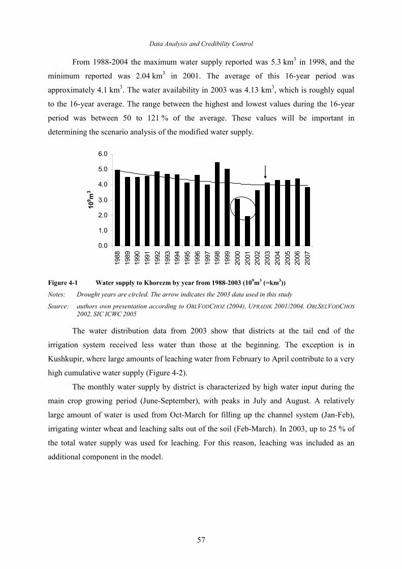
Data Analysis and Credibility Control
57
From 1988-2004 the maximum water supply reported was 5.3 km3 in 1998, and the
minimum reported was 2.04 km3 in 2001. The average of this 16-year period was
approximately 4.1 km3. The water availability in 2003 was 4.13 km3, which is roughly equal
to the 16-year average. The range between the highest and lowest values during the 16-year
period was between 50 to 121 % of the average. These values will be important in
determining the scenario analysis of the modified water supply.
0.0
1.0
2.0
3.0
4.0
5.0
6.0
1988
1989
1990
1991
1992
1993
1994
1995
1996
1997
1998
1999
2000
2001
2002
2003
2004
2005
2006
2007
109m
3
Figure 4-1 Water supply to Khorezm by year from 1988-2003 (10
9m
3 (=km
3))
Notes: Drought years are circled. The arrow indicates the 2003 data used in this study
Source: authors own presentation according to OBLVODCHOZ (2004), UPRADIK 2001/2004, OBLSELVODCHOS
2002, SIC ICWC 2005
The water distribution data from 2003 show that districts at the tail end of the
irrigation system received less water than those at the beginning. The exception is in
Kushkupir, where large amounts of leaching water from February to April contribute to a very
high cumulative water supply (Figure 4-2).
The monthly water supply by district is characterized by high water input during the
main crop growing period (June-September), with peaks in July and August. A relatively
large amount of water is used from Oct-March for filling up the channel system (Jan-Feb),
irrigating winter wheat and leaching salts out of the soil (Feb-March). In 2003, up to 25 % of
the total water supply was used for leaching. For this reason, leaching was included as an
additional component in the model.
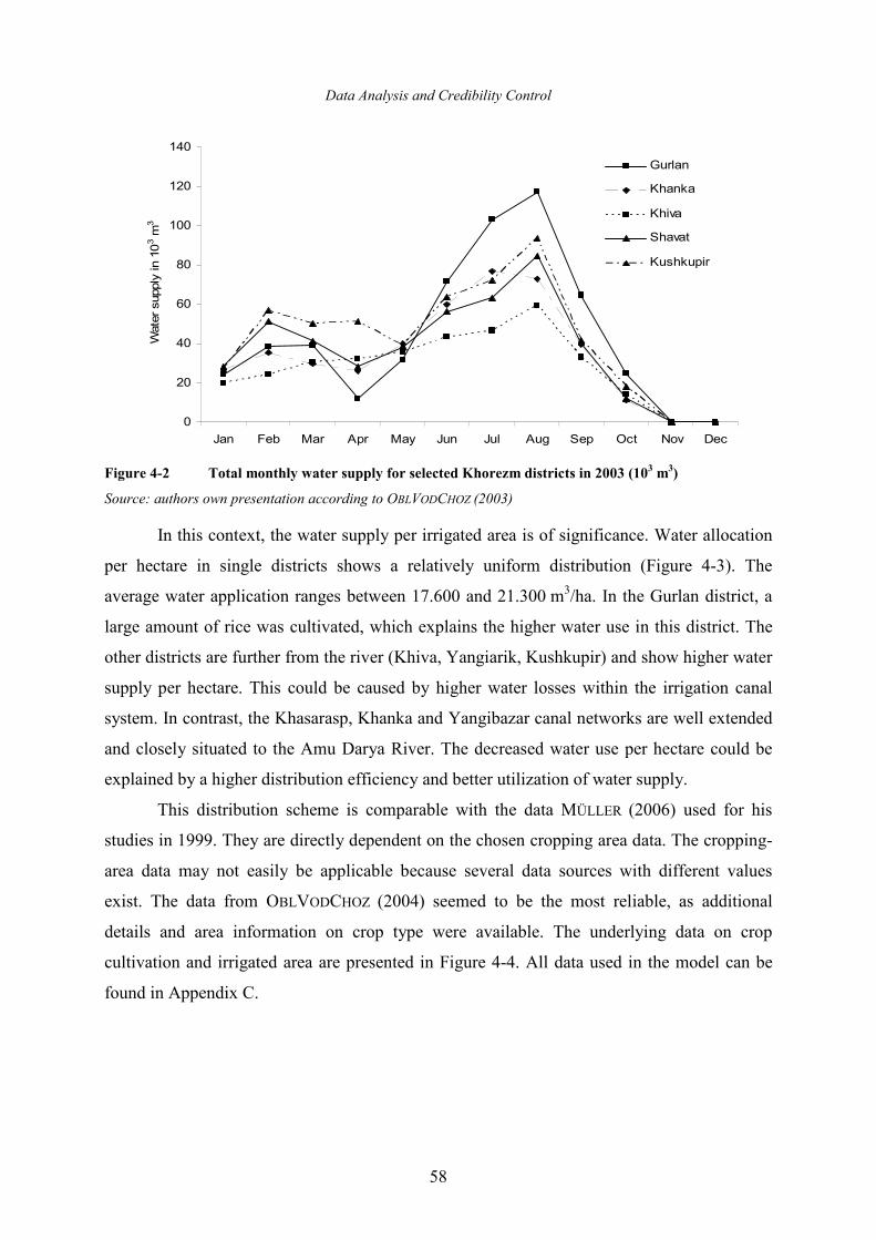
Data Analysis and Credibility Control
58
0
20
40
60
80
100
120
140
Jan Feb Mar Apr May Jun Jul Aug Sep Oct Nov Dec
Water supply in 103 m
3
Gurlan
Khanka
Khiva
Shavat
Kushkupir
Figure 4-2 Total monthly water supply for selected Khorezm districts in 2003 (103 m
3)
Source: authors own presentation according to OBLVODCHOZ (2003)
In this context, the water supply per irrigated area is of significance. Water allocation
per hectare in single districts shows a relatively uniform distribution (Figure 4-3). The
average water application ranges between 17.600 and 21.300 m3/ha. In the Gurlan district, a
large amount of rice was cultivated, which explains the higher water use in this district. The
other districts are further from the river (Khiva, Yangiarik, Kushkupir) and show higher water
supply per hectare. This could be caused by higher water losses within the irrigation canal
system. In contrast, the Khasarasp, Khanka and Yangibazar canal networks are well extended
and closely situated to the Amu Darya River. The decreased water use per hectare could be
explained by a higher distribution efficiency and better utilization of water supply.
This distribution scheme is comparable with the data MÜLLER (2006) used for his
studies in 1999. They are directly dependent on the chosen cropping area data. The cropping-
area data may not easily be applicable because several data sources with different values
exist. The data from OBLVODCHOZ (2004) seemed to be the most reliable, as additional
details and area information on crop type were available. The underlying data on crop
cultivation and irrigated area are presented in Figure 4-4. All data used in the model can be
found in Appendix C.
Data Analysis and Credibility Control
59
Figure 4-3 Irrigation water supply per hectare in 2003 at the district border (m3/ha)
Source: authors own calculation, based on data from OBLVODCHOZ (2003) and SoyuzNihiUzAshi, 1992
4.1.2 Soil Types
To account for the different soil types in the dataset, the model differentiates between
the hydro-module zones, which are a differentiation of soils based on soil texture and
groundwater table levels. This classification system seemed to be most suitable for the model.
The main soil types and related crop outcomes for those soil types can be considered without
overloading the model. Furthermore, the groundwater level within the hydro-module zones
classification is an important factor (especially for the Khorezm region) because the
groundwater table (and balances) will also be considered in the model.
Light soils are considered to be sandy and sandy-loamy soils (clay fraction <35 %),
whereas medium soils are moderately textured loamy soils. Heavy soils are the heavy loamy
and loamy soils with homogeneous and heterogeneous texture and a minimum clay fraction of
45 % (SOYUZNIHIUZASHI, 1992; for detailed information see Appendix C). Soil textural
classes determine important parameters such as soil hydraulic conductivity, basic soil water
characteristics (saturation, field capacity, permanent wilting point) and as a consequence soil
moisture. These parameters have a strong influence on soil-water balance and crop yields. As
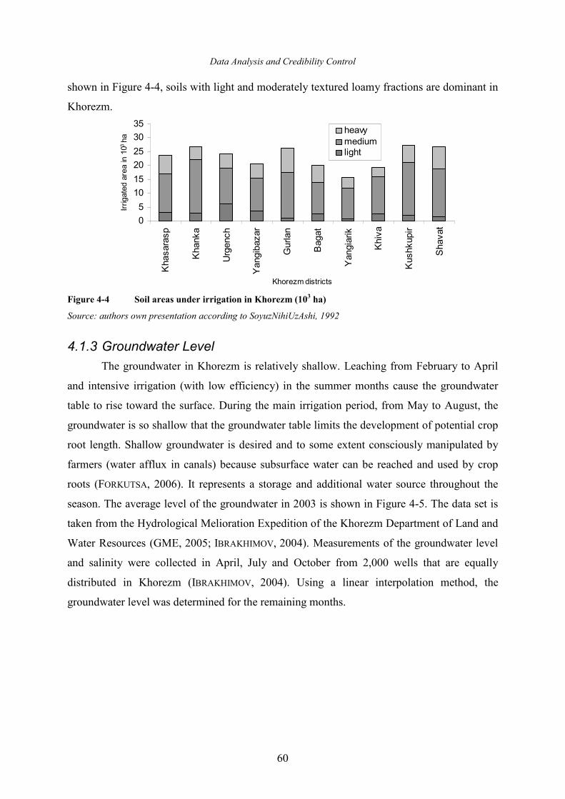
Data Analysis and Credibility Control
60
shown in Figure 4-4, soils with light and moderately textured loamy fractions are dominant in
Khorezm.
0
5
10
15
20
25
30
35
Khasarasp
Khanka
Urgench
Yangibazar
Gurlan
Bagat
Yangiarik
Khiva
Kushkupir
Shavat
Khorezm districts
Irrigated area in 103
ha
heavy
mediumlight
Figure 4-4 Soil areas under irrigation in Khorezm (10
3 ha)
Source: authors own presentation according to SoyuzNihiUzAshi, 1992
4.1.3 Groundwater Level
The groundwater in Khorezm is relatively shallow. Leaching from February to April
and intensive irrigation (with low efficiency) in the summer months cause the groundwater
table to rise toward the surface. During the main irrigation period, from May to August, the
groundwater is so shallow that the groundwater table limits the development of potential crop
root length. Shallow groundwater is desired and to some extent consciously manipulated by
farmers (water afflux in canals) because subsurface water can be reached and used by crop
roots (FORKUTSA, 2006). It represents a storage and additional water source throughout the
season. The average level of the groundwater in 2003 is shown in Figure 4-5. The data set is
taken from the Hydrological Melioration Expedition of the Khorezm Department of Land and
Water Resources (GME, 2005; IBRAKHIMOV, 2004). Measurements of the groundwater level
and salinity were collected in April, July and October from 2,000 wells that are equally
distributed in Khorezm (IBRAKHIMOV, 2004). Using a linear interpolation method, the
groundwater level was determined for the remaining months.
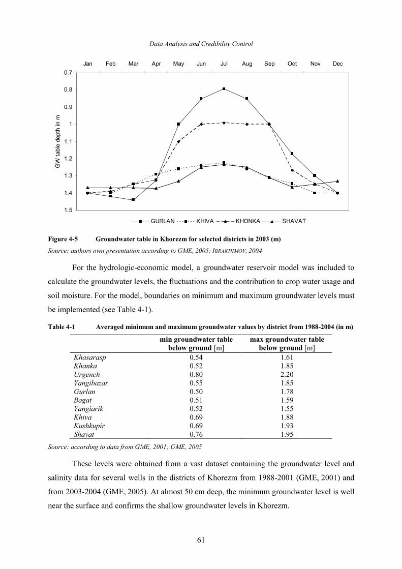
Data Analysis and Credibility Control
61
0.7
0.8
0.9
1
1.1
1.2
1.3
1.4
1.5
Jan Feb Mar Apr May Jun Jul Aug Sep Oct Nov DecGW table depth in m
GURLAN KHIVA KHONKA SHAVAT
Figure 4-5 Groundwater table in Khorezm for selected districts in 2003 (m)
Source: authors own presentation according to GME, 2005; IBRAKHIMOV, 2004
For the hydrologic-economic model, a groundwater reservoir model was included to
calculate the groundwater levels, the fluctuations and the contribution to crop water usage and
soil moisture. For the model, boundaries on minimum and maximum groundwater levels must
be implemented (see Table 4-1).
Table 4-1 Averaged minimum and maximum groundwater values by district from 1988-2004 (in m)
min groundwater table
below ground [m] max groundwater table
below ground [m] Khasarasp 0.54 1.61 Khanka 0.52 1.85 Urgench 0.80 2.20 Yangibazar 0.55 1.85 Gurlan 0.50 1.78 Bagat 0.51 1.59 Yangiarik 0.52 1.55 Khiva 0.69 1.88 Kushkupir 0.69 1.93 Shavat 0.76 1.95
Source: according to data from GME, 2001; GME, 2005
These levels were obtained from a vast dataset containing the groundwater level and
salinity data for several wells in the districts of Khorezm from 1988-2001 (GME, 2001) and
from 2003-2004 (GME, 2005). At almost 50 cm deep, the minimum groundwater level is well
near the surface and confirms the shallow groundwater levels in Khorezm.
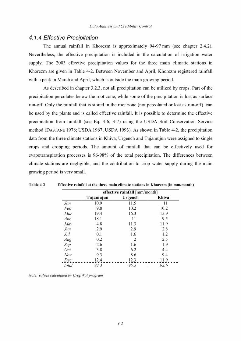
Data Analysis and Credibility Control
62
4.1.4 Effective Precipitation
The annual rainfall in Khorezm is approximately 94-97 mm (see chapter 2.4.2).
Nevertheless, the effective precipitation is included in the calculation of irrigation water
supply. The 2003 effective precipitation values for the three main climatic stations in
Khorezm are given in Table 4-2. Between November and April, Khorezm registered rainfall
with a peak in March and April, which is outside the main growing period.
As described in chapter 3.2.3, not all precipitation can be utilized by crops. Part of the
precipitation percolates below the root zone, while some of the precipitation is lost as surface
run-off. Only the rainfall that is stored in the root zone (not percolated or lost as run-off), can
be used by the plants and is called effective rainfall. It is possible to determine the effective
precipitation from rainfall (see Eq. 3-6, 3-7) using the USDA Soil Conservation Service
method (DASTANE 1978; USDA 1967; USDA 1993). As shown in Table 4-2, the precipitation
data from the three climate stations in Khiva, Urgench and Tujamujun were assigned to single
crops and cropping periods. The amount of rainfall that can be effectively used for
evapotranspiration processes is 96-98% of the total precipitation. The differences between
climate stations are negligible, and the contribution to crop water supply during the main
growing period is very small.
Table 4-2 Effective rainfall at the three main climate stations in Khorezm (in mm/month)
effective rainfall [mm/month] Tujamujun Urgench Khiva
Jan 10.9 11.5 11 Feb 9.8 10.2 10.2 Mar 19.4 16.3 15.9 Apr 18.1 11 9.5 May 4.8 11.3 11.9 Jun 2.9 2.9 2.8 Jul 0.1 1.6 1.2 Aug 0.2 2 2.5 Sep 2.6 1.6 1.9 Oct 3.8 6.2 4.4 Nov 9.3 8.6 9.4 Dec 12.4 12.3 11.9 total 94.3 95.5 92.6
Note: values calculated by CropWat program
Data Analysis and Credibility Control
63
4.2 Agro-Economical Crop Data and Efficiencies
4.2.1 Reference Evapotranspiration
The term ‘reference evapotranspiration’ (ETo) refers to the potential
evapotranspiration of a reference crop (grass) under given regional and climatologic
conditions with no water shortages. It is affected by climatic parameters such as pressure,
wind speed, temperature, radiation and sunlight hours and is calculated using the Penman-
Monteith method (see Eq. 3-10, ALLEN ET AL., 1998, FAO CropWat). Reference
evapotranspiration plays an important role in the model in the calculation of actual
evapotranspiration, crop water demand and, finally, crop yields. Weather data from the three
main climate stations in Khorezm were used.
The calculated ETo values in 2003 range from 1,166 to 1,515 mm/a, depending on the
climate station in Khorezm. The values peak during the hot and dry summer months (see
Figure 4-6 and Appendix C) and are comparable to the estimates of CONRAD (2006), who
reported values of 1,500 mm/a in Khorezm. Values of the FAO classification (FAO, 2000)
also range between 1,000-1,500 mm/a for this region. Compared with precipitation data for
the main growing season, a deficit in crop water supply is obvious and must be corrected with
intensive irrigation.
0
50
100
150
200
250
300
Jan
Feb
Mar
Apr
May
Jun
Jul
Aug
Sep
Oct
Nov
Dec
ETo in m
m/m
onth
Urgench
Khiva
Tujamujun
Figure 4-6 Reference evapotranspiration at the main climate stations in Khorezm (mm/month)
Note: values calculated by CropWat program
4.2.2 Kc-Values
Reference evapotranspiration (ETo) is the basis for calculating the potential
evapotranspiration of a specific crop (ETc). Kc values depend on specific crop characteristics
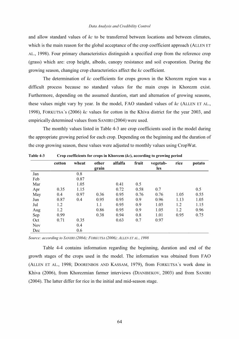
Data Analysis and Credibility Control
64
and allow standard values of kc to be transferred between locations and between climates,
which is the main reason for the global acceptance of the crop coefficient approach (ALLEN ET
AL., 1998). Four primary characteristics distinguish a specified crop from the reference crop
(grass) which are: crop height, albedo, canopy resistance and soil evaporation. During the
growing season, changing crop characteristics affect the kc coefficient.
The determination of kc coefficients for crops grown in the Khorezm region was a
difficult process because no standard values for the main crops in Khorezm exist.
Furthermore, depending on the assumed duration, start and alternation of growing seasons,
these values might vary by year. In the model, FAO standard values of kc (ALLEN ET AL.,
1998), FORKUTSA´s (2006) kc values for cotton in the Khiva district for the year 2003, and
empirically determined values from SANIIRI (2004) were used.
The monthly values listed in Table 4-3 are crop coefficients used in the model during
the appropriate growing period for each crop. Depending on the beginning and the duration of
the crop growing season, these values were adjusted to monthly values using CropWat.
Table 4-3 Crop coefficients for crops in Khorezm (kc), according to growing period
cotton wheat other
grain
alfalfa fruit vegetab-
les
rice potato
Jan 0.8 Feb 0.87 Mar 1.05 0.41 0.5 Apr 0.35 1.15 0.72 0.58 0.7 0.5 May 0.4 0.97 0.36 0.95 0.76 0.76 1.05 0.55 Jun 0.87 0.4 0.95 0.95 0.9 0.96 1.13 1.05 Jul 1.2 1.1 0.95 0.9 1.05 1.2 1.15 Aug 1.2 0.86 0.95 0.9 1.05 1.2 0.96 Sep 0.99 0.38 0.94 0.8 1.01 0.95 0.75 Oct 0.71 0.35 0.63 0.7 0.97 Nov 0.4 Dec 0.6
Source: according to SANIIRI (2004); FORKUTSA (2006); ALLEN ET AL., 1998
Table 4-4 contains information regarding the beginning, duration and end of the
growth stages of the crops used in the model. The information was obtained from FAO
(ALLEN ET AL., 1998; DOORENBOS AND KASSAM, 1979), from FORKUTSA´s work done in
Khiva (2006), from Khorezmian farmer interviews (DJANIBEKOV, 2003) and from SANIIRI
(2004). The latter differ for rice in the initial and mid-season stage.
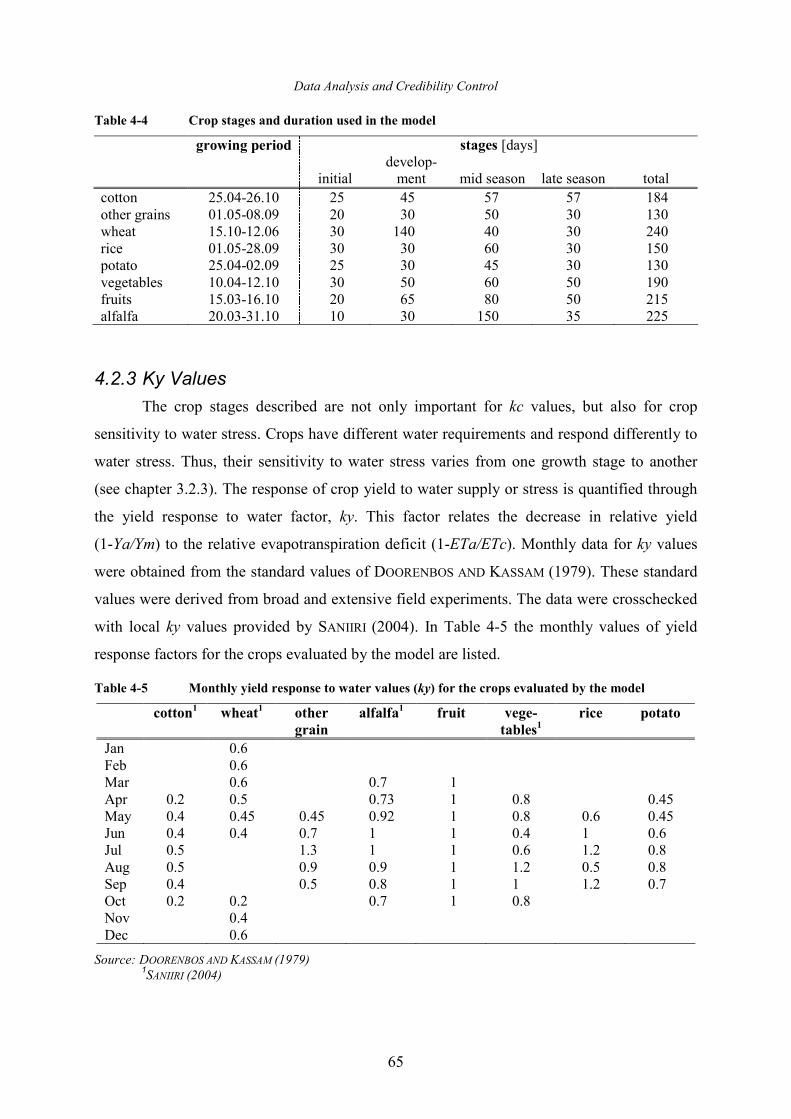
Data Analysis and Credibility Control
65
Table 4-4 Crop stages and duration used in the model
stages [days]
growing period
initial develop-
ment mid season late season total cotton 25.04-26.10 25 45 57 57 184 other grains 01.05-08.09 20 30 50 30 130 wheat 15.10-12.06 30 140 40 30 240 rice 01.05-28.09 30 30 60 30 150 potato 25.04-02.09 25 30 45 30 130 vegetables 10.04-12.10 30 50 60 50 190 fruits 15.03-16.10 20 65 80 50 215 alfalfa 20.03-31.10 10 30 150 35 225
4.2.3 Ky Values
The crop stages described are not only important for kc values, but also for crop
sensitivity to water stress. Crops have different water requirements and respond differently to
water stress. Thus, their sensitivity to water stress varies from one growth stage to another
(see chapter 3.2.3). The response of crop yield to water supply or stress is quantified through
the yield response to water factor, ky. This factor relates the decrease in relative yield
(1-Ya/Ym) to the relative evapotranspiration deficit (1-ETa/ETc). Monthly data for ky values
were obtained from the standard values of DOORENBOS AND KASSAM (1979). These standard
values were derived from broad and extensive field experiments. The data were crosschecked
with local ky values provided by SANIIRI (2004). In Table 4-5 the monthly values of yield
response factors for the crops evaluated by the model are listed.
Table 4-5 Monthly yield response to water values (ky) for the crops evaluated by the model
cotton1 wheat
1 other
grain
alfalfa1 fruit vege-
tables1
rice potato
Jan 0.6
Feb 0.6 Mar 0.6 0.7 1 Apr 0.2 0.5 0.73 1 0.8 0.45 May 0.4 0.45 0.45 0.92 1 0.8 0.6 0.45 Jun 0.4 0.4 0.7 1 1 0.4 1 0.6 Jul 0.5 1.3 1 1 0.6 1.2 0.8 Aug 0.5 0.9 0.9 1 1.2 0.5 0.8 Sep 0.4 0.5 0.8 1 1 1.2 0.7 Oct 0.2 0.2 0.7 1 0.8 Nov 0.4 Dec 0.6
Source: DOORENBOS AND KASSAM (1979) 1SANIIRI (2004)
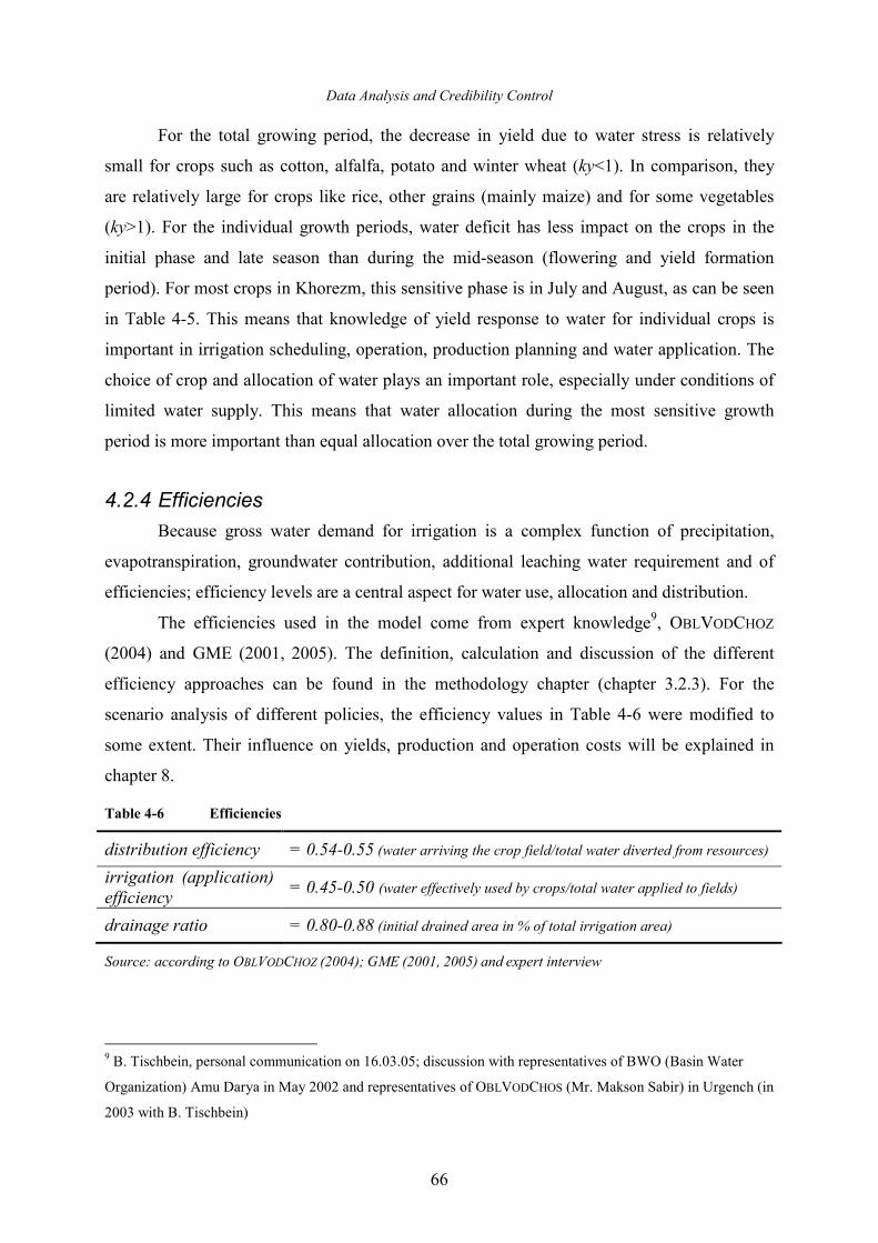
Data Analysis and Credibility Control
66
For the total growing period, the decrease in yield due to water stress is relatively
small for crops such as cotton, alfalfa, potato and winter wheat (ky<1). In comparison, they
are relatively large for crops like rice, other grains (mainly maize) and for some vegetables
(ky>1). For the individual growth periods, water deficit has less impact on the crops in the
initial phase and late season than during the mid-season (flowering and yield formation
period). For most crops in Khorezm, this sensitive phase is in July and August, as can be seen
in Table 4-5. This means that knowledge of yield response to water for individual crops is
important in irrigation scheduling, operation, production planning and water application. The
choice of crop and allocation of water plays an important role, especially under conditions of
limited water supply. This means that water allocation during the most sensitive growth
period is more important than equal allocation over the total growing period.
4.2.4 Efficiencies
Because gross water demand for irrigation is a complex function of precipitation,
evapotranspiration, groundwater contribution, additional leaching water requirement and of
efficiencies; efficiency levels are a central aspect for water use, allocation and distribution.
The efficiencies used in the model come from expert knowledge9, OBLVODCHOZ
(2004) and GME (2001, 2005). The definition, calculation and discussion of the different
efficiency approaches can be found in the methodology chapter (chapter 3.2.3). For the
scenario analysis of different policies, the efficiency values in Table 4-6 were modified to
some extent. Their influence on yields, production and operation costs will be explained in
chapter 8.
Table 4-6 Efficiencies
distribution efficiency = 0.54-0.55 (water arriving the crop field/total water diverted from resources)
irrigation (application) efficiency
= 0.45-0.50 (water effectively used by crops/total water applied to fields)
drainage ratio = 0.80-0.88 (initial drained area in % of total irrigation area)
Source: according to OBLVODCHOZ (2004); GME (2001, 2005) and expert interview
9 B. Tischbein, personal communication on 16.03.05; discussion with representatives of BWO (Basin Water
Organization) Amu Darya in May 2002 and representatives of OBLVODCHOS (Mr. Makson Sabir) in Urgench (in
2003 with B. Tischbein)
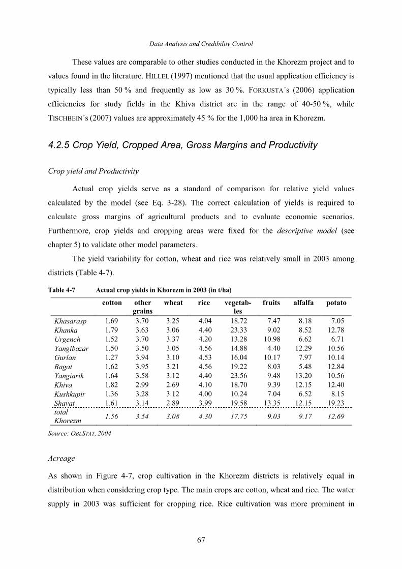
Data Analysis and Credibility Control
67
These values are comparable to other studies conducted in the Khorezm project and to
values found in the literature. HILLEL (1997) mentioned that the usual application efficiency is
typically less than 50 % and frequently as low as 30 %. FORKUSTA´s (2006) application
efficiencies for study fields in the Khiva district are in the range of 40-50 %, while
TISCHBEIN´s (2007) values are approximately 45 % for the 1,000 ha area in Khorezm.
4.2.5 Crop Yield, Cropped Area, Gross Margins and Productivity
Crop yield and Productivity
Actual crop yields serve as a standard of comparison for relative yield values
calculated by the model (see Eq. 3-28). The correct calculation of yields is required to
calculate gross margins of agricultural products and to evaluate economic scenarios.
Furthermore, crop yields and cropping areas were fixed for the descriptive model (see
chapter 5) to validate other model parameters.
The yield variability for cotton, wheat and rice was relatively small in 2003 among
districts (Table 4-7).
Table 4-7 Actual crop yields in Khorezm in 2003 (in t/ha)
cotton other
grains
wheat rice vegetab-
les
fruits alfalfa potato
Khasarasp 1.69 3.70 3.25 4.04 18.72 7.47 8.18 7.05 Khanka 1.79 3.63 3.06 4.40 23.33 9.02 8.52 12.78 Urgench 1.52 3.70 3.37 4.20 13.28 10.98 6.62 6.71 Yangibazar 1.50 3.50 3.05 4.56 14.88 4.40 12.29 10.56 Gurlan 1.27 3.94 3.10 4.53 16.04 10.17 7.97 10.14 Bagat 1.62 3.95 3.21 4.56 19.22 8.03 5.48 12.84 Yangiarik 1.64 3.58 3.12 4.40 23.56 9.48 13.20 10.56 Khiva 1.82 2.99 2.69 4.10 18.70 9.39 12.15 12.40 Kushkupir 1.36 3.28 3.12 4.00 10.24 7.04 6.52 8.15 Shavat 1.61 3.14 2.89 3.99 19.58 13.35 12.15 19.23 total Khorezm
1.56 3.54 3.08 4.30 17.75 9.03 9.17 12.69
Source: OBLSTAT, 2004
Acreage
As shown in Figure 4-7, crop cultivation in the Khorezm districts is relatively equal in
distribution when considering crop type. The main crops are cotton, wheat and rice. The water
supply in 2003 was sufficient for cropping rice. Rice cultivation was more prominent in
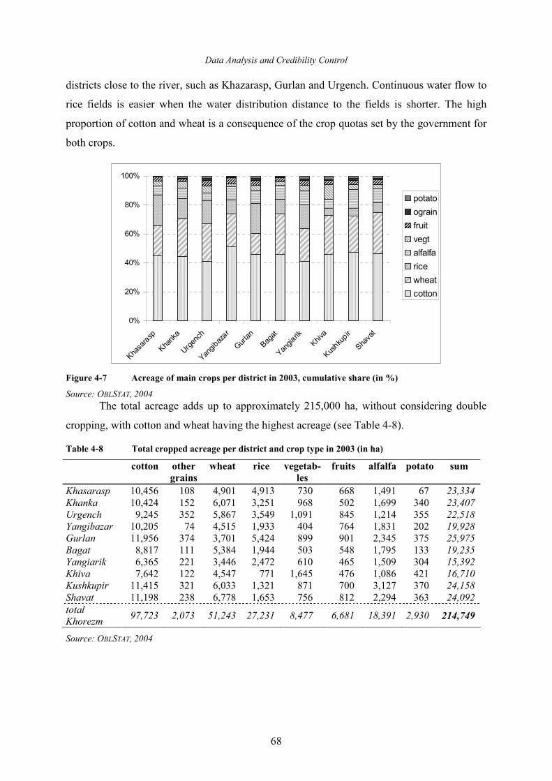
Data Analysis and Credibility Control
68
districts close to the river, such as Khazarasp, Gurlan and Urgench. Continuous water flow to
rice fields is easier when the water distribution distance to the fields is shorter. The high
proportion of cotton and wheat is a consequence of the crop quotas set by the government for
both crops.
0%
20%
40%
60%
80%
100%
Khasarasp
Khanka
Urgench
Yangibazar
Gurlan
Bagat
Yangiarik
Khiva
Kushkupir
Shavat
potato
ograin
fruit
vegt
alfalfa
rice
wheat
cotton
Figure 4-7 Acreage of main crops per district in 2003, cumulative share (in %)
Source: OBLSTAT, 2004 The total acreage adds up to approximately 215,000 ha, without considering double
cropping, with cotton and wheat having the highest acreage (see Table 4-8).
Table 4-8 Total cropped acreage per district and crop type in 2003 (in ha)
cotton other
grains
wheat rice vegetab-
les
fruits alfalfa potato sum
Khasarasp 10,456 108 4,901 4,913 730 668 1,491 67 23,334 Khanka 10,424 152 6,071 3,251 968 502 1,699 340 23,407 Urgench 9,245 352 5,867 3,549 1,091 845 1,214 355 22,518 Yangibazar 10,205 74 4,515 1,933 404 764 1,831 202 19,928 Gurlan 11,956 374 3,701 5,424 899 901 2,345 375 25,975 Bagat 8,817 111 5,384 1,944 503 548 1,795 133 19,235 Yangiarik 6,365 221 3,446 2,472 610 465 1,509 304 15,392 Khiva 7,642 122 4,547 771 1,645 476 1,086 421 16,710 Kushkupir 11,415 321 6,033 1,321 871 700 3,127 370 24,158 Shavat 11,198 238 6,778 1,653 756 812 2,294 363 24,092 total Khorezm
97,723 2,073 51,243 27,231 8,477 6,681 18,391 2,930 214,749
Source: OBLSTAT, 2004
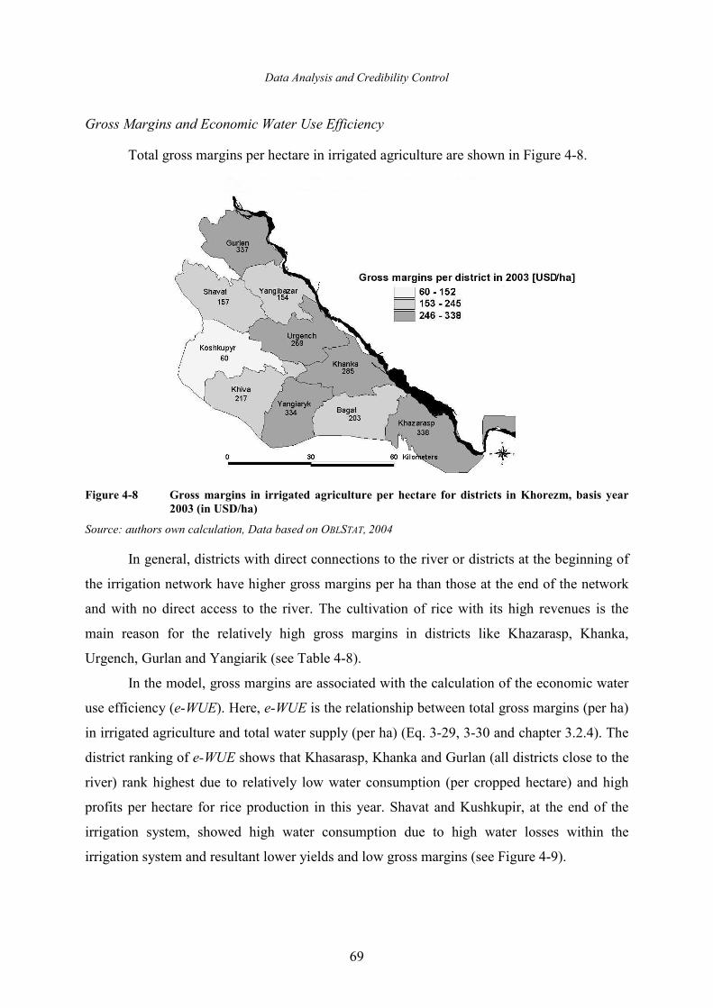
Data Analysis and Credibility Control
69
Gross Margins and Economic Water Use Efficiency
Total gross margins per hectare in irrigated agriculture are shown in Figure 4-8.
Figure 4-8 Gross margins in irrigated agriculture per hectare for districts in Khorezm, basis year
2003 (in USD/ha)
Source: authors own calculation, Data based on OBLSTAT, 2004
In general, districts with direct connections to the river or districts at the beginning of
the irrigation network have higher gross margins per ha than those at the end of the network
and with no direct access to the river. The cultivation of rice with its high revenues is the
main reason for the relatively high gross margins in districts like Khazarasp, Khanka,
Urgench, Gurlan and Yangiarik (see Table 4-8).
In the model, gross margins are associated with the calculation of the economic water
use efficiency (e-WUE). Here, e-WUE is the relationship between total gross margins (per ha)
in irrigated agriculture and total water supply (per ha) (Eq. 3-29, 3-30 and chapter 3.2.4). The
district ranking of e-WUE shows that Khasarasp, Khanka and Gurlan (all districts close to the
river) rank highest due to relatively low water consumption (per cropped hectare) and high
profits per hectare for rice production in this year. Shavat and Kushkupir, at the end of the
irrigation system, showed high water consumption due to high water losses within the
irrigation system and resultant lower yields and low gross margins (see Figure 4-9).
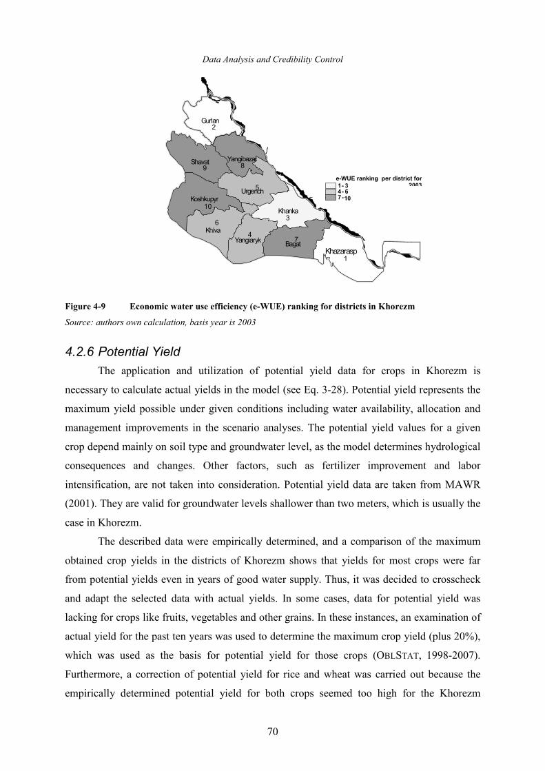
Data Analysis and Credibility Control
70
Figure 4-9 Economic water use efficiency (e-WUE) ranking for districts in Khorezm
Source: authors own calculation, basis year is 2003
4.2.6 Potential Yield
The application and utilization of potential yield data for crops in Khorezm is
necessary to calculate actual yields in the model (see Eq. 3-28). Potential yield represents the
maximum yield possible under given conditions including water availability, allocation and
management improvements in the scenario analyses. The potential yield values for a given
crop depend mainly on soil type and groundwater level, as the model determines hydrological
consequences and changes. Other factors, such as fertilizer improvement and labor
intensification, are not taken into consideration. Potential yield data are taken from MAWR
(2001). They are valid for groundwater levels shallower than two meters, which is usually the
case in Khorezm.
The described data were empirically determined, and a comparison of the maximum
obtained crop yields in the districts of Khorezm shows that yields for most crops were far
from potential yields even in years of good water supply. Thus, it was decided to crosscheck
and adapt the selected data with actual yields. In some cases, data for potential yield was
lacking for crops like fruits, vegetables and other grains. In these instances, an examination of
actual yield for the past ten years was used to determine the maximum crop yield (plus 20%),
which was used as the basis for potential yield for those crops (OBLSTAT, 1998-2007).
Furthermore, a correction of potential yield for rice and wheat was carried out because the
empirically determined potential yield for both crops seemed too high for the Khorezm
N
e-WUE ranking per district for 2003 1 - 3
4 - 6 7 - 10
Khiva
Ba g at
G u rl a n
S ha v at
Kh an ka
U r ge n c h K o sh kup y r
Y a n g i a ry k
Y a n gi b a z ar
K h a z a r a sp
10
5
9
2
7
3
4
8
6
1
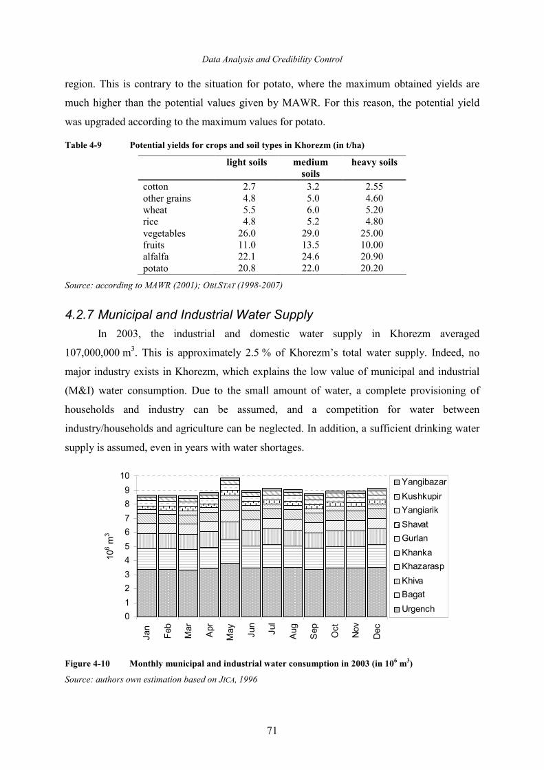
Data Analysis and Credibility Control
71
region. This is contrary to the situation for potato, where the maximum obtained yields are
much higher than the potential values given by MAWR. For this reason, the potential yield
was upgraded according to the maximum values for potato.
Table 4-9 Potential yields for crops and soil types in Khorezm (in t/ha)
light soils medium
soils
heavy soils
cotton 2.7 3.2 2.55 other grains 4.8 5.0 4.60 wheat 5.5 6.0 5.20 rice 4.8 5.2 4.80 vegetables 26.0 29.0 25.00 fruits 11.0 13.5 10.00 alfalfa 22.1 24.6 20.90 potato 20.8 22.0 20.20
Source: according to MAWR (2001); OBLSTAT (1998-2007)
4.2.7 Municipal and Industrial Water Supply
In 2003, the industrial and domestic water supply in Khorezm averaged
107,000,000 m3. This is approximately 2.5 % of Khorezm’s total water supply. Indeed, no
major industry exists in Khorezm, which explains the low value of municipal and industrial
(M&I) water consumption. Due to the small amount of water, a complete provisioning of
households and industry can be assumed, and a competition for water between
industry/households and agriculture can be neglected. In addition, a sufficient drinking water
supply is assumed, even in years with water shortages.
0
1
2
3
4
5
6
7
8
9
10
Jan
Feb
Mar
Apr
May
Jun
Jul
Aug
Sep
Oct
Nov
Dec
106 m
3
Yangibazar
Kushkupir
Yangiarik
Shavat
Gurlan
Khanka
Khazarasp
Khiva
Bagat
Urgench
Figure 4-10 Monthly municipal and industrial water consumption in 2003 (in 106 m
3)
Source: authors own estimation based on JICA, 1996
Data Analysis and Credibility Control
72
The data used to determine M&I water is from JICA, 1996. Due to some missing data,
M&I water consumption data from 1995 were interpolated taking of population development
into consideration (OBLSTAT, 2003) as well as trends in the piped water supply (Figure 4-10).
4.2.8 Other Data
Additional data used in the model, such as pumping capacities, maximum and
minimum yields, aquifer specific yield coefficient, hydraulic conductivity in aquifers, root
depth and other soil related parameters, crop prices and costs, elasticities and salinity, are
included in Appendix C.
73
5 Model Verification, Calibration and Positive Descriptive Modeling
According to WEHRHEIM (2003), complex models and the underlying data and
parameters need to be verified and validated for homogeneity, consistency, and sensitivity.
The terms “validation” and “verification” are often discussed in the literature but are very
controversial and depend on personal preferences or definitions. In this study, validation and
verification refer to the determination of the model behavior in comparison to real-world
behavior. Thus, verification requires determining how well a model serves its intended
purpose.
Therefore, verification “by construct” and “by result” can be performed (MCCARL
AND SPREEN, 1996). Verification by construct uses techniques that are employed in model
construction and is motivated by real-world observations (functions, modules of software,
equations, and values) to assure that the model was constructed properly. Verification by
results compares the results of the model ex post with data and observations (MCCARL AND
APLAND, 1986). A well-verified model has passed both verification methods.
The verification of both methods, including the applied functions and procedures and
model outcomes and behavior in comparison to real-world behavior, is included in chapter 5.
The model is based on a successfully applied basin-wide integrated economic-hydrologic
model for the Syr Darya River basin in Central Asia (CAI, 1999). The calculation of
evapotranspiration, yield and of the resultant objective function is based on a widely used
FAO crop water production model (CropWat, ALLEN ET AL., 1998). The required crop-
specific parameters have been determined and measured in Uzbekistan. The data were
compared with worldwide data collected from the literature. All other equations are based on
experiments and well-established theory10. Soil parameters and boundaries are based on field
10 Groundwater tank model based on BEAR, 1977; Groundwater contribution based on EAGLESON 1978; effective
rainfall based on USDA, 1969
Model Verification, Calibration and Positive Descriptive Modeling
74
measurements and were crosschecked with information from the literature11. The verification
of input parameters and data (plausibility control) is discussed in chapter 4. During the
verification process, calibration was also performed. The model calibration process involves
modification and adjustment of the model input until the model output matches field
conditions or observed data. Those modifications are only permissible if the data and
boundaries are within realistic limits. Calibration for this model was based on the results and
was performed manually. Manual calibration is very labor-intensive, but with the help of a
pre-conducted sensitivity analysis (see chapter 6), good results were obtained.
The best way to validate model results and input data is to directly compare model
outputs and inputs with observed or measured data from the study area. Consistency between
the measurements and model outcomes in time and space is required. Unfortunately, this
requirement cannot be fulfilled for most of the model input parameters and outcomes because
no direct field data or measurement for comparison exists. For example, the direct
measurement of groundwater fluxes, soil water balances or actual evapotranspiration is
difficult and cannot cover the entire study area. Data for groundwater and other hydraulic
values, such as deep percolation, groundwater extraction, water supply to districts, fields and
crops, and cropping prices (variable costs), are difficult to access and often depend on
estimates. Few measurements, if any, were taken for some soil, climatic and salinity
parameters. When data are missing, alternative verification must be carried out using a
comprehensive plausibility control.
In the following chapter a comparison of model outcomes with selected
measurements, literature values, and simulation results from other studies is described.
Additionally, the classification of parameters and variables within realistic dimensions and
boundaries is performed.
5.1 Positive Descriptive Modeling
For model verification and plausibility control, a so-called positive model is first
established to assess the model consistency with reality. A positive model analyzes “what is”,
in contrast to normative models that analyze “what should be” (see chapter 8). For the
positive model, relevant input parameters, including water supply, cropping areas and yields,
11 Soil moisture, groundwater table, permeability etc. according to SCHEFFER, SCHACHTSCHABEL (1998);
pumping capacity according to SOKOLOV (1999); for more details see chapter 3
Model Verification, Calibration and Positive Descriptive Modeling
75
are taken from actual data observation in 2003 and fixed in the model. This method will be
used to illustrate that the outputs, underlying formulas and data for water balances and crop
production processes are within a realistic range. In later analyses, these fixed parameters will
be relaxed to evaluate the impact of relevant parameters and to obtain a verified optimization
model with appropriate constraints.
In the following paragraphs, verification and plausibility analyses of major hydrologic
and agronomic model outcomes of the positive descriptive model, followed by an analysis of
economic outcomes, is undertaken.
Evapotranspiration
The determination of actual evapotranspiration (ETa) is one of the most important
calculations as crop growth, soil moisture and soil-water balance, as well as yields and
corresponding agricultural profit and benefits rely on this result. Monthly ETa was
determined for all ten districts, eight crops, and three soil types. The modeled ETa values
range between 404 mm for wheat and other grains (fodder maize and sorghum) to 1,142 mm
for vegetables and rice. The average ETa was 744 mm per year, of which approximately
700 mm occur within the growing period between April to October (see Table 5-1). Winter
wheat, which grows in winter and spring, has the lowest evapotranspiration, as shown in the
following figures. The low ETa for ”other grains” is due to the fact that maize cultivation
occurs after winter wheat as a secondary crop. The cultivation period is very short, and the
crop (plant matter, phylum) is harvested before ripening and is used as fodder. Due to high
water consumption requirements and the irrigation method, rice has a high evapotranspiration
rate. However, due to a relatively short growing period, the total ETa for the growing period
in total is not exceptionally high.
Modeled values for monthly ETa are highest in June and July (see Table 5-1 and
Figure 5-1) due to high evaporative demand driven by high radiation and low air humidity, as
well as soil evaporation and high transpiration due to advanced crop growth. High values of
ETa for alfalfa are attributable to the long growing period. The opposite is true for winter
wheat grown between October and June under lower radiation and temperature conditions
and, consequently, lower evaporation and transpiration rates.
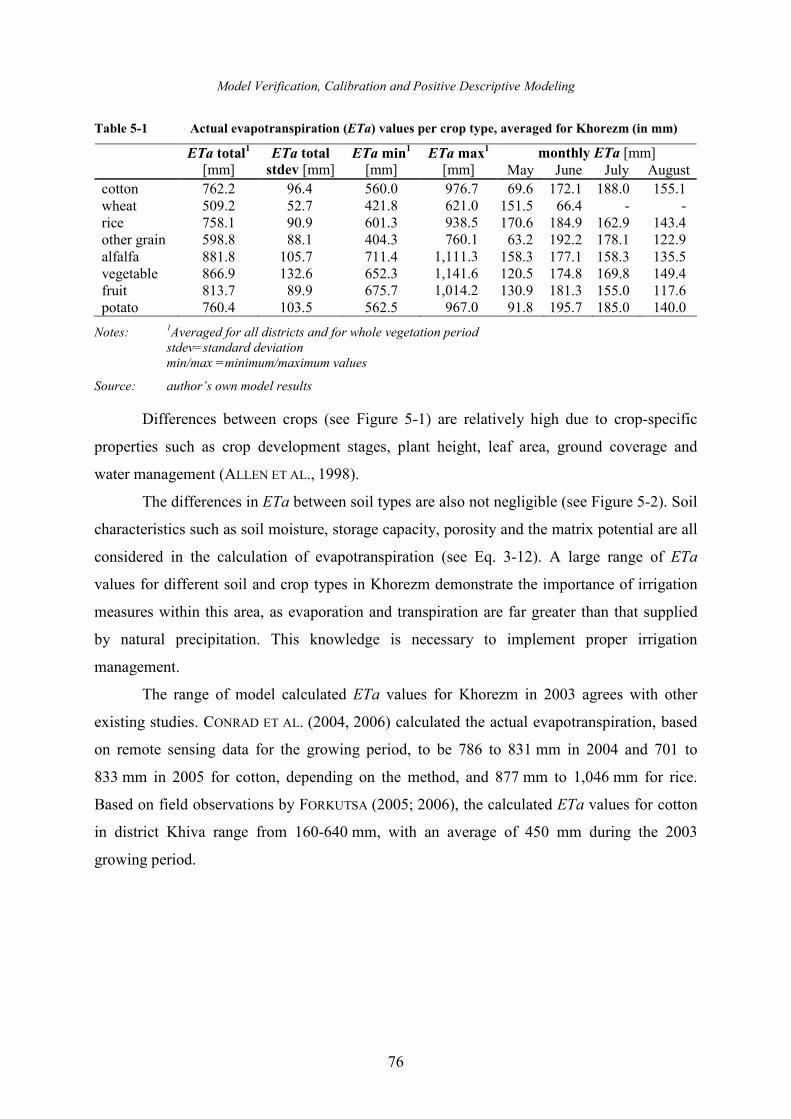
Model Verification, Calibration and Positive Descriptive Modeling
76
Table 5-1 Actual evapotranspiration (ETa) values per crop type, averaged for Khorezm (in mm)
monthly ETa [mm] ETa total1
[mm] ETa total stdev [mm]
ETa min1
[mm] ETa max
1
[mm] May June July August cotton 762.2 96.4 560.0 976.7 69.6 172.1 188.0 155.1 wheat 509.2 52.7 421.8 621.0 151.5 66.4 - - rice 758.1 90.9 601.3 938.5 170.6 184.9 162.9 143.4 other grain 598.8 88.1 404.3 760.1 63.2 192.2 178.1 122.9 alfalfa 881.8 105.7 711.4 1,111.3 158.3 177.1 158.3 135.5 vegetable 866.9 132.6 652.3 1,141.6 120.5 174.8 169.8 149.4 fruit 813.7 89.9 675.7 1,014.2 130.9 181.3 155.0 117.6 potato 760.4 103.5 562.5 967.0 91.8 195.7 185.0 140.0
Notes: 1Averaged for all districts and for whole vegetation period stdev=standard deviation min/max =minimum/maximum values
Source: author’s own model results
Differences between crops (see Figure 5-1) are relatively high due to crop-specific
properties such as crop development stages, plant height, leaf area, ground coverage and
water management (ALLEN ET AL., 1998).
The differences in ETa between soil types are also not negligible (see Figure 5-2). Soil
characteristics such as soil moisture, storage capacity, porosity and the matrix potential are all
considered in the calculation of evapotranspiration (see Eq. 3-12). A large range of ETa
values for different soil and crop types in Khorezm demonstrate the importance of irrigation
measures within this area, as evaporation and transpiration are far greater than that supplied
by natural precipitation. This knowledge is necessary to implement proper irrigation
management.
The range of model calculated ETa values for Khorezm in 2003 agrees with other
existing studies. CONRAD ET AL. (2004, 2006) calculated the actual evapotranspiration, based
on remote sensing data for the growing period, to be 786 to 831 mm in 2004 and 701 to
833 mm in 2005 for cotton, depending on the method, and 877 mm to 1,046 mm for rice.
Based on field observations by FORKUTSA (2005; 2006), the calculated ETa values for cotton
in district Khiva range from 160-640 mm, with an average of 450 mm during the 2003
growing period.
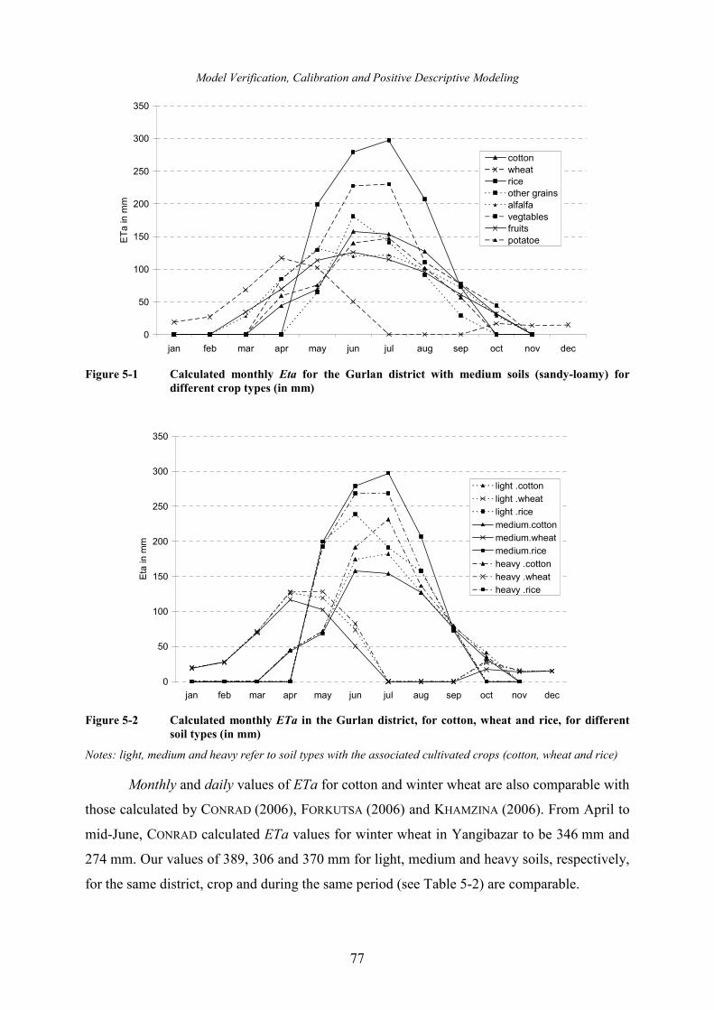
Model Verification, Calibration and Positive Descriptive Modeling
77
0
50
100
150
200
250
300
350
jan feb mar apr may jun jul aug sep oct nov dec
ETa in m
m
cotton
wheat
rice
other grains
alfalfa
vegtables
fruits
potatoe
Figure 5-1 Calculated monthly Eta for the Gurlan district with medium soils (sandy-loamy) for
different crop types (in mm)
0
50
100
150
200
250
300
350
jan feb mar apr may jun jul aug sep oct nov dec
Eta in mm
light .cotton
light .wheat
light .rice
medium.cotton
medium.wheat
medium.rice
heavy .cotton
heavy .wheat
heavy .rice
Figure 5-2 Calculated monthly ETa in the Gurlan district, for cotton, wheat and rice, for different
soil types (in mm)
Notes: light, medium and heavy refer to soil types with the associated cultivated crops (cotton, wheat and rice)
Monthly and daily values of ETa for cotton and winter wheat are also comparable with
those calculated by CONRAD (2006), FORKUTSA (2006) and KHAMZINA (2006). From April to
mid-June, CONRAD calculated ETa values for winter wheat in Yangibazar to be 346 mm and
274 mm. Our values of 389, 306 and 370 mm for light, medium and heavy soils, respectively,
for the same district, crop and during the same period (see Table 5-2) are comparable.
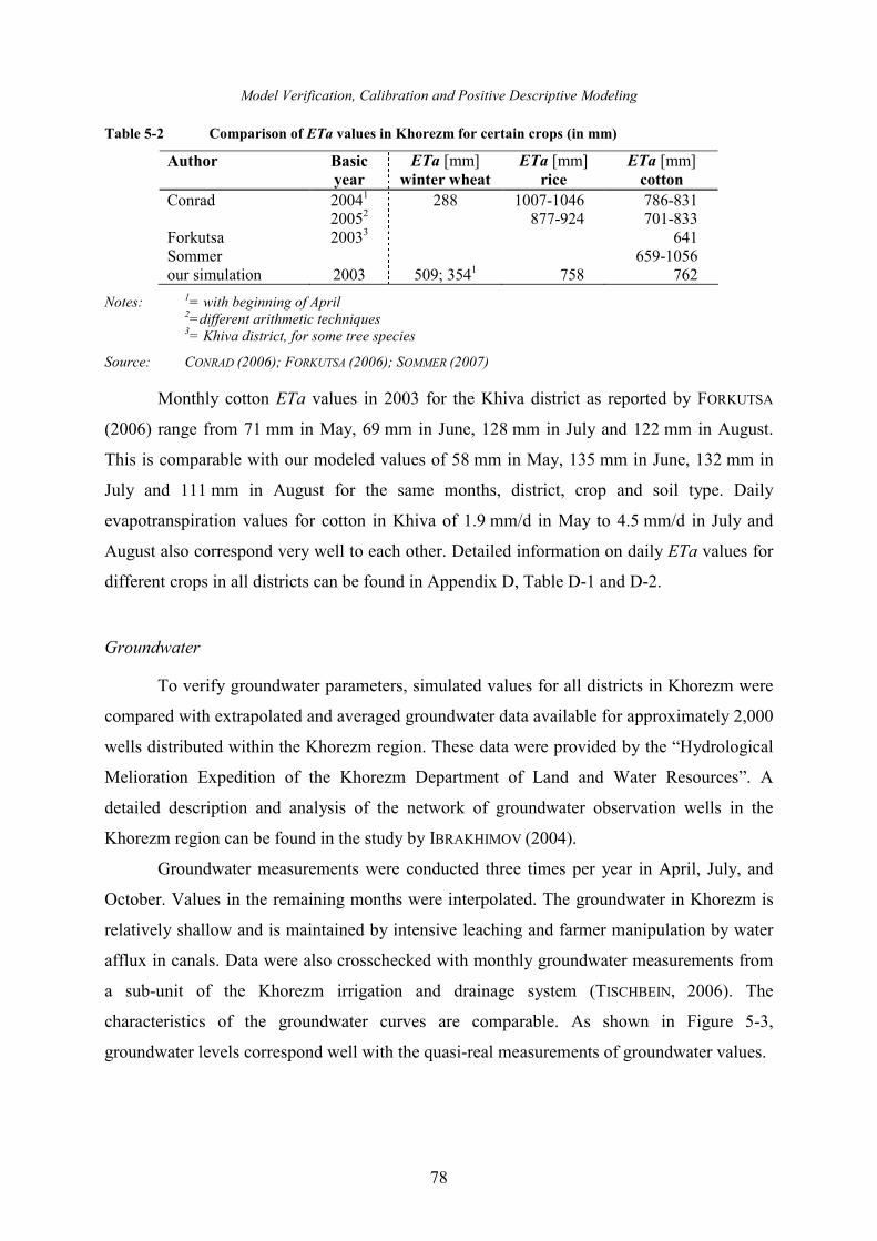
Model Verification, Calibration and Positive Descriptive Modeling
78
Table 5-2 Comparison of ETa values in Khorezm for certain crops (in mm)
Author Basic
year
ETa [mm] winter wheat
ETa [mm] rice
ETa [mm] cotton
Conrad 20041 288 1007-1046 786-831 20052 877-924 701-833 Forkutsa 20033 641 Sommer 659-1056 our simulation 2003 509; 3541 758 762
Notes: 1= with beginning of April 2=different arithmetic techniques 3= Khiva district, for some tree species
Source: CONRAD (2006); FORKUTSA (2006); SOMMER (2007)
Monthly cotton ETa values in 2003 for the Khiva district as reported by FORKUTSA
(2006) range from 71 mm in May, 69 mm in June, 128 mm in July and 122 mm in August.
This is comparable with our modeled values of 58 mm in May, 135 mm in June, 132 mm in
July and 111 mm in August for the same months, district, crop and soil type. Daily
evapotranspiration values for cotton in Khiva of 1.9 mm/d in May to 4.5 mm/d in July and
August also correspond very well to each other. Detailed information on daily ETa values for
different crops in all districts can be found in Appendix D, Table D-1 and D-2.
Groundwater
To verify groundwater parameters, simulated values for all districts in Khorezm were
compared with extrapolated and averaged groundwater data available for approximately 2,000
wells distributed within the Khorezm region. These data were provided by the “Hydrological
Melioration Expedition of the Khorezm Department of Land and Water Resources”. A
detailed description and analysis of the network of groundwater observation wells in the
Khorezm region can be found in the study by IBRAKHIMOV (2004).
Groundwater measurements were conducted three times per year in April, July, and
October. Values in the remaining months were interpolated. The groundwater in Khorezm is
relatively shallow and is maintained by intensive leaching and farmer manipulation by water
afflux in canals. Data were also crosschecked with monthly groundwater measurements from
a sub-unit of the Khorezm irrigation and drainage system (TISCHBEIN, 2006). The
characteristics of the groundwater curves are comparable. As shown in Figure 5-3,
groundwater levels correspond well with the quasi-real measurements of groundwater values.
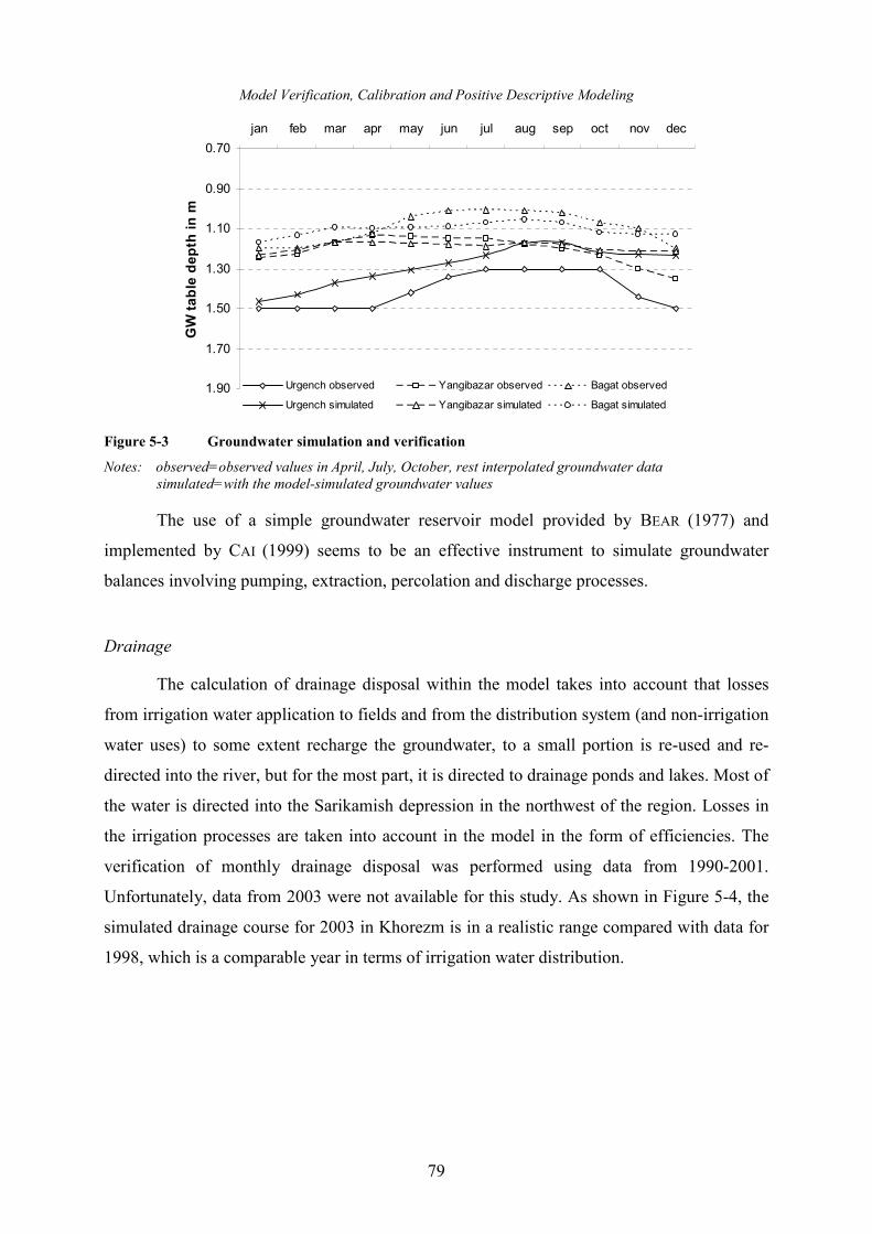
Model Verification, Calibration and Positive Descriptive Modeling
79
Groundwatervalidation
0.70
0.90
1.10
1.30
1.50
1.70
1.90
jan feb mar apr may jun jul aug sep oct nov dec
GW table depth in m
Urgench observed Yangibazar observed Bagat observed
Urgench simulated Yangibazar simulated Bagat simulated
Figure 5-3 Groundwater simulation and verification
Notes: observed=observed values in April, July, October, rest interpolated groundwater data simulated=with the model-simulated groundwater values
The use of a simple groundwater reservoir model provided by BEAR (1977) and
implemented by CAI (1999) seems to be an effective instrument to simulate groundwater
balances involving pumping, extraction, percolation and discharge processes.
Drainage
The calculation of drainage disposal within the model takes into account that losses
from irrigation water application to fields and from the distribution system (and non-irrigation
water uses) to some extent recharge the groundwater, to a small portion is re-used and re-
directed into the river, but for the most part, it is directed to drainage ponds and lakes. Most of
the water is directed into the Sarikamish depression in the northwest of the region. Losses in
the irrigation processes are taken into account in the model in the form of efficiencies. The
verification of monthly drainage disposal was performed using data from 1990-2001.
Unfortunately, data from 2003 were not available for this study. As shown in Figure 5-4, the
simulated drainage course for 2003 in Khorezm is in a realistic range compared with data for
1998, which is a comparable year in terms of irrigation water distribution.
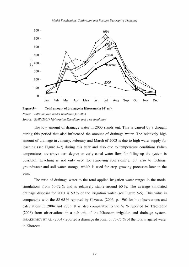
Model Verification, Calibration and Positive Descriptive Modeling
80
1990
1992
1994
1996
1998
2000
2003sim
0
100
200
300
400
500
600
700
800
Jan Feb Mar Apr May Jun Jul Aug Sep Oct Nov Dec
106 m
3
Figure 5-4 Total amount of drainage in Khorezm (in 106 m
3)
Notes: 2003sim, own model simulation for 2003
Source: GME (2001) Melioration Expedition and own simulation
The low amount of drainage water in 2000 stands out. This is caused by a drought
during this period that also influenced the amount of drainage water. The relatively high
amount of drainage in January, February and March of 2003 is due to high water supply for
leaching (see Figure 4-2) during this year and also due to temperature conditions (when
temperatures are above zero degree an early canal water flow for filling up the system is
possible). Leaching is not only used for removing soil salinity, but also to recharge
groundwater and soil water storage, which is used for crop growing processes later in the
year.
The ratio of drainage water to the total applied irrigation water ranges in the model
simulations from 50-72 % and is relatively stable around 60 %. The average simulated
drainage disposal for 2003 is 59 % of the irrigation water (see Figure 5-5). This value is
comparable with the 55-65 % reported by CONRAD (2006, p. 196) for his observations and
calculations in 2004 and 2005. It is also comparable to the 67 % reported by TISCHBEIN
(2006) from observations in a sub-unit of the Khorezm irrigation and drainage system.
IBRAKHIMOV ET AL. (2004) reported a drainage disposal of 70-75 % of the total irrigated water
in Khorezm.
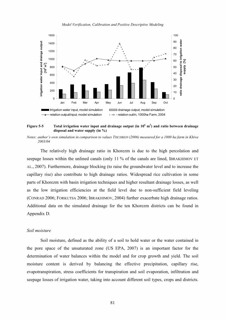
Model Verification, Calibration and Positive Descriptive Modeling
81
0
200
400
600
800
1000
1200
1400
1600
Jan Feb Mar Apr May Jun Jul Aug Sep Oct
irrigation water input and drainge output
[106 m
3]
0
10
20
30
40
50
60
70
80
90
100
ratio drainage disposal to irrigation water
supply [%
]
Irrigation water input, model simulation drainage output, model simulation
relation output/input, model simulation relation out/in, 1000ha Farm, 2004
Figure 5-5 Total irrigation water input and drainage output (in 10
6 m
3) and ratio between drainage
disposal and water supply (in %)
Notes: author’s own simulation in comparison to values TISCHBEIN (2006) measured for a 1000 ha farm in Khiva 2003/04
The relatively high drainage ratio in Khorezm is due to the high percolation and
seepage losses within the unlined canals (only 11 % of the canals are lined, IBRAKHIMOV ET
AL., 2007). Furthermore, drainage blocking (to raise the groundwater level and to increase the
capillary rise) also contribute to high drainage ratios. Widespread rice cultivation in some
parts of Khorezm with basin irrigation techniques and higher resultant drainage losses, as well
as the low irrigation efficiencies at the field level due to non-sufficient field leveling
(CONRAD 2006; FORKUTSA 2006; IBRAKHIMOV, 2004) further exacerbate high drainage ratios.
Additional data on the simulated drainage for the ten Khorezm districts can be found in
Appendix D.
Soil moisture
Soil moisture, defined as the ability of a soil to hold water or the water contained in
the pore space of the unsaturated zone (US EPA, 2007) is an important factor for the
determination of water balances within the model and for crop growth and yield. The soil
moisture content is derived by balancing the effective precipitation, capillary rise,
evapotranspiration, stress coefficients for transpiration and soil evaporation, infiltration and
seepage losses of irrigation water, taking into account different soil types, crops and districts.
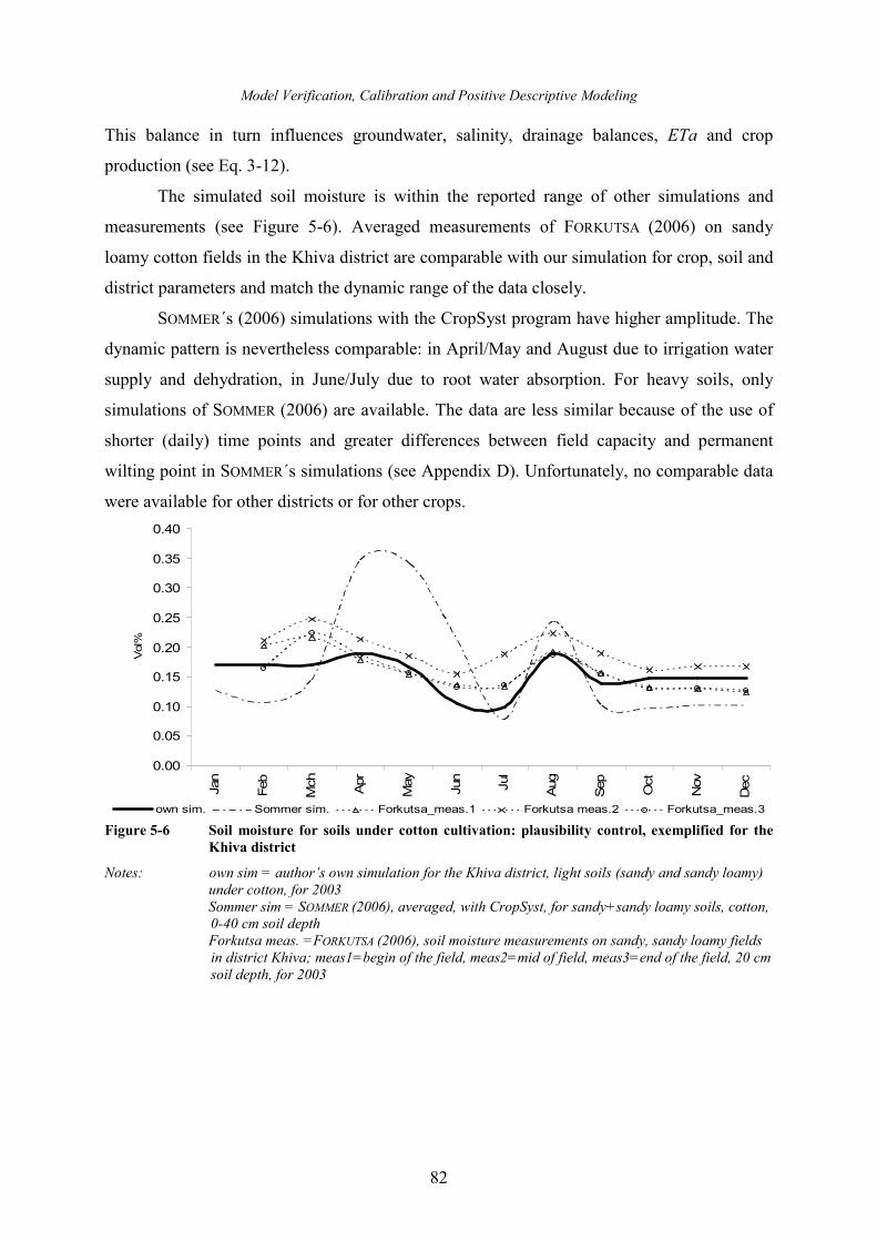
Model Verification, Calibration and Positive Descriptive Modeling
82
This balance in turn influences groundwater, salinity, drainage balances, ETa and crop
production (see Eq. 3-12).
The simulated soil moisture is within the reported range of other simulations and
measurements (see Figure 5-6). Averaged measurements of FORKUTSA (2006) on sandy
loamy cotton fields in the Khiva district are comparable with our simulation for crop, soil and
district parameters and match the dynamic range of the data closely.
SOMMER´s (2006) simulations with the CropSyst program have higher amplitude. The
dynamic pattern is nevertheless comparable: in April/May and August due to irrigation water
supply and dehydration, in June/July due to root water absorption. For heavy soils, only
simulations of SOMMER (2006) are available. The data are less similar because of the use of
shorter (daily) time points and greater differences between field capacity and permanent
wilting point in SOMMER´s simulations (see Appendix D). Unfortunately, no comparable data
were available for other districts or for other crops.
0.00
0.05
0.10
0.15
0.20
0.25
0.30
0.35
0.40
Jan
Feb
Mch
Apr
May
Jun
Jul
Aug
Sep
Oct
Nov
Dec
Vol%
own sim. Sommer sim. Forkutsa_meas.1 Forkutsa meas.2 Forkutsa_meas.3 Figure 5-6 Soil moisture for soils under cotton cultivation: plausibility control, exemplified for the
Khiva district
Notes: own sim = author’s own simulation for the Khiva district, light soils (sandy and sandy loamy) under cotton, for 2003 Sommer sim = SOMMER (2006), averaged, with CropSyst, for sandy+sandy loamy soils, cotton, 0-40 cm soil depth Forkutsa meas. =FORKUTSA (2006), soil moisture measurements on sandy, sandy loamy fields in district Khiva; meas1=begin of the field, meas2=mid of field, meas3=end of the field, 20 cm soil depth, for 2003
Model Verification, Calibration and Positive Descriptive Modeling
83
Deep percolation
Percolation is the portion of infiltrated irrigation and precipitation water that leaves the
root zone to the downward soil layer. Some of the percolation water is transferred to the
drainage system, while the rest enters the groundwater (see Eq. 3-5).
Water losses accompanying the intensive irrigation, mainly in cotton and especially in
rice fields, recharge the groundwater (deep percolation). The consequence is a rising
groundwater table and the establishment of shallow water tables (WILLIS 1996), which are
common in Khorezm. A second consequence, mainly in dry climates, is salinization of soils
(ZILBERMAN, 1998) and groundwater (SOTH ET AL., 1999). FORKUTSA (2006) mentioned an
attained cotton yield in cotton fields in Khorezm with no additional irrigation water supply
due to a high groundwater level. That claim seems reasonable because the crop has the ability
to use groundwater for growing processes. On the other hand, raising the groundwater leads to
unsustainable salinization and elevated pesticide concentrations (AKRAMKHANOV, 2005;
RICHARDS, 1954), which have not yet been examined in detail in the Khorezm area.
Percolation and deep percolation play an important role and is often by farmers
manipulated in the Khorezm region. The examination of the amount of deep percolation and
infiltration is very difficult because many factors are involved in the process of soil and
groundwater balances (such as drainage, groundwater extraction, groundwater recharge and
capillary rise). These factors can seldom be directly measured, especially in areas with high
groundwater levels and where percolation and deep percolation are difficult to distinguish.
For the Khorezm region, only one study on deep percolation was found (FORKUTSA 2006).
As shown in Figure 5-7, the percolation values for the cotton in Khiva match data
from FORKUTSA´s (2006) cotton-growing study. The field values from this study were
obtained using water balance calculations with the Hydrus-1d program (SIMUNEK ET AL.,
2005), as deep percolation to groundwater could not easily be measured directly. The
relatively large downward water fluxes in August due to the high irrigation water contribution
within this period are notable. In addition, large downward water fluxes can be observed in
FORKUTSA (2006)’s study and our simulation within the soil leaching period in April (due to
high leaching water supply for this time on the fields). FORKUTSA´s yearly percolation values
range from 275 to 572 mm depending on the location within the field (begin and middle of
the irrigated field). These values are comparable with our simulations for cotton-growing
areas in Khorezm and Khiva. Our values range between 259 mm for heavy soils, 603 mm for
medium soils and 407 mm for light soils in Khiva, and the fluxes in July to September are
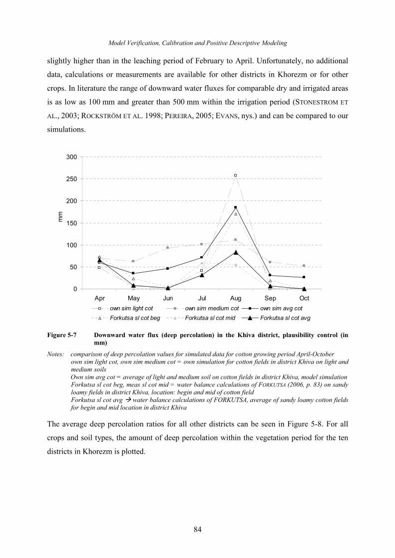
Model Verification, Calibration and Positive Descriptive Modeling
84
slightly higher than in the leaching period of February to April. Unfortunately, no additional
data, calculations or measurements are available for other districts in Khorezm or for other
crops. In literature the range of downward water fluxes for comparable dry and irrigated areas
is as low as 100 mm and greater than 500 mm within the irrigation period (STONESTROM ET
AL., 2003; ROCKSTRÖM ET AL. 1998; PEREIRA, 2005; EVANS, nys.) and can be compared to our
simulations.
0
50
100
150
200
250
300
Apr May Jun Jul Aug Sep Oct
mm
own sim light cot own sim medium cot own sim avg cot
Forkutsa sl cot beg Forkutsa sl cot mid Forkutsa sl cot avg
Figure 5-7 Downward water flux (deep percolation) in the Khiva district, plausibility control (in
mm)
Notes: comparison of deep percolation values for simulated data for cotton growing period April-October own sim light cot, own sim medium cot = own simulation for cotton fields in district Khiva on light and medium soils
Own sim avg cot = average of light and medium soil on cotton fields in district Khiva, model simulation Forkutsa sl cot beg, meas sl cot mid = water balance calculations of FORKUTSA (2006, p. 83) on sandy
loamy fields in district Khiva, location: begin and mid of cotton field Forkutsa sl cot avg � water balance calculations of FORKUTSA, average of sandy loamy cotton fields for begin and mid location in district Khiva
The average deep percolation ratios for all other districts can be seen in Figure 5-8. For all
crops and soil types, the amount of deep percolation within the vegetation period for the ten
districts in Khorezm is plotted.
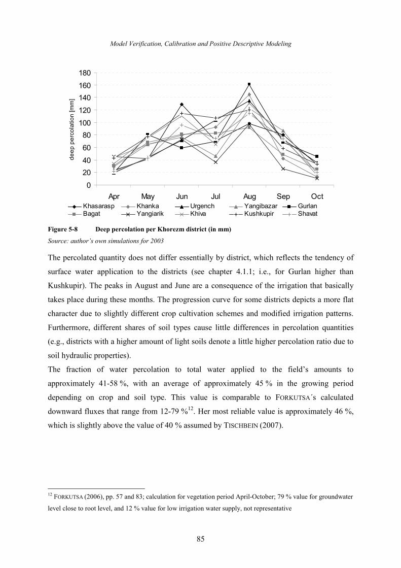
Model Verification, Calibration and Positive Descriptive Modeling
85
0
20
40
60
80
100
120
140
160
180
Apr May Jun Jul Aug Sep Oct
deep percolation [mm]
Khasarasp Khanka Urgench Yangibazar GurlanBagat Yangiarik Khiva Kushkupir Shavat
Figure 5-8 Deep percolation per Khorezm district (in mm)
Source: author’s own simulations for 2003
The percolated quantity does not differ essentially by district, which reflects the tendency of
surface water application to the districts (see chapter 4.1.1; i.e., for Gurlan higher than
Kushkupir). The peaks in August and June are a consequence of the irrigation that basically
takes place during these months. The progression curve for some districts depicts a more flat
character due to slightly different crop cultivation schemes and modified irrigation patterns.
Furthermore, different shares of soil types cause little differences in percolation quantities
(e.g., districts with a higher amount of light soils denote a little higher percolation ratio due to
soil hydraulic properties).
The fraction of water percolation to total water applied to the field’s amounts to
approximately 41-58 %, with an average of approximately 45 % in the growing period
depending on crop and soil type. This value is comparable to FORKUTSA´s calculated
downward fluxes that range from 12-79 %12. Her most reliable value is approximately 46 %,
which is slightly above the value of 40 % assumed by TISCHBEIN (2007).
12 FORKUTSA (2006), pp. 57 and 83; calculation for vegetation period April-October; 79 % value for groundwater
level close to root level, and 12 % value for low irrigation water supply, not representative
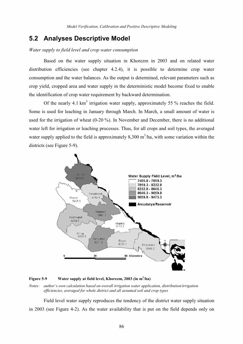
Model Verification, Calibration and Positive Descriptive Modeling
86
5.2 Analyses Descriptive Model
Water supply to field level and crop water consumption
Based on the water supply situation in Khorezm in 2003 and on related water
distribution efficiencies (see chapter 4.2.4), it is possible to determine crop water
consumption and the water balances. As the output is determined, relevant parameters such as
crop yield, cropped area and water supply in the deterministic model become fixed to enable
the identification of crop water requirement by backward determination.
Of the nearly 4.1 km3 irrigation water supply, approximately 55 % reaches the field.
Some is used for leaching in January through March. In March, a small amount of water is
used for the irrigation of wheat (0-20 %). In November and December, there is no additional
water left for irrigation or leaching processes. Thus, for all crops and soil types, the averaged
water supply applied to the field is approximately 8,300 m3/ha, with some variation within the
districts (see Figure 5-9).
Figure 5-9 Water supply at field level, Khorezm, 2003 (in m3/ha)
Notes: author’s own calculation based on overall irrigation water application, distribution/irrigation efficiencies, averaged for whole district and all assumed soil and crop types
Field level water supply reproduces the tendency of the district water supply situation
in 2003 (see Figure 4-2). As the water availability that is put on the field depends only on
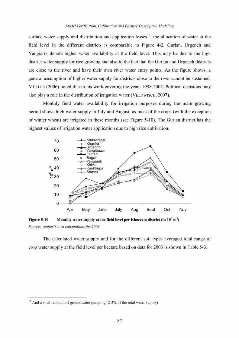
Model Verification, Calibration and Positive Descriptive Modeling
87
surface water supply and distribution and application losses13, the allocation of water at the
field level in the different districts is comparable to Figure 4-2. Gurlan, Urgench and
Yangiarik denote higher water availability at the field level. This may be due to the high
district water supply for rice growing and also to the fact that the Gurlan and Urgench districts
are close to the river and have their own river water entry points. As the figure shows, a
general assumption of higher water supply for districts close to the river cannot be sustained.
MÜLLER (2006) noted this in his work covering the years 1998-2002. Political decisions may
also play a role in the distribution of irrigation water (VELDWISCH, 2007).
Monthly field water availability for irrigation purposes during the main growing
period shows high water supply in July and August, as most of the crops (with the exception
of winter wheat) are irrigated in these months (see Figure 5-10). The Gurlan district has the
highest values of irrigation water application due to high rice cultivation.
0
10
20
30
40
50
60
70
Apr May June July Aug Sept Oct Nov
106 m
3
KhasaraspKhankaUrgenchYangibazarGurlanBagatYangiarikKhivaKushkupirShavat
Figure 5-10 Monthly water supply at the field level per Khorezm district (in 106 m
3)
Source: author’s own calculations for 2003
The calculated water supply and for the different soil types averaged total range of
crop water supply at the field level per hectare based on data for 2003 is shown in Table 5-3.
13 And a small amount of groundwater pumping (2-3% of the total water supply)
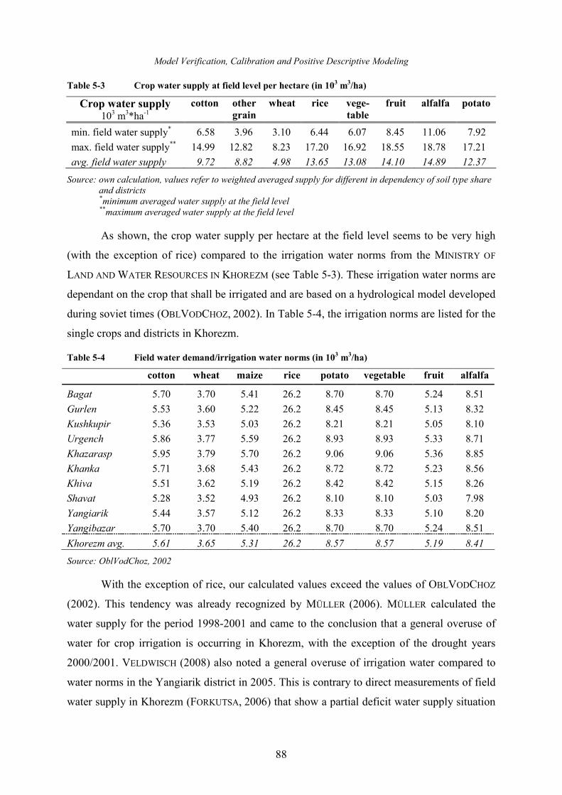
Model Verification, Calibration and Positive Descriptive Modeling
88
Table 5-3 Crop water supply at field level per hectare (in 103 m
3/ha)
Crop water supply 103 m3*ha-1
cotton other
grain
wheat rice vege-
table
fruit alfalfa potato
min. field water supply* 6.58 3.96 3.10 6.44 6.07 8.45 11.06 7.92
max. field water supply** 14.99 12.82 8.23 17.20 16.92 18.55 18.78 17.21
avg. field water supply 9.72 8.82 4.98 13.65 13.08 14.10 14.89 12.37
Source: own calculation, values refer to weighted averaged supply for different in dependency of soil type share and districts
*minimum averaged water supply at the field level **maximum averaged water supply at the field level
As shown, the crop water supply per hectare at the field level seems to be very high
(with the exception of rice) compared to the irrigation water norms from the MINISTRY OF
LAND AND WATER RESOURCES IN KHOREZM (see Table 5-3). These irrigation water norms are
dependant on the crop that shall be irrigated and are based on a hydrological model developed
during soviet times (OBLVODCHOZ, 2002). In Table 5-4, the irrigation norms are listed for the
single crops and districts in Khorezm.
Table 5-4 Field water demand/irrigation water norms (in 103 m
3/ha)
cotton wheat maize rice potato vegetable fruit alfalfa
Bagat 5.70 3.70 5.41 26.2 8.70 8.70 5.24 8.51
Gurlen 5.53 3.60 5.22 26.2 8.45 8.45 5.13 8.32
Kushkupir 5.36 3.53 5.03 26.2 8.21 8.21 5.05 8.10
Urgench 5.86 3.77 5.59 26.2 8.93 8.93 5.33 8.71
Khazarasp 5.95 3.79 5.70 26.2 9.06 9.06 5.36 8.85
Khanka 5.71 3.68 5.43 26.2 8.72 8.72 5.23 8.56
Khiva 5.51 3.62 5.19 26.2 8.42 8.42 5.15 8.26
Shavat 5.28 3.52 4.93 26.2 8.10 8.10 5.03 7.98
Yangiarik 5.44 3.57 5.12 26.2 8.33 8.33 5.10 8.20
Yangibazar 5.70 3.70 5.40 26.2 8.70 8.70 5.24 8.51
Khorezm avg. 5.61 3.65 5.31 26.2 8.57 8.57 5.19 8.41
Source: OblVodChoz, 2002
With the exception of rice, our calculated values exceed the values of OBLVODCHOZ
(2002). This tendency was already recognized by MÜLLER (2006). MÜLLER calculated the
water supply for the period 1998-2001 and came to the conclusion that a general overuse of
water for crop irrigation is occurring in Khorezm, with the exception of the drought years
2000/2001. VELDWISCH (2008) also noted a general overuse of irrigation water compared to
water norms in the Yangiarik district in 2005. This is contrary to direct measurements of field
water supply in Khorezm (FORKUTSA, 2006) that show a partial deficit water supply situation
Model Verification, Calibration and Positive Descriptive Modeling
89
in two cotton fields in the Khiva district14. TISCHBEIN (2007) also assumes a lower water
supply at the field level but only at the tail end locations in Khorezm (more than 95 km from
the Amu Darya). The situation depends on overall river/reservoir and district water supply
situations for different years and on the location and scale. In addition, some fields and
farmers will receive more or less water than others depending on their political and social
contacts (ZAVGORODNYAYA 2006; TREVISANI 2006) and on canal distances. As shown in
FORKUTSA´s work, field leveling causes irregular water supply for crops at different locations,
even within a single field, where one end of the field presuppose higher water applications to
assure sufficient water supply at the other end of the field. This questions the accuracy of the
efficiencies published by the government. However, an overuse of water represents inefficient
water management.
The surface water that is effectively used by the crop (see Table 5-5) depends on the
amount of water that is directed to the field (field water application and effective
precipitation), losses within the field due to drainage and evaporation and percolation to
layers below the root zone. Furthermore, supplementary water that a crop root can use via
capillary rise from groundwater and lower soil layers contributes to the crops total water use.
It can be added to the surface water effectively used by crops, resulting in evapotranspiration
processes (see chapter 3.2.3).
For the application efficiency, a value of approximately 42-47 % is assumed (defined
as the ratio of the average depth of irrigation water stored in the root zone for crop
consumptive use to the average depth applied). This value is derived from expert knowledge
and soil water-balance calculations. For the 1,000-ha farm in Khiva, a value of approximately
45 % is derived (TISCHBEIN 2005/2007). FORKUTSA (2006) calculated an application
efficiency of 40-50 % in her fields. Due to the introduction of the application efficiency term,
the additional surface water losses at the field level will be described. In addition to the losses
in the rest of the distribution system, the described percolation, drainage and soil evaporation
processes and the capillary rise processes add up to the amount of water that a crop can
effectively utilize for transpiration processes.
14 FORKUTSA stated 800-4,000 m3/ha for her cotton field study. In locations with shallow groundwater it is
possible to subsist with lower water supply.
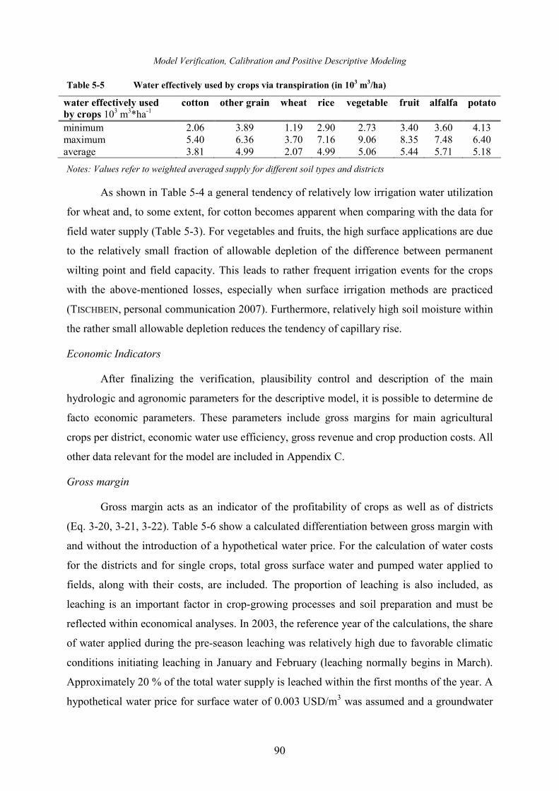
Model Verification, Calibration and Positive Descriptive Modeling
90
Table 5-5 Water effectively used by crops via transpiration (in 103 m
3/ha)
water effectively used by crops 103 m3*ha-1
cotton other grain wheat rice vegetable fruit alfalfa potato
minimum 2.06 3.89 1.19 2.90 2.73 3.40 3.60 4.13 maximum 5.40 6.36 3.70 7.16 9.06 8.35 7.48 6.40 average 3.81 4.99 2.07 4.99 5.06 5.44 5.71 5.18
Notes: Values refer to weighted averaged supply for different soil types and districts
As shown in Table 5-4 a general tendency of relatively low irrigation water utilization
for wheat and, to some extent, for cotton becomes apparent when comparing with the data for
field water supply (Table 5-3). For vegetables and fruits, the high surface applications are due
to the relatively small fraction of allowable depletion of the difference between permanent
wilting point and field capacity. This leads to rather frequent irrigation events for the crops
with the above-mentioned losses, especially when surface irrigation methods are practiced
(TISCHBEIN, personal communication 2007). Furthermore, relatively high soil moisture within
the rather small allowable depletion reduces the tendency of capillary rise.
Economic Indicators
After finalizing the verification, plausibility control and description of the main
hydrologic and agronomic parameters for the descriptive model, it is possible to determine de
facto economic parameters. These parameters include gross margins for main agricultural
crops per district, economic water use efficiency, gross revenue and crop production costs. All
other data relevant for the model are included in Appendix C.
Gross margin
Gross margin acts as an indicator of the profitability of crops as well as of districts
(Eq. 3-20, 3-21, 3-22). Table 5-6 show a calculated differentiation between gross margin with
and without the introduction of a hypothetical water price. For the calculation of water costs
for the districts and for single crops, total gross surface water and pumped water applied to
fields, along with their costs, are included. The proportion of leaching is also included, as
leaching is an important factor in crop-growing processes and soil preparation and must be
reflected within economical analyses. In 2003, the reference year of the calculations, the share
of water applied during the pre-season leaching was relatively high due to favorable climatic
conditions initiating leaching in January and February (leaching normally begins in March).
Approximately 20 % of the total water supply is leached within the first months of the year. A
hypothetical water price for surface water of 0.003 USD/m3 was assumed and a groundwater
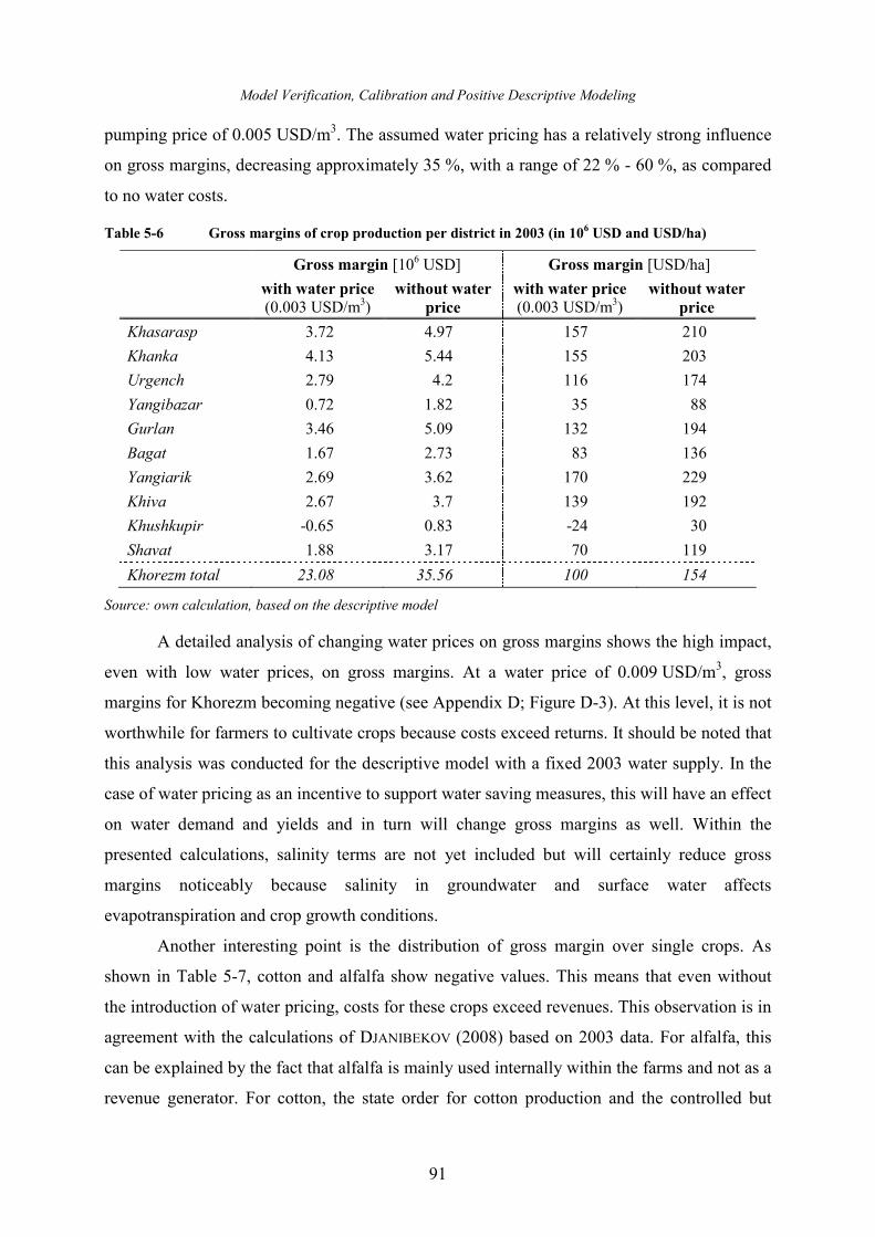
Model Verification, Calibration and Positive Descriptive Modeling
91
pumping price of 0.005 USD/m3. The assumed water pricing has a relatively strong influence
on gross margins, decreasing approximately 35 %, with a range of 22 % - 60 %, as compared
to no water costs.
Table 5-6 Gross margins of crop production per district in 2003 (in 106 USD and USD/ha)
Gross margin [106 USD] Gross margin [USD/ha] with water price
(0.003 USD/m3) without water
price
with water price
(0.003 USD/m3) without water
price
Khasarasp 3.72 4.97 157 210
Khanka 4.13 5.44 155 203
Urgench 2.79 4.2 116 174
Yangibazar 0.72 1.82 35 88
Gurlan 3.46 5.09 132 194
Bagat 1.67 2.73 83 136
Yangiarik 2.69 3.62 170 229
Khiva 2.67 3.7 139 192
Khushkupir -0.65 0.83 -24 30
Shavat 1.88 3.17 70 119
Khorezm total 23.08 35.56 100 154
Source: own calculation, based on the descriptive model
A detailed analysis of changing water prices on gross margins shows the high impact,
even with low water prices, on gross margins. At a water price of 0.009 USD/m3, gross
margins for Khorezm becoming negative (see Appendix D; Figure D-3). At this level, it is not
worthwhile for farmers to cultivate crops because costs exceed returns. It should be noted that
this analysis was conducted for the descriptive model with a fixed 2003 water supply. In the
case of water pricing as an incentive to support water saving measures, this will have an effect
on water demand and yields and in turn will change gross margins as well. Within the
presented calculations, salinity terms are not yet included but will certainly reduce gross
margins noticeably because salinity in groundwater and surface water affects
evapotranspiration and crop growth conditions.
Another interesting point is the distribution of gross margin over single crops. As
shown in Table 5-7, cotton and alfalfa show negative values. This means that even without
the introduction of water pricing, costs for these crops exceed revenues. This observation is in
agreement with the calculations of DJANIBEKOV (2008) based on 2003 data. For alfalfa, this
can be explained by the fact that alfalfa is mainly used internally within the farms and not as a
revenue generator. For cotton, the state order for cotton production and the controlled but
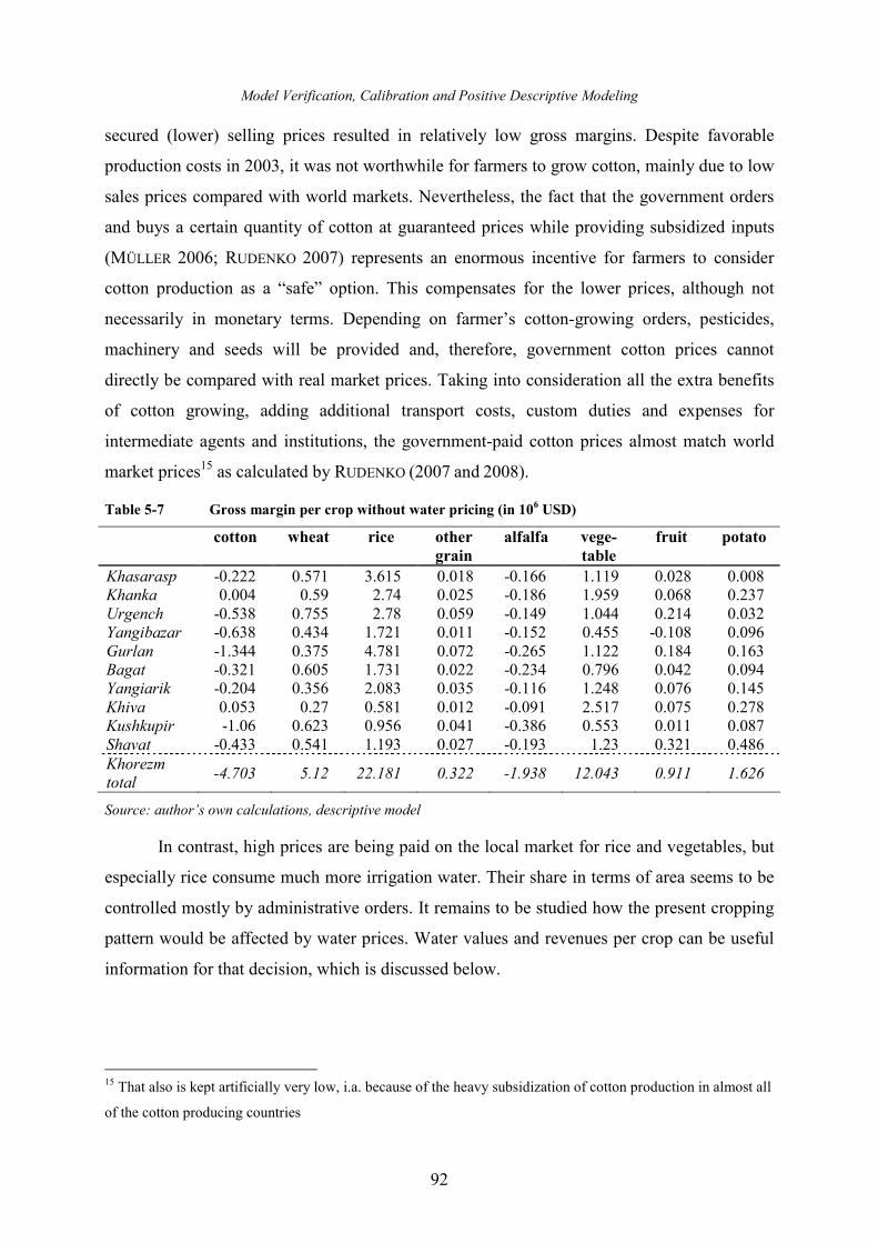
Model Verification, Calibration and Positive Descriptive Modeling
92
secured (lower) selling prices resulted in relatively low gross margins. Despite favorable
production costs in 2003, it was not worthwhile for farmers to grow cotton, mainly due to low
sales prices compared with world markets. Nevertheless, the fact that the government orders
and buys a certain quantity of cotton at guaranteed prices while providing subsidized inputs
(MÜLLER 2006; RUDENKO 2007) represents an enormous incentive for farmers to consider
cotton production as a “safe” option. This compensates for the lower prices, although not
necessarily in monetary terms. Depending on farmer’s cotton-growing orders, pesticides,
machinery and seeds will be provided and, therefore, government cotton prices cannot
directly be compared with real market prices. Taking into consideration all the extra benefits
of cotton growing, adding additional transport costs, custom duties and expenses for
intermediate agents and institutions, the government-paid cotton prices almost match world
market prices15 as calculated by RUDENKO (2007 and 2008).
Table 5-7 Gross margin per crop without water pricing (in 106 USD)
cotton wheat rice other
grain
alfalfa vege-
table
fruit potato
Khasarasp -0.222 0.571 3.615 0.018 -0.166 1.119 0.028 0.008 Khanka 0.004 0.59 2.74 0.025 -0.186 1.959 0.068 0.237 Urgench -0.538 0.755 2.78 0.059 -0.149 1.044 0.214 0.032 Yangibazar -0.638 0.434 1.721 0.011 -0.152 0.455 -0.108 0.096 Gurlan -1.344 0.375 4.781 0.072 -0.265 1.122 0.184 0.163 Bagat -0.321 0.605 1.731 0.022 -0.234 0.796 0.042 0.094 Yangiarik -0.204 0.356 2.083 0.035 -0.116 1.248 0.076 0.145 Khiva 0.053 0.27 0.581 0.012 -0.091 2.517 0.075 0.278 Kushkupir -1.06 0.623 0.956 0.041 -0.386 0.553 0.011 0.087 Shavat -0.433 0.541 1.193 0.027 -0.193 1.23 0.321 0.486 Khorezm total
-4.703 5.12 22.181 0.322 -1.938 12.043 0.911 1.626
Source: author’s own calculations, descriptive model
In contrast, high prices are being paid on the local market for rice and vegetables, but
especially rice consume much more irrigation water. Their share in terms of area seems to be
controlled mostly by administrative orders. It remains to be studied how the present cropping
pattern would be affected by water prices. Water values and revenues per crop can be useful
information for that decision, which is discussed below.
15 That also is kept artificially very low, i.a. because of the heavy subsidization of cotton production in almost all
of the cotton producing countries
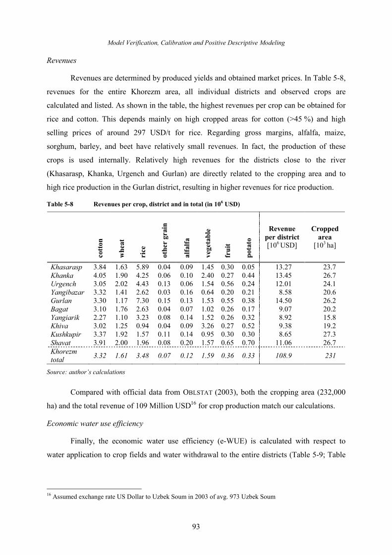
Model Verification, Calibration and Positive Descriptive Modeling
93
Revenues
Revenues are determined by produced yields and obtained market prices. In Table 5-8,
revenues for the entire Khorezm area, all individual districts and observed crops are
calculated and listed. As shown in the table, the highest revenues per crop can be obtained for
rice and cotton. This depends mainly on high cropped areas for cotton (>45 %) and high
selling prices of around 297 USD/t for rice. Regarding gross margins, alfalfa, maize,
sorghum, barley, and beet have relatively small revenues. In fact, the production of these
crops is used internally. Relatively high revenues for the districts close to the river
(Khasarasp, Khanka, Urgench and Gurlan) are directly related to the cropping area and to
high rice production in the Gurlan district, resulting in higher revenues for rice production.
Table 5-8 Revenues per crop, district and in total (in 106 USD)
cotton
whea
t
rice
oth
er gra
in
alfalfa
veg
etable
fruit
pota
to
Revenue
per district [106 USD]
Cropped
area [103 ha]
Khasarasp 3.84 1.63 5.89 0.04 0.09 1.45 0.30 0.05 13.27 23.7 Khanka 4.05 1.90 4.25 0.06 0.10 2.40 0.27 0.44 13.45 26.7 Urgench 3.05 2.02 4.43 0.13 0.06 1.54 0.56 0.24 12.01 24.1 Yangibazar 3.32 1.41 2.62 0.03 0.16 0.64 0.20 0.21 8.58 20.6 Gurlan 3.30 1.17 7.30 0.15 0.13 1.53 0.55 0.38 14.50 26.2 Bagat 3.10 1.76 2.63 0.04 0.07 1.02 0.26 0.17 9.07 20.2 Yangiarik 2.27 1.10 3.23 0.08 0.14 1.52 0.26 0.32 8.92 15.8 Khiva 3.02 1.25 0.94 0.04 0.09 3.26 0.27 0.52 9.38 19.2 Kushkupir 3.37 1.92 1.57 0.11 0.14 0.95 0.30 0.30 8.65 27.3 Shavat 3.91 2.00 1.96 0.08 0.20 1.57 0.65 0.70 11.06 26.7 Khorezm total
3.32 1.61 3.48 0.07 0.12 1.59 0.36 0.33 108.9 231
Source: author’s calculations
Compared with official data from OBLSTAT (2003), both the cropping area (232,000
ha) and the total revenue of 109 Million USD16 for crop production match our calculations.
Economic water use efficiency
Finally, the economic water use efficiency (e-WUE) is calculated with respect to
water application to crop fields and water withdrawal to the entire districts (Table 5-9; Table
16 Assumed exchange rate US Dollar to Uzbek Soum in 2003 of avg. 973 Uzbek Soum
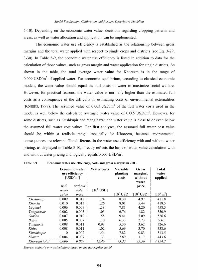
Model Verification, Calibration and Positive Descriptive Modeling
94
5-10). Depending on the economic water value, decisions regarding cropping patterns and
areas, as well as water allocation and application, can be implemented.
The economic water use efficiency is established as the relationship between gross
margins and the total water applied with respect to single crops and districts (see Eq. 3-29,
3-30). In Table 5-9, the economic water use efficiency is listed in addition to data for the
calculation of those values, such as gross margin and water application for single districts. As
shown in the table, the total average water value for Khorezm is in the range of
0.009 USD/m3 of applied water. For economic equilibrium, according to classical economic
models, the water value should equal the full costs of water to maximize social welfare.
However, for practical reasons, the water value is normally higher than the estimated full
costs as a consequence of the difficulty in estimating costs of environmental externalities
(ROGERS, 1997). The assumed value of 0.003 USD/m3 of the full water costs used in the
model is well below the calculated averaged water value of 0.009 USD/m3. However, for
some districts, such as Kushkupir and Yangibazar, the water value is close to or even below
the assumed full water cost values. For first analyses, the assumed full water cost value
should be within a realistic range, especially for Khorezm, because environmental
consequences are relevant. The difference in the water use efficiency with and without water
pricing, as displayed in Table 5-10, directly reflects the basis of water value calculation with
and without water pricing and logically equals 0.003 USD/m3.
Table 5-9 Economic water use efficiency, costs and gross margins in 2003
Economic water
use efficiency
[USD/m3]
with water price
without water price
Water costs
[106 USD]
Variable
planting
costs
[106 USD]
Gross
margins,
without
water
price
[106 USD]
Total
water
applied
[106 m3]
Khasarasp 0.009 0.012 1.24 8.30 4.97 411.8 Khanka 0.010 0.013 1.26 8.01 5.44 418.5 Urgench 0.006 0.009 1.38 7.81 4.20 458.5 Yangibazar 0.002 0.005 1.05 6.76 1.82 350.9 Gurlan 0.007 0.010 1.58 9.41 5.09 526.6 Bagat 0.005 0.007 1.10 6.33 2.73 366.1 Yangiarik 0.008 0.011 0.98 5.30 3.62 326.6 Khiva 0.008 0.011 1.02 5.69 3.70 338.6 Khushkupir 0 0.002 1.54 7.82 0.83 513.5 Shavat 0.004 0.007 1.33 7.89 3.17 443.6 Khorezm total 0.006 0.009 12.46 73.33 35.56 4,154.7
Source: author’s own calculations based on the descriptive model

Model Verification, Calibration and Positive Descriptive Modeling
95
For the determination and the analysis of water use efficiencies, the examination of
water values for single crops per district is significant. As shown in Table 5-10, the economic
water use efficiency for vegetables, rice and potatoes is relatively high compared to the other
crops. This is surprising, particularly for rice, as one would expect a lower value due to the
high water utilization rate of rice. However, revenues for rice are much higher than for other
crops, which means that it is worthwhile for farmers to grow rice in preferred areas with a
sufficient water supply, such as in Gurlan. Similarly, for vegetables and potatoes, the
correlation between gross margin and revenues is quite good, and additional water
consumption for both crops is not as high as for rice.
Table 5-10 Economic water use efficiency per crop and district, without water pricing (in
103 USD/m
3)
cotton wheat rice other
grain
alfalfa vegetable fruit potato
Khasarasp -1.0 12.0 42.0 7.0 -3.0 68.0 2.0 6.0 Khanka 0.02 8.0 31.0 6.0 -4.0 81.0 6.0 27.0 Urgench -3.0 10.0 26.0 7.0 -4.0 37.0 8.0 4.0 Yangibazar -4.0 10.0 31.0 7.0 -4.0 37.0 -5.0 18.0 Gurlan -6.0 9.0 32.0 8.0 -5.0 37.0 6.0 15.0 Bagat -2.0 15.0 43.0 17.0 -4.0 59.0 3.0 24.0 Yangiarik -1.0 19.0 33.0 16.0 -3.0 76.0 6.0 25.0 Khiva 0.3 5.0 22.0 8.0 -2.0 72.0 6.0 19.0 Kushkupir -5.0 9.0 22.0 7.0 -4.0 17.0 0.5 12.0 Shavat -2.0 7.0 33.0 6.0 -2.0 52.0 16.0 55.0 Khorezm total -2.4 10.4 31.5 8.9 -3.5 53.6 4.9 20.5
Source: author’s own calculations
As described in chapter 3, 4 and 5, verification of the model variables and parameters
matches very well with measurements and values from the literature. For this reason, the
model can be characterized as plausible and coherent. After a successful verification and
plausibility study of the model input (data, methodology, model formulation, see chapter 3
and 4) and output parameters (chapter 5), a sensitivity analysis is necessary to check the
robustness of the model with respect to parameter changes and the influence of input
parameter to output values. After implementing the sensitivity analysis, it will be possible to
perform the main simulations and the scenario analyses.
96
6 Sensitivity Analyses
Sensitivity analyses are primarily used to test the strength of the model and the quality
of the model definitions. They can also be used to determine the influence of input-factors on
certain output variables (SALTELLI, 2008) and in the ex ante identification of possible scenario
analyses, making them useful for policy recommendations.
For this type of parameter impact analysis, a local sensitivity analysis was chosen
because the implementation and execution is relatively simple, calculating efficiency is fast
and sensitivity is explicitly assigned to one input-parameter (HUISMAN ET AL., 2004).
For the sensitivity analyses of the model, the following parameters were considered to
be essential:
� natural inflow
� precipitation and effective rainfall
� reference crop evapotranspiration (ETo)
� irrigation/application efficiencies
� crop coefficients for transpiration, soil evaporation, yield response coefficient for
water (ETo, kc, ky), and potential yields
Thus, relevant key hydrologic and agronomic parameters of the model, such as water,
crop, climate, soil, and management, will be tested. The effects and characteristics of the
analyses on major outcomes, including agricultural benefits, water withdrawals, cropped
areas, crop share, and crop yields, will be described in following section. Unlike the following
scenario analyses and the previous descriptive model (for validation purposes), the sensitivity
analyses will be conducted with defixated (released) output variables (cropped area and
yields) to receive the general reactions to the entire system and the model outcome. A step-
by-step change of single input-parameters will be implemented simultaneously.
Various scenarios for sensitivity analyses for the different input-parameters were
defined. All values (input and output) are given in relative numbers for better clarity and
comparability and are shown in the tables below. For simplification, only the region-wide
average values are shown. The percent change of the input-parameters varies between 10 %
and 50 % according to high and low specific parameter levels.
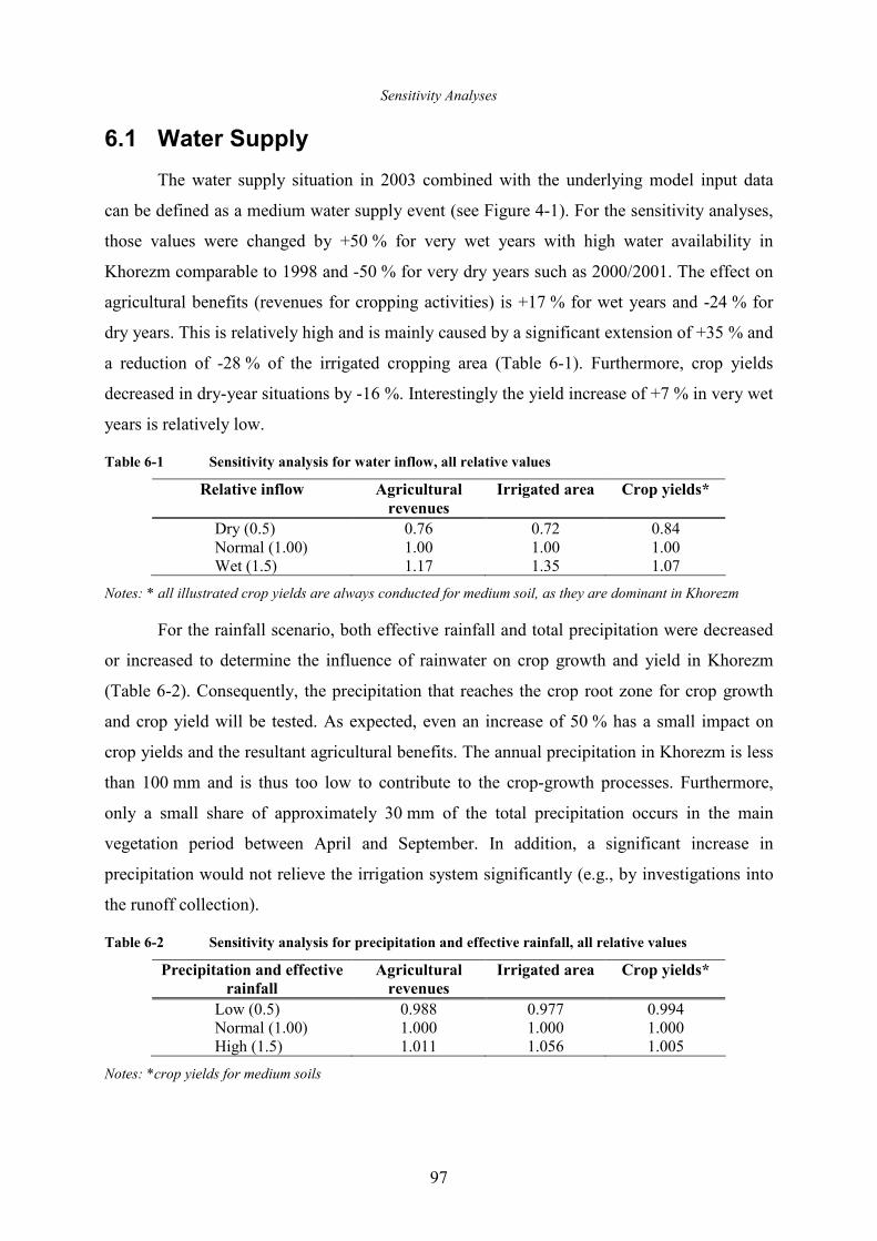
Sensitivity Analyses
97
6.1 Water Supply
The water supply situation in 2003 combined with the underlying model input data
can be defined as a medium water supply event (see Figure 4-1). For the sensitivity analyses,
those values were changed by +50 % for very wet years with high water availability in
Khorezm comparable to 1998 and -50 % for very dry years such as 2000/2001. The effect on
agricultural benefits (revenues for cropping activities) is +17 % for wet years and -24 % for
dry years. This is relatively high and is mainly caused by a significant extension of +35 % and
a reduction of -28 % of the irrigated cropping area (Table 6-1). Furthermore, crop yields
decreased in dry-year situations by -16 %. Interestingly the yield increase of +7 % in very wet
years is relatively low.
Table 6-1 Sensitivity analysis for water inflow, all relative values
Relative inflow Agricultural
revenues
Irrigated area Crop yields*
Dry (0.5) Normal (1.00) Wet (1.5)
0.76 1.00 1.17
0.72 1.00 1.35
0.84 1.00 1.07
Notes: * all illustrated crop yields are always conducted for medium soil, as they are dominant in Khorezm
For the rainfall scenario, both effective rainfall and total precipitation were decreased
or increased to determine the influence of rainwater on crop growth and yield in Khorezm
(Table 6-2). Consequently, the precipitation that reaches the crop root zone for crop growth
and crop yield will be tested. As expected, even an increase of 50 % has a small impact on
crop yields and the resultant agricultural benefits. The annual precipitation in Khorezm is less
than 100 mm and is thus too low to contribute to the crop-growth processes. Furthermore,
only a small share of approximately 30 mm of the total precipitation occurs in the main
vegetation period between April and September. In addition, a significant increase in
precipitation would not relieve the irrigation system significantly (e.g., by investigations into
the runoff collection).
Table 6-2 Sensitivity analysis for precipitation and effective rainfall, all relative values
Precipitation and effective
rainfall
Agricultural
revenues
Irrigated area Crop yields*
Low (0.5) Normal (1.00) High (1.5)
0.988 1.000 1.011
0.977 1.000 1.056
0.994 1.000 1.005
Notes: *crop yields for medium soils
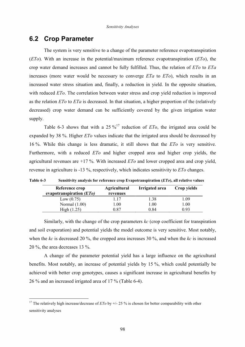
Sensitivity Analyses
98
6.2 Crop Parameter
The system is very sensitive to a change of the parameter reference evapotranspiration
(ETo). With an increase in the potential/maximum reference evapotranspiration (ETo), the
crop water demand increases and cannot be fully fulfilled. Thus, the relation of ETo to ETa
increases (more water would be necessary to converge ETa to ETo), which results in an
increased water stress situation and, finally, a reduction in yield. In the opposite situation,
with reduced ETo. The correlation between water stress and crop yield reduction is improved
as the relation ETo to ETa is decreased. In that situation, a higher proportion of the (relatively
decreased) crop water demand can be sufficiently covered by the given irrigation water
supply.
Table 6-3 shows that with a 25 %17 reduction of ETo, the irrigated area could be
expanded by 38 %. Higher ETo values indicate that the irrigated area should be decreased by
16 %. While this change is less dramatic, it still shows that the ETo is very sensitive.
Furthermore, with a reduced ETo and higher cropped area and higher crop yields, the
agricultural revenues are +17 %. With increased ETo and lower cropped area and crop yield,
revenue in agriculture is -13 %, respectively, which indicates sensitivity to ETo changes.
Table 6-3 Sensitivity analysis for reference crop Evapotranspiration (ETo), all relative values
Reference crop
evapotranspiration (ETo)
Agricultural
revenues
Irrigated area Crop yields
Low (0.75) Normal (1.00) High (1.25)
1.17 1.00 0.87
1.38 1.00 0.84
1.09 1.00 0.93
Similarly, with the change of the crop parameters kc (crop coefficient for transpiration
and soil evaporation) and potential yields the model outcome is very sensitive. Most notably,
when the kc is decreased 20 %, the cropped area increases 30 %, and when the kc is increased
20 %, the area decreases 13 %.
A change of the parameter potential yield has a large influence on the agricultural
benefits. Most notably, an increase of potential yields by 15 %, which could potentially be
achieved with better crop genotypes, causes a significant increase in agricultural benefits by
26 % and an increased irrigated area of 17 % (Table 6-4).
17 The relatively high increase/decrease of ETo by +/- 25 % is chosen for better comparability with other
sensitivity analyses
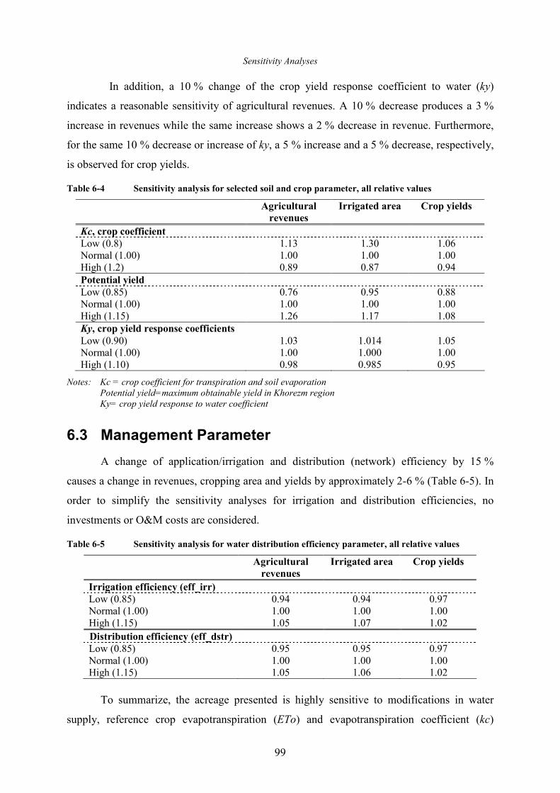
Sensitivity Analyses
99
In addition, a 10 % change of the crop yield response coefficient to water (ky)
indicates a reasonable sensitivity of agricultural revenues. A 10 % decrease produces a 3 %
increase in revenues while the same increase shows a 2 % decrease in revenue. Furthermore,
for the same 10 % decrease or increase of ky, a 5 % increase and a 5 % decrease, respectively,
is observed for crop yields.
Table 6-4 Sensitivity analysis for selected soil and crop parameter, all relative values
Agricultural
revenues
Irrigated area Crop yields
Kc, crop coefficient
Low (0.8) Normal (1.00) High (1.2)
1.13 1.00 0.89
1.30 1.00 0.87
1.06 1.00 0.94
Potential yield
Low (0.85) Normal (1.00) High (1.15)
0.76 1.00 1.26
0.95 1.00 1.17
0.88 1.00 1.08
Ky, crop yield response coefficients Low (0.90) Normal (1.00) High (1.10)
1.03 1.00 0.98
1.014 1.000 0.985
1.05 1.00 0.95
Notes: Kc = crop coefficient for transpiration and soil evaporation Potential yield=maximum obtainable yield in Khorezm region Ky= crop yield response to water coefficient
6.3 Management Parameter
A change of application/irrigation and distribution (network) efficiency by 15 %
causes a change in revenues, cropping area and yields by approximately 2-6 % (Table 6-5). In
order to simplify the sensitivity analyses for irrigation and distribution efficiencies, no
investments or O&M costs are considered.
Table 6-5 Sensitivity analysis for water distribution efficiency parameter, all relative values
Agricultural
revenues
Irrigated area Crop yields
Irrigation efficiency (eff_irr)
Low (0.85) Normal (1.00) High (1.15)
0.94 1.00 1.05
0.94 1.00 1.07
0.97 1.00 1.02
Distribution efficiency (eff_dstr)
Low (0.85) Normal (1.00) High (1.15)
0.95 1.00 1.05
0.95 1.00 1.06
0.97 1.00 1.02
To summarize, the acreage presented is highly sensitive to modifications in water
supply, reference crop evapotranspiration (ETo) and evapotranspiration coefficient (kc)
Sensitivity Analyses
100
values. Agricultural revenues are highly sensitive to modifications of kc, ETo, potential yields
and water supply. Crop yields are generally less sensitive than revenues and cropped areas.
However, crop yields show an increased sensibility to water intake, yield response to water
(ky), potential yields and efficiency. Precipitation parameter change shows no significant
sensitivity for any of the considered outcomes, as precipitation in Khorezm is generally too
low to contribute to crop water supply.
The reaction of the model is considered robust, because with parameter changes in
either direction the model can be solved properly. The model was used to solve for output
values in expected directions and ranges, which can then analyzed and closely examined with
the help of scenario analyses.
Between sensitivity and scenario analysis, there is a somewhat smooth transition as in
both cases a certain parameter change will be implemented and the reaction of the outcomes
will be analyzed. Similar input parameters such as efficiencies or water intake will also be
evaluated within the scenario analyses. The main difference between the two analyses is that
for sensitivity analyses, the influence of an input parameter change to defixated output values
will be considered, whereas for scenario analyses, a parameter change under ceteris paribus
constraints and/or multiple parameter changes will be conducted.
101
7 Description of Simulations and Scenario Analyses
The descriptive model; the verification and plausibility control of the main
parameters; data, formulas, the calibration; economic and hydrologic de facto analyses and
sensitivity analyses were all introduced in earlier chapters. The normative optimization model
will be described in this chapter. Scenario analyses are, similarly to the studies on sensitivity,
analyses that describe the output of considered parameters according to a change in input
parameters. Thus, in most cases, the two analyses cannot be clearly segregated from each
other. A scenario analysis is thus, by definition, also a sensitivity analysis. However, in
contrast to the sensitivity analyses, the scenario studies examine the impacts of different
policies and politically, socially, economically or environmentally induced measures. The
sensitivity analyses are used to verify the underlying model, model structure, data and
causalities. For this reason both analyses are separated into chapters to take into account
different policies and complete a more detailed reflection of not only the overall output
parameter but also the soil and crop specific parameters and water balances.
The main purpose of the model simulations is the analysis of the effects of planned
policies on agricultural, hydrologic, economic and agronomic outputs. The economical
analyses that will be conducted address the following questions:
1) How will the irrigated area and crop allocation change under various
hydrological conditions? How does it affect gross margins, revenues, cropping
patterns and yields?
2) What is the economic water use efficiency for different crops and demand sites
and how does it change under different water supply and management situations?
3) What influence on yields, benefits, cropping area, crop pattern, and hydrologic
balances causes a change in water use efficiency?
4) How will the change of output prices for cotton influence cultivation, cropping
area or crop type and how sensitive will the cropping area and crop prices are to
the modification of cotton prices?
Description of Simulation and Scenario Analyses
102
5) What will happen to water users, profit, demand, acreage, and to the water use
efficiency if water prices are introduced?
6) How, and in what direction, will market liberalization for cotton production
affect the entire cropping system?
7) Does the introduction of a demand- and supply-dependent crop price function
influence cropping pattern, sales prices, acreage and other economical outputs
such as revenues, gross margins and cost?
The selected scenarios were chosen in close coordination with the ZEF/UNESCO
Khorezm project and include policies that are planned to be implemented in this arid region or
appeared reasonable under the hydrologic conditions of the existing irrigation systems.
7.1 Scenario Description
The scenarios and their different experiments were subdivided into tree blocks.
Scenario block 1 comprises analyses for situations under status quo conditions with acreage
and cropping patterns similar to those found in 2003. Variable production cost and crop sales
prices were kept constant on the basis of 2003 prices. The crop yields were calculated
endogenously by the model in subject to described model methodology discussed in
chapter 3. The endogenously calculated crop yield is the main distinguishing feature in
contrast to the descriptive model, because there all the input parameters were fixed to 2003
levels to analyze, calibrate and validate the model intern processes and reactions. Scenario
block 1 will analyze politically and environmentally induced measures via experiments such
as the introduction of water pricing, water supply changes or management parameters under
status quo. The objective is to identify the hydrologic, agronomic and economic effects and
outcomes under the existing state procurement system with regulated cropping quotas for
cotton and wheat. The focus is on analyzing what would have happened to the existing system
if single variables were to change. Most important, the effect on the water balances will be
demonstrated with the help of this scenario.
Scenario block 2 contains experiments with released acreage (abolition of the cotton
quota system) but still with fixed actual 2003 variable cost and prices. This is to allow for
analyses of more efficient crop and water allocation and acreage under the existing system.
Experiments will again use the introduction of water pricing, water supply changes,
improvements in the management parameter and the modification in cotton subsidization to
see the effects of those measures on crop allocation and the resulting economical outcomes.
Description of Simulation and Scenario Analyses
103
In scenario block 3, the introduction of a demand- and supply-dependant crop sales
price function and the liberalization of the cotton sector and its consequences on crop
allocation and economy will be evaluated. Due to the implementation of a price function, it
shall be ensured that, as in reality, the most water- and economical effective crop (or crops)
will not necessarily be planted at the whole area. Crop selection will be dependant on
demand, and the willingness to pay the sales price for those crops will change over time.
Thus, the supply of those crops will be modified. Another change within this scenario is the
implementation of the liberalization of the cotton sector with modified production costs and
cotton prices. Production costs will be higher due to the abolition of governmental subsidies.
Cotton sales prices will be set up according to Central Asian and world market prices. The
single experiments of block 3 are thus multiple scenarios as more than one parameter and
variable will be changed simultaneously.
Within each of the three scenario blocks, some or all of the following experiments will
be performed (Table 7-1):
1. Baseline scenario
2. Modified water supply
3. Modified irrigation management
4. Introduction of water pricing system
5. Abolishment of cotton quota system (released crop acreage) and modification of
subsidization system for cotton18.
18 Not for block three, as it is already implemented
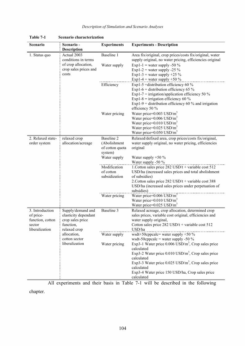
Description of Simulation and Scenario Analyses
104
Table 7-1 Scenario characterization
Scenario Scenario -
Description
Experiments Experiments - Description
Baseline 1 Area fix/original, crop prices/costs fix/original, water supply original, no water pricing, efficiencies original
Water supply Exp1-1 = water supply -50 % Exp1-2 = water supply -25 % Exp1-3 = water supply +25 % Exp1-4 = water supply +50 %
Efficiency Exp1-5 =distribution efficiency 60 % Exp1-6 = distribution efficiency 65 % Exp1-7 = irrigation/application efficiency 50 % Exp1-8 = irrigation efficiency 60 % Exp1-9 = distribution efficiency 60 % and irrigation efficiency 50 %
Water pricing Water price=0.003 USD/m3 Water price=0.006 USD/m3 Water price=0.010 USD/m3 Water price=0.025 USD/m3 Water price=0.050 USD/m3
1. Status quo Actual 2003 conditions in terms of crop allocation, crop sales prices and costs
Baseline 2 (Abolishment of cotton quota system)
Relaxed/defixed area, crop prices/costs fix/original, water supply original, no water pricing, efficiencies original
Water supply Water supply +50 % Water supply -50 %
Modification of cotton subsidization
1.Cotton sales price 282 USD/t + variable cost 512 USD/ha (increased sales prices and total abolishment of subsidies) 2.Cotton sales price 282 USD/t + variable cost 388 USD/ha (increased sales prices under perpetuation of subsidies)
2. Relaxed state- order system
relaxed crop allocation/acreage
Water pricing Water price=0.006 USD/m3 Water price=0.010 USD/m3 Water price=0.025 USD/m3
Baseline 3 Relaxed acreage, crop allocation, determined crop sales prices, variable cost original, efficiencies and water supply original, Cotton sales price 282 USD/t + variable cost 512 USD/ha
Water supply wsdt+50cppcalc= water supply +50 % wsdt-50cppcalc = water supply -50 %
3. Introduction of price-function, cotton sector liberalization
Supply/demand and elasticity dependant crop sales price function, relaxed crop allocation, cotton sector liberalization Water pricing Exp3-1 Water price 0.006 USD/m3, Crop sales price
calculated Exp3-2 Water price 0.010 USD/m3, Crop sales price calculated Exp3-3 Water price 0.025 USD/m3, Crop sales price calculated Exp3-4 Water price 150 USD/ha, Crop sales price calculated
All experiments and their basis in Table 7-1 will be described in the following
chapter.
Description of Simulation and Scenario Analyses
105
7.1.1 Baseline (BL)
The baselines are used as a basis for the comparison of the effects and outcomes of the
different experiments under the three scenario blocks. Consequently each scenario block has
one baseline.
Baseline 1 reflects the actual 2003 situation in terms of cropped area, water supply,
variable costs, selling prices and other input parameters such as climate and efficiencies.
Thus, the baseline scenario describes a status quo situation under the existing state
procurement system with given crop area and crop quantity restrictions as well as assignments
for cotton and wheat and given fixed crop selling prices. Production inputs, such as diesel and
fertilizer are still subsidized by the state.
In Baseline 2 the status quo situation is modified for crop allocation. The acreage is
unconfined/released while variable costs and selling prices remain the same as in 2003.
In Baseline 3 a price function is implemented, leaving sales prices unrestrained.
Furthermore, the governmental procurement system for cotton is abolished, and the acreage is
unrestricted/released.
7.1.2 Water Supply Modification
The last period of water scarcity in the main vegetation time in 2008 showed the
importance of the resource water in Khorezm. The increased demand of irrigation water in
Khorezm due to the cropping of water-intensive crops and the high volume of leaching at the
beginning of the year is one reason for the water shortages in the region of Khorezm and the
downstream areas. Rising competition between upstream and downstream water users and
between the riparian countries of the Amu Darya River19 are further contributions to water
shortages. The dramatic shrinking of the Aral Sea between 2006 and 2010 suggests that the
Aral Sea is far beyond repair, and it is likely that the Large Aral Sea will be dried out in less
than 10 years (ESA, 2009). Additionally climatic changes, such as temperature increases and
the melting of the glaciers in the watershed area of the Pamir Mountains, will account for an
increase of evapotranspiration and an additional decrease in water quantity in the long-term.
UNDP (2007) estimated that an increase of evapotranspiration caused by rising air
temperatures will cause leaching and pre-irrigation to be increased by 5-10 %. Furthermore,
the net irrigation will be increased by 10 %, which will be accompanied by increasing soil
19 Higher water demand for irrigation and for hydropower generation e.g., in Tajikistan
Description of Simulation and Scenario Analyses
106
salinization and further land degradation. NOVIKOV AND SAFAROV (2002) and the Tajik
Ministry of Water Economy estimate that the cotton water demand will increase an additional
22 % due to global warming, and this will cause another increase in irrigation water demand.
In reaction to this climatic development, the droughts in 2000, 2001 and 2008 and the
higher probabilities of droughts respectively, the following scenario addresses the situation of
a changed water supply and the effects on the water balances, the cropping system and the
economic outcomes of the model. The water scarce situation will be of particular interest, but
the effects of a situation with higher water availability than 2003 will also be analyzed
because a temporary increase in the water quantity in short- and mid-term perspective is
possible due to the melting glacier, resulting in supplemental water intake into the river
system.
The following water supply experiments will be performed within each of the three
scenario blocks (Table 7-1):
• Experiment 1 describes a situation with a water supply decrease by using 50 % of
the observed water values in 2003. This situation is comparable to the extreme
drought year of 2001, where the water volume was 44 % of the value in 2003.
• Experiment 2 describes a situation with a 25 % water volume decrease compared
to the Baseline scenario (2003).
• Experiment 3 and 4 describe a situation with 25 % and 50 % increase of water
supply, respectively. These situations are comparable to the good water supply
years of the 1990s, with water supply values 14 % - 38 % higher than in 2003.
7.1.3 Irrigation Management Modification
Irrigation and drainage management play a crucial role in meeting crop water demand
and managing salinity in arid areas such as Khorezm. These measures are therefore
prerequisites for the development of an agricultural economy and food security. Irrigation
scheduling according to time-dependent crop-specific requirements, the quality and quantity
of water, water reuse, drainage, leaching and potential environmental impacts are of special
interest in this area. However, soil characteristics, appropriate irrigation technology and
channels of adequate hydraulic capacity and sufficient uniformity of the surface of irrigated
fields are also important and should be considered. As described in chapter 2.4.4, the
irrigation and drainage systems in Khorezm are in poor condition. The lack of sufficient
maintenance of the channel system combined with the age of the channels cause leakages and
Description of Simulation and Scenario Analyses
107
seepage losses. Furthermore, channel construction technology and the absence of incentives
for the careful use of water results in a very low water use efficiency that is still declining.
UNDP (2007) noted that “in the current situation the operational life of the infrastructure will
further decrease and may reach critical limits”.
As a result of this development, experiments and analyses concerning changed water
use efficiencies will be performed. The effect of a further deterioration of the channel network
as well as the effect of an improvement of the systems due to new technologies and better
operation and management will also be analyzed.
To examine the effects of improved irrigation management, irrigation/field application
and distribution efficiencies will be changed. The distribution efficiency is mainly dependant
on canal properties and infiltration. A modification of the distribution efficiency to 60 % and
65 % of the original 54 % appears to be the most realistic (see DAMIS, 2008). A modification
of the original 40-45 % application/irrigation efficiency to 50 % and 60 % will also be
conducted. The application/irrigation efficiency is mainly dependant on soil, technology and
crop properties. In the last experiment in this step, both, the irrigation and distribution
efficiencies will be modified simultaneously to 60 % and 50 %, respectively.
7.1.4 Introduction of Water Pricing
Due to the expansion of irrigated agricultural cropping, water in Uzbekistan and the
downstream area of the Amu Darya River in Khorezm is in high demand and is extremely
valuable. The demand often reaches or even exceeds the available water resources.
Additionally, a rising competition in water quality and quantity between riparian states,
downstream and upstream users but also between farmers leads to a further aggravation of
this situation. Most notably, the droughts in 2000, 2001 and 2008 in Uzbekistan demonstrated
the importance and necessity of improved water management and a careful and sustainable
management of irrigation water for all parties concerned.
The introduction of water prices or water price reforms has taken place in many
countries all over the world (see DINAR AND SUBRAMANIAN, 1997; OECD, 1999; OECD,
2009). A long-term sustainable water management is, according to GURRIA (2008) only
possible if the water pricing is combined with other factors such as policies (e.g., decreasing
farmer’s support/subsidies and public financing) and if property rights are involved and
ensured.
Description of Simulation and Scenario Analyses
108
Indeed, Uzbekistan already adopted a water law in 1993 in which water saving and
water rights and the need for water pricing is documented (FAO, 1997b). So far, no direct
water pricing mechanisms have been introduced. In fact, the government bears the costs of the
irrigation and drainage system20 and due to the procurement system for crops such as cotton
and wheat; this does not contribute to a productive and efficient usage of irrigation water.
However, Uzbekistan is in the process of large-scale changes due to the farm- restructuring
process (see chapter 2.3). The reconsolidation of land and the change from large collective
farms to much smaller individual (private) farms with changed cropping patterns and water
management practices has resulted in deficiencies in water allocation and distribution
(ABDULLAYEV, 2008). Furthermore, the newly established Water User Associations (WUA)
has found it difficult to balance the general water supply and demand. Additionally, property
rights for the land used by Uzbek farmers are still not clearly defined. It raises the question of
whether water would be better managed and water wastage could be reduced if water was
treated and priced as a commodity.
Water pricing would have a significant impact on the national and local agricultural
structure. Farmers would be faced with reduced revenues and higher production costs that
primarily were subsidized by the state. Water pricing could lead to a better financial support
of the Water User Associations or public water suppliers and reduce the dependency of the
WUAs on the government. The obtained water charges could be re-invested into the
improvement of the irrigation and drainage system and would thus lead to an improvement of
water use efficiency, which in turn pays dividends to the farmers and the environment.
There are various water pricing approaches in agriculture, including volumetric
pricing, non-volumetric pricing and water markets, and each of these approaches has several
subgroups (TSUR ET AL., 2004). In volumetric pricing approaches, the water price is based on
the volume of water that is consumed by the farmer. In non-volumetric pricing the area-based
pricing method is primarily used. Using this approach, a fixed charge based on the irrigated
area is being levied. Charges based on crop type or irrigation techniques are also possible. By
using the complex system of water markets, individuals and companies could trade water at
an equilibrium price (EASTER AND LIU, 2005).
20 Members of Water User Associations (WUA) pay a small membership fee that should cover the expenses of
the public water suppliers (BOBOJONOV, 2008). This amount of less than 0.0005 USD/m3 (in 2005) could be
considered as indirect water pricing. However, as it is so marginal and did not only include water distribution
and operation costs, it will not be considered in detail.
Description of Simulation and Scenario Analyses
109
Although volumetric pricing methods are more difficult to implement, these methods
have the most water saving potential (CHOHIN-KUPER ET AL., 2003). Area-based pricing
methods are much easier to implement, as the installation of flow-meters for volume-
controlled pricing causes additional expenses and time (for e.g. the measurement and
monitoring equipment). In the water pricing scenario, both, monetary water pricing method
(based on volumetric water price per cubic meter of water use) and area-based water pricing
are implemented. The effects on water demand, cropping system, the economical outcomes
and the irrigated area will be reviewed. Based on the literature regarding developing and
transitional countries with water deficits (WEGREN, 1998; CORNISH, 2004), the assumed water
prices for volumetric pricing will be in the range of 25 USD/1000 m3-50 USD/1000 m3, and
for the area-based water pricing, it will be 150 USD/ha. Corresponding to the
recommendation of LERMAN (in WEGREN, 2004), who proposed a volumetric water price for
Uzbekistan of 6.3 USD/1000 m3, we will also analyze lower volumetric dependant water
prices of 6 USD/1000 m3 and 10 USD/1000 m3.
7.1.5 Market Liberalization
Abolition of the cotton quota system and modification of the cotton subsidization system
This scenario addresses the current state policy of fixing the price and the area the
farmers have to cultivate for cotton. Because cotton is the main export product of Uzbekistan
(45 % in 2004) and contributes to 25 % of the foreign exchange revenues and additional tax
revenues, this policy is understandable (GILLSON ET AL., 2004). Furthermore, the subsidies
and guarantied prices for cotton lead to a reduced risk for farmers.
However, due to the governmental procurement system, the cotton producers obtain
prices that are lower than market prices (RUDENKO, 2008). The state’s involvement in the
agricultural sector hampers the development of true private farms due to the limited access to
open markets, credits and inputs (FAO, 2003d). Furthermore, the intensive cultivation and, to
some extent, monoculture of cotton in this arid area is leading to previously described
problems such salinization and chemical contamination, waterlogging, high water
consumption, the reduction of soil fertility and soil crustification. These problems result in a
continuous reduction of cotton yields the last years (GUADAGNI ET AL., 2005). The quota
system also has negative impacts on water use and management because farmers have to
fulfill their quotas regardless of the suitability of the area and the availability of water
Description of Simulation and Scenario Analyses
110
(ABDULLAYEV ET AL., 2009). RUDENKO (2008) shows that the export of intermediate cotton
products such as fiber prevents the further development of the local processing industry and
the integration of the cotton sector into the remainder of the economy. Simultaneously, the
government transfers many of the subsidies for the maintenance and operation of the
irrigation system, including free irrigation water, a financing and credit system, write-offs and
agricultural inputs such as fertilizer, machinery and energy, to lower the prices.
It should also be noted that subsidies, support, direct payments and quotas for the
farmers in cotton-producing countries is standard. The subsidies in Europe (Spain, Portugal
and Greece) and in the United States account for more than 100 % and 50 % respectively of
the averaged world cotton prices in 2005/06 (USDA, 2005 and ICAC, 2007). These subsidies
are the highest in the world and may be damaging, especially for the cotton production in
developing countries, due to the distortion of competition. China and other countries such as
Turkey, Colombia, Mexico and Brazil provide direct income and price support. The impact of
those incentives is that cotton prices are kept artificially low. According to the studies
mentioned above, the world market prices of cotton would be approximately 10 %21 higher if
the subsidies were eliminated worldwide.
The situation just described reveals the controversy regarding subsidies and
governmental intervention. It provides a certain guarantee and safety for the farmers but
provides no incentives to reduce water consumption. Furthermore, the government
intervention leads to huge governmental expenditures and negative externalities on the
international cotton market, especially for developing countries.
WTO (2007) and the International Cotton Advisory Committee (ICAC, 2005)
arranged agreements for a rapid and elaborate reduction of governmental measures and
subsidies in the cotton sector. As a result the Uzbek “Cabinet of Ministers” and the President
passed several regulations and decrees on the reduction of subsidies and demonopolization of
Uzbeks ginning industry and cotton sector privatization (ASKAROV, 2005). In addition to the
progression of farm restructuring in Uzbekistan, another step in the direction of policy
transformation, market liberalization and privatization has thus been initiated.
The impact of the liberalization of the cotton market will be analyzed in the model for
the Khorezm region. For this scenario, an elimination of the governmental procurement
system is defined. There are several linkages between the explicit and implicit subsidies,
21 Ranging between a few % and up to 30 % higher
Description of Simulation and Scenario Analyses
111
taxes, credits, pricing and transfers back to agriculture that make it difficult to define the
essential factors and changes for this scenario. Both input and output factors have to be
changed. The state procurement price and the abolition of input subsidies for fertilizer, diesel,
fuel and operation and maintenance costs for the irrigation canals have to be adjusted.
It is assumed that the price for raw cotton in a liberalized market situation is increased.
RUDENKO (2008) showed that the Uzbek and Khorezmian cotton-producing farmers received
approximately 66 % of the export border price for cotton fiber in 2005. Because Uzbekistan is
not exporting raw cotton directly but rather cotton fiber, the processing of raw cotton into
cotton fiber with a current ginning efficiency of 32 % for Uzbekistan has to be taken into
account. RUDENKO, 2008 showed in a study on the Cotton Value Chain that 3.125 tons of raw
cotton yields approximately 1 ton of cotton fiber22. In addition, GUADAGNI ET AL., 2005 stated
that the border price for raw cotton in 2003 could be approximately 28 % higher than the
governmental price for raw cotton. This corresponds well with the 34 % cotton value chain
analysis by RUDENKO. Thus, a 30 % increase of the cotton price for the liberalization scenario
appears to be realistic.
The second factor is the simultaneous change of production costs for cotton in the
scenario of the abolition of the governmental subsidies. The costs for inputs such as fertilizer,
energy and diesel fuels, seeds and water, as well as the operation and maintenance of the
irrigation and drainage network, will increase for the farmers. Due to the absence of reliable,
empirical data these estimates must be based on data from neighboring countries and other
studies. BOBOJONOV (2008) indicates an increase of 36 % for fertilizer and 24 % for fuel and
DJANIBEKOV (2008) reported an increase of 28 % for cotton seeds and 20 % for pesticides in
Kazakhstan in 2003. The change in production costs under a liberalized cotton scenario in this
model is based on RUDENKO´s (2008) calculations of an increase of 32 % for the total
production costs, with fertilizer application being one of the major input factors in terms of
expenses.
22 With a changed ginning structure, which also is subsidized by the state, the efficiency would certainly change,
too.
112
8 Scenario Analyses - Results
8.1 Model Results Scenario Block 1 - Status Quo Scenario
The results of the three scenarios are considered separately for the sake of clarity. The
effects to internal system processes, such as a decreasing water supply to the groundwater,
drainage fluxes or to the soil water content, are explained in detail. The important outcomes
for each scenario are then discussed and compared relative to their assets and drawbacks with
respect to political, institutional, environmental and socio-economical settings.
8.1.1 Status Quo – Baseline 1
Baseline 1 considers status quo conditions, with acreage and cropping patterns found
in 2003. The production cost and the crop sales prices are based on observed 2003 prices and
were kept constant. The outcomes of the Baseline 1 scenario are included within the
description of the water supply, water pricing and efficiency experiments described below and
serve as a reference for comparison of the different experiments and underlying policies
within scenario block 1.
The analyses of the status quo scenarios serve to answer the question “what would
happen if” to water and soil balance processes, evapotranspiration and resultant yields.
Scenarios for different water supply, modified efficiencies and implementation of water
charges will be executed. The primary focus is on the hydrological and agronomical aspects,
but fundamental economical outcomes should also be considered and will not detract from the
analyses.
8.1.2 Status Quo - Water Supply Experiments
Gross margins
The influence of water supply on total gross margins is high. Simulations indicate a
strong reduction in agricultural income of 47 % and 19 % for cases with 50 % and 25 % water
supply decreases, respectively (Table 6-1). The added value in cases of a 25 % or 50 % water
supply increase is +14 and +25 %, respectively. Because the crop acreage does not changed in
the status quo Baseline 1 scenario, the increase in gross margins is a consequence of a
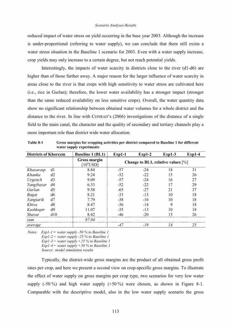
Scenario Analyses-Results
113
reduced impact of water stress on yield occurring in the base year 2003. Although the increase
is under-proportional (referring to water supply), we can conclude that there still exists a
water stress situation in the Baseline 1 scenario for 2003. Even with a water supply increase,
crop yields may only increase to a certain degree, but not reach potential yields.
Interestingly, the impacts of water scarcity in districts close to the river (d1-d6) are
higher than of those farther away. A major reason for the larger influence of water scarcity in
areas close to the river is that crops with high sensitivity to water stress are cultivated here
(i.e., rice in Gurlan); therefore, the lower water availability has a stronger impact (stronger
than the same reduced availability on less sensitive crops). Overall, the water quantity data
show no significant relationship between obtained water volumes for a whole district and the
distance to the river. In line with CONRAD’s (2006) investigations of the distance of a single
field to the main canal, the character and the quality of secondary and tertiary channels play a
more important role than district wide water allocation.
Table 8-1 Gross margins for cropping activities per district compared to Baseline 1 for different
water supply experiments
Districts of Khorezm Baseline 1 (BL1) Exp1-1 Exp1-2 Exp1-3 Exp1-4
Gross margin
[106USD] Change to BL1, relative values [%]
Khazarasp d1 8.84 -57 -24 18 31 Khanka d2 9.24 -52 -22 15 26 Urgench d3 9.09 -57 -24 16 27 Yangibazar d4 6.33 -52 -22 17 29 Gurlan d5 9.58 -65 -27 21 37 Bagat d6 8.21 -33 -13 10 18 Yangiarik d7 7.79 -38 -16 10 18 Khiva d8 8.47 -36 -14 9 18 Kushkupir d9 11.07 -35 -13 10 18 Shavat d10 8.42 -46 -20 15 26 sum 87.04 average -47 -19 14 25
Notes: Exp1-1 = water supply -50 % to Baseline 1 Exp1-2 = water supply -25 % to Baseline 1 Exp1-3 = water supply +25 % to Baseline 1 Exp1-4 = water supply +50 % to Baseline 1 Source: model simulation results
Typically, the district-wide gross margins are the product of all obtained gross profit
rates per crop, and here we present a second view on crop-specific gross margins. To illustrate
the effect of water supply on gross margins per crop type, two scenarios for very low water
supply (-50 %) and high water supply (+50 %) were chosen, as shown in Figure 8-1.
Comparable with the descriptive model, also in the low water supply scenario the gross
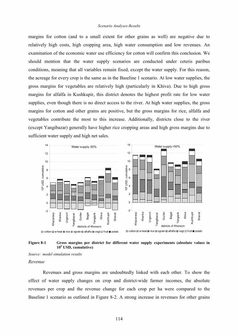
Scenario Analyses-Results
114
margins for cotton (and to a small extent for other grains as well) are negative due to
relatively high costs, high cropping area, high water consumption and low revenues. An
examination of the economic water use efficiency for cotton will confirm this conclusion. We
should mention that the water supply scenarios are conducted under ceteris paribus
conditions, meaning that all variables remain fixed, except the water supply. For this reason,
the acreage for every crop is the same as in the Baseline 1 scenario. At low water supplies, the
gross margins for vegetables are relatively high (particularly in Khiva). Due to high gross
margins for alfalfa in Kushkupir, this district denotes the highest profit rate for low water
supplies, even though there is no direct access to the river. At high water supplies, the gross
margins for cotton and other grains are positive, but the gross margins for rice, alfalfa and
vegetables contribute the most to this increase. Additionally, districts close to the river
(except Yangibazar) generally have higher rice cropping areas and high gross margins due to
sufficient water supply and high net sales.
Figure 8-1 Gross margins per district for different water supply experiments (absolute values in
106 USD, cumulative)
Source: model simulation results
Revenue
Revenues and gross margins are undoubtedly linked with each other. To show the
effect of water supply changes on crop and district-wide farmer incomes, the absolute
revenues per crop and the revenue change for each crop per ha were compared to the
Baseline 1 scenario as outlined in Figure 8-2. A strong increase in revenues for other grains
Water supply +50%
-2
0
2
4
6
8
10
12
14
Khazarasp
Khanka
Urgench
Yangibazar
Gurlan
Bagat
Yangiarik
Khiva
Kushkupir
Shavat
districts of Khorezm
106 USD, cumulative
cotton w heat rice ograin alfalfa vegt fruit potato
Water supply -50%
-2
0
2
4
6
8
10
12
14
Khazarasp
Khanka
Urgench
Yangibazar
Gurlan
Bagat
Yangiarik
Khiva
Kushkupir
Shavat
districts of Khorezm
106 USD, cumulative
cotton w heat rice ograin alfalfa vegt fruit potato
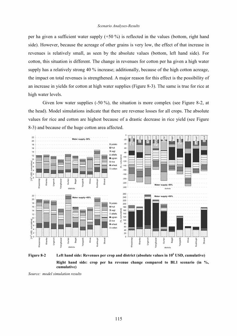
Scenario Analyses-Results
115
per ha given a sufficient water supply (+50 %) is reflected in the values (bottom, right hand
side). However, because the acreage of other grains is very low, the effect of that increase in
revenues is relatively small, as seen by the absolute values (bottom, left hand side). For
cotton, this situation is different. The change in revenues for cotton per ha given a high water
supply has a relatively strong 40 % increase; additionally, because of the high cotton acreage,
the impact on total revenues is strengthened. A major reason for this effect is the possibility of
an increase in yields for cotton at high water supplies (Figure 8-3). The same is true for rice at
high water levels.
Given low water supplies (-50 %), the situation is more complex (see Figure 8-2, at
the head). Model simulations indicate that there are revenue losses for all crops. The absolute
values for rice and cotton are highest because of a drastic decrease in rice yield (see Figure
8-3) and because of the huge cotton area affected.
Figure 8-2 Left hand side: Revenues per crop and district (absolute values in 10
6 USD, cumulative)
Right hand side: crop per ha revenue change compared to BL1 scenario (in %,
cumulative)
Source: model simulation results
Water supply -50%
-240
-220
-200
-180
-160
-140
-120
-100
-80
-60
-40
-20
0
Khazarasp
Khanka
Urgench
Yangibazar
Gurlan
Bagat
Yangiarik
Khiva
Kushkupir
Shavat
districts
[%, cumulative]
Water supply -50%
0
2
4
6
8
10
12
14
16
18
20
22
Khazarasp
Khanka
Urgench
Yangibazar
Gurlan
Bagat
Yangiarik
Khiva
Kushkupir
Shavat
districts
[106 USD, cumulative]
potato
fruit
vegt
alfalfa
ograin
rice
wheat
cotton
Water supply +50%
0
20
40
60
80
100
120
140
160
180
200
220
240
260
Khazarasp
Khanka
Urgench
Yangibazar
Gurlan
Bagat
Yangiarik
Khiva
Kushkupir
Shavat
districts
[%, cumulative]
Water supply +50%
0
2
4
6
8
10
12
14
16
18
20
22
Khazarasp
Khanka
Urgench
Yangibazar
Gurlan
Bagat
Yangiarik
Khiva
Kushkupir
Shavat
districts
[106 USD, cumulative]
potato
fruit
vegt
alfalfa
ograin
rice
wheat
cotton
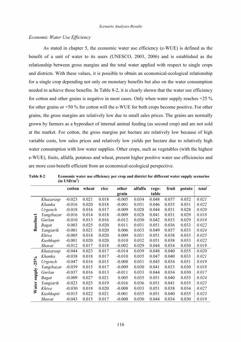
Scenario Analyses-Results
116
Economic Water Use Efficiency
As stated in chapter 5, the economic water use efficiency (e-WUE) is defined as the
benefit of a unit of water to its users (UNESCO, 2003, 2006) and is established as the
relationship between gross margins and the total water applied with respect to single crops
and districts. With these values, it is possible to obtain an economical-ecological relationship
for a single crop depending not only on monetary benefits but also on the water consumption
needed to achieve those benefits. In Table 8-2, it is clearly shown that the water use efficiency
for cotton and other grains is negative in most cases. Only when water supply reaches +25 %
for other grains or +50 % for cotton will the e-WUE for both crops become positive. For other
grains, the gross margins are relatively low due to small sales prices. The grains are normally
grown by farmers as a byproduct of internal animal feeding (as second crop) and are not sold
at the market. For cotton, the gross margins per hectare are relatively low because of high
variable costs, low sales prices and relatively low yields per hectare due to relatively high
water consumption with low water supplies. Other crops, such as vegetables (with the highest
e-WUE), fruits, alfalfa, potatoes and wheat, present higher positive water use efficiencies and
are more cost-benefit efficient from an economical-ecological perspective.
Table 8-2 Economic water use efficiency per crop and district for different water supply scenarios
(in USD/m3)
cotton wheat rice other
grain
alfalfa vege-
table
fruit potato total
Khazarasp -0.023 0.021 0.018 -0.005 0.034 0.048 0.037 0.032 0.021 Khanka -0.016 0.020 0.018 -0.001 0.031 0.046 0.035 0.031 0.022 Urgench -0.018 0.016 0.017 -0.009 0.028 0.044 0.031 0.028 0.020 Yangibazar -0.016 0.014 0.018 -0.009 0.028 0.041 0.031 0.029 0.018 Gurlan -0.010 0.013 0.016 -0.012 0.030 0.042 0.033 0.029 0.018 Bagat 0.003 0.025 0.020 0.011 0.031 0.051 0.036 0.033 0.022 Yangiarik -0.001 0.021 0.020 0.006 0.033 0.049 0.037 0.033 0.024 Khiva -0.005 0.018 0.020 0.009 0.031 0.051 0.038 0.033 0.025 Kushkupir -0.001 0.020 0.020 0.010 0.032 0.051 0.038 0.033 0.022
Base
line1
Shavat -0.012 0.017 0.018 -0.002 0.029 0.044 0.034 0.030 0.019 Khazarasp -0.044 0.023 0.017 -0.014 0.039 0.048 0.040 0.035 0.020 Khanka -0.038 0.018 0.017 -0.010 0.035 0.047 0.040 0.033 0.021 Urgench -0.047 0.016 0.015 -0.008 0.031 0.045 0.034 0.031 0.019 Yangibazar -0.039 0.015 0.017 -0.009 0.030 0.041 0.033 0.030 0.018 Gurlan -0.037 0.016 0.013 -0.011 0.033 0.044 0.034 0.030 0.017 Bagat -0.009 0.027 0.021 0.005 0.035 0.051 0.040 0.035 0.024 Yangiarik -0.023 0.025 0.019 -0.016 0.036 0.051 0.041 0.035 0.025 Khiva -0.030 0.018 0.020 -0.008 0.033 0.051 0.038 0.034 0.027 Kushkupir -0.015 0.022 0.021 -0.001 0.035 0.051 0.040 0.035 0.023 W
ater su
pply
-25%
Shavat -0.043 0.015 0.017 -0.008 0.030 0.044 0.034 0.030 0.019
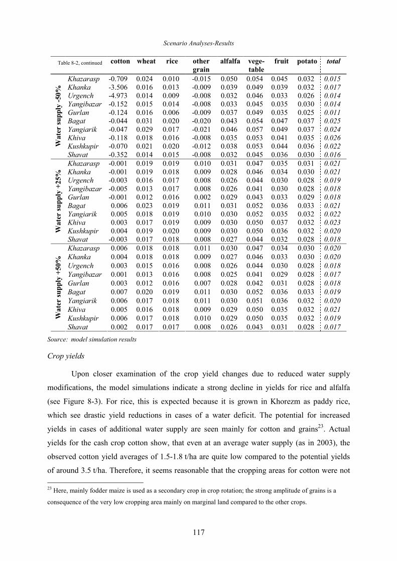
Scenario Analyses-Results
117
cotton wheat rice other
grain
alfalfa vege-
table
fruit potato total
Khazarasp -0.709 0.024 0.010 -0.015 0.050 0.054 0.045 0.032 0.015 Khanka -3.506 0.016 0.013 -0.009 0.039 0.049 0.039 0.032 0.017 Urgench -4.973 0.014 0.009 -0.008 0.032 0.046 0.033 0.026 0.014 Yangibazar -0.152 0.015 0.014 -0.008 0.033 0.045 0.035 0.030 0.014 Gurlan -0.124 0.016 0.006 -0.009 0.037 0.049 0.035 0.025 0.011 Bagat -0.044 0.031 0.020 -0.020 0.043 0.054 0.047 0.037 0.025 Yangiarik -0.047 0.029 0.017 -0.021 0.046 0.057 0.049 0.037 0.024 Khiva -0.118 0.018 0.016 -0.008 0.035 0.053 0.041 0.035 0.026 Kushkupir -0.070 0.021 0.020 -0.012 0.038 0.053 0.044 0.036 0.022 W
ater su
pply
-50%
Shavat -0.352 0.014 0.015 -0.008 0.032 0.045 0.036 0.030 0.016 Khazarasp -0.001 0.019 0.019 0.010 0.031 0.047 0.035 0.031 0.021 Khanka -0.001 0.019 0.018 0.009 0.028 0.046 0.034 0.030 0.021 Urgench -0.003 0.016 0.017 0.008 0.026 0.044 0.030 0.028 0.019 Yangibazar -0.005 0.013 0.017 0.008 0.026 0.041 0.030 0.028 0.018 Gurlan -0.001 0.012 0.016 0.002 0.029 0.043 0.033 0.029 0.018 Bagat 0.006 0.023 0.019 0.011 0.031 0.052 0.036 0.033 0.021 Yangiarik 0.005 0.018 0.019 0.010 0.030 0.052 0.035 0.032 0.022 Khiva 0.003 0.017 0.019 0.009 0.030 0.050 0.037 0.032 0.023 Kushkupir 0.004 0.019 0.020 0.009 0.030 0.050 0.036 0.032 0.020 W
ater su
pply
+25%
Shavat -0.003 0.017 0.018 0.008 0.027 0.044 0.032 0.028 0.018 Khazarasp 0.006 0.018 0.018 0.011 0.030 0.047 0.034 0.030 0.020 Khanka 0.004 0.018 0.018 0.009 0.027 0.046 0.033 0.030 0.020 Urgench 0.003 0.015 0.016 0.008 0.026 0.044 0.030 0.028 0.018 Yangibazar 0.001 0.013 0.016 0.008 0.025 0.041 0.029 0.028 0.017 Gurlan 0.003 0.012 0.016 0.007 0.028 0.042 0.031 0.028 0.018 Bagat 0.007 0.020 0.019 0.011 0.030 0.052 0.036 0.033 0.019 Yangiarik 0.006 0.017 0.018 0.011 0.030 0.051 0.036 0.032 0.020 Khiva 0.005 0.016 0.018 0.009 0.029 0.050 0.035 0.032 0.021 Kushkupir 0.006 0.017 0.018 0.010 0.029 0.050 0.035 0.032 0.019 W
ater su
pply
+50%
Shavat 0.002 0.017 0.017 0.008 0.026 0.043 0.031 0.028 0.017
Source: model simulation results
Crop yields
Upon closer examination of the crop yield changes due to reduced water supply
modifications, the model simulations indicate a strong decline in yields for rice and alfalfa
(see Figure 8-3). For rice, this is expected because it is grown in Khorezm as paddy rice,
which see drastic yield reductions in cases of a water deficit. The potential for increased
yields in cases of additional water supply are seen mainly for cotton and grains23. Actual
yields for the cash crop cotton show, that even at an average water supply (as in 2003), the
observed cotton yield averages of 1.5-1.8 t/ha are quite low compared to the potential yields
of around 3.5 t/ha. Therefore, it seems reasonable that the cropping areas for cotton were not
23 Here, mainly fodder maize is used as a secondary crop in crop rotation; the strong amplitude of grains is a
consequence of the very low cropping area mainly on marginal land compared to the other crops.
Table 8-2, continued
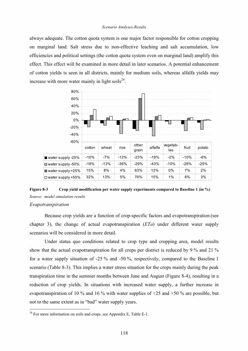
Scenario Analyses-Results
118
always adequate. The cotton quota system is one major factor responsible for cotton cropping
on marginal land. Salt stress due to non-effective leaching and salt accumulation, low
efficiencies and political settings (the cotton quota system even on marginal land) amplify this
effect. This effect will be examined in more detail in later scenarios. A potential enhancement
of cotton yields is seen in all districts, mainly for medium soils, whereas alfalfa yields may
increase with more water mainly in light soils24.
-60%
-40%
-20%
0%
20%
40%
60%
80%
water supply -25% -10% -7% -12% -23% -18% -2% -10% -6%
water supply -50% -18% -13% -36% -29% -43% -10% -28% -25%
water supply +25% 15% 8% 4% 63% 12% 0% 7% 2%
water supply +50% 32% 13% 5% 76% 15% 1% 8% 3%
cotton wheat riceother
grainalfalfa
vegetab-
lesfruit potato
Figure 8-3 Crop yield modification per water supply experiments compared to Baseline 1 (in %)
Source: model simulation results
Evapotranspiration
Because crop yields are a function of crop-specific factors and evapotranspiration (see
chapter 3), the change of actual evapotranspiration (ETa) under different water supply
scenarios will be considered in more detail.
Under status quo conditions related to crop type and cropping area, model results
show that the actual evapotranspiration for all crops per district is reduced by 9 % and 21 %
for a water supply situation of -25 % and -50 %, respectively, compared to the Baseline 1
scenario (Table 8-3). This implies a water stress situation for the crops mainly during the peak
transpiration time in the summer months between June and August (Figure 8-4), resulting in a
reduction of crop yields. In situations with increased water supply, a further increase in
evapotranspiration of 10 % and 16 % with water supplies of +25 and +50 % are possible, but
not to the same extent as in “bad” water supply years.
24 For more information on soils and crops, see Appendix E, Table E-1.
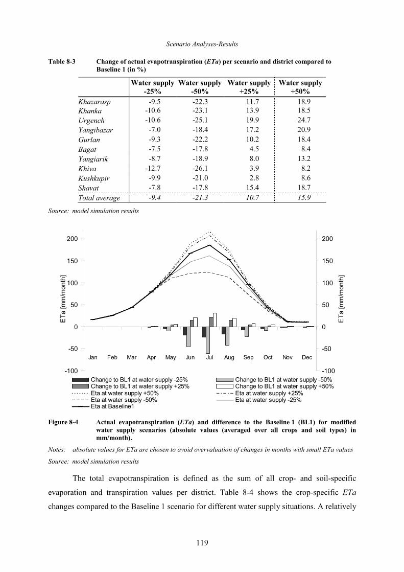
Scenario Analyses-Results
119
Table 8-3 Change of actual evapotranspiration (ETa) per scenario and district compared to
Baseline 1 (in %)
Water supply
-25%
Water supply
-50%
Water supply
+25%
Water supply
+50%
Khazarasp -9.5 -22.3 11.7 18.9 Khanka -10.6 -23.1 13.9 18.5 Urgench -10.6 -25.1 19.9 24.7 Yangibazar -7.0 -18.4 17.2 20.9 Gurlan -9.3 -22.2 10.2 18.4 Bagat -7.5 -17.8 4.5 8.4 Yangiarik -8.7 -18.9 8.0 13.2 Khiva -12.7 -26.1 3.9 8.2 Kushkupir -9.9 -21.0 2.8 8.6 Shavat -7.8 -17.8 15.4 18.7
Total average -9.4 -21.3 10.7 15.9
Source: model simulation results
-100
-50
0
50
100
150
200
Jan Feb Mar Apr May Jun Jul Aug Sep Oct Nov Dec
ETa [mm/month]
-100
-50
0
50
100
150
200
ETa [mm/month]
Change to BL1 at water supply -25% Change to BL1 at water supply -50%Change to BL1 at water supply +25% Change to BL1 at water supply +50%Eta at water supply +50% Eta at water supply +25%Eta at water supply -50% Eta at water supply -25%Eta at Baseline1
Figure 8-4 Actual evapotranspiration (ETa) and difference to the Baseline 1 (BL1) for modified
water supply scenarios (absolute values (averaged over all crops and soil types) in
mm/month).
Notes: absolute values for ETa are chosen to avoid overvaluation of changes in months with small ETa values
Source: model simulation results
The total evapotranspiration is defined as the sum of all crop- and soil-specific
evaporation and transpiration values per district. Table 8-4 shows the crop-specific ETa
changes compared to the Baseline 1 scenario for different water supply situations. A relatively
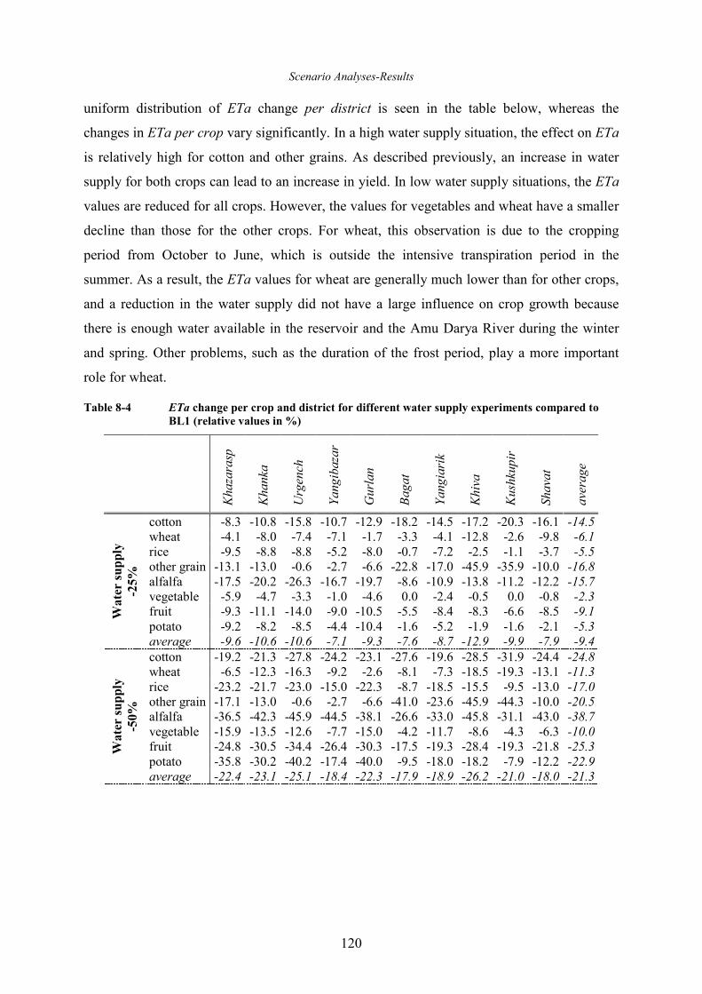
Scenario Analyses-Results
120
uniform distribution of ETa change per district is seen in the table below, whereas the
changes in ETa per crop vary significantly. In a high water supply situation, the effect on ETa
is relatively high for cotton and other grains. As described previously, an increase in water
supply for both crops can lead to an increase in yield. In low water supply situations, the ETa
values are reduced for all crops. However, the values for vegetables and wheat have a smaller
decline than those for the other crops. For wheat, this observation is due to the cropping
period from October to June, which is outside the intensive transpiration period in the
summer. As a result, the ETa values for wheat are generally much lower than for other crops,
and a reduction in the water supply did not have a large influence on crop growth because
there is enough water available in the reservoir and the Amu Darya River during the winter
and spring. Other problems, such as the duration of the frost period, play a more important
role for wheat.
Table 8-4 ETa change per crop and district for different water supply experiments compared to
BL1 (relative values in %)
Kha
zarasp
Kha
nka
Urgench
Yan
gibazar
Gurlan
Bag
at
Yan
giarik
Khiva
Kushkupir
Shavat
average
cotton -8.3 -10.8 -15.8 -10.7 -12.9 -18.2 -14.5 -17.2 -20.3 -16.1 -14.5 wheat -4.1 -8.0 -7.4 -7.1 -1.7 -3.3 -4.1 -12.8 -2.6 -9.8 -6.1 rice -9.5 -8.8 -8.8 -5.2 -8.0 -0.7 -7.2 -2.5 -1.1 -3.7 -5.5 other grain -13.1 -13.0 -0.6 -2.7 -6.6 -22.8 -17.0 -45.9 -35.9 -10.0 -16.8 alfalfa -17.5 -20.2 -26.3 -16.7 -19.7 -8.6 -10.9 -13.8 -11.2 -12.2 -15.7 vegetable -5.9 -4.7 -3.3 -1.0 -4.6 0.0 -2.4 -0.5 0.0 -0.8 -2.3 fruit -9.3 -11.1 -14.0 -9.0 -10.5 -5.5 -8.4 -8.3 -6.6 -8.5 -9.1 potato -9.2 -8.2 -8.5 -4.4 -10.4 -1.6 -5.2 -1.9 -1.6 -2.1 -5.3
Water su
pply
-25%
average -9.6 -10.6 -10.6 -7.1 -9.3 -7.6 -8.7 -12.9 -9.9 -7.9 -9.4 cotton -19.2 -21.3 -27.8 -24.2 -23.1 -27.6 -19.6 -28.5 -31.9 -24.4 -24.8 wheat -6.5 -12.3 -16.3 -9.2 -2.6 -8.1 -7.3 -18.5 -19.3 -13.1 -11.3 rice -23.2 -21.7 -23.0 -15.0 -22.3 -8.7 -18.5 -15.5 -9.5 -13.0 -17.0 other grain -17.1 -13.0 -0.6 -2.7 -6.6 -41.0 -23.6 -45.9 -44.3 -10.0 -20.5 alfalfa -36.5 -42.3 -45.9 -44.5 -38.1 -26.6 -33.0 -45.8 -31.1 -43.0 -38.7 vegetable -15.9 -13.5 -12.6 -7.7 -15.0 -4.2 -11.7 -8.6 -4.3 -6.3 -10.0 fruit -24.8 -30.5 -34.4 -26.4 -30.3 -17.5 -19.3 -28.4 -19.3 -21.8 -25.3 potato -35.8 -30.2 -40.2 -17.4 -40.0 -9.5 -18.0 -18.2 -7.9 -12.2 -22.9
Water su
pply
-50%
average -22.4 -23.1 -25.1 -18.4 -22.3 -17.9 -18.9 -26.2 -21.0 -18.0 -21.3
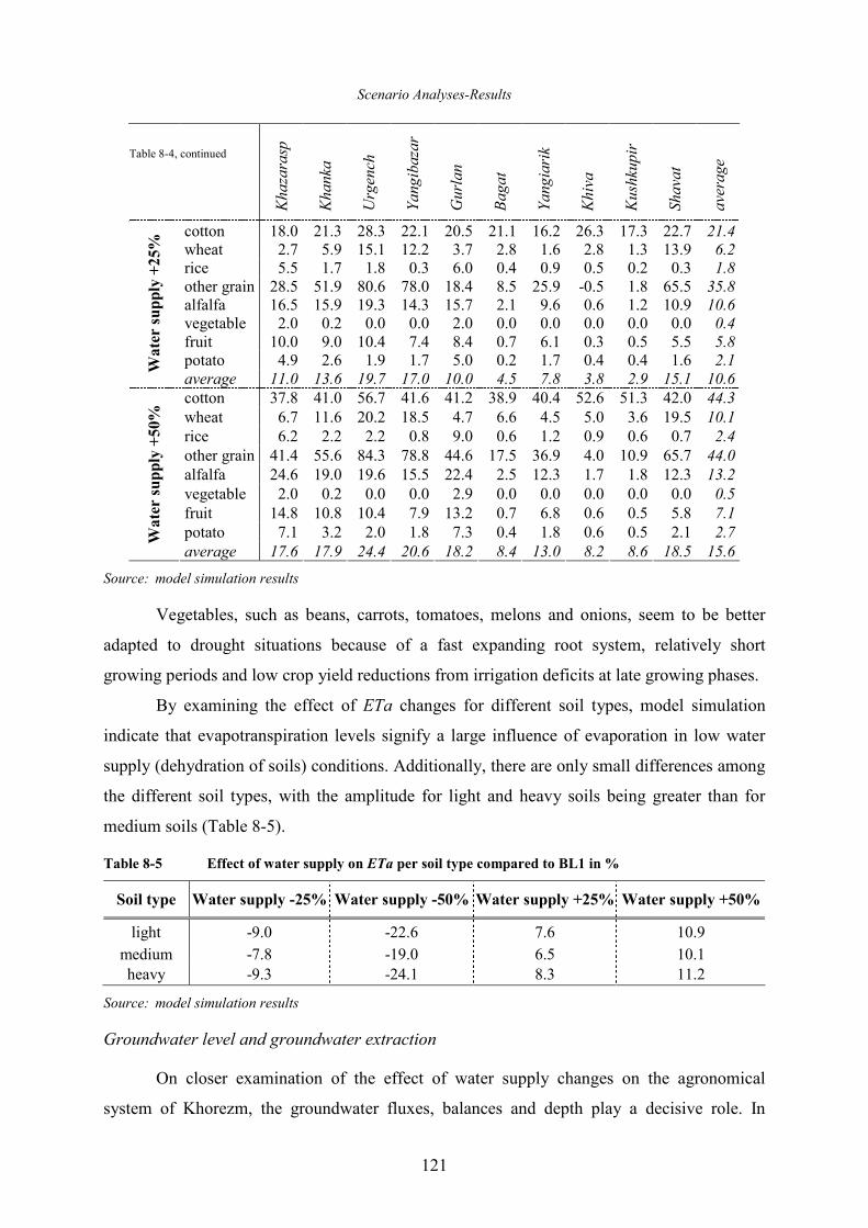
Scenario Analyses-Results
121
Kha
zarasp
Kha
nka
Urgench
Yan
gibazar
Gurlan
Bag
at
Yan
giarik
Khiva
Kushkupir
Shavat
average
cotton 18.0 21.3 28.3 22.1 20.5 21.1 16.2 26.3 17.3 22.7 21.4 wheat 2.7 5.9 15.1 12.2 3.7 2.8 1.6 2.8 1.3 13.9 6.2 rice 5.5 1.7 1.8 0.3 6.0 0.4 0.9 0.5 0.2 0.3 1.8 other grain 28.5 51.9 80.6 78.0 18.4 8.5 25.9 -0.5 1.8 65.5 35.8 alfalfa 16.5 15.9 19.3 14.3 15.7 2.1 9.6 0.6 1.2 10.9 10.6 vegetable 2.0 0.2 0.0 0.0 2.0 0.0 0.0 0.0 0.0 0.0 0.4 fruit 10.0 9.0 10.4 7.4 8.4 0.7 6.1 0.3 0.5 5.5 5.8 potato 4.9 2.6 1.9 1.7 5.0 0.2 1.7 0.4 0.4 1.6 2.1 W
ater su
pply
+25%
average 11.0 13.6 19.7 17.0 10.0 4.5 7.8 3.8 2.9 15.1 10.6 cotton 37.8 41.0 56.7 41.6 41.2 38.9 40.4 52.6 51.3 42.0 44.3 wheat 6.7 11.6 20.2 18.5 4.7 6.6 4.5 5.0 3.6 19.5 10.1 rice 6.2 2.2 2.2 0.8 9.0 0.6 1.2 0.9 0.6 0.7 2.4 other grain 41.4 55.6 84.3 78.8 44.6 17.5 36.9 4.0 10.9 65.7 44.0 alfalfa 24.6 19.0 19.6 15.5 22.4 2.5 12.3 1.7 1.8 12.3 13.2 vegetable 2.0 0.2 0.0 0.0 2.9 0.0 0.0 0.0 0.0 0.0 0.5 fruit 14.8 10.8 10.4 7.9 13.2 0.7 6.8 0.6 0.5 5.8 7.1 potato 7.1 3.2 2.0 1.8 7.3 0.4 1.8 0.6 0.5 2.1 2.7 W
ater su
pply
+50%
average 17.6 17.9 24.4 20.6 18.2 8.4 13.0 8.2 8.6 18.5 15.6
Source: model simulation results
Vegetables, such as beans, carrots, tomatoes, melons and onions, seem to be better
adapted to drought situations because of a fast expanding root system, relatively short
growing periods and low crop yield reductions from irrigation deficits at late growing phases.
By examining the effect of ETa changes for different soil types, model simulation
indicate that evapotranspiration levels signify a large influence of evaporation in low water
supply (dehydration of soils) conditions. Additionally, there are only small differences among
the different soil types, with the amplitude for light and heavy soils being greater than for
medium soils (Table 8-5).
Table 8-5 Effect of water supply on ETa per soil type compared to BL1 in %
Soil type Water supply -25% Water supply -50% Water supply +25% Water supply +50%
light -9.0 -22.6 7.6 10.9
medium -7.8 -19.0 6.5 10.1 heavy -9.3 -24.1 8.3 11.2
Source: model simulation results
Groundwater level and groundwater extraction
On closer examination of the effect of water supply changes on the agronomical
system of Khorezm, the groundwater fluxes, balances and depth play a decisive role. In
Table 8-4, continued
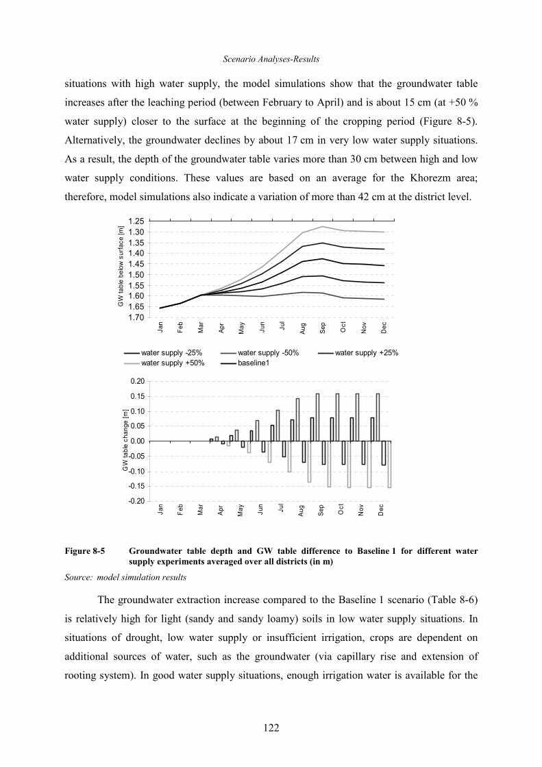
Scenario Analyses-Results
122
situations with high water supply, the model simulations show that the groundwater table
increases after the leaching period (between February to April) and is about 15 cm (at +50 %
water supply) closer to the surface at the beginning of the cropping period (Figure 8-5).
Alternatively, the groundwater declines by about 17 cm in very low water supply situations.
As a result, the depth of the groundwater table varies more than 30 cm between high and low
water supply conditions. These values are based on an average for the Khorezm area;
therefore, model simulations also indicate a variation of more than 42 cm at the district level.
Figure 8-5 Groundwater table depth and GW table difference to Baseline 1 for different water
supply experiments averaged over all districts (in m)
Source: model simulation results
The groundwater extraction increase compared to the Baseline 1 scenario (Table 8-6)
is relatively high for light (sandy and sandy loamy) soils in low water supply situations. In
situations of drought, low water supply or insufficient irrigation, crops are dependent on
additional sources of water, such as the groundwater (via capillary rise and extension of
rooting system). In good water supply situations, enough irrigation water is available for the
1.25
1.30
1.35
1.40
1.45
1.50
1.55
1.60
1.65
1.70
Jan
Feb
Mar
Apr
May
Jun
Jul
Aug
Sep
Oct
Nov
Dec
GW table below surface [m]
water supply -25% water supply -50% water supply +25%
water supply +50% baseline1
-0.20
-0.15
-0.10
-0.05
0.00
0.05
0.10
0.15
0.20
Jan
Feb
Mar
Apr
May
Jun
Jul
Aug
Sep
Oct
Nov
Dec
GW table change [m]
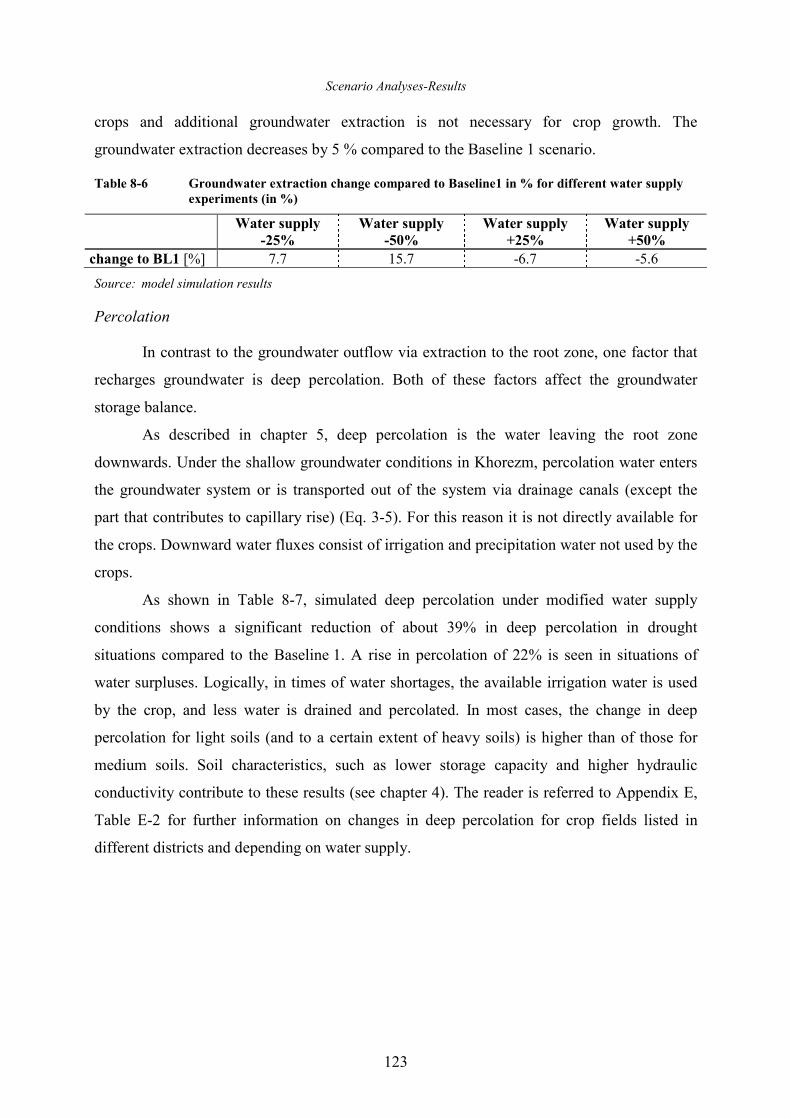
Scenario Analyses-Results
123
crops and additional groundwater extraction is not necessary for crop growth. The
groundwater extraction decreases by 5 % compared to the Baseline 1 scenario.
Table 8-6 Groundwater extraction change compared to Baseline1 in % for different water supply
experiments (in %)
Water supply
-25%
Water supply
-50%
Water supply
+25%
Water supply
+50%
change to BL1 [%] 7.7 15.7 -6.7 -5.6
Source: model simulation results
Percolation
In contrast to the groundwater outflow via extraction to the root zone, one factor that
recharges groundwater is deep percolation. Both of these factors affect the groundwater
storage balance.
As described in chapter 5, deep percolation is the water leaving the root zone
downwards. Under the shallow groundwater conditions in Khorezm, percolation water enters
the groundwater system or is transported out of the system via drainage canals (except the
part that contributes to capillary rise) (Eq. 3-5). For this reason it is not directly available for
the crops. Downward water fluxes consist of irrigation and precipitation water not used by the
crops.
As shown in Table 8-7, simulated deep percolation under modified water supply
conditions shows a significant reduction of about 39% in deep percolation in drought
situations compared to the Baseline 1. A rise in percolation of 22% is seen in situations of
water surpluses. Logically, in times of water shortages, the available irrigation water is used
by the crop, and less water is drained and percolated. In most cases, the change in deep
percolation for light soils (and to a certain extent of heavy soils) is higher than of those for
medium soils. Soil characteristics, such as lower storage capacity and higher hydraulic
conductivity contribute to these results (see chapter 4). The reader is referred to Appendix E,
Table E-2 for further information on changes in deep percolation for crop fields listed in
different districts and depending on water supply.
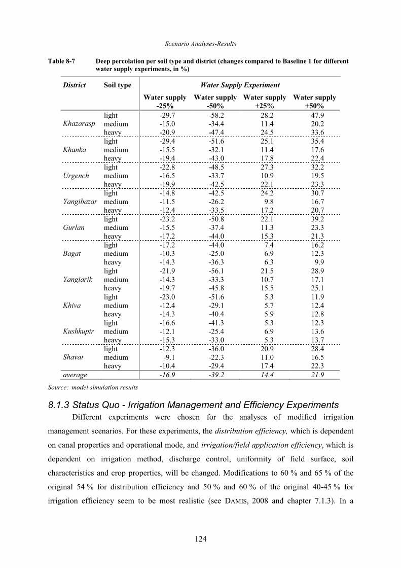
Scenario Analyses-Results
124
Table 8-7 Deep percolation per soil type and district (changes compared to Baseline 1 for different
water supply experiments, in %)
District Soil type Water Supply Experiment
Water supply
-25%
Water supply
-50%
Water supply
+25%
Water supply
+50%
light -29.7 -58.2 28.2 47.9 medium -15.0 -34.4 11.4 20.2 Khazarasp heavy -20.9 -47.4 24.5 33.6 light -29.4 -51.6 25.1 35.4 medium -15.5 -32.1 11.4 17.6 Khanka heavy -19.4 -43.0 17.8 22.4 light -22.8 -48.5 27.3 32.2 medium -16.5 -33.7 10.9 19.5 Urgench heavy -19.9 -42.5 22.1 23.3 light -14.8 -42.5 24.2 30.7 medium -11.5 -26.2 9.8 16.7 Yangibazar heavy -12.4 -33.5 17.2 20.7 light -23.2 -50.8 22.1 39.2 medium -15.5 -37.4 11.3 23.3 Gurlan heavy -17.2 -44.0 15.3 21.3 light -17.2 -44.0 7.4 16.2 medium -10.3 -25.0 6.9 12.3 Bagat heavy -14.3 -36.3 6.3 9.9 light -21.9 -56.1 21.5 28.9 medium -14.3 -33.3 10.7 17.1 Yangiarik heavy -19.7 -45.8 15.5 25.1 light -23.0 -51.6 5.3 11.9 medium -12.4 -29.1 5.7 12.4 Khiva heavy -14.3 -40.4 5.9 12.8 light -16.6 -41.3 5.3 12.3 medium -12.1 -25.4 6.9 13.6 Kushkupir heavy -15.3 -33.0 5.3 13.7 light -12.3 -36.0 20.9 28.4 medium -9.1 -22.3 11.0 16.5 Shavat heavy -10.4 -29.4 17.4 22.3
average -16.9 -39.2 14.4 21.9
Source: model simulation results
8.1.3 Status Quo - Irrigation Management and Efficiency Experiments
Different experiments were chosen for the analyses of modified irrigation
management scenarios. For these experiments, the distribution efficiency, which is dependent
on canal properties and operational mode, and irrigation/field application efficiency, which is
dependent on irrigation method, discharge control, uniformity of field surface, soil
characteristics and crop properties, will be changed. Modifications to 60 % and 65 % of the
original 54 % for distribution efficiency and 50 % and 60 % of the original 40-45 % for
irrigation efficiency seem to be most realistic (see DAMIS, 2008 and chapter 7.1.3). In a
Scenario Analyses-Results
125
separate experiment, both, the distribution and irrigation efficiencies will be improved
simultaneously (Exp. 1-9).
An increase in distribution efficiency can be achieved by changing the flow velocity,
which is affected by canal maintenance and straightening, thereby decreasing percolation and
evaporation. Additionally, changes in the canal lining or covering can decrease the porosity,
water leakage and evaporation. Most of these measures are cost intensive, undesirable and
difficult to accomplish. For instance, a certain amount of canal leakage may be ecologically
worthwhile by enhancing leaching and elution of salts in the soil layer. On the other hand,
seepage and percolation from canals contributes very little to leaching (effect is limited to the
area at the canal); however, canal seepage recharges groundwater (and in the case where
groundwater becomes shallow, there is enhancement of secondary soil salinization via the
groundwater). Consequently, canal operation (i.e., sufficient irrigation scheduling, better
coordination at the field and system levels), maintenance (i.e., cleaning, cutting and digging),
reparation and plugging of the canal basement and walls are required and represent low cost
measures that increase distribution efficiency, albeit a small change (approximately 5 %) from
the assumed 54 % - 65 % (Exp1-5, Exp1-6).
An improvement in irrigation efficiency can be attained by changing the irrigation
methods and technology, leveling the crop field and adjusting the crop irrigation scheduling
and management. According to GOYNE (2002), simple water and soil monitoring measures
can improve efficiencies in cotton and grain fields by at least 10 %. For this reason, a
modification of the original 40-45 % application/irrigation efficiency to 50 % and 60 % is
conducted (Exp1-7, Exp.1-8).
Gross Margins, Revenue and Water Value
As shown in the model simulations, basically a positive effect on the overall gross
margins can be attained by improving the irrigation efficiency at the field level. A 5 %
increase in irrigation efficiency causes an increase of 9 % for total averaged gross margins
(Table 8-8). A comparable increase of 10 % in gross margins can be achieved with a 10 %
increase in efficiency of the distribution system (at a distribution efficiency level of 65 %).
The results suggest that measures, especially at the field level, should be implemented to
attain higher yields and benefits.
Similarly to the water supply scenarios, the efficiency scenarios show that the
distribution of gross margins per crop is quite comparable (see Figure 8-6, exemplarily for
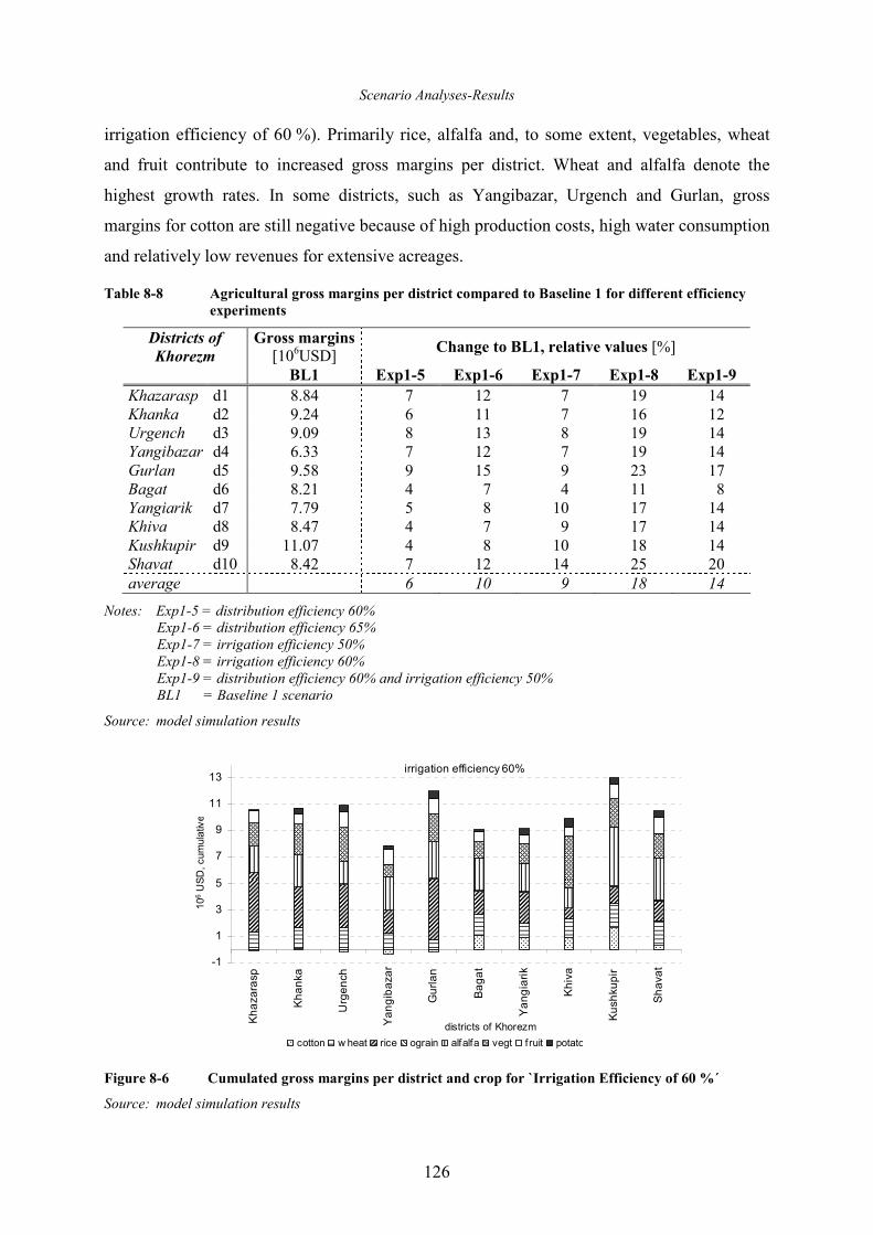
Scenario Analyses-Results
126
irrigation efficiency of 60 %). Primarily rice, alfalfa and, to some extent, vegetables, wheat
and fruit contribute to increased gross margins per district. Wheat and alfalfa denote the
highest growth rates. In some districts, such as Yangibazar, Urgench and Gurlan, gross
margins for cotton are still negative because of high production costs, high water consumption
and relatively low revenues for extensive acreages.
Table 8-8 Agricultural gross margins per district compared to Baseline 1 for different efficiency
experiments
Districts of
Khorezm
Gross margins [106USD]
Change to BL1, relative values [%]
BL1 Exp1-5 Exp1-6 Exp1-7 Exp1-8 Exp1-9
Khazarasp d1 8.84 7 12 7 19 14 Khanka d2 9.24 6 11 7 16 12 Urgench d3 9.09 8 13 8 19 14 Yangibazar d4 6.33 7 12 7 19 14 Gurlan d5 9.58 9 15 9 23 17 Bagat d6 8.21 4 7 4 11 8 Yangiarik d7 7.79 5 8 10 17 14 Khiva d8 8.47 4 7 9 17 14 Kushkupir d9 11.07 4 8 10 18 14 Shavat d10 8.42 7 12 14 25 20 average 6 10 9 18 14
Notes: Exp1-5 = distribution efficiency 60% Exp1-6 = distribution efficiency 65% Exp1-7 = irrigation efficiency 50% Exp1-8 = irrigation efficiency 60% Exp1-9 = distribution efficiency 60% and irrigation efficiency 50% BL1 = Baseline 1 scenario
Source: model simulation results
irrigation efficiency 60%
-1
1
3
5
7
9
11
13
Khazarasp
Khanka
Urgench
Yangibazar
Gurlan
Bagat
Yangiarik
Khiva
Kushkupir
Shavat
districts of Khorezm
106 USD, cumulative
cotton w heat rice ograin alfalfa vegt fruit potato
Figure 8-6 Cumulated gross margins per district and crop for `Irrigation Efficiency of 60 %´
Source: model simulation results
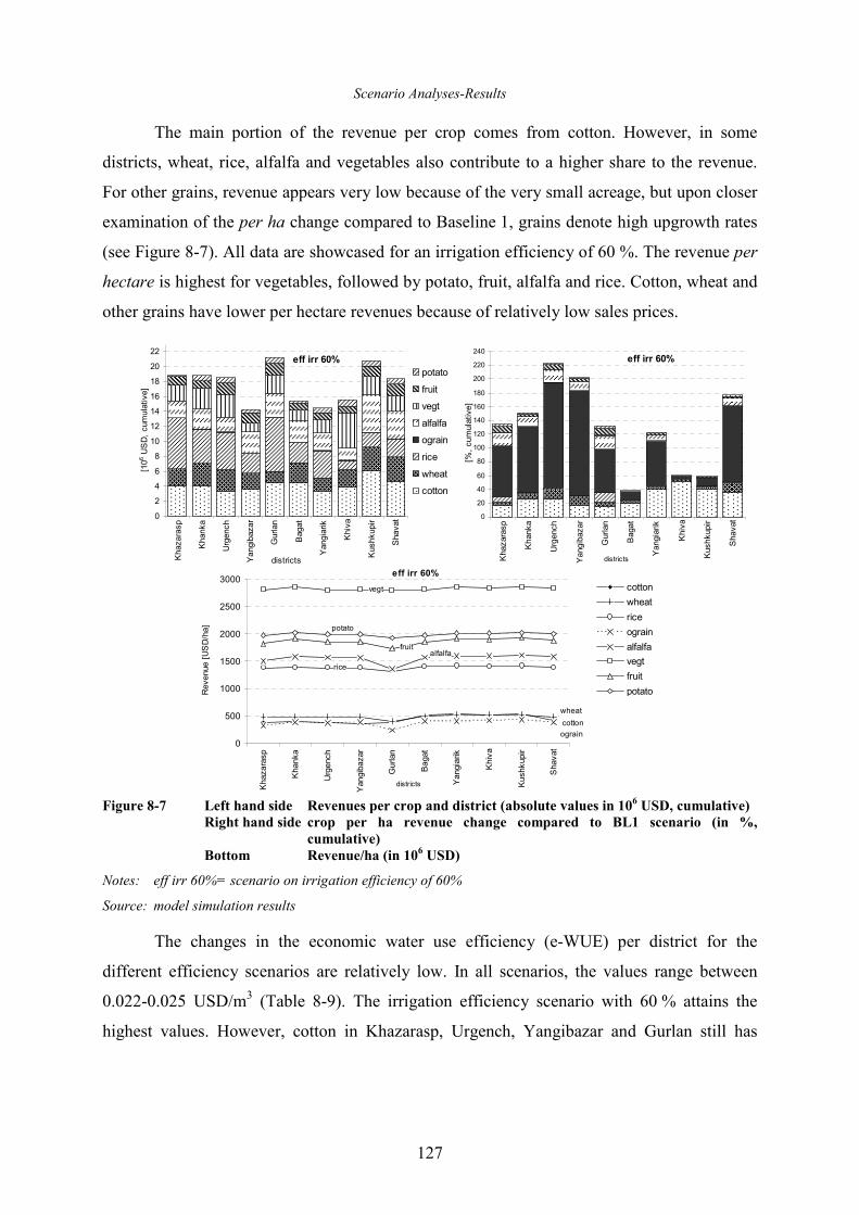
Scenario Analyses-Results
127
The main portion of the revenue per crop comes from cotton. However, in some
districts, wheat, rice, alfalfa and vegetables also contribute to a higher share to the revenue.
For other grains, revenue appears very low because of the very small acreage, but upon closer
examination of the per ha change compared to Baseline 1, grains denote high upgrowth rates
(see Figure 8-7). All data are showcased for an irrigation efficiency of 60 %. The revenue per
hectare is highest for vegetables, followed by potato, fruit, alfalfa and rice. Cotton, wheat and
other grains have lower per hectare revenues because of relatively low sales prices.
Figure 8-7 Left hand side Revenues per crop and district (absolute values in 10
6 USD, cumulative)
Right hand side crop per ha revenue change compared to BL1 scenario (in %,
cumulative)
Bottom Revenue/ha (in 106 USD)
Notes: eff irr 60%= scenario on irrigation efficiency of 60%
Source: model simulation results
The changes in the economic water use efficiency (e-WUE) per district for the
different efficiency scenarios are relatively low. In all scenarios, the values range between
0.022-0.025 USD/m3 (Table 8-9). The irrigation efficiency scenario with 60 % attains the
highest values. However, cotton in Khazarasp, Urgench, Yangibazar and Gurlan still has
eff irr 60%
0
2
4
6
8
10
12
14
16
18
20
22
Khazarasp
Khanka
Urgench
Yangibazar
Gurlan
Bagat
Yangiarik
Khiva
Kushkupir
Shavat
districts
[106 USD, cumulative]
potato
fruit
vegt
alfalfa
ograin
rice
wheat
cotton
eff irr 60%
0
20
40
60
80
100
120
140
160
180
200
220
240
Khazarasp
Khanka
Urgench
Yangibazar
Gurlan
Bagat
Yangiarik
Khiva
Kushkupir
Shavat
districts
[%, cumulative]
eff irr 60%
cotton
wheat
rice
ograin
alfalfa
vegt
fruit
potato
0
500
1000
1500
2000
2500
3000
Khazarasp
Khanka
Urgench
Yangibazar
Gurlan
Bagat
Yangiarik
Khiva
Kushkupir
Shavat
districts
Revenue [USD/ha]
cotton
wheat
rice
ograin
alfalfa
vegt
fruit
potato
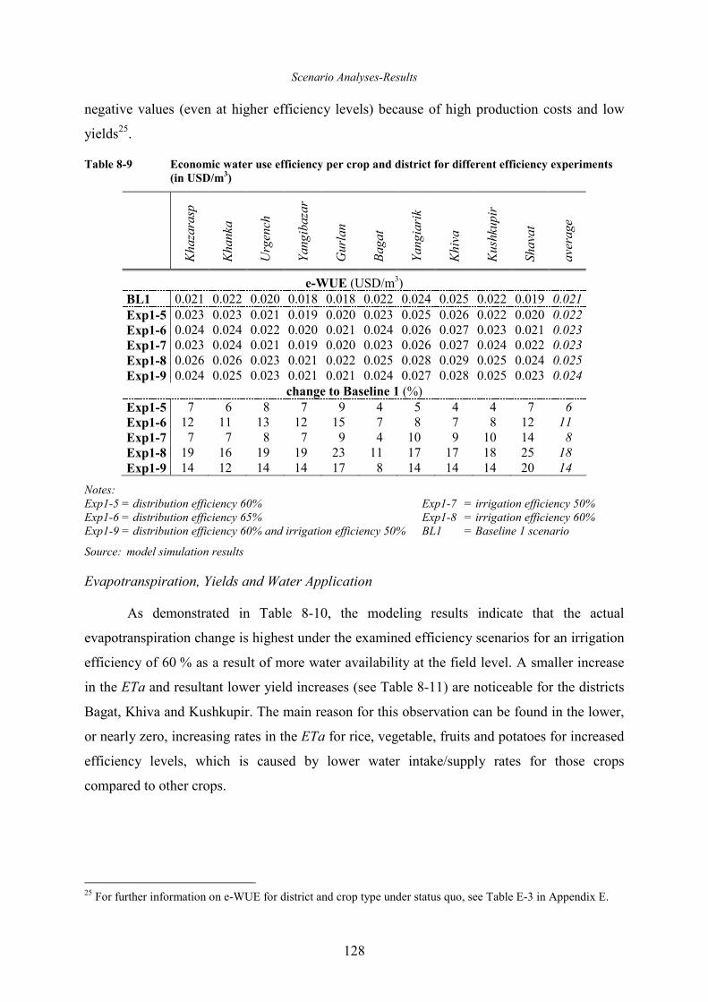
Scenario Analyses-Results
128
negative values (even at higher efficiency levels) because of high production costs and low
yields25.
Table 8-9 Economic water use efficiency per crop and district for different efficiency experiments
(in USD/m3)
Kha
zarasp
Kha
nka
Urgench
Yan
gibazar
Gurlan
Bag
at
Yan
giarik
Khiva
Kushkupir
Shavat
average
e-WUE (USD/m3) BL1 0.021 0.022 0.020 0.018 0.018 0.022 0.024 0.025 0.022 0.019 0.021 Exp1-5 0.023 0.023 0.021 0.019 0.020 0.023 0.025 0.026 0.022 0.020 0.022 Exp1-6 0.024 0.024 0.022 0.020 0.021 0.024 0.026 0.027 0.023 0.021 0.023 Exp1-7 0.023 0.024 0.021 0.019 0.020 0.023 0.026 0.027 0.024 0.022 0.023 Exp1-8 0.026 0.026 0.023 0.021 0.022 0.025 0.028 0.029 0.025 0.024 0.025 Exp1-9 0.024 0.025 0.023 0.021 0.021 0.024 0.027 0.028 0.025 0.023 0.024
change to Baseline 1 (%) Exp1-5 7 6 8 7 9 4 5 4 4 7 6 Exp1-6 12 11 13 12 15 7 8 7 8 12 11 Exp1-7 7 7 8 7 9 4 10 9 10 14 8 Exp1-8 19 16 19 19 23 11 17 17 18 25 18 Exp1-9 14 12 14 14 17 8 14 14 14 20 14
Notes: Exp1-5 = distribution efficiency 60% Exp1-7 = irrigation efficiency 50% Exp1-6 = distribution efficiency 65% Exp1-8 = irrigation efficiency 60% Exp1-9 = distribution efficiency 60% and irrigation efficiency 50% BL1 = Baseline 1 scenario
Source: model simulation results
Evapotranspiration, Yields and Water Application
As demonstrated in Table 8-10, the modeling results indicate that the actual
evapotranspiration change is highest under the examined efficiency scenarios for an irrigation
efficiency of 60 % as a result of more water availability at the field level. A smaller increase
in the ETa and resultant lower yield increases (see Table 8-11) are noticeable for the districts
Bagat, Khiva and Kushkupir. The main reason for this observation can be found in the lower,
or nearly zero, increasing rates in the ETa for rice, vegetable, fruits and potatoes for increased
efficiency levels, which is caused by lower water intake/supply rates for those crops
compared to other crops.
25 For further information on e-WUE for district and crop type under status quo, see Table E-3 in Appendix E.
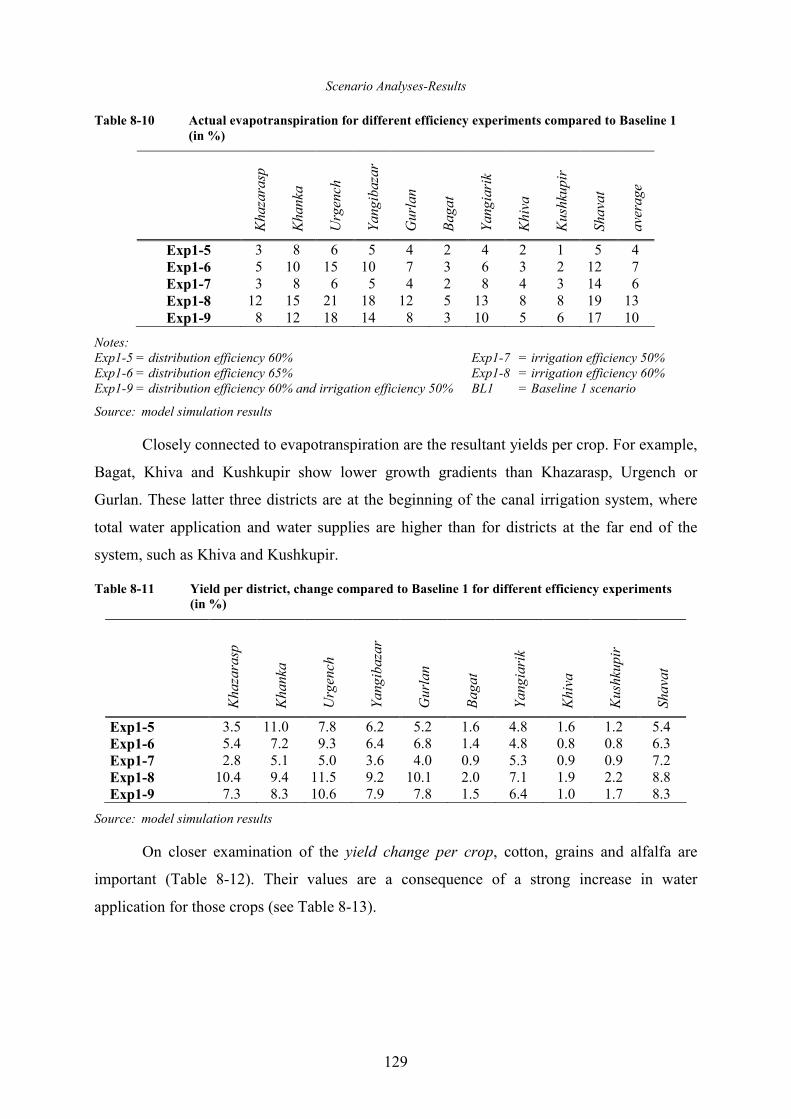
Scenario Analyses-Results
129
Table 8-10 Actual evapotranspiration for different efficiency experiments compared to Baseline 1
(in %)
Kha
zarasp
Kha
nka
Urgench
Yan
gibazar
Gurlan
Bag
at
Yan
giarik
Khiva
Kushkupir
Shavat
average
Exp1-5 3 8 6 5 4 2 4 2 1 5 4 Exp1-6 5 10 15 10 7 3 6 3 2 12 7 Exp1-7 3 8 6 5 4 2 8 4 3 14 6 Exp1-8 12 15 21 18 12 5 13 8 8 19 13 Exp1-9 8 12 18 14 8 3 10 5 6 17 10
Notes: Exp1-5 = distribution efficiency 60% Exp1-7 = irrigation efficiency 50% Exp1-6 = distribution efficiency 65% Exp1-8 = irrigation efficiency 60% Exp1-9 = distribution efficiency 60% and irrigation efficiency 50% BL1 = Baseline 1 scenario
Source: model simulation results
Closely connected to evapotranspiration are the resultant yields per crop. For example,
Bagat, Khiva and Kushkupir show lower growth gradients than Khazarasp, Urgench or
Gurlan. These latter three districts are at the beginning of the canal irrigation system, where
total water application and water supplies are higher than for districts at the far end of the
system, such as Khiva and Kushkupir.
Table 8-11 Yield per district, change compared to Baseline 1 for different efficiency experiments
(in %)
Kha
zarasp
Kha
nka
Urgench
Yan
gibazar
Gurlan
Bag
at
Yan
giarik
Khiva
Kushkupir
Shavat
Exp1-5 3.5 11.0 7.8 6.2 5.2 1.6 4.8 1.6 1.2 5.4 Exp1-6 5.4 7.2 9.3 6.4 6.8 1.4 4.8 0.8 0.8 6.3 Exp1-7 2.8 5.1 5.0 3.6 4.0 0.9 5.3 0.9 0.9 7.2 Exp1-8 10.4 9.4 11.5 9.2 10.1 2.0 7.1 1.9 2.2 8.8 Exp1-9 7.3 8.3 10.6 7.9 7.8 1.5 6.4 1.0 1.7 8.3
Source: model simulation results
On closer examination of the yield change per crop, cotton, grains and alfalfa are
important (Table 8-12). Their values are a consequence of a strong increase in water
application for those crops (see Table 8-13).
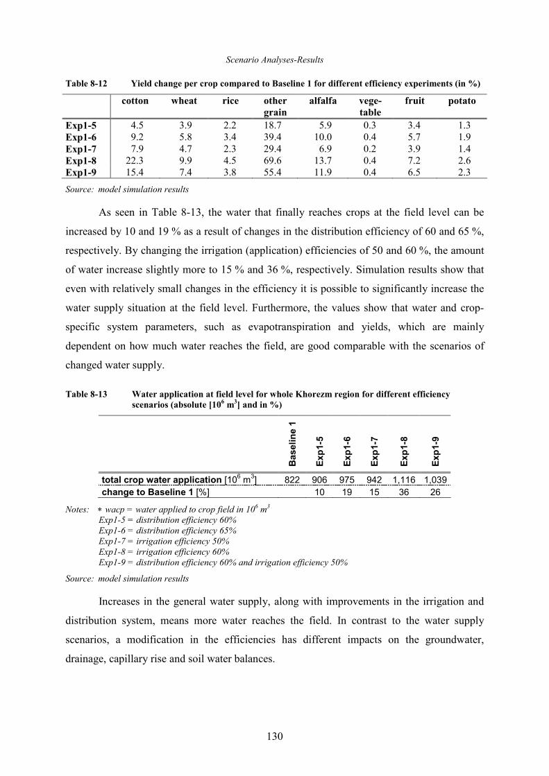
Scenario Analyses-Results
130
Table 8-12 Yield change per crop compared to Baseline 1 for different efficiency experiments (in %)
cotton wheat rice other
grain
alfalfa vege-
table
fruit potato
Exp1-5 4.5 3.9 2.2 18.7 5.9 0.3 3.4 1.3 Exp1-6 9.2 5.8 3.4 39.4 10.0 0.4 5.7 1.9 Exp1-7 7.9 4.7 2.3 29.4 6.9 0.2 3.9 1.4 Exp1-8 22.3 9.9 4.5 69.6 13.7 0.4 7.2 2.6 Exp1-9 15.4 7.4 3.8 55.4 11.9 0.4 6.5 2.3
Source: model simulation results
As seen in Table 8-13, the water that finally reaches crops at the field level can be
increased by 10 and 19 % as a result of changes in the distribution efficiency of 60 and 65 %,
respectively. By changing the irrigation (application) efficiencies of 50 and 60 %, the amount
of water increase slightly more to 15 % and 36 %, respectively. Simulation results show that
even with relatively small changes in the efficiency it is possible to significantly increase the
water supply situation at the field level. Furthermore, the values show that water and crop-
specific system parameters, such as evapotranspiration and yields, which are mainly
dependent on how much water reaches the field, are good comparable with the scenarios of
changed water supply.
Table 8-13 Water application at field level for whole Khorezm region for different efficiency
scenarios (absolute [106 m
3] and in %)
Baseline 1
Exp1-5
Exp1-6
Exp1-7
Exp1-8
Exp1-9
total crop water application [106 m
3] 822 906 975 942 1,116 1,039
change to Baseline 1 [%] 10 19 15 36 26
Notes: ∗ wacp = water applied to crop field in 106 m3 Exp1-5 = distribution efficiency 60% Exp1-6 = distribution efficiency 65% Exp1-7 = irrigation efficiency 50% Exp1-8 = irrigation efficiency 60% Exp1-9 = distribution efficiency 60% and irrigation efficiency 50%
Source: model simulation results
Increases in the general water supply, along with improvements in the irrigation and
distribution system, means more water reaches the field. In contrast to the water supply
scenarios, a modification in the efficiencies has different impacts on the groundwater,
drainage, capillary rise and soil water balances.
Scenario Analyses-Results
131
Drainage, Groundwater and Deep Percolation
Due to the increased distribution and application efficiencies less water can infiltrate
into the soil and recharge the groundwater by deep percolation; therefore, there were not
significant changes in the deep percolation and groundwater under improved efficiency
scenarios. The data for groundwater, groundwater table depth, drainage and groundwater
extraction are presented below.
The groundwater table depth and change in depth compared to the Baseline 1 scenario
is small, with a range of at most 3 cm for a distribution efficiency of 65 % (see Figure E-1 in
Appendix E). One reason is that an improvement in the irrigation and distribution efficiency
means less water is drained and percolated (see Table 8-14). However, more water is
available for crop growth, meaning that crops can meet their water requirements using the
additional available irrigation water instead of using ground- and soil-water extraction via
capillary rise (Table 8-14). Percolation by loss from the irrigation network is an input to the
groundwater system, whereas capillary rise is an output. Overall, the changes in groundwater
level due to increased efficiency (reduced input) and lower capillary rise (reduced output) is
small as a result of improved water supply in the root zone.
The drainage from sites during the main vegetation period was under improved
irrigation efficiency approximately 4 % decreased. For improved distribution efficiencies,
drainage decreased by 8 % because of lower leakage rates compared to the Baseline 1
scenario. Therefore, more water is available for crop growth. However, drainage is reduced,
especially in the leaching period from January to March (Table 8-14), which has negative
impacts on salt leaching and groundwater accumulation. At improved efficiencies mainly the
leaching of the distribution and canal system because of reduced leakages is affected.
Leaching at the field level is not heavily influenced (i.e., by activities such as laser leveling)
because leaching proceeds outside the vegetation period, and here water is sufficiently
available and provided only for this reason in most cases. An adjusted crop-soil-salinity
model could be used to clarify how modified off-seasonal leaching affects soil-salt extraction
or whether there may be additional leaching during the vegetation period.
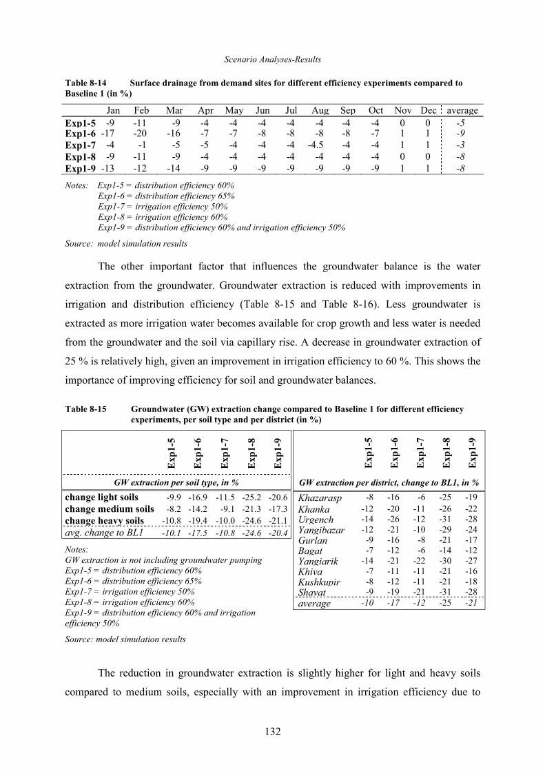
Scenario Analyses-Results
132
Table 8-14 Surface drainage from demand sites for different efficiency experiments compared to
Baseline 1 (in %)
Jan Feb Mar Apr May Jun Jul Aug Sep Oct Nov Dec average Exp1-5 -9 -11 -9 -4 -4 -4 -4 -4 -4 -4 0 0 -5 Exp1-6 -17 -20 -16 -7 -7 -8 -8 -8 -8 -7 1 1 -9 Exp1-7 -4 -1 -5 -5 -4 -4 -4 -4.5 -4 -4 1 1 -3 Exp1-8 -9 -11 -9 -4 -4 -4 -4 -4 -4 -4 0 0 -8 Exp1-9 -13 -12 -14 -9 -9 -9 -9 -9 -9 -9 1 1 -8
Notes: Exp1-5 = distribution efficiency 60% Exp1-6 = distribution efficiency 65% Exp1-7 = irrigation efficiency 50% Exp1-8 = irrigation efficiency 60% Exp1-9 = distribution efficiency 60% and irrigation efficiency 50%
Source: model simulation results
The other important factor that influences the groundwater balance is the water
extraction from the groundwater. Groundwater extraction is reduced with improvements in
irrigation and distribution efficiency (Table 8-15 and Table 8-16). Less groundwater is
extracted as more irrigation water becomes available for crop growth and less water is needed
from the groundwater and the soil via capillary rise. A decrease in groundwater extraction of
25 % is relatively high, given an improvement in irrigation efficiency to 60 %. This shows the
importance of improving efficiency for soil and groundwater balances.
Table 8-15 Groundwater (GW) extraction change compared to Baseline 1 for different efficiency
experiments, per soil type and per district (in %)
Exp1-5
Exp1-6
Exp1-7
Exp1-8
Exp1-9
GW extraction per district, change to BL1, in %
Khazarasp -8 -16 -6 -25 -19 Khanka -12 -20 -11 -26 -22 Urgench -14 -26 -12 -31 -28 Yangibazar -12 -21 -10 -29 -24 Gurlan -9 -16 -8 -21 -17 Bagat -7 -12 -6 -14 -12 Yangiarik -14 -21 -22 -30 -27 Khiva -7 -11 -11 -21 -16 Kushkupir -8 -12 -11 -21 -18 Shavat -9 -19 -21 -31 -28 average -10 -17 -12 -25 -21
The reduction in groundwater extraction is slightly higher for light and heavy soils
compared to medium soils, especially with an improvement in irrigation efficiency due to
Exp1-5
Exp1-6
Exp1-7
Exp1-8
Exp1-9
GW extraction per soil type, in %
change light soils -9.9 -16.9 -11.5 -25.2 -20.6 change medium soils -8.2 -14.2 -9.1 -21.3 -17.3 change heavy soils -10.8 -19.4 -10.0 -24.6 -21.1 avg. change to BL1 -10.1 -17.5 -10.8 -24.6 -20.4
Notes: GW extraction is not including groundwater pumping Exp1-5 = distribution efficiency 60% Exp1-6 = distribution efficiency 65% Exp1-7 = irrigation efficiency 50% Exp1-8 = irrigation efficiency 60% Exp1-9 = distribution efficiency 60% and irrigation efficiency 50%
Source: model simulation results
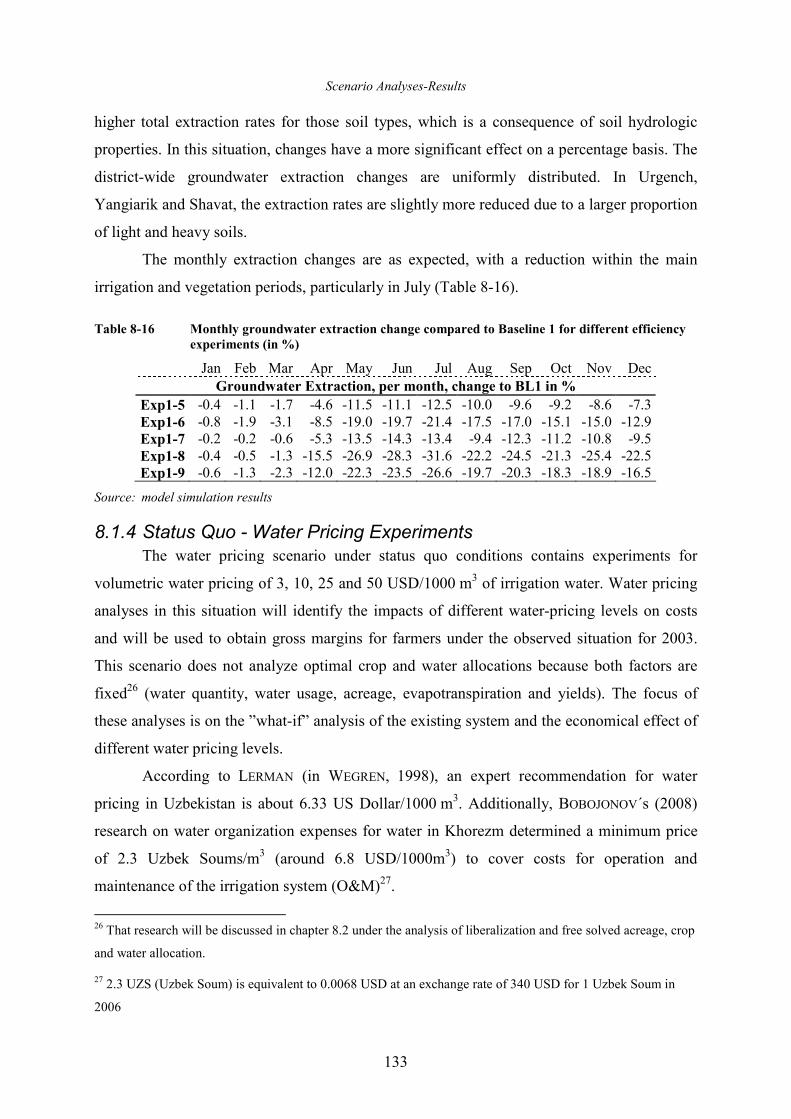
Scenario Analyses-Results
133
higher total extraction rates for those soil types, which is a consequence of soil hydrologic
properties. In this situation, changes have a more significant effect on a percentage basis. The
district-wide groundwater extraction changes are uniformly distributed. In Urgench,
Yangiarik and Shavat, the extraction rates are slightly more reduced due to a larger proportion
of light and heavy soils.
The monthly extraction changes are as expected, with a reduction within the main
irrigation and vegetation periods, particularly in July (Table 8-16).
Table 8-16 Monthly groundwater extraction change compared to Baseline 1 for different efficiency
experiments (in %)
Jan Feb Mar Apr May Jun Jul Aug Sep Oct Nov Dec Groundwater Extraction, per month, change to BL1 in %
Exp1-5 -0.4 -1.1 -1.7 -4.6 -11.5 -11.1 -12.5 -10.0 -9.6 -9.2 -8.6 -7.3 Exp1-6 -0.8 -1.9 -3.1 -8.5 -19.0 -19.7 -21.4 -17.5 -17.0 -15.1 -15.0 -12.9 Exp1-7 -0.2 -0.2 -0.6 -5.3 -13.5 -14.3 -13.4 -9.4 -12.3 -11.2 -10.8 -9.5 Exp1-8 -0.4 -0.5 -1.3 -15.5 -26.9 -28.3 -31.6 -22.2 -24.5 -21.3 -25.4 -22.5 Exp1-9 -0.6 -1.3 -2.3 -12.0 -22.3 -23.5 -26.6 -19.7 -20.3 -18.3 -18.9 -16.5
Source: model simulation results
8.1.4 Status Quo - Water Pricing Experiments
The water pricing scenario under status quo conditions contains experiments for
volumetric water pricing of 3, 10, 25 and 50 USD/1000 m3 of irrigation water. Water pricing
analyses in this situation will identify the impacts of different water-pricing levels on costs
and will be used to obtain gross margins for farmers under the observed situation for 2003.
This scenario does not analyze optimal crop and water allocations because both factors are
fixed26 (water quantity, water usage, acreage, evapotranspiration and yields). The focus of
these analyses is on the ”what-if” analysis of the existing system and the economical effect of
different water pricing levels.
According to LERMAN (in WEGREN, 1998), an expert recommendation for water
pricing in Uzbekistan is about 6.33 US Dollar/1000 m3. Additionally, BOBOJONOV´s (2008)
research on water organization expenses for water in Khorezm determined a minimum price
of 2.3 Uzbek Soums/m3 (around 6.8 USD/1000m3) to cover costs for operation and
maintenance of the irrigation system (O&M)27.
26 That research will be discussed in chapter 8.2 under the analysis of liberalization and free solved acreage, crop
and water allocation.
27 2.3 UZS (Uzbek Soum) is equivalent to 0.0068 USD at an exchange rate of 340 USD for 1 Uzbek Soum in
2006
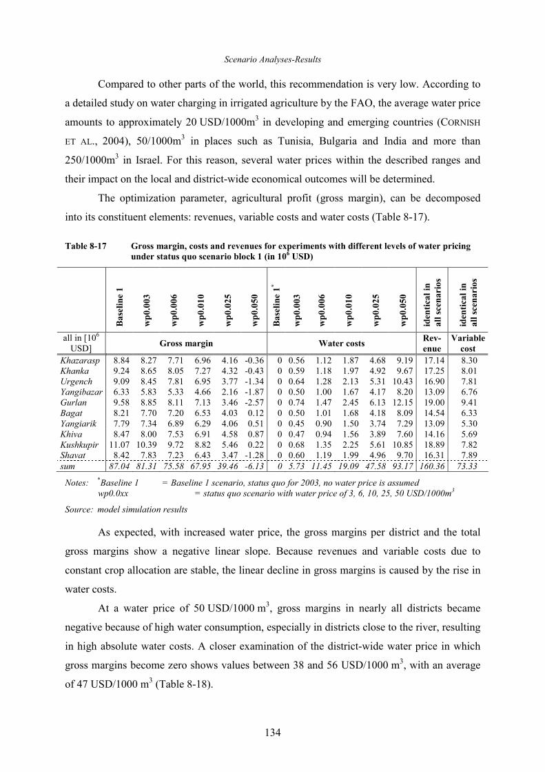
Scenario Analyses-Results
134
Compared to other parts of the world, this recommendation is very low. According to
a detailed study on water charging in irrigated agriculture by the FAO, the average water price
amounts to approximately 20 USD/1000m3 in developing and emerging countries (CORNISH
ET AL., 2004), 50/1000m3 in places such as Tunisia, Bulgaria and India and more than
250/1000m3 in Israel. For this reason, several water prices within the described ranges and
their impact on the local and district-wide economical outcomes will be determined.
The optimization parameter, agricultural profit (gross margin), can be decomposed
into its constituent elements: revenues, variable costs and water costs (Table 8-17).
Table 8-17 Gross margin, costs and revenues for experiments with different levels of water pricing
under status quo scenario block 1 (in 106 USD)
Base
line 1
wp0.003
wp0.006
wp0.010
wp0.025
wp0.050
Base
line 1*
wp0.003
wp0.006
wp0.010
wp0.025
wp0.050
iden
tica
l in
all sce
narios
iden
tica
l in
all sce
narios
all in [106 USD]
Gross margin Water costs Rev-
enue
Variable
cost
Khazarasp 8.84 8.27 7.71 6.96 4.16 -0.36 0 0.56 1.12 1.87 4.68 9.19 17.14 8.30 Khanka 9.24 8.65 8.05 7.27 4.32 -0.43 0 0.59 1.18 1.97 4.92 9.67 17.25 8.01 Urgench 9.09 8.45 7.81 6.95 3.77 -1.34 0 0.64 1.28 2.13 5.31 10.43 16.90 7.81 Yangibazar 6.33 5.83 5.33 4.66 2.16 -1.87 0 0.50 1.00 1.67 4.17 8.20 13.09 6.76 Gurlan 9.58 8.85 8.11 7.13 3.46 -2.57 0 0.74 1.47 2.45 6.13 12.15 19.00 9.41 Bagat 8.21 7.70 7.20 6.53 4.03 0.12 0 0.50 1.01 1.68 4.18 8.09 14.54 6.33 Yangiarik 7.79 7.34 6.89 6.29 4.06 0.51 0 0.45 0.90 1.50 3.74 7.29 13.09 5.30 Khiva 8.47 8.00 7.53 6.91 4.58 0.87 0 0.47 0.94 1.56 3.89 7.60 14.16 5.69 Kushkupir 11.07 10.39 9.72 8.82 5.46 0.22 0 0.68 1.35 2.25 5.61 10.85 18.89 7.82 Shavat 8.42 7.83 7.23 6.43 3.47 -1.28 0 0.60 1.19 1.99 4.96 9.70 16.31 7.89 sum 87.04 81.31 75.58 67.95 39.46 -6.13 0 5.73 11.45 19.09 47.58 93.17 160.36 73.33
Notes: *Baseline 1 = Baseline 1 scenario, status quo for 2003, no water price is assumed wp0.0xx = status quo scenario with water price of 3, 6, 10, 25, 50 USD/1000m3
Source: model simulation results
As expected, with increased water price, the gross margins per district and the total
gross margins show a negative linear slope. Because revenues and variable costs due to
constant crop allocation are stable, the linear decline in gross margins is caused by the rise in
water costs.
At a water price of 50 USD/1000 m3, gross margins in nearly all districts became
negative because of high water consumption, especially in districts close to the river, resulting
in high absolute water costs. A closer examination of the district-wide water price in which
gross margins become zero shows values between 38 and 56 USD/1000 m3, with an average
of 47 USD/1000 m3 (Table 8-18).
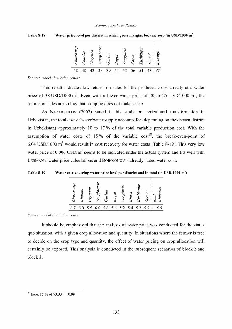
Scenario Analyses-Results
135
Table 8-18 Water price level per district in which gross margins became zero (in USD/1000 m3)
Kha
zarasp
Kha
nka
Urgench
Yan
gibazar
Gurlan
Bag
at
Yan
giarik
Khiva
Kushkupir
Shavat
average
48 48 43 38 39 51 53 56 51 43 47
Source: model simulation results
This result indicates low returns on sales for the produced crops already at a water
price of 38 USD/1000 m3. Even with a lower water price of 20 or 25 USD/1000 m3, the
returns on sales are so low that cropping does not make sense.
As NAZARKULOV (2002) stated in his study on agricultural transformation in
Uzbekistan, the total cost of water/water supply accounts for (depending on the chosen district
in Uzbekistan) approximately 10 to 17 % of the total variable production cost. With the
assumption of water costs of 15 % of the variable cost28, the break-even-point of
6.04 USD/1000 m3 would result in cost recovery for water costs (Table 8-19). This very low
water price of 0.006 USD/m3 seems to be indicated under the actual system and fits well with
LERMAN´s water price calculations and BOBOJONOV´s already stated water cost.
Table 8-19 Water cost-covering water price level per district and in total (in USD/1000 m3)
Kha
zarasp
Kha
nka
Urgench
Yan
gibazar
Gurlan
Bag
at
Yan
giarik
Khiva
Kushkupir
Shavat
total
Kho
rezm
6.7 6.0 5.5 6.0 5.8 5.6 5.2 5.4 5.2 5.9 6.0
Source: model simulation results
It should be emphasized that the analysis of water price was conducted for the status
quo situation, with a given crop allocation and quantity. In situations where the farmer is free
to decide on the crop type and quantity, the effect of water pricing on crop allocation will
certainly be exposed. This analysis is conducted in the subsequent scenarios of block 2 and
block 3.
28 here, 15 % of 73.33 = 10.99
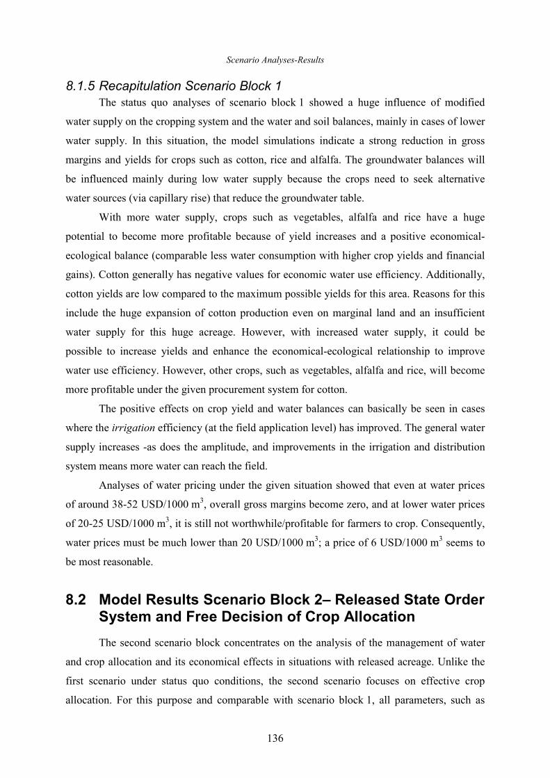
Scenario Analyses-Results
136
8.1.5 Recapitulation Scenario Block 1
The status quo analyses of scenario block 1 showed a huge influence of modified
water supply on the cropping system and the water and soil balances, mainly in cases of lower
water supply. In this situation, the model simulations indicate a strong reduction in gross
margins and yields for crops such as cotton, rice and alfalfa. The groundwater balances will
be influenced mainly during low water supply because the crops need to seek alternative
water sources (via capillary rise) that reduce the groundwater table.
With more water supply, crops such as vegetables, alfalfa and rice have a huge
potential to become more profitable because of yield increases and a positive economical-
ecological balance (comparable less water consumption with higher crop yields and financial
gains). Cotton generally has negative values for economic water use efficiency. Additionally,
cotton yields are low compared to the maximum possible yields for this area. Reasons for this
include the huge expansion of cotton production even on marginal land and an insufficient
water supply for this huge acreage. However, with increased water supply, it could be
possible to increase yields and enhance the economical-ecological relationship to improve
water use efficiency. However, other crops, such as vegetables, alfalfa and rice, will become
more profitable under the given procurement system for cotton.
The positive effects on crop yield and water balances can basically be seen in cases
where the irrigation efficiency (at the field application level) has improved. The general water
supply increases -as does the amplitude, and improvements in the irrigation and distribution
system means more water can reach the field.
Analyses of water pricing under the given situation showed that even at water prices
of around 38-52 USD/1000 m3, overall gross margins become zero, and at lower water prices
of 20-25 USD/1000 m3, it is still not worthwhile/profitable for farmers to crop. Consequently,
water prices must be much lower than 20 USD/1000 m3; a price of 6 USD/1000 m3 seems to
be most reasonable.
8.2 Model Results Scenario Block 2– Released State Order System and Free Decision of Crop Allocation
The second scenario block concentrates on the analysis of the management of water
and crop allocation and its economical effects in situations with released acreage. Unlike the
first scenario under status quo conditions, the second scenario focuses on effective crop
allocation. For this purpose and comparable with scenario block 1, all parameters, such as
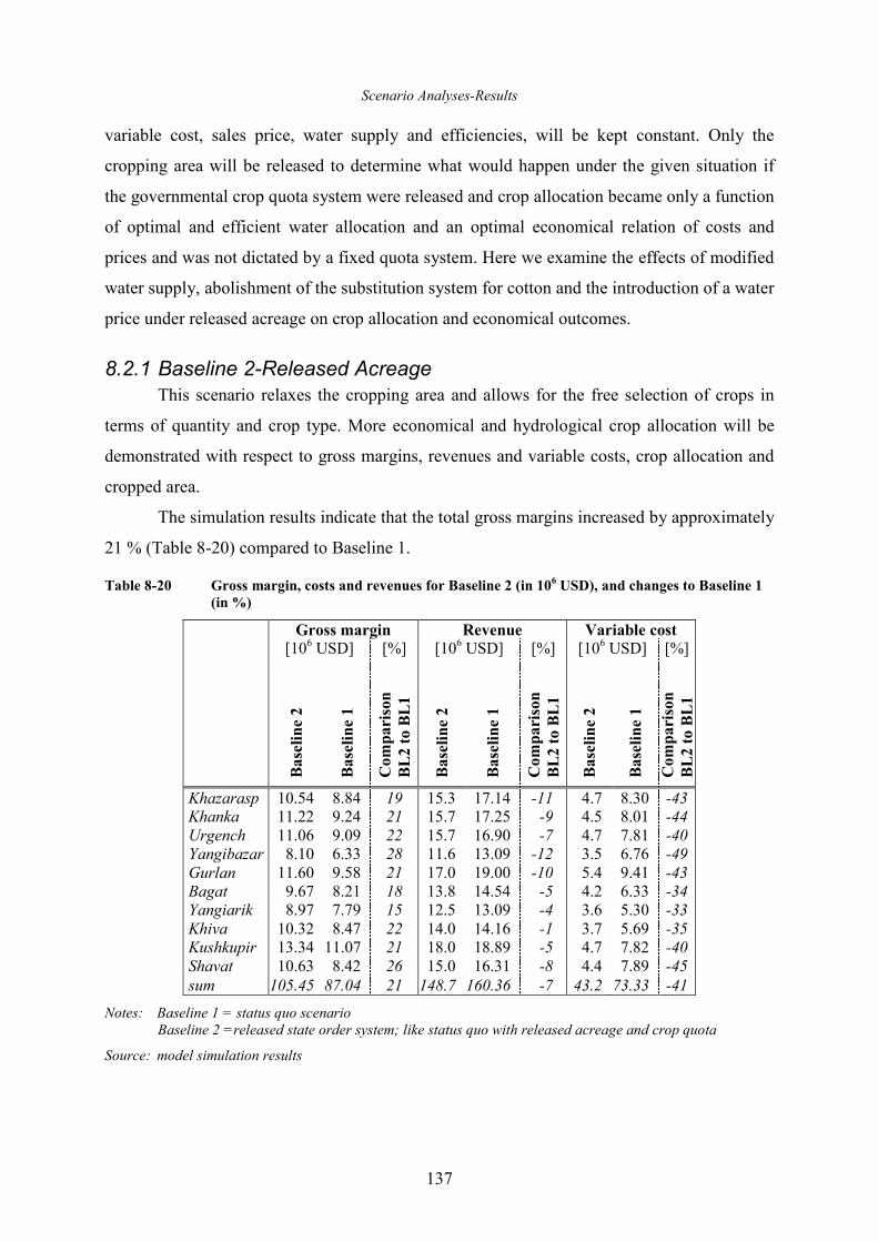
Scenario Analyses-Results
137
variable cost, sales price, water supply and efficiencies, will be kept constant. Only the
cropping area will be released to determine what would happen under the given situation if
the governmental crop quota system were released and crop allocation became only a function
of optimal and efficient water allocation and an optimal economical relation of costs and
prices and was not dictated by a fixed quota system. Here we examine the effects of modified
water supply, abolishment of the substitution system for cotton and the introduction of a water
price under released acreage on crop allocation and economical outcomes.
8.2.1 Baseline 2-Released Acreage
This scenario relaxes the cropping area and allows for the free selection of crops in
terms of quantity and crop type. More economical and hydrological crop allocation will be
demonstrated with respect to gross margins, revenues and variable costs, crop allocation and
cropped area.
The simulation results indicate that the total gross margins increased by approximately
21 % (Table 8-20) compared to Baseline 1.
Table 8-20 Gross margin, costs and revenues for Baseline 2 (in 106 USD), and changes to Baseline 1
(in %)
Gross margin Revenue Variable cost [106 USD] [%] [106 USD] [%] [106 USD] [%]
Base
line 2
Base
line 1
Com
pariso
n
BL2 to B
L1
Base
line 2
Base
line 1
Com
pariso
n
BL2 to B
L1
Base
line 2
Base
line 1
Com
pariso
n
BL2 to B
L1
Khazarasp 10.54 8.84 19 15.3 17.14 -11 4.7 8.30 -43 Khanka 11.22 9.24 21 15.7 17.25 -9 4.5 8.01 -44 Urgench 11.06 9.09 22 15.7 16.90 -7 4.7 7.81 -40 Yangibazar 8.10 6.33 28 11.6 13.09 -12 3.5 6.76 -49 Gurlan 11.60 9.58 21 17.0 19.00 -10 5.4 9.41 -43 Bagat 9.67 8.21 18 13.8 14.54 -5 4.2 6.33 -34 Yangiarik 8.97 7.79 15 12.5 13.09 -4 3.6 5.30 -33 Khiva 10.32 8.47 22 14.0 14.16 -1 3.7 5.69 -35 Kushkupir 13.34 11.07 21 18.0 18.89 -5 4.7 7.82 -40 Shavat 10.63 8.42 26 15.0 16.31 -8 4.4 7.89 -45 sum 105.45 87.04 21 148.7 160.36 -7 43.2 73.33 -41
Notes: Baseline 1 = status quo scenario Baseline 2 =released state order system; like status quo with released acreage and crop quota
Source: model simulation results
Scenario Analyses-Results
138
Major reason for this effect is a 41 % decrease in production costs, which is attributed
to a decrease in the cultivated cropping area and a modification to more water effective and
benefiting crops in monetary terms. The 7 % decrease in revenues is relatively moderate and
caused by a general decrease in acreage. However, the cost savings and reallocation of crops
compensate for this effect.
As seen in Table 8-21, the shares on gross margin are very high for alfalfa, rice,
vegetables, wheat and fruit. This general increase in the gross margins compared to the status
quo (Baseline 1) is mainly due to an increase in acreage and additional gains in gross margins
(of around 18-20 %) for crops like alfalfa, vegetables, fruit and potato29. In terms of irrigation
water consumption, crops such as wheat, with around 3600 m3/ha, and fruit, maize and cotton
(~5000 m3/ha) are most efficient30. However, considering additional economical aspects such
as production costs and sales prices, wheat and other crops (vegetables, fruit, potato and rice)
that have higher water consumption but better cost/benefit relations become more attractive.
For districts like Shavat and Yangibazar, the increase in gross margins is 26–28 % and
caused by the huge acreage of cotton and resultant losses in gross margins in the status quo
situation (see Table 8-21, for Baseline 1). On the contrary, in districts with less cotton acreage
in the status quo, such as Yangiarik, we see a smaller increase in gross margins because the
Baseline 1 situation is less negative. In Baseline 2, the cotton area is drastically reduced and
thus, losses in gross margins for cotton.
Further examination of acreage illustrates the correlation between gross margins (and
its linked variables like revenues and costs), crop variety and the cropped area. As seen in
Table 8-22, the total cropped area is reduced by 28 to 40 % because of a reduction in cotton
acreage. As a result of the negative gross margins for cotton due to the state quota and bad
cost/benefit relations under the status quo (Baseline 1), the cotton area with released acreage
is under Baseline 2 diminished by 92 % (see Table 8-23). However, the acreage for other
crops, such as vegetable, alfalfa, fruit, wheat and potato, has expanded by 20 % compared to
the status quo31.
29 The quotient of rice for the gross margins is approx. 24 Million USD, which seems very high, but the change
compared to Baseline 1 and 2 with 4.5 % is relatively low, as the acreage would not be expanded.
30 Vegetables, potatoes and alfalfa are ~8000 m3/ha, rice is ~26000 m3/ha.
31 The maximum crop area is used in the model as an upper boundary.
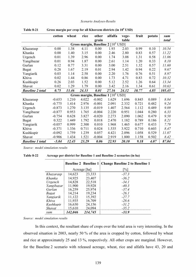
Scenario Analyses-Results
139
Table 8-21 Gross margin per crop for all Khorezm districts (in 106 USD)
cotton wheat rice other
grain
alfalfa vege-
table
fruit potato sum
total
Gross margin, Baseline 2 [106 USD] Khazarasp 0.00 1.38 4.11 0.00 1.93 2.03 0.99 0.10 10.54 Khanka 0.00 1.40 3.15 0.00 2.46 2.80 0.83 0.57 11.22 Urgench 0.01 1.39 2.96 0.00 1.74 3.08 1.31 0.58 11.06 Yangibazar 0.01 0.94 1.87 0.00 2.61 1.14 1.20 0.33 8.10 Gurlan 0.12 0.77 3.31 0.00 3.00 2.51 1.32 0.57 11.60 Bagat 0.28 1.67 2.19 0.01 2.94 1.42 0.94 0.22 9.67 Yangiarik 0.03 1.14 2.58 0.00 2.20 1.76 0.76 0.51 8.97 Khiva 0.02 1.44 0.86 0.00 1.73 4.71 0.83 0.72 10.32 Kushkupir 0.26 2.03 1.52 0.00 5.12 2.52 1.26 0.64 13.34 Shavat 0.02 1.29 1.79 0.00 3.42 2.16 1.34 0.61 10.63 Baseline 2 total 0.75 13.46 24.33 0.01 27.16 24.12 10.77 4.85 105.45
Gross margin, Baseline 1 [106 USD] Khazarasp -0.653 1.210 4.022 -0.002 1.629 1.696 0.845 0.089 8.84 Khanka -0.775 1.414 2.976 -0.001 2.091 2.332 0.721 0.482 9.24 Urgench -0.873 1.270 3.135 -0.019 1.407 2.564 1.112 0.489 9.09 Yangibazar -0.877 0.953 1.765 -0.004 2.220 0.951 1.044 0.280 6.33 Gurlan -0.754 0.628 3.827 -0.020 2.273 2.090 1.062 0.479 9.58 Bagat 0.322 1.449 1.792 0.018 2.470 1.182 0.789 0.186 8.21 Yangiarik -0.057 0.999 2.300 0.010 1.968 1.465 0.677 0.433 7.79 Khiva -0.371 1.336 0.711 0.024 1.535 3.922 0.710 0.603 8.47 Kushkupir -0.092 1.759 1.239 0.057 4.421 2.096 1.058 0.529 11.07 Shavat -0.906 1.434 1.521 -0.004 2.919 1.800 1.158 0.502 8.42 Baseline 1 total -5.04 12.45 23.29 0.06 22.93 20.10 9.18 4.07 87.04
Source: model simulation results
Table 8-22 Acreage per district for Baseline 1 and Baseline 2 scenarios (in ha)
Baseline 2 Baseline 1 Change Baseline 2 to Baseline 1
Acreage [ha] [%] Khazarasp 14,623 23,333 -37.3 Khanka 14,925 23,407 -36.2 Urgench 14,828 22,518 -34.1 Yangibazar 11,900 19,928 -40.3 Gurlan 16,259 25,974 -37.4 Bagat 14,214 19,234 -26.1 Yangiarik 11,122 15,392 -27.7 Khiva 11,935 16,709 -28.6 Kushkupir 16,630 24,156 -31.2 Shavat 15,610 24,094 -35.2 sum 142,046 214,745 -33.9
Source: model simulation results
In this context, the resultant share of crops over the total area is very interesting. In the
observed situation in 2003, nearly 50 % of the area is cropped by cotton, followed by wheat
and rice at approximately 25 and 13 %, respectively. All other crops are marginal. However,
for the Baseline 2 scenario with released acreage, wheat, rice and alfalfa have 43, 20 and
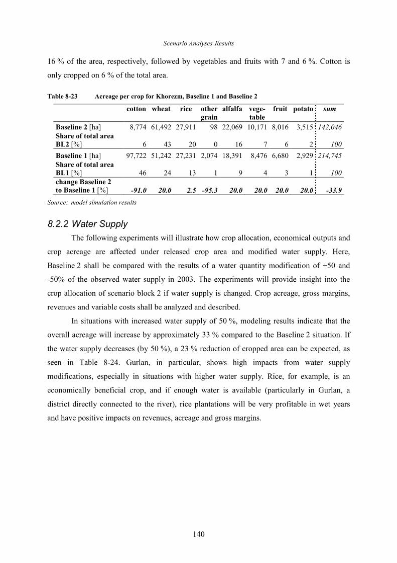
Scenario Analyses-Results
140
16 % of the area, respectively, followed by vegetables and fruits with 7 and 6 %. Cotton is
only cropped on 6 % of the total area.
Table 8-23 Acreage per crop for Khorezm, Baseline 1 and Baseline 2
cotton wheat rice other
grain
alfalfa vege-
table
fruit potato sum
Baseline 2 [ha] 8,774 61,492 27,911 98 22,069 10,171 8,016 3,515 142,046 Share of total area BL2 [%] 6 43 20 0 16 7 6 2 100
Baseline 1 [ha] 97,722 51,242 27,231 2,074 18,391 8,476 6,680 2,929 214,745 Share of total area BL1 [%] 46 24 13 1 9 4 3 1 100 change Baseline 2 to Baseline 1 [%] -91.0 20.0 2.5 -95.3 20.0 20.0 20.0 20.0 -33.9
Source: model simulation results
8.2.2 Water Supply
The following experiments will illustrate how crop allocation, economical outputs and
crop acreage are affected under released crop area and modified water supply. Here,
Baseline 2 shall be compared with the results of a water quantity modification of +50 and
-50% of the observed water supply in 2003. The experiments will provide insight into the
crop allocation of scenario block 2 if water supply is changed. Crop acreage, gross margins,
revenues and variable costs shall be analyzed and described.
In situations with increased water supply of 50 %, modeling results indicate that the
overall acreage will increase by approximately 33 % compared to the Baseline 2 situation. If
the water supply decreases (by 50 %), a 23 % reduction of cropped area can be expected, as
seen in Table 8-24. Gurlan, in particular, shows high impacts from water supply
modifications, especially in situations with higher water supply. Rice, for example, is an
economically beneficial crop, and if enough water is available (particularly in Gurlan, a
district directly connected to the river), rice plantations will be very profitable in wet years
and have positive impacts on revenues, acreage and gross margins.
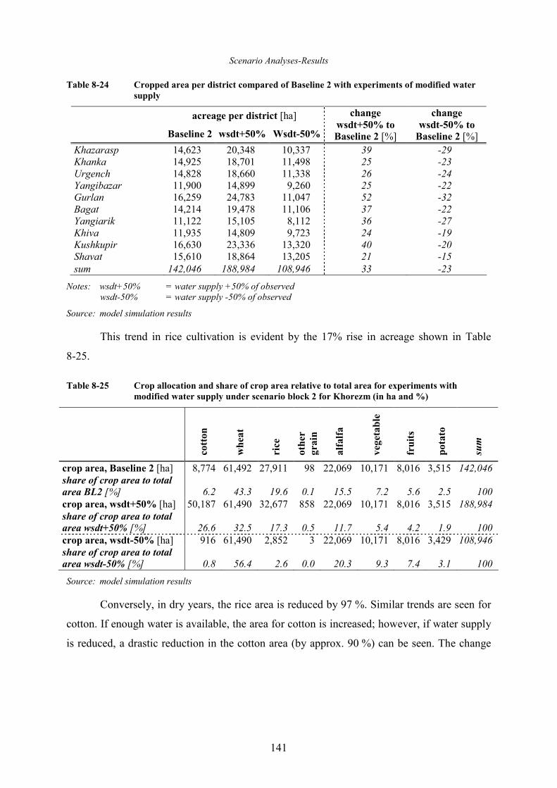
Scenario Analyses-Results
141
Table 8-24 Cropped area per district compared of Baseline 2 with experiments of modified water
supply
acreage per district [ha]
Baseline 2 wsdt+50% Wsdt-50%
change
wsdt+50% to Baseline 2 [%]
change
wsdt-50% to Baseline 2 [%]
Khazarasp 14,623 20,348 10,337 39 -29 Khanka 14,925 18,701 11,498 25 -23 Urgench 14,828 18,660 11,338 26 -24 Yangibazar 11,900 14,899 9,260 25 -22 Gurlan 16,259 24,783 11,047 52 -32 Bagat 14,214 19,478 11,106 37 -22 Yangiarik 11,122 15,105 8,112 36 -27 Khiva 11,935 14,809 9,723 24 -19 Kushkupir 16,630 23,336 13,320 40 -20 Shavat 15,610 18,864 13,205 21 -15 sum 142,046 188,984 108,946 33 -23
Notes: wsdt+50% = water supply +50% of observed wsdt-50% = water supply -50% of observed
Source: model simulation results
This trend in rice cultivation is evident by the 17% rise in acreage shown in Table
8-25.
Table 8-25 Crop allocation and share of crop area relative to total area for experiments with
modified water supply under scenario block 2 for Khorezm (in ha and %)
cotton
whea
t
rice
oth
er
gra
in
alfalfa
veg
etable
fruits
pota
to
sum
crop area, Baseline 2 [ha] 8,774 61,492 27,911 98 22,069 10,171 8,016 3,515 142,046 share of crop area to total
area BL2 [%] 6.2 43.3 19.6 0.1 15.5 7.2 5.6 2.5 100 crop area, wsdt+50% [ha] 50,187 61,490 32,677 858 22,069 10,171 8,016 3,515 188,984 share of crop area to total area wsdt+50% [%] 26.6 32.5 17.3 0.5 11.7 5.4 4.2 1.9 100 crop area, wsdt-50% [ha] 916 61,490 2,852 3 22,069 10,171 8,016 3,429 108,946 share of crop area to total area wsdt-50% [%] 0.8 56.4 2.6 0.0 20.3 9.3 7.4 3.1 100
Source: model simulation results
Conversely, in dry years, the rice area is reduced by 97 %. Similar trends are seen for
cotton. If enough water is available, the area for cotton is increased; however, if water supply
is reduced, a drastic reduction in the cotton area (by approx. 90 %) can be seen. The change
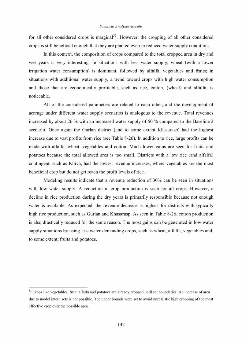
Scenario Analyses-Results
142
for all other considered crops is marginal32. However, the cropping of all other considered
crops is still beneficial enough that they are planted even in reduced water supply conditions.
In this context, the composition of crops compared to the total cropped area in dry and
wet years is very interesting. In situations with less water supply, wheat (with a lower
irrigation water consumption) is dominant, followed by alfalfa, vegetables and fruits; in
situations with additional water supply, a trend toward crops with high water consumption
and those that are economically profitable, such as rice, cotton, (wheat) and alfalfa, is
noticeable.
All of the considered parameters are related to each other, and the development of
acreage under different water supply scenarios is analogous to the revenue. Total revenues
increased by about 26 % with an increased water supply of 50 % compared to the Baseline 2
scenario. Once again the Gurlan district (and to some extent Khasarasp) had the highest
increase due to vast profits from rice (see Table 8-26). In addition to rice, large profits can be
made with alfalfa, wheat, vegetables and cotton. Much lower gains are seen for fruits and
potatoes because the total allowed area is too small. Districts with a low rice (and alfalfa)
contingent, such as Khiva, had the lowest revenue increases, where vegetables are the most
beneficial crop but do not get reach the profit levels of rice.
Modeling results indicate that a revenue reduction of 30% can be seen in situations
with low water supply. A reduction in crop production is seen for all crops. However, a
decline in rice production during the dry years is primarily responsible because not enough
water is available. As expected, the revenue decrease is highest for districts with typically
high rice production, such as Gurlan and Khasarasp. As seen in Table 8-26, cotton production
is also drastically reduced for the same reason. The most gains can be generated in low water
supply situations by using less water-demanding crops, such as wheat, alfalfa, vegetables and,
to some extent, fruits and potatoes.
32 Crops like vegetables, fruit, alfalfa and potatoes are already cropped until set boundaries. An increase of area
due to model intern sets is not possible. The upper bounds were set to avoid unrealistic high cropping of the most
effective crop over the possible area.
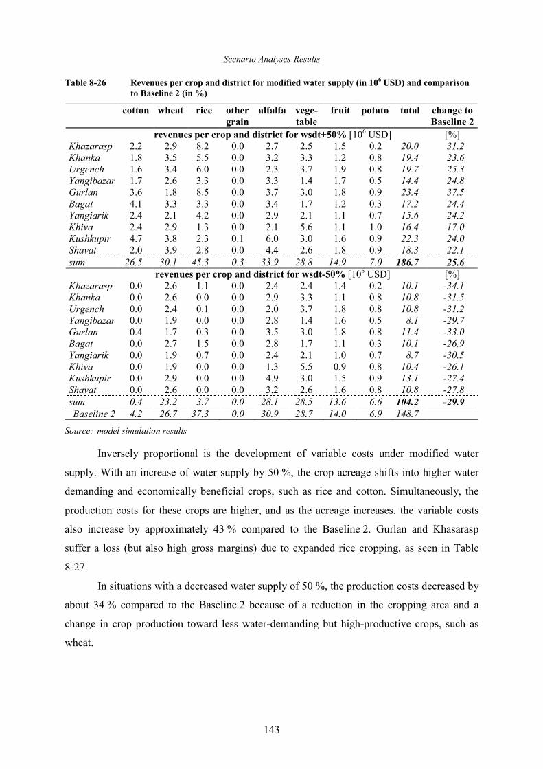
Scenario Analyses-Results
143
Table 8-26 Revenues per crop and district for modified water supply (in 106 USD) and comparison
to Baseline 2 (in %)
Source: model simulation results
Inversely proportional is the development of variable costs under modified water
supply. With an increase of water supply by 50 %, the crop acreage shifts into higher water
demanding and economically beneficial crops, such as rice and cotton. Simultaneously, the
production costs for these crops are higher, and as the acreage increases, the variable costs
also increase by approximately 43 % compared to the Baseline 2. Gurlan and Khasarasp
suffer a loss (but also high gross margins) due to expanded rice cropping, as seen in Table
8-27.
In situations with a decreased water supply of 50 %, the production costs decreased by
about 34 % compared to the Baseline 2 because of a reduction in the cropping area and a
change in crop production toward less water-demanding but high-productive crops, such as
wheat.
cotton wheat rice other
grain
alfalfa vege-
table
fruit potato total change to
Baseline 2
revenues per crop and district for wsdt+50% [106 USD] [%] Khazarasp 2.2 2.9 8.2 0.0 2.7 2.5 1.5 0.2 20.0 31.2 Khanka 1.8 3.5 5.5 0.0 3.2 3.3 1.2 0.8 19.4 23.6 Urgench 1.6 3.4 6.0 0.0 2.3 3.7 1.9 0.8 19.7 25.3 Yangibazar 1.7 2.6 3.3 0.0 3.3 1.4 1.7 0.5 14.4 24.8 Gurlan 3.6 1.8 8.5 0.0 3.7 3.0 1.8 0.9 23.4 37.5 Bagat 4.1 3.3 3.3 0.0 3.4 1.7 1.2 0.3 17.2 24.4 Yangiarik 2.4 2.1 4.2 0.0 2.9 2.1 1.1 0.7 15.6 24.2 Khiva 2.4 2.9 1.3 0.0 2.1 5.6 1.1 1.0 16.4 17.0 Kushkupir 4.7 3.8 2.3 0.1 6.0 3.0 1.6 0.9 22.3 24.0 Shavat 2.0 3.9 2.8 0.0 4.4 2.6 1.8 0.9 18.3 22.1 sum 26.5 30.1 45.3 0.3 33.9 28.8 14.9 7.0 186.7 25.6
revenues per crop and district for wsdt-50% [106 USD] [%] Khazarasp 0.0 2.6 1.1 0.0 2.4 2.4 1.4 0.2 10.1 -34.1 Khanka 0.0 2.6 0.0 0.0 2.9 3.3 1.1 0.8 10.8 -31.5 Urgench 0.0 2.4 0.1 0.0 2.0 3.7 1.8 0.8 10.8 -31.2 Yangibazar 0.0 1.9 0.0 0.0 2.8 1.4 1.6 0.5 8.1 -29.7 Gurlan 0.4 1.7 0.3 0.0 3.5 3.0 1.8 0.8 11.4 -33.0 Bagat 0.0 2.7 1.5 0.0 2.8 1.7 1.1 0.3 10.1 -26.9 Yangiarik 0.0 1.9 0.7 0.0 2.4 2.1 1.0 0.7 8.7 -30.5 Khiva 0.0 1.9 0.0 0.0 1.3 5.5 0.9 0.8 10.4 -26.1 Kushkupir 0.0 2.9 0.0 0.0 4.9 3.0 1.5 0.9 13.1 -27.4 Shavat 0.0 2.6 0.0 0.0 3.2 2.6 1.6 0.8 10.8 -27.8 sum 0.4 23.2 3.7 0.0 28.1 28.5 13.6 6.6 104.2 -29.9
Baseline 2 4.2 26.7 37.3 0.0 30.9 28.7 14.0 6.9 148.7
Scenario Analyses-Results
144
Table 8-27 Variable cost per crop and district for modified water supply (in 106 USD) and
comparison to Baseline 2 (in %)
cotton wheat rice other
grain
alfalfa vege-
table
fruit potato sum per
district
change
to BL2
Variable cost per crop and district for wsdt+50% [106 USD] [%] Khazarasp 1.9 1.3 2.7 0.0 0.3 0.4 0.3 0.0 7.0 48.0 Khanka 1.3 1.6 1.8 0.0 0.3 0.5 0.2 0.2 6.0 33.1 Urgench 1.2 1.5 2.0 0.0 0.2 0.6 0.4 0.2 6.2 33.0 Yangibazar 1.3 1.2 1.1 0.0 0.4 0.2 0.4 0.1 4.6 34.1 Gurlan 3.2 1.0 3.0 0.0 0.5 0.5 0.4 0.3 8.9 64.0 Bagat 2.7 1.4 1.1 0.0 0.4 0.3 0.3 0.1 6.2 48.9 Yangiarik 1.7 0.9 1.4 0.0 0.3 0.3 0.2 0.2 5.1 43.1 Khiva 1.6 1.2 0.4 0.0 0.2 0.9 0.2 0.3 4.8 29.9 Kushkupir 3.2 1.6 0.7 0.1 0.6 0.5 0.3 0.3 7.2 54.6 Shavat 1.4 1.7 0.9 0.0 0.5 0.4 0.4 0.3 5.6 29.0 sum per crop 19.5 13.2 15.2 0.2 3.7 4.6 3.3 2.0 61.6 42.7
Variable cost per crop and district for wsdt-50% [106 USD] [%] Khazarasp 0.0 1.3 0.4 0.0 0.3 0.4 0.3 0.0 2.8 -41.8 Khanka 0.0 1.6 0.0 0.0 0.3 0.5 0.2 0.2 2.9 -35.3 Urgench 0.0 1.5 0.0 0.0 0.2 0.6 0.4 0.2 3.1 -34.4 Yangibazar 0.0 1.2 0.0 0.0 0.4 0.2 0.4 0.1 2.3 -34.3 Gurlan 0.4 1.0 0.1 0.0 0.5 0.5 0.4 0.3 3.1 -42.8 Bagat 0.0 1.4 0.5 0.0 0.4 0.3 0.3 0.1 2.9 -30.9 Yangiarik 0.0 0.9 0.2 0.0 0.3 0.3 0.2 0.2 2.2 -38.1 Khiva 0.0 1.2 0.0 0.0 0.2 0.9 0.2 0.2 2.8 -25.5 Kushkupir 0.0 1.6 0.0 0.0 0.6 0.5 0.3 0.3 3.3 -30.1 Shavat 0.0 1.7 0.0 0.0 0.5 0.4 0.4 0.3 3.3 -24.9 sum per crop 0.4 13.2 1.3 0.0 3.7 4.6 3.3 2.0 28.5 -34.1
Source: model simulation results
The gross margins resulting from the difference between revenues and costs in cases
of modified water supply can be seen in Table 8-28. The overall gross margins increased by
19 % with additional water supply because of the extension of rice, alfalfa, vegetables and
wheat production. Unsurprisingly, the districts of Gurlan and Khasarasp attained the highest
growth due to the huge intensification of rice cropping. A tendency toward higher gross
margins can be seen for all districts closer to the river.
At a water supply of -50 % of the original, the reduction in gross margins is relatively
high at 28 %. Heavy losses in yields due to the water deficit were recorded for all crops33. In
those situations, a shift toward less water-demanding crops, such as wheat, and toward crops
with higher value added in economic terms, such as vegetables, fruit and alfalfa, can be seen.
Furthermore, the loss of gross margins due to less water supply is relatively equally
distributed in all districts, independent of river closeness or distance.
33 For this, see also detailed information on the water supply experiments of the Baseline 1 (status quo) scenario.
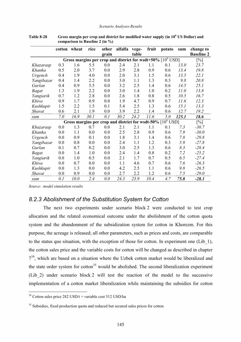
Scenario Analyses-Results
145
Table 8-28 Gross margin per crop and district for modified water supply (in 106 US Dollar) and
comparison to Baseline 2 (in %)
Source: model simulation results
8.2.3 Abolishment of the Substitution System for Cotton
The next two experiments under scenario block 2 were conducted to test crop
allocation and the related economical outcome under the abolishment of the cotton quota
system and the abandonment of the subsidization system for cotton in Khorezm. For this
purpose, the acreage is released; all other parameters, such as prices and costs, are comparable
to the status quo situation, with the exception of those for cotton. In experiment one (Lib_1),
the cotton sales price and the variable costs for cotton will be changed as described in chapter
734, which are based on a situation where the Uzbek cotton market would be liberalized and
the state order system for cotton35 would be abolished. The second liberalization experiment
(Lib_2) under scenario block 2 will test the reaction of the model to the successive
implementation of a cotton market liberalization while maintaining the subsidies for cotton
34 Cotton sales price 282 USD/t + variable cost 512 USD/ha
35 Subsidies, fixed production quota and reduced but secured sales prices for cotton
cotton wheat rice other
grain
alfalfa vege-
table
fruit potato sum change to
Baseline 2
Gross margins per crop and district for wsdt+50% [106 USD] [%] Khazarasp 0.3 1.6 5.5 0.0 2.4 2.1 1.1 0.1 13.0 23.7 Khanka 0.5 2.0 3.7 0.0 2.9 2.8 0.9 0.6 13.4 19.8 Urgench 0.4 1.9 4.0 0.0 2.0 3.1 1.5 0.6 13.5 22.1 Yangibazar 0.4 1.4 2.2 0.0 3.0 1.1 1.3 0.3 9.8 20.8 Gurlan 0.4 0.9 5.5 0.0 3.2 2.5 1.4 0.6 14.5 25.1 Bagat 1.3 1.9 2.2 0.0 3.0 1.4 1.0 0.2 11.0 13.8 Yangiarik 0.7 1.2 2.8 0.0 2.6 1.8 0.8 0.5 10.5 16.7 Khiva 0.9 1.7 0.9 0.0 1.9 4.7 0.9 0.7 11.6 12.3 Kushkupir 1.5 2.2 1.5 0.1 5.4 2.5 1.3 0.6 15.1 13.3 Shavat 0.6 2.1 1.9 0.0 3.9 2.2 1.4 0.6 12.7 19.2 sum 7.0 16.9 30.1 0.1 30.2 24.2 11.6 5.0 125.1 18.6
Gross margins per crop and district for wsdt-50% [106 USD] [%] Khazarasp 0.0 1.3 0.7 0.0 2.1 2.1 1.1 0.1 7.3 -30.7 Khanka 0.0 1.1 0.0 0.0 2.5 2.8 0.9 0.6 7.9 -30.0 Urgench 0.0 0.9 0.1 0.0 1.8 3.1 1.4 0.6 7.8 -29.8 Yangibazar 0.0 0.8 0.0 0.0 2.4 1.1 1.2 0.3 5.9 -27.8 Gurlan 0.1 0.7 0.2 0.0 3.0 2.5 1.3 0.6 8.3 -28.4 Bagat 0.0 1.4 1.0 0.0 2.4 1.4 0.8 0.2 7.2 -25.2 Yangiarik 0.0 1.0 0.5 0.0 2.1 1.7 0.7 0.5 6.5 -27.4 Khiva 0.0 0.7 0.0 0.0 1.1 4.6 0.7 0.6 7.6 -26.3 Kushkupir 0.0 1.3 0.0 0.0 4.2 2.5 1.1 0.6 9.8 -26.5 Shavat 0.0 0.9 0.0 0.0 2.7 2.2 1.2 0.6 7.5 -29.0 sum 0.1 10.0 2.4 0.0 24.3 23.9 10.4 4.7 75.8 -28.1
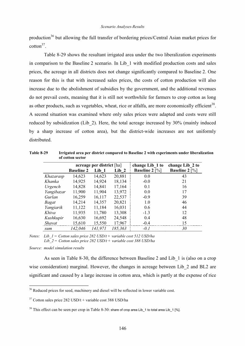
Scenario Analyses-Results
146
production36 but allowing the full transfer of bordering prices/Central Asian market prices for
cotton37.
Table 8-29 shows the resultant irrigated area under the two liberalization experiments
in comparison to the Baseline 2 scenario. In Lib_1 with modified production costs and sales
prices, the acreage in all districts does not change significantly compared to Baseline 2. One
reason for this is that with increased sales prices, the costs of cotton production will also
increase due to the abolishment of subsidies by the government, and the additional revenues
do not prevail costs, meaning that it is still not worthwhile for farmers to crop cotton as long
as other products, such as vegetables, wheat, rice or alfalfa, are more economically efficient38.
A second situation was examined where only sales prices were adapted and costs were still
reduced by subsidization (Lib_2). Here, the total acreage increased by 30% (mainly induced
by a sharp increase of cotton area), but the district-wide increases are not uniformly
distributed.
Table 8-29 Irrigated area per district compared to Baseline 2 with experiments under liberalization
of cotton sector
acreage per district [ha]
Baseline 2 Lib_1 Lib_2
change Lib_1 to Baseline 2 [%]
change Lib_2 to Baseline 2 [%]
Khazarasp 14,623 14,623 20,881 0.0 43 Khanka 14,925 14,924 18,134 -0.0 21 Urgench 14,828 14,841 17,164 0.1 16 Yangibazar 11,900 11,904 13,972 0.0 17 Gurlan 16,259 16,117 22,537 -0.9 39 Bagat 14,214 14,357 20,821 1.0 46 Yangiarik 11,122 11,184 16,031 0.6 44 Khiva 11,935 11,780 13,308 -1.3 12 Kushkupir 16,630 16,692 24,548 0.4 48 Shavat 15,610 15,550 17,967 -0.4 15 sum 142,046 141,971 185,363 -0.1 30
Notes: Lib_1 = Cotton sales price 282 USD/t + variable cost 512 USD/ha Lib_2 = Cotton sales price 282 USD/t + variable cost 388 USD/ha
Source: model simulation results
As seen in Table 8-30, the difference between Baseline 2 and Lib_1 is (also on a crop
wise consideration) marginal. However, the changes in acreage between Lib_2 and BL2 are
significant and caused by a large increase in cotton area, which is partly at the expense of rice
36 Reduced prices for seed, machinery and diesel will be reflected in lower variable cost.
37 Cotton sales price 282 USD/t + variable cost 388 USD/ha
38 This effect can be seen per crop in Table 8-30: share of crop area Lib_1 to total area Lib_1 [%].
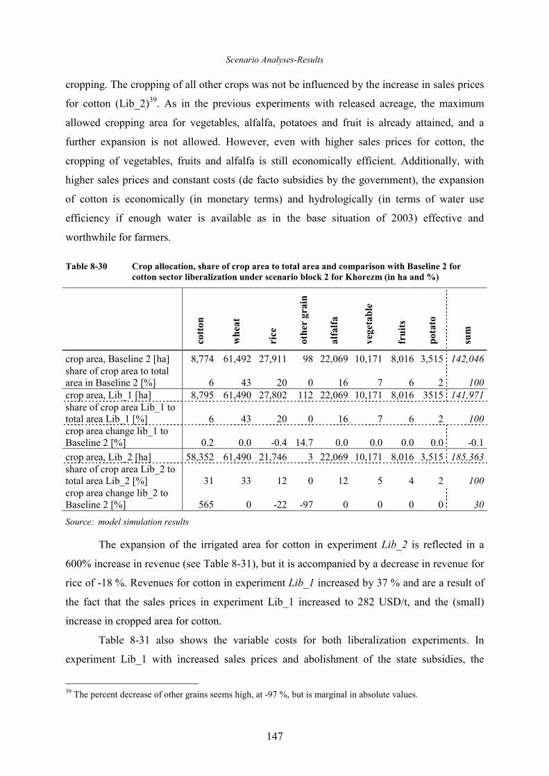
Scenario Analyses-Results
147
cropping. The cropping of all other crops was not be influenced by the increase in sales prices
for cotton (Lib_2)39. As in the previous experiments with released acreage, the maximum
allowed cropping area for vegetables, alfalfa, potatoes and fruit is already attained, and a
further expansion is not allowed. However, even with higher sales prices for cotton, the
cropping of vegetables, fruits and alfalfa is still economically efficient. Additionally, with
higher sales prices and constant costs (de facto subsidies by the government), the expansion
of cotton is economically (in monetary terms) and hydrologically (in terms of water use
efficiency if enough water is available as in the base situation of 2003) effective and
worthwhile for farmers.
Table 8-30 Crop allocation, share of crop area to total area and comparison with Baseline 2 for
cotton sector liberalization under scenario block 2 for Khorezm (in ha and %)
cotton
whea
t
rice
oth
er gra
in
alfalfa
veg
etable
fruits
pota
to
sum
crop area, Baseline 2 [ha] 8,774 61,492 27,911 98 22,069 10,171 8,016 3,515 142,046 share of crop area to total area in Baseline 2 [%] 6 43 20 0 16 7 6 2 100 crop area, Lib_1 [ha] 8,795 61,490 27,802 112 22,069 10,171 8,016 3515 141,971 share of crop area Lib_1 to total area Lib_1 [%] 6 43 20 0 16 7 6 2 100 crop area change lib_1 to Baseline 2 [%] 0.2 0.0 -0.4 14.7 0.0 0.0 0.0 0.0 -0.1
crop area, Lib_2 [ha] 58,352 61,490 21,746 3 22,069 10,171 8,016 3,515 185,363 share of crop area Lib_2 to total area Lib_2 [%] 31 33 12 0 12 5 4 2 100 crop area change lib_2 to Baseline 2 [%] 565 0 -22 -97 0 0 0 0 30
Source: model simulation results
The expansion of the irrigated area for cotton in experiment Lib_2 is reflected in a
600% increase in revenue (see Table 8-31), but it is accompanied by a decrease in revenue for
rice of -18 %. Revenues for cotton in experiment Lib_1 increased by 37 % and are a result of
the fact that the sales prices in experiment Lib_1 increased to 282 USD/t, and the (small)
increase in cropped area for cotton.
Table 8-31 also shows the variable costs for both liberalization experiments. In
experiment Lib_1 with increased sales prices and abolishment of the state subsidies, the
39 The percent decrease of other grains seems high, at -97 %, but is marginal in absolute values.
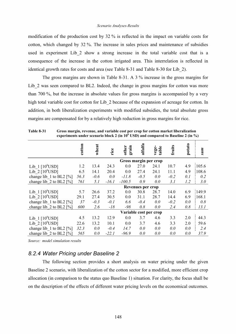
Scenario Analyses-Results
148
modification of the production cost by 32 % is reflected in the impact on variable costs for
cotton, which changed by 32 %. The increase in sales prices and maintenance of subsidies
used in experiment Lib_2 show a strong increase in the total variable cost that is a
consequence of the increase in the cotton irrigated area. This interrelation is reflected in
identical growth rates for costs and area (see Table 8-31 and Table 8-30 for Lib_2).
The gross margins are shown in Table 8-31. A 3 % increase in the gross margins for
Lib_2 was seen compared to BL2. Indeed, the change in gross margins for cotton was more
than 700 %, but the increase in absolute values for gross margins is accompanied by a very
high total variable cost for cotton for Lib_2 because of the expansion of acreage for cotton. In
addition, in both liberalization experiments with modified subsidies, the total absolute gross
margins are compensated for by a relatively high reduction in gross margins for rice.
Table 8-31 Gross margin, revenue, and variable cost per crop for cotton market liberalization
experiments under scenario block 2 (in 106 USD) and compared to Baseline 2 (in %)
cotton
whea
t
rice
oth
er
gra
in
alfalfa
veg
e-
table
fruits
pota
to
sum
Gross margin per crop
Lib_1 [106USD] 1.2 13.4 24.3 0.0 27.0 24.1 10.7 4.9 105.6 Lib_2 [106USD] 6.5 14.1 20.4 0.0 27.4 24.1 11.1 4.9 108.6 change lib_1 to BL2 [%] 56.3 -0.6 0.0 -11.8 -0.5 0.0 -0.2 0.1 0.2 change lib_2 to BL2 [%] 761 5.1 -16.1 -100.5 0.9 0.0 3.1 1.2 3.0 Revenues per crop
Lib_1 [106USD] 5.7 26.6 37.2 0.0 30.8 28.7 14.0 6.9 149.9 Lib_2 [106USD] 29.1 27.4 30.5 0.0 31.1 28.7 14.4 6.9 168.1 change lib_1 to BL2 [%] 37 -0.3 -0.1 6.6 -0.4 0.0 -0.2 0.0 0.8 change lib_2 to BL2 [%] 600 2.6 -18 -98 0.8 0.0 2.4 0.8 13.1 Variable cost per crop
Lib_1 [106USD] 4.5 13.2 12.9 0.0 3.7 4.6 3.3 2.0 44.3 Lib_2 [106USD] 22.6 13.2 10.1 0.0 3.7 4.6 3.3 2.0 59.6 change lib_1 to BL2 [%] 32.3 0.0 -0.4 14.7 0.0 0.0 0.0 0.0 2.4 change lib_2 to BL2 [%] 565 0.0 -22.1 -96.9 0.0 0.0 0.0 0.0 37.9
Source: model simulation results
8.2.4 Water Pricing under Baseline 2
The following section provides a short analysis on water pricing under the given
Baseline 2 scenario, with liberalization of the cotton sector for a modified, more efficient crop
allocation (in comparison to the status quo Baseline 1) situation. For clarity, the focus shall be
on the description of the effects of different water pricing levels on the economical outcomes.
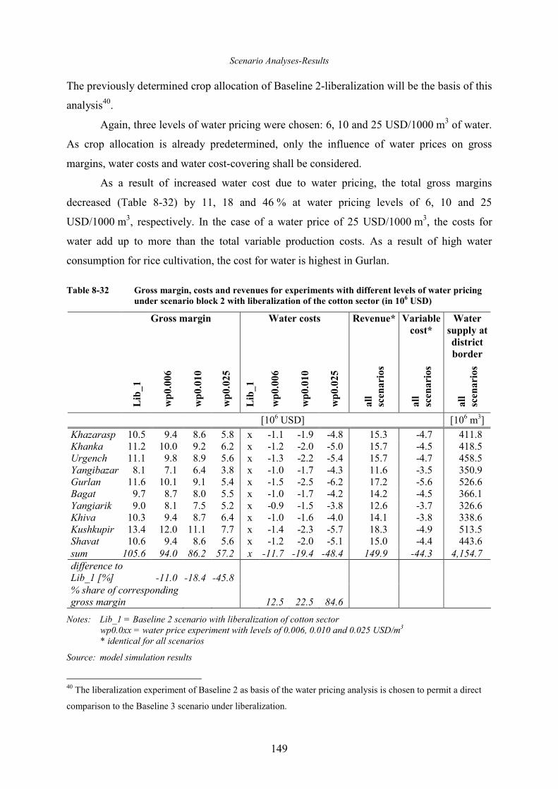
Scenario Analyses-Results
149
The previously determined crop allocation of Baseline 2-liberalization will be the basis of this
analysis40.
Again, three levels of water pricing were chosen: 6, 10 and 25 USD/1000 m3 of water.
As crop allocation is already predetermined, only the influence of water prices on gross
margins, water costs and water cost-covering shall be considered.
As a result of increased water cost due to water pricing, the total gross margins
decreased (Table 8-32) by 11, 18 and 46 % at water pricing levels of 6, 10 and 25
USD/1000 m3, respectively. In the case of a water price of 25 USD/1000 m3, the costs for
water add up to more than the total variable production costs. As a result of high water
consumption for rice cultivation, the cost for water is highest in Gurlan.
Table 8-32 Gross margin, costs and revenues for experiments with different levels of water pricing
under scenario block 2 with liberalization of the cotton sector (in 106 USD)
Gross margin Water costs Revenue* Variable
cost*
Water
supply at
district
border
Lib
_1
wp0.006
wp0.010
wp0.025
Lib
_1
wp0.006
wp0.010
wp0.025
all
scen
arios
all
scen
arios
all
scen
arios
[106 USD] [106 m3]
Khazarasp 10.5 9.4 8.6 5.8 x -1.1 -1.9 -4.8 15.3 -4.7 411.8 Khanka 11.2 10.0 9.2 6.2 x -1.2 -2.0 -5.0 15.7 -4.5 418.5 Urgench 11.1 9.8 8.9 5.6 x -1.3 -2.2 -5.4 15.7 -4.7 458.5 Yangibazar 8.1 7.1 6.4 3.8 x -1.0 -1.7 -4.3 11.6 -3.5 350.9 Gurlan 11.6 10.1 9.1 5.4 x -1.5 -2.5 -6.2 17.2 -5.6 526.6 Bagat 9.7 8.7 8.0 5.5 x -1.0 -1.7 -4.2 14.2 -4.5 366.1 Yangiarik 9.0 8.1 7.5 5.2 x -0.9 -1.5 -3.8 12.6 -3.7 326.6 Khiva 10.3 9.4 8.7 6.4 x -1.0 -1.6 -4.0 14.1 -3.8 338.6 Kushkupir 13.4 12.0 11.1 7.7 x -1.4 -2.3 -5.7 18.3 -4.9 513.5 Shavat 10.6 9.4 8.6 5.6 x -1.2 -2.0 -5.1 15.0 -4.4 443.6 sum 105.6 94.0 86.2 57.2 x -11.7 -19.4 -48.4 149.9 -44.3 4,154.7 difference to Lib_1 [%] -11.0 -18.4 -45.8 % share of corresponding gross margin 12.5 22.5 84.6
Notes: Lib_1 = Baseline 2 scenario with liberalization of cotton sector wp0.0xx = water price experiment with levels of 0.006, 0.010 and 0.025 USD/m3
* identical for all scenarios
Source: model simulation results
40 The liberalization experiment of Baseline 2 as basis of the water pricing analysis is chosen to permit a direct
comparison to the Baseline 3 scenario under liberalization.
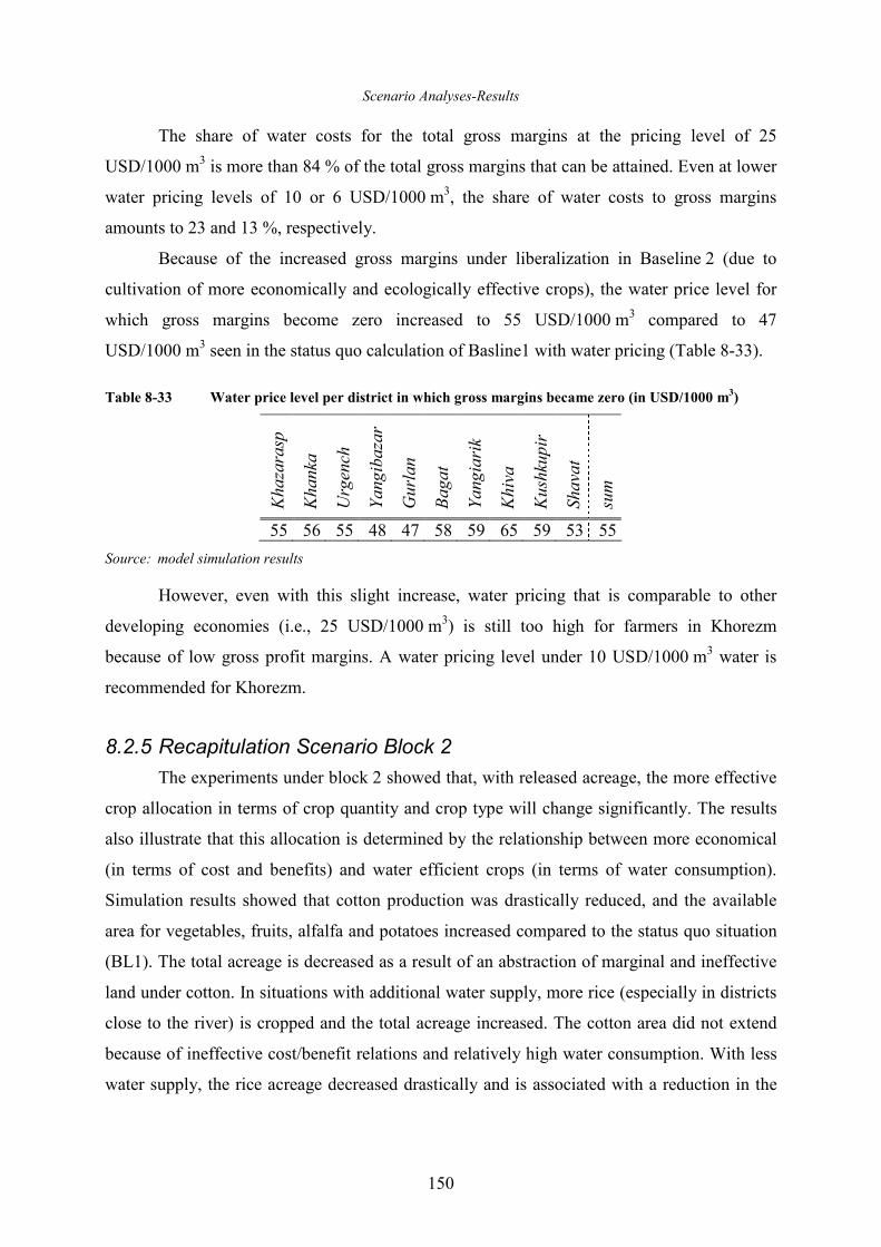
Scenario Analyses-Results
150
The share of water costs for the total gross margins at the pricing level of 25
USD/1000 m3 is more than 84 % of the total gross margins that can be attained. Even at lower
water pricing levels of 10 or 6 USD/1000 m3, the share of water costs to gross margins
amounts to 23 and 13 %, respectively.
Because of the increased gross margins under liberalization in Baseline 2 (due to
cultivation of more economically and ecologically effective crops), the water price level for
which gross margins become zero increased to 55 USD/1000 m3 compared to 47
USD/1000 m3 seen in the status quo calculation of Basline1 with water pricing (Table 8-33).
Table 8-33 Water price level per district in which gross margins became zero (in USD/1000 m3)
Kha
zarasp
Kha
nka
Urgench
Yan
giba
zar
Gurlan
Bag
at
Yan
giarik
Khiva
Kushkup
ir
Shavat
sum
55 56 55 48 47 58 59 65 59 53 55
Source: model simulation results
However, even with this slight increase, water pricing that is comparable to other
developing economies (i.e., 25 USD/1000 m3) is still too high for farmers in Khorezm
because of low gross profit margins. A water pricing level under 10 USD/1000 m3 water is
recommended for Khorezm.
8.2.5 Recapitulation Scenario Block 2
The experiments under block 2 showed that, with released acreage, the more effective
crop allocation in terms of crop quantity and crop type will change significantly. The results
also illustrate that this allocation is determined by the relationship between more economical
(in terms of cost and benefits) and water efficient crops (in terms of water consumption).
Simulation results showed that cotton production was drastically reduced, and the available
area for vegetables, fruits, alfalfa and potatoes increased compared to the status quo situation
(BL1). The total acreage is decreased as a result of an abstraction of marginal and ineffective
land under cotton. In situations with additional water supply, more rice (especially in districts
close to the river) is cropped and the total acreage increased. The cotton area did not extend
because of ineffective cost/benefit relations and relatively high water consumption. With less
water supply, the rice acreage decreased drastically and is associated with a reduction in the
Scenario Analyses-Results
151
total area and gross margins. The proportion of wheat production increased in situations with
less water supply because it is less water demanding.
With the liberalization of the cotton market and the abolishment of cotton subsidies,
the situation does not significantly change; the cost and water consumption for cotton is still
too high, and sales prices are too low to balance out the high production costs. If subsidies
remained (or cost will be reduced) and bordering prices for cotton could directly pass to
farmers, it may be worthwhile to grow cotton.
Regarding water consumption and water effectiveness, wheat and, to some extent,
potatoes and alfalfa are more water use efficient. If we consider economical efficiency, (ratio
of input cost/output benefit), vegetables, fruits, potatoes, alfalfa and, if enough water is
available, rice are most effective and should be cropped.
The analysis on water pricing under scenario block 2 showed that, even with increased
gross margins due to modified and more efficient crop allocation and cultivation, a water
pricing level of more than 10 USD/1000 m3 is not accomplishable because of relatively low
gross profit margins in Khorezm. At a higher water price level, crop cultivation is not
beneficial.
However, the results of scenario block 2 with released acreage also showed that the
crop allocation is only controlled by this hydrologic-economic efficiency optimization factor,
and the most effective crops were cropped over the entire area up to set boundaries. Modified
acreage and crop production, dependent on supply and demand and willingness to pay for a
certain product, will result in changed crop prices. These are not yet included in the
optimization and production function. The results and weaknesses shown here illustrate that
this demand- and supply-dependent price factor should taken into account for the next set of
experiments under scenario block 3. Nevertheless, this analysis was very important and
showed the effect of more efficient crop allocation considering both, water demand and the
cost/price effectiveness of the crops.
8.3 Model Results Scenario Block 3– Introduction of a Price-Function and Liberalization of Cotton Sector
The analysis of the previous scenarios addressed the inspection of water and the
cropping system in Khorezm under observed conditions in terms of cropping pattern and
acreage (Baseline 1 and its experiments), and sales prices and production costs with released
acreage (Baseline 2 and its experiments). The following scenario block 3 addresses the
Scenario Analyses-Results
152
situation with modified governmental procurement system for cotton and the implementation
of a price function. The scenario shall provide information on more effective crop allocation
and acreage, variable sales prices dependent on the market situation for certain crops in
Khorezm and the resultant economical impact. For this reason, it is necessary to first release
the crop area and then the sales prices for agricultural products in the following experiments.
According to chapter 3.2.4, an endogenously calculated crop price will be determined to
account for the variable crop sales prices that depend on demand and supply and the
willingness to pay for a product41. Thereby, both, sales prices and supply/acreage will be
modified internally.
8.3.1 Baseline 3
For the price function scenario with the abolishment of the state order for cotton, the
production costs of cotton increased by 32 %. Because cotton is exported and not traded on
local markets, a 30 % higher cotton price is assumed (see chapter 7.1.5). The acreage is
released and a price function is implemented. The resultant scenario (Baseline 3) will be the
basis of comparison with other price function scenarios under scenario block 3 by modifying
the water supply and introducing a water price.
Unlike the scenarios under status quo conditions (with observed acreage and existent
state order system, Baseline 1), where the effects of changes in water supply and water
management on soil and water balances and crop-parameters were considered in more detail,
the focus of the following experiments will be on the economical output to understand the
effect of price mechanisms, crop allocation and liberalization of the cotton sector on
agricultural profits, gross margins and revenues for changes in cropping pattern, areas, crop
pricing and allocation.
Revenues, cropping area, variable costs and gross margins under released state order system
Due to the implementation of endogenously determined and demand-dependent crop
sales prices, crop allocation is not only dependent on optimal water use and cost-price
relations for single crops (as already shown in Baseline 2), but it is also dependent on
cropping acreage and the resulting demand and supply controlled variable crop prices. If only
a few crops (here in the model mainly for optimal water allocation and maximal profits) are
grown in expanded areas and the supply on local markets increases, the resultant decreased
41 With the exception of cotton, as no trade on local market is taking place; bordering prices are assumed.
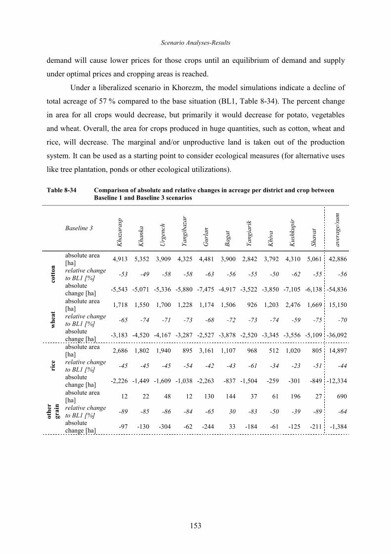
Scenario Analyses-Results
153
demand will cause lower prices for those crops until an equilibrium of demand and supply
under optimal prices and cropping areas is reached.
Under a liberalized scenario in Khorezm, the model simulations indicate a decline of
total acreage of 57 % compared to the base situation (BL1, Table 8-34). The percent change
in area for all crops would decrease, but primarily it would decrease for potato, vegetables
and wheat. Overall, the area for crops produced in huge quantities, such as cotton, wheat and
rice, will decrease. The marginal and/or unproductive land is taken out of the production
system. It can be used as a starting point to consider ecological measures (for alternative uses
like tree plantation, ponds or other ecological utilizations).
Table 8-34 Comparison of absolute and relative changes in acreage per district and crop between
Baseline 1 and Baseline 3 scenarios
Baseline 3
Kha
zarasp
Kha
nka
Urgench
Yan
giba
zar
Gurlan
Bag
at
Yan
giarik
Khiva
Kushkup
ir
Shavat
averag
e/sum
absolute area [ha]
4,913 5,352 3,909 4,325 4,481 3,900 2,842 3,792 4,310 5,061 42,886
relative change to BL1 [%]
-53 -49 -58 -58 -63 -56 -55 -50 -62 -55 -56
cotton
absolute change [ha]
-5,543 -5,071 -5,336 -5,880 -7,475 -4,917 -3,522 -3,850 -7,105 -6,138 -54,836
absolute area [ha]
1,718 1,550 1,700 1,228 1,174 1,506 926 1,203 2,476 1,669 15,150
relative change to BL1 [%]
-65 -74 -71 -73 -68 -72 -73 -74 -59 -75 -70
whea
t
absolute change [ha]
-3,183 -4,520 -4,167 -3,287 -2,527 -3,878 -2,520 -3,345 -3,556 -5,109 -36,092
absolute area [ha]
2,686 1,802 1,940 895 3,161 1,107 968 512 1,020 805 14,897
relative change to BL1 [%]
-45 -45 -45 -54 -42 -43 -61 -34 -23 -51 -44
rice
absolute change [ha]
-2,226 -1,449 -1,609 -1,038 -2,263 -837 -1,504 -259 -301 -849 -12,334
absolute area [ha]
12 22 48 12 130 144 37 61 196 27 690
relative change to BL1 [%]
-89 -85 -86 -84 -65 30 -83 -50 -39 -89 -64
oth
er
gra
in
absolute change [ha]
-97 -130 -304 -62 -244 33 -184 -61 -125 -211 -1,384
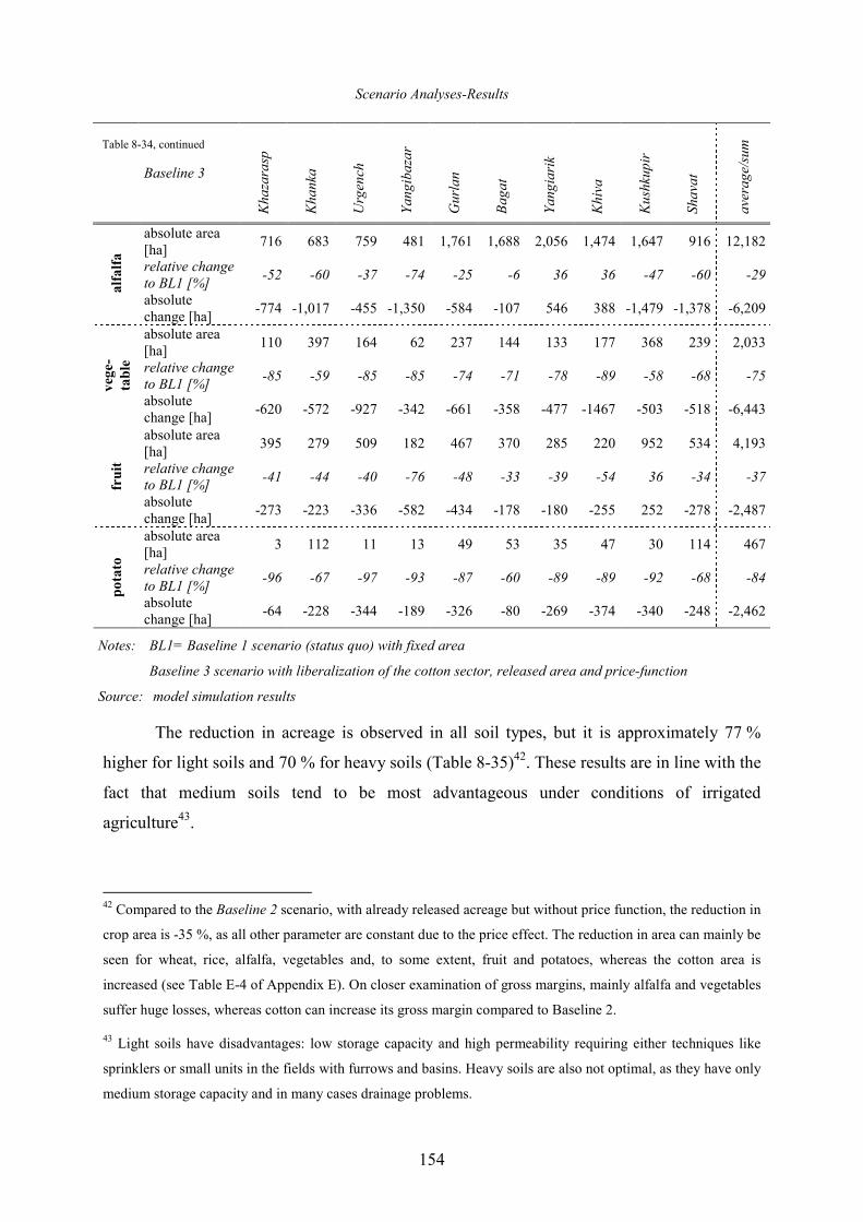
Scenario Analyses-Results
154
Baseline 3
Kha
zarasp
Kha
nka
Urgench
Yan
giba
zar
Gurlan
Bag
at
Yan
giarik
Khiva
Kushkup
ir
Shavat
averag
e/sum
absolute area [ha]
716 683 759 481 1,761 1,688 2,056 1,474 1,647 916 12,182
relative change to BL1 [%]
-52 -60 -37 -74 -25 -6 36 36 -47 -60 -29
alfalfa
absolute change [ha]
-774 -1,017 -455 -1,350 -584 -107 546 388 -1,479 -1,378 -6,209
absolute area [ha]
110 397 164 62 237 144 133 177 368 239 2,033
relative change to BL1 [%]
-85 -59 -85 -85 -74 -71 -78 -89 -58 -68 -75
veg
e-
table
absolute change [ha]
-620 -572 -927 -342 -661 -358 -477 -1467 -503 -518 -6,443
absolute area [ha]
395 279 509 182 467 370 285 220 952 534 4,193
relative change to BL1 [%]
-41 -44 -40 -76 -48 -33 -39 -54 36 -34 -37
fruit
absolute change [ha]
-273 -223 -336 -582 -434 -178 -180 -255 252 -278 -2,487
absolute area [ha]
3 112 11 13 49 53 35 47 30 114 467
relative change to BL1 [%]
-96 -67 -97 -93 -87 -60 -89 -89 -92 -68 -84
pota
to
absolute change [ha]
-64 -228 -344 -189 -326 -80 -269 -374 -340 -248 -2,462
Notes: BL1= Baseline 1 scenario (status quo) with fixed area
Baseline 3 scenario with liberalization of the cotton sector, released area and price-function
Source: model simulation results
The reduction in acreage is observed in all soil types, but it is approximately 77 %
higher for light soils and 70 % for heavy soils (Table 8-35)42. These results are in line with the
fact that medium soils tend to be most advantageous under conditions of irrigated
agriculture43.
42 Compared to the Baseline 2 scenario, with already released acreage but without price function, the reduction in
crop area is -35 %, as all other parameter are constant due to the price effect. The reduction in area can mainly be
seen for wheat, rice, alfalfa, vegetables and, to some extent, fruit and potatoes, whereas the cotton area is
increased (see Table E-4 of Appendix E). On closer examination of gross margins, mainly alfalfa and vegetables
suffer huge losses, whereas cotton can increase its gross margin compared to Baseline 2.
43 Light soils have disadvantages: low storage capacity and high permeability requiring either techniques like
sprinklers or small units in the fields with furrows and basins. Heavy soils are also not optimal, as they have only
medium storage capacity and in many cases drainage problems.
Table 8-34, continued
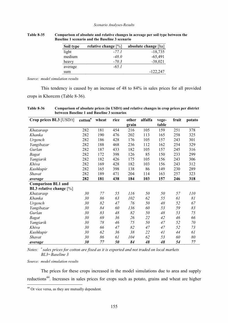
Scenario Analyses-Results
155
Table 8-35 Comparison of absolute and relative changes in acreage per soil type between the
Baseline 1 scenario and the Baseline 3 scenario
Soil type relative change [%] absolute change [ha] light -77.1 -18,735 medium -48.0 -65,491 heavy -70.3 -38,021 average -65.1 sum -122,247
Source: model simulation results
This tendency is caused by an increase of 48 to 84% in sales prices for all provided
crops in Khorezm (Table 8-36).
Table 8-36 Comparison of absolute prices (in USD/t) and relative changes in crop prices per district
between Baseline 1 and Baseline 3 scenarios
Crop prices BL3 [USD/t] cotton∗∗∗∗ wheat rice other
grain
alfalfa vege-
table
fruit potato
Khazarasp 282 181 454 216 105 159 251 378 Khanka 282 190 476 202 113 165 258 325 Urgench 282 186 428 176 105 157 243 301 Yangibazar 282 188 468 236 112 162 254 329 Gurlan 282 187 433 182 105 157 245 316 Bagat 282 172 398 126 85 150 233 299 Yangiarik 282 182 426 175 105 156 243 306 Khiva 282 169 428 182 103 156 243 312 Kushkupir 282 165 398 138 86 149 230 289 Shavat 282 189 471 204 114 163 257 323 average 282 181 438 184 103 157 246 318
Comparison BL1 and BL3 relative change [%] Khazarasp 30 77 55 116 50 50 57 110 Khanka 30 86 63 102 62 55 61 81 Urgench 30 82 47 76 50 48 52 67 Yangibazar 30 84 60 136 60 53 59 83 Gurlan 30 83 48 82 50 48 53 75 Bagat 30 69 36 26 22 42 46 66 Yangiarik 30 78 46 75 50 47 52 70 Khiva 30 66 47 82 47 47 52 73 Kushkupir 30 62 36 38 22 41 44 61 Shavat 30 86 61 104 62 53 60 80 average 30 77 50 84 48 48 54 77
Notes: ∗ sales prices for cotton are fixed as it is exported and not traded on local markets BL3=Baseline 3
Source: model simulation results
The prices for these crops increased in the model simulations due to area and supply
reductions44. Increases in sales prices for crops such as potato, grains and wheat are higher 44 Or vice versa, as they are mutually dependent.
Scenario Analyses-Results
156
than those for alfalfa, vegetables, fruit and rice because the latter (mainly vegetables and
fruits) are more water efficient and have a better cost-benefit relationship and are preferred for
cropping45. Crop supply is higher compared to potatoes, grains and wheat, whereas the
demand for those crops is increased (see also Baseline 2).
The total agricultural gross margins per district in Khorezm are, compared to the
Baseline 1 scenario under 2003 conditions, heterogeneously. For districts like Bagat,
Yangiarik, Khiva and Kushkupir, the absolute values are relatively low and are lower than
those for the Baseline 1 scenario (Table 8-37). The results are primarily a function of the
change in gross margins for cotton; which were mostly negative in the Baseline 1 scenario
(see Figure 8-1). Due to the abolishment of the governmental cotton quota system and the
increase in sales prices for cotton, the revenues for cotton increased in the price function
scenario (BL3). For most of the other crops, the gross margins decrease in the price function
scenario (compared to BL1) due to higher sales prices, decreased acreage, and less
production. The total gross margins are dependent on the relation between changes in gross
margins for cotton and for all other crops; in some cases, this change is negative or slightly
positive for districts, such as Khanka, Gurlan or Shavat because the acreage of cotton is
higher (see Table 8-34, absolute area) than in other districts.
Upon closer examination of gross margins per crop in the price function scenario, we
see that cotton, wheat, rice and, to some extent, fruit and vegetables have a huge share of the
gross margins because of the relationship between acreage and sales and production-costs.
For rice, this is true in districts close to the river, where rice is a beneficial crop in good water
supply years.
45 As demonstrated in the first scenarios under status quo conditions (Baseline 1).
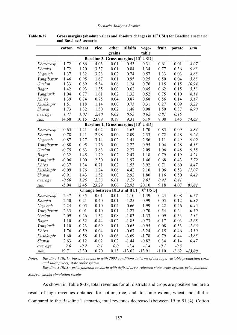
Scenario Analyses-Results
157
Table 8-37 Gross margins (absolute values and absolute changes in 106 USD) for Baseline 1 scenario
and Baseline 3 scenario
cotton wheat rice other
grains
alfalfa vege-
table
fruit potato sum
Baseline 3, Gross margins [106 USD] Khazarasp 1.72 0.86 4.03 0.01 0.53 0.31 0.61 0.01 8.07 Khanka 1.72 1.20 3.37 0.01 0.84 1.34 0.77 0.36 9.63 Urgench 1.37 1.32 3.23 0.02 0.74 0.57 1.33 0.03 8.63 Yangibazar 1.46 0.95 1.67 0.01 0.95 0.25 0.50 0.04 5.83 Gurlan 1.33 0.89 5.34 0.06 1.24 0.76 1.15 0.15 10.94 Bagat 1.42 0.93 1.35 0.00 0.62 0.45 0.62 0.15 5.53 Yangiarik 1.04 0.77 1.61 0.02 1.32 0.52 0.75 0.10 6.14 Khiva 1.39 0.74 0.75 0.04 0.87 0.68 0.56 0.14 5.17 Kushkupir 1.51 1.18 1.14 0.00 0.73 0.31 0.27 0.09 5.22 Shavat 1.73 1.32 1.50 0.02 1.48 0.98 1.50 0.37 8.90 average 1.47 1.02 2.40 0.02 0.93 0.62 0.81 0.15 sum 14.68 10.15 23.99 0.19 9.31 6.19 8.08 1.45 74.03
Baseline 1, Gross margins [106 USD] Khazarasp -0.65 1.21 4.02 0.00 1.63 1.70 0.85 0.09 8.84 Khanka -0.78 1.41 2.98 0.00 2.09 2.33 0.72 0.48 9.24 Urgench -0.87 1.27 3.14 -0.02 1.41 2.56 1.11 0.49 9.09 Yangibazar -0.88 0.95 1.76 0.00 2.22 0.95 1.04 0.28 6.33 Gurlan -0.75 0.63 3.83 -0.02 2.27 2.09 1.06 0.48 9.58 Bagat 0.32 1.45 1.79 0.02 2.47 1.18 0.79 0.19 8.21 Yangiarik -0.06 1.00 2.30 0.01 1.97 1.46 0.68 0.43 7.79 Khiva -0.37 1.34 0.71 0.02 1.53 3.92 0.71 0.60 8.47 Kushkupir -0.09 1.76 1.24 0.06 4.42 2.10 1.06 0.53 11.07 Shavat -0.91 1.43 1.52 0.00 2.92 1.80 1.16 0.50 8.42 average -0.50 1.25 2.33 0.01 2.29 2.01 0.92 0.41 sum -5.04 12.45 23.29 0.06 22.93 20.10 9.18 4.07 87.04
Change between BL3 and BL1 [106 USD] Khazarasp 2.37 -0.35 0.01 0.01 -1.10 -1.39 -0.23 -0.08 -0.77 Khanka 2.50 -0.21 0.40 0.01 -1.25 -0.99 0.05 -0.12 0.39 Urgench 2.24 0.05 0.10 0.04 -0.66 -1.99 0.22 -0.46 -0.46 Yangibazar 2.33 -0.01 -0.10 0.01 -1.27 -0.70 -0.54 -0.24 -0.50 Gurlan 2.09 0.26 1.52 0.08 -1.03 -1.33 0.09 -0.33 1.35 Bagat 1.10 -0.52 -0.44 -0.02 -1.85 -0.73 -0.17 -0.03 -2.68 Yangiarik 1.10 -0.23 -0.69 0.01 -0.65 -0.95 0.08 -0.33 -1.66 Khiva 1.76 -0.59 0.04 0.01 -0.67 -3.24 -0.15 -0.46 -3.30 Kushkupir 1.60 -0.58 -0.10 -0.06 -3.69 -1.78 -0.79 -0.44 -5.85 Shavat 2.63 -0.12 -0.02 0.02 -1.44 -0.82 0.34 -0.14 0.47 average 2.0 -0.2 0.1 0.0 -1.4 -1.4 -0.1 -0.3 sum 19.71 -2.30 0.70 0.13 -13.62 -13.91 -1.10 -2.62 -13.00
Notes: Baseline 1 (BL1): baseline scenario with 2003 conditions in terms of acreage, variable production costs and sales prices, state order system Baseline 3 (BL3): price function scenario with defixed area, released state order system, price function
Source: model simulation results
As shown in Table 8-38, total revenues for all districts and crops are positive and are a
result of high revenues obtained for cotton, rice, and, to some extent, wheat and alfalfa.
Compared to the Baseline 1 scenario, total revenues decreased (between 19 to 51 %). Cotton
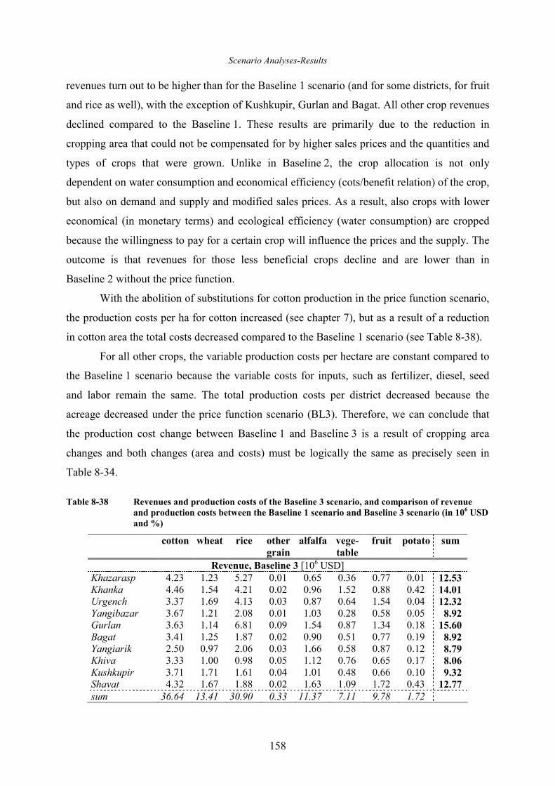
Scenario Analyses-Results
158
revenues turn out to be higher than for the Baseline 1 scenario (and for some districts, for fruit
and rice as well), with the exception of Kushkupir, Gurlan and Bagat. All other crop revenues
declined compared to the Baseline 1. These results are primarily due to the reduction in
cropping area that could not be compensated for by higher sales prices and the quantities and
types of crops that were grown. Unlike in Baseline 2, the crop allocation is not only
dependent on water consumption and economical efficiency (cots/benefit relation) of the crop,
but also on demand and supply and modified sales prices. As a result, also crops with lower
economical (in monetary terms) and ecological efficiency (water consumption) are cropped
because the willingness to pay for a certain crop will influence the prices and the supply. The
outcome is that revenues for those less beneficial crops decline and are lower than in
Baseline 2 without the price function.
With the abolition of substitutions for cotton production in the price function scenario,
the production costs per ha for cotton increased (see chapter 7), but as a result of a reduction
in cotton area the total costs decreased compared to the Baseline 1 scenario (see Table 8-38).
For all other crops, the variable production costs per hectare are constant compared to
the Baseline 1 scenario because the variable costs for inputs, such as fertilizer, diesel, seed
and labor remain the same. The total production costs per district decreased because the
acreage decreased under the price function scenario (BL3). Therefore, we can conclude that
the production cost change between Baseline 1 and Baseline 3 is a result of cropping area
changes and both changes (area and costs) must be logically the same as precisely seen in
Table 8-34.
Table 8-38 Revenues and production costs of the Baseline 3 scenario, and comparison of revenue
and production costs between the Baseline 1 scenario and Baseline 3 scenario (in 106 USD
and %)
cotton wheat rice other
grain
alfalfa vege-
table
fruit potato sum
Revenue, Baseline 3 [106 USD] Khazarasp 4.23 1.23 5.27 0.01 0.65 0.36 0.77 0.01 12.53
Khanka 4.46 1.54 4.21 0.02 0.96 1.52 0.88 0.42 14.01 Urgench 3.37 1.69 4.13 0.03 0.87 0.64 1.54 0.04 12.32
Yangibazar 3.67 1.21 2.08 0.01 1.03 0.28 0.58 0.05 8.92 Gurlan 3.63 1.14 6.81 0.09 1.54 0.87 1.34 0.18 15.60
Bagat 3.41 1.25 1.87 0.02 0.90 0.51 0.77 0.19 8.92 Yangiarik 2.50 0.97 2.06 0.03 1.66 0.58 0.87 0.12 8.79 Khiva 3.33 1.00 0.98 0.05 1.12 0.76 0.65 0.17 8.06
Kushkupir 3.71 1.71 1.61 0.04 1.01 0.48 0.66 0.10 9.32 Shavat 4.32 1.67 1.88 0.02 1.63 1.09 1.72 0.43 12.77
sum 36.64 13.41 30.90 0.33 11.37 7.11 9.78 1.72
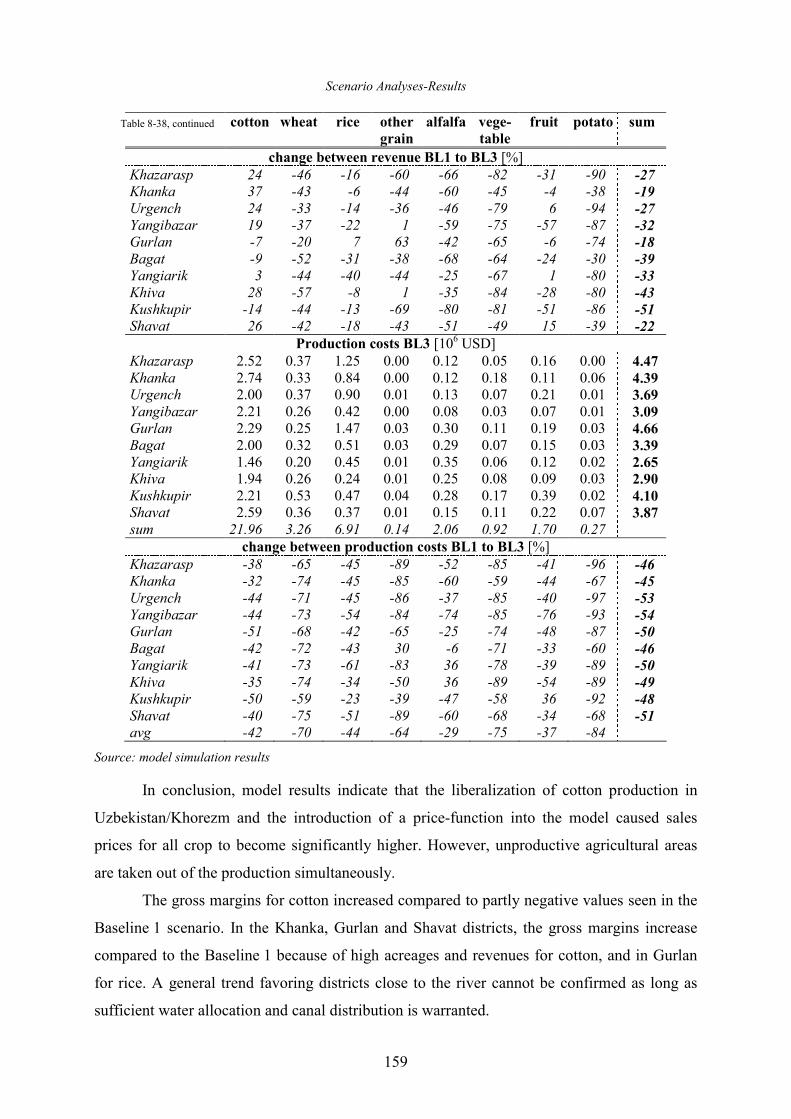
Scenario Analyses-Results
159
cotton wheat rice other
grain
alfalfa vege-
table
fruit potato sum
change between revenue BL1 to BL3 [%] Khazarasp 24 -46 -16 -60 -66 -82 -31 -90 -27 Khanka 37 -43 -6 -44 -60 -45 -4 -38 -19
Urgench 24 -33 -14 -36 -46 -79 6 -94 -27 Yangibazar 19 -37 -22 1 -59 -75 -57 -87 -32 Gurlan -7 -20 7 63 -42 -65 -6 -74 -18
Bagat -9 -52 -31 -38 -68 -64 -24 -30 -39 Yangiarik 3 -44 -40 -44 -25 -67 1 -80 -33
Khiva 28 -57 -8 1 -35 -84 -28 -80 -43 Kushkupir -14 -44 -13 -69 -80 -81 -51 -86 -51 Shavat 26 -42 -18 -43 -51 -49 15 -39 -22
Production costs BL3 [106 USD] Khazarasp 2.52 0.37 1.25 0.00 0.12 0.05 0.16 0.00 4.47
Khanka 2.74 0.33 0.84 0.00 0.12 0.18 0.11 0.06 4.39 Urgench 2.00 0.37 0.90 0.01 0.13 0.07 0.21 0.01 3.69
Yangibazar 2.21 0.26 0.42 0.00 0.08 0.03 0.07 0.01 3.09 Gurlan 2.29 0.25 1.47 0.03 0.30 0.11 0.19 0.03 4.66
Bagat 2.00 0.32 0.51 0.03 0.29 0.07 0.15 0.03 3.39 Yangiarik 1.46 0.20 0.45 0.01 0.35 0.06 0.12 0.02 2.65 Khiva 1.94 0.26 0.24 0.01 0.25 0.08 0.09 0.03 2.90
Kushkupir 2.21 0.53 0.47 0.04 0.28 0.17 0.39 0.02 4.10 Shavat 2.59 0.36 0.37 0.01 0.15 0.11 0.22 0.07 3.87
sum 21.96 3.26 6.91 0.14 2.06 0.92 1.70 0.27
change between production costs BL1 to BL3 [%] Khazarasp -38 -65 -45 -89 -52 -85 -41 -96 -46 Khanka -32 -74 -45 -85 -60 -59 -44 -67 -45
Urgench -44 -71 -45 -86 -37 -85 -40 -97 -53 Yangibazar -44 -73 -54 -84 -74 -85 -76 -93 -54 Gurlan -51 -68 -42 -65 -25 -74 -48 -87 -50
Bagat -42 -72 -43 30 -6 -71 -33 -60 -46 Yangiarik -41 -73 -61 -83 36 -78 -39 -89 -50
Khiva -35 -74 -34 -50 36 -89 -54 -89 -49 Kushkupir -50 -59 -23 -39 -47 -58 36 -92 -48
Shavat -40 -75 -51 -89 -60 -68 -34 -68 -51 avg -42 -70 -44 -64 -29 -75 -37 -84
Source: model simulation results
In conclusion, model results indicate that the liberalization of cotton production in
Uzbekistan/Khorezm and the introduction of a price-function into the model caused sales
prices for all crop to become significantly higher. However, unproductive agricultural areas
are taken out of the production simultaneously.
The gross margins for cotton increased compared to partly negative values seen in the
Baseline 1 scenario. In the Khanka, Gurlan and Shavat districts, the gross margins increase
compared to the Baseline 1 because of high acreages and revenues for cotton, and in Gurlan
for rice. A general trend favoring districts close to the river cannot be confirmed as long as
sufficient water allocation and canal distribution is warranted.
Table 8-38, continued
Scenario Analyses-Results
160
The modeling results indicate that the liberalization in cotton production and the
implementation of a price function would lead to higher production costs and higher sales
prices. Due to modified price regulations, supply, demand and the resulting sales prices will
change the whole crop allocation. Subsequently, less efficient crops, such as cotton, become
more attractive because the supply of other crops will decrease due to high sales prices. In
cooperation with the Water User Associations (WUA) and the management of common
resources, such as machinery-parks, it would be possible to reduce costs and use manpower
more effectively to reduce the costs for the individual farmer.
8.3.2 Price Function Scenario- Water Supply Experiments
The effect of modified water supply under liberalization and after introduction of a
price function will be described in the following paragraphs. Different levels of water supply
have significant impacts on crop allocation, gross margins and sales prices for crops. Here, an
increase and decrease in water supply by 50 % compared to the observed situation in 2003
will be examined.
Crop allocation and cropping area
A 53% increase in total cropped area is seen with increased water supply. This can be
attributed to a sharp rise in crops such as rice, vegetables and fruits (Table 8-39), which are
water demanding but very beneficial in terms of sales revenues. The percent increase for other
grains (maize, barley etc.) is more than 240 %, but their influence in absolute values is still
limited due to the relatively small area of not more than 1.2 % of the total area. The total
acreage for cotton is 45,000 ha, followed by rice, wheat and alfalfa (see Table 8-40).
Interestingly, with decreased water supply, the total cropping area increased by 17 %
compared to BL3, which is not necessarily expected because lower water supply usually
means less area can be sufficiently cropped. This same rationale can be applied to all other
crops, with the exception of cotton and wheat in some districts (see Table 8-39). In these
areas, cotton acreage is increasing and is a major influence for the total cropped area. The
total acreage of cotton is 58 % of the total area (see Table 8-40). The constant sales price for
cotton and beneficial revenues in the model help explain these results. Even with less water
and lower yields, it is worthwhile for farmers to grow cotton for export in the price function
scenario because sales prices are in BL3 increased and constant for cotton.
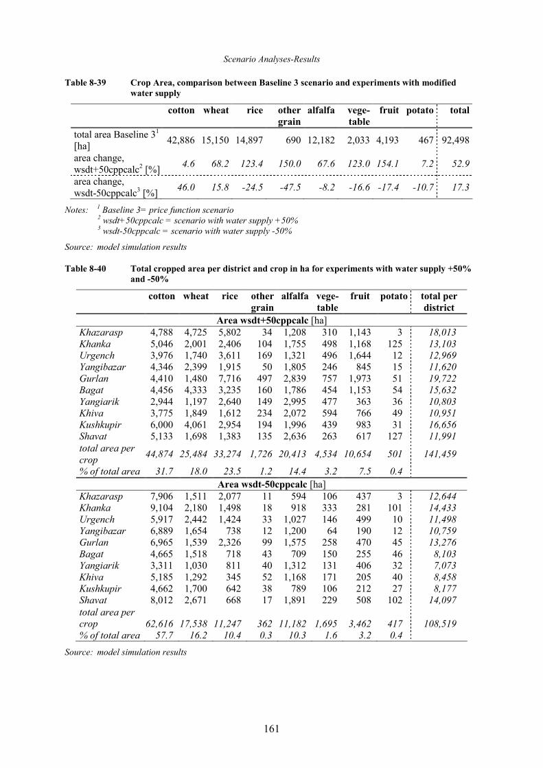
Scenario Analyses-Results
161
Table 8-39 Crop Area, comparison between Baseline 3 scenario and experiments with modified
water supply
Notes: 1 Baseline 3= price function scenario 2 wsdt+50cppcalc = scenario with water supply +50% 3 wsdt-50cppcalc = scenario with water supply -50%
Source: model simulation results
Table 8-40 Total cropped area per district and crop in ha for experiments with water supply +50%
and -50%
cotton wheat rice other
grain
alfalfa vege-
table
fruit potato total per
district
Area wsdt+50cppcalc [ha] Khazarasp 4,788 4,725 5,802 34 1,208 310 1,143 3 18,013 Khanka 5,046 2,001 2,406 104 1,755 498 1,168 125 13,103 Urgench 3,976 1,740 3,611 169 1,321 496 1,644 12 12,969 Yangibazar 4,346 2,399 1,915 50 1,805 246 845 15 11,620 Gurlan 4,410 1,480 7,716 497 2,839 757 1,973 51 19,722 Bagat 4,456 4,333 3,235 160 1,786 454 1,153 54 15,632 Yangiarik 2,944 1,197 2,640 149 2,995 477 363 36 10,803 Khiva 3,775 1,849 1,612 234 2,072 594 766 49 10,951 Kushkupir 6,000 4,061 2,954 194 1,996 439 983 31 16,656 Shavat 5,133 1,698 1,383 135 2,636 263 617 127 11,991 total area per crop
44,874 25,484 33,274 1,726 20,413 4,534 10,654 501 141,459
% of total area 31.7 18.0 23.5 1.2 14.4 3.2 7.5 0.4 Area wsdt-50cppcalc [ha]
Khazarasp 7,906 1,511 2,077 11 594 106 437 3 12,644 Khanka 9,104 2,180 1,498 18 918 333 281 101 14,433 Urgench 5,917 2,442 1,424 33 1,027 146 499 10 11,498 Yangibazar 6,889 1,654 738 12 1,200 64 190 12 10,759 Gurlan 6,965 1,539 2,326 99 1,575 258 470 45 13,276 Bagat 4,665 1,518 718 43 709 150 255 46 8,103 Yangiarik 3,311 1,030 811 40 1,312 131 406 32 7,073 Khiva 5,185 1,292 345 52 1,168 171 205 40 8,458 Kushkupir 4,662 1,700 642 38 789 106 212 27 8,177 Shavat 8,012 2,671 668 17 1,891 229 508 102 14,097 total area per crop 62,616 17,538 11,247 362 11,182 1,695 3,462 417 108,519 % of total area 57.7 16.2 10.4 0.3 10.3 1.6 3.2 0.4
Source: model simulation results
cotton wheat rice other
grain
alfalfa vege-
table
fruit potato total
total area Baseline 31 [ha]
42,886 15,150 14,897 690 12,182 2,033 4,193 467 92,498
area change, wsdt+50cppcalc2 [%]
4.6 68.2 123.4 150.0 67.6 123.0 154.1 7.2 52.9
area change, wsdt-50cppcalc3 [%]
46.0 15.8 -24.5 -47.5 -8.2 -16.6 -17.4 -10.7 17.3
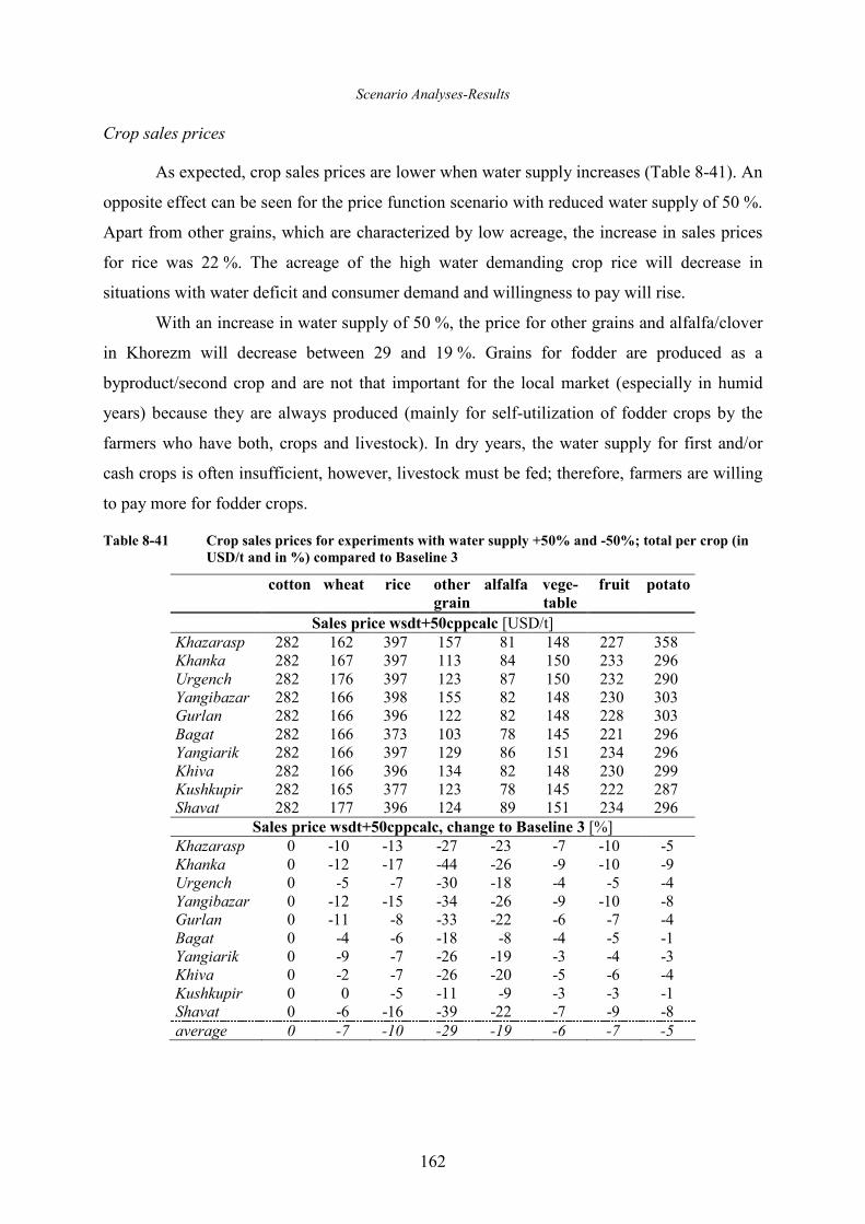
Scenario Analyses-Results
162
Crop sales prices
As expected, crop sales prices are lower when water supply increases (Table 8-41). An
opposite effect can be seen for the price function scenario with reduced water supply of 50 %.
Apart from other grains, which are characterized by low acreage, the increase in sales prices
for rice was 22 %. The acreage of the high water demanding crop rice will decrease in
situations with water deficit and consumer demand and willingness to pay will rise.
With an increase in water supply of 50 %, the price for other grains and alfalfa/clover
in Khorezm will decrease between 29 and 19 %. Grains for fodder are produced as a
byproduct/second crop and are not that important for the local market (especially in humid
years) because they are always produced (mainly for self-utilization of fodder crops by the
farmers who have both, crops and livestock). In dry years, the water supply for first and/or
cash crops is often insufficient, however, livestock must be fed; therefore, farmers are willing
to pay more for fodder crops.
Table 8-41 Crop sales prices for experiments with water supply +50% and -50%; total per crop (in
USD/t and in %) compared to Baseline 3
cotton wheat rice other
grain
alfalfa vege-
table
fruit potato
Sales price wsdt+50cppcalc [USD/t] Khazarasp 282 162 397 157 81 148 227 358 Khanka 282 167 397 113 84 150 233 296 Urgench 282 176 397 123 87 150 232 290 Yangibazar 282 166 398 155 82 148 230 303 Gurlan 282 166 396 122 82 148 228 303 Bagat 282 166 373 103 78 145 221 296 Yangiarik 282 166 397 129 86 151 234 296 Khiva 282 166 396 134 82 148 230 299 Kushkupir 282 165 377 123 78 145 222 287 Shavat 282 177 396 124 89 151 234 296
Sales price wsdt+50cppcalc, change to Baseline 3 [%] Khazarasp 0 -10 -13 -27 -23 -7 -10 -5 Khanka 0 -12 -17 -44 -26 -9 -10 -9 Urgench 0 -5 -7 -30 -18 -4 -5 -4 Yangibazar 0 -12 -15 -34 -26 -9 -10 -8 Gurlan 0 -11 -8 -33 -22 -6 -7 -4 Bagat 0 -4 -6 -18 -8 -4 -5 -1 Yangiarik 0 -9 -7 -26 -19 -3 -4 -3 Khiva 0 -2 -7 -26 -20 -5 -6 -4 Kushkupir 0 0 -5 -11 -9 -3 -3 -1 Shavat 0 -6 -16 -39 -22 -7 -9 -8 average 0 -7 -10 -29 -19 -6 -7 -5
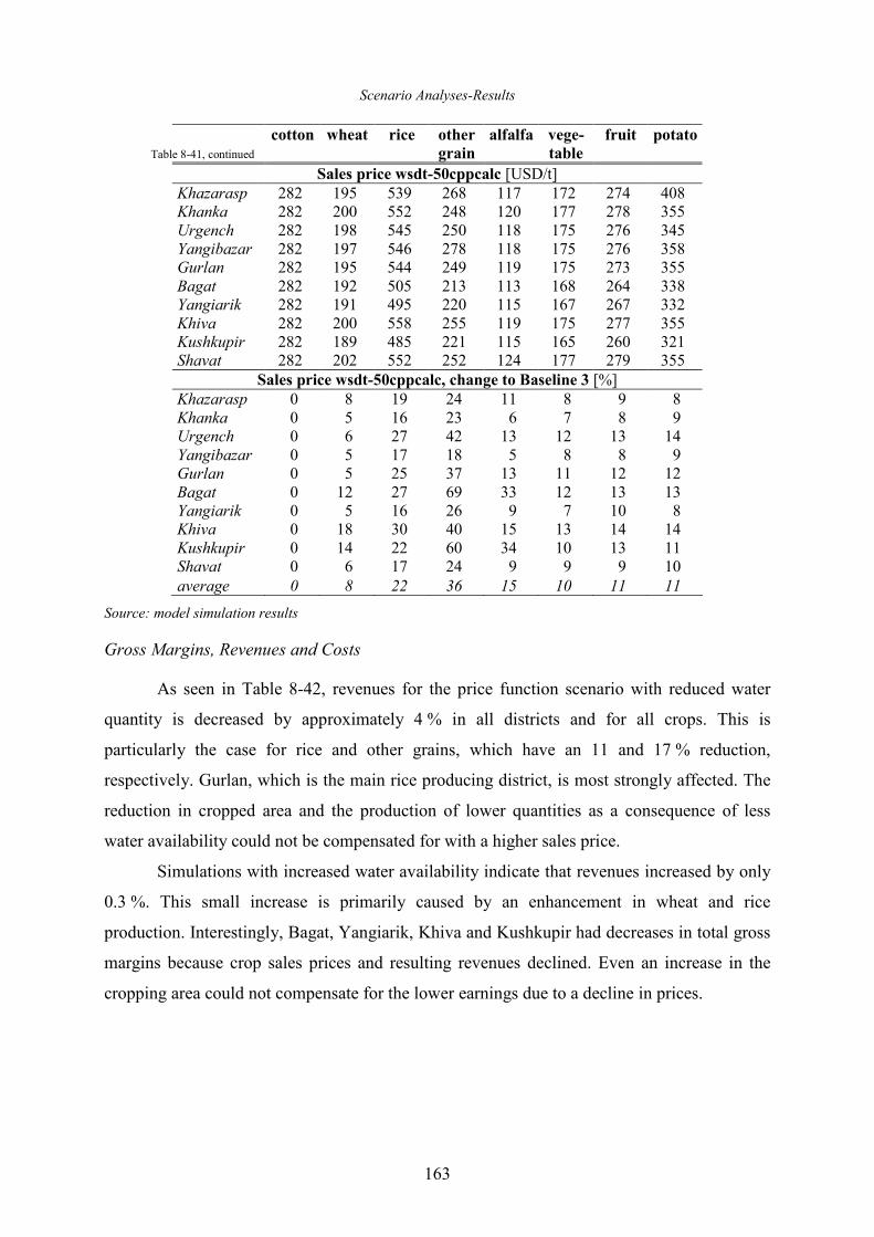
Scenario Analyses-Results
163
cotton wheat rice other
grain
alfalfa vege-
table
fruit potato
Sales price wsdt-50cppcalc [USD/t] Khazarasp 282 195 539 268 117 172 274 408 Khanka 282 200 552 248 120 177 278 355 Urgench 282 198 545 250 118 175 276 345 Yangibazar 282 197 546 278 118 175 276 358 Gurlan 282 195 544 249 119 175 273 355 Bagat 282 192 505 213 113 168 264 338 Yangiarik 282 191 495 220 115 167 267 332 Khiva 282 200 558 255 119 175 277 355 Kushkupir 282 189 485 221 115 165 260 321 Shavat 282 202 552 252 124 177 279 355
Sales price wsdt-50cppcalc, change to Baseline 3 [%] Khazarasp 0 8 19 24 11 8 9 8 Khanka 0 5 16 23 6 7 8 9 Urgench 0 6 27 42 13 12 13 14 Yangibazar 0 5 17 18 5 8 8 9 Gurlan 0 5 25 37 13 11 12 12 Bagat 0 12 27 69 33 12 13 13 Yangiarik 0 5 16 26 9 7 10 8 Khiva 0 18 30 40 15 13 14 14 Kushkupir 0 14 22 60 34 10 13 11 Shavat 0 6 17 24 9 9 9 10 average 0 8 22 36 15 10 11 11
Source: model simulation results
Gross Margins, Revenues and Costs
As seen in Table 8-42, revenues for the price function scenario with reduced water
quantity is decreased by approximately 4 % in all districts and for all crops. This is
particularly the case for rice and other grains, which have an 11 and 17 % reduction,
respectively. Gurlan, which is the main rice producing district, is most strongly affected. The
reduction in cropped area and the production of lower quantities as a consequence of less
water availability could not be compensated for with a higher sales price.
Simulations with increased water availability indicate that revenues increased by only
0.3 %. This small increase is primarily caused by an enhancement in wheat and rice
production. Interestingly, Bagat, Yangiarik, Khiva and Kushkupir had decreases in total gross
margins because crop sales prices and resulting revenues declined. Even an increase in the
cropping area could not compensate for the lower earnings due to a decline in prices.
Table 8-41, continued
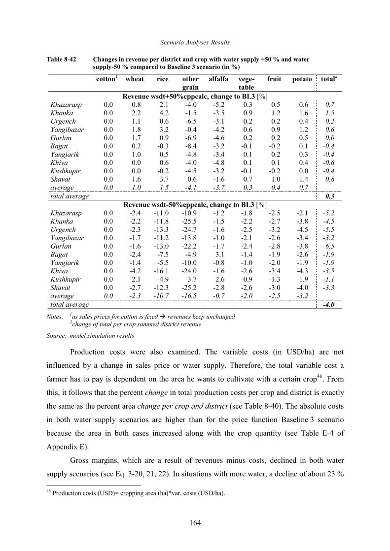
Scenario Analyses-Results
164
Table 8-42 Changes in revenue per district and crop with water supply +50 % and water
supply-50 % compared to Baseline 3 scenario (in %)
cotton1 wheat rice other
grain
alfalfa vege-
table
fruit potato total2
Revenue wsdt+50%cppcalc, change to BL3 [%] Khazarasp 0.0 0.8 2.1 -4.0 -5.2 0.3 0.5 0.6 0.7 Khanka 0.0 2.2 4.2 -1.5 -3.5 0.9 1.2 1.6 1.5 Urgench 0.0 1.1 0.6 -6.5 -3.1 0.2 0.2 0.4 0.2 Yangibazar 0.0 1.8 3.2 -0.4 -4.2 0.6 0.9 1.2 0.6 Gurlan 0.0 1.7 0.9 -6.9 -4.6 0.2 0.2 0.5 0.0 Bagat 0.0 0.2 -0.3 -8.4 -3.2 -0.1 -0.2 0.1 -0.4 Yangiarik 0.0 1.0 0.5 -4.8 -3.4 0.1 0.2 0.3 -0.4 Khiva 0.0 0.0 0.6 -4.0 -4.8 0.1 0.1 0.4 -0.6 Kushkupir 0.0 0.0 -0.2 -4.5 -3.2 -0.1 -0.2 0.0 -0.4 Shavat 0.0 1.6 3.7 0.6 -1.6 0.7 1.0 1.4 0.8 average 0.0 1.0 1.5 -4.1 -3.7 0.3 0.4 0.7
total average 0.3 Revenue wsdt-50%cppcalc, change to BL3 [%]
Khazarasp 0.0 -2.4 -11.0 -10.9 -1.2 -1.8 -2.5 -2.1 -5.2 Khanka 0.0 -2.2 -11.8 -25.5 -1.5 -2.2 -2.7 -3.8 -4.5 Urgench 0.0 -2.3 -13.3 -24.7 -1.6 -2.5 -3.2 -4.5 -5.5 Yangibazar 0.0 -1.7 -11.2 -13.8 -1.0 -2.1 -2.6 -3.4 -3.2 Gurlan 0.0 -1.6 -13.0 -22.2 -1.7 -2.4 -2.8 -3.8 -6.5 Bagat 0.0 -2.4 -7.5 -4.9 3.1 -1.4 -1.9 -2.6 -1.9 Yangiarik 0.0 -1.4 -5.5 -10.0 -0.8 -1.0 -2.0 -1.9 -1.9 Khiva 0.0 -4.2 -16.1 -24.0 -1.6 -2.6 -3.4 -4.3 -3.5 Kushkupir 0.0 -2.1 -4.9 -3.7 2.6 -0.9 -1.3 -1.9 -1.1 Shavat 0.0 -2.7 -12.3 -25.2 -2.8 -2.6 -3.0 -4.0 -3.3 average 0.0 -2.3 -10.7 -16.5 -0.7 -2.0 -2.5 -3.2
total average -4.0
Notes: 1as sales prices for cotton is fixed � revenues keep unchanged 2change of total per crop summed district revenue
Source: model simulation results
Production costs were also examined. The variable costs (in USD/ha) are not
influenced by a change in sales price or water supply. Therefore, the total variable cost a
farmer has to pay is dependent on the area he wants to cultivate with a certain crop46. From
this, it follows that the percent change in total production costs per crop and district is exactly
the same as the percent area change per crop and district (see Table 8-40). The absolute costs
in both water supply scenarios are higher than for the price function Baseline 3 scenario
because the area in both cases increased along with the crop quantity (see Table E-4 of
Appendix E).
Gross margins, which are a result of revenues minus costs, declined in both water
supply scenarios (see Eq. 3-20, 21, 22). In situations with more water, a decline of about 23 %
46 Production costs (USD)= cropping area (ha)*var. costs (USD/ha).
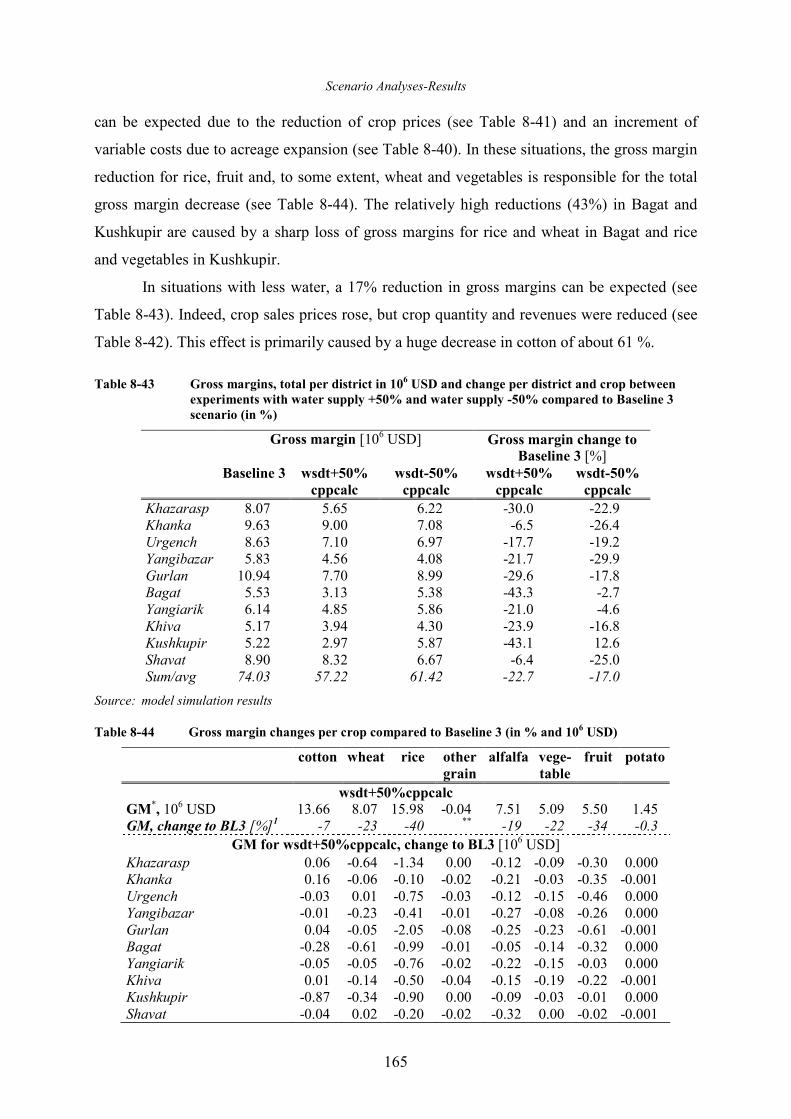
Scenario Analyses-Results
165
can be expected due to the reduction of crop prices (see Table 8-41) and an increment of
variable costs due to acreage expansion (see Table 8-40). In these situations, the gross margin
reduction for rice, fruit and, to some extent, wheat and vegetables is responsible for the total
gross margin decrease (see Table 8-44). The relatively high reductions (43%) in Bagat and
Kushkupir are caused by a sharp loss of gross margins for rice and wheat in Bagat and rice
and vegetables in Kushkupir.
In situations with less water, a 17% reduction in gross margins can be expected (see
Table 8-43). Indeed, crop sales prices rose, but crop quantity and revenues were reduced (see
Table 8-42). This effect is primarily caused by a huge decrease in cotton of about 61 %.
Table 8-43 Gross margins, total per district in 106 USD and change per district and crop between
experiments with water supply +50% and water supply -50% compared to Baseline 3
scenario (in %)
Gross margin [106 USD] Gross margin change to Baseline 3 [%]
Baseline 3 wsdt+50%
cppcalc
wsdt-50%
cppcalc
wsdt+50%
cppcalc
wsdt-50%
cppcalc
Khazarasp 8.07 5.65 6.22 -30.0 -22.9 Khanka 9.63 9.00 7.08 -6.5 -26.4 Urgench 8.63 7.10 6.97 -17.7 -19.2 Yangibazar 5.83 4.56 4.08 -21.7 -29.9 Gurlan 10.94 7.70 8.99 -29.6 -17.8 Bagat 5.53 3.13 5.38 -43.3 -2.7 Yangiarik 6.14 4.85 5.86 -21.0 -4.6 Khiva 5.17 3.94 4.30 -23.9 -16.8 Kushkupir 5.22 2.97 5.87 -43.1 12.6 Shavat 8.90 8.32 6.67 -6.4 -25.0 Sum/avg 74.03 57.22 61.42 -22.7 -17.0
Source: model simulation results
Table 8-44 Gross margin changes per crop compared to Baseline 3 (in % and 106 USD)
cotton wheat rice other
grain
alfalfa vege-
table
fruit potato
wsdt+50%cppcalc GM
*, 106 USD 13.66 8.07 15.98 -0.04 7.51 5.09 5.50 1.45
GM, change to BL3 [%]1 -7 -23 -40 ** -19 -22 -34 -0.3 GM for wsdt+50%cppcalc, change to BL3 [106 USD]
Khazarasp 0.06 -0.64 -1.34 0.00 -0.12 -0.09 -0.30 0.000 Khanka 0.16 -0.06 -0.10 -0.02 -0.21 -0.03 -0.35 -0.001 Urgench -0.03 0.01 -0.75 -0.03 -0.12 -0.15 -0.46 0.000 Yangibazar -0.01 -0.23 -0.41 -0.01 -0.27 -0.08 -0.26 0.000 Gurlan 0.04 -0.05 -2.05 -0.08 -0.25 -0.23 -0.61 -0.001 Bagat -0.28 -0.61 -0.99 -0.01 -0.05 -0.14 -0.32 0.000 Yangiarik -0.05 -0.05 -0.76 -0.02 -0.22 -0.15 -0.03 0.000 Khiva 0.01 -0.14 -0.50 -0.04 -0.15 -0.19 -0.22 -0.001 Kushkupir -0.87 -0.34 -0.90 0.00 -0.09 -0.03 -0.01 0.000 Shavat -0.04 0.02 -0.20 -0.02 -0.32 0.00 -0.02 -0.001
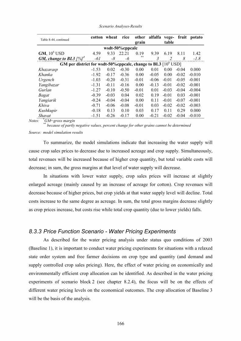
Scenario Analyses-Results
166
cotton wheat rice other
grain
alfalfa vege-
table
fruit potato
wsdt-50%cppcalc
GM, 106 USD 4.59 9.33 22.21 0.19 9.39 6.19 8.11 1.42 GM, change to BL3 [%]1 -61 -8 -6 ** 3 2 8 -1.8
GM per district for wsdt-50%cppcalc, change to BL3 [106 USD] Khazarasp -1.53 0.02 -0.30 0.00 0.01 0.00 -0.04 0.000 Khanka -1.92 -0.17 -0.36 0.00 -0.05 0.00 -0.02 -0.010 Urgench -1.03 -0.20 -0.31 -0.01 -0.06 -0.01 -0.05 -0.001 Yangibazar -1.31 -0.11 -0.16 0.00 -0.13 -0.01 -0.02 -0.001 Gurlan -1.27 -0.10 -0.50 -0.01 0.01 -0.03 -0.04 -0.004 Bagat -0.39 -0.03 0.04 0.02 0.19 -0.01 0.03 -0.001 Yangiarik -0.24 -0.04 -0.04 0.00 0.11 -0.01 -0.07 -0.001 Khiva -0.71 -0.06 -0.08 -0.01 0.03 -0.02 -0.02 -0.003 Kushkupir -0.18 0.13 0.10 0.03 0.17 0.11 0.29 0.000 Shavat -1.51 -0.26 -0.17 0.00 -0.21 -0.02 -0.04 -0.010
Notes: *GM=gross margin ** because of partly negative values, percent change for other grains cannot be determined
Source: model simulation results
To summarize, the model simulations indicate that increasing the water supply will
cause crop sales prices to decrease due to increased acreage and crop supply. Simultaneously,
total revenues will be increased because of higher crop quantity, but total variable costs will
decrease; in sum, the gross margins at that level of water supply will decrease.
In situations with lower water supply, crop sales prices will increase at slightly
enlarged acreage (mainly caused by an increase of acreage for cotton). Crop revenues will
decrease because of higher prices, but crop yields at that water supply level will decline. Total
costs increase to the same degree as acreage. In sum, the total gross margins decrease slightly
as crop prices increase, but costs rise while total crop quantity (due to lower yields) falls.
8.3.3 Price Function Scenario - Water Pricing Experiments
As described for the water pricing analysis under status quo conditions of 2003
(Baseline 1), it is important to conduct water pricing experiments for situations with a relaxed
state order system and free farmer decisions on crop type and quantity (and demand and
supply controlled crop sales pricing). Here, the effect of water pricing on economically and
environmentally efficient crop allocation can be identified. As described in the water pricing
experiments of scenario block 2 (see chapter 8.2.4), the focus will be on the effects of
different water pricing levels on the economical outcomes. The crop allocation of Baseline 3
will be the basis of the analysis.
Table 8-44, continued
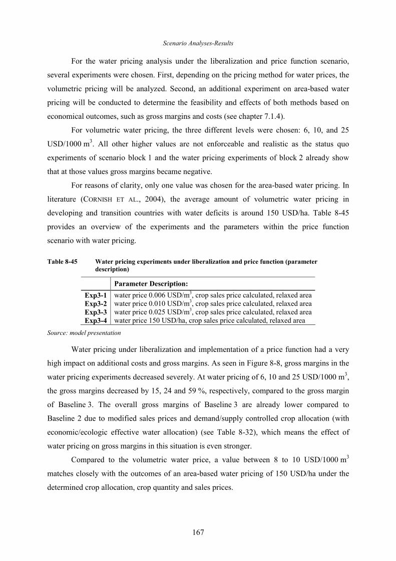
Scenario Analyses-Results
167
For the water pricing analysis under the liberalization and price function scenario,
several experiments were chosen. First, depending on the pricing method for water prices, the
volumetric pricing will be analyzed. Second, an additional experiment on area-based water
pricing will be conducted to determine the feasibility and effects of both methods based on
economical outcomes, such as gross margins and costs (see chapter 7.1.4).
For volumetric water pricing, the three different levels were chosen: 6, 10, and 25
USD/1000 m3. All other higher values are not enforceable and realistic as the status quo
experiments of scenario block 1 and the water pricing experiments of block 2 already show
that at those values gross margins became negative.
For reasons of clarity, only one value was chosen for the area-based water pricing. In
literature (CORNISH ET AL., 2004), the average amount of volumetric water pricing in
developing and transition countries with water deficits is around 150 USD/ha. Table 8-45
provides an overview of the experiments and the parameters within the price function
scenario with water pricing.
Table 8-45 Water pricing experiments under liberalization and price function (parameter
description)
Parameter Description:
Exp3-1 water price 0.006 USD/m3, crop sales price calculated, relaxed area Exp3-2 water price 0.010 USD/m3, crop sales price calculated, relaxed area Exp3-3 water price 0.025 USD/m3, crop sales price calculated, relaxed area Exp3-4 water price 150 USD/ha, crop sales price calculated, relaxed area
Source: model presentation
Water pricing under liberalization and implementation of a price function had a very
high impact on additional costs and gross margins. As seen in Figure 8-8, gross margins in the
water pricing experiments decreased severely. At water pricing of 6, 10 and 25 USD/1000 m3,
the gross margins decreased by 15, 24 and 59 %, respectively, compared to the gross margin
of Baseline 3. The overall gross margins of Baseline 3 are already lower compared to
Baseline 2 due to modified sales prices and demand/supply controlled crop allocation (with
economic/ecologic effective water allocation) (see Table 8-32), which means the effect of
water pricing on gross margins in this situation is even stronger.
Compared to the volumetric water price, a value between 8 to 10 USD/1000 m3
matches closely with the outcomes of an area-based water pricing of 150 USD/ha under the
determined crop allocation, crop quantity and sales prices.
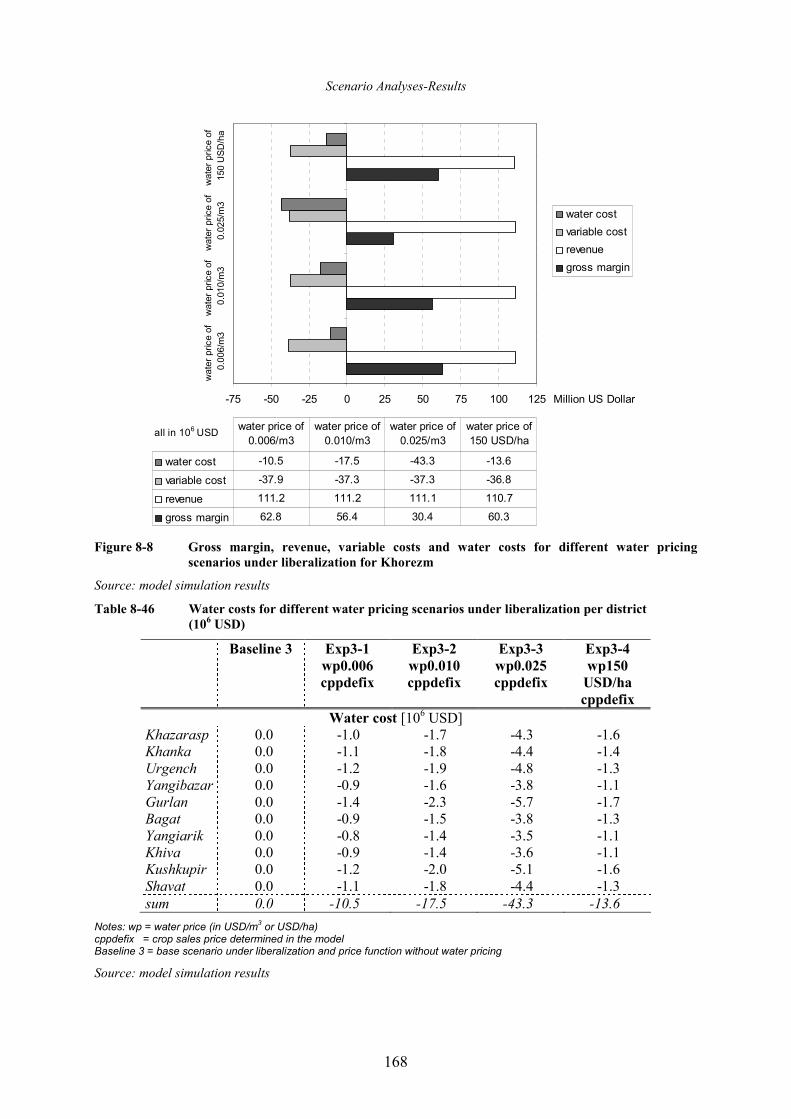
Scenario Analyses-Results
168
-75 -50 -25 0 25 50 75 100 125
water price of
0.006/m3
water price of
0.010/m3
water price of
0.025/m3
water price of
150 USD/ha
Million US Dollar
water cost
variable cost
revenue
gross margin
water cost -10.5 -17.5 -43.3 -13.6
variable cost -37.9 -37.3 -37.3 -36.8
revenue 111.2 111.2 111.1 110.7
gross margin 62.8 56.4 30.4 60.3
water price of
0.006/m3
water price of
0.010/m3
water price of
0.025/m3
water price of
150 USD/haall in 10
6 USD
Figure 8-8 Gross margin, revenue, variable costs and water costs for different water pricing
scenarios under liberalization for Khorezm
Source: model simulation results
Table 8-46 Water costs for different water pricing scenarios under liberalization per district
(106 USD)
Baseline 3 Exp3-1
wp0.006
cppdefix
Exp3-2
wp0.010
cppdefix
Exp3-3
wp0.025
cppdefix
Exp3-4
wp150
USD/ha
cppdefix
Water cost [106 USD] Khazarasp 0.0 -1.0 -1.7 -4.3 -1.6 Khanka 0.0 -1.1 -1.8 -4.4 -1.4 Urgench 0.0 -1.2 -1.9 -4.8 -1.3 Yangibazar 0.0 -0.9 -1.6 -3.8 -1.1 Gurlan 0.0 -1.4 -2.3 -5.7 -1.7 Bagat 0.0 -0.9 -1.5 -3.8 -1.3 Yangiarik 0.0 -0.8 -1.4 -3.5 -1.1 Khiva 0.0 -0.9 -1.4 -3.6 -1.1 Kushkupir 0.0 -1.2 -2.0 -5.1 -1.6 Shavat 0.0 -1.1 -1.8 -4.4 -1.3 sum 0.0 -10.5 -17.5 -43.3 -13.6
Notes: wp = water price (in USD/m3 or USD/ha)
cppdefix = crop sales price determined in the model Baseline 3 = base scenario under liberalization and price function without water pricing
Source: model simulation results
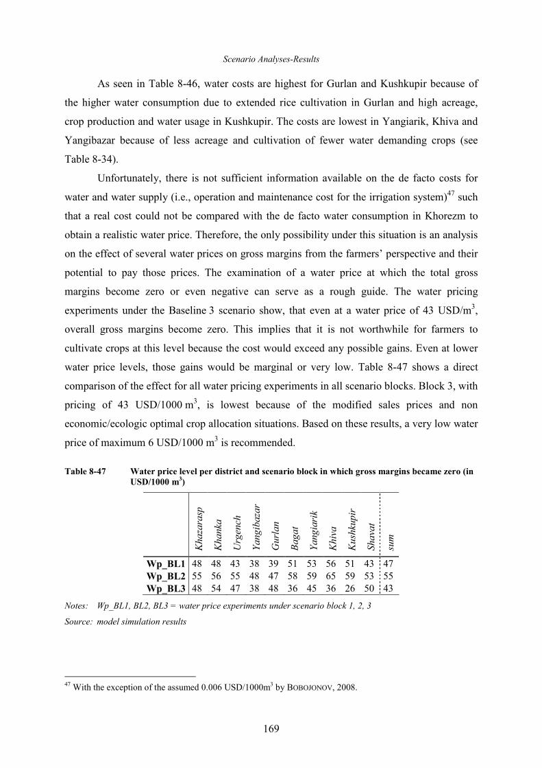
Scenario Analyses-Results
169
As seen in Table 8-46, water costs are highest for Gurlan and Kushkupir because of
the higher water consumption due to extended rice cultivation in Gurlan and high acreage,
crop production and water usage in Kushkupir. The costs are lowest in Yangiarik, Khiva and
Yangibazar because of less acreage and cultivation of fewer water demanding crops (see
Table 8-34).
Unfortunately, there is not sufficient information available on the de facto costs for
water and water supply (i.e., operation and maintenance cost for the irrigation system)47 such
that a real cost could not be compared with the de facto water consumption in Khorezm to
obtain a realistic water price. Therefore, the only possibility under this situation is an analysis
on the effect of several water prices on gross margins from the farmers’ perspective and their
potential to pay those prices. The examination of a water price at which the total gross
margins become zero or even negative can serve as a rough guide. The water pricing
experiments under the Baseline 3 scenario show, that even at a water price of 43 USD/m3,
overall gross margins become zero. This implies that it is not worthwhile for farmers to
cultivate crops at this level because the cost would exceed any possible gains. Even at lower
water price levels, those gains would be marginal or very low. Table 8-47 shows a direct
comparison of the effect for all water pricing experiments in all scenario blocks. Block 3, with
pricing of 43 USD/1000 m3, is lowest because of the modified sales prices and non
economic/ecologic optimal crop allocation situations. Based on these results, a very low water
price of maximum 6 USD/1000 m3 is recommended.
Table 8-47 Water price level per district and scenario block in which gross margins became zero (in
USD/1000 m3)
Kha
zarasp
Kha
nka
Urgench
Yan
gibazar
Gurlan
Bag
at
Yan
giarik
Khiva
Kushkupir
Shavat
sum
Wp_BL1 48 48 43 38 39 51 53 56 51 43 47 Wp_BL2 55 56 55 48 47 58 59 65 59 53 55 Wp_BL3 48 54 47 38 48 36 45 36 26 50 43
Notes: Wp_BL1, BL2, BL3 = water price experiments under scenario block 1, 2, 3
Source: model simulation results
47 With the exception of the assumed 0.006 USD/1000m3 by BOBOJONOV, 2008.
Scenario Analyses-Results
170
8.3.4 Decomposition
The experiments of scenario block 3 (and partly of block 2) were multivariable
scenarios. Several factors were modified to test a certain effect. In the following
decomposition analysis, the optimization parameter “agricultural profit/gross margin” shall be
decomposed into its single indicators to quantify the different structural effects on the overall
outcome. For this purpose, the optimization parameters of the scenarios with a stepwise
modification of only one single parameter were compared. The analysis allowed for
complexity and more transparency in the model (BÜRINGER, 2008; MAYER, 2006). The
following indicators are relevant for the analysis:
• Crop allocation effect (due to the relaxation of acreage and abolishment of the
state order system)
• Subsidization effect (abolishment of subsidies for cotton and implementation of
border prices for cotton)
• Sales price effect (due to implementation of an internally determined price
function for all other crops, with the exception of cotton)
• Water price effect (implementation of a water price of 6 USD/m3)
The total effect of the optimization parameter for the multivariable scenario accounts
for about -28 %. Figure 8-9 shows that this total effect is fragmented into its single effects.
The effect of supply- and demand-dependent sales prices due to the implementation of a price
function have a -36 % influence on the total gross margins and indirectly to crop allocation.
Not surprisingly, this effect is negative because crop allocation is oriented on consumers
demand and willingness to pay and not only driven by ecological aspects (crop water
consumption) and cost/benefit relations (yields, variable cost,…). The impact of relaxation of
the cropping area and abolition of the cotton and wheat quota system was 21 %. The free
decision on crop allocation and crop type by farmers according to economical and ecological
aspects resulted in the cultivation of more effective crops in terms of water consumption,
yields, acreage (on productive land) and positive cost/benefit relations. The effect from the
abolition of the cotton subsidization system was marginal at 0.2 % because sales prices for
cotton, according to world market prices, increased; however, production costs also increased
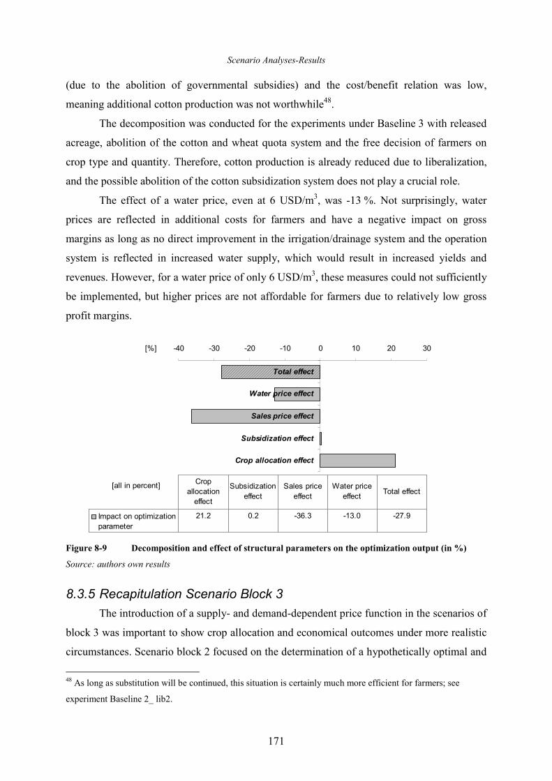
Scenario Analyses-Results
171
(due to the abolition of governmental subsidies) and the cost/benefit relation was low,
meaning additional cotton production was not worthwhile48.
The decomposition was conducted for the experiments under Baseline 3 with released
acreage, abolition of the cotton and wheat quota system and the free decision of farmers on
crop type and quantity. Therefore, cotton production is already reduced due to liberalization,
and the possible abolition of the cotton subsidization system does not play a crucial role.
The effect of a water price, even at 6 USD/m3, was -13 %. Not surprisingly, water
prices are reflected in additional costs for farmers and have a negative impact on gross
margins as long as no direct improvement in the irrigation/drainage system and the operation
system is reflected in increased water supply, which would result in increased yields and
revenues. However, for a water price of only 6 USD/m3, these measures could not sufficiently
be implemented, but higher prices are not affordable for farmers due to relatively low gross
profit margins.
-40 -30 -20 -10 0 10 20 30
Crop allocation effect
Subsidization effect
Sales price effect
Water price effect
Total effect
[%]
[all in percent]
Impact on optimization
parameter
21.2 0.2 -36.3 -13.0 -27.9
Crop
allocation
effect
Subsidization
effect
Sales price
effect
Water price
effectTotal effect
Figure 8-9 Decomposition and effect of structural parameters on the optimization output (in %)
Source: authors own results
8.3.5 Recapitulation Scenario Block 3
The introduction of a supply- and demand-dependent price function in the scenarios of
block 3 was important to show crop allocation and economical outcomes under more realistic
circumstances. Scenario block 2 focused on the determination of a hypothetically optimal and
48 As long as substitution will be continued, this situation is certainly much more efficient for farmers; see
experiment Baseline 2_ lib2.
Scenario Analyses-Results
172
more efficient crop allocation according to model-based agronomical, economical and
hydrological parameters. The focus under block 3 is a realistic crop allocation under
implementation of additional relevant factors, such as consideration of the market situation
(demand and supply) and the liberalization of the cotton sector.
The experiments under scenario block 3 indicate a general reduction in gross margins
and acreage and an increase in sales prices (of 50-70 %) for the considered crops.
Additionally, crop quantity and crop allocation changed significantly compared to Baseline 2.
Due to modified prices in Baseline 3, not only will the most efficient crop be cultivated, but
dependant on water supply, cost/benefit relations and demand also “second best options” (in
this case crops) will be cropped, which has significant impacts on inter alia crop allocation,
water consumption, revenues, and gross margins.
The total amount of basic crops that are produced in huge quantities, such as cotton,
wheat and rice, will decrease. However, compared to the Baseline 2 situation, the cultivation
of cotton in Baseline 3 increased (but still does not approach the values of the status quo
situation) as a reaction to high sales prices for other products and decreased demand or
reduced willingness to pay for those crops. Therefore, market equilibrium and the resulting
allocation are regulated in a completely different form if only ecological aspects are to be
considered.
In situations with decreased water supply, cotton production also increased (compared
to BL2), whereas rice cultivation (due to high water consumption but less water availability)
decrease. As a result, prices and demand for rice will increase. Additionally, the share of
wheat, which is the crop with the lowest water consumption rate, is favorable in situations
with less water availability. The same occurs for fodder crops that are essential, particularly in
dry years. As a result of less water availability and reduced yields, the demand and crop sales
prices will increase in dry years. In contrast, the situations with additional water supply. Sales
prices will be reduced due to augmented supply. The modeling results indicate that all
considered crops, especially rice, could be cultivated.
Finally, the introduction of a water price under scenarios block 3 shows the same
reaction as in block 1 and 2. Due to low gross profit margins for crops in Khorezm, the
implementation of a water price has significant impact on additional costs and revenues. Even
at a very low water price of 6 USD/1000 m3, the effect is immense. At a level of 43
USD/1000m3, overall gross margins become zero. This leads to the recommendation of a very
low price for water as long as gross profit margins in Khorezm are low.
173
9 Conclusion and Outlook
In this chapter the results of the research and the outcomes of the three scenarios and
their different experiments and its underlying policies will be summarized. Based on the
results, various recommendations and the feasibility of implication of those recommendations
will be described and analyzed.
The last section of the chapter gives an overall conclusion of the research and
discusses the benefits of the modeling and modeling framework, research limitations and
further research.
9.1 Research Conclusions, Policy Recommendations and Implications
The results of the three scenarios and their related experiments showed several
significant factors, of which the most important will be described in the following section.
The following four main categories will be discussed:
• Optimal crop allocation.
• Water balances, water supply and water efficiency.
• Abolition of cotton subsidization.
• Water pricing.
9.1.1 Optimal Crop Allocation under Released Acreage and Cotton Quota System
Results
The effect of a relaxation of acreage and the state order system for cotton and wheat
combined with the free choice of farmers on crop type and quantity decision has a positive
effect on revenues and gross margins. Due to the flexibility of farming activities and crop
allocation, it is likely that more farmers will choose to cultivate crops that can be traded on
local markets and crops with a good relationship between water consumption and
cost/revenues, resulting in high economic water use efficiency. Examples of these crops
Conclusion and Outlook
174
include vegetables, rice and alfalfa and, to a lesser extent, fruits, wheat, and potatoes. The
cultivation of wheat and rice is significantly influenced by water availability (high for rice and
low for wheat). These results correspond well with the findings of DJANIBEKOV, 2008.
Model results indicate that the cultivation of cotton is with abolishing of the state
order system not longer attractive for farmers. The state order system causes the sales prices
to be relatively low but the costs for growing cotton to be very high. Thus, e-WUE for cotton
is very low or even negative. If subsidies by the government were to be omitted, those costs
will increase, and the incentive for cultivate cotton will decline even further. Additionally, the
relatively high water consumption and decreasing yields due to cultivation on marginal land
and/or saline soils did not increase the attractiveness of cotton.
The second essential result of this scenario analyses is the major reduction of acreage
in general. This is mainly induced by a strong reduction of cotton cultivation, and it is most
apparent in situations with lower water supplies. Unproductive and marginal land is removed
from the system. Thus, the overall yield could be increased as more water is available for less
area, and more effective crops (in terms of water consumption and economic cost/revenue
relation) can be cropped.
Policy recommendations and Implementation
The model results suggest that the region could benefit from a general reduction of the
total cropped area by diminishing unproductive and marginal land. It would result in a
reduction of cotton cultivation and simultaneously produce a shift in crop allocation to more
economically and ecologically efficient crops and crops tradable on local markets. The
general reduction of acreage, mainly due to a drastic reduction of cotton area, would benefit
ecology, alternative crop allocation and water availability.
However, the structures for the intensive cultivation, processing and
commercialization of cotton in Khorezm still exist in the form of machinery parks, farm
workers and the high knowledge of farmers regarding cotton cultivation, especially in this
region. If maintaining the expanded and intensive cotton cultivation policy, the government
has to account for water shortages that, according to expert knowledge, will continue to occur
and even be exacerbated in the future due to climatic changes and the increased extraction of
Amu Darya river water by upstream riparian. Beside reduced water supply, decreased cotton
yields in Khorezm can be seen over the past years. This situation is not going to change as
long as marginal land is used and soil salinity continues to increase in soil. The third problem
Conclusion and Outlook
175
of cotton cultivation perpetuation is the reduced availability of productive land for the
cultivation of crops that are more economically and ecologically efficient and locally
utilizable.
If the expanded cotton cultivation in Khorezm is favored by the government, it can
only be sustained by a further perpetuation of the subsidization system, as shown by the
experiments on the liberalization of the cotton sector (chapter 9.1.3). It then becomes a
question of whether the continuation of cotton production under impeding conditions,
declining yields, possible water shortages and additional costs for the subsidization system
can be offset by the foreign exchange proceeds49.
Following RUDENKO (2008), a practicable recommendation would be a stepwise
reduction of the cotton cultivation and subsidization that would finally give the local
population the ability to grow and sell more diversified and desirable crops to feed the
increasing number of local inhabitants and livestock and to increase their ability to cope with
modified water supply. Diverse crop cultivation is also good for both, soil properties and for
risk management for the farmer. By reorganizing the agricultural system in Khorezm from
extensive cotton production to the diversified cultivation of crops such as vegetables, fodder
and fruits (and rice, if water availability is sufficient), the proportion of semi-subsistence
could be increased, and due to the labor-intensive crop cultivation of vegetables, the
employment rates of the rural population could be maintained.
The extension of wheat cultivation appears to be appropriate due to its low water
consumption and the possibility of double cropping. However, wheat is not favored by the
local population, and the attractiveness of rice is still much higher. In this case, information
campaigns could certainly be helpful. However, rice cultivation in years with additional water
available, especially in districts close to the river, is possible-especially because a possible
diminishment of cotton cultivation will leave more crop area and make additional water
available. The implementation of new, resistant, less water-consuming rice phenotypes as
well as an introduction of water-saving strategies would be advisable.
49 Macro-economical calculations taking into account the described circumstances would be helpful in the final
decision on cotton policy by the government
Conclusion and Outlook
176
9.1.2 Water Balances, Water Supply and Efficiency
Results
The influence of water supply on water balances, crop allocation and yields is
naturally very high. A large influence of modified water supply on the entire cropping system
and the water and soil balances can be detected (mainly in cases of low water supply). Crops
such as cotton, rice and alfalfa showed a strong reduction of gross margins and yields in the
simulations. With additional water supply, crops such as vegetables, alfalfa, fodder crops, rice
and wheat have a large potential to become more profitable as a result of yield increases and a
positive economic-ecologic balance.
Furthermore, the scenarios and experiments showed a large influence of groundwater
on crop water supply. The groundwater balances will be primarily affected in cases of low
water supply because in these cases, the crops need to seek alternative water sources via
capillary rise, which ultimately causes a strong reduction in the groundwater table. When
irrigation and precipitation water supply is not enough, groundwater must be used. Studies
have shown that even with zero water supplies it is possible for some crops to exist by
capillary rise out of the groundwater and by reaching the groundwater with the roots,
especially when the groundwater is very shallow, as is the case in major parts of Khorezm
(FORKUTSA, 2006 and Figure 4-5). The resulting groundwater fluctuation and amplitude
during the year, especially between the vegetation and non-vegetation period, can be up to
30 cm-40 cm. The fact that leaching is performed at the beginning of the year to elute salt out
of the soils and to enhance soil properties is adding to these groundwater fluctuations. This
leaching is absolutely essential in Khorezm to wash out the soils and to contribute to
groundwater replenishment and refill soil moisture at the beginning of the vegetation period.
Furthermore, the tremendous seepage losses of the irrigation system and the resulting low
efficiencies also contribute to groundwater replenishment and leaching of the saline soils,
which are both generally very positive effects.
Altogether, water supply scenarios demonstrate a huge effect on crop allocation, water
and soil balances, and yields and gross margins with modified water quantities. However,
even with a possible (but difficult to obtain) alteration of the general water supply, an increase
in water would be depleted due to low distribution and irrigation/application efficiency. As a
result, direct efforts towards the improvement of the irrigation and water management system
appear to be more effective and easier to implement. Several measures exist to improve the
distribution and irrigation efficiencies, the cropping system and water supply management in
Conclusion and Outlook
177
Khorezm. They will be discussed and checked for feasibility and practicability in the
following paragraphs.
Options, impacts and implementation of efficiency improvement measures
Multiple possibilities exist for increasing water use efficiency. Water savings and/or
improvement of the economic water use efficiency (e-WUE) at the field level could be
obtained by utilizing less water-intensive and more salt-tolerant crops as well as crop
combinations and double cropping. Crop rotation and base leveling for better and more
uniform water distribution within the fields are also possible solutions. In addition, a
reduction of conveyance losses at the farm level due to on-farm channel improvement,
irrigation scheduling according to variable and site-specific requirements (instead of norms),
and improving the current irrigation and cropping techniques could all improve the water use
efficiency. Current irrigation techniques could be improved by the introduction of modern
irrigation techniques such as surge flow, alternate furrow, drip-, double-side and sprinkler
irrigation, while cropping techniques could be improved by introducing mulching and zero-
tillage, hydrogel or the planting of shelterbelts. Furthermore, the on-farm drainage system is
open and requires desilting, reconstruction and repair (UNDP, 2007). An additional task
would be to gather information from each farm regarding soil and crop characteristics and on-
farm flow rates and use this information to determine water applications.
Improvements at the district level could be attained by the reconstruction and repair of
inter-farm and main channels, intake structures, hydro-mechanic equipment, and pumping
stations as well as the treatment and reuse of drainage water. Due to a complete desilting of
the Tuyamujun reservoir, the total amount of water could be increased, and as a result, more
water could be stored for water-scarce vegetation months. Admittedly, this measure is hardly
feasible and operable and is very cost intensive.
According to VLEK ET AL. (2001), canal lining, which has been completed for some
canals in Khorezm, is also very cost intensive, and the efficiency improvements are in a range
of about one percent. Thus, this engineering measure does not appear to be an immediate and
practicable option of water saving in Khorezm.
In addition, a further expansion of double cropping in Khorezm, such as winter wheat
with rice, winter wheat with vegetables with short-growing periods like onions, melons and
beets and winter wheat with maize or cotton, appears to be a advantageous measure.
However, it involves supplemental annual costs such as seed purchase, maintenance, harvest
Conclusion and Outlook
178
costs and fertilizer expenditure. Another issue is the unpredictability of the beginning and end
of the frost period as well as its duration. According to DAMIS (2008), only a small percentage
of cropping area in Khorezm could adopt this technique because social and economic factors
make it unfeasible.
A reasonable crop rotation such as cotton with sorghum would certainly improve soil
quality and diversification, but economically continuous cotton cropping would result in
much higher commodity prices, as the demand for cotton is higher than the demand for
sorghum. Furthermore, the state procurement system for cotton and wheat, which is still in
effect, induces more farmers to cultivate those crops. Similar to the possible reduction of
cropping area to reduce the amount of irrigation water, this measure is certainly very
advantageous but an improvement of e-WUE is not indicated.
It is also possible to crop less water-intensive but more salt-tolerant crops in Khorezm.
Particularly noteworthy are cotton, wheat, and garden beet50, in contrast to rice, fruit trees,
clover and, to some extent, potatoes. The use of aerobic rice instead of flooded rice would
reduce the amount of irrigation water but would still be less productive. For this reason, a
general reduction of rice-cropping areas in dry years is advisable.
The application of hydrogel, granules for holding soil moisture, is a promising water-
retaining mechanism, especially in arid areas. Hydrogels act as a reservoir and can absorb
approximately 400 times of their own weight in water. However, they are cost-intensive, and
the water holding capacity is decreased in irrigation water containing dissolved salt (JHURRY,
1997).
Another possibility to increase the supply of irrigation water is to re-use drainage
water. However, this is associated with high costs for treatment infrastructure.
An additional task could be the implementation of measures for controlled drainage as
a further development of the current drainage blocking system. Controlled drainage would
consider the temporal requirements of the groundwater level. Water table management with
controlled drainage51 would reduce the drainage water leaving the crop fields; the water level
in surrounding fields would rise. Additionally controlled drainage could favor locations with
rather low salt content in the groundwater to avoid increased salinity of the groundwater in
certain areas.
50 cotton and wheat are already intensively cropped in Khorezm
51 By installation of control structure, such as a flashboard riser
Conclusion and Outlook
179
All of the measures described to reduce water demand and/or supply show that
possibilities are available but are associated with immense costs or financial losses for
farmers or high subsidies from the government. Government purchases and capital
investments in the water sector are still declining and, at the same time, costs for electricity
(e.g. for pumping stations) and equipment are rising (UNDP, 2007).
The most suitable measure for improving water use efficiencies for local conditions in
Khorezm seems to be the perpetuation and extension of gravity irrigation such double-furrow
and surge-flow irrigation (DAMIS, 2008) and measures on controlled drainage. Sprinkler and
drip irrigation appear to be cost-intensive and, due to the high salinization in Khorezm,
impracticable.
In addition to gravity irrigation, a consistent base leveling using laser and the
introduction of soil moisture-increasing crop techniques, such as mulching, no-tilling
techniques, and the planting of shelterbelts, appears to be advisable. These techniques are
easy to implement, and implementation costs are relatively low. Land leveling by lasers has
been proven to be a good method of increasing water use efficiency and yields. Land
irregularities are eliminated, and scarce water resources can be utilized more efficiently and
distributed more equally (ASSIF ET AL., 2003). According to BOBOJONOV (2008), 70 % of the
cropped area in the region is unevenly leveled. Laser leveling could save around 25 % water,
and soil and crop properties could be improved, which would cause increased yields
(ERGAMBERDIEV ET AL., 2008).
9.1.3 Abolition of Cotton Subsidization and Transfer of Bordering Prices for Cotton
Results
The results of the different scenarios demonstrate that after relaxation of the acreage
and the increased freedom of farmers to decide how and how much to crop (chapter 9.1.1),
the effect of the liberalization of the cotton sector would result in a drastic decrease in cotton
cultivation. Indeed, the sales prices for cotton would increase, and thus, so would the income
for the farmers. However, the production cost to produce one unit of cotton would be
increased as well, due to the abolition of the governmental subsidies. The positive effect on
income for cotton sales would fully compensate for the abolition of governmental subsidies.
Due to the free decision of farmers, other higher-value adding crops such as
vegetables, fruit, fodder crops and rice, if enough water is available, would be cultivated.
Conclusion and Outlook
180
With the cultivation and marketing of those crops, the overall gross margins could be
increased, and the loss of income by the reduction of cotton cultivation could be compensated.
Only in cases of continued governmental subsidies would the further cultivation of
cotton be feasible. In this case, variable costs for cotton production must still be subsidized by
the state and any additional higher income as a result of increased sales prices for cotton
(bordering/world market prices) would benefit the farmers directly. However, sales price
increases for cotton must take into account deductions of costs for vendors, processing, taxes,
interest payments, administration, ginning, suppliers, etc, and the prices may not increase
enough to bring the production and cultivation of cotton up to the current level, which is
created by subsidies and fixed but secured governmental prices (RUDENKO, 2008).
Furthermore, according to BOBOJONOV (2008) the abolition of secured but, indeed, lower
sales prices for cotton would cause an increased risk for the farmers, as world market prices
for cotton fluctuate and the consistent higher prices is not assured.
Discussion and Implementation
The perpetuation of the current system of cotton quotas and subsidization by the
government creates considerable advantages for the state and farmers and thus, illuminate the
continuing system of the expanded cotton cultivation. The export of cotton and cotton fiber is
a very important source of foreign exchange earnings for the Uzbek government. Due to
marketing and the pre- and post-cotton-processing industry, including ginneries, cotton oil,
the cotton oil cake-extracting industry, the laundry soap industry, the textile industry and the
machine industry, the cotton cultivation constitutes a large share of the Uzbek economy.
Additional public revenues such as taxes, savings and agricultural tariffs and duties, as well as
an increase in the employment rate, can be attained by the state and could be reinvested into
the import of various goods and services. Another reason for continuing the current cotton
policy is the absence of sufficient alternatives. The dominance of the agricultural sector and
the high share of agriculture in the GDP (MÜLLER, 2006), combined with the missing sectoral
differentiation (secondary and tertiary sector) and the lack of urban agglomerations and
infrastructure in Uzbekistan leads to missing employment alternatives for the rural
population-especially in Khorezm, where almost 78 % of the population live in rural areas
(chapter 2.4.1).
Also for farmers, the cultivation of cotton has several advantages. They attain input
subsidies for the cropping of cotton and additional grants for the cultivation of other crops,
Conclusion and Outlook
181
such as reduced seed prices or discounted credits. Furthermore, the general acceptance of the
requested quantity of cotton for a guaranteed price represents an essential factor of risk
minimization for farmers. Moreover, the extensive knowledge of cotton cultivation and
irrigation schemes and the necessary machinery is still present, all of which represent
supplemental benefits. As the cotton production is relatively labor-intensive, employment
rates could be sustained, which is an important aspect in predominantly rural areas. The
continuation of subsidization of the cotton sector seems reasonable, especially if losses in
tariffs and credits would be taken into account52.
Many cotton-producing countries in the world act similarly regarding subsidization
and special concessions. However, the reduction and, ultimately, the total abolition of
subsidies is expected (chapter 7.1.5).
If the continued system of high cotton production and export remains favored by the
government, it would only be possible with subsidies. Without subsidies, the farmers would
grow more value-adding crops. If the reduction or abolition of the current cotton order system
is favored in Uzbekistan, as indicated by the scenarios, this would only be possible through a
step-wise reduction of the state order and cotton subsidies and would eventually require a
policy of promoting other crops, as has already been done for wheat. A modification of the
current state order system with reduced orders or free choice of the farmers regarding whether
or not to grow cotton for a reduced but assured price (production quota instead of crop-area
quota) seems to be the most advantageous. With this system, the farmers have the right to
choose what and how much to crop while simultaneously maintaining the possibility of
reducing the cropping risk. Additionally a general positive effect of diversification and the
innovation potential of farmers can be expected.
52 This analysis could not be performed here; for this purpose, a macroeconomic analysis of the liberalization in
the cotton sector is necessary
Conclusion and Outlook
182
9.1.4 Water Pricing
Results
The introduction of water pricing, even at extremely low levels, resulted in both
scenarios, status quo situation and scenario with relaxed state order for cotton in a sharp
decline of income for farmers. Comparatively low gross profit margins in Khorezm inhibit the
introduction of water pricing under the current system of subsidies and production quota.
These findings are consistent with BOBOJONOV (2008). However, even with liberalization of
the cotton market, pricing water seems to become very difficult because income and welfare
of farmers due to alternative crop allocation and higher sales prices could be increased, but
the growth rate of gross margins is relatively low, and high losses due to additional costs for
water pricing would thus eliminate additional income.
Implementation of a water price
The scenarios showed that the introduction of a water price of more than
approximately 6 USD/1000 m3-10 USD/1000 m3 is not feasible because otherwise the crop
cultivation is no longer worthwhile for farmers. The results demonstrate that an introduction
of a water price is a very sensible topic and needs careful implementation. A stepwise
introduction of a water charge with simultaneous reductions of subsidies for inputs in cotton
production seems to be appropriate to avoid overcharges of the farmers. Water pricing could
lead to a better financial support of the Water User Associations (WUAs) or public water
suppliers and reduce the dependency of WUAs on the government. The WUAs could re-
invest the attained water charges into the improvement of the irrigation and drainage system.
This could lead to an improvement of water use efficiency, which in turn pays off for both the
farmers and the environment. However, even with such a low water price, only the true cost
for the operation and maintenance of the irrigation system could be paid, not to mention
additional investments.
To improve the sensibility of the farmers for the cultivation of less water-demanding
crops, an introduction of a pricing method that depends on the crop type and vegetation period
seems to be advisable and affordable. Alternatively, the introduction of a block-rate, bonus or
quota-system could be considered. In this scenario, a certain supply of water could be
delivered to farmers for free, and the farmer would be charged for any additional water
consumed (remaining quotas could be traded on the local market). However, the problem is
the current absence of a reliable method of measuring the volume of water consumed and the
Conclusion and Outlook
183
high costs of installing the technology to accurately make such measurements. A mixture
between area-based charging and crop-type-based water pricing seems to be the most
advantageous. The crop-type-based charging provides incentives for farmers to save water.
Applying a higher water price for water-demanding crops would discourage the irrigation of
those crops. This would give the government the possibility of directing the crop cultivation
into favored crops (CHOHIN-KUPER ET AL., 2003).
As long as gross profit margins in Khorezm are low, charging for water in extreme
situations, as in years with reduced water supply, must be conducted depending on the
discharge within the river and the storage capacity of the reservoir.
9.1.5 Recapitulation
All of the results show that a liberalization of the cotton sector and the abolition of
subsidies are possible and would lead to a completely modified and ecologically more
efficient and sustainable crop allocation. This would lead to additional positive effects on the
income and revenues of the farmers. Furthermore, the introduction of a water price on a very
low level would be desirable for resource conservation and the environmental awareness of
the water consumers. However, the discussion showed that a perpetuation of the present
system with quotas and subsidies for cotton is indeed reasonable for both farmers and state,
but under the aspect of sustainability, a change out of the system must be implemented.
Converting to a long-term sustainable water management is only possible if the water
pricing is combined with other factors, such as policies (e.g. decrement of farmer’s
support/subsidies and public financing) and if property rights for farmers are assured
(GURRIA, 2008). According to THOMAS ET AL. (2000), improving incomes and living
standards is only possible by improving the quality of the legal systems, improving access to
education, protecting the environment, managing global risks, and improving the quality of
governance by the increased participation and transparency of institutions, combating of
corruption and bureaucratic harassment. Thus, solid macroeconomic policies and the
application of appropriate market-oriented microeconomic principles are basic elements. All
of these factors must be considered in order for a sustainable reconstruction of the system to
be possible.
Conclusion and Outlook
184
9.2 Overall Conclusion and Outlook
As outlined in the introduction of this study, efficient and sustainable water and crop
management are essential for the agricultural sector, the growing population, the environment
of Khorezm and the downstream water users. In the water-scarce region of Khorezm,
intensive irrigation agriculture is the major water user. It is characterized by its low efficiency
and the deterioration of ecology due to an exploitative and inefficient use of the water and soil
resources combined with the missing diversification of crops. The subsidization and cotton
quota system of the government, along with missing property rights and the lack of water-
saving incentives, promoted high water demand and social, economic and ecologic problems.
To determine a more economically and ecologically efficient strategy of crop and
water management and allocation, an understanding of the basic hydrologic and agronomic
characteristics and balances is of special importance. Thus, the determination of important
factors for more efficient water and crop management in Khorezm was one objective of the
study. It is also important to analyze the effects of modified social, technological,
environmental and institutional conditions. The analyses described were required in
preparation for the modeling. The objective was to build up an integrated and interdisciplinary
model with plenty of experimental, empirical, and statistical data with different spatial and
temporal resolutions. The model is a simplified framework to represent complex bio-physical
and economic processes. The results from the model simulations are based on the way the
model tries to capture reality. Thus, the detailed collection and verification of data and model
accuracy was another objective of the study.
The development of an integrated hydrologic, agronomic and economic model for the
Khorezm region turned out to be a suitable tool to analyze political incentives on the basis of
water, climatic and crop-specific parameters. The validation of the model and the various
results showed that the model and modeling framework could serve as a tool to provide
information on both the underlying hydrologic and agronomic processes and as a decision
support facility to evaluate the effects of political incentives on the regional water
distribution, crop allocation and economic outcomes.
9.3 Limitations and Further Research
Some limitations and assumptions in formulating, solving and analyzing the model, as
well as limits inherent in the modeling structure and underlying data and scenarios, became
Conclusion and Outlook
185
apparent. The acquiring and investigation of reliable data turned out to be a challenging task
because the availability and reliability of sufficient and coherent data can be problematic in
Uzbekistan and Khorezm.
As described in chapter 4, for some groundwater, crop, soil and water-related
characteristics, there were no direct measurements or reference values available. In these
cases, assumptions or literature values were used. The application of adapted regional data
would make the processes more precise.
More recent and detailed data on groundwater fluctuations show deeper groundwater
levels of 2 m-2.3 m below the surface in Khorezm in December/January on a daily resolution.
Because of the lack of those data at the calibration phase, they could not be used in the model.
The shallow groundwater situation in Khorezm, which leads to capillary rise, is of special
interest, the possible impacts of deeper groundwater should be investigated in future research.
However, the described groundwater depression will certainly have no large impact in the
main vegetation period.
The economic basis of the model included the applied prices and costs. They were
assumed to be constant throughout the year; however, this could be changed in further
research. If information on water supply costs or for instance the costs to install and operate
volume meter becomes available, a more in-depth analysis on the effects of water pricing
could be performed. This is also true for the information on costs that are necessary for
certain technical, institutional and political modifications, such as the investment costs to
improve the irrigation efficiency or opportunity costs if the cotton sector were to be
liberalized. It should then be possible to offset gains and implementation and maintaining
costs to obtain a more realistic view of the costs and the macro-economical benefits that those
measures would imply.
Furthermore, a possible extension of the various actors involved in the agricultural
sector of Khorezm could be interesting. The de-aggregation can provide information on
farmer’s income and crop allocation even at smaller levels. The connection with an already
successfully implemented model (“KhoRASM”, DJANIBEKOV, 2008) for the Khorezm region
with differentiation of the agricultural actors and a detailed modulation of supply and demand
would be recommend for further research.
The aggregation of certain crops into one single crop type, such as for vegetables,
fruits and other grains, is difficult because the same parameters (yield response to water,
growth period, salinity or potential yield) have to be considered for all crops in one aggregate.
Conclusion and Outlook
186
Due to the different characteristics of the single crops (especially for vegetables), this could
be problematic and could affect the results. It would be recommended to reduce the quantity
of crops in the model and de-aggregate the groups, reconsidering tomatoes, onions, berries or
melons as single crops. Furthermore, the different irrigation strategy for rice is not directly
comparable to those of the other crops and should be improved53.
No direct information on multiple cropping is included in this study. Furthermore, the
investment into the drainage system and drainage disposal will certainly be more important in
the future and could be analyzed with the help of this model. Additionally, the extension of
the salinity aspects in soil, surface water, drainage and groundwater is not yet included but
could provide further information on the effect of salt in water and soil, the possibility of
treatment and, eventually, the implementation of salt-taxes and their impacts.
The temporal extension of the model to analyze long-term perspectives could be used
in future research. However, due to the implementation of several indices and
multidimensionality, the calculation capacity was not sufficient, and it was thus not feasible to
include here. The same is true for the extension of the spatial resolution of the model and/or
the implementation of a node-link network to release water supply and receive information on
hydrological fluxes. Eventually, a splitting of the model could solve the problem of capacity
and computation time. However, it must be emphasized that a further extension of the model
will increase the model dimensionality and reduce clarity and reliability.
53 due to permanent downward movement of water, capillary rise should be close to zero
187
10 Bibliography
ABDULLAYEV I., CH. DE FRAITURE, M. GIARDANO, M. YAKUBOV, A. RASULOV (2009): Agricultural Water Use and Trade in Uzbekistan: Situation and Potential Impacts of Market Liberalization, in: Water Resources Development, Vol. 25, No. 1, March, 2009: 47-63.
ABDULLAYEV I., L. OBERKIRCHER, A.-K. HORNIDGE, M. UL HASSAN, A. MANSCHADI (2008): Strengthening Water Management Institutions in Uzbekistan, in: Zef-Uzbekistan Rivojlanishlari (ZUR) No. 7, December 2008, Center for Development Research, Bonn.
ABDULLAEV S. (1995): Agro-physical Basis of Saline Soils Amelioration in the Lower Reaches of the Amu-Darya (in Russian), pp. 1-44. State University, Tashkent.
ABDULLAEV U. (2002): Gateway to land and water Information: Uzbekistan National Report. http://www.fao.org/ag/agl/swlwpnr/reports/y_nr/z_uz/uz.htm
ADB (Asia Development Bank) (2006): Key indicators of Developing Asian and Pacific Countries in 2006. http://www.adb.org/Documents/Books/Key_indicators/2006/pdf/UZB.pdf
ADB (Asia Development Bank) (2007): Asian Development Outlook 2007: Uzbekistan. http://www.adb.org/Documents/Books/ADO/2007/UZB.pdf
AKRAMKHANOV A. (2005): The Spatial Distribution of Soil Salinity: Detection and Prediction, in: Ecology and Development Series No. 32, Dissertation, Cuvillier Verlag Göttingen.
ALLEN R. G., L. S. PEREIRA, D. RAES, M. SMITH (1998): Crop Evapotranspiration - Guidelines for Computing Crop Water Requirements - FAO Irrigation and drainage paper 56, Food and Agriculture Organization of the United Nations, Rome. http://www.fao.org/docrep/X0490E/x0490e00.htm#Contents
ASKAROV M. (2005): State Actions Aimed to Increase Privatization Efficiency in Cotton and Light Industry of Uzbekistan, Document for the International Cotton Advisory Committee (ICAC) Meeting: Cotton and Textiles – Important Factor of Economic Growth in Central Asia, Tashkent, Uzbekistan, 24-25 May, 2005. http://alida-algodon.org/meetings/uzbek_2005/papers/english.html
ASSIF M., M. AHMED, A. GAFOOR, Z. ASLAM (2003): Wheat Productivity, Land and Water Use Efficiencies by Traditional and Laser Land-Levelling Techniques, in: Online Journal of Biological Science 3 (2), 141-146, Asian network for scientific information.
BEAR J. (1977): Hydraulics of Groundwater, New York, McGraw-Hill International Book Co.
Bibliography
188
BLOCH P. C. (2002): Agrarian Reform in Uzbekistan and other Central Asian Countries, in: Working Paper, No. 49, Land Tenure Center University of Wisconsin–Madison.
BMZ (Federal Ministry of Economic Cooperation and Development) (2002): Länderbericht, Republik Usbekistan, Referat 201, Bonn.
BOBOJONOV I. (2004): Market Analysis of Agricultural Products in Irrigated Areas (Exemplified by Khorezm region for limited number of commodities), Master thesis, Tashkent Institute of Melioration and Irrigation.
BOBOJONOV I. (2008): Modeling Crop and Water Allocation under Uncertainty in Irrigated Agriculture: A case study on the Khorezm Region, Uzbekistan, Dissertation, University of Bonn.
BROOKE A., D. KENDRICK, A. MEERAUS, R. RAMAN (1998): GAMS: A Users Guide, Scientific Press, Oxford, UK.
BROUWER C., M. HEIBLOEM (1986): Irrigation Water Management, Training manual No. 3, Food and Agriculture Organization of the United Nations, Rome, Italy.
BÜRINGER H. (2008): Energieverbrauch und CO2-Emissionen der Wirtschaft in Baden-Württemberg im Ländervergleich, in: Statistisches Monatsheft, Feb. 2008, pp: 45-50, Stuttgart. http://www.statistik-portal.de/Veroeffentl/Monatshefte/essay.asp?xYear=2008&xMonth=02&eNr=08
CAI X. (1999): A Modeling Framework for Sustainable Water Resources Management, Dissertation, University of Texas at Austin, Texas.
CER (Center for Economic Research) (2004): Reorganization of Cooperative Agricultural Enterprises (Shirkats) into Farming Business Entities, Tashkent.
CHOHIN-KUPER A., T. RIEU, M. MONTGINOUL (2003): Water Policy Reforms: Pricing Water, Cost Recovery, Water Demand and Impact on Agriculture. Lessons from the Mediterranean experience, at the water pricing seminar, June/July 2003, Agencia Catalana del Agua and World Bank Institute, Barcelona. http://www.emwis.net/documents/database/water-policy-reforms-pricing-water-cost-recovery
CHRISTIAN D. (1998): A History of Russia, Central Asia and Mongolia; Volume I, Inner Eurasia from Prehistory to the Mongol Empire, Blackwell Publishing, Oxford.
COLEMAN J. M., O. K. HUH (2004): Major World Deltas, A Perspective from Space, Coastal Studies Institute, Louisiana State University, Baton Rouge, LA, NASA Report, 74p.
CONRAD C. (2006): Fernerkundungsbasierte Modellierung und hydrologische Messungen zur Analyse und Bewertung der landwirtschaftlichen Wassernutzung in der Region Khorezm (Usbekistan), Dissertation, Universität Würzburg.
Bibliography
189
CONRAD C.; G. R RÜCKER, C. SCHWEITZER, S. DECH, M. HAFEEZ (2004): Modeling Seasonal Actual Evapotranspiration with Remote Sensing and GIS in Khorezm Region, Uzbekistan, in: OWE M., G. D'URSO, B. T. GOUWELEEUW, A. M. JOCHUM [ed.]: Remote Sensing for Agriculture, Ecosystems, and Hydrology VI, Proceedings of SPIE, 5568, S. 214 - 224, 11th SPIE International Symposium on Remote Sensing, Mas Palomas, Gran Canaria, Spain, 14-16 September 2004.
COPELAND P. J., R. R. ALLMARAS, R. K. CROOKSTON, W. W. NELSON (1993): Corn-soybean Rotation Effects on Soil Water Depletion, in: Agronomy Journal, No. 85, pp 203-210.
CORNISH G., B. BOSWORTH, C. PERRY, J. BURKE (2004): Water Charging in Irrigated Agriculture, An Analysis of International Experience, in: FAO Water reports No. 28, Rome.
CURTIS G. E. (ed.) (1997): Kazakhstan, Kyrgyzstan, Tajikistan, Turkmenistan, and Uzbekistan: country studies, Federal Research Division, Library of Congress, Washington, D.C., 570 p.
CURTIS G. E. (ed.) (2004): Uzbekistan a Country Study, Chapter 5: Country Profile Uzbekistan, Library of Congress-Federal Research Division, Washington D.C. (Library of Congress Call Number DK851 .K34 1997). http://lcweb2.loc.gov/frd/cs/uztoc.html)
DAMIS J. (2008): Water Saving Options in Khorezm (Uzbekistan), Technical Aspects, Unpublished Project Report, Zef, Bonn.
DASTANE N. G. (1978): Effective Rainfall in Irrigated Agriculture, in: FAO Irrigation and Drainage Paper No 25, Rome.
DAZA O. H., R. C. PERALTA (1993): A framework for Integrating NPS Pollution Preventing and Optimal Perennial Groundwater Yield Planning, in: Management of Irrigation and Drainage Systems: Integrated perspectives, ed. K.G. Allen, 297–304. Park City, Utah: ASCE.
DEMIS Mapserver: http://www2.demis.nl/mapserver/mapper.asp and Wikimedia Commons: http://upload.wikimedia.org/wikipedia/commons/8/8e/Amudaryamap.png created by Shannon1
DICKENS M. (2002): Uz Geo Info [Online]. Available by Asia Travel International Group. http://www.oxuscom.com/uz-map.htm.
DINA A., A. SUBRAMANIAN (1997): Water Pricing Experience: An International Perspective, in: Worldbank, Technical paper No. 386, Washington.
DJANIBEKOV N. (2003): Personal Communication in 2003 with farmers (Muzzafar, Yumanzar) in Khorezm concerning Crop Calendar, Rotation, Leaching and Irrigation Schemes.
DJANIBEKOV N. (2008): A Micro-Economic Analysis of Farm Restructuring in Khorezm Region, Uzbekistan; Dissertation, University of Bonn, Germany.
Bibliography
190
DJURABEKOV I. H., N. T. LAKTAEV (1983): Improvement of Irrigation Systems and Soil Amelioration in Uzbekistan (in Russian), Tashkent.
DOORENBOS J., A. H. KASSAM (1979a): Yield Response to Water. FAO Irrigation Drainage Paper33, United Nations, Rome.
DOORENBOS J., A. H. KASSAM (1979b): Crop and Water. FAO Irrigation Drainage Paper 33, Part-B, United Nations, Rome.
DOORENBOS, J., W. O. PRUITT (1975): Guidelines for Predicting Crop Water Requirement, in: FAO Irrigation and Drainage Paper 24, 179 p., Roma.
EAGLESON, P. S. (1978): Climate, Soil and Vegetation, a Derived Distribution of Storm Surface Runoff, in: Water Resour. Res., 14(5): pp 740-748.
EAGLESON P. S. (1978): Climate, Soil and Vegetation, in: Water Resour. Res., 14(5), pp 705-776, American Geophysical Union, Washington D.C.
EAGLESON P. S. (2002), Ecohydrology, Darwinian Expression of Vegetation Form and Function, Cambridge University Press.
EARTHTRENDS (2009): Watersheds of the World: Asia and Oceania - Amu Darya Watershed. http://earthtrends.wri.org/maps_spatial/maps_detail_static.php?map_select=343&theme=2
EASTER K. W., Y. LIU (2005): Cost Recovery and Water Pricing for Irrigation and Drainage, What Works, in: Agricultural and Rural Development Notes, Issue 2, Dec. 2005, Worldbank, Washington.
ECOINFORMPROGNOZ (Department of the Ecological Information and Forecasting under the State Committee for Nature Protection of the Republic of Uzbekistan) (Goscompriroda of the Republic of Uzbekistan) (2001): Status of the Environment in Uzbekistan. Online Report. http://enrin.grida.no/htmls/uzbek/env2001/content/soe/english/index.htm
ERGAMBEDIEV O., B. TISCHBEIN, J. LAMERS, C. MARTIUS, J. FRANZ (2008): Laser land levelling: More about Water than about Soil, in: ZUR No.1, Zef-Unesco Rivojlanishlari, Apr. 2008, Center for Development Research, University of Bonn.
ESA (European Space Agency) (2009): Earth from Space: Declining Aral Sea. Online article. http://www.esa.int/esaEO/SEMGVT6CTWF_index_0.html
EU (European Commission) (1996): Water Resources Management and Agricultural Production in the Central Asian Republics, in: WARMAP Report, Volume IV, Irrigated Crop Production Systems, Tashkent.
EVANS R. G., D. K. CASSEL, R. E. SNEED (1996): Soil, Water, And Crop Characteristics important to Irrigation Scheduling, Published by North Carolina Cooperative Extension Service, Publication Number: AG 452-1.
Bibliography
191
EVANS R. G. (no year sp): Irrigation Technologies Comparisons (1980): Water-Salt Regime of the Soils Developed on the Different Alluvial Deposits of Amu-Darya River (in Khorezm Oasis) (in Russian), pp. 1-25. SANIIRI, Tashkent. http://www.sidney.ars.usda.gov/Site_Publisher_Site/pdfs/personnel/Irrigation%20Technologies%20Comparisons.pdf
FAO (Food and Agriculture Organization): CropWat Program. http://www.fao.org/ag/agl/aglw/cropwat.stm
FAO (Food and Agriculture Organization) (1997a): Country Profile Uzbekistan, Aquastat Database. http://www.fao.org/nr/water/aquastat/countries/uzbekistan/index.stm
FAO (Food and Agriculture Organization of the United Nations) (1997b): Irrigation in the countries of the former soviet unions in figures, Rome. http://www.fao.org/docrep/W6240E/w6240e00.htm#TOC
FAO (Food and Agriculture Organization) (2000): Global Map of Monthly Reference Evapotranspiration - 30 arc minutes, Rome, Italy. http://www.fao.org/geonetwork/srv/en/graphover.show?id=5017&fname=5017.gif&access=public
FAO (Food and Agriculture Organization) (2003a): Fertilizer Use by Crop in Uzbekistan, Food and Agriculture Organization of the United Nations, Rome.
FAO (Food and Agriculture Organization) (2003b): Land Degradation Assessment in Drylands (LADA), Technical Report, Republic of Uzbekistan, Taschkent.
FAO (Food and Agriculture Organization) (2003c): Fertilizer use by crop in Uzbekistan, Rome. http://www.fao.org/DOCREP/006/Y4711E/y4711e05.htm
FAO (Food and Agriculture Organization) (2003d): Uzbekistan, Investment Opportunities in the Agribusiness Sector, Report Series Nr. 5, Rome.
FAO/WFP (World Food Programme) (2000): Crop and Food Supply Assessment Mission to the Karakalpakistan and Khorezm Regions of Uzbekistan, Special Report, Economic and Social Department, Rome.
FORKUTSA I. (2005): Personal communication, 17.08.2005, Center for Development Research, University ob Bonn, Germany.
FORKUTSA I. (2006): Modeling Water and Salt Dynamics under Irrigated Cotton with Shallow Groundwater in the Khorezm Region of Uzbekistan, in: Ecology and Development Series, No 37, Cuvillier Publisher, Göttingen, 172 pages, Dissertation.
FORKUTSA I., R. SOMMER, Y. I. SHIROKOVA, J. P. A. LAMERS, K. M. KIENZLER, B. TISCHBEIN, C. MARTIUS, P. L. G. VLEK (2009): Modeling Irrigated Cotton with Shallow Groundwater in the Aral Sea Basin of Uzbekistan: I. Water dynamics, in: Irrigation Science, 27(4), pp 331-346.
FORKUTSA, I., R. SOMMER, Y. I. SHIROKOVA, J. P. A. LAMERS, K. M. KIENZLER, B. TISCHBEIN, C. MARTIUS, P. L. G. VLEK (2009): Modeling Irrigated Cotton with Shallow Groundwater in the Aral Sea Basin of Uzbekistan: II. Soil Salinity Dynamics, in: Irrigation Science 27 (4).
Bibliography
192
GIESE E. (1998): Die ökologische Krise des Aralsees und der Aralseeregion, in: GIESE E., G. BAHRO, D. BETKE (1998): Umweltzerstörungen in Trockengebieten Zentralasiens (West- und Ost-Turkestan), Ursachen, Auswirkungen, Maßnahmen, Erdkundliches Wissen, Vol. 125, Franz Steiner Verlag, Stuttgart.
GIESE, E. (2002): Wasserverknappung, Wassernutzungskonflikte und Wassermanagement in Trockengebieten Zentralasiens –Usbekistan, Kasachstan, Kirgisitan und Xinjiang/VR China, in: Spiegel der Forschung, Wissenschaftsmagazin, Justus-Liebig-Universität Giessen, 19. Jahrgang, No1, pp.50-56.
GILLSON I., C. POULTON, K. BALCOMP, S. PAGE (2004): Understanding the Impact of Cotton Subsidies on Developing Countries, Working Paper May 2004, EU-Africa Cotton Forum, Paris.
GINTZBURGER G., K. N. TODERICH, B. K. MARDONOV, M. M. MAHMUDOV (2003): Rangeland of the Arid and Semi-Arid Zones in Uzbekistan, Published jointly by CIRAD, France and ICARDA, Syria.
GLAVGIDROMET (Main Department of Hydrometeorology under the cabinet of Ministers of the Republic of Uzbekistan) (2003): Meteorological data, Tashkent.
GLAZIRIN G. E., S. C. SHANICHEVA, V. E. SHUB (1999): Kratkie Polojeniya Klimata Uzbekistana (Brief description of the climate in Uzbekistan) Chinor ENK – Galaba, Tashkent (in Russian).
GME (Hydrogeologic Melioration Expedition) Ministry of Agriculture and Water Resources (2001): Information about Ameliorative Conditions of the Irrigated Lands in the Khorezm Region, Tashkent.
GME (Hydrogeologic Melioration Expedition) Ministry of Agriculture and Water Resources (2005): Information on Groundwater Level and Salinity in the Khorezm Region, Uzbekistan, Tashkent.
GOYNE P. J. (2002): Rural Water Use Efficiency Initiative, Cotton and Grains Adoption Program, Milestone 3 Report.
GRAF G. (2002): Grundlagen der Volkswirtschaftslehre, Sec. ed., Physica-Verlag, Heidelberg.
GUADAGNI M.; M. RAISER, A. CROLE-REES, D. KHIDIROV (2005): Cotton Taxation in Uzbekistan, Opportunities for Reform, in: Environmentally and Socially Sustainable Development (ECSSD) Working Paper No. 41, World Bank, Washington.
GURRIA A. (2008): Remarks on the International Advisory Committee of Expo Zaragoza 2008, Zaragoza, Spain. http://www.oecd.org/document/10/0,3343,en_2649_34487_41311818_1_1_1_1,00.html
HANKS R. J. (1985): Crop Coefficients for Transpiration and Evapotranspiration, in: Am. Society of Agri. Engr. (ASAE), 430-438.
HARCHENKO S. I. (1975): Hydrology of Irrigated Lands (in Russian). Gidrometeoizdat, Leningrad.
Bibliography
193
HILLEL D. (1997): Small-scale Irrigation for Arid Zones: Principles and Options, in: FAO Developments Series, pp. 1-56. FAO, Rome.
HOFFMAN G. J., C. HALL (1996): Leaching Fraction and Root Zone Salinity Control, in: K.K. Tanji Agricultural Salinity Assessment and Management, pp. 237-261. ASCE Manuals and Reports on Engineering Practice No.71, American Society of Civil Engineers, New York.
HORSMAN S. (2001): Environmental Security in Central Asai, in: Briefing Paper New Series No. 17, January 2001, The Royal Institute of International Affairs, London. http://www.chathamhouse.org.uk/pdf/briefing_papers/enviromental_security.pdf
HORST M. G. (2001): Estimation of Water Use for Field with CROPWAT (FAO) Program Application (in Russian), in: DUKHOVNY V. A.: Regional problems of water utilization system: New approaches and tools of decision. Proceedings of SIC ICWC, pp. 69-85, Tashkent.
HUISMAN J. A., L. BREUER, H.-G. FREDE (2004): Sensitivity of Simulated Hydrological Fluxes towards Changes in Soil Properties in Response to Land Use Change, in: Physics and Chemistry of the Earth, Parts A/B/C, Volume 29, Issues 11-12, 2004, Pages 749-758.
IBRAKHIMOV M. (2004): Spatial and Temporal Dynamics of Groundwater Table and Salinity in Khorezm (Aral Sea Basin) Uzbekistan, in: Ecology and Development Series No. 23, 2004, Cuvillier Verlag Göttingen, Dissertation.
IBRAKHIMOV M., A. KHAMZINA, I. FORKUTSA, G. PALUASHEVA, J. P. A. LAMERS, B. TISCHBEIN, P. L. G. VLEK, C. MARTIUS (2007): Groundwater Table and Salinity: Spatial and Temporal Distribution and Influence on Soil Salinization in Khorezm Region (Uzbekistan, Aral Sea Basin), in: Irrigation and Drainage System No 21, pp219–236.
ICAC (International Cotton Advisory Committee) (2005): Statement of the 64th Plenary Meeting September 29, 2005, Liverpool.
ICAC (International Cotton Advisory Committee) (2007): Trends in World Cotton Prices, Discourse during the Directors General Consultative Framework on Cotton Mechanism on Cotton, June 18/2007, at WTO Headquarter in Geneva. http://icac.org/cotton_info/speeches/Townsend/2007/wto_june_2007.pdf
ICWC (Interstate Commission for Water Coordination for Central Asia) (2009): Basin Water Organization “Amudarya”. http://www.icwc-aral.uz/bwoamu.htm
IMF (International Monetary Fund) (2007): Regional Economic Outlook, Middle East and Central Asia, May 2007, Washington D.C.
ISRAELSEN O. W. (1932): Irrigation Principles and Practices- 1st Edition. John Wiley, New York.
JALALOV A. A. (nys): Republic of Uzbekistan - Country Report, National Report on Global Water Partnership, Tashkent. http://www.gwpcacena.org/en/pdf/uzbekistan.pdf
Bibliography
194
JENSEN M. E., , J. L.WRIGHT, B. L. PRATT (1971): Estimating Soil Moisture Depletion from Climatic, Crop and Soil Data, in: ASAE, 14(5):954-959.
JHURRY D. (1997): Agricultural Polymers, Food and Agricultural Research Council, University of Mauritius, Réduit, Mauritius.
JICA (Japan International Cooperation Agency) (1996): The study on Water Supply System in Six Cities of the Aral Sea Region in Uzbekistan - Final Report.
KANDIYOTI D. (2002): Agrarian Reform, Gender and Land Rights in Uzbekistan, in: Social Policy and Development Programme Paper No. 11, United Nations Research Institute for Social Development, UNRISD, Geneva, Switzerland.
KARIMOV I. (2000): Uzbekistan na poroge XXI veka. Ugrozy bezopasnosti, uslovija i garantii progressa (Usbekistan an der Schwelle zum 21. Jahrhundert: Gefährdung der Sicherheit, Bedingungen der Stabilität und Garantien für den Fortschritt), Düsseldorf.
KASSAM A., M. SMITH (2001): FAO Methodologies on Crop Water Use and Crop Water Productivity - Expert meeting on crop water productivity, Rome 3 - 5 December 2001.
KHAKNAZAR U. (2001): Regional Corner: Khorezm, Uzbekistan, in: BISNIS Bulletin, May 2001, Business Information Service for the Newly Independent States, US Department of Commerce. http://www.bisnis.doc.gov/bisnis/bulletin/015Bull7.htm
KHAMZINA A. (2006): The Assessment of Tree Species and Irrigation Techniques for Afforestation of Degraded Agricultural Landscapes in Khorezm, Uzbekistan, Aral Sea Basin, in Ecology and Development Series No. 39, 2006, Cuvillier Verlag, Göttingen, 151 p., Dissertation.
KHAN A. R. (1996): The Transition of Uzbekistan's Agriculture to a Market Policy, in: Issues in Development Discussion Paper No.14, International Labor Organization 1996, Geneva.
KHAN A. R., D. P. GHAI (1979): Collective Agriculture and Rural Development in Soviet Central Asia, (Uzbekistan, Tajikistan, Turkmenistan, Kirghizia), A study Prepared for the International Labour Office (ILO), within the Framework of the World Employment Programme, London (UK), Macmillan Press, 120p.
KIENZLER K. M. (2010): Improving the nitrogen use efficiency and crop quality in the Khorezm region, Uzbekistan, in: Ecology and Development Series No. 72, 2010, Cuvillier Verlag, Göttingen, Dissertation.
LÉTOLLE R., M. MAINGUET (1996): Der Aralsee. Eine ökologische Katastrophe. Springer Verlag, Berlin, Heidelberg.
MASOOD A., W. MAHWASH (2004): Water Resource Development in Northern Afghanistan and its Implications for Amu Darya Basin, in: World Bank Working Paper No. 36, Washington.
Bibliography
195
MATJABUKOV B. S. (2000) Meliorativvnoje sostojanie oroschaemovo zemledelija Choremskoi oblasti i predloschenija po ego ozdorovleniju, unpublished Disscussion Paper.
MAWR (Ministry of Agriculture and Water Resources of Uzbekistan), (1987): Scientific Production Association; Cotton Union, USSR, Tashkent.
MAWR (Ministry of Agriculture and Water Resources of Uzbekistan) (1997, 1999): Vodproject 1997, 1999; “VodProject” Production Association, Uzbekistan. Annual Reports.
MAWR (Ministry of Agriculture and Water Resources of Uzbekistan), (2001): Guide for Water Engineers in Shirkats and WUAs, Scientific Production Association "Mirob-A", Tashkent.
MAWR (Ministry of Agriculture and Water Resources of Uzbekistan) (2002): Hydrogeological Melioration Expedition (Khorezm) of the MAWR, April 1990-October 2001.
MAYER H. (2006): Umweltökonomische Analysen im Bereich der Energie, Anforderungen aus Sicht der umweltökonomischen Gesamtrechnung (UGR), in: UGR Online Publikationen, Statistisches Bundesamt, Wiesbaden. www.destatis.de/jetspeed/portal/cms/Sites/destatis/Internet/DE/Content/Publikationen/Fachveroeffentlichungen/UmweltoekonomischeGesamtrechnungen/OekonAnalysenBereichEnergy,property=file.pdf
MCCARL B., J. APLAND (1986): Validation of Linear Programming Models, in: Southern Journal of Agricultural Economics, December 1986, pp. 155-164.
MCKINNEY C. D., X. CAI, M. ROSEGRANT, C. RINGLER, C. A. SCOTT (1999): Modeling Water Resources Management at the Basin Level: Review and Future Directions, Research paper in International Water Management Institute Colombo, SWIM paper 6, Colombo, Sri Lanka.
MICKLIN P. (1991): The Water Management Crises in Soviet Central Asia, in: The Carl Beck Papers in Russian and East European Studies. Pittsburgh, USA: University of Pittsburg, Center for Russian and East European Studies.
MICKLIN P. (2000): Managing Water in Central Asia, Royal Institute of International Affairs, London, Washington D.C.
MINVODKHOZ (Ministry of land reclamation and water management of the Soviet Union) (1987): Protocol No. 566 (Improvement of the Scheme on Complex Use and Protection of Amu Darya Water Resources by Scientific and Technical Council), September 1987.
MURRAY-RUST, H.; I. ABDULLAEV, M. UL HASSAN, V. HORINKOVA (2003): Water Productivity in the Syr Darya River Basin, in: Research Report No: 67, Colombo, Sri Lanka: International Water Management Institute.
NAZARKULOV U. (2002): Prozess der Transformation der Landwirtschaft Usbekistans und Probleme bei der Umstrukturierung der landwirtschaftlichen Betriebe, Dissertation, Universität Hohenheim, Stuttgart.
Bibliography
196
NOVIKOV V., N. SAFAROV (2002): Tajikistan 2002, State of the Environment Report: Climate Change, electronic version. http://enrin.grida.no/htmls/tadjik/soe2001/eng/index.htm
OBLSTAT (Khorezm Regional Department of the Ministry of Macro-Economics and Statistics of the Republic of Uzbekistan in Khorezm Oblast) (1998-2003): Official Statistical Data on Agricultural Crop Production and Yields. Urgench.
OBLSTAT (Khorezm Regional Department of the Ministry of Macro-Economics and Statistics of the Republic of Uzbekistan in Khorezm Oblast) (1998-2007): Agricultural Indicators for Khorezm for several years (1998-2007), Urgench.
OBLSTAT (Khorezm Regional Department of the Ministry of Macro-Economics and Statistics of the Republic of Uzbekistan in Khorezm Oblast) (2003): Social and Economic Indicators of Khorezm region, Urgench.
OBLSTAT (Khorezm Regional Department of the Ministry of Macro-Economics and Statistics of the Republic of Uzbekistan in Khorezm Oblast) (2004): Annual Report on Agricultural Indicators for Khorezm Oblast in 2003, Urgench.
OBLVODCHOZ (Department of Agriculture and Water Resources in Khorezm Region) (2002): Data on Norms, Limits and Usage of Irrigation Water from 1997 to 2001, Urgench.
OBLWODCHOZ (Department of Agriculture and Water Resources in Khorezm Region) (2003): Data on monthly water supply per district in Khorezm, Urgench.
OBLWODCHOZ (Department of agriculture and water resources in Khorezm region) (2004): Final information on realization of water using plan during period of 2001-2004 in rayons of Khorezm region.
OBLVODCHOZ (Department of Agriculture and Water Resources in Khorezm Region) (2004): Hydro-Module-Zones in Khorezm for 2002, Urgench.
OBLWODCHOZ (Department of Agriculture and Water Resources in Khorezm Region): Information on Water Supply to Khorezm (2000-2004), Urgench.
OECD (Organisation for Economic Cooperation and Development) (1999): The price of Water, Trends in OECD Countries, Paris.
OECD (Organisation for Economic Cooperation and Development) (2009): Managing Water for All, An OECD Perspective on Pricing and Financing, OECD Publishing, Paris.
PEREIRA L. S. (2005): Improving Water and Land Management for Efficient Water Use in Irrigated Agriculture, presentation on the 19th ICID Congress, Beijing, Sept. 2005.
POMFRET R. (2000): Agrarian Reform in Uzbekistan: Why Has the Chinese Model Failed to Deliver?, in: Economic Development and Cultural Change (EDCC), University of Chicago Press, Vol. 48(2), pages 269-84.
PRAJAMWONG S., G. P. MERKLEY, R. G. ALLEN (1997): Decision Support Model for Irrigation Water Management, in: Journal of Irrig. Drain. Div., 123(2): 106- 115.
Bibliography
197
RASKIN P., E. HANSEN, Z. ZHU (1992): Simulation of Water Supply and Demand in the Aral Sea Region, in: Water International No:17(15-30).
REPUBLIC OF UZBEKISTAN (1998): Law of the Republic of Uzbekistan: On the Agricultural Cooperative, Tashkent, Uzbekistan.
REPUBLIC OF UZBEKISTAN (1998): Law of the Republic of Uzbekistan: On the Dekhkan Farm, Tashkent, Uzbekistan.
REPUBLIC OF UZBEKISTAN (1998): Law of the Republic of Uzbekistan: On the Farmer Enterprise, Tashkent, Uzbekistan.
REVENGA C., S. MURRAY, J. ABRAMOVITZ, A. HAMMOND (1998): Watersheds of the World: Ecological Value and Vulnerability. Washington, DC: World Resources Institute.
RHOADES J. D., A. KANDIAH, A. M. MASHALI (1992): The Use of Saline Waters for Cop Production - FAO Irrigation and Drainage Paper 48, Food and Agriculture Organization of the United Nations, Rome.
RICHARDS L. A. (ed.) (1954): Diagnosis and Improvement of Saline and Alkali Soils. Agriculture Handbook No. 60. USDA-ARS., Washington D.C.
ROCKSTRÖM J., P.-E. JANSSON ; J. BARRON (1998): Seasonal Rainfall Partitioning under Runon and Runoff Conditions on Sandy Soil in Niger. On-farm measurements and Water Balance Modeling, in: Journal of Hydrology , 1998, vol. 210, no1-4, pp. 68-92, Elsevier Science, Amsterdam.
ROGERS P. (1997): Integrating Water Resources Management with Economic and Social Development, in: United Nations Commission on Sustainable Development, United Nations Department of Economic and Social Affairs (DESA), Background Paper. http://www.un.org/documents/ecosoc/cn17/1998/background/ecn171998-roger.htm
ROSGIDROMET (Russia’s Weather Server) (2007): City Climatic Data, Russian HydroMetCenter. http://meteo.infospace.ru/climate/html/index.ssi
RUDENKO I. (2007): Personal communication, February 2007, Center for Development Research, University of Bonn, Germany.
RUDENKO I. (2008): Value Chains for Rural and Regional Development: The Case of Cotton, Wheat, Fruit and Vegetable Value Chains in the Lower Reaches of the Amu Darya River, Uzbekistan, Dissertation, University of Hannover.
RWUA (Region Department of Water User Associations) (2006): Information on Water User Associations in Khorezm, Urgench.
RYSBEKOV Y. K. (1986): Study of the Groundwater Table Influence on Cotton Evapotranspiration (in Russian), pp. 1-25. SANIIRI, Tashkent.
SALTELLI A., M. RATTO, T. ANDRES, F. CAMPOLONGO, J. CARIBONI, D. GATELLI, M. SAISANA, S. TARANTOLA (2008): Global Sensitivity Analysis. The Primer, John Wiley & Sons.
Bibliography
198
SAMAJLOV I. V. (1956): Die Flussmündungen, Verl. Hermann Haack, Germany, (translated from the Russian original Ust'ia Rek).
SANIIRI (2003): BWO Amu Darya, Expert Interview.
SANIIRI (n.y.specified): Data on Crop Coefficients, unpublished.
SAYUZNIHIUZASHI (1992): Hydro-Module-Zoning, Tashkent.
SCHAAP M. G., F. L. LEIJ, M. TH. VAN GENUCHTEN (2001): Rosetta: A Computer Program for Estimating Soil Hydraulic Parameters with Hierarchical Pedotransfer Functions, in: J. Hydrol. (Amsterdam) 251:163–176.
SCHÄFER W., P. L. G. VLEK, Y. SHIROKOVA, V. MATJABUKOV, A. TUSURNOV, I. FORKUTSA (2001): The Current Condition of Irrigated Soils in the Oasis Khorezm, Uzbekistan in Consequence of Human Activities and out of that Deduced Agricultural Concepts for an Agricultural Restructuring, unpublished Zef-Working Paper, Center for Development Research, Bonn.
SCHEFFER F, P. SCHACHTSCHABEL (ed.) (1998): Lehrbuch der Bodenkunde, 14. Auflage, Enke Verlag, Stuttgart.
SCS (State Statistical Committee of Uzbekistan) (2007): Statistical Review of the Republic of Uzbekistan, Basic results of social and economic development in Uzbekistan from 2005-2007. http://www.stat.uz/STAT/index.php?lng=1&article=27
SCS (State Statistical Committee of Uzbekistan) (2008): Information on the Republic of Uzbekistan. http://www.stat.uz/stat/index.php?lng=1&article=4#uz2
SCS (State Statistical Committee of Uzbekistan) (2009): Statistical Review of the Republic of Uzbekistan, The Basic results of social and economics development in January-June. http://www.stat.uz/STAT/I_2009/doklad_eng.pdf
SIC ICWC (Scientific Information Centre under the Interstate Commission for Water Coordination of Central Asia) (2007): On-line data of the Hydromet Center. http://www.cawater-info.net/index_e.htm
SIC ICWC (Scientific Information Centre under the Interstate Commission for Water Coordination of Central Asia) / UNEP-GRID-Arendal (United Nations Environment Program )/ UNECE (United Nation Economic Commission for Europe)/ SDC (Swiss Agency for Development and Cooperation) (2004-2005): “CAREWIB” - joint project: Cawater-Info, Information Portal for Water and Environmental Issues in Central Asia. http://www.cawater-info.net/index_e.htm
SIMUNEK J., M. TH. VAN GENUCHTEN, M. SEJNA (2005): The HYDRUS-1D Software Package for Simulating the Movement of Water, Heat, and Multiple Solutes in Variably Saturated Media, Version 3.0, HYDRUS Software Series 1, Department of Environmental Sciences, University of California Riverside, Riverside, California, USA, 270 pp. http://www.pc-progress.cz/Default.htm
Bibliography
199
SMIS IKI RAN (Space Monitoring Information Support laboratory) (2003): Russia's Weather Server - Weather Archive. http://meteo.infospace.ru/wcarch/html/e_sel_stn.sht?adm=782, last updated July 2005
SOKOLOV V. I. (1999): Integrated Water Resources Management in the Republic of Uzbekistan, in: Water International, Vol. 24(No.2): pp. 104-115.
SOMMER R. (2006): First Results of CropSyst simulations for Khorezm Region for Different Soil Types, unpubished.
SOMMER R. (2007): Personal communication, calculation of ETa via CropSyst-program, Center for Development Research, University of Bonn, Germany.
SOTH J., CH. GRASSER, R. SALERNO, P. THALMAN (1999): The Impact of Cotton on fresh Water Resources and Ecosystems, WWF Background Paper. http://assets.panda.org/downloads/impact_long.pdf
SOYUZNIHIUZASHI (Uzbek Academy of Agricultural science) (1992): Melioration and irrigation of crops in cotton rotation, Tashkent (in Russian).
SPOOR M. (2002): Agrarian Transition in former Soviet Central Asia: A Comparative Study of Kazakhstan, Kyrgyzstan and Uzbekistan, in: Working Paper Series No. 298, Institute of Social Studies, The Hague.
SPOOR M. (2007): Ten Propositions on Rural Poverty and Agrarian Transition in Central Eurasia, Institute Barcelona, IBEI Working Papers, Barcelona.
STONESTROM D. A., D. E. PRUDIC, R. J. LACZNIAK, K. C. AKSTIN, R. A. BOYD, K. K. HENKELMAN (2003): Estimates of Deep Percolation beneath Native Vegetation, Irrigated Fields, and the Amargosa-River Channel, Amargosa Desert, Nye County, Nevada, Open - File Report 03 – 104, U.S. Department of the Interior und U.S. Geological Survey, Carson City and Denver. http://pubs.usgs.gov/of/2003/ofr03-104/pdf/OFR-03-104_ver1.02.pdf
STULINA G., V. SEKTIMENKO (2004): The Change in Soil Cover on the Exposed Bed of the Aral Sea , in: Journal of Marine Systems, Volume 47, Issues 1-4, June 2004, Pp. 121-125, Elsevier B.V., Amsterdam.
THOMAS V., M. DAILAMI, A. DHARESHWAR, D. KAUFMANN, N. KISHOR, R. LOPEZ, Y. WANG (2000): The Quality of Growth, World Bank, Washington, Oxford University Press, New York.
TISCHBEIN B. (2005-2010): Personal communication, Center for Development Research, University of Bonn, Germany.
TREVISANI T. (2006): The Reshaping of Inequality in Uzbekistan: Reforms, Land, and Rural Incomes. Paper presented at the Workshop “Land and Markets beyond Transition,” within the International Conference on “Land, Poverty, Social Justice and Development”, The Hague, 12–13 January 2006.
Bibliography
200
TROUCHINE A., K. ZITZMANN (2005): Die Landwirtschaft Zentralasiens im Transformationsprozess, in: Zentrum für internationale Entwicklungs- und Umweltforschung der Justus-Liebig-Universität Gießen Nr.23, Gießen.
TRUSHIN, E. (1998): Uzbekistan: Problems of Development and Reform in the Agrarian Sector., in: RUMER B., S. ZHUKOV (eds.), Central Asia: The Challenges of Independence, M.E. Sharpe, New York, 1998.
TSUR Y., T. ROE, R. DOUKKALI, A. DINAR (2004): Pricing Irrigation Water, Principles and Cases form Developing Countries, in Co-publication with the Worldbank, Washington.
TURSUNOV A. (2006): Soils of Khorezm, a Short Assessment, Unpublished Zef Working Paper, Center for Development Research, Bonn.
UNDP (United Nations Development Program) (2007): Water –Critical Resource for Uzbekistan’s future, UNDP Energy and Environment Unit, Tashkent.
UNESCO (United Nations Educational, Scientific and Cultural Organization) (2000): Water Related Vision for the Aral Sea Basin for the Year 2025, United Nations Educational, Fontenoy, France.
UNESCO (2003, 2006): UN World Water Development Report, first (2003) and third (2006) edition, World Water Assessment Programme, UNESCO Publishing, Barcelona. http://www.unesco.org/water/wwap/facts_figures/valuing_water.shtml
UNITED NATIONS (2001): Environmental Performance Review, Uzbekistan, Environmental Performance Reviews Series No. 14, ECONOMIC COMMISSION FOR EUROPE, Committee on Environmental Policy New York and Geneva. http://enrin.grida.no/htmls/uzbek/env2001/content/epr/uzbekepr.pdf
UNITED NATIONS (2004) -Map Uzbekistan, No. 3777, Rev.6, January 2004. http://www.un.org/Depts/Cartographic/english/htmain.htm
UNITED STATES DEPARTMENT OF AGRICULTURE, SOIL CONSERVATION SERVICE (1970): Irrigation Water Requirements. Tech. Rel. No. 21, (rev. 1970) 88 pp.
UNITED STATES DEPARTMENT OF AGRICULTURE SOIL CONSERVATION SERVICE (1993): Irrigation Water Requirements, Chapter 2, Part 623 National Engineering Handbook, p.284, Washington, DC.
UNIVERSITY OF BONN (2004): WATSIM Database. http://www.agp.uni-bonn.de/agpo/rsrch/watsim/WATS_pub_e.HTM
UPRADIK (Department of Irrigation and Drainage System) (2000-2004): Information on Water Supply to Khorezm (2000-2004).
UPRADIK (Department of Irrigation and Drainage System) (2001): Technical Report for Year 2000, Urgench.
USAID (United States Agency for International Development) (2002): Transboundary Water and Related Energy Cooperation for the Aral Sea Basin Region of Central Asia.
Bibliography
201
USDA (United States Department of Agriculture) (Soil Conservation Service) (1967): Irrigation Water Requirements. Technical Release No. 21, Engineering Div., SCS, 83p.
USDA (United States Department of Agriculture) (Soil Conservation Service) (1993): National Engineering Handbook, Chapter 2, Irrigation water requirements. SCS, Engineering Division, Washington, DC.
USDA (United States Department of Agriculture) (2005): Cotton and Product, Cotton Policies in the European Union 2005, in: Gain Report Nr. 35035, Global Agriculture Information Network. www.fas.usda.gov/gainfiles/200502/146118924.pdf
USEPA (US Environmental Protection Agency) (2007): Glossary . http://www.epa.gov/OCEPAterms/
UZINFOCOM Data Centre (2008): Хокимият Хорезмской области 2008г. http://xorazm.uz/eng/
VELDWISCH G. J. A. (2007): Changing Patterns of Water Distribution under the Influence of Land Reforms and Simultaneous WUA Establishment: Two cases from Khorezm, Uzbekistan, in: Irrigation and Drainage Systems, DOI 10.1007/s10795-007-9017-3, Springer Science + Business Media B.V.
VELDWISCH G. J. A. (2008): Cotton, Rice and Water, the Transformation of Agrarian Relations, Irrigation Technology and Water Distribution in Khorezm, Uzbekistan, Dissertation, University of Bonn.
VLEK P. L. G., C. MARTIUS, P. WEHRHEIM, A. SCHOELLER SCHLETTER, J. LAMERS (2001): Economic Restructuring of Land and Water Use in the Region Khorezm (Uzbekistan) (Project Proposal for Phase I), ZEF Work Papers for Sustainable Development in Central Asia, Economic and Ecological Restructuring of Land and Water Use in Uzbekistan/Khorezm: A Pilot Program in Development Research, Bonn.
Vlek, P. L. G.; C. MARTIUS, P. WEHRHEIM, A. SCHOELLER SCHLETTER, J. LAMERS (2003): Economic and Ecological Restructuring of Land and Water Use in the Region Khorezm (Uzbekistan). ZEF Work Papers for Sustainable Development in Central Asia.
VON LAMPE M. (1999): A modelling Concept fort he Long-term Projection and Simulation of Agricultural World Market Developments- World Agricultural Trade Simulation Model WATSIM, in: Shaker Verlag, Dissertation, University of Bonn and Aachen.
WEGERICH K. (2001): The Potential for Success: The Uzbek Water Management, in: Occasional Paper No. 29, School of Oriental and African Studies (SOAS), London.
WEGREN S. K. (ed.)(1998): Land Reform in the Former Soviet Union and Eastern Europe, Routledge Studies of Societies in Transition, London, New York.
WEHRHEIM P. (2003): Modelling Russia’s Economy in Transition, Ashgate Publishers, Hants.
Bibliography
202
WILLIS. T. M., A. S. BLACK (1996): Irrigation increases groundwater recharge in the Macquairie Valley. in: Australian Journal of soil research. Vol. 34. Iss. 6. Page: 837-847.
WOLFF P., TH.-M. STEIN (1999): Water Saving Potentials of Irrigated Agriculture, in: Journal of Applied Irrigation Science (ISSN 0049-8602)´Vol. 33 (No. 2), 153 – 173 Frankfurt a. Main: DLG-Verlags-GmbH.
WRI (World Resource Institute): Watershed of Amu Darya River. http://www.wri.org/watersheds/asia/p2_71.pdf
WTO (World Trade Organization) (2007): The Legal Texts, The Results of the Uruguay Round of Multilateral Trade Negotiations (General Agreement on Tariffs and Trade, Agreement on Subsidies and Countervailing Measures), Cambridge University Press, Cambridge. http://www.wto.org/english/docs_e/legal_e/24-scm_01_e.htm
YOUNG R. A. (1996): Measuring Economic Benefits for Water Investments and Policies, in: World Bank Technical Paper No. 338. Washington, D.C, USA.
YUSUPOV A. R., A. U. USMANOV, H. E. YAKUBOV (1979): To Establish the Regularity of Changes in Soil during Leaching and Irrigation of Crops with Saline Water and to Develop the Mathematical Model for Salt Movement Calculation (in Russian). pp.1-50.
ZAFFARONI E., A. A. SCHNEITER (1989): Water Use Efficiency and Light Interception of Semi-Dwarf and Standard Height Sunflower Hybrids grown in Different Arrangements, in: Agronomy Journal, No. 81, pp 831-836.
ZAVGORODNYAYA D. (2006): Water User Associations in Uzbekistan: Theory and Practice. Dissertation, University of Bonn.
ZEF (Zentrum für Entwicklungsforschung)(2003): Economic and Ecological Restructuring of Land- and Water Use in the Region Khorezm (Uzbekistan). A Pilot Project in Development Research. Project Phase II: Field Research and Development of a Restructuring Concept (2004-2006). ZEF Bonn. 58 pp. http://www.khorezm.uni-bonn.de/downloads/ZEF-UZ-Proposal-Phase2.pdf
ZILBERMAN D. (1998): The impact of agriculture on water quality. in: OECD: Sustainable management of water in agriculture: issues and policies. Paris, p.133-149 (OECD).
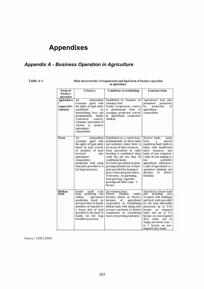
203
Appendixes
Appendix A - Business Operation in Agriculture
Source: CER (2004)
Table A-1
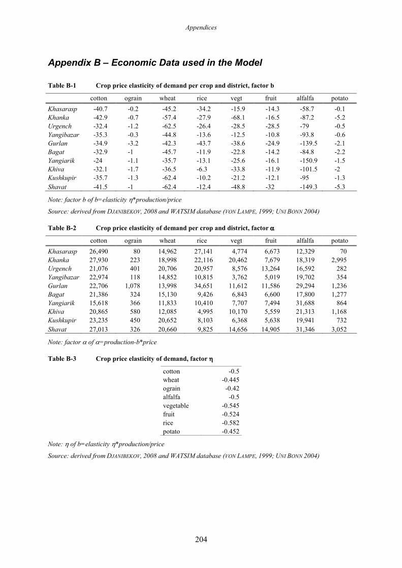
Appendices
204
Appendix B – Economic Data used in the Model
Table B-1 Crop price elasticity of demand per crop and district, factor b
cotton ograin wheat rice vegt fruit alfalfa potato
Khasarasp -40.7 -0.2 -45.2 -34.2 -15.9 -14.3 -58.7 -0.1 Khanka -42.9 -0.7 -57.4 -27.9 -68.1 -16.5 -87.2 -5.2 Urgench -32.4 -1.2 -62.5 -26.4 -28.5 -28.5 -79 -0.5 Yangibazar -35.3 -0.3 -44.8 -13.6 -12.5 -10.8 -93.8 -0.6 Gurlan -34.9 -3.2 -42.3 -43.7 -38.6 -24.9 -139.5 -2.1 Bagat -32.9 -1 -45.7 -11.9 -22.8 -14.2 -84.8 -2.2 Yangiarik -24 -1.1 -35.7 -13.1 -25.6 -16.1 -150.9 -1.5 Khiva -32.1 -1.7 -36.5 -6.3 -33.8 -11.9 -101.5 -2 Kushkupir -35.7 -1.3 -62.4 -10.2 -21.2 -12.1 -95 -1.3 Shavat -41.5 -1 -62.4 -12.4 -48.8 -32 -149.3 -5.3
Note: factor b of b=elasticity η*production/price
Source: derived from DJANIBEKOV, 2008 and WATSIM database (VON LAMPE, 1999; UNI BONN 2004)
Table B-2 Crop price elasticity of demand per crop and district, factor αααα
cotton ograin wheat rice vegt fruit alfalfa potato
Khasarasp 26,490 80 14,962 27,141 4,774 6,673 12,329 70 Khanka 27,930 223 18,998 22,116 20,462 7,679 18,319 2,995 Urgench 21,076 401 20,706 20,957 8,576 13,264 16,592 282 Yangibazar 22,974 118 14,852 10,815 3,762 5,019 19,702 354 Gurlan 22,706 1,078 13,998 34,651 11,612 11,586 29,294 1,236 Bagat 21,386 324 15,130 9,426 6,843 6,600 17,800 1,277 Yangiarik 15,618 366 11,833 10,410 7,707 7,494 31,688 864 Khiva 20,865 580 12,085 4,995 10,170 5,559 21,313 1,168 Kushkupir 23,235 450 20,652 8,103 6,368 5,638 19,941 732 Shavat 27,013 326 20,660 9,825 14,656 14,905 31,346 3,052
Note: factor α of α=production-b*price
Table B-3 Crop price elasticity of demand, factor ηηηη
cotton -0.5 wheat -0.445 ograin -0.42 alfalfa -0.5 vegetable -0.545 fruit -0.524 rice -0.582 potato -0.452
Note: η of b=elasticity η*production/price
Source: derived from DJANIBEKOV, 2008 and WATSIM database (VON LAMPE, 1999; UNI BONN 2004)
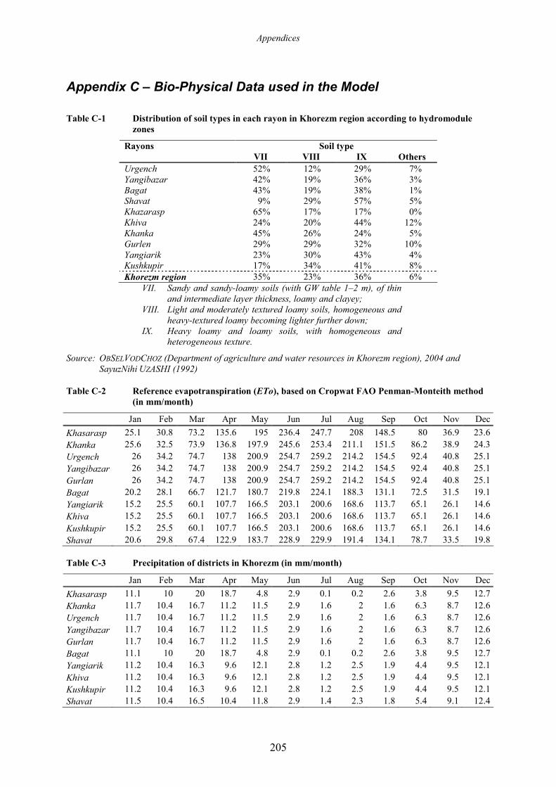
Appendices
205
Appendix C – Bio-Physical Data used in the Model
Table C-1 Distribution of soil types in each rayon in Khorezm region according to hydromodule
zones
Soil type Rayons
VII VIII IX Others
Urgench 52% 12% 29% 7% Yangibazar 42% 19% 36% 3% Bagat 43% 19% 38% 1% Shavat 9% 29% 57% 5% Khazarasp 65% 17% 17% 0% Khiva 24% 20% 44% 12% Khanka 45% 26% 24% 5% Gurlen 29% 29% 32% 10% Yangiarik 23% 30% 43% 4% Kushkupir 17% 34% 41% 8% Khorezm region 35% 23% 36% 6%
VII. Sandy and sandy-loamy soils (with GW table 1–2 m), of thin and intermediate layer thickness, loamy and clayey;
VIII. Light and moderately textured loamy soils, homogeneous and heavy-textured loamy becoming lighter further down;
IX. Heavy loamy and loamy soils, with homogeneous and heterogeneous texture.
Source: OBSELVODCHOZ (Department of agriculture and water resources in Khorezm region), 2004 and SayuzNihi UZASHI (1992)
Table C-2 Reference evapotranspiration (ETo), based on Cropwat FAO Penman-Monteith method
(in mm/month)
Jan Feb Mar Apr May Jun Jul Aug Sep Oct Nov Dec
Khasarasp 25.1 30.8 73.2 135.6 195 236.4 247.7 208 148.5 80 36.9 23.6 Khanka 25.6 32.5 73.9 136.8 197.9 245.6 253.4 211.1 151.5 86.2 38.9 24.3 Urgench 26 34.2 74.7 138 200.9 254.7 259.2 214.2 154.5 92.4 40.8 25.1 Yangibazar 26 34.2 74.7 138 200.9 254.7 259.2 214.2 154.5 92.4 40.8 25.1 Gurlan 26 34.2 74.7 138 200.9 254.7 259.2 214.2 154.5 92.4 40.8 25.1 Bagat 20.2 28.1 66.7 121.7 180.7 219.8 224.1 188.3 131.1 72.5 31.5 19.1 Yangiarik 15.2 25.5 60.1 107.7 166.5 203.1 200.6 168.6 113.7 65.1 26.1 14.6 Khiva 15.2 25.5 60.1 107.7 166.5 203.1 200.6 168.6 113.7 65.1 26.1 14.6 Kushkupir 15.2 25.5 60.1 107.7 166.5 203.1 200.6 168.6 113.7 65.1 26.1 14.6 Shavat 20.6 29.8 67.4 122.9 183.7 228.9 229.9 191.4 134.1 78.7 33.5 19.8
Table C-3 Precipitation of districts in Khorezm (in mm/month)
Jan Feb Mar Apr May Jun Jul Aug Sep Oct Nov Dec
Khasarasp 11.1 10 20 18.7 4.8 2.9 0.1 0.2 2.6 3.8 9.5 12.7 Khanka 11.7 10.4 16.7 11.2 11.5 2.9 1.6 2 1.6 6.3 8.7 12.6 Urgench 11.7 10.4 16.7 11.2 11.5 2.9 1.6 2 1.6 6.3 8.7 12.6 Yangibazar 11.7 10.4 16.7 11.2 11.5 2.9 1.6 2 1.6 6.3 8.7 12.6 Gurlan 11.7 10.4 16.7 11.2 11.5 2.9 1.6 2 1.6 6.3 8.7 12.6 Bagat 11.1 10 20 18.7 4.8 2.9 0.1 0.2 2.6 3.8 9.5 12.7 Yangiarik 11.2 10.4 16.3 9.6 12.1 2.8 1.2 2.5 1.9 4.4 9.5 12.1 Khiva 11.2 10.4 16.3 9.6 12.1 2.8 1.2 2.5 1.9 4.4 9.5 12.1 Kushkupir 11.2 10.4 16.3 9.6 12.1 2.8 1.2 2.5 1.9 4.4 9.5 12.1 Shavat 11.5 10.4 16.5 10.4 11.8 2.9 1.4 2.3 1.8 5.4 9.1 12.4
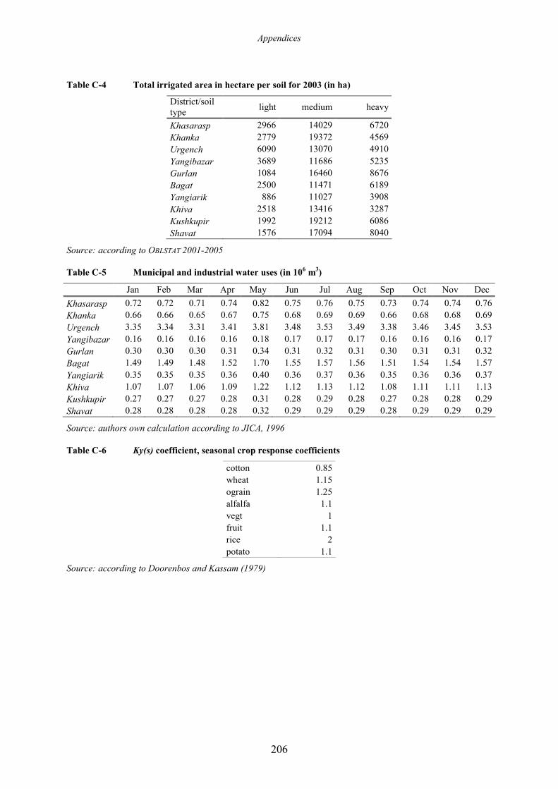
Appendices
206
Table C-4 Total irrigated area in hectare per soil for 2003 (in ha)
District/soil type
light medium heavy
Khasarasp 2966 14029 6720 Khanka 2779 19372 4569 Urgench 6090 13070 4910 Yangibazar 3689 11686 5235 Gurlan 1084 16460 8676 Bagat 2500 11471 6189 Yangiarik 886 11027 3908 Khiva 2518 13416 3287 Kushkupir 1992 19212 6086 Shavat 1576 17094 8040
Source: according to OBLSTAT 2001-2005
Table C-5 Municipal and industrial water uses (in 106 m
3)
Jan Feb Mar Apr May Jun Jul Aug Sep Oct Nov Dec
Khasarasp 0.72 0.72 0.71 0.74 0.82 0.75 0.76 0.75 0.73 0.74 0.74 0.76 Khanka 0.66 0.66 0.65 0.67 0.75 0.68 0.69 0.69 0.66 0.68 0.68 0.69 Urgench 3.35 3.34 3.31 3.41 3.81 3.48 3.53 3.49 3.38 3.46 3.45 3.53 Yangibazar 0.16 0.16 0.16 0.16 0.18 0.17 0.17 0.17 0.16 0.16 0.16 0.17 Gurlan 0.30 0.30 0.30 0.31 0.34 0.31 0.32 0.31 0.30 0.31 0.31 0.32 Bagat 1.49 1.49 1.48 1.52 1.70 1.55 1.57 1.56 1.51 1.54 1.54 1.57 Yangiarik 0.35 0.35 0.35 0.36 0.40 0.36 0.37 0.36 0.35 0.36 0.36 0.37 Khiva 1.07 1.07 1.06 1.09 1.22 1.12 1.13 1.12 1.08 1.11 1.11 1.13 Kushkupir 0.27 0.27 0.27 0.28 0.31 0.28 0.29 0.28 0.27 0.28 0.28 0.29 Shavat 0.28 0.28 0.28 0.28 0.32 0.29 0.29 0.29 0.28 0.29 0.29 0.29
Source: authors own calculation according to JICA, 1996
Table C-6 Ky(s) coefficient, seasonal crop response coefficients
cotton 0.85 wheat 1.15 ograin 1.25 alfalfa 1.1 vegt 1 fruit 1.1 rice 2 potato 1.1
Source: according to Doorenbos and Kassam (1979)
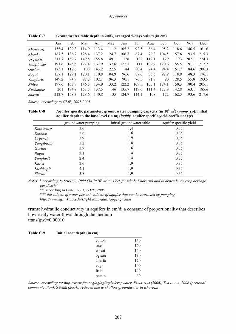
Appendices
207
Table C-7 Groundwater table depth in 2003, averaged 5-days values (in cm)
Jan Feb Mar Apr May Jun Jul Aug Sep Oct Nov Dec
Khasarasp 155.4 129.3 114.9 113.4 111.2 105.2 92.5 86.4 95.2 118.6 146.5 161.6 Khanka 187.5 136.7 128.4 137.2 124.7 106.7 87.4 79.3 104.5 157.6 193.5 215.3 Urgench 211.7 169.7 149.5 155.8 149.1 128 122 112.1 129 173 202.1 224.3 Yangibazar 191.6 145.5 122.4 131.9 137.6 122.7 111 109.2 120.6 155.5 191.1 217.2 Gurlan 173.1 112.6 108 143.2 122.5 84 80.4 74.4 94.4 151.7 184.6 206.3 Bagat 157.1 129.1 120.1 110.8 104.9 96.6 87.6 83.5 92.9 118.9 148.3 176.1 Yangiarik 149.2 94.9 98.2 102.1 96.3 90.1 76.5 71.7 90 128.5 155.8 193.5 Khiva 197.6 163.9 146.5 134.9 133.2 122.2 109.5 105.1 124.1 150.3 180.4 205.1 Kushkupir 201 174.8 153.5 137.5 146 135.7 119.6 111.4 122.9 142.8 163.1 185.6 Shavat 212.7 158.3 128.6 140.8 135 124.7 114.1 108 122 162.5 193.6 217.6
Source: according to GME, 2001-2005
Table C-8 Aquifer specific parameter: groundwater pumping capacity (in 106 m
3) (pump_cp); initial
aquifer depth to the base level (in m) (hg00); aquifer specific yield coefficient (sy)
groundwater pumping capacity in [M m3]*
initial groundwater table depth [m]**
aquifer specific yield coefficient [-]*** Khasarasp 3.6 1.4 0.35
Khanka 3.6 1.6 0.35 Urgench 3.9 1.9 0.35 Yangibazar 3.2 1.8 0.35 Gurlan 3.9 1.6 0.35 Bagat 3.1 1.4 0.35 Yangiarik 2.4 1.4 0.35 Khiva 2.6 1.9 0.35 Kushkupir 4.1 1.9 0.35 Shavat 3.8 1.9 0.35
Notes: * according to SOKOLV, 1999 (34.2*106 m3 in 1995 for whole Khorezm) and in dependency crop acreage per district ** according to GME, 2001; GME, 2005 *** the volume of water per unit volume of aquifer that can be extracted by pumping, http://www.kgs.ukans.edu/HighPlains/atlas/apgengw.htm
trans: hydraulic conductivity in aquifers in cm/d; a constant of proportionality that describes how easily water flows through the medium trans(gw)=0.00010
Table C-9 Initial root depth (in cm)
cotton 140 rice 160 wheat 140 ograin 130 alfalfa 120 vegt 100 fruit 140 potato 60
Source: according to: http://www.fao.org/ag/agl/aglw/cropwater, FORKUTSA (2006), TISCHBEIN, 2008 (personal communication), SANIIRI (2004), reduced due to shallow groundwater in Khorezm
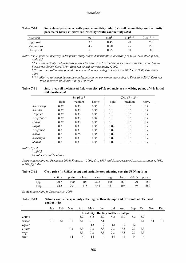
Appendices
208
Table C-10 Soil related parameter: soils pore connectivity index (cc); soil connectivity and turtuosity
parameter (mm); effective saturated hydraulic conductivity (khs)
Khorezm cc* mm** smp*** Khs****
Light soil 3.5 0.45 20 250 Medium soil 4.2 0.50 25 150 Heavy soil 7.3 0.55 80 80
Notes: *soils pore connectivity index permeability index, dimensionless, according to EAGLESON 2002, p.181, table 6.2 ** soil connectivity and turtuosity parameter pore size distribution index, dimensionless, according to FORKUTSA (2006), CAI (1999), ROSETTA neural network model (2002) *** saturated soil matric potential in cm suction, according to EAGLESON 2002, CAI 1999, KHAMZINA
2006 **** effective saturated hydraulic conductivity in cm per month, according to EAGLESON 2002, ROSETTA
NEURAL NETWORK MODEL (2002), CAI 1999
Table C-11 Saturated soil moisture at field capacity, pF 2; soil moisture at wilting point, pf 4.2; initial
soil moisture, z0
Zs, pF 2 * Zw, pF 4.2** light medium heavy light medium heavy
Khasarasp 0.22 0.33 0.35 0.1 0.15 0.17 Khanka 0.22 0.33 0.35 0.1 0.15 0.17 Urgench 0.22 0.33 0.35 0.1 0.15 0.17 Yangibazar 0.22 0.33 0.34 0.1 0.15 0.17 Gurlan 0.22 0.33 0.35 0.1 0.15 0.17 Bagat 0.2 0.3 0.35 0.09 0.13 0.17 Yangiarik 0.2 0.3 0.35 0.09 0.13 0.17 Khiva 0.2 0.25 0.36 0.09 0.13 0.17 Kushkupir 0.2 0.3 0.35 0.09 0.13 0.17 Shavat 0.2 0.3 0.35 0.09 0.13 0.17
Notes: *pF2 **pF4.2 All values in cm3*cm-3and
Source: according to: FORKUTSA 2006; KHAMZINA, 2006; CAI, 1999 and SCHEFFER AND SCHACHTSCHABEL (1998), p.189, fig 5.4-4
Table C-12 Crop price (in USD/t) (cpp) and variable crop planting cost (in USD/ha) (otc)
cotton ograin wheat rice vegt fruit alfalfa potato
cpp 217 100 102 292 106 160 70 180 crop 512 201 215 464 451 406 169 580
Source: according to DJANIBEKOV, 2008
Table C-13 Salinity coefficients; salinity effecting coefficient-slope and threshold of electrical
conductivity
Jan Feb Mar Apr May Jun Jul Aug Sep Oct Nov Dec
b, salinity effecting coefficient-slope
cotton 5.2 5.2 5.2 5.2 5.2 5.2 5.2 wheat 7.1 7.1 7.1 7.1 7.1 7.1 7.1 7.1 7.1 ograin 12 12 12 12 12 alfalfa 7.3 7.3 7.3 7.3 7.3 7.3 7.3 7.3 vegt 7.3 7.3 7.3 7.3 7.3 7.3 7.3 fruit 14 14 14 14 14 14 14 14
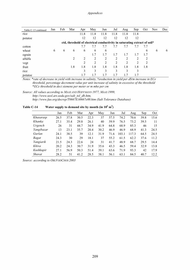
Appendices
209
Jan Feb Mar Apr May Jun Jul Aug Sep Oct Nov Dec
rice 11.8 11.8 11.8 11.8 11.8 11.8 potatoe 12 12 12 12 12 12
ctd, threshold of electrical conductivity in saturating extract of soil*
cotton 7.7 7.7 7.7 7.7 7.7 7.7 7.7 wheat 6 6 6 6 6 6 6 6 6 ograin 1.7 1.7 1.7 1.7 1.7 1.7 alfalfa 2 2 2 2 2 2 2 2 vegt 2 2 2 2 2 2 2 fruit 1.8 1.8 1.8 1.8 1.8 1.8 1.8 1.8 rice 3 3 3 3 3 3 potatoe 1.7 1.7 1.7 1.7 1.7 1.7 Notes: *rate of decrease in yield with increase in salinity, %reduction in yield per dS/m increase in ECe
threshold, percentage decrement value per unit increase of salinity in excessive of the threshold *ECe threshold in deci siemens per meter or m mho per cm
Source: All values according to MAAS AND HOFFMANN 1977, MAAS 1999, http://www.ussl.ars.usda.gov/salt_tol_db.htm, http://www.fao.org/docrep/T0667E/t0667e00.htm (Salt Tolerance Database)
Table C-14 Water supply to demand site by month (in 106 m
3)
Jan Feb Mar Apr May Jun Jul Aug Sep Oct
Khasarasp 26.5 37.8 30.5 22.3 37 57.5 74.2 70.6 39.8 15.6 Khanka 27.1 35.4 29.8 26.1 40 59.9 76.5 73.2 39.5 11 Urgench 26 31 44.7 34.9 41.9 64.8 68.9 85.3 46 15 Yangibazar 13 23.1 35.7 20.4 30.2 46.9 46.9 68.9 41.3 24.5 Gurlan 24.1 38.5 39 12.1 31.9 71.6 103.1 117.3 64.5 24.5 Bagat 24.3 30 29 18.1 37 55.2 61.5 62.2 37.6 11.2 Yangiarik 21.5 24.3 22.6 24 31 41.7 48.9 68.7 29.5 14.4 Khiva 20.2 24.3 30.7 31.9 35.6 43.3 46.5 59.4 32.9 13.8 Kushkupir 27.1 56.9 50.3 51.4 39.1 63.6 71.9 93.3 42 17.9 Shavat 28.2 51 41.2 28.5 38.1 56.1 63.1 84.5 40.7 12.2
Source: according to OBLVODCHOS 2003
Table C-13 continued
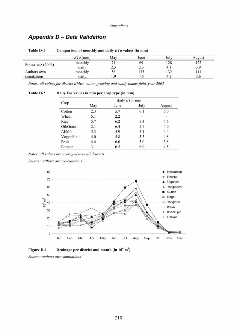
Appendices
210
Appendix D – Data Validation
Table D-1 Comparison of monthly and daily ETa values (in mm)
ETa [mm] May June July August monthly 71 69 128 122 FORKUTSA (2006)
daily 2.3 2.3 4.1 3.9 monthly 58 135 132 111 Authors own
simulations daily 1.9 4.5 4.2 3.6
Notes: all values for district Khiva, cotton growing and sandy loamy field, year 2003
Table D-2 Daily Eta values in mm per crop type (in mm)
daily ETa [mm] Crop
May June July August
Cotton 2.3 5.7 6.1 5.0 Wheat 5.1 2.2 - - Rice 5.7 6.2 5.3 4.6 OthGrain 2.1 6.4 5.7 4.0 Alfalfa 5.3 5.9 5.1 4.4 Vegetable 4.0 5.8 5.5 4.8 Fruit 4.4 6.0 5.0 3.8 Potatoe 3.1 6.5 6.0 4.5
Notes: all values are averaged over all districts
Source: authors own calculations
0
10
20
30
40
50
60
70
80
Jan Feb Mar Apr May Jun Jul Aug Sep Oct Nov Dec
106 m
3
Khasarasp
Khanka
Urgench
Yangibazar
Gurlan
Bagat
Yangiarik
Khiva
Kushkupir
Shavat
Figure D-1 Drainage per district and month (in 106 m
3)
Source: authors own simulations
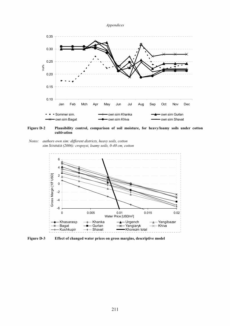
Appendices
211
0.10
0.15
0.20
0.25
0.30
0.35
Jan Feb Mch Apr May Jun Jul Aug Sep Oct Nov Dec
Vol%
Sommer sim. own sim Khanka own sim Gurlan
own sim Bagat own sim Khiva own sim Shavat
Figure D-2 Plausibility control, comparison of soil moisture, for heavy/loamy soils under cotton
cultivation
-6
-4
-2
0
2
4
6
0 0.005 0.01 0.015 0.02Water Price [USD/m3]
Gross Margin [106 USD]
Khasarasp Khanka Urgench YangibazarBagat Gurlan Yangiaryk KhivaKushkupir Shavat Khorezm total
Figure D-3 Effect of changed water prices on gross margins, descriptive model
Notes: authors own sim: different districts, heavy soils, cotton sim SOMMER (2006): cropsyst, loamy soils, 0-40 cm, cotton
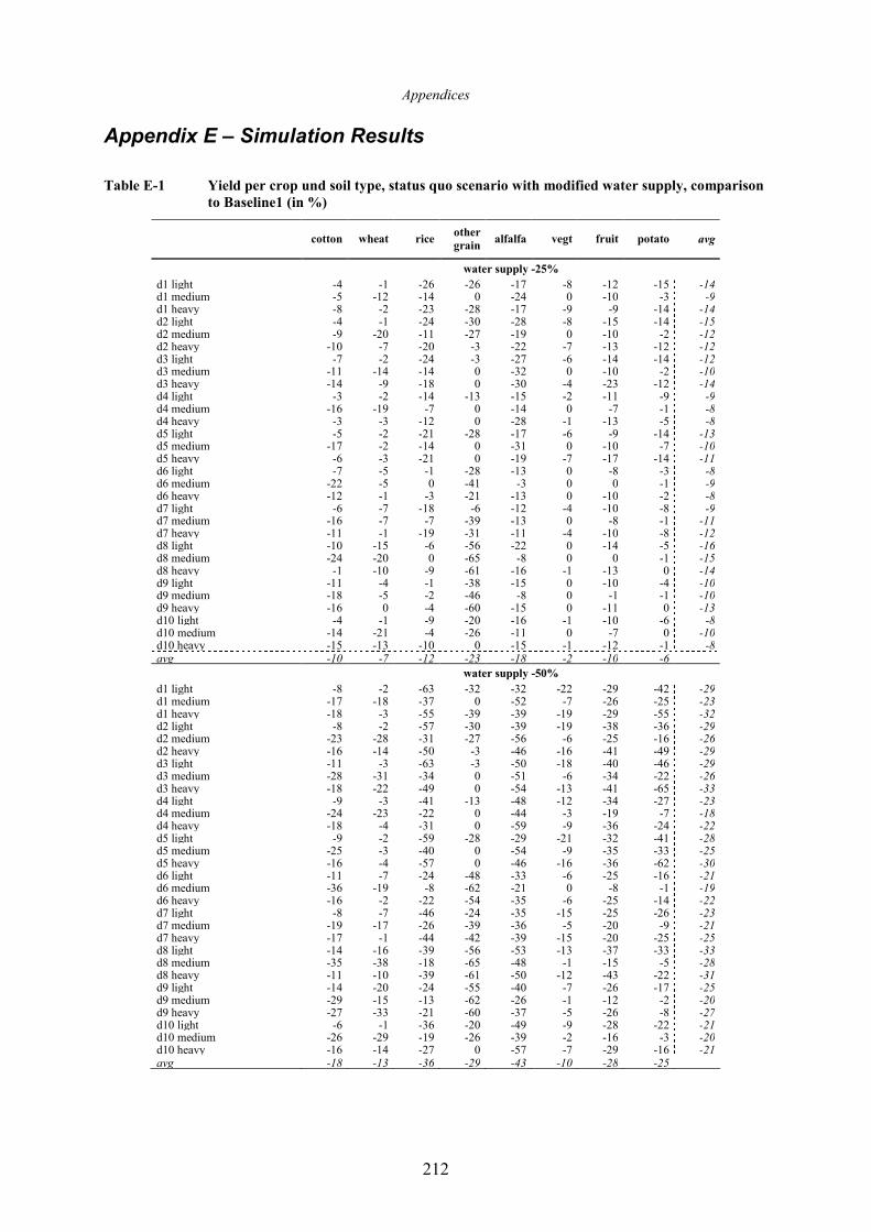
Appendices
212
Appendix E – Simulation Results
Table E-1 Yield per crop und soil type, status quo scenario with modified water supply, comparison
to Baseline1 (in %)
cotton wheat rice other
grain alfalfa vegt fruit potato avg
water supply -25%
d1 light -4 -1 -26 -26 -17 -8 -12 -15 -14 d1 medium -5 -12 -14 0 -24 0 -10 -3 -9 d1 heavy -8 -2 -23 -28 -17 -9 -9 -14 -14 d2 light -4 -1 -24 -30 -28 -8 -15 -14 -15 d2 medium -9 -20 -11 -27 -19 0 -10 -2 -12 d2 heavy -10 -7 -20 -3 -22 -7 -13 -12 -12 d3 light -7 -2 -24 -3 -27 -6 -14 -14 -12 d3 medium -11 -14 -14 0 -32 0 -10 -2 -10 d3 heavy -14 -9 -18 0 -30 -4 -23 -12 -14 d4 light -3 -2 -14 -13 -15 -2 -11 -9 -9 d4 medium -16 -19 -7 0 -14 0 -7 -1 -8 d4 heavy -3 -3 -12 0 -28 -1 -13 -5 -8 d5 light -5 -2 -21 -28 -17 -6 -9 -14 -13 d5 medium -17 -2 -14 0 -31 0 -10 -7 -10 d5 heavy -6 -3 -21 0 -19 -7 -17 -14 -11 d6 light -7 -5 -1 -28 -13 0 -8 -3 -8 d6 medium -22 -5 0 -41 -3 0 0 -1 -9 d6 heavy -12 -1 -3 -21 -13 0 -10 -2 -8 d7 light -6 -7 -18 -6 -12 -4 -10 -8 -9 d7 medium -16 -7 -7 -39 -13 0 -8 -1 -11 d7 heavy -11 -1 -19 -31 -11 -4 -10 -8 -12 d8 light -10 -15 -6 -56 -22 0 -14 -5 -16 d8 medium -24 -20 0 -65 -8 0 0 -1 -15 d8 heavy -1 -10 -9 -61 -16 -1 -13 0 -14 d9 light -11 -4 -1 -38 -15 0 -10 -4 -10 d9 medium -18 -5 -2 -46 -8 0 -1 -1 -10 d9 heavy -16 0 -4 -60 -15 0 -11 0 -13 d10 light -4 -1 -9 -20 -16 -1 -10 -6 -8 d10 medium -14 -21 -4 -26 -11 0 -7 0 -10 d10 heavy -15 -13 -10 0 -15 -1 -12 -1 -8 avg -10 -7 -12 -23 -18 -2 -10 -6
water supply -50%
d1 light -8 -2 -63 -32 -32 -22 -29 -42 -29 d1 medium -17 -18 -37 0 -52 -7 -26 -25 -23 d1 heavy -18 -3 -55 -39 -39 -19 -29 -55 -32 d2 light -8 -2 -57 -30 -39 -19 -38 -36 -29 d2 medium -23 -28 -31 -27 -56 -6 -25 -16 -26 d2 heavy -16 -14 -50 -3 -46 -16 -41 -49 -29 d3 light -11 -3 -63 -3 -50 -18 -40 -46 -29 d3 medium -28 -31 -34 0 -51 -6 -34 -22 -26 d3 heavy -18 -22 -49 0 -54 -13 -41 -65 -33 d4 light -9 -3 -41 -13 -48 -12 -34 -27 -23 d4 medium -24 -23 -22 0 -44 -3 -19 -7 -18 d4 heavy -18 -4 -31 0 -59 -9 -36 -24 -22 d5 light -9 -2 -59 -28 -29 -21 -32 -41 -28 d5 medium -25 -3 -40 0 -54 -9 -35 -33 -25 d5 heavy -16 -4 -57 0 -46 -16 -36 -62 -30 d6 light -11 -7 -24 -48 -33 -6 -25 -16 -21 d6 medium -36 -19 -8 -62 -21 0 -8 -1 -19 d6 heavy -16 -2 -22 -54 -35 -6 -25 -14 -22 d7 light -8 -7 -46 -24 -35 -15 -25 -26 -23 d7 medium -19 -17 -26 -39 -36 -5 -20 -9 -21 d7 heavy -17 -1 -44 -42 -39 -15 -20 -25 -25 d8 light -14 -16 -39 -56 -53 -13 -37 -33 -33 d8 medium -35 -38 -18 -65 -48 -1 -15 -5 -28 d8 heavy -11 -10 -39 -61 -50 -12 -43 -22 -31 d9 light -14 -20 -24 -55 -40 -7 -26 -17 -25 d9 medium -29 -15 -13 -62 -26 -1 -12 -2 -20 d9 heavy -27 -33 -21 -60 -37 -5 -26 -8 -27 d10 light -6 -1 -36 -20 -49 -9 -28 -22 -21 d10 medium -26 -29 -19 -26 -39 -2 -16 -3 -20 d10 heavy -16 -14 -27 0 -57 -7 -29 -16 -21 avg -18 -13 -36 -29 -43 -10 -28 -25
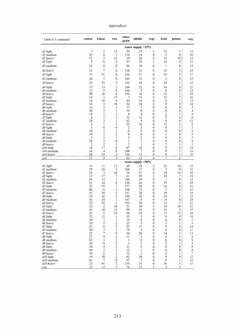
Appendices
213
Table E-1 continued cotton wheat rice other
grain alfalfa vegt fruit potato avg
water supply +25%
d1 light 7 2 15 29 23 2 15 7 13 d1 medium 23 6 1 114 14 0 5 0 20 d1 heavy 12 2 22 19 20 4 15 10 13 d2 light 9 6 5 53 24 1 16 6 15
d2 medium 25 8 0 96 10 0 1 0 18
d2 heavy 12 7 6 118 21 0 15 3 23 d3 light 15 21 6 126 27 0 16 5 27
d3 medium 20 5 0 163 12 0 3 0 25 d3 heavy 23 33 5 152 28 0 18 1 32
d4 light 13 13 2 104 23 0 14 4 22 d4 medium 12 8 0 166 8 0 0 0 24 d4 heavy 20 26 0 154 18 0 12 1 29 d5 light 14 1 17 7 21 4 12 7 10 d5 medium 14 10 8 44 16 0 8 1 13 d5 heavy 16 3 18 54 18 2 9 9 16 d6 light 14 5 1 17 3 0 0 0 5 d6 medium 20 3 1 10 0 0 0 0 4 d6 heavy 14 1 1 8 4 0 2 1 4 d7 light 6 3 3 31 13 0 9 4 8 d7 medium 28 2 1 62 4 0 0 0 12 d7 heavy 4 1 3 25 16 0 12 2 8 d8 light 3 6 0 2 2 0 0 1 2 d8 medium 34 1 1 -4 0 0 0 0 4 d8 heavy 19 3 2 0 0 0 1 0 3 d9 light 5 1 1 5 2 0 0 0 2 d9 medium 29 2 0 1 1 0 0 0 4 d9 heavy 2 2 1 2 1 0 2 1 1 d10 light 14 17 0 87 18 0 9 4 19 d10 medium 14 4 0 100 7 0 0 1 16 d10 heavy 18 35 2 156 13 0 9 1 29 avg 15 8 4 63 12 0 7 2
water supply +50%
d1 light 11 11 17 40 38 2 23 10 19 d1 medium 55 10 2 160 17 0 5 0 31 d1 heavy 23 3 24 34 31 4 24 14 20 d2 light 13 17 7 61 29 1 18 7 19 d2 medium 56 12 1 104 10 0 1 0 23 d2 heavy 21 14 6 120 26 0 19 4 26 d3 light 22 35 7 137 28 0 16 6 31 d3 medium 66 6 2 168 12 0 3 0 32 d3 heavy 27 38 5 157 28 0 18 1 34 d4 light 19 26 3 109 26 0 14 5 25 d4 medium 42 10 1 167 8 0 0 0 28 d4 heavy 25 35 1 153 20 0 14 1 31 d5 light 22 2 26 51 30 5 18 10 21 d5 medium 41 10 13 98 23 0 12 2 25 d5 heavy 25 6 24 94 25 4 15 13 26 d6 light 32 11 1 35 3 0 0 0 10 d6 medium 34 7 1 16 0 0 0 0 7 d6 heavy 24 5 2 22 5 0 2 1 8 d7 light 22 6 3 55 17 0 9 4 14 d7 medium 50 3 1 79 5 0 0 0 17 d7 heavy 22 7 4 34 20 0 14 2 13 d8 light 23 9 2 11 2 0 0 1 6 d8 medium 62 3 2 3 0 0 0 0 9 d8 heavy 26 6 2 3 3 0 2 1 5 d9 light 34 4 2 21 2 0 0 0 8 d9 medium 44 2 1 12 1 0 0 0 8 d9 heavy 34 6 1 12 3 0 2 1 7 d10 light 19 29 2 92 20 0 9 4 22 d10 medium 43 7 0 97 7 0 0 1 19 d10 heavy 22 41 2 155 15 0 10 1 31 avg 32 13 5 76 15 1 8 3
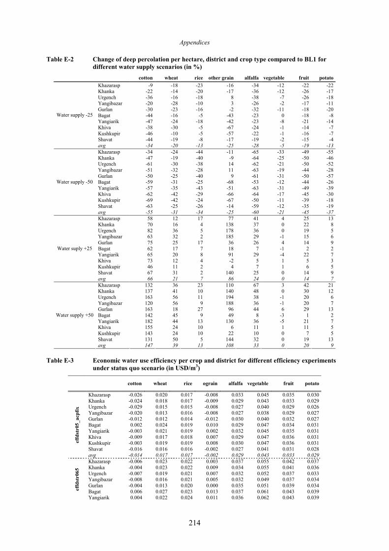
Appendices
214
Table E-2 Change of deep percolation per hectare, district and crop type compared to BL1 for
different water supply scenarios (in %)
cotton wheat rice other grain alfalfa vegetable fruit potato
Khazarasp -9 -18 -23 -16 -34 -12 -22 -22 Khanka -22 -14 -20 -17 -36 -12 -26 -17 Urgench -36 -16 -18 8 -38 -7 -26 -18 Yangibazar -20 -28 -10 3 -26 -2 -17 -11 Gurlan -30 -23 -16 -2 -32 -11 -18 -20 Bagat -44 -16 -5 -43 -23 0 -18 -8 Yangiarik -47 -24 -18 -42 -23 -8 -21 -14 Khiva -38 -30 -5 -67 -24 -1 -14 -7 Kushkupir -46 -10 -5 -57 -22 -1 -16 -7 Shavat -44 -19 -8 -17 -19 -2 -15 -4
Water supply -25
avg -34 -20 -13 -25 -28 -5 -19 -13 Khazarasp -34 -24 -44 -11 -65 -33 -49 -55 Khanka -47 -19 -40 -9 -64 -25 -50 -46 Urgench -61 -30 -38 14 -62 -21 -50 -52 Yangibazar -51 -32 -28 11 -63 -19 -44 -28 Gurlan -50 -25 -40 9 -61 -31 -50 -57 Bagat -59 -31 -25 -68 -53 -12 -44 -26 Yangiarik -57 -35 -43 -51 -63 -31 -49 -39 Khiva -62 -42 -29 -66 -64 -17 -45 -30 Kushkupir -69 -42 -24 -67 -50 -11 -39 -18 Shavat -63 -25 -26 -14 -59 -12 -35 -19
Water supply -50
avg -55 -31 -34 -25 -60 -21 -45 -37 Khazarasp 58 12 17 77 41 4 25 13 Khanka 70 16 4 138 37 0 22 8 Urgench 82 36 5 178 36 0 19 5 Yangibazar 63 32 2 185 29 -1 15 6 Gurlan 75 25 17 36 26 4 14 9 Bagat 62 17 7 18 7 -1 2 2 Yangiarik 65 20 8 91 29 -4 22 7 Khiva 73 12 4 -2 5 1 5 3 Kushkupir 46 11 2 4 7 1 6 5 Shavat 67 31 2 140 25 0 14 9
Water suply +25
avg 66 21 7 86 24 0 14 7 Khazarasp 132 36 23 110 67 3 42 21 Khanka 137 41 10 140 48 0 30 12 Urgench 163 56 11 194 38 -1 20 6 Yangibazar 120 56 9 188 36 -1 20 7 Gurlan 163 18 27 96 44 6 29 13 Bagat 142 45 9 49 8 -3 1 2 Yangiarik 182 44 13 130 36 -5 21 7 Khiva 155 24 10 6 11 1 11 5 Kushkupir 143 24 10 22 10 0 7 5 Shavat 131 50 5 144 32 0 19 13
Water supply +50
avg 147 39 13 108 33 0 20 9
Table E-3 Economic water use efficiency per crop and district for different efficiency experiments
under status quo scenario (in USD/m3)
cotton wheat rice ograin alfalfa vegetable fruit potato
Khazarasp -0.026 0.020 0.017 -0.008 0.033 0.045 0.035 0.030 Khanka -0.024 0.018 0.017 -0.009 0.029 0.043 0.033 0.029 Urgench -0.029 0.015 0.015 -0.008 0.027 0.040 0.029 0.026 Yangibazar -0.020 0.013 0.016 -0.008 0.027 0.038 0.029 0.027 Gurlan -0.012 0.012 0.014 -0.012 0.030 0.040 0.032 0.027 Bagat 0.002 0.024 0.019 0.010 0.029 0.047 0.034 0.031 Yangiarik -0.003 0.021 0.019 0.002 0.032 0.045 0.035 0.031 Khiva -0.009 0.017 0.018 0.007 0.029 0.047 0.036 0.031 Kushkupir -0.003 0.019 0.019 0.008 0.030 0.047 0.036 0.031 Shavat -0.016 0.016 0.016 -0.002 0.027 0.041 0.031 0.028
effd
str0
5_acp
fix
avg -0.014 0.017 0.017 -0.002 0.029 0.043 0.033 0.029 Khazarasp -0.006 0.023 0.022 0.003 0.037 0.055 0.042 0.037 Khanka -0.004 0.023 0.022 0.009 0.034 0.055 0.041 0.036 Urgench -0.007 0.019 0.021 0.007 0.032 0.052 0.037 0.033 Yangibazar -0.008 0.016 0.021 0.005 0.032 0.049 0.037 0.034 Gurlan -0.004 0.013 0.020 0.000 0.035 0.051 0.039 0.034 Bagat 0.006 0.027 0.023 0.013 0.037 0.061 0.043 0.039 ef
fdstr0
65
Yangiarik 0.004 0.022 0.024 0.011 0.036 0.062 0.043 0.039
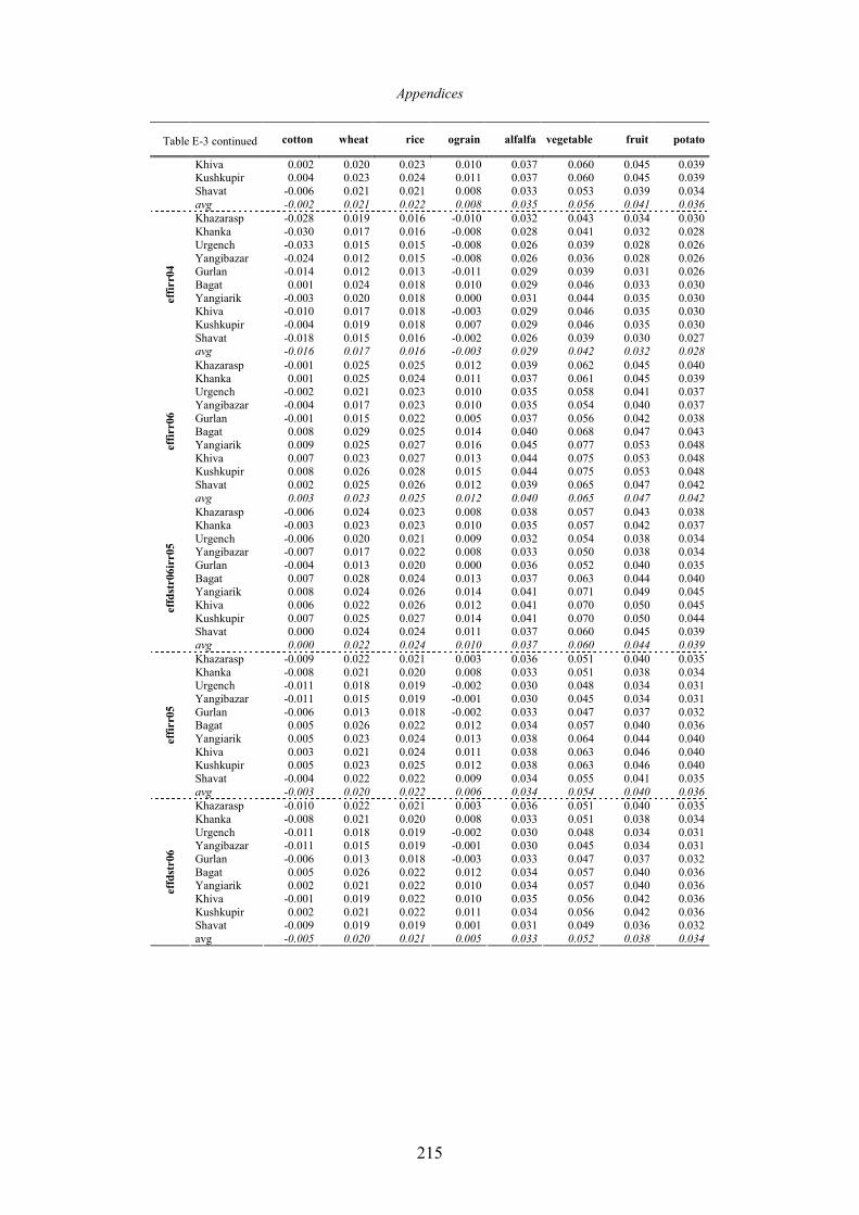
Appendices
215
cotton wheat rice ograin alfalfa vegetable fruit potato
Khiva 0.002 0.020 0.023 0.010 0.037 0.060 0.045 0.039 Kushkupir 0.004 0.023 0.024 0.011 0.037 0.060 0.045 0.039 Shavat -0.006 0.021 0.021 0.008 0.033 0.053 0.039 0.034 avg -0.002 0.021 0.022 0.008 0.035 0.056 0.041 0.036 Khazarasp -0.028 0.019 0.016 -0.010 0.032 0.043 0.034 0.030 Khanka -0.030 0.017 0.016 -0.008 0.028 0.041 0.032 0.028 Urgench -0.033 0.015 0.015 -0.008 0.026 0.039 0.028 0.026 Yangibazar -0.024 0.012 0.015 -0.008 0.026 0.036 0.028 0.026 Gurlan -0.014 0.012 0.013 -0.011 0.029 0.039 0.031 0.026 Bagat 0.001 0.024 0.018 0.010 0.029 0.046 0.033 0.030 Yangiarik -0.003 0.020 0.018 0.000 0.031 0.044 0.035 0.030 Khiva -0.010 0.017 0.018 -0.003 0.029 0.046 0.035 0.030 Kushkupir -0.004 0.019 0.018 0.007 0.029 0.046 0.035 0.030 Shavat -0.018 0.015 0.016 -0.002 0.026 0.039 0.030 0.027
effirr
04
avg -0.016 0.017 0.016 -0.003 0.029 0.042 0.032 0.028 Khazarasp -0.001 0.025 0.025 0.012 0.039 0.062 0.045 0.040 Khanka 0.001 0.025 0.024 0.011 0.037 0.061 0.045 0.039 Urgench -0.002 0.021 0.023 0.010 0.035 0.058 0.041 0.037 Yangibazar -0.004 0.017 0.023 0.010 0.035 0.054 0.040 0.037 Gurlan -0.001 0.015 0.022 0.005 0.037 0.056 0.042 0.038 Bagat 0.008 0.029 0.025 0.014 0.040 0.068 0.047 0.043 Yangiarik 0.009 0.025 0.027 0.016 0.045 0.077 0.053 0.048 Khiva 0.007 0.023 0.027 0.013 0.044 0.075 0.053 0.048 Kushkupir 0.008 0.026 0.028 0.015 0.044 0.075 0.053 0.048 Shavat 0.002 0.025 0.026 0.012 0.039 0.065 0.047 0.042
effirr
06
avg 0.003 0.023 0.025 0.012 0.040 0.065 0.047 0.042 Khazarasp -0.006 0.024 0.023 0.008 0.038 0.057 0.043 0.038 Khanka -0.003 0.023 0.023 0.010 0.035 0.057 0.042 0.037 Urgench -0.006 0.020 0.021 0.009 0.032 0.054 0.038 0.034 Yangibazar -0.007 0.017 0.022 0.008 0.033 0.050 0.038 0.034 Gurlan -0.004 0.013 0.020 0.000 0.036 0.052 0.040 0.035 Bagat 0.007 0.028 0.024 0.013 0.037 0.063 0.044 0.040 Yangiarik 0.008 0.024 0.026 0.014 0.041 0.071 0.049 0.045 Khiva 0.006 0.022 0.026 0.012 0.041 0.070 0.050 0.045 Kushkupir 0.007 0.025 0.027 0.014 0.041 0.070 0.050 0.044 Shavat 0.000 0.024 0.024 0.011 0.037 0.060 0.045 0.039
effd
str0
6irr0
5
avg 0.000 0.022 0.024 0.010 0.037 0.060 0.044 0.039 Khazarasp -0.009 0.022 0.021 0.003 0.036 0.051 0.040 0.035 Khanka -0.008 0.021 0.020 0.008 0.033 0.051 0.038 0.034 Urgench -0.011 0.018 0.019 -0.002 0.030 0.048 0.034 0.031 Yangibazar -0.011 0.015 0.019 -0.001 0.030 0.045 0.034 0.031 Gurlan -0.006 0.013 0.018 -0.002 0.033 0.047 0.037 0.032 Bagat 0.005 0.026 0.022 0.012 0.034 0.057 0.040 0.036 Yangiarik 0.005 0.023 0.024 0.013 0.038 0.064 0.044 0.040 Khiva 0.003 0.021 0.024 0.011 0.038 0.063 0.046 0.040 Kushkupir 0.005 0.023 0.025 0.012 0.038 0.063 0.046 0.040 Shavat -0.004 0.022 0.022 0.009 0.034 0.055 0.041 0.035
effirr
05
avg -0.003 0.020 0.022 0.006 0.034 0.054 0.040 0.036 Khazarasp -0.010 0.022 0.021 0.003 0.036 0.051 0.040 0.035 Khanka -0.008 0.021 0.020 0.008 0.033 0.051 0.038 0.034 Urgench -0.011 0.018 0.019 -0.002 0.030 0.048 0.034 0.031 Yangibazar -0.011 0.015 0.019 -0.001 0.030 0.045 0.034 0.031 Gurlan -0.006 0.013 0.018 -0.003 0.033 0.047 0.037 0.032 Bagat 0.005 0.026 0.022 0.012 0.034 0.057 0.040 0.036 Yangiarik 0.002 0.021 0.022 0.010 0.034 0.057 0.040 0.036 Khiva -0.001 0.019 0.022 0.010 0.035 0.056 0.042 0.036 Kushkupir 0.002 0.021 0.022 0.011 0.034 0.056 0.042 0.036 Shavat -0.009 0.019 0.019 0.001 0.031 0.049 0.036 0.032
effd
str0
6
avg -0.005 0.020 0.021 0.005 0.033 0.052 0.038 0.034
Table E-3 continued
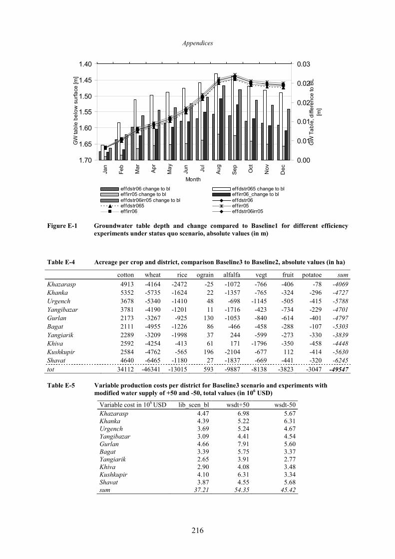
Appendices
216
1.40
1.45
1.50
1.55
1.60
1.65
1.70
Jan
Feb
Mar
Apr
May
Jun
Jul
Aug
Sep
Oct
Nov
Dec
Month
GW table below surface [m]
0.00
0.01
0.01
0.02
0.02
0.03
GW Table, difference to BL
[m]
effdstr06 change to bl effdstr065 change to bleff irr05 change to bl eff irr06_change to bl
effdstr06irr05 change to bl effdstr06effdstr065 effirr05effirr06 effdstr06irr05
Figure E-1 Groundwater table depth and change compared to Baseline1 for different efficiency
experiments under status quo scenario, absolute values (in m)
Table E-4 Acreage per crop and district, comparison Baseline3 to Baseline2, absolute values (in ha)
cotton wheat rice ograin alfalfa vegt fruit potatoe sum
Khazarasp 4913 -4164 -2472 -25 -1072 -766 -406 -78 -4069 Khanka 5352 -5735 -1624 22 -1357 -765 -324 -296 -4727 Urgench 3678 -5340 -1410 48 -698 -1145 -505 -415 -5788 Yangibazar 3781 -4190 -1201 11 -1716 -423 -734 -229 -4701 Gurlan 2173 -3267 -925 130 -1053 -840 -614 -401 -4797 Bagat 2111 -4955 -1226 86 -466 -458 -288 -107 -5303 Yangiarik 2289 -3209 -1998 37 244 -599 -273 -330 -3839 Khiva 2592 -4254 -413 61 171 -1796 -350 -458 -4448 Kushkupir 2584 -4762 -565 196 -2104 -677 112 -414 -5630 Shavat 4640 -6465 -1180 27 -1837 -669 -441 -320 -6245
tot 34112 -46341 -13015 593 -9887 -8138 -3823 -3047 -49547
Table E-5 Variable production costs per district for Baseline3 scenario and experiments with
modified water supply of +50 and -50, total values (in 106 USD)
Variable cost in 106 USD lib_scen_bl wsdt+50 wsdt-50 Khazarasp 4.47 6.98 5.67 Khanka 4.39 5.22 6.31 Urgench 3.69 5.24 4.67 Yangibazar 3.09 4.41 4.54 Gurlan 4.66 7.91 5.60 Bagat 3.39 5.75 3.37 Yangiarik 2.65 3.91 2.77 Khiva 2.90 4.08 3.48 Kushkupir 4.10 6.31 3.34 Shavat 3.87 4.55 5.68 sum 37.21 54.35 45.42
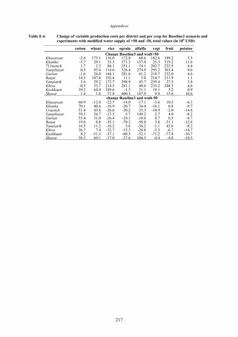
Appendices
217
Table E-6 Change of variable production costs per district and per crop for Baseline3 scenario and
experiments with modified water supply of +50 and -50, total values (in 106 USD)
cotton wheat rice ograin alfalfa vegt fruit potatoe
Change Baseline3 and wsdt+50 Khazarasp -2.6 175.1 116.0 172.8 68.6 182.6 189.2 5.5 Khanka -5.7 29.1 33.5 371.3 157.0 25.3 319.2 11.6 7Urgench 1.7 2.3 86.1 251.1 74.1 202.7 222.9 4.4 Yangibazar 0.5 95.4 114.0 326.4 274.9 295.2 363.4 9.6 Gurlan -1.6 26.0 144.1 281.6 61.2 218.7 322.0 4.6 Bagat 14.3 187.8 192.4 11.1 5.8 214.7 211.9 1.1 Yangiarik 3.6 29.2 172.7 298.9 45.7 259.4 27.5 3.8 Khiva -0.5 53.7 214.5 281.1 40.6 235.2 248.5 4.6 Kushkupir 39.2 64.0 189.6 -1.3 21.1 19.1 3.2 0.9 Shavat 1.4 1.8 71.8 400.3 187.9 9.9 15.6 10.6 change Baseline3 and wsdt-50 Khazarasp 60.9 -12.0 -22.7 -14.0 -17.1 -3.6 10.5 -6.3 Khanka 70.1 40.6 -16.9 -20.7 34.4 -16.1 0.8 -9.7 Urgench 51.4 43.6 -26.6 -30.2 35.3 -10.9 -2.0 -14.8 Yangibazar 59.3 34.7 -17.5 5.7 149.2 2.7 4.0 -9.2 Gurlan 55.4 31.0 -26.4 -24.1 -10.6 8.7 0.5 -8.7 Bagat 19.6 0.8 -35.1 -70.2 -58.0 3.8 -31.1 -12.6 Yangiarik 16.5 11.2 -16.2 5.6 -36.2 -1.1 42.6 -8.2 Khiva 36.7 7.4 -32.7 -15.3 -20.8 -3.3 -6.7 -14.7 Kushkupir 8.2 -31.3 -37.1 -80.5 -52.1 -71.2 -77.8 -10.7 Shavat 58.3 60.1 -17.0 -37.6 106.5 -4.4 -4.8 -10.5
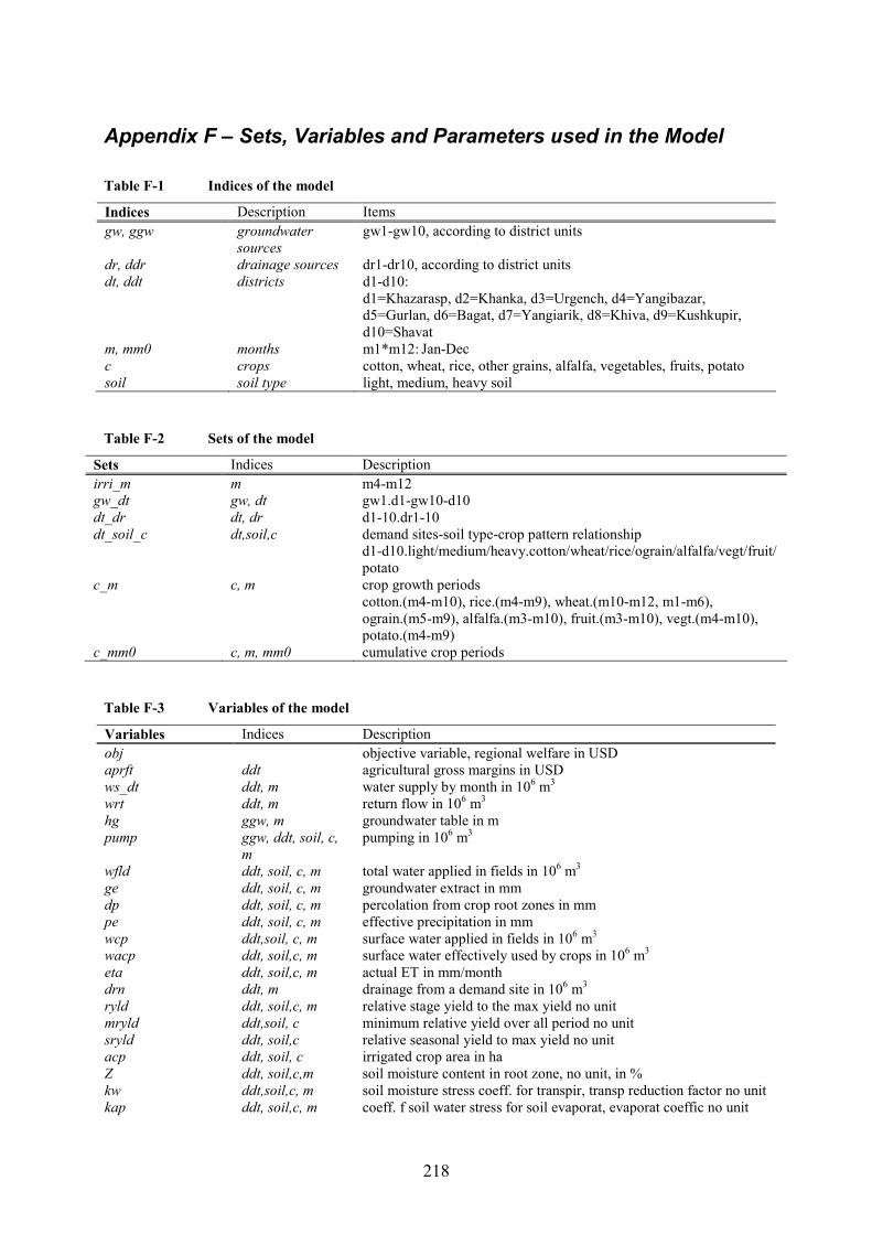
218
Appendix F – Sets, Variables and Parameters used in the Model
Table F-1 Indices of the model
Indices Description Items gw, ggw groundwater
sources gw1-gw10, according to district units
dr, ddr drainage sources dr1-dr10, according to district units dt, ddt districts d1-d10:
d1=Khazarasp, d2=Khanka, d3=Urgench, d4=Yangibazar, d5=Gurlan, d6=Bagat, d7=Yangiarik, d8=Khiva, d9=Kushkupir, d10=Shavat
m, mm0 months m1*m12: Jan-Dec c crops cotton, wheat, rice, other grains, alfalfa, vegetables, fruits, potato soil soil type light, medium, heavy soil
Table F-2 Sets of the model
Sets Indices Description irri_m m m4-m12 gw_dt gw, dt gw1.d1-gw10-d10 dt_dr dt, dr d1-10.dr1-10 dt_soil_c dt,soil,c demand sites-soil type-crop pattern relationship
d1-d10.light/medium/heavy.cotton/wheat/rice/ograin/alfalfa/vegt/fruit/ potato
c_m c, m crop growth periods cotton.(m4-m10), rice.(m4-m9), wheat.(m10-m12, m1-m6), ograin.(m5-m9), alfalfa.(m3-m10), fruit.(m3-m10), vegt.(m4-m10), potato.(m4-m9)
c_mm0 c, m, mm0 cumulative crop periods
Table F-3 Variables of the model
Variables Indices Description obj objective variable, regional welfare in USD aprft ddt agricultural gross margins in USD ws_dt ddt, m water supply by month in 106 m3 wrt ddt, m return flow in 106 m3 hg ggw, m groundwater table in m pump ggw, ddt, soil, c,
m pumping in 106 m3
wfld ddt, soil, c, m total water applied in fields in 106 m3 ge ddt, soil, c, m groundwater extract in mm dp ddt, soil, c, m percolation from crop root zones in mm pe ddt, soil, c, m effective precipitation in mm wcp ddt,soil, c, m surface water applied in fields in 106 m3 wacp ddt, soil,c, m surface water effectively used by crops in 106 m3 eta ddt, soil,c, m actual ET in mm/month drn ddt, m drainage from a demand site in 106 m3 ryld ddt, soil,c, m relative stage yield to the max yield no unit mryld ddt,soil, c minimum relative yield over all period no unit sryld ddt, soil,c relative seasonal yield to max yield no unit acp ddt, soil, c irrigated crop area in ha Z ddt, soil,c,m soil moisture content in root zone, no unit, in % kw ddt,soil,c, m soil moisture stress coeff. for transpir, transp reduction factor no unit kap ddt, soil,c, m coeff. f soil water stress for soil evaporat, evaporat coeffic no unit
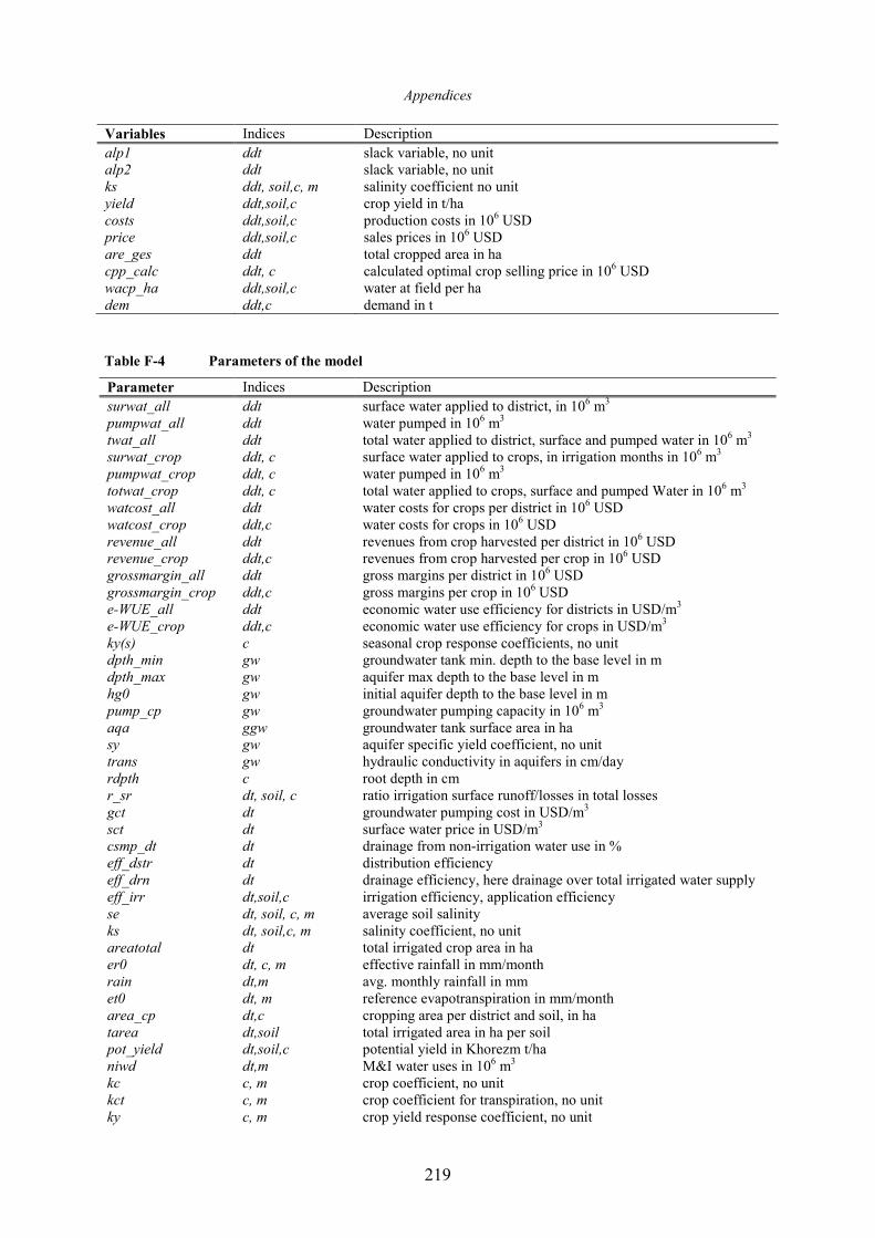
Appendices
219
Variables Indices Description alp1 ddt slack variable, no unit alp2 ddt slack variable, no unit ks ddt, soil,c, m salinity coefficient no unit yield ddt,soil,c crop yield in t/ha costs ddt,soil,c production costs in 106 USD price ddt,soil,c sales prices in 106 USD are_ges ddt total cropped area in ha cpp_calc ddt, c calculated optimal crop selling price in 106 USD wacp_ha ddt,soil,c water at field per ha dem ddt,c demand in t
Table F-4 Parameters of the model
Parameter Indices Description surwat_all ddt surface water applied to district, in 106 m3 pumpwat_all ddt water pumped in 106 m3 twat_all ddt total water applied to district, surface and pumped water in 106 m3 surwat_crop ddt, c surface water applied to crops, in irrigation months in 106 m3 pumpwat_crop ddt, c water pumped in 106 m3 totwat_crop ddt, c total water applied to crops, surface and pumped Water in 106 m3 watcost_all ddt water costs for crops per district in 106 USD watcost_crop ddt,c water costs for crops in 106 USD revenue_all ddt revenues from crop harvested per district in 106 USD revenue_crop ddt,c revenues from crop harvested per crop in 106 USD grossmargin_all ddt gross margins per district in 106 USD grossmargin_crop ddt,c gross margins per crop in 106 USD e-WUE_all ddt economic water use efficiency for districts in USD/m3 e-WUE_crop ddt,c economic water use efficiency for crops in USD/m3 ky(s) c seasonal crop response coefficients, no unit dpth_min gw groundwater tank min. depth to the base level in m dpth_max gw aquifer max depth to the base level in m hg0 gw initial aquifer depth to the base level in m pump_cp gw groundwater pumping capacity in 106 m3 aqa ggw groundwater tank surface area in ha sy gw aquifer specific yield coefficient, no unit trans gw hydraulic conductivity in aquifers in cm/day rdpth c root depth in cm r_sr dt, soil, c ratio irrigation surface runoff/losses in total losses gct dt groundwater pumping cost in USD/m3 sct dt surface water price in USD/m3 csmp_dt dt drainage from non-irrigation water use in % eff_dstr dt distribution efficiency eff_drn dt drainage efficiency, here drainage over total irrigated water supply eff_irr dt,soil,c irrigation efficiency, application efficiency se dt, soil, c, m average soil salinity ks dt, soil,c, m salinity coefficient, no unit areatotal dt total irrigated crop area in ha er0 dt, c, m effective rainfall in mm/month rain dt,m avg. monthly rainfall in mm et0 dt, m reference evapotranspiration in mm/month area_cp dt,c cropping area per district and soil, in ha tarea dt,soil total irrigated area in ha per soil pot_yield dt,soil,c potential yield in Khorezm t/ha niwd dt,m M&I water uses in 106 m3 kc c, m crop coefficient, no unit kct c, m crop coefficient for transpiration, no unit ky c, m crop yield response coefficient, no unit
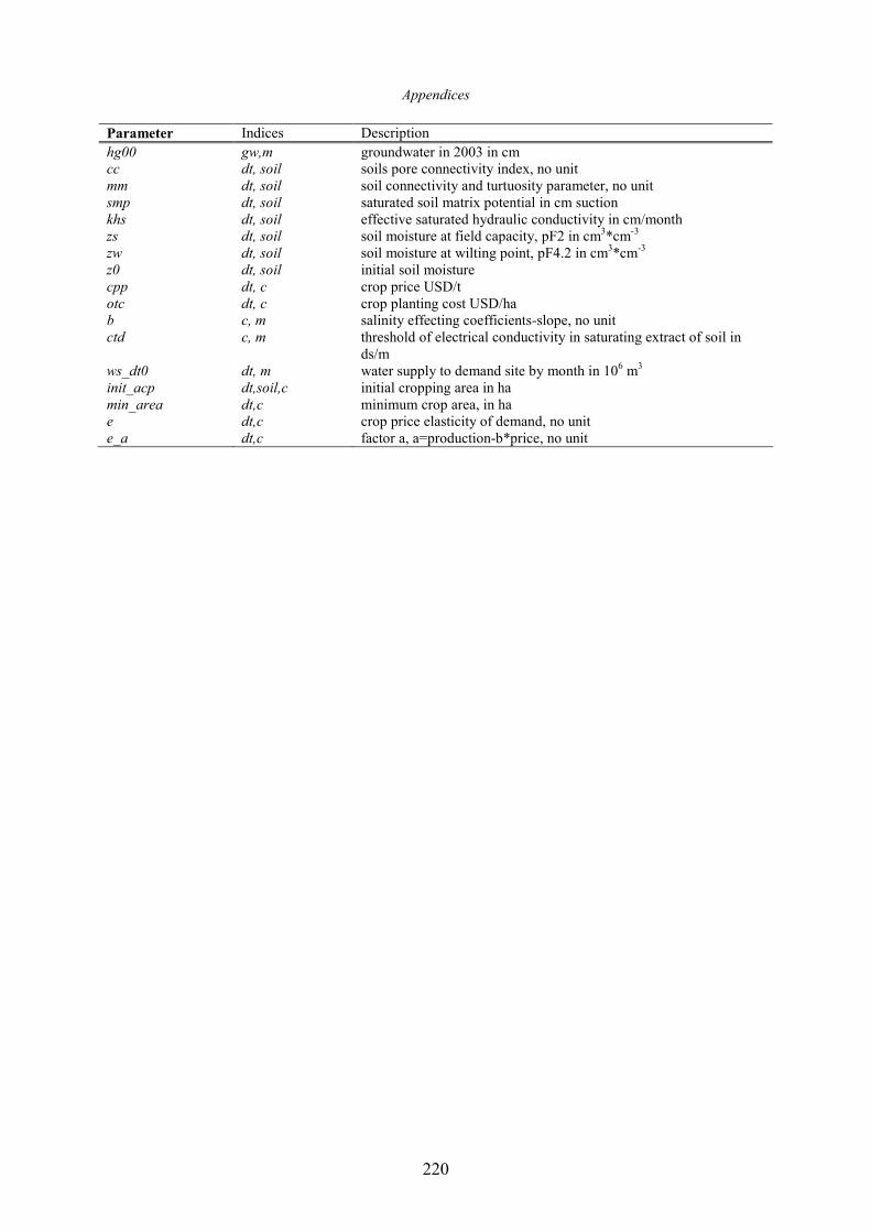
Appendices
220
Parameter Indices Description hg00 gw,m groundwater in 2003 in cm cc dt, soil soils pore connectivity index, no unit mm dt, soil soil connectivity and turtuosity parameter, no unit smp dt, soil saturated soil matrix potential in cm suction khs dt, soil effective saturated hydraulic conductivity in cm/month zs dt, soil soil moisture at field capacity, pF2 in cm3*cm-3 zw dt, soil soil moisture at wilting point, pF4.2 in cm3*cm-3 z0 dt, soil initial soil moisture cpp dt, c crop price USD/t otc dt, c crop planting cost USD/ha b c, m salinity effecting coefficients-slope, no unit ctd c, m threshold of electrical conductivity in saturating extract of soil in
ds/m ws_dt0 dt, m water supply to demand site by month in 106 m3 init_acp dt,soil,c initial cropping area in ha min_area dt,c minimum crop area, in ha e dt,c crop price elasticity of demand, no unit e_a dt,c factor a, a=production-b*price, no unit

221
Acknowledgement
I would like to express my deep gratitude to all the persons who have contributed to
this research. Without the support and guidance of numerous people this study would not
have been possible. I am grateful to my academic supervisors PD Dr. Peter Wehrheim and
Professor Dr. Bernd Diekkrüger. Dr. Wehrheim gave me the opportunity to perform my study
within the German-Uzbek Project. Without his encouragement I certainly would have
capitulate the balancing act between “growing family” and PhD.
I sincerely thank my tutor and mentor Dr. Cai Ximing for his valuable advice, constant
support and guidance of my research especially in the field of model development and on
hydrologic and agronomic aspects. I really enjoyed the short time I could spend at his Institute
of Civil and Environmental Engineering at the University of Illinois.
I am very indebted to Dr. Bernhard Tischbein for his tutorship. He comment my work
in great detail, gave valuable suggestions and supported me in the field of irrigation,
efficiencies and all groundwater and drainage related questions. I am thankful to Dr. Anik
Bhaduri for all his economy related advices; our former project coordinator Dr. Christopher
Martius and Susan Stromböm for their comments and proof reading of my work.
The research of this study was carried out within the ZEF/UNESCO project
“Economic and Ecologic Restructuring of Land- and Water Use in the Region Khorezm
(Uzbekistan): A Pilot Project in Development Research”, funded by the German Federal
Ministry of Education and Research. During that time I worked for several years as Research
Assistant for the project. For this time and the experiences, the internationality and
interdisciplinary work I am very thankful.
As a Doctoral Student of the PhD program “Bonn Interdisciplinary Graduate School
for Development Research (BiGS-DR)” I would like to express my gratitude to the Center for
Development Research (ZEF) at University of Bonn for the support, guidance and the
enjoyable experiences during my long time her at ZEF.
I would sincerely thank all those whom I failed to mention but also have contributed
to my work and working environment like the project staff members, colleagues at ZEF,
doctoral students, friends, many persons during my stay in Uzbekistan and office mates.
Finally I would like to thank my parents Eva and Ortwin Klebsch, my husband
Thomas and my children Jolina, Timon and Ruwen for their moral support, encouragement
and patience through all the years and up’s- and downs.