Embed Size (px)
Citation preview
UNIVERSITAT LINZJOHANNES KEPLER
JKU
Technisch-Naturwissenschaftliche
Fakultat
Analysis of single molecule microscopyimages with application to ultra-sensitive
microarrays
DISSERTATION
zur Erlangung des akademischen Grades
Doktorin
im Doktoratsstudium der
TECHNISCHEN WISSENSCHAFTEN
Eingereicht von:
Leila Muresan
Angefertigt am:
Institut fur Wissensbasierte Mathematische Systeme
Betreuung:
Univ.-Prof. Dr. Erich Peter Klement
A. Univ.-Prof. Dr. Gerhard Schutz
Linz, March 2010


Eidesstattliche Erklarung
Ich erklare an Eides statt, dass ich die vorliegende Dissertation selbststandig und
ohne fremde Hilfe verfasst, andere als die angegebenen Quellen und Hilfsmittel
nicht benutzt bzw. die wortlich oder sinngemaß entnommenen Stellen als solche
kenntlich gemacht habe.
Linz, 26.02.2010 Leila Muresan


Acknowledgment
First of all, I would like to express my deep gratitude to my supervisors, Prof.
Erich Peter Klement and Prof. Gerhard Schutz for the opportunity to discover an
exciting field of research and for the continuous guiding, support and encourage-
ment they provided during all these years.
I would like to thank the GEN-AU program of the Austrian Federal Ministry
of Education, Science and Culture for funding the research. Within this project,
I found the close cooperation with Dr. Jan Hesse and Dr. Jaroslaw Jacak very
enriching and motivating, and enjoyed the tremendous advantages of teamwork in
multidiciplinary research. I thank all the project members, colleagues from the
Biophysics Institute, (Johannes Kepler University, Linz), Dr. Alois Sonnleitner
and the Center for Biomedical Nanotechnology, Upper Austrian Research GmbH,
Prof. Anna-Maria Frischauf and Prof. Fritz Aberger at the Department of Molec-
ular Biology, Division of Genomics, (University of Salzburg) and Prof. Hannes
Stockinger and his team at the Department of Molecular Immunology, (Medical
University of Vienna) for the interesting discussions and the inspiration they pro-
vided.
I am very grateful to Dr. Irene Tiemann-Boege for explaining me the biological
background and relevance of microarrays, as well as for all the help and advices
she provided, and the careful reviewing of the biology related part of this thesis.
I would like to thank DI. Bettina Heise for the collaboration during the whole
project, and all my colleagues and friends for the great time spent together. I have
a very special thought for Sabine Lumpi for all the help in (not only) administrative
matters.
Finally, I thank Jerome and my family for everything.

Contents
Abstract 5
List of symbols 7
1 Introduction 15
1.1 Context . . . . . . . . . . . . . . . . . . . . . . . . . . . . . . . . . 15
1.2 Motivation . . . . . . . . . . . . . . . . . . . . . . . . . . . . . . . . 16
1.3 Outline of the thesis . . . . . . . . . . . . . . . . . . . . . . . . . . 17
2 Single molecule imaging: techniques and models 19
2.1 Fluorescence and fluorophores . . . . . . . . . . . . . . . . . . . . . 19
2.2 Microscopy techniques . . . . . . . . . . . . . . . . . . . . . . . . . 22
2.3 Image formation . . . . . . . . . . . . . . . . . . . . . . . . . . . . . 23
Point spread function (PSF) and spatial resolution . . . . . . . . . 24
Noise sources and signal-to-noise ratio (SNR) . . . . . . . . . . . . 25
Models of image formation . . . . . . . . . . . . . . . . . . . . . . . 27
3 Microarrays with single molecule sensitivity 29
3.1 Biological background . . . . . . . . . . . . . . . . . . . . . . . . . 29
3.2 Classical microarray technology . . . . . . . . . . . . . . . . . . . . 31
Measurement process . . . . . . . . . . . . . . . . . . . . . . . . . . 31
Data analysis . . . . . . . . . . . . . . . . . . . . . . . . . . . . . . 33
Limitations of microarray technology . . . . . . . . . . . . . . . . . 34
Types of arrays . . . . . . . . . . . . . . . . . . . . . . . . . . . . . 35
3.3 The high resolution technique . . . . . . . . . . . . . . . . . . . . . 36
Imaging setup . . . . . . . . . . . . . . . . . . . . . . . . . . . . . . 37
Main steps in single molecule microarray image analysis . . . . . . . 38
Mathematical model . . . . . . . . . . . . . . . . . . . . . . . . . . 40
1
2 CONTENTS
4 Multiscale signal decomposition 45
4.1 Continuous wavelet transform . . . . . . . . . . . . . . . . . . . . . 45
4.2 Frames . . . . . . . . . . . . . . . . . . . . . . . . . . . . . . . . . . 48
4.3 Multi-resolution analysis . . . . . . . . . . . . . . . . . . . . . . . . 52
4.4 Generalizations of MRA to two dimensions . . . . . . . . . . . . . . 55
4.5 B-spline frames . . . . . . . . . . . . . . . . . . . . . . . . . . . . . 57
4.6 Fast wavelet transform algorithms via filter banks . . . . . . . . . . 59
4.7 Translation invariance . . . . . . . . . . . . . . . . . . . . . . . . . 61
Undecimated wavelet transform . . . . . . . . . . . . . . . . . . . . 62
Isotropic undecimated wavelet transform . . . . . . . . . . . . . . . 63
5 Wavelet based detection 65
5.1 Statistical applications of wavelet transforms . . . . . . . . . . . . . 65
5.2 Wavelet coefficient estimation . . . . . . . . . . . . . . . . . . . . . 68
5.3 Wavelet thresholding . . . . . . . . . . . . . . . . . . . . . . . . . . 69
5.4 Signal sparsity . . . . . . . . . . . . . . . . . . . . . . . . . . . . . . 72
5.5 Threshold selection . . . . . . . . . . . . . . . . . . . . . . . . . . . 73
Universal threshold . . . . . . . . . . . . . . . . . . . . . . . . . . . 74
SURE . . . . . . . . . . . . . . . . . . . . . . . . . . . . . . . . . . 75
Bayesian thresholding . . . . . . . . . . . . . . . . . . . . . . . . . . 76
False Discovery Rate . . . . . . . . . . . . . . . . . . . . . . . . . . 77
Variance - covariance estimation . . . . . . . . . . . . . . . . . . . . 79
5.6 Other noise models . . . . . . . . . . . . . . . . . . . . . . . . . . . 80
5.7 Single molecule detection and evaluation of the detection method . 81
5.8 Signal detection via robust distance thresholding . . . . . . . . . . . 84
6 Spatial patterns 91
6.1 Introduction to spatial point processes . . . . . . . . . . . . . . . . 92
Moments of point processes . . . . . . . . . . . . . . . . . . . . . . 93
Point process operations . . . . . . . . . . . . . . . . . . . . . . . . 95
Point process models . . . . . . . . . . . . . . . . . . . . . . . . . . 96
6.2 Summary characteristics for (stationary)
point processes . . . . . . . . . . . . . . . . . . . . . . . . . . . . . 98
6.3 Testing in the framework of point patterns . . . . . . . . . . . . . . 100
6.4 Estimation of hybridization signal . . . . . . . . . . . . . . . . . . . 103
Analysis of count data via the method of moments . . . . . . . . . 105
CONTENTS 3
Expectation maximization (EM) based on Kth nearest neighbor
distances . . . . . . . . . . . . . . . . . . . . . . . . . . . . . 107
Segmentation of point processes based on a level set approach . . . 110
6.5 Evaluation of concentration estimation . . . . . . . . . . . . . . . . 114
7 Results of microarray analysis with single molecule sensitivity 119
7.1 Validation on simulated data . . . . . . . . . . . . . . . . . . . . . . 119
Simulation images . . . . . . . . . . . . . . . . . . . . . . . . . . . . 119
Classical microarray methods applied to downsampled simulation
data . . . . . . . . . . . . . . . . . . . . . . . . . . . . . . . 121
Correlation tests . . . . . . . . . . . . . . . . . . . . . . . . . . . . 125
7.2 Oligonucleotide dilution series . . . . . . . . . . . . . . . . . . . . . 129
7.3 Gene expression in multiple myeloma data . . . . . . . . . . . . . . 131
8 Conclusion 133
8.1 Summary . . . . . . . . . . . . . . . . . . . . . . . . . . . . . . . . 133
8.2 Outlook . . . . . . . . . . . . . . . . . . . . . . . . . . . . . . . . . 135
A Outliers and variance-covariance estimators 137
A.1 One-dimensional robust estimators of location and scale . . . . . . . 139
A.2 Robust covariance matrix estimation . . . . . . . . . . . . . . . . . 140
A.3 Distributions of Mahalanobis distances . . . . . . . . . . . . . . . . 143
Bibliography 155

4 CONTENTS
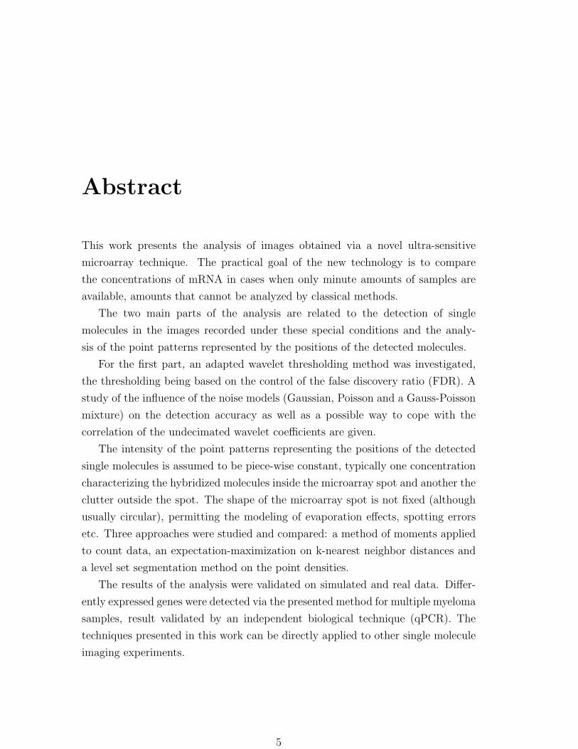
Abstract
This work presents the analysis of images obtained via a novel ultra-sensitive
microarray technique. The practical goal of the new technology is to compare
the concentrations of mRNA in cases when only minute amounts of samples are
available, amounts that cannot be analyzed by classical methods.
The two main parts of the analysis are related to the detection of single
molecules in the images recorded under these special conditions and the analy-
sis of the point patterns represented by the positions of the detected molecules.
For the first part, an adapted wavelet thresholding method was investigated,
the thresholding being based on the control of the false discovery ratio (FDR). A
study of the influence of the noise models (Gaussian, Poisson and a Gauss-Poisson
mixture) on the detection accuracy as well as a possible way to cope with the
correlation of the undecimated wavelet coefficients are given.
The intensity of the point patterns representing the positions of the detected
single molecules is assumed to be piece-wise constant, typically one concentration
characterizing the hybridized molecules inside the microarray spot and another the
clutter outside the spot. The shape of the microarray spot is not fixed (although
usually circular), permitting the modeling of evaporation effects, spotting errors
etc. Three approaches were studied and compared: a method of moments applied
to count data, an expectation-maximization on k-nearest neighbor distances and
a level set segmentation method on the point densities.
The results of the analysis were validated on simulated and real data. Differ-
ently expressed genes were detected via the presented method for multiple myeloma
samples, result validated by an independent biological technique (qPCR). The
techniques presented in this work can be directly applied to other single molecule
imaging experiments.
5

6 CONTENTS
Die vorliegende Arbeit prasentiert ein Bildanalyseverfahren, das fur eine neuar-
tige hochempfindliche Microarray-Technik entwickelt wurde. Das praktische Ziel
dieser neuen Technologie ist es, die Konzentration von mRNA in jenen Fallen zu
vergleichen, wo nur so geringe Probenmengen zur Verfugung stehen, daß diese
nicht durch klassische Methoden analysiert werden konnen.
Die beiden Hauptaufgaben der Analyse sind einerseits die Erkennung einzel-
ner Molekule unter den besonderen Bedingungen, die durch die neue Technologie
impliziert werden, und andererseits die Analyse der Punktmuster, welche die Po-
sitionen der erkannten Molekule reprasentieren.
Fur die erste Aufgabe wurde eine adaptierte Wavelet Thresholding Methode
verwendet, wobei die Schwellwerte auf der Kontrolle des False Discovery Ratio
(FDR) basierten. Es wurde sowohl der Einfluss von Rausch-Modellen (Gauß, Pois-
son und ein Gauß-Poisson Kombination) auf die Genauigkeit der Erkennung von
einzelnen Molekulen untersucht als auch ein moglicher Weg, um der Korrelation
der Undecimated Wavelet Koeffizienten gerecht zu werden.
Die Intensitat der Punktmuster, welche die Positionen der erkannten Molekule
reprasentieren, wird als stuckweise konstant angenommen, wobei typischerweise
eine Konzentration die hybridisierten Molekule im Microarray-Spot und eine
andere Konzentration die Stordaten außerhalb charakterisiert. Die Form des
Microarray-Spots ist nicht festgelegt (obwohl sie als kreisformig angenommen
wird), was es unter anderem ermoglicht, Verdunstungseffekte oder Spotting Fehler
zu modellieren.
Drei Ansatze wurden untersucht und verglichen: Eine Methode der Momente
angewandt auf Haufigkeitsdaten, eine Expectation-Maximization von k-NN Dis-
tanzen und eine Level Set Segmentation Methode auf den Punktdichten.
Die Ergebnisse der Analyse wurden anhand simulierter und realer Daten vali-
diert. Das vorgestellte Verfahren erkannte unterschiedliech exprimierte Gene fur
Proben des Multiplen Myeloms und das Resultat durch eine unabhangige biologis-
che Technik (qPCR) nachgewiesen. Die in dieser Arbeit vorgestellten Techniken
konnen auch direkt bei anderen Einzelmolekulfluoreszenz-Experimente angewen-
det werden.

List of symbols
⊥ Orthogonality U⊥V : ∀u ∈ U, v ∈ V, 〈u, v〉 = 0
+ Direct sum U+V = u+ v | u ∈ U, v ∈ V, U ∩ V = 0
〈f, g〉 Inner product 〈f, g〉 :=∫f(x)g(x) dx
E(X) Expectation of a random variable X
Ff(ω) Fourier transform Ff(ω) = f(ω) = 1√2π
∫f(x)e−ixω dx
N (µ, σ) Normal distribution with mean µ and variance σ2
Poi(µ) Poisson distribution of parameter µ
| A | Cardinality of the set A
⊕ Orthogonal sum U ⊕ V = U+V, and U⊥V
⊗ Tensor product
x Estimator of x
x Empiric value of x
f ∗ g Convolution (g ∗ f)(t) :=∫g(t− s)f(s) ds
i.i.d. Independent and identically distributed
7

8 CONTENTS

List of Figures
2.1 Jablonski diagram showing photophysical transitions. . . . . . . . . 20
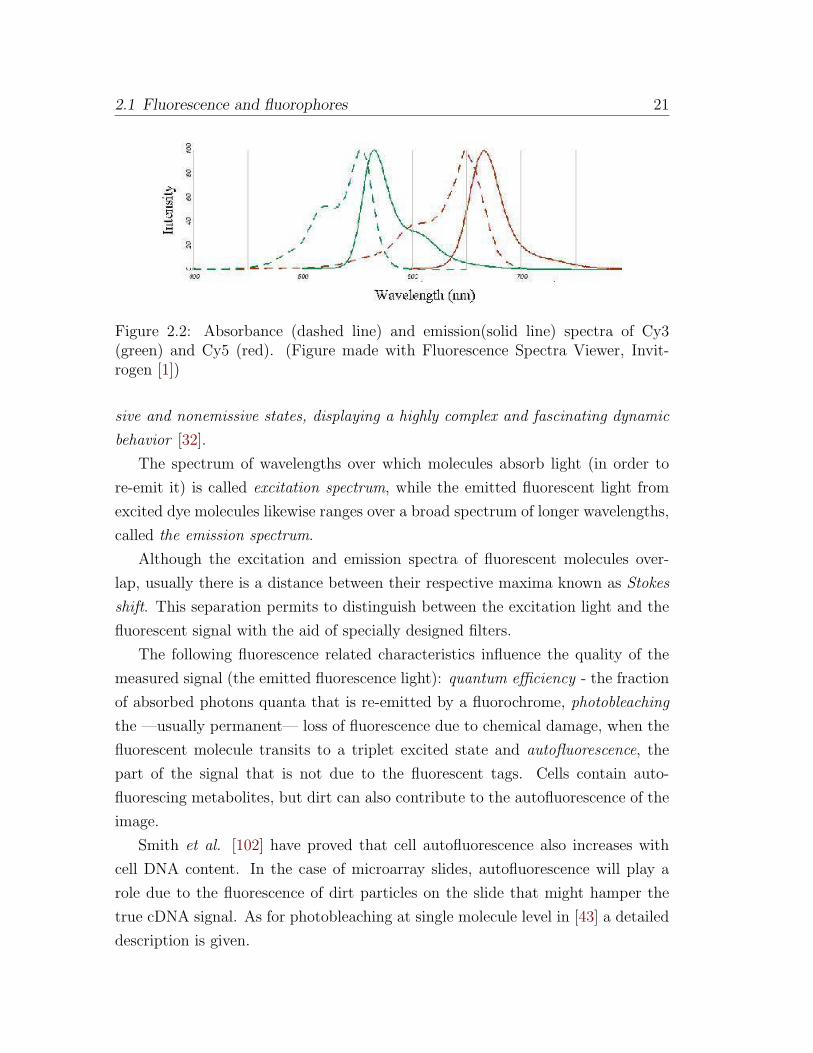
2.2 Absorbance (dashed line) and emission(solid line) spectra of Cy3
(green) and Cy5 (red). (Figure made with Fluorescence Spectra
Viewer, Invitrogen [1]) . . . . . . . . . . . . . . . . . . . . . . . . . 21
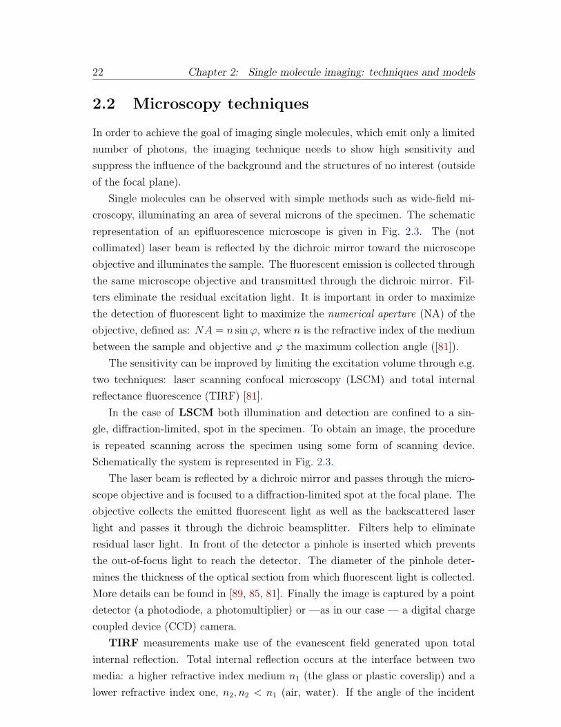
2.3 Microscope configurations: left - epifluorescence, middle – confocal,
right - TIRF . . . . . . . . . . . . . . . . . . . . . . . . . . . . . . . 23
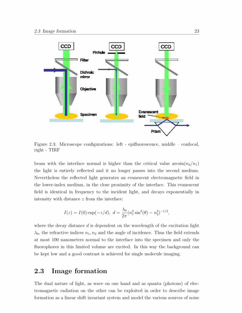
2.4 The Airy function - image of a point source . . . . . . . . . . . . . 24
3.1 Central dogma of molecular biology . . . . . . . . . . . . . . . . . . 30
3.2 Genes, the units of biological inheritance. Figure from [2]. . . . . . 30
3.3 Schematic representation of two-color microarray technology. Fig-
ure from [2]. . . . . . . . . . . . . . . . . . . . . . . . . . . . . . . 32
3.4 Detail of microarray. Pseudocolors indicate: red - high expression
in target labeled with Cy5, green - high expression in target labeled
with Cy3, yellow - similar expression in both samples. The gene is
identified by the position of the respective spot in the grid. . . . . 33
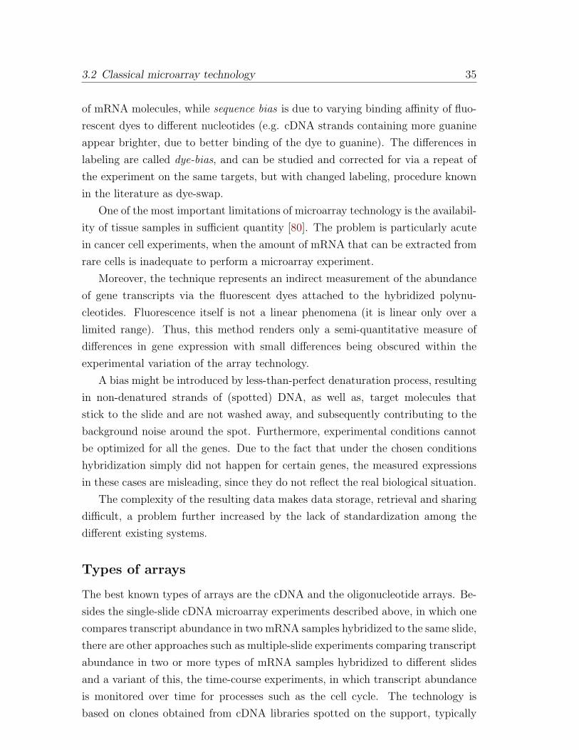
3.5 Image of a microarray spot with artifacts. (Left) Low resolution
image, with high intensity pixels (without visual clues for presence
of artifacts) (Right) High resolution image, where the artifact can
be distinguished from signal. The image intensity was rescaled for
better visibility. . . . . . . . . . . . . . . . . . . . . . . . . . . . . . 37
3.6 Nanoscout - the high resolution setup used in microarray imaging . 37
3.7 Analysis of a spot in a high-resolution microarray image. (a) Orig-
inal image, bright features correspond to molecules bound to the
chip. (b) Detection of single molecules. (c) Selection of single
molecule locations (local maxima on denoised image inside the de-
tection support in (b)). (d) Separation of hybridization signal from
clutter. . . . . . . . . . . . . . . . . . . . . . . . . . . . . . . . . . 40
9
10 LIST OF FIGURES
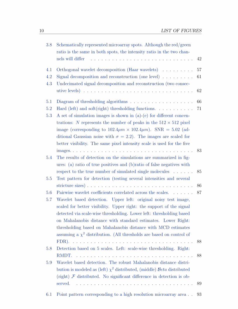
3.8 Schematically represented microarray spots. Although the red/green
ratio is the same in both spots, the intensity ratio in the two chan-
nels will differ . . . . . . . . . . . . . . . . . . . . . . . . . . . . . 42
4.1 Orthogonal wavelet decomposition (Haar wavelets) . . . . . . . . . 57
4.2 Signal decomposition and reconstruction (one level) . . . . . . . . . 61
4.3 Undecimated signal decomposition and reconstruction (two consec-
utive levels) . . . . . . . . . . . . . . . . . . . . . . . . . . . . . . . 62
5.1 Diagram of thresholding algorithms . . . . . . . . . . . . . . . . . . 66
5.2 Hard (left) and soft(right) thresholding functions. . . . . . . . . . . 71
5.3 A set of simulation images is shown in (a)-(e) for different concen-
trations: N represents the number of peaks in the 512 × 512 pixel
image (corresponding to 102.4µm × 102.4µm). SNR = 5.02 (ad-
ditional Gaussian noise with σ = 2.2). The images are scaled for
better visibility. The same pixel intensity scale is used for the five
images. . . . . . . . . . . . . . . . . . . . . . . . . . . . . . . . . . . 83
5.4 The results of detection on the simulations are summarized in fig-
ures: (a) ratio of true positives and (b)ratio of false negatives with
respect to the true number of simulated single molecules . . . . . . 85
5.5 Test pattern for detection (testing several intensities and several
stricture sizes) . . . . . . . . . . . . . . . . . . . . . . . . . . . . . . 86
5.6 Pairwise wavelet coefficients correlated across the scales. . . . . . . 87
5.7 Wavelet based detection. Upper left: original noisy test image,
scaled for better visibility. Upper right: the support of the signal
detected via scale-wise thresholding. Lower left: thresholding based
on Mahalanobis distance with standard estimates. Lower Right:
thresholding based on Mahalanobis distance with MCD estimates
assuming a χ2 distribution. (All thresholds are based on control of
FDR). . . . . . . . . . . . . . . . . . . . . . . . . . . . . . . . . . . 88
5.8 Detection based on 5 scales. Left: scale-wise thresholding. Right:
RMDT. . . . . . . . . . . . . . . . . . . . . . . . . . . . . . . . . . 88
5.9 Wavelet based detection. The robust Mahalanobis distance distri-
bution is modeled as (left) χ2 distributed, (middle) Beta distributed(right) F distributed. No significant difference in detection is ob-
served. . . . . . . . . . . . . . . . . . . . . . . . . . . . . . . . . . 89
6.1 Point pattern corresponding to a high resolution microarray area . . 93
LIST OF FIGURES 11
6.2 Summaries for the point pattern in Fig. 6.1 (different colors corre-
spond to different edge correction methods) . . . . . . . . . . . . . 100
6.3 Testing the CSR hypothesis . . . . . . . . . . . . . . . . . . . . . . 102
6.4 The density function of kNN distance Dk(λ1, λ2) for the spatial
Poisson mixture with concentrations λ1 inside and λ2 outside the
spot, respectively. . . . . . . . . . . . . . . . . . . . . . . . . . . . 108
6.5 Background/foreground separation of peaks for three different con-
centrations via the EM method applied to the Kth nearest neigh-
bour distances. . . . . . . . . . . . . . . . . . . . . . . . . . . . . . 109
6.6 Anomalous shape detection. A high concentration donut shape was
simulated on a background formed of low concentration clutter. The
proposed approach is able to separate signal from clutter. . . . . . 110
6.7 Nadaraya-Watson kernel smoothing . . . . . . . . . . . . . . . . . . 113
6.8 Segmentation of the point patterns via level sets for three choices
of smoothing bandwidths (red: h = hiq, green h = 1/4hiq and blue
h = 1/10hiq) . . . . . . . . . . . . . . . . . . . . . . . . . . . . . . . 114
6.9 Concentration estimation results for the MOM and EM method on
simulated data. The true λ values are represented as a stair-case
function and for better visibility, the estimation results were slightly
shifted on the abscissa. . . . . . . . . . . . . . . . . . . . . . . . . . 116
6.10 Concentration estimation results for the level set based method on
simulated data. The true λ values are represented as a stair-case
function and for better visibility, the estimation results were slightly
shifted on the abscissa. . . . . . . . . . . . . . . . . . . . . . . . . . 117
6.11 Mean squared error of the proposed algorithms over the range of
signal λ1 and clutter λ2 concentrations. The EM algorithm has the
best performance, followed by MOM and level sets with reestimated
concentrations. . . . . . . . . . . . . . . . . . . . . . . . . . . . . . 118
7.1 Simulation of microarray spots. Peak concentrations: left: 0.005
peaks/pixel inside the spot and 0.0005 peaks/pixel outside the spot,
right: 0.01 peaks/pixel inside the spot and 0.0025 peaks/pixel out-
side the spot . . . . . . . . . . . . . . . . . . . . . . . . . . . . . . . 120
7.2 Scanned oligonucleotide spots (dilution: 0.8 and 8 amol/80µl) . . . 121
12 LIST OF FIGURES
7.3 Simulation of microarrays spots. Left column: spots at single
molecule resolution (200nm pixel size) with different peak con-
centrations (λ) inside each spot. Starting from the first row up
till the fourth down: λ = 0.005, 0.007, 0.009, 011 peaks per pixel.
(Background concentration representing dirt, unspecific binding
etc.: 0.003 peaks per pixel). Middle column: the same spots down-
sampled to 4µm, the size used by existing commercial microarray
systems. Right column: The original spots, denoised via wavelet
thresholding and then downsampled to 4µm. . . . . . . . . . . . . 126
7.4 Correlations between the estimated and the true signal concentra-
tions for the three high resolution algorithms: MOM, EM and level
sets. The arrow indicates the correlation coefficient corresponding
to the images in Fig. 7.3. . . . . . . . . . . . . . . . . . . . . . . . 127
7.5 Correlations between the estimated and the true signal concentra-
tions. The single molecule analysis performs better than the analy-
sis on the downscaled data (original and denoised via wavelet thresh-
olding). The arrow indicates the correlation coefficient correspond-
ing to the images in Fig. 7.3. . . . . . . . . . . . . . . . . . . . . . 128
7.6 Comparison of the concentration estimates for the dilution series in
case of six low resolution algorithms . . . . . . . . . . . . . . . . . . 130
7.7 Comparison of the concentration estimates for the dilution series in
case of the three high resolution algorithms . . . . . . . . . . . . . . 130
7.8 The expression profiles of several side population genes showing
repressors and over-expressers. The repressed genes like CSEN,
CCT6A and CASQ1 were either not analyzed with the qPCR
method or showed not interpretable results. Rest of the presented
genes show a higher expression level, and are in a good agreement
with the microarray results . . . . . . . . . . . . . . . . . . . . . . . 132
A.1 (Left) Hawkins-Bradu-Kass 3d data. (Right) p-values of the data
plotted against the data index. The first 14 points represent outliers.138
LIST OF FIGURES 13
A.2 (Left) p-values of the robust Mahalanobis distances for the HBK
data. (Right) The Mahalanobis distances for the HBK data com-
puted according to (A.0.1) with the standard location and scatter
estimates plotted against the robust Mahalanobis distance (MCD
estimates). The 14 representing outliers are easily identifiable in
the case of robust distances (y axis), and blend in the rest of the
data for the standard estimates (x axis). . . . . . . . . . . . . . . . 139

14 LIST OF FIGURES
Chapter 1
Introduction
The aim of this work is to provide efficient tools for the analysis of single molecules
and the patterns they form in fluorescence microscopy images in general and ultra-
sensitive microarray scans in particular. The features of interest are fluorescent-
tagged single molecules, their image being typically equivalent to diffraction limited
point sources. The number, intensity and relative positions of single molecules,
and at a different scale, the various pattern these single molecules form represent
a source of information that can be exploited in inference on biological processes.
This information is not available in classical, lower resolution microscopy imag-
ing, in which case only an aggregated signal intensity is being measured. In or-
der to achieve detection of single molecules, high resolution and high sensitivity
images have to be obtained through a set of techniques affecting the resulting
two-dimensional signal. These techniques introduce new challenges including the
handling of significantly bigger images that correspond to the same scanned sample
size and also of a different imaging regime. Single molecule imaging is character-
ized by different dynamic range and under certain conditions by low signal-to-noise
ratios as well as a different impact of the Poisson and Gaussian measurement noise
on the recorded signal.
1.1 Context
The work presented in this thesis was performed in the frame of the multidisci-
plinary project Ultra-sensitive genomics and proteomics funded by Genome Re-
search - Austria including the following project partners
• Biophysics Institute - Johannes Kepler University of Linz
15
16 Chapter 1: Introduction
• Upper Austrian Research GmbH - Linz
• Department of Knowledge-based Mathematical Systems - Johannes Kepler
University of Linz
• Department of Molecular Biology - University of Salzburg
• Department of Molecular Immunology - Medical University of Vienna
The biological expertise was provided and the biological samples prepared by the
partners at the Department of Molecular Biology, University of Salzburg. The
ultra-sensitive microarray technique was developed and perfected by the Biophysics
Institute at Johannes Kepler University, Linz and Upper Austrian Research GmbH,
Linz. This work was done in close collaboration with Dr. Jan Hesse and Dr.
Jaroslaw Jacak and the project coordinator Dr. Gerhard Schutz.
1.2 Motivation
We shall motivate the technique of ultra-sensitive microarrays via the example of
the cancer stem cells (CSC) hypothesis [110].
The hypothesis received much attention recently and it states that tumors are
initiated by a small population of tumor cells similar to adult stem cells, that have
the ability to self-renew as well as give rise to differentiated tissue cells. Knowledge
of the gene expression profile of these special CSC is crucial in understanding
the biological mechanisms at work and in development of effective therapies. A
quite well established way to determine the expression profile is the microarray
technique that will be described in Chapter 3. The technique offers the advantage
of studying thousands of genes in the frame of a single experiment, thus under
identical experimental conditions. However it has several drawbacks, one of the
most restrictive in our case being the relatively important quantity of target sample
mRNA necessary for a reliable analysis. Since the fraction of CSC might be as
low as 1% [46] the classical microarray technique cannot be applied directly to the
minute amount of mRNA obtained from CSC.
In order to alleviate the restriction imposed by the small amount of avail-
able mRNA, the microarray technology is combined with high resolution imaging.
Thanks to the development of the Nanoreader [56], a fast and highly sensitive
imaging system, the scanning of areas of 1 × 0.2 cm2 at a pixel size of 200 nm
1.3 Outline of the thesis 17
became possible within 50 seconds, with a good ability to discriminate among
minute differences.
The resulting high resolution images of microarray spots can be understood
as a zoom in the classical, low-resolution microarray images and are formed of
single molecules clustered in a circular pattern, representing the hybridized single
molecules of interest corresponding to one gene. The analysis of this new kind
of images and the estimation of the hybridization signal makes the object of the
present work.
1.3 Outline of the thesis
Excluding this introduction, the thesis consists of seven chapters. The outline of
the chapters is given in the following.
The principles of fluorescence microscopy with focus on single molecule imaging
are presented in Chapter 2. Mathematical models of image formation as well as
single molecule image content are proposed in the end of the chapter. The next
chapter, Chapter 3 gives an overview of the microarray technology, together with
a discussion of the importance of the method, its advantages and the challenges
of the classical low-resolution approach.
The following two chapters are related to single molecule detection in the flu-
orescence microscopy images. First, Chapter 4 sets the framework for denoising
and detection via a brief introduction to wavelet transforms, then in Chapter 5
a detailed discussion of wavelet thresholding as an approach to denoising and de-
tection is given, together with several methods for threshold selection, adaptation
to specific noise models and effect of signal sparsity on detection. The discussion
emphasizes detection approaches and results for the models described in Chapter 2.
After the detection of single molecules, we estimate the concentration of the
hybridized molecules inside the microarray spot. This new hybridization measure
requires the separation of molecules bound to the microarray spot from unspecific
binding, dirt etc. outside of it. The modeling of the problem is based on spatial
point patterns and is described in Chapter 6 together with the algorithms that
separate two superposed point patterns (signal and clutter) based on the intensities
of the two processes.
The validation of the method of ultra-sensitive microarray technique is done
through analysis based on simulated images and image series as well as on real
data. The real data includes microarray images of oligonucleotide dilution series

18 Chapter 1: Introduction
and the scans of three competitively hybridized slides pertaining to an experiment
on multiple myeloma stem cells. The results are gathered in Chapter 7.
The last chapter of the thesis, Chapter 8, summarizes problems discussed in
this work as well as the proposed methods and concludes with possible applications
of the algorithms presented and indicates further lines of research.

Chapter 2
Single molecule imaging:
techniques and models
The main purpose of microscopic imaging is to detect small structures and visualize
their dynamics. Although other techniques can achieve the same or even higher
resolution (e.g. electron microscopy, atomic force microscopy etc.), fluorescence
microscopy is the most important in vivo approach, that can operate in biologically
relevant condition, without (or only minimally) disturbing the observed process.
Moreover the great specificity and ease of use make fluorescence microscopy the
main light microscopy tool in biomedical research.
In 1976, Hirschfeld achieved the first successful detection of single molecules
in solution [57] (although marking the molecule with multiple labels) and ever
since the field has received increasing attention in the fluorescence microscopy
community.
2.1 Fluorescence and fluorophores
The information offered by a typical light microscope is the intensity of light emit-
ted by an object, measured after having passed through an optical system. In the
case of fluorescence microscopy, the light is emitted by specific molecules, called
fluorophores, fluorochromes or fluorescent dyes that have the property that after
excitation with light at a certain wavelength as a response emit light at a longer
wavelength. If the molecules of interest are nonfluorescent, they can be tagged
with a fluorescent dye to make them visible. Various labeling methods have been
developed, like epitope tagging (inserting short DNA sequences of known epitopes
into the coding sequences of proteins), fluorescent proteins (the best known being
19
20 Chapter 2: Single molecule imaging: techniques and models
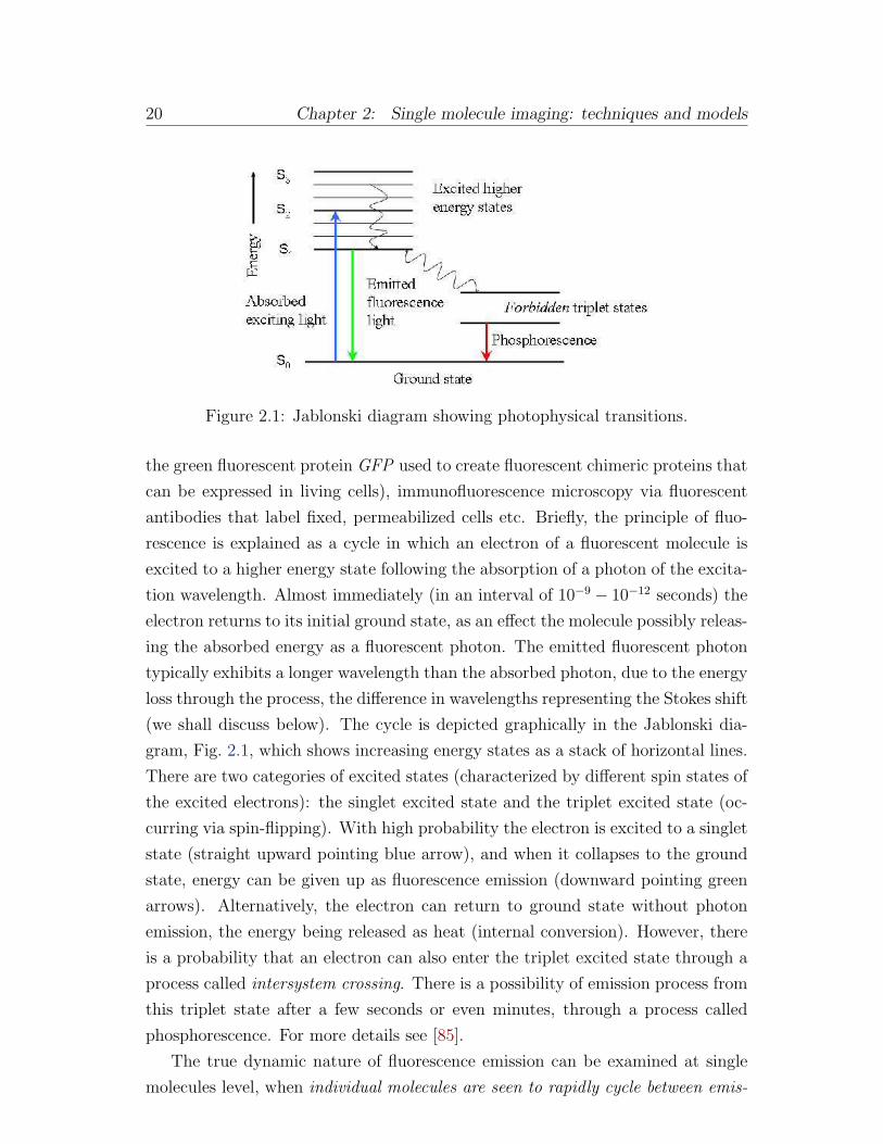
Figure 2.1: Jablonski diagram showing photophysical transitions.
the green fluorescent protein GFP used to create fluorescent chimeric proteins that
can be expressed in living cells), immunofluorescence microscopy via fluorescent
antibodies that label fixed, permeabilized cells etc. Briefly, the principle of fluo-
rescence is explained as a cycle in which an electron of a fluorescent molecule is
excited to a higher energy state following the absorption of a photon of the excita-
tion wavelength. Almost immediately (in an interval of 10−9 − 10−12 seconds) the
electron returns to its initial ground state, as an effect the molecule possibly releas-
ing the absorbed energy as a fluorescent photon. The emitted fluorescent photon
typically exhibits a longer wavelength than the absorbed photon, due to the energy
loss through the process, the difference in wavelengths representing the Stokes shift
(we shall discuss below). The cycle is depicted graphically in the Jablonski dia-
gram, Fig. 2.1, which shows increasing energy states as a stack of horizontal lines.
There are two categories of excited states (characterized by different spin states of
the excited electrons): the singlet excited state and the triplet excited state (oc-
curring via spin-flipping). With high probability the electron is excited to a singlet
state (straight upward pointing blue arrow), and when it collapses to the ground
state, energy can be given up as fluorescence emission (downward pointing green
arrows). Alternatively, the electron can return to ground state without photon
emission, the energy being released as heat (internal conversion). However, there
is a probability that an electron can also enter the triplet excited state through a
process called intersystem crossing. There is a possibility of emission process from
this triplet state after a few seconds or even minutes, through a process called
phosphorescence. For more details see [85].
The true dynamic nature of fluorescence emission can be examined at single
molecules level, when individual molecules are seen to rapidly cycle between emis-
2.1 Fluorescence and fluorophores 21
Figure 2.2: Absorbance (dashed line) and emission(solid line) spectra of Cy3(green) and Cy5 (red). (Figure made with Fluorescence Spectra Viewer, Invit-rogen [1])
sive and nonemissive states, displaying a highly complex and fascinating dynamic
behavior [32].
The spectrum of wavelengths over which molecules absorb light (in order to
re-emit it) is called excitation spectrum, while the emitted fluorescent light from
excited dye molecules likewise ranges over a broad spectrum of longer wavelengths,
called the emission spectrum.
Although the excitation and emission spectra of fluorescent molecules over-
lap, usually there is a distance between their respective maxima known as Stokes
shift. This separation permits to distinguish between the excitation light and the
fluorescent signal with the aid of specially designed filters.
The following fluorescence related characteristics influence the quality of the
measured signal (the emitted fluorescence light): quantum efficiency - the fraction
of absorbed photons quanta that is re-emitted by a fluorochrome, photobleaching
the —usually permanent— loss of fluorescence due to chemical damage, when the
fluorescent molecule transits to a triplet excited state and autofluorescence, the
part of the signal that is not due to the fluorescent tags. Cells contain auto-
fluorescing metabolites, but dirt can also contribute to the autofluorescence of the
image.
Smith et al. [102] have proved that cell autofluorescence also increases with
cell DNA content. In the case of microarray slides, autofluorescence will play a
role due to the fluorescence of dirt particles on the slide that might hamper the
true cDNA signal. As for photobleaching at single molecule level in [43] a detailed
description is given.
22 Chapter 2: Single molecule imaging: techniques and models
2.2 Microscopy techniques
In order to achieve the goal of imaging single molecules, which emit only a limited
number of photons, the imaging technique needs to show high sensitivity and
suppress the influence of the background and the structures of no interest (outside
of the focal plane).
Single molecules can be observed with simple methods such as wide-field mi-
croscopy, illuminating an area of several microns of the specimen. The schematic
representation of an epifluorescence microscope is given in Fig. 2.3. The (not
collimated) laser beam is reflected by the dichroic mirror toward the microscope
objective and illuminates the sample. The fluorescent emission is collected through
the same microscope objective and transmitted through the dichroic mirror. Fil-
ters eliminate the residual excitation light. It is important in order to maximize
the detection of fluorescent light to maximize the numerical aperture (NA) of the
objective, defined as: NA = n sinϕ, where n is the refractive index of the medium
between the sample and objective and ϕ the maximum collection angle ([81]).
The sensitivity can be improved by limiting the excitation volume through e.g.
two techniques: laser scanning confocal microscopy (LSCM) and total internal
reflectance fluorescence (TIRF) [81].
In the case of LSCM both illumination and detection are confined to a sin-
gle, diffraction-limited, spot in the specimen. To obtain an image, the procedure
is repeated scanning across the specimen using some form of scanning device.
Schematically the system is represented in Fig. 2.3.
The laser beam is reflected by a dichroic mirror and passes through the micro-
scope objective and is focused to a diffraction-limited spot at the focal plane. The
objective collects the emitted fluorescent light as well as the backscattered laser
light and passes it through the dichroic beamsplitter. Filters help to eliminate
residual laser light. In front of the detector a pinhole is inserted which prevents
the out-of-focus light to reach the detector. The diameter of the pinhole deter-
mines the thickness of the optical section from which fluorescent light is collected.
More details can be found in [89, 85, 81]. Finally the image is captured by a point
detector (a photodiode, a photomultiplier) or —as in our case — a digital charge
coupled device (CCD) camera.
TIRF measurements make use of the evanescent field generated upon total
internal reflection. Total internal reflection occurs at the interface between two
media: a higher refractive index medium n1 (the glass or plastic coverslip) and a
lower refractive index one, n2, n2 < n1 (air, water). If the angle of the incident
2.3 Image formation 23
Figure 2.3: Microscope configurations: left - epifluorescence, middle – confocal,right - TIRF
beam with the interface normal is higher than the critical value arcsin(n2/n1)
the light is entirely reflected and it no longer passes into the second medium.
Nevertheless the reflected light generates an evanescent electromagnetic field in
the lower-index medium, in the close proximity of the interface. This evanescent
field is identical in frequency to the incident light, and decays exponentially in
intensity with distance z from the interface:
I(z) = I(0) exp(−z/d), d =λ02π
(n21 sin
2(θ)− n22)−1/2,
where the decay distance d is dependent on the wavelength of the excitation light
λ0, the refractive indices n1, n2 and the angle of incidence. Thus the field extends
at most 100 nanometers normal to the interface into the specimen and only the
fluorophores in this limited volume are excited. In this way the background can
be kept low and a good contrast is achieved for single molecule imaging.
2.3 Image formation
The dual nature of light, as wave on one hand and as quanta (photons) of elec-
tromagnetic radiation on the other can be exploited in order to describe image
formation as a linear shift invariant system and model the various sources of noise
24 Chapter 2: Single molecule imaging: techniques and models
Figure 2.4: The Airy function - image of a point source
that are corrupting this process.
Point spread function (PSF) and spatial resolution
Making use of the wave description of light, the Fraunhofer diffraction caused by
a circular aperture of a point source on the optical axis produces an intensity
distribution centered at r = 0 also known as Airy pattern ([117]):
PSF(r) =
(2J1(πqcr)
πqcr
),
with J1 the Bessel function of the first kind of order 1 and qc =2NAλ
, such that the
shape of the Airy pattern depends on the wavelength of light λ and the numerical
aperture NA of the objective lens. The smaller the wavelength and the higher
the numerical aperture the smaller the Airy disk with direct implications on the
system’s resolution properties as we shall see below.
In practice, most often the PSF is approximated by the following functions
[58]: Gaussian:
G(r) = e−(
r2
2a2
)
(2.3.1)
modified Lorentzian:
L(r) =1
1 +(r2
a2
)b (2.3.2)
or a Moffat function:
M(r) =1
(1 + r2
a2
)b (2.3.3)
In biological experiments, the PSF depends on the specific refractive properties of
the sample [31]. An approximated PSF can be constructed by imaging small beads
2.3 Image formation 25
or in case this proves too difficult/tedious for the given biological experiment, by
extracting the images of small features. A similar procedure is used in astronomy,
where stars represent natural point like sources, which can be used to model the
system’s PSF.
The diffraction phenomenon affects the (spatial or lateral) resolution of an op-
tical system. Spatial resolution describes the smallest resolvable distance between
two points in an image. There exist several ways to define resolution.
The Abbe resolution is given by the FWHM (full width at half maximum) of
the Airy disk:
∆A ≈ λ
2NA.
The Rayleigh limit (resolution) is the distance between the central maximum and
the first minimum of the intensity of the Airy pattern generated by the optical
system:
∆A ≈ 0.61λ
NA.
The Sparrow limit is defined as the minimum distance of two point objects of equal
intensity so that no intensity minimum exists between both images:
∆A ≈ 0.48λ
NA.
Noise sources and signal-to-noise ratio (SNR)
All measurements have an inherent uncertainty referred to as noise. A quan-
tification of how much this uncertainty affects the measurement is given by the
signal-to-noise ratio (SNR). A high SNR indicates high confidence in the measured
value. According to their source different types of noise can be classified as:
• shot-noise- the number of photons recorded by the camera over a discrete
interval of time can be described due to the quantum nature of light as a
stochastic process with a Poisson distribution:
N ∼ Poi(µ), p(N) =µN exp(−µ)
N !,
where N is the number of detected photons and µ is the expected value of
the Poisson process. This kind of noise can not be suppressed.
• thermal noise or dark current - thermal electrons generated by the kinetic
vibrations of silicon atoms in the CCD that are mistaken for photoelectrons.

26 Chapter 2: Single molecule imaging: techniques and models
The number of thermal electrons follows a Poisson law. The higher the
temperature, the more important the contribution of thermal noise. Cooled
CCD cameras are used in order to suppress dark current.
• readout noise - noise added during readout of charges by the camera chip elec-
tronics and it is characterized by a Gaussian (normal) distribution N (µ, σ),
with probability density function (pdf)
p(x) =1√2πσ
exp
[−(x− µ)2
2σ2
].
(Note that a standard normal distribution has µ = 0 and σ = 1.) The
amount of noise depends on the readout rate. The higher the readout rate
the higher the readout noise level due to the on-chip electronics.
• quantization noise - the round off error due to the ADC when converting
analogue data to integer numbers. It depends on the number of bits used for
the digital representation of the data.
• dead/defect pixels - pixels with a constant white or black value.
An image is considered to be photon limited if the photon noise of the object signal
is greater than the camera read noise.
In order to measure the effect of the noise on the quality of signal the notion
of signal-to-noise (SNR) ratio is introduced. SNR is the ratio between the sum
of components contributing to the signal and the square root of the sums of the
variances of the various noise components. If the different types of noise are
independent the SNR can be written as:
SNR =S1 + S2 + S3 + . . .√N2
1 +N22 +N2
3 + . . ..
In microscopy, the background signal can be large, sometimes 90% of the total
signal representing an object. In most cases, photon noise from the background
is the major source of noise, not the read noise of the camera. Thus, the SNR
equation includes a term for the background noise. The signal S is equal to the
difference between the counts in the target area (T) and those in the background
area (B): S = T − B. The contrast is defined via normalization with B:
C =T − B
B,

2.3 Image formation 27
such that the signal in terms of contrast becomes: S = C · B. Due to the Poisson
statistic model of the image, for the standard deviation of the noise we get N =√B, and since T and B have similar values for low contrast, the SNR can be
written as:
SNR =C · B√B
= C√B,
or alternatively:
SNR = C√Φ · A,
where A is the area of the region of interest (the size of the smallest object we
wish to detect) and Φ is the photon flux (photons per unit area).
A more complex analytical equation for SNR was given by Newberry [86]:
SNR =
√Co√
[(1/g) + (nσ2/Co) + (nσ2/pCo)]
where
Co = T − B counts due to the object
n - number of pixels in measured object area
p - number of pixels in measured background area
σ2 - variance of background pixels
g - gain (the number of electrons recorded by the CCD camera per number of
digital units contained in the image).
Usual ways to improve SNR are to increase the amount of light by reducing
the scan rate, increasing the recording time or opening the confocal pinhole, by
averaging several frames of the same imaged object etc.
Models of image formation
The optical system is locally shift invariant, thus a microscope can be well approx-
imated as a linear and shift-invariant (LSI) system [121], so that each point source
in the object plane f is replaced by a scaled and translated PSF in the image plane
(Huygens principle)
g(x, y) = f(x, y)⊗ PSF =
∫∫
Ω
PSF(u, v)f(x− u, y − v) du dv.
28 Chapter 2: Single molecule imaging: techniques and models
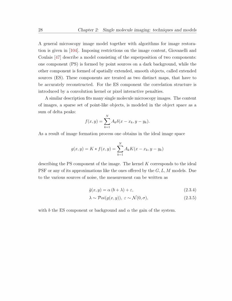
A general microscopy image model together with algorithms for image restora-
tion is given in [104]. Imposing restrictions on the image content, Giovanelli and
Coulais [47] describe a model consisting of the superposition of two components:
one component (PS) is formed by point sources on a dark background, while the
other component is formed of spatially extended, smooth objects, called extended
sources (ES). These components are treated as two distinct maps, that have to
be accurately reconstructed. For the ES component the correlation structure is
introduced by a convolution kernel or pixel interactive penalties.
A similar description fits many single molecule microscopy images. The content
of images, a sparse set of point-like objects, is modeled in the object space as a
sum of delta peaks:
f(x, y) =N∑
k=1
Akδ(x− xk, y − yk).
As a result of image formation process one obtains in the ideal image space
g(x, y) = K ∗ f(x, y) =N∑
k=1
AkK(x− xk, y − yk)
describing the PS component of the image. The kernel K corresponds to the ideal
PSF or any of its approximations like the ones offered by the G,L,M models. Due
to the various sources of noise, the measurement can be written as
g(x, y) = α (b+ λ) + ε, (2.3.4)
λ ∼ Poi(g(x, y)), ε ∼ N (0, σ), (2.3.5)
with b the ES component or background and α the gain of the system.
Chapter 3
Microarrays with single molecule
sensitivity
Cells exposed to toxins, pharmacologic agents, human hormones etc. respond to
these changes by changes in the expression of particular genes [80]. Change in
gene expressions can occur also in normal cellular activity, e.g. cell division. Thus
the gene expression levels are highly informative about the cell state, the activity
of genes as well as changes in protein abundance in the cell.
The complete set of DNA transcripts and their relative levels of expression per-
taining to a cell or tissue as well as a specific condition is called the transcriptome.
As opposed to the genome, it is highly dynamic, changing rapidly in response to
environmental conditions or during certain cellular events [75].
Microarray technology offers an advanced and efficient way to measure gene
expression of large sets of different genes at a high throughput. As a consequence,
it is an important tool in solving problems such as the detection of differently
expressed genes for different conditions, the annotation of gene function — in
case the encoded protein’s function is unknown, shared regulation patterns with
genes whose function is known offers valuable cues on the function of interest—,
definition of genetic pathways (the regulation of gene expression by other genes)
via temporal profiling, molecular phenotyping for prediction of pharmacological
response or evolution of a disease, etc. (see [108, 75]).
3.1 Biological background
Chromosomes are structures found in the cell nucleus, formed by a single molecule
of coiled deoxyribonucleic acid (DNA) carrying the individual’s hereditary mate-
29
30 Chapter 3: Microarrays with single molecule sensitivity
Figure 3.1: Central dogma of molecular biology
rial, and DNA-bound proteins. The DNA molecule is a double-stranded helix, each
strand formed of linkages of sugar-phosphate. The strands are bound together by
the noncovalent hydrogen bonding between pairs of attached bases.
The basic units of biological inheritance are the genes, specific segments of
a DNA molecule that contain all coding information for the cell to synthesize a
specific product, as an RNA molecule or a protein. They occupy a specific location
(locus) on a chromosome and are identified according to their function. Some
of the genes, the so-called housekeeping genes, encode proteins needed for basic
cellular activity, and thus are expressed in all cells. Others have specific tasks, as
coding the synthesis of specific antibodies or limit the formation of malignant cells
(antioncongene). More details can be found in [80, 69, 116, 33].
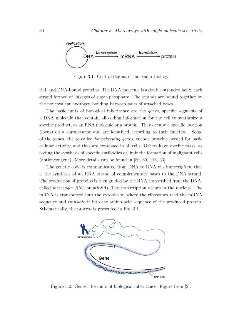
The genetic code is communicated from DNA to RNA via transcription, that
is the synthesis of an RNA strand of complementary bases to the DNA strand.
The production of proteins is then guided by the RNA transcribed from the DNA,
called messenger RNA or mRNA). The transcription occurs in the nucleus. The
mRNA is transported into the cytoplasm, where the ribosomes read the mRNA
sequence and translate it into the amino acid sequence of the produced protein.
Schematically, the process is presented in Fig. 3.1.
Figure 3.2: Genes, the units of biological inheritance. Figure from [2].
3.2 Classical microarray technology 31
A typical microarray experiment measures (and compares) the mRNA abun-
dance (expression levels) of the cell samples in order to infer the type and the
function of the proteins produced under certain conditions in the cell. However
the mRNA molecule is fragile and can be easily broken down by enzymes from bio-
logical solutions. Instead the more stable complementary DNA (cDNA) is created
from the mRNA sample, through reverse transcription and subsequently used in
the experiment.
3.2 Classical microarray technology
The high density DNA microarray allows the monitoring via single experiments
and on a single experimental medium the interactions among thousand of gene
transcripts in an organism. Good overviews of the technique can be found in
[119, 69, 80, 103].
Although the first immunoassay technologies were developed already in the
1950s and 1960s, the Southern blot developed in 1975 was the first array of ge-
netic material [105]. The miniaturization of the technique, microspotting in the
1980s [40] and the subsequent technological improvements (mechanization of the
construction of slides and of microspotting) lead to the industrialization of the
technology.
The technology is based on the specific pattern of bonding known as (Watson-
Crick) base pairing : the base known as adenine (A) specifically bonds with thymine
(T) while cytosine (C) specifically bonds with guanine (G). Note that in the case
of RNA, adenine bonds to uracil (U). The amine base that will form a bonding pair
with another amine base is considered its complementary base, and single DNA
or RNA (ribonucleic acid) strands form stable bonds or hybridize only with a
complementary strand. Hybridization is the fundamental process that constitutes
the basis of DNA microarray technology [69]. The hydrogen bonding between bases
is weak and breaks at approximately 90C, through a process called denaturation.
After cooling, at about 60C reassociation occurs.
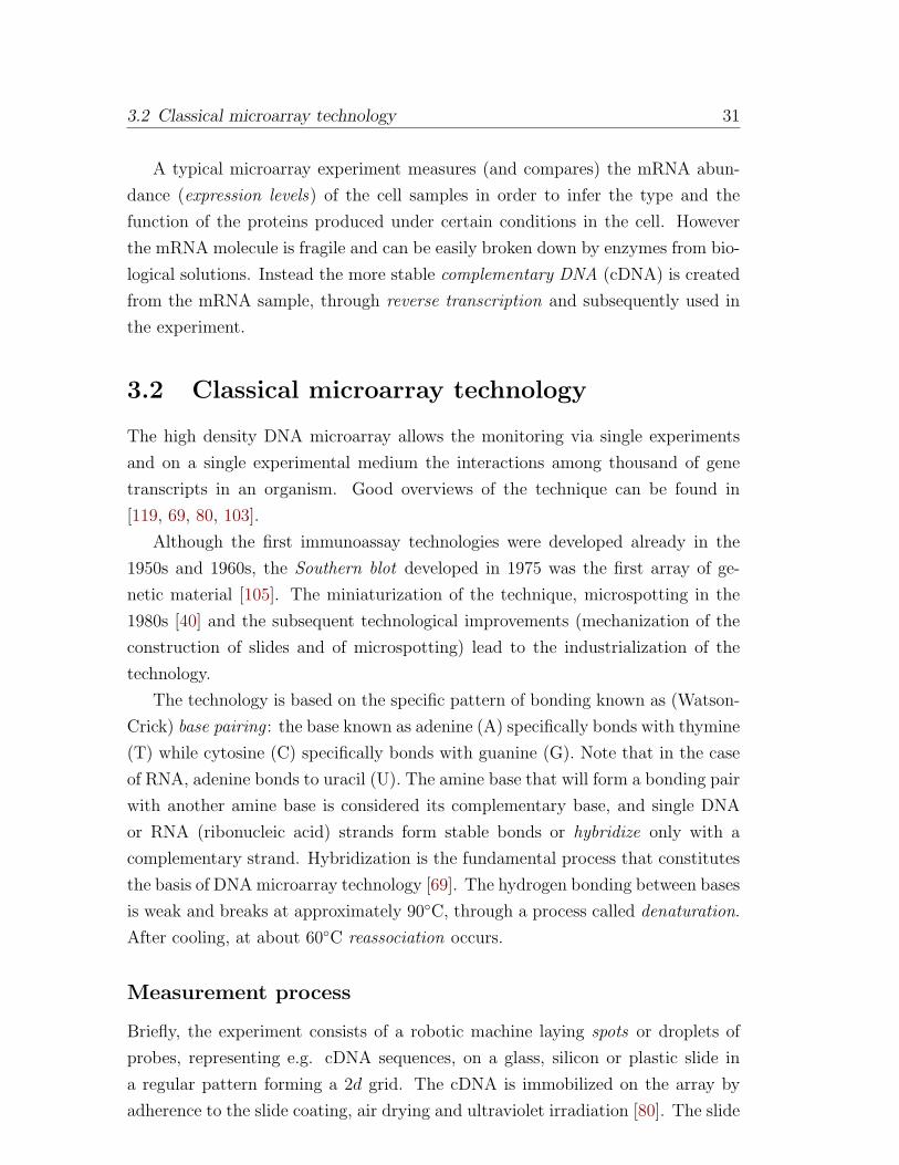
Measurement process
Briefly, the experiment consists of a robotic machine laying spots or droplets of
probes, representing e.g. cDNA sequences, on a glass, silicon or plastic slide in
a regular pattern forming a 2d grid. The cDNA is immobilized on the array by
adherence to the slide coating, air drying and ultraviolet irradiation [80]. The slide
32 Chapter 3: Microarrays with single molecule sensitivity
Figure 3.3: Schematic representation of two-color microarray technology. Figurefrom [2].
with the affixed spots is called microarray or chip and it represents a dictionary of
probes, in which an entry (DNA, oligonucleotide, antibody etc.) is identified by its
position in the grid. The process is represented in the upper right part of Fig. 3.3.
Via denaturation, double stranded cDNA is broken into single strands preparing
for the binding of target samples. For the sake of statistical soundness, each probe
on the chip is replicated a certain number of times subject to a trade-off between
cost and reliability of results.
Next, the target sample is marked with a fluorescent tag during reverse tran-
scription and washed over the chip. In the case of two different samples, a control
sample and an unknown target sample, (e.g. a control from normal cells and a
sample from cancerous cells), the samples are marked with distinguishable tags,
emitting at different wavelengths (typically red and green, Cyanine 5, Cy5 with
emission maximum at about 670nm, and Cyanine 3, Cy3 with maximum approxi-
mately at 570nm), then equal amounts of the samples are mixed and finally washed
over the microarray slide, where molecular hybridization takes place. If necessary,
the quantity of DNA can be amplified via a process called polymerase chain re-
action (PCR). The amount of bound sample to the probes is an indicator of the
strength of interaction intensity with the respective probe.
This hybridization is measured by scanning the microarray after excitation with
laser light. The scanning is performed usually with a confocal laser microscope
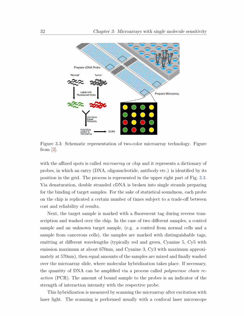
3.2 Classical microarray technology 33
Figure 3.4: Detail of microarray. Pseudocolors indicate: red - high expression intarget labeled with Cy5, green - high expression in target labeled with Cy3, yellow- similar expression in both samples. The gene is identified by the position of therespective spot in the grid.
and the fluorescent intensity for each probe spot (and in each color) is recorded.
The output of the last step are 16 bit images, a pseudocolored detail of which can
be seen in Fig. 3.4. The images have to be analyzed by robust image processing
tools to produce reliable intensity estimates that describe the hybridization.
Data analysis
According to [69], the main tasks image processing has to perform are:
Gridding Matching a grid to the image of the printed spot pattern and identi-
fying the approximate position of each spot
Segmentation Separation of foreground(signal) and background pixels for each
spot region. If shape priors are included in the process, the simplest assump-
tion is a circular shape with fixed or variable radius.
34 Chapter 3: Microarrays with single molecule sensitivity
Intensity extraction Computation of a summary statistic that best describes
intensity of the spot (e.g. mean, median etc.)
Background correction If necessary, the signal intensity is corrected with the
estimate of the local or global background (most often an additive back-
ground model is assumed). The effect of this step might be crucial in the
case of weakly expressed genes (dim spots).
The result of the image processing step is a gene expression matrix of (mean)
fluorescence intensity of each spot (or of the ratio of the intensities recorded in the
two channels). Normalization and data interpretations are the last steps of the
analysis that leads to the gain of biological insight on the role the reporters play in
the problem at hand. Normalization adjusts microarray data for effects which arise
from variation in the technology (systematic errors) rather than from biological
differences between the mRNA samples. It is a sequence of sophisticated statistical
methods that takes into account several factors such as unequal quantities of start-
ing RNA, differences in dye incorporation during labeling or detection efficiencies
between the fluorescent dyes used, variations in spotting and/or background, and
systematic biases in the measured expression levels (see [41, 120, 39, 16, 33] for
details). Normalization can be performed on several levels: within a single array
(among replicate spots), between a pair of replicate arrays and among multiple
arrays (over samples to be compared).
The last step, data interpretation is based on a plethora of tools from statisti-
cal hypothesis testing, to clustering, cluster analysis, data mining and it tries to
answer biological questions such as the detection of differently expressed genes (for
two sample experiments), the detection of co-regulated genes, characterization of
expression profiles etc.
Limitations of microarray technology
Each step of the technique is prone to distortions and noise contamination. A
thorough description of variation and noise sources can be found in [10, 80, 71].
Most of these factors have to be dealt with by the algorithms used for the analysis.
Results are influenced by several factors related to the surface of the array, the
binding efficiency, the typical number of dye attached to each cDNA molecule,
differences in PCR amplification, etc. For instance, reverse transcription bias oc-
curs due to variation in the degree of efficiency corresponding to different types
3.2 Classical microarray technology 35
of mRNA molecules, while sequence bias is due to varying binding affinity of fluo-
rescent dyes to different nucleotides (e.g. cDNA strands containing more guanine
appear brighter, due to better binding of the dye to guanine). The differences in
labeling are called dye-bias, and can be studied and corrected for via a repeat of
the experiment on the same targets, but with changed labeling, procedure known
in the literature as dye-swap.
One of the most important limitations of microarray technology is the availabil-
ity of tissue samples in sufficient quantity [80]. The problem is particularly acute
in cancer cell experiments, when the amount of mRNA that can be extracted from
rare cells is inadequate to perform a microarray experiment.
Moreover, the technique represents an indirect measurement of the abundance
of gene transcripts via the fluorescent dyes attached to the hybridized polynu-
cleotides. Fluorescence itself is not a linear phenomena (it is linear only over a
limited range). Thus, this method renders only a semi-quantitative measure of
differences in gene expression with small differences being obscured within the
experimental variation of the array technology.
A bias might be introduced by less-than-perfect denaturation process, resulting
in non-denatured strands of (spotted) DNA, as well as, target molecules that
stick to the slide and are not washed away, and subsequently contributing to the
background noise around the spot. Furthermore, experimental conditions cannot
be optimized for all the genes. Due to the fact that under the chosen conditions
hybridization simply did not happen for certain genes, the measured expressions
in these cases are misleading, since they do not reflect the real biological situation.
The complexity of the resulting data makes data storage, retrieval and sharing
difficult, a problem further increased by the lack of standardization among the
different existing systems.
Types of arrays
The best known types of arrays are the cDNA and the oligonucleotide arrays. Be-
sides the single-slide cDNA microarray experiments described above, in which one
compares transcript abundance in two mRNA samples hybridized to the same slide,
there are other approaches such as multiple-slide experiments comparing transcript
abundance in two or more types of mRNA samples hybridized to different slides
and a variant of this, the time-course experiments, in which transcript abundance
is monitored over time for processes such as the cell cycle. The technology is
based on clones obtained from cDNA libraries spotted on the support, typically
36 Chapter 3: Microarrays with single molecule sensitivity
formed by strands of 500 to 5000 bases of known sequence [80]. The design of the
array (the selection of cloned cDNA) can be optimized for the (hypothesis testing)
problem at hand.
Oligonucleotides are short sequences of base-pair segments, having a length
between 15 and 70 nucleotides. They can be used as probing material on the
array (one of the best known chip is the GeneChip produced by Affymetrix). The
advantages of this kind of arrays are specificity and efficiency of hybridization (due
to uniform length), they are also easier to engineer and easier to use for finding
optimal hybridization conditions. The disadvantages of the oligo arrays are cross-
hybridization with several genes, due to the short lengths of the oligonucleotides
— this can be seen as a strength when the purpose is discovery and not predefined
sequence matching— the absence of purification processes, irregularities in the
fluorescence signal, etc.
Other types of microarrays involve chromatin immunoprecipitation assays
(ChIP-chip)[118] or protein microarrays [114, 51].
3.3 The high resolution technique
A main objectives of our project was to correct some of the limitations described
in Section 3.2, such as unspecific binding (due to randomly bound molecules or
unattached fluorophores), the varying background intensity profile of the array,
the binding efficiency of the sample (which might be gene dependent), the dye
distribution per molecule (also gene dependent), varying illumination distortion
etc.
Our technology is based on the combination of the classical technology with
ultrasensitive fluorescence microscopy for reading the specially designed DNA chip.
Some of the advantages of scanning spots with ultrasensitive microscopy capa-
ble of measuring the signal of single dyes equivalent to single hybridization events
are illustrated in Fig. 3.5. In the low resolution image on the left, only the intensity
can be observed, without any further visual clue if it is due to true signal or arti-
facts. On the right, in the high resolution image, one can clearly distinguish the
bright artifacts (probably dirt) around the microarray spot from the true signal.
Artifacts that might distort the low-resolution signal intensity are identified using
ultrasensitive fluorescent microscopy.
3.3 The high resolution technique 37
Figure 3.5: Image of a microarray spot with artifacts. (Left) Low resolution image,with high intensity pixels (without visual clues for presence of artifacts) (Right)High resolution image, where the artifact can be distinguished from signal. Theimage intensity was rescaled for better visibility.
Imaging setup
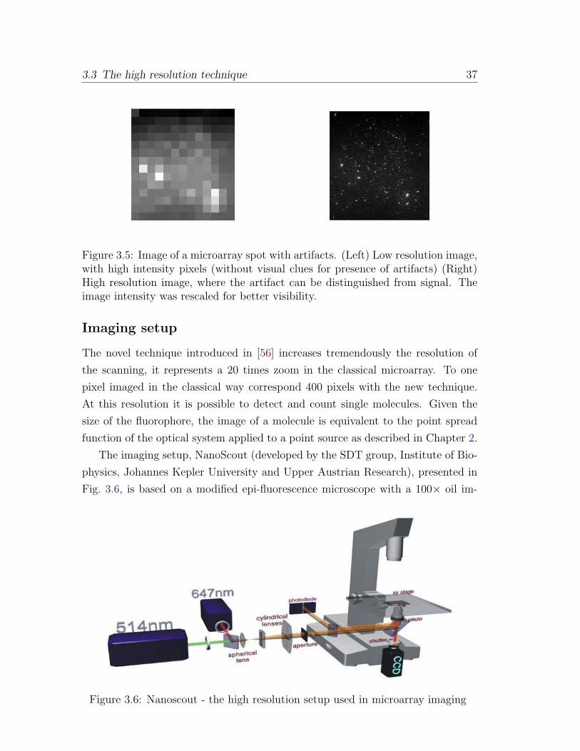
The novel technique introduced in [56] increases tremendously the resolution of
the scanning, it represents a 20 times zoom in the classical microarray. To one
pixel imaged in the classical way correspond 400 pixels with the new technique.
At this resolution it is possible to detect and count single molecules. Given the
size of the fluorophore, the image of a molecule is equivalent to the point spread
function of the optical system applied to a point source as described in Chapter 2.
The imaging setup, NanoScout (developed by the SDT group, Institute of Bio-
physics, Johannes Kepler University and Upper Austrian Research), presented in
Fig. 3.6, is based on a modified epi-fluorescence microscope with a 100× oil im-
Figure 3.6: Nanoscout - the high resolution setup used in microarray imaging
38 Chapter 3: Microarrays with single molecule sensitivity
mersion objective (α-Plan Fluar, NA = 1.45, Zeiss). The samples are illuminated
in objective-type total internal reflection (TIR) configuration. For the selective
excitation of the dyes, Cy3 and Cy5, respectively, Ar+− and Kr+− lasers (514nm
and 647nm) are used. After appropriate filtering using standard Cy3 and Cy5 fil-
ter sets (Chroma Technology Corp., VT), the fluorescence images are taken with a
12-bit back-illuminated CCD camera (chip-size 1300×100 pixel, 20µm pixel-size).
The CCD camera is operated in time delay and integration (TDI)-mode. The
samples are mounted on a motorized xy-stage and synchronized to the line-shift
of the camera. This allows fast scanning of large areas (1 × 0.02cm2 in 58s) with
single fluorophore sensitivity and diffraction limited resolution. The setup and the
imaging process are described in detail in [56, 55, 61].
For validation of the system, microarrays comprising two full complementary
60mer oligonucleotides were used (Human Genome Oligo Set Version 3 (Operon)).
Hybridization of a dilution series of Cy5-labeled target oligonucleotides yielded
a quantification limit of 1.3fM corresponding to only 39.000 molecules in 50µl
sample.
The ultra-sensitive microarray technique was used to study the expression pro-
file of putative Multiple Myeloma (MM) stem cells using the human MM cell line
NCI-H929 and the results are provided in Chapter 7. This new technology brings
important insights in the field of biochips, with several advantages, like the anal-
ysis of images with very low sample concentrations, a new way of background
suppression, and more refinement in information.
Main steps in single molecule microarray image analysis
The high resolution microarray image analysis preserves the same main tasks as
the low resolution technique:
• Addressing/ Gridding - Localization of each spot of the grid pattern in the
image
• Estimation of the hybridization measure for each spot via spot identification
and concentration estimation
• Gene expression analysis.
However there is a need to redesign and/or adapt the existing algorithms in order
to be applicable to the new kind of data. Gridding is performed on a down-sampled
3.3 The high resolution technique 39
version of the original image, while for the other tasks new algorithms are designed,
implemented and validated.
Gridding is performed by registering a predefined grid pattern with the image
of detected microarray spots. There is a plethora of methods to find the location
(and shape) of bright microarray spots. Among these we mention the method of
Angulo and Serra based on mathematical morphology [7], clustering of the pixels
into foreground, background and artifact pixels [14], watershed based algorithms
etc. Some of these approaches also adjust the shape and position of spots in a
subsequent step after an initial grid was found.
However, in our case due to the low amount of mRNA the spots appear much
dimmer than in the classical microarray images, making both tasks, spot detec-
tion and grid estimation, more difficult. For spot detection we have used the
same wavelet thresholding algorithms as for single molecule detection, in this case
applied to a downscaled, low resolution image. All the details are described in
Chapter 5. The combination of the resulting images from the two samples (cor-
responding to the red and green channel) improve the registration result. As the
result of the gridding step, we assume that the detected rectangular region in-
cludes a single microarray spot, potentially surrounded by background pixels (as
in Fig. 3.7(a)).
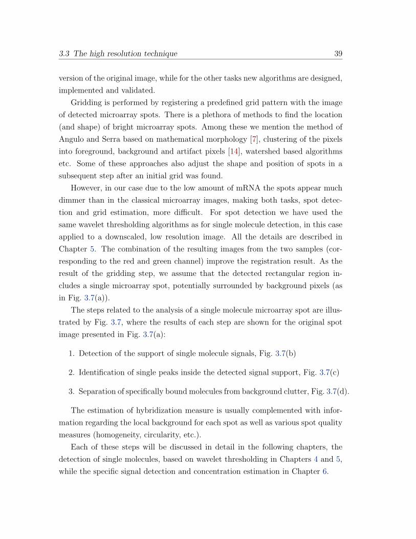
The steps related to the analysis of a single molecule microarray spot are illus-
trated by Fig. 3.7, where the results of each step are shown for the original spot
image presented in Fig. 3.7(a):
1. Detection of the support of single molecule signals, Fig. 3.7(b)
2. Identification of single peaks inside the detected signal support, Fig. 3.7(c)
3. Separation of specifically bound molecules from background clutter, Fig. 3.7(d).
The estimation of hybridization measure is usually complemented with infor-
mation regarding the local background for each spot as well as various spot quality
measures (homogeneity, circularity, etc.).
Each of these steps will be discussed in detail in the following chapters, the
detection of single molecules, based on wavelet thresholding in Chapters 4 and 5,
while the specific signal detection and concentration estimation in Chapter 6.
40 Chapter 3: Microarrays with single molecule sensitivity
Figure 3.7: Analysis of a spot in a high-resolution microarray image. (a) Originalimage, bright features correspond to molecules bound to the chip. (b) Detectionof single molecules. (c) Selection of single molecule locations (local maxima ondenoised image inside the detection support in (b)). (d) Separation of hybridizationsignal from clutter.
Mathematical model
The differences between the low resolution and high resolution microarray experi-
ments might be best understood by describing an underlying model of fluorescence
intensity for each of them.
Our aim is to propose a new measure for hybridization: instead of aggregations
of the pixel intensities inside the spot we use as hybridization measure single
molecule counts (or concentration of hybridized molecules per area unit). The
model we propose as well as the new hybridization measure suggest that the high
resolution technique has the following advantages: besides offering a way to analyze
very low concentration samples, it removes bias due to background heterogeneity
and PCR amplification, making several normalization steps and dye swap (all
prone to distortions and errors) unnecessary.
3.3 The high resolution technique 41
So far, for the classical case of low resolution imaging, the analysis is based
on the comparison of appropriately chosen summary statistics of pixels inside the
spot. Conventional analysis is based on models of the microarray signal formation,
like the ones proposed by [10, 6, 23, 70, 74]. These models include several aspects
of the acquired data such as image intensity, spot shapes, noise.
A very simple but frequently used spot intensity model proposed in [6] can be
written
Yi = µi · s(i− ic) + εi,
where Yi is the intensity of the spot at pixel i, µi represents the amplitude of the
spot as a measure of the hybridization, s is a function describing the shape and
texture of the spot, while ic represents the center of the spot, and εi models the
local and/or global background noise, usually εi ∼ N (0, σ).
A more realistic model, taking into account the sensor properties, includes both
additive and multiplicative noise [71]:
Yi = αµieηi + εi,
where α is the gain of the sensor, eηi and εi representing the multiplicative and
additive noise, respectively.
Often a lognormal model of pixel values Yi is assumed. If Y is replaced by G
or R for intensities in the green or red channel respectively, and BRi and BGi
are the respective background estimates used for background correction, the final
quantity of interest is:
log(Gi − BGi)− log(Ri − BRi). (3.3.1)
The log-transform plays also a variance stabilizing role.
However, gaining access to microarray spot images at single molecule reso-
lution, we understand better the image formation process in both high and low
resolutions. For modeling we shall adopt an approach close to the concentration
modeling described in [23].
For the classical low-resolution microarray image analysis we propose a com-
pound Poisson process model explained below. The discussion of the high res-
olution model will be detailed in Chapter 6. We first give the definition of the
compound Poisson process and than see how it helps in modeling the microarray
pixel intensities.
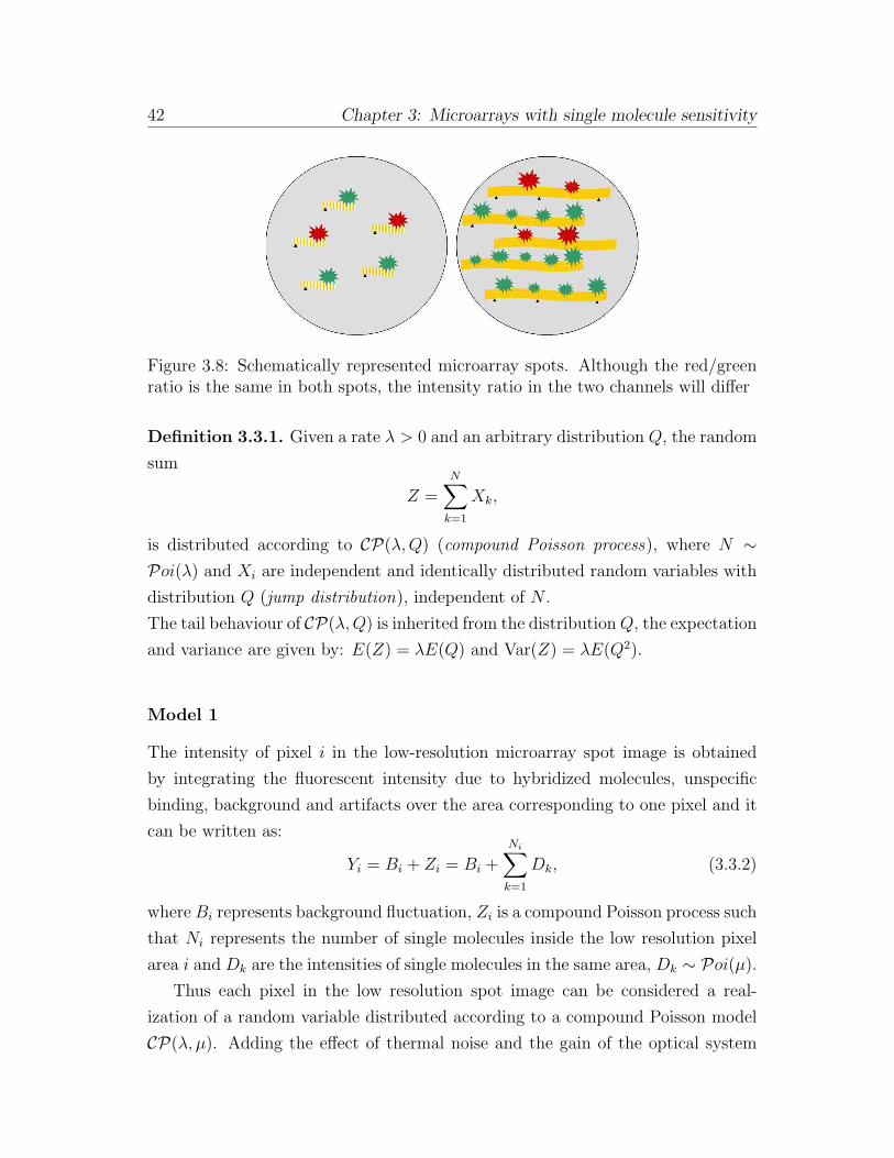
42 Chapter 3: Microarrays with single molecule sensitivity
Figure 3.8: Schematically represented microarray spots. Although the red/greenratio is the same in both spots, the intensity ratio in the two channels will differ
Definition 3.3.1. Given a rate λ > 0 and an arbitrary distribution Q, the random
sum
Z =N∑
k=1
Xk,
is distributed according to CP(λ,Q) (compound Poisson process), where N ∼Poi(λ) and Xi are independent and identically distributed random variables with
distribution Q (jump distribution), independent of N .
The tail behaviour of CP(λ,Q) is inherited from the distributionQ, the expectation
and variance are given by: E(Z) = λE(Q) and Var(Z) = λE(Q2).
Model 1
The intensity of pixel i in the low-resolution microarray spot image is obtained
by integrating the fluorescent intensity due to hybridized molecules, unspecific
binding, background and artifacts over the area corresponding to one pixel and it
can be written as:
Yi = Bi + Zi = Bi +
Ni∑
k=1
Dk, (3.3.2)
where Bi represents background fluctuation, Zi is a compound Poisson process such
that Ni represents the number of single molecules inside the low resolution pixel
area i and Dk are the intensities of single molecules in the same area, Dk ∼ Poi(µ).Thus each pixel in the low resolution spot image can be considered a real-
ization of a random variable distributed according to a compound Poisson model
CP(λ, µ). Adding the effect of thermal noise and the gain of the optical system
3.3 The high resolution technique 43
(as in Section 2.3), a pixel can be modeled as
gi(x, y) = α (Yi) + ε = α
(Bi +
Ni∑
k=1
Dk
)+ εi,
Bi ∼ Poi(B), ε ∼ N (0, σ),
Model 2
A more complex model takes into account the variation of the number of fluo-
rophores, Mk, bound to each molecule. In this case the the jump distribution D
follows itself a compound Poisson distribution, CP(λ1, CP(λ2, µ)). If Mk is the
number of dyes bound to a molecule, Mk ∼ Poi(λ2), and Djk is the intensity of a
single dye, Djk ∼ Poi(µ), the model can be written as:
Yi = Bi + Zi = Bi +
Ni∑
k=1
Mk∑
j=1
Djk. (3.3.3)
The compound Poisson process model has applications in gene expression anal-
ysis ([73, 113]), but to our knowledge has not been used in the case of microarray
image analysis. The compound Poisson model is useful in illustrating the difference
between the classical low resolution microarray analysis and the high resolution
one.
The technology of high resolution microarrays offers access to previously hidden
information: instead of analyzing the low-resolution pixel values Yi, the inference
is based on Ni the number of single molecules in the image. The measure of
hybridization is in our case the concentration of single molecules inside the spot
of interest. The knowledge of the background values of Bi and photon counts Dk
has little or no relevance, being only nuisance parameters.
In microarray analysis the identification of the true signal and the control of the
unspecific intensity variation is essential. We have identified the following short-
comings of the low resolution technique, which make this analysis less appropriate
than the single molecule one:
1. In case of low concentrations, many spots are rejected from analysis due to
low signal-to-noise (SNR) ratio and artifacts, especially in the case of dim
spots. Low resolution microarrays cannot discriminate between signal and
background. In the high resolution technique, single molecules are as easily
detected in low concentration (dim spots) as in high concentration ones,
44 Chapter 3: Microarrays with single molecule sensitivity
allowing the analysis of trace amount of biological sample.
2. Even when segmentation is possible, background estimation is difficult in
low resolution microarray images and might introduce a bias. In the high
resolution case, background subtraction becomes irrelevant, it is implicitly
achieved by the single molecule detection procedure.
3. It was shown that the labeling efficiency is gene dependent (see, e.g., [55])
and it can distort the results in the case of low-resolution microarrays. In
the high resolution case, the hybridization measure is represented by counts
of single molecules and it is not affected by the variability of the number of
fluorophores bound the a molecule. Dye swap normalization typically per-
formed for classical arrays in order to compensate for dye related differences
also becomes unnecessary.
4. We note that although normally only the count information is relevant in
the case of the high resolution technique, still it is possible to use the inten-
sity corresponding to a single molecule, for instance to discriminate it from
dirt. Dirt particles show autofluorescence, with a significantly lower (but
sometimes not negligible) intensity than the dye marked molecules. The
high resolution technique allows discrimination between two or several en-
tities based on total intensity of a single molecule but the same cannot be
performed in low resolution images, since the information is not available at
this granularity .
Some of the challenges of the new method are related to the huge amount of
data that has to be processed (22 GB per slide), the scarcity of the highly expressed
spots necessary to perform the gridding, the high variance of the Poisson processes
modeling the counting of molecules. Also, in case of high density of the molecules in
a spot, when single molecules cannot be discriminated, classical intensity summary
based methods have to be used instead of single molecule counting algorithms.
Chapter 4
Multiscale signal decomposition
This chapter gives a brief introduction to wavelets, both the continuous (CWT)
and discrete wavelet transform (DWT), as well as to multiresolution analysis, or-
thogonal wavelet bases and their generalization, the wavelet frames. We focus on
particular discretizations of the CWT, the dyadic wavelet transform,the undeci-
mated wavelet transform and the isotropic undecimated wavelet transform (for the
two dimensional case), and on a particular wavelet shape, the B-spline wavelet,
especially fitted to the analysis of biological images. The isotropic undecimated
wavelet transform is the representation of the signal that will be used in the next
chapter to detect single molecules.
4.1 Continuous wavelet transform
The choice of wavelet transforms for the problem of single molecule detection can
be motivated in a first step by Mallat’s heuristic: Bases of smooth wavelets are
the best bases for representing objects composed of singularities, when there may
be an arbitrary number of singularities, which may be located in all possible spatial
positions (see for instance [36]).
Since the Fourier basis functions are localized in frequency but not in time, the
Fourier transform
Ff(ω) = f(ω) =1√2π
∫
R
f(x)e−ixω d x
is the ideal tool to study stationary signals defined by invariance of statistical
properties over time. However a small perturbation of frequencies in the Fourier
domain will produce changes over the whole time domain.
45
46 Chapter 4: Multiscale signal decomposition
On the other hand, wavelet transforms, local in both frequency (scale) and
time, provide the way to analyze non-stationary signals, characterized by transient
events [78, 63]. They offer a compact representation of a signal (e.g. with sharp
transitions), which for comparable approximation properties takes significantly
fewer wavelet basis functions than Fourier basis functions.
The wavelet transform breaks up a complicated signal in ”atoms”, called
wavelets.
A wavelet (also calledmother wavelet) is a function ψ ∈ L2, which is normalized
‖ψ‖ = 1, has zero average ∫ +∞
−∞ψ(t)dt = 0,
and is centered in the neighborhood of t = 0.
The wavelet ψ is said to have order m ∈ N if it has m vanishing moments:
∫ +∞
−∞tnψ(t)dt = 0, n = 0, 1, . . .m− 1
and∫ +∞−∞ tmψ(t)dt 6= 0. Thus a wavelet of order m is orthogonal to polynomials of
degree smaller than m.
The mother wavelet generates a family of wavelets ψs,u(x), s > 0, u ∈ R by
change of scale s (i.e. by dilation) and by change of position u (i.e. by translation)
of the mother wavelet function ψ(x). Thus each wavelet of the family is obtained
from ψ as:
ψs,u(t) =1√sψ
(t− u
s
).
Definition 4.1.1. The (basic) wavelet ψ ∈ L2 satisfies the admissibility condition
if
Cψ =
∫ +∞
0
|(Fψ)(ω)|2ω
dω < +∞. (4.1.1)
If ψ satisfies (4.1.1), the continuous wavelet transform (CWT) of f ∈ L2(R) at
position u and scale s is defined by
(Wf) (u, s) = 〈f, ψs,u〉 =∫ +∞
−∞f(t)
1√sψ
(t− u
s
)dt = f ∗ ψs(u), (4.1.2)
where u, s ∈ R, u 6= 0 , ∗ denotes the convolution operator and
ψs(t) =1√sψ∗(−ts
).
4.1 Continuous wavelet transform 47
Under the assumption (4.1.1), it follows that for reasonable conditions imposed
on ψ (i.e. ψ ∈ L1(R)) the continuous function ψ satisfies ψ(0) = 0, or equivalently∫∞−∞ ψ(t) dt = 0, justifying the use of condition (4.1.1) as an alternative definition
of wavelet functions.
The wavelet transform measures the variation of f in a neighborhood of u of
size proportional to s. The regularity of the function f in the neighborhood of u
is characterized by the decay of the respective wavelet coefficients, allowing the
detection of transients in the signal.
The Fourier transform of Wf with respect to the u variable is
(FWf)(ω, s) = (Ff)(ω) · (Fψ)(sω)
and this equation is often used for the implementation of the CWT. The decompo-
sition obtained after the wavelet transform can be further processed for different
purposes, such as compression, denoising, pattern recognition etc. These tasks are
easier performed in the new wavelet space. Inversion formulas make possible the
recovery of the original or a suitably improved function from the expression of the
original function in terms of its wavelet transform.
The necessary condition to obtain the inverse of a wavelet transform is the
admissibility condition (4.1.1). According to [78], p.81, Calderon in 1964, and
Grossman and Morlet in 1984 prove independently that (4.1.1) is the condition for
a wavelet transform to be complete (to admit an inverse transform) and conserve
energy.
Theorem 4.1.2. Let the function ψ ∈ L2 satisfying the admissibility condi-
tion (4.1.1). Any function f ∈ L2 satisfies
f(t) =1
Cψ
∫ +∞
0
∫ +∞
−∞Wf(u, s)
1√sψ
(t− u
s
)du
ds
s2
and ∫ +∞
−∞|f(t)|2 dt = 1
Cψ
∫ +∞
0
∫ +∞
−∞
∣∣Wf(u, s)2∣∣ du ds
s2.
If Wf(u, s) is known only for s < s0, in order to recover f the information
48 Chapter 4: Multiscale signal decomposition
corresponding to s ≥ s0 can be obtained via a scaling function ϕ, satisfying:
|(Fϕ)(ω)|2 =∫ +∞
1
|(Fψ)(sω)|2 dss
=
∫ +∞
ω
|(Fψ)(ξ)|2ξ
dξ,
and from the admissibility condition results that: limω→0 |ϕ(ω)|2 = Cψ.
The scaling function ϕ can be interpreted as a low-pass filter, and the low
frequency approximation of function f at scale s is written as:
Lf(u, s) =
⟨f(t),
1√sϕ
(t− u
s
)⟩= f ∗ ϕs(u).
With the help of the scaling function ϕ, Theorem 4.1.2 can be reformulated as:
f(t) =1
Cψ
∫ s
0
Wf(·, s) ∗ ψs(t)ds
s2+
1
Cψs0Lf(·, s) ∗ ϕs0(t). (4.1.3)
4.2 Frames
Although very elegant and descriptively rich, the CWT has several drawbacks,
such as dimension increase via the introduction of an extra dimension through
the scale parameter, high redundancy of the representation as well as the need to
adapt the CWT for the case of discrete signals, that are overwhelming in prac-
tical applications. In order to overcome these drawbacks, frames are defined as
(not necessarily independent) generalizations of bases, leading to redundant sig-
nal expansions. Ubiquitous examples of frames are the discrete windowed Fourier
transform and the discrete wavelet transforms, we will describe later.
Intuitively, frames are families of functions ϕnn∈Γ , Γ ⊂ N that characterize
a signal f via its inner products. The study of frames was motivated by the search
for the necessary and sufficient conditions that f ∈ H, where H is a Hilbert space,
is characterized by the inner products 〈f, ϕn〉 (the frame wavelet coefficients),
meaning that: 〈f1, ϕn〉 = 〈f2, ϕn〉 implies f1 = f2 [30]. Moreover, if f can be
reconstructed via these inner products, the reconstruction turns out to be of the
following simple form:
f =∑
n∈Γ〈f, ϕn〉 ϕn, (4.2.1)
where ϕn is the dual frame of ϕn, and will be defined below.
Definition 4.2.1. The sequence ϕnn∈Γ is a frame of a Hilbert space H if there

4.2 Frames 49
exist two constants A,B > 0 such that for any f ∈ H
A ‖f‖2 ≤∑
n∈Γ|〈f, ϕn〉|2 ≤ B ‖f‖2 . (4.2.2)
If A = B the frame is called a tight frame.
The linear operator fromH to ℓ2(Γ) =x = (xj)j∈Γ : ‖x‖2 =∑j∈Γ |x|
2j <∞
,
defined as (Ff)j := 〈f, ϕj〉 is called a frame operator.
Condition (4.2.2), called stability condition, ensures that a function can be
recovered from its wavelet frame transform 〈f, ϕn〉 as in (4.2.1).
When the frame is normalized, ‖ϕn‖ = 1, A and B give a measure of the
redundancy:
• if ϕnn∈Γ are linearly independent then A ≤ 1 ≤ B.
• ϕnn∈Γ is an orthonormal basis if and only if A = B = 1.
• If A > 1 the frame is redundant, and A can be seen as a measure of the
redundancy factor.
The adjoint of the frame operator F ∗ can be computed as
〈F ∗x, f〉 = 〈x, Ff〉 =∑
j∈Γxj〈f, ϕj〉 =
∑
j∈Γxj 〈ϕj, f〉 ,
so that F ∗x =∑
j∈Γ xjϕj.
Note that F ∗F is invertible ([30]), and F := (F ∗F )−1F ∗ is the left inverse, of
minimum sup norm, called pseudo-inverse (see [78]).
Definition 4.2.2. The dual frame of ϕnn∈Γ is defined as:
ϕj = (F ∗F )−1 ϕj.
It can be shown that the dual frame is indeed a frame, satisfying
1
B‖f‖2 ≤
∑
j∈Γ
∣∣〈f, ϕj〉2∣∣ ≤ 1
A‖f‖2 .
If the frame is tight then ϕj = A−1ϕj (for the proof and further details see [30]).
50 Chapter 4: Multiscale signal decomposition
Finally, the reconstruction formula can be now written:
f = F−1Ff =∑
j∈Γ〈f, ϕj〉 ϕj =
∑
j∈Γxj 〈ϕj, f〉ϕj.
A wavelet frame is constructed from a continuous wavelet family by restrict-
ing the parameter u and s in (4.1.2) to discrete values. Since the energy of a
wavelet is concentrated around u over a domain proportional to s (in frequency
space 1/s), for good localization properties in both domains, s is sampled along
an exponential sequence ajj∈Z, while the translation parameter u is sampled
uniformly proportional to aj:
ψj,n(t) =1√ajψ
(t− nu0a
j
aj
)(4.2.3)
Not every choice of ψ, a and u0 generates a frame of L2(R), even if ψ is admissible
(the frame condition actually imposes the admissibility of ψ). Necessary and
sufficient conditions for ψ, a and u0 to form a frame are given in [30].
In general, the canonical dual frame ψj,n = (F ∗F )−1ψj,n does not have nec-
essarily a wavelet structure, since F ∗F does not commute with translation, and
neither does (F ∗F )−1 (however commutativity with dilation is fulfilled).
The function ψj is called also analysis wavelet, while ψj when it has a wavelet
structure is called the synthesis wavelet, corresponding to the analysis (decompo-
sition) and the synthesis (reconstruction) steps in the wavelet transform.
Since a frame does not have to be linearly independent (e.g Haar family), the
stability condition is weaker than the Riesz basis requirement, defined below.
Definition 4.2.3. A family ϕk is Riesz basis for L2(R), if
L2(R) = span ϕ(· − k)|k ∈ Z
and
A∑
k∈Zc2k ≤
∥∥∥∥∥∑
k∈Zckϕ(· − k)
∥∥∥∥∥
2
L2
≤ B∑
k∈Zc2k
for all ckk∈Z ∈ l2(Z), where A and B are positive constants.
Every orthonormal basis is a Riesz basis, and every Riesz basis is a frame. The
following theorem on the relationship between frames and Riesz bases is proven in
[24]:

4.2 Frames 51
Theorem 4.2.4. Given ψ ∈ L2(R) the following statements are equivalent:
• ψj,k is a Riesz basis of L2(R)
• ψj,k is a frame of L2(R) and it is a ℓ2-linearly independent family, i.e.,
∑cj,kψj,k = 0 ⇒ cj,k = 0.
Moreover the Riesz bounds coincide with the frame bounds.
For two particular frame classes the duals have an easy characterization, for
semi-orthogonal wavelets and the more restrictive orthogonal wavelets both pre-
sented in the following definition.
Definition 4.2.5. Given a wavelet ψ ∈ L2((R))
a) ψ is called an orthogonal wavelet if ψj,k satisfies:
〈ψj,k, ψl,m〉 = δj,k · δl,m, ∀j, k, l,m ∈ Z,
b) ψ is called a semi-orthogonal wavelet if
〈ψj,k, ψl,m〉 = 0, ∀j 6= l, k,m ∈ Z.
Note that the orthogonal wavelets are self-dual: ψj,k = ψj,k, while the result
concerning the dual of a semi-orthogonal wavelet is given in the following theorem
(see [24], for details).
Theorem 4.2.6. If ψ ∈ L2(R) is a semi-orthogonal wavelet then its dual can be
defined via its Fourier transform as:
(F ψ)(ω) := (Fψ)∑∞−∞ |(Fψ)(ω + 2πk)|2
meaning that ⟨ψj,k, ψl,m
⟩= δj,kδl,m, ∀j, k, l,m ∈ Z, (4.2.4)
where ψl,m := 2l/2ψ(2lx−m).
In this case the dual has a wavelet structure generated by ψ and every f ∈L2(R) can be written as:
f =∑
j,k∈Zcj,kψj,k(x) =
∑
j,k∈Zdj,kψj,k(x), (4.2.5)
52 Chapter 4: Multiscale signal decomposition
where the sums are known as wavelet series and from (4.2.4) follows that:
cj,k =⟨f, ψj,k
⟩
dj,k = 〈f, ψj,k〉 .
It is clear that ψ and ψ are interchangeable (either one can be used in analysis
and the other in synthesis).
4.3 Multi-resolution analysis
For an efficient computation of the wavelet transform and the reconstruction of a
signal via the inverse transform the concept of multiresolution analysis is intro-
duced. The multiresolution analysis (MRA) offers a hierarchical framework for
interpreting the information in the signal, with a parsimonious representation of
important features at different scales in only a few coefficients. It allows a scale
invariant analysis of signal features and via a special coarse-to-fine strategy ex-
amines the decorrelated components of the signal at different resolutions. It is a
convenient tool in pattern recognition, denoising, detection etc.
The computations implied by MRA can be conveniently described through
filters and filter banks. For every continuous linear operator F : ℓ2(Z) → ℓ2(Z)
there exist hkk∈Z ∈ ℓ2(Z) such that
(Fx)k =∑
n∈Zhk−nxn.
h = (. . . hk−1, hk, hk+1 . . .) represents the impulse response of the filter, and the
elements are called filter coefficients. A convenient way to describe filters is through
their Z transform, expressed as a Laurent polynomial:
H(z) =∑
i
hiz−i.
Louis et al. [76] give an elegant motivation for multiresolution analysis. A
signal f ∈ V−1, where V−1 is a subspace of L2(R), is decomposed in a smooth (low-
frequency) component via a projection P0f ∈ V0 and a detail (high-frequency)
component, Q0f ∈ W0, where W0 is the orthogonal complement of V0, W0 =
4.3 Multi-resolution analysis 53
x ∈ V−1 : 〈x, y〉 = 0, y ∈ V0 denoted V−1 = V0 ⊕W0, such that
f = P0f +Q0f.
In the next step, P0f is decomposed by projections P1 and Q1 on orthogonal
subspaces V1 and W1, respectively, such that P0f = P1f + Q1f and f = P1f +
Q1f +Q0f . The process can be repeated recursively.
Definition 4.3.1. A sequence of nested, closed subspaces Vj ⊂ L2(R),
0 ⊂ . . . V2 ⊂ V1 ⊂ V0 ⊂ V−1 ⊂ V−2 . . . ⊂ L2(R)
is called a multiresolution analysis (MRA) if
• limj→−∞ Vj =⋃j∈Z = L2(R)
• limj→∞ Vj =⋂j∈Z Vj = 0
• f(·) ∈ Vj if and only if f(2j·) ∈ V0
• f ∈ Vj if and only if f(· − 2jk) ∈ Vj,k ∈ Z
• ∃ϕ ∈ L2(R) : ϕ(· − k)k∈Z is a Riesz basis for V0.
It can be shown that f ∈ V0 if and only if f(· − k) ∈ V0, ∀k ∈ Z and
Vj = span ϕj,k(· − k)|k ∈ Z,
where ϕj,k(x) := 2−j/2ϕ(2−jx− k).
To approximate f in Vj the projection on the scaling basis is considered, such
that the inner products
cj,n = 〈f, φj,n〉 =∫ ∞
−∞f(t)
1
2j/2φ
(t− 2jn
2j
)dt
represent a discrete approximation at scale 2j.
The following lemma is a consequence of the observation:
2−1/2ϕ(x/2) ∈ V1 ⊂ V0 = span ϕ(x− k)|k ∈ Z.
Lemma 4.3.2. There exists hkk∈Z ∈ R such that
2−1/2ϕ(x2
)=∑
k∈Zhkϕ(x− k), (4.3.1)
54 Chapter 4: Multiscale signal decomposition
where
hk =⟨2−1/2ϕ
(x2
), ϕ(x− k)
⟩.
Equation (4.3.1) is called two-scale equation or refinement equation.
Lemma 4.3.2 relates a dilation of ϕ by 2 to its integer translations via h, a
discrete filter called conjugate mirror filter.
On the other hand, the difference of information between the approximation
of the function f at resolution 2j+1 and 2j respectively is called detail signal at
resolution 2j. By denoting with Wj the complement of Vj in Vj+1, Vj−1 = Vj+Wj,
one can write the decomposition of L2(R) as the direct sum of the Wj spaces :
L2(R) =∑
j∈ZWj = . . . +W1+W0+W1 . . . .
As opposed to the nested subspaces Vj, the subspaces Wj are disjunct: ∀j 6=l, Wj ∩Wl = 0 . In order to have an orthonormal basis one can chose Wj to be
the orthogonal complement of Vj in Vj−1, Vj⊥Wj, as in the motivational example
for MRA,:
Vj−1 = Vj ⊕Wj.
The following theorem due to Mallat and Meyer [78] p.236 gives the construction of
an orthonormal basis of Wjby scaling and translations of a wavelet ψ, constructed
upon a scaling function ϕ.
Theorem 4.3.3. Given ϕ a scaling function and h the corresponding conjugate
mirror filter, denote by ψ the function whose Fourier transform is
(Fψ)(ω) = 1√2(Fg)
(ω2
)(F(ϕ)
(ω2
),
where
(Fg)(ω) = e−iω(Fh∗)(ω + π). (4.3.2)
For any scale 2j, ψj,nn∈Z is an orthonormal basis of Wj, where
ψj,n(t) =1√2jψ
(t− 2jn
2j
).
For all scales, ψj,n(j,n)∈Z2 is an orthonormal basis of L2(R).
4.4 Generalizations of MRA to two dimensions 55
From Theorem 4.3.3 it results that
2−1/2ψ(x2
)=∑
k∈Zgkϕ(x− k),
and subsequently
gk =⟨2−1/2ψ
(x2
), ϕ(x− k)
⟩.
Finally, the relation between g and h in (4.3.2) can be rewritten after the
inverse Fourier transform as:
gk = (−1)1−kh1−k.
4.4 Generalizations of MRA to two dimensions
The previous one dimensional multiresolution analysis setting can be extended to
higher dimensions L2(Rd) in a straightforward way.
If Vjj∈Z is a two-dimensional multiresolution analysis, the two-dimensional
signal f(x, y) ∈ L2(R2) can be approximated by its projection on Vj. Denoting
ϕ2j := 22j
ϕ(2j, 2jy), it can be shown that the family of functions obtained by the
dilation and translation of the scaling function ϕ(x, y):
2−jϕ2j(x− 2−jn, y − 2−jm)
(n,m)∈Z2
forms an orthonormal basis of Vj.
The function ϕ(x, y) is unique with respect to a given multiresolution analysis.
A special case of multiresolution approximations is the one of separable MRA,
where each vector space Vj can be decomposed as a tensor product of two identical
subspaces of L2(R) (representing MRA of L2(R))
Vj = V 1j ⊗ V 1
j = spanf(x)g(y) | f, g ∈ V 1
j
.
and subsequently the scaling function can be written as ϕ(x, y) = ϕ(x)ϕ(y), where
ϕ(x) is the respective one-dimensional scaling function.
The orthogonal basis of Vj is given by:
2−jϕ2j(x− 2−jn, y − 2−jm)
(n,m)∈Z2 =
2−jϕ2j(x− 2−jn)ϕ2j(y − 2−jm)
(n,m)∈Z2
and the approximation of the signal f(x, y) at resolution 2−j is characterized by
56 Chapter 4: Multiscale signal decomposition
the inner products:
⟨f(x, y), ϕ2j(x− 2−jn)ϕ2j(y − 2−jm)
⟩(m,n)∈Z2 .
Just as Vj is defined with the help of V 1j , also the details Wj of the two-
dimensional MRA, are based on the respective W 1j the complements of V 1
j in the
one dimensional case:
Vj−1 = V 1j−1 ⊗ V 1
j−1
= (V 1j ⊕W 1
j )⊗ (V 1j ⊕W 1
j )
= (V 1j ⊗ V 1
j )⊕ ((V 1j ⊗W 1
j )⊕ (W 1j ⊗ V 1
j )⊕ (W 1j ⊗W 1
j ))
= Vj ⊕Wj.
Using the notations above, the following result, is proven in [77]:
Theorem 4.4.1. If Wj is the orthogonal complement of Vj, where Vjj∈Z is an
MRA of L2(R2), with generating scaling function ϕ(x, y) = ϕ(x)ϕ(x), and ψ(x) is
the one-dimensional wavelet associated to ϕ(x) then
2−jψ12j(x− 2−jn, 2j, y − 2−jm),
2−jψ22j(x− 2−jn, 2j, y − 2−jm),
2−jψ32j(x− 2−jn, 2j, y − 2−jm)(n,m)∈Z2 ,
where
ψh(x, y) = ϕ(x)ψ(y), ψv(x, y) = ψ(x)ϕ(y), ψd(x, y) = ψ(x)ψ(y),
is an orthonormal basis of Wj.
The scalar products corresponding to the three kinds of wavelets give the details
of the function f(x, y), with respect to three emphasized directions: horizontal,
vertical and diagonal. These directions might have a special role in human vision,
however are not so important in microscopy images.
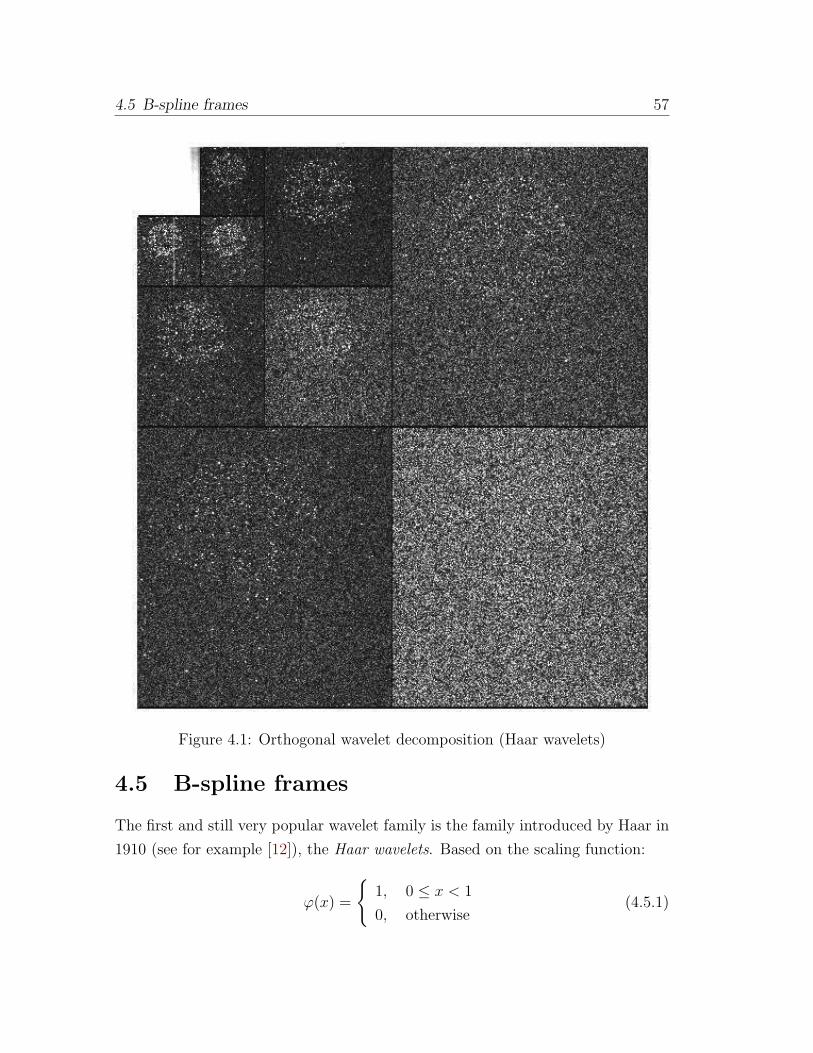
4.5 B-spline frames 57
Figure 4.1: Orthogonal wavelet decomposition (Haar wavelets)
4.5 B-spline frames
The first and still very popular wavelet family is the family introduced by Haar in
1910 (see for example [12]), the Haar wavelets. Based on the scaling function:
ϕ(x) =
1, 0 ≤ x < 1
0, otherwise(4.5.1)

58 Chapter 4: Multiscale signal decomposition
they fulfill a simple scaling equation:
ϕj+1,k =1√2(ϕj,2k − ϕj,2k+1)
and based on the difference 1√2(ϕj,2k − ϕj,2k+1) = ψj+1,k the Haar wavelet can be
written as:
ϕ(x) =
1, 0 ≤ x < 1/2
−1, 1/2 ≤ x < 1
0, otherwise.
(4.5.2)
Haar wavelets are a particular case of B-spline wavelets (of order 0). The n-th
order B-spline is recursively defined as:
B0(x) = χ[0,1](2x)
Bn+1(x) = (Bn ∗B0)(x) =
∫ ∞
−∞Bm−1(x− t)B0(t) dt =
∫ 1
0
Bm−1(x− t) dt,
normalized such that∫RBn(x) dx = 1. The Fourier transform of Bm is
(FBm)(ω) =1√2π
(sin(ω/2)
ω/2
)m+1
=1√2π
sincm+1(ω/2).
For any j and m ≥ 2 the family
Bj :=2j/2Bm(2
jx− k), k ∈ Z
is a Riesz basis of V mj . Since the spline function Bm(2
jx) ∈ V mj and V m
j ⊂ V mj+1 it
results that it can be written as:
Bm(2jx) =
∞∑
k=−∞pm,kBm(2
j+1x− k), (4.5.3)
where pm,k : k ∈ Z is a ℓ2-sequence. Solving (4.5.3) for pm,k in Fourier domain
yields:
pm,k =
2−m+1
(m
k
), 0 ≤ k < m
0, otherwise
(4.5.4)
4.6 Fast wavelet transform algorithms via filter banks 59
and the corresponding two-scale relation is then given by:
Bm(x) =m∑
k=0
2−m+1
(m
k
)Bm(2x− k).
The first result concerning spline wavelets associated to B-spline scaling func-
tions of order m are called cardinal spline wavelets (see [24] for a detailed descrip-
tion). Their disadvantage is that although the wavelets have exponential decay,
their support is not compact thus being tedious to compute.
In order to remedy this shortcoming the orthogonality requirement is dropped.
Semi-orthogonal wavelets with compact supports always exist if the two-scale se-
quence of the scaling function ϕ has finite support. Chui in [24] describes the
unique solution for the compactly supported semi-orthogonal wavelet ψm with
minimum support that corresponds to the m-th order cardinal B-spline:
ψm(x) :=∑
n qnBm(2x− n)
qn = (−1)n2m−1
∑ml=0
(m
l
)B2m(n+ 1− l), n = 0, . . . , 3m− 2.
(4.5.5)
Several properties of spline wavelets are discussed in [24, 111, 77, 78].
4.6 Fast wavelet transform algorithms via filter
banks
In most of practical cases, one has to deal with discrete signals. A real digital
signal is a sequence fi = f(i) ∈ R. We shall consider only square summable
signals f ∈ l2(Z). The simplest discretization of an analog input f(t) can be
achieved via natural sampling:
f [n] = f(t = n), n ∈ Z.
The discrete signal can be related to f(t) also via a D/A converter:
f(t) ≈∑
n
f [n]χ(t− n).
It includes the natural sampling case when χ(n) = δ0n. Wavelet algorithms for
discrete signals as well as their connection to the CWT were thoroughly described
60 Chapter 4: Multiscale signal decomposition
in [100, 77, 90, 87], with a focus on computational details.
Most frequently computations are made over the dyadic grid u = 2j, s = k2j
for the scale and translation parameter of the wavelet. Mallat in [77] proposed
the use of conjugate mirror filters for the computation of the discrete wavelet
transform (DWT) in the frame of multiresolution analysis. Two special operators
are used in the transition from one resolution to another. The decimation operator
D : ℓ2(Z) → ℓ2(2Z), Dk,m = δ2k,m retains only the terms with even index in the
sequence (alternative notation: 2 ↓ 1). The Fourier transform of a decimated
signal yn = x2n is
y(2ω) =∑
n
x2ne−i2nω =
1
2(x(ω) + x(ω + π)) .
The component x(ω + π) creates a frequency folding called aliasing that must be
canceled at the reconstruction of the signal.
The adjoint operator E = D∗ : ℓ2(2Z) → ℓ2(Z) inserts 0’s at the odd indices:
Ek,m = δk,2m resulting in
. . . 0, x−1, 0, x0, 0, x1, 0 . . .
It is also denoted by 1 ↑ 2.
The signal f is decomposed iteratively by the low pass filter h and the high-pass
filter g, both filtered results being subsequently decimated (by using the operator
D). The procedure is repeated for the low-pass filtered signal. These steps applied
recursively represent the analysis part of the algorithm, depicted on the left of
Fig. 4.2. The connection between ϕ, ψ and h and g, respectively was given at the
end of Section 4.2.
The computation can be summarized as the iteration of the following steps:
cj,n(f) =∑
k
h2n−kcj−1,k(f), (4.6.1)
wj,n(f) =∑
k
g2n−kcj−1,k(f), (4.6.2)
where c0,k = f(k) and
gi = (−1)ih−i+1, hi = 21/2∫ϕ(x− i)ϕ(2x) dx.
As for reconstruction (synthesis), on the right side in Fig. 4.2, since cj,n(f)
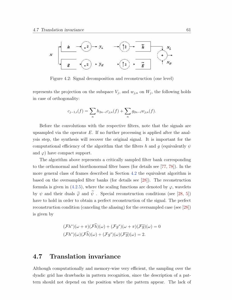
4.7 Translation invariance 61
Figure 4.2: Signal decomposition and reconstruction (one level)
represents the projection on the subspace Vj, and wj,n on Wj, the following holds
in case of orthogonality:
cj−1,i(f) =∑
n
h2n−icj,n(f) +∑
n
g2n−iwj,n(f).
Before the convolutions with the respective filters, note that the signals are
upsampled via the operator E. If no further processing is applied after the anal-
ysis step, the synthesis will recover the original signal. It is important for the
computational efficiency of the algorithm that the filters h and g (equivalently ψ
and ϕ) have compact support.
The algorithm above represents a critically sampled filter bank corresponding
to the orthonormal and biorthonormal filter bases (for details see [77, 78]). In the
more general class of frames described in Section 4.2 the equivalent algorithm is
based on the oversampled filter banks (for details see [28]). The reconstruction
formula is given in (4.2.5), where the scaling functions are denoted by ϕ, wavelets
by ψ and their duals ϕ and ψ . Special reconstruction conditions (see [28, 5])
have to hold in order to obtain a perfect reconstruction of the signal. The perfect
reconstruction condition (canceling the aliasing) for the oversampled case (see [28])
is given by
(Fh∗)(ω + π)(F h)(ω) + (Fg∗)(ω + π)(F g)(ω) = 0
(Fh∗)(ω)(F h)(ω) + (Fg∗)(ω)(F g)(ω) = 2.
4.7 Translation invariance
Although computationally and memory-wise very efficient, the sampling over the
dyadic grid has drawbacks in pattern recognition, since the description of a pat-
tern should not depend on the position where the pattern appear. The lack of
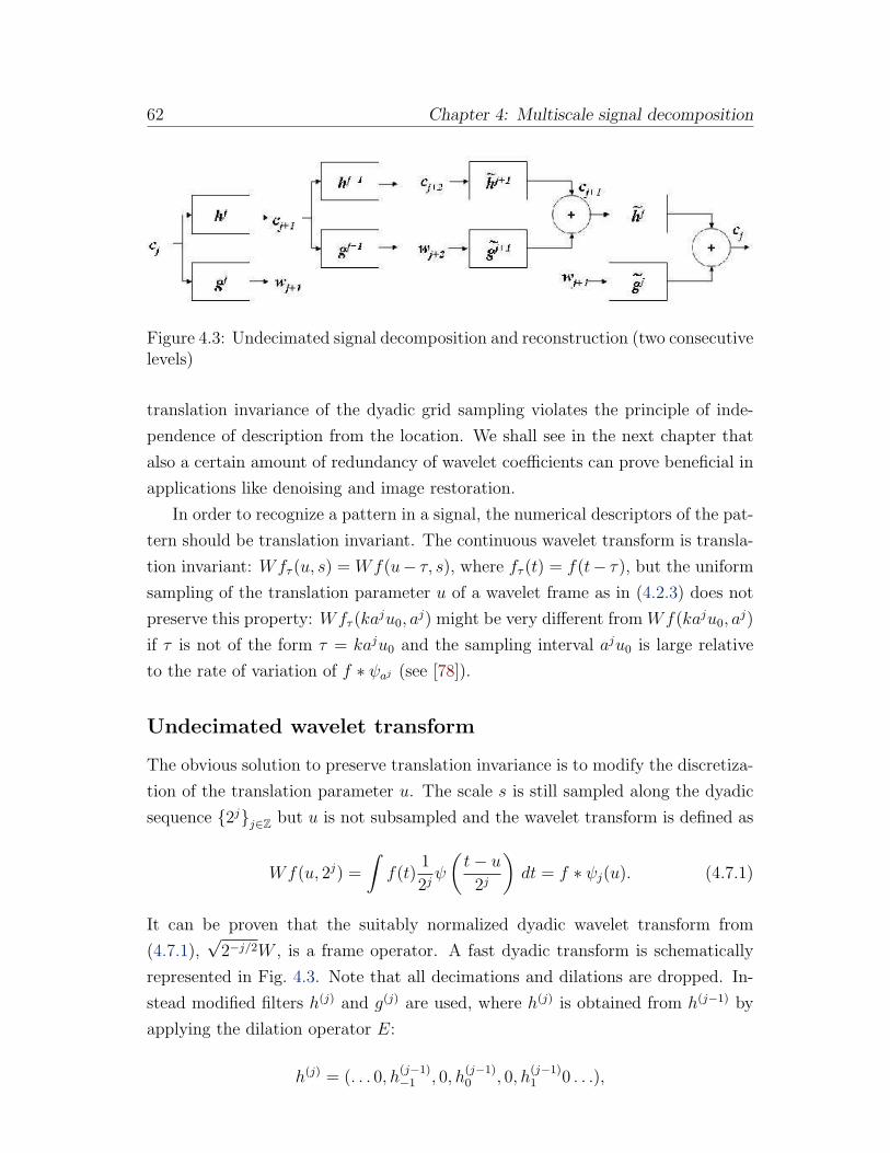
62 Chapter 4: Multiscale signal decomposition
Figure 4.3: Undecimated signal decomposition and reconstruction (two consecutivelevels)
translation invariance of the dyadic grid sampling violates the principle of inde-
pendence of description from the location. We shall see in the next chapter that
also a certain amount of redundancy of wavelet coefficients can prove beneficial in
applications like denoising and image restoration.
In order to recognize a pattern in a signal, the numerical descriptors of the pat-
tern should be translation invariant. The continuous wavelet transform is transla-
tion invariant: Wfτ (u, s) = Wf(u− τ, s), where fτ (t) = f(t− τ), but the uniform
sampling of the translation parameter u of a wavelet frame as in (4.2.3) does not
preserve this property: Wfτ (kaju0, a
j) might be very different fromWf(kaju0, aj)
if τ is not of the form τ = kaju0 and the sampling interval aju0 is large relative
to the rate of variation of f ∗ ψaj (see [78]).
Undecimated wavelet transform
The obvious solution to preserve translation invariance is to modify the discretiza-
tion of the translation parameter u. The scale s is still sampled along the dyadic
sequence 2jj∈Z but u is not subsampled and the wavelet transform is defined as
Wf(u, 2j) =
∫f(t)
1
2jψ
(t− u
2j
)dt = f ∗ ψj(u). (4.7.1)
It can be proven that the suitably normalized dyadic wavelet transform from
(4.7.1),√2−j/2W , is a frame operator. A fast dyadic transform is schematically
represented in Fig. 4.3. Note that all decimations and dilations are dropped. In-
stead modified filters h(j) and g(j) are used, where h(j) is obtained from h(j−1) by
applying the dilation operator E:
h(j) = (. . . 0, h(j−1)−1 , 0, h
(j−1)0 , 0, h
(j−1)1 0 . . .),
4.7 Translation invariance 63
and g(j) is obtained similarly from g(j−1). In order to compute the multiresolution
analysis, the operation above performs the dilation of the wavelet ψ and scaling
function ϕ (and also samples these functions in more points) in order to compensate
the lack of decimation of the signal, through which multiresolution was achieved
in the algorithm of Mallat. The construction based on zero insertion inspired the
name of the method (a trous is French for ’with holes’).
With these new filters the algorithm becomes the iteration of
cj+1,k = cjk ∗ h(j)k , wj+1,k = cjk ∗ g(j)k (4.7.2)
as decomposition steps and as for reconstruction:
cj+1,k =1
2(cj+1,k ∗ h(j)k + wj+1,k ∗ g(j)k ).
The extension of the undecimated wavelet transform to two dimensions is
achieved (for the sake of simplicity) via separable filters:
cj+1(k, l) = (h(j)h(j) ∗ cj)(k, l)w1j+1(k, l) = (g(j)h(j) ∗ cj)(k, l)
w2j+1(k, l) = (h(j)g(j) ∗ cj)(k, l)
w3j+1(k, l) = (g(j)g(j) ∗ cj)(k, l), j = 1, . . . , J − 1.
Note that each of the transformed images has the same size as the original image,
such that the redundancy factor is 3(J − 1) + 1.
Isotropic undecimated wavelet transform
In single molecule images, features are usually isotropic and in order to perform a
good image analysis the isotropy of the filters is a desirable property. In order to
preserve isotropy, the filters h and g as well as the scaling function and the mother
wavelet function ϕ and ψ have to be nearly isotropic. A popular choice is based
on one-dimensional B-spline scaling function of order 3, ϕ(x) = B3(x), to which
corresponds the filter hk =[
116, 1
4, 3
8, 1
4, 1
16
]. Based on ϕ(x), a 2d separable filter
is constructed such that:
ϕ(x, y) = B3(x)B3(y)
and
ψ(x2,y
2
)= 4ϕ(x, y)− ϕ
(x2,y
2
).

64 Chapter 4: Multiscale signal decomposition
The related filters are h(k,l) = hk×hl and g(k,l) = 10,0−hk,l, where 10,0 = 1 at (0, 0)
and is null otherwise. It means that the wavelet detail coefficients are given by:
wj+1,(k,l) = cj,(k,l) − cj+1,(k,l) [106] and the reconstruction is the sum of all details
and the coarsest approximation:
f(k,l) = cJ,(k,l) +J∑
j=0
wj+1,(k,l). (4.7.3)
The detail at each resolution has the same dimension as the original 2d signal.
When there is no confusion, a single index will be used to denote the 2d index
(k, l). The index j will be preserved to denote the scale.
The relation to the UWT based on the same h and g = 1 − h =
[−1,−4, 10,−4,−1] is
w1j + w2
j + w3j = wj = cj − cj+1
Further details on UWT and IUWT can be found in [106]. The a trous scheme
was used in [107] for astronomical images, and in [106, 88] for microscopy.
Chapter 5
Wavelet based detection
The previous chapter offered a short introduction in wavelet transforms and fo-
cused on the transforms suited to analyze biological structures in general, and
single molecules in particular, like the IUWT transform described in Section 4.7.
The multiresolution analysis of a signal makes possible a good localization of
interesting areas (e.g. singularities) as well as a sparse representation, by only few
important wavelet coefficients, since the transform adapts to the local regularity of
the signal. Jaffard and Meyer ([62]) explain the efficiency of the wavelet transform
via the following paradigm: Objects, images, or signals with simple geometrical
structures have sparse wavelet expansions. Conversely, functions whose wavelet
expansion is sparse have interesting geometrical properties. In this chapter we shall
describe thresholding algorithms that make use of the convenient representation
with the final goal of performing the single molecule detection task.
5.1 Statistical applications of wavelet transforms
The solution of several statistical problems (estimation, approximation, model se-
lection, pattern recognition, etc.) can be generically formulated as the recovery of
the original (signal) coefficients expressed in a certain basis from the empirical ones
(see e.g. [78, 19]). Donoho explored the connection between the estimation prob-
lem and the representation problem, and showed that ”efficient representations
lead to efficient estimations” [36, 37, 19].
The efficiency of estimation is motivated by the decorrelating property of a
wavelet transform which creates a sparse signal, with most coefficients zero or close
to zero. The noise however affects equally all coefficients and if its level is moderate,
signal wavelet coefficients can be easily discriminated from coefficients due to noise
65
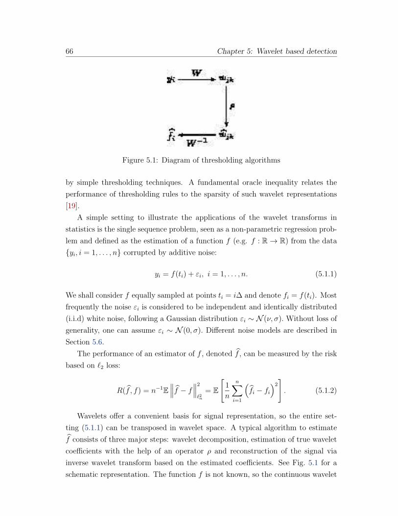
66 Chapter 5: Wavelet based detection
Figure 5.1: Diagram of thresholding algorithms
by simple thresholding techniques. A fundamental oracle inequality relates the
performance of thresholding rules to the sparsity of such wavelet representations
[19].
A simple setting to illustrate the applications of the wavelet transforms in
statistics is the single sequence problem, seen as a non-parametric regression prob-
lem and defined as the estimation of a function f (e.g. f : R → R) from the data
yi, i = 1, . . . , n corrupted by additive noise:
yi = f(ti) + εi, i = 1, . . . , n. (5.1.1)
We shall consider f equally sampled at points ti = i∆ and denote fi = f(ti). Most
frequently the noise εi is considered to be independent and identically distributed
(i.i.d) white noise, following a Gaussian distribution εi ∼ N (ν, σ). Without loss of
generality, one can assume εi ∼ N (0, σ). Different noise models are described in
Section 5.6.
The performance of an estimator of f , denoted f , can be measured by the risk
based on ℓ2 loss:
R(f , f) = n−1E∥∥∥f − f
∥∥∥2
ℓ2n
= E
[1
n
n∑
i=1
(fi − fi
)2]. (5.1.2)
Wavelets offer a convenient basis for signal representation, so the entire set-
ting (5.1.1) can be transposed in wavelet space. A typical algorithm to estimate
f consists of three major steps: wavelet decomposition, estimation of true wavelet
coefficients with the help of an operator ρ and reconstruction of the signal via
inverse wavelet transform based on the estimated coefficients. See Fig. 5.1 for a
schematic representation. The function f is not known, so the continuous wavelet
5.1 Statistical applications of wavelet transforms 67
coefficients
wj,k =
∫f(u)ψj,k(u) du
cannot be directly computed, and are estimated from the empirical wavelet co-
efficients. The coefficients wj,k of the discrete wavelet transform of the signal
f = (fi)i∈1,...n at scale j and location k are given by:
wj,k =n∑
i=1
fiψj,i.
Moreover, the empirical coefficients wj,k of the discrete wavelet transform of the
noisy data y = (yi)i∈1,...n at scale j and location k are given by:
wj,k =n∑
i=1
yiψj,i.
Given an estimate wi,k of the wavelet coefficient of the signal f and an orthogonal
wavelet transform, one can get an estimate of the signal by applying the following
inverse transform:
fi =J∑
j=1
2j−1∑
k=0
wj,kψj,k +2J∑
k=0
cJ,kϕJ,k.
The approximation n1/2ψj,k(i) ≈ 2j/2ψ(2ju − k), u = i/n holds for the discrete
case. Furthermore, to each wavelet level corresponds an estimation problem of
type (5.1.1), and we have:
wj,k = wj,k + εj,k for all j = 1, . . . , J and k = 0, . . . , 2j − 1, (5.1.3)
where E [εj,k] = 0 and E [ε2j,k] = σ2j .
Finally, due to the orthonormality we have also E εi1ǫi2 = σ2δi1−i2 since:
E
(∑
i1
ψj1,k1εi1
)(∑
i2
ψj2,k2εi2
)=∑
i1
∑
i2
E εi1εi2ψj1,k1ψj2,k2
= σ2δ(j1,k1),(j2,k2). (5.1.4)
Thus, the orthogonal wavelet transformed noise coefficients are also white noise.
68 Chapter 5: Wavelet based detection
5.2 Wavelet coefficient estimation
The problem described in (5.1.1) can be transposed in wavelet space, as a wavelet
coefficient estimation problem. The risk equivalent to (5.1.2) becomes:
R(f , f) = E
[∑
j
∑
k
(wj,k − wj,k)2
]. (5.2.1)
The minimization of the risk is achieved via the algorithms described in Fig. 5.1,
more precisely the modification of wavelet coefficients via the operator ρ. In gen-
eral, these algorithms operate with two simplifications. First, only diagonal esti-
mators are considered, and second, these estimators have a special form (linear or
thresholding functions, called also shrinkage functions).
A diagonal estimator in the discrete wavelet basis estimates independently
each wj,k from wj,k via a function ρ: wj,k = ρ(wj,k). The algorithm can be thus
summarized as:
f =J∑
j=1
2j−1∑
k=0
ρ (〈y, ψj,k〉)ψj,k +2J∑
k=0
ρ (〈y, ϕJ,k〉)ϕJ,k.
Additionally as a simple scenario we can assume ρ to be a linear function
ρ(wj,k) = aj,kwj,k that minimizes the risk (5.2.1). Level-wise, considering (5.1.3)
it follows that
E ‖wj,k − aj,kwj,k‖2 = |wj,k|2 (1− aj,k)2 + aj,kσ
2j . (5.2.2)
The minimum of (5.2.2) is attained for
aj,k =|wj,k|2
|wj,k|2 + σ2j
,
yielding
RL(f , f) =∑
j,k
|wj,k|2 σ2j
|wj,k|2 + σ2j
.
We note that the linear factor aj,k cannot be computed in practice, since it depends
on the unknown coefficient wj,k. Therefore the risk is not reachable, it is an ideal
risk that can be attained only with information on ideal smoothing of f provided
by an oracle, (an information which practically is not available). The ideal risk has
5.3 Wavelet thresholding 69
theoretical importance, being a term of comparison for the optimality of estimation
algorithms.
Since the signal is assumed sparse, there are only a few important features at
detail level, the rest of the wavelet coefficients being zero or very close to zero.
This motivates the introduction of a further restriction: aj,k ∈ 0, 1.The nonlinear projector that minimizes (5.2.2) consists of the selection of the
bases that correlate best with the signal, thus having the most extreme valued
wavelet coefficients |wj,k| = |〈f, ψj, k〉|. This selection shows the signal dependent
aspect of the procedure. It can be described for instance via a thresholding defined
by:
aj,k =
1, |wj,k| ≥ σ
0, |wj,k| < σ.(5.2.3)
Basically the thresholding includes the coefficients that exceed the noise level.
Again the estimator via aj,k depends on the unknown signal, such that an oracle
is necessary to decide which coefficients are above the noise level.
The risk of the oracle projector is
RNL =∑
j,k
min(w2j,k, σ
2)
which is of the same order as RL:
RNL ≥ RL ≥ 1
2RNL
since min(x, y) ≥ xy(x+y)
≥ 12min(x, y).
Donoho proved that simple estimates of wj,k are remarkably close to RNL.
Some of these simple estimates are the subject of Section 5.3 [36].
5.3 Wavelet thresholding
Thresholding means setting to zero the small wavelet coefficients wj,k ≤ T , for
a given threshold T . It is equivalent to ignore the details of the signal at the
respective scale and location and describe the signal based only on the coarser
(smoother) approximation level. It can be seen as a local smoothing of the signal,
when the signal is regular. At detail level only a few coefficients are kept, that are
exceeding the amplitude of (the transformed) noise. These coefficients correspond
to the sharp signal transitions, assumed to be limited in number and that translate

70 Chapter 5: Wavelet based detection
in high wavelet coefficients in the neighborhood of the transition. Thus the wavelet
thresholding represents an adaptive smoothing approach, with adaptive bandwidth
with respect to the local regularity of the signal. Several problems arise such as
• the exact form of the thresholding function ρT essential for the estimation of
the wavelet coefficients,
• the automatic choice of the threshold value T ,
• if the value T should be unique over all levels or level dependent (Tj),
• if the threshold should be fixed or data-dependent.
In general, thresholding functions ρ are supposed to fulfill the following properties
[65]:
• ρT (−y) = ρT (y)
• ρT (y) ≤ x if y ≥ 0 (shrinking)
• x− ρT (y) ≤ T + b if y ≥ 0 (boundedness)
• ρT (y) = 0 if |y| ≤ T.
The two most well-known thresholding functions are the hard and the soft thresh-
oldings, represented in Fig. 5.2. The hard thresholding ρH of wavelet coefficients
is a ”keep-or-kill” rule, according to which only those wjk coefficients are kept that
exceed a certain threshold T , while the others are set to 0:
ρH(y) =
y, |y| ≥ T
0, |y| < T.(5.3.1)
In order to avoid visual artifacts, hard thresholding can be replaced by a continuous
function, known as the soft thresholding function, and defined as:
ρS(y) =
y − T, y ≥ T
0, |y| < T.
y + T, y ≤ −T(5.3.2)
The hard thresholding rule solves the following penalized least square problem:
ρH(y) = ρH(y, T ) = argminf (y − f)2 + T 2∥∥∥f∥∥∥0
= argminf (y − f)2 + T 2If 6=0 (5.3.3)
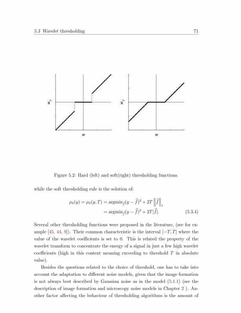
5.3 Wavelet thresholding 71
Figure 5.2: Hard (left) and soft(right) thresholding functions.
while the soft thresholding rule is the solution of:
ρS(y) = ρS(y, T ) = argminf (y − f)2 + 2T∥∥∥f∥∥∥1
= argminf (y − f)2 + 2T |f |. (5.3.4)
Several other thresholding functions were proposed in the literature, (see for ex-
ample [45, 44, 9]). Their common characteristic is the interval [−T, T ] where the
value of the wavelet coefficients is set to 0. This is related the property of the
wavelet transform to concentrate the energy of a signal in just a few high wavelet
coefficients (high in this context meaning exceeding to threshold T in absolute
value).
Besides the questions related to the choice of threshold, one has to take into
account the adaptation to different noise models, given that the image formation
is not always best described by Gaussian noise as in the model (5.1.1) (see the
description of image formation and microscopy noise models in Chapter 2 ). An-
other factor affecting the behaviour of thresholding algorithms is the amount of
72 Chapter 5: Wavelet based detection
signal (sparsity) discussed in the following.
5.4 Signal sparsity
We have described how the signal can be approximated by a few significant wavelet
coefficients, referring to this property as sparsity in wavelet bases. We shall de-
scribe in the subsequent the notion of sparsity in more detail.
The notion is related in the case of a wavelet transformed signal to the number
of significant wavelet coefficients in the wavelet representation.
More generally, sparsity implies that most of the signal strength is concen-
trated in a few of the coefficients. The most straightforward examples are the
spike (1, 0, ..., 0) and the comb vectors (n1/2, ..., n1/2) [19]. They have the same ℓ2
norm, however the spike is considerably more sparse than the comb signal. If the
two vectors are two representations of the same signal in two different bases and
knowing that the noise would normally not correlate with any basis (is not sparse
in any basis) the spike representation would be easier denoised, (the significant
coefficients easier found) then the comb one.
According to [4], an intuitive definition of sparsity of a signal µ is that it implies
a relatively small proportion of nonzero coefficients. For a fixed proportion η and
the l0 quasi-norm ‖x‖0 = | i : xi 6= 0 | the set with a proportion η of nonzero
entries is
B0(η) = µ ∈ Rn : ‖µ‖0 ≤ ηn .
Alternatively, sparsity can be defined on the decreasing rearrangement of the
amplitudes: ∣∣µ(1)
∣∣ ≥∣∣µ(2)
∣∣ . . . ≥∣∣µ(n)
∣∣
as a term-wise power-law bound:
∣∣µ(k)
∣∣ ≤ C · k−β, k = 1, 2 . . . .
Finally, sparsity can be measured using lp norms, with p small:
‖µ‖p =(
n∑
i=1
|µi|p)1/p
.
5.5 Threshold selection 73
Strong-lp balls of small average radius η are defined as:
Bp(η) =
µ ∈ R
n : 1/nn∑
i=1
|µi|p ≤ ηp
In the light of the sparsity definitions above, the sparsity of signal represen-
tation in wavelet space is thus related to the lp norm of the wavelet coefficient
vectors, for p small. Thus the regularizations terms (ℓ0 and ℓ1 penalties in (5.3.3)
and (5.3.4)) corresponding to the soft and hard thresholding justify the preference
of nonlinear thresholding estimators over the linear one.
5.5 Threshold selection
Strongly connected to the sparsity of a signal is the selection of the threshold T
in the thresholding function ρ = ρ(·, T ). For a sparse signal only a few coefficients
should be kept, while if the signal is not as sparse more coefficients are expected
to appear in the representation. Therefore, the threshold T has to be adjusted
according to the (unknown) sparsity of the signal.
In order to perform the selection one can think of at least two general classes
of algorithms, generated by two ways of modeling the wavelet coefficients. Both
ways are based on a signal-background separation problem formulation based on
the assumption that a given data sample xi, i = 1, . . . n was generated partly by
a (possibly very general) signal distribution PS (θPS) while the rest of the samples
pertain to the background distribution PB (θPB), θPB
, θPSrepresenting the param-
eters of PB and PS . Different views on the modeling of this problem lead to
different approaches in setting the right threshold T and detecting the significant
coefficients.
Model 1
One possible approach to model the data xi is by considering it a realization
of random variables Xi distributed according to the following two-component
mixture:
Xi ∼ πPS (θPS) + (1− π)PB (θPB
) ,
where π represents the proportion of signal in the data (and thus reflects the
sparsity of the signal). Note that PS might represent an arbitrary complex
distribution, for example it can be at its turn a mixture distribution.

74 Chapter 5: Wavelet based detection
Model 2
The drawback of the previous approach is that a model of the signal has to be
specified. An alternative view, especially appropriate when the proportion
of the background, 1 − π, is much higher than that of the signal samples,
is to consider the signal samples as outliers with respect to the distribution
PB, i.e. as data deviating from the data described by PB.
The problem of outlier-detection is closely related to the robust estimation of
θPB, the parameters of PB, which are usually unknown. Consequently, the two
tasks are intertwined: if the parameters are known, the outliers can be identified
based on the deviation from PB(θPB), on the other hand, if we would know (and
remove) the outliers, the parameters could be correctly estimated based on the
remaining data.
Universal threshold
One approach to model the outliers is related to their link to the extremal value
of the background distribution. A simple view in one dimension would be that
all elements higher than the maximum (smaller than the minimum) of a sequence
of i.i.d. random variables distributed according to PB are considered outliers. It
is an approach based on Model 2 described above, since it does not make any
assumption neither on the signal nor the signal distribution and was proposed by
Donoho and Johnstone in [36] under the name universal thresholding.
The universal threshold is defined as
TU =√2 log nσ,
where σ is the standard deviation of the distribution of wavelet coefficients (or an
appropriate estimate of it) and n is the number of coefficients. It originates from
modeling the wavelet coefficients assumed normally distributed, wj,k ∼ N (0, σ),
given that most coefficients are due to Gaussian noise and only a few are generated
by signal.
The threshold TU is an extreme value of the wj,k and is based on the following
property([72]): given a sequence of i.i.d. Z1, . . . , Zn ∼ N (0, 1)
P(
max1≤i≤n|Zi| >√2 log n
)≤ 1√
4π log n→ 0.
However the convergence is slow and the threshold often proves to be too high.
5.5 Threshold selection 75
Instead of the unknown parameter σ a robust estimation of the standard deviation
is used. More details on the estimate can be found in Appendix A.
Finally, Donoho proved the following optimality result [36].
Theorem 5.5.1. The risk RT (f , f) of a hard or soft thresholding estimator with
threshold TU =√2 log nσ satisfies for n ≥ 4
RT (f , f) ≥ (2 log n+ 1)(σ2 +RNL(f)
),
and is optimal among diagonal estimators D:
limn→∞
infD
supf∈F
E
∥∥∥f − f∥∥∥
σ2 +RNL
1
2 log n= 1.
A similar result holds as well in the case of colored noise.
SURE
A data driven, sub-band adaptive threshold is SURE (Stein Unbiased Risk Esti-
mation) proposed in [38].
The equivalent problem to wavelet coefficients estimation can be defined for
each wavelet level as a mean vector estimation (w1, . . . , wn)T (we omit the scale
index j to simplify the notation) based on the data wk ∼ N (wk, 1), k = 1, . . . , n
with minimum risk. In case of a sparse data sample, most wk are thought to be
zero. The result of Stein [87] states that µ(x) = x+ g(x) is an unbiased estimator,
where g = (g1, g2, . . . , gn) : Rn → R
n is weakly differentiable:
E ‖µ(x)− µ‖2 = n+ Eµ
‖g(x)‖2 + 2∇ · g(x)
.
Using the soft thresholding function one gets
gk(wk) = ρS(wk)− wk =
−T, wk ≥ T
−wk, −T ≤ wk < T
t, wk < −T
and ‖g(w)‖2 =∑nk=1 min2(|wk|, T ). Also
∇ · g ≡n∑
k=1
∂
∂wkgk(w) = −
n∑
k=1
1[−T,T ](wk)
76 Chapter 5: Wavelet based detection
so that Stein’s estimate of risk can be written as:
SURE(T,w) = −n+ 2 · | k : |wk| > T |+n∑
k=1
min2(|wk|, T ).
The threshold is chosen to minimize the estimate of risk:
T0 = argminT≥0SURE(T,w).
It has been noted that the threshold computed by the SURE criterion is often
too low. Donoho and Johnson also proposed a correction for the very sparse
signals, when the method is known to have a weaker performance. The correction
is based on the use of the universal threshold if the signal is sparse and of the SURE
criterion otherwise. Heuristically, the signal is considered sparse if its variance (the
mean being assumed 0) satisfies:
n∑
k=1
w2k ≤ 1 +
(log2 n)3/2
√n
.
Bayesian thresholding
In a Bayes setting, according to Model 1 above, the wavelet coefficients corre-
sponding to problem (5.1.1) (or more precisely after the DWT to (5.1.3)) follow a
prior distributions defined usually as a mixture
wj,k ∼ (1− πj)δ(0) + πjγ,
where γ is assumed a fixed unimodal symmetric density, e.g. the normal distri-
bution N (0, τj) as in [25] or a heavy tail distribution, like a double exponential
as in [66, 67]. The parameter πj gives a measure of the sparsity of the signal.
The prior can be chosen directly based on available information or can be con-
structed partially or totally on the data itself, as in the case of the empirical Bayes
procedure (EBayes), described below [67].
The noise is considered independent of the wavelet coefficients and normally
distributed. Using the notation g = γ ∗ Φ, Φ being the standard normal density,
the maximum likelihood estimator πj of πj is obtained as the maximizer of the
5.5 Threshold selection 77
Declared non-significant Declared significant TotalTrue H0 U V m0
False H0 T S m−m0
m-R R m
Table 5.1: Cases in multiple hypothesis testing
marginal log-likelihood:
ℓ(π) =n∑
i=1
log (1− πj)Φ(wji) + πg(wji) ,
subject to the constraint πj ≤√2 log n, the universal threshold representing the
largest value obtained from a zero signal and it corresponds to the limit case
πj → 0. The estimated value πj is plugged back into the prior and the wavelet
coefficients are estimated via a Bayesian procedure as the mean or median of the
posterior distribution (see [66, 67] for computational details).
False Discovery Rate
The task of significant wavelet coefficient selection can be reformulated from a
multiple hypothesis testing point of view: to each wavelet coefficient of the true,
unknown function f corresponds the null hypothesis Hjk : wjk = 0, representing
the case that the wavelet coefficients corresponds exclusively to noise, to the no
signal case (m such hypotheses in total).
We expect that most of the empirical wavelet coefficient values are small, the
variation around 0 due only to noise. Ideally, only the signal coefficients should be
kept in the reconstruction meaning that only in these cases Hjk should be rejected.
This setting corresponds to Model 2 of wavelet coefficients described above.
Suppose that Hjk is rejected or accepted based on the value of a test statistic
Tjk(wjk), more specifically Hjk is rejected if Tjk(wjk) < cjk. The p-value related
to a test is defined as the probability of having a larger value than a fixed p given
that the null hypothesis H0 is true: P (t > p|H0).
Let R denote the number of coefficients kept in the representation out of which
S are correctly and V are erroneously kept, R = V + S. V represent the false
positives or false discoveries (also known as type I errors ). The false negatives
(type II errors) are denoted by T . These quantities are summarized in Table 5.1.
Of all the variables that appear in Table 5.1, only m and R are observed.
The importance of controlling the false positives is convincingly motivated
78 Chapter 5: Wavelet based detection
through the humorous but noteworthy False Positive Rules of Young [115]:
• With enough testing, false positives will occur
• Internal evidence will not contradict a false positive result
• Good investigators will come up with a possible explanation
• It only happens to the other person.
Definition 5.5.2. The Family-Wise Error Rate (FWER) is the probability of
making any false positive call P (V ≤ 1), at the desired significance level α.
An approach based on controlling the FWER is the Bonferroni approach and
consists of adjusting the p-values by the number of comparisons (or tests) m:
pj = min(1,m · pj) and reject the hypothesis for which the adjusted p-values are
smaller than desired significance level α.
The approach is often too conservative and lacks enough power to detect sig-
nificant differences (produces too many false negatives). A better power can be
obtained by the Sidak adjusted p-values pj = 1 − (1 − pj)m that control FWER
when the comparisons are independent.
Definition 5.5.3. The False Discovery Rate (FDR) is defined as the expecta-
tion of Q, the expected proportion of erroneously kept coefficients among all the
coefficients kept in the representation:
FDR = E(Q), Q = V/R.
The random variable Q, represents the proportion of (false positives) coeffi-
cients, that were kept although they should have been dropped, and it is an error
measure of this procedure. Naturally, when R = 0 also Q is set to 0.
The Benjamini-Hochberg method described in [11] was applied to wavelet
thresholding (see [3, 4]) and maximizes the number of kept coefficients, controlling
meanwhile the FDR to a level q.
Benjamini-Hochberg algorithm
For each wavelet detail level j:
1. For each wjk calculate the two-sided p-value:
pjk = 2 (1− Φ (|wjk| /σ)) ,
5.5 Threshold selection 79
where Φ is the standard normal distribution function.
2. Order ascendingly the computed pjk-s,
p(1) ≤ p(2) ≤ . . . ≤ p(m).
3. Find the largest i such that p(i) ≤ imq and denote it i0.
Compute λi0 = σΦ−1(1 − p(i0)/2). The true value σ can be replaced by an
estimate of the wavelet coefficients’ variance.
4. The estimates wjk are obtained by thresholding all coefficients wjk at level
λi0 .
Note that if the data is pure noise the control of the FDR is equivalent to the
Bonferroni approach. If many true coefficients are present, R tends to be large,
and FDR will be smaller, so that the error rate is adaptive with respect to the
sparsity of the estimated function.
It was proved in [11] that the above procedure controls the FDR at the (un-
known) level m0
mq ≤ q. In the case of non-Gaussian noise one should replace Φ
with F the c.d.f. of the noise model.
Variance - covariance estimation
As we have seen most of the wavelet threshold estimates rely on the variance of
the noise distribution (or wavelet transformed noise at the respective scale). In the
FDR approach the variance appears in the formulation of the null-hypotheses and
the computation of p-values. Most conveniently, we shall use an estimate of the
variance, computed from the data. However, since the data is a mixture of noise
and true signal, we have to strive to compute the estimate of the noise variance
based only on true noise values, a typical problem from the field of robust statistics
[52]. For the robust estimation of scale we adopt, as description of the data, the
Model 2 above, assuming that the true signal coefficients are a small fraction of
all the coefficients and can be regarded as outliers.
For the one dimensional case the most frequently used scale estimator is
MAD(x) = median |x−median(x)| /0.674 (the estimator is described in Ap-
pendix A). For higher dimensional problems, a state of the art methods is the
Minimum Covariance Determinant (MCD) estimate. Based on the MCD estimate
of the covariance, the Mahalanobis distances (MD) of wavelet coefficients (seen as
80 Chapter 5: Wavelet based detection
tuples) are computed, and used in an alternative algorithm for detection of sig-
nificant wavelet coefficients as proposed in Section 5.8 below. Several distribution
can be used to approximate the distribution of MD in order to construct the H0
hypothesis of the FDR approach, such as χ2,F and Beta (all details can be found
in Appendix A).
We shall incorporate the variance and covariance estimates described in the
Appendix A found at the end of this work in the wavelet thresholding algorithms
used for signal reconstruction in general, and in our particular case, for single
molecule detection.
5.6 Other noise models
Wavelet methods are typically designed for additive Gaussian noise: Xi = µi + εi,
where εi ∼ N (0, σ). In the case of microscopy imaging, the three most frequent
models based on image formation are- in order of model accuracy but also increas-
ing difficulty/complexity:
• M1: Gaussian noise
yi = µi + εi, ε ∼ N (0, σ)
• M2: Poisson noise
yi = xi, xi ∼ Poi(µi)
• M3: Poisson and Gaussian noise
yi = xi + εi, xi ∼ Poi(θi), εi ∼ N (µ, σ) (5.6.1)
Especially low intensities (small photon counts) collected by the sensor are not
well modeled by Gaussian noise (M1).
A combination of Poisson (shot-noise) and Gaussian noise is more appropriate
to describe photon count variations and read-out noise. The main difference is the
heteroscedasticity of models M2 and M3 as opposed to M1, the variance of the
noise being dependent on the signal.
Several methods were devised to handle models M2 and M3. The most straight-
forward is to consider their simple approximation via a Gaussian model, given that
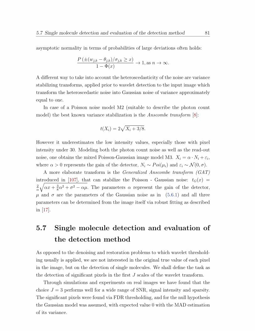
5.7 Single molecule detection and evaluation of the detection method 81
asymptotic normality in terms of probabilities of large deviations often holds:
P (±(wj,k − θj,k)/σj,k ≥ x)
1− Φ(x)→ 1, as n→ ∞.
A different way to take into account the heteroscedasticity of the noise are variance
stabilizing transforms, applied prior to wavelet detection to the input image which
transform the heteroscedastic noise into Gaussian noise of variance approximately
equal to one.
In case of a Poisson noise model M2 (suitable to describe the photon count
model) the best known variance stabilization is the Anscombe transform [8]:
t(Xi) = 2√Xi + 3/8.
However it underestimates the low intensity values, especially those with pixel
intensity under 30. Modeling both the photon count noise as well as the read-out
noise, one obtains the mixed Poisson-Gaussian image model M3. Xi = α ·Ni+ εi,
where α > 0 represents the gain of the detector, Ni ∼ Poi(µi) and εi ∼ N (0, σ).
A more elaborate transform is the Generalized Anscombe transform (GAT)
introduced in [107], that can stabilize the Poisson - Gaussian noise: tG(x) =2α
√αx+ 3
8α2 + σ2 − αµ. The parameters α represent the gain of the detector,
µ and σ are the parameters of the Gaussian noise as in (5.6.1) and all three
parameters can be determined from the image itself via robust fitting as described
in [17].
5.7 Single molecule detection and evaluation of
the detection method
As opposed to the denoising and restoration problems to which wavelet threshold-
ing usually is applied, we are not interested in the original true value of each pixel
in the image, but on the detection of single molecules. We shall define the task as
the detection of significant pixels in the first J scales of the wavelet transform.
Through simulations and experiments on real images we have found that the
choice J = 3 performs well for a wide range of SNR, signal intensity and sparsity.
The significant pixels were found via FDR thresholding, and for the null hypothesis
the Gaussian model was assumed, with expected value 0 with the MAD estimation
of its variance.
82 Chapter 5: Wavelet based detection
The significant pixels, those belonging to true signal are those that have non-
zero coefficients in all the J detail levels (except the finest, which usually is pure
noise). The binary image obtained from the J detail coefficient levels after level-
wise wavelet thresholding and combination of each level via a logical AND opera-
tion is an indicator image for the support of the detected single molecules:
B =J∏
j=j0
1wjk>λi0 (j).
If the first detail level is too noisy, one can set j0 = 2.
At very low concentrations the single molecules are mostly well separated of
each other. At higher concentrations, the support of imaged single molecules can
be touching each other, so that the number of connected components in the binary
image underestimates (strongly in case of high concentration) the number of single
molecules in the image.
In order to alleviate the problem, a denoised image is additionally obtained
after applying the reconstruction step (4.7.3) with thresholded detail coefficients.
Since the wavelet detection algorithm has the “resolution” described above, two
molecules that are spatially close together will be detected as one. The correction
of the estimation of the number of molecules consists in combining the binary image
obtained after the detection step with the denoised image (via a simple product
operation), and all the local maxima of the denoised image inside the support of
the binary mask are considered distinct single molecules (see for instance Fig. 3.7,
c).
The detection algorithm was tested on a set of simulation images with varied
image quality parameters, as measured by the signal-to-noise ratio (SNR), as well
as several molecule concentrations. Each image is of dimension 512 × 512 pixels
and contains 10, 50, 100, 500 or 1000 randomly placed molecules.
To each single molecule corresponds a diffraction limited spot, approximated
by a two-dimensional Gaussian shape, with width s corresponding to the point
spread function of the optical system (1.1 in our simulations). Both the con-
stant background intensity and the peak intensity S were chosen on a logarithmic
scale between 10 and 100. Noise is generated for each pixel as described in (5.6):
the photon count noise was modeled by draws from Poisson distributions, and
finally Gaussian noise is added to each pixel from N (0, σ), where σ was chosen
as 0, 5, 10, 15 and 20% of the maximum peak intensity. For this special case of
Poisson-Gaussian model described, we use the following signal-to-noise (SNR) def-
5.7 Single molecule detection and evaluation of the detection method 83
(a) N = 10 (b) N = 50
(c) N = 100 (d) N = 500
(e) N = 1000
Figure 5.3: A set of simulation images is shown in (a)-(e) for different concentra-tions: N represents the number of peaks in the 512×512 pixel image (correspondingto 102.4µm × 102.4µm). SNR = 5.02 (additional Gaussian noise with σ = 2.2).The images are scaled for better visibility. The same pixel intensity scale is usedfor the five images.
84 Chapter 5: Wavelet based detection
inition as described in Chapter 2:
SNR =S√
B + σ2,
where S represents the single molecule intensity, B the (local) background of the
image and σ the standard deviation of the read-out noise. (For simplicity S is the
maximum intensity of the single molecule profile).
The SNR for our simulations is between 0.9 and 31.6.. For each set of param-
eters 10 images were generated and analyzed. One set of simulations is presented
in Fig. 5.3 (a)− (e).
The results are summarized in Fig. 5.4 (a) and (b). For SNR above 10 the de-
tection for all five concentrations levels exceeds 80% true positives for less than 500
molecules, but is only above 60% for high concentrations (N = 1000). However,
at high concentrations the spots can be analyzed also with conventional methods
designed for low resolution microarrays. The SNR typical for our system, is usu-
ally at least 15, (at this level true positives are higher than 85% for N = 500,
and 70% forN = 1000). The rate of false positives is under 9% even for very
low concentrations (N = 10) and substantially lower for N > 100. The detection
performance was similar for simulation with the same SNR, independent of the
weight of Poisson and Gaussian noise in the generation of the simualtion image.
5.8 Signal detection via robust distance thresh-
olding
In the case of orthogonal wavelet transforms, the independent thresholding of
wavelet coefficients at different scales is the natural approach. However, in the
case of the redundant a trous transform the wavelet coefficients are still correlated
across scales, the gain of translation invariance being made at the price of losing
orthogonality. We shall investigate the effect of the correlation between wavelet
scales on the detection task. As alternative to the scale-wise thresholding of the
wavelet coefficients we suggest the modeling of the null-hypothesis in a higher
dimensional space. In case we are using J wavelet detail levels, H0 will be modeled
in a J-dimensional space, taking into account the correlations between detail levels.
If wij, j = 1, . . . J are the wavelet coefficients obtained via the wavelet trans-
form of the image, we assume that H0 is described by a J-dimensional Gaussian
N (T, S), where T and S are the MCD robust estimates described in Appendix A.
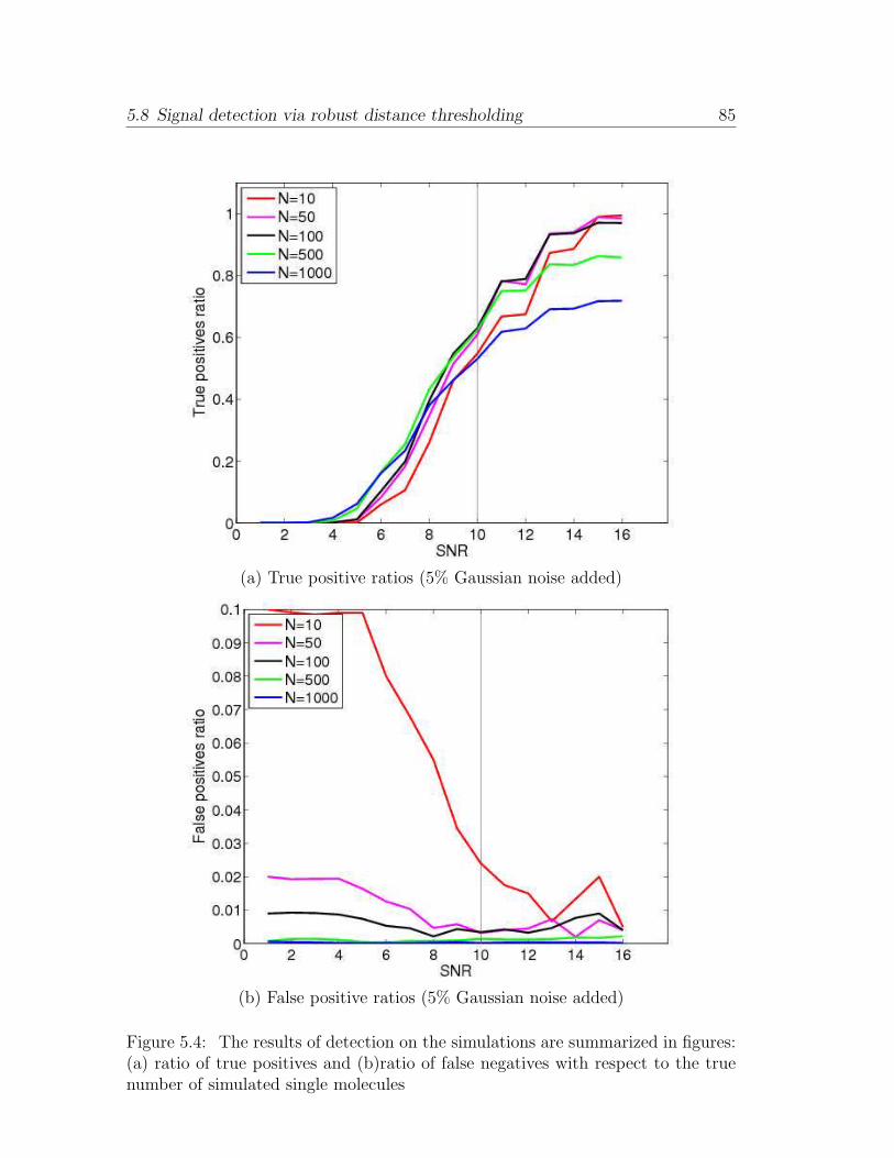
5.8 Signal detection via robust distance thresholding 85
(a) True positive ratios (5% Gaussian noise added)
(b) False positive ratios (5% Gaussian noise added)
Figure 5.4: The results of detection on the simulations are summarized in figures:(a) ratio of true positives and (b)ratio of false negatives with respect to the truenumber of simulated single molecules
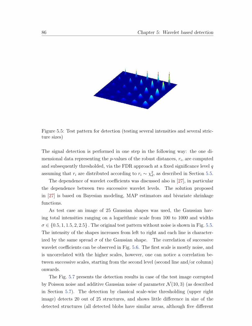
86 Chapter 5: Wavelet based detection
Figure 5.5: Test pattern for detection (testing several intensities and several stric-ture sizes)
The signal detection is performed in one step in the following way: the one di-
mensional data representing the p-values of the robust distances, ri, are computed
and subsequently thresholded, via the FDR approach at a fixed significance level q
assuming that ri are distributed according to ri ∼ χ2d, as described in Section 5.5.
The dependence of wavelet coefficients was discussed also in [27], in particular
the dependence between two successive wavelet levels. The solution proposed
in [27] is based on Bayesian modeling, MAP estimators and bivariate shrinkage
functions.
As test case an image of 25 Gaussian shapes was used, the Gaussian hav-
ing total intensities ranging on a logarithmic scale from 100 to 1000 and widths
σ ∈ 0.5, 1, 1.5, 2, 2.5 . The original test pattern without noise is shown in Fig. 5.5.
The intensity of the shapes increases from left to right and each line is character-
ized by the same spread σ of the Gaussian shape. The correlation of successive
wavelet coefficients can be observed in Fig. 5.6. The first scale is mostly noise, and
is uncorrelated with the higher scales, however, one can notice a correlation be-
tween successive scales, starting from the second level (second line and/or column)
onwards.
The Fig. 5.7 presents the detection results in case of the test image corrupted
by Poisson noise and additive Gaussian noise of parameter N (10, 3) (as described
in Section 5.7). The detection by classical scale-wise thresholding (upper right
image) detects 20 out of 25 structures, and shows little difference in size of the
detected structures (all detected blobs have similar areas, although five different
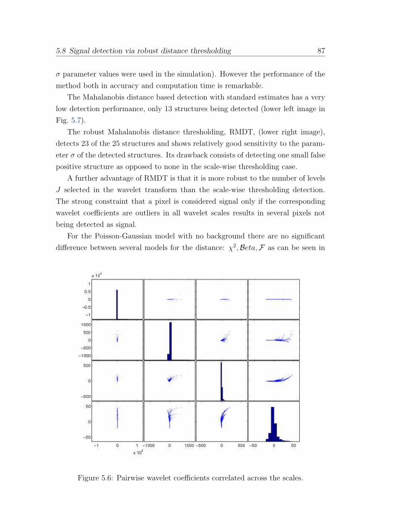
5.8 Signal detection via robust distance thresholding 87
σ parameter values were used in the simulation). However the performance of the
method both in accuracy and computation time is remarkable.
The Mahalanobis distance based detection with standard estimates has a very
low detection performance, only 13 structures being detected (lower left image in
Fig. 5.7).
The robust Mahalanobis distance thresholding, RMDT, (lower right image),
detects 23 of the 25 structures and shows relatively good sensitivity to the param-
eter σ of the detected structures. Its drawback consists of detecting one small false
positive structure as opposed to none in the scale-wise thresholding case.
A further advantage of RMDT is that it is more robust to the number of levels
J selected in the wavelet transform than the scale-wise thresholding detection.
The strong constraint that a pixel is considered signal only if the corresponding
wavelet coefficients are outliers in all wavelet scales results in several pixels not
being detected as signal.
For the Poisson-Gaussian model with no background there are no significant
difference between several models for the distance: χ2,Beta,F as can be seen in
Figure 5.6: Pairwise wavelet coefficients correlated across the scales.
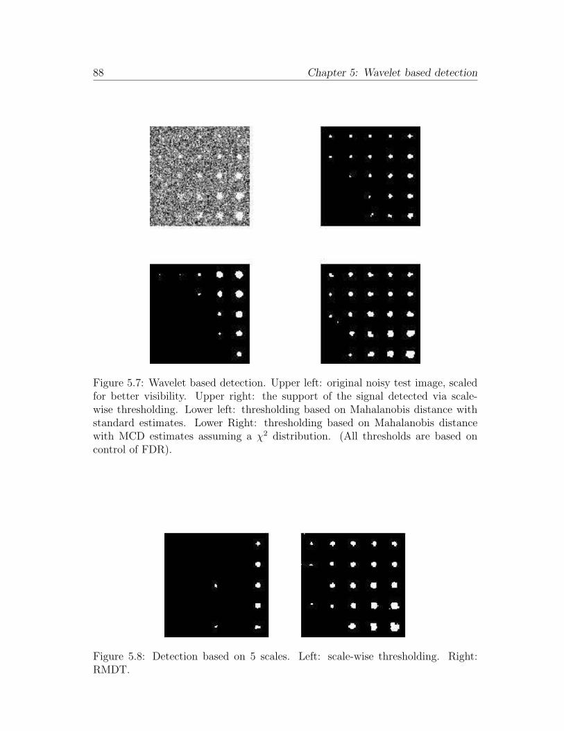
88 Chapter 5: Wavelet based detection
Figure 5.7: Wavelet based detection. Upper left: original noisy test image, scaledfor better visibility. Upper right: the support of the signal detected via scale-wise thresholding. Lower left: thresholding based on Mahalanobis distance withstandard estimates. Lower Right: thresholding based on Mahalanobis distancewith MCD estimates assuming a χ2 distribution. (All thresholds are based oncontrol of FDR).
Figure 5.8: Detection based on 5 scales. Left: scale-wise thresholding. Right:RMDT.
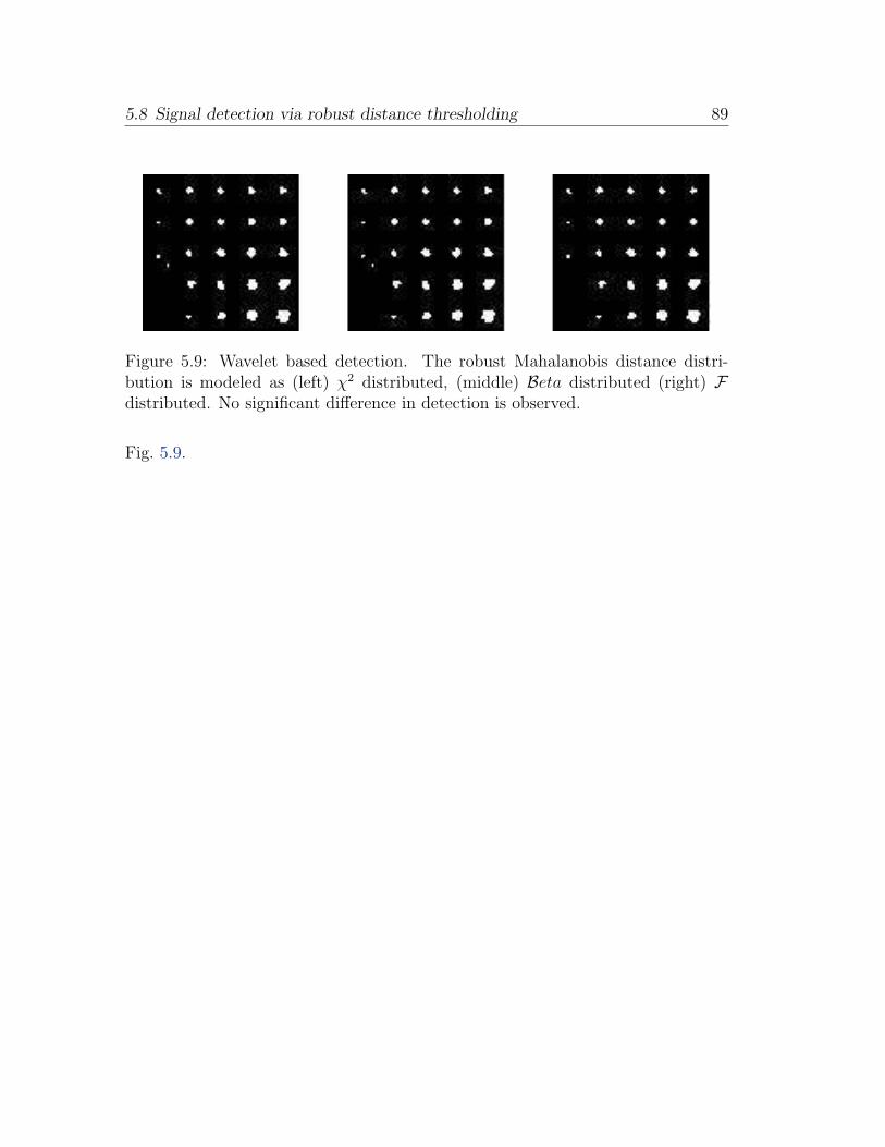
5.8 Signal detection via robust distance thresholding 89
Figure 5.9: Wavelet based detection. The robust Mahalanobis distance distri-bution is modeled as (left) χ2 distributed, (middle) Beta distributed (right) Fdistributed. No significant difference in detection is observed.
Fig. 5.9.

90 Chapter 5: Wavelet based detection
Chapter 6
Spatial patterns
After detecting the approximate position of spots and localizing the single molecule
peaks in the detected region it is necessary to refine the analysis in order to remove
single peaks outside the printed spot. Typically peaks representing non-specific
binding, artifacts, dirt, etc. outside the spot area have to be separated from
hybridized peaks. This step corresponds to the background/foreground pixel sep-
aration in the classical microarray image analysis.
The main assumption for this step of the analysis is that the concentration of
false peaks is different - typically lower - from the concentration of the peaks inside
the spot. For this reason, the signal and the background are jointly modeled as a
mixture of two (spatial) point processes.
This chapter presents a brief introduction in the field of spatial point patterns,
in order to offer a perspective of modeling single molecules as point patterns. We
will focus on two models, the two-dimensional stationary Poisson process and the
mixture of stationary Poisson processes. The latter will be used in separating
hybridized single molecules from clutter.
Furthermore we describe and compare solutions for two problems: the complete
randomness test and concentration estimation. We apply the described algorithms
to prove the soundness of randomness assumption in the case of single molecule
microarray images, as well as concentration estimation at the single molecule level,
which will give the measure of hybridization for each spot in the high resolution
microarray.
91
92 Chapter 6: Spatial patterns
6.1 Introduction to spatial point processes
Intuitively, point processes are stochastic models for finite or countable collection of
points X lying in some set S ⊆ Rd, d ≥ 1. A point pattern is typically interpreted
as a realization of a point process.
The area where points of the pattern can possibly be observed is called obser-
vation window, denoted usually by W . When the point pattern is restricted to W
(W = S), we talk about finite point patterns. More frequently thoughW is strictly
contained in S (W ⊂ S). Since there is no information for the unobserved region
Rd\W , in the case of certain statistical summaries one has to handle the problems
raised by the missing data that could affect these summaries. This problem is
known under the name of boundary or edge effects.
We use the notations: XA = X ∩ A and X(A) is the cardinality of XA, where
A ⊂ Rd is a bounded Borel set.
Definition 6.1.1. A point process defined on S ⊂ Rd is a random variable X
taking values in a measurable space [N,N ], where N is the family of all locally
finite point configurations in S:
N = x ⊂ S : x(A) <∞, ∀A ∈ B0
and B0 denotes the class of bounded Borel sets in S and such that the points have
single multiplicity (xi 6= xj if i 6= j.) N is the smallest σ-algebra generated by
all sets of the form x ∈ N : x(A) = m, with A ∈ B0 and m ∈ N0. X can be
regarded as a measure on a probability field (Ω,F ,P) that makes all mappings
X(A) : Ω → N measurable.
Intuitively, a point process, denoted by X has two interpretations:
1. a random counting measure: X(B) = n meaning that B contains n points
of N.
2. a random closed set X = x1, x2, . . . = xi, or xi ∈ N
The point process X generates a distribution P on [N,N ]. The distribution P
is determined by the probabilities P (Y ) = P (X ∈ Y ). Several good introductions
in the theory of points process are available, e.g. [109, 29, 82, 60].
Two important properties of point processes are stationarity and isotropy.
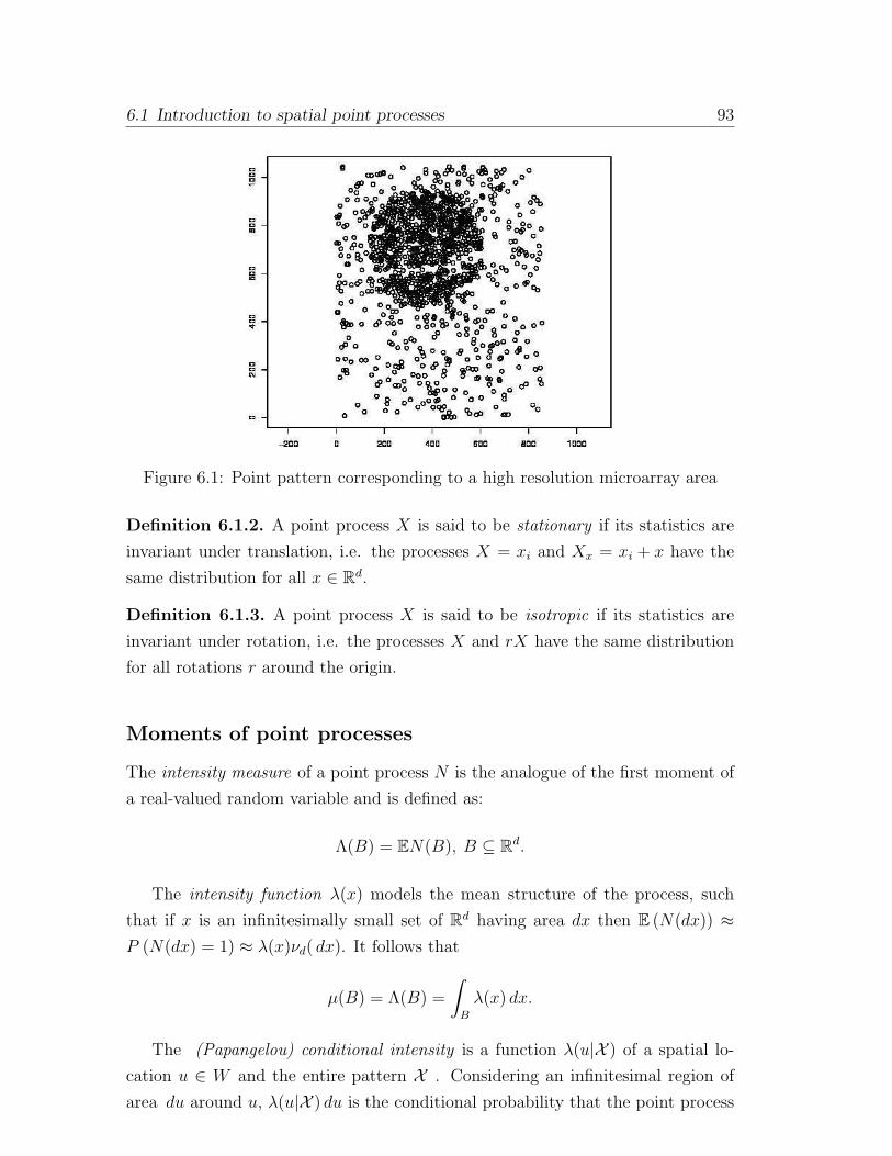
6.1 Introduction to spatial point processes 93
Figure 6.1: Point pattern corresponding to a high resolution microarray area
Definition 6.1.2. A point process X is said to be stationary if its statistics are
invariant under translation, i.e. the processes X = xi and Xx = xi + x have the
same distribution for all x ∈ Rd.
Definition 6.1.3. A point process X is said to be isotropic if its statistics are
invariant under rotation, i.e. the processes X and rX have the same distribution
for all rotations r around the origin.
Moments of point processes
The intensity measure of a point process N is the analogue of the first moment of
a real-valued random variable and is defined as:
Λ(B) = EN(B), B ⊆ Rd.
The intensity function λ(x) models the mean structure of the process, such
that if x is an infinitesimally small set of Rd having area dx then E (N(dx)) ≈P (N(dx) = 1) ≈ λ(x)νd( dx). It follows that
µ(B) = Λ(B) =
∫
B
λ(x) dx.
The (Papangelou) conditional intensity is a function λ(u|X ) of a spatial lo-
cation u ∈ W and the entire pattern X . Considering an infinitesimal region of
area du around u, λ(u|X ) du is the conditional probability that the point process
94 Chapter 6: Spatial patterns
contains a point in this region, given the position of all the points in the process
outside of the infinitesimal region:
E(N( dx) = 1|N ∩ dxC = X
)≈ λ(x|X )ν( dx).
The stationary Poisson process discussed below has the conditional intensity
λ(u|X ) = β, where β is the intensity of the process.
Higher order moments
Computations of expected values, usually are simplified when the Campbell theo-
rem is applied (see [109]).
Theorem 6.1.4. If f is a non-negative measurable function and S =∑
x∈X f(x)
then
E(S) = E
(∑
x∈Xf(x)
)=
∫
Rd
f(x)λ(x) dx. (6.1.1)
Generalizing the first moment measure, one obtains the nth-order moment
measures µ(n) of the point process X defined by
∫f(x1, . . . , xn)µ
(n)( d(x1, . . . , xn)) = E
(∑
x1,...,xn∈Xf(x1, . . . , xn)
)(6.1.2)
where f(x1, . . . , xn) is any non-negative measurable function on Rnd.
The following equalities hold
µ(n)(B1 × . . .× Bn) = E (X(B1) . . . X(Bn)))
and in case B1 = . . . = Bn = B, µ(n)(Bn) = EX(B)n.
In particular:
n = 1 : µ(1)(B) = EX(B) = Λ(B)
n = 2 : µ(2)(B1 × B2) = EX(B1)X(B2)
var (X(B)) = µ(2)(B × B)− (Λ(B))2
cov (X(B1), X(B2)) = µ(2)(B1 × B2)− Λ(B1)Λ(B2)
6.1 Introduction to spatial point processes 95
Factorial moments
The nth order factorial moment measure α(n) of the point process X is defined
by:
∫f(x1, . . . , xn)α
(n)( d(x1, . . . , xn)) = E
∑
x1 6=x2 6=... 6=xn∈Xf (x1, . . . , xn) ,
where f is a non-negative measurable function on Rnd.
For n = 2, µ(2)(B1 × B2) = Λ(B1 ∩ B2) + α(2)(B1 × B2). If B1, . . . , Bn are
pairwise disjoint, then
µ(n)(B1 × . . .× Bn) = α(n)(B1 × . . .× Bn).
The name factorial moment is justified by the following equality:
α(n)(Bn) = E [X(B)(X(B)− 1) . . . (X(B)− n+ 1)] ,
such that αn(Bn) is the factorial moment of X(B).
Point process operations
Many point process models can be derived from simpler models by applying one
or several operations, such as thinning, superposition, clustering.
A thinning operation consists of removal of certain points of a point process
N0, yielding the thinned point process N ∈ N0. The removal of a point x can be
done according to a constant probability p, a location dependent probability p(x)
or a random probability. We talk of independent thinnings if removal of points is
done independently of other points, and of dependent thinnings, when the removal
depends on the configuration of N0.
The intensity function of a p(x)-thinned process with original process intensity
λ0 is
λ(x) = p(x)λ0(x), x ∈ Rd.
In a superposition operation two or more point processes are superimposed
onto each other, such that the resulting process is the set-theoretic union of the
operand processes: N = N1 ∪ N2 . . . ∪ Nk. The intensity of the resulting process
is the sum of the intensities of component processes λ = λ1 + λ2 + . . .+ λk.
Finally, clustering is the operation through which points x of the process N0
96 Chapter 6: Spatial patterns
are replaced by clusters Nx of points. The union of the clusters defines the cluster
point process
N = ∪x∈N0Nx.
A special case of clustering is when all clusters have the same distribution, with c
the mean number of points in each cluster. In this case the intensity of the cluster
process is
λ = cλ0. (6.1.3)
Point process models
With a few simple generating mechanisms and the operation described above sev-
eral point process models can be described. The simplest and best studied point
process is the (homogeneous) Poisson point process.
Spatial Poisson process
Definition 6.1.5. A Poisson process N defined on S and with intensity measure
Λ and intensity function λ satisfies for any bounded region B ⊆ S with Λ(B) > 0:
Poisson distribution of point counts : for all bounded Borel sets B:
P (N(B) = m) = [Λ(B)]m · exp (−Λ(B)) /m!, m = 0, 1, 2, . . .
Independent scattering property: the number of points of N in k disjoint sets
form k independent random variables.
The homogeneous Poisson process is a special case, such that Λ(B) = λν(B),
for a constant λ > 0, which also implies that the process is isotropic. The homo-
geneous Poisson process represents a model for no interaction or complete spatial
randomness (CSR) since for any disjoint subsets A,B ⊆ S, N(A) and N(B) are
independent.
In the case of an inhomogeneous Poisson process, the intensity is not propor-
tional to Lebesgue measure, but is a deterministic function of spatial location. If
a inhomogeneous Poisson process has random mean measures we talk of doubly
stochastic processes or Cox processes. For instance a stationary Poisson process
with randomized intensity parameter is a particular Cox process, called mixed
Poisson process.
6.1 Introduction to spatial point processes 97
As an exemplification of clustering processes we shall define Neymann-Scott
point processes and in order to illustrate processes that exhibit regularity we in-
troduce the hard-core models.
Neymann-Scott processes are the result of homogeneous independent clustering
applied to stationary point processes. The points of the parent process form a
stationary Poisson process of intensity λ0 and are not observable. Each parent
point x generates a cluster Nx of average size c, independently and identically
distributed around the parent point. The process has the intensity given in (6.1.3).
If Nx is a cluster of independently and uniformly distributed points in a ball
b(x,R) the point process is called Matern cluster process, while if the daughter
points follow a normal distribution around the parent point the process is called
(modified) Thomas process (see [60]).
The hard core models belong to the class of point processes that model inhi-
bition or regularity and are characterized by a minimal distance r0 between their
points. No points may be located at distance smaller than r0 of each other.
The simplest model is the Matern hard-core process I, NI , obtained from a
homogeneous Poisson process N0 with intensity λ0 by deleting all pairs of events
of N0 that are separated by a distance smaller than r0. The probability that a
point is retained in NI is exp−λ0Vdrd0
and the intensity of NI is
λ = λ0 exp−λ0Vdrd0
,
where Vd = πd/2/Γ(1+ d/2) is the volume of the unit sphere. If the initial process
N0 is endowed with independent marks Z(x), the model II of Matern hard-core
process NII is defined as the process obtained after the deletion of points u, such
that ‖u− x‖ < r0 and Z(u) < Z(x). The probability that an arbitrary point is
retained in NII is1− exp
(−λ0Vdrd0
)/λ0Vdr
d0
and the intensity of NII is
λ =1− exp
(−λ0Vdrd0
)
Vdrd0.
Several other point process models are known in the literature, many of which are
described in [91, 109, 26, 60].
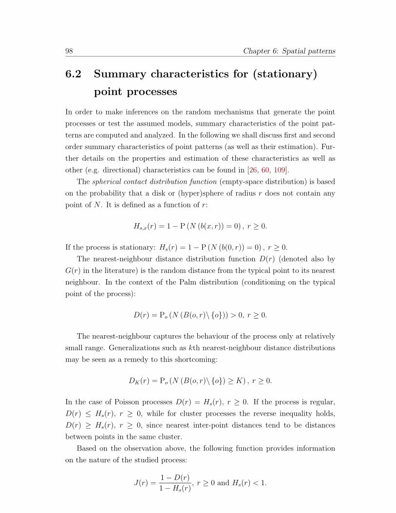
98 Chapter 6: Spatial patterns
6.2 Summary characteristics for (stationary)
point processes
In order to make inferences on the random mechanisms that generate the point
processes or test the assumed models, summary characteristics of the point pat-
terns are computed and analyzed. In the following we shall discuss first and second
order summary characteristics of point patterns (as well as their estimation). Fur-
ther details on the properties and estimation of these characteristics as well as
other (e.g. directional) characteristics can be found in [26, 60, 109].
The spherical contact distribution function (empty-space distribution) is based
on the probability that a disk or (hyper)sphere of radius r does not contain any
point of N . It is defined as a function of r:
Hs,x(r) = 1− P (N (b(x, r)) = 0) , r ≥ 0.
If the process is stationary: Hs(r) = 1− P (N (b(0, r)) = 0) , r ≥ 0.
The nearest-neighbour distance distribution function D(r) (denoted also by
G(r) in the literature) is the random distance from the typical point to its nearest
neighbour. In the context of the Palm distribution (conditioning on the typical
point of the process):
D(r) = Po (N (B(o, r)\ o)) > 0, r ≥ 0.
The nearest-neighbour captures the behaviour of the process only at relatively
small range. Generalizations such as kth nearest-neighbour distance distributions
may be seen as a remedy to this shortcoming:
DK(r) = Po (N (B(o, r)\ o) ≥ K) , r ≥ 0.
In the case of Poisson processes D(r) = Hs(r), r ≥ 0. If the process is regular,
D(r) ≤ Hs(r), r ≥ 0, while for cluster processes the reverse inequality holds,
D(r) ≥ Hs(r), r ≥ 0, since nearest inter-point distances tend to be distances
between points in the same cluster.
Based on the observation above, the following function provides information
on the nature of the studied process:
J(r) =1−D(r)
1−Hs(r), r ≥ 0 and Hs(r) < 1.
6.2 Summary characteristics for (stationary)point processes 99
For Poisson processes J(r) = 1 holds. However the inverse implication does not
hold, there exist other processes different from Poisson, with J(r) = 1.
The estimation of J(r) poses some difficulties, especially for small values of
1−Hs(r) (i.e. for large r). Furthermore, the numerator and denominator are point-
and location-related summaries, respectively, each with different fluctuations that
do not cancel out.
The summaries discussed so far are restricted to describe the point pattern
in small neighborhoods of a typical point. For longer-range spatial correlation
analysis a better approach is offered by second order characteristics.
The inhomogeneous reduced second moment measure is defined as:
K(B) =1
|A|E∑
u∈N(A)
∑
v∈N\u
1u−v∈Bλ(u) · λ(v) , (6.2.1)
where the point process N is second-order reweighted stationary, meaning that
the right hand side of (6.2.1) does not depend on the choice of A ⊆ R, where
0 < |A| < ∞. When the process is stationary and isotropic, the reduced moment
function becomes Ripley’s K−function (see [91]):
K(r) = K (b(o, r)) , r ≥ 0.
The quantity λK(r) represents the mean number of points of N within a sphere
of radius r centered on a ’typical point’, which itself is excluded from the count.
The function K is monotonically non-decreasing on r > 0 and converges to 0 as
r → 0. In the case of a stationary Poisson process: K(r) = bdrd, r ≥ 0. A variance
stabilized transformation of K ( K estimated by non-parametric methods) is the
L-function defined as:
L(r) =
√K(r)
π, (6.2.2)
in the planar case, and as
L(r) = d
√K(r)
bd, r ≥ 0, (6.2.3)
in the general d-dimensional case.
For a Poisson process, L(r) = r. In general, L(r) > r indicates aggregation
and L(r) < r indicates regularity.
100 Chapter 6: Spatial patterns
Figure 6.2: Summaries for the point pattern in Fig. 6.1 (different colors correspondto different edge correction methods)
6.3 Testing in the framework of point patterns
Based on the summary characteristics described in the previous section, several
statistical tests are designed in order to gain information on the studied point
process, its properties and generating mechanism.
In the frame of microarray analysis, we would like to test the randomness of
the single molecule distributions inside the spots of the high resolution microarray
data. Therefore the positions of the single molecules, obtained by the wavelet
detection methods will form the input data we test against the CSR hypothesis.
Since the homogeneous Poisson process is the mathematical model that de-
scribes CSR, the ”null model” implying complete lack of structure, the CSR tests
consist of estimating a summary statistic (scalar or functional) from the data and
compare it with the relevant summary characteristic for a Poisson process. If
the difference between the two characteristics is large, the Poisson hypothesis is
rejected.
We describe two CSR tests, one based on point numbers and the other on
6.3 Testing in the framework of point patterns 101
inter-point distances of the point patterns, which we apply in order to test if the
assumption of randomness of single molecule positions inside the microarray spot
should be rejected or not.
The index-of-dispersion test
The sampling window W can be divided into subregions of equal size, called
quadrats, usually for practical reasons in squares or rectangular grid cells. Un-
der the homogeneous Poisson process hypothesis, the number of points in each
quadrat follows a Poisson distribution of mean λ · ν(Q) and the counts in disjoints
quadrats are independent.
The test is defined based on the index of dispersion defined as:
I =(k − 1)s2
x,
where k is the number of quadrats, x the mean of the number of points per quadrat,
and s2 is the sample variance of the number of points per quadrat. It represents
the χ2 goodness-of-fit test of the hypothesis that the n points are independently
and uniformly distributed in W . It follows approximately a χ2 distribution with
k − 1 degrees of freedom, for k > 6 and λ · ν(Q) > 1.
The CSR hypothesis is rejected if I > χ2k−1;α (the alternative being that there
is aggregation in the process), or if I < χ2k−1;1−α (alternative: regularity of point
pattern).
An extension of the above approach is the Greig-Smith method, which basically
applies the previous test to a quadtree structure. It also gives information at which
scale clustering occurs, if at all.
L test
In order to test the hypothesis that the single molecules are randomly distributed
we compute the empirical L−function based on the location of single molecules,
obtained via the wavelet transform approach. Knowing that the L−function of
a homogeneous Poisson process has the simple linear form: L(r) = r for r ≥ 0,
the large deviation of the empirical L−function indicates rejection of the CSR
hypothesis. The square root transformation in the computation of the L−function:
L(r) =√K(R)/π has a variance stabilization effect, that makes the L−function
a better candidate for the test than the K−function.
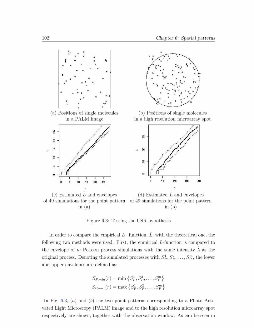
102 Chapter 6: Spatial patterns
(a) Positions of single moleculesin a PALM image
(b) Positions of single moleculesin a high resolution microarray spot
(c) Estimated L and envelopesof 49 simulations for the point pattern
in (a)
(d) Estimated L and envelopesof 49 simulations for the point pattern
in (b)
Figure 6.3: Testing the CSR hypothesis
In order to compare the empirical L−function, L, with the theoretical one, the
following two methods were used. First, the empirical L-function is compared to
the envelope of m Poisson process simulations with the same intensity λ as the
original process. Denoting the simulated processes with S1P , S
2P , . . . , S
mP , the lower
and upper envelopes are defined as:
SP,min(r) = minS1P , S
2P , . . . , S
mP
SP,max(r) = maxS1P , S
2P , . . . , S
mP
In Fig. 6.3, (a) and (b) the two point patterns corresponding to a Photo Acti-
vated Light Microscopy (PALM) image and to the high resolution microarray spot
respectively are shown, together with the observation window. As can be seen in
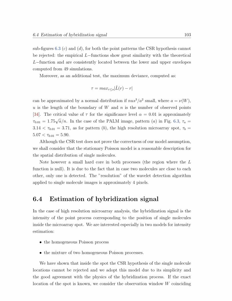
6.4 Estimation of hybridization signal 103
sub-figures 6.3 (c) and (d), for both the point patterns the CSR hypothesis cannot
be rejected: the empirical L−functions show great similarity with the theoretical
L−function and are consistently located between the lower and upper envelopes
computed from 49 simulations.
Moreover, as an additional test, the maximum deviance, computed as:
τ = maxr≤s|L(r)− r|
can be approximated by a normal distribution if nus3/a2 small, where a = ν(W ),
u is the length of the boundary of W and n is the number of observed points
[34]. The critical value of τ for the significance level α = 0.01 is approximately
τ0.01 = 1.75√a/n. In the case of the PALM image, pattern (a) in Fig. 6.3, τa =
3.14 < τ0.01 = 3.71, as for pattern (b), the high resolution microarray spot, τb =
5.07 < τ0.01 = 5.90.
Although the CSR test does not prove the correctness of our model assumption,
we shall consider that the stationary Poisson model is a reasonable description for
the spatial distribution of single molecules.
Note however a small hard core in both processes (the region where the L
function is null). It is due to the fact that in case two molecules are close to each
other, only one is detected. The ”resolution” of the wavelet detection algorithm
applied to single molecule images is approximately 4 pixels.
6.4 Estimation of hybridization signal
In the case of high resolution microarray analysis, the hybridization signal is the
intensity of the point process corresponding to the position of single molecules
inside the microarray spot. We are interested especially in two models for intensity
estimation:
• the homogeneous Poisson process
• the mixture of two homogeneous Poisson processes.
We have shown that inside the spot the CSR hypothesis of the single molecule
locations cannot be rejected and we adopt this model due to its simplicity and
the good agreement with the physics of the hybridization process. If the exact
location of the spot is known, we consider the observation window W coinciding
104 Chapter 6: Spatial patterns
with the spot and the positions of single molecules inside the spot represent an
homogeneous Poisson process, with the only parameter the intensity λ.
A short overview of estimation methods for this case is given in [60].
• If the number of points in the sampling window W is N(W ) and the area
(hyper-volume) of W is denoted ν(W ) then:
λ =N(W )
ν(W )(6.4.1)
is an unbiased estimator with variance var(λ) = λν(W )
. This is also the max-
imum likelihood estimator.
• Distance methods are based on ”nearest neighbour”-type distances, having
a known distribution for homogeneous Poisson process model.
• Confidence intervals for λ are based on the normal approximation of the
Poisson distributed N(W ) = λν(W ):
(zα/22
−√N(W )
)2≤ λν(W ) ≤
(zα/22
+√N(W ) + 1
)2,
where zα/2 are quantiles of the standard normal distribution. This method is
most useful in determining the window size required for a given estimation
accuracy: if δ is the desired width of the confidence interval and α is the
required confidence level from
δν(W ) ≈(zα/2
2+√λν(W ) + 1
)2−(zα/2
2+√λν(W )
)2
results that the required window size is
ν(W ) ≈ 4zα/2λ
δ2. (6.4.2)
As we have mentioned in the beginning of the chapter, not all the peaks detected
in the subimage corresponding to a grid element belong to the spot of interest (see
Fig 3.7, c)). The background might be heavily contaminated by unspecifically
bound signal, impurities, etc. which we shall call generally clutter, which when
unaccounted for could seriously distort the hybridization results. Also in practice
the exact spot location inside the subimage is not known, small distortion might
be due to printing tip motion, scanning artifacts etc.
6.4 Estimation of hybridization signal 105
Each rectangular subimage of the microarray, obtained after the gridding step,
contains the circular spot of mRNA hybridized to the printed cDNA (foreground)
surrounded by a background region with clutter. Therefore, peaks detected in the
subimages have to be assigned either to foreground or background. In order to
make a correct concentration estimation (or hybridization estimation), we have to
model both the spot and the background concentration. A straightforward model
turns out to be the superposition of spatial Poisson point processes. However
a more precise model is that of a homogeneous Poisson process (modeling the
clutter) on which is superposed another homogeneous Poisson process restricted
to a subdomain of the initial process. The new process has piecewise-constant
intensity function. The estimation of the intensity of the process can be done
either by parametric methods, typically based on mixture models on one hand,
and on nonparametric methods, on the other hand.
In the case of parametric models, in order to distinguish between peaks within
the spot, representing true hybridization signal and those representing clutter we
use spatial information, counts of peaks in subregions or relative distances of the
peaks to each other and design a spatial mixture model based on this information.
One component of the mixture will represent the true signal, while the other the
clutter.
In the case of non-parametric intensity estimation approaches first the intensity
is estimated and subsequently the location of the spot is found. We will use
the Nadaraya-Watson kernel estimate or a wavelet estimation method, and in
both cases the spot position is found after intensity estimation via segmentations
methods.
In the classical microarray case, this step corresponds to foreground/background
segmentation and in [14] it is based on a Gaussian mixture model for pixel inten-
sity values, where each pixel is assumed having a mixture distribution of two
(signal/background) or three (signal/background/artifacts) components.
Analysis of count data via the method of moments
A first parametric approach for concentration estimation is to consider the count
yi, of the detected peaks inside non-overlapping systematic quadrats of size s× s
pixels covering the spot subimage, where i is an index over the quadrat covering,
i ∈ 1, . . . , N. Let Y be the random variables whose realizations are the counts yi.
It is supposed to follow a mixture distribution with K components and we would
like to determine the parameters of this mixture distribution. The basic idea is
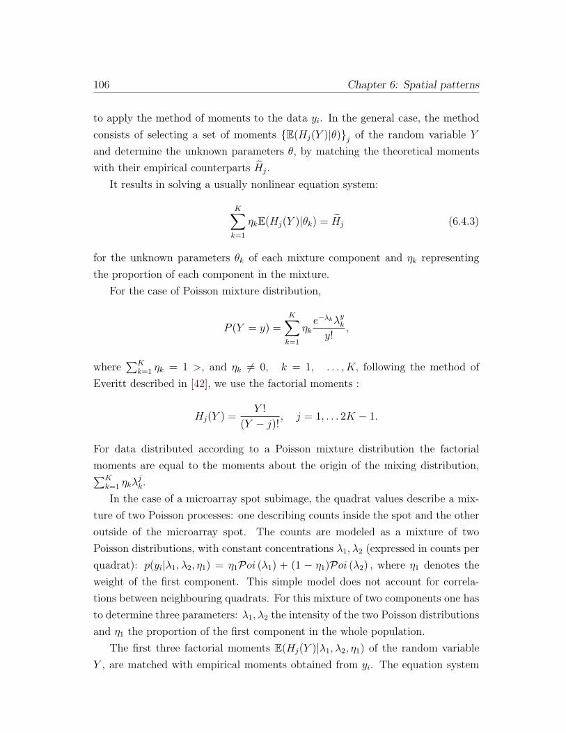
106 Chapter 6: Spatial patterns
to apply the method of moments to the data yi. In the general case, the method
consists of selecting a set of moments E(Hj(Y )|θ)j of the random variable Y
and determine the unknown parameters θ, by matching the theoretical moments
with their empirical counterparts Hj.
It results in solving a usually nonlinear equation system:
K∑
k=1
ηkE(Hj(Y )|θk) = Hj (6.4.3)
for the unknown parameters θk of each mixture component and ηk representing
the proportion of each component in the mixture.
For the case of Poisson mixture distribution,
P (Y = y) =K∑
k=1
ηke−λkλyky!
,
where∑K
k=1 ηk = 1 >, and ηk 6= 0, k = 1, . . . , K, following the method of
Everitt described in [42], we use the factorial moments :
Hj(Y ) =Y !
(Y − j)!, j = 1, . . . 2K − 1.
For data distributed according to a Poisson mixture distribution the factorial
moments are equal to the moments about the origin of the mixing distribution,∑Kk=1 ηkλ
jk.
In the case of a microarray spot subimage, the quadrat values describe a mix-
ture of two Poisson processes: one describing counts inside the spot and the other
outside of the microarray spot. The counts are modeled as a mixture of two
Poisson distributions, with constant concentrations λ1, λ2 (expressed in counts per
quadrat): p(yi|λ1, λ2, η1) = η1Poi (λ1) + (1 − η1)Poi (λ2) , where η1 denotes the
weight of the first component. This simple model does not account for correla-
tions between neighbouring quadrats. For this mixture of two components one has
to determine three parameters: λ1, λ2 the intensity of the two Poisson distributions
and η1 the proportion of the first component in the whole population.
The first three factorial moments E(Hj(Y )|λ1, λ2, η1) of the random variable
Y , are matched with empirical moments obtained from yi. The equation system
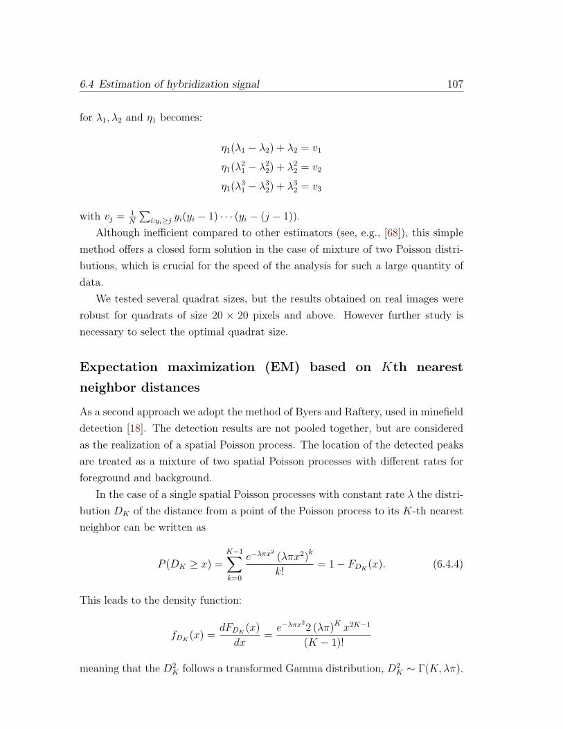
6.4 Estimation of hybridization signal 107
for λ1, λ2 and η1 becomes:
η1(λ1 − λ2) + λ2 = v1
η1(λ21 − λ22) + λ22 = v2
η1(λ31 − λ32) + λ32 = v3
with vj =1N
∑i:yi≥j yi(yi − 1) · · · (yi − (j − 1)).
Although inefficient compared to other estimators (see, e.g., [68]), this simple
method offers a closed form solution in the case of mixture of two Poisson distri-
butions, which is crucial for the speed of the analysis for such a large quantity of
data.
We tested several quadrat sizes, but the results obtained on real images were
robust for quadrats of size 20 × 20 pixels and above. However further study is
necessary to select the optimal quadrat size.
Expectation maximization (EM) based on Kth nearest
neighbor distances
As a second approach we adopt the method of Byers and Raftery, used in minefield
detection [18]. The detection results are not pooled together, but are considered
as the realization of a spatial Poisson process. The location of the detected peaks
are treated as a mixture of two spatial Poisson processes with different rates for
foreground and background.
In the case of a single spatial Poisson processes with constant rate λ the distri-
bution DK of the distance from a point of the Poisson process to its K-th nearest
neighbor can be written as
P (DK ≥ x) =K−1∑
k=0
e−λπx2(λπx2)
k
k!= 1− FDK
(x). (6.4.4)
This leads to the density function:
fDK(x) =
dFDK(x)
dx=e−λπx
22 (λπ)K x2K−1
(K − 1)!
meaning that the D2K follows a transformed Gamma distribution, D2
K ∼ Γ(K,λπ).
108 Chapter 6: Spatial patterns
(a) Easily separable components of themixture
λ1 = 0.025, λ2 = 0.005
(b) A case with mixture componentsdifficult to separateλ1 = 0.065, λ2 = 0.045
Figure 6.4: The density function of kNN distanceDk(λ1, λ2) for the spatial Poissonmixture with concentrations λ1 inside and λ2 outside the spot, respectively.
The maximum likelihood estimate of the rate of the Poisson process is:
λ =K
π∑n
i=1 d2i
(6.4.5)
where di, i = 1, . . . , n are the realizations of the K-th nearest neighbour distances.
In the case of a mixture of two Poisson processes with two intensity rates λ1
and λ2, the model for DK can be written as
DK ∼ p Γ12 (K,λ1π) + (1− p)Γ
12 (K,λ2π) . (6.4.6)
The pdf of the mixture is plotted in Fig. 6.4. The Figure 6.4 is a pseudo-surface
representing the distribution function of the k-th nearest neighbour Dk(λ1, λ2)
in the spatial mixture model for each fixed value K on the axis kNN , and for
fixed rates λ1 and λ2. The bigger the difference between the signal and clutter
concentration the easier is to separate the two components of the mixture. Also,
as one can see in Fig. 6.4 for high concentrations the task is more challenging than
for lower concentrations. As opposed to the method of moments’ η, p represents a
proportion of the samples DK . The three unknown parameters that describe the
distribution DK : p, λ1, λ2, are estimated via the EM algorithm, together with the
assignments to components (“missing data”) δi ∈ 0, 1, where δi = 1 if the i−th
point belongs to the first component (signal), and δi = 0 otherwise.
6.4 Estimation of hybridization signal 109
(a) 0.08 amol/80µl (b) 0.8 amol/80µl (c) 8 amol/80µl
Figure 6.5: Background/foreground separation of peaks for three different concen-trations via the EM method applied to the Kth nearest neighbour distances.
The expectation step becomes:
E(δ(t+1)i
)=
p(t)fDK
(di, λ
(t)1
)
p(t)fDK
(di, λ
(t)1
)+ (1− p(t))fDK
(di, λ
(t)2
)
and the maximization:
λ(t+1)1 =
K∑n
i=1 δ(t+1)i
π∑n
i=1 d2i δ
(i t+ 1)
λ(t+1)2 =
K∑n
i=1
(1− δ
(t+1)i
)
π∑n
i=1 d2i
(1− δ
(t+1)i
)
p(t+1) =n∑
i=1
δ(t+1)i
n.
As initial values for the three parameters one can use the results obtained
through the method of moments. In order to gain insight in the challenges of
microarray image analysis, we present the results of the classical method and the
high resolution adapted peak counting method for three different concentration:
0.08, 0.08, and 8 amol/80µl. In Fig. 6.5 the result of the EM method applied to real
oligonucleotide data is shown. In the leftmost image, characterized by low concen-
tration of molecules, one can see that only for a part of the spot the hybridized
signal was correctly identified. For higher concentrations (middle and right image)
the spot shape can clearly be recognized. The EM method is insensitive to the
shape that has to be detected, allowing for the analysis of anomalous spots due
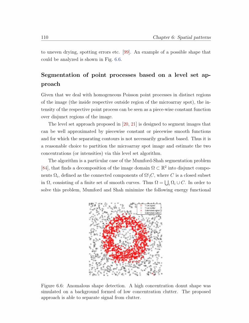
110 Chapter 6: Spatial patterns
to uneven drying, spotting errors etc. [99]. An example of a possible shape that
could be analyzed is shown in Fig. 6.6.
Segmentation of point processes based on a level set ap-
proach
Given that we deal with homogeneous Poisson point processes in distinct regions
of the image (the inside respective outside region of the microarray spot), the in-
tensity of the respective point process can be seen as a piece-wise constant function
over disjunct regions of the image.
The level set approach proposed in [20, 21] is designed to segment images that
can be well approximated by piecewise constant or piecewise smooth functions
and for which the separating contours is not necessarily gradient based. Thus it is
a reasonable choice to partition the microarray spot image and estimate the two
concentrations (or intensities) via this level set algorithm.
The algorithm is a particular case of the Mumford-Shah segmentation problem
[84], that finds a decomposition of the image domain Ω ⊂ R2 into disjunct compo-
nents Ωi, defined as the connected components of Ω\C, where C is a closed subset
in Ω, consisting of a finite set of smooth curves. Thus Ω =⋃iΩi ∪ C. In order to
solve this problem, Mumford and Shah minimize the following energy functional
Figure 6.6: Anomalous shape detection. A high concentration donut shape wassimulated on a background formed of low concentration clutter. The proposedapproach is able to separate signal from clutter.
6.4 Estimation of hybridization signal 111
with respect to u and C
FMS =
∫
Ω
(u− u0)2 dx dy + µ
∫
Ω\C|∇u|2 dx dy + ν|C|,
where u0 : Ω → R is the bounded image function, |C| denotes the length of
C and ν and µ are fixed weight parameters. In particular, if u0 is formed of
regions of approximately piecewise-constant intensities, approximately c1 inside C
and approximately c2 outside this region and setting µ = 0 (for constant regions
having anyway ∇u0 = 0 fulfilled) the minimizing problem becomes:
infu,C
F = λ1
∫
int(C)
(u(x, y)−c1)2 dx dy+λ2∫
out(C)
(u(x, y)−c2)2 dx dy+ν|C|. (6.4.7)
As a matter of notation if Ω∗ ⊂ Ω an open subset then C is the boundary of the
subset C = ∂Ω∗ , int(C) = Ω∗ and out(C) = Ω\Ω∗. An ubiquitous choice of
parameters is λ1 = λ2 = 1.
The algorithms makes use of the implicit representation for the evolving curves
C as the zero level set of a scalar Lipschitz continuous function φ : Ω → R such
that φ(x, y) > 0 in int(C), φ(x, y) < 0 in out(C) and φ(x, y) = 0 on C and with
the help of the Heaviside function H
H(z) =
1, if z ≥ 0
0, if z < 0
and the Dirac measure δa given by
δa(A) =
1, if a ∈ A
0, if a /∈ A
By replacing H and δ with their regularized versions Hε and δε (e.g. obtained via
convolution with a molifier), δε(z) =ddzHε(z), the length of C can be expressed as
|C| = limε←0
∫
Ω
|∇Hε(φ(x, y))| dx dy = limε←0
∫
Ω
δε(φ(x, y))|∇φ(x, y)| dx dy.
112 Chapter 6: Spatial patterns
Chan and Vese rewrite (6.4.7) as
infu,C
F =
∫
Ω
(u(x, y)− c1)2Hε(φ) dx dy+
∫
Ω
(u(x, y)− c2)2(1−Hε(φ)) dx dy + ν
∫
Ω
|∇Hε(φ)|. (6.4.8)
Now the solution can be written as: u(x, y) = c1H(φ(x, y))+c2(1−H(φ(x, y)))
and the constants c1, c2 minimizing (6.4.8) for fixed φ are
c1(φ) =
∫Ωu0(x, y)Hǫ(φ(x, y)) dx dy∫
ΩHǫ(φ(x, y)) dx dy
c2(φ) =
∫Ωu0(x, y)(1−Hǫ(φ(x, y))) dx dy∫
Ω(1−Hǫ(φ(x, y))) dx dy
while for fixed constants c1, c2 the minimizer with respect to φ is
∂φ
∂t= δǫ
[νdiv
( ∇φ|∇φ|
)− (u0 − c1)
2 + (u0 − c2)2
]. (6.4.9)
The authors summarize the advantages of this method as opposed to other active
contour methods as being able to segment images in which the contour is not
necessarily based on the gradient, (as in our case, where the two different point
Processes are separated by a cognitive contour and not a gradient based one), it
detects interior contours and is not dependent on the initial starting contour. See
[20, 21] for more details 1.
The level set approach applied directly to our point process (or even to the
microarray spot image) however, does not detect the two regions of different point
concentrations, but instead detects single peaks (for a very wide range of the
penalization terms - we have tested a range over 10 orders of magnitude). Instead
the approach is applied to a kernel density estimate of the point process described
below.
Nadaraya-Watson kernel density estimator The best known non-parametric
intensity estimator is the Nadaraya-Watson or simply kernel estimator [101]. The
kernel estimator with kernel K is defined by
f(x) =1
nh
n∑
i=1
K
(x−Xi
h
),
1The implementation of the level set segmentation method was kindly provided by BettinaHeise (Dept. of Knowledge-based Mathematical Systems, Johannes Kepler University, Linz).
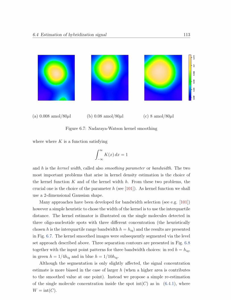
6.4 Estimation of hybridization signal 113
(a) 0.008 amol/80µl (b) 0.08 amol/80µl (c) 8 amol/80µl
Figure 6.7: Nadaraya-Watson kernel smoothing
where where K is a function satisfying
∫ ∞
−∞K(x) dx = 1
and h is the kernel width, called also smoothing parameter or bandwidth. The two
most important problems that arise in kernel density estimation is the choice of
the kernel function K and of the kernel width h. From these two problems, the
crucial one is the choice of the parameter h (see [101]). As kernel function we shall
use a 2-dimensional Gaussian shape.
Many approaches have been developed for bandwidth selection (see e.g. [101])
however a simple heuristic to chose the width of the kernel is to use the interquartile
distance. The kernel estimator is illustrated on the single molecules detected in
three oligo-nucleotide spots with three different concentration (the heuristically
chosen h is the interquartile range bandwidth h = hiq) and the results are presented
in Fig. 6.7. The kernel smoothed images were subsequently segmented via the level
set approach described above. Three separation contours are presented in Fig. 6.8
together with the input point patterns for three bandwidth choices: in red h = hiq,
in green h = 1/4hiq and in blue h = 1/10hiq.
Although the segmentation is only slightly affected, the signal concentration
estimate is more biased in the case of larger h (when a higher area is contributes
to the smoothed value at one point). Instead we propose a simple re-estimation
of the single molecule concentration inside the spot int(C) as in (6.4.1), where
W = int(C).
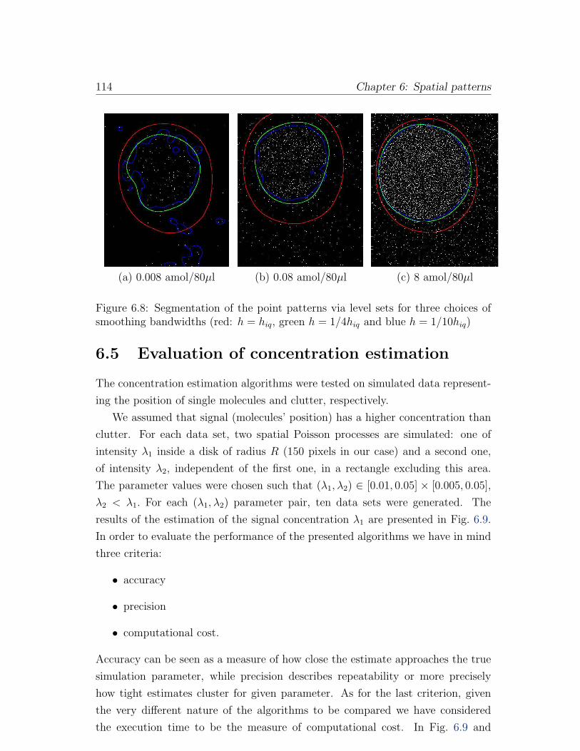
114 Chapter 6: Spatial patterns
(a) 0.008 amol/80µl (b) 0.08 amol/80µl (c) 8 amol/80µl
Figure 6.8: Segmentation of the point patterns via level sets for three choices ofsmoothing bandwidths (red: h = hiq, green h = 1/4hiq and blue h = 1/10hiq)
6.5 Evaluation of concentration estimation
The concentration estimation algorithms were tested on simulated data represent-
ing the position of single molecules and clutter, respectively.
We assumed that signal (molecules’ position) has a higher concentration than
clutter. For each data set, two spatial Poisson processes are simulated: one of
intensity λ1 inside a disk of radius R (150 pixels in our case) and a second one,
of intensity λ2, independent of the first one, in a rectangle excluding this area.
The parameter values were chosen such that (λ1, λ2) ∈ [0.01, 0.05] × [0.005, 0.05],
λ2 < λ1. For each (λ1, λ2) parameter pair, ten data sets were generated. The
results of the estimation of the signal concentration λ1 are presented in Fig. 6.9.
In order to evaluate the performance of the presented algorithms we have in mind
three criteria:
• accuracy
• precision
• computational cost.
Accuracy can be seen as a measure of how close the estimate approaches the true
simulation parameter, while precision describes repeatability or more precisely
how tight estimates cluster for given parameter. As for the last criterion, given
the very different nature of the algorithms to be compared we have considered
the execution time to be the measure of computational cost. In Fig. 6.9 and
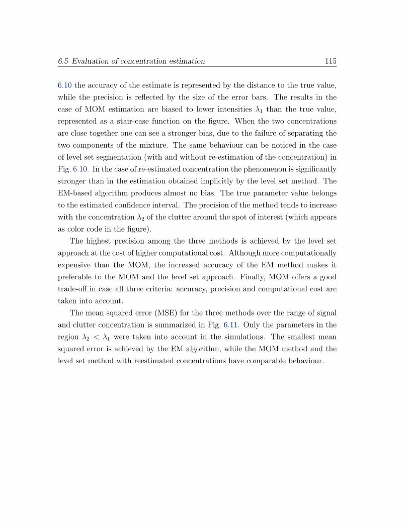
6.5 Evaluation of concentration estimation 115
6.10 the accuracy of the estimate is represented by the distance to the true value,
while the precision is reflected by the size of the error bars. The results in the
case of MOM estimation are biased to lower intensities λ1 than the true value,
represented as a stair-case function on the figure. When the two concentrations
are close together one can see a stronger bias, due to the failure of separating the
two components of the mixture. The same behaviour can be noticed in the case
of level set segmentation (with and without re-estimation of the concentration) in
Fig. 6.10. In the case of re-estimated concentration the phenomenon is significantly
stronger than in the estimation obtained implicitly by the level set method. The
EM-based algorithm produces almost no bias. The true parameter value belongs
to the estimated confidence interval. The precision of the method tends to increase
with the concentration λ2 of the clutter around the spot of interest (which appears
as color code in the figure).
The highest precision among the three methods is achieved by the level set
approach at the cost of higher computational cost. Although more computationally
expensive than the MOM, the increased accuracy of the EM method makes it
preferable to the MOM and the level set approach. Finally, MOM offers a good
trade-off in case all three criteria: accuracy, precision and computational cost are
taken into account.
The mean squared error (MSE) for the three methods over the range of signal
and clutter concentration is summarized in Fig. 6.11. Only the parameters in the
region λ2 < λ1 were taken into account in the simulations. The smallest mean
squared error is achieved by the EM algorithm, while the MOM method and the
level set method with reestimated concentrations have comparable behaviour.
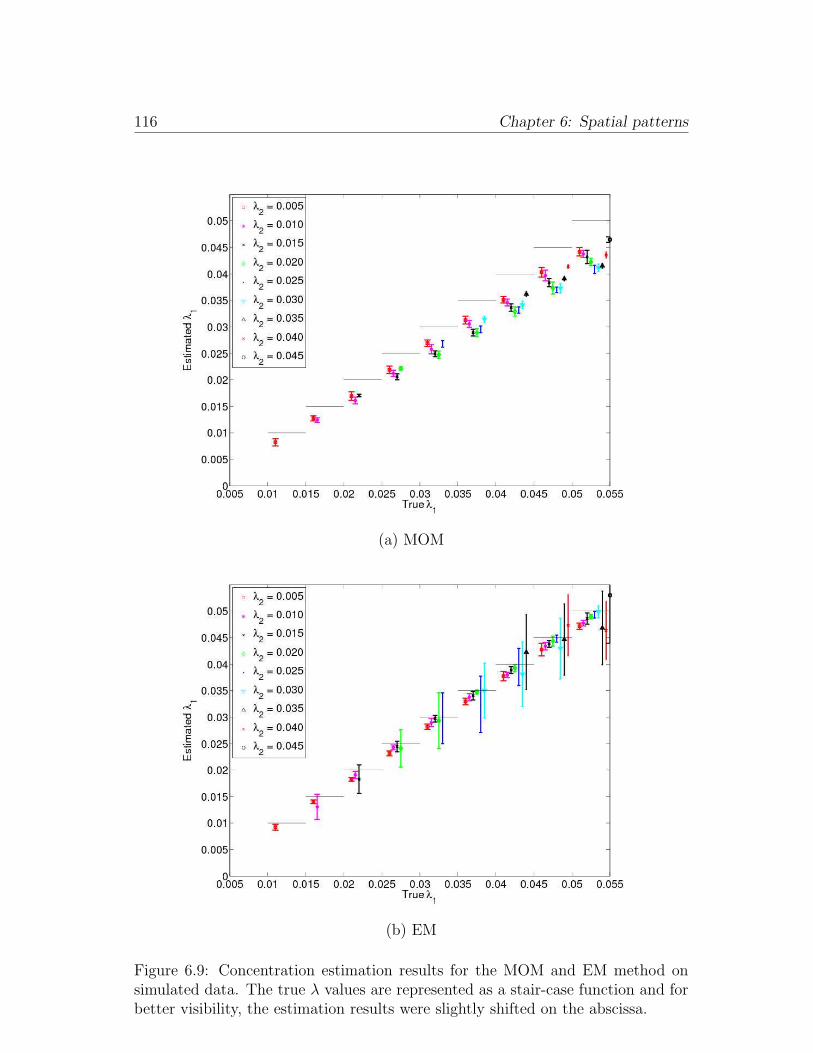
116 Chapter 6: Spatial patterns
(a) MOM
(b) EM
Figure 6.9: Concentration estimation results for the MOM and EM method onsimulated data. The true λ values are represented as a stair-case function and forbetter visibility, the estimation results were slightly shifted on the abscissa.
6.5 Evaluation of concentration estimation 117
(a) Concentration estimation after level set segmentation
(b) Reestimated concentration after level set segmentation
Figure 6.10: Concentration estimation results for the level set based method onsimulated data. The true λ values are represented as a stair-case function and forbetter visibility, the estimation results were slightly shifted on the abscissa.
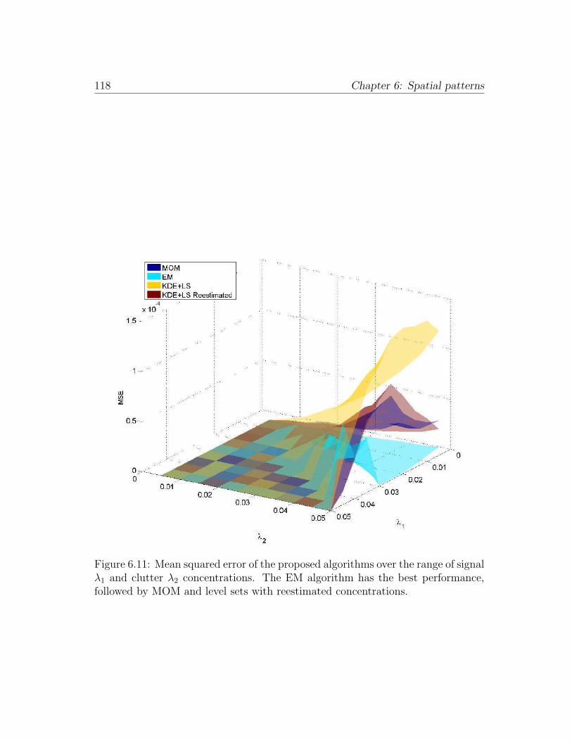
118 Chapter 6: Spatial patterns
Figure 6.11: Mean squared error of the proposed algorithms over the range of signalλ1 and clutter λ2 concentrations. The EM algorithm has the best performance,followed by MOM and level sets with reestimated concentrations.
Chapter 7
Results of microarray analysis
with single molecule sensitivity
Given the huge amount of data that needs to be analyzed the single molecule
detection and signal estimation algorithms have to be fast, and in the same time
accurate and robust to noise and model misspecification. Moreover, the range
of interest of mRNA and cDNA concentration in the sample is much below the
required concentration for classical low-resolution microarray analysis.
The proposed single molecule analysis tackles all the above described difficul-
ties. We have separately evaluated the single molecule detection algorithms in
Chapter 5 and the concentration estimation in Chapter 6. Now we validate our
entire approach on simulations that check the correlation of the estimated param-
eters with the simulation parameters, as well as on real high-resolution microarray
images. Since the ground truth in the case of real images is not known, special dilu-
tion series experiments for oligonucleotide arrays are used. Finally, we describe the
results of a full analysis of cDNA microarray slides for a Multiple Myeloma sample.
The list of differently expressed genes obtained via this analysis was confirmed by
independent PCR analysis.
7.1 Validation on simulated data
Simulation images
Simulation images represent a square domain of 512 × 512 pixels with a spot
of radius 150 pixels at its center (the proportions correspond to the real case
situation). The (optional) background of the image, due in practice mainly to the
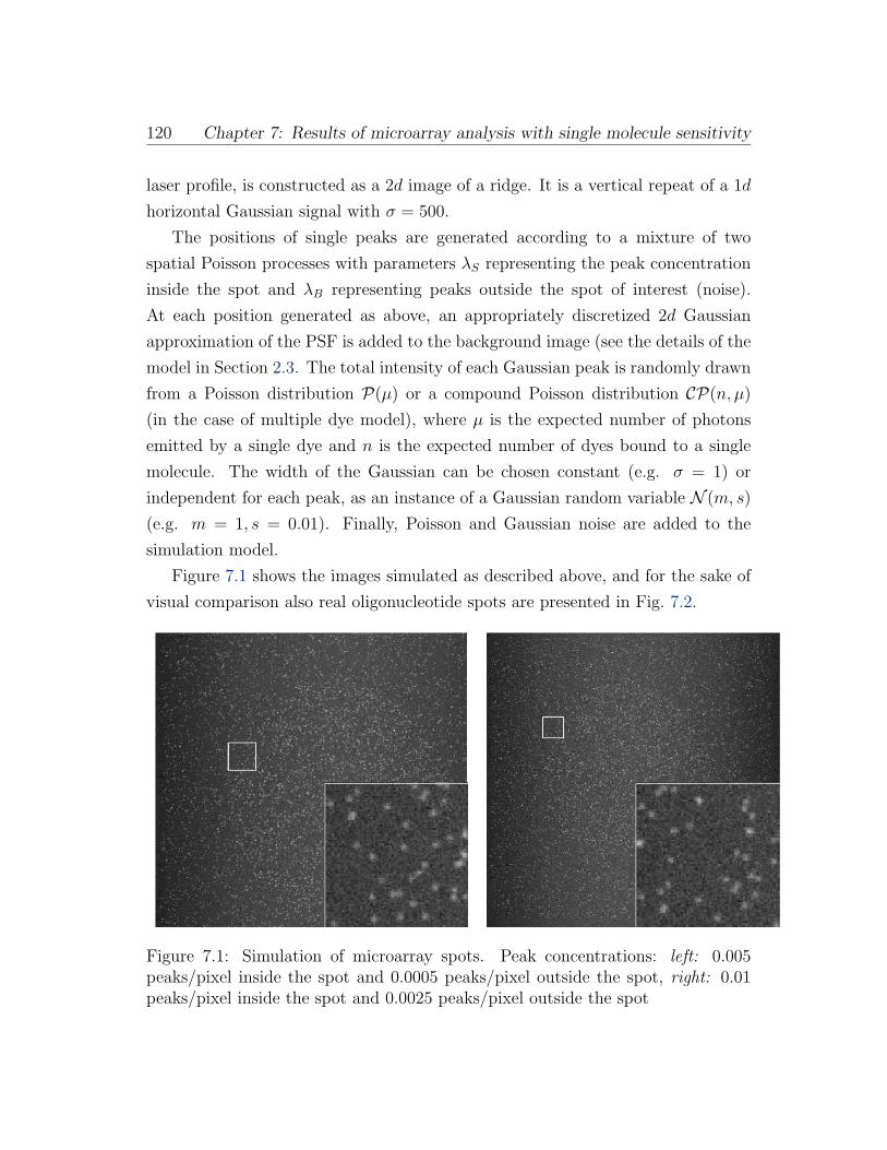
120 Chapter 7: Results of microarray analysis with single molecule sensitivity
laser profile, is constructed as a 2d image of a ridge. It is a vertical repeat of a 1d
horizontal Gaussian signal with σ = 500.
The positions of single peaks are generated according to a mixture of two
spatial Poisson processes with parameters λS representing the peak concentration
inside the spot and λB representing peaks outside the spot of interest (noise).
At each position generated as above, an appropriately discretized 2d Gaussian
approximation of the PSF is added to the background image (see the details of the
model in Section 2.3. The total intensity of each Gaussian peak is randomly drawn
from a Poisson distribution P(µ) or a compound Poisson distribution CP(n, µ)
(in the case of multiple dye model), where µ is the expected number of photons
emitted by a single dye and n is the expected number of dyes bound to a single
molecule. The width of the Gaussian can be chosen constant (e.g. σ = 1) or
independent for each peak, as an instance of a Gaussian random variable N (m, s)
(e.g. m = 1, s = 0.01). Finally, Poisson and Gaussian noise are added to the
simulation model.
Figure 7.1 shows the images simulated as described above, and for the sake of
visual comparison also real oligonucleotide spots are presented in Fig. 7.2.
Figure 7.1: Simulation of microarray spots. Peak concentrations: left: 0.005peaks/pixel inside the spot and 0.0005 peaks/pixel outside the spot, right: 0.01peaks/pixel inside the spot and 0.0025 peaks/pixel outside the spot
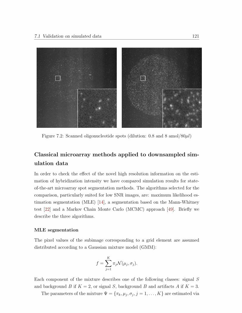
7.1 Validation on simulated data 121
Figure 7.2: Scanned oligonucleotide spots (dilution: 0.8 and 8 amol/80µl)
Classical microarray methods applied to downsampled sim-
ulation data
In order to check the effect of the novel high resolution information on the esti-
mation of hybridization intensity we have compared simulation results for state-
of-the-art microarray spot segmentation methods. The algorithms selected for the
comparison, particularly suited for low SNR images, are: maximum likelihood es-
timation segmentation (MLE) [14], a segmentation based on the Mann-Whitney
test [22] and a Markov Chain Monte Carlo (MCMC) approach [49]. Briefly we
describe the three algorithms.
MLE segmentation
The pixel values of the subimage corresponding to a grid element are assumed
distributed according to a Gaussian mixture model (GMM):
f =K∑
j=1
πjN (µj, σj).
Each component of the mixture describes one of the following classes: signal S
and background B if K = 2, or signal S, background B and artifacts A if K = 3.
The parameters of the mixture Ψ = πk, µj, σj, j = 1, . . . , K are estimated via
122 Chapter 7: Results of microarray analysis with single molecule sensitivity
maximization of the log-likelihood:
ℓ(x) =N∑
i=1
log f(xi|Ψ) =N∑
i=1
log
K∑
j=1
πjN (µj, σj)
.
The maximization of the log-likelihood can be obtained e.g. via an expectation-
maximization approach similar to the one described in Section 6.4.
Segmentation based on Mann-Whitney test
The iterative algorithm starts with an initial partition of the region of interest in
foreground (signal) Si, i = 1, . . . ,m and background pixels Bj, j = 1, . . . , n.
The iteration step consists of the (non-parametric and distribution-free) Mann-
Whitney test applied to eight random background pixels B8j and the eight lowest
intensity foreground pixels S8j . For each pixel value a testing problem is defined,
based on the accept/reject of the null hypothesis
H0 : µS − µB = 0
the alternative hypothesis being
H1 : µS − µB > 0,
where µS and µB are the mean values of signal, respective background. The test
is based on the rank-sum statistic R, the sum of the ranks of all the samples S8j
in the ordered sequence of S8j ∪ B8
j . The hypothesis H0 is rejected if R ≥ rα, the
critical value corresponding to the significance level α, knowing that under the null
hypothesis
R− n(n+1)2
− mn2√
mn(m+n+1)12
∝ N (0, 1),
for m,n ≥ 8 ( and can be directly computed for smaller values).
If H0 is not rejected, the smallest values (possibly only one) of Si, i = 1, . . . ,m
are discarded and the lowest eight samples from the remaining Si values are selected
as S8j and the procedure is iterated until no potential signal pixels remain or the
H0 is rejected. If the second situation occurs, all the remaining pixels in Si are
signal, the rest belonging to the background of the spot. Further details on the
approach can be found in [22].
7.1 Validation on simulated data 123
MCMC segmentation
The approach is based on a hierarchical Bayes model of the spot image and
uses Markov Chain Monte Carlo algorithms as computational tool to sample
the posterior distribution and estimate the parameters of the model. The al-
gorithm was fully described in [35], and reimplemented and applied to low-
resolution microarray images in [99]. The parameters describe the spot shape
model and the signal intensity model. We assume a simplified circular spot shape
R(τ) = z = (x, y) : (x− x0)2 + (y − y0)
2 ≤ r2, where τ = [x0, y0, r] represents
the shape parameter vector, but it is possible to consider more complex shapes,
like ellipse or annulus. The subimage corresponding to a grid element can be
written as the union of the spot region and the complement of the spot region:
G = R(τ) ∪RC(τ).
Each pixel r is assumed normally distributed, and corrupted by additive mea-
surement noise εr: u(r) = u0(r) + εr, εr ∼ N (0, σB). The pixels inside the
spot are normally distributed around an average hybridization level µ with hy-
bridization signal variability σ, while those outside the spot have a mean value
0:
p(u(r)|φ) =
N (µ,
√σ2 + σ2
B) if r ∈ R(τ)
N (0, σB) if r ∈ RC(τ).(7.1.1)
The likelihood of the measurement u given the parameters φ is
L(u|φ) =∏
z∈R(τ)
N (u(·);µ,√σ2 + σ2
B) ·∏
z∈RC(τ)
N (u(·); 0, σB)
∝(1 +
σ2
σ2B
)−N(τ)2
exp
−1
2
∑
r∈R(τ)
[(u(·)− µ)2
σ2 + σ2B
− (u(·))2σ2B
] (7.1.2)
where N(τ) =∑
z 1z∈R(τ) is the number of signal measurements in the sub-image.
The shape τ and the signal θ = [µ, σ] parameters are considered independent
a priori. For each parameter a uniform prior is assumed
Px0(x0) ∼ U [xMIN, xMAX],
Py0(y0) ∼ U [yMIN, yMAX],
Pr(r) ∼ U [rMIN, rMAX],
Pµ(µ) ∼ U [0, σMAX],
Pσ(σ) ∼ U [0, σMAX],

124 Chapter 7: Results of microarray analysis with single molecule sensitivity
and given the independence of the parameters, the joint prior distribution is given
by:
Pφ(φ) = Pτ (τ)Pθ(θ) = Px0(x0) · Py0(y0) · Pr(r) · Pµ(µ)Pσ(σ).
In order to estimate the parameters of the model, samples are drawn via Gibbs
sampling from the posterior probability density function
p(φ|u) ∝ Pφ(φ)L(u|φ).
The estimator based on the samples φ(t) is defined as the average of a part of
the samples:
φ =1
T − t0
(T∑
t=t0+1
φ(t)
),
where t0 is the burn-in period, and the first t0 samples are discarded. Note that the
estimator minimizes the mean square error based on the samples φ(t), t = t0, . . . T.
The details of the algorithm can be found in [35, 99].
However classical methods are not directly applicable to high resolution images.
Instead we apply them to downsampled versions of the original high resolution
images. The downsampling can be done in several ways:
1. integration over a quadratic region of size q × q
2. integration over a quadratic region of size q × q over the denoised image via
wavelet thresholding
3. integration over a quadratic region of size q × q over the counts of single
molecules after detection
4. kernel smoothed counts of single molecules
5. adaptive kernel smoothed counts of single molecules.
6. non parametric wavelet estimation applied to counts of single molecules.
Except for the first case, all other downsampling methods are based on in-
formation available only via the high resolution technique. A first issue is the
selection of the downsampling region size (q × q) for some of the downsamplings.
As we have seen in the MOM estimation approach the size of q × q influences the
estimation of hybridization intensity: for small q the bias is small and variance is
high, wile for large q the reverse holds (high bias, but small variance). We use
7.1 Validation on simulated data 125
in our computations q = 20. In future we plan implementation of the algorithms
based on adaptive kernel smoothed data and wavelet smoothed images.
Correlation tests
In Chapter 5 we have validated the detection results on simulation images, while
in Chapter 6 we have tested the separation of point patterns on simulated data.
In this section, we perform correlation tests in order to compare the results of our
analysis to those obtained by classical, low-resolution, ensemble analysis on the
downscaled images of the same data. Since our method results in peaks/pixel con-
centrations, while the ensemble approach gives mean pixel intensity values we com-
pare the correlation coefficients of the estimated hybridization measures computed
by each method with the ground truth concentrations used in the simulations.
For this purpose, 60 sets of images were generated with SNR between 2.85
and 31.6. Each set of images, characterized by a SNR value, contains 15 im-
ages. In each image, single molecules were simulated with concentrations λ1 ∈0.003, 0.005, 0.007, 0.009, 0.01 peaks/pixels inside a disk of radius 150 pixels.
The concentration λ2 of peaks corresponding to clutter outside this disk was also
varied from 0.001 to λ1 − 0.002 by steps of 0.002.
In Fig. 7.3 are shown the images corresponding to background value λ = 0.003,
SNR = 12.52. The single molecule simulation procedure is the one described in
Section 7.1.
In Fig. 7.4 we present the correlation results for the three high resolution al-
gorithms: MOM, EM and level set method. Each point in Fig. 7.4 corresponds
to a correlation coefficient computed between the hybridization measure (the es-
timated λ1 values) and the true λ1 values used in simulations. MOM performs
slightly worse than the other two algorithms, while EM and the level set method
have similarly good performance, with a small advantage for the level set method.
In order to compare the algorithms with state of the art microarray segmen-
tation methods we have created the corresponding low resolution images, by inte-
grating the intensities of the high resolution images over 20×20 pixel patches. The
pixel intensities of the downscaled images were modeled as a Gaussian mixture of
foreground (signal) and background pixels respectively and the parameters of the
mixture were estimated via a maximum likelihood (ML) approach as described in
the previous section. Moreover, we have applied the same downsampling and ML
estimating procedure to the original high-resolution image after a wavelet denois-
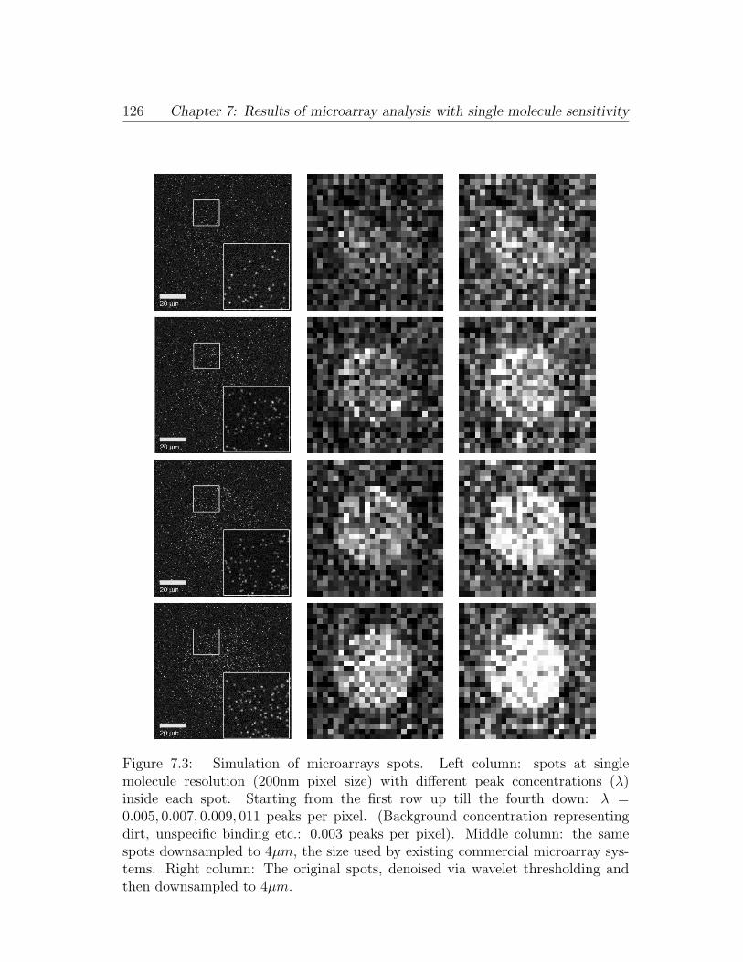
126 Chapter 7: Results of microarray analysis with single molecule sensitivity
Figure 7.3: Simulation of microarrays spots. Left column: spots at singlemolecule resolution (200nm pixel size) with different peak concentrations (λ)inside each spot. Starting from the first row up till the fourth down: λ =0.005, 0.007, 0.009, 011 peaks per pixel. (Background concentration representingdirt, unspecific binding etc.: 0.003 peaks per pixel). Middle column: the samespots downsampled to 4µm, the size used by existing commercial microarray sys-tems. Right column: The original spots, denoised via wavelet thresholding andthen downsampled to 4µm.
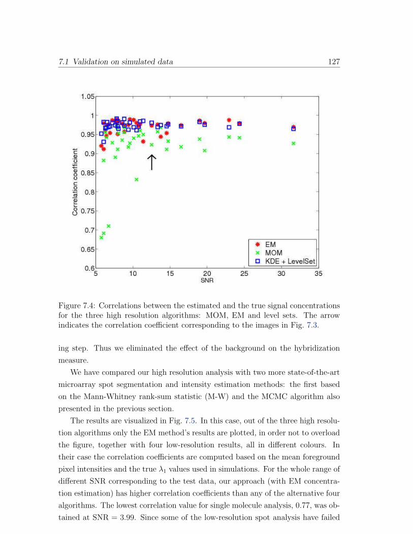
7.1 Validation on simulated data 127
Figure 7.4: Correlations between the estimated and the true signal concentrationsfor the three high resolution algorithms: MOM, EM and level sets. The arrowindicates the correlation coefficient corresponding to the images in Fig. 7.3.
ing step. Thus we eliminated the effect of the background on the hybridization
measure.
We have compared our high resolution analysis with two more state-of-the-art
microarray spot segmentation and intensity estimation methods: the first based
on the Mann-Whitney rank-sum statistic (M-W) and the MCMC algorithm also
presented in the previous section.
The results are visualized in Fig. 7.5. In this case, out of the three high resolu-
tion algorithms only the EM method’s results are plotted, in order not to overload
the figure, together with four low-resolution results, all in different colours. In
their case the correlation coefficients are computed based on the mean foreground
pixel intensities and the true λ1 values used in simulations. For the whole range of
different SNR corresponding to the test data, our approach (with EM concentra-
tion estimation) has higher correlation coefficients than any of the alternative four
algorithms. The lowest correlation value for single molecule analysis, 0.77, was ob-
tained at SNR = 3.99. Since some of the low-resolution spot analysis have failed
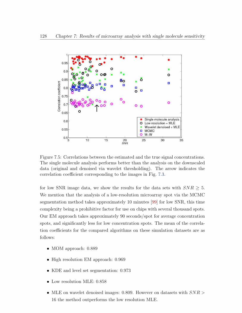
128 Chapter 7: Results of microarray analysis with single molecule sensitivity
Figure 7.5: Correlations between the estimated and the true signal concentrations.The single molecule analysis performs better than the analysis on the downscaleddata (original and denoised via wavelet thresholding). The arrow indicates thecorrelation coefficient corresponding to the images in Fig. 7.3.
for low SNR image data, we show the results for the data sets with SNR ≥ 5.
We mention that the analysis of a low-resolution microarray spot via the MCMC
segmentation method takes approximately 10 minutes [99] for low SNR, this time
complexity being a prohibitive factor for use on chips with several thousand spots.
Our EM approach takes approximately 90 seconds/spot for average concentration
spots, and significantly less for low concentration spots. The mean of the correla-
tion coefficients for the compared algorithms on these simulation datasets are as
follows:
• MOM approach: 0.889
• High resolution EM approach: 0.969
• KDE and level set segmentation: 0.973
• Low resolution MLE: 0.858
• MLE on wavelet denoised images: 0.809. However on datasets with SNR >
16 the method outperforms the low resolution MLE.
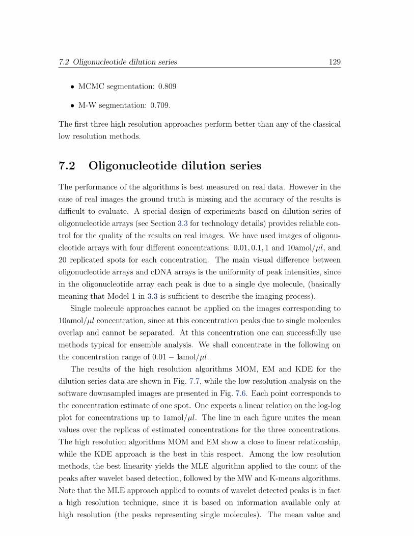
7.2 Oligonucleotide dilution series 129
• MCMC segmentation: 0.809
• M-W segmentation: 0.709.
The first three high resolution approaches perform better than any of the classical
low resolution methods.
7.2 Oligonucleotide dilution series
The performance of the algorithms is best measured on real data. However in the
case of real images the ground truth is missing and the accuracy of the results is
difficult to evaluate. A special design of experiments based on dilution series of
oligonucleotide arrays (see Section 3.3 for technology details) provides reliable con-
trol for the quality of the results on real images. We have used images of oligonu-
cleotide arrays with four different concentrations: 0.01, 0.1, 1 and 10amol/µl, and
20 replicated spots for each concentration. The main visual difference between
oligonucleotide arrays and cDNA arrays is the uniformity of peak intensities, since
in the oligonucleotide array each peak is due to a single dye molecule, (basically
meaning that Model 1 in 3.3 is sufficient to describe the imaging process).
Single molecule approaches cannot be applied on the images corresponding to
10amol/µl concentration, since at this concentration peaks due to single molecules
overlap and cannot be separated. At this concentration one can successfully use
methods typical for ensemble analysis. We shall concentrate in the following on
the concentration range of 0.01− 1amol/µl.
The results of the high resolution algorithms MOM, EM and KDE for the
dilution series data are shown in Fig. 7.7, while the low resolution analysis on the
software downsampled images are presented in Fig. 7.6. Each point corresponds to
the concentration estimate of one spot. One expects a linear relation on the log-log
plot for concentrations up to 1amol/µl. The line in each figure unites the mean
values over the replicas of estimated concentrations for the three concentrations.
The high resolution algorithms MOM and EM show a close to linear relationship,
while the KDE approach is the best in this respect. Among the low resolution
methods, the best linearity yields the MLE algorithm applied to the count of the
peaks after wavelet based detection, followed by the MW and K-means algorithms.
Note that the MLE approach applied to counts of wavelet detected peaks is in fact
a high resolution technique, since it is based on information available only at
high resolution (the peaks representing single molecules). The mean value and
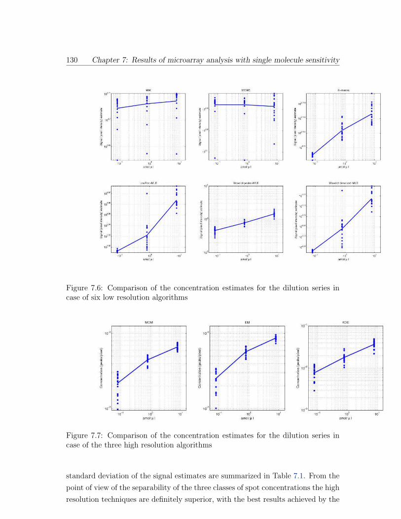
130 Chapter 7: Results of microarray analysis with single molecule sensitivity
Figure 7.6: Comparison of the concentration estimates for the dilution series incase of six low resolution algorithms
Figure 7.7: Comparison of the concentration estimates for the dilution series incase of the three high resolution algorithms
standard deviation of the signal estimates are summarized in Table 7.1. From the
point of view of the separability of the three classes of spot concentrations the high
resolution techniques are definitely superior, with the best results achieved by the
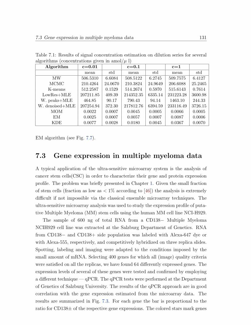
7.3 Gene expression in multiple myeloma data 131
Table 7.1: Results of signal concentration estimation on dilution series for severalalgorithms (concentrations given in amol/µ l)
Algorithm c=0.01 c=0.1 c=1
mean std mean std mean std
MW 506.5310 6.6084 508.5122 6.2745 509.7575 6.4127MCMC 210.4264 24.0670 210.3824 24.9649 206.6088 25.2465K-means 512.2587 0.1529 514.2674 0.5970 515.6143 0.7614
LowRes+MLE 207211.85 409.39 214352.35 6335.14 231223.28 3600.98W. peaks+MLE 464.85 90.17 790.43 94.14 1463.10 244.33
W. denoised+MLE 207254.94 372.30 217812.76 6394.59 233116.49 3726.15MOM 0.0022 0.0007 0.0045 0.0005 0.0066 0.0005EM 0.0025 0.0007 0.0057 0.0007 0.0087 0.0006KDE 0.0077 0.0028 0.0180 0.0045 0.0367 0.0070
EM algorithm (see Fig. 7.7).
7.3 Gene expression in multiple myeloma data
A typical application of the ultra-sensitive microarray system is the analysis of
cancer stem cells(CSC) in order to characterize their gene and protein expression
profile. The problem was briefly presented in Chapter 1. Given the small fraction
of stem cells (fraction as low as < 1% according to [46]) the analysis is extremely
difficult if not impossible via the classical ensemble microarray techniques. The
ultra-sensitive microarray analysis was used to study the expression profile of puta-
tive Multiple Myeloma (MM) stem cells using the human MM cell line NCI-H929.
The sample of 600 ng of total RNA from a CD138− Multiple Myeloma
NCIH929 cell line was extracted at the Salzburg Department of Genetics. RNA
from CD138− and CD138+ side population was labeled with Alexa-647 dye or
with Alexa-555, respectively, and competitively hybridized on three replica slides.
Spotting, labeling and imaging were adapted to the conditions imposed by the
small amount of mRNA. Selecting 400 genes for which all (image) quality criteria
were satisfied on all the replicas, we have found 64 differently expressed genes. The
expression levels of several of these genes were tested and confirmed by employing
a different technique — qPCR. The qPCR tests were performed at the Department
of Genetics of Salzburg University. The results of the qPCR approach are in good
correlation with the gene expression estimated from the microarray data. The
results are summarized in Fig. 7.3. For each gene the bar is proportional to the
ratio for CD138± of the respective gene expressions. The colored stars mark genes
132 Chapter 7: Results of microarray analysis with single molecule sensitivity
Figure 7.8: The expression profiles of several side population genes showing re-pressors and over-expressers. The repressed genes like CSEN, CCT6A and CASQ1were either not analyzed with the qPCR method or showed not interpretable re-sults. Rest of the presented genes show a higher expression level, and are in agood agreement with the microarray results
compared with PCR. The gene ratios confirmed in the validation are marked with
a green star, while the three red stars show the ratios diverging in their expression
profile from the qPCR results.
Chapter 8
Conclusion
In the concluding chapter of this thesis, we are giving a brief overview of the image
processing tasks implied by the new technique of ultra-sensitive microarrays as well
as the results discussed in detail in the previous chapters. We shall also point out
possible applications of our study to other problems in microscopy as well as other
fields. Further ideas and lines of study will be pointed out in the second section
of the chapter that concludes this thesis.
8.1 Summary
This work was motivated by the new technology of high-resolution microarray
analysis, representing a combination between fast single molecule imaging and the
microarray technique. Each step of the microarray technique had to be evaluated
and adapted to the novel challenges, the most crucial of which being the small
amount of target mRNA typically used in the new technology.
Spotting, labeling and imaging were adapted to the new conditions and the
technical innovation in the biological and physical aspects of the problem resulted
in a new type of images to be analyzed. The challenges of the new technique from
an image processing and analysis point of view are related to:
The modified content of the microarray image. Instead of a microarray
circular spot representing the signal over a (uniform) background we have to
deal with information at two resolution levels: at high resolution the single
molecule peaks can be detected, and at a larger scale these peaks form the
hybridized spot imposed over a background of clutter. The detection of single
molecule peaks was implemented based on a wavelet thresholding algorithm.
The position of the single peaks were modeled as a superposition of two
134 Chapter 8: Conclusion
homogeneous Poisson processes corresponding to hybridization signal and
clutter. The intensity of the signal process was proposed as a new measure
of hybridization (Chapter 6).
Wide range of SNR and combined Poisson-Gaussian noise models. Sin-
gle molecule imaging poses new challenges related to SNR of the image and
the contrast of signal. Typically detection algorithms have to be very robust
over a wide range of SNR and contrast parameters. The support of the signal
is very small (of the order of a few pixels) which makes the detection prob-
lem difficult. Moreover, the concentration of the peaks (the sparsity of the
signal) is influencing the detection, and therefore was also taken into account
in our examination. We studied in Chapter 5 the behaviour of the detection
algorithms and summarized their results on systematic simulations of im-
ages, over a range of simulation parameters and implicitly SNRs, as well as
on real images. For the conditions imposed by single molecule imaging the
wavelet thresholding methods proved reliable and accurate. Although the
detection is based on the control of false positive cases, for the evaluation
of the algorithms we measured both the false positive as well as the false
negative detections.
The size of the images and complexity of algorithms. To each microarray
slide correspond approximately 22GB of image data (partitioned in several
subimages). Therefore the time and space complexities of the chosen al-
gorithms bear a crucial importance. Wavelet thresholding methods show
good performance with respect to time and memory, thanks to the one step
approach and to the special form of operators, (diagonal operators) used.
The concentration estimation is very fast in the case of MOM approach, and
slightly more computationally intensive in case of the EM and the level set
algorithms, with the advantage of increased accuracy. Each additional step,
such as improved noise variance estimation or variance stabilization trans-
forms further increase the computation time. Nevertheless the proposed
algorithms are on average 10 times faster than some of the state-of-the art
algorithms analyzing low-resolution microarray images, such as [99] (see Sec-
tion 7.1). However, in order to target a wider public, we plan improvements
of both memory and time performance.
Low mRNA concentration. The low fluorophore concentration results in few
single molecule peaks, which in turn, at low resolution, translate to dim
8.2 Outlook 135
spots. The wavelet-based detection algorithm used for single molecule de-
tection was successfully applied also to the detection of microarray spots in
downsampled (originally high-resolution) microarray images (Section 7.3).
The gridding algorithm has also been adapted so that the grid pattern match-
ing works robustly even in the case of missing (or dim) column and/or lines
of microarray spots.
Understanding the advantages and disadvantages of the new tech-
nique. The access to high resolution information permitted modeling at
single molecule and single dye level. It also helped in gaining understanding
on image formation, both in the low-resolution and high-resolution cases.
Modeling both cases allowed a better identification of the sources of bias
and errors in each case, as well as to perform a better comparison of the two
techniques (as described in Chapters 2 and 7).
Validation of the results. In order to validate the results the algorithms were
tested on simulated and real data. For the real data the ground truth is not
available, however with the help of specially designed experiments, such as
the dilution series of oligonucleotide arrays the correctness of the results could
be evaluated (see Section 7.2). The results of our approach on a real data
set based on multiple myeloma were confirmed by an independent technique
(qPCR) as described in Section 7.3.
We have presented in this work a comprehensive image processing solution for a
new microarray technique, analyzing the similarities and differences to the state-of-
the art approaches used in the standard microarray applications. Besides the signal
processing and image analysis approach this work attempted to accommodate the
point of view of the biologists and biophysicists involved, since it is the result of a
close and continuous collaboration in the framework of a multidisciplinary project.
8.2 Outlook
Beyond applications to the ultra-sensitive microarray technology, the study of
algorithms analyzing single molecule images has an interest in its own. All the
present and future applications of single molecule imaging might benefit of the
algorithms detecting single molecules, with special concern to low level SNR, the
specific noise model and single molecule concentrations.
136 Chapter 8: Conclusion
A reliable method, based on wavelet thresholding, of finding significant pixels
in a microscopy image was described in Chapter 5. The special focus was the
detection of pixels due to single molecules. Further analysis of the values of these
pixels might provide insight in the temporal behaviour of fluorophores, character-
izing the phenomena known as blinking and bleaching (Section 2.1). We envisage
to address the problem of subpixel accuracy, which classically is based on fitting
a 2d Gaussian shape to the pixel values corresponding to the single molecule im-
age. Bobroff [15] discussed the importance of the signal support over which this
fitting is performed. We will investigate the effect of signal support selection via
wavelet thresholding on the fitting procedure. Finally, we will extend the analy-
sis of molecule intensities, which for the moment only discriminates between two
classes of signal intensity: due to single dyes and due to dirt, to more general
stoichiometry problems, as e.g. the one described in [83].
We plan to study different models (e.g. truncated and censored distribu-
tions) for the description of single molecule positions and counts, knowing that
the wavelet detection methods have a certain ”resolution” (see Section 6.4), thus
introducing a truncation of the data. We would like to look into the benefits of
wavelet methods as density estimators in case of spatial point patterns in general
and in microscopy in particular.
A possible line of study in the future is the utility of spatial point pattern
approaches to microscopy images of single molecules. There are already a few
attempts of using spatial patterns in co-localization [122], tracking [64] and at
a higher scale, in the study of the differences between the patterns of nuclei of
malignant epithelial tumor (adenocarcenomas) cells as opposed to normal cells
[79]. We are interested in characterizing videomicroscopy image sequences of single
molecules previous to tracking, in order to assess their quality, make inferences
about the dynamics and finally, facilitate the tracking. We believe that point
pattern analysis — both as hypothesis testing and parameter estimation — will
prove to be a useful tool in PALM imaging [13].
As previously mentioned, optimized versions of the algorithms and their im-
plementations, more efficient both in run-time and memory, are planned to be
developed in order to improve the use of the proposed approach.
Appendix A
Outliers and variance-covariance
estimators
Several intuitive descriptions of outliers have been proposed in the literature. We
adopt the one offered in [98], according to which outliers are ”observations that do
not follow the pattern of the majority of the data”.
The deviation of the outliers from the majority of the data is measured by a
convenient measure, such as the quadratic distance measure between data x and
a location y, given by the (squared) Mahalanobis distance:
MD2(x, y) = (x− y)TS−1(x− y), (A.0.1)
where y is a d-dimensional vector and S is a positive definite symmetric d × d
dimensional matrix. The Mahalanobis distance represents the distance from the
point x to the ”center” of the data cloud, taking into account the shape of the
point cloud. Typically if this distance is larger than a predetermined threshold, x
is considered an outlier.
The importance of the Mahalanobis distance is justified by the aim to find
methods that are affine equivariant, so that ”measurement scale changes and other
linear transformations do not alter the behavior of analysis method” (see [93]).
Usually, y and S are replaced by estimations of the location and scatter, e.g.
the standard estimators, average of the sample x = 1/n∑n
i=1 xi for location and
for scatter the sample covariance matrix: S = n−1(x− x)T (x− x).
For multivariate normally distributed d-dimensional data the values are ap-
proximately χ2 distributed with d degrees of freedom ([48]).
The standard sample location and shape parameters are not robust estimators
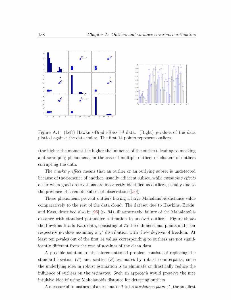
138 Chapter A: Outliers and variance-covariance estimators
0 10 20 30 40 50 60 70 800
0.1
0.2
0.3
0.4
0.5
0.6
0.7
0.8
0.9
1
Figure A.1: (Left) Hawkins-Bradu-Kass 3d data. (Right) p-values of the dataplotted against the data index. The first 14 points represent outliers.
(the higher the moment the higher the influence of the outlier), leading to masking
and swamping phenomena, in the case of multiple outliers or clusters of outliers
corrupting the data.
The masking effect means that an outlier or an outlying subset is undetected
because of the presence of another, usually adjacent subset, while swamping effects
occur when good observations are incorrectly identified as outliers, usually due to
the presence of a remote subset of observations([50]).
These phenomena prevent outliers having a large Mahalanobis distance value
comparatively to the rest of the data cloud. The dataset due to Hawkins, Bradu,
and Kass, described also in [96] (p. 94), illustrates the failure of the Mahalanobis
distance with standard parameter estimation to uncover outliers. Figure shows
the Hawkins-Bradu-Kass data, consisting of 75 three-dimensional points and their
respective p-values assuming a χ2 distribution with three degrees of freedom. At
least ten p-vales out of the first 14 values corresponding to outliers are not signif-
icantly different from the rest of p-values of the clean data.
A possible solution to the aforementioned problem consists of replacing the
standard location (T ) and scatter (S) estimates by robust counterparts, since
the underlying idea in robust estimation is to eliminate or drastically reduce the
influence of outliers on the estimates. Such an approach would preserve the nice
intuitive idea of using Mahalanobis distance for detecting outliers.
A measure of robustness of an estimator T is its breakdown point ε∗, the smallest
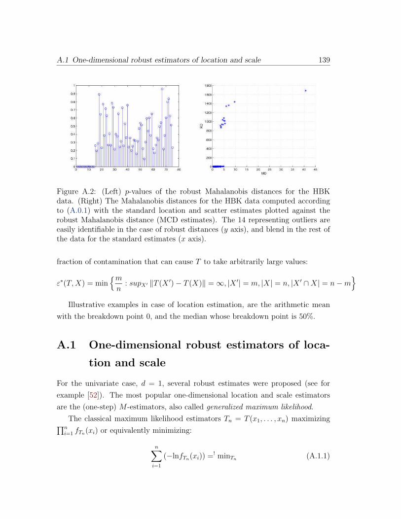
A.1 One-dimensional robust estimators of location and scale 139
Figure A.2: (Left) p-values of the robust Mahalanobis distances for the HBKdata. (Right) The Mahalanobis distances for the HBK data computed accordingto (A.0.1) with the standard location and scatter estimates plotted against therobust Mahalanobis distance (MCD estimates). The 14 representing outliers areeasily identifiable in the case of robust distances (y axis), and blend in the rest ofthe data for the standard estimates (x axis).
fraction of contamination that can cause T to take arbitrarily large values:
ε∗(T,X) = minmn
: supX′ ‖T (X ′)− T (X)‖ = ∞, |X ′| = m, |X| = n, |X ′ ∩X| = n−m
Illustrative examples in case of location estimation, are the arithmetic mean
with the breakdown point 0, and the median whose breakdown point is 50%.
A.1 One-dimensional robust estimators of loca-
tion and scale
For the univariate case, d = 1, several robust estimates were proposed (see for
example [52]). The most popular one-dimensional location and scale estimators
are the (one-step) M -estimators, also called generalized maximum likelihood.
The classical maximum likelihood estimators Tn = T (x1, . . . , xn) maximizing∏ni=1 fTn(xi) or equivalently minimizing:
n∑
i=1
(−lnfTn(xi)) =! minTn (A.1.1)
140 Chapter A: Outliers and variance-covariance estimators
are replaced by the following minimization problem
n∑
i=1
ρ (xi, Tn) =! minTn , (A.1.2)
where ρ is a function defined on X ×Θ, (where X is the range of the variable and
Θ is the parameter space), with derivative ψ(x, θ) = ∂∂θρ(x, θ), such that (A.1.2)
is replaced by:n∑
i=1
ψ (xi, Tn) = 0.
One of the simplest robust location estimator is the median of the sample. As
for scale, the median absolute deviation (MAD) is a popular choice:
ψMAD(x) = sign(|x| − Φ−1(3/4)
)
resulting in MAD(x) = median |x−median(x)| /0.674. This is the estimate of
scale for the distribution of wavelet coefficients proposed in [36, 37] and used in
wavelet thresholding.
We have implemented two alternatives to the MAD robust scale approximation
are described in [95]:
Sn = c1 ·medi medj |xi − xj| ,
where medixi denotes the median of the sample x1, x2, . . . xn and
Qn = c2 · |xi − xj| : i < j (k),
Their advantage is greater (Gaussian) efficiency and no underlying assumption of
a symmetric distribution, with the drawback of higher computation time (which
was especially limiting for the large microarray images).
A.2 Robust covariance matrix estimation
The robust estimation in multivariate case, and especially d > 2, is much more
challenging than in the univariate one. Outliers are difficult or impossible to
detect even by visual inspection and sample covariance matrices are very sensitive
to outliers. Moreover, Gnanadesikan and Kettenring ([48]) identify several other
causes that make outlier detection particularly challenging in high dimensions:
A.2 Robust covariance matrix estimation 141
outliers may corrupt not only location and scale, but also orientation parameters
(i.e. correlations), the view of outlier as an extremal value does not hold in high
dimensions, an outlier might be characterized by a gross error in one dimension, or
milder errors in several (or all) dimensions (relating the problem to that of sparsity
of the error vector).
A presentation of the difficulties of the task as well as a comparison of some of
the solutions is given in [93]. The robust approaches are classified in [59] in three
categories:
• Robust estimation of individual matrix elements of the covariance matrix
• Robust estimation of variances in sufficiently many selected directions, to
which a quadratic form is then fitted
• Direct estimation of shape matrix for some elliptical distribution.
The breakdown point of all affine equivariant M -estimators is at most 1d+1
or even lower, if the outliers belong to a lower dimensional space. This makes
the multivariate location and shape problem a very difficult problem to tackle.
However a popular choice from the combinatorial category of location and shape
estimators in the multivariate case, the Minimum Covariance Determinant (MCD)
estimates, have been proved to work well over a wide range of situations.
The objective of the MCD estimator, first introduced in [94] is to find h obser-
vation out of the total n whose classical covariance matrix has the lowest determi-
nant. The location and scatter are the standard estimates based on the chosen h
observations.
Formally, given n data points, x1, . . . , xn, the MCD is based on the sub-
sample xi, i ∈ H, where H ⊂ 1, 2, · · · , n of size h, h ≤ n, that minimizes the
determinant of the covariance matrix, more precisely:
MCD = (TH , SH), (A.2.1)
142 Chapter A: Outliers and variance-covariance estimators
where
H : i ∈ H , |H| = h : det(SH) ≤ det(SK), ∀K, det(K) = h
TH =1
h
∑
i∈Hxi
SH =1
h
∑
i∈H(xi − TH)(xi − TH)
T .
The estimator is affine equivariant because the determinant of the covariance ma-
trix of the transformed data satisfies:
det(ATCA) = (det(A))2 det(C)
The main idea of the MCD algorithm is that of obtaining a sample subset H2 ⊂1, . . . , n starting from the subset H1 with the same cardinality, |H1| = |H2| = h,
such that the new subset has a smaller covariance matrix determinant than the
initial one. The process of obtaining a new subset H2 is called a C-step in [97] and
it is summarized in the following theorem.
We denote with dk(i) = MD(xi, Tk, Sk) the Mahalanobis distance of the ith
point, i ∈ Hk, with respect to the standard estimators of location and shape, Tk
and Sk, of the subset Hk.
Theorem A.2.1. Given X = x1, . . . , xn p-variate observations and the subset
H1 ⊂ X, such that |H1| = h, if det(S1) 6= 0 and
H2 = π(i), i = 1, . . . h : d1(π(1)) ≤ d1(π(2)) ≤ . . . ≤ d1(π(n)) ,
where π : 1, . . . , n → 1, . . . , n is the permutation corresponding to the increas-
ing ordering of the data then
det(S2) ≤ det(S1).
The equality holds if and only if T2 = T1 and S2 = S1.
A proof of the theorem is given in [97].
The exact MCD solution can be found only in very simple cases, instead approx-
imations based on random search [96], steepest descent [54] and heuristic search
optimization [92, 93] were proposed. We use a computationally efficient version of

A.3 Distributions of Mahalanobis distances 143
the random search MCD algorithm, introduced in [97] and implemented in LIBRA
[112].
The properties of the MCD estimators were extensively studied, for example
in order to choose the parameter h the maximum breakdown point of the MCD
estimator is achieved for h =⌊n+p+1
2
⌋. However for a good trade-off between
robustness and efficiency the authors recommend 0.75 · n (see [96, 53]).
A.3 Distributions of Mahalanobis distances
The Mahalanobis squared distances give a one-dimensional measure of how far a
point is from a location with respect to a shape. Several approximations of the
distribution of the Mahalanobis distance are known in the literature. Some results
are given in [48, 53] and summarized as follows.
Consider n multivariate data points in Rp, Xi ∼ N (µ,Σ), and S an estimate
of Σ. The three distributional results for distances based on multivariate normal
data are given below.
1. Considering the true parameters µ and Σ known, if the data are normal
distributed, the Mahalanobis distances have an exact χ2d distribution:
MD(xi, µ,Σ) ∼ χ2d,
with
E [MD(xi, µ,Σ)] = d
var [MD(xi, µ,Σ)] = 2d.
2. The Mahalanobis distances based on the standard estimates have an exact
Beta distribution:
n
(n− 1)2MD(xi, T, S) ∼ Beta
(d
2,n− d− 1
2
),
and
E
[n
(n− 1)MD(xi, T, S)
]= d
var
[n
(n− 1)MD(xi, T, S)
]= 2d
n− d− 1
n+ 1.
144 Chapter A: Outliers and variance-covariance estimators
3. The Mahalanobis distances based on an estimate S of Σ, independent of
xi have an exact F distribution when µ is the location argument, and an
approximate F distribution when the standard location estimate is used.
n− d
d(n− 1)MD(xi, T, S) ∼ F (d, n− d) ,
and
E
[n− d− 2
(n− 1)MD(xi, T, S)
]= d
var
[n− d− 2
(n− 1)MD(xi, T, S)
]= 2d
n− 2
n− d− 4.
The above distributions can be incorporated in outlier detecting algorithms. Quan-
tiles, especially χ2 quantiles are a straightforward way to identify outliers, although
the results are often spoiled by the high amount of false positives ( see [98]).

Bibliography
[1] http://www.invitrogen.com/site/us/en/home/support/Research-
Tools/Fluorescence-SpectraViewer.html.
[2] http://www.genome.gov.
[3] F. Abramovich and Y. Benjamini. Adaptive thresholding of wavelet coeffi-
cients. Computational Statistics and Data Analysis, 22:351–361, 1996.
[4] F. Abramovich, Y. Benjamini, D. Donoho, and I.M. Johnstone. Adapting
to unknown sparsity by controlling the false discovery rate. The Annals of
Statistics, 34(2):584–653, 2006.
[5] V.T. Acharya and A.K. Ray. Image processing: Principles and Applications.
John Wiley & Sons, 2005.
[6] J. Angulo. Polar modelling and segmentation of genomic microarray spots
using mathematical morphology. Image Anal. Stereol., 27:107–124, 2008.
[7] Jesus Angulo and Jean Serra. Automatic analysis of DNA microarray images
using mathematical morphology. Bioinformatics, 19(5):553–562, 2003.
[8] F.J. Anscombe. The transformation of Poisson, binomial and negative-
binomial data. Biometrika, 35(3/4):246–254, 1948.
[9] A. Antoniadis. Wavelet methods in statistics: Some recent developments
and their applications. Statistics Surveys, 1:16–55, 2007.
[10] Y. Balagurunathan, N. Wang, E. R. Dougherty, D. Nguyen, Y. Chen, M.L.
Bittner, J. Tent, and R. Carroll. Noise factor analysis for cdna microarrays.
Journal of Biomedical Optics, 9(4):663–678, 2004.
[11] Y. Benjamini and Y. Hochberg. Controlling the false discovery rate: A
practical and powerful approach to multiple testing. J. R. Statist. Soc. B,
57(1):289–300, 1995.
146 BIBLIOGRAPHY
[12] T. Berger and J.O. Stromberg. Exact reconstruction algorithms for the
discrete wavelet transform using spline wavelets. Applied and Computational
Harmonic Analysis, 2:392–397, 1995.
[13] E. Betzig, G. H. Patterson, R. Sougrat, O. W. Lindwasser, S. Olenych,
J. S. Bonifacino, M. W. Davidson, J. Lippincott-Schwartz, and H. F. Hess.
Imaging intracellular fluorescent proteins at nanometer resolution. Science,
313(5793):1642–1645, 2006.
[14] K. Blekas, N. P. Galatsanos, A. Likas, and I. E. Lagaris. Mixture model
analysis of DNA microarray images. IEEE Transactions on Medical Imaging,
24:901–909, 2005.
[15] N. Bobroff. Position measurement with a resolution and noise-limited in-
strument. Rev. Sci. Instrum., 57(6), 1986.
[16] B.M. Bolstad, R.A. Irizarry, M. Astrand, and T.P. Speed. A comparison of
normalization methods for high density oligonucleotide array data based on
variance and bias. Bioinformatics, 19(2):185–193, 2003.
[17] J. Boulanger, J.-B. Sibarita, Ch. Kervrann, and P. Bouthemy. Non-
parametric regression for patch-based fluorescence microscopy image se-
quence denoising. In Proc. IEEE Int. Symp. on Biomedical Imaging: from
nano to macro (ISBI), 2008.
[18] S. Byers and A. E. Raftery. Nearest-neighbor clutter removal for estimat-
ing features in spatial point processes. Journal of the American Staistical
Association, 93:577–584, 1998.
[19] E.J. Candes. Modern statistical estimation via oracle inequalities. Acta
Numerica, 15:257–325, 2006.
[20] T. F. Chan and L. A. Vese. Active contours without edges. IEEE Transac-
tions on Image Processing, 10(2):266–277, 2001.
[21] T. F. Chan and L. A. Vese. A multiphase level set framework for image
segmentation using the mumford and shah model. International Journal of
Computer Vision, 50(3):271–293, 2002.
[22] Y. Chen, E.R. Dougherty, and M.L. Bittner. Ratio-based decisions and the
quantitative analysis of cDNA microarray images. Journal of Biomedical
Optics, 2(4):364–374, 1997.
BIBLIOGRAPHY 147
[23] E. Chudin, S. Kruglyak, S.C. Baker, S. Oeser, D. Barker, and T.K. Mc-
Daniel. A model of technical variation of microarray signals. Journal of
Computational Biology, 13(4):996–1003, 2006.
[24] C.K. Chui. An introduction to wavelets. Academic Press, New York, 1992.
[25] M. Clyde, G. Parmigiani, and B. Vidakovic. Multiple shrinkage and subset
selection in wavelets. Biometrika, 85:391–401, 1998.
[26] N. Cressie. Statistics for spatial data. Wiley series in probability and math-
ematical statistics. Applied probability and statistics section, 1991.
[27] L. Sendur and I.W. Selesnick. Bivariate shrinkage functions for wavelet-
based denoising exploiting interscale dependency. IEEE Transactions on
Signal Processing, 50(11):2744–2756, 2002.
[28] Z. Cvetkovic and M. Vetterli. Oversampled filter banks. IEEE Transactions
on Signal Processing, 46(5), 1998.
[29] D.J. Daley and D. Vere-Jones. An Introduction to the Theory of Point Pro-
cesses, volume I. Elementary Theory and methods. Springer, 2003.
[30] I. Daubechies. Ten lectures on wavelets. SIAM, 1992.
[31] J. Boutel de Monvel, E. Scarfone, S. Le Calvez, and M. Ulfendahl. Image-
adaptive deconvolution for three-dimensional deep biological imaging. Bio-
physical Journal, 85:3991–4001, December 2003.
[32] P. Dedecker, J. Hofkens, and J. Hotta. Diffraction-unlimited optical mi-
croscopy. Materials Today, pages 12–21, 2008.
[33] R.C. Deonier, S. Tavare, and M.S. Waterman. Computational Genome Anal-
ysis. An introduction. Springer, 2005.
[34] P.J. Diggle. Statistical Analysis of Spatial Point Patterns. Edward Arnold,
2003.
[35] A. Dogandzic and B. Zhang. Bayesian NDE defect signal analysis. IEEE
Transactions on Signal Processing, 55(1), 2007.
[36] D. Donoho and I. Johnstone. Ideal spatial adaptation via wavelet shrinkage.
Biometrika, 81:425–455, 1994.
148 BIBLIOGRAPHY
[37] D.L. Donoho. De-noising by soft-thresholidng. IEEE Transactions on Infor-
mation Theory, 41(3):613–627, 1995.
[38] D.L. Donoho and I.M. Johnstone. Adapting to unknown smoothness via
wavelet shrinkage. Journal of the American Statistical Association, 90:1200–
1224, 1995.
[39] S. Dudoit, Y.H. Yang, M.J. Callow, and T.P. Speed. Statistical methods
for identifying differentially expressed genes in replicated cDNA microarray
experiments. Statistica Sinica, 12:111–139, 2002.
[40] R.P. Ekins and F.W. Chu. Multianalyte microspot immunoassay-
microanalytical ”compact disc” of the future. Clinical Chemistry, 37(1955-
1967), 1991.
[41] J. Fan, P. Tam, G. Vande Woude, and Y. Ren. Normalization and analysis of
cDNA microarrays using within-array replications applied to neuroblastoma
cell response to a cytokine. PNAS, 101(5):1135–1140, 2004.
[42] S. Fruhwirth-Schnatter. Finite Mixture and Markov Switching Models.
Springer New York, 2006.
[43] E. Fureder-Kitzmuler, J. Hesse, A. Ebner, H. J. Gruber, and G. J. Schutz.
Non-exponential bleaching of single bioconjugated Cy5 molecules. Chemical
Physics Letters, 404:13–18, 2005.
[44] H. Y. Gao. Wavelet shrinkage denoising using the non-negative garrote. J.
Comp.Graph.Statist., 7:469–488, 1998.
[45] H. Y. Gao and A.G. Bruce. Waveshrink with firm shrinkage. Stat.Sinica,
7:855–874, 1997.
[46] N. Ghosh and W. Matsui. Cancer stem cells in multiple myeloma. Cancer
Letters, 277(1):1–7, 2009.
[47] J.-F. Giovanelli and A. Coulais. Positive deconvolution for superimposed
extended source and point sources. Astronomy and Astrophysics, 439:401–
412, 2005.
[48] R. Gnanadesikan and J. R. Kettenring. Robust estimates, residuals, and
outlier detection with multiresponse data. Biometrics, 28(1):81–124, 1972.
BIBLIOGRAPHY 149
[49] R. Gottardo, J. Besag, A. Murua, and M. Stephens. Probabilistic segmenta-
tion and intensity estimation for microarray images. Biostatistics, 7(1):85–
99, 2006.
[50] A.S. Hadi and J.S. Simonoff. Procedures for the identification of multiple
outliers in linear models. Journal of the American Statistical Association,
88(424):1264–1272, 1993.
[51] D.A. Hall, J. Ptacek, and M. Snyder. Protein microarray technology. Mech-
anisms of Ageing and Development, 128:161–167, 2007.
[52] F. R. Hampel, E.M. Ronchetti, P.J. Rousseeuw, and W.A. Stahel. Robust
Statistics. The Approach based on Influence Functions. Wiley & Sons, 1986.
[53] J. Hardin and D. M. Rocke. The distribution of robust distances. Journal
of Computational and Graphical Statistics, 14(4):928–946, 2005.
[54] D. M. Hawkins. The feasible solution algorithm for the minimum covari-
ance determinant estimator. Computational Statistics and Data Analysis,
17(2):197–210, 1994.
[55] J. Hesse, J. Jacak, M. Kasper, G. Regl, T. Eichberger, M. Winkl-
mayr, F. Aberger, M. Sonnleitner, R. Schlapak, S. Howorka, L. Muresan,
A. Frischauf, and G. J. Schutz. RNA expression profiling at the single
molecule level. Genome Research, 16:1041–1045, 2006.
[56] J. Hesse, M. Sonnleitner, A. Sonnleitner, G. Freudenthaler, J. Jacak,
O. Hoglinger, H. Schindler, and G.J Schutz. Single-molecule reader for high-
throughput bioanalysis. Anal. Chem., 76:5960–5964, 2004.
[57] T. Hisrchfeld. Optical microscopic observation of single small molecules.
Applied Optics, 15(12):2965–2966, 1976.
[58] S. B. Howell. Handbook of CCD Astronomy. Cambridge University Press,
2000.
[59] P.J. Huber. Robust Statistics. Wiley & Sons, 2nd edition, 2004.
[60] J. Illian, A. Penttinen, H. Stoyan, and D. Stoyan. Statistical Analysis and
Modelling of Spatial Point Patterns. Wiley & Sons, Ltd., 2008.
150 BIBLIOGRAPHY
[61] J. Jacak, J. Hesse, C. Hesch, M. Kasper, F. Aberger, A. Frischauf,
G. Freudenthaler, S. Howorka, and G.J. Sch utz. Ultrasensitive dna detection
on microarrays. volume 5699, pages 442–449, 2005.
[62] S. Jaffard and Y. Meyer. On the pointwise regularity of functions in critical
besov spaces. Journal of Functional Analysis, 175(2):415–434, 2000.
[63] S. Jaffard, Y. Meyer, and R. D. Ryan. Wavelets. Tools for Science & Tech-
nology. SIAM, 2001.
[64] K. Jaqaman, D. Loerke, M. M. Mettlen, H. Kuwata, S. Grinstein,
S.and Schmid, and G. Danuser. Robust single particle tracking in live cell
time-lapse sequences. Nature Methods, 5:695–702, 2008.
[65] I. Johnstone. Threshold selection in transform shrinkage. In E.D. Feigelson
and G.J. Babu, editors, Statistical challenges in astronomy.Third Statistical
Challenges in Modern Astronomy (SCMA III) Conference, pages 343 – 364.
Springer, 2003.
[66] I.M Johnstone and B.W. Silverman. Needles and straw in haystacks: Empir-
ical Bayes estimates of possibly sparse sequences. The Annals of Statistics,
32(4):1594–1649, 2004.
[67] I.M Johnstone and B.W. Silverman. Empirical Bayes selection of wavelet
thresholds. The Annals of Statistics, 33(4):1700–1752, 2005.
[68] D. Karlis and E. Xekalaki. A zero frequency alternative method to the mo-
ment method of estimation in finite Poisson mixtures. Journal of Statistical
Computation and Simulation, 73(6):409–427, 2003.
[69] S. Knudsen. Guide to analysis of DNA microarray data. Wiley-Liss, second
edition edition, 2004.
[70] E.L. Korn, J.K. Habermann, M.B. Upender, T. Ried, and L.M. McShane.
Objective method of comparing DNA microarray image analysis systems.
Bioimaging, 36(6):960–967, 2004.
[71] D.P Kreil and R. R. Russel. There is no silver bullet - a guide to low-
level data transforms and normalisation methods for microarray data. Brief.
Bioinform., 6(1):86–97, 2005.
BIBLIOGRAPHY 151
[72] M.R. Leadbetter, G. Lindgren, and H. Rootzen. Extremes and Related Prop-
erties of Random Sequences and Processes. Springer Series in Statistics.
Springer, 1983.
[73] A.M. Levin, D. Ghosh, K.R. Cho, and S.L.R. Kardia. A model-based scan
statistic for identifying extreme chromosomal regions of gene expression in
human tumors. Bioinformatics, 21:2867–2874, 2005.
[74] Q. Li, C. Fraley, R.E. Bumgarner, K.Y. Yeung, and A.E. Raftery. Donuts,
scratches and blanks: robust model-based segmentation of microarray im-
ages. Bioinformatics, 21(12):2875–2882, 2005.
[75] D.J. Lockhart and E.A. Winzeler. Genomics, gene expression and DNA
arrays. Nature, 405:829–836, 2000.
[76] A.K. Louis, P. Maas, and A. Rieder. Wavelets. Teubner Studienbucher,
1998.
[77] Mallat. A theory of multiresolution signal decomposition: The wavelet
represntation. IEEE Transactions on Pattern Analysis and Machine In-
telligence, 11(7), 1989.
[78] S. Mallat. A wavelet tour of signal processing. Academic Press, 1999.
[79] T. Mattfeldt, S. Eckel, and V. Fleischer, F. andSchmidt. Statistical anal-
ysis of labelling patterns of mammary carcinoma cell nuclei on histological
sections. Journal of Microscopy, 235(1):106–118, 2009.
[80] G.J. McLachlan, K.A. Do, and C. Ambroise. Analyzing microarray gene
expression data. Wiley-Interscience, 2004.
[81] W. E. Moerner and D. P. Fromm. Methods of single-molecule fluorescence
spectroscopy and microscopy. Review of Scientific Instruments, 74(8):3597–
3619, 2003.
[82] J. Møller and R. P. Waagepetersen. Modern statistics for spatial point pro-
cesses. Scandinavian Journal of Statistics, 34(4), 2007.
[83] M. Mortelmaier, M. Brameshuber, M. Linimeier, G. Schutz, and
H. Stockinger. Thinning out clusters while conserving stoichiometry of la-
beling. Appl. Phys. Lett., 87(26):263903, 2005.
152 BIBLIOGRAPHY
[84] D. Mumford and J. Shah. Optimal approximations by piecewise smooth
functions and associated variational problems. Communications on Pure
and Applied Mathematic, 42(5):577–685, 1989.
[85] D. B. Murphy. Fundamentals of light microscopy and electronic imaging.
Willey-LISS, 2001.
[86] M. V. Newberry. Signal-to-noise considerations for sky-subtracted ccd data.
Astronomical Society of the Pacific, 103:122–130, 1991.
[87] R.T. Ogden. Essential Wavelets for Statistical Applications and Data Anal-
ysis. Birkhauser, 1997.
[88] J.-C. Olivo-Marin. Extraction of spots in biological images using multiscale
products. Pattern Recognition, 35:1989–1996, 2002.
[89] S.W. Paddock. Principles and practices of laser scanning confocal mi-
croscopy. Molecular Biotechnology, 16(127-149), 2000.
[90] O. Rioul and P. Duhamel. Fast algorithms for discrete and continuous
wavelet transforms. IEEE Transcations on Information Theory, 38(2), 1992.
[91] B. D. Ripley. Spatial statistics. John Wiley & Sons, 1981.
[92] D. M. Rocke and D. L. Woodruff. Computation of robust estimates of mul-
tivariate location and shape. Statistica Neerlandica, 47(1):27–42, 1993.
[93] D. M. Rocke and D. L. Woodruff. Identification of outliers in multivariate
data. Journal of the American Statistical Association, 91(435):1047–1061,
1996.
[94] P.J. Rousseeuw. Least median of squares regression. Journal of the American
Statistical Association, 79:871–881, 1984.
[95] P.J. Rousseeuw and C. Croux. Alternatives to the median absolute deviation.
Journal of the American Statistical Association, 88(424):1273–1283, 1993.
[96] P.J. Rousseeuw and A.M. Leroy. Robust regression and outlier detection.
John Wiley & Sons, 1987.
[97] P.J. Rousseeuw and K. van Driessen. A fast algorithm for the minimum
covariance determinant estimator. Technometrics, 41(3):212–223, 1999.
BIBLIOGRAPHY 153
[98] P.J. Rousseeuw and B.C. van Zomeren. Unmasking multivariate out-
liers and leverage points. Journal of the American Statistical Association,
85(411):633–639, 1990.
[99] P. Sarder, A. Nehorai, P. H. Davis, and S. L. Jr. Stanley. Estimating gene sig-
nals from noisy microarray images. IEEE Transactions on Nanobioscience,
7(2), 2008.
[100] M. Shensa. The discrete wavelet transform: Wedding the a trous and Mallat
algorithms. IEEE Trans. on Signal Processing, 40(10):2464–2482, 1992.
[101] B. W. Silverman. Density Estimation for Statistics and Data Analysis. Chap-
mann and Hall, 1986.
[102] Ch. A. Smith, A. Pollice, D. Emlet, and S.E. Shackney. A simple correction
for cell autofluorescence for multiparameter cell-based analysis of human
solid tumors. Cytometry Part B (Clinical Cytometry), 70B:91–103, 2006.
[103] Gordon K. Smyth, Yee Hwa Yang, and Terry Speed. Statistical issues in
cDNA microarray data analysis. In M.J. Brownstein and A.B. Khodursky,
editors, Functional Genomics: Methods and Protocols. Humana Press, 2002.
[104] Donald L. Snyder, Abed M. Hammoud, and Richard L. White. Image recov-
ery from data acquired with a charge-coupled-device camera. J. Opt. Soc.
Am. A, 10:1014–1023, 1993.
[105] E.M. Southern. Detection of specific sequences among dna fragments sepa-
rated by gel electrophoresis. Journal of Molecular Biology, 98:503–517, 1975.
[106] J. L. Starck, J. Fadili, and F. Murtagh. The undecimated wavelet decom-
position and its reconstruction. IEEE Trans. on Image Processing, 16(2),
2007.
[107] J.-L. Starck, F. Murtagh, and A. Bijaoui. Image and Data Analysis: The
Multiscale Approach. Cambridge University Press, 1998.
[108] R. B. Stoughton. Applications of DNA microarrays in biology. Annual
Review of Biochemistry, 74(53-82), 2005.
[109] D. Stoyan, W.S. Kendall, and J. Mecke. Stochastic geometry and its appli-
cations. Wiley & Sons, 1987.
154 BIBLIOGRAPHY
[110] B.T. Tan, C. Y. Park, L.E. Ailles, and I.L. Weissman. The cancer stem cell
hypothesis: a work in progress. Lab Invest, 86(12):1203–1207, 2006.
[111] M. Unser. Ten good reasons for using spline wavelets. In Proc. SPIE,
Wavelets Applications in Signal and Image Processing V, pages 422–431,
1997.
[112] S. Verboven and M. Hubert. Libra: a matlab library for robust analysis.
Chemometrics and Intelligent Laboratory Systems, 75:127–136.
[113] J. Z. Wang, B.G.Lindsay, L. Cui, P.K. Wall, J. Marion, J. Zhang, and C. W.
dePamphilis. Gene capture prediction and overlap estimation in EST se-
quencing from one or multiple libraries. BMC Bioinformatics, 6(300), 2005.
[114] C.L. Warren, N.C.S. Kratochvil, K.E. Hauschild, S. Foister, M.L. Brezin-
ski, P.B. Dervan, G.N. Phillips, and A.Z. Ansari. Defining the sequence-
recognition profile of DNA-binding molecules. PNAS, 103(4):867–872, 2006.
[115] P.H. Westfall and S.S. Young. Resampling-based multiple testing: examples
and methods for P-value adjustment. John Wiley & Sons, 1993.
[116] E. Wit and J. McClure. Statistics for Microarrays. Wiley & Sons, 2004.
[117] D.E. Wolf. The optics of microscope image formation. Methods in Cell
Biology, 81:11–42, 2007.
[118] J. Wu, L.T Smith, C. Plass, and T. H.-M. Huang. ChIP-chip comes of age for
genome-wide functional analysis. Cancer Research, 66(14):6899–6902, 2006.
[119] Y. H. Yang, J.M. Buckley, S. Dudoit, and T. P Speed. Comparison of meth-
ods for image analysis on cDNA microarray data. Journal of Computational
and Graphical Statistics, 11:108–136, 2002.
[120] Y.H. Yang, S. Dudoit, P. Luu, D.M. Lin, V. Peng, J. Ngai, and T.P. Speed.
Normalization for cdna microarray data: a robust composite method ad-
dressing single and multiple slide systematic variation. Nucleic Acid Re-
search, 30(4), 2002.
[121] I.T. Young. Methods in Cell Biology, chapter Image fidelity: Characterizing
the imaging transfer function, pages 1–45. Academic Press, 1989.

BIBLIOGRAPHY 155
[122] B. Zhang, N. Chenouard, J.-C. Olivo-Marin, and V. Meas-Yedid. Statistical
colocalization in biological imaging with false discovery control. In Proc.
IEEE Int. Symp. on Biomedical Imaging: from nano to macro (ISBI), 2008.

156 BIBLIOGRAPHY
Curriculum Vitae
of Leila Muresan
Affiliation and Address
Leila Muresan
Department of Knowledge-based Mathematical Systems - FLLL
Johannes Kepler University, Linz
Altenbergerstr. 69, 4040 Linz
Phone: 0043 732/2468-9195
Email: [email protected]
URL: http://www.flll.jku.at
Personal Data
Date and place of birth: 31.05.1974, Cluj
Nationality: Romanian
Education
2004-: PhD studies, Johannes Kepler University, Linz
1996-1997: M.Sc. degree, Faculty of Mathematics and Computer Sci-
ence, ”Babes-Bolyai” University, Cluj, Romania
1992-1996: B.Sc. degree, Faculty of Mathematics and Computer Sci-
ence, ”Babes-Bolyai” University, Cluj, Romania
158 BIBLIOGRAPHY
Career History
since 2002: Research assistant at Department of Knowledge-based
Mathematical Systems/FLLL, Johannes Kepler Univer-
sity, Linz
1999-2002: Department of Telecommunication and Telematics and
Automobile Department of Road Vehicles, Technical Uni-
versity of Budapest, Hungary
1997-1998: Software Engineer, Reseaux et Systemes Informatiques
SARL.
1996-1997: Teaching assistant at Faculty of Mathematics and Com-
puter Science, ”Babes-Bolyai” University, Cluj, Romania
Career Related Activities
GEN-AU I - II - II, 2002 - : Ultrasensitive proteomics and genomics : (Inves-
tigator). Topics: Single dye microscopy image analysis, ultra-sensitive microarray
analysis.
Scholarship at the Complex Systems Summer School (1 month), Santa Fe In-
stitute, Santa Fe, NM, June 2004
Ceepus (Central European Exchange Programme for University Studies) schol-
arships at:
• Czech Technical University, Prague - 2004
• J. Kepler University, Linz (Fuzzy Logic Laboratory) (4 months)
• Ostrava University of Science (1 month) - 2001
• Slovakian Technical University, Bratislava (2 months) - 1999, 2002
Chair of the IEEE EMBS Student Club, Johannes Kepler University, 2005-
2007.
BIBLIOGRAPHY 159
Selected Publications
1. Muresan,L., Jacak,J., Klement, E.P., Hesse, J., Schutz, G. J.
Microarray analysis at single molecule resolution
IEEE Transcations on Nanobioscience, 2010, in print
2. Vlad, A., Yakunin, S., Kolmhofer, E., Kolotovska, V., Muresan, L., Sonnleit-
ner, A., Bauerle,D., Pedarnig,J.D.
Deposition, characterization and biological application of epitaxial Li:ZnO/Al:ZnO
double-layers
In Thin Solid Films, vol. 518, 2009, pp. 1350-1354
3. Hesse, J. , Jacak, J. , Regl, G., Eichberger, T. , Aberger, F. , Schlapak, R.,
Howorka , S., Muresan, L. , Frischauf, A.-M. , Schutz , G.J.
Single molecule fluorescence microscopy for ultra-sensitive RNA expression
profiling
In Electronic Imaging, SPIE / 6444, 2007
4. Muresan, L., Heise, B., Klement, E.P.
Tracking fluorescent spots in wide-field microscopy images
In Electronic Imaging, San Jose, SPIE / IST 2006
5. Muresan, L., Klement, E.P.
Denoising Microscopy Image Sequences with Fine Structure Preservation
InWorkshop of the Austrian Association for Pattern Recognition , OAGM/AAPR
2006
6. Hesse, J., Jacak, J., Kasper, M., Regl, G., Eichberger, T., Winklmayr,
M., Aberger, F., Sonnleitner, M., Schlapak, R., Howorka, S., Muresan, L.,
Frischauf, A-M., Schutz, G.J.
RNA expression profiling at the single molecule level
In Genome Res. , vol. 16, pp. 1041-1045, 2006
7. Muresan L., Heise B., Kybic J., Klement E.P.,
Quantitative microarray Analysis of Microarray Images,
In International Conference on Image Processing, ICIP 2005, Genoa, Italy,
pp. 1274-1277
8. Muresan, L., Tracking in microscopy images In Uncertainty Modelling,
Bratislava, 2003
160 BIBLIOGRAPHY
9. Koczy, L.T., Muresan, L.,
Interpolation in hierarchical rule bases with normal conclusion
In Lecture Notes in Computer Science, Springer, 3-6, 2002, no. 2275, pp.
34-39.
10. Muresan, L., Koczy, L.T.,
Similarity in hierarchical fuzzy rule-base systems
In IEEE Int. Conf. on Fuzzy Systems FUZZ-IEEE’02, Hawaii, U.S.A., vol.
1, 2002, pp. 746-750.
11. Muresan, L., Vida, G.,
An approach to the detection of possible vehicle insurance frauds
In The transport of the 21st century, International Scientific Conference,
Warsaw, 2001, pp. 237–242.
12. Tikk, D., Baranyi, P., Gedeon, T.D., Muresan, L.,
Generalization of the rule interpolation method resulting always in accept-
able conclusion
In Tatra Mt. Math. Publ. 21, 2001, pp. 73–91.
13. Koczy, L.T., Muresan, L.,
Fuzzy systems with interpolation. An overview
In Joint 9th IFSA World Congress and 20th NAFIPS International Confer-
ence, 2001, vol. 5, 2001, pp. 2494-2498.
14. Tikk, D., Baranyi, P., Gedeon, T.D., Muresan, L.,
Generalization and properties of the modified rule interpolation method
In Proceedings of 6th International Conference on Soft Computing, Iizuka,
2000, pp. 769-776.
15. Koczy, L.T., Hirota, K.,Muresan, L.,
Interpolation in hierarchical fuzzy rule bases
International Journal of Fuzzy Systems, vol. 1, no. 2, December, 1999, pp.
77-84.
16. M.Sc. Thesis:Transactions in Object Oriented Database Management Sys-
tems
Supervisor: Dr. Pop Dragos, Babes-Bolyai University, Cluj, Romania, 1997

BIBLIOGRAPHY 161
17. B.Sc. Thesis: Fuzzy Logic and Approximate Reasoning
Supervisor:Prof. Dr. Dan Dumitrescu, Babes-Bolyai University, Cluj, Ro-
mania, 1996

162 BIBLIOGRAPHY