Embed Size (px)
Citation preview

GRS - A - 3432
Untersuchungen von PTS-relevanten Strö-mungsphänomenen im Rahmen des EU-Projekts NURESIM Vorhaben RS1164 Abschlussbericht

Gesellschaft für Anlagen- und Reaktorsicherheit (GRS) mbH
Abschlussbericht/ Final Report Reaktorsicherheitsforschung-Vorhabens Nr.:/ Reactor Safety Research-Project No.: RS1164 Vorhabenstitel / Project Title: Untersuchungen von PTS-relevanten Strömungsphäno-menen im Rahmen des EU-Projekts NURESIM Investigation of PTS-relevant flow phenomena in the frame oft he EC-project NURESIM
Autor / Author: M. Scheuerer
Berichtszeitraum / Publication Date:
Juni 2008
Anmerkung: Das diesem Bericht zugrunde lie-gende F&E-Vorhaben wurde im Auftrag des Bundesministeriums für Wirtschaft und Technologie (BMWi) unter dem Kennzeichen RS1164 durchgeführt. Die Verantwortung für den Inhalt dieser Veröffentlichung liegt beim Auftragnehmer.
GRS - A - 3432

I
Kurzfassung
Im Rahmen der Reaktorsicherheitsforschung des BMWA, Forschungsschwerpunkt
"Transientenanalyse und Unfallabläufe" wurde das Vorhaben „RS 1164“ mit dem Titel
„Untersuchung von PTS-relevanten Strömungsphänomenen“ durchgeführt. Dieses
Vorhaben ist Teilprojekt eines Vorhabens der Europäischen Union auf Kosten-
teilungsbasis „NURESIM, Nuclear Reactor SIMulation“ im 6. EURATOM-Rahmen-
programm. Die Ergebnisse des Projekts stehen auf der NURESIM-Webseite unter
https://www.nuresim.org zur Verfügung.
Ziel des NURESIM Teilprojekts Thermohydraulik (NURESIM-SP2-TH) und RS 1164
war es, wichtige Probleme zum Thema „Pressurized Thermal Shocks“ (PTS)
einschließlich „Direct Contact Condensation“ (DCC) zu behandlen. Zunächst wurde
eine Beschreibung der Methodik der Überwachungsprogramme und der
Vorgehensweise bei der Simulation PTS-relevanter Strömungen in Druckwasser-
reaktoren am Beispiel eines deutschen Konvoi Reaktors erstellt und die wichtigsten
Ergebnisse, die im Rahmen der internationalen Vergleichsstudie von PTS-
Phänomenen im Reaktordruckbehälter (RPV PTS ICAS) dokumentiert wurden,
zusammengefaßt. Dann wurden die wichtigsten Strömungs- und Vermischungsphäno-
mene identifiziert, und vorhandene Experimente ausgewählt, die zur Validierung von
dreidimensionalen CFD Rechnungen geeignet sind.
Die GRS führte mit dem CFD Programm ANSYS-CFX Berechnungen für geschichtete
Strömungen mit Kondensation und Verdampfung an der Phasengrenze durch. Zwei
Validierungstestfälle wurden ausgewählt, ein Einzeleffekt-Experiment aus einer
skalierten Versuchsanlage und ein grossskaliges Experiment mit kombinierten
Strömungsphänomenen. Der Einzeleffekttest wurde aus den LAOKOON Experimenten
ausgewählt, die an der TU-München durchführt wurden. Mit Hilfe der LAOKOON Daten
wurden Turbulenz- und Zweiphasenmodelle validiert und die CFD Ergebnisse
konsistent und systematisch hinsichtlich der numerischen und physikalischen
Genauigkeit bewertet und interpretiert. Als Demonstrationstestfall wurde ein
Experiment der Upper Plenum Test Facility (UPTF) ausgewählt.
II
Abstract
In the frame of reactor safety research of BMWi, with emphasis on “Transient and
accident analysis”, the project “RS 1164” was financed with the title: “Investigation of
PTS-relevant flow phenomena”. It is part of the European project on the basis of a
shared cost action in the frame of the 6th EURATOM programme. The project results
are made availabe via internet at https://www.nuresim.org.
The objective of the NURESIM Sub-Project for Thermo-Hydrauliks (NURESIM-SP2--
TH) and RS 1164 is to investigate important flow phenomena for „Pressurized Thermal
Shocks“ (PTS) including „Direct Contact Condensation“ (DCC). At first, the
methodology for German RPV PTS assessment was described and the assumptions
for thermal hydraulic analysis of PTS-relevant flows in pressurized water reactors were
exemplified for a German Konvoi Reactor. In addition, the results obtained for the
international assessment study on reactor pressure vessels under PTS loading (RPV
PTS ICAS) were summarized. Then existing experimental data was reviewed for the
development, verification and validation of models for the simulation of a two-phase
PTS situation: This includes single effect data, which are useful for the development
and validation of closure models for CFD codes as well as integral test data for the
validation of the applicability of the code for PTS situations. For the development and
validation of closure models for CFD codes, data are required with a high resolution in
space and time.
GRS performed calculations with the ANSYS CFX programme for free surface flows
with condensation and evaporation. Two validation test cases were selected, one
separate effect test case in a scaled test facility and one industrial, demonstration test
case with combined effects for a large scale experiment. The separate effect tests was
taken from the LAOKOON experiment. The LAOKOON data was used to validate
turbulence and two-phase flow models. As demonstration test case, a combined effect
experiment from the Upper Plenum Test Facility (UPTF) was chosen.
III
Inhaltsverzeichnis
1 Einleitung ................................................................................................. 1
2 Arbeitsprogramm ..................................................................................... 2
3 Durchgeführte Arbeiten ........................................................................... 3
3.1 Methodik der Überwachungsprogramme und Identifizierung relevanter
PTS-Szenarien .......................................................................................... 3
3.2 Auswahl von Experimenten zur Validierung von CFD Simulationen ........... 4
3.3 Berechnung einer stratifizierten Wasser/Dampfströmung mit
Kondensation ............................................................................................. 5
3.4 Berechnung eines UPTF TRAM C1 Experiments....................................... 6
4 Zusammenfassung und Schlussfolgerung ............................................ 8
5 Abbildungen ............................................................................................. 9
6 Referenzen ............................................................................................. 14
7 Verteiler .................................................................................................. 17
Anhänge:
Deliverable D2.1.1: Identification Of Relevant PTS-Scenarios, State Of The Art Of
Modelling And Needs For Model Improvements (1/123)
Deliverable D2.1.3.4: Synthesis Report On Work Package 2.1: Pressurized
Thermal Shock (PTS) (1/38)
Deliverable D2.1.4.1: Report About Benchmarking With ANSYS CFX On Single-
Effect Experiments (1/36)
Deliverable D2.1.4.2: Report About Benchmarking With ANSYS CFX On
Combined-Effect Experiment (1/34)
Numerical Simulation Of Free Surface Flows With Heat And Mass Transfer (1/12)

1
1 Einleitung
Im Rahmen der Reaktorsicherheitsforschung des BMWi, Forschungsschwerpunkt
"Transientenanalyse und Unfallabläufe" wurde das Vorhaben „RS1164“ mit dem Titel
„Untersuchung von PTS-relevanten Strömungsphänomenen“ durchgeführt. Dieses
Vorhaben ist Teilprojekt eines Vorhabens der Europäischen Union auf
Kostenteilungsbasis „NURESIM, Nuclear Reactor SIMulation“ im 6. EURATOM-
Rahmenprogramm.
Im integrierten Projekt NURESIM waren unter der Führung von Frankreich (CEA,EDF)
Partner aus Belgien (UCL), Bulgarien (INRNE), Deutschland (FZR, GRS, Uni-
Karlsruhe), Finnland (LUT, VTT), Italien (U-Pisa), Niederlande (TU-Delft), Schweden
(KTH), Schweiz (PSI), Slowenien (JSI), Spanien (UPM), Tschechien (NRI), und Ungarn
(KFKI) beteiligt. Die Vorhaben NURESIM und RS1164 begannen am 01.03.2005 und
sollten am 31.01.2008 enden. Das EU-Vorhaben NURESIM wurde bis 31.12.2008
verlängert. Abweichend davon wurde das BMWi-Vorhaben RS1164 nicht verlängert, es
endete am 01.02.2008. Zum Vorhaben gibt es einen vorläufigen Abschlussbericht, der
in der vollständigen Originalversion beiliegt.
2
2 Arbeitsprogramm
Im Rahmen des Vorhabens NURESIM-SP2-TH / RS1164 wurden wichtige Probleme
zum Thema „Pressurized Thermal Shocks“ (PTS) einschließlich „Direct Contact
Condensation“ (DCC) behandlet. Zu diesem Zweck wurde die Methodik der
Überwachungsprogramme und der Vorgehensweise bei der Simulation PTS-relevanter
Strömungen in den französichen, deutschen und russischen Druckwasserreaktoren
beschrieben, siehe EU-Bericht /Lucas 2005a/. Der GRS Beitrag zur Vorgehensweise
am Beispiel eines deutschen Konvoi Reaktors und die wichtigsten Ergebnisse der
internationalen Vergleichsstudie von PTS-Szenarien im Reaktordruckbehälter (RPV
PTS ICAS) ist in Abschnitt 3.1 zusammengefasst.
Die Identifizierung der wichtigsten PTS-relevanten Strömungsphänomene, die bei der
Notkühleinspeisung in den kalten Strang eines Druckwasserreaktors auftreten sind im
EU-Bericht /Lucas 2005b/ beschrieben. Diese Phänomene werden stark durch die
turbulente Vermischung beeinflusst, die wiederum von der Kühlmitteleinspeisung, den
Wandreibungskräften, den Zwischenphasenkräften und der Zwischenphasenwellen-
struktur in Wasser/Dampfströmungen abhängt. Deshalb ist der Schwerpunkt der
Arbeiten die Verbesserung der vorhandenen physikalischen Modelle (Wärmeüber-
gangskoeffizienten zwischen Wasser und Dampf, Instabilitäten an der Zwischen-
phasenfläche) und der numerischen Verfahren (Genauigkeit, CPU Zeit). Die verbesser-
ten CFD-Modelle werden durch Experimente validiert, die wiederum mit einer hohen,
räumlich und zeitlich auflösenden Messtechnik ausgestattet sein müssen. Der Beitrag
der GRS und die Ergebnisse der ANSYS-CFX Berechnungen einer geschichteten
Wasser/Dampf-Strömung mit Kondensation an der Phasengrenze wird in den
Abschnitten 3.2 und 3.3 beschrieben. Die Beschreibung und Rechenergebnisse des
Demonstrationstestfalls UPTF TRAM C1 RUN 21A2 sind in Abschnitt 3.4 zusammen-
gefasst.
3
3 Durchgeführte Arbeiten
3.1 Methodik der Überwachungsprogramme und Identifizierung
relevanter PTS-Szenarien
Im NURESIM-SP2-TH Bericht /Lucas 2005a/ werden PTS-Szenarien für einen
französischen 900 MW CPY Druckwasserreaktor, den deutschen 1300 MW Konvoi
Reaktor, dem Loviisa 400 MW VVER und dem Russian VVER-1000 identifiziert und die
Vorgehensweise zur Vermeidung von thermischen Schäden in den jeweiligen Ländern
beschrieben. Ein PTS-Szenarium, das die Lebensdauer des Reaktordruckbehälters
stark begrenzt, ist die Notkühleinspeisung in den kalten Strang während eines Kühl-
mittelverluststörfalls (LOCA). Dabei können die horizontalen Hauptkühlmittelleitungen
ganz oder teilweise mit Dampf gefüllten sein. Die auftretenden Zweiphasenphänomene
hängen von der Bruchgröße, der Bruchposition und den Betriebsbedingungen in der
Reaktoranlage ab. Die numerische Untersuchungen und ausgewählten Validierungs-
experimente umfassen deshalb Zweiphasenströmungen mit einem breiten Spektrum
von Anfangs- und Rand-bedingungen.
In Deutschland wurden PTS-Szenarien im Rahmen des „Transient and Accident
Management“ (TRAM) Programms in der Upper Plenum Test Facility (UPTF)
untersucht /Mayinger et al., 1999/. In diesem Programm wurden Transienten, die zum
thermischen Schock führen können, in der Orginalgeometrie des Primärsystems eines
1300 MWe Druckwasserreaktors untersucht. Diese Experimente verbesserten deutlich
das Verständnis der thermohydraulischen Prozesse, wie z.B. der Kondensation
während der Einspeisung von Notkühlwasser, oder der Strömungsbedingungen bei
Naturkonvektion im Primärsystem eines Druckwasserreaktors. Die UPTF-Daten
werden deshalb in Deutschland als Basis für die Strukturanalyse von Reaktordruckbe-
hältern und anderen Komponenten herangezogen.
Im Rahmen einer internationalen Studie (International Comparative Assessment Study
of Pressurized Thermal Shock in Reactor Pressure Vessels, RPV PTS ICAS) wurden,
unter der Leitung der GRS /Sievers, 2000)/, analytische Methoden zur Bewertung der
Integrität von Reaktordruckbehältern unter PTS-Bedingungen verglichen. Das Ziel der
Studie war, sowohl deterministische und probabilistische Vorgehensweisen in der
Strukturmechnik als auch verschiedene Ansätze zur Simulationen der thermohydrau-
lischen Vermischung zu bewerten. Die Ergebnisse der thermohydraulischen Unter-
4
suchungen haben gezeigt, dass Simulationsansätze, die grobe Gitter oder parallele
Kanäle anwenden, nicht ausreichen um lokale Fluidtemperaturen vorherzusagen.
Ingenieurmodelle mit Korrelation, die von speziellen Experimenten abgeleitet sind, be-
rechnen lokale Fluidtemperaturen im einphasigen und zweiphasigen Strömungsregime
mit ausreichender Genauigkeit. Sie sind jedoch hinsichtlich ihrer Übertragbarkeit auf
andere Anlagen und Geometrien begrenzt. CFD-Programme haben das Potential
lokale Temperaturen zu bestimmen. Die vorhandenen CFD-Modelle müssen jedoch
zur Charakterisierung von Mehrphasenströmung noch weiter entwickelt werden.
3.2 Auswahl von Experimenten zur Validierung von CFD Simulationen
Im Übersichtsbericht „Review of the existing data basis for the validation of models for
PTS“ /Lucas 2005b/ wurden Experimente zusammengefasst, die zur Modellvalidierung
von zweiphasigen PTS-Phänomenen verwendet werden können. Als Ergebnis der
identifizierten PTS-Szenarien, sollten die zweiphasigen Strömungssimulationen die
folgenden Einzeleffektphänomene behandeln:
Verhalten des eingespeisten Kaltwasserstrahls, einschließlich Stabilität und
Kondensation an der freien Oberfläche
Aufprall des Wasserstrahls, einschließlich Turbulenzproduktion und Dampfblasen-
einschluß unterhalb der Wasseroberfläche
Wasser/Dampfströmungen mit Energie- Massen- und Impulsaustausch inklusive
Wellenbildung an der freien Oberfläche und Temperaturschichtung
Phasenseparation im Ringraum und an der Einspeisestelle
Es wurden zwölf Experimente ausgewählt, in denen eine oder mehrere der
aufgelisteten Strömungsphänomen untersucht wurden. Die Daten aus sog. Einzel-
effektexperimente, die meist in kleinen, skalierten Versuchsanordnungen erzeugt
werden, dienen der Entwicklung und Validierung von Schließungsmodellen in den
Rechenprogrammen. Integrale Experimente in großskaligen Anlagen umfassen meist
komplexe Transienten mit kombinierten Strömungsphänomenen, mit deren Hilfe die
Robustheit und Effizienz der Simulationswerkzeuge demonstriert werden kann. Zur
Validierung der CFD-Programme werden jedoch Messungen mit hoher lokaler und
zeitlicher Auflösung benötigt.
5
Das von der GRS beschriebene LAOKOON Experiment /Goldbrunner et al., 2002/und
das Prallstrahl-Experiment von Bonetto und Lahey /1993/ wird den Einzeleffekt-
experimenten zugeordnet /Lucas 2005b/. In den LAOKOON Experimenten wurde die
Kondensation an der freien Oberfläche einer Wasser/Dampf-Strömung in einem
horizontalen Kanal untersucht. Der Versuchsaufbau der LAOKOON Anlage an der
Technischen Universität München wird ausführlich von Hein et al. /1995/ beschrieben.
Verfügbare Messdaten schließen die Wasser- und Dampfmassenströme, die
Wassertemperatur am Einströmrand und die Temperaturverteilung in der
Wasserschicht ein.
Der Aufprall eines turbulenten Wasserstrahls auf eine frei Wasseroberfläche in der
Umgebeung von Luft wurde von Bonetto und Lahey /1993/ untersucht. Im Experiment
wurde der Eintrag von Luftblasen, d.h. der Volumenanteil von Luft und die Wasser- und
Luftgeschwindigkeit unterhalb der Wasseroberfläche in mehreren Abständen ge-
messen. Dabei wurde der Abstand der Einspeisedüse über der Wasseroberfläche
variiert.
3.3 Berechnung einer stratifizierten Wasser/Dampfströmung mit
Kondensation
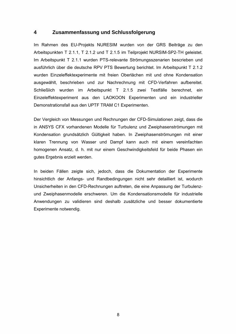
Bei der GRS wurden ausgewählte LAOKOON Experimente mit dem CFD-Programm
ANSYS CFX berechnet, siehe /Scheuerer 2006/. In den LAOKOON Experimenten
wurden stratifizierte, horizontale Wasser/Dampf Strömungen untersucht, die eine freie
Oberfläche zwischen der unterkühlten Wasserschicht und dem gesättigten Dampf
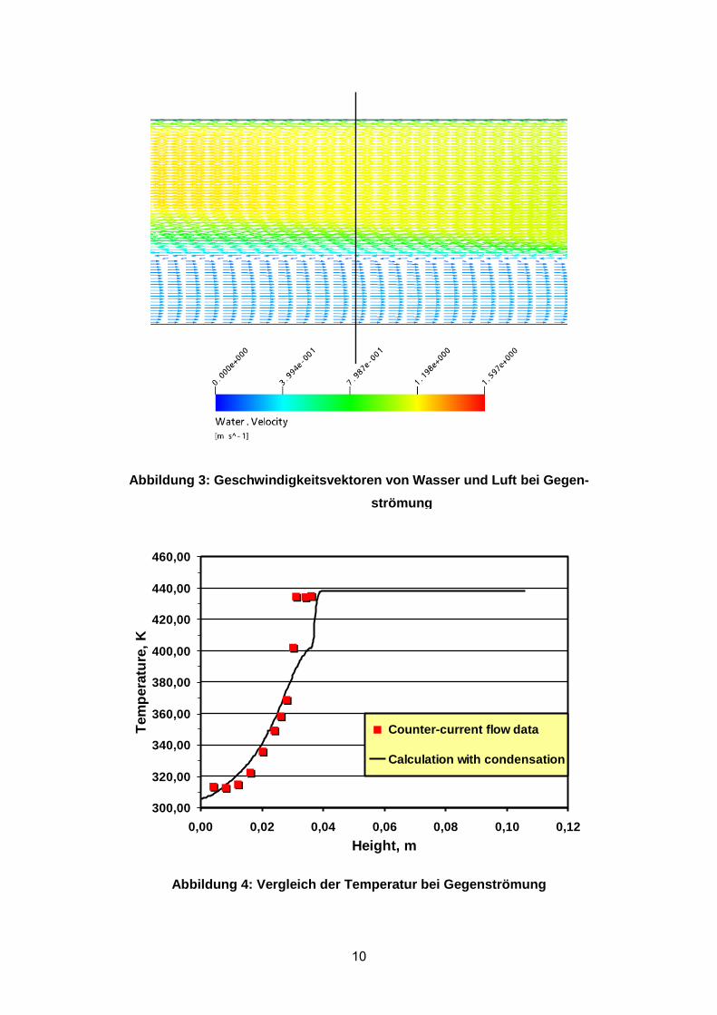
haben. Die Nachrechnung erfolgte jeweils für einen Testfall, bei dem Wasser und
Dampf im Gleichstrom und im Gegenstrom bei hohen Reynoldszahlen auftreten.
Zwei unterschiedliche Methoden werden verwendet, um die Simulation der
Zweiphasenströmungen hinsichtlich Genauigkeit und Effizienz zu überprüfen. Zuerst
werden die Strömungen mit freien Oberflächen mit Hilfe eines homogenen
Strömungsmodells simuliert. Dann wurde ein Zwei-Fluid-Ansatz mit den
entsprechenden Zwischenphasen-Modellen eingesetzt. In einem weiteren Schritt
wurden der Massen- und Wärmeübergang an der freien Oberfläche einbezogen.
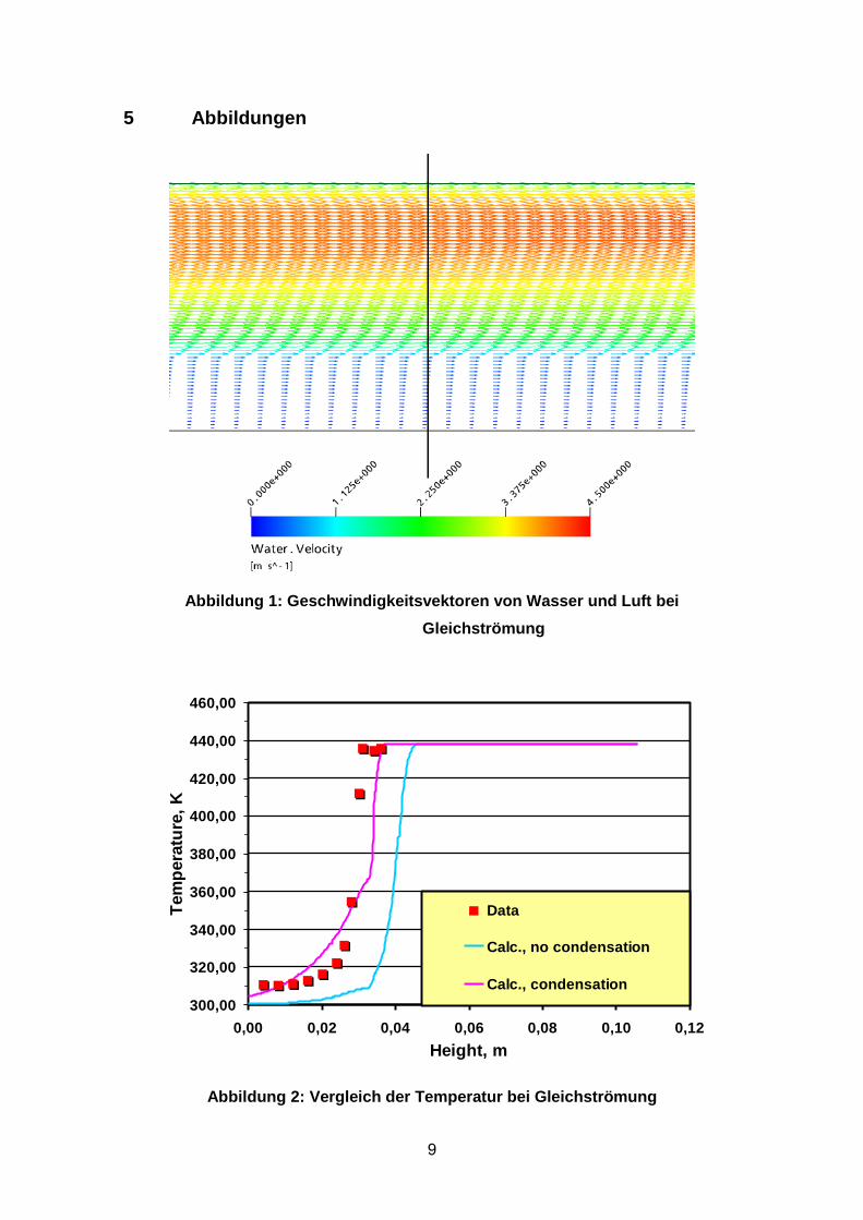
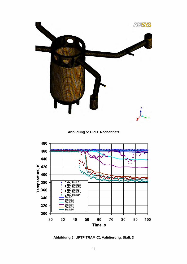
Der Vergleich der Temperaturverteilung von Rechnung und Messung zeigte in beiden
Fällen, bei Gleich- und bei Gegenströmung, gute Übereinstimmung nachdem das
Rechennetzes, der Zeitschritt und die Modellparameter im Kondensationsmodell
6
optimiert wurden, siehe Abbildung 1 bis Abbildung 4. Damit konnte gezeigt werden,
dass der in ANSYS CFX vorhandene Modellansatz zur Simulation der Kondensation
an der freien Oberfläche grundsätzlich Gültigkeit hat. Da jedoch Temperaturprofile nur
an einer Stelle im Strömungskanal gemessen wurden und keine Geschwin-
digkeitsmessungen vorhanden sind, ist es schwierig allgemeingültige Modellan-
passungen durchzuführen. Die Ergebnisse wurden in der NURETH-12 Konferenz
vorgestellt, siehe /Scheuerer et al., 2007/.
3.4 Berechnung eines UPTF TRAM C1 Experiments
Ein grossskaliges Experiment, in dem geschichtete Wasser/Dampfströmung und
Kondensation als kombinierten Strömungsphänomenen auftreten, wurde aus den
UPTF TRAM C1 Versuchen ausgewählt. Im Testlauf RUN21A2 wird kaltes ECC-
Wasser über den kalten Strang 2 in den mit heißem Wasser gefüllten Druckbehälter
eingespeist. Die Wasserhöhe im Druckbehälter wird während der gesamten Transiente
bei einer Höhe von 9,25 m oberhalb der Mittellinie des kalten Strangs konstant
gehalten. Überschüssiges Wasser wird durch das KTA-System im unteren Plenum des
Druckbehälters abgeführt. Über der freien Wasseroberfläche befindet sich mit Stickstoff
gesättigter Wasserdampf. Stickstoff wird in den Kühlkreislauf eingespeist, um den
Systemdruck bei 17 bar konstant zu halten, und um Kondensation zu vermindern. Die
Pumpensimulatoren sind während des Experiments geschlossen /UPTF-TRAM
Versuch C1/C2, 1996/.
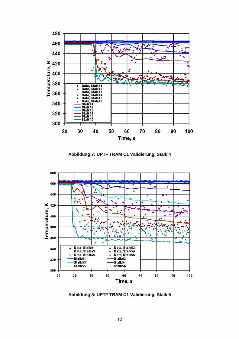
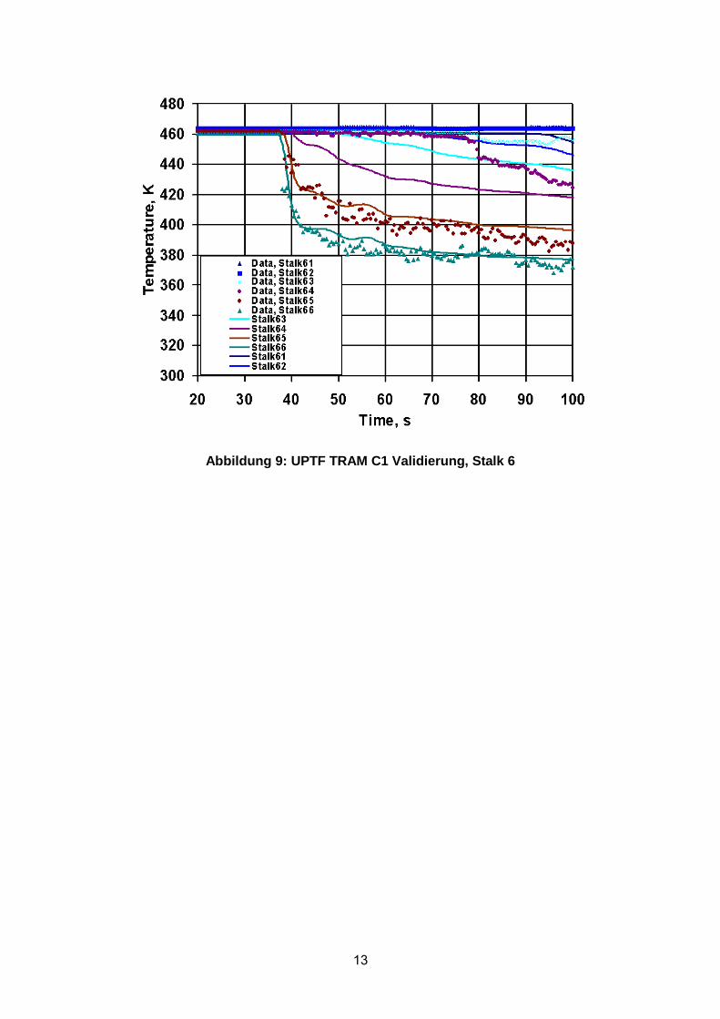
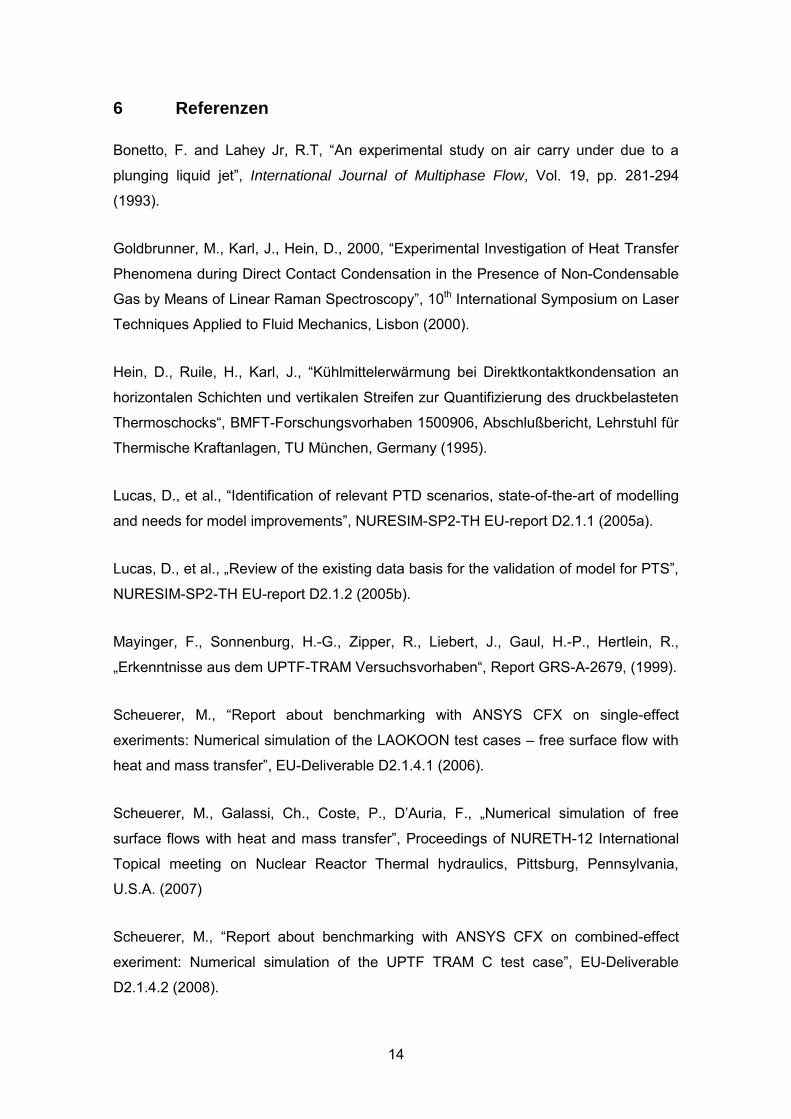
Zur Vorbereitung der CFD-Rechnungen wurden die Temperatur und der Massenstrom
am ECC-Eintritt, sowie die Änderungen der Wasserhöhe im kalten Strang 2 analysiert.
Die Stoffwerte für Wasser und Stickstoff wurden aus NIST-Tabellen entnommen. Dabei
wird angenommen, dass Stickstoff ein ideales Gas ist, dessen Dichte sich als Funktion
von Temperatur und Druck ändert. Als Zielgrößen für den Vergleich von Messung und
Rechnung wurden die lokalen Temperaturen an den Messstellen Stalk 3, Stalk 4, Stalk
5 und Stalk 6 im kalten Strang 2 und Temperaturmessungen im Ringraum und in der
Downcomerwand ausgewählt.
Im nächsten Schritt wurde mit dem ANSYS CFX DesignModeler ein dreidimensionales
Model des Integrationsgebiets erstellt. Da die ECC-Einspeisung nur in einem kalten
Strang erfolgt, muss in der CFD-Rechnung die vollständige Geometrie mit allen vier
Strängen abgebildet werden. Die heißen Stränge werden dabei abgeriegelt und das
7
Modell für den Kernbereich wird als undurchlässiges, poröses Medium simuliert.
Dadurch kann Wasser nur durch die KTA-Rohre austreten. Das Rechennetz besteht
überwiegend aus hexahedralen Elementen. Um eine gute, homogene Verteilung der
Gitterpunkt zu erhalten, wurden auch Tetraeder und Pyramiden-Elemente verwendet.
Das vollständige Rechennetz besteht aus 4 004 514 Netzknoten, siehe Abbildung 5.
Zur Abschätzung des Rechenaufwandes und zur Überprüfung der numerischen
Parameter und der Konsistenz der Modelle wurden zunächst einphasige Rechnungen
gemacht, siehe /Scheuerer, 2008/. Selbst mit dieser vereinfachenden Annahme ist die
Übereinstimmung von Rechnungen und Messungen sehr zufriedenstellend und zeigt
das korrekte Strömungsverhalten, siehe Abbildung 6 bis Abbildung 9. Für die
Simulation der Strömung mit freier Oberfläche konnten auf Grund der stark begrenzten
Rechenleistung nur sehr vorläufige Ergebnisse erzielt werden. Diese Beschränkungen
machten es unmöglich, die Zweiphasenberechnungen in der vollständigen UPTF
Geometrie innerhalb der verbleibenden fünf Monate NURESIM-Projektzeit
abzuwickeln. Die Erwartung ist jedoch, dass unter Anwendung der Zweiphasenmodelle
die Übereinstimmung mit den UPTF-Daten weiter verbessert wird.
8
4 Zusammenfassung und Schlussfolgerung
Im Rahmen des EU-Projekts NURESIM wurden von der GRS Beiträge zu den
Arbeitspunkten T 2.1.1, T 2.1.2 und T 2.1.5 im Teilprojekt NURSIM-SP2-TH geleistet.
Im Arbeitspunkt T 2.1.1 wurden PTS-relevante Strömungsszenarien bescrieben und
ausführlich über die deutsche RPV PTS Bewertung berichtet. Im Arbeitspunkt T 2.1.2
wurden Einzeleffektexperimente mit freien Oberlächen mit und ohne Kondensation
ausgewählt, beschrieben und zur Nachrechnung mit CFD-Verfahren aufbereitet.
Schließlich wurden im Arbeitspunkt T 2.1.5 zwei Testfälle berechnet, ein
Einzeleffektexperiment aus den LAOKOON Experimenten und ein industrieller
Demonstrationsfall aus den UPTF TRAM C1 Experimenten.
Der Vergleich von Messungen und Rechnungen der CFD-Simulationen zeigt, dass die
in ANSYS CFX vorhandenen Modelle für Turbulenz und Zweiphasenströmungen mit
Kondensation grundsätzlich Gültigkeit haben. In Zweiphasenströmungen mit einer
klaren Trennung von Wasser und Dampf kann auch mit einem vereinfachten
homogenen Ansatz, d. h. mit nur einem Geschwindigkeitsfeld für beide Phasen ein
gutes Ergebnis erzielt werden.
In beiden Fällen zeigte sich, jedoch, dass die Dokumentation der Experimente
hinsichtlich der Anfangs- und Randbedingungen nicht sehr detailliert ist, wodurch
Unsicherheiten in den CFD-Rechnungen auftreten, die eine Anpassung der Turbulenz-
und Zweiphasenmodelle erschweren. Um die Kondensationsmodelle für industrielle
Anwendungen zu validieren sind deshalb zusätzliche und besser dokumentierte
Experimente notwendig.
9
5 Abbildungen
Abbildung 1: Geschwindigkeitsvektoren von Wasser und Luft bei
Gleichströmung
300,00
320,00
340,00
360,00
380,00
400,00
420,00
440,00
460,00
0,00 0,02 0,04 0,06 0,08 0,10 0,12
Height, m
Tem
pera
ture
, K
Data
Calc., no condensation
Calc., condensation
Abbildung 2: Vergleich der Temperatur bei Gleichströmung
10
Abbildung 3: Geschwindigkeitsvektoren von Wasser und Luft bei Gegen-
strömung
300,00
320,00
340,00
360,00
380,00
400,00
420,00
440,00
460,00
0,00 0,02 0,04 0,06 0,08 0,10 0,12
Height, m
Tem
pera
ture
, K
Counter-current flow data
Calculation with condensation
Abbildung 4: Vergleich der Temperatur bei Gegenströmung
11
Abbildung 5: UPTF Rechennetz
Abbildung 6: UPTF TRAM C1 Validierung, Stalk 3
12
Abbildung 7: UPTF TRAM C1 Validierung, Stalk 4
Abbildung 8: UPTF TRAM C1 Validierung, Stalk 5
13
Abbildung 9: UPTF TRAM C1 Validierung, Stalk 6
14
6 Referenzen
Bonetto, F. and Lahey Jr, R.T, “An experimental study on air carry under due to a
plunging liquid jet”, International Journal of Multiphase Flow, Vol. 19, pp. 281-294
(1993).
Goldbrunner, M., Karl, J., Hein, D., 2000, “Experimental Investigation of Heat Transfer
Phenomena during Direct Contact Condensation in the Presence of Non-Condensable
Gas by Means of Linear Raman Spectroscopy”, 10th International Symposium on Laser
Techniques Applied to Fluid Mechanics, Lisbon (2000).
Hein, D., Ruile, H., Karl, J., “Kühlmittelerwärmung bei Direktkontaktkondensation an
horizontalen Schichten und vertikalen Streifen zur Quantifizierung des druckbelasteten
Thermoschocks“, BMFT-Forschungsvorhaben 1500906, Abschlußbericht, Lehrstuhl für
Thermische Kraftanlagen, TU München, Germany (1995).
Lucas, D., et al., “Identification of relevant PTD scenarios, state-of-the-art of modelling
and needs for model improvements”, NURESIM-SP2-TH EU-report D2.1.1 (2005a).
Lucas, D., et al., „Review of the existing data basis for the validation of model for PTS”,
NURESIM-SP2-TH EU-report D2.1.2 (2005b).
Mayinger, F., Sonnenburg, H.-G., Zipper, R., Liebert, J., Gaul, H.-P., Hertlein, R.,
„Erkenntnisse aus dem UPTF-TRAM Versuchsvorhaben“, Report GRS-A-2679, (1999).
Scheuerer, M., “Report about benchmarking with ANSYS CFX on single-effect
exeriments: Numerical simulation of the LAOKOON test cases – free surface flow with
heat and mass transfer”, EU-Deliverable D2.1.4.1 (2006).
Scheuerer, M., Galassi, Ch., Coste, P., D’Auria, F., „Numerical simulation of free
surface flows with heat and mass transfer”, Proceedings of NURETH-12 International
Topical meeting on Nuclear Reactor Thermal hydraulics, Pittsburg, Pennsylvania,
U.S.A. (2007)
Scheuerer, M., “Report about benchmarking with ANSYS CFX on combined-effect
exeriment: Numerical simulation of the UPTF TRAM C test case”, EU-Deliverable
D2.1.4.2 (2008).

15
Sievers, J., Boyd, C., D’Auria, F., Filo, J., Häfner, W., Scheuerer, , M. “Thermal-
Hydraulic Aspects of the International Comparative Assessment Study on Reactor
Pressure Vessels under PTS loading (RPV PTS ICAS)”, CSNI Workshop on Advanced
Thermal-Hydraulic and Neutronic Codes: Current and Future Applications, Barcelona,
Spain, (2000).
UPTF-TRAM Versuch C1/C2 - Strähnen- und Streifenkühlung der RDB-Wand, „Quick
Look Report“, NT31/96/17, Siemens AG, Erlangen, Bereich Energieerzeugung, März
1996.

16
17
7 Verteiler
BMWi Referat III B 4 1 x GRS-PT/B
Internationale Verteilung 40 x Projektbegleiter (fss) 3 x GRS
Geschäftsführung (hah, stj) je 1 x Bereichsleiter (zir, tes, rot, erv, lim, prg) je 1 x Abteilungsleiter (gls, poi, bea, paa) je 1 x Projektbetreuung (kgl) 1 x Projektleiterin (bam) 1 x Informationsverarbeitung (nit) 1 x Bibliothek (Garching, Köln) je 1 x Autorin (bam) 3 x
Gesamtauflage
64 Exemplare

EUROPEAN COMMISSION 6th EURATOM FRAMEWORK PROGRAMME 2005-2008 INTEGRATED PROJECT (IP): NURESIM Nuclear Reactor Simulations SUB-PROJECT 2: Thermal Hydraulics
DELIVERABLE D2.1.1: IDENTIFICATION OF RELEVANT PTS-
SCENARIOS, STATE OF THE ART OF MODELLING AND NEEDS FOR MODEL IMPROVEMENTS
D. Lucas (Editor) Forschungszentrum Rossendorf e.V.
P.O.Box 510119, D-01314 Dresden, Germany
Abstract
This report identifies PTS-scenarios for the French 900 MW CPY PWR, the German 1300 MW Kon-voi reactor, the Loviisa 400 MW VVER, the Russian VVER-1000 and the Czech VVER-100. Accord-ing to the resulting basic flow conditions relevant physical phenomena for the simulation of the scenes during Emergency Core Cooling (ECC) injection into the cold leg are identified. The main focus is on two-phase flow phenomena. The state of the art of modelling these phenomena and needs for models improvement are discussed. Thus the report is a suitable basis for the specification of the main topics to be provided in Task T2.1.4 of the NURESIM project.
Dissemination level: RE: restricted to a group specified by the partners of the NURESIM project
NURESIM-SP2-TH D 2.1.1
12/2005 2/123
LIST OF AUTHORS Section Authors
1 D. Lucas (FZR), D. Bestion (CEA), A. Bousbia Salah, F. Moretti, F. D’Auria (UPisa) 2.1 D. Bestion (CEA), A. Martin (EDF) 2.2 M. Scheuerer (GRS) 2.3 V. Riikonen (LUT), M. Ilvonen (VTT) 2.4 F. D’Auria, D. Mazzini, F. Moretti (UPisa) 2.5 P. Kral, J. Macek (NRI) 2.6 E. Bodele, D. Lucas (FZR) 3 A. Bousbia Salah, F. Moretti, F. D’Auria (UPisa) 4.1 A. Bousbia Salah, F. Moretti, F. D’Auria (UPisa) 4.2 A. Manera, D. Lucas (FZR) 4.3 D. Bestion (CEA), D. Lakehal (ASCOMP) 4.4 D. Bestion (CEA), D. Lakehal (ASCOMP) 4.5 J.-M. Seynhaeve (UCL), L. Strubelj, I. Tiselj (JSI), A. Bousbia Salah (UPisa) 5 D. Lucas (FZR)
LIST OF INSTITUTIONS
ASCOMP ASCOMP GmbH, Switzerland CEA Commissariat à l’Energie Atomique, France EDF Electricité de France , France FZR Forschungszentrum Rossendorf, Germany GRS Gesellschaft für Anlagen- und Reaktorsicherheit, Germany JSI Jožef Stefan Institute, Slovenia LUT Lappeenranta University of Technology, Finland UCL Université Catholique de Louvain La Neuve, Belgium UPisa Università di Pisa, Italy VTT VTT Industrial Systems, Finland
NURESIM-SP2-TH D 2.1.1
12/2005 3/123
TABLE OF CONTENTS
1 INTRODUCTION 6
2 IDENTIFICATION OF RELEVANT PTS-SCENARIOS 9
2.1 French 900 MW CPY PWR 9
2.1.1 Methodology for the French RPV PTS assessment 9
2.1.2 The worst case “single-phase PTS scenario” 10
2.1.3 The base case “two phase-PTS scenario” 11
2.1.3.1 Scenario and reactor transient modelling with the system code 11
2.1.3.2 Results of the transient simulation with the system code 11
2.1.3.3 Boundary conditions for the CFD calculation 12
2.1.3.4 Plots of calculated parameters 12
2.1.3.5 Required range of parameters for CFD simulation 19
2.2 German 1300 MW Konvoi reactor 19
2.2.1 Methodology for the German RPV PTS assessment 19
2.2.2 Assumptions for Thermal Hydraulic Analysis 20
2.2.3 Assessment Study on Reactor Pressure Vessels under PTS loading 21
2.2.3.1 Problem Statement 22
2.2.3.2 Results 22
2.2.3.3 Conclusion 23
2.2.4 Range of parameters for CFD simulation of UPTF experiments 27
2.3 Loviisa 440 MW VVER 27
2.3.1 Internal cooling of the pressure vessel 30
2.3.1.1 Large break LOCA 30
2.3.1.2 Small break LOCA 30
2.3.1.3 Steam leaks 32
2.3.2 External cooling of the pressure vessel 32
2.3.2.1 Spurious operation of the external spray systems 33
2.3.2.2 LOCAs 33
2.3.2.3 Steam leaks in the containment 33
2.3.3 Pressurization of the primary circuit in the cold state 33
2.3.4 Relevant phenomena to be simulated 33
2.4 Russian VVER 1000 34
2.4.1 General remarks 34
2.4.2 VVER-1000 relevant design characteristics 35
2.4.2.1 Reactor coolant system 35
2.4.2.2 Reactor pressure vessel 35
2.4.2.3 Emergency core cooling system 38
2.4.3 Relevant initiating events for the VVER-1000 PTS analysis 40
2.4.3.1 Categorization of the sequences 40
2.4.3.2 VVER-1000 initiating events and their significance 41
2.4.4 Numerical models for PTS analysis 41
2.4.4.1 RELAP5 NPP nodalisation and RPV schematisation 42
NURESIM-SP2-TH D 2.1.1
12/2005 4/123
2.4.4.2 RPV ANSYS Mesh 45
2.4.4.3 Fracture mechanics model 46
2.4.5 PTS investigations of DMSLB and DEGB sequences 46
2.4.5.1 Main thermal-hydraulic results 47
2.4.5.2 Main structural-fracture mechanics results 50
2.4.5.3 Comparison of the DMSLB and DEGB sequences 51
2.4.5.4 Effect of the non-uniform distribution of the wall cooling 53
2.4.6 Conclusions and required range of parameters for CFD simulation 55
2.5 Czech VVER-1000 56
2.5.1 Methodology for the Czech PTS assessment 56
2.5.1.1 Selection of scenarios for TH analyses 56
2.5.1.2 Computer codes used in Czech PTS studies so far 58
2.5.1.3 Basic info to VVER-1000 input model for RELAP5 59
2.5.1.4 Conservative assumptions applied in system TH analysis for PTS 60
2.5.2 Specification of the case for CFD evaluation 61
2.5.2.1 Specification of the initiating event and boundary conditions 61
2.5.2.2 Results of system TH analysis 61
2.6 Conclusion from the PTS scenarios for CFD modelling 68
3 THE USE OF CFD CODES FOR PTS-SIMULATIONS 69
3.1 General remarks on CFD codes 69
3.2 CFD modelling of PTS phenomena in ECORA 70
3.2.1 Jet impingement on free surface 70
3.2.1.1 Simulation strategy (in CFX-5) 70
3.2.1.2 Simulation results 71
3.2.2 Contact Condensation in Stratified Steam-Water Flow 71
3.2.2.1 Modelling free surfaces with momentum, heat and mass transfer in CFX-5 72
3.2.2.2 Simulation Results and Conclusion 73
3.3 Recommendations for CFD Simulations 73
3.3.1 Interface Fitting vs. Interface Capturing 73
3.3.2 Direct Simulation vs. Model Correlation 73
3.3.3 Definition of Target Variables for Convergence and Grid Refinement Tests 74
3.4 General requirements for the qualification of CFD codes for two-phase PTS 74
4 STATE OF THE ART AND NEEDS FOR SINGLE EFFECT MODEL IMPROVEMENTS 76
4.1 Instabilities of the jet at ECC injection 76
4.1.1 Experimental and Numerical Investigations 77
4.1.2 Recommendations 83
4.2 Bubble entrainment by plunging liquid jets 84
4.2.1 State-of-the-art on modelling and correlations 86
4.2.1.1 Correlations for minimum entrainment velocity 86
4.2.1.2 Correlations for volumetric flow rate of entrained gas 87
4.2.2 Characteristics of bubble dispersion 89
4.2.2.1 Bubbles size distribution 89
NURESIM-SP2-TH D 2.1.1
12/2005 5/123
4.2.2.2 Distribution of gas concentration 89
4.2.2.3 Local models for bubbles migration after entrainment 90
4.2.3 Further research needs 91
4.2.4 Nomenclature for section 4.2 91
4.3 Turbulence 93
4.3.1 Turbulence production below the jet 93
4.3.2 Influence of bubble entrainment on turbulence 94
4.3.3 Turbulence production in wall and interfacial shear layers 95
4.3.4 Interaction between interfacial waves and turbulence production 96
4.3.5 Effects of temperature stratification upon turbulent diffusion 97
4.3.6 Transient Flow Separation in the Downcomer 98
4.4 Interfacial momentum, mass and heat transfer at the free surface 100
4.4.1 Condensation at a vapor-liquid interface: literature overview 100
4.4.2 Modelling interfacial transfers at free surface 104
4.5 Direct Contact Condensation (DCC) 106
4.5.1 DCC on the interface of the liquid jet before mixing in case of ECC 106
4.5.2 Instabilities in stratified flow connected to DCC 109
4.5.2.1 Kelvin-Helmholtz instabilities 109
4.5.2.2 Transition from stratified to slug flow 109
4.5.3 Direct contact condensation in horizontal flow and effect upon interfacial and wave structure 110
4.5.3.1 DCC models in 1D two-fluid computer codes 111
4.5.3.2 Condensation induced water hammer (CIWH) in horizontal pipes 112
4.5.4 CFD and DCC in horizontally stratified flow 112
5 CONCLUSIONS 114
6 REFERENCES 116
NURESIM-SP2-TH D 2.1.1
12/2005 6/123
1 INTRODUCTION
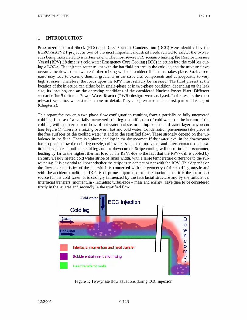
Pressurized Thermal Shock (PTS) and Direct Contact Condensation (DCC) were identified by the EUROFASTNET project as two of the most important industrial needs related to safety, the two is-sues being interrelated to a certain extent. The most severe PTS scenario limiting the Reactor Pressure Vessel (RPV) lifetime is a cold water Emergency Core Cooling (ECC) injection into the cold leg dur-ing a LOCA. The injected water mixes with the hot fluid present in the cold leg and the mixture flows towards the downcomer where further mixing with the ambient fluid there takes place. Such a sce-nario may lead to extreme thermal gradients in the structural components and consequently to very high stresses. Therefore, the loads upon the RPV must reliably be assessed. The fluid present at the location of the injection can either be in single-phase or in two-phase condition, depending on the leak size, its location, and on the operating conditions of the considered Nuclear Power Plant. Different scenarios for 5 different Power Water Reactor (PWR) designs were analysed. In the results the most relevant scenarios were studied more in detail. They are presented in the first part of this report (Chapter 2). This report focuses on a two-phase flow configuration resulting from a partially or fully uncovered cold leg. In case of a partially uncovered cold leg a stratification of cold water on the bottom of the cold leg with counter-current flow of hot water and steam on top of this cold-water layer may occur (see Figure 1). There is a mixing between hot and cold water. Condensation phenomena take place at the free surfaces of the cooling water jet and of the stratified flow. These strongly depend on the tur-bulence in the fluid. There is a plume cooling in the downcomer. If the water level in the downcomer has dropped below the cold leg nozzle, cold water is injected into vapor and direct contact condensa-tion takes place in both the cold leg and the downcomer. Stripe cooling will occur in the downcomer, leading by far to the highest thermal load of the RPV, due to the fact that the RPV-wall is cooled by an only weakly heated cold water stripe of small width, with a large temperature difference to the sur-rounding. It is essential to know whether the stripe is in contact or not with the RPV. This depends on the flow characteristics of the jet, which is connected with the geometry of the cold leg nozzle and with the accident conditions. DCC is of prime importance in this situation since it is the main heat source for the cold water. It is strongly influenced by the interfacial structure and by the turbulence. Interfacial transfers (momentum - including turbulence – mass and energy) have then to be considered firstly in the jet area and secondly in the stratified flow.
Figure 1: Two-phase flow situations during ECC injection
NURESIM-SP2-TH D 2.1.1
12/2005 7/123
Three basic ways are currently used to evaluate local fluid temperatures and local thermal loads, namely “engineering models”, coarse-grid and parallel-channel techniques, and CFD-codes. The en-gineering models employ correlations obtained from specialized experiments (e.g. the CREARE and the UPTF-TRAM experiments). Since engineering models are applied to geometrical conditions that differ from those underlying the original specialized experiments, scaling considerations become es-sential for applications. Often, therefore, additional experiments (up to scales of 1:1) are necessary to prove the validity of the respective engineering models. Furthermore, engineering models are highly conservative and cannot be applied to ageing reactors. On the other hand, coarse-grid and parallel-channel techniques are based on the capability of thermal-hydraulic system codes to subdivide the downcomer azimuthally into separate parallel channels. However, the parameterization of the inter-connection between the ensuing parallel channels needs dedicated experiments. Without dedicated experiments, the results provided by these techniques are still far from being realistic (as shown within the framework of the RPV PTS ICAS standard problem, Sievers et al., 1999). The third method is to use CFD-codes. Although CFD codes are helpful for a limited understanding of the un-derlying processes, the quantitative accuracy of the results thus obtained is still unsatisfactory, par-ticularly for two-phase flows. Nevertheless, appropriately improved 3D CFD codes are expected to be used extensively for research on nuclear power plant life extension. In the frame of the ECORA pro-ject different PTS-relevant test cases were simulated using CFD codes (Egorov, 2004). It is a common understanding among the thermal-hydraulic experts that the system analysis codes have currently reached an acceptable degree of maturity. The reliable application, however, is still limited to the validated domain. The use of Computational Fluid Dynamics (CFD) codes, which base on physical local models, is being requested more and more for assessing the safety of the existing re-actors and for developing advanced reactor systems (Misak and Royen, 2002). According to Bestion et al., 2004, the results issued from the ECORA project have shown a satisfactory performance of the employed CFD codes for single-phase flow problems, and for two-phase flow problems with single dominant interface morphology. This includes free surface flows, or bubbly flows. However, for cases with more than one morphology, for instance for a jet impinging on free surface flow with bubble en-trainment or for the transition of bubble to churn flow, the available two-phase models show poor re-sults and need to be improved. Some aspects of the simulation of PTS using CFD codes are discussed in Chapter 3. New experimental works are in principle needed in order to fill any lack of knowledge or understand-ing of a physical phenomena or process. Experimental data is also needed for the quantification of code uncertainties, for checking the scale-up capability to fill the gap between the real plant and test facility scales and for the development of new generation codes or advanced reactor systems. A sec-ond report (D.2.1.2) addresses available and needed experimental data for PTS and DCC. The simulation of PTS including DCC scenarios must be enhanced beyond the current state-of-the-art by improving substantially the two-phase flow modelling capabilities of current CFD-codes. This in-cludes the modelling of impinging jet and free surfaces, entrainment of droplets and bubbles, and di-rect contact condensation. These phenomena are strongly influenced by the turbulence of the liquid, which depends, in turn, on the safety injection jet, the wall shear and interfacial shear, and the interfa-cial wave structure. DCC might play a crucial role and coupling between condensation and turbu-lence. Improvements are necessary both for the physical models (heat transfer coefficient at the inter-face between liquid and vapor, instabilities of the interface) and for the numerical schemes (accuracy, CPU time). According to the identified PTS scenarios and the resulting flow situations the state of the art and needs for further model development for the relevant physical phenomena is discussed in Chapter 4. Improving the current state-of-the-art CFD-codes must be based on existing experiments, and, on new experiments equipped with novel measuring techniques (e. g., mean velocity, turbulent fluctuations,

NURESIM-SP2-TH D 2.1.1
12/2005 8/123
liquid temperatures, high-frequency wire-mesh sensors) that offer sufficient resolution in space and time for comparison with the CFD computations. There is a need for both an integral-type experiment and also for separate effect test data. Furthermore, simulating the transient heat transfer to the RPV requires that the walls be included into the simulations. It is only the knowledge of the time dependent temperature fields inside the vessels that allows a sound fracture mechanical analysis. Because there is no feedback from the fracture mechanics to the thermal-hydraulics (one way coupling) this is not in-cluded in the NURESIM work program.
NURESIM-SP2-TH D 2.1.1
12/2005 9/123
2 IDENTIFICATION OF RELEVANT PTS-SCENARIOS
2.1 French 900 MW CPY PWR
2.1.1 Methodology for the French RPV PTS assessment
The present French RPV PTS assessment methodology includes many aspects such as the following: - the taking into account of realistic flaws (size and location), based on manufacturing and in-
service inspections, located in the cladding or in the base metal of the vessel, - a deterministic approach based on the computation of the stress intensity factor at the crack tip
and its comparison to the material fracture toughness for the base metal, and for the cladding, - the use of a reference fracture toughness curve– indexed on the RTNDT – for the base metal frac-
ture toughness properties, - a set of transients to take into account in the assessment; LOCA transients (including Small Break
LOCA (SBLOCA) are the most important ones), - some safety required criteria in the corresponding category of situations depending on the occur-
rence of postulated transients, - the taking into consideration of the stainless steel cladding in the structural integrity assessment,
both on thermal and mechanical computations. The first methodology applied in the 1980s was based on the following steps : - the global parameters of the primary circuit computed by the system code FRARELAP by
FRAMATOME, - the local definition of the transient in the downcomer based on an experimental correlation de-
rived from EPRI tests (CREARE mock-up), - the heat transfer coefficients derived from the experimental results of the VESTALE loop per-
formed around 1980 leading to ‘envelope’ coefficients for different locations of the studied de-fects in the downcomer.
It was noticeable that this approach was far too conservative. So in 1997, within the frame of the French RPV safety margin reassessment, a new methodology was adopted using up-to-date CFD codes. At present, this methodology is used only for small primary breaks and it is not certain that it will be extended to other types of transients. The thermal-hydraulic analysis was performed in two steps : - the evolution of the global parameters (pressure, injection flow rate) of the primary circuit is
given by the CATHARE system code, - the definition of the temperatures in the downcomer, after the interruption of the natural convec-
tion in the loops, is established through an accurate analysis with specific 3D CFD tools. Lastly, through a fast fracture analysis, the safety margins have been calculated for different locations of subclad defects in the downcomer and compared to the required criteria in the corresponding cate-gory of situations. Depending on the transient condition, the water level in the downcomer during ECC injection can be either above the cold leg, or lower with a partially uncovered cold leg, or even lower with a totally uncovered cold leg. The RPV PTS assessments have shown that the most severe loading conditions were the SBLOCA accidents (2" and 3" SBLOCA) due to the pressurized injection of cold water into the downcomer of the RPV. Such scenarios correspond to cold legs either full of water or partially uncovered. In the first case, flow mixing in the cold legs and in the downcomer may be simulated by single phase CFD tools.
NURESIM-SP2-TH D 2.1.1
12/2005 10/123
In the second case, condensation is the main source of heat for the cold injected water and a two-phase CFD tool is necessary for an accurate simulation. The development of the NEPTUNE two-phase CFD tool has been launched in this purpose (amongst other applications). Therefore PTS thermal-hydraulics investigations will include: - the simulation of a worst case “single-phase PTS scenario”, - the simulation of a worst case two-phase scenario with a partially uncovered cold leg, - the two-phase simulation tool should also be qualified for situations with “fully uncovered cold
leg”.
2.1.2 The worst case “single-phase PTS scenario”
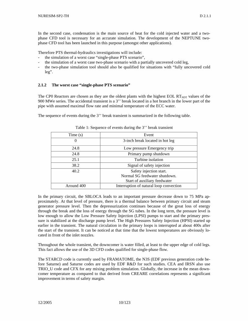
The CP0 Reactors are chosen as they are the oldest plants with the highest EOL RTNDT values of the 900 MWe series. The accidental transient is a 3’’ break located in a hot branch in the lower part of the pipe with assumed maximal flow rate and minimal temperature of the ECC water. The sequence of events during the 3’’ break transient is summarized in the following table.
Table 1: Sequence of events during the 3’’ break transient
Time (s) Event 0 3-inch break located in hot leg
24.8 Low pressure Emergency trip 24.8
Primary pump shutdown
25.1
Turbine isolation 38.2
Signal of safety injection
40.2 Safety injection start. Normal SG feedwater shutdown.
Start of auxiliary feedwater Around 400 Interruption of natural loop convection
In the primary circuit, the SBLOCA leads to an important pressure decrease down to 75 MPa ap-proximately. At that level of pressure, there is a thermal balance between primary circuit and steam generator pressure level. Then the depressurization continues because of the great loss of energy through the break and the loss of energy through the SG tubes. In the long term, the pressure level is low enough to allow the Low Pressure Safety Injection (LPSI) pumps to start and the primary pres-sure is stabilized at the discharge pump level. The High Pressures Safety Injection (HPSI) started up earlier in the transient. The natural circulation in the primary loops is interrupted at about 400s after the start of the transient. It can be noticed at that time that the lowest temperatures are obviously lo-cated in front of the inlet nozzles. Throughout the whole transient, the downcomer is water filled, at least to the upper edge of cold legs. This fact allows the use of the 3D CFD codes qualified for single-phase flow. The STARCD code is currently used by FRAMATOME, the N3S (EDF previous generation code be-fore Saturne) and Saturne codes are used by EDF R&D for such studies. CEA and IRSN also use TRIO_U code and CFX for any mixing problem simulation. Globally, the increase in the mean down-comer temperature as compared to that derived from CREARE correlations represents a significant improvement in terms of safety margin.
NURESIM-SP2-TH D 2.1.1
12/2005 11/123
2.1.3 The base case “two phase-PTS scenario”
2.1.3.1 Scenario and reactor transient modelling with the system code
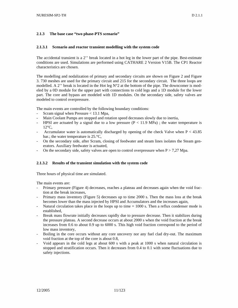
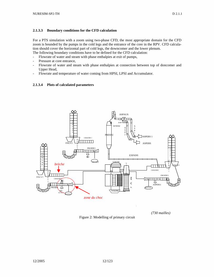
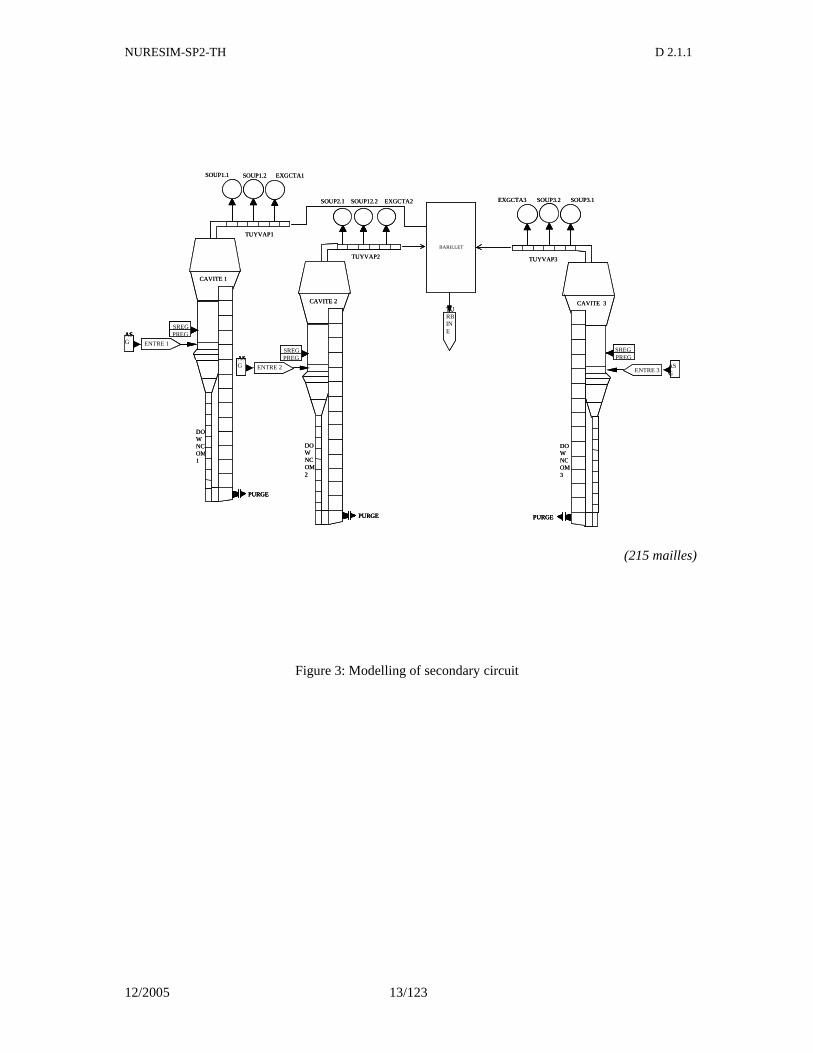
The accidental transient is a 2’’ break located in a hot leg in the lower part of the pipe. Best-estimate conditions are used. Simulations are performed using CATHARE 2 Version V15B. The CP1 Reactor characteristics are chosen. The modelling and nodalization of primary and secondary circuits are shown on Figure 2 and Figure 3. 730 meshes are used for the primary circuit and 215 for the secondary circuit. The three loops are modelled. A 2’’ break is located in the Hot leg N°2 at the bottom of the pipe. The downcomer is mod-eled by a 0D module for the upper part with connections to cold legs and a 1D module for the lower part. The core and bypass are modeled with 1D modules. On the secondary side, safety valves are modeled to control overpressure. The main events are controlled by the following boundary conditions: - Scram signal when Pressure < 13.1 Mpa, - Main Coolant Pumps are stopped and rotation speed decreases slowly due to inertia, - HPSI are actuated by a signal due to a low pressure (P < 11.9 MPa) ; the water temperature is
12°C, - Accumulator water is automatically discharged by opening of the check Valve when P < 43.85
bar.; the water temperature is 25.°C, - On the secondary side, after Scram, closing of feedwater and steam lines isolates the Steam gen-
erators. Auxiliary feedwater is actuated, - On the secondary side, safety valves are open to control overpressure when P > 7,27 Mpa.
2.1.3.2 Results of the transient simulation with the system code
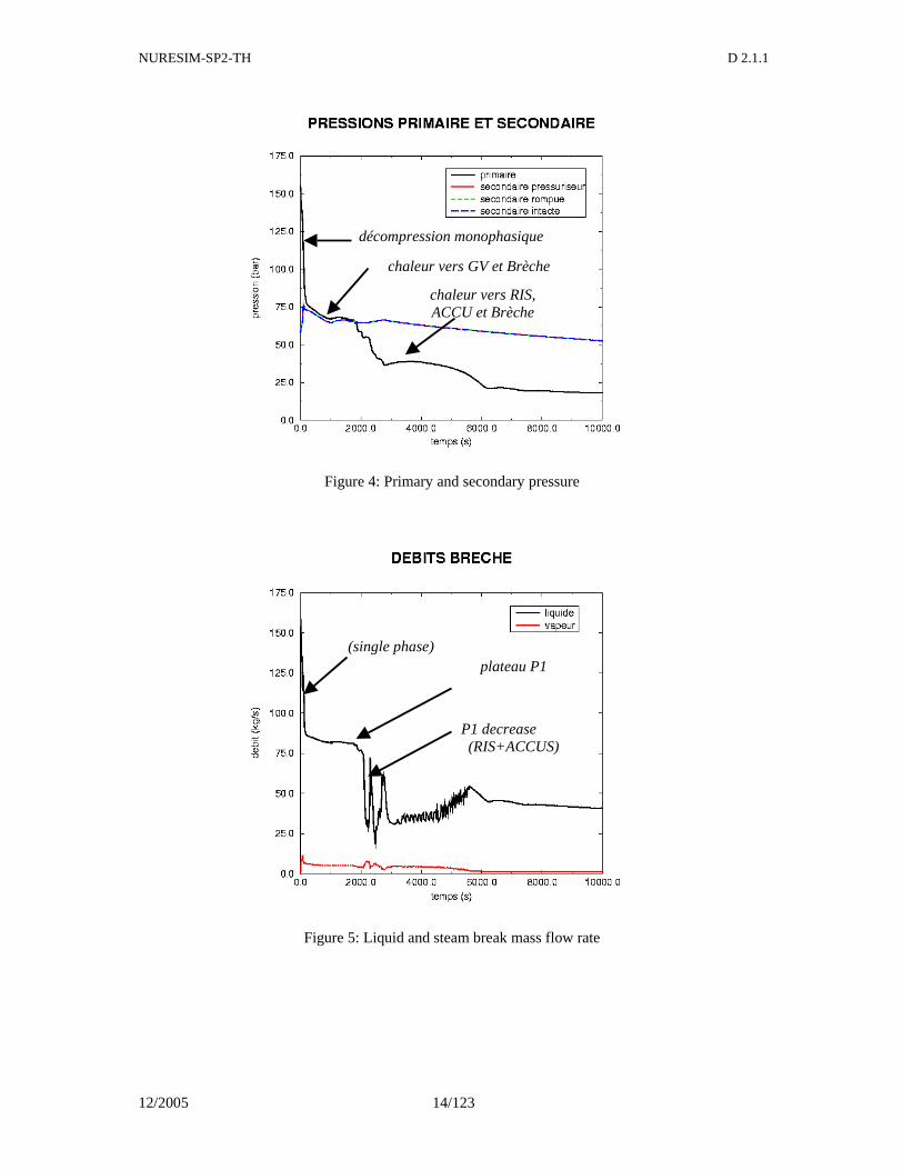
Three hours of physical time are simulated. The main events are: - Primary pressure (Figure 4) decreases, reaches a plateau and decreases again when the void frac-
tion at the break increases, - Primary mass inventory (Figure 5) decreases up to time 2000 s. Then the mass loss at the break
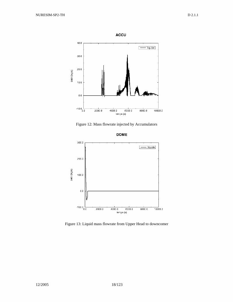
becomes lower than the mass injected by HPSI and Accumulators and the increases again, - Natural circulation takes place in the loops up to time = 1000 s. Then a reflux condenser mode is
established, - Break mass flowrate initially decreases rapidly due to pressure decrease. Then it stabilizes during
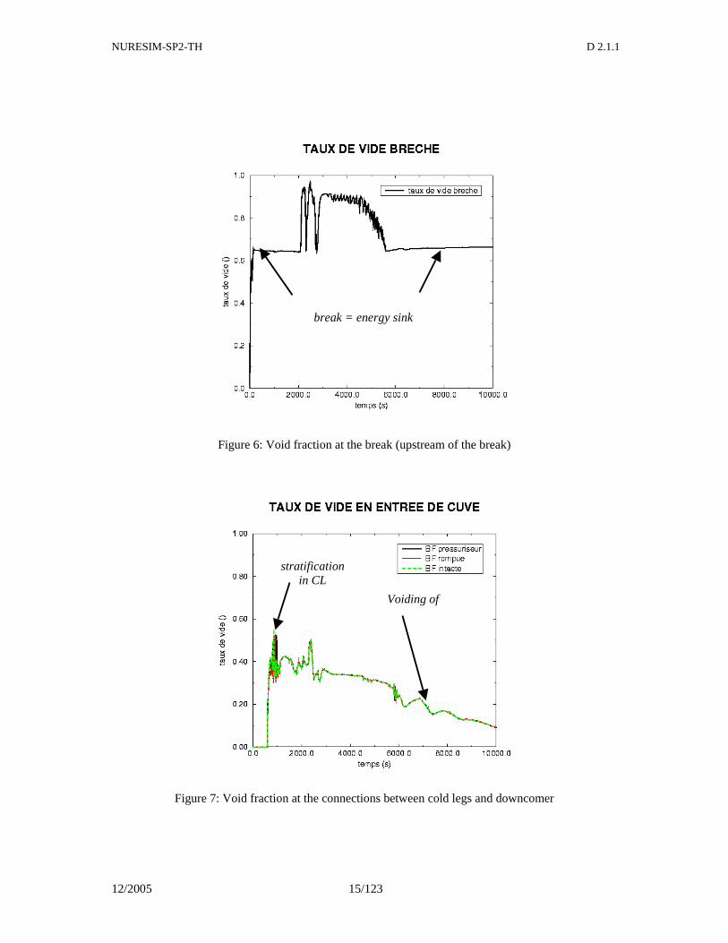
the pressure plateau. A second decrease occurs at about 2000 s when the void fraction at the break increases from 0.6 to about 0.9 up to 6000 s. This high void fraction correspond to the period of low mass inventory,
- Boiling in the core occurs without any core uncovery nor any fuel clad dry-out. The maximum void fraction at the top of the core is about 0.8,
- Void appears in the cold legs at about 600 s with a peak at 1000 s when natural circulation is stopped and stratification occurs. Then it decreases from 0.4 to 0.1 with some fluctuations due to safety injections.
NURESIM-SP2-TH D 2.1.1
12/2005 12/123
2.1.3.3 Boundary conditions for the CFD calculation
For a PTS simulation with a zoom using two-phase CFD, the most appropriate domain for the CFD zoom is bounded by the pumps in the cold legs and the entrance of the core in the RPV. CFD calcula-tion should cover the horizontal part of cold legs, the downcomer and the lower plenum. The following boundary conditions have to be defined for the CFD calculation: - Flowrate of water and steam with phase enthalpies at exit of pumps, - Pressure at core entrance, - Flowrate of water and steam with phase enthalpies at connection between top of doncomer and
Upper Head, - Flowrate and temperature of water coming from HPSI, LPSI and Accumulator.
2.1.3.4 Plots of calculated parameters
Figure 2: Modelling of primary circuit
ACC ACCU3 TGU
BYP
BP
PLEN C
OEUR
VOLDOWN DOWN
•
•
•
•
PRE
ASP ASPAUX
AS A
S ASPERS
2 EXPANS G
ENV FING D
EBG
FROID
CHAUD
ASPERS1 ACC
ACC
RC FROID
CHAUD DEBG
FING
GENV
GENV FING D
EBG CHAUD
FROID RC
COUVE TGU
BYP
VOLINF
BP
PLEN C
OEUR
DOWN
••
••
••
••
PRESSU SEBIM
ASP ASP1 A
SP2
ASPERS 1 GENVAP 1
FINGV1 DEBGV 1
FROIDE1 CHAUDE1
ACCU1 ACC ACCU2 AS-
PERS2 RC
FROIDE2 CHAUDE 2
DEBGV 2 FINGV2
GENVAP 2
GENVAP 3
FINGV3 DEBGV 3
CHAUDE 3 FROIDE3
RC brèche
zone du choc froid
(730 mailles)
Dow
NURESIM-SP2-TH D 2.1.1
12/2005 13/123
Figure 3: Modelling of secondary circuit
BARILLET
SOUP1.1 SOUP1.2 EXGCTA1
TUYVAP1
TUYVAP2 TUYVAP3
TURBINE
SOUP2.1 SOUP12.2 EXGCTA2 EXGCTA3 SOUP3.1 SOUP3.2
CAVITE 1
CAVITE 2 CAVITE 3
DOWNCOM 1
DOWNCOM 2
DOWNCOM 3
ENTRE 1 ASG
SREG PREG
SREG PREG
ENTRE 3 ASG ENTRE 2
ASG
SREG PREG
Modélisation du circuit secondaire CP1 V14
PURGE
PURGE PURGE
BARILLET
SOUP1.1 SOUP1.2 EXGCTA1
TUYVAP1
TUYVAP2 TUYVAP3
TURBINE
SOUP2.1 SOUP12.2 EXGCTA2 EXGCTA3 SOUP3.1 SOUP3.2
CAVITE 1
CAVITE 2 CAVITE 3
DOWNCOM 1
DOWNCOM 2
DOWNCOM 3
ENTRE 1 ASG ENTRE 1 ENTRE 1 ASG ASG
SREG PREG SREG PREG SREG SREG PREG PREG
SREG PREG SREG PREG SREG SREG PREG PREG
ENTRE 3 ASG ENTRE 2
ASG ASG
SREG PREG SREG PREG SREG SREG PREG PREG
Modélisation du circuit secondaire CP1 V14 Modélisation du circuit secondaire CP1 V14
PURGE PURGE
PURGE PURGE PURGE PURGE
(215 mailles)
NURESIM-SP2-TH D 2.1.1
12/2005 14/123
Figure 4: Primary and secondary pressure
Figure 5: Liquid and steam break mass flow rate
décompression monophasique
chaleur vers GV et Brèche
chaleur vers RIS, ACCU et Brèche
P1 decrease (RIS+ACCUS)
(single phase)
plateau P1
NURESIM-SP2-TH D 2.1.1
12/2005 15/123
Figure 6: Void fraction at the break (upstream of the break)
Figure 7: Void fraction at the connections between cold legs and downcomer
break = energy sink
stratification in CL
Voiding of
NURESIM-SP2-TH D 2.1.1
12/2005 16/123
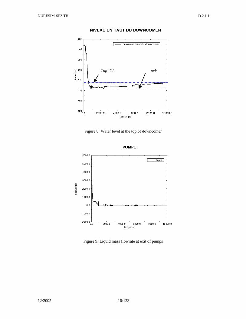
Figure 8: Water level at the top of downcomer
Figure 9: Liquid mass flowrate at exit of pumps
axis Top CL
NURESIM-SP2-TH D 2.1.1
12/2005 17/123
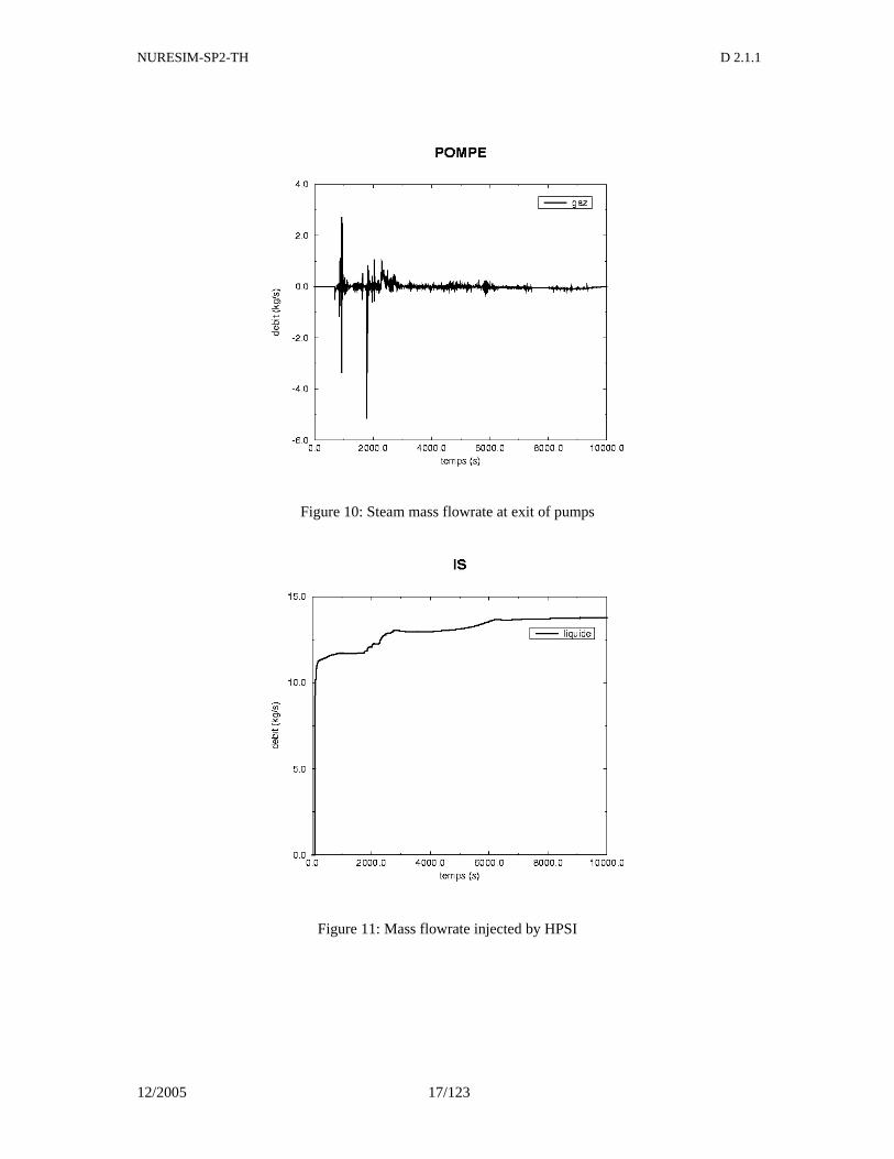
Figure 10: Steam mass flowrate at exit of pumps
Figure 11: Mass flowrate injected by HPSI
NURESIM-SP2-TH D 2.1.1
12/2005 18/123
Figure 12: Mass flowrate injected by Accumulators
Figure 13: Liquid mass flowrate from Upper Head to downcomer
NURESIM-SP2-TH D 2.1.1
12/2005 19/123
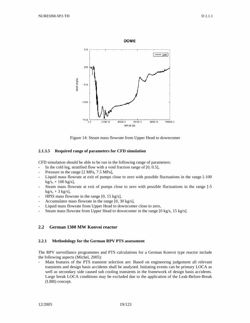
Figure 14: Steam mass flowrate from Upper Head to downcomer
2.1.3.5 Required range of parameters for CFD simulation
CFD simulation should be able to be run in the following range of parameters: - In the cold leg, stratified flow with a void fraction range of [0, 0.5], - Pressure in the range [2 MPa, 7.5 MPa], - Liquid mass flowrate at exit of pumps close to zero with possible fluctuations in the range [-100
kg/s, + 100 kg/s], - Steam mass flowrate at exit of pumps close to zero with possible fluctuations in the range [-5
kg/s, + 3 kg/s], - HPIS mass flowrate in the range [0, 15 kg/s], - Accumulator mass flowrate in the range [0, 30 kg/s], - Liquid mass flowrate from Upper Head to downcomer close to zero, - Steam mass flowrate from Upper Head to downcomer in the range [0 kg/s, 15 kg/s].
2.2 German 1300 MW Konvoi reactor
2.2.1 Methodology for the German RPV PTS assessment
The RPV surveillance programmes and PTS calculations for a German Konvoi type reactor include the following aspects (Michel, 2005): - Main features of the PTS transient selection are: Based on engineering judgement all relevant
transients and design basis accidents shall be analysed. Initiating events can be primary LOCA as well as secondary side caused sub cooling transients in the framework of design basis accidents. Large break LOCA conditions may be excluded due to the application of the Leak-Before-Break (LBB) concept.
NURESIM-SP2-TH D 2.1.1
12/2005 20/123
- Main features of RPV wall fluence determination: RTlimit may be used for all materials within the validity limits for Ni and Cu. Lower values might also be used if justified by the results of the surveillance programme. In this case, calculated fluence values are used, which are validated by the results of the dosimetry. Uncertainties are taken into account. For each material (upper and lower ring, core weld) the maximum fluence at the inner ferritic surface of the RPV is used.
- Main features of thermal hydraulic calculation: Thermal hydraulic calculations should give the necessary input data for structural mechanical analyses, especially downcomer temperature field, coolant-to-wall heat transfer coefficients in the downcomer and primary circuit pressure. Non uni-form cool down in azimuthal and axial directions should be analyzed taking into account thermal stratification of injection water.
- Main features for the structure mechanical analyses: o Postulated defect types/sizes for crack initiation: The aspect ratio of the postulated
semi-elliptical surface crack series is a/c = 1/3. The postulated crack depth is up to 1/4 of the wall thickness dependent on the operating levels. Smaller maximum crack sizes might be accepted if properly justified, e.g. by qualified in-service inspections. A safety factor of 2 has to be assured with regard to the crack size which is found with high reliability.
o Postulated defect types/sizes for crack arrest: Based on the code crack-arrest has to be assured within 3/4 of the wall thickness. However, for the plants in operation, a mar-gin against crack initiation has been shown. Crack arrest analyses may be used in the sense of defence in depth.
o Postulated defect orientation: The orientation of the postulated defects should be normal to the maximum principal stress.
o Crack front points to be checked: Deepest point and the interface point between the cladding and base metal have to be checked.
o Stress intensity calculations method: For the calculation of stress intensity factors simplified engineering methods as well as numerical methods can be used if properly qualified.
o Fracture toughness for crack initiation: The static fracture toughness of RPV materi-als can be determined for the unirradiated state as well as for irradiated states by the formula: KIC =1153+97.51٠exp[0,036٠(T - RTNDT+ 55.5-∆T41)] , unit: N/mm3/2 , where RTNDT is the initial reference temperature, and ∆T41 is the shift of the Charbj-energy curve at the 41 joule level
o Fracture toughness for crack arrest: The crack arrest toughness of RPV materials can be determined for the unirradiated state as well as for irradiated states by the formula: K IC =930+42.5٠exp[0.026٠(T - RTNDT+ 88.9 - ∆T41)] , unit: N/mm3/2
2.2.2 Assumptions for Thermal Hydraulic Analysis
In German Konvoi reactors high pressure injection for small break loss of coolant accidents is not relevant, as ECC-injection into the cold legs only takes place after pressure has dropped to a level be-low 1.1 MPa diminishing considerably the danger of brittle fracture. Moreover, pressurised thermal shock scenarios have been analysed in the frame of the Upper Plenum Test Facility (UPTF) Transient and Accident Management (TRAM) programme (Mayinger et al., 1999). In this programme, transients which might provoke a pressurised thermal shock have been in-vestigated in the original geometry of the primary system of a 1300 MWe-PWR. These experiments give a considerably improved understanding of the thermo hydraulic processes, e.g. condensation dur-ing ECC-injection, or flow regime development under natural circulation conditions. Thus the UPTF results, supplemented with theoretical analyses and experiments in smaller test facilities, are a reliable basis for the structure analysis of the RPV and other components in the primary system.
NURESIM-SP2-TH D 2.1.1
12/2005 21/123
Background for the UPTF experiments TRAM C1 and TRAM C2 are the following typical transients in the range of assumed operating levels according to KTA-rules (1996): - Double ended break of the reactor coolant line (RCL) - Small to medium size leaks in RCL - Main steam line break - Unintended opening of main steam by-pass valve - Malfunction of the RHR system - Malfunction of safety injection pumps after rotation-symmetrical cooling of the RPV wall Analysis methods follow general guidelines similar to the guidelines on pressurized thermal shock analysis for WWER nuclear power plants (IAEA, 1997). In these guidelines the following general considerations for thermal hydraulic analysis are given: - The selection of PTS transients should be performed in a comprehensive way taking into account
various accident sequences including the impact of equipment malfunctions and/or operator ac-tions. The main goal is to select initiating events which by themselves are PTS events or along with other consequences can lead to a PTS event.
- The selection of transients for deterministic analysis can be based on engineering judgement using the design basis accident analysis approach.
- For the deterministic selection of transients, it is important to consider several factors determining thermal and mechanical loading mechanisms in the downcomer during cooling events. These fac-tors are:
o The final temperature in the downcomer, o The temperature decrease rate, o Non uniform cooling of the RPV, characterized by plumes and their interaction and
by the non uniformity of the coolant-to-wall heat transfer coefficient in the down-comer,
o The level of primary pressure Based on these loading mechanisms, the accident sequences to be considered in the PTS can be se-lected. The most effective way for the selection of transients is the probabilistic event tree methodol-ogy. This method would help to identify the specific transient scenarios which would contribute most significantly to the PTS risk. However, a systematic analysis following the outlined procedure is not available for German Konvoi plants.
2.2.3 Assessment Study on Reactor Pressure Vessels under PTS loading
Within the frame of the International Comparative Assessment Study of Pressurized-Thermal-Shock in Reactor Pressure Vessels (RPV PTS ICAS) an international group of experts from research, utilities and regulatory organizations was brought together in order to perform a comparative evaluation of analysis methodologies employed in the assessment of RPV integrity under PTS loading conditions. The ICAS project was co-ordinated by Sievers (2000) from GRS. Emphasis was placed on identifying the different approaches to RPV integrity assessment being employed within the international nuclear technology community. A Problem Statement including a detailed task matrix was drafted that de-fined Western type four-loop RPVs with postulated cracks and defined loss-of-coolant scenarios. The assessment activities were divided in three tasks: deterministic fracture mechanics (DFM), probabilis-tic fracture mechanics (PFM) and thermal-hydraulic mixing (THM). In addition, two parametric stud-ies were proposed for the THM task in order to investigate the influence of variations of the water level in the downcomer (Task PMIX) and the influence of variations in the emergency cooling water injection rate per cold leg (Task PINJ).
NURESIM-SP2-TH D 2.1.1
12/2005 22/123
2.2.3.1 Problem Statement
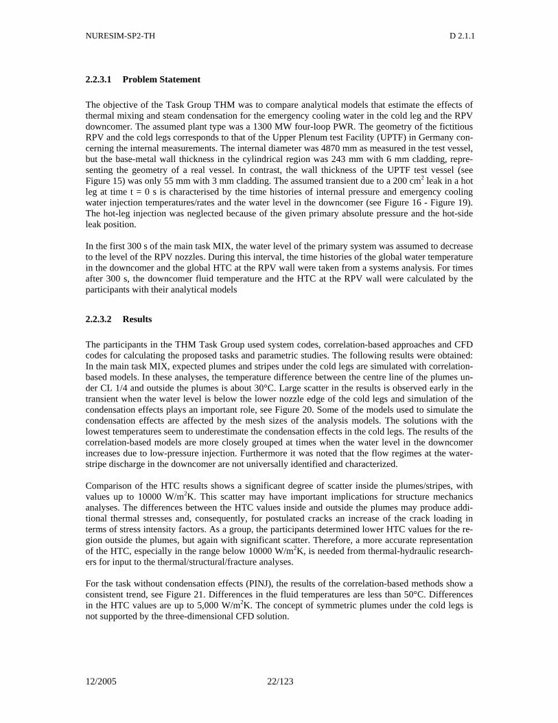
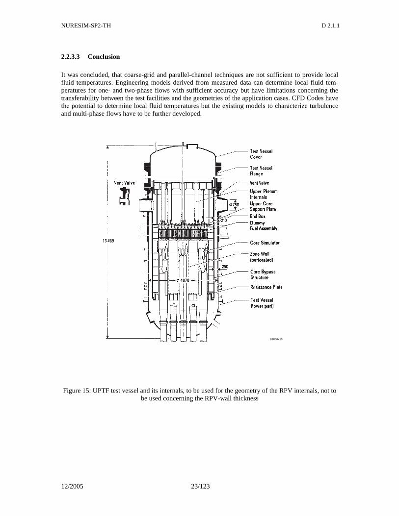
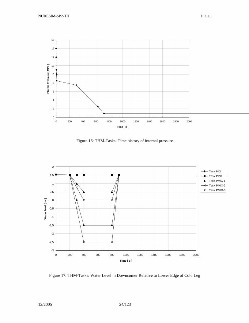
The objective of the Task Group THM was to compare analytical models that estimate the effects of thermal mixing and steam condensation for the emergency cooling water in the cold leg and the RPV downcomer. The assumed plant type was a 1300 MW four-loop PWR. The geometry of the fictitious RPV and the cold legs corresponds to that of the Upper Plenum test Facility (UPTF) in Germany con-cerning the internal measurements. The internal diameter was 4870 mm as measured in the test vessel, but the base-metal wall thickness in the cylindrical region was 243 mm with 6 mm cladding, repre-senting the geometry of a real vessel. In contrast, the wall thickness of the UPTF test vessel (see Figure 15) was only 55 mm with 3 mm cladding. The assumed transient due to a 200 cm2 leak in a hot leg at time t = 0 s is characterised by the time histories of internal pressure and emergency cooling water injection temperatures/rates and the water level in the downcomer (see Figure 16 - Figure 19). The hot-leg injection was neglected because of the given primary absolute pressure and the hot-side leak position. In the first 300 s of the main task MIX, the water level of the primary system was assumed to decrease to the level of the RPV nozzles. During this interval, the time histories of the global water temperature in the downcomer and the global HTC at the RPV wall were taken from a systems analysis. For times after 300 s, the downcomer fluid temperature and the HTC at the RPV wall were calculated by the participants with their analytical models
2.2.3.2 Results
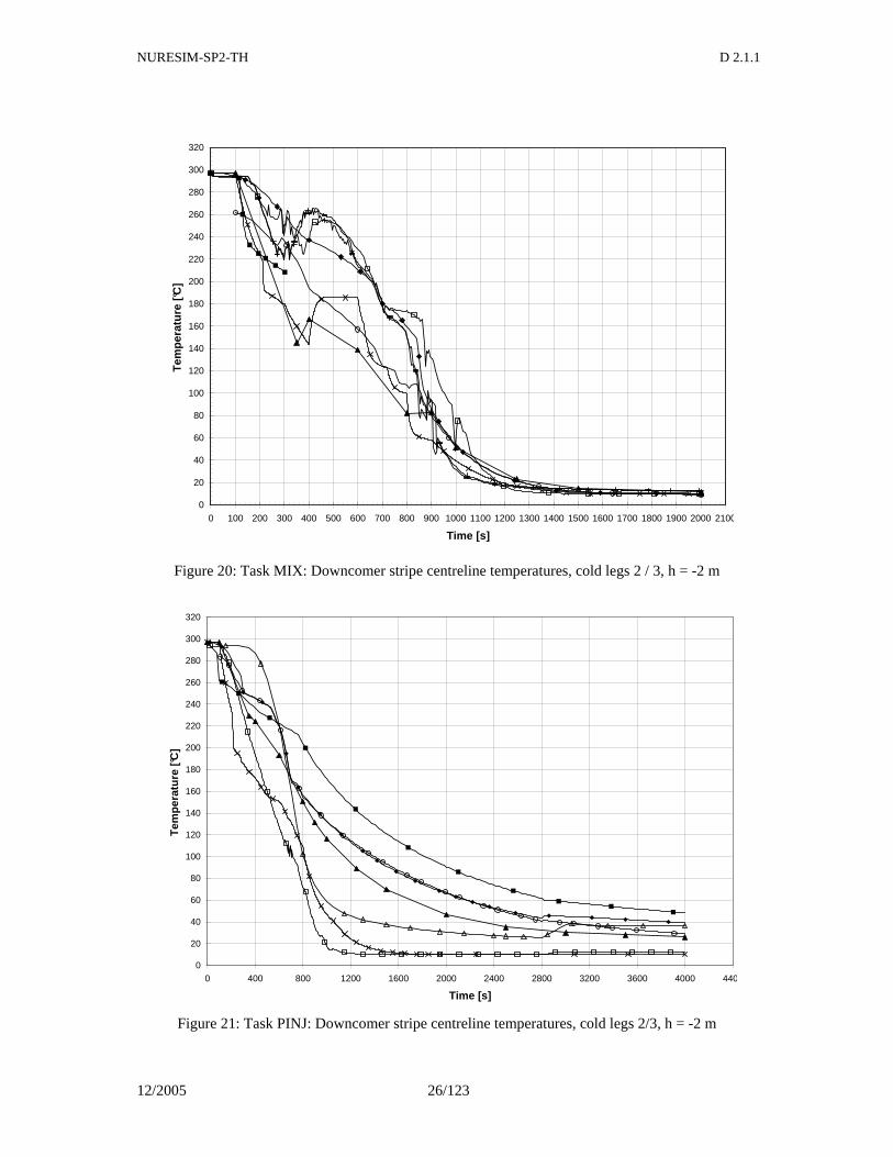
The participants in the THM Task Group used system codes, correlation-based approaches and CFD codes for calculating the proposed tasks and parametric studies. The following results were obtained: In the main task MIX, expected plumes and stripes under the cold legs are simulated with correlation-based models. In these analyses, the temperature difference between the centre line of the plumes un-der CL 1/4 and outside the plumes is about 30°C. Large scatter in the results is observed early in the transient when the water level is below the lower nozzle edge of the cold legs and simulation of the condensation effects plays an important role, see Figure 20. Some of the models used to simulate the condensation effects are affected by the mesh sizes of the analysis models. The solutions with the lowest temperatures seem to underestimate the condensation effects in the cold legs. The results of the correlation-based models are more closely grouped at times when the water level in the downcomer increases due to low-pressure injection. Furthermore it was noted that the flow regimes at the water-stripe discharge in the downcomer are not universally identified and characterized. Comparison of the HTC results shows a significant degree of scatter inside the plumes/stripes, with values up to 10000 W/m2K. This scatter may have important implications for structure mechanics analyses. The differences between the HTC values inside and outside the plumes may produce addi-tional thermal stresses and, consequently, for postulated cracks an increase of the crack loading in terms of stress intensity factors. As a group, the participants determined lower HTC values for the re-gion outside the plumes, but again with significant scatter. Therefore, a more accurate representation of the HTC, especially in the range below 10000 W/m2K, is needed from thermal-hydraulic research-ers for input to the thermal/structural/fracture analyses. For the task without condensation effects (PINJ), the results of the correlation-based methods show a consistent trend, see Figure 21. Differences in the fluid temperatures are less than 50°C. Differences in the HTC values are up to 5,000 W/m2K. The concept of symmetric plumes under the cold legs is not supported by the three-dimensional CFD solution.
NURESIM-SP2-TH D 2.1.1
12/2005 23/123
2.2.3.3 Conclusion
It was concluded, that coarse-grid and parallel-channel techniques are not sufficient to provide local fluid temperatures. Engineering models derived from measured data can determine local fluid tem-peratures for one- and two-phase flows with sufficient accuracy but have limitations concerning the transferability between the test facilities and the geometries of the application cases. CFD Codes have the potential to determine local fluid temperatures but the existing models to characterize turbulence and multi-phase flows have to be further developed.
Figure 15: UPTF test vessel and its internals, to be used for the geometry of the RPV internals, not to be used concerning the RPV-wall thickness
99006x13
NURESIM-SP2-TH D 2.1.1
12/2005 24/123
Figure 16: THM-Tasks: Time history of internal pressure
Figure 17: THM-Tasks: Water Level in Downcomer Relative to Lower Edge of Cold Leg
0
2
4
6
8
10
12
14
16
18
0 200 400 600 800 1000 1200 1400 1600 1800 2000
Time [ s ]
Inte
rnal
Pre
ssur
e [ M
Pa
]
-3
-2,5
-2
-1,5
-1
-0,5
0
0,5
1
1,5
2
0 200 400 600 800 1000 1200 1400 1600 1800 2000
Time [ s ]
Wat
er le
vel [
m ]
Task MIX
Task PINJ
Task PMIX-1
Task PMIX-2
Task PMIX-3
NURESIM-SP2-TH D 2.1.1
12/2005 25/123
Figure 18: THM-Tasks: Time history of injection temperatures of emergency cooling water
Figure 19: Task THM-MIX: Time history of injection rates of emergency cooling water for each cold leg
0
2
4
6
8
10
12
14
16
0 200 400 600 800 1000 1200 1400 1600 1800 2000
Time [ s ]
EC
C-I
njec
tion
Tem
pera
ture
[ °C
]Cold Leg 2/3
Cold Leg 1/4
0
10
20
30
40
50
60
70
80
90
100
0 200 400 600 800 1000 1200 1400 1600 1800 2000
Time [ s ]
EC
C-I
njec
tion
Rat
e [ k
g/s
]
High Pressure
Low Pressure
NURESIM-SP2-TH D 2.1.1
12/2005 26/123
Figure 20: Task MIX: Downcomer stripe centreline temperatures, cold legs 2 / 3, h = -2 m
Figure 21: Task PINJ: Downcomer stripe centreline temperatures, cold legs 2/3, h = -2 m
0
20
40
60
80
100
120
140
160
180
200
220
240
260
280
300
320
0 100 200 300 400 500 600 700 800 900 1000 1100 1200 1300 1400 1500 1600 1700 1800 1900 2000 2100
Time [s]
Tem
pera
ture
[°C
]
0
20
40
60
80
100
120
140
160
180
200
220
240
260
280
300
320
0 400 800 1200 1600 2000 2400 2800 3200 3600 4000 4400
Time [s]
Tem
pera
ture
[°C
]
NURESIM-SP2-TH D 2.1.1
12/2005 27/123
2.2.4 Range of parameters for CFD simulation of UPTF experiments
The range of parameters which should be used in the CFD simulations is the same as in the UPTF TRAM C1/C2 experimental investigations. It should encompass the following values: - Cold leg partially or completely filled with water - Maximum system pressure of 2 MPa - Injection of water with mass flow rates in the range [0, 180 kg/s] - Injection of steam through core simulator in the mass flow rate range [0, 50 kg/s] - Injection of steam through steam generator in the mass flow rate range [0, 15 kg/s] In the experiments, there was a bypass mass flow rate between the upper plenum and the downcomer, which was caused by gaps along the four hot legs. This bypass mass flow rate is proportional to the static pressure difference ∆P, with a friction factor ξ of 84. Liebert and Ahrens (1993) define the fric-tion factor by:
2
2
SSV
P
ρξ ∆=
The index ‘s’ stands for steam properties.
2.3 Loviisa 440 MW VVER
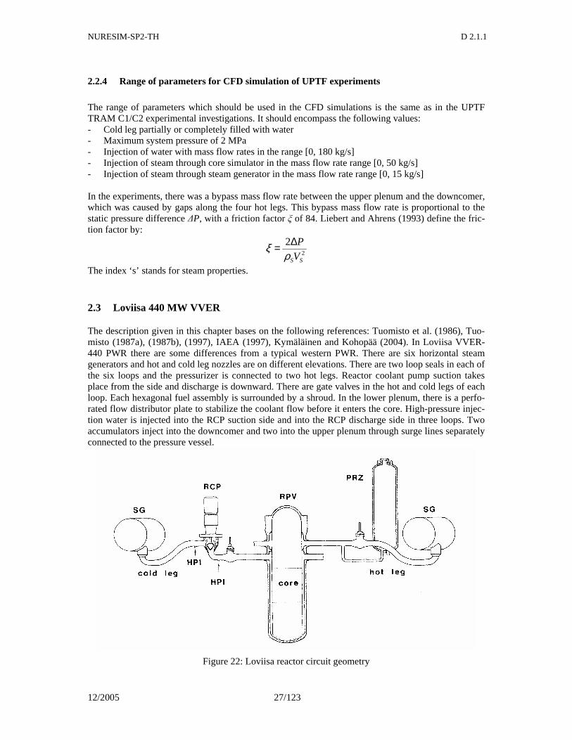
The description given in this chapter bases on the following references: Tuomisto et al. (1986), Tuo-misto (1987a), (1987b), (1997), IAEA (1997), Kymäläinen and Kohopää (2004). In Loviisa VVER-440 PWR there are some differences from a typical western PWR. There are six horizontal steam generators and hot and cold leg nozzles are on different elevations. There are two loop seals in each of the six loops and the pressurizer is connected to two hot legs. Reactor coolant pump suction takes place from the side and discharge is downward. There are gate valves in the hot and cold legs of each loop. Each hexagonal fuel assembly is surrounded by a shroud. In the lower plenum, there is a perfo-rated flow distributor plate to stabilize the coolant flow before it enters the core. High-pressure injec-tion water is injected into the RCP suction side and into the RCP discharge side in three loops. Two accumulators inject into the downcomer and two into the upper plenum through surge lines separately connected to the pressure vessel.
Figure 22: Loviisa reactor circuit geometry
NURESIM-SP2-TH D 2.1.1
12/2005 28/123
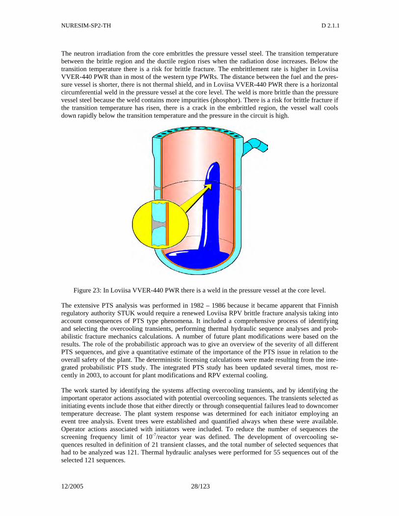
The neutron irradiation from the core embrittles the pressure vessel steel. The transition temperature between the brittle region and the ductile region rises when the radiation dose increases. Below the transition temperature there is a risk for brittle fracture. The embrittlement rate is higher in Loviisa VVER-440 PWR than in most of the western type PWRs. The distance between the fuel and the pres-sure vessel is shorter, there is not thermal shield, and in Loviisa VVER-440 PWR there is a horizontal circumferential weld in the pressure vessel at the core level. The weld is more brittle than the pressure vessel steel because the weld contains more impurities (phosphor). There is a risk for brittle fracture if the transition temperature has risen, there is a crack in the embrittled region, the vessel wall cools down rapidly below the transition temperature and the pressure in the circuit is high.
Figure 23: In Loviisa VVER-440 PWR there is a weld in the pressure vessel at the core level.
The extensive PTS analysis was performed in 1982 – 1986 because it became apparent that Finnish regulatory authority STUK would require a renewed Loviisa RPV brittle fracture analysis taking into account consequences of PTS type phenomena. It included a comprehensive process of identifying and selecting the overcooling transients, performing thermal hydraulic sequence analyses and prob-abilistic fracture mechanics calculations. A number of future plant modifications were based on the results. The role of the probabilistic approach was to give an overview of the severity of all different PTS sequences, and give a quantitative estimate of the importance of the PTS issue in relation to the overall safety of the plant. The deterministic licensing calculations were made resulting from the inte-grated probabilistic PTS study. The integrated PTS study has been updated several times, most re-cently in 2003, to account for plant modifications and RPV external cooling.
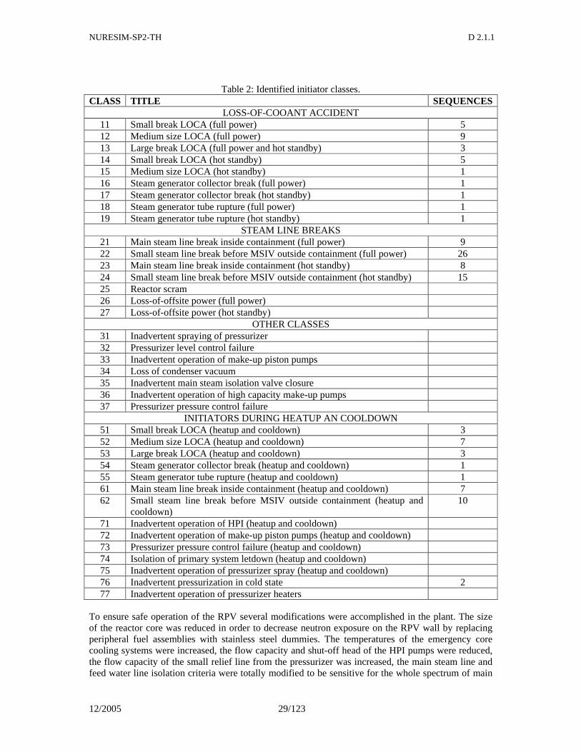
The work started by identifying the systems affecting overcooling transients, and by identifying the important operator actions associated with potential overcooling sequences. The transients selected as initiating events include those that either directly or through consequential failures lead to downcomer temperature decrease. The plant system response was determined for each initiator employing an event tree analysis. Event trees were established and quantified always when these were available. Operator actions associated with initiators were included. To reduce the number of sequences the screening frequency limit of 10-7/reactor year was defined. The development of overcooling se-quences resulted in definition of 21 transient classes, and the total number of selected sequences that had to be analyzed was 121. Thermal hydraulic analyses were performed for 55 sequences out of the selected 121 sequences.
NURESIM-SP2-TH D 2.1.1
12/2005 29/123
Table 2: Identified initiator classes.
CLASS TITLE SEQUENCES LOSS-OF-COOANT ACCIDENT
11 Small break LOCA (full power) 5 12 Medium size LOCA (full power) 9 13 Large break LOCA (full power and hot standby) 3 14 Small break LOCA (hot standby) 5 15 Medium size LOCA (hot standby) 1 16 Steam generator collector break (full power) 1 17 Steam generator collector break (hot standby) 1 18 Steam generator tube rupture (full power) 1 19 Steam generator tube rupture (hot standby) 1
STEAM LINE BREAKS 21 Main steam line break inside containment (full power) 9 22 Small steam line break before MSIV outside containment (full power) 26 23 Main steam line break inside containment (hot standby) 8 24 Small steam line break before MSIV outside containment (hot standby) 15 25 Reactor scram 26 Loss-of-offsite power (full power) 27 Loss-of-offsite power (hot standby)
OTHER CLASSES 31 Inadvertent spraying of pressurizer 32 Pressurizer level control failure 33 Inadvertent operation of make-up piston pumps 34 Loss of condenser vacuum 35 Inadvertent main steam isolation valve closure 36 Inadvertent operation of high capacity make-up pumps 37 Pressurizer pressure control failure
INITIATORS DURING HEATUP AN COOLDOWN 51 Small break LOCA (heatup and cooldown) 3 52 Medium size LOCA (heatup and cooldown) 7 53 Large break LOCA (heatup and cooldown) 3 54 Steam generator collector break (heatup and cooldown) 1 55 Steam generator tube rupture (heatup and cooldown) 1 61 Main steam line break inside containment (heatup and cooldown) 7 62 Small steam line break before MSIV outside containment (heatup and
cooldown) 10
71 Inadvertent operation of HPI (heatup and cooldown) 72 Inadvertent operation of make-up piston pumps (heatup and cooldown) 73 Pressurizer pressure control failure (heatup and cooldown) 74 Isolation of primary system letdown (heatup and cooldown) 75 Inadvertent operation of pressurizer spray (heatup and cooldown) 76 Inadvertent pressurization in cold state 2 77 Inadvertent operation of pressurizer heaters
To ensure safe operation of the RPV several modifications were accomplished in the plant. The size of the reactor core was reduced in order to decrease neutron exposure on the RPV wall by replacing peripheral fuel assemblies with stainless steel dummies. The temperatures of the emergency core cooling systems were increased, the flow capacity and shut-off head of the HPI pumps were reduced, the flow capacity of the small relief line from the pressurizer was increased, the main steam line and feed water line isolation criteria were totally modified to be sensitive for the whole spectrum of main
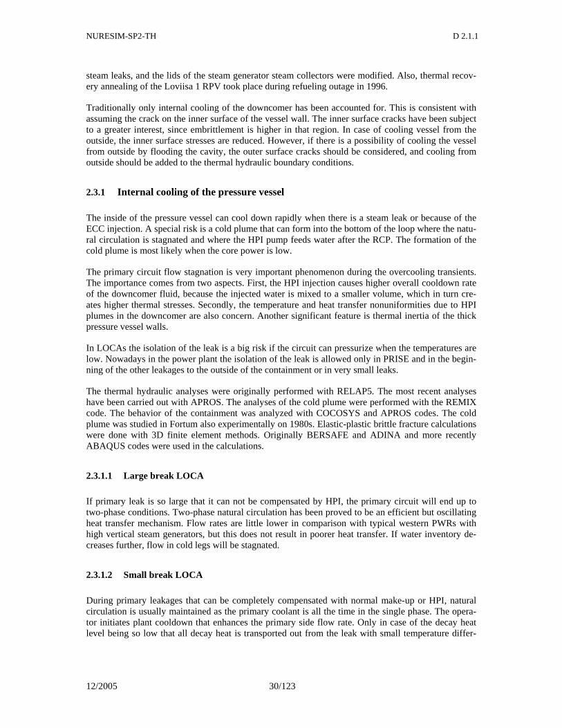
NURESIM-SP2-TH D 2.1.1
12/2005 30/123
steam leaks, and the lids of the steam generator steam collectors were modified. Also, thermal recov-ery annealing of the Loviisa 1 RPV took place during refueling outage in 1996.
Traditionally only internal cooling of the downcomer has been accounted for. This is consistent with assuming the crack on the inner surface of the vessel wall. The inner surface cracks have been subject to a greater interest, since embrittlement is higher in that region. In case of cooling vessel from the outside, the inner surface stresses are reduced. However, if there is a possibility of cooling the vessel from outside by flooding the cavity, the outer surface cracks should be considered, and cooling from outside should be added to the thermal hydraulic boundary conditions.
2.3.1 Internal cooling of the pressure vessel
The inside of the pressure vessel can cool down rapidly when there is a steam leak or because of the ECC injection. A special risk is a cold plume that can form into the bottom of the loop where the natu-ral circulation is stagnated and where the HPI pump feeds water after the RCP. The formation of the cold plume is most likely when the core power is low.
The primary circuit flow stagnation is very important phenomenon during the overcooling transients. The importance comes from two aspects. First, the HPI injection causes higher overall cooldown rate of the downcomer fluid, because the injected water is mixed to a smaller volume, which in turn cre-ates higher thermal stresses. Secondly, the temperature and heat transfer nonuniformities due to HPI plumes in the downcomer are also concern. Another significant feature is thermal inertia of the thick pressure vessel walls.
In LOCAs the isolation of the leak is a big risk if the circuit can pressurize when the temperatures are low. Nowadays in the power plant the isolation of the leak is allowed only in PRISE and in the begin-ning of the other leakages to the outside of the containment or in very small leaks.
The thermal hydraulic analyses were originally performed with RELAP5. The most recent analyses have been carried out with APROS. The analyses of the cold plume were performed with the REMIX code. The behavior of the containment was analyzed with COCOSYS and APROS codes. The cold plume was studied in Fortum also experimentally on 1980s. Elastic-plastic brittle fracture calculations were done with 3D finite element methods. Originally BERSAFE and ADINA and more recently ABAQUS codes were used in the calculations.
2.3.1.1 Large break LOCA
If primary leak is so large that it can not be compensated by HPI, the primary circuit will end up to two-phase conditions. Two-phase natural circulation has been proved to be an efficient but oscillating heat transfer mechanism. Flow rates are little lower in comparison with typical western PWRs with high vertical steam generators, but this does not result in poorer heat transfer. If water inventory de-creases further, flow in cold legs will be stagnated.
2.3.1.2 Small break LOCA
During primary leakages that can be completely compensated with normal make-up or HPI, natural circulation is usually maintained as the primary coolant is all the time in the single phase. The opera-tor initiates plant cooldown that enhances the primary side flow rate. Only in case of the decay heat level being so low that all decay heat is transported out from the leak with small temperature differ-
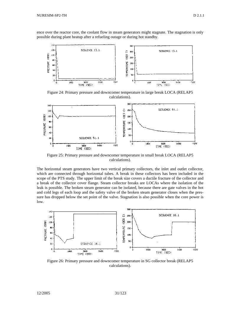
NURESIM-SP2-TH D 2.1.1
12/2005 31/123
ence over the reactor core, the coolant flow in steam generators might stagnate. The stagnation is only possible during plant heatup after a refueling outage or during hot standby.
Figure 24: Primary pressure and downcomer temperature in large break LOCA (RELAP5 calculations).
Figure 25: Primary pressure and downcomer temperature in small break LOCA (RELAP5 calculations).
The horizontal steam generators have two vertical primary collectors, the inlet and outlet collector, which are connected through horizontal tubes. A break in these collectors has been included in the scope of the PTS study. The upper limit of the break size covers a ductile fracture of the collector and a break of the collector cover flange. Steam collector breaks are LOCAs where the isolation of the leak is possible. The broken steam generator can be isolated, because there are gate valves in the hot and cold legs of each loop and the safety valve of the broken steam generator closes when the pres-sure has dropped below the set point of the valve. Stagnation is also possible when the core power is low.
Figure 26: Primary pressure and downcomer temperature in SG collector break (RELAP5 calculations).
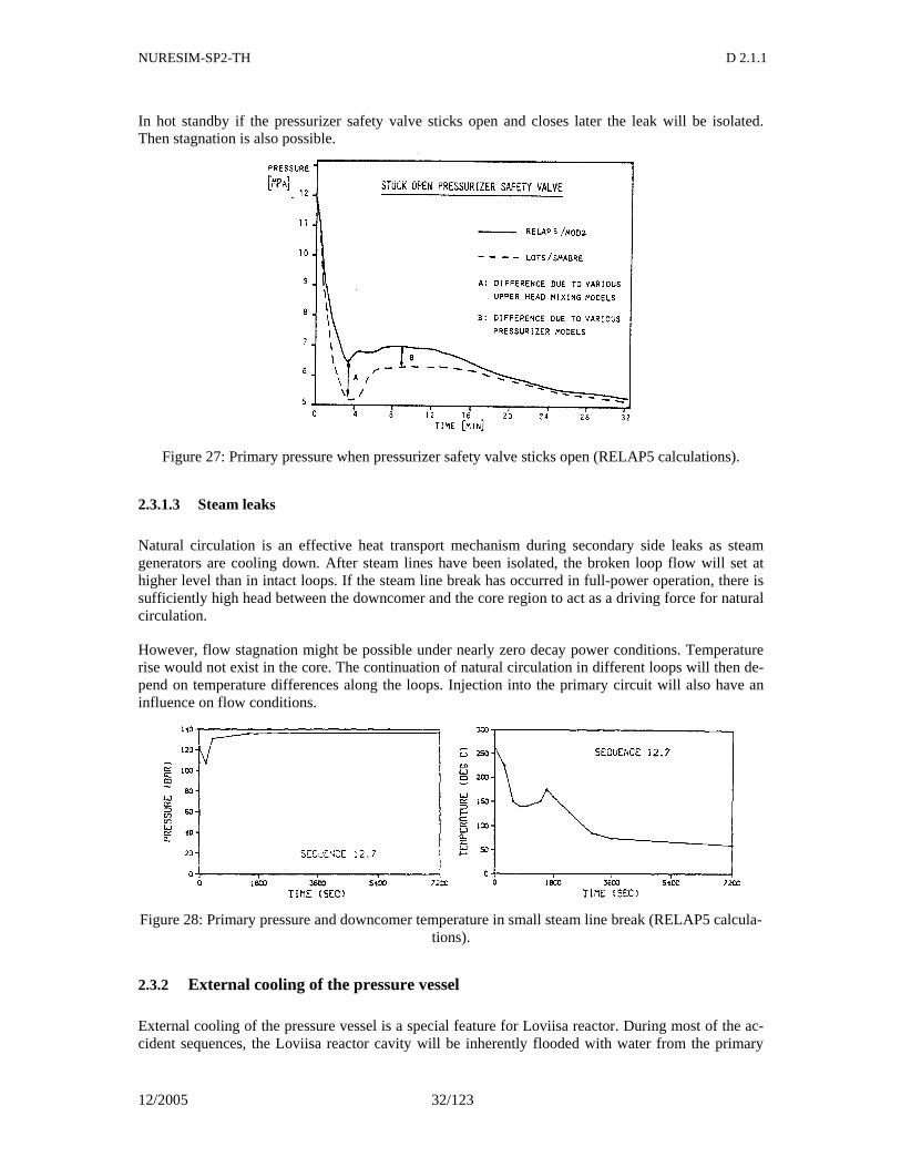
NURESIM-SP2-TH D 2.1.1
12/2005 32/123
In hot standby if the pressurizer safety valve sticks open and closes later the leak will be isolated. Then stagnation is also possible.
Figure 27: Primary pressure when pressurizer safety valve sticks open (RELAP5 calculations).
2.3.1.3 Steam leaks
Natural circulation is an effective heat transport mechanism during secondary side leaks as steam generators are cooling down. After steam lines have been isolated, the broken loop flow will set at higher level than in intact loops. If the steam line break has occurred in full-power operation, there is sufficiently high head between the downcomer and the core region to act as a driving force for natural circulation.
However, flow stagnation might be possible under nearly zero decay power conditions. Temperature rise would not exist in the core. The continuation of natural circulation in different loops will then de-pend on temperature differences along the loops. Injection into the primary circuit will also have an influence on flow conditions.
Figure 28: Primary pressure and downcomer temperature in small steam line break (RELAP5 calcula-tions).
2.3.2 External cooling of the pressure vessel
External cooling of the pressure vessel is a special feature for Loviisa reactor. During most of the ac-cident sequences, the Loviisa reactor cavity will be inherently flooded with water from the primary
NURESIM-SP2-TH D 2.1.1
12/2005 33/123
circuit leakage, from the ECCS and external spray systems, and from the melting ice condenser. Flooding of the reactor cavity might take place also during a spurious operation of the external spray system, even though such sequences can be shown to be very unlikely. The water flows quite easily from the steam generator space to the reactor cavity through the channels near the biological shields or through the severe accident management flow paths. The external cooling of the pressure vessel may lead to the integrity problem, if the crack is assumed to locate on the outer surface of the vessel. The risk for external thermal shock is significant if the water is cold and the primary pressure is high. Especially the water from the external spray systems can be very cold in some cold sequences. Fortu-nately, embrittlement due the neutron exposure is not so severe near the outer surface.
2.3.2.1 Spurious operation of the external spray systems
If there is a spurious operation of the external spray systems or the reactor recooling system the water flowing to the reactor cavity can be about 30 ºC during the wintertime.
The safety margins in some of these sequences can actually be less than in sequences with internal cooling. The operator is instructed to stop inadvertently initiated external spray systems as soon as possible.
2.3.2.2 LOCAs
The biggest risk for external cooldown is the initiation of the external spray systems. The spray sys-tems can make the water in the containment emergency sump very cold. The external spray systems together with its cooling systems have to be stopped when the need for them has disappeared. Also, the temperature of the water in the containment emergency sump has to be observed.
2.3.2.3 Steam leaks in the containment
It is essential to isolate the leaking steam generator in time. Then only the inventory of the leaking steam generator flows into the containment and the spray systems will not initiate unnecessarily.
2.3.3 Pressurization of the primary circuit in the cold state
The pressurization of the primary circuit in cold state is potentially a severe transient because the whole wall of the pressure vessel is cold and if the crack begins to expand it will not stop. That is why the circuit is not allowed to pressurize when the temperature is below 50 °C. If the circuit can pressur-ize then in addition to the shutdown safety valve at least one main safety valve has to be available.
2.3.4 Relevant phenomena to be simulated
The external cooldown of the pressure vessel by spurious operation of the external spray systems is the most significant overcooling transient. The leaks from the primary side where a cold plume can form in the cold leg and downcomer and the leaks that can be isolated (leaks of the pressurizer safety valve, PRISE) are the most significant accidents where the pressure vessel cools down from the in-side.
Thermal hydraulic analyses of overcooling sequences include many features that are different from the traditional thermal hydraulic accident analyses. First, it has to be realized that perfect operation of
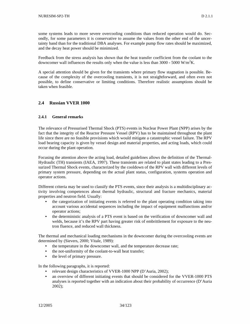
NURESIM-SP2-TH D 2.1.1
12/2005 34/123
some systems leads to more severe overcooling conditions than reduced operation would do. Sec-ondly, for some parameters it is conservative to assume the values from the other end of the uncer-tainty band than for the traditional DBA analyses. For example pump flow rates should be maximized, and the decay heat power should be minimized.
Feedback from the stress analysis has shown that the heat transfer coefficient from the coolant to the downcomer wall influences the results only when the value is less than 3000 - 5000 W/m2K.
A special attention should be given for the transients where primary flow stagnation is possible. Be-cause of the complexity of the overcooling transients, it is not straightforward, and often even not possible, to define conservative or limiting conditions. Therefore realistic assumptions should be taken when feasible.
2.4 Russian VVER 1000
2.4.1 General remarks
The relevance of Pressurised Thermal Shock (PTS) events in Nuclear Power Plant (NPP) arises by the fact that the integrity of the Reactor Pressure Vessel (RPV) has to be maintained throughout the plant life since there are no feasible provisions which would mitigate a catastrophic vessel failure. The RPV load bearing capacity is given by vessel design and material properties, and acting loads, which could occur during the plant operation. Focusing the attention above the acting load, detailed guidelines allows the definition of the Thermal-Hydraulic (TH) transients (IAEA, 1997). These transients are related to plant states leading to a Pres-surized Thermal Shock events, characterized by the cooldown of the RPV wall with different levels of primary system pressure, depending on the actual plant status, configuration, systems operation and operator actions. Different criteria may be used to classify the PTS events, since their analysis is a multidisciplinary ac-tivity involving competences about thermal hydraulic, structural and fracture mechanics, material properties and neutron field. Usually:
• the categorization of initiating events is referred to the plant operating condition taking into account various accidental sequences including the impact of equipment malfunctions and/or operator actions;
• the deterministic analysis of a PTS event is based on the verification of downcomer wall and welds, because it’s the RPV part having greater risk of embrittlement for exposure to the neu-tron fluence, and reduced wall thickness.
The thermal and mechanical loading mechanisms in the downcomer during the overcooling events are determined by (Sievers, 2000; Vitale, 1989):
• the temperature in the downcomer wall, and the temperature decrease rate; • the not-uniformity of the coolant-to-wall heat transfer; • the level of primary pressure.
In the following paragraphs, it is reported:
• relevant design characteristics of VVER-1000 NPP (D’Auria, 2002); • an overview of different initiating events that should be considered for the VVER-1000 PTS
analyses is reported together with an indication about their probability of occurrence (D’Auria 2002);
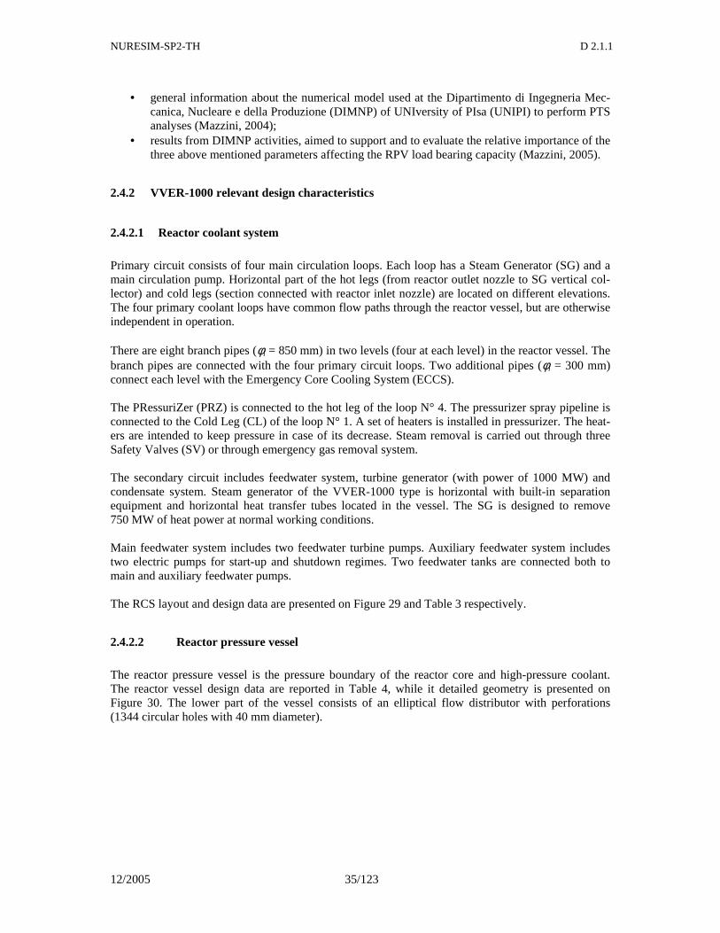
NURESIM-SP2-TH D 2.1.1
12/2005 35/123
• general information about the numerical model used at the Dipartimento di Ingegneria Mec-canica, Nucleare e della Produzione (DIMNP) of UNIversity of PIsa (UNIPI) to perform PTS analyses (Mazzini, 2004);
• results from DIMNP activities, aimed to support and to evaluate the relative importance of the three above mentioned parameters affecting the RPV load bearing capacity (Mazzini, 2005).
2.4.2 VVER-1000 relevant design characteristics
2.4.2.1 Reactor coolant system
Primary circuit consists of four main circulation loops. Each loop has a Steam Generator (SG) and a main circulation pump. Horizontal part of the hot legs (from reactor outlet nozzle to SG vertical col-lector) and cold legs (section connected with reactor inlet nozzle) are located on different elevations. The four primary coolant loops have common flow paths through the reactor vessel, but are otherwise independent in operation. There are eight branch pipes (φi = 850 mm) in two levels (four at each level) in the reactor vessel. The branch pipes are connected with the four primary circuit loops. Two additional pipes (φi = 300 mm) connect each level with the Emergency Core Cooling System (ECCS). The PRessuriZer (PRZ) is connected to the hot leg of the loop N° 4. The pressurizer spray pipeline is connected to the Cold Leg (CL) of the loop N° 1. A set of heaters is installed in pressurizer. The heat-ers are intended to keep pressure in case of its decrease. Steam removal is carried out through three Safety Valves (SV) or through emergency gas removal system. The secondary circuit includes feedwater system, turbine generator (with power of 1000 MW) and condensate system. Steam generator of the VVER-1000 type is horizontal with built-in separation equipment and horizontal heat transfer tubes located in the vessel. The SG is designed to remove 750 MW of heat power at normal working conditions. Main feedwater system includes two feedwater turbine pumps. Auxiliary feedwater system includes two electric pumps for start-up and shutdown regimes. Two feedwater tanks are connected both to main and auxiliary feedwater pumps. The RCS layout and design data are presented on Figure 29 and Table 3 respectively.
2.4.2.2 Reactor pressure vessel
The reactor pressure vessel is the pressure boundary of the reactor core and high-pressure coolant. The reactor vessel design data are reported in Table 4, while it detailed geometry is presented on Figure 30. The lower part of the vessel consists of an elliptical flow distributor with perforations (1344 circular holes with 40 mm diameter).
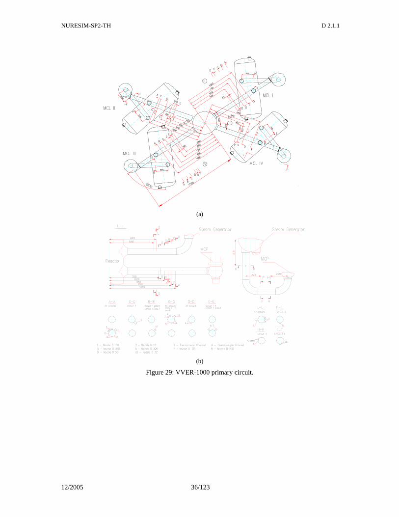
NURESIM-SP2-TH D 2.1.1
12/2005 36/123
All sections and views on figure 3.1.2.3.
(a)
(b)
Figure 29: VVER-1000 primary circuit.
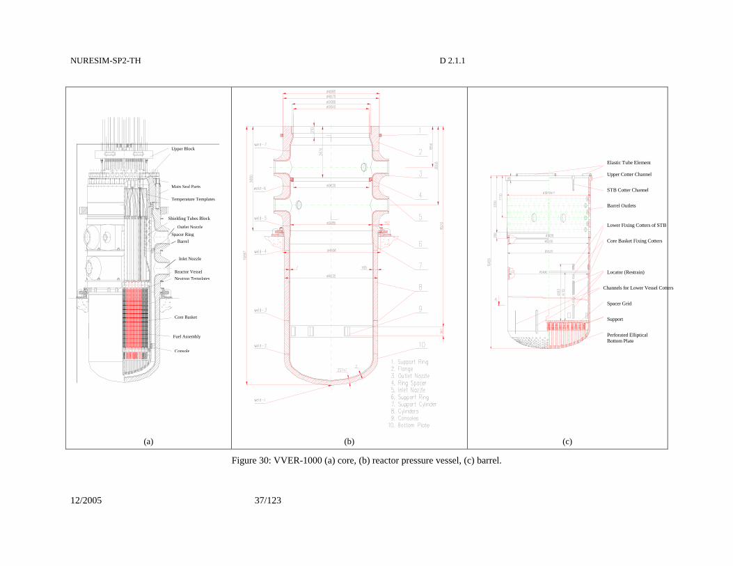
NURESIM-SP2-TH D 2.1.1
12/2005 37/123
Upper Block
Main Seal Parts
Temperature Templates
Shielding Tubes Block
Spacer Ring
Barrel
Outlet Nozzle
Reactor Vessel
Inlet Nozzle
Neutron Templates
Core Basket
Fuel Assembly
Console
(a)
(b)
Elastic Tube Element
Upper Cotter Channel
STB Cotter Channel
Barrel Outlets
Lower Fixing Cotters of STB
Core Basket Fixing Cotters
Locator (Restrain)
Channels for Lower Vessel Cotters
Spacer Grid
Support
Perforated Elliptical Bottom Plate
(c)
Figure 30: VVER-1000 (a) core, (b) reactor pressure vessel, (c) barrel.
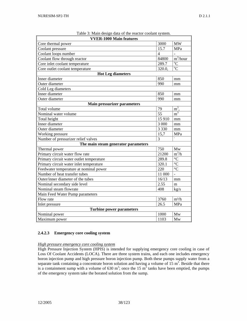
NURESIM-SP2-TH D 2.1.1
12/2005 38/123
Table 3: Main design data of the reactor coolant system. VVER-1000 Main features
Core thermal power 3000 MW Coolant pressure 15.7 MPa Coolant loops number 4 - Coolant flow through reactor 84800 m3/hour Core inlet coolant temperature 289.7 oC Core outlet coolant temperature 320.0, oC
Hot Leg diameters Inner diameter 850 mm Outer diameter 990 mm Cold Leg diameters Inner diameter 850 mm Outer diameter 990 mm
Main pressurizer parameters Total volume 79 m3, Nominal water volume 55 m3 Total height 15 910 mm Inner diameter 3 000 mm Outer diameter 3 330 mm Working pressure 15,7 MPa Number of pressurizer relief valves 3 -
The main steam generator parameters Thermal power 750 Mw Primary circuit water flow rate 21200 m3/h Primary circuit water outlet temperature 289.8 °C Primary circuit water inlet temperature 320.1 °C Feedwater temperature at nominal power 220 °C Number of heat transfer tubes 11 000 - Outer/inner diameter of the tubes 16/13 mm Nominal secondary side level 2.55 m Nominal steam flowrate 408 kg/s Main Feed Water Pump parameters Flow rate 3760 m³/h Inlet pressure 26.5 MPa
Turbine power parameters Nominal power 1000 Mw Maximum power 1103 Mw
2.4.2.3 Emergency core cooling system
High pressure emergency core cooling system High Pressure Injection System (HPIS) is intended for supplying emergency core cooling in case of Loss Of Coolant Accidents (LOCA). There are three system trains, and each one includes emergency boron injection pump and high pressure boron injection pump. Both these pumps supply water from a separate tank containing a concentrate boron solution and having a volume of 15 m3. Beside that there is a containment sump with a volume of 630 m3; once the 15 m3 tanks have been emptied, the pumps of the emergency system take the borated solution from the sump.
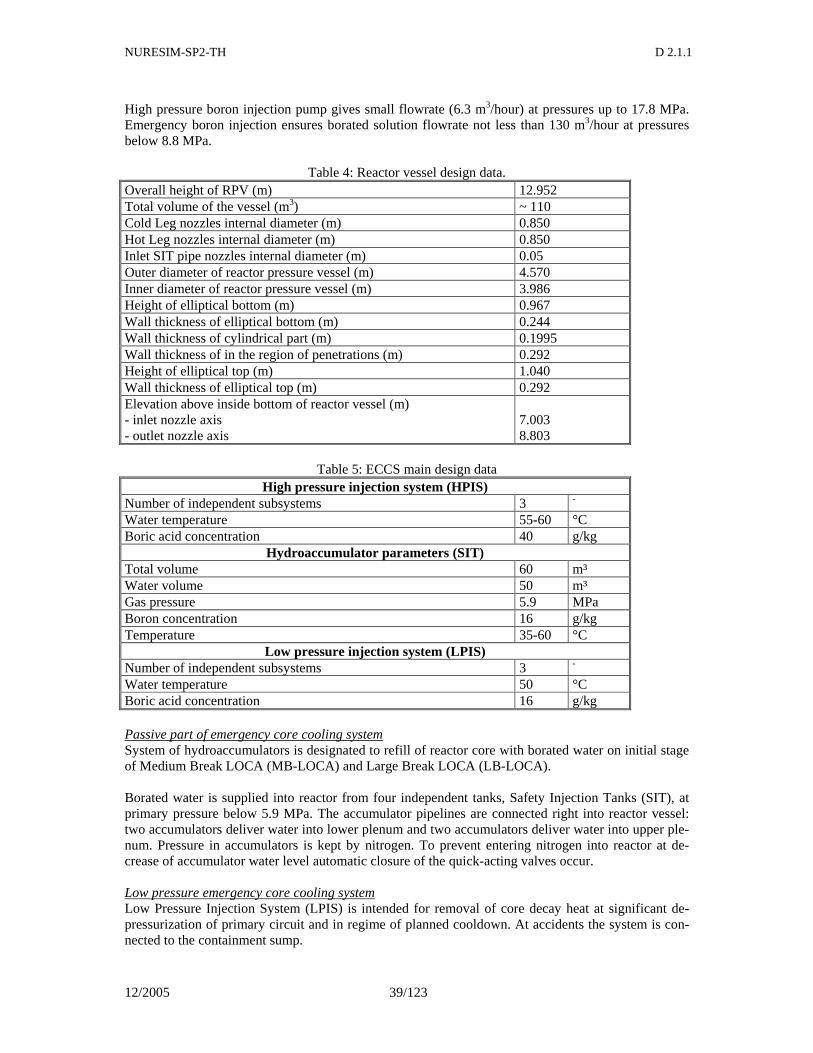
NURESIM-SP2-TH D 2.1.1
12/2005 39/123
High pressure boron injection pump gives small flowrate (6.3 m3/hour) at pressures up to 17.8 MPa. Emergency boron injection ensures borated solution flowrate not less than 130 m3/hour at pressures below 8.8 MPa.
Table 4: Reactor vessel design data. Overall height of RPV (m) 12.952 Total volume of the vessel (m3) ~ 110 Cold Leg nozzles internal diameter (m) 0.850 Hot Leg nozzles internal diameter (m) 0.850 Inlet SIT pipe nozzles internal diameter (m) 0.05 Outer diameter of reactor pressure vessel (m) 4.570 Inner diameter of reactor pressure vessel (m) 3.986 Height of elliptical bottom (m) 0.967 Wall thickness of elliptical bottom (m) 0.244 Wall thickness of cylindrical part (m) 0.1995 Wall thickness of in the region of penetrations (m) 0.292 Height of elliptical top (m) 1.040 Wall thickness of elliptical top (m) 0.292 Elevation above inside bottom of reactor vessel (m) - inlet nozzle axis - outlet nozzle axis
7.003 8.803
Table 5: ECCS main design data
High pressure injection system (HPIS) Number of independent subsystems 3 -
Water temperature 55-60 °C Boric acid concentration 40 g/kg
Hydroaccumulator parameters (SIT) Total volume 60 m³ Water volume 50 m³ Gas pressure 5.9 MPa Boron concentration 16 g/kg Temperature 35-60 °C
Low pressure injection system (LPIS) Number of independent subsystems 3 -
Water temperature 50 °C Boric acid concentration 16 g/kg Passive part of emergency core cooling system System of hydroaccumulators is designated to refill of reactor core with borated water on initial stage of Medium Break LOCA (MB-LOCA) and Large Break LOCA (LB-LOCA). Borated water is supplied into reactor from four independent tanks, Safety Injection Tanks (SIT), at primary pressure below 5.9 MPa. The accumulator pipelines are connected right into reactor vessel: two accumulators deliver water into lower plenum and two accumulators deliver water into upper ple-num. Pressure in accumulators is kept by nitrogen. To prevent entering nitrogen into reactor at de-crease of accumulator water level automatic closure of the quick-acting valves occur. Low pressure emergency core cooling system Low Pressure Injection System (LPIS) is intended for removal of core decay heat at significant de-pressurization of primary circuit and in regime of planned cooldown. At accidents the system is con-nected to the containment sump.
NURESIM-SP2-TH D 2.1.1
12/2005 40/123
The system ensures boron solution delivery flowrate not less than 250-300 m3/hour at primary pres-sure of 2.2 MPa and not less than 700-750 m3/hour at primary pressure of 0.1 MPa.
2.4.3 Relevant initiating events for the VVER-1000 PTS analysis
2.4.3.1 Categorization of the sequences
The accidental transients threatening the RPV integrity may be grouped as in the following: • Loss of Coolant Accidents:
assuming different break sizes for cold and hot legs, and other pipes connected to primary system, the transients are characterized by rapid downcomer cooldown for the actuation of the ECCS, especially if flow stagnation and cold plumes occur; the pressure level depends on the break area and location, but cold repressurisation should be considered too if it could take place for the break isolation (having higher priority in the operating procedures of the VVER reactors);
• Stuck open pressurizer relief and safety valve: similarly at the previous group of events, stuck open pressurizer safety or relief valve causes an downcomer wall overcooling for ECCS actuation, while the system pressure may be pre-served after having reached the final temperature, or a severe repressurisation can be caused by valve reclosure;
• PRImary to SEcondary leakage accidents (PRISE): ECCS actuation happens also during the transients belonging to this group; different sizes for single and multiple Steam Generator Tube Rupture (SGTR) up to the full steam generator col-lector cover opening (corresponding to break area of about 100 cm2); if the operator isolates the affected steam generator the primary circuit repressurisation may take place;
• Large secondary leaks: if secondary side depressurises, a cooldown (and depressurisation) of primary circuit occurs for enhanced heat transfer due to boiling phenomena, and an additional contribution to down-comer cooling may occur if ECCS intervenes; a repressurization can be expected in both cases of ECCS actuation or not because of the reduced heat removal capacity of the secondary circuit;
• Inadvertent actuation of high pressure injection or make-up systems: it can result in a fast pressure increase in primary system.
A last type of PTS event may results from the cooling of the outside RPV wall in case of reactor cav-ity flooding. Its relevance appeared to be lower than the other groups because of the cleavage propa-gation of crack like defects needs a high degree of neutron embrittlement (the material damage de-creases from the inside surface towards outside surface of the RPV wall). All the transients grouped above should be analysed assuming different plant operating conditions (such as full power, hot zero power, heat up, cool down and cold shutdown), and various interacting systems and operator actions. Their significance for applying more stringent requirements is estab-lished with respect to the probability of occurrence. The sequences are classified as:
• “anticipated transients”, if their frequency of occurrence is higher than 10-2 per reactor year; they are deviations from normal operating conditions expected to occur (i.e. caused by com-ponent malfunction or operator error);
• “postulated transients”, if their frequency of occurrence is less than 10-2 per reactor year; they are deviations from normal operating conditions not expected to occur, but considered in the design (i.e. rupture of a pipe line).
NURESIM-SP2-TH D 2.1.1
12/2005 41/123
2.4.3.2 VVER-1000 initiating events and their significance
The list of principal initiating events considered for the integrity assessment of VVER-1000 RPV (as supported by Dr. Fill Nicolay - GYDROPRESS, Russia, Moscow District, Head of Department), is reported in the following:
LOCA (when there are no indication, the cold and hot legs rupture is assumed): o 25 mm break; o 50 mm break; o 80 mm break; o 105 mm break; o 125 mm break (high pressure ECCS line); o 207 mm break (line between PRZ and PRZ SV); o 279 mm break (low pressure ECCS line); o 850 mm break;
Stuck open pressurizer safety or relief valve: o PRZ SV opening;
PRISE: o SGTR; o SG collector rupture (100 mm); o SG collector cover opening;
Large secondary leaks: o SG SV, BRU-A, BRU-K opening; o Steam Line Break (SLB) between SG and MSIV; o SLB between MSIV and main steam header; o Feed water line break ;
Inadvertent actuation of high pressure injection or make-up systems: o Inadvert ECCS operation during RCS heating up; o CVCS malfunction.
Based on data of plant in operation available to DIMNP, the magnitude order of the frequencies of occurrence estimated for the above mentioned transients are:
LOCA (when there are no indication, the cold and hot legs rupture is assumed): o 10-2÷10-1 for Small Break LOCA (SB-LOCA) having a rupture area less than 50 mm; o 10-2÷10-3 for MB-LOCA having a rupture area up to 280 mm; o 10-5÷10-3 for LB-LOCA having a rupture area up to 850 mm;
Stuck open pressurizer safety or relief valve: o 10-2÷10-3 for PRZ SV opening;
PRISE: o 5⋅10-3÷5⋅10-2 for the SGTR; o 10-3÷10-2 for the SG collector rupture (100 mm); o 10-4÷10-3 for the SG collector cover opening;
Large secondary leaks: o 10-2÷10-3 for SG SV, BRU-A, BRU-K opening; o 10-2÷10-3 for the Steam Line Break (SLB) between SG and MSIV; o 10-2÷10-3 for Feed water line break ;
2.4.4 Numerical models for PTS analysis
The activity performed at DIMNP-UNIPI on VVER-1000 RPV integrity assessment were conducted developing numerical tools to calculate loads, induced thermal-mechanical stresses in the pressure wall, and Stress Intensity Factor (SIF) for postulated defects. Same scooping investigations were con-
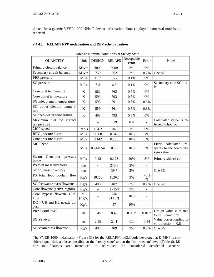
NURESIM-SP2-TH D 2.1.1
12/2005 42/123
ducted for a generic VVER-1000 NPP. Relevant information about employed numerical models are reported.
2.4.4.1 RELAP5 NPP nodalisation and RPV schematisation
Table 6: Nominal conditions at Steady State
QUANTITY Unit DESIGN RELAP5 Acceptable
error Error Notes
Primary circuit balance MWth 3000 3000 2% 0% Secondary circuit balance MWth 750 752 2% 0.2% One SG PRZ pressure MPa 15.7 15.7 0.1% 0% SG pressure
MPa 6.3 6.3 0.1% 0% Secondary side SG out-let
Core inlet temperature K 562 562 0.5% 0% Core outlet temperature K 593 593 0.5% 0% SG inlet plenum temperature K 593 591 0.5% 0.3% SG outlet plenum tempera-ture
K 559 561 0.5% 0.3%
SG feed–water temperature K 493 493 0.5% 0% Maximum fuel rod surface temperature
K – 619 10K - Calculated value is re-ferred to hot rod
MCP speed Rad/s 104.2 104.2 1% 0% RPV pressure losses MPa 0.368 0.342 10% 7% Core pressure losses MPa 0.142 0.135 10% 5% MCP head
MPa 0.74/0.54 0.55 10% 2% Error calculated re-spects to the lower de-sign value
Steam Generator pressure losses
MPa 0.12 0.123 10% 3% Primary side circuit
PS total mass inventory ton - 240.8 2% - SG SS mass inventory ton - 39.7 2% - One SG PS total loop coolant flow rate
Kg/s 18250 18262 2% <0.1%
SG feedwater mass flowrate Kg/s 408 407 2% 0.2% One SG Core flowrate (active region) Kg/s – 17150 2% - Core bypass flowrate (LP–UP)
% (Kg/s)
– 6%
(1112) 10% -
DC – UH and HL nozzle by-pass
Kg/s – 57 10% -
PRZ liquid level m 8.45 8.46 0.05m 0.01m
Design value is related to EOL condition
SG SS level m 2.55 2.41 0.1 0.14
Value corresponding to void fraction > 0.5
SG steam mass flowrate Kg/s 408 409 2% 0.2% One SG
The VVER-1000 nodalisation (Figure 31) for the RELAP5/mod3.3 code developed at DIMNP is con-sidered qualified, as far as possible, at the ‘steady state’ and at the ‘on transient’ level (Table 6). Mi-nor modifications are introduced to reproduce the considered accidental scenario.
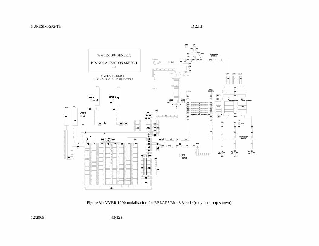
NURESIM-SP2-TH D 2.1.1
12/2005 43/123
Figure 31: VVER 1000 nodalisation for RELAP5/Mod3.3 code (only one loop shown).
WWER-1000 GENERIC
PTS NODALIZATION SKETCH1/2
OVERALL SKETCH( 1 of 4 SG and LOOP represented )
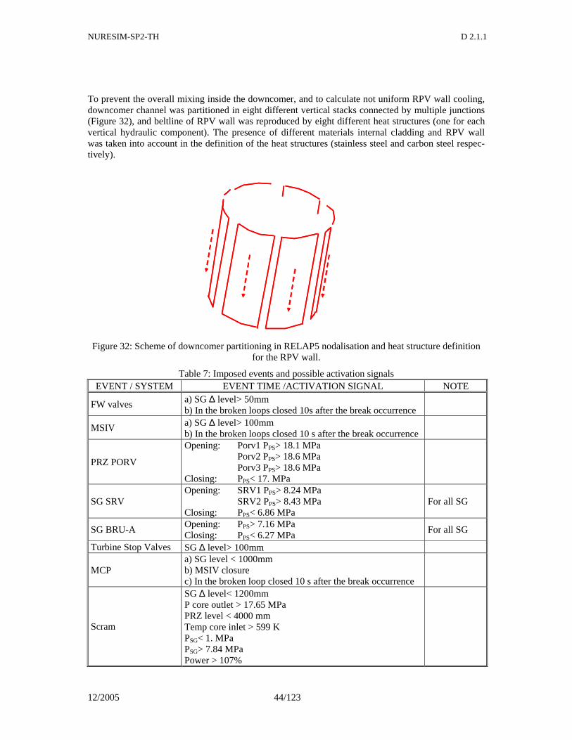
NURESIM-SP2-TH D 2.1.1
12/2005 44/123
To prevent the overall mixing inside the downcomer, and to calculate not uniform RPV wall cooling, downcomer channel was partitioned in eight different vertical stacks connected by multiple junctions (Figure 32), and beltline of RPV wall was reproduced by eight different heat structures (one for each vertical hydraulic component). The presence of different materials internal cladding and RPV wall was taken into account in the definition of the heat structures (stainless steel and carbon steel respec-tively).
Figure 32: Scheme of downcomer partitioning in RELAP5 nodalisation and heat structure definition for the RPV wall.
Table 7: Imposed events and possible activation signals EVENT / SYSTEM EVENT TIME /ACTIVATION SIGNAL NOTE
FW valves a) SG ∆ level> 50mm b) In the broken loops closed 10s after the break occurrence
MSIV a) SG ∆ level> 100mm b) In the broken loops closed 10 s after the break occurrence
PRZ PORV
Opening: Porv1 PPS> 18.1 MPa Porv2 PPS> 18.6 MPa Porv3 PPS> 18.6 MPa Closing: PPS< 17. MPa
SG SRV Opening: SRV1 PPS> 8.24 MPa SRV2 PPS> 8.43 MPa Closing: PPS< 6.86 MPa
For all SG
SG BRU-A Opening: PPS> 7.16 MPa Closing: PPS< 6.27 MPa
For all SG
Turbine Stop Valves SG ∆ level> 100mm
MCP a) SG level < 1000mm b) MSIV closure c) In the broken loop closed 10 s after the break occurrence
Scram
SG ∆ level< 1200mm P core outlet > 17.65 MPa PRZ level < 4000 mm Temp core inlet > 599 K PSG< 1. MPa PSG> 7.84 MPa Power > 107%
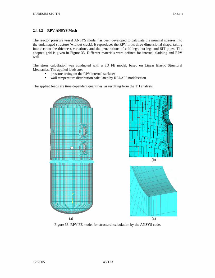
NURESIM-SP2-TH D 2.1.1
12/2005 45/123
2.4.4.2 RPV ANSYS Mesh
The reactor pressure vessel ANSYS model has been developed to calculate the nominal stresses into the undamaged structure (without crack). It reproduces the RPV in its three-dimensional shape, taking into account the thickness variations, and the penetrations of cold legs, hot legs and SIT pipes. The adopted grid is given in Figure 33. Different materials were defined for internal cladding and RPV wall. The stress calculation was conducted with a 3D FE model, based on Linear Elastic Structural Mechanics. The applied loads are:
pressure acting on the RPV internal surface; wall temperature distribution calculated by RELAP5 nodalisation.
The applied loads are time dependent quantities, as resulting from the TH analysis.
(a)
1
WWER-1000 (b)
1
WWER-1000 (c)
Figure 33: RPV FE model for structural calculation by the ANSYS code.
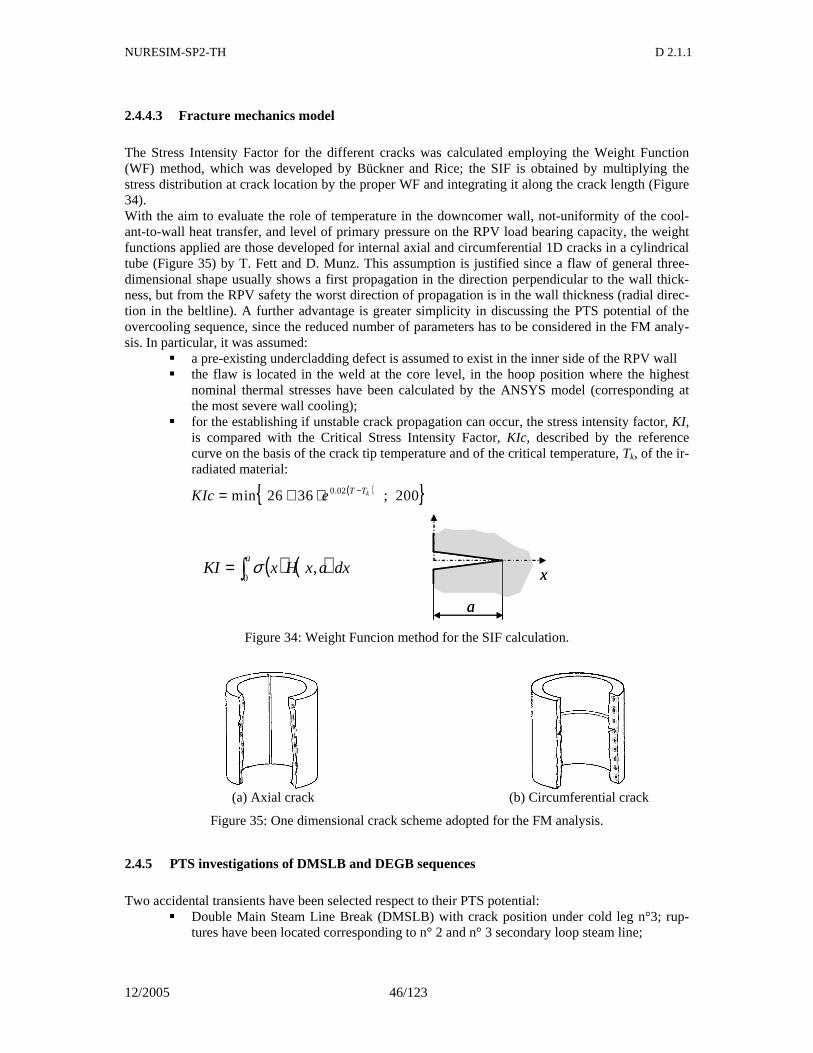
NURESIM-SP2-TH D 2.1.1
12/2005 46/123
2.4.4.3 Fracture mechanics model
The Stress Intensity Factor for the different cracks was calculated employing the Weight Function (WF) method, which was developed by Bückner and Rice; the SIF is obtained by multiplying the stress distribution at crack location by the proper WF and integrating it along the crack length (Figure 34). With the aim to evaluate the role of temperature in the downcomer wall, not-uniformity of the cool-ant-to-wall heat transfer, and level of primary pressure on the RPV load bearing capacity, the weight functions applied are those developed for internal axial and circumferential 1D cracks in a cylindrical tube (Figure 35) by T. Fett and D. Munz. This assumption is justified since a flaw of general three-dimensional shape usually shows a first propagation in the direction perpendicular to the wall thick-ness, but from the RPV safety the worst direction of propagation is in the wall thickness (radial direc-tion in the beltline). A further advantage is greater simplicity in discussing the PTS potential of the overcooling sequence, since the reduced number of parameters has to be considered in the FM analy-sis. In particular, it was assumed:
a pre-existing undercladding defect is assumed to exist in the inner side of the RPV wall the flaw is located in the weld at the core level, in the hoop position where the highest
nominal thermal stresses have been calculated by the ANSYS model (corresponding at the most severe wall cooling);
for the establishing if unstable crack propagation can occur, the stress intensity factor, KI, is compared with the Critical Stress Intensity Factor, KIc, described by the reference curve on the basis of the crack tip temperature and of the critical temperature, Tk, of the ir-radiated material:
( ) 200;3626min 02.0 kTTeKIc −⋅+=
( ) ( )dxaxHxKIa
,0∫= σ
a
x
a
x
Figure 34: Weight Funcion method for the SIF calculation.
(a) Axial crack
(b) Circumferential crack
Figure 35: One dimensional crack scheme adopted for the FM analysis.
2.4.5 PTS investigations of DMSLB and DEGB sequences
Two accidental transients have been selected respect to their PTS potential: Double Main Steam Line Break (DMSLB) with crack position under cold leg n°3; rup-
tures have been located corresponding to n° 2 and n° 3 secondary loop steam line;
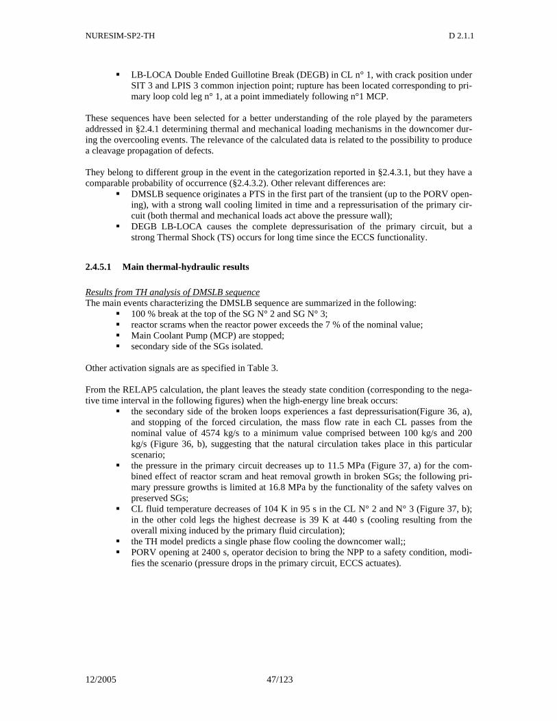
NURESIM-SP2-TH D 2.1.1
12/2005 47/123
LB-LOCA Double Ended Guillotine Break (DEGB) in CL n° 1, with crack position under SIT 3 and LPIS 3 common injection point; rupture has been located corresponding to pri-mary loop cold leg n° 1, at a point immediately following n°1 MCP.
These sequences have been selected for a better understanding of the role played by the parameters addressed in §2.4.1 determining thermal and mechanical loading mechanisms in the downcomer dur-ing the overcooling events. The relevance of the calculated data is related to the possibility to produce a cleavage propagation of defects. They belong to different group in the event in the categorization reported in §2.4.3.1, but they have a comparable probability of occurrence (§2.4.3.2). Other relevant differences are:
DMSLB sequence originates a PTS in the first part of the transient (up to the PORV open-ing), with a strong wall cooling limited in time and a repressurisation of the primary cir-cuit (both thermal and mechanical loads act above the pressure wall);
DEGB LB-LOCA causes the complete depressurisation of the primary circuit, but a strong Thermal Shock (TS) occurs for long time since the ECCS functionality.
2.4.5.1 Main thermal-hydraulic results
Results from TH analysis of DMSLB sequence The main events characterizing the DMSLB sequence are summarized in the following:
100 % break at the top of the SG N° 2 and SG N° 3; reactor scrams when the reactor power exceeds the 7 % of the nominal value; Main Coolant Pump (MCP) are stopped; secondary side of the SGs isolated.
Other activation signals are as specified in Table 3. From the RELAP5 calculation, the plant leaves the steady state condition (corresponding to the nega-tive time interval in the following figures) when the high-energy line break occurs:
the secondary side of the broken loops experiences a fast depressurisation(Figure 36, a), and stopping of the forced circulation, the mass flow rate in each CL passes from the nominal value of 4574 kg/s to a minimum value comprised between 100 kg/s and 200 kg/s (Figure 36, b), suggesting that the natural circulation takes place in this particular scenario;
the pressure in the primary circuit decreases up to 11.5 MPa (Figure 37, a) for the com-bined effect of reactor scram and heat removal growth in broken SGs; the following pri-mary pressure growths is limited at 16.8 MPa by the functionality of the safety valves on preserved SGs;
CL fluid temperature decreases of 104 K in 95 s in the CL N° 2 and N° 3 (Figure 37, b); in the other cold legs the highest decrease is 39 K at 440 s (cooling resulting from the overall mixing induced by the primary fluid circulation);
the TH model predicts a single phase flow cooling the downcomer wall;; PORV opening at 2400 s, operator decision to bring the NPP to a safety condition, modi-
fies the scenario (pressure drops in the primary circuit, ECCS actuates).
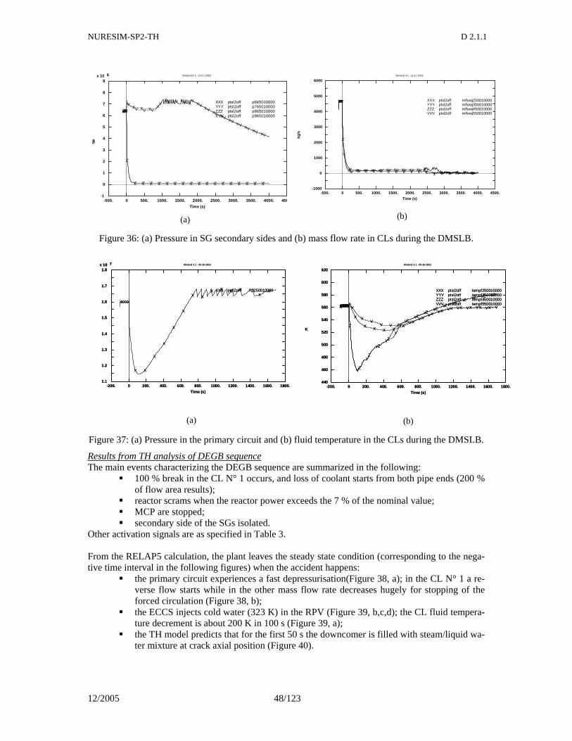
NURESIM-SP2-TH D 2.1.1
12/2005 48/123
-500. 0 500. 1000. 1500. 2000. 2500. 3000. 3500. 4000. 4500.
Time (s)
-1
0
1
2
3
4
5
6
7
8
9x 10 6
Pa
WinGraf 4.1 - 12-17-2003
XXX ptsl2off p665010000
XXXX X X X
X X XX X
XX
XX
XX
XX
YYY ptsl2off p765010000YYY
Y Y Y Y Y Y Y Y Y Y Y Y Y Y Y Y Y
ZZZ ptsl2off p865010000ZZ
Z
Z Z Z Z Z Z Z Z Z Z Z Z Z Z Z Z Z
VVV ptsl2off p965010000VV
VV V V
V V V V VV
VV
VV
VV
VV
(a)
-500. 0 500. 1000. 1500. 2000. 2500. 3000. 3500. 4000. 4500.
Time (s)
-1000
0
1000
2000
3000
4000
5000
6000
kg/s
WinGraf 4.1 - 12-17-2003
XXX ptsl2off mflowj250010000XXX
X X X X X X X X X X X XX X X X X
YYY ptsl2off mflowj350010000YYY
Y Y Y Y Y Y Y Y Y Y Y Y Y Y Y Y Y
ZZZ ptsl2off mflowj450010000
ZZ
Z
Z Z Z Z Z Z Z Z Z Z Z Z Z Z Z Z Z
VVV ptsl2off mflowj550010000
VV
V
V V V V V V V V V V V VV V V V V
(b)
Figure 36: (a) Pressure in SG secondary sides and (b) mass flow rate in CLs during the DMSLB.
-200. 0 200. 400. 600. 800. 1000. 1200. 1400. 1600. 1800.
Time (s)
1.1
1.2
1.3
1.4
1.5
1.6
1.7
1.8x 10 7 WinGraf 4.1 - 09-30-2003
XXX ptsl2off p250010000
XXXXX
X X
X
X
X
X
X XX X X X X
XX
-200. 0 200. 400. 600. 800. 1000. 1200. 1400. 1600. 1800.
Time (s)
1.1
1.2
1.3
1.4
1.5
1.6
1.7
1.8x 10 7 WinGraf 4.1 - 09-30-2003
XXX ptsl2off p250010000
XXXXX
X X
X
X
X
X
X XX X X X X
XX
(a)
-200. 0 200. 400. 600. 800. 1000. 1200. 1400. 1600. 1800.
Time (s)
440
460
480
500
520
540
560
580
600
620
K
WinGraf 4.1 - 09-30-2003
XXX ptsl2off tempf250010000
XXXXX
X
XX X X
XX
XX
XX X X X X
YYY ptsl2off tempf350010000
YYYYY
Y
Y
YY
Y
YY
YY
YY
Y Y Y YZZZ ptsl2off tempf450010000
ZZZZ
Z
Z
Z
Z
Z
ZZ
ZZ
ZZ
ZZ Z Z Z
VVV ptsl2off tempf550010000VVVV V
VV
V V VV
VV
VV V V V V V
(b)
Figure 37: (a) Pressure in the primary circuit and (b) fluid temperature in the CLs during the DMSLB.
Results from TH analysis of DEGB sequence The main events characterizing the DEGB sequence are summarized in the following:
100 % break in the CL N° 1 occurs, and loss of coolant starts from both pipe ends (200 % of flow area results);
reactor scrams when the reactor power exceeds the 7 % of the nominal value; MCP are stopped; secondary side of the SGs isolated.
Other activation signals are as specified in Table 3. From the RELAP5 calculation, the plant leaves the steady state condition (corresponding to the nega-tive time interval in the following figures) when the accident happens:
the primary circuit experiences a fast depressurisation(Figure 38, a); in the CL N° 1 a re-verse flow starts while in the other mass flow rate decreases hugely for stopping of the forced circulation (Figure 38, b);
the ECCS injects cold water (323 K) in the RPV (Figure 39, b,c,d); the CL fluid tempera-ture decrement is about 200 K in 100 s (Figure 39, a);
the TH model predicts that for the first 50 s the downcomer is filled with steam/liquid wa-ter mixture at crack axial position (Figure 40).
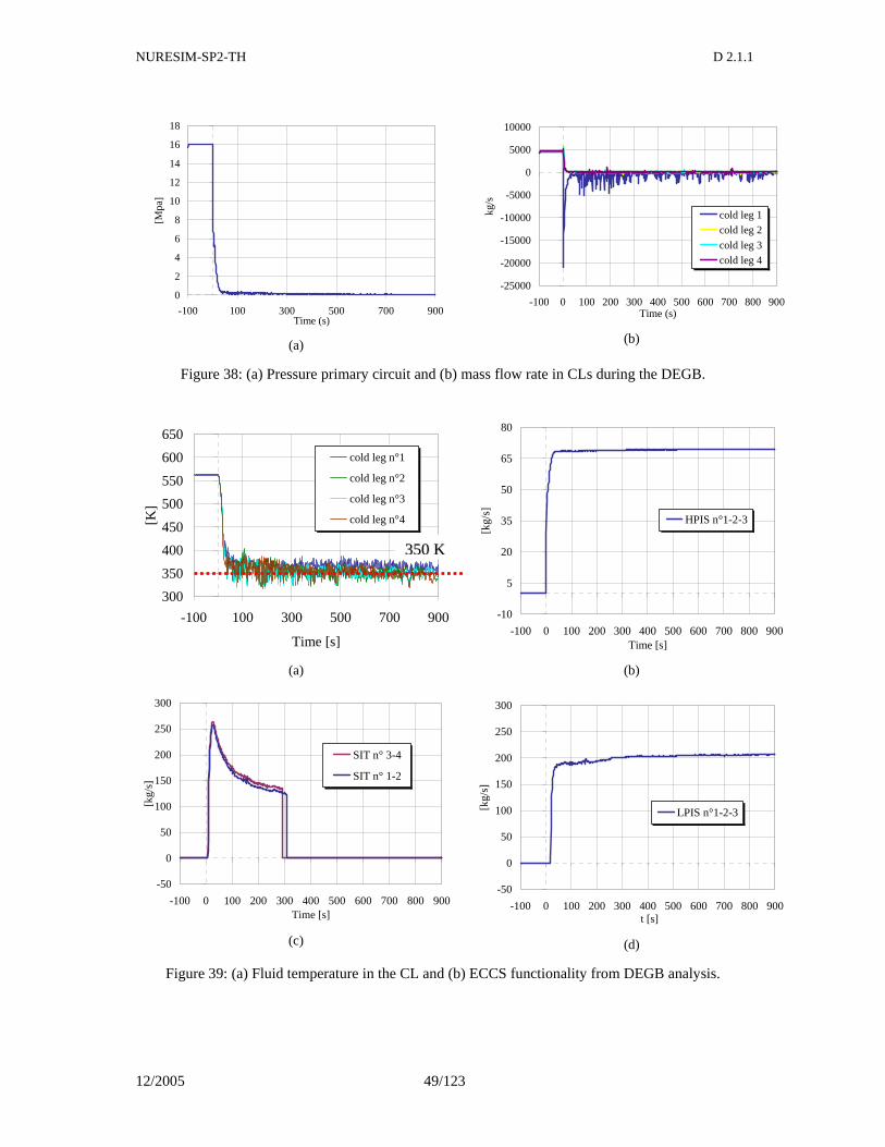
NURESIM-SP2-TH D 2.1.1
12/2005 49/123
0
2
4
6
8
10
12
14
16
18
-100 100 300 500 700 900Time (s)
[Mp
a]
(a)
-25000
-20000
-15000
-10000
-5000
0
5000
10000
-100 0 100 200 300 400 500 600 700 800 900Time (s)
kg/s
cold leg 1cold leg 2
cold leg 3cold leg 4
(b)
Figure 38: (a) Pressure primary circuit and (b) mass flow rate in CLs during the DEGB.
300
350
400
450
500
550
600
650
-100 100 300 500 700 900
Time [s]
[K]
cold leg n°1
cold leg n°2
cold leg n°3
cold leg n°4
(a)
-10
5
20
35
50
65
80
-100 0 100 200 300 400 500 600 700 800 900Time [s]
[kg
/s]
HPIS n°1-2-3
(b)
-50
0
50
100
150
200
250
300
-100 0 100 200 300 400 500 600 700 800 900Time [s]
[kg
/s]
SIT n° 3-4
SIT n° 1-2
(c)
-50
0
50
100
150
200
250
300
-100 0 100 200 300 400 500 600 700 800 900t [s]
[kg
/s]
LPIS n°1-2-3
(d)
Figure 39: (a) Fluid temperature in the CL and (b) ECCS functionality from DEGB analysis.
335500 KK
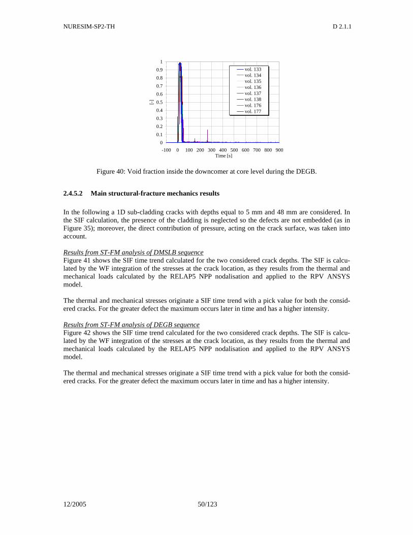
NURESIM-SP2-TH D 2.1.1
12/2005 50/123
0
0.1
0.2
0.3
0.4
0.5
0.6
0.7
0.8
0.9
1
-100 0 100 200 300 400 500 600 700 800 900Time [s]
[-]
vol. 133vol. 134vol. 135vol. 136vol. 137vol. 138vol. 176vol. 177
Figure 40: Void fraction inside the downcomer at core level during the DEGB.
2.4.5.2 Main structural-fracture mechanics results
In the following a 1D sub-cladding cracks with depths equal to 5 mm and 48 mm are considered. In the SIF calculation, the presence of the cladding is neglected so the defects are not embedded (as in Figure 35); moreover, the direct contribution of pressure, acting on the crack surface, was taken into account. Results from ST-FM analysis of DMSLB sequence Figure 41 shows the SIF time trend calculated for the two considered crack depths. The SIF is calcu-lated by the WF integration of the stresses at the crack location, as they results from the thermal and mechanical loads calculated by the RELAP5 NPP nodalisation and applied to the RPV ANSYS model. The thermal and mechanical stresses originate a SIF time trend with a pick value for both the consid-ered cracks. For the greater defect the maximum occurs later in time and has a higher intensity. Results from ST-FM analysis of DEGB sequence Figure 42 shows the SIF time trend calculated for the two considered crack depths. The SIF is calcu-lated by the WF integration of the stresses at the crack location, as they results from the thermal and mechanical loads calculated by the RELAP5 NPP nodalisation and applied to the RPV ANSYS model. The thermal and mechanical stresses originate a SIF time trend with a pick value for both the consid-ered cracks. For the greater defect the maximum occurs later in time and has a higher intensity.
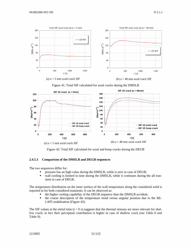
NURESIM-SP2-TH D 2.1.1
12/2005 51/123
Total SIF axial crack tip (a = 5 mm)
0
40
80
120
160
200
0 500 1000 1500t [s]
[MP
a m
0.5 ]
1D WF
(a) a = 5 mm axial crack SIF
Total SIF axial crack tip (a = 48 mm)
0
40
80
120
160
200
0 500 1000 1500t [s]
[MP
a m
0.5]
1D WF
(b) a = 48 mm axial crack SIF
Figure 41: Total SIF calculated for axial cracks during the DMSLB
SIF 1D crack (a = 5mm)
0
20
40
60
80
100
120
0 200 400 600 800
t [s]
[Mpa
*m0.
5 ]
SIF 1D axial crackSIF 1D hoop crack
(a) a = 5 mm axial crack SIF
SIF 1D crack (a = 48mm)
0
20
40
60
80
100
120
140
160
180
0 200 400 600 800
t [s]
[Mpa
*m0.
5 ]
SIF 1D axial crackSIF 1D hoop crack
(b) a = 48 mm axial crack SIF
Figure 42: Total SIF calculated for axial and hoop cracks during the DEGB
2.4.5.3 Comparison of the DMSLB and DEGB sequences
The two sequences differ for: pressure has an high value during the DMSLB, while is zero in case of DEGB; wall cooling is limited in time during the DMSLB, while it continues during the all tran-
sient in case of DEGB. The temperature distribution on the inner surface of the wall temperature along the considered weld is reported in for both considered transients. It can be observed as:
the higher cooling capability of the DEGB sequence than the DMSLB accident; the coarse description of the temperature trend versus angular position due to the RE-
LAP5 nodalisation (Figure 43). The SIF values at the initial time (t = 0 s) suggests that the thermal stresses are more relevant for shal-low crack; in fact their perceptual contribution is higher in case of shallow crack (see Table 8 and Table 9).
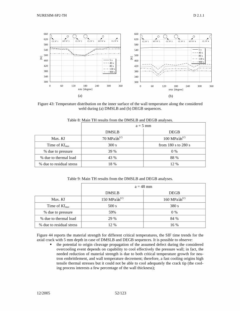
NURESIM-SP2-TH D 2.1.1
12/2005 52/123
300
340
380
420
460
500
540
580
620
660
0 60 120 180 240 300 360teta [degree]
[K]
5 s40 s80 s130 s900 s
CL N° 1 SIT N° 3 CL N° 2 CL N° 3 SIT N° 4 CL N° 4
(a)
300
340
380
420
460
500
540
580
620
660
0 60 120 180 240 300 360teta [degree]
[K]
5 s40 s80 s130 s900 s
CL N° 1 SIT N° 3 CL N° 2 CL N° 3 SIT N° 4 CL N° 4
(b)
Figure 43: Temperature distribution on the inner surface of the wall temperature along the considered weld during (a) DMSLB and (b) DEGB sequences.
Table 8: Main TH results from the DMSLB and DEGB analyses.
a = 5 mm
DMSLB DEGB
Max. KI 70 MPa⋅m0.5 100 MPa⋅m0.5
Time of KImax 300 s from 180 s to 280 s
% due to pressure 39 % 0 %
% due to thermal load 43 % 88 %
% due to residual stress 18 % 12 %
Table 9: Main TH results from the DMSLB and DEGB analyses.
a = 48 mm
DMSLB DEGB
Max. KI 150 MPa⋅m0.5 160 MPa⋅m0.5
Time of KImax 500 s 380 s
% due to pressure 59% 0 %
% due to thermal load 29 % 84 %
% due to residual stress 12 % 16 % Figure 44 reports the material strength for different critical temperatures, the SIF time trends for the axial crack with 5 mm depth in case of DMSLB and DEGB sequences. It is possible to observe:
the potential to origin cleavage propagation of the assumed defect during the considered overcooling event depends on capability to cool effectively the pressure wall; in fact, the needed reduction of material strength is due to both critical temperature growth for neu-tron embrittlement, and wall temperature decrement; therefore, a fast cooling origins high tensile thermal stresses but it could not be able to cool adequately the crack tip (the cool-ing process interests a few percentage of the wall thickness);
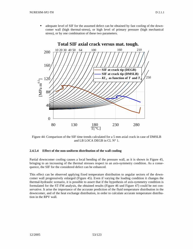
NURESIM-SP2-TH D 2.1.1
12/2005 53/123
adequate level of SIF for the assumed defect can be obtained by fast cooling of the down-comer wall (high thermal-stress), or high level of primary pressure (high mechanical stress), or by one combination of these two parameters.
Total SIF axial crack versus mat. tough.
0
40
80
120
160
200
80 130 180 230 280T[°C]
[MP
a m
0.5]
160 210 10 20 30 40 50 64 100
SIF at crack tip (DEGB)SIF at crack tip (DMSLB)KI C as function of T and T k
250
Figure 44: Comparison of the SIF time trends calculated for a 5 mm axial crack in case of DMSLB and LB LOCA DEGB in CL N° 1.
2.4.5.4 Effect of the non-uniform distribution of the wall cooling
Partial downcomer cooling causes a local bending of the pressure wall, as it is shown in Figure 45, bringing to an increasing of the thermal stresses respect to an axis-symmetry condition. As a conse-quence, the SIF for the considered defect can be enhanced. This effect can be observed applying fixed temperature distribution to angular sectors of the down-comer wall progressively enlarged (Figure 45). Even if varying the loading condition it changes the thermal-hydraulic scenario, it is possible to assert that if the hypothesis of axis-symmetry condition is formulated for the ST-FM analysis, the obtained results (Figure 46 und Figure 47) could be not con-servative. It arise the importance of the accurate prediction of the fluid temperature distribution in the downcomer, and of the heat exchange distribution, in order to calculate accurate temperature distribu-tion in the RPV wall.
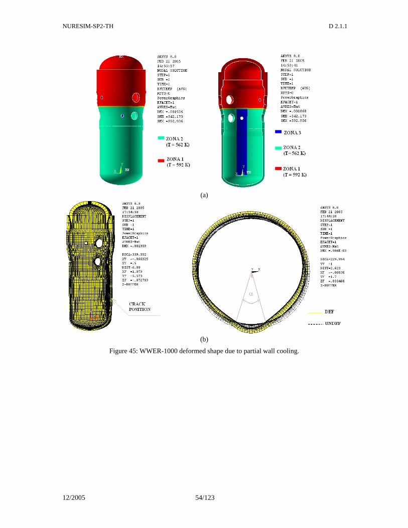
NURESIM-SP2-TH D 2.1.1
12/2005 54/123
(a)
(b)
Figure 45: WWER-1000 deformed shape due to partial wall cooling.
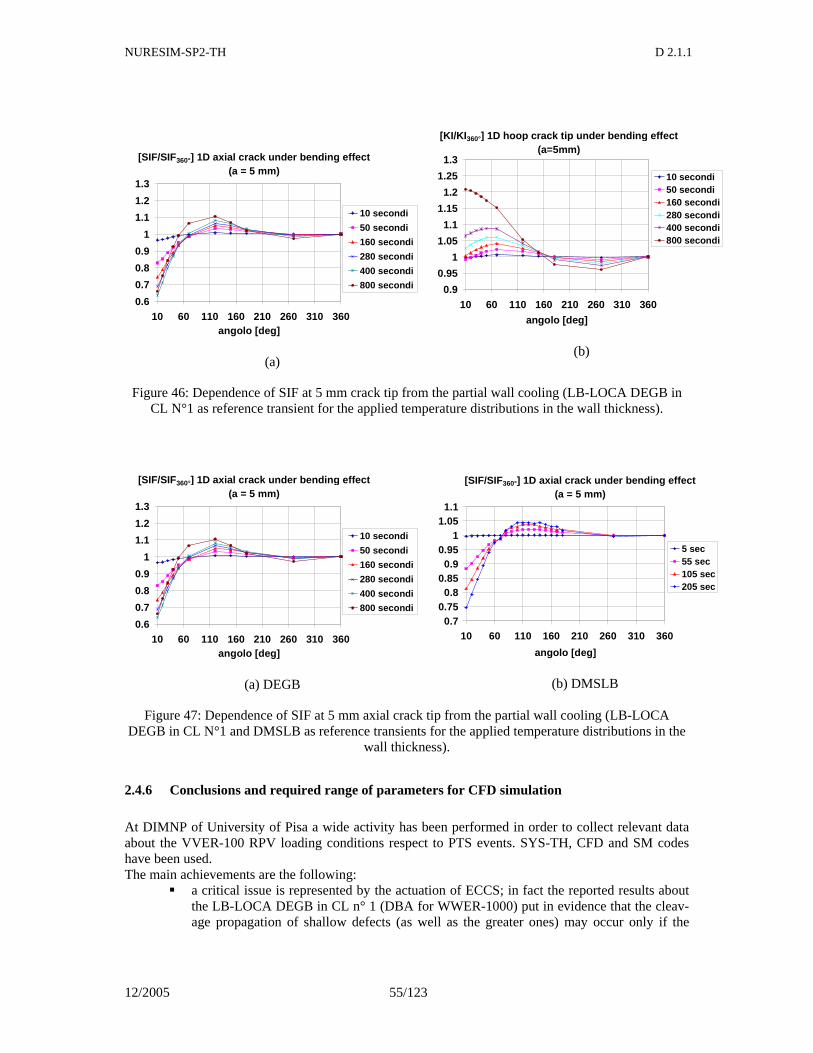
NURESIM-SP2-TH D 2.1.1
12/2005 55/123
[SIF/SIF360°] 1D axial crack under bending effect (a = 5 mm)
0.6
0.7
0.8
0.9
1
1.1
1.2
1.3
10 60 110 160 210 260 310 360angolo [deg]
10 secondi
50 secondi
160 secondi
280 secondi
400 secondi
800 secondi
(a)
[KI/KI 360°] 1D hoop crack tip under bending effect (a=5mm)
0.9
0.95
1
1.05
1.1
1.15
1.2
1.25
1.3
10 60 110 160 210 260 310 360
angolo [deg]
10 secondi50 secondi160 secondi280 secondi400 secondi800 secondi
(b)
Figure 46: Dependence of SIF at 5 mm crack tip from the partial wall cooling (LB-LOCA DEGB in CL N°1 as reference transient for the applied temperature distributions in the wall thickness).
[SIF/SIF360°] 1D axial crack under bending effect (a = 5 mm)
0.6
0.7
0.8
0.9
1
1.1
1.2
1.3
10 60 110 160 210 260 310 360angolo [deg]
10 secondi
50 secondi
160 secondi
280 secondi
400 secondi
800 secondi
(a) DEGB
[SIF/SIF360°] 1D axial crack under bending effect (a = 5 mm)
0.70.75
0.80.85
0.90.95
11.05
1.1
10 60 110 160 210 260 310 360
angolo [deg]
5 sec55 sec105 sec205 sec
(b) DMSLB
Figure 47: Dependence of SIF at 5 mm axial crack tip from the partial wall cooling (LB-LOCA DEGB in CL N°1 and DMSLB as reference transients for the applied temperature distributions in the
wall thickness).
2.4.6 Conclusions and required range of parameters for CFD simulation
At DIMNP of University of Pisa a wide activity has been performed in order to collect relevant data about the VVER-100 RPV loading conditions respect to PTS events. SYS-TH, CFD and SM codes have been used. The main achievements are the following:
a critical issue is represented by the actuation of ECCS; in fact the reported results about the LB-LOCA DEGB in CL n° 1 (DBA for WWER-1000) put in evidence that the cleav-age propagation of shallow defects (as well as the greater ones) may occur only if the
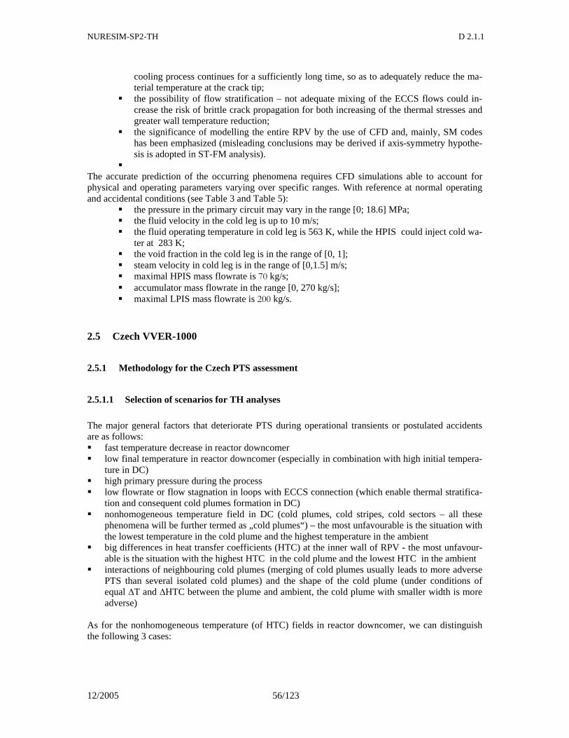
NURESIM-SP2-TH D 2.1.1
12/2005 56/123
cooling process continues for a sufficiently long time, so as to adequately reduce the ma-terial temperature at the crack tip;
the possibility of flow stratification – not adequate mixing of the ECCS flows could in-crease the risk of brittle crack propagation for both increasing of the thermal stresses and greater wall temperature reduction;
the significance of modelling the entire RPV by the use of CFD and, mainly, SM codes has been emphasized (misleading conclusions may be derived if axis-symmetry hypothe-sis is adopted in ST-FM analysis).
The accurate prediction of the occurring phenomena requires CFD simulations able to account for physical and operating parameters varying over specific ranges. With reference at normal operating and accidental conditions (see Table 3 and Table 5):
the pressure in the primary circuit may vary in the range [0; 18.6] MPa; the fluid velocity in the cold leg is up to 10 m/s; the fluid operating temperature in cold leg is 563 K, while the HPIS could inject cold wa-
ter at 283 K; the void fraction in the cold leg is in the range of [0, 1]; steam velocity in cold leg is in the range of [0,1.5] m/s; maximal HPIS mass flowrate is 70 kg/s; accumulator mass flowrate in the range [0, 270 kg/s]; maximal LPIS mass flowrate is 200 kg/s.
2.5 Czech VVER-1000
2.5.1 Methodology for the Czech PTS assessment
2.5.1.1 Selection of scenarios for TH analyses
The major general factors that deteriorate PTS during operational transients or postulated accidents are as follows: fast temperature decrease in reactor downcomer low final temperature in reactor downcomer (especially in combination with high initial tempera-
ture in DC) high primary pressure during the process low flowrate or flow stagnation in loops with ECCS connection (which enable thermal stratifica-
tion and consequent cold plumes formation in DC) nonhomogeneous temperature field in DC (cold plumes, cold stripes, cold sectors – all these
phenomena will be further termed as „cold plumes“) – the most unfavourable is the situation with the lowest temperature in the cold plume and the highest temperature in the ambient
big differences in heat transfer coefficients (HTC) at the inner wall of RPV - the most unfavour-able is the situation with the highest HTC in the cold plume and the lowest HTC in the ambient
interactions of neighbouring cold plumes (merging of cold plumes usually leads to more adverse PTS than several isolated cold plumes) and the shape of the cold plume (under conditions of equal ∆T and ∆HTC between the plume and ambient, the cold plume with smaller width is more adverse)
As for the nonhomogeneous temperature (of HTC) fields in reactor downcomer, we can distinguish the following 3 cases:
NURESIM-SP2-TH D 2.1.1
12/2005 57/123
a) cold plumes (connected with flow stagnation and thermal stratification in cold leg; the cold water from SI consequently flows down along the inner surface of RPV wall; typical for SBLOCA, PRISE, later phase of LBLOCA, SI to non-affected loop in MSLB etc.)
b) cold stripes (stripe of cold water flowing down in steam ambient; typical for medium- and large-break LOCA)
c) cold sectors (typical for MSLB starting from full reactor power with strong forced or natu-ral circulation in RCS, cold water coming from affected SG enters reactor through the whole cross-section of inlet nozzle(s) and flows downward through the whole width of DC to the reactor bottom)
Based on the IAEA methodology guide for PTS and base on our experience from PTS evaluation for NPP Dukovany (VVER 440/213) we had selected the following scenarios for the system TH analyses in frame of PTS evaluation (initial plan):
a) Loss-of-coolant accident (LOCA)
A1. small break LOCA with break size of D32 mm in the cold leg (2 variant scenarios with maximum/minimum number of ECCS systems available, zero reactor power)
A2. small break LOCA with break size of D60 mm in the cold leg (2 scenarios with max/min ECCS, zero reactor power)
A3. medium-break LOCA with break size of D125 mm in the cold leg (2 scenarios with max/min ECCS, zero reactor power)
A4. medium-break LOCA with rupture of the PRZ SV pipe D210 mm (4 scenarios with max/min ECCS and full/zero reactor power)
A5. large-break LOCA with break size of D300 mm in the cold leg (2 scenarios with max/min ECCS, full reactor power)
A6. large-break LOCA with break size of D300 mm in the hot leg (2 scenarios with max/min ECCS, full reactor power)
A7. double-ended guillotine rupture 2xD850 in the cold leg (1 scenario with min ECCS and full reactor power)
A8. double-ended guillotine rupture 2xD850 in the hot leg (2 scenarios: first one with max ECCS and zero reactor power, second one with min ECCS and full reactor power)
b) Increase of heat removal by secondary circuit
B1. main steam line break (MSLB) close to SG (2 scenarios with full/zero reactor power)
B2. main steam line break (MSLB) upstream of main steam isolation valve (MSIV) (2 scenarios with full/zero reactor power)
B3. main steam line break (MSLB) between MSIV and main steam header (MSH) (1 scenario with zero reactor power)
B4. main steam header rupture (MSHR) (2 scenarios with full/zero reactor power)
B5. main steam line break (MSLB) downstream of MSHR (1 scenario with zero reactor power)
B6. inadvertent opening of steam dump to atmosphere (SDA) (1 scenario with zero reactor power)
B7. inadvertent opening of steam dump to condenser (SDC) (1 scenario with zero reactor power)
NURESIM-SP2-TH D 2.1.1
12/2005 58/123
c) Leaks from primary to secondary side of steam generator
C1. rupture of 1 SG tube (SGTR) (1 scenario with max ECCS and zero reactor power)
C2. rupture of 3 SG tube (1 scenario with max ECCS and zero reactor power)
C3. SG primary collector cover lift-up (2 scenarios with max/min ECCS, zero reactor power)
d) Other initiating events
D1. inadvertent opening of PRZ SV and its reclosure (2 scenarios with max/min ECCS, zero reactor power)
D2. inadvertent actuation of high pressure injection system (HPIS) (2 scenarios with various initial regime of the unit)
D3. make-up system malfunction leading to increase of RCS inventory (1 scenario)
D4. analysis of feed&bleed (EOP procedure FR-H.1) (1 scenario)
D5. interfacing LOCA (1 scenarios with max ECCS and zero reactor power)
D6. inadvertent start of hydroaccumulator injection due to operating personnel mistake (1 scenario)
The meaning of “minimum number of ECCS systems” or “min ECCS”, which is used above, is the availability of 1/3 high-high pressure systems (HHPIS), 1/3 high pressure systems (HPIS) and 1/3 low-pressure systems (LPIS) and 2/4 hydroaccumulators (one to downcomer, one to upper plenum). As for the active ECCS system, the maximum characteristics of pumps are used also in these analyses with “min ECCS”. Finally, due to additional variants analyses for some types of events, the number of scenarious ana-lysed was higher: 17 cases of LOCA, 4 cases of PRISE, 13 cases of MSLB, 20 cases of inadvertent opening of PRZSV and 3 “other” cases (+ numerous sensitivity calculations) were analysed in frame of PTS evaluation of VVER-1000.
2.5.1.2 Computer codes used in Czech PTS studies so far
The basic computer tools that were utilised in PTS evaluation for NPP Dukovany (VVER-440/213) and NPP Temelin (VVER-1000/320) are the following: system TH analysis: RELAP5 mixing calculation: REMIX/NEWMIX CATHARE 2D (for 2-phase cases) structural calculation: SYSTUS COSMOS/M For some minor or special purposes we used also the ATHLET, MELCOR, COCOSYS, FLUTAN, and FLUENT(mixing in CL by SI, mixing in DC and LP) computer codes.
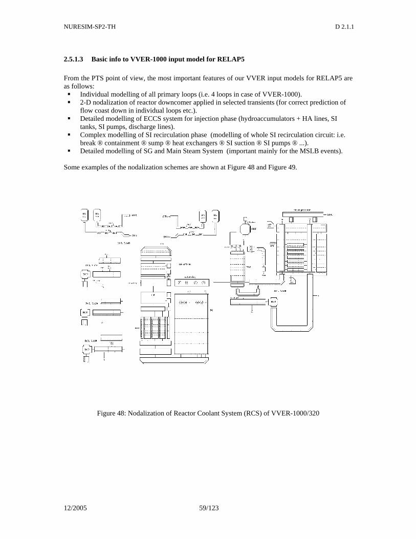
NURESIM-SP2-TH D 2.1.1
12/2005 59/123
2.5.1.3 Basic info to VVER-1000 input model for RELAP5
From the PTS point of view, the most important features of our VVER input models for RELAP5 are as follows: Individual modelling of all primary loops (i.e. 4 loops in case of VVER-1000). 2-D nodalization of reactor downcomer applied in selected transients (for correct prediction of
flow coast down in individual loops etc.). Detailed modelling of ECCS system for injection phase (hydroaccumulators + HA lines, SI
tanks, SI pumps, discharge lines). Complex modelling of SI recirculation phase (modelling of whole SI recirculation circuit: i.e.
break ® containment ® sump ® heat exchangers ® SI suction ® SI pumps ® ...). Detailed modelling of SG and Main Steam System (important mainly for the MSLB events).
Some examples of the nodalization schemes are shown at Figure 48 and Figure 49.
Figure 48: Nodalization of Reactor Coolant System (RCS) of VVER-1000/320
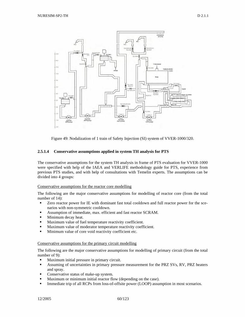
NURESIM-SP2-TH D 2.1.1
12/2005 60/123
Figure 49: Nodalization of 1 train of Safety Injection (SI) system of VVER-1000/320.
2.5.1.4 Conservative assumptions applied in system TH analysis for PTS
The conservative assumptions for the system TH analysis in frame of PTS evaluation for VVER-1000 were specified with help of the IAEA and VERLIFE methodology guide for PTS, experience from previous PTS studies, and with help of consultations with Temelin experts. The assumptions can be divided into 4 groups: Conservative assumptions for the reactor core modelling
The following are the major conservative assumptions for modelling of reactor core (from the total number of 14): Zero reactor power for IE with dominant fast total cooldown and full reactor power for the sce-
narios with non-symmetric cooldown. Assumption of immediate, max. efficient and fast reactor SCRAM. Minimum decay heat. Maximum value of fuel temperature reactivity coefficient. Maximum value of moderator temperature reactivity coefficient. Minimum value of core void reactivity coefficient etc.
Conservative assumptions for the primary circuit modelling
The following are the major conservative assumptions for modelling of primary circuit (from the total number of 9): Maximum initial pressure in primary circuit. Assuming of uncertainties in primary pressure measurement for the PRZ SVs, RV, PRZ heaters
and spray. Conservative status of make-up system. Maximum or minimum initial reactor flow (depending on the case). Immediate trip of all RCPs from loss-of-offsite power (LOOP) assumption in most scenarios.
NURESIM-SP2-TH D 2.1.1
12/2005 61/123
Maximum initial temperature in the reactor downcomer etc. Conservative assumptions for the secondary circuit modelling
The following are the major conservative assumptions for modelling of secondary circuit: Maximum initial secondary pressure for relevant IE (MSLB etc.). Minimum of maximum initial SG level (depending on the case). Assumptions for maximum capacity of FW system. Minimum FW temperature etc.
Conservative assumptions for the ECCS and containment modelling
The following are the major conservative assumptions for modelling of ECCS and containment (from the total number of 10): Increased characteristics of SI pumps (HHPIS, HPIS, LPIS). Minimum start-up time of dieselgenerators in cases with LOOP. Minimum start-up time of SI pumps. Minimum temperatures in SI tanks, sump, HA, and ECCS piping. Minimum initial temperature in containment.
Maximum boron acid concentration in all parts of ECCS system etcSpecification of the case
for CFD evaluation
To get 2-phase conditions in reactor DC and to avoid too long scenarios, we propose to analyse a D300 break in hot leg. In the system TH analysis one can see several hundred seconds of strongly two-phase flow in reactor DC. The system TH analysis was performed for 1 hour of the transient, when the “PTS critical time” predicted in similar case in PTS evaluation for VVER-1000 was about 2500 s.
2.5.2.1 Specification of the initiating event and boundary conditions
The initiating event is a partial rupture D300 mm of hot leg (full diameter = 850 mm) of loop no. 4 with discharge coefficient 1.0 and immediate opening of the break (in 1 time step). The major conservative assumptions are as follows: (full reactor power) minimal initial reactor flowrate as high as possible initial reactor inlet temperature (max. sec. pressure etc.) break located in loop with PRZ connection loss-of-offsite power at 0. s immediate reactor SCRAM + decay heat reduced by factor 0.8x minimal ECCS capacity for maximally asymmetric cooldown (1/3 HPIS and 1/3 LPIS injecting
to CL1, 2/4 HA with one of them – YT14 injecting to DC close to CL1 entry) increased ECCS pumps characteristics minimal temperatures in ECCS tanks etc.
2.5.2.2 Results of system TH analysis
System TH analysis was performed with the RELAP5 computer code. The following results were ob-tained.
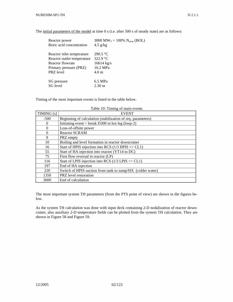
NURESIM-SP2-TH D 2.1.1
12/2005 62/123
The initial parameters of the model at time 0 s (i.e. after 500 s of steady state) are as follows:
Reactor power 3000 MWT = 100% Nnom (BOL) Boric acid concentration 4.5 g/kg Reactor inlet temperature 290.5 °C Reactor outlet temperature 322.9 °C Reactor flowrate 16614 kg/s Primary pressure (PRZ) 16.2 MPa PRZ level 4.0 m SG pressure 6.5 MPa SG level 2.30 m
Timing of the most important events is listed in the table below.
Table 10: Timing of main events TIMING [s] EVENT
-500 Beginning of calculation (stabilization of req. parameters) 0 Initiating event = break D300 in hot leg (loop-2) 0 Loss-of-offsite power 0 Reactor SCRAM 8 PRZ empty 10 Boiling and level formation in reactor downcomer 16 Start of HPIS injection into RCS (1/3 HPIS => CL1) 55 Start of HA injection into reactor (YT14 to DC) 75 First flow reversal in reactor (LP) 116 Start of LPIS injection into RCS (1/3 LPIS => CL1) 197 End of HA injection 220 Switch of HPIS suction from tank to sump/HX (colder water) 1350 PRZ level restoration 3600 End of calculation
The most important system TH parameters (from the PTS point of view) are shown in the figures be-low. As the system TH calculation was done with input deck containing 2-D nodalization of reactor down-comer, also auxiliary 2-D temperature fields can be plotted from the system TH calculation. They are shown in Figure 58 and Figure 59.
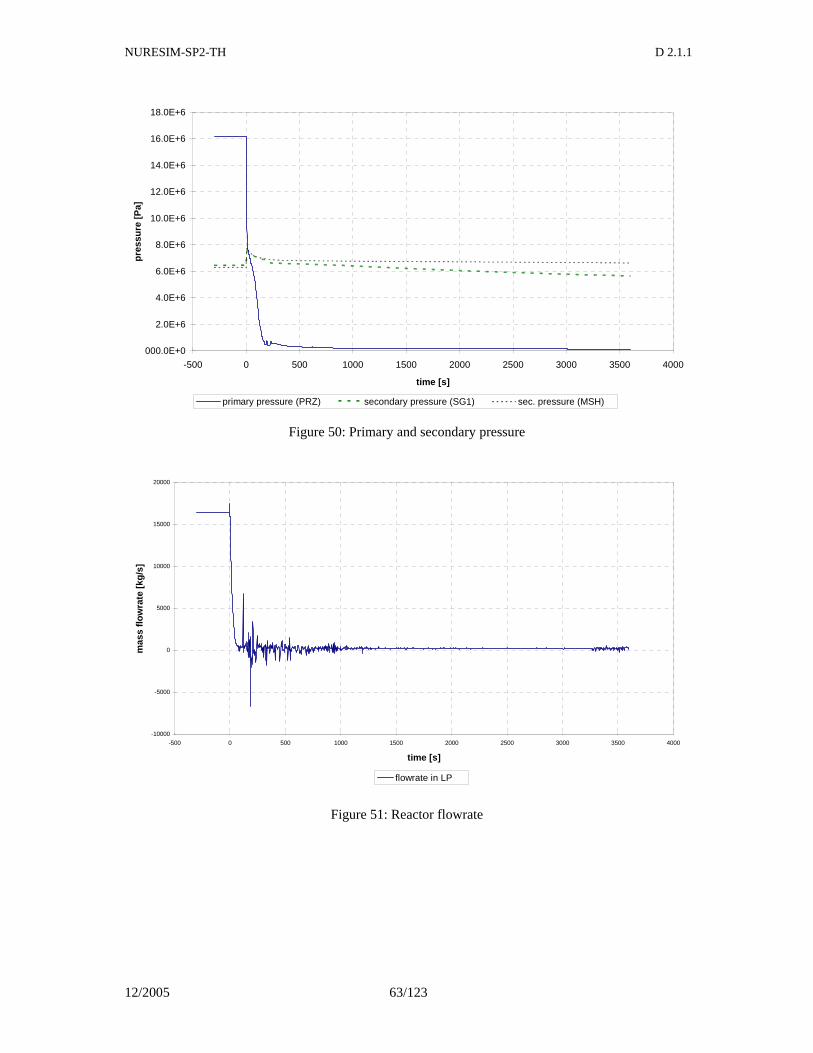
NURESIM-SP2-TH D 2.1.1
12/2005 63/123
000.0E+0
2.0E+6
4.0E+6
6.0E+6
8.0E+6
10.0E+6
12.0E+6
14.0E+6
16.0E+6
18.0E+6
-500 0 500 1000 1500 2000 2500 3000 3500 4000
time [s]
pres
sure
[Pa]
primary pressure (PRZ) secondary pressure (SG1) sec. pressure (MSH)
Figure 50: Primary and secondary pressure
-10000
-5000
0
5000
10000
15000
20000
-500 0 500 1000 1500 2000 2500 3000 3500 4000
time [s]
mas
s flo
wra
te [k
g/s]
flowrate in LP
Figure 51: Reactor flowrate
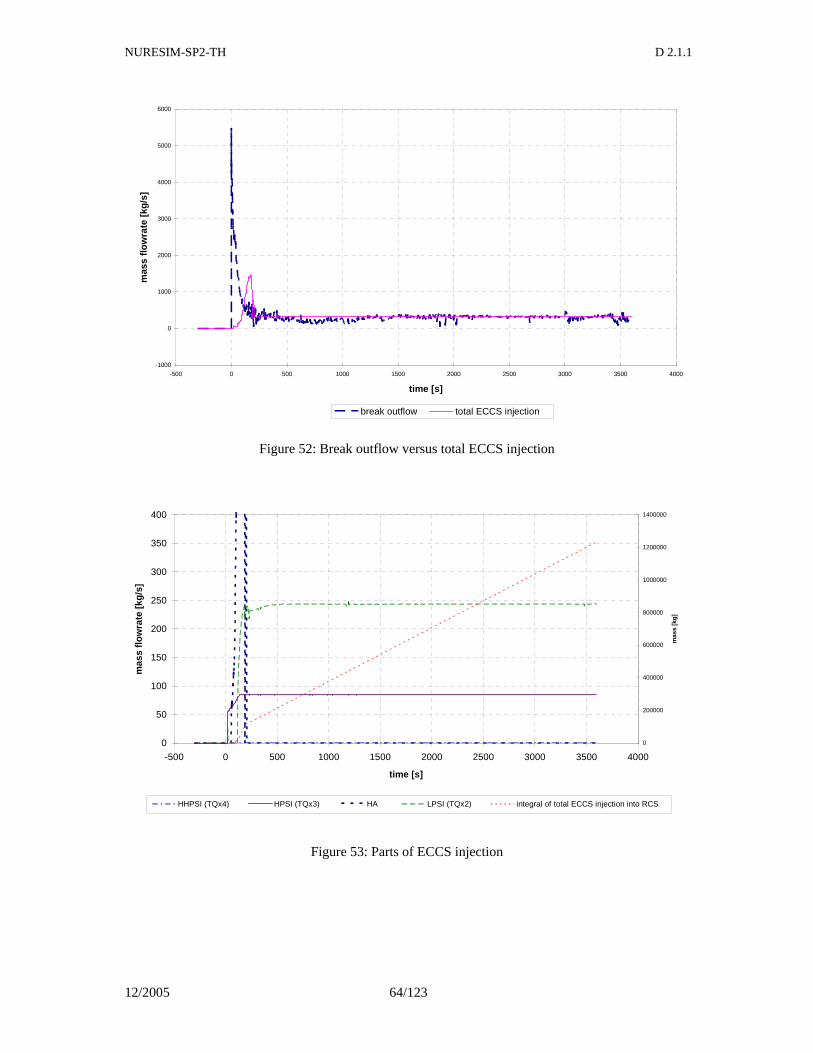
NURESIM-SP2-TH D 2.1.1
12/2005 64/123
-1000
0
1000
2000
3000
4000
5000
6000
-500 0 500 1000 1500 2000 2500 3000 3500 4000
time [s]
mas
s flo
wra
te [k
g/s]
break outflow total ECCS injection
Figure 52: Break outflow versus total ECCS injection
0
50
100
150
200
250
300
350
400
-500 0 500 1000 1500 2000 2500 3000 3500 4000
time [s]
mas
s flo
wra
te [k
g/s]
0
200000
400000
600000
800000
1000000
1200000
1400000
mas
s [k
g]
HHPSI (TQx4) HPSI (TQx3) HA LPSI (TQx2) integral of total ECCS injection into RCS
Figure 53: Parts of ECCS injection
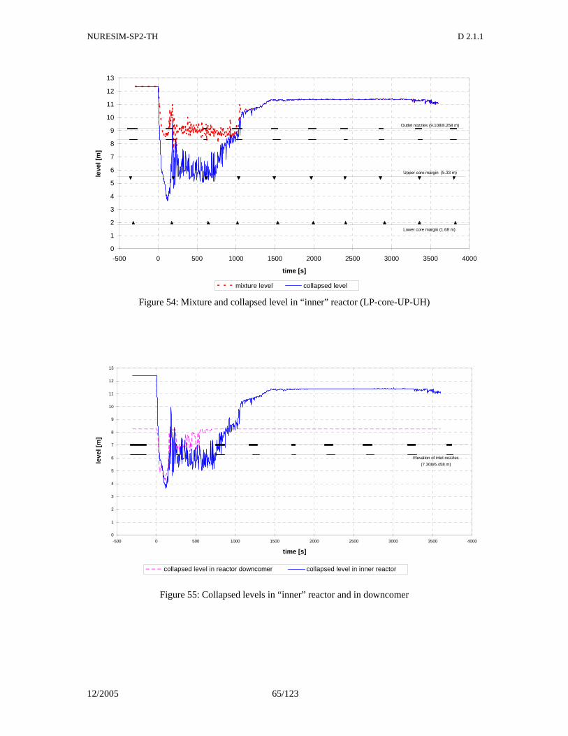
NURESIM-SP2-TH D 2.1.1
12/2005 65/123
0
1
2
3
4
5
6
7
8
9
10
11
12
13
-500 0 500 1000 1500 2000 2500 3000 3500 4000
time [s]
leve
l [m
]
mixture level collapsed level
Outlet nozzles (9.108/8.258 m)
Upper core margin (5.33 m)
Lower core margin (1.68 m)
Figure 54: Mixture and collapsed level in “inner” reactor (LP-core-UP-UH)
0
1
2
3
4
5
6
7
8
9
10
11
12
13
-500 0 500 1000 1500 2000 2500 3000 3500 4000
time [s]
leve
l [m
]
collapsed level in reactor downcomer collapsed level in inner reactor
Elevation of inlet nozzles
(7.308/6.458 m)
Figure 55: Collapsed levels in “inner” reactor and in downcomer
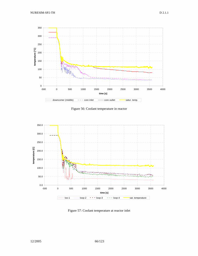
NURESIM-SP2-TH D 2.1.1
12/2005 66/123
0
50
100
150
200
250
300
350
-500 0 500 1000 1500 2000 2500 3000 3500 4000
time [s]
tem
pera
ture
[o C
]
downcomer (middle) core inlet core outlet satur. temp.
Figure 56: Coolant temperature in reactor
0.0
50.0
100.0
150.0
200.0
250.0
300.0
350.0
-500 0 500 1000 1500 2000 2500 3000 3500 4000
time [s]
tem
pera
ture
[C]
loo-1 loop-2 loop-3 loop-4 sat. temperature
Figure 57: Coolant temperature at reactor inlet
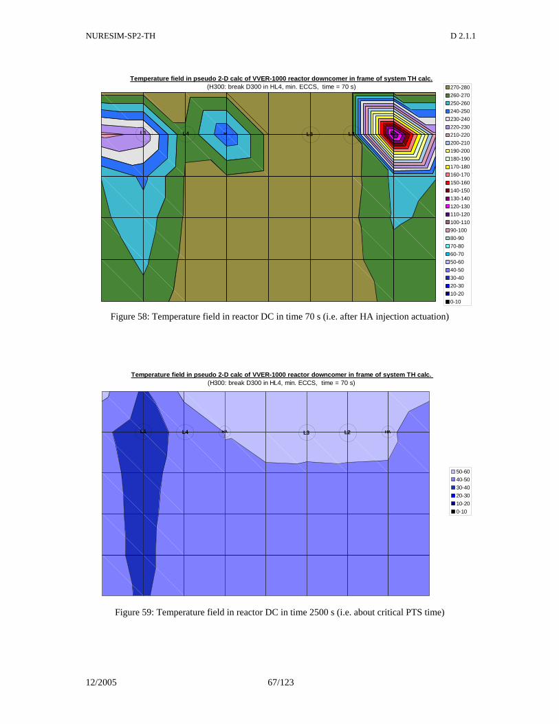
NURESIM-SP2-TH D 2.1.1
12/2005 67/123
Temperature field in pseudo 2-D calc of VVER-1000 reactor downcomer in frame of system TH calc.(H300: break D300 in HL4, min. ECCS, time = 70 s) 270-280
260-270
250-260
240-250
230-240
220-230
210-220
200-210
190-200
180-190
170-180
160-170
150-160
140-150
130-140
120-130
110-120
100-110
90-100
80-90
70-80
60-70
50-60
40-50
30-40
20-30
10-20
0-10
L3L4 L2L1 H H
Figure 58: Temperature field in reactor DC in time 70 s (i.e. after HA injection actuation)
Temperature field in pseudo 2-D calc of VVER-1000 reactor downcomer in frame of system TH calc. (H300: break D300 in HL4, min. ECCS, time = 70 s)
50-60
40-50
30-40
20-30
10-20
0-10
L3L4 L2L1 HA HA
Figure 59: Temperature field in reactor DC in time 2500 s (i.e. about critical PTS time)
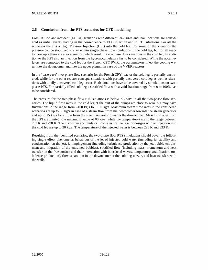
NURESIM-SP2-TH D 2.1.1
12/2005 68/123
2.6 Conclusion from the PTS scenarios for CFD modelling
Loss Of Coolant Accident (LOCA) scenarios with different leak sizes and leak locations are consid-ered as initial events leading in the consequence to ECC injection and to PTS situations. For all the scenarios there is a High Pressure Injection (HPI) into the cold leg. For some of the scenarios the pressure can be stabilized to stay within single-phase flow conditions in the cold leg, but for all reac-tor concepts there are also scenarios, which result in two-phase flow situations in the cold leg. In addi-tion to the HPI also an injection from the hydroaccumulators has to be considered. While the accumu-lators are connected to the cold leg for the French CPY PWR, the accumulators inject the cooling wa-ter into the downcomer and into the upper plenum in case of the VVER reactors. In the “base-case” two-phase flow scenario for the French CPY reactor the cold leg is partially uncov-ered, while for the other reactor concepts situations with partially uncovered cold leg as well as situa-tions with totally uncovered cold leg occur. Both situations have to be covered by simulations on two-phase PTS. For partially filled cold leg a stratified flow with a void fraction range from 0 to 100% has to be considered. The pressure for the two-phase flow PTS situations is below 7.5 MPa in all the two-phase flow sce-narios. The liquid flow rates in the cold leg at the exit of the pumps are close to zero, but may have fluctuations in the range from –100 kg/s to +100 kg/s. Maximum steam flow rates in the considered scenarios are up to 50 kg/s in case of a steam flow from the downcomer towards the steam generator and up to 15 kg/s for a flow from the steam generator towards the downcomer. Mass flow rates from the HPI are limited to a maximum value of 80 kg/s, while the temperatures are in the range between 283 K and 298 K. The maximum accumulator flow rates for the reactor designs with an injection into the cold leg are up to 30 kg/s. The temperature of the injected water is between 298 K and 333 K. Resulting from the identified scenarios, the two-phase flow PTS simulations should cover the follow-ing single effect phenomena: behaviour of the jet of injected cold water (including jet stability and condensation on the jet), jet impingement (including turbulence production by the jet, bubble entrain-ment and migration of the entrained bubbles), stratified flow (including mass, momentum and heat transfer on the free surface and their interaction with interfacial waves, temperature stratification, tur-bulence production), flow separation in the downcomer at the cold leg nozzle, and heat transfers with the walls.
NURESIM-SP2-TH D 2.1.1
12/2005 69/123
3 THE USE OF CFD CODES FOR PTS-SIMULATIONS
3.1 General remarks on CFD codes
CFD codes solve the mass-, momentum- and energy conservation equations in their two- or three-dimensional form. Initially, they were developed for one-phase flows, but they are also increasingly applied for the calculation of two-phase flows. Velocity-, pressure- and temperature fields can be de-termined with a high degree of accuracy. The discretisation aspect in CFD codes is less sensitive than in coarse-grid methods. CFD codes base on local physical closure laws and are for that reason widely geometry-independent. Thus, a higher degree of universal validity can be expected. The application limits of CFD codes are to be found in the large effort required for a calculation, on the one hand, and the accuracy of the turbulence and phase interactions modelling, on the other hand. With respect to the integrity assessment of pressure vessels, a large number of load cases have to be calculated rang-ing from normal operation with start-up and shut-down over faulty excitation of the emergency core cooling systems up to loss-of-coolant accidents with different leak sizes. The exact prediction of one-phase cooling mechanisms, such as the plume cooling, also represents a challenge for the CFD codes. The flows within the cold leg and the downcomer are driven by density differences between cold emergency cooling water and the residual hot water inventory in the vessel. In the cold leg and in the downcomer, regions of stagnation and of relatively low velocities occur. Therefore, a transition from turbulent to laminar flows takes place at the borders of these regions. This means for CFD codes and the implemented turbulence models that both buoyancy effects and effects of small Reynolds numbers have to be modeled adequately. This can be done either by the application and calibration of two-equation turbulence models with empirical corrections or “Second Moment Closure Turbulence Mod-els” requiring more time and efforts, corresponding to a modelling of fluctuations. Up to now, the laminar-turbulent transition is not reliably predicted with the turbulence models used so far. CFD software used to predict PTS must be accurate, robust and efficient and satisfy the following cri-teria:
• The software must reproduce the test case data within a given error band. • The software must produce these results in a consistent and convergent manner, i.e. it must be
shown empirically that numerical solution errors of the method are bounded and become smaller as the spatial and temporal grids get refined.
• Conservation of the global mass, momentum and energy balances must be guaranteed within the iteration and/or discretisation accuracy.
• The software must be robust. However, a mathematical convergence proof for three-dimensional CFD methods, which could be used as an absolute benchmark for robustness, does not exist. Therefore, robustness of the CFD methods can only be defined in a statistical sense.
The ‘optimum’ CFD software needs to satisfy the above requirements, at the same minimizing com-puting time and computer memory demands. To intensify the application of CFD-methods in the field of nuclear technology, the calculation time has to be reduced considerably, e.g. by the use of parallel computers. Furthermore, the existing turbu-lence models have to be refined. In this respect, it is a challenging task to make models available for the description of multi-phase flows as well as for the description of the interactions between multi-phase flows and turbulence. Only with this extended basis, a CFD analysis may be made available also to the load cases with the cooling mechanism "stripe cooling".
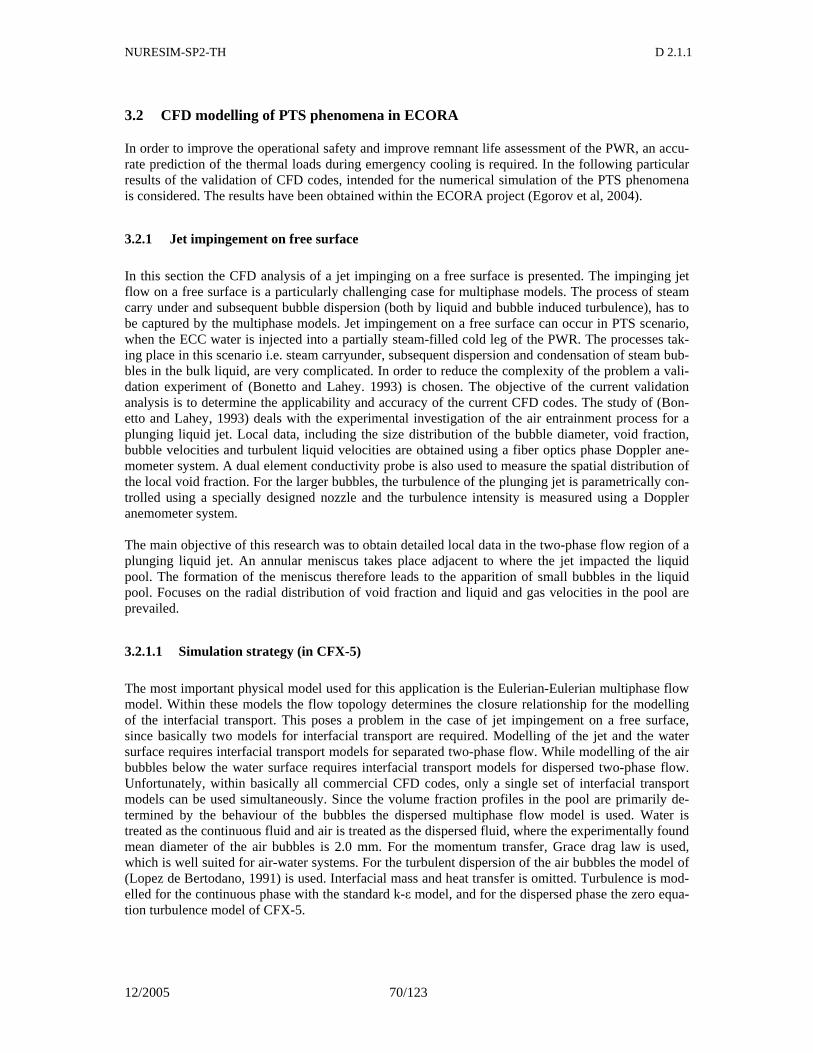
NURESIM-SP2-TH D 2.1.1
12/2005 70/123
3.2 CFD modelling of PTS phenomena in ECORA
In order to improve the operational safety and improve remnant life assessment of the PWR, an accu-rate prediction of the thermal loads during emergency cooling is required. In the following particular results of the validation of CFD codes, intended for the numerical simulation of the PTS phenomena is considered. The results have been obtained within the ECORA project (Egorov et al, 2004).
3.2.1 Jet impingement on free surface
In this section the CFD analysis of a jet impinging on a free surface is presented. The impinging jet flow on a free surface is a particularly challenging case for multiphase models. The process of steam carry under and subsequent bubble dispersion (both by liquid and bubble induced turbulence), has to be captured by the multiphase models. Jet impingement on a free surface can occur in PTS scenario, when the ECC water is injected into a partially steam-filled cold leg of the PWR. The processes tak-ing place in this scenario i.e. steam carryunder, subsequent dispersion and condensation of steam bub-bles in the bulk liquid, are very complicated. In order to reduce the complexity of the problem a vali-dation experiment of (Bonetto and Lahey. 1993) is chosen. The objective of the current validation analysis is to determine the applicability and accuracy of the current CFD codes. The study of (Bon-etto and Lahey, 1993) deals with the experimental investigation of the air entrainment process for a plunging liquid jet. Local data, including the size distribution of the bubble diameter, void fraction, bubble velocities and turbulent liquid velocities are obtained using a fiber optics phase Doppler ane-mometer system. A dual element conductivity probe is also used to measure the spatial distribution of the local void fraction. For the larger bubbles, the turbulence of the plunging jet is parametrically con-trolled using a specially designed nozzle and the turbulence intensity is measured using a Doppler anemometer system. The main objective of this research was to obtain detailed local data in the two-phase flow region of a plunging liquid jet. An annular meniscus takes place adjacent to where the jet impacted the liquid pool. The formation of the meniscus therefore leads to the apparition of small bubbles in the liquid pool. Focuses on the radial distribution of void fraction and liquid and gas velocities in the pool are prevailed.
3.2.1.1 Simulation strategy (in CFX-5)
The most important physical model used for this application is the Eulerian-Eulerian multiphase flow model. Within these models the flow topology determines the closure relationship for the modelling of the interfacial transport. This poses a problem in the case of jet impingement on a free surface, since basically two models for interfacial transport are required. Modelling of the jet and the water surface requires interfacial transport models for separated two-phase flow. While modelling of the air bubbles below the water surface requires interfacial transport models for dispersed two-phase flow. Unfortunately, within basically all commercial CFD codes, only a single set of interfacial transport models can be used simultaneously. Since the volume fraction profiles in the pool are primarily de-termined by the behaviour of the bubbles the dispersed multiphase flow model is used. Water is treated as the continuous fluid and air is treated as the dispersed fluid, where the experimentally found mean diameter of the air bubbles is 2.0 mm. For the momentum transfer, Grace drag law is used, which is well suited for air-water systems. For the turbulent dispersion of the air bubbles the model of (Lopez de Bertodano, 1991) is used. Interfacial mass and heat transfer is omitted. Turbulence is mod-elled for the continuous phase with the standard k-ε model, and for the dispersed phase the zero equa-tion turbulence model of CFX-5.
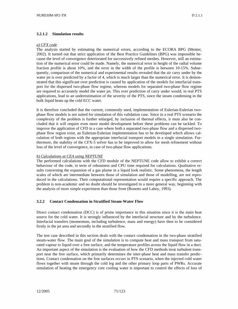
NURESIM-SP2-TH D 2.1.1
12/2005 71/123
3.2.1.2 Simulation results
a) CFX code The analysis started by estimating the numerical errors, according to the ECORA BPG (Menter, 2002). It turned out that strict application of the Best Practice Guidelines (BPG) was impossible be-cause the level of convergence deteriorated for successively refined meshes. However, still an estima-tion of the numerical error could be made. Namely, the numerical error in height of the radial volume fraction profile is about 10%, and the error in the width of the profile is between 10-15%. Subse-quently, comparison of the numerical and experimental results revealed that the air carry under by the water jet is over predicted by a factor of 4, which is much larger than the numerical error. It is demon-strated that this significant over prediction is caused by application of the models for interfacial trans-port for the dispersed two-phase flow regime, whereas models for separated two-phase flow regime are required to accurately model the water jet. This over prediction of carry under would, in real PTS applications, lead to an underestimation of the severity of the PTS, since the steam condensing in the bulk liquid heats up the cold ECC water. It is therefore concluded that the current, commonly used, implementation of Eulerian-Eulerian two-phase flow models is not suited for simulation of this validation case. Since in a real PTS scenario the complexity of the problem is further enlarged, by inclusion of thermal effects, it must also be con-cluded that it will require even more model development before these problems can be tackled. To improve the application of CFD in a case where both a separated two-phase flow and a dispersed two-phase flow region exist, an Eulerian-Eulerian implementation has to be developed which allows cal-culation of both regions with the appropriate interfacial transport models in a single simulation. Fur-thermore, the stability of the CFX-5 solver has to be improved to allow for mesh refinement without loss of the level of convergence, in case of two-phase flow applications. b) Calculations at CEA using NEPTUNE The performed calculations with the CFD module of the NEPTUNE code allow to exhibit a correct behaviour of the code, in term of robustness and CPU time required for calculations. Qualitative re-sults concerning the expansion of a gas plume in a liquid look realistic. Some phenomena, the length scales of which are intermediate between those of simulation and those of modelling, are not repro-duced in the calculations. Their computational representation would require a specific approach. The problem is non-academic and no doubt should be investigated in a more general way, beginning with the analysis of more simple experiment than those from (Bonetto and Lahey, 1993).
3.2.2 Contact Condensation in Stratified Steam-Water Flow
Direct contact condensation (DCC) is of prime importance in this situation since it is the main heat source for the cold water. It is strongly influenced by the interfacial structure and by the turbulence. Interfacial transfers (momentum, including turbulence, mass and energy) have then to be considered firstly in the jet area and secondly in the stratified flow. The test case described in this section deals with the contact condensation in the two-phase stratified steam-water flow. The main goal of the simulation is to compute heat and mass transport from satu-rated vapour to liquid over a free surface, and the temperature profiles across the liquid flow in a duct. An important aspect of the simulation is the evaluation of how the CFD methods treat turbulent trans-port near the free surface, which primarily determines the inter-phase heat and mass transfer predic-tions. Contact condensation on the free surfaces occurs in PTS scenario, when the injected cold water flows together with steam through the cold leg and the other primary loop parts of PWRs. Accurate simulation of heating the emergency core cooling water is important to control the effects of loss of
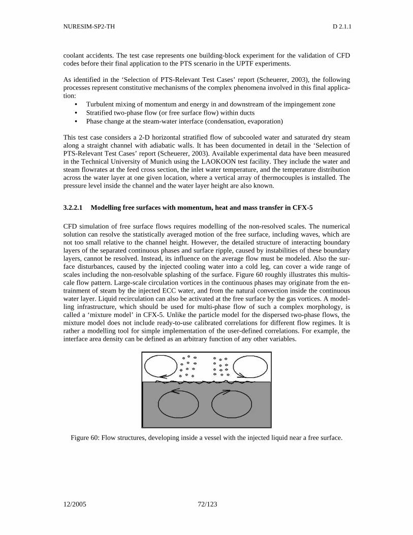
NURESIM-SP2-TH D 2.1.1
12/2005 72/123
coolant accidents. The test case represents one building-block experiment for the validation of CFD codes before their final application to the PTS scenario in the UPTF experiments. As identified in the ‘Selection of PTS-Relevant Test Cases’ report (Scheuerer, 2003), the following processes represent constitutive mechanisms of the complex phenomena involved in this final applica-tion:
• Turbulent mixing of momentum and energy in and downstream of the impingement zone • Stratified two-phase flow (or free surface flow) within ducts • Phase change at the steam-water interface (condensation, evaporation)
This test case considers a 2-D horizontal stratified flow of subcooled water and saturated dry steam along a straight channel with adiabatic walls. It has been documented in detail in the ‘Selection of PTS-Relevant Test Cases’ report (Scheuerer, 2003). Available experimental data have been measured in the Technical University of Munich using the LAOKOON test facility. They include the water and steam flowrates at the feed cross section, the inlet water temperature, and the temperature distribution across the water layer at one given location, where a vertical array of thermocouples is installed. The pressure level inside the channel and the water layer height are also known.
3.2.2.1 Modelling free surfaces with momentum, heat and mass transfer in CFX-5
CFD simulation of free surface flows requires modelling of the non-resolved scales. The numerical solution can resolve the statistically averaged motion of the free surface, including waves, which are not too small relative to the channel height. However, the detailed structure of interacting boundary layers of the separated continuous phases and surface ripple, caused by instabilities of these boundary layers, cannot be resolved. Instead, its influence on the average flow must be modeled. Also the sur-face disturbances, caused by the injected cooling water into a cold leg, can cover a wide range of scales including the non-resolvable splashing of the surface. Figure 60 roughly illustrates this multis-cale flow pattern. Large-scale circulation vortices in the continuous phases may originate from the en-trainment of steam by the injected ECC water, and from the natural convection inside the continuous water layer. Liquid recirculation can also be activated at the free surface by the gas vortices. A model-ling infrastructure, which should be used for multi-phase flow of such a complex morphology, is called a ‘mixture model’ in CFX-5. Unlike the particle model for the dispersed two-phase flows, the mixture model does not include ready-to-use calibrated correlations for different flow regimes. It is rather a modelling tool for simple implementation of the user-defined correlations. For example, the interface area density can be defined as an arbitrary function of any other variables.
Figure 60: Flow structures, developing inside a vessel with the injected liquid near a free surface.
NURESIM-SP2-TH D 2.1.1
12/2005 73/123
3.2.2.2 Simulation Results and Conclusion
CFX-5 Calculations ANSYS CFX-5 code was used to simulate the condensation phenomenon in stratified steam-water flow by implementing the low Reynolds number model of turbulence at a free surface. A consistent set of model correlations for the interfacial area density, the drag and heat transfer coefficients at the free surface is formulated and tested. The calculated temperature profile agrees well with the experi-ment. Further model development for the full-scale PTS simulation should focus on the non-resolved disturbances of a free surface. Conclusion according to the NEPTUNE Calculations The comparison of the NEPTUNE CFD module results with the LAOKOON test facility gives a good qualitative temperature profile for the low Reynolds number, and a correct condensation rate, provid-ing that the heat transfer correlation is adjusted in some way. On the contrary, when the Reynolds number of steam is high, the condensation rate obtained is weaker than the experimental one. The pa-rametrical study shows that the two-phase turbulence model with separated phases presents some dif-ficulties to predict the flow when the Reynolds number of the steam is high. Then, the model under predicts the water temperature in the lower part of the channel. This parametrical study emphasizes also the importance of the grid refinement on the condensation rate due mainly to the interfacial area computation.
3.3 Recommendations for CFD Simulations
3.3.1 Interface Fitting vs. Interface Capturing
Several different approaches are used for the CFD simulation of free surface flows, with the different classifications proposed in the review papers. Regarding the way of modelling the inter-phase trans-port processes, basically any method can be assigned to one of the two general classes:
• Interface fitting methods, including both the interface reconstruction methods like the original • Volume of Fluid (VoF) method, and the interface tracking methods (moving grid methods,
Level Set method, etc.). A common feature of these methods is the representation of the free surface as a sharp discontinuity.
• Interface capturing methods like those implemented in CFX-5. With these methods the free surfaces are smeared for few grid cells, and the flow variables are distributed continuously with high gradients at the phase separation surfaces. Special numerical precautions are taken to prevent the transition regions from too high smearing. Different situations have to be tested with the methods, which do not dynamically fit the interface with a node surface of the 3-D grid (or node line in the 2-D calculation):
o Interface, coinciding with the grid line o Interface, dividing the parallel row of grid cells o Interface, arbitrarily crossing the grid cells
With such a testing, it is assumed, that the interface fitting procedure itself can be validated sepa-rately. Since the ultimate project goals require the CFD simulation of complex flows in the real pri-mary loop geometries, it is not recommended to mimic the interface fitting methods by the given loca-tion of the interface boundary, if the code does not have a robust interface fitting procedure.
3.3.2 Direct Simulation vs. Model Correlation
Simple flow pattern of the considered validation test case allows the direct numerical simulation (DNS) of the inter-phase momentum, heat and mass processes by resolving the water boundary layer
NURESIM-SP2-TH D 2.1.1
12/2005 74/123
at the free surface as it is normally done when simulating the single-phase wall boundary layers. A proper treatment of the free surface by the model of turbulence is a primary issue here. A special care should be taken to prevent the strong grid dependence of the results. Such a grid de-pendence may take place with the Nusselt number correlations, when the liquid temperature in the first internal control volume is selected as the liquid core flow temperature. Obviously, the direct simulation is the much more resource consuming approach. However it is valid in a wide range of flow parameters, is consistent with the basic CFD methodology, and finds more and more applications with the increasing computer power. Besides, this approach can be used for calibration of the problem-specific model correlations as an alternative to the real experiments.
3.3.3 Definition of Target Variables for Convergence and Grid Refinement Tests
Since the condensation rate in the considered flow is fully controlled by the heat transport in the liquid phase, the two following groups of target variables are selected as target variables:
• Temperature profile at the measurement probe location, mass flow average water temperature distribution along the channel, mass flow average water temperature at the measurement probe location.
• Steam mass flow distribution along the channel, integral condensation rate over the surface between the steam inlet and the measurement probe location.
3.4 General requirements for the qualification of CFD codes for two-phase PTS
Multi-dimensional modelling of multiphase flows has become more prevalent as computer capabili-ties have significantly expanded. Such analyses are necessary if the flow physics demonstrates behav-iour that is fundamentally different from the estimates of one-dimensional analyses. Multiphase multi-dimensional behaviour may involve physical mechanisms that interact with the flow field transverse to the main fluid direction and feedback into downstream processes. Nowadays it is recognized that multidimensional aspects of the flow existed and affected the multiphase flow physics. However, the expected detail of the analyses did not require, nor did the computational abilities allow for more so-phisticated multi-dimensional analyses for these multiphase systems within reasonable time and re-source constraints. Most of the two-phase flow codes have initially been developed for industrial applications with large geometrical scales. In such large-scale flows, the structures of dispersed phases like bubbles or drop-lets cannot be recognized individually. In cases where the bubble sizes are significantly smaller than the sizes of the numerical cells, their behaviour must be schematically represented via statistical clo-sure laws. These closure laws are used in each cell. Moreover, in multi-phase flow codes, a set of mass, momentum and energy equations is solved for each phase. This leads to a large number of coupled equations. The individual phases in the domain are indicated by means of statistically averaged volume fractions. However, the definition of the vol-ume fraction as an averaged quantity is still not clear, at least not concerning the filtering scales (Del-haye and Achard, 1976). Consequently, the transport equations solved in multi-phase flow codes are much more complex than those of single-phase flow codes. The potential of numerical methods in multi-phase codes is thus difficult to estimate without the help of computational results. The simulation of PTS including jet flows and DCC phenomena must be enhanced beyond the current state-of-the-art by improving substantially the two-phase flow modelling capabilities of current CFD-codes and system codes. This should include the following improvements:
NURESIM-SP2-TH D 2.1.1
12/2005 75/123
• Turbulence model in the gas phase near the liquid surface should treat the smooth surface as a moving wall. However the non-zero normal velocity of vapour on the free surface should also be taken into account, like in models of flows near the perforated walls with suction. Accurate prediction of the interface shear stress may in general have some influence on the thermal boundary layer on the liquid side of the interface, although this effect should not be signifi-cant because of the high ratio of phasic densities.
• Turbulence model in the liquid phase should be able to take the non-zero shear stress on the free surface into account, which may influence the turbulent heat flux. The anisotropy effects can be addressed by applying the Reynolds stress transport turbulence model with the corre-spondent turbulent heat flux transport equations.
• All inter-phase transport source terms have to be accurately represented in the solved equa-tions, including the secondary transport terms in the two-fluid formulation (transport of mo-mentum and energy by the condensing vapour mass).
• Simulation of the strongly coupled interface transport of momentum, heat and mass requires a numerically stable and robust solver. In case of the interface fitting by a grid surface, proper discretization of the interface source terms should be applied to describe the conjugated heat and mass transport between the phases. In case of the interface capturing (a smeared continu-ous transition between the phases), the strict conservation of mass, momentum and energy should be achieved. In the latter case the interface area density (participating in the inter-phase transport source terms) should be calculated consistently with the physical model and the interface capturing procedure.
Improvements are necessary both for the physical models (heat transfer coefficient at the interface be-tween liquid and vapor, instabilities of the interface) and for the numerical schemes (accuracy, CPU time). Improving the current state-of-the-art CFD-codes must be based on existing experiments, and on new experiments equipped with novel measuring techniques (e. g., mean velocity, turbulent fluc-tuations, liquid temperatures, high-frequency wire-mesh sensors) that offer sufficient resolution in space and time for comparison with the CFD computations. The model improvement could be, for instance inspired by recent works published in the open scien-tific literature as (Lahey Jr et al., 2001) who proposed a two-fluid model, based upon accurate mecha-nistic computational fluid dynamic, that can predict a wide variety of steady and transient multiphase flow phenomena. A wide range of mechanistic models could also be found in the paper dedicated to gas-oil multiphase flow as could be found in (Petalas, 2000). However as outlined by (Yadigaroglu, 2000), in the current generation of codes, the mechanistic models for interfacial area depend on the flow regime; the flow regimes are typically determined using a collection of mechanistic transition criteria with relatively simple flow regime "maps" result. This approach may lead to abrupt flow re-gime changes and possibly to certain unphysical situations. For the calculation techniques Lakehal, (2002) proposed novel developments in the DNS-based turbu-lence modelling strategy for calculating jets in crossflow. The new trends in computational methods for nuclear reactor thermal–hydraulics, are discussed by (Yadigaroglu, 2005) who proposes a new Computational Multi-Fluid Dynamics (CMFD) for a better simulation of multiphase flow phenomena.
NURESIM-SP2-TH D 2.1.1
12/2005 76/123
4 STATE OF THE ART AND NEEDS FOR SINGLE EFFECT MODEL IM-PROVEMENTS
The state of the art and the needs for model improvements for the most relevant local physical models are discussed in this section. Such models are required as closure laws in the CFD simulations as dis-cussed in Chapter 3. Relevant physical phenomena for the two-phase PTS case are:
• Instabilities of the jet from ECC injection, • Condensation on the jet itself before mixing, • Entrainment of steam bubbles below the water level, • Migration of entrained bubbles, • Turbulence production below the jet, • Interfacial transfer of momentum and heat & mass at free surface, • Effects of turbulent diffusion upon condensation, • Turbulence production in wall shear layers & in interfacial shear layer, • Interactions between interfacial waves and interfacial turbulence production, • Effect of condensation upon interfacial structure and wave structure, • Effects of temperature stratification upon turbulent diffusion, • Flow separation or not in dowcomer at cold leg nozzle, • Influence of non-condensible gases on condensation, • Heat transfers with cold leg and RPV walls.
These phenomena are addressed in the sections below expect for “Influence of non-condensible gases on condensation”, which is of second importance and which will be investigated later and “Heat trans-fers with cold leg and RPV walls” which is not addressed by the NURESIM project.
4.1 Instabilities of the jet at ECC injection
The stability analysis of a liquid jet injected into a gaseous medium is a crucial matter for several technical applications. In particular, a good understanding of the jet breakup mechanism is fundamen-tal for the development of enhanced injection systems as ECCS in PWR, ink jet printing, and direct fuel injection for diesel engines. Due to these technological applications, the problem of jet stability has been widely investigated, both experimentally and theoretically. The pioneering work on such topics was performed in the 19th century by Rayleigh who developed a theory for surface waves on a liquid jet, caused by small perturbations in velocity and pressure. He made a linearized analysis of the capillary stability of an incompressible liquid. The linear stability theory allows predicting the break-up length (i.e. the distance from the nozzle exit where the break-up occurs) and the drops dimension. Those quantities were shown to depend upon the Weber number (W=ρV2a/σ), which represents the “ratio” between the inertial forces and the capillary forces. A liquid jet issuing from a nozzle may breakup into small drops when it is subjected to even minute disturbances. The fundamental mechanism responsible for the breakup of a liquid jet is surface ten-sion induced instability. Other mechanisms, however, can modify the breakup process and alter both the continuous length of the jet and the size distribution of the drops. These mechanisms include other effects that influence the jet stability as:
• the velocity profile relaxation at the nozzle exit: a laminar jet, for instance, is characterized by a parabolic velocity profile; after the jet exits from the nozzle however, no more wall shear stresses are present and the profile tends to become uniform
• the interaction between the liquid jet and the surrounding gas: the relative motion between the jet and the surrounding air gives rise to pressure forces on the jet, thus enhancing the instabil-
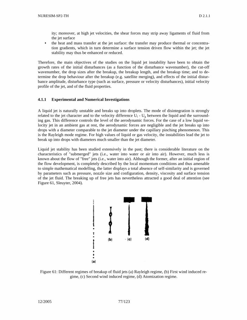
NURESIM-SP2-TH D 2.1.1
12/2005 77/123
ity; moreover, at high jet velocities, the shear forces may strip away ligaments of fluid from the jet surface
• the heat and mass transfer at the jet surface: the transfer may produce thermal or concentra-tion gradients, which in turn determine a surface tension driven flow within the jet; the jet stability may thus be enhanced or reduced.
Therefore, the main objectives of the studies on the liquid jet instability have been to obtain the growth rates of the initial disturbances (as a function of the disturbance wavenumber), the cut-off wavenumber, the drop sizes after the breakup, the breakup length, and the breakup time; and to de-termine the drop behaviour after the breakup (e.g. satellite merging), and effects of the initial distur-bance amplitude, disturbance type (such as surface, pressure or velocity disturbances), initial velocity profile of the jet, and of the fluid properties.
4.1.1 Experimental and Numerical Investigations
A liquid jet is naturally unstable and breaks up into droplets. The mode of disintegration is strongly related to the jet character and to the velocity difference Ul - Ug between the liquid and the surround-ing gas. This difference controls the level of the aerodynamic forces. For the case of a low liquid ve-locity jet in an ambient gas at rest, the aerodynamic forces are negligible and the jet breaks up into drops with a diameter comparable to the jet diameter under the capillary pinching phenomenon. This is the Rayleigh mode regime. For high values of liquid or gas velocity, the instabilities lead the jet to break up into drops with diameters much smaller than the jet diameter. Liquid jet stability has been studied extensively in the past; there is considerable literature on the characteristics of "submerged" jets (i.e., water into water or air into air). However, much less is known about the flow of "free" jets (i.e., water into air). Although the former, after an initial region of the flow development, is completely described by the local momentum conditions and thus amenable to simple mathematical modelling, the latter displays a total absence of self-similarity and is governed by parameters such as pressure, nozzle size and configuration, density, viscosity and surface tension of the jet fluid. The breaking up of free jets has nevertheless attracted a good deal of attention (see Figure 61, Sleuyter, 2004).
Figure 61: Different regimes of breakup of fluid jets (a) Rayleigh regime, (b) First wind induced re-gime, (c) Second wind induced regime, (d) Atomization regime.
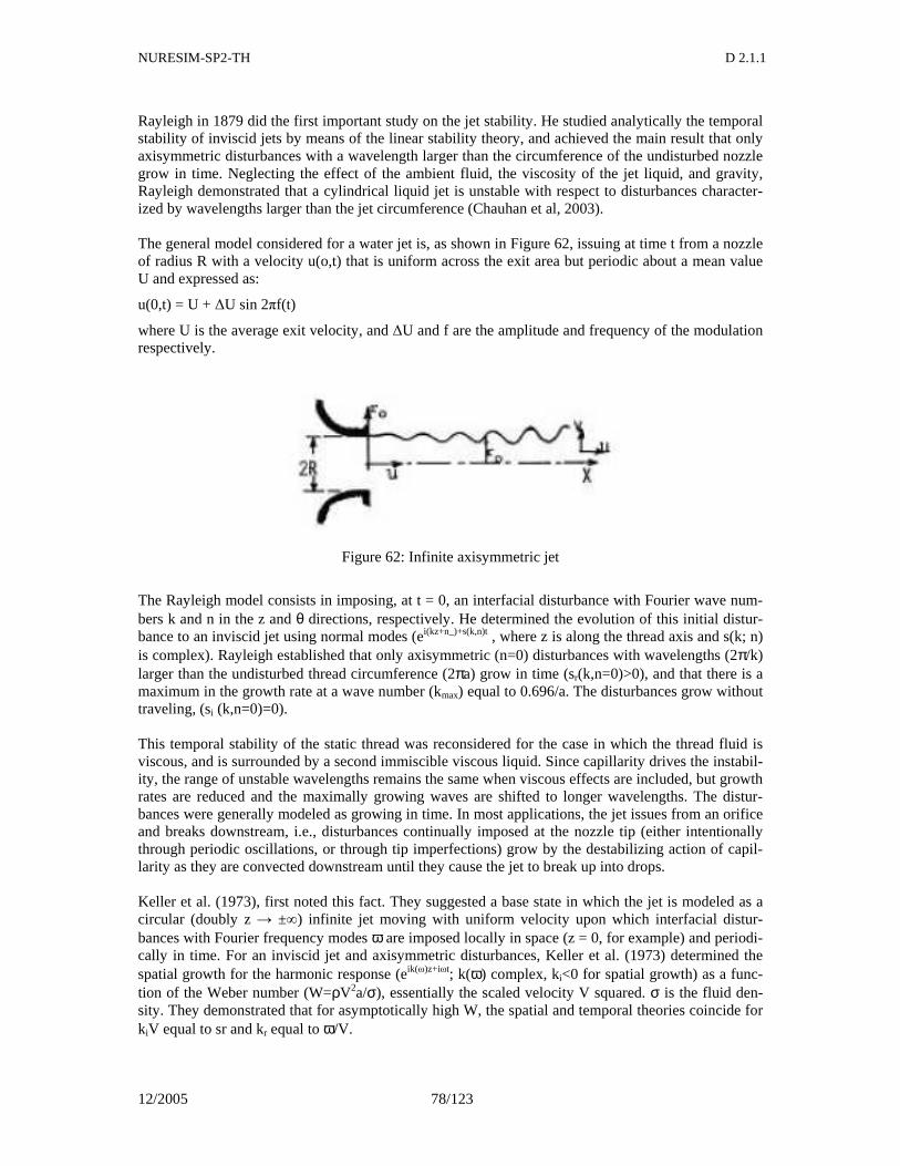
NURESIM-SP2-TH D 2.1.1
12/2005 78/123
Rayleigh in 1879 did the first important study on the jet stability. He studied analytically the temporal stability of inviscid jets by means of the linear stability theory, and achieved the main result that only axisymmetric disturbances with a wavelength larger than the circumference of the undisturbed nozzle grow in time. Neglecting the effect of the ambient fluid, the viscosity of the jet liquid, and gravity, Rayleigh demonstrated that a cylindrical liquid jet is unstable with respect to disturbances character-ized by wavelengths larger than the jet circumference (Chauhan et al, 2003). The general model considered for a water jet is, as shown in Figure 62, issuing at time t from a nozzle of radius R with a velocity u(o,t) that is uniform across the exit area but periodic about a mean value U and expressed as:
u(0,t) = U + ∆U sin 2πf(t)
where U is the average exit velocity, and ∆U and f are the amplitude and frequency of the modulation respectively.
Figure 62: Infinite axisymmetric jet
The Rayleigh model consists in imposing, at t = 0, an interfacial disturbance with Fourier wave num-bers k and n in the z and θ directions, respectively. He determined the evolution of this initial distur-bance to an inviscid jet using normal modes (ei(kz+n_)+s(k,n)t , where z is along the thread axis and s(k; n) is complex). Rayleigh established that only axisymmetric (n=0) disturbances with wavelengths (2π/k) larger than the undisturbed thread circumference (2πa) grow in time (sr(k,n=0)>0), and that there is a maximum in the growth rate at a wave number (kmax) equal to 0.696/a. The disturbances grow without traveling, (si (k,n=0)=0). This temporal stability of the static thread was reconsidered for the case in which the thread fluid is viscous, and is surrounded by a second immiscible viscous liquid. Since capillarity drives the instabil-ity, the range of unstable wavelengths remains the same when viscous effects are included, but growth rates are reduced and the maximally growing waves are shifted to longer wavelengths. The distur-bances were generally modeled as growing in time. In most applications, the jet issues from an orifice and breaks downstream, i.e., disturbances continually imposed at the nozzle tip (either intentionally through periodic oscillations, or through tip imperfections) grow by the destabilizing action of capil-larity as they are convected downstream until they cause the jet to break up into drops. Keller et al. (1973), first noted this fact. They suggested a base state in which the jet is modeled as a circular (doubly z → ±∞) infinite jet moving with uniform velocity upon which interfacial distur-bances with Fourier frequency modes ω are imposed locally in space (z = 0, for example) and periodi-cally in time. For an inviscid jet and axisymmetric disturbances, Keller et al. (1973) determined the spatial growth for the harmonic response (eik(ω)z+iωt; k(ω) complex, ki<0 for spatial growth) as a func-tion of the Weber number (W=ρV2a/σ), essentially the scaled velocity V squared. σ is the fluid den-sity. They demonstrated that for asymptotically high W, the spatial and temporal theories coincide for kiV equal to sr and kr equal to ω/V.
NURESIM-SP2-TH D 2.1.1
12/2005 79/123
In addition, for moderate W and dimensionless frequencies or Strouhal numbers (ωa/V) between zero and approximately one (the exact cutoff being a function of W), localized periodic disturbances still grow axially, but with wave lengths and linear growth rates that increasingly deviate from the tempo-ral theory as W is reduced. For frequencies in the unstable range, the drop size and distance to breakup can be predicted (assuming the linear theory is valid up to break-up; see the experimental verification discussed below) since the drops which are formed then have a size which scales as 1/kr(ω), and the distance downstream from breakup is of order 1/ki(ω). A large body of experiments studying the breakup of jets into drops have been undertaken, usually by applying disturbances generated with different techniques:
• Acoustic induced vibrations • Electro-magnetic induced vibrations • Mechanically induced vibrations • Thermal modulation of the surface tension.
Generally a sinusoidal periodic disturbance of frequency ω applied at the nozzle tip using acoustic, electromagnetic, or piezo-electric-induced pressure vibrations or a vibrating impinging needle. In all the above studies the distance between two successive peaks determines the wavelength of the distur-bances. The (spatial) growth rate was measured by measuring the breakup length or by measuring the amplitude of the disturbance at two successive peak/troughs and assuming exponential spatial growth. In addition the waves were assumed to convect with the jet velocity and thus that the temporal theory applies in the moving frame. Drazin and Reid, 1982 performed stability analysis for plane jets similar to Rayleigh’s analysis for a cylindrical jet. They found that non-viscous infinite plane jet is stable to all disturbances because sur-face tension has always a damping effect and forces the surface back to its initial shape when per-turbed. Sou and Tomiyama, 2003 studied the effect of turbulent cavitating flow within an atomization nozzle and liquid jet discharged from the nozzle. A numerical simulation based upon a hybrid numerical method considering combination of a two-way bubble tracking method and an interface tracking method. The hybrid method enabled to examine the effects of cavitation bubbles on liquid jet defor-mation. As a result of bubble tracking simulations and hybrid simulations, the following conclusions were obtained:
• The method gives good predictions for the distributions of pressure and bubbles within the nozzle, the relation between injection pressure and liquid flow rate, and the behaviour of cavi-tation bubbles such as the formation of vortex cavitation and collapse in a reentrant flow re-gion.
• The collapse of bubble clouds within liquid jet enhances the deformation of liquid jet. • The vortices generated in a nozzle play more important role in the jet deformation than inter-
facial forces acting on liquid jet do. Cinnella et al., 2004, performed a preliminary step towards the understanding of non axisymmetric liquid jet breakup mechanisms. Specifically, the objective was to investigate whether, and how, the use of noncircular nozzles influences the jet breakup properties. A numerical approach is used using a finite volume code. The Volume of Fluid (VOF) front capturing methodology was considered to rep-resent the liquid/gas interface. Numerical results concern jets in the Rayleigh regime emanating from either circular or square-edged nozzles were emphasized. In their model the jets are subject to a sinu-ous velocity perturbation at the nozzle inlet, and are characterized by growing values of the Weber number. For square jets, at least in the range of Weber considered, a significant reduction of the breakup length with respect to the axisymmetric case, and a reduced sensitivity of the breakup length
NURESIM-SP2-TH D 2.1.1
12/2005 80/123
to the jet Weber number have been found. These phenomena seem related to the appearance of secon-dary flows, whose intensity grows with jet speed, which promote jet instability. A numerical investigation was carried out by Ibrahim, 1997 on the evolution of asymmetrical distur-bances on a viscous liquid jet in an inviscid gas medium. The asymmetrical disturbances were shown to become relevant at high Weber numbers. The effects of the gas to liquid density ratio and of the Ohnesorge number were investigated. On the other hand, Furlani, 2005 studied the effect of surface tension on the break up and drop forma-tion. The surface tension was locally modulated by heating the surface of the jet as it leaves its orifice. An analytical closed-form expression for the time dependence of the jet radius was derived. This ex-pression enables rapid parametric analysis of jet instability (time to drop formation) as a function of jet radius, velocity, viscosity, density, and surface tension. Sami and Ansari, 1981, studied the effects of velocity profile relaxation on the instability of laminar liquid jets cast from long tubes. There is substantial evidence to indicate that the result of these effects are similar to the result of relative motion between the jet and its ambient gas, i.e. as the velocity is increased, the jet length reaches a maximum and then decreases as the velocity is increased further. The effect of velocity profile relaxation on the drop size distribution, however, has not yet been meas-ured. The breakup of the jet can additionally be dependent on the nozzle geometry. Karasawa et al. (1992) clearly showed the effect of the nozzle length on the development of instabilities on the liquid jet sur-face. When the nozzle length increases, the jet surface shape changes from smooth to corrugated. The initial velocity profile at the nozzle exit can thus have a real influence on the liquid jet stability and the sensitivity of the jet to the velocity profile is particularly true for low mean velocity (laminar) flows. While the effect of nozzle turbulence on the drop size distribution was experimentally investi-gated by Sterling, and Abbott, 2004. Pan and Suga, 2004 used Direct Numerical Simulations (DNS) to simulate water jets into air. The level-set method is adopted in the present simulations as a front-capture methodology to track the dy-namically evolving liquid/gas interface. The Reynolds number at jet exit ranges from 480 to 15000, Weber number from 3 to 10000. The liquid/gas density ratio is 816. The dynamic features of liq-uid/gas jet flows and the primary breakup are reasonably captured by the present simulations. The numerical simulations confirm the effects of the gravity and the surface tension forces on the breakup process at relative low Reynolds numbers. It is also observed that the radial velocity, which is induced during the relaxation of the axial liquid velocity profile, leads to the disintegration of high speed jets. (see Figure 63 and Figure 64). The study supports the experimental observation that high-speed lami-nar jets are more prone to be unstable and in an extremely violent pattern much sooner than fully de-veloped turbulent jets to break up. However, the velocity profile relaxation with turbulence effects needs to be further investigated. Demuren and Wilson, 1999 investigated complex streamwise vorticity fields in the evolution of non-circular jets. Generation mechanisms are investigated via Reynolds-averaged (RANS), large-eddy (LES) and direct numerical (DNS) simulations of laminar and turbulent rectangular jets. Complex vortex interactions are found in DNS of laminar jets, but axis-switching is observed only when a sin-gle instability mode is present in the incoming mixing layer. With several modes present, the struc-tures are not coherent and no axis-switching occurs. RANS computations also produce no axis-switching. On the other hand, LES of high Reynolds number turbulent jets produce axis-switching even for cases with several instability modes in the mixing layer. Three-dimensional simulations of laminar and turbulent jets with rectangular cross-section were performed. At low Reynolds numbers DNS were performed, while at higher Reynolds numbers LES or RANS computations were per-
NURESIM-SP2-TH D 2.1.1
12/2005 81/123
formed. Figure 65 shows contours of the instantaneous total vorticity for rectangular jets at low Rey-nolds number (=750) along major and minor axes, respectively.
Figure 63: Water jet into air at Re=480, We=7.45. Mesh resolution: D/∆=20
It was also shown that with the addition of the sub-harmonic mode the tendency is towards jet bifurca-tion. Figure 66 shows the instantaneous total and streamwise vorticity from the LES of rectangular jets at high Reynolds number (=75,000), with broad-mode instabilities, along minor and major axes, respectively. There is no discernible streamwise vorticity in the first 2 diameters, and the evolution trends are quite different from those of the laminar jet: there is expansion in the minor-axis plane and contraction in the major-axis plane. As a conclusion, the origin of secondary flow or streamwise vorticity under different conditions of the spectral content of the initial jet mixing layer or Reynolds number are investigated through budgets of the mean streamwise vorticity derived from the DNS and LES data. Inviscid mechanisms, which can be explained by the evolution of vortex rings are responsible for the distortion of laminar jets with discrete mode forcing. Natural laminar jets evolve in an uneventful manner from rectangular to circu-lar cross-section. In turbulent jets, streamwise vorticity is generated by terms involving derivatives of
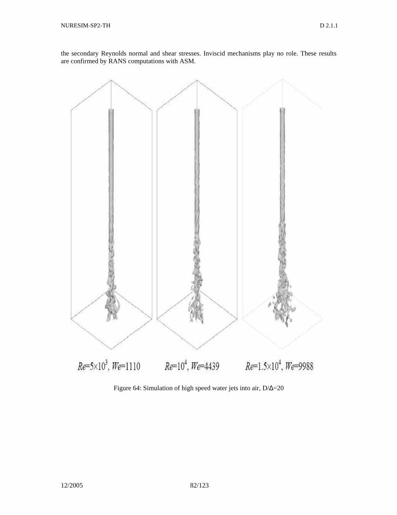
NURESIM-SP2-TH D 2.1.1
12/2005 82/123
the secondary Reynolds normal and shear stresses. Inviscid mechanisms play no role. These results are confirmed by RANS computations with ASM.
Figure 64: Simulation of high speed water jets into air, D/∆=20
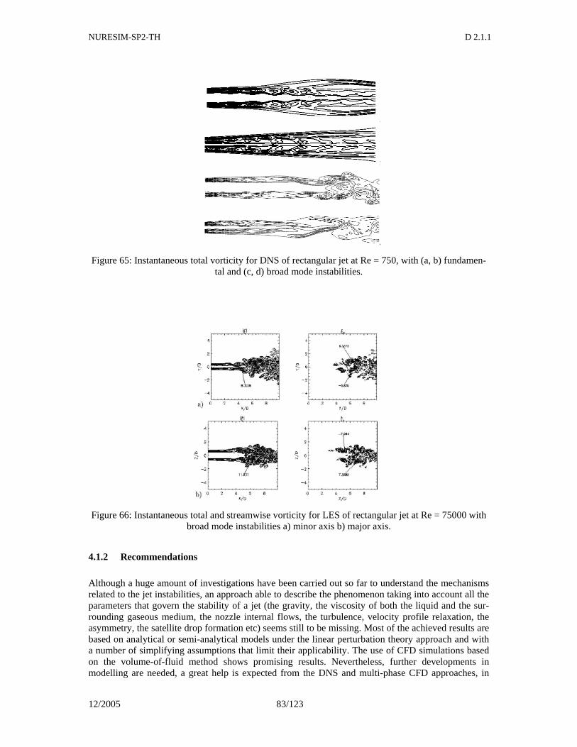
NURESIM-SP2-TH D 2.1.1
12/2005 83/123
Figure 65: Instantaneous total vorticity for DNS of rectangular jet at Re = 750, with (a, b) fundamen-tal and (c, d) broad mode instabilities.
Figure 66: Instantaneous total and streamwise vorticity for LES of rectangular jet at Re = 75000 with broad mode instabilities a) minor axis b) major axis.
4.1.2 Recommendations
Although a huge amount of investigations have been carried out so far to understand the mechanisms related to the jet instabilities, an approach able to describe the phenomenon taking into account all the parameters that govern the stability of a jet (the gravity, the viscosity of both the liquid and the sur-rounding gaseous medium, the nozzle internal flows, the turbulence, velocity profile relaxation, the asymmetry, the satellite drop formation etc) seems still to be missing. Most of the achieved results are based on analytical or semi-analytical models under the linear perturbation theory approach and with a number of simplifying assumptions that limit their applicability. The use of CFD simulations based on the volume-of-fluid method shows promising results. Nevertheless, further developments in modelling are needed, a great help is expected from the DNS and multi-phase CFD approaches, in
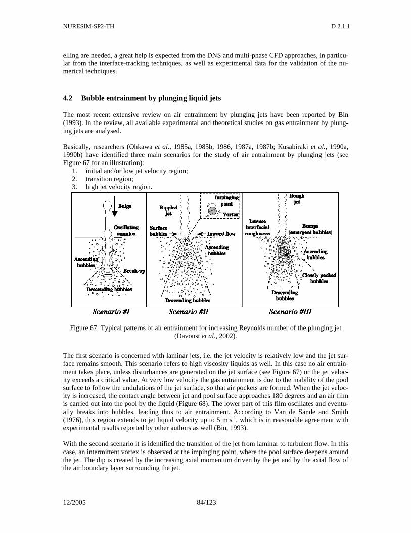
NURESIM-SP2-TH D 2.1.1
12/2005 84/123
elling are needed, a great help is expected from the DNS and multi-phase CFD approaches, in particu-lar from the interface-tracking techniques, as well as experimental data for the validation of the nu-merical techniques.
4.2 Bubble entrainment by plunging liquid jets
The most recent extensive review on air entrainment by plunging jets have been reported by Bin (1993). In the review, all available experimental and theoretical studies on gas entrainment by plung-ing jets are analysed. Basically, researchers (Ohkawa et al., 1985a, 1985b, 1986, 1987a, 1987b; Kusabiraki et al., 1990a, 1990b) have identified three main scenarios for the study of air entrainment by plunging jets (see Figure 67 for an illustration):
1. initial and/or low jet velocity region; 2. transition region; 3. high jet velocity region.
Figure 67: Typical patterns of air entrainment for increasing Reynolds number of the plunging jet (Davoust et al., 2002).
The first scenario is concerned with laminar jets, i.e. the jet velocity is relatively low and the jet sur-face remains smooth. This scenario refers to high viscosity liquids as well. In this case no air entrain-ment takes place, unless disturbances are generated on the jet surface (see Figure 67) or the jet veloc-ity exceeds a critical value. At very low velocity the gas entrainment is due to the inability of the pool surface to follow the undulations of the jet surface, so that air pockets are formed. When the jet veloc-ity is increased, the contact angle between jet and pool surface approaches 180 degrees and an air film is carried out into the pool by the liquid (Figure 68). The lower part of this film oscillates and eventu-ally breaks into bubbles, leading thus to air entrainment. According to Van de Sande and Smith (1976), this region extends to jet liquid velocity up to 5 m·s-1, which is in reasonable agreement with experimental results reported by other authors as well (Bin, 1993). With the second scenario it is identified the transition of the jet from laminar to turbulent flow. In this case, an intermittent vortex is observed at the impinging point, where the pool surface deepens around the jet. The dip is created by the increasing axial momentum driven by the jet and by the axial flow of the air boundary layer surrounding the jet.
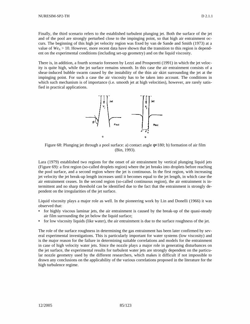
NURESIM-SP2-TH D 2.1.1
12/2005 85/123
Finally, the third scenario refers to the established turbulent plunging jet. Both the surface of the jet and of the pool are strongly perturbed close to the impinging point, so that high air entrainment oc-curs. The beginning of this high jet velocity region was fixed by van de Sande and Smith (1973) at a value of WeA > 10. However, more recent data have shown that the transition to this region is depend-ent on the experimental conditions (including set-up geometry) and on the liquid viscosity. There is, in addition, a fourth scenario foreseen by Lezzi and Prosperetti (1991) in which the jet veloc-ity is quite high, while the jet surface remains smooth. In this case the air entrainment consists of a shear-induced bubble swarm caused by the instability of the thin air skirt surrounding the jet at the impinging point. For such a case the air viscosity has to be taken into account. The conditions in which such mechanism is of importance (i.e. smooth jet at high velocities), however, are rarely satis-fied in practical applications.
Figure 68: Plunging jet through a pool surface: a) contact angle φ<180; b) formation of air film (Bin, 1993).
Lara (1979) established two regions for the onset of air entrainment by vertical plunging liquid jets (Figure 69): a first region (so-called droplets region) where the jet breaks into droplets before reaching the pool surface, and a second region where the jet is continuous. In the first region, with increasing jet velocity the jet break-up length increases until it becomes equal to the jet length, in which case the air entrainment ceases. In the second region (so-called continuous region), the air entrainment is in-termittent and no sharp threshold can be identified due to the fact that the entrainment is strongly de-pendent on the irregularities of the jet surface. Liquid viscosity plays a major role as well. In the pioneering work by Lin and Donelli (1966) it was observed that: • for highly viscous laminar jets, the air entrainment is caused by the break-up of the quasi-steady
air film surrounding the jet below the liquid surface; • for low viscosity liquids (like water), the air entrainment is due to the surface roughness of the jet. The role of the surface roughness in determining the gas entrainment has been later confirmed by sev-eral experimental investigations. This is particularly important for water systems (low viscosity) and is the major reason for the failure in determining suitable correlations and models for the entrainment in case of high velocity water jets. Since the nozzle plays a major role in generating disturbances on the jet surface, the experimental results for turbulent water jets are strongly dependent on the particu-lar nozzle geometry used by the different researchers, which makes it difficult if not impossible to drawn any conclusions on the applicability of the various correlations proposed in the literature for the high turbulence regime.
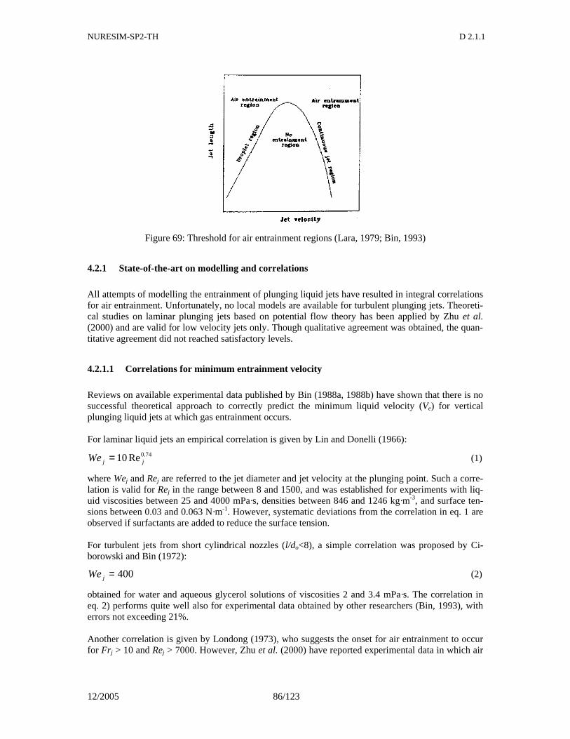
NURESIM-SP2-TH D 2.1.1
12/2005 86/123
Figure 69: Threshold for air entrainment regions (Lara, 1979; Bin, 1993)
4.2.1 State-of-the-art on modelling and correlations
All attempts of modelling the entrainment of plunging liquid jets have resulted in integral correlations for air entrainment. Unfortunately, no local models are available for turbulent plunging jets. Theoreti-cal studies on laminar plunging jets based on potential flow theory has been applied by Zhu et al. (2000) and are valid for low velocity jets only. Though qualitative agreement was obtained, the quan-titative agreement did not reached satisfactory levels.
4.2.1.1 Correlations for minimum entrainment velocity
Reviews on available experimental data published by Bin (1988a, 1988b) have shown that there is no successful theoretical approach to correctly predict the minimum liquid velocity (Ve) for vertical plunging liquid jets at which gas entrainment occurs. For laminar liquid jets an empirical correlation is given by Lin and Donelli (1966):
74.0Re10 jjWe = (1)
where Wej and Rej are referred to the jet diameter and jet velocity at the plunging point. Such a corre-lation is valid for Rej in the range between 8 and 1500, and was established for experiments with liq-uid viscosities between 25 and 4000 mPa·s, densities between 846 and 1246 kg·m-3, and surface ten-sions between 0.03 and 0.063 N·m-1. However, systematic deviations from the correlation in eq. 1 are observed if surfactants are added to reduce the surface tension. For turbulent jets from short cylindrical nozzles (l/do<8), a simple correlation was proposed by Ci-borowski and Bin (1972):
400=jWe (2)
obtained for water and aqueous glycerol solutions of viscosities 2 and 3.4 mPa·s. The correlation in eq. 2) performs quite well also for experimental data obtained by other researchers (Bin, 1993), with errors not exceeding 21%. Another correlation is given by Londong (1973), who suggests the onset for air entrainment to occur for Fr j > 10 and Rej > 7000. However, Zhu et al. (2000) have reported experimental data in which air
NURESIM-SP2-TH D 2.1.1
12/2005 87/123
entrainment does not occur beyond the limits given by Londong, if the jet nozzle is designed in such a way to reduce disturbances of the jet surface. The onset for entrainment in the droplet region can be approximated by the correlation:
937.079.10
50 104.1 jj WeddL −−⋅= (3)
obtained on the basis of data from Bin (1988a) and Kumagai and Endoh (1983). The relation is valid for nozzles of diameters ranging from 2 to 10.2 mm. The accuracy of the correlation is estimated to be around 10%. However, experiments performed with more viscous fluids suggest that the effect of liq-uid viscosity and surface tension should be included as well. The air entrainment in the droplet region ceases when the jet length becomes equal to the jet break-up length. Experimental data points can be approximated by a power law equation of the type:
pB cWedL 00 = (4)
where LB is the break-up length of the liquid jet. The power exponent in eq. (4) is in the range 0.44 to 0.52 and is apparently independent on the nozzle diameter. With regards to the continuous jet region, unfortunately no correlations can be found for the minimum entrainment velocity. Such a finding comes not as a surprise, since in the continuous region the gas entrainment is strongly dependent on the perturbations travelling on the jet surface, which are in turn strongly dependent on the nozzle geometry.
4.2.1.2 Correlations for volumetric flow rate of entrained gas
Low jet velocity region For the low velocity region it is assumed that bubble entrainment is caused as a result of surface ten-sion forces preventing the receiving flows from following the disturbances of the jet (Sene, 1988). On
the basis of theoretical analysis, Sene found that the air entrainment QA is proportional to 3jV and is
strongly dependent on the turbulence intensity in the jet. Van de Sande (1976) suggested that the air entrainment beyond the break-up point of the jet is directly related to the kinetic energy (or power) of the jet and can be expressed as:
( )
=
=− 5.15.032
0
75.0
sin
015.0
αjj
A
LVdX
XQ (5)
By comparison with other experimental data available in literature (Bin, 1993), it appears that eq. (5) gives the upper limit of QA obtainable for nozzles with sufficient cylindrical sections (l/do≥10). Jet produced by shorter nozzles will lead to less gas entrainment at the same value of X. It is interesting to note that eq. (5) predicts, in accordance with experimental evidence, that inclined jets entrain more air than vertical ones. More recently El Hammoumi et al. (2002) attempted the derivation of a correlation on the basis of dimensionless analysis and proposed the following expression for laminar jets:
32.047.129.110.09 ~1085.5 jjjja FrZHWeWe −−⋅= (6)
High jet velocity region For the high jet velocity region, Sene (1988) assumed that an air layer around the liquid jet is put into motion by the action of the shear stresses at the jet surface and that this air layer is successively bro-
NURESIM-SP2-TH D 2.1.1
12/2005 88/123
ken into bubbles by instability waves on its surface. By a pressure gradient in the air layer, Sene (1988) obtained the following relation for the gas entrainment for circular jets:
jjL
AA dV
gQ 23
sin
∝
αρµ
(7)
Eq. (7) suggests that for high jet velocities, the air entrainment is independent on the surface tension of the liquid and that it can be scaled up by relating it to the jet circumference, (QA/(πdj) for circular jets, or by referring it to the unit width of the jet in case of planar jets). Note that the dependence on the surface tension should be expected for the low velocity jet region. Other authors (Bin, 1993) suggest two mechanisms for air entrainment by high velocity liquid jets. The first mechanism is related to the entrainment QA1 of the air cylinder (air envelope) that surrounds the jet. The second mechanism is related to the entrainment QA2 of the air in the boundary layer that develops outside the air envelope. The total air entrainment is given by the sum of the two compo-nents QA1 + QA2. The air captured by the jet roughness can be written as:
( )20
201 4
ddV
Q jA −=π
(8)
where the spreading of the liquid jet dj can be derived by means of the equation:
( )mlengthA
j Wecd
dRe
0
= (9)
with Relength = VoLj/νL. For this relation, Van de Sande and Smith (1973) proposed c=0.125 and m=1/6. The air dragged as laminar boundary layer can be expressed as:
∫∞
=2
2 2jd
AA drrVQ π (10)
being VA the local velocity in the boundary layer at a given radius measured from the jet axis. From a momentum balance in the air boundary layer the following expression can be found for the air veloc-ity:
−
+
−=
jjj
A
d
r
d
r
d
r
V
V 2ln
12ln
22ln
21 4
43
30 βββ
(11)
where β is a coefficient dependent on the jet geometry. Expressions for β are given by Bin (1993). For the transition region between low and high velocity jets, van de Sande (1974) suggested a simple procedure based on the interpolation between eq. (6) and eqs.(8)-(10). Correlations are given also in terms of entrainment ratio QA/QW. Bin (1993) proposed the following relation for the gas flow rate entrained by a vertical plunging jet:
( ) 4.00
28.004.0 dLFrQQ jjwA = (12)
valid for ( ) 1000 ≤dL j , ( ) 100 ≥dl and ( ) 104.00
28.0 ≥dLFr jj , within an uncertainty of ± 20%.
NURESIM-SP2-TH D 2.1.1
12/2005 89/123
For shorter nozzles, the ration QA/QW will be smaller, at the same values of the main parameters (Vj, Lj, d0). For nozzle with ( ) 40 ≥dl , the entrainment ratio is still proportional to 0dL j raised to a
power of 0.5-0.6, provided that ( ) 1000 ≤dL j . For ( ) 1000 >dL j , this power is 0.70.
Additional experimental evidence suggests that the multiplying constant in eq. (12) might depend on the level of turbulence of the jet. As for the laminar jet, a correlation was proposed by El Hammoumi et al. (2002) for turbulent jets as well:
89.059.277.134.12 ~1037.1 jjjja FrZHWeWe −⋅= (13)
The correlation was obtained with several circular nozzles of diameters ranging from 2.9 to 11 mm and aspect ratio larger than 50. Wjj ranged from 66 to 967, Z from 1.2·103 to 56.66·103, Fr jj from 6.17
to 71.62 and the aspect ratio ( )jdHH =~ from 14.55 to 82.76.
4.2.2 Characteristics of bubble dispersion
4.2.2.1 Bubbles size distribution
The gas bubbles entrained by plunging liquid jets can be grouped into two distinct regions. The first region contains the primary bubbles, having diameter smaller than 1 mm (Lahey and Bonetto, 1993, report about bubbles smaller than 20 µm). The second region, surrounding the primary bubbles, con-tains bigger rising bubbles (secondary bubbles). In the latter region, Sauter diameters of about 3-4 mm have been observed in water-air systems, independently on jet velocity and nozzle diameter. The bub-ble size distribution is close to the normal distribution. A few attempts have been made to derive cor-relations for the entrained bubbles diameters, but with quite limited range of validity. Simonin pro-posed a quasi-theoretical relationship for the equivalent bubble diameter as function of the entrain-ment ratio:
( ) 313103.4 wAb QQd −⋅= [m] (14)
which worked fairly well with the experimental data by Bin (1993).
4.2.2.2 Distribution of gas concentration
For the bubble distributions below the pool surface Cummings and Chanson (1997a) proposed a sim-ple diffusion model. The solution for the bubble concentrations is given by:
( )
( )
−−=
−+
−
1
1
1*0
1
4
1
1
1* 2
1
4
11
1
21
*
r
xxrr
DIe
r
xxDQ
QC r
xxrr
D
w
A (15)
where x is the distance from the jet nozzle along the flow direction, r is the radial distance from jet vertical axis, D*=D t/(V1r1) a dimensionless bubble diffusivity coefficient, r1 the radial position at which the bubble concentration C assumes maximum value, and I0 is the modified Bessel function and D*=D t/(V1r1), x is the distance along the flow direction. See Figure 70 for a sketch of the corre-sponding geometry and system of coordinates. The profile of eq. (15) is in very good agreement with experimental results reported by Cummings and Chanson (1997b) and Bonetto and Lahey (1993).
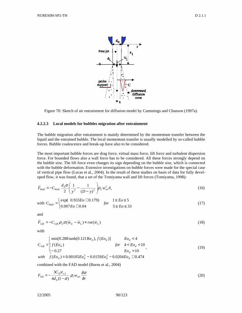
NURESIM-SP2-TH D 2.1.1
12/2005 90/123
Figure 70: Sketch of air entrainment for diffusion model by Cummings and Chanson (1997a).
4.2.2.3 Local models for bubbles migration after entrainment
The bubble migration after entrainment is mainly determined by the momentum transfer between the liquid and the entrained bubble. The local momentum transfer is usually modelled by so-called bubble forces. Bubble coalescence and break-up have also to be considered. The most important bubble forces are drag force, virtual mass force, lift force and turbulent dispersion force. For bounded flows also a wall force has to be considered. All these forces strongly depend on the bubble size. The lift force even changes its sign depending on the bubble size, which is connected with the bubble deformation. Extensive investigations on bubble forces were made for the special case of vertical pipe flow (Lucas et al., 2004). In the result of these studies on basis of data for fully devel-oped flow, it was found, that a set of the Tomiyama wall and lift forces (Tomiyama, 1998):
rrelLb
WallWall nwyDy
dCF
rr2
22 )(
11
2ρα
−−−= (16)
with
≤≤≤≤
++−
=335
51
04.0007.0
)179.0933.0exp(
Eo
Eofor
Eo
EoCWall (17)
and
)()( LLGLLiftLift wrotwwCFrrrr
×−−= αρ (18)
with
474.00204.00159.000105.0)(
1027.0
104)(
4)](),Re121.0tanh(288.0min[
23 +−−=
>−<<
<=
dddd
d
dd
ddb
Lift
EoEoEoEofwith
Eo
EoforEof
EoEof
C, (19)
combined with the FAD model (Burns et al., 2004)
rw
d
CF rell
b
LtDTD ∂
∂−
−= αρα
ν)1(4
3 , (20)
NURESIM-SP2-TH D 2.1.1
12/2005 91/123
are applicable for a wide range of flow situations. Similar results were obtained using the wall force model of Hosokawa et al. (2002)
= EoCb
Wall 0217.0,Re
7max
9.1 (21)
together with the deformation force, introduced by Lucas et al. (2004)
xb
deform nxx
xx
xx
xx
xdF
rr2)
1
1arcsin4
1
1arcsin3(
1
1
36
64
62
6
62−
−
−−−
−+−
−= σ (22)
instead of the Tomiyama wall force. Here x is the distance from the wall divided by the bubble radius. On the other hand some disagreement to the experimental results was found for developing flow (Lu-cas et al. 2005). That’s why it is important to test and validate the applicability of these models for bubble forces in the impinging jet zone. Different models for bubble coalescence and break-up can be found in literature, but the resulting coa-lescence rates and break-up frequencies differ in wide range. Among the most popular models are the coalescence model by Prince and Blanch (1990) and the break-up model by Luo and Svendson (1996). It has to be tested whether these models or other models from literature are suitable for the simulation of bubble coalescence and break-up up in the highly turbulent zone of the impinging jet region.
4.2.3 Further research needs
From the literature review presented in the previous chapters, it is clear that development of local models are needed if the gas entrainment has to be modelled by means of CFD codes. For PTS appli-cations, the region of high liquid velocity jets is of major interest. In this region, the strongest contri-bution to the gas entrainment is given by the drag of the gas boundary layer driven by the liquid jet. The formation of entrained gas bubbles in such a case is strongly dependent on the rough-ness/perturbations of the jet surface. A possibility that could be foreseen is a development of appropriate ‘wall’ functions for the modelling of the gas boundary layer region surrounding the liquid jet. Such an approach would be justified by the high density differences between gas and liquid phases and thus by the fact that the gas phase sees the liquid phase as a solid wall. For such an approach, appropriate boundary conditions have to be im-posed. Some steps in this direction have already been made (Pigny, 2003), with regards to the model-ling of stratified flows with CFD codes, though several questions remain still open. Given the complexity of the problem, case studies should be considered in which few effects play a role at the same time. As an example, it might be interesting to consider a simplified test case, in which at the pool surface a mixture of liquid and gas phase is given as boundary condition. In such a test case, the bubble dispersion below the surface can be studied as function of liquid/gas velocities and bubble size distribution, separating this effect from the influence of jet entrainment.
4.2.4 Nomenclature for section 4.2
d0 = nozzle diameter [m] db = equivalent bubble diameter [m] dj = jet diameter [m] dh = horizontal bubble diameter [m]
NURESIM-SP2-TH D 2.1.1
12/2005 92/123
D = diameter of the pipe [m] F = force per unit volume [N m-3] H = distance between nozzle exit and jet impact point [m] l = length of cylindrical section of nozzle [m] L j = jet length [m] V0 = jet velocity at nozzle outlet [m·s-1] VA = local velocity of boundary layer air [m·s-1] V j = jet velocity [m·s-1] Ve = minimum gas entrainment velocity [m·s-1] QA = air volumetric flow rate [m3·s-1] QW = liquid volumetric flow rate [m3·s-1] wrel = relative velocity between gas and liquid [m/s] y = distance from the wall [m] x = 2.*y/db related distance from the wall [-] Greek letters α = angle of jet inclination [deg] α = gas volume fraction [-] ρ = density [Kg·m-3] νL = liquid kinematic viscosity [m2·s-1] σ = surface tension [N m-1] Subscript A = air G = gas L = liquid t = turbulent Dimensionless numbers
σρρ 2)( bgl dg
Eo−
=
σρρ 2)( hgl
d
dgEo
−=
( )02 gdVFr jj =
( )jjjj gdVFr 2=
( )Ljej dV ν=Re
l
brellb
dw
µρ
=Re
( )σρ jAaa dVWe 2=
( )σρ jeLj dVWe 2=
( )σρ jLLjj dVWe 2=
jLL dZ σρν=
NURESIM-SP2-TH D 2.1.1
12/2005 93/123
4.3 Turbulence
Condensation is mainly dependent on the interfacial structure and on the turbulent mixing in the liquid phase. Many research works support that turbulence behaviour near the interface plays a dominant role for the interfacial transfers. For ECC injection cases, the turbulence mainly comes from impact of water jet (Janicot et al. 1993). The COSI tests (Bestion et al. 1989) simulated the ECC injection in a cold leg. They showed that most of the condensation occurs in a small area in the very vicinity of the injection jet. Some of it occurs on the jet surface itself before entering the free surface but it should not be the major part. Another part is due to entrained bubbles of steam below the free surface which are likely to collapse rapidly. The most important part is probably at the free surface itself in a region close to the jet which is influenced by large scale turbulence induced by the jet. Thus, as a first step to simulate such scenarios, an adequate modelling of turbulence due to the jet is necessary.
4.3.1 Turbulence production below the jet
One possible reason for the strong enhancement of condensation near a water jet is the turbulence in-duced by a water jet when it impacts on a water pool. Some experiments investigated the effects of a jet: • In the data of Iguchi et al. (1998), the water was injected through a straight circular pipe with an
inner diameter dinj = 5mm and a length L of 0.6m vertically into a cylindrical water bath with an inner diameter R of 0.2m and a height H of 0.39m .
• In the experiment of Bonetto and Lahey (1993) local data, including the size distribution of the bubble diameter, void fraction, bubble velocities and turbulent liquid velocities are obtained using a fiber optics phase Doppler anemometer system. A dual element conductivity probe is also used to measure the spatial distribution of the local void fraction. For the larger bubbles, the turbulence of the plunging jet is parametrically controlled using a specially designed nozzle and the turbu-lence intensity is measured using a Doppler anemometer system
The data of Iguchi et al (1998) were simulated with two-phase CFD by Yao et al. (2003) The data of Bonetto and Lahey (1993) were simulated within the ECORA project by both the NEPTUNE code and by the CFX code but without any comparison of the predicted and measured turbulence field
Simulations of Iguchi et al. experiment
Simulations were performed by Yao et al. (2003) using a preliminary version of the NEPTUNE code using a two-fluid model and a k-ε model. It appears that the predicted results of mean velocity field is quite good compared to the experimental data. The root-mean-square value of axial velocity fluctuation components are either well predicted or underestimated by up to 45%. Gas bubbles are entrained below the free surface by the jet whereas this phenomenon was not predicted by the model. The non predicted presence of gas bubbles below the free surface which may significantly increase the turbulence level may be a reason for the underesti-mation of the turbulence intensity. In a subcooled water such bubbles should rapidly collapse due to condensation and this phenomenon might not be so important Then the under prediction of bubble carry under should not be so important and would in real PTS applications, lead to a conservative pre-diction, since the steam condensing in the bulk liquid heats up the cold ECC water. Though there is some confidence on the predicting capability of standard k - ε model on the water jet impact effect, it still remains uncertain if the standard k-ε can predict the turbulent parameters near the free surface (which is very important to precisely predict the interfacial transfers) because of the lack
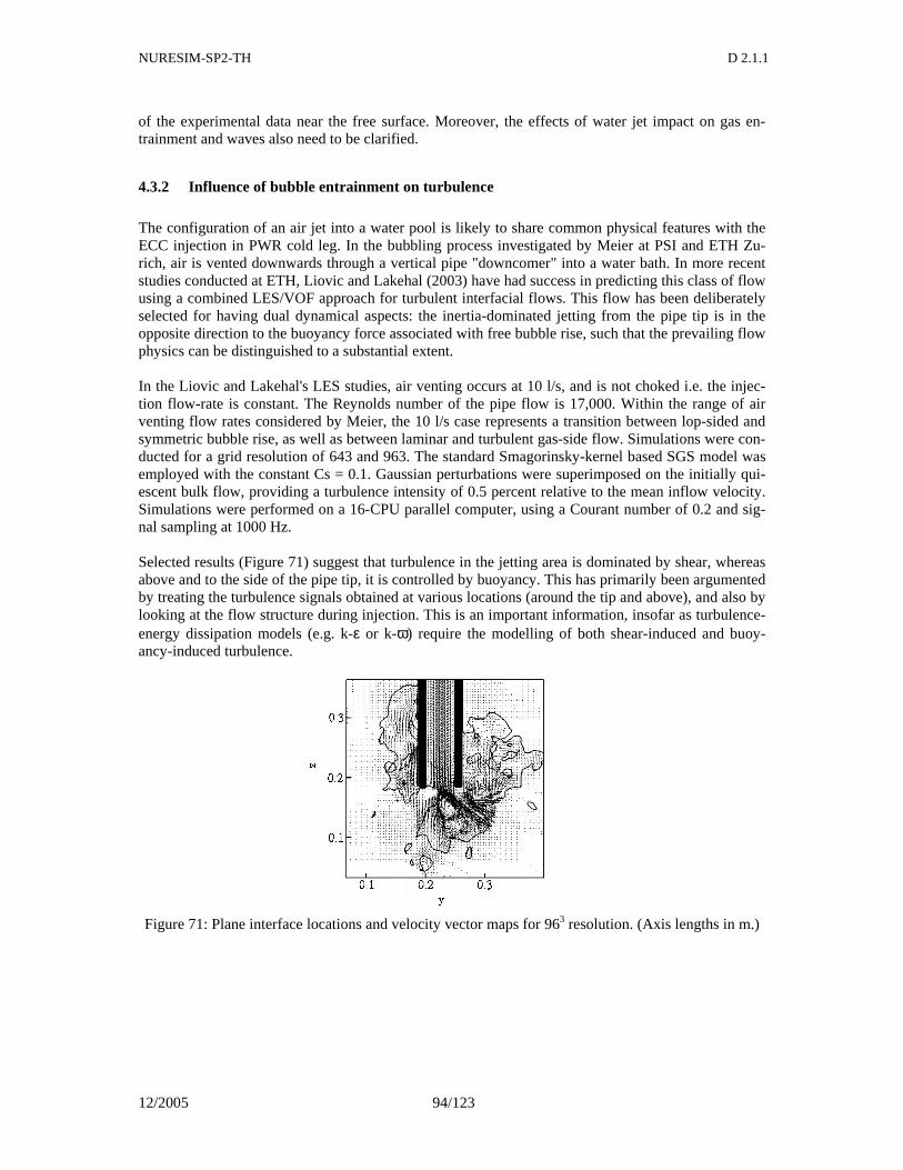
NURESIM-SP2-TH D 2.1.1
12/2005 94/123
of the experimental data near the free surface. Moreover, the effects of water jet impact on gas en-trainment and waves also need to be clarified.
4.3.2 Influence of bubble entrainment on turbulence
The configuration of an air jet into a water pool is likely to share common physical features with the ECC injection in PWR cold leg. In the bubbling process investigated by Meier at PSI and ETH Zu-rich, air is vented downwards through a vertical pipe "downcomer" into a water bath. In more recent studies conducted at ETH, Liovic and Lakehal (2003) have had success in predicting this class of flow using a combined LES/VOF approach for turbulent interfacial flows. This flow has been deliberately selected for having dual dynamical aspects: the inertia-dominated jetting from the pipe tip is in the opposite direction to the buoyancy force associated with free bubble rise, such that the prevailing flow physics can be distinguished to a substantial extent. In the Liovic and Lakehal's LES studies, air venting occurs at 10 l/s, and is not choked i.e. the injec-tion flow-rate is constant. The Reynolds number of the pipe flow is 17,000. Within the range of air venting flow rates considered by Meier, the 10 l/s case represents a transition between lop-sided and symmetric bubble rise, as well as between laminar and turbulent gas-side flow. Simulations were con-ducted for a grid resolution of 643 and 963. The standard Smagorinsky-kernel based SGS model was employed with the constant Cs = 0.1. Gaussian perturbations were superimposed on the initially qui-escent bulk flow, providing a turbulence intensity of 0.5 percent relative to the mean inflow velocity. Simulations were performed on a 16-CPU parallel computer, using a Courant number of 0.2 and sig-nal sampling at 1000 Hz. Selected results (Figure 71) suggest that turbulence in the jetting area is dominated by shear, whereas above and to the side of the pipe tip, it is controlled by buoyancy. This has primarily been argumented by treating the turbulence signals obtained at various locations (around the tip and above), and also by looking at the flow structure during injection. This is an important information, insofar as turbulence-energy dissipation models (e.g. k-ε or k-ω) require the modelling of both shear-induced and buoy-ancy-induced turbulence.
Figure 71: Plane interface locations and velocity vector maps for 963 resolution. (Axis lengths in m.)
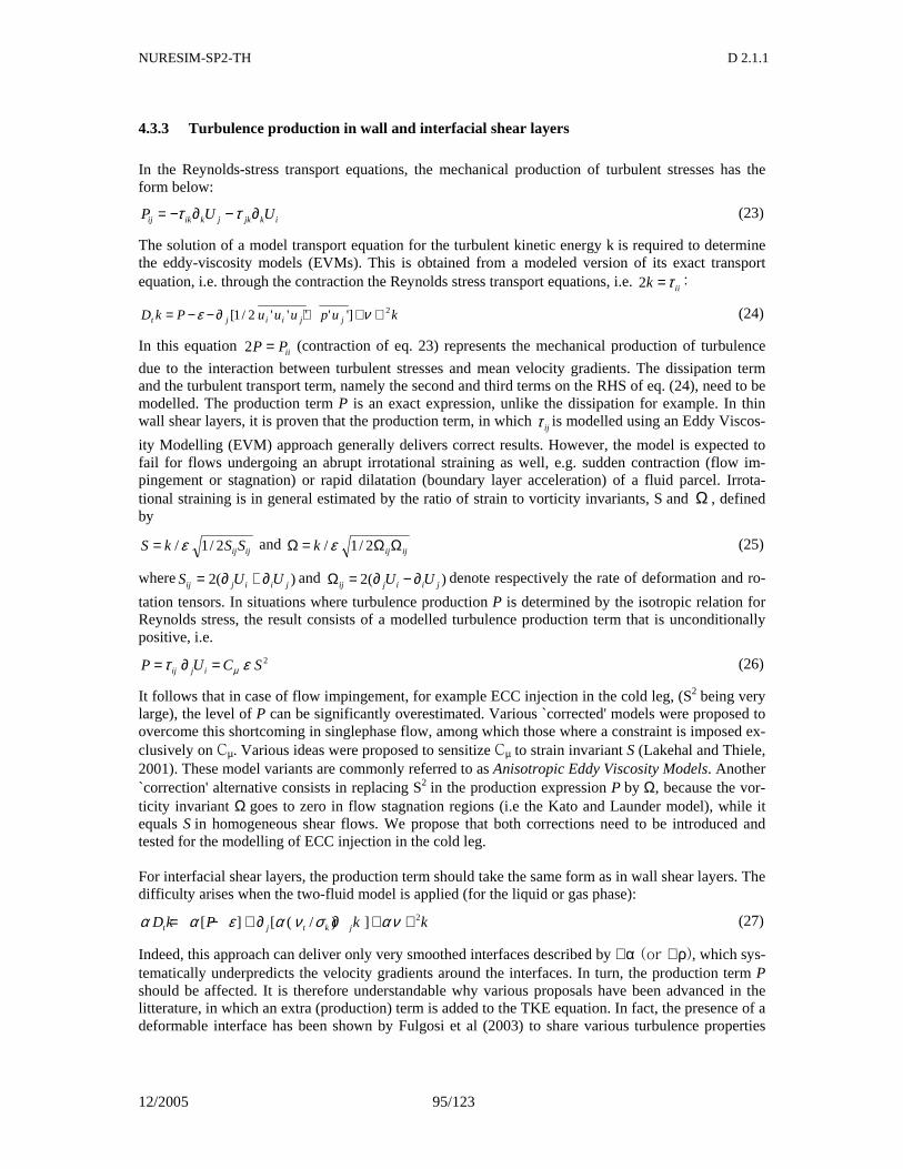
NURESIM-SP2-TH D 2.1.1
12/2005 95/123
4.3.3 Turbulence production in wall and interfacial shear layers
In the Reynolds-stress transport equations, the mechanical production of turbulent stresses has the form below:
ikjkjkikij UUP ∂−∂−= ττ (23)
The solution of a model transport equation for the turbulent kinetic energy k is required to determine the eddy-viscosity models (EVMs). This is obtained from a modeled version of its exact transport equation, i.e. through the contraction the Reynolds stress transport equations, i.e. iik τ=2 :
kupuuuPkD jjiijt2]'''''2/1[ ∇++∂−−= νε (24)
In this equation iiPP =2 (contraction of eq. 23) represents the mechanical production of turbulence
due to the interaction between turbulent stresses and mean velocity gradients. The dissipation term and the turbulent transport term, namely the second and third terms on the RHS of eq. (24), need to be modelled. The production term P is an exact expression, unlike the dissipation for example. In thin wall shear layers, it is proven that the production term, in which ijτ is modelled using an Eddy Viscos-
ity Modelling (EVM) approach generally delivers correct results. However, the model is expected to fail for flows undergoing an abrupt irrotational straining as well, e.g. sudden contraction (flow im-pingement or stagnation) or rapid dilatation (boundary layer acceleration) of a fluid parcel. Irrota-tional straining is in general estimated by the ratio of strain to vorticity invariants, S and Ω , defined by
ijij SSkS 2/1/ε= and ijijk ΩΩ=Ω 2/1/ε (25)
where )(2 jiijij UUS ∂+∂= and )(2 jiijij UU ∂−∂=Ω denote respectively the rate of deformation and ro-
tation tensors. In situations where turbulence production P is determined by the isotropic relation for Reynolds stress, the result consists of a modelled turbulence production term that is unconditionally positive, i.e.
2SCUP ijij ετ µ=∂= (26)
It follows that in case of flow impingement, for example ECC injection in the cold leg, (S2 being very large), the level of P can be significantly overestimated. Various `corrected' models were proposed to overcome this shortcoming in singlephase flow, among which those where a constraint is imposed ex-clusively on Cµ. Various ideas were proposed to sensitize Cµ to strain invariant S (Lakehal and Thiele, 2001). These model variants are commonly referred to as Anisotropic Eddy Viscosity Models. Another `correction' alternative consists in replacing S2 in the production expression P by Ω, because the vor-ticity invariant Ω goes to zero in flow stagnation regions (i.e the Kato and Launder model), while it equals S in homogeneous shear flows. We propose that both corrections need to be introduced and tested for the modelling of ECC injection in the cold leg. For interfacial shear layers, the production term should take the same form as in wall shear layers. The difficulty arises when the two-fluid model is applied (for the liquid or gas phase):
kkPkD jktjt2])/([][ ∇+∂∂+−= νασναεαα (27)
Indeed, this approach can deliver only very smoothed interfaces described by ∇α (or ∇ρ), which sys-tematically underpredicts the velocity gradients around the interfaces. In turn, the production term P should be affected. It is therefore understandable why various proposals have been advanced in the litterature, in which an extra (production) term is added to the TKE equation. In fact, the presence of a deformable interface has been shown by Fulgosi et al (2003) to share various turbulence properties
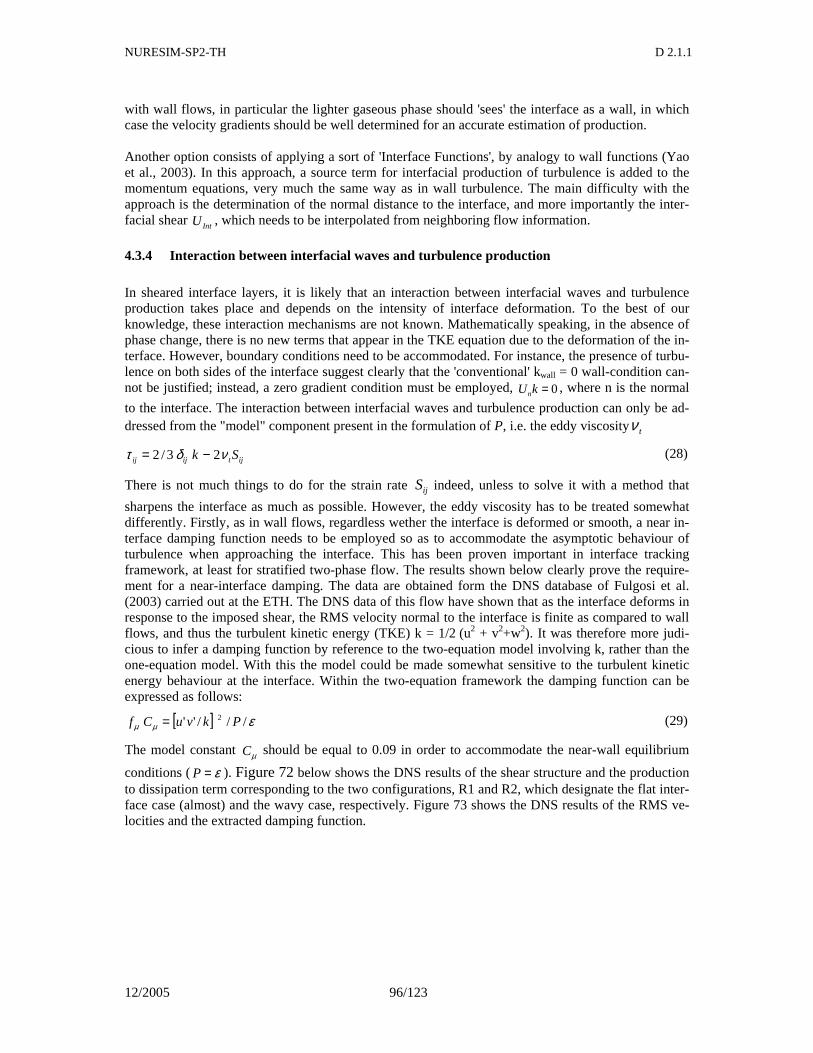
NURESIM-SP2-TH D 2.1.1
12/2005 96/123
with wall flows, in particular the lighter gaseous phase should 'sees' the interface as a wall, in which case the velocity gradients should be well determined for an accurate estimation of production. Another option consists of applying a sort of 'Interface Functions', by analogy to wall functions (Yao et al., 2003). In this approach, a source term for interfacial production of turbulence is added to the momentum equations, very much the same way as in wall turbulence. The main difficulty with the approach is the determination of the normal distance to the interface, and more importantly the inter-facial shear IntU , which needs to be interpolated from neighboring flow information.
4.3.4 Interaction between interfacial waves and turbulence production
In sheared interface layers, it is likely that an interaction between interfacial waves and turbulence production takes place and depends on the intensity of interface deformation. To the best of our knowledge, these interaction mechanisms are not known. Mathematically speaking, in the absence of phase change, there is no new terms that appear in the TKE equation due to the deformation of the in-terface. However, boundary conditions need to be accommodated. For instance, the presence of turbu-lence on both sides of the interface suggest clearly that the 'conventional' kwall = 0 wall-condition can-not be justified; instead, a zero gradient condition must be employed, 0=kUn
, where n is the normal
to the interface. The interaction between interfacial waves and turbulence production can only be ad-dressed from the "model" component present in the formulation of P, i.e. the eddy viscositytν
ijtijij Sk νδτ 23/2 −= (28)
There is not much things to do for the strain rate ijS indeed, unless to solve it with a method that
sharpens the interface as much as possible. However, the eddy viscosity has to be treated somewhat differently. Firstly, as in wall flows, regardless wether the interface is deformed or smooth, a near in-terface damping function needs to be employed so as to accommodate the asymptotic behaviour of turbulence when approaching the interface. This has been proven important in interface tracking framework, at least for stratified two-phase flow. The results shown below clearly prove the require-ment for a near-interface damping. The data are obtained form the DNS database of Fulgosi et al. (2003) carried out at the ETH. The DNS data of this flow have shown that as the interface deforms in response to the imposed shear, the RMS velocity normal to the interface is finite as compared to wall flows, and thus the turbulent kinetic energy (TKE) k = 1/2 (u2 + v2+w2). It was therefore more judi-cious to infer a damping function by reference to the two-equation model involving k, rather than the one-equation model. With this the model could be made somewhat sensitive to the turbulent kinetic energy behaviour at the interface. Within the two-equation framework the damping function can be expressed as follows:
[ ] εµµ ///'' 2 PkvuCf = (29)
The model constant µC should be equal to 0.09 in order to accommodate the near-wall equilibrium
conditions ( ε=P ). Figure 72 below shows the DNS results of the shear structure and the production to dissipation term corresponding to the two configurations, R1 and R2, which designate the flat inter-face case (almost) and the wavy case, respectively. Figure 73 shows the DNS results of the RMS ve-locities and the extracted damping function.
NURESIM-SP2-TH D 2.1.1
12/2005 97/123
Figure 72: DNS results of the production-to-dissipation ratio and the structure parameter -[ ]kvu /''
Figure 73: DNS results of RMS streamwise fluctuations and fµ-distributions
The other important point to note is that the presence of deformable interfaces causes a strong a ani-sotropy of turbulence around the interface. This means that the above (eq. 28) isotropic relationship for
ijτ should be modified to account for the anisotropy of turbulence in one way or the other. One
route consists in simply adopting the Algebraic Stress Models, or use an Anisotropic Eddy Viscosity mode, where
ijjijij Sk Γ−= 23/2 δτ (30)
Here 1Γ may be equal to εν µ /kCt = , but not necessarily 2Γ and 3Γ . In exploring various ways to
accommodate tν to deformable interfaces, it is important to note that while TKE cannot be modified
(but its wall boundary condition), both µC and ε can indeed be modified in accordance. Leschziner
and Rodi (1981) have already introduced modifications accounting for the curvature of the flow streamlines. Something similar can be proposed in the context of deformable interfaces, where the curvature of the flow streamlines is associated with those of the interface. As a last resort we modify the near-interface dissipation intε . For small slope weak-to-mild interface deformations, the waves
may be thought of as roughness elements. In which case, the dissipation of turbulence at the interface could be estimated by including the characteristic length scale of wave deformation (κy ), which
should depend on the curvature κ = − ∇α:
( )κεερε yyCk nl +== ll ;/2/3int (31)
where ny is the interface distance, Cl a model coefficient (for walls Cl = 0.41 Cµ−3/4), and yκ ∼ 1/κ.
4.3.5 Effects of temperature stratification upon turbulent diffusion
In PTS scenarios with ECCS injection and two-phase stratified flow in the cold leg, a rather strong temperature stratification takes place in the liquid. Water is saturated and lighter at the free surface,
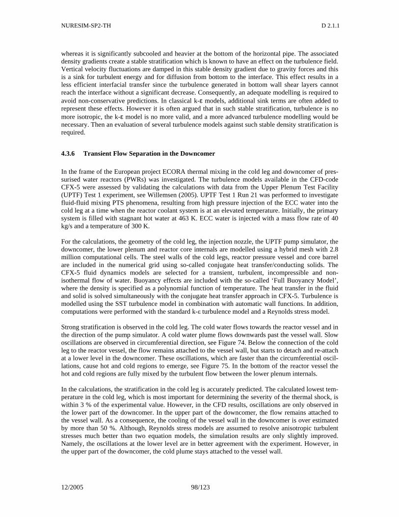
NURESIM-SP2-TH D 2.1.1
12/2005 98/123
whereas it is significantly subcooled and heavier at the bottom of the horizontal pipe. The associated density gradients create a stable stratification which is known to have an effect on the turbulence field. Vertical velocity fluctuations are damped in this stable density gradient due to gravity forces and this is a sink for turbulent energy and for diffusion from bottom to the interface. This effect results in a less efficient interfacial transfer since the turbulence generated in bottom wall shear layers cannot reach the interface without a significant decrease. Consequently, an adequate modelling is required to avoid non-conservative predictions. In classical k-ε models, additional sink terms are often added to represent these effects. However it is often argued that in such stable stratification, turbulence is no more isotropic, the k-ε model is no more valid, and a more advanced turbulence modelling would be necessary. Then an evaluation of several turbulence models against such stable density stratification is required.
4.3.6 Transient Flow Separation in the Downcomer
In the frame of the European project ECORA thermal mixing in the cold leg and downcomer of pres-surised water reactors (PWRs) was investigated. The turbulence models available in the CFD-code CFX-5 were assessed by validating the calculations with data from the Upper Plenum Test Facility (UPTF) Test 1 experiment, see Willemsen (2005). UPTF Test 1 Run 21 was performed to investigate fluid-fluid mixing PTS phenomena, resulting from high pressure injection of the ECC water into the cold leg at a time when the reactor coolant system is at an elevated temperature. Initially, the primary system is filled with stagnant hot water at 463 K. ECC water is injected with a mass flow rate of 40 kg/s and a temperature of 300 K. For the calculations, the geometry of the cold leg, the injection nozzle, the UPTF pump simulator, the downcomer, the lower plenum and reactor core internals are modelled using a hybrid mesh with 2.8 million computational cells. The steel walls of the cold legs, reactor pressure vessel and core barrel are included in the numerical grid using so-called conjugate heat transfer/conducting solids. The CFX-5 fluid dynamics models are selected for a transient, turbulent, incompressible and non-isothermal flow of water. Buoyancy effects are included with the so-called ‘Full Buoyancy Model’, where the density is specified as a polynomial function of temperature. The heat transfer in the fluid and solid is solved simultaneously with the conjugate heat transfer approach in CFX-5. Turbulence is modelled using the SST turbulence model in combination with automatic wall functions. In addition, computations were performed with the standard k-ε turbulence model and a Reynolds stress model. Strong stratification is observed in the cold leg. The cold water flows towards the reactor vessel and in the direction of the pump simulator. A cold water plume flows downwards past the vessel wall. Slow oscillations are observed in circumferential direction, see Figure 74. Below the connection of the cold leg to the reactor vessel, the flow remains attached to the vessel wall, but starts to detach and re-attach at a lower level in the downcomer. These oscillations, which are faster than the circumferential oscil-lations, cause hot and cold regions to emerge, see Figure 75. In the bottom of the reactor vessel the hot and cold regions are fully mixed by the turbulent flow between the lower plenum internals. In the calculations, the stratification in the cold leg is accurately predicted. The calculated lowest tem-perature in the cold leg, which is most important for determining the severity of the thermal shock, is within 3 % of the experimental value. However, in the CFD results, oscillations are only observed in the lower part of the downcomer. In the upper part of the downcomer, the flow remains attached to the vessel wall. As a consequence, the cooling of the vessel wall in the downcomer is over estimated by more than 50 %. Although, Reynolds stress models are assumed to resolve anisotropic turbulent stresses much better than two equation models, the simulation results are only slightly improved. Namely, the oscillations at the lower level are in better agreement with the experiment. However, in the upper part of the downcomer, the cold plume stays attached to the vessel wall.
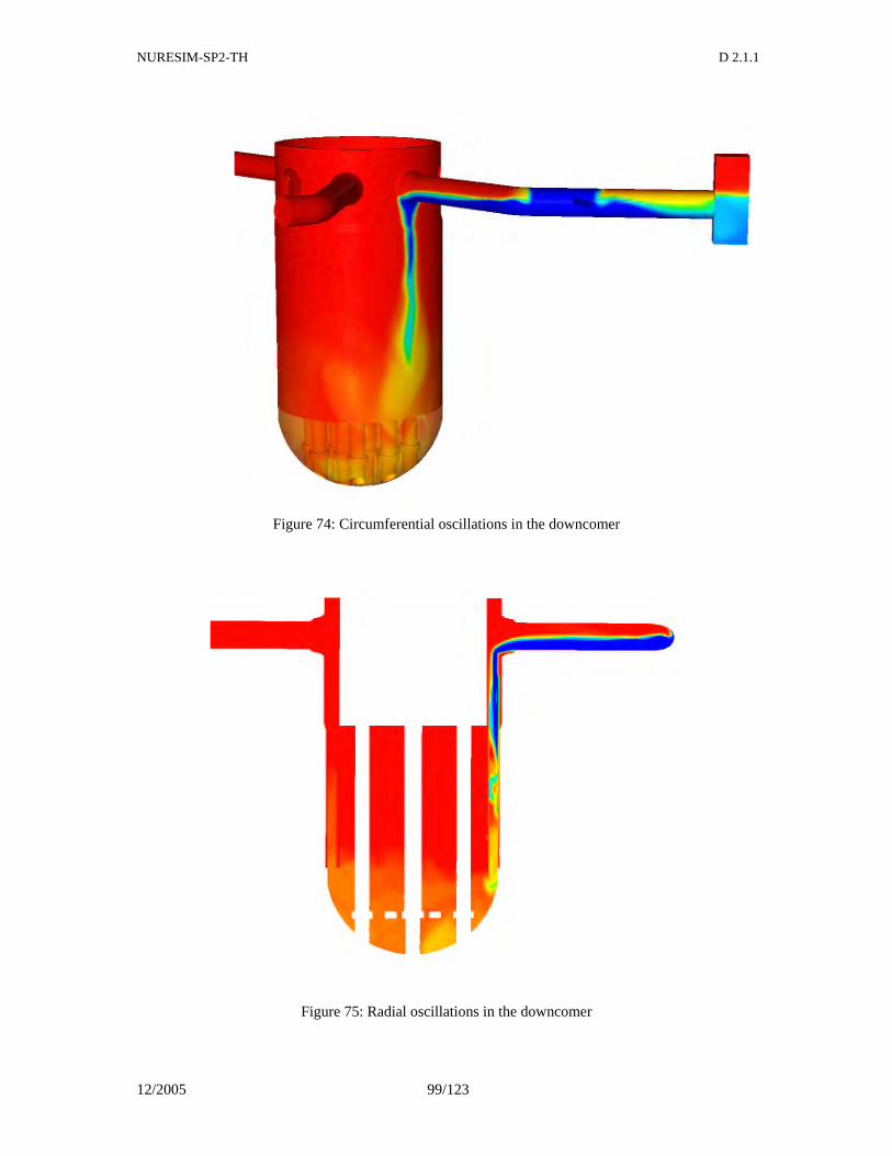
NURESIM-SP2-TH D 2.1.1
12/2005 99/123
Figure 74: Circumferential oscillations in the downcomer
Figure 75: Radial oscillations in the downcomer
NURESIM-SP2-TH D 2.1.1
12/2005 100/123
In order to improve the results, the following recommendations are given: • A low Reynolds approach can improve the results, as it is well known that the use of wall
functions is not very accurate in predicting separation points, see Wilcox (1994) • Alternative methods like Large Eddy Simulations or Scale Adaptive Simulations have a
higher potential to simulate the complex flow phenomena in the downcomer.
4.4 Interfacial momentum, mass and heat transfer at the free surface
In recent years, the modelling of condensation heat transfer has been of major importance in connec-tion with the analysis of nuclear reactor safety systems. For example, in the case of a loss-of-coolant accident (LOCA) in a pressurized water reactor, emergency-cooling water is injected into the primary system to prevent overheating. When the sub-cooled water is brought into contact with the escaping steam, condensation occurs; the heat transfer is thus characterized by the transport of heat and mass through a moving vapor-liquid interface. Owing to increased turbulence in the vicinity of the inter-face, heat transfer is enhanced. The complexity of the thermal-hydraulic coupling of the liquid and vapor phases has resulted in a large number of correlations, but still this coupling is not fully under-stood. Transport models for turbulent heat and mass transfer can be divided into two major classes: models based on the turbulent diffusivity concept and models based on the surface renewal theory. In the first class, the turbulent transport mechanisms are embedded into a steady, Reynolds averaged, turbulent diffusion coefficient. This approach is based on the evaluation of the turbulent diffusivity, which is set to be proportional to the distance from the interface and inversely proportional to the time-scale associated to the turbulence conditions just below the interface. In the other class, the transport is associated to the periodical renewal of fluid elements occurring at the interface, i.e. the fluid from the bulk is pumped towards the interface by the turbulent motion. Here, the key is the de-termination of the relationship between the interfacial turbulence characteristics and the so-called "contact time", which is the typical time that an eddy spends in contact with the interface. One should notice that, since both approaches are based on similar physical assumptions, they give substantially identical results. With either approach, in fact, the problem is reduced to the estimation of a characteristic time-scale associated with the turbulent interfacial eddies that control the transport. In each class, there are many different models available, which simply differ in the way this time-scale is related to the liquid properties, flow conditions and turbulence characteristics just underneath the gas-liquid interface. This last aspect seems to be the most critical one since there is no consensual agreement and sufficient knowledge about the interfacial turbulence structure. It is also important to stress that condensation differs from the transport phenomena without phase change because it is ac-companied by bulk convection in the direction normal to the interface. This motion, which is usually superimposed to the existing mean motion, further complicates the turbulent conditions at the gas-liquid interface. For this reason, applying to condensation the knowledge gained from passive heat/mass transfer might be a misleading approach. However, if the condensation rate remains low, the existing turbulent boundary layer will not be significantly modified.
4.4.1 Condensation at a vapor-liquid interface: literature overview
Direct contact condensation heat transfer is generally defined as heat transfer between two or more mass streams without the presence of an intervening wall. The mass streams can be co-current, counter-current or even cross-flow. In particular, the stratified flow configuration is such that the con-densation heat transfer takes place across the interface between the two continuous fluid steams. Linehan (1968) conducted one of the earliest experiments on DCC, consisting of a co-current strati-fied flow of saturated steam over a sub-cooled water film in a rectangular channel, where the bottom wall was adiabatic. The heat transfer coefficient was correlated to the mean film velocity through
NURESIM-SP2-TH D 2.1.1
12/2005 101/123
fUK 0073.0= (32)
The values of K obtained with this relation were 2.5 to 4.2 times greater than those obtained using Carpenter and Colburn’s relation for wall heat transfer, although the experimental conditions were different. In the Carpenter and Colburn correlation, the thermal resistance was considered to lie in the viscous sublayer near the wall, whereas in Linehan's experiment it was in the liquid just below the in-terface. The analysis conducted by Thomas (1979), considered a pool of cold water covered by an at-mosphere of steam. In such a situation, the free surface would be nearly at the steam temperature and the rate of condensation is determined by the speed at which heat can be transferred from the free sur-face to the bulk water. This author restricted the analysis to a relatively simple set of conditions, such as low turbulence intensity in the liquid and small super-heating and sub-cooling. By dimensional analysis, the heat transfer coefficient (HTC) could be expressed as
Pr)(Re,fL
HTCλ= (33)
where λ is the molecular conductivity of the water, L is the pool length scale, Re and Pr the Rey-nolds (based on L) and the Prandtl number of the water, respectively. In his work, Thomas investi-gated different flow configurations such as a vertical jet impinging on a free surface from below, grid turbulence decaying in an open channel, and recirculating flows generated by submerged horizontal jets. The main outcome may be summarized as follows: (i) the condensation rate showed a stronger variation with the Reynolds number than the expected 3/4-power dependence; (ii) a considerable in-crease in the rate of condensation occurred when the agitation of the free surface became sufficiently severe to cause entrainment of steam bubbles. Over the years, several experiments in inclined rectan-gular channels have been carried out to estimate the local heat transfer coefficient for direct contact condensation. Even though in all the experiments fully developed conditions for the condensing flow were never obtained, local flow properties were used to correlate the data. A number of empirical cor-relations of the form
431 PrReRe 2 a
La
Ga
GaNu= (34)
have been proposed. In (12), a1, a2, a3 and a4 are experimental constants, Nu = HTC δ/λ is the local Nusselt number defined using the mean water layer thickness δ, and the Reynolds numbers are de-fined using G, the mass flow rate per unit width, i.e. Re=G/µ. For example, Seguev et al (1981) estimated the heat transfer coefficient in a counter-current inclined steam-water flow at atmospheric pressure. Condensation HTCs were investigated varying steam and water flow rates, the degree of liquid sub-cooling and the channel inclination. Their data, in the region of pebbly surface and roll waves for a fixed inlet water temperature, were correlated by
05.087.028.0 PrReRe00116.0 LLGNu = (35)
whereas when large amplitude roll waves were present on the interface, the condensation heat transfer was correlated by
0.208.1016.0 PrReRe000579.0 LLGNu = (36)
Lim et al (1984) performed extensive condensation heat transfer coefficient measurements for a co-current steam-water flow in a horizontal channel at atmospheric pressure varying, in different runs, the inflow conditions for both the vapor and the water, the water thickness and the degree of water sub-cooling. In all the experiments, the thermal resistance in the liquid layer was dominant. Depend-ing on the experimental conditions, these authors obtained three types of data: one where the interface was smooth throughout the channel, a second where the interface was wavy throughout the channel, and a third one where the interface was smooth at the entrance and became wavy toward the exit. For the first two sets of data, the correlations proposed are
NURESIM-SP2-TH D 2.1.1
12/2005 102/123
3.0358.0 PrReRe534.0 La
LGNu = (37)
for smooth interfaces, and
3.042.058.0 PrReRe0291.0 LLGNu = (38)
for wavy interfaces. Kim and Bankoff (1983) studied condensation in counter-current stratified flow of steam and sub-cooled water in a rectangular channel inclined (at maximum 33 deg to the horizontal). The experimen-tal parameter range was restricted to: liquid Reynolds number 800-5000, and gas Reynolds number 3000-18000. The local heat transfer coefficient was seen to increase smoothly from the minimum value at the water entry towards the water exit, where both interfacial shear stress and wave ampli-tudes were maximum. The condensing two-phase flow was never fully developed and the local fluid properties were used as correlating parameters. They provided correlation for the local Nusselt num-ber in terms of the local gas and liquid Reynolds numbers, and possibly the liquid Prandtl number (as the thermal resistance lies principally on the liquid side)
42.049.0027.0 PrReRe173.0 LLGNu = (39)
for smooth interfaces, and
16.156.01.210 PrReRe10.43.3 LLGNu −= (40)
for rough interfaces. Moving from smooth to rough interfaces, the gas Reynolds number becomes much more important as the interfacial shear stress is no longer negligible. The wave structure is thus controlling the growth of the thermal boundary layer in the liquid as well as the transport mechanisms. A correlation encompassing both the smooth and rough interfaces was provided by incorporating an-other dimensionless group consisting of a dimensionless wave amplitude (a’):
82.089.04.047.0 'PrReRe00936.0 aNu LLG= (41)
Moreover, the authors found that the steam Reynolds number had a powerful effect on the wave am-plitude. The interfacial shear increased with increasing steam and water flow rates and decreasing liq-uid temperature, in a similar fashion as the condensation rate. The interfacial transport of momentum in the presence of condensation was simply augmented by an amount equal to the condensation rate times the average vapor velocity (the interface velocity could be neglected in comparison to the vapor velocity). in which FrG is the Froude number, defined based on the channel depth H. For a given flow condition, the heat transfer coefficient increased as the water-layer thickness decreased (or, equiva-lently, the inclination angle decreased), since the effect of the water-layer thickness is included in the local Nusselt number. Another correlation for the local Nusselt number was obtained by replacing the gas Reynolds number with the gas Froude number to take into account the thickness of the gas and liquid layers:
95.08.098.0 PrRe000966.0 LGL FrNu = (42)
in which FrG is the Froude number, defined based on the channel depth H. For a given flow condition, the heat transfer coefficient increased as the water-layer thickness decreased (or, equivalently, the in-clination angle decreased), since the effect of the water-layer thickness is included in the local Nusselt number. Kim and Bankoff (1983) also correlated the dimensionless heat transfer coefficient, follow-ing the same approach as in the literature for soluble gas absorption, where models relating the mass transfer coefficient to the local turbulent properties have been suggested for different turbulent Rey-nolds number (Ret) ranges in the liquid (i.e. small and large eddy models). The authors observed that the accuracy of these models depended on the prediction of the turbulent velocity and length scales, ut and lt. For the counter-current steam-water flow in an inclined channel, the comparison between measured and predicted values revealed large discrepancies. Their conclusion was that appropriate
NURESIM-SP2-TH D 2.1.1
12/2005 103/123
values are difficult to define for the turbulent intensity, ut, and turbulent length scale, lt, due to the highly agitated steam-water interface and large condensation rates, which, in turn, augment the effect of the interfacial shear stress. By considering the strong effect of the sheared and disturbed interface on the turbulence properties, Kim and Bankoff defined the turbulent velocity and length scales in terms of interfacial parameters such as ( ) 2/1
IntIntt Uu τρ== and at =l , the wave amplitude, and
Intτ includes also the momentum transfer dictated by condensation. Using these reference scales, Kim
and Bankoff proposed a correlation for condensation heat transfer of the form
5.012.1 PrRe061.0 LttNu = (43)
Jensen and Yuen (1982) measured both the steam condensation rate and turbulence intensities in an open channel flow where the liquid-side turbulence was induced by the shear stress exerted by the flowing steam. When the steam shear controls the condensation rate, the surface has a "pebbled" wavy appearance, and the authors correlated K to the liquid frictional velocity through appearance, and the authors correlated K to the liquid frictional velocity through
τUK L5.0Pr14.0 −= (44)
where uτ is the frictional velocity based on the interfacial shear and liquid density, and PrL is the mo-lecular Prandtl number based on bulk liquid properties. The Prandtl number dependency was actually only postulated because they worked with a fixed value of PrL=6.2. Sonin et al (1986) investigated the problem of vapor condensation onto a non-sheared and relatively flat liquid interface, in which the turbulence was produced from below and was essentially isotropic in the horizontal plane. Relating the condensation heat transfer coefficient with the turbulence parameters, they found
'0098.0 vK = (45)
where v’ represents a measure of the turbulence intensity (either horizontal or vertical), which implies independence from the water Prandtl number. In order to get a more general correlation, the authors related K to the liquid-side turbulence (velocity and length scales), liquid properties (only changes in the viscosity were taken into account) and latent heat of condensation, which controls the relative magnitudes of the conductive and convective heat fluxes at the interface. Again, in the range of pa-rameters investigated and with the water Prandtl number fixed at 1.76, they obtained eq. (45). On the basis of LDA measurements, Jensen and Yuen (1982) provided the r.m.s. of the the fluctuating streamwise velocity component as v’ = 2.9 uτ. Plugging this value into correlation (44) the coefficient becomes double of the one in eq. (23), i.e. K/v’ = 0.019, suggesting that the condensation coefficient is not controlled just by the value of v’ at the interface, but depends also on how the turbulence is generated, i.e. on the structure of the turbulence field. Sonin et al (1986) compared their results also with those for gas absorption into water, where the Schmidt number is very high. The comparison was made with Krenkel and Orlob's correlation (1962), which was obtained for gas absorption in a turbu-lent channel flow without shear at the interface
τUK 000865.0= (46)
According to Plate and Friedrich (1984), the r.m.s. value of the streamwise fluctuating velocity at the surface is approximately equal to uτ, hence eq. (45) can be rewritten as K = 0.0009 v’, for Sc = 500. For the case of channel with wind induced shear, McCready and Hanratty (1984) proposed a correla-tion of the form
τUScK 5.0)2.01.0( −−= (47)
where uτ is the frictional velocity based on the interfacial shear and liquid density. Using u’ = 2.9 uτ, correlation (25) can be rewritten as ')003.00015.0( 5.0 vScK −−= , for Sc = 500. However, Sonin et al
NURESIM-SP2-TH D 2.1.1
12/2005 104/123
(1986) concluded that the comparison with these data was uncertain because of the different type of turbulence considered, i.e. turbulence induced at the interface by the shear stress and from below.
4.4.2 Modelling interfacial transfers at free surface
In a turbulent stratified flow, the interfacial heat transfer is controlled by turbulence in the vicinity of an interface. One part of the turbulence near the interface is diffused through the bulk flow from the wall region, another part is due to the turbulence production at the interface by the interfacial friction and interfacial waves. For interfacial transfers, though there are extensive studies on gas absorption at a gas-liquid interface in chemical engineering and on condensation on a thin liquid film which is slightly sub-cooled (Side-man et al. 1975, Collier 1972), the modelling of interfacial transfer at a stratified interface is still open to question due to the theoretical and experimental difficulties concerning a deformable interface. Re-cently, special attention was paid on the safety analysis of nuclear reactors where rapid direct contact condensation of vapor on a thick sub-cooled liquid layer may occur during a sequence of safety injec-tions of cold water (Bankoff 1980, Hughes and Duffey 1991, Murata, et al. 1992 Zhang et al.1993 Chu et al. 2000). After the thin film model introduced by Lewis and Whitman (1924), many theoreti-cal models for interfacial transfers are proposed which can be mainly divided into two classes of models, one based on a surface renewal concept (Higbie, 1935) and another based on the eddy diffu-sivity concept (Danckwerts, 1951). The two approaches deal with same problems from different as-pects, say, the first one is micro-scale phenomenological analysis which focuses on the dynamic be-haviour of typical eddy element, and the second one is a macro-scale Reynolds average analysis which focuses on the average effect of all the eddies. For the first class of models, one should point out that until now there are still conflicting opinions about which kind of eddies renew the surface. Based on their experimental analysis, some researchers argued (Fortescue and. Pearson 1967, Komori et al. 1982, Rashidi et al. 1991) that large energy-containing eddies generated from the bottom wall renew the gas-liquid interface and control interfa-cial heat/mass transfer. On the contrary, others (Lamont and Scott, 1970, Hughes and Duffey, 1991, etc.) believed that small eddies of Kolmogorov micro-scale control the transport across an interface. Furthermore, when the models based on the small renewal eddies concept are attempted to apply to the interfacial heat transfer problems in steam-water system )e.g. Bankoff, 1980, Hughes and Duffey, 1991) with Pr ≈ 1 (Theofanous et al. 1976), it should be noted that this kind of models lies in the fact that the penetration depth δ during the contact time should be less than the eddy size le i.e.,
2/1
e
Pr4l
−≈δ<< 1 or Pr >> 16 (48)
Though it can be used in gas absorption problems with very large Sc numbers, the direct application of these models to steam-water flow is questionable in theory. For the second class of the models based on the eddy viscosity concept, the asymptotic behaviour of eddy viscosity at an interface is considered because the transfer resistance mainly lies on a thin layer near an interface, especially for large Sc or Pr number fluid. Ueda et al. (1977) surveyed several pub-lished eddy viscosity profiles which have asymptotic characteristics at an interface as
nst Cy=ν , (49)
where C depends on the physical properties of fluid and flow condition near an interface. The power n appears to be from 1 to 4 according to different authors, and Ueda et al. (1977) concluded that the eddy viscosity decreases to zero in proportion to the distance from the interface with the power of more than two by checking several gas absorption experimental data set. Recently, direct numerical simulation (DNS) results (Shen et al. 2000, Yamamoto, et al. 2001) showed that there is a non zero
NURESIM-SP2-TH D 2.1.1
12/2005 105/123
value of eddy viscosity at a free surface (no interfacial shear). This value is very small and compara-ble to that of molecular viscosity. Unlike a solid-fluid interface, the asymptotic behaviour of a gas-liquid interface remains unclear due to the measurement difficulties. Thus, the interfacial transfer models based on the eddy viscosity concept inherit these uncertainties (such as uncertainties on the coefficients C and n). Another approach is to use the concept of “wall function”. Wall function has successfully been applied to the momentum, heat and mass transfer problems at a fluid-solid interface. Experimental and DNS evidence showed that near a gas-liquid interface, similar sub-layer exists and the “wall function” may be useful to predict the interfacial heat transfer problems for engineering ap-plication. Yao et al. (2003) modelled turbulent stratified flow with/without condensation with a CFD approach based on the two-fluid model. A modified turbulent K-ε model is used with turbulence production in-duced by interfacial friction. A model of interfacial friction based on a interfacial sub-layer concept and three interfacial heat transfer models, namely, a model based on the small eddies controlled sur-face renewal concept (Hughes and. Duffey, 1991), a model based on the asymptotic behaviour of the eddy viscosity (EVM), and a model based on the interfacial sublayer concept (ISM) were imple-mented into a preliminary version of the NEPTUNE code. Firstly, an experiment with adiabatic turbu-lent air-water stratified flow (Fabre et al. 1987) is calculated to evaluate the models which control the velocity and turbulence profiles. Then an experiment of turbulent steam-water stratified flow with condensation (Lim et al. 1984) is applied to compare the three interfacial heat transfer models men-tioned above.
Interfacial friction (Interfacial sub-layer model in the gas phase, ISM)
In the two-phase region of the free surface, the average location of the surface is determined and this interface is treated as a moving boundary for the gas region and the liquid region. The wall function method is applied like for solid boundaries. The effects of the surface roughness due to interfacial waves are not taken into account in this first approach. Due to the significant difference of density of liquid and gas phases, the gas phase “sees” the liquid phase like a moving solid wall. Thus, ui = uL is a good approximation. In the experimental data of Fabre et al. (1987), a stratified air-water co-current flow in a horizontal channel of rectangular cross-section is investigated with systematic measurements of the components of the mean velocities and Reynolds stresses. The calculations predicted reasonably well the liquid velocity, turbulent kinetic intensity and shear profiles in the liquid layer, compared to the experimen-tal data, though with a little underestimation of turbulent kinetic energy and turbulent shear stress. The model has proved some capability to capture the momentum transfers and turbulence characteristics at least with a rather smooth interface and without heat transfers.
Interfacial heat transfer
Three models were evaluated by Yao et al. (2003). The first model is based on interfacial sublayers concept (ISM) and applies an “interfacial function”, similar to a wall function, to the transfer prob-lems at the gas-liquid interface. The second model is based on the asymptotic behaviour of eddy vis-cosity (EVM) and follows investigations by Shen (2000) using DNS. The third model is based on sur-face renewal concept with small eddies (HDM, Hughes and Duffey, 1991) Lim et al. experimental data on condensation in a turbulent stratified steam-water flow in a horizontal channel of rectangular cross-section were calculated with the three models. Experimental results showed a significant increment of condensation if the transition from glossy to wavy interface hap-pened. For the glossy interface conditions, ISM gave the best predicted results, while EVM underes-timated and HDM significantly overestimated interfacial heat transfer. ISM and EVM underestimate the condensation when interfacial waves exist. HDM highly overestimated interfacial heat transfers even on a wavy interface. Further efforts are necessary in particular for wavy interface.
NURESIM-SP2-TH D 2.1.1
12/2005 106/123
4.5 Direct Contact Condensation (DCC)
The present paragraph attempts to review the state-of-the art in the field of the direct contact conden-sation (DCC) on the jet itself before mixing in case of ECC and on the interface in stratified flow. The interface instabilities in horizontal stratified pipe flow are also discussed, especially in terms of the onset which leads to the transition of flow regimes from stratified to slug flow. While most of the papers mentioned in this paragraph treat DCC and interface stability in stratified flow as separate topics, they may actually be closely connected in the flows where the condensation of the vapour on the sub-cooled liquid accelerates the vapour by suction effect. The acceleration process of the vapour clearly depends on the mass transfer rate at the free surface (already discussed in § 4.4) and may lead to velocities difference at the interface which could start the flow transition from strati-fied to wavy and slug flow regime. Research of this particular topic is planned at the "Jožef Stefan" Institute and at UCL within the NURESIM project with the transient multi-dimensional fluid dynamics simulations using CFX and FLUENT codes respectively. It is also planned to use NEPTUNE code. The following text is split into several paragraphs:
• The paragraph 4.5.1 deals with the direct contact condensation on the interface of the liquid jet before mixing in case of ECC.
• The paragraph 4.5.2 treat the problem of instabilities in stratified flow connected to DCC. In this paragraph, the transition from the smooth stratified into wavy stratified and into slug flow in the horizontally stratified flows is discussed with negligible heat and mass transfer.
• The paragraph 4.5.3 mainly concerns the existing state of the art in the field of DCC in the horizontally stratified flow. It contains two subsections about the models of the DCC in 1D nuclear thermal-hydraulic codes and about the DCC induced water hammer in the horizontal pipes which has been underlined in the European WAHALoads project.
• Finally, the paragraph 4.5.4 contains discussion about the CFD approaches that might be used within the NURESIM project for the treatment of the DCC and interfacial instabilities in the horizontally stratified flow.
4.5.1 DCC on the interface of the liquid jet before mixing in case of ECC
In the current framework special attention is given for the DCC that occurs around an ECC jet injec-tion during a transient in pressurized water reactors. In large break LOCAs very large injection flowrates may occur particularly during the accumulator discharge. These situations are characterized by a strong thermo-mechanical coupling and strong instabilities may be created by high instantaneous condensation rates. This leads to plug formation in cold legs, which strongly affects the flow regime and the delivery of water to the vessel (intermittent water delivery to the downcomer). These phe-nomena were observed experimentally in the scale 1 Upper Plenum Test Facility (UPTF) test facility by (Weiss, 1989). Therefore, the prediction of thermal-hydraulic interactions by contact condensation of steam on water surface is of interest for an efficient ECC injection. The experimental results performed in the COSI test facility (Janicot & Bestion, 1993) show that a large fraction of the total condensation occurs in the zone of the jet and more particularly around the injection. Since the condensation increase in the vicinity of the injection they suggest that the turbu-lence induced by the jet is the main controlling mechanism (compare section 4.3). In ideal conditions where the jet is continuous without breakup Janicot & Bestion (1993) suggested to use the Iciek correlation to predict the condensation on the jet, notwithstanding the fact that no ex-perimental evidence exists to confirm this model. The correlation is expressed in terms of Stanton
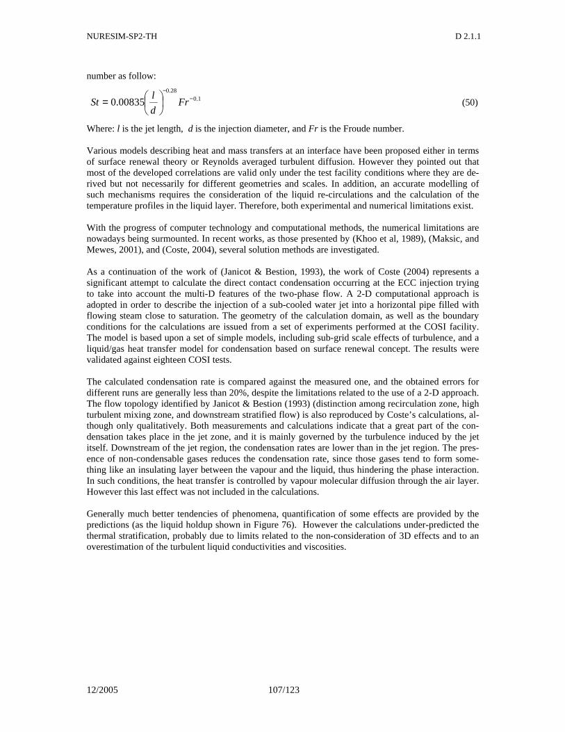
NURESIM-SP2-TH D 2.1.1
12/2005 107/123
number as follow:
1.028.0
00835.0 −−
= Frd
lSt (50)
Where: l is the jet length, d is the injection diameter, and Fr is the Froude number. Various models describing heat and mass transfers at an interface have been proposed either in terms of surface renewal theory or Reynolds averaged turbulent diffusion. However they pointed out that most of the developed correlations are valid only under the test facility conditions where they are de-rived but not necessarily for different geometries and scales. In addition, an accurate modelling of such mechanisms requires the consideration of the liquid re-circulations and the calculation of the temperature profiles in the liquid layer. Therefore, both experimental and numerical limitations exist. With the progress of computer technology and computational methods, the numerical limitations are nowadays being surmounted. In recent works, as those presented by (Khoo et al, 1989), (Maksic, and Mewes, 2001), and (Coste, 2004), several solution methods are investigated. As a continuation of the work of (Janicot & Bestion, 1993), the work of Coste (2004) represents a significant attempt to calculate the direct contact condensation occurring at the ECC injection trying to take into account the multi-D features of the two-phase flow. A 2-D computational approach is adopted in order to describe the injection of a sub-cooled water jet into a horizontal pipe filled with flowing steam close to saturation. The geometry of the calculation domain, as well as the boundary conditions for the calculations are issued from a set of experiments performed at the COSI facility. The model is based upon a set of simple models, including sub-grid scale effects of turbulence, and a liquid/gas heat transfer model for condensation based on surface renewal concept. The results were validated against eighteen COSI tests. The calculated condensation rate is compared against the measured one, and the obtained errors for different runs are generally less than 20%, despite the limitations related to the use of a 2-D approach. The flow topology identified by Janicot & Bestion (1993) (distinction among recirculation zone, high turbulent mixing zone, and downstream stratified flow) is also reproduced by Coste’s calculations, al-though only qualitatively. Both measurements and calculations indicate that a great part of the con-densation takes place in the jet zone, and it is mainly governed by the turbulence induced by the jet itself. Downstream of the jet region, the condensation rates are lower than in the jet region. The pres-ence of non-condensable gases reduces the condensation rate, since those gases tend to form some-thing like an insulating layer between the vapour and the liquid, thus hindering the phase interaction. In such conditions, the heat transfer is controlled by vapour molecular diffusion through the air layer. However this last effect was not included in the calculations. Generally much better tendencies of phenomena, quantification of some effects are provided by the predictions (as the liquid holdup shown in Figure 76). However the calculations under-predicted the thermal stratification, probably due to limits related to the non-consideration of 3D effects and to an overestimation of the turbulent liquid conductivities and viscosities.
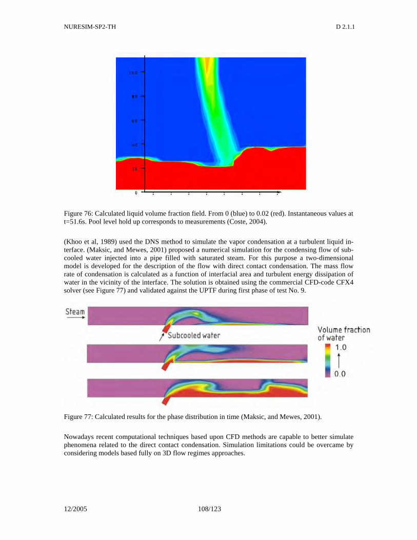
NURESIM-SP2-TH D 2.1.1
12/2005 108/123
Figure 76: Calculated liquid volume fraction field. From 0 (blue) to 0.02 (red). Instantaneous values at t=51.6s. Pool level hold up corresponds to measurements (Coste, 2004).
(Khoo et al, 1989) used the DNS method to simulate the vapor condensation at a turbulent liquid in-terface. (Maksic, and Mewes, 2001) proposed a numerical simulation for the condensing flow of sub-cooled water injected into a pipe filled with saturated steam. For this purpose a two-dimensional model is developed for the description of the flow with direct contact condensation. The mass flow rate of condensation is calculated as a function of interfacial area and turbulent energy dissipation of water in the vicinity of the interface. The solution is obtained using the commercial CFD-code CFX4 solver (see Figure 77) and validated against the UPTF during first phase of test No. 9.
Figure 77: Calculated results for the phase distribution in time (Maksic, and Mewes, 2001).
Nowadays recent computational techniques based upon CFD methods are capable to better simulate phenomena related to the direct contact condensation. Simulation limitations could be overcame by considering models based fully on 3D flow regimes approaches.
NURESIM-SP2-TH D 2.1.1
12/2005 109/123
4.5.2 Instabilities in stratified flow connected to DCC
4.5.2.1 Kelvin-Helmholtz instabilities
Kelvin-Helmholtz (K-H) instability is one of the basic instabilities of two-fluid systems, which affects an interface submitted to a shear. When two fluids separated by a free surface move with different ve-locities, their interface could be unstable due to inertia. An inviscid linear analysis of the phenomenon can be found in various textbooks, for example in Chandrasekhar (1961), Drazin and Reid (1982). As shown in the experiment of Thorpe (1969), the linear analysis is applicable in the case of two liquids of similar densities. However, the problem becomes much more complicated for large density differ-ences, which are encountered in transients in nuclear power plants. For example, the instability of the sea surface appears at wind speeds significantly lower than the critical wind speed given by the linear inviscid analysis (Gondret and Rabaud, 1997). The phenomenon described as ”subcritical Kelvin-Helmholtz Instability” was analyzed by Meignin et al. (2003) and was found to be a result of the nonlinear analysis. As shown in the report of Štrubelj and Tiselj (2005), even the simulation of the rather simple K-H in-stability - tilted-tube experiment (Reynolds, 1883, Thorpe, 1969) - can be a though problem for the CFD codes. Tilted-tube experiment of Thorpe (1969) is especially convenient for CFD analysis be-cause of a two-dimensional nature of the experiment, which allows an approximate analytical ap-proach and numerical simulation, and because the experiment is performed with two fluids of similar density. Thorpe's experimental results are in agreement with predictions of the inviscid linear analy-sis. However, it should be noted that despite the simplicity and careful control of the initial and boundary conditions in the Thorpe's experiment, the wavelengths of the most unstable waves devel-oped in the various runs of the same experiment varied for almost 50% around the mean value. This observation clearly shown the uncertainty on the onset of occurrence of interface instabilities in strati-fied flows. The simulation of the Kelvin-Helmholtz instability with large density differences thus presents a de-manding task due to the importance of the viscosity and nonlinear effects. Readers are referred to the paper of Funada and Joseph (2001) for a review of the experiments with Kelvin-Helmholtz instability in systems with large density differences. Some recent CFD simulations of simple K-H instability are described by Hou et. al. (2001), where two inviscid fluids of equal density are considered in zero gravity conditions, and Černe and Petelin (1999), who simulated the problem with a combined VOF interface tracking model and 2D two-fluid model. K-H instability experiment of Thorpe (1969) is planned to be used as a benchmark also for the NURESIM platform.
4.5.2.2 Transition from stratified to slug flow
What is usually required in engineering applications is not only the onset of the Kelvin-Helmholtz in-stability, which can be often described with linearized equations, but also the break-up of the waves or onset of slugging in the pipes with horizontally stratified flow. This type of knowledge cannot be ob-tained with purely analytical approach but requires also experimental work. One of the first works treating the criterion for the transition from stratified to slug flow relevant for nuclear engineering was paper of Wallis and Dobson (1973), who combined the experiment and theory to derive a simple crite-rion for the transition:
NURESIM-SP2-TH D 2.1.1
12/2005 110/123
ggfgcrit
critr
ghv
vv
ρρρ /)(5.0 −=
≥ (50)
which predicts slugging when relative velocity between gas and liquid phase exceeds the critical ve-locity, with hg denoting height of the vapour layer in stratified flow. This correlation was later modi-fied by Taitel and Dukler (1976) and by Mishima, Ishii (1980), who derived similar criteria with less empiricism. An important contribution to the understanding of the transition from smooth-stratified to wavy-stratified and slug or plug flow in the horizontal or nearly horizontal pipes, was given by Hanratty and his coworkers (review paper Hanratty et. al., 2000). Andritsos and Hanratty (1987a,b) discussed vari-ous instabilities in stratified flow experiment, analyzed the influence of the viscosity and determined the models of interfacial friction. Andritsos et. al. (1993) made an overview of theories for the initia-tion of slugging and classified them by whether they invoked a long-wave assumption and whether they included viscous and nonlinear effects. Importance of nonlinear corrections and large amplitude K-H waves were discussed by Bontozoglou (1992), while Fan et. al. (1993) presented measurements of the pressure profiles in slug flow. Some later works of Hanratty discuss difference between the slug formation in horizontal and slightly inclined pipe (Woods et. al. 2000), Hurlburt and Hanratty (2002) analyzed slugging in long pipes and beside K-H instability stressed the importance of the "viscous large wavelength" instability (generated by the interfacial and wall stress) and slug stability. Slug sta-bility was analyzed recently by Soleimani and Hanratty (2003). Some other contributions to the modelling of transition from stratified to slug flow were given by Bendiksen and Espedal (1992) who presented two different criteria for the onset of the waves and for the onset of the stable slug flow, Crowley et. al. (1992) that upgraded the approach of Taitel and Duk-ler (1976) and Jayanti et. al. (1996), who analyzed the forces of the gas phase on the assumed standing liquid wave with 2D CFD analysis. Models for stratified to slug flow transition and correlations for interfacial friction in stratified and slug flow mentioned in the previous paragraphs are used mainly in 1D two-fluid models of two-phase flow. Interfacial friction plays a dominant role comparing to the inter-phase heat and mass transfer in 1D computer codes for oil industry (De Henau, Raithby (1995), (Issa, Kempf, 2002). On the other side, the computer codes for thermal-hydraulic analyses in nuclear engineering (RELAP5, TRAC, CATHARE), still need accurate interfacial friction models, which are dominant in equilibrium strati-fied flows (Nakamura et. al. 1994, 1995), however, these codes are expected to be accurate also in non-equilibrium and stratified flows even in transient, where significant heat and mass exchange be-tween both phases appears. The use of these models in such conditions is questionable.
4.5.3 Direct contact condensation in horizontal flow and effect upon interfacial and wave
structure
Chapter 10 of the Collier (1981) textbook "Convective boiling and condensation" is probably a good start to get an insight into condensation of steam on sub-cooled water in stratified flow. Condensation at a vapour-liquid interface is already discussed in general in paragraph 4.4.1. Since only a limited analytical approach to the problem of DCC in stratified horizontal flow is possible, the experimental support is inevitable and necessary. Two frequently used correlations for the Nusselt number for heat and mass transfer during the DCC in stratified flow were derived from experimental results by Lim et.al. (1984) and Kim, Lee and Bankoff (1985). Unlike Lim et. al. (1984) and Kim et .al. (1985) who performed their experiments in the pipe, Celata et. al. (1986) measured DCC on a slowly moving sub-cooled water in a "pressurizer-like" geometry and developed a special set of correlations for that pur-pose. Chan and Yuen (1990) used the experimental device of Lim et. al. (1984) and analyzed the in-fluence of air on the DCC in stratified horizontal flow.
NURESIM-SP2-TH D 2.1.1
12/2005 111/123
Hughes and Duffey (1991) introduced a "surface renewal theory" for DCC in turbulent separated flow, which points to an important role of the turbulence in the liquid layer. Experiments and models of DCC in a rectangular duct and rectangular tank were later described by Lorencez et. al. (1997) and Mikielewicz et. al. (1997), respectively. Especially Lorencez et. al. (1997) with their sophisticated ex-periment made a detailed measurement of the turbulence near the free surface and clarified the impact of the turbulence on the interfacial heat and mass transfer coefficients. Chun, Yu (2000a) described their air-water and steam-water experiments in nearly horizontal stratified flow and compared various correlations for the stratified-to-slug transition with their experiments. They suggested a new model, which gives (comparing to Mishima, Ishii, 1980, and Taitel, Dukler, 1976) more accurate prediction of transition at low liquid superficial velocities. Ramamurti et. al. (2001) performed a DCC experi-ment on a thick layer of moving water in the vessel with a stagnant vapor bubble and expressed the heat transfer coefficients in terms of Nusselt number as a function of liquid Reynolds and Prandtl number and the sub-cooling intensity. The recent paper of Kim, Park, Song (2004) is about DCC in a steam plume, however it deserves to be mentioned due to the clear literature overview of the DCC in the horizontally stratified flow. One of the most important phenomena in the nuclear thermal-hydraulics is behaviour of the cold Emergency Core Cooling (ECC) water injected from the top or from the bottom into the horizontal section of the hot leg near the reactor vessel during the loss of coolant accident (Kircher, Bankoff, 1985). Ohnuki et. al. (1988) analyzed the influence of the scale (pipe diameter) on the stratified flow during the ECC injection into the stratified flow in the hot leg from the bottom side. They compared their own experimental results obtained on small scale and results obtained on full scale UPTF device (Mayinger et. al., 1993). Aya, Nariai (1990) examined the past experimental DCC data and focused on the phenomena appearing during the ECC injection from the top side of the hot leg where DCC appears also on the cold liquid jet and not only in the horizontally stratified flow regime. Another ex-perimental study where ECC is injected from the top of the hot leg of the COSI experimental device is described by Janicot and Bestion (1993). Today, the issues of ECC injection are still relevant for nu-clear safety - for example - Gargallo et. al. (2005) used a new test facility WENKA and developed a new counter-current flow limitations criterion during the hot leg injection. The goal of "Jožef Stefan" Institute and UCL within the NURESIM project is to address some of the stratified flow phenomena related to the ECC injection with the multi-dimensional fluid dynamics simulations (CFX, Fluent, NEPTUNE).
4.5.3.1 DCC models in 1D two-fluid computer codes
Most of the DCC models described in the previous section were later tested in 1D computer codes for simulations of the various thermal-hydraulic fast transients, mainly in the field of nuclear engineering. Ohnuki et. al. (1991) has focused on the interfacial friction model around the Counter-Current Flow Limit (CCFL) in gas liquid flow and built and tested their model in TRAC code. Asaka et. al. (1991) improved the interfacial drag model in TRAC in high-pressure horizontally stratified flow. Zhang et. al. (1993) tested and compared Lim's (Lim et. al. 1984) and Bankoff's (Kim et. al. 1985) correlations in TRAC. Janicot and Bestion (1993) applied the results of the COSI experiment on ECC condensation meas-urements and improved the DCC correlations in stratified flow in CATHARE (Bestion, 1990). Choi et. al. (2002). improved RELAP5 correlations for DCC in horizontally stratified flow by taking into account the presence of the non-condensable gas and it's influence on the condensation rate. Similar work was performed by Park et. al. (2003) who modified RELAP5/MOD3 with new correla-tions for DCC in horizontal (and vertical) stratified flows.
NURESIM-SP2-TH D 2.1.1
12/2005 112/123
4.5.3.2 Condensation induced water hammer (CIWH) in horizontal pipes
CIWH in horizontal pipes is a safety issue for various fields of engineering. The phenomenon starts with DCC of steam on subcooled liquid in horizontally stratified flow. Once the slug is formed, a rapid condensation of the bubble entrapped behind the slug may follow, resulting in a strong pressure peak. Most of the CIWH studies is related with the nuclear energy, however, the phenomenon is rele-vant also for other fields (see Streicher, 2000, CIWH in solar thermal plants. Chun and Yu (2000b) developed a set of prevention guidelines based on analytical approximations and their experimental research of condensation-induced water hammer. Yao et. al. (1999) and He et. al. (2000) presented their CIWH experiment in horizontal pipe and 2D numerical simulations of the phenomena with VOF model for interfacial tracking, however, their results were obtained on very coarse grids. Ansari (1999) presented his own experimental device for CIWH in horizontally stratified flow and suggested a correction to the Mishima, Ishii (1980) model for stratified-to-slug transition. Another set of experiments with improved vapour volume fraction measurement was run at Hungarian KFKI experimental device PMK2 (Prasser et. al., 2004) within the WAHALoads project of the 5th EU research program. These experiments are described in the deliverable D2.1.2. Attempts to de-scribe the KFKI experiment with 1D two-fluid model of WAHA code (Tiselj et. al. 2004) pointed to a large uncertainties of the simulations related to the model of stratified-to-slug flow transition and cor-relations for interfacial heat, mass and momentum transfer. One of the objectives Goal of the JSI and UCL team within the NURESIM project are improved simulations of the CIWH experiments per-formed on KFKI PMK2 device with the multi-dimensional simulation using the existing computa-tional fluid dynamics commercial computer codes and codes of the NURESIM platform as well (NEPTUNE).
4.5.4 CFD and DCC in horizontally stratified flow
Various techniques for multidimensional simulations of stratified flows are described in literature. Several review papers can be found in "Annual review of Fluid Mechanics": Tsai and Yue (1996) dis-cuss computation of free-surface flows with interface tracking algorithms mainly from the standpoint of maritime and ocean engineering. They present boundary-discretization methods applicable for po-tential free surface flows and volume-discretization methods for the flows that are not irrotational. Among the volume-discretization methods, which are considered to be relevant for the NURESIM project, the most important techniques for the interface tracking (IT) are probably: VOF method re-viewed by Scardovelli and Zaleski (1999), level-set method reviewed by Sethian and Smereka (2003), and the method of Unverdi and Tryggvason (1992) that was extended for the simulations of the phase change by Juric and Tryggvason (1998). All these methods consider the interface as a physical discontinuity, although Unverdi and Tryggvason (1992) applied a numerically diffuse description of the interface. The assumption of the sharp-interface is not always appropriate (Anderson et. al., 1998) as the thickness of the interface may not be negligible comparing to the relevant scales especially near the critical temperature. Anderson et. al. (1998) present a review of the models and methods, that can be applied for simulations of diffuse-interfaces of finite thickness. An innovative approach by Lakehal et. al. (2003) based on pseudo-spectral DNS of turbulent wavy flow at low Reynolds number is to be mentioned, as a very accurate tool, but like all today's DNS studies - limited to a narrow range of flows. Another option for multidimensional simulations of two-phase flows are two-fluid models, which can be found mainly in 1D nuclear thermal-hydraulic codes. However, the multidimensional two-fluid models with a suitable algorithms for tracking of the "major" interfaces, might be an alternative to the pure interface tracking methods, which fail when the surface characteristic scales become comparable
NURESIM-SP2-TH D 2.1.1
12/2005 113/123
or smaller than the grid size (see Yadigaroglu, 2005, for discussion about two-fluid and interface tracking models of two-phase flow). An example of such two-fluid model is used in CFD code CFX5, which was used by Mouza et. al. (2001) for simulation of the 3D wavy stratified flow without conden-sation on ~60000 grid points. Berthelsen and Ytrehus (2005) performed 2D simulation of stratified flow in the pipe without condensation, assuming steady-state turbulent flow without condensation. the Further example of multidimensional two-fluid model for stratified flow can be found in paper of Line and Lopez (1997), where only 1D results for wavy stratified flow are shown. Simulations of stratified flow with 2D two-fluid model are further performed by Yao et. al. (2003), who made simulations of stratified flow with and without the condensation. 2D CFD simulations of ECC injection of sub-cooled water into horizontally stratified hot leg flow were performed by Coste (2004) using two-fluid model with interfacial heat and mass transfer model based on surface renewal concept. Two types of approach are expected within the NURESIM project:
• To use one of the interface tracking (IT) methods for the simulation of the DCC in the strati-fied flow and the wavy flow (VOF approach with Fluent CFD code). The interface dispersion will probably prevent further simulations with the IT methods.
• The main focus will be multidimensional two-fluid model approach, which might be slightly less accurate than IT methods, but is not limited to flows with modest dispersion of the inter-facial surface. Use of NURESIM platform and CFX5 computer code is planned for that task.
NURESIM-SP2-TH D 2.1.1
12/2005 114/123
5 CONCLUSIONS
This report focuses on the modelling of two-phase flow PTS. Initiating events and scenarios, which may lead to such cases, are illustrated in the first part of the report for 5 different PWR designs. The different scenarios may lead to situations with partially or totally uncovered cold leg. There is a wide range of initial parameters, which has to be covered by simulations (see e.g. section 2.1.3.5). CFD codes are nowadays widely used for single-phase flow simulations. There are numerous attempts to expand the application of such codes also to complex two-phase phenomena. Despite some success for special cases there are still considerable shortcomings resulting from the non-adequate modelling of the interaction between the phases. The use of the two-fluid model is connected with averaging procedures, which lead to a loss of information on the details of the interface. Instead, closure models, which base on a local physical reflection of phenomena, are needed for the modelling of interfacial transfers, i.e. mass, momentum and heat transfer between the phases. There is a dependency of these interfacial transfers on the local flow structure, but also a dependency of the local flow structure on these transfers. The same is true for interfacial transfers and turbulence. To improve the simulation capabilities of CFD codes for two-phase flow situations foremost these closure models have to be improved, including the consideration of the above-mentioned complex in-teractions. Different models are needed for different local flow situations. That’s why the considera-tion of single effect phenomena depending on the local flow situation is necessary. For PTS 4 differ-ent zones can be distinguished: the jet of highly sub-cooled liquid in steam, the jet impingement into a stratified flow, the stratified flow, and the flow in the downcomer. For the zone of the jet, instabilities and condensation on the jet surface, which are closely related, have to be simulated. As discussed in section 4.1 there are some promising attempts to apply VOF-methods on the investigation on jet instability. Since the length of the jet is limited in case of ECC in-jection into the cold leg, the investigations on jet instabilities are considered to be of medium priority only. On the other hand the condensation on the jet surface significantly contributes to the overall condensation caused by the high subcooling. For this reason this subject has to be investigated more in detail using the support of DNS simulations. There are no experimental data on the condensation at the jet itself available (see Deliverable D2.1.2). The jet stability influences the bubble entrainment into the liquid layer below the plunging jet. Some correlations for the total gas entrainment and the bubble dispersion exist, but since these models do not base on local flow parameter, they cannot directly be used in a CFD code. There is a clear need for the development of models suitable for CFD simulations as shown in section 4.2. On the other hand some local models for the bubble migration, i.e. for the momentum exchange between the bub-bles and the liquid flow field exist. They have to be validated for the flow situation in the vicinity of the plunging jet. Bubble entrainment and migration may have an important influence on the mixing of the hot and cold water. On the other hand the bigger part of turbulence production results from the impinging jet itself. For this reason bubble entrainment and migration is assessed to be of medium priority. The most important physical phenomenon leading to the mixing is turbulence, which is discussed in section 4.3. There is a turbulence production below the jet caused by shear as well as by interaction with the entrained bubbles. For the stratified flow wall shear and interfacial shear are the most impor-tant sources of turbulence. Different approaches are suggested and have to be validated against ex-perimental data. DNS calculations have the capability to give valuable information on the complex interaction between the structure of the interface and turbulence. Model development and validation for turbulence in the above mentioned flow situations are of high priority. The temperature and den-sity stratification in the liquid may affect the turbulence field and these effects should be properly

NURESIM-SP2-TH D 2.1.1
12/2005 115/123
modelled since a stable stratification may decrease the heat transfer from the free surface to the bot-tom of the cold leg. Turbulence is closely connected with the interfacial transfer of mass, momentum and heat at free sur-face. Some models for these transfers are available (compare section 4.4). They have to be validated by experimental data. This is also of high priority. Two-phase PTS is closely connected with DCC. Interface tracking and VOF-methods have to be ap-plied to the different zones to simulate the strong condensation processes (section 4.5). Condensation also influences the mixing and the final thermal loads at the RPV walls. Model development and vali-dation on DCC are assessed to have a high priority.
NURESIM-SP2-TH D 2.1.1
12/2005 116/123
6 REFERENCES
D. M. Anderson, G. B. McFadden, A. A. Wheeler, “Diffuse-interface methods in fluid mechanics”, Annual Review of Fluid Mechanics, 30, 139–65, (1998).
N. Andritsos, V. Bontozoglou, T.J. Hanratty, “Transition to slug flow in horizontal pipes”, Chemical Engineeging Communications 118, 361-385 (1992).
N. Andritsos, T.J. Hanratty, “Interfacial instabilities for horizontal gas-liquid flows in pipelines”, In-ternational Journal of Multiphase flow 13, 583-603, (1987a).
N. Andritsos, T.J. Hanratty, “Influence of interfacial waves in stratified gas-liquid flows”, AICHE Journal 33, 444-454, (1987b).
M. R. Ansari, “Slug induced water-hammer in steam-water stratified two-phase flow during condensation phenomena”, Proceedings of 3rd ASME/JSME Joint Fluids Engineering Conference, FEDSM99-6893, San Francisco, CA, (1999).
ANSYS, CFX 5.6 User Guide, Computational Fluid Dynamics Services, Harwell Laboratory, Oxford-shire, UK, (2003).
H. Asaka, Y. Kukita, Y. Anoda, H. Nakamura, K. Tasaka, “Improvement of TRAC-PF1 interfacial drag model for analysis of High-Pressure Horizontally-Stratified two-phase flow”, Journal of Nu-clear Science and Technology 28, 33-4, (1991).
I. Aya, H. Nariai, “Evaluation of heat-transfer coefficient at direct contact condensation of cold water and steam”, Nuclear Engineering and Design 131, 17-24, (1991).
S.G. Bankoff, “Some condensation studies pertinent to LWR safety”, Int. J. Multiphase Flow, 6, 51-67, (1980).
K. Bendiksen, M. Espedal, “Onset of slugging in horizontal gas-liquid pipe-flow”, International Journal of Multiphase flow, 18, 237-247, (1992).
P.A. Berthelsen, T. Ytrehus, “Calculations of stratified wavy two-phase flow in pipes”, International Journal of Multiphase flow 31, 571-592, (2005).
D. Bestion, L. Gros d’Aillon, “Condensation tests : interpretation and modelling for the Cathare code”, European Two-Phase Flow Group Meeting, Paris, May 29-June 1, 1989.
D. Bestion, “The physical closure laws in the cathare code”, Nuclear Engineering and Design 124, 229-245, (1990).
D. Bestion et al, “Recommendation on Use of CFD Codes for Nuclear Reactor Safety Analysis”, 5th Euratom Framework Programm ECORA project-WP8, (2004).
F. Bonetto, R. T. Lahey, Jr, “An experimental study on air carry-under due to a plunging liquid jet”, Int. J. Multiphase Flow, 19, 281 – 294, (1993).
F. Bonetto, D. Drew, R. T. Lahey, Jr, “The analysis of a plunging liquid jet – the air entrainment process”, Chem. Eng. Comm., 130, 11 – 29 (1994).
A.D. Burns, T. Frank, I. Hamill, J.-M. Shi, “The favre averaged drag model for turbulence dispersion in Eulerian multi-phase flows”, 5th Int. Conf. on Multiphase Flow, ICMF’2004, Yokohama, Ja-pan, (2004).
G. P. Celata, M. Cumo, G. E. Farello, G. Focardi, “Direct contact condensation of steam on slowly moving water”, Nuclear Engineering and Design, 96, 21-31, (1986).
G. Cerne, S. Petelin, “Simulation of the Kelvin-Helmholtz instability with the volume of fluid method”, Proceedings of NURETH-9, Int. Topical Meeting on Nuclear Reactor Thermal Hydrau-lics, San Francisco, CA, (1999).
G. Černe, S. Petelin, I. Tiselj, “Coupling of the interface tracking and the two-fluid models for the simulation of incompressible two-phase flow”, Journal of Computational Physics, 171, 776-804, (2001).
T.S. Chan, M. C. Yuen, “The effect of air on condensation of stratified horizontal concurrent steam water-flow”, Journal of heat transfer - T ASME, 112, 1092-1095, (1990).
S. Chandrasekhar, Hydrodynamic and hydromagnetic stability. Oxford University Press, (1961). K. C. Chaudhary, L. G. Redekopp, "The Nonlinear Capillary Instability of a Liquid Jet. Part 1. The-
ory", J. Fluid. Mechanics, 96, pt. 2, 257-274, (1980).
NURESIM-SP2-TH D 2.1.1
12/2005 117/123
A. Chauhan, C. Maldarelli, D.S. Rumschitzki, D.T. Papageorgiou, “An experimental investigation of the convective instability of a jet”, Chemical Engineering Science, 58, 2421–2432, (2003).
K. Y. Choi, H. J. Chung, H. C. No, “Direct-contact condensation heat transfer model in RE-LAP5/MOD3.2 with/without non-condensable gases for horizontally stratified flow”, Nuclear Engineering and Design, 221, 139-151, (2002).
I.C. Chu, M.K. Chung, S.O. Yu, M.H. Chun, “Interfacial condensation heat transfer for countercurrent steam-water stratified flow in a circular pipe”, Journal of the Korean Nuclear Society, 32, 142-156, (2000).
M.-H. Chun, S.-O. Yu, ”Effect of steam condensation on countercurrent flow limiting in nearly hori-zontal two-phase flow”, Nuclear Engineering and Design 196, 201-217, (2000a).
M.-H. Chun, S.-O. Yu, ”A parametric study and a guide chart to avoid condensation-induced water hammer in a horizontal pipe”, Nuclear Engineering and Design 201, 239-257, (2000b).
P. Cinnella, L. Pastore, D. Laforgia, “Comparison of the stability properties of round and square li-quid jets”, In: 59° Congresso ATI “Generazione di Energia e Conservazione dell’Ambiente”, Vol. II , pp. 965-975, SG Editoriali, Padova. ISBN: 88-86281-93-5, (2004).
J. Ciborowski, A. Bin, “Minimum entrainment velocity for free liquid jets”, Inz. Chem., 2, 453–469, (1972).
J.G. Collier, Convective boiling and condensation, McGraw-Hill, London (1972). J.G. Collier, Convective boiling and condensation, McGraw-Hill, 2nd edition, London (1981). P. Coste, “Computational simulation of multi-D liquid –vapour thermal shock with condensation”, 5th
International Conference on Multiphase Flow (ICMF'04), paper no. 420, (2004). L. Crane, S. Birch, P.D. McCormack, "The Effect of Mechanical Vibration on the Breakup of a Cy-
lindrical Water Jet in Air", Brit. J. Appl. Phys., 15, 743-750, (1964). C. J. Crowley, G. B. Wallis, J. J. Barry, “Validation of a one-dimensional wave model for the strati-
fied-to-slug flow regime transition, with consequences for wave growth and slug frequency”, In-ternational Journal of Multiphase flow, 18, 249-271, (1992).
P. D. Cummings, H. Chanson, “Air entrainment in the developing flow region of plunging jets – Part 1: theoretical development”, J. Fluids Eng., 119, 597–602, (1997a).
P. D. Cummings, H. Chanson, “Air entrainment in the developing flow region of plunging jets – Part 2: Experiental”, J. Fluids Eng., 119, 603–608, (1997b).
P.V. Danckwerts, “Significance of liquid film coefficients in gas absorption”, Ind. Engng Chem., 43, 1460-1467, (1951).
F. D’Auria, G. Galassi, W. Giannotti, D. Araneo, “Nodalization of the WWER 1000 for the RELAP5 Code”, Pisa University, DIMNP -NT 428 (02) rev0, Pisa, Italy, October (2002).
L. Davoust, J.L. Achard, M. El Hammoumi, “Air entrainment by a plunging jet: the dynamical rough-ness concept and its estimation by a light absorption technique”, Int. j. Multiphase Flow, 28, 1541–1564, (2002).
De Henau V., Raithby G. D., 1995. A transient 2-fluid model for the simulation of slug flow in pipe-lines -1. Theory. International Journal of Multiphase flow 21 (3), 335-349.
J. M. Delhaye, J. L. Achard, “On the Averaging Operators Introduced in Two-Phase Flow Model-ling”, Proceedings of CSNI Specialist Meeting on Transient Two-Phase Flow, Toronto, (1976).
A. O. Demuren, R. W. Wilson, “Streamwise Vorticity Generation in Laminar and Turbulent Jets”, NASA/CR-1999-209517. ICASE Report No. 99-33, (1999).
P.G. Drazin, W.H. Reid, Hydrodynamic Stability, Cambridge University Press,Cambridge, (1982). Y. Egorov et al, “Validation of CFD codes with PTS-relevant test cases”, 5th Euratom Framework
Programm ECORA project WP4, (2004). G.E. Fortescue, J.R.A. Pearson, “On gas absorption into a turbulent liquid”, Chem. Engng. Sci., 22,
1163-1167, (1967). M.L. El Hammoumi, J. L. Achard, L. Davoust, “Measurements of air entrainment by vertical plung-
ing liquid jets”, Exp. In Fluids, 32, 624–638, (2002). J. Fabre, L. Masbernat, C. Suzanne, “Stratified flow, Part I : local structure”, Multiphase Science and
Technology, 3, Ed. by G. F. Hewitt, J. M. Delhaye, and N. Zuber, 285-301, (1987).
NURESIM-SP2-TH D 2.1.1
12/2005 118/123
Z. Fan, Z. Ruder, T.J. Hanratty, ”Pressure profiles for slugs in a horizontal pipelines”, International Journal of Multiphase Flow, 19, 421-437, (1993).
M. Fulgosi, D. Lakehal, S. Banerjee, V. DeAngelis, “Direct Numerical Simulation of Turbulence in a Sheared Air—Water Flow with Deformable Interface”, J. Fluid Mech., 482, 310, (2003).
T. Funada, D.D. Joseph, “Viscous potential flow analysis of Kelvin-Helmholtz instability in a chan-nel”, Journal of Fluid Mechanics, 445, 263–283, (2001).
E.P. Furlani, “Temporal instability of viscous liquid microjets with spatially varying surface tension”, J. Phys. A: Math. Gen., 38, 263–276, (2005).
M. Gargallo, T. Schulenberg, L. Meyer, E. Laurien, “Counter-current flow limitations during hot leg injection in pressurized water reactors”, Nuclear Engineering and Design, 235, 785-804, (2005).
P. Gondret, M. Rabaud, “Shear instability of two-fluid parallel flow in a Hele-Shaw cell”, Physics of Fluids, 9, 3267–3274, (1997).
T.J. Hanratty, B.D. Woods, I. Iliopoulos, L. Pan, “The roles of interfacial stability and particle dynam-ics in multiphase flows: a personal viewpoint”, International Journal of Multiphase Flow 26, 169-190, (2000).
F. He, J. Yang, X. Wang, “Condensation-induced steam bubble collapse in a pipeline”, Tsinghua sci-ence and technology 5, 424-427, (2000).
H. Higbie, “The rate of absorption of a pure gas into a still liquid during short periods of exposure”, Trans. AIChE, 31, 365-388, (1935).
S. Hosokawa, A. Tomiyama, S. Misaki, T. Hamada, “Lateral migration of single bubbles due to the presence of wall”, Proceedings of ASME Fluids Engineering Division Summer Meeting, Mont-real, Ouebec, Canada, (2002).
T. Y. Hou, J. S. Lowengrub, M. J. Shelley, “Boundary integral methods for multicomponent fluids and multiphase materials”, Journal of Computational Physics, 169, 302–362, (2001).
E. T. Hurlburt, T. J. Hanratty, “Prediction of the transition from stratified to slug and plug flow for long pipes”, International Journal of Multiphase flow 28, 707-729, (2002).
E.D. Hughes, R.B. Duffey, “Direct contact condensation and momentum transfer in turbulent sepa-rated flows”, Int. J. Multiphase Flow, 17, 599-619, (1991).
IAEA, Guidelines on pressurized thermal shock analysis for WWER nuclear power plants, Report IAEA-EBP-WWER-08, (1997).
E. A. Ibrahim, “Asymmetric instability of a viscous liquid jet”, Journal of colloid and interface sci-ence, 189, 181-183, (1997).
M. Iguchi, K. Okita, F. Yamamoto, “Mean velocity and turbulence characteristics of water flow in the bubble dispersion region induced by plunging water jet”, Int. J. Multiphase Flow, 24, 523-537, (1998).
R. I. Issa, M. H W. Kempf, “Simulation of slug flow in horizontal and nearly horizontal pipes with two-fluid model”, International Journal of Multiphase flow, 29, 69-95, (2002).
A. Janicot, D. Bestion, “Condensation modelling for ECC injection”, Nuclear Engineering & Design, 145, 37–45, (1993).
S. Jayanti, A. Tokarz, G. F. Hewitt, “Theoretical investigation of the diameter effect on flooding in countercurrent flow”, International Journal of Multiphase Flow, 22, 307-324, (1996).
R.J. Jensen, M.C. Yuen, “Inter-phase Transport in Horizontal Stratified Concurrent Flow”, U.S. Nu-clear Regulatory Commission, Report NUREG/CR—2334, (1982).
T. Karasawa, T. Masaki, K. Abe, S. Shiga, T. Kurabayashi, “Effect of nozzle con-figuration on the atomization of a steady spray”, Atomization Sprays, 2, 411–426, (1992).
J. B. Keller, S. I. Rubinow, Y. O. Tu, “Spatial instability of a jet”, Physics of Fluids, 16, 2052–2055, (1973).
B.C. Khoo, A.T. Patera, A.A. Sonin, “Direct Numerical Simulation of Pure Vapor Condensation at a Turbulent Liquid Interface, An Extracted-Subdomain Approach”, Heat Transfer Division, HTD, ASME, 114, 39-50, (1989).
H.J. Kim, S.G. Bankoff, “Local Heat Transfer Coefficient for Condensation in Stratified Countercur-rent Steam--Water Flows”, ASME J. Heat Transfer, 105, 706, (1983).
NURESIM-SP2-TH D 2.1.1
12/2005 119/123
H.J. Kim, S.C. Lee, S.G. Bankoff, “Heat Transfer and Interfacial Drag in Countercurrent Steam—Water Stratified Flow”, Int. J. Multiphase Flow, 11, 593, (1985).
H.J. Kim, S.G. Bankoff, “Local Heat Transfer Coefficient for Condensation in Stratified Countercur-rent Steam--Water Flows”, ASME J. Heat Transfer, 105, 706, (1983).
W. Kirchner, S. G. Bankoff, “Condensation effects in reactor transients”, Nuclear Science and Engi-neering 89, 310-321, (1985).
S. Komori, H. Ueda, F. Ogino et al., “Turbulence structure and transport mechanism at the free sur-face in an open channel flow”, Int. J. Heat Mass Transfer, 25, 513-521, (1982).
P.A. Krenkel, G.T. Orlob, “Turbulent Diffusion and the Reareation Coefficient”, J. Sanitary Engng. Div., Proc. ASCE, 88, 53, (1962).
KTA-Regelwerk 3201.2, ’Teil 2: Auslegung, Konstruktion und Berechnung’, Carl Heymanns Verlag, Köln, Fassung 6/96, (1996).
M. Kumagai, K. Endoh, “A note on the relationship between gas entrainment curve and its starting velocity”, J. Chem. Eng. Jap., 16, 74–75,(1983).
D. Kusabiraki, H. Niki, K. Yamagiwa, A. Ohkawa, “Gas entrainment rate and flow pattern of vertical plunging liquid jets”, Can. J. Chem. Eng., 68, 893–903, (1990a).
D. Kusabiraki, M. Murota, S. Ohno, K. Yamagiwa, M. Yasuda, A. Ohkawa, “Gas entrainment rate and flow pattern in a plunging liquid jet aeration system using inclined nozzles”, J. Chem. Eng. Jap., 23, 704–710, (1990b).
O. Kymäläinen, J. Kohopää, “Reaktoripaineastian haurasmurtumariski”, Loviisa, KT-päivä, (2004). R.T. Lahey Jr, D.A. Drew, “The analysis of two-phase flow and heat transfer using a multidimen-
sional, four field, two-fluid model”, Nuclear Engineering and Design, 204, 29-44, (2001). D. Lakehal, F. Thiele, “Sensitivity of Vortex shedding flows to non-linear stress-strain relations”,
Comp. Fluids, 30, 1, (2001). D. Lakehal, “Near-Wall Modeling of Turbulent Convective Heat Transport in Film Cooling of Tur-
bine Blades With the Aid of Direct Numerical Simulation Data”, Journal of Turbomachinery, 124, 485-498, (2002).
D. Lakehal, M Fulgosi, G Yadigaroglu, S Banerjee, “Direct numerical simulation of turbulent heat transfer across a mobile, sheared gas-liquid interface”, Journal of heat transfer - T ASME, 125, 1129-1139, (2003).
D. Lakehal, “DNS and LES of Turbulent Multifluid Flows. In: Keynote Lecture”, 3rd Symp. of Two-Phase Flow Modelling and Experimentation, Pisa Sept. 22-24. G-P. Celata and P. Di Marco, (2004).
J.C. Lamont, D.S. Scott, “An eddy cell model of mass transfer into the surface of a turbulent liquid”, AIChE J., 16, 513-519, (1970).
P. Lara, “Onset of air entrainment for a water jet impinging vertically on a water surface”, Chem. Eng. Sci., 34, 1164–1165, (1979).
S. J. Leib, M.E, Goldstein, „Convective and absolute instability of a viscous jet”, Physics of Fluids, 29, 952–954, (1986).
M. Leschziner, W. Rodi, “Calculation of annular and twin parallel jets using various turbulence mod-els”, ASME transactions, 103, 352, (1981).
W.K. Lewis, W.G. Whitman, “Principles of gas absorption”, Ind. Engng. Chem., 16, 1215-1220, (1924).
J. Liebert, G. Ahrens, “Experimentelle Ermittlung der Widerstandszahl des Bypasses zwischen obe-rem Plenum und Ringraum von UPTF“, Berichtsnummer S554/93/008, Siemens AG, Erlangen, Bereich Energieerzeugung, (1993).
I.S. Lim, R.S. Tankin, M.C. Yuen, “Condensation measurement of horizontal cocurrent steam/water flow”, ASME J. Heat Transfer, 106, 425, (1984).
T. J. Lin, H. G. Donelli, “Gas bubble entrainment by plunging laminar liquid jets”, AiChE J., 12, 563–571, (1966).
J.H. Linehan, “The Interaction of Two-Dimensional Stratified Turbulent Air-Water and Steam-Water Flows”, Ph.D. Thesis, Dept. of Mech. Eng., University of Wisconsin, (1968).
NURESIM-SP2-TH D 2.1.1
12/2005 120/123
P. Liovic, D. Lakehal, J.-L. Liow, “LES of turbulent bubble formation and break-up based on inter-face tracking”, Direct and Large-Eddy Simulation V Amsterdam: Kluwer Academic, 5, 261-270, (2004).
D. Londong, “Über den Sauerstoffeintrag an freien Überfällen“, Ph.d. thesis, Technische Universität Aachen, (1973).
C. Lorencez, Nasr-Esfahany, M. Kawaji, “Turbulence structure and prediction of interfacial heat and mass transfer in wavy-stratified flow”, AIChE Journal, 43, 1426-1435, (1997).
D. Lucas, J.-M. Shi, E. Krepper, H.-M. Prasser, “Models for the forces acting on bubbles in compari-son with experimental data for vertical pipe flow”, 3rd International Symposium on Two-Phase Flow Modelling and Experimentation, Pisa, Italy, Paper ha04, (2004).
D. Lucas, E. Krepper, H.-M. Prasser, “Modelling of the evolution of bubbly flow along a large verti-cal pipe”, The 11th International Topical Meeting on Nuclear Reactor Thermal-Hydraulics (NURETH-11), Popes’ Palace Conference Center, Avignon, France, (2005).
H. Luo, H.F. Svendsen, “Theoretical Model for Drop and Bubble Breakup in Turbulent Dispersions”, AIChE Journal, 42, 1225-1233, (1996).
S. Maksic, D. Mewes, “Numerical Calculation of the Direct Contact Condensation by Cold Leg ECC-Injection”, 39th European Two-Phase Flow Group Meeting, Aveiro, Portugal, (2001).
F. Mayinger, P. Weiss, K. Wolfert, “2-phase flow phenomena in full-scale reactor geometry”, Nuclear Science and Engineering, 145, 47-61, (1993).
F. Mayinger, H.-G. Sonnenburg, R. Zipper, J. Liebert, H.-P. Gaul, R. Hertlein, R., „Erkenntnisse aus dem UPTF-TRAM Versuchsvorhaben“, Report GRS-A-2679, (1999).
D. Mazzini, M. Beghini, F. D’Auria, L. Frustaci, B. Di Maro, “PTS Analysis Methodology for VVER-1000 RPV by Coupled Codes”, Eighth International Information Exchange Forum on “Safety Analysis for Nuclear Power Plants of the VVER and RBMK Types”, Piestany, Slovakia, 27 - 30 September (2004).
D. Mazzini, L. Frustaci, F. D’Auria, “Evaluation of WWER 1000/320 Loading Condition Due to Dif-ferent PTS Events”, DIMNP NT 560(05), Università di Pisa, Pisa, June (2005).
M.J. McCready, T.J. Hanratty, “A Comparison of Turbulent Mass Transfer at Gas--Liquid and at Solid--Liquid Interfaces”, in GAS TRANSFER AT WATER SURFACES, 283--292, Edited by W Brutsaert and G. H. Jirka, (1984).
L. Meignin, P. Gondret, C. Ruyer-Quil, M. Rabaud, “Subcritical Kelvin-Helmholtz instability in a Hele-Shaw cell”, Physical Review Letters, 90 (23), 234502–1– 234502–4, (2003).
W. K. Melville, “The role of surface-wave breaking in air-sea interaction”, Annual Review of Fluid Mechanics, 28, 279-321, (1996).
F. Menter, “CFD Best Practice Guidelines for CFD Code Validation for Reactor-Safety Applica-tions”, EC-report EVOL-ECORA-D01, (2002).
F. Michel, “Technical Advice of the Nuclear Safety Autority on Aging and Residual Lifetime Man-agement Programme, Hungary, Task 2: Review of Aging Degradation Mechanisms and Issues”, EC- Project PHARE No ZZ99-16-PR/TS/06, Task Report, January (2005).
J. Mikielewicz, M. Trela, E. Ihnatowicz, “A theoretical and experimental investigation of dorect con-tact condensation on a liquid layer”, Experimental Thermal and fluid Science, 15, 221-227, (1997).
J. Misak, J. Royen, IAEA/NEA workshop on the Use of CFD codes for safety analysis of reactor sys-tems including containment, Pisa, Italy, IAEA-TECDOC-1379, (2003).
K. Mishima, M. Ishii, “Theoretical prediction of onset of horizontal slug flow”, Journal of Fluids En-gineering-T ASME, 102, 441-445, (1980).
A. A. Mouza, S. V. Paras, A. J. Karabelas, “CFD code application to wavy stratified gas-liquid flow”, Chemical Engineering Research and Design 79, 561-568, (2001).
A. Murata, E. Hihara and T. Saito, “Prediction of heat transfer by direct contact condensation at a steam-subcooled water interface”, Int. J. Heat Mass Transfer, 35, 101-109, (1992).
H. Nakamura, Y. Kukita, K. Tasaka, “An evaluation of Bernoulli effect on slugging in horizontal two-phase flow”, Journal of Nuclear Science and Technology, 31, 113-121, (1994).
NURESIM-SP2-TH D 2.1.1
12/2005 121/123
H. Nakamura, Y. Kukita, K. Tasaka, “Interfacial friction factor for high-pressure steam/water strati-fied-wavy flow in a horizontal pipe”, Journal of Nuclear Science and Technology 32, 868-879, (1995).
A. Ohkawa, Y. Shiokawa, N. Sakai, K. Endoh, K., “Gas hold-up in downflow bubble columns with gas entrainment by a liquid jet”, J. Chem. Eng. Jap., 18, 172 – 174, (1985a).
A. Ohkawa, Y. Shiokawa, N. Sakai, H. Imai, “Flow characteristics of downflow bubble columns with gas entrainment by a liquid jet”, J. Chem. Eng. Jap., 18, 466 – 469, (1985b).
A. Ohkawa, D. Kusabiraki, Y. Kawai, N. Sakai, “Some flow characteristics of a vertical liquid jet sys-tem having downcomers”, Chem. Eng. Sci., 41, 2347 – 2361, (1986).
A. Ohkawa, D. Kusabiraki, N. Sakai, “Effect of nozzle length on gas entrainment characteristics of vertical liquid jet”, J. Chem. Eng. Jap., 20, 295 – 300, (1987a).
A. Ohkawa, D. Kusabiraki, Y. Kawai, N.Sakai, N., “Flow characteristics of an air-entrainment type aerator having a long downcomer”, Chem. Eng. Sci., 42, 2788 – 2790, (1987b).
A. Ohnuki, H. Adachi, Y. Murao, “Scale effects on countercurrent gas-liquid flow in a horizontal tube connected to inclined riser”, Nuclear Engineering and Design, 107, 183-294, (1988).
A. Ohnuki, H. Akimoto, Y. Murao, “Development of interfacial friction model for two-fluid model code against countercurrent gas-liquid flow limitation in PWR hot leg”, Journal of Nuclear Sci-ence and Technology, 29, 223-232, (1992).
Y. Pan, K. Suga, “Direct Simulation of Water Jet into Air”, 5th International Conference on Multi-phase Flow, ICMF’04 , Paper No. 377, Yokohama, Japan, May 30–June 4, (2004).
H. S. Park, H. C. No, Y. S. Bang, “Analysis of experiments for in-tube steam condensation in the presence of noncondensable gases at a low pressure using the RELAP5/MOD3.2 code modified with a non-iterative condensation model”, Nuclear Engineering and Design, 225, 173-190, (2003).
N. Petalas, K. Aziz, “A Mechanistic Model for Multiphase Flow in Pipes”, J. Can. Pet. Tech., 39, 43-55, (2000).
S. Pigny, “Selection of PTS-relevant models”, EU project report, FIKS-CT-2001-00154, EVOL-ECORA-D05b, (2003).
E.J. Plate, R. Friedrich, “Reareation of Open Channel Flow. in GAS TRANSFER AT WATER SUR-FACES”, 333-346, Edited by W. Brutsaert and G. H. Jirka, (1984).
H. M. Prasser, G. Ezsol, G. Baranyai, “PMK-2 water hammer tests, condensation caused by cold wa-ter injection into main steam-line of VVER-440-type PWR - Quick-Look Report (QLR)”, WA-HALoads project deliverable D48, (2004a).
H. M. Prasser, G. Ezsol, G. Baranyai, “PMK-2 water hammer tests, condensation caused by cold wa-ter injection into main steam-line of VVER-440-type PWR - Data Evaluation Report (DER)”, WAHALoads project deliverable D51, (2004b).
M.-J. Prince, H.W. Blanch, “Bubble Coalescence and Break-Up in Air-Sparged Bubble Columns”, AIChE Journal, 36, 1485-1499, (1990).
K. Ramamurthi, S. Kumar Sunil, “Collapse of vapor locks by condensation over moving subcooled liquid”, International Journal of Heat and Mass Transfer, 44, 2983-2994, (2001).
M. Rashidi, G. Hetsroni, S. Banerjee, Mechanisms of heat and mass transport at gas-liquid interfaces, Int. J. Heat Mass Transfer, 34 (7), pp. 1799-1810 (1991)
O. Reynolds, “An experimental investigation of the circumstances which determine whether the mo-tion of water shall be direct or sinuous, and of the law of resistance in parallel channels”, Philoso-phical Transactions of the Royal Society, 174, 935–982, (1883).
S. Sami, H. Ansari, “Governing Equations in a Modulated Liquid Jet”, Proceedings of the First U S. WATER JET CONFERENCE, April 7-9, (1981).
M. Scheuerer, “Selection of PTS-Relevant Test Cases”, EC-report EVOL-ECORA-D05a, (2003). R. Scardovelli, S. Zaleski, “Direct numerical simulation of free-surface and interfacial flow”, Annual
Review of Fluid Mechanics, 31, 567–603, (1999). A. Segev, L.J. Flanigan, R.E. Kurt, R.P. Collier, “Experimental Study of Countercurrent Steam Con-
densation”, ASME J. Heat Transfer, 103, 307, (1981).
NURESIM-SP2-TH D 2.1.1
12/2005 122/123
L. Shen, G.S. Triantafyllou, D.K.P. Yue, “Turbulent diffusion near a free surface”, J. Fluid Mech., 407, 145-166, (2000).
K. J. Sene, “Air entrainment by plunging jets”, Chem. Eng. Sci., 43, 2615 – 2623, (1988). S. Sideman, W.V. Pinczewski, Turbulent heat and mass transfer at interfaces: transport models and
mechanisms, In: Gutfinger C. (Ed.), Topics in Transport phenomena, Hemisphere Publishing Corporation, pp. 47-207 (1975)
J. Sievers, H. Schulz, B.R. Bass, C.E. Pugh, “Final report on the International Comparative Assess-ment Study of Pressurized Thermal-Shock in Reactor Pressure Vessels, (RPV PTS ICAS)”, NEA/CSNI/R(99) 3, GRS-152, (1999).
J. Sievers, C. Boyd, F. D’Auria, J. Filo, W. Häfner, M. Scheuerer, “Thermal-Hydraulic Aspects of the International Comparative Assessment Study on Reactor Pressure Vessels under PTS loading (RPV PTS ICAS)”, CSNI Workshop on Advanced Thermal-Hydraulic and Neutronic Codes: Cur-rent and Future Applications, Barcelona, Spain, (2000).
Sleuyter, “Stabilty of Flashing and non-flashing Liquid Jets”, Master Thesis university of Eindhoven, (2004).
P. Smereka, J.A. Sethian, “Level set methods for fluid interfaces”, Annual Review of Fluid Mechanics 35, 341-372, (2003).
A. Soleimani, T. J. Hanratty, “Critical liquid flows for transition from pseudo-slug and stratified pat-terns to slug flow”, International Journal of Multiphase Flow, 29, 51-67, (2003).
A.A. Sonin, M.A. Shimko, J.H. Chun, “Vapor Condensation onto a Turbulent Liquid -- I. The Steady Condensation Rate as a Function of the Liquid--side Turbulence”, Int. J. Heat and Mass Transfer, 29, 1319, (1986).
A. Sou, A. Tomiyama, “Numerical Simulation of Liquid Jet Deformation Based on Hybrid Combina-tion Of Interface And Bubble Tracking Methods”, 3rd European-Japanese Two-Phase Flow Group Meeting Certosa di Pontignano, 21-27 September, (2003).
A.M. Sterling, W.T. Abbott, “Mechanisms of Water Jet Instability”, Proceedings of the First U S. WATER JET CONFERENCE, April 7-9, (1981).
V. Stevanovic, M. Studovic, “A simple model for vertical annular and horizontal stratified two-phase flows with liquid entrainment and phase transitions: one-dimensional steady state conditions”, Nuclear Engineering and Design, 154, 357-379, (1995).
W. Streicher, “Minimising the risk of water hammer and other problems at the beginning of stagna-tion of solar thermal plants- a theoretical approach”, Solar Energy, 69, 187-196, (2000).
L. Štrubelj, I. Tiselj, “Simulation Of Kelvin-Helmholtz Instability With CFX Code”, Proceedings of the 4th international conference on transport phenomena in multiphase systems - HEAT’2005, Gdansk, Poland, (2005).
Y. Taitel, A. E. Dukler, “Model for predicting flow regime transitions in horizontal and near horizon-tal gas-liquid flow”, AICHE Journal, 22, 47-55, (1976).
T.G. Theofanous, R.N. Houze, L.K. Brumfield, “Turbulent mass transfer at free gas-liquid interfaces, with applications to open-channel, bubble and jet flow”, Int. J. Heat Mass Transfer, 19, 613-624,
R.M. Thomas, “Condensation of Steam on Water in Turbulent Motion”, Int. J. Multiphase Flow, 5, 1, (1979).
S. A. Thorpe, “Experiments on the instability of stratified shear flows: immiscible fluids”, Journal of Fluid Mechanics, 39, 25–48, (1969).
I. Tiselj, G. Černe, A. Horvat, J. Gale, I. Parzer, M. Giot, J.M. Seynhaeve, B. Kucienska, H. Lemon-nier, “WAHA3 code manua”l, WAHALoads project deliverable D10, (2004).
A. Tomiyama, “Struggle with computational bubble dynamics”, Third Int. Conf. on Multiphase Flow, ICMF'98, Lyon, France, (1998).
W. T. Tsai, D. K. P. Yue, “Computation of nonlinear free-surface flows”, Annual Review of Fluid Mechanics, 28, 249-78, (1996).
H. Tuomisto, “Thermal-hydraulics of the Loviisa reactor pressure vessel overcooling transients”, Re-search Report IVO-A-01/87, Helsinki, (1987a).
NURESIM-SP2-TH D 2.1.1
12/2005 123/123
H. Tuomisto, “Experiments and analyses of thermal mixing and stratification during overcooling ac-cidents in a pressurized water reactor”, ANS national heat transfer conference, Pittsburgh, Penn-sylvania, USA, (1987b).
H. Tuomisto, B. Mohsen, H. Kantee, J. Miettinen, “Thermal Hydraulic Analyses of Selected Over-cooling Transients in the Probabilistic PTS Study of the Loviisa reactor pressure vessel”, ENC’86, Geneva, (1986).
H. Tuomisto, “Overcooling transient selection and thermal hydraulic analyses of the Loviisa PTS as-sessments”, IAEA specialists meeting on methodology for pressurized thermal shock evaluation, Esztergom, Hungary, (1997).
H. Ueda, R. Moller, S. Komori, and T. Mizushina, Eddy diffusivity near the free surface of open channel flow, Int. J. Heat Mass Transfer, 20, pp. 1127-1136 (1977)
S. O. Unverdi, G. Tryggvason, “A front-tracking method for viscous, incompressible, multi-fluid flows”, Journal of Computational Physics, 100, 25-37, (1992).
E. Van de Sande, J.M. Smith, “Surface entrainment of air by high velocity water jets”, Chem. Eng. Sci., 28, 1161 – 1168, (1973).
E. Van de Sande, “Air entrainment by plunging liquid jets”, Ph.D. Thesis, Techinische Hogeschool Delft, (1974).
E. Van de Sande, J.M. Smith, “Jet break-up and air entrainment by low velocity turbulent water jets”, Chem. Eng. Sci., 31, 219 – 224, (1976).
E. Vitale, "Trends in the evaluation of the structural integrity of RPVs", Nuclear Engineering & De-sign, 116, 73-100, (1989).
G. B. Wallis, J. E. Dobson, “The onset of slugging in horizontal stratified air-water flow”, Interna-tional Journal of Multiphase Flow, 1, 173-193, (1973).
P. Weiss, P., “UPTF Experiment: Principal full scale test results for enhanced knowledge of large break LOCA scenario in PWR's”, Fourth International Topical Meeting on Nuclear Reactor Thermal-Hydraulics, Karlsruhe, (1989).
D.C. Wilcox, “Turbulence Modelling for CFD”, DCW Industries Inc., La Canada, California, (1994). S. M. Willemsen, E.M.J. Komen, “Assessment of RANS CFD Modelling for Pressurised Thermal
Shock Analysis”, The 11th International Topical Meeting on Nuclear Reactor Thermal-Hydraulics (NURETH-11), Popes’ Palace Conference Center, Avignon, France, (2005).
B. D. Woods, E. T. Hurlburt, T. J. Hanratty, “Mechanism of slug formation in downwardly inclined pipes”, International Journal of Multiphase Flow, 26, 977-998, (2000).
G. Yadigaroglu, “Computational Fluid Dynamics for nuclear applications: from CFD to multi-scale CMFD”, Nuclear Engineering and Design, 235, 153–164, (2005).
G. Yadigaroglu, “The interfacial area in transient computations: review and developments”, Trends in numerical and physical modeling for industrial multiphase flows. Minisymposium on Interfacial Area, Minisymposium on Interfacial Area. Institut d'Etudes Scientifiques de Cargèse (Corse), France 27th-29th September, (2000).
Y. Yamamoto, T. Kunugi, A. Serizawa, “Turbulence statistics and scalar transport in an open-channel flow”, Journal of Turbulence, 2, 1-16, (2001).
Z. Yao, P. Hao, X. Wang, “Condensation-induced water hammer analaysis on the steam generator ac-cident relief system”, Transactions of the 15th International conference on structural Mechanics in reactor technology (SMiRT-15) J03/4, (1999).
W. Yao, P. Coste, D. Bestion, “Two-phase Pressurized Thermal Shock investigations using 3D two-fluid modelling of stratified flow with condensation”, 10th International Topical Meeting on Nu-clear Reactor Thermal Hydraulics (NURETH-10), Seoul, Korea, (2003).
Q. Zhang, G.F. Hewitt, D.C. Leslie, “Nuclear safety code modeling of condensation in stratified flow”, Nuc. Eng. & Des., 139, 1-15, (1993).
Y. Zhu, H.N. Oğuz, A. Prosperetti, “On the mechanism of air entrainment by liquid jets at a free sur-face”, J. Fluid Mech., 404, 151 – 177, (2000).

NURESIM-SP2-TH D2.1.3.4
January, 2008 1/38
EUROPEAN COMMISSION 6th EURATOM FRAMEWORK PROGRAMME 2005-2008 INTEGRATED PROJECT (IP): NURESIM Nuclear Reactor Simulations SUB-PROJECT 2: Thermal Hydraulics
Deliverable D2.1.3.4
SYNTHESIS REPORT ON WORK PACKAGE 2.1: PRESSURIZED THERMAL SHOCK (PTS)
Final report
D. Lucas Forschungszentrum Dresden-Rossendorf e.V. (FZD), Institute of Safety Research
P.O.Box 510 119, 01314 Dresden, Germany
D. Bestion Commissariat à l’Énergie Atomique (CEA), Centre d’Études Nucléaires de Grenoble
17 Rue des Martyrs, 38054 Grenoble, France
P. Coste, J. Pouvreau, Ch. Morel, Commissariat à l’Énergie Atomique (CEA) A. Martin, M. Boucker, Électricité de France (EDF) E. Bodele, M. Schmidtke, Forschungszentrum Dresden-Rossendorf e.V. (FZD) M. Scheuerer, Gesellschaft für Anlagen- und Reaktorsicherheit (GRS) B. Smith, M. T. Dhotre, B. Niceno, Paul Scherrer Institute (PSI) D. Lakehal, ASCOMP GmbH M.C. Galassi, D. Mazzini, F. D’Auria, Università di Pisa Y. Bartosiewicz, J.-M. Seynhaeve, Université Catholique de Louvain La Neuve (UCL) I. Tiselj, L. Štrubelj, A. Prošek Jožef Stefan Institute (JSI) M. Ilvonen, VTT Industrial Systems, R. Kyrki-Rajamäki, V. Taskanen, M.Puustinen, J. Laine, Lappeenranta University of Technology (LUT)
Dissemination level:
RE: restricted to a group specified by the partners of the NURESIM project
NURESIM-SP2-TH D2.1.3.4
January, 2008 2/38
Abstract
This report summarizes the results of the NURESIM project for the work package 2.1 “Pressurized Thermal Shock (PTS)”. It includes summaries of the single tasks done by the partners involved in this work package. In the Introduction chapter some more general information on the PTS issue is given, which should help to clarify the integration of the single activities. Since the PTS scenario involves different flow situations, for which also different modelling approaches are necessary, the tasks are sorted according to these flow situations. The relation of the work done to the general aim of the NURESIM project, which is to establish a new code platform, is indicated by assigning the activities to 6 different types. The results achieved in the PTS work package are in agreement with the expectations to the NURESIM project. The conclusion drawn from the single investigations and recommendations for future work are discussed in a separate chapter. It was shown, that for further improvement of the CFD-code capabilities for the two-phase PTS case new well-instrumented experimental data are needed especially for condensation at the surface of a sub-cooled liquid jet in a steam environment as well as on free surfaces, turbulence production and bubble entrainment below the jet and mixing in a stratified flow. Integral experiments, which reflect the PTS flow situations, are important to test the interplay between all the sub-models. Some of the local flow situations can be already captured quite well by presently available CFD codes, for other still many open questions exist. In general more flexible models are required which allow switching between different approaches within one flow domain but for the different local flow situations. Examples for such model approaches are the Large Scale Simulation (LSS) which should allow the application of a two-fluid model for dispersed flows and Interface Tracking Methods for large surfaces and the Scale Adaptive Simulations (SAS) which allow the simulation of large eddies while modelling the turbulence at the unresolved scales. The work done leads to a clear improvement of the simulation capabilities regarding a two-phase PTS situation, but caused by the complexity of the issue it will still be a long way to enable predictive simulations for all the different phenomena that occur in this application. In the near term, one may envisage a simplified treatment of two-phase PTS transients by neglecting some effects which are not yet controlled.
NURESIM-SP2-TH D2.1.3.4
January, 2008 3/38
TABLE OF CONTENTS
1 INTRODUCTION ...............................................................................................................................5
2 OBJECTIVES OF THE PTS WORK PACKAGE...............................................................................7
3 PROGRAM OF WORK IN WP2.1 .....................................................................................................7
4 SUMMARY OF RESULTS OBTAINED ..........................................................................................10
4.1 Bubbly flow in the impinging jet region .....................................................................................10
4.1.1 Large eddy simulation of a bubble column...........................................................................10
4.1.2 CFD Simulation of large scale bubble plumes ..................................................................... 11
4.1.3 LES demonstration case by NEPTUNE_CFD......................................................................12
4.1.4 Commentary on suitability of LES approach to modelling plunging jets.............................12
4.1.5 Investigations on bubble migration after entrainment below the liquid surface...................13
4.1.6 Investigations on bubble entrainment by a plunging jet .......................................................13
4.1.7 Comparative simulations of bubble entrainment cases with NURESIM-CFD and CFX-10 14
4.1.8 NEPTUNE CFD module validation on turbulence below a plunging jet .............................15
4.2 Stratified flow in the cold leg without heat and mass transfer ....................................................16
4.2.1 DNS database for momentum and turbulence transfer at the interface ................................16
4.2.2 Kelvin-Helmholtz instability ................................................................................................16
4.2.3 Comparison of NURESIM_CFD and FLUENT predictions against FZD air/water
slug flow in a horizontal channel.........................................................................................18
4.2.4 Validation of NURESIM-CFD code with an adiabatic stratified flow experiment ..............19
4.2.5 CFD Code Validation and Benchmarking on Air/Water Flow in rectangular Channel ........20
4.3 Stratified flow in the cold leg with heat and mass transfer .........................................................20
4.3.2 Direct Numerical Simulation of condensing stratified two-phase flow................................20
4.3.2 Simulation of the LAOKOON test case ...............................................................................21
4.3.2 NEPTUNE CFD module validation for condensation on stratified steam-water flow.........22
4.4 Direct Contact Condensation.......................................................................................................23
4.4.1 Direct contact condensation in horizontally stratified flow of AEKI PMK-2 device...........23
4.4.2 Validation of CFX and NEPTUNE CFD with KFKI water hammer data ............................24
4.4.3 Condensation pool experiments with steam using insulated DN200 blowdown pipe..........25
4.4.4 Validation of NURESIM-CFD against POOLEX condensation pool experiment................26
4.4.5 Validation on POOLEX data (CFD simulation of steam blowdown)...................................26
4.5 Benchmarking of NURESIM_CFD with CFX and FLUENT on a Jet impingement Problem...28
4.6 Integral simulation.......................................................................................................................28
4.6.1 NURESIM-CFD code calculations of COSI tests without weir ...........................................28
4.6.2 Validation of NEPTUNE_CFD against the UPTF Tram C1 run 21a2 data ..........................29
4.6.3 Benchmarking of CFD on Combined-Effect Experiment.....................................................30
5. CONCLUSIONS AND RECOMMENDATIONS ............................................................................31

NURESIM-SP2-TH D2.1.3.4
January, 2008 4/38
5.1 Remaining needs of additional experimental data.......................................................................31
5.2 Status of the CFD-code application to PTS.................................................................................32
5.3 Recommendation for future R & D work....................................................................................33
REFERENCES .....................................................................................................................................34
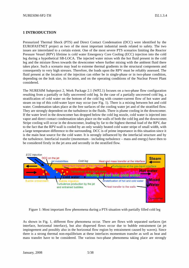
NURESIM-SP2-TH D2.1.3.4
January, 2008 5/38
1 INTRODUCTION
Pressurized Thermal Shock (PTS) and Direct Contact Condensation (DCC) were identified by the EUROFASTNET project as two of the most important industrial needs related to safety. The two issues are interrelated to a certain extent. One of the most severe PTS scenarios limiting the Reactor Pressure Vessel (RPV) lifetime is cold water Emergency Core Cooling (ECC) injection into the cold leg during a hypothetical SB-LOCA. The injected water mixes with the hot fluid present in the cold leg and the mixture flows towards the downcomer where further mixing with the ambient fluid there takes place. Such a scenario may lead to extreme thermal gradients in the structural components and consequently to very high stresses. Therefore, the loads upon the RPV must be reliably assessed. The fluid present at the location of the injection can either be in single-phase or in two-phase condition, depending on the leak size, its location, and on the operating conditions of the Nuclear Power Plant considered. The NURESIM Subproject 2, Work Package 2.1 (WP2.1) focuses on a two-phase flow configuration resulting from a partially or fully uncovered cold leg. In the case of a partially uncovered cold leg, a stratification of cold water on the bottom of the cold leg with counter-current flow of hot water and steam on top of this cold-water layer may occur (see Fig. 1). There is a mixing between hot and cold water. Condensation takes place at the free surfaces of the cooling water jet and of the stratified flow. They are strongly dependent on the turbulence in the fluids. There is plume cooling in the downcomer. If the water level in the downcomer has dropped below the cold leg nozzle, cold water is injected into vapor and direct contact condensation takes place on the walls of both the cold leg and the downcomer. Stripe cooling will occur in the downcomer, leading by far to the highest thermal load of the RPV, due to the fact that the RPV-wall is cooled by an only weakly heated cold water stripe of small width, with a large temperature difference to the surrounding. DCC is of prime importance in this situation since it is the main heat source for the cold water. It is strongly influenced by the interfacial structure and by the turbulence. Interfacial transfer (momentum - including turbulence – mass and energy) have then to be considered firstly in the jet area and secondly in the stratified flow.
Figure 1: Most important flow phenomena during a PTS situation with partially filled cold leg As shown in Fig. 1, different flow phenomena occur. There are flows with separated surfaces (jet interface, horizontal interface), but also dispersed flows occur due to bubble entrainment (at jet impingement and possibly also in the horizontal flow region by entrainment caused by waves). Since there is a strong thermal non-equilibrium at these interfaces momentum transfer as well as heat and mass transfer have to be considered. The various two-phase phenomena taking place are strongly
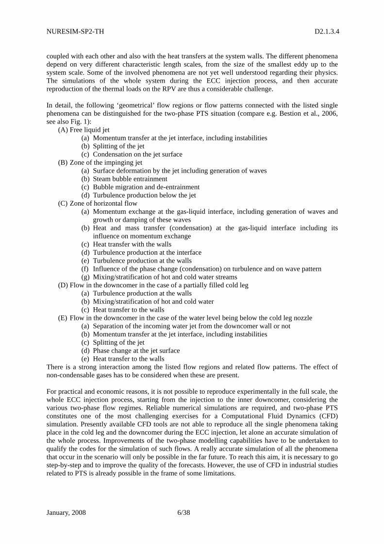
NURESIM-SP2-TH D2.1.3.4
January, 2008 6/38
coupled with each other and also with the heat transfers at the system walls. The different phenomena depend on very different characteristic length scales, from the size of the smallest eddy up to the system scale. Some of the involved phenomena are not yet well understood regarding their physics. The simulations of the whole system during the ECC injection process, and then accurate reproduction of the thermal loads on the RPV are thus a considerable challenge.
In detail, the following ‘geometrical’ flow regions or flow patterns connected with the listed single phenomena can be distinguished for the two-phase PTS situation (compare e.g. Bestion et al., 2006, see also Fig. 1):
(A) Free liquid jet (a) Momentum transfer at the jet interface, including instabilities (b) Splitting of the jet (c) Condensation on the jet surface
(B) Zone of the impinging jet (a) Surface deformation by the jet including generation of waves (b) Steam bubble entrainment (c) Bubble migration and de-entrainment (d) Turbulence production below the jet
(C) Zone of horizontal flow (a) Momentum exchange at the gas-liquid interface, including generation of waves and
growth or damping of these waves (b) Heat and mass transfer (condensation) at the gas-liquid interface including its
influence on momentum exchange (c) Heat transfer with the walls (d) Turbulence production at the interface (e) Turbulence production at the walls (f) Influence of the phase change (condensation) on turbulence and on wave pattern (g) Mixing/stratification of hot and cold water streams
(D) Flow in the downcomer in the case of a partially filled cold leg (a) Turbulence production at the walls (b) Mixing/stratification of hot and cold water (c) Heat transfer to the walls
(E) Flow in the downcomer in the case of the water level being below the cold leg nozzle (a) Separation of the incoming water jet from the downcomer wall or not (b) Momentum transfer at the jet interface, including instabilities (c) Splitting of the jet (d) Phase change at the jet surface (e) Heat transfer to the walls
There is a strong interaction among the listed flow regions and related flow patterns. The effect of non-condensable gases has to be considered when these are present. For practical and economic reasons, it is not possible to reproduce experimentally in the full scale, the whole ECC injection process, starting from the injection to the inner downcomer, considering the various two-phase flow regimes. Reliable numerical simulations are required, and two-phase PTS constitutes one of the most challenging exercises for a Computational Fluid Dynamics (CFD) simulation. Presently available CFD tools are not able to reproduce all the single phenomena taking place in the cold leg and the downcomer during the ECC injection, let alone an accurate simulation of the whole process. Improvements of the two-phase modelling capabilities have to be undertaken to qualify the codes for the simulation of such flows. A really accurate simulation of all the phenomena that occur in the scenario will only be possible in the far future. To reach this aim, it is necessary to go step-by-step and to improve the quality of the forecasts. However, the use of CFD in industrial studies related to PTS is already possible in the frame of some limitations.
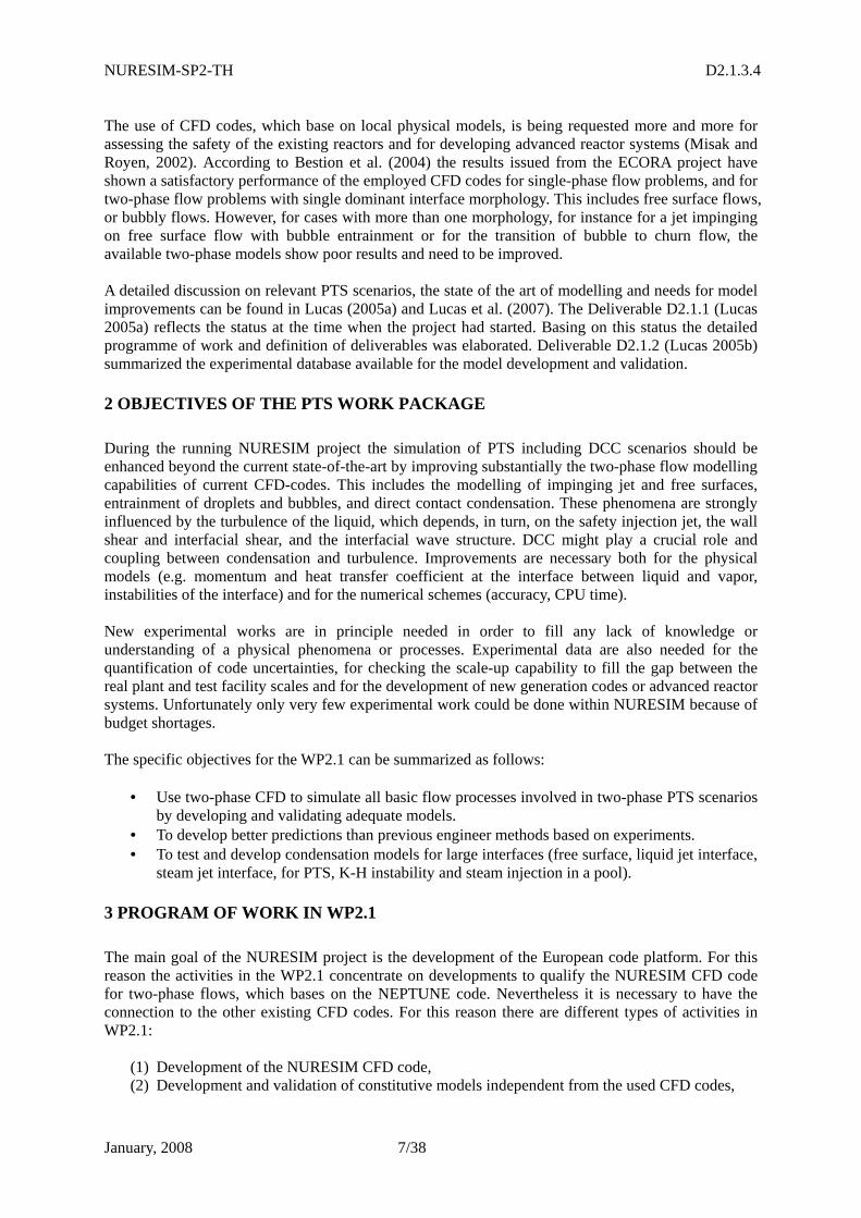
NURESIM-SP2-TH D2.1.3.4
January, 2008 7/38
The use of CFD codes, which base on local physical models, is being requested more and more for assessing the safety of the existing reactors and for developing advanced reactor systems (Misak and Royen, 2002). According to Bestion et al. (2004) the results issued from the ECORA project have shown a satisfactory performance of the employed CFD codes for single-phase flow problems, and for two-phase flow problems with single dominant interface morphology. This includes free surface flows, or bubbly flows. However, for cases with more than one morphology, for instance for a jet impinging on free surface flow with bubble entrainment or for the transition of bubble to churn flow, the available two-phase models show poor results and need to be improved. A detailed discussion on relevant PTS scenarios, the state of the art of modelling and needs for model improvements can be found in Lucas (2005a) and Lucas et al. (2007). The Deliverable D2.1.1 (Lucas 2005a) reflects the status at the time when the project had started. Basing on this status the detailed programme of work and definition of deliverables was elaborated. Deliverable D2.1.2 (Lucas 2005b) summarized the experimental database available for the model development and validation.
2 OBJECTIVES OF THE PTS WORK PACKAGE
During the running NURESIM project the simulation of PTS including DCC scenarios should be enhanced beyond the current state-of-the-art by improving substantially the two-phase flow modelling capabilities of current CFD-codes. This includes the modelling of impinging jet and free surfaces, entrainment of droplets and bubbles, and direct contact condensation. These phenomena are strongly influenced by the turbulence of the liquid, which depends, in turn, on the safety injection jet, the wall shear and interfacial shear, and the interfacial wave structure. DCC might play a crucial role and coupling between condensation and turbulence. Improvements are necessary both for the physical models (e.g. momentum and heat transfer coefficient at the interface between liquid and vapor, instabilities of the interface) and for the numerical schemes (accuracy, CPU time). New experimental works are in principle needed in order to fill any lack of knowledge or understanding of a physical phenomena or processes. Experimental data are also needed for the quantification of code uncertainties, for checking the scale-up capability to fill the gap between the real plant and test facility scales and for the development of new generation codes or advanced reactor systems. Unfortunately only very few experimental work could be done within NURESIM because of budget shortages. The specific objectives for the WP2.1 can be summarized as follows:
• Use two-phase CFD to simulate all basic flow processes involved in two-phase PTS scenarios by developing and validating adequate models.
• To develop better predictions than previous engineer methods based on experiments. • To test and develop condensation models for large interfaces (free surface, liquid jet interface,
steam jet interface, for PTS, K-H instability and steam injection in a pool).
3 PROGRAM OF WORK IN WP2.1
The main goal of the NURESIM project is the development of the European code platform. For this reason the activities in the WP2.1 concentrate on developments to qualify the NURESIM CFD code for two-phase flows, which bases on the NEPTUNE code. Nevertheless it is necessary to have the connection to the other existing CFD codes. For this reason there are different types of activities in WP2.1:
(1) Development of the NURESIM CFD code, (2) Development and validation of constitutive models independent from the used CFD codes,
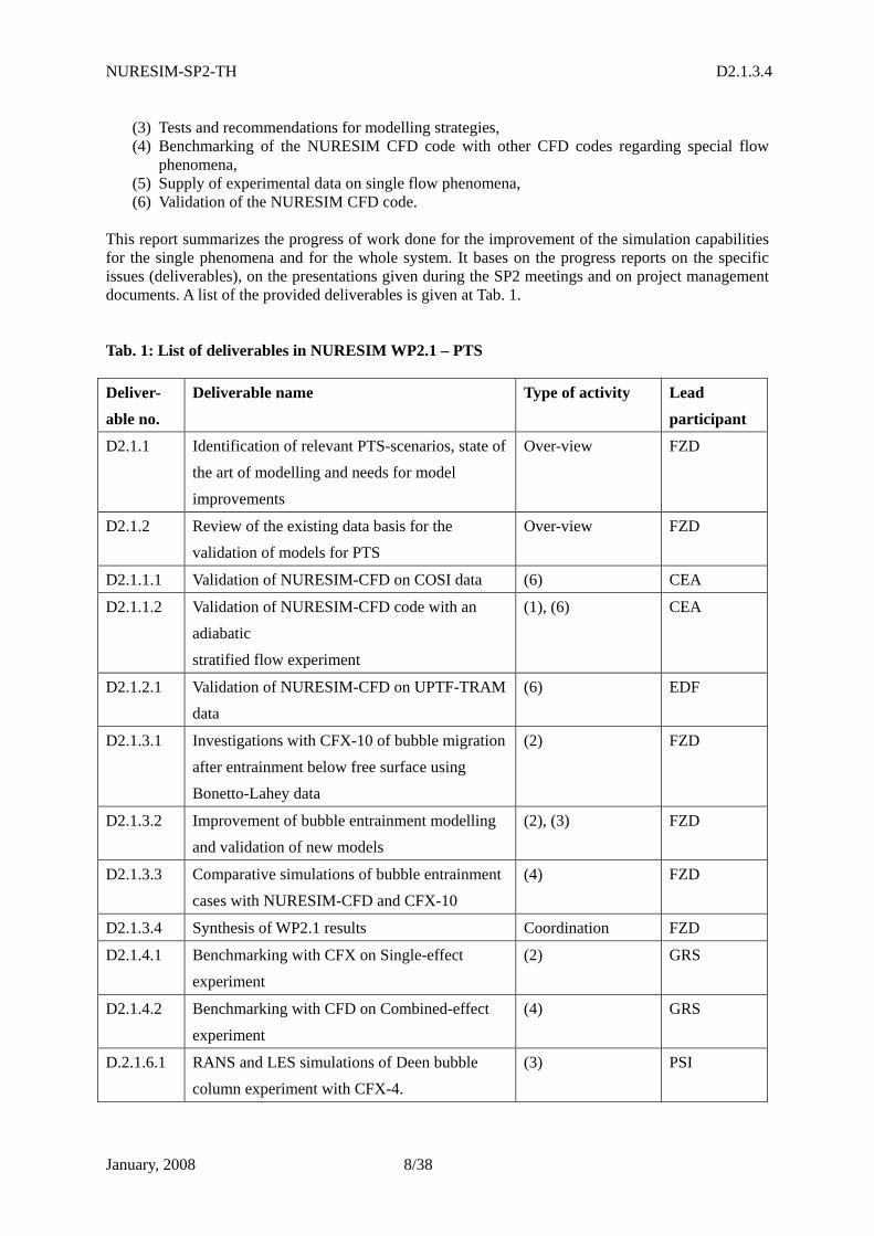
NURESIM-SP2-TH D2.1.3.4
January, 2008 8/38
(3) Tests and recommendations for modelling strategies, (4) Benchmarking of the NURESIM CFD code with other CFD codes regarding special flow
phenomena, (5) Supply of experimental data on single flow phenomena, (6) Validation of the NURESIM CFD code.
This report summarizes the progress of work done for the improvement of the simulation capabilities for the single phenomena and for the whole system. It bases on the progress reports on the specific issues (deliverables), on the presentations given during the SP2 meetings and on project management documents. A list of the provided deliverables is given at Tab. 1. Tab. 1: List of deliverables in NURESIM WP2.1 – PTS
Deliver-
able no.
Deliverable name Type of activity Lead
participant
D2.1.1 Identification of relevant PTS-scenarios, state of
the art of modelling and needs for model
improvements
Over-view FZD
D2.1.2 Review of the existing data basis for the
validation of models for PTS
Over-view FZD
D2.1.1.1 Validation of NURESIM-CFD on COSI data (6) CEA
D2.1.1.2 Validation of NURESIM-CFD code with an
adiabatic
stratified flow experiment
(1), (6) CEA
D2.1.2.1 Validation of NURESIM-CFD on UPTF-TRAM
data
(6) EDF
D2.1.3.1 Investigations with CFX-10 of bubble migration
after entrainment below free surface using
Bonetto-Lahey data
(2) FZD
D2.1.3.2 Improvement of bubble entrainment modelling
and validation of new models
(2), (3) FZD
D2.1.3.3 Comparative simulations of bubble entrainment
cases with NURESIM-CFD and CFX-10
(4) FZD
D2.1.3.4 Synthesis of WP2.1 results Coordination FZD
D2.1.4.1 Benchmarking with CFX on Single-effect
experiment
(2) GRS
D2.1.4.2 Benchmarking with CFD on Combined-effect
experiment
(4) GRS
D.2.1.6.1 RANS and LES simulations of Deen bubble
column experiment with CFX-4.
(3) PSI
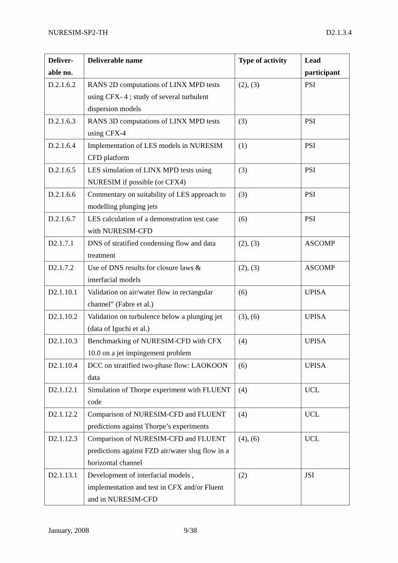
NURESIM-SP2-TH D2.1.3.4
January, 2008 9/38
Deliver-
able no.
Deliverable name Type of activity Lead
participant
D.2.1.6.2 RANS 2D computations of LINX MPD tests
using CFX- 4 ; study of several turbulent
dispersion models
(2), (3) PSI
D.2.1.6.3 RANS 3D computations of LINX MPD tests
using CFX-4
(3) PSI
D.2.1.6.4 Implementation of LES models in NURESIM
CFD platform
(1) PSI
D.2.1.6.5 LES simulation of LINX MPD tests using
NURESIM if possible (or CFX4)
(3) PSI
D.2.1.6.6 Commentary on suitability of LES approach to
modelling plunging jets
(3) PSI
D.2.1.6.7 LES calculation of a demonstration test case
with NURESIM-CFD
(6) PSI
D2.1.7.1 DNS of stratified condensing flow and data
treatment
(2), (3) ASCOMP
D2.1.7.2 Use of DNS results for closure laws &
interfacial models
(2), (3) ASCOMP
D2.1.10.1 Validation on air/water flow in rectangular
channel” (Fabre et al.)
(6) UPISA
D2.1.10.2 Validation on turbulence below a plunging jet
(data of Iguchi et al.)
(3), (6) UPISA
D2.1.10.3 Benchmarking of NURESIM-CFD with CFX
10.0 on a jet impingement problem
(4) UPISA
D2.1.10.4 DCC on stratified two-phase flow: LAOKOON
data
(6) UPISA
D2.1.12.1 Simulation of Thorpe experiment with FLUENT
code
(4) UCL
D2.1.12.2 Comparison of NURESIM-CFD and FLUENT
predictions against Thorpe’s experiments
(4) UCL
D2.1.12.3 Comparison of NURESIM-CFD and FLUENT
predictions against FZD air/water slug flow in a
horizontal channel
(4), (6) UCL
D2.1.13.1 Development of interfacial models ,
implementation and test in CFX and/or Fluent
and in NURESIM-CFD
(2) JSI
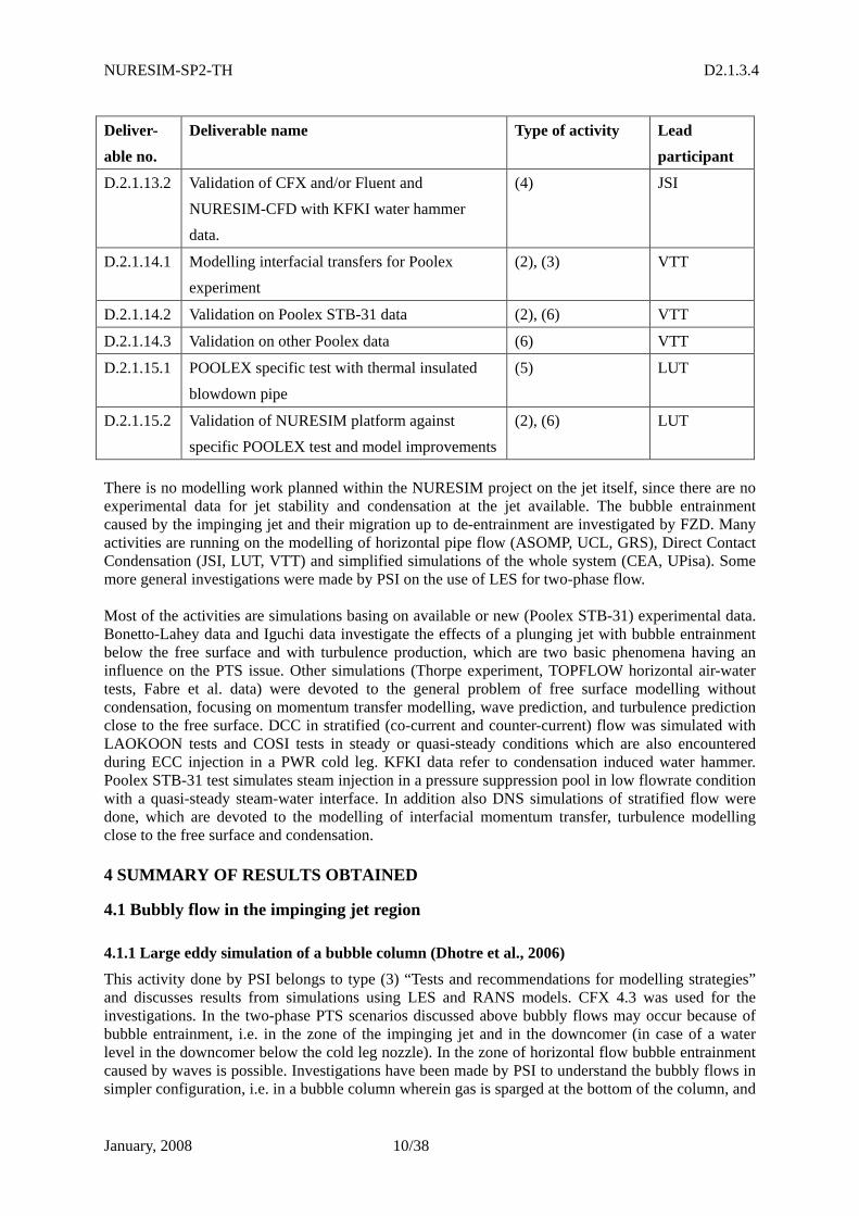
NURESIM-SP2-TH D2.1.3.4
January, 2008 10/38
Deliver-
able no.
Deliverable name Type of activity Lead
participant
D.2.1.13.2 Validation of CFX and/or Fluent and
NURESIM-CFD with KFKI water hammer
data.
(4) JSI
D.2.1.14.1 Modelling interfacial transfers for Poolex
experiment
(2), (3) VTT
D.2.1.14.2 Validation on Poolex STB-31 data (2), (6) VTT
D.2.1.14.3 Validation on other Poolex data (6) VTT
D.2.1.15.1 POOLEX specific test with thermal insulated
blowdown pipe
(5) LUT
D.2.1.15.2 Validation of NURESIM platform against
specific POOLEX test and model improvements
(2), (6) LUT
There is no modelling work planned within the NURESIM project on the jet itself, since there are no experimental data for jet stability and condensation at the jet available. The bubble entrainment caused by the impinging jet and their migration up to de-entrainment are investigated by FZD. Many activities are running on the modelling of horizontal pipe flow (ASOMP, UCL, GRS), Direct Contact Condensation (JSI, LUT, VTT) and simplified simulations of the whole system (CEA, UPisa). Some more general investigations were made by PSI on the use of LES for two-phase flow. Most of the activities are simulations basing on available or new (Poolex STB-31) experimental data. Bonetto-Lahey data and Iguchi data investigate the effects of a plunging jet with bubble entrainment below the free surface and with turbulence production, which are two basic phenomena having an influence on the PTS issue. Other simulations (Thorpe experiment, TOPFLOW horizontal air-water tests, Fabre et al. data) were devoted to the general problem of free surface modelling without condensation, focusing on momentum transfer modelling, wave prediction, and turbulence prediction close to the free surface. DCC in stratified (co-current and counter-current) flow was simulated with LAOKOON tests and COSI tests in steady or quasi-steady conditions which are also encountered during ECC injection in a PWR cold leg. KFKI data refer to condensation induced water hammer. Poolex STB-31 test simulates steam injection in a pressure suppression pool in low flowrate condition with a quasi-steady steam-water interface. In addition also DNS simulations of stratified flow were done, which are devoted to the modelling of interfacial momentum transfer, turbulence modelling close to the free surface and condensation.
4 SUMMARY OF RESULTS OBTAINED
4.1 Bubbly flow in the impinging jet region
4.1.1 Large eddy simulation of a bubble column (Dhotre et al., 2006)
This activity done by PSI belongs to type (3) “Tests and recommendations for modelling strategies” and discusses results from simulations using LES and RANS models. CFX 4.3 was used for the investigations. In the two-phase PTS scenarios discussed above bubbly flows may occur because of bubble entrainment, i.e. in the zone of the impinging jet and in the downcomer (in case of a water level in the downcomer below the cold leg nozzle). In the zone of horizontal flow bubble entrainment caused by waves is possible. Investigations have been made by PSI to understand the bubbly flows in simpler configuration, i.e. in a bubble column wherein gas is sparged at the bottom of the column, and
NURESIM-SP2-TH D2.1.3.4
January, 2008 11/38
rises through it in the form of bubbles (Dhotre et al., 2006). The resulting flow is characterized by many distinct flow structures of various length scales (from tiny vortices shed by an individual bubble to macroscopic circulation covering the whole column). The simulations have been carried out for the square cross-sectioned bubble column. Euler-Euler simulations of the gas-liquid flow in a bubble column using a LES (two subgrid scale models) and RANS (k-ε) model predictions have been compared with the experimental data from Deen et al. (2000). All the non-drag forces - virtual mass force, lift force and drag forces were incorporated in the model. An extra contribution in the effective viscosity for the turbulence induced by bubbles was taken into account using the Sato model. The performance of two different subgrid scale models, a Smagorinsky model and Dynamic model of Germano, has been assessed. Modifying the subgrid scale (SGS) models to account for bubble induced turbulence did not much change the results. It was observed that the dynamic approach of Germano does not perform better than the Smagorinsky model for this configuration with CS equal to 0.12. In fact, it has been found that the averaged Cs values obtained with Dynamic model converge towards Cs = 0.12. However, though Germano model predictions agree with Smagorinsky, still it can be used to have estimates of CS value which are not known a priori. As for the RANS approach, it was found that with all the forces incorporated and using the extra source terms for turbulent kinetic energy and dissipation rate, an enhanced k-ε model including the effects of bubble-induced turbulence (Simonin and Viollet model) gives reasonably good agreement with the experimental data except for the radial and axial distribution of the fluctuating liquid velocity and turbulent kinetic energy close to the wall. More details on this activity can be found in the Deliverable D2.1.6.1 (Dhotre et al., 2006). Together with this report the source code for implementation of bubble forces has been delivered.
4.1.2 CFD Simulation of large scale bubble plumes (Dhotre and Smith, 2006, Dhotre, et al.,
2007)
This activity is related to types (2) and (3), “Development and validation of constitutive models independent from the used CFD codes” and “Tests and recommendations for modelling strategies”. In Euler-Euler simulations of gas-liquid flow in large-scale, bubble plumes have been simulated using the Large Eddy Simulation (LES) and Reynolds-Averaged Navier Stokes (RANS) formulations of turbulence have been undertaken. The interfacial forces between the phases and bubble-induced turbulence effects have been included. As well as the drag force, the non-drag forces (turbulent dispersion force for RANS only), virtual mass force and lift force have been incorporated in the model. CFD simulations have been carried out for the prediction of the bubble-flow characteristics observed in the LINX experiments The axial mean liquid velocity and gas velocity at all the measurement levels exhibit the expected Gaussian profiles and plume spreading. Both model predictions of the void fraction, axial gas and liquid velocities are in reasonable agreement with the experimental data, except near the injector. The RANS model (k-ε, but with extra source terms in the equations to represent bubble-induced turbulence effects) gives reasonably good agreement with the mean experimental data, except for the radial and axial distribution of the fluctuating liquid velocity and turbulent kinetic energy. In contrast, the turbulent kinetic energy turbulent shear stresses are well captured by LES at the two higher measurement positions (away from the bubble injector), but over-prediction was observed at the lowest position (near the injector). From the CFD predictions obtained in the present work, it can be concluded that LES can be a useful tool, if the objective is to find information about structural and statistical features of flow, but if only the mean variables are required, RANS also does well, except where turbulence anisotropy is an important feature. In general, quantitative comparison with experimental data has revealed that, by applying proper models of inter-phase momentum transfer, and performing simulations based on the two-fluid model, satisfactory predictions of mean flow quantities can be obtained for this application.
NURESIM-SP2-TH D2.1.3.4
January, 2008 12/38
In results of the activities described in this section and the one before LES and RANS models were implemented into the NURESIM CFD platform (Deliverable D2.1.6.4, activity of type (1) “Development of the NURESIM CFD code”).
4.1.3 LES demonstration case by NEPTUNE_CFD (Dhotre, et al. 2007b)
This activity done by PSI belongs to type (6) “Validation of the NURESIM CFD code”. Euler-Euler-Large Eddy Simulations (EELES) of gas-liquid flow in a vertical cylindrical pipe have been simulated using NEPTUNE_CFD. The Smagorinksy subgrid-scale model had already been implemented and successfully used as described in D2.2.6.2. Quality data are available for comparison from the water/air experiments of Hibiki et al. in the form of void fraction distribution, axial liquid velocity and axial gas velocity at two elevations (Z/D=6.0 and 53.0). Detailed comparisons have revealed that the distribution for void fraction and axial gas velocity in the pipe centre is in good agreement with the experimental data. However, the distribution of void fraction, as well as axial gas velocity at the wall is over-predicted. The axial liquid velocity predictions are in agreement with the experimental data across the pipe cross-section. The discrepancies observed in the model predictions could be attributed to the lack of a wall lubrication force model in the code or improper implementation of boundary conditions at the wall. This issue is still under investigation.
4.1.4 Commentary on suitability of LES approach to modelling plunging jets (B. Ničeno, 2007)
This activity done by PSI belongs to type (3) “Tests and recommendations for modelling strategies”. The ability of CFD to accurately predict plunging jets would represent an important step towards successful analysis of the PTS phenomenon. The applicability of the LES technique, which is thought by many to be a promising and emerging tool for turbulence prediction, to the analysis of plunging jet flows has been assessed. The work at this stage has been restricted to water/air configurations, i.e. without heat and/or mass transfer, and has concentrated on the plunging jet experiment of Bonetto & Lahey, though the conclusions might be considered of more general applicability. Even with this simplification, the task of assessing the potential of LES is considerable, since different resolution levels of an LES also imply different treatments of air/water interface. Three variants of the LES technique for multiphase flows are considered. The first is Interface Tracking LES (ITLES), which explicitly resolves the interface between the two fluids. The second is Euler-Euler LES (EELES), in which one set of (volume-averaged) equations is used for each phase, together with models for the interface exchange terms. Third is Large Scale Simulation (LSS), which is a combination of the former two. It is concluded that the third variant, i.e. a combination of LES, and explicit surface tracking where possible on a given grid size, together with EE modelling of interfacial forces on the scales smaller than the grid size, fits best into the LES framework (large turbulent structures resolved on the grid, and the smaller ones represented by a sub-grid scale or SGS model). This option converges towards ever more realistic physical situations with grid refinement, and can be achieved at reduced computational cost compared to ITLES. Furthermore, the grid may be refined in the regions of the flow where more important phenomena take place, without violation of any physical principle, as is the case in EELES. It should also be emphasised that a CFD tool which is to be used for simulations of plunging jets using LES must be efficient computationally with large numbers of grid cells, and it must be able to prescribe some kind of pseudo turbulence at the inlet. Efficiency does not stem only from increase in computational power alone, but also from the usage of more efficient numerical algorithms.
NURESIM-SP2-TH D2.1.3.4
January, 2008 13/38
4.1.5 Investigations on bubble migration after entrainment below the liquid surface (Bodele and
Lucas, 2006)
The investigations regarding bubble entrainment by the impinging jet and the subsequent bubble migration done by FZD are of type (2) “Development and validation of constitutive models independent from the used CFD codes”. To separate the tasks in this first step bubble entrainment itself was excluded from the simulation. Instead a two-phase mixture injection below the liquid surface was assumed to investigate bubble migration. The investigations were done using CFX-10. The base for the numerical simulations is the Bonetto & Lahey (1993) experiment but strong variations have been considered. For avoiding the explicit prediction of the gas entrainment mechanism at the impinging region (presently, it is not possible to predict the entrainment mechanism with sufficient precision – see next sections), the injector has been directly introduced in the liquid phase and the initial jet is a two-phase jet (continuous liquid phase with included bubbles). The impingement between the jet and the liquid free surface is not explicitly numerically predicted. The main objectives of these investigations consist in testing several hypothesis on the mesh (3D, 2D axisymmetric or 2D plane), the boundary conditions (location for the outlets, properties of the walls…), initial conditions, models used for the prediction of the gas behaviour (use of the non drag forces models, most appropriate turbulence model) and on the numerical assumptions (steady state or transient computations). These tests should permit to define the most appropriate elements to take into account for the numerical prediction of the gas behaviour below the free surface, before the development and introduction of the new models. A domain was defined, which is suitable for the calculations of the bubble migration below the free surface, the bubble entrainment by the plunging jet (by adjusting the initial water level in the domain) and for the bubble de-entrainment at the free surface. This configuration permits to obtain results in one or two days computing time, which permits to study the variation of various parameters. Tests were made for steady state and transient assumptions. In the result of the steady state simulations it was shown, that this approach is not suitable for the simulation of the considered configuration. Despite of the symmetric boundary conditions, the simulations didn’t lead to a symmetric final solution as it should be expected, since the process itself is transient (oscillating bubble plume). This conclusion has also been confirmed by the transient calculations, which have clearly shown this transient behaviour of the phenomenon (at least for the highest initial gas volume fraction). Simulations were made with and without consideration of non-drag forces. The jet gas volume fraction, bubble, bubble diameter and flow rates were varied. The non-drag forces (lift and turbulent dispersion force) permit to reproduce more accurately the jet behaviour by avoiding the jet separation at the injector exit and in increasing the gas migration, which facilitate the gas escape for the recirculation zone close to the injector. The initial gas volume fraction plays an important role for the appearing of the transient behaviour. Indeed, the calculation with the lowest initial gas volume fraction (1%) didn’t permit to reproduce the transient behaviour. The initial gas volume fraction plays also a role on the gas and liquid velocity below the free liquid surface. The initial bubble diameter influences the gas volume fraction profiles. These effects have to be studied more in detail, because of the boundary conditions, which maintain constant the velocity when varying the initial gas volume fraction (the liquid mass flow rate is increased when the gas volume fraction is decreased). The effects of the initial velocity on the jet characteristics have also to be studied.
4.1.6 Investigations on bubble entrainment by a plunging jet (Bodele and Lucas, 2007,
Schmidtke and Lucas, 2007a)
The investigations regarding bubble entrainment by the impinging jet and the subsequent bubble migration done by FZD are of type (3) “Tests and recommendations for modelling strategies”. Different plunging jet configurations in which a free falling liquid jet impacts a liquid pool surface
NURESIM-SP2-TH D2.1.3.4
January, 2008 14/38
already existing in the facility were considered. While first configurations were close to the one of the Bonetto & Lahey experiment later on a case more suitable for generic investigations was used. The physical process of bubble generation takes place at a very small length scale. A thin air film around the jet is pulled below the water. At a certain depth this film breaks up into bubbles. In general the Euler-Euler approach is used for the simulation of the large scale phenomena in the pool. For this reason a model for the bubble entrainment which can be in used this frame is needed. In a multiphase Euler-Euler simulation, the coefficients of the closures depend on the morphology of the phases. For an impinging jet the water can be regarded as a continuous phase everywhere, whereas the air occurs as a continuous phase above the water level, and as a dispersed phase (bubbly) below the water level. In the first attempts described in the Progress report by Bodele and Lucas (2007) gas entrainment was much too high both in simulations using CFX but also in such using NURESIM-CFD code. Even if bubble entrainment is assumed to be less important for the integral two-phase PTS simulation it would be necessary to suppress this artificial entrainment. It was found, that the air entrainment near the jet is basically determined by the drag force. In the drag force closure, the morphology of the phases is reflected by different values for the drag coefficient and the interfacial area density. To apply the appropriate coefficients, the morphology of the phases has to be identified everywhere in the domain. A simple approach assumes bubbly flow where the gas void fraction is low and continuous gas phase where the gas void fraction is high. In general a model for gas entrainment consists of two parts: A set of coefficients, which depend on the local morphologies of the phases and an algorithm for the identification of the morphologies. One algorithm which enables such a modelling is the so-called the algebraic interfacial area density (AIAD) model. The AIAD model applies two different drag coefficients for free surface and for bubbly flow. A blending function based on the gas void fraction is used to apply the adequate drag coefficient depending on the flow regime. The dependency of the air entrainment on the free surface drag coefficient and the definition of the blending function were investigated. It was shown that this modelling approach enables to control the bubble entrainment. The intensity of the gas entrainment depends on the value of the surface drag coefficient and the shape of the blending function. For quantitative description of the gas entrainment, upward and downward gas fluxes are evaluated separately in dependency of the depth below the water level. This evaluation is used to check the quality of the numerical solution with respect to the mass conservation. By integrating the vertical gas fluxes just under the water surface a global value for the gas entrainment rate is defined. This integral quantity allows a comparison of the numerical results with empirical correlations. Also the influence of the grid size on the results was studied. In the result of the investigation the use of an AIAD model concept is recommended to account for bubble entrainment or at least to suppress entrainment. Appropriate correlations for the drag coefficients as well as an optimization of blending functions are still required. To do this a more detailed database than Bennetto & Lahey data are required.
4.1.7 Comparative simulations of bubble entrainment cases with NURESIM-CFD and CFX-10
(Schmidtke and Lucas, 2007b)
The investigations regarding bubble entrainment by the impinging jet and the subsequent bubble migration done by FZD are of type (3) “Tests and recommendations for modeling strategies”. One plunging jet configuration in which a free falling liquid jet impacts a liquid pool surface already existing in the facility was simulated using both NURESIM-CFD and CFX-10 and the results are compared with respect to the gas entrainment below the liquid pool surface. The NURESIM-CFD provides the SIMMER drag model. In this model, bubbles are assumed to be
NURESIM-SP2-TH D2.1.3.4
January, 2008 15/38
present, where the gas void fraction is low. In areas with high gas void fraction the drag of droplets in air is used. For medium gas void fraction a linear interpolation of bubble drag and droplet drag is applied. In the SIMMER model, the drag for both droplets and bubbles is calculated according to the Schiller-Naumann drag correlation for spherical particles. This drag model was implemented within CFX-10 in the frame of this work. A modified SIMMER drag model was tested with both codes. The modified model is based on a constant drag coefficient for spherical particles instead of the Schiller-Naumann drag coefficient which depends on the Reynolds number. The results of the NURESIM-CFD and CFX code were substantially different: In the CFX simulation the flow fields became stable a few seconds after the release of the jet. In the NURESIM-CFD simulation the entrained gas accumulated in the vortex where the jet reaches the bottom of the domain. After approximately half minute the gas void fraction distribution changes and degassing begins. When the Schiller-Naumann drag correlation was replaced by a constant drag coefficient only little effect on the results was observed for both CFD-codes. In reality the large scale flow structure below an impinging jet becomes stable within a few seconds after the jet release. So the results of the CFX-simulation seem to be more realistic. Within the SIMMER model the bubble and the droplet diameter are the only free parameters available, but it would be unphysical to modify these values for fitting the entrainment in the simulation to values observed in experiments. In the AIAD model the free surface drag coefficient allows to control the entrainment.
4.1.8 NEPTUNE CFD module validation on turbulence below a plunging jet (Galassi et al.,
2006)
This activity done by UPisa and CEA belongs to types (3) “Tests and recommendations for modelling strategies” and (6) “Validation of the NURESIM CFD code”. A Two-dimensional simulation of a Plunging Water Jet Entering a Free Surface (Iguchi data) through NEPTUNE CFD module was done aiming at code turbulence models verification and validation against experimental data.
This study was done with an extensive performance comparison of different turbulence models in predicting the flow characteristics. Together with NEPTUNE standard models, a CEA/Grenoble modified k-ε model was tested. One test was simulated, where only small bubbles are entrained below the free surface without influencing the turbulence intensity. Such small bubbles are obtained with a short distance (2mm) between the pipe exit and the free surface of the bath.
Numerical predictions of the mean velocity field were always in a rather good agreement with experimental data. Calculated air volume fraction distribution showed that numerical simulations effectively account for air entrainment near the free surface (z = 10cm) and bubble dispersion in the whole water vessel (z = 20 and 30 cm), but with very small void fraction values. The predicted void fraction below the free surface is very low (less than 0.5 %) which is qualitatively consistent with observations of the Iguchi tests, but quantitative comparison is not possible due to the absence of void fraction measurement.
Turbulence prediction was generally not bad but significant underestimation is obtained far from the jet axis region. Big differences are also observed in the prediction of turbulent velocities components near the free surface. In fact, calculations predicted nearly the same values for the two turbulent velocity components, u’rms and v’rms, failing to catch the anisotropy of the problem. This is a classical feature of the k-ε model. Adopting a different turbulence model that accurately predicts the Reynolds stresses with anisotropy would probably improve the code performances. However the main objective of the turbulence model is here to predict turbulent diffusion of heat in the liquid layer and a k-ε model may be sufficient.
NURESIM-SP2-TH D2.1.3.4
January, 2008 16/38
Considering the Interfacial Turbulence Effects (interfacial production and dissipation), which would increase calculated turbulence (accounting for the dispersed phase contribution), in contrast to what expected brought worst results causing a further reduction in turbulence estimation. In fact, in the present formulation, the additional dissipation has more influence than the additional production. Normally due to the small size of bubbles, there should not be a significant influence of bubbles on the turbulence as mentioned by Iguchi. Trying to modify the relative importance of production and dissipation terms in the turbulent energy equation did not lead to better results. It is then recommended to further consider the formulation of the interfacial production and dissipation terms in case of small bubbles. Anyway, an under prediction of turbulence would, in real PTS applications, lead to an overestimation of the severity of the scenario, since steam condensation in the bulk liquid is strongly enhanced by the turbulence level.
4.2 Stratified flow in the cold leg without heat and mass transfer
4.2.1 DNS database for momentum and turbulence transfer at the interface (Lakehal, 2006)
The ASCOMP contribution to NURESIM is mainly of type (2) “Development and validation of constitutive models independent from the used CFD codes”, but is also related to type (3) “Tests and recommendations for modeling strategies”. Interface transport models are proposed based on the DNS data of turbulent sheared air-water flow. The database has been developed by Fulgosi et al. (2003), Lakehal et al. (2003), Banerjee et al. (2004), Fulgosi (2004) and very recently by Lakehal et al. (2008). It has been explored in order to infer modelling approaches to turbulence transport at interfacial two-phase flows. The models have been developed in the spirit of the 2-equation modelling concept, focusing in particular on the boundary conditions and limiting behaviour of turbulence quantities at sheared interfaces. This is an important step towards proper modelling of this class of flow. The DNS set-up from which the data have been extracted is explained by Lakehal (2006). Also the equations and simulation technique are discussed. The second part of the document dealing with turbulence modelling at sheared interfaces starts with a brief analysis of the major issues in modelling bubbly flows, assuming that this particular structure is a result of a strong deformation of interfaces at impingement. Three drawbacks related to the production term in the turbulent kinetic energy equation when used in the Two-Fluid formulation are made evident: (1) the sensitivity to the presence of bubbles by an additional buoyancy-induced generation mechanism term; (2) combined vorticity/strain sensitivity to correct the isotropic EVM concept for jetting in the cold leg; and (3) interface sharpening to reduce the smoothing or under-resolution of the interfacial shear. The exact asymptotic (limiting) behaviour of relevant quantities at the interface is developed and compared to known wall-flow laws. The study has helped clarify boundary conditions issues for the use in RANS modelling. Also the issue of eddy diffusivity distribution at sheared interfaces was addressed. New interface damping laws are proposed. Turbulence anisotropy near interfaces, where new laws have been developed is analysed and compared to wall-flow models. The report also deals with the modelling of scalar transfer across interfaces, by reference to the surface divergence theory, which we believe is best suited for the problems under consideration. The models presented by Lakehal (2006) can be thought of as main ‘modelling guidelines’ and need to be validated first. This validation process was started within the NURESIM project.
4.2.2 Kelvin-Helmholtz instability (Bartosiewicz et al., 2006a,b,c, 2007a,b)
Benchmarking of the NURESIM-CFD code with FLUENT for Kelvin-Helmholtz instability was done by UCL (activity of types (3)). This Benchmark relies on the Thorpe experiment (Thorpe 1969) to model the occurrence and development of instabilities in a stratified two phase flow. The first part of
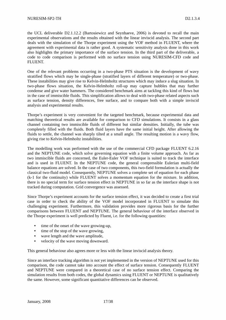
NURESIM-SP2-TH D2.1.3.4
January, 2008 17/38
the UCL deliverable D2.1.12.2 (Bartosiewicz and Seynhaeve, 2006) is devoted to recall the main experimental observations and the results obtained with the linear inviscid analysis. The second part deals with the simulation of the Thorpe experiment using the VOF method in FLUENT, where the agreement with experimental data is rather good. A systematic sensitivity analysis done in this work also highlights the primary importance of the surface tension. In the third part of the deliverable, a code to code comparison is performed with no surface tension using NURESIM-CFD code and FLUENT. One of the relevant problems occurring in a two-phase PTS situation is the development of wavy stratified flows which may be single-phase (stratified layers of different temperature) or two-phase. These instabilities may give rise to Kelvin-Helmholtz structures which may induce a slug situation. In two-phase flows situation, the Kelvin-Helmholtz roll-up may capture bubbles that may further condense and give water hammers. The considered benchmark aims at tackling this kind of flows but in the case of immiscible fluids. This simplification allows to deal with two-phase related aspects such as surface tension, density differences, free surface, and to compare both with a simple inviscid analysis and experimental results. Thorpe’s experiment is very convenient for the targeted benchmark, because experimental data and matching theoretical results are available for comparison to CFD simulations. It consists in a glass channel containing two immiscible fluids of different but similar densities. Initially, the tube was completely filled with the fluids. Both fluid layers have the same initial height. After allowing the fluids to settle, the channel was sharply tilted at a small angle. The resulting motion is a wavy flow, giving rise to Kelvin-Helmholtz instabilities. The modelling work was performed with the use of the commercial CFD package FLUENT 6.2.16 and the NEPTUNE code, which solve governing equation with a finite volume approach. As far as two immiscible fluids are concerned, the Euler-Euler VOF technique is suited to track the interface and is used in FLUENT. In the NEPTUNE code, the general compressible Eulerian multi-field balance equations are solved. In the case of two components, this two-field formulation is actually the classical two-fluid model. Consequently, NEPTUNE solves a complete set of equation for each phase (k-1 for the continuity) while FLUENT solves a momentum equation for the mixture. In addition, there is no special term for surface tension effect in NEPTUNE in so far as the interface shape is not tracked during computation. Grid convergence was assessed. Since Thorpe’s experiment accounts for the surface tension effect, it was decided to create a first trial case in order to check the ability of the VOF model incorporated in FLUENT to simulate this challenging experiment. Furthermore, this validation provides more rigorous basis for the further comparisons between FLUENT and NEPTUNE. The general behaviour of the interface observed in the Thorpe experiment is well predicted by Fluent, i.e. for the following quantities:
• time of the onset of the wave growing-up, • time of the stop of the wave growing, • wave length and the wave amplitude, • velocity of the wave moving downward.
This general behaviour also agrees more or less with the linear inviscid analysis theory. Since an interface tracking algorithm is not yet implemented in the version of NEPTUNE used for this comparison, the code cannot take into account the effect of surface tension. Consequently FLUENT and NEPTUNE were compared in a theoretical case of no surface tension effect. Comparing the simulation results from both codes, the global dynamics using FLUENT or NEPTUNE is qualitatively the same. However, some significant quantitative differences can be observed.
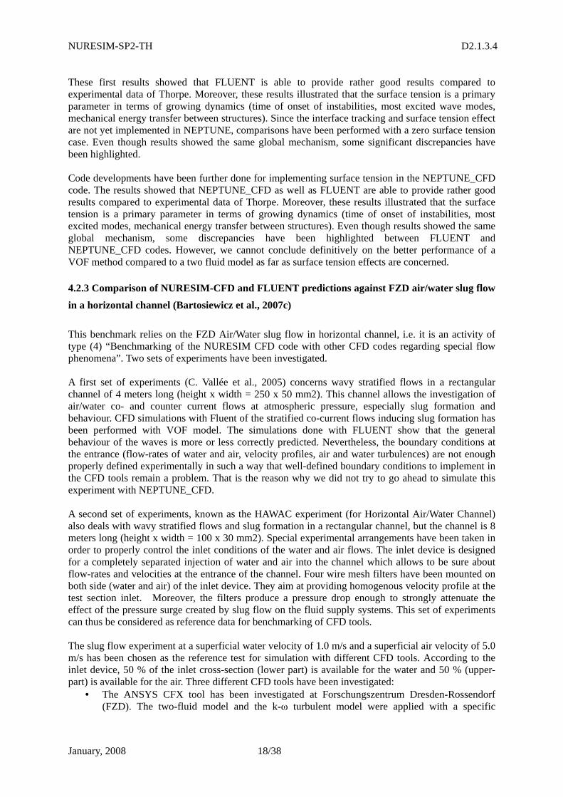
NURESIM-SP2-TH D2.1.3.4
January, 2008 18/38
These first results showed that FLUENT is able to provide rather good results compared to experimental data of Thorpe. Moreover, these results illustrated that the surface tension is a primary parameter in terms of growing dynamics (time of onset of instabilities, most excited wave modes, mechanical energy transfer between structures). Since the interface tracking and surface tension effect are not yet implemented in NEPTUNE, comparisons have been performed with a zero surface tension case. Even though results showed the same global mechanism, some significant discrepancies have been highlighted. Code developments have been further done for implementing surface tension in the NEPTUNE_CFD code. The results showed that NEPTUNE_CFD as well as FLUENT are able to provide rather good results compared to experimental data of Thorpe. Moreover, these results illustrated that the surface tension is a primary parameter in terms of growing dynamics (time of onset of instabilities, most excited modes, mechanical energy transfer between structures). Even though results showed the same global mechanism, some discrepancies have been highlighted between FLUENT and NEPTUNE_CFD codes. However, we cannot conclude definitively on the better performance of a VOF method compared to a two fluid model as far as surface tension effects are concerned.
4.2.3 Comparison of NURESIM-CFD and FLUENT predictions against FZD air/water slug flow
in a horizontal channel (Bartosiewicz et al., 2007c)
This benchmark relies on the FZD Air/Water slug flow in horizontal channel, i.e. it is an activity of type (4) “Benchmarking of the NURESIM CFD code with other CFD codes regarding special flow phenomena”. Two sets of experiments have been investigated. A first set of experiments (C. Vallée et al., 2005) concerns wavy stratified flows in a rectangular channel of 4 meters long (height x width = 250 x 50 mm2). This channel allows the investigation of air/water co- and counter current flows at atmospheric pressure, especially slug formation and behaviour. CFD simulations with Fluent of the stratified co-current flows inducing slug formation has been performed with VOF model. The simulations done with FLUENT show that the general behaviour of the waves is more or less correctly predicted. Nevertheless, the boundary conditions at the entrance (flow-rates of water and air, velocity profiles, air and water turbulences) are not enough properly defined experimentally in such a way that well-defined boundary conditions to implement in the CFD tools remain a problem. That is the reason why we did not try to go ahead to simulate this experiment with NEPTUNE_CFD. A second set of experiments, known as the HAWAC experiment (for Horizontal Air/Water Channel) also deals with wavy stratified flows and slug formation in a rectangular channel, but the channel is 8 meters long (height x width = 100 x 30 mm2). Special experimental arrangements have been taken in order to properly control the inlet conditions of the water and air flows. The inlet device is designed for a completely separated injection of water and air into the channel which allows to be sure about flow-rates and velocities at the entrance of the channel. Four wire mesh filters have been mounted on both side (water and air) of the inlet device. They aim at providing homogenous velocity profile at the test section inlet. Moreover, the filters produce a pressure drop enough to strongly attenuate the effect of the pressure surge created by slug flow on the fluid supply systems. This set of experiments can thus be considered as reference data for benchmarking of CFD tools. The slug flow experiment at a superficial water velocity of 1.0 m/s and a superficial air velocity of 5.0 m/s has been chosen as the reference test for simulation with different CFD tools. According to the inlet device, 50 % of the inlet cross-section (lower part) is available for the water and 50 % (upper-part) is available for the air. Three different CFD tools have been investigated:
• The ANSYS CFX tool has been investigated at Forschungszentrum Dresden-Rossendorf (FZD). The two-fluid model and the k-ω turbulent model were applied with a specific
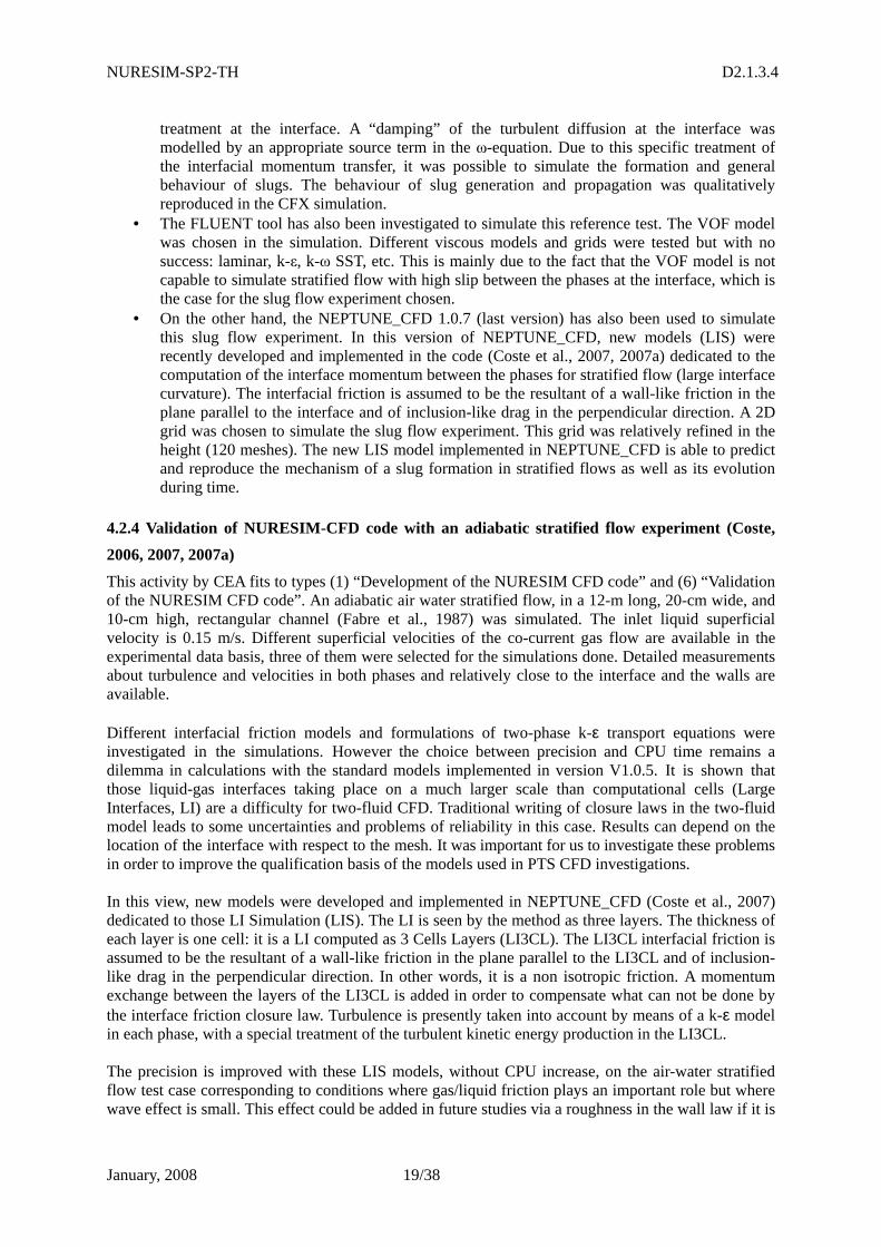
NURESIM-SP2-TH D2.1.3.4
January, 2008 19/38
treatment at the interface. A “damping” of the turbulent diffusion at the interface was modelled by an appropriate source term in the ω-equation. Due to this specific treatment of the interfacial momentum transfer, it was possible to simulate the formation and general behaviour of slugs. The behaviour of slug generation and propagation was qualitatively reproduced in the CFX simulation.
• The FLUENT tool has also been investigated to simulate this reference test. The VOF model was chosen in the simulation. Different viscous models and grids were tested but with no success: laminar, k-ε, k-ω SST, etc. This is mainly due to the fact that the VOF model is not capable to simulate stratified flow with high slip between the phases at the interface, which is the case for the slug flow experiment chosen.
• On the other hand, the NEPTUNE_CFD 1.0.7 (last version) has also been used to simulate this slug flow experiment. In this version of NEPTUNE_CFD, new models (LIS) were recently developed and implemented in the code (Coste et al., 2007, 2007a) dedicated to the computation of the interface momentum between the phases for stratified flow (large interface curvature). The interfacial friction is assumed to be the resultant of a wall-like friction in the plane parallel to the interface and of inclusion-like drag in the perpendicular direction. A 2D grid was chosen to simulate the slug flow experiment. This grid was relatively refined in the height (120 meshes). The new LIS model implemented in NEPTUNE_CFD is able to predict and reproduce the mechanism of a slug formation in stratified flows as well as its evolution during time.
4.2.4 Validation of NURESIM-CFD code with an adiabatic stratified flow experiment (Coste,
2006, 2007, 2007a)
This activity by CEA fits to types (1) “Development of the NURESIM CFD code” and (6) “Validation of the NURESIM CFD code”. An adiabatic air water stratified flow, in a 12-m long, 20-cm wide, and 10-cm high, rectangular channel (Fabre et al., 1987) was simulated. The inlet liquid superficial velocity is 0.15 m/s. Different superficial velocities of the co-current gas flow are available in the experimental data basis, three of them were selected for the simulations done. Detailed measurements about turbulence and velocities in both phases and relatively close to the interface and the walls are available. Different interfacial friction models and formulations of two-phase k-ε transport equations were investigated in the simulations. However the choice between precision and CPU time remains a dilemma in calculations with the standard models implemented in version V1.0.5. It is shown that those liquid-gas interfaces taking place on a much larger scale than computational cells (Large Interfaces, LI) are a difficulty for two-fluid CFD. Traditional writing of closure laws in the two-fluid model leads to some uncertainties and problems of reliability in this case. Results can depend on the location of the interface with respect to the mesh. It was important for us to investigate these problems in order to improve the qualification basis of the models used in PTS CFD investigations. In this view, new models were developed and implemented in NEPTUNE_CFD (Coste et al., 2007) dedicated to those LI Simulation (LIS). The LI is seen by the method as three layers. The thickness of each layer is one cell: it is a LI computed as 3 Cells Layers (LI3CL). The LI3CL interfacial friction is assumed to be the resultant of a wall-like friction in the plane parallel to the LI3CL and of inclusion-like drag in the perpendicular direction. In other words, it is a non isotropic friction. A momentum exchange between the layers of the LI3CL is added in order to compensate what can not be done by the interface friction closure law. Turbulence is presently taken into account by means of a k-ε model in each phase, with a special treatment of the turbulent kinetic energy production in the LI3CL. The precision is improved with these LIS models, without CPU increase, on the air-water stratified flow test case corresponding to conditions where gas/liquid friction plays an important role but where wave effect is small. This effect could be added in future studies via a roughness in the wall law if it is
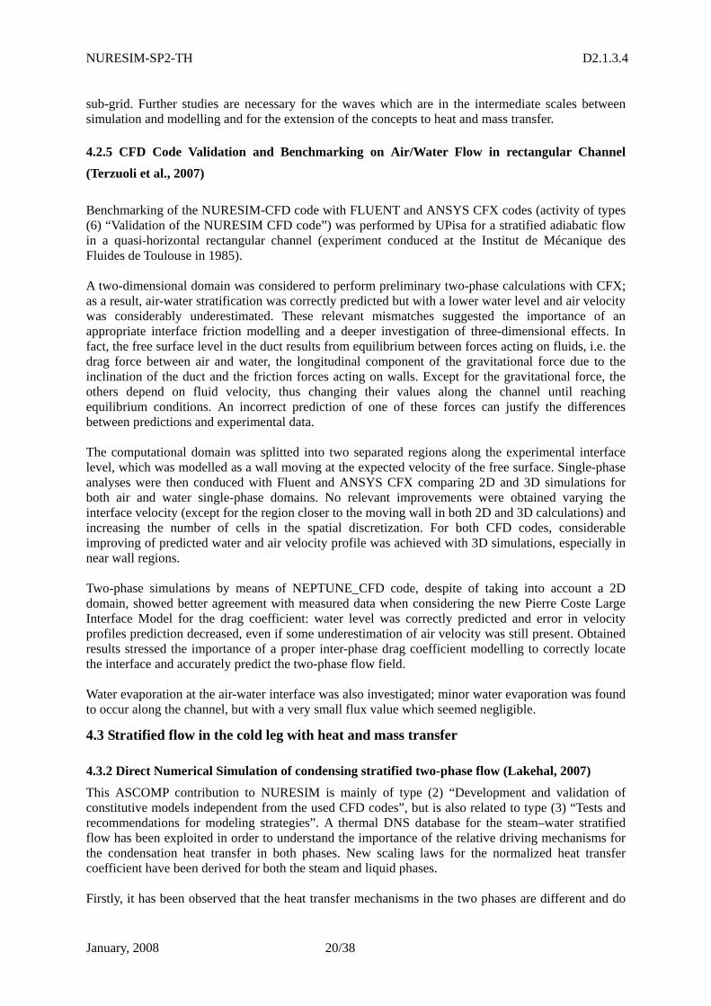
NURESIM-SP2-TH D2.1.3.4
January, 2008 20/38
sub-grid. Further studies are necessary for the waves which are in the intermediate scales between simulation and modelling and for the extension of the concepts to heat and mass transfer.
4.2.5 CFD Code Validation and Benchmarking on Air/Water Flow in rectangular Channel
(Terzuoli et al., 2007)
Benchmarking of the NURESIM-CFD code with FLUENT and ANSYS CFX codes (activity of types (6) “Validation of the NURESIM CFD code”) was performed by UPisa for a stratified adiabatic flow in a quasi-horizontal rectangular channel (experiment conduced at the Institut de Mécanique des Fluides de Toulouse in 1985). A two-dimensional domain was considered to perform preliminary two-phase calculations with CFX; as a result, air-water stratification was correctly predicted but with a lower water level and air velocity was considerably underestimated. These relevant mismatches suggested the importance of an appropriate interface friction modelling and a deeper investigation of three-dimensional effects. In fact, the free surface level in the duct results from equilibrium between forces acting on fluids, i.e. the drag force between air and water, the longitudinal component of the gravitational force due to the inclination of the duct and the friction forces acting on walls. Except for the gravitational force, the others depend on fluid velocity, thus changing their values along the channel until reaching equilibrium conditions. An incorrect prediction of one of these forces can justify the differences between predictions and experimental data. The computational domain was splitted into two separated regions along the experimental interface level, which was modelled as a wall moving at the expected velocity of the free surface. Single-phase analyses were then conduced with Fluent and ANSYS CFX comparing 2D and 3D simulations for both air and water single-phase domains. No relevant improvements were obtained varying the interface velocity (except for the region closer to the moving wall in both 2D and 3D calculations) and increasing the number of cells in the spatial discretization. For both CFD codes, considerable improving of predicted water and air velocity profile was achieved with 3D simulations, especially in near wall regions. Two-phase simulations by means of NEPTUNE_CFD code, despite of taking into account a 2D domain, showed better agreement with measured data when considering the new Pierre Coste Large Interface Model for the drag coefficient: water level was correctly predicted and error in velocity profiles prediction decreased, even if some underestimation of air velocity was still present. Obtained results stressed the importance of a proper inter-phase drag coefficient modelling to correctly locate the interface and accurately predict the two-phase flow field. Water evaporation at the air-water interface was also investigated; minor water evaporation was found to occur along the channel, but with a very small flux value which seemed negligible.
4.3 Stratified flow in the cold leg with heat and mass transfer
4.3.2 Direct Numerical Simulation of condensing stratified two-phase flow (Lakehal, 2007)
This ASCOMP contribution to NURESIM is mainly of type (2) “Development and validation of constitutive models independent from the used CFD codes”, but is also related to type (3) “Tests and recommendations for modeling strategies”. A thermal DNS database for the steam–water stratified flow has been exploited in order to understand the importance of the relative driving mechanisms for the condensation heat transfer in both phases. New scaling laws for the normalized heat transfer coefficient have been derived for both the steam and liquid phases. Firstly, it has been observed that the heat transfer mechanisms in the two phases are different and do
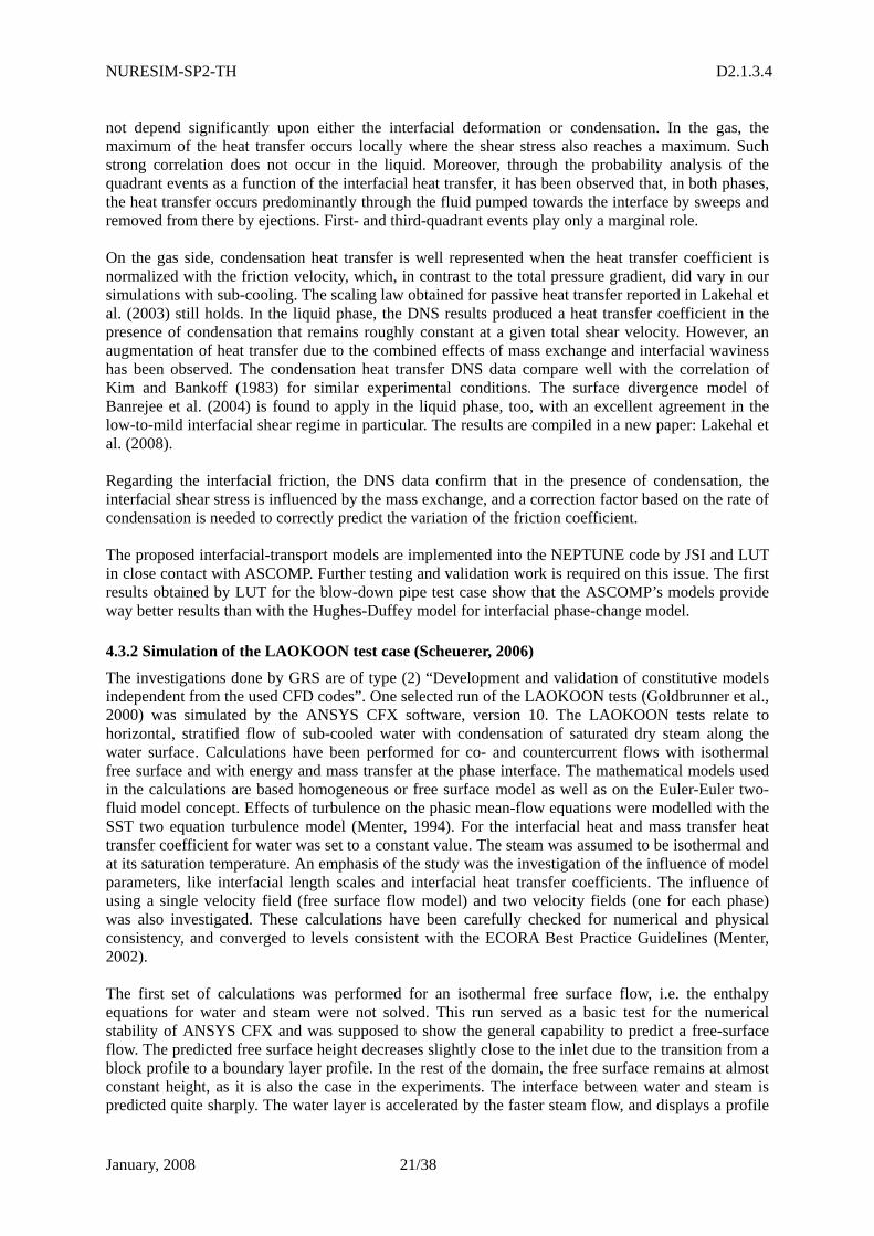
NURESIM-SP2-TH D2.1.3.4
January, 2008 21/38
not depend significantly upon either the interfacial deformation or condensation. In the gas, the maximum of the heat transfer occurs locally where the shear stress also reaches a maximum. Such strong correlation does not occur in the liquid. Moreover, through the probability analysis of the quadrant events as a function of the interfacial heat transfer, it has been observed that, in both phases, the heat transfer occurs predominantly through the fluid pumped towards the interface by sweeps and removed from there by ejections. First- and third-quadrant events play only a marginal role. On the gas side, condensation heat transfer is well represented when the heat transfer coefficient is normalized with the friction velocity, which, in contrast to the total pressure gradient, did vary in our simulations with sub-cooling. The scaling law obtained for passive heat transfer reported in Lakehal et al. (2003) still holds. In the liquid phase, the DNS results produced a heat transfer coefficient in the presence of condensation that remains roughly constant at a given total shear velocity. However, an augmentation of heat transfer due to the combined effects of mass exchange and interfacial waviness has been observed. The condensation heat transfer DNS data compare well with the correlation of Kim and Bankoff (1983) for similar experimental conditions. The surface divergence model of Banrejee et al. (2004) is found to apply in the liquid phase, too, with an excellent agreement in the low-to-mild interfacial shear regime in particular. The results are compiled in a new paper: Lakehal et al. (2008). Regarding the interfacial friction, the DNS data confirm that in the presence of condensation, the interfacial shear stress is influenced by the mass exchange, and a correction factor based on the rate of condensation is needed to correctly predict the variation of the friction coefficient. The proposed interfacial-transport models are implemented into the NEPTUNE code by JSI and LUT in close contact with ASCOMP. Further testing and validation work is required on this issue. The first results obtained by LUT for the blow-down pipe test case show that the ASCOMP’s models provide way better results than with the Hughes-Duffey model for interfacial phase-change model.
4.3.2 Simulation of the LAOKOON test case (Scheuerer, 2006)
The investigations done by GRS are of type (2) “Development and validation of constitutive models independent from the used CFD codes”. One selected run of the LAOKOON tests (Goldbrunner et al., 2000) was simulated by the ANSYS CFX software, version 10. The LAOKOON tests relate to horizontal, stratified flow of sub-cooled water with condensation of saturated dry steam along the water surface. Calculations have been performed for co- and countercurrent flows with isothermal free surface and with energy and mass transfer at the phase interface. The mathematical models used in the calculations are based homogeneous or free surface model as well as on the Euler-Euler two-fluid model concept. Effects of turbulence on the phasic mean-flow equations were modelled with the SST two equation turbulence model (Menter, 1994). For the interfacial heat and mass transfer heat transfer coefficient for water was set to a constant value. The steam was assumed to be isothermal and at its saturation temperature. An emphasis of the study was the investigation of the influence of model parameters, like interfacial length scales and interfacial heat transfer coefficients. The influence of using a single velocity field (free surface flow model) and two velocity fields (one for each phase) was also investigated. These calculations have been carefully checked for numerical and physical consistency, and converged to levels consistent with the ECORA Best Practice Guidelines (Menter, 2002). The first set of calculations was performed for an isothermal free surface flow, i.e. the enthalpy equations for water and steam were not solved. This run served as a basic test for the numerical stability of ANSYS CFX and was supposed to show the general capability to predict a free-surface flow. The predicted free surface height decreases slightly close to the inlet due to the transition from a block profile to a boundary layer profile. In the rest of the domain, the free surface remains at almost constant height, as it is also the case in the experiments. The interface between water and steam is predicted quite sharply. The water layer is accelerated by the faster steam flow, and displays a profile
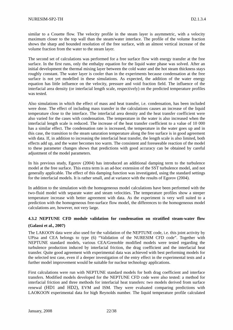
NURESIM-SP2-TH D2.1.3.4
January, 2008 22/38
similar to a Couette flow. The velocity profile in the steam layer is asymmetric, with a velocity maximum closer to the top wall than the steam/water interface. The profile of the volume fraction shows the sharp and bounded resolution of the free surface, with an almost vertical increase of the volume fraction from the water to the steam layer. The second set of calculations was performed for a free surface flow with energy transfer at the free surface. In the first runs, only the enthalpy equation for the liquid water phase was solved. After an initial development the thermal mixing layer between the cold water and the hot steam thickness stays roughly constant. The water layer is cooler than in the experiments because condensation at the free surface is not yet modelled in these simulations. As expected, the addition of the water energy equation has little influence on the velocity, pressure and void fraction field. The influence of the interfacial area density (or interfacial length scale, respectively) on the predicted temperature profiles was tested. Also simulations in which the effect of mass and heat transfer, i.e. condensation, has been included were done. The effect of including mass transfer in the calculations causes an increase of the liquid temperature close to the interface. The interfacial area density and the heat transfer coefficient were also varied for the cases with condensation. The temperature in the water is also increased when the interfacial length scale is reduced. The increase of the heat transfer coefficient to a value of 10 000 has a similar effect. The condensation rate is increased, the temperature in the water goes up and in this case, the transition to the steam saturation temperature along the free surface is in good agreement with data. If, in addition to increasing the interfacial heat transfer, the length scale is also limited, both effects add up, and the water becomes too warm. The consistent and foreseeable reaction of the model to these parameter changes shows that predictions with good accuracy can be obtained by careful adjustment of the model parameters. In his previous study, Egorov (2004) has introduced an additional damping term to the turbulence model at the free surface. This extra term is an ad-hoc extension of the SST turbulence model, and not generally applicable. The effect of this damping function was investigated, using the standard settings for the interfacial models. It is rather small, and at variance with the results of Egorov (2004). In addition to the simulation with the homogeneous model calculations have been performed with the two-fluid model with separate water and steam velocities. The temperature profiles show a steeper temperature increase with better agreement with data. As the experiment is very well suited to a prediction with the homogeneous free-surface flow model, the differences to the homogeneous model calculations are, however, not very large.
4.3.2 NEPTUNE CFD module validation for condensation on stratified steam-water flow
(Galassi et al., 2007)
The LAKOON data were also used for the validation of the NEPTUNE code, i.e. this joint activity by UPisa and CEA belongs to type (6) “Validation of the NURESIM CFD code”. Together with NEPTUNE standard models, various CEA/Grenoble modified models were tested regarding the turbulence production induced by interfacial friction, the drag coefficient and the interfacial heat transfer. Quite good agreement with experimental data was achieved with best performing models for the selected test case, even if a deeper investigation of the entry effect in the experimental tests and a further model improvement would be suitable for nuclear technology applications. First calculations were run with NEPTUNE standard models for both drag coefficient and interface transfers. Modified models developed for the NEPTUNE CFD code were also tested: a method for interfacial friction and three methods for interfacial heat transfers: two models derived from surface renewal (HD1 and HD2), EVM and ISM. They were evaluated comparing predictions with LAOKOON experimental data for high Reynolds number. The liquid temperature profile calculated
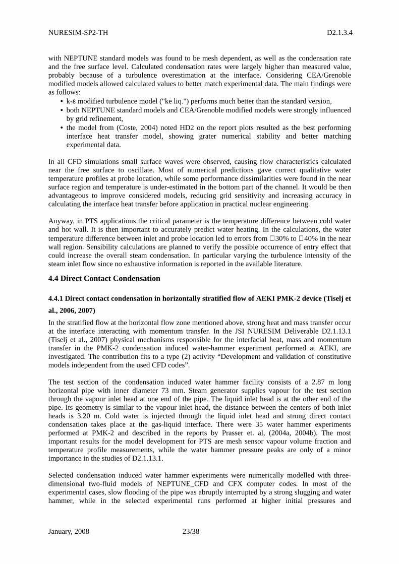
NURESIM-SP2-TH D2.1.3.4
January, 2008 23/38
with NEPTUNE standard models was found to be mesh dependent, as well as the condensation rate and the free surface level. Calculated condensation rates were largely higher than measured value, probably because of a turbulence overestimation at the interface. Considering CEA/Grenoble modified models allowed calculated values to better match experimental data. The main findings were as follows:
• k-ε modified turbulence model ("ke liq.") performs much better than the standard version, • both NEPTUNE standard models and CEA/Grenoble modified models were strongly influenced
by grid refinement, • the model from (Coste, 2004) noted HD2 on the report plots resulted as the best performing
interface heat transfer model, showing grater numerical stability and better matching experimental data.
In all CFD simulations small surface waves were observed, causing flow characteristics calculated near the free surface to oscillate. Most of numerical predictions gave correct qualitative water temperature profiles at probe location, while some performance dissimilarities were found in the near surface region and temperature is under-estimated in the bottom part of the channel. It would be then advantageous to improve considered models, reducing grid sensitivity and increasing accuracy in calculating the interface heat transfer before application in practical nuclear engineering. Anyway, in PTS applications the critical parameter is the temperature difference between cold water and hot wall. It is then important to accurately predict water heating. In the calculations, the water temperature difference between inlet and probe location led to errors from ∼ 30% to ∼ 40% in the near wall region. Sensibility calculations are planned to verify the possible occurrence of entry effect that could increase the overall steam condensation. In particular varying the turbulence intensity of the steam inlet flow since no exhaustive information is reported in the available literature.
4.4 Direct Contact Condensation
4.4.1 Direct contact condensation in horizontally stratified flow of AEKI PMK-2 device (Tiselj et
al., 2006, 2007)
In the stratified flow at the horizontal flow zone mentioned above, strong heat and mass transfer occur at the interface interacting with momentum transfer. In the JSI NURESIM Deliverable D2.1.13.1 (Tiselj et al., 2007) physical mechanisms responsible for the interfacial heat, mass and momentum transfer in the PMK-2 condensation induced water-hammer experiment performed at AEKI, are investigated. The contribution fits to a type (2) activity “Development and validation of constitutive models independent from the used CFD codes”. The test section of the condensation induced water hammer facility consists of a 2.87 m long horizontal pipe with inner diameter 73 mm. Steam generator supplies vapour for the test section through the vapour inlet head at one end of the pipe. The liquid inlet head is at the other end of the pipe. Its geometry is similar to the vapour inlet head, the distance between the centers of both inlet heads is 3.20 m. Cold water is injected through the liquid inlet head and strong direct contact condensation takes place at the gas-liquid interface. There were 35 water hammer experiments performed at PMK-2 and described in the reports by Prasser et. al, (2004a, 2004b). The most important results for the model development for PTS are mesh sensor vapour volume fraction and temperature profile measurements, while the water hammer pressure peaks are only of a minor importance in the studies of D2.1.13.1. Selected condensation induced water hammer experiments were numerically modelled with three-dimensional two-fluid models of NEPTUNE_CFD and CFX computer codes. In most of the experimental cases, slow flooding of the pipe was abruptly interrupted by a strong slugging and water hammer, while in the selected experimental runs performed at higher initial pressures and
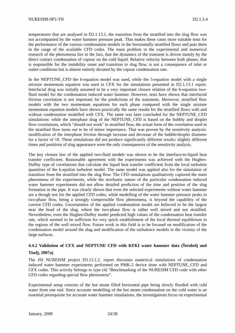
NURESIM-SP2-TH D2.1.3.4
January, 2008 24/38
temperatures that are analysed in D2.1.13.1, the transition from the stratified into the slug flow was not accompanied by the water hammer pressure peak. That makes these cases more suitable tests for the performance of the various condensation models in the horizontally stratified flows and puts them in the range of the available CFD codes. The main problem in the experimental and numerical research of the phenomena lies in the fact, that the dynamics of the transient is driven mainly by the direct contact condensation of vapour on the cold liquid. Relative velocity between both phases, that is responsible for the instability onset and transition to slug flow, is not a consequence of inlet or outlet conditions but is almost entirely dictated by the vapour condensation rate. In the NEPTUNE_CFD the 6-equation model was used, while the 5-equation model with a single mixture momentum equation was used in CFX for the simulations presented in D2.1.13.1 report. Interfacial drag was initially assumed to be a very important closure relation of the 6-equation two-fluid model for the condensation induced water hammer. However, tests have shown that interfacial friction correlation is not important for the predictions of the transients. Moreover, stratified flow models with the two momentum equations for each phase compared with the single mixture momentum equation models have shown practically the same results for the stratified flows with and without condensation modelled with CFX. The same was later concluded for the NEPTUNE_CFD simulations: while the interphase drag of the NEPTUNE_CFD is based on the bubbly and droplet flow correlations, which "should not work" in stratified flow, the actual form of the correlation used in the stratified flow turns out to be of minor importance. That was proven by the sensitivity analysis: modification of the interphase friction through increase and decrease of the bubble/droplet diameter for a factor of 10. These simulations did not produce significantly different results: slightly different times and positions of slug appearance were the only consequences of the sensitivity analysis. The key closure law of the applied two-fluid models was shown to be the interface-to-liquid heat transfer coefficient. Reasonable agreement with the experiments was achieved with the Hughes-Duffey type of correlations that calculate the liquid heat transfer coefficient from the local turbulent quantities of the k-epsilon turbulent model. The same model was applied also for the simulation of transition from the stratified into the slug flow. The CFD simulations qualitatively captured the main phenomena of the experiments, while the stochastic nature of the particular condensation induced water hammer experiments did not allow detailed prediction of the time and position of the slug formation in the pipe. It was clearly shown that even the selected experiments without water hammer are a though test for the applied CFD codes, while modelling of the water hammer pressure peaks in two-phase flow, being a strongly compressible flow phenomena, is beyond the capability of the current CFD codes. Uncertainties of the applied condensation model are believed to be the largest near the head of the slug, where the two-phase flow is rather well mixed and not stratified. Nevertheless, even the Hughes-Duffey model predicted high values of the condensation heat transfer rate, which seemed to be sufficient for very quick establishment of the local thermal equilibrium in the regions of the well mixed flow. Future work in this field is to be focused on modification of the condensation model around the slug and modification of the turbulence models in the vicinity of the large surfaces.
4.4.2 Validation of CFX and NEPTUNE CFD with KFKI water hammer data (Štrubelj and
Tiselj, 2007a)
The JSI NUREISM project D3.13.1.2. report discusses numerical simulations of condensation induced water hammer experiments performed on PMK-2 device done with NEPTUNE_CFD and CFX codes. This activity belongs to type (4) “Benchmarking of the NURESIM CFD code with other CFD codes regarding special flow phenomena”. Experimental setup consists of the hot steam filled horizontal pipe being slowly flooded with cold water from one end. Since accurate modelling of the hot steam condensation on the cold water is an essential prerequisite for accurate water hammer simulations, the investigations focus on experimental
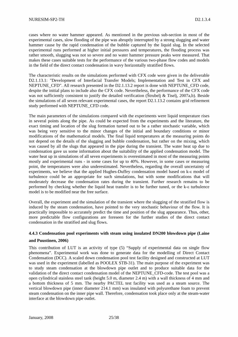
NURESIM-SP2-TH D2.1.3.4
January, 2008 25/38
cases where no water hammer appeared. As mentioned in the previous sub-section in most of the experimental cases, slow flooding of the pipe was abruptly interrupted by a strong slugging and water hammer cause by the rapid condensation of the bubble captured by the liquid slug. In the selected experimental runs performed at higher initial pressures and temperatures, the flooding process was rather smooth, slugging was not so severe and no water hammer pressure peaks were measured. That makes these cases suitable tests for the performance of the various two-phase flow codes and models in the field of the direct contact condensation in wavy horizontally stratified flows. The characteristic results on the simulations performed with CFX code were given in the deliverable D2.1.13.1: "Development of Interfacial Transfer Models; Implementation and Test in CFX and NEPTUNE_CFD". All research presented in the D2.1.13.2 report is done with NEPTUNE_CFD code, despite the initial plans to include also the CFX code. Nevertheless, the performance of the CFX code was not sufficiently consistent to justify the detailed verification (Štrubelj & Tiselj, 2007a,b). Beside the simulations of all seven relevant experimental cases, the report D2.1.13.2 contains grid refinement study performed with NEPTUNE_CFD code. The main parameters of the simulations compared with the experiments were liquid temperature rises in several points along the pipe. As could be expected from the experiments and the literature, the exact timing and location of the slug formation turned out to be a rather stochastic variable, which was being very sensitive to the minor changes of the initial and boundary conditions or minor modifications of the mathematical models. The final liquid temperatures at the measuring points do not depend on the details of the slugging and bubble condensation, but rather on the mixing, which was caused by all the slugs that appeared in the pipe during the transient. The water heat up due to condensation gave us some information about the suitability of the applied condensation model. The water heat up in simulations of all seven experiments is overestimated in most of the measuring points mostly and experimental runs - in some cases for up to 40%. However, in some cases or measuring point, the temperatures were also underestimated. Nevertheless, regarding the overall uncertainty of experiments, we believe that the applied Hughes-Duffey condensation model based on k-ε model of turbulence could be an appropriate for such simulations, but with some modifications that will moderately decrease the condensation rates during the transient. Further research remains to be performed by checking whether the liquid heat transfer is to be further tuned, or the k-ε turbulence model is to be modified near the free surface. Overall, the experiment and the simulation of the transient where the slugging of the stratified flow is induced by the steam condensation, have pointed to the very stochastic behaviour of the flow. It is practically impossible to accurately predict the time and position of the slug appearance. Thus, other, more predictable flow configurations are foreseen for the further studies of the direct contact condensation in the stratified and slug flows.
4.4.3 Condensation pool experiments with steam using insulated DN200 blowdown pipe (Laine
and Puustinen, 2006)
This contribution of LUT is an activity of type (5) “Supply of experimental data on single flow phenomena”. Experimental work was done to generate data for the modelling of Direct Contact Condensation (DCC). A scaled down condensation pool test facility designed and constructed at LUT was used in the experiment (labelled as POOLEX STB-31). The main purpose of the experiment was to study steam condensation at the blowdown pipe outlet and to produce suitable data for the validation of the direct contact condensation model of the NEPTUNE_CFD-code. The test pool was a open cylindrical stainless steel tank (height 5.0 m, diameter 2.4 m) with a wall thickness of 4 mm and a bottom thickness of 5 mm. The nearby PACTEL test facility was used as a steam source. The vertical blowdown pipe (inner diameter 214.1 mm) was insulated with polyurethane foam to prevent steam condensation on the inner pipe wall. Therefore, condensation took place only at the steam-water interface at the blowdown pipe outlet.
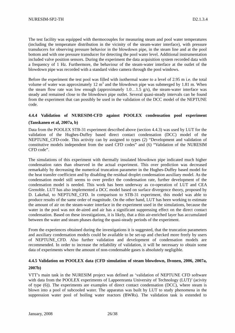
NURESIM-SP2-TH D2.1.3.4
January, 2008 26/38
The test facility was equipped with thermocouples for measuring steam and pool water temperatures (including the temperature distribution in the vicinity of the steam-water interface), with pressure transducers for observing pressure behavior in the blowdown pipe, in the steam line and at the pool bottom and with one pressure transducer for detecting the pool water level. Additional instrumentation included valve position sensors. During the experiment the data acquisition system recorded data with a frequency of 1 Hz. Furthermore, the behaviour of the steam-water interface at the outlet of the blowdown pipe was recorded with a standard video camera through the pool windows. Before the experiment the test pool was filled with isothermal water to a level of 2.95 m i.e. the total volume of water was approximately 12 m3 and the blowdown pipe was submerged by 1.81 m. When the steam flow rate was low enough (approximately 1.0…1.5 g/s), the steam-water interface was steady and remained close to the blowdown pipe outlet. Several quasi-steady intervals can be found from the experiment that can possibly be used in the validation of the DCC model of the NEPTUNE code.
4.4.4 Validation of NURESIM-CFD against POOLEX condensation pool experiment
(Tanskanen et al, 2007a, b)
Data from the POOLEX STB-31 experiment described above (section 4.4.3) was used by LUT for the validation of the Hughes-Duffey based direct contact condensation (DCC) model of the NEPTUNE_CFD-code. This activity can by assigned to types (2) “Development and validation of constitutive models independent from the used CFD codes” and (6) “Validation of the NURESIM CFD code”. The simulations of this experiment with thermally insulated blowdown pipe indicated much higher condensation rates than observed in the actual experiment. This over prediction was decreased remarkably by decreasing the numerical truncation parameter in the Hughes-Duffey based model for the heat transfer coefficient and by disabling the residual droplet condensation auxiliary model. As the condensation model still seems to over predict the condensation rate, further development of the condensation model is needed. This work has been underway as co-operation of LUT and CEA Grenoble. LUT has also implemented a DCC model based on surface divergence theory, proposed by D. Lakehal, to NEPTUNE_CFD. In comparison to STB-31 experiment, this model was able to produce results of the same order of magnitude. On the other hand, LUT has been working to estimate the amount of air on the steam-water interface in the experiment used in the simulations, because the water in the pool was not de-aired and air has a significant suppressing effect on the direct contact condensation. Based on these investigations, it is likely, that a thin air-enriched layer has accumulated between the water and steam phases during the quasi-steady periods of the experiment. From the experiences obtained during the investigations it is suggested, that the truncation parameters and auxiliary condensation models could be available to be set-up and checked more freely by users of NEPTUNE_CFD. Also further validation and development of condensation models are recommended. In order to increase the reliability of validation, it will be necessary to obtain some data of experiments where the amount of non-condensable gases is absolutely negligible.
4.4.5 Validation on POOLEX data (CFD simulation of steam blowdown, Ilvonen, 2006, 2007a,
2007b)
VTT’s main task in the NURESIM project was defined as ‘validation of NEPTUNE CFD software with data from the POOLEX experiments of Lappeenranta University of Technology (LUT)’ (acivity of type (6)). The experiments are examples of direct contact condensation (DCC), where steam is blown into a pool of subcooled water. The apparatus was built by LUT to study phenomena in the suppression water pool of boiling water reactors (BWRs). The validation task is extended to
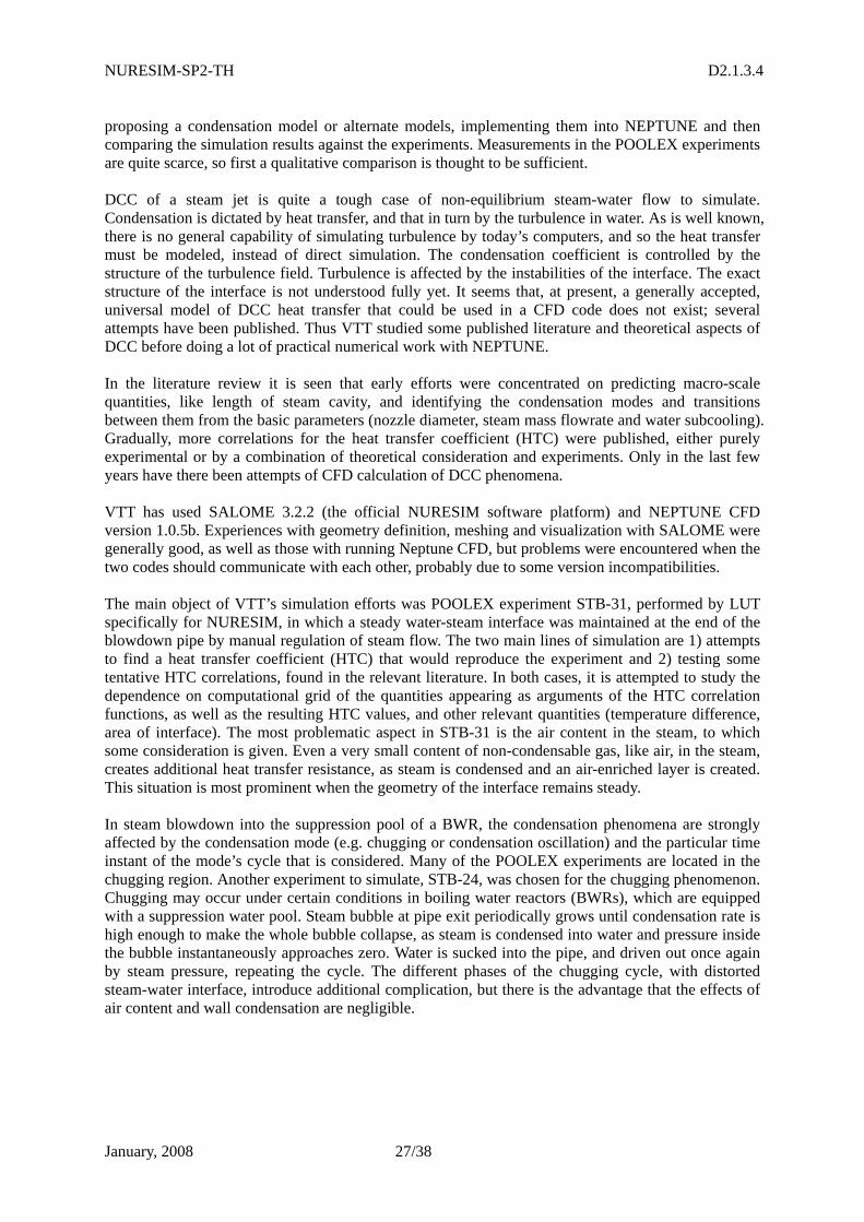
NURESIM-SP2-TH D2.1.3.4
January, 2008 27/38
proposing a condensation model or alternate models, implementing them into NEPTUNE and then comparing the simulation results against the experiments. Measurements in the POOLEX experiments are quite scarce, so first a qualitative comparison is thought to be sufficient. DCC of a steam jet is quite a tough case of non-equilibrium steam-water flow to simulate. Condensation is dictated by heat transfer, and that in turn by the turbulence in water. As is well known, there is no general capability of simulating turbulence by today’s computers, and so the heat transfer must be modeled, instead of direct simulation. The condensation coefficient is controlled by the structure of the turbulence field. Turbulence is affected by the instabilities of the interface. The exact structure of the interface is not understood fully yet. It seems that, at present, a generally accepted, universal model of DCC heat transfer that could be used in a CFD code does not exist; several attempts have been published. Thus VTT studied some published literature and theoretical aspects of DCC before doing a lot of practical numerical work with NEPTUNE. In the literature review it is seen that early efforts were concentrated on predicting macro-scale quantities, like length of steam cavity, and identifying the condensation modes and transitions between them from the basic parameters (nozzle diameter, steam mass flowrate and water subcooling). Gradually, more correlations for the heat transfer coefficient (HTC) were published, either purely experimental or by a combination of theoretical consideration and experiments. Only in the last few years have there been attempts of CFD calculation of DCC phenomena. VTT has used SALOME 3.2.2 (the official NURESIM software platform) and NEPTUNE CFD version 1.0.5b. Experiences with geometry definition, meshing and visualization with SALOME were generally good, as well as those with running Neptune CFD, but problems were encountered when the two codes should communicate with each other, probably due to some version incompatibilities. The main object of VTT’s simulation efforts was POOLEX experiment STB-31, performed by LUT specifically for NURESIM, in which a steady water-steam interface was maintained at the end of the blowdown pipe by manual regulation of steam flow. The two main lines of simulation are 1) attempts to find a heat transfer coefficient (HTC) that would reproduce the experiment and 2) testing some tentative HTC correlations, found in the relevant literature. In both cases, it is attempted to study the dependence on computational grid of the quantities appearing as arguments of the HTC correlation functions, as well as the resulting HTC values, and other relevant quantities (temperature difference, area of interface). The most problematic aspect in STB-31 is the air content in the steam, to which some consideration is given. Even a very small content of non-condensable gas, like air, in the steam, creates additional heat transfer resistance, as steam is condensed and an air-enriched layer is created. This situation is most prominent when the geometry of the interface remains steady. In steam blowdown into the suppression pool of a BWR, the condensation phenomena are strongly affected by the condensation mode (e.g. chugging or condensation oscillation) and the particular time instant of the mode’s cycle that is considered. Many of the POOLEX experiments are located in the chugging region. Another experiment to simulate, STB-24, was chosen for the chugging phenomenon. Chugging may occur under certain conditions in boiling water reactors (BWRs), which are equipped with a suppression water pool. Steam bubble at pipe exit periodically grows until condensation rate is high enough to make the whole bubble collapse, as steam is condensed into water and pressure inside the bubble instantaneously approaches zero. Water is sucked into the pipe, and driven out once again by steam pressure, repeating the cycle. The different phases of the chugging cycle, with distorted steam-water interface, introduce additional complication, but there is the advantage that the effects of air content and wall condensation are negligible.
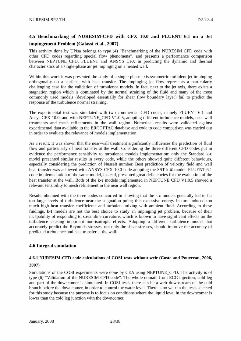
NURESIM-SP2-TH D2.1.3.4
January, 2008 28/38
4.5 Benchmarking of NURESIM-CFD with CFX 10.0 and FLUENT 6.1 on a Jet
impingement Problem (Galassi et al., 2007)
This activity done by UPisa belongs to type (4) “Benchmarking of the NURESIM CFD code with other CFD codes regarding special flow phenomena”, and presents a performance comparison between NEPTUNE_CFD, FLUENT and ANSYS CFX in predicting the dynamic and thermal characteristics of a single-phase air jet impinging on a heated wall. Within this work it was presented the study of a single-phase axis-symmetric turbulent jet impinging orthogonally on a surface, with heat transfer. The impinging jet flow represents a particularly challenging case for the validation of turbulence models. In fact, next to the jet axis, there exists a stagnation region which is dominated by the normal straining of the fluid and many of the most commonly used models (developed essentially for shear flow boundary layer) fail to predict the response of the turbulence normal straining. The experimental test was simulated with two commercial CFD codes, namely FLUENT 6.1 and Ansys CFX 10.0, and with NEPTUNE_CFD V1.0.5, adopting different turbulence models, near wall treatments and mesh refinements in the wall region. Numerical results were validated against experimental data available in the ERCOFTAC database and code to code comparison was carried out in order to evaluate the relevance of models implementation. As a result, it was shown that the near-wall treatment significantly influences the prediction of fluid flow and particularly of heat transfer at the wall. Considering the three different CFD codes put in evidence the performance sensitivity to turbulence models implementation: only the Standard k-ε model presented similar results in every code, while the others showed quite different behaviours, especially considering the prediction of Nusselt number. Best prediction of velocity field and wall heat transfer was achieved with ANSYS CFX 10.0 code adopting the SST k-ω model. FLUENT 6.1 code implementation of the same model, instead, presented great deficiencies for the evaluation of the heat transfer at the wall. Both of the k-ε models implemented in NEPTUNE CFD V1.0.5 showed a relevant sensibility to mesh refinement in the near wall region. Results obtained with the three codes concurred in showing that the k-ε models generally led to far too large levels of turbulence near the stagnation point; this excessive energy in turn induced too much high heat transfer coefficients and turbulent mixing with ambient fluid. According to these findings, k-ε models are not the best choice to study an impinging jet problem, because of their incapability of responding to streamline curvature, which is known to have significant effects on the turbulence causing important non-isotropic effects. Adopting a different turbulence model that accurately predict the Reynolds stresses, not only the shear stresses, should improve the accuracy of predicted turbulence and heat transfer at the wall.
4.6 Integral simulation
4.6.1 NURESIM-CFD code calculations of COSI tests without weir (Coste and Pouvreau, 2006,
2007)
Simulations of the COSI experiments were done by CEA using NEPTUNE_CFD. The activity is of type (6) “Validation of the NURESIM CFD code”. The whole domain from ECC injection, cold leg and part of the downcomer is simulated. In COSI tests, there can be a weir downstream of the cold branch before the downcomer, in order to control the water level. There is no weir in the tests selected for this study because the purpose is to focus on conditions where the liquid level in the downcomer is lower than the cold leg junction with the downcomer.
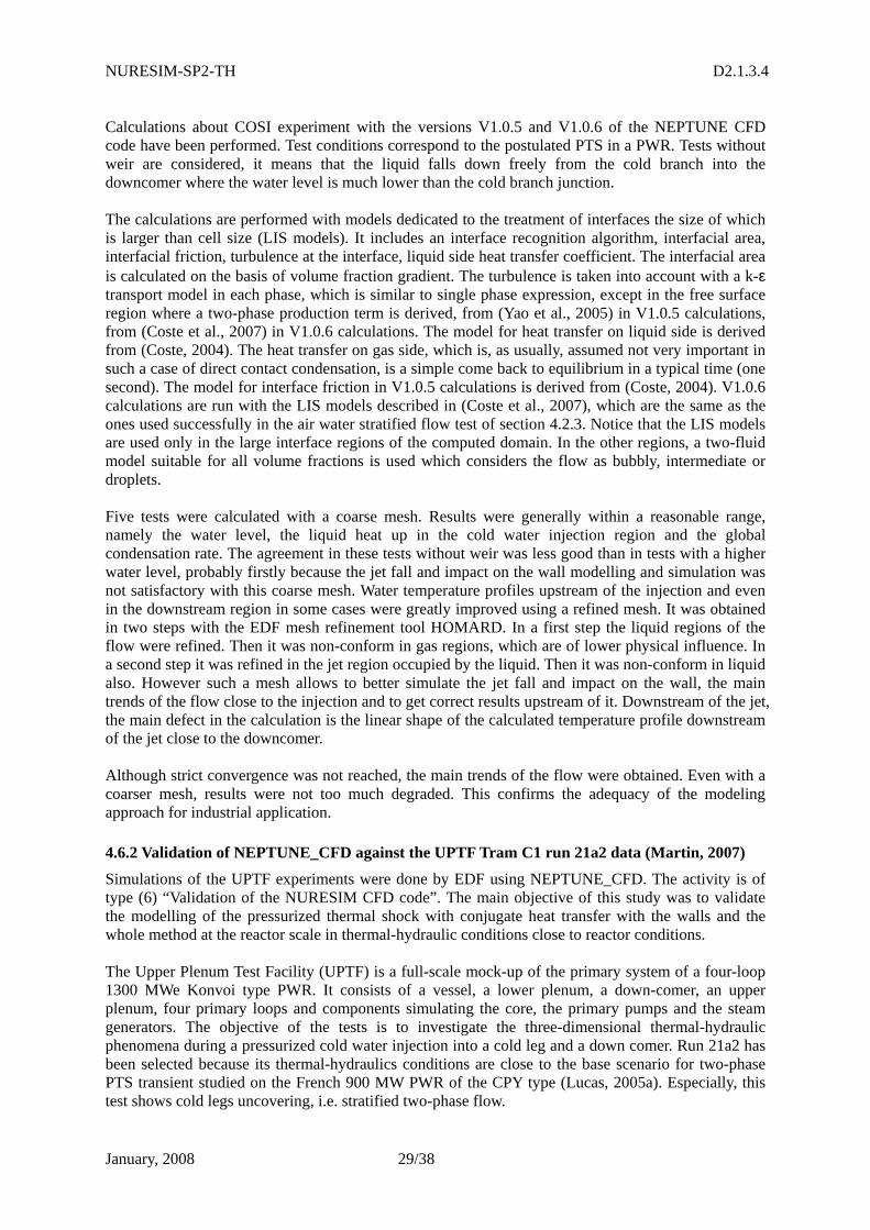
NURESIM-SP2-TH D2.1.3.4
January, 2008 29/38
Calculations about COSI experiment with the versions V1.0.5 and V1.0.6 of the NEPTUNE CFD code have been performed. Test conditions correspond to the postulated PTS in a PWR. Tests without weir are considered, it means that the liquid falls down freely from the cold branch into the downcomer where the water level is much lower than the cold branch junction. The calculations are performed with models dedicated to the treatment of interfaces the size of which is larger than cell size (LIS models). It includes an interface recognition algorithm, interfacial area, interfacial friction, turbulence at the interface, liquid side heat transfer coefficient. The interfacial area is calculated on the basis of volume fraction gradient. The turbulence is taken into account with a k-ε transport model in each phase, which is similar to single phase expression, except in the free surface region where a two-phase production term is derived, from (Yao et al., 2005) in V1.0.5 calculations, from (Coste et al., 2007) in V1.0.6 calculations. The model for heat transfer on liquid side is derived from (Coste, 2004). The heat transfer on gas side, which is, as usually, assumed not very important in such a case of direct contact condensation, is a simple come back to equilibrium in a typical time (one second). The model for interface friction in V1.0.5 calculations is derived from (Coste, 2004). V1.0.6 calculations are run with the LIS models described in (Coste et al., 2007), which are the same as the ones used successfully in the air water stratified flow test of section 4.2.3. Notice that the LIS models are used only in the large interface regions of the computed domain. In the other regions, a two-fluid model suitable for all volume fractions is used which considers the flow as bubbly, intermediate or droplets. Five tests were calculated with a coarse mesh. Results were generally within a reasonable range, namely the water level, the liquid heat up in the cold water injection region and the global condensation rate. The agreement in these tests without weir was less good than in tests with a higher water level, probably firstly because the jet fall and impact on the wall modelling and simulation was not satisfactory with this coarse mesh. Water temperature profiles upstream of the injection and even in the downstream region in some cases were greatly improved using a refined mesh. It was obtained in two steps with the EDF mesh refinement tool HOMARD. In a first step the liquid regions of the flow were refined. Then it was non-conform in gas regions, which are of lower physical influence. In a second step it was refined in the jet region occupied by the liquid. Then it was non-conform in liquid also. However such a mesh allows to better simulate the jet fall and impact on the wall, the main trends of the flow close to the injection and to get correct results upstream of it. Downstream of the jet, the main defect in the calculation is the linear shape of the calculated temperature profile downstream of the jet close to the downcomer. Although strict convergence was not reached, the main trends of the flow were obtained. Even with a coarser mesh, results were not too much degraded. This confirms the adequacy of the modeling approach for industrial application.
4.6.2 Validation of NEPTUNE_CFD against the UPTF Tram C1 run 21a2 data (Martin, 2007)
Simulations of the UPTF experiments were done by EDF using NEPTUNE_CFD. The activity is of type (6) “Validation of the NURESIM CFD code”. The main objective of this study was to validate the modelling of the pressurized thermal shock with conjugate heat transfer with the walls and the whole method at the reactor scale in thermal-hydraulic conditions close to reactor conditions. The Upper Plenum Test Facility (UPTF) is a full-scale mock-up of the primary system of a four-loop 1300 MWe Konvoi type PWR. It consists of a vessel, a lower plenum, a down-comer, an upper plenum, four primary loops and components simulating the core, the primary pumps and the steam generators. The objective of the tests is to investigate the three-dimensional thermal-hydraulic phenomena during a pressurized cold water injection into a cold leg and a down comer. Run 21a2 has been selected because its thermal-hydraulics conditions are close to the base scenario for two-phase PTS transient studied on the French 900 MW PWR of the CPY type (Lucas, 2005a). Especially, this test shows cold legs uncovering, i.e. stratified two-phase flow.
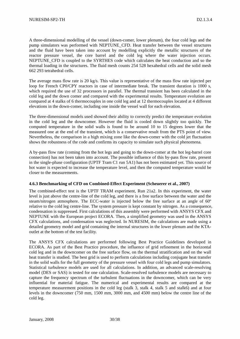
NURESIM-SP2-TH D2.1.3.4
January, 2008 30/38
A three-dimensional modelling of the vessel (down-comer, lower plenum), the four cold legs and the pump simulators was performed with NEPTUNE_CFD. Heat transfer between the vessel structures and the fluid have been taken into account by modelling explicitly the metallic structures of the reactor pressure vessel, the core barrel and the cold leg where the water injection occurs. NEPTUNE_CFD is coupled to the SYRTHES code which calculates the heat conduction and so the thermal loading in the structures. The fluid mesh counts 254 528 hexahedral cells and the solid mesh 662 293 tetrahedral cells. The average mass flow rate is 20 kg/s. This value is representative of the mass flow rate injected per loop for French CP0/CPY reactors in case of intermediate break. The transient duration is 1000 s, which required the use of 32 processors in parallel. The thermal transient has been calculated in the cold leg and the down comer and compared with the experimental results. Temperature evolution are compared at 4 stalks of 6 thermocouples in one cold leg and at 12 thermocouples located at 4 different elevations in the down-comer, including one inside the vessel wall for each elevation. The three-dimensional models used showed their ability to correctly predict the temperature evolution in the cold leg and the downcomer. However the fluid is cooled down slightly too quickly. The computed temperature in the solid walls is found to be around 10 to 15 degrees lower that the measured one at the end of the transient, which is a conservative result from the PTS point of view. Nevertheless, the comparison in a high mixing zone like the down-comer with the cold jet fluctuation shows the robustness of the code and confirms its capacity to simulate such physical phenomena. A by-pass flow rate (coming from the hot legs and going to the down-comer at the hot leg-barrel core connection) has not been taken into account. The possible influence of this by-pass flow rate, present in the single-phase configuration (UPTF Tram C1 run 5A1) has not been estimated yet. This source of hot water is expected to increase the temperature level, and then the computed temperature would be closer to the measurements.
4.6.3 Benchmarking of CFD on Combined-Effect Experiment (Scheuerer et al., 2007)
The combined-effect test is the UPTF TRAM experiment, Run 21a2. In this experiment, the water level is just above the centre-line of the cold leg, and there is a free surface between the water and the steam/nitrogen atmosphere. The ECC-water is injected below the free surface at an angle of 60º relative to the cold leg centre-line. The system pressure is kept constant by nitrogen. As a consequence, condensation is suppressed. First calculations of this assembly were performed with ANSYS CFX and NEPTUNE with the European project ECORA. Then, a simplified geometry was used in the ANSYS CFX calculations, and condensation was neglected. In NURESIM, the calculations are made using a detailed geometry model and grid containing the internal structures in the lower plenum and the KTA-outlet at the bottom of the test facility. The ANSYS CFX calculations are performed following Best Practice Guidelines developed in ECORA. As part of the Best Practice procedure, the influence of grid refinement in the horizontal cold leg and in the downcomer on the free surface flow, on the thermal stratification and on the wall heat transfer is studied. The best grid is used to perform calculations including conjugate heat transfer in the solid walls for the full geometry of the pressure vessel with four cold legs and pump simulators. Statistical turbulence models are used for all calculations. In addition, an advanced scale-resolving model (DES or SAS) is tested for one calculation. Scale-resolved turbulence models are necessary to capture the frequency spectrum of the turbulent fluctuations in the downcomer, which can be very influential for material fatigue. The numerical and experimental results are compared at the temperature measurement positions in the cold leg (stalk 3, stalk 4, stalk 5 and stalk6) and at four levels in the downcomer (750 mm, 1500 mm, 3000 mm, and 4500 mm) below the centre line of the cold leg.
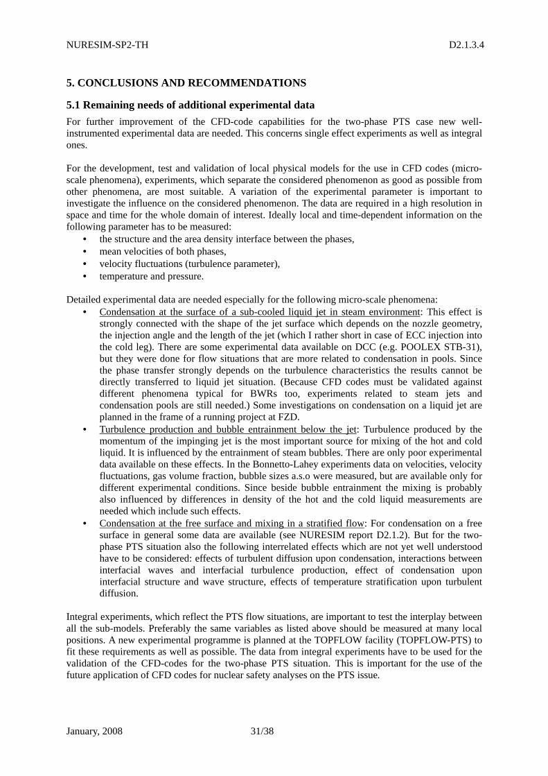
NURESIM-SP2-TH D2.1.3.4
January, 2008 31/38
5. CONCLUSIONS AND RECOMMENDATIONS
5.1 Remaining needs of additional experimental data
For further improvement of the CFD-code capabilities for the two-phase PTS case new well-instrumented experimental data are needed. This concerns single effect experiments as well as integral ones. For the development, test and validation of local physical models for the use in CFD codes (micro-scale phenomena), experiments, which separate the considered phenomenon as good as possible from other phenomena, are most suitable. A variation of the experimental parameter is important to investigate the influence on the considered phenomenon. The data are required in a high resolution in space and time for the whole domain of interest. Ideally local and time-dependent information on the following parameter has to be measured:
• the structure and the area density interface between the phases, • mean velocities of both phases, • velocity fluctuations (turbulence parameter), • temperature and pressure.
Detailed experimental data are needed especially for the following micro-scale phenomena:
• Condensation at the surface of a sub-cooled liquid jet in steam environment: This effect is strongly connected with the shape of the jet surface which depends on the nozzle geometry, the injection angle and the length of the jet (which I rather short in case of ECC injection into the cold leg). There are some experimental data available on DCC (e.g. POOLEX STB-31), but they were done for flow situations that are more related to condensation in pools. Since the phase transfer strongly depends on the turbulence characteristics the results cannot be directly transferred to liquid jet situation. (Because CFD codes must be validated against different phenomena typical for BWRs too, experiments related to steam jets and condensation pools are still needed.) Some investigations on condensation on a liquid jet are planned in the frame of a running project at FZD.
• Turbulence production and bubble entrainment below the jet: Turbulence produced by the momentum of the impinging jet is the most important source for mixing of the hot and cold liquid. It is influenced by the entrainment of steam bubbles. There are only poor experimental data available on these effects. In the Bonnetto-Lahey experiments data on velocities, velocity fluctuations, gas volume fraction, bubble sizes a.s.o were measured, but are available only for different experimental conditions. Since beside bubble entrainment the mixing is probably also influenced by differences in density of the hot and the cold liquid measurements are needed which include such effects.
• Condensation at the free surface and mixing in a stratified flow: For condensation on a free surface in general some data are available (see NURESIM report D2.1.2). But for the two-phase PTS situation also the following interrelated effects which are not yet well understood have to be considered: effects of turbulent diffusion upon condensation, interactions between interfacial waves and interfacial turbulence production, effect of condensation upon interfacial structure and wave structure, effects of temperature stratification upon turbulent diffusion.
Integral experiments, which reflect the PTS flow situations, are important to test the interplay between all the sub-models. Preferably the same variables as listed above should be measured at many local positions. A new experimental programme is planned at the TOPFLOW facility (TOPFLOW-PTS) to fit these requirements as well as possible. The data from integral experiments have to be used for the validation of the CFD-codes for the two-phase PTS situation. This is important for the use of the future application of CFD codes for nuclear safety analyses on the PTS issue.
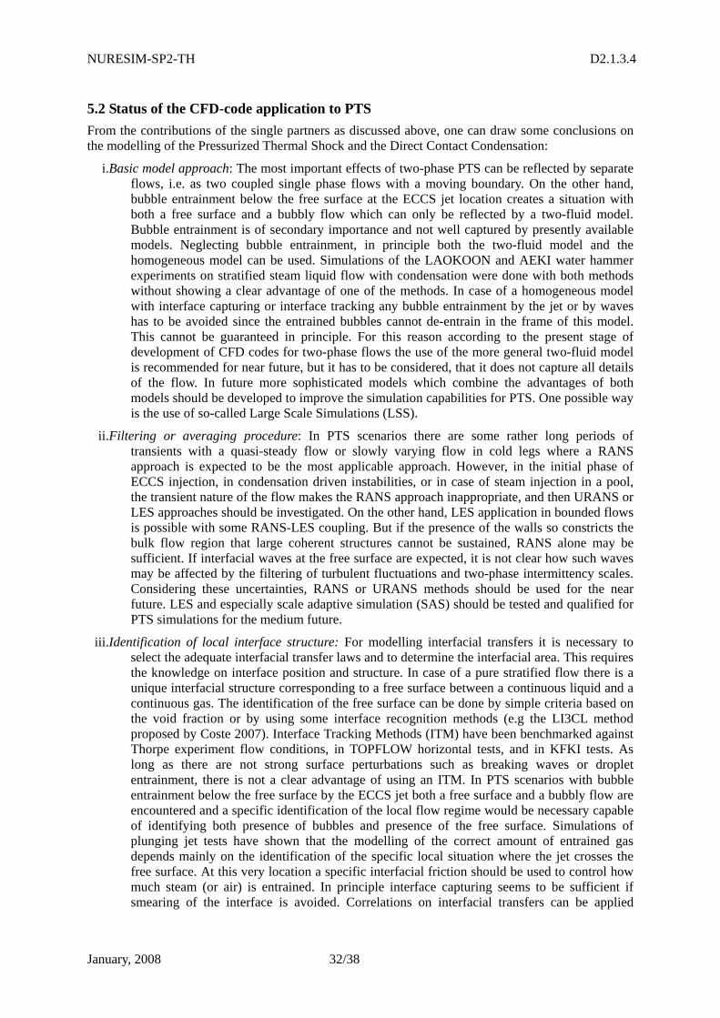
NURESIM-SP2-TH D2.1.3.4
January, 2008 32/38
5.2 Status of the CFD-code application to PTS
From the contributions of the single partners as discussed above, one can draw some conclusions on the modelling of the Pressurized Thermal Shock and the Direct Contact Condensation:
i.Basic model approach: The most important effects of two-phase PTS can be reflected by separate flows, i.e. as two coupled single phase flows with a moving boundary. On the other hand, bubble entrainment below the free surface at the ECCS jet location creates a situation with both a free surface and a bubbly flow which can only be reflected by a two-fluid model. Bubble entrainment is of secondary importance and not well captured by presently available models. Neglecting bubble entrainment, in principle both the two-fluid model and the homogeneous model can be used. Simulations of the LAOKOON and AEKI water hammer experiments on stratified steam liquid flow with condensation were done with both methods without showing a clear advantage of one of the methods. In case of a homogeneous model with interface capturing or interface tracking any bubble entrainment by the jet or by waves has to be avoided since the entrained bubbles cannot de-entrain in the frame of this model. This cannot be guaranteed in principle. For this reason according to the present stage of development of CFD codes for two-phase flows the use of the more general two-fluid model is recommended for near future, but it has to be considered, that it does not capture all details of the flow. In future more sophisticated models which combine the advantages of both models should be developed to improve the simulation capabilities for PTS. One possible way is the use of so-called Large Scale Simulations (LSS).
ii.Filtering or averaging procedure: In PTS scenarios there are some rather long periods of transients with a quasi-steady flow or slowly varying flow in cold legs where a RANS approach is expected to be the most applicable approach. However, in the initial phase of ECCS injection, in condensation driven instabilities, or in case of steam injection in a pool, the transient nature of the flow makes the RANS approach inappropriate, and then URANS or LES approaches should be investigated. On the other hand, LES application in bounded flows is possible with some RANS-LES coupling. But if the presence of the walls so constricts the bulk flow region that large coherent structures cannot be sustained, RANS alone may be sufficient. If interfacial waves at the free surface are expected, it is not clear how such waves may be affected by the filtering of turbulent fluctuations and two-phase intermittency scales. Considering these uncertainties, RANS or URANS methods should be used for the near future. LES and especially scale adaptive simulation (SAS) should be tested and qualified for PTS simulations for the medium future.
iii. Identification of local interface structure: For modelling interfacial transfers it is necessary to select the adequate interfacial transfer laws and to determine the interfacial area. This requires the knowledge on interface position and structure. In case of a pure stratified flow there is a unique interfacial structure corresponding to a free surface between a continuous liquid and a continuous gas. The identification of the free surface can be done by simple criteria based on the void fraction or by using some interface recognition methods (e.g the LI3CL method proposed by Coste 2007). Interface Tracking Methods (ITM) have been benchmarked against Thorpe experiment flow conditions, in TOPFLOW horizontal tests, and in KFKI tests. As long as there are not strong surface perturbations such as breaking waves or droplet entrainment, there is not a clear advantage of using an ITM. In PTS scenarios with bubble entrainment below the free surface by the ECCS jet both a free surface and a bubbly flow are encountered and a specific identification of the local flow regime would be necessary capable of identifying both presence of bubbles and presence of the free surface. Simulations of plunging jet tests have shown that the modelling of the correct amount of entrained gas depends mainly on the identification of the specific local situation where the jet crosses the free surface. At this very location a specific interfacial friction should be used to control how much steam (or air) is entrained. In principle interface capturing seems to be sufficient if smearing of the interface is avoided. Correlations on interfacial transfers can be applied
NURESIM-SP2-TH D2.1.3.4
January, 2008 33/38
according to this information.
iv.Interfacial transfer: If bubble entrainment is considered the complete set of bubble forces has to be included in the simulation of the region of bubbly flow to reflect the interfacial momentum transfer. More problems arise for the modelling of interfacial transfers on free surfaces. Effects of the meshing have to be considered in this case. One approach which could improve the simulations regarding such effects is the so-called Large Interface Simulation, which assumes an interface modeled by 3 layers of computational cells (LI3CL method proposed by Coste 2007). However this model is not yet fully mature. Additional tests and developments are required. Other methods make use of interfacial functions similar to wall functions. They should be able to provide a good modelling without any large influence of interfacial waves. Such approaches should allow providing a converged solution with a reasonably coarse nodalization. When waves are likely to occur and to produce a strong increase of the roughness and of the friction coefficient, the main question is to be able to characterize this roughness. This remains a difficult and fully open problem. The interfacial heat transfer in presence of condensation remains partly unresolved although some reasonable predictions were obtained for COSI and LAOKOON. The formulation of the liquid-to-interface heat transfer using a wall function approach should be able to provide a converged solution with a reasonably coarse nodalization, which is not yet achieved so far. Additional work on heat transfer is required.
v. Turbulent transfers: Liquid turbulence plays a dominant role in PTS scenarios. It influences the mixing of the cold and hot liquids, and consequently the amount of condensation and the minimum liquid temperature at inlet of the Reactor Pressure Vessel (RPV). The jet impact being the main source of turbulence, first simulations of Iguchi jet test have shown that a k-epsilon model could predict reasonably well this turbulence but it should be complemented by measurements in a more representative geometry. Beside the choice of appropriate turbulence models discussed above also the coupling of the turbulence fields is important. In case of bubbly flows the bubble induced turbulence should be considered. For coupling of turbulence on a free surface special measures as turbulence damping due to stratification have to be applied. The influence of condensation on the turbulent fields is still an open question. Neglecting this effect should result in conservative results regarding the thermal loads on the RPV walls.
vi. Wall transfers: Classical single-phase wall functions for momentum and heat transfer at wall are currently used in stratified flow. None of the available experiments could provide a validation of these wall functions but it is not expected that they represent a main source of uncertainty in PTS simulation.
vii.DNS-LES simulations: DNS simulation for stratified flow were used to derive some closure laws for interfacial momentum, turbulence and heat transfer, which can be used by CFD codes. Future work is still necessary to conclude, with implementation of these laws in NURESIM-CFD and comparison with DNS-LES on the same flow conditions, and validation against experimental data.
5.3 Recommendation for future R & D work
Simulations of the considered two-phase PTS case include different local flow situations. Some of these local flow situations can be already captured quite well by presently available CFD codes, for other still many open questions exist. The most important problems are connected with the coupling of the different flow regions as well as the coupling of the single effects determining the resulting flow in these regions. This concerns also the treatment of gas or liquid phases which may occur simultaneously as continuous phase and disperse phase in one flow domain. Despite some clear progress achieved during NURESIM further R&D work is required. New experimental data are required for single effects as well as for the integral PTS situation. They
NURESIM-SP2-TH D2.1.3.4
January, 2008 34/38
should provide data in high resolution in time and space to be suitable for CFD validation. The specific needs are discussed in section 5.1. Basing on such experiments new models and modelling strategies have to be developed, tested and validated. In general more flexible models are required which allow switching between different approaches within one flow domain but for the different local flow situations. This requirement arises from the different characteristics of local flow situation observed in the two-phase PTS case. Examples for such model approaches are the Large Scale Simulation (LSS) which should allow the application of a two-fluid model for dispersed flows and Interface Tracking Methods for large surfaces and the Scale Adaptive Simulations (SAS) which allow the simulation of large eddies while modelling the turbulence at the unresolved scales. While LSS modelling should be envisaged for far future SAS models already exist and should be validated for the flow situations typical for PTS. In addition the applicability of LES should be investigated. Beside turbulence also condensation has a considerable effect on the final thermal loads on the RPV wall. Condensation and heat transfer models for the different flow configurations (surface of the jet, horizontal flows which can be flat or wavy) have to be developed. Also the influence of condensation on the turbulent field should be a topic of future R&D work. For modelling the transfers at a free interface it is recommended to test and validate new strategies as the Large Interface Method to limit the effect of the numerical grid. In frame of the NURESIM project it was shown, that beside from information obtained by experimental investigations also DNS can provide information to build correlations for coarser CFD simulation not resolving the specific phenomenon. Further effort to implement, test and validate the results obtained for interfacial transfers for free surfaces by DNS should be done. Bubble entrainment due to jet impingement and such caused by waves has to be modelled on a physical basis. Up to now it is mainly determined by numerical effects. This future R&D work is connected with the more general modelling of transitions for gas (liquid) being the continuous phase and gas (liquid) being the dispersed phase. Finally future R&D work has to be aimed on the validation of the interplay between the single models basing on well instrumented integral experiments. In the near term, one may envisage a simplified treatment of two-phase PTS transients by neglecting some effects which are not yet controlled like the bubble entrainment and the possible effects of waves on the free surface. A better modelling of interfacial transfers of heat and mass at the free surface allowing convergence with a reasonable coarse mesh is still required to be able to predict the minimum liquid temperature entering the downcomer. It is very likely that neglecting entrained bubbles and interfacial waves leads to conservative predictions since both phenomena may increase condensation and mixing.
REFERENCES
S. Banerjee, M. Fulgosi, D. Lakehal, “Surface Divergence Models Between Turbulent Streams”, IJMF, 30(7/8), pp. 963-977, (2004). Y. Bartosiewicz, J.-M. Seynhaeve, “Report about benchmarking of NEPTUNE using Thorpe’s experiments and FLUENT simulation”, 6th Euratom Framework Program NURESIM, Deliverable D2.1.12.2, (2006a).
NURESIM-SP2-TH D2.1.3.4
January, 2008 35/38
Y. Bartosiewicz, J.-M. Seynhaeve, “Numerical investigation on the Kelvin-Helmholtz instability in the case of immiscible fluids”, The 13th International Conference on Fluid Flow Technologies Budapest, Hungary, September 6-9, (2006b).
Y. Bartosiewicz, J.-M. Seynhaeve, “Assessment of the NEPTUNE_CFD code to model the occurrence of instabilities in a stratified flow” 10TH International Conference Multiphase Flow in Industrial Plant, Tropea (Italy), 20-22 September, (2006c).
Y. Bartosiewicz, J. Lavieville and J.-M. Seynhaeve “A First Assessment of the NEPTUNE_CFD code: Instabilities in a Stratified Flow - Comparison between the VOF Method and a Two-Field Approach” To be published in International of Heat and Fluid Flow, (2007a).
Y. Bartosiewicz, J. Laviéville and J.-M. Seynhaeve “A validation case for the NEPTUNE_CFD platform : instabilities in a stratified flow. Experimental, theoritical, and code to code comparison” The 12th International Topical Meeting on Nuclear Reactor Thermal Hydraulics (NURETH-12), Pittsburgh, Pennsylvania, U.S.A. September 30-October 4, (2007b).
Y. Bartosiewicz, J.-M. Seynhaeve, T. Höhne, C. Vallée, J.-M. Lavieville, “Comparison of NEPTUNE_CFD and FLUENT predictions against FZD air/water slug flow experiments in horizontal channels”, 6th Euratom Framework Program NURESIM, Deliverable D2.1.12.3, (2007c).
D. Bestion et al, “Extension of CFD Codes to Two-phase Flow Safety Problems”, Technical Note, NEA/SEN/SIN/AMA(2006)2, OECD Nuclear Energy Agency (2006). D. Bestion et al, “Recommendation on Use of CFD Codes for Nuclear Reactor Safety Analysis”, 5th Euratom Framework Program ECORA project-WP8, (2004). F. Bonetto, R. T. Lahey, Jr, “An experimental study on air carry-under due to a plunging liquid jet”, Int. J. Multiphase Flow, 19, 281 – 294, (1993). E. Bodele, and D. Lucas, “Progress Report on the simulation of the plunging jet configuration”, 6th Euratom Framework Program NURESIM, Deliverable D2.1.3.1, (2006). E. Bodele, and D. Lucas, “Progress Report on the simulation of the plunging jet configuration”, 6th Euratom Framework Program NURESIM, Deliverable D2.1.3.2, (2007). P. Coste, ”Computational Simulation of Multi-D Liquid-Vapor Thermal Shock with Condensation”, Proc. of Int. Conf. on Multiphase Flow ’04, Yokohama, Japan, (2004). P. Coste, “Progress Validation of NURESIM-CFD code with an adiabatic stratified flow experiment”, 6th Euratom Framework Program NURESIM, Deliverable D2.1.1.2, (2006). P. Coste, “Modelling and Validation of NURESIM-CFD code about Turbulence and Friction in an Adiabatic Stratified Flow”, 6th Euratom Framework Program NURESIM, Deliverable D2.1.1.2b, (2007). P. Coste and J. Pouvreau, “NURESIM-CFD code calculations of COSI tests without weir”, 6th Euratom Framework Program NURESIM, Deliverable D2.1.1.1b, (2007). P. Coste, J. Pouvreau, C. Morel, J. Laviéville, M. Boucker, A. Martin, “Modelling Turbulence and Friction around a Large Interface in a Three-Dimension Two-Velocity Eule-rian Code”, Proc. of Int. Conf. NURETH 12, Pittsburgh, USA (2007a).
NURESIM-SP2-TH D2.1.3.4
January, 2008 36/38
N. G. Deen, T. Solberg, B.H. Hjertager, “Large eddy simulation of the gas liquid flow in a square cross-sectioned bubble column” Chem. Eng. Sci., 56, 6341-6349 (2001). M. T. Dhotre, B. L. Smith, “Large eddy simulation of a bubble column”, 6th Euratom Framework Program NURESIM, Deliverable D2.1.6.1, (2006). M. T. Dhotre, B. Niceno, B. L. Smith, “CFD Simulation of large scale bubble plumes: Development of flow pattern”, 6th Euratom Framework Program NURESIM, Deliverable D2.1.6.2, (2006). M. T. Dhotre, B. Niceno, B. L. Smith, “Large Eddy Simulation of large scale bubble plume”, 6th Euratom Framework Program NURESIM, Deliverable D2.1.6.5, (2007a). M. T. Dhotre, B. L. Smith,B. Niceno, “LES of a vertical two-phase pipe flow”, 6th Euratom Framework Program NURESIM, Deliverable D2.1.6.7 (2007b) M. Fulgosi, D. Lakehal, S. Banerjee, V. De Angelis: Direct numerical simulation of turbulence in a sheared air-water flow with deformable interface, J. Fluid Mechanics, 482, pp. 319-345, (2003). M. Fulgosi, “DNS Turbulent heat transfer and condensation in stratified flow and deformable interfaces”, Ph.D Thesis, ETH Zurich, (2004). M. C Galassi, D. Mazzini, F. D’Auria, Ch. Morel, D. Bestion, J. Pouvreau, “NEPTUNE CFD module validation on turbulence below a plunging jet”, 6th Euratom Framework Program NURESIM, Deliverable D2.1.10.2, (2006). M. C Galassi, F. D’Auria, P. Coste, “NEPTUNE CFD module validation for condensation on stratified steam-water flow”, 6th Euratom Framework Program NURESIM, Deliverable D2.1.10.4, (2007). M. Goldbrunner, J. Karl, D. Hein, D., “Experimental Investigation of Heat Transfer Phenomena during Direct Contact Condensation in the Presence of Non-Condensable Gas by Means of Linear Raman Spectroscopy”, 10th International Symposium on Laser Techniques Applied to Fluid Mechanics, Lisbon, (2000). M. Ilvonen, “Modeling interfacial transfers for Poolex experiment”, 6th Euratom Framework Program NURESIM, Deliverable D2.1.14.1, (2007a). M. Ilvonen, “Validation on POOLEX STB-31 data (CFD simulation of steam blowdown)”, 6th Euratom Framework Program NURESIM, Deliverable D2.1.14.2, (2006). M. Ilvonen, “Validation on POOLEX data)”, 6th Euratom Framework Program NURESIM, Deliverable D2.1.14.3, (2007b). H. J. Kim, and S. G. Bankoff, “Local Heat Transfer Coefficient for Condensation in Stratified Countercurrent Steam–Water Flows”, ASME J. Heat Transfer, 706 (1983). J. Laine, M.Puustinen, “Condensation pool experiments with steam using insulated DN200 blowdown pipe”, 6th Euratom Framework Program NURESIM, Deliverable D2.1.15.1, (2006). D. Lakehal, M. Fulgosi, G. Yadigaroglu, and S. Banerjee, “Direct numerical simulation of turbulent heat transfer across a mobile, sheared gas–liquid interface”, ASME J. Heat Transfer 125, pp. 1129–1140, (2003).
NURESIM-SP2-TH D2.1.3.4
January, 2008 37/38
D. Lakehal, “Turbulence structure at interfacial two-phase flow”, 6th Euratom Framework Program NURESIM, Deliverable D2.1.7.1, (2006). D. Lakehal, “Direct Numerical Simulation of condensing stratified two-phase”, 6th Euratom Framework Program NURESIM, Deliverable D2.1.7.2, (2007). D. Lakehal, M. Fulgosi, G. Yadigaroglu, DNS of a condensing stratified steam-water flow, ASME J. Heat Transfer, (available online: DOI: 10.1115/1.2789723), 130, 2008.
D. Lucas, (Editor), “Review Identification of relevant PTS-scenarios, state of the art of modelling and needs for model improvements”, 6th Euratom Framework Program NURESIM, Deliverable D2.1.1, (2005a).
D. Lucas, (Editor), “Review of the existing data basis for the validation of models for PTS”, 6th Euratom Framework Program NURESIM, Deliverable D2.1.2, (2005b).
D. Lucas, D. Bestion, E. Bodèle, M. Scheuerer, F. D’Auria, D. Mazzini, B. Smith, I. Tiselj, A. Martin, D. Lakehal, J.-M. Seynhaeve, R. Kyrki-Rajamäki, M. Ilvonen, J. Macek, “On the simulation of two-phase flow pressurized thermal shock (PTS)”, The 12th International Topical Meeting on Nuclear Reactor Thermal Hydraulics (NURETH-12) Pittsburgh, Pennsylvania, U.S.A.,September 30-October 4, (2007), paper 035.
A. Martin, “Validation of NEPTUNE_CFD against the UPTF Tram C1 run 21a2 data”, 6th Euratom Framework Program NURESIM, Deliverable D2.1.2.1, (2007). F. R. Menter, “Two-Equation Eddy-Viscosity Turbulence Models for Engineering Applications”, AIAA-Journal, Vol. 32, pp. 269 – 289, (1994). F. R. Menter, “CFD Best Practice Guidelines for CFD Code Validation for Reactor-Safety Ap-plications”, ECORA, Deliverable Report EVOL-ECORA-D01, (2002). J. Misak, J. Royen, IAEA/NEA workshop on the Use of CFD codes for safety analysis of reactor sys-tems including containment, Pisa, Italy, IAEA-TECDOC-1379, (2003).
B. Niceno, “Commentary on suitability of LES approach to modelling plunging jets”, 6th Euratom Framework Program NURESIM, Deliverable D2.1.6.6 (2007)
J. Pouvreau and P. Coste, “NURESIM-CFD code calculations of COSI tests without weir”, 6th Euratom Framework Program NURESIM, Deliverable D2.1.1.1a, (2006). H.-M. Prasser, G. Ezsol, G. Baranyai, “PMK-2 water hammer tests, condensation caused by cold water injection into main steam-line of VVER-440-type PWR - Quick-Look Report (QLR)”, WAHALoads project deliverable D48, (2004a). H.-M. Prasser, G. Ezsol, G. Baranyai, “PMK-2 water hammer tests, condensation caused by cold water injection into main steam-line of VVER-440-type PWR - Data Evaluation Report (DER)”, WAHALoads project deliverable D51, (2004a). M. Scheuerer, “Numerical simulation of the LAOKOON test cases – free surface flow with heat and mass transfer”, 6th Euratom Framework Program NURESIM, Deliverable D2.1.4.1b, (2006). M. Schmidtke, D. Lucas, “Investigations on bubble entrainment by a plunging jet”, 6th Euratom Framework Program NURESIM, Deliverable D2.1.3.2, (2007a).
NURESIM-SP2-TH D2.1.3.4
January, 2008 38/38
M. Schmidtke, D. Lucas, “Comparative simulations of bubble entrainment cases with NURESIM-CFD and CFX-10”, 6th Euratom Framework Program NURESIM, Deliverable D2.1.3.3, (2007b). L. Štrubelj, I. Tiselj, “Validation of CFX and NEPTUNE CFD with KFKI water hammer data”, 6th Euratom Framework Program NURESIM, Deliverable D2.1.13.2, (2007a). L. Štrubelj, I. Tiselj, “Numerical Modelling of condensation of saturated steam on subcooled water surface in horizontally stratified flow”, The 12th International Topical Meeting on Nuclear Reactor Thermal Hydraulics (NURETH-12), Pittsburgh, Pennsylvania, U.S.A., September 30-October 4, (2007b) V. Taskanen, M.Puustinen, J. Laine, “Validation of NURESIM-CFD against POOLEX condensation pool experiment”, 6th Euratom Framework Program NURESIM, Deliverable D2.1.15.2, Progress report (2007a), Final report (2007b). S.A. Thorpe, “Experiments on the instability of stratified shear flows: immiscible fluids”, J. Fluid Mech., 39, 25-48, (1969). I. Tiselj, L. Štrubelj, A. Prošek, “Direct contact condensation in horizontally stratified flow of AEKI PMK-2 device”, 6th Euratom Framework Program NURESIM, Deliverable D2.1.13.1 (Progress report), (2006). I. Tiselj, L. Štrubelj, A. Prošek, “Development of interfacial models , implementation and test in CFX and/or Fluent and in NURESIM-CFD: Models for Direct contact condensation in horizontally stratified flow of AEKI PMK-2 device", 6th Euratom Framework Programm NURESIM, Deliverable D2.1.13.1, (2007). C Vallée, T. Höhne, H.-M. Prasser, T Sühnel, “Experimental modelling and CFD simulation of air/water flow in a horizontal channel”, 11th International Topical Meeting on Nuclear Reactor Thermal-Hydraulics (NURETH 11), Avignon, France, October (2005). Yao, W., Bestion, D., Coste, P., Boucker, M., “A Three-Dimensional Two-Fluid Modelling of Stratified Flow with Condensation for Pressurized Thermal Shock Investigations”, Journal of Nuclear Technology, Vol. 152, pp. 129-142, (2005).
NURESIM-SP2-TH D2.1.4.1
December, 2006 1/36
EUROPEAN COMMISSION 6th EURATOM FRAMEWORK PROGRAMME 2005-2008 INTEGRATED PROJECT (IP): NURESIM Nuclear Reactor Simulations SUB-PROJECT 2: Thermal Hydraulics
DELIVERABLE D2.1.4.1: REPORT ABOUT BENCHMARKING WITH AN-SYS CFX ON SINGLE-EFFECT EXPERIMENTS
NUMERICAL SIMULATION OF THE LAOKOON TEST CASES – FREE
SURFACE FLOW WITH HEAT AND MASS TRANSFER
Scheuerer M. Gesellschaft für Anlagen- und Reaktorsicherheit GmbH
Forschungsinstitute, 85748 Garching, GERMANY
Abstract
This progress report presents models and computational results which were obtained for the LAOKOON test cases. It relates to horizontal, stratified flow of sub-cooled water with condensation of saturated dry steam along the water surface. Calculations have been performed for co- and counter-current flows with isothermal free surface and with energy and mass transfer at the phase interface. The mathematical models used in the calculations are based on the Euler-Euler two-fluid model con-cept. Effects of turbulence on the phasic mean-flow equations were modelled with the SST two-equation turbulence model. An emphasis of the study was the investigation of the influence of model parameters, like interfacial length scales and interfacial heat transfer coefficients. The influence of us-ing a single velocity field (free surface flow model) and two velocity fields (one for each phase) was also investigated. Calculation results were carefully checked for numerical and physical consistency.
Dissemination level:
RE: restricted to a group specified by the partners of the NURESIM project
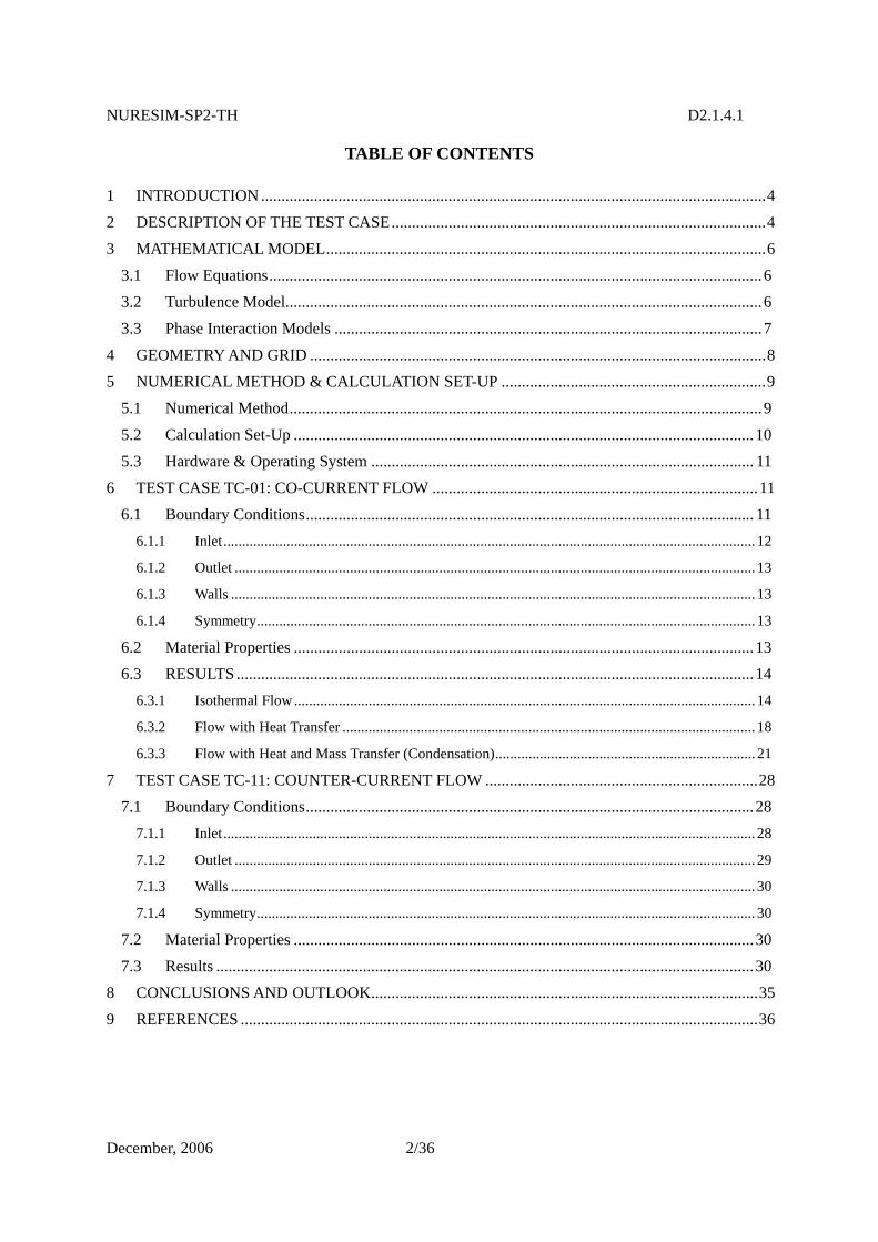
NURESIM-SP2-TH D2.1.4.1
December, 2006 2/36
TABLE OF CONTENTS 1 INTRODUCTION ............................................................................................................................4 2 DESCRIPTION OF THE TEST CASE............................................................................................4 3 MATHEMATICAL MODEL............................................................................................................6
3.1 Flow Equations.........................................................................................................................6 3.2 Turbulence Model.....................................................................................................................6 3.3 Phase Interaction Models .........................................................................................................7
4 GEOMETRY AND GRID ................................................................................................................8 5 NUMERICAL METHOD & CALCULATION SET-UP .................................................................9
5.1 Numerical Method....................................................................................................................9 5.2 Calculation Set-Up .................................................................................................................10 5.3 Hardware & Operating System .............................................................................................. 11
6 TEST CASE TC-01: CO-CURRENT FLOW ................................................................................11 6.1 Boundary Conditions.............................................................................................................. 11
6.1.1 Inlet............................................................................................................................................... 12 6.1.2 Outlet ............................................................................................................................................ 13 6.1.3 Walls ............................................................................................................................................. 13 6.1.4 Symmetry...................................................................................................................................... 13
6.2 Material Properties .................................................................................................................13 6.3 RESULTS ...............................................................................................................................14
6.3.1 Isothermal Flow............................................................................................................................ 14 6.3.2 Flow with Heat Transfer ............................................................................................................... 18 6.3.3 Flow with Heat and Mass Transfer (Condensation)...................................................................... 21
7 TEST CASE TC-11: COUNTER-CURRENT FLOW ...................................................................28 7.1 Boundary Conditions..............................................................................................................28
7.1.1 Inlet............................................................................................................................................... 28 7.1.2 Outlet ............................................................................................................................................ 29 7.1.3 Walls ............................................................................................................................................. 30 7.1.4 Symmetry...................................................................................................................................... 30
7.2 Material Properties .................................................................................................................30 7.3 Results ....................................................................................................................................30
8 CONCLUSIONS AND OUTLOOK...............................................................................................35 9 REFERENCES ...............................................................................................................................36
NURESIM-SP2-TH D2.1.4.1
December, 2006 3/36
NOMENCLATURE CFD Computational Fluid Dynamics hws Empirical, interfacial heat transfer coefficient HR High Resolution Hsat Saturation enthalpy
wH Mass weighted static water enthalpy
Lws Interfacial length scale
NAC Numerical Advection Correction SST Shear Stress Turbulence
sT Mass-weighted steam temperatures
wT Mass-weighted water temperatures
qs Interfacial heat flux of steam qw Interfacial heat flux of water
mwq Phase-weighted molecular energy fluxes
twq Phase-weighted turbulent energy fluxes
Um velocity component UDS Upwind Differencing Scheme Гw Interfacial mass transfer term
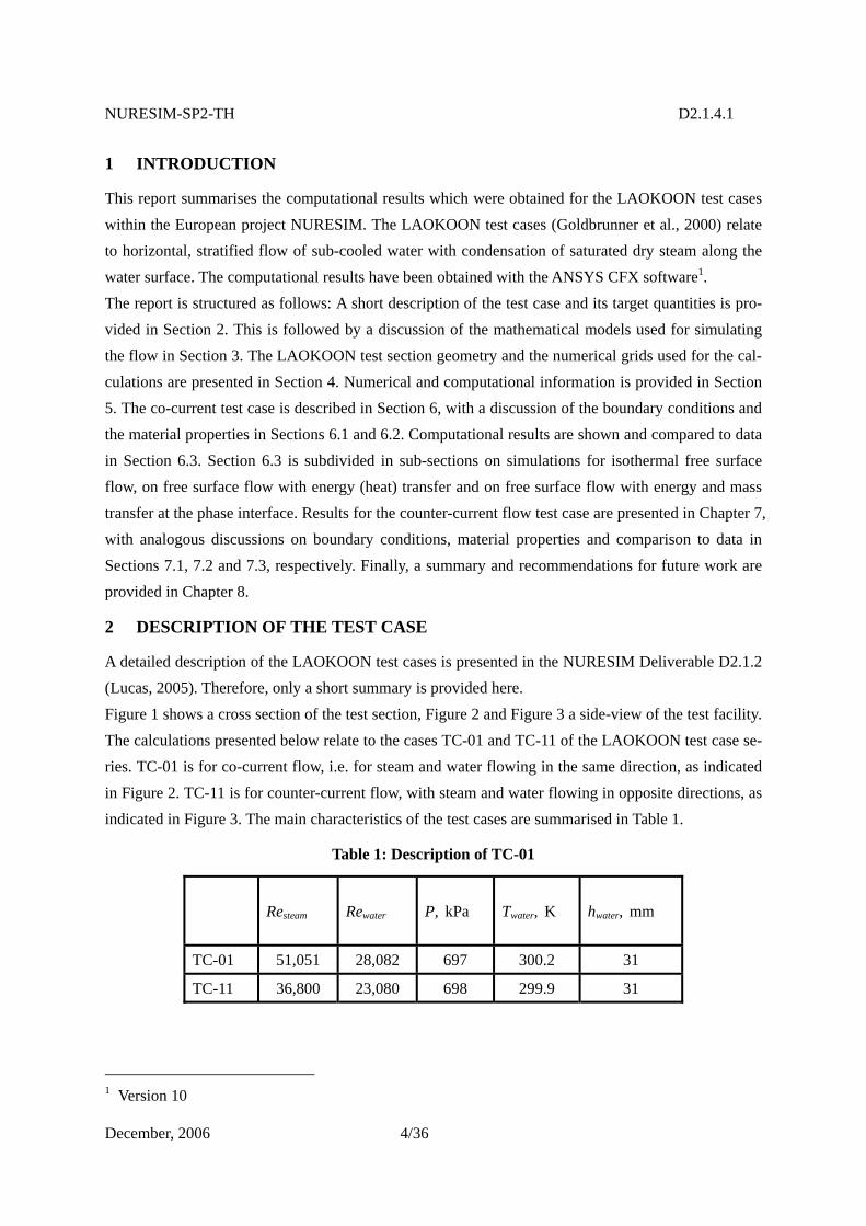
NURESIM-SP2-TH D2.1.4.1
December, 2006 4/36
1 INTRODUCTION
This report summarises the computational results which were obtained for the LAOKOON test cases within the European project NURESIM. The LAOKOON test cases (Goldbrunner et al., 2000) relate to horizontal, stratified flow of sub-cooled water with condensation of saturated dry steam along the water surface. The computational results have been obtained with the ANSYS CFX software1. The report is structured as follows: A short description of the test case and its target quantities is pro-vided in Section 2. This is followed by a discussion of the mathematical models used for simulating the flow in Section 3. The LAOKOON test section geometry and the numerical grids used for the cal-culations are presented in Section 4. Numerical and computational information is provided in Section 5. The co-current test case is described in Section 6, with a discussion of the boundary conditions and the material properties in Sections 6.1 and 6.2. Computational results are shown and compared to data in Section 6.3. Section 6.3 is subdivided in sub-sections on simulations for isothermal free surface flow, on free surface flow with energy (heat) transfer and on free surface flow with energy and mass transfer at the phase interface. Results for the counter-current flow test case are presented in Chapter 7, with analogous discussions on boundary conditions, material properties and comparison to data in Sections 7.1, 7.2 and 7.3, respectively. Finally, a summary and recommendations for future work are provided in Chapter 8.
2 DESCRIPTION OF THE TEST CASE
A detailed description of the LAOKOON test cases is presented in the NURESIM Deliverable D2.1.2 (Lucas, 2005). Therefore, only a short summary is provided here. Figure 1 shows a cross section of the test section, Figure 2 and Figure 3 a side-view of the test facility. The calculations presented below relate to the cases TC-01 and TC-11 of the LAOKOON test case se-ries. TC-01 is for co-current flow, i.e. for steam and water flowing in the same direction, as indicated in Figure 2. TC-11 is for counter-current flow, with steam and water flowing in opposite directions, as indicated in Figure 3. The main characteristics of the test cases are summarised in Table 1.
Table 1: Description of TC-01
Resteam Rewater P, kPa Twater, K hwater, mm
TC-01 51,051 28,082 697 300.2 31
TC-11 36,800 23,080 698 299.9 31
1 Version 10
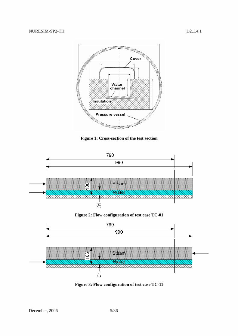
NURESIM-SP2-TH D2.1.4.1
December, 2006 5/36
Figure 1: Cross-section of the test section
Figure 2: Flow configuration of test case TC-01
Figure 3: Flow configuration of test case TC-11
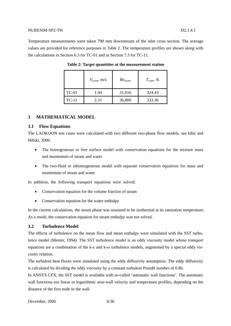
NURESIM-SP2-TH D2.1.4.1
December, 2006 6/36
Temperature measurements were taken 790 mm downstream of the inlet cross section. The average values are provided for reference purposes in Table 2. The temperature profiles are shown along with the calculations in Section 6.3 for TC-01 and in Section 7.3 for TC-11.
Table 2: Target quantities at the measurement station
Vsteam m/s Resteam Twater K
TC-01 1.94 31,016 324.43
TC-11 2.31 36,800 333.36
3 MATHEMATICAL MODEL
3.1 Flow Equations The LAOKOON test cases were calculated with two different two-phase flow models, see Ishii and Hibiki, 2006:
• The homogeneous or free surface model with conservation equations for the mixture mass and momentum of steam and water
• The two-fluid or inhomogeneous model with separate conservation equations for mass and momentum of steam and water
In addition, the following transport equations were solved:
• Conservation equation for the volume fraction of steam
• Conservation equation for the water enthalpy
In the current calculations, the steam phase was assumed to be isothermal at its saturation temperature. As a result, the conservation equation for steam enthalpy was not solved.
3.2 Turbulence Model The effects of turbulence on the mean flow and mean enthalpy were simulated with the SST turbu-lence model (Menter, 1994). The SST turbulence model is an eddy viscosity model whose transport equations are a combination of the k-ε and k-ω turbulence models, augmented by a special eddy vis-cosity relation. The turbulent heat fluxes were simulated using the eddy diffusivity assumption. The eddy diffusivity is calculated by dividing the eddy viscosity by a constant turbulent Prandtl number of 0.86. In ANSYS CFX, the SST model is available with so-called ‘automatic wall functions’. The automatic wall functions use linear or logarithmic near-wall velocity and temperature profiles, depending on the distance of the first node to the wall.
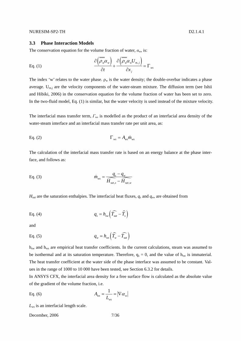
NURESIM-SP2-TH D2.1.4.1
December, 2006 7/36
3.3 Phase Interaction Models The conservation equation for the volume fraction of water, αw, is:
Eq. (1) ( ) ( ),w w w w m j
wsj
U
t x
ρ α ρ α∂ ∂+ = Γ
∂ ∂
The index ‘w’ relates to the water phase. ρw is the water density; the double-overbar indicates a phase average. Um,j are the velocity components of the water-steam mixture. The diffusion term (see Ishii and Hibiki, 2006) in the conservation equation for the volume fraction of water has been set to zero. In the two-fluid model, Eq. (1) is similar, but the water velocity is used instead of the mixture velocity. The interfacial mass transfer term, Гw, is modelled as the product of an interfacial area density of the water-steam interface and an interfacial mass transfer rate per unit area, as: Eq. (2) ws ws wsA mΓ = The calculation of the interfacial mass transfer rate is based on an energy balance at the phase inter-face, and follows as:
Eq. (3) , ,
s wws
sat s sat w
q qmH H
−=
−
Hsat are the saturation enthalpies. The interfacial heat fluxes, qs and qw, are obtained from
Eq. (4) ( )s sw sat sq h T T= −
and
Eq. (5) ( )w ws w satq h T T= −
hsw and hws are empirical heat transfer coefficients. In the current calculations, steam was assumed to be isothermal and at its saturation temperature. Therefore, qs = 0, and the value of hsw is immaterial. The heat transfer coefficient at the water side of the phase interface was assumed to be constant. Val-ues in the range of 1000 to 10 000 have been tested, see Section 6.3.2 for details. In ANSYS CFX, the interfacial area density for a free surface flow is calculated as the absolute value of the gradient of the volume fraction, i.e.
Eq. (6) 1
ws wws
AL
α= = ∇
Lws is an interfacial length scale.
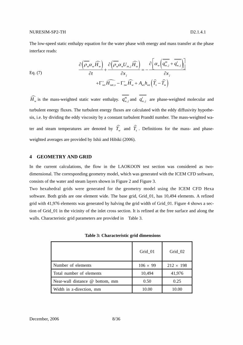
NURESIM-SP2-TH D2.1.4.1
December, 2006 8/36
The low-speed static enthalpy equation for the water phase with energy and mass transfer at the phase interface reads:
Eq. (7) ( ) ( ) ( )
( )
, ,,
,
m tw w j w jw w w w w m j w
j j
ws sat s sw w ws ws s w
q qH U H
t x x
H H A h T T
αρ α ρ α
+ +
⎡ ⎤∂ +∂ ∂ ⎢ ⎥⎣ ⎦+ = −∂ ∂ ∂
+Γ − Γ + −
wH is the mass-weighted static water enthalpy. ,mw jq and ,
tw jq are phase-weighted molecular and
turbulent energy fluxes. The turbulent energy fluxes are calculated with the eddy diffusivity hypothe-sis, i.e. by dividing the eddy viscosity by a constant turbulent Prandtl number. The mass-weighted wa-
ter and steam temperatures are denoted by wT and sT . Definitions for the mass- and phase-
weighted averages are provided by Ishii and Hibiki (2006).
4 GEOMETRY AND GRID
In the current calculations, the flow in the LAOKOON test section was considered as two-dimensional. The corresponding geometry model, which was generated with the ICEM CFD software, consists of the water and steam layers shown in Figure 2 and Figure 3. Two hexahedral grids were generated for the geometry model using the ICEM CFD Hexa software. Both grids are one element wide. The base grid, Grid_01, has 10,494 elements. A refined grid with 41,976 elements was generated by halving the grid width of Grid_01. Figure 4 shows a sec-tion of Grid_01 in the vicinity of the inlet cross section. It is refined at the free surface and along the walls. Characteristic grid parameters are provided in Table 3.
Table 3: Characteristic grid dimensions
Grid_01 Grid_02
Number of elements 106 × 99 212 × 198
Total number of elements 10,494 41,976
Near-wall distance @ bottom, mm 0.50 0.25
Width in z-direction, mm 10.00 10.00
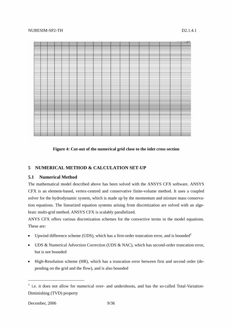
NURESIM-SP2-TH D2.1.4.1
December, 2006 9/36
Figure 4: Cut-out of the numerical grid close to the inlet cross section
5 NUMERICAL METHOD & CALCULATION SET-UP
5.1 Numerical Method The mathematical model described above has been solved with the ANSYS CFX software. ANSYS CFX is an element-based, vertex-centred and conservative finite-volume method. It uses a coupled solver for the hydrodynamic system, which is made up by the momentum and mixture mass conserva-tion equations. The linearized equation systems arising from discretization are solved with an alge-braic multi-grid method. ANSYS CFX is scalably parallelized. ANYS CFX offers various discretization schemes for the convective terms in the model equations. These are:
• Upwind difference scheme (UDS), which has a first-order truncation error, and is bounded2
• UDS & Numerical Advection Correction (UDS & NAC), which has second-order truncation error, but is not bounded
• High-Resolution scheme (HR), which has a truncation error between first and second order (de-pending on the grid and the flow), and is also bounded
2 i.e. it does not allow for numerical over- and undershoots, and has the so-called Total-Variation-Diminishing (TVD) property
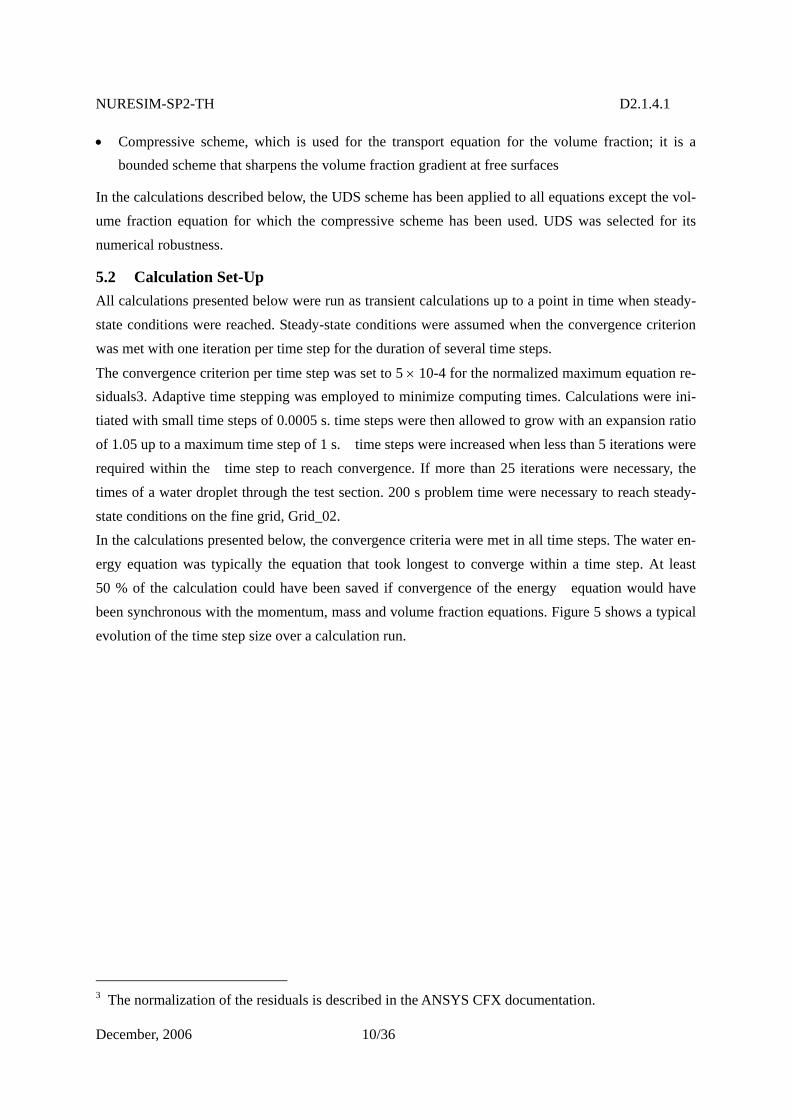
NURESIM-SP2-TH D2.1.4.1
December, 2006 10/36
• Compressive scheme, which is used for the transport equation for the volume fraction; it is a bounded scheme that sharpens the volume fraction gradient at free surfaces
In the calculations described below, the UDS scheme has been applied to all equations except the vol-ume fraction equation for which the compressive scheme has been used. UDS was selected for its numerical robustness.
5.2 Calculation Set-Up All calculations presented below were run as transient calculations up to a point in time when steady-state conditions were reached. Steady-state conditions were assumed when the convergence criterion was met with one iteration per time step for the duration of several time steps.
The convergence criterion per time step was set to 5 × 10⁻⁴ for the normalized maximum equation re-siduals3. Adaptive time stepping was employed to minimize computing times. Calculations were ini-tiated with small time steps of 0.0005 s. time steps were then allowed to grow with an expansion ratio of 1.05 up to a maximum time step of 1 s. time steps were increased when less than 5 iterations were required within the time step to reach convergence. If more than 25 iterations were necessary, the times of a water droplet through the test section. 200 s problem time were necessary to reach steady-state conditions on the fine grid, Grid_02. In the calculations presented below, the convergence criteria were met in all time steps. The water en-ergy equation was typically the equation that took longest to converge within a time step. At least 50 % of the calculation could have been saved if convergence of the energy equation would have been synchronous with the momentum, mass and volume fraction equations. Figure 5 shows a typical evolution of the time step size over a calculation run.
3 The normalization of the residuals is described in the ANSYS CFX documentation.
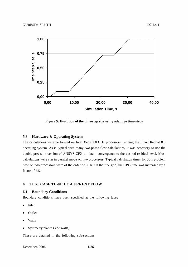
NURESIM-SP2-TH D2.1.4.1
December, 2006 11/36
0,00
0,25
0,50
0,75
1,00
0,00 10,00 20,00 30,00 40,00
Simulation Time, s
Tim
e St
ep S
ize,
s
Figure 5: Evolution of the time-step size using adaptive time-steps
5.3 Hardware & Operating System The calculations were performed on Intel Xeon 2.8 GHz processors, running the Linux Redhat 8.0 operating system. As is typical with many two-phase flow calculations, it was necessary to use the double-precision version of ANSYS CFX to obtain convergence to the desired residual level. Most calculations were run in parallel mode on two processors. Typical calculation times for 30 s problem time on two processors were of the order of 30 h. On the fine grid, the CPU-time was increased by a factor of 3.5.
6 TEST CASE TC-01: CO-CURRENT FLOW
6.1 Boundary Conditions Boundary conditions have been specified at the following faces
• Inlet
• Outlet
• Walls
• Symmetry planes (side walls)
These are detailed in the following sub-sections.
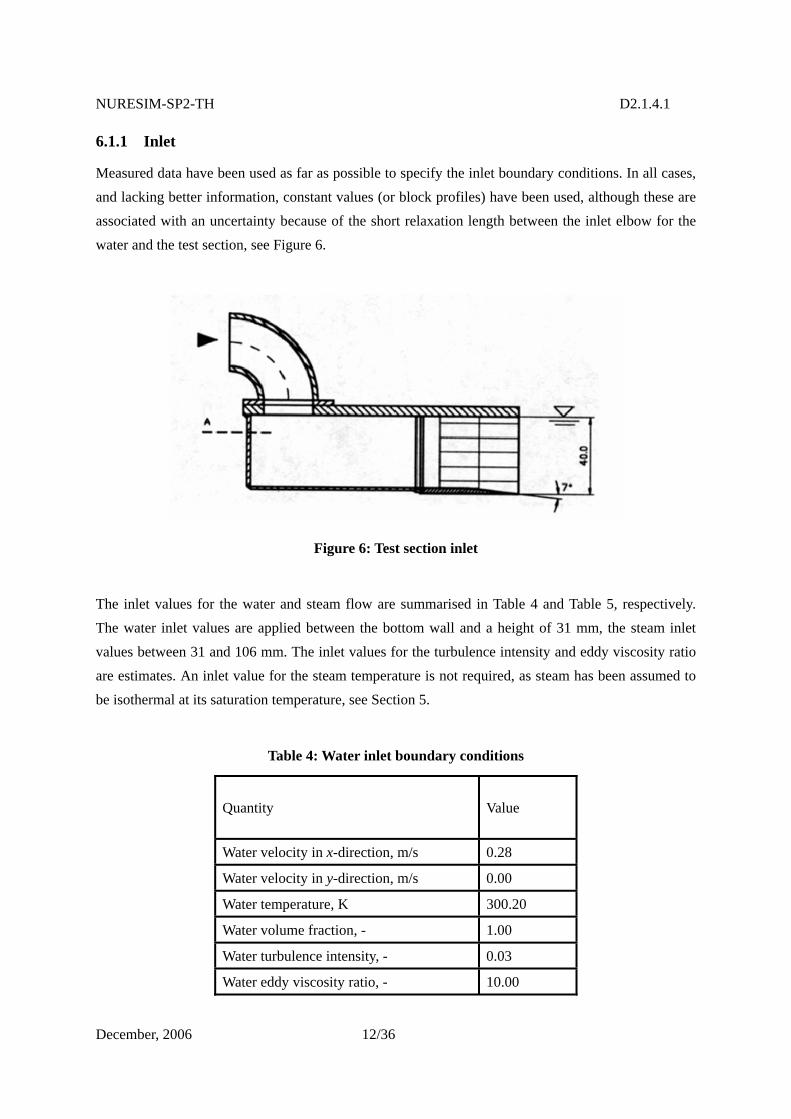
NURESIM-SP2-TH D2.1.4.1
December, 2006 12/36
6.1.1 Inlet
Measured data have been used as far as possible to specify the inlet boundary conditions. In all cases, and lacking better information, constant values (or block profiles) have been used, although these are associated with an uncertainty because of the short relaxation length between the inlet elbow for the water and the test section, see Figure 6.
Figure 6: Test section inlet
The inlet values for the water and steam flow are summarised in Table 4 and Table 5, respectively. The water inlet values are applied between the bottom wall and a height of 31 mm, the steam inlet values between 31 and 106 mm. The inlet values for the turbulence intensity and eddy viscosity ratio are estimates. An inlet value for the steam temperature is not required, as steam has been assumed to be isothermal at its saturation temperature, see Section 5.
Table 4: Water inlet boundary conditions
Quantity Value
Water velocity in x-direction, m/s 0.28
Water velocity in y-direction, m/s 0.00
Water temperature, K 300.20
Water volume fraction, - 1.00
Water turbulence intensity, - 0.03
Water eddy viscosity ratio, - 10.00
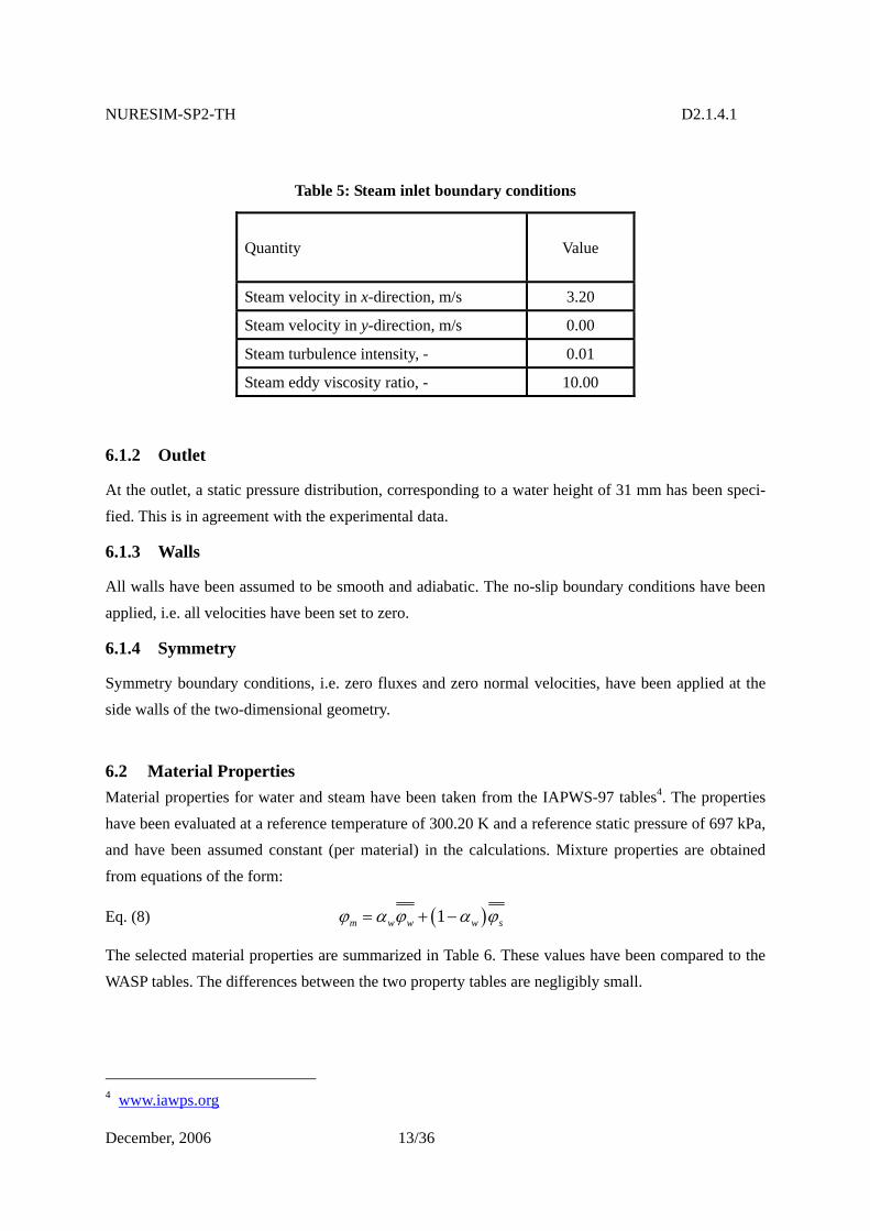
NURESIM-SP2-TH D2.1.4.1
December, 2006 13/36
Table 5: Steam inlet boundary conditions
Quantity Value
Steam velocity in x-direction, m/s 3.20
Steam velocity in y-direction, m/s 0.00
Steam turbulence intensity, - 0.01
Steam eddy viscosity ratio, - 10.00
6.1.2 Outlet
At the outlet, a static pressure distribution, corresponding to a water height of 31 mm has been speci-fied. This is in agreement with the experimental data.
6.1.3 Walls
All walls have been assumed to be smooth and adiabatic. The no-slip boundary conditions have been applied, i.e. all velocities have been set to zero.
6.1.4 Symmetry
Symmetry boundary conditions, i.e. zero fluxes and zero normal velocities, have been applied at the side walls of the two-dimensional geometry.
6.2 Material Properties Material properties for water and steam have been taken from the IAPWS-97 tables4. The properties have been evaluated at a reference temperature of 300.20 K and a reference static pressure of 697 kPa, and have been assumed constant (per material) in the calculations. Mixture properties are obtained from equations of the form:
Eq. (8) ( )1m w w w sϕ α ϕ α ϕ= + −
The selected material properties are summarized in Table 6. These values have been compared to the WASP tables. The differences between the two property tables are negligibly small.
4 www.iawps.org
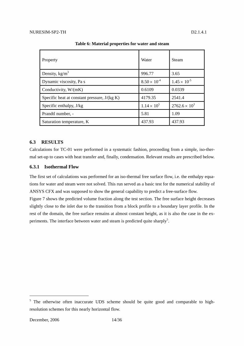
NURESIM-SP2-TH D2.1.4.1
December, 2006 14/36
Table 6: Material properties for water and steam
Property Water Steam
Density, kg/m3 996.77 3.65
Dynamic viscosity, Pa s 8.50 × 10⁻⁴ 1.45 × 10⁻⁵
Conductivity, W/(mK) 0.6109 0.0339
Specific heat at constant pressure, J/(kg K) 4179.35 2541.4
Specific enthalpy, J/kg 1.14 × 10⁵ 2762.6 × 103
Prandtl number, - 5.81 1.09
Saturation temperature, K 437.93 437.93
6.3 RESULTS Calculations for TC-01 were performed in a systematic fashion, proceeding from a simple, iso-ther-mal set-up to cases with heat transfer and, finally, condensation. Relevant results are prescribed below.
6.3.1 Isothermal Flow
The first set of calculations was performed for an iso-thermal free surface flow, i.e. the enthalpy equa-tions for water and steam were not solved. This run served as a basic test for the numerical stability of ANSYS CFX and was supposed to show the general capability to predict a free-surface flow. Figure 7 shows the predicted volume fraction along the test section. The free surface height decreases slightly close to the inlet due to the transition from a block profile to a boundary layer profile. In the rest of the domain, the free surface remains at almost constant height, as it is also the case in the ex-periments. The interface between water and steam is predicted quite sharply5.
5 The otherwise often inaccurate UDS scheme should be quite good and comparable to high-resolution schemes for this nearly horizontal flow.
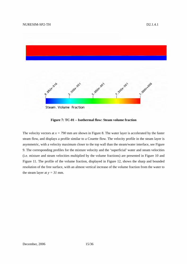
NURESIM-SP2-TH D2.1.4.1
December, 2006 15/36
Figure 7: TC-01 – Isothermal flow: Steam volume fraction
The velocity vectors at x = 790 mm are shown in Figure 8. The water layer is accelerated by the faster steam flow, and displays a profile similar to a Couette flow. The velocity profile in the steam layer is asymmetric, with a velocity maximum closer to the top wall than the steam/water interface, see Figure 9. The corresponding profiles for the mixture velocity and the ‘superficial’ water and steam velocities (i.e. mixture and steam velocities multiplied by the volume fractions) are presented in Figure 10 and Figure 11. The profile of the volume fraction, displayed in Figure 12, shows the sharp and bounded resolution of the free surface, with an almost vertical increase of the volume fraction from the water to the steam layer at y = 31 mm.
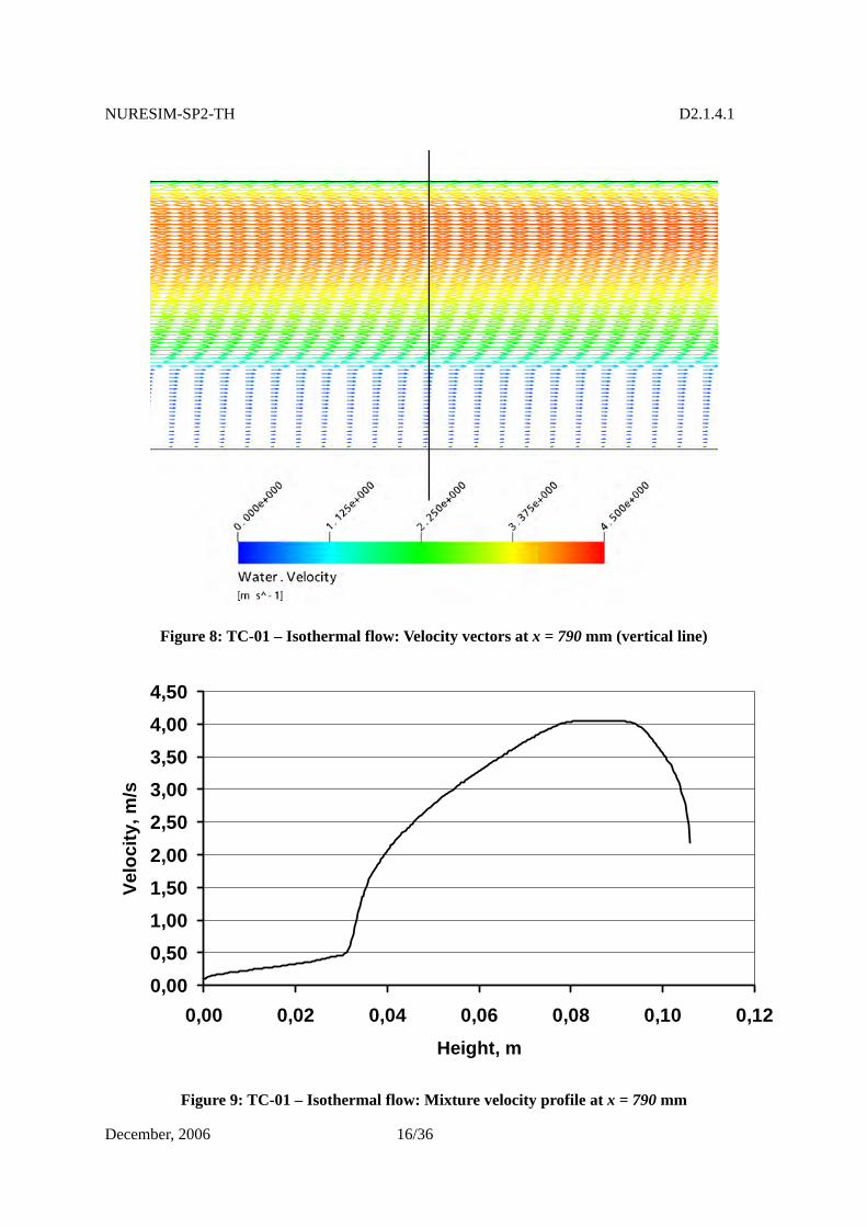
NURESIM-SP2-TH D2.1.4.1
December, 2006 16/36
Figure 8: TC-01 – Isothermal flow: Velocity vectors at x = 790 mm (vertical line)
0,000,501,001,502,002,503,003,504,004,50
0,00 0,02 0,04 0,06 0,08 0,10 0,12Height, m
Velo
city
, m/s
Figure 9: TC-01 – Isothermal flow: Mixture velocity profile at x = 790 mm
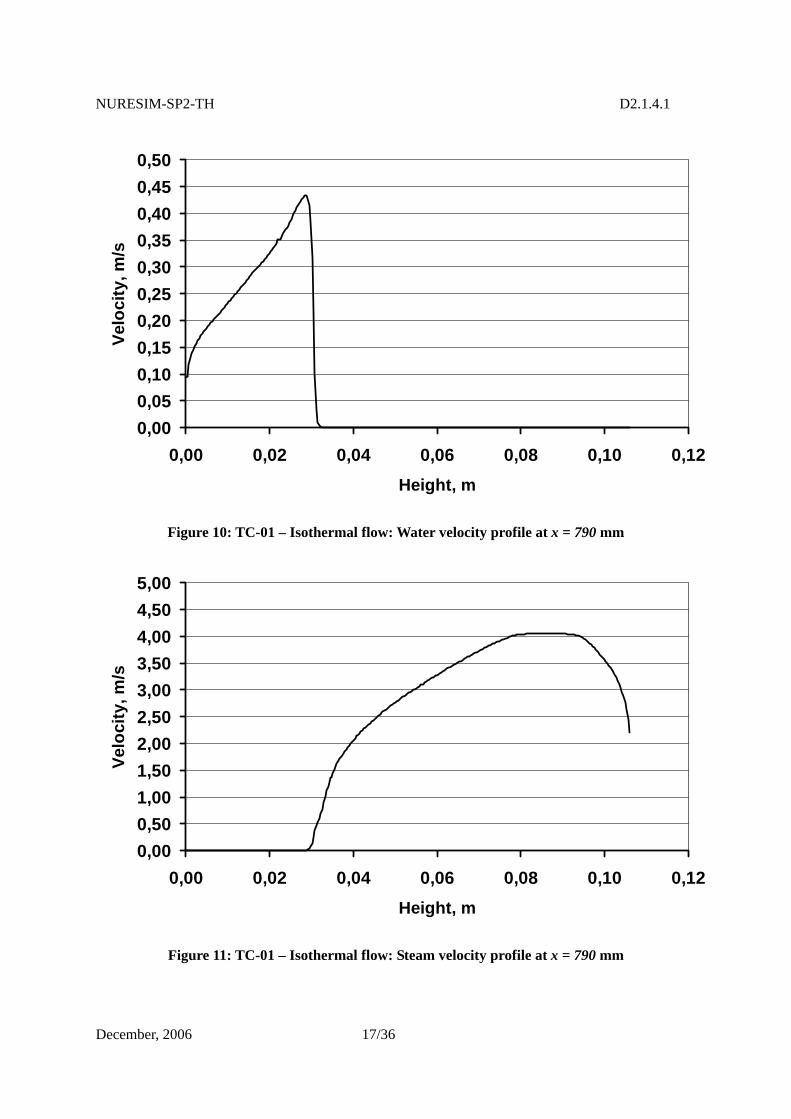
NURESIM-SP2-TH D2.1.4.1
December, 2006 17/36
0,000,050,100,150,200,250,300,350,400,450,50
0,00 0,02 0,04 0,06 0,08 0,10 0,12Height, m
Velo
city
, m/s
Figure 10: TC-01 – Isothermal flow: Water velocity profile at x = 790 mm
0,000,501,001,502,002,503,003,504,004,505,00
0,00 0,02 0,04 0,06 0,08 0,10 0,12Height, m
Velo
city
, m/s
Figure 11: TC-01 – Isothermal flow: Steam velocity profile at x = 790 mm
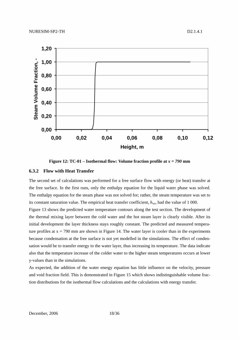
NURESIM-SP2-TH D2.1.4.1
December, 2006 18/36
0,00
0,20
0,40
0,60
0,80
1,00
1,20
0,00 0,02 0,04 0,06 0,08 0,10 0,12Height, m
Stea
m V
olum
e Fr
actio
n, -
Figure 12: TC-01 – Isothermal flow: Volume fraction profile at x = 790 mm
6.3.2 Flow with Heat Transfer
The second set of calculations was performed for a free surface flow with energy (or heat) transfer at the free surface. In the first runs, only the enthalpy equation for the liquid water phase was solved. The enthalpy equation for the steam phase was not solved for; rather, the steam temperature was set to its constant saturation value. The empirical heat transfer coefficient, hws, had the value of 1 000. Figure 13 shows the predicted water temperature contours along the test section. The development of the thermal mixing layer between the cold water and the hot steam layer is clearly visible. After its initial development the layer thickness stays roughly constant. The predicted and measured tempera-ture profiles at x = 790 mm are shown in Figure 14. The water layer is cooler than in the experiments because condensation at the free surface is not yet modelled in the simulations. The effect of conden-sation would be to transfer energy to the water layer, thus increasing its temperature. The data indicate also that the temperature increase of the colder water to the higher steam temperatures occurs at lower y-values than in the simulations. As expected, the addition of the water energy equation has little influence on the velocity, pressure and void fraction field. This is demonstrated in Figure 15 which shows indistinguishable volume frac-tion distributions for the isothermal flow calculations and the calculations with energy transfer.
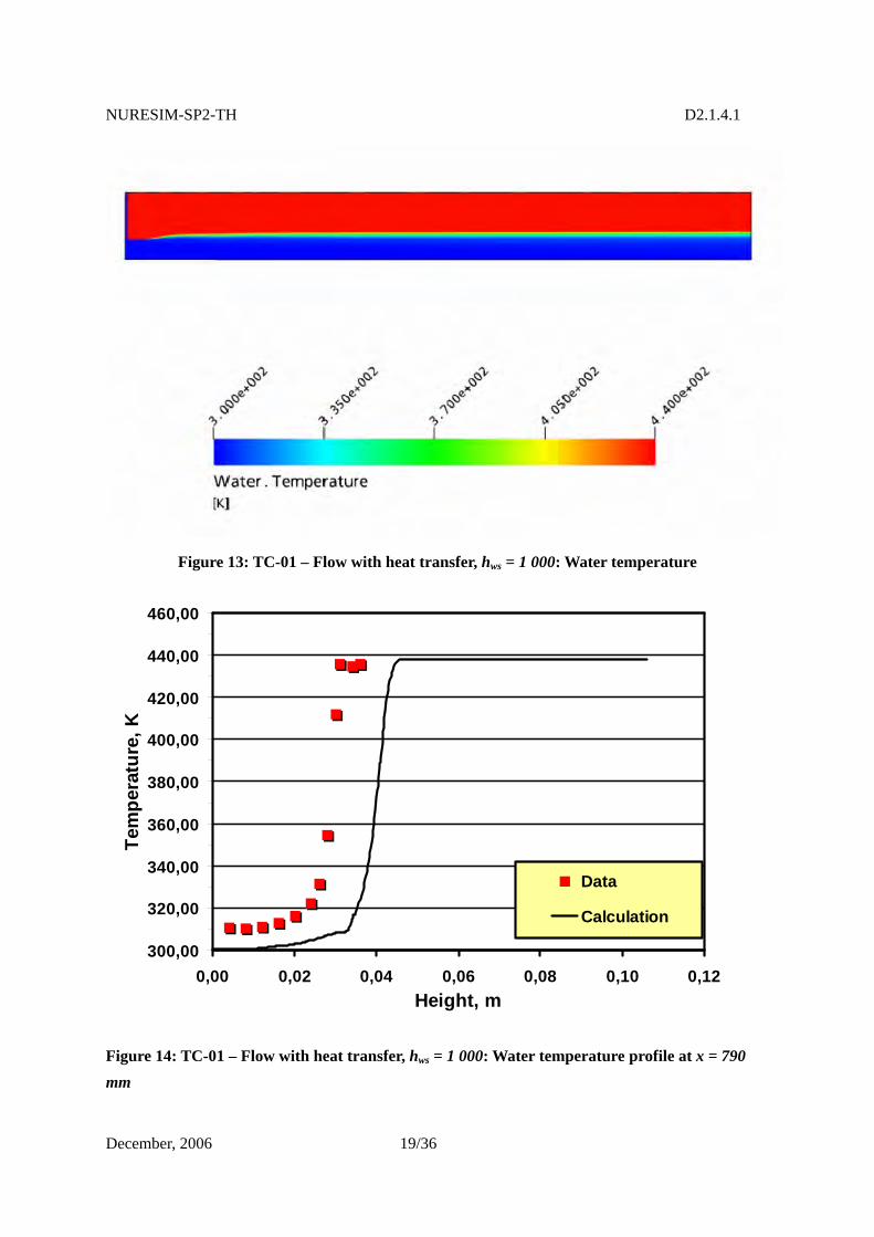
NURESIM-SP2-TH D2.1.4.1
December, 2006 19/36
Figure 13: TC-01 – Flow with heat transfer, hws = 1 000: Water temperature
300,00
320,00
340,00
360,00
380,00
400,00
420,00
440,00
460,00
0,00 0,02 0,04 0,06 0,08 0,10 0,12Height, m
Tem
pera
ture
, K
Data
Calculation
Figure 14: TC-01 – Flow with heat transfer, hws = 1 000: Water temperature profile at x = 790 mm
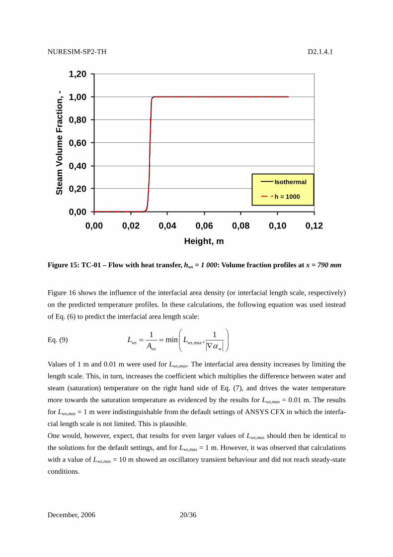
NURESIM-SP2-TH D2.1.4.1
December, 2006 20/36
0,00
0,20
0,40
0,60
0,80
1,00
1,20
0,00 0,02 0,04 0,06 0,08 0,10 0,12Height, m
Stea
m V
olum
e Fr
actio
n, -
Isothermal
h = 1000
Figure 15: TC-01 – Flow with heat transfer, hws = 1 000: Volume fraction profiles at x = 790 mm
Figure 16 shows the influence of the interfacial area density (or interfacial length scale, respectively) on the predicted temperature profiles. In these calculations, the following equation was used instead of Eq. (6) to predict the interfacial area length scale:
Eq. (9) ,max1 1min ,ws wsws w
L LA α
⎛ ⎞= = ⎜ ⎟
∇⎝ ⎠
Values of 1 m and 0.01 m were used for Lws,max. The interfacial area density increases by limiting the length scale. This, in turn, increases the coefficient which multiplies the difference between water and steam (saturation) temperature on the right hand side of Eq. (7), and drives the water temperature more towards the saturation temperature as evidenced by the results for Lws,max = 0.01 m. The results for Lws,max = 1 m were indistinguishable from the default settings of ANSYS CFX in which the interfa-cial length scale is not limited. This is plausible. One would, however, expect, that results for even larger values of Lws,max should then be identical to the solutions for the default settings, and for Lws,max = 1 m. However, it was observed that calculations with a value of Lws,max = 10 m showed an oscillatory transient behaviour and did not reach steady-state conditions.
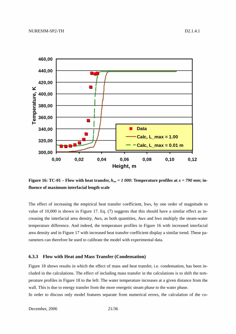
NURESIM-SP2-TH D2.1.4.1
December, 2006 21/36
300,00
320,00
340,00
360,00
380,00
400,00
420,00
440,00
460,00
0,00 0,02 0,04 0,06 0,08 0,10 0,12Height, m
Tem
pera
ture
, K
Data
Calc, L_max = 1.00
Calc, L_max = 0.01 m
Figure 16: TC-01 – Flow with heat transfer, hws = 1 000: Temperature profiles at x = 790 mm; in-fluence of maximum interfacial length scale
The effect of increasing the empirical heat transfer coefficient, hws, by one order of magnitude to value of 10,000 is shown in Figure 17. Eq. (7) suggests that this should have a similar effect as in-creasing the interfacial area density, Aws, as both quantities, Aws and hws multiply the steam-water temperature difference. And indeed, the temperature profiles in Figure 16 with increased interfacial area density and in Figure 17 with increased heat transfer coefficient display a similar trend. These pa-rameters can therefore be used to calibrate the model with experimental data.
6.3.3 Flow with Heat and Mass Transfer (Condensation)
Figure 18 shows results in which the effect of mass and heat transfer, i.e. condensation, has been in-cluded in the calculations. The effect of including mass transfer in the calculations is to shift the tem-perature profiles in Figure 18 to the left: The water temperature increases at a given distance from the wall. This is due to energy transfer from the more energetic steam phase to the water phase. In order to discuss only model features separate from numerical errors, the calculation of the co-

NURESIM-SP2-TH D2.1.4.1
December, 2006 22/36
current flow case with condensation was repeated on the refined grid, Grid_02, which had 42,000 elements (see Table 3). Grid_02 has the same topology as Grid_01, however with halved grid dis-tances. Figure 19 shows that the grid influence is very small. The discrepancies between data and pre-dictions must, therefore, reside in the model or in other systematic differences between calculations and experiment.
300,00
320,00
340,00
360,00
380,00
400,00
420,00
440,00
460,00
0,00 0,02 0,04 0,06 0,08 0,10 0,12Height, m
Tem
pera
ture
, K
Data
Calc, h = 1 000
Calc, h = 10 000
Figure 17: TC-01 – Flow with heat transfer; Temperature profiles at x = 790 mm; influence of heat transfer coefficient
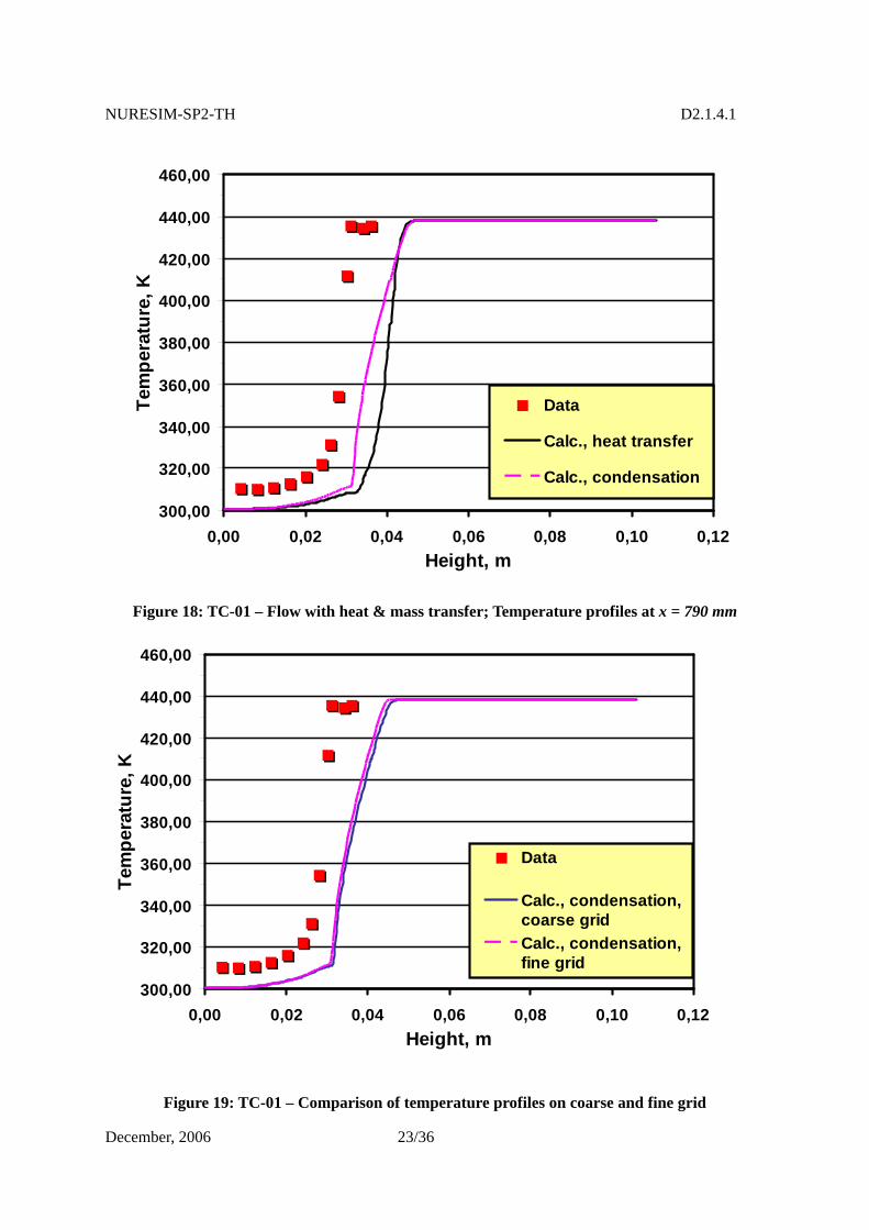
NURESIM-SP2-TH D2.1.4.1
December, 2006 23/36
300,00
320,00
340,00
360,00
380,00
400,00
420,00
440,00
460,00
0,00 0,02 0,04 0,06 0,08 0,10 0,12Height, m
Tem
pera
ture
, K
Data
Calc., heat transfer
Calc., condensation
Figure 18: TC-01 – Flow with heat & mass transfer; Temperature profiles at x = 790 mm
Figure 19: TC-01 – Comparison of temperature profiles on coarse and fine grid
300,00
320,00
340,00
360,00
380,00
400,00
420,00
440,00
460,00
0,00 0,02 0,04 0,06 0,08 0,10 0,12Height, m
Tem
pera
ture
, K
Data
Calc., condensation,coarse gridCalc., condensation,fine grid
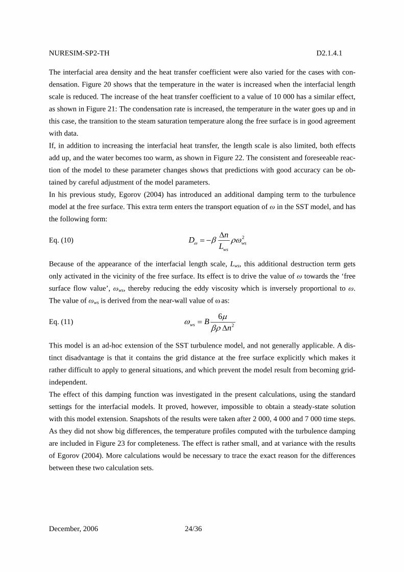
NURESIM-SP2-TH D2.1.4.1
December, 2006 24/36
The interfacial area density and the heat transfer coefficient were also varied for the cases with con-densation. Figure 20 shows that the temperature in the water is increased when the interfacial length scale is reduced. The increase of the heat transfer coefficient to a value of 10 000 has a similar effect, as shown in Figure 21: The condensation rate is increased, the temperature in the water goes up and in this case, the transition to the steam saturation temperature along the free surface is in good agreement with data. If, in addition to increasing the interfacial heat transfer, the length scale is also limited, both effects add up, and the water becomes too warm, as shown in Figure 22. The consistent and foreseeable reac-tion of the model to these parameter changes shows that predictions with good accuracy can be ob-tained by careful adjustment of the model parameters. In his previous study, Egorov (2004) has introduced an additional damping term to the turbulence model at the free surface. This extra term enters the transport equation of ω in the SST model, and has the following form:
Eq. (10) 2ws
ws
nDLω β ρωΔ
= −
Because of the appearance of the interfacial length scale, Lws, this additional destruction term gets only activated in the vicinity of the free surface. Its effect is to drive the value of ω towards the ‘free surface flow value’, ωws, thereby reducing the eddy viscosity which is inversely proportional to ω. The value of ωws is derived from the near-wall value of ω as:
Eq. (11) 2
6ws B
nμω
βρ=
Δ
This model is an ad-hoc extension of the SST turbulence model, and not generally applicable. A dis-tinct disadvantage is that it contains the grid distance at the free surface explicitly which makes it rather difficult to apply to general situations, and which prevent the model result from becoming grid-independent. The effect of this damping function was investigated in the present calculations, using the standard settings for the interfacial models. It proved, however, impossible to obtain a steady-state solution with this model extension. Snapshots of the results were taken after 2 000, 4 000 and 7 000 time steps. As they did not show big differences, the temperature profiles computed with the turbulence damping are included in Figure 23 for completeness. The effect is rather small, and at variance with the results of Egorov (2004). More calculations would be necessary to trace the exact reason for the differences between these two calculation sets.
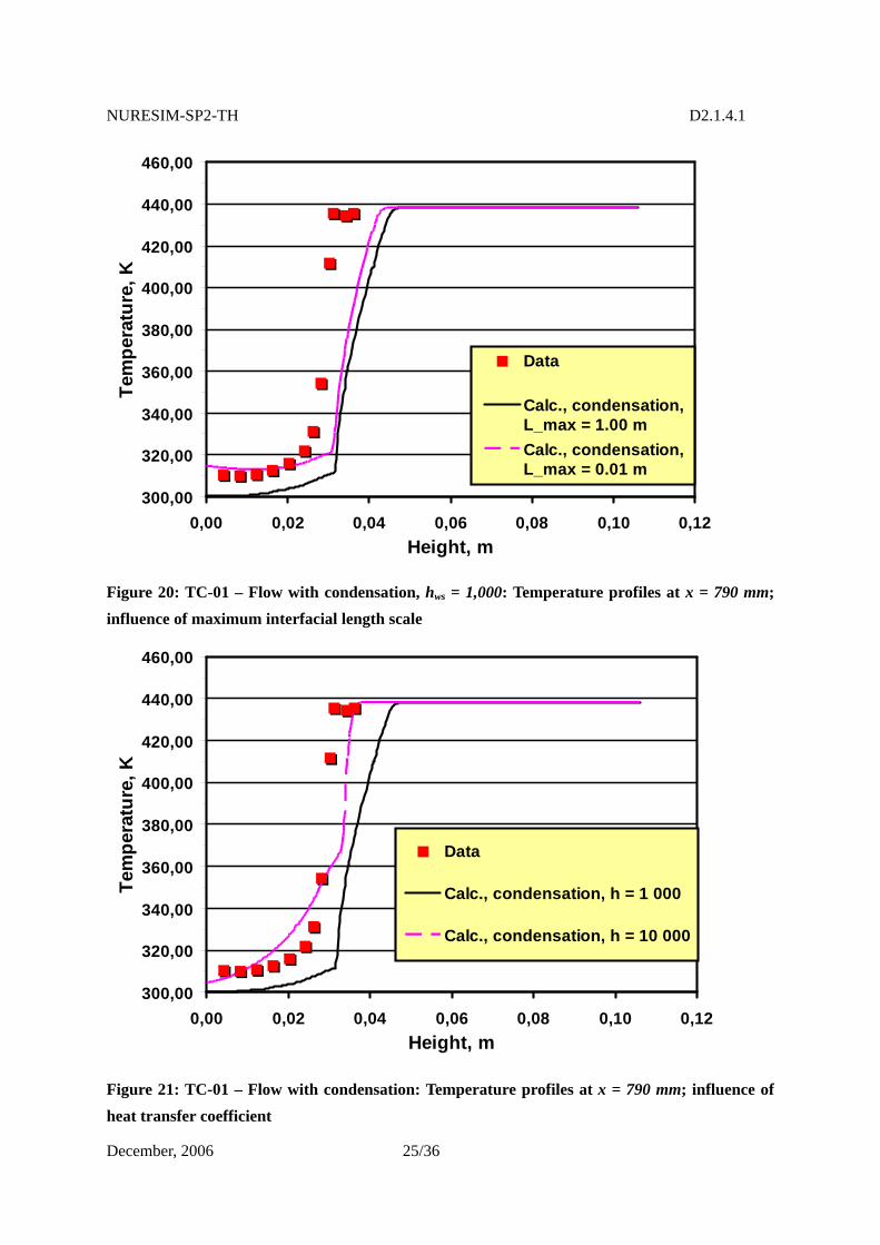
NURESIM-SP2-TH D2.1.4.1
December, 2006 25/36
Figure 20: TC-01 – Flow with condensation, hws = 1,000: Temperature profiles at x = 790 mm; influence of maximum interfacial length scale
Figure 21: TC-01 – Flow with condensation: Temperature profiles at x = 790 mm; influence of heat transfer coefficient
300,00
320,00
340,00
360,00
380,00
400,00
420,00
440,00
460,00
0,00 0,02 0,04 0,06 0,08 0,10 0,12Height, m
Tem
pera
ture
, K
Data
Calc., condensation, h = 1 000
Calc., condensation, h = 10 000
300,00
320,00
340,00
360,00
380,00
400,00
420,00
440,00
460,00
0,00 0,02 0,04 0,06 0,08 0,10 0,12Height, m
Tem
pera
ture
, K
Data
Calc., condensation,L_max = 1.00 mCalc., condensation,L_max = 0.01 m
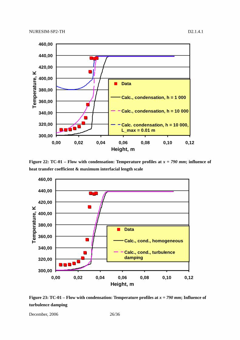
NURESIM-SP2-TH D2.1.4.1
December, 2006 26/36
Figure 22: TC-01 – Flow with condensation: Temperature profiles at x = 790 mm; influence of heat transfer coefficient & maximum interfacial length scale
Figure 23: TC-01 – Flow with condensation: Temperature profiles at x = 790 mm; Influence of turbulence damping
300,00
320,00
340,00
360,00
380,00
400,00
420,00
440,00
460,00
0,00 0,02 0,04 0,06 0,08 0,10 0,12Height, m
Tem
pera
ture
, K
Data
Calc., cond., homogeneous
Calc., cond., turbulencedamping
300,00
320,00
340,00
360,00
380,00
400,00
420,00
440,00
460,00
0,00 0,02 0,04 0,06 0,08 0,10 0,12Height, m
Tem
pera
ture
, K
Data
Calc., condensation, h = 1 000
Calc., condensation, h = 10 000
Calc. condensation, h = 10 000,L_max = 0.01 m
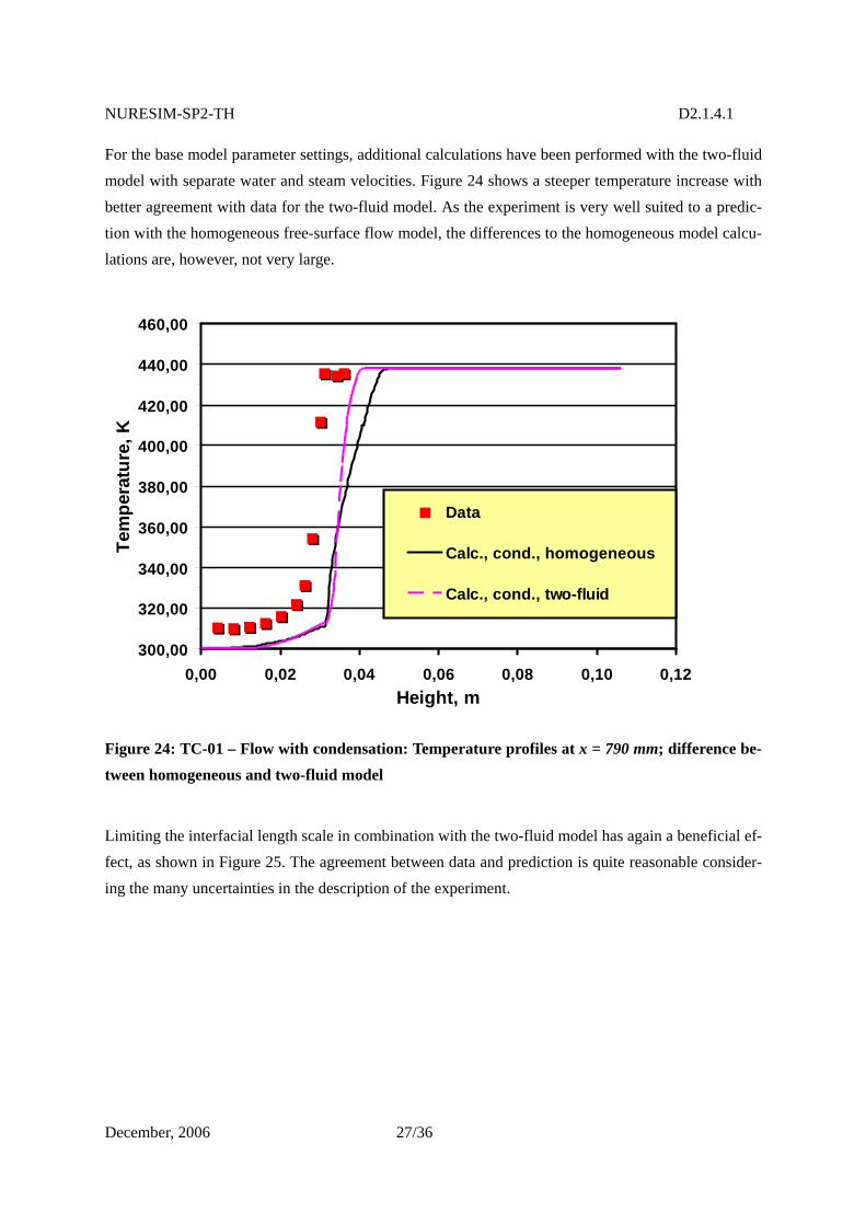
NURESIM-SP2-TH D2.1.4.1
December, 2006 27/36
For the base model parameter settings, additional calculations have been performed with the two-fluid model with separate water and steam velocities. Figure 24 shows a steeper temperature increase with better agreement with data for the two-fluid model. As the experiment is very well suited to a predic-tion with the homogeneous free-surface flow model, the differences to the homogeneous model calcu-lations are, however, not very large.
Figure 24: TC-01 – Flow with condensation: Temperature profiles at x = 790 mm; difference be-tween homogeneous and two-fluid model
Limiting the interfacial length scale in combination with the two-fluid model has again a beneficial ef-fect, as shown in Figure 25. The agreement between data and prediction is quite reasonable consider-ing the many uncertainties in the description of the experiment.
300,00
320,00
340,00
360,00
380,00
400,00
420,00
440,00
460,00
0,00 0,02 0,04 0,06 0,08 0,10 0,12Height, m
Tem
pera
ture
, K
Data
Calc., cond., homogeneous
Calc., cond., two-fluid
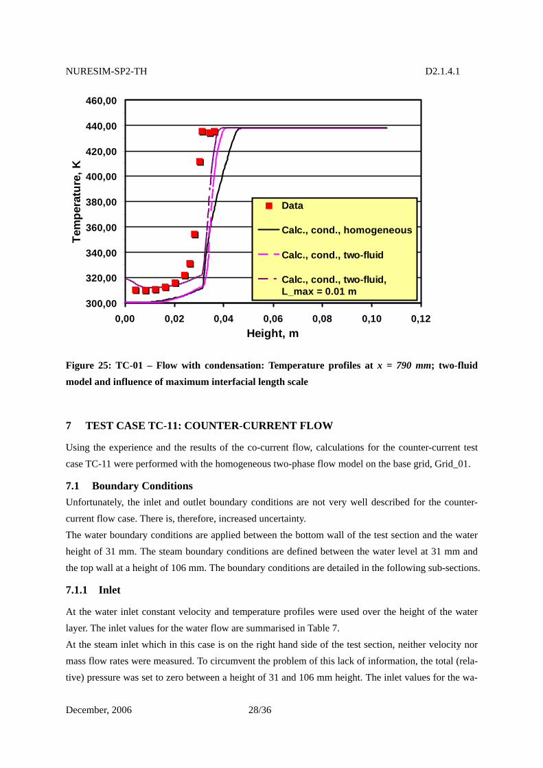
NURESIM-SP2-TH D2.1.4.1
December, 2006 28/36
Figure 25: TC-01 – Flow with condensation: Temperature profiles at x = 790 mm; two-fluid model and influence of maximum interfacial length scale
7 TEST CASE TC-11: COUNTER-CURRENT FLOW
Using the experience and the results of the co-current flow, calculations for the counter-current test case TC-11 were performed with the homogeneous two-phase flow model on the base grid, Grid_01.
7.1 Boundary Conditions Unfortunately, the inlet and outlet boundary conditions are not very well described for the counter-current flow case. There is, therefore, increased uncertainty. The water boundary conditions are applied between the bottom wall of the test section and the water height of 31 mm. The steam boundary conditions are defined between the water level at 31 mm and the top wall at a height of 106 mm. The boundary conditions are detailed in the following sub-sections.
7.1.1 Inlet
At the water inlet constant velocity and temperature profiles were used over the height of the water layer. The inlet values for the water flow are summarised in Table 7. At the steam inlet which in this case is on the right hand side of the test section, neither velocity nor mass flow rates were measured. To circumvent the problem of this lack of information, the total (rela-tive) pressure was set to zero between a height of 31 and 106 mm height. The inlet values for the wa-
300,00
320,00
340,00
360,00
380,00
400,00
420,00
440,00
460,00
0,00 0,02 0,04 0,06 0,08 0,10 0,12Height, m
Tem
pera
ture
, K
Data
Calc., cond., homogeneous
Calc., cond., two-fluid
Calc., cond., two-fluid,L_max = 0.01 m
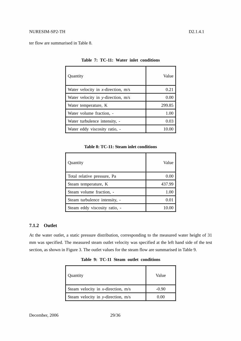
NURESIM-SP2-TH D2.1.4.1
December, 2006 29/36
ter flow are summarised in Table 8.
Table 7: TC-11: Water inlet conditions
Quantity Value
Water velocity in x-direction, m/s 0.21
Water velocity in y-direction, m/s 0.00
Water temperature, K 299.85
Water volume fraction, - 1.00
Water turbulence intensity, - 0.03
Water eddy viscosity ratio, - 10.00
Table 8: TC-11: Steam inlet conditions
Quantity Value
Total relative pressure, Pa 0.00
Steam temperature, K 437.99
Steam volume fraction, - 1.00
Steam turbulence intensity, - 0.01
Steam eddy viscosity ratio, - 10.00
7.1.2 Outlet
At the water outlet, a static pressure distribution, corresponding to the measured water height of 31 mm was specified. The measured steam outlet velocity was specified at the left hand side of the test section, as shown in Figure 3. The outlet values for the steam flow are summarised in Table 9.
Table 9: TC-11 Steam outlet conditions
Quantity Value
Steam velocity in x-direction, m/s -0.90
Steam velocity in y-direction, m/s 0.00
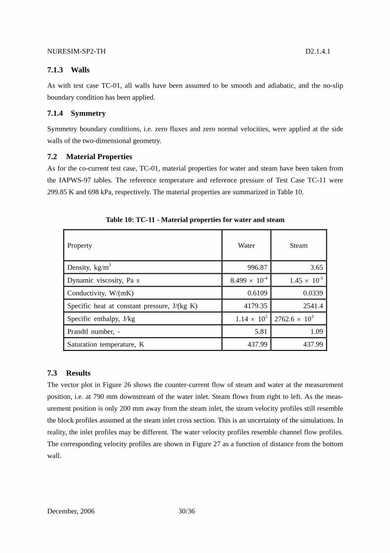
NURESIM-SP2-TH D2.1.4.1
December, 2006 30/36
7.1.3 Walls
As with test case TC-01, all walls have been assumed to be smooth and adiabatic, and the no-slip boundary condition has been applied.
7.1.4 Symmetry
Symmetry boundary conditions, i.e. zero fluxes and zero normal velocities, were applied at the side walls of the two-dimensional geometry.
7.2 Material Properties As for the co-current test case, TC-01, material properties for water and steam have been taken from the IAPWS-97 tables. The reference temperature and reference pressure of Test Case TC-11 were 299.85 K and 698 kPa, respectively. The material properties are summarized in Table 10.
Table 10: TC-11 - Material properties for water and steam
Property Water Steam
Density, kg/m3 996.87 3.65
Dynamic viscosity, Pa s 8.499 × 10⁻⁴ 1.45 × 10⁻⁵
Conductivity, W/(mK) 0.6109 0.0339
Specific heat at constant pressure, J/(kg K) 4179.35 2541.4
Specific enthalpy, J/kg 1.14 × 10⁵ 2762.6 × 103
Prandtl number, - 5.81 1.09
Saturation temperature, K 437.99 437.99
7.3 Results The vector plot in Figure 26 shows the counter-current flow of steam and water at the measurement position, i.e. at 790 mm downstream of the water inlet. Steam flows from right to left. As the meas-urement position is only 200 mm away from the steam inlet, the steam velocity profiles still resemble the block profiles assumed at the steam inlet cross section. This is an uncertainty of the simulations. In reality, the inlet profiles may be different. The water velocity profiles resemble channel flow profiles. The corresponding velocity profiles are shown in Figure 27 as a function of distance from the bottom wall.
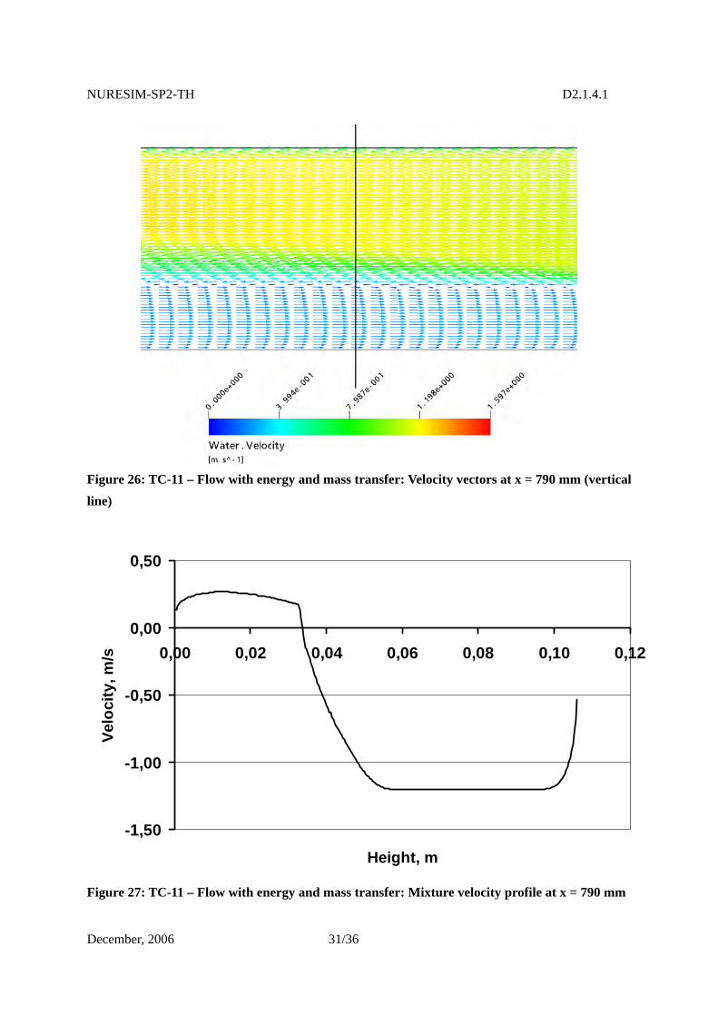
NURESIM-SP2-TH D2.1.4.1
December, 2006 31/36
Figure 26: TC-11 – Flow with energy and mass transfer: Velocity vectors at x = 790 mm (vertical line)
-1,50
-1,00
-0,50
0,00
0,50
0,00 0,02 0,04 0,06 0,08 0,10 0,12
Height, m
Velo
city
, m/s
Figure 27: TC-11 – Flow with energy and mass transfer: Mixture velocity profile at x = 790 mm
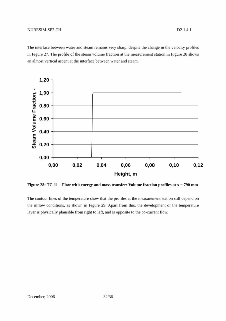
NURESIM-SP2-TH D2.1.4.1
December, 2006 32/36
The interface between water and steam remains very sharp, despite the change in the velocity profiles in Figure 27. The profile of the steam volume fraction at the measurement station in Figure 28 shows an almost vertical ascent at the interface between water and steam.
0,00
0,20
0,40
0,60
0,80
1,00
1,20
0,00 0,02 0,04 0,06 0,08 0,10 0,12
Height, m
Stea
m V
olum
e Fr
actio
n, -
Figure 28: TC-11 – Flow with energy and mass transfer: Volume fraction profiles at x = 790 mm The contour lines of the temperature show that the profiles at the measurement station still depend on the inflow conditions, as shown in Figure 29. Apart from this, the development of the temperature layer is physically plausible from right to left, and is opposite to the co-current flow.
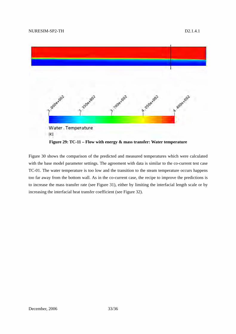
NURESIM-SP2-TH D2.1.4.1
December, 2006 33/36
Figure 29: TC-11 – Flow with energy & mass transfer: Water temperature
Figure 30 shows the comparison of the predicted and measured temperatures which were calculated with the base model parameter settings. The agreement with data is similar to the co-current test case TC-01. The water temperature is too low and the transition to the steam temperature occurs happens too far away from the bottom wall. As in the co-current case, the recipe to improve the predictions is to increase the mass transfer rate (see Figure 31), either by limiting the interfacial length scale or by increasing the interfacial heat transfer coefficient (see Figure 32).
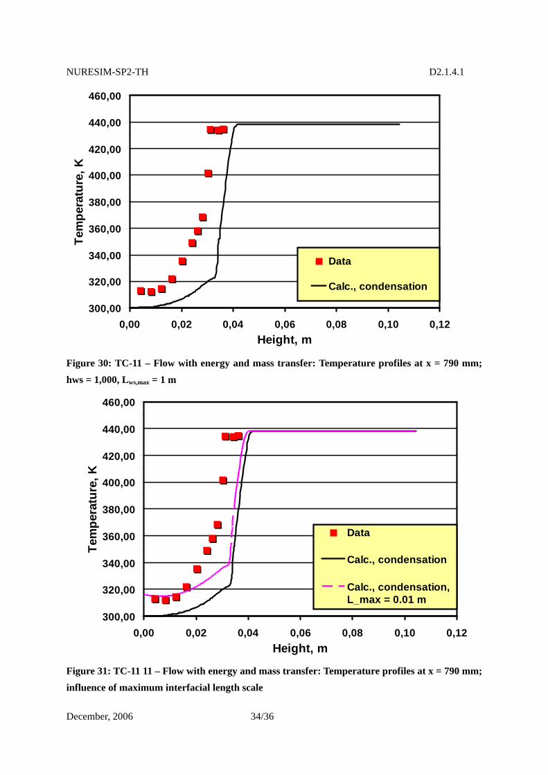
NURESIM-SP2-TH D2.1.4.1
December, 2006 34/36
300,00
320,00
340,00
360,00
380,00
400,00
420,00
440,00
460,00
0,00 0,02 0,04 0,06 0,08 0,10 0,12Height, m
Tem
pera
ture
, K
Data
Calc., condensation
Figure 30: TC-11 – Flow with energy and mass transfer: Temperature profiles at x = 790 mm; hws = 1,000, Lws,max = 1 m
Figure 31: TC-11 11 – Flow with energy and mass transfer: Temperature profiles at x = 790 mm; influence of maximum interfacial length scale
300,00
320,00
340,00
360,00
380,00
400,00
420,00
440,00
460,00
0,00 0,02 0,04 0,06 0,08 0,10 0,12Height, m
Tem
pera
ture
, K
Data
Calc., condensation
Calc., condensation,L_max = 0.01 m
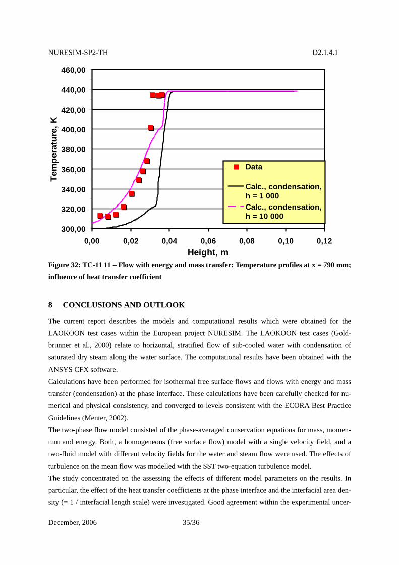
NURESIM-SP2-TH D2.1.4.1
December, 2006 35/36
300,00
320,00
340,00
360,00
380,00
400,00
420,00
440,00
460,00
0,00 0,02 0,04 0,06 0,08 0,10 0,12Height, m
Tem
pera
ture
, K
Data
Calc., condensation,h = 1 000Calc., condensation,h = 10 000
Figure 32: TC-11 11 – Flow with energy and mass transfer: Temperature profiles at x = 790 mm; influence of heat transfer coefficient
8 CONCLUSIONS AND OUTLOOK
The current report describes the models and computational results which were obtained for the LAOKOON test cases within the European project NURESIM. The LAOKOON test cases (Gold-brunner et al., 2000) relate to horizontal, stratified flow of sub-cooled water with condensation of saturated dry steam along the water surface. The computational results have been obtained with the ANSYS CFX software. Calculations have been performed for isothermal free surface flows and flows with energy and mass transfer (condensation) at the phase interface. These calculations have been carefully checked for nu-merical and physical consistency, and converged to levels consistent with the ECORA Best Practice Guidelines (Menter, 2002). The two-phase flow model consisted of the phase-averaged conservation equations for mass, momen-tum and energy. Both, a homogeneous (free surface flow) model with a single velocity field, and a two-fluid model with different velocity fields for the water and steam flow were used. The effects of turbulence on the mean flow was modelled with the SST two-equation turbulence model. The study concentrated on the assessing the effects of different model parameters on the results. In particular, the effect of the heat transfer coefficients at the phase interface and the interfacial area den-sity (= 1 / interfacial length scale) were investigated. Good agreement within the experimental uncer-
NURESIM-SP2-TH D2.1.4.1
December, 2006 36/36
tainty was achieved by tuning the coefficients in the condensation model, thus demonstrating the basic validity of the model approach. A disadvantage is that the documentation of the LAOKOON docu-ments is not very detailed concerning inlet and outlet boundary conditions. This casts uncertainties on the results and makes model adjustment difficult. It is, therefore, desirable to have additional and bet-ter documented data available for validating condensation models for industrial applications.
9 REFERENCES
Egorov. Y., 2004, “Validation of CFD Codes with PTS-Relevant Test Cases”, ECORA, Deliverable Report EVOL-ECORA-D07
Goldbrunner, M., Karl, J., Hein, D., 2000, “Experimental Investigation of Heat Transfer Phenomena during Direct Contact Condensation in the Presence of Non-Condensable Gas by Means of Lin-ear Raman Spectroscopy”, 10th International Symposium on Laser Techniques Applied to Fluid Mechanics, Lisbon
Ishii, M., Hibiki, T., 2006, Thermo-Fluid Dynamics of Two-Phase Flow, Springer Science+Business Media, New York
Lucas, D., 2005, "Review of the Existing Data Basis for the Validation of Models for PTS", NURE-SIM, Deliverable Report D2.1.2, www.nuresim.org/SP2/Documet/D2.1.2_final.pdf
Menter, F. R., 1994, “Two-Equation Eddy-Viscosity Turbulence Models for Engineering Applica-tions”, AIAA-Journal, Vol. 32, pp. 269 - 289
Menter, F. R., 2002, “CFD Best Practice Guidelines for CFD Code Validation for Reactor-Safety Ap-plications”, ECORA, Deliverable Report EVOL-ECORA-D01
May 08 -1-
EUROPEAN COMMISSION 6th EURATOM FRAMEWORK PROGRAMME 2005-2008 INTEGRATED PROJECT (IP): NURESIM Nuclear Reactor Simulations SUB-PROJECT 2: Thermal Hydraulics
DELIVERABLE D2.1.4.2: REPORT ABOUT BENCHMARKING WITH ANSYS CFX ON COMBINED-EFFECT EXPERIMENT
NUMERICAL SIMULATION OF THE UPTF TRAM C TEST CASE
Scheuerer, M. Gesellschaft für Anlagen- und Reaktorsicherheit GmbH
Forschungsinstitute 85748 Garching, GERMANY
Abstract
This progress report presents the models and computational results which were obtained for the large-scale UPTF TRAM C experiment, Run 21a2. In this experiment, water mixing during ECC-injection at mid-loop operation has been investigated. Calculations were performed with ANSYS CFX. The focus of the numerical simulations was the inves-tigation of the thermal mixing and the temperature distribution in the downcomer and at the adjacent walls. For this purpose a three-dimensional model of the UPTF geometry was constructed with the AN-SYS DesignModeler software. The geometry model included internal structures in the lower plenum and four KTA outlet pipes. A mixed-element numerical grid with 10 million cells was used for the CFD simulations. Because of its physical and geometrical complexity, the simulations of the unsteady-state, three-dimensional, two-phase flow took very long, when the full geometry was considered. Within the 5-months NURESIM sub-project time allocated to GRS, simulations were performed for a single-phase flow, including the effect of variable fluid properties and energy transfer at the walls.
Dissemination level:
RE: restricted to a group specified by the partners of the NURESIM project
May 08 -2-
TABLE OF CONTENTS 1 INTRODUCTION............................................................................................................................3 2 DESCRIPTION OF THE TEST CASE ...........................................................................................3 3 GEOMETRY AND GRID................................................................................................................4 4 BOUNDARY CONDITIONS ..........................................................................................................9 4.1 Inlet ..................................................................................................................................................9 4.1.1 Mass Flow Rate .............................................................................................................................................. 9 4.1.2 Temperature .................................................................................................................................................. 10 4.1.3 Turbulence Parameters.................................................................................................................................. 11 4.2 Outlet.............................................................................................................................................. 11 4.3 Walls............................................................................................................................................... 11 4.3.1 Walls in Contact with Fluid .......................................................................................................................... 11 4.3.2 Outer Walls ................................................................................................................................................... 11 4.4 Symmetry ....................................................................................................................................... 11 5 INITIAL CONDITIONS................................................................................................................ 11 6 MATERIAL PROPERTIES ........................................................................................................... 11 6.1 Fluid Properties .............................................................................................................................. 11 6.1.1 Water............................................................................................................................................................. 12 6.1.2 Nitrogen ........................................................................................................................................................ 12 7 NUMERICAL METHOD & CALCULATION SET-UP...............................................................12 7.1 Numerical Method .........................................................................................................................12 7.2 Calculation Set-Up .........................................................................................................................13 7.3 Hardware & Operating System ......................................................................................................13 8 COMPUTATIONAL RESULTS ....................................................................................................14 9 CONCLUSIONS AND OUTLOOK ..............................................................................................34 10 REFERENCES...............................................................................................................................34
May 08 -3-
1 INTRODUCTION
This report summarises the computational results which were obtained for the UPTF test cases within the European project NURESIM. The test case UPTF TRAM C1, RUN21a2, relates to fluid-fluid mix-ing and condensation phenomena in the cold legs, and in the downcomer, and features ECC-water injec-tion at mid-loop operation. The mixing and condensation phenomena determine the cooling and the temperature distribution in the cold leg and in the downcomer, and are therefore important boundary conditions for the thermal shock related fracture mechanical analysis of the reactor pressure vessel (Tenckhoff et al., 1996). The computational results have been obtained with the ANSYS CFX software. The current report is structured as follows: A short description of the test case and its target quantities is provided in Section 2. The UPTF test section geometry and the numerical grid used for the calculations are presented in Section 3. This is followed by a discussion of the boundary and initial conditions in Sections 4 and 5. Material properties are given in Section 6. Numerical and computational information is provided in Section 7. Finally, computational results are shown and compared to data in Section 8.
2 DESCRIPTION OF THE TEST CASE
A detailed description of the UPTF test facility and the tests conducted in the UPTF test facility is pre-sented in the NURESIM Deliverable D2.1.2 (Lucas, 2005). In the UPTF TRAM C1 experiments, steam-water flow in the intact cold legs and in the downcomer of a pressurized water reactor during the end of blow-down of a cold leg loss-of-coolant-accident is investigated. The coolant water of the pri-mary system flows rapidly through the break, and a significant fraction of the water flashes to steam. The pressure in the primary system decreases as the blow-down progresses. When the pressure has reached a threshold value, the accumulators begin to inject emergency core coolant water into the cold legs. This was the point in time when the measurements were started. In the experiments, the steam was replaced by nitrogen to prevent condensation effects. In the test case UPTF TRAM C1, Run21a2, the water level in the cold leg was just above the cold leg centreline, see Figure 1.
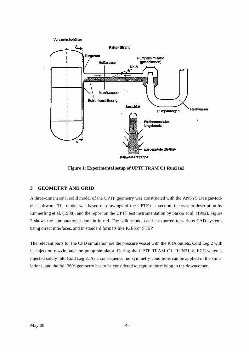
May 08 -4-
Figure 1: Experimental setup of UPTF TRAM C1 Run21a2
3 GEOMETRY AND GRID
A three-dimensional solid model of the UPTF geometry was constructed with the ANSYS DesignMod-eler software. The model was based on drawings of the UPTF test section, the system description by Emmerling et al. (1988), and the report on the UPTF test instrumentation by Sarkar et al. (1992). Figure 2 shows the computational domain in red. The solid model can be exported to various CAD systems using direct interfaces, and in standard formats like IGES or STEP. The relevant parts for the CFD simulation are the pressure vessel with the KTA outlets, Cold Leg 2 with its injection nozzle, and the pump simulator. During the UPTF TRAM C1, RUN21a2, ECC-water is injected solely into Cold Leg 2. As a consequence, no symmetry conditions can be applied in the simu-lations, and the full 360º-geometry has to be considered to capture the mixing in the downcomer.
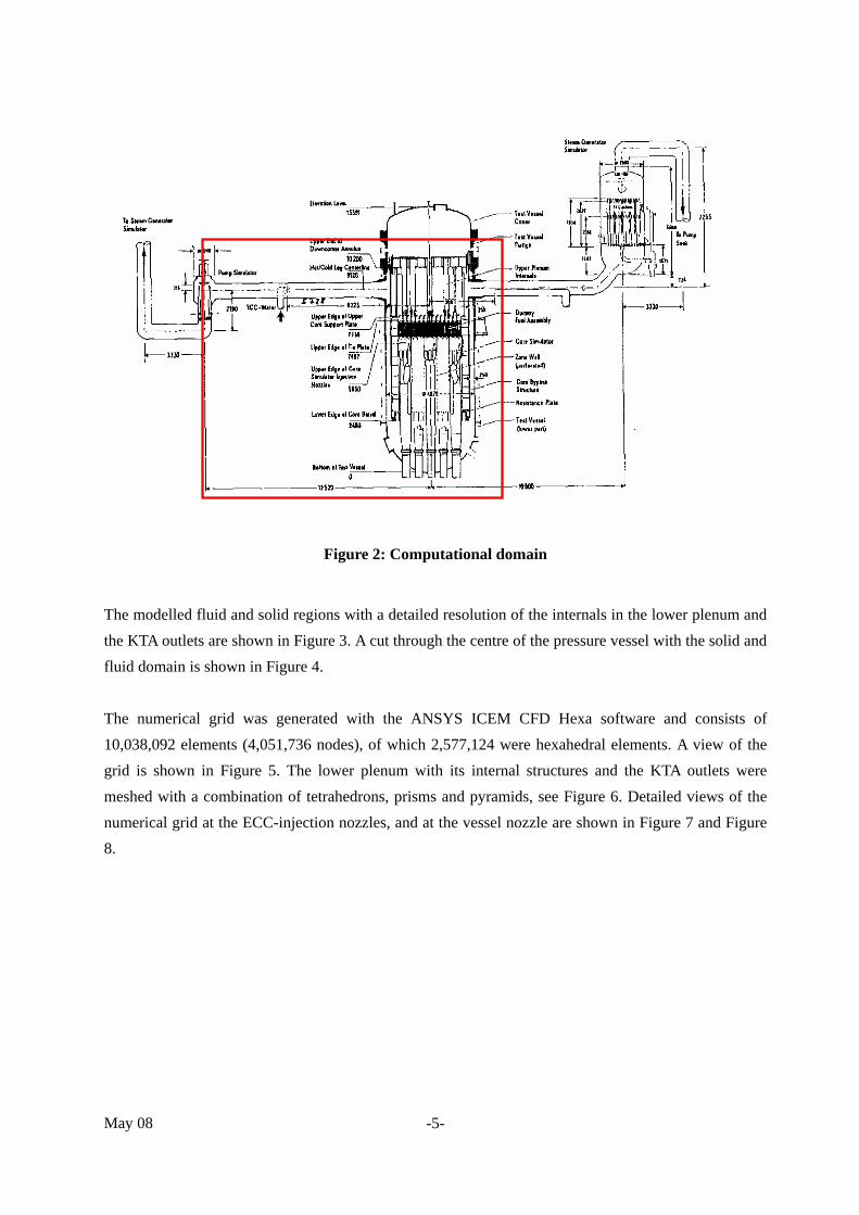
May 08 -5-
Figure 2: Computational domain
The modelled fluid and solid regions with a detailed resolution of the internals in the lower plenum and the KTA outlets are shown in Figure 3. A cut through the centre of the pressure vessel with the solid and fluid domain is shown in Figure 4. The numerical grid was generated with the ANSYS ICEM CFD Hexa software and consists of 10,038,092 elements (4,051,736 nodes), of which 2,577,124 were hexahedral elements. A view of the grid is shown in Figure 5. The lower plenum with its internal structures and the KTA outlets were meshed with a combination of tetrahedrons, prisms and pyramids, see Figure 6. Detailed views of the numerical grid at the ECC-injection nozzles, and at the vessel nozzle are shown in Figure 7 and Figure 8.
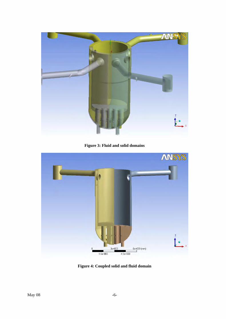
May 08 -6-
Figure 3: Fluid and solid domains
Figure 4: Coupled solid and fluid domain
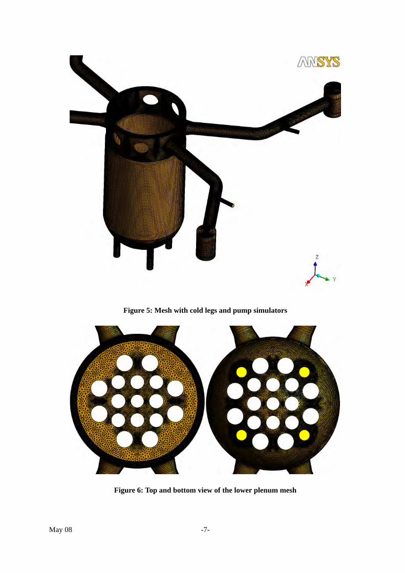
May 08 -7-
Figure 5: Mesh with cold legs and pump simulators
Figure 6: Top and bottom view of the lower plenum mesh
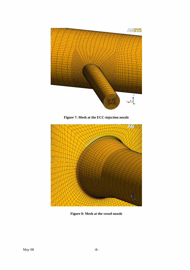
May 08 -8-
Figure 7: Mesh at the ECC-injection nozzle
Figure 8: Mesh at the vessel nozzle
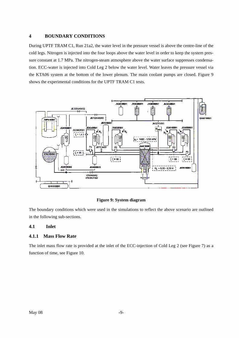
May 08 -9-
4 BOUNDARY CONDITIONS
During UPTF TRAM C1, Run 21a2, the water level in the pressure vessel is above the centre-line of the cold legs. Nitrogen is injected into the four loops above the water level in order to keep the system pres-sure constant at 1.7 MPa. The nitrogen-steam atmosphere above the water surface suppresses condensa-tion. ECC-water is injected into Cold Leg 2 below the water level. Water leaves the pressure vessel via the KTA06 system at the bottom of the lower plenum. The main coolant pumps are closed. Figure 9 shows the experimental conditions for the UPTF TRAM C1 tests.
Figure 9: System diagram
The boundary conditions which were used in the simulations to reflect the above scenario are outlined in the following sub-sections.
4.1 Inlet
4.1.1 Mass Flow Rate
The inlet mass flow rate is provided at the inlet of the ECC-injection of Cold Leg 2 (see Figure 7) as a function of time, see Figure 10.
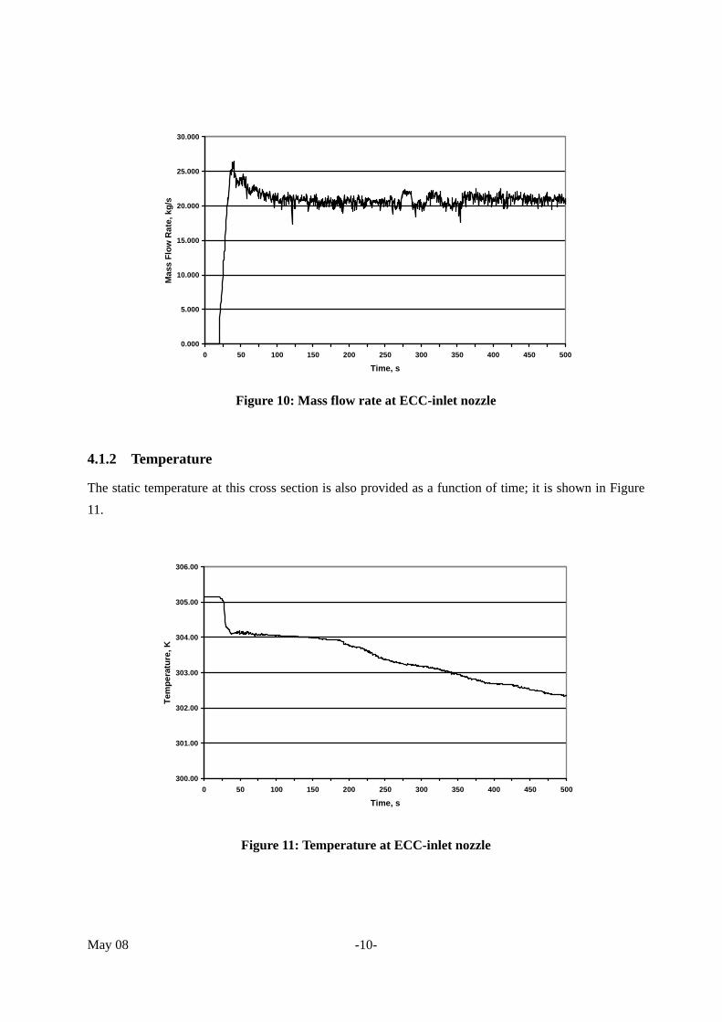
May 08 -10-
0.000
5.000
10.000
15.000
20.000
25.000
30.000
0 50 100 150 200 250 300 350 400 450 500
Time, s
Mas
s Fl
ow R
ate,
kg/
s
Figure 10: Mass flow rate at ECC-inlet nozzle
4.1.2 Temperature
The static temperature at this cross section is also provided as a function of time; it is shown in Figure 11.
300.00
301.00
302.00
303.00
304.00
305.00
306.00
0 50 100 150 200 250 300 350 400 450 500
Time, s
Tem
pera
ture
, K
Figure 11: Temperature at ECC-inlet nozzle
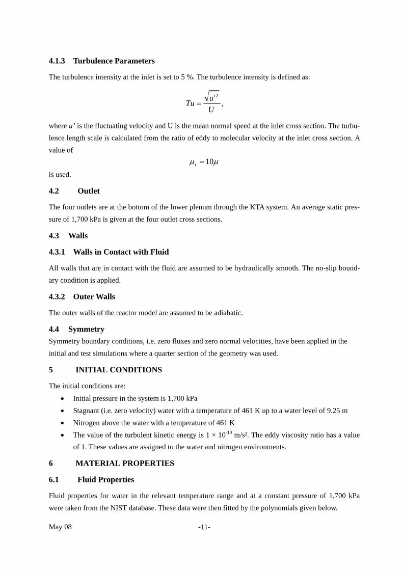
May 08 -11-
4.1.3 Turbulence Parameters
The turbulence intensity at the inlet is set to 5 %. The turbulence intensity is defined as:
UuTu
2'= ,
where u’ is the fluctuating velocity and U is the mean normal speed at the inlet cross section. The turbu-lence length scale is calculated from the ratio of eddy to molecular velocity at the inlet cross section. A value of
μμ 10=t
is used.
4.2 Outlet
The four outlets are at the bottom of the lower plenum through the KTA system. An average static pres-sure of 1,700 kPa is given at the four outlet cross sections.
4.3 Walls
4.3.1 Walls in Contact with Fluid
All walls that are in contact with the fluid are assumed to be hydraulically smooth. The no-slip bound-ary condition is applied.
4.3.2 Outer Walls
The outer walls of the reactor model are assumed to be adiabatic.
4.4 Symmetry Symmetry boundary conditions, i.e. zero fluxes and zero normal velocities, have been applied in the initial and test simulations where a quarter section of the geometry was used.
5 INITIAL CONDITIONS
The initial conditions are:
• Initial pressure in the system is 1,700 kPa • Stagnant (i.e. zero velocity) water with a temperature of 461 K up to a water level of 9.25 m • Nitrogen above the water with a temperature of 461 K • The value of the turbulent kinetic energy is 1 × 10⁻¹⁰ m/s². The eddy viscosity ratio has a value
of 1. These values are assigned to the water and nitrogen environments.
6 MATERIAL PROPERTIES
6.1 Fluid Properties
Fluid properties for water in the relevant temperature range and at a constant pressure of 1,700 kPa were taken from the NIST database. These data were then fitted by the polynomials given below.
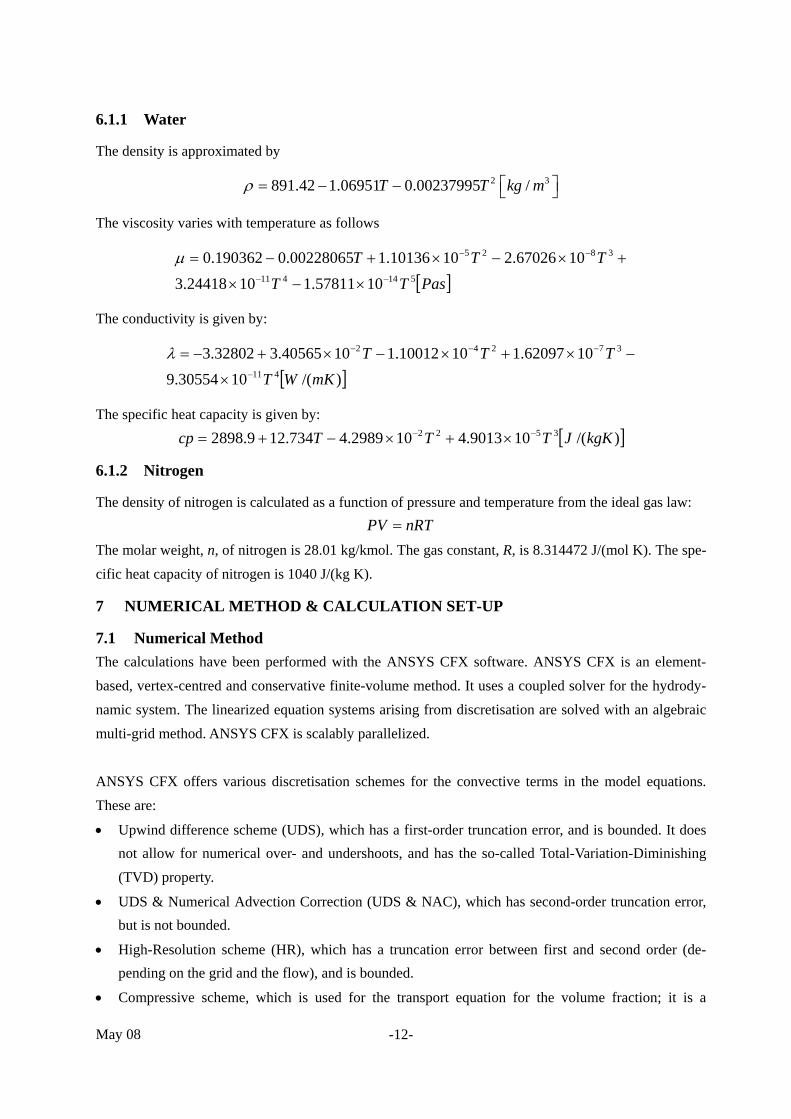
May 08 -12-
6.1.1 Water
The density is approximated by
2 3891.42 1.06951 0.00237995 /T T kg mρ ⎡ ⎤= − − ⎣ ⎦
The viscosity varies with temperature as follows
[ ]PasTTTTT
514411
3825
1057811.11024418.31067026.21010136.100228065.0190362.0
−−
−−
×−×
+×−×+−=μ
The conductivity is given by:
[ ])/(1030554.91062097.11010012.11040565.332802.3
411
37242
mKWTTTT
−
−−−
×
−×+×−×+−=λ
The specific heat capacity is given by: [ ])/(109013.4102989.4734.129.2898 3522 kgKJTTTcp −− ×+×−+=
6.1.2 Nitrogen
The density of nitrogen is calculated as a function of pressure and temperature from the ideal gas law: nRTPV =
The molar weight, n, of nitrogen is 28.01 kg/kmol. The gas constant, R, is 8.314472 J/(mol K). The spe-cific heat capacity of nitrogen is 1040 J/(kg K).
7 NUMERICAL METHOD & CALCULATION SET-UP
7.1 Numerical Method The calculations have been performed with the ANSYS CFX software. ANSYS CFX is an element-based, vertex-centred and conservative finite-volume method. It uses a coupled solver for the hydrody-namic system. The linearized equation systems arising from discretisation are solved with an algebraic multi-grid method. ANSYS CFX is scalably parallelized. ANSYS CFX offers various discretisation schemes for the convective terms in the model equations. These are:
• Upwind difference scheme (UDS), which has a first-order truncation error, and is bounded. It does not allow for numerical over- and undershoots, and has the so-called Total-Variation-Diminishing (TVD) property.
• UDS & Numerical Advection Correction (UDS & NAC), which has second-order truncation error, but is not bounded.
• High-Resolution scheme (HR), which has a truncation error between first and second order (de-pending on the grid and the flow), and is bounded.
• Compressive scheme, which is used for the transport equation for the volume fraction; it is a
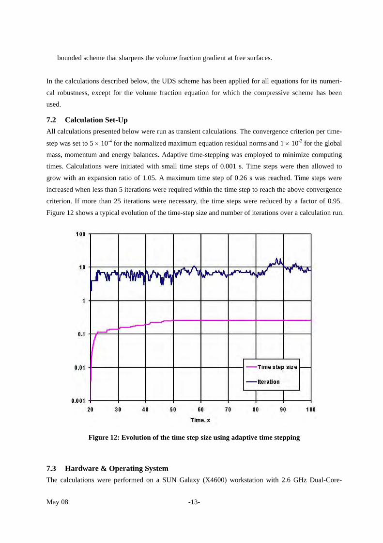
May 08 -13-
bounded scheme that sharpens the volume fraction gradient at free surfaces. In the calculations described below, the UDS scheme has been applied for all equations for its numeri-cal robustness, except for the volume fraction equation for which the compressive scheme has been used.
7.2 Calculation Set-Up All calculations presented below were run as transient calculations. The convergence criterion per time-
step was set to 5 × 10⁻⁴ for the normalized maximum equation residual norms and 1 × 10⁻² for the global mass, momentum and energy balances. Adaptive time-stepping was employed to minimize computing times. Calculations were initiated with small time steps of 0.001 s. Time steps were then allowed to grow with an expansion ratio of 1.05. A maximum time step of 0.26 s was reached. Time steps were increased when less than 5 iterations were required within the time step to reach the above convergence criterion. If more than 25 iterations were necessary, the time steps were reduced by a factor of 0.95. Figure 12 shows a typical evolution of the time-step size and number of iterations over a calculation run.
Figure 12: Evolution of the time step size using adaptive time stepping
7.3 Hardware & Operating System The calculations were performed on a SUN Galaxy (X4600) workstation with 2.6 GHz Dual-Core-
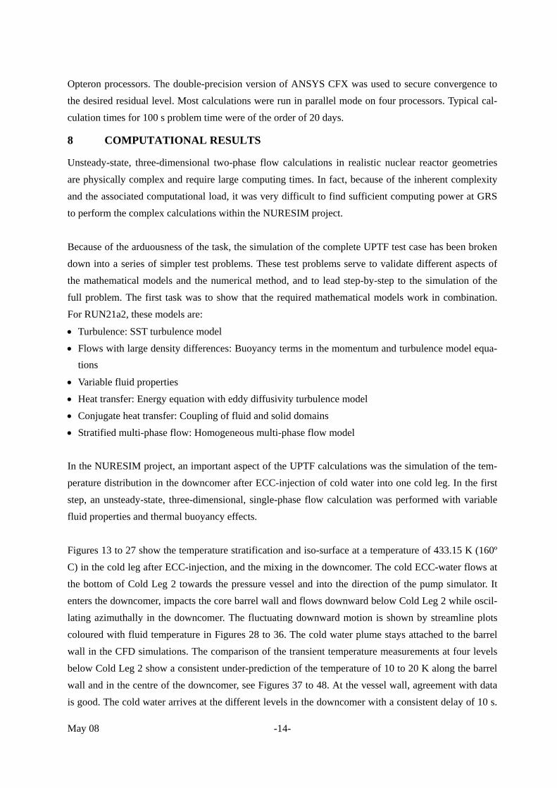
May 08 -14-
Opteron processors. The double-precision version of ANSYS CFX was used to secure convergence to the desired residual level. Most calculations were run in parallel mode on four processors. Typical cal-culation times for 100 s problem time were of the order of 20 days.
8 COMPUTATIONAL RESULTS
Unsteady-state, three-dimensional two-phase flow calculations in realistic nuclear reactor geometries are physically complex and require large computing times. In fact, because of the inherent complexity and the associated computational load, it was very difficult to find sufficient computing power at GRS to perform the complex calculations within the NURESIM project. Because of the arduousness of the task, the simulation of the complete UPTF test case has been broken down into a series of simpler test problems. These test problems serve to validate different aspects of the mathematical models and the numerical method, and to lead step-by-step to the simulation of the full problem. The first task was to show that the required mathematical models work in combination. For RUN21a2, these models are:
• Turbulence: SST turbulence model • Flows with large density differences: Buoyancy terms in the momentum and turbulence model equa-
tions
• Variable fluid properties • Heat transfer: Energy equation with eddy diffusivity turbulence model • Conjugate heat transfer: Coupling of fluid and solid domains • Stratified multi-phase flow: Homogeneous multi-phase flow model In the NURESIM project, an important aspect of the UPTF calculations was the simulation of the tem-perature distribution in the downcomer after ECC-injection of cold water into one cold leg. In the first step, an unsteady-state, three-dimensional, single-phase flow calculation was performed with variable fluid properties and thermal buoyancy effects. Figures 13 to 27 show the temperature stratification and iso-surface at a temperature of 433.15 K (160º C) in the cold leg after ECC-injection, and the mixing in the downcomer. The cold ECC-water flows at the bottom of Cold Leg 2 towards the pressure vessel and into the direction of the pump simulator. It enters the downcomer, impacts the core barrel wall and flows downward below Cold Leg 2 while oscil-lating azimuthally in the downcomer. The fluctuating downward motion is shown by streamline plots coloured with fluid temperature in Figures 28 to 36. The cold water plume stays attached to the barrel wall in the CFD simulations. The comparison of the transient temperature measurements at four levels below Cold Leg 2 show a consistent under-prediction of the temperature of 10 to 20 K along the barrel wall and in the centre of the downcomer, see Figures 37 to 48. At the vessel wall, agreement with data is good. The cold water arrives at the different levels in the downcomer with a consistent delay of 10 s.
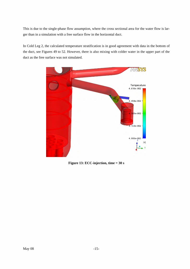
May 08 -15-
This is due to the single-phase flow assumption, where the cross sectional area for the water flow is lar-ger than in a simulation with a free surface flow in the horizontal duct. In Cold Leg 2, the calculated temperature stratification is in good agreement with data in the bottom of the duct, see Figures 49 to 52. However, there is also mixing with colder water in the upper part of the duct as the free surface was not simulated.
Figure 13: ECC-injection, time = 30 s

May 08 -16-
Figure 14: ECC-injection, time = 35 s
Figure 15: ECC-injection, time = 40 s
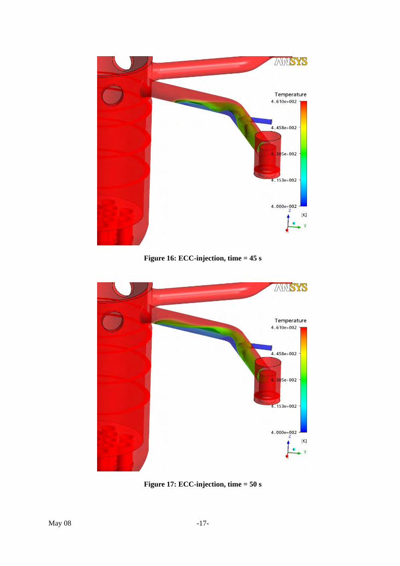
May 08 -17-
Figure 16: ECC-injection, time = 45 s
Figure 17: ECC-injection, time = 50 s
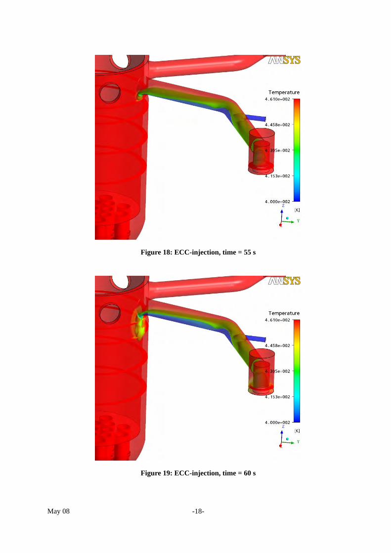
May 08 -18-
Figure 18: ECC-injection, time = 55 s
Figure 19: ECC-injection, time = 60 s
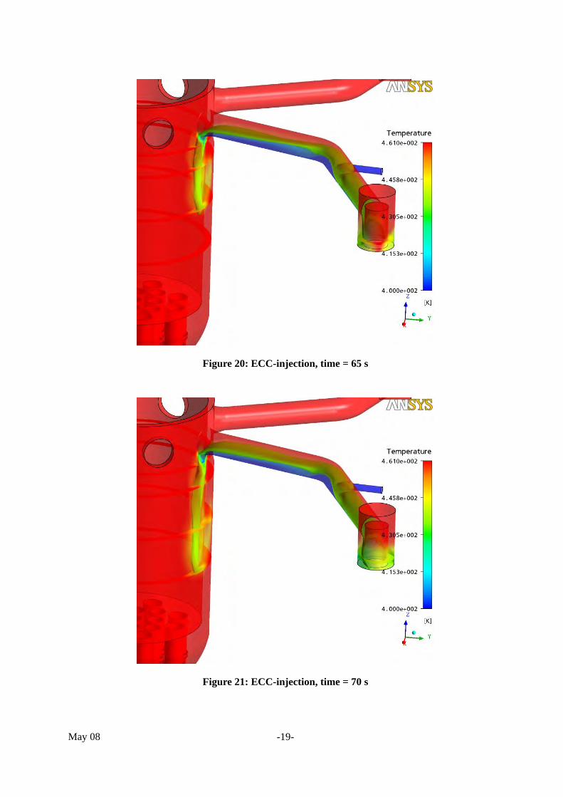
May 08 -19-
Figure 20: ECC-injection, time = 65 s
Figure 21: ECC-injection, time = 70 s
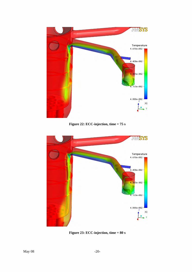
May 08 -20-
Figure 22: ECC-injection, time = 75 s
Figure 23: ECC-injection, time = 80 s
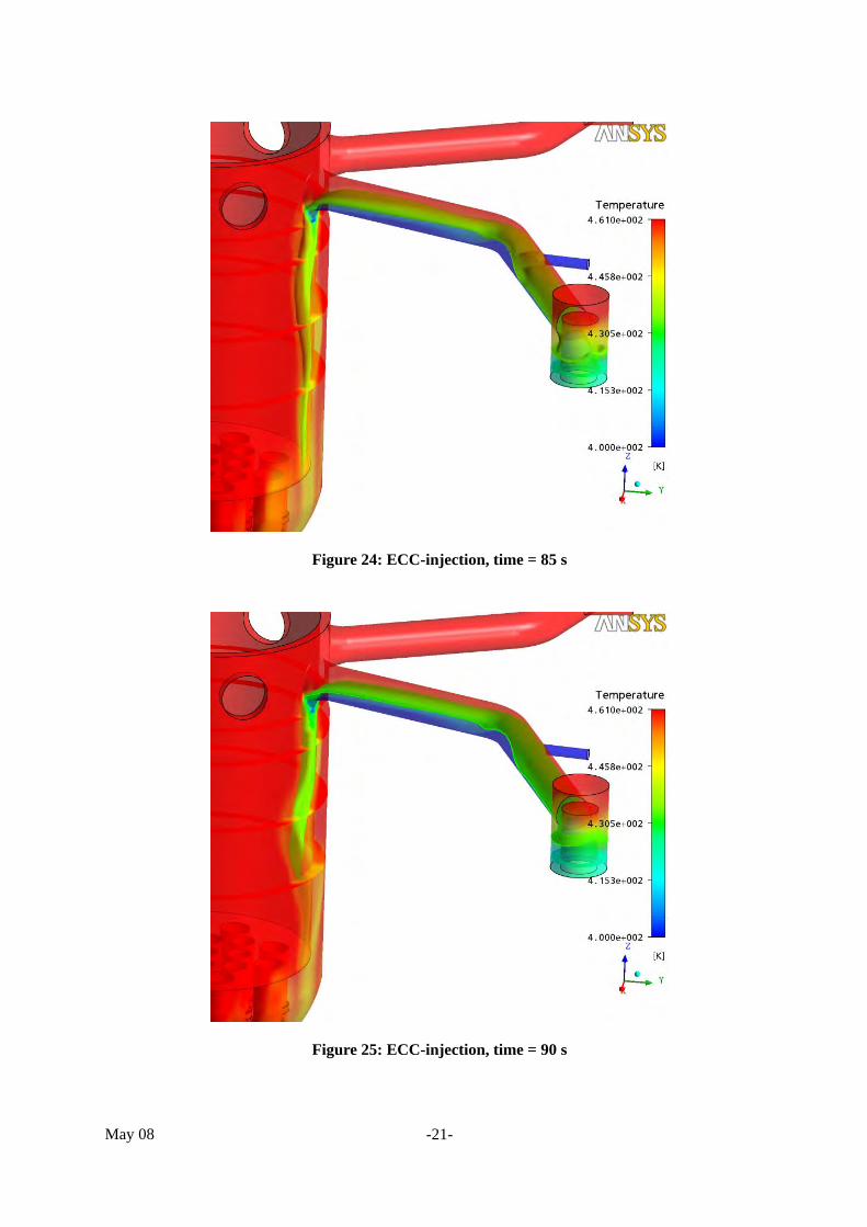
May 08 -21-
Figure 24: ECC-injection, time = 85 s
Figure 25: ECC-injection, time = 90 s
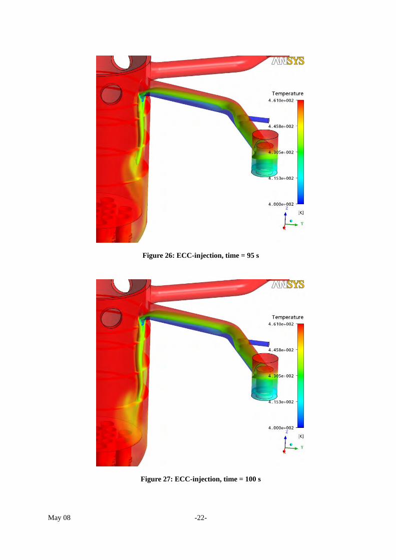
May 08 -22-
Figure 26: ECC-injection, time = 95 s
Figure 27: ECC-injection, time = 100 s
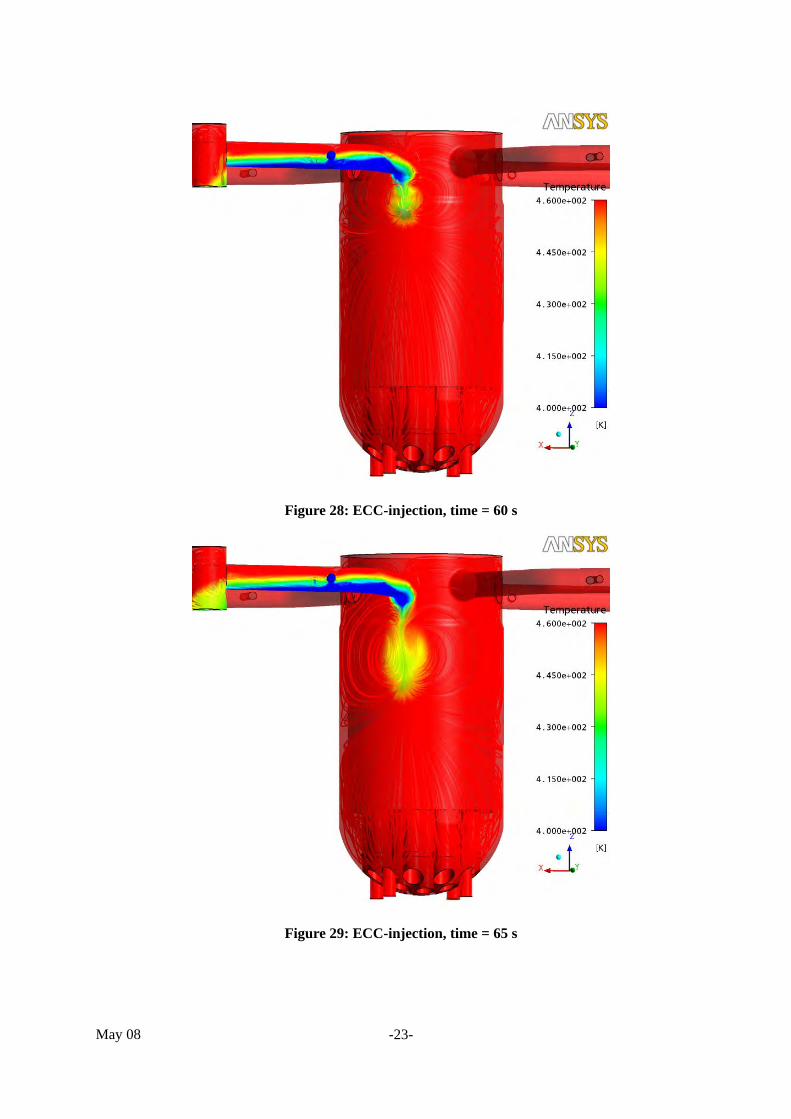
May 08 -23-
Figure 28: ECC-injection, time = 60 s
Figure 29: ECC-injection, time = 65 s
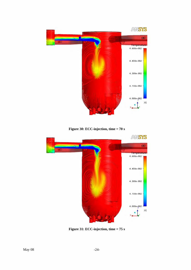
May 08 -24-
Figure 30: ECC-injection, time = 70 s
Figure 31: ECC-injection, time = 75 s
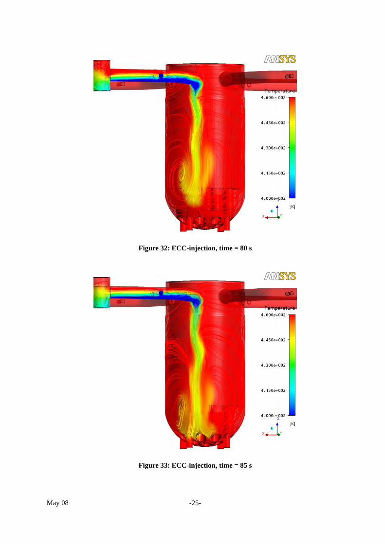
May 08 -25-
Figure 32: ECC-injection, time = 80 s
Figure 33: ECC-injection, time = 85 s
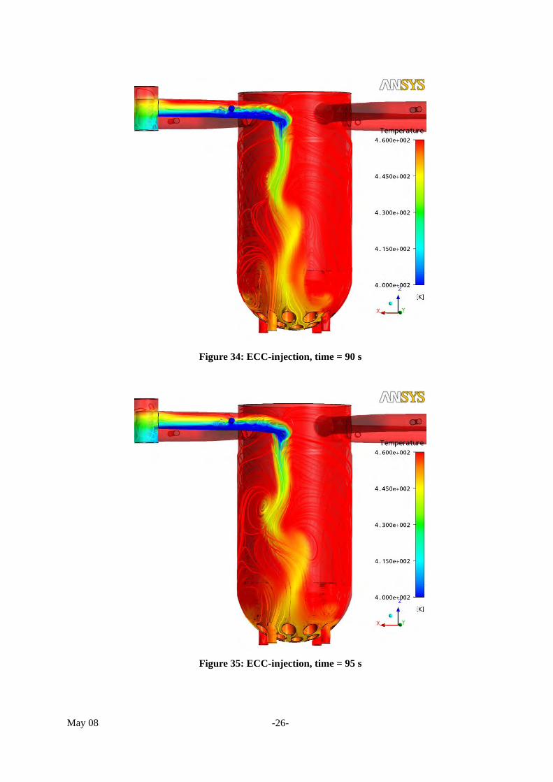
May 08 -26-
Figure 34: ECC-injection, time = 90 s
Figure 35: ECC-injection, time = 95 s
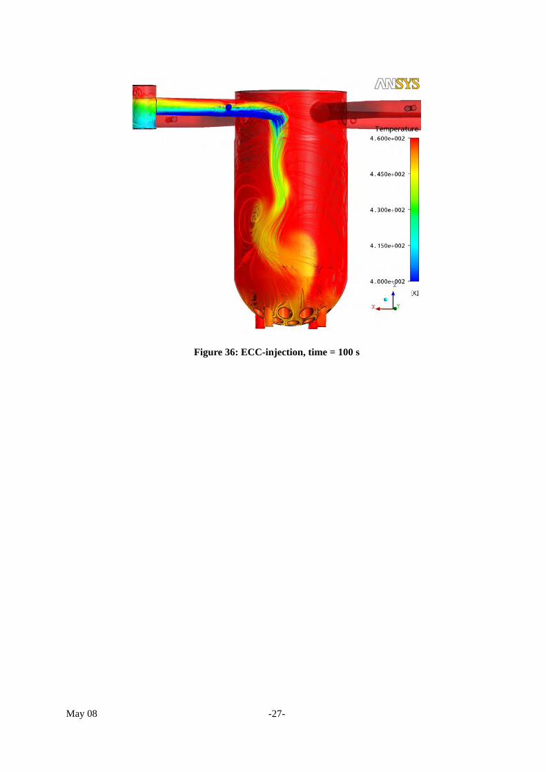
May 08 -27-
Figure 36: ECC-injection, time = 100 s
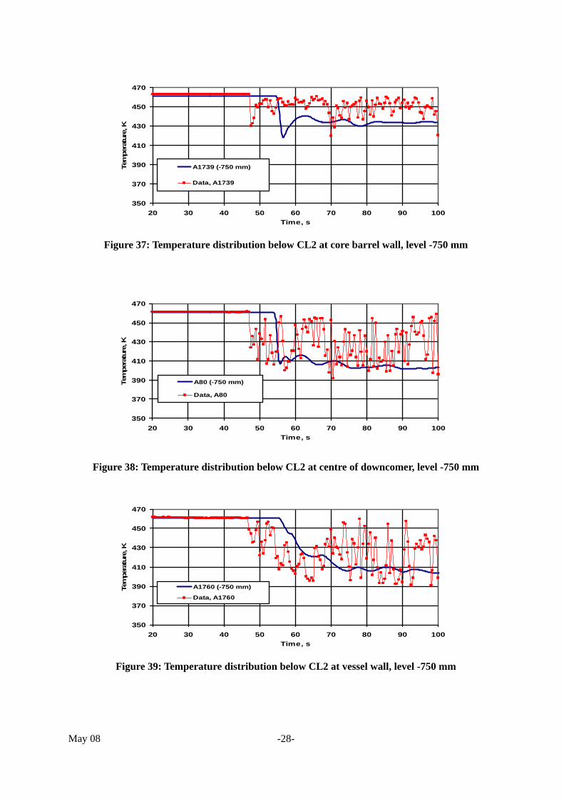
May 08 -28-
350
370
390
410
430
450
470
20 30 40 50 60 70 80 90 100Time, s
Tem
pera
ture
, K
A1739 (-750 mm)
Data, A1739
Figure 37: Temperature distribution below CL2 at core barrel wall, level -750 mm
350
370
390
410
430
450
470
20 30 40 50 60 70 80 90 100Time, s
Tem
pera
ture
, K
A80 (-750 mm)
Data, A80
Figure 38: Temperature distribution below CL2 at centre of downcomer, level -750 mm
350
370
390
410
430
450
470
20 30 40 50 60 70 80 90 100Time, s
Tem
pera
ture
, K
A1760 (-750 mm)
Data, A1760
Figure 39: Temperature distribution below CL2 at vessel wall, level -750 mm
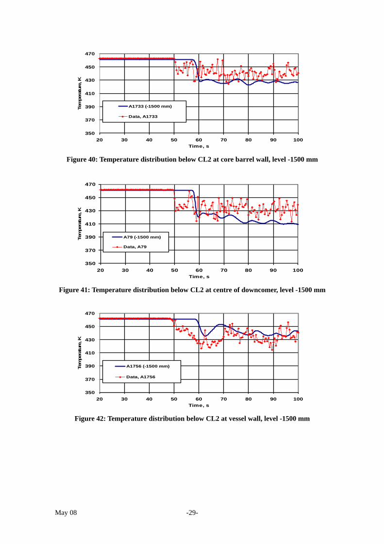
May 08 - - 29
350
370
390
410
430
450
470
20 30 40 50 60 70 80 90 100Time, s
Tem
pera
ture
, K
A1733 (-1500 mm)
Data, A1733
Figure 40: Temperature distribution below CL2 at core barrel wall, level -1500 mm
350
370
390
410
430
450
470
20 30 40 50 60 70 80 90 100Time, s
Tem
pera
ture
, K
A79 (-1500 mm)
Data, A79
Figure 41: Temperature distribution below CL2 at centre of downcomer, level -1500 mm
350
370
390
410
430
450
470
20 30 40 50 60 70 80 90 100Time, s
Tem
pera
ture
, K
A1756 (-1500 mm)
Data, A1756
Figure 42: Temperature distribution below CL2 at vessel wall, level -1500 mm
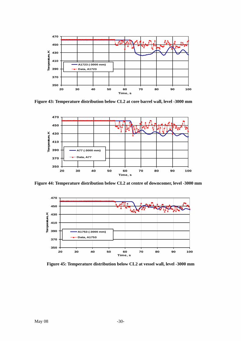
May 08 - - 30
350
370
390
410
430
450
470
20 30 40 50 60 70 80 90 100Time, s
Tem
pera
ture
, K
A1723 (-3000 mm)
Data, A1723
Figure 43: Temperature distribution below CL2 at core barrel wall, level -3000 mm
350
370
390
410
430
450
470
20 30 40 50 60 70 80 90 100Time, s
Tem
pera
ture
, K
A77 (-3000 mm)
Data, A77
Figure 44: Temperature distribution below CL2 at centre of downcomer, level -3000 mm
350
370
390
410
430
450
470
20 30 40 50 60 70 80 90 100Time, s
Tem
pera
ture
, K
A1753 (-3000 mm)
Data, A1753
Figure 45: Temperature distribution below CL2 at vessel wall, level -3000 mm
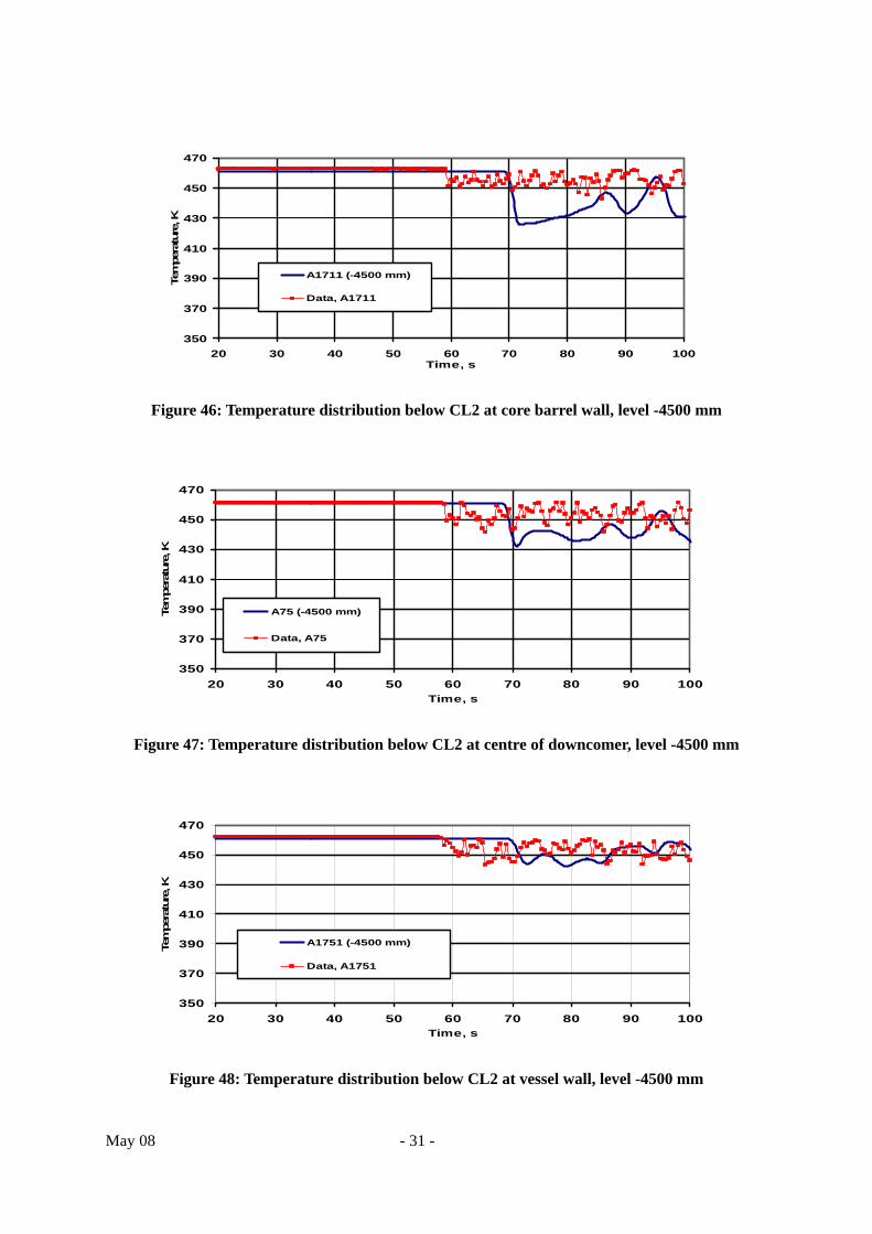
May 08 - 31 -
350
370
390
410
430
450
470
20 30 40 50 60 70 80 90 100Time, s
Tem
pera
ture
, K
A1711 (-4500 mm)
Data, A1711
Figure 46: Temperature distribution below CL2 at core barrel wall, level -4500 mm
350
370
390
410
430
450
470
20 30 40 50 60 70 80 90 100Time, s
Tem
pera
ture
, K
A75 (-4500 mm)
Data, A75
Figure 47: Temperature distribution below CL2 at centre of downcomer, level -4500 mm
350
370
390
410
430
450
470
20 30 40 50 60 70 80 90 100Time, s
Tem
pera
ture
, K
A1751 (-4500 mm)
Data, A1751
Figure 48: Temperature distribution below CL2 at vessel wall, level -4500 mm
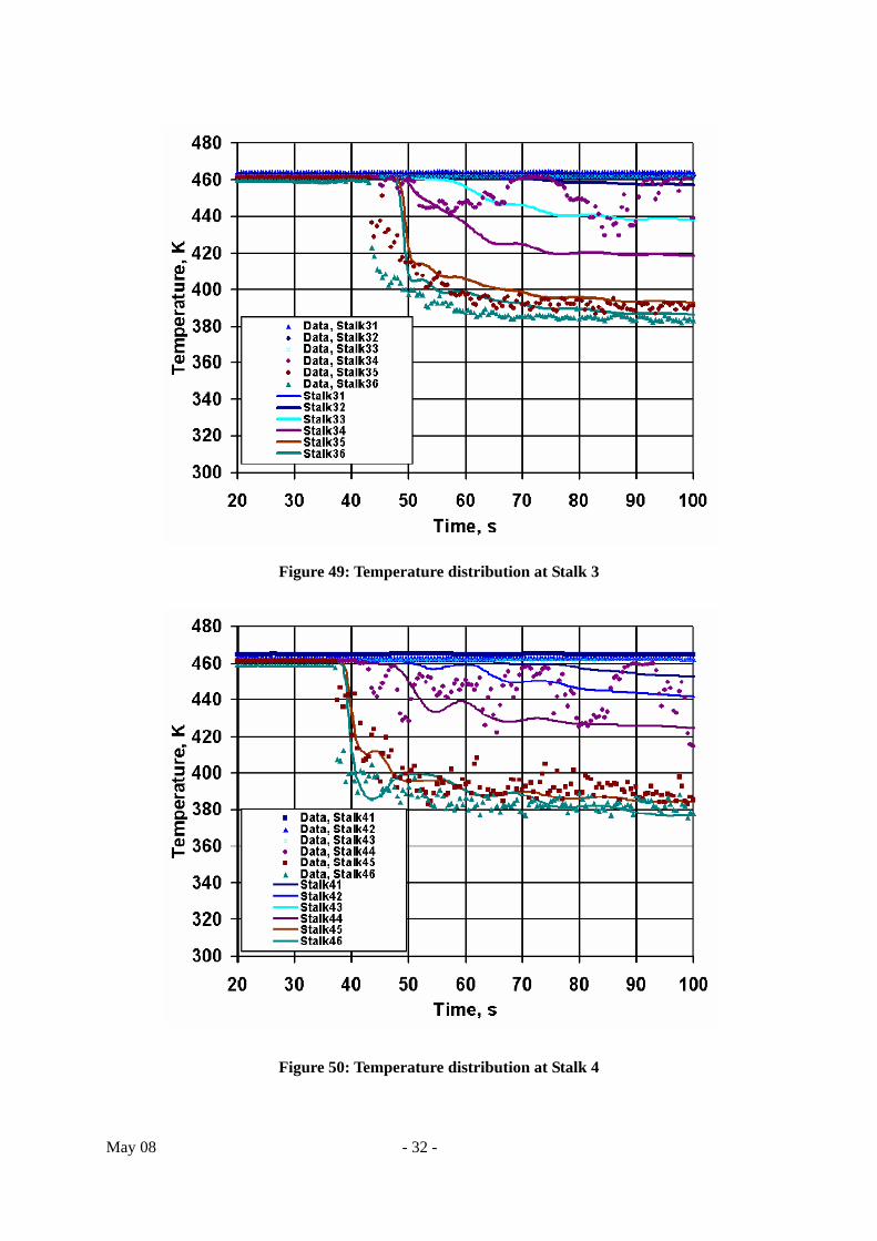
May 08 - 32 -
Figure 49: Temperature distribution at Stalk 3
Figure 50: Temperature distribution at Stalk 4
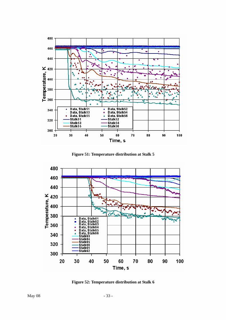
May 08 - 33 -
Figure 51: Temperature distribution at Stalk 5
Figure 52: Temperature distribution at Stalk 6
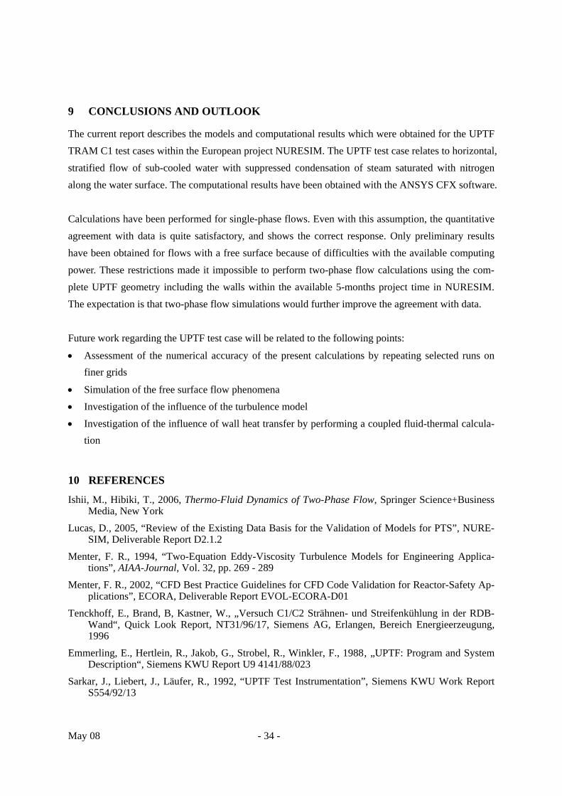
May 08 - 34 -
9 CONCLUSIONS AND OUTLOOK
The current report describes the models and computational results which were obtained for the UPTF TRAM C1 test cases within the European project NURESIM. The UPTF test case relates to horizontal, stratified flow of sub-cooled water with suppressed condensation of steam saturated with nitrogen along the water surface. The computational results have been obtained with the ANSYS CFX software. Calculations have been performed for single-phase flows. Even with this assumption, the quantitative agreement with data is quite satisfactory, and shows the correct response. Only preliminary results have been obtained for flows with a free surface because of difficulties with the available computing power. These restrictions made it impossible to perform two-phase flow calculations using the com-plete UPTF geometry including the walls within the available 5-months project time in NURESIM. The expectation is that two-phase flow simulations would further improve the agreement with data. Future work regarding the UPTF test case will be related to the following points:
• Assessment of the numerical accuracy of the present calculations by repeating selected runs on finer grids
• Simulation of the free surface flow phenomena • Investigation of the influence of the turbulence model • Investigation of the influence of wall heat transfer by performing a coupled fluid-thermal calcula-
tion
10 REFERENCES
Ishii, M., Hibiki, T., 2006, Thermo-Fluid Dynamics of Two-Phase Flow, Springer Science+Business Media, New York
Lucas, D., 2005, “Review of the Existing Data Basis for the Validation of Models for PTS”, NURE-SIM, Deliverable Report D2.1.2
Menter, F. R., 1994, “Two-Equation Eddy-Viscosity Turbulence Models for Engineering Applica-tions”, AIAA-Journal, Vol. 32, pp. 269 - 289
Menter, F. R., 2002, “CFD Best Practice Guidelines for CFD Code Validation for Reactor-Safety Ap-plications”, ECORA, Deliverable Report EVOL-ECORA-D01
Tenckhoff, E., Brand, B, Kastner, W., „Versuch C1/C2 Strähnen- und Streifenkühlung in der RDB-Wand“, Quick Look Report, NT31/96/17, Siemens AG, Erlangen, Bereich Energieerzeugung, 1996
Emmerling, E., Hertlein, R., Jakob, G., Strobel, R., Winkler, F., 1988‚ „UPTF: Program and System Description“, Siemens KWU Report U9 4141/88/023
Sarkar, J., Liebert, J., Läufer, R., 1992, “UPTF Test Instrumentation”, Siemens KWU Work Report S554/92/13