Embed Size (px)
Citation preview
Vegetation ecology of a woodland-savanna mosaic in central Benin (West Africa): Ecosystem analysis with a focus on the impact of selective logging
Dissertation
zur
Erlangung des akademischen Grades
Doctor rerum naturalium (Dr. rer. nat.)
der Mathematischen-Naturwissenschaftlichen Fakultät
der Universität Rostock
vorgelegt von
Bettina Orthmann, geb. am 13.07.1972 in Paderborn
aus Rostock
Rostock, 01.04.2005

Gutachter:
Prof. Dr. Stefan Porembski
Prof. Dr. Martin Diekmann
Prof. Dr. Rüdiger Wittig
Tag der Verteidigung: 11.07.2005
Contents
Contents
Contents .......................................................................................................................................i
List of Figures............................................................................................................................iv
List of Tables .............................................................................................................................vi
1 Introduction.........................................................................................................................1
1.1 Ecosystem analysis .....................................................................................................3
1.1.1 Vegetation composition and classification .........................................................3
1.1.2 Vegetation structure............................................................................................4
1.1.3 Environmental parameters and vegetation..........................................................5
1.2 Impact of selective logging on the woodland-savanna mosaic ..................................6
2 Study site ............................................................................................................................8
2.1 Climate........................................................................................................................9
2.2 Geology, hydrology, and pedology ..........................................................................10
2.3 Vegetation.................................................................................................................12
2.4 Human impact on the woodland-savanna mosaic ....................................................13
2.4.1 Pastoralism and grazing regime........................................................................13
2.4.2 Fire....................................................................................................................14
2.4.3 Short history of logging activities in the Upper Ouémé Valley .......................15
3 Methods ............................................................................................................................16
3.1 Sampling design........................................................................................................16
3.1.1 Site selection of relevé plots .............................................................................16
3.1.2 Site selection of gap plots .................................................................................19
3.1.3 Plot design of relevé and gap plots ...................................................................19
3.2 Sampling of vegetation data in relevé and gap plots ................................................20
3.2.1 Identification of species ....................................................................................20
3.2.2 Sampling of tree layer data ...............................................................................21
3.2.3 Sampling of herb layer data..............................................................................22
3.2.4 Sampling of data on seedlings and saplings of woody species ........................23
3.3 Sampling of data on environmental parameters in relevé and gap plots ..................23
3.3.1 Soil....................................................................................................................23
i
Contents
3.3.2 Microclimate.....................................................................................................24
3.3.3 Fire....................................................................................................................25
3.3.4 Topographical position .....................................................................................25
3.4 Survey of logging history and intensity....................................................................25
3.5 Data analysis .............................................................................................................26
3.5.1 Tabular comparison of vegetation data.............................................................26
3.5.2 Statistical analysis.............................................................................................26
3.5.2.1 Univariate data analysis ................................................................................27
3.5.2.2 Multivariate data analysis .............................................................................28
4 Results ..............................................................................................................................32
4.1 Floristic characteristics of the relevé plots ...............................................................32
4.1.1 Tabular comparison ..........................................................................................32
4.1.1.1 Tree layer ......................................................................................................32
4.1.1.2 Herb layer .....................................................................................................34
4.1.2 Multivariate ordination .....................................................................................37
4.1.2.1 Tree layer ......................................................................................................38
4.1.2.2 Herb layer .....................................................................................................41
4.1.2.3 Tree and herb layer – Bas fonds relevé plots excluded ................................42
4.2 Structural characteristics of vegetation types ...........................................................45
4.2.1 Tree layer ..........................................................................................................45
4.2.2 Herb layer .........................................................................................................49
4.3 Environmental parameters of vegetation types.........................................................51
4.3.1 Microclimate.....................................................................................................51
4.3.2 Fire....................................................................................................................54
4.3.3 Topography and soil .........................................................................................55
4.3.4 Correlation between environmental parameters ...............................................59
4.4 Relation of species data and environmental parameters...........................................60
4.4.1 Significance of environmental parameters – model selection procedure .........61
4.4.2 Variance partitioning: vegetation types versus environmental parameters ......64
4.5 Logging history and intensity ...................................................................................66
4.6 Comparison between gaps and vegetation types ......................................................67
4.6.1 Environmental parameters ................................................................................67
4.6.2 Species data of the herb layer ...........................................................................69
4.6.3 Seedlings and saplings of woody species .........................................................70
ii
Contents
5 Discussion.........................................................................................................................75
5.1 Classification of vegetation types and floristic characteristics.................................75
5.2 Structural characteristics of vegetation types ...........................................................77
5.3 Environmental parameters and vegetation................................................................81
5.3.1 Vegetation types ...............................................................................................81
5.3.2 Vegetation composition ....................................................................................84
5.4 Impact of selective logging on the woodland-savanna mosaic ................................88
Summary...................................................................................................................................93
Zusammenfassung ....................................................................................................................95
References.................................................................................................................................97
Acknowledgements.................................................................................................................116
Appendix.................................................................................................................................117
iii
List of Figures
List of Figures
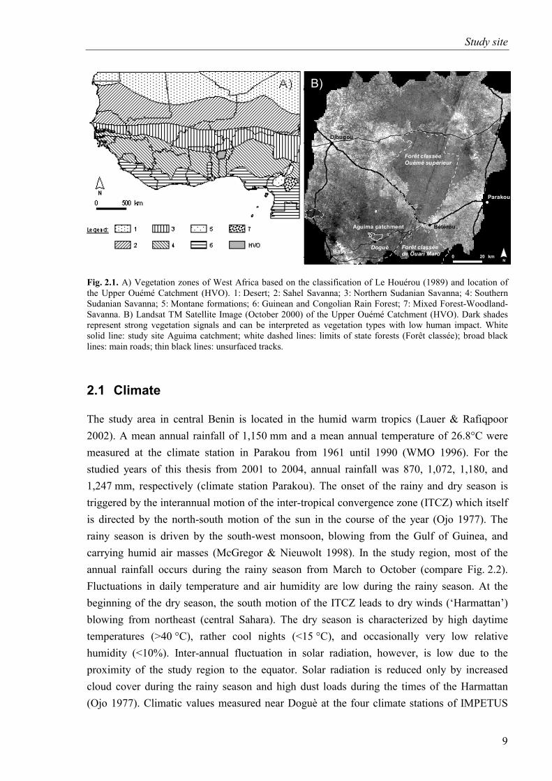
Fig. 2.1. Vegetation zones of West Africa and location of the Upper Ouémé Catchment........9
Fig. 2.2. Long-term average of rainfall and air temperature (Parakou)...................................10
Fig. 2.3. Idealized distribution of vegetation types along a toposequence ..............................12
Fig. 3.1. Location of study areas and of relevé and gap plots. ................................................17
Fig. 3.2. Design of relevé and gap plots and crown projection of trees ..................................20
Fig. 3.3. Explanation of boxplots.............................................................................................27
Fig. 3.4. Partitioning of the floristic variability in species data...............................................29
Fig. 4.1. DCA-diagram based on the cover of tree species (SB and SM included). Relevé plots are marked according to vegetation types...............................................................39
Fig. 4.2. DCA-diagram based on the cover of tree species (SB and SM included). Relevé plots are marked according to floristic blocks.................................................................40
Fig. 4.3. DCA-diagram based on species cover in the herb layer (SB and SM included). Relevé plots are marked according to vegetation types...................................................41
Fig. 4.4. DCA-diagram based on species cover in the herb layer (SB and SM included). Relevé plots are marked according to floristic blocks.....................................................42
Fig. 4.5. DCA-diagram based on the cover of tree species (SB and SM excluded) Relevé plots are marked according to vegetation types...............................................................43
Fig. 4.6. DCA-diagram based on species cover in the herb layer (SB and SM excluded). Relevé plots are marked according to vegetation types...................................................44
Fig. 4.7. Diameter class distribution of trees for vegetation types ..........................................46
Fig. 4.8. Height class distribution of trees for vegetation types ..............................................47
Fig. 4.9. Calculated and estimated tree cover for vegetation types .........................................48
Fig. 4.10. Woody biomass, biomass of litter, biomass of grasses, and biomass of herbs for vegetation types ...............................................................................................................49
Fig. 4.11. Visible sky for vegetation types ..............................................................................52
Fig. 4.12. 10-day-moving average for minimum air humidity, amplitude of air temperature, and maximum of vapour pressure deficit for vegetation types and precipitation measured at the meteorological station in Doguè.......................................53
Fig. 4.13. Linear regression of tree cover and visible sky.......................................................54
Fig. 4.14. Date of fire occurrence and fire temperature for vegetation types..........................55
Fig. 4.15. Relative topographic position and inclination for vegetation types ........................56
iv
List of Figures
Fig. 4.16. Soil depth and depth of the Ah-horizon for vegetation types..................................56
Fig. 4.17. Sand-silt-clay portion and skeleton in the two upper horizons for vegetation types.................................................................................................................................57
Fig. 4.18. Selected parameters of soil chemistry (pH, sum of basic cations, C/N-ratio, phosphate ) for the two upper horizons for vegetation types...........................................59
Fig. 4.19. Environmental parameters plotted in DCA-diagrams .............................................63
Fig. 4.20. Illustration of the results of variance partitioning for four species-data sets ..........65
Fig. 4.21. Four environmental parameters (visible sky; air humidity; grass biomass; sand fraction) for the gap plots and the relevé plots of vegetation types.................................68
Fig. 4.22. DCA-diagram based on species cover in the herb layer of the gap plots and the relevé plots of vegetation types (SB and SM excluded). Relevé plots are marked according to vegetation types ..........................................................................................69
Fig. 4.23. Species number and density of seedlings and saplings for all species and density for selected woody species (2001-2004).............................................................71
Fig. 4.24. Density of seedlings and saplings for selected woody species (2001-2004) ..........72
Fig. 4.25. Comparison between species composition of seedlings and saplings of woody species by means of PRC sampled in gap plots and relevé plots of vegetation types from 2001 to 2004 ...........................................................................................................74
A-Fig. 1. 10-day-moving average of microclimatic parameters............................................127
A-Fig. 2. Boxplots of the 10-day-mean microclimatic parameters (25.9. to 5.10.2001) for vegetation types .............................................................................................................128
A-Fig. 3. Boxplots of selected parameters of soil chemistry of the two upper horizons for vegetation types .............................................................................................................129
v
List of Tables
List of Tables
Table 3.1. Definition of vegetation types according to the classification approach of the Yangambi conference found in the Upper Aguima catchment. ......................................18
Table 3.2. Abbreviation and number of relevé plots for each vegetation type........................19
Table 4.1. Cover of tree species in the relevé plots. Relevé plots and species were sorted according to phytosociological criteria............................................................................33
Table 4.2. Summary of species groups found for species in the herb layer of the relevé plots..................................................................................................................................34
Table 4.3. Cover of species in the herb layer of the relevé plots. Relevé plots and species were sorted according to phytosociological criteria ........................................................36
Table 4.4. Summaries of DCA based on species cover of the tree and the herb layer of the relevé plots.......................................................................................................................37
Table 4.5. Correlation and regression analysis of structural parameters sampled in biomass and relevé plots, and correlation and regression analysis of structural parameters and biomass sampled in biomass plots (data from 2001 and 2002)..............51
Table 4.6. Explained floristic variability for two species data sets of the herb layer (with and without Bas fonds) ....................................................................................................61
Table 4.7. Explained floristic variability for two species data sets of the tree layer (with and without Bas fonds) ....................................................................................................62
Table 4.8. Density of logged tree individuals in 1999, 2001, and 2002 in a woodland dominated by Isoberlinia doka ........................................................................................66
Table 4.9. Number of species found in gap plots compared to number of species found in relevé plots of different vegetation types with regard to species groups extracted for the herb layer ...................................................................................................................68
A-Table 1. List of abbreviations............................................................................................118
A-Table 2. Cover of tree species larger 10 cm dbh in the relevé plots..................................119
A-Table 3. Cover of species in the herb layer of the relevé plots .........................................120
A-Table 4. Woody biomass, calculated cover of trees, and tree density for vegetation types according to diameter classes ...............................................................................123
A-Table 5. Woody biomass, calculated cover of trees, and tree density for vegetation types according to height classes ...................................................................................124
A-Table 6. Median and quartile of structural and grazing parameters sampled in 2001 and 2002 for vegetation types........................................................................................125
A-Table 7. Pearson’s correlation coefficients for cover of trees larger than 10 cm dbh and visible sky correlated with microclimatic parameters. ..................................................126
vi
List of Tables
A-Table 8. Cross table of rank-correlation of environmental parameters measured in relevé plots (SB and SM plots included) ........................................................................130
A-Table 9. Cross table of rank-correlation of environmental parameters measured in relevé plots (SB and SM plots excluded) .......................................................................131
A-Table 10. Variance partitioning for the tree-layer data-set (SB and SM plots included)...132
A-Table 11. Variance partitioning for the tree-layer data-set (SB and SM plots excluded) ..133
A-Table 12. Variance partitioning for the herb-layer data-set (SB and SM plots included)..134
A-Table 13. Variance partitioning for the herb-layer data-set (SB and SM plots excluded) .135
A-Table 14. Environmental parameters measured for gap-plots and comparison of gap plots with relevé plots....................................................................................................136
vii
Introduction
1 Introduction
Worldwide, mankind is facing the negative repercussions of global change (Walker et al. 1999, IPCC 2000, WBGU 2000). A main consequence of global change is an increasing shortage of natural resources, especially the resource freshwater, but also a threat to biodiversity (Cosgrove & Rijsberman 2000, Wolters et al. 2000, Lambin et al. 2003, Thomas et al. 2004). In the semiarid and subhumid zones of West Africa, abnormal drought occurred in the last decades affecting the socio-economy of the local population (IUCN 2004). Variations in the sea surface temperatures of the tropical Atlantic and changes of the land surface (e.g. vegetation cover) are generally considered to be a major cause of interannual to multidecadal rainfall variability across tropical West Africa (Nicholson 2000, Giannini et al. 2003, Paeth & Hense 2004). Therefore, it is important to understand how land use change influences precipitation patterns due to soil-vegetation-precipitation feedback mechanisms and conversely, how seasonal rainfall variations affect vegetation dynamics (IUCN 2004, Paeth & Hense 2004).
In the Guinean and Congolian Rain Forest zone of West Africa, land use change was strongly enhanced by timber logging and the conversion of former dense forests into plantations and arable land starting with the beginning of the last century (e.g. Chatelain et al. 1996a, Chatelain et al. 1996b, Fairhead & Leach 1998, FAO 2001, Poorter et al. 2004). In the Sudanian zone, land use change was strongly accelerated during the last 30 years due to an improvement of infrastructure and an increase in population. The latter is a result of an elevated population growth rate, but in particular a consequence of migration from northern regions. There the above mentioned climatic change in combination with the overuse of natural resources and the degradation of soils caused people to migrate (compare Williams 2003, Albert et al. 2004). The most drastic and directly obvious land use change is the conversion of forests, woodlands, and savannas to arable land and settlements (FAO 2001). The forest-savanna mosaic, however, can also be strongly influenced by an increase of less destructive land use forms, above all grazing and selective logging of valuable tree species (Bassett et al. 2003). Consequences of an increase of the latter two land use forms, however, occur more gradually within longer time spans.
For any modelling approach in the context of global change, data on land cover and land use, and in particular their change over time are highly demanded. In order to set up land cover and vegetation maps, knowledge on spatial distribution and characteristics of land cover and vegetation classes is needed. When land use maps are of interest, complex information on the relation between land cover and land use as well as on the properties of each class is additionally required (Innes & Koch 1998, de Bie 2000). However, compared to other regions
1
Introduction
in the world, such knowledge is relatively sparse for tropical regions in general and particularly for West Africa. Therefore, studies that address both general properties of ecosystems and effects of land use on ecosystems are urgently needed.
IMPETUS framework
Shortage of fresh water is expected to be a central problem of the 21th century that may even lead to social and political instability. Cosgrove & Rijsberman (2000) predict that in 2025 about half of the human population will live in countries with high water stress due to increased use of fresh water, also caused by population growth, and in particular due to the impact of global change on the hydrological cycle (UNESCO 2003). Fresh water supply could become problematic especially in West Africa, where droughts have been observed since the last three decades. In this context, the German Federal Ministry of Education and Research (BMBF) founded the research program GLOWA (Globaler Wandel des Wasserkreislaufes) to study the water cycle of different climatic zones and to develop integrative strategies for the sustainable use of fresh water. GLOWA comprises five projects, one of which is IMPETUS (Integratives Management Projekt für den effizienten und tragfähigen Umgang mit der Ressource Süßwasser) – an integrated approach to the efficient management of scarce water resources in West Africa. IMPETUS is a cooperative, interdisciplinary and integrative project located in Morocco (sub-tropical Northwest Africa) and Benin (tropical West Africa).
The aim of IMPETUS, with a project duration of eight years, is to offer concrete ways of translating scientific results into action through scientifically based strategies. In the first three-year phase, the project’s focus was set on the identification and analysis of factors influencing different aspects of the water budget. In this context, the present thesis on vegetation ecology, located in central Benin, is embedded in the IMPETUS sub-project A3-2 (Analysis and modelling of spatio-temporal vegetation dynamic in the Upper Ouémé Valley in dependence of climatic and anthropogenic factors) to provide an ecosystem analysis of dominant vegetation types with low human impact that play a central role within the hydrological cycle controlling fresh water availability. In the second three-year phase, methods will be developed to predict changes during the coming decades based on the results of the first phase. In the final two years, the collected insights of all disciplines will be coupled in order to assess management options and to install operative tools for decision-making process (IMPETUS 1999, 2002, 2003).
2
Introduction
Aims of the present thesis
The present thesis comprises two main topics. The first topic deals with the ecosystem analysis of the woodland-savanna mosaic of the Upper Aguima catchment in central Benin (Chapter 4.1 – 4.4 and 5.1 – 5.3). The ecosystem analysis is subdivided in three sub-topics that focus on the analyses of vegetation composition and their classification (Chapter 4.1 and 5.1), structural parameters (Chapter 4.2 and 5.2), and the relation of environment and vegetation (Chapter 4.3 – 4.4 and 5.3).
The second topic addresses the impact of selective logging on woodlands dominated by Isoberlinia doka (Chapter 4.5 – 4.6 and 5.4). Here, the logging history and intensity, the impact of gap creation on environmental parameters and floristic composition, and the recruitment of woody species in gaps are treated.
The aims of these topics are introduced separately in the following two sub-chapters (Chapter 1.1 and 1.2).
1.1 Ecosystem analysis
1.1.1 Vegetation composition and classification
In West Africa, most fundamental for the classification of vegetation was the accord of the Yangambi conference (CSA 1956) that has been extended by diverse notes of several authors (e.g. Keay 1956, Aubréville 1957, Trochain 1957, Monod 1963, Aubréville 1965). This approach is mainly based on physiognomic aspects of vegetation (compare Table 3.1). Additional criteria for particular categories are part of the Yangambi classification, e.g. ecological, physiological, dynamic, floristic, and physiographic ones (Menaut 1983). This has been criticized by Lawesson (1994) as inappropriate combination of criteria. However, for savannas and woodland, the Yangambi categories refer only to physiognomic criteria. The importance of the Yangambi classification is its applicability to wide regions of West Africa (Lawesson 1994) due to descriptive definitions without orders of magnitude for the considered parameters. Sanford & Isichei (1986) elaborated a classification for West African savannas based on physiognomic and structural characteristics giving detailed values for stem density and girth distribution of the tree layer. The applicability of the latter approach for larger regions, however, has not yet been tested.
Phytosociological approaches in West Africa are sparse (Hall & Jenik 1968, Hall & Swaine 1981, Hahn-Hadjal 1998). On local and regional scale, some studies used floristic data for classification (e.g. Emberger et al. 1950, Mangenot 1955, Adjanohoun 1964, Schmidt 1973, Jenik & Hall 1976, Sinsin 1993, Hahn 1996, Devineau et al. 1997, Sokpon et al. 2001,
3
Introduction
Sieglstetter 2002). Some approaches for phytosociological classification of particular vegetation classes in West Africa were undertaken, e.g. by Sinsin (1993) for savannas in northern Benin. Nevertheless, an overall integrative classification system as it exists for other regions, e.g. Europe (Willner 2002) and Japan (Miyawaki 1980), is missing for West Africa. Schmitz (1988) developed a floristic classification system for Rwanda, Burundi and Zaïre. West African studies often refer to this classification system, but its direct transferability is questionable and would be worthwhile to be tested and discussed by integrative studies.
In botanical as well as applied studies (e.g. pastoral or forestry), the Yangambi approach is one that is most frequently used for vegetation classification. This is not exclusively a result of its applicability to wide regions (Lawesson 1994), but its current importance has been extended by the widespread access to remote sensing techniques (e.g. CENATEL 2002, Mayaux et al. 2002). Remotely sensed data, especially from satellite images, are related to the photosynthetic active surface, being often expressed as NDVI (Normalized Difference Vegetation Index), and therefore to the density of vegetation cover and its physiognomic characteristics (Jensen 1996). Thus, the Yangambi categories appear to be reasonable to set up a classification scheme for analyses of remote sensing data. Unfortunately, this often led to an uncritical utilization of the physiognomic vegetation types. The classified physiognomic types are often intermingled with further information such as land use properties and floristic composition (e.g. CENATEL 2002). From a botanical point of view, it can not be expected that the physiognomic vegetation types can be translated directly into land use classes or to floristic composition (compare Mueller-Dombois & Ellenberg 1974, Dierschke 1994, Crawley 1997). Nevertheless, there is some evidence that for specific regions, physiognomic vegetation types can be related to floristic characteristics (Poilecot et al. 1991, César 1992, Reiff 1998).
The objective of this sub-topic is to describe floristic characteristics of the vegetation of the study area in central Benin in order to establish to which extent physiognomic but ecological meaningful classes can be related to phytosociological classes. In order to identify their limits and feasibility, two classification approaches are compared by means of tabular comparison and multivariate ordination. The first approach is based on the physiognomic categories of Yangambi (CSA 1956) in combination with a separation of zonal and azonal sites and a further subdivision of woodlands according to dominant tree species. In the second approach, vegetation data are classified according to phytosociological criteria.
1.1.2 Vegetation structure
Knowledge on structural characteristics of vegetation is highly demanded both globally and locally. On the global scale, more detailed and standardized data on biomass and vegetation structure of vegetation units are needed (Brown & Gaston 1996, FAO 2001) in order to parameterise global vegetation maps (e.g. Loveland et al. 1999), and in particular to be
4
Introduction
implemented into climatic and hydrological modelling approaches (IPCC 2000). For example, with regards to biogeochemical cycles, tree layers represent an important carbon stock and are one of the most important variables that influences the magnitude of the terrestrial carbon flux. Annual burning of the herb layer on the other hand, is of high relevance for the emission of reactive and greenhouse gases (Delmas et al. 1991, Cahoon et al. 1992, Isichei et al. 1995, Lacaux et al. 1995, Brown & Gaston 1996).
On the local scale, knowledge on structural characteristics of vegetation as well as standardized inventories of these properties are strongly required for the compilation of silvicultural and pastoral management plans (Brown & Gaston 1996, PAMF 1996, CENATEL 2002). In West Africa and in particular in the study region, local forest, pasture and fire management options are needed since both population density and land-use pressure on these recourses have dramatically increased in recent years (Sayer & Green 1992, Sodeik 1999, Doevenspeck 2004). In addition, structural vegetation data may help to understand ecosystem processes and the historical development of vegetation units.
With regard to the herb layer, many studies can be found in the literature from the Sahel to the Sudanian zone (compare Le Houérou 1989), and also in the studied region, several studies have been conducted (Sinsin 1993, Houinato 1996, Agonyissa & Sinsin 1998, Yayi 1998, Biaou 1999, Hunhyet 2000). However, as the economic value of the closed forest stands in the coastal region of West Africa is much higher than that of woodlands and savannas, little attention was given to the structure of the tree layer of woodlands and savannas (Brown & Gaston 1996). Thus, the aims of this sub-topic are firstly to give detailed structural descriptions of both the tree and the herb layer with respect to the stratified vegetation types, and secondly, to compare the vegetation types in terms of structural parameters.
1.1.3 Environmental parameters and vegetation
The savanna biome covers about 20% of the global land surface, and about half of the area of Africa (Huntley & Walker 1982, Scholes & Walker 1993, Scholes & Archer 1997). Savannas can be found over a broad range of climatic conditions with annual rainfall of less than 300 mm to more than 1,500 mm and are generally characterized by the coexistences of trees and grasses (Huntley & Walker 1982, Solbrig et al. 1996, Mistry 2000a). To explain the coexistence of trees and grasses in savanna systems, Walter (1971) focused in his hypothesis of the separation of rooting niches on the competition for soil moisture in different soil horizons. According to Walter (1971), trees have access to water in deeper soil horizons, whereas grasses are superior competitors for water in the upper horizons (see also Walker & Noy-Meir 1982). Detailed field studies led to the rejection of the Walter hypothesis as the singular explanation for tree-grass coexistence (e.g. studies in West Africa: Le Roux et al. 1995, Seghieri 1995, Mordelet et al. 1997, Le Roux & Bariac 1998). Beside soil moisture, several other environmental parameters have been discussed to be important for the
5
Introduction
maintenance of savannas such as nutrient availability, fire, grazing and browsing, geology and geomorphology, soil, cultivation history, and termites (e.g. Frost et al. 1986, Furley et al. 1992, Abbadie et al. 1996, Furley 1997, Scholes & Archer 1997, van Langevelde et al. 2003). However, the interaction of environmental parameters in savannas leading to the coexistence of grasses and trees is complex (see review in Scholes & Archer 1997, Sankaran et al. 2004) and may vary between different savanna types (Jeltsch et al. 2000). Recently, Jeltsch et al. (2000) proposed in a unifying concept of tree-grass coexistence to focus on ecological buffering mechanisms which prevent the savanna system from crossing the boundaries to other vegetation systems, i.e. pure grassland and closed forest.
In contrast to abundant studies and theories on the coexistence of trees and grasses in savannas, studies linking species composition to environmental parameters are sparse for West African savanna systems (e.g. Schmidt 1973, Sinsin 1993, Hahn 1996, Devineau 2001). Such knowledge, is however required in order to expand the understanding of ecosystem processes, to relate vegetation maps to ecological properties, and as a basis for modelling approaches.
Therefore, the first aim of this sub-topic is to characterize the stratified vegetation types with regards to environmental parameters. In a second step, the environmental parameters will be correlated with the species composition of herb and tree layer and their significance to explain species composition will be examined. Third, the power of environmental parameters selected in respective models and the power of single key parameters that are supposed to integrate various environmental gradients will be compared with each other in order to explain floristic variability.
1.2 Impact of selective logging on the woodland-savanna mosaic
In the woodland-savanna mosaic of Benin selective logging was introduced in the 1950ies (PAMF 1996, Sodeik 1999). It is the most frequent form of forest exploitation, apart from which only a few teak plantations are found in the country (Sayer & Green 1992). Selective logging of single tree individuals of valuable timber wood leads to disturbance in form of more or less evenly distributed gaps in the woodland-savanna mosaic. According to Pickett & White (1985), disturbance compromises “any relatively discrete event in time that disrupts ecosystems community or population structure, and changes resources, substrate availability of the physical environment”. Gaps are defined as fine scale disturbances, i.e. disturbances of low intensity from <100 to 1000 m² size. Such disturbances do not kill or remove all organisms in the gap (Runkle 1985, Denslow 1987, Connell 1989, Spies & Franklin 1989, Veblen 1989). Natural disturbances transform about 1-2% of the forest area into a canopy gap each year in tropical rain forests as well as in temperate forests (e.g. Brokaw & Scheiner 1989, Connell 1989, Schupp et al. 1989, Hartshorn 1990, Jans et al. 1993, van der Meer &
6
Introduction
Bongers 1996). Gaps are often interpreted as one phase of forest cycles that consists of three phases: gap (open), building (growth) and mature (closed), whereby the influence of the gap phase on the species composition is widely discussed (e.g. Brokaw & Scheiner 1989, Whitmore 1989). However, with respect to successional processes within a gap, multiple successional pathways are conceivable (McCook 1994, Gibson 1996, Perry 2002). Nevertheless, forest composition has often been related to size and frequency of treefall gaps (see review in Veblen 1989). Important characteristics of gaps are their episodic nature, within-gap environmental heterogeneity such as microtopographic variation or presence of woody debris, interference from understorey plants, and changes in microenvironment (Veblen 1989). Especially the microenvironmental parameters light, water and nutrient availability can be expected to change after gap creation (compare Bongers & Popma 1988, Whitmore 1996).
Since the 1980ies gaps in closed forest formations in the tropics and temperate zones have been studied widely (e.g. special feature in Ecology 70(3), 1989). Studies on gaps in woodland and savanna systems are however absent from the literature, both for gaps created by natural disturbance and by humans. This is also true in Benin, although selective logging has been a frequent process in woodlands and savannas since the 1950ies with an unknown impact on the ecosystem. Therefore, the incorporation of ecological gap research into plans for silvicultural management of woodlands and savannas is highly needed as already recommended by Hartshorn (1989) for forest formations.
With respect to gaps created by selective logging in the studied woodland-savanna mosaic, this topic aims at clarifying two aspects. Firstly, the logging history of the study area is described and the logging intensity examined for an intensely logged area. Secondly, it is assessed how gaps created by selective logging in an Isoberlinia woodland differ from undisturbed vegetation types concerning environmental parameters, species composition of the herb layer, and composition of seedling and sapling of woody species.
7
Study site
2 Study site
The study was carried out in a woodland-savanna mosaic in the Upper Aguima catchment with an extension of about 3 km² located near the village Doguè in central Benin (9°13’N, 1°91’W, compare Fig. 2.1 and Fig. 3.1). Within the interdisciplinary research project IMPETUS, the Upper Augima catchment was chosen as the study site for all detailed studies carried out in natural vegetation with low human impact. Results of these studies should serve as a reference for studies in areas with high human impact. Other important criteria for the site selection were its representative character for the Upper Ouémé Valley in Benin and comparable climatic zones in West Africa. Population density in the Upper Ouémé Valley was rather low until the 1970ies (see Doevenspeck 2004). Reasons were the low soil fertility coupled with the infestation with tsetse flies, the insect vector of sleeping sickness (trypanosomiasis), and simuliid flies, which transmit river blindness (onchocerciasis). This led to a low human impact on vegetation (Sayer & Green 1992). Campaigns to eliminate river blindness and the availability of drugs to treat trypanosomiasis in cattle have lowered the risk of these illnesses and made the region much more attractive for settlers from other regions. These modifications together with the improvement of infrastructure as well as droughts further in the north led to an enormous migration pressure on the Upper Ouémé Valley (Doevenspeck 2004). The construction of a bridge on the track from Bétérou to Bassila in 1997 doubled population along the track until 2003 as it enables access during the whole year (Doevenspeck 2004). However, the better accessibility led not only to an increase in population, but also to an enormous increase in the conversion of natural vegetation into arable land, in logging activities, and in the need for settlement area (IMPETUS 2003, Doevenspeck 2004).
In the satellite image taken in 2000 (Fig. 2.1 B), the protected state forests, in which settlements and logging activities are not allowed, can be clearly distinguished from their surrounding by means of their dense vegetation cover. Nevertheless, also in other regions of the Upper Ouémé Valley a comparable density of vegetation cover was found within a certain distance to the main roads. This is also true for the selected study site of the Aguima catchment. In contrast, vegetation density is strongly reduced around the regional centres Parakou, Djougou, and Bassila as well as along the main roads. In the whole Upper Ouémé Valley, agricultural land has doubled from 1986 to 2001 (IMPETUS 2003).
8
Study site
#
#
#
#
#
Forêt classéeOuémé supérieur
Forêt classéede Ouari Maro
Aguima catchment
Parakou
Doguè
Bétérou
Bassila
Djougou
N0 20 km
���������������������������������������������������������������������������������������������������������������������������������������������������������������������������������������������������������������������������������������������������������������������������������������������������������������������������������������������������������������������������������������������������������������������������������������������������������������������������������������������������������������������������������������������������������������������������
�������������������������������������������� ������� ������� ��������� ���������� ��������� ���������� ������������ ������������� ������������������������������������������������������������������������������������������������������������������������������������������������������������������������������������������������������������������������������������������������������������������������������������������������������������������������������������������������������������������������������������������������������������������������������������������������������������������������������������������������������������������������������������������������������������������������������������������������������������������������������������������������������������������������������������������������������������������������������������������������������������������������������������������������������������������������������������������������������������������������������������������������������������������������������������������������������������������������������������������������������������������������������������������������������������������������������������������������������������������������������������������������������������������������������������������������������������������������������������������������������������������������������������������������������������������������������������������������������������������������������������������������������������������������������������������������������������������������������������������������������������������������������������������������������������������������������������������������������������������������������������������������������������������������������������������������������������������ ������������������������ ������������������������� �������������������������� �������������������������� ��������������������������� ��������������������������� ��������������������������� ��������������������������� ����������������������������� ����������������������������� ���������������������������� ���������������������������� ����������������������������� �� ����������������������������� ��� ������������������������������ ����� ������������������������������ ������ ������������������������������� ������� ������������������������������� �������� ������������������������������� �������� ������������������������������� �������� ������������������������������� ��������� �������������������������������� ���������� ���������������������������������������������������������
��������������������
��������������������������������������� ���������� ���������������������������������� ����������� ���������������������������������� ����������� ���������������������������������� ������������ ���������������������������������� ������������ ���������������������������������� ������������� ���������������������������������� ������������� ���������������������������������� ������������� ���������������������������������� ������������� ������������������������������������ �������������� ������������������������������������ �������������� ������������������������������������� ��������������� ������������������������������������� ��������������� ������������������������������������� ���������������� ������������������������������������� ���������������� ������������������������������������� ���������������� ������������������������������������� ���������������� �������������������������������������� ������������������ ��������������������������������������� ������������������ ��������������������������������������� ������������������ ���������������������������������������� ������������������ ���������������������������������������� ������������������� ����������������������������������������� �������������������� ����������������������������������������� �������������������� ����������������������������������������� �������������������� ����������������������������������������� ��������������������� ������������������������������������������ ���������������������� ������������������������������������������� ���������������������� ������������������������������������������� ���������������������� ������������������������������������������� ����������������������� ������������������������������������������� ����������������������� ������������������������������������������� ������������������������ ��������������������������������������������� ������������������������ ��������������������������������������������� ������������������������� ���������������������������������������������� ������������������������� ����������������������������������������������� �������������������������� ����������������������������������������������� ��������������������������� ������������������������������������������������� ���������������������������� ������������������������������������������������� ����������������������������� ������������������������������������������������� �������������������������������������������������������������������������������� ��������������������������������������������������������������������������������� ��������������������������������������������������������������������������������� ���������������������������������������������������������������������������������� ���������������������������������������������������������������������������������� ������������������������������������������������������������������������������������ ������������������������������������������������������������������������������������� ������������������������������������������������������������������������������������� ������������������������������������������������������������������������������������� ��������������������������������������������������������������������������������������� ���������������������������������������������������������������������������������������� ���������������������������������������������������������������������������������������� ����������������������������������������������������������������������������������������� �������������������������������������������������������������������������������������������� ����������������������������������������������������������������������������������������������������������������������������������������������������������������������������������������������������������������������������������������������������������������������������������������������������������������������������������������������������������������������������������������������������������������������������������������������������������������������������������������������������������������������������������������������������������������������������������������������������������������������������������������������������������������������������������������������������������������������������������������������������������������������������������������������������������������������������������������������������������������������������������������������������������������������������������������������������������������������������������������������������������������������������������������������������������������������������������������������������������������������������������������������������������������������������������������������������������������������������������������������������������������������������������������������������������������������������������������������������������������������������������������������������������������������������������������������������������������������������������������������������������������������������������������������������������������������������������������������������������������������������������������������������������������������������������������������������������������������������������������������������������������������������������������������������������������������������������������������������������������������������������������������������������������������������������������������������������������������������������������������������������������������������������������������������������������������������������������������������������������������������������������������������������������������������������������������������������������������������������������������������������������������������������������������������������������������������������������������������������������������������������������������������������������������������������������������������������������������������������������������������������������������������������������������������������������������������������������������������������������������������������������������������������������������������������������������������������������������������������������������������������������������������������������������������������������������������������������������������������������������������������������������������������������������������������������������������������������������������������������������������������������������������������������������������������������������������������������������������������������������������������������������������������������������������������������������������������������������������������������������������������������������������������������������������������������������������������������������������������������������������������������������������������������������������������������������������������������������������������������������������������������������������������������������������������������������������������������������������������������������������������������������������������������������������������������������������������������������������������������������������������������������������������������������������������������������������������������������������������������������������������������������������������������������������������������������������������������������������������������������������������������������������������������������������������������������������������������������������������������������������������������������������������������������������������������������������������������������������������������������������������������������������������������������������
����������������������������������������������������������������������������������������������������������������������������������������������������������������������������������������������������������������������������������������������������������������������������������������������������������������������������������������������������������������������������������������������������������������������������������������������������������������������������������������������������������������������������������������������������������������������������������������������������������������������������������������������������������������������������������������������������������������������������������������������������������������������������������������������������������������������������������������������������������������������������������������������������������������������������������������������������������������������������������������������������������������������������������������������������������������������������������������������������������������������������������������������������������������������������������������������������������������������������������������������������������������������������������������������������������������������������������������������������������������������������������������������������������������������������������������������������������������������������������������������������������������������������������������������������������������������������������������������������������������������������������������������������������������������������������������������������������������������������������������������������������������������������������������������������������������������������������������������������������������������������������������������������������������������������������������������������������������������������������������������������������������������������������������������������������������������������������������������������������������������������������������������������������������������������������������������������������������������������������������������������������������������������������������������������������������������������������������������������������������������������������������������������������������������������������������������������������������������������������������������������������������������������������������������������������������������������������������������������������������������������������������������������������������������������������������������������������������������������������������������������������������������������������������������������������������������������������������������������������������������������������������������������������������������������������������������������������������������������������������������������������������������������������������������������������������������������������������������������������������������������������������������������������������������������������������������������������������������������������������������������������������������������������������������������������������������������������������������������������������������������������������������������������������������������������������������������������������������������������������������������������������������������������������������������������������������������������������������������������������������������������������������������������������������������������������������������������������������������������������������������������������������������������������������������������������������������������������������������������������������������������������������������������������������������������������������������������������������������������������������������������������������������������������������������������������������������������������������������������������������������������������������������������������������������������������������������������������������������������������������������������������������������������������������������������������������������������������������������������������������������������������������������������������������������������������������������������������������������������������������������������������������������������������������������������������������������������������������������������������������������������������������������������������������������������������������������������������������������������������������������������������������������������������������������������������������������������������������������������������������������������������������������������������������������������������������������������������������������������������������������������������������������������������������������������������������������������������������������������������������������������������������������������������������������������������������������������������������������������������������������������������������������������������������������������������������������������������������������������������������������������������������������������������������������������������������������������������������������������������������������������������������������������������������������������������������������������������������������������������������������������������������������������������������������������������������������������������������������������������������������������������������������������������������������������������������������������������������������������������������������������������������������������������������������������������������������������������������������������������������������������������������������������������������������������������������������������������������������������������������������������������������������������������������������������������������������������������������������������������������������������������������������������������������������������������������������������������������������������������������������������������������������������������������������������������������������������������������������������������������������������������������������������������������������������������������������������������������������������������������������������������������������������������������������������������������������������������������������������������������������������������������������������������������������������������������������������������������������������������������������������������������������������������������������������������������������������������������������������������������������������������������������������������������������������������������������������������������������������������������������������������������������������������������������������������������������������������������������������������������������������������������������������������������������������������������������������������������������������������������������������������������������������������������������������������������������������������������������������������������������������������������������������������������������������������������������������������������������������������������������������������������������������������������������������������������������������������������������������������������������������������������������������������������������������������������������������������������������������������������������������������������������������������������������������������������������������������������������������������������������������������������������������������������������������������������������������������������������������������������������������������������������������������������������������������������������������������������������������������������������������������������������������������������������������������������������������������������������������������������������������������������������������������������������������������������������������������������������������������������������������������������������������������������������������������������������������������������������������������������������������������������������������������������������������������������������������������������������������������������������������������������������������������������������������������������������������������������������������������������������������������������������������������������������������������������������������������������������������������������������������������������������������������������������������������������������������������������������������������������������������������������������������������������������������������������������������������������������������������������������������������������������������������������������������������������������������������������������������������������������������������������������������������������������������������������������������������������������������������������������������������������������������������������������������������������������������������������������������������������������������������������������������������������������������������������������������������������������������������������������������������������������������������������������������������������������������������������������������������������������������������������������������������������������������������������������������������������������������������������������������������������������������������������������������������������������������������������������������������������������������������������������������������������������������������������������������������������������������������������������������������������������������������������������������������������������������������������������������������������������������������������������������������������������������������������������������������������������������������������������������������������������������������������������������������������������������������������������������������������������������������������������������������������������������������������������������������������������������������������������������������������������������������������������������������������������������������������������������������������������������������������������������������������������������������������������������������������������������������������������������������������������������������������������������������������������������������������������������������������������������������������������������������������������������������������������������������������������������������������������������������������������������������������������������������������������������������������������������������������������������������������������������������������������������������������������������������������������������������������������������������������������������������������������������������������������������������������������������������������������������������������������������������������������������������������������������������������������������������������������������������������������������������������������������������������������������������������������������������������������������������������������������������������������������������������������������������������������������������������������������������������������������������������������������������������������������������������������������������������������������������������������������������������������������������������������������������������������������������������������������������������������������������������������������������������������������������������������������������������������������������������������������������������������������������������������������������������������������������������������������������������������������������������������������������������������������������������������������������������������������������������������������������������������������������������������������������������������������������������������������������������������������������������������������������������������������������������������������������������������������������������������������������������������������������������������������������������������������������������������������������������������������������������������������������������������������������������������������������������������������������������������������������������������������������������������������������������������������������������������������������������������������������������������������������������������������������������������������������������������������������������������������������������������������������������������������������������������������������������������������������������������������������������������������������������������������������������������������������������������������������������������������������������������������������������������������������������������������������������� ����������������������������������������������������������������������������������������������������� ��������������������������������������������������������������������������������������������������� ������������������������������������������������������������������������������������������������� ���������������������������������������������������������������������������������������������� ������������������������������������������������������������������������������������������� ������������������������������������������������������������������������������������������ ��������������������������������������������������������������������������������������� ������������������������������������������������������������������������������������� ������������������������������������������������������������������������������������ �������������������������������������������������������������������������������� ����������������������������������������������������������������������������� �������������������������������������������������������������������������� �������������������������������������������������������������������� ���������������������������������������������������������������������������������������������������������������������������������������������������������������������������������������������������������������������������������������������������������������������������������������������������������������������������������������������������������������������������������������������������������������������������������������������������������������������������������������������������������������������������������������������������������������������������������������������������������������������������������������������������������������������������������������������������������������������������������������������������������������������������������������������������������������������������������������������������������������������������������������������������������������������������������������������������������������������������������������������������������������������������������������������������������������������������������������������������������������������������������������������������������������������������� ������������������������������������������������������� ����������������������������������������������������� ��������������������������������������������������� ������������������������������������������������� ������������������������������������������������ ���������������������������������������������� �������������������������������������������� �������������������������������������������� ������������������������������������������� ������������������������������������������ ����������������������������������������� ��������������������������������������� �������������������������������������� ������������������������������������� ����������������������������������� ����������������������������������� ��������������������������������� ��������������������������������� �������������������������������� ������������������������������ �������������������������� ������������������������� ���������������������� �������������������� �������������������������������������������������������������������������������������������������������������������������������������������������������������������������������������������������������������������������������������������������������
�����������������������������������������������������������������������������������������������������������������������������������������������������������������������������������������������������������������������������������������������������������������������������������������������������������������������������������������������������������������������������������������������������������������������������������������������������������������������������������������������������������������������������������������������������������������������������������������������������������������������������������������������������������������������������������������������������������������������������������������������������������������������������������������������������������������������������
������������������������������������������������������������������������������������������������������������������������������������������������������������������������������������������������������������������������������������������������������������������������������������������������������������������������������������������������������������������������������������������������������������������������������������������ �������������������� ��������������������� ���������������������� ���������������������� ����������������������� ����������������������� ������������������������� �������������������������� ��������������������������� ��������������������������� ���������������������������� ������������������������������� ����������������������������������������������������������������������������������������������������������������������������������������������������������������������������������������������������������������������������������������������������������������������������������������������������������������������������������������������������������������������������������������������������������������������������������������������������������������������������������������������������������������������������������������������������������������������������������������������������������������������������������������������������������������������������������������������������������������������������������������������������������������������������������������������������������������������������������������������������������������������������������������������������������������������������������������������������������������������������������� ������������������������������������� �������������������������������������� ��������������������������������������� �������������������������������������� �������������������������������������� �������������������������������������� �������������������������������������� �������������������������������������� �������������������������������������� ���������������������������������������� ����������������������������������������� ������������������������������������������ ����������������������������������������� ����������������������������������������� ����������������������������������������� ����������������������������������������� ������������������������������������������ ������������������������������������������� �������������������������������������������� ����������� ������������������������������� ��������������������������������������������� ��������������������������������������������� �������������������������������������������� �������������������������������������������� ��������������������������������������������� ���������������������������������������������� ���������������������������������������������� ������������������������������������������� �������������������������������������������� �������������������������������������������� ��������������������������������������������� ����������������������������������������������� ����������������������������������������������� ����������������������������������������������� ����������������������������������������������� ����������������������������������������������� �������������
���������������������������������������������������������������������
������������������������������������������������������������� ������������������������������������������������� ������������������������������������������������� �������������������������������������������������� �������������������������������������������������� �������������������������������������������������� ��������������������������������������������������� ��������������������������������������������������� ���������������������������������������������������� ���������������������������������������������������� ����������������������������������������������������� ���������������������������������������������������� ������������������������������������������������������ ������������������������������������������������������ ������������������������������������������������������ ������������������������������������������������������ ������������������������������������������������������� �������������������������������������������������������� �������������������������������������������������������� �������������������������������������������������������� �������������������������������������������������������� �������������������������������������������������������� ��������������������������������������������������������� ���������������������������������������������������������� ��������������������������������������������������������� ����������������������������������������������������������� ����������������������������������������������������������� ����������������������������������������������������������� ����������������������������������������������������������� ������������������������������������������������������������� �������������������������������������������������������������� ������������������������������������������������������������ ������������������������������������������������������������� ������������������������������������������������������������� ������������������������������������������������������������� ���������������������������������������������������������������� ���������������������������������������������������������������� ���������������������������������������������������������������� ���������������������������������������������������������������� ���������������������������������������������������������������� ��������������������������������������������������������������� ���������������������������������������������������������������� ������������������������������������������������������������������� ������������������������������������������������������������������� ������������������������������������������������������������������ ������������������������������������������������������������������ ������������������������������������������������������������������ ������������������������������������������������������������������� ������������������������������������������������������������������� ������������������������������������������������������������������� ������������������������������������������������������������������� ������������������������������������������������������������������� �������������������������������������������������������������������� ��������������������������������������������������������������������� ���������������������������������������������������������������������� ���������������������������������������������������������������������� ���������������������������������������������������������������������� ����������������������������������������������������������������������� ������������������������������������������������������������������������ ������������������������������������������������������������������������� ������������������������������������������������������������������������� ������������������������������������������������������������������������� �������������������������������������������������������������������������� �������������������������������������������������������������������������� ��������������������������������������������������������������������������� ��������������������������������������������������������������������������� ��������������������������������������������������������������������������� ���������������������������������������������������������������������������� ���������������������������������������������������������������������������� ����������������������������������������������������������������������������� ������������������������������������������������������������������������������ ������������������������������������������������������������������������������ ������������������������������������������������������������������������������� ������������������������������������������������������������������������������� ��������������������������������������������������������������������������������� ��������������������������������������������������������������������������������� ��������������������������������������������������������������������������������� ���������������������������������������������������������������������������������� ����������������������������������������������������������������������������������� ����������������������������������������������������������������������������������� ����������������������������������������������������������������������������������� ����������������������������������������������������������������������������������� ������������������������������������������������������������������������������������� ������������������������������������������������������������������������������������� ���������������������������������������������������������������������������������������������������������������������������������������������������������������������������������������������������������������������������������������������������������������������������������������������������������������������������������������������������������������������������������������������������������������������������������������������������������������������������������������������������������������������������������������������������������������������������������������������������������������������������������������������������������������������������������������������������������������������������������������������������������������������������������������������������������������������������������������������������������������������������������������������������������������������������������������������������������������������������������������������������������������
��������������������������������������������������������������������������������������������������������������������������������������������������������������������������������������������������������������������������������������������������������������������������������������������������������������������������������������������������������������������������������������������������������������������������������������������������������������������������������������������������������������������������������������������������������������������������������������������������������������������������������������������������������������������������������������������������������������������������������������������������������������������������������������������������������������������������������������������������������������������������������������������������������������������������������������������������������������������������������������������������������������������������������������������������������������������������������������������������������������������������������������������������������������������������������������������������������������������������������������������������������������������������������������������������������������������������������������������������������������������������������������������������������������������������������������������������������������������������������������������������������������������������������������������������������������������������������������������������������������������������������������������������������������������������������������������������������������������������������������������������������������������������������������������������������������������������������������������������������������������������������������������������������������������������������������������������������������������������������������������������������������������������������������������������������������������������������������������������������������������������������������������������������������������������������������������������������������������������������������������������������������������������������������������������������������������������������������������������������������������������������������������������������������������������������������������������������������������������������������������������������������������������������������������������������������������������������������������������������������������������������������������������������������������������������������������������������������������������������������������������������������������������������������������������� �������������������������������������������������������������������������������������� �������������������������������������������������������������������������������������� ��������������������������������������������������������������������������������������� ��������������������������������������������������������������������������������������� ���������������������������������������������������������������������������������������� ���������������������������������������������������������������������������������������� ����������������������������������������������������������������������������������������� �������������������������������������������������������������������������������������������������������������������������������������������������������������������������������������������������������������������������������������������������������������������������������������������������������������������������������������������������������������������������������������������������������������������������������������������������������������������������������������������������������������������������������������������������������������������������������������������������������������������������������������������������������������������������������������������������������������������������������������������������������������������������������������������������������������������������������������������������������������������������������������������������������������������������������������������������������������������������������������������������������������������������������������������������������������������������������������������������������������������������������������������������������������������������������������������������������������������������������������������������������������������������������������������������������������������������������������������������������������������������������������������������������������������������������������������������������������������������������������������������������������������������������������������������������������������������������������������������������������������������������������������������������������������������������������������������������������������������������������������������������������������������������������������������������������������������������������������������������������������������������������������������������������������������������������������������������������������������������������������������������������������������������������������������������������������������������������������������������������������������������������������������������������������������������������������������������������������������������������������������������������������������������������������������������������������������������������������������������������������������������������������������������������������������������������������������������������������������������������������������������������������������������������������������������������������������������������������������������������������������������������������������������������������������������������������������������������������������������������������������������������������������������������������������������������������������������������������������������������������������������������������������������������������������������������������������������������������������������������������������������������������������������������������������������������������������������������������������������������������������������������������������������������������������������������������������� ��������������������������������������������������������������������������������������� ��������������������������������������������������������������������������������������� ��������������������������������������������������������������������������������������� ���������������������������������������������������������������������������������������� ��������������������������������������������������������������������������������������� ��������������������������������������������������������������������������������������� ������������������������������������������������������������������������������������ ������������������������������������������������������������������������������������ ������������������������������������������������������������������������������������ ������������������������������������������������������������������������������������ ������������������������������������������������������������������������������������ ������������������������������������������������������������������������������������ ����������������������������������������������������������������������������������� ����������������������������������������������������������������������������������� ����������������������������������������������������������������������������������� ����������������������������������������������������������������������������������� ����������������������������������������������������������������������������������� ����������������������������������������������������������������������������������� ����������������������������������������������������������������������������������� ����������������������������������������������������������������������������������� ���������������������������������������������������������������������������������� ���������������������������������������������������������������������������������� ������������������������������������������ ��������������������������������������� ������������������������������������������ ���������������������������������������
�����������������������������������������������������������������������������������������������������������������������
������������������������������������������� ����������������������������������������� ��������������������������������������� ����������������������������������������� ��������������������������������������� ����������������������������������������� ��������������������������������������� ����������������������������������������� ��������������������������������������� ����������������������������������������� �������������������������������������� ����������������������������������������� �������������������������������������� ��������������� ������������������������� �������������������������������������� ��������������� ������������������������ �������������������������������������� ��������������� ����������������������� �������������������������������������� �������������� ����������������������� �������������������������������������� �������������� ����������������������� �������������������������������������� �������������� ����������������������� �������������������������������������� �������������� ����������������������� �������������������������������������� ������������� ����������������������� �������������������������������������� ������������� ����������������������� �������������������������������������� ������������� ���������������������� �������������������������������������� ������������� ���������������������� ����������������������� �������������� ������������� ���������������������� ��������������������� �������������� ������������� ���������������������� ��������������������� �������������� ������������� ���������������������� ��������������������� �������������� ������������� ���������������������� ��������������������� �������������� ������������� ���������������������� ��������������������� �������������� ������������� ���������������������� ��������������������� ������������� ������������� ��������������������� ��������������������� ������������� ������������� �������������������� ���������� ���������� ������������� ������������� �������������������� ���������� ���������� ������������ ������������� �������������������� ���������� ���������� ����������� ������������� �������������������� ��������� ���������� ����������� ������������� �������������������� ��������� ���������� ����������� ������������� �������������������� �������� ���������� ���������� ������������� �������������������� ������� ���������� ���������� ������������� �������������������� ����� ���������� ���������� ������������ �������������������� �������������� ���������� ������������ �������������������� �������������� ��������� ������������ �������������������� �������������� ��������� ������������ �������������������� �������������� ��������� ������������ �������������������� ������������� ��������� ������������ �������������������� ������������� ��������� ������������ �������������������� ������������� ��������� ������������ ������������������� ������������� �������� ������������ ������������������� ������������� �������� ������������ ������������������� ������������� �������� ����������� ������������������� ������������� �������� ����������� ������������������� ������������� �������� ����������� ������������������� ������������� �������� ����������� ������������������� ������������� �������� ����������� ������������������� ������������� �������� ����������� ������������������� ������������� �������� ����������� ������������������� ������������� �������� ����������� ������������������� ������������� ������� ����������� ������������������� ������������� ������� ����������� ������������������� ������������� ������� ����������� ������������������ ������������� ������� ����������� ������������������ ������������� ������� ����������� ������������������� ������������� ������� ����������� ������������������� ������������� ������ ���������� ������������������ ������������� ������ ���������� ������������������ ������������� ������ ���������� ������������������ ������������� ������ ���������� ������������������ ������������� ������ ���������� ������������������ ������������� ������ ���������� ������������������ �������������� ������ ���������� ������������������ �������������� ����� ���������� ������������������ �������������� ����� ���������� ������������������ �������������� ����� ���������� ����������������� ������� ������ ����� ���������� ����������������� ����������� ����� ���������� ����������������� ���������� ����� ���������� ����������������� ���������� ���� ���������� ����������������� ���������� ���� ���������� ����������������� ���������� ���� ��������� ����������������� ���������� ���� ��������� ����������������� ���������� ���� ��������� ���������������� ����������� �������������� ���������������� ����������� ������������� ���������������� ����������� ������������� ���������������� ����������� ��� ��������� ���������������� ����������� ��� ��������� ��������������� ����������� ��� ��������� ��������������� ����������� ��� ��������� ��������������� ����������� ��� ��������� ��������������� ���������� ��� ��������� �������������� ���������� ��� ��������� �������������� ����������� ��� ��������� ��������������� ����������� ��� ��������� ������������� ����������� ��� ��������� ������ ������ ����������� ��� ��������� ������ ����� ����������� ��� ��������� ������ ����� ����������� ��� ��������� ������ ����� ����������� �� ��������� ������ ���� ����������� �� ��������� ������ ���� ����������� �� �������� ������ ���� ����������� �� ������� ����� ��� ����������� �� ������� ���� �� �����������
�������
������������
��������
����
������������������� �� ������ ���� �� ����������� �������� ���� �� ����������� �������� ���� �� ���������� �������� ���� � ���������� �������� ��� � ���������� �������� ���������� �������� �������� ������� �������� ������� ������� ������� ������� ������� ������ ������ ������ ������ ����� ������ ����� ������ ���� ����� ���� ����� ��� ����� ��� ������� ������� ������� ������ ������ ����� ����� �������������
������������������������������������
����������������������������������������������������������������������������������������������������������������������������������������������������������������������������������������������������
������������ ���������
���������
��������������������������������������������������������������������������������������������������������������������������������������������������������������������������������������������������������0 500 km
N
������������������������������
������������������������������
���������������������������
���������Legend: 1
2 6
73 5
4 HVO
A) B)
Fig. 2.1. A) Vegetation zones of West Africa based on the classification of Le Houérou (1989) and location of the Upper Ouémé Catchment (HVO). 1: Desert; 2: Sahel Savanna; 3: Northern Sudanian Savanna; 4: Southern Sudanian Savanna; 5: Montane formations; 6: Guinean and Congolian Rain Forest; 7: Mixed Forest-Woodland-Savanna. B) Landsat TM Satellite Image (October 2000) of the Upper Ouémé Catchment (HVO). Dark shades represent strong vegetation signals and can be interpreted as vegetation types with low human impact. White solid line: study site Aguima catchment; white dashed lines: limits of state forests (Forêt classée); broad black lines: main roads; thin black lines: unsurfaced tracks.
2.1 Climate
The study area in central Benin is located in the humid warm tropics (Lauer & Rafiqpoor 2002). A mean annual rainfall of 1,150 mm and a mean annual temperature of 26.8°C were measured at the climate station in Parakou from 1961 until 1990 (WMO 1996). For the studied years of this thesis from 2001 to 2004, annual rainfall was 870, 1,072, 1,180, and 1,247 mm, respectively (climate station Parakou). The onset of the rainy and dry season is triggered by the interannual motion of the inter-tropical convergence zone (ITCZ) which itself is directed by the north-south motion of the sun in the course of the year (Ojo 1977). The rainy season is driven by the south-west monsoon, blowing from the Gulf of Guinea, and carrying humid air masses (McGregor & Nieuwolt 1998). In the study region, most of the annual rainfall occurs during the rainy season from March to October (compare Fig. 2.2). Fluctuations in daily temperature and air humidity are low during the rainy season. At the beginning of the dry season, the south motion of the ITCZ leads to dry winds (‘Harmattan’) blowing from northeast (central Sahara). The dry season is characterized by high daytime temperatures (>40 °C), rather cool nights (<15 °C), and occasionally very low relative humidity (<10%). Inter-annual fluctuation in solar radiation, however, is low due to the proximity of the study region to the equator. Solar radiation is reduced only by increased cloud cover during the rainy season and high dust loads during the times of the Harmattan (Ojo 1977). Climatic values measured near Doguè at the four climate stations of IMPETUS
9
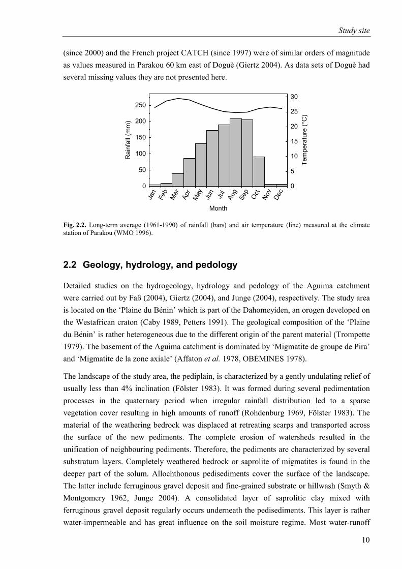
Study site
(since 2000) and the French project CATCH (since 1997) were of similar orders of magnitude as values measured in Parakou 60 km east of Doguè (Giertz 2004). As data sets of Doguè had several missing values they are not presented here.
0
50
100
150
200
250
Rai
nfal
l(m
m)
Jan
Feb
Mar Apr
May Jun
Jul
Aug
Sep
Oct
Nov
Dec
Month
0
5
10
15
20
25
30
Tem
pera
ture
(°C
)
Fig. 2.2. Long-term average (1961-1990) of rainfall (bars) and air temperature (line) measured at the climate station of Parakou (WMO 1996).
2.2 Geology, hydrology, and pedology
Detailed studies on the hydrogeology, hydrology and pedology of the Aguima catchment were carried out by Faß (2004), Giertz (2004), and Junge (2004), respectively. The study area is located on the ‘Plaine du Bénin’ which is part of the Dahomeyiden, an orogen developed on the Westafrican craton (Caby 1989, Petters 1991). The geological composition of the ‘Plaine du Bénin’ is rather heterogeneous due to the different origin of the parent material (Trompette 1979). The basement of the Aguima catchment is dominated by ‘Migmatite de groupe de Pira’ and ‘Migmatite de la zone axiale’ (Affaton et al. 1978, OBEMINES 1978).
The landscape of the study area, the pediplain, is characterized by a gently undulating relief of usually less than 4% inclination (Fölster 1983). It was formed during several pedimentation processes in the quaternary period when irregular rainfall distribution led to a sparse vegetation cover resulting in high amounts of runoff (Rohdenburg 1969, Fölster 1983). The material of the weathering bedrock was displaced at retreating scarps and transported across the surface of the new pediments. The complete erosion of watersheds resulted in the unification of neighbouring pediments. Therefore, the pediments are characterized by several substratum layers. Completely weathered bedrock or saprolite of migmatites is found in the deeper part of the solum. Allochthonous pedisediments cover the surface of the landscape. The latter include ferruginous gravel deposit and fine-grained substrate or hillwash (Smyth & Montgomery 1962, Junge 2004). A consolidated layer of saprolitic clay mixed with ferruginous gravel deposit regularly occurs underneath the pedisediments. This layer is rather water-impermeable and has great influence on the soil moisture regime. Most water-runoff
10
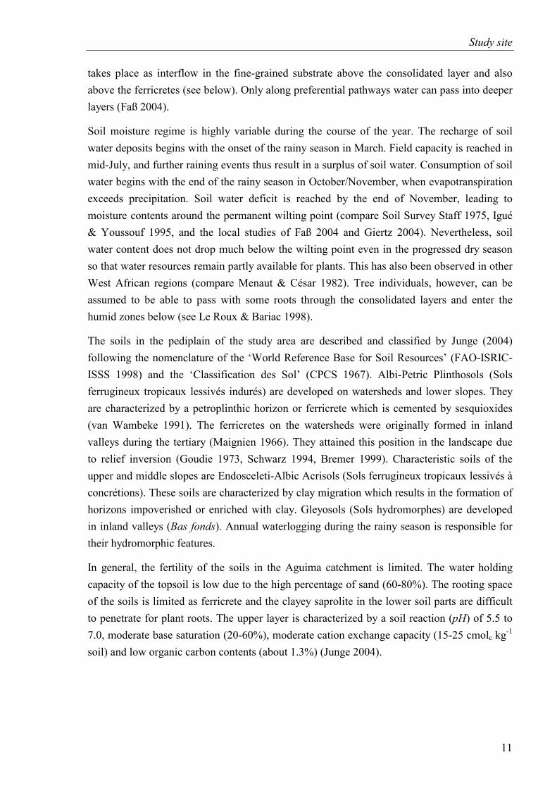
Study site
takes place as interflow in the fine-grained substrate above the consolidated layer and also above the ferricretes (see below). Only along preferential pathways water can pass into deeper layers (Faß 2004).
Soil moisture regime is highly variable during the course of the year. The recharge of soil water deposits begins with the onset of the rainy season in March. Field capacity is reached in mid-July, and further raining events thus result in a surplus of soil water. Consumption of soil water begins with the end of the rainy season in October/November, when evapotranspiration exceeds precipitation. Soil water deficit is reached by the end of November, leading to moisture contents around the permanent wilting point (compare Soil Survey Staff 1975, Igué & Youssouf 1995, and the local studies of Faß 2004 and Giertz 2004). Nevertheless, soil water content does not drop much below the wilting point even in the progressed dry season so that water resources remain partly available for plants. This has also been observed in other West African regions (compare Menaut & César 1982). Tree individuals, however, can be assumed to be able to pass with some roots through the consolidated layers and enter the humid zones below (see Le Roux & Bariac 1998).
The soils in the pediplain of the study area are described and classified by Junge (2004) following the nomenclature of the ‘World Reference Base for Soil Resources’ (FAO-ISRIC-ISSS 1998) and the ‘Classification des Sol’ (CPCS 1967). Albi-Petric Plinthosols (Sols ferrugineux tropicaux lessivés indurés) are developed on watersheds and lower slopes. They are characterized by a petroplinthic horizon or ferricrete which is cemented by sesquioxides
(van Wambeke 1991). The ferricretes on the watersheds were originally formed in inland valleys during the tertiary (Maignien 1966). They attained this position in the landscape due to relief inversion (Goudie 1973, Schwarz 1994, Bremer 1999). Characteristic soils of the upper and middle slopes are Endosceleti-Albic Acrisols (Sols ferrugineux tropicaux lessivés à concrétions). These soils are characterized by clay migration which results in the formation of horizons impoverished or enriched with clay. Gleyosols (Sols hydromorphes) are developed in inland valleys (Bas fonds). Annual waterlogging during the rainy season is responsible for their hydromorphic features.
In general, the fertility of the soils in the Aguima catchment is limited. The water holding capacity of the topsoil is low due to the high percentage of sand (60-80%). The rooting space of the soils is limited as ferricrete and the clayey saprolite in the lower soil parts are difficult to penetrate for plant roots. The upper layer is characterized by a soil reaction (pH) of 5.5 to 7.0, moderate base saturation (20-60%), moderate cation exchange capacity (15-25 cmolc kg-1
soil) and low organic carbon contents (about 1.3%) (Junge 2004).
11
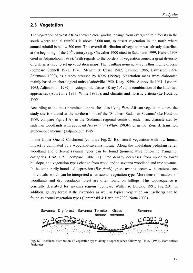
Study site
2.3 Vegetation
The vegetation of West Africa shows a clear gradual change from evergreen rain forests in the south where annual rainfalls is above 2,000 mm, to desert vegetation in the north where annual rainfall is below 300 mm. This overall distribution of vegetation was already described at the beginning of the 20th century (e.g. Chevalier 1900 cited in Salzmann 1999, Hubert 1908 cited in Adjanohoun 1989). With regards to the borders of vegetation zones, a great diversity of criteria is used to set up vegetation maps. The resulting nomenclature is thus highly diverse (compare Schnell 1971, 1976, Menaut & César 1982, Lawson 1986, Lawesson 1994, Salzmann 1999), as already stressed by Keay (1959c). Vegetation maps were elaborated mainly based on chorological units (Aubréville 1950, Keay 1959a, Aubréville 1961, Léonard 1965, Adjanohoun 1989), physiognomic classes (Keay 1959c), a combination of the latter two approaches (Aubréville 1937, White 1983b), and climatic and floristic criteria (Le Houérou 1989).
According to the most prominent approaches classifying West African vegetation zones, the study site is situated at the northern limit of the ‘Southern Sudanian Savanna’ (Le Houérou 1989, compare Fig. 2.1 A), in the ‘Sudanian regional centre of endemism, characterized by sudanian woodlands with abundant Isoberlinia’ (White 1983b), or in the ‘Zone de transition guinéo-soudanienne’ (Adjanohoun 1989).
In the Upper Ouémé Catchment (compare Fig. 2.1 B), natural vegetation with low human impact is dominated by a woodland-savanna mosaic. Along the undulating pediplain relief, woodland and different savanna types can be found (nomenclature following Yangambi categories, CSA 1956, compare Table 3.1). Tree density decreases from upper to lower hillslope, and vegetation types change from woodland to savanna woodland and tree savanna. In the temporarily inundated depression (Bas fonds), grass savanna occurs with scattered tree individuals, which can be interpreted as an azonal vegetation type. More dense formations of woodlands and dry deciduous forest are often found on hilltops. This toposequence is generally described for savanna regions (compare Walter & Breckle 1991, Fig. 2.3). In addition, gallery forest at the riversides as well as typical vegetation on inselbergs can be found as azonal vegetation types (Porembski & Barthlott 2000, Natta 2003).
Dry forest SavannaSavanna Grass savanna
SavannaTermitemound
Fig. 2.3. Idealized distribution of vegetation types along a toposequence following Tinley (1982). Bars reflect ferricretes.
12
Study site
2.4 Human impact on the woodland-savanna mosaic
Local population takes advantage of many resources in the woodland-savanna mosaic (Schreckenberg 2000). Most important factors of human impact are grazing activities by cattle herds, fire, and selective logging. Other activities such as the collection of firewood and of vegetables and fruits for nutritive and medicinal purposes are of minor importance for the studied ecosystem (e.g. Sodeik 1999, Schreckenberg 2000, Doevenspeck 2004). Today’s hunting activities and their impact on the system are negligible because of the already strongly reduced densities of wildlife. (PAMF 1996).
2.4.1 Pastoralism and grazing regime
Since density of large wild herbivores have declined dramatically in recent years (compare Sodeik 1999, Mistry 2000b, 2001), most important grazing activities in the study area take place by domestic animals, mainly by cattle herds. Cattle husbandry is the domain of the Fulani (French: Peulh) in West Africa. Different groups of Fulani exist in Benin, which are either settled and partly transhumant or live completely nomadic (Sturm 1993, Bierschenk 1997). Traditionally, the Upper Ouémé Valley was only used as grazing area during the dry season (long-distance transhumance) by Fulani from northern Nigeria as well as from northern Benin (Houinato 2001). Due to large scale migration processes caused by periodic droughts in the Sahel regions, expansion of cotton cultivation, and stricter management of national parks in northern Benin, grazing regime has changed considerably in the last 10 years in the Upper Ouémé Valley (Sinsin & Heymans 1988, Wotto 2003, Doevenspeck 2004).
Wotto (2003) carried out a detailed study on grazing regime and impact of grazing on the territory of the village Doguè. With regard to the grazing regime in the course of the year he found that cattle herds of the Fulani settling in Doguè are subjected to long-distance transhumance during the dry season either to Togo or into the adjacent state forests (Forêt classé) in the Upper Ouémé Valley. Meanwhile, the pasture on the territory of the village Doguè is exploited by herds coming from northern Benin or Nigeria. During this time of the year, the open savannas are the preferred pasture due to already resprouting grasses. In addition, the sprouted leaves of Afzelia africana, Khaya senegalensis and Pterocarpus erinaceus are cut as fodder. At the beginning of the rainy season when the local herds have returned, fallows and natural pasture near the camps are exploited for resprouting grass. During the rainy season, it becomes more and more difficult to pass through the field-fallow belt surrounding the villages without damaging the growing crops and, therefore, a short-distance transhumance is performed. The herds are driven to sites outside the field-fallow belt and stay there also during the night. Woodlands are the preferred pasture at the beginning of the rainy season. In the progressed rainy season also dense savannas are used, until the beginning of the dry season, when the water table in the depression has fallen far enough to
13
Study site
allow exploitation also of the depression. This general pattern of the grazing regime of the Fulani herdsmen is applied over wide regions in West Africa and has been described by several authors (e.g. for Benin: Sturm 1993, Bierschenk 1997)
Regarding the history of Fulani settlement in the study region, Wotto (2003) found that the first Fulani settlers arrived in 1996. Until 2003, 55 Fulani households were counted which owned about 6,000 cattle. Calculations of Wotto (2003) revealed already a three times overcharge of the pastures of the considered area. It can be assumed that the migration of farmers into the study region will continue and will lead to a conversion of large areas into farmland. Thus, the availability of woodland-savanna sites as pasture will decline continuously (IMPETUS 2003, Doevenspeck 2004). In addition, further restriction for Fulani to use areas in the National parks in northern Benin as well as areas of the Forêt classée surrounding Doguè will lead to an increasing pressure on the pasture of this region (Wotto 2003).
2.4.2 Fire
A high portion of the land cover in the Upper Ouémé Valley is burned annually (Oertel et al. 2004). Natural fires, e.g. due to lightning are nowadays rare (Goldammer 1993a). In savanna systems, fire is known to be used by humans for various reasons (compare Gillon 1983, Menaut et al. 1991, Roberts 2000, Bassett et al. 2003), which are similar to those given by the population in the Upper Ouémé Valley: fires are frequently used around settlements to clear ground for agriculture and to establish fire breaks to protect fields and settlements against uncontrolled fires (own observations). Interviews revealed that a central reason for the population of Doguè to light fires around settlements, but also in savannas and woodlands, was the achievement of higher visibility. Visibility reduces a general fear and in fact the risk of attacks by or accidents with wild animals. Hunters are interested in a higher visibility in order to find their prey, and they also use fires as a hunting method. Herdsmen set fires to initiate an off-season re-growth of perennial herbs as well as to get rid of the unpalatable stubbles (compare Menaut et al. 1991, Sturm 1993). However, fires get out of control quite often or are set accidentally and burn down vast areas. Fire activities start at the end of October with fires near the villages in order to establish fire breaks and continue until or even after the first raining events in March.
The occurrence of fires is a highly stochastic process, on the one hand due to lightning activities of humans and on the other hand due to different parameters such as fuel moisture content, available fuel load, natural fire breaks, and wind direction and velocity (DeBano et al. 1998, Stott 2000). With the exception of gallery forest and dense forest islands where due to fuel conditions, fires occur with a very low probability (compare Biddulph & Kellman 1998), nearly every site is usually burned annually. However, also savanna and woodland sites of varying size and location may remain unburned each year by chance.
14
Study site
2.4.3 Short history of logging activities in the Upper Ouémé Valley
Logging activities in the Upper Ouémé Valley started about 1950 with the construction of some sawmills along the western border of Benin, especially around Bassila (Fig. 2.1 B, Sodeik 1999). Sawmills were constructed by French entrepreneurs (PAMF 1996). In this time, single trees of different valuable timber species of enormous diameter were exploited. Logging took place especially in dry deciduous forest islands and in gallery forests (mainly Ceiba pentandra, Khaya grandifolia, Antiaris africana, and Chlorophora excelsa) as well as in woodlands and savannas (mainly Afzelia africana and Khaya senegalensis). Trees were felled and transported as trunks to the sawmills (PAMF 1996). Until about 1985, all sawmills (private and state-owned) had closed, mostly due to financial problems (Doevenspeck 2004) caused by the decline of valuable timber species (Sodeik 1999). Since then, felled trees are sawn directly in the field and timber boards are exploited. Because felled species became sparse, logging activities are now concentrated on individuals of smaller diameter of remaining individuals. In addition, logging activity have been extended to Pterocarpus erinaceus and Isoberlinia doka (PAMF 1996). In general, permits to cut timber were, and still are, allocated on an individual tree basis by the Forest Department (Sayer & Green 1992). Nevertheless, most logging activities in the study region take place without concessions. They are therefore completely illegal and enter the vast field of corruption (Siebert & Elwert 2002, Siebert 2003).
15
Methods
3 Methods
3.1 Sampling design
Most data of the present thesis were collected in two types of permanent plots, relevé and gap plots. Both plot types were located in the Upper Aguima catchment. Relevé plots were situated in stratified vegetation types, whereas gap plots were exclusively situated in Isoberlinia dominated woodland. Gap plots comprised gaps created by one selectively logged tree individual. However, in both plot types the same data collection was carried out. Due to an agreement between the landowner and the IMEPTUS project, logging activities were forbidden in the Upper Augima catchment since 2001. In order to study the typical logging regime for the studied region with respect to intensity and quality, one additional representative Isoberlinia dominated woodland stand was chosen outside the Upper Aguima catchment (Fig. 3.1).
3.1.1 Site selection of relevé plots
Within the Upper Aguima catchment– chosen as the test site for all studies carried out in sites with low human impact within the IMPETUS project (see Fig. 2.1 and 3.1) – a woodland-savanna mosaic was found. As overall stratification, the classification approach of the Yangambi conference (CSA 1956, Table 3.1) was used. In contrast to many criteria applied in order to subdivide forest formations according to the Yangambi categories, for the subdivision of woodland and savannas no further criteria were designated by the Yangambi approach. This strict structural classification for these vegetation types was extended by some subdivisions in the present thesis, as described below.
16
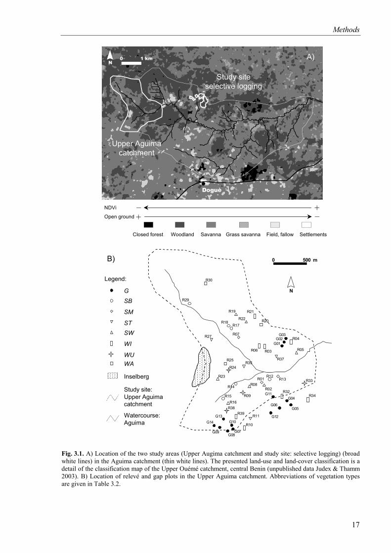
Methods
����������������������������������������������������������������������������������������������������������������
G01G02
G03
G04
G05G06
G07G08
G09
G10
G11
G12G13G14
R01
R02
R03
R04
R05R06
R07
R08
R09
R10
R11
R12R13
R14
R15R16
R17R18
R19
R20
R21
R22
R23
R24
R25
R27
R29
R30
R32
R33
R34
R35R37
R38R39
���������Inselberg
Study site:Upper Aguima catchment
Watercourse: Aguima
GSB
SM
STSW
WI
WUWA
Legend:
B) 0 500 m
N
#
Doguè
N0 1 km
Closed forest Field, fallow SettlementsGrass savannaSavannaWoodland
–+Open ground– +NDVi
A)
Upper Aguima catchment
Study site selective logging
Fig. 3.1. A) Location of the two study areas (Upper Augima catchment and study site: selective logging) (broad white lines) in the Aguima catchment (thin white lines). The presented land-use and land-cover classification is a detail of the classification map of the Upper Ouémé catchment, central Benin (unpublished data Judex & Thamm 2003). B) Location of relevé and gap plots in the Upper Aguima catchment. Abbreviations of vegetation types are given in Table 3.2.
17
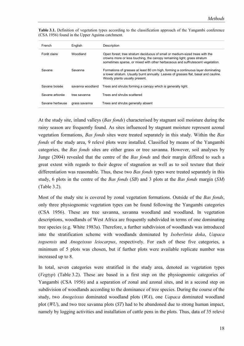
Methods
Table 3.1. Definition of vegetation types according to the classification approach of the Yangambi conference (CSA 1956) found in the Upper Aguima catchment.
French
Forêt claire
Savane
Savane boisée
Savane arborée
Savane herbeuse
English
Woodland
Savanna
savanna woodland
tree savanna
grass savanna
Description
Open forest; tree stratum deciduous of small or medium-sized trees with thecrowns more or less touching, the canopy remaining light; grass stratumsometimes sparse, or mixed with other herbaceous and suffrutescent vegetation.
Formations of grasses at least 80 cm high, forming a continuous layer dominatinga lower stratum. Usually burnt annually. Leaves of grasses flat, basal and cauline.Woody plants usually present.
Trees and shrubs forming a canopy which is generally light.
Trees and shrubs scattered
Trees and shrubs generally absent
At the study site, inland valleys (Bas fonds) characterised by stagnant soil moisture during the rainy season are frequently found. As sites influenced by stagnant moisture represent azonal vegetation formations, Bas fonds sites were treated separately in this study. Within the Bas fonds of the study area, 9 relevé plots were installed. Classified by means of the Yangambi categories, the Bas fonds sites are either grass or tree savanna. However, soil analyses by Junge (2004) revealed that the centre of the Bas fonds and their margin differed to such a great extent with regards to their degree of stagnation as well as to soil texture that their differentiation was reasonable. Thus, these two Bas fonds types were treated separately in this study, 6 plots in the centre of the Bas fonds (SB) and 3 plots at the Bas fonds margin (SM) (Table 3.2).
Most of the study site is covered by zonal vegetation formations. Outside of the Bas fonds, only three physiognomic vegetation types can be found following the Yangambi categories (CSA 1956). These are tree savanna, savanna woodland and woodland. In vegetation descriptions, woodlands of West Africa are frequently subdivided in terms of one dominating tree species (e.g. White 1983a). Therefore, a further subdivision of woodlands was introduced into the stratification scheme with woodlands dominated by Isoberlinia doka, Uapaca togoensis and Anogeissus leiocarpus, respectively. For each of these five categories, a minimum of 5 plots was chosen, but if further plots were available replicate number was increased up to 8.
In total, seven categories were stratified in the study area, denoted as vegetation types (Vegtyp) (Table 3.2). These are based in a first step on the physiognomic categories of Yangambi (CSA 1956) and a separation of zonal and azonal sites, and in a second step on subdivision of woodlands according to the dominance of tree species. During the course of the study, two Anogeissus dominated woodland plots (WA), one Uapaca dominated woodland plot (WU), and two tree savanna plots (ST) had to be abandoned due to strong human impact, namely by logging activities and installation of cattle pens in the plots. Thus, data of 35 relevé
18
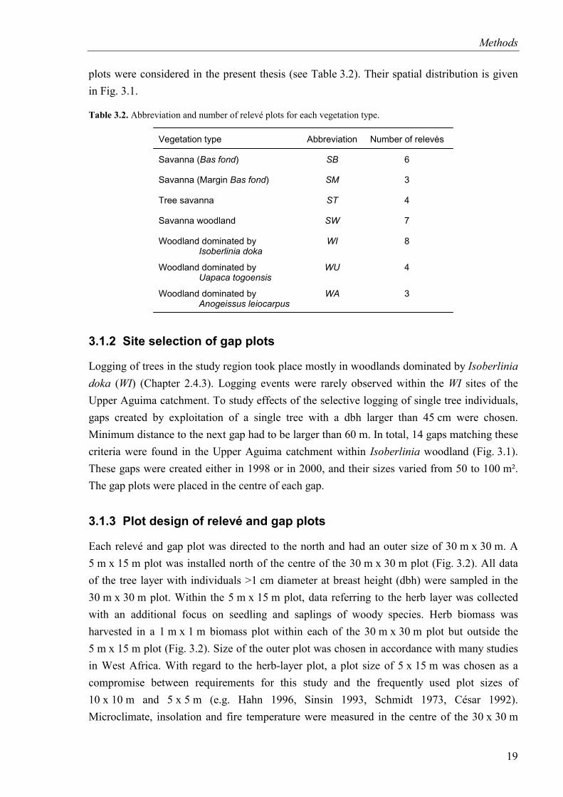
Methods
plots were considered in the present thesis (see Table 3.2). Their spatial distribution is given in Fig. 3.1.
Table 3.2. Abbreviation and number of relevé plots for each vegetation type.
Vegetation type
Savanna ( )Bas fond
Savanna (Margin )Bas fond
Tree savanna
Savanna woodland
Woodland dominated byIsoberlinia doka
Woodland dominated byUapaca togoensis
Woodland dominated byAnogeissus leiocarpus
Abbreviation
SB
SM
ST
SW
WI
WU
WA
Number of relevés
6
3
4
7
8
4
3
3.1.2 Site selection of gap plots
Logging of trees in the study region took place mostly in woodlands dominated by Isoberlinia doka (WI) (Chapter 2.4.3). Logging events were rarely observed within the WI sites of the Upper Aguima catchment. To study effects of the selective logging of single tree individuals, gaps created by exploitation of a single tree with a dbh larger than 45 cm were chosen. Minimum distance to the next gap had to be larger than 60 m. In total, 14 gaps matching these criteria were found in the Upper Aguima catchment within Isoberlinia woodland (Fig. 3.1). These gaps were created either in 1998 or in 2000, and their sizes varied from 50 to 100 m². The gap plots were placed in the centre of each gap.
3.1.3 Plot design of relevé and gap plots
Each relevé and gap plot was directed to the north and had an outer size of 30 m x 30 m. A 5 m x 15 m plot was installed north of the centre of the 30 m x 30 m plot (Fig. 3.2). All data of the tree layer with individuals >1 cm diameter at breast height (dbh) were sampled in the 30 m x 30 m plot. Within the 5 m x 15 m plot, data referring to the herb layer was collected with an additional focus on seedling and saplings of woody species. Herb biomass was harvested in a 1 m x 1 m biomass plot within each of the 30 m x 30 m plot but outside the 5 m x 15 m plot (Fig. 3.2). Size of the outer plot was chosen in accordance with many studies in West Africa. With regard to the herb-layer plot, a plot size of 5 x 15 m was chosen as a compromise between requirements for this study and the frequently used plot sizes of 10 x 10 m and 5 x 5 m (e.g. Hahn 1996, Sinsin 1993, Schmidt 1973, César 1992). Microclimate, insolation and fire temperature were measured in the centre of the 30 x 30 m
19
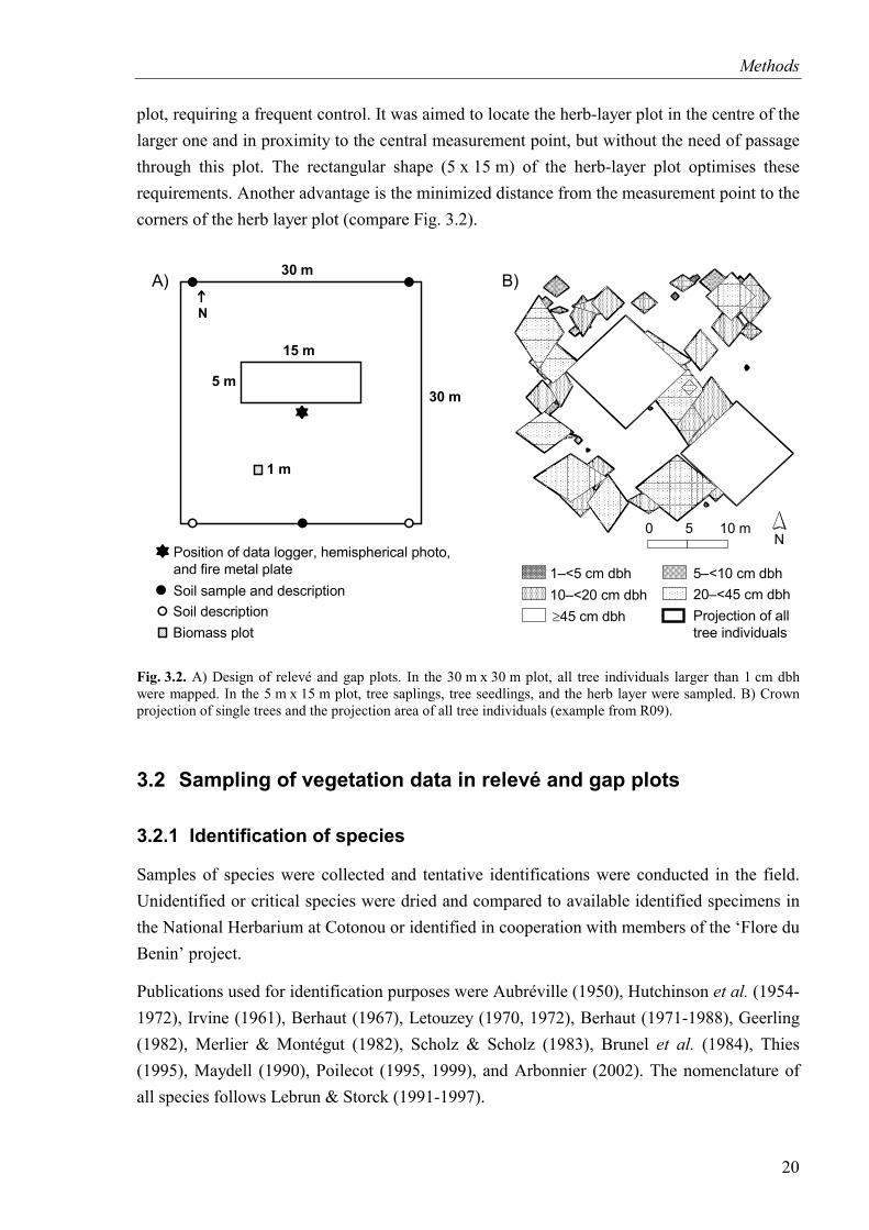
Methods
plot, requiring a frequent control. It was aimed to locate the herb-layer plot in the centre of the larger one and in proximity to the central measurement point, but without the need of passage through this plot. The rectangular shape (5 x 15 m) of the herb-layer plot optimises these requirements. Another advantage is the minimized distance from the measurement point to the corners of the herb layer plot (compare Fig. 3.2).
0 5 10 mN
1–<5 cm dbh10–<20 cm dbh≥45 cm dbh
5–<10 cm dbh20–<45 cm dbhProjection of all tree individuals
30 m
N
30 m
15 m
1 m
5 m
Position of data logger, hemispherical photo, and fire metal plate Soil sample and descriptionSoil descriptionBiomass plot
A) B)
Fig. 3.2. A) Design of relevé and gap plots. In the 30 m x 30 m plot, all tree individuals larger than 1 cm dbh were mapped. In the 5 m x 15 m plot, tree saplings, tree seedlings, and the herb layer were sampled. B) Crown projection of single trees and the projection area of all tree individuals (example from R09).
3.2 Sampling of vegetation data in relevé and gap plots
3.2.1 Identification of species
Samples of species were collected and tentative identifications were conducted in the field. Unidentified or critical species were dried and compared to available identified specimens in the National Herbarium at Cotonou or identified in cooperation with members of the ‘Flore du Benin’ project.
Publications used for identification purposes were Aubréville (1950), Hutchinson et al. (1954-1972), Irvine (1961), Berhaut (1967), Letouzey (1970, 1972), Berhaut (1971-1988), Geerling (1982), Merlier & Montégut (1982), Scholz & Scholz (1983), Brunel et al. (1984), Thies (1995), Maydell (1990), Poilecot (1995, 1999), and Arbonnier (2002). The nomenclature of all species follows Lebrun & Storck (1991-1997).
20
Methods
Species of the genera Gardenia and Strychnos were sampled as Gardenia spec. and Strychnos spec., respectively, due to difficulties of determination. Within the genera Vigna, only the species V. filicaulis, V. frutescens, V. luteola, V. racemosa and V. reticulata were differentiated, all other species were summarized as Vigna spec..
3.2.2 Sampling of tree layer data
Height and diameter of trees
Within each 30 x 30 m plot, all tree individuals >1 cm dbh were permanently and individually marked. Position within the plot and maximum tree height were measured with a combined range finder and hypsometer (VERTEX III, Haglöf, Inc., Finland) and field compass (KB 14/400g, SUUNTO, Inc., Finland). Dbh was measured with a measuring tape. In order to characterize tree structure of the relevé plots, tree data were grouped in four height classes (0-<2 m, 2-<5 m, 5-<10 m, ≥10 m) and in five diameter classes (<5 cm dbh, 5-<10 cm dbh, 10-<20 cm dbh, 20-<45 cm dbh, ≥45 cm dbh). These classes are thought to be ecologically meaningful. Individuals of smaller size classes are still affected in their crown by surface fires, those of medium size classes dominate the lower tree layer, and tree individuals of larger size class build the upper tree layer. Most individuals with a dbh ≥45 cm have reached their fertile phase.
Calculation of tree cover
For each tree individual in the 30 x 30 m plot, crown range in north-south and east-west direction was estimated by perpendicular crown projection. Cover of each tree individual was calculated as a rhombus:
Cover = (crown length in north-south direction) * (crown length in east-west direction)2
Even though this is still an approximation, it overestimates the cover of tree individuals much less than the calculation as an ellipse. In order to calculate the cover of all tree individuals in a plot as perpendicular projection on the ground, the four corner points of each crown were imported to ArcView Gis (3.2). The corners of the crown of each tree individual were converted with the extension Edit Tools (3.6) to a polygon. In order to receive the projection area of all individuals, in contrast to the sum of the cover of all individuals, the extension Geoprocessing was used. Additionally the projection was calculated for different strata (e.g. all individuals with a dbh >10 cm, all individuals <10 m height, compare Fig. 3.2).
21
Methods
Estimation of tree cover
Total cover of trees as well as the cover of each single tree species was estimated as perpendicular projection of all leaves reaching into the 30 x 30 m plot. Cover of tree species was estimated according to the decimal scale of Londo (Dierschke 1994).
Woody biomass
Woody biomass was calculated after Schöngart (2003) as:
Woody biomass = height [m]2
dbh [m]2* ( )2
* * wood density [t/m³]π
Data on wood density were not available for the 51 sampled tree species. Own pilot studies on wood density of six dominating tree species by means of core extraction and gravimetric measurements (Kramer & Akça 1995) revealed a mean value for these species of 0.69 [t m-³] (Afzelia africana: 0.70, Anogeissus leiocarpus: 0.78, Daniellia oliveri: 0.53, Isoberlinia doka: 0.63, Khaya senegalensis: 0.68, Pterocarpus erinaceus: 0.76). Brown (1997) gives wood densities for many African tree species within the range of 0.5 - 0.79 [t m-³]. Taking into account only those occurring in the southern Sudanian savanna, a mean value of 0.61 [t m-³] was calculated. However, only some of the 51 sampled tree species were mentioned by Brown (1997). For the calculation of woody biomass finally 0.65 [t m-³] was chosen as a reasonable compromise as dense woods were sampled in this thesis in contrast to Brown (1997), where light wooded species of humid sites were dominating.
3.2.3 Sampling of herb layer data
Species composition
Vegetation surveys were conducted in the 5 m x 15 m plot (Fig. 3.2) in October 2002 at the peak of flowering of grass species according to Braun-Blanquet (Dierschke 1994). With respect to the herb layer, cover of each species was estimated according to the decimal scale of Londo (Dierschke 1994), considering all leaves being in the projection of the plot.
Structural parameters
The structural parameters: cover of herbs (HEC), cover of grasses (GC), cover of non-grass litter (LNGC), cover of grass litter (LGC) and the sum of the two litter fractions (LC), cover of open ground (OGC), cover of dead woody biomass (DWBC diameter >1 cm) and cover of termite mound (TM) were estimated in October 2001 and 2002 at biomass maximum of the herb layer and peak of flowering of grass species. Concerning herbs and grasses, also their maximum height (HEH, GH) was measured and volume (HEVol, GVol) calculated as height * cover. Grazing impact (GI) in the plots was estimated as percentage of grazed plants
22
Methods
and trampling damage (TD) in classes of 1 to 5 (1: no TD, 2: low TD, 3: medium TD, 4: strong TD and 5: very strong TD). These data were sampled in the 5 m x 15 m plot as well as in an adjacent 1 m x 1 m biomass plot (Fig. 3.2).
Biomass
After sampling of structural parameters, herb biomass was harvested at the end of October in the 1 m x 1 m biomass plots (Fig. 3.2). Biomass was separated into the fractions grasses, herbs and litter which were dried to weight constancy.
3.2.4 Sampling of data on seedlings and saplings of woody species
From 2001 to 2004, number of seedlings and saplings of woody species were sampled at the end of the rainy season in September within all 5 m x 15 m plots. Species of each tree individual was determined and its age was estimated. Seedlings from the respective year could clearly be distinguished from older individuals by growth form. In the category saplings, individuals with an estimated age between one and five years were grouped.
3.3 Sampling of data on environmental parameters in relevé and gap plots
3.3.1 Soil
Soil samples were taken in cooperation with Birte Junge (see Junge 2004) in September 2001. A soil description was made at five locations at the borders of the plots by extracting cores with a Pürckhauer driller (Fig. 3.2). The depth of the different soil layers was recorded. From three of the five locations, soil samples of the upper two layers were taken with an Edelmann driller and merged as a mixed sample for each plot. Analyses of grain size distribution after Köhn (1928) and pH (CaCl2) were conducted by the Laboratory of the Hydrology Research Group, University of Bonn. All chemical analyses were done on air-dried soil samples (<2 mm grain size) in duplicate by the Laboratory of the Institute for Soil Science, University of Bonn. The exchangeable cation concentration was determined for Na+, K+, Ca2+ and Mg2+ according to Trüby & Aldinger (1989). Test for carbonate content with HCl in the field revealed that the soil samples contained no carbonate at all. In consequence no carbonate determination was performed in the laboratory. Organic content (Corg) and total nitrogen concentration (N) were determined by a C/N-Analyser. Analysis of available phosphate (P, P2O5) was carried out after Bray & Kurtz (1945) using NH4F.
23
Methods
3.3.2 Microclimate
Air temperature, air humidity, and vapour pressure deficit
A data logger (Tinytag Plus TGP-1500 Gemini Data Loggers, Ltd., UK) was placed in the centre of each relevé and gap plot in 1.3 m height, above maximum volume of the herb layer, and protected by a radiation shield. Air temperature and relative air humidity were logged every 10 minutes. The first measurement campaign started in September 2001. The logged data were exported with the GLM Windows Software (Gemini Data Loggers, Ltd., UK) in intervals of three month. The measurements continued until December 2002 with an interruption from December 2001 to February to March 2002 due to fire events in the study area. Several data loggers suffered from technical problems during the course of the measurement period, especially those recording air humidity. Therefore and due to loss of data loggers the number of data loggers, and recorded time series declined continuously, mainly in the last period from August to December 2002.
The vapour pressure deficit (VPD) was calculated according to Arya (2001) from air temperature (T) and relative air humidity (H).
VPD = (6.107*10^((7.5*T)/(237+T)))-((6.107*10^((7.5*T)/(237+T)))*H/100)
For each of the parameter, temperature, humidity, and vapour pressure deficit, values were controlled for plausibility and diurnal mean, maximum, minimum and amplitude were calculated. For graphical presentation 10-day-moving averages were calculated.
Hemispherical photographs
At the beginning of October 2002, during the rainy season, hemispherical photos were taken with the HemiView System (Delta-T Devices, Ltd., UK). This system includes a self-levelling unit with a digital camera and a fisheye lens. Direction towards the north and south are marked by flashlights on the photographs. Own measurements revealed that values did not differ considerably if the mean of five photographs distributed over the plot were taken into account or if only one photograph at the centre was considered. Therefore, at each plot one photograph above the herbaceous layer was taken in the centre of the plot. To benefit from uniform sky conditions, photographs were taken shortly before sunrise or after sunset. Photographs were post-processed with the HemiView Software, HMV1 (Delta-T Devices, Ltd., UK).
The most reasonable parameters had to be chosen for analysis out of the many parameters calculated by the HemiView Software. Visible sky (VS) gives the overall proportion of the sky hemisphere that is visible. The global site factor (GSF) is calculated as the ratio of total radiation below the canopy to total radiation above the canopy. Likewise, indirect site factor (ISF) and direct site factor (DSF) are calculated using indirect and direct radiation below and
24
Methods
above the canopy, respectively. HemiView algorithms estimate leaf area index (LAI) as half of the total leaf area per unit ground area, what is a rough approximation.
3.3.3 Fire
Five different fire chalks were used which change their colour if exposed to the specific temperatures (120, 195, 215, 245, 295, 320, 335, 365, 460, 505, 600°C) for an estimation of fire temperature (compare Bloesch 2002). For each plot, one metal plate with markers of the chalks was set up in the centre of the plot 30 cm above ground. The height was chosen as compromise between data found in the literature. Gillon (1983) summarized 50 cm as maximum fire temperature in savannas, whereas Bloesch (2002) found highest fire temperature at 10 cm above ground and Hopkins (1965a) directly above the soil. Metal plates were placed in the field at the beginning of December 2001 and 2002 and controlled every week. When fires passed, date and maximum temperature were recorded.
3.3.4 Topographical position
From the centre of each plot inclination (Inc) was measured by an inclinometer (PM-5/400 PC, SUUNTO, Inc., Finland) and exposition (Exp) was measured by a field compass (KB 14/400g, SUUNTO, Inc., Finland). Relative topographic position (TopH) of each plot was measured as absolute height above sea level minus absolute height of run-off line based on a digital elevation model derived from Aster Satellite data (unpublished data Drey & Thamm 2004).
3.4 Survey of logging history and intensity
The survey on logging history at the village Doguè is based on informal interviews with the council of elders of the village of Doguè as well as on the information of inhabitants who guide the tree fellers to logging sites and on own observations.
As logging activity was relatively sparse in the Upper Aguima catchment, one representative Isoberlinia doka dominated woodland (WI) near Doguè characterized by a high intensity of selective logging was chosen as study site in order to study logging intensity and quality (Fig. 3.1). At this site with an extension of 18.8 ha, logging took place in 1999, 2001, and 2002. In April 2002, all logged tree individuals were mapped with a handheld GPS (Garmin III+) and data were introduced in a GIS (ArcView 3.2). The remaining stump of each logged tree individual as well as woody debris were used to determine the species and to estimate dbh and number and size of explored timber boards. Height was calculated via a dbh-height regression based on the data from permanent plots. Woody biomass was calculated for extracted timber boards and felled trees following Chapter 3.2.2.
25
Methods
3.5 Data analysis
3.5.1 Tabular comparison of vegetation data
Data on tree and herb layer were treated separately since e.g. Hahn (1996) and Devineau et al. (1997) showed that floristically distinct herb layer groups can be associated to different tree layer groups and vice versa. Data on vegetation composition were converted into vegetation tables. Two approaches were chosen for tabular comparison. In the first approach, data were sorted by phytosociological criteria, based on the method of Braun-Blanquet as described in Dierschke (1994) and Mueller-Dombois & Ellenberg (1974). The resulting groups of relevé plots of this phytosociological sorting were denoted as floristic blocks. In the second approach, the position of vegetation types (Vegtyp, columns) were fixed by in the order SB, SM, ST, SW, WI, WU, and WA (Table 3.2), but relevé plots within each vegetation type were sorted. Position of species (rows) in the tables was ordered primarily by their occurrence and additionally by their dominance.
The tabular procedure for these two approaches was exclusively carried out in order to compare both classification approaches with each other with regard to floristic composition of tree and herb layer. It was not aimed to integrate neither resulting floristic blocks nor vegetation types into phytosociological syntaxonomic systems.
3.5.2 Statistical analysis
Univariate and multivariate data analyses were carried out. Univariate analyses and pairwise comparison of multivariate data were computed in R 1.8.0 (2003). All other multivariate analyses were performed with the Software package CANOCO for Windows Version 4.51. Boxplots are computed in Xact (Version 7.22b, Scilab GmbH).
For all parameters it was tested whether they were normal distributed before introduction into any statistical analysis. Some parameters showed normal distribution, others were only fairly normal distributed due to both rather low sampling number and heterogeneity of samples. However, transformation did not improve distribution of data towards a normal distribution. Therefore non-parametric analyses were carried out for most univariate data analyses. Though multivariate statistics are also based on the assumption of normal distribution, they are known to be much more robust against violation of this assumption (ter Braak & Smilauer 2002).
When many parameters are measured in the same plots – as it is the case in the present thesis – and when several test of significance are carried out simultaneously, the probability of type I error becomes larger than the nominal value α (Sokal & Rohlf 1995, Legendre & Legendre 1998). In these cases the significance level should be reduced by applying Bonferroni correction or comparable methods (review in Wright 1992). Nevertheless, this is a controversial issue (Cabin & Mitchell 2000). Moran (2003) states that from mathematical to
26
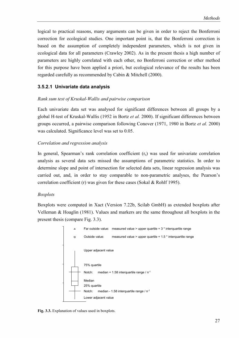
Methods
logical to practical reasons, many arguments can be given in order to reject the Bonferroni correction for ecological studies. One important point is, that the Bonferroni correction is based on the assumption of completely independent parameters, which is not given in ecological data for all parameters (Crawley 2002). As in the present thesis a high number of parameters are highly correlated with each other, no Bonferroni correction or other method for this purpose have been applied a priori, but ecological relevance of the results has been regarded carefully as recommended by Cabin & Mitchell (2000).
3.5.2.1 Univariate data analysis
Rank sum test of Kruskal-Wallis and pairwise comparison
Each univariate data set was analysed for significant differences between all groups by a global H-test of Kruskal-Wallis (1952 in Bortz et al. 2000). If significant differences between groups occurred, a pairwise comparison following Conover (1971, 1980 in Bortz et al. 2000) was calculated. Significance level was set to 0.05.
Correlation and regression analysis
In general, Spearman’s rank correlation coefficient (rs) was used for univariate correlation analysis as several data sets missed the assumptions of parametric statistics. In order to determine slope and point of intersection for selected data sets, linear regression analysis was carried out, and, in order to stay comparable to non-parametric analyses, the Pearson’s correlation coefficient (r) was given for these cases (Sokal & Rohlf 1995).
Boxplots
Boxplots were computed in Xact (Version 7.22b, Scilab GmbH) as extended boxplots after Velleman & Hoaglin (1981). Values and markers are the same throughout all boxplots in the present thesis (compare Fig. 3.3).
Far outside value: measured value > upper quartile + 3 * interquartile range
Outside value: measured value > upper quartile + 1.5 * interquartile range
Upper adjacent value
75% quartile
Notch: median - 1.58 interquartile range / n-1
Notch: median + 1.58 interquartile range / n-1
Median
Lower adjacent value
25% quartile
Fig. 3.3. Explanation of values used in boxplots.
27
Methods
3.5.2.2 Multivariate data analysis
For species data sets, Detrended Correspondence Analysis (DCA) was chosen for two reasons. Firstly, the calculated length of gradient for the analysed data sets recommended unimodal models (ter Braak & Smilauer 2002). Secondly, an arch effect occurred calculating Correspondence Analysis (CA) for the data sets (compare Hill & Gauch 1980, Gauch 1982, Jongman et al. 1987, Økland 1990, Palmer 1993). Canonical Correspondence Analysis (CCA) was chosen as constrained unimodal method for the joint analysis of species and environmental parameter data sets. Rare species may have an overproportional large influence on the analyses (ter Braak 1995, Lawesson 1997, ter Braak & Smilauer 2002). Accordingly, only species with more than two occurrences were used in the analyses of the herb species. This was the case for 296 of the 327 species. As the data set of the tree layer contained overall only 51 species, all species were considered. Nevertheless the effect of the species with very low number of occurrences was always checked after the analyses, and they were found to have low influence on the results.
Detrended Correspondence Analysis
A DCA was carried out with ‘detrended by segments’ in order to determine the length of gradient. As comparable amounts of floristic variability were explained by the first four axes, the option ‘detrending by fourth order polynomial’ was chosen for the calculation of the presented DCA (ter Braak & Smilauer 2002). ‘Inter sample distance’ and ‘Hill scaling’ were chosen since the analysis was aimed to be focussed on sample position. Species were log-transformed (log(x+1)) to increase the influence of subordinate species compared to dominate ones (compare Lepš & Smilauer 2003).
Canonical Correspondence Analysis
Canonical Correspondence Analyses (CCA) were calculated to gain knowledge on the explanation of floristic variability by environmental parameters. Species were log-transformed (log(x+1)) in the run of each CCA and ‘inter sample distance’ and ‘Hill scaling’ were chosen. Many of the environmental parameters were strongly and significantly correlated with each other. The inclusion of these correlated parameters into the respective CCA would lead to an overestimation of explained environmental variability (Økland & Eilertsen 1994). Therefore a model-selection procedure as described below was used to include only parameters which significantly improve the model and to exclude automatically parameters which are collinear or strongly correlated with already selected parameters (see Lepš & Smilauer 2003). Another advantage of the application of the model-selection procedure is that inclusion of noisy or irrelevant environmental variables which can seriously distort the representation of gradients can be avoided (compare McCune 1997). A manual step by step selection with subsequent Monte Carlo permutation test implemented in CANOCO
28
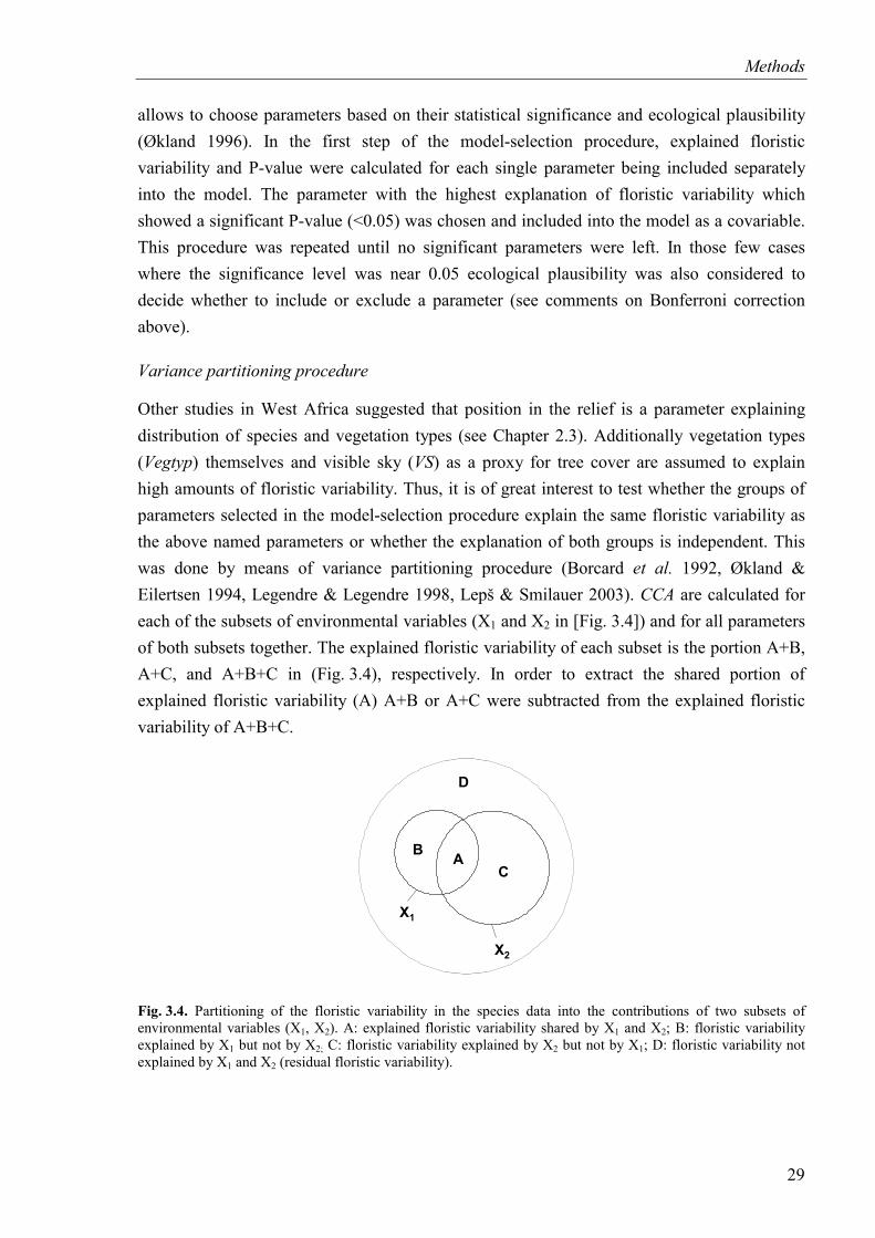
Methods
allows to choose parameters based on their statistical significance and ecological plausibility (Økland 1996). In the first step of the model-selection procedure, explained floristic variability and P-value were calculated for each single parameter being included separately into the model. The parameter with the highest explanation of floristic variability which showed a significant P-value (<0.05) was chosen and included into the model as a covariable. This procedure was repeated until no significant parameters were left. In those few cases where the significance level was near 0.05 ecological plausibility was also considered to decide whether to include or exclude a parameter (see comments on Bonferroni correction above).
Variance partitioning procedure
Other studies in West Africa suggested that position in the relief is a parameter explaining distribution of species and vegetation types (see Chapter 2.3). Additionally vegetation types (Vegtyp) themselves and visible sky (VS) as a proxy for tree cover are assumed to explain high amounts of floristic variability. Thus, it is of great interest to test whether the groups of parameters selected in the model-selection procedure explain the same floristic variability as the above named parameters or whether the explanation of both groups is independent. This was done by means of variance partitioning procedure (Borcard et al. 1992, Økland & Eilertsen 1994, Legendre & Legendre 1998, Lepš & Smilauer 2003). CCA are calculated for each of the subsets of environmental variables (X1 and X2 in [Fig. 3.4]) and for all parameters of both subsets together. The explained floristic variability of each subset is the portion A+B, A+C, and A+B+C in (Fig. 3.4), respectively. In order to extract the shared portion of explained floristic variability (A) A+B or A+C were subtracted from the explained floristic variability of A+B+C.
BC
D
A
X2
X1
Fig. 3.4. Partitioning of the floristic variability in the species data into the contributions of two subsets of environmental variables (X1, X2). A: explained floristic variability shared by X1 and X2; B: floristic variability explained by X1 but not by X2; C: floristic variability explained by X2 but not by X1; D: floristic variability not explained by X1 and X2 (residual floristic variability).
29
Methods
Principal response curve analysis
By means of Principal Response Curve analysis (PRC), time series of different experimental treatments can be compared to one time series of ‘control treatments’ (van den Brink & ter Braak 1998, 1999). In this study, treatment levels are gap plots and vegetation types. The PRC is based on a Redundancy Analysis (RDA) with the interaction of measurement time and vegetation type used as explanatory variables and measurement time coded as a 1/0-matrix introduced as covariables. Interaction effects including the ‘control treatment’ are omitted from the explanatory variables in order to represent a reference point for each measurement time. In CanoDraw, the canonical regression coefficients and species scores are transformed for graphical presentation (ter Braak & Smilauer 2002, Lepš & Smilauer 2003). Two approaches were calculated in the present thesis. To test for significant differences between time series of gaps and each vegetation type, PRC was computed for each of the seven couples considering the respective vegetation type as ‘control treatment’ followed by a Monte Carlo permutation test with split-plot design restricted to the measurement times. For a compromised illustration of the results of these seven PRC, an overall analysis for all vegetation types and the gap plots as ‘control treatment’ was calculated. The resulting graph was presented as the implied message did not differ from the results of each single analysis
Pairwise comparison of multivariate data
In order to test for significant differences in multivariate vegetation data, a Monte Carlo permutation test is recommended (Legendre & Legendre 1998, Tabachnick & Fidell 2001, ter Braak & Smilauer 2002). Comparable to the global H-test for univariate data (see Chapter 3.5.2.1), each multivariate data set was tested for significant differences between vegetation types applying Canonical Correspondence Analysis (CCA) followed by a Monte Carlo permutation test (5,000 replicates). Species data were treated as constrained variables and vegetation types as unconstrained variables (0-1 matrix = dummy variables) (Lepš & Smilauer 2003). As for all presented data sets significant differences occurred between vegetation types based on multivariate data, it was of interest to detect by means of pairwise comparison, which vegetation types differed significantly from each other.
For multivariate data, no implemented pairwise comparison based on a permutation test exist. Therefore, a multiple comparison procedure based on CCA was constructed where each pair of vegetation types was tested for significant differences. The significance level of each pair of vegetation types was computed applying CCA including dummy variables of the two vegetation types as explanatory variables and species data as response variables, followed by a Monte Carlo permutation test (5,000 replicates). The result of each single comparison enters into a matrix containing the significance levels of all single comparisons. This matrix was transformed to a 0-1 matrix where significance levels smaller than 0.05 (internal P-value)
30
Methods
were set to 1 and the others to 0. From this matrix, the number of significant groups and the ‘membership’ of each vegetation type to these groups was extracted by logical combination.
In order to test for the necessity for a Bonferroni correction of the internal P-value of 0.05 within the described pairwise comparison based on CCA, this type of pairwise comparison was computed for univariate data of the present thesis that are also analysed by means of non-parametric pairwise comparison (see Chapter 3.5.2.1). The non-parametric pairwise comparison, however, included an internal correction of the P-value. Except for vegetation types with a low number of replicates, both univariate approaches revealed almost the same significance groups for the vegetation types, though no Bonferroni correction of the internal P-value was applied within the univariate pairwise comparison based on CCA. Therefore, also within the multivariate pairwise comparison procedure, no Bonferroni correction was applied for the internal P-value of 0.05 (see also comments on Bonferroni correction above).
The described procedure was programmed in R 1.8.0 (2003) using the CCA function (Legendre & Legendre 1998, R-package vegan). Results of CCA of selected data sets computed in R and Software package CANOCO for Windows Version 4.51 showed that only minor differences between these two programs occurred. The advantage of R is its flexibility especially for programming. Thus, all pairwise comparisons were computed in R. The advantage of CANOCO is its graphical tool CanoDraw that was used for graphical presentations in the present thesis (see above).
31
Results
4 Results
4.1 Floristic characteristics of the relevé plots
This chapter focuses on the description of the floristic composition of relevé plots by means of two classification approaches. The first classification approach is based on the physiognomic classification approach of the Yangambi conference in 1956 (CSA 1956), extended by a separation of zonal and azonal sites as well as a subdivision of woodlands according to dominant tree species (see Chapter 3.1.1). Stratified categories were denoted as vegetation types (Vegtyp) (Table 3.2). In the second approach floristic blocks are derived by a strict phytosociological classification. Beside the comparison between these two approaches, significance of vegetation types (Vegtyp) and floristic blocks is tested based on floristic composition. Tree and herb layer are treated separately (Chapter 3.2.2 and 3.2.3), and tree layer is defined as the cover of all individuals larger 10 cm dbh (Chapter 3.2.2).
4.1.1 Tabular comparison
4.1.1.1 Tree layer
Vegetation types
Relevé plots of the tree layer are shown in the Appendix (A-Table 2). The relevé plots were ordered according to the stratified vegetation types (Table 3.2). Within vegetation types, species were ordered by their occurrence and their dominance. In total, 49 tree species out of 22 families were found in the relevé plots. The three tree species Isoberlinia doka, Uapaca togoensis and Anogeissus leiocarpus, which were chosen to subdivide different woodland types, showed indeed clear dominance in the different woodland types but they also occurred in relevé plots of other vegetation types. Terminalia macroptera and Terminalia schimperiana as well as Syzygium guineense were restricted to SB and SM plots. Some species were observed in all vegetation types, e.g. Daniellia oliveri and Vitellaria paradoxa, whereas many species were completely absent from the Bas fonds. Representative species of the latter species group were Burkea africana, Lannea acida, Monotes kerstingii and Parinari curatellifolia. Even though species groups could be distinguished in A-Table 2, the overall impression is a diffuse gradient of tree species distribution from open savannas to woodlands.
32

Results
Floristic blocks
The ordination of the tree species data according to phytosociological criteria is shown in Table 4.1, where the relevé plots of the Bas fonds were grouped together as well as plots of the woodlands. This ordination of relevé plots and species revealed more distinct species groups as compared to table A-Table 2.
In total, four floristic blocks of relevé plots were distinguished in Table 4.1. The first floristic block representing Bas fonds conditions was again characterized by Terminalia macroptera and Terminalia schimperiana (compare A-Table 2). The third floristic block is defined by Isoberlinia doka, Uapaca togoensis and Monotes kerstingii. Between the first and the third floristic block, a transition block (block 2) characterized by Daniellia oliveri occurred where typical species of both the first and the third block were mostly absent. The fourth floristic block of relevé plots was characterized by the absence of the characteristic species of the first three blocks.
Within the third floristic block of relevé plots, Anogeissus leiocarpus, Ficus sur, Crossopteryx febrifuga, and Khaya senegalensis differentiated a sub-block. Vitellaria paradoxa, Pterocarpus erinaceus and Burkea africana occurred in all reléve plots except of those in the Bas fonds. One plot, R19, was characterized by the absence of characteristic species and could not be associated to any of the four floristic blocks. In R15 tree species (dbh >10 cm) were completely absent.
Table 4.1. Cover of tree species larger 10 cm dbh in the relevé plots. Presented are species used for classification (compare complete species list A-Table 2). Relevé plots and species were sorted according to phytosociological criteria. Abbreviations of vegetation types are given in Table 3.2.
Cover of trees 2 2 1 2 15 2 10 10 15 20 48 65 35 35 18 20 45 55 75 55 65 60 70 55 55 60 65 75 65 45 50 70 45 45 0 Floristic block 1 1 1 1 1 2 2 2 2 2 2 3 3 3 3 3 3 3 3 3 3 3 3 3 3 3 3 3 3 3 4 4 4 5 -
Vegetation type SB
SB
SB
SB
SM
SM
SM
SB
ST
ST
SW
WU
SW
SW
ST
ST
SW
WI
WU
WI
WI
WI
WI
WI
WI
WI
WU
WU
WA
SW
WA
WA
SW
SW
SB
Plot R
14
R17
R12
R29
R07
R13
R01
R18
R35
R27
R08
R09
R02
R16
R11
R37
R05
R39
R38
R21
R10
R03
R04
R06
R32
R34
R33
R24
R25
R22
R30
R20
R23
R19
R15
Species Terminalia schimperiana 2 1 . . 28 1 3 . . . . . . . . . . . . . . . . . . . . . . . . . . . . Terminalia macroptera . 1 3 . . . . . . . . . . . . . . . . . . . . . . . . . . . . . . . . Syzygium guineense . . . 1 . . . . . . 1 . . . 1 . . . . . . . . . . . . . . . . . . . . Daniellia oliveri . . . . . 12 26 8 5 15 9 13 1 9 . . . . . . . . . . . . . 3 . . 6 . . . . Isoberlinia doka . . . . . . . 7 . . . . 4 11 9 7 . 56 8 28 34 12 24 19 34 32 . . . . . . . . . Uapaca togoensis . . . . . . . . . . . 8 . 1 2 3 42 . 35 . . 2 12 . 2 18 39 87 4 4 . . . . . Monotes kerstingii . . . . . . . . . 2 . 2 3 1 . 4 15 . 1 1 . . 2 . . . . . 1 4 . . 1 . . Anogeissus leiocarpus . . . . . . . . . 1 . . . . . . . . . . . 11 3 9 4 10 15 11 8 . 33 25 . . . Ficus sur . . . . . . . . . . . . . . . . . . . . . . 2 1 2 . . 1 1 . . 1 . . . Crossopteryx febrifuga . . . . . . . . . . 3 . . . . . . . . . . . . . . 1 4 . . 4 . 7 9 . . Khaya senegalensis . . . . . . . . . . . . . . . . . . . . . . 1 . . . 2 . . . . 1 . . . Vitellaria paradoxa . . 2 1 . . . 3 7 6 14 23 9 1 7 3 9 7 2 4 4 4 4 1 2 4 12 4 3 5 10 4 11 6 . Pterocarpus erinaceus . . . 4 . . . . . . 1 10 1 4 1 . . . . 7 5 7 3 7 1 3 10 1 12 2 1 6 1 . . Burkea africana . . . . . . . . . 3 7 4 6 2 9 . . 8 1 6 2 11 4 7 11 1 13 . 7 6 7 . . 15 .
33
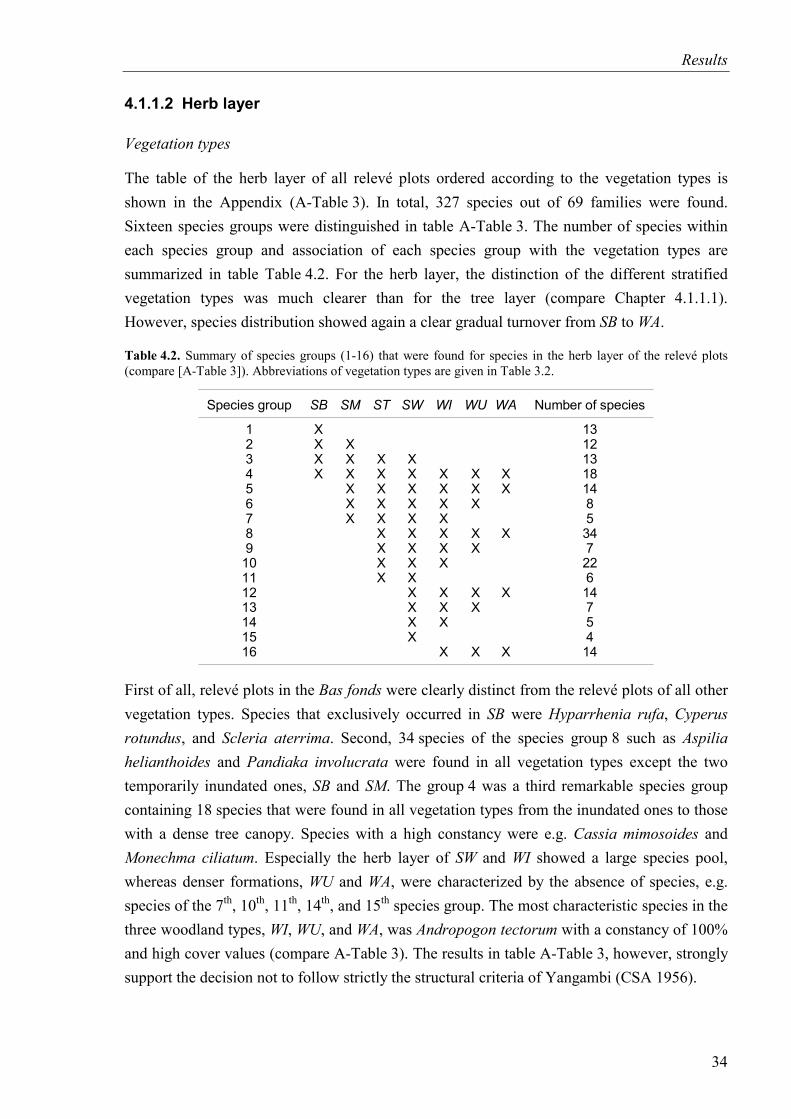
Results
4.1.1.2 Herb layer
Vegetation types
The table of the herb layer of all relevé plots ordered according to the vegetation types is shown in the Appendix (A-Table 3). In total, 327 species out of 69 families were found. Sixteen species groups were distinguished in table A-Table 3. The number of species within each species group and association of each species group with the vegetation types are summarized in table Table 4.2. For the herb layer, the distinction of the different stratified vegetation types was much clearer than for the tree layer (compare Chapter 4.1.1.1). However, species distribution showed again a clear gradual turnover from SB to WA.
Table 4.2. Summary of species groups (1-16) that were found for species in the herb layer of the relevé plots (compare [A-Table 3]). Abbreviations of vegetation types are given in Table 3.2.
Species group
123456789
10111213141516
SB
XXXX
SM
XXXXXX
ST
XXXXXXXXX
SW
XXXXXXXXXXXXX
WI
XXXXXXX
XXX
X
WU
XXX
XX
XX
X
WA
XX
X
X
X
Number of species
1312131814853472261475414
First of all, relevé plots in the Bas fonds were clearly distinct from the relevé plots of all other vegetation types. Species that exclusively occurred in SB were Hyparrhenia rufa, Cyperus rotundus, and Scleria aterrima. Second, 34 species of the species group 8 such as Aspilia helianthoides and Pandiaka involucrata were found in all vegetation types except the two temporarily inundated ones, SB and SM. The group 4 was a third remarkable species group containing 18 species that were found in all vegetation types from the inundated ones to those with a dense tree canopy. Species with a high constancy were e.g. Cassia mimosoides and Monechma ciliatum. Especially the herb layer of SW and WI showed a large species pool, whereas denser formations, WU and WA, were characterized by the absence of species, e.g. species of the 7th, 10th, 11th, 14th, and 15th species group. The most characteristic species in the three woodland types, WI, WU, and WA, was Andropogon tectorum with a constancy of 100% and high cover values (compare A-Table 3). The results in table A-Table 3, however, strongly support the decision not to follow strictly the structural criteria of Yangambi (CSA 1956).
34
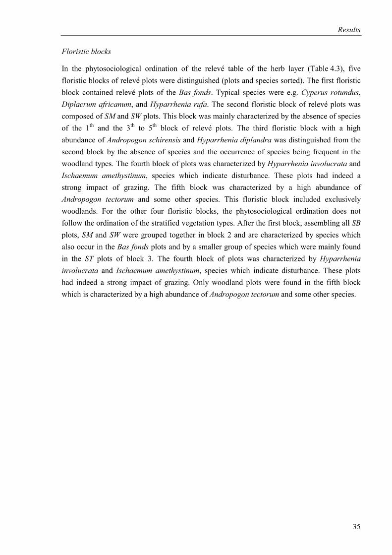
Results
Floristic blocks
In the phytosociological ordination of the relevé table of the herb layer (Table 4.3), five floristic blocks of relevé plots were distinguished (plots and species sorted). The first floristic block contained relevé plots of the Bas fonds. Typical species were e.g. Cyperus rotundus, Diplacrum africanum, and Hyparrhenia rufa. The second floristic block of relevé plots was composed of SM and SW plots. This block was mainly characterized by the absence of species of the 1th and the 3th to 5th block of relevé plots. The third floristic block with a high abundance of Andropogon schirensis and Hyparrhenia diplandra was distinguished from the second block by the absence of species and the occurrence of species being frequent in the woodland types. The fourth block of plots was characterized by Hyparrhenia involucrata and Ischaemum amethystinum, species which indicate disturbance. These plots had indeed a strong impact of grazing. The fifth block was characterized by a high abundance of Andropogon tectorum and some other species. This floristic block included exclusively woodlands. For the other four floristic blocks, the phytosociological ordination does not follow the ordination of the stratified vegetation types. After the first block, assembling all SB plots, SM and SW were grouped together in block 2 and are characterized by species which also occur in the Bas fonds plots and by a smaller group of species which were mainly found in the ST plots of block 3. The fourth block of plots was characterized by Hyparrhenia involucrata and Ischaemum amethystinum, species which indicate disturbance. These plots had indeed a strong impact of grazing. Only woodland plots were found in the fifth block which is characterized by a high abundance of Andropogon tectorum and some other species.
35
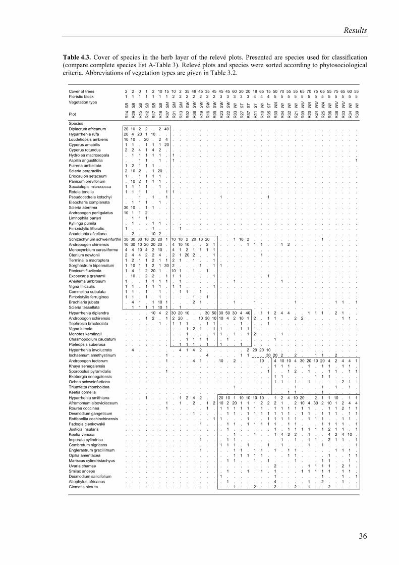
Results
Table 4.3. Cover of species in the herb layer of the relevé plots. Presented are species used for classification (compare complete species list A-Table 3). Relevé plots and species were sorted according to phytosociological criteria. Abbreviations of vegetation types are given in Table 3.2.
Cover of trees 2 2 0 1 2 10 15 10 2 35 48 45 35 45 45 45 60 20 20 18 65 15 50 70 55 55 65 70 75 65 55 75 65 60 55 Floristic block 1 1 1 1 1 1 1 2 2 2 2 2 2 2 3 3 3 3 3 4 4 4 5 5 5 5 5 5 5 5 5 5 5 5 5 Vegetation type SB
SB
SB
SB
SB
SB
SM
SM
SM
SW
SW
SW
SW
SW
SW
SW
WI
ST
ST
ST
WI
ST
WA
WI
WI
WI
WU
W
A
WU
W
A W
I W
U
WU
WI
WI
Plot R
14
R29
R
15
R12
R
17
R18
R
07
R01
R
13
R02
R
08
R19
R
16
R05
R23
R
22
R03
R
27
R37
R
11
R10
R
35
R30
R
04
R32
R
21
R09
R
20
R24
R
25
R06
R
38
R33
R
34
R39
Species Diplacrum africanum 20 10 2 2 . 2 40 . . . . . . . . . . . . . . . . . . . . . . . . . . . . Hyparrhenia rufa 20 4 20 1 10 . . . . . . . . . . . . . . . . . . . . . . . . . . . . . . Loudetiopsis ambiens 10 10 . 20 . 2 4 . . . . . . . . . . . . . . . . . . . . . . . . . . . . Cyperus amabilis 1 1 . 1 1 1 20 . . . . . . . . . . . . . . . . . . . . . . . . . . . . Cyperus rotundus 2 2 4 1 4 2 . . . . . . . . . . . . . . . . . . . . . . . . . . . . . Hydrolea macrosepala . 1 1 1 1 1 . 1 . . . . . . . . . . . . . . . . . . . . . . . . . . . Aspilia angustifolia . . 1 1 . 1 . 1 . . . . . . . . . . . . . . . . . . . . . . . . . . 1 Fuirena umbellata 1 2 1 1 1 . . . . . . . . . . . . . . . . . . . . . . . . . . . . . . Scleria pergracilis 2 10 2 . 1 20 . . . . . . . . . . . . . . . . . . . . . . . . . . . . . Eriocaulon setaceum 1 . 1 1 1 1 . . . . . . . . . . . . . . . . . . . . . . . . . . . . . Panicum brevifolium . 10 2 1 1 1 . . . . . . . . . . . . . . . . . . . . . . . . . . . . . Sacciolepis micrococca 1 1 1 1 . 1 . . . . . . . . . . . . . . . . . . . . . . . . . . . . . Rotala tenella 1 1 1 1 . . 1 1 . . . . . . . . . . . . . . . . . . . . . . . . . . . Pseudocedrela kotschyi . . 1 . 1 . 1 . . . . . . . 1 . . . . . . 1 . . . . . . . . . . . . . Eleocharis complanata . 1 1 1 . 1 . . . . . . . . . . . . . . . . . . . . . . . . . . . . . Scleria aterrima 30 10 . 1 1 . . . . . . . . . . . . . . . . . . . . . . . . . . . . . . Andropogon perligulatus 10 1 1 2 . . . . . . . . . . . . . . . . . . . . . . . . . . . . . . . Limnophila barteri . 1 1 1 . . . . . . . . . . . . . . . . . . . . . . . . . . . . . . . Kyllinga pumila . 1 . . 1 1 . . . . . . . . . . . . . . . . . . . . . . . . . . . . . Fimbristylis littoralis 1 . . . 1 . . . 1 . . . . . . . . . . . . . . . . . . . . . . . . . . Anadelphia afzeliana . 2 . . 10 2 . . . . . . . . . . . . . . . . . . . . . . . . . . . . . Schizachyrium schweinfurthii 30 30 30 10 20 20 1 10 10 2 20 10 20 . . . 1 10 2 . . . . . . . . . . 1 . . . . . Andropogon chinensis 10 30 10 20 20 20 . 4 10 10 . . 2 1 . . . . 1 1 1 . . 1 2 . . . . . . . . . . Monocymbium ceresiiforme 4 4 10 4 2 10 . 4 1 2 1 1 1 1 . . . . . . . . . . . . . . . . . . . . . Ctenium newtonii 2 4 4 2 2 4 . 2 1 20 2 . . 1 . . . . . . 1 . . . . . . . . . . . . . . Terminalia macroptera 1 2 1 1 2 1 1 2 1 . 1 . . 1 . . . . . . . . . . . . . . . . . . . . . Sorghastrum bipennatum 1 10 1 1 2 1 30 2 . . . 1 . 1 1 . . . . . . . . . . . . . . . . . . . . Panicum fluviicola 1 4 1 2 20 1 . 10 1 . 1 . 1 . . . . . . . . . . . . . . . . . . . . . . Excoecaria grahamii . 10 . 2 2 . 1 1 1 . . . . 1 . . . . . . . 1 . . . . . . . . . . . . . Aneilema umbrosum 1 . . 1 1 1 1 . 1 . . . . . . . 1 . . . . . . 1 . . . . . . . . . . . Vigna filicaulis 1 1 . 1 1 1 . 1 1 . . . . 1 . . . . . . . . . . . . . . . . . . . . . Commelina subulata 1 1 . 1 . 1 . . 1 1 . 1 . . . . . . . . . . . . . . . . . . . . . . . Fimbristylis ferruginea 1 1 . 1 . 1 . . . . 1 . 1 . . . . . . . . . . . . . . . . . . . . . . Brachiaria jubata . 4 1 . 1 10 1 . . . 2 1 . . . . 1 . . 1 . . . . . 1 . . . . . 1 1 . 1 Scleria tessellata . 1 1 1 1 10 1 . 1 . . . . . . . . . . . . . . . . . . . . . . . . . . Hyparrhenia diplandra . . . . 10 4 2 30 20 10 . . 30 50 30 50 30 4 40 . 1 1 2 4 4 . . 1 1 1 . 2 1 . . Andropogon schirensis . . . 1 2 . 1 2 20 . . 10 30 10 10 4 2 10 1 2 . 1 1 . . 2 2 . . . . . 1 1 . Tephrosia bracteolata . . . . . 1 . 1 1 1 . . 1 1 . . . 1 . . . 1 . . . . . . . . . . . . . Vigna luteola . . . . . . . . . 1 2 1 . 1 1 . . 1 1 1 . . . . . . . . . . . . . . . Monotes kerstingii . . . . . . . . . 1 . . . 1 1 . 1 . 1 2 . . . 1 . . . . . . . . . . . Chasmopodium caudatum . . . . . . . . . 1 1 1 1 . . 1 . . . . . . 1 . . . . . . . . . . . . Pteleopsis suberosa . . . . . . . . 1 1 1 . 1 . 1 . . 1 . . . . . . . . . . . . . . . . . Hyparrhenia involucrata . 4 . . . . . . 4 1 4 2 . . . . . . 2 20 20 10 . . . . . . . . . . . . . Ischaemum amethystinum . . . . . . 1 . . . . . 4 . . . . 1 1 . . 30 20 2 . 2 . . 1 1 . 2 . . . Andropogon tectorum . . . . . . 1 . . . 4 1 . . 10 . 2 . . . 10 . 4 10 10 4 30 20 10 20 4 2 4 4 1 Khaya senegalensis . . . . . . . . . . . . . . . . . . . . . . 1 1 1 . . 1 . 1 1 . 1 1 . Sporobolus pyramidalis . . . . . . 1 . . . . . . . . . . . . . . 1 . . 1 2 . 1 . . 1 1 . 1 1 Ekebergia senegalensis . . . . . . . . . . . . . . . . . . . . . . 1 1 . . . . 1 1 1 . . . . Ochna schweinfurtiana . . . . . . . . . . . . . . . . . . . . . . 1 1 . 1 . 1 . . . . 2 1 . Triumfetta rhomboidea . . . . . . . . . . . . . . . . 1 . . . . . . . . 1 . . . 1 . 1 . 1 . Keetia cornelia . . . . . . . . . . . . . . . . . . . . . . . . 1 1 . . . 1 . . . . . Hyparrhenia smithiana . . . 1 . . . . 1 2 4 2 . . 20 10 1 10 10 10 10 . 1 2 4 10 20 . 2 1 1 10 . 1 1 Aframomum alboviolaceum . . . . . . 1 . 1 . 2 . 1 2 10 2 20 1 1 1 2 2 2 1 . 2 10 4 30 2 10 1 2 4 4 Rourea coccinea . . . . . . 1 . . . . . 1 . 1 1 1 1 1 1 1 . 1 1 1 1 1 1 . . 1 1 2 1 1 Desmodium gangeticum . . . . . . . . . . 1 . . . . 1 1 . 1 1 1 1 1 1 1 . 1 1 . 1 1 1 . 1 1 Rottboellia cochinchinensis . . . . . . . . . . . . . 1 1 . . . 1 . . 1 1 1 1 1 . 1 1 1 . . 1 1 . Fadogia cienkowskii . . . . . . . . . . . 1 . . . 1 1 . 1 1 1 1 1 . 1 1 . . . 1 1 1 1 . 1 Justicia insularis . . . . . . . . . . . . . . . 1 . . . . . . 1 . 1 1 1 1 1 1 2 1 1 . 1 Keetia venosa . . . . . . . . . . . . . . . . 1 . . 1 . . 1 4 2 2 . 1 . . 4 2 4 10 . Imperata cylindrica . . . . . . . . . . . 1 . . . 1 1 . . . . . . 1 . 1 . 1 1 . 2 1 1 . 1 Combretum nigricans . . . . . . . . . . . . . . 1 1 1 . 1 . . 1 . 1 . . . 1 . 1 . . . . 1 Englerastrum gracillimum . . . . . . . . . . . 1 . . . . 1 1 . 1 1 . 1 . 1 1 . . . . . 1 1 1 . Opilia amentacea . . . . . . . . . . . . . . . . 1 1 1 1 1 . . . 1 1 . . . . 1 . . 1 1 Mariscus cylindristachyus . . . . . . . . . . . . . . . 1 1 . . 1 . 1 . . . 1 . . . 1 1 . . 1 . Uvaria chamae . . . . . . . . . . . . . . . . . . . . . . 2 . . . . 1 1 1 1 . 2 1 . Smilax anceps . . . . . . . . . . . . . . . 1 . . 1 . 1 . 1 . . . 1 1 1 1 1 . 1 1 . Desmodium salicifolium . . . . . . . . . . . . . . 1 . . . . . . . 1 . . . . . . 1 . . 1 . 1 Allophylus africanus . . . . . . . . . . . . . . . 1 . . . . . . 4 . . . . 1 . 2 . . 1 . . Clematis hirsuta . . . . . . . . . . . . . . . . 1 . . 2 . . 2 . . 2 . 1 . . 2 . . . .
36
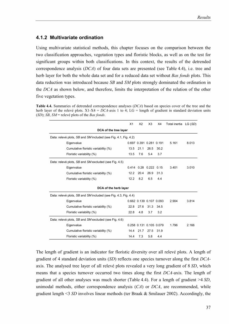
Results
4.1.2 Multivariate ordination
Using multivariate statistical methods, this chapter focuses on the comparison between the two classification approaches, vegetation types and floristic blocks, as well as on the test for significant groups within both classifications. In this context, the results of the detrended correspondence analysis (DCA) of four data sets are presented (see Table 4.4), i.e. tree and herb layer for both the whole data set and for a reduced data set without Bas fonds plots. This data reduction was introduced because SB and SM plots strongly dominated the ordination in the DCA as shown below, and therefore, limits the interpretation of the relation of the other five vegetation types.
Table 4.4. Summaries of detrended correspondence analyses (DCA) based on species cover of the tree and the herb layer of the relevé plots. X1-X4 = DCA-axis 1 to 4; LG = length of gradient in standard deviation units (SD); SB, SM = relevé plots of the Bas fonds.
DCA of the tree layer
Data: relevé plots, and included (see Fig. 4.1, Fig. 4.2)SB SM
Eigenvalue
Cumulative floristic variability (%)
Floristic variability (%)
Data: relevé plots, and excluded (see Fig. 4.5)SB SM
Eigenvalue
DCA of the herb layer
Data: relevé plots, and included (see Fig. 4.3, Fig. 4.4)SB SM
Eigenvalue
Data: relevé plots, and excluded (see Fig. 4.6)SB SM
Eigenvalue
0.697
13.5
13.5
0.414
12.2
12.2
0.662
22.8
22.8
0.258
14.4
14.4
0.391
21.1
7.6
0.28
20.4
8.2
0.139
27.6
4.8
0.131
21.7
7.3
0.281
26.5
5.4
0.222
26.9
6.5
0.107
31.3
3.7
0.105
27.5
5.8
0.191
30.2
3.7
0.15
31.3
4.4
0.093
34.5
3.2
0.079
31.9
4.4
5.161
3.401
2.904
1.796
8.013
3.010
3.814
2.166
X1 X2 X3 X4 Total inertia LG ( )SD
Cumulative floristic variability (%)
Floristic variability (%)
Cumulative floristic variability (%)
Floristic variability (%)
Cumulative floristic variability (%)
Floristic variability (%)
The length of gradient is an indicator for floristic diversity over all relevé plots. A length of gradient of 4 standard deviation units (SD) reflects one species turnover along the first DCA-axis. The analysed tree layer of all relevé plots revealed a very long gradient of 8 SD, which means that a species turnover occurred two times along the first DCA-axis. The length of gradient of all other analyses was much shorter (Table 4.4). For a length of gradient >4 SD, unimodal methods, either correspondence analysis (CA) or DCA, are recommended, while gradient length <3 SD involves linear methods (ter Braak & Smilauer 2002). Accordingly, the
37
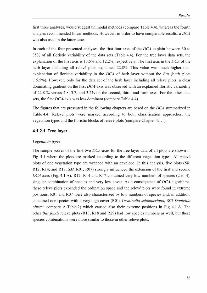
Results
first three analyses, would suggest unimodal methods (compare Table 4.4), whereas the fourth analysis recommended linear methods. However, in order to have comparable results, a DCA was also used in the latter case.
In each of the four presented analyses, the first four axes of the DCA explain between 30 to 35% of all floristic variability of the data sets (Table 4.4). For the tree layer data sets, the explanation of the first axis is 13.5% and 12.2%, respectively. The first axis in the DCA of the herb layer including all relevé plots explained 22.8%. This value was much higher than explanation of floristic variability in the DCA of herb layer without the Bas fonds plots (15.5%). However, only for the data set of the herb layer including all relevé plots, a clear dominating gradient on the first DCA-axis was observed with an explained floristic variability of 22.8 % versus 4.8, 3.7, and 3.2% on the second, third, and forth axes. For the other data sets, the first DCA-axis was less dominant (compare Table 4.4).
The figures that are presented in the following chapters are based on the DCA summarized in Table 4.4. Relevé plots were marked according to both classification approaches, the vegetation types and the floristic blocks of relevé plots (compare Chapter 4.1.1).
4.1.2.1 Tree layer
Vegetation types
The sample scores of the first two DCA-axes for the tree layer data of all plots are shown in Fig. 4.1 where the plots are marked according to the different vegetation types. All relevé plots of one vegetation type are wrapped with an envelope. In this analysis, five plots (SB: R12, R14, and R17; SM: R01, R07) strongly influenced the extension of the first and second DCA-axes (Fig. 4.1 A). R12, R14 and R17 contained very low numbers of species (2 to 4), singular combination of species and very low cover. As a consequence of DCA-algorithms, these relevé plots expanded the ordination space and the relevé plots were found in extreme positions. R01 and R07 were also characterized by low numbers of species and, in addition, contained one species with a very high cover (R01: Terminalia schimperiana, R07 Daniellia oliveri, compare A-Table 2) which caused also their extreme positions in Fig. 4.1 A. The other Bas fonds relevé plots (R13, R18 and R29) had low species numbers as well, but these species combinations were more similar to those in other relevé plots.
38
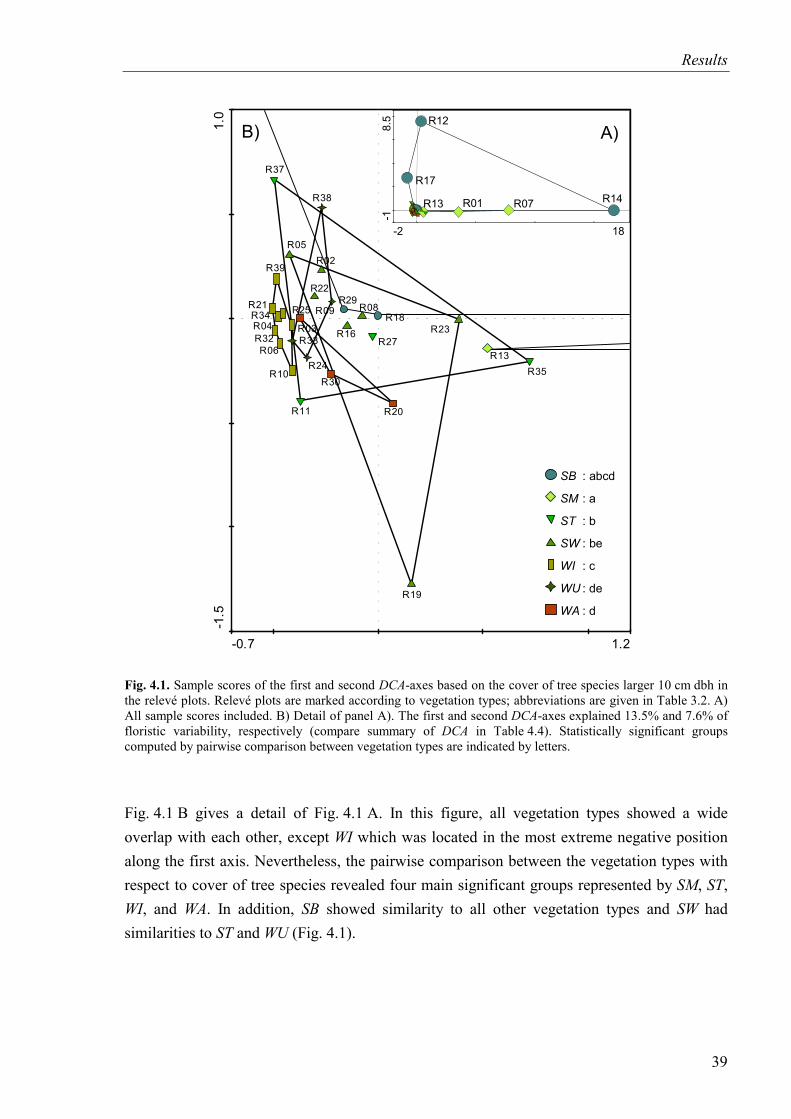
Results
-0.7 1.2
-1.5
1.0
R18
R29
R13
R11
R27
R35
R37
R02R05
R08
R16
R19
R22
R23R03R04
R06
R10
R21
R32
R34
R39
R09
R24
R33
R38
R20
R25
R30
SB : abcd
SM : a
ST : b
SW : be
WI : c
WU : de
WA : d
-2 18
-18.
5 R12
R14R17
R01 R07R13
B) A)
Fig. 4.1. Sample scores of the first and second DCA-axes based on the cover of tree species larger 10 cm dbh in the relevé plots. Relevé plots are marked according to vegetation types; abbreviations are given in Table 3.2. A) All sample scores included. B) Detail of panel A). The first and second DCA-axes explained 13.5% and 7.6% of floristic variability, respectively (compare summary of DCA in Table 4.4). Statistically significant groups computed by pairwise comparison between vegetation types are indicated by letters.
Fig. 4.1 B gives a detail of Fig. 4.1 A. In this figure, all vegetation types showed a wide overlap with each other, except WI which was located in the most extreme negative position along the first axis. Nevertheless, the pairwise comparison between the vegetation types with respect to cover of tree species revealed four main significant groups represented by SM, ST, WI, and WA. In addition, SB showed similarity to all other vegetation types and SW had similarities to ST and WU (Fig. 4.1).
39
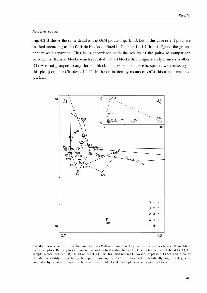
Results
Floristic blocks
Fig. 4.2 B shows the same detail of the DCA plot as Fig. 4.1 B, but in this case relevé plots are marked according to the floristic blocks outlined in Chapter 4.1.1.1. In this figure, the groups appear well separated. This is in accordance with the results of the pairwise comparison between the floristic blocks which revealed that all blocks differ significantly from each other. R19 was not grouped to any floristic block of plots as characteristic species were missing in this plot (compare Chapter 4.1.1.1). In the ordination by means of DCA this aspect was also obvious.
B) A)
-0.7 1.2
-1.5
1.0
R18R29
R13
R11
R27
R35
R37
R02R05
R08
R16
R19
R22
R23R03R04
R06
R10
R21
R32
R34
R39
R09
R24
R33
R38
R20
R25
R30
1 : a
2 : b
3 : c
4 : d
5 : -
-2 18
-18.
5
R14
R17
R12
R07R01R13
Fig. 4.2. Sample scores of the first and second DCA-axes based on the cover of tree species larger 10 cm dbh in the relevé plots. Relevé plots are marked according to floristic blocks of relevé plots (compare Table 4.1). A) All sample scores included. B) Detail of panel A). The first and second DCA-axes explained 13.5% and 7.6% of floristic variability, respectively (compare summary of DCA in Table 4.4). Statistically significant groups computed by pairwise comparison between floristic blocks of relevé plots are indicated by letters.
40
Results
4.1.2.2 Herb layer
Vegetation types
Sample scores of the first two DCA-axes for the herb layer were marked according to the vegetation types shown in Fig. 4.3. The relevé plots of SB and SM were located on the positive side of the first DCA-axis and are well separated from the other vegetation types which appear rather aggregated on the negative side of the first DCA-axis. The floristic composition of SB and SM was responsible for the distinct gradient along the first DCA-axis with the high explanation of 22.8 % (compare Table 4.4). Pairwise comparison between the vegetation types also showed that both SB and SM belong to a common single significant group. This underlines again the floristic difference of SB and SM from all other vegetation types. The other five vegetation types showed a continuous transition in the following order: SW - ST - WI - WU - WA. Hereby, each vegetation type was similar to its neighbour (Fig. 4.3). This result is in agreement with the results shown in A-Table 2.
-1.6 4.0
-1.0
1.5
R12
R14
R15R17R18
R29
R01
R07
R13
R11
R27
R35
R37
R02
R05
R08
R16R19
R22R23
R03R04
R06
R10
R21
R32R34
R39 R09
R24
R33
R38
R20
R25
R30
SB : a
SM : b
ST : cd
SW : c
WI : de
WU : ef
WA : f
Fig. 4.3. Sample scores of the first and second DCA-axes based on the species cover in the herb layer of the relevé plots. Relevé plots are marked according to vegetation types; abbreviations are given in Table 3.2. The first and second DCA-axes explained 22.8% and 4.8% of floristic variability, respectively (compare summary of DCA in Table 4.4). Statistically significant groups computed by pairwise comparison between vegetation types are indicated by letters.
41
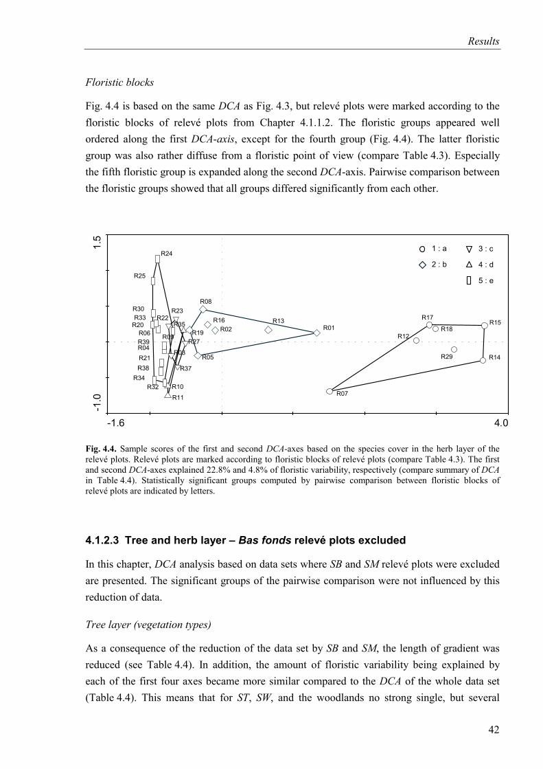
Results
Floristic blocks
Fig. 4.4 is based on the same DCA as Fig. 4.3, but relevé plots were marked according to the floristic blocks of relevé plots from Chapter 4.1.1.2. The floristic groups appeared well ordered along the first DCA-axis, except for the fourth group (Fig. 4.4). The latter floristic group was also rather diffuse from a floristic point of view (compare Table 4.3). Especially the fifth floristic group is expanded along the second DCA-axis. Pairwise comparison between the floristic groups showed that all groups differed significantly from each other.
-1.6 4.0
-1.0
1.5
R12
R14
R15R17
R18
R29
R01
R07
R13
R11
R27
R35
R37
R02
R05
R08
R16
R19
R22R23
R03R04
R06
R10
R21
R32R34
R39R09
R24
R33
R38
R20
R25
R30
1 : a
2 : b
3 : c
4 : d
5 : e
Fig. 4.4. Sample scores of the first and second DCA-axes based on the species cover in the herb layer of the relevé plots. Relevé plots are marked according to floristic blocks of relevé plots (compare Table 4.3). The first and second DCA-axes explained 22.8% and 4.8% of floristic variability, respectively (compare summary of DCA in Table 4.4). Statistically significant groups computed by pairwise comparison between floristic blocks of relevé plots are indicated by letters.
4.1.2.3 Tree and herb layer – Bas fonds relevé plots excluded
In this chapter, DCA analysis based on data sets where SB and SM relevé plots were excluded are presented. The significant groups of the pairwise comparison were not influenced by this reduction of data.
Tree layer (vegetation types)
As a consequence of the reduction of the data set by SB and SM, the length of gradient was reduced (see Table 4.4). In addition, the amount of floristic variability being explained by each of the first four axes became more similar compared to the DCA of the whole data set (Table 4.4). This means that for ST, SW, and the woodlands no strong single, but several
42
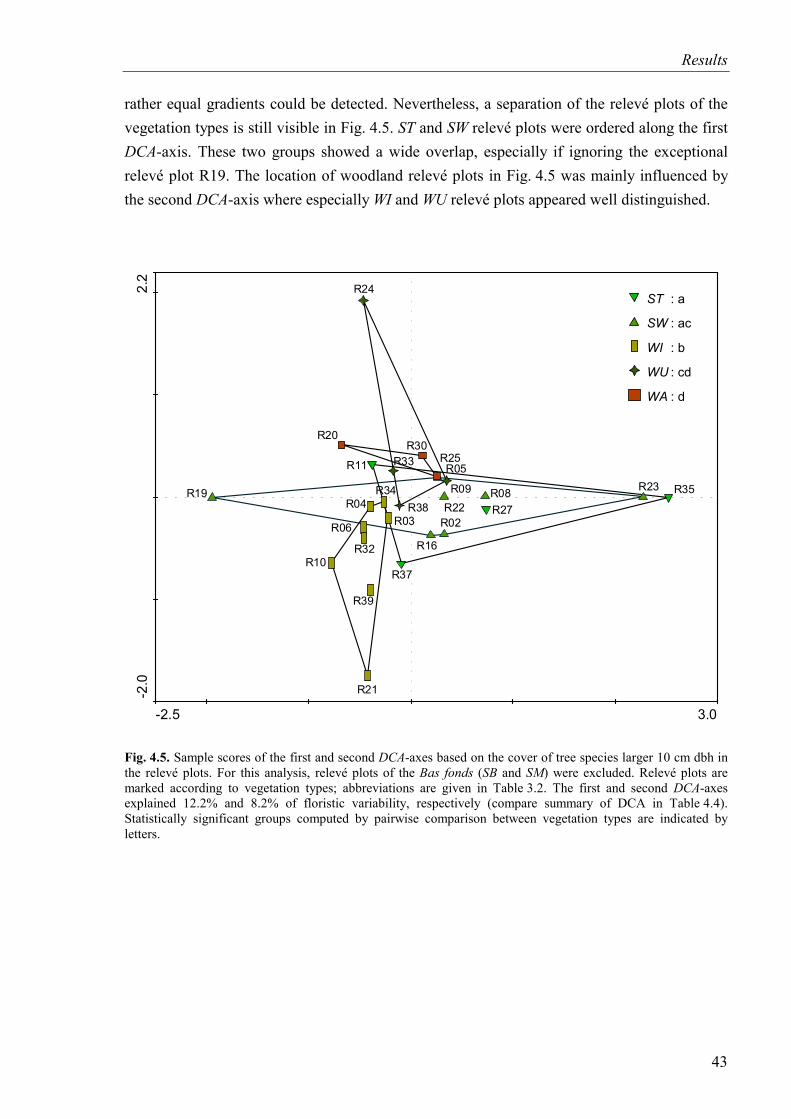
Results
rather equal gradients could be detected. Nevertheless, a separation of the relevé plots of the vegetation types is still visible in Fig. 4.5. ST and SW relevé plots were ordered along the first DCA-axis. These two groups showed a wide overlap, especially if ignoring the exceptional relevé plot R19. The location of woodland relevé plots in Fig. 4.5 was mainly influenced by the second DCA-axis where especially WI and WU relevé plots appeared well distinguished.
-2.5 3.0
-2.0
2.2
R11
R27
R35
R37
R02
R05
R08
R16
R19R22
R23
R03R04
R06
R10
R21
R32
R34
R39
R09
R24
R33
R38
R20
R25R30
ST : a
SW : ac
WI : b
WU : cd
WA : d
Fig. 4.5. Sample scores of the first and second DCA-axes based on the cover of tree species larger 10 cm dbh in the relevé plots. For this analysis, relevé plots of the Bas fonds (SB and SM) were excluded. Relevé plots are marked according to vegetation types; abbreviations are given in Table 3.2. The first and second DCA-axes explained 12.2% and 8.2% of floristic variability, respectively (compare summary of DCA in Table 4.4). Statistically significant groups computed by pairwise comparison between vegetation types are indicated by letters.
43
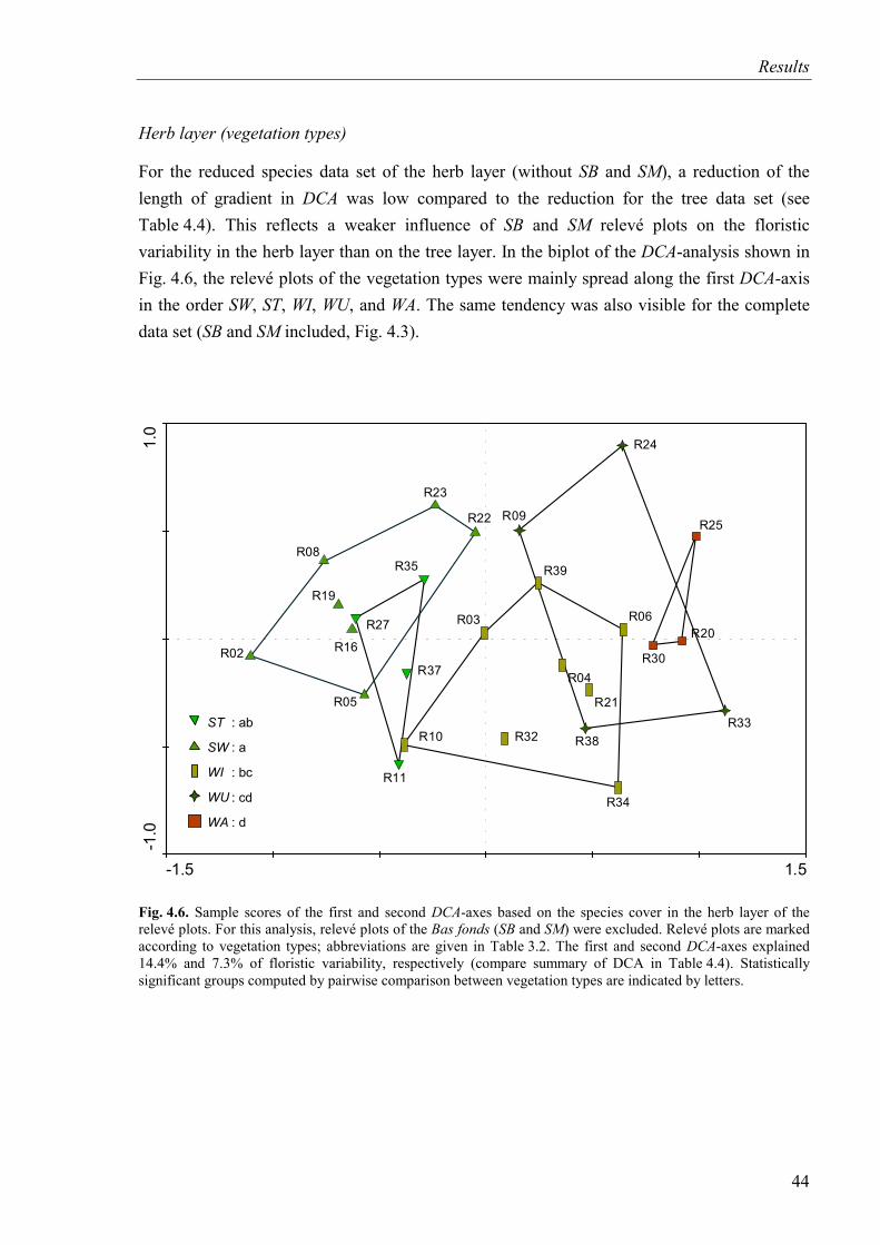
Results
Herb layer (vegetation types)
For the reduced species data set of the herb layer (without SB and SM), a reduction of the length of gradient in DCA was low compared to the reduction for the tree data set (see Table 4.4). This reflects a weaker influence of SB and SM relevé plots on the floristic variability in the herb layer than on the tree layer. In the biplot of the DCA-analysis shown in Fig. 4.6, the relevé plots of the vegetation types were mainly spread along the first DCA-axis in the order SW, ST, WI, WU, and WA. The same tendency was also visible for the complete data set (SB and SM included, Fig. 4.3).
-1.5 1.5
-1.0
1.0
R11
R27
R35
R37R02
R05
R08
R16
R19
R22
R23
R03
R04
R06
R10
R21
R32
R34
R39
R09
R24
R33R38
R20
R25
R30
ST : ab
SW : a
WI : bc
WU : cd
WA : d
Fig. 4.6. Sample scores of the first and second DCA-axes based on the species cover in the herb layer of the relevé plots. For this analysis, relevé plots of the Bas fonds (SB and SM) were excluded. Relevé plots are marked according to vegetation types; abbreviations are given in Table 3.2. The first and second DCA-axes explained 14.4% and 7.3% of floristic variability, respectively (compare summary of DCA in Table 4.4). Statistically significant groups computed by pairwise comparison between vegetation types are indicated by letters.
44
Results
4.2 Structural characteristics of vegetation types
This chapter focuses on structural characteristics of the studied vegetation types. For the tree layer (Chapter 4.2.1), the distribution of height and diameter classes as well as tree cover and tree biomass are presented. For the herb layer (Chapter 4.2.2), cover, height, volume and mass of grass, herb and litter fraction are shown. In addition, the parameters cover of open ground, cover of dead woody biomass and cover of termite mounds are given in A-Table 6.
4.2.1 Tree layer
Diameter classes
Diameter class distribution of tree individuals in all relevé plots showed a general tendency of an age pyramid with smaller diameter classes occurring with a higher density than larger ones (Fig. 4.7). However, especially in WU the trees of medium diameter class had largest densities. The maximal density of the smallest trees (<5 cm dbh) with 500 tree individuals ha-1 was found in SW, whereas a maximum density of 200 and 33 tree individuals ha-1 occurred for the diameter class 20-<45 cm dbh in SW and the diameter class ≥45 cm dbh in WI, respectively. As expected, woodland types (WI, WU, and WA) and SW showed higher tree densities than SB, SM, and ST. This was especially the case for the medium diameter classes 10-<20 and 20-<45 cm dbh. The change from open to closed stands, however, is not abrupt but has a gradual character. The multivariate pairwise comparison between the vegetation types based on the diameter class distribution supported this observation. Even though the ‘open savanna’ (SB) was clearly distinguished from ‘dense woodlands’ (WU and WA), a wide overlap of statistical groups was found.
Height classes
With respect to the height class distribution of vegetation types presented in Fig. 4.8, vegetation types can be divided into two groups. The first group (SB, SM, and ST) showed a rather similar density within each height class, whereas the second group (SW, WI, WU, and WA) was characterized by high abundance of taller tree individuals, especially of the height class 5-<10 m. The latter vegetation types generally build up higher stands than the first group.
Separation of vegetation types by means of height class distribution was much clearer than by means of diameter classes. Pairwise comparison between vegetation types by means of height classes revealed four significant groups being characterised by SB, ST, SW, and WU (Fig. 4.8). SM showed similarities to SB, ST, and SW, whereas WI and WA were similar to ST, SW, and WU.
45
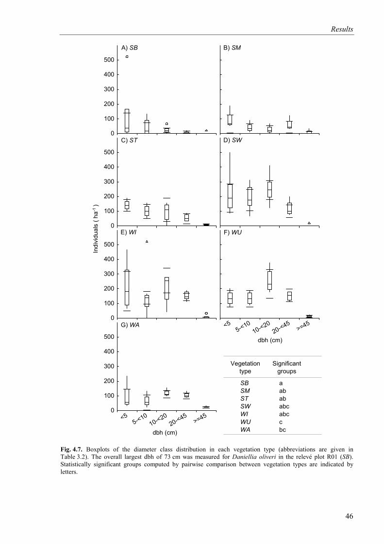
Results
0
100
200
300
400
500
<55-<10
10-<2020-<45 <45
dbh (cm)
B) SM
0
100
200
300
400
500
<55-<10
10-<2020-<45 <45
dbh (cm)
A) SB
0
100
200
300
400
500
<55-<10
10-<2020-<45 <45
dbh (cm)
D) SW
0
100
200
300
400
500
<55-<10
10-<2020-<45 <45
dbh (cm)
C) ST
0
100
200
300
400
500
<55-<10
10-<2020-<45 <45
F) WU
0
100
200
300
400
500
<55-<10
10-<2020-<45 <45
dbh (cm)
E) WI
0
100
200
300
400
500
<55-<10
10-<2020-<45
>=45
G) WA
Indi
vidu
als
(ha
)-1
dbh (cm)
dbh (cm)
SBSMSTSWWIWUWA
Vegetationtype
aabababcabccbc
<55-<10
10-<2020-<45
>=45
Significantgroups
Fig. 4.7. Boxplots of the diameter class distribution in each vegetation type (abbreviations are given in Table 3.2). The overall largest dbh of 73 cm was measured for Daniellia oliveri in the relevé plot R01 (SB). Statistically significant groups computed by pairwise comparison between vegetation types are indicated by letters.
46
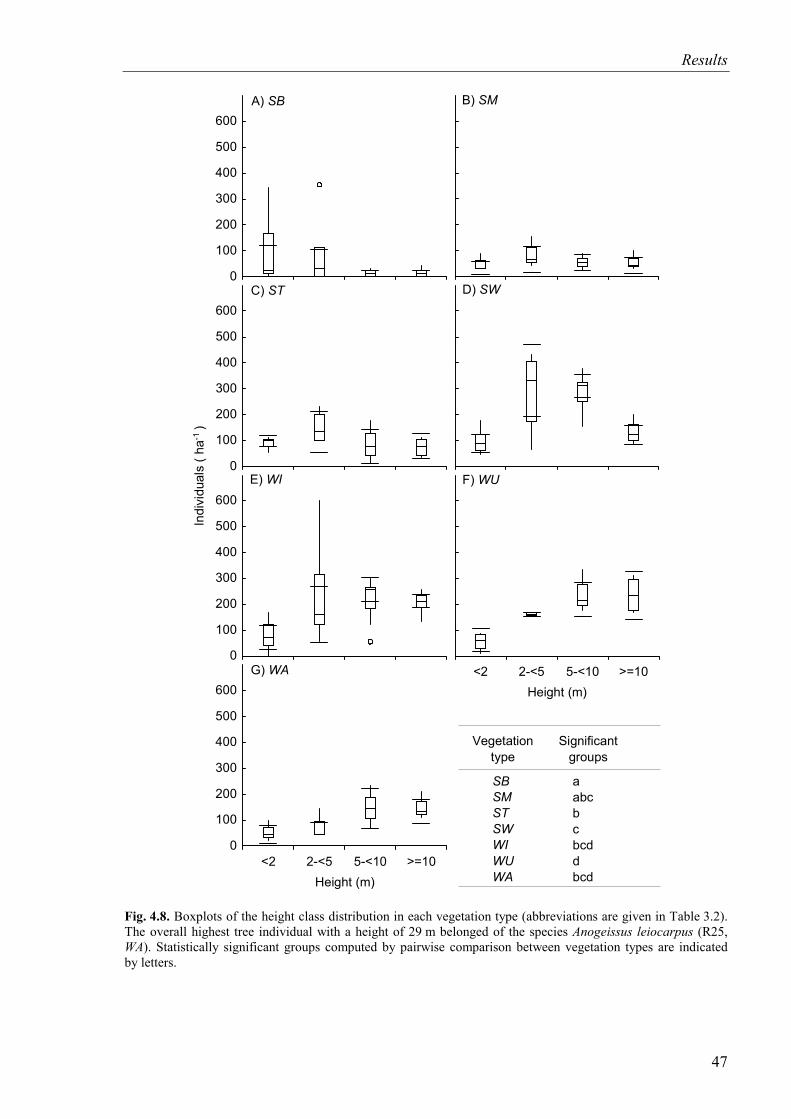
Results
Indi
vidu
als
(ha
)-1
0
100
200
300
400
500
600
<2 2-<5 5-<10 >=10Height (m)
0
100
200
300
400
500
600
<2 2-<5 5-<10 >=10Height (m)
A) SB B) SM
C) STD) SW
SBSMSTSWWIWUWA
Vegetationtype
aabcbcbcddbcd
0
100
200
300
400
500
600
<2 2-<5 5-<10 >=10Height (m)
0
100
200
300
400
500
600
<2 2-<5 5-<10 >=10Height (m)
0
100
200
300
400
500
600
<2 2-<5 5-<10 >=10Height (m)
0
100
200
300
400
500
600
<2 2-<5 5-<10 >=10Height (m)
E) WI F) WU
0
100
200
300
400
500
600
<2 2-<5 5-<10 >=10Height (m)
G) WA
C) ST D) SW
Significantgroups
Fig. 4.8. Boxplots of the height class distribution in each vegetation type (abbreviations are given in Table 3.2). The overall highest tree individual with a height of 29 m belonged of the species Anogeissus leiocarpus (R25, WA). Statistically significant groups computed by pairwise comparison between vegetation types are indicated by letters.
47
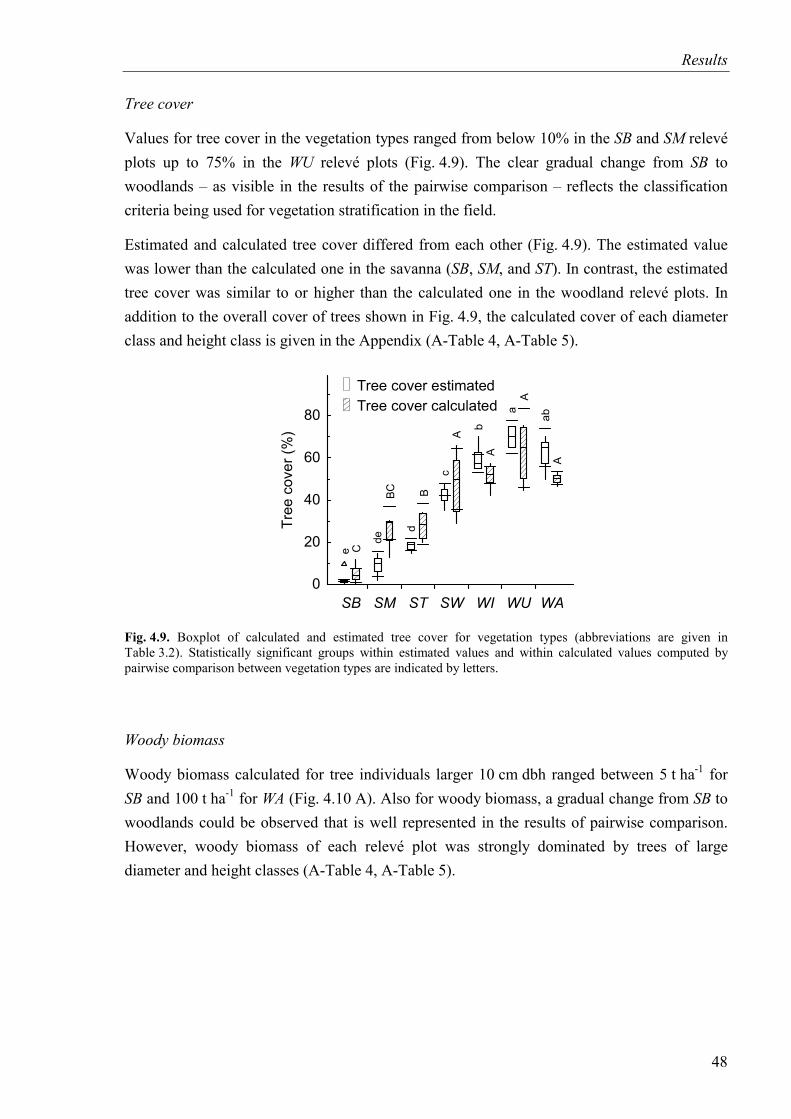
Results
Tree cover
Values for tree cover in the vegetation types ranged from below 10% in the SB and SM relevé plots up to 75% in the WU relevé plots (Fig. 4.9). The clear gradual change from SB to woodlands – as visible in the results of the pairwise comparison – reflects the classification criteria being used for vegetation stratification in the field.
Estimated and calculated tree cover differed from each other (Fig. 4.9). The estimated value was lower than the calculated one in the savanna (SB, SM, and ST). In contrast, the estimated tree cover was similar to or higher than the calculated one in the woodland relevé plots. In addition to the overall cover of trees shown in Fig. 4.9, the calculated cover of each diameter class and height class is given in the Appendix (A-Table 4, A-Table 5).
0
20
40
60
80
Tree
cove
r(%
)
Tree cover estimated
SB SM ST SW WI WU WA
Tree cover calculated
e C
deBC
dB
cA
bA
aA
abA
Fig. 4.9. Boxplot of calculated and estimated tree cover for vegetation types (abbreviations are given in Table 3.2). Statistically significant groups within estimated values and within calculated values computed by pairwise comparison between vegetation types are indicated by letters.
Woody biomass
Woody biomass calculated for tree individuals larger 10 cm dbh ranged between 5 t ha-1 for SB and 100 t ha-1 for WA (Fig. 4.10 A). Also for woody biomass, a gradual change from SB to woodlands could be observed that is well represented in the results of pairwise comparison. However, woody biomass of each relevé plot was strongly dominated by trees of large diameter and height classes (A-Table 4, A-Table 5).
48
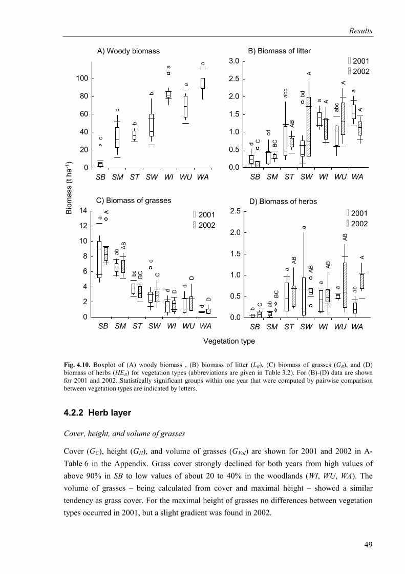
Results
Vegetation type
B) Biomass of litter
0.0
0.5
1.0
1.5
2.0
2.5
3.0
SB SM ST SW WI WU WASB SM ST SW WI WU WA
20012002
SB SM ST SW WI WU WA
d C
cdBC
abc
AB
bdA
a A
abc
A
aA
0
2
4
6
8
10
12
14
SB SM ST SW WI WU WASB SM ST SW WI WU WASB SM ST SW WI WU WA
20012002
C) Biomass of grasses
aA
abAB
bc BC
cC
d D
dD
dD
0
20
40
60
80
100
SB SM ST SW WI WU WA
A) Woody biomass
c
b
b
b
a
a
a
0.0
0.5
1.0
1.5
2.0
2.5
SB SM ST SW WI WU WASB SM ST SW WI WU WASB SM ST SW WI WU WA
20012002
D) Biomass of herbs
b C abBC
aAB
aAB
aAB
aAB
abA
Biom
ass
(tha
)-1
Fig. 4.10. Boxplot of (A) woody biomass , (B) biomass of litter (LB), (C) biomass of grasses (GB), and (D) biomass of herbs (HEB) for vegetation types (abbreviations are given in Table 3.2). For (B)-(D) data are shown for 2001 and 2002. Statistically significant groups within one year that were computed by pairwise comparison between vegetation types are indicated by letters.
4.2.2 Herb layer
Cover, height, and volume of grasses
Cover (GC), height (GH), and volume of grasses (GVol) are shown for 2001 and 2002 in A-Table 6 in the Appendix. Grass cover strongly declined for both years from high values of above 90% in SB to low values of about 20 to 40% in the woodlands (WI, WU, WA). The volume of grasses – being calculated from cover and maximal height – showed a similar tendency as grass cover. For the maximal height of grasses no differences between vegetation types occurred in 2001, but a slight gradient was found in 2002.
49
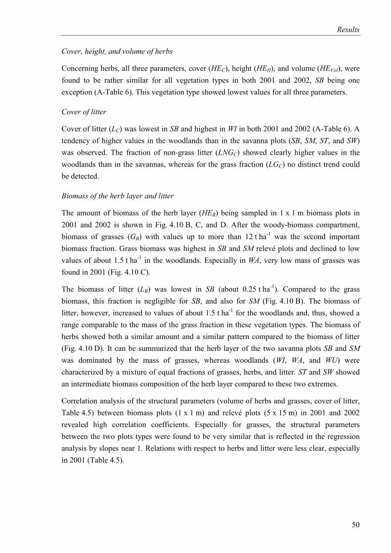
Results
Cover, height, and volume of herbs
Concerning herbs, all three parameters, cover (HEC), height (HEH), and volume (HEVol), were found to be rather similar for all vegetation types in both 2001 and 2002, SB being one exception (A-Table 6). This vegetation type showed lowest values for all three parameters.
Cover of litter
Cover of litter (LC) was lowest in SB and highest in WI in both 2001 and 2002 (A-Table 6). A tendency of higher values in the woodlands than in the savanna plots (SB, SM, ST, and SW) was observed. The fraction of non-grass litter (LNGC) showed clearly higher values in the woodlands than in the savannas, whereas for the grass fraction (LGC) no distinct trend could be detected.
Biomass of the herb layer and litter
The amount of biomass of the herb layer (HEB) being sampled in 1 x 1 m biomass plots in 2001 and 2002 is shown in Fig. 4.10 B, C, and D. After the woody-biomass compartment, biomass of grasses (GB) with values up to more than 12 t ha-1 was the second important biomass fraction. Grass biomass was highest in SB and SM relevé plots and declined to low values of about 1.5 t ha-1 in the woodlands. Especially in WA, very low mass of grasses was found in 2001 (Fig. 4.10 C).
The biomass of litter (LB) was lowest in SB (about 0.25 t ha-1). Compared to the grass biomass, this fraction is negligible for SB, and also for SM (Fig. 4.10 B). The biomass of litter, however, increased to values of about 1.5 t ha-1 for the woodlands and, thus, showed a range comparable to the mass of the grass fraction in these vegetation types. The biomass of herbs showed both a similar amount and a similar pattern compared to the biomass of litter (Fig. 4.10 D). It can be summarized that the herb layer of the two savanna plots SB and SM was dominated by the mass of grasses, whereas woodlands (WI, WA, and WU) were characterized by a mixture of equal fractions of grasses, herbs, and litter. ST and SW showed an intermediate biomass composition of the herb layer compared to these two extremes.
Correlation analysis of the structural parameters (volume of herbs and grasses, cover of litter, Table 4.5) between biomass plots (1 x 1 m) and relevé plots (5 x 15 m) in 2001 and 2002 revealed high correlation coefficients. Especially for grasses, the structural parameters between the two plots types were found to be very similar that is reflected in the regression analysis by slopes near 1. Relations with respect to herbs and litter were less clear, especially in 2001 (Table 4.5).
50
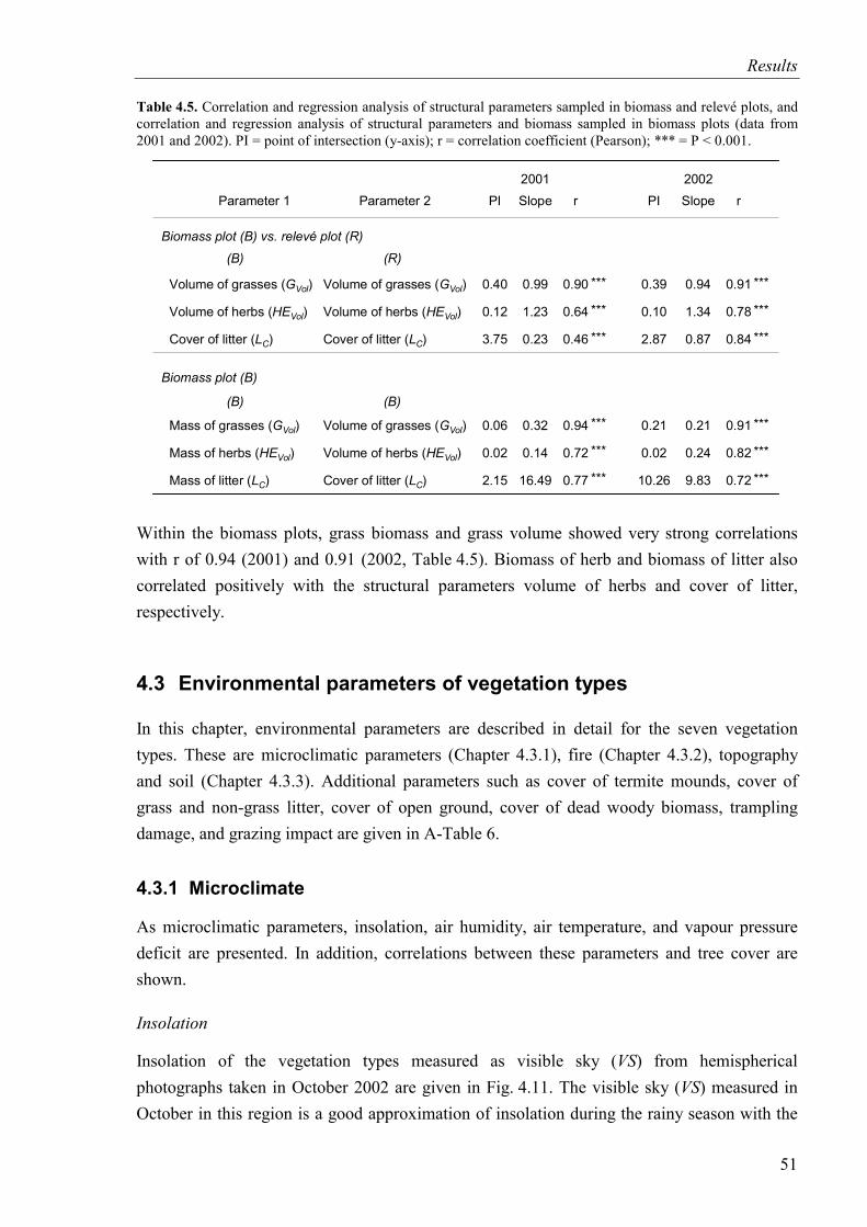
Results
Table 4.5. Correlation and regression analysis of structural parameters sampled in biomass and relevé plots, and correlation and regression analysis of structural parameters and biomass sampled in biomass plots (data from 2001 and 2002). PI = point of intersection (y-axis); r = correlation coefficient (Pearson); *** = P < 0.001.
Biomass plot ( ) vs. relevé plot (R)B
Biomass plot (B)
Parameter 1
Volume of grasses ( )GVol
Volume of herbs ( )HEVol
Cover of litter ( )LC
Mass of grasses ( )GVol
Mass of herbs ( )HEVol
Mass of litter ( )LC
Parameter 2
Volume of grasses ( )GVol
Volume of herbs ( )HEVol
Cover of litter ( )LC
Volume of grasses ( )GVol
Volume of herbs ( )HEVol
Cover of litter ( )LC
PI
0.40
0.12
3.75
0.06
0.02
2.15
Slope
0.99
1.23
0.23
0.32
0.14
16.49
r
0.90
0.64
0.46
0.94
0.72
0.77
***
***
***
***
***
***
PI
0.39
0.10
2.87
0.21
0.02
10.26
Slope
0.94
1.34
0.87
0.21
0.24
9.83
r
0.91
0.78
0.84
0.91
0.82
0.72
2001 2002
***
***
***
***
***
***
(B) (B)
( )B ( )R
Within the biomass plots, grass biomass and grass volume showed very strong correlations with r of 0.94 (2001) and 0.91 (2002, Table 4.5). Biomass of herb and biomass of litter also correlated positively with the structural parameters volume of herbs and cover of litter, respectively.
4.3 Environmental parameters of vegetation types
In this chapter, environmental parameters are described in detail for the seven vegetation types. These are microclimatic parameters (Chapter 4.3.1), fire (Chapter 4.3.2), topography and soil (Chapter 4.3.3). Additional parameters such as cover of termite mounds, cover of grass and non-grass litter, cover of open ground, cover of dead woody biomass, trampling damage, and grazing impact are given in A-Table 6.
4.3.1 Microclimate
As microclimatic parameters, insolation, air humidity, air temperature, and vapour pressure deficit are presented. In addition, correlations between these parameters and tree cover are shown.
Insolation
Insolation of the vegetation types measured as visible sky (VS) from hemispherical photographs taken in October 2002 are given in Fig. 4.11. The visible sky (VS) measured in October in this region is a good approximation of insolation during the rainy season with the
51
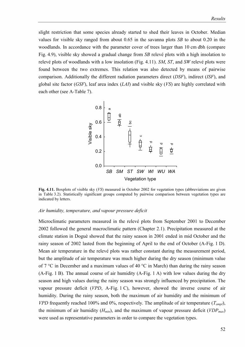
Results
slight restriction that some species already started to shed their leaves in October. Median values for visible sky ranged from about 0.65 in the savanna plots SB to about 0.20 in the woodlands. In accordance with the parameter cover of trees larger than 10 cm dbh (compare Fig. 4.9), visible sky showed a gradual change from SB relevé plots with a high insolation to relevé plots of woodlands with a low insolation (Fig. 4.11). SM, ST, and SW relevé plots were found between the two extremes. This relation was also detected by means of pairwise comparison. Additionally the different radiation parameters direct (DSF), indirect (ISF), and global site factor (GSF), leaf area index (LAI) and visible sky (VS) are highly correlated with each other (see A-Table 7).
0.0
0.2
0.4
0.6
0.8
Visi
ble
sky
SB SM ST SW WI WU WAVegetation type
a
ab
bc
c
dd d
Fig. 4.11. Boxplots of visible sky (VS) measured in October 2002 for vegetation types (abbreviations are given in Table 3.2). Statistically significant groups computed by pairwise comparison between vegetation types are indicated by letters.
Air humidity, temperature, and vapour pressure deficit
Microclimatic parameters measured in the relevé plots from September 2001 to December 2002 followed the general macroclimatic pattern (Chapter 2.1). Precipitation measured at the climate station in Doguè showed that the rainy season in 2001 ended in mid October and the rainy season of 2002 lasted from the beginning of April to the end of October (A-Fig. 1 D). Mean air temperature in the relevé plots was rather constant during the measurement period, but the amplitude of air temperature was much higher during the dry season (minimum value of 7 °C in December and a maximum values of 40 °C in March) than during the rainy season (A-Fig. 1 B). The annual course of air humidity (A-Fig. 1 A) with low values during the dry season and high values during the rainy season was strongly influenced by precipitation. The vapour pressure deficit (VPD, A-Fig. 1 C), however, showed the inverse course of air humidity. During the rainy season, both the maximum of air humidity and the minimum of VPD frequently reached 100% and 0%, respectively. The amplitude of air temperature (Tampl), the minimum of air humidity (Hmin), and the maximum of vapour pressure deficit (VDPmax) were used as representative parameters in order to compare the vegetation types.
52
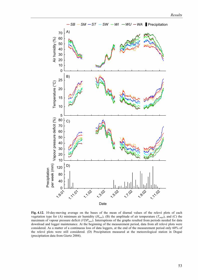
Results
010203040506070
Airh
umid
ity(%
)
1.9.01
1.11.0
11.1
.021.3
.021.5
.021.7
.021.9
.02
1.11.0
2
SB SM ST SW WI WU WA Precipitation
5
10
15
20
25
Tem
pera
ture
(°C
)
1.9.01
1.11.0
11.1
.021.3
.021.5
.021.7
.021.9
.02
1.11.0
2
Spalte 1
1020304050607080
Vapo
urpr
essu
rede
ficit
(%)
1.9.01
1.11.0
11.1
.021.3
.021.5
.021.7
.021.9
.02
1.11.0
2
Spalte 1
0
40
80
120
Prec
ipita
tion
perw
eek
(mm
)
1.9.01
1.11.0
11.1
.021.3
.021.5
.021.7
.021.9
.02
1.11.0
2
Date
A)
B)
C)
D)
Fig. 4.12. 10-day-moving average on the bases of the mean of diurnal values of the relevé plots of each vegetation type for (A) minimum air humidity (Hmin), (B) the amplitude of air temperature (Tampl), and (C) the maximum of vapour pressure deficit (VDPmax). Interruptions of the graphs resulted from periods needed for data download and logger maintenance. At the beginning of the measurement period, data from all relevé plots were considered. As a matter of a continuous loss of data loggers, at the end of the measurement period only 60% of the relevé plots were still considered. (D) Precipitation measured at the meteorological station in Doguè (precipitation data from Giertz 2004).
53
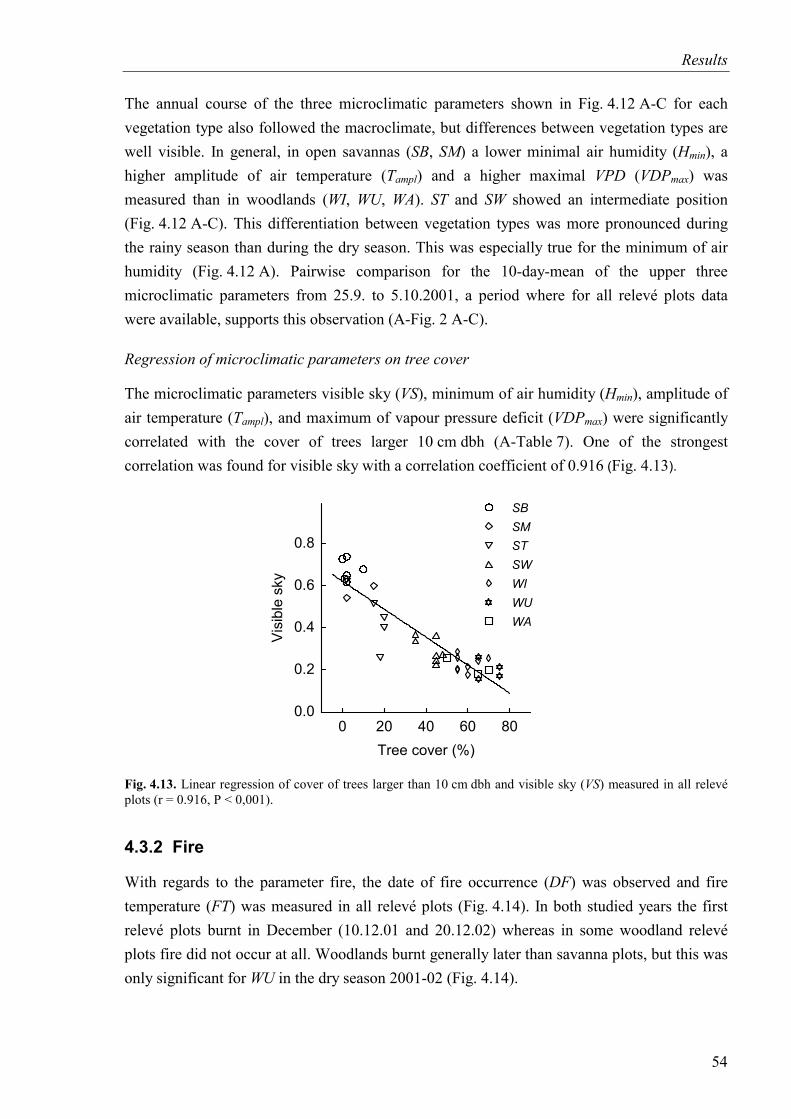
Results
The annual course of the three microclimatic parameters shown in Fig. 4.12 A-C for each vegetation type also followed the macroclimate, but differences between vegetation types are well visible. In general, in open savannas (SB, SM) a lower minimal air humidity (Hmin), a higher amplitude of air temperature (Tampl) and a higher maximal VPD (VDPmax) was measured than in woodlands (WI, WU, WA). ST and SW showed an intermediate position (Fig. 4.12 A-C). This differentiation between vegetation types was more pronounced during the rainy season than during the dry season. This was especially true for the minimum of air humidity (Fig. 4.12 A). Pairwise comparison for the 10-day-mean of the upper three microclimatic parameters from 25.9. to 5.10.2001, a period where for all relevé plots data were available, supports this observation (A-Fig. 2 A-C).
Regression of microclimatic parameters on tree cover
The microclimatic parameters visible sky (VS), minimum of air humidity (Hmin), amplitude of air temperature (Tampl), and maximum of vapour pressure deficit (VDPmax) were significantly correlated with the cover of trees larger 10 cm dbh (A-Table 7). One of the strongest correlation was found for visible sky with a correlation coefficient of 0.916 (Fig. 4.13).
0.0
0.2
0.4
0.6
0.8
Visi
ble
sky
0 20 40 60 80Tree cover (%)
SBSMSTSWWIWUWA
Fig. 4.13. Linear regression of cover of trees larger than 10 cm dbh and visible sky (VS) measured in all relevé plots (r = 0.916, P < 0,001).
4.3.2 Fire
With regards to the parameter fire, the date of fire occurrence (DF) was observed and fire temperature (FT) was measured in all relevé plots (Fig. 4.14). In both studied years the first relevé plots burnt in December (10.12.01 and 20.12.02) whereas in some woodland relevé plots fire did not occur at all. Woodlands burnt generally later than savanna plots, but this was only significant for WU in the dry season 2001-02 (Fig. 4.14).
54
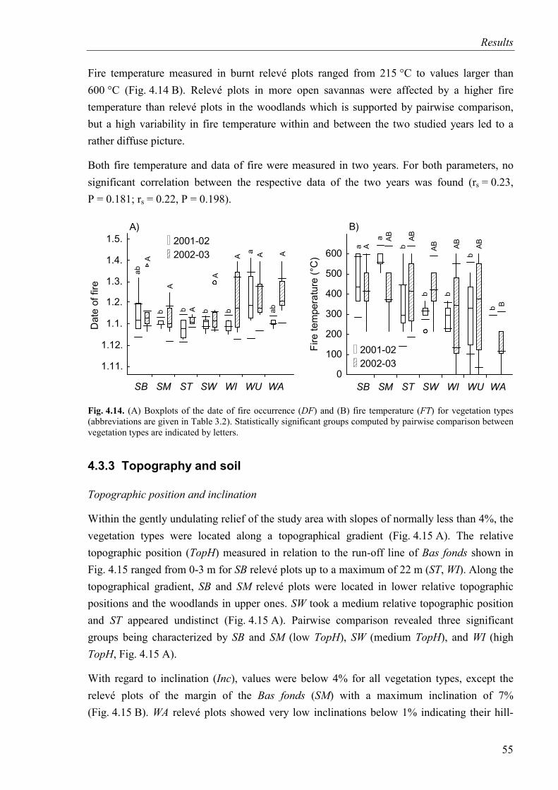
Results
Fire temperature measured in burnt relevé plots ranged from 215 °C to values larger than 600 °C (Fig. 4.14 B). Relevé plots in more open savannas were affected by a higher fire temperature than relevé plots in the woodlands which is supported by pairwise comparison, but a high variability in fire temperature within and between the two studied years led to a rather diffuse picture.
Both fire temperature and data of fire were measured in two years. For both parameters, no significant correlation between the respective data of the two years was found (rs = 0.23, P = 0.181; rs = 0.22, P = 0.198).
0
100
200
300
400
500
600
Fire
tem
pera
ture
(°C
)
SB SM ST SW WI WU WASB SM ST SW WI WU WASB SM ST SW WI WU WA
2001-022002-03
B)
a A
a AB
bAB
bAB
bAB
bAB
b B
62
92
122
152
182
212
242
Dat
eof
fire
SB SM ST SW WI WU WASB SM ST SW WI WU WA
2001-022002-03
A)
SB SM ST SW WI WU WA
ab
b b b b
a
ab
A
A
A
A
A A A
1.11.
1.12.
1.1.
1.2.
1.3.
1.4.
1.5.
Fig. 4.14. (A) Boxplots of the date of fire occurrence (DF) and (B) fire temperature (FT) for vegetation types (abbreviations are given in Table 3.2). Statistically significant groups computed by pairwise comparison between vegetation types are indicated by letters.
4.3.3 Topography and soil
Topographic position and inclination
Within the gently undulating relief of the study area with slopes of normally less than 4%, the vegetation types were located along a topographical gradient (Fig. 4.15 A). The relative topographic position (TopH) measured in relation to the run-off line of Bas fonds shown in Fig. 4.15 ranged from 0-3 m for SB relevé plots up to a maximum of 22 m (ST, WI). Along the topographical gradient, SB and SM relevé plots were located in lower relative topographic positions and the woodlands in upper ones. SW took a medium relative topographic position and ST appeared undistinct (Fig. 4.15 A). Pairwise comparison revealed three significant groups being characterized by SB and SM (low TopH), SW (medium TopH), and WI (high TopH, Fig. 4.15 A).
With regard to inclination (Inc), values were below 4% for all vegetation types, except the relevé plots of the margin of the Bas fonds (SM) with a maximum inclination of 7% (Fig. 4.15 B). WA relevé plots showed very low inclinations below 1% indicating their hill-
55
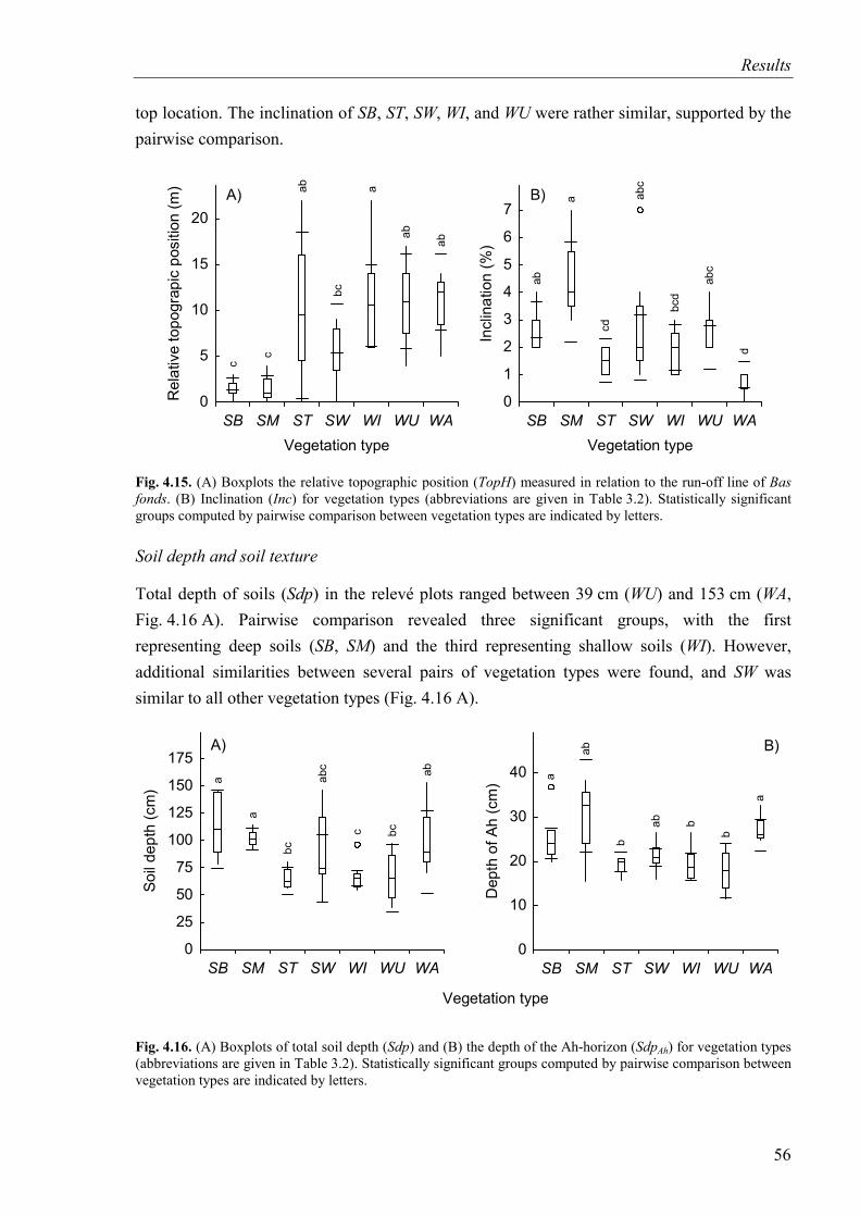
Results
top location. The inclination of SB, ST, SW, WI, and WU were rather similar, supported by the pairwise comparison.
0
5
10
15
20
Rel
ativ
eto
pogr
apic
posi
tion
(m)
SB SM ST SW WI WU WAVegetation type
0
1
2
3
4
5
6
7
Incl
inat
ion
(%)
SB SM ST SW WI WU WAVegetation type
A) B)
c
c
ab
bc
a
ab
ab
ab
a
cd
abc
bcd
abc
d
Fig. 4.15. (A) Boxplots the relative topographic position (TopH) measured in relation to the run-off line of Bas fonds. (B) Inclination (Inc) for vegetation types (abbreviations are given in Table 3.2). Statistically significant groups computed by pairwise comparison between vegetation types are indicated by letters.
Soil depth and soil texture
Total depth of soils (Sdp) in the relevé plots ranged between 39 cm (WU) and 153 cm (WA, Fig. 4.16 A). Pairwise comparison revealed three significant groups, with the first representing deep soils (SB, SM) and the third representing shallow soils (WI). However, additional similarities between several pairs of vegetation types were found, and SW was similar to all other vegetation types (Fig. 4.16 A).
0
25
50
75
100
125
150
175
Soil
dept
h(c
m)
SB SM ST SW WI WU WA
a
a
bc
abc
c bc
ab
0
10
20
30
40
Dep
thof
Ah(c
m)
SB SM ST SW WI WU WA
a
ab
b
ab b
b
a
Vegetation type
A) B)
Fig. 4.16. (A) Boxplots of total soil depth (Sdp) and (B) the depth of the Ah-horizon (SdpAh) for vegetation types (abbreviations are given in Table 3.2). Statistically significant groups computed by pairwise comparison between vegetation types are indicated by letters.
56
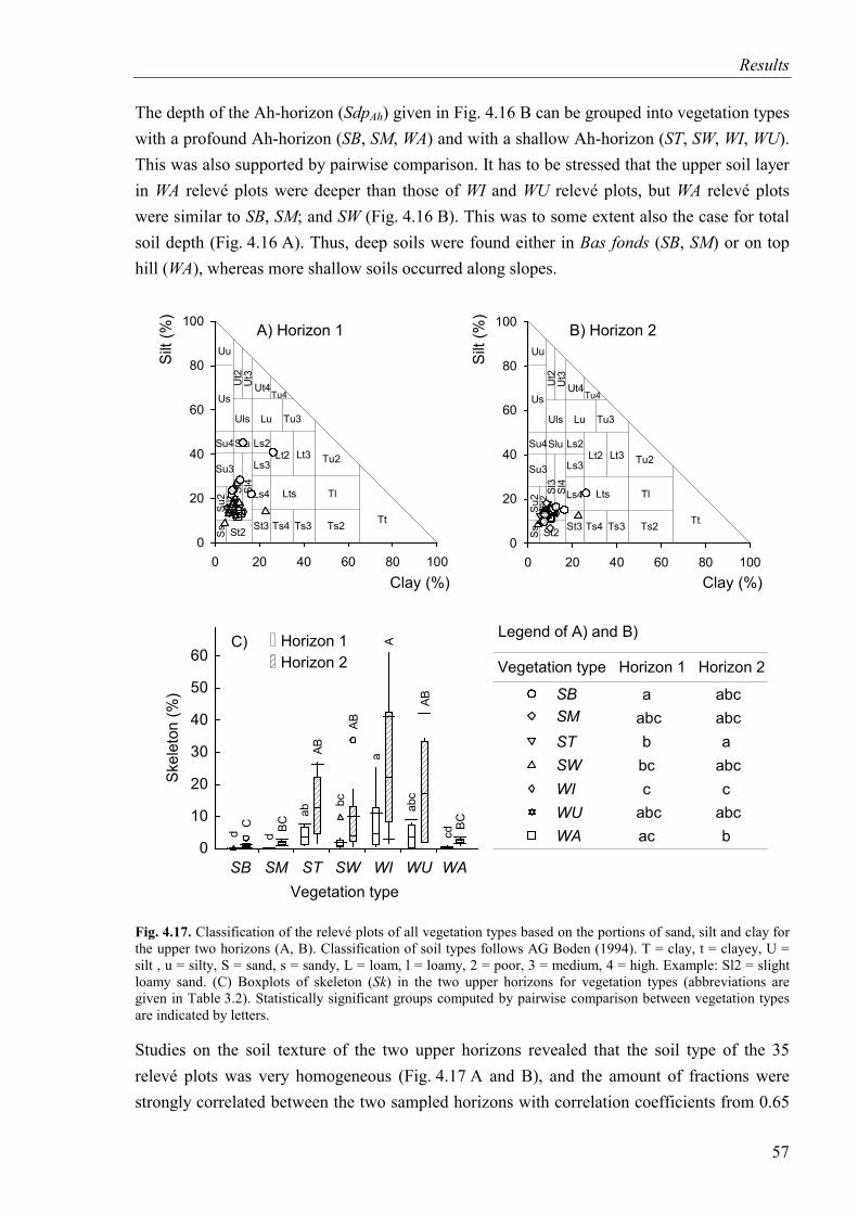
Results
The depth of the Ah-horizon (SdpAh) given in Fig. 4.16 B can be grouped into vegetation types with a profound Ah-horizon (SB, SM, WA) and with a shallow Ah-horizon (ST, SW, WI, WU). This was also supported by pairwise comparison. It has to be stressed that the upper soil layer in WA relevé plots were deeper than those of WI and WU relevé plots, but WA relevé plots were similar to SB, SM; and SW (Fig. 4.16 B). This was to some extent also the case for total soil depth (Fig. 4.16 A). Thus, deep soils were found either in Bas fonds (SB, SM) or on top hill (WA), whereas more shallow soils occurred along slopes.
0
10
20
30
40
50
60
Skel
eton
(%)
SB SM ST SW WI WU WASB SM ST SW WI WU WASB SM ST SW WI WU WA
d d
ab
bc
a
abc
cd
C BC
AB
AB
A
AB
BC
SBSMSTSWWIWUWA
aabcbbcc
abcac
abcabca
abcc
abcb
Vegetation type Horizon 1 Horizon 2
TtTs2
Tl
Tu2
Ts3Ts4
Lts
Lt2 Lt3
Tu3LuUls
Us
Uu
Su4Slu Ls2
Ls3
Ls4
St3St2
Su3
Tu4Ut4U
t3Ut2
Ss
Su2 Sl2
Sl3
Sl4
0
20
40
60
80
100
0 20 40 60 80 100Clay (%)
Silt
(%)
TtTs2
Tl
Tu2
Ts3Ts4
Lts
Lt2 Lt3
Tu3LuUls
Us
Uu
Su4Slu Ls2
Ls3
Ls4
St3St2
Su3
Tu4Ut4U
t3Ut2
SsSu
2Sl
2Sl
3Sl
40
20
40
60
80
100
0 20 40 60 80 100Clay (%)
Silt
(%)
Vegetation type
A) Horizon 1 B) Horizon 2
C) Legend of A) and B)Horizon 1Horizon 2
Fig. 4.17. Classification of the relevé plots of all vegetation types based on the portions of sand, silt and clay for the upper two horizons (A, B). Classification of soil types follows AG Boden (1994). T = clay, t = clayey, U = silt , u = silty, S = sand, s = sandy, L = loam, l = loamy, 2 = poor, 3 = medium, 4 = high. Example: Sl2 = slight loamy sand. (C) Boxplots of skeleton (Sk) in the two upper horizons for vegetation types (abbreviations are given in Table 3.2). Statistically significant groups computed by pairwise comparison between vegetation types are indicated by letters.
Studies on the soil texture of the two upper horizons revealed that the soil type of the 35 relevé plots was very homogeneous (Fig. 4.17 A and B), and the amount of fractions were strongly correlated between the two sampled horizons with correlation coefficients from 0.65
57
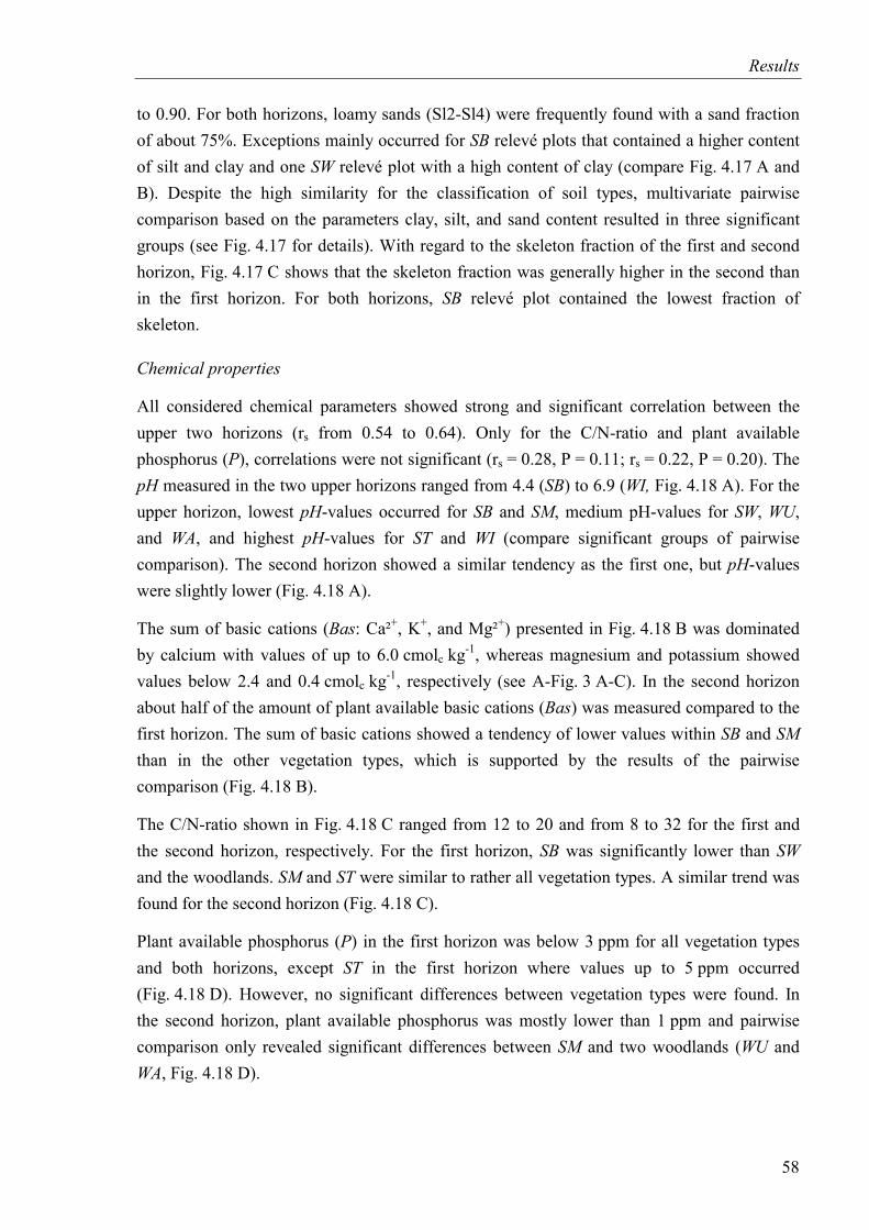
Results
to 0.90. For both horizons, loamy sands (Sl2-Sl4) were frequently found with a sand fraction of about 75%. Exceptions mainly occurred for SB relevé plots that contained a higher content of silt and clay and one SW relevé plot with a high content of clay (compare Fig. 4.17 A and B). Despite the high similarity for the classification of soil types, multivariate pairwise comparison based on the parameters clay, silt, and sand content resulted in three significant groups (see Fig. 4.17 for details). With regard to the skeleton fraction of the first and second horizon, Fig. 4.17 C shows that the skeleton fraction was generally higher in the second than in the first horizon. For both horizons, SB relevé plot contained the lowest fraction of skeleton.
Chemical properties
All considered chemical parameters showed strong and significant correlation between the upper two horizons (rs from 0.54 to 0.64). Only for the C/N-ratio and plant available phosphorus (P), correlations were not significant (rs = 0.28, P = 0.11; rs = 0.22, P = 0.20). The pH measured in the two upper horizons ranged from 4.4 (SB) to 6.9 (WI, Fig. 4.18 A). For the upper horizon, lowest pH-values occurred for SB and SM, medium pH-values for SW, WU, and WA, and highest pH-values for ST and WI (compare significant groups of pairwise comparison). The second horizon showed a similar tendency as the first one, but pH-values were slightly lower (Fig. 4.18 A).
The sum of basic cations (Bas: Ca²+, K+, and Mg²+) presented in Fig. 4.18 B was dominated by calcium with values of up to 6.0 cmolc kg-1, whereas magnesium and potassium showed values below 2.4 and 0.4 cmolc kg-1, respectively (see A-Fig. 3 A-C). In the second horizon about half of the amount of plant available basic cations (Bas) was measured compared to the first horizon. The sum of basic cations showed a tendency of lower values within SB and SM than in the other vegetation types, which is supported by the results of the pairwise comparison (Fig. 4.18 B).
The C/N-ratio shown in Fig. 4.18 C ranged from 12 to 20 and from 8 to 32 for the first and the second horizon, respectively. For the first horizon, SB was significantly lower than SW and the woodlands. SM and ST were similar to rather all vegetation types. A similar trend was found for the second horizon (Fig. 4.18 C).
Plant available phosphorus (P) in the first horizon was below 3 ppm for all vegetation types and both horizons, except ST in the first horizon where values up to 5 ppm occurred (Fig. 4.18 D). However, no significant differences between vegetation types were found. In the second horizon, plant available phosphorus was mostly lower than 1 ppm and pairwise comparison only revealed significant differences between SM and two woodlands (WU and WA, Fig. 4.18 D).
58
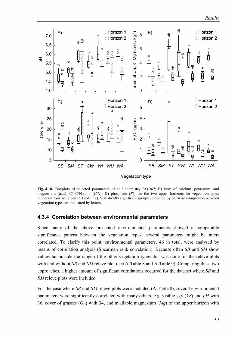
Results
0
2
4
6
8
Sum
ofC
a,K,
Mg
(cm
olkg
)c
-1
SB SM ST SW WI WU WASB SM ST SW WI WU WASB SM ST SW WI WU WA
bAB
bB
abAB
abB
aAB
abA
aAB
4.0
4.5
5.0
5.5
6.0
6.5
7.0pH
SB SM ST SW WI WU WASB SM ST SW WI WU WASB SM ST SW WI WU WA
dD
dC
D
ab AB
cBC
aA
bc AB abc
BC
5
10
15
20
25
30
C/N
-ratio
SB SM ST SW WI WU WASB SM ST SW WI WU WASB SM ST SW WI WU WA
cBC
bcC
abc
A
aA
abA
abA
aAB
0
1
2
3
4
5
PO
(ppm
)2
5
SB SM ST SW WI WU WASB SM ST SW WI WU WASB SM ST SW WI WU WA
aAB
aA
aAB
aAB
aB
aAB
aB
A) B)
C) D)
Vegetation type
Horizon 1Horizon 2
Horizon 1Horizon 2
Horizon 1Horizon 2
Horizon 1Horizon 2
Horizon 1Horizon 2
Horizon 1Horizon 2
Horizon 1Horizon 2
Horizon 1Horizon 2
Fig. 4.18. Boxplots of selected parameters of soil chemistry [A) pH; B) Sum of calcium, potassium, and magnesium (Bas); C) C/N-ratio (C/N); D) phosphate (P)] for the two upper horizons for vegetation types (abbreviations are given in Table 3.2). Statistically significant groups computed by pairwise comparison between vegetation types are indicated by letters.
4.3.4 Correlation between environmental parameters
Since many of the above presented environmental parameters showed a comparable significance pattern between the vegetation types, several parameters might be inter-correlated. To clarify this point, environmental parameters, 46 in total, were analysed by means of correlation analysis (Spearman rank correlation). Because often SB and SM show values far outside the range of the other vegetation types this was done for the relevé plots with and without SB and SM relevé plot (see A-Table 8 and A-Table 9). Comparing these two approaches, a higher amount of significant correlations occurred for the data set where SB and SM relevé plots were included.
For the case where SB and SM relevé plots were included (A-Table 8), several environmental parameters were significantly correlated with many others, e.g. visible sky (VS) and pH with 36, cover of grasses (GC) with 34, and available magnesium (Mg) of the upper horizon with
59
Results
32 other environmental parameters. On the other hand, several parameters appeared to be more independent from the others. Examples are cover of termite mounds (TM), exposition (Exp), date of fire (DF), and plant available phosporus (P), for which 0, 2, 2, and 4 significant correlations were computed, respectively (A-Table 8).
With respect to the correlation analysis without SB and SM relevé plots (A-Table 9), significant correlations mostly occurred between parameters that belong to a different block of parameters such as microclimate or soil, even though high numbers of correlations occurred. For example, visible sky (VS) was correlated with 16 environmental parameters, 7 of which belong to microclimate and 4 to the amount of grasses (A-Table 9).
The presented cross tables clearly demonstrate the strong inter-correlation between the environmental parameters measured for the relevé plots. Thus, much of the information carried by environmental parameters is redundant. Therefore, for the correlation of environmental parameters with species data, only a reduced number of environmental parameters was entered into the respective CCA, and within the CCA for this reduced set of environmental parameters a model-selection procedure was applied to avoid redundancy in correlation (see Chapter 4.4).
4.4 Relation of species data and environmental parameters
In Chapter 4.1 and 4.3, floristic pattern and environmental conditions of the studied plots were presented in detail. In this chapter, floristic variability is related to local environmental conditions. Four data sets were considered: the tree and the herb layer, both with and without SB and SM plots. Because environmental data showed strong inter-correlations, a model-selection procedure was applied as described in Chapter 3.5.2.2. Based on the results of the correlation analysis, only 26 of the environmental parameters presented before have been included into this analysis (A-Table 10 gives the list of all parameters in the first column). From the soil parameters, only the first horizon was included as it dominates the whole nutrient stock and is presumably most relevant for herbs and grasses. In terms of biomass of grasses (GB), biomass of herbs (HEB) and litter (LB), trampling damage (TM), grazing impact (GI), date of fire (DF) and fire temperature (FT), the means of 2001 and 2002 have been chosen. Details of the explained floristic variability of single environmental parameters to the respective species data sets and their significance levels are given in the Appendix (A-Table 10 to A-Table 13).
60
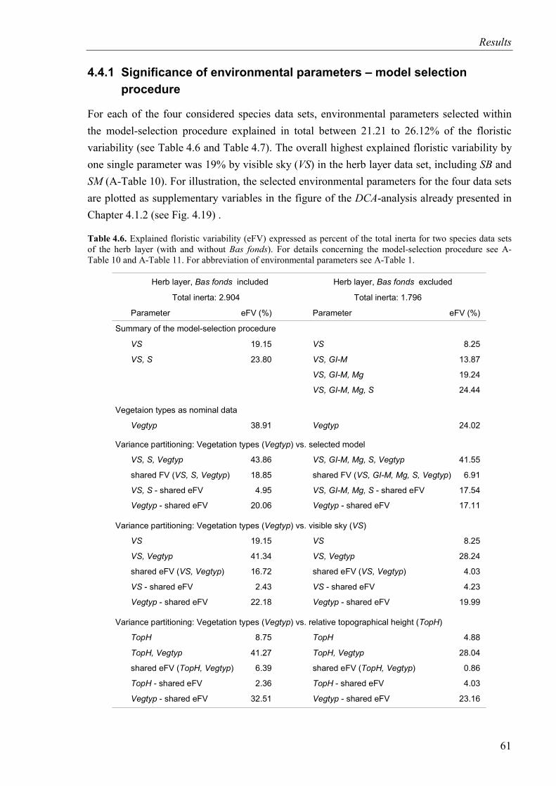
Results
4.4.1 Significance of environmental parameters – model selection procedure
For each of the four considered species data sets, environmental parameters selected within the model-selection procedure explained in total between 21.21 to 26.12% of the floristic variability (see Table 4.6 and Table 4.7). The overall highest explained floristic variability by one single parameter was 19% by visible sky (VS) in the herb layer data set, including SB and SM (A-Table 10). For illustration, the selected environmental parameters for the four data sets are plotted as supplementary variables in the figure of the DCA-analysis already presented in Chapter 4.1.2 (see Fig. 4.19) .
Table 4.6. Explained floristic variability (eFV) expressed as percent of the total inerta for two species data sets of the herb layer (with and without Bas fonds). For details concerning the model-selection procedure see A-Table 10 and A-Table 11. For abbreviation of environmental parameters see A-Table 1.
Total inerta: 2.904
VS
VS, S
Vegetaion types as nominal data
Vegtyp
Variance partitioning: Vegetation types ( ) vs. selected modelVegtyp
VS, S, Vegtyp
shared FV ( )VS, S, Vegtyp
VS, S - shared eFV
Vegtyp - shared eFV
Variance partitioning: Vegetation types vs. visible sky ( )( )Vegtyp VS
VS
VS, Vegtyp
shared eFV ( )VS, Vegtyp
VS - shared eFV
Vegtyp - shared eFV
Variance partitioning: Vegetation types vs. relative topographical height ( )( )Vegtyp TopH
TopH
TopH, Vegtyp
shared eFV ( )TopH, Vegtyp
TopH - shared eFV
Vegtyp - shared eFV
19.15
23.80
38.91
43.86
18.85
4.95
20.06
19.15
41.34
16.72
2.43
22.18
8.75
41.27
6.39
2.36
32.51
Total inerta: 1.796
VS
VS, GI-M
VS, GI-M, Mg
VS, GI-M, Mg, S
Vegtyp
VS, GI-M, Mg, S, Vegtyp
shared FV ( )VS, GI-M, Mg, S, Vegtyp
VS, GI-M, Mg, S - shared eFV
Vegtyp - shared eFV
VS
VS, Vegtyp
shared eFV ( )VS, Vegtyp
VS - shared eFV
Vegtyp - shared eFV
TopH
TopH, Vegtyp
shared eFV ( )TopH, Vegtyp
TopH - shared eFV
Vegtyp - shared eFV
8.25
13.87
19.24
24.44
24.02
41.55
6.91
17.54
17.11
8.25
28.24
4.03
4.23
19.99
4.88
28.04
0.86
4.03
23.16
Herb layer, includedBas fonds Herb layer, excludedBas fonds
Parameter eFV (%) Parameter eFV (%)
Summary of the model-selection procedure
61
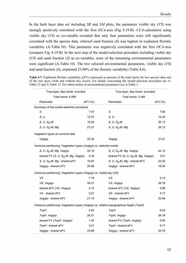
Results
In the herb layer data set including SB and SM plots, the parameter visible sky (VS) was strongly positively correlated with the first DCA-axis (Fig. 4.19 B). CCA-calculation using visible sky (VS) as co-variable revealed that only four parameters were still significantly correlated with the species data, whereof sand fraction (S) was highest in explained floristic variability (A-Table 10). This parameter was negatively correlated with the first DCA-axis (compare Fig. 4.19 B). In the next step of the model-selection procedure including visible sky (VS) and sand fraction (S) as co-variables, none of the remaining environmental parameters were significant (A-Table 10). The two selected environmental parameters, visible sky (VS) and sand fraction (S), explained 23.80% of the floristic variability (Table 4.6).
Table 4.7. Explained floristic variability (eFV) expressed as percent of the total inerta for two species data sets of the tree layer (with and without Bas fonds). For details concerning the model-selection procedure see A-Table 12 and A-Table 13. For abbreviation of environmental parameters see A-Table 1.
Total inerta: 4.958
Summary of the model-selection procedureS
S, U
S, U, GB-M
S, U, GB-M, Mg
Vegetaion types as nominal data
Vegtyp
Variance partitioning: Vegetation types ( ) vs. selected modelVegtyp
S, U, GB-M, Mg, Vegtyp
shared FV ( )S, U, GB-M, Mg, Vegtyp
S, U, GB-M, Mg - shared eFV
Vegtyp - shared eFV
Variance partitioning: Vegetation types vs. visible sky ( )( )Vegtyp VS
VS
VS, Vegtyp
shared eFV ( )VS, Vegtyp
VS - shared eFV
Vegtyp - shared eFV
Variance partitioning: Vegetation types vs. relative topographical height ( )( )Vegtyp TopH
TopH
TopH, Vegtyp
shared FV ( )TopH, Vegtyp
TopH - shared eFV
Vegtyp - shared eFV
7.47
12.57
16.92
21.21
25.30
42.16
4.34
16.87
20.96
7.16
28.31
4.15
3.01
21.15
4.63
28.51
1.42
3.21
23.88
Total inerta: 3.248
S
S, U
S, U, GB-M
S, U, GB-M, Mg
Vegtyp
S, U, GB-M, Mg, Vegtyp
shared FV ( )S, U, GB-M, Mg, Vegtyp
S, U, GB-M, Mg - shared eFV
Vegtyp - shared eFV
VS
VS, Vegtyp
shared eFV ( )VS, Vegtyp
VS - shared eFV
Vegtyp - shared eFV
TopH
TopH, Vegtyp
shared FV ( )TopH, Vegtyp
TopH - shared eFV
Vegtyp - shared eFV
7.86
14.20
20.13
26.12
21.61
44.12
3.61
22.50
18.00
6.13
26.78
0.96
5.17
20.66
6.02
26.78
0.85
5.17
20.76
Tree layer, includedBas fonds Tree layer, excludedBas fonds
Parameter eFV (%) Parameter eFV (%)
62
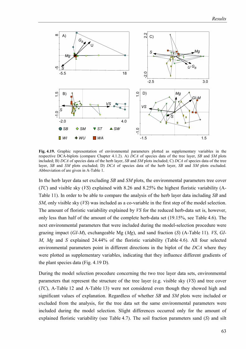
Results
-1.5 1.5-1
.01.
0
VS
S
MgGI-M
-5.5 18
-58
S
U
Mg
GB
SB SM ST SW
WI WU WA
A)
-2.5 3.0
-2.0
2.2
GB
S
U
Mg
C)
D)
-2.0 4.0
-1.0
1.5
VSS
B)
Fig. 4.19. Graphic representation of environmental parameters plotted as supplementary variables in the respective DCA-biplots (compare Chapter 4.1.2). A) DCA of species data of the tree layer, SB and SM plots included; B) DCA of species data of the herb layer, SB and SM plots included; C) DCA of species data of the tree layer, SB and SM plots excluded; D) DCA of species data of the herb layer, SB and SM plots excluded. Abbreviation of are given in A-Table 1.
In the herb layer data set excluding SB and SM plots, the environmental parameters tree cover (TC) and visible sky (VS) explained with 8.26 and 8.25% the highest floristic variability (A-Table 11). In order to be able to compare the analysis of the herb layer data including SB and SM, only visible sky (VS) was included as a co-variable in the first step of the model selection. The amount of floristic variability explained by VS for the reduced herb-data set is, however, only less than half of the amount of the complete herb-data set (19.15%, see Table 4.6). The next environmental parameters that were included during the model-selection procedure were grazing impact (GI-M), exchangeable Mg (Mg), and sand fraction (S) (A-Table 11). VS, GI-M, Mg and S explained 24.44% of the floristic variability (Table 4.6). All four selected environmental parameters point in different directions in the biplot of the DCA where they were plotted as supplementary variables, indicating that they influence different gradients of the plant species data (Fig. 4.19 D).
During the model selection procedure concerning the two tree layer data sets, environmental parameters that represent the structure of the tree layer (e.g. visible sky (VS) and tree cover (TC), A-Table 12 and A-Table 13) were not considered even though they showed high and significant values of explanation. Regardless of whether SB and SM plots were included or excluded from the analysis, for the tree data set the same environmental parameters were included during the model selection. Slight differences occurred only for the amount of explained floristic variability (see Table 4.7). The soil fraction parameters sand (S) and silt
63
Results
(U), were selected to be included in the first two steps of the model-selection procedure (A-Table 12 and A-Table 13). Next, the parameters grass biomass (GB-M), and finally exchangeable Mg (Mg) were selected. Thus, three of the four selected environmental parameters belong to the soil characteristics. The graphical illustration of the environmental parameters is given in Fig. 4.19 A and C.
4.4.2 Variance partitioning: vegetation types versus environmental parameters
As shown in Chapter 4.3, many of the considered environmental parameters were related to the vegetation types being used for stratification. The information of the nominal key parameter vegetation type (Vegtyp) was correlated with the vegetation data using a 0-1 matrix. The parameter vegetation type (Vegtyp), explained between 24.02 and 38.91% of the floristic variability in the four considered species data sets (Table 4.6 and Table 4.7). For the herb and tree layer data sets including SB and SM, the explanation by vegetation types (Vegtyp) was always higher than using the selected environmental parameters (herbs: 38.91 vs. 24.02%; trees: 25.30 vs. 21.61%). For the two cases excluding SB and SM, the explanation by Vegtyp was lower than or equal to the approach using environmental parameters.
The variance partitioning procedure was used to compare the amount of explained floristic variability of the parameter vegetation type (Vegtyp) compared to the environmental parameters. In order to do so, variance partitioning was carried out for the parameter vegetation type (Vegtyp) versus all environmental parameter data sets that were included in the models presented above. In addition, the same analysis was computed for only two single environmental parameters, visible sky (VS) and relative topographical height (TopH) (see Table 4.6, Table 4.7, and Fig. 4.20). Visible sky was selected because this parameter is strongly related with tree cover. Tree cover and density are the most important parameter used to define vegetation types in West Africa (compare Table 3.1) and therefore visible sky (VS) can be supposed to represent an ordinal variable of the nominal variable vegetation type (Vegtyp). As outlined in Chapter 1.1.1, West African vegetation types are often described to be very well related to topography. Therefore, the parameter relative topographical height (TopH) was tested separately as well.
The variance partitioning procedure considering vegetation types (Vegtyp) and all selected environmental parameters included in the models revealed for three of the considered species data sets, herb layer without Bas fonds, tree layer with and without Bas fonds, that the amount of explained floristic variability that was shared by the two groups was generally low with values between 3.61% and 6.91% (Table 4.6, Table 4.7, and Fig. 4.20). This means that the parameter vegetation type and each group of environmental parameters explained mainly different parts of the floristic variability. The herb layer species data set including SB and SM represents the exception. Here, the shared floristic variability of 18.85% was very high
64
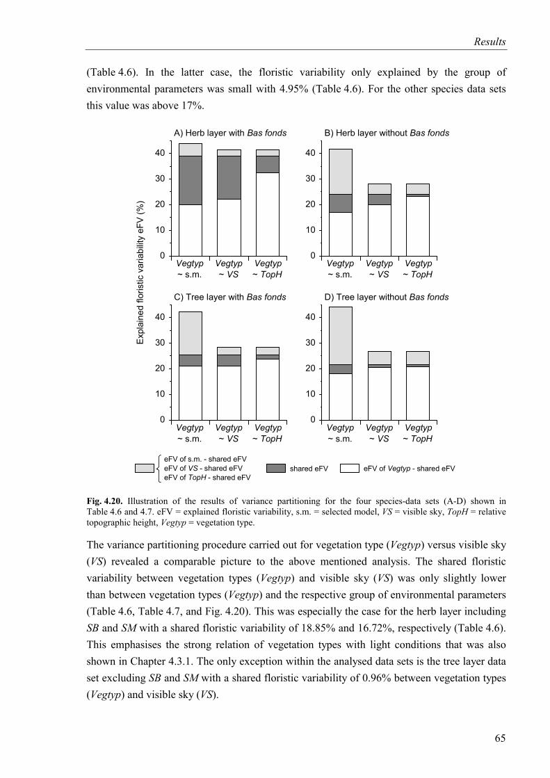
Results
(Table 4.6). In the latter case, the floristic variability only explained by the group of environmental parameters was small with 4.95% (Table 4.6). For the other species data sets this value was above 17%.
0
10
20
30
40
C) Tree layer with Bas fonds
0
10
20
30
40
D) Tree layer without Bas fonds
0
10
20
30
40
A) Herb layer with Bas fonds
0
10
20
30
40
B) Herb layer without Bas fonds
eFV of Vegtyp - shared eFVshared eFVeFV of s.m. - shared eFVeFV of - shared eFVVSeFV of - shared eFVTopH
Vegtyp~ s.m.
Vegtyp~ VS
Vegtyp~ TopH
Vegtyp~ s.m.
Vegtyp~ VS
Vegtyp~ TopH
Expl
aine
dflo
ristic
varia
bilit
yeF
V(%
)
Vegtyp~ s.m.
Vegtyp~ VS
Vegtyp~ TopH
Vegtyp~ s.m.
Vegtyp~ VS
Vegtyp~ TopH
Fig. 4.20. Illustration of the results of variance partitioning for the four species-data sets (A-D) shown in Table 4.6 and 4.7. eFV = explained floristic variability, s.m. = selected model, VS = visible sky, TopH = relative topographic height, Vegtyp = vegetation type.
The variance partitioning procedure carried out for vegetation type (Vegtyp) versus visible sky (VS) revealed a comparable picture to the above mentioned analysis. The shared floristic variability between vegetation types (Vegtyp) and visible sky (VS) was only slightly lower than between vegetation types (Vegtyp) and the respective group of environmental parameters (Table 4.6, Table 4.7, and Fig. 4.20). This was especially the case for the herb layer including SB and SM with a shared floristic variability of 18.85% and 16.72%, respectively (Table 4.6). This emphasises the strong relation of vegetation types with light conditions that was also shown in Chapter 4.3.1. The only exception within the analysed data sets is the tree layer data set excluding SB and SM with a shared floristic variability of 0.96% between vegetation types (Vegtyp) and visible sky (VS).
65
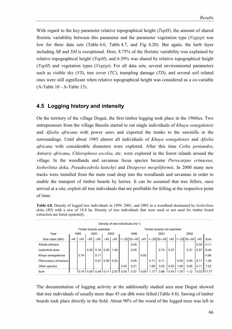
Results
With regard to the key parameter relative topographical height (TopH), the amount of shared floristic variability between this parameter and the parameter vegetation type (Vegtyp) was low for three data sets (Table 4.6, Table 4.7, and Fig. 4.20). But again, the herb layer including SB and SM is exceptional. Here, 8.75% of the floristic variability was explained by relative topographical height (TopH), and 6.39% was shared by relative topographical height (TopH) and vegetation types (Vegtyp). For all data sets, several environmental parameters such as visible sky (VS), tree cover (TC), trampling damage (TD), and several soil related ones were still significant when relative topographical height was considered as a co-variable (A-Table 10 - A-Table 13).
4.5 Logging history and intensity
On the territory of the village Doguè, the first timber logging took place in the 1960ies. Two entrepreneurs from the village Bassila started to cut single individuals of Khaya senegalensis and Afzelia africana with power saws and exported the trunks to the sawmills in the surroundings. Until about 1985 almost all individuals of Khaya senegalensis and Afzelia africana with considerable diameters were explored. After this time Ceiba pentandra, Antiaris africana, Chlorophora excelsa, etc. were explored in the forest islands around the village. In the woodlands and savannas focus species became Pterocarpus erinaceus, Isoberlinia doka, Pseudocedrela kotschyi and Diospyros mespiliformis. In 2000 many new tracks were installed from the main road deep into the woodlands and savannas in order to enable the transport of timber boards by lorries. It can be assumed that tree fellers, once arrived at a site, exploit all tree individuals that are profitable for felling at the respective point of time.
Table 4.8. Density of logged tree individuals in 1999, 2001, and 2002 in a woodland dominated by Isoberlinia doka (WI) with a size of 18.8 ha. Density of tree individuals that were used or not used for timber board extraction are listed separately.
Year
Size class (dbh)
Afzelia africana
Isoberlinia doka
Khaya senegalensis
Pterocarpus erinaceus
Other species
Sum
1999
<45 ≥45
0.74
0.74
2001
<45
0.05
0.05
≥45
5.16
0.11
0.21
5.48
2002
<45
0.05
0.05
0.11
≥45
1.54
0.53
2.07
1- 20<
0.05
0.05
1999
20- 45<
0.05
0.05
0.21
0.37
≥45
0.05
0.05
1- 20<
0.11
1.06
1.17
2001
20- 45<
0.74
0.11
3.03
3.88
≥45
0.37
0.05
0.43
1- 20<
0.05
1.65
1.70
2002
20- 45<
0.21
0.05
0.85
1.12
≥45
0.05
0.27
0.11
0.11
0.53
Sum
0.11
8.46
0.90
1.28
7.02
17.77
Timber boards exploited Timber boards not exploited
Density of tree individuals (ha-1)
0.05
The documentation of logging activity at the additionally studied area near Doguè showed that tree individuals of usually more than 45 cm dbh were felled (Table 4.8). Sawing of timber boards took place directly in the field. About 90% of the wood of the logged trees was left in
66
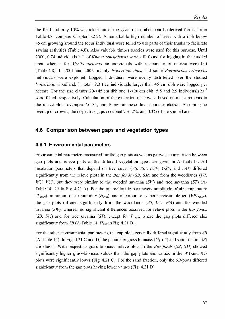
Results
the field and only 10% was taken out of the system as timber boards (derived from data in Table 4.8, compare Chapter 3.2.2). A remarkable high number of trees with a dbh below 45 cm growing around the focus individual were felled to use parts of their trunks to facilitate sawing activities (Table 4.8). Also valuable timber species were used for this purpose. Until 2000, 0.74 individuals ha-1 of Khaya senegalensis were still found for logging in the studied area, whereas for Afzelia africana no individuals with a diameter of interest were left (Table 4.8). In 2001 and 2002, mainly Isoberlinia doka and some Pterocarpus erinaceus individuals were explored. Logged individuals were evenly distributed over the studied Isoberlinia woodland. In total, 9.3 tree individuals larger than 45 cm dbh were logged per hectare. For the size classes 20-<45 cm dbh and 1-<20 cm dbh, 5.5 and 2.9 individuals ha-1 were felled, respectively. Calculation of the extension of crowns, based on measurements in the relevé plots, averages 75, 35, and 10 m² for these three diameter classes. Assuming no overlap of crowns, the respective gaps occupied 7%, 2%, and 0.3% of the studied area.
4.6 Comparison between gaps and vegetation types
4.6.1 Environmental parameters
Environmental parameters measured for the gap plots as well as pairwise comparison between gap plots and relevé plots of the different vegetation types are given in A-Table 14. All insolation parameters that depend on tree cover (VS, ISF, DSF, GSF, and LAI) differed significantly from the relevé plots in the Bas fonds (SB, SM) and from the woodlands (WI, WU, WA), but they were similar to the wooded savanna (SW) and tree savanna (ST) (A-Table 14, VS in Fig. 4.21 A). For the microclimatic parameters amplitude of air temperature (Tampl), minimum of air humidity (Hmin), and maximum of vapour pressure deficit (VPDmax), the gap plots differed significantly from the woodlands (WI, WU, WA) and the wooded savanna (SW), whereas no significant differences occurred for relevé plots in the Bas fonds (SB, SM) and for tree savanna (ST), except for Tampl, where the gap plots differed also significantly from SB (A-Table 14, Hmin in Fig. 4.21 B).
For the other environmental parameters, the gap plots generally differed significantly from SB (A-Table 14). In Fig. 4.21 C and D, the parameter grass biomass (GB-02) and sand fraction (S) are shown. With respect to grass biomass, relevé plots in the Bas fonds (SB, SM) showed significantly higher grass-biomass values than the gap plots and values in the WA-and WI-plots were significantly lower (Fig. 4.21 C). For the sand fraction, only the SB-plots differed significantly from the gap plots having lower values (Fig. 4.21 D).
67
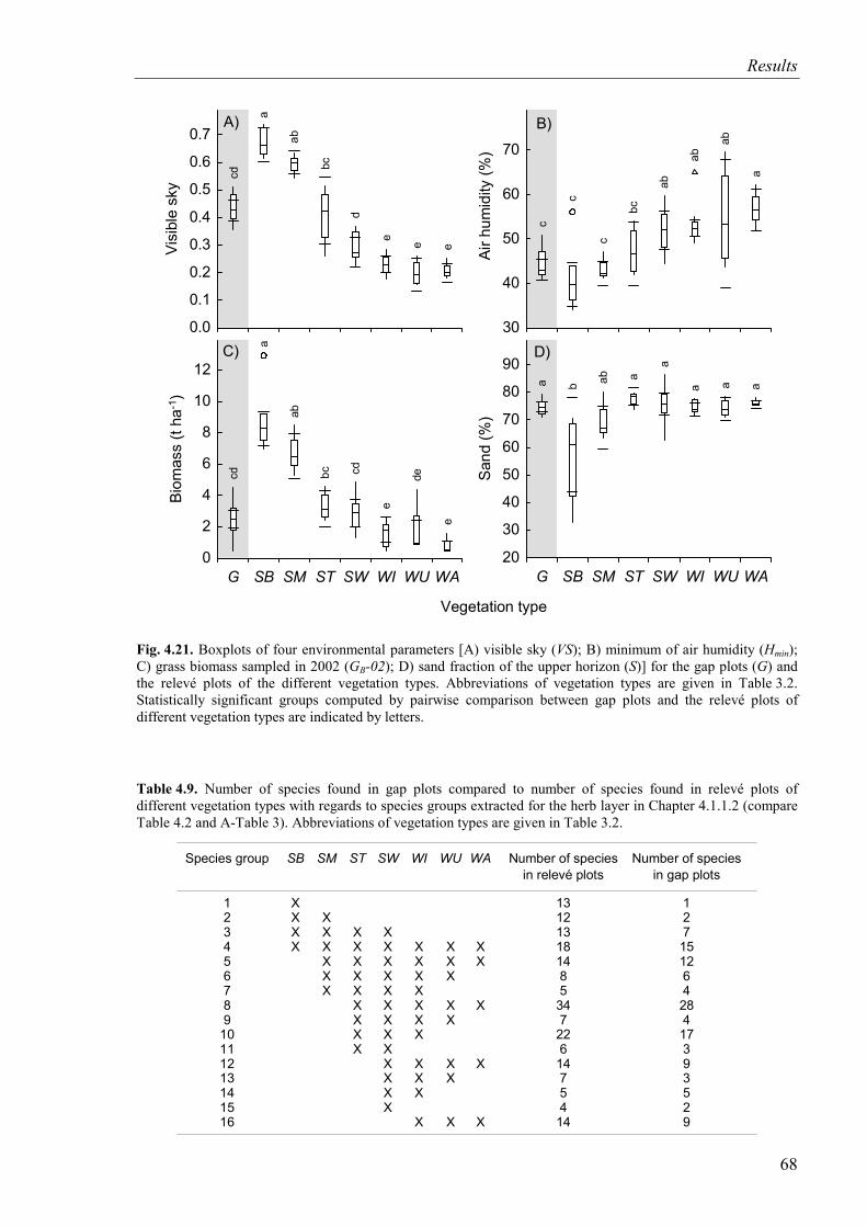
Results
30
40
50
60
70
Airh
umid
ity(%
)
c
c
bc
ab
a
ab
ab
c
0.0
0.1
0.2
0.3
0.4
0.5
0.6
0.7
Visi
ble
sky
a
ab
bc
d
e
e e
cd
20
30
40
50
60
70
80
90
Sand
(%)
G SB SM ST SW WI WU WAb ab a
a
aa aa
A)
Vegetation type
B)
0
2
4
6
8
10
12
Biom
ass
(tha
)-1
G SB SM ST SW WI WU WA
a
ab
bc cd
e
e
decd
C) D)
Fig. 4.21. Boxplots of four environmental parameters [A) visible sky (VS); B) minimum of air humidity (Hmin); C) grass biomass sampled in 2002 (GB-02); D) sand fraction of the upper horizon (S)] for the gap plots (G) and the relevé plots of the different vegetation types. Abbreviations of vegetation types are given in Table 3.2. Statistically significant groups computed by pairwise comparison between gap plots and the relevé plots of different vegetation types are indicated by letters.
Table 4.9. Number of species found in gap plots compared to number of species found in relevé plots of different vegetation types with regards to species groups extracted for the herb layer in Chapter 4.1.1.2 (compare Table 4.2 and A-Table 3). Abbreviations of vegetation types are given in Table 3.2.
Species group
123456789
10111213141516
SB
XXXX
SM
XXXXXX
ST
XXXXXXXXX
SW
XXXXXXXXXXXXX
WI
XXXXXXX
XXX
X
WU
XXX
XX
XX
X
WA
XX
X
X
X
Number of speciesin relevé plots
131213181485
347
226
14754
14
Number of speciesin gap plots
12715126428417393529
68
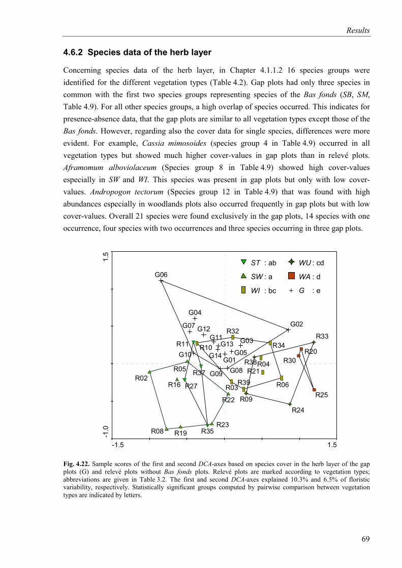
Results
4.6.2 Species data of the herb layer
Concerning species data of the herb layer, in Chapter 4.1.1.2 16 species groups were identified for the different vegetation types (Table 4.2). Gap plots had only three species in common with the first two species groups representing species of the Bas fonds (SB, SM, Table 4.9). For all other species groups, a high overlap of species occurred. This indicates for presence-absence data, that the gap plots are similar to all vegetation types except those of the Bas fonds. However, regarding also the cover data for single species, differences were more evident. For example, Cassia mimosoides (species group 4 in Table 4.9) occurred in all vegetation types but showed much higher cover-values in gap plots than in relevé plots. Aframomum alboviolaceum (Species group 8 in Table 4.9) showed high cover-values especially in SW and WI. This species was present in gap plots but only with low cover-values. Andropogon tectorum (Species group 12 in Table 4.9) that was found with high abundances especially in woodlands plots also occurred frequently in gap plots but with low cover-values. Overall 21 species were found exclusively in the gap plots, 14 species with one occurrence, four species with two occurrences and three species occurring in three gap plots.
-1.5 1.5
-1.0
1.5
R11
R27
R35
R37R02
R05
R08
R16
R19
R22
R23
R03
R04
R06
R10
R21
R32
R34
R39
R09R24
R33
R38R20
R25
R30G01
G02
G03
G04
G05
G06
G07
G08G09
G10
G11G12
G13G14
ST : ab
SW : a
WI : bc
WU : cd
WA : d
G : e+
Fig. 4.22. Sample scores of the first and second DCA-axes based on species cover in the herb layer of the gap plots (G) and relevé plots without Bas fonds plots. Relevé plots are marked according to vegetation types; abbreviations are given in Table 3.2. The first and second DCA-axes explained 10.3% and 6.5% of floristic variability, respectively. Statistically significant groups computed by pairwise comparison between vegetation types are indicated by letters.
69
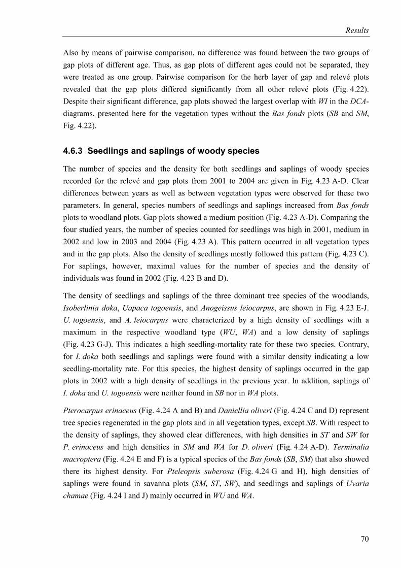
Results
Also by means of pairwise comparison, no difference was found between the two groups of gap plots of different age. Thus, as gap plots of different ages could not be separated, they were treated as one group. Pairwise comparison for the herb layer of gap and relevé plots revealed that the gap plots differed significantly from all other relevé plots (Fig. 4.22). Despite their significant difference, gap plots showed the largest overlap with WI in the DCA-diagrams, presented here for the vegetation types without the Bas fonds plots (SB and SM, Fig. 4.22).
4.6.3 Seedlings and saplings of woody species
The number of species and the density for both seedlings and saplings of woody species recorded for the relevé and gap plots from 2001 to 2004 are given in Fig. 4.23 A-D. Clear differences between years as well as between vegetation types were observed for these two parameters. In general, species numbers of seedlings and saplings increased from Bas fonds plots to woodland plots. Gap plots showed a medium position (Fig. 4.23 A-D). Comparing the four studied years, the number of species counted for seedlings was high in 2001, medium in 2002 and low in 2003 and 2004 (Fig. 4.23 A). This pattern occurred in all vegetation types and in the gap plots. Also the density of seedlings mostly followed this pattern (Fig. 4.23 C). For saplings, however, maximal values for the number of species and the density of individuals was found in 2002 (Fig. 4.23 B and D).
The density of seedlings and saplings of the three dominant tree species of the woodlands, Isoberlinia doka, Uapaca togoensis, and Anogeissus leiocarpus, are shown in Fig. 4.23 E-J. U. togoensis, and A. leiocarpus were characterized by a high density of seedlings with a maximum in the respective woodland type (WU, WA) and a low density of saplings (Fig. 4.23 G-J). This indicates a high seedling-mortality rate for these two species. Contrary, for I. doka both seedlings and saplings were found with a similar density indicating a low seedling-mortality rate. For this species, the highest density of saplings occurred in the gap plots in 2002 with a high density of seedlings in the previous year. In addition, saplings of I. doka and U. togoensis were neither found in SB nor in WA plots.
Pterocarpus erinaceus (Fig. 4.24 A and B) and Daniellia oliveri (Fig. 4.24 C and D) represent tree species regenerated in the gap plots and in all vegetation types, except SB. With respect to the density of saplings, they showed clear differences, with high densities in ST and SW for P. erinaceus and high densities in SM and WA for D. oliveri (Fig. 4.24 A-D). Terminalia macroptera (Fig. 4.24 E and F) is a typical species of the Bas fonds (SB, SM) that also showed there its highest density. For Pteleopsis suberosa (Fig. 4.24 G and H), high densities of saplings were found in savanna plots (SM, ST, SW), and seedlings and saplings of Uvaria chamae (Fig. 4.24 I and J) mainly occurred in WU and WA.
70
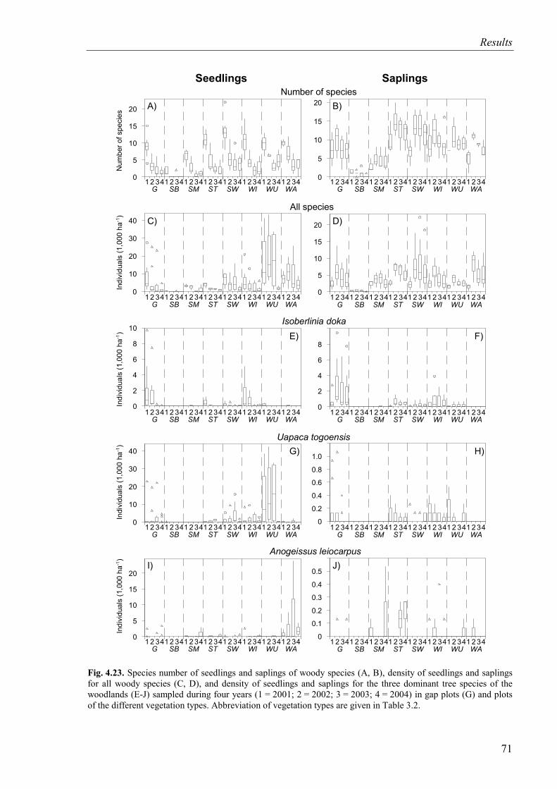
Results
Indi
vidu
als
(1,0
00ha
)-1
Indi
vidu
als
(1,0
00ha
)-1
Indi
vidu
als
(1,0
00ha
)-1
G SB SM ST SW WI WU WA0
5
10
15
20
Number of species
Isoberlinia doka
Uapaca togoensis
Anogeissus leiocarpus
Seedlings Saplings
0
5
10
15
20
All species
1 2 341 2 341 2 341 2 341 2 341 2341 2 341 2 34G SB SM ST SW WI WU WA
1 2 341 2 341 2 341 2 341 2 341 2 341 2 341 2 34
G SB SM ST SW WI WU WA1 2 341 2 341 2 341 2 341 2 341 2341 2 341 2 34
G SB SM ST SW WI WU WA1 2 341 2 341 2 341 2 341 2 341 2 341 2 341 2 34
A) B)
C) D)
I) J)
G) H)
E) F)
Num
bero
fspe
cies
Indi
vidu
als
(1,0
00ha
)-1
G SB SM ST SW WI WU WA1 2 341 2 341 2 341 2 341 2 341 2341 2 341 2 34
G SB SM ST SW WI WU WA1 2 341 2 341 2 341 2 341 2 341 2 341 2 341 2 34
G SB SM ST SW WI WU WA1 2 341 2 341 2 341 2 341 2 341 2341 2 341 2 34
G SB SM ST SW WI WU WA1 2 341 2 341 2 341 2 341 2 341 2 341 2 341 2 34
G SB SM ST SW WI WU WA1 2 341 2 341 2 341 2 341 2 341 2341 2 341 2 34
G SB SM ST SW WI WU WA1 2 341 2 341 2 341 2 341 2 341 2 341 2 341 2 34
0
10
20
30
40
0
5
10
15
20
0
2
4
6
8
10
0
2
4
6
8
0
10
20
30
40
0
0.2
0.4
0.6
0.8
1.0
0
5
10
15
20
0
0.1
0.2
0.3
0.4
0.5
Fig. 4.23. Species number of seedlings and saplings of woody species (A, B), density of seedlings and saplings for all woody species (C, D), and density of seedlings and saplings for the three dominant tree species of the woodlands (E-J) sampled during four years (1 = 2001; 2 = 2002; 3 = 2003; 4 = 2004) in gap plots (G) and plots of the different vegetation types. Abbreviation of vegetation types are given in Table 3.2.
71
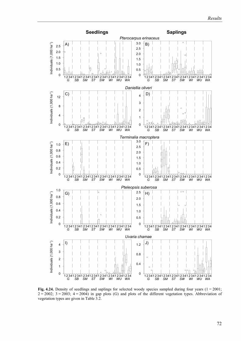
Results
G SB SM ST SW WI WU WA
Pterocarpus erinaceus
Terminalia macroptera
Pteleopsis suberosa
Uvaria chamae
Seedlings Saplings
Daniellia oliveri
1 2 341 2 341 2 341 2 341 2 341 2 341 2 341 2 34G SB SM ST SW WI WU WA
1 2 341 2 341 2 341 2 341 2 341 2 341 2 341 2 34
G SB SM ST SW WI WU WA1 2 341 2 341 2 341 2 341 2 341 2 341 2 341 2 34
G SB SM ST SW WI WU WA1 2 341 2 341 2 341 2 341 2 341 2 341 2 341 2 34
A) B)
C)
G SB SM ST SW WI WU WA1 2 341 2 341 2 341 2 341 2 341 2 341 2 341 2 34
G SB SM ST SW WI WU WA1 2 341 2 341 2 341 2 341 2 341 2 341 2 341 2 34
G SB SM ST SW WI WU WA1 2 341 2 341 2 341 2 341 2 341 2 341 2 341 2 34
G SB SM ST SW WI WU WA1 2 341 2 341 2 341 2 341 2 341 2 341 2 341 2 34
G SB SM ST SW WI WU WA1 2 341 2 341 2 341 2 341 2 341 2 341 2 341 2 34
G SB SM ST SW WI WU WA1 2 341 2 341 2 341 2 341 2 341 2 341 2 341 2 34
D)
E) F)
G) H)
I) J)
Indi
vidu
als
(1,0
00ha
)-1
Indi
vidu
als
(1,0
00ha
)-1
Indi
vidu
als
(1,0
00ha
)-1
Indi
vidu
als
(1,0
00ha
)-1
Indi
vidu
als
(1,0
00ha
)-1
0
0.5
1.0
1.5
2.0
2.5
00.51.01.52.02.53.0
0
4
8
12
0
1
2
3
4
0
0.2
0.4
0.6
0.8
1.0
0
0.5
1.0
1.5
2.0
2.5
3.0
0
0.2
0.4
0.6
0.8
1.0
0
0.5
1.0
1.5
2.0
2.5
0
1
2
3
4
0
0.4
0.8
1.2
Fig. 4.24. Density of seedlings and saplings for selected woody species sampled during four years (1 = 2001; 2 = 2002; 3 = 2003; 4 = 2004) in gap plots (G) and plots of the different vegetation types. Abbreviation of vegetation types are given in Table 3.2.
72
Results
Comparison between the species composition of gap plots with those of the different vegetation types was carried out with Principal Response Curves analysis (PRC) in order to consider the time-series aspect of the data (Fig. 4.25). For illustration, data of the gap plots were defined as base line and data of the different vegetation types are given in relation to this base line (Fig. 4.25 A and C). With regard to the species composition of seedlings, all vegetation types differed significantly from the gap plots, except ST and WI, computed by pairwise comparison between each vegetation type and the gap plots by means of PRC. This is illustrated in the plots as these two vegetation types were plotted near the base line in Fig. 4.25 A. Species scores of the first axis (Fig. 4.25 B) reveal that this axis was strongly influenced by the species already presented in detail in Fig. 4.23 and Fig. 4.24. Especially Uapaca togoensis was of importance due to absolute species scores. For the species composition of saplings, all vegetation types differed significantly from the gap plots without exception, but again ST and WI were most similar to the gap plots (Fig. 4.25 C). Concerning the species scores of the first axis (Fig. 4.25 D), species such as I. doka, T. macroptera and D. oliveri expanded the first PRC-axis most strongly. In contrast to the PRC of the seedlings (Fig. 4.25 B), U. togoensis and A. leiocarpus showed an intermediate position on the first PRC-axis, whereas species such as Vitellaria paradoxa, Trichilia emetica, Pseudocedrela kotschyi, Pterocarpus erinaceus, and Parinari curatellifolia were of importance (Fig. 4.25 D).
73
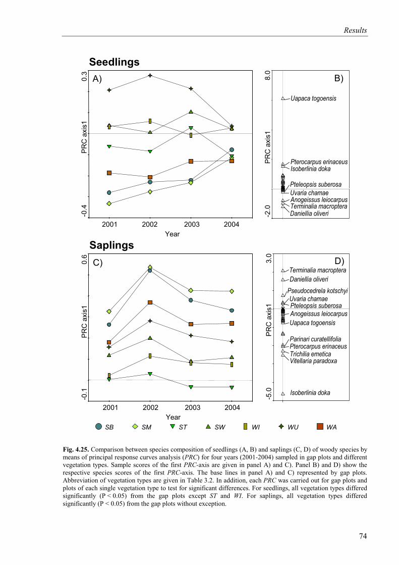
Results
2001Year
-0.4
0.3
PRC
axi
s1
2002 2003 2004
-0.1
0.6
PRC
axi
s1
2001Year
2002 2003 2004
-2.0
8.0
PRC
axi
s1
Anogeissus leiocarpus
Daniellia oliveri
Isoberlinia dokaPterocarpus erinaceus
Pteleopsis suberosa
Terminalia macroptera
Uapaca togoensis
Uvaria chamae
-5.0
3.0
PRC
axi
s1
Anogeissus leiocarpus
Vitellaria paradoxa
Daniellia oliveri
Isoberlinia doka
Parinari curatellifolia
Pseudocedrela kotschyi
Pterocarpus erinaceus
Pteleopsis suberosa
Terminalia macroptera
Trichilia emetica
Uapaca togoensis
Uvaria chamae
SB SM ST SW WI WU WA
A) B)
C) D)Saplings
Seedlings
Fig. 4.25. Comparison between species composition of seedlings (A, B) and saplings (C, D) of woody species by means of principal response curves analysis (PRC) for four years (2001-2004) sampled in gap plots and different vegetation types. Sample scores of the first PRC-axis are given in panel A) and C). Panel B) and D) show the respective species scores of the first PRC-axis. The base lines in panel A) and C) represented by gap plots. Abbreviation of vegetation types are given in Table 3.2. In addition, each PRC was carried out for gap plots and plots of each single vegetation type to test for significant differences. For seedlings, all vegetation types differed significantly (P < 0.05) from the gap plots except ST and WI. For saplings, all vegetation types differed significantly (P < 0.05) from the gap plots without exception.
74
Discussion
5 Discussion
5.1 Classification of vegetation types and floristic characteristics
Classification of species data of the tree and herb layer sampled at the study area revealed a clear gradual species turnover from open savannas in the Bas fonds to woodlands. Two ordination approaches of the tree and herb layer data were carried out. The first approach was based on the physiognomic categories of Yangambi (CSA 1956) extended by a separation of zonal and azonal sites and a subdivision of woodlands by dominant tree species. In the second approach, vegetation data were classified according to phytosociological criteria. Significant differences between groups occurred for both ordination approaches. However, for both the tree and especially the herb layer the classification based on phytosociological criteria revealed more distinct groups of relevé plots. This was additionally confirmed by multivariate data analysis. Though phytosociological groups were more distinct, it was also possible to relate physiognomic characteristics to species composition.
Menaut (1983) suggested that for an overall comparability and comprehensibility it would be very useful to apply the Yangambi categories for an overall stratification, and then to apply detailed phytosociological classification within each of the Yangambi categories. This was first done by Langdale-Brown (1959-60 cited in Menaut 1983), and also successfully applied e.g. in central Ivory Coast by César (1992), in north-eastern Ivory Coast by Poilecot et al. (1991), and in the northern Benin by Reiff (1998). This led to relations of physiognomic vegetation types with floristic characteristics for specific regions. Vice versa, Adjanohoun (1964), Schmidt (1973) and Spichiger (1975) were able to relate phytosociological units to characteristic physiognomic features for savannas in the Guinea zone (Ivory Coast). These examples together with this study indicate that on a local to regional scale, a relation between floristic and physiognomic features can be established.
In this context, some important aspects have to be considered. For example, grass savannas (according to Yangambi) can be found on shallow soils with limited water supply as well as in depressions with temporarily stagnant water (e.g. Schmidt 1973). The establishment of trees is limited in both cases leading to a similar physiognomic structure, but profoundly different species composition. The necessity to differentiate these two azonal sites appears evident. In this study, the extension of the physiognomic Yangambi criteria by differentiating azonal sites in the Bas fonds and zonal sites outside of the Bas fonds proved to be floristically meaningful. Therefore, the differentiation of zonal and azonal sites within the Yangambi classification should improve its applicability. The subdivision of the woodland formation
75
Discussion
according to the three dominant tree species (Isoberlinia doka, Uapaca togoensis and Anogeissus leiocarpus) proved to be reasonable and revealed significant different species composition. A differentiation of Isoberlinia and Uapaca dominated woodlands is also described by Houinato (2001) and Anogeissus dominated woodland and forests are known over wide regions (Sobey 1978, Hahn 1996, Neumann & Müller-Haude 1999, Hennenberg 2005 unpublished dissertation). Nevertheless, the three studied woodland types are more similar to each other than to the other structural vegetation types. Thus, the subdivision according to dominating species distinguishes on a finer scale than the strict physiognomic classification, but the coarse scale of the Yangambi categories is also meaningful with respect to species composition.
In this study, classification of the tree layer data revealed less distinct groups than the classification of the herb layer data. This is not surprising as Hall & Jenik (1968) pointed out that West African tree species are not useful as solitary criteria for floristic classification approaches as their overall species number is low and most species show both a wide distribution range and a large ecological amplitude. Floristic blocks of the tree layer classified by phytosociological criteria coincide with the floristic blocks of the herb layer mainly for the Bas fonds plots and the open savannas. For the more dense savannas and woodlands, tree species did not differentiate much and therefore do not coincide with the classification of herb layer. However, an independence of herb and tree layer especially for intermediate sites which are neither open savannas nor dense forests as thoroughly discussed by Menaut (1983) and Hahn (1996), can not be confirmed for the study site. This might be due to the local scale, but also Houinato (2001) found on a larger scale in proximity to the study area of the present thesis a good agreement of floristic tree and herb layer classification.
In summary, it can be stated that it is possible in the studied area to link physiognomic characteristics with vegetation composition on a local to regional scale, if azonal sites and zonal sites are distinguished. Nevertheless, such relation can only be expected, if processes are absent that uncouple structure and species composition. Crop cultivation followed by fallows is a frequently occurring process in West Africa. Young fallows, for examples, must be classified after the physiognomic Yangambi categories as shrub savannas, but they differ to a great extend in their species composition from undisturbed shrub savannas.
In order to elaborate vegetation and land-cover maps by means of remote sensing techniques, physiognomic classification of vegetation is of great advantage as a matter of its general compatibility with remote sensing data, despite the general problem of small-scale patchy distribution of vegetation types. However, to parameterise these classes with information on ecological and floristic properties as well as with information on land use, a strict physiognomic approach is by far not sufficient. In order to distinguish azonal and zonal sites as well as fallows and arable land, multitemporal approaches are frequently applied (Reed et al. 1994, Hahn-Hadjal & Schmid 1999, Schmid 1999). These demand detailed knowledge e.g.
76
Discussion
on phenological characteristics of vegetation but seem to be challenging (Mistry 2000b, Roehrig et al. 2005). The possibility to link physiognomic vegetation types with species composition – as shown in this study and those cited above – suggests that also floristic information may be incorporated in remote sensing maps. However, much further research will be needed in order to increase the quantity and quality of ground data as well as the knowledge of ecological processes. Despite of its intrinsic value, the elaboration of a phytosociological system of West Africa – in combination with the comparison of such a system with a physiognomic classification – would also be of much help in this context. On the one hand, a phytosociological system would facilitate the categorization of results of local studies. On the other hand, a phytosociological system could help to interpret classes in remote sensing maps and could especially improve the set up of knowledge based decision trees for remote sensing algorithms.
5.2 Structural characteristics of vegetation types
Tree data
The parameters woody biomass, tree cover, and composition of tree-size classes revealed a gradual change from open savannas to woodlands. Woody biomass ranged from about 90 t ha-1 for the woodlands and about 40 t ha-1 for the savanna types SM, ST, and SW to below 10 t ha-1 for the open savanna in the Bas fond. The same tendency was found for tree cover with high values in the woodlands (about 70%) and low values in the Bas fonds (below 10%). Tree-size class-composition concerning height classes showed much more distinct groups than classification based on diameter classes. In general, woodlands were characterized by a higher total number of individuals than the savannas. In savannas (SB, SM, ST), mostly less than 200 individuals with a diameter lager than 10 cm dbh were counted per hectare. For woodlands and the wooded savanna, this value was about 350 individuals ha-1. In addition, tree-size class composition of woodlands showed a higher number of larger tree individuals for both height and diameter classes than savannas.
In West Africa, detailed analysis of tree-size classes and biomass were frequently carried out in closed and mainly in moist forests formations (Ghana: Hall & Swaine 1981, Lawson 1986, Swaine et al. 1987, Swaine et al. 1990; Liberia and Ivory Coast: van Rompaey 1993 and national forest inventories cited in Bongers et al. 1999; Benin: Nansen et al. 2001, Sokpon et al. 2001). In contrast, for savannas and woodlands such data are sparse. However, for woodlands, Monnier (1981) and Menaut et al. (1995) integrated several data collected in West Africa. For tree density, Monnier (1981) presented values of about 250 individuals ha-1 for woodlands in northern Ivory Coast. With regard to woody above-ground biomass, Menaut et al. (1995) estimated a value of 100 t ha-1 for West African woodlands. Monnier (1981, northern Ivory Coast) gave a value of 92 t ha-1.
77
Discussion
With respect to savannas, Keay (1949) measured for trees larger 10 cm dbh values from 62 to 185 individuals ha-1 for different savanna types in the Sudanian zone of Nigeria. Hennenberg (unpublished data, compare Hennenberg et al. 2005) counted for the same size class about 110 individuals ha-1 for a tree savannas in the Comoé National Park in northeastern Ivory Coast. Lawson et al. (1956) measured in the Mole game reserve in northwestern Ghana for a wooded savanna a mean tree density of about 300 individuals ha-1 larger 10 cm dbh. Monnier (1981) found 80 to 350 and 250 to 400 individuals ha-1 for Guinea and Sudanian savannas, where woody biomass values were given to be about 30 and 10 t ha-1, respectively.
In addition, the subdivision of tree-size classes is very inconsistent and often the derivation of tree densities is impossible from existing studies. For example, Couteron & Kokou (1997) counted all tree individuals larger 1.5 m in height, Hovestadt (1997) measured the density of trees larger 2 m and shrubs larger 1 m in height, Sobey (1978) included only selected species, and PAMF (1996) focused on valuable timber species for presentation. Even though each of the mentioned studies is of high value of its own, the necessity to establish standardized tree inventories for savannas and woodlands in West Africa is to be stressed to enhance comparability of individual studies. The absence of these inventories might be a result of higher commercial values found in closed forest formations based on timber exploitation than in savannas and woodlands (compare Brown & Gaston 1996).
However, the cited values are of the same orders of magnitude as those measured in the present study indicating an overall comparability of the studied savannas and woodlands with those in other areas of the Sudanian and Guinea zone in West Africa. The presented structural data of woody species for different vegetation types, however, contribute and help to complete the low number of existing data. These data are additionally valuable, e.g. for the interpretation of remote sensing data, as key parameters for meteorological and hydrological modelling, and especially as a base for the development of forest management plans. In addition, the applied vegetation types, that are primarily based on the physiognomic Yangambi categories, proved to be well related to structural parameters of the tree layer as recorded in this thesis. The most differentiating parameters have been the distribution of height classes of trees and tree cover.
Herb data
Biomass of grasses was highest in the Bas fonds with mean values of 8 t ha-1 and maximum values of about 12 t ha-1 (SB-plots). In contrast, in the woodlands about 2 t ha-1 of grass biomass were measured. Both, the biomass of herbs and litter were very low in the open savannas (< 0.5 t ha-1), but for the woodlands, these fractions were in the same range as the grass biomass.
In contrast to the low number of studies on woody biomass of savannas and woodlands and due to the importance of herb biomass as pasture, many studies deal with biomass of the herb
78
Discussion
layer of these vegetation types in West Africa, especially in Ivory Coast and Burkina Faso. Biomass values for the herb layer range from about 2 t ha-1 in woodlands to 14 t ha-1 in grass savannas in depressions (Menaut & César 1979, 1982, Villecourt et al. 1979, 1980, César 1981, 1992, Monnier 1981, Fournier 1983, Menaut et al. 1987, 1991, 1995). From studies on the pasture value of different vegetation types in central-eastern Benin near Parakou (Ferme d’Elevage de l’Okpara), Sinsin (2003) gives biomass values of the herb layer for Bas fonds of 7.0 and 7.9 t ha-1 for 2001 and 2002, respectively. These values measured for the same years as those of the present thesis are in the same order of the data presented here. Similar values of 7.2 and 6.2 t ha-1 in 1996 and 1997 were also measured by Houinato (2001) for Bas fonds in central-western Benin (region of Monts Kouffé). For savannas similar to ST and SW, Sinsin (2003) found 4.8 and 4.3 t ha-1 in 2001 and 2002. These values were similar to the studied ST plots of this study with about 4.2 t ha-1 in 2001, but ST plots in 2002 (about 3.4 t ha-1) and SW plots in 2001 and 2002 (about 2.3 and 3.4 t ha-1) showed lower biomass values of the herb layer. This difference can be explained by grazing impact that was not excluded in this study but in Sinsin (2003). For an Isoberlinia dominated woodland, Sinsin (2003) gives biomass values for the herb layer of 4.5 and 3.1 t ha-1 (2001/2002, no grazing impact), and Houinato (2001) measured for a woodland dominated by Isoberlinia doka and Uapaca togoensis a herb biomass of 3.2 t ha-1 (low grazing impact). Again, the values are in the same order as those measured in the Aguima catchment for comparable vegetation types. In northern Benin (Péhunco near Natitingou), Sturm (1993) measured in 1990 biomass values of the herb layer of 6.4 t ha-1 for grass savannas in depressions, 2.9 t ha-1 for tree savannas, 1.7 t ha-1 for wooded savannas, and 1.8 t ha-1 for woodlands. These values are in general lower as those mentioned above which might have been caused by the low annual rainfall of 995 mm in 1990 (see discussion below). In total, it can be concluded that the biomass values of the herb layer measured in the Aguima catchment are representative for central Benin and comparable to those of the southern Sudanian and Guinean zone in West Africa.
Annual litter data are quite sparse again. Devineau (1982) gives values from 4.7 to 6.8 t ha-1 for annual leaf litter fall for different forest formations from Guinea to Sudanian zone. The biomass of litter of the studied woodlands was dominated by leaf litter and took values of about 2 t ha-1, whereas grass litter was dominant in the savannas. As additional leaf fall occurred after the date of sampling at the beginning of the dry season these values are underestimated. Hennenberg (2005 unpublished dissertation) found in savanna and forest system in northern Ivory Coast a doubling of the leaf litter fraction from the end of the rainy sesason to the end of the dry season.
Considering all studied plots, the transfer of structural data (cover, height and volume), from small plots (1 m x 1 m) to larger ones (5 m x 15 m) proofed to be satisfying for grasses, but limited for herbs and litter. The main reason for the latter might be the rather sparse and heterogeneous occurrence of herbs and litter. Correlation analyses between structural
79
Discussion
parameters and biomass values (1 m x 1 m plots) revealed strong correlations, again especially with respect to grasses (mass of grasses versus volume of grasses: r > 0.9). Also Fournier (1991) and Hennenberg (2005 unpublished dissertation) found that the maximum grass height was strongly correlated with grass biomass. Thus, such correlations may be used in future studies to reduce the labour required for sampling, as measuring structural parameters is less time consuming than measuring biomass.
Interannual differences between the two measured years for the three considered biomass fractions of the herb layer were rather low. This is probably a result of similar rain fall regimes in the two studied years (see Chapter 2.1). However, differences in rainfall can lead to strong differences in biomass production of the herb layer in savannas and woodlands (César 1992, Sturm 1993, van de Vijver 1999). For the example of a grass savanna on shallow soil in Péhunco (northern Benin), Sturm (1993) measured for a year of low rainfall (995 mm a-1) a herb biomass of 3.5 t ha-1, whereas in the following year with a high annual rainfall (1,484 mm) this value was 5.9 t ha-1. Le Houérou et al. (1988) found a good relation for variability of annual precipitation to herbaceous biomass production on a global level. Nevertheless, annual biomass production appears to be much more variable than variability in the sum of annual rainfall. César (1981, 1992) pointed out in regional studies, that the variation of the biomass production of the herb layer in the Sudanian Zone is much better correlated with the duration of the rainy season than with the sum of annual rainfall. In the Guinea zone sum of rainfall during the second peak of rainy season correlated best (César 1981, 1992).
Not only annual rainfall but a complex interaction of biotic and abiotic parameters has influence on the herb biomass at one site. Especially competition of trees and grasses for resources (e.g. light, nutrients, and soil water) is of high importance (Walker & Noy-Meir 1982, Scholes & Archer 1997, Higgins et al. 2000). A negative relation between tree cover and herb biomass has often been described (review in Scholes & Archer 1997). For the Sudanian zone, Fournier (1987), César (1992) and Sturm (1993) found a threshold value of about 25% tree cover to strongly reduce grass biomass production, whereas César (1992) revealed 40% tree cover for the Guinea zone. In this study, a significant decrease in grass biomass compared to the open savanna sites in the Bas fonds occurred for ST plots that were characterized by a tree cover of about 20%. Beside light conditions, patterns of nutrient availability and water supply are to be discussed with respect to herb biomass. For the Sahel and the Sudanian zone, Breman & de Wit (1983) found a strong increase in herb biomass due to fertilization. Such effect, however, was much lower in the Guinea zone (César 1992). Data of Menaut & César (1982) and Sturm (1993) indicate the effect of water availability on herb biomass. Especially the relation of nutrient availability and water supply with topography may play a role for the densities of grasses and trees in the studied system. This aspect will be stressed in the following chapter.
80
Discussion
5.3 Environmental parameters and vegetation
5.3.1 Vegetation types
In the present study, a wide number of different environmental parameters were recorded. For most of these parameters, significant differences were found between the applied vegetation types that are in first order based on the physiognomic Yangambi categories.
Microclimate
Especially microclimatic parameters such as visible sky (VS) and vapour pressure deficit (VPD) revealed clear gradual and significant differences from open savannas to woodlands. The general course of microclimate was, of course, driven by macroclimate. Open sites were influenced by higher insolation and extremer conditions for air temperature (T), humidity (H) and vapour pressure deficit (VPD) than closed sites. Microclimatic conditions were found to be strongly correlated with tree cover. During the rainy season microclimate differed to a greater extent between vegetation types than during the dry season.
The effect of tree cover on insolation and in consequence on microclimate is well known in ecology and was described, e.g. on a regional scale in Zaïre for a gradient from dry forest over woodland to savanna by Freson et al. (1974), and on a local scale in Kenya from forest over savanna to grassland (Belsky & Amundson 1992). Studies on microclimate on a local scale are rare for West Africa and do not focus on the comparison of vegetation types (e.g. Lawson et al. 1956, 1970, Hopkins 1965b). Lawson et al. (1970) pointed out, that microclimate mostly affects species of the lower strata such as herbs, grasses and seedlings and saplings of trees. With regards to tree individuals of the upper strata, microclimatic conditions – measured in a height of 1.3 m above the ground – must be interpreted rather as the cause of those conditions than being influenced by them.
Soil parameters and topographical position
In contrast, to microclimatic parameters, other parameters such as soil parameters can be assumed to be much more and relative topographic height (TopH) to be completely independent from tree cover. Also for these parameters significant differences were found from open savannas in the Bas fonds to woodlands. These differences were less pronounced than those for microclimatic parameters. Soil conditions of the study area were in general rather similar. For physical soil properties, significant differences between vegetation types occurred, but not gradually along the vegetation types. Chemical soil parameters showed slight gradual differences between vegetation types with most pronounced changes between open savannas in the Bas fonds and savannas and woodlands on the slopes. With respect to relative topographic height, vegetation types also showed a gradual change with open savannas located at the deepest position in the Bas fonds and woodlands on the upper slopes.
81
Discussion
The overall similarity of soil parameters in the study area was also stressed by Junge (2004) for the study region and is confirmed for many other regions in West African savanna systems (e.g. Menaut & César 1982, Hahn 1996). Menaut & César (1982) pointed out, that with regards to chemical properties, seasonal variations are often higher than spatial differences. Junge (2004) based her classification of soil types of the study region on the topographic position and differences were found for both chemical and physical soil parameters. Ground water influence in the depression was the most differentiating factor for all soil types considered in the present thesis (Junge 2004). Along the topographical gradient, long-term erosion as well as lateral transport of fine material due to water flow led to a gradual differentiation of soil types resulting, e.g. in less profound soil profiles on hilltops or in elevated potassium and sodium concentration in the Bas fonds (Junge 2004). Similar differentiation of soil types along topographical gradients were found in many other West African regions in the Sudanian and Guinea zone (e.g. Faust 1989, Swoboda 1992) and vegetation types were described to occur along these gradients (Aubréville 1965, Schmidt 1973, Spichiger 1975, Menaut & César 1982, Fournier 1991, Menaut et al. 1995, Devineau et al. 1997, Diatta et al. 1998, Devineau 2001). Comparable toposequences were also mentioned, e.g. the miombo vegetation in southern Africa (Chidumayo 1997) and moist forests in West Africa (van Rompaey 1993).
The topographic gradient at the study site can be characterized overall by a clay/sand opposition, a gradient in exchangeable cation richness and in hydric conditions (compare Devineau 2001). Soil texture at the study site is rather homogeneous with slightly elevated clay and silt contents in the Bas fonds. Nevertheless, the sum of basic cations as well as pH and C/N ratio showed a gradual decrease from the hilltop where the woodlands are situated into the depression with open savannas. This and the strong correlations of soil parameters with each other stresses the interdependence of physical and chemical soil properties due to the described processes which led to the topographic gradient.
Termite mounds, fire and grazing
The edaphic topographic gradient can be strongly influenced by termite activity which might superimpose the strict gradual change from hilltop to depression. With the exception of the ground water influenced sites in the Bas fonds, termite mounds are evenly dispersed at the study site (Junge 2004). The influence of termite activity on chemical and physical soil properties leading to microsites differing from the overall edaphic properties is described by many authors (Trapnell et al. 1976, Montgomery & Askew 1983, Swoboda 1992, Menaut et al. 1995, Korb 1997, Konaté et al. 1999, Bloesch 2002). Junge (2004) found that the influence of termite mounds on soil profiles at the study site led to a transport of clay to upper horizons, to a base saturation near 100%, and to the only occurrences of carbonate in the soil at the study region. Despite the patchy distribution of termite mounds, an overall accordance
82
Discussion
of vegetation type with topographic position and edaphic parameters was observed in the present thesis.
Beside termite activity, also fire and grazing may cause patchiness of vegetation (Backéus 1992, Binkley et al. 1993, Christensen 1993, van Langevelde et al. 2003). The occurrence of both fire and grazing is nowadays mainly driven by humans (Menaut et al. 1991, Goldammer 1993b, Dwyer et al. 1998, Roberts 2000). Hunters and herdsmen frequently light fires and herdsmen conduct their cattle herds to attractive pastures. This led to an intense discussion whether savannas and woodlands evolved exclusively under human influence and if the exclusion of human-made fires and grazing would bring back the dominance of natural forests in the Sudanian and Guinea zone (Keay 1959b, Walter 1971, Knapp 1973, Anhuf & Frankenberg 1991, Anhuf 1994, 1997). Many authors reject this view because fires also occurred without the impact of humans, and today’s impact of cattle herds substitute former impact of large herbivores though frequency, spatial patterns, and intensity might be different (Gillon 1983, Trollope 1984, Weiss et al. 1996, Roberts 2000, Salzmann 2000, Stott 2000, Salzmann et al. 2002, Neumann et al. 2004).
In the study area, fire is frequently lit by farmers and herdsmen. In 2001 and 2002, fires started in December at already desiccated sites (compare Chapter 2.4.2). The intensity of surface fires in savannas is known to be strongly related to the amount of fuel, but also its moisture content is of importance as well as other factors, e.g. velocity and direction of wind, air humidity and time of the day (Gillon 1983, Goldammer 1993a, 1993b, Whelan 1995, DeBano et al. 1998, Stott 2000, van Langevelde et al. 2003). Also in the study area, fire temperature was strongly and positively correlated with the amount of biomass of the herb layer. Fire temperature was with 100 to 600 °C in the same range as cited in the review of Ramsey & Rose-Innes (1963) and measured by Hopkins (1965a). The rise in temperature during fire is with four to five minutes very brief and the highest temperatures do not persist for more than a few seconds (Gillon 1983). Higher temperatures and longer burning duration will be achieved by the burning of trunks and other large woody compartments which are frequently found at the study site but which are spatially restricted (Stott 2000, Bloesch 2002). The moisture content of fuel generally declines as the dry season proceeds, resulting in hotter and more uniform late fires, and a more complete combustion (Hopkins 1965a, Afolayan 1978, Gillon 1983, Montgomery & Askew 1983, Trollope 1984, Goldammer 1993b, Grenz 1998, Sinsin & Saidou 1998, Houinato et al. 2001). This relation could not be confirmed for the studied plots over all vegetation types, probably due to the high variability in fuel loads in combination with the high man-made stochastic of date of fire.
With regards to the studied vegetation types, open savannas tend to be influenced by higher fire temperatures than woodlands. The date of fire occurrence in the studied plots was quite variable and differed only slightly between vegetation types with a tendency for woodlands and sites in the Bas fonds to burn later than other savannas. On the one hand, this might be a
83
Discussion
result of the water content of the material and its drying behaviour in dependence to site conditions (compare Gillon 1983, Biddulph & Kellman 1998, Stott 2000). On the other hand, ignition by humans is highly stochastic which may explain the variability of the date of fire. Anderson (1982) stated that the amount of fuel fractions with a high volume-to-area ratio such as grasses and herbs is of importance for the ignition of fires and, thus, for the spread of fires. This might explain the low occurrences of fires in the Uapaca dominated woodlands, as the leaves of Uapaca togoensis are thick and not easy flammable. Fuls (1992) showed that the spread of fire can be limited by a reduction of grassy biomass. In the latter study, patchy grazing of herbivores led to a patchy occurrence of fire (see also Adler et al. 2001). Thus, the high variability of the fire-temperature data in the present thesis may also be a result of the patchiness of grazing.
Grazing intensity – estimated as grazing impact and trampling damage – was rather similar for all vegetation types considered in the present thesis, except plots in the Bas fonds that were rarely visited by cattle herds until the date of sampling at the end of the rainy season due to the high water table at these sites. However, grazing intensity was much higher in 2002 than in 2001. This is in accordance with the general increase in cattle density in the study region due to the arrival of many new herds in 2002 (Wotto 2003). The impact of grazing on savanna systems can act both positively and negatively (Jeltsch et al. 2000, van Langevelde et al. 2003, Neumann et al. 2004). In a direct manner plant species that are sensible to grazing and trampling may be reduced in abundance or even eliminated (César 1982, 1992, Sturm 1993, Hahn 1996). Indirectly reduced fire intensity as a result of a reduced herb biomass by grazing (see above) may promote the establishment of fire-sensitive plant species (Scholes & Archer 1997, Neumann et al. 2004). Long-term monitoring of the permanent plots installed during the present thesis may clarify the effect of the increase of the grazing intensity in the study area. However, grazing and fire intensity – in interrelationship with herb biomass production – tend to show a gradual change from open savannas in the Bas fonds to the woodlands, but this gradient is strongly superimposed by the stochastic occurrence of these two parameters.
5.3.2 Vegetation composition
Above the relation of vegetation types with environmental parameters has been discussed, this chapter will focus on the relation of species composition and environmental parameters, and the power of the latter in order to explain floristic variability.
Environmental parameters
Canonical correspondence analyses (CCA) was carried out for species composition of the herb and the tree layer, both Bas fonds plots included and excluded, versus environmental parameters. The applied forward selection procedure (Chapter 3.5.2.2) revealed that for each
84
Discussion
dataset only two up to four of the considered environmental parameters had to be included into the models. With respect to the large species number and the low number of environmental parameters considered in each CCA, the amount of floristic variability of 20-26% explained by environmental parameters is very high (compare ter Braak & Smilauer 2002, Lepš & Smilauer 2003). Økland (1999) demonstrated that the ratio of constrained to unconstrained total inerta alone is no valuable proof in order to state the degree of explained floristic variability. He suggested that only via comparison of the explained floristic variability from different environmental datasets knowledge can be gained on the response of species data to particular environmental data, what was done in this study (see discussion below). The reason why only a low number of environmental parameters could be significantly included into the models is that many environmental parameters are highly inter-correlated (compare A-Table 8 and 9 in the Appendix). Thus, single parameters included in a CCA can be interpreted to represent a group of parameters that explain a similar part of the floristic variability of a data set.
For the data set of the herb layer, visible sky (VS), sand fraction (S) and magnesium (Mg), and grazing impact (GI-M) could be significantly included into the model. These parameters may represent microclimatic parameters (VS ≅ light, temperature, humidity), soil conditions (S ≅ soil texture and soil moisture s.l.; Mg ≅ chemical soil properties) and the impact of cattle herds. The parameter visible sky (VS), depending directly on tree cover, showed the highest explanation of floristic variability of the species composition of the herb layer. This parameter as well as in a broader sense herb layer composition must be interpreted as a result of tree cover and can neither be the cause for tree layer composition nor for the structural vegetation types. For the tree data sets, also soil parameters explained a large amount of the floristic variability beside the biomass of grasses (GB-M) which is strongly related to fire intensity. Thus, especially for the tree, but also for the herb layer, soil parameters were the most important parameters to explain the variability of species composition in the studied savanna and woodland systems.
Sinsin (1993) analysed herb layer data in combination with soil data for savanna formations in Benin and found likewise that the chemical properties showed significant differences between vegetation types, but that the sand-fraction explained highest amounts of floristic variability. This was also confirmed by Sturm (1993) who states that species show a rather indifferent pattern with regards to differences in chemical soil properties. For southwestern Burkina Faso Hahn (1996) found – except for the fine-material richer and therefore nutrient richer soils in the depressions – only slight differences in soil nutrient content and emphasized the role of soil moisture availability, depending mainly on the physical properties. Schmidt (1973) stresses in a study in the Ivory Coast that the occurrences of one vegetation type on soils with different physical properties, either sand-dominated or clay-dominated sites, gives a strong hint on the importance of soil moisture availability. This most important role of soil moisture
85
Discussion
availability and its vertical distribution is stressed by many studies for the different savanna regions (Frost et al. 1986; Ivory Coast and Burkina Faso: Fournier 1991, Menaut et al. 1995, Hahn 1996; Kenya: Ludwig et al. 2004).
From both the results of the present thesis and those of the cited studies it can be concluded that water availability as a result of physical soil properties and topographical position is a central parameter for the species composition and vegetation type distribution in West African savannas. Already Morison et al. (1948) described the process chain of high soil moisture availability leading to an increased herb biomass production, causing higher fire temperatures which result in elevated mortality rates, especially of young tree individuals. This results in more open vegetation formations, while low soil moisture availability, leads to more closed stands. Such process chains often used to explain the coexistences of trees and grasses in savanna systems (see also reviews: Scholes & Archer 1997, Higgins et al. 2000, Jeltsch et al. 2000, Sankaran et al. 2004) show a high potential to be used to explain species composition of vegetation types in West Africa.
However, the measurement of plant relevant soil-water availability is rather sophisticated and not yet sufficiently solved. The problems range from high measurement uncertainties in times of low soil-water contents to strongly heterogeneous capabilities of species and individuals to deal with water stress (Larcher 2001). At the study site, spatial patchiness of soil moisture content is caused by microrelief, termite activity as well as clufts in the ferricretes which enables a faster water transport from upper soil layers under the ferricrete as well as to preferential pathways for roots. Though Giertz (2004) observed in the study area a general trend in the soil moisture content with lower values in hill tops and higher ones in the Bas fonds, she showed that the variability of soil moisture content at the same topographic position can be as high as between different topographic positions. This does not hinder generalizations being of good use in terms of e.g. water-runoff models (Giertz 2004) but it does not lead to reliable and spatially explicit data, relevant for the presence of single plant individuals at particular sites.
Vegetation types versus environmental parameters
Parameters measured on an ordinal or relative scale can usually explain a higher amount of floristic variability than nominal parameters due to the explanation of higher amounts of small-scale variability. But with respect to uncertainties to measure plant-relevant environmental parameters of the studied system as discussed above, nominal parameters that integrate plant-relevant parameters should explain a higher amount of floristic variability than those measured on an ordinal or relative scale. Thus, in the present thesis, the nominal key parameter vegetation type was compared with measured parameters with regard to the amount of explained floristic variability and the amount of shared floristic variability. This was done for groups of parameter that were included into models by the model-selection procedure as
86
Discussion
well as for the measured key parameters visible sky and topographical height. Visible sky was strongly related to tree cover and should represent the nominal variable vegetation type on an relative scale. Topographic height was chosen in accordance with its importance in the conceptual vegetation models for savanna systems (e.g. Morison et al. 1948, Spichiger 1975, Menaut et al. 1995, Scholes & Archer 1997, Higgins et al. 2000).
For the herb layer data set, the upper assumption seems to be correct comparing vegetation type (Vegtyp) and environmental parameters of the selected model, VS and S. Vegtyp explained a much higher amount of floristic variability than the environmental parameters. In addition, most of the floristic variability explained by the environmental parameters was also explained by Vegtyp. In contrast, for the other three approaches (herb layer without Bas fond plots, tree layer with and without Bas fond plots), a similar amount of the floristic variability was explained by the environmental parameters of the respective selected model and Vegtyp. The amount of shared floristic variability between environmental parameters and Vegtyp was very low for these three approaches. Thus, the nominal variables vegetation type (Vegtyp) and the environmental parameters included into the respective selected models explained different aspects of the floristic variability.
A central point leading to these results might be the dominant gradient of the first axis for the data set of the herb layer (Bas fonds included) that comprised 23% of the floristic variability. This gradient is dominated by the abrupt change in species composition from the temporal inundated Bas fonds to all other vegetation types. As the included environmental parameters as well as Vegtyp followed this gradient, a high amount of the floristic variability was shared between both. For the herb layer data without Bas fond plots, no dominating floristic gradient could be found, and environmental parameters and Vegtyp were less directed. This is – not at least – a result of the generally high patchiness of savannas and woodlands (Braithwaithe 1996). Results concerning the tree layer data without Bas fonds may be explained in the same manner. But also for the tree data set Bas fonds included, this explanation may be consistent due to the absence of an obvious gradient towards the Bas fonds sites.
The analyses for the parameter visible sky (VS) revealed that the explained floristic variability for this parameter is always considerably below the explained variability by the nominal parameter Vegtyp. Thus, though VS is recorded on a higher scale than Vegtyp, it is not appropriate to substitute the nominal variable Vegtyp. Shared variability between the two parameters was only high for the herb layer data set including Bas fonds, and again the dominating gradient of the first axis and the abrupt species turnover along this axis can be cited as explanation.
Topography, a parameter often stressed to be responsible for the distribution of the vegetation in many regions of West Africa (e.g. Aubréville 1965, Schmidt 1973, Spichiger 1975, Fournier 1991, Menaut et al. 1995, Devineau 2001, see above), only explained low amounts
87
Discussion
of floristic variability and was not suitable to substitute Vegtyp. For this parameter, however, it has to be taken into account that it was interpolated from digital elevation model derived from satellite images. Thus, resolution in both height and position was limited and the parameter relative topographic height (TopH) has to be considered as rough approximation. As a matter of the high patchiness of parameters related to soil moisture content found in the study area (compare Giertz 2004, Junge 2004) it is questionable if a higher resolution could improve the analysis.
In the present study, measured key parameters VS and TopH as well as environmental parameters included into selected models were limited to substitute the nominal variable Vegtyp and vice versa. Thus the importance to consider both integrating nominal variables and measured environmental parameters as well as their relation has to be stressed in order to explain floristic compositions of West African woodlands and savannas.
5.4 Impact of selective logging on the woodland-savanna mosaic
Environmental parameters and species data of the herb layer
The gap plots, that were included in this study, originated from single logging events in Isoberlinia doka woodlands. With respect to environmental parameters and especially for microclimatic parameters, these gap plots appeared to be more similar to wooded savanna (SW) and tree savanna (ST) than to Isoberlinia woodlands (WI). This was also true for grass biomass, whereas soil parameters were rather unaffected from gap creation.
In tropical forests, gap creation has immediate impacts on PAR interception, latent and sensible heat fluxes, water stress and plant productivity (Bongers & Popma 1988, Whitmore 1996, Asner et al. 2004). Sterck (1997) summarizes for tropical rain forests that closed canopies may intercept 99% of the incident light, whereas the light levels may reach up to 50% in gaps. In the studied Isoberlinia woodlands (WI), intercepted light was about 75% in undisturbed plots and about 55% after gap creation. Therefore, changes in microclimatic parameters show the same trend as in closed forests but more moderate (compare McGuire et al. 2001). Grass biomass production increased, following the pattern of insolation. This might be additionally favoured by reduced competition for soil water due to the absence of the felled tree individual (compare Sawadogo et al. 2005), an aspect demonstrated for gaps in moist forests in Ghana (Veenendaal et al. 1995).
Species data (composition and abundance) of the herb layer of the gap plots – two and four years after gap creation – differed from all other vegetation types. In the DCA diagram (Fig. 4.22, Bas fonds excluded), however, species data of gap plots were most similar to those in plots of Isoberlinia woodlands (WI), though gap creation within WI led to significant changes in several environmental parameters, particularly microclimate, towards conditions
88
Discussion
typical for SW and ST. This is not surprising because the establishment of species being characteristic for more open savannas as well as the disappearance of perennial species being present before gap creation may take longer (compare Connell 1989, Costa & Magnusson 2002, 2003, Sawadogo et al. 2005). In fact, changes mainly occurred on the level of species abundances, e.g. decrease of cover values for Andropogon tectorum and Aframomum alboviolaceum in gap plots and increase of cover values for Cassia mimosoides. These changes in abundance might be the result of a high phenotypic plasticity of many species as a reaction on the change in environmental parameters (Obot 1988, Ludwig et al. 2004, see also Popma & Bongers 1991, Sterck et al. 1999, Marod et al. 2004). In this context, grass-biomass production – and therefore growth of several grass species that occur in Isoberlinia woodlands – can be interpreted as an increase of fitness, e.g. due to higher insolation and soil moisture (see Chapter 5.2).
Recruitment of woody species in vegetation types after selective logging
With respect to recruitment of woody species, seedlings and saplings were sampled in all relevé and gap plots from 2001 until 2004. Total species number and density of seedlings differed strongly and simultaneously between the years across all vegetation types and gaps. This showed that some years were in general favourable and others were unfavourable for tree recruitment. In favourable years for recruitment (particularly 2001) characterized by a high species number and density of seedlings, differences between vegetation types and gaps were much more obvious than in the most unfavourable year (2004). Saplings, however, appeared to be mainly influenced by the density of seedlings of the former year. This was especially apparent for the peak of species number and density of saplings in 2002 that followed the respective peaks of seedlings in 2001. In general, it can be assumed that higher recruitment of seedlings should occur in wetter years. However, the pattern found was the inverse. In 2001, when highest seedling recruitment occurred, annual rainfall was lowest. One explanation of this relation could be that lower rainfall would reduce competition between seedlings and e.g. grasses due to reduced grass growth (compare Jeltsch et al. 2000, Witkowski & Garner 2000). Also periods of drought are known to be of high importance for the survival of seedlings and saplings (Swaine 1996, Veenendaal et al. 1996). Another reason for the observed pattern might be the direct impact of cattle pasture (Sturm 1993, Weber et al. 1998, Schwartz & Caro 2003) that strongly increased after 2001 (Wotto 2003). Also the fire regime of the previous year could have strongly influenced the amount of seeds being available for recruitment of seedlings (Gillon 1983). This impact could provoke both, an increase in recruitment due to fire-induced germination, or a decrease in recruitment due to a higher mortality rate in seeds (Gillon 1983, Swaine 1992, Witkowski & Garner 2000). As no information is available on the reaction of the studied species to the above mentioned parameters, detailed studies on single species would be helpful to clarify these aspects (compare Gignoux et al. 1997).
89
Discussion
Several aspects are known to play an important role in the dynamics of tree establishment in gap plots such as environmental conditions, seed bank, seed input, and the survival of species that already occurred before gap creation (Connell 1989, Garwood 1989, Schupp et al. 1989, Lieberman & Li 1992). For tropical forests, Swaine & Whitmore (1988) proposed a classification of tree species in pioneers and non-pioneers. Beside others, a central aspect of this classification is the ability of species to regenerate under full-light conditions (pioneers) or in the shade of a closed canopy (non-pioneers). The dichotomous pioneer/climax framework has often been criticised as simplistic classification (e.g. Martinez-Ramos et al. 1989, Agyeman et al. 1999, Brokaw & Busing 2000, Baker et al. 2003). For the studied woodland-savanna system, this classification is a priori limited as canopy conditions are much more open (compare Chapter 4.3.1, and discussion above). Nevertheless, many species demonstrated clear preferences. For example, Pterocarpus erinaceus, Daniellia oliveri, and Terminalia macroptera regenerated in more open savannas and e.g. Uapaca togoensis and Uvaria chamae in more closed woodlands. For gap plots, especially the high density of seedlings and sapling of Isoberlinia doka, the dominant tree species of the initial vegetation type (WI), is to be stressed. This species appeared to regenerate well in the gaps during favourable years (seedlings), and additionally may have the potential to close the stand again due to the high survival rates of saplings. Even though species composition of both seedlings and saplings of the gap plots was similar to WI plots, it was also similar to ST and SW plots. Thus, gap plots may also have the potential to develop towards more open savanna types. Assuming the possibility of multiple pathways of succession, i.e. towards WI, SW, and ST, the question arises which factors favour a particular successional pathway (e.g. Gibson 1996, Łaska 2001). As outlined above, gaps exhibit higher grass-biomass production than the woodland stands and are therefore probably affected by an increase in fire risk and intensity (Sawadogo et al. 2005). Though the effect of fire on the recruitment of the species in the studied gaps is not known, a general suppression of trees by frequent and especially late fires is well studied for West Africa (Aubréville 1953, Hopkins 1963, 1965a, Ramsey & Rose-Innes 1963, Afolayan 1978, Swaine et al. 1992, Louppe et al. 1995, Ola-Adams & Ojo 1999, Houinato et al. 2001). Thus, a higher fire risk and intensity would favour the succession towards more open savannas. Succession towards open savannas may also be supported by a high trampling damage by grazers due to an increased mortality rate of seedlings and saplings (compare discussion above). But in contrast, grazing may also reduce the fire risk (see Chapter 5.3.1). However, if the impact of fire and grazers will not increase excessively and disturbance will be restricted to single gaps, the succession towards Isoberlinia woodland seems to be the most probable pathway as seed input is still available and soil parameters are hardly influenced by gap creation.
90
Discussion
Intensive selective logging and recommendation for management
At the site for the study on intensive selective logging (Fig. 3.1), in total about 7% of the upper tree layer was removed by selective logging. Though this amount clearly exceeded the amount of natural disturbance in forests of approximately 1% (Hartshorn 1990, Jans et al. 1993, van der Meer & Bongers 1996), many of the aspects measured in the gap plots in the Upper Aguima catchment – and already discussed above – may be transferable. However, two additional aspects may be of importance. First, distance between logged individuals was often smaller than 60 m what could lead to additive effects with regards to microclimate, insolation as well as related parameters such as grass-biomass production (Popma et al. 1988, van der Meer et al. 1994). Second, for the tree species of interest, most tree individuals with a size above 45 cm were felled. Thus, recruitment of these species may be strongly limited due to a reduction of seed rain, as all logged species enter their fertile phase with diameters above 45 cm dbh (unpublished data Orthmann). This aspect is strengthened by the absence of a soil seed bank of the logged tree species (unpublished data Orthmann, compare Hall & Swaine 1981, Garwood 1989). However, these two aspects may raise the probability of successional pathways towards more open stands.
With regards to management plans, Hartshorn (1989) proposed the incorporation of insights of ecological gap research in forestry. In accordance with studies from other regions (Hawthorne 1993, Sist et al. 2003), it can be concluded from this study, that parent trees with an ecological meaningful minimum diameter must be retained evenly dispersed throughout a stand in order to guarantee seed dispersal and sufficient seed rain. In the study area, this was not respected during the logging history of Afzelia africana and Khaya senegalensis, nowadays reflected by very low densities of young tree individuals of these species. Both species as well as Pterocarpus erinaceus are furthermore used by herdsmen that cut the young leaves as fodder during the time of fruiting (Sturm 1993, Sieglstetter 2002, Wotto 2003). This aspect leads to an additional decline in available seeds for recruitment and should be taken into account for management plans to avoid conflicts of interest between herdsman and forest management. In addition, Hawthorne (1993) and Sist et al. (2003) strongly emphasize the need for further criteria such as a maximum number of tree individuals allowed for cutting, reduced-impact logging practices (minimizing size and connectivity of gaps, avoidance of understorey clearings), and reasonable felling cycles. For the study region, a growth model based on tree-ring analysis of Isoberlinia doka revealed a cutting cycle of once every 20 years with a minimum logging diameter of 48 cm to be economically reasonable (Schöngart et al. unpublished data). Thus, for management plans of selective logging of Isoberlinia doka, economical and ecological recommendations coincide. A more efficient usage of logged tree individuals, however, could lead to an important reduction of logging requirements in the study area as nowadays only 10% of the logged individual is taken out of the systems as timber boards, whereas about 90% is left as woody debris in the field (compare Abebe &
91
Discussion
Holm 2003a, Abebe & Holm 2003b). Nevertheless, apart from these ecological and silvicultural concerns, it has to be stressed that the clarification of land properties is most essential in order to translate into action any management strategies (Doevenspeck 2004).
92
Summary
Summary
Worldwide, mankind is facing the negative repercussions of global change. A main consequence of global change is an increasing shortage of natural resources, especially the resource freshwater, but also a threat to biodiversity. In the Sudanian zone of West Africa, land use change strongly increased during the last 30 years caused by an increase in population due to population growth and immigration as well as the improvement of infrastructure.
Fieldwork was conducted in the Upper Aguima catchment near the village Doguè (Upper Ouémé Valley, central Benin). Here, a woodland-savanna mosaic which is typical for the Sudanian zone in West Africa was studied within the interdisciplinary research project IMPETUS (Integratives Management Projekt für den effizienten und tragfähigen Umgang mit der Ressource Süßwasser) to gain knowledge on ecosystems with low human impact. Most important human impacts on natural vegetation are cattle grazing, annual burning, and selective logging of valuable tree species such as Isoberlinia doka, Pterocarpus erinaceus, Afzelia africana, and Khaya senegalensis.
Classification of vegetation at the study site followed in a first step the physiognomic categories defined at the Yangambi conference in 1956 and a separation of zonal and azonal sites. In a second step, woodlands were subdivided according to dominant tree species. Seven vegetation types were differentiated wherein 35 relevé plots were studied from 2001 to 2004: savanna in inland valleys (Bas fonds) (SB), savanna at the Bas fonds margin (SM), tree savanna (ST), savanna woodland (SW), and woodlands dominated by Isoberlina doka (WI), Uapaca togoensis (WU), and Anogeissus leiocarpus (WA). Within WI, 14 gap plots were installed in gaps created by felling of one single tree individual of Isoberlinia doka with a dbh larger 45 cm and with a distance of at least 60 m to the next felled tree. As logging activity was comparably sparse in the Upper Aguima catchment, one additional Isoberlinia doka dominated woodland (WI) near Doguè characterized by a high logging intensity was chosen for comparison.
The present thesis comprises two main topics. The first topic deals with the ecosystem analysis of the woodland-savanna mosaic of the Upper Aguima catchment, focussing on the analysis of species composition, structural parameters, and the relation of environment and vegetation. Vegetation composition showed a gradual species turnover from open savannas in the Bas fonds to woodlands for both tree and herb layer, though many species occurred in all vegetation types. Tabular comparison based on strict phytosociological criteria revealed more
93
Summary
distinct species groups than classification following the stratified vegetation types based on extended Yangambi categories. Pairwise comparison of species data revealed significant differences between savanna types and woodlands but also within woodlands. Thus, the linkage between physiognomic characteristics and species composition was possible. Structural data of the tree and herb layer showed gradual changes from open savanna to woodlands with high grass biomass in open savannas and in particular high densities of trees of medium diameter and height classes in woodlands. The differentiation within woodlands was not significant for most structural parameters. As studies on structural data of the tree layer in woodlands and savannas in West Africa are sparse, this study expands the knowledge on these formations. For the studied environmental parameters, clear differences between stratified vegetation types following the gradient from open savanna to woodlands were found for microclimatic parameters, whereas for soil and fire related parameters as well as for grazing impact differences were less distinct. However, many environmental parameters showed inter-correlations. With regard to the species composition of the herb layer, canonical correspondence analysis revealed that light conditions explained most of the floristic variability followed by soil conditions. For tree species composition, also soil parameters were of prominent importance. Variance partitioning revealed that in order to explain floristic variability single key parameters such as vegetation type, topographical position, and visible sky were limited to substitute measured environmental parameters.
The second topic addresses the impact of selective logging on Isoberlinia dominated woodlands (WI). Here, the logging history and intensity, the impact of gap creation on micro-environment and floristic properties, and the recruitment of woody species in gaps were studied. Concerning the microclimatic parameters and biomass of the herb layer, gaps were more similar to savannas (mainly SW and ST) than to woodlands, but soil parameters did not differ. Species composition of the herb layer of the gap plots was most similar to those of WI plots. Recruitment of seedlings and saplings of woody species in gaps was comparable to those in WI, SW, and ST. Due to unchanged soil conditions and if seed input is guaranteed, succession towards WI appears most likely. But intensive selective logging and changes in grazing intensity may favour succession towards more open stands.
The detailed ecosystem analysis of the present thesis contributes to a better understanding of the woodland-savanna mosaic in central Benin and the findings can now be incorporated into modelling approaches of IMPETUS. Studies on the impact of selective logging may help to set up plans for silvicultural management of savannas and woodlands in Benin.
94
Zusammenfassung
Zusammenfassung
Weltweit wird die Menschheit mit den negativen Folgen des globalen Wandels konfrontiert. Zu den wichtigsten Auswirkungen zählt die Verknappung von Ressourcen, wie etwa Süßwasser, aber auch die Bedrohung der Biodiversität. In der Sudanzone in Westafrika ist in den letzten 30 Jahren eine starke Intensivierung der Landnutzung zu beobachten. Dies resultiert aus einer Verbesserung der Infrastruktur, sowie der Zunahme der Bevölkerung durch Bevölkerungswachstum und Immigration.
Die Datenerhebung zur vorliegenden Arbeit wurde im Oberen Aguima Einzugsgebiet in der Nähe des Dorfes Doguè (Oberes Ouémé Einzugsgebiet, Zentral-Benin) durchgeführt, welches durch ein für die Sudanzone typisches Mosaik aus lichten Trockenwäldern und Savannen-typen charakterisiert ist. Das interdisziplinäre Forschungsprojekt IMPETUS (Integratives Management Projekt für den effizienten und tragfähigen Umgang mit der Ressource Süßwasser) untersucht hier Ökosysteme mit geringem menschlichen Einfluss. Die wichtigsten Einflüsse sind Rinderbeweidung, jährliche Brände und selektiver Einschlag von Wertholz-arten wie Isoberlinia doka, Pterocarpus erinaceus, Afzelia africana und Khaya senegalensis.
Die Vegetation des Untersuchungsgebietes wurde nach den physiognomischen Kategorien der Yangambi Konferenz (1956) und durch eine Trennung von zonalen und azonalen Standorten klassifiziert. Lichte Trockenwälder wurden zudem nach dominanten Baumarten unterteilt. In den sieben stratifizierten Vegetationstypen – Savanne in feuchten Senken (Bas fonds) (SB), Savanne am Rande der Bas fonds (SM), Baumsavanne (ST), Waldsavanne (SW) und lichte Trockenwälder mit Dominanzen von Isoberlina doka (WI), Uapaca togoensis (WU) und Anogeissus leiocarpus (WA) – wurden von 2001 bis 2004 in 35 Flächen Daten erhoben. Zudem wurden in WI 14 Lückenflächen untersucht, die durch Einzelbaumentnahme von Isoberlinia doka mit einem dbh von mindestens 45 cm entstanden waren. In einem WI-Bestand mit starkem selektiven Holzeinschlag fanden weitere Untersuchungen statt.
Die vorliegende Arbeit gliedert sich in zwei Themenbereiche. Der erste Themenbereich umfasst eine Ökosystemanalyse des Vegetationsmosaiks des Oberen Aguima Einzugsgebietes mit den Schwerpunkten Vegetationszusammensetzung, Vegetationsstruktur und dem Zusammenhang von Umweltparametern und Vegetation. Die Vegetationszusammensetzung zeigte in der Kraut- und Baumschicht einen graduellen Wechsel von offenen Savannen in den Bas fonds zu lichten Trockenwäldern, wobei viele Arten in allen Vegetationstypen anzutreffen waren. Tabellenarbeit nach strikten phytosoziologischen Kriterien ergab klarere Artengruppen als eine Sortierung basierend auf den erweiterten Yangambi Kategorien. Der
95
Zusammenfassung
statistische Einzelvergleich der Artenzusammensetzung wies signifikante Unterschiede zwischen den Savannentypen und lichten Trockenwäldern, aber auch innerhalb der lichten Trockenwälder auf. Somit war eine Verknüpfung von physiognomischen Charakteristiken und Artenzusammensetzung möglich. Die Vegetationsstruktur der Kraut- und Baumschicht zeigte eine graduelle Veränderung von offenen Savannen zu lichten Trockenwäldern mit hoher Grasbiomasse in offenen Savannen und insbesondere hohen Baumdichten mittlerer Durchmesser- und Höhenklassen in den lichten Trockenwäldern. Die meisten strukturellen Parameter unterschieden sich innerhalb der lichten Trockenwälder jedoch nicht signifikant voneinander. Da zur Struktur der Baumschicht lichter Trockenwälder und Savannen in Westafrika bislang wenige Daten vorliegen, verbessert diese Studie den Wissenstand zu diesen Formationen. Für die untersuchten Umweltparameter wurde eine besonders klare Differenzierung der Vegetationstypen entlang des Gradienten von offener Savanne zu lichten Trockenwälder für mikroklimatische Parameter gefunden. Für Boden-, Feuer- und Beweidungsparameter war diese Differenzierung weniger deutlich. Viele Umweltparameter korrelierten signifikant miteinander. Für die Artenzusammensetzung der Krautschicht ergaben Kanonische Korrespondenzanalysen, dass Licht- gefolgt von Bodenbedingungen die meiste floristische Variabilität erklärten. Für die Baumartenzusammensetzung waren ebenfalls Bodenparameter von vorrangiger Bedeutung. Die Varianzpartizipation zeigte, dass zur Erklärung floristischer Variabilität gemessene Umweltparameter nur im begrenzten Maße durch einzelne Schlüsselparameter wie Vegetationstypen, topographische Lage oder Baumdeckung ersetzt werden konnten.
Der zweiten Themenbereich befasst sich mit dem Einfluss von selektivem Holzeinschlag auf Isoberlinia dominierte lichte Trockenwälder (WI). Untersucht wurde die Geschichte und Intensität des Holzeinschlages und der Einfluss von Lückenbildung auf Umweltparameter, Ausprägung der Krautschicht sowie die Verjüngung von Baumarten. Die mikroklimatischen Parameter und die krautige Biomasse in den Lückenflächen zeigten größere Ähnlichkeit zu den Savannentypen SW und ST als zu den lichten Trockenwäldern. Die Bodenparameter unterschieden sich nicht. Die Artenzusammensetzung der Lückenflächen ähnelte am meisten der von WI und die Verjüngung der Baumarten war vergleichbar mit der in WI, SW, and ST. Aufgrund der unveränderten Bodenbedingungen, bei vorhandenem Sameneintrag, erscheint eine Sukzession der Lückenflächen zu WI als wahrscheinlich. Eine Intensivierung von selek-tivem Holzeinschlag und Beweidung kann hingegen eine Sukzession zu Savannen fördern.
Die detaillierte Ökosystemanalyse der vorliegenden Arbeit trägt zu einem verbesserten Verständnis des untersuchten Mosaiks aus lichten Trockenwäldern und verschiedenen Savannentypen in Zentral-Benin bei. Die Ergebnisse stehen zur Einarbeitung in Modellieransätze in IMPETUS zur Verfügung. Die Untersuchungen zum selektiven Holzeinschlag können als Unterstützung bei der Entwicklung von forstlichen Managementplänen in vergleichbaren Systemen in Westafrika dienen.
96
References
References
Abbadie, L., Lepage, M. & Menaut, J.-C. 1996. Paradoxes d'une savane africaine. La Recherche 287: 36-38.
Abebe, T. & Holm, S. 2003a. Estimation of wood residues from small-scale commercial selective logging and sawmilling in tropical rain forests of south-western Ethiopia. International Forestry Review 5: 45-52.
Abebe, T. & Holm, S. 2003b. The effect of commercial selective logging on a residual stand in tropical rain forest of south-western Ethiopia. Journal of Tropical Forest Science 15: 387-398.
Adjanohoun, E. 1964. Végétation des savanes et rochers découverts en Côte d'Ivoire centrale. Mémoires ORSTOM, Paris.
Adjanohoun, E. J. 1989. Contribution aux études ethnobotaniques et floristiques en République populaire du Bénin. Agence de Cooperation Culturelle et Technique, Paris.
Adler, P. B., Raff, D. A. & Lauenroth, W. K. 2001. The effect of grazing on the spatial heterogeneity of vegetation. Oecologia 128: 465-479.
Affaton, P., Iassere, J. L., Lawson, L. T. & Vincent, P. L. 1978. Note explicative des Cartes Géologiques à 1/200.000 de la République du Togo et de la République du Bénin entre les 9e et 10e Degrés de Latitude Nord, Feuille Bassari – Djougou, Feuille Parakou - Nikki. OBEMINES, Cotonou.
Afolayan, T. A. 1978. Savanna burning in Kainji-Lake-National-Park, Nigeria. East African Wildlife Journal 16: 245-255.
AG Boden 1994. Bodenkundliche Kartieranleitung. Schweizerbarth Verlag, Stuttgart.
Agonyissa, D. & Sinsin, B. 1998. Productivité et capacité de charge des pâturages naturels au Bénin. Revue Élev. Méd. vét. Pays trop. 51: 239-246.
Agyeman, V. K., Swaine, M. D. & Thompson, J. 1999. Responses of tropical forest tree seedlings to irradiance and the derivation of a light response index. Journal of Ecology 87: 815-827.
Albert, K.-D., Löhr, D. & Neumann, K. 2004. Mensch und Natur in Westafrika: Ergebnisse aus dem Sonderforschungsbereich 268 "Kulturentwicklung und Sprachgeschichte im Naturraum Westafrikanische Savanne". Wiley-VCH, Weinheim.
Anderson, H. E. 1982. Aids to determining fuel models for estimating fire behavior. Intermountain Forest and Range Experiment Station. USDA Forest Service general technical Report, INT-122, Ogden, Utah.
Anhuf, D. 1994. Veränderung der Vegetationsbedeckung in Côte d'Ivoire: zeitlicher Vegetations- und Klimawandel in Côte d'Ivoire. Erdwissenschaftliche Forschung Vol. 30, Akademie der Wissenschaften und der Literatur, Franz Steiner Verlag, Stuttgart.
Anhuf, D. 1997. Satellitengestützte Vegetationsklassifikation der Côte d'Ivoire. Mannheimer Geographische Arbeiten 45, Universität Mannheim, Mannheim.
97
References
Anhuf, D. & Frankenberg, P. 1991. Die naturnahen Vegetationszonen Westafrikas. Die Erde 122: 243-265.
Arbonnier, M. 2002. Arbres, arbustes et lianes des zones sèches d'Afrique de l'Ouest. CIRAD, Paris.
Arya, P. S. P. 2001. Introduction to micrometeorology. Academic Press, San Diego.
Asner, G. P., Keller, M. & Silva, J. N. M. 2004. Spatial and temporal dynamics of forest canopy gaps following selective logging in the eastern Amazon. Global Change Biology 10: 765-783.
Aubréville, A. 1937. Les forêts du Dahomey et du Togo. Bull. Com. Et. Hist. Scientif. A. O. F. 20: 1-112.
Aubréville, A. 1950. Flore forestière soudano-guinéenne. Soc. Éd. Géogr. Marit. Colon., Paris.
Aubréville, A. 1953. Les expériences de reconstitution de la savane boisée en Côte d'Ivoire. Bois et Forêts des Tropiques 32: 4-10.
Aubréville, A. 1957. Accord à Yangambi sur la nomenclature des types africains de végétation. Bois et Forêts des Tropiques 51: 23-27.
Aubréville, A. 1961. Savanisation tropicale et glaciations quaternaires. Adansonia 2: 16-84.
Aubréville, A. 1965. Principes d'une systématique des formations végétales tropicales. Adansonia 5: 153-196.
Backéus, I. 1992. Distribution and vegetation dynamics of humid savannas in Africa and Asia. Journal of Vegetation Science 3: 345-356.
Baker, T. R., Swaine, M. D. & Burslem, D. F. R. P. 2003. Variation in tropical forest growth rates: combined effects of functional group composition and resource availability. Perspectives in Plant Ecology Evolution and Systematics 6: 21-36.
Bassett, T. J., Bi, Z. K. & Ouattara, T. 2003. Fire in the savanna: environmental change & land reform in northern Côte d'Ivoire. In: Bassett, T. J. & Crummey, D. (eds.) African savannas: global narratives and local knowledge of environmental change, pp. 53-71. Currey, Oxford.
Belsky, J. A. & Amundson, R. G. 1992. Effects of trees on understorey vegetation and soils at forest-savanna boundaries in East Africa. In: Furley, P. A., Proctor, J. & Ratter, J. A. (eds.) Nature and Dynamics of Forest-Savanna Boundaries, pp. 353-366. Chapman & Hall, London.
Berhaut, J. 1967. Flore du Sénégal. Claireafrique éd., Dakar, Senegal.
Berhaut, J. 1971-1988. Flore illustrée du Sénégal. Claireafrique éd., Dakar.
Biaou, H. S. S. 1999. Possibilities of sustainable management of Bassila forest reserve (North Benin): structure and dynamics of the main plant communities and cutting cycle. Diplôme d’étude, Université Nationale du Bénin, Faculté des Sciences Agronomiques, Cotonou.
Biddulph, J. & Kellman, M. 1998. Fuels and fire at savanna gallery forest boundaries in southeastern Venezuela. Journal of Tropical Ecology 14: 445-461.
Bierschenk, T. 1997. Die Fulbe Nordbénins: Geschichte, soziale Organisation, Wirtschaftsweise. LIT Verlag, Hamburg.
Binkley, D., Becker-Heidmann, P., Clark, J. S., Crutzen, P. J., Frost, P., Gill, A. M., Granström, A., Mack, F., Menaut, J.-C., van Wilgen, B. & Wein, R. W. 1993. Group
98
References
report: impact of fires on ecosystems. In: Crutzen, P. J. & Goldammer, J. G. (eds.) Fire in the environment: the ecological, atmospheric and climatic importance of vegetation fires, pp. 359-374. John Wiley and Sons, Chichester.
Bloesch, U. 2002. The dynamics of thicket clumps in the Kagera savanna landscape, East Africa. Shaker, Aachen.
Bongers, F., Poorter, L., Van-Rompaey, R.-S. & Parren, M.-P. E. 1999. Distribution of twelve moist forest canopy tree species in Liberia and Côte d'Ivoire: response curves to a climatic gradient. Journal of Vegetation Science 10: 371-382.
Bongers, F. & Popma, J. 1988. Trees and gaps in a mexican tropical rain forest: species differentiation in relation to gap associated environmental heterogeneity. Dissertation, Rijksuniversiteit Utrecht.
Borcard, D., Legendre, P. & Drapeau, P. 1992. Partialling out the spatial component of ecological variation. Ecology 73: 1045-1055.
Bortz, J., Lienert, G. A. & Boehnke, K. 2000. Verteilungsfreie Methoden in der Biostatistik. Springer, Berlin.
Braithwaithe, R. 1996. Biodiversity and fire in the savanna landscape. In: Solbrig, O. T., Medina, E. & Silva, J. F. (eds.) Biodiversity and savanna ecosystem processes: a global perspective, pp. 121-142. Springer, Berlin.
Bray, R. H. & Kurtz, L. T. 1945. Determination of total organic and available forms of phosphorus in soils. Soil Science 59: 39-45.
Breman, H. & de Wit, C. T. 1983. Rangeland productivity and exploitation in the Sahel. Science 221: 1341-1347.
Bremer, H. 1999. Die Tropen. Geographische Synthese einer fremden Welt im Umbruch. Gebr. Bornträger Verlag, Berlin.
Brokaw, N. & Busing, R. T. 2000. Niche versus chance and tree diversity in forest gaps. Trends in Ecology & Evolution 15: 183-188.
Brokaw, N. V. L. & Scheiner, S. M. 1989. Species composition in gaps and structure of a tropical forest. Ecology 70: 538-541.
Brown, S. 1997. Estimating biomass and biomass change of tropical forests: a primer. Forestry paper 134, FAO, Rome.
Brown, S. & Gaston, G. 1996. Estimates of biomass density for tropical forests. In: Levine, J. S. (ed.) Biomass burning and global change, pp. 133-139. The MIT Press, Cambridge.
Brunel, J. F., Hiepko, P. & Scholz, H. 1984. Flore analytique du Togo. Phanérogames. Botanischer Garten und Botanisches Museum Berlin-Dahlem & GTZ, Berlin & Eschborn.
Cabin, R. J. & Mitchell, R. J. 2000. To Bonferroni or not to Bonferroni: when and how are the questions. Bulletin of the Ecological Society of America 81: 246-248.
Caby 1989. The Pan-African belt of West-Africa from the Sahara desert to the Gulf of Benin. In: Schaer, J. P. & Prodgers, J. (eds.) The anatomy of mountain ranges, pp. 129-170. Princton University Press, New Jersey.
Cahoon, D. R., Stocks, B. J., Levine, J. S., Cofer, W. R. & O'Neill, K. P. 1992. Seasonal distribution of African savanna fires. Nature 359: 812-815.
CENATEL 2002. Rapport final: base de données géoréférencées sur l'utilisation agricole des terres au Bénin. FAO, Cotonou.
99
References
César, J. 1981. Cycles de la biomasse et des repousses après coupe en savane de Côte-d'Ivoire. Revue D’Elevage et de Médecine Vétérinaire des Pays Tropicaux 34: 73-81.
César, J. 1982. Contribution à l'étude de la composition floristique des savanes exploitées par coupe. Revue D’Elevage et de Médecine Vétérinaire des Pays Tropicaux 35: 435-442.
César, J. 1992. La production biologique des savanes de Côte d'Ivoire et son utilisation par l'homme: biomasse, valeur pastorale et production fourragère. IEMVT, CIRAD, Université Paris, Maisons Alfort.
Chatelain, C., Gautier, L. & Spichiger, R. 1996a. A recent history of forest fragmentation in southwestern Ivory Coast. Biodiversity and Conservation 5: 37-53.
Chatelain, C., Gautier, L. & Spichiger, R. 1996b. Deforestation in southern Côte d'Ivoire: a high-resolution remote sensing approach. In: van der Maesen, L. J. G., van der Burgt, X. M. & van Medenbach de Rooy, J. M. (eds.) The Biodiversity of African Plants - Proceedings XIVth AETFAT Congress, pp. 259-266. Kluwer Academic Publishers, Dodrecht.
Chidumayo, E. N. 1997. Miombo: Ecology and management - an introduction. Stockholm Environmental Institute, London.
Christensen, N.L. 1993. Fire regimes and ecosystem dynamics. In: Crutzen, P. J. & Goldammer, J. G. (eds.) Fire in the environment: the ecological, atmospheric and climatic importance of vegetation fires, pp. 233-244. John Wiley and Sons, Chichester.
Connell, J. H. 1989. Some processes affecting the species composition in forest gaps. Ecology 70: 560-562.
Cosgrove, W. J. & Rijsberman, F. R. 2000. World Water Vision. Making Water Everybody's Business. World Water Council, Earthscan, London.
Costa, F. R. C. & Magnusson, W. 2002. Selective logging effects on abundance, diversity, and composition of tropical understory herbs. Ecological Applications 12: 807-819.
Costa, F. R. C. & Magnusson, W. E. 2003. Effects of selective logging on the diversity and abundance of flowering and fruiting understory plants in a central Amazonian forest. Biotropica 35: 103-114.
Couteron, P. & Kokou, K. 1997. Woody vegetation spatial patterns in a semi-arid savanna of Burkina Faso, West Africa. Plant Ecology 132: 211-227.
CPCS (Commission de Pédologie et de Cartographie des sols) 1967. Classification des Sols. ENSA, Grignon.
Crawley, M. J. 1997. Plant ecology. Blackwell Science, Oxford.
Crawley, M. J. 2002. Statistical computing: an introduction to data analysis using S-Plus. John Wiley & Sons, Chichester.
CSA 1956. Specialist meeting on phytogeography, Yangambi. Scientific Council for Africa South of the Sahara 53: 1-33.
De Bie, C. A. J. M. 2000. Comparative performance analysis of agro-ecosystems. Dissertation, University of Wageningen.
DeBano, L. F., Neary, D. G. & Ffolliott, P. F. 1998. Fire's effect on ecosystems. Wiley, New York.
100
References
Delmas, R., Loudjani, P., Podaire, A. & Menaut, J.-C. 1991. Biomass burning in West Africa: an assessment of annually burned biomass. In: Levine, J. S. (ed.) Global biomass burning, pp. 126-132. The MIT Press, Cambridge.
Denslow, J. S. 1987. Tropical rainforest gaps and tree species diversity. ARES 18: 431-451.
Devineau, J.-L. 1982. Etude pondérale des litières d'arbres dans deux types de forêts trophophiles en Côte d'Ivoire. Annales de l'Université d'Abidjan E 15: 27-62.
Devineau, J.-L. 2001. Les espèces ligneuses indicatrices des sols dans des savanes et jachères de l'Ouest du Burkina Faso. Phytocoenologia 31: 325-351.
Devineau, J.-L., Fournier, A. & Kaloga, B. 1997. Les sols et la végétation de la région de Bondoukui (Ouest burkinabé). ORSTOM, Paris.
Diatta, M., Grouzis, M. & Faye, E. 1998. Typologie de la végétation ligneuse en zone soudanienne. Bois et foréts des tropiques 257: 23-36.
Dierschke, H. 1994. Pflanzensoziologie: Grundlagen und Methoden. Ulmer, Stuttgart.
Doevenspeck, M. 2004. Migration im ländlichen Benin: sozialgeographische Untersuchungen an einer afrikanischen Frontier. Dissertation, Universität Bayreuth.
Dwyer, E., Gregoire, J. M. & Malingreau, J. P. 1998. A global analysis of vegetation fires using satellite images: spatial and temporal dynamics. Ambio 27: 175-181.
Emberger, L., Mangenot, G. & Miège, J. 1950. Existence d'associations végétales typiques dans la forêt dense équatoriale. C. R. Acad. Sci. 231: 640-642.
Fairhead, J. & Leach, M. 1998. Reframing deforestation: global analysis and local realities - studies in West Africa. Routledge, London.
FAO 2001. Global forest resources assessment. FAO, Rom.
FAO-ISRIC-ISSS 1998. World Reference Base for Soil Resources. FAO, Rom.
Faß, T. 2004. Hydrogeologie im Aguima Einzugsgebiet in Benin/Westafrika. Dissertation, Universität Bonn. http://hss.ulb.uni-bonn.de/diss_online/math_nat_fak/2004/fass_thorsten/ index.htm
Faust, D. 1989. Die Böden der Monts Kabye (N-Togo): Eigenschaften, Genese und Aspekte ihrer agrarischen Nutzung. Frankfurter geowissenschaftliche Arbeiten: Serie D, Vol. 13, Physische Geographie, Bär, Frankfurt am Main.
Fournier, A. 1983. Contribution à l'étude de la végétation herbacée des savanes de Ouango-Fitini (Côte d'Ivoire), les grands traits de la phénologie et de la structure. Candollea 38: 237-265.
Fournier, A. 1987. Cycle saisonnier de la phytomasse et de la production herbacée dans les savanes soudaniennes de Nazinga (Burkina Faso). Comparaison avec d'autres savanes ouest-africaines. Bull. Ecol. 18: 409-430.
Fournier, A. 1991. Phénologie, croissance et production végétales dans quelques savanes d'Afrique de l'Ouest. Variation selon un gradient climatique. ORSTOM, Paris.
Fölster, H. 1983. Bodenkunde - Westafrika (Nigeria, Kamerun). Afrika-Kartenwerk, Serie W, Beiheft zu Blatt 4, Gebrüder Borntraeger, Berlin.
Freson, R., Goffinet, G. & Malaisse, F. 1974. Ecological effects of the regressive succession Muhulu-Miombo-savannah in upper Shaba (Zaire). In: Proceedings of the first international congress of ecology., pp. 365-371. PUDOC, Wageningen.
101
References
Frost, P., Medina, E., Menaut, J. C., Solbrig, O., Swift, M. & Walker, B. H. 1986. Responses of savannas to stress and disturbance. Biology International (special issue) 10: 1-82.
Fuls, E. R. 1992. Ecosystem modification created by patch-overgrazing in semiarid grassland. Journal of Arid Environments 23: 59-69.
Furley, P. 1997. Plant ecology, soil environments and dynamic change in tropical savannas. Progress in Physical Geography 21: 257-284.
Furley, P. A., Proctor, J. & Ratter, J. A. 1992. Nature and dynamics of forest-savanna boundaries. Chapman & Hall, London.
Garwood, N. C. 1989. Tropical soil seed banks: a review. In: Leck, M. A., Parker, V. T. & Simpson, R. L. (eds.) Ecology of soil seed banks, pp. 149-210. Academic Press, San Diego.
Gauch, H. G. 1982. Multivariate analysis in community ecology. Cambridge University Press, Cambridge.
Geerling, C. 1982. Guide de terrain des ligneux sahéliens et soudano-guinéens. Mededelingen Landbouwhogeschool, Wageningen.
Giannini, A., Saravanan, R. & Chang, P. 2003. Oceanic forcing of Sahel rainfall on interannual to interdecadal time scales. Science 302: 1027-1030.
Gibson, D. J. 1996. Textbook misconceptions: the climax concept of succession. American Biology Teacher 58: 135-140.
Giertz, S. 2004. Analyse der hydrologischen Prozesse in den sub-humiden Tropen Westafrikas unter besonderer Berücksichtigung der Landnutzung am Beispiel des Aguima-Einzugsgebietes in Benin. Dissertation, Universität Bonn. http://hss.ulb.uni-bonn.de/diss_online/math_nat_fak/2004/giertz_simone/index.htm
Gignoux, J., Clobert, J. & Menaut, J.-C. 1997. Alternative fire resistance strategies in savanna trees. Oecologia 110: 576-583.
Gillon, D. 1983. The fire problem in tropical savannas. In: Bourliere, F. (ed.) Tropical Savannas, pp. 617-641. Elsevier, Amsterdam.
Goldammer, J. G. 1993a. Feuer in Waldökosystemen der Tropen und Subtropen. Birkhäuser Verlag, Basel.
Goldammer, J. G. 1993b. Historical biogeography of fire: tropical and subtropical. In: Crutzen, P. J. & Goldammer, J. G. (eds.) Fire in the environment: the ecological, atmospheric and climatic importance of vegetation fires, pp. 297-314. John Wiley and Sons, Chichester.
Goudie, A. S. 1973. Duricrusts in Tropical and Subtropical Landscapes. Clarendon Press, Oxford.
Grenz, M. 1998. Die Bedeutung von Savannenbränden als Landnutzungsfaktor sowie Konsequenzen für ein Brandmanagement im Rahmen der Weidewirtschaft. In: Meurer, M. (ed.) Geo- und weideökologische Untersuchungen in der subhumiden Savannenzone NW-Benins, pp. 194-211. Institut für Geographie und Geoökologie der Universität Karlsruhe, Karlsruhe.
Hahn, K. 1996. Die Pflanzengesellschaften der Savannen im Südosten Burkina Fasos (Westafrika). Ihre Beeinflussung durch den Menschen und die Naturräumlichen Gegebenheiten. Dissertation, Universität Frankfurt am Main.
102
References
Hahn-Hadjal, K. 1998. Pflanzensoziologische Studien der sudanischen Savannen im Südosten Burkina Fasos (Westafrika). Studien zur Flora und Vegetation von Burkina Faso und seinen Nachbarländern 3: 3-79.
Hahn-Hadjal, K. & Schmid, S. 1999. Untersuchungen von Savannengesellschaften der Sudanzone Burkina Fasos (Westafrika) mit multitemporalen SPOT-Satellitendaten. Die Erde 130, 1-16.
Hall, J. B. & Jenik, J. 1968. Contribution towards the classification of savanna in Ghana. Bulletin de l´I. F. A. N. 15: 84-93.
Hall, J. B. & Swaine, M. D. 1981. Distribution and ecology of vascular plants in a tropical rain forest: forest vegetation in Ghana. Junk, The Hague, Boston, London.
Hartshorn, G. S. 1989. Application of gap theory to tropical forest management: Natural regeneration on strip clear-cuts in the peruvian Amazon. Ecology 70: 567-569.
Hartshorn, G. S. 1990. An overview of neotropical forest dynamics. In: Gentry, A. H. (ed.) Four neotropical rain forests Yale University Press, New Haven.
Hawthorne, W. D. 1993. Forest regenration after logging: Findings of a study in the Bia South Game Production Reserve Ghana. Overseas Developement Administration, London.
Hennenberg, K. J., Goetze, D., Minden, V., Traoré, D. & Porembski, S. 2005. Size class distribution of Anogeissus leiocarpus (Combretaceae) along forest-savanna ecotones in northern Ivory Coast. Journal of Tropical Ecology 21: 1-9.
Higgins, S. I., Bond, W. J. & Trollope, W. S. W. 2000. Fire, resprouting and variability: a recipe for grass-tree coexistence in savanna. Journal of Ecology 88: 213-229.
Hill, M. O. & Gauch, H. G. 1980. Detrended correspondence analysis: an improved ordination technique. Vegetatio 42: 47-58.
Hopkins, B. 1963. The role of fire in promoting the sprouting of some savanna species. Journal of the West African Science Association 7: 154-162.
Hopkins, B. 1965a. Observations on savanna burning in the Olokemeji Forest Reserve, Nigeria. Journal of Applied Ecology 2: 367-381.
Hopkins, B. 1965b. Vegetation of the Olokemeji forest reserve, Nigeria. III. The microclimates with special reference to their seasonal changes. Journal of Ecology 53: 125-138.
Houinato, M., Sinsin, B. & Lejoly, J. 2001. Impact of bush fire on the dynamics of vegetation in Bassila forest (Benin). Acta Botanica Gallica 148: 237-251.
Houinato, M. R. B. 1996. Intégration de la dimension pastorale dans le cadre de l'aménagement des massifs forestiers d'Agoua, des Monts Kouffé et de Wari-Maro. DFRN/MDR, Cotonou.
Houinato, M. R. B. 2001. Phytosociologie, écologie, production et capacité de charge des formations végétales pâturées dans la région des Monts Kouffé (Bénin). Dissertation, Universite Libre de Bruxelles.
Hovestadt, T. 1997. Fruchtmerkmale, endozoochore Samenausbreitung und ihre Bedeutung für die Zusammensetzung der Pflanzengemeinschaft: Untersuchungen im Wald-Savannenmosaik des Comoé Nationalparks, Elfenbeinküste. Wissenschaft & Technik, Berlin.
103
References
Hunhyet, O. P. K. 2000. Contribution to sustainable management of Monts-Kouffé reserve forest: structure and dynamic of the main plant communities and cutting cycle. Diplôme d’étude, Faculté des sciences agronomiques, Université d'Abomey-Calavi, Cotonou.
Huntley, B. J. & Walker, B. H. 1982. Ecology of tropical savannas. Springer, Berlin.
Hutchinson, J., Dalziel, J. M., Keay, R. W. J. & Hepper, F. N. 1954-1972. Flora of West Tropical Africa. 2nd edition. Vol. I-III, The Whitefriars Press, London.
Igué, A. M. & Youssouf, I. 1995. Etude au 1/5000 de l`état de dégradation des sols de la station de recherche sur les cultures vivrières d'Ina. CENAP, Cotonou.
IMPETUS 1999. Integratives Management-Projekt für einen effizienten und tragfähigen Umgang mit Süßwasser in Westafrika: Fallstudien für ausgewählte Flußeinzugsgebiete in unterschiedlichen Klimazonen. Band 1. IMPETUS, Köln.
IMPETUS 2002. Integratives Management-Projekt für einen effizienten und tragfähigen Umgang mit Süßwasser in Westafrika: Fallstudien für ausgewählte Flußeinzugsgebiete in unterschiedlichen Klimazonen. Fortsetzungsantrag Band 1. IMPETUS, Köln.
IMPETUS 2003. An integrated approach to the efficient management of scarce water resources in West Africa: case studies for selected river catchments in different climatic zones. Final Report. IMPETUS, Köln.
Innes, J. L. & Koch, B. 1998. Forest biodiversity and its assessment by remote sensing. Global Ecology and Biogeography 7: 397-419.
IPCC 2000. Land use, land-use change, and forestry: summary for policymakers. WMO, UNEP, Intergovernmental Panel on Climate Change.
Irvine, F. R. 1961. Woody plants of Ghana. Oxford University Press, London.
Isichei, A. O., Muoghalu, J. I., Akeredolu, F. A. & Afolabi, O. A. 1995. Fuel characteristics and emissions from biomass burning and land-use change in Nigeria. Environmental Monitoring and Assessment 38: 279-289.
IUCN 2004. Reducing West Africa's vulnerability to climate impacts on water resources, wetlands and deserfication: elements for a regional strategy for preparedness and adaptation. IUCN, Gland.
Jans, L., Poorter, L., van Rompaey, R. S. A. R. & Bongers, F. 1993. Gaps and forest zones in tropical moist forest in Ivory-Coast. Biotropica 25: 258-269.
Jeltsch, F., Weber, G. E. & Grimm, V. 2000. Ecological buffering mechanisms in savannas: a unifying theory of long-term tree-grass coexistence. Plant Ecology 161: 161-171.
Jenik, J. & Hall, J. B. 1976. Plant communities of the Accra plains, Ghana. Folia Geobot. Phytotax. 11: 163-212.
Jensen, J. R. 1996. Introductory digital image processing: a remote sensing perspective. Prentice-Hall, Upper Saddle River.
Jongman, R. H. G., ter Braak, C. J. F. & van Tongeren, O. F. R. 1987. Data analysis in community and landscape ecology. Pudoc, Wageningen.
Junge, B. 2004. Die Böden des oberen Ouémé-Einzugsgebietes in Benin/Westafrika. Pedologie, Klassifizierung, Nutzung und Degradierung. Dissertation, Universität Bonn. http://hss.ulb.uni-bonn.de/diss_online/landw_fak/2004/junge_birte/index.htm
Keay, R. W. J. 1949. An example of Sudan zone vegetation in Nigeria. Journal of Ecology 37: 335-364.
104
References
Keay, R. W. J. 1956. African vegetation: meeting at Yangambi. Nature 178: 1273-1274.
Keay, R. W. J. 1959a. An outline of Nigerian vegetation. Government Printer, Lagos, Nigeria.
Keay, R. W. J. 1959b. Derived savanna: derived from what? Bulletin d'IFAN Ser. A. 21: 427-438.
Keay, R. W. J. 1959c. Vegetation map of Africa south of the tropic of cancer. Oxford University Press, Oxford.
Knapp, R. 1973. Die Vegetation von Afrika. Gustav Fischer, Stuttgart.
Köhn, M. 1928. Bemerkungen zur mechanischen Bodenanalyse III: Ein neuer Pipettapparat. Zeitschr. Pflanzenernähr. Düngung Bodenk. 11: 50-54.
Konaté, S., Le Roux, X., Tessier, D. & Lepage, M. 1999. Influence of large termitaria on soil characteristics, soil water regime, and tree leaf shedding pattern in a West African savanna. Plant and Soil 206: 47-60.
Korb, J. 1997. Lokale und regionale Verbreitung von Macrotermes bellicosus (Isoptera, Macrotermitinae): Stochastik oder Deterministik? Wissenschaft und Technik Verlag, Berlin.
Kramer, H. & Akça, A. 1995. Leitfaden zur Waldmeßlehre. 3rd edition. Sauerländer, Frankfurt am Main.
Lacaux, J. P., Brustet, J. M., Delmas, R., Menaut, J.-C., Abbadie, L., Bonsang, B., Cachier, H., Baudet, J., Andreae, M. O. & Helas, G. 1995. Biomass burning in the tropical savannas of Ivory-Coast: an overview of the field experiment fire of savannas (FOS/DECAFE 91). Journal of Atmospheric Chemistry 22: 195-216.
Lambin, E. F., Geist, H. J. & Lepers, E. 2003. Dynamics of land-use and land-cover change in tropical regions. Annual Review of Environment and Resources 28: 205-241.
Larcher, W. 2001. Ökophysiologie der Pflanzen: Leben, Leistung und Stressbewältigung der Pflanzen in ihrer Umwelt. 6th edition. Ulmer, Stuttgart.
Łaska, G. 2001. The disturbance and vegetation dynamics: a review and an alternative framework. Plant Ecology 157: 77-99.
Lauer, W. & Rafiqpoor, M. D. 2002. Die Klima der Erde: eine Klassifikation auf der Grundlage der ökophysiologischen Merkmale der realen Vegetation. Steiner, Stuttgart.
Lawesson, J. E. 1994. Some comments on the classification of African vegetation. Journal of Vegetation Science 5: 441-444.
Lawesson, J. E. 1997. Effects of species partition on explanatory variables in direct gradient analysis: a case study from Senegal. Journal of Vegetation Science 8: 409-414.
Lawson, G. W. 1986. Plant ecology in West Africa: systems and processes. John Wiley & Sons, Chichester.
Lawson, G. W., Armstrong-Mensah, K. O. & Hall, J. B. 1970. A catena in tropical moist semi-deciduous forest near Kade, Ghana. Journal of Ecology 58: 371-398.
Lawson, G. W., Jenik, J. & Armstrong-Mensah, K. O. 1956. A study of a vegetation catena in Guinea Savanna at mole Game Reserve (Ghana). Journal of Ecology 44: 505-522.
Le Houérou, H. N. 1989. The grazing land ecosystems of the African Sahel. Springer-Verlag, Berlin.
105
References
Le Houérou, H. N., Bingham, R. L. & Skerbek, W. 1988. Relationship between the variability of primary production and the variability of annual precipitation in world arid lands. Journal of Arid Environments 15: 1-18.
Le Roux, X. & Bariac, T. 1998. Seasonal variations in soil, grass and shrub water status in a West African humid savanna. Oecologia 113: 456-466.
Le Roux, X., Bariac, T. & Mariotti, A. 1995. Spatial partitioning of the soil water resource between grass and shrub components in a West African humid savanna. Oecologia 104: 147-155.
Lebrun, J. P. & Storck, A. L. 1991-1997. Enumération des plantes à fleurs d'Afrique tropicale. Conservatoire et Jardin Botaniques de Genève, Geneva, Vol. I-IV.
Legendre, P. & Legendre, L. 1998. Numerical ecology. Elsevier Science Pub Co, Amsterdam.
Léonard, J. 1965. Contribution à la subdivision phytogéographique de la région guinéo-congolaise d'après la répartition géographique d'Euphorbiacées d'Afrique tropicale. Webbia 19: 627-649.
Lepš, J. & Smilauer, P. 2003. Multivariate analysis of ecological data using CANOCO. Cambridge University Press, Cambridge.
Letouzey, R. 1970. Manuel de botanique forestière, Afrique Tropicale, Tome 2A, Familles (1ère partie). Centre technique forestier tropical, Nogent s/Marne.
Letouzey, R. 1972. Manuel de botanique forestière, Afrique Tropicale, Tome 2B, Familles (2e partie). Centre technique forestier tropical, Nogent s/Marne.
Lieberman, D. & Li, M. G. 1992. Seedling recruitment patterns in a tropical dry forest in Ghana. Journal of Vegetation Science 3: 375-382.
Louppe, D., Ouattara, N. & Coulibaly, A. 1995. Effet des feux de brousse sur la végétation. Bois et Forêts des Tropiques 245: 59-74.
Loveland, T. R., Zhu, Z., Ohlen, D. O., Brown, J. F., Reed, B. C. & Yang, L. 1999. An analysis of the IGBP global land-cover characterization process. Phtogrammetric Engineering and Remote Sensing 65: 1021-1032.
Ludwig, F., de Kroon, H., Berendse, F. & Prins, H. H. T. 2004. The influence of savanna trees on nutrient, water and light availability and the understorey vegetation. Plant Ecology 170: 93-105.
Maignien, R. 1966. Review of research on laterites. UNESCO, Paris.
Mangenot, G. 1955. Etude sur les forets des plaines et plateaux de la Côte d'Ivoire. Etudes Eburneennes 4: 5-61.
Marod, D., Kutintara, U., Tanaka, H. & Nakashizuka, T. 2004. Effects of drought and fire on seedling survival and growth under contrasting light conditions in a seasonal tropical forest. Journal of Vegetation Science 15: 691-700.
Martinez-Ramos, M., Alvarez-Buylla, E. & Sarukhan, J. 1989. Tree demography and gap dynamics in a tropical rain forest. Ecology 70: 555-558.
Mayaux, P., Bartholome, E., Massart, M. & Belward, A. S. 2002. The land cover of Africa for the year 2000. LUCC Newsletter 8: 4-6.
Maydell, H.-J. v. 1990. Arbres et arbustes du Sahel. Verlag Josef Margraf, Weikersheim.
McCook, L. J. 1994. Understanding ecological community succession: causal-models and theories, a review. Vegetatio 110: 115-147.
106
References
McCune, B. 1997. Influence of noisy environmental data on canonical correspondence analysis. Ecology 78: 2617-2623.
McGregor, G. R. & Nieuwolt, S. 1998. Tropical climatology: an introduction to the climates of the low latitudes. Wiley, Chichester.
McGuire, J. P., Mitchell, R. J., Moser, E. B., Pecot, S. D., Gjerstad, D. H. & Hedman, C. W. 2001. Gaps in a gappy forest: plant resources, longleaf pine regeneration, and understory response to tree removal in longleaf pine savannas. Canadian Journal of Forest Research 31: 765-778.
Menaut, J. C., Abbadie, L., Lavenu, F., Loudjani, P. & Podaire, A. 1991. Biomass burning in West Africa savannas. In: Levine, J. S. (ed.) Global Biomass Burning, pp. 133-142. Cambridge, Mass.
Menaut, J.-C. 1983. The vegetation of African savannas. In: Bourliere, F. (ed.) Tropical Savannas, pp. 109-149. Elsevier, Amsterdam.
Menaut, J.-C. & César, J. 1979. Structure and primary productivity of Lamto savannas, Ivory Coast. Ecology 60: 1197-1210.
Menaut, J.-C. & César, J. 1982. The structure and dynamics of a west African savanna. In: Huntley, B. J. & Walker, B. H. (eds.) Ecology of Tropical Savannas, pp. 80-100. Springer, Berlin.
Menaut, J.-C., Lepage, M. & Abbadie, L. 1995. Savannas, woodlands and dry forests in Africa. In: Bullock, S. H., Mooney, H. A. & Medina, E. (eds.) Seasonally dry tropical forests, pp. 64-92. Cambridge University Press, Cambridge.
Merlier, H. & Montégut, J. 1982. Adventices tropicales. ORSTOM, CIRAD-GERDAT, ENSH, Montpellier, France.
Mistry, J. 2000a. Savannas. Progress in Physical Geography 24: 601-608.
Mistry, J. 2000b. World savannas: ecology and human use. Longman (Pearson Education), Harlow.
Mistry, J. 2001. Savannas. Progress in Physical Geography 25: 552-559.
Miyawaki, A. 1980. Vegetation of Japan. Vol. 1: Yakushima. Shibundo, Tokyo.
Monnier, Y. 1981. La poussière et la cendre: paysages, dynamique des formations végétales et stratégies des sociétés en Afrique de l'Ouest. Agence de Coopération Culturelle et Technique, Paris.
Monod, T. 1963. Après Yangambi (1956): notes de phytogéographie africaine. Bulletin de l'Institut Fondamental d'Afrique Noire, sér. A 24: 594-657.
Montgomery, R. F. & Askew, G. P. 1983. Soils of tropical savannas. In: Bourliere, F. (ed.) Tropical Savannas, pp. 63-78. Elsevier, Amsterdam.
Moran, M. D. 2003. Arguments for rejecting the sequential Bonferroni in ecological studies. Oikos 100: 403-405.
Mordelet, P., Menaut, J. C. & Mariotti, A. 1997. Tree and grass rooting patterns in an African humid savanna. Journal of Vegetation Science 8: 65-70.
Morison, C. G. T., Hoyle, A. C. & Hope-Simpson, J. F. 1948. Tropical soil-vegetation catenas and mosaics. Journal of Ecology 36: 1-84.
Mueller-Dombois, D. & Ellenberg, H. 1974. Aims and methods of vegetation ecology. John Wiley & Sons, New York.
107
References
Nansen, C., Tchabi, A. & Meikle, W. G. 2001. Successional sequence of forest types in a disturbed dry forest reserve in southern Benin, West Africa. Journal of Tropical Ecology 17: 525-539.
Natta, A. K. 2003. Ecological assessment of riparian forests in Benin: phytodiversity, phytosociology and spatial distribution of tree species. Dissertation, University of Wageningen.
Neumann, K., Hahn-Hadjal, K. & Salzmann, U. 2004. Die Savannen der Sudanzone in Westafrika – natürlich oder menschengemacht? In: Albert, K. D., Löhr, D. & Neumann, K. (eds.) Mensch und Natur in Westafrika. - Ergebnisse aus dem Sonderforschungsbereich "Kulturentwicklung und Sprachgeschichte im Naturraum Westafrikanische Savanne" Wiley-VCH, Weinheim.
Neumann, K. & Müller-Haude, P. 1999. Forêts sèches au sud-ouest du Burkina Faso: végétation - sols - action de l'homme. Phytocoenologia 29: 53-85.
Nicholson, S. E. 2000. The nature of rainfall variability over Africa on time scales of decades to millenia. Global and Planetary Change 26: 137-158.
OBEMINES (Office Beninois des Mines) 1978. Cartes Géologiques à 1/200.000 de la République du Togo et de la République du Bénin entre les 9e et 10e Degrés de Latitude Nord, Feuille Bassari – Djougou, Feuille Parakou – Nikki. Cotonou.
Obot, E. A. 1988. Estimating the optimum tree density for maximum herbaceous production in the Guinea savanna of Nigeria. Journal of Arid Environments 14: 267-273.
Oertel, D., Zhukov, B., Thamm, H. P., Roehrig, J. & Orthmann, B. 2004. Space-borne high resolution fire remote sensing in Benin, West Africa. International Journal of Remote Sensing 25: 2209-2216.
Ojo, O. 1977. The climates of West Africa. Heinemann, London.
Økland, R. H. 1990. Vegetation ecology: theory, methods and applications with reference to Fennoscandia. Sommerfeltia Supplement 1: 1-233.
Økland, R. H. 1996. Are ordination and constrained ordination alternative or complementary strategies in general ecological studies? Journal of Vegetation Science 7: 289-292.
Økland, R. H. 1999. On the variation explained by ordination and constrained ordination axes. Journal of Vegetation Science 10: 131-136.
Økland, R. H. & Eilertsen, O. 1994. Canonical correspondence analysis with variation partitioning: some comments and an application. Journal of Vegetation Science 5: 117-126.
Ola-Adams, B. A. & Ojo, L. O. 1999. Studies on tree population dynamics, growth, mortality and regeneration in a fire treated derived savanna in southwestern Nigeria. Journal of Tropical Forest Science 11: 368-379.
Paeth, H. & Hense, A. 2004. SST versus climate change signals in West African rainfall: 20th-century variations and future projections. Climatic Change 65: 179-208.
Palmer, M. W. 1993. Putting things in even better order: The advantages of canonical correspondence analysis. Ecology 74: 2215-2230.
PAMF 1996. Projet aménagement des massifs forestiers d'Agoua, des Monts Kouffe et de Wari Maro - Mission de préparation. Cotonou.
Perry, G. L. W. 2002. Landscapes, space and equilibrium: shifting viewpoints. Progress in Physical Geography 26: 339-359.
108
References
Petters, S. W. 1991. Regional geology of Africa. Springer-Verlag, Berlin.
Pickett, S. T. A. & White, P. S. 1985. Patch dynamics: a synthesis. In: Pickett, S. T. A. & White, P. S. (eds.) The ecology of natural disturbance and patch dynamics, pp. 371-384. Academic Press, San Diego.
Poilecot, P. 1995. Les Poaceae de Côte-d'Ivoire. Conservatoire et Jardin Botaniques, Geneva.
Poilecot, P. 1999. Les Poaceae du Niger. Conservatoire et Jardin Botaniques, Geneva.
Poilecot, P., Bonfou, K., Dosso, H., Lauginie, F., N'Dri, K., Nicole, M. & Sangare, Y. 1991. Un écosystème de savane soudanienne: le Parc National de la Comoé (Côte d'Ivoire). UNESCO, Paris.
Poorter, L., Bongers, F., Kouamé, F. N'. & Hawthorne, W. D. 2004. Biodiversity of West African forests: an ecological atlas of woody plant species. CABI Publishing, Wallingford, Cambridge.
Popma, J. & Bongers, F. 1991. Acclimation of Seedlings of 3 Mexican Tropical Rain-Forest Tree Species to A Change in Light Availability. Journal of Tropical Ecology 7: 85-97.
Popma, J., Bongers, F., Martinez-Ramos, M. & Veneklaas, E. 1988. Pioneer species distribution in treefall gaps in Neotropical rain forest: a gap definition and its consequences. Journal of Tropical Ecology 4: 77-88.
Porembski, S. & Barthlott, W. 2000. Inselbergs. Biotic diversity of isolated rock outcrops in tropical and temperate regions. Springer-Verlag, Berlin.
R 1.8.0 2003. The R Project for Statistical Computing. http://www.r-project.org/
Ramsey, J. M. & Rose-Innes, R. 1963. Some quantitative observations on the effects of fire on the Guinea savanna vegetation of northern Ghana over a period of eleven years. African Soils 8: 41-86.
Reed, B. C., Brown, J. F., Vanderzee, D., Loveland, T. R., Merchant, J. W. & Ohlen, D. O. 1994. Measuring phenological variability from satellite imagery. Journal of Vegetation Science 5: 703-714.
Reiff, K. 1998. Das weidewirtschaftliche Nutzpotential der Savannen Nordwest-Benins aus floristisch-vegetationskundlicher Sicht. In: Meurer, M. (ed.) Geo- und weideökologische Untersuchungen in der subhumiden Savannenzone NW-Benins, pp. 51-86. Institut für Geographie und Geoökologie der Universität Karlsruhe, Karlsruhe.
Roberts, S. J. 2000. Tropical fire ecology. Progress in Physical Geography 24: 281-288.
Roehrig, J., Thamm, H.-P., Menz, G., Porembski, S. & Orthmann, B. 2005. A phenological classification approach for the Upper Ouémé in Benin, West Africa using Spot Vegetation. Proceedings of the Second International SPOT VEGETATION Users Conference March 24th - 26th, Antwerp, Belgium.
Rohdenburg, H. 1969. Hangpedimentation und Klimawechsel als wichtigste Faktoren der Flächen- und Stufenbildung in den wechselfeuchten Tropen an Beispielen aus Westafrika, besonders aus dem Schichtstufenland Südost-Nigerias. Göttinger Bodenkundl. Ber. 10: 57-152.
Runkle, J. R. 1985. Disturbance regimes in temperate forests. In: Pickett, S. T. A. & White, P. S. (eds.) The ecology of natural disturbance and patch dynamics, pp. 17-33. Academic Press, San Diego.
109
References
Salzmann, U. 1999. Zur holozänen Vegetations- und Klimaentwicklung der westafrikanischen Savannen: paläoökologische Untersuchungen in der Sahel- und Sudanzone NO-Nigerias. Johann Wolfgang Goethe-Universität Frankfurt am Main, Frankfurt am Main.
Salzmann, U. 2000. Are modern savannas degraded forests? A Holocene pollen record from the Sudanian vegetation zone of NE Nigeria. Vegetation History and Archaeobotany 9: 1-15.
Salzmann, U., Hoelzmann, P. & Morczinek, I. 2002. Late Quaternary climate and vegetation of the Sudanian zone of northeast Nigeria. Quaternary Research 58: 73-83.
Sanford, W. W. & Isichei, A. O. 1986. Savanna. In: Lawson, G. W. (ed.) Plant ecology in West Africa: systems and processes, pp. 95-150. John Wiley & Sons, Chichester.
Sankaran, M., Ratnam, J. & Hanan, N. P. 2004. Tree-grass coexistence in savannas revisited - insights from an examination of assumptions and mechanisms invoked in existing models. Ecology Letters 7: 480-490.
Sawadogo, L., Tiveau, D. & Nygard, R. 2005. Influence of selective tree cutting, livestock and prescribed fire on herbaceous biomass in the savannah woodlands of Burkina Faso, West Africa. Agriculture Ecosystems & Environment 105: 335-345.
Sayer, J. A. & Green, A. 1992. Benin and Togo. In: Sayer, J. A., Harcourt, C. S. & Collins, N. M. (eds.) The conservation atlas of tropical forests. Africa., pp. 97-101. IUCN.
Schmid, S. 1999. Untersuchungen zum Informationsgehalt von multitemporalen SPOT-Satellitendaten am Beispiel der Savannen im Süden von Burkina Faso (Westafrika). Fachbereich Geowissenschaften der Johann Wolfgang Goethe-Universität Frankfurt am Main, Frankfurt am Main.
Schmidt, W. 1973. Vegetationskundliche Untersuchungen im Savannenreservat Lamto (Elfenbeinküste). Vegetatio 28: 145-200.
Schmitz, A. 1988. Révision des groupements végétaux décrits du Zaïre, du Rwanda et du Burundi. Tervuren, Musée Royale de l'Afrique Centrale. Annales sciences economiques.
Schnell, R. 1971. Introduction à la phytogéographie des pays tropicaux, vol 2.: Les milieux, les groupements végétaux. Gauthier-Villars, Paris.
Schnell, R. 1976. Introduction à la phytogéographie des pays tropicaux, vol 3.: La flore et la végétation de l'Afrique tropicale. Gauthier-Villars, Paris.
Scholes, R. J. & Archer, S. R. 1997. Tree-grass interactions in savannas. ARES 28: 517-544.
Scholes, R. J. & Walker, B. H. 1993. An African savannah: synthesis of the Nylsvley study. Cambridge University Press, Cambridge.
Scholz, H. & Scholz, U. 1983. Flore descriptive des Cypéracées et Graminées du Togo. Cramer, Vaduz.
Schöngart, J. 2003. Dendrochronologische Untersuchung in Überschwemmungswäldern der várzea Zentralamazoniens. Dissertation, Fakultät für Forstwissenschaften und Waldökologie, Universität Göttingen.
Schreckenberg, K. 2000. Non-timber forest products in the woody savannas of Benin Republic. In: Cline-Cole, R. & Madge, C. (eds.) Contesting forestry in West Africa, pp. 285-306. Ashgate, Adlershot.
Schupp, E. W., Howe, H. F., Augspurger, C. K. & Levey, D. J. 1989. Arrival and survival in tropical treefall gaps. Ecology 70: 562-564.
110
References
Schwartz, M. W. & Caro, T. M. 2003. Effect of selective logging on tree and understory regeneration in Miombo woodland in western Tanzania. African Journal of Ecology 41: 75-82.
Schwarz, T. 1994. Ferricrete formation and relief inversion: an example from Central Sudan. Catena 21: 257-268.
Seghieri, J. 1995. The rooting patterns of woody and herbaceous plants in a savanna: are they complementary or in competition? African Journal of Ecology 33: 358-365.
Siebert, U. 2003. Heilige Wälder und Naturschutz: Empirische Fallbeispiele aus der Region Bassila, Nordbénin. Dissertation, Fachbereich Politik- und Sozialwissenschaften, Universität Berlin.
Siebert, U. & Elwert, G. 2002. Forestry corruption and illegal logging in Bénin: a policy oriented analysis. Sozialanthropologische Arbeitspapiere, Heft 94, Verlag Hans Schiler, Berlin.
Sieglstetter, R. 2002. Wie die Haare der Erde: vegetationsökologische und soziokulturelle Untersuchungen zur Savannenvegetation der Südsudanzone Westafrikas und ihrer Nutzung und Wahrnehmung durch die ländliche Bevölkerung am Beispiel der Region Atakora im Nordwesten Benins. Disseration, Fachbereich Biologie und Informatik, Universität Frankfurt am Main.
Sinsin, B. 1993. Phytosociologie, écologie, valeur pastorale, production et capacité de charge des pâturages naturels du périmètre Nikki-Kalalé au Nord-Bénin. Dissertation, Université Libre de Bruxelles.
Sinsin, B. 2003. Suivi ecologique et gestion des ecosystemes. Rapport annuel 2002. Ministère de l'Agriculure de l'Elevage et de la Pêche, Cotonou.
Sinsin, B. & Heymans, J. C. 1988. Problèmes lies a la transhumance des animaux domestiques a travers les parcs nationaux. Nature et Faune 4: 27-31.
Sinsin, B. & Saidou, A. 1998. Impact des feux contrôles sur la productivité des pâturages naturels des savanes soudano-guinéennes du ranch de l'Okpara au Bénin. Annales des sciences Agronomiques du Bénin 1: 11-30.
Sist, P., Fimbel, R., Sheil, D., Nasi, R. & Chevallier, M. H. 2003. Towards sustainable management of mixed dipterocarp forests of South-east Asia: moving beyond minimum diameter cutting limits. Environmental Conservation 30: 364-374.
Smyth, A. J. & Montgomery, R. F. 1962. Soils and land use in Central Western Nigeria. Western Ministry of Agriculture and Nature Resources, Ibadan, Nigeria.
Sobey, D. G. 1978. Anogeissus groves on abandoned village sites in the Mole National Park, Ghana. Biotropica 10: 87-99.
Sodeik, E. 1999. Ungleiche Partner: die Schnittstelle von lokalen Selbsthilfeorganisationen und Forstprojekten im Norden Benins. Markgraf, Weikersheim.
Soil Survey Staff 1975. Soil Taxonomy, a basic system of soil classification for making and interpreting soil surveys. USDA, Washington.
Sokal, R. R. & Rohlf, F. J. 1995. Biometry: the principles and practice of statistics in biological research. W. H. Freeman and Company, New York.
Sokpon, N., Sinadouwirou, T., Gbaguidi, F. & Biaou, S. H. 2001. Survey of the wetland forests of Benin. Belgian Journal of Botany 134: 79-93.
111
References
Solbrig, O. T., Medina, E. & Silva, J. F. 1996. Determinants of tropical savannas. In: Solbrig, O. T., Medina, E. & Silva, J. F. (eds.) Biodiversity and savanna ecosystem processes: a global perspective, pp. 31-44. Springer, Berlin.
Spichiger, R. 1975. Recherches sur le contact forêt-savane en Côte-d'Ivoire: Les groupements écologiques dans une savane à Loudetia simplex du sud du pays Baoulé. Candollea 30: 157-176.
Spies, T. A. & Franklin, J. F. 1989. Gap characteristics and vegetation response in coniferous forests of the pacific Northwest. Ecology 70: 543-545.
Sterck, F. J. 1997. Trees and light: Tree development and morphology in relation to light availability in a tropical rain forest in French Guiana. CIP-Data Koninklijke Bibliotheek, Den Haag.
Sterck, F. J., Clark, D. B., Clark, D. A. & Bongers, F. 1999. Light fluctuations, crown traits, and response delays for tree saplings in a Costa Rican lowland rain forest. Journal of Tropical Ecology 15: 83-95.
Stott, P. 2000. Combustion in tropical biomass fires: a critical review. Progress in Physical Geography 24: 355-377.
Sturm, H. J. 1993. Produktions- und weideökologische Untersuchungen in der subhumiden Savannenzone Nordbenins. Karlsruher Schriften zur Geographie und Geoökologie 2: 1-94.
Swaine, M. D. 1992. Characteristics of dry forest in West Africa and the influence of fire. Journal of Vegetation Science 3: 365-374.
Swaine, M. D. 1996. The ecology of tropical forest tree seedlings. UNESCO; The Parthenon Publishing Group, Paris.
Swaine, M. D., Hall, J. B. & Alexander, I. J. 1987. Tree population dynamics of Kade, Ghana (1968-1982). Journal of Tropical Ecology 3: 331-345.
Swaine, M. D., Hawthorne, W. D. & Orgie, T. K. 1992. The effects of fire exclusion on savanna vegetation at Kpong, Ghana. Biotropica 24: 166-172.
Swaine, M. D., Liebermann, D. & Hall, J. B. 1990. Structure and dynamics of a tropical dry forest in Ghana. Vegetatio 88: 31-51.
Swaine, M. D. & Whitmore, T. C. 1988. On the definition of ecological species groups in tropical rain forests. Vegetatio 75: 81-86.
Swoboda, J. 1992. Geoökologische Grundlagen der Bodennutzung und deren Auswirkungen auf die Bodenerosion im Grundgebirgsbereich Nord-Benins; ein Beitrag zur Landnutzungsplanung. Frankfurter geowissenschaftliche Arbeiten: Serie D, Physische Geographie, Bär, Frankfurt am Main.
Tabachnick, B. G. & Fidell, L. S. 2001. Using multivariate statistics. Allyn and Bacon, Boston.
Ter Braak, C. J. F. 1995. Ordination. In: Jongman, R. H. G., ter Braak, C. J. F. & van Tongeren, O. F. R. (eds.) Data analysis in community and landscape ecology, pp. 91-173. Cambridge University Press, Cambridge.
Ter Braak, C. J. F. & Smilauer, P. 2002. CANOCO reference manual and CanoDraw for Windows user's guide: software for canonical community ordination (version 4.5). Biometrics, Wageningen.
Thies, E. 1995. Principaux ligneux (agro-)forestiers de la Guinée. GTZ-Verl-Ges., Rossdorf.
112
References
Thomas, D. C., Cameron, A., Green, R. E., Bakkenes, M., Beaumont, L. B., Collingham, Y. C., Erasmus, B. F. N., Ferreira de Siqueira, M., Grainger, A., Hannah, L., Hughes, H., Huntley, B., van Jaarsveld, A. S., Midgley, G. F., Miles, L., Ortega-Huerta, M. A., Peterson, A. T., Phillips, O. L. & Williams, S. E. 2004. Extinction risk from climate change. Nature 427: 145-148.
Tinley, K. L. 1982. The influence of soil moisture balance on ecosystem patterns in Southern Africa. In: Huntley, B. J. & Walker, B. H. (eds.) Ecology of tropical savannas, pp. 175-192. Springer, Berlin, Heidelberg, New York.
Trapnell, C. G., Friend, M. T., Chamberlain, G. T. & Birch, H. F. 1976. Effects of fire and termites on a zambian woodland soil. Journal of Ecology 64: 577-588.
Trochain, J.-L. 1957. Accord interafricain sur la définition des types de végétation de l'Afrique tropicale. Bull. Inst. Centraf. N. S. 13-14: 55-93.
Trollope, W. S. W. 1984. Fire in savanna. In: Booysen, P. d. V. & Tainton, N. M. (eds.) Ecological effects of fire in South African ecosystems, pp. 149-175. Springer, Berlin.
Trompette, R. 1979. Les Dahomeyiden au Bénin, Togo et Ghana: une chaîne de collision d'âge pan-africain. Rev. Géol. Dyn. Géogr. Phys. 21: 339-349.
Trüby, P. & Aldinger, E. 1989. Eine Methode zur Bestimmung austauschbarer Kationen in Waldböden. Zeitschrift für Pflanzenernährung und Bodenkunde 152: 301-306.
UNESCO 2003. Water for people, water for life. The United Nations World Water Development Report. http//:www.unesco.org/wwap.html
Van de Vijver, C. A. D. M. 1999. Fire and life in Tarangire. Effects of burning and herbivory on an East African savanna system. Dissertation, Wageningen University.
Van den Brink, P. J. & ter Braak, C. J. F. 1998. Multivariate analysis of stress in experimental ecosystems by Principal Response Curves and similarity analysis. Aquatic Ecology 32: 163-178.
Van den Brink, P. J. & ter Braak, C. J. F. 1999. Principal response curves: Analysis of time-dependent multivariate responses of biological community to stress. Environmental Toxicology and Chemistry 18: 138-148.
Van der Meer, P. J. & Bongers, F. 1996. Formation and closure of canopy gaps in the rain forest at Nouragues, French Guiana. Vegetatio 126: 167-179.
Van der Meer, P. J., Bongers, F., Chatrou, L. & Riera, B. 1994. Defining canopy gaps in a tropical rain forest: effects on gap size and turnover time. Acta Oecologica 15: 701-714.
Van Langevelde, F., van de Vijver, C. A. D. M., Kumar, L., van de Koppel, J., de Ridder, N., van Andel, J., Skidmore, A. K., Hearne, J. W., Stroosnijder, L., Bond, W. J., Prins, H. H. T. & Rietkerk, M. 2003. Effects of fire and herbivory on the stability of savanna ecosystems. Ecology 84: 337-350.
Van Rompaey, R. S. A. R. 1993. Forest gradients in West Africa: A spatial gradient analysis. Dissertation, Wageningen University.
Van Wambeke, A. 1991. Soils of the tropics: properties and appraisal. Mc Graw-Hill, New York.
Veblen, T. T. 1989. Tree regeneration responses to gaps along a transandean gradient. Ecology 70: 541-543.
Veenendaal, E. M., Swaine, M. D., Agyeman, V. K., Blay, D., Abebrese, I. K. & Mullins, C. E. 1995. Differences in plant and soil water relations in and around a forest gap in West
113
References
Africa during the dry season may influence seedling establishment and survival. Journal of Ecology 84: 83-90.
Veenendaal, E. M., Swaine, M. D., Blay, D., Yelifari, N. B. & Mullins, C. E. 1996. Seasonal and long-term soil water regime in West African tropical forest. Journal of Vegetation Science 7: 473-482.
Velleman, P. F. & Hoaglin, D. C. 1981. Applications, basics, and computing of exploratory data analysis. Duxbery Press, Boston.
Villecourt, P., Schmidt, W. & César, J. 1979. Recherche sur la composition chimique (N, P, K) de la strate herbacée de la savane de Lamto (Côte d'Ivoire). Revue D Ecologie et de Biologie du Sol 16: 9-15.
Villecourt, P., Schmidt, W. & César, J. 1980. Pertes d'un écosystème à l'occasion du feu de brousse (Savane tropicale de Lamto, Côte d'Ivoire). Revue D Ecologie et de Biologie du Sol 17: 7-12.
Walker, B. H. & Noy-Meir, I. 1982. Aspects of the stability and resilience of savanna ecosystems. In: Huntley, B. J. & Walker, B. H. (eds.) Ecology of tropical savannas, pp. 556-590. Springer, Berlin, Heidelberg, New York.
Walker, S., Steffen, W., Canadell, J. & Ingram, J. 1999. The terrestical biosphere and global change. Cambridge University Press, Campridge.
Walter, H. 1971. Ecology of tropical and subtropical vegetation. Oliver and Boyd, Edinburgh.
Walter, H. & Breckle, S.-W. 1991. Ökologie der Erde: Geo-Biosphäre. Bd. 2. Spezielle Ökologie der tropischen und subtropischen Zonen. Gustav Fischer Verlag, Stuttgart.
WBGU 2000. Welt im Wandel: Erhalt und nachhaltige Nutzung der Biosphäre. Springer Verlag, Berlin.
Weber, G. E., Jeltsch, F., Van Rooyen, N. & Milton, S. J. 1998. Simulated long-term vegetation response to grazing heterogeneity in semi-arid rangelands. Journal of Applied Ecology 35: 687-699.
Weiss, K.-F., Goldammer, J. G., Clark, J. S., Livingstone, D. A. & Andreae, M. O. 1996. Reconstruction of prehistoric fir regimes in East Africa by lake sediment analysis. In: Levine, J. S. (ed.) Biomass burning and global change, pp. 545-551. The MIT Press, Cambridge.
Whelan, R. J. 1995. The ecology of fire, Cambridge University Press, Cambridge.
White, F. 1983a. The vegetation of Africa. UNESCO, Paris.
White, F. 1983b. Vegetation map of Africa south of the tropical cancer. Cook, Hammond & Kell, London.
Whitmore, T. C. 1989. Canopy gaps and the two major groups of forest trees. Ecology 70: 536-538.
Whitmore, T. C. 1996. A review of some aspects of tropical rain forest seedling ecology with suggestions for further enquiry. In: Swaine, M. D. (ed.) The ecology of tropical forest tree seedlings, pp. 3-39. UNESCO; The Parthenon Publishing Group, Paris.
Williams, M. 2003. Changing land use and environmental fluctuations in the African savannas. In: Bassett, T. J. & Crummey, D. (eds.) African savannas: global narratives and local knowledge of environmental change, pp. 31-52. Currey, Oxford.
114
References
Willner, W. 2002. Syntaxonomische Revision der südmitteleuropäischen Buchenwälder. Phytocoenologia 32: 337-453.
Witkowski, E. T. F. & Garner, R. D. 2000. Spatial distribution of soil seed banks of three African savanna woody species at two contrasting sites. Plant Ecology 149: 91-106.
WMO (World Metereological Organization) 1996. Climatological normals (CLINO) for the period 1961-1990. WMO/OMM, Geneva.
Wolters, V., Silver, W. L., Bignell, D. E., Coleman, D. C., Lavelle, P., Van der Putten, W. H., De Ruiter, P., Rusek, J., Wall, D. H., Wardle, D. A., Brussaard, L., Dangerfield, J. M., Brown, V. K., Giller, K. E., Hooper, D. U., Sala, O., Tiedje, J. & Van Veen, J. A. 2000. Effects of global changes on above- and belowground biodiversity in terrestrial ecosystems: Implications for ecosystem functioning. Bioscience 50: 1089-1098.
Wotto, J. 2003. Pratique de l'élevage des bovins au Bénin: son intégration dans la gestion des écosystèmes du terroir de Doguè. Diplôme d’étude, Faculté des sciences agronomiques, Université d'Abomey-Calavi, Cotonou.
Wright, S. P. 1992. Adjusted P-values for simultaneous inference. Biometrics 48: 1005-1013.
Yayi, A. C. 1998. Contribution à l'aménagement de la forêt classée de l'Ouémé Superieur au Nord-Bénin: structure et dynamique des différents groupements végétaux. Diplôme d’étude, Faculté des sciences agronomiques, Université d'Abomey-Calavi, Cotonou.
115
Acknowledgements
Acknowledgements
Many people contributed to this work in different ways. My sincere thanks go to all of them, also those not mentioned explicitly.
Prof. Dr. Stefan Porembski supervised the research leading to this PhD thesis. I would like to thank him for his continuous support.
I’m indebted to Prof. Dr. Peter Speth, Prof. Dr. Wilhelm Barthlott, Dr. Michael Christoph and Dr. Elisabeth van den Akker, who coordinated the project on different levels and enabled me to carry out the studies in Benin.
Particular thanks first of all to Prof. Dr. Brice Sinsin, but also to Yacoubou Boni, Pierre Agbani, Gaston Houngue, and Oscar Teka for good cooperation, valuable support on plant determination and most interesting discussions.
My colleagues, Dr. Martin Doevenspeck, Dr. Simone Giertz, Michael Judex, Dr. Birte Junge, Dr. Ursula Karlowski, Sven Adler, Valens Mulindabigwi, Julia Röhrig, Dr. Ute Siebert, Dr. Hans-Peter Thamm, Jules Wotto and many others, for constructive discussions, providing data, valuable comments on the manuscript, and support in various ways.
My warm thanks go to the council of elders of the village of Doguè and the landowners, who allowed us to work on their land and who made it possible to study a system with traditionally low human impact.
Especially without Boniface, but also de Gaulle, Menusier, Francois, Salami, Yaya, Simione, Boucé, Cassim, and Matthieu the fieldwork would not have succeeded as it did – thank you all for your work, your support to guard all plots, the enriching discussions, and all I could learn from you.
Thanks to all members of the Department of Botany, especially Petra Kiehl and Gabriele Schöley, Oliver Wilck, Frank Glöde, and Juliane Reiter for their contributions in the background of this study.
Special thanks go to the ‘referee team’ Dr. Anja Eggert, Dr. Karen Hahn-Hadjali and Dr. Else Bünemann for continuous motivation, most constructive discussion on diverse aspects, and prompt lecture.
Many thanks go to Klaus Hennenberg for endless discussions, enriching ideas, his persistence and his continuous support in all aspects.
This study was embedded in the program IMPETUS (Integratives Management Projekt für den effizienten und tragfähigen Umgang mit der Ressource Süßwasser), funded by the German Federal Ministry of Education and Research (BMBF) and by the Ministry for Science and Research of North Rhine-Westphalia , project ID 223-21200200.
116

Appendix
Appendix
117
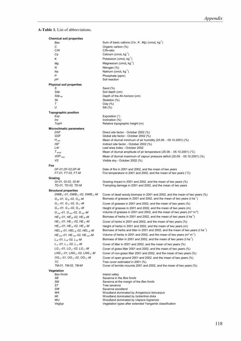
Appendix
A-Table 1. List of abbreviations.
Chemical soil propertiesBas Sum of basic cations (Ca , K , Mg ) (cmolc kg-1)C Organic carbon (%)C/N C/N-ratio Ca Calcium (cmolc kg-1)K Potassium (cmolc kg-1)Mg Magnesium (cmolc kg-1)N Nitrogen (%)Na Natrium (cmolc kg-1)P Phosphate (ppm)pH Soil reaction
Physical soil propertiesS Sand (%)Sdp Soil depth (cm)Sdp Ah Depth of the Ah-horizon (cm)Sk Skeleton (%)T Clay (%)U Silt (%)
Topographic positionExp Exposition (°)Inc Inclination (%)TopH Relative topographic height (m)
Microclimatic parametersDSF Direct site factor - October 2002 (%)GSF Global site factor - October 2002 (%)H min Mean of diurnal minimum of air humidity (25.09. - 05.10.2001) (%)ISF Indirect site factor - October 2002 (%)LAI Leaf area index - October 2002T ampl Mean of diurnal amplitude of air temperature (25.09. - 05.10.2001) (°C)VDP max Mean of diurnal maximum of vapour pressure deficit (25.09. - 05.10.2001) (%)VS Visible sky - October 2002 (%)
FireDF-01,DF-02,DF-M Date of fire in 2001 and 2002, and the mean of two yearsFT-01, FT-02, FT-M Fire temperature in 2001 and 2002, and the mean of two years (°C)
GrazingGI-01, GI-02, GI-M Grazing impact in 2001 and 2002, and the mean of two years (%)TD-01, TD-02, TD-M Trampling damage in 2001 and 2002, and the mean of two years
Structural propertiesDWB C -01, DWB C -02, DWB C -M Cover of dead woody biomass in 2001 and 2002, and the mean of two years (%)G B -01, G B -02, G B -M Biomass of grasses in 2001 and 2002, and the mean of two years (t ha-1)G C -01, G C -02, G C -M Cover of grasses in 2001 and 2002, and the mean of two years (%)G H -01, G H -02, G H -M Height of grasses in 2001 and 2002, and the mean of two years (m)G Vol -01, G Vol -02, G Vol -M Volume of grasses in 2001 and 2002, and the mean of two years (m³ m-²)HE B -01, HE B -02, HE B -M Biomass of herbs in 2001 and 2002, and the mean of two years (t ha-1)HE C -01, HE C -02, HE C -M Cover of herbs in 2001 and 2002, and the mean of two years (%)HE H -01, HE H -02, HE H -M Height of herbs in 2001 and 2002, and the mean of two years (m)HEL B -01, HEL B -02, HEL B -M Biomass of herbs and litter in 2001 and 2002, and the mean of two years (t ha-1)HE Vol -01, HE Vol -02, HE Vol -M Volume of herbs in 2001 and 2002, and the mean of two years (m³ m-2)L B -01, L B -02, L B -M Biomass of litter in 2001 and 2002, and the mean of two years (t ha-1)L C -01, L C -02, L C -M Cover of litter in 2001 and 2002, and the mean of two years (%)LG C -01, LG C -02, LG C -M Cover of grass litter 2001 and 2002, and the mean of two years (%)LNG C -01, LNG C -02, LNG C -M Cover of non-grass litter 2001 and 2002, and the mean of two years (%)OG C -01, OG C -02, OG C -M Cover of open ground 2001 and 2002, and the mean of two years (%)TC Tree cover estimated in 2001 (%)TM-01, TM-02, TM-M Cover of termite mounds 2001 and 2002, and the mean of two years (%)
VegetationBas fonds Inland valleySB Savanna in the Bas fondsSM Savanna at the margin of the Bas fondsST Tree savannaSW Savanna woodlandWA Woodland dominated by Anogeissus leiocarpusWI Woodland dominated by Isoberlinia dokaWU Woodland dominated by Uapaca togoensisVegtyp Vegetation types after extended Yangambi classification
118
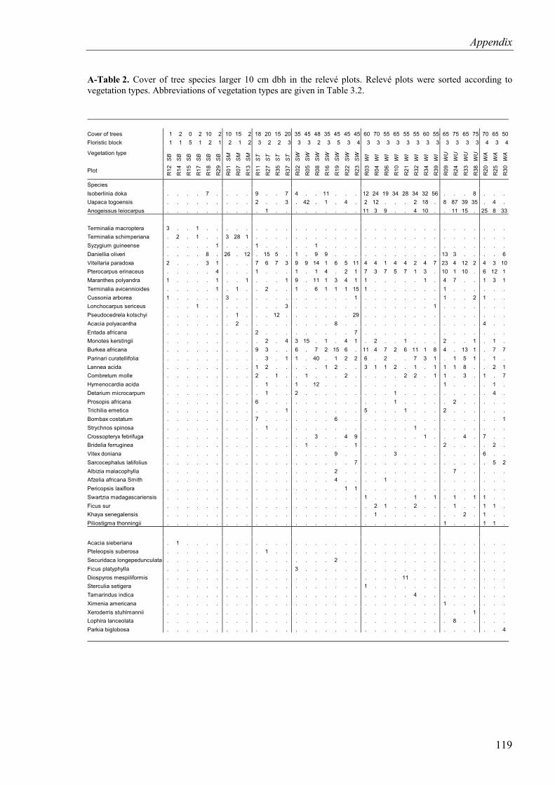
Appendix
A-Table 2. Cover of tree species larger 10 cm dbh in the relevé plots. Relevé plots were sorted according to vegetation types. Abbreviations of vegetation types are given in Table 3.2.
Cover of trees 1 2 0 2 10 2 10 15 2 18 20 15 20 35 45 48 35 45 45 45 60 70 55 65 55 55 60 55 65 75 65 75 70 65 50 Floristic block 1 1 5 1 2 1 2 1 2 3 2 2 3 3 3 2 3 5 3 4 3 3 3 3 3 3 3 3 3 3 3 3 4 3 4
Vegetation type
SB
SB
SB
SB
SB
SB
SM
SM
SM
ST
ST
ST
ST
SW
SW
SW
SW
SW
SW
SW
WI
WI
WI
WI
WI
WI
WI
WI
WU
WU
WU
WU
WA
WA
WA
Plot R12
R14
R15
R17
R18
R29
R01
R07
R13
R11
R27
R35
R37
R02
R05
R08
R16
R19
R22
R23
R03
R04
R06
R10
R21
R32
R34
R39
R09
R24
R33
R38
R20
R25
R30
Species Isoberlinia doka . . . . 7 . . . . 9 . . 7 4 . . 11 . . . 12 24 19 34 28 34 32 56 . . . 8 . . . Uapaca togoensis . . . . . . . . . 2 . . 3 . 42 . 1 . 4 . 2 12 . . . 2 18 . 8 87 39 35 . 4 . Anogeissus leiocarpus . . . . . . . . . . 1 . . . . . . . . . 11 3 9 . . 4 10 . . 11 15 . 25 8 33
Terminalia macroptera 3 . . 1 . . . . . . . . . . . . . . . . . . . . . . . . . . . . . . . Terminalia schimperiana . 2 . 1 . . 3 28 1 . . . . . . . . . . . . . . . . . . . . . . . . . . Syzygium guineense . . . . . 1 . . . 1 . . . . . 1 . . . . . . . . . . . . . . . . . . . Daniellia oliveri . . . . 8 . 26 . 12 . 15 5 . 1 . 9 9 . . . . . . . . . . . 13 3 . . . . 6 Vitellaria paradoxa 2 . . . 3 1 . . . 7 6 7 3 9 9 14 1 6 5 11 4 4 1 4 4 2 4 7 23 4 12 2 4 3 10 Pterocarpus erinaceus . . . . . 4 . . . 1 . . . 1 . 1 4 . 2 1 7 3 7 5 7 1 3 . 10 1 10 . 6 12 1 Maranthes polyandra 1 . . . . 1 . . 1 . . . 1 9 . 11 1 3 4 1 1 . . . . . 1 . 4 7 . . 1 3 1 Terminalia avicennioides . . . . . 1 . 1 . . 2 . . 1 . 6 1 1 1 15 1 . . . . . . . 1 . . . . . . Cussonia arborea 1 . . . . . 3 . . . . . . . . . . . . 1 . . . . . . . . 1 . . 2 1 . . Lonchocarpus sericeus . . . 1 . . . . . . . . 3 . . . . . . . . . . . . . . 1 . . . . . . . Pseudocedrela kotschyi . . . . . . . 1 . . . 12 . . . . . . . 29 . . . . . . . . . . . . . . . Acacia polyacantha . . . . . . . 2 . . . . . . . . . 8 . . . . . . . . . . . . . . 4 . . Entada africana . . . . . . . . . 2 . . . . . . . . . 7 . . . . . . . . . . . . . . . Monotes kerstingii . . . . . . . . . . 2 . 4 3 15 . 1 . 4 1 . 2 . . 1 . . . 2 . . 1 . 1 . Burkea africana . . . . . . . . . 9 3 . . 6 . 7 2 15 6 . 11 4 7 2 6 11 1 8 4 . 13 1 . 7 7 Parinari curatellifolia . . . . . . . . . . 3 . 1 1 . 40 . 1 2 2 6 . 2 . . 7 3 1 . 1 5 1 . 1 . Lannea acida . . . . . . . . . 1 2 . . . . . 1 2 . . 3 1 1 2 . 1 . 1 1 1 8 . . 2 1 Combretum molle . . . . . . . . . 2 . 1 . . 1 . . . 2 . . . . . 2 2 . 1 1 . 3 . 1 . 7 Hymenocardia acida . . . . . . . . . . 1 . . 1 . 12 . . . . . . . . . . . . 1 . . . . 1 . Detarium microcarpum . . . . . . . . . . 1 . . 2 . . . . . . . . . 1 . . . . . . . . . 4 . Prosopis africana . . . . . . . . . 6 . . . . . . . . . . . . . 1 . . . . . 2 . . . . . Trichilia emetica . . . . . . . . . . . . 1 . . . . . . . 5 . . . 1 . . . 2 . . . . . . Bombax costatum . . . . . . . . . 7 . . . . . . . 6 . . . . . . . . . . . . . . . . 1 Strychnos spinosa . . . . . . . . . . 1 . . . . . . . . . . . . . . 1 . . . . . . . . . Crossopteryx febrifuga . . . . . . . . . . . . . . . 3 . . 4 9 . . . . . . 1 . . . 4 . 7 . . Bridelia ferruginea . . . . . . . . . . . . . . 1 . . . . 1 . . . . . . . . 2 . . . . 2 . Vitex doniana . . . . . . . . . . . . . . . . . 9 . . . . . 3 . . . . . . . . 6 . . Sarcocephalus latifolius . . . . . . . . . . . . . . . . . . . 7 . . . . . . . . . . . . . 5 2 Albizia malacophylla . . . . . . . . . . . . . . . . . 2 . . . . . . . . . . . 7 . . . . . Afzelia africana Smith . . . . . . . . . . . . . . . . . 4 . . . . 1 . . . . . . . . . . . . Pericopsis laxiflora . . . . . . . . . . . . . . . . . . 1 1 . . . . . . . . . . . . . . . Swartzia madagascariensis . . . . . . . . . . . . . . . . . . . . 1 . . . . 1 . 1 . 1 . 1 1 . . Ficus sur . . . . . . . . . . . . . . . . . . . . . 2 1 . . 2 . . . 1 . . 1 1 . Khaya senegalensis . . . . . . . . . . . . . . . . . . . . . 1 . . . . . . . . 2 . 1 . . Piliostigma thonningii . . . . . . . . . . . . . . . . . . . . . . . . . . . . 1 . . . 1 1 .
Acacia sieberiana . 1 . . . . . . . . . . . . . . . . . . . . . . . . . . . . . . . . . Pteleopsis suberosa . . . . . . . . . . 1 . . . . . . . . . . . . . . . . . . . . . . . . Securidaca longepedunculata . . . . . . . . . . . . . . . . . 2 . . . . . . . . . . . . . . . . . Ficus platyphylla . . . . . . . . . . . . . 3 . . . . . . . . . . . . . . . . . . . . . Diospyros mespiliformis . . . . . . . . . . . . . . . . . . . . . . . . 11 . . . . . . . . . . Sterculia setigera . . . . . . . . . . . . . . . . . . . . 1 . . . . . . . . . . . . . . Tamarindus indica . . . . . . . . . . . . . . . . . . . . . . . . . 4 . . . . . . . . . Ximenia americana . . . . . . . . . . . . . . . . . . . . . . . . . . . . 1 . . . . . . Xeroderris stuhlmannii . . . . . . . . . . . . . . . . . . . . . . . . . . . . . . . 1 . . . Lophira lanceolata . . . . . . . . . . . . . . . . . . . . . . . . . . . . . 8 . . . . . Parkia biglobosa . . . . . . . . . . . . . . . . . . . . . . . . . . . . . . . . . . 4
119
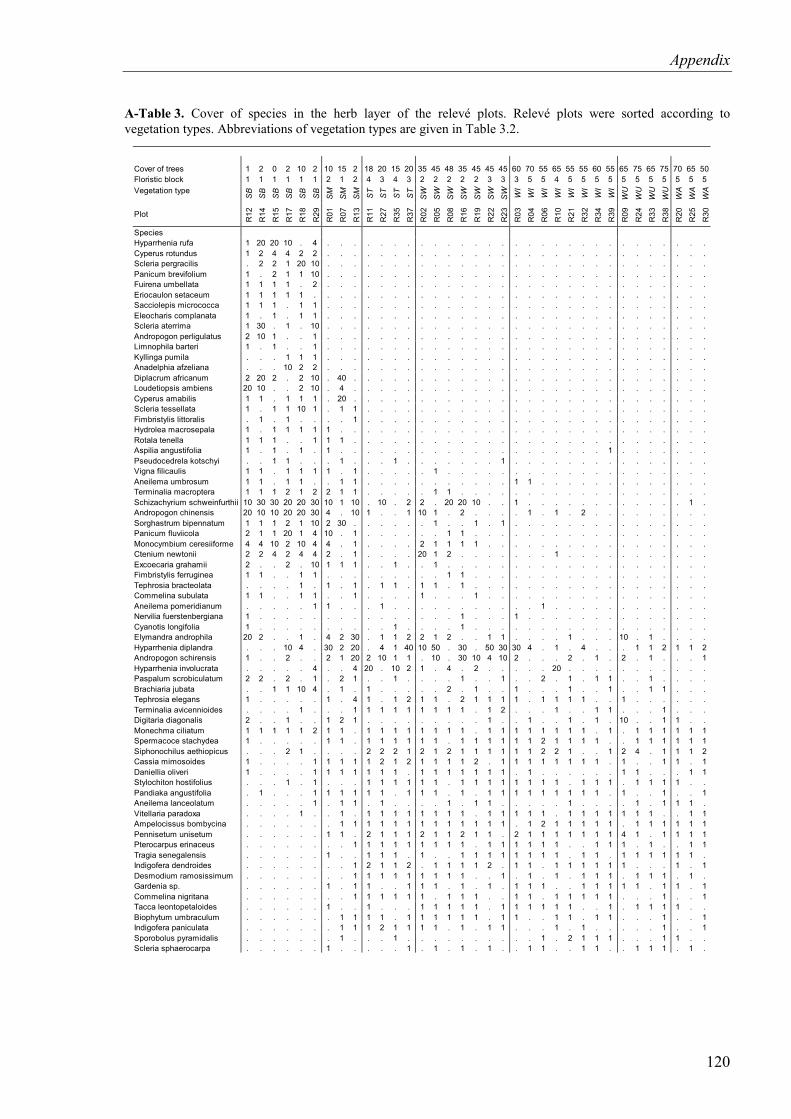
Appendix
A-Table 3. Cover of species in the herb layer of the relevé plots. Relevé plots were sorted according to
vegetation types. Abbreviations of vegetation types are given in Table 3.2.
Cover of trees 1 2 0 2 10 2 10 15 2 18 20 15 20 35 45 48 35 45 45 45 60 70 55 65 55 55 60 55 65 75 65 75 70 65 50 Floristic block 1 1 1 1 1 1 2 1 2 4 3 4 3 2 2 2 2 2 3 3 3 5 5 4 5 5 5 5 5 5 5 5 5 5 5 Vegetation type S
B
SB
S
B
SB
S
B
SB
S
M
SM
S
M
ST
ST
ST
ST
SW
S
W
SW
S
W
SW
S
W
SW
W
I W
I W
I W
I W
I W
I W
I W
I W
U
WU
W
U
WU
W
A
WA
W
A
Plot R
12
R14
R
15
R17
R
18
R29
R
01
R07
R
13
R11
R
27
R35
R
37
R02
R
05
R08
R
16
R19
R
22
R23
R
03
R04
R
06
R10
R
21
R32
R
34
R39
R
09
R24
R
33
R38
R
20
R25
R
30
Species Hyparrhenia rufa 1 20 20 10 . 4 . . . . . . . . . . . . . . . . . . . . . . . . . . . . . Cyperus rotundus 1 2 4 4 2 2 . . . . . . . . . . . . . . . . . . . . . . . . . . . . . Scleria pergracilis . 2 2 1 20 10 . . . . . . . . . . . . . . . . . . . . . . . . . . . . . Panicum brevifolium 1 . 2 1 1 10 . . . . . . . . . . . . . . . . . . . . . . . . . . . . . Fuirena umbellata 1 1 1 1 . 2 . . . . . . . . . . . . . . . . . . . . . . . . . . . . . Eriocaulon setaceum 1 1 1 1 1 . . . . . . . . . . . . . . . . . . . . . . . . . . . . . . Sacciolepis micrococca 1 1 1 . 1 1 . . . . . . . . . . . . . . . . . . . . . . . . . . . . . Eleocharis complanata 1 . 1 . 1 1 . . . . . . . . . . . . . . . . . . . . . . . . . . . . . Scleria aterrima 1 30 . 1 . 10 . . . . . . . . . . . . . . . . . . . . . . . . . . . . . Andropogon perligulatus 2 10 1 . . 1 . . . . . . . . . . . . . . . . . . . . . . . . . . . . . Limnophila barteri 1 . 1 . . 1 . . . . . . . . . . . . . . . . . . . . . . . . . . . . . Kyllinga pumila . . . 1 1 1 . . . . . . . . . . . . . . . . . . . . . . . . . . . . . Anadelphia afzeliana . . . 10 2 2 . . . . . . . . . . . . . . . . . . . . . . . . . . . . . Diplacrum africanum 2 20 2 . 2 10 . 40 . . . . . . . . . . . . . . . . . . . . . . . . . . . Loudetiopsis ambiens 20 10 . . 2 10 . 4 . . . . . . . . . . . . . . . . . . . . . . . . . . . Cyperus amabilis 1 1 . 1 1 1 . 20 . . . . . . . . . . . . . . . . . . . . . . . . . . . Scleria tessellata 1 . 1 1 10 1 . 1 1 . . . . . . . . . . . . . . . . . . . . . . . . . . Fimbristylis littoralis . 1 . 1 . . . . 1 . . . . . . . . . . . . . . . . . . . . . . . . . . Hydrolea macrosepala 1 . 1 1 1 1 1 . . . . . . . . . . . . . . . . . . . . . . . . . . . . Rotala tenella 1 1 1 . . 1 1 1 . . . . . . . . . . . . . . . . . . . . . . . . . . . Aspilia angustifolia 1 . 1 . 1 . 1 . . . . . . . . . . . . . . . . . . . . 1 . . . . . . . Pseudocedrela kotschyi . . 1 1 . . . 1 . . . 1 . . . . . . . 1 . . . . . . . . . . . . . . . Vigna filicaulis 1 1 . 1 1 1 1 . 1 . . . . . 1 . . . . . . . . . . . . . . . . . . . . Aneilema umbrosum 1 1 . 1 1 . . 1 1 . . . . . . . . . . . 1 1 . . . . . . . . . . . . . Terminalia macroptera 1 1 1 2 1 2 2 1 1 . . . . . 1 1 . . . . . . . . . . . . . . . . . . . Schizachyrium schweinfurthii 10 30 30 20 20 30 10 1 10 . 10 . 2 2 . 20 20 10 . . 1 . . . . . . . . . . . . 1 . Andropogon chinensis 20 10 10 20 20 30 4 . 10 1 . . 1 10 1 . 2 . . . . 1 . 1 . 2 . . . . . . . . . Sorghastrum bipennatum 1 1 1 2 1 10 2 30 . . . . . . 1 . . 1 . 1 . . . . . . . . . . . . . . . Panicum fluviicola 2 1 1 20 1 4 10 . 1 . . . . . . 1 1 . . . . . . . . . . . . . . . . . . Monocymbium ceresiiforme 4 4 10 2 10 4 4 . 1 . . . . 2 1 1 1 1 . . . . . . . . . . . . . . . . . Ctenium newtonii 2 2 4 2 4 4 2 . 1 . . . . 20 1 2 . . . . . . . 1 . . . . . . . . . . . Excoecaria grahamii 2 . . 2 . 10 1 1 1 . . 1 . . 1 . . . . . . . . . . . . . . . . . . . . Fimbristylis ferruginea 1 1 . . 1 1 . . . . . . . . . 1 1 . . . . . . . . . . . . . . . . . . Tephrosia bracteolata . . . . 1 . 1 . 1 . 1 1 . 1 1 . 1 . . . . . . . . . . . . . . . . . . Commelina subulata 1 1 . . 1 1 . . 1 . . . . 1 . . . 1 . . . . . . . . . . . . . . . . . Aneilema pomeridianum . . . . . 1 1 . . . 1 . . . . . . . . . . . 1 . . . . . . . . . . . . Nervilia fuerstenbergiana 1 . . . . . . . . . . . . . . . 1 . . . 1 . . . . . . . . . . . . . . Cyanotis longifolia 1 . . . . . . . . . . 1 . . . . 1 . . . . . . . . . . . . . . . . . . Elymandra androphila 20 2 . . 1 . 4 2 30 . 1 1 2 2 1 2 . . 1 1 . . . . 1 . . . 10 . 1 . . . . Hyparrhenia diplandra . . . 10 4 . 30 2 20 . 4 1 40 10 50 . 30 . 50 30 30 4 . 1 . 4 . . . 1 1 2 1 1 2 Andropogon schirensis 1 . . 2 . . 2 1 20 2 10 1 1 . 10 . 30 10 4 10 2 . . . 2 . 1 . 2 . 1 . . . 1 Hyparrhenia involucrata . . . . . 4 . . 4 20 . 10 2 1 . 4 . 2 . . . . . 20 . . . . . . . . . . . Paspalum scrobiculatum 2 2 . 2 . 1 . 2 1 . . 1 . . . . 1 . . 1 . . 2 . 1 . 1 1 . . 1 . . . . Brachiaria jubata . . 1 1 10 4 . 1 . 1 . . . . . 2 . 1 . . 1 . . . 1 . . 1 . . 1 1 . . . Tephrosia elegans 1 . . . . . 1 . 4 1 . 1 2 1 1 . 2 1 1 1 1 . 1 1 1 1 . . 1 . . . . . . Terminalia avicennioides . . . . 1 . . . 1 1 1 1 1 1 1 1 1 . 1 2 . . . 1 . . 1 1 . . . 1 . . . Digitaria diagonalis 2 . . 1 . . 1 2 1 . . . . . . . . . 1 . . 1 . . 1 . 1 . 10 . . 1 1 . . Monechma ciliatum 1 1 1 1 1 2 1 1 . 1 1 1 1 1 1 1 1 . 1 1 1 1 1 1 1 1 . 1 . 1 1 1 1 1 1 Spermacoce stachydea 1 . . . . . 1 1 . 1 1 1 1 1 1 . 1 1 1 1 1 1 2 1 1 1 1 . . 1 1 1 1 1 1 Siphonochilus aethiopicus . . . 2 1 . . . . 2 2 2 1 2 1 2 1 1 1 1 1 1 2 2 1 . . 1 2 4 . 1 1 1 2 Cassia mimosoides 1 . . . . 1 1 1 1 1 2 1 2 1 1 1 1 2 . 1 1 1 1 1 1 1 1 . 1 . . 1 1 . 1 Daniellia oliveri 1 . . . . 1 1 1 1 1 1 1 . 1 1 1 1 1 1 1 . 1 . . . . . . 1 1 . . . 1 1 Stylochiton hostifolius . . . 1 . 1 . . . 1 1 1 1 1 1 . 1 1 1 1 1 1 1 1 . 1 1 1 . 1 1 1 1 . . Pandiaka angustifolia . 1 . . . 1 1 1 1 1 1 . 1 1 1 . 1 . 1 1 1 1 1 1 1 1 1 . 1 . . 1 . . 1 Aneilema lanceolatum . . . . . 1 . 1 1 . 1 . . . . 1 . 1 1 . . . . . 1 . . . . 1 . 1 1 1 . Vitellaria paradoxa . . . . 1 . . 1 . 1 1 1 1 1 1 1 1 . 1 1 1 1 1 . 1 1 1 1 1 1 1 . . 1 1 Ampelocissus bombycina . . . . . . . 1 1 1 1 1 1 1 1 1 1 1 1 1 . 1 2 1 1 1 1 1 . 1 1 1 1 1 1 Pennisetum unisetum . . . . . . 1 1 . 2 1 1 1 2 1 1 2 1 1 . 2 1 1 1 1 1 1 1 4 1 . 1 1 1 1 Pterocarpus erinaceus . . . . . . . . 1 1 1 1 1 1 1 1 1 . 1 1 1 1 1 1 . . 1 1 1 . 1 . . 1 1 Tragia senegalensis . . . . . . 1 . . 1 1 1 . 1 . . 1 1 1 1 1 1 1 1 . 1 1 . 1 1 1 1 1 1 . Indigofera dendroides . . . . . . . . 1 2 1 1 2 . 1 1 1 1 2 . 1 1 . 1 1 1 1 1 1 . . . 1 . 1 Desmodium ramosissimum . . . . . . . . 1 1 1 1 1 1 1 1 1 . . 1 . 1 . 1 . 1 1 1 . 1 1 1 . 1 . Gardenia sp. . . . . . . 1 . 1 1 . . 1 1 1 . 1 . 1 . 1 1 1 . . 1 1 1 1 1 . 1 1 . 1 Commelina nigritana . . . . . . . . 1 1 1 1 1 1 . 1 1 1 . . 1 1 . 1 1 1 1 1 . . . 1 . . 1 Tacca leontopetaloides . . . . . . 1 . . 1 . . . 1 1 1 1 1 . 1 1 1 1 1 1 . . 1 . 1 1 1 1 . . Biophytum umbraculum . . . . . . . 1 1 1 1 . 1 1 1 1 1 1 . 1 1 . . 1 1 . 1 1 . . . 1 . . 1 Indigofera paniculata . . . . . . . 1 1 1 2 1 1 1 1 . 1 . 1 1 . . . 1 . 1 . . . . . 1 . . 1 Sporobolus pyramidalis . . . . . . . 1 . . . 1 . . . . . . . . . . 1 . 2 1 1 1 . . . 1 1 . . Scleria sphaerocarpa . . . . . . 1 . . . . . 1 . 1 . 1 . 1 . . 1 1 . . 1 1 . . 1 1 1 . 1 .
120
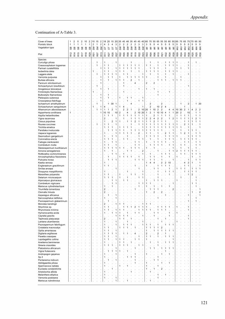
Appendix
Continuation of A-Table 3. Cover of trees 1 2 0 2 10 2 10 15 2 18 20 15 20 35 45 48 35 45 45 45 60 70 55 65 55 55 60 55 65 75 65 75 70 65 50 Floristic block 1 1 1 1 1 1 2 1 2 4 3 4 3 2 2 2 2 2 3 3 3 5 5 4 5 5 5 5 5 5 5 5 5 5 5 Vegetation type S
B
SB
S
B
SB
S
B
SB
S
M
SM
S
M
ST
ST
ST
ST
SW
S
W
SW
S
W
SW
S
W
SW
W
I W
I W
I W
I W
I W
I W
I W
I W
U
WU
W
U
WU
W
A
WA
W
A
Plot R
12
R14
R
15
R17
R
18
R29
R
01
R07
R
13
R11
R
27
R35
R
37
R02
R
05
R08
R
16
R19
R
22
R23
R
03
R04
R
06
R10
R
21
R32
R
34
R39
R
09
R24
R
33
R38
R
20
R25
R
30
Species Curculigo pilosa . . . . . . . 1 . 1 . . 1 . . . 1 . . . . 1 . 1 . 1 1 1 1 . . 1 . 1 . Crassocephalum togoense . . . . . . . 1 . 1 1 . . 1 1 1 1 1 1 . 1 1 . 1 . 1 1 1 1 . . 1 . . . Parinari curatellifolia . . . . . . . . 1 1 1 . 1 1 1 1 1 1 1 . . 1 1 1 . 1 . . 1 1 . 1 . . . Isoberlinia doka . . . . . . 1 . . 1 1 . 1 1 1 . 1 . 1 . 1 1 1 1 . 1 1 1 1 . . . . . . Laggera alata . . . . . . . 1 . 1 1 1 1 . 1 1 . . . 1 . 1 . 1 . 1 . 1 . . . 1 . . . Vernonia purpurea . . . . . . . . 1 . 1 1 . 1 . 1 1 1 1 1 1 . . 1 . 1 . . . 1 . . . . . Burkea africana . . . . . . . . 1 . 1 . 1 1 1 . 2 . 1 . . . . 1 1 1 . 1 1 1 . . . . . Panicum strictissimum . . . . . . . . 1 . . . . . 1 . . 4 . . 2 . 2 . . . . . . . . . . . . Schizachyrium brevifolium . . . . . . . 1 . . . . . . 1 . . . . . . . . . . . . . . . . 1 . . . Anogeissus leiocarpus . . . . . . . . 1 . 1 . . . . . . . 1 . 1 . 1 . . . . . . . . . . . . Fimbristylis filamentosa . . . . . . 1 . . . . . . . 1 . . . . . . . . 1 . . 1 . . . . . . . . Bulbostylis filamentosa . . . . . . . . 1 . 1 . . . . . . . . . . . . 1 . . . . . . . . . . . Pteleopsis suberosa . . . . . . . . 1 . 1 . . 1 . 1 1 . . 1 . . . . . . . . . . . . . . . Crossopteryx febrifuga . . . . . . . . 1 . . . . . . 1 . . 1 1 . . . . . . . . . . . . . . . Ischaemum amethystinum . . . . . . . 1 . . 1 30 1 . . . 4 . . . . 2 . . 2 . . . . 1 . 2 . 1 20 Schizachyrium sanguineum . . . . . . 1 . 1 4 . . 1 1 4 . . . . 1 . 2 . 10 2 4 . . . . 1 . . . . Aframomum alboviolaceum . . . . . . . 1 1 1 1 2 1 . 2 2 1 . 2 10 20 1 10 2 2 . 4 4 10 30 2 1 4 2 2 Hyparrhenia smithiana 1 . . . . . . . 1 10 10 . 10 2 . 4 . 2 10 20 1 2 1 10 10 4 1 1 20 2 . 10 . 1 1 Aspilia helianthoides . . . . . . . . . 1 1 1 . 1 1 1 1 1 1 1 1 . 2 1 1 1 1 . 1 1 1 1 . 1 1 Vigna racemosa . . . . . . . . . 2 . . 1 . 1 . 1 1 1 1 2 2 4 2 2 . 1 2 1 1 1 1 1 2 1 Cissus populnea . . . . . . . . . 1 . 2 1 1 . 1 1 2 1 1 1 1 2 1 1 1 . . 1 . 1 1 1 1 1 Rourea coccinea . . . . . . . 1 . 1 1 . 1 . . . 1 . 1 1 1 1 1 1 1 1 1 1 1 . 2 1 1 . 1 Trichilia emetica . . . . . . . . . 1 1 1 . 1 1 1 1 . . 1 1 1 1 1 1 1 1 1 1 1 . 1 . . 1 Pandiaka involucrata . . . . . . . . . . 1 1 1 1 1 . 1 1 1 1 1 1 1 1 1 . . 1 . 1 . 1 1 1 . Uapaca togoensis . . . . . . . . . 1 . . 1 1 1 1 1 . 2 . 1 1 . 1 . 2 1 1 . 1 2 1 . 1 1 Desmodium gangeticum . . . . . . . . . 1 . 1 1 . . 1 . . 1 . 1 1 1 1 . 1 1 1 1 . . 1 1 1 1 Commelina erecta . . . . . . . . . 1 1 1 . . 1 1 . . 1 1 . 1 . 1 . 1 1 1 . 1 1 1 1 1 . Fadogia cienkowskii . . . . . . . . . 1 . 1 1 . . . . 1 1 . 1 . 1 1 1 1 . 1 . . 1 1 . 1 1 Combretum molle . . . . . . . . . 1 1 . 1 . . . . 1 1 . . 1 1 1 1 . 1 1 . 1 1 . . 1 1 Stereospermum kunthianum . . . . . . . . . 1 1 1 1 1 1 . 1 1 1 . 1 . 1 . . . . 1 . 1 . 1 . 1 . Annona senegalensis . . . . . . . . . 1 . 1 . . . 1 1 . . 2 . . . 1 . . 1 1 2 1 1 1 1 1 . Rottboellia cochinchinensis . . . . . . . . . . . 1 1 . 1 . . . . 1 . 1 . . 1 1 1 . . 1 1 . 1 1 1 Amorphophallus flavovirens . . . . . . . . . . 1 . . 1 1 1 1 . 1 . . 1 1 . 1 . 1 . 1 . . . 1 . 1 Pulicaria incisa . . . . . . . . . . 1 1 1 . . . . 1 1 1 . 1 1 . 1 . . 1 . . . 1 . 1 1 Keetia venosa . . . . . . . . . 1 . . . . . . . . . . 1 4 4 . 2 2 10 . . . 4 2 1 . 1 Englerastrum gracillimum . . . . . . . . . 1 1 . . . . . . 1 . . 1 . . 1 1 1 1 . . . 1 1 . . 1 Smilax anceps . . . . . . . . . . . . 1 . . . . . 1 . . . 1 1 . . 1 . 1 1 1 . 1 1 1 Diospyros mespiliformis . . . . . . . . . 1 . . . . . 1 . . . 1 . . . 1 . 1 1 1 . . 1 1 1 1 . Maranthes polyandra . . . . . . . . . 1 1 . . 1 . . 1 1 . 1 . . . 1 . . 1 . . . . 1 2 . . Detarium microcarpum . . . . . . . . . 1 1 1 . 1 . 1 . . 1 1 . . . 1 . . . . . 1 . . . 1 . Alysicarpus glumaceus . . . . . . . . . . . 1 1 . 1 1 . . . . 1 . 1 1 1 . . . 1 . . . . 1 . Combretum nigricans . . . . . . . . . . . 1 1 . . . . . 1 1 1 1 . . . . . 1 . . . . 1 1 . Mariscus cylindristachyus . . . . . . . . . 1 . 1 . . . . . . 1 . 1 . 1 . 1 . 1 . . . . . . 1 . Triumfetta tomentosa . . . . . . . . . 2 . . . . . . . 1 . . . 1 1 1 . . . 2 . . . . . . 1 Clematis hirsuta . . . . . . . . . 2 . . . . . . . . . . 1 . 2 . 2 . . . . . . . 1 . 2 Asparagus africanus . . . . . . . . . . 1 . 1 . . . . . . . . . . . . 1 . . . . . 1 . . 1 Sarcocephalus latifolius . . . . . . . . . 1 . . 1 . . . . . . . . . . 1 . . . . . . . . . 1 . Psorospermum glaberrimum . . . . . . . . . . 1 . . . . . . . . . . . . . . . . . . . . 1 . 1 . Monotes kerstingii . . . . . . . . . 2 . . 1 1 1 . . . . 1 1 1 . . . . . . . . . . . . . Strychnos sp. . . . . . . . . . 1 1 . . . 1 1 1 2 1 1 1 . . 1 1 1 1 . 1 . . 1 . . . Rhynchosia minima . . . . . . . . . 1 1 . 1 1 1 . . . 1 1 1 1 . 1 1 1 . . . . . 1 . . . Hymenocardia acida . . . . . . . . . 1 . 1 1 1 . 1 . 1 1 . . . 1 1 . . 1 . 1 . . . . . . Cayratia gracilis . . . . . . . . . . . . 1 1 1 1 . . . 1 . . 1 . . . 1 . . . . 1 . . . Tephrosia platycarpa . . . . . . . . . 2 . . . 1 1 . 1 . . . . . . 1 . 1 . . . . . 1 . . . Lantana ukambensis . . . . . . . . . 1 . . 1 . . 1 . . . 1 . . . . 1 . . . 1 . . . . . . Psorospermum febrifugum . . . . . . . . . 1 . . 1 . 1 1 1 . . 1 1 1 . 1 . 1 1 1 . . . . . . . Crotalaria macrocalyx . . . . . . . . . 1 1 . . 1 1 1 . 1 . . 1 1 1 1 2 . . . . . . . . . . Opilia amentacea . . . . . . . . . 1 1 . 1 . . . . . . . 1 . 1 1 1 1 1 1 . . . . . . . Digitaria argillacea . . . . . . . . . 1 1 1 1 . 1 1 . 4 . . 2 . . 2 . 1 . . . . . . . . . Pavetta crassipes . . . . . . . . . 1 1 . 1 . . . . . 1 . 1 1 . 1 . 1 1 1 . . . . . . . Lepidagathis collina . . . . . . . . . 1 1 . 1 1 1 . . 1 1 . 1 . . . . . . 1 . . . . . . . Aneilema beniniense . . . . . . . . . 1 . . . 1 1 . 1 . . . . 1 . 1 . 1 1 1 . . . . . . . Grewia cissoides . . . . . . . . . 1 1 1 . 1 1 1 . . 1 1 . . . 1 . . . . . . . . . . . Platostoma africanum . . . . . . . . . . . . 1 . . . . 1 . . . 1 1 . 1 1 1 1 . . . . . . . Vigna frutescens . . . . . . . . . . 1 1 1 1 . 1 . . . . . . . . . 1 . . . . . . . . . Andropogon gayanus . . . . . . . . . 1 . . 1 . . . . 1 . . 1 . . . 1 . 1 . . . . . . . . Sp.3 . . . . . . . . . 1 . . . . . 1 1 1 . . . . . 1 . . . . . . . . . . . Pentanema indicum . . . . . . . . . . 1 . 1 . . . . 1 . . . . 1 1 . . . . . . . . . . . Abildgaardia pilosa . . . . . . . . . 1 . . . . . . . 1 . . 1 . . . 1 . 1 . . . . . . . . Spermacoce radiata . . . . . . . . . 1 . . . 1 . 1 . . . . 1 . . 1 . . . . . . . . . . . Euclasta condylotricha . . . . . . . . . . . 1 . . . . . . . . 1 . 1 . 2 . . . . . . . . . . Aristolochia albida . . . . . . . . . 1 . . . . . . 1 . . . . 1 . . . . . . . . . . . . . Melanthera elliptica . . . . . . . . . 1 . . . . . . . . . . . . . 1 . 1 . . . . . . . . . Vernonia poskeana . . . . . . . . . 1 . . 1 . . . . . . . . . . 1 . . . . . . . . . . . Mariscus rubrotinctus . . . . . . . . . . . . 1 . . 1 . . . . . 1 . . . . . . . . . . . . .
121
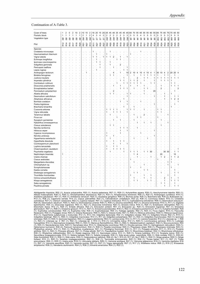
Appendix
122
Continuation of A-Table 3.
Cover of trees 1 2 0 2 10 2 10 15 2 18 20 15 20 35 45 48 35 45 45 45 60 70 55 65 55 55 60 55 65 75 65 75 70 65 50 Floristic block 1 1 1 1 1 1 2 1 2 4 3 4 3 2 2 2 2 2 3 3 3 5 5 4 5 5 5 5 5 5 5 5 5 5 5 Vegetation type S
B
SB
S
B
SB
S
B
SB
S
M
SM
S
M
ST
ST
ST
ST
SW
S
W
SW
S
W
SW
S
W
SW
W
I W
I W
I W
I W
I W
I W
I W
I W
U
WU
W
U
WU
W
A
WA
W
A
Plot R
12
R14
R
15
R17
R
18
R29
R
01
R07
R
13
R11
R
27
R35
R
37
R02
R
05
R08
R
16
R19
R
22
R23
R
03
R04
R
06
R10
R
21
R32
R
34
R39
R
09
R24
R
33
R38
R
20
R25
R
30
Species Crotalaria microcarpa . . . . . . . . . 1 . . . . 1 . . . . . . . . 1 . . . . . . . . . . . Haumaniastrum lilacinum . . . . . . . . . . 1 . . 1 . . . . . . 1 . . . . . . . . . . . . . . Vigna luteola . . . . . . . . . 1 1 . 1 1 1 2 . 1 . 1 . . . . . . . . . . . . . . . Echinops longifolius . . . . . . . . . . 1 . . . . . 1 1 . . . . . . . . . . . . . . . . . Ipomoea coscinosperma . . . . . . . . . . 1 1 . . 1 . . . . . . . . . . . . . . . . . . . . Indigofera geminata . . . . . . . . . . . 1 . . 1 . . 2 . . . . . . . . . . . . . . . . . Pericopsis laxiflora . . . . . . . . . . . 1 . . . 1 . . . 1 . . . . . . . . . . . . . . . Lippia rugosa . . . . . . . . . . 1 . . . . . . . 1 1 . . . . . . . . . . . . . . . Andropogon tectorum . . . . . . . 1 . . . . . . . 4 . 1 . 10 2 10 4 10 4 10 4 1 30 10 4 2 20 20 4 Bridelia ferruginea . . . . . . . . . . . . . . 1 1 . . . 1 . 1 . 1 1 1 1 1 1 . 1 1 . 1 . Justicia insularis . . . . . . . . . . . . . . . . . . 1 . . . 2 . 1 1 . 1 1 1 1 1 1 1 1 Imperata cylindrica . . . . . . . . . . . . . . . . . 1 1 . 1 1 2 . 1 . . 1 . 1 1 1 1 . . Combretum collinum . . . . . . . . . . . . . . . . 1 . 1 1 1 1 1 1 . . 1 1 . . . . 1 1 . Dioscorea praehensilis . . . . . . . . . . . . . . . 1 . 1 . . 1 . 1 . 1 . . . . 1 . . 1 1 1 Encephalartos barteri . . . . . . . . . . . . . . . . . 1 1 1 . 1 . . 1 1 . . . 2 . . . . 2 Pennisetum polystachion . . . . . . . . . . . . . . . 2 . . . . . . . . 1 . . 20 . . . . . 1 . Afzelia africana . . . . . . . . . . . . . . 1 1 . . . 1 1 . . . 1 . . . . . 1 . 1 . . Desmodium salicifolium . . . . . . . . . . . . . . . . . . . 1 . . . . . . . 1 . . 1 . . 1 1 Allophylus africanus . . . . . . . . . . . . . . . . . . 1 . . . . . . . . . . . 1 . 1 2 4 Bombax costatum . . . . . . . . . . . . . . . . . 1 . 1 . . . 1 . . . . . . . . . . 1 Parkia biglobosa . . . . . . . . . . . . . . . . . . . 1 . . . . . . . 1 . . . . . 1 . Brachiaria brizantha . . . . . . . . . . . . . . . . . . 1 . . 1 . . . . . . . . . . 1 . . Cussonia arborea . . . . . . . . . . . . . 1 1 1 1 . . 1 1 1 . . 1 . . . 1 1 . . . . . Vigna reticulata . . . . . . . . . . . . . 1 . 1 1 1 . 1 . . . . . . . . 1 1 . . . . . Teramnus labialis . . . . . . . . . . . . . . 1 . . . . . . 1 . . 2 . . . . . . 1 . . . Ficus sur . . . . . . . . . . . . . . . . 1 . . . . . 1 1 . . . . 1 . . . . . . Syzygium guineense . . . . . . . . . . . . . . . 1 . 1 . . . 1 . . . . . . . 1 . . . . . Hybanthus enneaspermus . . . . . . . . . . . . . . . . . . . . . . 1 . 1 . 1 . . . . 1 . . . Cissus sokodensis . . . . . . . . . . . . . . 1 1 . . . . . . . . . . . . . 1 . . . . . Nervilia reniformis . . . . . . . . . . . . . . . . . 1 1 1 . . 1 . . . . . . . . . . . . Hibiscus asper . . . . . . . . . . . . . . . . . 1 . 1 . . . . . . . 1 . . . . . . . Cyperus incompressus . . . . . . . . . . . . . 1 . . . 1 . . . . . 1 . . . . . . . . . . . Nervilia umbrosa . . . . . . . . . . . . . 1 . 1 . . . . . . . . . . . 1 . . . . . . . Hyparrhenia welwitschii . . . . . . . . . . . . . . 1 . . . . . . 1 . . . 1 . . . . . . . . . Hyperthelia dissoluta . . . . . . . . . . . . . 1 . 1 . 1 1 . . . . . . . . . . . . . . . . Cochlospermum planchonii . . . . . . . . . . . . . . . 1 . 1 . 1 . . . . . . . . . . . . . . . Lophira lanceolata . . . . . . . . . . . . . 1 . 1 1 . . . . . . . . . . . . . . . . . . Chasmopodium caudatum . . . . . . . . . . . . . 1 . 1 1 1 1 . . . . . . . . . . . . . . . 1 Psychotria vogeliana . . . . . . . . . . . . . . 1 . . . 1 . 1 1 1 . 1 1 30 . . . 30 30 . 1 1 Nephrolepis biserrata 1 . . . . . . . . . . . . . . . . . . . . 1 4 . . . . . . 20 . . . 10 . Uvaria chamae . . . . . . . . . . . . . . . . . . . . . . 1 . . . 1 . . 1 2 . 1 1 2 Cissus aralioides . . . . . . . . . . . . . . . . . . . . 1 . . . . . . . 1 . . . 1 . . Margaritaria discoidea . . . . . . . . . . . . . . . . . . . . . 1 . . . . . . . . . 1 1 . . Chlorophytum sp. . . . . . . . . . . . . . . . . . . . . . . . . 1 . . . . . . 1 . . 1 Scrophulariaceae . . . . . . . . . . . . . . . . . . . . 1 . . 1 . . . . . . . . 1 . . Keetia cornelia . . . . . . . . . . . . . . . . . . . . . . . . 1 1 . . . . . . . 1 . Ekebergia senegalensis . . . . . . . . . . . . . . . . . . . . . 1 1 . . . . . . 1 . . . 1 1 Triumfetta rhomboidea . . . . . . . . . . . . . . . . . . . . 1 . . . 1 . 1 . . . . 1 . 1 . Ochna schweinfurthiana . . . . . . . . . . . . . . . . . . . . . 1 . . 1 . 1 . . . 2 . 1 . 1 Khaya senegalensis . . . . . . . . . . . . . . . . . . . . . 1 1 . . 1 1 . . . 1 . 1 1 1 Saba senegalensis . . . . . . . . . . . . . . . . . . . . . . . . . . . . . 1 1 . . 1 . Paullinia pinnata . . . . . . . . . . . . . . . . . . . . . . . . . . . . . . 1 . . 1 1 Abildgaardia hispidula: R02 (1); Acacia polyacantha: R20 (1); Acacia sieberiana: R07 (1), R29 (1); Achyranthes aspera: R39 (1); Aeschynomene lateritia: R05 (1); Albizia malacophylla: R38 (1), R39 (1); Amorphophallus abyssinicus: R20 (1), R33 (1); Ampelocissus leonensis: R09 (1), R20 (1); Andropogon curvifolius: R16 (1); Aneilema paludosum: R01 (1), R35 (1); Antidesma venosum: R25 (1); Asystasia gangetica: R06 (1); Blumea aurita: R35 (1); Brachiaria lata: R35 (2); Bulbostylis sp.: R13 (1), R38 (1); Caperonia serrata: R14 (1); Cissus palmatifida: R33 (1); Clerodendrum umbellatum: R33 (2), R38 (1); Corchorus tridens: R10 (1); Crotalaria ochroleuca: R27 (1); Ctenium canescens: R02 (1); Cyperus haspan: R01 (1); Cyperus imbricatus: R12 (1); Cyphostemma sokodense: R06 (1); Desmodium tortuosum: R20 (4); Desmodium velutinum: R39 (1), R25 (1); Dichrostachys cinerea: R30 (1), R39 (1); Dicoma sessiliflora: R37 (1); Dicoma tomentosa: R10 (1), R11 (1); Digitaria leptorhachis: R35 (1); Dioscorea togoensis: R03 (1), R23 (1); Dioscorea tomentosa: R20 (1); Drosera indica: R18 (1), R29 (1); Ectadiopsis oblongifolia: R22 (1); Eleocharis dulcis: R12 (1), R29 (1); Entada africana: R23 (1); Eriocaulon jordanii: R01 (1); Eriocaulon sp.: R29 (1); Eriocaulon togoense: R01 (1); Eriosema glomeratum: R07 (1), R08 (1); Eriosema griseum: R13 (1), R27 (1); Eriosema psoraleoides: R16 (1), R02 (1); Eriosema pulcherrimum: R11 (1); Eulophia horsfallii: R29 (1); Euphorbia convolvuloides: R35 (1); Euphorbia hirta: R35 (1); Euphorbiaceae: R04 (1); Fadogia agrestis: R02 (1), R24 (1); Ficus ingens: R19 (1); Flacourtia flavescens: R30 (1); Flueggea virosa: R20 (1); Grewia flavescens: R09 (1), R20 (1); Grewia mollis: R27 (1), R30 (1); Hibiscus articulatus: R39 (1); Hibiscus squamosus: R12 (1); Hyparrhenia subplumosa x involucrata: R12 (1), R13 (10); Indgofera leptoclada: R32 (1); Indigofera colutea: R02 (1); Indigofera hirsuta: R02 (1), R19 (1); Indigofera kerstingii: R02 (1), R08 (1); Indigofera macrocalyx: R13 (1), R11 (2); Indigofera polysphaera: R07 (1), R35 (1); Indigofera rhynchocarpa: R23 (1); Ipomoea eriocarpa: R25 (1); R39 (1); Ipomoea togoensis: R03 (1); Laggera pterodonta: R03 (1); Lannea acida: R10 (1); R11 (1); Leersia hexandra: R12 (1); Liliaceae sp. 1: R08 (1), R23 (1); Liliaceae sp. 2: R01 (1), R02 (1); Liliaceae sp. 3: R10 (1); R16 (1); Limnophila indica: R12 (1), R29 (1); Lonchocarpus sericeus: R16 (1); Ludwigia hyssopifolia: R14 (1); Macrosphyra longistyla: R09 (1), R20 (1); Mariscus flambelliformis: R04 (1), R06 (1); Melastomastrum capitatum: R38 (1); Mucuna pruriens: R24 (1), R25 (1); Neorautanenia mitis: R20 (1); Nymphaea lotus: R14 (1); Oldenlandia corymbosa: R29 (1); Oncoba spinosa: R30 (1); Ophioglossum reticulatum: R39 (1); Oplismenus burmannii: R39 (2); Panicum hymeniochilum: R34 (1), R39 (1); Pavetta corymbosa: R25 (1); Phaulopsis ciliata: R39 (1); Phaulopsis imbricata: R25 (1); Phyllanthus amarus: R19 (1), R35 (1); Phyllanthus muellerianus: R21 (1); Piliostigma thonningii: R10 (1), R11 (1); Polygala arenaria: R11 (1), R13 (1); Pouteria alnifolia: R23 (1), R25 (1); Prosopis africana: R27 (1); Protea elliottii: R27 (1); Pseudarthria hookeri: R23 (1); Rhynchosia buettneri: R32 (1); Rhynchosia orthobotrya: R39 (1); Rhytachne rottboellioides: R03 (1); Rotala stagnina: R29 (1); Sacciolepis indica: R12 (1), R29 (1); Scleria bulbifera: R13 (1); Scoparia dulcis: R35 (1); Securidaca longepedunculata: R19 (1); Setaria barbata: R39 (1); Setaria longiseta: R39 (1); Sida acuta subsp. carpinifolia: R06 (1); Sida cordata: R30 (1), R39 (4); Sida rhombifolia: R30 (1), R39 (1); Sida urens: R39 (1); Solenostemon latifolius: R06 (2); Sp.1: R15 (2), R17 (2); Sp.2: R09 (1), R30 (1); Striga asiatica: R29 (1); Striga forbesii: R15 (1), R29 (1); Swartzia madagascariensis: R02 (1), R38 (1); Terminalia schimperiana: R25 (1), R30 (1); Tinnea barteri: R11 (1), R27 (1); Tridax procumbens: R24 (1), R35 (1); Uraria picta: R18 (1); Utricularia stellaris: R29 (1); Vernonia ambigua: R27 (1); Vernonia glaberrima: R19 (1); Vernonia nigritiana: R16 (1), R27 (1); Vernonia pauciflora: R30 (1); Vernonia pumila: R27 (1), R37 (1); Vigna stenophylla: R07 (1), R17 (1); Waltheria indica: R06 (1), R19 (1); Wissadula amplissima: R39 (1); Xeroderris stuhlmannii: R04 (1), R38 (1) Ximenia americana: R04 (1); R22 (1).
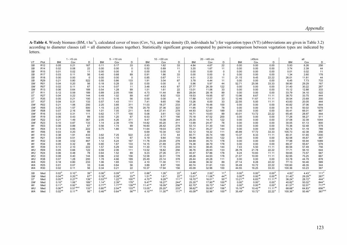
Appendix
A-Ta 4. Woody biomass (BM, t ha-1), calculated cover of trees (Cov, %), and tree density (D, individuals ha-1) for vegetation types (VT) (abbreviations are given in Table 3.2) accor to diameter classes (all = all diameter classes together). Statistically significant groups computed by pairwise comparison between vegetation types are indicated by letter
1 - <5 cm 5 - <10 cm 10 - <20 cm 20 - <45 cm ≥45cm all
ble dings.
VT BM Cov D BM Cov D BM Cov D BM Cov D BM CoPlot v D BM Cov D SB 0.05 0.21 167 0.11 0.17 33 0.93 1.62 33 4.84 4.67 22 0.00 0.00 0.00 5.93 6.26 256 R12SB 0.02 0.08 22 0.00 0.00 0 0.52 0.89 11 3.20 1.67 11 0.00 0.00 0.00 3.74 2.39 44 R14SB 0.01 0.02 11 0.00 0.00 0 0.00 0.00 0 0.00 0.00 0 0.00 0.00 0.00 0.01 0.02 11 R15SB 0.03 0.11 56 0.40 0.68 89 0.91 1.86 33 0.00 0.00 0 0.00 0.00 0.00 1.34 2.60 178 R17SB 0.00 0.00 0 0.00 0.00 0 0.85 0.67 11 4.01 2.33 11 21.15 9.45 22.22 26.01 11.81 44 R18SB 0.21 0.80 522 0.55 0.86 133 1.91 3.04 67 3.78 4.44 11 0.00 0.00 0.00 6.45 7.73 733 R29SM 0.04 0.20 56 0.18 0.28 33 0.00 0.00 0 5.96 5.97 44 52.71 25.56 33.33 58.90 29.29 167 R01SM 0.02 0.11 67 0.14 0.07 11 3.48 4.63 67 27.77 26.39 122 0.00 0.00 0.00 31.40 30.22 267 R07 SM R13 0.06 0.64 189 0.54 1.28 89 1.51 1.61 22 13.01 11.06 33 0.00 0.00 0.00 15.12 12.88 333 ST R11 0.12 0.59 189 0.89 2.05 156 4.73 11.44 89 28.04 28.18 89 0.00 0.00 0.00 33.79 34.10 522 ST R27 0.04 0.22 144 0.49 1.02 89 4.67 8.92 133 19.53 19.95 67 13.96 8.67 11.11 38.70 33.75 444 ST R35 0.05 0.21 100 0.15 0.16 56 0.00 0.00 0 17.88 12.07 33 12.46 11.67 11.11 30.54 23.69 200 ST R37 0.04 0.31 133 0.57 1.43 111 7.41 9.65 156 13.26 6.00 33 22.55 5.00 11.11 43.83 20.05 444 SW R02 0.21 1.06 200 2.20 3.85 311 11.03 18.27 233 27.38 16.48 100 0.00 0.00 0.00 40.82 37.06 844 SW R05 0.25 1.57 500 1.15 2.25 178 20.79 37.36 322 11.95 17.90 78 0.00 0.00 0.00 34.15 50.02 1078 SW R08 0.07 2.16 189 1.01 7.05 211 9.40 27.41 278 44.93 52.81 189 0.00 0.00 0.00 55.41 66.01 867 SW R16 0.03 0.31 111 0.62 1.77 100 5.08 3.61 122 16.71 10.63 89 43.01 13.72 22.22 65.45 28.97 444 SW R19 0.06 0.43 89 0.50 1.20 67 6.53 8.77 156 70.18 47.52 200 0.00 0.00 0.00 77.26 56.27 511 SW R22 0.21 1.49 367 2.05 4.26 311 9.47 15.08 244 25.35 14.75 122 0.00 0.00 0.00 37.08 32.39 1044 SW R23 0.10 0.87 133 1.14 2.39 178 14.82 45.20 411 13.99 24.47 78 0.00 0.00 0.00 30.05 61.13 800 WI R03 0.08 0.89 67 0.56 1.74 89 16.60 26.42 278 53.13 31.30 144 0.00 0.00 0.00 70.36 52.48 578 WI R04 0.14 0.95 222 0.75 1.80 144 11.64 19.03 278 70.21 35.27 144 0.00 0.00 0.00 82.74 51.19 789 WI R06 0.03 0.20 89 6.69 10.34 122 53.12 18.32 111 45.89 17.72 33.33 105.73 42.38 356 WI R10 0.38 1.91 433 3.62 7.25 522 2.22 2.72 44 60.71 35.74 189 13.37 8.33 11.11 80.31 51.65 1200 WI R21 0.09 0.51 144 0.34 1.10 67 5.19 9.84 133 76.96 38.03 122 0.00 0.00 0.00 82.58 45.67 467 WI R32 0.38 3.52 467 1.12 5.24 167 11.78 23.09 278 64.69 35.73 178 0.00 0.00 0.00 77.98 55.94 1089 WI R34 0.05 0.32 89 0.80 1.67 133 14.15 21.69 278 74.38 38.79 178 0.00 0.00 0.00 89.37 55.67 678 WI R39 0.13 2.10 222 1.57 5.29 144 11.30 17.15 233 60.14 38.45 144 7.43 5.50 11.11 80.56 57.49 756 WU R09 0.05 0.66 122 0.59 2.06 111 13.52 18.82 256 36.76 26.93 133 26.78 21.78 22.22 77.71 56.10 644 WU R24 0.06 0.48 78 0.64 1.52 89 9.23 27.26 211 40.47 57.86 178 9.24 10.83 11.11 59.65 73.57 567 WU R33 0.08 0.40 144 0.96 2.02 156 12.58 32.31 178 48.26 44.93 178 21.07 10.00 11.11 82.95 75.25 667 WU R38 0.07 1.28 200 1.78 4.66 189 25.49 23.14 378 26.44 20.28 111 0.00 0.00 0.00 53.78 44.79 878 WA R20 0.18 0.80 233 1.06 1.65 133 4.10 11.30 111 44.66 36.32 89 27.14 8.28 22.22 77.13 50.46 589 WA R25 0.01 0.07 33 0.46 0.64 56 3.89 8.97 100 60.74 31.81 133 35.49 10.72 22.22 100.60 46.35 344 WA R30 0.02 0.11 56 0.34 0.21 22 10.37 17.94 156 45.09 32.96 100 44.55 16.25 33.33 100.36 53.23 367 SB Med 0.02b 0.10 e 39 a 0.06d 0.09 e 17 e 0.88 e 1.26 c 22d 3.49e 2.00 c 11 d 0.00 b 0.00 b 0.00 b 4.83c 4.43 c 111 d SM Med 0.04ab 0.20 ce 67 a 0.18d 0.28 e 33 de 1.51 de 1.61 c 22cd 13.01d 11.06 bc 44 bc 0.00 ab 0.00 ab 0.00 ab 31.40b 29.29 bc 267 d ST Med 0.05ab 0.27 be 139 a 0.53bcd 1.22 bce 100 ae 4.70 de 9.28 bc 111cd 18.70cd 16.01 b 50 cd 13.21 ab 6.83 ab 11.11 ab 36.24b 28.72 b 444 d SW Med 0.10a 1.06 a 189 a 1.14a 2.39 a 178 a 9.47 ab 18.27 a 244a 25.35cd 17.90 ab 100 ab 0.00 b 0.00 b 0.00 b 40.82b 50.02 a 844 a WI Med 0.11a 0.92 a 183 a 0.77ac 1.77 acd 139 acd 11.47 ac 18.09 a 256ab 62.70a 35.73 a 144 a 0.00 b 0.00 ab 0.00 b 81.57a 52.07 a 717 ab WU Med 0.06ab 0.57 abcd 133 a 0.80ab 2.04 ab 133 ab 13.05 a 25.20 a 233a 38.62bc 35.93 a 156 a 15.16 ab 10.42 ab 11.11 ab 68.68a 64.83 a 656 ac WA Med 0.02ab 0.11 de 56 a 0.46ad 0.64 de 56 bce 4.10 bcd 11.30 ab 111bc 45.09ab 32.96 a 100 ac 35.49 a 10.72 a 22.22 a 100.36a 50.46 a 367 bcd
123
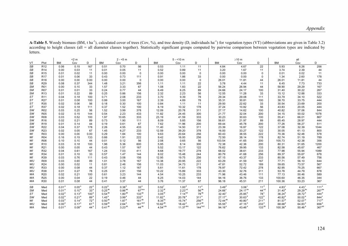
Appendix
A-Table 5. Woody biomass (BM, t ha-1), calculated cover of trees (Cov, %), and tree density (D, individuals ha-1) for vegetation types (VT) (abbreviations are given in Table 3.2) according to height classes (all = all diameter classes together). Statistically significant groups computed by pairwise comparison between vegetation types are indicated by letters.
<2 m 2 - <5 m 5 - <10 m ≥10 m all VT Plot BM Cov D BM Cov D BM Cov D BM Cov D BM Cov D SB R12 0.06 0.19 167 0.51 0.70 56 0.53 1.11 11 4.84 4.67 22 5.93 6.26 256 SB R14 0.00 0.03 11 0.01 0.05 11 0.52 0.89 11 3.20 1.67 11 3.74 2.39 44 SB R15 0.01 0.02 11 0.00 0.00 0 0.00 0.00 0 0.00 0.00 0 0.01 0.02 11 SB R17 0.01 0.06 33 0.43 0.73 111 0.91 1.86 33 0.00 0.00 0 1.34 2.60 178 SB R18 0.00 0.00 0.00 0.00 0.00 0 0.00 0.00 0 26.01 11.81 44 26.01 11.81 44 SB R29 0.08 0.37 344 1.48 3.21 356 1.11 1.11 22 3.78 4.44 11 6.45 7.73 733 SM R01 0.00 0.10 33 1.57 3.33 67 1.08 1.83 22 56.24 26.94 44 58.90 29.29 167 SM R07 0.01 0.01 33 0.24 0.77 44 6.49 6.25 89 24.66 24.17 100 31.40 30.22 267 SM R13 0.01 0.22 89 0.25 0.86 156 2.32 2.23 56 12.55 11.28 33 15.12 12.88 333 ST R11 0.04 0.18 100 0.71 2.08 233 3.70 9.39 78 29.34 29.08 111 33.79 34.10 522 ST R27 0.01 0.08 100 0.99 3.00 167 2.39 4.89 78 35.31 30.81 100 38.70 33.75 444 ST R35 0.02 0.06 56 0.18 0.30 100 0.84 1.11 11 29.50 22.62 33 30.54 23.69 200 ST R37 0.02 0.18 111 0.37 1.52 100 6.19 10.32 178 37.24 10.82 56 43.83 20.05 444 SW R02 0.03 0.25 56 1.52 3.99 378 12.09 20.78 311 27.17 14.62 100 40.82 37.06 844 SW R05 0.02 0.19 144 0.54 2.23 433 11.82 24.45 300 21.77 32.04 200 34.15 50.02 1078 SW R08 0.03 0.52 100 1.97 10.65 333 23.19 41.59 333 30.23 30.63 100 55.41 66.01 867 SW R16 0.02 0.21 89 0.73 1.90 111 8.09 5.85 156 56.61 21.97 89 65.45 28.97 444 SW R19 0.01 0.14 44 0.19 0.61 67 7.62 11.96 200 69.44 45.78 200 77.26 56.27 511 SW R22 0.04 0.37 178 2.26 4.55 433 11.40 14.50 311 23.39 16.87 122 37.08 32.39 1044 SW R23 0.02 0.05 67 1.45 6.27 233 12.59 39.20 378 16.00 33.27 122 30.05 61.13 800 WI R03 0.00 0.00 0.00 0.29 1.84 100 9.63 20.64 256 60.43 38.55 222 70.36 52.48 578 WI R04 0.16 0.19 133 0.66 1.91 222 9.42 16.00 256 72.50 38.14 178 82.74 51.19 789 WI R06 0.10 0.10 44 0.01 0.12 56 2.08 0.65 56 103.54 41.65 200 105.73 42.38 356 WI R10 0.03 0.18 100 1.96 5.36 600 5.95 8.14 300 72.38 42.36 200 80.31 51.65 1200 WI R21 0.00 0.05 44 0.43 1.57 167 5.52 13.17 122 76.62 39.95 133 82.58 45.67 467 WI R32 0.04 0.61 167 1.24 7.03 411 8.68 19.77 278 68.02 38.61 233 77.98 55.94 1089 WI R34 0.01 0.10 33 0.57 1.47 144 8.02 15.48 244 80.79 41.68 256 89.37 55.67 678 WI R39 0.03 0.76 111 0.43 3.08 156 12.95 19.75 256 67.15 43.37 233 80.56 57.49 756 WU R09 0.03 0.65 89 1.01 3.78 167 13.38 20.95 222 63.29 41.59 167 77.71 56.10 644 WU R24 0.00 0.02 11 0.81 2.46 156 11.03 34.73 211 47.81 52.72 189 59.65 73.57 567 WU R33 0.00 0.08 44 0.37 1.12 167 5.61 11.61 178 76.97 72.42 278 82.95 75.25 667 WU R38 0.01 0.27 78 0.25 2.81 156 10.22 15.89 333 43.30 32.76 311 53.78 44.79 878 WA R20 0.02 0.21 100 0.61 3.23 144 4.54 10.25 233 71.96 43.46 111 77.13 50.46 589 WA R25 0.00 0.04 22 0.19 0.46 44 6.25 14.03 144 94.16 36.76 133 100.60 46.35 344 WA R30 0.01 0.08 44 0.41 3.37 44 3.76 11.37 67 96.18 45.51 211 100.36 53.23 367 SB Med 0.01 a 0.05a 22 a 0.22 b 0.38 b 33 e 0.52 f 1.00 d 11 e 3.49d 3.06 c 11 d 4.83c 4.43 c 111 e SM Med 0.01 a 0.10a 33 a 0.25 ab 0.86 ab 67 bce 2.32 df 2.23 cd 56 de 24.66c 24.17 bc 44 cd 31.40b 29.29 bc 267 de ST Med 0.02 a 0.13a 100 a 0.54 ab 1.80 ab 133 ae 3.05 ef 7.14 bd 78 de 32.40c 25.85 b 78 c 36.24b 28.72 b 444 d SW Med 0.02 a 0.21a 89 a 1.45 a 3.99 a 333 a 11.82 a 20.78 a 311 a 27.17c 30.63 b 122 b 40.82b 50.02 a 844 c WI Med 0.03 a 0.14a 72 a 0.50 ab 1.87 a 161 ab 8.35 bc 15.74 a 256 ac 72.44ab 40.80 a 211 a 81.57a 52.07 a 717 b WU Med 0.00 a 0.17a 61 a 0.59 ab 2.64 a 161 acd 10.62 ab 18.42 a 217 ab 55.55b 47.15 a 233 a 68.68a 64.83 a 656 a WA Med 0.01 a 0.08a 44 a 0.41 ab 3.23 ab 44 de 4.54 cde 11.37 abc 144 bcd 94.16a 43.46 a 133 ab 100.36a 50.46 a 367 ab
124
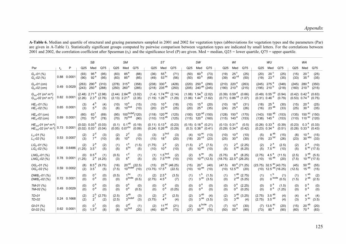
Appendix
A-Table 6. Median and quartile of structural and grazing parameters sampled in 2001 and 2002 for vegetation types (abbreviations for vegetation types and the parameters (Par) are given in A-Table 1). Statistically significant groups computed by pairwise comparison between vegetation types are indicated by small letters. For the correlations between 2001 and 2002, the correlation coefficient after Spearman (r ) and the significance level (P) are given. Med = median, Q25 = lower quartile, Q75 = upper quartile. S
(93)(90)
(263)(243)
(2.48)(2.26)
(3)(3)
(60)(70)
(0.02)(0.02)
(2)(3)
(2)(1.25)
(0)(1.25)
(8)(2)
(0)(0)
(0)(0)
(2)(2)
(0)(0)
SB
9592
290250
2.712.3
45
6370
0.030.03
27
23.5
0.52
8.53.5
00
00
22
01.5
(95)(95)
(310)(288)
(2.98)(2.76)
(4)(5)
(69)(78)
(0.03)(0.04)
(3)(10)
(2)(5)
(1)(4.25)
(9.75)(5)
(0)(0)
(0)(0)
(2.75)(2)
(0)(8)
aa
aa
aa
bd
fd
bc
de
ac
de
df
ce
aa
bf
fd
(83)(83)
(278)(250)
(2.44)(2.13)
(10)(8)
(95)(70)
(0.1)(0.05)
(2)(8)
(1)(5)
(0.5)(3)
(16)(7.5)
(0.5)(0)
(0)(0)
(2.5)(2.5)
(0)(8)
SM
8585
315260
2.842.21
1010
10070
0.10.07
210
15
15
2010
10
00
33
010
(88)(85)
(358)(285)
(3.02)(2.35)
(15)(10)
(120)(90)
(0.19)(0.09)
(3)(10)
(1.5)(5)
(1)(5)
(22.5)(10)
(1)(0.5)
(0)(0.5)
(3)(3)
(1)(20)
aa
aa
aba
abcd
bcdefbcd
abbc
de
abc
de
cdbcdef
bcbcde
aa
abbcdef
efbcd
(36)(49)
(238)(218)
(1.4)(1.19)
(10)(20)
(118)(110)
(0.11)(0.24)
(3)(15)
(1.75)(10)
(1)(5)
(15)(13.75)
(2)(2.75)
(0)(0)
(2)(3.75)
(2)(46)
ST
5553
330235
1.741.26
1023
120115
0.130.26
318
210
1.57.5
2517.5
2.54.5
00
24
1165
(71)(56)
(428)(250)
(2.14)(1.29)
(18)(25)
(125)(125)
(0.23)(0.29)
(3)(20)
(2)(10)
(2)(10)
(46.25)(22.5)
(3.5)(7)
(0)(0.25)
(2.5)(4)
(21)(73)
bbc
aab
abcbc
aac
aeab
aab
bcdd
aa
bcdbcde
bca
aa
aa
ba
adab
(50)(50)
(220)(205)
(1.08)(1.06)
(10)(20)
(100)(115)
(0.15)(0.3)
(4)(18)
(1.5)(5)
(2)(10)
(15)(10)
(1)(1)
(0)(0)
(2)(3)
(2)(27)
SW
6060
250240
1.541.44
1525
120120
0.180.38
1020
210
510
2010
13
00
33
550
(73)(68)
(290)(245)
(2.02)(1.62)
(20)(35)
(150)(160)
(0.21)(0.41)
(13)(23)
(7.5)(10)
(5)(12.5)
(40)(10)
(1.5)(3.5)
(0)(0)
(4)(3.5)
(7)(70)
bb
aab
bb
aa
ada
aa
accd
aab
acac
cae
bac
aa
abae
bcdeac
(19)(39)
(210)(190)
(0.39)(0.71)
(10)(24)
(128)(115)
(0.13)(0.29)
(10)(25)
(1)(5)
(5.75)(18.75)
(47.5)(10)
(1)(0)
(0)(0)
(2)(3)
(7)(50)
WI
2540
220210
0.590.86
1825
150140
0.310.34
1030
25
822.5
6012.5
12
00
33
1055
(25)(50)
(263)(215)
(0.66)(1.07)
(31)(26)
(170)(153)
(0.5)(0.42)
(10)(30)
(2.25)(6.25)
(8.25)(26.25)
(71.25)(20)
(2.75)(5.25)
(2.25)(0.25)
(3.25)(4)
(30)(90)
ccd
ab
dcd
aa
aa
aa
aa
aac
aa
aac
abad
aa
abab
aa
(20)(19)
(245)(195)
(0.49)(0.31)
(18)(16)
(143)(138)
(0.26)(0.23)
(5)(19)
(2)(5)
(2.75)(10)
(23.75)(10)
(1)(0)
(0)(0)
(2.75)(2.75)
(7)(73)
WU
2023
275210
0.550.46
2523
150145
0.330.34
823
27.5
4.515
32.512.5
10
00
3.53.5
13.585
(25)(35)
(348)(218)
(0.94)(0.79)
(30)(33)
(153)(153)
(0.39)(0.51)
(15)(26)
(2.5)(10)
(11.5)(20)
(43.75)(16.25)
(1)(0.5)
(1.5)(1.25)
(4)(4)
(20)(90)
cd
ab
cdd
aab
aba
aa
abbd
aac
aab
acad
bbcde
aa
abad
aca
(15)(33)
(245)(160)
(0.42)(0.53)
(15)(25)
(135)(110)
(0.23)(0.28)
(8)(23)
(2)(5)
(2.5)(7.5)
(45)(12.5)
(1)(1.5)
(0)(0)
(4)(3)
(15)(60)
WA
2035
280210
0.420.74
2030
150110
0.30.33
1030
25
310
5015
12
00
43
2070
(25)(35)
(350)(215)
(0.63)(0.75)
(25)(35)
(150)(120)
(0.33)(0.43)
(15)(33)
(10)(17.5)
(5.5)(17.5)
(55)(15)
(2)(2.5)
(0)(0)
(4)(3.5)
(20)(83)
cd
ab
dd
aa
acac
aa
aabc
aac
abad
abab
abab
aa
aac
aba
GC-01 (%)GC-02 (%)
GH-01 (cm)GH-02 (cm)
GVol-01 (m³ m ²)-
GVol-02 (m³ m ²)-
HEC-01 (%)HEC-02 (%)
HEH-01 (cm)HEH-02 (cm)
HEVol-01 (m³ m ²)-
HEVol-02 (m³ m ²)-
LC-01 (%)LC-02 (%)
LGC-01 (%)LGC-02 (%)
LNGC-01 (%)LNGC-02 (%)
OGC-01 (%)OGC-02 (%)
DWBC-01 (%)DWBC-02 (%)
TM-01 (%)TM-02 (%)
TD-01TD-02
GI-01 (%)GI-02 (%)
0.88
0.49
0.82
0.65
0.69
0.73
0.53
0.08
0.78
0.59
0.72
0.49
0.24
0.62
0.0001
0.0029
0.0001
0.0001
0.0001
0.0001
0.0007
0.6486
0.0001
0.0002
0.0001
0.0029
0.1668
0.0001
Q25 Med Q75 Q25 Med Q75 Q25 Med Q75 Q25 Med Q75 Q25 Med Q75 Q25 Med Q75 Q25 Med Q75Par rs P
125
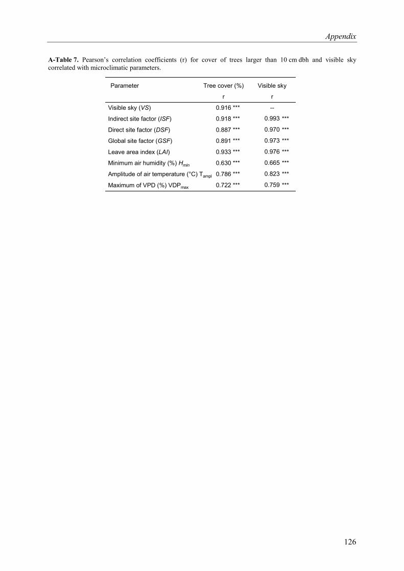
Appendix
126
A-Tab earson’s correlation coefficients (r) for cover of trees larger than 10 cm dbh and visible sky correl microclimatic parameters.
le 7. Pated with
Parameter
Visible sky ( )VS
Indirect site factor ( )ISF
Direct site factor ( )DSF
Global site factor ( )GSF
Leave area index ( )LAI
Minimum air humidity (%) Hmin
Amplitude of air temperature (°C) Tampl
Maximum of VPD (%) VDPmax
Tree cover (%)
r
0.916
0.918
0.887
0.891
0.933
0.630
0.786
0.722
***
***
***
***
***
***
***
***
Visible sky
r
--
***
***
***
***
***
***
***
0.993
0.970
0.973
0.976
0.665
0.823
0.759
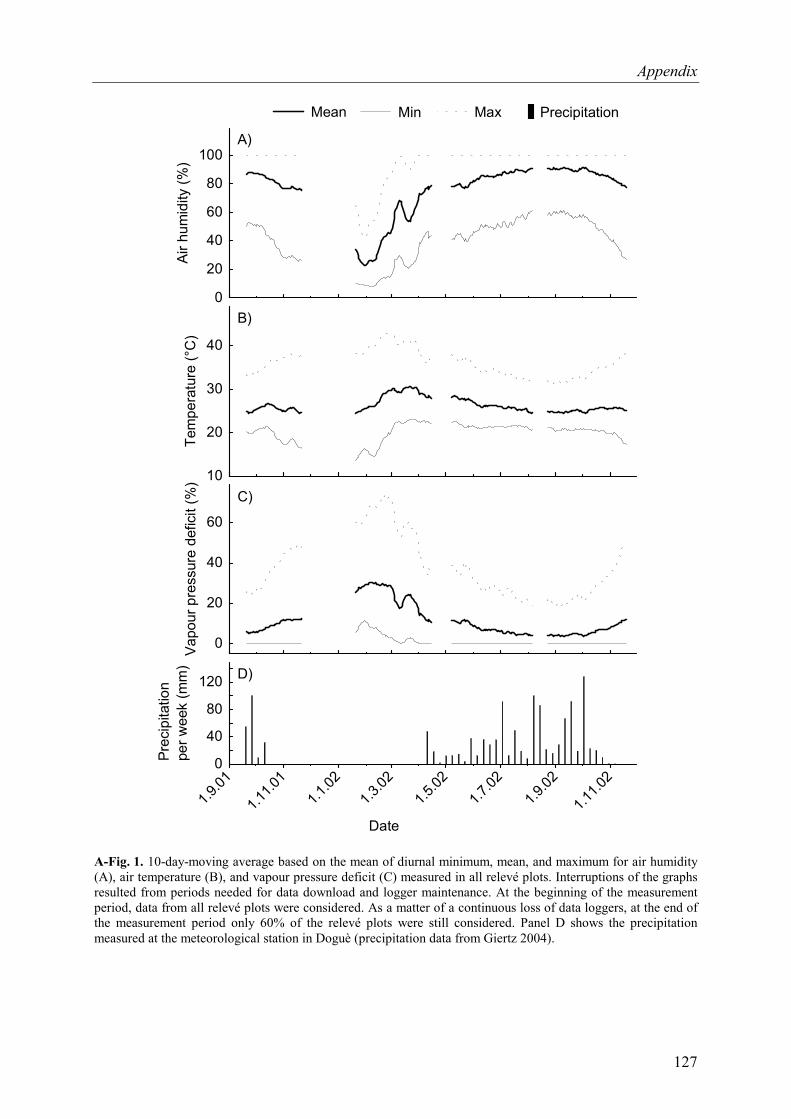
Appendix
0
20
40
60
80
100
Airh
umid
ity(%
)
1.9.01
1.11.0
11.1
.021.3
.021.5
.021.7
.021.9
.02
1.11.0
2
Date
Mean Min Max Precipitation
A)
10
20
30
40
Tem
pera
ture
(°C
)
1.9.01
1.11.0
11.1
.021.3
.021.5
.021.7
.021.9
.02
1.11.0
2
Datum
0
20
40
60
Vapo
urpr
essu
rede
ficit
(%)
Sep
'01
Nov
'01
Jan
'02
Mär
'02
Mai
'02
Jul'
02
Sep
'02
Nov
'02
Date
0
40
80
120
Prec
ipita
tion
perw
eek
(mm
)
1.9.01
1.11.0
11.1
.021.3
.021.5
.021.7
.021.9
.02
1.11.0
2
Date
B)
C)
D)
A-Fig. 1. 10-day-moving average based on the mean of diurnal minimum, mean, and maximum for air humidity (A), air temperature (B), and vapour pressure deficit (C) measured in all relevé plots. Interruptions of the graphs resulted from periods needed for data download and logger maintenance. At the beginning of the measurement period, data from all relevé plots were considered. As a matter of a continuous loss of data loggers, at the end of the measurement period only 60% of the relevé plots were still considered. Panel D shows the precipitation measured at the meteorological station in Doguè (precipitation data from Giertz 2004).
127
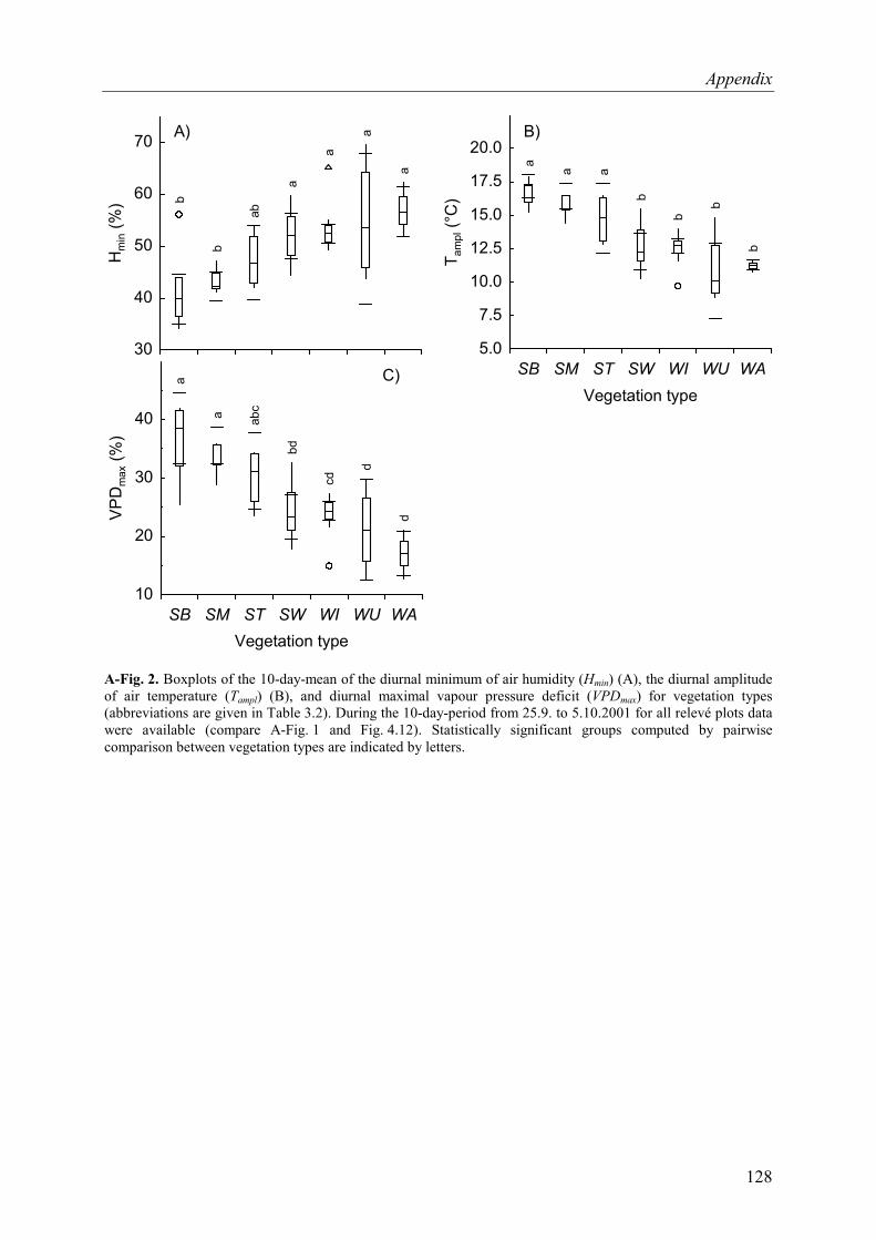
Appendix
30
40
50
60
70H
(%)
min
SB SM ST SW WI WU WAVegetation type
b
b
ab
a
a
a
a5.0
7.5
10.0
12.5
15.0
17.5
20.0
T(°
C)
ampl
SB SM ST SW WI WU WAVegetation type
a
a a
b
b
b
b
10
20
30
40
VPD
(%)
max
SB SM ST SW WI WU WAVegetation type
a
a abc
bd
d
cd
d
A)
C)
B)
A-Fig. 2. Boxplots of the 10-day-mean of the diurnal minimum of air humidity (Hmin) (A), the diurnal amplitude of air temperature (Tampl) (B), and diurnal maximal vapour pressure deficit (VPDmax) for vegetation types (abbreviations are given in Table 3.2). During the 10-day-period from 25.9. to 5.10.2001 for all relevé plots data were available (compare A-Fig. 1 and Fig. 4.12). Statistically significant groups computed by pairwise comparison between vegetation types are indicated by letters.
128
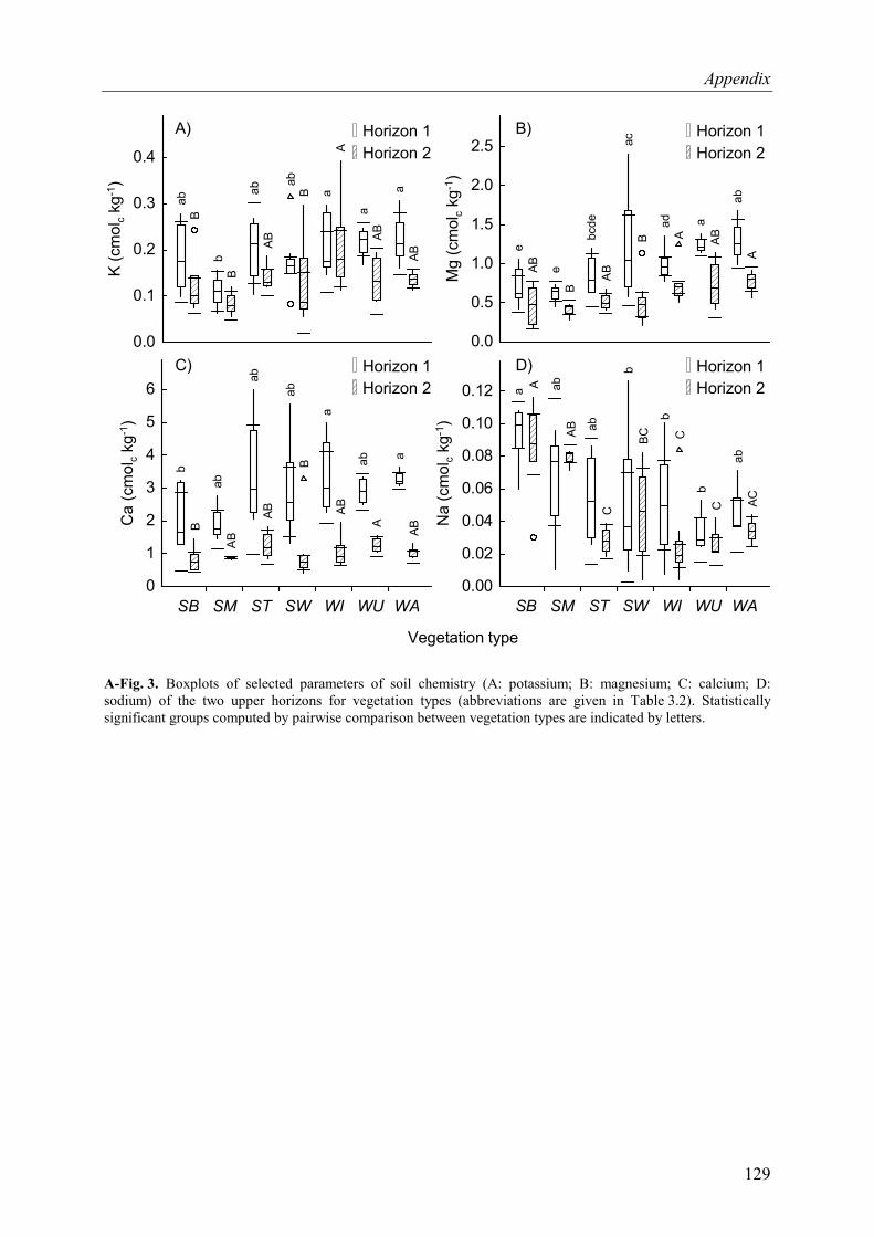
Appendix
0.0
0.5
1.0
1.5
2.0
2.5
Mg
(cm
olkg
)c
-1
SB SM ST SW WI WU WASB SM ST SW WI WU WA
eAB e
B
bcde
AB
acB
adA
aAB
abA
0.0
0.1
0.2
0.3
0.4
K(c
mol
kg)
c-1
SB SM ST SW WI WU WASB SM ST SW WI WU WA
abB
bB
abAB
abB a
A
aAB
aAB
0
1
2
3
4
5
6
Ca
(cm
olkg
)c
-1
SB SM ST SW WI WU WASB SM ST SW WI WU WASB SM ST SW WI WU WA
bB
abAB
abAB
abB
aAB
abA
aAB
0.00
0.02
0.04
0.06
0.08
0.10
0.12
Na
(cm
olkg
)c
-1
SB SM ST SW WI WU WASB SM ST SW WI WU WASB SM ST SW WI WU WA
a A abAB ab
C
bBC
bC
bC
abAC
A) B)
C) D)
Vegetation type
Horizon 1Horizon 2
Horizon 1Horizon 2
Horizon 1Horizon 2
Horizon 1Horizon 2
A-Fig. 3. Boxplots of selected parameters of soil chemistry (A: potassium; B: magnesium; C: calcium; D: sodium) of the two upper horizons for vegetation types (abbreviations are given in Table 3.2). Statistically significant groups computed by pairwise comparison between vegetation types are indicated by letters.
129
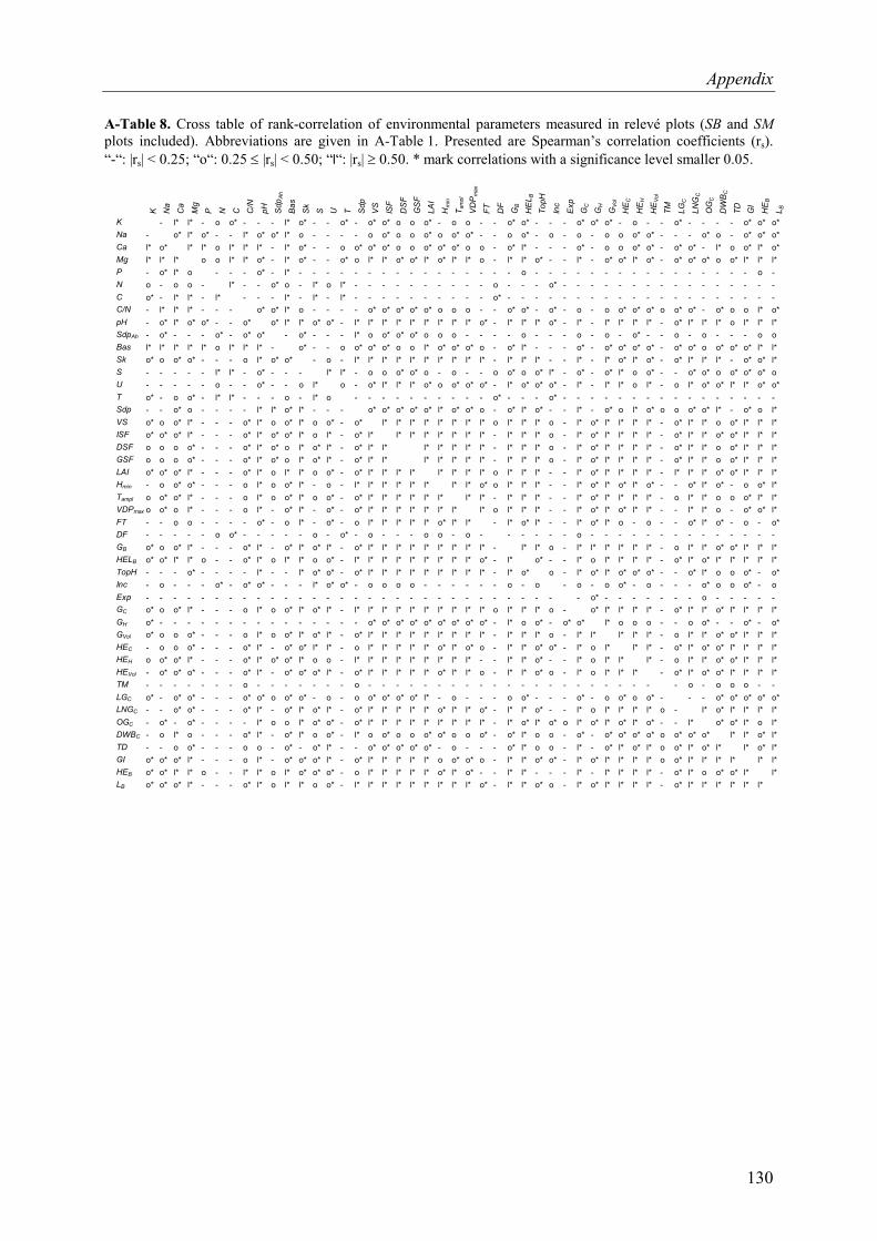
Appendix
A-Table 8. Cross table of rank-correlation of environmental parameters measured in relevé plots (SB and SM plots included). Abbreviations are given in A-Table 1. Presented are Spearman’s correlation coefficients (rs). “-“: |rs| < 0.25; “o“: 0.25 ≤ |rs| < 0.50; “l“: |rs| ≥ 0.50. * mark correlations with a significance level smaller 0.05.
K
Na
Ca
Mg
P
N
C
C/N
pH
S
dpAh
B
as
Sk
S
U
T Sdp
V
S
ISF
DS
F G
SF
LAI
Hm
in
T am
pl
VD
Pm
ax
FT
DF
GB
HE
L B
TopH
Inc
Exp
G
C
GH
GVo
l H
EC
HE
H
HE
Vol
TM
LGC
LNG
C
OG
C
DW
BC
TD
GI
HE
B L B
K - l* l* - o o* - - - l* o* - - o* - o* o* o o o* - o o - - o* o* - - - o* o* o* - o - - o* - - - - o* o* o* Na - o* l* o* - - l* o* o* l* o - - - - o o* o o o* o o* o* - - o o* - o - o - o o o* o* - - - o* o - o* o* o* Ca l* o* l* l* o l* l* l* - l* o* - - o o* o* o* o o o* o* o* o o - o* l* - - - o* - o o o* o* - o* o* - l* o o* l* o* Mg l* l* l* o o l* l* o* - l* o* - - o* o l* l* o* o* l* o* l* l* o - l* l* o* - - l* - o* o* l* o* - o* o* o* o o* l* l* l* P - o* l* o - - - o* - l* - - - - - - - - - - - - - - - - o - - - - - - - - - - - - - - - - o - N o - o o - l* - - o* o - l* o l* - - - - - - - - - - o - - - o* - - - - - - - - - - - - - - - - C o* - l* l* - l* - - - l* - l* - l* - - - - - - - - - - o* - - - - - - - - - - - - - - - - - - - - C/N - l* l* l* - - - o* o* l* o - - - - o* o* o* o* o* o o o - - o* o* - o* - o - o o* o* o* o o* o* - o* o o l* o* pH - o* l* o* o* - - o* o* l* l* o* o* - l* l* l* l* l* l* l* l* l* o* - l* l* l* o* - l* - l* l* l* l* - o* l* l* l* o l* l* l* SdpAh - o* - - - o* - o* o* - o* - - - l* o o* o* o* o o o - - - - o - - - o - o - o* - - o - o - - - o o Bas l* l* l* l* l* o l* l* l* - o* - - o o* o* o* o o l* o* o* o* o - o* l* - - - o* - o* o* o* o* - o* o* o o* o* o* l* l* Sk o* o o* o* - - - o l* o* o* - o - l* l* l* l* l* l* l* l* l* l* - l* l* l* - - l* - l* o* l* o* - o* l* l* l* - o* o* l* S - - - - - l* l* - o* - - - l* l* - o o o* o* o - o - - o o* o o* l* - o* - o* l* o o* - - o* o* o o* o* o* o U - - - - - o - - o* - - o l* o - o* l* l* l* o* o o* o* o* - l* o* o* o* - l* - l* l* o l* - o l* o* o* l* l* o* o* T o* - o o* - l* l* - - - o - l* o - - - - - - - - - - o* - - - o* - - - - - - - - - - - - - - - - Sdp - - o* o - - - - l* l* o* l* - - - o* o* o* o* o* l* o* o* o - o* l* o* - - l* - o* o l* o* o o o* o* l* - o* o l* VS o* o o* l* - - - o* l* o o* l* o o* - o* l* l* l* l* l* l* l* l* o l* l* l* o - l* o* l* l* l* l* - o* l* l* o o* l* l* l* ISF o* o* o* l* - - - o* l* o* o* l* o l* - o* l* l* l* l* l* l* l* l* - l* l* l* o - l* o* l* l* l* l* - o* l* l* o* o* l* l* l* DSF o o o o* - - - o* l* o* o l* o* l* - o* l* l* l* l* l* l* l* - l* l* l* o - l* o* l* l* l* l* - o* l* l* o o* l* l* l* GSF o o o o* - - - o* l* o* o l* o* l* - o* l* l* l* l* l* l* l* - l* l* l* o - l* o* l* l* l* l* - o* l* l* o o* l* l* l* LAI o* o* o* l* - - - o* l* o l* l* o o* - o* l* l* l* l* l* l* l* l* o l* l* l* - - l* o* l* l* l* l* - l* l* l* o* o* l* l* l* Hmin - o o* o* - - - o l* o o* l* - o - l* l* l* l* l* l* l* l* o* o l* l* l* - - l* o* l* o* l* o* - - o* l* o* - o o* l* Tampl o o* o* l* - - - o l* o o* l* o o* - o* l* l* l* l* l* l* l* l* - l* l* l* - - l* o* l* l* l* l* - o l* l* o o o* l* l* VDPmax o o* o l* - - - o l* - o* l* - o* - o* l* l* l* l* l* l* l* l* o l* l* l* - - l* o* l* o* l* l* - - l* l* o - o* o* l* FT - - o o - - - - o* - o l* - o* - o l* l* l* l* l* o* l* l* - l* o* l* - - l* o* l* o - o - - o* l* o* - o - o* DF - - - - - o o* - - - - - o - o* - o - - - o o - o - - - - - - o - - - - - - - - - - - - - - GB o* o o* l* - - - o* l* - o* l* o* l* - o* l* l* l* l* l* l* l* l* l* - l* l* o - l* l* l* l* l* l* - o l* l* o* o* l* l* l* HELB o* o* l* l* o - - o* l* o l* l* o o* - l* l* l* l* l* l* l* l* l* o* - l* o* - - l* o l* l* l* l* - o* l* o* l* l* l* l* l* TopH - - - o* - - - - l* - - l* o* o* - o* l* l* l* l* l* l* l* l* l* - l* o* o - l* o* l* o* o* o* - - o* l* o o o* - o* Inc - o - - - o* - o* o* - - - l* o* o* - o o o o - - - - - - o - o - o - o o* - o - - - o* o o o* - o Exp - - - - - - - - - - - - - - - - - - - - - - - - - - - - - - - o* - - - - - - - o - - - - - GC o* o o* l* - - - o l* o o* l* o* l* - l* l* l* l* l* l* l* l* l* l* o l* l* l* o - o* l* l* l* l* - o* l* l* o* l* l* l* l* GH o* - - - - - - - - - - - - - - - o* o* o* o* o* o* o* o* o* - l* o o* - o* o* l* o o o - - o o* - - o* - o* GVol o* o o o* - - - o l* o o* l* o* l* - o* l* l* l* l* l* l* l* l* l* - l* l* l* o - l* l* l* l* l* - o l* l* o* o* l* l* l* HEC - o o o* - - - o* l* - o* o* l* l* - o l* l* l* l* l* o* l* o* o - l* l* o* o* - l* o l* l* l* - o* l* o* o* l* l* l* l*
l* HEH o o* o* l* - - - o* l* o* o* l* o o - l* l* l* l* l* l* l* l* l* - - l* l* o* - - l* o l* l* l* - o l* l* o* o* l* l*
o* o* l* o l* DWBC - o l* o - - - o* l* - o* l* o o* - l* o o* o o o* o* o o o* - o* l* o o - o* - o* o* o* o* o o* o* o* l* l* o* l* TD - - o o* - - - o o - o* - o* l* - - o* o* o* o* o* - o - - - o* l* o o - l* - o* l* o* l* o o* l* o* l* l* o* l* GI o* o* o* l* - - - o l* - o* o* o* l* - o* l* l* l* l* l* o o* o* o - l* l* o* o* - l* o* l* l* l* l* o o* l* l* l* l* l* l* HEB o* o* l* l* o - - l* l* o l* o* o* o* - o l* l* l* l* l* o* l* o* - - l* l* - - - l* - l* l* l* l* - o* l* o o* o* l* l* LB o* o* o* l* - - - o* l* o l* l* o o* - l* l* l* l* l* l* l* l* l* o* - l* l* o* o - l* o* l* l* l* l* - o* l* l* l* l* l* l*
HEVol - o* o* o* - - - o* l* - o* o* o* l* - o* l* l* l* l* l* o* l* l* o - l* l* o* o - l* o l* l* l* - o* l* o* o* l* l* l* l* TM - - - - - - - o - - - - - - - o - - - - - - - - - - - - - - - - - - - - - - o - o o o - - LGC o* - o* o* - - - o* o* o o* o* - o - o o* o* o* o* l* - o - - - o o* - - - o* - o o* o o* - - - o* o* o* o* o* LNGC - - o* o* - - - o* l* - o* l* o* l* - o* l* l* l* l* l* o* l* l* o* - l* l* o* - - l* o l* l* l* l* o - l* o* l* l* l* l* OGC - o* - o* - - - - l* o o l* o* o* - o* l* l* l* l* l* l* l* l* l* - l* o* l* o* o l* o* l* o* l* o* - - l*
130
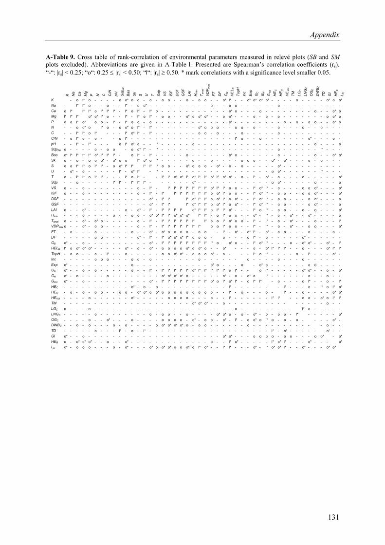
Appendix
A-Table 9. Cross table of rank-correlation of environmental parameters measured in relevé plots (SB and SM plots excluded). Abbreviations are given in A-Table 1. Presented are Spearman’s correlation coefficients (rs). “-“: |rs| < 0.25; “o“: 0.25 ≤ |rs| < 0.50; “l“: |rs| ≥ 0.50. * mark correlations with a significance level smaller 0.05.
K
Na
Ca
Mg
P
N
C
C/N
pH
Sdp
Ah
Bas
S
k
S
U
T Sdp
V
S
ISF
DS
F G
SF
LAI
Hm
in
T am
pl
VD
Pm
ax
FT
DF
GB
HE
L B
TopH
In
c E
xp
GC
GH
GVo
l H
EC
HE
H
HE
Vol
TM
LGC
LNG
C
OG
C
DW
BC
TD
GI
HE
B L B
K - o l* o - - - - o o* o o - o - o o - - o - o o - - o* l* - - o* o* o* o* - - - - o - - - - o* o o* Na - l* l* o - - o - - l* - o o* - - - - - - - - - - o - - o o - - - - - - o - - - - - - - - - - Ca o l* l* l* o l* l* l* - l* o l* - l* o - - - - - - - - - - - o* o - - - o - - - - - - - - o - - o* o Mg l* l* l* o* o* l* o - - l* - l* o l* - o o - - o* o o* o* - - o o* - - - o - o - o - - - - - - - o o* o P o o l* o* o o - l* - l* o o - o - - - - - - - - - - - - o* - - - - - - - - o - o - o o - - o* o N - - o o* o l* o - o o* o l* - l* - - - - - - - o* o o o - - o o - o - - - o - - - o - - o - - - C - - l* l* o l* - - - l* o* l* - l* - - - - - - - o o - o - - - o - - - - - o - - - - - - - - - - C/N - o l* o - o - - o l* - - - - - - - - - - - - - - - - - l* o - - o - - - - - - - o* - - - o - pH - - l* - l* - - - o l* o* o - - l* - - - - - o - - - - - - - - - - - - - - - - - - - o - - - o SdpAh o - - - - o - o o - o o* l* - l* - - - - - - - - - - - - - - - - - - - o - - - - - - l* - - - Bas o* l* l* l* l* o* l* l* l* - o l* - l* - - - - - o - - - - - - o* o - - - - - - o - - - - - o - - o* o* Sk o - o - o o o* - o* o o l* o* o l* - - - - - o - - o - - - - o o o - - o* - o* - - - o - o - - - S o o l* l* o l* l* - o o* l* l* l* l* l* o o - - o* o o o - o* - o - o - - - - - o* - - - - - - - - - - U - o* - o - - - - - l* - o* l* - l* - - - - - - - - - - - - - - - - - - o o* - - - - - - l* - - - T o - l* l* o l* l* - - - l* o l* - - l* l* o* o* l* o* l* l* o* l* o* o* - o - l* - o* - o - - - o - - - - - o* Sdp - - o - - - - - l* l* - l* l* l* - - - - - - o* - - - - - - - - - - - - o o* - - - - - o - - - o VS o - - o - - - - - - - - o - l* - l* l* l* l* l* l* l* o* l* l* o o - - l* o* l* - o - - - o o o* - - - o* ISF o - - o - - - - - - - - o - l* - l* l* l* l* l* l* l* o o* l* o o - - l* o* l* - o o - - o o o* - - - o* DSF - - - - - - - - - - - - - - o* - l* l* l* o* l* l* o o* l* o o* - - l* o* l* - o o - - - o o* - - - o GSF - - - - - - - - - - - - - - o* - l* l* l* o* l* l* o o* l* o o* - - l* o* l* - o o - - - o o* - - - o LAI o - - o* - - - - - - o - o* - l* - l* l* l* l* o* l* l* o l* l* o* - - - l* o l* - o o - - o - o - - - o* Hmin - - - o - - - - o - - o o - o* o* l* l* o* o* o* l* l* - o l* o o - - o* - l* - o - o* - - o* - - - - o Tampl o - - o* - o* o - - - - - o - l* - l* l* l* l* l* l* l* o o l* o* o o - l* - l* - o - o* - - - o - - - l* VDPmax o - - o* - o o - - - - - o - l* - l* l* l* l* l* l* l* o o l* o o - - l* - l* - o - o* - - o o - - - o* FT - o - - - o - - - - - o - - o* - o* o o o o - o o - l* - o* - o* l* - o* - o o - - - o - - - o - DF - - - - - o o - - - - - o* - l* - l* o* o* o* l* o o o - o - - - o l* - o - - - - - o* - - - - - - GB o* - - o - - - - - - - - - - o* - l* l* l* l* l* l* l* l* l* o o* o - - l* o* l* - - - o - o* o* - - o* - l* HELB l* o o* o* o* - - - - - o* - o - o* - o o o o o* o o* o - - o* - - - o - o* l* l* l* - - o - - - o* l* l* TopH - o o - - o - l* - - o - - - - - o o o* o* - o o o o* - o - - - l* o l* - - - - o - l* - - - o* - Inc - - - - - o o o - - - o o - o - - - - - - - o - - - - - - o - - - - o - - - o - - - - - - Exp o* - - - - - - - - - - o - - - - - - - - - - - - o* o - - - o - o* o - - - - - - o o - - - - GC o* - - o - o - - - - - o - - l* - l* l* l* l* l* o* l* l* l* l* l* o l* - - o l* - - - - - o* o* - - o - o* GH o* - o - - - - o - - - - - - - - o* o* o* o* o - - - - - o* - o - o* o l* - - - - - - o - - o - - GVol o* - - o - - - - - - - - - - o* - l* l* l* l* l* l* l* l* o* o l* o* l* - o l* l* - o - - - o l* - - o - l* HEC - - - - - - - - - - - o* - o - o - - - - - - - - - - - l* - - - - - - - l* - - - o - l* o l* o* HEH - o - o - o o - - o o - o* o* o o* o o o o o o o o o - - l* - o - - - o - l* - - o - - - - o* o* HEVol - - - - o - - - - - - o* - - - - - o o o o - - - o - - l* - - - - - - l* l* - - o o - o* o l* l* TM - - - - - - - - - - - - - - - - - - - - - o* o* o* - - o - - - - - - - - - - - - - - - o - - LGC o - - - o - - - - - - - - - - - - - - - - - - - - - - - o - - - - - - - - - l* o - - - - - LNGC - - - - - o - - - - - - - - o - o o - - o - - - - o* o* o - o - o* - o - o o - l* - - - - - o* OGC - - - - o - - o* - - - o - - - - o o o o - o* - o o - o* - l* - o o* o l* o - o - o - - - - o* - DWBC - - o - o - - - o - o - - - - o o* o* o* o* o - o o - - - - - - o - - - - - - - - - - - o - - TD - - - - - o - - - l* - o - l* - - - - - - - - - - - - - - - - - - - - l* - o* - - - - - o* - - GI o* - - o - - - - - - - - - - - - - - - - - - - - - - o* o* - - - o o o o - o o - - - o o* - o* HEB o - o* o* o* - - o - - o* - - - - - - - - - - - - - o - - l* o* - - - - - l* o* l* - - - o* - - - o* LB o* - o o o - - - o - o* - - - o* o o* o* o o o* o l* o* - - l* l* - - - o* - l* o* o* l* - - o* - - - o* o*
131
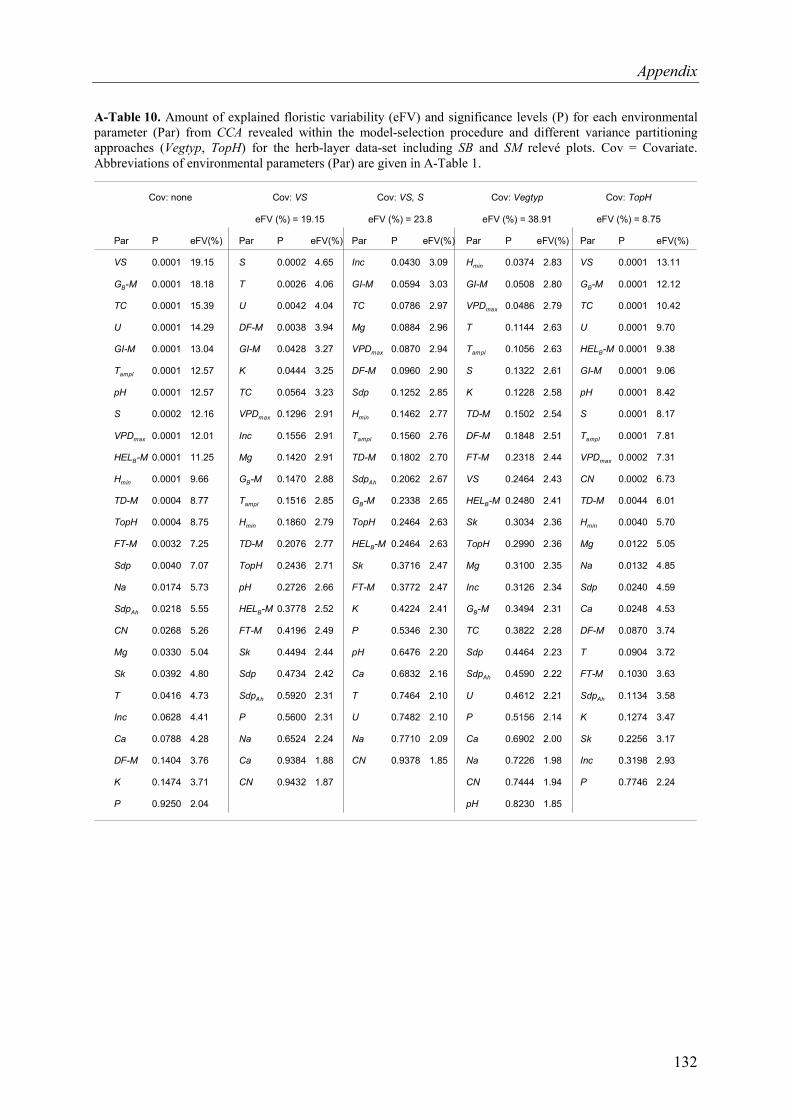
Appendix
A-Table 10. Amount of explained floristic variability (eFV) and significance levels (P) for each environmental parameter (Par) from CCA revealed within the model-selection procedure and different variance partitioning approaches (Vegtyp, TopH) for the herb-layer data-set including SB and SM relevé plots. Cov = Covariate. Abbreviations of environmental parameters (Par) are given in A-Table 1.
Cov: none
Par
VS
GB-M
TC
U
GI-M
Tampl
pH
S
VPDmax
HELB-M
Hmin
TD-M
TopH
FT-M
Sdp
Na
SdpAh
CN
Mg
Sk
T
Inc
Ca
DF-M
K
P
P
0.0001
0.0001
0.0001
0.0001
0.0001
0.0001
0.0001
0.0002
0.0001
0.0001
0.0001
0.0004
0.0004
0.0032
0.0040
0.0174
0.0218
0.0268
0.0330
0.0392
0.0416
0.0628
0.0788
0.1404
0.1474
0.9250
eFV(%)
19.15
18.18
15.39
14.29
13.04
12.57
12.57
12.16
12.01
11.25
9.66
8.77
8.75
7.25
7.07
5.73
5.55
5.26
5.04
4.80
4.73
4.41
4.28
3.76
3.71
2.04
Cov: VS
eFV (%) = 19.15
Par
S
T
U
DF-M
GI-M
K
TC
VPDmax
Inc
Mg
GB-M
Tampl
Hmin
TD-M
TopH
pH
HELB-M
FT-M
Sk
Sdp
SdpAh
P
Na
Ca
CN
P
0.0002
0.0026
0.0042
0.0038
0.0428
0.0444
0.0564
0.1296
0.1556
0.1420
0.1470
0.1516
0.1860
0.2076
0.2436
0.2726
0.3778
0.4196
0.4494
0.4734
0.5920
0.5600
0.6524
0.9384
0.9432
eFV(%)
4.65
4.06
4.04
3.94
3.27
3.25
3.23
2.91
2.91
2.91
2.88
2.85
2.79
2.77
2.71
2.66
2.52
2.49
2.44
2.42
2.31
2.31
2.24
1.88
1.87
Cov: VS, S
eFV (%) = 23.8
Par
Inc
GI-M
TC
Mg
VPDmax
DF-M
Sdp
Hmin
Tampl
TD-M
SdpAh
GB-M
TopH
HELB-M
Sk
FT-M
K
P
pH
Ca
T
U
Na
CN
P
0.0430
0.0594
0.0786
0.0884
0.0870
0.0960
0.1252
0.1462
0.1560
0.1802
0.2062
0.2338
0.2464
0.2464
0.3716
0.3772
0.4224
0.5346
0.6476
0.6832
0.7464
0.7482
0.7710
0.9378
eFV(%)
3.09
3.03
2.97
2.96
2.94
2.90
2.85
2.77
2.76
2.70
2.67
2.65
2.63
2.63
2.47
2.47
2.41
2.30
2.20
2.16
2.10
2.10
2.09
1.85
Cov: Vegtyp
eFV (%) = 38.91
Par
Hmin
GI-M
VPDmax
T
Tampl
S
K
TD-M
DF-M
FT-M
VS
HELB-M
Sk
TopH
Mg
Inc
GB-M
TC
Sdp
SdpAh
U
P
Ca
Na
CN
pH
P
0.0374
0.0508
0.0486
0.1144
0.1056
0.1322
0.1228
0.1502
0.1848
0.2318
0.2464
0.2480
0.3034
0.2990
0.3100
0.3126
0.3494
0.3822
0.4464
0.4590
0.4612
0.5156
0.6902
0.7226
0.7444
0.8230
eFV(%)
2.83
2.80
2.79
2.63
2.63
2.61
2.58
2.54
2.51
2.44
2.43
2.41
2.36
2.36
2.35
2.34
2.31
2.28
2.23
2.22
2.21
2.14
2.00
1.98
1.94
1.85
Cov: TopH
eFV (%) = 8.75
Par
VS
GB-M
TC
U
HELB-M
GI-M
pH
S
Tampl
VPDmax
CN
TD-M
Hmin
Mg
Na
Sdp
Ca
DF-M
T
FT-M
SdpAh
K
Sk
Inc
P
P
0.0001
0.0001
0.0001
0.0001
0.0001
0.0001
0.0001
0.0001
0.0001
0.0002
0.0002
0.0044
0.0040
0.0122
0.0132
0.0240
0.0248
0.0870
0.0904
0.1030
0.1134
0.1274
0.2256
0.3198
0.7746
eFV(%)
13.11
12.12
10.42
9.70
9.38
9.06
8.42
8.17
7.81
7.31
6.73
6.01
5.70
5.05
4.85
4.59
4.53
3.74
3.72
3.63
3.58
3.47
3.17
2.93
2.24
132
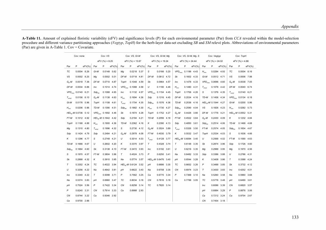
Appendix
A-Table 11. Amount of explained floristic variability (eFV) and significance levels (P) for each environmental parameter (Par) from CCA revealed within the on procedure and different variance partitioning approaches (Vegtyp, TopH) for the herb-layer data-set excluding SB and SM relevé plots. Abbreviations of environme rs (Par) are given in A-Table 1. Cov = Covariate.
model-selectintal paramete
Cov: none
Par
TC
VS
GB-M
DF-M
VPDmax
Tampl
GI-M
Hmin
HELB-M
FT-M
TopH
Mg
Sdp
K
TD-M
SdpAh
S
Sk
T
U
Inc
Na
pH
P
CN
Ca
P
0.0004
0.0002
0.0018
0.0034
0.0140
0.0156
0.0176
0.0206
0.0736
0.1012
0.1168
0.1310
0.1424
0.1296
0.1666
0.1664
0.1970
0.2888
0.3352
0.3256
0.3340
0.5374
0.7024
0.8240
0.8744
0.9700
eFV(%)
8.26
8.25
7.38
6.88
6.21
6.10
5.96
5.96
5.12
4.92
4.88
4.80
4.79
4.77
4.67
4.60
4.57
4.32
4.24
4.22
4.22
3.83
3.56
3.31
3.22
2.88
Cov: VS
eFV (%) = 8.25
Par
GI-M
Mg
DF-M
Inc
SdpAh
GB-M
TopH
TD-M
VPDmax
HELB-M
Hmin
Tampl
Sdp
S
U
Sk
FT-M
K
TC
Na
T
pH
P
CN
Ca
P
0.0148
0.0552
0.0710
0.1014
0.1088
0.1138
0.1108
0.1390
0.1692
0.1642
0.1900
0.1996
0.2484
0.2748
0.2602
0.3138
0.3804
0.3910
0.4022
0.4642
0.5098
0.6960
0.7422
0.7614
0.9346
eFV(%)
5.62
5.01
4.87
4.74
4.65
4.63
4.61
4.51
4.46
4.42
4.36
4.32
4.21
4.21
4.20
4.10
3.96
3.95
3.94
3.81
3.71
3.47
3.34
3.33
2.92
Cov: VS, GI-M
eFV (%) = 13.87
Par
Mg
DF-M
TopH
VPDmax
Inc
Hmin
Tampl
SdpAh
Sk
Sdp
TD-M
S
GB-M
U
K
FT-M
T
Na
HELB-M
pH
P
TC
CN
Ca
P
0.0218
0.0718
0.1048
0.1088
0.1132
0.1694
0.1754
0.1882
0.1974
0.2184
0.2362
0.2730
0.2978
0.3014
0.3370
0.3472
0.4524
0.5774
0.6124
0.6622
0.7562
0.8034
0.8258
0.8988
eFV(%)
5.37
4.81
4.59
4.58
4.57
4.36
4.35
4.30
4.28
4.21
4.16
4.12
4.08
4.03
3.97
3.93
3.73
3.57
3.52
3.43
3.25
3.18
3.14
2.93
Cov: VS, GI-M, Mg
eFV (%) = 19.24
Par
S
DF-M
Sk
U
VPDmax
Sdp
SdpAh
Hmin
TopH
TD-M
K
GB-M
FT-M
Tampl
T
Inc
P
HELB-M
pH
Na
Ca
CN
TC
P
0.0166
0.0812
0.0964
0.1190
0.1154
0.1316
0.1576
0.1730
0.1752
0.2056
0.2390
0.3524
0.4030
0.4128
0.4328
0.5192
0.6250
0.6476
0.6686
0.6708
0.6770
0.7616
0.7820
eFV(%)
5.20
4.72
4.57
4.46
4.45
4.45
4.36
4.27
4.27
4.18
4.13
3.89
3.79
3.77
3.74
3.61
3.41
3.40
3.35
3.35
3.34
3.18
3.14
Cov: VS, GI-M, Mg, S
eFV (%) = 24.44
Par
VPDmax
Sk
Inc
Hmin
TopH
DF-M
TD-M
SdpAh
GB-M
FT-M
Sdp
Tampl
K
HELB-M
T
U
Na
pH
TC
CN
P
Ca
P
0.1186
0.1602
0.1478
0.1480
0.1706
0.2034
0.2036
0.2590
0.4426
0.4522
0.4850
0.5326
0.5532
0.6094
0.6148
0.6216
0.6482
0.6544
0.6652
0.6974
0.7368
0.7788
eFV(%)
4.43
4.33
4.33
4.31
4.26
4.16
4.16
4.04
3.66
3.64
3.61
3.50
3.47
3.40
3.35
3.35
3.33
3.28
3.26
3.23
3.10
3.05
Cov: Vegtyp
eFV (%) = 24.02
Par
Hmin
GI-M
VPDmax
Tampl
S
TD-M
HELB-M
VS
DF-M
GB-M
SdpAh
FT-M
TopH
U
Sk
Mg
Sdp
K
P
T
Na
TC
Inc
pH
Ca
CN
P
0.0284
0.0512
0.0696
0.1078
0.1376
0.1406
0.1544
0.1826
0.1776
0.2430
0.2514
0.2574
0.2534
0.2568
0.2874
0.2988
0.3386
0.3408
0.3488
0.3430
0.5260
0.5776
0.6086
0.6884
0.7212
0.7454
eFV(%)
4.93
4.71
4.60
4.42
4.35
4.34
4.27
4.23
4.21
4.09
4.06
4.05
4.03
4.02
3.96
3.95
3.88
3.86
3.85
3.83
3.58
3.48
3.39
3.29
3.24
3.18
Cov: TopH
eFV (%) = 4.88
Par
TC
VS
GB-M
DF-M
Tampl
VPDmax
GI-M
Hmin
HELB-M
K
TD-M
SdpAh
S
FT-M
Sdp
Mg
U
T
Sk
Inc
Na
pH
CN
P
Ca
P
0.0004
0.0006
0.0038
0.0040
0.0140
0.0134
0.0200
0.0282
0.0552
0.1232
0.1468
0.1654
0.1636
0.1590
0.1726
0.1970
0.2786
0.3388
0.3732
0.4252
0.5960
0.6490
0.6820
0.8876
0.9754
eFV(%)
8.16
7.98
7.05
6.74
6.21
6.18
5.96
5.73
5.31
4.84
4.68
4.67
4.66
4.63
4.60
4.56
4.31
4.24
4.12
4.01
3.68
3.61
3.57
3.06
2.67
133
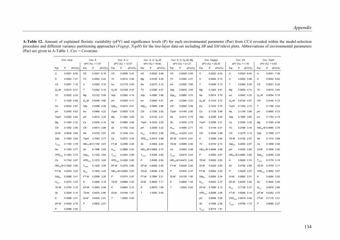
Appendix
A-Table 12. Amount of explained floristic variability (eFV) and significance levels (P) for each environmental parameter (Par) from CCA revealed within the model-selection procedure and different variance partitioning approaches (Vegtyp, TopH) for the tree-layer data-set including SB and SM relevé plots. Abbreviations of environmental parameters (Par) are given in A-Table 1. Cov = Covariate.
Par
U
S
VS
GB-M
TC
T
Inc
pH
TopH
Mg
CN
GI-M
Sdp
Tampl
Na
VPDmax
Ca
HELB-M
FT-M
SdpAh
Hmin
TD-M
Sk
K
DF-M
P
P
0.0001
0.0002
0.0001
0.0014
0.0002
0.1028
0.0632
0.0450
0.0282
0.1040
0.1092
0.0836
0.1560
0.1150
0.1250
0.1404
0.1742
0.1820
0.2532
0.2686
0.3272
0.3704
0.3508
0.4588
0.5430
0.5598
eFV(%)
8.05
7.47
7.16
6.31
6.24
4.89
4.87
4.63
4.63
4.32
3.95
3.85
3.82
3.79
3.77
3.72
3.67
3.56
3.43
3.41
3.23
3.18
3.14
3.01
2.76
2.55
Cov: SeFV (%) = 7.47
Par
VS
TC
U
T
Mg
GB-M
Sdp
Inc
pH
Ca
CN
Na
TopH
HELB-M
Sk
SdpAh
VPDmax
Tampl
Hmin
FT-M
K
DF-M
TD-M
GI-M
P
P
0.0001
0.0002
0.0292
0.0302
0.0122
0.0048
0.0386
0.0468
0.0612
0.0436
0.0814
0.0752
0.1042
0.1150
0.1998
0.1332
0.1272
0.1240
0.1976
0.2958
0.2846
0.3954
0.4670
0.6420
0.5602
eFV(%)
6.19
5.42
5.10
5.10
5.09
4.80
4.26
4.22
4.20
4.18
3.88
3.87
3.77
3.67
3.65
3.64
3.60
3.59
3.44
3.20
3.18
2.98
2.86
2.61
2.51
Par
VS
TC
Inc
GB-M
Sdp
pH
SdpAh
TopH
Mg
Na
Sk
CN
Ca
FT-M
Hmin
Tampl
VPDmax
DF-M
HELB-M
P
TD-M
K
GI-M
T
P
0.0006
0.0014
0.0178
0.0188
0.0360
0.0500
0.0474
0.0920
0.1562
0.0980
0.1752
0.1246
0.2072
0.2398
0.3866
0.4054
0.4328
0.4276
0.6080
0.5374
0.6868
0.8690
0.9188
1.0000
eFV(%)
5.43
5.08
4.49
4.34
4.19
4.17
4.01
3.76
3.69
3.66
3.62
3.61
3.35
3.29
2.93
2.89
2.85
2.85
2.53
2.47
2.40
2.10
1.97
0.00
Cov: S, U, GB-MeFV (%) = 16.92
Par
VS
Mg
Na
TC
Sdp
Inc
SdpAh
CN
Ca
TopH
pH
Hmin
VPDmax
Sk
HELB-M
Tampl
P
DF-M
TD-M
FT-M
GI-M
K
T
P
0.0032
0.0700
0.0270
0.0396
0.0586
0.0640
0.0690
0.1246
0.2122
0.2232
0.2508
0.3610
0.3914
0.3962
0.4808
0.5306
0.5006
0.6082
0.6936
0.7884
0.9650
0.9678
1.0000
eFV(%)
5.09
4.29
4.10
4.07
3.98
3.91
3.86
3.55
3.31
3.25
3.22
2.95
2.88
2.83
2.70
2.66
2.54
2.50
2.35
2.21
1.71
1.68
0.00
Cov: S, U, GB-M, MgeFV (%) = 21.21
Par
VS
TC
Inc
Sdp
SdpAh
pH
CN
TopH
Na
Sk
Hmin
VPDmax
DF-M
TD-M
Ca
Tampl
HELB-M
FT-M
P
GI-M
K
T
P
0.0048
0.0394
0.0526
0.0630
0.0884
0.2284
0.2684
0.4184
0.4214
0.4008
0.4596
0.5230
0.5016
0.5696
0.5462
0.6218
0.6472
0.6428
0.5404
0.9138
0.9858
1.0000
eFV(%)
4.99
4.07
3.95
3.94
3.70
3.23
3.08
2.80
2.78
2.78
2.71
2.61
2.61
2.50
2.48
2.44
2.40
2.40
2.37
1.90
1.43
0.00
Cov: VegtypeFV (%) = 25.30
Par
S
U
T
Mg
Na
GB-M
Inc
Ca
Sdp
TopH
VS
CN
K
TC
HELB-M
P
TD-M
GI-M
FT-M
SdpAh
Hmin
DF-M
VPDmax
pH
Sk
Tampl
P
0.0022
0.0050
0.0496
0.1062
0.0814
0.1310
0.1430
0.1126
0.2288
0.2298
0.3148
0.3538
0.3588
0.4730
0.4848
0.4562
0.5092
0.5226
0.6062
0.6954
0.6922
0.7888
0.8288
0.8098
0.7486
0.8774
eFV(%)
6.03
5.15
5.14
3.91
3.79
3.72
3.70
3.69
3.29
3.21
3.01
2.96
2.94
2.73
2.68
2.67
2.63
2.62
2.45
2.34
2.27
2.13
2.08
2.08
2.06
1.91
Cov: VSeFV (%) = 7.16
Par
S
U
T
Mg
Inc
GB-M
TopH
Na
Sdp
Ca
TC
CN
TD-M
SdpAh
pH
HELB-M
K
Sk
P
GI-M
DF-M
Hmin
FT-M
VPDmax
Tampl
P
0.0004
0.0002
0.0464
0.0600
0.0942
0.0720
0.1394
0.1164
0.1680
0.2090
0.2598
0.3278
0.4152
0.4054
0.4520
0.4860
0.5628
0.4782
0.5208
0.6892
0.6302
0.7126
0.8268
0.8876
0.9758
eFV(%)
6.50
5.98
5.58
4.74
4.33
4.07
3.72
3.68
3.65
3.48
3.34
3.13
2.97
2.97
2.85
2.82
2.74
2.69
2.57
2.51
2.50
2.37
2.18
2.08
1.72
Cov: TopHeFV (%) = 4.63
Par
U
S
VS
TC
GB-M
CN
T
pH
Inc
Mg
HELB-M
Sdp
Na
Ca
GI-M
SdpAh
Tampl
TD-M
VPDmax
K
Sk
Hmin
DF-M
FT-M
P
P
0.0001
0.0002
0.0001
0.0010
0.0054
0.0146
0.1188
0.0890
0.1192
0.1040
0.0980
0.1598
0.1310
0.1898
0.1606
0.2994
0.3178
0.3700
0.3892
0.4264
0.3904
0.4876
0.5352
0.7178
0.6568
eFV(%)
7.28
6.62
6.25
5.64
5.18
4.72
4.62
4.23
4.19
4.08
3.78
3.77
3.68
3.58
3.55
3.29
3.19
3.11
3.07
3.02
2.95
2.86
2.75
2.51
2.27
Cov: S, UeFV (%) = 12.57
Cov: none
134
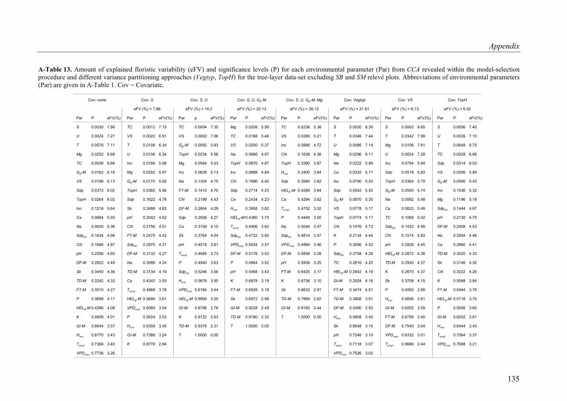
Appendix
A-Table 13. Amount of explained floristic variability (eFV) and significance levels (P) for each environmental parameter (Par) from CCA revealed within the model-selection procedure and different variance partitioning approaches (Vegtyp, TopH) for the tree-layer data-set excluding SB and SM relevé plots. Abbreviations of environmental parameters (Par) are given in A-Table 1. Cov = Covariate.
Cov: none
Par
S
U
T
Mg
TC
GB-M
VS
Sdp
TopH
Inc
Ca
Na
SdpAh
CN
pH
DF-M
Sk
TD-M
FT-M
P
HELB-M
K
GI-M
Hmin
Tampl
VPDmax
P
0.0030
0.0024
0.0576
0.0252
0.0036
0.0162
0.0196
0.0372
0.0264
0.1216
0.0684
0.0630
0.1634
0.1686
0.2556
0.2822
0.3440
0.3242
0.3510
0.3698
0.4286
0.4608
0.6644
0.6770
0.7366
0.7736
eFV(%)
7.86
7.27
7.11
6.68
6.66
6.18
6.13
6.02
6.02
5.64
5.50
5.36
4.98
4.87
4.60
4.49
4.36
4.33
4.27
4.17
4.08
4.01
3.57
3.43
3.40
3.26
Cov: S
eFV (%) = 7.86
Par
TC
VS
T
U
Inc
Mg
GB-M
TopH
Sdp
Sk
pH
CN
FT-M
SdpAh
DF-M
Na
TD-M
Ca
Tampl
HELB-M
VPDmax
P
Hmin
GI-M
K
P
0.0012
0.0022
0.0108
0.0106
0.0166
0.0252
0.0170
0.0360
0.1622
0.2488
0.2042
0.2156
0.2470
0.2970
0.3132
0.3088
0.3134
0.4242
0.4868
0.5690
0.6080
0.5624
0.6358
0.7388
0.8778
eFV(%)
7.15
6.91
6.34
6.34
5.98
5.97
5.92
5.56
4.78
4.62
4.62
4.51
4.42
4.31
4.27
4.24
4.19
3.93
3.78
3.61
3.54
3.53
3.45
3.24
2.84
Cov: S, U
eFV (%) = 14.2
Par
TC
VS
GB-M
TopH
Mg
Inc
Na
FT-M
CN
DF-M
Sdp
Ca
Sk
pH
Tampl
P
SdpAh
Hmin
VPDmax
HELB-M
GI-M
K
TD-M
T
p
0.0004
0.0002
0.0092
0.0234
0.0564
0.0638
0.1304
0.1410
0.2198
0.2664
0.2926
0.3106
0.3764
0.4518
0.4684
0.4940
0.5246
0.5676
0.6184
0.6900
0.8796
0.9122
0.9376
1.0000
eFV(%)
7.35
7.06
5.93
5.56
5.53
5.13
4.75
4.70
4.43
4.29
4.27
4.15
4.04
3.81
3.73
3.63
3.58
3.50
3.44
3.25
2.76
2.63
2.31
0.00
Cov: S, U, GB-M
eFV (%) = 20.13
Par
Mg
TC
VS
Na
TopH
Inc
CN
Sdp
Ca
Hmin
HELB-M
Tampl
SdpAh
VPDmax
DF-M
P
pH
K
FT-M
Sk
GI-M
TD-M
T
P
0.0208
0.0188
0.0250
0.0666
0.0876
0.0888
0.1996
0.2714
0.2434
0.3958
0.4380
0.4906
0.4722
0.5034
0.5178
0.4864
0.5468
0.6878
0.6928
0.6972
0.9228
0.9180
1.0000
eFV(%)
5.99
5.46
5.37
4.97
4.87
4.84
4.40
4.23
4.23
3.82
3.70
3.62
3.60
3.57
3.53
3.52
3.43
3.19
3.18
2.98
2.49
2.32
0.00
Cov: S, U, GB-M, Mg
eFV (%) = 26.12
Par
TC
VS
Inc
CN
TopH
Hmin
Sdp
HELB-M
Ca
Tampl
P
Na
SdpAh
VPDmax
DF-M
pH
FT-M
K
Sk
TD-M
GI-M
T
P
0.0236
0.0280
0.0986
0.1638
0.3390
0.3400
0.3584
0.4288
0.4294
0.4752
0.4446
0.5046
0.4814
0.4994
0.5858
0.5936
0.6420
0.6736
0.6632
0.7994
0.9182
1.0000
eFV(%)
5.38
5.21
4.72
4.38
3.87
3.84
3.82
3.64
3.62
3.52
3.50
3.47
3.47
3.46
3.28
3.25
3.17
3.10
2.91
2.62
2.44
0.00
Cov: Vegtyp
eFV (%) = 21.61
Par
S
T
U
Mg
Na
Ca
Inc
Sdp
GB-M
VS
TopH
CN
K
P
SdpAh
TC
HELB-M
GI-M
FT-M
TD-M
DF-M
Hmin
Sk
pH
Tampl
VPDmax
P
0.0020
0.0346
0.0066
0.0296
0.0222
0.0332
0.0790
0.0542
0.0870
0.0778
0.0774
0.1476
0.2134
0.2656
0.2758
0.2816
0.2842
0.2924
0.3474
0.3808
0.5490
0.5608
0.6648
0.7246
0.7118
0.7526
eFV(%)
8.39
7.44
7.14
6.11
5.89
5.71
5.53
5.50
5.30
5.17
5.17
4.73
4.44
4.33
4.26
4.20
4.19
4.16
4.01
3.91
3.50
3.45
3.15
3.10
3.07
3.02
Cov: VS
eFV (%) = 6.13
Par
S
T
Mg
U
Inc
Sdp
TopH
GB-M
Na
Ca
TC
SdpAh
CN
pH
HELB-M
TD-M
K
Sk
P
Hmin
GI-M
FT-M
DF-M
VPDmax
Tampl
P
0.0002
0.0342
0.0106
0.0024
0.0794
0.0518
0.0364
0.0550
0.0582
0.0622
0.1068
0.1432
0.1574
0.2828
0.2872
0.2930
0.2670
0.3708
0.4092
0.5656
0.6202
0.6756
0.7540
0.8332
0.9686
eFV(%)
8.65
7.99
7.61
7.29
5.94
5.83
5.79
5.74
5.48
5.48
5.42
4.99
4.83
4.45
4.38
4.37
4.37
4.15
3.99
3.61
3.59
3.40
3.04
3.01
2.44
Cov: TopH
eFV (%) = 6.02
Par
S
U
T
TC
Sdp
VS
GB-M
Inc
Mg
SdpAh
pH
DF-M
Na
Ca
TD-M
Sk
CN
K
FT-M
HELB-M
P
GI-M
Hmin
Tampl
VPDmax
P
0.0056
0.0026
0.0648
0.0028
0.0314
0.0206
0.0590
0.1536
0.1196
0.1444
0.2130
0.2408
0.2554
0.2860
0.3020
0.3146
0.3222
0.5068
0.5444
0.5718
0.5056
0.6202
0.6444
0.7064
0.7688
eFV(%)
7.40
7.10
6.75
6.66
6.03
5.89
5.43
5.32
5.18
4.97
4.75
4.53
4.48
4.41
4.33
4.30
4.26
3.84
3.76
3.70
3.65
3.61
3.43
3.37
3.21
135
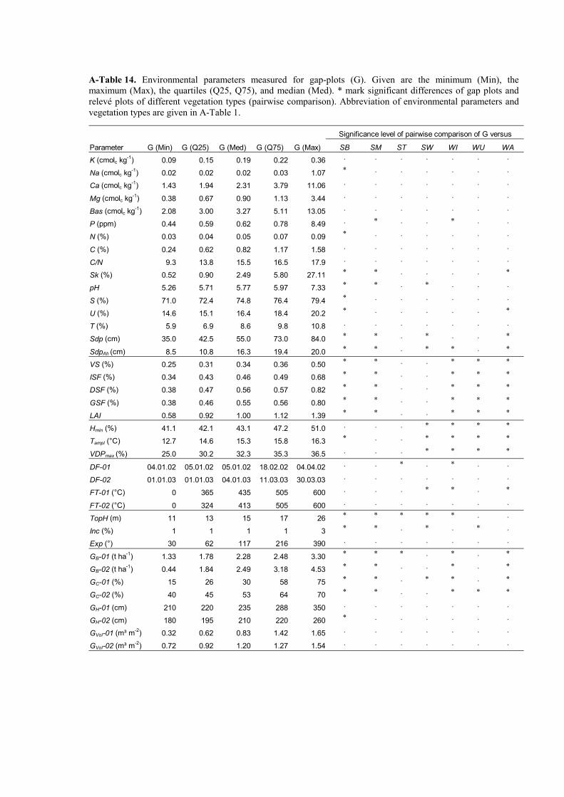
A-Tablmaximurelevé pvegetat
e 14. Environmental parameters measured for gap-plots (G). Given are the minimum (Min), the m (Max), the quartiles (Q25, Q75), and median (Med). * mark significant differences of gap plots and lots of different vegetation types (pairwise comparison). Abbreviation of environmental parameters and
ion types are given in A-Table 1.
Significance level of pairwise comparison of G versus
Parameter G (Min) G (Q25) G (Med) G (Q75) G (Max) SB SM ST SW WI WU WA
K (cmolc kg-1) 0.09 0.15 0.19 0.22 0.36 . . . . . . .
Na (cmo
Ca (cmo
Mg (cmo
Bas (cm
lc kg-1) 0.02 0.02 0.02 0.03 1.07 * . . . . . .
lc kg-1) 1.43 1.94 2.31 3.79 11.06 . . . . . . .
lc kg-1) 0.38 0.67 0.90 1.13 3.44 . . . . . . .
olc kg-1) 2.08 3.00 3.27 5.11 13.05 . . . . . . .
0.44 0.59 0.62 0.78 8.49 . * . . * . .
0.03 0.04 0.05 0.07 0.09 * . . . . . .
0.24 0.62 0.82 1.17 1.58 . . . . . . .
9.3 13.8 15.5 16.5 17.9 . . . . . . .
0.52 0.90 2.49 5.80 27.11 * * . . . . *
5.26 5.71 5.77 5.97 7.33 * * . * . . .
71.0 72.4 74.8 76.4 79.4 * . . . . . .
14.6 15.1 16.4 18.4 20.2 * . . . . . *
5.9 6.9 8.6 9.8 10.8 . . . . . . .
) 35.0 42.5 55.0 73.0 84.0 * * . * . . *
m) 8.5 10.8 16.3 19.4 20.0 * * . * * . *
0.25 0.31 0.34 0.36 0.50 * * . . * * *
P (ppm)
N (%)
C (%) C/N Sk (%) pH
S (%) U (%) T (%) Sdp (cm
SdpAh (c
VS (%) ISF (%) DSF (%
GSF (%
LAI
Hmin (%)
0.34 0.43 0.46 0.49 0.68 * * . . * * *
) 0.38 0.47 0.56 0.57 0.82 * * . . * * *
) 0.38 0.46 0.55 0.56 0.80 * * . . * * *
0.58 0.92 1.00 1.12 1.39 * * . . * * *
41.1 42.1 43.1 47.2 51.0 . . . * * * *
Tampl (°C
VDPmax (%
DF-01
) 12.7 14.6 15.3 15.8 16.3 * . . * * * *
) 25.0 30.2 32.3 35.3 36.5 . . . * * * *
04.01.02 05.01.02 05.01.02 18.02.02 04.04.02 . . * . * . .
DF-02
FT-01 (°
FT-02 (°
TopH (m
01.01.03 01.01.03 04.01.03 11.03.03 30.03.03 . . . . . . .
C) 0 365 435 505 600 . . . * * . *
C) 0 324 413 505 600 . . . . . . .
) 11 13 15 17 26 * * * * * . .
Inc (%) Exp (°)
GB-01 (t
1 1 1 1 3 * * . * . * .
30 62 117 216 390 . . . . . . .
ha-1) 1.33 1.78 2.28 2.48 3.30 * * * . * . *
GB-02 (t ha-1
GC-01 (%) GC-02 (%)
GH-01 (cm) GH-02 (cm) GVol-01 (m³
) 0.44 1.84 2.49 3.18 4.53 * * . . * . *
15 26 30 58 75 * * . * * . *
40 45 53 64 70 * * . . * * *
210 220 235 288 350 . . . . . . .
180 195 210 220 260 * . . . . . .
m-2) 0.32 0.62 0.83 1.42 1.65 . . . . . . .
m-2)GVol-02 (m³ 0.72 0.92 1.20 1.27 1.54 . . . . . . .
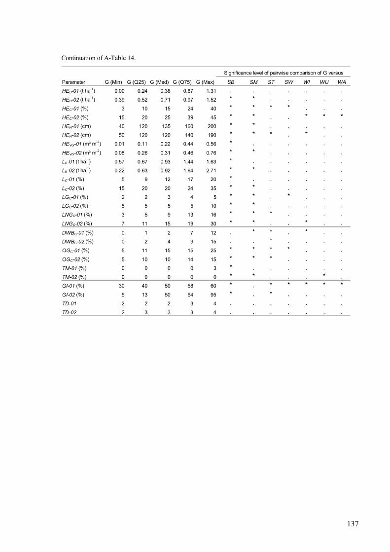
Continuation of A-Table 14.
Significance level of pairwise comparison of G versus
Parameter G (Min) G (Q25) G (Med) G (Q75) G (Max) SB SM ST SW WI WU WA
HEB-01 (t ha-1) 0.00 0.24 0.38 0.67 1.31 . . . . . . . HEB-02 (t ha-1) 0.39 0.52 0.71 0.97 1.52 * * . . . . . HEC-01 (%) 3 10 15 24 40 * * * * . . . HEC-02 (%) 15 20 25 39 45 * * . . * * * HEH-01 (cm) 40 120 135 160 200 * * . . . . . HEH-02 (cm) 50 120 120 140 190 * * * . * . . HEVol-01 (m³ m-2) 0.01 0.11 0.22 0.44 0.56 * . . . . . . HEVol-02 (m³ m-2) 0.08 0.26 0.31 0.46 0.76 * * . . . . . LB-01 (t ha-1) 0.57 0.67 0.93 1.44 1.63 * . . . . . . LB-02 (t ha-1) 0.22 0.63 0.92 1.64 2.71 * * . . . . . LC-01 (%) 5 9 12 17 20 * . . . . . . LC-02 (%) 15 20 20 24 35 * * . . . . . LGC-01 (%) 2 2 3 4 5 * * . * . . . LGC-02 (%) 5 5 5 5 10 * * . . . . . LNGC-01 (%) 3 5 9 13 16 * * * . . . . LNGC-02 (%) 7 11 15 19 30 * * . . * . . DWBC-01 (%) 0 1 2 7 12 . * * . * . . DWBC-02 (%) 0 2 4 9 15 . . * . . . . OGC-01 (%) 5 11 15 15 25 * * * * . . . OGC-02 (%) 5 10 10 14 15 * * * . . . . TM-01 (%) 0 0 0 0 3 * . . . . . . TM-02 (%) 0 0 0 0 0 * * . . . * . GI-01 (%) 30 40 50 58 60 * . * * * * * GI-02 (%) 5 13 50 64 95 * . * . . . . TD-01 2 2 2 3 4 . . . . . . . TD-02 2 3 3 3 4 . . . . . . .
137
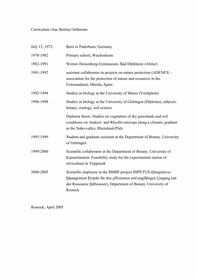
Curriculum vitae Bettina Orthmann
July 13, 1972 Born in Paderborn, Germany
1978-1982 Primary school, Wachenheim
1982-1991 Werner-Heisenberg-Gymnasium, Bad Dürkheim (Abitur)
1991-1992 assistant collaborator in projects on nature protection (ADENEX – association for the protection of nature and resources in the Extremadura), Mérida, Spain
1992-1994 Studies in biology at the University of Mainz (Vordiplom)
1994-1998 Studies in biology at the University of Göttingen (Diploma), subjects: botany, zoology, soil science
Diploma thesis: Studies on vegetation of dry grasslands and soil conditions on Andesit- and Rhyolit-outcrops along a climatic gradient in the Nahe-valley, Rheinland-Pfalz
1995-1999 Student and graduate assistant at the Department of Botany, University of Göttingen
1999-2000 Scientific collaborator at the Department of Botany, University of Kaiserslautern: Feasibility study for the experimental station of silviculture in Trippstadt
000-2005 Scientific employee in the BMBF-project IMPETUS (I2 ntegratives Management Projekt für den effizienten und tragfähigen Umgang mit der Ressource Süßwasser), Department of Botany, University of Rostock
Rostock, April 2005
Hier chte Dissertation selbständig und ohne fremde Hilfe verfasst, andere als die von mir angegebenen Quellen und Hilfsmittel nicht benutzt und die den benutzten Werken wörtlich oder inhaltlich entnommenen Stellen als solche kenntlich gem
Rost
mit erkläre ich, dass ich die eingerei
acht habe.
ock, April 2005
139