Embed Size (px)
Citation preview
Deutsche Geodätische Kommission
der Bayerischen Akademie der Wissenschaften
Reihe C Dissertationen Heft Nr. 709
Richard Steffen
Visual SLAM from image sequences
acquired by unmanned aerial vehicles
München 2013
Verlag der Bayerischen Akademie der Wissenschaftenin Kommission beim Verlag C. H. Beck
ISSN 0065-5325 ISBN 978-3-7696-5121-8
Diese Arbeit ist gleichzeitig veröffentlicht in:
Schriftenreihe des Instituts für Geodäsie und Geoinformation
der Rheinischen Friedrich-Wilhelms Universität Bonn
ISSN 1864-1113, Nr. 34, Bonn 2009

Deutsche Geodätische Kommission
der Bayerischen Akademie der Wissenschaften
Reihe C Dissertationen Heft Nr. 709
Visual SLAM from image sequences
acquired by unmanned aerial vehicles
Inaugural-Dissertation zur
Erlangung des akademischen Grades
Doktor-Ingenieur (Dr.-Ing.)
der Hohen Landwirtschaftlichen Fakultät
der Rheinischen Friedrich-Wilhelms Universität
zu Bonn
vorgelegt
am 27.07.2009 von
Richard Steffen
aus Schwerin
München 2013
Verlag der Bayerischen Akademie der Wissenschaftenin Kommission beim Verlag C. H. Beck
ISSN 0065-5325 ISBN 978-3-7696-5121-8
Diese Arbeit ist gleichzeitig veröffentlicht in:
Schriftenreihe des Instituts für Geodäsie und Geoinformation
der Rheinischen Friedrich-Wilhelms Universität Bonn
ISSN 1864-1113, Nr. 34, Bonn 2009

Adresse der Deutschen Geodätischen Kommission:
Deutsche Geodätische KommissionAlfons-Goppel-Straße 11 ! D – 80 539 München
Telefon +49 – 89 – 23 031 1113 ! Telefax +49 – 89 – 23 031 - 1283 / - 1100e-mail [email protected] ! http://www.dgk.badw.de
Diese Publikation ist als pdf-Dokument veröffentlicht im Internet unter der Adresse /This volume is published in the internet
<http://dgk.badw.de> ! <http://hss.ulb.uni-bonn.de/2009/1971/1971.htm>
Prüfungskommission
Referent: Prof. Dr.-Ing. Wolfgang Förstner1. Korreferent: Prof. Dr. techn. Wolf–Dieter Schuh
Tag der mündlichen Prüfung: 20.11.2009
© 2013 Deutsche Geodätische Kommission, München
Alle Rechte vorbehalten. Ohne Genehmigung der Herausgeber ist es auch nicht gestattet,die Veröffentlichung oder Teile daraus auf photomechanischem Wege (Photokopie, Mikrokopie) zu vervielfältigen
ISSN 0065-5325 ISBN 978-3-7696-5121-8

3
Never try, never know ...

4
This dissertation is dedicated to my parents and to my sister. Thank you for giving
me the strength and hope. Foremost, this work would not have been possible without Prof.
Wolfgang Forstner. It was the best decision in my life to join your research group. Thank you
for your excellent advise, patience and all your support. I will never forget this time. A special
thanks goes to my colleagues at the Department of Photogrammetry for all the productive
discussions. The genial work atmosphere was one of the reasons that made this thesis a
success. In particular, I thank Hanns-Florian Schuster, Mark Luxen, Christian Beder and
Jochen Meidow for giving me the opportunity to learn from you. A special thanks to Heidi
for checking the English spellings. I will remember you as the good spirit of the department.
Finally, I am grateful to all my friends who shared the path of my lifeThis is much more
important to me, than you can imagine.

5
Zusammenfassung
Visuelle gleichzeitige Lokalisierung und Kartierung aus Bildfolgen von unbemannten
Flugkorpern
Diese Arbeit zeigt, dass die Kalmanfilter basierte Losung der Triangulation zur Lokali-
sierung und Kartierung aus Bildfolgen von unbemannten Flugkorpern realisierbar ist. Auf-
grund von Echtzeitanforderungen autonomer Systeme erreichen rekursive Schatz-verfahren,
insbesondere Kalmanfilter basierte Ansatze, große Beliebheit. Bedauerlicherweise treten da-
bei durch die Nichtlinearitat der Triangulation einige Effekte auf, welche die Konsistenz und
Genauigkeit der Losung hinsichtlich der geschatzten Parameter maßgeblich beeinflussen.
Der erste Beitrag dieser Arbeit besteht in der Herleitung eines generellen Verfahrens
zum rekursiven Verbessern im Kalmanfilter mit impliziten Beobachtungsgleichungen. Wir
zeigen, dass die klassischen Verfahren im Kalmanfilter eine Spezialisierung unseres Ansatzes
darstellen.
Im zweiten Beitrag erweitern wir die klassische Modellierung fur ein Einkameramodell zu
einem Mehrkameramodell im Kalmanfilter. Diese Erweiterung erlaubt es uns, die Pradiktion
fur eine lineares Bewegungsmodell vollkommen linear zu berechnen.
In einem dritten Hauptbeitrag stellen wir ein neues Verfahren zur Initialisierung von Neu-
punkten im Kalmanfilter vor. Anhand von empirischen Untersuchungen unter Verwendung
simulierter und realer Daten einer Bildfolge eines photogrammetrischen Streifens zeigen und
vergleichen wir, welchen Einfluß die Initialisierungsmethoden fur Neupunkte im Kalmanfilter
haben und welche Genauigkeiten fur diese Szenarien erreichbar sind.
Am Beispiel von Bildfolgen eines unbemannten Flugkorpern zeigen wir in dieser Arbeit
als vierten Beitrag, welche Genauigkeit zur Lokalisierung und Kartierung durch Triangula-
tion moglich ist. Diese theoretische Analyse kann wiederum zu Planungszwecken verwendet
werden.
6
Abstract
Visual SLAM from image sequences acquired by unmanned aerial vehicles
This thesis shows that Kalman filter based approaches are sufficient for the task of si-
multaneous localization and mapping from image sequences acquired by unmanned aerial
vehicles. Using solely direction measurements to solve the problem of simultaneous localiza-
tion and mapping (SLAM) is an important part of autonomous systems. Because the need for
real-time capable systems, recursive estimation techniques, Kalman filter based approaches
are the main focus of interest. Unfortunately, the non-linearity of the triangulation using the
direction measurements cause decrease of accuracy and consistency of the results.
The first contribution of this work is a general derivation of the recursive update of the
Kalman filter. This derivation is based on implicit measurement equations, having the classi-
cal iterative non-linear as well as the non-iterative and linear Kalman filter as specializations
of our general derivation.
Second, a new formulation of linear-motion models for the single camera state model
and the sliding window camera state model are given, that make it possible to compute the
prediction in a fully linear manner.
The third major contribution is a novel method for the initialization of new object points
in the Kalman filter. Empirical studies using synthetic and real data of an image sequence
of a photogrammetric strip are made, that demonstrate and compare the influences of the
initialization methods of new object points in the Kalman filter.
Forth, the accuracy potential of monoscopic image sequences from unmanned aerial ve-
hicles for autonomous localization and mapping is theoretically analyzed, which can be used
for planning purposes.
Contents
1 Introduction 11
1.1 Motivation . . . . . . . . . . . . . . . . . . . . . . . . . . . . . . . . . . . . . 12
1.2 Collaborations and publications . . . . . . . . . . . . . . . . . . . . . . . . . . 14
1.3 Notation . . . . . . . . . . . . . . . . . . . . . . . . . . . . . . . . . . . . . . . 15
2 Previous work 19
2.1 Previous work on general estimation techniques . . . . . . . . . . . . . . . . . 21
2.2 Previous work with different sensor types . . . . . . . . . . . . . . . . . . . . 25
2.3 Previous work with different map representations . . . . . . . . . . . . . . . . 26
2.4 Previous work with different ambiances . . . . . . . . . . . . . . . . . . . . . 27
2.5 Previous work for large scenes . . . . . . . . . . . . . . . . . . . . . . . . . . . 28
3 Background theory 31
3.1 Geometric entities and transformations . . . . . . . . . . . . . . . . . . . . . . 31
3.1.1 Geometric entities . . . . . . . . . . . . . . . . . . . . . . . . . . . . . 31
3.1.1.1 Points and lines in the 2d space . . . . . . . . . . . . . . . . 32
3.1.1.2 Points, planes and lines in the 3d space . . . . . . . . . . . . 32
3.1.1.3 Incidence constrains and entity construction . . . . . . . . . 34
3.1.2 Rotations . . . . . . . . . . . . . . . . . . . . . . . . . . . . . . . . . . 35
3.1.3 Motions and homographies . . . . . . . . . . . . . . . . . . . . . . . . 39
3.2 Basic image geometry . . . . . . . . . . . . . . . . . . . . . . . . . . . . . . . 41
3.2.1 The geometry of the single image . . . . . . . . . . . . . . . . . . . . . 41
3.2.2 The geometry of the image pair . . . . . . . . . . . . . . . . . . . . . . 44
3.3 Least squares . . . . . . . . . . . . . . . . . . . . . . . . . . . . . . . . . . . . 47
3.3.1 Least squares optimization . . . . . . . . . . . . . . . . . . . . . . . . 47
7
8 CONTENTS
3.3.2 Outlier detection and robustification . . . . . . . . . . . . . . . . . . . 51
3.3.3 Parameter elimination in the normal equation system . . . . . . . . . 54
3.4 Recursive state estimation . . . . . . . . . . . . . . . . . . . . . . . . . . . . . 55
3.4.1 General recursive state estimation . . . . . . . . . . . . . . . . . . . . 56
3.4.2 The derivation of Kalman filtering . . . . . . . . . . . . . . . . . . . . 57
3.4.3 The particle based Kalman filtering . . . . . . . . . . . . . . . . . . . 63
3.4.4 Outlier detection and robustification of Kalman filtering . . . . . . . . 66
4 Kalman filter based localization and mapping with a single camera 69
4.1 Introduction . . . . . . . . . . . . . . . . . . . . . . . . . . . . . . . . . . . . . 69
4.2 Feature extraction, tracking and matching . . . . . . . . . . . . . . . . . . . . 72
4.3 State representation . . . . . . . . . . . . . . . . . . . . . . . . . . . . . . . . 75
4.3.1 Single camera state . . . . . . . . . . . . . . . . . . . . . . . . . . . . . 76
4.3.2 Sliding window camera state . . . . . . . . . . . . . . . . . . . . . . . 78
4.3.3 Feature representation and update models . . . . . . . . . . . . . . . . 81
4.3.4 The initialization problem . . . . . . . . . . . . . . . . . . . . . . . . . 83
4.3.4.1 Control point initialization . . . . . . . . . . . . . . . . . . . 84
4.3.4.2 Scale free bundle adjustment initialization . . . . . . . . . . 84
4.3.4.3 Inverse distance feature initialization and reduction . . . . . 86
4.3.4.4 Stable feature initialization procedure . . . . . . . . . . . . . 89
4.4 Georeferencing . . . . . . . . . . . . . . . . . . . . . . . . . . . . . . . . . . . 91
4.5 On particle based Kalman filtering for simultaneous localization and mapping 93
5 Evaluation of the proposed methods 97
5.1 On the theoretical accuracy of photogrammetric strips from image sequences 98
5.1.1 Experimental setup . . . . . . . . . . . . . . . . . . . . . . . . . . . . . 101
5.1.2 The influence of the field of view . . . . . . . . . . . . . . . . . . . . . 103
5.1.3 The influence of the base length . . . . . . . . . . . . . . . . . . . . . 104
5.1.4 The influence of measurement accuracy . . . . . . . . . . . . . . . . . 105
5.1.5 The influence of map density . . . . . . . . . . . . . . . . . . . . . . . 106
5.1.6 A general law to assess the theoretical accuracy of a photogrammetric
strip . . . . . . . . . . . . . . . . . . . . . . . . . . . . . . . . . . . . . 106
5.2 The influence of the initialization method . . . . . . . . . . . . . . . . . . . . 109
CONTENTS 9
5.3 Evaluation on simulated image data . . . . . . . . . . . . . . . . . . . . . . . 124
5.4 Real experiment evaluation . . . . . . . . . . . . . . . . . . . . . . . . . . . . 135
5.4.1 Used hardware architecture . . . . . . . . . . . . . . . . . . . . . . . . 135
5.4.2 Flight-test area and reference data . . . . . . . . . . . . . . . . . . . . 137
5.4.3 Kalman filter based results of a real image sequence . . . . . . . . . . 139
6 Conclusion and future work 143
A Appendix 147
A.1 Angular differentiation of circular motion using quaternion . . . . . . . . . . 147
A.2 Linear dynamic model derivation . . . . . . . . . . . . . . . . . . . . . . . . . 149
A.3 Uncertainty transfer . . . . . . . . . . . . . . . . . . . . . . . . . . . . . . . . 152
A.4 Accuracy analysis of the general law . . . . . . . . . . . . . . . . . . . . . . . 154
A.5 Distortion field of the reconstructed object coordinates in the simulated envi-
ronment . . . . . . . . . . . . . . . . . . . . . . . . . . . . . . . . . . . . . . . 156

10 CONTENTS

Chapter 1
Introduction
A major goal of photogrammetry and computer vision is a fully automatic reconstruction
of an environment from images. An important aspect is the determination of the image lo-
cation and orientation. Although much progress has been made, the problem still remains
an active research field. A lot of attention to this problem has been received by the robotics
community simply because images carry manifold information about the scene. Hence, au-
tonomous systems are able to use the image information for different tasks, even for their
location determination.
The human ability to learn maps of the surrounding environment and to use them for
localization has inspired researchers in the robotics community over the last decades. The
understanding and acquisition of this ability has been identified as a fundamental problem in
robotics. The process of incremental map construction is called simultaneous localization and
mapping (SLAM). This task is a key component for building autonomous mobile devices, that
for many applications has been a dream of researchers. In the field of civil applications service,
robots perform cleaning, inspection and transportation tasks or medical and construction
assistance. Robots also operate in dangerous environments, say for life rescue or pollution
control. Robots can be used in a wide field of research applications, for instance space and
deep sea exploration. Moreover, in military applications for instance robots are useful in
investigating areas and for transportation and rescue tasks.
The research community is focused on different kinds of aspects concerning the map-
ping ability. Various sensor types and configurations to obtain map information as well as
knowledge about the robots location will be used. Of course, the developed methods depend
on the application environment and the a-priori information about it. The use of multiple
11
12 CHAPTER 1. INTRODUCTION
cooperating robots is of interest, caused by its advantages in case of fault-tolerance and to
accomplish a task faster. Available solutions for narrowed environments are well understood.
For unstructured large-scale environments open problems remain. These are issues regarding
map representation and its uncertainty, real-time capable update methods and sensor fusion
algorithms. Almost every technique assumes the environment to be static. A more difficult
problem occurs if the environment changes over time.
A module to solve the task of simultaneous localization and mapping can be understood as
a subcomponent of an entire system for autonomous robots. Its main function is to aggregate
observations obtained by sensors in order to obtain information of the environment stored in
a map and provide this informations to other subsystems. The map and the relative location
of the robot may be used for interaction with the environment depending on the robots
task. This interaction comprises for instance safe navigation, exploration of areas where the
robots knowledge about the map is uncertain, identifying and following dynamic objects or
manipulation of the environment.
1.1 Motivation
The task of simultaneous localization and mapping is an old problem. Since the computer
technology provides sufficient computation power and data from sensor systems is digitalized
automatically, classical techniques becomes practical for real-time applications. One of the
well-established techniques is named as triangulation, where direction measurements from
different locations are used to determine the location of an observed object and the location
of the observer himself. In the area of nautical navigation this task is called dead reckoning
and is known since millenniums.
In classical photogrammetry a realization incorporating uncertainties of the direction
measurements into the triangulation is given by a least square solution known as bundle
adjustment. This technique can be adapted to the real-time localization and mapping problem
of a robot. It becomes even more complex in the case of large environments and a huge
number of observations and mapping parameters. To handle this complexity a reformulation
of the least square solution to a recursive update that is part of the Kalman filter can be
used. Several researchers adapted this technique to recover the map structure as well as the
localization of the robot at any point in time. One argument to use the recursive update
1.1. MOTIVATION 13
is always the high computational performance. Unfortunately, many researchers observe
disadvantages concerning the consistency of the resulting estimates and its uncertainty. These
inconsistencies appear dominant in the case when only direction measurements are used.
The contribution of this thesis is to derive real-time capable models based on a recur-
sive update technique using image measurements only and to compare their benefit to the
results concerning consistency and precision. In practice we are interested in the domain of
lightweight unmanned aerial vehicles (UAV). Intentionally we do not incorporate additional
sensors like global positioning systems (e.g. GPS) and inertial systems (INS) to determine
the location of the robot directly. There are several applications to use a UAV without access
to a global positing system for a specific task supposable, for instance indoor applications,
between skyscrapers, under bridges, in tunnels or in military faced approaches where the
GPS signals are jammed as well as extra-planetary missions. High accurate INS sensors are
still heavy and expensive and therefore not usable in all kinds of applications. It is certainly
advisable to incorporate additional sensor information if available. This work may be con-
sidered as a continuation of the work of Ackermann (1965) and Li (1987). Both highlighted
aspects about the accuracy and the sensitivity analysis of the outlier detection of the trian-
gulation using high resolution wide baseline aerial images. Our approach will deal with a low
resolution image sequence. This thesis will examine the questions of
• how to represent the environment and the robots dynamics in a Kalman filter,
• how the initialization of new object points in the map influences the overall consistency
and precision of the results,
• how to deal with outliers in the observations, and
• how to find a general law to assess the achievable accuracy in case of aerial image
sequences.
The common method to represent the environment and the robots dynamics in a Kalman
filter follows Davison (2003). We will improve and extend this representation to be more
flexible. To our knowledge, the inconsistency of the Kalman filter based results observed
by many researchers e. g. Castellanos et al. (2004), Bailey et al. (2006) has not yet been
analyzed for photogrammetric strips. Furthermore, the known previous work assumes that
the observations are free of gross errors in the observations. This assumption cannot be
14 CHAPTER 1. INTRODUCTION
guaranteed. Hence, we will present a method to reduce the outlier influence in a Kalman
filter based approach. The question about the achievable accuracy in case of low resolution
aerial image sequences becomes interesting to assess the approach for new application tasks.
This thesis is organized as follows. First, we will give an overview about the meaning and
available techniques of the simultaneous localization and mapping problem and review the
previous work in a broader context.
In Chapter 3 the relevant methods to this thesis in the area of projective geometry, image
geometry and least squares solutions are presented. A novel algorithm for a recursive update
will be introduced. It will be shown, that this novel algorithm is a generalization of the
classical recursive update of the Kalman filter. In addition, we will examine the task of
outlier detection and elimination.
Chapter 4 addresses the problem how the environment can be represented in a Kalman
filter. We will introduce a new state representation for the robot pose and a completely linear
dynamic model. In the second part we will highlight the problem of parameter initialization
in terms of a variable state according to the extended knowledge of the environment during
exploration. In this context we will introduce a new approach to initialize new object points
into the filter state.
The proposed algorithms will be evaluated in Chapter 5 using synthetic datasets and
real datasets. We develop a model for the theoretical accuracy as a function of the design
parameters of a flight line. In a second step the influence of the initialization method of new
object points to the resulting observers trajectory will be analyzed in case of full synthetic
observations, synthetic image sequences and real image sequences. Finally we will conclude
this thesis with an outlook to future work.
1.2 Collaborations and publications
Some algorithms proposed in this thesis were developed in cooperation with other people.
The idea of a non-linear recursive update as well as a quality measure for the intersection of
projection rays have been presented by Christian Beder in Steffen & Beder (2007) and Beder
& Steffen (2006). A new solution to initialize object points in a Kalman filter based approach
for the mapping task was done in collaboration with Wolfgang Forstner, presented in Steffen
& Forstner (2008). Parts of this thesis have been published in the following articles:
1.3. NOTATION 15
• Christian Beder and Richard Steffen. Determining an initial image pair for fixing the
scale of a 3d reconstruction from an image sequence. In K. Franke, K.-R. Muller,
B. Nickolay, and R. Schafer, editors, Pattern Recognition, number 4174 in LNCS, pages
657–666. Springer, 2006.
• Christian Beder and Richard Steffen. Incremental estimation without specifying a-
priori covariance matrices for the novel parameters. VLMP Workshop on CVPR.
Anchorage, USA, 2008.
• Wolfgang Forstner and Richard Steffen. Online geocoding and evaluation of large scale
imagery without GPS. Photogrammetric Week, Heidelberg, Wichmann Verlag, 2007.
• Richard Steffen and Christian Beder. Recursive estimation with implicit constraints.
In F.A. Hamprecht, C. Schnorr, and B. Jahne, editors, Proceedings of the DAGM 2007,
number 4713 in LNCS, pages 194–203. Springer, 2007.
• Richard Steffen and Wolfgang Forstner. On visual real time mapping for unmanned
aerial vehicles. In 21st Congress of the International Society for Photogrammetry and
Remote Sensing (ISPRS), Beijing, China, 2008.
1.3 Notation
symbol meaning
general writing style
x,X . . . . . . . . . . . . . . . . . . . . . . . . . . . . . . . . . . . . . . . . . . . . . . . . . . . scalar value
x,X . . . . . . . . . . . . . . . . . . . . . . . . . . . . . . . . . . . . . . . . . . . . . . . . . . . . . . . . . vector
X . . . . . . . . . . . . . . . . . . . . . . . . . . . . . . . . . . . . . . . . . . . . . . . . . . . . . . . . matrix
x,X . . . . . . . . . . . . . . . . . . . . . . . . . . . . . . . . . . . . . . . . . . . homogeneous vector
X . . . . . . . . . . . . . . . . . . . . . . . . . . . . . . . . . . . . . . . . . . homogeneous matrix
x . . . . . . . . . . . . . . . . . . . . . . . . . . . . . . . . . . . . . . . . . . . . . estimated variable
x . . . . . . . . . . . . . . . . . . . . . . . . . . . . . .true value of stochastical variable
~x . . . . . . . . . . . . . . . . . . . . . . . . . . . . . . . . . . . . . . . . . . . . . . . predicted vector
S(•) . . . . . . . . . . . . . . . . . . . . . . . . . . . . . . . . . . . . . .skew matrix of a 3-vector
reserved symbols
16 CHAPTER 1. INTRODUCTION
L . . . . . . . . . . . . . . . . . . . . . . . . . . . . . . . . . . . . . . . . . . . . roundness measure
R . . . . . . . . . . . . . . . . . . . . . . . . . . . . . . . . . . . . . . . . . . . . . . . rotation matrix
M . . . . . . . . . . . . . . . . . . . . . . . . . . . . . . . . . . .homogeneous motion matrix
K . . . . . . . . . . . . . . . . . . . . . . . . . . . . . . . . . . . . . camera calibration matrix
P . . . . . . . . . . . . . . . . . . . . . . . . . . . . . . . . . . . . . .camera projection matrix
P (·) . . . . . . . . . . . . . . . . . . . . . . probability density function of a variable
p . . . . . . . . . . . . . . . . . . . . . . . . . . . . . . . . . . . . . .parameter vector or state
D . . . . . . . . . . . . . . . . . . . . . . duality matrix for homogeneous elements
V . . . . . . . . . . . . . . . . . . . . . . . . . . . . . . unit quaternion inversion matrix
U . . . . . . . . . . . . . . . . . . . . . concatenation matrix for small quaternion
Υ . . . . . . . . . . . . . . . . . . . . . . quaternion representation in matrix form
Υ . . . . . . . . . . . . reinverse quaternion representation in matrix form
z . . . . . . . . . . . . . . . . . . . . . . . . . . . . . . . . . . . . . . . . . . . . . observation vector
ω, φ, κ . . . . . . . . . . . . . . . . Euler angles for rotations around X,Y, Z - axis
Θ . . . . . . . . . . . . . . . . . . . . . . . . . . . . . . . . . . threshold of a scalar variable
statistic symbols
σ . . . . . . . . . . . . . . . . . . . . . . . . . . . . . . . . . . . . . . . . . . . . standard deviation
C . . . . . . . . . . . . . . . . . . . . . . . . . . . . . . . . . . . . . . . . . . . . . covariance matrix
ε . . . . . . . . . . . . . . . . . . . . . . . . . . . . . white noise vector with mean zero
χ2 . . . . . . . . . . . . . . . . . . . . . . . . . . . . . . . . . . . . . . . . . .χ-square distribution
N(µ,C ) . . . . . normal distribution with mean vector µ and covariance C
CXX . . . . . . . . . . . . . . . . . . . . . . covariance matrix of parameter vector X
mathematic operators and indices
XT transpose
X−1 inverse of a matrix
X−T
inverse transpose of a matrix
X(ν) iteration ν counter
Xt time index
|A| determinant of the matrix A
|X| L2-norm of the vector X
tr(A) trace or sum of the diagonal elements of A

1.3. NOTATION 17
reference indices
cX variable in camera coordinate systemoX variable in object coordinate systemwX variable in world coordinate system or geo-referenced systemwMo homogeneous motion from object to world systemwM−1o = oMw inverse homogeneous motion from object to world system
is equivalent to the transformation from world to object system

18 CHAPTER 1. INTRODUCTION
Chapter 2
Previous work
In this chapter we will present the previous work that has been done in the field of simul-
taneous localization and mapping. To classify the available literature we have to clarify
the meaning of localization, mapping and simultaneous localization and mapping as a joint
problem.
The localization in a known environment as a single problem is to determine the pose of
an observer relative to a given map. The pose can usually not be sensed directly and has to
be inferred from sensor data. For the localization determination almost every system is based
on triangulation, where directions, distances or both of a known object are measured. The
real problem is to establishing correspondences between the map and the acquired sensor
data. In case of active systems like GPS the object identification is simple as the GPS
satellites communicate its identification. Using image measurements or range scanners the
identification, also known as the data association problem, becomes challenging.
The mapping task as a single problem determines the locations of objects in the observers
environment. The determination assumes to know the observers location. In case the sensor
system to obtain the map gets multiple observations of an object, then the map estimation
method has to be taken into account the uncertainty of the observations as well as the uncer-
tainty of the observers location. Again, the data association problem has to be solved. The
mapping approach should be able to identify map changes and update the map respectively.
Simultaneous localization and mapping as a joined problem is much more complicated.
This task was identified as one of the fundamental problems in the field of autonomous
robotics. The problem arises when an observer does not have any information about its
location and does not know anything about its environment. The task of simultaneous local-
19
20 CHAPTER 2. PREVIOUS WORK
ization and mapping can be considered as a time driven process. We distinguish between two
major forms following Thrun et al. (2005). First, the observer will determine its momentary
location only, also termed as online SLAM. Second, the observer will determine the entire
path of the observers trajectory at every point in time, known as full SLAM. Both concepts
combined with the ability to fall back on previous observations afford different solutions of
the problem. In the area of photogrammetry the aero-triangulation is a well understood
example for a full SLAM approach. But, in case of large maps and real-time tasks full SLAM
may not be applicable. Due to large maps implicating a huge number of observations and
therefore a huge storage space, they are therefore usually not real-time capable. Instead,
online SLAM performs the integration of new observations one-at-a-time. Typically, a fall
back to previous observations is not possible. The information of the observations will be
accumulated and represented by a posterior distribution of the map and of the observer’s
location. Some solutions also neglect the information of past locations which are not neces-
sary anymore. Depending on the task, map information can also be discarded, e. g. if only a
save motion is required. Often, these systems operate in an egocentric system comparable to
human perception. Approaches, which do not neglect information and resolve inconsistencies
of previous and actual observations are called optimal. The ”‘gold standard”’ is to estimate
the full posterior distribution about the environment. However, approximative approaches
are able to approximate this full posterior distribution in a sufficient manner. The gain is a
speed up of the computation and a reduction of the necessary storage space.
The main problem to classify the available literature arises from the wide field of appli-
cations, environments, sensors and their combinations. We identified two main areas caused
by the sensor type, namely visual sensors and range sensors. The first induces direction
measurements. Using multiple image sensors, distances can also be determined at one point
in time. Secondly, range sensors measure distances and directions directly. Both will divide
the proposed concepts into visual SLAM and scan-matching SLAM.
In the following sections we will review general estimation techniques in the context of
metric simultaneous localization and mapping. The influence of different sensor types and
metric map representations on the complexity of the joined location and map estimation will
be highlighted and we will outline the benefits of these approaches in various ambiances of
particular publications. The main leading works in the already addressed problem of huge
maps will be presented.
2.1. PREVIOUS WORK ON GENERAL ESTIMATION TECHNIQUES 21
2.1 Previous work on general estimation techniques
In the task of simultaneous localization and mapping orientation parameters of an observer
and parameters of the observed environment have to be estimated. At the moment there
are three general methods in the focus of the community, namely least squares, recursive
estimation and particle based methods. Thrun (2002) presents an overview of the state of
the art techniques. The paper points out the relative strength and weakness of the proposed
algorithms.
1. Least squares is a commonly-used technique for the parameter estimation tasks (c. f.
section 3.3). Here, the posteriori distribution will be approximated by a Gaussian
distribution. In case of direction measurements the method will be addressed as bundle
adjustment and usually will solve the full SLAM problem. A very good overview of
the bundle adjustment techniques in terms of estimation theory and robustification,
solving large normal equation systems efficiently, incremental updates, gauge problems,
outlier detection and sensitivity analysis, model selection and network design is given
by Triggs et al. (1999).
To achieve real-time capability, algorithms were developed to reduce the computational
cost of solving the normal equation system of the least squares solution. These take
advantage of the special structure of the normal equation system. Grun (1982) dis-
cusses a normal equation factorization method based on the Schur-complement1, which
is able to subdivide the parameter vector into two independent solutions. Additionally,
a formalism to detect blunder via Baarda’s data-snooping is introduced. Also Thrun &
Montemerlo (2005) presented this factorization method of Grun (1982) for large scale
mapping. To obtain the data association a statistically motivated method based on
incrementally updated maps is introduced. Besides the factorization method, a com-
promise between between full and online SLAM can be used to significantly reduce the
parameter space. According to a hierarchical map representation, the estimation will
be performed only on a local map which will be adjusted at any point in time. This
means only the last few orientation parameters of the observer and only a fragment
of the environment will be used in the estimation process. This adaptation is called
sliding window, e. g. Bibby & Reid (2007). Mouragnon et al. (2006) propose a local
1In the following we will refer to the Schur-complement as a factorization.
22 CHAPTER 2. PREVIOUS WORK
bundle adjustment using observations of a set of arbitrary chosen images (keyframes)
to reduce the number of parameters. Correlations between previous orientation param-
eters (the observer trajectory) will be ignored. This makes it impossible to resolve the
inconsistencies in case of a loop closing in an optimal manner. Additionally, estimated
uncertainties of the parameters are too optimistic.
Another important aspect to the time consuming complexity of the least squares solu-
tion is the re-linearization of the non-linear observation model in an iterative manner.
The convergence of the iteration depends on the degree of the non-linearity as well as on
the accuracy of the initial approximate values. Sibley (2006) and McLauchlan (2000)
argue, that a re-linearization on previous orientation parameters is not necessary. How-
ever, their described methods use a sliding window for the orientation parameters to
enhance the solution.
Sometimes only information about the trajectory of the observer is desired. Using
image data only the task can be denoted as visual odometry estimation. Sunderhauf
et al. (2005) describes a sparse bundle approach using a sliding window to estimate the
motion of the observer only.
As a compendium, Dellaert (2005) reviews the factorization techniques used in bundle
adjustment and enhanced the classical model by a dynamic model of an autonomous
system. Additionally, he compared some implementations in case of complexity and
runtime.
Faugeras et al. (1998) introduce an algorithm to recover the structure of an image
sequence with uncalibrated cameras. The reconstruction leads to an unknown projective
transformation, which can be recovered up to an affine transformation using three pairs
of parallel lines and to a similarity transformation using orthogonal lines.
2. Recursive methods are based on an update technique of already estimated parame-
ters using new observations to increase its accuracy that can be used to solve the
online-SLAM problem. The most popular technique is the Kalman filter2 introduced
by Kalman (1960), which will approximate the posteriori distribution of the parameters
using a Gaussian distribution. An good overview about Kalman filter techniques can
2We do not distinguish between the linear Kalman filter, the extended Kalman filter and the iterative
extended Kalman filter in the review section.
2.1. PREVIOUS WORK ON GENERAL ESTIMATION TECHNIQUES 23
be found in Simon (2006). The Kalman filter update can be derived from the least
squares solution as well as from the weighted mean of the Bayes theorem, e. g. Koch
(1997) p. 182ff and Thrun et al. (2005) p. 45ff.
A well-established method using a Kalman filter based technique is proposed for in-
stance by Davison (2003). A linear motion model to get approximate values is used.
Civera et al. (2007a) extend the approach to an unknown scale factor of the environ-
ment. This is useful if no a-priori metric information is available. Julier & Uhlmann
(2007) introduced a Kalman filter technique with the update complexity of O(1) ignor-
ing the correlations inside the covariance matrix and a special update procedure. In
their experiments the uncertainty is growing three times faster.
In McLauchlan & Murray (1995) and McLauchlan (2000) the interconnections between
least squares and recursive estimation for the localization and mapping problem are
analyzed. Here observer localization and map parameters will be separated into two
groups of parameters. There are three update methods proposed: 1) A recursive update
according to the factorization method of Grun (1982) is introduced. For a large number
of localization parameters this can be expensive in terms of computational complex-
ity. 2) Only the new localization parameters will be updated, the previous localization
parameters are fixed and the correlations are neglected. 3) The new localization pa-
rameters will be determined in larger time steps, where the approximate values will
be obtained by a prediction using a linear motion model. In all three cases the map
parameters will be updated using the factorization method. In contrast, Beder & Stef-
fen (2008) calculate the update for the localization parameters similar to the second
method proposed by McLauchlan & Murray (1995), though the previous localization
parameters will not be fixed. As an advantage this will consider the correlations.
In case of a highly non-linear prediction and measurement model the Kalman filter
can diverge caused by the linear error propagation. To reduce this effect Julier &
Uhlmann (1997) introduced an error propagation method for non-linear functions called
the unscented transformation as it does reduce the bias in propagation the first and
second moments of the distribution. This non-linear error propagation for Gaussian
distribution guarantees to keep either the second in mean or fourth moments in variance.
It can be applied to the Kalman filter resulting in the so-called sigma point Kalman
filter. As an extension, Sibley et al. (2006) introduced an iterated version of the sigma
24 CHAPTER 2. PREVIOUS WORK
point Kalman filter. The computational overhead of calculation is the computation of
the inverse of the whole covariance matrix of the state vector.
An alternative way is to approximate non-Gaussian distributions of the parameters,
which will usually arise if new parameters have to be initialized, by a sum of Gaussian
distributions. Sola et al. (2005) introduce a multi-hypothesis initialization of new object
points in a Kalman filter based approach.
3. Particle filter as non-parametric filter are the common way to represent the posterior
distribution by a set of random states assigned with a probability. A good overview
on localization and mapping using non-parametric filter can be found in Thrun et al.
(2005) p. 85ff. However, the number of particles will increase exponentially with the
number of parameters and is therefore not suitable for the SLAM task.
Hence, another idea to solve the online-SLAM problem is to decouple the map and ob-
server trajectory into two separated parts. This decoupling will be used in the so-called
Fast-SLAM algorithm introduced by Montemerlo et al. (2002). The trajectory is repre-
sented by a Particle filter. Every particle is associated by an individual map, stored in a
tree based data structure for fast access and memory usage reduction. The environment
object locations are estimated by separated Kalman filter for every particle and every
object simultaneously. Spero & Jarvis (2005) extended the Fast-SLAM algorithm by
the use of robot hypotheses with no underlying distribution. The hypotheses are com-
puted and valuated in a feature matching process in a RANSAC based manner. Eliazar
& Parr (2003) introduced a particle filter based method according to Fast-SLAM using
range scanners. Here multi hypothesis grid maps for multi-hypothesis trajectories of
the observer are associated with a balanced tree, that reduces the memory consumption
significantly.
In Pupilli & Calway (2005) and Pupilli & Calway (2006) also the trajectory parameters
of an observer are represented by a particle filter. Here in contrast, one single map
is updated by a sigma point Kalman filter with weighted multi hypothesis updates of
the object locations according to every particle of the observers trajectory. Taubig &
Schroter (2004) extended the approach of Montemerlo et al. (2002) by using a par-
ticle filter also for the environment parameter estimation. This enables multi-modal
distributions of object locations.
2.2. PREVIOUS WORK WITH DIFFERENT SENSOR TYPES 25
2.2 Previous work with different sensor types
Simultaneous localization and mapping approaches are strongly influenced by the used sensor
system. In the case of the environment perception this can be monocular or stereo image
sensors, range sensors like laser scanners, sonar or radar sensors. Additionally odometry
sensors like wheel sensors, GPS or initial sensors for rotation and velocity are used.
The integration of odometry sensors will always stabilize a system, especially in case of
weak sensors to acquire information about the environment. For example, Davison & Kita
(2001) demonstrate the benefit of the integration of roll and pitch sensors. The propagation
of the observers location will be much more accurate. Therefore, gross errors in the data
association can be determined much more precisely and the data association search space
will be reduced.
In close range environments autonomous systems can carry stereo and multi stereo vi-
sion systems. Comparable with range sensors, these systems are used to determine depth
informations at any point in time.
One method to solve the SLAM task is to extend the monocular vision approaches by
incorporating the new sensor information of a second camera using the same observation
model. In Davison & Murray (2002) a stereo vision system is used. The Kalman filter based
model represents the observers trajectory in a 2d environment and the object locations in a
3d environment.
Another method is to determine a dense depth map at a discrete point of time. The
observers motion will be determined by a scan matching of at least two depth maps of the
same parts of the environment. The key problem is to find correspondences between the
depth maps. A popular technique to do this is the iterative closest point algorithm and
its extensions, c. f. Besl & D.McKay (1992), Rusinkiewicz & Levoy (2001). The work of
Akbarzadeh et al. (2006) is based on a multi stereo image sensor system. First a dense map
will be obtained and used for scan matching. The map will be represented by a point cloud,
obtained by a median fusion algorithm of different scans. Scan matching can be performed
with 3d sonar sensors Ribas et al. (2006), laser scanners Brennecke et al. (2003) as well as
radar sensors Dissanayake et al. (2001). The scan matching can also be performed using 2d
range scans, e. g. Lu & Milios (1994).
Simple multiple scan matching will result in discrepancies arising from the inaccuracy
of the matching process and the sensor noise. To incorporate the uncertainty the relative
26 CHAPTER 2. PREVIOUS WORK
motion of the observer derived by the scan matching can be used as a measurement in a
least squares solution. Nuchter (2007) showed, that the inconsistencies in this case can be
minimized.
The idea of Nieto et al. (2005) combines scan matching and Kalman filter based SLAM.
Here objects will be separated in the range data. The location of an object in the observer’s
coordinate system will be used as a direct observation of a landmark in a Kalman filter based
approach.
2.3 Previous work with different map representations
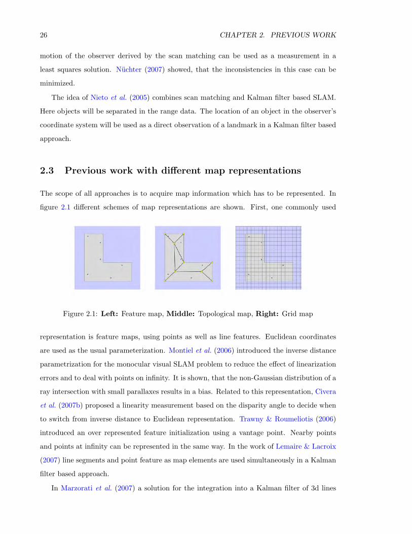
The scope of all approaches is to acquire map information which has to be represented. In
figure 2.1 different schemes of map representations are shown. First, one commonly used
Figure 2.1: Left: Feature map, Middle: Topological map, Right: Grid map
representation is feature maps, using points as well as line features. Euclidean coordinates
are used as the usual parameterization. Montiel et al. (2006) introduced the inverse distance
parametrization for the monocular visual SLAM problem to reduce the effect of linearization
errors and to deal with points on infinity. It is shown, that the non-Gaussian distribution of a
ray intersection with small parallaxes results in a bias. Related to this representation, Civera
et al. (2007b) proposed a linearity measurement based on the disparity angle to decide when
to switch from inverse distance to Euclidean representation. Trawny & Roumeliotis (2006)
introduced an over represented feature initialization using a vantage point. Nearby points
and points at infinity can be represented in the same way. In the work of Lemaire & Lacroix
(2007) line segments and point feature as map elements are used simultaneously in a Kalman
filter based approach.
In Marzorati et al. (2007) a solution for the integration into a Kalman filter of 3d lines
2.4. PREVIOUS WORK WITH DIFFERENT AMBIANCES 27
and points acquired by a stereo camera system is described. The model is generated using
homogeneous representations of geometric entities. Rodrıguez-Losada et al. (2006) introduced
a sub-map representation in an Kalman filter. For every new set of features its own reference
coordinate system is defined. The actual location of the observer can also be transformed to
this coordinate system. One positive effect is the reduction of the linearizion error, but it
increases the computational costs.
Second, topological maps are typically used if the environment can be separated into
distinct locations. In Kuipers et al. (2000) the connections between spacial semantic and
localization and mapping using autonomous systems is outlined. The topological map rep-
resented by a Voronoi graph is introduced in Choset & Nagatani (2001), which also encodes
metric information about the environment. The key feature of this approach is to construct
the graph incrementally using a set of basic control laws. Another example using a topolog-
ical graph representation has been shown by Folkesson & Christensen (2004). The approach
is able to impose global constraints (e. g. loop closing) and to represent inconsistencies using
an energy term of the graph nodes.
Third, grid maps can be used to represent map information. Most of these implemen-
tations are limited to 2d environments, for example Howard & Kitchen (1997), Montemerlo
& Thrun (2003), Eliazar & Parr (2004), where the grid cells are signed as occluded or not
occluded. Grisetti et al. (2006) for example extends the grid map approach using particles
associated with a probability for the map occlusion. Using an elevation grid map based ap-
proach is outlined in Pfaff et al. (2007). Also a dimension extension to 3d grid maps (voxel
maps) will be feasible, e. g. Yu & Zhang (2006) and Zask & Dailey (2009). Grid maps in
general are limited in their accuracy depending on the chosen grid resolution, which will be
a trade-off between memory usage and sensor accuracy.
2.4 Previous work with different ambiances
Different kinds of solution can be separated into different ambiances. Very popular are
systems for indoor environments, such as Davison (2003) using a single camera approach,
Harati et al. (2007) using laser scans or Tardos et al. (2002) using sonar measurements.
In an outdoor environment most systems focus on safe navigation to autonomous vehicles,
e. g. Holz et al. (2008), Nuchter et al. (2006). Particularly detecting dynamical objects is
28 CHAPTER 2. PREVIOUS WORK
one of the major problems Liao et al. (2003). The localization and mapping problem can be
simplified using GPS.
Using unmanned aerial vehicles as a sensor platform in any kind of altitude becomes
more and more affordable. Kim & Sukkarieh (2006) described an airborne platform with
range, bearing and inertial sensors. A single camera system combined with GPS and inertial
sensors was used in Sunderhauf et al. (2007) to demonstrate the capability of the sigma point
Kalman Filter with inverse distance parametrization in the context of autonomous airships.
Also Schlaile et al. (2006) presented a vision based framework for small unmanned aerial
vehicles in indoor environments. Visual data can be used to achieve odometer information
of a UAV proposed by Ollero et al. (2004) and Benıtez et al. (2005). In case of stratospheric
UAV system, e. g. Everaerts et al. (2004), the mapping task will be simplified into a 2d map
problem.
Sonar sensors makes it possible to perform the localization and mapping problem for
autonomous underwater vehicles (AUV), e. g. P. M. Newman & Rikoski (2003), Fairfield
et al. (2006) and Ribas et al. (2008).
Extra-planetary missions will be the most spectacular environment for the simultaneous
localization and mapping task. Primarily camera sensors will be used, because of its hardware
robustness, lightweight construction and high information gain, e. g. Se et al. (2005). Future
missions will also incorporate satellite images. For instance Li et al. (2005) propose a network
vision system using ground image series and satellite images. The challenge is a robust, fully
autonomous system for outdoor environments, which do not have any access to a global
positioning system.
2.5 Previous work for large scenes
All presented approaches in the previous sections are very suitable in small areas. In case
of large maps Kalman filter based algorithms shows inconsistencies between the estimated
uncertainties and the parameters and becomes instable in terms of its numerical stability.
Castellanos et al. (2004) investigated the inconsistency of a Kalman filter approach versus a
local map joining. They introduced a robocentric mapping approach, where the world coor-
dinate system is defined by the observer. It is shown, that a map-consistency improvement
for this approach can be obtained. The reason is, that higher order terms of the linearization
2.5. PREVIOUS WORK FOR LARGE SCENES 29
becomes smaller due to the robocentric coordinate system. Also Bailey et al. (2006) ana-
lyzed the consistency of Kalman filter based methods for large loops. It is pointed out, that
the angular uncertainty of measurements has the overall influence to the divergence of the
Kalman filter approaches. In J. A. Castellanos & Tardos (1999) a framework is introduced
to deal with uncertain geometric symmetry of segments (e. g. walls) using a Kalman filter
method. It is shown that symmetry information improves significantly the consistency of the
filter.
Simultaneous localization and mapping for large scenes typically can be solved by a hier-
archical mapping. Small local maps with high inner accuracy and consistency can be joined.
In case of an unmanned aerial vehicle, classical algorithms using image pair geometry can
be used to obtain an independent photogrammetric model. These local maps can be joined
to make large maps as shown in Kanade et al. (2004). Clemente et al. (2007) also used a
hierarchical map approach. For obtaining independent local maps with a Kalman filter based
approach with inverse distance map representation, an overall transformation of the gener-
ated local maps will be computed to yield an optimal solution, if a loop closing is detected.
Paz et al. (2007) proposed a technique to join local independent maps at fixed intervals using
a binary tree to reduce the complexity of joining the maps. Martinez-Cantin & Castellanos
(2005) showed implementation details on the integration of the sigma point Kalman filter to
the SLAM problem and introduced an innovation-based consistency checking for large scale
outdoor navigation using a 2d laser range sensor. In Estrada et al. (2005) an example for
combining several local maps under the loop closing constraint is shown. All local maps are
adjusted, but the inner precision of every local map does not change. Blanco et al. (2007)
also introduce a hierarchical SLAM approach to combine small local maps with a superior
Bayesian network. Sub-maps are computed by the FAST-SLAM algorithm. Guivant et al.
(2004) introduce a new hybrid map representation. The global map is partitioned in Lo-
cal Triangular Regions (LTR) based on selected landmarks, which defines independent skew
symmetric coordinate systems. The observer’s location is embedded in this system. The
observed landmarks therefore can be updated using separated Kalman filter.
In this chapter we specified the meaning of localization, mapping and its joint problem as
a time dependent process. As outlined, the goal of a simultaneous localization and mapping
approach is to estimate the full posterior distribution of an observers location and its environ-

30 CHAPTER 2. PREVIOUS WORK
ment. In a review part we gave a broad overview about different solutions distinguishable by
the parameter estimation technique, map representation and used sensor systems. It can be
observed that existing approaches score well for different kinds of ambiances in small areas.
However, building larger maps still seems to be challenging.
Chapter 3
Background theory
3.1 Geometric entities and transformations
In this section we will present the construction and relationship of geometric entities and
basic coordinate transformation techniques. We will briefly describe the representation of
rotations, the extension to motions and homographies as a general coordinate transformation
in the 3d space. Using homogeneous coordinates we are able to formulate rotations, motions
as well as homographies as linear transformation in a 2- and 3-dimensional projective space.
For a broad introduction to homogeneous coordinates, its transformations and its historical
background please refer to Heuel (2004). For an interpretation of the different writing styles
of variables please refer to the notation definition.
3.1.1 Geometric entities
In this section we will present the fundamentals of algebraic projective geometry which we
use in this dissertation. In a first step we introduce homogeneous coordinates to represent
points and lines in the 2-dimensional space. Secondly, we present the extension to tree-
dimensional space using points, planes and lines followed by construction1 elements and
incidence contradictions.
1The construction of an element from two elements will be indicated by the operator ∧ and the intersection
of two elements by ∩.
31
32 CHAPTER 3. BACKGROUND THEORY
3.1.1.1 Points and lines in the 2d space
Homogeneous coordinates in general are invariant with respect to multiplication by a scalar
factor λ 6= 0. Every Euclidean coordinate x = [x, y]T can be represented as a homogeneous
vector
x =
x0
xh
=
u
v
w
. (3.1)
Normalizing the homogeneous vector by dividing x by w, than x0 represents the Euclidean
part of x. All points [u, v, w]T 6= 0 build the so called projective plane consisting of all points
[x, y]T of the Euclidean plane together with the points at infinity [u, v, 0]T.
Every line in in R2 can be represented in Hessian normal form
x cosφ+ y sinφ− d = 0 (3.2)
and has the homogeneous coordinate vector
l =
lhl0
=
a
b
c
=√a2 + b2
cosφ
sinφ
−d
(3.3)
as long as√a2 + b2 6= 0. Every line with the same coordinates as a point up to an arbitrary
factor λ 6= 0 is called the dual element of the point. The line at infinity is [0, 0, 1]T.
3.1.1.2 Points, planes and lines in the 3d space
In the 3-dimensional space a point X = [X,Y, Z]T can be represented similar to the two-
dimensional space by
X =
X0
Xh
=
U
V
W
T
. (3.4)
The dual element of a 3d point in homogeneous coordinates is a plane. From the implicit
plane representation
AX +BY + CZ +D = 0 (3.5)
3.1. GEOMETRIC ENTITIES AND TRANSFORMATIONS 33
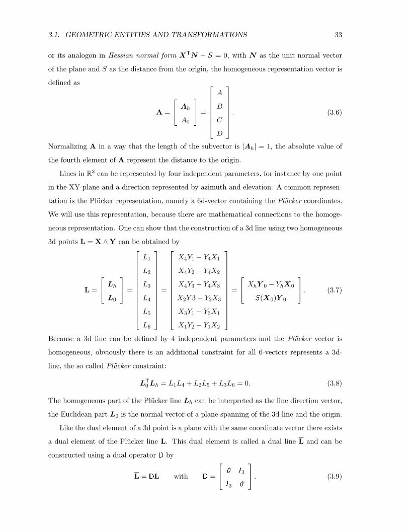
or its analogon in Hessian normal form XTN − S = 0, with N as the unit normal vector
of the plane and S as the distance from the origin, the homogeneous representation vector is
defined as
A =
Ah
A0
=
A
B
C
D
. (3.6)
Normalizing A in a way that the length of the subvector is |Ah| = 1, the absolute value of
the fourth element of A represent the distance to the origin.
Lines in R3 can be represented by four independent parameters, for instance by one point
in the XY-plane and a direction represented by azimuth and elevation. A common represen-
tation is the Plucker representation, namely a 6d-vector containing the Plucker coordinates.
We will use this representation, because there are mathematical connections to the homoge-
neous representation. One can show that the construction of a 3d line using two homogeneous
3d points L = X ∧Y can be obtained by
L =
LhL0
=
L1
L2
L3
L4
L5
L6
=
X4Y1 − Y4X1
X4Y2 − Y4X2
X4Y3 − Y4X3
X2Y 3− Y2X3
X3Y1 − Y3X1
X1Y2 − Y1X2
=
XhY 0 − YhX0
S(X0)Y 0
. (3.7)
Because a 3d line can be defined by 4 independent parameters and the Plucker vector is
homogeneous, obviously there is an additional constraint for all 6-vectors represents a 3d-
line, the so called Plucker constraint:
LT0Lh = L1L4 + L2L5 + L3L6 = 0. (3.8)
The homogeneous part of the Plucker line Lh can be interpreted as the line direction vector,
the Euclidean part L0 is the normal vector of a plane spanning of the 3d line and the origin.
Like the dual element of a 3d point is a plane with the same coordinate vector there exists
a dual element of the Plucker line L. This dual element is called a dual line L and can be
constructed using a dual operator D by
L = DL with D =
0 I 3
I 3 0
. (3.9)
34 CHAPTER 3. BACKGROUND THEORY
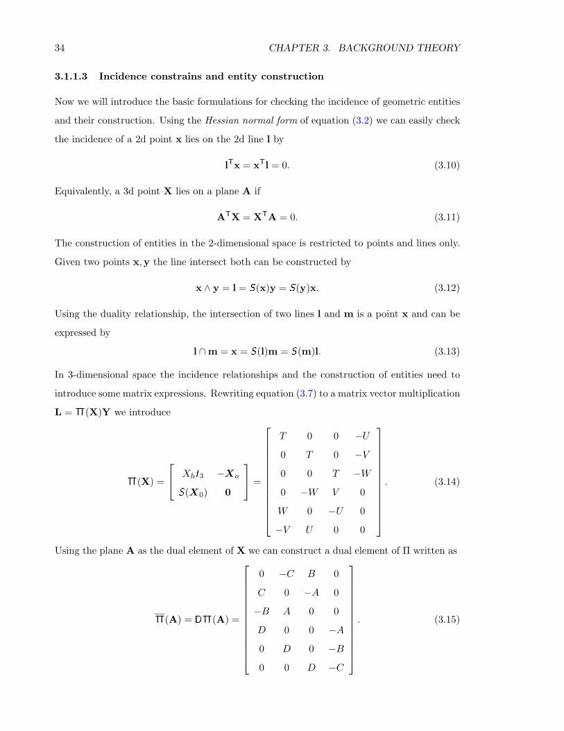
3.1.1.3 Incidence constrains and entity construction
Now we will introduce the basic formulations for checking the incidence of geometric entities
and their construction. Using the Hessian normal form of equation (3.2) we can easily check
the incidence of a 2d point x lies on the 2d line l by
lTx = xTl = 0. (3.10)
Equivalently, a 3d point X lies on a plane A if
ATX = XTA = 0. (3.11)
The construction of entities in the 2-dimensional space is restricted to points and lines only.
Given two points x,y the line intersect both can be constructed by
x ∧ y = l = S(x)y = S(y)x. (3.12)
Using the duality relationship, the intersection of two lines l and m is a point x and can be
expressed by
l ∩m = x = S(l)m = S(m)l. (3.13)
In 3-dimensional space the incidence relationships and the construction of entities need to
introduce some matrix expressions. Rewriting equation (3.7) to a matrix vector multiplication
L = I I (X)Y we introduce
I I (X) =
XhI 3 −Xo
S(X0) 0
=
T 0 0 −U
0 T 0 −V
0 0 T −W
0 −W V 0
W 0 −U 0
−V U 0 0
. (3.14)
Using the plane A as the dual element of X we can construct a dual element of Π written as
I I (A) = D I I (A) =
0 −C B 0
C 0 −A 0
−B A 0 0
D 0 0 −A
0 D 0 −B
0 0 D −C
. (3.15)
3.1. GEOMETRIC ENTITIES AND TRANSFORMATIONS 35
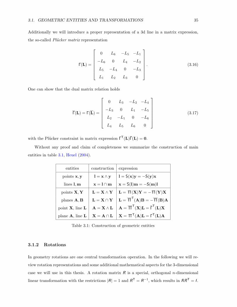
Additionally we will introduce a proper representation of a 3d line in a matrix expression,
the so-called Plucker matrix representation
I (L) =
0 L6 −L5 −L1
−L6 0 L4 −L2
L5 −L4 0 −L3
L1 L2 L3 0
. (3.16)
One can show that the dual matrix relation holds
I (L) = I (L) =
0 L3 −L2 −L4
−L3 0 L1 −L5
L2 −L1 0 −L6
L4 L5 L6 0
(3.17)
with the Plucker constraint in matrix expression I T(L)I (L) = 0.
Without any proof and claim of completeness we summarize the construction of main
entities in table 3.1, Heuel (2004).
entities construction expression
points x,y l = x ∧ y l = S(x)y = −S(y)x
lines l,m x = l ∩m x = S(l)m = −S(m)l
points X,Y L = X ∧Y L = I I (X)Y = − I I (Y)X
planes A,B L = X ∩Y L = I IT(A)B = − I I (B)A
point X, line L A = X ∧ L A = I IT(X)L = I
T(L)X
plane A, line L X = A ∩ L X = I I T(A)L = I T(L)A
Table 3.1: Construction of geometric entities
3.1.2 Rotations
In geometry rotations are one central transformation operation. In the following we will re-
view rotation representations and some additional mathematical aspects for the 3-dimensional
case we will use in this thesis. A rotation matrix R is a special, orthogonal n-dimensional
linear transformation with the restrictions |R| = 1 and RT = R
−1, which results in RRT = I .
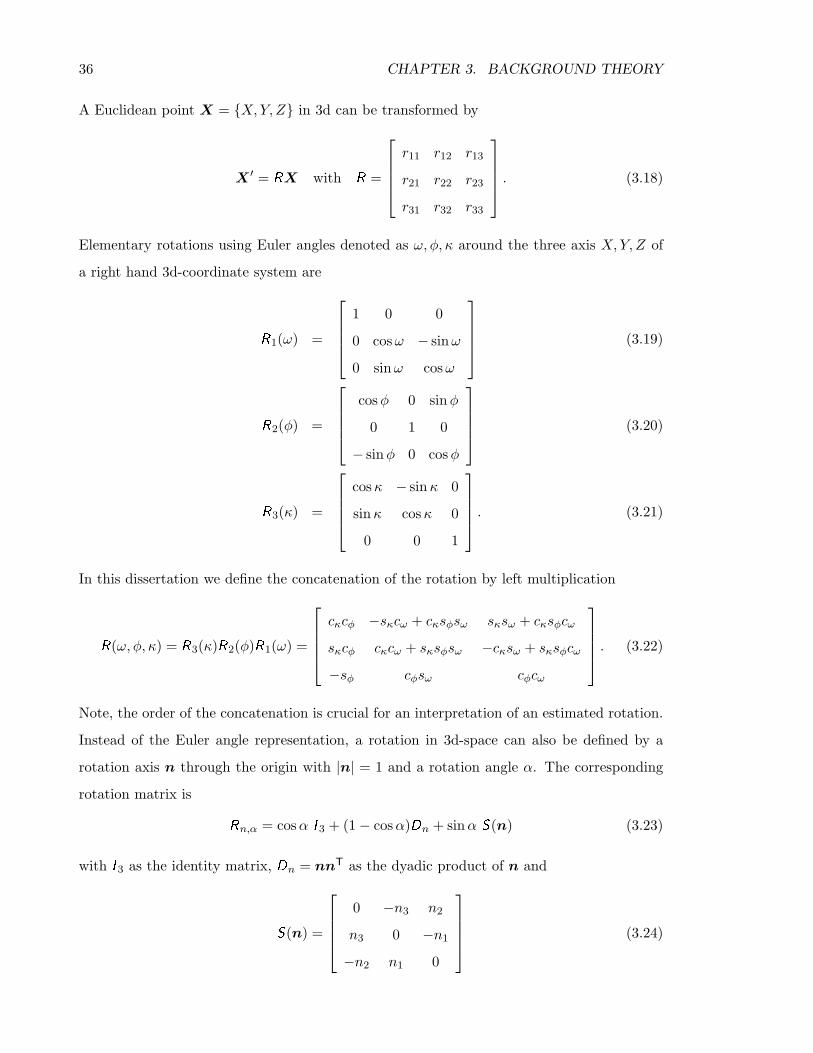
36 CHAPTER 3. BACKGROUND THEORY
A Euclidean point X = X,Y, Z in 3d can be transformed by
X ′ = RX with R =
r11 r12 r13
r21 r22 r23
r31 r32 r33
. (3.18)
Elementary rotations using Euler angles denoted as ω, φ, κ around the three axis X,Y, Z of
a right hand 3d-coordinate system are
R1(ω) =
1 0 0
0 cosω − sinω
0 sinω cosω
(3.19)
R2(φ) =
cosφ 0 sinφ
0 1 0
− sinφ 0 cosφ
(3.20)
R3(κ) =
cosκ − sinκ 0
sinκ cosκ 0
0 0 1
. (3.21)
In this dissertation we define the concatenation of the rotation by left multiplication
R(ω, φ, κ) = R3(κ)R2(φ)R1(ω) =
cκcφ −sκcω + cκsφsω sκsω + cκsφcω
sκcφ cκcω + sκsφsω −cκsω + sκsφcω
−sφ cφsω cφcω
. (3.22)
Note, the order of the concatenation is crucial for an interpretation of an estimated rotation.
Instead of the Euler angle representation, a rotation in 3d-space can also be defined by a
rotation axis n through the origin with |n| = 1 and a rotation angle α. The corresponding
rotation matrix is
Rn,α = cosα I 3 + (1− cosα)Dn + sinα S(n) (3.23)
with I 3 as the identity matrix, Dn = nnT as the dyadic product of n and
S(n) =
0 −n3 n2
n3 0 −n1
−n2 n1 0
(3.24)
3.1. GEOMETRIC ENTITIES AND TRANSFORMATIONS 37
as the skew-symmetric matrix of n. From a given rotation matrix we can compute the angle
and rotation vector in the following way. Given the vector a from the elements of R
a = −
r23 − r32
r31 − r13
r12 − r21
(3.25)
the rotation angle is given by
α = atan2 (|a|, tr(R)− 1) (3.26)
and the rotation vector n by
n =a
|a|if |a| 6= 0. (3.27)
Rotations represented by Euler angle as well as axis and angle require trigonometric functions
which may be a disadvantage. The quaternion representation introduced by W. R. Hamilton
is closely related to the axis and angle representation, but there is no need for trigonometric
terms. Quaternions are also closely related to complex numbers and they define their own
algebra. Furthermore the quaternion representation for rotations is unique except for a sign
and shows no singularities. A quaternion consists of a scalar part q = q0 and a vector part
q = q1, q2, q3. We can write a quaternion as a 4-vector
q =
q
q
=
q0
q1
q2
q3
. (3.28)
The corresponding rotation matrix can be computed by
R(q) =1
q20 + q2
1 + q22 + q2
3
q2
0 + q21 − q2
2 − q23 2(q1q2 − q0q3) 2(q1q3 + q0q2)
2(q2q1 + q0q3) q20 − q2
1 + q22 − q2
3 2(q2q3 − q0q1)
2(q3q1 − q0q2) 2(q3q2 + q0q1) q20 − q2
1 − q22 + q2
3
.(3.29)
We observe, that R(q) is invariant with respect to a multiplication of q with a scalar 6= 0.
It can be shown, that the vector part q is parallel to the rotation axis n. Using the unit
quaternion |q| = 1 the relationship between quaternions and the axis-angle representation is
defined by
q =
cos α2sin α
2n
. (3.30)
38 CHAPTER 3. BACKGROUND THEORY
We can easily derive the concatenation of two rotations q and r represented by quaternion
as a quaternion multiplication p = qr defined as the matrix vector multiplication
p = qr = Υ(q)r = Υ(r)q (3.31)
with the 4× 4 matrix
Υ(q) =
q0 −q1 −q2 −q3
q1 q0 −q3 q2
q2 q3 q0 −q1
q3 −q2 q1 q0
(3.32)
and
Υ(r) =
r0 −r1 −r2 −r3
r1 r0 r3 −r2
r2 −r3 r0 r1
r3 r2 −r1 r0
. (3.33)
In case of |q| = 1 the inverse element of q is defined by
q−1 =
q
−q
Υq−1 = Υ−1q (3.34)
or as matrix-vector multiplication
q−1 = Vq with V =
1 0
0T −I 3
. (3.35)
For a small rotation qk which depends on k concatenations of a small rotation q around the
same axis a sufficient approximation can be obtained by
qk ≈
1
kq
(3.36)
or written as matrix vector product
qk ≈ Ukq with Uk =
1 0
0T kI 3
. (3.37)
This approximation is very useful for the representation of small angular velocities and ac-
celerations we will use in chapter 4.
In the following we will show for the special case of small circular motions, that the
quaternion concatenation can be used to obtain a rotation from angular velocity. First, lets
3.1. GEOMETRIC ENTITIES AND TRANSFORMATIONS 39
assume an angle α is a function of time t depends on an initial angle α0 and an angular
velocity α, so
αt = α0 + αt. (3.38)
Substitute αt into the unit quaternion representation in equation (3.30) we get
q(t) =
cos(α0+αt2 )
sin(α0+αt2 )n
(3.39)
as the quaternion as a function of time. Using the theorems
cos(x+ y) = cos(x) cos(y)− sin(x) sin(y) (3.40)
sin(x+ y) = sin(x) cos(y) + cos(x) sin(y) (3.41)
and reformulate equation (3.39) we get
q(t) =
cos(α02 ) cos( αt2 )− sin(α0
2 ) sin( αt2 )(sin(α0
2 ) cos( αt2 ) + cos(α02 ) sin( αt2 )
)n
. (3.42)
Evaluate (3.42) at t0 = 0 and α0 = 0 and approximate sin( αt2 ) ≈ αt2 and cos( αt2 ) ≈ 1 we get
q(t) =
1
( αt2 )n
=
1
( α2n)t
, (3.43)
which can be expressed using equations (3.36) and (3.37) with k = t and q = α2n. A
derivation using a Taylor expansion and incorporation of acceleration can be found in the
appendix in section A.1.
3.1.3 Motions and homographies
In many geometric tasks linear transformations are necessary. The projective transformation,
also known as a homography, can be applied to a homogeneous point as a 4×4 matrix multi-
plication with 15 degrees of freedom. As the homography H is homogeneous, a normalization
with respect to the last element is useful.
X′ = HX→
X
Y
Z
1
′
=
a b c d
e f g h
i j k l
m n o 1
X
Y
Z
1
. (3.44)
40 CHAPTER 3. BACKGROUND THEORY
This general linear transformation can be specialized to the motion of coordinate systems.
In the Euclidean 3d space a motion is defined by a rotation R and a translation T of a
3-dimensional point X
X ′ = RX + T (3.45)
and its inversion
X = RT(X − T ). (3.46)
Using homogeneous coordinates for the point X = [X,Y, Z, 1]T we can rewrite the motion in
(3.45) to a linear mapping using a matrix vector multiplication
X′ = MX (3.47)
with the homogeneous motion matrix
M =
R T
0T 1
. (3.48)
From equation (3.46) we can show that the inversion of the motion can be computed by
M−1 =
RT −RTT
0T 1
(3.49)
and so is MM−1 = I 4. We are able to concatenate motion similar to rotations.
Example: As an example for the concatenation of motions we will rotate a point-cloud
Xi around its centroid Tc. First we translate the centroid to the origin, rotate the point-cloud
and translate back by using the motion matrix
M = MTcMRM−1Tc
=
I 3 T c
0T 1
R 0
0T 1
I 3 −T c
0T 1
=
R −RT c + T c
0T 1
.(3.50)
A second specialization is the 7-parameter Helmert-transformation (similarity transforma-
tion) as a concatenation of a motion and a scale factor. This restricted homography can be
derived by the following concatenation:
H = HsMRMT =
λI 3 0
0T 1
RT 0
0T 1
I 3 −T
0T 1
. (3.51)
3.2. BASIC IMAGE GEOMETRY 41
In the same manner also a 3d affine transformation with 12 degrees of freedom can be repre-
sented. The rotation, motion and the homography can also be applied to 2d space coordinates
by canceling the third row and column of the transformation matrices. As an example the
2d affine transformation can be represented by a matrix multiplication as a concatenation of
base transformations, namely a translation Ht, a rotation Hr, a scaling Hs with individual
scales for both vector components and an unsymmetric shearing Hsh
x′ = Hx = HtHrHsHshx =
a b c
d e f
0 0 1
x. (3.52)
For an overview of possible transformations have a look to McGlone et al. (2004) page 143ff.
Rotations in the 2d space are embedded in the 3d space as a rotation only around the Z-Axis
using equation (3.21).
3.2 Basic image geometry
In this section we will briefly introduce the basic issues that deal with images. The term
image will be used in a broad context. Usually an image is a mapping of the 3d world to a 2d
image using a camera. There are numbers of real world camera with different constructions
and projection principles Sturm et al. (2006). In this work we will assume cameras with a
single projection center and a perspective projection. However, for every kind of cameras
given an image point x′ it is possible to reconstruct at least one projection ray, which is a 3d
line L(x′) from an object point to an arbitrary projection center given by a measured image
point x′. This principle allows to assign the geometry reconstruction principle in this work
to all different kinds of camera models.
3.2.1 The geometry of the single image
In general, we distinguish between the interior and exterior orientation of a camera. The
interior orientation describes the transformation of an image point x′ to the projection ray
in a fixed camera coordinate system cS and vice versa, the exterior orientation describes the
location of the camera system cS in a world system wS.
The exterior orientation can be represented by the position and angular orientation of
the camera. The interior orientation of perspective cameras can be modeled using an affine
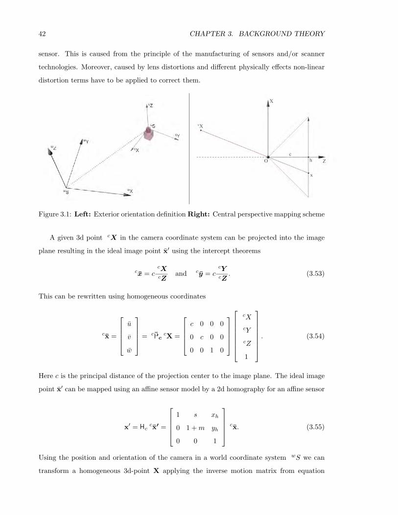
42 CHAPTER 3. BACKGROUND THEORY
sensor. This is caused from the principle of the manufacturing of sensors and/or scanner
technologies. Moreover, caused by lens distortions and different physically effects non-linear
distortion terms have to be applied to correct them.
Figure 3.1: Left: Exterior orientation definition Right: Central perspective mapping scheme
A given 3d point cX in the camera coordinate system can be projected into the image
plane resulting in the ideal image point x′ using the intercept theorems
cx = ccXcZ
and cy = ccYcZ
. (3.53)
This can be rewritten using homogeneous coordinates
cx =
u
v
w
= cPc
cX =
c 0 0 0
0 c 0 0
0 0 1 0
cX
cY
cZ
1
. (3.54)
Here c is the principal distance of the projection center to the image plane. The ideal image
point x′ can be mapped using an affine sensor model by a 2d homography for an affine sensor
x′ = Hccx′ =
1 s xh
0 1 +m yh
0 0 1
cx. (3.55)
Using the position and orientation of the camera in a world coordinate system wS we can
transform a homogeneous 3d-point X applying the inverse motion matrix from equation
3.2. BASIC IMAGE GEOMETRY 43
(3.48). We obtain a point cX in the camera system by
cX = cMX =
RT −RTT
0T 1
X1
. (3.56)
Combining the equations (3.54), (3.55) and (3.56) and substituting the commonly named
calibration matrix
K =
c sc xh
0 (1 +m)c yh
0 0 1
(3.57)
we get the projection of a 3d point in a world coordinate system to the image plane by
x′ = PX = KRT[I 3 | −T ]X. (3.58)
The Euclidean coordinates of the image point can be derived by normalizing x′. Assuming
zero shear and scale differences we get the collinearity equations
x′ = cr11(X −XT ) + r21(Y − YT ) + r31(Z − ZT )r13(X −XT ) + r23(Y − YT ) + r33(Z − ZT )
+ xh (3.59)
y′ = cr12(X −XT ) + r22(Y − YT ) + r32(Z − ZT )r13(X −XT ) + r23(Y − Y v) + r33(Z − ZT )
+ yh (3.60)
with T = [XT , YT , ZT ]T as the camera projection center and rij are the entries in R. We can
see from equation (3.54) that the projection is not invertible, because we lose the information
about the depth of the object point. Splitting the projection matrix into two parts
P = [H∞|h] = [KRT | −KRTT ] (3.61)
as H∞ map points at the plane of infinity into the image plane, we can derive the direction
to a projected object point in the camera system by
d = H−1∞ x′. (3.62)
Assuming a distance d to the object points X we can calculate its location by
X = dd|d|
+ T . (3.63)
So far, from the principle of linear transformations the camera model is straight-line-preserving.
Real cameras are not straight line preserving, due to several physical influences such as lens
distortions or refraction. In the literature different non-linear distortion models are available.
44 CHAPTER 3. BACKGROUND THEORY
For a overview please c. f. Abraham (1999). A general way to represent all these models
is by using a distortion lockup-table. This means, for every real image point x′ exists a
distortion vector to get the straight-line-preserving image point coordinate and vice versa.
The distortion lookup-table can be obtained in a camera calibration process. A measured
Euclidean image point xm can be corrected by
x′ = xm + ∆x(xm) (3.64)
to get image coordinates following the model above. Typically, for non-integer coordinates
the distortion are interpolated.
3.2.2 The geometry of the image pair
In this section we introduce the basic concept for 3d geometry retrieval from two images. For
a general introduction we refer to Hartley & Zisserman (2000).
In general the two cameras have different exterior and interior orientations. In the fol-
lowing we assume to know the interior orientation of the cameras, which can be obtained by
a previous calibration Abraham (1999). The proposed approaches are useful for consistency
checks of automatic feature measurements which we will use in subsequent algorithms.
Forward intersection Knowing the interior and exterior orientation of at least two cam-
eras given by their projection matrices P we can derive the 3d point coordinate as the in-
tersection of the projection rays from corresponding image measurements x in both images.
This can be formulated in an equation system as follows:
The incidence of the projected point X can be implicitly rewritten as
S(x)PX = 0. (3.65)
Using two rows2 of (3.65) for two cameras and stack them to S(x′)P′
S(x′′)P′′
︸ ︷︷ ︸
A4×4
X != 0 (3.66)
we can derive X as an approximate solution of (3.66) using for instance the singular value
decomposition as a method of an equation solver. With more cameras two additional lines
can be added to A for each additional ray.2Only two rows of equation (3.65) are independent.
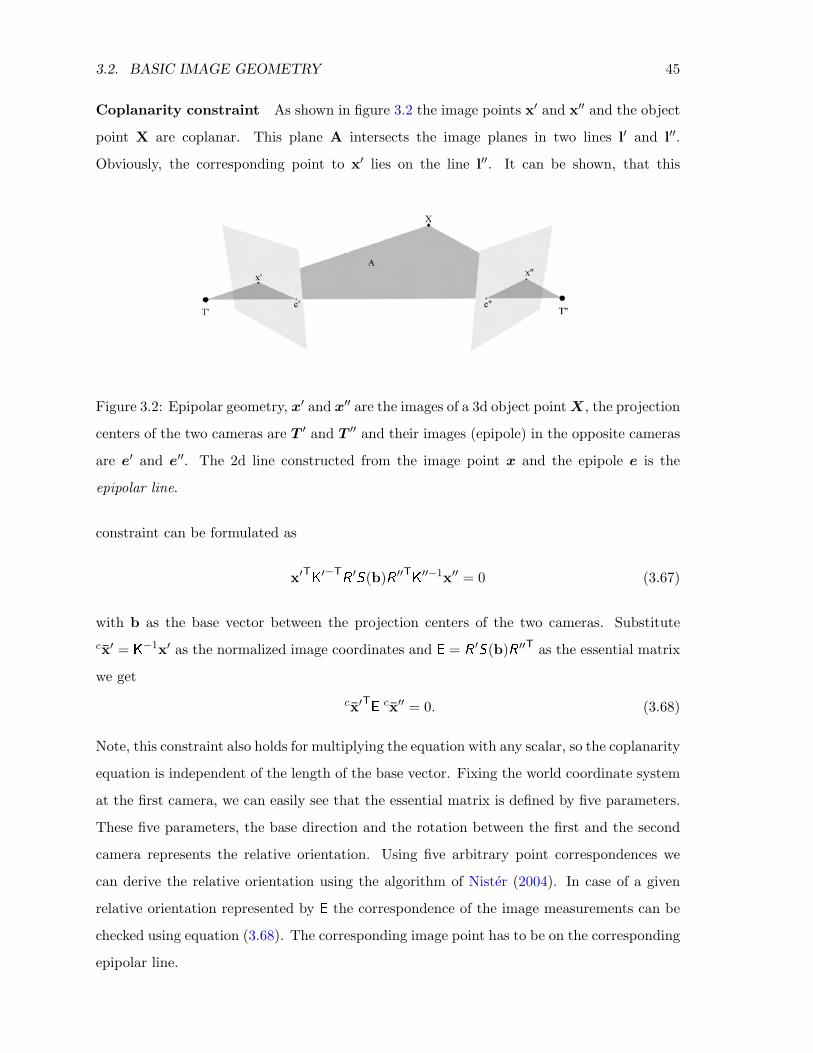
3.2. BASIC IMAGE GEOMETRY 45
Coplanarity constraint As shown in figure 3.2 the image points x′ and x′′ and the object
point X are coplanar. This plane A intersects the image planes in two lines l′ and l′′.
Obviously, the corresponding point to x′ lies on the line l′′. It can be shown, that this
Figure 3.2: Epipolar geometry, x′ and x′′ are the images of a 3d object pointX, the projection
centers of the two cameras are T ′ and T ′′ and their images (epipole) in the opposite cameras
are e′ and e′′. The 2d line constructed from the image point x and the epipole e is the
epipolar line.
constraint can be formulated as
x′TK′−TR′S(b)R ′′TK′′−1x′′ = 0 (3.67)
with b as the base vector between the projection centers of the two cameras. Substitutecx′ = K
−1x′ as the normalized image coordinates and E = R′S(b)R ′′T as the essential matrix
we get
cx′TE cx′′ = 0. (3.68)
Note, this constraint also holds for multiplying the equation with any scalar, so the coplanarity
equation is independent of the length of the base vector. Fixing the world coordinate system
at the first camera, we can easily see that the essential matrix is defined by five parameters.
These five parameters, the base direction and the rotation between the first and the second
camera represents the relative orientation. Using five arbitrary point correspondences we
can derive the relative orientation using the algorithm of Nister (2004). In case of a given
relative orientation represented by E the correspondence of the image measurements can be
checked using equation (3.68). The corresponding image point has to be on the corresponding
epipolar line.
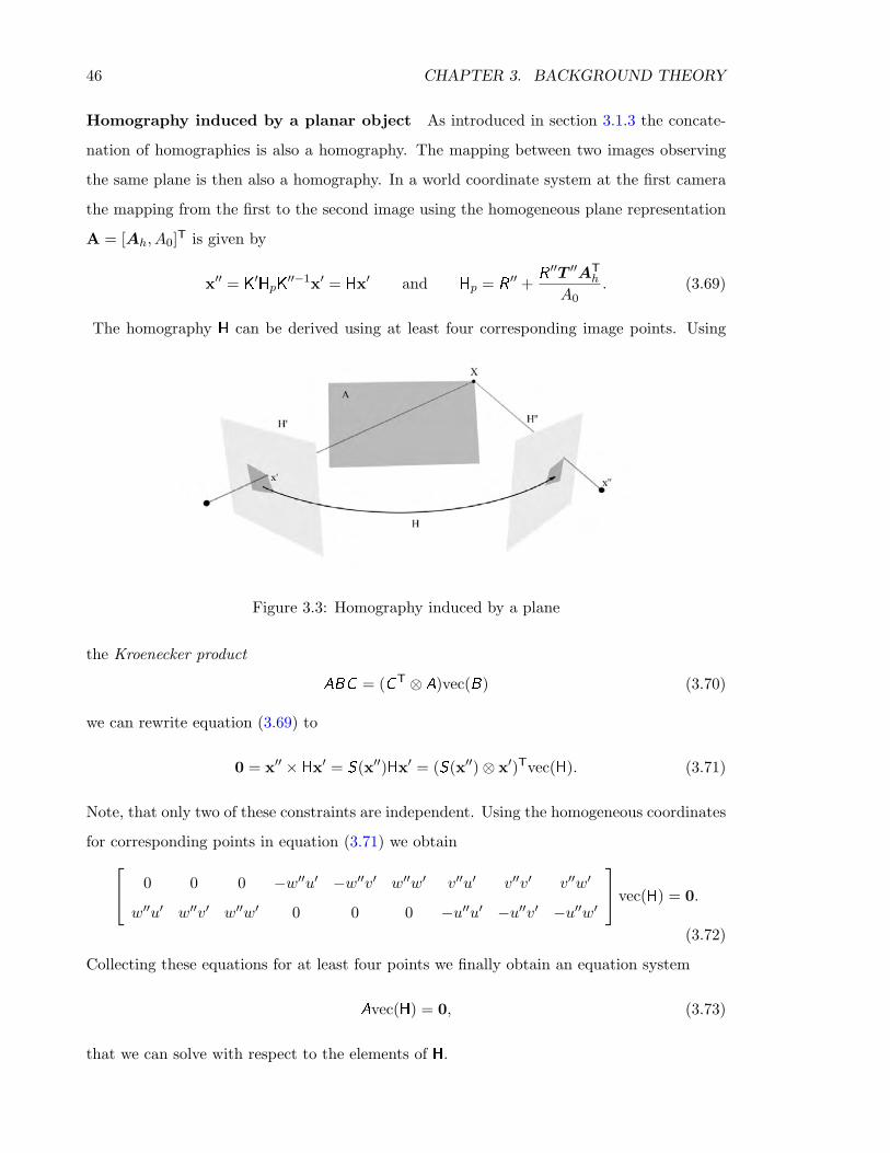
46 CHAPTER 3. BACKGROUND THEORY
Homography induced by a planar object As introduced in section 3.1.3 the concate-
nation of homographies is also a homography. The mapping between two images observing
the same plane is then also a homography. In a world coordinate system at the first camera
the mapping from the first to the second image using the homogeneous plane representation
A = [Ah, A0]T is given by
x′′ = K′HpK
′′−1x′ = Hx′ and Hp = R′′ +
R′′T ′′AT
h
A0. (3.69)
The homography H can be derived using at least four corresponding image points. Using
Figure 3.3: Homography induced by a plane
the Kroenecker product
ABC = (CT ⊗ A)vec(B) (3.70)
we can rewrite equation (3.69) to
0 = x′′ × Hx′ = S(x′′)Hx′ = (S(x′′)⊗ x′)Tvec(H). (3.71)
Note, that only two of these constraints are independent. Using the homogeneous coordinates
for corresponding points in equation (3.71) we obtain 0 0 0 −w′′u′ −w′′v′ w′′w′ v′′u′ v′′v′ v′′w′
w′′u′ w′′v′ w′′w′ 0 0 0 −u′′u′ −u′′v′ −u′′w′
vec(H) = 0.
(3.72)
Collecting these equations for at least four points we finally obtain an equation system
Avec(H) = 0, (3.73)
that we can solve with respect to the elements of H.
3.3. LEAST SQUARES 47
The proposed algorithms starting from equation (3.66) assume independent and equal
measurement accuracy. Here we neglected statistical conditions, which can be easily intro-
duced by weights for the observations. The accuracy of the obtained parameters can be
derived using error propagation. Furthermore, the extension for the case of image blocks
is possible. To consider the different uncertainty of observations and achieve multi-image
integration we propose a least square solution, which will be introduced in the next section.
3.3 Least squares
Finding a set of parameters of a model given a set of observations is known as an optimiza-
tion problem. To do this, the least square method is a very effective numerical method.
The proposed algorithms are embedded in the broad context of probability theory. For lin-
ear relationships of Gaussian distributed observations and unknown parameters, the least
squares method leads to best unbiased estimators. In the physical world, measurements can
well be approximated by Gaussian distributions. Because least square methods approximate
probability density function by Gaussian distributions, least squares methods becomes very
popular.
In this section we will derive various forms of functional models. This derivation follows
the concept of specialization of a universal form to specific specializations. These derivations
can be found in several publications, for instance Mikhail & Ackermann (1976), Koch (1988),
Niemeier (2001) or Forstner & Wrobel (2004). Our motivation to derive these algorithms
again lies in a novel derivation of recursive least square estimation in the subsequent section.
Furthermore we will present standard methods for outlier detection and robustification as
well as a technique for parameter reduction.
3.3.1 Least squares optimization
Optimizing linear Gauss-Helmert-model with constraints At the beginning we start
with the definition of two linear constraints
cg = Ap+ BT(z − z) (3.74)
ch = HTp (3.75)
where p of size U is the parameter vector to be optimized. The contradiction vectors cg and
ch of size G and H therefore depend on the estimated parameter vector as well as on the
48 CHAPTER 3. BACKGROUND THEORY
fitted observations z with size N . Therefore, the linear model in A has the size G×U , H has
the size U ×H and B has the size N × G. The basic concept of the least square method is
to find p by minimizing the function
Ω2 =12vTC−1zz v =
12
(z − z)C−1zz (z − z)T (3.76)
with z as the observation vector with its covariance matrix C zz and z as the estimated ob-
servation vector under the constrains in (3.74) and (3.75). To incorporate the contradictions
it is necessary that we minimize
Ω2 =12
(z − z)C−1zz (z − z)T + λT(Ap+ B
T(z − z)− cg) + µT(HTp− ch) (3.77)
by introducing the Lagrangian multipliers λ and µ. To find the minimum of this function
we set the first derivation with respect to all parameters to zero. We obtain four equations(∂Ω∂z
)T
= C−1zz v + Bλ = 0 (3.78)(
∂Ω∂p
)T
= ATλ+ Hµ = 0 (3.79)(
∂Ω∂λ
)T
= Ap+ BTv − cg = 0 (3.80)(
∂Ω∂µ
)T
= −ch + 2HTp = 0 (3.81)
Solving (3.78) with respect to the residuals v, substitute v into (3.80) and solve with respect
to λ we get
λ = (BTC zzB)−1(Ap− cg) (3.82)
and for the residuals
v = −C zzB(BTC zzB)−1(Ap− cg). (3.83)
The sub-term BTC zzB can be interpreted as a projection of the covariance of the observations
to the space of the contradictions. The inverse can only be computed if the column rank of
B is N . This is a special case of the general Gauss-Helmert model. In the following we will
assume our model guarantees full rank of the sub-term. Now, substitute λ into (3.79) and
use equation (3.81) we can arrange these two equations to the normal equation system AT(BT
C zzB)−1A H
HT
0
p
µ
=
AT(BT
C zzB)−1cg
ch
(3.84)
3.3. LEAST SQUARES 49
The inverse of the left side of the normal equation system is the theoretical covariance matrix
of the parameter vector, so N H
HT
0
−1
=
C pp S
ST
T
(3.85)
and can only be computed if the stacked matrix [ATH]T has full column rank. Substituting
the solution for p into (3.83) we can compute the variance factor
σ20 =
vTC−1zz v
G+H − U(3.86)
with G as the number of constraints, H as the number of contradictions and U as the number
of unknown parameters inside the vector p. The estimated covariance matrix for the unknown
parameters is therefore
C pp = σ20C pp (3.87)
By error propagation of (3.83) we can show, that the covariance matrix of the residuals is
C vv = C zzB(BTC zzB)−1(I − AC ppAT(BT
C zzB)−1)BTC zz (3.88)
c. f. Mikhail & Ackermann (1976) p. 197.
Optimizing Nonlinear Gauss-Helmert-Model with constraints Now let us assume
we have a nonlinear model with the nonlinear implicit contradictions and constrains according
to equations (3.74) and (3.75)
g(p, z) = 0 (3.89)
h(p) = 0 (3.90)
These equations hold for the true parameters p and observations z. Using estimated param-
eters and observations the following system holds
g(p, z) = 0 (3.91)
h(p) = 0 (3.92)
with z = z + v. Approximate these functions using a Taylor expansion on the approximate
values p0 and z0 up to the first order we get
g(p, z) ≈ g(p0, z0) + A(p− p0) + BT(z − z0) (3.93)
h(p) ≈ h(p0) + HT(p− p0) (3.94)
50 CHAPTER 3. BACKGROUND THEORY
with the Jacobians
AG×U
=∂g(p, z)∂p
∣∣∣∣p,z
(3.95)
BN×G
=∂g(p, z)T
∂z
∣∣∣∣p,z
(3.96)
HU×H
=∂h(p∂p
∣∣∣∣p
(3.97)
taken at the current approximation of p and z. Now we enlarge the third term of equation
(3.93) by z − z and we get
g(p, z) ≈ g(p0, z0) + A(p− p0) + BT(z + z − z − z0) = 0. (3.98)
Split equation (3.98) into two separated parts cg and substitute ∆p = p − p0 we define a
nonlinear contradiction
cg = −g(p0, z0) + BT(z0 − z) (3.99)
and a linear contradiction
cg = A(p− p0) + BT(z − z) = A∆p+ B
Tv. (3.100)
Note, both terms are equal if and only if the linearization point for the observation is
z0 = z and for the unknown parameters is p0 = p so
0 = A∆p = −g(p0 = p, z0 = z). (3.101)
The residuals v are equal to equation (3.83) replacing p with ∆p. Because we do not know
a-priori p and z we have to find the solution by iteration. After rewriting equation (3.94)
and using (3.100) we get the linearized normal equation system AT(BT
C zzB)−1A H
HT
0
∆p
µ
=
AT(BT
C zzB)−1cg
ch
(3.102)
with cg from equation (3.99) and
ch = −h(p0). (3.103)
In every iteration ν we update p(ν+1) = p(ν) + ∆p(ν)
and z(ν+1) = z+ v(ν). The convergence
of this iteration scheme depends on the linearity of the optimization space around the ap-
proximate values p(ν) and z(ν). Note, that this scheme does not guaranty to find the optimal
minimum, because the optimization space depends on nonlinear functions and therefore can
be non-convex. There are several methods to apparently overcome this limitation e. g. the
Levenberg-Marquardt algorithm.
3.3. LEAST SQUARES 51
Optimizing Gauss-Markov-Model with constraints Now we assume that the relation-
ship between the unknown parameters and the observations can be formulated as an explicit
function of the form z = f(p). We can always rewrite these functions to implicit functions by
subtracting z from both sides. After replacing the true values against the estimated values
we get
0 = g(p, z) = f(p)− z. (3.104)
Applying the estimation algorithm of the nonlinear Gauss-Helmert model we always get
the Jacobian B = −I . Setting the approximate value for the observations as z0 = f(p0),
substitute (3.104) and B in equations (3.102), (3.99) and (3.100) we get
cg = −(f(p0)− z0)− (z0 − z) (3.105)
= ∆z = z − z0 (3.106)
= A∆p− v (3.107)
and therefore the normal equation system is ATC−1zz A H
HT
0
∆p
µ
=
ATC−1zz ∆z
ch
. (3.108)
The residuals in equation (3.83) simplify to
v = A∆p−∆z. (3.109)
As we can see the Gauss-Markov model is a simplification of the more general Gauss-Helmert
model.
3.3.2 Outlier detection and robustification
The least square estimation schemes presented so far minimize the square residuals of the
observations. This is known to be extremely sensitive to outliers. In general we are not able
to discriminate between systematic errors and gross errors. Systematic error can be caused
by errors in the functional model or by non-modeled effects of the observation process. The
last one can be a non-Gaussian distribution of the observations or neglected correlations. To
analyze where these residuals do come from we have to distinguish between systematic and
gross errors. In the following we assume that our functional model holds and therefore no
systematic error appears. We will now show how gross errors, also called outliers, may be
52 CHAPTER 3. BACKGROUND THEORY
detected by looking at the plausibility of the computed residuals with respect to the expected
uncertainty. Outliers can be eliminated canceling the observation, or their influence on the
estimation process can be reduced.
Outlier detection by testing the residuals Following Baarda (1967) a test value tn for
uncorrelated observations in the Gauss-Markov-model can by obtained by
tn =−vnσvn
. (3.110)
If there are no gross errors in the observations tn ∼ N(0, 1) is normally distributed. The
computation of σvn can be expensive as the covariance of the parameters is required. In
the case that all observation can be assumed to have the same influence to the parameter
vector, it is suitable to use σzn instead. In various cases, groups of observations are strongly
correlated to each other but uncorrelated to the remaining observations. In this case we
cannot distinguish which of the observations in the group i causes the error, but we can test
the group itself Stefanovic (1978) with
Ti = vTi C−1vivi vi ∼ χ
2I (3.111)
where I is the size of the group i and C vivi is the regular sub-matrix of the covariance of the
residuals.
Using implicit functions in the Gauss-Helmert model we can formulate functional models,
where a number of contradiction groups depend on a set of observations. In this case we
cannot test the observation groups themselves according to equation (3.111) because of the
functionally dependent on the contradictions. Using the relation (3.100) in the convergence
point that ∆p = 0, we get
cg = BT(z − z0) = B
Tv with C cgcg = BTC viviB (3.112)
and a test value for the groups of observations composed of the contradiction relations with
Ti = cTgiC−1cgicgi
cgi ∼ χ2I . (3.113)
Corresponding groups of observations than can be determined as outliers if the test value Ti
exceeds a chosen threshold. The sub-covariance matrix C vivi can be singular and we are not
able to compute the test value. However, if we assume that all observations have the same
influence to the parameter vector, it is suitable to use C zz instead.
3.3. LEAST SQUARES 53
Influence reduction Outliers can be eliminated in the estimation process. Alternatively,
their influence on the minimization function can be reduced. This technique is called reweight-
ing. The key idea is to adjust the assumed weight of the observations or rather groups by
an influence function, so that their influence on the minimization function is not square. If
there is a-priori information about the distribution of the gross errors, the function should be
chosen accordingly. The influence of the square residuals to the estimated parameter vector
can be adjusted using different functions ρ (c. f. Hampel et al. (1986). In table (3.3.2) we can
see commonly used influence and corresponding weighting functions. Assuming uncorrelated
and independent observations than equation (3.76) can be rewritten as
Ω2 =∑n
Ω2n =
∑n
12
(vnσzn
)2
=∑n
ρ(x) (3.114)
This means that the influence function for the least square case is ρ(x) = 12x
2. Instead
to replace the influence function, we can reweight the variances of the observations by its
corresponding weighting function. The weighting function for the observations according to
the influence function can be derived by
w(x) =dρ(x)dx
x(3.115)
which leads to weighting factors wn for individual uncorrelated observations n. To reduce
the influence of outliers we multiply the covariance of the observation group by
C(ν)zizi =
1
w(x(ν)i )
C(0)zizi (3.116)
in the νth iteration.
Outlier detection by testing the variance components In case that a group of ob-
servations belongs together in a functional manner, alternatively the variance component of
this group can be tested to detect that the group does not fulfill the functional model and
should be eliminated from the optimization process. The variance factor of the i-th group
can be computed following Forstner (1987) by
σ20i =
vTi C−1zizi vi
ri(3.117)
with the redundancy numbers ri
ri = tr(C viviC−1zizi). (3.118)
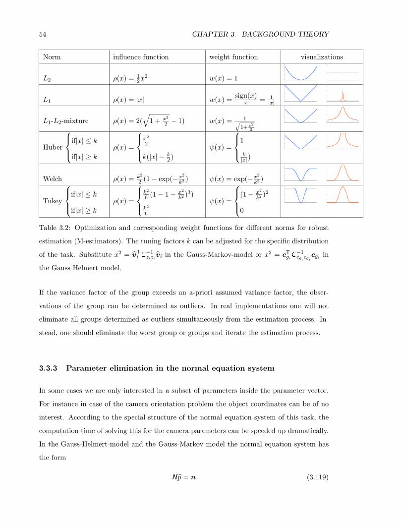
54 CHAPTER 3. BACKGROUND THEORY
Norm influence function weight function visualizations
L2 ρ(x) = 12x
2 w(x) = 1
L1 ρ(x) = |x| w(x) = sign(x)x = 1
|x|
L1-L2-mixture ρ(x) = 2(√
1 + x2
2 − 1) w(x) = 1√1+x2
2
Huber
if|x| ≤ k
if|x| ≥ kρ(x) =
x2
2
k(|x| − k2 )
ψ(x) =
1
k|x|)
Welch ρ(x) = k2
2 (1− exp(−x2
k2 ) ψ(x) = exp(−x2
k2 )
Tukey
if|x| ≤ k
if|x| ≥ kρ(x) =
k2
6 (1− 1− x2
k2 )3)
k2
6
ψ(x) =
(1− x2
k2 )2
0
Table 3.2: Optimization and corresponding weight functions for different norms for robust
estimation (M-estimators). The tuning factors k can be adjusted for the specific distribution
of the task. Substitute x2 = vTi C−1zizi vi in the Gauss-Markov-model or x2 = cT
giC−1cgicgi
cgi in
the Gauss Helmert model.
If the variance factor of the group exceeds an a-priori assumed variance factor, the obser-
vations of the group can be determined as outliers. In real implementations one will not
eliminate all groups determined as outliers simultaneously from the estimation process. In-
stead, one should eliminate the worst group or groups and iterate the estimation process.
3.3.3 Parameter elimination in the normal equation system
In some cases we are only interested in a subset of parameters inside the parameter vector.
For instance in case of the camera orientation problem the object coordinates can be of no
interest. According to the special structure of the normal equation system of this task, the
computation time of solving this for the camera parameters can be speeded up dramatically.
In the Gauss-Helmert-model and the Gauss-Markov model the normal equation system has
the form
N p = n (3.119)
3.4. RECURSIVE STATE ESTIMATION 55
ignoring contradictions on the parameter. Let us assume we can split the unknown parameter
vector into two parts
p =
p1
p2
. (3.120)
The normal equation system can then be rewritten as N11 N12
N21 N22
p1
p2
=
n1
n2
(3.121)
which leads to the equations
N11p1 + N12p2 = n1 (3.122)
N21p1 + N22p2 = n2. (3.123)
Drawing N21p1 from the left hand side of (3.123) and multiplying the left hand side with
N−122 we get the subvector solution with respect to p1 as
p2 = N−122 n2 − N−1
22 N21p1. (3.124)
Now substitute (3.124) into (3.122) we get
N11p1 + N12p2 = n1 (3.125)
N11p1 + N12(N−122 n2 − N−1
22 N21p1) = n1 (3.126)
(N11 − N12N−122 N21)p1 = n1 − N12N
−122 n2 (3.127)
N11p1 = n1. (3.128)
Observe, that the inverse of N22 has to be computed in equation 3.127 and therefore has to
be full rank. Without any limitation we can expand (3.128) using contradiction Hp = 0, if
the common normal equations system is regular.
3.4 Recursive state estimation
In this section we will introduce the concept of estimating states from sensor models in a
recursive manner. State here means a time varying unknown parameter vector. The aim is to
derive a recursive least square estimator and embedding it into a broader context of recursive
state estimation.
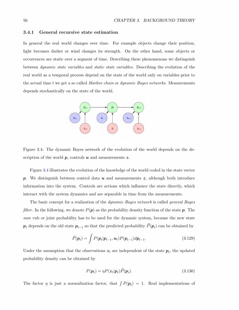
56 CHAPTER 3. BACKGROUND THEORY
3.4.1 General recursive state estimation
In general the real world changes over time. For example objects change their position,
light becomes darker or wind changes its strength. On the other hand, some objects or
occurrences are static over a segment of time. Describing these phenomenons we distinguish
between dynamic state variables and static state variables. Describing the evolution of the
real world as a temporal process depend on the state of the world only on variables prior to
the actual time t we get a so called Markov chain or dynamic Bayes networks. Measurements
depends stochastically on the state of the world.
Figure 3.4: The dynamic Bayes network of the evolution of the world depends on the de-
scription of the world p, controls u and measurements z.
Figure 3.4 illustrates the evolution of the knowledge of the world coded in the state vector
p. We distinguish between control data u and measurements z, although both introduce
information into the system. Controls are actions which influence the state directly, which
interact with the system dynamics and are separable in time from the measurements.
The basic concept for a realization of the dynamic Bayes network is called general Bayes
filter. In the following, we denote P (p) as the probability density function of the state p. The
sum rule or joint probability has to be used for the dynamic system, because the new state
pt depends on the old state pt−1 so that the predicted probability ~P (pt) can be obtained by
~P (pt) =∫P (pt|pt−1,ut)P (pt−1)dpt−1. (3.129)
Under the assumption that the observations zt are independent of the state pt, the updated
probability density can be obtained by
P (pt) = ηP (zt|pt)~P (pt). (3.130)
The factor η is just a normalization factor, that∫P (pt) = 1. Real implementations of
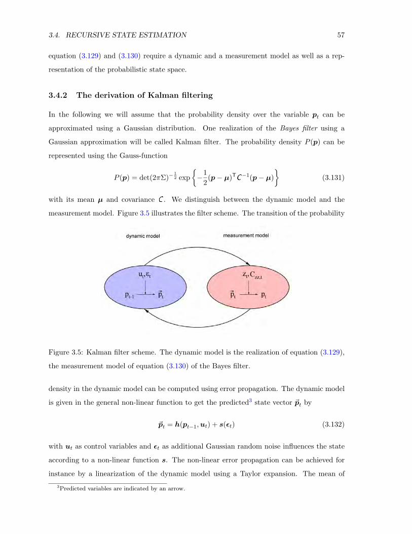
3.4. RECURSIVE STATE ESTIMATION 57
equation (3.129) and (3.130) require a dynamic and a measurement model as well as a rep-
resentation of the probabilistic state space.
3.4.2 The derivation of Kalman filtering
In the following we will assume that the probability density over the variable pt can be
approximated using a Gaussian distribution. One realization of the Bayes filter using a
Gaussian approximation will be called Kalman filter. The probability density P (p) can be
represented using the Gauss-function
P (p) = det(2πΣ)−12 exp
−1
2(p− µ)TC−1(p− µ)
(3.131)
with its mean µ and covariance C . We distinguish between the dynamic model and the
measurement model. Figure 3.5 illustrates the filter scheme. The transition of the probability
Figure 3.5: Kalman filter scheme. The dynamic model is the realization of equation (3.129),
the measurement model of equation (3.130) of the Bayes filter.
density in the dynamic model can be computed using error propagation. The dynamic model
is given in the general non-linear function to get the predicted3 state vector ~pt by
~pt = h(pt−1,ut) + s(εt) (3.132)
with ut as control variables and εt as additional Gaussian random noise influences the state
according to a non-linear function s. The non-linear error propagation can be achieved for
instance by a linearization of the dynamic model using a Taylor expansion. The mean of
3Predicted variables are indicated by an arrow.
58 CHAPTER 3. BACKGROUND THEORY
the posterior distribution can be transformed using the non-linear model and the Gaussian
distribution C pp of the state using the linearized error propagation
C ~p~p,t = HC pp,t−1HT + SC εε,tS
T (3.133)
with
H =∂h(pt−1,ut)
∂pt−1
∣∣∣∣pt−1,ut
(3.134)
S =∂s(pt−1)∂pt−1
∣∣∣∣pt−1
. (3.135)
After the prediction we obtain measurements from the world to update or correct the
predicted state. This process can be interpreted as a weighted mean of a direct measurement
of the state itself and an indirect measurements from the sensor data.
Typically, in the common literature the derivation of the update equation will be for-
mulated specializing the linear case going to non-linear iterative case. Here we will derive
a general novel form of an implicit update equation similar to the Gauss-Helmert model in
section 3.3.1 and we will show, that the classical linear, non-linear and iterative non-linear
update equations are specializations of our formulation.
Recursive update in the Gauss-Helmert-model4 From equation (3.91) we can split
the parameter estimation into two groups of implicit constraints g1(p, z1)
g2(p, z2)
= 0 (3.136)
with g1 as a direct observation of the state and g2 as an indirect observation. In the following
p is equal to pt. Using the normal equation system in equation (3.102) and neglecting the
constraints on the parameter vector, we can rewrite the left side as
AT(BT
C zzB)−1A =
A1
A2
T BT11 B
T12
BT21 B
T22
C 11 C 12
C 21 C 22
B11 B12
B21 B22
−1 A1
A2
(3.137)
and the right side as
AT(BT
C zzB)−1cg =
A1
A2
T BT11 B
T12
BT21 B
T22
C 11 C 12
C 21 C 22
B11 B12
B21 B22
−1 cg1cg2
.(3.138)
4First publication in Steffen & Beder (2007)
3.4. RECURSIVE STATE ESTIMATION 59
In the following we will assume that the two observation blocks are stochastically indepen-
dent, i.e. C 12 = C 21 = 0 as well as functionally independent, i.e. B12 = B21 = 0 . Observe,
that these boundary conditions are implicitly defined in the Bayes filtering scheme. Then we
can rewrite the left and right side as
AT(BT
C zzB)−1A = A
T1 (BT
11C 11B11)−1A1 + A
T2 (BT
22C 22B22)−1A2 (3.139)
and
AT(BT
C zzB)−1cg = AT1 (BT
11C 11B11)−1cg1 + AT2 (BT
22C 22B22)−1cg2 . (3.140)
Using the substitution W = BTC zzB, the final solution, that incorporates both observation
z1 and z2, may be obtained iteratively at the approximate values p(ν) and z(ν) using the
update
∆p = (AT1W
−111 A1 + A
T2W
−122 A2)−1(AT
1W−111 cg1 + A
T2W
−122 cg2). (3.141)
In the following the dependency on the first set of contradiction cg1 and therefore on the first
set of observation z1 should be removed. The goal of recursive estimation is now to derive
such a solution ∆p2 for the combined constraints using the solution of the first constraint
block g1 represented by ∆p1 and its covariance matrix C p1p1 as well as the new constraint
block g2 together with the new observations z2 and their covariance matrix C 22. In order to
achieve this goal equation (3.141) may be re-written as
∆p2 = (AT1W
−111 A1︸ ︷︷ ︸
C−1p1p1
+AT2W
−122 A2)−1
︸ ︷︷ ︸C p2p2
(AT1W
−111 ~cg1︸ ︷︷ ︸
C−1p1p1
∆p1
+AT1W
−111 ∆cg1 + A
T2W
−122 cg2)
(3.142)
with the contradictions for the first block being separated into
cg1 = ~cg1 + ∆cg1 . (3.143)
Observe that the contradictions5 ~cg1 for the first contradiction block g1 at p1 change due to
the change of parameters resulting from the new contradiction block g2, due to the depen-
dence on p of equation (3.99). As a consequence, the residuals for the observations of the
first contradiction block change as well
v1 = C 11B1W−111 (~cg1 + ∆cg1 − A1∆p2) (3.144)
= C 11B1W−111 (~cg1 − A1∆p1)︸ ︷︷ ︸
~v1
+C 11B1W−111 (∆cg1 − A1(∆p2 − ∆p1))︸ ︷︷ ︸
∆v1
. (3.145)
5Here we use ~(·) to indicate, that the vector depends on a prediction to be consistent in the following
equations.
60 CHAPTER 3. BACKGROUND THEORY
The expression C p2p2 in equation (3.142) is the inverse of a sum and can be decomposed using
the matrix inversion identity (c.f. Koch (1988) page 37)
(K + LN−1M)−1 = K
−1 − K−1L(N +MK
−1L)−1
MK−1 (3.146)
that follows
C p2p2 = C p1p1 − C p1p1AT2 (W 22 + A2C p1p1A
T2 )−1︸ ︷︷ ︸
F
A2C p1p1 (3.147)
= C p1p1 − FA2C p1p1 (3.148)
= (I − FA2)C p1p1 (3.149)
= C p1p1 − F (W 22 + A2C p1p1AT2 )FT (3.150)
with F being the gain or influence matrix. We can see, that this update of C p2p2 does not
involve the inversion of the full normal equation matrix. Substituting this back into equation
(3.142) we obtain
∆p2 = (I − FA2)C p1p1C−1p1p1∆p1 + (I − FA2)C p1p1A
T2W
−122 cg2 + (3.151)
(I − FA2)C p1p1AT1W
−111 ∆cg1
= ∆p1 − FA2∆p1 + Fcg2 + (I − FA2)C p1p1AT1W
−111 ∆cg1 (3.152)
using the identity Koch (1988) page 37
F = (I − FA2)C p1p1AT2W
−122 = C p1p1A
T2 (W 22 + A2C p1p1A
T2 )−1. (3.153)
The only remaining part still depending on z1 is now the change of the contradictions (see
equation (3.99))
∆cg1 = cg1 − ~cg1 = −g1(p2, z1) + BT1 v1 + g1(p1, z1)− BT
1 ~v1. (3.154)
In order to remove this remaining dependence on the previous observations, we bring in mind
that the whole first contradiction block is encoded in the first two moments of the parameter
vector only. We therefore replace the first contradiction block by a direct observation of the
parameters itself from the prediction, i.e. z1 = ~pt = p1 and C p1p1 = C ~p~p,t, so that
g1(p1, z1) = p1 − z1 = 0 (3.155)
3.4. RECURSIVE STATE ESTIMATION 61
immediately fulfills the constraint and therefore
~cg1 = 0 (3.156)
~v1 = 0 (3.157)
∆p1 = 0. (3.158)
Furthermore the Jacobians are given by A1 = I and B1 = −I independently of the lineariza-
tion point. Now equation (3.152) simplifies to
∆p2 = Fcg2 + (I − FA2)∆cg1 (3.159)
with
∆cg1 = −g1(p(ν), z1)− v1
= −p(ν) + ~pt + v1 − v1
= −p(ν) + ~pt. (3.160)
For the second contradiction block we can compute the residuals
v2 = C 22B2W−122 (cg2 − A2∆p2) (3.161)
and the contradictions
cg2 = −g2(p(ν), z(ν)) + BT2 v2 (3.162)
where p(ν+1)0 = p(ν) + ∆p
(ν)
2 and z(ν+1) = z2 + v(ν)2 has to be iterated until convergence is
reached. We will summarize the update algorithm in 3.1.
Recursive update in the Gauss-Markov-model Similar to the derivation of the least
square estimation we can derive the Kalman filter update equations for the Gauss-Markov
model as a specialization of the Gauss-Helmert model. Again beginning at the explicit ob-
servation model z = f(p), which can be rewritten to the implicit model using (3.104). The
Jacobian is with respect to the observations B2 = −I . The Gain matrix from equation (3.153)
simplifies to
F = C p1p1AT2 (C zz + A2C p1p1A
T2 )−1. (3.163)
Substitute the model into (3.162) we get
cg2 = −g2(p(ν), z(ν)) + BT2 v2
= −(f(p(ν))− (z2 + v2))− v2
= z2 − f(p(ν)). (3.164)
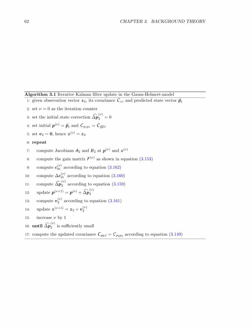
62 CHAPTER 3. BACKGROUND THEORY
Algorithm 3.1 Iterative Kalman filter update in the Gauss-Helmert-model1: given observation vector z2, its covariance C zz and predicted state vector ~pt
2: set ν = 0 as the iteration counter
3: set the initial state correction ∆p(ν)
2 = 0
4: set initial p(ν) = ~pt and C p1p1 = C ~p~p,t
5: set v2 = 0, hence z(ν) = z2
6: repeat
7: compute Jacobians A2 and B2 at p(ν) and z(ν)
8: compute the gain matrix F (ν) as shown in equation (3.153)
9: compute c(ν)g2 according to equation (3.162)
10: compute ∆c(ν)g1 according to equation (3.160)
11: compute ∆p(ν)
2 according to equation (3.159)
12: update p(ν+1) = p(ν) + ∆p(ν)
2
13: compute v(ν)2 according to equation (3.161)
14: update z(ν+1) = z2 + v(ν)2
15: increase ν by 1
16: until ∆p(ν)
2 is sufficiently small
17: compute the updated covariance C pp,t = C p2p2 according to equation (3.149)
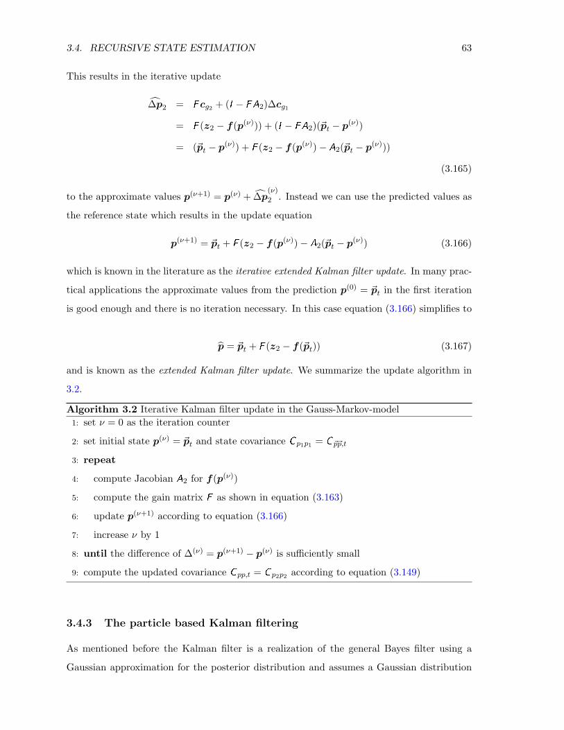
3.4. RECURSIVE STATE ESTIMATION 63
This results in the iterative update
∆p2 = Fcg2 + (I − FA2)∆cg1
= F (z2 − f(p(ν))) + (I − FA2)(~pt − p(ν))
= (~pt − p(ν)) + F (z2 − f(p(ν))− A2(~pt − p(ν)))
(3.165)
to the approximate values p(ν+1) = p(ν) + ∆p(ν)
2 . Instead we can use the predicted values as
the reference state which results in the update equation
p(ν+1) = ~pt + F (z2 − f(p(ν))− A2(~pt − p(ν)) (3.166)
which is known in the literature as the iterative extended Kalman filter update. In many prac-
tical applications the approximate values from the prediction p(0) = ~pt in the first iteration
is good enough and there is no iteration necessary. In this case equation (3.166) simplifies to
p = ~pt + F (z2 − f(~pt)) (3.167)
and is known as the extended Kalman filter update. We summarize the update algorithm in
3.2.
Algorithm 3.2 Iterative Kalman filter update in the Gauss-Markov-model1: set ν = 0 as the iteration counter
2: set initial state p(ν) = ~pt and state covariance C p1p1 = C ~p~p,t
3: repeat
4: compute Jacobian A2 for f(p(ν))
5: compute the gain matrix F as shown in equation (3.163)
6: update p(ν+1) according to equation (3.166)
7: increase ν by 1
8: until the difference of ∆(ν) = p(ν+1) − p(ν) is sufficiently small
9: compute the updated covariance C pp,t = C p2p2 according to equation (3.149)
3.4.3 The particle based Kalman filtering
As mentioned before the Kalman filter is a realization of the general Bayes filter using a
Gaussian approximation for the posterior distribution and assumes a Gaussian distribution
64 CHAPTER 3. BACKGROUND THEORY
after the correction step. The transition and update through non-linear functions are realized
by a Taylor expansion. The Gaussian distribution is transformed using the non-linear trans-
formation for its mean and by a linear transformation for its covariance. Higher degrees of the
non-linear transformation are neglected. Another error propagation method is the so-called
unscented transformation introduced by Julier & Uhlmann (1996). Instead of approximating
the non-linear function by a Taylor series the posterior Gaussian distribution can be approx-
imated using a series of particles, which will be passed through the non-linear function itself.
Instead of using randomly selected particles according to a Monte Carlo simulation, Julier &
Uhlmann (1996) choose deterministically particles. These particles are called Sigma points.
First we will briefly describe the error propagation through the unscented transformation and
then apply this algorithm to a dynamic system resulting in the so-called Unscented Kalman
filter. For a more detailed explanation c. f. van der Merwe (2004).
The posterior distribution is assumed to be n-dimensional Gaussian by its mean µ and
its covariance C . We compute 2n+ 1 sigma points χ[i]:
χ[1] = µ
χ[i] = µ+ (√
(n+ λ)C )i i = 1, ..., n
χ[i] = µ− (√
(n+ λ)C )i i = n+ 1, ..., 2n (3.168)
where the scaled root of the covariance (√
(n+ λ)C ) is a matrix square root computed by a
Cholesky-decomposition6. The sigma points are associated with weights W [i], that reflect the
influence of the i-th sigma point to the Gaussian approximation.
W [0] =λ
n+ λ
W [i] =1
2(n+ λ)i = 1, .., 2n. (3.169)
Here λ is a tuning factor. For Gaussian distributions select λ = 3−n (c. f. Julier & Uhlmann
(1996)). The general non-linear error propagation is summarized in algorithm 3.4.3.
As we have shown before, the Kalman filter consists of two parts, a dynamic model per-
formed by error propagation using the general model in equation (3.132) and a measurement
model. The measurement update using the unscented transformation is applicable for explicit
measurement functions (Gauss-Markov-model) only.
6In case of a singular covariance matrix C , we use an incomplete Cholesky decomposition.
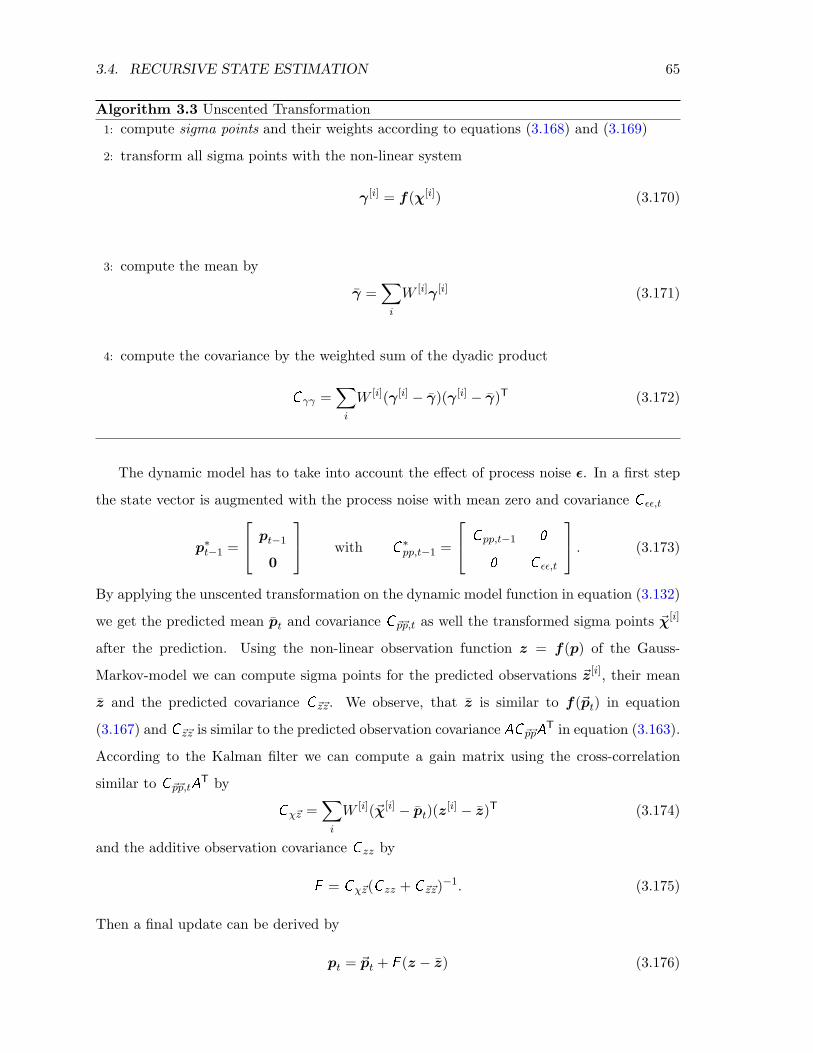
3.4. RECURSIVE STATE ESTIMATION 65
Algorithm 3.3 Unscented Transformation1: compute sigma points and their weights according to equations (3.168) and (3.169)
2: transform all sigma points with the non-linear system
γ[i] = f(χ[i]) (3.170)
3: compute the mean by
γ =∑i
W [i]γ[i] (3.171)
4: compute the covariance by the weighted sum of the dyadic product
C γγ =∑i
W [i](γ[i] − γ)(γ[i] − γ)T (3.172)
The dynamic model has to take into account the effect of process noise ε. In a first step
the state vector is augmented with the process noise with mean zero and covariance C εε,t
p∗t−1 =
pt−1
0
with C∗pp,t−1 =
C pp,t−1 0
0 C εε,t
. (3.173)
By applying the unscented transformation on the dynamic model function in equation (3.132)
we get the predicted mean pt and covariance C ~p~p,t as well the transformed sigma points ~χ[i]
after the prediction. Using the non-linear observation function z = f(p) of the Gauss-
Markov-model we can compute sigma points for the predicted observations ~z[i], their mean
z and the predicted covariance C~z~z. We observe, that z is similar to f(~pt) in equation
(3.167) and C~z~z is similar to the predicted observation covariance AC ~p~pAT in equation (3.163).
According to the Kalman filter we can compute a gain matrix using the cross-correlation
similar to C ~p~p,tAT by
Cχ~z =∑i
W [i](~χ[i] − pt)(z[i] − z)T (3.174)
and the additive observation covariance C zz by
F = Cχ~z(C zz + C~z~z)−1. (3.175)
Then a final update can be derived by
pt = ~pt + F (z − z) (3.176)
66 CHAPTER 3. BACKGROUND THEORY
with its covariance using equation (3.150)
C pp,t = C ~p~p,t − F (C zz + C~z~z)FT. (3.177)
The Unscented Kalman filter above has two advantages. First, the Gaussian approxima-
tion of the transformed uncertainty through the non-linear transformation take higher order
therms up to degree four of a Taylor expansion into account. Second, the computational
complexity is equal to the Kalman filter but parallelizable. But there are also disadvan-
tages. First, the update scheme does not ensure a positive definite covariance matrix C pp,t.
A solution of this disadvantage is the Square root Kalman filter, which ensure positive semi-
definiteness. Second, the non-linear functions must be continuous. We will explain this last
issue in chapter 4 in more detail.
3.4.4 Outlier detection and robustification of Kalman filtering
As we mentioned the update process is a weighted mean of the direct observation of the
state obtained by the dynamic model and a set of noisy observations. Comparing it to the
least square outlier detection in section 3.3.2 this mean process can be reformulated using
the normal equations. Therefore the predicted state vector is a pseudo observation vector
with full correlations, so that from the theory of outlier detection we can only test the whole
pseudo observation as a group. Additionally, the unknowns in the state vector depends on
groups of observations of the measurement model. Following the considerations in 3.3.2, it
is not possible to distinguish between gross errors in the prediction and gross errors in the
observations.
However, in some real applications the mean and covariance of the predicted state approx-
imate the true state very well. If and only if we can neglect the influence of the prediction we
can test the observations against gross errors using equation (3.111) in the Gauss-Markov-
model (3.113) in the Gauss-Helmert-model respectively.
Therefore, the residuals for the recursive update using the Gauss-Markov-model have to
be obtained at the estimated state using
v = z − f(p). (3.178)
The contradictions for the recursive update in the Gauss-Helmert-model can be tested using
equations (3.112) and (3.113) at the convergence point.
3.4. RECURSIVE STATE ESTIMATION 67
Similar to the reweighting method for the least square method the reweighting scheme is
applicable to the recursive update using equation (3.116). A method to estimate the variance
components of individual groups of observations can be found in Caspary (1998).
In this chapter we first summarized basic concepts in image geometry followed by a deriva-
tion of global least square methods. We introduced the notion of dynamic state systems as
a general Bayes filter and derived similar to the global least square method, a new formu-
lation of an implicit recursive estimation scheme. We showed that the classical least square
recursive estimation algorithm is a specialization of our new derivation. Furthermore, we
explained how outliers can be rejected and their influence can be reduced to achieve more
robust estimation with respect to erroneous observations inside the global least square as well
as in the recursive estimation scheme.

68 CHAPTER 3. BACKGROUND THEORY
Chapter 4
Kalman filter based localization and
mapping with a single camera
The goal of this chapter is to work out the details of a Kalman filter based system for the
task of localization and mapping for a single camera only. We are especially focused on the
state representation and initialization.
Full autonomous simultaneous localization and mapping using image based measurements
is still a hard problem. A broad range of applications, especially in the field of robotics and
surveillance, require fully autonomous, robust, accurate and real-time capable methods. The
goal of such applications is to acquire detailed map information. This includes an adequate
surface model and the determination of the full observer localization at every point in time.
In the following we will discuss the requirements of such systems using a single camera
sensor only and we will focus on the problem of real-time capable recursive estimation of the
environment. As motivated in the introduction the environment is focused on the task of
acquiring elevation maps from an unmanned aerial vehicle (UAV).
4.1 Introduction
Unmanned aerial vehicles become more and more interesting as a tool for medium and large
scale image acquisition. To determine a dense surface model of an observed scene the camera
orientations of the acquired images in a fixed world coordinate system are necessary. Clas-
sical offline approaches are well-known in the photogrammetric community. In this case the
images are acquired with large baselines, information about the projection center and camera
69
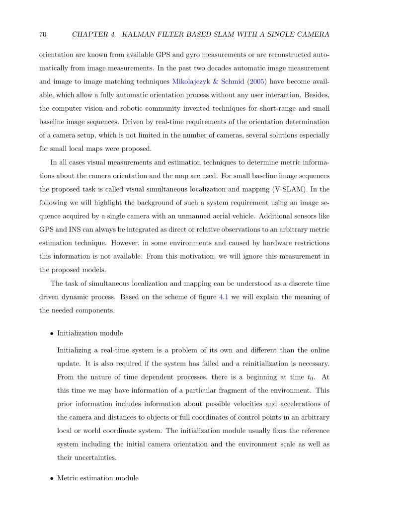
70 CHAPTER 4. KALMAN FILTER BASED SLAM WITH A SINGLE CAMERA
orientation are known from available GPS and gyro measurements or are reconstructed auto-
matically from image measurements. In the past two decades automatic image measurement
and image to image matching techniques Mikolajczyk & Schmid (2005) have become avail-
able, which allow a fully automatic orientation process without any user interaction. Besides,
the computer vision and robotic community invented techniques for short-range and small
baseline image sequences. Driven by real-time requirements of the orientation determination
of a camera setup, which is not limited in the number of cameras, several solutions especially
for small local maps were proposed.
In all cases visual measurements and estimation techniques to determine metric informa-
tions about the camera orientation and the map are used. For small baseline image sequences
the proposed task is called visual simultaneous localization and mapping (V-SLAM). In the
following we will highlight the background of such a system requirement using an image se-
quence acquired by a single camera with an unmanned aerial vehicle. Additional sensors like
GPS and INS can always be integrated as direct or relative observations to an arbitrary metric
estimation technique. However, in some environments and caused by hardware restrictions
this information is not available. From this motivation, we will ignore this measurement in
the proposed models.
The task of simultaneous localization and mapping can be understood as a discrete time
driven dynamic process. Based on the scheme of figure 4.1 we will explain the meaning of
the needed components.
• Initialization module
Initializing a real-time system is a problem of its own and different than the online
update. It is also required if the system has failed and a reinitialization is necessary.
From the nature of time dependent processes, there is a beginning at time t0. At
this time we may have information of a particular fragment of the environment. This
prior information includes information about possible velocities and accelerations of
the camera and distances to objects or full coordinates of control points in an arbitrary
local or world coordinate system. The initialization module usually fixes the reference
system including the initial camera orientation and the environment scale as well as
their uncertainties.
• Metric estimation module
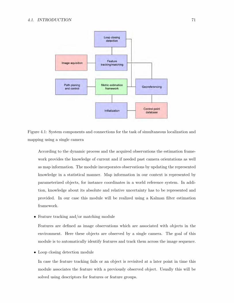
4.1. INTRODUCTION 71
Figure 4.1: System components and connections for the task of simultaneous localization and
mapping using a single camera
According to the dynamic process and the acquired observations the estimation frame-
work provides the knowledge of current and if needed past camera orientations as well
as map information. The module incorporates observations by updating the represented
knowledge in a statistical manner. Map information in our context is represented by
parameterized objects, for instance coordinates in a world reference system. In addi-
tion, knowledge about its absolute and relative uncertainty has to be represented and
provided. In our case this module will be realized using a Kalman filter estimation
framework.
• Feature tracking and/or matching module
Features are defined as image observations which are associated with objects in the
environment. Here these objects are observed by a single camera. The goal of this
module is to automatically identify features and track them across the image sequence.
• Loop closing detection module
In case the feature tracking fails or an object is revisited at a later point in time this
module associates the feature with a previously observed object. Usually this will be
solved using descriptors for features or feature groups.
72 CHAPTER 4. KALMAN FILTER BASED SLAM WITH A SINGLE CAMERA
• Georeferencing module
Depending on the a-priori knowledge introduced by the initialization module a later
georeferencing stage can be applied, if there are observations available to achieve abso-
lute orientations in a fixed world coordinate system.
• Path planing and control module
Depending on the task and the a-priori knowledge of the autonomous system this mod-
ule generates control actions to achieve a complete mapping. In the case of mapping
with unmanned aerial vehicles often the path is fixed a-priori using an approximate
knowledge of the surface and of the achievable accuracy.
The aim of an implementation of the scheme above is to provide an autonomous local-
ization and navigation using visual information only. In our opinion the core module is the
metric estimation framework. The requirements of this framework are real-time capability,
high accuracy and robustness. In this section we will therefore focus on the estimation frame-
work, its initialization and required observations. To achieve real-time capable estimation of
a set of metric parameters the Kalman filter framework will be our choice. We will derive
and discuss different kinds of state representations as well as their initialization and dynamic
evolution in time.
4.2 Feature extraction, tracking and matching
First we will clarify the meaning of features. In general images are only light intensity
information in different directions. The image is a carrier of such information. Known from
the information theory the information can be measured globally or locally by its entropy.
But, we cannot decide by only one image whether its information is high or low. It depends
on our task.
We give a small example: Assuming we already mapped a large green area like a golf
field. We get an image of a homogeneous bright surface. The information inside the image
can be low according to its entropy, but the information for the localization task can be high
according to the identification of a sand strap.
From this consideration, in our opinion we have to distinguish between landmarks usable
as control points, which are high level location based objects or information in a global map
4.2. FEATURE EXTRACTION, TRACKING AND MATCHING 73
and features as pure image based metric objects usable as tie points. Features for instance are
interest points, blobs1 and line segments. Moreover, features can also be identifiable objects,
for instance cars or windows. In our experiments we will only use interest points as features,
but every kind of feature can be used for our task. A point based feature should fulfill certain
criteria:
1. Invariance - The detection of a specific feature should be invariant with respect to geo-
metric and radiometric distortions, for instance relative rotations or intensity changes.
2. Stability - The detection of a feature should be robust against noise in the observation.
3. Distinctness - The feature should be distinguishable from neighboring features in terms
of local image information.
4. Infrequency - For the task of loop closing detection the surrounding local image infor-
mation of a feature should be unique.
5. Interpretability - In case of object recognition tasks it is necessary that the feature or
a feature group can be assigned to semantic objects.
In the past decade many point based interest operators were developed Forstner & Gulch
(1987), Harris & Stephens (1988), Lindeberg (1998), Mikolajczyk & Schmid (2002), Lowe
(2003). We will use interest points according to Forstner/Harris, which are suitable for
matching. Matching here means to identify the same feature, which is associated to a location
in the world space, in a following image. There are two situations possible. First the following
image was taken with small disparities, then tracking algorithms can be used for matching.
Second, a feature is revisited and has to be identified.
Tracking algorithms assume small disparities as well as small scale and rotation changes.
The surrounding local image information of a feature will be used as a template. The as-
sumption is, that the corresponding object point is locally planar. It has been shown by
Forstner (1982), that the accuracy of template based matching using least square methods
depends on the signal noise ratio and on window size around a feature point. Using a large
window size, the planar assumption can be corrupted and therefore it is necessary to find a
trade off between accuracy and local planarity of a feature. A well known tracking algorithm
1Blobs are homogeneous image areas.
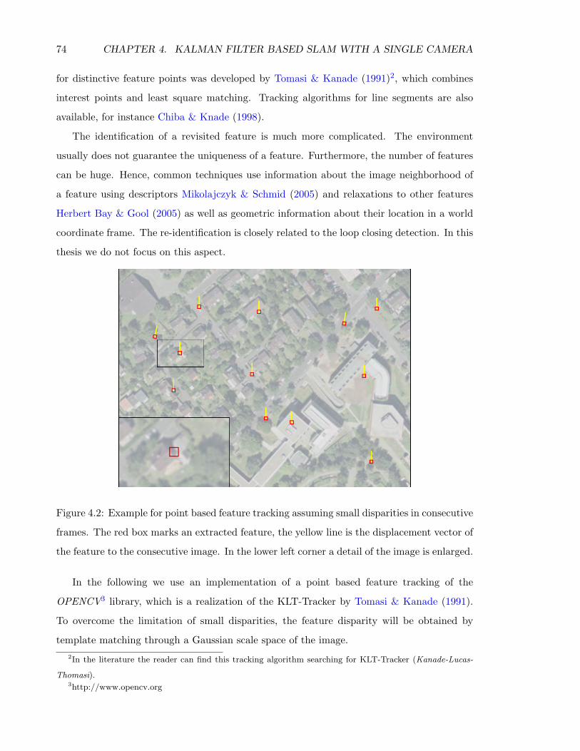
74 CHAPTER 4. KALMAN FILTER BASED SLAM WITH A SINGLE CAMERA
for distinctive feature points was developed by Tomasi & Kanade (1991)2, which combines
interest points and least square matching. Tracking algorithms for line segments are also
available, for instance Chiba & Knade (1998).
The identification of a revisited feature is much more complicated. The environment
usually does not guarantee the uniqueness of a feature. Furthermore, the number of features
can be huge. Hence, common techniques use information about the image neighborhood of
a feature using descriptors Mikolajczyk & Schmid (2005) and relaxations to other features
Herbert Bay & Gool (2005) as well as geometric information about their location in a world
coordinate frame. The re-identification is closely related to the loop closing detection. In this
thesis we do not focus on this aspect.
Figure 4.2: Example for point based feature tracking assuming small disparities in consecutive
frames. The red box marks an extracted feature, the yellow line is the displacement vector of
the feature to the consecutive image. In the lower left corner a detail of the image is enlarged.
In the following we use an implementation of a point based feature tracking of the
OPENCV3 library, which is a realization of the KLT-Tracker by Tomasi & Kanade (1991).
To overcome the limitation of small disparities, the feature disparity will be obtained by
template matching through a Gaussian scale space of the image.2In the literature the reader can find this tracking algorithm searching for KLT-Tracker (Kanade-Lucas-
Thomasi).3http://www.opencv.org
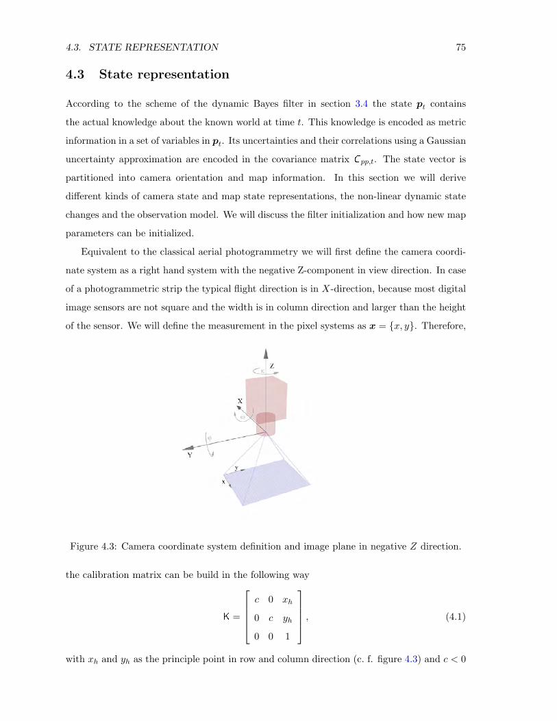
4.3. STATE REPRESENTATION 75
4.3 State representation
According to the scheme of the dynamic Bayes filter in section 3.4 the state pt contains
the actual knowledge about the known world at time t. This knowledge is encoded as metric
information in a set of variables in pt. Its uncertainties and their correlations using a Gaussian
uncertainty approximation are encoded in the covariance matrix C pp,t. The state vector is
partitioned into camera orientation and map information. In this section we will derive
different kinds of camera state and map state representations, the non-linear dynamic state
changes and the observation model. We will discuss the filter initialization and how new map
parameters can be initialized.
Equivalent to the classical aerial photogrammetry we will first define the camera coordi-
nate system as a right hand system with the negative Z-component in view direction. In case
of a photogrammetric strip the typical flight direction is in X-direction, because most digital
image sensors are not square and the width is in column direction and larger than the height
of the sensor. We will define the measurement in the pixel systems as x = x, y. Therefore,
Figure 4.3: Camera coordinate system definition and image plane in negative Z direction.
the calibration matrix can be build in the following way
K =
c 0 xh
0 c yh
0 0 1
, (4.1)
with xh and yh as the principle point in row and column direction (c. f. figure 4.3) and c < 0
76 CHAPTER 4. KALMAN FILTER BASED SLAM WITH A SINGLE CAMERA
as the principle distance. To achieve the rotation between the image and the camera system
we multiply K right hand side by a rotation matrix R(κ = 180) around the Z-component.
4.3.1 Single camera state
The camera orientation in a 3-dimensional space is defined by using six parameters, its
location and its angular orientation. As mentioned in section 3.1.2 an angular representation
using Euler angles involves trigonometric functions and can fail in case of deviations close to
the 180 degree singularity. For this reason the angular orientation will be represented using
quaternions. A convenient effect is that the dynamic state change equation becomes linear.
Therefore the actual state can be represented as follows:
pt = [T t,qt,X1, . . . ,Xn, . . . ,XN ]T (4.2)
with T t = Xt, Yt, Zt as the camera position and qt as the angular camera orientation repre-
sented as quaternion. Additionally the state contains N object point coordinates. Following
the state representation model of Davison (2003) the state also contains the velocity and
angular velocity.
pt =
T t,qt, T t, qt︸ ︷︷ ︸13
,X1, . . . ,Xn, . . . ,XN︸ ︷︷ ︸3N
T
(4.3)
We denote, that the angular velocity qt is usually small and below 180. In this case we can
represent the velocity as the vector part only as a three component vector, c. f. equation
(3.36). As an extension also the acceleration can be added. The scheme of a single camera
state is outlined in figure 4.4.
In the following, we will present a linear dynamic model and the error propagation using
accelerations as a perturbation with mean zero. The derivation can be found in the appendix
in section A.2. The prediction of the state according to a time difference ∆t can then be
computed as
~pt+1 = h(pt) =
T t + T t∆t+ 12 T t∆t
2
Υ(12 qt∆t
2)Υ(q∆t)qt
T t + T t∆t
qt∆t+ q
X1
...
XN
, (4.4)
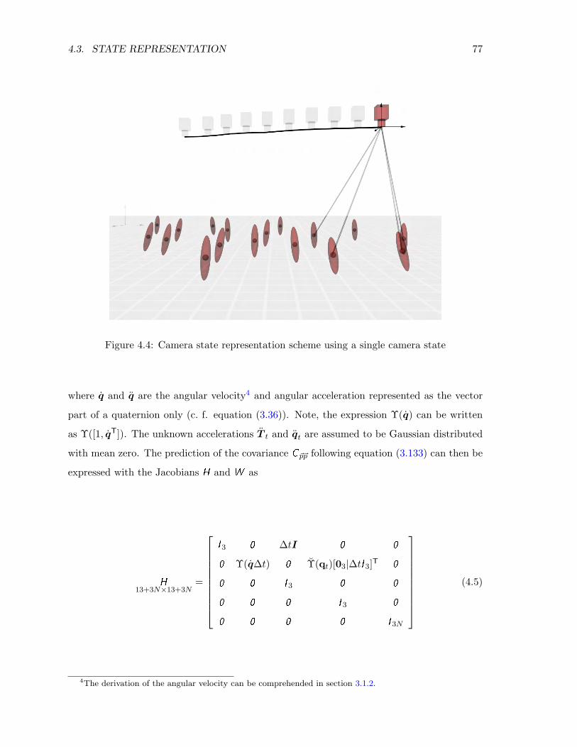
4.3. STATE REPRESENTATION 77
Figure 4.4: Camera state representation scheme using a single camera state
where q and q are the angular velocity4 and angular acceleration represented as the vector
part of a quaternion only (c. f. equation (3.36)). Note, the expression Υ(q) can be written
as Υ([1, qT]). The unknown accelerations T t and qt are assumed to be Gaussian distributed
with mean zero. The prediction of the covariance C ~p~p following equation (3.133) can then be
expressed with the Jacobians H and W as
H13+3N×13+3N
=
I 3 0 ∆tI 0 0
0 Υ(q∆t) 0 Υ(qt)[03|∆tI 3]T 0
0 0 I 3 0 0
0 0 0 I 3 0
0 0 0 0 I 3N
(4.5)
4The derivation of the angular velocity can be comprehended in section 3.1.2.
78 CHAPTER 4. KALMAN FILTER BASED SLAM WITH A SINGLE CAMERA
and for the system noise
W13+3N×6
=
12∆t2I 3 0
0 Υ(Υ(q∆t)qt)[03|12∆t2I 3]T
∆tI 3 0
0 ∆tI 3
0 0
. (4.6)
We observe, that using quaternions and assuming small rotations, matrix multiplications
without any trigonometric functions are necessary.
4.3.2 Sliding window camera state
It is well known from an entire bundle adjustment with all camera orientations, arbitrary
camera parameters are correlated. Using the single camera state representation presented so
far we neglect past camera orientations as well as their correlations. For this reason there
is an leakage of information. The correlation between close camera locations is high and
should not be neglected. Furthermore, the map will be updated by new observations, which
will indirectly influence past camera parameters, which are useful for an off-line dense map
computation. Therefore we propose a multiple camera state as outlined in figure 4.5. In the
following we will show how the linear prediction model can be applied to a multi camera state
representation. Because we have take into account the correlations between all the camera
orientations and the estimated object points, the error propagation in the prediction step has
to be performed using a state extension. We extend the state to the new camera position
at time t + 1 computed from the state at time pt. Let us assume we take k sets of camera
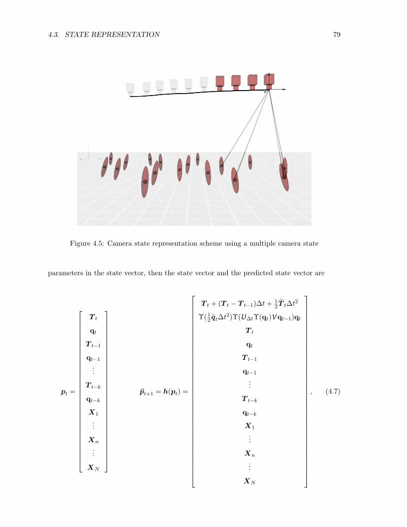
4.3. STATE REPRESENTATION 79
Figure 4.5: Camera state representation scheme using a multiple camera state
parameters in the state vector, then the state vector and the predicted state vector are
pt =
T t
qt
T t−1
qt−1
...
T t−k
qt−k
X1
...
Xn
...
XN
~pt+1 = h(pt) =
T t + (T t − T t−1)∆t+ 12 T t∆t
2
Υ(12 qt∆t
2)Υ(U∆tΥ(qt)Vqt−1)qt
T t
qt
T t−1
qt−1
...
T t−k
qt−k
X1
...
Xn
...
XN
, (4.7)
80 CHAPTER 4. KALMAN FILTER BASED SLAM WITH A SINGLE CAMERA
where ∆t = tt+1−tttt−tt−1
is a time dependent ratio factor. The extended covariance matrix can be
obtained using the error propagation for the prediction step using the Jacobian
H7(k+2)+3N×7(k+1)+3N
=
I 3 + ∆tI 3 0 −∆tI 3 0 0
0 Υ(U∆tΥ(qt)Vqt−1)+ 0 Υ(qt)U∆tΥ(qt)V 0
Υ(qt)U∆tΥ(Vqt−1)
I 3 0 0 0 0
0 I 4 0 0 0
0 0 I 3 0 0
0 0 0 I 4 0
0 0 0 0 I 7(k−1)+3N
(4.8)
and for the system noise
W7(k+2)+3N×6
=
12∆t2I 3 0
0 Υ(Υ(U∆tΥ(qt)Vqt−1)qt)[0|12∆t2I 3]
0 0
(4.9)
with U and V from equations (3.37) and (3.35). The derivation is outlined in the appendix
in section A.2.
Up to now, the state is expanded by the new camera orientation. If intended, the camera
parameter for the camera at time t−k can be neglected. To do so, we delete the corresponding
rows and columns of the covariance respectively of the state vector. For real implementations
the memory reordering for the covariance matrix can be performed using an error propagation
scheme with the Jacobian
J7(k+1)+3N×7(k+2)+3N
=
I 7(k+1) 0 0
0 0 I 3N
. (4.10)
Discussion: One can show, that the single camera representation including velocities is
equivalent to a multi-camera state representation with k = 1, by using error propagation one
representation can be transformed to the other one and vice versa. In case of large system
noise the dynamic state change model will not cause correlations between consecutive camera
orientations. But correlations transfered to past camera orientations across the map state
4.3. STATE REPRESENTATION 81
further on exist. The overhead of the computational complexity using a sliding window cam-
era state is usually small. An implementation should decide which past camera orientations
have to stay inside the state vector. This decision should be taken into account which past
cameras are useful for off-line dense map computation and the degree of correlations.
4.3.3 Feature representation and update models
In this section we will describe the representation of the object point coordinates and for-
mulate the corresponding update or observation model which can be used in the bundle
adjustment and in the Kalman filter based solution.
Euclidean representation. In the classical case a point in the object space will be
represented by its Euclidean coordinates Xn = Xn, Yn, Zn. As shown in section 3.2.1 the
observation model can be described by the colinear equation (3.59) or (3.58). Using equation
(3.58) the projection matrix and therefore the projection of all visible points Xn in frame t
can be computed as
xn = KRT(qt)[I 3| − T t]Xn (4.11)
from the predicted state vector representation of the camera position and angular orienta-
tion. Note, that in the case of the bundle adjustment the over-representation of the camera
orientation using the quaternion cause a rank deficiency. To avoid this rank deficiency in the
bundle adjustment two solutions are available. First, we can formulate the constraint, that
the length of the quaternion is equal to one. Second we can introduce a pseudo observation
with a high weight for their length. In a Kalman filter based approach there is no inversion
of a rank deficient matrix necessary. But, the free length of the quaternion can cause numer-
ical instabilities. The quaternion length can grow up to large values, which cause numerical
instability. In contrast, we do not know any method for a constraint on the state vector
in a Kalman filter similar to the global least square method. Instead we can use a pseudo
observation for the quaternion length in arbitrary time steps.
Inverse distance representation - The inverse distance representation was introduced
by Montiel et al. (2006). Instead of a Euclidean representation of an object point, the point
will be represented using polar coordinates with an inverse distance. It has been shown and
quantified that for small parallax angles the distribution of the intersection in Euclidean
space is not well modeled. This can be proven by a Monte-Carlo simulation shown in figure
4.7. The advantage of an inverse distance representation is a better approximation of the
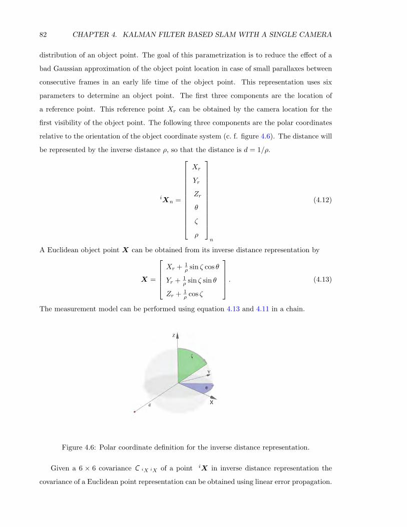
82 CHAPTER 4. KALMAN FILTER BASED SLAM WITH A SINGLE CAMERA
distribution of an object point. The goal of this parametrization is to reduce the effect of a
bad Gaussian approximation of the object point location in case of small parallaxes between
consecutive frames in an early life time of the object point. This representation uses six
parameters to determine an object point. The first three components are the location of
a reference point. This reference point Xr can be obtained by the camera location for the
first visibility of the object point. The following three components are the polar coordinates
relative to the orientation of the object coordinate system (c. f. figure 4.6). The distance will
be represented by the inverse distance ρ, so that the distance is d = 1/ρ.
iXn =
Xr
Yr
Zr
θ
ζ
ρ
n
(4.12)
A Euclidean object point X can be obtained from its inverse distance representation by
X =
Xr + 1
ρ sin ζ cos θ
Yr + 1ρ sin ζ sin θ
Zr + 1ρ cos ζ
. (4.13)
The measurement model can be performed using equation 4.13 and 4.11 in a chain.
Figure 4.6: Polar coordinate definition for the inverse distance representation.
Given a 6 × 6 covariance C iX iX of a point iX in inverse distance representation the
covariance of a Euclidean point representation can be obtained using linear error propagation.
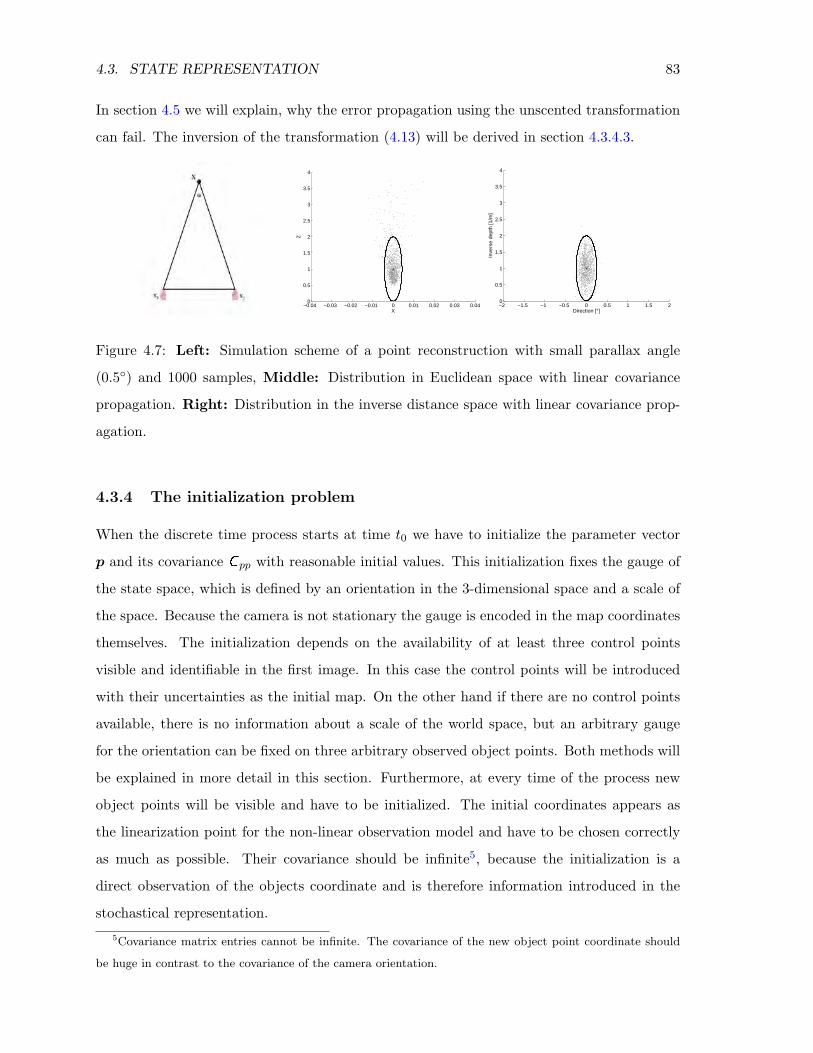
4.3. STATE REPRESENTATION 83
In section 4.5 we will explain, why the error propagation using the unscented transformation
can fail. The inversion of the transformation (4.13) will be derived in section 4.3.4.3.
−0.04 −0.03 −0.02 −0.01 0 0.01 0.02 0.03 0.040
0.5
1
1.5
2
2.5
3
3.5
4
X
Z−2 −1.5 −1 −0.5 0 0.5 1 1.5 20
0.5
1
1.5
2
2.5
3
3.5
4
Direction [°]
Inve
rse
dept
h [1
/m]
Figure 4.7: Left: Simulation scheme of a point reconstruction with small parallax angle
(0.5) and 1000 samples, Middle: Distribution in Euclidean space with linear covariance
propagation. Right: Distribution in the inverse distance space with linear covariance prop-
agation.
4.3.4 The initialization problem
When the discrete time process starts at time t0 we have to initialize the parameter vector
p and its covariance C pp with reasonable initial values. This initialization fixes the gauge of
the state space, which is defined by an orientation in the 3-dimensional space and a scale of
the space. Because the camera is not stationary the gauge is encoded in the map coordinates
themselves. The initialization depends on the availability of at least three control points
visible and identifiable in the first image. In this case the control points will be introduced
with their uncertainties as the initial map. On the other hand if there are no control points
available, there is no information about a scale of the world space, but an arbitrary gauge
for the orientation can be fixed on three arbitrary observed object points. Both methods will
be explained in more detail in this section. Furthermore, at every time of the process new
object points will be visible and have to be initialized. The initial coordinates appears as
the linearization point for the non-linear observation model and have to be chosen correctly
as much as possible. Their covariance should be infinite5, because the initialization is a
direct observation of the objects coordinate and is therefore information introduced in the
stochastical representation.
5Covariance matrix entries cannot be infinite. The covariance of the new object point coordinate should
be huge in contrast to the covariance of the camera orientation.
84 CHAPTER 4. KALMAN FILTER BASED SLAM WITH A SINGLE CAMERA
4.3.4.1 Control point initialization
The initialization of the filter can be performed using at least three control points. Usually
these control points can be obtained by a-priori global or local map information, e.g. from
an independent absolute measurement. Their coordinates, uncertainties as well as their
correlations will be used to initialize the map coordinates inside the filter.
The initial camera parameter can be obtained using the observations of the control points
in the first image. The advantage of a direct approach is that we do not need any approximate
values a-priori. Using three points only few direct approaches are available to determine the
distances of the camera projection center to the control points. A good overview can be
found in Haralick et al. (1991), who analyzes the numerical stability of different approaches.
These approaches result in up to four equivalent solutions. We need a fourth point to pick
up the correct one.
The camera position T and the angular orientation R can be obtained solving the model
λimi = R(Xi − T ) (4.14)
with mi as the normalized directions to the control points Xi and λi as the distances to the
control points already obtained by the direct solution. The algorithm for the determination
of T and R can be found in McGlone et al. (2004) pages 786ff.
The covariance matrix for the camera parameter will be initialized with a huge uncertainty.
In the following Kalman filter measurement update the camera parameter will be corrected.
4.3.4.2 Scale free bundle adjustment initialization
In some real environments no control points and no additional information about the visible
world space are available. To make the Kalman filter operable and to fix the gauge we propose
a free bundle adjustment initialization procedure in the early stage of the process. To do so,
we have to decide which of the obtained frames we will use for the initialization.
Here we will derive a real-time capable algorithm to decide when the acquired images are
adequate to initialize the estimation process, c. f. Beder & Steffen (2006). The contribu-
tion is to present a statistically motivated measure for the quality of a bundle adjustment
initialization procedure.
We will now analyze the uncertainty of an object point from two measured corresponding
image coordinates. Observe that we will neglect the correlation between a set of points. If a
4.3. STATE REPRESENTATION 85
scene point X is observed by two projective cameras P1 and P2, the image coordinates x1 and
x2 can be computed using equation (3.58) which can be rewritten using the skew-symmetric
matrix reflecting the cross product as
0 = x× PX = S(x)PX = −S(PX)x. (4.15)
Only two constrains are independent. Using (4.15) for two observations and choosing two
arbitrary constrains indicated by S2(·), both expressions are linear in the object point as well
as in the image point, so that follows S2(x1)P1
S2(x2)P2
︸ ︷︷ ︸
A4×4
X = 0 (4.16)
and −S2(P1X) 0
0 −S2(P2X)
︸ ︷︷ ︸
B4×6
x1
x2
= 0. (4.17)
Now the scene point coordinate and the two image point coordinates are assumed to be
random variables with Gaussian distribution. We observe that, as all three quantities are
homogeneous, the covariance matrices of their distributions are singular. In case the covari-
ances of the image points are given by C 11 and C 22, then it has been shown by Heuel (2004)
according to our derivation of the normal equation system in section 3.3, that the covariance
matrix CXX of an object point is proportional to the upper left 4×4-submatrix of the inverse
of
N =
AT
B C 11 0
0 C 22
BT
−1
A X
XT 0
. (4.18)
We have neglected the effect of the uncertainty of the projection matrices P here, because
the relative orientation of two cameras is determined by many points, so that it is of superior
precision compared to a single object point. In the second step we can compute the Euclidean
covariance of X indicated by eCXX using the error-propagation with the Jacobian
eJ =
∂X0/Xh
∂X0=
1Xh
[I 3 | −
X0
Xh
](4.19)
86 CHAPTER 4. KALMAN FILTER BASED SLAM WITH A SINGLE CAMERA
according toeCXX = e
JCXXeJ
T. (4.20)
The roundness as a measure for the reconstruction stability is directly related to the condi-
tion number of the 3d reconstruction of the object point. Hence, apply the singular value
decomposition6 to the covariance
eCXX = G
λ1 0 0
0 λ2 0
0 0 λ3
GT (4.21)
the roundness L is defined as the square root of the quotient of the smallest and the largest
singular value
L =√λ3
λ1. (4.22)
This measure lies between zero and one, is invariant to scale changes and only depends on
the relative geometry of the camera pose and on the measured image point accuracy.
The algorithm for a scale free bundle adjustment initialization is outlined in 4.1.
4.3.4.3 Inverse distance feature initialization and reduction
As shown in 4.3.3 an object point can be represented using polar coordinates with respect
to a reference system. Here we will show, how the object point can be initialized using the
inverse distance parametrization and explain the introduction into the state vector and its
covariance matrix. Furthermore we will describe the transformation from the inverse distance
representation to the Euclidean representation.
The first time a new object point is visible the point can be introduced to the state vector.
Because we will fix the reference polar coordinate system to the actual camera position, we
have to take into consideration to its uncertainty. The direction to the object point can be
determined using image observation.
Using the estimated camera orientation Rt at time t and the observed image point x in
homogeneous representation we obtain the direction vector d = dX , dY , dZ to the object
point by
d = −RtK−1x. (4.23)
6Note, the value decomposition of a covariance matrix leads to a symmetric solution, where G is a rotation
matrix.
4.3. STATE REPRESENTATION 87
Algorithm 4.1 Scale free bundle adjustment initialization algorithm1: Fix the first image of the sequence and let its projection matrix be Pt=1 = K[I 3|0]
2: Extract the interest points x1,n together with their covariance matrices C 11,n from this
image
3: repeat
4: Get the next image at time t = t+ 1
5: Extract the interest points xt,n together with their covariance matrices C tt,n from this
new image
6: Determine the point correspondences x1,n ↔ xt,n and the relative orientation Rt, T t to
the first image of the sequence according to the algorithm proposed in Nister (2004).
The camera matrix for the current image is then Pt = KRTt [I 3| − T t] with |T t| = 1.
7: Determine the scene point positions Xn for each found correspondence by forward
intersection according to the linear system in equation (4.16) using the singular value
decomposition as an linear equation solver.
8: Determine the roundness Ln (c. f. equation (4.22)) of each scene point Xn’s confidence
ellipsoid as outlined.
9: until the mean roundness is above a given threshold ΘL for example 0.1.
10: Compute approximate values for the camera orientations P2..t−1 by spatial resection using
the scene points Xn.
11: Perform a bundle adjustment with all images up to time t by fixing the gauge on the first
camera and the base line length to the camera at time t with one.
12: Use the reconstructed point cloud and according camera orientations for the initialization
of the state vector of the Kalman filter approach.
We observe, that the negative direction has to be used with respect to the view direction to
the negative Z-component. Applying the polar transformation
θ = atan2 (dY , dX) (4.24)
ζ = atan2(√
d2X + d2
Y , dZ
)(4.25)
to the direction vector and choosing a reasonable distance we get the inverse distance param-
eterization as iX = f(T t,qt, z, ρ). The state vector then has to be extended by iX. The
88 CHAPTER 4. KALMAN FILTER BASED SLAM WITH A SINGLE CAMERA
extended covariance matrix xC pp has to be computed using error propagation with
xC pp = x
J
C pp 0 0
0 C zz 0
0 0 σ2ρ
xJ
T (4.26)
xJ =
I 7 0 0
0 I 0[∂ iX∂T t|∂ iX∂qt
]0
[∂ iX∂z |
∂ iX∂ρ
] . (4.27)
The analytical derivation in equation (4.27) is complex and depends on a set of trigonometric
functions. We get these derivatives using numerical differentiation. As we mentioned before,
the inverse distance representation enlarges the state vector significantly. Therefore Gaussian
approximation in the Euclidean space can be obtained, if the object point will be observed
several times from different directions. In this case it is sufficient to change the representation
of an object point from inverse representation to a Euclidean one.
Using the roundness measurement of equation (4.22) we can determine whether a Eu-
clidean representation is sufficient for the uncertainty representation.
The transformation of an arbitrary point iXn inside the state vector can be computed
using equation (4.13). The covariance again can be obtained using error propagation by
eC pp = e
JC ppeJ
T (4.28)
eJ =
I 0 0
0∂Xn
∂ iXn0
0 0 I
(4.29)
with
∂Xn
∂ iXn=
I 3
−1ρ sin ζ sin θ 1
ρ cos ζ cos θ − 1ρ2
sin ζ cos θ1ρ sin ζ cos θ 1
ρ cos ζ sin θ − 1ρ2
sin ζ sin θ
0 −1ρ sin ζ − 1
ρ2cos ζ
. (4.30)
In our experiments in chapter 5 we will analyze the influence of the parameter reduction
using different roundness measurement thresholds on the estimated camera orientation in a
photogrammetric strip.
4.3. STATE REPRESENTATION 89
4.3.4.4 Stable feature initialization procedure
As already outlined in figure 4.7, due to the small parallaxes, the distribution of the inter-
section point cannot be approximated with a Gaussian well enough. As we will show in the
experimental section this will lead to a bias in the recursive estimation. The problem can be
circumvented by the inverse distance representation, but requires more parameters to repre-
sent object points and furthermore increases the update computation complexity as well as
a complicated point management.
In Steffen & Forstner (2008) we introduce a new algorithm, which is able to deal with a
single camera state and uses a Euclidean object point representation. This approach is able
to reduce the bias problem significantly.
We suggest postponing the initialization until the geometry guarantees the 3D-point is
stable. This requires to store for each 3d-point coordinate Xn, which is observed in frame t
for the first time, the orientation parameters T t, qt and the measured image coordinate xt.
As the initialization needs not to be perfect in terms of accuracy, we do not need to introduce
this data into the Kalman filter at later stages > t.
Each new point is tracked leading to a sequence of image points xt, t = tk, tk + 1, ... in
the following frames. At each time t we select that pair of frames (to, t) with to ∈ tk, tk+1, ...
for determining the 3D-point where the length of the basis |T to −T t| is largest, as we expect
the determination of the 3D-point to be most stable. If the covariance matrix of the 3d-
point is round enough (c. f. section 4.3.4.2), we initialize the 3D-point and include it into
the Kalman filter. The roundness can be computed according to the proposed algorithm in
section 4.3.4.2.
The covariance matrix can be determined assuming the camera orientation parameters to
be error free. In our implementation the triangulation and the error propagation is performed
using the unscented transformation Julier & Uhlmann (1997), c. f. section 3.4.3.
Therefore the precision is overestimated and, what is even more severe, the correlations
between the new point and the state of the system are zero. Thus a blind inclusion of the
point together with its covariance matrix, derived this way, would make this new point act
like a control point. For this reason we need to couple the uncertainty of the parameters of
the state vector and the uncertainty of the new point. The idea is to determine the new point
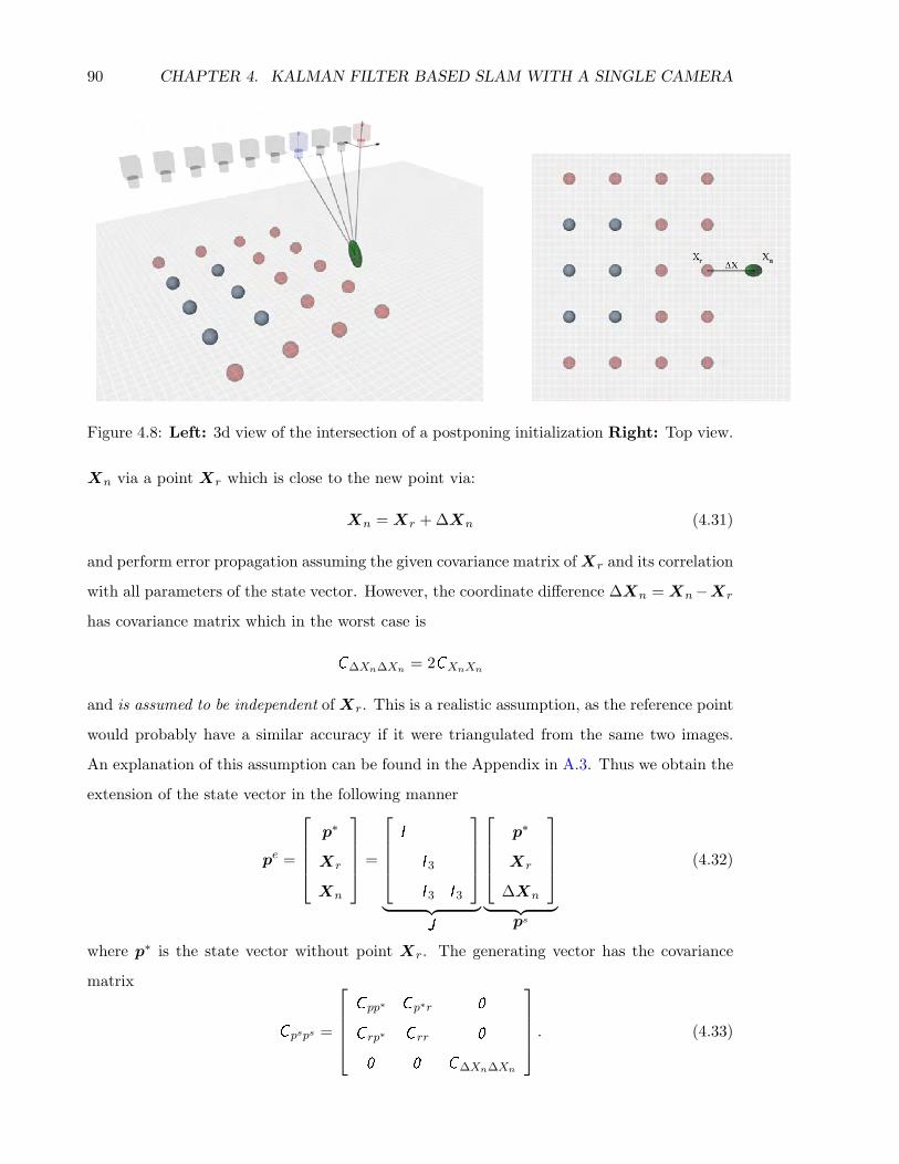
90 CHAPTER 4. KALMAN FILTER BASED SLAM WITH A SINGLE CAMERA
Figure 4.8: Left: 3d view of the intersection of a postponing initialization Right: Top view.
Xn via a point Xr which is close to the new point via:
Xn = Xr + ∆Xn (4.31)
and perform error propagation assuming the given covariance matrix ofXr and its correlation
with all parameters of the state vector. However, the coordinate difference ∆Xn = Xn−Xr
has covariance matrix which in the worst case is
C∆Xn∆Xn = 2CXnXn
and is assumed to be independent of Xr. This is a realistic assumption, as the reference point
would probably have a similar accuracy if it were triangulated from the same two images.
An explanation of this assumption can be found in the Appendix in A.3. Thus we obtain the
extension of the state vector in the following manner
pe =
p∗
Xr
Xn
=
I
I 3
I 3 I 3
︸ ︷︷ ︸
J
p∗
Xr
∆Xn
︸ ︷︷ ︸
ps
(4.32)
where p∗ is the state vector without point Xr. The generating vector has the covariance
matrix
C psps =
C pp∗ C p∗r 0
C rp∗ C rr 0
0 0 C∆Xn∆Xn
. (4.33)
4.4. GEOREFERENCING 91
The new covariance matrix of the state vector including the new landmark can now be
calculated as follows
C pepe = JC pspsJT =
C p∗p∗ C p∗r C p∗r
C rp∗ C rr C rr
C rp∗ C rr C rr + C∆Xn∆Xn
. (4.34)
This covariance matrix is guaranteed to be positive semi-definite and reflects the new situation
realistically. Obviously, the linear transformation is sparse and except for the addition of the
covariance matrices of the reference and the point difference only copies need to be realized,
which is extremely efficient. The algorithm for initialization of new points thus can be
summarized as follows:
Algorithm 4.2 Stable Initialization Procedure algorithm1: Detecting that a new point xn is observed at time tk.
2: repeat
3: Get the next observation at time t = t+ 1
4: Determine the frame at time to with the longest base length
d = argmaxto∈tk..t (|T t − T to |).
5: Determine Xn and its covariance matrix using frame pair (to, t) and its roundness Ln
6: until Ln > ΘL
7: Search for the point Xr closest to Xn.
8: Include the new point into the state vector using (4.32) and (4.34).
The proposed algorithm is able to initialize new points in a stable manner considering
the correlation structure.
4.4 Georeferencing
As we have shown before the initialization of the Kalman filter can be performed using control
points or a scale free bundle adjustment procedure. The control points can be given in a global
coordinate system as well as in a local reference system. In the following we will assume that
the initialization was performed by control points in a local reference system or by a scale free
bundle adjustment. In case we are able to detect at least three non-collinear control points
in a global reference system, we can transform the state vectors and its covariance using a
general Helmert-transformation. Using only three identical points a direct solution can be
92 CHAPTER 4. KALMAN FILTER BASED SLAM WITH A SINGLE CAMERA
computed. If more points are available we will obtain the best results using a least square
solution. In the following we will first derive the transformation using three points only. In a
second step we use the estimated parameters to transform the state and its covariance matrix
and additionally transform the gauge of the system with respect to the control points.
First, we assume three control points Xci corresponding to three object points Xi, i =
1..3 inside the state vector are given. For all points the incidence equation
Xci = MλMRM∆TXi (4.35)
with MT as a translation, MR as a rotation and MS as a scale matrix must hold. The
transformation parameter λ,R and ∆T can easily be derived using the direct solution for the
Helmert-transformation by Horn et al. (1988).
Now we are able to transform the state coordinate system to the world coordinate
system using the estimated parameters of the Helmert-transformation, also called the K-
transformation according to Molenaar (1981). The transformation can be obtained by a
non-linear function as
ph =
λR(qh)T + ∆T
qhq
k
[λR(qh) + ∆T ]i
(4.36)
for all camera orientations k and all points i inside the state vector. The transformation of
the covariance matrix can be performed using error propagation with the Jacobian
J =
λR(qh) 0 0
0 Υ(qh) 0
0 0 λR(qh)
. (4.37)
Actually, the gauge is still defined by the initialization method of the state vector. If de-
sired, the gauge can be transformed to the three reference points using the S-Transformation,
c. f. Baarda (1973) and Dickscheid et al. (2008). The transformation can be applied to the
covariance matrix in the following way: First create an stacked matrix A consistent of Ak for
all camera parameter and Ai for all object points
A =
A1..K
A1..I
(4.38)
4.4. ON PARTICLE BASED KALMAN FILTERING FOR SLAM 93
with
Ak =
I 3 −S(T ) T
0
−12q
T
12(qI 3 − S(q))
0
k
(4.39)
Ai =[I 3 0 0
]i. (4.40)
The Jacobian can then be computed by
JS = I − A(ATWA)−1
ATW (4.41)
with the gauge points selection matrix, where the diagonal elements according to the reference
point coordinates are one. Applying the Jacobian to the covariance matrix, the gauge is
transformed to the specified reference points.
The proposed geo-referencing algorithm is applicable using a sliding window state repre-
sentation. Furthermore, it is assumed that the transformation parameters are non-stochastic
and the control point uncertainty is zero.
4.5 On particle based Kalman filtering for simultaneous local-
ization and mapping
In section 3.4.3 we introduced the unscented transformation and its enhancement to a particle
based Kalman filter. In the literature the reader will find examples for successful applications
of the sigma point Kalman filter, e. g. Sunderhauf et al. (2007), van der Merwe (2004). Nev-
ertheless, we will show that these approaches will fail for the task of simultaneous localization
and mapping in case of larger uncertainties of parameters in the state vector.
First we will illustrate these at the error propagation using the inverse distance rep-
resentation and in a second example on the measurement update using a Euclidean point
representation. The distance d of a point is represented in the inverse distance representation
ρ = 1d . We assume the uncertainty representation is a Gaussian with mean µρ and their
standard deviation σρ. A small value µ is equal to a large distance and it is necessary that
d = lim+|ρ|→0
1ρ
=∞. (4.42)
On the other hand for negative values of µρ it is necessary that
d = lim−|ρ|→0
1ρ
= −∞. (4.43)
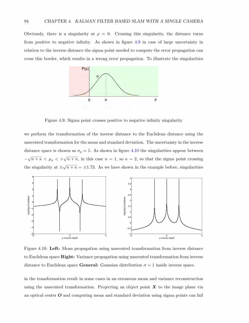
94 CHAPTER 4. KALMAN FILTER BASED SLAM WITH A SINGLE CAMERA
Obviously, there is a singularity at ρ = 0. Crossing this singularity, the distance turns
from positive to negative infinity. As shown in figure 4.9 in case of large uncertainty in
relation to the inverse distance the sigma point needed to compute the error propagation can
cross this border, which results in a wrong error propagation. To illustrate the singularities
Figure 4.9: Sigma point crosses positive to negative infinity singularity
we perform the transformation of the inverse distance to the Euclidean distance using the
unscented transformation for the mean and standard deviation. The uncertainty in the inverse
distance space is chosen as σρ = 1. As shown in figure 4.10 the singularities appear between
−√n+ κ < µρ < +
√n+ κ, in this case n = 1, so κ = 2, so that the sigma point crossing
the singularity at ±√n+ κ = ±1.73. As we have shown in the example before, singularities
−5 0 5−5
−4
−3
−2
−1
0
1
2
3
4
µ inverse depth
log1
0(µ)
Euc
lidea
n
−5 0 5−1
−0.5
0
0.5
1
1.5
2
2.5
3
3.5
4
µ inverse depth
log1
0(σ)
Euc
lidea
n
Figure 4.10: Left: Mean propagation using unscented transformation from inverse distance
to Euclidean space Right: Variance propagation using unscented transformation from inverse
distance to Euclidean space General: Gaussian distribution σ = 1 inside inverse space.
in the transformation result in some cases in an erroneous mean and variance reconstruction
using the unscented transformation. Projecting an object point X to the image plane via
an optical center O and computing mean and standard deviation using sigma points can fail
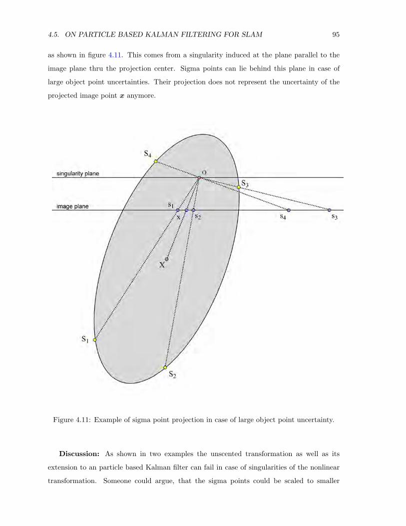
4.5. ON PARTICLE BASED KALMAN FILTERING FOR SLAM 95
as shown in figure 4.11. This comes from a singularity induced at the plane parallel to the
image plane thru the projection center. Sigma points can lie behind this plane in case of
large object point uncertainties. Their projection does not represent the uncertainty of the
projected image point x anymore.
Figure 4.11: Example of sigma point projection in case of large object point uncertainty.
Discussion: As shown in two examples the unscented transformation as well as its
extension to an particle based Kalman filter can fail in case of singularities of the nonlinear
transformation. Someone could argue, that the sigma points could be scaled to smaller
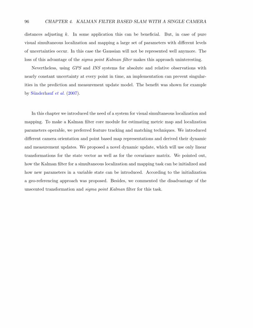
96 CHAPTER 4. KALMAN FILTER BASED SLAM WITH A SINGLE CAMERA
distances adjusting k. In some application this can be beneficial. But, in case of pure
visual simultaneous localization and mapping a large set of parameters with different levels
of uncertainties occur. In this case the Gaussian will not be represented well anymore. The
loss of this advantage of the sigma point Kalman filter makes this approach uninteresting.
Nevertheless, using GPS and INS systems for absolute and relative observations with
nearly constant uncertainty at every point in time, an implementation can prevent singular-
ities in the prediction and measurement update model. The benefit was shown for example
by Sunderhauf et al. (2007).
In this chapter we introduced the need of a system for visual simultaneous localization and
mapping. To make a Kalman filter core module for estimating metric map and localization
parameters operable, we preferred feature tracking and matching techniques. We introduced
different camera orientation and point based map representations and derived their dynamic
and measurement updates. We proposed a novel dynamic update, which will use only linear
transformations for the state vector as well as for the covariance matrix. We pointed out,
how the Kalman filter for a simultaneous localization and mapping task can be initialized and
how new parameters in a variable state can be introduced. According to the initialization
a geo-referencing approach was proposed. Besides, we commented the disadvantage of the
unscented transformation and sigma point Kalman filter for this task.
Chapter 5
Evaluation of the proposed methods
In this chapter the applicability of Kalman filter based localization and mapping will be
demonstrated. In the classical aerial-triangulation images are be taken with large baselines
according to an image overlapping of approximately 60%. Therefore, an object point typically
is visible in at least three images. Special high resolution cameras with a stable interior
orientation will be used. These cameras are mounted on a motion compensation platform to
prevent motion blur coming from longitudinal and angular velocity. In contrast we will use
an image sequence taken from an unmanned aerial vehicle. The camera is a low resolution
consumer video camera. Due to the limited speed of flight in our case we deal with an
overlapping ratio of consecutive images of larger than 95%. Hence object points are visible
multiple times with small disparities in consecutive images, also called frames.
First we will derive a general law to assess the theoretical accuracy of a photogrammetric
strip. To neglect systematic errors arising from camera calibration errors, gross errors in
the point based feature tracking and influences of the approximate values of the parameters
the law will be determined using synthetic observation of a simulated environment. In a
second step the influence of the representation and initialization of new object points in
a Kalman filter will be analyzed. In an evaluation we will compare the different methods
regarding accuracy and consistency. To proof the applicability of our point based feature
tracking we will use two different kinds of rendered scenes. One scene consists of a planar
surface mapped with real image data of a high altitude airborne image data provided by the
company Vexcel. The second scene consists of a model of the Basilika St. Peter in Rome.
The texture was generated using a fractal texture algorithm. For both scenes the interior
and exterior orientation was extracted from the rendering software. Finally, we will run the
97
98 CHAPTER 5. EVALUATION OF THE PROPOSED METHODS
algorithms on a full real data set.
5.1 On the theoretical accuracy of photogrammetric strips
from image sequences
In the classical aero-photogrammetry a general law for the evolution of the triangulation
accuracy of a strip flight has been found by Finsterwalder & Hofmann (1964). The proposed
law specifies the accuracy of the camera location and angular orientation depending on the
image number and the base length between consecutive frames up to a scale factor. The scale
factor depends on the configuration of the photogrammetric strip, the camera parameters and
the measurement accuracy. For every configuration the scale factor have to be determined
individually. In this section we extend this law, so that we incorporate the flight configuration
parameters as well as the camera parameters. This extended general law has the following
challenge:
a) The goal of a general law is to calculate the achievable accuracy under specific parameter
settings using a simple approximation function.
b) The function has to be as precise as possible for a specific interval for the given param-
eter.
First, we have to distinguished between a systematic errors and a stochastic errors. The error
propagation laws by Finsterwalder & Hofmann (1964) summarized in table 5.1 are useful to
assess the achievable accuracy of classical photogrammetric aerial-triangulation for very long
strips. This law has been derived from the error propagation and has been simplified for very
long strips. We can interpret the variance transition factors in that way, that smaller factor
yield in an accuracy improvement of the estimated camera orientations. These laws are true
under the condition that the gauge definition depends on the first frame and the covariance
matrix has a significant band structure for the strip. However, there are only a small number
of different aerial camera systems available and the configuration of flight strips is typically
fixed to 60% longitudinal overlapping. For this reason only a small set of variance transition
factors has to be analyzed for different configurations.
In the field of an unmanned aerial vehicle arbitrary cameras and flight configurations are
possible. In this case the variance transition factors are functions of a large set of parameters,
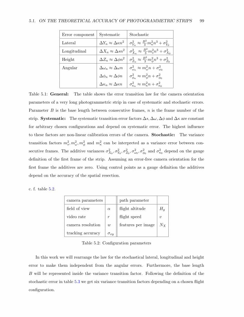
5.1. ON THE THEORETICAL ACCURACY OF PHOTOGRAMMETRIC STRIPS 99
Error component Systematic Stochastic
Lateral ∆Yn ≈ ∆κn2 σ2Yn≈ B2
3 m2κn
3 + σ2Y0
Longitudinal ∆Xn ≈ ∆sn2 σ2Xn≈ B2
3 m2sn
3 + σ2X0
Height ∆Zn ≈ ∆φn2 σ2Zn≈ B2
3 m2φn
3 + σ2Z0
Angular ∆ωn ≈ ∆ωn σ2ωn ≈ m
2ωn+ σ2
ω0
∆φn ≈ ∆φn σ2φn≈ m2
φn+ σ2φ0
∆κn ≈ ∆κn σ2κn ≈ m
2κn+ σ2
κ0
Table 5.1: General: The table shows the error transition law for the camera orientation
parameters of a very long photogrammetric strip in case of systematic and stochastic errors.
Parameter B is the base length between consecutive frames, n is the frame number of the
strip. Systematic: The systematic transition error factors ∆s,∆ω,∆φ and ∆κ are constant
for arbitrary chosen configurations and depend on systematic error. The highest influence
to these factors are non-linear calibration errors of the camera. Stochastic: The variance
transition factors m2s,m
2ω,m
2φ and m2
κ can be interpreted as a variance error between con-
secutive frames. The additive variances σ2X0, σ2
Y0, σ2
Z0, σ2
ω0, σ2
φ0and σ2
κ0depend on the gauge
definition of the first frame of the strip. Assuming an error-free camera orientation for the
first frame the additives are zero. Using control points as a gauge definition the additives
depend on the accuracy of the spatial resection.
c. f. table 5.2.
camera parameters path parameter
field of view α flight altitude Hg
video rate r flight speed v
camera resolution w features per image NX
tracking accuracy σxy
Table 5.2: Configuration parameters
In this work we will rearrange the law for the stochastical lateral, longitudinal and height
error to make them independent from the angular errors. Furthermore, the base length
B will be represented inside the variance transition factor. Following the definition of the
stochastic error in table 5.3 we get six variance transition factors depending on a chosen flight
configuration.
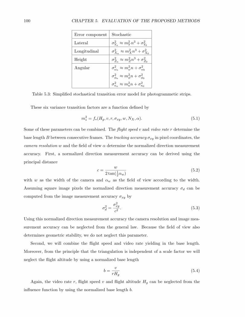
100 CHAPTER 5. EVALUATION OF THE PROPOSED METHODS
Error component Stochastic
Lateral σ2Yn≈ m2
Y n3 + σ2
Y0
Longitudinal σ2Xn≈ m2
Xn3 + σ2
X0
Height σ2Zn≈ m2
Zn3 + σ2
Z0
Angular σ2ωn ≈ m
2ωn+ σ2
ω0
σ2φn≈ m2
φn+ σ2φ0
σ2κn ≈ m
2κn+ σ2
κ0
Table 5.3: Simplified stochastical transition error model for photogrammetic strips.
These six variance transition factors are a function defined by
m2∗ = f∗(Hg, v, r, σxy, w,NX , α). (5.1)
Some of these parameters can be combined. The flight speed v and video rate r determine the
base length B between consecutive frames. The tracking accuracy σxy in pixel coordinates, the
camera resolution w and the field of view α determine the normalized direction measurement
accuracy. First, a normalized direction measurement accuracy can be derived using the
principal distance
c =w
2 tan(12αw)
(5.2)
with w as the width of the camera and αw as the field of view according to the width.
Assuming square image pixels the normalized direction measurement accuracy σd can be
computed from the image measurement accuracy σxy by
σ2d =
σ2xy
c2. (5.3)
Using this normalized direction measurement accuracy the camera resolution and image mea-
surement accuracy can be neglected from the general law. Because the field of view also
determines geometric stability, we do not neglect this parameter.
Second, we will combine the flight speed and video rate yielding in the base length.
Moreover, from the principle that the triangulation is independent of a scale factor we will
neglect the flight altitude by using a normalized base length
b =v
rHg(5.4)
Again, the video rate r, flight speed v and flight altitude Hg can be neglected from the
influence function by using the normalized base length b.
5.1. ON THE THEORETICAL ACCURACY OF PHOTOGRAMMETRIC STRIPS 101
As a consequence the achievable accuracy of a photogrammetric strip depends on four
parameters. In the following we will analyze in some experiments, how does the accuracy
depends on these parameters.
5.1.1 Experimental setup
As we shown above the stochastical accuracy of a photogrammetric strip will be influenced by
four parameters. To analyze their influence we here define four experiments. The parameter
themeself are physically bounded. For example, a camera view angle larger than 180 is
not reasonable. Furthermore the smallest base length can be zero, the largest base length
is restricted by the overlapping, and so indirect of the maximal possible video rate and the
maximum flight speed.
In table 5.4 we will define a standard configuration and different experiment configurations
of our simulated environment.
Exp 1: In this experiment we will change the field of view angle between 40 and 120 degree.
The lowest bound is a typical small angle camera objective, the upper bound is a wide
angle objective.
Exp 2: This experiment varies the base length, depending on the video rate and the flight speed
according to equation (5.4). The maximum base length is restricted by an overlapping
ratio of the images of approximately 60% to guarantee, so that a subset of object points
are visible in at least three images. This is neccessary to achieve the transition of the
scale factor to consecutive frames in a bundle adjustment solution.
Exp 3: The fully automatic detection and tracking accuracy can be broken down to σxy ≈
0.1[pel] using a sub-pixel estimation. Typically point based features on the original
image resolution are unstable in case of image noise. Therefore it is suitable to track
features at a reduced resolution which can by quantified by a change of the tracking
accuracy.
Exp 4: The mean number of used object points in an image is proportional to the size of the
unknown parameter. Here a trade of between computational complexity and achievable
accuracy has to be found. Furthermore, the content of the observed scene limits the
number of identifiable and trackable object points. It has been shown in our experiments
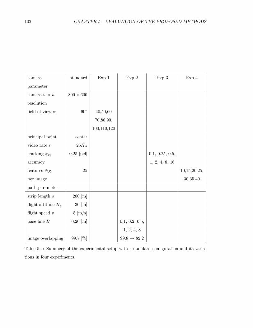
102 CHAPTER 5. EVALUATION OF THE PROPOSED METHODS
camera standard Exp 1 Exp 2 Exp 3 Exp 4
parameter
camera w × h 800× 600
resolution
field of view α 90 40,50,60
70,80,90,
100,110,120
principal point center
video rate r 25Hz
tracking σxy 0.25 [pel] 0.1, 0.25, 0.5,
accuracy 1, 2, 4, 8, 16
features NX 25 10,15,20,25,
per image 30,35,40
path parameter
strip length s 200 [m]
flight altitude Hg 30 [m]
flight speed v 5 [m/s]
base line B 0.20 [m] 0.1, 0.2, 0.5,
1, 2, 4, 8
image overlapping 99.7 [%] 99.8 → 82.2
Table 5.4: Summery of the experimental setup with a standard configuration and its varia-
tions in four experiments.
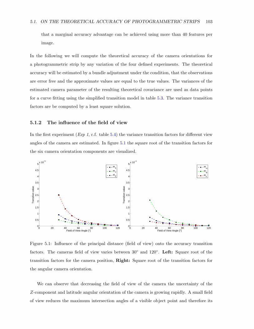
5.1. ON THE THEORETICAL ACCURACY OF PHOTOGRAMMETRIC STRIPS 103
that a marginal accuracy advantage can be achieved using more than 40 features per
image.
In the following we will compute the theoretical accuracy of the camera orientations for
a photogrammetric strip by any variation of the four defined experiments. The theoretical
accuracy will be estimated by a bundle adjustment under the condition, that the observations
are error free and the approximate values are equal to the true values. The variances of the
estimated camera parameter of the resulting theoretical covariance are used as data points
for a curve fitting using the simplified transition model in table 5.3. The variance transition
factors are be computed by a least square solution.
5.1.2 The influence of the field of view
In the first experiment (Exp 1, c.f. table 5.4) the variance transition factors for different view
angles of the camera are estimated. In figure 5.1 the square root of the transition factors for
the six camera orientation components are visualized.
0 20 40 60 80 100 1200
0.5
1
1.5
2
2.5
3
3.5
4
4.5
5x 10
−5
Field of View Angle [°]
Tra
nsiti
on v
alue
mX
mY
mZ
0 20 40 60 80 100 1200
0.5
1
1.5
2
2.5
3
3.5
4
4.5
5x 10
−4
Field of View Angle [°]
Tra
nsiti
on v
alue
mωmφmκ
Figure 5.1: Influence of the principal distance (field of view) onto the accuracy transition
factors. The cameras field of view varies between 30 and 120. Left: Square root of the
transition factors for the camera position, Right: Square root of the transition factors for
the angular camera orientation.
We can observe that decreasing the field of view of the camera the uncertainty of the
Z-component and latitude angular orientation of the camera is growing rapidly. A small field
of view reduces the maximum intersection angles of a visible object point and therefore its
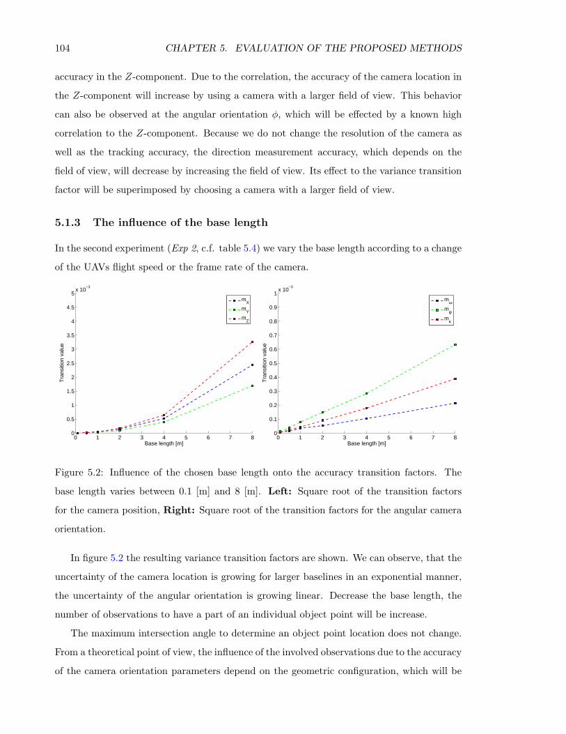
104 CHAPTER 5. EVALUATION OF THE PROPOSED METHODS
accuracy in the Z-component. Due to the correlation, the accuracy of the camera location in
the Z-component will increase by using a camera with a larger field of view. This behavior
can also be observed at the angular orientation φ, which will be effected by a known high
correlation to the Z-component. Because we do not change the resolution of the camera as
well as the tracking accuracy, the direction measurement accuracy, which depends on the
field of view, will decrease by increasing the field of view. Its effect to the variance transition
factor will be superimposed by choosing a camera with a larger field of view.
5.1.3 The influence of the base length
In the second experiment (Exp 2, c.f. table 5.4) we vary the base length according to a change
of the UAVs flight speed or the frame rate of the camera.
0 1 2 3 4 5 6 7 80
0.5
1
1.5
2
2.5
3
3.5
4
4.5
5x 10
−3
Base length [m]
Tra
nsiti
on v
alue
mX
mY
mZ
0 1 2 3 4 5 6 7 80
0.1
0.2
0.3
0.4
0.5
0.6
0.7
0.8
0.9
1x 10
−3
Base length [m]
Tra
nsiti
on v
alue
mωmφmκ
Figure 5.2: Influence of the chosen base length onto the accuracy transition factors. The
base length varies between 0.1 [m] and 8 [m]. Left: Square root of the transition factors
for the camera position, Right: Square root of the transition factors for the angular camera
orientation.
In figure 5.2 the resulting variance transition factors are shown. We can observe, that the
uncertainty of the camera location is growing for larger baselines in an exponential manner,
the uncertainty of the angular orientation is growing linear. Decrease the base length, the
number of observations to have a part of an individual object point will be increase.
The maximum intersection angle to determine an object point location does not change.
From a theoretical point of view, the influence of the involved observations due to the accuracy
of the camera orientation parameters depend on the geometric configuration, which will be
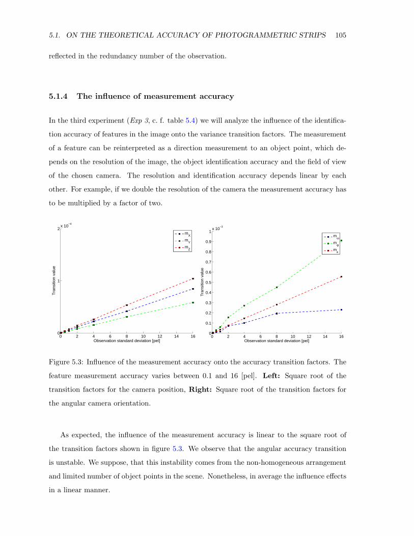
5.1. ON THE THEORETICAL ACCURACY OF PHOTOGRAMMETRIC STRIPS 105
reflected in the redundancy number of the observation.
5.1.4 The influence of measurement accuracy
In the third experiment (Exp 3, c. f. table 5.4) we will analyze the influence of the identifica-
tion accuracy of features in the image onto the variance transition factors. The measurement
of a feature can be reinterpreted as a direction measurement to an object point, which de-
pends on the resolution of the image, the object identification accuracy and the field of view
of the chosen camera. The resolution and identification accuracy depends linear by each
other. For example, if we double the resolution of the camera the measurement accuracy has
to be multiplied by a factor of two.
0 2 4 6 8 10 12 14 160
1
2x 10
−4
Observation standard deviation [pel]
Tra
nsiti
on v
alue
mX
mY
mZ
0 2 4 6 8 10 12 14 160
0.1
0.2
0.3
0.4
0.5
0.6
0.7
0.8
0.9
1x 10
−3
Observation standard deviation [pel]
Tra
nsiti
on v
alue
mωmφmκ
Figure 5.3: Influence of the measurement accuracy onto the accuracy transition factors. The
feature measurement accuracy varies between 0.1 and 16 [pel]. Left: Square root of the
transition factors for the camera position, Right: Square root of the transition factors for
the angular camera orientation.
As expected, the influence of the measurement accuracy is linear to the square root of
the transition factors shown in figure 5.3. We observe that the angular accuracy transition
is unstable. We suppose, that this instability comes from the non-homogeneous arrangement
and limited number of object points in the scene. Nonetheless, in average the influence effects
in a linear manner.
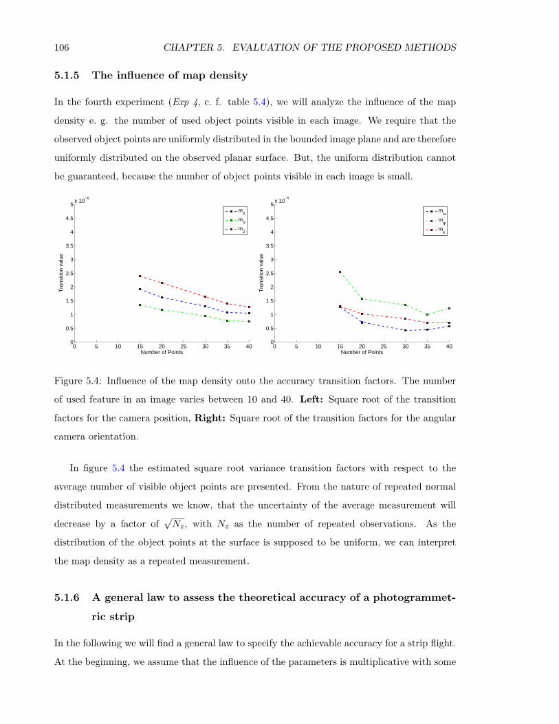
106 CHAPTER 5. EVALUATION OF THE PROPOSED METHODS
5.1.5 The influence of map density
In the fourth experiment (Exp 4, c. f. table 5.4), we will analyze the influence of the map
density e. g. the number of used object points visible in each image. We require that the
observed object points are uniformly distributed in the bounded image plane and are therefore
uniformly distributed on the observed planar surface. But, the uniform distribution cannot
be guaranteed, because the number of object points visible in each image is small.
0 5 10 15 20 25 30 35 400
0.5
1
1.5
2
2.5
3
3.5
4
4.5
5x 10
−6
Number of Points
Tra
nsiti
on v
alue
mX
mY
mZ
0 5 10 15 20 25 30 35 400
0.5
1
1.5
2
2.5
3
3.5
4
4.5
5x 10
−5
Number of Points
Tra
nsiti
on v
alue
mωmφmκ
Figure 5.4: Influence of the map density onto the accuracy transition factors. The number
of used feature in an image varies between 10 and 40. Left: Square root of the transition
factors for the camera position, Right: Square root of the transition factors for the angular
camera orientation.
In figure 5.4 the estimated square root variance transition factors with respect to the
average number of visible object points are presented. From the nature of repeated normal
distributed measurements we know, that the uncertainty of the average measurement will
decrease by a factor of√Nz, with Nz as the number of repeated observations. As the
distribution of the object points at the surface is supposed to be uniform, we can interpret
the map density as a repeated measurement.
5.1.6 A general law to assess the theoretical accuracy of a photogrammet-
ric strip
In the following we will find a general law to specify the achievable accuracy for a strip flight.
At the beginning, we assume that the influence of the parameters is multiplicative with some
5.1. ON THE THEORETICAL ACCURACY OF PHOTOGRAMMETRIC STRIPS 107
unknown exponentials ib,α,N,d and unknown factors k. Furthermore, the transition factors
for the angular orientation components must be independent of the flight altitude Hg.
m2X,Y,Z = kX,Y,Z · bib · f(α)iα ·N iN
X · σidd ·H
2g (5.5)
m2ω,φ,κ = kω,φ,κ · bib · f(α)iα ·N iN
X · σidd (5.6)
As we have shown in figures 5.3, the accuracy transition factor grows linearly with the ex-
pected tracking accuracy. Therefore the exponent should be two. As we mentioned before,
doubling the number of observations will divide the uncertainty by the factor√
2. Therefore
the exponent of NX can be set to minus one. The length of the base between consecutive
images directly influences the number of observations of an object point. Furthermore, the
maximum intersection angle will be divided in more peaces of intersections. The influence
of every individual observation caused by a smaller baseline is not equal. In figure 5.2 we
observe, that the accuracy transition factors for the angular orientation increase linearly with
respect to the base length. Therefore we set the exponent to two. The influence of the base
length to the location parameter seems to be square. Therefore we set the exponent to 4.
We model the influence of the field of view angle α using a trigonometric function. The
choice is motivated by the dependency of an angle. As we found out, a good approximation
is achievable using different exponents for the six component.
fX(α) = tan(α
2
)−5(5.7)
fY (α) = tan(α
2
)−4(5.8)
fZ(α) = tan(α
2
)−6(5.9)
fω(α) = tan(α
2
)−6(5.10)
fφ(α) = tan(α
2
)−6(5.11)
fκ(α) = tan(α
2
)−4(5.12)
and we finally obtain the approximation functions
m2X,Y,Z = kX,Y,Z
b4
NXfX,Y,Z(α) σ2
d H2g (5.13)
m2ω,φ,κ = kω,φ,κ
b2
NXfω,φ,κ(α) σ2
d (5.14)
Using the determined transition factors of the four experiments we estimate the constant
factors kX , kY , kZ , kω, kφ and kκ in a least square solution using equations (5.13) and (5.14)
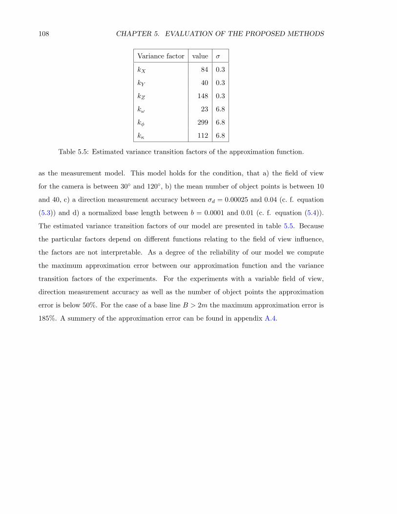
108 CHAPTER 5. EVALUATION OF THE PROPOSED METHODS
Variance factor value σ
kX 84 0.3
kY 40 0.3
kZ 148 0.3
kω 23 6.8
kφ 299 6.8
kκ 112 6.8
Table 5.5: Estimated variance transition factors of the approximation function.
as the measurement model. This model holds for the condition, that a) the field of view
for the camera is between 30 and 120, b) the mean number of object points is between 10
and 40, c) a direction measurement accuracy between σd = 0.00025 and 0.04 (c. f. equation
(5.3)) and d) a normalized base length between b = 0.0001 and 0.01 (c. f. equation (5.4)).
The estimated variance transition factors of our model are presented in table 5.5. Because
the particular factors depend on different functions relating to the field of view influence,
the factors are not interpretable. As a degree of the reliability of our model we compute
the maximum approximation error between our approximation function and the variance
transition factors of the experiments. For the experiments with a variable field of view,
direction measurement accuracy as well as the number of object points the approximation
error is below 50%. For the case of a base line B > 2m the maximum approximation error is
185%. A summery of the approximation error can be found in appendix A.4.
5.2. THE INFLUENCE OF THE INITIALIZATION METHOD 109
5.2 The influence of the initialization method of new object
points in a Kalman filter based estimation
In the following we will analyze, how the Kalman filter based approaches performs on the same
dataset using different initialization methods for new object points proposed in section 4.3. As
we already mentioned, the initialization has a main influence on the consistency of the result
due to the small disparities of feature observations in consecutive images, which is caused by
a poorly Gaussian approximation of the object point determination by ray intersection. In all
experiments, where the new object points will be introduced instantly, new object points are
initialized at the first projection ray with a huge uncertainty. The distance will be assumed
to be known using the ground truth distance obtainable as the Euclidean distance between
the camera projection center and the object point location. The object point coordinate to
be introduced can be computed using equation (3.63). As the dynamic motion model will be
used to obtain approximate values for the camera orientation only, the error propagation will
be computed with large system noise for the camera parameter transition. As a consequence
the uncertainty of the predicted camera parameter is large and the correlations between the
predicted camera parameters and previous camera parameters as well as the object points
after the prediction step are equal to zero. Therefore, our dynamic model does not restrict
the trajectory. We do so, because the camera trajectory in the bundle adjustment solution is
also not restricted and therefore the results are comparable. The measurement update can be
considered as a spatial resection to obtain the camera orientation. An update of the object
point locations will be caused by the influence of the residuals between the measurements
and the back-projected object points themselves.
We will run the Kalman filter using the initialization methods with
1. Euclidean representation
2. Euclidean representation with sliding window camera model
3. Inverse distance representation
4. Inverse distance representation with reparameterization to the Euclidean representation
5. Delayed initialization with sliding window camera model
6. Delayed initialization using stable initialization procedure
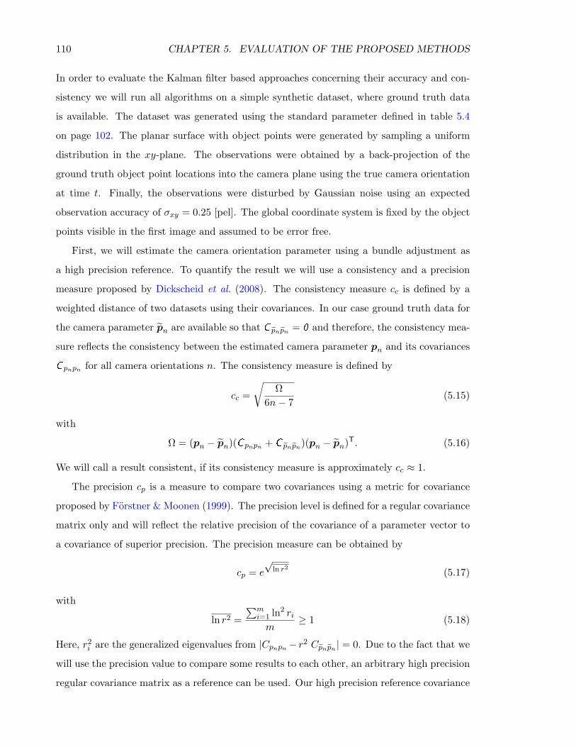
110 CHAPTER 5. EVALUATION OF THE PROPOSED METHODS
In order to evaluate the Kalman filter based approaches concerning their accuracy and con-
sistency we will run all algorithms on a simple synthetic dataset, where ground truth data
is available. The dataset was generated using the standard parameter defined in table 5.4
on page 102. The planar surface with object points were generated by sampling a uniform
distribution in the xy-plane. The observations were obtained by a back-projection of the
ground truth object point locations into the camera plane using the true camera orientation
at time t. Finally, the observations were disturbed by Gaussian noise using an expected
observation accuracy of σxy = 0.25 [pel]. The global coordinate system is fixed by the object
points visible in the first image and assumed to be error free.
First, we will estimate the camera orientation parameter using a bundle adjustment as
a high precision reference. To quantify the result we will use a consistency and a precision
measure proposed by Dickscheid et al. (2008). The consistency measure cc is defined by a
weighted distance of two datasets using their covariances. In our case ground truth data for
the camera parameter pn are available so that C pnpn = 0 and therefore, the consistency mea-
sure reflects the consistency between the estimated camera parameter pn and its covariances
C pnpn for all camera orientations n. The consistency measure is defined by
cc =
√Ω
6n− 7(5.15)
with
Ω = (pn − pn)(C pnpn + C pnpn)(pn − pn)T. (5.16)
We will call a result consistent, if its consistency measure is approximately cc ≈ 1.
The precision cp is a measure to compare two covariances using a metric for covariance
proposed by Forstner & Moonen (1999). The precision level is defined for a regular covariance
matrix only and will reflect the relative precision of the covariance of a parameter vector to
a covariance of superior precision. The precision measure can be obtained by
cp = e
√ln r2 (5.17)
with
ln r2 =∑m
i=1 ln2 rim
≥ 1 (5.18)
Here, r2i are the generalized eigenvalues from |Cpnpn − r2 Cpnpn | = 0. Due to the fact that we
will use the precision value to compare some results to each other, an arbitrary high precision
regular covariance matrix as a reference can be used. Our high precision reference covariance
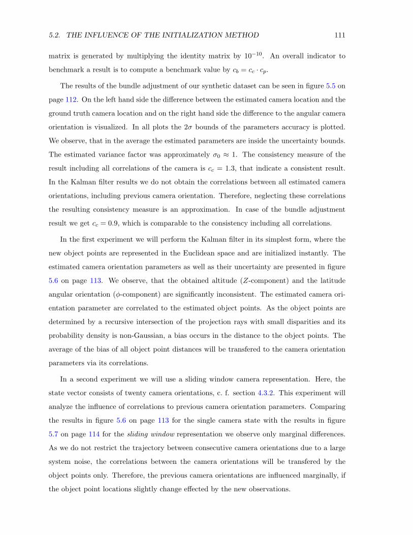
5.2. THE INFLUENCE OF THE INITIALIZATION METHOD 111
matrix is generated by multiplying the identity matrix by 10−10. An overall indicator to
benchmark a result is to compute a benchmark value by cb = cc · cp.
The results of the bundle adjustment of our synthetic dataset can be seen in figure 5.5 on
page 112. On the left hand side the difference between the estimated camera location and the
ground truth camera location and on the right hand side the difference to the angular camera
orientation is visualized. In all plots the 2σ bounds of the parameters accuracy is plotted.
We observe, that in the average the estimated parameters are inside the uncertainty bounds.
The estimated variance factor was approximately σ0 ≈ 1. The consistency measure of the
result including all correlations of the camera is cc = 1.3, that indicate a consistent result.
In the Kalman filter results we do not obtain the correlations between all estimated camera
orientations, including previous camera orientation. Therefore, neglecting these correlations
the resulting consistency measure is an approximation. In case of the bundle adjustment
result we get cc = 0.9, which is comparable to the consistency including all correlations.
In the first experiment we will perform the Kalman filter in its simplest form, where the
new object points are represented in the Euclidean space and are initialized instantly. The
estimated camera orientation parameters as well as their uncertainty are presented in figure
5.6 on page 113. We observe, that the obtained altitude (Z-component) and the latitude
angular orientation (φ-component) are significantly inconsistent. The estimated camera ori-
entation parameter are correlated to the estimated object points. As the object points are
determined by a recursive intersection of the projection rays with small disparities and its
probability density is non-Gaussian, a bias occurs in the distance to the object points. The
average of the bias of all object point distances will be transfered to the camera orientation
parameters via its correlations.
In a second experiment we will use a sliding window camera representation. Here, the
state vector consists of twenty camera orientations, c. f. section 4.3.2. This experiment will
analyze the influence of correlations to previous camera orientation parameters. Comparing
the results in figure 5.6 on page 113 for the single camera state with the results in figure
5.7 on page 114 for the sliding window representation we observe only marginal differences.
As we do not restrict the trajectory between consecutive camera orientations due to a large
system noise, the correlations between the camera orientations will be transfered by the
object points only. Therefore, the previous camera orientations are influenced marginally, if
the object point locations slightly change effected by the new observations.
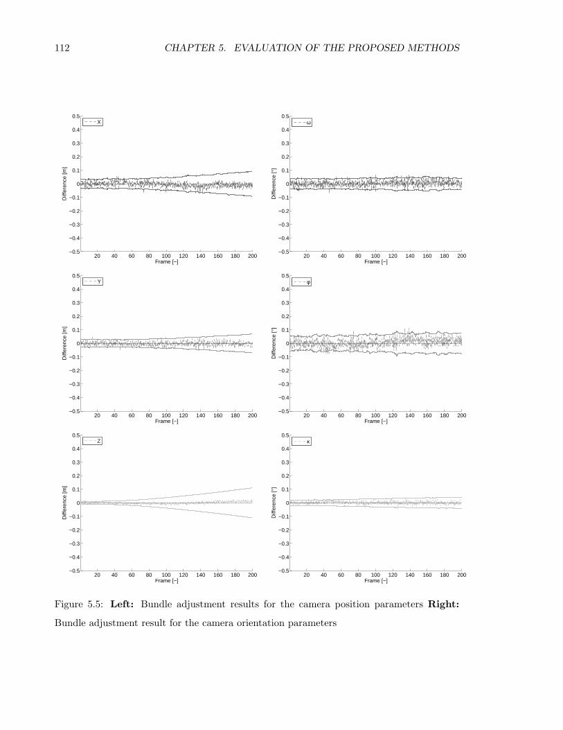
112 CHAPTER 5. EVALUATION OF THE PROPOSED METHODS
20 40 60 80 100 120 140 160 180 200−0.5
−0.4
−0.3
−0.2
−0.1
0
0.1
0.2
0.3
0.4
0.5
Diff
eren
ce [m
]
Frame [−]
X
20 40 60 80 100 120 140 160 180 200−0.5
−0.4
−0.3
−0.2
−0.1
0
0.1
0.2
0.3
0.4
0.5
Diff
eren
ce [°
]
Frame [−]
ω
20 40 60 80 100 120 140 160 180 200−0.5
−0.4
−0.3
−0.2
−0.1
0
0.1
0.2
0.3
0.4
0.5
Diff
eren
ce [m
]
Frame [−]
Y
20 40 60 80 100 120 140 160 180 200−0.5
−0.4
−0.3
−0.2
−0.1
0
0.1
0.2
0.3
0.4
0.5D
iffer
ence
[°]
Frame [−]
φ
20 40 60 80 100 120 140 160 180 200−0.5
−0.4
−0.3
−0.2
−0.1
0
0.1
0.2
0.3
0.4
0.5
Diff
eren
ce [m
]
Frame [−]
Z
20 40 60 80 100 120 140 160 180 200−0.5
−0.4
−0.3
−0.2
−0.1
0
0.1
0.2
0.3
0.4
0.5
Diff
eren
ce [°
]
Frame [−]
κ
Figure 5.5: Left: Bundle adjustment results for the camera position parameters Right:
Bundle adjustment result for the camera orientation parameters
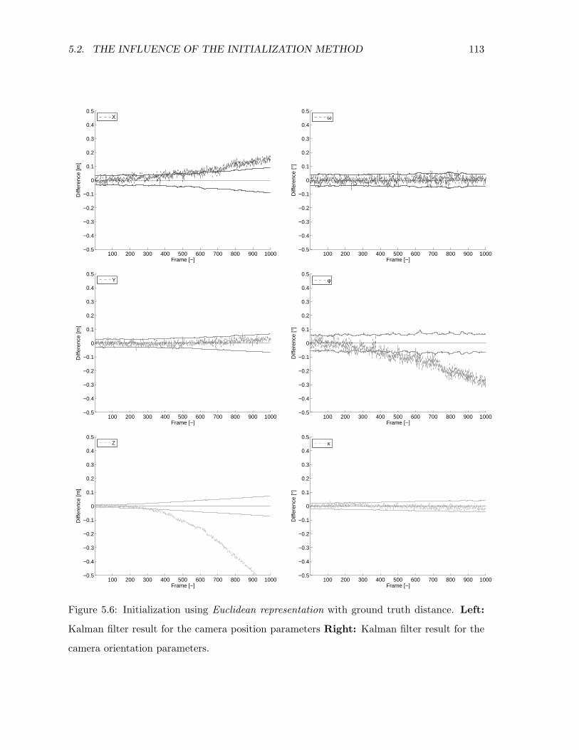
5.2. THE INFLUENCE OF THE INITIALIZATION METHOD 113
100 200 300 400 500 600 700 800 900 1000−0.5
−0.4
−0.3
−0.2
−0.1
0
0.1
0.2
0.3
0.4
0.5
Diff
eren
ce [m
]
Frame [−]
X
100 200 300 400 500 600 700 800 900 1000−0.5
−0.4
−0.3
−0.2
−0.1
0
0.1
0.2
0.3
0.4
0.5
Diff
eren
ce [°
]
Frame [−]
ω
100 200 300 400 500 600 700 800 900 1000−0.5
−0.4
−0.3
−0.2
−0.1
0
0.1
0.2
0.3
0.4
0.5
Diff
eren
ce [m
]
Frame [−]
Y
100 200 300 400 500 600 700 800 900 1000−0.5
−0.4
−0.3
−0.2
−0.1
0
0.1
0.2
0.3
0.4
0.5
Diff
eren
ce [°
]
Frame [−]
φ
100 200 300 400 500 600 700 800 900 1000−0.5
−0.4
−0.3
−0.2
−0.1
0
0.1
0.2
0.3
0.4
0.5
Diff
eren
ce [m
]
Frame [−]
Z
100 200 300 400 500 600 700 800 900 1000−0.5
−0.4
−0.3
−0.2
−0.1
0
0.1
0.2
0.3
0.4
0.5
Diff
eren
ce [°
]
Frame [−]
κ
Figure 5.6: Initialization using Euclidean representation with ground truth distance. Left:
Kalman filter result for the camera position parameters Right: Kalman filter result for the
camera orientation parameters.

114 CHAPTER 5. EVALUATION OF THE PROPOSED METHODS
100 200 300 400 500 600 700 800 900 1000−0.5
−0.4
−0.3
−0.2
−0.1
0
0.1
0.2
0.3
0.4
0.5
Diff
eren
ce [m
]
Frame [−]
X
100 200 300 400 500 600 700 800 900 1000−0.5
−0.4
−0.3
−0.2
−0.1
0
0.1
0.2
0.3
0.4
0.5
Diff
eren
ce [°
]
Frame [−]
ω
100 200 300 400 500 600 700 800 900 1000−0.5
−0.4
−0.3
−0.2
−0.1
0
0.1
0.2
0.3
0.4
0.5
Diff
eren
ce [m
]
Frame [−]
Y
100 200 300 400 500 600 700 800 900 1000−0.5
−0.4
−0.3
−0.2
−0.1
0
0.1
0.2
0.3
0.4
0.5D
iffer
ence
[°]
Frame [−]
φ
100 200 300 400 500 600 700 800 900 1000−0.5
−0.4
−0.3
−0.2
−0.1
0
0.1
0.2
0.3
0.4
0.5
Diff
eren
ce [m
]
Frame [−]
Z
100 200 300 400 500 600 700 800 900 1000−0.5
−0.4
−0.3
−0.2
−0.1
0
0.1
0.2
0.3
0.4
0.5
Diff
eren
ce [°
]
Frame [−]
κ
Figure 5.7: Initialization using ground truth distance and a sliding window camera represen-
tation (20). Left: Kalman filter result for the camera position parameters Right: Kalman
filter result for the camera orientation parameters.
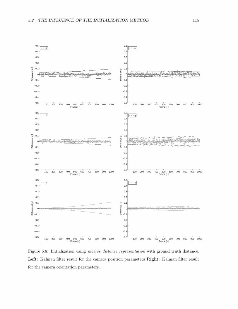
5.2. THE INFLUENCE OF THE INITIALIZATION METHOD 115
100 200 300 400 500 600 700 800 900 1000−0.5
−0.4
−0.3
−0.2
−0.1
0
0.1
0.2
0.3
0.4
0.5
Diff
eren
ce [m
]
Frame [−]
X
100 200 300 400 500 600 700 800 900 1000−0.5
−0.4
−0.3
−0.2
−0.1
0
0.1
0.2
0.3
0.4
0.5
Diff
eren
ce [°
]
Frame [−]
ω
100 200 300 400 500 600 700 800 900 1000−0.5
−0.4
−0.3
−0.2
−0.1
0
0.1
0.2
0.3
0.4
0.5
Diff
eren
ce [m
]
Frame [−]
Y
100 200 300 400 500 600 700 800 900 1000−0.5
−0.4
−0.3
−0.2
−0.1
0
0.1
0.2
0.3
0.4
0.5
Diff
eren
ce [°
]
Frame [−]
φ
100 200 300 400 500 600 700 800 900 1000−0.5
−0.4
−0.3
−0.2
−0.1
0
0.1
0.2
0.3
0.4
0.5
Diff
eren
ce [m
]
Frame [−]
Z
100 200 300 400 500 600 700 800 900 1000−0.5
−0.4
−0.3
−0.2
−0.1
0
0.1
0.2
0.3
0.4
0.5
Diff
eren
ce [°
]
Frame [−]
κ
Figure 5.8: Initialization using inverse distance representation with ground truth distance.
Left: Kalman filter result for the camera position parameters Right: Kalman filter result
for the camera orientation parameters.
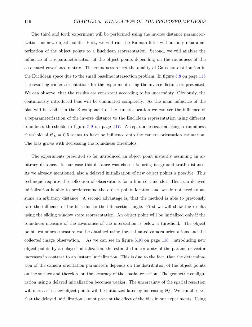
116 CHAPTER 5. EVALUATION OF THE PROPOSED METHODS
The third and forth experiment will be performed using the inverse distance parameter-
ization for new object points. First, we will run the Kalman filter without any reparame-
terization of the object points to a Euclidean representation. Second, we will analyze the
influence of a reparameterization of the object points depending on the roundness of the
associated covariance matrix. The roundness reflect the quality of Gaussian distribution in
the Euclidean space due to the small baseline intersection problem. In figure 5.8 on page 115
the resulting camera orientations for the experiment using the inverse distance is presented.
We can observe, that the results are consistent according to its uncertainty. Obviously, the
continuously introduced bias will be eliminated completely. As the main influence of the
bias will be visible in the Z-component of the camera location we can see the influence of
a reparameterization of the inverse distance to the Euclidean representation using different
roundness thresholds in figure 5.9 on page 117. A reparameterization using a roundness
threshold of ΘL = 0.5 seems to have no influence onto the camera orientation estimation.
The bias grows with decreasing the roundness thresholds.
The experiments presented so far introduced an object point instantly assuming an ar-
bitrary distance. In our case this distance was chosen knowing its ground truth distance.
As we already mentioned, also a delayed initialization of new object points is possible. This
technique requires the collection of observations for a limited time slot. Hence, a delayed
initialization is able to predetermine the object points location and we do not need to as-
sume an arbitrary distance. A second advantage is, that the method is able to previously
rate the influence of the bias due to the intersection angle. First we will show the results
using the sliding window state representation. An object point will be initialized only if the
roundness measure of the covariance of the intersection is below a threshold. The object
points roundness measure can be obtained using the estimated camera orientations and the
collected image observation. As we can see in figure 5.10 on page 118 , introducing new
object points by a delayed initialization, the estimated uncertainty of the parameter vector
increases in contrast to an instant initialization. This is due to the fact, that the determina-
tion of the camera orientation parameters depends on the distribution of the object points
on the surface and therefore on the accuracy of the spatial resection. The geometric configu-
ration using a delayed initialization becomes weaker. The uncertainty of the spatial resection
will increase, if new object points will be initialized later by increasing ΘL. We can observe,
that the delayed initialization cannot prevent the effect of the bias in our experiments. Using
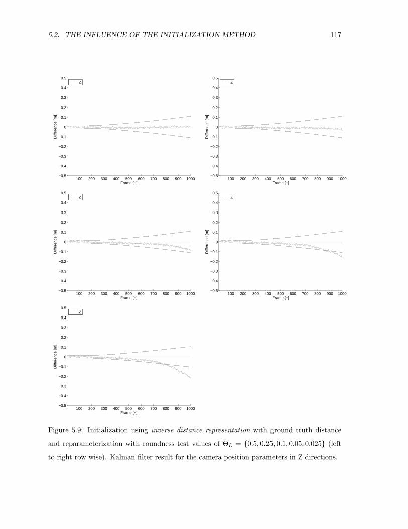
5.2. THE INFLUENCE OF THE INITIALIZATION METHOD 117
100 200 300 400 500 600 700 800 900 1000−0.5
−0.4
−0.3
−0.2
−0.1
0
0.1
0.2
0.3
0.4
0.5
Diff
eren
ce [m
]
Frame [−]
Z
100 200 300 400 500 600 700 800 900 1000−0.5
−0.4
−0.3
−0.2
−0.1
0
0.1
0.2
0.3
0.4
0.5
Diff
eren
ce [m
]
Frame [−]
Z
100 200 300 400 500 600 700 800 900 1000−0.5
−0.4
−0.3
−0.2
−0.1
0
0.1
0.2
0.3
0.4
0.5
Diff
eren
ce [m
]
Frame [−]
Z
100 200 300 400 500 600 700 800 900 1000−0.5
−0.4
−0.3
−0.2
−0.1
0
0.1
0.2
0.3
0.4
0.5
Diff
eren
ce [m
]
Frame [−]
Z
100 200 300 400 500 600 700 800 900 1000−0.5
−0.4
−0.3
−0.2
−0.1
0
0.1
0.2
0.3
0.4
0.5
Diff
eren
ce [m
]
Frame [−]
Z
Figure 5.9: Initialization using inverse distance representation with ground truth distance
and reparameterization with roundness test values of ΘL = 0.5, 0.25, 0.1, 0.05, 0.025 (left
to right row wise). Kalman filter result for the camera position parameters in Z directions.
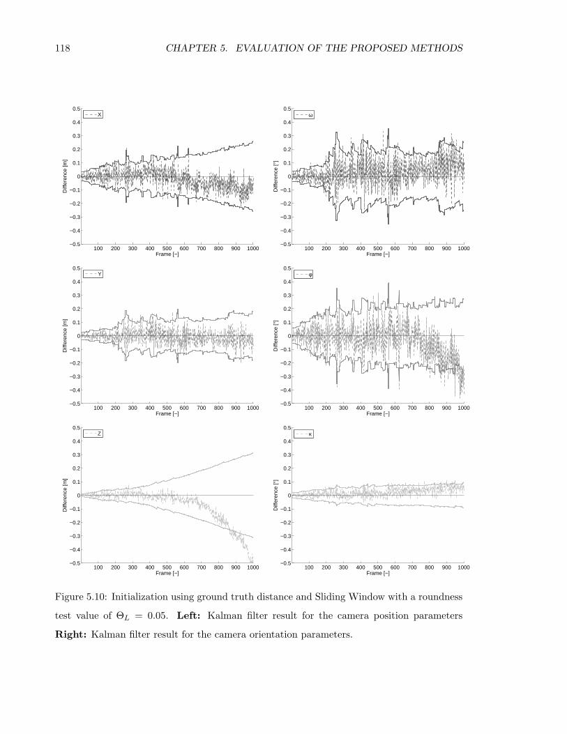
118 CHAPTER 5. EVALUATION OF THE PROPOSED METHODS
100 200 300 400 500 600 700 800 900 1000−0.5
−0.4
−0.3
−0.2
−0.1
0
0.1
0.2
0.3
0.4
0.5
Diff
eren
ce [m
]
Frame [−]
X
100 200 300 400 500 600 700 800 900 1000−0.5
−0.4
−0.3
−0.2
−0.1
0
0.1
0.2
0.3
0.4
0.5
Diff
eren
ce [°
]
Frame [−]
ω
100 200 300 400 500 600 700 800 900 1000−0.5
−0.4
−0.3
−0.2
−0.1
0
0.1
0.2
0.3
0.4
0.5
Diff
eren
ce [m
]
Frame [−]
Y
100 200 300 400 500 600 700 800 900 1000−0.5
−0.4
−0.3
−0.2
−0.1
0
0.1
0.2
0.3
0.4
0.5D
iffer
ence
[°]
Frame [−]
φ
100 200 300 400 500 600 700 800 900 1000−0.5
−0.4
−0.3
−0.2
−0.1
0
0.1
0.2
0.3
0.4
0.5
Diff
eren
ce [m
]
Frame [−]
Z
100 200 300 400 500 600 700 800 900 1000−0.5
−0.4
−0.3
−0.2
−0.1
0
0.1
0.2
0.3
0.4
0.5
Diff
eren
ce [°
]
Frame [−]
κ
Figure 5.10: Initialization using ground truth distance and Sliding Window with a roundness
test value of ΘL = 0.05. Left: Kalman filter result for the camera position parameters
Right: Kalman filter result for the camera orientation parameters.
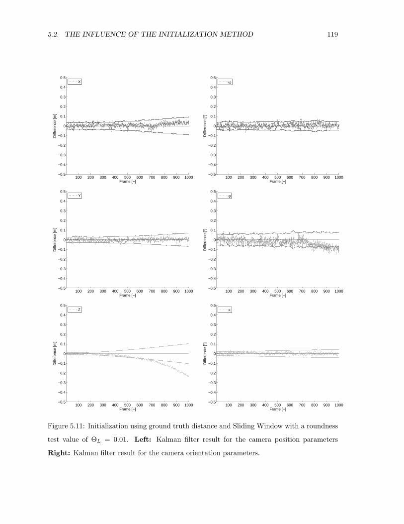
5.2. THE INFLUENCE OF THE INITIALIZATION METHOD 119
100 200 300 400 500 600 700 800 900 1000−0.5
−0.4
−0.3
−0.2
−0.1
0
0.1
0.2
0.3
0.4
0.5
Diff
eren
ce [m
]
Frame [−]
X
100 200 300 400 500 600 700 800 900 1000−0.5
−0.4
−0.3
−0.2
−0.1
0
0.1
0.2
0.3
0.4
0.5
Diff
eren
ce [°
]
Frame [−]
ω
100 200 300 400 500 600 700 800 900 1000−0.5
−0.4
−0.3
−0.2
−0.1
0
0.1
0.2
0.3
0.4
0.5
Diff
eren
ce [m
]
Frame [−]
Y
100 200 300 400 500 600 700 800 900 1000−0.5
−0.4
−0.3
−0.2
−0.1
0
0.1
0.2
0.3
0.4
0.5
Diff
eren
ce [°
]
Frame [−]
φ
100 200 300 400 500 600 700 800 900 1000−0.5
−0.4
−0.3
−0.2
−0.1
0
0.1
0.2
0.3
0.4
0.5
Diff
eren
ce [m
]
Frame [−]
Z
100 200 300 400 500 600 700 800 900 1000−0.5
−0.4
−0.3
−0.2
−0.1
0
0.1
0.2
0.3
0.4
0.5
Diff
eren
ce [°
]
Frame [−]
κ
Figure 5.11: Initialization using ground truth distance and Sliding Window with a roundness
test value of ΘL = 0.01. Left: Kalman filter result for the camera position parameters
Right: Kalman filter result for the camera orientation parameters.
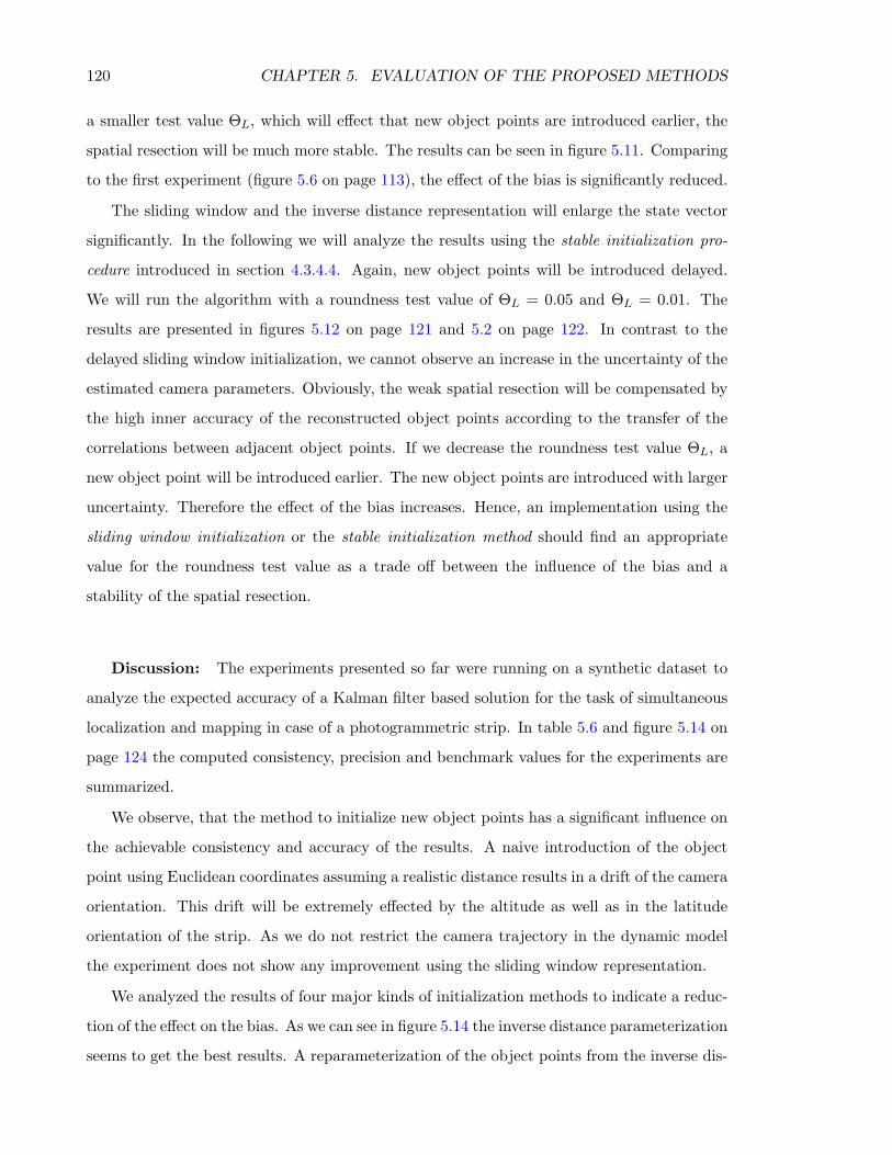
120 CHAPTER 5. EVALUATION OF THE PROPOSED METHODS
a smaller test value ΘL, which will effect that new object points are introduced earlier, the
spatial resection will be much more stable. The results can be seen in figure 5.11. Comparing
to the first experiment (figure 5.6 on page 113), the effect of the bias is significantly reduced.
The sliding window and the inverse distance representation will enlarge the state vector
significantly. In the following we will analyze the results using the stable initialization pro-
cedure introduced in section 4.3.4.4. Again, new object points will be introduced delayed.
We will run the algorithm with a roundness test value of ΘL = 0.05 and ΘL = 0.01. The
results are presented in figures 5.12 on page 121 and 5.2 on page 122. In contrast to the
delayed sliding window initialization, we cannot observe an increase in the uncertainty of the
estimated camera parameters. Obviously, the weak spatial resection will be compensated by
the high inner accuracy of the reconstructed object points according to the transfer of the
correlations between adjacent object points. If we decrease the roundness test value ΘL, a
new object point will be introduced earlier. The new object points are introduced with larger
uncertainty. Therefore the effect of the bias increases. Hence, an implementation using the
sliding window initialization or the stable initialization method should find an appropriate
value for the roundness test value as a trade off between the influence of the bias and a
stability of the spatial resection.
Discussion: The experiments presented so far were running on a synthetic dataset to
analyze the expected accuracy of a Kalman filter based solution for the task of simultaneous
localization and mapping in case of a photogrammetric strip. In table 5.6 and figure 5.14 on
page 124 the computed consistency, precision and benchmark values for the experiments are
summarized.
We observe, that the method to initialize new object points has a significant influence on
the achievable consistency and accuracy of the results. A naive introduction of the object
point using Euclidean coordinates assuming a realistic distance results in a drift of the camera
orientation. This drift will be extremely effected by the altitude as well as in the latitude
orientation of the strip. As we do not restrict the camera trajectory in the dynamic model
the experiment does not show any improvement using the sliding window representation.
We analyzed the results of four major kinds of initialization methods to indicate a reduc-
tion of the effect on the bias. As we can see in figure 5.14 the inverse distance parameterization
seems to get the best results. A reparameterization of the object points from the inverse dis-
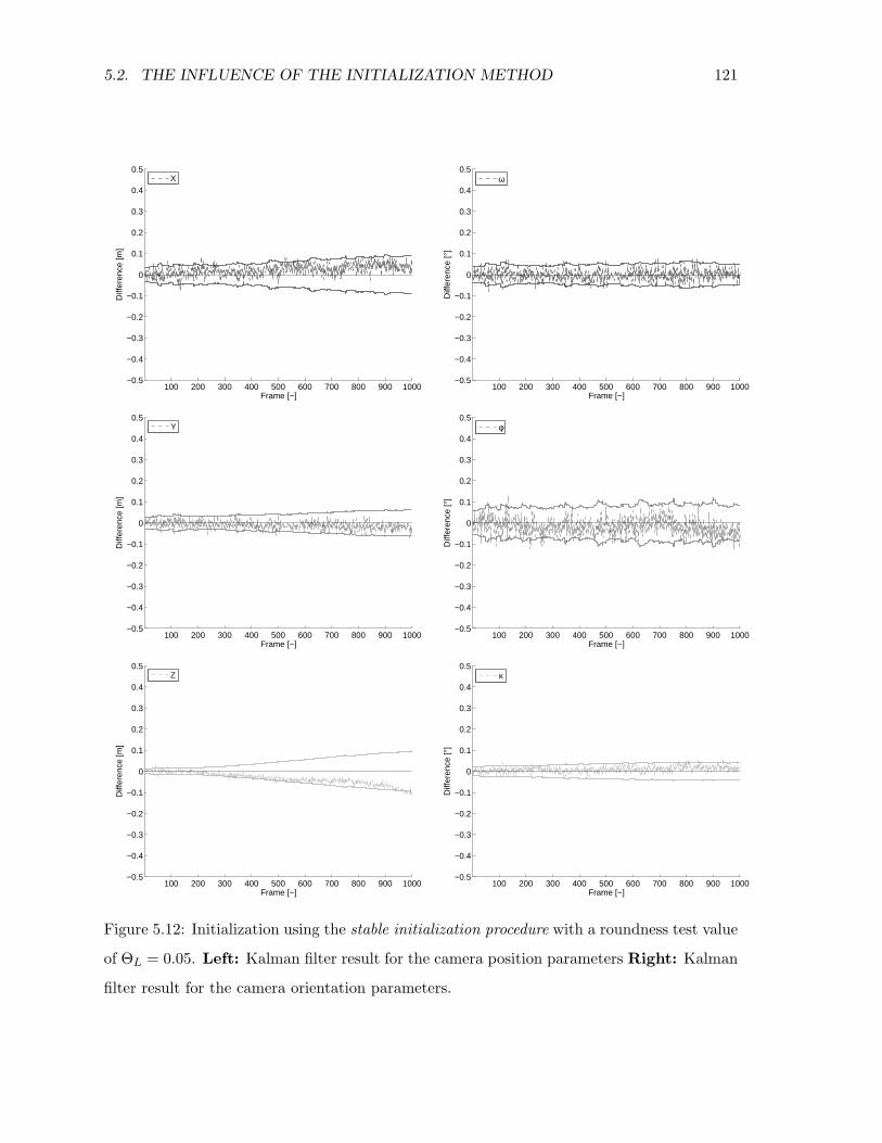
5.2. THE INFLUENCE OF THE INITIALIZATION METHOD 121
100 200 300 400 500 600 700 800 900 1000−0.5
−0.4
−0.3
−0.2
−0.1
0
0.1
0.2
0.3
0.4
0.5
Diff
eren
ce [m
]
Frame [−]
X
100 200 300 400 500 600 700 800 900 1000−0.5
−0.4
−0.3
−0.2
−0.1
0
0.1
0.2
0.3
0.4
0.5
Diff
eren
ce [°
]
Frame [−]
ω
100 200 300 400 500 600 700 800 900 1000−0.5
−0.4
−0.3
−0.2
−0.1
0
0.1
0.2
0.3
0.4
0.5
Diff
eren
ce [m
]
Frame [−]
Y
100 200 300 400 500 600 700 800 900 1000−0.5
−0.4
−0.3
−0.2
−0.1
0
0.1
0.2
0.3
0.4
0.5
Diff
eren
ce [°
]
Frame [−]
φ
100 200 300 400 500 600 700 800 900 1000−0.5
−0.4
−0.3
−0.2
−0.1
0
0.1
0.2
0.3
0.4
0.5
Diff
eren
ce [m
]
Frame [−]
Z
100 200 300 400 500 600 700 800 900 1000−0.5
−0.4
−0.3
−0.2
−0.1
0
0.1
0.2
0.3
0.4
0.5
Diff
eren
ce [°
]
Frame [−]
κ
Figure 5.12: Initialization using the stable initialization procedure with a roundness test value
of ΘL = 0.05. Left: Kalman filter result for the camera position parameters Right: Kalman
filter result for the camera orientation parameters.
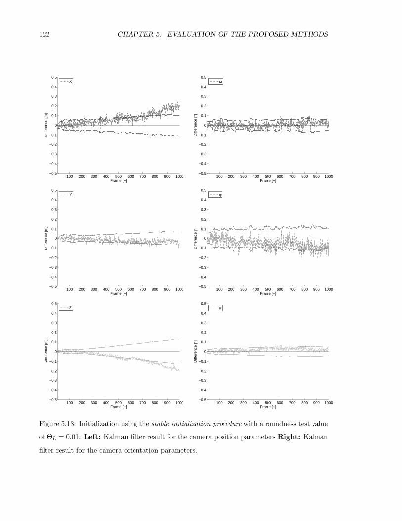
122 CHAPTER 5. EVALUATION OF THE PROPOSED METHODS
100 200 300 400 500 600 700 800 900 1000−0.5
−0.4
−0.3
−0.2
−0.1
0
0.1
0.2
0.3
0.4
0.5
Diff
eren
ce [m
]
Frame [−]
X
100 200 300 400 500 600 700 800 900 1000−0.5
−0.4
−0.3
−0.2
−0.1
0
0.1
0.2
0.3
0.4
0.5
Diff
eren
ce [°
]
Frame [−]
ω
100 200 300 400 500 600 700 800 900 1000−0.5
−0.4
−0.3
−0.2
−0.1
0
0.1
0.2
0.3
0.4
0.5
Diff
eren
ce [m
]
Frame [−]
Y
100 200 300 400 500 600 700 800 900 1000−0.5
−0.4
−0.3
−0.2
−0.1
0
0.1
0.2
0.3
0.4
0.5D
iffer
ence
[°]
Frame [−]
φ
100 200 300 400 500 600 700 800 900 1000−0.5
−0.4
−0.3
−0.2
−0.1
0
0.1
0.2
0.3
0.4
0.5
Diff
eren
ce [m
]
Frame [−]
Z
100 200 300 400 500 600 700 800 900 1000−0.5
−0.4
−0.3
−0.2
−0.1
0
0.1
0.2
0.3
0.4
0.5
Diff
eren
ce [°
]
Frame [−]
κ
Figure 5.13: Initialization using the stable initialization procedure with a roundness test value
of ΘL = 0.01. Left: Kalman filter result for the camera position parameters Right: Kalman
filter result for the camera orientation parameters.
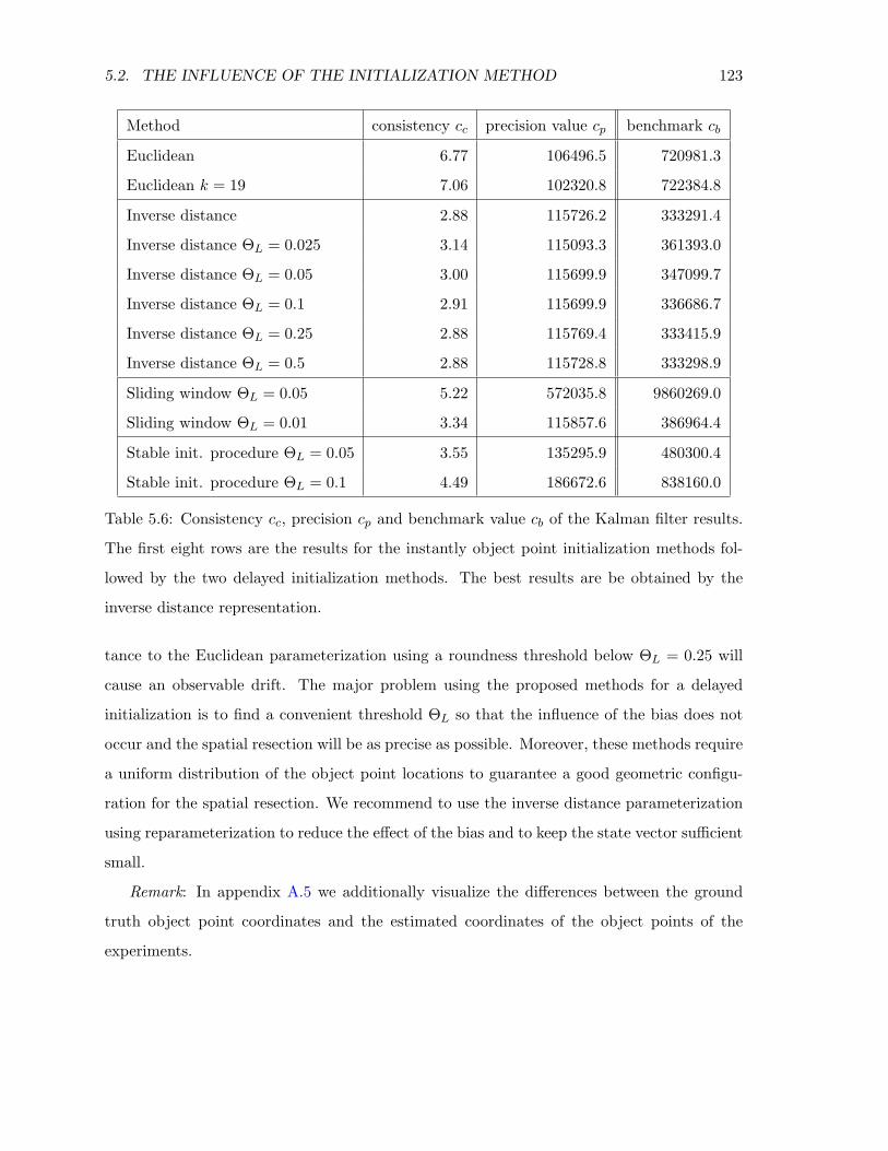
5.2. THE INFLUENCE OF THE INITIALIZATION METHOD 123
Method consistency cc precision value cp benchmark cb
Euclidean 6.77 106496.5 720981.3
Euclidean k = 19 7.06 102320.8 722384.8
Inverse distance 2.88 115726.2 333291.4
Inverse distance ΘL = 0.025 3.14 115093.3 361393.0
Inverse distance ΘL = 0.05 3.00 115699.9 347099.7
Inverse distance ΘL = 0.1 2.91 115699.9 336686.7
Inverse distance ΘL = 0.25 2.88 115769.4 333415.9
Inverse distance ΘL = 0.5 2.88 115728.8 333298.9
Sliding window ΘL = 0.05 5.22 572035.8 9860269.0
Sliding window ΘL = 0.01 3.34 115857.6 386964.4
Stable init. procedure ΘL = 0.05 3.55 135295.9 480300.4
Stable init. procedure ΘL = 0.1 4.49 186672.6 838160.0
Table 5.6: Consistency cc, precision cp and benchmark value cb of the Kalman filter results.
The first eight rows are the results for the instantly object point initialization methods fol-
lowed by the two delayed initialization methods. The best results are be obtained by the
inverse distance representation.
tance to the Euclidean parameterization using a roundness threshold below ΘL = 0.25 will
cause an observable drift. The major problem using the proposed methods for a delayed
initialization is to find a convenient threshold ΘL so that the influence of the bias does not
occur and the spatial resection will be as precise as possible. Moreover, these methods require
a uniform distribution of the object point locations to guarantee a good geometric configu-
ration for the spatial resection. We recommend to use the inverse distance parameterization
using reparameterization to reduce the effect of the bias and to keep the state vector sufficient
small.
Remark: In appendix A.5 we additionally visualize the differences between the ground
truth object point coordinates and the estimated coordinates of the object points of the
experiments.
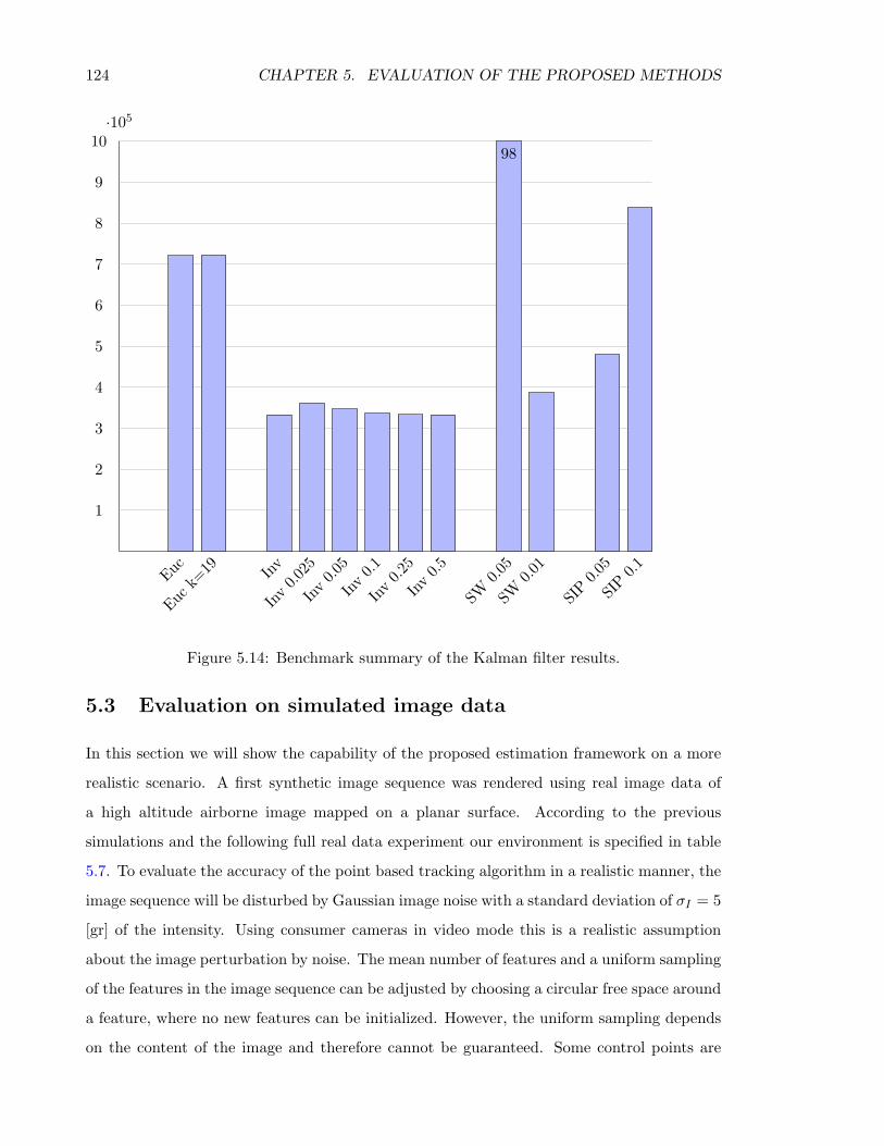
124 CHAPTER 5. EVALUATION OF THE PROPOSED METHODS
·105
1
2
3
4
5
6
7
8
9
10
Euc
Euck=
19 Inv
Inv 0.0
25
Inv 0.0
5
Inv 0.1
Inv 0.2
5
Inv 0.5
SW0.0
5
SW0.0
1
SIP
0.05
SIP
0.1
98
Figure 5.14: Benchmark summary of the Kalman filter results.
5.3 Evaluation on simulated image data
In this section we will show the capability of the proposed estimation framework on a more
realistic scenario. A first synthetic image sequence was rendered using real image data of
a high altitude airborne image mapped on a planar surface. According to the previous
simulations and the following full real data experiment our environment is specified in table
5.7. To evaluate the accuracy of the point based tracking algorithm in a realistic manner, the
image sequence will be disturbed by Gaussian image noise with a standard deviation of σI = 5
[gr] of the intensity. Using consumer cameras in video mode this is a realistic assumption
about the image perturbation by noise. The mean number of features and a uniform sampling
of the features in the image sequence can be adjusted by choosing a circular free space around
a feature, where no new features can be initialized. However, the uniform sampling depends
on the content of the image and therefore cannot be guaranteed. Some control points are
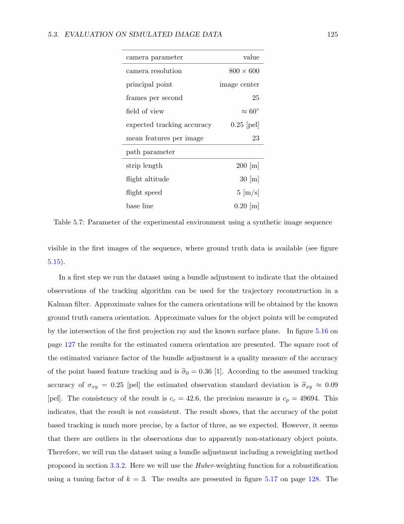
5.3. EVALUATION ON SIMULATED IMAGE DATA 125
camera parameter value
camera resolution 800× 600
principal point image center
frames per second 25
field of view ≈ 60
expected tracking accuracy 0.25 [pel]
mean features per image 23
path parameter
strip length 200 [m]
flight altitude 30 [m]
flight speed 5 [m/s]
base line 0.20 [m]
Table 5.7: Parameter of the experimental environment using a synthetic image sequence
visible in the first images of the sequence, where ground truth data is available (see figure
5.15).
In a first step we run the dataset using a bundle adjustment to indicate that the obtained
observations of the tracking algorithm can be used for the trajectory reconstruction in a
Kalman filter. Approximate values for the camera orientations will be obtained by the known
ground truth camera orientation. Approximate values for the object points will be computed
by the intersection of the first projection ray and the known surface plane. In figure 5.16 on
page 127 the results for the estimated camera orientation are presented. The square root of
the estimated variance factor of the bundle adjustment is a quality measure of the accuracy
of the point based feature tracking and is σ0 = 0.36 [1]. According to the assumed tracking
accuracy of σxy = 0.25 [pel] the estimated observation standard deviation is σxy ≈ 0.09
[pel]. The consistency of the result is cc = 42.6, the precision measure is cp = 49694. This
indicates, that the result is not consistent. The result shows, that the accuracy of the point
based tracking is much more precise, by a factor of three, as we expected. However, it seems
that there are outliers in the observations due to apparently non-stationary object points.
Therefore, we will run the dataset using a bundle adjustment including a reweighting method
proposed in section 3.3.2. Here we will use the Huber-weighting function for a robustification
using a tuning factor of k = 3. The results are presented in figure 5.17 on page 128. The
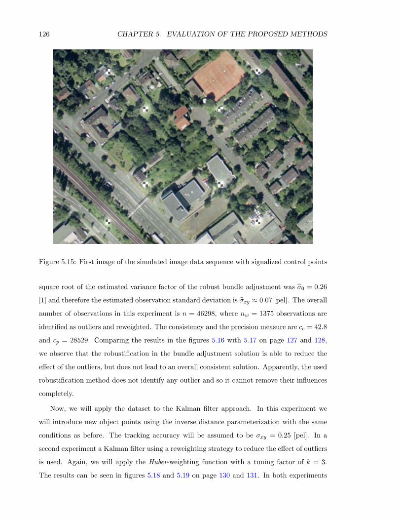
126 CHAPTER 5. EVALUATION OF THE PROPOSED METHODS
Figure 5.15: First image of the simulated image data sequence with signalized control points
square root of the estimated variance factor of the robust bundle adjustment was σ0 = 0.26
[1] and therefore the estimated observation standard deviation is σxy ≈ 0.07 [pel]. The overall
number of observations in this experiment is n = 46298, where nw = 1375 observations are
identified as outliers and reweighted. The consistency and the precision measure are cc = 42.8
and cp = 28529. Comparing the results in the figures 5.16 with 5.17 on page 127 and 128,
we observe that the robustification in the bundle adjustment solution is able to reduce the
effect of the outliers, but does not lead to an overall consistent solution. Apparently, the used
robustification method does not identify any outlier and so it cannot remove their influences
completely.
Now, we will apply the dataset to the Kalman filter approach. In this experiment we
will introduce new object points using the inverse distance parameterization with the same
conditions as before. The tracking accuracy will be assumed to be σxy = 0.25 [pel]. In a
second experiment a Kalman filter using a reweighting strategy to reduce the effect of outliers
is used. Again, we will apply the Huber-weighting function with a tuning factor of k = 3.
The results can be seen in figures 5.18 and 5.19 on page 130 and 131. In both experiments
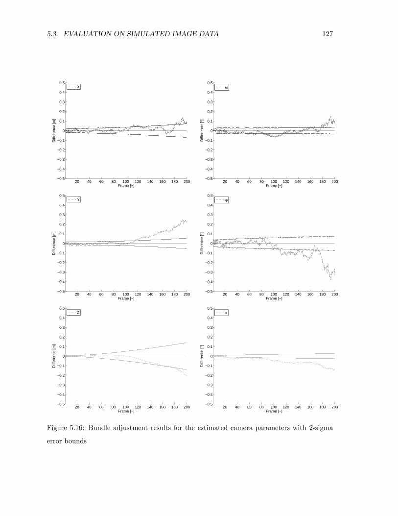
5.3. EVALUATION ON SIMULATED IMAGE DATA 127
20 40 60 80 100 120 140 160 180 200−0.5
−0.4
−0.3
−0.2
−0.1
0
0.1
0.2
0.3
0.4
0.5
Diff
eren
ce [m
]
Frame [−]
X
20 40 60 80 100 120 140 160 180 200−0.5
−0.4
−0.3
−0.2
−0.1
0
0.1
0.2
0.3
0.4
0.5
Diff
eren
ce [°
]
Frame [−]
ω
20 40 60 80 100 120 140 160 180 200−0.5
−0.4
−0.3
−0.2
−0.1
0
0.1
0.2
0.3
0.4
0.5
Diff
eren
ce [m
]
Frame [−]
Y
20 40 60 80 100 120 140 160 180 200−0.5
−0.4
−0.3
−0.2
−0.1
0
0.1
0.2
0.3
0.4
0.5
Diff
eren
ce [°
]
Frame [−]
φ
20 40 60 80 100 120 140 160 180 200−0.5
−0.4
−0.3
−0.2
−0.1
0
0.1
0.2
0.3
0.4
0.5
Diff
eren
ce [m
]
Frame [−]
Z
20 40 60 80 100 120 140 160 180 200−0.5
−0.4
−0.3
−0.2
−0.1
0
0.1
0.2
0.3
0.4
0.5
Diff
eren
ce [°
]
Frame [−]
κ
Figure 5.16: Bundle adjustment results for the estimated camera parameters with 2-sigma
error bounds
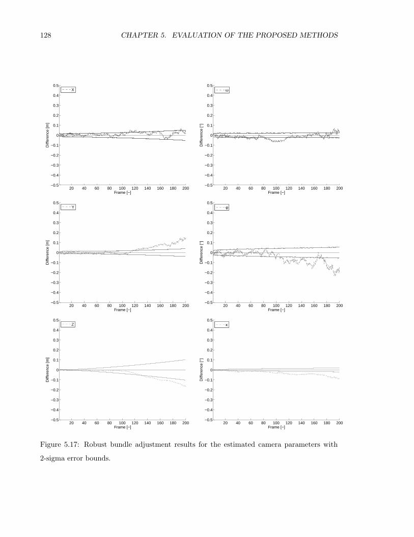
128 CHAPTER 5. EVALUATION OF THE PROPOSED METHODS
20 40 60 80 100 120 140 160 180 200−0.5
−0.4
−0.3
−0.2
−0.1
0
0.1
0.2
0.3
0.4
0.5
Diff
eren
ce [m
]
Frame [−]
X
20 40 60 80 100 120 140 160 180 200−0.5
−0.4
−0.3
−0.2
−0.1
0
0.1
0.2
0.3
0.4
0.5
Diff
eren
ce [°
]
Frame [−]
ω
20 40 60 80 100 120 140 160 180 200−0.5
−0.4
−0.3
−0.2
−0.1
0
0.1
0.2
0.3
0.4
0.5
Diff
eren
ce [m
]
Frame [−]
Y
20 40 60 80 100 120 140 160 180 200−0.5
−0.4
−0.3
−0.2
−0.1
0
0.1
0.2
0.3
0.4
0.5D
iffer
ence
[°]
Frame [−]
φ
20 40 60 80 100 120 140 160 180 200−0.5
−0.4
−0.3
−0.2
−0.1
0
0.1
0.2
0.3
0.4
0.5
Diff
eren
ce [m
]
Frame [−]
Z
20 40 60 80 100 120 140 160 180 200−0.5
−0.4
−0.3
−0.2
−0.1
0
0.1
0.2
0.3
0.4
0.5
Diff
eren
ce [°
]
Frame [−]
κ
Figure 5.17: Robust bundle adjustment results for the estimated camera parameters with
2-sigma error bounds.
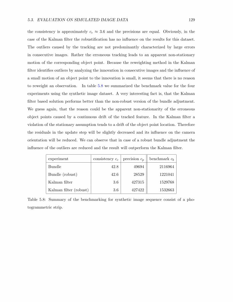
5.3. EVALUATION ON SIMULATED IMAGE DATA 129
the consistency is approximately cc ≈ 3.6 and the precisions are equal. Obviously, in the
case of the Kalman filter the robustification has no influence on the results for this dataset.
The outliers caused by the tracking are not predominantly characterized by large errors
in consecutive images. Rather the erroneous tracking leads to an apparent non-stationary
motion of the corresponding object point. Because the reweighting method in the Kalman
filter identifies outliers by analyzing the innovation in consecutive images and the influence of
a small motion of an object point to the innovation is small, it seems that there is no reason
to reweight an observation. In table 5.8 we summarized the benchmark value for the four
experiments using the synthetic image dataset. A very interesting fact is, that the Kalman
filter based solution performs better than the non-robust version of the bundle adjustment.
We guess again, that the reason could be the apparent non-stationarity of the erroneous
object points caused by a continuous drift of the tracked feature. In the Kalman filter a
violation of the stationary assumption tends to a drift of the object point location. Therefore
the residuals in the update step will be slightly decreased and its influence on the camera
orientation will be reduced. We can observe that in case of a robust bundle adjustment the
influence of the outliers are reduced and the result will outperform the Kalman filter.
experiment consistency cc precision cp benchmark cb
Bundle 42.8 49694 2116964
Bundle (robust) 42.6 28529 1221041
Kalman filter 3.6 427315 1529768
Kalman filter (robust) 3.6 427422 1532663
Table 5.8: Summary of the benchmarking for synthetic image sequence consist of a pho-
togrammetric strip.
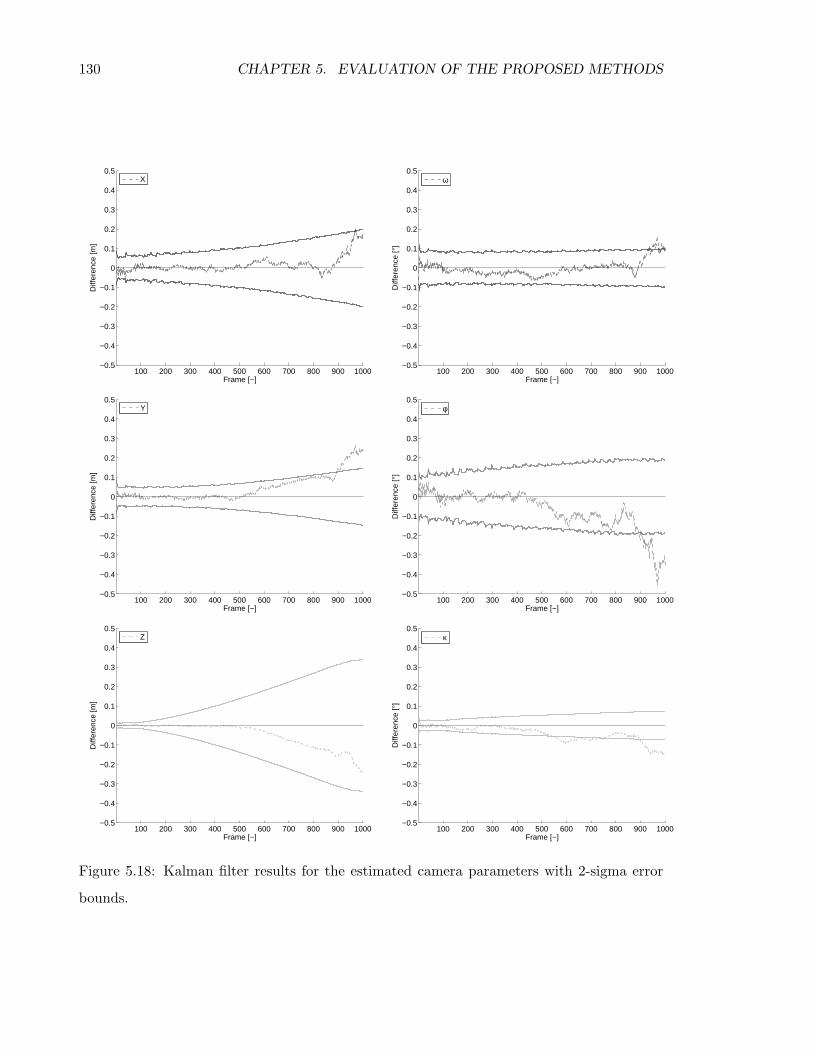
130 CHAPTER 5. EVALUATION OF THE PROPOSED METHODS
100 200 300 400 500 600 700 800 900 1000−0.5
−0.4
−0.3
−0.2
−0.1
0
0.1
0.2
0.3
0.4
0.5
Diff
eren
ce [m
]
Frame [−]
X
100 200 300 400 500 600 700 800 900 1000−0.5
−0.4
−0.3
−0.2
−0.1
0
0.1
0.2
0.3
0.4
0.5
Diff
eren
ce [°
]
Frame [−]
ω
100 200 300 400 500 600 700 800 900 1000−0.5
−0.4
−0.3
−0.2
−0.1
0
0.1
0.2
0.3
0.4
0.5
Diff
eren
ce [m
]
Frame [−]
Y
100 200 300 400 500 600 700 800 900 1000−0.5
−0.4
−0.3
−0.2
−0.1
0
0.1
0.2
0.3
0.4
0.5D
iffer
ence
[°]
Frame [−]
φ
100 200 300 400 500 600 700 800 900 1000−0.5
−0.4
−0.3
−0.2
−0.1
0
0.1
0.2
0.3
0.4
0.5
Diff
eren
ce [m
]
Frame [−]
Z
100 200 300 400 500 600 700 800 900 1000−0.5
−0.4
−0.3
−0.2
−0.1
0
0.1
0.2
0.3
0.4
0.5
Diff
eren
ce [°
]
Frame [−]
κ
Figure 5.18: Kalman filter results for the estimated camera parameters with 2-sigma error
bounds.
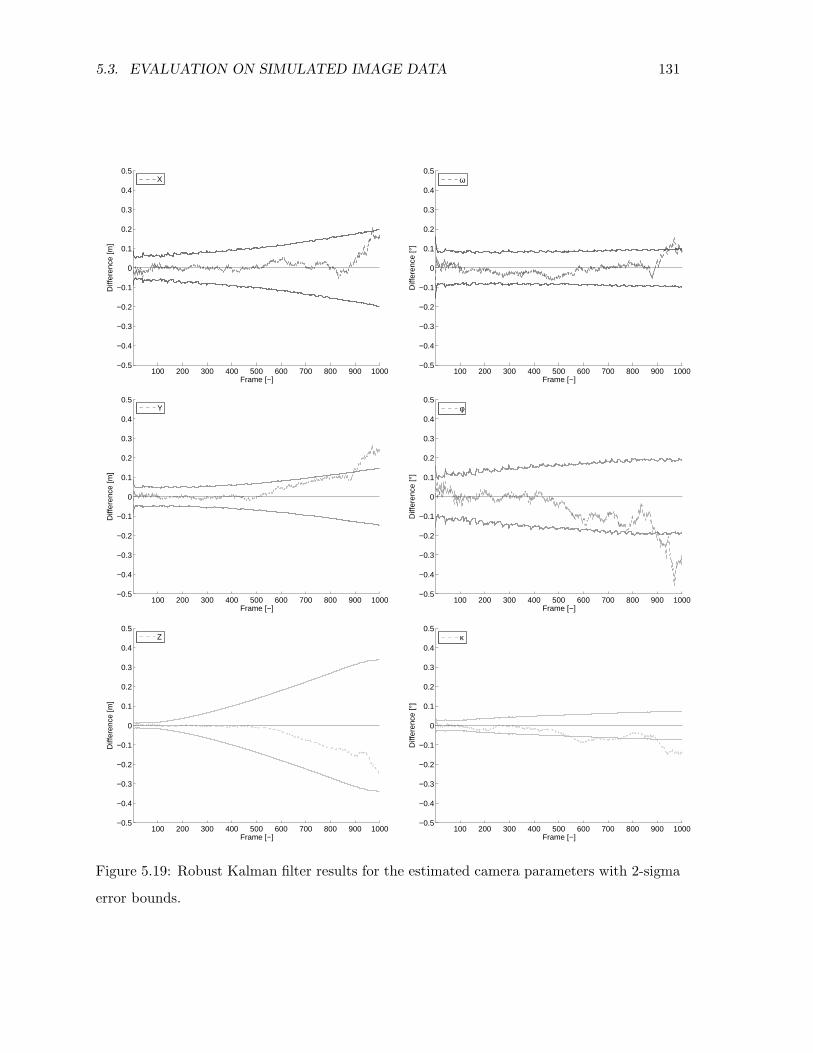
5.3. EVALUATION ON SIMULATED IMAGE DATA 131
100 200 300 400 500 600 700 800 900 1000−0.5
−0.4
−0.3
−0.2
−0.1
0
0.1
0.2
0.3
0.4
0.5
Diff
eren
ce [m
]
Frame [−]
X
100 200 300 400 500 600 700 800 900 1000−0.5
−0.4
−0.3
−0.2
−0.1
0
0.1
0.2
0.3
0.4
0.5
Diff
eren
ce [°
]
Frame [−]
ω
100 200 300 400 500 600 700 800 900 1000−0.5
−0.4
−0.3
−0.2
−0.1
0
0.1
0.2
0.3
0.4
0.5
Diff
eren
ce [m
]
Frame [−]
Y
100 200 300 400 500 600 700 800 900 1000−0.5
−0.4
−0.3
−0.2
−0.1
0
0.1
0.2
0.3
0.4
0.5
Diff
eren
ce [°
]
Frame [−]
φ
100 200 300 400 500 600 700 800 900 1000−0.5
−0.4
−0.3
−0.2
−0.1
0
0.1
0.2
0.3
0.4
0.5
Diff
eren
ce [m
]
Frame [−]
Z
100 200 300 400 500 600 700 800 900 1000−0.5
−0.4
−0.3
−0.2
−0.1
0
0.1
0.2
0.3
0.4
0.5
Diff
eren
ce [°
]
Frame [−]
κ
Figure 5.19: Robust Kalman filter results for the estimated camera parameters with 2-sigma
error bounds.
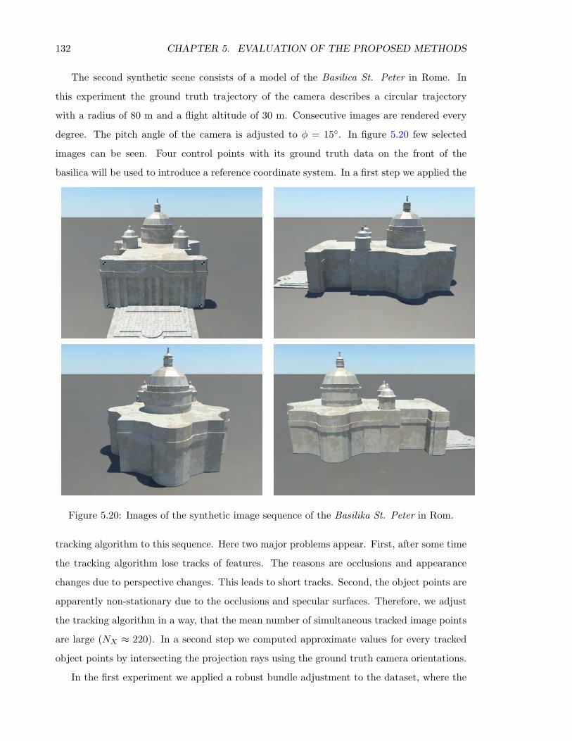
132 CHAPTER 5. EVALUATION OF THE PROPOSED METHODS
The second synthetic scene consists of a model of the Basilica St. Peter in Rome. In
this experiment the ground truth trajectory of the camera describes a circular trajectory
with a radius of 80 m and a flight altitude of 30 m. Consecutive images are rendered every
degree. The pitch angle of the camera is adjusted to φ = 15. In figure 5.20 few selected
images can be seen. Four control points with its ground truth data on the front of the
basilica will be used to introduce a reference coordinate system. In a first step we applied the
Figure 5.20: Images of the synthetic image sequence of the Basilika St. Peter in Rom.
tracking algorithm to this sequence. Here two major problems appear. First, after some time
the tracking algorithm lose tracks of features. The reasons are occlusions and appearance
changes due to perspective changes. This leads to short tracks. Second, the object points are
apparently non-stationary due to the occlusions and specular surfaces. Therefore, we adjust
the tracking algorithm in a way, that the mean number of simultaneous tracked image points
are large (NX ≈ 220). In a second step we computed approximate values for every tracked
object points by intersecting the projection rays using the ground truth camera orientations.
In the first experiment we applied a robust bundle adjustment to the dataset, where the
5.3. EVALUATION ON SIMULATED IMAGE DATA 133
influence of outliers will be reduced by a reweighting method using the Huber-weighting func-
tion. The algorithm diverges due to the large number of outliers. Obviously, the reweighting
method is not able to detect the huge number of outliers and to reduce their effects.
In a second experiment we applied a bundle adjustment to this synthetic dataset by
eliminating outliers iteratively. Here, we estimate the variance components of all groups of
observations to have a part of the determination of individual object points, c. f. section
3.3.2. In every iteration all groups with a variance component above a threshold of Θσ0 > 2
will be identified. We eliminate the observations of the worst 10% groups and run the
algorithm again. The resulting residuals between the ground truth and estimated camera
trajectory are shown in figure 5.21. The computed square root of the variance factor of the
remaining observations is σ0 = 0.63 [1]. The dataset contains of N = 2536 object points. The
outlier detection method classified 1166 object points as outliers. We can observe, that the
result is not consistent. The estimated accuracy does not reflect the true uncertainty of the
results. Also the outlier detection method based on the variance component cannot detect
all apparently non-stationary object points in this sequence. A more robust implementation
should detect outliers using a filter step prior to the adjustment. The filter can determine
the relative orientation between two selected images using the coplanarity constraint. In case
of a huge number of wrong correspondences a robust estimation can be achieved using the
RANSAC-procedure following Fischler & Bolles (1981). Object points should be eliminated,
where the coplanarity constraint does not hold. From the concept of the Kalman filter we
typically are not able to fall back to previous observations. Observe, that these observations
are already encoded in the state of the system and cannot be removed.
In a third experiment using this dataset we tried to estimate the trajectory by a Kalman
filter based approach using the inverse distance representation. We observed an early diver-
gence of the filter process. We suppose that the huge number of outliers in the observation
cause numerical instabilities.
In the previous sections we analyzed the capability of the Kalman filter to the task
of simultaneous localization and mapping from image sequences. The experiments were
restricted to the case of classical photogrammetric strips. We first derived a general law
to assess the stochastical accuracy of a photogrammetric strip. The law is generalized to
get the accuracy under different kinds of flight configurations. Second, we compared the
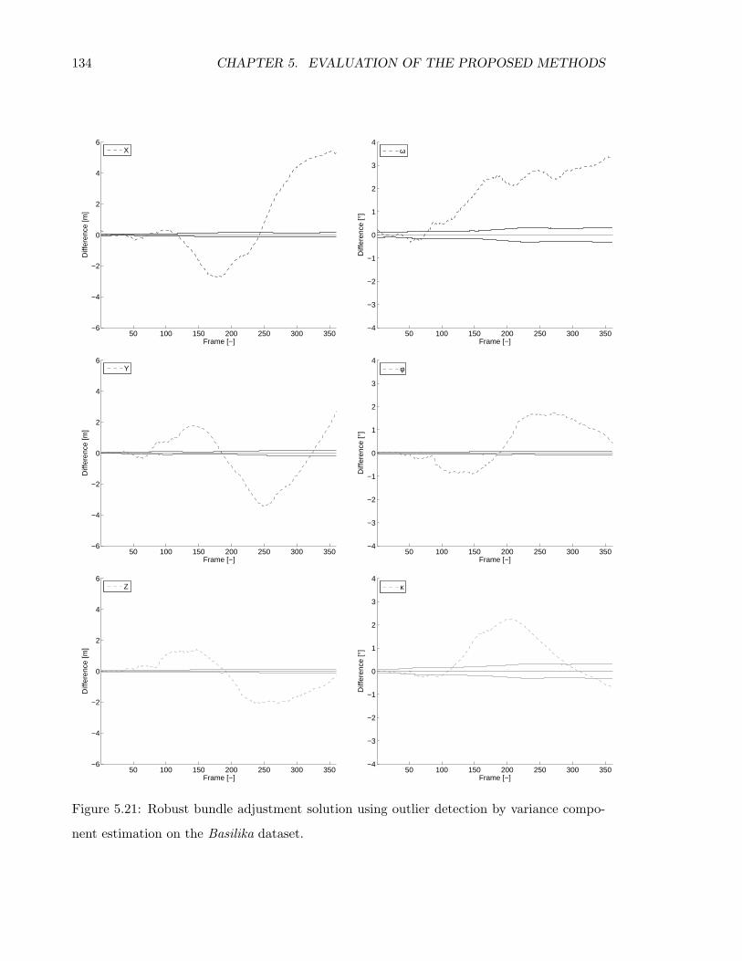
134 CHAPTER 5. EVALUATION OF THE PROPOSED METHODS
50 100 150 200 250 300 350−6
−4
−2
0
2
4
6
Diff
eren
ce [m
]
Frame [−]
X
50 100 150 200 250 300 350−4
−3
−2
−1
0
1
2
3
4
Diff
eren
ce [°
]
Frame [−]
ω
50 100 150 200 250 300 350−6
−4
−2
0
2
4
6
Diff
eren
ce [m
]
Frame [−]
Y
50 100 150 200 250 300 350−4
−3
−2
−1
0
1
2
3
4D
iffer
ence
[°]
Frame [−]
φ
50 100 150 200 250 300 350−6
−4
−2
0
2
4
6
Diff
eren
ce [m
]
Frame [−]
Z
50 100 150 200 250 300 350−4
−3
−2
−1
0
1
2
3
4
Diff
eren
ce [°
]
Frame [−]
κ
Figure 5.21: Robust bundle adjustment solution using outlier detection by variance compo-
nent estimation on the Basilika dataset.
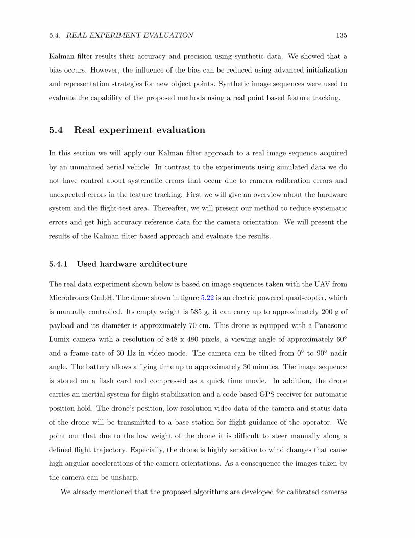
5.4. REAL EXPERIMENT EVALUATION 135
Kalman filter results their accuracy and precision using synthetic data. We showed that a
bias occurs. However, the influence of the bias can be reduced using advanced initialization
and representation strategies for new object points. Synthetic image sequences were used to
evaluate the capability of the proposed methods using a real point based feature tracking.
5.4 Real experiment evaluation
In this section we will apply our Kalman filter approach to a real image sequence acquired
by an unmanned aerial vehicle. In contrast to the experiments using simulated data we do
not have control about systematic errors that occur due to camera calibration errors and
unexpected errors in the feature tracking. First we will give an overview about the hardware
system and the flight-test area. Thereafter, we will present our method to reduce systematic
errors and get high accuracy reference data for the camera orientation. We will present the
results of the Kalman filter based approach and evaluate the results.
5.4.1 Used hardware architecture
The real data experiment shown below is based on image sequences taken with the UAV from
Microdrones GmbH. The drone shown in figure 5.22 is an electric powered quad-copter, which
is manually controlled. Its empty weight is 585 g, it can carry up to approximately 200 g of
payload and its diameter is approximately 70 cm. This drone is equipped with a Panasonic
Lumix camera with a resolution of 848 x 480 pixels, a viewing angle of approximately 60
and a frame rate of 30 Hz in video mode. The camera can be tilted from 0 to 90 nadir
angle. The battery allows a flying time up to approximately 30 minutes. The image sequence
is stored on a flash card and compressed as a quick time movie. In addition, the drone
carries an inertial system for flight stabilization and a code based GPS-receiver for automatic
position hold. The drone’s position, low resolution video data of the camera and status data
of the drone will be transmitted to a base station for flight guidance of the operator. We
point out that due to the low weight of the drone it is difficult to steer manually along a
defined flight trajectory. Especially, the drone is highly sensitive to wind changes that cause
high angular accelerations of the camera orientations. As a consequence the images taken by
the camera can be unsharp.
We already mentioned that the proposed algorithms are developed for calibrated cameras
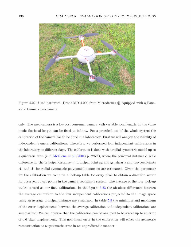
136 CHAPTER 5. EVALUATION OF THE PROPOSED METHODS
Figure 5.22: Used hardware. Drone MD 4-200 from Microdrones c© equipped with a Pana-
sonic Lumix video camera.
only. The used camera is a low cost consumer camera with variable focal length. In the video
mode the focal length can be fixed to infinity. For a practical use of the whole system the
calibration of the camera has to be done in a laboratory. First we will analyze the stability of
independent camera calibrations. Therefore, we performed four independent calibrations in
the laboratory on different days. The calibration is done with a radial symmetric model up to
a quadratic term (c. f. McGlone et al. (2004) p. 297ff), where the principal distance c, scale
difference for the principal distance m, principal point xh and yh, shear s and two coefficients
A1 and A2 for radial symmetric polynomial distortion are estimated. Given the parameter
for the calibration we compute a look-up table for every pixel to obtain a direction vector
for observed object points in the camera coordinate system. The average of the four look-up
tables is used as our final calibration. In the figures 5.23 the absolute differences between
the average calibration to the four independent calibrations projected to the image space
using an average principal distance are visualized. In table 5.9 the minimum and maximum
of the error displacements between the average calibration and independent calibrations are
summarized. We can observe that the calibration can be assumed to be stable up to an error
of 0.6 pixel displacement. This non-linear error in the calibration will effect the geometric
reconstruction as a systematic error in an unpredictable manner.
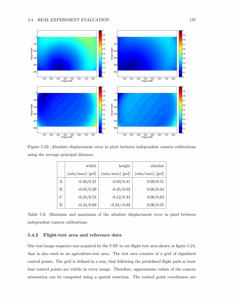
5.4. REAL EXPERIMENT EVALUATION 137
Image width
Imag
e he
ight
100 200 300 400 500 600 700 800
0
100
200
300
400
500
0
0.1
0.2
0.3
0.4
0.5
0.6
0.7
0.8
0.9
1
Image width
Imag
e he
ight
100 200 300 400 500 600 700 800
0
100
200
300
400
500
0
0.1
0.2
0.3
0.4
0.5
0.6
0.7
0.8
0.9
1
Image width
Imag
e he
ight
100 200 300 400 500 600 700 800
0
100
200
300
400
500
0
0.1
0.2
0.3
0.4
0.5
0.6
0.7
0.8
0.9
1
Image width
Imag
e he
ight
100 200 300 400 500 600 700 800
0
100
200
300
400
500
0
0.1
0.2
0.3
0.4
0.5
0.6
0.7
0.8
0.9
1
Figure 5.23: Absolute displacement error in pixel between independent camera calibrations
using the average principal distance.
width height absolut
(min/max) [pel] (min/max) [pel] (min/max) [pel]
A -0.40/0.21 -0.03/0.41 0.00/0.51
B -0.05/0.29 -0.25/0.02 0.00/0.34
C -0.24/0.53 -0.12/0.34 0.00/0.63
D -0.44/0.09 -0.34/-0.02 0.06/0.55
Table 5.9: Minimum and maximum of the absolute displacement error in pixel between
independent camera calibrations.
5.4.2 Flight-test area and reference data
Our real image sequence was acquired by the UAV in our flight-test area shown in figure 5.24,
that is also used as an agriculture-test area. The test area consists of a grid of signalized
control points. The grid is defined in a way, that following the predefined flight path at least
four control points are visible in every image. Therefore, approximate values of the camera
orientation can be computed using a spatial resection. The control point coordinates are
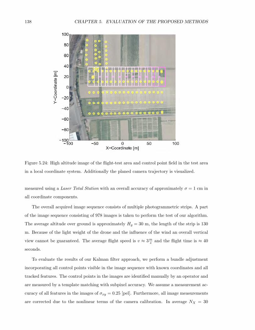
138 CHAPTER 5. EVALUATION OF THE PROPOSED METHODS
Figure 5.24: High altitude image of the flight-test area and control point field in the test area
in a local coordinate system. Additionally the planed camera trajectory is visualized.
measured using a Laser Total Station with an overall accuracy of approximately σ = 1 cm in
all coordinate components.
The overall acquired image sequence consists of multiple photogrammetric strips. A part
of the image sequence consisting of 978 images is taken to perform the test of our algorithm.
The average altitude over ground is approximately Hg = 30 m, the length of the strip is 130
m. Because of the light weight of the drone and the influence of the wind an overall vertical
view cannot be guaranteed. The average flight speed is v ≈ 3ms and the flight time is ≈ 40
seconds.
To evaluate the results of our Kalman filter approach, we perform a bundle adjustment
incorporating all control points visible in the image sequence with known coordinates and all
tracked features. The control points in the images are identified manually by an operator and
are measured by a template matching with subpixel accuracy. We assume a measurement ac-
curacy of all features in the images of σxy = 0.25 [pel]. Furthermore, all image measurements
are corrected due to the nonlinear terms of the camera calibration. In average NX = 30
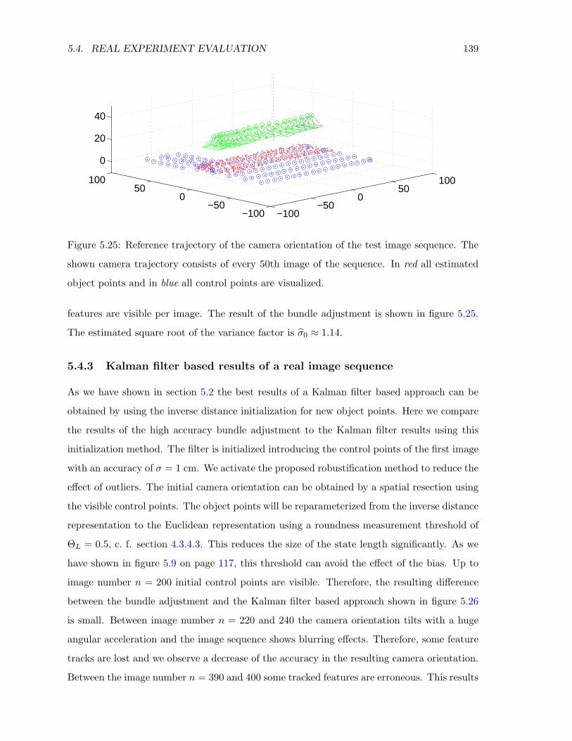
5.4. REAL EXPERIMENT EVALUATION 139
−100−50
050
100
−100−50
050
100
0
20
40
Figure 5.25: Reference trajectory of the camera orientation of the test image sequence. The
shown camera trajectory consists of every 50th image of the sequence. In red all estimated
object points and in blue all control points are visualized.
features are visible per image. The result of the bundle adjustment is shown in figure 5.25.
The estimated square root of the variance factor is σ0 ≈ 1.14.
5.4.3 Kalman filter based results of a real image sequence
As we have shown in section 5.2 the best results of a Kalman filter based approach can be
obtained by using the inverse distance initialization for new object points. Here we compare
the results of the high accuracy bundle adjustment to the Kalman filter results using this
initialization method. The filter is initialized introducing the control points of the first image
with an accuracy of σ = 1 cm. We activate the proposed robustification method to reduce the
effect of outliers. The initial camera orientation can be obtained by a spatial resection using
the visible control points. The object points will be reparameterized from the inverse distance
representation to the Euclidean representation using a roundness measurement threshold of
ΘL = 0.5, c. f. section 4.3.4.3. This reduces the size of the state length significantly. As we
have shown in figure 5.9 on page 117, this threshold can avoid the effect of the bias. Up to
image number n = 200 initial control points are visible. Therefore, the resulting difference
between the bundle adjustment and the Kalman filter based approach shown in figure 5.26
is small. Between image number n = 220 and 240 the camera orientation tilts with a huge
angular acceleration and the image sequence shows blurring effects. Therefore, some feature
tracks are lost and we observe a decrease of the accuracy in the resulting camera orientation.
Between the image number n = 390 and 400 some tracked features are erroneous. This results
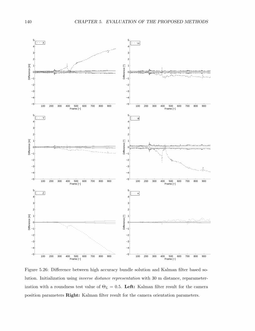
140 CHAPTER 5. EVALUATION OF THE PROPOSED METHODS
100 200 300 400 500 600 700 800 900−5
−4
−3
−2
−1
0
1
2
3
4
5
Diff
eren
ce [m
]
Frame [−]
X
100 200 300 400 500 600 700 800 900−5
−4
−3
−2
−1
0
1
2
3
4
5
Diff
eren
ce [°
]
Frame [−]
ω
100 200 300 400 500 600 700 800 900−5
−4
−3
−2
−1
0
1
2
3
4
5
Diff
eren
ce [m
]
Frame [−]
Y
100 200 300 400 500 600 700 800 900−5
−4
−3
−2
−1
0
1
2
3
4
5
Diff
eren
ce [°
]
Frame [−]
φ
100 200 300 400 500 600 700 800 900−5
−4
−3
−2
−1
0
1
2
3
4
5
Diff
eren
ce [m
]
Frame [−]
Z
100 200 300 400 500 600 700 800 900−5
−4
−3
−2
−1
0
1
2
3
4
5
Diff
eren
ce [°
]
Frame [−]
κ
Figure 5.26: Difference between high accuracy bundle solution and Kalman filter based so-
lution. Initialization using inverse distance representation with 30 m distance, reparameter-
ization with a roundness test value of ΘL = 0.5. Left: Kalman filter result for the camera
position parameters Right: Kalman filter result for the camera orientation parameters.
5.4. REAL EXPERIMENT EVALUATION 141
in an immediate change of the camera orientation. However, we can observe an apparently
continuous drift in the estimated parameters. We suppose, this drift comes from the erroneous
camera calibration and acts as a constant systematic error.
Discussion: In this section we presented our results for a real image sequence. In
opposite to the experiments using a simulated environment additional influences on the results
occur. First, we do not have ground truth data for the camera orientation. Instead, we used
the results of a robust bundle adjustment incorporating high accuracy control points in all
images. Nevertheless, the bundle adjustment is influenced by systematic errors of an imperfect
camera calibration. We are not able to quantify this error. However, the bundle adjustment
incorporate control point coordinates and the influence of the imperfect calibration can be
assumed to be small. In the Kalman filter based approach, the information of the control
points are neglected except for the initial images. We observed a continuous drift in the
estimated camera orientation parameters. Second, gross errors in the feature tracks have a
significant effect to the Kalman filter based estimate. Obviously, our robustification method
is not able to reduce the effect of outliers completely. At present the algorithm does not
have a prefiltering to identify gross errors in the feature tracking. This could be achieved by
verifying the coplanarity constraint or the homography constraint1 in consecutive images (c. f.
section 3.2.2). Third, the real image sequence shows huge angular accelerations. Therefore,
some feature tracks are lost in corresponding images. The associated object points recur
in the following images. An advanced algorithm should reidentify these object points and
continue the feature track. An alternative way is to stabilize the angular camera orientation
by force to the nadir view by a hardware solution.
1The homography constraint can be used in case of small camera location chances or a planar object space.

142 CHAPTER 5. EVALUATION OF THE PROPOSED METHODS
Chapter 6
Conclusion and future work
In this thesis the theory and the applicability of a Kalman filter based framework has been
presented that can be used to solve the task of simultaneous localization and mapping using
image sequences only. It has been shown that the reconstruction of the trajectory of a single
calibrated camera using point based features is feasible. Although, Kalman filter based
solutions as an online SLAM approach need to consider additional issues as opposite to full
SLAM approaches such as a bundle adjustment. These issues can be separated into two
different aspects.
First, it has been shown that the continuous enlargement of the state requires an adequate
initialization method for geometric entities. The initialization method has to be taken into
account of the non-Gaussian distribution of the recovery of an object point coordinate for
small disparities in consecutive frames. When neglecting this issue a continuous bias occurs.
A comparison of the results using instant initialization methods and delayed initialization
methods has been shown. It seems that the inverse distance parameterization of new object
points is the best way to overcome the bias effect.
Second, compared to a bundle adjustment the detection of gross errors in the observations
in a Kalman filter based method is more difficult. In case object points are non-stationary,
their identification seems to be apparently impossible without having any access to previous
observations of the object point.
In case of image sequences acquired by an unmanned aerial vehicle the approaches has a
great potential shown by synthetic data. If gross errors can be excluded and systematic errors
from imperfect camera calibration can be minimized the results are comparable with a bundle
adjustment solution. The advantage compared to the bundle adjustment appears, when the
143
144 CHAPTER 6. CONCLUSION AND FUTURE WORK
number of object points is small and the number of images is large. If the application requires
a state solution at any point of time the computational complexity can be significantly reduced
using a Kalman filter based approach. However, in case of real image data Kalman filter based
approaches are extremely sensitive to outliers.
This thesis consists of novel algorithms and methods close to the Kalman filter based
simultaneous localization and mapping task. The first contribution of this work is a general
derivation of the recursive update of the Kalman filter. This derivation is based on implicit
measurement equations. Similar to the derivation of the least square methods based on the
Gauss-Helmert-model (c. f. McGlone et al. (2004) p. 79ff) it has been shown that the classical
iterative non-linear as well as the non-iterative and linear Kalman filter are specializations
of our general Kalman filter. A significant improvement can be expected by using a Kalman
filter based SLAM solution incorporating new geometric entities using this general framework.
Second, a new formulation of a linear prediction for the single camera state model and
the sliding window camera state model has been derived. Here, the prediction of the state
can be computed using matrix vector multiplications only. The angular orientation is defined
by a quaternion representation, so that no singularities can occur. The method is limited to
the case that the angular velocity is small.
The third contribution is a new method to initialize new object points in a delayed manner.
The advantage of this method is that it is not necessary to keep previous camera orientations
inside the state in contrast to other delayed initialization methods. However, it has been
shown in the experiments that this method cannot maintain the consistency of the results.
Forth, a general law to assess the stochastical accuracy of the camera orientation of a
photogrammetric strip has been derived. The law depends on four parameters to describe
different kinds of flight configurations. The law can be considered as a generalization of the
law introduced by Finsterwalder & Hofmann (1964) applied to image sequences. It has been
shown that in image sequences with a small baseline to object distance ratio the law can
predict the achievable accuracy of a photogrammetric strip up to an error of ±50%.
The final major contribution of this work is an analysis of the influence of different ini-
tialization methods for new object points to the Kalman filter based results. The effect of
the bias is still a major challenge using the Kalman filter to solve the SLAM problem.
It has been shown that the analyzed methods have assets and drawbacks concerning
computational complexity and consistency of the results.
145
Several main research paths in concatenation of this work are possible. In case the en-
vironment is large the Kalman filter seems to be sensitive to numerical inaccuracy of the
covariance update of the state vector. Advanced methods such as a square root update or
a covariance regularization satisfies numerical stability. Furthermore, it would be very im-
portant to integrate other geometric primitives and constraints between them. The practical
problem to do this is that the observation models and constraints often yield in implicit equa-
tions. In my opinion the most promising approach to incorporate new geometric primitives
for instance lines and planes and constraints between them would be to apply the novel iter-
ative implicit Kalman filter proposed in this thesis. Also the integration of other sensor data
such as GPS and INS is a very interesting topic. The main advantage is that the long term
drift which occurs by systematic errors can be potentially compensated. Although, it must
be studied how these observations have an effect on the inner accuracy of the reconstruction,
especially on the problem of the continuous bias and on the numerical stability of the filter.
Moreover, from a practical point of view the detection of erroneous observation, also known
as the data association problem, would be very important. A major problem faced in this
case is that without the access to past observations, which is usually desired to keep the
memory usage small, the detection of non-stationary objects seems to be impossible. Using
pre-filtering and rating strategies for the observations can possibly improve the robustness
and accuracy of the presented framework. However, further studies are desired regarding to
extended recursive update techniques, incorporate additional sensor data and robustification
methods.

146 CHAPTER 6. CONCLUSION AND FUTURE WORK
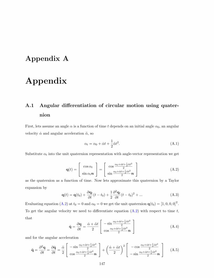
Appendix A
Appendix
A.1 Angular differentiation of circular motion using quater-
nion
First, lets assume an angle α is a function of time t depends on an initial angle α0, an angular
velocity α and angular acceleration α, so
αt = α0 + αt+12αt2. (A.1)
Substitute αt into the unit quaternion representation with angle-vector representation we get
q(t) =
cosαt
sinαtn
=
cos α0+αt+ 12αt2
2
sin α0+αt+ 12αt2
2 n
(A.2)
as the quaternion as a function of time. Now lets approximate this quaternion by a Taylor
expansion by
q(t) = q(t0) +∂qt∂t
(t− t0) +12∂2qt∂t
(t− t0)2 + ... (A.3)
Evaluating equation (A.2) at t0 = 0 and α0 = 0 we get the unit quaternion q(t0) = [1, 0, 0, 0]T.
To get the angular velocity we need to differentiate equation (A.2) with respect to time t,
that
q =∂q∂t
=α+ αt
2
− sin α0+αt+ 12αt2
2
cos α0+αt+ 12αt2
2 n
(A.4)
and for the angular acceleration
q =∂2q∂t
=∂q∂t
=α
2
− sin α0+αt+ 12αt2
2
cos α0+αt+ 12αt2
2 n
+(α+ αt
2
)2 − cos α0+αt+ 1
2αt2
2
− sin α0+αt+ 12αt2
2 n
(A.5)
147
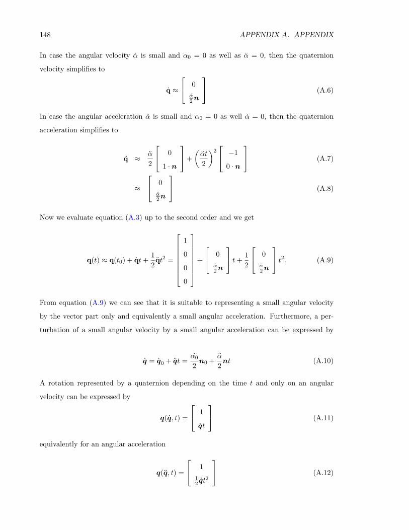
148 APPENDIX A. APPENDIX
In case the angular velocity α is small and α0 = 0 as well as α = 0, then the quaternion
velocity simplifies to
q ≈
0α2n
(A.6)
In case the angular acceleration α is small and α0 = 0 as well α = 0, then the quaternion
acceleration simplifies to
q ≈ α
2
0
1 · n
+(αt
2
)2 −1
0 · n
(A.7)
≈
0α2n
(A.8)
Now we evaluate equation (A.3) up to the second order and we get
q(t) ≈ q(t0) + qt+12qt2 =
1
0
0
0
+
0α2n
t+12
0α2n
t2. (A.9)
From equation (A.9) we can see that it is suitable to representing a small angular velocity
by the vector part only and equivalently a small angular acceleration. Furthermore, a per-
turbation of a small angular velocity by a small angular acceleration can be expressed by
q = q0 + qt =α0
2n0 +
α
2nt (A.10)
A rotation represented by a quaternion depending on the time t and only on an angular
velocity can be expressed by
q(q, t) =
1
qt
(A.11)
equivalently for an angular acceleration
q(q, t) =
112 qt
2
(A.12)
A.2. LINEAR DYNAMIC MODEL DERIVATION 149
A.2 Linear dynamic model derivation
Let us assume that we have a uniformly accelerated linear motion in 3d space in the time
interval ∆t. Following classical physics this motion can be described by
T t+1 = T t + T t∆t+12T t∆t2 (A.13)
If we differentiate with respect to ∆t we get the velocity
T t+1 = T t + T t∆t (A.14)
The other partial derivatives of equation (A.13) with respect to T t, T t and T t are given by
∂T t+1
∂T t= I 3 (A.15)
∂T t+1
∂T t= ∆tI 3 (A.16)
∂T t+1
∂T t=
12
∆t2I 3 (A.17)
The partial derivatives of equation (A.14) with respect to T t and T t are given by
∂T t+1
∂T t= I 3 (A.18)
∂T t+1
∂T t= ∆tI 3 (A.19)
In some cases it is useful to replace the velocity by T t = T t − T t−1 and equation (A.13) can
be rewritten as
T t+1 = T t + (T t − T t−1)∆t+12T t∆t2 (A.20)
and therefore the partial derivatives with respect to T t and T t−1 are given by
∂T t+1
∂T t= I 3 + ∆tI 3 (A.21)
∂T t+1
∂T t−1= −∆tI 3. (A.22)
In case of uniformly accelerated linear circular motion in 3d space during the time interval
∆t we can compute the partial derivatives in the same manner. To represent the rotation we
will use quaternions. Similar to the linear motion model in equation (A.13) we can compute
the linear circular motion as
qt+1 = q(qt)q(qt)qt. (A.23)
150 APPENDIX A. APPENDIX
We will assume that the angular velocity qt and angular acceleration qt are small, so that it is
sufficient to use the vector part only. in this case equation (3.36) can be used to concatenate
two rotations. The rotation around a fixed axis in the time interval ∆t given the angular
velocity and angular acceleration can be computed using quaternion representation simply
as
q(q) =
1
qt∆t
(A.24)
q(q) =
112 qt∆t
2
. (A.25)
Now using equation (3.31) the linear circular motion in equation (A.23) can be written as
qt+1 = Υ(q(q))Υ(q(q))qt. (A.26)
Also note that using equation (3.31) this can be conveniently rewritten to extract the desired
vector on the right hand side as follows
qt+1 = Υ(12qt∆t
2)Υ(qt∆t)qt (A.27)
= Υ(12qt∆t
2)Υ(qt)q(qt∆t) (A.28)
= Υ(Υ(qt∆t)qt)q(12qt∆t
2). (A.29)
The partial derivatives of equation (A.29) w.r.t. qt, qt and qt are therefore easily obtained as
∂qt+1
∂qt= Υ(
12qt∆t
2)Υ(qt∆t) (A.30)
∂qt+1
∂qt= Υ(
12qt∆t
2)Υ(qt) [03|∆tI 3] (A.31)
∂qt+1
∂qt= Υ(Υ(qt∆t)qt)
[03|
12
∆t2qt
]. (A.32)
Now we will assume a series of rotations with constant time differences ∆t is given. The
rotational difference between two time steps can be computed as
∆q = qtq−1t−1. (A.33)
A.2. LINEAR DYNAMIC MODEL DERIVATION 151
Assuming a linear circular motion, the rotation at time t + 1 can be obtained according to
equation (A.23) by
qt+1 = q(12qt∆t
2)∆qqt (A.34)
= q(12qt∆t
2)qtq−1t−1qt (A.35)
= Υ(12qt∆t
2)Υ(qt)Υ(q−1t−1)qt (A.36)
= Υ(12qt∆t
2)Υ(qt)Υ(qt)Vqt−1 (A.37)
= Υ(12qt∆t
2)Υ(Υ(qt)Vqt−1)qt (A.38)
= Υ(Υ(qt)Υ(q−1t−1)qt)q(
12qt∆t
2) (A.39)
The partial derivatives of qt+1 w.r.t. qt−1, q and qt using the chain rule are then given by
∂qt+1
∂qt−1= Υ(
12qt∆t
2)Υ(qt)Υ(qt)V (A.40)
∂qt+1
∂qt= Υ(Υ(qt)Υ(q−1
t−1)qt)[0|12
∆t2I 3] (A.41)
∂qt+1
∂qt= Υ(
12qt∆t
2)(Υ(qt)Υ(Vqt−1) + Υ(Υ(qt)Vqt−1)) (A.42)
In some cases the time difference between consecutive images changes. In this case we have
to deal with the time dependent factor denoted as ∆t here. It is given by
∆t =tt+1 − tttt − tt−1
. (A.43)
In case the rotation ∆q is small we can use the concatenation approximation
∆q∆t = U∆t(qtq−1t−1) = U∆tΥ(qt)Vqt−1 (A.44)
Now using this approximation the new rotation at time t+ 1 can be computed as
qt+1 = Υ(12qt∆t
2)Υ(U∆tΥ(qt)Vqt−1)qt (A.45)
= Υ(12qt∆t
2)Υ(qt)U∆tΥ(qt)Vqt−1 (A.46)
= Υ(12qt∆t
2)Υ(qt)U∆tΥ(Vqt−1)qt (A.47)
= Υ(Υ(U∆tΥ(qt)Vqt−1)qt)q(12qt∆t
2) (A.48)
The derivative w.r.t qt−1 and qt is therefore given by
∂qt+1
∂qt−1
= Υ(12qt∆t
2)Υ(qt)U∆tΥ(qt)V (A.49)
∂qt+1
∂qt= Υ(Υ(U∆tΥ(qt)Vqt−1)qt)[03|
12
∆t2I 3]. (A.50)
152 APPENDIX A. APPENDIX
The derivative w.r.t. qt using the chain rule is given by
∂qt+1
∂qt= Υ(
12qt∆t
2)(Υ(U∆tΥ(qt)Vqt−1) + Υ(qt)U∆tΥ(Vqt−1)). (A.51)
A.3 Uncertainty transfer
Lets assume we have a reference point Xr and a new point Xn close to each other. The
uncertainty of a Euclidean coordinate derived from camera observations can be expressed as
a sum of two independent parts
dXr = dvXr + dcXr (A.52)
dXn = dvXn + dcXn (A.53)
with v as the uncertainty part of the intersection and c as the uncertainty part of the camera
orientation. Furthermore we can assume, that the uncertainty of the new point Xn can be
expressed as the uncertainty of the reference point adding an unknown additional relative
uncertainty.
dXn = dvXr + d∆X (A.54)
This d∆X can be expressed using the difference of equation (A.52) and (A.53)
dXn = dXr + (dvXn + dcXn − (dvXr + dcXr)) (A.55)
Now, lets assume the influence part of the orientation for both points are equal, which is a
sufficient assumption. In this case equation (A.55) simplifies to
dXn = dXr + dvXn − dvXr (A.56)
Now lets rewrite in matrix expression dXr
d∆X
=
I I 0
−I 0 I
︸ ︷︷ ︸
A
dvXr
dcXr
dvXn
(A.57)
and apply the transformation to a Gaussian uncertainty representation which leads to
CXr∆X = A
CvXr 0 0
0 CcXr 0
0 0 CvXn
AT =
CvXr + C
cXr −C
vXn
−C vXn 2C vXn
=
CXr −C vXn−C vXn 2C vXn
(A.58)
Note, that C vXn should be smaller than CXr to guarantee positive semi-definiteness.

A.3. UNCERTAINTY TRANSFER 153
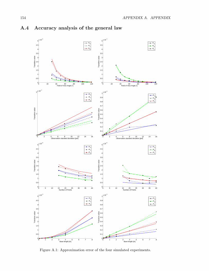
154 APPENDIX A. APPENDIX
A.4 Accuracy analysis of the general law
0 20 40 60 80 100 1200
0.5
1
1.5
2
2.5
3
3.5
4
4.5
5x 10
−5
Field of View Angle [°]
Tra
nsiti
on v
alue
mX
mY
mZ
0 20 40 60 80 100 1200
0.5
1
1.5
2
2.5
3
3.5
4
4.5
5x 10
−4
Field of View Angle [°]
Tra
nsiti
on v
alue
mωmφmκ
0 2 4 6 8 10 12 14 160
1
2x 10
−4
Observation standard deviation [pel]
Tra
nsiti
on v
alue
mX
mY
mZ
0 2 4 6 8 10 12 14 160
0.1
0.2
0.3
0.4
0.5
0.6
0.7
0.8
0.9
1x 10
−3
Observation standard deviation [pel]
Tra
nsiti
on v
alue
mωmφmκ
0 5 10 15 20 25 30 35 400
0.5
1
1.5
2
2.5
3
3.5
4
4.5
5x 10
−6
Number of Points
Tra
nsiti
on v
alue
mX
mY
mZ
0 5 10 15 20 25 30 35 400
0.5
1
1.5
2
2.5
3
3.5
4
4.5
5x 10
−5
Number of Points
Tra
nsiti
on v
alue
mωmφmκ
0 1 2 3 4 5 6 7 80
0.5
1
1.5
2
2.5
3
3.5
4
4.5
5x 10
−3
Base length [m]
Tra
nsiti
on v
alue
mX
mY
mZ
0 1 2 3 4 5 6 7 80
0.1
0.2
0.3
0.4
0.5
0.6
0.7
0.8
0.9
1x 10
−3
Base length [m]
Tra
nsiti
on v
alue
mωmφmκ
Figure A.1: Approximation error of the four simulated experiments.

A.4. ACCURACY ANALYSIS OF THE GENERAL LAW 155
Negative approx. error Positive approx. error
Exp σX σY σZ σω σφ σκ σX σY σZ σω σφ σκ
Fov
30 39 27 10 22 11 14 33 21 25 22 41 36
40 40 28 9 25 16 14 31 14 40 17 37 51
50 30 26 11 30 15 14 29 22 34 27 40 45
60 36 34 10 41 24 12 27 1 39 1 9 28
70 26 20 4 25 22 9 24 14 38 17 30 35
80 23 11 6 23 28 13 32 25 33 31 44 29
90 16 11 7 24 25 8 26 19 28 21 38 24
100 12 14 12 15 17 8 25 19 20 21 31 20
110 8 5 7 3 12 5 23 25 29 34 39 28
120 26 18 9 28 36 11 7 21 24 20 14 17
σxy[pel]
0.05 14 12 1 23 15 6 31 20 42 25 46 36
0.1 24 22 7 29 27 10 16 13 21 16 23 23
0.5 20 11 8 22 23 9 22 23 26 23 28 21
1 23 17 9 20 23 7 13 20 25 23 17 20
2 43 24 7 34 44 12 8 11 26 11 11 16
4 34 25 22 27 38 17 15 15 33 12 7 19
8 21 18 9 20 22 7 23 16 34 14 29 27
16 10 10 3 16 17 8 22 26 41 26 35 32
NX [-]
10 62 83 58 87 64 34 25 1 36 3 35 21
15 30 32 29 40 39 20 9 15 24 15 16 18
20 27 25 7 33 32 11 28 16 16 18 40 19
30 16 12 6 20 19 9 26 21 18 28 34 21
35 18 5 4 7 18 4 25 23 31 33 33 28
40 18 18 7 24 18 8 24 16 37 20 33 26
B[m]
0.1 37 23 16 31 40 14 9 11 29 6 4 12
0.5 16 9 8 28 16 8 23 21 29 27 38 41
1 34 29 14 33 24 10 14 15 45 4 21 49
2 10 7 14 26 8 10 27 23 55 24 55 98
4 23 19 16 21 19 9 24 28 72 30 64 140
8 23 14 28 33 23 16 31 33 168 36 58 185
min‖max 62 83 58 87 64 34 33 33 168 36 64 185
Table A.1: Approximation error in percent.
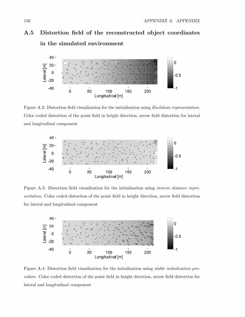
156 APPENDIX A. APPENDIX
A.5 Distortion field of the reconstructed object coordinates
in the simulated environment
Figure A.2: Distortion field visualization for the initialization using Euclidean representation.
Color coded distortion of the point field in height direction, arrow field distortion for lateral
and longitudinal component
Figure A.3: Distortion field visualization for the initialization using inverse distance repre-
sentation. Color coded distortion of the point field in height direction, arrow field distortion
for lateral and longitudinal component
Figure A.4: Distortion field visualization for the initialization using stable initialization pro-
cedure. Color coded distortion of the point field in height direction, arrow field distortion for
lateral and longitudinal component
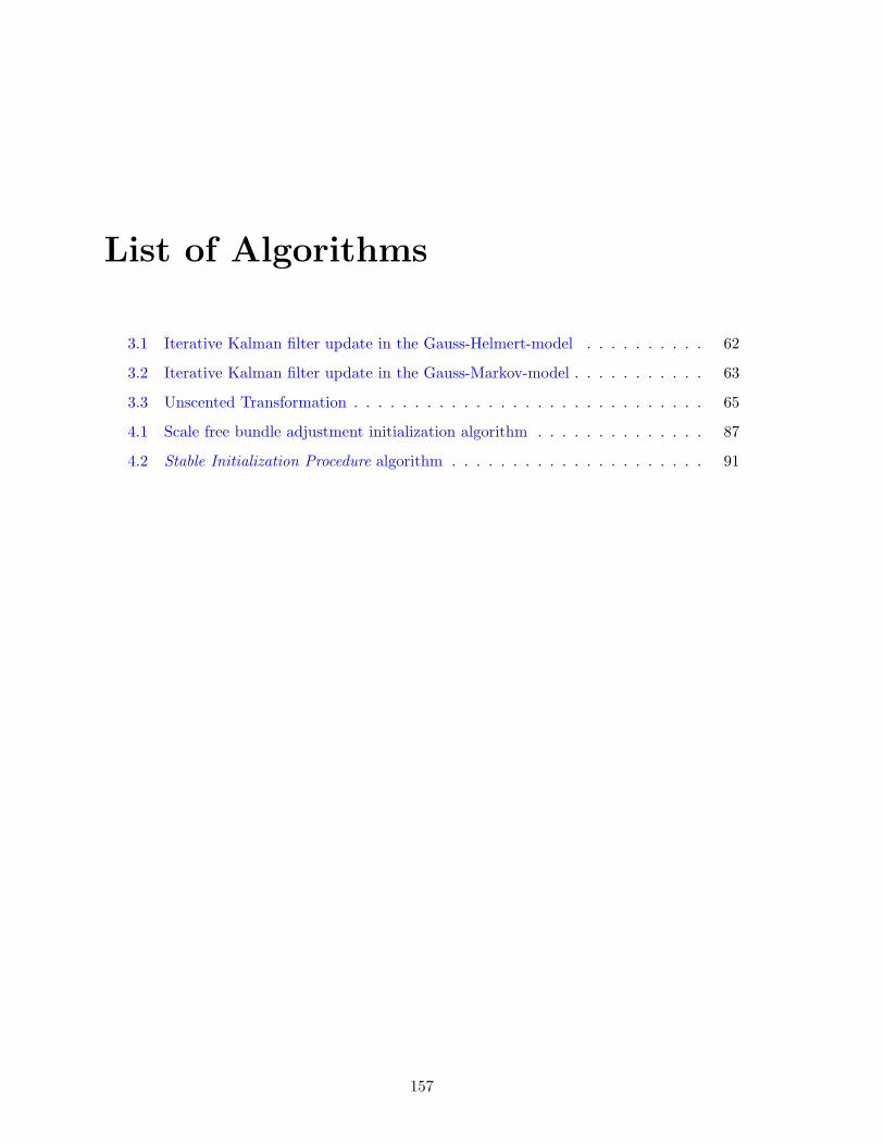
List of Algorithms
3.1 Iterative Kalman filter update in the Gauss-Helmert-model . . . . . . . . . . 62
3.2 Iterative Kalman filter update in the Gauss-Markov-model . . . . . . . . . . . 63
3.3 Unscented Transformation . . . . . . . . . . . . . . . . . . . . . . . . . . . . . 65
4.1 Scale free bundle adjustment initialization algorithm . . . . . . . . . . . . . . 87
4.2 Stable Initialization Procedure algorithm . . . . . . . . . . . . . . . . . . . . . 91
157

158 LIST OF ALGORITHMS
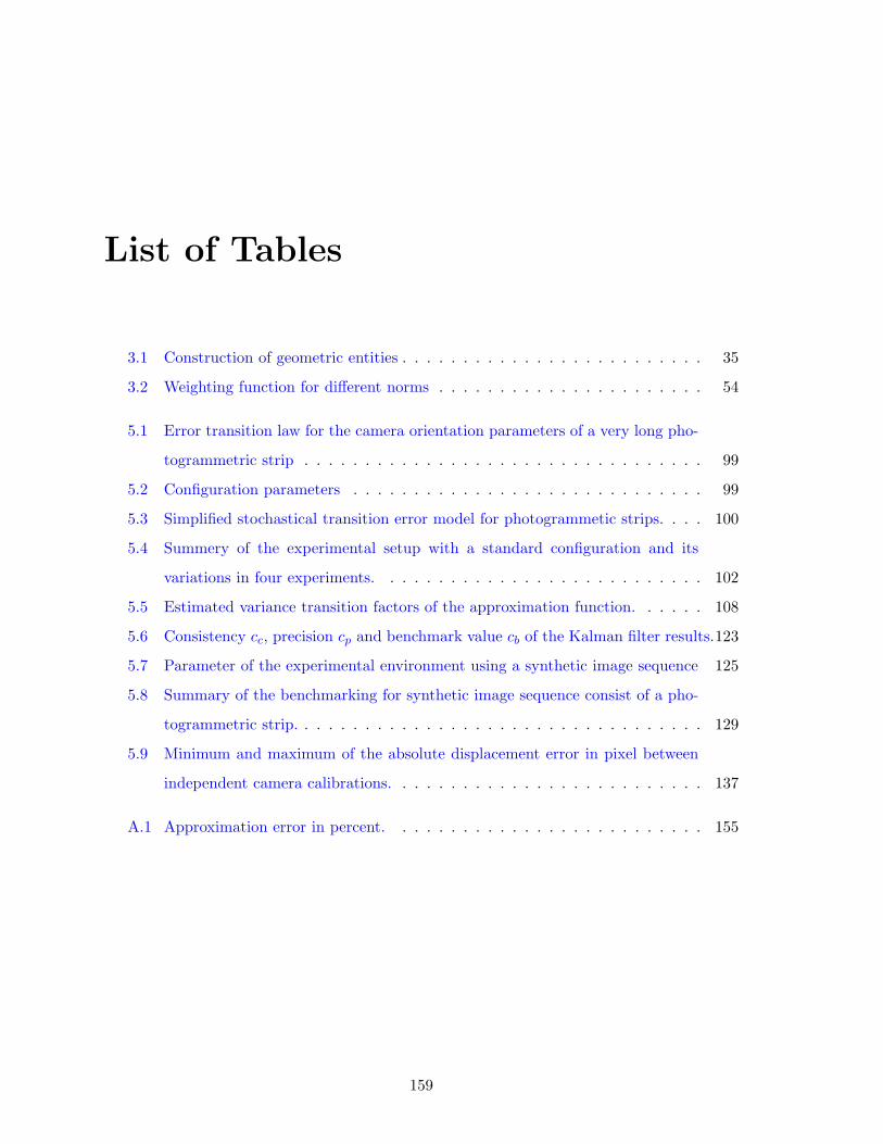
List of Tables
3.1 Construction of geometric entities . . . . . . . . . . . . . . . . . . . . . . . . . 35
3.2 Weighting function for different norms . . . . . . . . . . . . . . . . . . . . . . 54
5.1 Error transition law for the camera orientation parameters of a very long pho-
togrammetric strip . . . . . . . . . . . . . . . . . . . . . . . . . . . . . . . . . 99
5.2 Configuration parameters . . . . . . . . . . . . . . . . . . . . . . . . . . . . . 99
5.3 Simplified stochastical transition error model for photogrammetic strips. . . . 100
5.4 Summery of the experimental setup with a standard configuration and its
variations in four experiments. . . . . . . . . . . . . . . . . . . . . . . . . . . 102
5.5 Estimated variance transition factors of the approximation function. . . . . . 108
5.6 Consistency cc, precision cp and benchmark value cb of the Kalman filter results.123
5.7 Parameter of the experimental environment using a synthetic image sequence 125
5.8 Summary of the benchmarking for synthetic image sequence consist of a pho-
togrammetric strip. . . . . . . . . . . . . . . . . . . . . . . . . . . . . . . . . . 129
5.9 Minimum and maximum of the absolute displacement error in pixel between
independent camera calibrations. . . . . . . . . . . . . . . . . . . . . . . . . . 137
A.1 Approximation error in percent. . . . . . . . . . . . . . . . . . . . . . . . . . 155
159

160 LIST OF TABLES
List of Figures
2.1 Map representations . . . . . . . . . . . . . . . . . . . . . . . . . . . . . . . . 26
3.1 Exterior orientation and camera mapping scheme . . . . . . . . . . . . . . . . 42
3.2 Epipolar geometry . . . . . . . . . . . . . . . . . . . . . . . . . . . . . . . . . 45
3.3 Homography induced by a plane . . . . . . . . . . . . . . . . . . . . . . . . . 46
3.4 Dynamic Bayes network . . . . . . . . . . . . . . . . . . . . . . . . . . . . . . 56
3.5 Kalman filter scheme . . . . . . . . . . . . . . . . . . . . . . . . . . . . . . . . 57
4.1 System components and connections for the task of simultaneous localization
and mapping using a single camera . . . . . . . . . . . . . . . . . . . . . . . . 71
4.2 Example for point based feature tracking . . . . . . . . . . . . . . . . . . . . 74
4.3 Camera coordinate system definition . . . . . . . . . . . . . . . . . . . . . . . 75
4.4 Camera state representation scheme using a single camera state . . . . . . . . 77
4.5 Camera state representation scheme using a multiple camera state . . . . . . 79
4.6 Polar coordinate definition for the inverse distance representation. . . . . . . 82
4.7 Simulation scheme of a point reconstruction with small parallax . . . . . . . . 83
4.8 Stable Initialization Procedure scheme . . . . . . . . . . . . . . . . . . . . . . 90
4.9 Sigma point crosses positive to negative infinity singularity . . . . . . . . . . 94
4.10 Mean propagation using unscented transformation from inverse distance to
Euclidean space . . . . . . . . . . . . . . . . . . . . . . . . . . . . . . . . . . . 94
4.11 Example of sigma point projection in case of large object point uncertainty. . 95
5.1 The influence of the principal distance onto the accuracy transition factors . . 103
5.2 The influence of base length onto the accuracy transition factors . . . . . . . 104
5.3 The influence of the measurement accuracy onto the accuracy transition factors105
161
162 LIST OF FIGURES
5.4 The influence of the map density onto the accuracy transition factors . . . . . 106
5.5 Bundle adjustment results for the camera position parameters . . . . . . . . . 112
5.6 Initialization using Euclidean representation with ground truth distance. . . . 113
5.7 Initialization using ground truth distance and a sliding window camera repre-
sentation. . . . . . . . . . . . . . . . . . . . . . . . . . . . . . . . . . . . . . . 114
5.8 Initialization using inverse distance representation with ground truth distance. 115
5.9 Initialization using inverse distance representation with ground truth distance
and reparameterization . . . . . . . . . . . . . . . . . . . . . . . . . . . . . . . 117
5.10 Initialization using ground truth distance and Sliding Window with a round-
ness test value of ΘL = 0.05. . . . . . . . . . . . . . . . . . . . . . . . . . . . 118
5.11 Initialization using ground truth distance and Sliding Window with a round-
ness test value of ΘL = 0.01. . . . . . . . . . . . . . . . . . . . . . . . . . . . 119
5.12 Initialization using the stable initialization procedure with a roundness test
value of ΘL = 0.05. . . . . . . . . . . . . . . . . . . . . . . . . . . . . . . . . . 121
5.13 Initialization using the stable initialization procedure with a roundness test
value of ΘL = 0.01. . . . . . . . . . . . . . . . . . . . . . . . . . . . . . . . . . 122
5.14 Benchmark summary of the Kalman filter results. . . . . . . . . . . . . . . . . 124
5.15 First image of the simulated image data sequence with signalized control points126
5.16 Bundle adjustment results for the estimated camera parameters with 2-sigma
error bounds . . . . . . . . . . . . . . . . . . . . . . . . . . . . . . . . . . . . 127
5.17 Robust bundle adjustment results for the estimated camera parameters with
2-sigma error bounds. . . . . . . . . . . . . . . . . . . . . . . . . . . . . . . . 128
5.18 Kalman filter results for the estimated camera parameters with 2-sigma error
bounds. . . . . . . . . . . . . . . . . . . . . . . . . . . . . . . . . . . . . . . . 130
5.19 Robust Kalman filter results for the estimated camera parameters with 2-sigma
error bounds. . . . . . . . . . . . . . . . . . . . . . . . . . . . . . . . . . . . . 131
5.20 Images of the synthetic image sequence of the Basilika St. Peter in Rom. . . 132
5.21 Robust bundle adjustment solution using outlier detection by variance com-
ponent estimation on the Basilika dataset. . . . . . . . . . . . . . . . . . . . . 134
5.22 Used hardware. Drone MD 4-200 from Microdrones c© equipped with a Pana-
sonic Lumix video camera. . . . . . . . . . . . . . . . . . . . . . . . . . . . . . 136
LIST OF FIGURES 163
5.23 Absolute displacement error in pixel between independent camera calibrations
using the average principal distance. . . . . . . . . . . . . . . . . . . . . . . . 137
5.24 High altitude image of the flight-test area and control point field in the test
area in a local coordinate system. . . . . . . . . . . . . . . . . . . . . . . . . . 138
5.25 Reference trajectory of the camera orientation of the test image sequence. . . 139
5.26 Difference between high accuracy bundle solution and Kalman filter based
solution. . . . . . . . . . . . . . . . . . . . . . . . . . . . . . . . . . . . . . . . 140
A.1 Approximation error of the four simulated experiments. . . . . . . . . . . . . 154
A.2 Distortion field visualization for the initialization using Euclidean representa-
tion. Color coded distortion of the point field in height direction, arrow field
distortion for lateral and longitudinal component . . . . . . . . . . . . . . . . 156
A.3 Distortion field visualization for the initialization using inverse distance repre-
sentation. Color coded distortion of the point field in height direction, arrow
field distortion for lateral and longitudinal component . . . . . . . . . . . . . 156
A.4 Distortion field visualization for the initialization using stable initialization
procedure. Color coded distortion of the point field in height direction, arrow
field distortion for lateral and longitudinal component . . . . . . . . . . . . . 156

164 LIST OF FIGURES
Bibliography
Abraham, Steffen. 1999. Kamera Kalibrierung und metrische Auswertung monokularer
Bildfolgen. Ph.D. thesis, Institute of Photogrammetry, University of Bonn.
Ackermann, Friedrich. 1965. Fehlertheoretische Untersuchungen uber die Genauigkeit
photogrammetrischer Streifentriangulationen. Ph.D. thesis, Deutsche Geodatische Kom-
mission, Reihe C, Nr. 87, Munchen.
Akbarzadeh, A., Frahm, J.-M., Mordohai, P., Clipp, B., Engels, C., Gallup, D.,
Merrell, P., Phelps, M., Sinha, S., Talton, B., Wang, L., Yang, Q., Steweius,
H., Yang, R., Welch, G., Towles, H., Nister, D.,Pollefeys, M. 2006. Towards
urban 3d reconstruction from video. In: Third International Symposium on 3D Data
Processing, Visualization and Transmission (3DPVT).
Baarda, Willem. 1967. Statistical Concepts in Geodesy. New Series, vol. 2. Delft: Nether-
lands Geodetic Commission.
Baarda, Willem. 1973. S-Transformations and Criterion Matrices. Netherlands geodetic
Commission, volume 5 of 1.
Bailey, Tim, Nieto, Juan, Guivant, Jose, Stevens, Michael,Nebot, Eduardo.
2006. Consistency of the EKF-SLAM Algorithm. In: International Conference on Intelli-
gent Robots and Systems.
Beder, Christian,Steffen, Richard. 2006. Determining an initial image pair for fixing
the scale of a 3d reconstruction from an image sequence. Pages 657–666 of: Franke,
K., Muller, K.-R., Nickolay, B.,Schafer, R. (eds), Pattern Recognition. LNCS, no.
4174. Springer.
165
166 BIBLIOGRAPHY
Beder, Christian,Steffen, Richard. 2008. Incremental estimation without specifying
a-priori covariance matrices for the novel parameters. VLMP Workshop on CVPR. An-
chorage, USA.
Benıtez, Fernando Caballero, Cabanas, Luis Merino, Melero, Joaquin Fer-
ruz,Baturone, Anibal Ollero. 2005. A Visual Odometer Without 3d Reconstruction
for Aerial Vehicles. Applications to Building Inspection. Pages 4684–4689 of: IEEE Inter-
national Conference on Robotics and Automation.
Besl, Paul J.,D.McKay, Neil. 1992. A Method for Registration of 3-D Shapes. IEEE
Trans. Pattern Anal. Mach. Intell., 14(2), 239–256.
Bibby, Charles,Reid, Ian. 2007. Simultaneous Localisation and Mapping in Dynamic En-
vironments (SLAMIDE) with Reversible Data Association. Robotics: Sience and Systems.
Blanco, Jose-Luis, Fernandez-Madrigal, Juan-Antonio,Gonzalez, Javier. 2007.
A New Approach for Large-Scale Localization and Mapping: Hybrid Metric-Topological
SLAM. Pages 2061–2067 of: ICRA.
Brennecke, Christian, Wolf, Oliver,Wagner, Bernardo. 2003. Using 3D Laser
Range Data for SLAM in Outdoor Environments. In: IEEE/RSJ International Conference
on Intelligent Robots and Systems.
Caspary, W., Wang J. 1998. Redundanzanteile und Varianzkomponenten im Kalman
Filter. ZfV 123, 121–128.
Castellanos, Jose A., Neira, Jose,Tardos, Juan D. 2004. Limits to the Consistency
of EKF-based SLAM. 5th symposium on Intelligent Autonomous Vehicles, 21–26.
Chiba, Naoki,Knade, Takeo. 1998. A Tracker for Broken and Closely-Spaced Lines.
ISPRS International Archives of Photogrammetry and Remote Sensing, XXXII, 676–683.
Choset, Howie,Nagatani, K. 2001. Topological simultaneous localization and mapping
(SLAM): toward exact localization without explicit localization. IEEE Transactions on
Robotics and Automation, 17(1), 125 – 137.
Civera, Javier, Davison, Andrew J.,Montiel, J. M. M. 2007a. Dimensionless Monoc-
ular SLAM. In: IBPRIA.
BIBLIOGRAPHY 167
Civera, Javier, Davison, Andrew J.,Montiel, J. M. M. 2007b. Inverse Depth to
Depth Conversion for Monocular SLAM. In: ICRA.
Clemente, Laura, Davison, Andrew, Reid, Ian, Neira, Jose,Tardos,
Juan Domingo. 2007 (June). Mapping Large Loops with a Single Hand-Held Camera.
In: Proc. Robotics: Science and Systems Conference.
Davison, Andrew J. 2003. Real-Time Simultaneous Localisation and Mapping with a
Single Camera. In: Proc. International Conference on Computer Vision, Nice.
Davison, Andrew J.,Kita, Nobuyuki. 2001. 3D Simultaneous Localisation and Map-
Building Using Active Vision for a Robot Moving on Undulating Terrain. In: CVPR.
Davison, Andrew J.,Murray, David W. 2002. Simultaneous Localisation and Map-
Building using Active Vision. IEEE Transactions on Pattern Analysis and Machine Intel-
ligence, 24(7), 865–880.
Dellaert, Frank. 2005 (June). Square Root SAM. In: Proceedings of Robotics: Science
and Systems.
Dickscheid, Timo, Labe, Thomas,Forstner, Wolfgang. 2008. Benchmarking Auto-
matic Bundle Adjustment Results. In: To appear in: 21st Congress of the International
Society for Photogrammetry and Remote Sensing (ISPRS).
Dissanayake, M. W. M. Gamini, Newman, Paul, Clark, Steven, Durrant-whyte,
Hugh F.,Csorba, M. 2001. A solution to the simultaneous localization and map building
(SLAM) problem. IEEE Transactions on Robotics and Automation, 17, 229–241.
Eliazar, Austin I.,Parr, Ronald. 2003. DP-SLAM: Fast, Robust Simultaneous Local-
ization and Mapping Without Predetermined Landmarks. Pages 1135–1142 of: IJCAI.
Eliazar, Austin I.,Parr, Ronald. 2004. DP-SLAM 2.0. Pages 1314–1320 of: ICRA.
Estrada, Carlos, Neira, Jose,Tardos, Juan D. 2005. Hierarchical SLAM: real-time
accurate mapping of large environments. IEEE Transactions on Robotics, 588–596.
Everaerts, J., Lewyckyj, N.,Fransaer, D. 2004. PEGASUS: Design of a Stratospheric
Long Endurance UAV System for Remote Sensing. In: The International Archives of the
Photogrammetry, Remote Sensing and Spatial Information Sciences, vol. XXXV Part B2.
168 BIBLIOGRAPHY
Fairfield, Nathaniel, Kantor, George A.,Wettergreen, David. 2006 (May). To-
wards Particle Filter SLAM with Three Dimensional Evidence Grids in a Flooded Subter-
ranean Environment. Pages 3575 – 3580 of: Proceedings of ICRA 2006.
Faugeras, Olivier, Robert, Luc, Laveau, Stephane, Csurka, Gabriella, Zeller,
Cyril, Gauclin, Cyrille,Zoghlami, Imed. 1998. 3-D Reconstruction of Urban Scenes
from Image Sequences. Pages 229–309 of: Computer Vision and Image Understanding,
vol. 69-3.
Finsterwalder, Richard,Hofmann, Walter. 1964. Photogrammetrie. Walter de
Gruyter, Berlin.
Fischler, M. A.,Bolles, R. C. 1981. Random Sample Consensus: A Paradigm for Model
Fitting with Applications to Image Analysis and Automated Cartography. Pages 381–395
of: Comm. of the ACM, vol. Vol 24.
Folkesson, John,Christensen, Hendrik. 2004. Graphical slam - a self-correction map.
In IEEE International Conference on Robotics and Automation.
Forstner, Wolfgang. 1987. Reliability Analysis of Parameter Estimation in Linear Mod-
els with Applications to Mensuration Problems in Computer Vision. Pages 273–310 of:
CVGIP - Computer Vision, Graphics and Image Processing.
Forstner, Wolfgang,Moonen, Boudewijn. 1999. A Metric for Covariance Matrices. In:
In: Krumm, F. / Schwarze, V. S. (Hg.): Quo vadis geodesia ...?, Festschrift for Erik W.
Grafarend on the occasion of his 60th birthday. TR Dept. of Geodesy and Geoinformatics,
Stuttgart University.
Forstner, Wolfgang,Wrobel, Bernhard. 2004. Mathematical Concepts in Photogram-
metry. Pages 15–180 of: J.C.McGlone, E.M.Mikhail,J.Bethel (eds), Manual of Pho-
togrammetry. ASPRS.
Forstner, Wolfgang. 1982. On the Geometric Precision of Digital Correlation. Pages
176–189 of: Proceedings of the ISPRS Symposium Mathematical Models, Accuray Aspects
and Quality Control.
BIBLIOGRAPHY 169
Forstner, Wolfgang,Gulch, Eberhard. 1987. A Fast Operator for Detection and
Precise Location of Distict Point, Corners and Centres of Circular Features. Pages 281–
305 of: Proceedings of the ISPRS Conference on Fast Processing of Photogrammetric Data.
Grisetti, Giorgio, Stachniss, Cyrill,Burgard, Wolfram. 2006. Improved Tech-
niques for Grid Mapping with Rao-Blackwellized Particle Filters. IEEE Transactions on
Robotics.
Grun, Armin. 1982. An Optimum Algorithm for On-Line Triangulation. Pages 131–151 of:
International Society for Photogrammetry and Remote Sensing, Volume 24 - III/2.
Guivant, Jose E., Nebot, Eduardo Mario, Nieto, Juan,Masson, Favio R. 2004.
Navigation and Mapping in Large Unstructured Environments. I. J. Robotic Res., 23(4-5),
449–472.
Hampel, Frank R., Ronchetti, Elvezio M., Rousseeuw, Peter J.,Stahel,
Werner A. 1986. Robust Statistics - The Approach Based on Influence Functions. Wiley.
Haralick, R. M., Lee, C., Ottenberg, K.,Nolle, M. 1991. Analysis and Solutions of
the Three Point Perspective Pose Estimation Problem. Pages 592–598 of: Proc. of the
IEEE Comp. Society Conf. on “Computer Vision and Pattern Recognition”.
Harati, A., Gachter, S.,Siegwart, R. 2007. Fast Range Image Segmentation for Indoor
3D-SLAM. In: Proceedings of the Sixth IFAC Symposium on Intelligent Autonomous
Vehicles (IAV-6).
Harris, Chris,Stephens, Mike. 1988. A Combined Corner and Edge Detector. Pages
147–151 of: The Fourth Alvey Vision Conference.
Hartley, Richard I.,Zisserman, Andrew. 2000. Multiple View Geometry in Computer
Vision. Cambridge University Press, ISBN: 0521623049.
Herbert Bay, Vittorio Ferraris,Gool, Luc Van. 2005. Wide-baseline stereo matching
with line segments. Pages 329–336 vol. 1 of: Computer Vision and Pattern Recognition,
2005. CVPR 2005. IEEE Computer Society Conference on, vol. 1.
Heuel, Stephan. 2004. Uncertain Projective Geometry - Statistical Reasoning for Polyhedral
Object Reconstruction. Springer.
170 BIBLIOGRAPHY
Holz, D., Lorken, C.,Surmann, H. 2008 (30 2008-July 3). Continuous 3D sensing for
navigation and SLAM in cluttered and dynamic environments. Pages 1–7 of: 11th Inter-
national Conference on Information Fusion.
Horn, Berthold K. P., Hilden, H.M.,Negahdaripour, Shariar. 1988. Closed-Form
Solution of Absolute Orientation using Orthonormal Matrices. Journal of the Optical
Society A, 5(7), 1127–1135.
Howard, Andrew,Kitchen, Les. 1997. Fast Visual mapping for Mobile Robot Navigation.
ICIPS’97 IEEE International Conference on Intelligent Processing Systems, Beijing.
J. A. Castellanos, J. M. M. Montiel, J. Neira,Tardos, J. D. 1999. The SPmap: A
Probabilistic Framework for Simultaneous Localization and Map Building. IEEE Trans-
actions on Robotics and Automation, 15(5)(October), pp. 948 – 952.
Julier, S.,Uhlmann, J. 1996. A General Method for Approximating Nonlinear Transfor-
mations of Probability Distributions. Tech. rept. Oxford University.
Julier, S.,Uhlmann, J. 1997. A new extension of the Kalman filter to nonlinear systems.
In: Int. Symp. Aerospace/Defense Sensing, Simul. and Controls,Orlando, FL.
Julier, Simon J.,Uhlmann, Jeffrey K. 2007. Using covariance intersection for SLAM.
Robot. Auton. Syst., 55(1), 3–20.
Kalman, R.E. 1960. A new approach to linear filtering and prediction problems,. Transac-
tions of the ASME - Journal of Basic Engineering on Automatic Control, 82(D), 35–45.
Kanade, Takeo, Amidi, Omead,Ke, Qifa. 2004 (December). Real-Time and 3D Vision
for Autonomous Small and Micro Air Vehicles. In: 43rd IEEE Conference on Decision and
Control (CDC 2004).
Kim, Jong-Hyuk,Sukkarieh, Salah. 2006. Robust Multi-loop Airborne SLAM in Un-
known Wind Environments. Pages 1536–1541 of: ICRA. IEEE.
Koch, K.-R. 1988. Parameter estimation and hypothesis testing in linear models. Springer.
Koch, Karl-Rudolf. 1997. Parameterschatzung und Hypothesentests. Dummler.
Kuipers, Benjamin, Browning, Rob, Gribble, Bill, Hewett, Mike,Remolina,
Emilio. 2000. The Spatial Semantic Hierarchy. Artificial Intelligence, 119, 191–233.
BIBLIOGRAPHY 171
Lemaire, Thomas,Lacroix, Simon. 2007 (April). Monocular-vision based SLAM using
line segments. In: IEEE International Conference on Robotics and Automation.
Li, Deren. 1987. Theorie und Untersuchung der Trennbarkeit von groben Paßpunktfehlern
und systematischen Bildfehlern bei der photogrammetrischen Punktbestimmung. Ph.D. the-
sis, Deutsche Geodatische Kommission, Reihe C, Nr. 324, Munchen.
Li, Ron, Di, Kaichang, Wang, Jue, Agarwal, Sanchit, Matthies, Larry, Howard,
Andrew,Willson, Reg. 2005. Incremental Bundle Adjustment Techniques Using Net-
worked Overhead and Ground Imagery for Long-Range Autonomous Mars Rover Localiza-
tion. Proceedings of the 8th International Symposium on Artificial Intelligence, Robotics
and Automation (iSAIRAS), Munich, Germany.
Liao, L., Fox, D., Hightower, J., Kautz, H.,Schulz, D. 2003. Voronoi tracking:
Location estimation using sparse and noisy sensor data.
Lindeberg, Tony. 1998. Feature detection with automatic scale selection. International
Journal of Computer Vision, 30, 79–116.
Lowe, David. 2003. Distinctive image features from scale-invariant keypoints. Pages 91–110
of: International Journal of Computer Vision, vol. 20.
Lu, Feng,Milios, Evangelos. 1994. Robot Pose Estimation in Unknown Environments
by Matching 2D Range Scans. Journal of Intelligent and Robotic Systems, 18, 249–275.
Martinez-Cantin, Ruben,Castellanos, Jose A. 2005. Unscented SLAM for Large-
Scale Outdoor Environments. IEEE/RSJ International Conference on Intelligent Robots
and Systems, 328–333.
Marzorati, Daniele, Matteucci, Matteo, Migliore, Davide,Sorrenti,
Domenico G. 2007. Integration of 3D Lines and Points in 6DoF Visual SLAM by
Uncertain Projective Geometry. Proceedings of ECMR.
McGlone, J. Chris, Mikhail, Edward M., Bethel, James,Mullen, Roy (eds). 2004.
Manual of Photogrammetry. American Society for Photogrammetry and Remote Sensing.
McLauchlan, Philip F.,Murray, David W. 1995. A Unifying Framework for Struc-
ture and Motion Recovery from Image Sequences. Pages 314–320 of: Proceedings of the
International Conference on Computer Vision.
172 BIBLIOGRAPHY
McLauchlan, Philip.F. 2000. A Batch/Recursive Algorithm for 3D Scene Reconstruction.
Pages II: 738–743 of: CVPR00.
Mikhail, E. M.,Ackermann, F. 1976. Observations and Least Squares. University Press
of America.
Mikolajczyk, Krystian,Schmid, Cordelia. 2002. An Affine Invariant Interest Point
Detector. Pages 128–142 of: ECCV ’02: Proceedings of the 7th European Conference on
Computer Vision-Part I. London, UK: Springer-Verlag.
Mikolajczyk, Krystian,Schmid, Cordelia. 2005. A performance evaluation of local
descriptors. IEEE Transactions on Pattern Analysis and Machine Intelligence, 27(10),
1615–1630.
Molenaar, M. 1981. A further inquiry into the theory of S-transformation and criterion
matrices. Publications on geodesy, Vol. 7(1), Netherlands geodetic Commision, Delft.
Montemerlo, M.,Thrun, S. 2003. Simultaneous localization and mapping with unknown
data association using FastSLAM. In: In Proceedings of the IEEE International Conference
on Robotics and Automation (ICRA).
Montemerlo, M., Thrun, S., Koller, D.,Wegbreit, B. 2002. FastSLAM: A Fac-
tored Solution to the Simultaneous Localization and Mapping Problem. Pages 593–598 of:
Proceedings of the 18th National Conference on Artificial Intelligence (AAAI).
Montiel, J.M.M., Civera, Javier,Davison, Andrew J. 2006. Unified Inverse Depth
Parametrization for Monocular SLAM. In: Robotics Science and Systems.
Mouragnon, E., Lhuillier, Maxime, Dhome, Michel, Dekeyser, Fabien,Sayd,
Patrick. 2006. Monocular Vision Based SLAM for Mobile Robots. Pages 1027–1031
of: ICPR (3). IEEE Computer Society.
Nuchter, Andreas. 2007. Parallelization of Scan Matching for Robotic 3D Mapping. In:
In Proceedings of the 3rd European Conference on Mobile Robots (ECMR ’07), Freiburg.
Nuchter, Andreas, Lingemann, Kai,Hertzberg, Joachim. 2006. Extracting drivable
surfaces in outdoor 6d slam. In: In Proc. of the 37nd Int. Symp. on Robotics (ISR 06.
Niemeier, Wolfgang. 2001. Augleichungsrechnung. deGruyter-Verlag.
BIBLIOGRAPHY 173
Nieto, Juan, Bailey, Tim,Nebot, Eduardo Mario. 2005. Scan-SLAM: Combining
EKF-SLAM and Scan Correlation. Pages 167–178 of: FSR.
Nister, David. 2004. An Efficient Solution to the Five-Point Relative Pose Problem. IEEE
Trans. Pattern Anal. Mach. Intell., 26(6), 756–777.
Nister, David. 2004. An Efficient Solution to the Five-Point Relative Pose Problem. IEEE
Transactions on Pattern Analysis and Machine Intelligence, 26(6), 756–777.
Ollero, Anibal, Ferruz, Joaquin, Caballero, Fernando, Hurtado, Se-
bastian,Merino, Luis. 2004. Motion Compensation and Object Detection for Au-
tonomous Helicopter Visual Navigation in the Comets System. In: IEEE International
Conference on Robotics & Automation.
P. M. Newman, J. J. Leonard,Rikoski, R. J. 2003. Towards Constant-Time SLAM on
an Autonomous Underwater Vehicle Using Synthetic Aperture Sonar. In: Proceedings of
the Eleventh International Symposium on Robotics Research, Sienna, Italy.
Paz, L.M., Jensfelt, P., Tardos, J.D.,Neira, J. 2007 (apr). EKF SLAM updates in
O(n) with Divide and Conquer SLAM. In: Proc. of the IEEE International Conference on
Robotics and Automation (ICRA’07).
Pfaff, Patrick, Triebel, Rudolph,Burgard, Wolfram. 2007. An Efficient Extension
to Elevation Maps for Outdoor Terrain Mapping and Loop Closing. Int. J. Rob. Res.,
26(2), 217–230.
Pupilli, Mark,Calway, Andrew. 2005. Real-Time Camera Tracking Using a Particle
Filter. Pages 519–528 of: Proceedings of the British Machine Vision Conference. BMVA
Press.
Pupilli, Mark,Calway, Andrew. 2006 (June). Real-time Visual SLAM with Resilience
to Erratic Motion. In: IEEE Computer Vision and Pattern Recognition.
Ribas, D., Neira, J., Ridao, P.,Tardos, J.D. 2006 (October). SLAM using an imaging
sonar for partially structured environments. In: IEEE/RSJ International Conference on
Intelligent Robots and Systems.
Ribas, David, Ridao, Pere, Tardos, Juan Domingo,Neira, Jose. 2008. Underwater
SLAM in man-made structured environments. J. Field Robot., 25(11-12), 898–921.
174 BIBLIOGRAPHY
Rodrıguez-Losada, Diego, Matıa, Fernando, Jimenez, Agustın,Galan, Ramon.
2006. Consistency Improvement for SLAM - EKF for Indoor Environments. ICRA, 418–
423.
Rusinkiewicz, Szymon,Levoy, Marc. 2001 (jun). Efficient Variants of the ICP Algorithm.
In: Third International Conference on 3D Digital Imaging and Modeling (3DIM).
Schlaile, Christian, Meister, Oliver, Wendel, Jan,Trommer, Gert F. 2006. Vi-
sion based navigation of a four rotor helicopter in unprepared indoor environments. Euro-
pean Micro Air Vehicle Conference and Flight Competition 2006.
Se, S., Barfoot, T.,Jasiobedzki, P. 2005 (August). Visual Motion Estimation and
Terrain Modeling for Planetary Rovers. In: ’i-SAIRAS 2005’ - The 8th International
Symposium on Artificial Intelligence, Robotics and Automation in Space. ESA Special
Publication, vol. 603.
Sibley, G., Sukhatme, G.,Matthies, L. 2006 (August). The Iterated Sigma Point Kalman
Filter with Applications to Long Range Stereo. In: Proceedings of Robotics: Science and
Systems.
Sibley, Gabe. 2006. Sliding Window Filters for SLAM. Tech. rept. University of Southern
California.
Simon, Dan. 2006. Optimal State Estimation: Kalman, H Infinity, and Nonlinear Ap-
proaches. 1. auflage edn. Wiley & Sons.
Sunderhauf, Nico, Konolige, Kurt, Lacroix, Simon,PeterProtzel. 2005. Visual
Odometry using Sparse Bundle Adjustment on an Autonomous Outdoor Vehicle. Tagungs-
band Autonome Mobile Systeme, 157–163.
Sunderhauf, Nico, Lange, Sven,Protzel, Peter. 2007. Using the Unscented Kalman
Filter for Mono-SLAM with Inverse Depth Parametrization for Autonomous Airship Con-
trol. Proc. of IEEE International Workshop on Safety Security and Rescue Robotics, SSRR,
Rome.
Sola, Joan, Monin, Andre, Devy, Michel,Lemaire, Thomas. 2005. Undelayed ini-
tialization in bearing only slam. IEEE International Conference on Intelligent Robots and
Systems.
BIBLIOGRAPHY 175
Spero, D. J.,Jarvis, R. A. 2005 (15 Jul.). A new solution to the simultaneous localisation
and map building (SLAM) problem. Tech. rept. MECSE-27-2005. Department of Electrical
and Computer Systems Engineering, Monash University, Melbourne, Australia.
Stefanovic, P. 1978. Blunder and least square. Publications of the International Institute
for Aerial Survey and Earth Science (ITC).
Steffen, Richard,Beder, Christian. 2007. Recursive Estimation with Implicit Con-
straints. Pages 194–203 of: Hamprecht, F.A., Schnorr, C.,Jahne, B. (eds), Proceed-
ings of the DAGM 2007. LNCS, no. 4713. Springer.
Steffen, Richard,Forstner, Wolfgang. 2008. On Visual Real Time Mapping for Un-
manned Aerial Vehicles. In: 21st Congress of the International Society for Photogrammetry
and Remote Sensing (ISPRS).
Sturm, Peter, Ramalingam, Srikumar,Lodha, Suresh. 2006. On Calibration, Struc-
ture from Motion and Multi-View Geometry for Generic Camera Models. In: Daniilidis,
Kostas,Klette, Reinhard (eds), Imaging Beyond the Pinhole Camera. Computational
Imaging and Vision, vol. 33. Springer.
Tardos, Juan D., Neira, Jose, Newman, Paul M.,Leonard, John J. 2002. Robust
mapping and localization in indoor environments using sonar data. Int. J. Robotics Re-
search, 21, 311–330.
Thrun, S. 2002. Robotic Mapping: A Survey. In: Lakemeyer, G.,Nebel, B. (eds),
Exploring Artificial Intelligence in the New Millenium. Morgan Kaufmann. to appear.
Thrun, S.,Montemerlo, M. 2005. The GraphSLAM Algorithm With Applications to
Large-Scale Mapping of Urban Structures. International Journal on Robotics Research,
25(5/6), 403–430.
Thrun, Sebastian, Burgard, Wolfram,Fox, Dieter. 2005. Probabilistic robotics. MIT
Press.
Tomasi, Carlo,Kanade, Takeo. 1991 (April). Detection and Tracking of Point Features.
Tech. rept. CMU-CS-91-132. Carnegie Mellon University.

176 BIBLIOGRAPHY
Trawny, Nikolas,Roumeliotis, Stergios I. 2006 (May 15 – May 19). A Unified Frame-
work for Nearby and Distant Landmarks in Bearing-Only SLAM. Pages 1923–1929 of:
Proceedings of the IEEE International Conference on Robotics and Automation (ICRA),
vol. 1.
Triggs, B., McLauchlan, P.F., Hartley, R.I.,Fitzgibbon, A.W. 1999. Bundle Ad-
justment - A Modern Synthesis. Pages 298–372 of: Vision Algorithms: Theory and Prac-
tice. Springer-Verlag.
Taubig, Holger,Schroter, Christof. 2004. Simultaneous Localisation and Mapping
(SLAM) mit Hierarchischen Partikelfiltern. In: 3rd Workshop an SelfOrganization af Adap-
tive Behavior.
van der Merwe, Rudolph. 2004 (April). Sigma-Point Kalman Filters for Probabilistic
Inference in Dynamic State-Space Models. Ph.D. thesis, OGI School of Science & Engi-
neering, Oregon Health & Science University, Portland, OR, USA.
Yu, Chunhe,Zhang, Danping. 2006 (16-20). A New 3D Map Reconstruction Based Mobile
Robot Navigation. Pages – of: 8th International Conference on Signal Processing, vol. 4.
Zask, R.,Dailey, M.N. 2009. Rapid 3D visualization of indoor scenes using 3D occupancy
grid isosurfaces. In: In Proceedings of ECTI-CON.