Wasserstein GAN

Martin Arjovsky1, Soumith Chintala2, and Leon Bottou1,2

1Courant Institute of Mathematical Sciences2Facebook AI Research

1 Introduction

The problem this paper is concerned with is that of unsupervised learning. Mainly,what does it mean to learn a probability distribution? The classical answer to thisis to learn a probability density. This is often done by defining a parametric familyof densities (Pθ)θ∈Rd and finding the one that maximized the likelihood on our data:if we have real data examples {x(i)}mi=1, we would solve the problem

maxθ∈Rd

1

m

m∑i=1

logPθ(x(i))

If the real data distribution Pr admits a density and Pθ is the distribution of theparametrized density Pθ, then, asymptotically, this amounts to minimizing theKullback-Leibler divergence KL(Pr‖Pθ).

For this to make sense, we need the model density Pθ to exist. This is notthe case in the rather common situation where we are dealing with distributionssupported by low dimensional manifolds. It is then unlikely that the model manifoldand the true distribution’s support have a non-negligible intersection (see [1]), andthis means that the KL distance is not defined (or simply infinite).

The typical remedy is to add a noise term to the model distribution. This is whyvirtually all generative models described in the classical machine learning literatureinclude a noise component. In the simplest case, one assumes a Gaussian noisewith relatively high bandwidth in order to cover all the examples. It is well known,for instance, that in the case of image generation models, this noise degrades thequality of the samples and makes them blurry. For example, we can see in therecent paper [22] that the optimal standard deviation of the noise added to themodel when maximizing likelihood is around 0.1 to each pixel in a generated image,when the pixels were already normalized to be in the range [0, 1]. This is a veryhigh amount of noise, so much that when papers report the samples of their models,they don’t add the noise term on which they report likelihood numbers. In otherwords, the added noise term is clearly incorrect for the problem, but is needed tomake the maximum likelihood approach work.

1

arX

iv:1

701.

0787

5v1

[st

at.M

L]

26

Jan

2017

Rather than estimating the density of Pr which may not exist, we can define arandom variable Z with a fixed distribution p(z) and pass it through a paramet-ric function gθ : Z → X (typically a neural network of some kind) that directlygenerates samples following a certain distribution Pθ. By varying θ, we can changethis distribution and make it close to the real data distribution Pr. This is usefulin two ways. First of all, unlike densities, this approach can represent distribu-tions confined to a low dimensional manifold. Second, the ability to easily generatesamples is often more useful than knowing the numerical value of the density (forexample in image superresolution or semantic segmentation when considering theconditional distribution of the output image given the input image). In general, itis computationally difficult to generate samples given an arbitrary high dimensionaldensity [15].

Variational Auto-Encoders (VAEs) [9] and Generative Adversarial Networks(GANs) [4] are well known examples of this approach. Because VAEs focus onthe approximate likelihood of the examples, they share the limitation of the stan-dard models and need to fiddle with additional noise terms. GANs offer much moreflexibility in the definition of the objective function, including Jensen-Shannon [4],and all f -divergences [16] as well as some exotic combinations [6]. On the otherhand, training GANs is well known for being delicate and unstable, for reasonstheoretically investigated in [1].

In this paper, we direct our attention on the various ways to measure howclose the model distribution and the real distribution are, or equivalently, on thevarious ways to define a distance or divergence ρ(Pθ,Pr). The most fundamentaldifference between such distances is their impact on the convergence of sequencesof probability distributions. A sequence of distributions (Pt)t∈N converges if andonly if there is a distribution P∞ such that ρ(Pt,P∞) tends to zero, something thatdepends on how exactly the distance ρ is defined. Informally, a distance ρ induces aweaker topology when it makes it easier for a sequence of distribution to converge.1

Section 2 clarifies how popular probability distances differ in that respect.In order to optimize the parameter θ, it is of course desirable to define our model

distribution Pθ in a manner that makes the mapping θ 7→ Pθ continuous. Continuitymeans that when a sequence of parameters θt converges to θ, the distributionsPθt also converge to Pθ. However, it is essential to remember that the notionof the convergence of the distributions Pθt depends on the way we compute thedistance between distributions. The weaker this distance, the easier it is to define acontinuous mapping from θ-space to Pθ-space, since it’s easier for the distributionsto converge. The main reason we care about the mapping θ 7→ Pθ to be continuousis as follows. If ρ is our notion of distance between two distributions, we wouldlike to have a loss function θ 7→ ρ(Pθ,Pr) that is continuous, and this is equivalentto having the mapping θ 7→ Pθ be continuous when using the distance betweendistributions ρ.

1More exactly, the topology induced by ρ is weaker than that induced by ρ′ when the set ofconvergent sequences under ρ is a superset of that under ρ′.

2

The contributions of this paper are:

• In Section 2, we provide a comprehensive theoretical analysis of how the EarthMover (EM) distance behaves in comparison to popular probability distancesand divergences used in the context of learning distributions.

• In Section 3, we define a form of GAN called Wasserstein-GAN that mini-mizes a reasonable and efficient approximation of the EM distance, and wetheoretically show that the corresponding optimization problem is sound.

• In Section 4, we empirically show that WGANs cure the main training prob-lems of GANs. In particular, training WGANs does not require maintaininga careful balance in training of the discriminator and the generator, and doesnot require a careful design of the network architecture either. The modedropping phenomenon that is typical in GANs is also drastically reduced.One of the most compelling practical benefits of WGANs is the ability tocontinuously estimate of the EM distance by training the discriminator to op-timality. Plotting these learning curves is not only useful for debugging andhyperparameter searches, but also correlate remarkably well with the observedsample quality.

2 Different Distances

We now introduce our notation. Let X be a compact metric set (such as thespace of images [0, 1]d) and let Σ denote the set of all the Borel subsets of X . LetProb(X ) denote the space of probability measures defined on X . We can now defineelementary distances and divergences between two distributions Pr,Pg ∈ Prob(X ):

• The Total Variation (TV) distance

δ(Pr,Pg) = supA∈Σ|Pr(A)− Pg(A)| .

• The Kullback-Leibler (KL) divergence

KL(Pr‖Pg) =

∫log

(Pr(x)

Pg(x)

)Pr(x)dµ(x) ,

where both Pr and Pg are assumed to be absolutely continuous, and thereforeadmit densities, with respect to a same measure µ defined on X .2 The KLdivergence is famously assymetric and possibly infinite when there are pointssuch that Pg(x) = 0 and Pr(x) > 0.

2Recall that a probability distribution Pr ∈ Prob(X ) admits a density pr(x) with respect to µ,that is, ∀A ∈ Σ, Pr(A) =

∫A Pr(x)dµ(x), if and only it is absolutely continuous with respect to µ,

that is, ∀A ∈ Σ, µ(A) = 0 ⇒ Pr(A) = 0 .

3

• The Jensen-Shannon (JS) divergence

JS(Pr,Pg) = KL(Pr‖Pm) +KL(Pg‖Pm) ,

where Pm is the mixture (Pr + Pg)/2. This divergence is symmetrical andalways defined because we can choose µ = Pm.

• The Earth-Mover (EM) distance or Wasserstein-1

W (Pr,Pg) = infγ∈Π(Pr,Pg)

E(x,y)∼γ[‖x− y‖

], (1)

where Π(Pr,Pg) denotes the set of all joint distributions γ(x, y) whose marginalsare respectively Pr and Pg. Intuitively, γ(x, y) indicates how much “mass”must be transported from x to y in order to transform the distributions Printo the distribution Pg. The EM distance then is the “cost” of the optimaltransport plan.

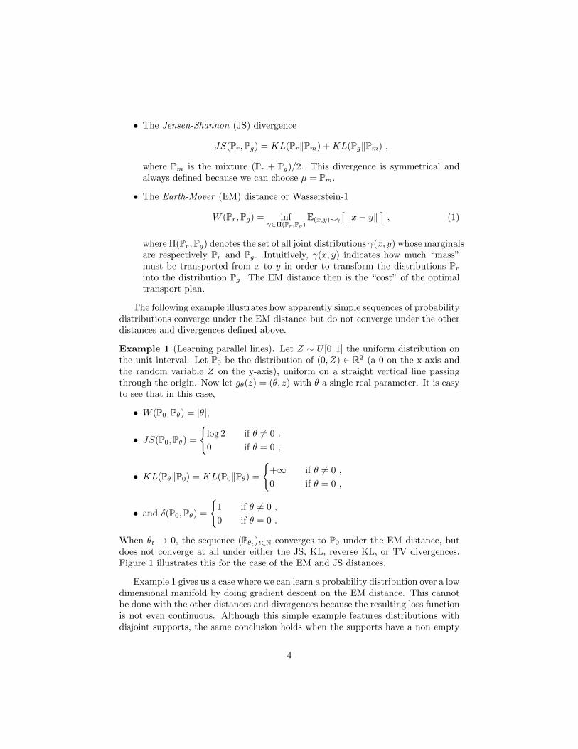
The following example illustrates how apparently simple sequences of probabilitydistributions converge under the EM distance but do not converge under the otherdistances and divergences defined above.

Example 1 (Learning parallel lines). Let Z ∼ U [0, 1] the uniform distribution onthe unit interval. Let P0 be the distribution of (0, Z) ∈ R2 (a 0 on the x-axis andthe random variable Z on the y-axis), uniform on a straight vertical line passingthrough the origin. Now let gθ(z) = (θ, z) with θ a single real parameter. It is easyto see that in this case,

• W (P0,Pθ) = |θ|,

• JS(P0,Pθ) =

{log 2 if θ 6= 0 ,

0 if θ = 0 ,

• KL(Pθ‖P0) = KL(P0‖Pθ) =

{+∞ if θ 6= 0 ,

0 if θ = 0 ,

• and δ(P0,Pθ) =

{1 if θ 6= 0 ,

0 if θ = 0 .

When θt → 0, the sequence (Pθt)t∈N converges to P0 under the EM distance, butdoes not converge at all under either the JS, KL, reverse KL, or TV divergences.Figure 1 illustrates this for the case of the EM and JS distances.

Example 1 gives us a case where we can learn a probability distribution over a lowdimensional manifold by doing gradient descent on the EM distance. This cannotbe done with the other distances and divergences because the resulting loss functionis not even continuous. Although this simple example features distributions withdisjoint supports, the same conclusion holds when the supports have a non empty

4

Figure 1: These plots show ρ(Pθ,P0) as a function of θ when ρ is the EM distance (leftplot) or the JS divergence (right plot). The EM plot is continuous and provides a usablegradient everywhere. The JS plot is not continuous and does not provide a usable gradient.

intersection contained in a set of measure zero. This happens to be the case whentwo low dimensional manifolds intersect in general position [1].

Since the Wasserstein distance is much weaker than the JS distance3, we can nowask whether W (Pr,Pθ) is a continuous loss function on θ under mild assumptions.This, and more, is true, as we now state and prove.

Theorem 1. Let Pr be a fixed distribution over X . Let Z be a random variable(e.g Gaussian) over another space Z. Let g : Z × Rd → X be a function, that willbe denoted gθ(z) with z the first coordinate and θ the second. Let Pθ denote thedistribution of gθ(Z). Then,

1. If g is continuous in θ, so is W (Pr,Pθ).

2. If g is locally Lipschitz and satisfies regularity assumption 1, then W (Pr,Pθ)is continuous everywhere, and differentiable almost everywhere.

3. Statements 1-2 are false for the Jensen-Shannon divergence JS(Pr,Pθ) andall the KLs.

Proof. See Appendix C

The following corollary tells us that learning by minimizing the EM distancemakes sense (at least in theory) with neural networks.

Corollary 1. Let gθ be any feedforward neural network4 parameterized by θ, andp(z) a prior over z such that Ez∼p(z)[‖z‖] < ∞ (e.g. Gaussian, uniform, etc.).

3 The argument for why this happens, and indeed how we arrived to the idea that Wassersteinis what we should really be optimizing is displayed in Appendix A. We strongly encourage theinterested reader who is not afraid of the mathematics to go through it.

4By a feedforward neural network we mean a function composed by affine transformations andpointwise nonlinearities which are smooth Lipschitz functions (such as the sigmoid, tanh, elu,softplus, etc). Note: the statement is also true for rectifier nonlinearities but the proof is moretechnical (even though very similar) so we omit it.

5

Then assumption 1 is satisfied and therefore W (Pr,Pθ) is continuous everywhereand differentiable almost everywhere.

Proof. See Appendix C

All this shows that EM is a much more sensible cost function for our problemthan at least the Jensen-Shannon divergence. The following theorem describes therelative strength of the topologies induced by these distances and divergences, withKL the strongest, followed by JS and TV, and EM the weakest.

Theorem 2. Let P be a distribution on a compact space X and (Pn)n∈N be asequence of distributions on X . Then, considering all limits as n→∞,

1. The following statements are equivalent

• δ(Pn,P)→ 0 with δ the total variation distance.

• JS(Pn,P)→ 0 with JS the Jensen-Shannon divergence.

2. The following statements are equivalent

• W (Pn,P)→ 0.

• PnD−→ P where

D−→ represents convergence in distribution for randomvariables.

3. KL(Pn‖P)→ 0 or KL(P‖Pn)→ 0 imply the statements in (1).

4. The statements in (1) imply the statements in (2).

Proof. See Appendix C

This highlights the fact that the KL, JS, and TV distances are not sensiblecost functions when learning distributions supported by low dimensional manifolds.However the EM distance is sensible in that setup. This obviously leads us to thenext section where we introduce a practical approximation of optimizing the EMdistance.

3 Wasserstein GAN

Again, Theorem 2 points to the fact that W (Pr,Pθ) might have nicer propertieswhen optimized than JS(Pr,Pθ). However, the infimum in (1) is highly intractable.On the other hand, the Kantorovich-Rubinstein duality [21] tells us that

W (Pr,Pθ) = sup‖f‖L≤1

Ex∼Pr [f(x)]− Ex∼Pθ [f(x)] (2)

where the supremum is over all the 1-Lipschitz functions f : X → R. Note that ifwe replace ‖f‖L ≤ 1 for ‖f‖L ≤ K (consider K-Lipschitz for some constant K),then we end up with K ·W (Pr,Pg). Therefore, if we have a parameterized family of

6

functions {fw}w∈W that are all K-Lipschitz for some K, we could consider solvingthe problem

maxw∈W

Ex∼Pr [fw(x)]− Ez∼p(z)[fw(gθ(z)] (3)

and if the supremum in (2) is attained for some w ∈ W (a pretty strong assumptionakin to what’s assumed when proving consistency of an estimator), this processwould yield a calculation of W (Pr,Pθ) up to a multiplicative constant. Further-more, we could consider differentiating W (Pr,Pθ) (again, up to a constant) byback-proping through equation (2) via estimating Ez∼p(z)[∇θfw(gθ(z))]. While thisis all intuition, we now prove that this process is principled under the optimalityassumption.

Theorem 3. Let Pr be any distribution. Let Pθ be the distribution of gθ(Z) with Za random variable with density p and gθ a function satisfying assumption 1. Then,there is a solution f : X → R to the problem

max‖f‖L≤1

Ex∼Pr [f(x)]− Ex∼Pθ [f(x)]

and we have∇θW (Pr,Pθ) = −Ez∼p(z)[∇θf(gθ(z))]

when both terms are well-defined.

Proof. See Appendix C

Now comes the question of finding the function f that solves the maximizationproblem in equation (2). To roughly approximate this, something that we can dois train a neural network parameterized with weights w lying in a compact spaceW and then backprop through Ez∼p(z)[∇θfw(gθ(z))], as we would do with a typicalGAN. Note that the fact that W is compact implies that all the functions fw willbe K-Lipschitz for some K that only depends onW and not the individual weights,therefore approximating (2) up to an irrelevant scaling factor and the capacity ofthe ‘critic’ fw. In order to have parameters w lie in a compact space, somethingsimple we can do is clamp the weights to a fixed box (say W = [−0.01, 0.01]l) aftereach gradient update. The Wasserstein Generative Adversarial Network (WGAN)procedure is described in Algorithm 1.

The fact that the EM distance is continuous and differentiable a.e. means thatwe can (and should) train the critic till optimality. The argument is simple, themore we train the critic, the more reliable gradient of the Wasserstein we get, whichis actually useful by the fact that Wasserstein is differentiable almost everywhere.For the JS, as the discriminator gets better the gradients get more reliable but thetrue gradient is 0 since the JS is locally saturated and we get vanishing gradients,as can be seen in Figure 1 of this paper and Theorem 2.4 of [1]. In Figure 2we show a proof of concept of this, where we train a GAN discriminator and aWGAN critic till optimality. The discriminator learns very quickly to distinguishbetween fake and real, and as expected provides no reliable gradient information.The critic, however, can’t saturate, and converges to a linear function that gives

7

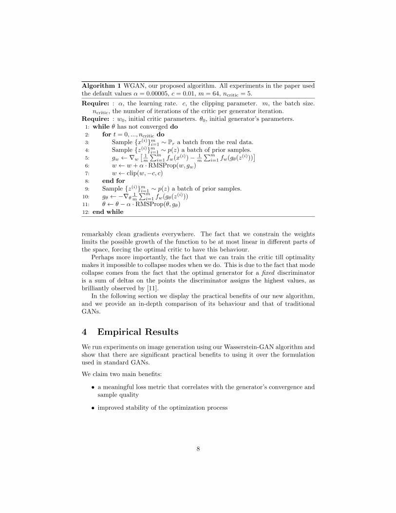
Algorithm 1 WGAN, our proposed algorithm. All experiments in the paper usedthe default values α = 0.00005, c = 0.01, m = 64, ncritic = 5.

Require: : α, the learning rate. c, the clipping parameter. m, the batch size.ncritic, the number of iterations of the critic per generator iteration.

Require: : w0, initial critic parameters. θ0, initial generator’s parameters.1: while θ has not converged do2: for t = 0, ..., ncritic do3: Sample {x(i)}mi=1 ∼ Pr a batch from the real data.4: Sample {z(i)}mi=1 ∼ p(z) a batch of prior samples.5: gw ← ∇w

[1m

∑mi=1 fw(x(i))− 1

m

∑mi=1 fw(gθ(z

(i)))]

6: w ← w + α · RMSProp(w, gw)7: w ← clip(w,−c, c)8: end for9: Sample {z(i)}mi=1 ∼ p(z) a batch of prior samples.

10: gθ ← −∇θ 1m

∑mi=1 fw(gθ(z

(i)))11: θ ← θ − α · RMSProp(θ, gθ)12: end while

remarkably clean gradients everywhere. The fact that we constrain the weightslimits the possible growth of the function to be at most linear in different parts ofthe space, forcing the optimal critic to have this behaviour.

Perhaps more importantly, the fact that we can train the critic till optimalitymakes it impossible to collapse modes when we do. This is due to the fact that modecollapse comes from the fact that the optimal generator for a fixed discriminatoris a sum of deltas on the points the discriminator assigns the highest values, asbrilliantly observed by [11].

In the following section we display the practical benefits of our new algorithm,and we provide an in-depth comparison of its behaviour and that of traditionalGANs.

4 Empirical Results

We run experiments on image generation using our Wasserstein-GAN algorithm andshow that there are significant practical benefits to using it over the formulationused in standard GANs.

We claim two main benefits:

• a meaningful loss metric that correlates with the generator’s convergence andsample quality

• improved stability of the optimization process

8

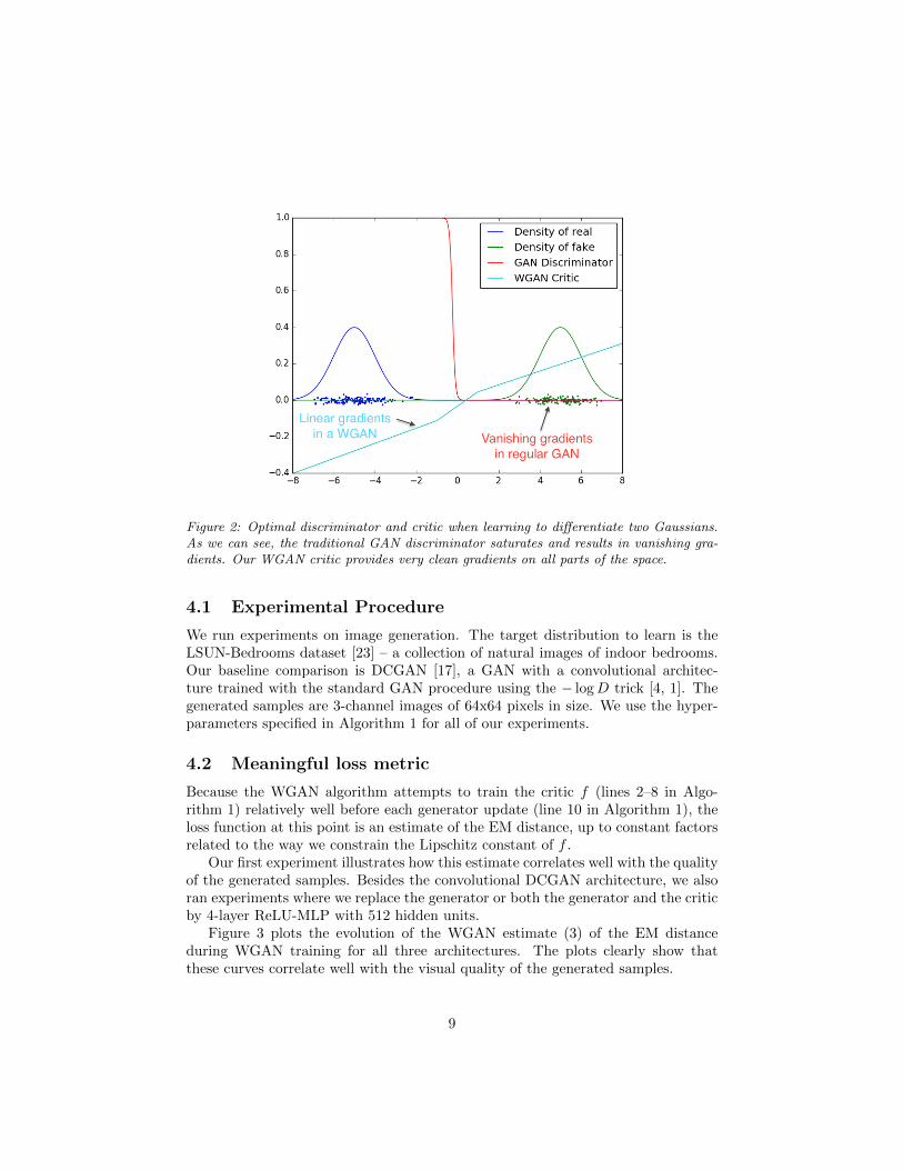
Figure 2: Optimal discriminator and critic when learning to differentiate two Gaussians.As we can see, the traditional GAN discriminator saturates and results in vanishing gra-dients. Our WGAN critic provides very clean gradients on all parts of the space.

4.1 Experimental Procedure

We run experiments on image generation. The target distribution to learn is theLSUN-Bedrooms dataset [23] – a collection of natural images of indoor bedrooms.Our baseline comparison is DCGAN [17], a GAN with a convolutional architec-ture trained with the standard GAN procedure using the − logD trick [4, 1]. Thegenerated samples are 3-channel images of 64x64 pixels in size. We use the hyper-parameters specified in Algorithm 1 for all of our experiments.

4.2 Meaningful loss metric

Because the WGAN algorithm attempts to train the critic f (lines 2–8 in Algo-rithm 1) relatively well before each generator update (line 10 in Algorithm 1), theloss function at this point is an estimate of the EM distance, up to constant factorsrelated to the way we constrain the Lipschitz constant of f .

Our first experiment illustrates how this estimate correlates well with the qualityof the generated samples. Besides the convolutional DCGAN architecture, we alsoran experiments where we replace the generator or both the generator and the criticby 4-layer ReLU-MLP with 512 hidden units.

Figure 3 plots the evolution of the WGAN estimate (3) of the EM distanceduring WGAN training for all three architectures. The plots clearly show thatthese curves correlate well with the visual quality of the generated samples.

9

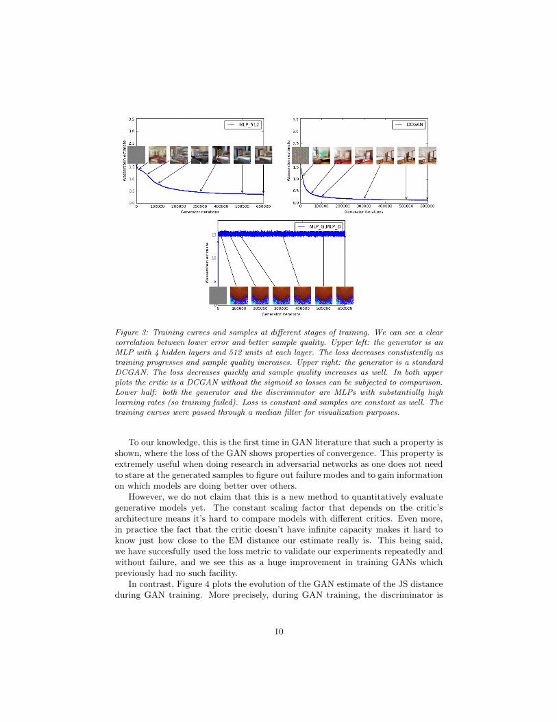
Figure 3: Training curves and samples at different stages of training. We can see a clearcorrelation between lower error and better sample quality. Upper left: the generator is anMLP with 4 hidden layers and 512 units at each layer. The loss decreases constistently astraining progresses and sample quality increases. Upper right: the generator is a standardDCGAN. The loss decreases quickly and sample quality increases as well. In both upperplots the critic is a DCGAN without the sigmoid so losses can be subjected to comparison.Lower half: both the generator and the discriminator are MLPs with substantially highlearning rates (so training failed). Loss is constant and samples are constant as well. Thetraining curves were passed through a median filter for visualization purposes.

To our knowledge, this is the first time in GAN literature that such a property isshown, where the loss of the GAN shows properties of convergence. This property isextremely useful when doing research in adversarial networks as one does not needto stare at the generated samples to figure out failure modes and to gain informationon which models are doing better over others.

However, we do not claim that this is a new method to quantitatively evaluategenerative models yet. The constant scaling factor that depends on the critic’sarchitecture means it’s hard to compare models with different critics. Even more,in practice the fact that the critic doesn’t have infinite capacity makes it hard toknow just how close to the EM distance our estimate really is. This being said,we have succesfully used the loss metric to validate our experiments repeatedly andwithout failure, and we see this as a huge improvement in training GANs whichpreviously had no such facility.

In contrast, Figure 4 plots the evolution of the GAN estimate of the JS distanceduring GAN training. More precisely, during GAN training, the discriminator is

10

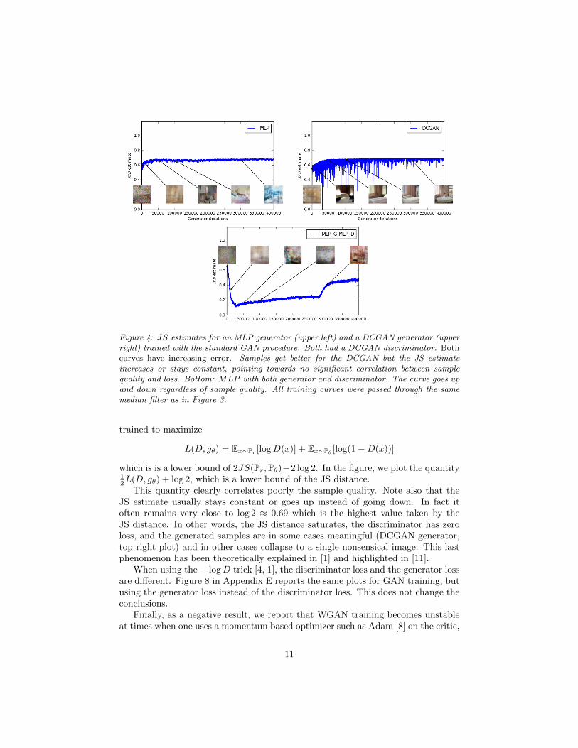
Figure 4: JS estimates for an MLP generator (upper left) and a DCGAN generator (upperright) trained with the standard GAN procedure. Both had a DCGAN discriminator. Bothcurves have increasing error. Samples get better for the DCGAN but the JS estimateincreases or stays constant, pointing towards no significant correlation between samplequality and loss. Bottom: MLP with both generator and discriminator. The curve goes upand down regardless of sample quality. All training curves were passed through the samemedian filter as in Figure 3.

trained to maximize

L(D, gθ) = Ex∼Pr [logD(x)] + Ex∼Pθ [log(1−D(x))]

which is is a lower bound of 2JS(Pr,Pθ)−2 log 2. In the figure, we plot the quantity12L(D, gθ) + log 2, which is a lower bound of the JS distance.

This quantity clearly correlates poorly the sample quality. Note also that theJS estimate usually stays constant or goes up instead of going down. In fact itoften remains very close to log 2 ≈ 0.69 which is the highest value taken by theJS distance. In other words, the JS distance saturates, the discriminator has zeroloss, and the generated samples are in some cases meaningful (DCGAN generator,top right plot) and in other cases collapse to a single nonsensical image. This lastphenomenon has been theoretically explained in [1] and highlighted in [11].

When using the − logD trick [4, 1], the discriminator loss and the generator lossare different. Figure 8 in Appendix E reports the same plots for GAN training, butusing the generator loss instead of the discriminator loss. This does not change theconclusions.

Finally, as a negative result, we report that WGAN training becomes unstableat times when one uses a momentum based optimizer such as Adam [8] on the critic,

11

or when one uses high learning rates. Since the loss for the critic is nonstationary,momentum based methods like Adam seemed to perform worse. We identifiedmomentum as a potential cause because, as the loss blew up and samples got worse,the cosine between the Adam step and the gradient turned negative. The onlyplaces where this cosine was negative was in these situations of instability. Wetherefore switched to RMSProp [20] which is known to perform well even on verynonstationary problems [13].

4.3 Improved stability

One of the benefits of WGAN is that it allows us to train the critic till optimality.When the critic is trained to completion, it simply provides a loss to the generatorthat we can train as any other neural network. This tells us that we no longer needto balance generator and discriminator’s capacity properly. The better the critic,the higher quality the gradients we use to train the generator.

We observe that WGANs are much more robust than GANs when one variesthe architectural choices for the generator. We illustrate this by running experi-ments on three generator architectures: (1) a convolutional DCGAN generator, (2)a convolutional DCGAN generator without batch normalization and with a con-stant number of filters, and (3) a 4-layer ReLU-MLP with 512 hidden units. Thelast two are known to perform very poorly with GANs. We keep the convolutionalDCGAN architecture for the WGAN critic or the GAN discriminator.

Figures 5, 6, and 7 show samples generated for these three architectures usingboth the WGAN and GAN algorithms. We refer the reader to Appendix F for fullsheets of generated samples. Samples were not cherry-picked.

In no experiment did we see evidence of mode collapse for the WGANalgorithm.

5 Related Work

There’s been a number of works on the so called Integral Probability Metrics (IPMs)[14]. Given F a set of functions from X to R, we can define

dF (Pr,Pθ) = supf∈F

Ex∼Pr [f(x)]− Ex∼Pθ [f(x)] (4)

as an integral probability metric associated with the function class F . It is easilyverified that if for every f ∈ F we have −f ∈ F (such as all examples we’ll consider),then dF is nonnegative, satisfies the triangular inequality, and is symmetric. Thus,dF is a pseudometric over Prob(X ).

While IPMs might seem to share a similar formula, as we will see different classesof functions can yeald to radically different metrics.

• By the Kantorovich-Rubinstein duality [21], we know thatW (Pr,Pθ) = dF (Pr,Pθ)when F is the set of 1-Lipschitz functions. Furthermore, if F is the set of K-Lipschitz functions, we get K ·W (Pr,Pθ) = dF (Pr,Pθ).

12

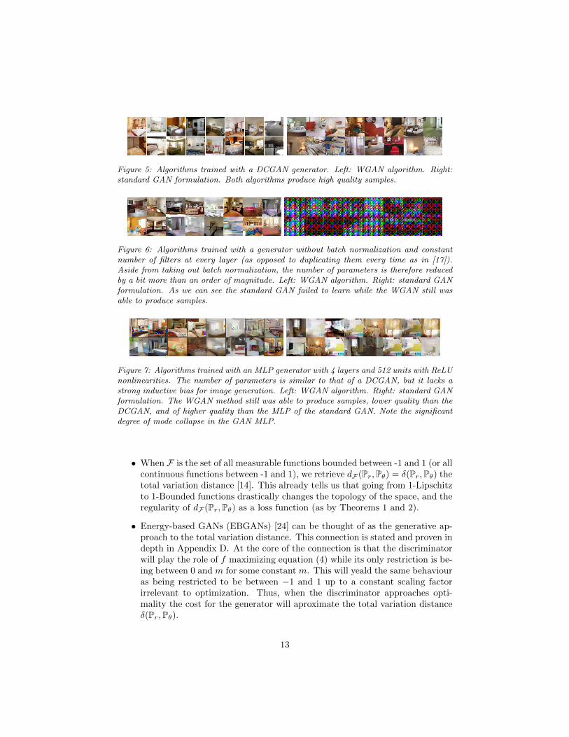
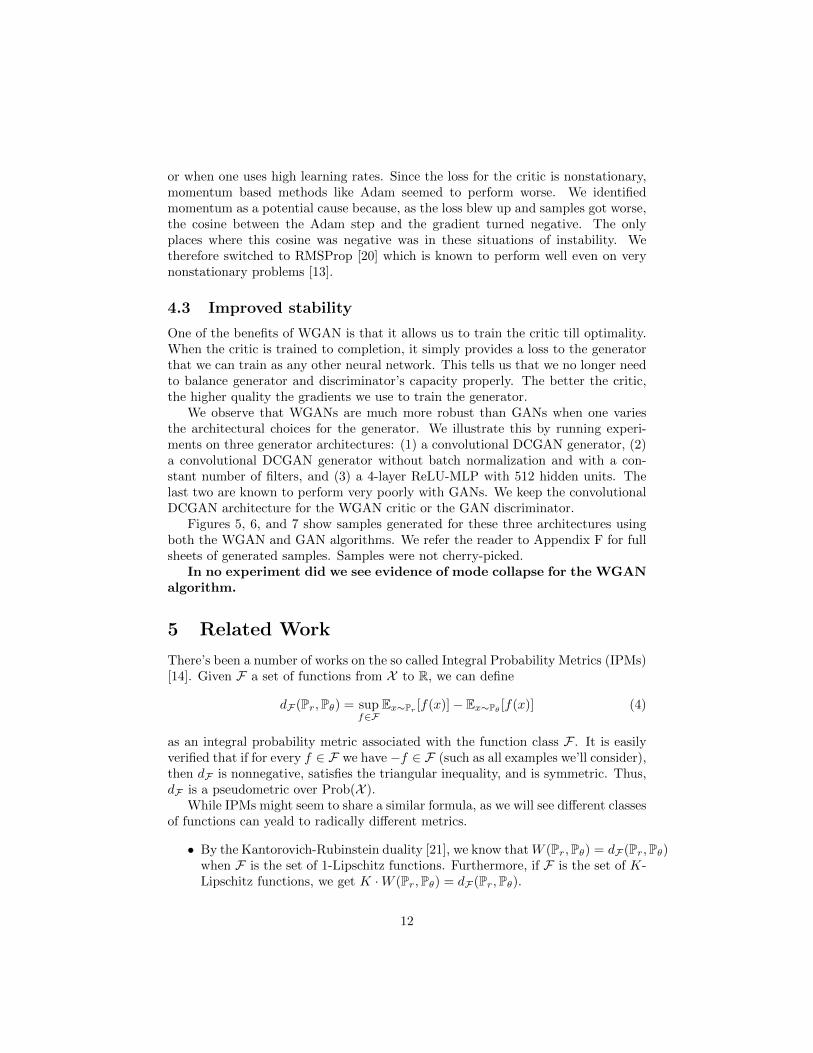
Figure 5: Algorithms trained with a DCGAN generator. Left: WGAN algorithm. Right:standard GAN formulation. Both algorithms produce high quality samples.

Figure 6: Algorithms trained with a generator without batch normalization and constantnumber of filters at every layer (as opposed to duplicating them every time as in [17]).Aside from taking out batch normalization, the number of parameters is therefore reducedby a bit more than an order of magnitude. Left: WGAN algorithm. Right: standard GANformulation. As we can see the standard GAN failed to learn while the WGAN still wasable to produce samples.

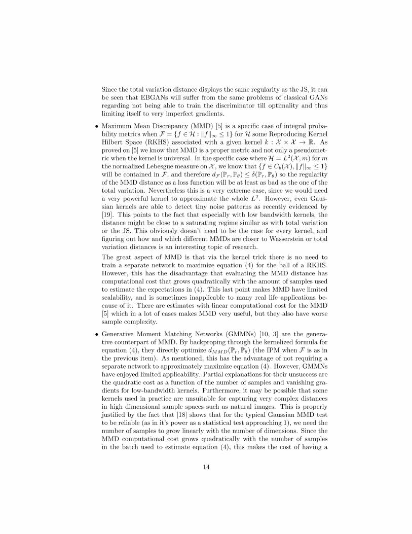
Figure 7: Algorithms trained with an MLP generator with 4 layers and 512 units with ReLUnonlinearities. The number of parameters is similar to that of a DCGAN, but it lacks astrong inductive bias for image generation. Left: WGAN algorithm. Right: standard GANformulation. The WGAN method still was able to produce samples, lower quality than theDCGAN, and of higher quality than the MLP of the standard GAN. Note the significantdegree of mode collapse in the GAN MLP.

• When F is the set of all measurable functions bounded between -1 and 1 (or allcontinuous functions between -1 and 1), we retrieve dF (Pr,Pθ) = δ(Pr,Pθ) thetotal variation distance [14]. This already tells us that going from 1-Lipschitzto 1-Bounded functions drastically changes the topology of the space, and theregularity of dF (Pr,Pθ) as a loss function (as by Theorems 1 and 2).

• Energy-based GANs (EBGANs) [24] can be thought of as the generative ap-proach to the total variation distance. This connection is stated and proven indepth in Appendix D. At the core of the connection is that the discriminatorwill play the role of f maximizing equation (4) while its only restriction is be-ing between 0 and m for some constant m. This will yeald the same behaviouras being restricted to be between −1 and 1 up to a constant scaling factorirrelevant to optimization. Thus, when the discriminator approaches opti-mality the cost for the generator will aproximate the total variation distanceδ(Pr,Pθ).

13

Since the total variation distance displays the same regularity as the JS, it canbe seen that EBGANs will suffer from the same problems of classical GANsregarding not being able to train the discriminator till optimality and thuslimiting itself to very imperfect gradients.

• Maximum Mean Discrepancy (MMD) [5] is a specific case of integral proba-bility metrics when F = {f ∈ H : ‖f‖∞ ≤ 1} for H some Reproducing KernelHilbert Space (RKHS) associated with a given kernel k : X × X → R. Asproved on [5] we know that MMD is a proper metric and not only a pseudomet-ric when the kernel is universal. In the specific case whereH = L2(X ,m) for mthe normalized Lebesgue measure on X , we know that {f ∈ Cb(X ), ‖f‖∞ ≤ 1}will be contained in F , and therefore dF (Pr,Pθ) ≤ δ(Pr,Pθ) so the regularityof the MMD distance as a loss function will be at least as bad as the one of thetotal variation. Nevertheless this is a very extreme case, since we would needa very powerful kernel to approximate the whole L2. However, even Gaus-sian kernels are able to detect tiny noise patterns as recently evidenced by[19]. This points to the fact that especially with low bandwidth kernels, thedistance might be close to a saturating regime similar as with total variationor the JS. This obviously doesn’t need to be the case for every kernel, andfiguring out how and which different MMDs are closer to Wasserstein or totalvariation distances is an interesting topic of research.

The great aspect of MMD is that via the kernel trick there is no need totrain a separate network to maximize equation (4) for the ball of a RKHS.However, this has the disadvantage that evaluating the MMD distance hascomputational cost that grows quadratically with the amount of samples usedto estimate the expectations in (4). This last point makes MMD have limitedscalability, and is sometimes inapplicable to many real life applications be-cause of it. There are estimates with linear computational cost for the MMD[5] which in a lot of cases makes MMD very useful, but they also have worsesample complexity.

• Generative Moment Matching Networks (GMMNs) [10, 3] are the genera-tive counterpart of MMD. By backproping through the kernelized formula forequation (4), they directly optimize dMMD(Pr,Pθ) (the IPM when F is as inthe previous item). As mentioned, this has the advantage of not requiring aseparate network to approximately maximize equation (4). However, GMMNshave enjoyed limited applicability. Partial explanations for their unsuccess arethe quadratic cost as a function of the number of samples and vanishing gra-dients for low-bandwidth kernels. Furthermore, it may be possible that somekernels used in practice are unsuitable for capturing very complex distancesin high dimensional sample spaces such as natural images. This is properlyjustified by the fact that [18] shows that for the typical Gaussian MMD testto be reliable (as in it’s power as a statistical test approaching 1), we need thenumber of samples to grow linearly with the number of dimensions. Since theMMD computational cost grows quadratically with the number of samplesin the batch used to estimate equation (4), this makes the cost of having a

14

reliable estimator grow quadratically with the number of dimensions, whichmakes it very inapplicable for high dimensional problems. Indeed, for some-thing as standard as 64x64 images, we would need minibatches of size at least4096 (without taking into account the constants in the bounds of [18] whichwould make this number substantially larger) and a total cost per iterationof 40962, over 5 orders of magnitude more than a GAN iteration when usingthe standard batch size of 64.

That being said, these numbers can be a bit unfair to the MMD, in thesense that we are comparing empirical sample complexity of GANs with thetheoretical sample complexity of MMDs, which tends to be worse. However,in the original GMMN paper [10] they indeed used a minibatch of size 1000,much larger than the standard 32 or 64 (even when this incurred in quadraticcomputational cost). While estimates that have linear computational costas a function of the number of samples exist [5], they have worse samplecomplexity, and to the best of our knowledge they haven’t been yet appliedin a generative context such as in GMMNs.

6 Conclusion

We introduced an algorithm that we deemed WGAN, an alternative to traditionalGAN training. In this new model, we showed that we can improve the stabilityof learning, get rid of problems like mode collapse, and provide meaningful learn-ing curves useful for debugging and hyperparameter searches. Furthermore, weshowed that the corresponding optimization problem is sound, and provided exten-sive theoretical work highlighting the deep connections to other distances betweendistributions.

References

[1] Martin Arjovsky and Leon Bottou. Towards principled methods for traininggenerative adversarial networks. In International Conference on Learning Rep-resentations, 2017. Under review.

[2] Patrick Billingsley. Convergence of probability measures. Wiley Series in Prob-ability and Statistics: Probability and Statistics. John Wiley & Sons Inc., NewYork, second edition, 1999. A Wiley-Interscience Publication.

[3] Gintare Karolina Dziugaite, Daniel M. Roy, and Zoubin Ghahramani. Train-ing generative neural networks via maximum mean discrepancy optimization.CoRR, abs/1505.03906, 2015.

[4] Ian J. Goodfellow, Jean Pouget-Abadie, Mehdi Mirza, Bing Xu, David Warde-Farley, Sherjil Ozair, Aaron Courville, and Yoshua Bengio. Generative adver-sarial nets. In Advances in Neural Information Processing Systems 27, pages2672–2680. Curran Associates, Inc., 2014.

15

[5] Arthur Gretton, Karsten M. Borgwardt, Malte J. Rasch, Bernhard Scholkopf,and Alexander Smola. A kernel two-sample test. J. Mach. Learn. Res., 13:723–773, 2012.

[6] Ferenc Huszar. How (not) to train your generative model: Scheduled sampling,likelihood, adversary? CoRR, abs/1511.05101, 2015.

[7] Shizuo Kakutani. Concrete representation of abstract (m)-spaces (a characteri-zation of the space of continuous functions). Annals of Mathematics, 42(4):994–1024, 1941.

[8] Diederik P. Kingma and Jimmy Ba. Adam: A method for stochastic optimiza-tion. CoRR, abs/1412.6980, 2014.

[9] Diederik P. Kingma and Max Welling. Auto-encoding variational bayes. CoRR,abs/1312.6114, 2013.

[10] Yujia Li, Kevin Swersky, and Rich Zemel. Generative moment matching net-works. In Proceedings of the 32nd International Conference on Machine Learn-ing (ICML-15), pages 1718–1727. JMLR Workshop and Conference Proceed-ings, 2015.

[11] Luke Metz, Ben Poole, David Pfau, and Jascha Sohl-Dickstein. Unrolled gen-erative adversarial networks. Corr, abs/1611.02163, 2016.

[12] Paul Milgrom and Ilya Segal. Envelope theorems for arbitrary choice sets.Econometrica, 70(2):583–601, 2002.

[13] Volodymyr Mnih, Adria Puigdomenech Badia, Mehdi Mirza, Alex Graves, Tim-othy P. Lillicrap, Tim Harley, David Silver, and Koray Kavukcuoglu. Asyn-chronous methods for deep reinforcement learning. In Proceedings of the 33ndInternational Conference on Machine Learning, ICML 2016, New York City,NY, USA, June 19-24, 2016, pages 1928–1937, 2016.

[14] Alfred Mller. Integral probability metrics and their generating classes of func-tions. Advances in Applied Probability, 29(2):429–443, 1997.

[15] Radford M. Neal. Annealed importance sampling. Statistics and Computing,11(2):125–139, April 2001.

[16] Sebastian Nowozin, Botond Cseke, and Ryota Tomioka. f-gan: Training genera-tive neural samplers using variational divergence minimization. pages 271–279,2016.

[17] Alec Radford, Luke Metz, and Soumith Chintala. Unsupervised representa-tion learning with deep convolutional generative adversarial networks. CoRR,abs/1511.06434, 2015.

16

[18] Aaditya Ramdas, Sashank J. Reddi, Barnabas Poczos, Aarti Singh, and LarryWasserman. On the high-dimensional power of linear-time kernel two-sampletesting under mean-difference alternatives. Corr, abs/1411.6314, 2014.

[19] Dougal J Sutherland, Hsiao-Yu Tung, Heiko Strathmann, Soumyajit De, Aa-ditya Ramdas, Alex Smola, and Arthur Gretton. Generative models and modelcriticism via optimized maximum mean discrepancy. In International Confer-ence on Learning Representations, 2017. Under review.

[20] T. Tieleman and G. Hinton. Lecture 6.5—RmsProp: Divide the gradient bya running average of its recent magnitude. COURSERA: Neural Networks forMachine Learning, 2012.

[21] Cedric Villani. Optimal Transport: Old and New. Grundlehren der mathema-tischen Wissenschaften. Springer, Berlin, 2009.

[22] Yuhuai Wu, Yuri Burda, Ruslan Salakhutdinov, and Roger B. Grosse.On the quantitative analysis of decoder-based generative models. CoRR,abs/1611.04273, 2016.

[23] Fisher Yu, Yinda Zhang, Shuran Song, Ari Seff, and Jianxiong Xiao. LSUN:Construction of a large-scale image dataset using deep learning with humansin the loop. Corr, abs/1506.03365, 2015.

[24] Junbo Zhao, Michael Mathieu, and Yann LeCun. Energy-based generativeadversarial network. Corr, abs/1609.03126, 2016.

17

A Why Wasserstein is indeed weak

We now introduce our notation. Let X ⊆ Rd be a compact set (such as [0, 1]d thespace of images). We define Prob(X ) to be the space of probability measures overX . We note

Cb(X ) = {f : X → R, f is continuous and bounded}

Note that if f ∈ Cb(X ), we can define ‖f‖∞ = maxx∈X |f(x)|, since f is bounded.With this norm, the space (Cb(X ), ‖ · ‖∞) is a normed vector space. As for anynormed vector space, we can define its dual

Cb(X )∗ = {φ : Cb(X )→ R, φ is linear and continuous}

and give it the dual norm ‖φ‖ = supf∈Cb(X ),‖f‖∞≤1 |φ(f)|.With this definitions, (Cb(X )∗, ‖ · ‖) is another normed space. Now let µ be a

signed measure over X , and let us define the total variation distance

‖µ‖TV = supA⊆X

|µ(A)|

where the supremum is taken all Borel sets in X . Since the total variation is anorm, then if we have Pr and Pθ two probability distributions over X ,

δ(Pr,Pθ) := ‖Pr − Pθ‖

is a distance in Prob(X ) (called the total variation distance).We can consider

Φ : (Prob(X ), δ)→ (Cb(X )∗, ‖ · ‖)

where Φ(P)(f) := Ex∼P[f(x)] is a linear function over Cb(X ). The Riesz Represen-tation theorem ([7], Theorem 10) tells us that Φ is an isometric immersion. Thistells us that we can effectively consider Prob(X ) with the total variation distanceas a subset of Cb(X )∗ with the norm distance. Thus, just to accentuate it one moretime, the total variation over Prob(X ) is exactly the norm distance over Cb(X )∗.

Let us stop for a second and analyze what all this technicality meant. The mainthing to carry is that we introduced a distance δ over probability distributions.When looked as a distance over a subset of Cb(X )∗, this distance gives the normtopology. The norm topology is very strong. Therefore, we can expect that notmany functions θ 7→ Pθ will be continuous when measuring distances between dis-tributions with δ. As we will show later in Theorem 2, δ gives the same topologyas the Jensen-Shannon divergence, pointing to the fact that the JS is a very strongdistance, and is thus more propense to give a discontinuous loss function.

Now, all dual spaces (such as Cb(X )∗ and thus Prob(X )) have a strong topology(induced by the norm), and a weak* topology. As the name suggests, the weak*topology is much weaker than the strong topology. In the case of Prob(X ), thestrong topology is given by the total variation distance, and the weak* topology isgiven by the Wasserstein distance (among others) [21].

18

B Assumption definitions

Assumption 1. Let g : Z×Rd → X be locally Lipschitz between finite dimensionalvector spaces. We will denote gθ(z) it’s evaluation on coordinates (z, θ). We saythat g satisfies assumption 1 for a certain probability distribution p over Z if thereare local Lipschitz constants L(θ, z) such that

Ez∼p[L(θ, z)] < +∞

C Proofs of things

Proof of Theorem 1. Let θ and θ′ be two parameter vectors in Rd. Then, we willfirst attempt to bound W (Pθ,Pθ′), from where the theorem will come easily. Themain element of the proof is the use of the coupling γ, the distribution of the joint(gθ(Z), gθ′(Z)), which clearly has γ ∈ Π(Pθ,Pθ′).

By the definition of the Wasserstein distance, we have

W (Pθ,Pθ′) ≤∫X×X

‖x− y‖ dγ

= E(x,y)∼γ [‖x− y‖]= Ez[‖gθ(z)− gθ′(z)‖]

If g is continuous in θ, then gθ(z) →θ→θ′ gθ′(z), so ‖gθ − gθ′‖ → 0 pointwise asfunctions of z. Since X is compact, the distance of any two elements in it has tobe uniformly bounded by some constant M , and therefore ‖gθ(z)− gθ′(z)‖ ≤M forall θ and z uniformly. By the bounded convergence theorem, we therefore have

W (Pθ,Pθ′) ≤ Ez[‖gθ(z)− gθ′(z)‖]→θ→θ′ 0

Finally, we have that

|W (Pr,Pθ)−W (Pr,Pθ′)| ≤W (Pθ,Pθ′)→θ→θ′ 0

proving the continuity of W (Pr,Pθ).Now let g be locally Lipschitz. Then, for a given pair (θ, z) there is a constant

L(θ, z) and an open set U such that (θ, z) ∈ U , such that for every (θ′, z′) ∈ U wehave

‖gθ(z)− g′θ(z′)‖ ≤ L(θ, z)(‖θ − θ′‖+ ‖z − z′‖)By taking expectations and z′ = z we

Ez[‖gθ(z)− gθ′(z)‖] ≤ ‖θ − θ′‖Ez[L(θ, z)]

whenever (θ′, z) ∈ U . Therefore, we can define Uθ = {θ′|(θ′, z) ∈ U}. It’s easy tosee that since U was open, Uθ is as well. Furthermore, by assumption 1, we candefine L(θ) = Ez[L(θ, z)] and achieve

|W (Pr,Pθ)−W (Pr,Pθ′)| ≤W (Pθ,Pθ′) ≤ L(θ)‖θ − θ′‖

19

for all θ′ ∈ Uθ, meaning that W (Pr,Pθ) is locally Lipschitz. This obviously impliesthat W (Pr,Pθ) is everywhere continuous, and by Radamacher’s theorem we knowit has to be differentiable almost everywhere.

The counterexample for item 3 of the Theorem is indeed Example 1.

Proof of Corollary 1. We begin with the case of smooth nonlinearities. Since g isC1 as a function of (θ, z) then for any fixed (θ, z) we have L(θ, Z) ≤ ‖∇θ,xgθ(z)‖+εis an acceptable local Lipschitz constant for all ε > 0. Therefore, it suffices to prove

Ez∼p(z)[‖∇θ,zgθ(z)‖] < +∞

If H is the number of layers we know that ∇zgθ(z) =∏Hk=1WkDk where Wk are

the weight matrices and Dk is are the diagonal Jacobians of the nonlinearities.Let fi:j be the application of layers i to j inclusively (e.g. gθ = f1:H). Then,

∇Wkgθ(z) =

((∏Hi=k+1WiDi

)Dk

)f1:k−1(z). We recall that if L is the Lipschitz

constant of the nonlinearity, then ‖Di‖ ≤ L and ‖f1:k−1(z)‖ ≤ ‖z‖Lk−1∏k−1i=1 Wi.

Putting this together,

‖∇z,θgθ(z)‖ ≤ ‖H∏i=1

WiDi‖+

H∑k=1

‖

((H∏

i=k+1

WiDi

)Dk

)f1:k−1(z)‖

≤ LHK∏i=H

‖Wi‖+

H∑k=1

‖z‖LH(k−1∏i=1

‖Wi‖

)(H∏

i=k+1

‖Wi‖

)

If C1(θ) = LH(∏H

i=1 ‖Wi‖)

and C2(θ) =∑Hk=1 L

H(∏k−1

i=1 ‖Wi‖)(∏H

i=k+1 ‖Wi‖)

thenEz∼p(z)[‖∇θ,zgθ(z)‖] ≤ C1(θ) + C2(θ)Ez∼p(z)[‖z‖] < +∞

finishing the proof

Proof of Theorem 2.

1. • (δ(Pn,P) → 0 ⇒ JS(Pn,P) → 0) — Let Pm be the mixture dis-tribution Pm = 1

2Pn + 12P (note that Pm depends on n). It is easily

verified that δ(Pm,Pn) ≤ δ(Pn,P), and in particular this tends to 0 (asdoes δ(Pm,P)). We now show this for completeness. Let µ be a signedmeasure, we define ‖µ‖TV = supA⊆X |µ(A)|. for all Borel sets A. In thiscase,

δ(Pm,Pn) = ‖Pm − Pn‖TV

= ‖1

2P +

1

2Pn − Pn‖TV

=1

2‖P− Pn‖TV

=1

2δ(Pn,P) ≤ δ(Pn,P)

20

Let fn = dPndPm be the Radon-Nykodim derivative between Pn and the

mixture. Note that by construction for every Borel set A we havePn(A) ≤ 2Pm(A). If A = {fn > 3} then we get

Pn(A) =

∫A

fn dPm ≥ 3Pm(A)

which implies Pm(A) = 0. This means that fn is bounded by 3 Pm(andtherefore Pn and P)-almost everywhere. We could have done this for anyconstant larger than 2 but for our purposes 3 will sufice.

Let ε > 0 fixed, and An = {fn > 1 + ε}. Then,

Pn(An) =

∫An

fn dPm ≥ (1 + ε)Pm(An)

Therefore,

εPm(An) ≤ Pn(An)− Pm(An)

≤ |Pn(An)− Pm(An)|≤ δ(Pn,Pm)

≤ δ(Pn,P).

Which implies Pm(Am) ≤ 1ε δ(Pn,P). Furthermore,

Pn(An) ≤ Pm(An) + |Pn(An)− Pm(An)|

≤ 1

εδ(Pn,P) + δ(Pn,Pm)

≤ 1

εδ(Pn,P) + δ(Pn,P)

≤(

1

ε+ 1

)δ(Pn,P)

We now can see that

KL(Pn‖Pm) =

∫log(fn) dPn

≤ log(1 + ε) +

∫An

log(fn) dPn

≤ log(1 + ε) + log(3)Pn(An)

≤ log(1 + ε) + log(3)

(1

ε+ 1

)δ(Pn,P)

Taking limsup we get 0 ≤ lim supKL(Pn‖Pm) ≤ log(1 + ε) for all ε > 0,which means KL(Pn‖Pm)→ 0.

In the same way, we can define gn = dPdPm , and

2Pm({gn > 3}) ≥ P({gn > 3}) ≥ 3Pm({gn > 3})

21

meaning that Pm({gn > 3}) = 0 and therefore gn is bounded by 3 almosteverywhere for Pn,Pm and P. With the same calculation, Bn = {gn >1 + ε} and

P(Bn) =

∫Bn

gn dPm ≥ (1 + ε)Pm(Bn)

so Pm(Bn) ≤ 1ε δ(P,Pm) → 0, and therefore P(Bn) → 0. We can now

show

KL(P‖Pm) =

∫log(gn) dP

≤ log(1 + ε) +

∫Bn

log(gn) dP

≤ log(1 + ε) + log(3)P(Bn)

so we achieve 0 ≤ lim supKL(P‖Pm) ≤ log(1+ε) and then KL(P‖Pm)→0. Finally, we conclude

JS(Pn,P) =1

2KL(Pn‖Pm) +

1

2KL(P‖Pm)→ 0

• (JS(Pn,P) → 0 ⇒ δ(Pn,P) → 0) — by a simple application of thetriangular and Pinsker’s inequalities we get

δ(Pn,P) ≤ δ(Pn,Pm) + δ(P,Pm)

≤√

1

2KL(Pn‖Pm) +

√1

2KL(P‖Pm)

≤ 2√JS(Pn,P)→ 0

2. This is a long known fact that W metrizes the weak* topology of (C(X ), ‖ ·‖∞) on Prob(X ), and by definition this is the topology of convergence indistribution. A proof of this can be found (for example) in [21].

3. This is a straightforward application of Pinsker’s inequality

δ(Pn,P) ≤√

1

2KL(Pn‖P)→ 0

δ(P,Pn) ≤√

1

2KL(P‖Pn)→ 0

4. This is trivial by recalling the fact that δ and W give the strong and weak*topologies on the dual of (C(X ), ‖ · ‖∞) when restricted to Prob(X ).

22

Proof of Theorem 3. Let us define

V (f , θ) = Ex∼Pr [f(x)]− Ex∼Pθ [f(x)]

= Ex∼Pr [f(x)]− Ez∼p(z)[f(gθ(z))]

where f lies in F = {f : X → R , f ∈ Cb(X ), ‖f‖L ≤ 1} and θ ∈ Rd.Since X is compact, we know by the Kantorovich-Rubenstein duality [21] that

there is an f ∈ F that attains the value

W (Pr,Pθ) = supf∈F

V (f , θ) = V (f, θ)

Let us define X∗(θ) = {f ∈ F : V (f, θ) = W (Pr,Pθ)}. By the above point we knowthen that X∗(θ) is non-empty. We know that by a simple envelope theorem ([12],Theorem 1) that

∇θW (Pr,Pθ) = ∇θV (f, θ)

for any f ∈ X∗(θ) when both terms are well-defined.Let f ∈ X∗(θ), which we knows exists since X∗(θ) is non-empty for all θ. Then,

we get

∇θW (Pr,Pθ) = ∇θV (f, θ)

= ∇θ[Ex∼Pr [f(x)]− Ez∼p(z)[f(gθ(z))]

= −∇θEz∼p(z)[f(gθ(z))]

under the condition that the first and last terms are well-defined. The rest of theproof will be dedicated to show that

−∇θEz∼p(z)[f(gθ(z))] = −Ez∼p(z)[∇θf(gθ(z))] (5)

when the right hand side is defined. For the reader who is not interested in suchtechnicalities, he or she can skip the rest of the proof.

Since f ∈ F , we know that it is 1-Lipschitz. Furthermore, gθ(z) is locallyLipschitz as a function of (θ, z). Therefore, f(gθ(z)) is locally Lipschitz on (θ, z)with constants L(θ, z) (the same ones as g). By Radamacher’s Theorem, f(gθ(z))has to be differentiable almost everywhere for (θ, z) jointly. Rewriting this, the setA = {(θ, z) : f ◦ g is not differentiable} has measure 0. By Fubini’s Theorem, thisimplies that for almost every θ the section Aθ = {z : (θ, z) ∈ A} has measure 0.Let’s now fix a θ0 such that the measure of Aθ0 is null (such as when the righthand side of equation (5) is well defined). For this θ0 we have ∇θf(gθ(z))|θ0is well-defined for almost any z, and since p(z) has a density, it is defined p(z)-a.e.By assumption 1 we know that

Ez∼p(z)[‖∇θf(gθ(z))|θ0‖] ≤ Ez∼p(z)[L(θ0, z)] < +∞

so Ez∼p(z)[∇θf(gθ(z))|θ0 ] is well-defined for almost every θ0. Now, we can see

Ez∼p(z)[f(gθ(z))]− Ez∼p(z)[f(gθ0(z))]− 〈(θ − θ0),Ez∼p(z)[∇θf(gθ(z))|θ0 ]〉‖θ − θ0‖

(6)

23

= Ez∼p(z)[f(gθ(z))− f(gθ0(z))− 〈(θ − θ0),∇θf(gθ(z))|θ0〉

‖θ − θ0‖

]

By differentiability, the term inside the integral converges p(z)-a.e. to 0 as θ → θ0.Furthermore,

‖f(gθ(z))− f(gθ0(z))− 〈(θ − θ0),∇θf(gθ(z))|θ0〉‖θ − θ0‖

‖

≤ ‖θ − θ0‖L(θ0, z) + ‖θ − θ0‖‖∇θf(gθ(z))|θ0‖‖θ − θ0‖

≤ 2L(θ0, z)

and since Ez∼p(z)[2L(θ0, z)] < +∞ by assumption 1, we get by dominated conver-gence that Equation 6 converges to 0 as θ → θ0 so

∇θEz∼p(z)[f(gθ(z))] = Ez∼p(z)[∇θf(gθ(z))]

for almost every θ, and in particular when the right hand side is well defined. Notethat the mere existance of the left hand side (meaning the differentiability a.e. ofEz∼p(z)[f(gθ(z))]) had to be proven, which we just did.

24

D Energy-based GANs optimize total variation

In this appendix we show that under an optimal discriminator, energy-based GANs(EBGANs) [24] optimize the total variation distance between the real and generateddistributions.

Energy-based GANs are trained in a similar fashion to GANs, only under adifferent loss function. They have a discriminator D who tries to maximize, and agenerator network gθ that’s trained to minimize

L(D, gθ) = Ex∼Pr [D(x)] + Ez∼p(z)[[m−D(gθ(z))]+]

for some m > 0 and [x]+ = max(0, x). Very importantly, D is constrained to benon-negative, since otherwise the trivial solution for D would be to set everythingto arbitrarily low values.

We say that a measurable function D∗ : X → [0,+∞) is optimal for gθ (or Pθ)if L(D∗, gθ) ≥ L(D, gθ) for all other measurable functions D. We show that sucha discriminator always exists for any two distributions Pr and Pθ, and that undersuch a discriminator, L(D∗, gθ) is proportional to δ(Pr,Pθ). As a simple corollary,we get the fact that L(D∗, gθ) attains its minimum value if and only if δ(Pr,Pθ) isat its minimum value, which is 0, and Pr = Pθ (Theorems 1-2 of [24]).

Theorem 4. Let Pr be a the real data distribution over a compact space X . Letgθ : Z → X be a measurable function (such as any neural network). Then, anoptimal discriminator D∗ exists for Pr and Pθ, and

L(D∗, gθ) = m+m

2δ(Pr,Pθ)

Proof. First, we prove that there exists an optimal discriminator. Let D : X →[0,+∞) be a measurable function, then D′(x) = min(D(x),m) is also a measurablefunction, and L(D′, gθ) ≥ L(D, gθ). Therefore, a function D∗ : X → [0,+∞) isoptimal if and only if D∗′ is. Furthermore, it is optimal if and only if L(D∗, gθ) ≥L(D, gθ) for all D : X → [0,m]. We are then interested to see if there’s an optimaldiscriminator for the problem max0≤D(x)≤m L(D, gθ).

Note now that if 0 ≤ D(x) ≤ m we have

L(D∗, gθ) = Ex∼Pr [D(x)] + Ez∼p(z)[[m−D(gθ(z))]+]

= Ex∼Pr [D(x)] + Ez∼p(z)[m−D(gθ(z))]

= m+ Ex∼Pr [D(x)]− Ez∼p(z)[D(gθ(z))]

= m+ Ex∼Pr [D(x)]− Ex∼Pθ [D(x)]

Therefore, we know that

sup0≤D(x)≤m

L(D, gθ) = m+ sup0≤D(x)≤m

Ex∼Pr [D(x)]− Ex∼Pθ [D(x)]

= m+ sup−m2 ≤D(x)≤m2

Ex∼Pr [D(x)]− Ex∼Pθ [D(x)]

= m+m

2sup

−1≤D(x)≤1

Ex∼Pr [D(x)]− Ex∼Pθ [D(x)]

25

The interesting part is that

sup−1≤f(x)≤1

Ex∼Pr [f(x)]− Ex∼Pθ [f(x)] = δ(Pr,Pθ) (7)

And furthermore, there is an f∗ : X → [−1, 1] such that δ(Pr,Pθ) = Ex∼Pr [f∗(x)]−Ex∼Pθ [f∗(x)]. Note that the existence of said f∗ then implies that

L(D, gθ) ≤ m+m

2(Ex∼Pr [f∗(x)]− Ex∼Pθ [f∗(x)]) = m+

m

2δ(Pr,Pθ)

Equation (7) and the existence of said f∗ are wide known facts seen for examplein [14, 2] but nevertheless we show the proof for completeness. Take µ = Pr − Pθ,which is a signed measure, and (P,Q) its Hahn decomposition. Then, we can definef∗ := 1P − 1Q. By construction, then

Ex∼Pr [f∗(x)]− Ex∼Pθ [f∗(x)] = µ(P )− µ(Q) = ‖µ‖TV = ‖Pr − Pθ‖TV = δ(Pr,Pθ)

Furthermore, if f is bounded between -1 and 1, we get

Ex∼Pr [f(x)]− Ex∼Pθ [f(x)] =

∫f dPr −

∫f dPθ

=

∫f dµ

≤∫|f |d|µ|

= |µ|(X ) = ‖µ‖TV = δ(Pr,Pθ)

Finally, defining D∗ = m2 + m

2 f∗ we end up with

L(D∗, gθ) = Ex∼Pr [D∗(x)] + Ex∼Pθ [m−D(x)]

= m+m

2(Ex∼Pr [f∗(x)]− Ex∼Pθ [f∗(x)])

= m+m

2δ(Pr,Pθ)

≥ L(D, gθ)

finishing the proof

26

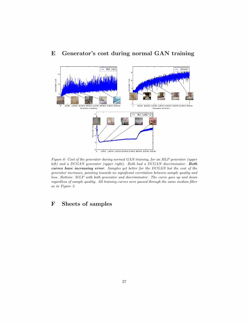
E Generator’s cost during normal GAN training

Figure 8: Cost of the generator during normal GAN training, for an MLP generator (upperleft) and a DCGAN generator (upper right). Both had a DCGAN discriminator. Bothcurves have increasing error. Samples get better for the DCGAN but the cost of thegenerator increases, pointing towards no significant correlation between sample quality andloss. Bottom: MLP with both generator and discriminator. The curve goes up and downregardless of sample quality. All training curves were passed through the same median filteras in Figure 3.

F Sheets of samples

27

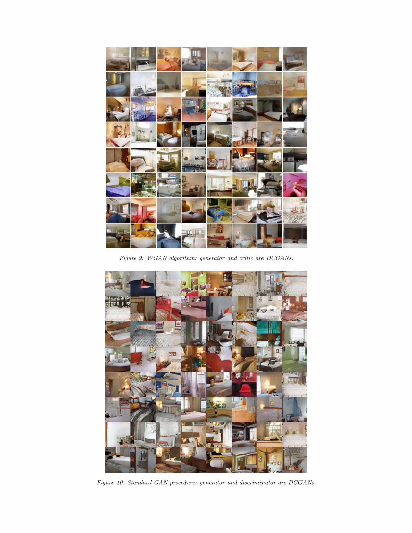
Figure 9: WGAN algorithm: generator and critic are DCGANs.

Figure 10: Standard GAN procedure: generator and discriminator are DCGANs.

28

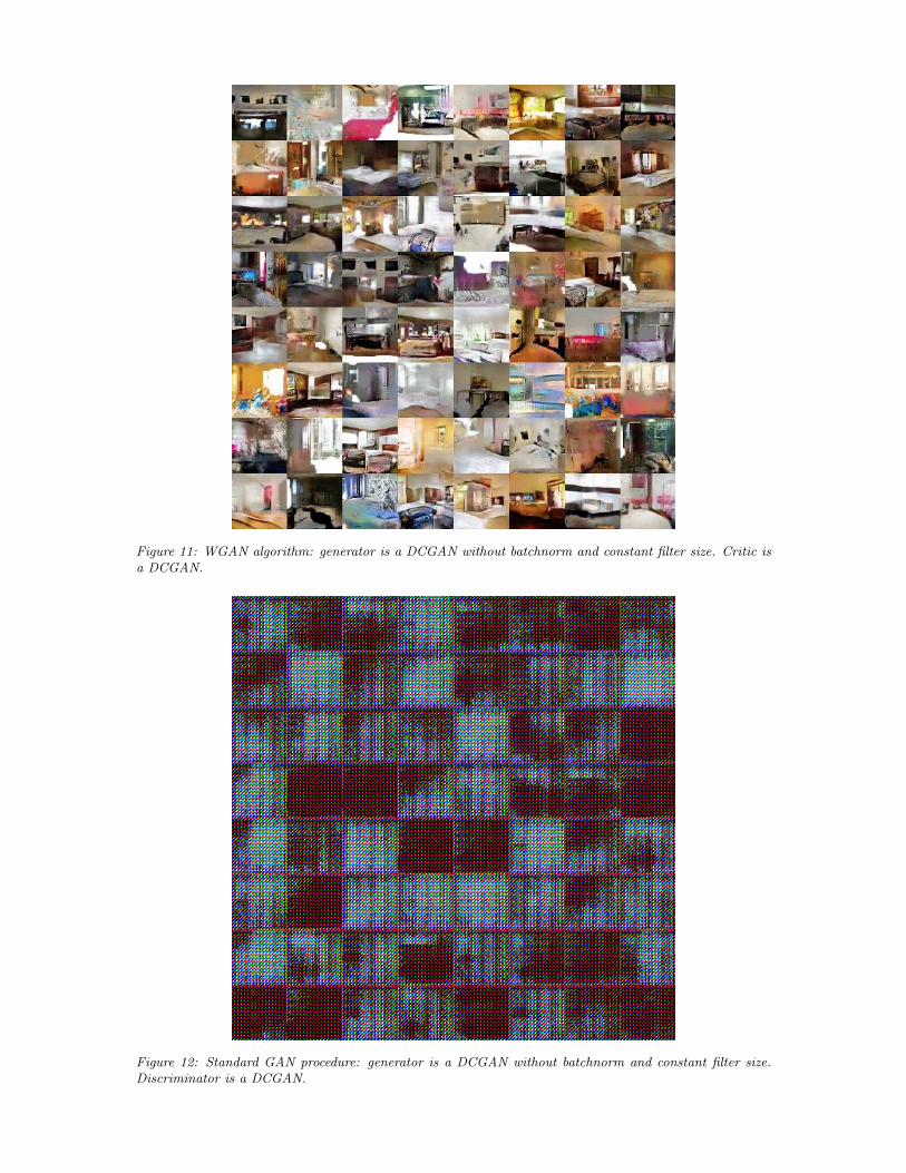
Figure 11: WGAN algorithm: generator is a DCGAN without batchnorm and constant filter size. Critic isa DCGAN.

Figure 12: Standard GAN procedure: generator is a DCGAN without batchnorm and constant filter size.Discriminator is a DCGAN.

29

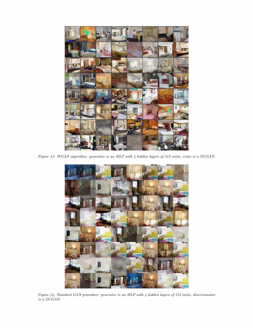
Figure 13: WGAN algorithm: generator is an MLP with 4 hidden layers of 512 units, critic is a DCGAN.

Figure 14: Standard GAN procedure: generator is an MLP with 4 hidden layers of 512 units, discriminatoris a DCGAN.

30