Fakultät Mathematik und Naturwissenschaften, FR Psychologie, Institut für Allgemeine Psychologie, Biopsychologie und Methoden der Psychologie, Professur Neuroimaging

May 11th 2015

What are we measuring with M/EEG?

Stefan Kiebel

M/EEG measurement Slide 2/30

Overview

1 History

2 Genesis of EEG/MEG signal

3 Measurement specifics

4 Forward models

M/EEG measurement Slide 3/30

Overview

1 History

2 Genesis of M/EEG signal

3 Measurement specifics

4 Forward models

M/EEG measurement Slide 4/30

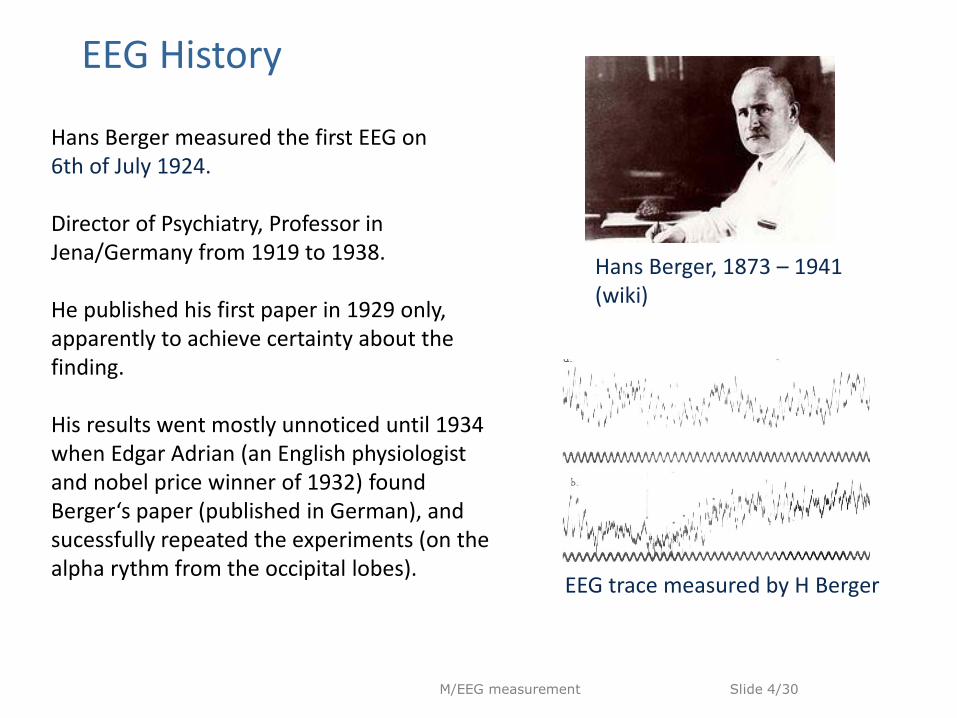
Hans Berger measured the first EEG on 6th of July 1924. Director of Psychiatry, Professor in Jena/Germany from 1919 to 1938. He published his first paper in 1929 only, apparently to achieve certainty about the finding. His results went mostly unnoticed until 1934 when Edgar Adrian (an English physiologist and nobel price winner of 1932) found Berger‘s paper (published in German), and sucessfully repeated the experiments (on the alpha rythm from the occipital lobes).

EEG History

Hans Berger, 1873 – 1941 (wiki)

EEG trace measured by H Berger

M/EEG measurement Slide 5/30

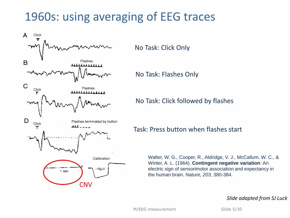
Walter, W. G., Cooper, R., Aldridge, V. J., McCallum, W. C., &

Winter, A. L. (1964). Contingent negative variation: An

electric sign of sensorimotor association and expectancy in

the human brain. Nature, 203, 380-384.

No Task: Click Only

No Task: Flashes Only

No Task: Click followed by flashes

Task: Press button when flashes start

CNV

1960s: using averaging of EEG traces

Slide adapted from SJ Luck

M/EEG measurement Slide 6/30

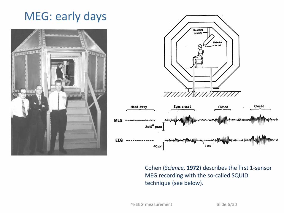
MEG: early days

Cohen (Science, 1972) describes the first 1-sensor MEG recording with the so-called SQUID technique (see below).

M/EEG measurement Slide 7/30

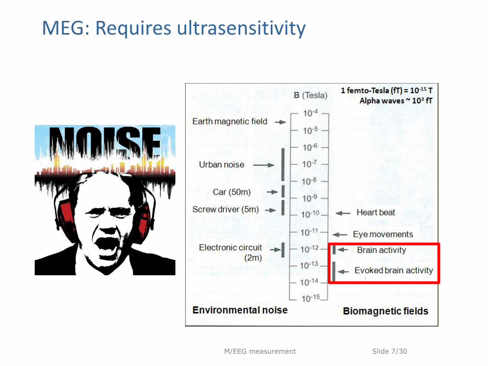
MEG: Requires ultrasensitivity

M/EEG measurement Slide 8/30

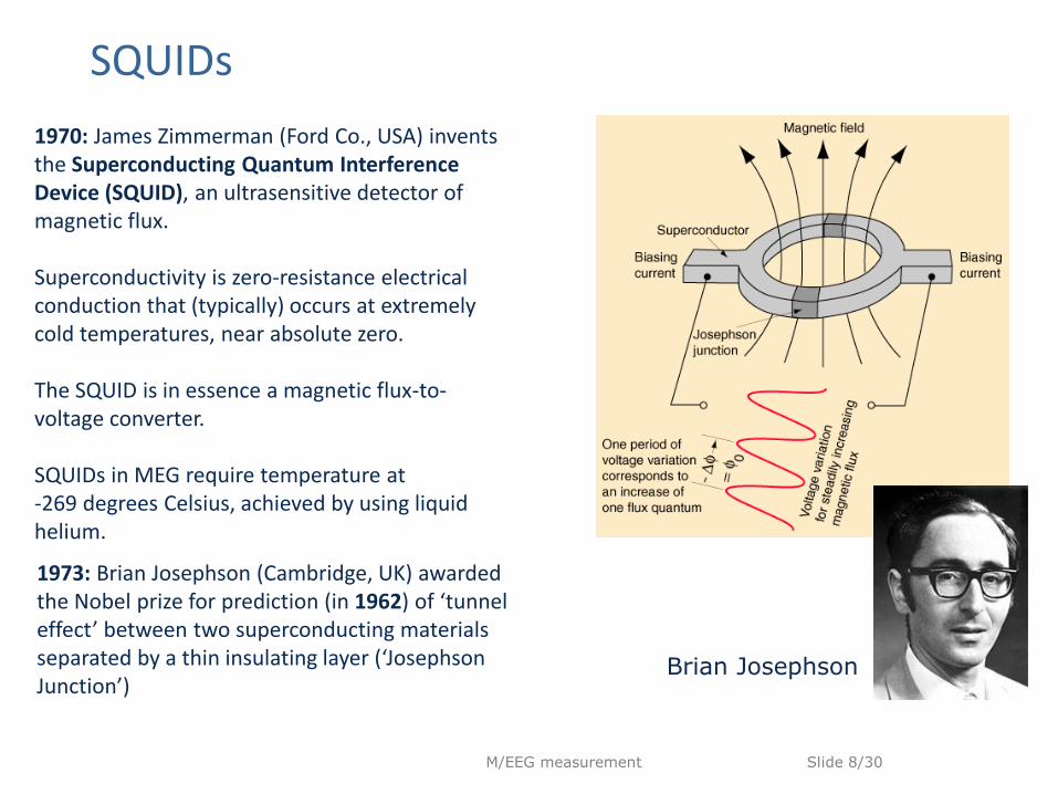
SQUIDs

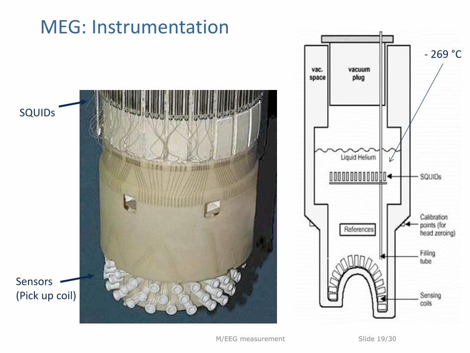
1970: James Zimmerman (Ford Co., USA) invents the Superconducting Quantum Interference Device (SQUID), an ultrasensitive detector of magnetic flux. Superconductivity is zero-resistance electrical conduction that (typically) occurs at extremely cold temperatures, near absolute zero. The SQUID is in essence a magnetic flux-to-voltage converter. SQUIDs in MEG require temperature at -269 degrees Celsius, achieved by using liquid helium.

1973: Brian Josephson (Cambridge, UK) awarded the Nobel prize for prediction (in 1962) of ‘tunnel effect’ between two superconducting materials separated by a thin insulating layer (‘Josephson Junction’)

Brian Josephson

M/EEG measurement Slide 9/30

Overview

1 History

2 Genesis of M/EEG signal

3 Measurement specifics

4 Forward models

M/EEG measurement Slide 10/30

- +

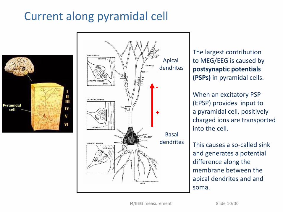
The largest contribution to MEG/EEG is caused by postsynaptic potentials (PSPs) in pyramidal cells. When an excitatory PSP (EPSP) provides input to a pyramidal cell, positively charged ions are transported into the cell.

Current along pyramidal cell

Apical dendrites

Basal dendrites This causes a so-called sink

and generates a potential difference along the membrane between the apical dendrites and and soma.

M/EEG measurement Slide 11/30

- +

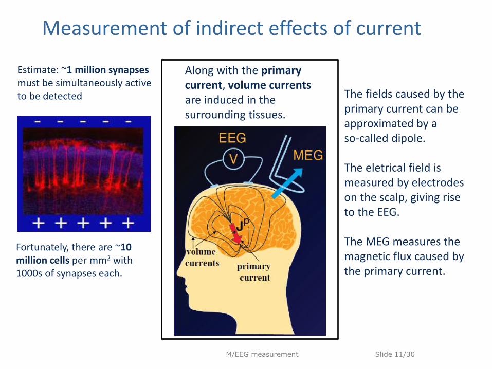
Estimate: ~1 million synapses must be simultaneously active to be detected

Fortunately, there are ~10 million cells per mm2 with 1000s of synapses each.

Along with the primary current, volume currents are induced in the surrounding tissues.

The fields caused by the primary current can be approximated by a so-called dipole. The eletrical field is measured by electrodes on the scalp, giving rise to the EEG. The MEG measures the magnetic flux caused by the primary current.

Measurement of indirect effects of current

M/EEG measurement Slide 12/30

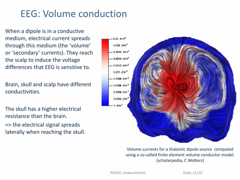
When a dipole is in a conductive medium, electrical current spreads through this medium (the ‘volume’ or ‘secondary’ currents). They reach the scalp to induce the voltage differences that EEG is sensitive to.

Brain, skull and scalp have different conductivities.

The skull has a higher electrical resistance than the brain.

=> the electrical signal spreads laterally when reaching the skull.

Volume currents for a thalamic dipole source computed using a so-called finite element volume conductor model.

(scholarpedia, C Wolters)

EEG: Volume conduction

M/EEG measurement Slide 13/30

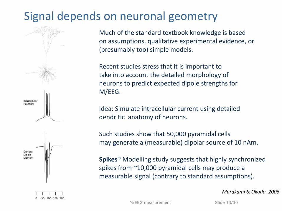
Murakami & Okada, 2006

Signal depends on neuronal geometry Much of the standard textbook knowledge is based on assumptions, qualitative experimental evidence, or (presumably too) simple models. Recent studies stress that it is important to take into account the detailed morphology of neurons to predict expected dipole strengths for M/EEG. Idea: Simulate intracellular current using detailed dendritic anatomy of neurons. Such studies show that 50,000 pyramidal cells may generate a (measurable) dipolar source of 10 nAm. Spikes? Modelling study suggests that highly synchronized spikes from ~10,000 pyramidal cells may produce a measurable signal (contrary to standard assumptions).

M/EEG measurement Slide 14/30

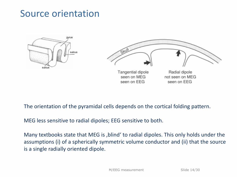
Source orientation

The orientation of the pyramidal cells depends on the cortical folding pattern. MEG less sensitive to radial dipoles; EEG sensitive to both. Many textbooks state that MEG is ‚blind‘ to radial dipoles. This only holds under the assumptions (i) of a spherically symmetric volume conductor and (ii) that the source is a single radially oriented dipole.

M/EEG measurement Slide 15/30

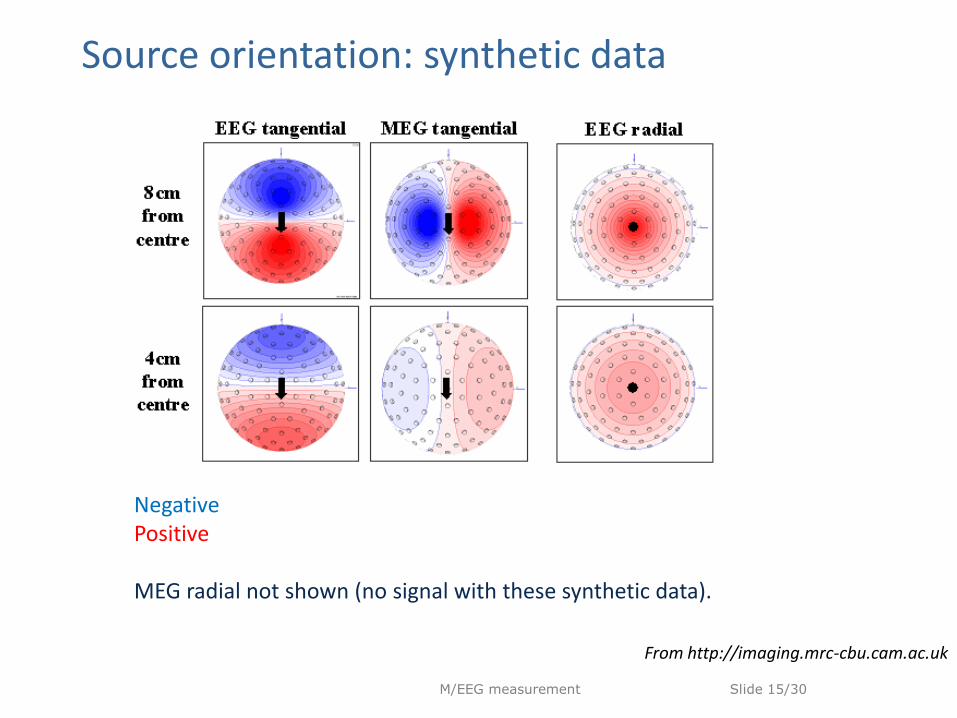
Source orientation: synthetic data

Negative Positive MEG radial not shown (no signal with these synthetic data).

From http://imaging.mrc-cbu.cam.ac.uk

M/EEG measurement Slide 16/30

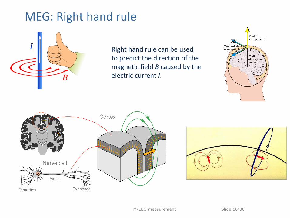
MEG: Right hand rule

Right hand rule can be used to predict the direction of the magnetic field B caused by the electric current I.

M/EEG measurement Slide 17/30

Overview

1 History

2 Genesis of M/EEG signal

3 Measurement specifics

4 Forward models

M/EEG measurement Slide 18/30

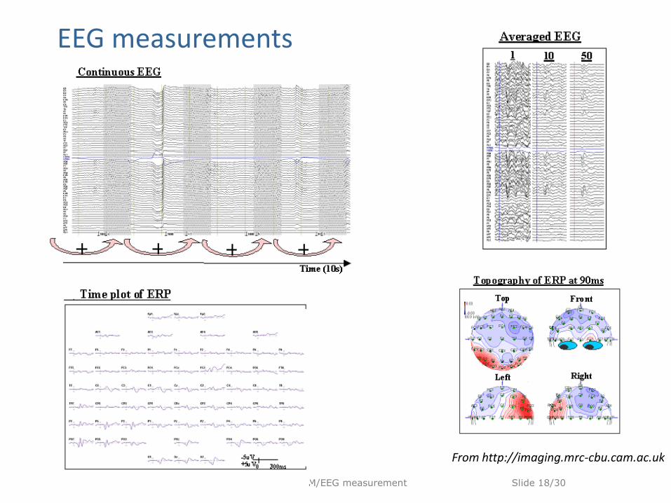
From http://imaging.mrc-cbu.cam.ac.uk

v

v v

EEG measurements

M/EEG measurement Slide 19/30

MEG: Instrumentation

Sensors (Pick up coil)

SQUIDs

- 269 °C

M/EEG measurement Slide 20/30

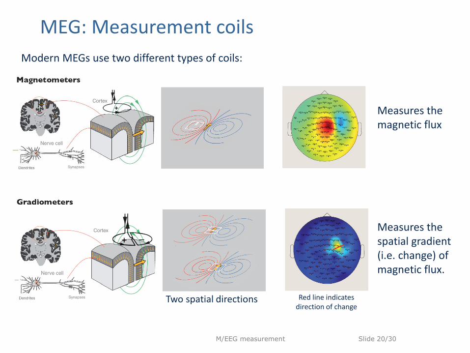
MEG: Measurement coils

Modern MEGs use two different types of coils:

Measures the magnetic flux

Measures the spatial gradient (i.e. change) of magnetic flux.

Two spatial directions Red line indicates direction of change

M/EEG measurement Slide 21/30

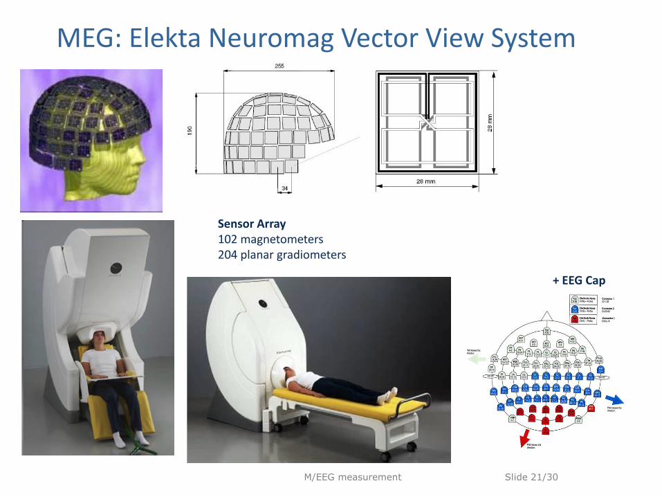
+ EEG Cap

Sensor Array 102 magnetometers 204 planar gradiometers

MEG: Elekta Neuromag Vector View System

M/EEG measurement Slide 22/30

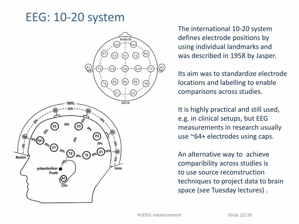
EEG: 10-20 system The international 10-20 system defines electrode positions by using individual landmarks and was described in 1958 by Jasper. Its aim was to standardize electrode locations and labelling to enable comparisons across studies. It is highly practical and still used, e.g. in clinical setups, but EEG measurements in research usually use ~64+ electrodes using caps. An alternative way to achieve comparibility across studies is to use source reconstruction techniques to project data to brain space (see Tuesday lectures) .

M/EEG measurement Slide 23/30

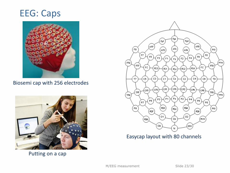
EEG: Caps

Easycap layout with 80 channels

Biosemi cap with 256 electrodes

Putting on a cap

M/EEG measurement Slide 24/30

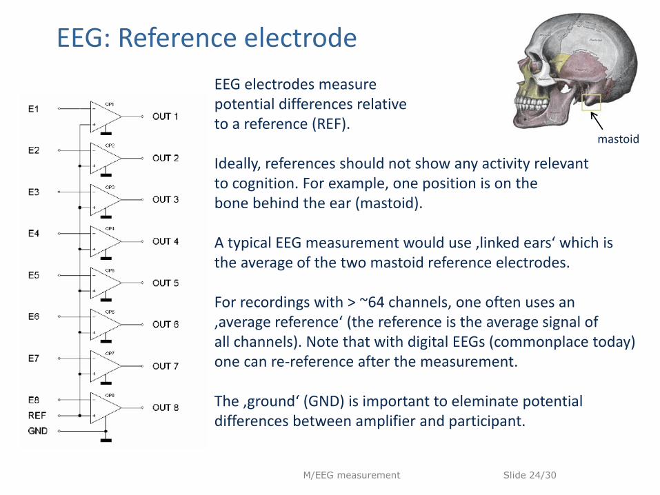
EEG: Reference electrode

EEG electrodes measure potential differences relative to a reference (REF). Ideally, references should not show any activity relevant to cognition. For example, one position is on the bone behind the ear (mastoid). A typical EEG measurement would use ‚linked ears‘ which is the average of the two mastoid reference electrodes. For recordings with > ~64 channels, one often uses an ‚average reference‘ (the reference is the average signal of all channels). Note that with digital EEGs (commonplace today) one can re-reference after the measurement. The ‚ground‘ (GND) is important to eleminate potential differences between amplifier and participant.

mastoid

M/EEG measurement Slide 25/30

Overview

1 History

2 Genesis of EEG/MEG signal

3 Measurement specifics

4 Forward models

M/EEG measurement Slide 26/30

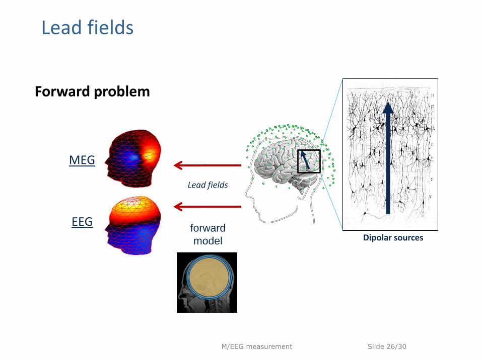
Lead fields

Forward problem

Lead fields

MEG

EEG Dipolar sources

forward

model

M/EEG measurement Slide 27/30

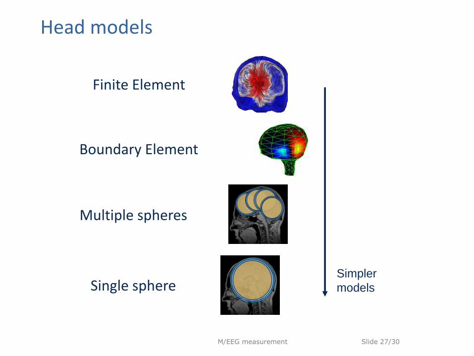
Head models

Simpler

models

Finite Element

Boundary Element

Multiple spheres

Single sphere

M/EEG measurement Slide 28/30

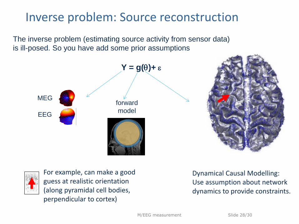
Inverse problem: Source reconstruction

Y = g()+

forward

model

MEG

For example, can make a good guess at realistic orientation (along pyramidal cell bodies, perpendicular to cortex)

EEG

The inverse problem (estimating source activity from sensor data)

is ill-posed. So you have add some prior assumptions

Dynamical Causal Modelling: Use assumption about network dynamics to provide constraints.

M/EEG measurement Slide 29/30

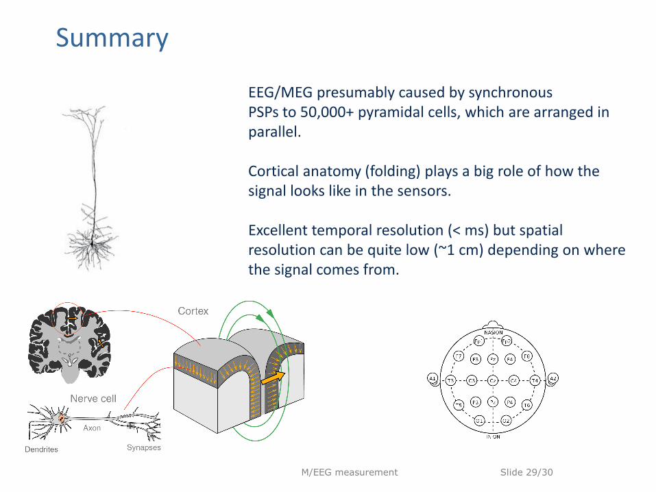
Summary

EEG/MEG presumably caused by synchronous PSPs to 50,000+ pyramidal cells, which are arranged in parallel. Cortical anatomy (folding) plays a big role of how the signal looks like in the sensors. Excellent temporal resolution (< ms) but spatial resolution can be quite low (~1 cm) depending on where the signal comes from.

M/EEG measurement Slide 30/30

Acknowledgments

Thanks to Dorothea Hämmerer @ Institute of Cognitive Neuroscience, UCL, London Steven Luck @ Center for Mind and Brain, UC Davis Saskia Helbling @ IMP, Goethe-Univ., Frankfurt Jeremie Mattout @ Lyon Neuroscience Research Center, Lyon Vladimir Litvak @ WTC for Neuroimaging, UCL, London FIL methods group @ WTC for Neuroimaging, UCL, London