Technische Universität Wien Studienrichtung Vermessungswesen und Geoinformation
DISSERTATION
Precision Target Mensuration in Vision Metrology
ausgeführt zum Zwecke der Erlangung des akademischen Grades eines Doktors der
technischen Wissenschaften unter der Leitung von
Professor Clive S. Fraser (BAppSc, MSurvSc, PhD) Department of Geomatics, Melbourne University
und
O.Univ.Prof. Dipl.-Ing. Dr.techn. Karl Kraus E122, Institut für Photogrammetrie und Fernerkundung, TU-Wien
eingereicht an der Technischen Universität Wien
Fakultät für Mathematik und Geoinformation
von
Dipl.-Ing. Johannes Otepka Matrikelnummer 93 26 413
Ottensheimerstraße 64, 4040 Linz
Wien, im Oktober 2004

Acknowledgement
First, I want to thank my girlfriend, Gerhild, as well as both our families for their support.
Moreover, I want to thank Professor Karl Kraus and Professor Clive Fraser for supervising my
research topic. I also extend my gratitude to both for providing all required resources at their
Departments in Vienna and Melbourne.
I also wish to extend special thanks to Harry Hanley and Danny Brizzi for their friendship and for
their support, both technical and in regard to accommodation, during my visits to Australia. The
very useful mathematical insights from Helmut Kager also deserve special recognition.
Additionally, I want to thank Ute, Tom, Camille, Cronksta, Georg R., Georg V., Gisela, Harrison,
Hartwig, Laurie, Matt, Megan, Paul, and Takeshi all of whom are friends in Vienna, Linz and
Melbourne. They have made my research time very pleasant and always interesting.
Finally, many thanks to the Austrian Academy of Sciences for honouring me with the DOC
scholarship award. Without the scholarship, both the conduct of the doctoral research and the
preparation of this thesis would not have been possible.
ii
Abstract
Digital close-range photogrammetry, commonly referred to as vision metrology (VM), is regularly
used as a flexible and highly accurate 3D measurement system. VM’s most common applications
lie within the manufacturing and precision engineering industries.
Through the use of triangulation combined with specialized targets to mark points of interest,
accuracies exceeding 1:100,000 can be achieved with VM. In practical applications, circular targets
are used to achieve the highest accuracy. Common types include: retro-reflective targets, which
provide a high contrast image with flash photography, and white targets on a black background.
Accuracy requirements and varying target reflective properties dictate which type of targeting is
most suitable for a particular application.
The precise measurement of targets is one of the main factors within VM and directly influences
the ability to achieve high accuracy. Mathematical algorithms are used to determine the centres of
imaged targets in 2D space. These 2D centroids are then used in a triangulation process to calculate
the target position in 3D space. This computational process assumes that the targets represent
perfect points in space. In practice, however, target thickness and target diameter adversely effect
this assumption. This can lead to the introduction of error and to incorrect calculation of the desired
3D positions. If the target plane is known, however, the 2D centroids can be corrected for these
errors.
A central theme of the thesis is the development of a mathematical model and associated
computational scheme for the automatic determination of the surface plane of circular targets. The
target plane description is determined in two stages. First, the elliptical target images are analysed
in each digital photograph. Then, the information gained is used to calculate the target plane via the
method of least-squares estimation. The developed process has been implemented and evaluated in
the photogrammetric software package Australis.
In addition to the development of the new technique for target plane determination, the research
also included an investigation, using two groups of network simulations, of induced systematic
errors within the photogrammetric measurement process. The first set of simulations investigated
the image error effect on the determined target position in 3D space in instances where the derived
image coordinate correction functions were not applied. The second group of simulations were
conducted to quantify and assess the distortion induced in the 3D measurement process by curved
targets. This aspect is especially relevant for the typical VM application of dimensional inspection
of surfaces, where targets are directly affixed to the surfaces of interest.
iii

An important component of the research was to analyse the practical relevance of the developed
processes and algorithms. As it turns out, high accuracy application domains can benefit from the
outcomes of the research conducted, through the enabling of higher measurement precision. In the
case of medium-accuracy VM applications or 3D surface inspection, the new techniques for target
plane orientation determination can be employed as part of the surface survey, as well as to assist
visually in the interpretation of the 3D measurement results.
iv

Zusammenfassung
Digitale Nahbereichsphotogrammetrie, im Englischen meist als „Vision Metrology“ bezeichnet,
wird heutzutage als flexibles und hochgenaues 3D-Meßverfahren in unterschiedlichen industriellen
Bereichen verwendet. Durch die Verwendung spezieller Zielmarken ist eine hochgenaue
Punktbestimmung markierter Objektpunkte möglich. Die erzielbare Punktgenauigkeit dieser
Messmethode liegt bei 1/100.000 der Objektgröße. In diesem Zusammenhang wird der Begriff
„Triangulierungsgenauigkeit“ oft verwendet.
Üblicherweise werden für die Signalisierung der Punkte kreisrunde Zielmarken verwendet. Diese
erlauben höchste Genauigkeit zu erzielen. Neben Zielmarken aus retro-reflektierendem Material
werden auch einfache weiße Marken auf schwarzem Hintergrund benutzt. Die Wahl des
Zielmarkenmaterials bzw. -typs richtet sich nach der geforderten Genauigkeit und dem
notwendigen Reflektionsgrad der Signale bei der Aufnahme der Bilder.
Die Messgenauigkeit der Zielmarken ist einer der entscheidenden Faktoren für eine hohe
Triangulierungsgenauigkeit. Mit Hilfe von speziellen Algorithmen werden die Zentren der
Zielmarken im digitalen Bild ermittelt, welche es erlauben die Objektpunkte dreidimensional zu
triangulieren. Dabei wird vorausgesetzt, dass Zielmarken „perfekte“ Punkte im Raum darstellen,
was aufgrund der Stärke des Markenmaterials und der Größe des Zielmarkendurchmessers nur
bedingt der Fall ist. Diese Tatsache führt zu Exzentrizitäten zwischen den Zentren der abgebildeten
Zielmarken und ihren tatsächlichen Mittelpunkten. Daraus resultieren Fehler im
Berechnungsprozess, welche zu einer verfälschten Raumlage der Punkte führen. Ist die
Orientierung der einzelnen Zielmarken bekannt, so können die entsprechenden Exzentrizitäten
rechnerisch ermittelt und damit die Raumlage der Punkte korrigiert werden.
Ein zentrales Ziel dieser Arbeit war die Entwicklung mathematischer Formeln und Algorithmen für
die automatische Bestimmung der Kreisebenen der Zielmarken. Der dafür entworfene Prozess
berechnet diese Ebenen in zwei Phasen. Zuerst wird die elliptische Form der abgebildeten
Zielmarken aus den digitalen Bildern extrahiert. Anschließend wird diese Information für die
eigentliche Berechnung der Kreisebene verwendet, wobei Ausgleichungsverfahren eingesetzt
werden. Der dazu entwickelte Berechnungsprozess wurde in das photogrammetrische
Softwarepaket Australis implementiert und anhand von praktischen Anwendungen evaluiert.
Im weiteren Verlauf der Arbeit werden die Ergebnisse von Simulationsrechnungen präsentiert,
welche den Einfluss von zwei unterschiedlichen Fehlerarten aufzeigen. Der erste Teil der
Simulationen untersucht die Auswirkung der oben angeführten Exzentrizität auf die Objektpunkte.
v

Die zweite Gruppe der Simulationsrechnungen analysiert den Fehlereinfluss von gekrümmten
Zielmarken auf den Zielmarkenmessprozess. Dieser Einfluss ist vor allem bei der Vermessung von
gewölbten Oberflächen interessant, da hier die Zielmarken direkt auf den zu bestimmenden
Oberflächen fixiert werden.
Obwohl bei den vorliegenden Untersuchungen primär theoretische Fragestellungen im
Vordergrund stehen, widmet sich ein Teil der Arbeit auch der praktischen Relevanz der
entwickelten Prozesse und Algorithmen. Dabei konnte bewiesen werden, dass die
Berücksichtigung der Exzentrizitäten entsprechende Genauigkeitsvorteile bei hochgenauen
Vermessungen bringt. Zusätzlich werden Vorteile für Oberflächenanalysen sowie Aufgaben
mittlerer Genauigkeit aufgezeigt.
vi
Table of Contents
1. Introduction .....................................................................................................1 1.1. Motivation..........................................................................................................................1 1.2. General Aims .....................................................................................................................1 1.3. Thesis Structure .................................................................................................................2
2. Vision Metrology .............................................................................................3 2.1. Concepts of Automated VM..............................................................................................4 2.2. State-of-the-art Target Measurement.................................................................................6
2.2.1. Intensity-Weighted Centroiding ................................................................................7
3. Geometric Aspects of Circular Target Measurement...................................8 3.1. Mathematical Model of a 3D Circle and its Perspective Image ........................................9 3.2. Special Geometric Aspects of Retro-Reflective Targets .................................................14
4. Target Plane Determination within Digital Images.....................................18 4.1. Least-Squares Adjustment ...............................................................................................18 4.2. Ellipse-Fitting of Imaged Targets ....................................................................................20
4.2.1. Best-Fit Ellipse of Intensity Levelled Points ...........................................................20 4.2.2. 2D Gaussian Distribution Fitting.............................................................................22
4.3. Target Plane Adjustment .................................................................................................25 4.3.1. Target Plane Adjustment by Point Projection .........................................................25 4.3.2. Target Plane Adjustment by Observing Implicit Ellipse Parameters ......................27
5. Eccentricity Effect on Bundle Adjustment..................................................31 5.1. Creating Simulated Images..............................................................................................31 5.2. Eccentricity Effect on a Plane Test Field.........................................................................35 5.3. Eccentricity Effect on a Parabolic Antenna.....................................................................38 5.4. Eccentricity Effect on a Cylindrical Hull.........................................................................40 5.5. Eccentricity Effect on a Sinus-Shaped Surface ...............................................................43 5.6. Eccentricity Effect on a Rough Plane Test Field .............................................................45
6. Curved Targets and their Distortional Effect..............................................49 6.1. Derivations for Cylindrical Curved Targets ....................................................................49
6.1.1. Continuous Derivations ...........................................................................................49 6.1.2. Discrete Derivations ................................................................................................53
6.1.2.1. Intensity characteristics of retro-reflective targets .......................................53 6.1.2.2. Intensity characteristics of plane white targets.............................................56
vii
6.1.2.3. Rasterising Algorithm ..................................................................................57 6.1.2.4. Discrete Distortion Estimations ...................................................................59
7. Evaluation of Target Plane Determination ..................................................68 7.1. Australis: An Ideal Evaluation Environment...................................................................68
7.1.1. Ellipse-Fitting Process in Australis .........................................................................69 7.1.2. Target Plane Determination in Australis .................................................................70
7.2. Accuracy of the Target Plane Determination within Real Applications..........................71 7.2.1. Test Project 1: Calibration Table.............................................................................72 7.2.2. Test Project 2: Cylindrical Hull...............................................................................73
7.3. Accuracy Gain by Considering the Eccentricity Effect ...................................................74
8. Conclusions ..................................................................................................77 8.1. Benefits for Practical Applications ..................................................................................77 8.2. Future Research Aims......................................................................................................79
Appendix A1 : Conversion of Ellipse Parameters............................................80
Appendix A2 : Conversion of Variance-Covariance Matrices of Different Ellipse Parameters.....................................................................81
Appendix A3 : Best-fit Ellipse Adjustment .......................................................81
Appendix A4 : Best-fit Polynomial Surface Adjustment..................................82
Appendix B1 : Tables of Distortion Errors for Plane White Targets...............84
References........ ...................................................................................................85
viii
1. Introduction
1. Introduction
1.1. Motivation Photogrammetry has always been one of the author’s research interests. In his masters thesis, the
author concentrated on digital close-range photogrammetry, thus becoming aware of the high
accuracy potential of this surveying method.
Digital close-range photogrammetry, commonly referred to as vision metrology (VM), makes use
of circular targets to mark points of interest. After imaging the targets from different points of
views, mathematical algorithms are used to determine the centres of imaged targets in 2D space.
These 2D centroids are then used to triangulate the target position in 3D space. This computation
process assumes that the centre of the imaged target is identical with the projected centre of the
circle. Knowledge regarding perspectivity shows that this assumption is not strictly correct. There
is a small offset which is universally ignored in today’s VM systems because its magnitude is
generally insignificant, especially for small targets.
Although this eccentricity is of no importance for medium accuracy applications, it is always
unsatisfactory to knowingly introduce systematic errors into the triangulation process. The
eccentricity limits the radius of the targets being used, which again limits the achievable accuracy.
The main aim of the research has been to overcome these shortcomings by correcting the measured
centres for the eccentricity.
1.2. General Aims Ahn et al. (1999) have reported an eccentricity correction formula using the target orientation.
Since the target plane is generally not known, this equation cannot be employed. As it will be
shown, however, the target plane can be determined if the shape of the imaged target is extracted
from at least two images. Hence, one major aim of the thesis research was to develop an automated
target plane determination process, which first accurately extracts the imaged target shape in all
digital photographs. Then, the information gained from all images is used to estimate the target
orientation, always considering that only a precise target plane description will be subsequently
usable.
By employing the target plane determination, it is now possible to correct the aforementioned
eccentricity, which should enable higher precision photogrammetric surveys to be conducted,
especially in high accuracy VM application domains. However, it will be shown that even medium
accuracy applications can benefit from the target plane determination in the case of surface
inspection.
1
1. Introduction
Besides the mathematical derivations of the developed process, various simulation results will be
reported in this thesis. For example, the distortional effects of the eccentricity on the triangulation
process are analysed. Another group of simulations allow investigation of the distortion caused by
curved targets of different materials. This will help in the selection of the correct target radius if
curved surfaces are inspected. Therefore, the radiometric aspects of different target materials were
investigated.
Although the main characteristic of this thesis is its mathematical derivations and theoretical
considerations, the outcomes are always evaluated from a practical point of view as well.
1.3. Thesis Structure All developed algorithms and processes were implemented and evaluated within the
photogrammetric software package Australis (Photometrix 2004). Consequently, the
implementation of algorithms in Visual C++ was an essential part of this research. As mentioned,
however, the main focus was upon mathematical derivations and the design of corresponding
algorithms.
At this point, some details about the thesis structure and its chapters will be presented. The
following chapter introduces VM. Here, the technology and history of digital close-range
photogrammetry is described. Then, in the central chapter of the thesis, the mathematical
relationship between a circular target and its perspective image is derived. In Chapter 4, algorithms
to extract the shape of imaged targets are reported. Afterwards, results of simulations are presented.
These investigate the distortional effect of the eccentricity in the triangulation process. A chapter
about simulations of the distortional effect of curved targets then follows. In the second last
chapter, an evaluation of the developed processes is made. There, accuracies of the target plane
determination within real applications are presented and compared with simulated results. The
thesis is concluded with a conclusions chapter with remarks for future research and a description of
benefits from the outcomes for practical applications.
2
2. Vision Metrology
2. Vision Metrology In the early 1980s, optical 3D coordinate measurement systems were introduced in the
manufacturing and precision engineering sectors. Film-based photogrammetry and other 3D
measuring devices became routine tools for high-accuracy dimensional inspection. Today, digital
close-range photogrammetry, digital theodolites and laser trackers are the most commonly
employed non-contact measurement methods. The first of these, digital close-range
photogrammetry, is commonly referred to as vision metrology or VM in short, and it is regularly
used in large-scale industrial manufacturing and engineering. Its flexible vision-based concept
combined with new developments such as high-resolution digital cameras and new computational
models have made digital close-range photogrammetry a highly-automated, high-precision 3D
coordinate measurement technology.
Although there are many potential uses of VM, adoption of the technology by industry has been
most pronounced in the automobile, aircraft and aerospace manufactioning sectors, as well as in
shipbuilding and construction engineering. Dimensional inspection with VM is carried out to
support such requirements as quality assurance, deformation measurement, conformance to design
surveys and reverse-engineering
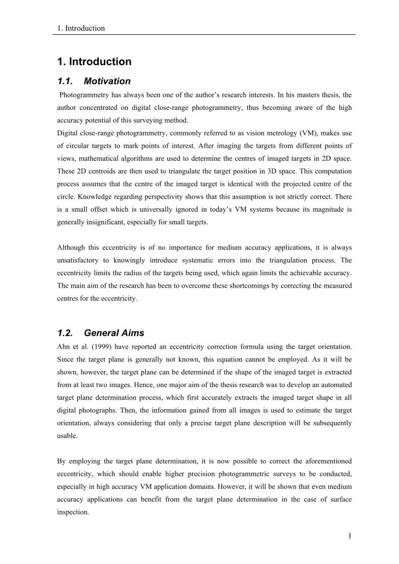
VM strategies employ triangulation to determine three dimensional (3D) object point coordinates.
Therefore the geometric principle of images, central projection, is used. Every imaged point defines
a three dimensional ray in space. Multiple images with different view angles allow triangulation of
the required object feature points, as shown in Figure 2.1.
Figure 2.1: Triangulation principle of VM
To achieve high accuracies within the sub-millimetre range, VM strategies make use of special
targets to mark points of interest. Various investigations have shown that circular targets deliver the
most satisfying results regarding accuracy and automated centroid recognition and mensuration.
3
2. Vision Metrology
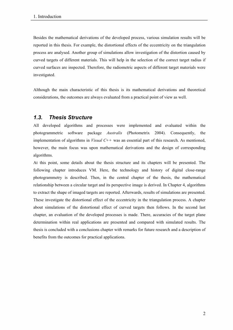
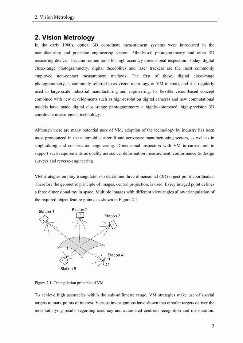
For such targets, retro-reflective material is widely used because on-axis illumination of these
targets returns many times more light than a normal white textured surface. Using this property,
high contrast imagery can be achieved even in bright light conditions, as indicated in Figure 2.2
and Figure 2.3. High contrast images are a key requirement for both high precision and a high level
of measurement automation in VM.
Figure 2.2: Normal contrast image of car door
Figure 2.3: High contrast image of car door
Using the radiometric information of high contrast images, and fully utilising the geometric
resolution of the camera, accuracies can be greatly increased. Besides retro-reflective signalisation,
targets of various different materials are also available, for example plane white targets which can
even result in higher accuracy than retro-reflective targets. Complexity with correct exposure,
however, has meant that such targets are not often used. Another “target material” is structured
light where illuminated spots or patterns are projected onto the surface of the object to be measured
(Luhmann 2000, Kraus 1996).
2.1. Concepts of Automated VM Nowadays, VM offers a high degree of automation, which has opened up a broad field of practical
applications. Since results and outcomes of this thesis will improve and enhance the state-of-the-art
strategies in VM, a short overview about its concepts will be presented in this section. For more
details see e.g. Fraser (1997) or Otepka et al. (2002).
Though there are various strategies for the highly-automated VM measurement process, they all
have a first stage in common, namely automated target recognition and measurement. This is the
basic requirement for any measurement process which delivers the image coordinates of the target
centres in all images.
4
2. Vision Metrology
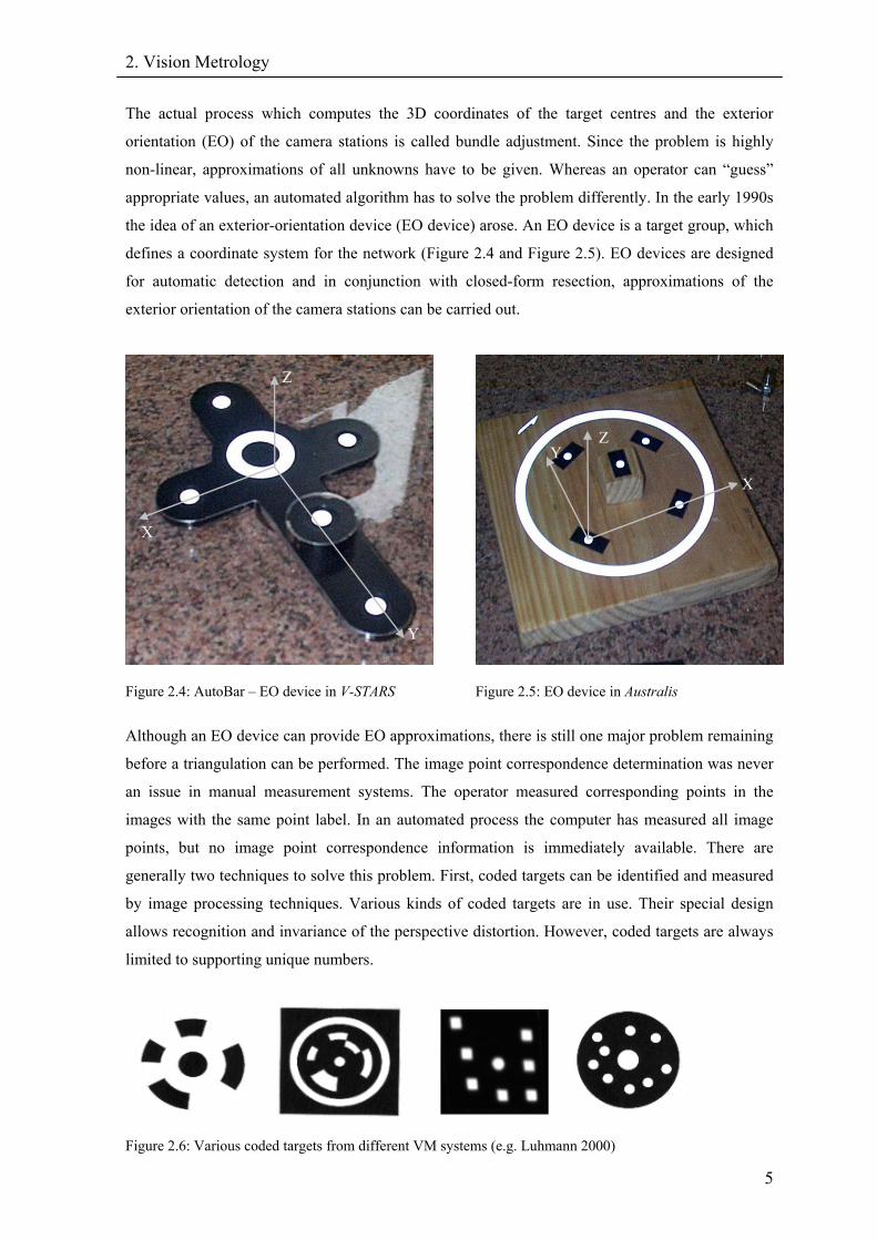
The actual process which computes the 3D coordinates of the target centres and the exterior
orientation (EO) of the camera stations is called bundle adjustment. Since the problem is highly
non-linear, approximations of all unknowns have to be given. Whereas an operator can “guess”
appropriate values, an automated algorithm has to solve the problem differently. In the early 1990s
the idea of an exterior-orientation device (EO device) arose. An EO device is a target group, which
defines a coordinate system for the network (Figure 2.4 and Figure 2.5). EO devices are designed
for automatic detection and in conjunction with closed-form resection, approximations of the
exterior orientation of the camera stations can be carried out.
Figure 2.4: AutoBar – EO device in V-STARS
Z
Z Y
X
X
Y
Figure 2.5: EO device in Australis
Although an EO device can provide EO approximations, there is still one major problem remaining
before a triangulation can be performed. The image point correspondence determination was never
an issue in manual measurement systems. The operator measured corresponding points in the
images with the same point label. In an automated process the computer has measured all image
points, but no image point correspondence information is immediately available. There are
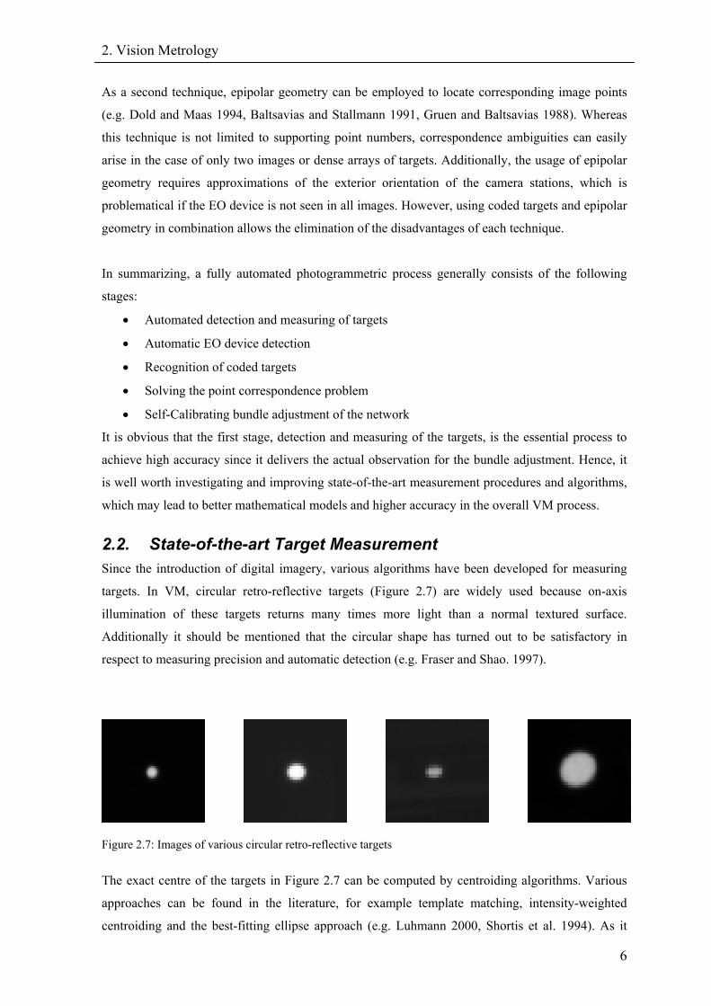
generally two techniques to solve this problem. First, coded targets can be identified and measured
by image processing techniques. Various kinds of coded targets are in use. Their special design
allows recognition and invariance of the perspective distortion. However, coded targets are always
limited to supporting unique numbers.
Figure 2.6: Various coded targets from different VM systems (e.g. Luhmann 2000)
5
2. Vision Metrology
As a second technique, epipolar geometry can be employed to locate corresponding image points
(e.g. Dold and Maas 1994, Baltsavias and Stallmann 1991, Gruen and Baltsavias 1988). Whereas
this technique is not limited to supporting point numbers, correspondence ambiguities can easily
arise in the case of only two images or dense arrays of targets. Additionally, the usage of epipolar
geometry requires approximations of the exterior orientation of the camera stations, which is
problematical if the EO device is not seen in all images. However, using coded targets and epipolar
geometry in combination allows the elimination of the disadvantages of each technique.
In summarizing, a fully automated photogrammetric process generally consists of the following
stages:
• Automated detection and measuring of targets
• Automatic EO device detection
• Recognition of coded targets
• Solving the point correspondence problem
• Self-Calibrating bundle adjustment of the network
It is obvious that the first stage, detection and measuring of the targets, is the essential process to
achieve high accuracy since it delivers the actual observation for the bundle adjustment. Hence, it
is well worth investigating and improving state-of-the-art measurement procedures and algorithms,
which may lead to better mathematical models and higher accuracy in the overall VM process.
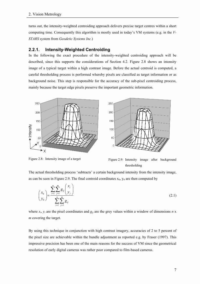
2.2. State-of-the-art Target Measurement Since the introduction of digital imagery, various algorithms have been developed for measuring
targets. In VM, circular retro-reflective targets (Figure 2.7) are widely used because on-axis
illumination of these targets returns many times more light than a normal textured surface.
Additionally it should be mentioned that the circular shape has turned out to be satisfactory in
respect to measuring precision and automatic detection (e.g. Fraser and Shao. 1997).
Figure 2.7: Images of various circular retro-reflective targets
The exact centre of the targets in Figure 2.7 can be computed by centroiding algorithms. Various
approaches can be found in the literature, for example template matching, intensity-weighted
centroiding and the best-fitting ellipse approach (e.g. Luhmann 2000, Shortis et al. 1994). As it
6
2. Vision Metrology
turns out, the intensity-weighted centroiding approach delivers precise target centres within a short
computing time. Consequently this algorithm is mostly used in today’s VM systems (e.g. in the V-
STARS system from Geodetic Systems Inc.)
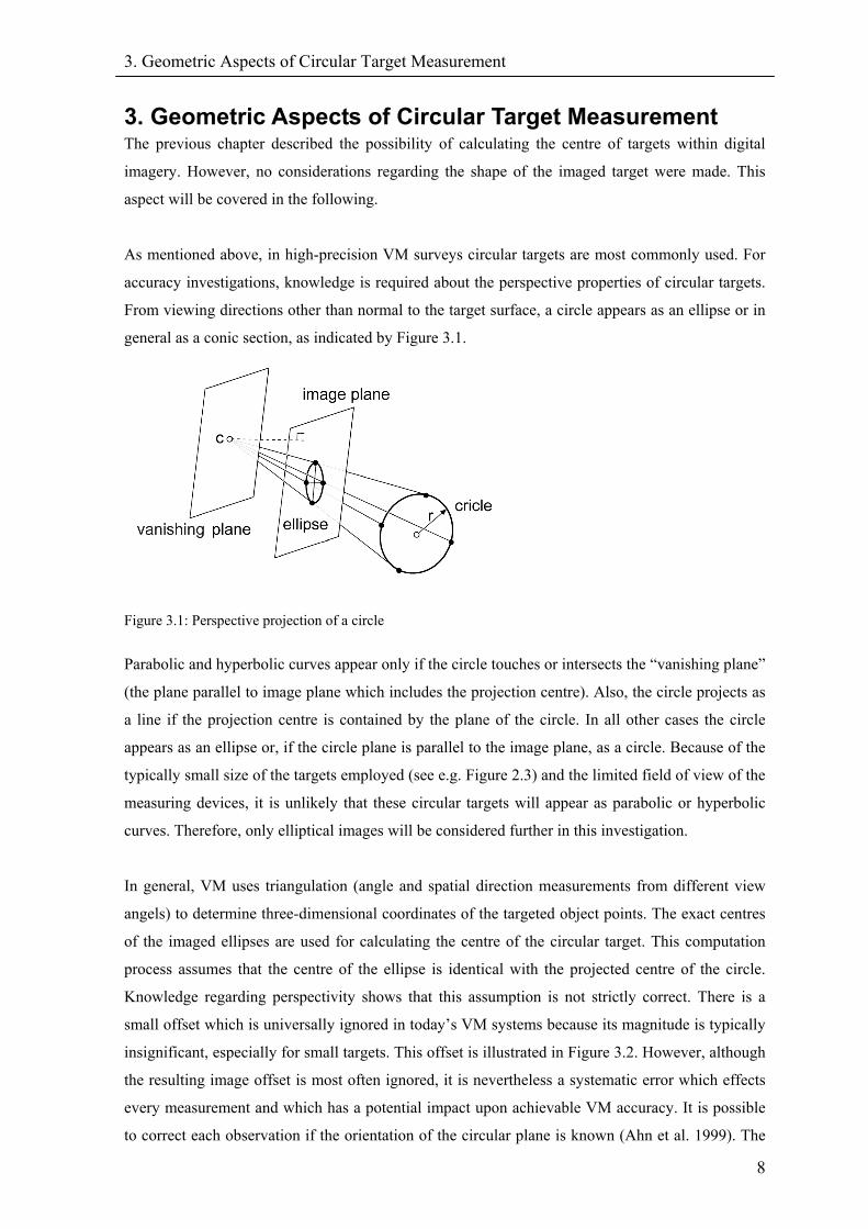
2.2.1. Intensity-Weighted Centroiding In the following the exact procedure of the intensity-weighted centroiding approach will be
described, since this supports the considerations of Section 4.2. Figure 2.8 shows an intensity
image of a typical target within a high contrast image. Before the actual centroid is computed, a
careful thresholding process is performed whereby pixels are classified as target information or as
background noise. This step is responsible for the accuracy of the sub-pixel centroiding process,
mainly because the target edge pixels preserve the important geometric information.
Figure 2.8: Intensity image of a target
Figure 2.9: Intensity image after background
thresholding
The actual thresholding process ‘subtracts’ a certain background intensity from the intensity image,
as can be seen in Figure 2.9. The final centroid coordinates x0, y0 are then computed by
1 10
0
1 1
n mi
iji j j
n m
iji j
xg
yxy g
= =
= =
⎛ ⎞⎜ ⎟
⎛ ⎞ ⎝ ⎠=⎜ ⎟⎝ ⎠
∑∑
∑∑ (2.1)
where xi, yi are the pixel coordinates and gij are the grey values within a window of dimensions n x
m covering the target.
By using this technique in conjunction with high contrast imagery, accuracies of 2 to 5 percent of
the pixel size are achievable within the bundle adjustment as reported e.g. by Fraser (1997). This
impressive precision has been one of the main reasons for the success of VM since the geometrical
resolution of early digital cameras was rather poor compared to film-based cameras.
7
3. Geometric Aspects of Circular Target Measurement
8
3. Geometric Aspects of Circular Target Measurement The previous chapter described the possibility of calculating the centre of targets within digital
imagery. However, no considerations regarding the shape of the imaged target were made. This
aspect will be covered in the following.
As mentioned above, in high-precision VM surveys circular targets are most commonly used. For
accuracy investigations, knowledge is required about the perspective properties of circular targets.
From viewing directions other than normal to the target surface, a circle appears as an ellipse or in
general as a conic section, as indicated by Figure 3.1.
Figure 3.1: Perspective projection of a circle
Parabolic and hyperbolic curves appear only if the circle touches or intersects the “vanishing plane”
(the plane parallel to image plane which includes the projection centre). Also, the circle projects as
a line if the projection centre is contained by the plane of the circle. In all other cases the circle
appears as an ellipse or, if the circle plane is parallel to the image plane, as a circle. Because of the
typically small size of the targets employed (see e.g. Figure 2.3) and the limited field of view of the
measuring devices, it is unlikely that these circular targets will appear as parabolic or hyperbolic
curves. Therefore, only elliptical images will be considered further in this investigation.
In general, VM uses triangulation (angle and spatial direction measurements from different view
angels) to determine three-dimensional coordinates of the targeted object points. The exact centres
of the imaged ellipses are used for calculating the centre of the circular target. This computation
process assumes that the centre of the ellipse is identical with the projected centre of the circle.
Knowledge regarding perspectivity shows that this assumption is not strictly correct. There is a
small offset which is universally ignored in today’s VM systems because its magnitude is typically
insignificant, especially for small targets. This offset is illustrated in Figure 3.2. However, although
the resulting image offset is most often ignored, it is nevertheless a systematic error which effects
every measurement and which has a potential impact upon achievable VM accuracy. It is possible
to correct each observation if the orientation of the circular plane is known (Ahn et al. 1999). The
3. Geometric Aspects of Circular Target Measurement
9
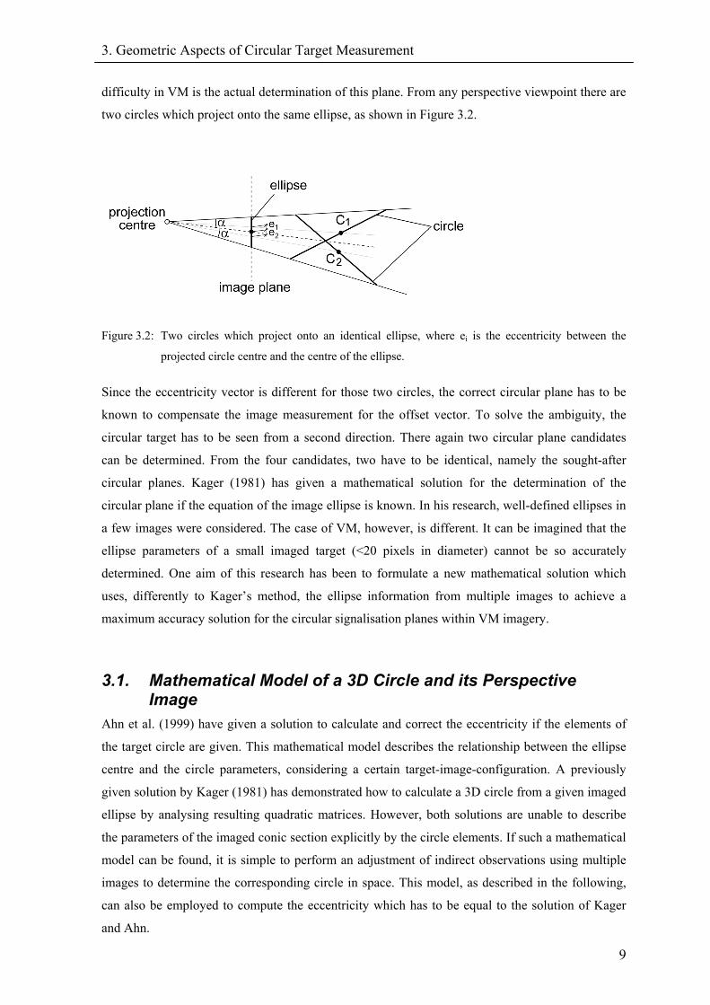
difficulty in VM is the actual determination of this plane. From any perspective viewpoint there are
two circles which project onto the same ellipse, as shown in Figure 3.2.
Figure 3.2: Two circles which project onto an identical ellipse, where ei is the eccentricity between the
projected circle centre and the centre of the ellipse.
Since the eccentricity vector is different for those two circles, the correct circular plane has to be
known to compensate the image measurement for the offset vector. To solve the ambiguity, the
circular target has to be seen from a second direction. There again two circular plane candidates
can be determined. From the four candidates, two have to be identical, namely the sought-after
circular planes. Kager (1981) has given a mathematical solution for the determination of the
circular plane if the equation of the image ellipse is known. In his research, well-defined ellipses in
a few images were considered. The case of VM, however, is different. It can be imagined that the
ellipse parameters of a small imaged target (<20 pixels in diameter) cannot be so accurately
determined. One aim of this research has been to formulate a new mathematical solution which
uses, differently to Kager’s method, the ellipse information from multiple images to achieve a
maximum accuracy solution for the circular signalisation planes within VM imagery.
3.1. Mathematical Model of a 3D Circle and its Perspective Image
Ahn et al. (1999) have given a solution to calculate and correct the eccentricity if the elements of
the target circle are given. This mathematical model describes the relationship between the ellipse
centre and the circle parameters, considering a certain target-image-configuration. A previously
given solution by Kager (1981) has demonstrated how to calculate a 3D circle from a given imaged
ellipse by analysing resulting quadratic matrices. However, both solutions are unable to describe
the parameters of the imaged conic section explicitly by the circle elements. If such a mathematical
model can be found, it is simple to perform an adjustment of indirect observations using multiple
images to determine the corresponding circle in space. This model, as described in the following,
can also be employed to compute the eccentricity which has to be equal to the solution of Kager
and Ahn.
3. Geometric Aspects of Circular Target Measurement
10
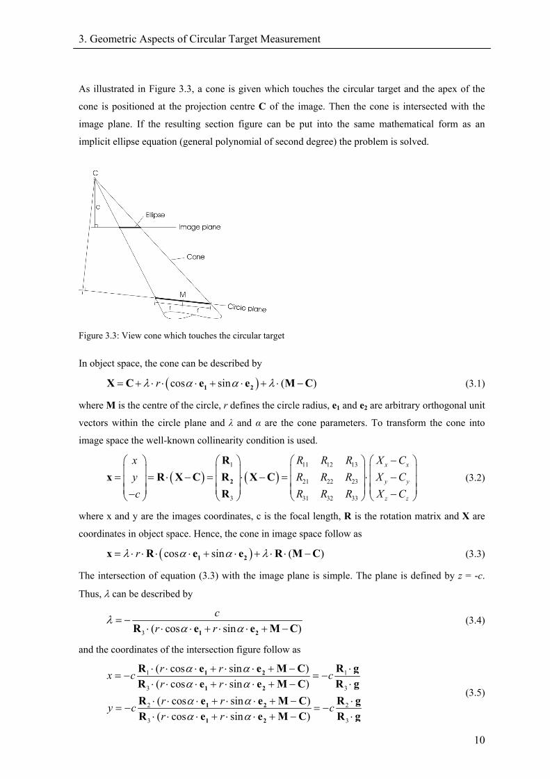
As illustrated in Figure 3.3, a cone is given which touches the circular target and the apex of the
cone is positioned at the projection centre C of the image. Then the cone is intersected with the
image plane. If the resulting section figure can be put into the same mathematical form as an
implicit ellipse equation (general polynomial of second degree) the problem is solved.
Figure 3.3: View cone which touches the circular target
In object space, the cone can be described by
( )cos sin ( )rλ α α λ= + ⋅ ⋅ ⋅ + ⋅ + ⋅ −1 2X C e e M C (3.1)
where M is the centre of the circle, r defines the circle radius, e1 and e2 are arbitrary orthogonal unit
vectors within the circle plane and λ and α are the cone parameters. To transform the cone into
image space the well-known collinearity condition is used.
( ) ( )1 11 12 13
21 22 23
3 31 32 33
x x
y y
z z
x R R R X Cy R Rc R R
−⎛ ⎞ ⎛ ⎞ ⎛ ⎞ ⎛ ⎞⎜ ⎟ ⎜ ⎟ ⎜ ⎟ ⎜ ⎟= = ⋅ − = ⋅ − = ⋅ −⎜ ⎟ ⎜ ⎟ ⎜ ⎟ ⎜ ⎟⎜ ⎟ ⎜ ⎟ ⎜ ⎟ ⎜ ⎟− −⎝ ⎠ ⎝ ⎠ ⎝ ⎠ ⎝ ⎠
2
Rx R X C R X C
RR X CR X C
C
(3.2)
where x and y are the images coordinates, c is the focal length, R is the rotation matrix and X are
coordinates in object space. Hence, the cone in image space follow as
(3.3) ( )cos sin ( )rλ α α λ= ⋅ ⋅ ⋅ ⋅ + ⋅ + ⋅ ⋅ −1 2x R e e R M
The intersection of equation (3.3) with the image plane is simple. The plane is defined by z = -c.
Thus, λ can be described by
3 ( cos sin )
cr r
λα α
= −⋅ ⋅ ⋅ + ⋅ ⋅ + −1 2R e e M C
(3.4)
and the coordinates of the intersection figure follow as
1 1
3
2 2
3 3
( cos sin )( cos sin )( cos sin )( cos sin )
r rx c cr rr ry c cr r
α αα αα αα α
⋅ ⋅ ⋅ + ⋅ ⋅ + − ⋅= − = −
⋅ ⋅ ⋅ + ⋅ ⋅ + − ⋅⋅ ⋅ ⋅ + ⋅ ⋅ + − ⋅
= − = −⋅ ⋅ ⋅ + ⋅ ⋅ + − ⋅
1 2
1 2
1 2
1 2
R e e M C R
3
gR e e M C R gR e e M C R gR e e M C R g
(3.5)
3. Geometric Aspects of Circular Target Measurement
11
If the equations (3.5) can be transformed so that the parameter α gets eliminated, the problem is
solved. First the equations are transformed as shown below:
(3.6) 3 1
3 2
x cy c
− ⋅ ⋅ = ⋅ ⋅⇒
− ⋅ ⋅ = ⋅ ⋅R g R gR g R g
( ) ( )( ) ( )
3 1 3 1 3 1
3 2 3 2 3 2
cos sin ( ) ( )cos sin ( ) ( )
r x c r x c x cr y c r y c y c
α αα α
− ⋅ ⋅ − ⋅ ⋅ + − ⋅ ⋅ − ⋅ ⋅ ⋅ + ⋅ ⋅ −=− ⋅ ⋅ − ⋅ ⋅ + − ⋅ ⋅ − ⋅ ⋅ ⋅ + ⋅ ⋅ −=
1 1 2 2
1 1 2 2
R e R e R e R e R R M CR e R e R e R e R R M C
(3.7)
equation (3.7) can also be described as
1 1 1 2
2 2 2 1 1
cos sincos sin
r x r y c x yr x r y c x y
α αα α
⎫⋅ + ⋅ ⋅ ⋅ −= ⎫⎪ 2+ +⎬⋅ + ⋅ ⋅ − ⋅= ⎪ ⎭⎭⎬ (3.8)
or, after the proposed transformations, the following two equations are generated:
( )( )
21 2 2 1 1 2 2 1
21 2 2 1 2 1 2 2
sin
cos
r y x y x c x c x
r y x y x c y c y
α
α
− = − ⎫+⎬
− = − ⎭ (3.9)
After squaring and adding equations (3.9) the final sought-after equation without an α term is
found:
(3.10) ( ) ( ) (2 221 2 2 1 1 2 2 1 2 1 2 2r y x y x c x c x c y c y− = − + − )2
This equation can be transformed into a general polynomial of the second degree in x and y as
(3.11) 2 21 2 3 4 5 1 0a x a xy a y a x a y⋅ + ⋅ + ⋅ + ⋅ + ⋅ − =
where the corresponding coefficients are
2 2 2 21 1 1
1
21 2 1 2 1 2
2
2 2 2 22 2 2
3
21 3 1 3 1 3
4
22 3 2 3 2 3
5
2
2
2
r i j kad
r i i j j k kad
r i j kad
j j k k r i ia cd
j j k k r i ia cd
⋅ − −=
⋅ ⋅ − ⋅ − ⋅=
⋅ − −=
⋅ + ⋅ − ⋅ ⋅= ⋅
⋅ + ⋅ − ⋅ ⋅= ⋅
(3.12)
using the following auxiliary variables
(3.13) (2 2 2 2 23 3 3d c j k r i= + − ⋅ )
( ) ( ) ( ) ( )( ) ( ) ( )( ) ( )( ) (
( ) ( ) ( )( ) ( )( ) ( )
1 2 3 1
1 2 3 1 1 1
1 2 2 2 23
T
T
T
i i i
j j j
k k k
= = ⋅ × ⋅ = ⋅ × = ⋅
= = ⋅ × ⋅ − = ⋅ × − = ⋅ ×
= = ⋅ × ⋅ − = ⋅ × − = ⋅
2 1 2i R e R e R e e R n
)×
j R e R C M R e C M R e v
k R e R C M R e C M R e v
(3.14)
It is permitted to use the distributive law in equations (3.14) since R is a rotation matrix.
3. Geometric Aspects of Circular Target Measurement
12
While infinite sets of the vectors e1 and e2 exist to describe the same circle in space, the polynomial
coefficients (3.12) have to be invariant regarding the selected vector set. Since the normal vector of
the circle plane (n in object space; i in image space) is invariant to e1 and e2 as well, it has to be
possible to find a description of equations (3.12) using only the vectors i and v (= C - M). It is
noticeable that the elements of the vectors j and k always appear combined and in quadratic form
within the coefficients. If these 6 quadratic sums can be expressed by i and v the problem is solved.
For the following derivation the unit vectors e1 and e2 in image space are defined by using rotation
matrices as
22
1 cos cos0 sin sin cos cos sin0 cos sin cos + sin sin
1 cos sin0 sin sin sin cos cos0 cos sin sin + sin cos
α β γ
α β πγ
β γα β γ α γα β γ α γ
β γα β γ α γα β γ α γ
+
⎛ ⎞ ⎛ ⎞⎜ ⎟ ⎜ ⎟= ⋅ = −⎜ ⎟ ⎜ ⎟⎜ ⎟ ⎜ ⎟⎝ ⎠ ⎝ ⎠
−⎛ ⎞ ⎛ ⎞⎜ ⎟ ⎜ ⎟= ⋅ = − −⎜ ⎟ ⎜ ⎟⎜ ⎟ ⎜ ⎟−⎝ ⎠ ⎝ ⎠
1e RX RY RZ
e RX RY RZ
(3.15)
where γ describes the degrees of freedom within the circle plane and RX, RY and RZ are rotation
matrices, as defined by
1 0 0 cos 0 sin0 cos sin 0 1 00 sin cos sin 0 cos
cos sin 0sin cos 00 0 1
α β
γ
β βα αα α β β
γ γγ γ
−⎛ ⎞ ⎛⎜ ⎟ ⎜= =⎜ ⎟ ⎜⎜ ⎟ ⎜−⎝ ⎠ ⎝⎛ ⎞⎜ ⎟= −⎜ ⎟⎜ ⎟⎝ ⎠
RX RY
RZ
⎞⎟⎟⎟⎠ (3.16)
Substituting vectors 1e and 2e in equations (3.14) it follows that
sinsin coscos cos
βα βα β
⎛ ⎞⎜= × = −⎜⎜ ⎟−⎝ ⎠
1 2i e e ⎟⎟ (3.17)
( )( ) ( )
( )( )
3 2
1 3
1 2
sin sin cos cos sin cos sin cos sin sin
cos sin cos sin sin cos cos
sin sin cos cos sin cos cos
v v
v v
v v
α β γ α γ α β γ α γ
α β γ α γ β γ
α β γ α γ β γ
= × ⋅ = × =
⎛ ⎞− + − −⎜ ⎟
= + −⎜ ⎟⎜ ⎟⎜ ⎟− + +⎝ ⎠
1 1j e R v e v
(3.18)
( )( ) ( )
( )( )
3 2
1 3
1 3
sin sin sin cos cos cos sin sin sin cos
cos sin sin sin cos cos sin
sin sin sin cos cos cos sin
v v
v v
v v
α β γ α γ α β γ α γ
α β γ α γ β γ
α β γ α γ β γ
= × ⋅ = × =
⎛ ⎞− − + −⎜ ⎟
= − + +⎜ ⎟⎜ ⎟⎜ ⎟+ −⎝ ⎠
2 2k e R v e v
(3.19)
3. Geometric Aspects of Circular Target Measurement
13
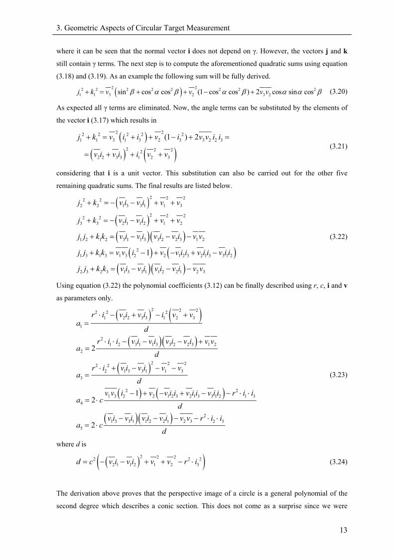
where it can be seen that the normal vector i does not depend on γ. However, the vectors j and k
still contain γ terms. The next step is to compute the aforementioned quadratic sums using equation
(3.18) and (3.19). As an example the following sum will be fully derived.
( )2 22 2 2 2 2 2 2 21 1 3 2 3 2sin cos cos (1 cos cos ) 2 cos sin cosj k v v v vβ α β α β α α+ = + + − + β (3.20)
As expected all γ terms are eliminated. Now, the angle terms can be substituted by the elements of
the vector i (3.17) which results in
( )
( ) ( )2 22 2 2 2 2
1 1 3 1 3 2 3 3 2 2 3
2 2 222 2 3 3 1 2 3
(1 ) 2j k v i i v i v v i i
v i v i i v v
+ = + + − +
= + + +
= (3.21)
considering that i is a unit vector. This substitution can also be carried out for the other five
remaining quadratic sums. The final results are listed below.
( )( )( ) ( )
( ) ( )( ) ( )
2 2 22 22 2 1 3 3 1 1 3
2 2 22 23 3 2 1 1 2 1 2
1 2 1 2 3 1 1 3 3 2 2 3 1 2
21 3 1 3 1 3 2 2 1 2 3 2 1 3 3 1 2
2 3 2 3 1 3 3 1 1 2 2 1 2 3
1
j k v i v i v v
j k v i v i v v
j j k k v i v i v i v i v v
j j k k v v i v v i i v i i v i i
j j k k v i v i v i v i v v
+ = − − + +
+ = − − + +
+ = − − −
+ = − + − + −
+ = − − −
(3.22)
Using equation (3.22) the polynomial coefficients (3.12) can be finally described using r, c, i and v
as parameters only.
( ) ( )
( )( )
( )
( ) ( )
( )( )
2 2 22 2 21 2 2 3 3 1 2 3
1
21 2 3 1 1 3 3 2 2 3 1 2
2
2 2 22 22 1 3 3 1 1 3
3
2 21 3 2 2 1 2 3 2 1 3 3 1 2 1 3
4
21 3 3 1 1 2 2 1 2 3 2 3
5
2
12
2
r i v i v i i v va
dr i i v i v i v i v i v v
ad
r i v i v i v va
dv v i v v i i v i i v i i r i i
a cd
v i v i v i v i v v r i ia c
d
⋅ − + − +=
⋅ ⋅ − − − +=
⋅ + − − −=
− + − + − − ⋅ ⋅= ⋅
− − − − ⋅ ⋅= ⋅
(3.23)
where d is
( )( 2 2 222 1 1 2 1 2 3d c v i v i v v r i= − − + + − ⋅ )2 2 (3.24)
The derivation above proves that the perspective image of a circle is a general polynomial of the
second degree which describes a conic section. This does not come as a surprise since we were
3. Geometric Aspects of Circular Target Measurement
14
intersecting a cone with a plane. For completnees it should be mentioned that this is also valid for
oblique cones as no limitations were set on the view cone at the beginning.
The conversion of the implicit ellipse equation (3.11) to its parametric from is described in
Appendix A1. This allows computation of the centre coordinates of the ellipse. By projecting the
circle centre M into the image the eccentricity vector can be calculated. Using discreet values the
derived model was compared with the formula given by Ahn et al. (1999) and Kager (1981). All
three methods turned out to yield identical results.
3.2. Special Geometric Aspects of Retro-Reflective Targets So far, the geometric aspects of circular target measurement have been discussed in general terms.
The eccentricity appears at any circular target independent of its material and pointing method
(total stations, laser tracker, etc.). For retro-reflective targets, however, additional offsets appear
and these must be taken into account. To gain an understanding of these offsets the structure of a
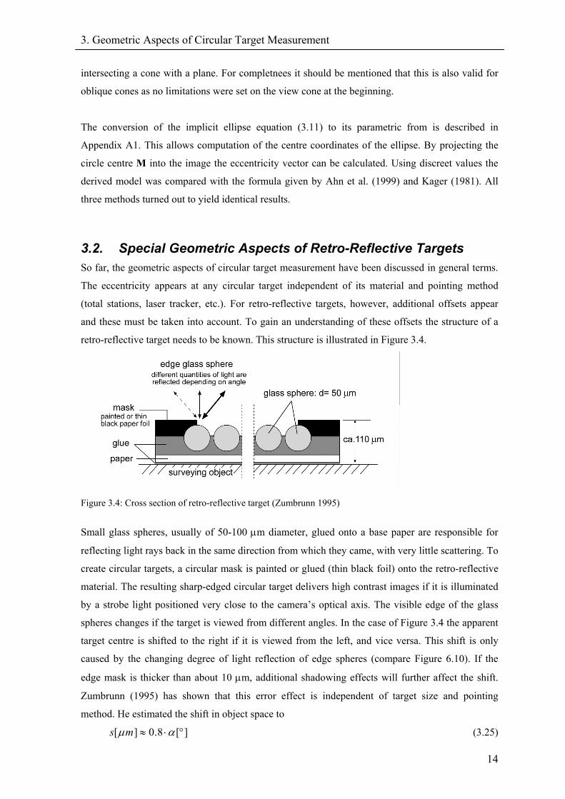
retro-reflective target needs to be known. This structure is illustrated in Figure 3.4.
Figure 3.4: Cross section of retro-reflective target (Zumbrunn 1995)
Small glass spheres, usually of 50-100 µm diameter, glued onto a base paper are responsible for
reflecting light rays back in the same direction from which they came, with very little scattering. To
create circular targets, a circular mask is painted or glued (thin black foil) onto the retro-reflective
material. The resulting sharp-edged circular target delivers high contrast images if it is illuminated
by a strobe light positioned very close to the camera’s optical axis. The visible edge of the glass
spheres changes if the target is viewed from different angles. In the case of Figure 3.4 the apparent
target centre is shifted to the right if it is viewed from the left, and vice versa. This shift is only
caused by the changing degree of light reflection of edge spheres (compare Figure 6.10). If the
edge mask is thicker than about 10 µm, additional shadowing effects will further affect the shift.
Zumbrunn (1995) has shown that this error effect is independent of target size and pointing
method. He estimated the shift in object space to
[ ] 0.8 [s m ]µ α≈ ⋅ ° (3.25)
3. Geometric Aspects of Circular Target Measurement
15
where α is the angle between the target plane normal and the direction from the target to the
projection centre. The direction of the shift is described as transverse to the line of sight and points
towards the more distant target edge. Since Zumbrunn was employing a video-theodolite for his
investigations, his derived direction of the shift is not valid for Photogrammetry, as shown below.
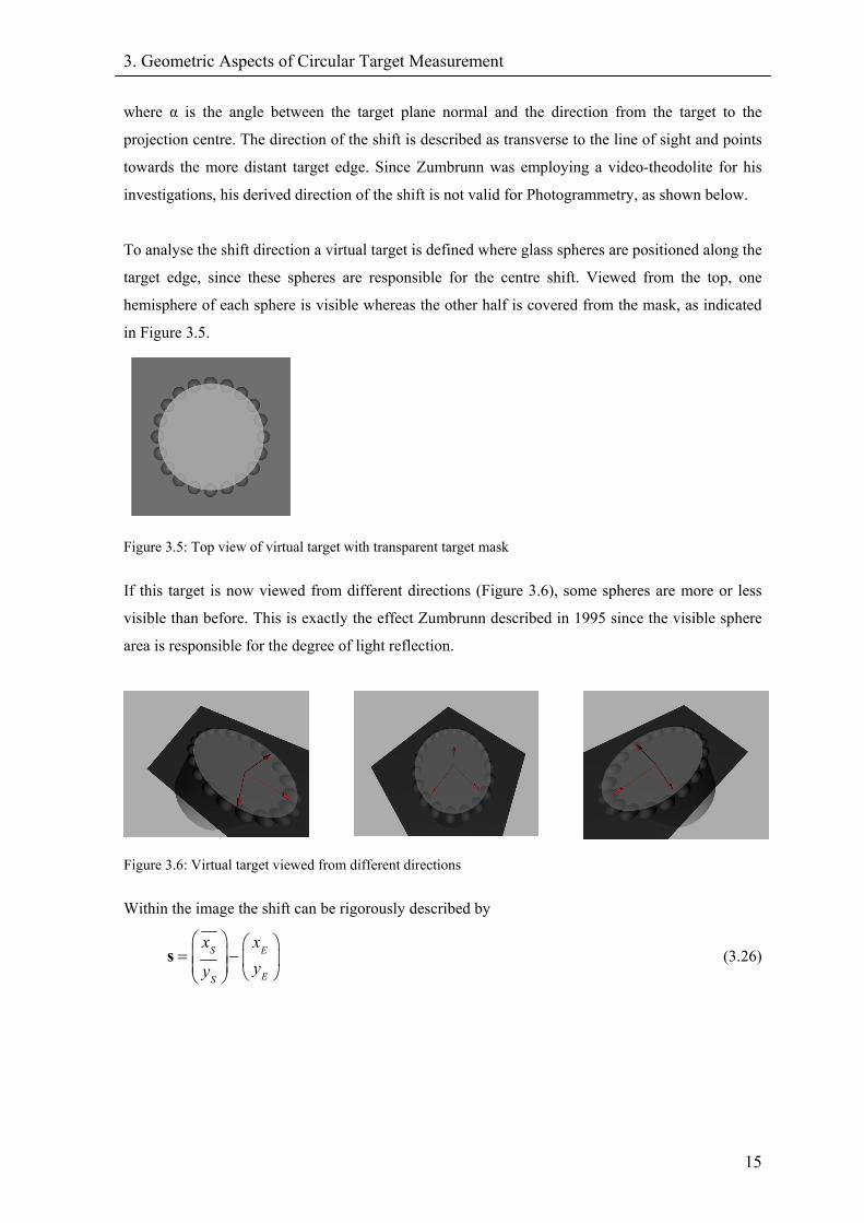
To analyse the shift direction a virtual target is defined where glass spheres are positioned along the
target edge, since these spheres are responsible for the centre shift. Viewed from the top, one
hemisphere of each sphere is visible whereas the other half is covered from the mask, as indicated
in Figure 3.5.
Figure 3.5: Top view of virtual target with transparent target mask
If this target is now viewed from different directions (Figure 3.6), some spheres are more or less
visible than before. This is exactly the effect Zumbrunn described in 1995 since the visible sphere
area is responsible for the degree of light reflection.
Figure 3.6: Virtual target viewed from different directions
Within the image the shift can be rigorously described by
S
ES
x Exyy
⎛ ⎞ ⎛ ⎞= −⎜ ⎟ ⎜⎜ ⎟ ⎝ ⎠⎝ ⎠
s ⎟ (3.26)
3. Geometric Aspects of Circular Target Measurement
16
vS
sv
S
vS
sv
S
x Ax
A
y Ay
A
⋅=
⋅=
∑∑
∑∑
(3.27)
where xE and yE are the centre coordinates of the ellipse, Av is the visible area of a glass sphere and
x and y are the corresponding area centre coordinates. However, this equation cannot be
employed in practise because the real ellipse centre is not known and the glass spheres are glued in
irregular dense patterns on to the carrier material. Hence, an approximation of the shift direction is
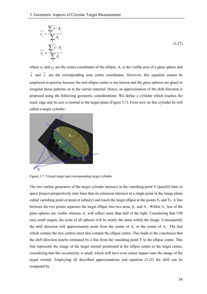
proposed using the following geometric considerations. We define a cylinder which touches the
mask edge and its axis is normal to the target plane (Figure 3.7). From now on this cylinder be will
called a target cylinder.
A+
A_
T1
V
T2
Figure 3.7: Virtual target and corresponding target cylinder
The two outline generatrix of the target cylinder intersect in the vanishing point V (parallel lines in
space project perspectively onto lines that on extension intersect at a single point in the image plane
called vanishing point or point at infinity) and touch the target ellipse at the points T1 and T2. A line
between the two points separates the target ellipse into two areas A+ and A_. Within A_ less of the
glass spheres are visible whereas A+ will reflect more than half of the light. Considering that VM
uses small targets, the scale of all spheres will be nearly the same within the image. Consequently
the shift direction will approximately point from the centre of A_ to the centre of A+. The line
which contain the two centres must also contain the ellipse centre. This leads to the conclusion that
the shift direction maybe estimated by a line from the vanishing point V to the ellipse centre. This
line represents the image of the target normal positioned at the ellipse centre or the target centre,
considering that this eccentricity is small, which will have even minor impact onto the image of the
target normal. Employing all described approximations and equation (3.25) the shift can be
computed by

3. Geometric Aspects of Circular Target Measurement
17
( )
( ) ( )
1
1 1
2
2 2
2 1
0.8 0.8 arccos
xyc
xyc
α
⎛ ⎞⎜ ⎟= = ⋅ −⎜ ⎟⎜ ⎟−⎝ ⎠⎛ ⎞ ⎛ ⎞⎛ ⎞− ⋅⎜ ⎟= = ⋅ + ⋅ ⋅ − = ⋅ + ⋅ ⋅ −⎜ ⎟⎜ ⎟⎜ ⎟ ⎜ ⎟−⎝ ⎠⎜ ⎟ ⎝ ⎠−⎝ ⎠
≈ −
x R X C
C X nx R X n C R X n
C X
s x x
C (3.28)
where X are the object space coordinates of the target centre and n is the target normal as unit
vector.
Whereas the eccentricity adds an offset towards the less distant target edge, the edge shift of retro-
reflective targets points towards the more distant target edge, though the two offset vectors are only
roughly parallel. Theoretically, there is an ideal target size where the two error offsets mostly
cancel out since the eccentricity depends on the target size and the edge shift is diameter
independent. Unfortunately, the target size for photogrammetric applications is defined by the size
of the object being surveyed. However, both error effects can be corrected if the target plane is
known.
4. Target Plane Determination within Digital Images
18
4. Target Plane Determination within Digital Images In this chapter the actual target plane determination process will be described. The general concept
can be divided into two stages. First, the ellipse parameters of all imaged targets are determined.
Then the ellipse information from multiple images of one circular target is used to compute its
target plane. For the second stage the geometry of the photogrammetric network has to be known
which means that a bundle adjustment is required within the target plane determination process.
Since the target plane determination is dealing with stochastic variables, least-squares adjustment is
an appropriate method to determine the estimates. Though least-squares strategies are well-known
for redundant engineering problems, basic knowledge about least-squares, which is necessary to
understand derivations within the current chapter, will be discussed in the following.
4.1. Least-Squares Adjustment In a statistical sense, adjustment is a method of deriving estimates for stochastic variables and their
distribution parameters from observed samples. Of the different adjustment methods least squares
is by far the most common. Its principles are based on derivations for an astronomical problem by
C.F. Gauss. Its practical importance has recently been enhanced by the introduction of electronic
computers, by the formulation of techniques in matrix notation, and by connecting its concept to
statistics (Mikhail et al. 1996).
In the following, the special case of adjustment of indirect observations is described. First a model
has to be found which connects stochastic variables. These can be differentiated into observations
and parameters. The group of observations is given with a priori precision values, whereas the
parameters should be determined in the adjustment process. In this special adjustment case, a
mathematical description of each observation using only parameters is given. Since an adjustment
system has to be redundant, there have to be more observations than parameters. To find a unique
solution, however, only a subset of nobs observations is needed to determine the npar parameters.
Consequently, multiple solutions can be computed. To overcome this problem least-squares
methods add corrections, so called residuals, to each observation. This allows the observation
equations to be written as
(4.1) ( )F+ =l v x
where l is the vector of observations, v the residual vector and x the sought-after vector of
parameters. The equation system is solved using the constraint below (This is where the name
least-squares comes from).
(4.2) minimumTΦ = →v Wv
The weight matrix W allows observations of different precision, as well as of different type to be
treated correctly in a statistical sense. In simple adjustment problems the W matrix is often
replaced by the identity matrix.
4. Target Plane Determination within Digital Images
19
Whereas it is a straightforward matter to solve linear problems, non-linear systems have to be
linearised and solved in iterations. Using matrix notation, linear and linearised problems can be
described as
( )( ) FF ∂
+ = + ⋅ = + ⋅∂0 0
xl v x ∆ l B ∆x
(4.3)
where ∆ represents x in linear systems and corrections to x in non-linear adjustments and B is the
Jacobian matrix of the observation equations with respect to x. In the non-linear case
approximations of the parameters have to be known and the final estimates of the parameters are
found iteratively by employing
(4.4) + = +i 1 ix x ∆
after each iteration. Using equations (4.2) and (4.3), ∆ can be computed by
(4.5) ( ) 11 T
x
Tx
−−= =
= ⋅
Q N B WB
∆ Q B Wl
In the presented adjustment model it is assumed that a minimum set of parameters are chosen
which are all independent. However, in certain circumstances the mathematical description of the
functional model is easier and more flexible if it is over-parameterised. In these cases the
introduced degrees of freedom can be eliminated by added constraints to the adjustment model.
The linearised constraints can be described by
(4.6) ⋅ =C ∆ g
Consequently the main quadratic minimum condition (4.2) has to be extended
(4.7) ( )2 minimumT TΦ = − ⋅ ⋅ − →v Wv k C ∆ g
where k is a vector of Lagrange multipliers. Considering the new minimum condition the equation
system can be solved by
1
0
T T Tx cx
cx c
T
−⎛ ⎞ ⎛ ⎞
= =⎜ ⎟ ⎜ ⎟⎜ ⎟ ⎝⎝ ⎠⎛ ⎞⎛ ⎞
= ⋅ ⎜ ⎟⎜ ⎟⎝ ⎠ ⎝ ⎠
Q Q B WB CQ
Q Q C
∆ B WlQ
k g
⎠ (4.8)
Beside the determination of the parameters, least-squares provide accuracy estimations of the
computed parameters and adjusted observations. The first quantity is σ0², the variance of unit
weight or also called the reference variance.
20
T
Observations Parameters Constraints
rr n n n
σ =
= − +
v Wv (4.9)
4. Target Plane Determination within Digital Images
20
Above r is called the redundancy which depends on the number of observations, parameters and
constraints. Using σ0, the variance-covariance matrix of the estimated parameters can be described
as
(4.10) 20x σ=Σ Qx
TF
TB
Often, not only the estimated standard error of the parameter is interesting, but also the standard
error of variables, which can be described as a function of the parameters. Assuming variable(s) f
(4.11) ( )f F= x
its linearisation can be described as
(4.12) ∂ = ⋅f F ∆Using error propagation the variance-covariance matrix of the variables f is defined by
(4.13) 20
Tf x xσ= =Σ FΣ F FQ
The observations can be described as formula (4.11) , hence its variance-covariance matrix follows
as
(4.14) 20
Tl x xσ= =Σ BΣ B BQ
Now, all necessary formulas are represented. The exact derivation of equations (4.1) to (4.14) can
be found in the literature (e.g. Mikhail et al. 1996).
4.2. Ellipse-Fitting of Imaged Targets As derived in Chapter 3.1, a plane circular target projects as a conic section into the image.
However, in the case of VM it is justified to only consider ellipses as images (see Chapter 3).
Because of lens distortion and other deformations (e.g. unflatness of the CCD chip) a target
projects as an ellipse only by approximation, if the problem is analysed rigorously. This distortional
effects may be neglected in the case of small target images since the central projection condition is
very well fulfilled in small image patches.
The main issue in the ellipse-fitting process is to derive continuous ellipse parameters from a
discreet image. In the following, two developed methods will be described which vary in
computation speed and in the accuracy of the obtained ellipse parameters.
4.2.1. Best-Fit Ellipse of Intensity Levelled Points Luhmann (2000) describes a solution where, from a rough ellipse centre, profile lines in various
directions are computed. Then points on all profile lines at a certain intensity level are determined
which are finally used to perform a best-fit ellipse adjustment. Using the new centre the process is
repeated until convergence of the centre coordinates. In my research a slightly different approach
4. Target Plane Determination within Digital Images
21
has been adopted, which can be solved without iterations and without computing profile lines of
any orientation.
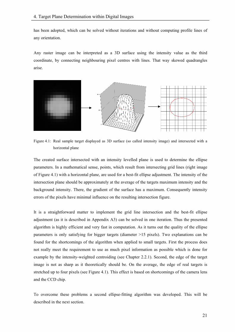
Any raster image can be interpreted as a 3D surface using the intensity value as the third
coordinate, by connecting neighbouring pixel centres with lines. That way skewed quadrangles
arise.
Figure 4.1: Real sample target displayed as 3D surface (so called intensity image) and intersected with a
horizontal plane
The created surface intersected with an intensity levelled plane is used to determine the ellipse
parameters. In a mathematical sense, points, which result from intersecting grid lines (right image
of Figure 4.1) with a horizontal plane, are used for a best-fit ellipse adjustment. The intensity of the
intersection plane should be approximately at the average of the targets maximum intensity and the
background intensity. There, the gradient of the surface has a maximum. Consequently intensity
errors of the pixels have minimal influence on the resulting intersection figure.
It is a straightforward matter to implement the grid line intersection and the best-fit ellipse
adjustment (as it is described in Appendix A3) can be solved in one iteration. Thus the presented
algorithm is highly efficient and very fast in computation. As it turns out the quality of the ellipse
parameters is only satisfying for bigger targets (diameter >15 pixels). Two explanations can be
found for the shortcomings of the algorithm when applied to small targets. First the process does
not really meet the requirement to use as much pixel information as possible which is done for
example by the intensity-weighted centroiding (see Chapter 2.2.1). Second, the edge of the target
image is not as sharp as it theoretically should be. On the average, the edge of real targets is
stretched up to four pixels (see Figure 4.1). This effect is based on shortcomings of the camera lens
and the CCD chip.
To overcome these problems a second ellipse-fitting algorithm was developed. This will be
described in the next section.
4. Target Plane Determination within Digital Images
22
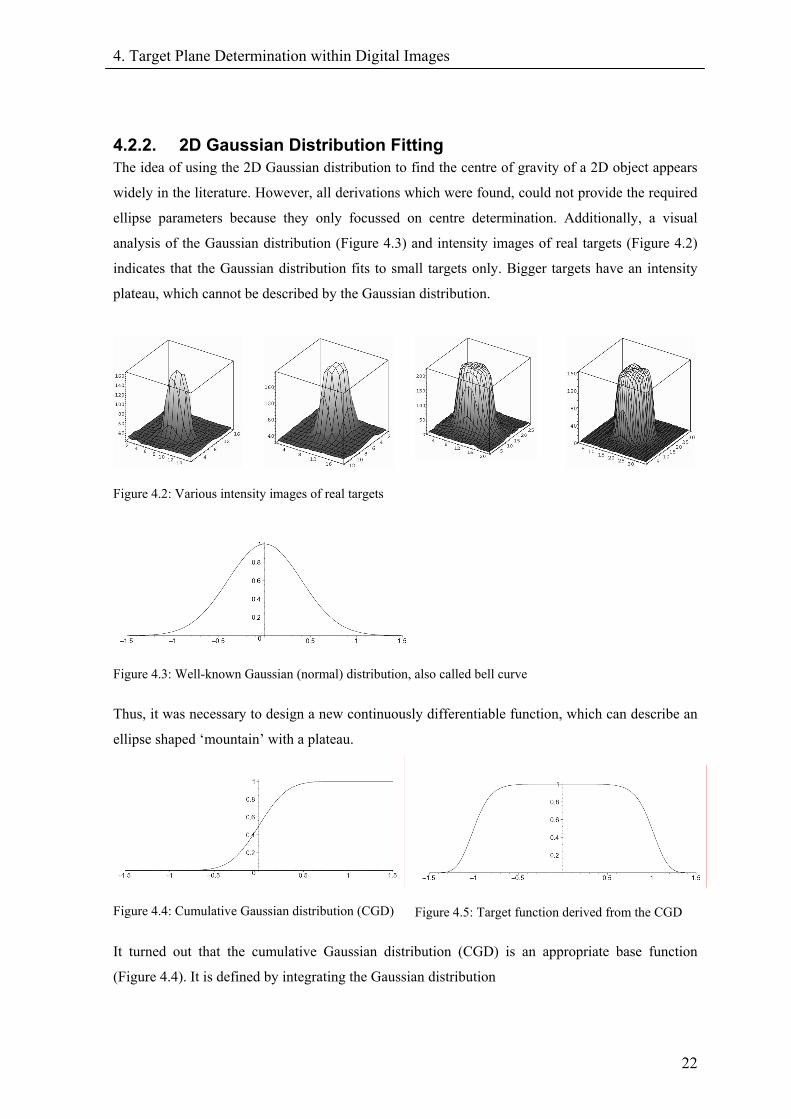
4.2.2. 2D Gaussian Distribution Fitting The idea of using the 2D Gaussian distribution to find the centre of gravity of a 2D object appears
widely in the literature. However, all derivations which were found, could not provide the required
ellipse parameters because they only focussed on centre determination. Additionally, a visual
analysis of the Gaussian distribution (Figure 4.3) and intensity images of real targets (Figure 4.2)
indicates that the Gaussian distribution fits to small targets only. Bigger targets have an intensity
plateau, which cannot be described by the Gaussian distribution.
Figure 4.2: Various intensity images of real targets
Figure 4.3: Well-known Gaussian (normal) distribution, also called bell curve
Thus, it was necessary to design a new continuously differentiable function, which can describe an
ellipse shaped ‘mountain’ with a plateau.
Figure 4.4: Cumulative Gaussian distribution (CGD)
Figure 4.5: Target function derived from the CGD
It turned out that the cumulative Gaussian distribution (CGD) is an appropriate base function
(Figure 4.4). It is defined by integrating the Gaussian distribution
4. Target Plane Determination within Digital Images
23
2
2( )
222
( )
2
1 1( ) G( ) erf2 2
xx x xx c x dx e dxµ
σ
πσ
µ
σ
−−
−∞ −∞
−⎛ ⎞Ω = = = +⎜ ⎟⎝ ⎠∫ ∫
1 (4.15)
where σ is the standard deviation and µ the expectation. Substituting x by )1(2
−− x in equation
(4.15) leads to a 1D function which has the sought-after properties (Figure 4.5). The next step is to
substitute x by an implicit ellipse equation, which finally results in the desired equation:
cos sinsin cos
x
y
x cxy cy
φ φφ φ
−⎛ ⎞ ⎛ ⎞⎛ ⎞=⎜ ⎟ ⎜⎜ ⎟⎜ ⎟ −−⎝ ⎠⎝ ⎠⎝ ⎠
⎟ (4.16)
2 2
2 2 1x ya b
Ε = + − (4.17)
( )( , , , , , , , , 0)x ys c c a b sβ φ σ µ βΤ = = ⋅Ω −Ε + (4.18)
Whereas equation (4.16) describes a transformation, its usage in the implicit ellipse equation (4.17)
allows interpretation of cx and cy as the centre of the ellipse and φ as the bearing of the semi major
axis. Formula (4.18) describes, for the adjustment used, the best-fit equation where s defines a scale
factor (Ω can only provide values between 0 and 1) and β the background noise. By modelling the
background, a thresholding process, as needed for the intensity-weighted centroiding, can be cut
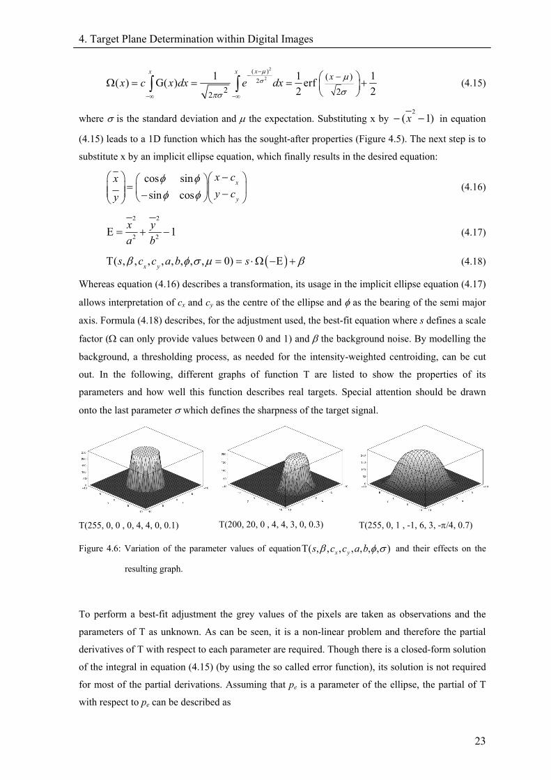
out. In the following, different graphs of function T are listed to show the properties of its
parameters and how well this function describes real targets. Special attention should be drawn
onto the last parameter σ which defines the sharpness of the target signal.
T(255, 0, 0 , 0, 4, 4, 0, 0.1)
T(200, 20, 0 , 4, 4, 3, 0, 0.3)
T(255, 0, 1 , -1, 6, 3, -π/4, 0.7)
Figure 4.6: Variation of the parameter values of equation ),,,,,,,( σφβ baccs yxΤ and their effects on the
resulting graph.
To perform a best-fit adjustment the grey values of the pixels are taken as observations and the
parameters of T as unknown. As can be seen, it is a non-linear problem and therefore the partial
derivatives of T with respect to each parameter are required. Though there is a closed-form solution
of the integral in equation (4.15) (by using the so called error function), its solution is not required
for most of the partial derivations. Assuming that pe is a parameter of the ellipse, the partial of T
with respect to pe can be described as

4. Target Plane Determination within Digital Images
24
( )G( ) ( G( ) ) ( G( ) )
G( ) G( )
e e e
e e
s c x dx x dx x dx
e
xs c s cp p p x
x Es c x s c Ep p
β∂ ⋅ + ∂ ∂∂Τ ∂= = ⋅ = ⋅
∂ ∂ ∂ ∂
∂ ∂= ⋅ ⋅ = − ⋅ ⋅ −
∂ ∂
∫ ∫ ∫p
=∂ (4.19)
Because the partial of the implicit ellipse equation with respect to pe is straightforward, only the
final derivation is presented here:
2 2
2 2
T cos sin
T sin cosx
y
x yhc a b
x yhc a b
φ φ
φ φ
⎛ ⎞∂= −⎜ ⎟∂ ⎝ ⎠
⎛ ⎞∂= +⎜ ⎟∂ ⎝ ⎠
(4.20)
2
3
2
3
T
T
xha a
yhb b
⎛ ⎞∂= ⎜ ⎟⎜ ⎟∂ ⎝ ⎠
⎛ ⎞∂= ⎜ ⎟⎜ ⎟∂ ⎝ ⎠
(4.21)
2 2T 1h x y
b aφ∂ ⎛= ⋅ −⎜∂ ⎝ ⎠
1 ⎞⎟
)
(4.22)
where h can be described as
2 G(h s c σ= ⋅ ⋅ ⋅ −Ε (4.23)
The partial derivatives with respect to σ, s and β are
T G( E)
T ( E)
T 1
E s
s
σ
β
∂= − ⋅ ⋅ −
∂∂
= Ω −∂∂
=∂
(4.24)
Thus, all necessary derivations to perform a best-fit adjustment are made. As will be shown in
Chapter 7.2, this method of determining the ellipse parameters delivers satisfying results even for
small targets. In the case of very small targets (diameter <5 pixels), however, there is a high
correlation between σ and a. This is why the adjustment mostly diverges. This shortcoming can be
passed over by ‘observing’ σ in the adjustment.
4. Target Plane Determination within Digital Images
25
4.3. Target Plane Adjustment In this section the actual target plane determination stage is described using the ellipse information
gained from ellipse-fitting adjustments. As mentioned, the problem can be solved if the geometry
of the network configuration is known.
Whereas the plane determination method described by Kager (1981) uses information of only one
ellipse, the new method needed to use the ellipse information of all photos where the target was
imaged. This is necessary since the target images are small in diameter, which results in low
accuracy of the extracted ellipse parameters. For the thesis, two rigorous methods were developed,
which met the stated requirements. The method, which will be reported next, was developed first.
Compared to the second method, the required formulas are relatively simple. However, it has also
two disadvantages regarding matrix sizes and error propagation as described below.
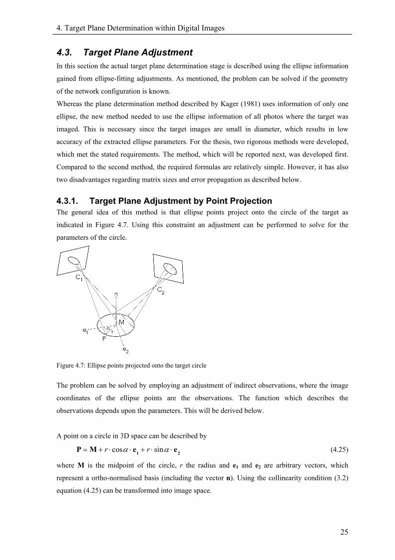
4.3.1. Target Plane Adjustment by Point Projection The general idea of this method is that ellipse points project onto the circle of the target as
indicated in Figure 4.7. Using this constraint an adjustment can be performed to solve for the
parameters of the circle.
Figure 4.7: Ellipse points projected onto the target circle
The problem can be solved by employing an adjustment of indirect observations, where the image
coordinates of the ellipse points are the observations. The function which describes the
observations depends upon the parameters. This will be derived below.
A point on a circle in 3D space can be described by
cos sinr rα α= + ⋅ ⋅ + ⋅ ⋅1P M e e2 (4.25)
where M is the midpoint of the circle, r the radius and e1 and e2 are arbitrary vectors, which
represent a ortho-normalised basis (including the vector n). Using the collinearity condition (3.2)
equation (4.25) can be transformed into image space.
4. Target Plane Determination within Digital Images
26
( )( )
( )( )
( )( )
( )( )
11 1
3 33
22 1
3 33
cos sincos sin
cos sincos sin
r rx c c c
r r
r ry c c c
r r
α αα α
α αα α
− + ⋅ ⋅ + ⋅ ⋅−= − = − = −
− − + ⋅ ⋅ + ⋅ ⋅
− + ⋅ ⋅ + ⋅ ⋅−= − = − = −
− − + ⋅ ⋅ + ⋅ ⋅
1 2
1 2
1 2
1 2
R M C e eR P C R vR P C R vR M C e e
R M C e eR P C R vR P C R vR M C e e
(4.26)
Because the system is non-linear, the partial derivatives with respect to the circle parameters (M, r,
e1 and e2) and angle parameter α have to be calculated. It should be mentioned that each point has
its own angle parameter.
( )( )
2
2 2
cos sin
cos sin
α α
α α
= ⋅
= ⋅ ⋅ + ⋅
= ⋅ ⋅ − ⋅1 1
1
v R v
e R e e
e R e e
(4.27)
( )
( )
( )
2 31 1 11 3
3
2 32 1 12 3
3
2 33 1 13 3
3
x
y
z
x c R v R vC vx c R v R v
C vx c R v R v
C v
∂= ⋅ − ⋅
∂
∂= ⋅ − ⋅
∂
∂= ⋅ − ⋅
∂
( )
( )
( )
2 31 1 11 31 3
2 32 1 12 31 3
2 33 1 13 31 3
cos
cos
cos
x
y
z
x c r R v R ve vx c r R v R v
e vx c r R v R v
e v
α
α
α
∂ ⋅ ⋅= ⋅ −
∂
∂ ⋅ ⋅= ⋅ −
∂
∂ ⋅ ⋅= ⋅ −
∂
⋅
⋅
⋅
( )
( )
( )
2 31 1 11 32 3
2 32 1 12 32 3
2 33 1 13 32 3
sin
sin
sin
x
y
z
x c r R v R ve vx c r R v R v
e vx c r R v R v
e v
α
α
α
∂ ⋅ ⋅= ⋅ −
∂
∂ ⋅ ⋅= ⋅ −
∂
∂ ⋅ ⋅= ⋅ −
∂
⋅
⋅
⋅
( )2 1 1 1 3
3
z x
x c e v e vr v
∂= ⋅ − ⋅
∂ (4.28)
( )2 2 1 2 3
3
z x
x c r e v e vvα
∂ ⋅= ⋅ − ⋅
∂
( )
( )
( )
2 31 2 21 3
3
2 32 2 22 3
3
2 33 2 23 3
3
x
y
z
y c R v R vC vy c R v R v
C vy c R v R v
C v
∂= ⋅ − ⋅
∂
∂= ⋅ − ⋅
∂
∂= ⋅ − ⋅
∂
( )
( )
( )
2 31 2 21 31 3
2 32 2 22 31 3
2 33 2 23 31 3
cos
cos
cos
x
y
z
y c r R v R ve vy c r R v R v
e vy c r R v R v
e v
α
α
α
∂ ⋅ ⋅= ⋅ − ⋅
∂
∂ ⋅ ⋅= ⋅ − ⋅
∂
∂ ⋅ ⋅= ⋅ − ⋅
∂
( )
( )
( )
2 31 2 21 32 3
2 32 2 22 32 3
2 33 2 23 32 3
sin
sin
sin
x
y
z
y c r R v R ve vy c r R v R v
e vy c r R v R v
e v
α
α
α
∂ ⋅ ⋅= ⋅ − ⋅
∂
∂ ⋅ ⋅= ⋅ − ⋅
∂
∂ ⋅ ⋅= ⋅ − ⋅
∂
(2 2 2 2 3
3
z x
y c e v e vr v
)∂= ⋅ − ⋅
∂ (4.29)
( )2 1 2 1 3
3
z x
y c r e v e vvα
∂ ⋅= ⋅ − ⋅
∂
Using six parameters within the vectors e1 and e2 to described the circle plane, the system is over-
parameterised since two angles are sufficient to described any target plane orientation. To eliminate
4. Target Plane Determination within Digital Images
27
the four degrees of freedom within the parameterisation, constraints have to be introduced into the
adjustment. The following three constrains secure the ortho-normalised basis
1
2
3
1 0
1 0
0
c
c
c
= − =
= − =
= ⋅ =
1
2
1 2
e
e
e e
⇒1 1 1 1 1 1 1
2 2 2 2 2 2 2
3 2 1 2 1 2 1 1 2 1 2 1 2
1 021 02
0
x x y y z z
x x y y z z
x x y y z z x x y y z z
c e e e e e e
c e e e e e e
c e e e e e e e e e e e e
∂ = ⋅∂ + ⋅∂ + ⋅∂ =
∂ = ⋅∂ + ⋅∂ + ⋅∂ =
∂ = ⋅∂ + ⋅∂ + ⋅∂ + ⋅∂ + ⋅∂ + ⋅∂ =
(4.30)
The final constraint has to prevent e1 and e2 from rotation within the target plane, which can be
defined in multiple ways. E.g. e1 has to be normal to the y axis. However, the implemented
adjustment uses the following differential constraint:
(4.31) 4 2 1 2 1 2 1 0x x y y z zc e e e e e e∂ = ⋅ ∂ + ⋅ ∂ + ⋅∂ =
As mentioned, each point has its own angle parameter (4.25). Hence the size of the equation system
depends on the number of ‘observed’ points. It turns out that five points per ellipse (=10
observations) are needed to achieve appropriate results. If there are less than four ellipses available,
10 points per ellipse (=20 observations) should be used. This is an unsatisfactory fact since an
ellipse can only provide five independent observations. Additionally, it is not possible to directly
introduce the covariance information from previous ellipse-fitting adjustments. To overcome these
two shortcomings a second, mathematically more complex target plane adjustment was developed,
as described in the next section.
4.3.2. Target Plane Adjustment by Observing Implicit Ellipse Parameters
This adjustment model is based on the derivations made in Chapter 3.1. There a description of the
implicit ellipse parameters depending on the target elements (see equation 3.23) was found which
can be used for an adjustment of indirect observations. Since the formula uses the normal vector n
rather than the ortho-normalised basis e1 and e2, the adjustment has to solve for 7 unknowns only
(target centre M, radius r and vector n).
Again, it is a non-linear system and partial derivations are required. Since the final formulas are
lengthy, the derivation is presented in stages and auxiliary variables are introduced. The five
observation equations can be written in the following form
jj
ba
d= (4.32)
Using the quotient rule, the partials regarding the target centre, the target normal and the radius
follow as
2
jj
j k
k
b dd bakM M
M d
∂ ∂−∂ ∂ ∂
=∂
(4.33)

4. Target Plane Determination within Digital Images
28
2
jj
j k
k
b dd ba n nn d
∂ ∂−∂ ∂ ∂
=∂
k (4.34)
2
jjj
b dd ba rr d
∂ ∂−∂ ∂=
∂r∂ (4.35)
The required partial derivations of the coefficients bj and d are straightforward and listed below.
First the partial derivatives regarding the circle centre coordinates Mk are determined:
( )( ) ( )( )212 2 3 3 2 2 3 3 1 2 2 3 32 k k k k
k
bv i v i R i R i i R v R v
M∂
= − + + + +∂
( ) ( ) ( ) ( )( )223 2 1 1 2 3 3 2 1 1 2 3 1 2 3 2 1 3 3 1 22 1 2k k k k k k
k
bi R v R v R i i v i v v R i i R i i R i i
M∂
= − + + + + + −∂
( ) ( )( )31 3 3 1 1 3 1 1 1 1 3 32 k k k k
k
bv i v i R i R i R v R v
M∂
= − − − −∂
(4.36)
( ) ( ) ( )( ) ( )( )241 1 3 3 1 2 2 3 1 1 3 1 3 2 2 2 3 1 12 1 2k k k k k
k
bc i R v R v R i v i v i i i v v i R i R i
M∂
= − + − + − − +∂ 3
( ) ( ) ( ) ( )( )251 3 2 2 3 1 1 3 2 2 3 1 1 2 3 3 1 2 2 12 1 2k k k k k k
k
bc i R v R v R i i v i v v R i i R i i R i i
M∂
= − + − + + − −∂ 3
( )( )( )22 1 1 2 1 2 2 1 1 1 2 22 k k k k
k
d c v i v i R i R i R v R vM∂
= − − + +∂
Next, the partial derivations required for the target normal parameters nk are derived:
( ) ( ) ( )( )2 2211 1 2 3 2 2 3 3 2 2 3 32 k k
k
bR i r v v v i v i R v R v
n∂
= − − − + +∂ k
( ) ( ) ( ) ( )( )2223 1 2 2 1 3 3 1 2 2 1 3 1 3 2 2 3 1 1 2 32 2k k k k k
k
br v R i R i v i R v R v R v v i v v i v v i
n∂
= − + + + + + −∂
( ) ( )( )232 2 1 3 3 1 3 1 1 32 k k
k
bR r i v i v i R v R v
n∂
= + − −∂ k
( ) ( ) ( )( )( )42 1 2 3 3 2 2 1 3 3 1 3 2 1 1 2 2 1 3 22 2k k k
k
bc v R v i v i R v i v i R v i v i R v v i
n∂
= − − + + − +∂ k (4.37)
( ) ( ) ( ) ( )( )2 251 3 2 2 3 1 1 3 2 2 3 1 2 3 1 1 3 2 1 2 32 2k k k k k
k
bc v r R i R i v i R v R v R v v i v v i v v i
n∂
= − + − + + − −∂
( ) ( )( )2 22 1 1 2 1 2 2 1 3 32 k k k
k
d c v i v i R v R v R r in
∂= − − − +
∂
Finally the simple partial derivatives regarding the radius r are given as
4. Target Plane Determination within Digital Images
29
2112
bri
r∂
=∂
21 22
bri i
r∂
=∂
2322
bri
r∂
=∂
41 32
bcri i
r∂
= −∂
52 32
bcri i
r∂
= −∂
(4.38)
2 232d c ri
r∂
= −∂
For this adjustment model only one constrain is needed which secures that the target normal is a
unit vector.
1 1
11 0 02 x x y y z zc c n n n n= − = ⇒ ∂ = ⋅∂ + ⋅∂ + ⋅∂ =n n n (4.39)
Compared to the first target plane adjustment (see Chapter 4.3.1), this model offers several
advantages. The full information for the ellipse is introduced by only five observations, comparing
to ≥10 observations in the previous model. Secondly, the normal equation matrix always has the
same size, namely 8 by 8 (7 unknowns + 1 constraint), whereas the normal equation matrix size in
the first model usually exceeded 40. Hence, the second model clearly offers a better computation
performance.
However, this model provides a statistical advantage also. It allows the introduction of the full
variance-covariance information from the ellipse-fit adjustment. It only has to be considered that
the ellipse-fit adjustment uses different ellipse parameters than this adjustment model. The
necessary conversion of the variance matrix is described in Appendix A2.
Since the described adjustment model is a non-linear equation system, approximations of the
unknowns are required (see Chapter 4.1). Whereas approximations of the target centre are directly
given from the previously performed bundle adjustment, appropriate starting values for the target
normal are much more difficult to obtain. A neat solution can be found if the derived equations
from Kager (1981) are employed. As described in his work, it is possible to determine the target
normal using only one ellipse, based on the eigenvalue decomposition of symmetric matrices.
However, an ambiguity of two solutions exists as already indicated in Figure 3.2. To resolve this
ambiguity multiple algorithms appear possible. Though, it has to be considered that the correct
solution of the target normal approximation can be distorted by up to 10 degrees in the case of
small targets.
The current method uses only one set of target normals which is computed from the ellipse with the
biggest diameter and the highest diameter ratio (semi-major divided by semi-minor). This secures a
clear separation of the two target normal approximations. To select the correct solution, the average
radius and its standard deviation are computed by projecting ellipse points from all images onto the
target plane. The solution with the smaller standard deviation of the radius is chosen as the correct

4. Target Plane Determination within Digital Images
30
one. This turned out to be a very fast and robust method for practical applications. Additionally, the
algorithm delivers an accurate value for the radius along the way.
The achievable accuracy of the target normal determination within practical application is
presented in Chapter 7.2. Next, the distortional effect of the eccentricity on the bundle adjustment
will be described.
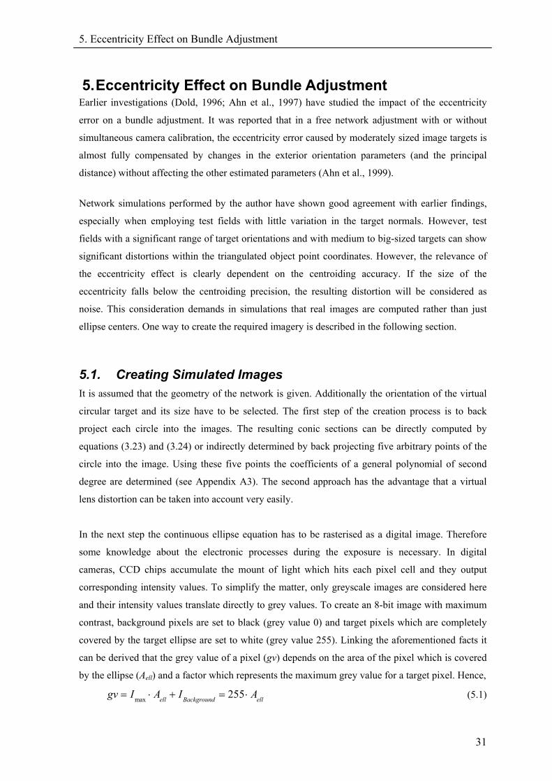
5. Eccentricity Effect on Bundle Adjustment
31
5. Eccentricity Effect on Bundle Adjustment Earlier investigations (Dold, 1996; Ahn et al., 1997) have studied the impact of the eccentricity
error on a bundle adjustment. It was reported that in a free network adjustment with or without
simultaneous camera calibration, the eccentricity error caused by moderately sized image targets is
almost fully compensated by changes in the exterior orientation parameters (and the principal
distance) without affecting the other estimated parameters (Ahn et al., 1999).
Network simulations performed by the author have shown good agreement with earlier findings,
especially when employing test fields with little variation in the target normals. However, test
fields with a significant range of target orientations and with medium to big-sized targets can show
significant distortions within the triangulated object point coordinates. However, the relevance of
the eccentricity effect is clearly dependent on the centroiding accuracy. If the size of the
eccentricity falls below the centroiding precision, the resulting distortion will be considered as
noise. This consideration demands in simulations that real images are computed rather than just
ellipse centers. One way to create the required imagery is described in the following section.
5.1. Creating Simulated Images It is assumed that the geometry of the network is given. Additionally the orientation of the virtual
circular target and its size have to be selected. The first step of the creation process is to back
project each circle into the images. The resulting conic sections can be directly computed by
equations (3.23) and (3.24) or indirectly determined by back projecting five arbitrary points of the
circle into the image. Using these five points the coefficients of a general polynomial of second
degree are determined (see Appendix A3). The second approach has the advantage that a virtual
lens distortion can be taken into account very easily.
In the next step the continuous ellipse equation has to be rasterised as a digital image. Therefore
some knowledge about the electronic processes during the exposure is necessary. In digital
cameras, CCD chips accumulate the mount of light which hits each pixel cell and they output
corresponding intensity values. To simplify the matter, only greyscale images are considered here
and their intensity values translate directly to grey values. To create an 8-bit image with maximum
contrast, background pixels are set to black (grey value 0) and target pixels which are completely
covered by the target ellipse are set to white (grey value 255). Linking the aforementioned facts it
can be derived that the grey value of a pixel (gv) depends on the area of the pixel which is covered
by the ellipse (Aell) and a factor which represents the maximum grey value for a target pixel. Hence,
(5.1) max 255ell Background ellgv I A I A= ⋅ + = ⋅
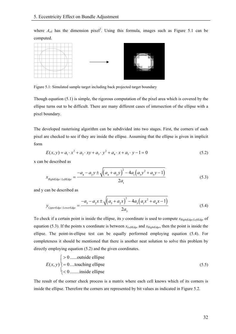
5. Eccentricity Effect on Bundle Adjustment
32
where Aell has the dimension pixel2. Using this formula, images such as Figure 5.1 can be
computed.
Figure 5.1: Simulated sample target including back projected target boundary
Though equation (5.1) is simple, the rigorous computation of the pixel area which is covered by the
ellipse turns out to be difficult. There are many different cases of intersection of the ellipse with a
pixel boundary.
The developed rasterising algorithm can be subdivided into two stages. First, the corners of each
pixel are checked to see if they are inside the ellipse. Assuming that the ellipse is given in implicit
form
(5.2) 2 21 2 3 4 5( , ) 1 0E x y a x a xy a y a x a y= ⋅ + ⋅ + ⋅ + ⋅ + ⋅ − =
x can be described as
( ) ( )2 2
4 2 4 2 1 3 5/
1
4 1
2RightEdge LeftEdge
a a y a a y a a y a yx
a
− − ± + − + −= (5.3)
and y can be described as
( ) ( )2 2
5 2 5 2 3 1 4/
3
4 1
2UpperEdge LowerEdge
a a x a a x a a x a xy
a
− − ± + − + −= (5.4)
To check if a certain point is inside the ellipse, its y coordinate is used to compute xRightEdge/LeftEdge of
equation (5.3). If the points x coordinate is between xLeftEdge and xRightEdge, then the point is inside the
ellipse. The point-in-ellipse test can be equally performed employing equation (5.4). For
completeness it should be mentioned that there is another neat solution to solve this problem by
directly employing equation (5.2) and the given coordinates.
(5.5)
0 ......outside ellipse( , ) 0....touching ellipse
0 ........inside ellipseE x y
>⎧⎪=⎨⎪<⎩
The result of the corner check process is a matrix where each cell knows which of its corners is
inside the ellipse. Therefore the corners are represented by bit values as indicated in Figure 5.2.
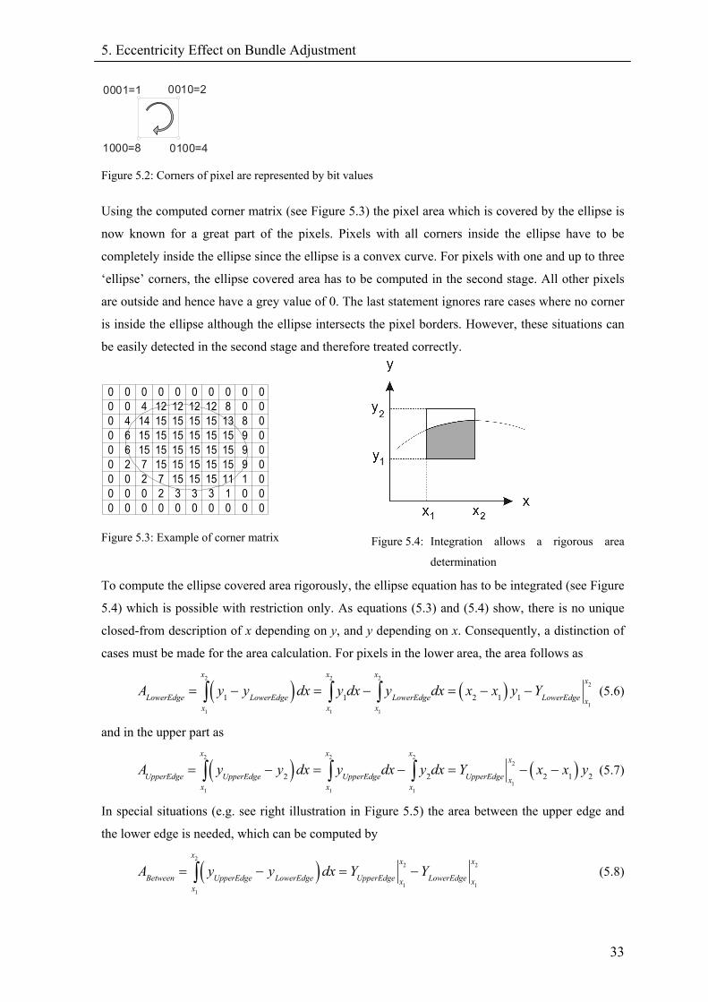
5. Eccentricity Effect on Bundle Adjustment
33
0001=1 0010=2
1000=8 0100=4
Figure 5.2: Corners of pixel are represented by bit values
Using the computed corner matrix (see Figure 5.3) the pixel area which is covered by the ellipse is
now known for a great part of the pixels. Pixels with all corners inside the ellipse have to be
completely inside the ellipse since the ellipse is a convex curve. For pixels with one and up to three
‘ellipse’ corners, the ellipse covered area has to be computed in the second stage. All other pixels
are outside and hence have a grey value of 0. The last statement ignores rare cases where no corner
is inside the ellipse although the ellipse intersects the pixel borders. However, these situations can
be easily detected in the second stage and therefore treated correctly.
0 0 0 0 0 0 0 0 0 00 0 4 12 12 12 12 8 0 00 4 14 15 15 15 15 13 8 00 6 15 15 15 15 15 15 9 00 6 15 15 15 15 15 15 9 00 2 7 15 15 15 15 15 9 00 0 2 7 15 15 15 11 1 00 0 0 2 3 3 3 1 0 00 0 0 0 0 0 0 0 0 0
Figure 5.3: Example of corner matrix
Figure 5.4: Integration allows a rigorous area
determination
To compute the ellipse covered area rigorously, the ellipse equation has to be integrated (see Figure
5.4) which is possible with restriction only. As equations (5.3) and (5.4) show, there is no unique
closed-from description of x depending on y, and y depending on x. Consequently, a distinction of
cases must be made for the area calculation. For pixels in the lower area, the area follows as
( ) ( )2 2 2
2
11 1 1
1 1 2 1 1
x x xx
LowerEdge LowerEdge LowerEdge LowerEdge xx x x
A y y dx y dx y dx x x y Y= − = − = − −∫ ∫ ∫ (5.6)
and in the upper part as
( ) ( )2 2 2
2
11 1 1
2 2
x x xx
UpperEdge UpperEdge UpperEdge UpperEdge xx x x
A y y dx y dx y dx Y x= − = − = − −∫ ∫ ∫ 2 1 2x y (5.7)
In special situations (e.g. see right illustration in Figure 5.5) the area between the upper edge and
the lower edge is needed, which can be computed by
( )2
2
1 11
xx x
Between UpperEdge LowerEdge UpperEdge LowerEdgex xx
A y y dx Y Y= − = −∫2
(5.8)
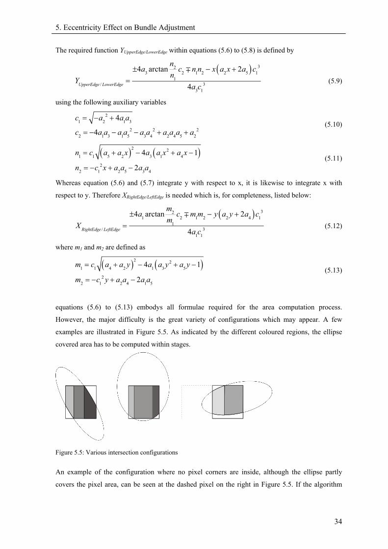
5. Eccentricity Effect on Bundle Adjustment
34
The required function YUpperEdge/LowerEdge within equations (5.6) to (5.8) is defined by
( ) 32
3 2 1 2 2 51
3/3 1
4 arctan 2
4UpperEdge LowerEdge
na c n n x a x a
nY
a c
± −=
∓ 1c+ (5.9)
using the following auxiliary variables
2
1 2 1 3
2 22 1 3 1 5 3 4 2 4 5
4
4
c a a a
c a a a a a a a a a a
= − +
= − − − + + 22
(5.10)
( ) ( )2 21 1 5 2 3 1 4
22 1 2 5 3 4
4 1
2
n c a a x a a x a x
n c x a a a a
= + − + −
= − + − (5.11)
Whereas equation (5.6) and (5.7) integrate y with respect to x, it is likewise to integrate x with
respect to y. Therefore XRightEdge/LeftEdge is needed which is, for completeness, listed below:
( ) 32
1 2 1 2 2 41
3/1 1
4 arctan 2
4RightEdge LeftEdge
ma c m m y a y a
mX
a c
± −=
∓ 1c+ (5.12)
where m1 and m2 are defined as
( ) ( )2 21 1 4 2 1 3 5
22 1 2 4 1 5
4 1
2
m c a a y a a y a y
m c y a a a a
= + − + −
= − + − (5.13)
equations (5.6) to (5.13) embodys all formulae required for the area computation process.
However, the major difficulty is the great variety of configurations which may appear. A few
examples are illustrated in Figure 5.5. As indicated by the different coloured regions, the ellipse
covered area has to be computed within stages.
Figure 5.5: Various intersection configurations
An example of the configuration where no pixel corners are inside, although the ellipse partly
covers the pixel area, can be seen at the dashed pixel on the right in Figure 5.5. If the algorithm
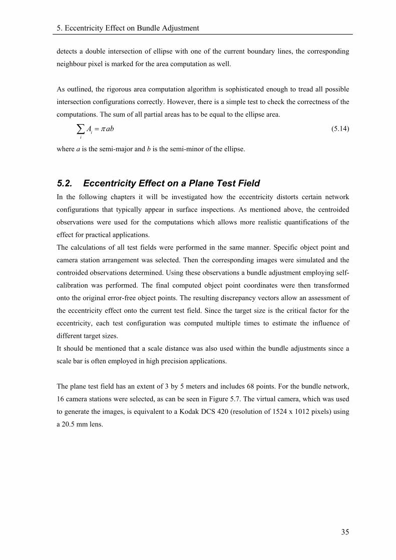
5. Eccentricity Effect on Bundle Adjustment
35
detects a double intersection of ellipse with one of the current boundary lines, the corresponding
neighbour pixel is marked for the area computation as well.
As outlined, the rigorous area computation algorithm is sophisticated enough to tread all possible
intersection configurations correctly. However, there is a simple test to check the correctness of the
computations. The sum of all partial areas has to be equal to the ellipse area.
ii
A abπ=∑ (5.14)
where a is the semi-major and b is the semi-minor of the ellipse.
5.2. Eccentricity Effect on a Plane Test Field In the following chapters it will be investigated how the eccentricity distorts certain network
configurations that typically appear in surface inspections. As mentioned above, the centroided
observations were used for the computations which allows more realistic quantifications of the
effect for practical applications.
The calculations of all test fields were performed in the same manner. Specific object point and
camera station arrangement was selected. Then the corresponding images were simulated and the
controided observations determined. Using these observations a bundle adjustment employing self-
calibration was performed. The final computed object point coordinates were then transformed
onto the original error-free object points. The resulting discrepancy vectors allow an assessment of
the eccentricity effect onto the current test field. Since the target size is the critical factor for the
eccentricity, each test configuration was computed multiple times to estimate the influence of
different target sizes.
It should be mentioned that a scale distance was also used within the bundle adjustments since a
scale bar is often employed in high precision applications.
The plane test field has an extent of 3 by 5 meters and includes 68 points. For the bundle network,
16 camera stations were selected, as can be seen in Figure 5.7. The virtual camera, which was used
to generate the images, is equivalent to a Kodak DCS 420 (resolution of 1524 x 1012 pixels) using
a 20.5 mm lens.
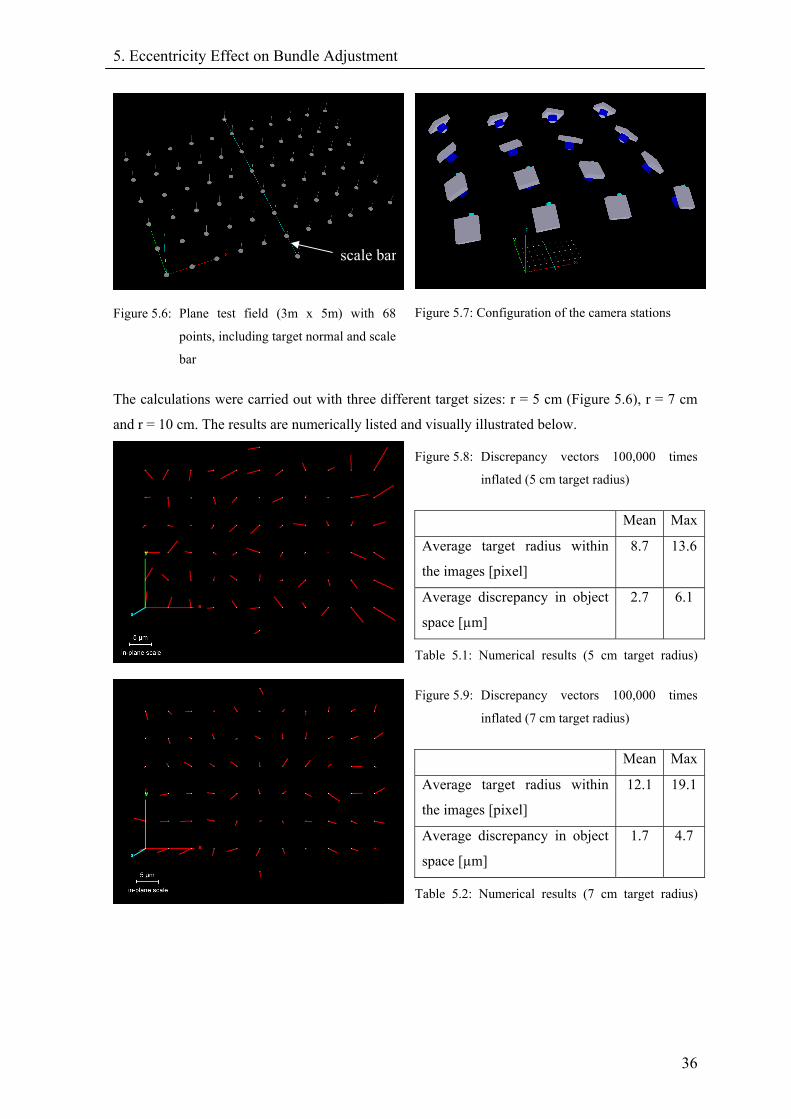
5. Eccentricity Effect on Bundle Adjustment
Figure 5.6: Plane test field (3m x 5m
points, including target norm
bar
The calculations were carried out wit
and r = 10 cm. The results are numeri
scale bar
36
) with 68
al and scale
Figure 5.7: Configuration of the camera stations
h three different target sizes: r = 5 cm (Figure 5.6), r = 7 cm
cally listed and visually illustrated below.
Figure 5.8: Discrepancy vectors 100,000 times
inflated (5 cm target radius)
Mean Max
Average target radius within
the images [pixel]
8.7 13.6
Average discrepancy in object
space [µm]
2.7 6.1
Table 5.1: Numerical results (5 cm target radius)
Figure 5.9: Discrepancy vectors 100,000 times
inflated (7 cm target radius)
Mean Max
Average target radius within
the images [pixel]
12.1 19.1
Average discrepancy in object
space [µm]
1.7 4.7
Table 5.2: Numerical results (7 cm target radius)
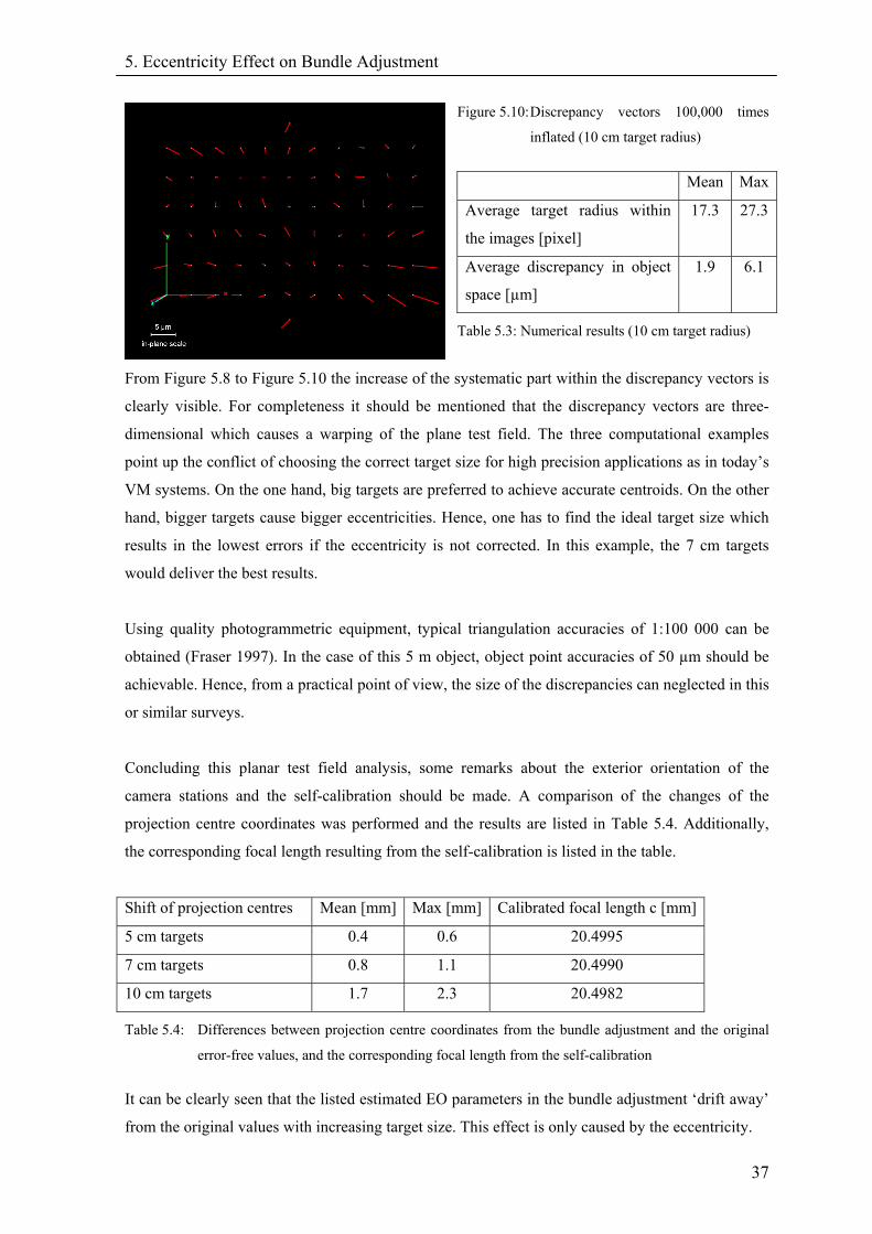
5. Eccentricity Effect on Bundle Adjustment
37
Figure 5.10: Discrepancy vectors 100,000 times
inflated (10 cm target radius)
Mean Max
Average target radius within
the images [pixel]
17.3 27.3
Average discrepancy in object
space [µm]
1.9 6.1
Table 5.3: Numerical results (10 cm target radius)
From Figure 5.8 to Figure 5.10 the increase of the systematic part within the discrepancy vectors is
clearly visible. For completeness it should be mentioned that the discrepancy vectors are three-
dimensional which causes a warping of the plane test field. The three computational examples
point up the conflict of choosing the correct target size for high precision applications as in today’s
VM systems. On the one hand, big targets are preferred to achieve accurate centroids. On the other
hand, bigger targets cause bigger eccentricities. Hence, one has to find the ideal target size which
results in the lowest errors if the eccentricity is not corrected. In this example, the 7 cm targets
would deliver the best results.
Using quality photogrammetric equipment, typical triangulation accuracies of 1:100 000 can be
obtained (Fraser 1997). In the case of this 5 m object, object point accuracies of 50 µm should be
achievable. Hence, from a practical point of view, the size of the discrepancies can neglected in this
or similar surveys.
Concluding this planar test field analysis, some remarks about the exterior orientation of the
camera stations and the self-calibration should be made. A comparison of the changes of the
projection centre coordinates was performed and the results are listed in Table 5.4. Additionally,
the corresponding focal length resulting from the self-calibration is listed in the table.
Shift of projection centres Mean [mm] Max [mm] Calibrated focal length c [mm]
5 cm targets 0.4 0.6 20.4995
7 cm targets 0.8 1.1 20.4990
10 cm targets 1.7 2.3 20.4982
Table 5.4: Differences between projection centre coordinates from the bundle adjustment and the original
error-free values, and the corresponding focal length from the self-calibration
It can be clearly seen that the listed estimated EO parameters in the bundle adjustment ‘drift away’
from the original values with increasing target size. This effect is only caused by the eccentricity.
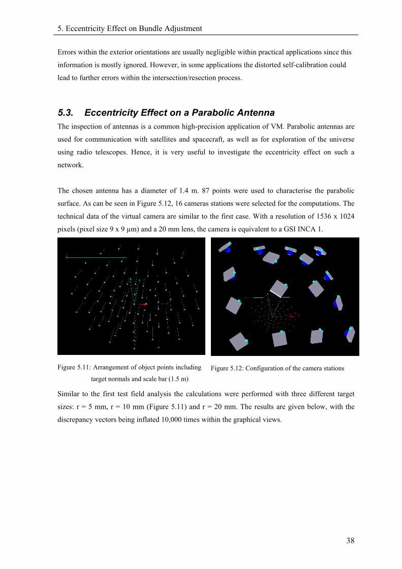
5. Eccentricity Effect on Bundle Adjustment
38
Errors within the exterior orientations are usually negligible within practical applications since this
information is mostly ignored. However, in some applications the distorted self-calibration could
lead to further errors within the intersection/resection process.
5.3. Eccentricity Effect on a Parabolic Antenna The inspection of antennas is a common high-precision application of VM. Parabolic antennas are
used for communication with satellites and spacecraft, as well as for exploration of the universe
using radio telescopes. Hence, it is very useful to investigate the eccentricity effect on such a
network.
The chosen antenna has a diameter of 1.4 m. 87 points were used to characterise the parabolic
surface. As can be seen in Figure 5.12, 16 cameras stations were selected for the computations. The
technical data of the virtual camera are similar to the first case. With a resolution of 1536 x 1024
pixels (pixel size 9 x 9 µm) and a 20 mm lens, the camera is equivalent to a GSI INCA 1.
Figure 5.11: Arrangement of object points including
target normals and scale bar (1.5 m)
Figure 5.12: Configuration of the camera stations
Similar to the first test field analysis the calculations were performed with three different target
sizes: r = 5 mm, r = 10 mm (Figure 5.11) and r = 20 mm. The results are given below, with the
discrepancy vectors being inflated 10,000 times within the graphical views.
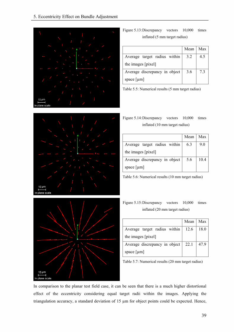
5. Eccentricity Effect on Bundle Adjustment
39
Figure 5.13: Discrepancy vectors 10,000 times
inflated (5 mm target radius)
Mean Max
Average target radius within
the images [pixel]
3.2 4.5
Average discrepancy in object
space [µm]
3.6 7.3
Table 5.5: Numerical results (5 mm target radius)
Figure 5.14: Discrepancy vectors 10,000 times
inflated (10 mm target radius)
Mean Max
Average target radius within
the images [pixel]
6.3 9.0
Average discrepancy in object
space [µm]
5.6 10.4
Table 5.6: Numerical results (10 mm target radius)
Figure 5.15: Discrepancy vectors 10,000 times
inflated (20 mm target radius)
Mean Max
Average target radius within
the images [pixel]
12.6 18.0
Average discrepancy in object
space [µm]
22.1 47.9
Table 5.7: Numerical results (20 mm target radius)
In comparison to the planar test field case, it can be seen that there is a much higher distortional
effect of the eccentricity considering equal target radii within the images. Applying the
triangulation accuracy, a standard deviation of 15 µm for object points could be expected. Hence,
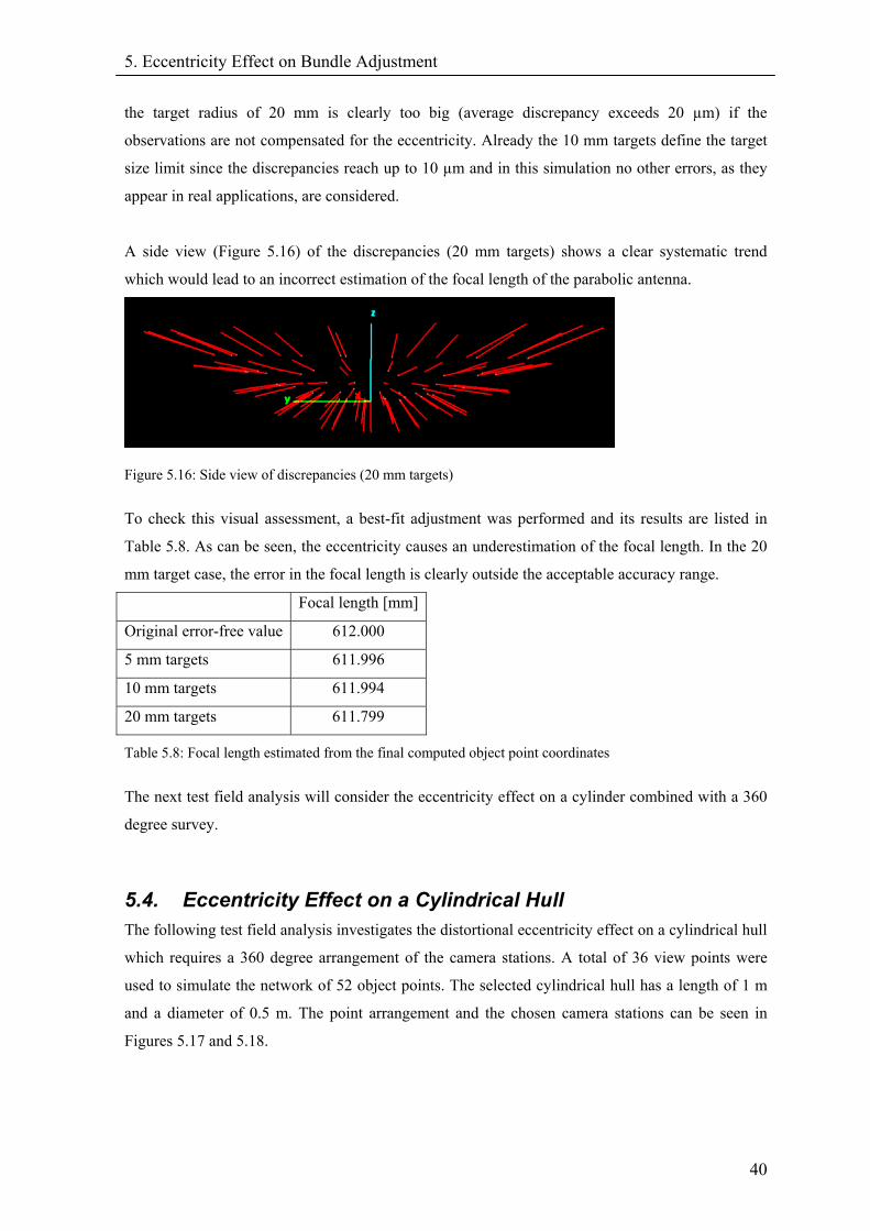
5. Eccentricity Effect on Bundle Adjustment
40
the target radius of 20 mm is clearly too big (average discrepancy exceeds 20 µm) if the
observations are not compensated for the eccentricity. Already the 10 mm targets define the target
size limit since the discrepancies reach up to 10 µm and in this simulation no other errors, as they
appear in real applications, are considered.
A side view (Figure 5.16) of the discrepancies (20 mm targets) shows a clear systematic trend
which would lead to an incorrect estimation of the focal length of the parabolic antenna.
Figure 5.16: Side view of discrepancies (20 mm targets)
To check this visual assessment, a best-fit adjustment was performed and its results are listed in
Table 5.8. As can be seen, the eccentricity causes an underestimation of the focal length. In the 20
mm target case, the error in the focal length is clearly outside the acceptable accuracy range.
Focal length [mm]
Original error-free value 612.000
5 mm targets 611.996
10 mm targets 611.994
20 mm targets 611.799
Table 5.8: Focal length estimated from the final computed object point coordinates
The next test field analysis will consider the eccentricity effect on a cylinder combined with a 360
degree survey.
5.4. Eccentricity Effect on a Cylindrical Hull The following test field analysis investigates the distortional eccentricity effect on a cylindrical hull
which requires a 360 degree arrangement of the camera stations. A total of 36 view points were
used to simulate the network of 52 object points. The selected cylindrical hull has a length of 1 m
and a diameter of 0.5 m. The point arrangement and the chosen camera stations can be seen in
Figures 5.17 and 5.18.
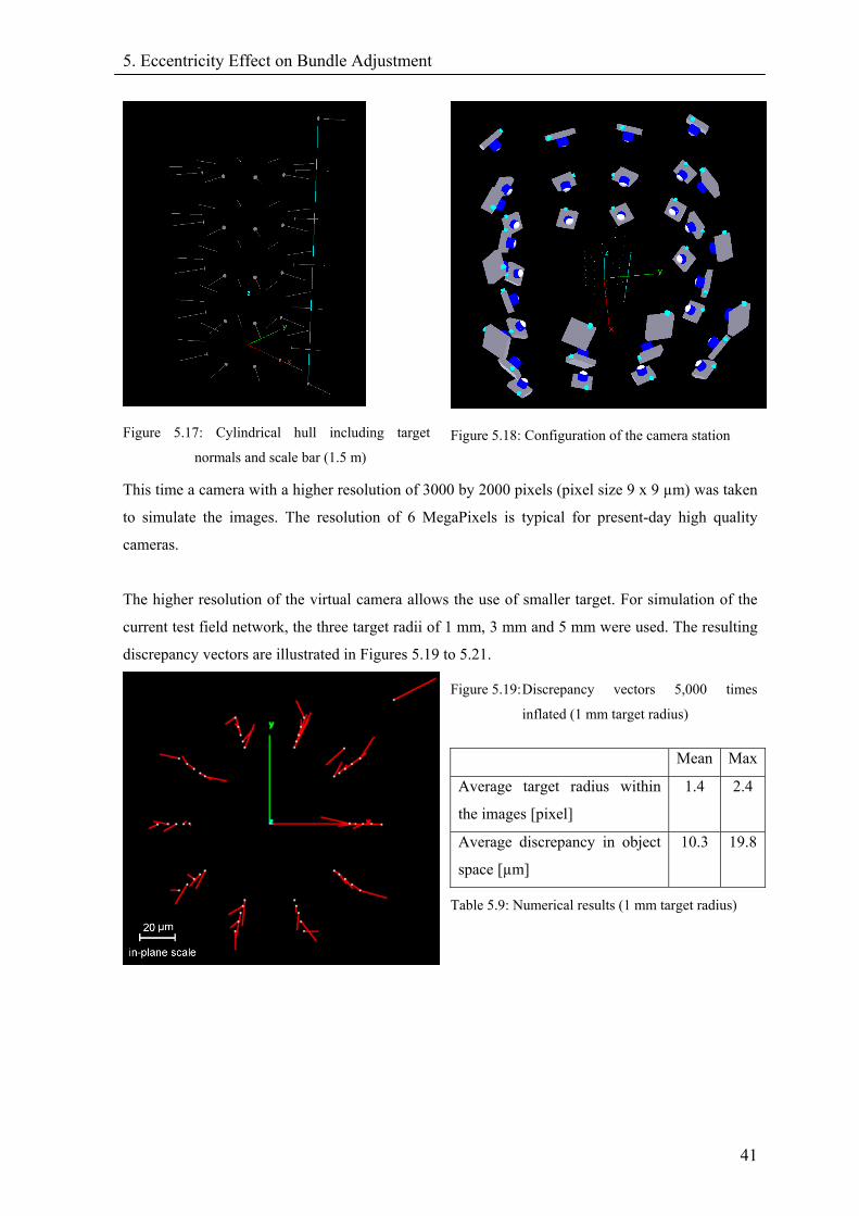
5. Eccentricity Effect on Bundle Adjustment
41
Figure 5.17: Cylindrical hull including target
normals and scale bar (1.5 m)
Figure 5.18: Configuration of the camera station
This time a camera with a higher resolution of 3000 by 2000 pixels (pixel size 9 x 9 µm) was taken
to simulate the images. The resolution of 6 MegaPixels is typical for present-day high quality
cameras.
The higher resolution of the virtual camera allows the use of smaller target. For simulation of the
current test field network, the three target radii of 1 mm, 3 mm and 5 mm were used. The resulting
discrepancy vectors are illustrated in Figures 5.19 to 5.21.
Figure 5.19: Discrepancy vectors 5,000 times
inflated (1 mm target radius)
Mean Max
Average target radius within
the images [pixel]
1.4 2.4
Average discrepancy in object
space [µm]
10.3 19.8
Table 5.9: Numerical results (1 mm target radius)
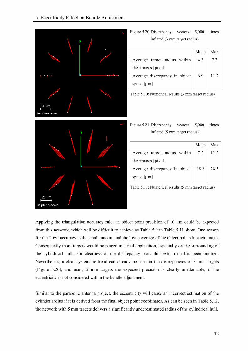
5. Eccentricity Effect on Bundle Adjustment
42
Figure 5.20: Discrepancy vectors 5,000 times
inflated (3 mm target radius)
Mean Max
Average target radius within
the images [pixel]
4.3 7.3
Average discrepancy in object
space [µm]
6.9 11.2
Table 5.10: Numerical results (3 mm target radius)
Figure 5.21: Discrepancy vectors 5,000 times
inflated (5 mm target radius)
Mean Max
Average target radius within
the images [pixel]
7.2 12.2
Average discrepancy in object
space [µm]
18.6 28.3
Table 5.11: Numerical results (5 mm target radius)
Applying the triangulation accuracy rule, an object point precision of 10 µm could be expected
from this network, which will be difficult to achieve as Table 5.9 to Table 5.11 show. One reason
for the ‘low’ accuracy is the small amount and the low coverage of the object points in each image.
Consequently more targets would be placed in a real application, especially on the surrounding of
the cylindrical hull. For clearness of the discrepancy plots this extra data has been omitted.
Nevertheless, a clear systematic trend can already be seen in the discrepancies of 3 mm targets
(Figure 5.20), and using 5 mm targets the expected precision is clearly unattainable, if the
eccentricity is not considered within the bundle adjustment.
Similar to the parabolic antenna project, the eccentricity will cause an incorrect estimation of the
cylinder radius if it is derived from the final object point coordinates. As can be seen in Table 5.12,
the network with 5 mm targets delivers a significantly underestimated radius of the cylindrical hull.
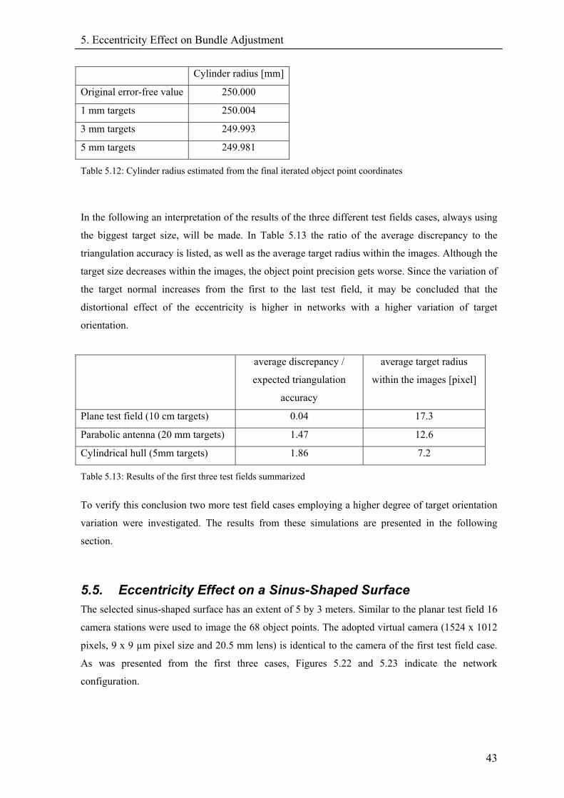
5. Eccentricity Effect on Bundle Adjustment
43
Cylinder radius [mm]
Original error-free value 250.000
1 mm targets 250.004
3 mm targets 249.993
5 mm targets 249.981
Table 5.12: Cylinder radius estimated from the final iterated object point coordinates
In the following an interpretation of the results of the three different test fields cases, always using
the biggest target size, will be made. In Table 5.13 the ratio of the average discrepancy to the
triangulation accuracy is listed, as well as the average target radius within the images. Although the
target size decreases within the images, the object point precision gets worse. Since the variation of
the target normal increases from the first to the last test field, it may be concluded that the
distortional effect of the eccentricity is higher in networks with a higher variation of target
orientation.
average discrepancy /
expected triangulation
accuracy
average target radius
within the images [pixel]
Plane test field (10 cm targets) 0.04 17.3
Parabolic antenna (20 mm targets) 1.47 12.6
Cylindrical hull (5mm targets) 1.86 7.2
Table 5.13: Results of the first three test fields summarized
To verify this conclusion two more test field cases employing a higher degree of target orientation
variation were investigated. The results from these simulations are presented in the following
section.
5.5. Eccentricity Effect on a Sinus-Shaped Surface The selected sinus-shaped surface has an extent of 5 by 3 meters. Similar to the planar test field 16
camera stations were used to image the 68 object points. The adopted virtual camera (1524 x 1012
pixels, 9 x 9 µm pixel size and 20.5 mm lens) is identical to the camera of the first test field case.
As was presented from the first three cases, Figures 5.22 and 5.23 indicate the network
configuration.
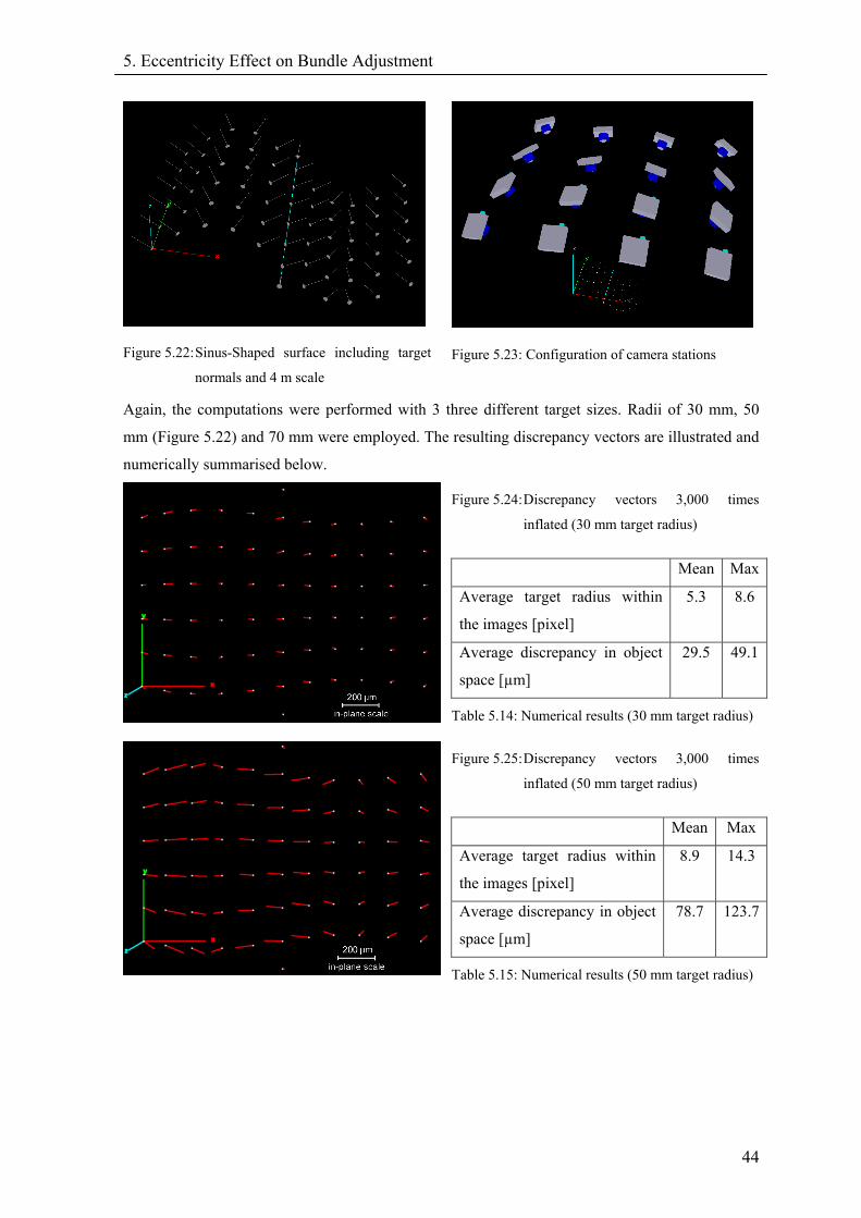
5. Eccentricity Effect on Bundle Adjustment
44
Figure 5.22: Sinus-Shaped surface including target
normals and 4 m scale
Figure 5.23: Configuration of camera stations
Again, the computations were performed with 3 three different target sizes. Radii of 30 mm, 50
mm (Figure 5.22) and 70 mm were employed. The resulting discrepancy vectors are illustrated and
numerically summarised below.
Figure 5.24: Discrepancy vectors 3,000 times
inflated (30 mm target radius)
Mean Max
Average target radius within
the images [pixel]
5.3 8.6
Average discrepancy in object
space [µm]
29.5 49.1
Table 5.14: Numerical results (30 mm target radius)
Figure 5.25: Discrepancy vectors 3,000 times
inflated (50 mm target radius)
Mean Max
Average target radius within
the images [pixel]
8.9 14.3
Average discrepancy in object
space [µm]
78.7 123.7
Table 5.15: Numerical results (50 mm target radius)
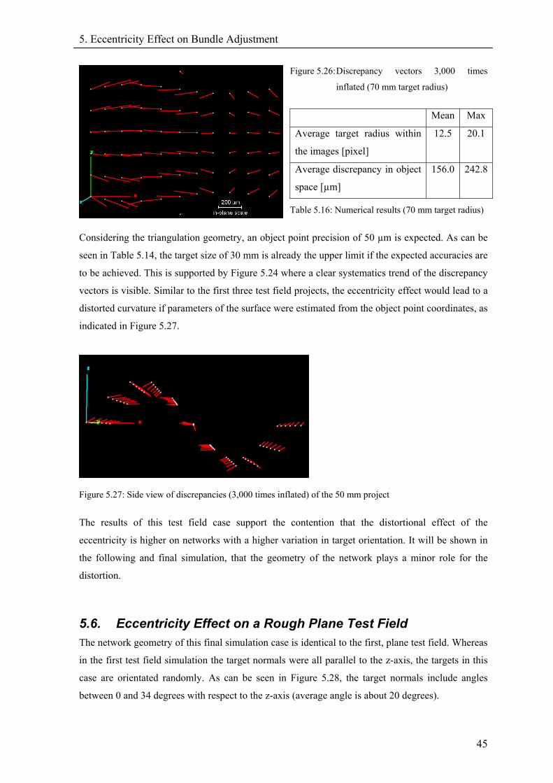
5. Eccentricity Effect on Bundle Adjustment
45
Figure 5.26: Discrepancy vectors 3,000 times
inflated (70 mm target radius)
Mean Max
Average target radius within
the images [pixel]
12.5 20.1
Average discrepancy in object
space [µm]
156.0 242.8
Table 5.16: Numerical results (70 mm target radius)
Considering the triangulation geometry, an object point precision of 50 µm is expected. As can be
seen in Table 5.14, the target size of 30 mm is already the upper limit if the expected accuracies are
to be achieved. This is supported by Figure 5.24 where a clear systematics trend of the discrepancy
vectors is visible. Similar to the first three test field projects, the eccentricity effect would lead to a
distorted curvature if parameters of the surface were estimated from the object point coordinates, as
indicated in Figure 5.27.
Figure 5.27: Side view of discrepancies (3,000 times inflated) of the 50 mm project
The results of this test field case support the contention that the distortional effect of the
eccentricity is higher on networks with a higher variation in target orientation. It will be shown in
the following and final simulation, that the geometry of the network plays a minor role for the
distortion.
5.6. Eccentricity Effect on a Rough Plane Test Field The network geometry of this final simulation case is identical to the first, plane test field. Whereas
in the first test field simulation the target normals were all parallel to the z-axis, the targets in this
case are orientated randomly. As can be seen in Figure 5.28, the target normals include angles
between 0 and 34 degrees with respect to the z-axis (average angle is about 20 degrees).
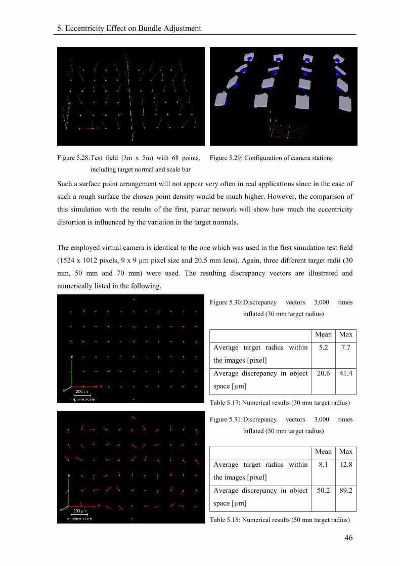
5. Eccentricity Effect on Bundle Adjustment
46
Figure 5.28: Test field (3m x 5m) with 68 points,
including target normal and scale bar
Figure 5.29: Configuration of camera stations
Such a surface point arrangement will not appear very often in real applications since in the case of
such a rough surface the chosen point density would be much higher. However, the comparison of
this simulation with the results of the first, planar network will show how much the eccentricity
distortion is influenced by the variation in the target normals.
The employed virtual camera is identical to the one which was used in the first simulation test field
(1524 x 1012 pixels, 9 x 9 µm pixel size and 20.5 mm lens). Again, three different target radii (30
mm, 50 mm and 70 mm) were used. The resulting discrepancy vectors are illustrated and
numerically listed in the following.
Figure 5.30: Discrepancy vectors 3,000 times
inflated (30 mm target radius)
Mean Max
Average target radius within
the images [pixel]
5.2 7.7
Average discrepancy in object
space [µm]
20.6 41.4
Table 5.17: Numerical results (30 mm target radius)
Figure 5.31: Discrepancy vectors 3,000 times
inflated (50 mm target radius)
Mean Max
Average target radius within
the images [pixel]
8.1 12.8
Average discrepancy in object
space [µm]
50.2 89.2
Table 5.18: Numerical results (50 mm target radius)
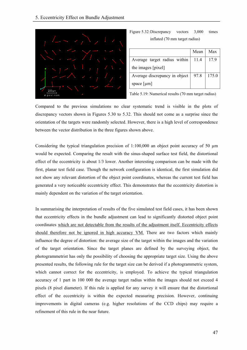
5. Eccentricity Effect on Bundle Adjustment
47
Figure 5.32: Discrepancy vectors 3,000 times
inflated (70 mm target radius)
Mean Max
Average target radius within
the images [pixel]
11.4 17.9
Average discrepancy in object
space [µm]
97.8 175.0
Table 5.19: Numerical results (70 mm target radius)
Compared to the previous simulations no clear systematic trend is visible in the plots of
discrepancy vectors shown in Figures 5.30 to 5.32. This should not come as a surprise since the
orientation of the targets were randomly selected. However, there is a high level of correspondence
between the vector distribution in the three figures shown above.
Considering the typical triangulation precision of 1:100,000 an object point accuracy of 50 µm
would be expected. Comparing the result with the sinus-shaped surface test field, the distortional
effect of the eccentricity is about 1/3 lower. Another interesting comparison can be made with the
first, planar test field case. Though the network configuration is identical, the first simulation did
not show any relevant distortion of the object point coordinates, whereas the current test field has
generated a very noticeable eccentricity effect. This demonstrates that the eccentricity distortion is
mainly dependent on the variation of the target orientation.
In summarising the interpretation of results of the five simulated test field cases, it has been shown
that eccentricity effects in the bundle adjustment can lead to significantly distorted object point
coordinates which are not detectable from the results of the adjustment itself. Eccentricity effects
should therefore not be ignored in high accuracy VM. There are two factors which mainly
influence the degree of distortion: the average size of the target within the images and the variation
of the target orientation. Since the target planes are defined by the surveying object, the
photogrammetrist has only the possibility of choosing the appropriate target size. Using the above
presented results, the following rule for the target size can be derived if a photogrammetric system,
which cannot correct for the eccentricity, is employed. To achieve the typical triangulation
accuracy of 1 part in 100 000 the average target radius within the images should not exceed 4
pixels (8 pixel diameter). If this rule is applied for any survey it will ensure that the distortional
effect of the eccentricity is within the expected measuring precision. However, continuing
improvements in digital cameras (e.g. higher resolutions of the CCD chips) may require a
refinement of this rule in the near future.

5. Eccentricity Effect on Bundle Adjustment
48
In addition, it should be recalled that the object point coordinates are not the only distorted
parameter within the bundle adjustment (see Chapter 5.2). The estimates of the exterior orientation
and the focal length can be substantially affected as well. Since this is of no concern in a typical
surface inspection application, a detailed analysis of this effect has not been considered here.
However, surveying strategies were unwanted deformation may appear can be envisaged.
6. Curved Targets and their Distortional Effect
49
6. Curved Targets and their Distortional Effect If a photogrammetry system is capable of correcting the ellipse eccentricity, no restriction
concerning the target size needs to be made. Bigger targets resulting in higher centroiding
accuracies can be employed, which will eventually lead to better surveying precision. In some
applications, however, limitations in the target size may be a requirement due to point density or
due to the curvature of the surface to be surveyed. So far circular targets have always been
considered as perfect planar circles in space. However, if a target is glued onto a surface, the
planarity of the target edge is not guaranteed in general and it is convincing that bigger targets are
more effected by the surface curvature than smaller. Since this thesis proposes the use of bigger
targets for higher accuracy, it is well worth investigating the effect of curved targets on the
measuring process. The derivation of the required formulas and an estimation of the effect will be
described in this chapter.
For completeness, it should be mentioned that there are target size limitations from a practical point
of view as well. Retro-reflective targets on rolls are usually manufactured only to a certain
diameter. Additionally, bigger targets are more difficult to attach to the surface free of air bubbles.
Considering rigorousness, a target can be glued on a surface without folding only if the current part
of the surface can be developed into a plane. Hence, planes, cones and cylinders are imaginable
target positions. Since the carrier material of a retro-reflective target is usually flexible, the targets
can also be affixed to other surfaces which describe the aforementioned surfaces only by
approximation. This is of minor concern for the following derivations, because here it is only
estimated how much curvature depending on target size is acceptable considering a given
measuring precision. Also, only cylinders are considered since other conic surfaces will show
similar distortional effects.
6.1. Derivations for Cylindrical Curved Targets
6.1.1. Continuous Derivations To analyse the distortional effect of a target which is fixed on a cylindrical surface, a mathematical
description of the target edge has to be found. To simplify the matter, the coordinate system was
selected as indicated in Figure 6.1, where the origin was set to the target centre and the z-axis was
selected parallel to the cylinder axis.
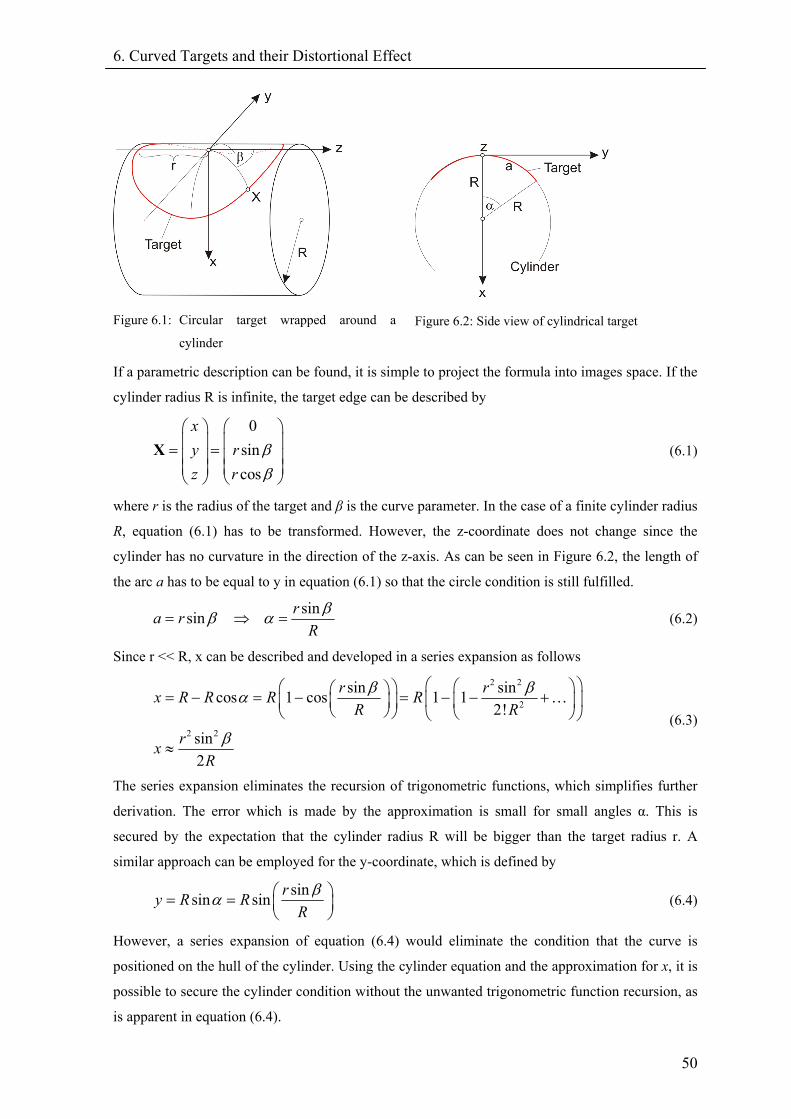
6. Curved Targets and their Distortional Effect
50
Figure 6.1: Circular target wrapped around a
cylinder
Figure 6.2: Side view of cylindrical target
If a parametric description can be found, it is simple to project the formula into images space. If the
cylinder radius R is infinite, the target edge can be described by
0sincos
xy rz r
ββ
⎛ ⎞ ⎛ ⎞⎜ ⎟ ⎜ ⎟= =⎜ ⎟ ⎜ ⎟⎜ ⎟ ⎜ ⎟⎝ ⎠ ⎝ ⎠
X (6.1)
where r is the radius of the target and β is the curve parameter. In the case of a finite cylinder radius
R, equation (6.1) has to be transformed. However, the z-coordinate does not change since the
cylinder has no curvature in the direction of the z-axis. As can be seen in Figure 6.2, the length of
the arc a has to be equal to y in equation (6.1) so that the circle condition is still fulfilled.
sinsin ra rR
ββ α= ⇒ = (6.2)
Since r << R, x can be described and developed in a series expansion as follows
2 2
2
2 2
sin sincos 1 cos 1 12!
sin2
r rx R R R RR R
rxR
β βα
β
⎛ ⎞⎛ ⎞⎛ ⎞⎛ ⎞= − = − = − − +⎜ ⎟⎜ ⎟ ⎜⎜ ⎟⎝ ⎠⎝ ⎠ ⎝⎝
≈
…⎟⎠⎠ (6.3)
The series expansion eliminates the recursion of trigonometric functions, which simplifies further
derivation. The error which is made by the approximation is small for small angles α. This is
secured by the expectation that the cylinder radius R will be bigger than the target radius r. A
similar approach can be employed for the y-coordinate, which is defined by
sinsin sin ry R RR
βα ⎛= = ⎜⎝ ⎠
⎞⎟ (6.4)
However, a series expansion of equation (6.4) would eliminate the condition that the curve is
positioned on the hull of the cylinder. Using the cylinder equation and the approximation for x, it is
possible to secure the cylinder condition without the unwanted trigonometric function recursion, as
is apparent in equation (6.4).
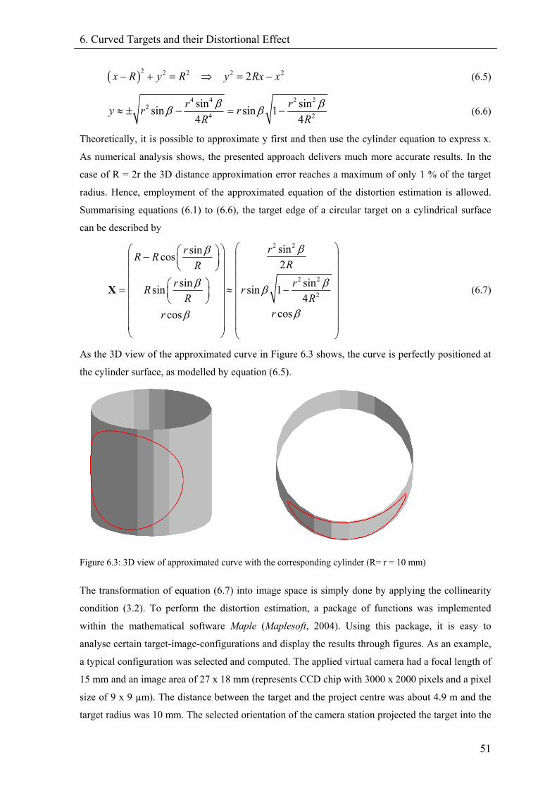
6. Curved Targets and their Distortional Effect
51
( )2 2 2 2 2 2x R y R y Rx x− + = ⇒ = − (6.5)
4 4 2 2
24
sin sinsin sin 14 4
r ry r rR R2
β ββ β≈ ± − = − (6.6)
Theoretically, it is possible to approximate y first and then use the cylinder equation to express x.
As numerical analysis shows, the presented approach delivers much more accurate results. In the
case of R = 2r the 3D distance approximation error reaches a maximum of only 1 % of the target
radius. Hence, employment of the approximated equation of the distortion estimation is allowed.
Summarising equations (6.1) to (6.6), the target edge of a circular target on a cylindrical surface
can be described by
2 2
2 2
2
sinsincos2
sin sinsin sin 14
coscos
rrR RRR
rR rR R
rr
ββ
rβ ββ
ββ
⎛ ⎞⎛ ⎞⎛ ⎞− ⎜ ⎟⎜ ⎟⎜ ⎟⎝ ⎠ ⎜ ⎟⎜ ⎟⎜ ⎟⎜ ⎟⎛ ⎞= ≈ −⎜⎜ ⎟⎜ ⎟
⎝ ⎠ ⎜ ⎟⎜ ⎟⎜ ⎟⎜ ⎟⎜ ⎟⎜ ⎟
⎝ ⎠ ⎝ ⎠
X ⎟ (6.7)
As the 3D view of the approximated curve in Figure 6.3 shows, the curve is perfectly positioned at
the cylinder surface, as modelled by equation (6.5).
Figure 6.3: 3D view of approximated curve with the corresponding cylinder (R= r = 10 mm)
The transformation of equation (6.7) into image space is simply done by applying the collinearity
condition (3.2). To perform the distortion estimation, a package of functions was implemented
within the mathematical software Maple (Maplesoft, 2004). Using this package, it is easy to
analyse certain target-image-configurations and display the results through figures. As an example,
a typical configuration was selected and computed. The applied virtual camera had a focal length of
15 mm and an image area of 27 x 18 mm (represents CCD chip with 3000 x 2000 pixels and a pixel
size of 9 x 9 µm). The distance between the target and the project centre was about 4.9 m and the
target radius was 10 mm. The selected orientation of the camera station projected the target into the
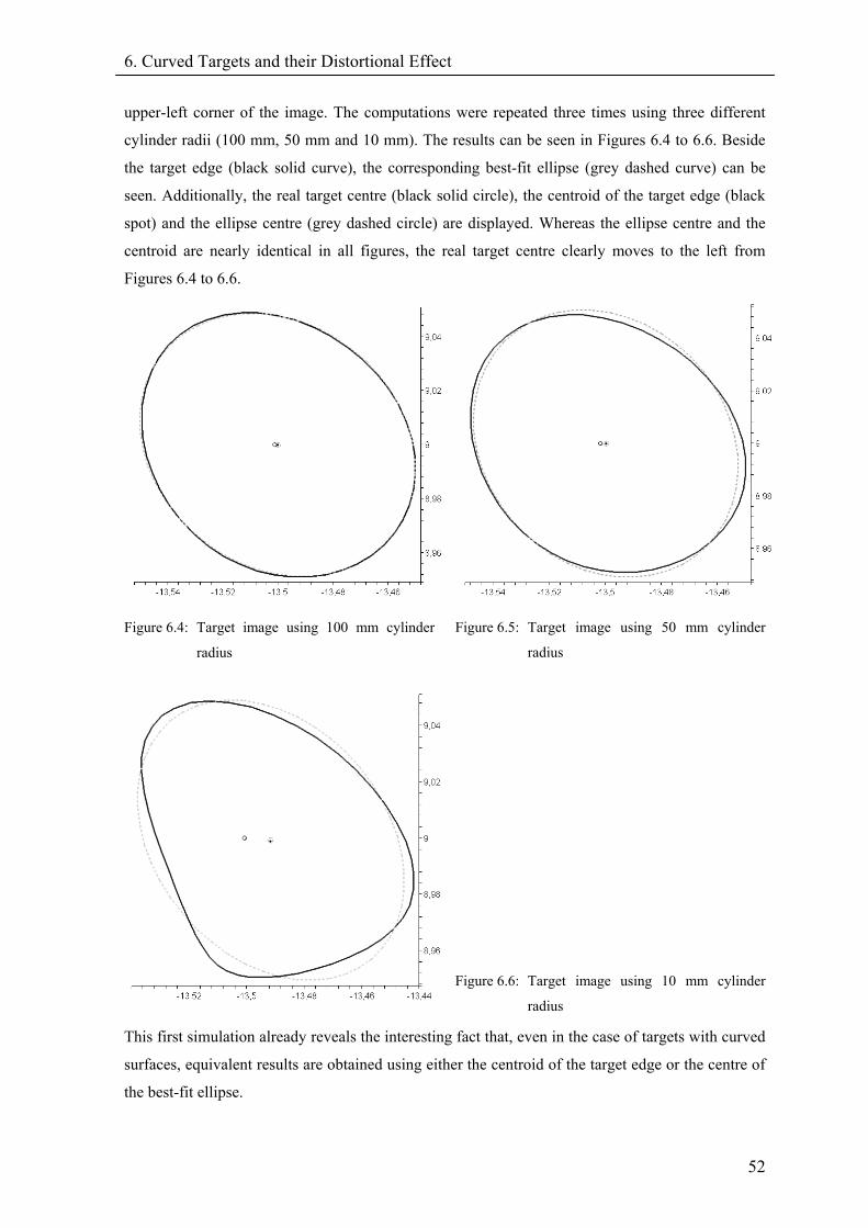
6. Curved Targets and their Distortional Effect
52
upper-left corner of the image. The computations were repeated three times using three different
cylinder radii (100 mm, 50 mm and 10 mm). The results can be seen in Figures 6.4 to 6.6. Beside
the target edge (black solid curve), the corresponding best-fit ellipse (grey dashed curve) can be
seen. Additionally, the real target centre (black solid circle), the centroid of the target edge (black
spot) and the ellipse centre (grey dashed circle) are displayed. Whereas the ellipse centre and the
centroid are nearly identical in all figures, the real target centre clearly moves to the left from
Figures 6.4 to 6.6.
Figure 6.4: Target image using 100 mm cylinder
radius
Figure 6.5: Target image using 50 mm cylinder
radius
Figure 6.6: Target image using 10 mm cylinder
radius
This first simulation already reveals the interesting fact that, even in the case of targets with curved
surfaces, equivalent results are obtained using either the centroid of the target edge or the centre of
the best-fit ellipse.
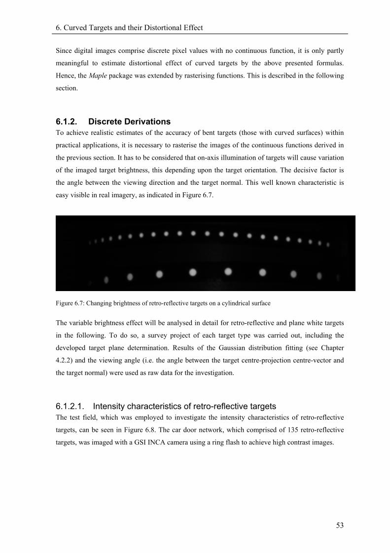
6. Curved Targets and their Distortional Effect
53
Since digital images comprise discrete pixel values with no continuous function, it is only partly
meaningful to estimate distortional effect of curved targets by the above presented formulas.
Hence, the Maple package was extended by rasterising functions. This is described in the following
section.
6.1.2. Discrete Derivations To achieve realistic estimates of the accuracy of bent targets (those with curved surfaces) within
practical applications, it is necessary to rasterise the images of the continuous functions derived in
the previous section. It has to be considered that on-axis illumination of targets will cause variation
of the imaged target brightness, this depending upon the target orientation. The decisive factor is
the angle between the viewing direction and the target normal. This well known characteristic is
easy visible in real imagery, as indicated in Figure 6.7.
Figure 6.7: Changing brightness of retro-reflective targets on a cylindrical surface
The variable brightness effect will be analysed in detail for retro-reflective and plane white targets
in the following. To do so, a survey project of each target type was carried out, including the
developed target plane determination. Results of the Gaussian distribution fitting (see Chapter
4.2.2) and the viewing angle (i.e. the angle between the target centre-projection centre-vector and
the target normal) were used as raw data for the investigation.
6.1.2.1. Intensity characteristics of retro-reflective targets The test field, which was employed to investigate the intensity characteristics of retro-reflective
targets, can be seen in Figure 6.8. The car door network, which comprised of 135 retro-reflective
targets, was imaged with a GSI INCA camera using a ring flash to achieve high contrast images.
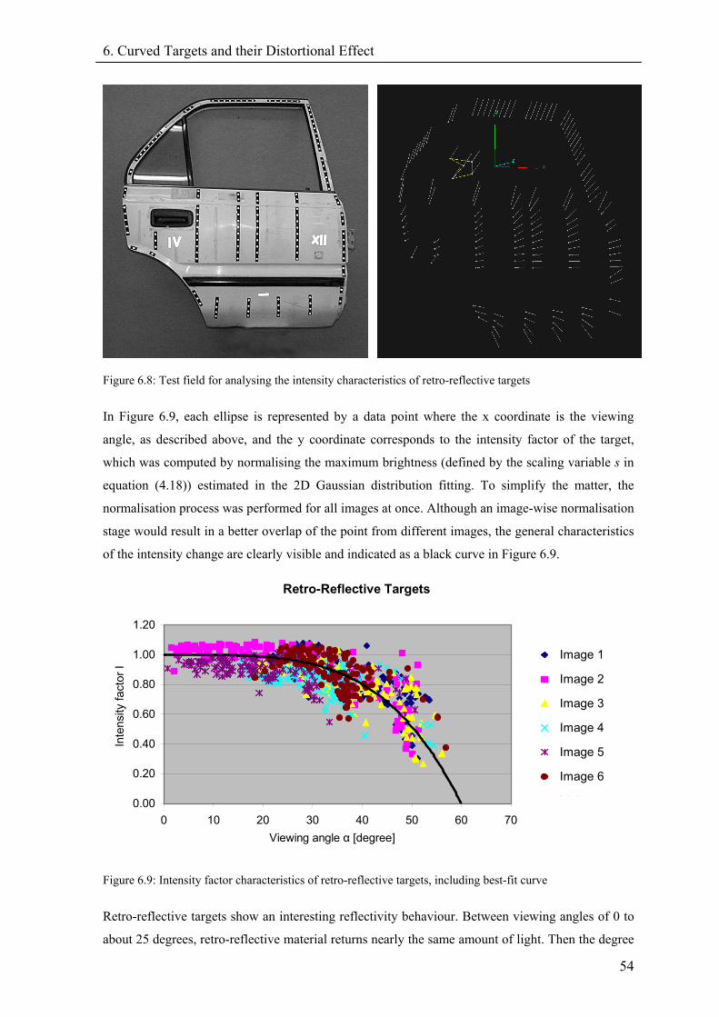
6. Curved Targets and their Distortional Effect
54
Figure 6.8: Test field for analysing the intensity characteristics of retro-reflective targets
In Figure 6.9, each ellipse is represented by a data point where the x coordinate is the viewing
angle, as described above, and the y coordinate corresponds to the intensity factor of the target,
which was computed by normalising the maximum brightness (defined by the scaling variable s in
equation (4.18)) estimated in the 2D Gaussian distribution fitting. To simplify the matter, the
normalisation process was performed for all images at once. Although an image-wise normalisation
stage would result in a better overlap of the point from different images, the general characteristics
of the intensity change are clearly visible and indicated as a black curve in Figure 6.9.
Retro-Reflective Targets
0.00
0.20
0.40
0.60
0.80
1.00
1.20
0 10 20 30 40 50 60 70
Image 1
Image 2
Image 3
Image 4
Image 5
Image 6
Li i
Viewing angle α [degree]
Inte
nsity
fact
or I
Figure 6.9: Intensity factor characteristics of retro-reflective targets, including best-fit curve
Retro-reflective targets show an interesting reflectivity behaviour. Between viewing angles of 0 to
about 25 degrees, retro-reflective material returns nearly the same amount of light. Then the degree
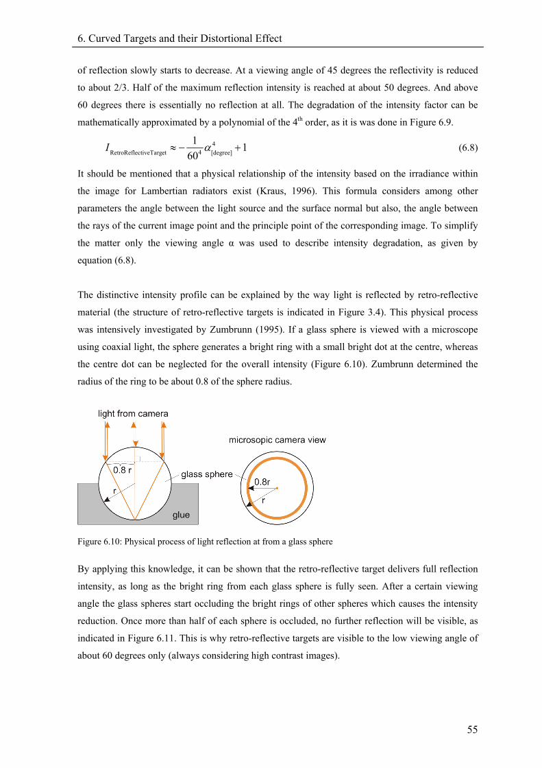
6. Curved Targets and their Distortional Effect
55
of reflection slowly starts to decrease. At a viewing angle of 45 degrees the reflectivity is reduced
to about 2/3. Half of the maximum reflection intensity is reached at about 50 degrees. And above
60 degrees there is essentially no reflection at all. The degradation of the intensity factor can be
mathematically approximated by a polynomial of the 4th order, as it is was done in Figure 6.9.
44RetroReflectiveTarget [degree]
1 160
I α≈ − + (6.8)
It should be mentioned that a physical relationship of the intensity based on the irradiance within
the image for Lambertian radiators exist (Kraus, 1996). This formula considers among other
parameters the angle between the light source and the surface normal but also, the angle between
the rays of the current image point and the principle point of the corresponding image. To simplify
the matter only the viewing angle α was used to describe intensity degradation, as given by
equation (6.8).
The distinctive intensity profile can be explained by the way light is reflected by retro-reflective
material (the structure of retro-reflective targets is indicated in Figure 3.4). This physical process
was intensively investigated by Zumbrunn (1995). If a glass sphere is viewed with a microscope
using coaxial light, the sphere generates a bright ring with a small bright dot at the centre, whereas
the centre dot can be neglected for the overall intensity (Figure 6.10). Zumbrunn determined the
radius of the ring to be about 0.8 of the sphere radius.
Figure 6.10: Physical process of light reflection at from a glass sphere
By applying this knowledge, it can be shown that the retro-reflective target delivers full reflection
intensity, as long as the bright ring from each glass sphere is fully seen. After a certain viewing
angle the glass spheres start occluding the bright rings of other spheres which causes the intensity
reduction. Once more than half of each sphere is occluded, no further reflection will be visible, as
indicated in Figure 6.11. This is why retro-reflective targets are visible to the low viewing angle of
about 60 degrees only (always considering high contrast images).
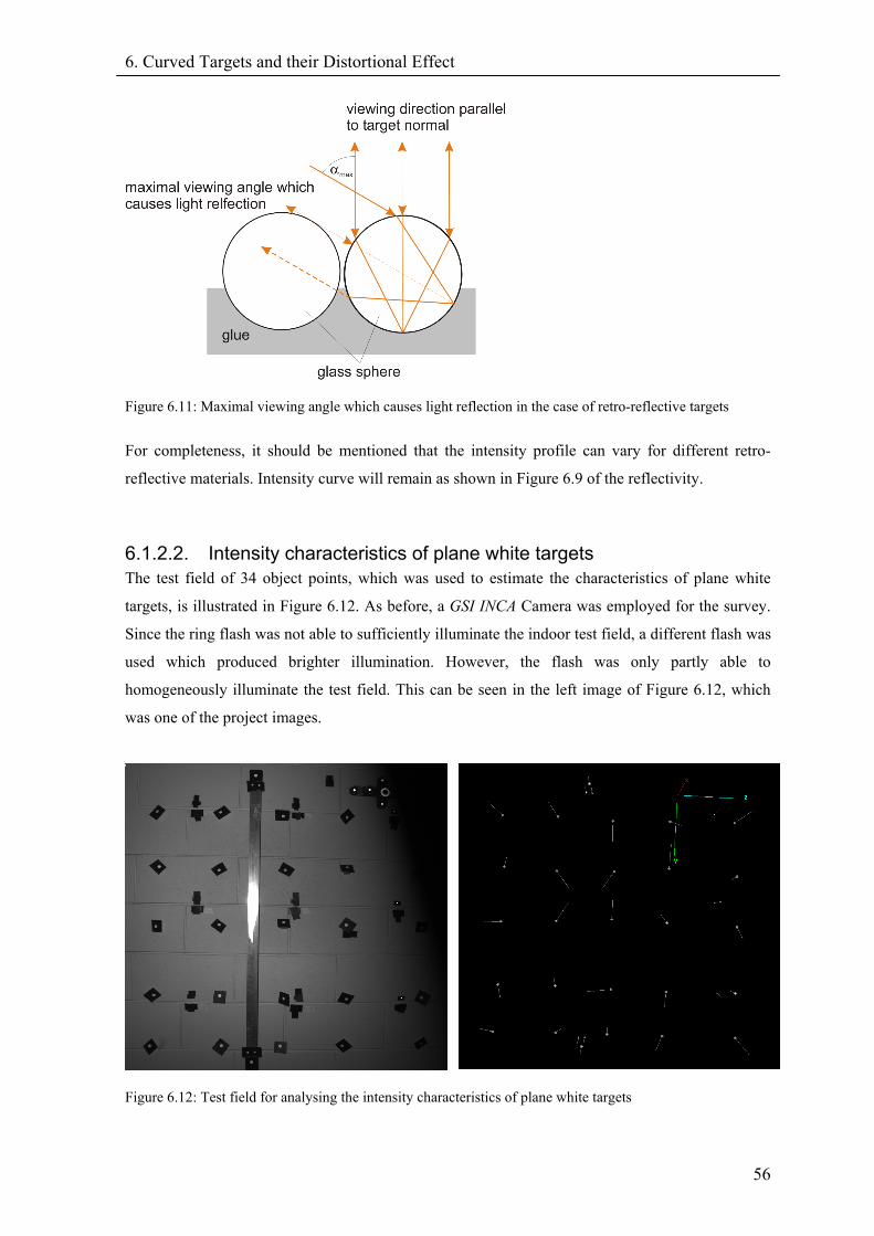
6. Curved Targets and their Distortional Effect
56
Figure 6.11: Maximal viewing angle which causes light reflection in the case of retro-reflective targets
For completeness, it should be mentioned that the intensity profile can vary for different retro-
reflective materials. Intensity curve will remain as shown in Figure 6.9 of the reflectivity.
6.1.2.2. Intensity characteristics of plane white targets The test field of 34 object points, which was used to estimate the characteristics of plane white
targets, is illustrated in Figure 6.12. As before, a GSI INCA Camera was employed for the survey.
Since the ring flash was not able to sufficiently illuminate the indoor test field, a different flash was
used which produced brighter illumination. However, the flash was only partly able to
homogeneously illuminate the test field. This can be seen in the left image of Figure 6.12, which
was one of the project images.
Figure 6.12: Test field for analysing the intensity characteristics of plane white targets
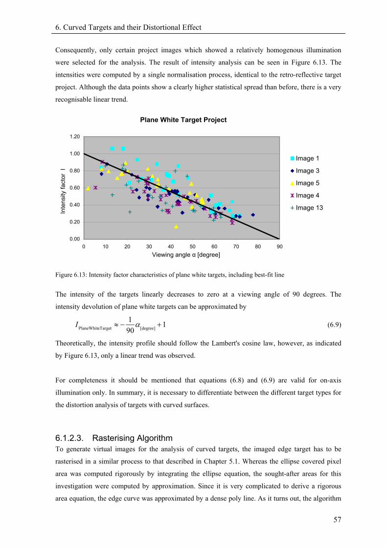
6. Curved Targets and their Distortional Effect
57
Consequently, only certain project images which showed a relatively homogenous illumination
were selected for the analysis. The result of intensity analysis can be seen in Figure 6.13. The
intensities were computed by a single normalisation process, identical to the retro-reflective target
project. Although the data points show a clearly higher statistical spread than before, there is a very
recognisable linear trend.
Plane White Target Project
0.00
0.20
0.40
0.60
0.80
1.00
1.20
0 10 20 30 40 50 60 70 80 90
Image 1
Image 3
Image 5
Image 4
Image 13
Viewing angle α [degree]
Inte
nsity
fact
or I
Figure 6.13: Intensity factor characteristics of plane white targets, including best-fit line
The intensity of the targets linearly decreases to zero at a viewing angle of 90 degrees. The
intensity devolution of plane white targets can be approximated by
PlaneWhiteTarget [degree]
1 190
I α≈ − + (6.9)
Theoretically, the intensity profile should follow the Lambert's cosine law, however, as indicated
by Figure 6.13, only a linear trend was observed.
For completeness it should be mentioned that equations (6.8) and (6.9) are valid for on-axis
illumination only. In summary, it is necessary to differentiate between the different target types for
the distortion analysis of targets with curved surfaces.
6.1.2.3. Rasterising Algorithm To generate virtual images for the analysis of curved targets, the imaged edge target has to be
rasterised in a similar process to that described in Chapter 5.1. Whereas the ellipse covered pixel
area was computed rigorously by integrating the ellipse equation, the sought-after areas for this
investigation were computed by approximation. Since it is very complicated to derive a rigorous
area equation, the edge curve was approximated by a dense poly line. As it turns out, the algorithm
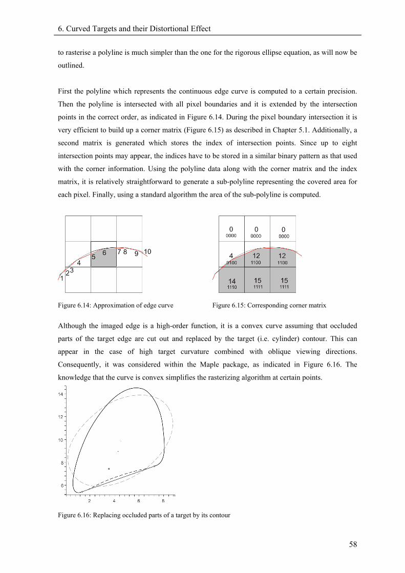
6. Curved Targets and their Distortional Effect
58
to rasterise a polyline is much simpler than the one for the rigorous ellipse equation, as will now be
outlined.
First the polyline which represents the continuous edge curve is computed to a certain precision.
Then the polyline is intersected with all pixel boundaries and it is extended by the intersection
points in the correct order, as indicated in Figure 6.14. During the pixel boundary intersection it is
very efficient to build up a corner matrix (Figure 6.15) as described in Chapter 5.1. Additionally, a
second matrix is generated which stores the index of intersection points. Since up to eight
intersection points may appear, the indices have to be stored in a similar binary pattern as that used
with the corner information. Using the polyline data along with the corner matrix and the index
matrix, it is relatively straightforward to generate a sub-polyline representing the covered area for
each pixel. Finally, using a standard algorithm the area of the sub-polyline is computed.
Figure 6.14: Approximation of edge curve
Figure 6.15: Corresponding corner matrix
Although the imaged edge is a high-order function, it is a convex curve assuming that occluded
parts of the target edge are cut out and replaced by the target (i.e. cylinder) contour. This can
appear in the case of high target curvature combined with oblique viewing directions.
Consequently, it was considered within the Maple package, as indicated in Figure 6.16. The
knowledge that the curve is convex simplifies the rasterizing algorithm at certain points.
Figure 6.16: Replacing occluded parts of a target by its contour
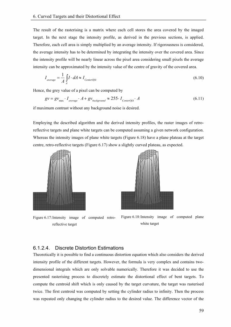
6. Curved Targets and their Distortional Effect
59
The result of the rasterising is a matrix where each cell stores the area covered by the imaged
target. In the next stage the intensity profile, as derived in the previous sections, is applied.
Therefore, each cell area is simply multiplied by an average intensity. If rigorousness is considered,
the average intensity has to be determined by integrating the intensity over the covered area. Since
the intensity profile will be nearly linear across the pixel area considering small pixels the average
intensity can be approximated by the intensity value of the centre of gravity of the covered area.
1
average CenterOfAA
I I dA IA
= ⋅ ≈∫ (6.10)
Hence, the grey value of a pixel can be computed by
(6.11) max 255average background CenterOfAgv gv I A gv I A= ⋅ ⋅ + ≈ ⋅ ⋅
if maximum contrast without any background noise is desired.
Employing the described algorithm and the derived intensity profiles, the raster images of retro-
reflective targets and plane white targets can be computed assuming a given network configuration.
Whereas the intensity images of plane white targets (Figure 6.18) have a plane plateau at the target
centre, retro-reflective targets (Figure 6.17) show a slightly curved plateau, as expected.
Figure 6.17: Intensity image of computed retro-
reflective target
Figure 6.18: Intensity image of computed plane
white target
6.1.2.4. Discrete Distortion Estimations Theoretically it is possible to find a continuous distortion equation which also considers the derived
intensity profile of the different targets. However, the formula is very complex and contains two-
dimensional integrals which are only solvable numerically. Therefore it was decided to use the
presented rasterising process to discretely estimate the distortional effect of bent targets. To
compute the centroid shift which is only caused by the target curvature, the target was rasterised
twice. The first centroid was computed by setting the cylinder radius to infinity. Then the process
was repeated only changing the cylinder radius to the desired value. The difference vector of the
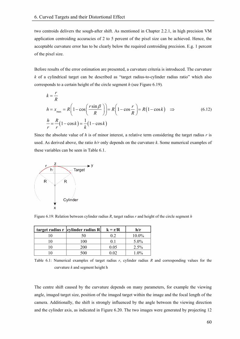
6. Curved Targets and their Distortional Effect
60
two centroids delivers the sough-after shift. As mentioned in Chapter 2.2.1, in high precision VM
application centroiding accuracies of 2 to 5 percent of the pixel size can be achieved. Hence, the
acceptable curvature error has to be clearly below the required centroiding precision. E.g. 1 percent
of the pixel size.
Before results of the error estimation are presented, a curvature criteria is introduced. The curvature
k of a cylindrical target can be described as “target radius-to-cylinder radius ratio” which also
corresponds to a certain height of the circle segment h (see Figure 6.19).
( )
( ) ( )
max
sin1 cos 1 cos 1 cos
11 cos 1 cos
rkR
r rh x R R R kR R
h R k kr r k
β
=
⎛ ⎞⎛ ⎞ ⎛ ⎞= = − = − = −⎜ ⎟ ⎜ ⎟⎜ ⎟⎝ ⎠ ⎝ ⎠⎝ ⎠
= − = −
⇒ (6.12)
Since the absolute value of h is of minor interest, a relative term considering the target radius r is
used. As derived above, the ratio h/r only depends on the curvature k. Some numerical examples of
these variables can be seen in Table 6.1.
Figure 6.19: Relation between cylinder radius R, target radius r and height of the circle segment h
target radius r cylinder radius R k = r/R h/r 10 50 0.2 10.0% 10 100 0.1 5.0% 10 200 0.05 2.5% 10 500 0.02 1.0%
Table 6.1: Numerical examples of target radius r, cylinder radius R and corresponding values for the
curvature k and segment height h
The centre shift caused by the curvature depends on many parameters, for example the viewing
angle, imaged target size, position of the imaged target within the image and the focal length of the
camera. Additionally, the shift is strongly influenced by the angle between the viewing direction
and the cylinder axis, as indicated in Figure 6.20. The two images were generated by projecting 12
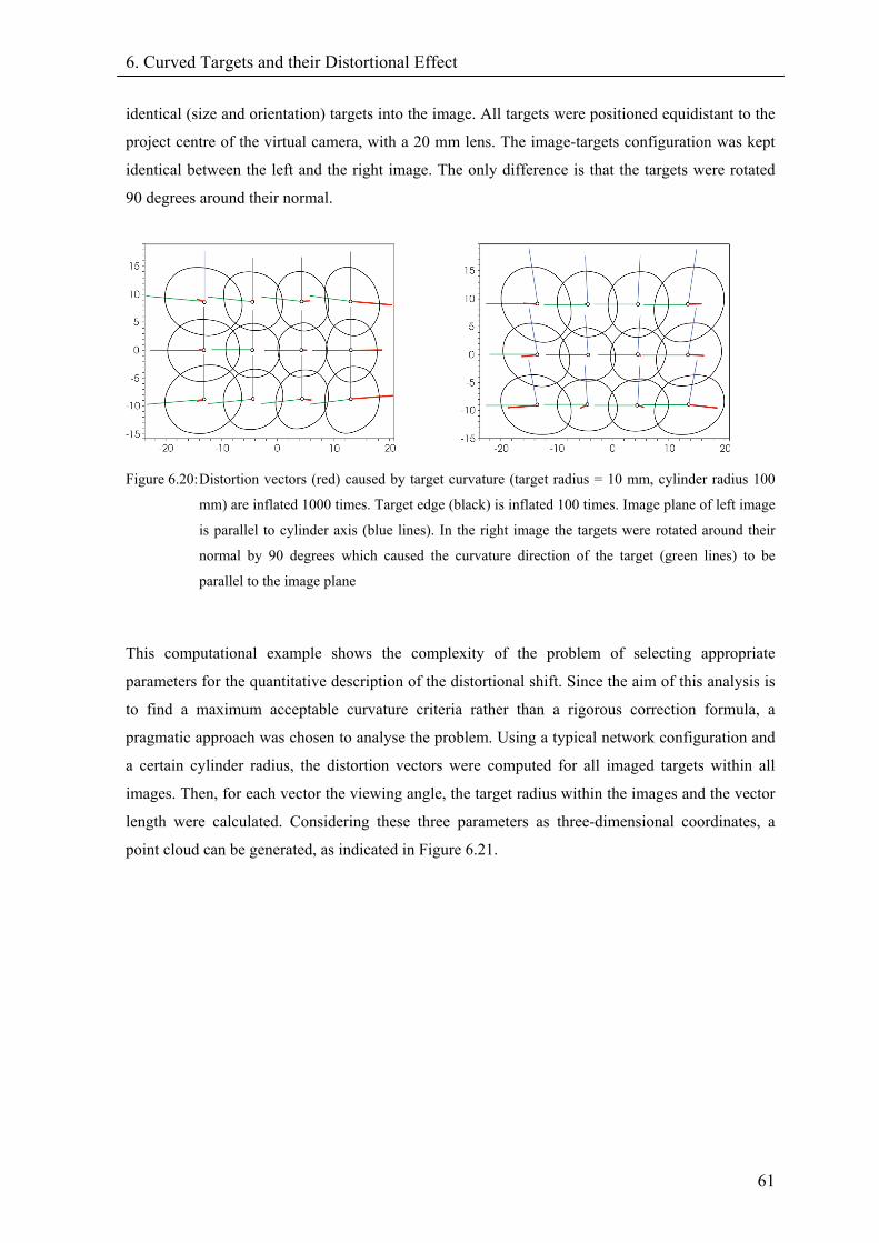
6. Curved Targets and their Distortional Effect
61
identical (size and orientation) targets into the image. All targets were positioned equidistant to the
project centre of the virtual camera, with a 20 mm lens. The image-targets configuration was kept
identical between the left and the right image. The only difference is that the targets were rotated
90 degrees around their normal.
Figure 6.20: Distortion vectors (red) caused by target curvature (target radius = 10 mm, cylinder radius 100
mm) are inflated 1000 times. Target edge (black) is inflated 100 times. Image plane of left image
is parallel to cylinder axis (blue lines). In the right image the targets were rotated around their
normal by 90 degrees which caused the curvature direction of the target (green lines) to be
parallel to the image plane
This computational example shows the complexity of the problem of selecting appropriate
parameters for the quantitative description of the distortional shift. Since the aim of this analysis is
to find a maximum acceptable curvature criteria rather than a rigorous correction formula, a
pragmatic approach was chosen to analyse the problem. Using a typical network configuration and
a certain cylinder radius, the distortion vectors were computed for all imaged targets within all
images. Then, for each vector the viewing angle, the target radius within the images and the vector
length were calculated. Considering these three parameters as three-dimensional coordinates, a
point cloud can be generated, as indicated in Figure 6.21.
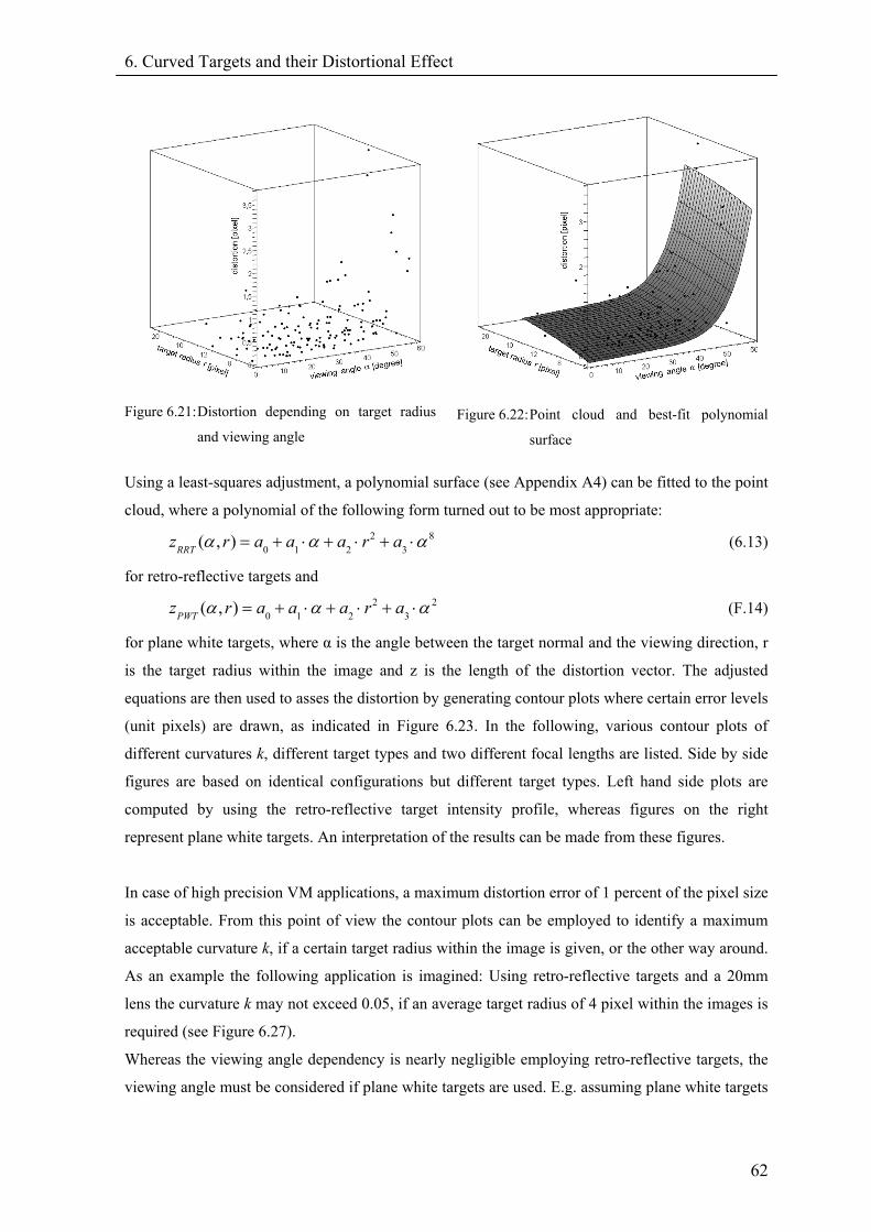
6. Curved Targets and their Distortional Effect
62
Figure 6.21: Distortion depending on target radius
and viewing angle
Figure 6.22: Point cloud and best-fit polynomial
surface
Using a least-squares adjustment, a polynomial surface (see Appendix A4) can be fitted to the point
cloud, where a polynomial of the following form turned out to be most appropriate:
20 1 2 3( , )RRTz r a a a r a 8α α= + ⋅ + ⋅ + ⋅α
2
(6.13)
for retro-reflective targets and
20 1 2 3( , )PWTz r a a a r aα α= + ⋅ + ⋅ + ⋅α (F.14)
for plane white targets, where α is the angle between the target normal and the viewing direction, r
is the target radius within the image and z is the length of the distortion vector. The adjusted
equations are then used to asses the distortion by generating contour plots where certain error levels
(unit pixels) are drawn, as indicated in Figure 6.23. In the following, various contour plots of
different curvatures k, different target types and two different focal lengths are listed. Side by side
figures are based on identical configurations but different target types. Left hand side plots are
computed by using the retro-reflective target intensity profile, whereas figures on the right
represent plane white targets. An interpretation of the results can be made from these figures.
In case of high precision VM applications, a maximum distortion error of 1 percent of the pixel size
is acceptable. From this point of view the contour plots can be employed to identify a maximum
acceptable curvature k, if a certain target radius within the image is given, or the other way around.
As an example the following application is imagined: Using retro-reflective targets and a 20mm
lens the curvature k may not exceed 0.05, if an average target radius of 4 pixel within the images is
required (see Figure 6.27).
Whereas the viewing angle dependency is nearly negligible employing retro-reflective targets, the
viewing angle must be considered if plane white targets are used. E.g. assuming plane white targets
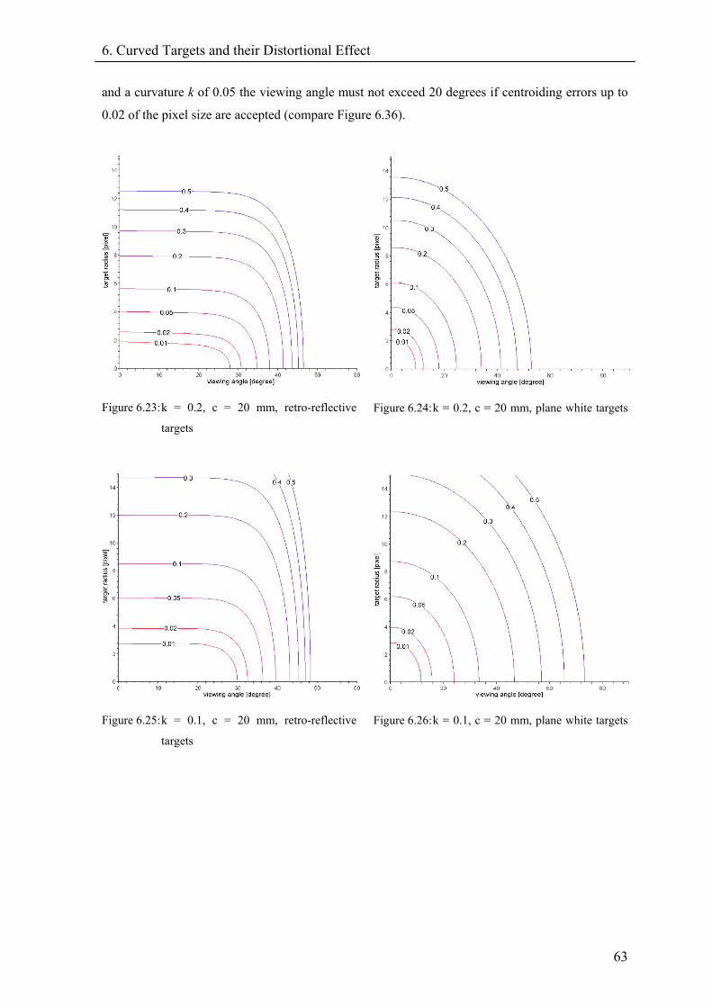
6. Curved Targets and their Distortional Effect
63
and a curvature k of 0.05 the viewing angle must not exceed 20 degrees if centroiding errors up to
0.02 of the pixel size are accepted (compare Figure 6.36).
Figure 6.23: k = 0.2, c = 20 mm, retro-reflective
targets
Figure 6.24: k = 0.2, c = 20 mm, plane white targets
Figure 6.25: k = 0.1, c = 20 mm, retro-reflective
targets
Figure 6.26: k = 0.1, c = 20 mm, plane white targets
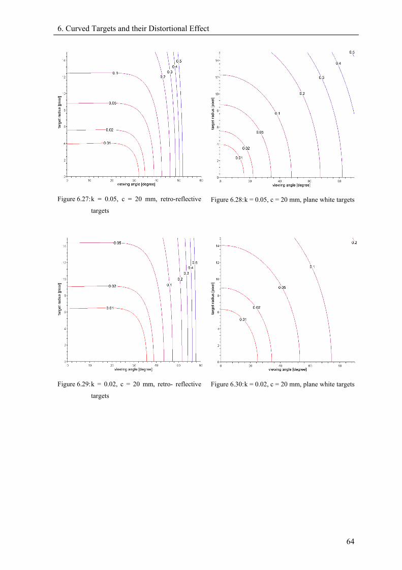
6. Curved Targets and their Distortional Effect
64
Figure 6.27: k = 0.05, c = 20 mm, retro-reflective
targets
Figure 6.28: k = 0.05, c = 20 mm, plane white targets
Figure 6.29: k = 0.02, c = 20 mm, retro- reflective
targets
Figure 6.30: k = 0.02, c = 20 mm, plane white targets
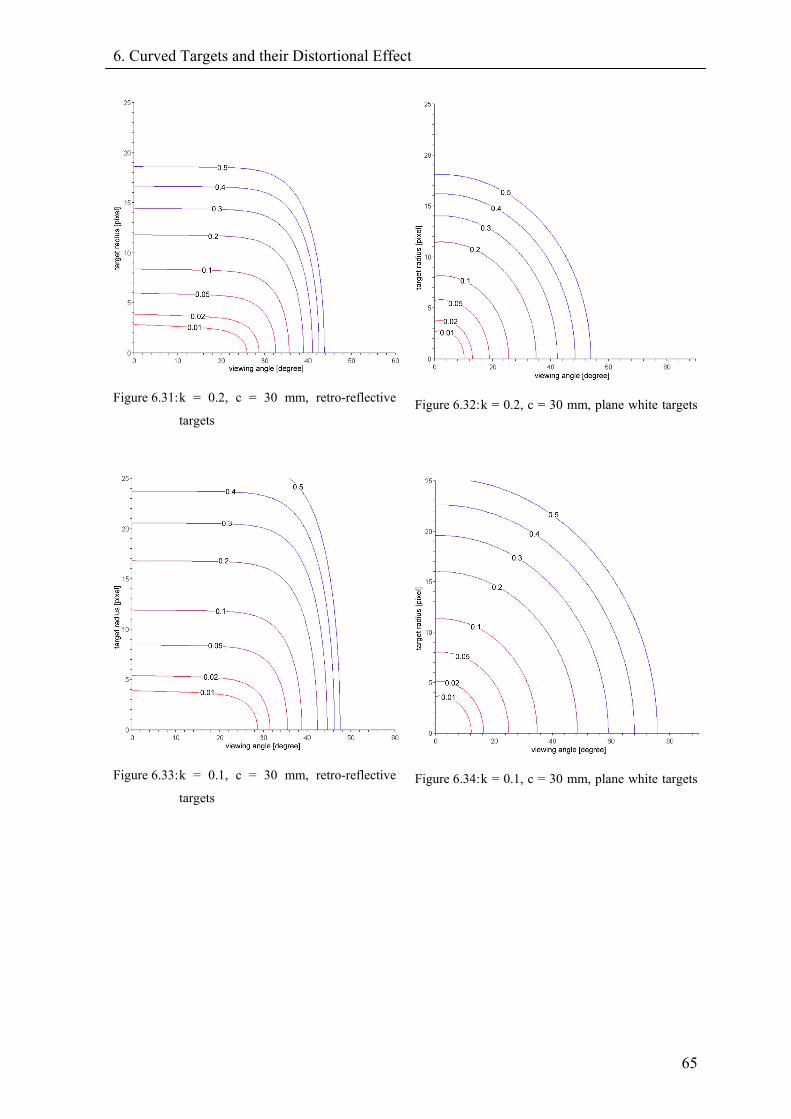
6. Curved Targets and their Distortional Effect
65
Figure 6.31: k = 0.2, c = 30 mm, retro-reflective
targets
Figure 6.32: k = 0.2, c = 30 mm, plane white targets
Figure 6.33: k = 0.1, c = 30 mm, retro-reflective
targets
Figure 6.34: k = 0.1, c = 30 mm, plane white targets
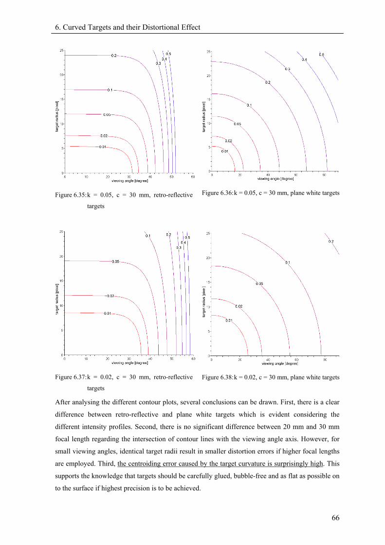
6. Curved Targets and their Distortional Effect
66
Figure 6.35: k = 0.05, c = 30 mm, retro-reflective
targets
Figure 6.36: k = 0.05, c = 30 mm, plane white targets
Figure 6.37: k = 0.02, c = 30 mm, retro-reflective
targets
Figure 6.38: k = 0.02, c = 30 mm, plane white targets
After analysing the different contour plots, several conclusions can be drawn. First, there is a clear
difference between retro-reflective and plane white targets which is evident considering the
different intensity profiles. Second, there is no significant difference between 20 mm and 30 mm
focal length regarding the intersection of contour lines with the viewing angle axis. However, for
small viewing angles, identical target radii result in smaller distortion errors if higher focal lengths
are employed. Third, the centroiding error caused by the target curvature is surprisingly high. This
supports the knowledge that targets should be carefully glued, bubble-free and as flat as possible on
to the surface if highest precision is to be achieved.
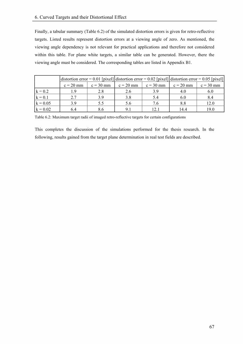
6. Curved Targets and their Distortional Effect
67
Finally, a tabular summary (Table 6.2) of the simulated distortion errors is given for retro-reflective
targets. Listed results represent distortion errors at a viewing angle of zero. As mentioned, the
viewing angle dependency is not relevant for practical applications and therefore not considered
within this table. For plane white targets, a similar table can be generated. However, there the
viewing angle must be considered. The corresponding tables are listed in Appendix B1.
distortion error = 0.01 [pixel] distortion error = 0.02 [pixel] distortion error = 0.05 [pixel] c = 20 mm c = 30 mm c = 20 mm c = 30 mm c = 20 mm c = 30 mm k = 0.2 1.9 2.8 2.6 3.9 4.0 6.0 k = 0.1 2.7 3.9 3.8 5.4 6.0 8.4 k = 0.05 3.9 5.5 5.6 7.6 8.8 12.0 k = 0.02 6.4 8.6 9.1 12.1 14.4 19.0
Table 6.2: Maximum target radii of imaged retro-reflective targets for certain configurations
This completes the discussion of the simulations performed for the thesis research. In the
following, results gained from the target plane determination in real test fields are described.
7. Evaluation of Target Plane Determination
68
7. Evaluation of Target Plane Determination This chapter addresses practical aspects of the developed target plane determination process. The
precision of the computed target planes will be reported. Initially, however, a short introduction to
the photogrammetric software package Australis will be given, since all developed processes and
algorithms were implemented and evaluated within this software system designed for VM.
7.1. Australis: An Ideal Evaluation Environment Australis (Photometrix 2004) was originally developed at the Department of Geomatics, University
of Melbourne, but it is now maintained and distributed Photometrix Pty Ltd. The software package
is designed for off-line digital close-range photogrammetric image measurement, orientation,
triangulation and sensor calibration. It is used to teach photogrammetric principles and practices
and is a valuable tool for both research and practical measurement applications. At present there are
more than 80 installations of Australis worldwide.
Australis uses images produced from digital cameras or digitally scanned imagery from film-based
cameras. It is equally useful for high-precision metrology applications using ‘metric’ digital
cameras (or scanned imagery) or low- to moderate-accuracy measurement employing off-the-shelf,
amateur still video CCD cameras. The software offers manual, semiautomatic and fully automatic
measurement techniques.
Since Australis provides all standard photogrammetric procedures, and a high degree of user
interaction, it turned out to be an ideal tool to implement and evaluate the developed processes. The
software is programmed in Microsoft Visual C++, which is why the new algorithms were also
implemented in object-orientated code within the same language. Although a lot of research time
was consumed by programming and evaluating the new algorithms, an attempt was made to focus
on the theoretical and mathematical aspects of target mensuration. This explains why the users
point of view of the new developments is presented, rather than a detailed account of the source
code development. For completeness, it should be mentioned that all eccentricity simulations of
Chapter 5 were also performed using Australis.
At the current state the target plane determination is performed as a post-processing stage to the
normal photogrammetric orientation process. This gives the user the option to employ the
corrective process only, if required. Additionally, a fully resolved network simplifies certain stages
of the target plane determination.
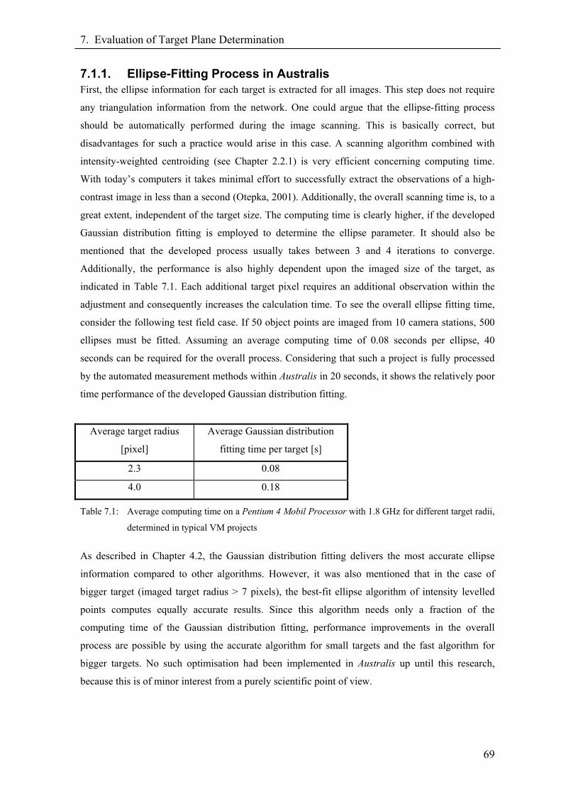
7. Evaluation of Target Plane Determination
69
7.1.1. Ellipse-Fitting Process in Australis First, the ellipse information for each target is extracted for all images. This step does not require
any triangulation information from the network. One could argue that the ellipse-fitting process
should be automatically performed during the image scanning. This is basically correct, but
disadvantages for such a practice would arise in this case. A scanning algorithm combined with
intensity-weighted centroiding (see Chapter 2.2.1) is very efficient concerning computing time.
With today’s computers it takes minimal effort to successfully extract the observations of a high-
contrast image in less than a second (Otepka, 2001). Additionally, the overall scanning time is, to a
great extent, independent of the target size. The computing time is clearly higher, if the developed
Gaussian distribution fitting is employed to determine the ellipse parameter. It should also be
mentioned that the developed process usually takes between 3 and 4 iterations to converge.
Additionally, the performance is also highly dependent upon the imaged size of the target, as
indicated in Table 7.1. Each additional target pixel requires an additional observation within the
adjustment and consequently increases the calculation time. To see the overall ellipse fitting time,
consider the following test field case. If 50 object points are imaged from 10 camera stations, 500
ellipses must be fitted. Assuming an average computing time of 0.08 seconds per ellipse, 40
seconds can be required for the overall process. Considering that such a project is fully processed
by the automated measurement methods within Australis in 20 seconds, it shows the relatively poor
time performance of the developed Gaussian distribution fitting.
Average target radius
[pixel]
Average Gaussian distribution
fitting time per target [s]
2.3 0.08
4.0 0.18
Table 7.1: Average computing time on a Pentium 4 Mobil Processor with 1.8 GHz for different target radii,
determined in typical VM projects
As described in Chapter 4.2, the Gaussian distribution fitting delivers the most accurate ellipse
information compared to other algorithms. However, it was also mentioned that in the case of
bigger target (imaged target radius > 7 pixels), the best-fit ellipse algorithm of intensity levelled
points computes equally accurate results. Since this algorithm needs only a fraction of the
computing time of the Gaussian distribution fitting, performance improvements in the overall
process are possible by using the accurate algorithm for small targets and the fast algorithm for
bigger targets. No such optimisation had been implemented in Australis up until this research,
because this is of minor interest from a purely scientific point of view.
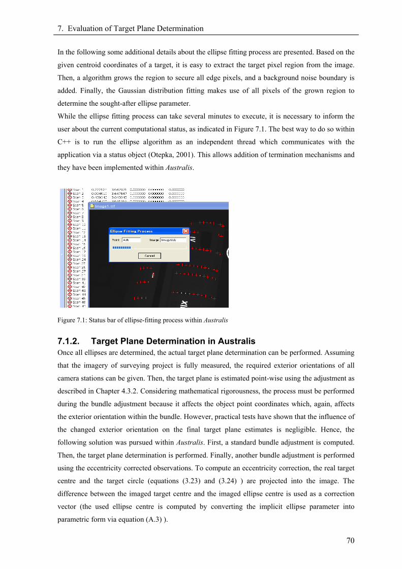
7. Evaluation of Target Plane Determination
70
In the following some additional details about the ellipse fitting process are presented. Based on the
given centroid coordinates of a target, it is easy to extract the target pixel region from the image.
Then, a algorithm grows the region to secure all edge pixels, and a background noise boundary is
added. Finally, the Gaussian distribution fitting makes use of all pixels of the grown region to
determine the sought-after ellipse parameter.
While the ellipse fitting process can take several minutes to execute, it is necessary to inform the
user about the current computational status, as indicated in Figure 7.1. The best way to do so within
C++ is to run the ellipse algorithm as an independent thread which communicates with the
application via a status object (Otepka, 2001). This allows addition of termination mechanisms and
they have been implemented within Australis.
Figure 7.1: Status bar of ellipse-fitting process within Australis
7.1.2. Target Plane Determination in Australis Once all ellipses are determined, the actual target plane determination can be performed. Assuming
that the imagery of surveying project is fully measured, the required exterior orientations of all
camera stations can be given. Then, the target plane is estimated point-wise using the adjustment as
described in Chapter 4.3.2. Considering mathematical rigorousness, the process must be performed
during the bundle adjustment because it affects the object point coordinates which, again, affects
the exterior orientation within the bundle. However, practical tests have shown that the influence of
the changed exterior orientation on the final target plane estimates is negligible. Hence, the
following solution was pursued within Australis. First, a standard bundle adjustment is computed.
Then, the target plane determination is performed. Finally, another bundle adjustment is performed
using the eccentricity corrected observations. To compute an eccentricity correction, the real target
centre and the target circle (equations (3.23) and (3.24) ) are projected into the image. The
difference between the imaged target centre and the imaged ellipse centre is used as a correction
vector (the used ellipse centre is computed by converting the implicit ellipse parameter into
parametric form via equation (A.3) ).
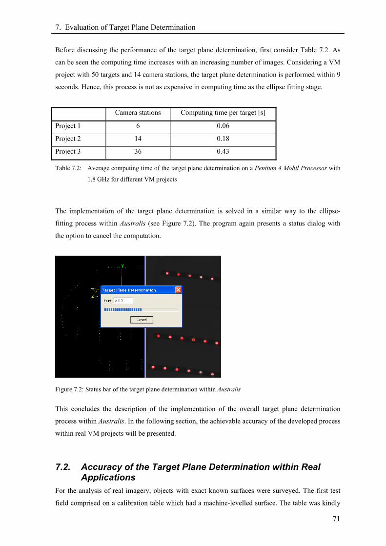
7. Evaluation of Target Plane Determination
71
Before discussing the performance of the target plane determination, first consider Table 7.2. As
can be seen the computing time increases with an increasing number of images. Considering a VM
project with 50 targets and 14 camera stations, the target plane determination is performed within 9
seconds. Hence, this process is not as expensive in computing time as the ellipse fitting stage.
Camera stations Computing time per target [s]
Project 1 6 0.06
Project 2 14 0.18
Project 3 36 0.43
Table 7.2: Average computing time of the target plane determination on a Pentium 4 Mobil Processor with
1.8 GHz for different VM projects
The implementation of the target plane determination is solved in a similar way to the ellipse-
fitting process within Australis (see Figure 7.2). The program again presents a status dialog with
the option to cancel the computation.
Figure 7.2: Status bar of the target plane determination within Australis
This concludes the description of the implementation of the overall target plane determination
process within Australis. In the following section, the achievable accuracy of the developed process
within real VM projects will be presented.
7.2. Accuracy of the Target Plane Determination within Real Applications
For the analysis of real imagery, objects with exact known surfaces were surveyed. The first test
field comprised on a calibration table which had a machine-levelled surface. The table was kindly
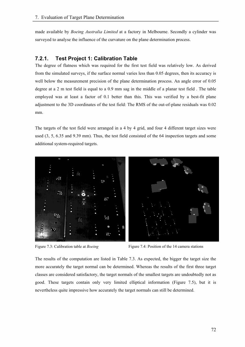
7. Evaluation of Target Plane Determination
72
made available by Boeing Australia Limited at a factory in Melbourne. Secondly a cylinder was
surveyed to analyse the influence of the curvature on the plane determination process.
7.2.1. Test Project 1: Calibration Table The degree of flatness which was required for the first test field was relatively low. As derived
from the simulated surveys, if the surface normal varies less than 0.05 degrees, then its accuracy is
well below the measurement precision of the plane determination process. An angle error of 0.05
degree at a 2 m test field is equal to a 0.9 mm sag in the middle of a planar test field . The table
employed was at least a factor of 0.1 better than this. This was verified by a best-fit plane
adjustment to the 3D coordinates of the test field: The RMS of the out-of-plane residuals was 0.02
mm.
The targets of the test field were arranged in a 4 by 4 grid, and four 4 different target sizes were
used (3, 5, 6.35 and 9.39 mm). Thus, the test field consisted of the 64 inspection targets and some
additional system-required targets.
Figure 7.3: Calibration table at Boeing
Figure 7.4: Position of the 14 camera stations
The results of the computation are listed in Table 7.3. As expected, the bigger the target size the
more accurately the target normal can be determined. Whereas the results of the first three target
classes are considered satisfactory, the target normals of the smallest targets are undoubtedly not as
good. These targets contain only very limited elliptical information (Figure 7.5), but it is
nevertheless quite impressive how accurately the target normals can still be determined.
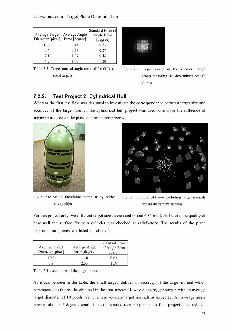
7. Evaluation of Target Plane Determination
73
Average Target Diameter [pixel]
Average Angle Error [degree]
Standard Error of Angle Error
[degree] 13.2 0.43 0.25 8.6 0.57 0.27 7.1 1.09 0.48 4.2 3.06 1.20
Table 7.3: Target normal angle error of the different
sized targets
Figure 7.5: Target image of the smallest target
group including the determined best-fit
ellipse
7.2.2. Test Project 2: Cylindrical Hull Whereas the first test field was designed to investigate the correspondence between target size and
accuracy of the target normal, the cylindrical hull project was used to analyse the influence of
surface curvature on the plane determination process.
Figure 7.6: An old theodolite ‘bomb’ as cylindrical
survey object
Figure 7.7: Final 3D view including target normals
and all 40 camera stations
For this project only two different target sizes were used (3 and 6.35 mm). As before, the quality of
how well the surface fits to a cylinder was checked as satisfactory. The results of the plane
determination process are listed in Table 7.4.
Average Target Diameter [pixel]
Average Angle Error [degree]
Standard Error of Angle Error
[degree] 10.0 1.16 0.61 5.9 2.33 1.59
Table 7.4: Accuracies of the target normal
As it can be seen in the table, the small targets deliver an accuracy of the target normal which
corresponds to the results obtained in the first survey. However, the bigger targets with an average
target diameter of 10 pixels result in less accurate target normals as expected. An average angle
error of about 0.5 degrees would fit to the results from the planar test field project. This reduced
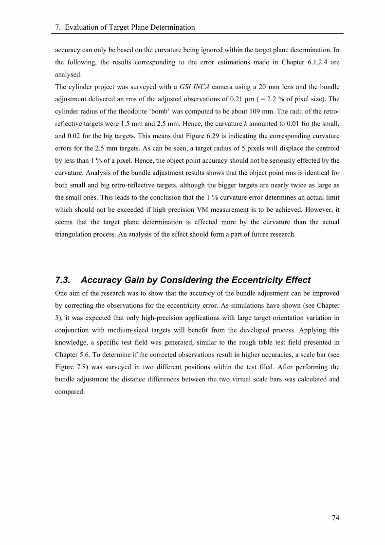
7. Evaluation of Target Plane Determination
74
accuracy can only be based on the curvature being ignored within the target plane determination. In
the following, the results corresponding to the error estimations made in Chapter 6.1.2.4 are
analysed.
The cylinder project was surveyed with a GSI INCA camera using a 20 mm lens and the bundle
adjustment delivered an rms of the adjusted observations of 0.21 µm ( = 2.2 % of pixel size). The
cylinder radius of the theodolite ‘bomb’ was computed to be about 109 mm. The radii of the retro-
reflective targets were 1.5 mm and 2.5 mm. Hence, the curvature k amounted to 0.01 for the small,
and 0.02 for the big targets. This means that Figure 6.29 is indicating the corresponding curvature
errors for the 2.5 mm targets. As can be seen, a target radius of 5 pixels will displace the centroid
by less than 1 % of a pixel. Hence, the object point accuracy should not be seriously effected by the
curvature. Analysis of the bundle adjustment results shows that the object point rms is identical for
both small and big retro-reflective targets, although the bigger targets are nearly twice as large as
the small ones. This leads to the conclusion that the 1 % curvature error determines an actual limit
which should not be exceeded if high precision VM measurement is to be achieved. However, it
seems that the target plane determination is effected more by the curvature than the actual
triangulation process. An analysis of the effect should form a part of future research.
7.3. Accuracy Gain by Considering the Eccentricity Effect One aim of the research was to show that the accuracy of the bundle adjustment can be improved
by correcting the observations for the eccentricity error. As simulations have shown (see Chapter
5), it was expected that only high-precision applications with large target orientation variation in
conjunction with medium-sized targets will benefit from the developed process. Applying this
knowledge, a specific test field was generated, similar to the rough table test field presented in
Chapter 5.6. To determine if the corrected observations result in higher accuracies, a scale bar (see
Figure 7.8) was surveyed in two different positions within the test filed. After performing the
bundle adjustment the distance differences between the two virtual scale bars was calculated and
compared.
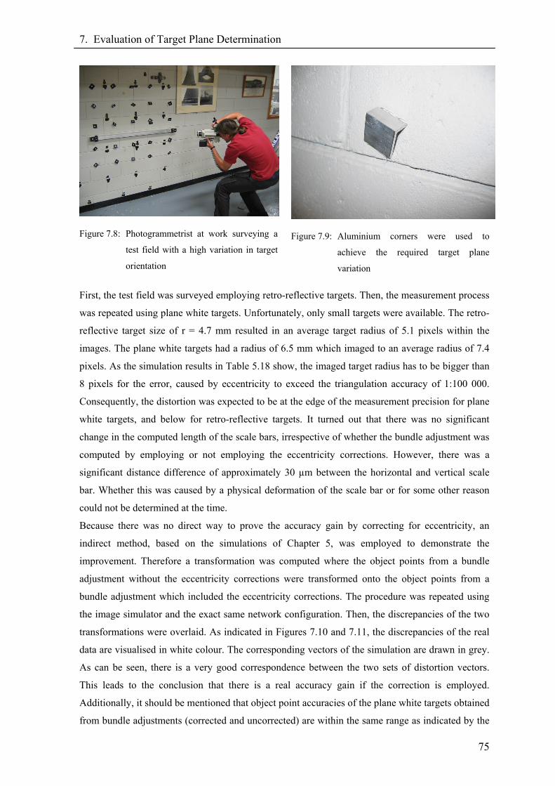
7. Evaluation of Target Plane Determination
75
Figure 7.8: Photogrammetrist at work surveying a
test field with a high variation in target
orientation
Figure 7.9: Aluminium corners were used to
achieve the required target plane
variation
First, the test field was surveyed employing retro-reflective targets. Then, the measurement process
was repeated using plane white targets. Unfortunately, only small targets were available. The retro-
reflective target size of r = 4.7 mm resulted in an average target radius of 5.1 pixels within the
images. The plane white targets had a radius of 6.5 mm which imaged to an average radius of 7.4
pixels. As the simulation results in Table 5.18 show, the imaged target radius has to be bigger than
8 pixels for the error, caused by eccentricity to exceed the triangulation accuracy of 1:100 000.
Consequently, the distortion was expected to be at the edge of the measurement precision for plane
white targets, and below for retro-reflective targets. It turned out that there was no significant
change in the computed length of the scale bars, irrespective of whether the bundle adjustment was
computed by employing or not employing the eccentricity corrections. However, there was a
significant distance difference of approximately 30 µm between the horizontal and vertical scale
bar. Whether this was caused by a physical deformation of the scale bar or for some other reason
could not be determined at the time.
Because there was no direct way to prove the accuracy gain by correcting for eccentricity, an
indirect method, based on the simulations of Chapter 5, was employed to demonstrate the
improvement. Therefore a transformation was computed where the object points from a bundle
adjustment without the eccentricity corrections were transformed onto the object points from a
bundle adjustment which included the eccentricity corrections. The procedure was repeated using
the image simulator and the exact same network configuration. Then, the discrepancies of the two
transformations were overlaid. As indicated in Figures 7.10 and 7.11, the discrepancies of the real
data are visualised in white colour. The corresponding vectors of the simulation are drawn in grey.
As can be seen, there is a very good correspondence between the two sets of distortion vectors.
This leads to the conclusion that there is a real accuracy gain if the correction is employed.
Additionally, it should be mentioned that object point accuracies of the plane white targets obtained
from bundle adjustments (corrected and uncorrected) are within the same range as indicated by the
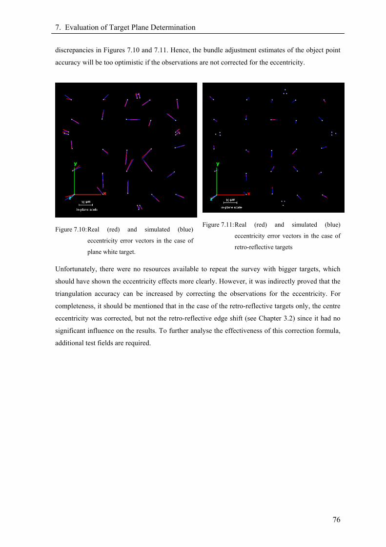
7. Evaluation of Target Plane Determination
76
discrepancies in Figures 7.10 and 7.11. Hence, the bundle adjustment estimates of the object point
accuracy will be too optimistic if the observations are not corrected for the eccentricity.
Figure 7.10: Real (red) and simulated (blue)
eccentricity error vectors in the case of
plane white target.
Figure 7.11: Real (red) and simulated (blue)
eccentricity error vectors in the case of
retro-reflective targets
Unfortunately, there were no resources available to repeat the survey with bigger targets, which
should have shown the eccentricity effects more clearly. However, it was indirectly proved that the
triangulation accuracy can be increased by correcting the observations for the eccentricity. For
completeness, it should be mentioned that in the case of the retro-reflective targets only, the centre
eccentricity was corrected, but not the retro-reflective edge shift (see Chapter 3.2) since it had no
significant influence on the results. To further analyse the effectiveness of this correction formula,
additional test fields are required.
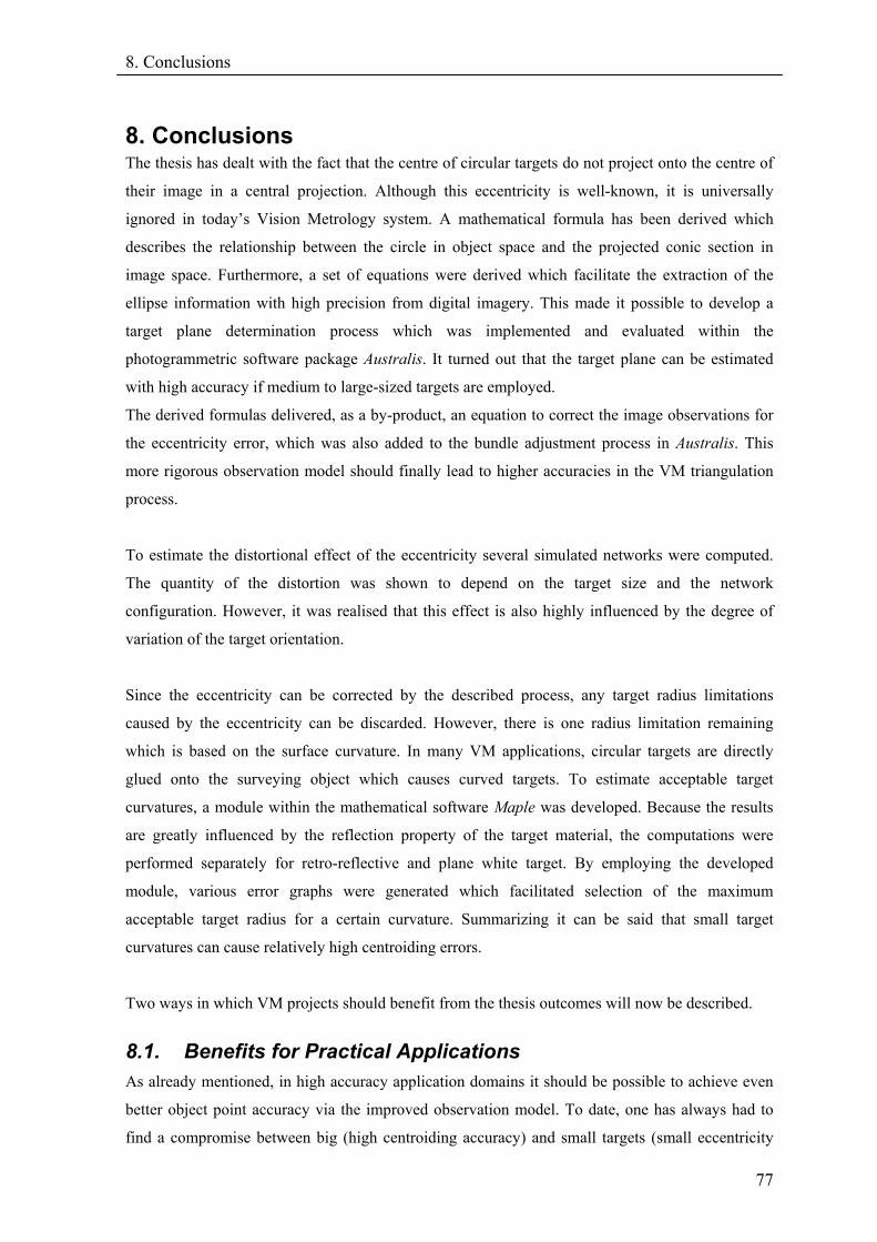
8. Conclusions
8. Conclusions The thesis has dealt with the fact that the centre of circular targets do not project onto the centre of
their image in a central projection. Although this eccentricity is well-known, it is universally
ignored in today’s Vision Metrology system. A mathematical formula has been derived which
describes the relationship between the circle in object space and the projected conic section in
image space. Furthermore, a set of equations were derived which facilitate the extraction of the
ellipse information with high precision from digital imagery. This made it possible to develop a
target plane determination process which was implemented and evaluated within the
photogrammetric software package Australis. It turned out that the target plane can be estimated
with high accuracy if medium to large-sized targets are employed.
The derived formulas delivered, as a by-product, an equation to correct the image observations for
the eccentricity error, which was also added to the bundle adjustment process in Australis. This
more rigorous observation model should finally lead to higher accuracies in the VM triangulation
process.
To estimate the distortional effect of the eccentricity several simulated networks were computed.
The quantity of the distortion was shown to depend on the target size and the network
configuration. However, it was realised that this effect is also highly influenced by the degree of
variation of the target orientation.
Since the eccentricity can be corrected by the described process, any target radius limitations
caused by the eccentricity can be discarded. However, there is one radius limitation remaining
which is based on the surface curvature. In many VM applications, circular targets are directly
glued onto the surveying object which causes curved targets. To estimate acceptable target
curvatures, a module within the mathematical software Maple was developed. Because the results
are greatly influenced by the reflection property of the target material, the computations were
performed separately for retro-reflective and plane white target. By employing the developed
module, various error graphs were generated which facilitated selection of the maximum
acceptable target radius for a certain curvature. Summarizing it can be said that small target
curvatures can cause relatively high centroiding errors.
Two ways in which VM projects should benefit from the thesis outcomes will now be described.
8.1. Benefits for Practical Applications As already mentioned, in high accuracy application domains it should be possible to achieve even
better object point accuracy via the improved observation model. To date, one has always had to
find a compromise between big (high centroiding accuracy) and small targets (small eccentricity
77
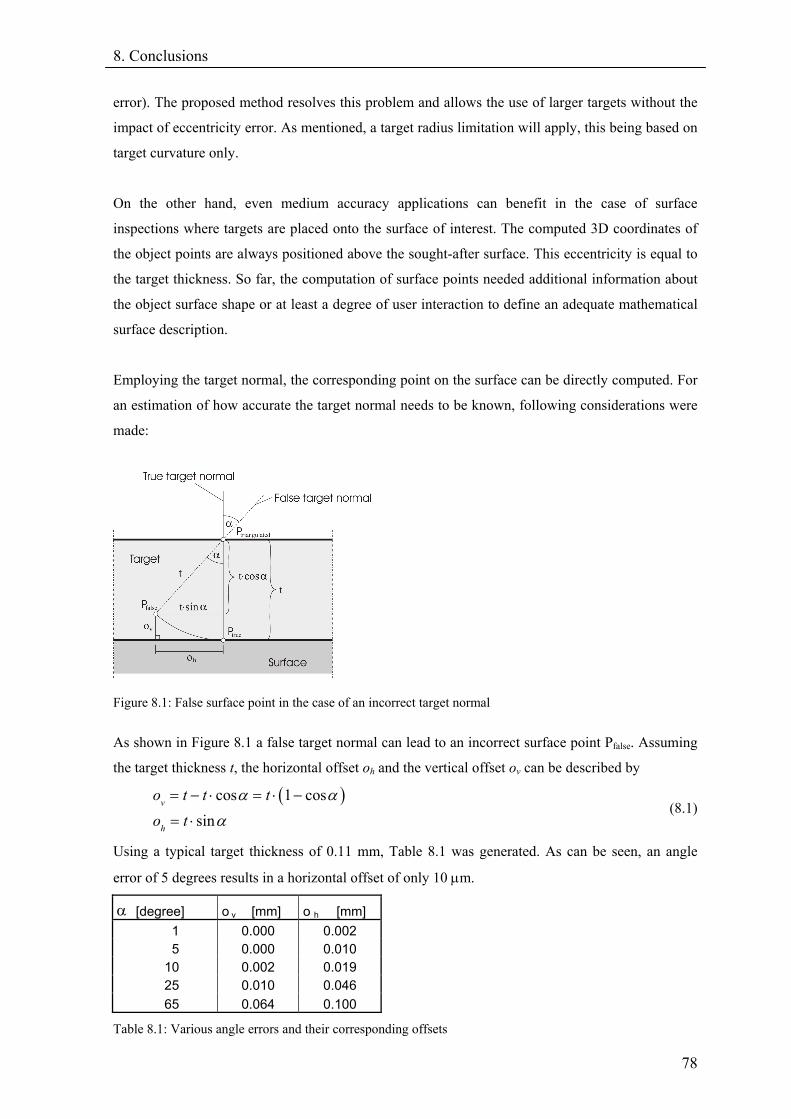
8. Conclusions
error). The proposed method resolves this problem and allows the use of larger targets without the
impact of eccentricity error. As mentioned, a target radius limitation will apply, this being based on
target curvature only.
On the other hand, even medium accuracy applications can benefit in the case of surface
inspections where targets are placed onto the surface of interest. The computed 3D coordinates of
the object points are always positioned above the sought-after surface. This eccentricity is equal to
the target thickness. So far, the computation of surface points needed additional information about
the object surface shape or at least a degree of user interaction to define an adequate mathematical
surface description.
Employing the target normal, the corresponding point on the surface can be directly computed. For
an estimation of how accurate the target normal needs to be known, following considerations were
made:
Figure 8.1: False surface point in the case of an incorrect target normal
As shown in Figure 8.1 a false target normal can lead to an incorrect surface point Pfalse. Assuming
the target thickness t, the horizontal offset oh and the vertical offset ov can be described by
( )cos 1 cos
sinv
h
o t t to t
α α
α
= − ⋅ = ⋅ −
= ⋅ (8.1)
Using a typical target thickness of 0.11 mm, Table 8.1 was generated. As can be seen, an angle
error of 5 degrees results in a horizontal offset of only 10 µm.
α [degree] o v [mm] o h [mm] 1 0.000 0.002 5 0.000 0.010 10 0.002 0.019 25 0.010 0.046 65 0.064 0.100
Table 8.1: Various angle errors and their corresponding offsets
78
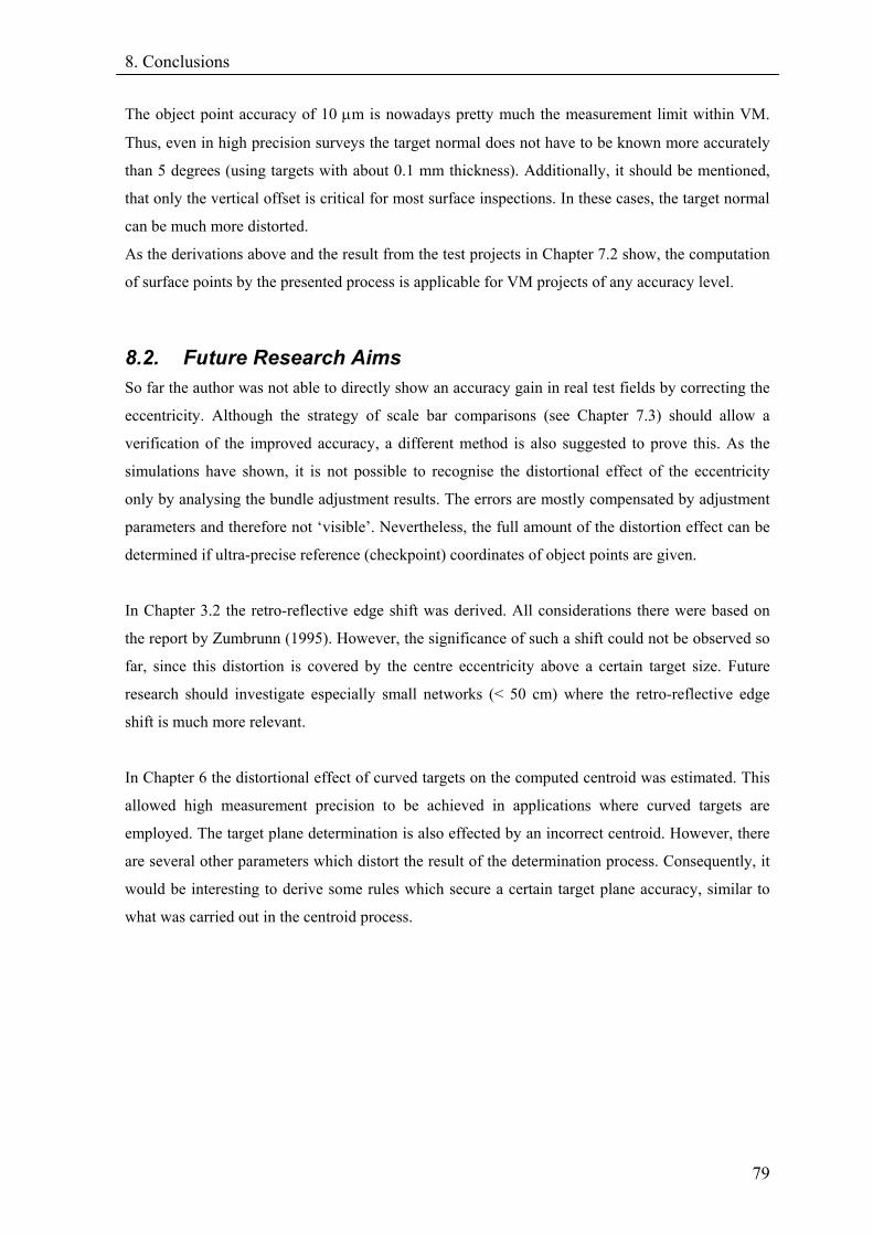
8. Conclusions
The object point accuracy of 10 µm is nowadays pretty much the measurement limit within VM.
Thus, even in high precision surveys the target normal does not have to be known more accurately
than 5 degrees (using targets with about 0.1 mm thickness). Additionally, it should be mentioned,
that only the vertical offset is critical for most surface inspections. In these cases, the target normal
can be much more distorted.
As the derivations above and the result from the test projects in Chapter 7.2 show, the computation
of surface points by the presented process is applicable for VM projects of any accuracy level.
8.2. Future Research Aims So far the author was not able to directly show an accuracy gain in real test fields by correcting the
eccentricity. Although the strategy of scale bar comparisons (see Chapter 7.3) should allow a
verification of the improved accuracy, a different method is also suggested to prove this. As the
simulations have shown, it is not possible to recognise the distortional effect of the eccentricity
only by analysing the bundle adjustment results. The errors are mostly compensated by adjustment
parameters and therefore not ‘visible’. Nevertheless, the full amount of the distortion effect can be
determined if ultra-precise reference (checkpoint) coordinates of object points are given.
In Chapter 3.2 the retro-reflective edge shift was derived. All considerations there were based on
the report by Zumbrunn (1995). However, the significance of such a shift could not be observed so
far, since this distortion is covered by the centre eccentricity above a certain target size. Future
research should investigate especially small networks (< 50 cm) where the retro-reflective edge
shift is much more relevant.
In Chapter 6 the distortional effect of curved targets on the computed centroid was estimated. This
allowed high measurement precision to be achieved in applications where curved targets are
employed. The target plane determination is also effected by an incorrect centroid. However, there
are several other parameters which distort the result of the determination process. Consequently, it
would be interesting to derive some rules which secure a certain target plane accuracy, similar to
what was carried out in the centroid process.
79

Appendix A
Appendix A1 : Conversion of Ellipse Parameters
An ellipse can be described in implicit form as a general polynomial of second degree
(A.1) 2 21 2 3 4 5 1 0a x a xy a y a x a y⋅ + ⋅ + ⋅ + ⋅ + ⋅ − =
or in parametric from as
cos sin cossin cos cos
x
y
Mx AMy B
θ θ αθ θ α
⎛ ⎞⎛ ⎞ ⎛ ⎞⎛ ⎞= +⎜ ⎟⎜ ⎟ ⎜ ⎟⎜ ⎟−⎝ ⎠ ⎝ ⎠⎝ ⎠⎝ ⎠
(A.2)
where Mx, My are the centre coordinates, θ is the bearing of the semi-major axis, A and B are the
semi major and semi minor axes of the ellipse.
By the following equations the implicit parameters can be converted to ellipse parameters:
2 5 3 42
1 3 2
2 4 1 52
1 3 2
2
1 3
24
24
1 arctan2
x
x
a a a aMa a a
a a a aMa a a
aa a
θ
⋅ − ⋅ ⋅=
⋅ ⋅ −
⋅ − ⋅ ⋅=
⋅ ⋅ −
= −−
(A.3)
54
2 21 2 3
54
2 23 2 1
aa12 2
a cos a sin cos sin
aa12 2
a cos a sin cos a sin
x y
x y
M MA
a
M MB
θ θ θ θ
θ θ θ
− −=
⋅ − ⋅ ⋅ + ⋅
− −=
⋅ + ⋅ ⋅ + ⋅ θ
(A.4)
The reverse conversion can be performed by
2 2
1 2 2
2 2 2
2 2
3 2 2
2 21 2
cos sin
1 12 cos sin
sin cos
d 1 x x y y
aA B
aB A
aA B
3M a M M a M a
θ θ
θ θ
θ θ
= +
⎛ ⎞= ⋅ ⋅ ⋅ −⎜ ⎟⎝ ⎠
= +
= − ⋅ − ⋅ ⋅ − ⋅
(A.5)
1 211 4
322 5
33
2
2
x y
y x 2
M a M aaa ad d
M a M aaa ad daad
⋅ ⋅ + ⋅= = −
⋅ ⋅ + ⋅= = −
=
(A.6)
80
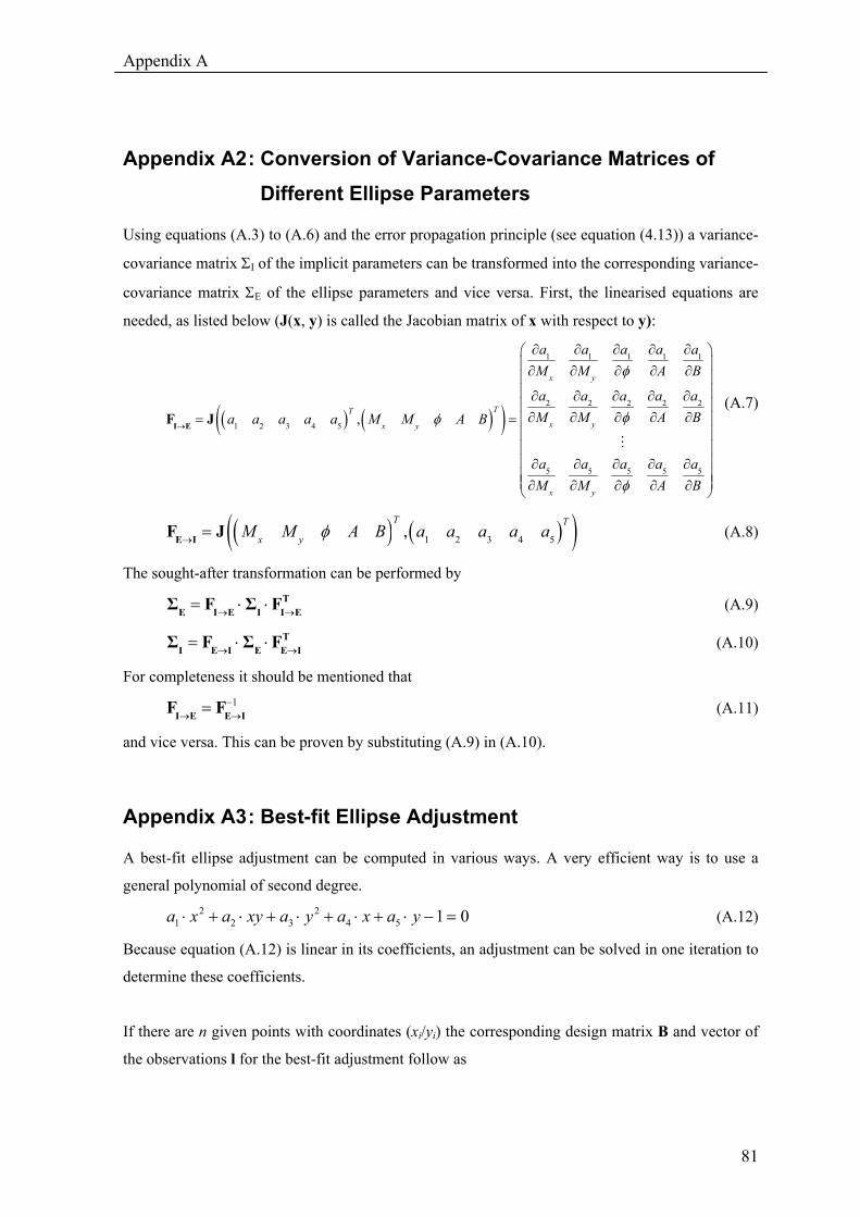
Appendix A
Appendix A2 : Conversion of Variance-Covariance Matrices of Different Ellipse Parameters
Using equations (A.3) to (A.6) and the error propagation principle (see equation (4.13)) a variance-
covariance matrix ΣI of the implicit parameters can be transformed into the corresponding variance-
covariance matrix ΣE of the ellipse parameters and vice versa. First, the linearised equations are
needed, as listed below (J(x, y) is called the Jacobian matrix of x with respect to y):
( ) ( )( )
1 1 1 1 1
2 2 2 2
1 2 3 4 5
5 5 5 5
,
x y
TTx yx y
x y
a a a a a
2
5
M M A
a a a a a
B
M M Aa a a a a M M A B
a a a a a
B
M M A
φ
φφ
φ
→
∂ ∂ ∂ ∂ ∂⎛ ⎞⎜ ⎟
B
∂ ∂ ∂ ∂ ∂⎜ ⎟⎜ ⎟∂ ∂ ∂ ∂ ∂⎜ ⎟
∂ ∂ ∂ ∂ ∂= = ⎜ ⎟⎜ ⎟⎜ ⎟⎜ ⎟∂ ∂ ∂ ∂ ∂⎜ ⎟⎜ ⎟∂ ∂ ∂ ∂ ∂⎝ ⎠
I EF J (A.7)
( ) (( )1 2 3 4 5,T T
x yM M A B a a a a aφ→ =E IF J )
→E
→I
→
(A.8)
The sought-after transformation can be performed by
(A.9) →= ⋅ ⋅ TE I E I IΣ F Σ F
(A.10) →= ⋅ ⋅ TI E I E EΣ F Σ F
For completeness it should be mentioned that
(A.11) 1−→ =I E E IF F
and vice versa. This can be proven by substituting (A.9) in (A.10).
Appendix A3 : Best-fit Ellipse Adjustment
A best-fit ellipse adjustment can be computed in various ways. A very efficient way is to use a
general polynomial of second degree.
(A.12) 2 21 2 3 4 5 1 0a x a xy a y a x a y⋅ + ⋅ + ⋅ + ⋅ + ⋅ − =
Because equation (A.12) is linear in its coefficients, an adjustment can be solved in one iteration to
determine these coefficients.
If there are n given points with coordinates (xi/yi) the corresponding design matrix B and vector of
the observations l for the best-fit adjustment follow as
81
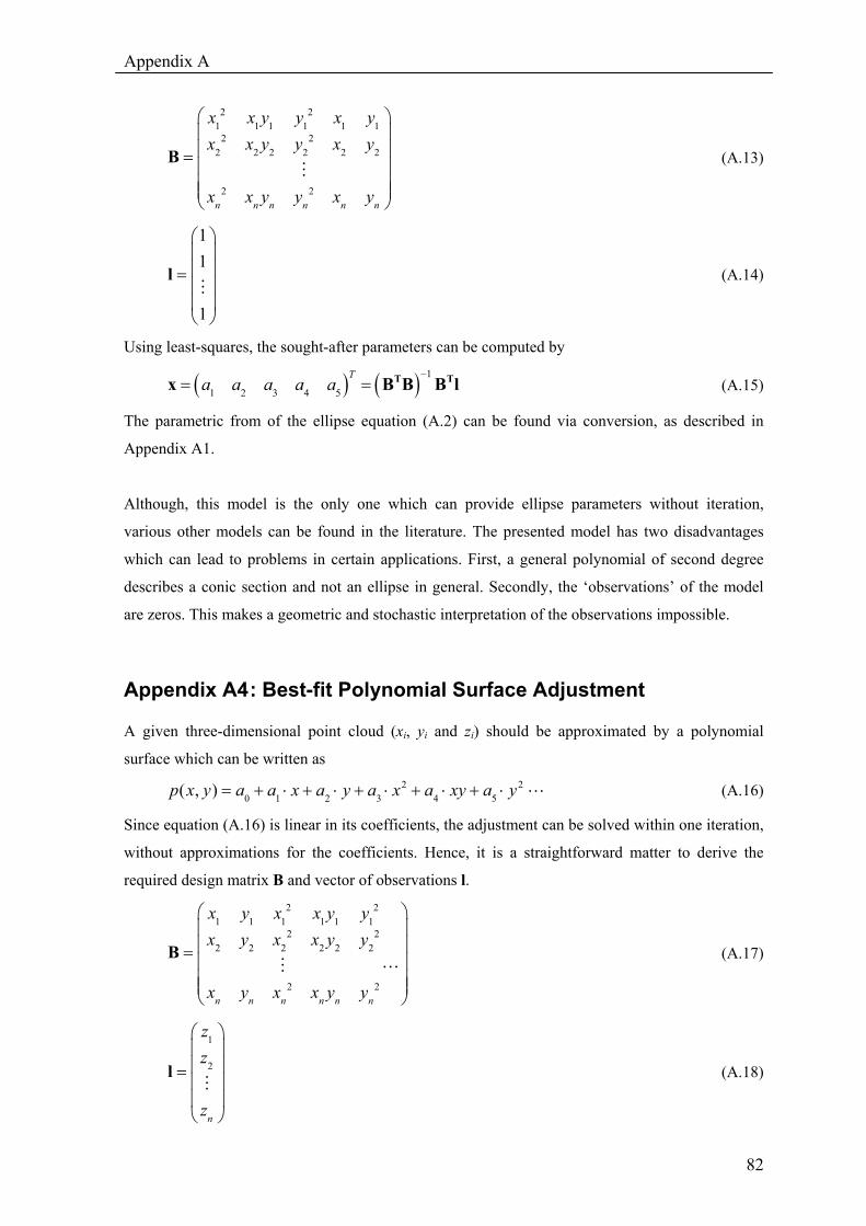
Appendix A
2 21 1 1 1 1 1
2 22 2 2 2 2 2
2 2n n n n n n
x x y y x yx x y y x y
x x y y x y
⎛ ⎞⎜ ⎟⎜= ⎜⎜ ⎟⎜ ⎟⎝ ⎠
B ⎟⎟ (A.13)
(A.14)
11
1
⎛ ⎞⎜ ⎟⎜ ⎟=⎜ ⎟⎜ ⎟⎝ ⎠
l
Using least-squares, the sought-after parameters can be computed by
( ) ( ) 1
1 2 3 4 5
Ta a a a a
−= = Tx TB B B l
2
⎟⎟
(A.15)
The parametric from of the ellipse equation (A.2) can be found via conversion, as described in
Appendix A1.
Although, this model is the only one which can provide ellipse parameters without iteration,
various other models can be found in the literature. The presented model has two disadvantages
which can lead to problems in certain applications. First, a general polynomial of second degree
describes a conic section and not an ellipse in general. Secondly, the ‘observations’ of the model
are zeros. This makes a geometric and stochastic interpretation of the observations impossible.
Appendix A4 : Best-fit Polynomial Surface Adjustment
A given three-dimensional point cloud (xi, yi and zi) should be approximated by a polynomial
surface which can be written as
(A.16) 20 1 2 3 4 5( , )p x y a a x a y a x a xy a y= + ⋅ + ⋅ + ⋅ + ⋅ + ⋅
Since equation (A.16) is linear in its coefficients, the adjustment can be solved within one iteration,
without approximations for the coefficients. Hence, it is a straightforward matter to derive the
required design matrix B and vector of observations l.
(A.17)
2 21 1 1 1 1 1
2 22 2 2 2 2 2
2 2n n n n n n
x y x x y yx y x x y y
x y x x y y
⎛ ⎞⎜ ⎟⎜= ⎜⎜ ⎟⎜ ⎟⎝ ⎠
B
(A.18)
1
2
n
zz
z
⎛ ⎞⎜ ⎟⎜ ⎟=⎜ ⎟⎜ ⎟⎝ ⎠
l
82

Appendix A
Using least-squares, the sought-after coefficients can be computed by
( ) ( ) 1
0 1 2 3 4 5
Ta a a a a a
−= Tx = TB B B l (A.19)
As can be seen, such a surface approximation is very easy to compute. However, it is well known
that polynomial approximations are very sensitive against the degree of the used equation. High
order polynomials tend to ‘swing’, especially at regions with few data points. On the other hand
low-order approximations may not be able to describe the characteristics of the point cloud. Hence,
it is essential to select the appropriate order of the polynomial function.
83
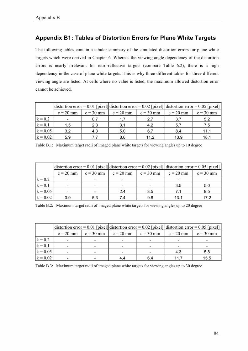
Appendix B
Appendix B1 : Tables of Distortion Errors for Plane White Targets
The following tables contain a tabular summary of the simulated distortion errors for plane white
targets which were derived in Chapter 6. Whereas the viewing angle dependency of the distortion
errors is nearly irrelevant for retro-reflective targets (compare Table 6.2), there is a high
dependency in the case of plane white targets. This is why three different tables for three different
viewing angle are listed. At cells where no value is listed, the maximum allowed distortion error
cannot be achieved.
distortion error = 0.01 [pixel] distortion error = 0.02 [pixel] distortion error = 0.05 [pixel] c = 20 mm c = 30 mm c = 20 mm c = 30 mm c = 20 mm c = 30 mm k = 0.2 - 0.7 1.7 2.7 3.7 5.2 k = 0.1 1.5 2.3 3.1 4.2 5.7 7.5 k = 0.05 3.2 4.3 5.0 6.7 8.4 11.1 k = 0.02 5.9 7.7 8.6 11.2 13.9 18.1
Table B.1: Maximum target radii of imaged plane white targets for viewing angles up to 10 degree
distortion error = 0.01 [pixel] distortion error = 0.02 [pixel] distortion error = 0.05 [pixel] c = 20 mm c = 30 mm c = 20 mm c = 30 mm c = 20 mm c = 30 mm k = 0.2 - - - - - - k = 0.1 - - - - 3.5 5.0 k = 0.05 - - 2.4 3.5 7.1 9.5 k = 0.02 3.9 5.3 7.4 9.8 13.1 17.2
Table B.2: Maximum target radii of imaged plane white targets for viewing angles up to 20 degree
distortion error = 0.01 [pixel] distortion error = 0.02 [pixel] distortion error = 0.05 [pixel] c = 20 mm c = 30 mm c = 20 mm c = 30 mm c = 20 mm c = 30 mm k = 0.2 - - - - - - k = 0.1 - - - - - - k = 0.05 - - - - 4.3 5.8 k = 0.02 - - 4.4 6.4 11.7 15.5
Table B.3: Maximum target radii of imaged plane white targets for viewing angles up to 30 degree
84
References
References Ahn, S. J. and Kotowski, R., 1997. Geometric image measurement errors of circular object targets. Optical 3-
D Measurement Techniques IV (Eds. A. Gruen and H. Kahmen). Herbert Wichmann Verlag, Heidelberg. 494
pages: 463–471.
Ahn, S.J., Warnecke, H.-J. and Kotowski, R., 1999, Systematic Geometric Image Measurement Errors of
Circular Object Targets: Mathematical Formulation and Correction, Photogrammetric Record, 16(93), pp
485-502
Baltsavias E. P., Stallmann D., 1991, Trinocular Vision for Automatic and Robust Three-Dimensional
Determination of the Trajectories of Moving Objects. PERS, Vol. 57, No. 8, pp. 1079 - 1086.
Dold, J., Maas H.-G., 1994, An application of epipolar line intersection in a hybrid close range
photogrammetric system, IAPRS, Vol. 30/5, Melbourne, pp. 65-70
Dold, J., 1996. Influence of large targets on the results of photogrammetric bundle adjustment. International
Archives of Photogrammetry and Remote Sensing, 31(B5): 119–123
Fraser, C.S., 1997, Automation in Digital Close-Range Photogrammetry, 1st Trans Tasman Surveyors
Conference, Fryer J (ed), Proceedings of the 1st Trans Tasman Surveyors Conference, 1: 8.1 - 8.10.
Newcastle, NSW: Institute of Surveyors, Australia.
Fraser, C.S. and Shao, J., 1997, An Image Mensuration Strategy for Automated Vision Metrology, Optical 3D
Measurement Techniques IV, Heidelberg, Germany: Wichmann Verlag, 187-197
Gruen A., Baltsavias E. P., 1988, Geometrically Constrained Multiphoto Matching, PERS, Vol. 54, No. 5,
pp. 633 - 641.
Ho, C.-S., 1983, Precision of Digital Vision Systems. IEEE Transactions on Pattern Analysis & Machine
Intelligence, Vol. PAMI-5, No. 6, 593-601
Kager H., 1981, Bündeltriangulation mit indirekt beobachteten Kreiszentren. Geowissenschaftliche
Mittelungen Heft 19, Institut für Photogrammetrie der Technischen Universität Wien
Kraus, K., 1996, Photogrammetry, Volume 2, Advanced Methods and Applications, with contributions by J.
Jansa and H. Kager, 4th edition, Dümmler/Bonn.
Luhmann, T., 2000, Nahbereichsphotogrammetrie, Grundlagen, Methoden und Anwendungen, Herbert
Wichmann Verlag, pp 408-413
Maplesoft, 2004, Web site: http://www.maplesoft.com/ (accessed October 2004)
Mikhail, E.M., 1983, Photogrammetric Target Location to Sub-Pixel Accuracy in Digital Images. 39th
Photogrammetric Week., Stuttgart, Sept. 19-24, 25 pages.
85
References
Mikhail, Edward M. and Ackermann, F., 1996, Observations and Least Squares, IEP-A Dun-Donnelley
Publisher
Otepka, J., 2001, Algorithms and their Implementation in an Automated Close-Range Photogrammetric
System, Master Thesis, University of Technology Vienna
Otepka, J., Hanely, H.B., Fraser, C.S, 2002, Algorithm Developments for Automated Off-Line Vision
Metrology, Proceedings of the ISPRS Commission V Symposium 2002
Photometrix, 2004, Web site: http://www.photometrix.com.au (accessed October 2004).
Shortis, M.R., Clarke, T.A. and Short, T., 1994, Comparison of some techniques for the subpixel location of
discrete target images, SPIE Proceedings Vol. 2350, Paper #25
Trinder, J.C., 1989. Precision of digital target location. Photogrammetric Engineering & Remote Sensing,
Vol. 55, No 6, June, pp. 883-886
Trinder, J.C., Jansa, J. and Huang, Y., 1995, An assessment of the precision & accuracy of methods of digital
target location. ISPRS Journal of Photogrammetry and Remote Sensing, 50(2): 12-20
Zumbrunn, R., 1995, Systematic pointing errors with retroreflective targets. Optical Engineering, 34(9), pp.
2691–2695.
86

Curriculum Vitae
Johannes Otto Otepka
Date of Birth: 29.10.1975 - Vienna
Education
1981-1985
1985-1993
15.6.1993
Since 1993
9.6.1997
2000-2001
29.10.2001
Since December
2002
Volksschule Unterstadt in Imst
BRG in Imst
Reifeprüfung
“Vermessung und Geoinformation” at the University of Technology Vienna
1. Diplomprüfung
Exchange semester for Diploma thesis at the Melbourne University, Australia
2. Diplomprüfung
PhD at the University of Technology Vienna and the Melbourne University
“Precision Target Mensuration in Vision Metrology”
Working Experience during Studies
1994, 95 and 97
1995, 96 and 97
1996
1995-1997
1997-2000
1998
1999 and 2000
1999
Vermessung AVT, Imst: cadastral and technical surveying
TU, Vienna: tutor for “Structured Programming in Turbo Pascal”
ÖAI (Österreichisches Archäologisches Institut), Turkey: surveying at the
archaeological side Ephesos
ÖH (Österreichische Hochschülerschaft), Vienna: “Studienrichtungsvertreter“
ÖH, Vienna: member of the “Studienkommission”
Vermessungsbüro Bauer, Linz: cadastral and rail track surveying
IDC-EDV, Imst: programming adjustment module for surveying software Geosi
IPF (Institut für Photogrammetrie und Fernerkundung), Vienna: self-employed
programming for the “Berghöfekataster” project in conjunction with the BEV
(Bundesamt für Eich- und Vermessungswesen).
Professional Records
2001-2002
June 2002-
November 2002
Self-employed programming and research
• IDC-EDV: adjustment module for surveying software Geosi
• IPF and BEV: continuing project of the “Berghöfekataster” project
• Melbourne University: further developments for the digital close-range
photogrammetric software Australis
IPF, Vienna: interface programming for SCOP (digital terrain data program)
and the Oracle® Spatial Database
Recommended