Tourism, Climate Change and the Coastal Zone
Dissertation
Jacqueline M. Hamilton
Tourism, Climate Change and the Coastal Zone
Dissertation
zur Erlangung des Grades eines Doktors der Wirtschaftswissenschaften (Dr. rer. pol.) der
Fakultät Wirtschafts- und
Sozialwissenschaften Department Wirtschaftswissenschaften
der Universität Hamburg
Vorgelegt von
Jacqueline Margaret Hamilton MA (Hons) MCD
aus Greenock, Vereinigtes Königreich
2005
Tourism, Climate Change and the Coastal Zone
Dissertation
Mitglieder der Prüfungskommission:
Vorsitzender: Prof. Dr. Heiner Hautau Erstgutachter: Prof. Dr. Richard S.J. Tol
Zweitgutachter: Prof. Dr. Thomas Straubhaar
Das wissenschaftliche Gespräch fand am 2. November 2005 statt
ii
Acknowledgements
First, I would like to thank my supervisor Richard Tol for his support, encouragement and
patience over the years. Thanks go to David Maddison, Andrea Bigano and Maren Lau for
their work on the articles that they co-authored as well as for their comments on drafts of
other chapters. David Maddison helped a lot in my first years as a PhD student. I would also
like to thank Stefan Gössling for his thought-provoking emails and the chance to develop
certain ideas into a book chapter. Horst Sterr provided information and contacts that were
extremely helpful for the Schleswig-Holstein study. Mike Biddulph, Katrin Rehdanz and
Kerstin Ronneberger took time to provide helpful comments on various draft chapters and
articles. Katrin Rehdanz also deserves special thanks for introducing me to the joys of
STATA.
All of the studies presented in this thesis rely on tourism and other datasets, which were
procured from various sources. The survey of chapter 3 would not have been possible without
the assistance of DB Autozug GmbH, Flughafen Hamburg GmbH, Lübecker
Hafengesellschaft, Seehafen Kiel GmbH und Co. KG and ZOB Hamburg GmbH. The tourism
data, used in chapters 4 and 5, was provided by the “Zentralarchiv für empirische
Sozialforschung” and the “Forschungsgemeinschaft Urlaub und Reisen e.V”, and its use is
gratefully acknowledged. Thanks also go to FNU’s student assistants Jenny Behm, Hanna
Breitkreuz, André Krebber, Aydin Nasseri, Christian Röbke, Petia Staykova and Ina Thiel,
who helped with data collection, data processing and GIS.
This thesis was funded through the European Commission Research DG I project DINAS-
COAST (EVK2-2000-22024). As well as the financial support, the project provided me with
the chance to present my work and to get feedback from the other project members. In
particular, I would like to thank Luke Brander, Richard Klein, Rik Leemans, Anne de la
Vega-Leinert, Loraine McFadden, Robert Nicholls and Frank Thomalla.
The meetings of the International Society of Biometeorology Commission on Climate,
Tourism and Recreation as well as meetings of the climate change and tourism research
network éCLAT were extremely important in the development of this thesis. The comments,
criticism and suggestions of the participants at these meetings contributed a great deal to this
thesis. Particular thanks go to: Maureen Agnew, Bas Amelung, Scott Cunliffe, Chris de
iii

Freitas, Hans Elsasser, Andreas Matzarakis, Allen and Sue Perry, Dan Scott, Murray Simpson
and David Viner.
Back in Hamburg, the day to day grind of writing a thesis was lightened by the other research
assistants, PhD students and student assistants at the Research Unit Sustainability and Global
Change, at the Department of Economics and at the Meteorological Institute. Over the years,
Michael Link has sorted out many a computer problem and Marie-Francoise Lamort-Budde
has kept the administrative side going.
I would also like to thank the following people for their professional assistance: Dr. Brigitte
Ahrens, Dascha Angermaier, Sybille Droste-Boué, Gepa Göschel, Dr. Cordula Jerg, Dr.
Manoshi Christina Pakrasi, Dr. Peter Winkelmann and Dr. Walfrid Winkelmann.
This thesis would not have been completed without the support of my friends and family.
Special thanks go to Andrew, Anne (Cris), Diana, Elisabeth, Fabe, Feng, Fiona, Katrin, Lars,
Rixa, Silke, Steffen and Susanne for being there when things were tough. And to Frank whose
patience and encouragement (not to mention the cups of tea and backrubs) kept me going
through the last four and a half years.
iv

Contents
Acknowledgements iii
List of tables ix
List of figures xi
Chapter 1 Introduction 1
1.1 General introduction 1
1.2 Purpose, aims and scope 2
1.3 Outline 3
Chapter 2 Context 62.1 An introduction to tourism 6
2.1.1 Concepts and definitions 6
2.1.2 Historical development 8
2.1.3 Modern tourism 10
2.2 Climate, the coast and tourism 12
2.2.1 Climate and weather 12
2.2.2 Historical importance of climate and the coast for tourism 14
2.2.3 Review of studies on climate, the coast and tourism 15
2.3 Climate change and tourism 18
2.3.1 Climate change 18
2.3.2 Review of studies on climate change and tourism 20
2.4 Conclusion 22
Chapter 3 The role of climate information in tourist destination choice decision-making
24
3.1 Introduction 24
3.2 Literature review and hypothesis formulation 25
3.2.1 Destination image 26
3.2.2 Decision-making and information search 27
3.2.3 Climate information 29
3.3 Research Design 32
3.3.1 Hypothesis A1 33
v
3.3.2 Hypotheses B1 and B2 34
3.3.3 Hypotheses C1, C2 and C3 35
3.3.4 Hypotheses D1, D2 and D3 36
3.4 Analysis 36
3.4.1 General results 36
3.4.2 Research question A: climate as a factor in decision-making 39
3.4.3 Research question B: decision-making process and information search 40
3.4.4 Research question C: sources of climate information 41
3.4.5 Research question D: types of climate information 44
3.5 Discussion and conclusion 45
Chapter 4 Climate and the destination choice of German tourists 48
4.1 Introduction 48
4.2 Methodology: the pooled travel cost method 49
4.3 Data and model specification 51
4.4 Results 56
4.5 Comparison with other studies 58
4.6 The climate attractiveness index and a scenario of climate change 59
4.7 Limitations of the method 61
4.8 Conclusion 62
Chapter 5 Climate preferences and destination choice: a segmentation approach
64
5.1 Introduction 64
5.2 Literature review 65
5.3 The model and its application 68
5.3.1 Data 68
5.3.2 Segmentation specification and data 69
5.4 Model estimation and empirical results 71
5.4.1 Life cycle segments 71
5.4.2 Regional Segments 74
5.4.3 Activity and motivation segments 76
5.5 Discussion and conclusion 81
vi
Chapter 6 Coastal landscape and the hedonic price of accommodation 83
6.1 Introduction 83
6.2 Study area 84
6.3 The hedonic price method 85
6.4 Data and model specification 86
6.4.1 Data 86
6.4.2 Specifications 89
6.4.3 Functional form and implicit prices 90
6.5 Results 91
6.5.1 Results of the regression analysis 91
6.5.2 Hedonic prices of coastal and other landscape features 94
6.6 Discussion 95
6.7 Conclusion 98
Chapter 7 International tourism and climate change: a simulation study 99
7.1 Introduction 99
7.2 The model and basic results 100
7.2.1 Model structure 100
7.2.2 Baseline 100
7.2.3 Population and economic growth 103
7.2.4 Climate change 107
7.2.5 Distance travelled 110
7.3 Sensitivity analyses 111
7.4 Discussion and conclusion 116
Chapter 8 The impact of climate change on domestic and international tourism: a simulation study
117
8.1 Introduction 117
8.2 The data 118
8.2.1 Domestic tourism 118
8.3 The model 121
8.4 Results 124
8.4.1 Base results 124
8.4.2 Sensitivity analysis 129
8.5 Discussion and conclusion 133
vii

Chapter 9 Conclusion 135
9.1 Realisation of aims 135
9.2 Relevance to the research field of tourism and climate change 139
9.3 Relevance to the tourism industry 140
9.4 Relevance to policy 141
9.5 Outlook 141
References 143
English Summary 157
Deutsche Zusammenfassung 160
Short CV
viii

List of tables
Table 1-1 Comparison of the methods, data and scales used in chapters 3 to 8 4
Table 3-1 Sources of attributes for the questionnaire 34
Table 3-2 Descriptive profile of respondents (n=394) 37
Table 3-3 Descriptive profile of holidays (n=394) 38
Table 3-4 Results of the ranking of destination attributes (n= 370) 39
Table 3-5 Mean differences between destination attribute rank values (n= 370) 39
Table 3-6 Cross-tabulations of climate information and the weather in the week before the holiday
41
Table 3-7 Number of information sources used 42
Table 3-8 Cross-tabulations of information sources and the weather and having visited the destination previously
43
Table 3-9 Preferences for information about climate attributes 44
Table 3-10 Preferences for the presentation of information about climate attributes 45
Table 4-1 Countries included in the analysis 51
Table 4-2 Country groupings included in the analysis 52
Table 4-3 Definition of the variables used in the analysis 55
Table 4-4 Characteristics of the data used 55
Table 4-5 Results of the regression analysis 57
Table 4-6 Comparison of the estimated climate optima for the different model specifications
57
Table 4-7 Comparison of the case study results with those of the UK and Dutch studies
59
Table 4-8 Comparison of the results of the arbitrary scenario and the scenario results of a climate model
62
Table 5-1 Definition of the segments 70
Table 5-2 Results for the life cycle segments 72
Table 5-3 Chow test F-Statistics for differences between the segments, the inverse of the segments and the full model
72
Table 5-4 Optimal values of the climate variables for each segment. 73
Table 5-5 Results for the regional segments 75
Table 5-6 Results for the motivation segments 77
Table 5-7 Results for the activity segments 78
ix
Table 6-1 Definition of the variables 89
Table 6-2 Summary statistics of the variables 89
Table 6-3 Results for the first landscape specification 92
Table 6-4 Results for the second landscape specification 93
Table 6-5 Hedonic prices in € of the accommodation and district characteristics for the first landscape specification
95
Table 6-6 Hedonic prices in € of the accommodation and district characteristics for the second landscape specification
95
Table 6-7 Hedonic prices in € of the characteristics for the coastal characteristics for the three accomodation types in the districts of Westerland and Timmendorfer Strand
96
Table 6-8 Losses in € from the conversion of 1 km of open coast to 1km of dikes in the districts of Westerland and Timmendorfer Strand (Specification C3-L1)
97
Table 6-9 Losses in € from the conversion of 1 km of open coast to 1km of dikes in the districts of Westerland and Timmendorfer Strand (Specification C1-L1 and C2-L1)
97
Table 7-1 Market share of arrivals 105
Table 7-2 Ranking of countries with the highest and lowest fractional change in tourist arrivals through development (left) and climate change (right)
106
Table 7-3 Market share of departures 107
x
List of figures
Figure 3-1 Conceptual model with hypotheses of the role of climate information in the tourist decision-making process
31
Figure 4-1 Climate attractiveness index for the month of August for selected European countries
60
Figure 4-2 Climate attractiveness index values for August for selected European countries expressed as a fraction of Spain’s index value
61
Figure 5-1 Climate index values for the life cycle segments 74
Figure 5-2 Climate index values for the regional segments 76
Figure 5-3 Climate index values for the motivation segments 79
Figure 5-4 Climate index values for the activity segments 80
Figure 7-1 The share of worldwide arrivals per country as observed (top) and modelled (bottom) in 1995
104
Figure 7-2 Modelled versus observed arrivals (left panel) and departures (right panel) in 1995
104
Figure 7-3 The most popular destinations of German tourists as observed and as modelled
105
Figure 7-4 The percentage change in arrivals as a result of a 1°C (top) and a 4°C (bottom) global warming in 2025
108
Figure 7-5 The percentage change in departures as a result of a 1°C (top) and a 4°C (bottom) global warming in 2025
109
Figure 7-6 The total distance travelled with and without climate change (left axis) and the difference between them for the world as a whole, and minimum and maximum difference per country (right axis); results are for the A1B scenario
110
Figure 7-7 Climate change induced difference in total distance travelled for the six SRES scenarios, as fraction of the total distance travelled in the corresponding scenario without climate change
111
Figure 7-8 Tourist arrivals per country in 2075 (A1B), constant travel costs versus declining travel costs; the left panel displays absolute numbers of travellers without climate change; the right panel displays the effect induced by climate change, expressed as a fraction of the case without climate change
112
Figure 7-9 The total number of international tourists in the A1B scenario with climate change (CC – right axis, fraction deviation) and without (NCC – left axis, total numbers) for the base estimate of the income elasticity of tourism demand (low) and an alternative estimate (high)
113
xi
Figure 7-10 Climate change induced change to tourist arrivals per country in 2075 (A1B), tourist behaviour according to Equation 7-1 versus according to Lise and Tol (2002); of the latter, world aver-age tourist behaviour and Italian tourist behaviour is shown
114
Figure 7-11 Climate change induced change to tourist arrivals per country in 2075 (A1B) for medium climate change versus high and low climate change
115
Figure 8-1 The income elasticity of the ratio of domestic to total tourists, and expenditures per tourist per day as a function of per capita income
120
Figure 8-2 Observed versus modelled international arrivals in 1980, 1985, 1990 and 1995
123
Figure 8-3 Observed versus modelled international departures in 1980, 1985, 1990 and 1995
124
Figure 8-4 The regional distribution of domestic tourists (top, left), international departures (top, right), international arrivals (bottom, left) and tourism receipts (bottom, right) for the A1B scenarios without climate change
125
Figure 8-5 The effect of climate change on domestic tourist numbers, as a percentage of the numbers without climate change; top panel: world average, maximum impact (positive), and minimum impact (negative); bottom panel: impact in 2100, countries ranked to their annual average temperature in 1961-1990
126
Figure 8-6 The effect of climate change on international tourist arrivals, as a percentage of the numbers without climate change; top panel: world average, maximum impact (positive), and minimum impact (negative); bottom panel: impact in 2100, countries ranked to their annual average temperature in 1961-1990
127
Figure 8-7 The effect of climate change on total tourism expenditures, as a percentage of the numbers without climate change; top panel: world average, maximum impact (positive), and minimum impact (negative); bottom panel: impact in 2100, countries ranked to their annual average temperature in 1961-1990
128
Figure 8-8 The effect of changing the income elasticity of Equation 8-2 on the impact of climate change on international arrivals (top panel) and tourism expenditures (bottom panel) in the year 2100
130
Figure 8-9 The effect of changing the temperature parameters of Equation 8-2 on the impact of climate change on domestic tourists (top panel) and international arrivals (bottom panel) in the year 2100
131
Figure 8-10 The effect of including sea level rise on the impact of climate change on domestic tourists (top panel) and international arrivals (bottom panel) in the year 2100
132
xii

Chapter 1
Introduction
1.1 General introduction
Tourism has become one of the world’s major cultural and economic activities. Tourists travel
to a wide variety of environments, including high-density urban areas and uninhabited re-
gions. The coastal zone, however, is the main destination of tourists. Furthermore, tourism
takes place in a wide variety of climates, ranging from the cold of the arctic, to the warmth
and humidity of tropical countries and to the dry heat of the desert. As climate varies over the
year, tourists have the possibility to experience a destination under a variety of climatic condi-
tions. Nevertheless, there is a distinct pattern of seasonality in tourism demand. In other
words, tourists not only choose a spatial location for their holiday, they also choose a tempo-
ral location.
Climate scientists are very certain that the Earth’s climate will change at an unprecedented
rate over the 21st century (Houghton et al., 2001). Whether through the direct effects of cli-
mate change, such as increased temperature, or through ancillary effects such as sea-level rise
or the impact on landscapes, it can be expected that the spatial and temporal pattern of tour-
ism demand will adjust. Despite the apparent seasonality of tourism and its overwhelming
dependence on climatic factors, relatively few studies have tackled the impact of climate
change on tourism (Butler, 2001; Scott et al., 2005). This is reflected in the brief coverage of
the impacts on tourism in the Intergovernmental Panel on Climate Change (IPCC) reports
(Watson et al., 1997; McCarthy et al., 2001).1 Since these reports were completed, however,
the number of studies has been increasing. Nevertheless, there is still a scarcity of quantitative
studies on the effect that climate change will have on tourism. This thesis is a step towards
reducing the scarcity, and so providing information for the tourism industry as well as policy-
makers.
1 The Intergovernmental Panel on Climate Change was established in 1988 by the World Meteorological Organi-zation (WMO) and the United Nations Environment Programme (UNEP). Its task is to assess the scientific in-formation on the risk of climate change, its impacts and possible response strategies (IPCC, 2004).
1
Section 1.2 presents the purpose, aims and scope of this study. The structure of this thesis is
outlined in section 1.3.
1.2 Purpose, aims and scope
In 2003 in Djerba, Tunisia, the World Tourism Organisation (WTO) and other UN agencies
organised the first international conference on tourism and climate change with the purpose of
creating an awareness of the issue within the tourism industry and within governmental agen-
cies involved in tourism policy and planning (Scott et al., 2005). This conference resulted in
the “Djerba Declaration on Climate Change and Tourism” (WTO, 2003a), which was signed
by representatives of 45 nations. One of the points agreed to by the participants was that there
is still a need for research on “the reciprocal implications between tourism and climate
change” (WTO, 2003a). A further point is that such information is necessary for decision-
making on adaptation and mitigation strategies (WTO, 2003a). The purpose of this thesis is to
contribute to the information that can be used in the decision-making process.
This thesis will focus on one direction of the “the reciprocal implications.” To be precise, the
impact that climate change will have on tourism and in particular on the demand for destina-
tions. The impact of tourism on climate change will not be covered here (see Gössling, 2002;
Becken and Simmons, 2005) nor will the impact of climate change policy on tourism be ex-
amined (see Piga, 2003). Of course, the role that the factors climate and the coast play in the
development of tourism supply at particular destinations, regions or even countries is an im-
portant issue when considering the adaptation of the tourism industry to climate change. This,
however, would be a thesis in its own right and so will be deferred to future research. First, it
is necessary to examine how demand will change in response to climate change. This will be
done with particular reference to tourism in the coastal zone. The aims of the thesis are:
1. to review the historical evidence and contemporary scientific literature on the impor-
tance of climate and the coastal zone for tourism demand,
2. to provide quantitative evidence that climate and the coast are important destination
characteristics that affect tourists decisions for a particular destination,
3. to establish the quantitative relationship between climate and tourism demand as well
as between coastal characteristics and tourism demand,
4. to use these relationships to examine the effects of climate change on tourism, and.
2
5. to examine the impact of climate change at various destination and source market spa-
tial scales.
The extensiveness and diversity of tourism has lead to this thesis being focussed on one
source market. Germany is the second largest source market in the world, accounting for 10%
of the global expenditure on international tourism (WTO, 2005b). Additionally, it has a very
large domestic market. For these reasons, along with the relative ease of access to tourism
data and the possibility to survey outbound tourists, Germany makes an ideal focus for this
thesis. Chapters 7 and 8 are an exception to this: they examine the global picture.
1.3 Outline
Chapter 2 provides background information on tourism, climate, the coast and climate
change. Along with a sketch of the historical development of tourism with particular reference
to climate and the coast, chapter 2 reviews the contemporary literature on the relationships
between tourism and climate and tourism and the coastal zone. The perspective is then shifted
to the future. The causes and impacts of climate change are briefly discussed. This is followed
by a review of the literature on the impacts of climate change on tourism. Furthermore, chap-
ter 2 locates this thesis in the aforementioned literature.
The focus of chapter 3 is the role that information about the climate of destinations plays in
the destination choice of tourists. This is examined using data from a survey of German tour-
ists carried out in summer 2004. This study examines if tourists actively inform themselves
about the climate of their planned destination. In addition, the sources of information they use
are determined as well as establishing the phase in the holiday decision-making process where
the information search occurs. Another aspect of the survey is the ranking of the most impor-
tant characteristics of the destination that were crucial for the tourist’s decision to go to the
chosen destination. The results are examined using descriptive statistics and hypothesis test-
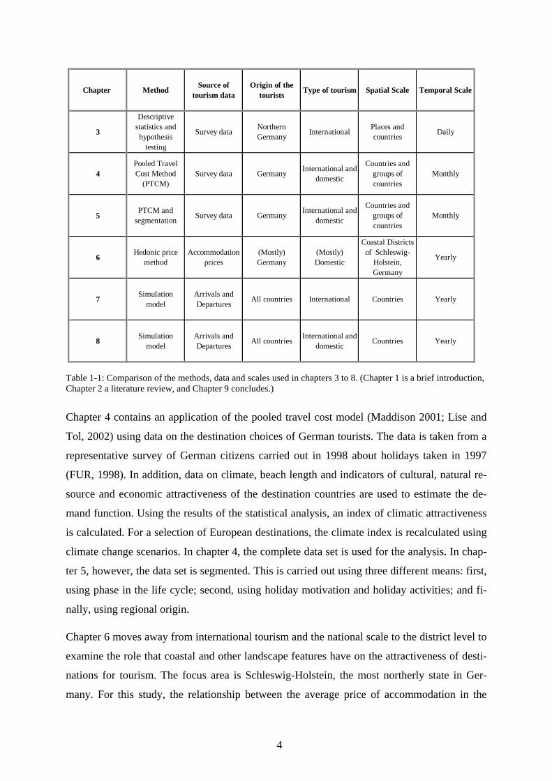
ing. The methods, data and spatial scale of the studies contained in chapters 3 to 8 are de-
picted in table 1-1.
3
Chapter Method Source of tourism data
Origin of the tourists Type of tourism Spatial Scale Temporal Scale
3
Descriptive statistics and hypothesis
testing
Survey data Northern Germany International Places and
countries Daily
4Pooled Travel Cost Method
(PTCM)Survey data Germany International and
domestic
Countries and groups of countries
Monthly
5PTCM and
segmentation Survey data Germany International and domestic
Countries and groups of countries
Monthly
6Hedonic price
methodAccommodation
prices(Mostly) Germany
(Mostly) Domestic
Coastal Districts of Schleswig-
Holstein, Germany
Yearly
7Simulation
modelArrivals and Departures All countries International Countries Yearly
8Simulation
modelArrivals and Departures All countries International and
domestic Countries Yearly
Table 1-1: Comparison of the methods, data and scales used in chapters 3 to 8. (Chapter 1 is a brief introduction, Chapter 2 a literature review, and Chapter 9 concludes.)
Chapter 4 contains an application of the pooled travel cost model (Maddison 2001; Lise and
Tol, 2002) using data on the destination choices of German tourists. The data is taken from a
representative survey of German citizens carried out in 1998 about holidays taken in 1997
(FUR, 1998). In addition, data on climate, beach length and indicators of cultural, natural re-
source and economic attractiveness of the destination countries are used to estimate the de-
mand function. Using the results of the statistical analysis, an index of climatic attractiveness
is calculated. For a selection of European destinations, the climate index is recalculated using
climate change scenarios. In chapter 4, the complete data set is used for the analysis. In chap-
ter 5, however, the data set is segmented. This is carried out using three different means: first,
using phase in the life cycle; second, using holiday motivation and holiday activities; and fi-
nally, using regional origin.
Chapter 6 moves away from international tourism and the national scale to the district level to
examine the role that coastal and other landscape features have on the attractiveness of desti-
nations for tourism. The focus area is Schleswig-Holstein, the most northerly state in Ger-
many. For this study, the relationship between the average price of accommodation in the
4

coastal districts of Schleswig-Holstein and the characteristics of these districts is examined
using the hedonic price technique.
Returning to the international scale, chapters 7 and 8 extend the examination of the impacts of
climate change to global tourism, modelling both the demand from countries and the demand
for countries. In chapter 7, a simulation model of international tourism is introduced. The cur-
rent pattern of international tourist flows is modelled using 1995 data on departures and arri-
vals for 207 countries. Using this basic model, the impact on arrivals and departures through
changes in population, per capita income and climate change are analysed. In chapter 8, the
model is extended to include domestic tourism and tourist expenditures. The results of the
simulation model are discussed with special reference to Germany.
In the final chapter, the results of the previous chapters are summarized, and their relevance to
the research field of tourism and climate change, to the tourism industry and to policy is dis-
cussed.
5
Chapter 1
Introduction
1.1 General introduction
Tourism has become one of the world’s major cultural and economic activities. Tourists travel
to a wide variety of environments, including high-density urban areas and uninhabited re-
gions. The coastal zone, however, is the main destination of tourists. Furthermore, tourism
takes place in a wide variety of climates, ranging from the cold of the arctic, to the warmth
and humidity of tropical countries and to the dry heat of the desert. As climate varies over the
year, tourists have the possibility to experience a destination under a variety of climatic condi-
tions. Nevertheless, there is a distinct pattern of seasonality in tourism demand. In other
words, tourists not only choose a spatial location for their holiday, they also choose a tempo-
ral location.
Climate scientists are very certain that the Earth’s climate will change at an unprecedented
rate over the 21st century (Houghton et al., 2001). Whether through the direct effects of cli-
mate change, such as increased temperature, or through ancillary effects such as sea-level rise
or the impact on landscapes, it can be expected that the spatial and temporal pattern of tour-
ism demand will adjust. Despite the apparent seasonality of tourism and its overwhelming
dependence on climatic factors, relatively few studies have tackled the impact of climate
change on tourism (Butler, 2001; Scott et al., 2005). This is reflected in the brief coverage of
the impacts on tourism in the Intergovernmental Panel on Climate Change (IPCC) reports
(Watson et al., 1997; McCarthy et al., 2001).1 Since these reports were completed, however,
the number of studies has been increasing. Nevertheless, there is still a scarcity of quantitative
studies on the effect that climate change will have on tourism. This thesis is a step towards
reducing the scarcity, and so providing information for the tourism industry as well as policy-
makers.
1 The Intergovernmental Panel on Climate Change was established in 1988 by the World Meteorological Organi-zation (WMO) and the United Nations Environment Programme (UNEP). Its task is to assess the scientific in-formation on the risk of climate change, its impacts and possible response strategies (IPCC, 2004).
1

Section 1.2 presents the purpose, aims and scope of this study. The structure of this thesis is
outlined in section 1.3.
1.2 Purpose, aims and scope
In 2003 in Djerba, Tunisia, the World Tourism Organisation (WTO) and other UN agencies
organised the first international conference on tourism and climate change with the purpose of
creating an awareness of the issue within the tourism industry and within governmental agen-
cies involved in tourism policy and planning (Scott et al., 2005). This conference resulted in
the “Djerba Declaration on Climate Change and Tourism” (WTO, 2003a), which was signed
by representatives of 45 nations. One of the points agreed to by the participants was that there
is still a need for research on “the reciprocal implications between tourism and climate
change” (WTO, 2003a). A further point is that such information is necessary for decision-
making on adaptation and mitigation strategies (WTO, 2003a). The purpose of this thesis is to
contribute to the information that can be used in the decision-making process.
This thesis will focus on one direction of the “the reciprocal implications.” To be precise, the
impact that climate change will have on tourism and in particular on the demand for destina-
tions. The impact of tourism on climate change will not be covered here (see Gössling, 2002;
Becken and Simmons, 2005) nor will the impact of climate change policy on tourism be ex-
amined (see Piga, 2003). Of course, the role that the factors climate and the coast play in the
development of tourism supply at particular destinations, regions or even countries is an im-
portant issue when considering the adaptation of the tourism industry to climate change. This,
however, would be a thesis in its own right and so will be deferred to future research. First, it
is necessary to examine how demand will change in response to climate change. This will be
done with particular reference to tourism in the coastal zone. The aims of the thesis are:
1. to review the historical evidence and contemporary scientific literature on the impor-
tance of climate and the coastal zone for tourism demand,
2. to provide quantitative evidence that climate and the coast are important destination
characteristics that affect tourists decisions for a particular destination,
3. to establish the quantitative relationship between climate and tourism demand as well
as between coastal characteristics and tourism demand,
4. to use these relationships to examine the effects of climate change on tourism, and.
2

5. to examine the impact of climate change at various destination and source market spa-
tial scales.
The extensiveness and diversity of tourism has lead to this thesis being focussed on one
source market. Germany is the second largest source market in the world, accounting for 10%
of the global expenditure on international tourism (WTO, 2005b). Additionally, it has a very
large domestic market. For these reasons, along with the relative ease of access to tourism
data and the possibility to survey outbound tourists, Germany makes an ideal focus for this
thesis. Chapters 7 and 8 are an exception to this: they examine the global picture.
1.3 Outline
Chapter 2 provides background information on tourism, climate, the coast and climate
change. Along with a sketch of the historical development of tourism with particular reference
to climate and the coast, chapter 2 reviews the contemporary literature on the relationships
between tourism and climate and tourism and the coastal zone. The perspective is then shifted
to the future. The causes and impacts of climate change are briefly discussed. This is followed
by a review of the literature on the impacts of climate change on tourism. Furthermore, chap-
ter 2 locates this thesis in the aforementioned literature.
The focus of chapter 3 is the role that information about the climate of destinations plays in
the destination choice of tourists. This is examined using data from a survey of German tour-
ists carried out in summer 2004. This study examines if tourists actively inform themselves
about the climate of their planned destination. In addition, the sources of information they use
are determined as well as establishing the phase in the holiday decision-making process where
the information search occurs. Another aspect of the survey is the ranking of the most impor-
tant characteristics of the destination that were crucial for the tourist’s decision to go to the
chosen destination. The results are examined using descriptive statistics and hypothesis test-
ing. The methods, data and spatial scale of the studies contained in chapters 3 to 8 are de-
picted in table 1-1.
3

Chapter Method Source of tourism data
Origin of the tourists Type of tourism Spatial Scale Temporal Scale
3
Descriptive statistics and hypothesis
testing
Survey data Northern Germany International Places and
countries Daily
4Pooled Travel Cost Method
(PTCM)Survey data Germany International and
domestic
Countries and groups of countries
Monthly
5PTCM and
segmentation Survey data Germany International and domestic
Countries and groups of countries
Monthly
6Hedonic price
methodAccommodation
prices(Mostly) Germany
(Mostly) Domestic
Coastal Districts of Schleswig-
Holstein, Germany
Yearly
7Simulation
modelArrivals and Departures All countries International Countries Yearly
8Simulation
modelArrivals and Departures All countries International and
domestic Countries Yearly
Table 1-1: Comparison of the methods, data and scales used in chapters 3 to 8. (Chapter 1 is a brief introduction, Chapter 2 a literature review, and Chapter 9 concludes.)
Chapter 4 contains an application of the pooled travel cost model (Maddison 2001; Lise and
Tol, 2002) using data on the destination choices of German tourists. The data is taken from a
representative survey of German citizens carried out in 1998 about holidays taken in 1997
(FUR, 1998). In addition, data on climate, beach length and indicators of cultural, natural re-
source and economic attractiveness of the destination countries are used to estimate the de-
mand function. Using the results of the statistical analysis, an index of climatic attractiveness
is calculated. For a selection of European destinations, the climate index is recalculated using
climate change scenarios. In chapter 4, the complete data set is used for the analysis. In chap-
ter 5, however, the data set is segmented. This is carried out using three different means: first,
using phase in the life cycle; second, using holiday motivation and holiday activities; and fi-
nally, using regional origin.
Chapter 6 moves away from international tourism and the national scale to the district level to
examine the role that coastal and other landscape features have on the attractiveness of desti-
nations for tourism. The focus area is Schleswig-Holstein, the most northerly state in Ger-
many. For this study, the relationship between the average price of accommodation in the
4

coastal districts of Schleswig-Holstein and the characteristics of these districts is examined
using the hedonic price technique.
Returning to the international scale, chapters 7 and 8 extend the examination of the impacts of
climate change to global tourism, modelling both the demand from countries and the demand
for countries. In chapter 7, a simulation model of international tourism is introduced. The cur-
rent pattern of international tourist flows is modelled using 1995 data on departures and arri-
vals for 207 countries. Using this basic model, the impact on arrivals and departures through
changes in population, per capita income and climate change are analysed. In chapter 8, the
model is extended to include domestic tourism and tourist expenditures. The results of the
simulation model are discussed with special reference to Germany.
In the final chapter, the results of the previous chapters are summarized, and their relevance to
the research field of tourism and climate change, to the tourism industry and to policy is dis-
cussed.
5

Chapter 2
Context*
2.1 Tourism
2.1.1 An introduction to tourism
Although tourism is economically, socially and politically important, there is still debate over
what tourism exactly is. This can be seen in the range of definitions of tourism that can be
found in the literature. One commonly used definition of a tourist (and hence tourism) is that
of the World Tourism Organisation (WTO):
“Persons travelling to and staying in places outside their usual environment for not more
than one consecutive year for leisure, business and other purposes” (WTO, 2002a,
online).
This is a technical definition, which was created to harmonize the different national tourism
statistics. Furthermore, it is a demand side definition. Attempts at a supply-side definition
have been made but these are also disputed. For example, Smith has developed a definition:
“Tourism is the aggregate of all business that directly provide goods or services to fa-
cilitate business, pleasure, and leisure activities away from the home environment”
(Smith, 1988, 183)
For the purposes of this thesis, the term tourism industry will be used as an umbrella term to
cover the businesses that Smith includes in his definition. For tourists, the WTO definition
will be used. Domestic tourism “is the tourism of resident visitors within the economic terri-
tory of the country of reference” (WTO, 2000). International tourism, on the other hand, con-
sists of all trips that tourists make to a country other than that in which they are residents
(WTO, 2000).
* Sections of this chapter are based on Hamilton and Tol (2004).
6

The demand and supply sides of tourism can also be mapped spatially. Leiper (1979) de-
scribes tourism as a system consisting of a generating region, a destination region and a transit
zone. Tourists and the tourism industry can be found in all of the regions in the system. At the
generating region a tourist’s need or motivation to go on holiday develops, which leads the
potential tourist to gather information about destinations and activities, and to book or pur-
chase elements of the holiday. The tourism industry is also present in the generating region,
for example travel agents, tour operators and transport providers. The tourism industry in the
transit zone will mainly consist of transport operators but also of hospitality services. At the
destination, the tourist uses the hospitality services, participates in activities and visits attrac-
tions. Attractions can range from the natural to the artificial. Artificial attractions may be his-
torical, cultural or purpose built for tourism. Aspects of the natural environment that are at-
tractions for tourism include climate, landscape, beaches, the sea and lakes and mountains
(Mieczokowski, 1990). Smith (1988) states that his definition depicts tourism as a retail ser-
vice industry. Nonetheless, the supply-side of tourism embodies more than just businesses;
inherent features of destinations are also “supplied“ to tourists.
Tourism would not take place without the tourist’s decision to go on holiday. The process of
coming to a decision about whether to go on holiday and where to go on holiday is the subject
of holiday decision-making models. The first phase in such models is typically the individ-
ual’s motivation to go on holiday (Van Raaij, 1986; Gunn, 1989; Ahmed, 1991; Mansfeld,
1992). Motivation is often understood as being composed of two factors: first, push factors
that influence the need to have a holiday and the need to leave the origin region; and second,
pull factors that generate the need to undertake particular activities and attract tourists to a
particular region (Ryan, 2003). The normal environment of the tourist may be a push factor.
For example, a stressful urban environment or an extremely wet winter may be motivating
factors to take a holiday. The strength of the pull factor will depend on the image that tourists
have of the destination, which is a function of the attributes of the destination. Environmental
preferences will have a role to play in this (Fridgen, 1984), and, of course, the natural attrac-
tions of the destination.
There will be an array of combinations of potential destination regions, potential times to take
the holiday and other potential holiday options that may meet the tourist's needs, although
these will be constrained by available income and leisure time. The tourist’s choice of a par-
ticular destination, time and type of holiday represent the observable demand side of the tour-
7
ism system. Forecasting tourism demand is a large branch of the tourism literature. Typically,
these studies do not include environmental factors in the estimation of demand; they focus
rather on economic or demographic factors. Morley (1992) criticizes tourism demand studies
for this reason, and because they do not consider utility in the decision making process.
Moreover, he suggests an alternative way to estimate demand based on the expected utility
derived from the characteristics of the product. Lancaster (1966) originally developed the
concept that the characteristics of a good are more important to the consumer than the actual
good itself. In the case of tourism, the good is the holiday at a certain destination and at a cer-
tain time and this product will have certain characteristics. How these characteristics are per-
ceived, in other words the image, will determine the expected utility. Section 3.2.1 deals with
the subject of destination image in more detail.
2.1.2 Historical development
The previous subsection introduced the main concepts of modern tourism. However, people
have been travelling for business and pleasure since ancient times. This section briefly de-
scribes the development of European tourism from the Classical period to the start of modern
tourism in the 1950s.
Travel in Ancient Greece was not only for trade and for warfare. People would travel shorter
distances to religious and sporting events. Roman roads and a unified coin system made travel
easier within the Roman Empire (Mieczokowski, 1990). For young, rich Romans Athens and
other Greek cities were part of an educational tour (Towner, 1996). Richer Romans were able
to afford second homes either in the countryside or at the coast (and occasionally both). By
the first century BC there were many villas scattered in the hills surrounding Rome. This
practice spread to other parts of the Empire (Sharpley, 1994). During the Middle Ages, travel
was mainly for religious reasons. Long pilgrimages were undertaken and suffering was an
expected part of the journey (Mieczokowski, 1990).
The Grand Tour, a long tour of Europe for educational purposes, is thought to have originated
in the early 16th century. Those on the Grand Tour would visit Italy as well as the Nether-
lands, France and Germany. Towner (1985) finds that age, social class and education of those
on the Grand Tour changed over the period 1547 and 1840. In addition, an analysis of primary
sources of information shows that there were some changes in the spatial aspects of the tour
(Towner, 1985). As the social class of the tourists changed and more middle class tourists
8

were going on a tour, the tour gradually became shorter and developed into a summer tour of
one or two months.
Spas were popular in ancient times and this popularity was revived in Europe during the Ren-
aissance (Holloway, 1998). During the 16th and 17th centuries, the health-bringing effect of
the waters was the main attractions of the spas. In the 18th century, however, the spas were
one of the places where the high society met and a trip to take “the cure” was an important
part of the social calendar, even if the trip was more for pleasure than health. The clientele at
the spas changed over the course of the 18th century; the gentry gave way to merchants and
those from the professional classes (Sharpley, 1994). According to Holloway (1998), the life
cycle of the spas popularity in the rest of Europe was much longer than in England.
It was the recommendations of English doctors in the mid 18th century that were to popular-
ise sea bathing and holidays at the coast, and so stimulate the popularity of seaside towns and
villages, mainly in the south of England, as health and eventually as pleasure resorts (Towner,
1996). The costs of the journey to a resort, both in terms of time and money, restricted the
seaside resorts to the wealthy until 1830 (Sharpley, 1994). Then steamer services from Lon-
don to the coast opened up the seaside resort for the less wealthy. As the domestic resorts be-
came popular with other social groups, the gentry and the aristocracy began to seek exclu-
siveness elsewhere (Towner, 1996). Advances in transport technology at the end of the 19th
Century allowed those who could afford it to travel abroad to seek out the best waters and
more exclusive resorts. In particular, the French and Italian Riviera were popular; the Cote
d’Azur was the main destination of the European aristocracy (Sharpley, 1994). Across Europe
development at the coast for touristic purposes continued up until the First World War
(Walton, 1997). In France, development extended into Brittany. The Belgian coast also devel-
oped. In Spain, the main resorts were still on the northern coast and this was not to change
until the advent of coach and charter flight package holidays. Estoril in Portugal began to
compete for the Spanish tourists. Further east resorts could be found in what are now Croatia,
Rumania and the Crimea (Walton, 1997).
New and faster modes of transport may have opened up resorts further a field but there were
still considerable barriers for the middle classes: these barriers included language, currency,
finding a suitable destination and of course suitable accommodation. In 1841, Thomas Cook
first began with organised day trips to nearby cities, moving on to interregional tours, trips to
Europe from 1855 on, to the United States from 1866 and in 1872, the first round the world
9
tour (Mieczokowski, 1990). Cook’s company organised all of the travel arrangements for
their clients even providing a form of credit note that could be used at participating hotels or
banks (Sharpley, 1994). Cook’s tours made tourism available to the wider population. Thus,
he is often credited as having brought democratisation to tourism and of developing the fore-
runner of the modern package tour (Sharpley, 1994).
In the early 20th century transport innovations, in particular public transport, increased the
number of places that were accessible for tourists. With the invention of the car followed by
increasing car ownership, domestic motoring holidays became popular (Mieczokowski,
1990). It was not until the 1950s that travel by air became as cheap if not cheaper than travel
by the other modes. The first charter flight, using second-hand planes from the airlines, was
organised by Vladimir Raitz in 1950 (Holloway, 1998). The first trip to Corsica was a suc-
cess; Raitz continued to offer package tours, and many other companies in the UK and Europe
copied him. The package tour by plane to destinations on the Mediterranean coast became the
main tourism product (Sharpley, 1994). The countries of the Mediterranean were less devel-
oped than those of northern Europe were. This was not the only reason that made tourism
there so popular: the climatic advantage over the north or what Raitz coined “the rush to the
sun” was also important (Holloway, 1998).
From this brief review, it can be seen that many forms of tourism that were popular in the past
still exist today. Travel for education, sport, religious reasons, social reasons, health and bath-
ing at the sea are still the main motivations of tourists.
2.1.3 Modern tourism
The WTO has documented the rapid increase in tourism since the birth of the package tour in
the 1950s. The WTO is the main source of statistics on tourism. Hence, the information con-
tained in the following paragraphs on the size of tourism and its main markets is taken from
the latest overview report of the WTO (2005b). There were a total 25 million international
arrivals globally in 1950. By 1975 arrivals had increased by over 800% to 222.3 million, and
by 2002 global tourist arrivals had reached 702 million.2 Europe and the Americas had market
shares of 66.4% and 29.6% in 1950 respectively. In 2002 these had declined to 56.9% and
16% respectively, and the Asia and the Pacific region overtook the Americas to become the
2 Preliminary figures for 2004 show tourist arrivals of 763 million (WTO, 2005b).
10
second largest market (18.6%). For the period 1950 to 2002, the WTO reports that the annual
average growth rate was 6.6%. The Asia and Pacific region had a higher than average growth
rate of 13%. France, the most popular destination, had 77 million arrivals in 2002, which cor-
responds to 11% of global market. In second place was Spain (7.4%) closely followed by the
US, Italy and China (5.2%).
Also of interest is the distribution of departures. As well as having the most arrivals, Europe
generates slightly more than half of all departures (404.9 million). Moreover, 352.1 million of
these are within Europe. The other regions also have intraregional shares higher than 70% but
these are considerably smaller in absolute terms. Of the interregional flows, the largest are 23
million from the Americas to Europe, 18 million from Europe to the Americas and 16 million
from Europe to Asia and the Pacific region.
Tourism receipts have also expanded enormously. In 1950, the global total was US$ 2.1 bil-
lion, which had increased to 40.7 billion in 1975 and in 2002, receipts had reached 474.2 bil-
lion. Again, Europe dominates with 50.7% of all receipts. The Americas have the second
highest market share of 24.1%. In terms of individual countries the US earned 66.5 billion
US$ in 2002, which amounts to a market share of 14%. China, Italy, France and Spain all
earned more than US$ 20 billion. These countries and the US have a combined market share
of 38%. Within Europe the bulk of the receipts are in the countries of Southern Europe3 and
Western Europe4 with market shares of 34.2% and 36.2% respectively.
The countries of the top ten tourism spenders account for slightly more than half of the global
total expenditure. The US, Germany, the UK and Japan had international tourism expendi-
tures of over US$ 20 billion in 2002: the US and Germany with US$ 58 and US$ 53 respec-
tively, corresponding to market shares of 12.2% and 11.2%.
One of the main services provided by the tourism industry is accommodation. For hotels and
similar establishments, the WTO recorded 17.4 million rooms globally in 2001. Around one
four of these are in the US, roughly one in ten in Japan and one in twenty in Italy, Germany
and China. These values reflect the high levels of domestic tourism and country specific pat-
terns of accommodation types.
3 Albania, Andorra, Bosnia Herzgovina, Croatia, Former Yugoslav Republic of Macedonia, Greece, Italy, Malta, Portugal, San Marino, Serbia and Montenegro, Slovenia and Spain. 4 Austria, Belgium, France, Germany, Liechtenstein, Luxembourg, Monaco, Netherlands and Switzerland.
11
As well as collecting statistics on the development of tourism over the years, the WTO pro-
vides a long term forecast for the global and regional development of tourism in 2010 and
2020. Tourism arrivals are expected to continue to grow at 4.1%, although there will be re-
gional differences. The WTO (2005a) predicts that the Americas and Europe will experience
lower than average growth rates. By 2010, the number of arrivals is expected to reach the 1
billion mark and by 2020, almost 1.6 billion arrivals are expected (WTO, 2005a). Europe
Central and Eastern Europe will increase in importance, overtaking Western Europe to have
the highest market share. The WTO predicts that by 2020 346 million tourists will visit desti-
nations at the Mediterranean accounting for more than a fifth of all arrivals (WTO, 2001b).
France remains the largest destination market within Europe in 2020 but with a decreasing
market share. In addition, Germany continues to be the major source market of tourists within
Europe. The Indian Ocean region is expected to have an average growth rate of 6.3% and will
reach a market share of 11% (WTO, 2001a). China will overtake France to have the most visi-
tors: the WTO (2001a) predict 130 million arrivals.
2.2 Climate, the coast and tourism
2.2.1 Climate, weather and the coast
Climate describes the weather conditions that can be expected at a certain time and place, and
is calculated from the average of thirty years of weather data. Weather is the current state of
the atmosphere that is actually experienced. The weather is typically described in terms of
temperature, humidity, levels and frequency of precipitation, wind, cloud cover and other
weather features (Perry and Thompson, 1997).
For humans, weather has a direct effect on physiological functioning. Core body temperature
must be maintained to avoid discomfort and in extreme cases life threatening illness. High air
temperatures lead to increased body temperatures, if the relative humidity is so high that
sweat cannot evaporate. Depending on humidity, heat stress can occur from 26°C. Activity
also raises body temperature. Thus, strenuous activities will increase the likelihood of heat
stress than passive activities carried out in the same weather conditions. Wind increases the
rate that the body losses heat. At higher temperatures this may be wished for; at colder tem-
peratures, however, wind-chill causes the body to lose heat rapidly resulting in increased dis-
comfort and the need for extra clothing. These are the thermal aspects of weather.
12
In addition, the weather also has neuro-biochemical effects on well-being (Parker, 2001).
Sunlight stimulates the production of serotonin (Lambert et al., 2002), a neuro-transmitter
responsible for mood. Low levels of serotonin are associated with depression, whereas normal
to high levels of serotonin are associated with feelings of happiness and relaxation.
According to de Freitas (2001), there are two further aspects of climate that are relevant for
tourism: first, there is the physical aspect. Here, the climate facilitates or hinders certain tour-
ist activities whether through rain, wind or snow. For example, wind and rain will make a day
of sunbathing at the beach impossible. Second, there is the aesthetic aspect of climate. This
may be through the quality of light that affects the appearance of the tourists’ surroundings or
it may come from the appearance of the sky and of the sea and other water bodies. In the long
run, climate has an effect on other elements that fall under the aesthetic category of de Freitas.
The appearance of the built environment is influenced by, among other things, climate. Land-
scape is also influenced by climate. Climate determines the types of crop that are possible to
grow and through this the appearance of the cultivated landscape. Moreover, the influence of
climate on the types of flora and fauna that exist in a particular area affects the appearance of
cultivated environments as well as ones that are more natural.
The coast is the interface of the sea and the land, which Mieczokowski (1990) calls “a junc-
tion of seascape and landscape.” Coastal tourism can be found mostly on sandy coasts; rocky
or marsh coasts are less popular (Wong, 1994). Mieczokowski (1990) divides the coastal zone
into four areas that are relevant to tourism: the marine zone, the beach, the shoreland and the
hinterland. The beach is the most important of these, as it is where the main tourist activities
take place. Defert (1966) differentiates between four kinds of coastal type. First, there is the
oceanic type with a large tidal range. The oceanic type may be continuous with long stretches
of beach or discontinuous, where cliffs or marshland interrupt the beach. Second, there is the
Mediterranean type. Again, this can be continuous or discontinuous. The coast has a special
climate. Cooler air from the sea that flows landwards creates a breeze at the seashore. Without
this breeze the thermal conditions at the beach would not be as pleasant (Mieczokowski,
1990).
Although attempts have been made to describe the “best” climate or coastal type, it is difficult
to determine a generally applicable set of conditions: people have different tastes. Moreover,
preferences for certain kinds of climate, landscape or seascape have changed over time. A
13
brief review of historical changes in the relevance of climate and the coast to tourism is given
in the following section.
2.2.2 Historical importance of climate and the coast for tourism
In Ancient Rome, countryside or coastal villas were mainly used in summer to escape the heat
in the cities (Ryan, 2003). Access to the coastal areas during the summer months was made
easier by the road network. The first of Rome’s resorts was Baia, near Naples, which was
originally a winter spa resort but developed into a summer resort (Sharpley, 1994). According
to Sharpley (1994), the Romans introduced the idea of the summer holiday, a form of tourism
that died (temporarily) with the Empire.
Seasonality was also an aspect of the Grand Tour. This was partly due to the social season in
England but also festivals and conditions at the destination or on transit routes. Towner
(1985) states that climate "kept tourists away from southern regions especially in June, July
and August." These southern regions had a winter season as opposed to a summer one. Re-
search has shown that tourists moved to the Alban hills from Rome rather than travelling
north during the summer heat. Tours of Switzerland were undertaken in summer (Sharpley,
1994).
As stated above, the popularity of coast as a tourist destination began in the 18th century. His-
torically, the coast was not always as attractive as it is to the modern visitor. Up until the 17th
century, the sea and the coast were wholly unattractive and were even seen as disgusting
(Corbin, 1999). Corbin (1999) explains the change towards an appreciation and celebration of
the coast by the public, and its subsequent popularity for tourism, through the developments
in science and the Romantic and Picturesque movements. With the increased popularity came
the need for guidebooks. These contained assessments of the physical environment and the
climate of resorts. The authors considered factors such as “wind direction and strength, air
quality, temperature variations…” (Towner, 1996:201). Moreover, Towner (1996) finds that
the southern coasts of Britain were considered superior. Quality of the air was an important
factor from the 18th century through to the 20th century. That is, whether it was bracing or
soothing. The constitution of the prospective tourist would determine which air quality was
suitable (Adler, 1989; Towner, 1996). Towner (1996) mentions a guidebook of 1914, which
published comparative assessments of the climate of the English coastal resorts and destina-
tions in Switzerland.
14
At first, tourism at the French Riviera was during the winter – the tourists were there to es-
cape from the northern winter. The winter season lasted from October until the end of April
(Boyer, 2001). The British also visited resorts such as Biarritz in the winter. During the same
period, resorts not far away in Spain were popular as summer destinations (Boyer, 2001). In
the mid-nineteenth century, Spain had become popular as a destination for international tour-
ists (Walton, 1997). Different resorts and different seasons were popular with domestic and
international tourists. For example, Malaga had some popularity with the English as a winter
climatic resort. However, the northern Atlantic coast of Spain was popular with domestic
tourists (Walton, 1997). According to Walton (1997) the summer season at San Sebastian and
other developing resorts was partly to do with the need to escape from the heat of the cities
and because of the trend at that time for doctors to prescribe cold and bracing seas.
The fashion of pale skin was replaced by the popularity of the suntan in the 1920s. Previously,
white skin that had been darkened with the sun was associated with a lower social status. Now
the suntan was associated with wealth. This change in fashion had a large impact on the pre-
ferred seasons. The French Riviera became a summer resort as well as a winter one (Boyer,
2001). The popularity of the suntan is still one of the main motives for going on holiday.
From this brief review of the historical importance of climate and the coast for tourism, the
following points are evident. First, climate has exerted both a push and a pull effect on the
motivation to go on holiday. Second, through the centuries different kinds of climate were
considered the healthiest or were fashionable. Third, the popularity of the coast has also seen
great changes since the Classical period. The next section looks at contemporary studies on
the importance of climate and the coast for tourism.
2.2.3 Review of studies on climate, the coast and tourism
Whether in the process of deciding on the destination and the right time for a holiday or in the
daily choices made about recreation activities whilst on holiday, climate and weather play an
important role. One would suspect that, “last minute” holidays and short breaks apart, tourist
destination choice is affected by the expected weather (climate) rather than the actual weather.
For daily recreation choices, actual weather is the decisive factor in decision-making. In the
literature, there are two broad types of study where the importance of climate and weather for
tourism and recreation has been examined: attitudinal studies and behavioural studies.
15
Two kinds of attitudinal studies exist, those that examine the subjective rating of climate
compared to the ratings from indices of weather data and those that examine the significance
of climate in the image and the attractiveness of particular destinations. Thermal comfort in-
dices have been developed in order to capture the complexity of the thermal aspect of climate,
which is argued to be a composite of temperature, wind, humidity and radiation. Special
modifications of such indices have been used to assess the suitability of certain climates for
tourism (e.g. Amelung et al., forthcoming). The basis of these indices, however, is subjective
and arbitrary according to de Freitas (2003). In a case study, carried out at a beach in Queen-
sland, Australia on 24 days spread over a single year, de Freitas (1990) finds that the relation-
ship between HEBIDEX, a body-atmosphere energy budget index, and the subjective rating
of the weather by beach users is highly correlated. Furthermore, he finds that the optimal
thermal conditions for beach users are not at the minimum heat stress level but at a point of
mild heat stress. Using the thermal comfort index, predicted mean vote, Thorson et al. (2004)
find a positive relationship between thermal comfort and urban park use for recreational ac-
tivities in Göteborg, Sweden. They also find, however, that there is a discrepancy in the sub-
jective rating of the weather and the rating of the weather according to the index. The majority
of those surveyed said that the weather was “acceptable” when it was “warm” or “hot” ac-
cording to the calculated index. These levels are associated with heat stress.
In spite of the popularity of studies of destination image in the tourism literature, only one of
the 142 destination image papers that are reviewed by Pike (2002) specifically deals with
weather. This was a study by Lohmann and Kaim (1999), who note that there is a lack of em-
pirical evidence on the importance of weather/climate on destination choice decision-making.
Using a representative survey of German citizens, the importance of certain destination char-
acteristics was assessed. Landscape was found to be the most important aspect even before
price considerations. Weather and bio-climate were ranked third and eighth respectively for
all destinations. Moreover, they found that although weather is an important factor, destina-
tions are also chosen in spite of the likely bad weather. Measuring the importance of destina-
tion characteristics is also the focus of a study by Hu and Ritchie (1993). They review several
studies from the 1970s and find that “natural beauty and climate” are of universal importance
in defining destinations’ attractiveness. In their own study, they examine the image of Hawaii,
Australia, Greece, France and China using a survey of Canadian citizens. They find that cli-
mate is the second most important characteristic for the group of tourists on a “recreational”
holiday. For the group of tourists taking an “educational” holiday climate ranks 12th. When
16
the images of the countries are compared, Hawaii is found to have the most attractive climate.
Attitudinal studies looking specifically at tourists’ preferences for coastal types were not
found.
Some behavioural studies examine daily recreational use patterns of particular sites in terms
of weather data. For example, Dwyer (1988) has estimated a daily site use model, for an ur-
ban forest in Chicago, USA, using data on noon temperature, percentage sunshine, percentage
rain and snow depth. In this study, data on wind-chill is not useful for estimating the use lev-
els. Demand is highest on the sunniest days and on days that are exceptionally warm espe-
cially when these conditions occur in late spring or in early summer. High temperatures in
July decrease demand. Brandenburg and Arnberger (2001) predict daily use levels of the Da-
nube Flood Plains National Park in Austria. They find that using standard climate data does
not produce any satisfactory results. Instead they use the Physiological Equivalent Tempera-
ture (PET), the occurrence of precipitation and cloud cover to estimate the number of visitors
per day in total and for four groups: cyclists, hikers, joggers and dog walkers. The PET value
is very important in determining the use levels, particularly for cyclists and hikers.
Other studies examine the statistical relationship between tourism demand and weather. For
example, Agnew and Palutikof (2001) model domestic tourism and international inbound and
outbound tourism using a time series of UK tourism and weather data. The results show that
temperature is the strongest indicator of domestic demand. In contrast, wetter weather in-
creases the demand for trips abroad in the current period and in the year following. Snow de-
pendent activities are the focus of a survey of US college students carried out in 1997 and
1998 by Englin and Moeltner (2004). Using data on price, weekly conditions at ski resorts in
California and Nevada and the participant’s income they find that although demand increases
as snow amount increases, trip demand is more responsive to changes in price. As said before
tourism (as opposed to recreation) is likely to be affected by the expected weather (climate)
rather than the actual weather.
Another set of studies uses climate data to capture the role of expected weather in destination
choice and consequently demand. Lise and Tol (2002) study the holiday travel patterns of
tourists from a range of OECD countries. The data and method are crude, but the results sug-
gest that people from different climates have the same climate preferences for their holidays:
The climate of Southern France and California is preferred by everyone, regardless of the
home climate. (Of course, this does not imply that all tourists travel to these places; climate is
17
not the only factor in tourist destination choice.) Bigano et al. (forthcoming) confirm this re-
sult, using less crude econometrics for a much wider range of countries including African and
Asian ones. However, Bigano et al. (forthcoming) also find that people from hotter places
tend to have sharper preferences. That is, while Southern France is preferred by people from
both hot and cold places, people from hot places would feel much worse about going else-
where than Southern France than would people from cold places.
Also using climate data, the Pooled Travel Cost Model (PTCM) has been applied to the de-
mand of tourists from the UK and the Netherlands for a range of countries (Maddison, 2001;
Lise and Tol, 2002). The studies include temperature and temperature squared in their estima-
tion of demand. The estimated coefficients on these studies allow the optimal temperature to
be calculated. That is, where demand for a country is highest. Demand for a country by tour-
ists from the UK is maximized when the quarterly maximum daytime temperature is 31°C. In
the Dutch study, the coefficients on the temperature variables were not significant.
There have been some economic studies that examine the demand of tourists for visits to the
beach (Bell and Leeworthy, 1990; Chen et al., 2004) and others that seek to examine the eco-
nomic value of the shoreline (Brown and Pollakowski, 1979). These studies, however, do not
use the characteristics of the sites in their estimation process.
2.3 Climate change and tourism
2.3.1 Climate change
Climate scientists have observed that over the 20th century that the climate has been changing.
The earth’s climate has changed at other points in history. Nevertheless, there is a consensus
among climate scientists that the change occurring now is unlike previous changes in that it is
partly influenced by human activity. The IPCC compiles the latest scientific evidence of cli-
mate change and the predictions of climate change for the coming decades from the various
general circulation models. The information in this and following paragraphs is drawn from
the publications of the IPCC (Houghton et al., 2001; McCarthy et al., 2001). From the 11th to
the 20th century, the 1990s was the warmest decade. In addition, 1998 was the warmest year
since recorded history. Other evidence for climate change can be seen in the shrinkage of the
glaciers, thawing of permafrost, the extension of growing seasons and in the shift in the range
of animal and plant species. For the 21st century a temperature rise of 1.4°C to 5.8°C is pre-
dicted. This increase will occur at a rate higher than that seen in the 20th century. In addition,
18
precipitation patterns are predicted to change. In mid to high latitudes of the northern hemi-
sphere precipitation is predicted to increase in winter whereas at low latitudes of both hemi-
spheres there will be increases and decreases depending on the region. Model predictions es-
timate that snow cover and sea ice will decrease in the northern hemisphere. Moreover, gla-
ciers and ice caps will continue to shrink. It is likely that there will be changes in the fre-
quency of extreme climate events. A further effect of climate change is sea level rise, which
will be dealt with below.
Changes in human activities since the industrial revolution are the main anthropogenic causes
of climate change. The most significant of these is the use of fossil fuels as an energy source.
The combustion of fossil fuels results in the production of the gases carbon dioxide, methane
and nitrous oxide. These gases belong to the group of gases found in the atmosphere called
greenhouse gases, which, because they reflect infrared radiation in all directions, create an
effect known as the greenhouse effect - more energy enters the earth’s atmosphere than leaves
the atmosphere. As the concentration of these gases increases in the atmosphere, the green-
house effect is enhanced and consequently the atmosphere warms. Fossil fuel combustion also
results in the emission of aerosols. In addition, the emission of CFCs and other compounds
deplete the ozone layer adding to the radiative forcing. Emissions are not the only anthropo-
genic source of disturbance to the climate system: changes in land use also influence the
greenhouse effect. Urbanisation and agriculture change the physical and biological properties
of the earth’s surface.
Warming not only affects the climate it also affects the global sea level. As the atmosphere
warms the volume of the seas and oceans increases through thermal expansion. Glacier loss
and ice cap shrinkage also contribute to the increase in sea level. In the 20th century, it was
observed that the sea level increased by 10 to 20 cm. For the 21st century, however, an in-
crease in sea level of 9cm, for the low emissions scenario to 88cm, for the highest emissions
scenario is predicted. Tectonic movements will affect the regional net sea level rise. Accord-
ing to Nicholls and Hoozemans (1996), the main impacts of sea-level rise are erosion, inunda-
tion, an increased risk of flooding and impeded drainage, salinity intrusion and higher water
tables.
Climate change will affect ecosystems. In particular, the following systems are at risk: gla-
ciers, coral reefs, atolls, mangroves, tropical forests, polar and alpine ecosystems and prairie
wetlands. It is expected that many species will be lost leading to a decrease in biodiversity.
19
There will also be major impacts for human systems. These can be summarised in the follow-
ing categories: changes in the availability of water resources, changes in agricultural crop
yields, impacts on the coastal zone, the effects of flooding on settlements, changes in energy
requirements and impacts on human health.
What impact will climate change have on tourism? This can be through two means: directly
through the changed climate and indirectly through the environmental changes brought about
by climate change. In both cases, these impacts will occur at the origin country or region and
at the destination country. These impacts will be discussed in the following section.
2.3.2 The impact of climate change on tourism and recreation
Climate change impact studies can be categorized as qualitative and quantitative. Qualitative
impact studies provide information about vulnerabilities and the likely direction of change;
nevertheless, they do not provide estimates of changes in demand. Quantitative impact studies
can be categorized further into three groups: first, studies that predict changes to the supply of
tourism services; second, studies that use tourism climate indices to predict the change in cli-
matic attractiveness and finally, studies that use the statistical relationship between demand
and weather or climate to estimate the change in demand.
Qualitative studies rely on experts’ opinions on the likely impact of climate change. For ex-
ample, Perry (2000) discusses the impact that climate change will have on tourism at the
Mediterranean. The main impact caused by an increase in temperature will be a “doughnut”
shaped pattern of demand: in the shoulder season there will be more visits than in the summer
season. In addition, he expects that there will be an increase in the demand for long winter
holidays particularly from the older generations. The indirect effect of enhanced beach ero-
sion caused by sea level rise will reduce demand and increase the need for planning restric-
tions in the coastal zone. According to Gable (1997), Caribbean coastal areas will also experi-
ence a drop in demand through beach loss. Viner and Agnew (1999) describe the current cli-
mate and market situation for the most popular tourist destinations of the British. In addition,
the consequences for demand for these destinations under a changed climate in the 2020s and
2050s are discussed. Currently warm resorts such as those in the Eastern Mediterranean are
expected to become less attractive as temperature and humidity increase. As summer weather
becomes more favourable and reliable in temperate countries, tourism is expected to increase.
All of these studies rely on a synthesis of existing work on the physical impacts of climate
change or on the expert opinion of the authors; a direct link with demand (or supply) of tour-
20
ism is not made. Nevertheless, these studies highlight the range of impacts that climate
change will have. One qualitative study, however, has involved the tourism industry. This a
study by Krupp (1997), where tourism experts from the local tourist industry discussed the
impact of climate change on tourism in the West coast of Schleswig-Holstein in Germany.
Krupp finds that an increase in summer precipitation will reduce the willingness of the tour-
ism industry to make new investments in tourism infrastructure and facilities.
Predicting changes in the supply of tourism services has been applied to the winter sports in-
dustry. Breiling and Charamza (1999) analyse, for all districts in Austria, the impact of a 2°C
change in temperature on seasonal snow-cover depth. They estimate that these changes will
reduce ski season length and the usability of ski facilities. Warming will have strong impact
on low altitude resorts, which the authors expect will disappear first and the remaining resorts
will become more expensive. Similar studies have been carried out for winter sports tourism
in Scotland (Harrison et al., 1999), Switzerland (Abegg, 1996; Elsasser and Messerli, 2001),
Finland (Kuoppamaeki, 1996) and Canada (Scott et al., 2001). These studies find a general
decline in natural skiing conditions, although this will be less of a problem at high altitude
sites. Moreover, the use of snow making machines is also temperature dependent, which re-
stricts the adaptation options available.
The index approach, discussed in section 2, has been used to examine the impact of climate
change on the climatic attractiveness of tourist destinations. Scott et al. (2004) apply the tour-
ism index approach to the impact of climate change on city tourism in several North Ameri-
can cities. Cities are ranked according to their climatic appropriateness for tourism and the
relationship between tourist accommodation expenditures is examined. Then this ranking is
recalculated using data from scenarios of (the lower and middle bounds of) climate change for
the 2050s and the 2080s. The attractiveness of the cities improves in both time slices. Im-
provements in spring are the largest of all the seasons. The authors predict an increase in
revenue from tourist accommodation for Canadian cities. Amelung et al. (forthcoming) also
use a tourism index to analyse tourism potential for Europe. The attractiveness of a location
for tourists depends on temperature, precipitation, humidity and wind in a very non-linear
way. They calculate the index values for a spatial resolution of 0.5˚ x 0.5˚ using monthly data
for the 2020s, 2050s and the 2080s. The results show that climate change would shift tourists
towards higher latitudes and altitudes. In addition, there would be a shift from summer to
spring and autumn in some destinations and from spring and autumn to winter in other desti-
nations.
21
There are studies that examine the impact of climate change on recreation demand. For exam-
ple, the impact of climate change in the US on eight recreation activities is examined by
Loomis and Crespi (1999). They estimate demand equations relating the number of activity
days to temperature and precipitation. Under a scenario of a +2.5°C change in temperature
and a 7% reduction in precipitation in 2060, they predict sharp reductions in the number of
skiing days (-52%) and increases in the number of days spent playing golf (14%), at the beach
(14%) and at reservoirs (9%). Mendelsohn and Markowski (1999) estimate the impact of cli-
mate change on a range of recreation activities using the same climate change scenario and
timeframe as Loomis and Crespi (1999). The aggregate impact is estimated in terms of wel-
fare and ranges from a reduction of 0.8 billion 1991$ to an increase of 26.5 billion 1991$.
Using the contingent visitation approach, Richardson and Loomis (2004) find that tempera-
ture is a positive determinant of demand for visits to the Rocky Mountain National Park in
Colorado. Moreover, depending on the climate scenario, they estimate an increase in recrea-
tional visits from 9.9% to 13.6% in 2020. These three studies examine domestic demand
within the United States either at site level or for each state, and although they refer to recrea-
tion tourist trips (involving an overnight stay) have been included in their data.
Agnew and Palutikof (2001) examine national demand for domestic and international tourism.
They find that a 1°C increase in the summer temperature leads to a 1%-5% increase in UK
domestic demand. Another UK study finds that the number of visits and the consumer surplus
per year increase as the temperature increases although only until the optimal maximum daily
temperature (Maddison, 2001). More specifically, Maddison (2001) finds that for a climate
change scenario for the 2030s, a temperature increase of 2°C and a reduction in precipitation
of 15% in summer, leads to a 1.3% reduction in trips from the UK to Greece and a 2.2% in-
crease in trips to Spain. For the other seasons, there are increases in the number of trips and in
the consumer surplus.
2.4 Conclusion
Tourism has developed from its beginnings in the Classical period to an industry that gener-
ates over 700 million international arrivals. Estimates for the 21st century expect arrivals to
reach 1.6 billion by 2020. Climate has been shown to be both a push and a pull factor since
the Classical period. Despite the unpopularity of the coast up until the 17th century, it has de-
veloped into one of the main tourist destinations. For these reasons, climate change, in terms
of the direct effects such as temperature or precipitation changes as well as ancillary effects
22

such as sea-level rise, is likely to have considerable impact on tourism. A review of the litera-
ture on the impacts of climate change on tourism highlights the following gaps: first, the cov-
erage of countries and activities has been piecemeal. Second, substitution between countries
has not properly been considered. Third, existing studies focus on particular origin countries
or on particular destinations: the global picture is neglected. Fourth, there have not been any
studies that look directly at the impact of sea-level rise on coastal tourism. The following
chapters deal with these gaps.
23
Chapter 3
The role of climate information in tourist destination choice
decision-making*
3.1 Introduction
Chapter 2 shows that the impact of climate change on tourism has been examined quantita-
tively in several different ways. There are economic theory based studies that involve estimat-
ing the demand for destinations using various climate variables (see Maddison, 2001; Lise
and Tol, 2002; chapters 4 and 5 of this publication). Related to these studies are global models
of tourism flows that include temperature as a determinant of the flows of tourists between
countries (Berrittella et al., in press; chapters 7 and 8 of this publication). There are also stud-
ies that use tourism climate indices to predict the effect of a changed climate on tourism de-
mand (Scott et al, 2004; Amelung et al, forthcoming). The third group of studies combine
climate variables in a more complex way to reflect the thermal, physical, and aesthetic proper-
ties of climate. The first two groups take a more simplistic approach: they include temperature
and up to two other climate variables. Some researchers argue that this reduces the applicabil-
ity of such studies. Moreover, de Freitas (2003) argues that climate data expressed as an aver-
age, as used in the economic studies mentioned above, has no psychological meaning. Never-
theless, the economic theory based studies and the global models base their analysis on the
actual behaviour of tourists, in other words actual destination choices. A tourist’s choice of
destination will be based on what they expect from the chosen destination. Furthermore, what
tourists expect will be driven by the image that they have of the destination. Of course,
weather is not experienced as a set of separable and independent attributes but as a complex
impression. In terms of climate, this leads to the question: do tourists have an image of the
climate of their intended holiday destination and if so, how was this image formed? More-
over, it is unclear whether tourists form a complex picture of climate or if information on a
few key attributes tells them enough about climate to construct an image. Lohmann and Kaim
(1999) note that there is a lack of empirical evidence on the importance of climate on destina-
tion choice decision-making. In contrast to the German travel surveys reported on by Loh-
* This chapter is based on Hamilton and Lau (2005).
24
mann and Kaim, this study is focussed on climate image and climate information. This is the
first study of its kind, and there is a considerable gap to be filled.
After considering the aforementioned issues, the following research questions have been for-
mulated:
A: How decisive is climate as a factor in decision-making?
B: At what point in the holiday decision-making process do tourists gather information
about climate and weather?
C: What sources of climate information are most frequently used?
D: What are the most frequently used types of climate information?
In order to gather data to answer these questions, a survey of tourists departing from Hamburg
and its vicinity was carried out during July and August 2004. The survey produced 394 use-
able completed questionnaires. The questionnaire provided details on the current holiday, on
destination image, on information sources, on the type and presentation of information and on
demographic details of the respondents.
This chapter continues in the second section with a review of the literature related to climate
and tourism demand, tourist decision making and destination image and develops the hy-
potheses. The third section presents the research design. The results of the study are presented
in section four. The fifth section discusses the implications and the limitations of this study
and concludes.
3.2 Literature review and hypothesis formulation
Morley (1992) criticizes tourism demand studies, which typically focus purely on economic
factors, because they do not consider utility in the decision making process.5 Moreover, he
suggests an alternative way to estimate demand based on the expected utility derived from the
characteristics of the product – in this case the destination country is the product. Lancaster
(1966) originally developed the concept that the characteristics of a good are more important
to the consumer than the actual good itself. How these characteristics are perceived will de-
termine the expected utility. In the case of tourism, the product is the holiday at a certain des-
5 For an extensive review of tourism demand studies see Witt and Witt (1995) and Lim (1995).
25

tination and at a certain time, and this product will have certain characteristics. Knowledge of
destination characteristics will be limited for a first time tourist. As climate can be temporally
as well as spatially defined, even repeat visitors will not necessarily have experienced all sea-
sons at the destination. Limits to knowledge lead Um and Crompton (1990) to argue that “the
image and attitude dimensions of a place as a travel destination are likely to be critical ele-
ments in the destination choice process, irrespective of whether or not they are true represen-
tations of what the place has to offer” (Um and Crompton, 1990, p. 433).
The final choice of destination is the result of a decision-making process that involves the use
of information, whether from personal experience or through an active search, to generate an
image of the destination. This section develops the hypotheses related to destination image, to
decision-making and information search as well as to climate information for tourists.
3.2.1 Destination image
There are many different definitions of what destination image actually is (Gallarza et al.,
2002). There is, however, a consensus that destination image plays an important role in desti-
nation choice. What role does climate play in destination image? Not all studies of destination
image include climate as an image defining attribute, as can be seen in the extensive review of
destination image studies by Gallarza et al. (2002). Of the 25 destination image studies re-
viewed, climate was included as an attribute in 12 studies. Nevertheless, from the list of 20
attributes used in all of the studies reviewed, climate is the seventh most frequently used at-
tribute. Studies of destination image, that include climate/weather as an attribute, find that it is
one of the most important attributes. There are, however, differences in the preferences shown
by different types of tourists and for tourists from different places (Hu and Ritchie, 1993;
Shoemaker, 1994; Kozak, 2002; Beerli and Martin, 2004).
Only one of the 142 destination image papers reviewed by Pike (2002) specifically deals with
weather. This was a study by Lohmann and Kaim (1999), who assess, using a representative
survey of German citizens, the importance of certain destination characteristics. Landscape
was found to be the most important aspect even before price considerations. Weather and bio-
climate were ranked third and eighth respectively for all destinations. Moreover, they found
that although weather is an important factor, destinations are also chosen in spite of the likely
bad weather. In a study by Gössling et al. (2006) of tourists surveyed in Zanzibar, tourists
were asked to rate climate’s importance for their decision to travel to Zanzibar. More than
half rated climate important but a small share of the respondents (17%) stated that climate
26

was not important at all. Based on the existing literature, it seems that climate is an important
factor for tourists when choosing their holiday destination. Thus, the following hypothesis has
been formulated:
Hypothesis A1:
Destination climate is an important consideration for the choice of
destination.
3.2.2 Decision-making and information search
Fridgen (1984) expands on the five-phase model of recreation behaviour of Clawson and
Knetsch (1966). The five phases are anticipation, travel to the site, on site behaviour, return
travel and recollection of the trip. The anticipation phase includes decision-making and prepa-
ration for the holiday. According to Fridgen (1984), tourism decision-making involves envi-
ronmental preferences and the cognitive image of what tourists expect from the destination.
Other models of decision-making in the tourism literature contain a number of stages. Among
these stages may be the motivation to go on holiday, information gathering and evaluation of
the holiday, which may include feedback loops into the next holiday decision (see, for exam-
ple Van Raaij, 1986; Gunn, 1989; Ahmed, 1991; and Mansfeld, 1992). The temporal aspect of
the holiday decision, in other words when to go on holiday, is absent from these models of
decision-making. Sirakaya and Woodside (2005) distinguish between behavioural and choice
set approaches to decision-making. According to them, behavioural approaches seek to iden-
tify the different stages in the decision-making process and the factors that influence the proc-
ess. Choice set approaches involve identifying the various destinations that are in the aware-
ness set and following an active information search, an evoked set develops (see, for example,
Um and Crompton, 1990). From the latter set, the final destination is chosen. In both of these
models, the tourist assesses the destination options available using information acquired from
their search and gradually eliminates the options that do not meet their needs. In both cases
and in the studies discussed above, information is gathered in order to make the decision.
27
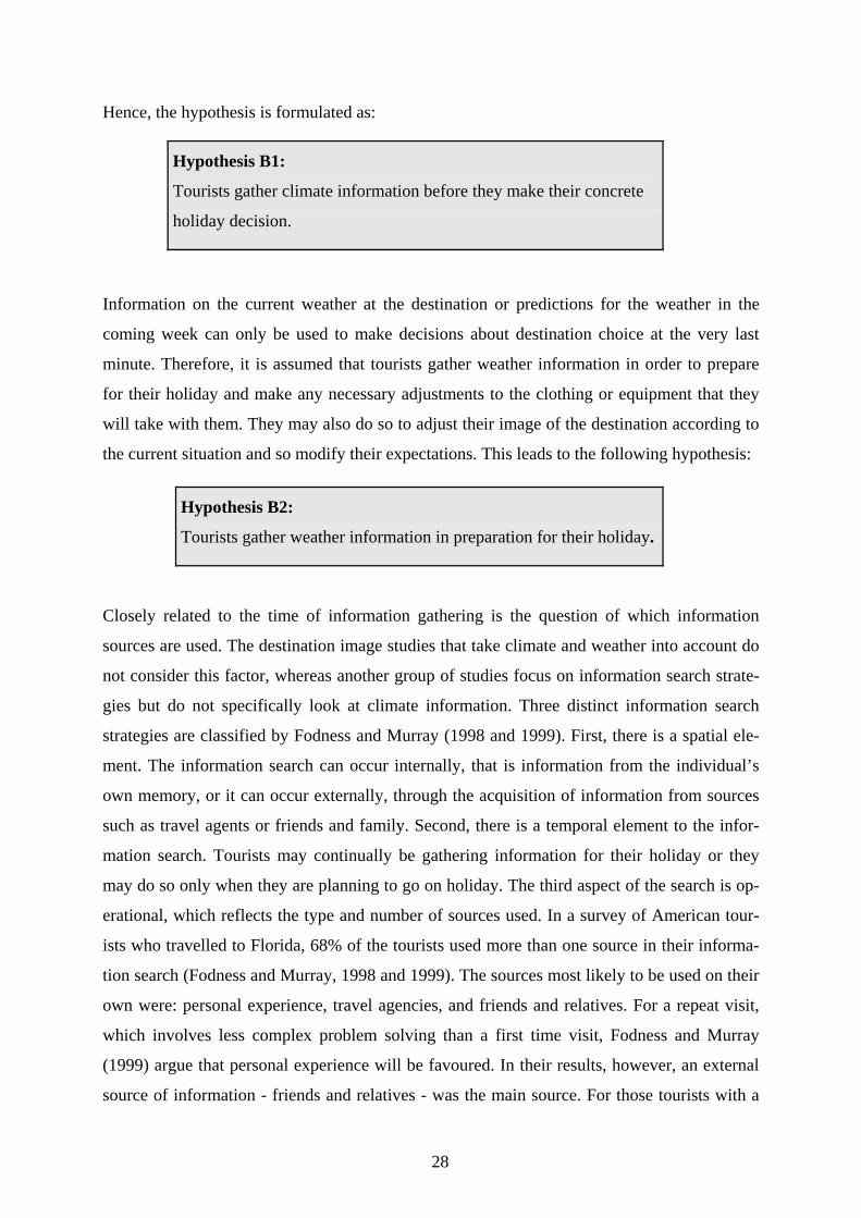
Hence, the hypothesis is formulated as:
Hypothesis B1:
Tourists gather climate information before they make their concrete
holiday decision.
Information on the current weather at the destination or predictions for the weather in the
coming week can only be used to make decisions about destination choice at the very last
minute. Therefore, it is assumed that tourists gather weather information in order to prepare
for their holiday and make any necessary adjustments to the clothing or equipment that they
will take with them. They may also do so to adjust their image of the destination according to
the current situation and so modify their expectations. This leads to the following hypothesis:
Hypothesis B2:
Tourists gather weather information in preparation for their holiday.
Closely related to the time of information gathering is the question of which information
sources are used. The destination image studies that take climate and weather into account do
not consider this factor, whereas another group of studies focus on information search strate-
gies but do not specifically look at climate information. Three distinct information search
strategies are classified by Fodness and Murray (1998 and 1999). First, there is a spatial ele-
ment. The information search can occur internally, that is information from the individual’s
own memory, or it can occur externally, through the acquisition of information from sources
such as travel agents or friends and family. Second, there is a temporal element to the infor-
mation search. Tourists may continually be gathering information for their holiday or they
may do so only when they are planning to go on holiday. The third aspect of the search is op-
erational, which reflects the type and number of sources used. In a survey of American tour-
ists who travelled to Florida, 68% of the tourists used more than one source in their informa-
tion search (Fodness and Murray, 1998 and 1999). The sources most likely to be used on their
own were: personal experience, travel agencies, and friends and relatives. For a repeat visit,
which involves less complex problem solving than a first time visit, Fodness and Murray
(1999) argue that personal experience will be favoured. In their results, however, an external
source of information - friends and relatives - was the main source. For those tourists with a
28
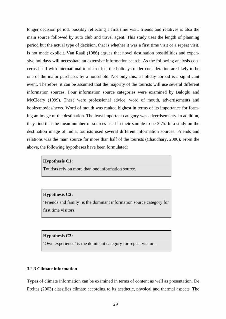
longer decision period, possibly reflecting a first time visit, friends and relatives is also the
main source followed by auto club and travel agent. This study uses the length of planning
period but the actual type of decision, that is whether it was a first time visit or a repeat visit,
is not made explicit. Van Raaij (1986) argues that novel destination possibilities and expen-
sive holidays will necessitate an extensive information search. As the following analysis con-
cerns itself with international tourism trips, the holidays under consideration are likely to be
one of the major purchases by a household. Not only this, a holiday abroad is a significant
event. Therefore, it can be assumed that the majority of the tourists will use several different
information sources. Four information source categories were examined by Baloglu and
McCleary (1999). These were professional advice, word of mouth, advertisements and
books/movies/news. Word of mouth was ranked highest in terms of its importance for form-
ing an image of the destination. The least important category was advertisements. In addition,
they find that the mean number of sources used in their sample to be 3.75. In a study on the
destination image of India, tourists used several different information sources. Friends and
relations was the main source for more than half of the tourists (Chaudhary, 2000). From the
above, the following hypotheses have been formulated:
Hypothesis C1:
Tourists rely on more than one information source.
Hypothesis C2:
‘Friends and family’ is the dominant information source category for
first time visitors.
Hypothesis C3:
‘Own experience’ is the dominant category for repeat visitors.
3.2.3 Climate information
Types of climate information can be examined in terms of content as well as presentation. De
Freitas (2003) classifies climate according to its aesthetic, physical and thermal aspects. The
29
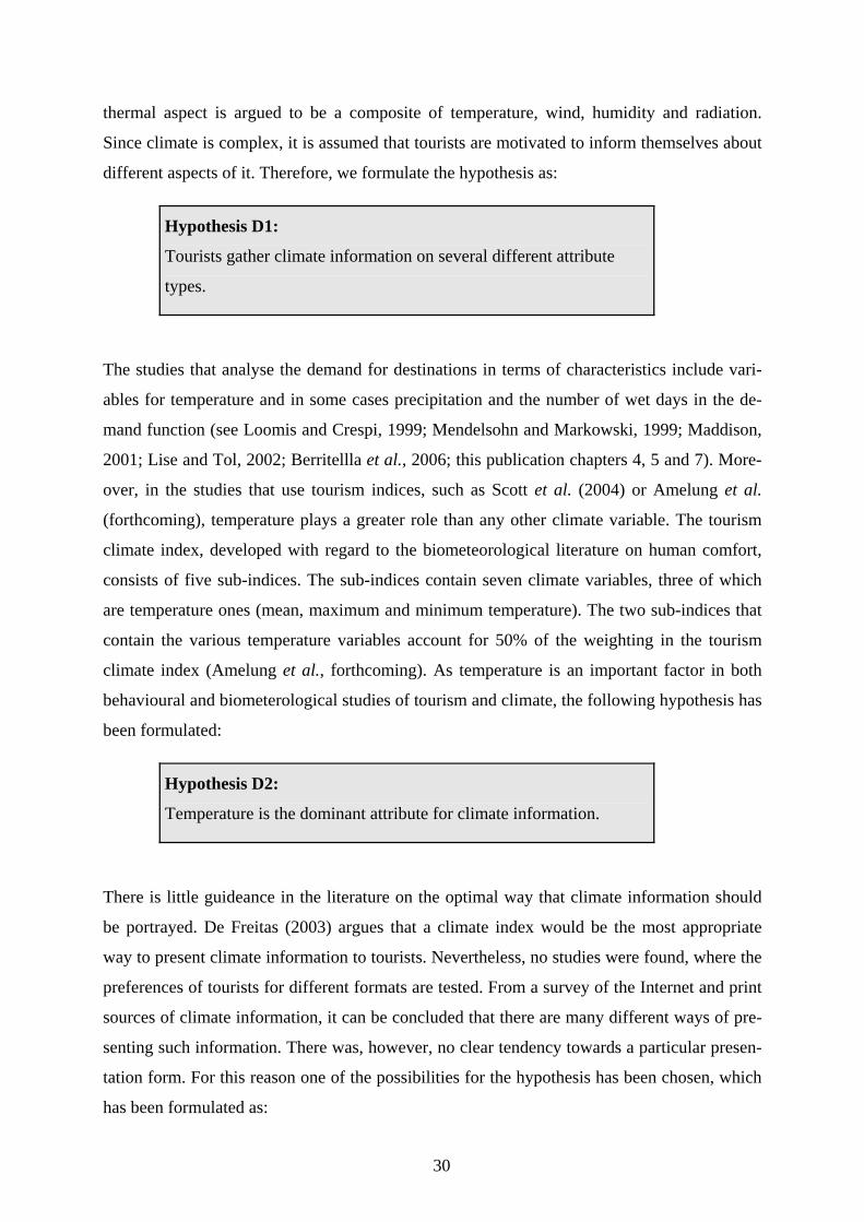
thermal aspect is argued to be a composite of temperature, wind, humidity and radiation.
Since climate is complex, it is assumed that tourists are motivated to inform themselves about
different aspects of it. Therefore, we formulate the hypothesis as:
Hypothesis D1:
Tourists gather climate information on several different attribute
types.
The studies that analyse the demand for destinations in terms of characteristics include vari-
ables for temperature and in some cases precipitation and the number of wet days in the de-
mand function (see Loomis and Crespi, 1999; Mendelsohn and Markowski, 1999; Maddison,
2001; Lise and Tol, 2002; Berritellla et al., 2006; this publication chapters 4, 5 and 7). More-
over, in the studies that use tourism indices, such as Scott et al. (2004) or Amelung et al.
(forthcoming), temperature plays a greater role than any other climate variable. The tourism
climate index, developed with regard to the biometeorological literature on human comfort,
consists of five sub-indices. The sub-indices contain seven climate variables, three of which
are temperature ones (mean, maximum and minimum temperature). The two sub-indices that
contain the various temperature variables account for 50% of the weighting in the tourism
climate index (Amelung et al., forthcoming). As temperature is an important factor in both
behavioural and biometerological studies of tourism and climate, the following hypothesis has
been formulated:
Hypothesis D2:
Temperature is the dominant attribute for climate information.
There is little guideance in the literature on the optimal way that climate information should
be portrayed. De Freitas (2003) argues that a climate index would be the most appropriate
way to present climate information to tourists. Nevertheless, no studies were found, where the
preferences of tourists for different formats are tested. From a survey of the Internet and print
sources of climate information, it can be concluded that there are many different ways of pre-
senting such information. There was, however, no clear tendency towards a particular presen-
tation form. For this reason one of the possibilities for the hypothesis has been chosen, which
has been formulated as:
30
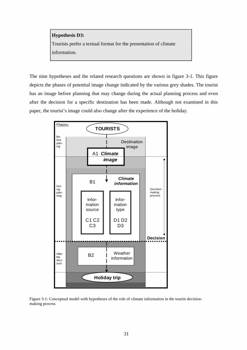
Hypothesis D3:
Tourists prefer a textual format for the presentation of climate
information.
The nine hypotheses and the related research questions are shown in figure 3-1. This figure
depicts the phases of potential image change indicated by the various grey shades. The tourist
has an image before planning that may change during the actual planning process and even
after the decision for a specific destination has been made. Although not examined in this
paper, the tourist’s image could also change after the experience of the holiday.
Figure 3-1: Conceptual model with hypotheses of the role of climate information in the tourist decision-making process
TOURISTS
Infor-mation source
C1 C2
C3
Infor-mation type
D1 D2
D3
Destination image
Climate information
Weather information
B2
B1
A1
Decision
Phases:
Be-fore plan-ing
Dur-ing plan-ning
After the deci-sion
Decision- making process
Holiday trip
Climate
image
31
3.3 Research Design
The fact that this study includes not only the questions of which information sources and
which information types but also emphasizes the time of information gathering lead to the
choice of a specific point in time to survey tourists – shortly before departure. This allowed
the travelpreparation phase to be included. The study population are those residents of Ger-
many going on an outbound holiday and departing from Hamburg and its vicinity. Our sam-
pling frame consists of those tourists departing from Hamburg and its vicinity at specific
points of departure: the airport, the train station,6 the international bus terminal and the har-
bours of Travemünde and Kiel (for ferries to Scandinavia).7 The convenience sample consists
of those tourists travelling on the selected days and on the selected departures. All participants
were aged 16 or over and resident in Germany. Additionally, only one person out of a travel
party was asked to take part in the survey. Business travellers have been purposefully ex-
cluded from the sample.
The following quotas were paid attention to:
1) Destination countries according to the market shares from the Reiseanalyse (FUR,
1998 and 2004)
2) Transportation mode market shares also from the Reiseanalyse (FUR, 1998 and 2004)
The survey was carried out on 20 days spread over the months of July and August 2004. The
days and times of the survey were chosen to correspond with departures to the countries with
a high quota. The study period covered the main parts of the local school holidays.8 The
schedule and budget of this study did not allow for an inclusion of car travellers according to
the market share of about one third of all travellers. Therefore, this group was left for future
research. The quotas, therefore, corresponded to the relative market shares of the other trans-
port modes.
6 Car-train departures to southern Europe from the station Hamburg-Altona were chosen. This gave us direct access to tourists travelling abroad by train, whereas with the normal international trains it would have taken a lot of time to locate the international travellers as domestic travellers also use the international trains. 7 There are no international ferries departing directly from Hamburg. 8 The six-week long school holidays of the states of Hamburg, Schleswig-Holstein and Mecklenburg-Pomerania were partly covered by the study period. For the states of Bremen and Lower Saxony, the school holidays coin-cided with the study period.
32
While creating the questionnaire a group of specialists was consulted, who then commented
on the preliminary versions of the questionnaire. These were tourism experts from academia
as well as professionals from the tourism industry and others from the fields of marketing and
quantitative research. A two-step pilot study was carried out at the end of June with two dif-
ferent groups: tourists leaving from Hamburg Airport and a group of randomly chosen stu-
dents. The comments of the experts and the results of the pilot phase were used to reformulate
individual questions and improve the structure of the questionnaire, and so improve the over-
all intelligibility.
The following provides an overview of the relevant questions from the questionnaire that
were used in this analysis. The first section of the questionnaire includes general questions on
the holiday: the destination country, the length of stay and the organizational form of the trip.
This section is largely oriented on the Reiseanalyse (FUR, 1998 and 2004) in order to guaran-
tee comparability to other studies. As far as possible, these questions are in multiple-choice
format. Another section contains two questions that identify the main image attributes and the
main information sources. See table 3-1 for details of the sources used to formulate these
questions. The next section begins with a filter question about whether the respondent had
been to the destination country before. If answered positively, the respondents are then asked
to complete five additional questions. After this, there is another filter question on whether the
respondent had informed themselves about the climate of their destination. If answered posi-
tively, another block of five questions follows. The questionnaire closes with a section con-
taining demographic questions that provide details on the respondent’s place of residence,
gender, age, and education level.
3.3.1 Hypothesis A1
This hypothesis is tested by examining if climate is at least the third most important attribute
for the choice of destination. In order to assess this the respondents were asked to rank the
three most important attributes out of ten attributes. The ten attributes were chosen according
to an analysis of the attributes that were found to be the most important9 for tourists in studies
on destination image (see table 3-1 for the sources used). This ranking question was deliber-
ately put on the first page of the questionnaire. Respondents were not told in advance the spe-
9 The five highest valued attributes from each study were taken and the frequency that each attribute appeared over all the studies was calculated. The ten most frequent were then taken from this list.
33
cific focus of the questionnaire. This way the individual’s perception of the importance of
climate could be assessed before the respondent became aware that climate was the main
theme of the questionnaire.
Tested attributes Source of attributes
Destination image Baloglu and Mangaloglu (2001), Baloglu and McCleary (1999), Kozak (2002), Lohmann and Kaim (1999), Gallarza et al . (2002), Hu and Ritchie (1993) and Yuan and McDonald (1990)
Information sources Baloglu and McCleary (1999), Chaudhary (2000), Fodness and Murray (1999) and Phelps (1986)
Type and presentation of information
own research of online weather information providers, online travel guides, information provided online by travel agents, tour operators, foreign offices and tourist boards, and print travel guides
General information on the trip and demographic information
FUR (1998 and 2004)
Table 3-1: Sources of attributes for the questionnaire
The assumption that climate information is indeed important within the decision-making
process purposefully does not mean a particular climate, e.g. as Baloglu and Mangaloglu
(2001) do when using the attribute ‘good climate’. This is unclear, as it could mean either a
good climate according to the individual’s preferences or a good climate for certain activities
that the tourist prefers to undertake while on holiday. It is assumed that some tourists will
search for warmer places to go, others may prefer a cooler climate than they experience in
their home region at the same time of the year and some may be completely indifferent.
Moreover, the individual’s perception of the climate at the destination as being ‘good’ may be
influenced by the home weather at the time of booking. In the region of Hamburg, where the
survey was undertaken, the summer of 2004 was comparatively cold and wet. In this study
only climate is referred to and not a valuation of it.
3.3.2 Hypotheses B1 and B2
Motivated by the decision phases formulated in the studies by Fridgen (1984), Ahmed (1991)
and Mansfeld (1992) three distinct phases of information gathering have been derived. The
first phase is limited to the time before the tourist decides to go on holiday. It is not an active
information gathering phase, since an image of the climate of the destination may be there
34
already either through previous experience in the country (or comparable climatic regions) or
through knowledge gained from a general interest in the area. The second phase covers the
period after the tourist is motivated to go on holiday but has not made the actual decision of
where and when. In this phase, information is actively gathered in order to make these deci-
sions. The third phase includes information gathering in preparation for the holiday. This is
carried out after the decision has been made but before the actual trip.
The hypotheses B1 and B2 are tested using the results of two questions. The first question
asks the tourists to state when they informed themselves about climate. There were seven op-
tions, which belonged to the following three groups: before planning, during planning and
after the decision, which correspond to the phases 1 to 3 respectively. The tourists were given
the opportunity to choose more than one option. The second question concerns the actual
weather at the destination before the trip: the tourists were asked whether they had been fol-
lowing the weather during the week before their holiday.
Pinpointing the time at which information is gathered also contributes to the analysis of cli-
mate as an important factor in decision-making (see hypothesis A1). Information gathering
during planning indicates a decisive character, while after the decision indicates, for example,
an adaptation of clothing to the climate and does not play an important role in the decision to
go to the destination.
3.3.3 Hypotheses C1, C2 and C3
A question on the sources of information about the destination in general was included in the
questionnaire. Information sources for general information on a destination may be different
from the sources used for climate information. From the review of the studies shown in table
3-1, 12 possible sources of information were compiled, including friends and family and own
experience as well as weather information providers. The latter was included not only because
of the purpose of this study but also because such sites contain information about destinations
and links to online travel agents, tour operators and airlines.
In order to test the hypotheses, the exact same sources were included in a question specifically
focusing on climate. The tourists were asked to rate, on a five point Likert scale, the actual
information sources used according to the importance for the decision. A filter question on
previous visits is used to establish the two groups of first time and repeat visitors.
35
3.3.4 Hypotheses D1, D2 and D3
In these hypotheses, the presentation of information is examined separately from the content
of the information. An examination of typical sources of destination information and destina-
tion climate information resulted in the inclusion of the following presentation categories: text
format, maps, diagrams and numerical data (see table 3-1 for the sources). The various infor-
mation sources provide different types of climate information, these range from several tem-
perature types to precipitation related information and less frequently mentioned attributes
such as humidity or UV-radiation.
3.4 Analysis
3.4.1 General results
Not all of the tourists asked to participate in the survey agreed to take part. The response rate
differed in two ways: first, between July and August and second, according to the departure
point where the survey was carried out. Generally, July showed a better response rate (of 2:1
and even better) than August. The response rate at the airport was generally not as high as at
the bus terminal, train station or ferry terminal. At the airport, the choice of terminal had an
effect. The survey was easier to carry out in the charter flight terminal, where the response
rate was 3:1 during August, whereas at the terminal for scheduled flights there was a response
rate of 10:1 on some survey days. In total, 413 questionnaires were returned. Questionnaires
where core questions were unanswered had to be removed from the sample, and so 394 ques-
tionnaires could be coded.
Table 3-2 shows the demographic profile of the tourists surveyed. Compared to the age struc-
ture from the Reiseanalyse data from 1998 (FUR, 1998), this survey has a more distinctive bi-
modal pattern, which can be seen by the larger shares of tourists in the 20-29 and 40-49 age
groups and a much smaller share in the 30-39 age group. The male/female split corresponds to
that of the current population of Germany. Compared to the Reiseanalyse from 1998, this sur-
vey has a much larger share of those with a degree or who have a university entrance diploma.
36
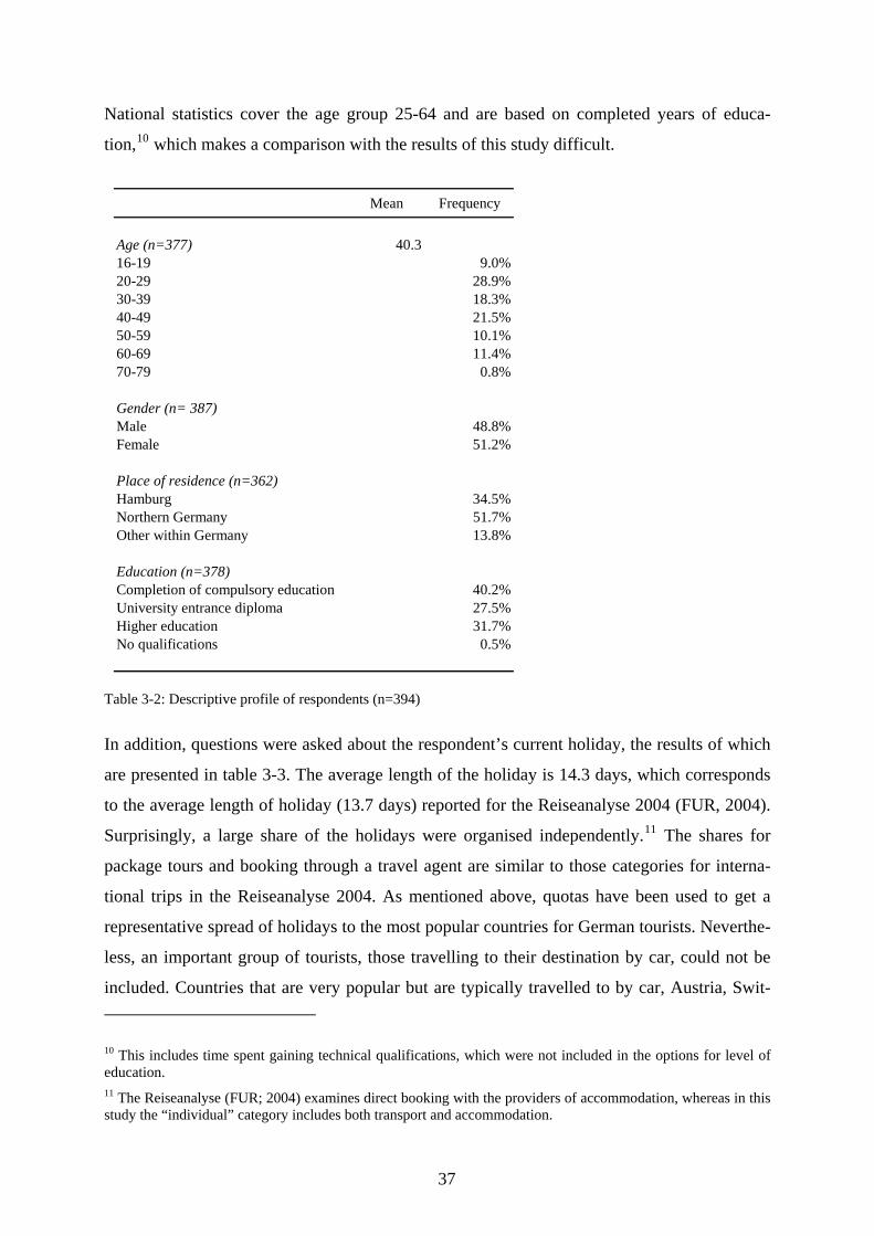
National statistics cover the age group 25-64 and are based on completed years of educa-
tion,10 which makes a comparison with the results of this study difficult.
Mean Frequency
Age (n=377) 40.316-19 9.0%20-29 28.9%30-39 18.3%40-49 21.5%50-59 10.1%60-69 11.4%70-79 0.8%
Gender (n= 387)Male 48.8%Female 51.2%
Place of residence (n=362)Hamburg 34.5%Northern Germany 51.7%Other within Germany 13.8%
Education (n=378)Completion of compulsory education 40.2%University entrance diploma 27.5%Higher education 31.7%No qualifications 0.5%
Table 3-2: Descriptive profile of respondents (n=394)
In addition, questions were asked about the respondent’s current holiday, the results of which
are presented in table 3-3. The average length of the holiday is 14.3 days, which corresponds
to the average length of holiday (13.7 days) reported for the Reiseanalyse 2004 (FUR, 2004).
Surprisingly, a large share of the holidays were organised independently.11 The shares for
package tours and booking through a travel agent are similar to those categories for interna-
tional trips in the Reiseanalyse 2004. As mentioned above, quotas have been used to get a
representative spread of holidays to the most popular countries for German tourists. Neverthe-
less, an important group of tourists, those travelling to their destination by car, could not be
included. Countries that are very popular but are typically travelled to by car, Austria, Swit-
10 This includes time spent gaining technical qualifications, which were not included in the options for level of education. 11 The Reiseanalyse (FUR; 2004) examines direct booking with the providers of accommodation, whereas in this study the “individual” category includes both transport and accommodation.
37
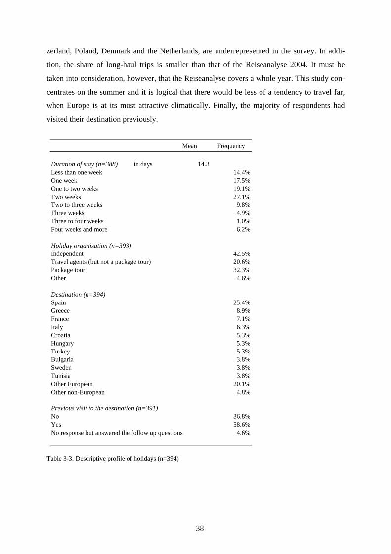
zerland, Poland, Denmark and the Netherlands, are underrepresented in the survey. In addi-
tion, the share of long-haul trips is smaller than that of the Reiseanalyse 2004. It must be
taken into consideration, however, that the Reiseanalyse covers a whole year. This study con-
centrates on the summer and it is logical that there would be less of a tendency to travel far,
when Europe is at its most attractive climatically. Finally, the majority of respondents had
visited their destination previously.
Mean Frequency
Duration of stay (n=388) in days 14.3Less than one week 14.4%One week 17.5%One to two weeks 19.1%Two weeks 27.1%Two to three weeks 9.8%Three weeks 4.9%Three to four weeks 1.0%Four weeks and more 6.2%
Holiday organisation (n=393)Independent 42.5%Travel agents (but not a package tour) 20.6%Package tour 32.3%Other 4.6%
Destination (n=394)Spain 25.4%Greece 8.9%France 7.1%Italy 6.3%Croatia 5.3%Hungary 5.3%Turkey 5.3%Bulgaria 3.8%Sweden 3.8%Tunisia 3.8%Other European 20.1%Other non-European 4.8%
Previous visit to the destination (n=391)No 36.8%Yes 58.6%No response but answered the follow up questions 4.6%
Table 3-3: Descriptive profile of holidays (n=394)
38
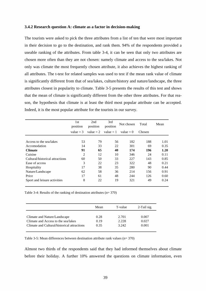
3.4.2 Research question A: climate as a factor in decision-making
The tourists were asked to pick the three attributes from a list of ten that were most important
in their decision to go to the destination, and rank them. 94% of the respondents provided a
useable ranking of the attributes. From table 3-4, it can be seen that only two attributes are
chosen more often than they are not chosen: namely climate and access to the sea/lakes. Not
only was climate the most frequently chosen attribute, it also achieves the highest ranking of
all attributes. The t-test for related samples was used to test if the mean rank value of climate
is significantly different from that of sea/lakes, culture/history and nature/landscape, the three
attributes closest in popularity to climate. Table 3-5 presents the results of this test and shows
that the mean of climate is significantly different from the other three attributes. For that rea-
son, the hypothesis that climate is at least the third most popular attribute can be accepted.
Indeed, it is the most popular attribute for the tourists in our survey.
1st position
2nd position
3rd position Not chosen Total Mean
value = 3 value = 2 value = 1 value = 0 Chosen
Access to the sea/lakes 53 79 56 182 188 1.01Accomodation 14 33 22 301 69 0.35Climate 91 65 40 174 196 1.20Cuisine 2 12 10 346 24 0.11Cultural/historical attractions 60 50 33 227 143 0.85Ease of access 3 22 23 322 48 0.21Hospitality 17 38 35 280 90 0.44Nature/Landscape 62 58 36 214 156 0.91Price 17 61 48 244 126 0.60Sport and leisure activities 8 22 19 321 49 0.24
Table 3-4: Results of the ranking of destination attributes (n= 370)
Table 3-5: Mean differences between destination attribute rank values (n= 370)
Mean T-value 2-Tail sig.
Climate and Nature/Landscape 0.28 2.701 0.007Climate and Access to the sea/lakes 0.19 2.228 0.027Climate and Cultural/historical attractions 0.35 3.242 0.001
Almost two thirds of the respondents said that they had informed themselves about climate
before their holiday. A further 10% answered the questions on climate information, even
39
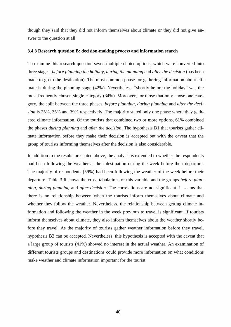
though they said that they did not inform themselves about climate or they did not give an-
swer to the question at all.
3.4.3 Research question B: decision-making process and information search
To examine this research question seven multiple-choice options, which were converted into
three stages: before planning the holiday, during the planning and after the decision (has been
made to go to the destination). The most common phase for gathering information about cli-
mate is during the planning stage (42%). Nevertheless, “shortly before the holiday” was the
most frequently chosen single category (34%). Moreover, for those that only chose one cate-
gory, the split between the three phases, before planning, during planning and after the deci-
sion is 25%, 35% and 39% respectively. The majority stated only one phase where they gath-
ered climate information. Of the tourists that combined two or more options, 61% combined
the phases during planning and after the decision. The hypothesis B1 that tourists gather cli-
mate information before they make their decision is accepted but with the caveat that the
group of tourists informing themselves after the decision is also considerable.
In addition to the results presented above, the analysis is extended to whether the respondents
had been following the weather at their destination during the week before their departure.
The majority of respondents (59%) had been following the weather of the week before their
departure. Table 3-6 shows the cross-tabulations of this variable and the groups before plan-
ning, during planning and after decision. The correlations are not significant. It seems that
there is no relationship between when the tourists inform themselves about climate and
whether they follow the weather. Nevertheless, the relationship between getting climate in-
formation and following the weather in the week previous to travel is significant. If tourists
inform themselves about climate, they also inform themselves about the weather shortly be-
fore they travel. As the majority of tourists gather weather information before they travel,
hypothesis B2 can be accepted. Nevertheless, this hypothesis is accepted with the caveat that
a large group of tourists (41%) showed no interest in the actual weather. An examination of
different tourists groups and destinations could provide more information on what conditions
make weather and climate information important for the tourist.
40
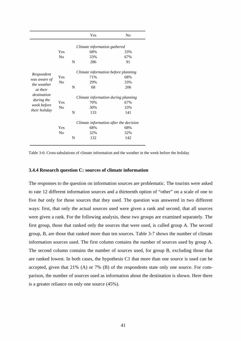
Yes No
Yes 68% 33%No 33% 67%
N 286 91
Yes 71% 68%No 29% 33%
N 68 206
Yes 70% 67%No 30% 33%
N 133 141
Yes 68% 68%No 32% 32%
N 132 142
Respondent was aware of the weather
at their destination during the
week before their holiday
Climate information gathered
Climate information after the decision
Climate information during planning
Climate information before planning
Table 3-6: Cross-tabulations of climate information and the weather in the week before the holiday
3.4.4 Research question C: sources of climate information
The responses to the question on information sources are problematic. The tourists were asked
to rate 12 different information sources and a thirteenth option of “other” on a scale of one to
five but only for those sources that they used. The question was answered in two different
ways: first, that only the actual sources used were given a rank and second, that all sources
were given a rank. For the following analysis, these two groups are examined separately. The
first group, those that ranked only the sources that were used, is called group A. The second
group, B, are those that ranked more than ten sources. Table 3-7 shows the number of climate
information sources used. The first column contains the number of sources used by group A.
The second column contains the number of sources used, for group B, excluding those that
are ranked lowest. In both cases, the hypothesis C1 that more than one source is used can be
accepted, given that 21% (A) or 7% (B) of the respondents state only one source. For com-
parison, the number of sources used as information about the destination is shown. Here there
is a greater reliance on only one source (45%).
41
Climate-Group A Climate-Group B Destination
1 21% 7% 45%2 24% 6% 28%3 24% 20% 17%4 17% 19% 8%5 4% 10% 2%6 4% 17% <1%7 <2% 9% <1%8 <2% 14%9 <2% 7%10 2% 8%11 4%12 6%13 2%
N 141 138 392
Table 3-7: Number of information sources used
For the first time visitors of group A, friends and family and travel guides are the most fre-
quently chosen sources with 51% each (more than one response was possible). The second
most important sources are travel agent and tour operator. For the group of repeat visitors of
group A, own experience was chosen by 69% of the respondents followed by friends and fam-
ily (53%) and travel guides (40%). An examination like this is difficult for group B as they
rank (almost) all of the sources. From this preliminary analysis, it seems that the hypothesis
C2 and C3 can be accepted. Nonetheless, a more detailed analysis is needed. Table 3-8, shows
the cross-tabulations of previous visit (yes/no) with the sources family and friends (yes/no)
and with own experience (yes/no). This is shown for the sources of information on the desti-
nation in general (for all tourists) and on climate for the groups A and B. For destination in-
formation and for climate information (group A), there is no statistically significant effect of
being a first time visitor on the likelihood of getting information from family and friends. For
group B, the effect is significant but counter-intuitive. Having visited the destination before
has the effect that you are more likely to ask family and friends about climate. The results are
much clearer for own experience. The positive relationship between previous visit and own
experience is significant for all groups.
Not only is it possible to examine the most frequently chosen sources, the mean rank values
can also be analysed. There are no statistically significant differences in the means of own
experience and family and friends for groups A and B. There are, however, differences in the
means, if the groups of repeat and first time visitors are examined separately. For group A,
42
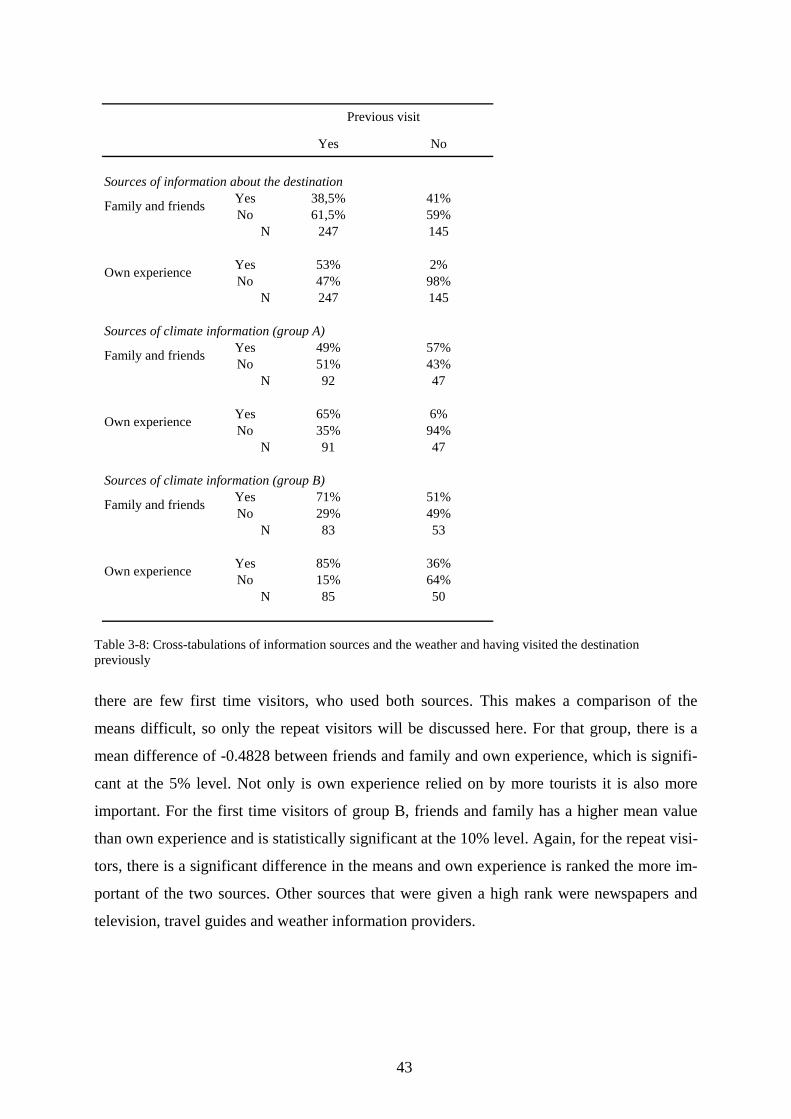
Yes No
Sources of information about the destination Yes 38,5% 41%No 61,5% 59%
N 247 145
Yes 53% 2%No 47% 98%
N 247 145
Sources of climate information (group A)Yes 49% 57%No 51% 43%
N 92 47
Yes 65% 6%No 35% 94%
N 91 47
Sources of climate information (group B)Yes 71% 51%No 29% 49%
N 83 53
Yes 85% 36%No 15% 64%
N 85 50
Own experience
Family and friends
Own experience
Previous visit
Family and friends
Family and friends
Own experience
Table 3-8: Cross-tabulations of information sources and the weather and having visited the destination previously
there are few first time visitors, who used both sources. This makes a comparison of the
means difficult, so only the repeat visitors will be discussed here. For that group, there is a
mean difference of -0.4828 between friends and family and own experience, which is signifi-
cant at the 5% level. Not only is own experience relied on by more tourists it is also more
important. For the first time visitors of group B, friends and family has a higher mean value
than own experience and is statistically significant at the 10% level. Again, for the repeat visi-
tors, there is a significant difference in the means and own experience is ranked the more im-
portant of the two sources. Other sources that were given a high rank were newspapers and
television, travel guides and weather information providers.
43
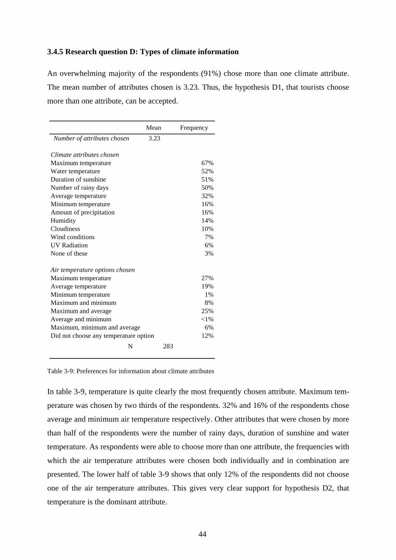
3.4.5 Research question D: Types of climate information
An overwhelming majority of the respondents (91%) chose more than one climate attribute.
The mean number of attributes chosen is 3.23. Thus, the hypothesis D1, that tourists choose
more than one attribute, can be accepted.
Mean Frequency Number of attributes chosen 3.23
Climate attributes chosenMaximum temperature 67%Water temperature 52%Duration of sunshine 51%Number of rainy days 50%Average temperature 32%Minimum temperature 16%Amount of precipitation 16%Humidity 14%Cloudiness 10%Wind conditions 7%UV Radiation 6%None of these 3%
Air temperature options chosenMaximum temperature 27%Average temperature 19%Minimum temperature 1%Maximum and minimum 8%Maximum and average 25%Average and minimum <1%Maximum, minimum and average 6%Did not choose any temperature option 12%
N 283
Table 3-9: Preferences for information about climate attributes
In table 3-9, temperature is quite clearly the most frequently chosen attribute. Maximum tem-
perature was chosen by two thirds of the respondents. 32% and 16% of the respondents chose
average and minimum air temperature respectively. Other attributes that were chosen by more
than half of the respondents were the number of rainy days, duration of sunshine and water
temperature. As respondents were able to choose more than one attribute, the frequencies with
which the air temperature attributes were chosen both individually and in combination are
presented. The lower half of table 3-9 shows that only 12% of the respondents did not choose
one of the air temperature attributes. This gives very clear support for hypothesis D2, that
temperature is the dominant attribute.
44
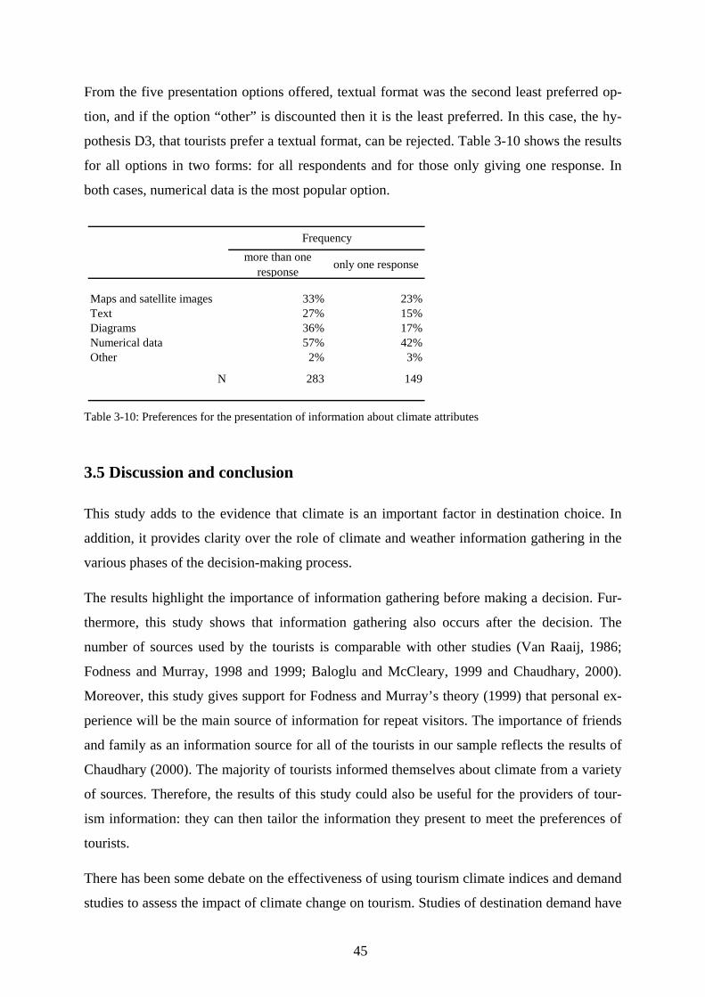
From the five presentation options offered, textual format was the second least preferred op-
tion, and if the option “other” is discounted then it is the least preferred. In this case, the hy-
pothesis D3, that tourists prefer a textual format, can be rejected. Table 3-10 shows the results
for all options in two forms: for all respondents and for those only giving one response. In
both cases, numerical data is the most popular option.
more than one response only one response
Maps and satellite images 33% 23%Text 27% 15%Diagrams 36% 17%Numerical data 57% 42%Other 2% 3%
N 283 149
Frequency
Table 3-10: Preferences for the presentation of information about climate attributes
3.5 Discussion and conclusion
This study adds to the evidence that climate is an important factor in destination choice. In
addition, it provides clarity over the role of climate and weather information gathering in the
various phases of the decision-making process.
The results highlight the importance of information gathering before making a decision. Fur-
thermore, this study shows that information gathering also occurs after the decision. The
number of sources used by the tourists is comparable with other studies (Van Raaij, 1986;
Fodness and Murray, 1998 and 1999; Baloglu and McCleary, 1999 and Chaudhary, 2000).
Moreover, this study gives support for Fodness and Murray’s theory (1999) that personal ex-
perience will be the main source of information for repeat visitors. The importance of friends
and family as an information source for all of the tourists in our sample reflects the results of
Chaudhary (2000). The majority of tourists informed themselves about climate from a variety
of sources. Therefore, the results of this study could also be useful for the providers of tour-
ism information: they can then tailor the information they present to meet the preferences of
tourists.
There has been some debate on the effectiveness of using tourism climate indices and demand
studies to assess the impact of climate change on tourism. Studies of destination demand have
45
been criticised of simplistically representing climate using single variables, such as tempera-
ture and precipitation and not a weighted group of variables. The results presented in this
study support the use of temperature as the main determining variable in destination demand
studies. Nevertheless, it cannot be claimed from these results that temperature alone is enough
to represent the considerations of tourists about destination climate. This study does not find
support for de Freitas’ argument (2003) that data presented as averages have no psychological
meaning. Travel guides typically present climate data as monthly averages and these were,
along with family and friends, the most frequently used source for first time visitors.
The limitations of this study need to be addressed. A major issue is that of the sample used.
Time and budget considerations limited the study to easily accessible departure points. As
tourists travelling by car have no common departure point, this group had to be omitted from
our sample. This had the consequence that certain destinations, such as Italy, Denmark, the
Netherlands and Austria, were underrepresented. Nevertheless, climatically comparable desti-
nations were well represented. It is unclear if different information search strategies are re-
lated to particular travel mode choices. In addition, a non-random sampling method was used,
which limits the ability to generalize from these results. The survey period encompassed the
school holidays of the states of Northern Germany. This peak holiday period can easily be
avoided by other groups of tourists who are not tied to institutional holidays. Therefore, the
study may be biased towards tourists travelling with children. From other survey sources, it
can be seen that older travellers favour the off-peak months (for example, Oppermann, 1995).
Despite two pilot studies, certain questions were not formulated clearly enough, which hin-
dered the analysis (see the results for research question C). An interview methodology may be
better to examine such complex issues but this would be expensive and time consuming on
this scale. Instead of using a self-administered questionnaire, verbally administering the ques-
tionnaire could bring more success.
Although they have quite different definitions, the terms weather and climate are used inter-
changeably by the public. This can also be seen in some of the image studies that refer to
weather, even though what is actually meant is climate. Even though great care was taken to
be clear and to distinguish between weather and climate in our survey, in some questions it is
possible that the respondents misunderstood and gave responses in terms of weather informa-
tion. This is particularly the case with climate information sources, where some of the sources
46

listed can give information on past weather, the climate, current weather and predicted
weather. For example, online weather information providers12 or even family and friends
could provide such information. Again, a verbally administered questionnaire could be more
effective.
Global climate change is already having an effect on mean temperature and its further course
is very likely to have an impact on the tourism industry as well. As the results of this study
show, climate is a defining factor for the destination choice of tourists. When the climate
changes, destinations’ attractiveness will change and with it – probably with a considerable
time lag – tourists’ images of the destinations. An ancillary effect of global warming is that of
sea-level rise. Access to the sea will change considerably as the quality of beaches will mostly
deteriorate, with intensified erosion and change of slope occurring. As this study shows that
the access to the sea and to lakes is the second most important attribute to tourists when
choosing a destination, sea-level rise will have a large effect on the tourism industry, as tour-
ists will not necessarily adopt to the new situation by changing their preferences, they would
rather change destinations.
Having carried out this survey, the first of its kind to focus on climate as a specific attribute of
destination image and on its role in the decision-making process, a valuable database that can
be used for further research has been produced. For instance, the issue of whether the tourists’
images of climate are accurate when compared to the climate of their destination can be as-
sessed (Um and Crompton, 1990). Some destination image studies found that there were dif-
ferences in image for different groups of tourists (Shoemaker, 1994 and Kozak, 2002). It
would be an interesting extension of this study to examine, whether different information
preferences exist for different demographic or holiday groups of this survey.
12 For example www.wetter.com, the website of the German Meteorological Service, where it is possible to ac-cess a climate data bank, plot weather data from the recent past, check current weather and get a ten day forecast for many towns and cities in the world.
47
Chapter 4
Climate and the destination choice of German tourists∗
4.1 Introduction
Typically, when estimating tourism demand the attributes of destinations are not included.
However, these attributes, according to Morley (1991), will determine the utility of a visit to a
certain destination with a certain set of characteristics. This study looks further than just to the
different spatial attributes of destinations but also to the temporal ones; different months have
different climatic conditions. Moreover, climate change implies that these attributes will
change over the long term and so utility and the resulting patterns of demand will change.
With this in mind, the purpose of this chapter is to examine demand in terms of destination
characteristics. This is done by way of a case study of German tourists. German tourists make
up the second largest market in terms of expenditure (after the USA) and they account for
10% of world spending on tourism (WTO, 2005b). Their market importance means that an
examination of the possible impacts of climate change on the patterns of demand is of particu-
lar interest. The estimated relationships between the climate variables can then be used to ex-
amine the impact of climate change on demand. The pooled travel cost method, which is used
in this study, had been developed in other case studies for the UK and the Netherlands. How-
ever, in this study, the set of destination attributes used in the regression analysis is extended
and the temporal aspect is examined at the monthly scale as opposed to the quarterly scale.
Whereas previous PTCM studies have used quarterly data and focussed on outbound tourism,
this study uses monthly data and the origin country Germany is included as a destination op-
tion.
This chapter is structured as follows. In the second section, the pooled travel cost method is
discussed. The data used in this study is presented in the third section. The fourth section pre-
sents the results of the regression analysis. The implications of these are discussed in the fifth
section. In the sixth section, the impact of climate change on climatic attractiveness is exam-
∗ This chapter is based on Hamilton (2003).
48
ined. Some limitations of the methodology are discussed in section 7. The eighth section con-
cludes.
Only two studies examine quantitatively the sensitivity of tourism demand to climate and cli-
mate change. Maddison (2001) examines climate as a determinant of the destination choices
of British tourists and estimates a demand function that included climate variables and beach
length for each country. The estimated function is then used to examine changes in the num-
ber of tourists as well as changes in welfare using projected changes in temperature and pre-
cipitation under a “business as usual” greenhouse gas emissions scenario. Lise and Tol (2002)
adapt Maddison's model and apply it to data on the destination choices of Dutch tourists.
4.2. Methodology: the pooled travel cost method
The pooled travel cost method, which is based on microeconomic theory, includes character-
istics of destinations which Morley (1992) and Papatheodorou (2001) argue to be necessary.
This technique is a variant of the travel cost models, which have been widely used for esti-
mating the demand for recreation sites. Two different types of these models exist: those that
focus on single sites and those that examine multiple sites. In the former case, the purpose is
to calculate the total economic value of the site and, in the latter case, the object is to obtain a
measure of the change in value when site characteristics change. It is this second set of mod-
els that is useful for examining the impact of climate change.
The basic premise of both types of model, however, lies in the fact that in order to use ser-
vices provided by a certain site you have to travel there. This will involve a cost in terms of
travel expenditure and the opportunity cost of time. If recreation is a normal good then sites
with a higher travel cost will be visited less than those with the same characteristics but a
lower travel cost. In the case of single sites, individuals who incur a lower travel cost for a
certain site will visit that site more frequently than those individuals with a higher travel cost
will. Using data on the number of visits and the cost of these visits, a demand function can be
estimated. The total value of the site can be measured by the area under the demand curve. In
the case of multiple sites, the characteristics of sites are included in the demand function.
As travel is necessary for the consumption of the environmental amenities at a particular site,
it is said to be a complement to them. That is, changes in the price of travel will affect the
number of trips and through this, the quantity consumed of the amenities. Further, travel cost
49
exhibits the quality of weak complementarity for the environmental amenities. Weak com-
plementarity exists when there is a price where demand for the market good will be zero and
changes in the public good, the environmental quality, will have no effect on welfare. In terms
of travel to a site, this means that if the price of travel to a particular place is so high that no
one wants to go there then changes in the qualities of that site do not bring any benefits to
consumers. This enables the use of the demand curve for the market good to estimate the
value of the non-market good, which in this case is the environmental quality of a site. When
certain characteristics of a site improve, the demand curve for the market good, in this case
travel cost, will shift outwards and to the right and so more of the favoured amenities are
available at the same travel cost. To value this change, the difference in the area under the
demand curves but above the market price for the original level of amenities and for the im-
proved level is calculated.
Freemann (1993) describes the methods used to estimate the demand for multiple sites, with
the qualification that these models have limitations through their simplification. One tech-
nique involves pooling the number of visits to recreation sites and estimating a single demand
equation. The set of explanatory variables will include quality variables, which must be suffi-
ciently varied across the sites, in order to use regression techniques to estimate the demand
function. The coefficients on the parameters are the same across all sites. Freeman states that
such models can be used to examine changes in the characteristics at one site, but argues that
as they do not contain substitute site qualities or prices in the specification, it is not possible to
examine the case where quality changes occur at more than one site.
Maddison (2001) adapted the recreation demand models described by Freemann (1993) and
applied it to a case study of international tourism. Using data on British tourists' destination
choices, he pools the choices of individuals for different destinations and estimates the de-
mand function for British tourists as a group. He assumes that tourists have perfect informa-
tion about the climate of countries. In addition, the demand function is used to analyse the
impact of changes in environmental quality, in this case changes in climate. The model de-
scribed by Maddison will be used in this study to examine the sensitivity of the demand of
German tourists to climate and other destination factors.
50
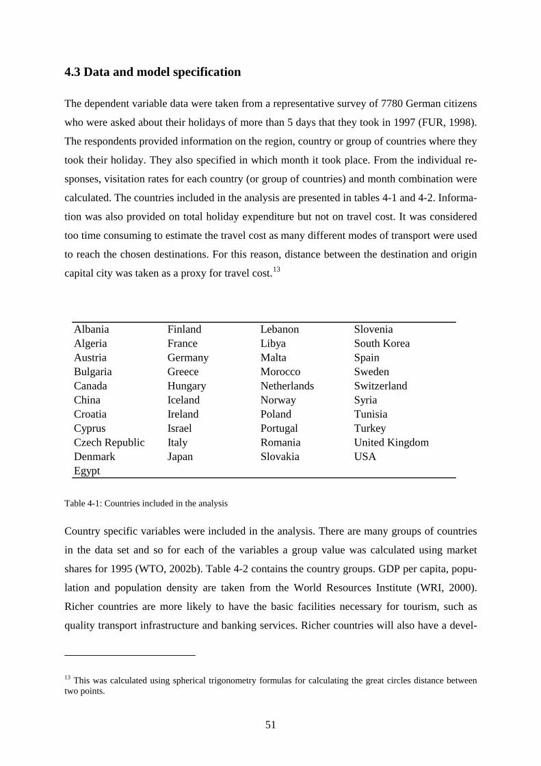
4.3 Data and model specification
The dependent variable data were taken from a representative survey of 7780 German citizens
who were asked about their holidays of more than 5 days that they took in 1997 (FUR, 1998).
The respondents provided information on the region, country or group of countries where they
took their holiday. They also specified in which month it took place. From the individual re-
sponses, visitation rates for each country (or group of countries) and month combination were
calculated. The countries included in the analysis are presented in tables 4-1 and 4-2. Informa-
tion was also provided on total holiday expenditure but not on travel cost. It was considered
too time consuming to estimate the travel cost as many different modes of transport were used
to reach the chosen destinations. For this reason, distance between the destination and origin
capital city was taken as a proxy for travel cost.13
Albania Finland Lebanon SloveniaAlgeria France Libya South KoreaAustria Germany Malta SpainBulgaria Greece Morocco SwedenCanada Hungary Netherlands SwitzerlandChina Iceland Norway SyriaCroatia Ireland Poland TunisiaCyprus Israel Portugal TurkeyCzech Republic Italy Romania United KingdomDenmark Japan Slovakia USAEgypt
Table 4-1: Countries included in the analysis
Country specific variables were included in the analysis. There are many groups of countries
in the data set and so for each of the variables a group value was calculated using market
shares for 1995 (WTO, 2002b). Table 4-2 contains the country groups. GDP per capita, popu-
lation and population density are taken from the World Resources Institute (WRI, 2000).
Richer countries are more likely to have the basic facilities necessary for tourism, such as
quality transport infrastructure and banking services. Richer countries will also have a devel-
13 This was calculated using spherical trigonometry formulas for calculating the great circles distance between two points.
51
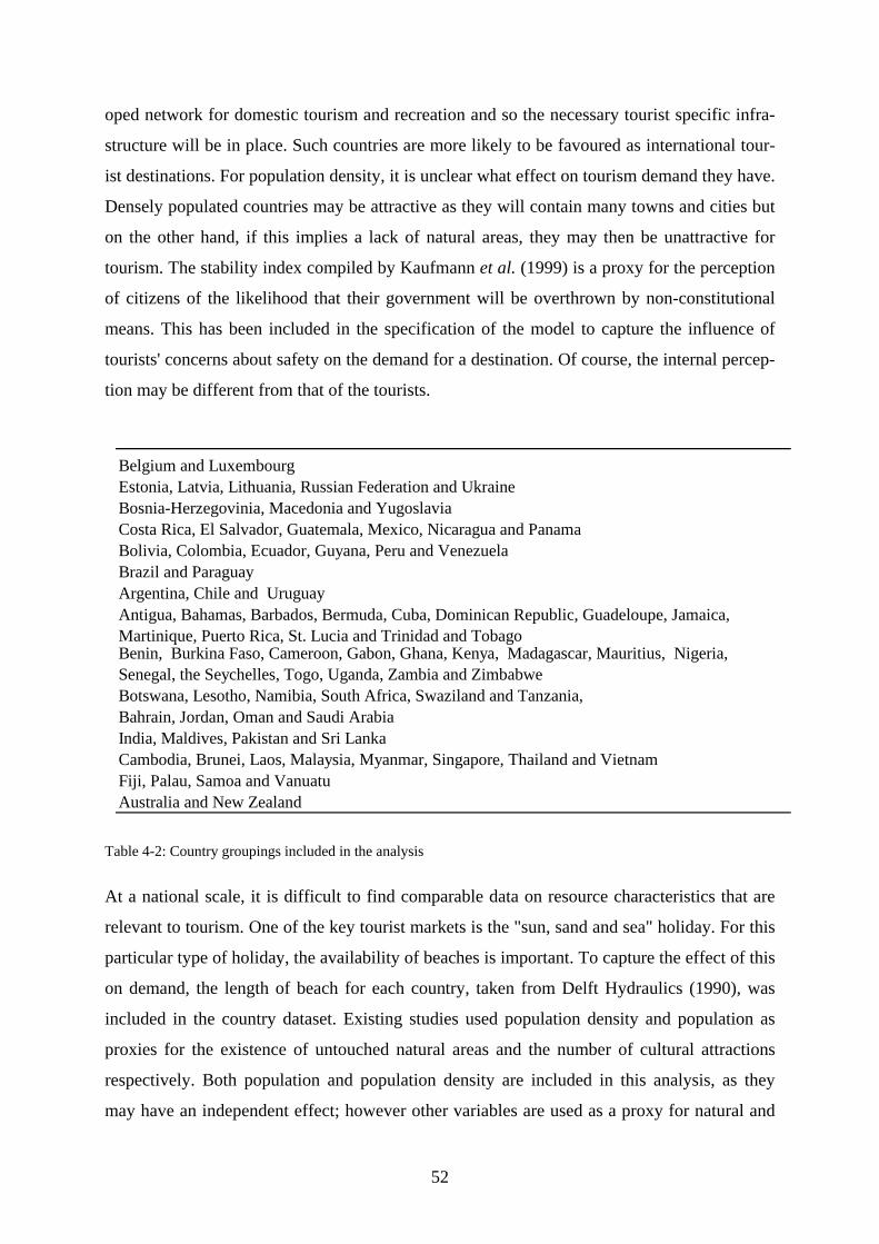
oped network for domestic tourism and recreation and so the necessary tourist specific infra-
structure will be in place. Such countries are more likely to be favoured as international tour-
ist destinations. For population density, it is unclear what effect on tourism demand they have.
Densely populated countries may be attractive as they will contain many towns and cities but
on the other hand, if this implies a lack of natural areas, they may then be unattractive for
tourism. The stability index compiled by Kaufmann et al. (1999) is a proxy for the perception
of citizens of the likelihood that their government will be overthrown by non-constitutional
means. This has been included in the specification of the model to capture the influence of
tourists' concerns about safety on the demand for a destination. Of course, the internal percep-
tion may be different from that of the tourists.
Australia and New ZealandFiji, Palau, Samoa and Vanuatu
Antigua, Bahamas, Barbados, Bermuda, Cuba, Dominican Republic, Guadeloupe, Jamaica, Martinique, Puerto Rica, St. Lucia and Trinidad and Tobago
Bahrain, Jordan, Oman and Saudi Arabia India, Maldives, Pakistan and Sri LankaCambodia, Brunei, Laos, Malaysia, Myanmar, Singapore, Thailand and Vietnam
Botswana, Lesotho, Namibia, South Africa, Swaziland and Tanzania,
Bolivia, Colombia, Ecuador, Guyana, Peru and VenezuelaBrazil and Paraguay
Benin, Burkina Faso, Cameroon, Gabon, Ghana, Kenya, Madagascar, Mauritius, Nigeria, Senegal, the Seychelles, Togo, Uganda, Zambia and Zimbabwe
Argentina, Chile and Uruguay
Belgium and LuxembourgEstonia, Latvia, Lithuania, Russian Federation and UkraineBosnia-Herzegovinia, Macedonia and YugoslaviaCosta Rica, El Salvador, Guatemala, Mexico, Nicaragua and Panama
Table 4-2: Country groupings included in the analysis
At a national scale, it is difficult to find comparable data on resource characteristics that are
relevant to tourism. One of the key tourist markets is the "sun, sand and sea" holiday. For this
particular type of holiday, the availability of beaches is important. To capture the effect of this
on demand, the length of beach for each country, taken from Delft Hydraulics (1990), was
included in the country dataset. Existing studies used population density and population as
proxies for the existence of untouched natural areas and the number of cultural attractions
respectively. Both population and population density are included in this analysis, as they
may have an independent effect; however other variables are used as a proxy for natural and
52
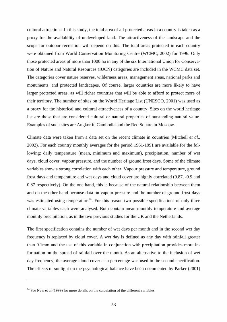
cultural attractions. In this study, the total area of all protected areas in a country is taken as a
proxy for the availability of undeveloped land. The attractiveness of the landscape and the
scope for outdoor recreation will depend on this. The total areas protected in each country
were obtained from World Conservation Monitoring Centre (WCMC, 2002) for 1996. Only
those protected areas of more than 1000 ha in any of the six International Union for Conserva-
tion of Nature and Natural Resources (IUCN) categories are included in the WCMC data set.
The categories cover nature reserves, wilderness areas, management areas, national parks and
monuments, and protected landscapes. Of course, larger countries are more likely to have
larger protected areas, as will richer countries that will be able to afford to protect more of
their territory. The number of sites on the World Heritage List (UNESCO, 2001) was used as
a proxy for the historical and cultural attractiveness of a country. Sites on the world heritage
list are those that are considered cultural or natural properties of outstanding natural value.
Examples of such sites are Angkor in Cambodia and the Red Square in Moscow.
Climate data were taken from a data set on the recent climate in countries (Mitchell et al.,
2002). For each country monthly averages for the period 1961-1991 are available for the fol-
lowing: daily temperature (mean, minimum and maximum), precipitation, number of wet
days, cloud cover, vapour pressure, and the number of ground frost days. Some of the climate
variables show a strong correlation with each other. Vapour pressure and temperature, ground
frost days and temperature and wet days and cloud cover are highly correlated (0.87, -0.9 and
0.87 respectively). On the one hand, this is because of the natural relationship between them
and on the other hand because data on vapour pressure and the number of ground frost days
was estimated using temperature14. For this reason two possible specifications of only three
climate variables each were analysed. Both contain mean monthly temperature and average
monthly precipitation, as in the two previous studies for the UK and the Netherlands.
The first specification contains the number of wet days per month and in the second wet day
frequency is replaced by cloud cover. A wet day is defined as any day with rainfall greater
than 0.1mm and the use of this variable in conjunction with precipitation provides more in-
formation on the spread of rainfall over the month. As an alternative to the inclusion of wet
day frequency, the average cloud cover as a percentage was used in the second specification.
The effects of sunlight on the psychological balance have been documented by Parker (2001)
14 See New et al (1999) for more details on the calculation of the different variables
53
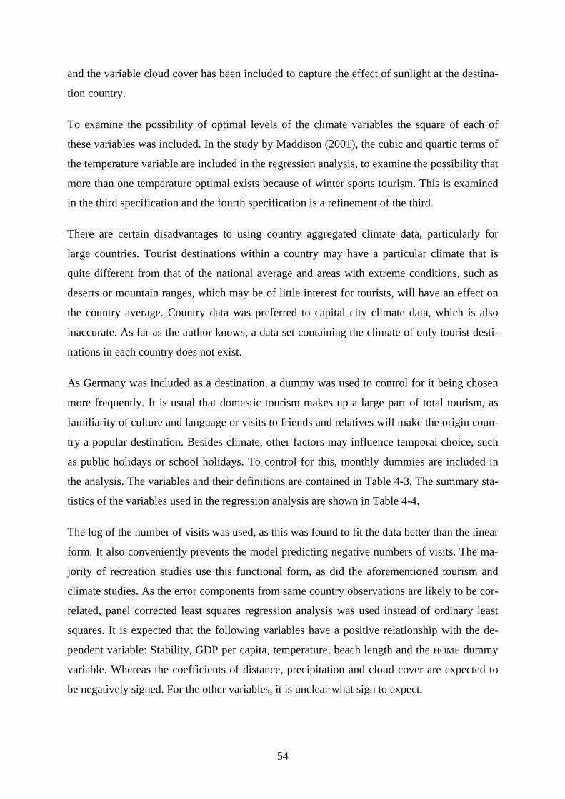
and the variable cloud cover has been included to capture the effect of sunlight at the destina-
tion country.
To examine the possibility of optimal levels of the climate variables the square of each of
these variables was included. In the study by Maddison (2001), the cubic and quartic terms of
the temperature variable are included in the regression analysis, to examine the possibility that
more than one temperature optimal exists because of winter sports tourism. This is examined
in the third specification and the fourth specification is a refinement of the third.
There are certain disadvantages to using country aggregated climate data, particularly for
large countries. Tourist destinations within a country may have a particular climate that is
quite different from that of the national average and areas with extreme conditions, such as
deserts or mountain ranges, which may be of little interest for tourists, will have an effect on
the country average. Country data was preferred to capital city climate data, which is also
inaccurate. As far as the author knows, a data set containing the climate of only tourist desti-
nations in each country does not exist.
As Germany was included as a destination, a dummy was used to control for it being chosen
more frequently. It is usual that domestic tourism makes up a large part of total tourism, as
familiarity of culture and language or visits to friends and relatives will make the origin coun-
try a popular destination. Besides climate, other factors may influence temporal choice, such
as public holidays or school holidays. To control for this, monthly dummies are included in
the analysis. The variables and their definitions are contained in Table 4-3. The summary sta-
tistics of the variables used in the regression analysis are shown in Table 4-4.
The log of the number of visits was used, as this was found to fit the data better than the linear
form. It also conveniently prevents the model predicting negative numbers of visits. The ma-
jority of recreation studies use this functional form, as did the aforementioned tourism and
climate studies. As the error components from same country observations are likely to be cor-
related, panel corrected least squares regression analysis was used instead of ordinary least
squares. It is expected that the following variables have a positive relationship with the de-
pendent variable: Stability, GDP per capita, temperature, beach length and the HOME dummy
variable. Whereas the coefficients of distance, precipitation and cloud cover are expected to
be negatively signed. For the other variables, it is unclear what sign to expect.
54
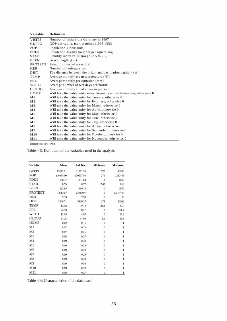
VISITSGDPPCPOP Population (thousands)PDEN Population density (number per square km) STABBLENPROTECTHERDISTTEMPPREW ETDCLOUD Average monthly cloud cover in percentHOM EM1M2M3M4M5M6M7M8M9M10 M11Sources: see text
Variable Definition
Number of visits from Germany in 1997GDP per capita, market prices (1995 US$)
Stability index value (range -2.5 to 2.5)Beach length (km)
Average monthly precipitation (mm)Average number of wet days per month
W ill take the value unity when Germany is the destination, otherwise 0
Area of protected areas (ha)Number of heritage sitesThe distance between the origin and destination capital (km)Average monthly mean temperature (°C)
W ill take the value unity for January, otherwise 0W ill take the value unity for February, otherwise 0W ill take the value unity for M arch, otherwise 0W ill take the value unity for April, otherwise 0W ill take the value unity for M ay, otherwise 0
W ill take the value unity for October, otherwise 0W ill take the value unity for November, otherwise 0
W ill take the value unity for June, otherwise 0W ill take the value unity for July, otherwise 0W ill take the value unity for August, otherwise 0W ill take the value unity for September, otherwise 0
Table 4-3: Definition of the variables used in the analysis
Table 4-4: Characteristics of the data used
GDPPC 13171.11 11771.36 520 40998POP 100484.90 230597.80 271 1232456PDEN 180.37 291.84 3 1620STAB 0.55 0.77 -2.42 1.69BLEN 263.85 480.73 0 2970PROTECT 1.47E+07 2.68E+07 0 1.04E+08HER 9.33 7.98 0 33DIST 3548.71 3916.27 174 16933TEMP 13.92 9.14 -21.2 30.7PRE 74.93 50.27 0 251.4WETD 11.14 4.97 0 22.3CLOUD 57.25 14.93 8.1 86.8HOME 0.02 0.15 0 1M1 0.07 0.25 0 1M2 0.07 0.25 0 1M3 0.08 0.27 0 1M4 0.09 0.28 0 1M5 0.09 0.28 0 1M6 0.09 0.29 0 1M7 0.09 0.29 0 1M8 0.09 0.28 0 1M9 0.10 0.30 0 1M10 0.09 0.29 0 1M11 0.08 0.27 0 1
MaximumVariable Mean Std. Dev. Minimum
55
4.4 Results
The results of the regression analysis are presented in Table 4-5. For specification 1, the re-
gression explains 58.4% of the variation in the log of the number of visits. The number of
heritage sites, length of beach and the level of GDP per capita are all highly significant and
signed as expected. The stability variable STAB has a positive relationship to the dependent
variable but it is not significant. The coefficient for PROTECT is negatively signed but is sig-
nificant only at the 10% level. Although protected areas may be an attraction for tourists
many of these protected areas may not in fact be accessible for tourists or tourist development
has been restricted because the land has been protected. The coefficient on DIST is as ex-
pected, highly significant and negatively signed. The popularity of domestic tourism is re-
flected in the positive and highly significant coefficient for the variable HOME. The coeffi-
cients on population and population density are not significant. From the monthly dummies,
the months February and November are found to be negative and significant. This result is
plausible considering that these two months lie either side of the Christmas and New Year
holiday period, when many people take holidays and also a large portion of the household
budget will be used during the festive period.
Temperature is highly significant. However, the square of temperature is not significant.
Therefore, the optimal temperature cannot be calculated. Here we have a positive relationship
between demand and temperature; as temperature increases so will demand. Purely from the
human physiological point of view, this is rather unlikely, as at high temperatures, particularly
in combination with high levels of humidity, a state of discomfort will occur. For precipita-
tion, a minimum turning point is found at 137mm per month, which is much higher than the
observed values for any month in Germany or in Northern Europe. Before this point, any in-
crease in precipitation will have a negative effect on demand. There is an optimal number of
wet days at 11.5 days per month. The Northern European countries have more wet days per
month all year round and such a value is typical of a Mediterranean winter. The calculated
optimal values for each specification are shown in Table 4-6.
56
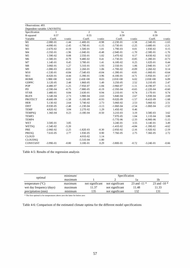
Observations: 493Dependent variable: LN(VISITS)Specification R-squaredVariable Coeff. t-ratio Coeff. t-ratio Coeff. t-ratio Coeff. t-ratioM1 -2.08E-01 -1.44 -1.40E-01 -0.98 -2.23E-01 -1.58 -2.34E-01 -1.63M2 -4.09E-01 -2.45 -1.79E-01 -1.15 -3.73E-01 -2.25 -3.68E-01 -2.21M3 -2.67E-02 -0.19 1.50E-01 1.01 1.79E-03 0.01 1.93E-02 0.15M4 -3.35E-01 -1.96 -1.04E-01 -0.48 -2.94E-01 -1.70 -2.58E-01 -1.76M5 1.59E-02 0.08 2.55E-01 1.02 3.47E-02 0.17 8.03E-02 0.5M6 -1.58E-01 -0.79 9.48E-02 0.41 -1.73E-01 -0.85 -1.28E-01 -0.73M7 1.14E-01 0.45 3.78E-01 1.41 6.10E-02 0.25 1.02E-01 0.4M8 3.06E-01 1.27 5.31E-01 1.93 2.55E-01 1.06 2.94E-01 1.3M9 -1.08E-03 -0.01 2.26E-01 1.06 -1.70E-02 -0.09 2.26E-02 0.14M10 -1.53E-01 -0.84 -7.54E-03 -0.04 -1.39E-01 -0.81 -1.06E-01 -0.64M11 -6.02E-01 -4.44 -5.39E-01 -3.96 -6.10E-01 -4.71 -5.95E-01 -4.57HOME 1.98E+00 6.02 2.43E+00 8.03 2.01E+00 6.02 2.03E+00 6.09GDPPC 3.12E-05 2.48 1.86E-05 1.49 3.25E-05 2.52 3.21E-05 2.4POP -4.48E-07 -1.25 -7.95E-07 -1.84 -3.96E-07 -1.11 -4.19E-07 -1.15PD -2.59E-04 -0.75 -7.88E-05 -0.19 -2.35E-04 -0.65 -2.22E-04 -0.60STAB 2.48E-01 0.84 2.63E-01 0.94 2.21E-01 0.74 2.17E-01 0.7BLEN 5.54E-04 2.73 5.98E-04 2.63 5.84E-04 2.67 5.93E-04 2.6PROTECT -8.60E-09 -1.58 -5.10E-09 -0.93 -9.02E-09 -1.57 -9.41E-09 -1.68HER 5.13E-02 2.64 5.74E-02 2.73 5.06E-02 2.53 5.06E-02 2.51DIST -9.93E-05 -2.48 -1.23E-04 -3.13 -1.06E-04 -2.54 -1.06E-04 -2.52TEMP 4.82E-02 3.04 2.27E-02 1.29 1.45E-02 0.46TEMPSQ 1.36E-04 0.23 -3.18E-04 -0.50 3.21E-03 3.19 3.58E-03 3.62TEMP3 7.97E-05 1.04 1.11E-04 3.88TEMP4 -5.77E-06 -2.33 -6.90E-06 -5.15WET 3.50E-01 3.85 3.24E-01 3.55 3.14E-01 3.49WETSQ -1.54E-02 -5.20 -1.41E-02 -4.84 -1.39E-02 -4.62PRE -2.06E-02 -2.25 -1.82E-03 -0.30 -2.05E-02 -2.16 -1.92E-02 -2.19PRESQ 7.61E-05 2.77 1.93E-05 0.90 7.76E-05 2.75 7.36E-05 2.7CLOUD 4.01E-02 1.14CLOUDSQ -5.51E-04 -1.80CONSTANT -3.99E-01 -0.80 3.10E-01 0.29 -3.80E-01 -0.72 -3.24E-01 -0.66
1 2 1a 1b0.57 0.55 0.59 0.59
2
47
7
49
2
Table 4-5: Results of the regression analysis
Table 4-6: Comparison of the estimated climate optima for the different model specifications
1 2 1a 1btemperature (°C) maximum not significant not significant 23 and -11 * 23 and -10 *wet day frequency (days) maximum 11.37 not significant 11.48 11.33precipitation (mm) minimum 135 not significant 132 131* The first optimal is for temperatures above zero the latter for below zero
Specificationminimum/ maximumoptimal
57
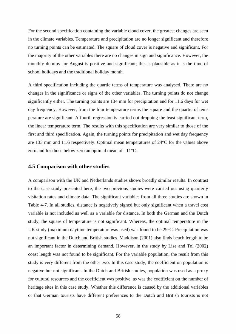
For the second specification containing the variable cloud cover, the greatest changes are seen
in the climate variables. Temperature and precipitation are no longer significant and therefore
no turning points can be estimated. The square of cloud cover is negative and significant. For
the majority of the other variables there are no changes in sign and significance. However, the
monthly dummy for August is positive and significant; this is plausible as it is the time of
school holidays and the traditional holiday month.
A third specification including the quartic terms of temperature was analysed. There are no
changes in the significance or signs of the other variables. The turning points do not change
significantly either. The turning points are 134 mm for precipitation and for 11.6 days for wet
day frequency. However, from the four temperature terms the square and the quartic of tem-
perature are significant. A fourth regression is carried out dropping the least significant term,
the linear temperature term. The results with this specification are very similar to those of the
first and third specification. Again, the turning points for precipitation and wet day frequency
are 133 mm and 11.6 respectively. Optimal mean temperatures of 24°C for the values above
zero and for those below zero an optimal mean of –11°C.
4.5 Comparison with other studies
A comparison with the UK and Netherlands studies shows broadly similar results. In contrast
to the case study presented here, the two previous studies were carried out using quarterly
visitation rates and climate data. The significant variables from all three studies are shown in
Table 4-7. In all studies, distance is negatively signed but only significant when a travel cost
variable is not included as well as a variable for distance. In both the German and the Dutch
study, the square of temperature is not significant. Whereas, the optimal temperature in the
UK study (maximum daytime temperature was used) was found to be 29°C. Precipitation was
not significant in the Dutch and British studies. Maddison (2001) also finds beach length to be
an important factor in determining demand. However, in the study by Lise and Tol (2002)
coast length was not found to be significant. For the variable population, the result from this
study is very different from the other two. In this case study, the coefficient on population is
negative but not significant. In the Dutch and British studies, population was used as a proxy
for cultural resources and the coefficient was positive, as was the coefficient on the number of
heritage sites in this case study. Whether this difference is caused by the additional variables
or that German tourists have different preferences to the Dutch and British tourists is not
58
clear. Not included in the German study, but in the others, was a variable to measure the price
level in each country. Variables to examine the influence of age and income were also used in
the Dutch study, which improved the R2.
Maddison (2001)
Lise and Tol (2002)
This study Specification 1
Origin Country United Kingdom The Netherlands GermanyYear 1994 1988/1992 1997Observations 305 187 493R2 0.5 0.43 0.57Variable GDPPC + + +BLEN + ne +PDEN - ns ns
POP + + ns
DIST ns - -TEMP + + +TEMP2 - ns ns
PRE ns ns -
Significant variables and their signs
1 "ne" denotes the variables that were not included in the particular analysis and "ns" indicates that the variables were included but were not found to be significant.
Table 4-7: Comparison of the case study results with those of the UK and Dutch studies
4.6 The climate attractiveness index and a scenario of climate change
According to the Third Assessment Report of the IPCC, it is projected that global surface
temperature and the sea level are expected to increase during this century. Based upon the
results of a set of different climate models and greenhouse gas emissions scenarios, an in-
crease in the global mean temperature of between 0.8°C and 2.6°C is projected for the period
1990 to 2050 (Houghton et al., 2001). Globally the average annual precipitation is also ex-
pected to increase, however at the regional scale there may also be considerable decreases in
the level of precipitation. It is possible to examine the impact of these changes on the attrac-
tiveness of a destination using the results of this case study. This has been done through the
construction of a climate index. Taking only the climate data for each country and the coeffi-
cients for each of the climate variables resulting from the regression analysis, the contribution
of climate to demand can be calculated and the countries then ranked according to their cli-
59
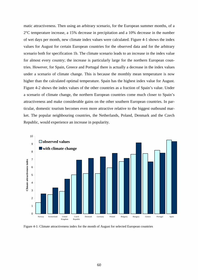
matic attractiveness. Then using an arbitrary scenario, for the European summer months, of a
2°C temperature increase, a 15% decrease in precipitation and a 10% decrease in the number
of wet days per month, new climate index values were calculated. Figure 4-1 shows the index
values for August for certain European countries for the observed data and for the arbitrary
scenario both for specification 1b. The climate scenario leads to an increase in the index value
for almost every country; the increase is particularly large for the northern European coun-
tries. However, for Spain, Greece and Portugal there is actually a decrease in the index values
under a scenario of climate change. This is because the monthly mean temperature is now
higher than the calculated optimal temperature. Spain has the highest index value for August.
Figure 4-2 shows the index values of the other countries as a fraction of Spain’s value. Under
a scenario of climate change, the northern European countries come much closer to Spain’s
attractiveness and make considerable gains on the other southern European countries. In par-
ticular, domestic tourism becomes even more attractive relative to the biggest outbound mar-
ket. The popular neighbouring countries, the Netherlands, Poland, Denmark and the Czech
Republic, would experience an increase in popularity.
Figure 4-1: Climate attractiveness index for the month of August for selected European countries
0
1
2
3
4
5
6
7
8
9
Norway Switzerland UnitedKingdom
CzechRepublic
Denmark Germany Poland Bulgaria Hungary Greece Portugal Spain
Clim
ate
attr
activ
enes
s ind
ex
10
observed values
with climate change
60
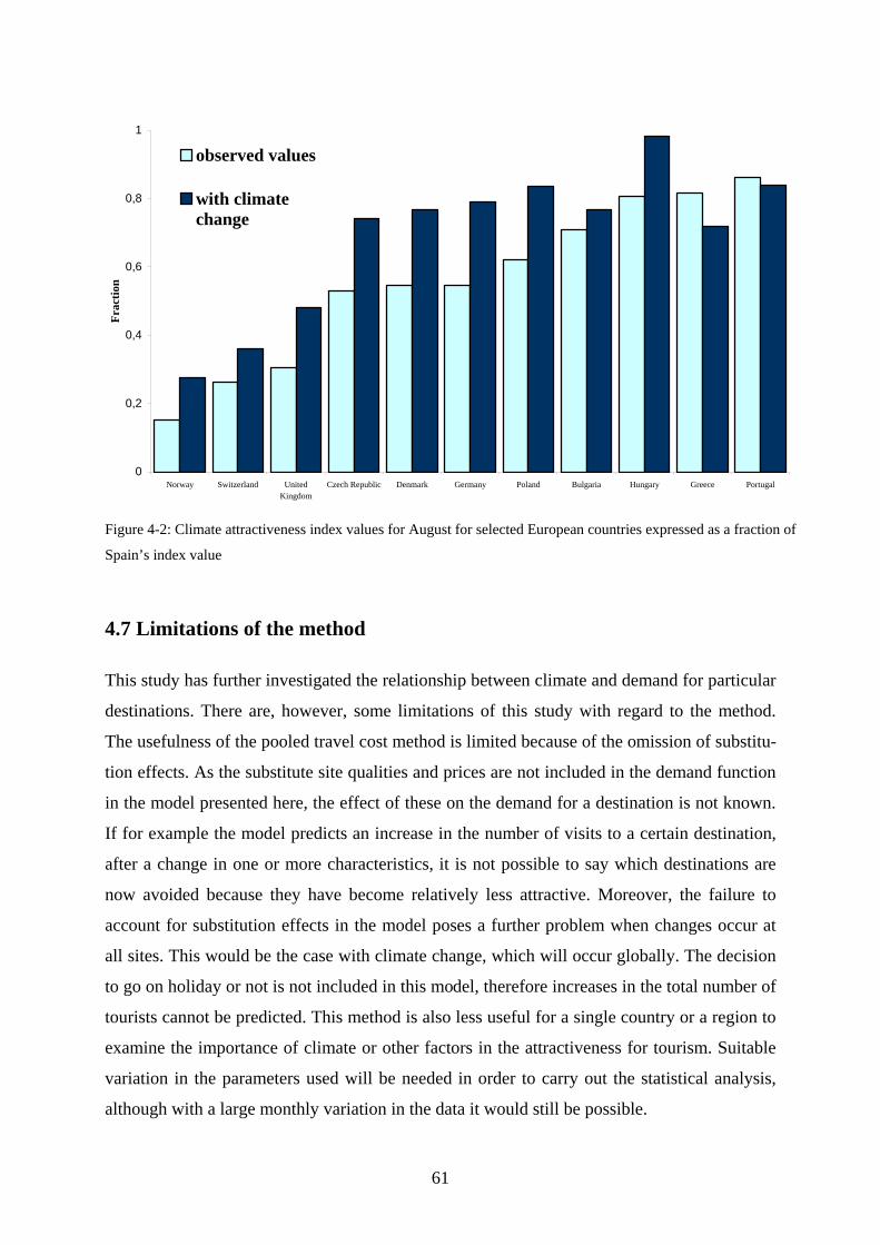
0
0,2
0,4
0,6
0,8
1
Norway Switzerland UnitedKingdom
Czech Republic Denmark Germany Poland Bulgaria Hungary Greece Portugal
Frac
tion
observed values
with climatechange
Figure 4-2: Climate attractiveness index values for August for selected European countries expressed as a fraction of
Spain’s index value
4.7 Limitations of the method
This study has further investigated the relationship between climate and demand for particular
destinations. There are, however, some limitations of this study with regard to the method.
The usefulness of the pooled travel cost method is limited because of the omission of substitu-
tion effects. As the substitute site qualities and prices are not included in the demand function
in the model presented here, the effect of these on the demand for a destination is not known.
If for example the model predicts an increase in the number of visits to a certain destination,
after a change in one or more characteristics, it is not possible to say which destinations are
now avoided because they have become relatively less attractive. Moreover, the failure to
account for substitution effects in the model poses a further problem when changes occur at
all sites. This would be the case with climate change, which will occur globally. The decision
to go on holiday or not is not included in this model, therefore increases in the total number of
tourists cannot be predicted. This method is also less useful for a single country or a region to
examine the importance of climate or other factors in the attractiveness for tourism. Suitable
variation in the parameters used will be needed in order to carry out the statistical analysis,
although with a large monthly variation in the data it would still be possible.
61
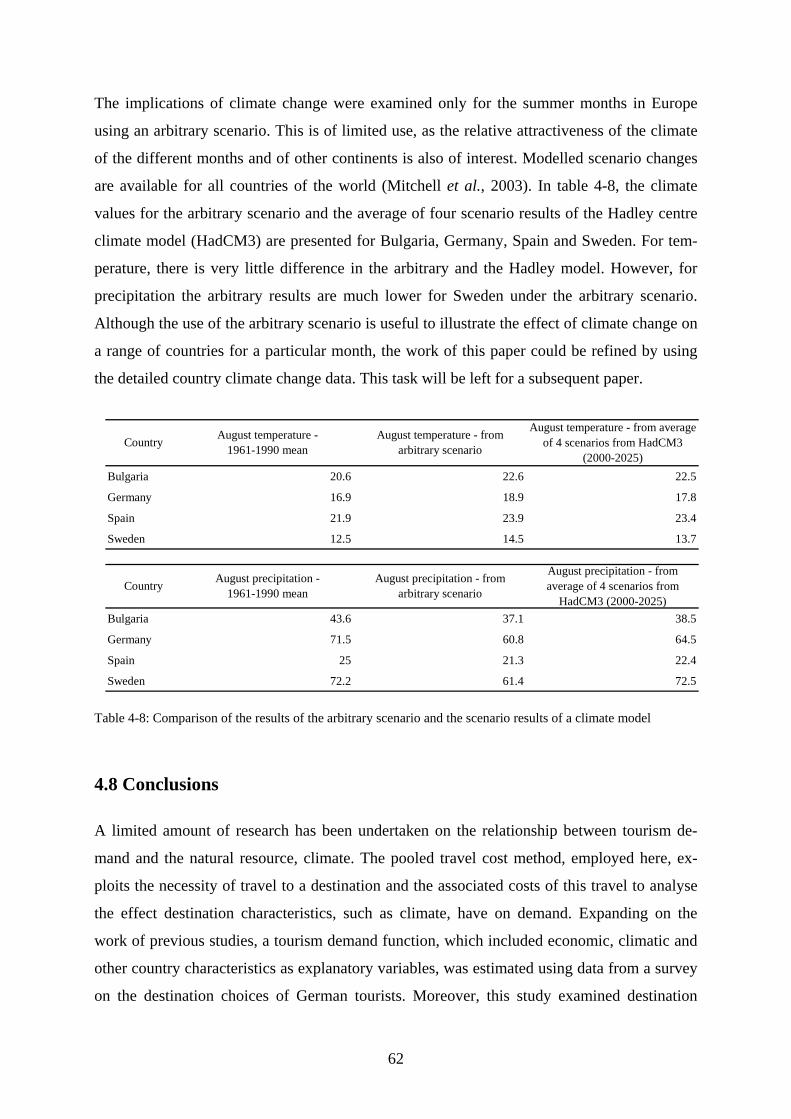
The implications of climate change were examined only for the summer months in Europe
using an arbitrary scenario. This is of limited use, as the relative attractiveness of the climate
of the different months and of other continents is also of interest. Modelled scenario changes
are available for all countries of the world (Mitchell et al., 2003). In table 4-8, the climate
values for the arbitrary scenario and the average of four scenario results of the Hadley centre
climate model (HadCM3) are presented for Bulgaria, Germany, Spain and Sweden. For tem-
perature, there is very little difference in the arbitrary and the Hadley model. However, for
precipitation the arbitrary results are much lower for Sweden under the arbitrary scenario.
Although the use of the arbitrary scenario is useful to illustrate the effect of climate change on
a range of countries for a particular month, the work of this paper could be refined by using
the detailed country climate change data. This task will be left for a subsequent paper.
Bulgaria 20.6 22.6 22.5
Germany 16.9 18.9 17.8
Spain 21.9 23.9 23.4
Sweden 12.5 14.5 13.7
Bulgaria 43.6 37.1 38.5
Germany 71.5 60.8 64.5
Spain 25 21.3 22.4
Sweden 72.2 61.4 72.5
August temperature - 1961-1990 mean
August precipitation - 1961-1990 meanCountry
CountryAugust temperature - from average
of 4 scenarios from HadCM3 (2000-2025)
August temperature - from arbitrary scenario
August precipitation - from arbitrary scenario
August precipitation - from average of 4 scenarios from
HadCM3 (2000-2025)
Table 4-8: Comparison of the results of the arbitrary scenario and the scenario results of a climate model
4.8 Conclusions
A limited amount of research has been undertaken on the relationship between tourism de-
mand and the natural resource, climate. The pooled travel cost method, employed here, ex-
ploits the necessity of travel to a destination and the associated costs of this travel to analyse
the effect destination characteristics, such as climate, have on demand. Expanding on the
work of previous studies, a tourism demand function, which included economic, climatic and
other country characteristics as explanatory variables, was estimated using data from a survey
on the destination choices of German tourists. Moreover, this study examined destination
62
choice at the monthly level, extended the set of country characteristics used and examined
domestic and outbound tourism. Proxy variables to measure safety and cultural attractiveness
were included and two specifications with different climate variables were examined. The
specification including wet day frequency was found to perform better than the specification
with the variable cloud cover. The former specification was extended to include cubic and
quartic terms. In addition to the optimal wet day frequency and precipitation levels, two opti-
mal temperature values were estimated. For temperatures above zero, the optimal was found
to be at 24°C. All of the specifications improve on the results of the earlier studies for the
Netherlands and the United Kingdom. An index of climate attractiveness for each country and
month was calculated and used to examine the changes in attractiveness under an arbitrary
climate change scenario. The northern European countries increase in attractiveness with cli-
mate change; the southern European countries becoming relatively less attractive. Using a
more detailed climate change scenario, for each country and month, as opposed to an arbitrary
one for a particular month and a restricted set of countries, would be an improvement on the
current study. Although the travel cost methodology provides us with an insight in to the rela-
tionship between tourism demand and destination characteristics, it inadequately describes the
substitution process. For this reason, further research is needed to find suitable ways to model
this process.
63
Chapter 5
Climate preferences and destination choice: a segmentation approach*
5.1 Introduction
In the previous chapter the impact of climate change on tourism is examined in terms of the
behaviour of the average tourist. This chapter moves on to investigate the climate-related be-
haviour of German tourists, not on average, but of several classes of tourists.
Recent studies assessing the impact of climate change on tourism demand patterns use current
behavioural patterns to estimate what demand will be under scenarios of climate change (Lise
and Tol, 2002; Maddison, 2001; this publication chapters 4, 7 and 8). As well as environ-
mental changes such as climate change, countries can be expected to experience changes in
population, in income, in values and in policy emphasis. In order to gain an insight into the
possible range of impacts in an unknown future, scenarios are used. The SRES scenarios of
population change and economic development are based on storylines describing different
futures according to a positioning on a globalization-regionalization scale and on an eco-
nomic-environmental emphasis scale (IMAGE Team, 2001). These different storylines have
different energy use and emissions patterns and therefore different estimates of climate
change. Chapters 7 and 8 of this thesis examine future changes in global tourism flows with
respect to, not only a climate change scenario, but also to the economic and population sce-
narios of SRES. But it is not only will the amount of tourists that will change. In addition, the
socio-economic and demographic characteristics of those who travel will change. Moreover,
on a long-term scale, it is plausible that tourism trends and tourist preferences will change. On
the supply side, new destinations may emerge, while some existing destinations may no
longer be available for tourism.
To extend existing studies, tourism scenarios that describe possible tourism trends or that in-
clude demographic changes could be used along side the socio-economic and climate scenar-
ios. Such scenarios would extend the storylines of the SRES scenarios to include tourism as-
pects. The core of these scenarios would be the relationship between demand and destination
* This chapter is based on Hamilton et al. (2005c).
64
climate, and for each scenario there would be a different tourism demand and climate rela-
tionship.
Market segmentation involves defining tourist groups according to certain demographic, be-
havioural or psychographic traits. In the numerous segmentation studies in the literature, the
segments are compared according to socio-economic characteristics, holiday characteristics or
preferences for certain destination characteristics. One of the frequently used means of seg-
mentation is nationality. Although not segmentation studies, the studies by Maddison (2001),
Lise and Tol, (2002) and chapter 4 in this publication have examined the tourism demand of
the UK, the Netherlands and Germany respectively. These studies use the pooled travel cost
method to examine the relationship between destination characteristics and demand. More-
over, climate variables, namely temperature, precipitation and in the case of the German
study, wet day frequency, were included in the demand equation. Using the climate coeffi-
cients obtained from the regression analyses, the optimal values of the climate variables are
estimated. The results of these studies apply to the demand of a nation as a whole. For tourism
scenarios that, for example, seek to examine a new trend or a demographic change, the inter-
est is in the climatic preferences of certain demographic or behavioural groups and not in na-
tional groups.
The objective of this study is to combine the segmentation approach and the pooled travel
cost method to examine the climate preferences of different segments and so provide quantita-
tive information for tourism scenarios. A survey of the holiday travel behaviour of German
citizens during 1997 is segmented using three different means: phase in the life cycle, holiday
motivation and holiday activities, and region of residence. The next section begins with a re-
view of the literature on segmentation. Following this, the methods used to segment the sur-
vey data and to analyse the climate-demand relationships of the segments are presented. The
results of the statistical analyses and, as a means of comparison, the climate index values for
certain destinations are discussed in section four. The fifth section concludes.
5.2 Literature review
Segmentation can be carried out using various criteria; the most common, however, is the use
of the life cycle. Lawson (1991) examines the expenditure and activities of eight family life
cycle groups. These groups were heterogeneous in terms of spending and in the activities cho-
sen. Unfortunately, this study does not examine the behaviour of different national groups
even though five countries are represented. Oppermann (1995) argues that travel patterns are
65

dynamic over the life cycle. What is more, childhood holiday experience, according to Op-
permann, has an influence on destination choice later in the life cycle. These ideas are con-
firmed in a longitudinal study of German tourist behaviour: younger tourists leave Central
Europe more frequently than older tourists, and for the age group 34-48 there is a decline in
demand compared to the other age groups. In addition, different generations show different
travel patterns at the same point in the life cycle. The bi-modal demand pattern over the life
cycle, with the trough occurring in the thirties to late forties, is observed by Collins and Tis-
dell (2002). Psychological needs also change over the life cycle and as a consequence the type
of tourist behaviour chosen. Gibson and Yiannakis (2002) note that, for a survey of citizens of
the USA, getting older affects the pattern of behavioural roles taken. In their study, the tourist
role “sun lover” is observed most frequently. Nevertheless, this role becomes less important
over the lifetime of the individuals surveyed. Segmentation according to age has been carried
out extensively for the senior market. Even within the senior market there are heterogeneous
groups (Shoemaker, 1989). Reviewing the literature on the senior market, Fleischer and Pi-
zam (2002) find that income and health are the determinants of heterogeneity between the
groups in terms of number of vacation days. Moreover, the number of vacation days decreases
with age.
The use of nationality as a segmentation approach has generated some debate (Dann, 1993;
Mykletun et al. 2001). Mykletun et al. (2001) find that nationality is the most important factor
in defining groups according to levels of expenditure or of satisfaction. Other studies confirm
that there are differences in the behaviour of nationalities in terms of destination choice moti-
vation, spatial distribution patterns and the likelihood of independent travel (Oppermann,
1992; Oppermann, 1994; Kozak, 2002). Yuan and MacDonald (1990), however, find that the
motivation for travelling is the same across national groups.
In order to gain a profile of high spending groups, segmentation studies have been carried out
according to levels of expenditure at a destination. Mok and Iverson (2000) note that very
little work has been done on segmentation according to expenditure. Nevertheless, studies on
visitors to the Canary Islands and the Balearic Islands show that different nationalities and
different demographic clusters have heterogeneous expenditure patterns (Bethencourt et al.,
2002; Perez and Sampol, 2000).
66
The activities undertaken by tourists are also used to segment the tourist market. This can be
done generally by defining different types of tourists (Gibson and Yiannakis, 2002; Wickens,
2002) or more specifically using activity choices to build homogeneous clusters (Lise and
Tol, 2002; Shoemaker, 1994).
Some of the segmentation studies analyse different preferences for destination characteristics.
Hu and Ritchie (1993) find that for a survey of Americans, climate is ranked higher by recrea-
tional tourists than by educational ones. Moreover, climate is ranked second from 16 possible
attributes by the former segment and ranked 12th by the latter. Shoemaker (1994) uses factor
analysis to build three segments of tourists: adventurous/educational travellers get
away/family travellers and gamblers/fun travellers. The gamblers/fun travellers rank “good
climate/weather” higher than the other two groups. In addition, this group ranks “opportunity
to sunbathe“ and “good beaches“ higher than the other groups. Based on segmentation ac-
cording to nationality, Kozak (2002) examines the push and pull motivations of German and
British tourists visiting Mallorca and Turkey. He found that there are some differences in the
importance attached to destination characteristics between the resorts visited and by the origin
country of the tourists. For both origin countries “enjoying good weather” is the most impor-
tant motivational factor. From the destination-based factors, “weather” is the second most
attractive factor for the British visitors to Mallorca and the most important for those visiting
Turkey. The German tourists rank “weather” as the most important characteristic for both
destinations.
These studies demonstrate that climate is a significant factor in determining a country’s at-
tractiveness. Nevertheless, the rank position does not tell us how climate influences the de-
mand for different countries. Using factor analysis and data on the destination choices of
Dutch tourists, Lise and Tol (2002) construct nine activity clusters. For each of the activity
clusters a demand function is estimated using climate other country characteristics. They find
that the optimal temperature for fishing and playing tennis is 18°C. For visiting amusement
parks and other attractions they find an optimal of 15°C, and for travelling with public trans-
port, which they interpret as budget holiday makers, they find an optimal of 20°C. Surpris-
ingly, for their beach holiday segment they do not find an optimal temperature.
67
5.3 The model and its application
The model specification and the data set of country characteristics that are used in this chapter
are taken from chapter 4, where detail on the data sources and the pooled travel cost method-
ology can be found.
5.3.1 Data
The original survey contained the responses of 7780 German citizens in 1998 to questions
about the holidays that they took in 1997 (FUR, 1998). Those not taking a holiday were
dropped from the data set. The data set has been constructed so that for every destination and
month, the total number of trips taken by the survey group was calculated. In addition, for
each country the data shown in tables 4-3 and 4-4 were collected. For each month and coun-
try, climate data on the average monthly temperature, wet day frequency, and the average
monthly precipitation are included in the data set.
As well as the destination and departure month, the travel survey contains information about
the type of accommodation, the transport mode and total expenditure for each holiday. More-
over, a series of questions deals with holiday motivation and the activities undertaken on
holiday. For a scenario that assumes a change in holiday trends, it is useful to know if certain
holiday activities or certain motivations have different climate-demand relationships. Three
segments were made from the responses about motivation and three were made from re-
sponses about activities. In addition, the travel survey contains information about the socio-
economic characteristics of the respondents: for example, gender, age, education, profession,
origin state and phase in the life cycle. Using age and family status to segment the data allows
an examination of the climate preferences of different age groups and of the differences in
behaviour of households with and without dependent children. Four segments were con-
structed using phase in the life cycle. As geographic regions have diverse environmental con-
ditions, it is interesting to study if these conditions affect environmental preferences for holi-
day destinations. Moreover, these regions may exhibit cultural dissimilarities. Segmentation
was carried out according to four broad geographic groups. In addition to the segments of
interest, the inverse of each segment was generated. For example, for the segment of all tour-
ists under 40 without dependent children, the inverse segment was created containing all of
the destination choices of the survey respondents who were over 40 or had dependent chil-
dren.
68
In chapter 4, the best fit was achieved with the following specification (equation 5-1), which
was estimated using panel corrected least squares regression for the complete data set:
Equation 5-1:
3 4 5 6
ln( ) 1 2 3 4 5 6 7 8
9 10 11 12 13 14 15
16 17 18 19 20 21
22 2 2 2 22 2
VISITS a + M1+ M2+ M3+ M4 + M5+ M6 + M7 + M8 +M9 + M10 + M11+ HOME + GDPPC + POP + PDEN +STAB + BLEN + PROTECT + HERITAGE + DIST + TEMP +
TEMP + PRE + PRE + WETD + WETD
β β β β β β β ββ β β β β β ββ β β β β β
β β β β β
=
2 + ε
This specification was used to estimate the demand function for each segment and its inverse.
In order to test whether there are differences between the estimated demand equation for the
segment (containing a subset of the destination choices) and the pooled model (containing all
of the observed destination choices), a Chow test is used. This tests the null hypothesis that
the two models are equivalent. In this case, the test is if the complete model (containing the
destination choices of all of the surveyed tourists) is significantly different from the seg-
mented models, that is, the segment of interest and its inverse. The test statistic is given by:
Equation 5-2: ( 2 2) / /( 1)c sn p SSR n pSSR − − − −⋅
and is distributed as F(n-p-1, n-2p-2), where SSRc and SSRs are the sum of squared residuals
for the complete model and the segmented models respectively. The number of observations
is denoted by n, and p is the number of parameters. The subscripts c and s denote the com-
plete model and the segmented model respectively.
For each segment, it is possible to compare the estimated coefficients. Moreover, the esti-
mated coefficients can be used to estimate the optimal value of the climate variables. In chap-
ter 4 climate index values for the complete data set, calculated using the estimated coefficients
of the climate variables, are presented for the climate of certain European countries in August.
In this chapter, the index values of each segment are calculated and compared.
5.3.2 Segmentation specification and data
Firstly, segmentation according to the stage in the life cycle of the respondents was carried
out. There were eight possible responses covering three age groups and whether there were
dependent children in the household or not. These were combined to form four clusters. In
addition, the inverse segment of Children was examined more closely. The segment defini-
tions are presented in table 5-1.
69
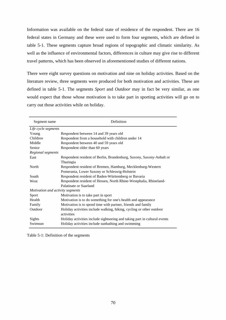
Information was available on the federal state of residence of the respondent. There are 16
federal states in Germany and these were used to form four segments, which are defined in
table 5-1. These segments capture broad regions of topographic and climatic similarity. As
well as the influence of environmental factors, differences in culture may give rise to different
travel patterns, which has been observed in aforementioned studies of different nations.
There were eight survey questions on motivation and nine on holiday activities. Based on the
literature review, three segments were produced for both motivation and activities. These are
defined in table 5-1. The segments Sport and Outdoor may in fact be very similar, as one
would expect that those whose motivation is to take part in sporting activities will go on to
carry out those activities while on holiday.
Young Respondent between 14 and 39 years oldChildren Respondent from a household with children under 14 Middle Respondent between 40 and 59 years oldSenior Respondent older than 60 years
East Respondent resident of Berlin, Brandenburg, Saxony, Saxony-Anhalt or Thuringia
North Respondent resident of Bremen, Hamburg, Mecklenburg-Western Pomerania, Lower Saxony or Schleswig-Holstein
South Respondent resident of Baden-Württemberg or BavariaWest Respondent resident of Hessen, North Rhine-Westphalia, Rhineland-
Palatinate or Saarland
Sport Motivation is to take part in sportHealth Motivation is to do something for one's health and appearanceFamily Motivation is to spend time with partner, friends and familyOutdoor Holiday activities include walking, hiking, cycling or other outdoor
activitiesSights Holiday activities include sightseeing and taking part in cultural eventsSwimsun Holiday activities include sunbathing and swimming
Life cycle segments
Motivation and activity segments
Regional segments
Segment name Definition
Table 5-1: Definition of the segments
70
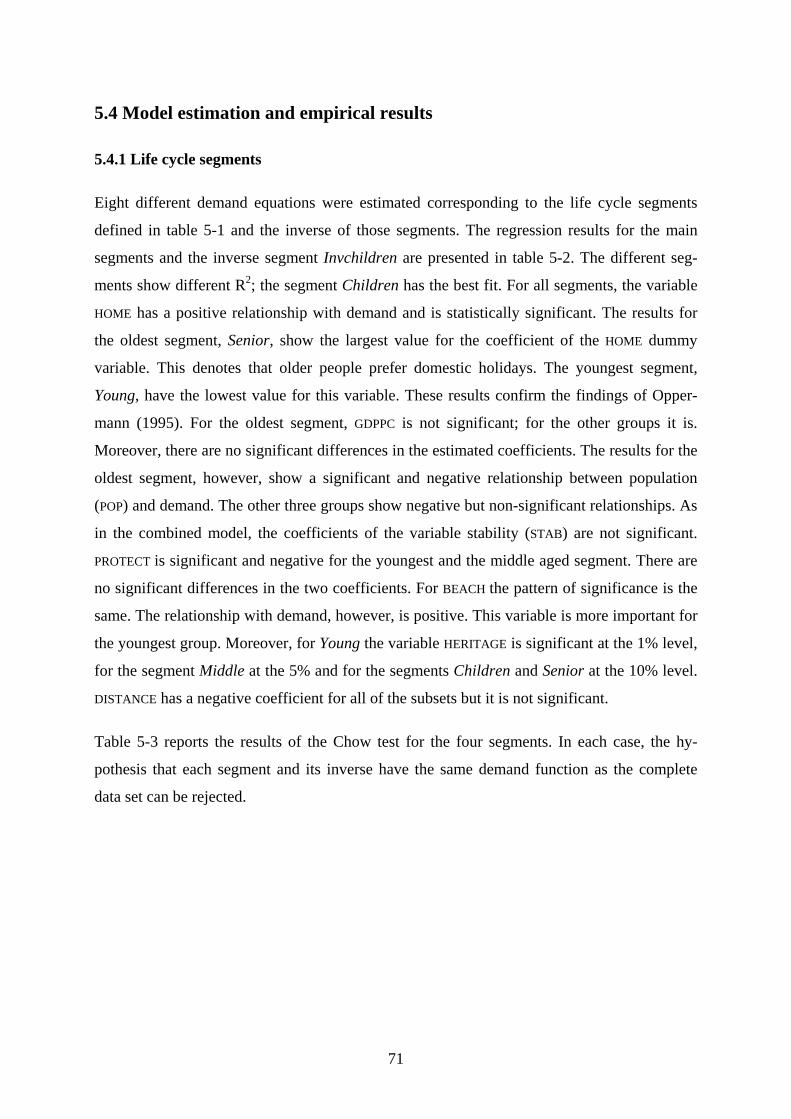
5.4 Model estimation and empirical results
5.4.1 Life cycle segments
Eight different demand equations were estimated corresponding to the life cycle segments
defined in table 5-1 and the inverse of those segments. The regression results for the main
segments and the inverse segment Invchildren are presented in table 5-2. The different seg-
ments show different R2; the segment Children has the best fit. For all segments, the variable
HOME has a positive relationship with demand and is statistically significant. The results for
the oldest segment, Senior, show the largest value for the coefficient of the HOME dummy
variable. This denotes that older people prefer domestic holidays. The youngest segment,
Young, have the lowest value for this variable. These results confirm the findings of Opper-
mann (1995). For the oldest segment, GDPPC is not significant; for the other groups it is.
Moreover, there are no significant differences in the estimated coefficients. The results for the
oldest segment, however, show a significant and negative relationship between population
(POP) and demand. The other three groups show negative but non-significant relationships. As
in the combined model, the coefficients of the variable stability (STAB) are not significant.
PROTECT is significant and negative for the youngest and the middle aged segment. There are
no significant differences in the two coefficients. For BEACH the pattern of significance is the
same. The relationship with demand, however, is positive. This variable is more important for
the youngest group. Moreover, for Young the variable HERITAGE is significant at the 1% level,
for the segment Middle at the 5% and for the segments Children and Senior at the 10% level.
DISTANCE has a negative coefficient for all of the subsets but it is not significant.
Table 5-3 reports the results of the Chow test for the four segments. In each case, the hy-
pothesis that each segment and its inverse have the same demand function as the complete
data set can be rejected.
71
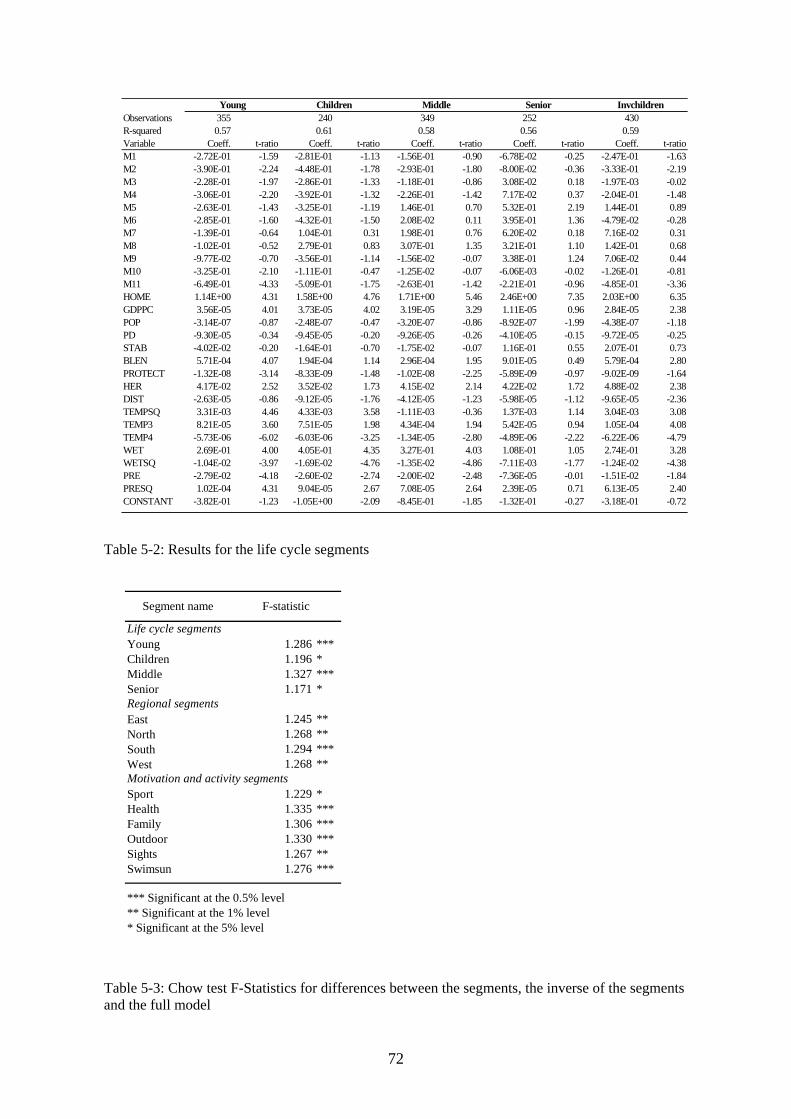
Observations 355 240 349 252 430R-squared 0.57 0.61 0.58 0.56 0.59Variable Coeff. t-ratio Coeff. t-ratio Coeff. t-ratio Coeff. t-ratio Coeff. t-ratioM1 -2.72E-01 -1.59 -2.81E-01 -1.13 -1.56E-01 -0.90 -6.78E-02 -0.25 -2.47E-01 -1.63M2 -3.90E-01 -2.24 -4.48E-01 -1.78 -2.93E-01 -1.80 -8.00E-02 -0.36 -3.33E-01 -2.19M3 -2.28E-01 -1.97 -2.86E-01 -1.33 -1.18E-01 -0.86 3.08E-02 0.18 -1.97E-03 -0.02M4 -3.06E-01 -2.20 -3.92E-01 -1.32 -2.26E-01 -1.42 7.17E-02 0.37 -2.04E-01 -1.48M5 -2.63E-01 -1.43 -3.25E-01 -1.19 1.46E-01 0.70 5.32E-01 2.19 1.44E-01 0.89M6 -2.85E-01 -1.60 -4.32E-01 -1.50 2.08E-02 0.11 3.95E-01 1.36 -4.79E-02 -0.28M7 -1.39E-01 -0.64 1.04E-01 0.31 1.98E-01 0.76 6.20E-02 0.18 7.16E-02 0.31M8 -1.02E-01 -0.52 2.79E-01 0.83 3.07E-01 1.35 3.21E-01 1.10 1.42E-01 0.68M9 -9.77E-02 -0.70 -3.56E-01 -1.14 -1.56E-02 -0.07 3.38E-01 1.24 7.06E-02 0.44M10 -3.25E-01 -2.10 -1.11E-01 -0.47 -1.25E-02 -0.07 -6.06E-03 -0.02 -1.26E-01 -0.81M11 -6.49E-01 -4.33 -5.09E-01 -1.75 -2.63E-01 -1.42 -2.21E-01 -0.96 -4.85E-01 -3.36HOME 1.14E+00 4.31 1.58E+00 4.76 1.71E+00 5.46 2.46E+00 7.35 2.03E+00 6.35GDPPC 3.56E-05 4.01 3.73E-05 4.02 3.19E-05 3.29 1.11E-05 0.96 2.84E-05 2.38POP -3.14E-07 -0.87 -2.48E-07 -0.47 -3.20E-07 -0.86 -8.92E-07 -1.99 -4.38E-07 -1.18PD -9.30E-05 -0.34 -9.45E-05 -0.20 -9.26E-05 -0.26 -4.10E-05 -0.15 -9.72E-05 -0.25STAB -4.02E-02 -0.20 -1.64E-01 -0.70 -1.75E-02 -0.07 1.16E-01 0.55 2.07E-01 0.73BLEN 5.71E-04 4.07 1.94E-04 1.14 2.96E-04 1.95 9.01E-05 0.49 5.79E-04 2.80PROTECT -1.32E-08 -3.14 -8.33E-09 -1.48 -1.02E-08 -2.25 -5.89E-09 -0.97 -9.02E-09 -1.64HER 4.17E-02 2.52 3.52E-02 1.73 4.15E-02 2.14 4.22E-02 1.72 4.88E-02 2.38DIST -2.63E-05 -0.86 -9.12E-05 -1.76 -4.12E-05 -1.23 -5.98E-05 -1.12 -9.65E-05 -2.36TEMPSQ 3.31E-03 4.46 4.33E-03 3.58 -1.11E-03 -0.36 1.37E-03 1.14 3.04E-03 3.08TEMP3 8.21E-05 3.60 7.51E-05 1.98 4.34E-04 1.94 5.42E-05 0.94 1.05E-04 4.08TEMP4 -5.73E-06 -6.02 -6.03E-06 -3.25 -1.34E-05 -2.80 -4.89E-06 -2.22 -6.22E-06 -4.79WET 2.69E-01 4.00 4.05E-01 4.35 3.27E-01 4.03 1.08E-01 1.05 2.74E-01 3.28WETSQ -1.04E-02 -3.97 -1.69E-02 -4.76 -1.35E-02 -4.86 -7.11E-03 -1.77 -1.24E-02 -4.38PRE -2.79E-02 -4.18 -2.60E-02 -2.74 -2.00E-02 -2.48 -7.36E-05 -0.01 -1.51E-02 -1.84PRESQ 1.02E-04 4.31 9.04E-05 2.67 7.08E-05 2.64 2.39E-05 0.71 6.13E-05 2.40CONSTANT -3.82E-01 -1.23 -1.05E+00 -2.09 -8.45E-01 -1.85 -1.32E-01 -0.27 -3.18E-01 -0.72
InvchildrenYoung Children Middle Senior
Table 5-2: Results for the life cycle segments
Young 1.286 ***Children 1.196 *Middle 1.327 ***Senior 1.171 *
East 1.245 **North 1.268 **South 1.294 ***West 1.268 **
Sport 1.229 *Health 1.335 ***Family 1.306 ***Outdoor 1.330 ***Sights 1.267 **Swimsun 1.276 ***
*** Significant at the 0.5% level** Significant at the 1% level* Significant at the 5% level
F-statistic
Regional segments
Motivation and activity segments
Life cycle segments
Segment name
Table 5-3: Chow test F-Statistics for differences between the segments, the inverse of the segments and the full model
72
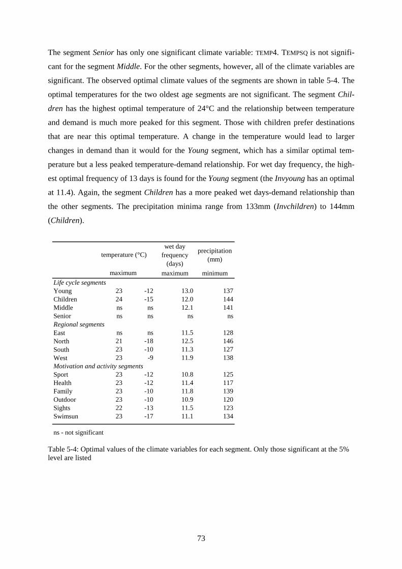
The segment Senior has only one significant climate variable: TEMP4. TEMPSQ is not signifi-
cant for the segment Middle. For the other segments, however, all of the climate variables are
significant. The observed optimal climate values of the segments are shown in table 5-4. The
optimal temperatures for the two oldest age segments are not significant. The segment Chil-
dren has the highest optimal temperature of 24°C and the relationship between temperature
and demand is much more peaked for this segment. Those with children prefer destinations
that are near this optimal temperature. A change in the temperature would lead to larger
changes in demand than it would for the Young segment, which has a similar optimal tem-
perature but a less peaked temperature-demand relationship. For wet day frequency, the high-
est optimal frequency of 13 days is found for the Young segment (the Invyoung has an optimal
at 11.4). Again, the segment Children has a more peaked wet days-demand relationship than
the other segments. The precipitation minima range from 133mm (Invchildren) to 144mm
(Children).
wet day frequency
(days)
precipitation (mm)
maximum minimumLife cycle segmentsYoung 23 -12 13.0 137Children 24 -15 12.0 144Middle ns ns 12.1 141Senior ns ns ns nsRegional segmentsEast ns ns 11.5 128North 21 -18 12.5 146South 23 -10 11.3 127West 23 -9 11.9 138Motivation and activity segmentsSport 23 -12 10.8 125Health 23 -12 11.4 117Family 23 -10 11.8 139Outdoor 23 -10 10.9 120Sights 22 -13 11.5 123Swimsun 23 -17 11.1 134
ns - not significant
temperature (°C)
maximum
Table 5-4: Optimal values of the climate variables for each segment. Only those significant at the 5% level are listed
73

Climate index values were calculated for the month of August for certain European countries.
The different values for each of the segments and the index values for the pooled model are
shown in Figure 5-1. The highest index values are for the segment Children, which has even
higher values than the combined data set. The lowest values are estimated for the segment
Senior. In general, the Middle segment has higher climate values than the Young segment.
There are some differences in the ranking of the different countries.
0
2
4
6
8
10
12
14
16
18
20
Norway Switzerland UnitedKingdom
CzechRepublic
Denmark Germany Poland Bulgaria Hungary Greece Portugal Spain
Clim
ate
attr
activ
enes
s ind
ex
all young
children middle
senior
Figure 5-1: Climate index values for the life cycle segments
5.4.2 Regional segments
The demand equations of the four regional segments as defined in table 5-1 and four inverse
segments were estimated. The results of the main segments are shown in table 5-5. Again,
there are different R2 values for each of the segments; South has the worst fit of all. The seg-
ment East has the largest coefficient for the variable HOME of all of the segments. GDPPC is
significant for all segments apart from East. The segment West has the largest coefficient for
GDPPC. The coefficient on population is negative and significant at the 10% level for the seg-
ment East. This was also seen for the oldest group in the life cycle segmentation. The coeffi-
cient for BEACH is positive for each segment but significant for the segments North and West;
the latter has a larger coefficient. The segment North has a negative and significant coefficient
for PROTECT. The segments South and West have positive and significant coefficients for HERI-
TAGE. The coefficient on DISTANCE has the correct sign for all segments but is only significant
at the 10 % level for East and South.
74
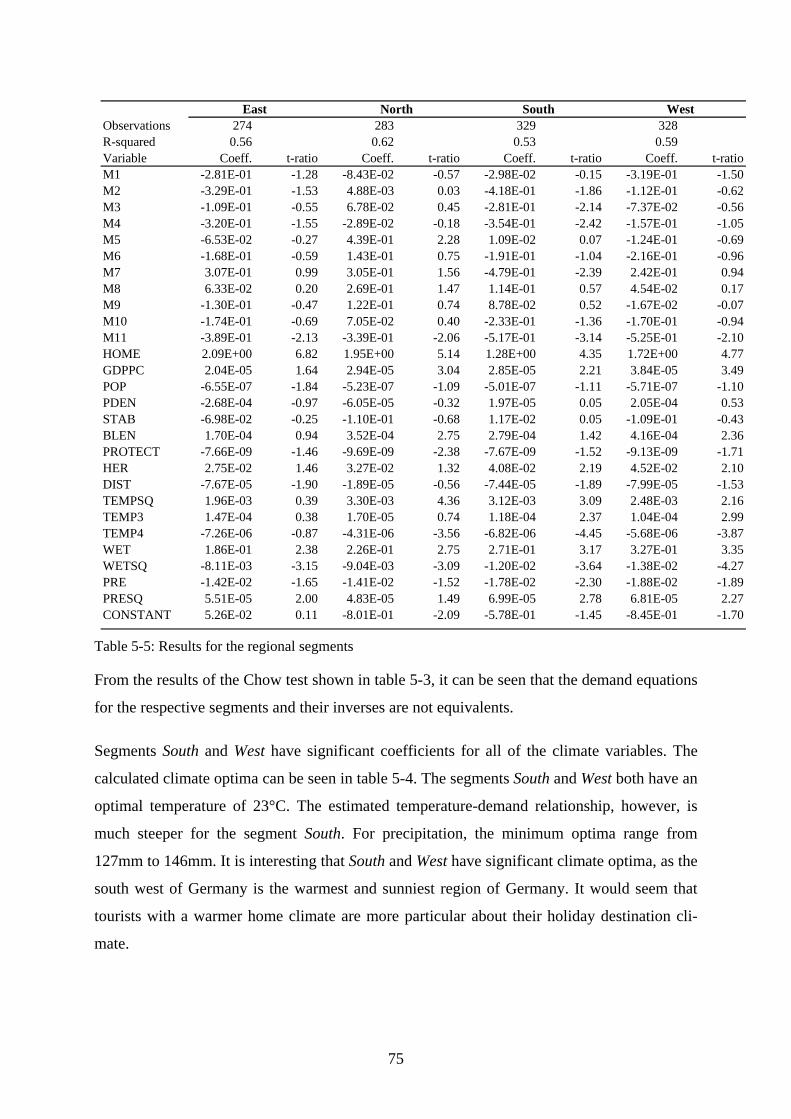
Observations 274 283 329 328R-squared 0.56 0.62 0.53 0.59Variable Coeff. t-ratio Coeff. t-ratio Coeff. t-ratio Coeff. t-ratioM1 -2.81E-01 -1.28 -8.43E-02 -0.57 -2.98E-02 -0.15 -3.19E-01 -1.50M2 -3.29E-01 -1.53 4.88E-03 0.03 -4.18E-01 -1.86 -1.12E-01 -0.62M3 -1.09E-01 -0.55 6.78E-02 0.45 -2.81E-01 -2.14 -7.37E-02 -0.56M4 -3.20E-01 -1.55 -2.89E-02 -0.18 -3.54E-01 -2.42 -1.57E-01 -1.05M5 -6.53E-02 -0.27 4.39E-01 2.28 1.09E-02 0.07 -1.24E-01 -0.69M6 -1.68E-01 -0.59 1.43E-01 0.75 -1.91E-01 -1.04 -2.16E-01 -0.96M7 3.07E-01 0.99 3.05E-01 1.56 -4.79E-01 -2.39 2.42E-01 0.94M8 6.33E-02 0.20 2.69E-01 1.47 1.14E-01 0.57 4.54E-02 0.17M9 -1.30E-01 -0.47 1.22E-01 0.74 8.78E-02 0.52 -1.67E-02 -0.07M10 -1.74E-01 -0.69 7.05E-02 0.40 -2.33E-01 -1.36 -1.70E-01 -0.94M11 -3.89E-01 -2.13 -3.39E-01 -2.06 -5.17E-01 -3.14 -5.25E-01 -2.10HOME 2.09E+00 6.82 1.95E+00 5.14 1.28E+00 4.35 1.72E+00 4.77GDPPC 2.04E-05 1.64 2.94E-05 3.04 2.85E-05 2.21 3.84E-05 3.49POP -6.55E-07 -1.84 -5.23E-07 -1.09 -5.01E-07 -1.11 -5.71E-07 -1.10PDEN -2.68E-04 -0.97 -6.05E-05 -0.32 1.97E-05 0.05 2.05E-04 0.53STAB -6.98E-02 -0.25 -1.10E-01 -0.68 1.17E-02 0.05 -1.09E-01 -0.43BLEN 1.70E-04 0.94 3.52E-04 2.75 2.79E-04 1.42 4.16E-04 2.36PROTECT -7.66E-09 -1.46 -9.69E-09 -2.38 -7.67E-09 -1.52 -9.13E-09 -1.71HER 2.75E-02 1.46 3.27E-02 1.32 4.08E-02 2.19 4.52E-02 2.10DIST -7.67E-05 -1.90 -1.89E-05 -0.56 -7.44E-05 -1.89 -7.99E-05 -1.53TEMPSQ 1.96E-03 0.39 3.30E-03 4.36 3.12E-03 3.09 2.48E-03 2.16TEMP3 1.47E-04 0.38 1.70E-05 0.74 1.18E-04 2.37 1.04E-04 2.99TEMP4 -7.26E-06 -0.87 -4.31E-06 -3.56 -6.82E-06 -4.45 -5.68E-06 -3.87WET 1.86E-01 2.38 2.26E-01 2.75 2.71E-01 3.17 3.27E-01 3.35WETSQ -8.11E-03 -3.15 -9.04E-03 -3.09 -1.20E-02 -3.64 -1.38E-02 -4.27PRE -1.42E-02 -1.65 -1.41E-02 -1.52 -1.78E-02 -2.30 -1.88E-02 -1.89PRESQ 5.51E-05 2.00 4.83E-05 1.49 6.99E-05 2.78 6.81E-05 2.27CONSTANT 5.26E-02 0.11 -8.01E-01 -2.09 -5.78E-01 -1.45 -8.45E-01 -1.70
WestEast North South
Table 5-5: Results for the regional segments
From the results of the Chow test shown in table 5-3, it can be seen that the demand equations
for the respective segments and their inverses are not equivalents.
Segments South and West have significant coefficients for all of the climate variables. The
calculated climate optima can be seen in table 5-4. The segments South and West both have an
optimal temperature of 23°C. The estimated temperature-demand relationship, however, is
much steeper for the segment South. For precipitation, the minimum optima range from
127mm to 146mm. It is interesting that South and West have significant climate optima, as the
south west of Germany is the warmest and sunniest region of Germany. It would seem that
tourists with a warmer home climate are more particular about their holiday destination cli-
mate.
75
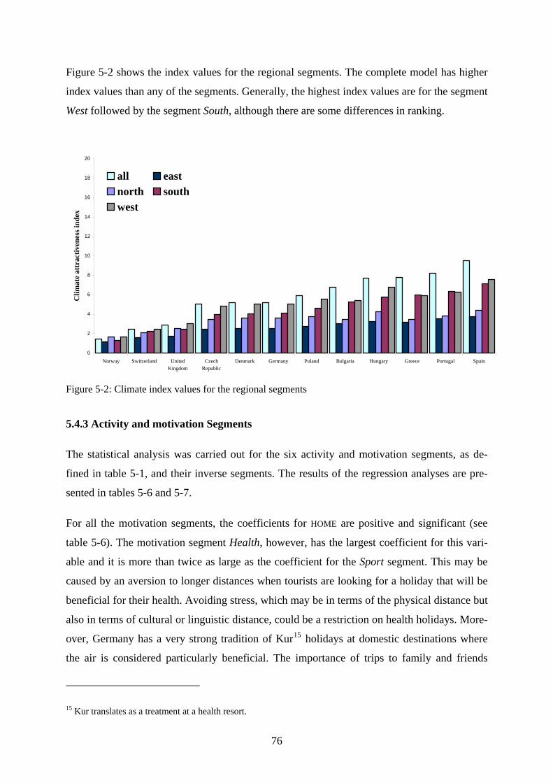
Figure 5-2 shows the index values for the regional segments. The complete model has higher
index values than any of the segments. Generally, the highest index values are for the segment
West followed by the segment South, although there are some differences in ranking.
0
2
4
6
8
10
12
14
16
18
20
Norway Switzerland UnitedKingdom
CzechRepublic
Denmark Germany Poland Bulgaria Hungary Greece Portugal Spain
Clim
ate
attr
activ
enes
s ind
ex
all eastnorth southwest
Figure 5-2: Climate index values for the regional segments
5.4.3 Activity and motivation Segments
The statistical analysis was carried out for the six activity and motivation segments, as de-
fined in table 5-1, and their inverse segments. The results of the regression analyses are pre-
sented in tables 5-6 and 5-7.
For all the motivation segments, the coefficients for HOME are positive and significant (see
table 5-6). The motivation segment Health, however, has the largest coefficient for this vari-
able and it is more than twice as large as the coefficient for the Sport segment. This may be
caused by an aversion to longer distances when tourists are looking for a holiday that will be
beneficial for their health. Avoiding stress, which may be in terms of the physical distance but
also in terms of cultural or linguistic distance, could be a restriction on health holidays. More-
over, Germany has a very strong tradition of Kur15 holidays at domestic destinations where
the air is considered particularly beneficial. The importance of trips to family and friends
15 Kur translates as a treatment at a health resort.
76
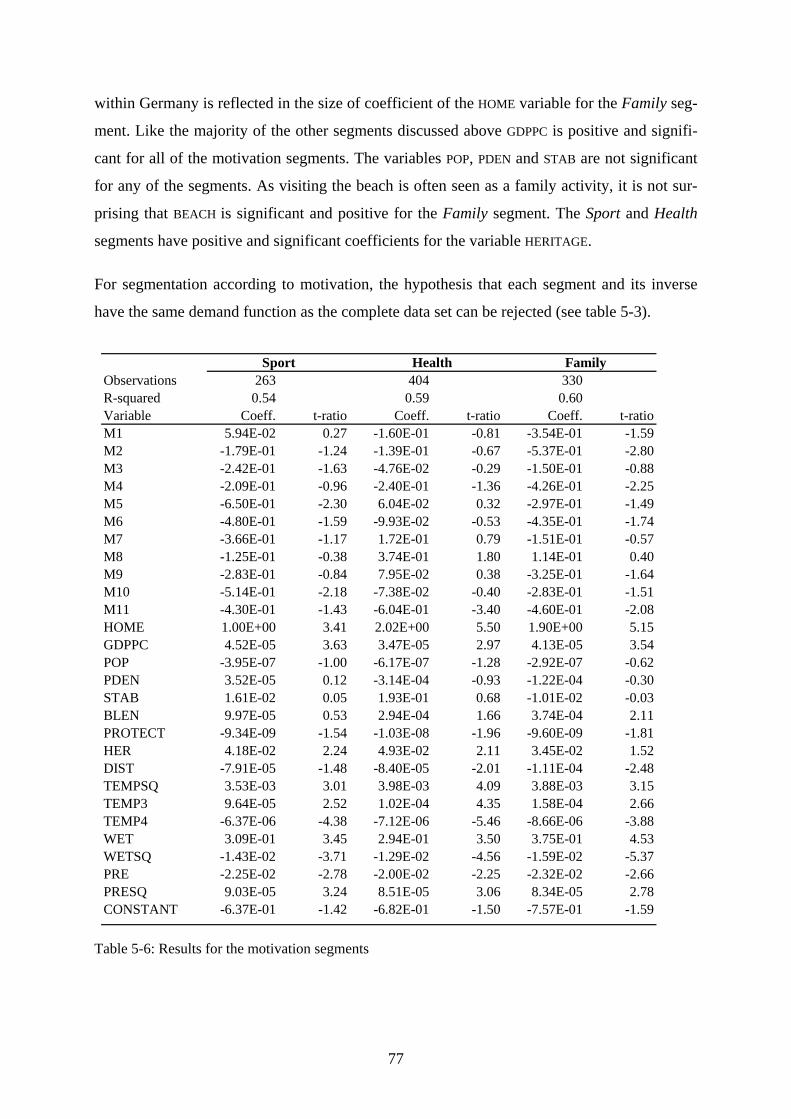
within Germany is reflected in the size of coefficient of the HOME variable for the Family seg-
ment. Like the majority of the other segments discussed above GDPPC is positive and signifi-
cant for all of the motivation segments. The variables POP, PDEN and STAB are not significant
for any of the segments. As visiting the beach is often seen as a family activity, it is not sur-
prising that BEACH is significant and positive for the Family segment. The Sport and Health
segments have positive and significant coefficients for the variable HERITAGE.
For segmentation according to motivation, the hypothesis that each segment and its inverse
have the same demand function as the complete data set can be rejected (see table 5-3).
Observations 263 404 330R-squared 0.54 0.59 0.60Variable Coeff. t-ratio Coeff. t-ratio Coeff. t-ratioM1 5.94E-02 0.27 -1.60E-01 -0.81 -3.54E-01 -1.59M2 -1.79E-01 -1.24 -1.39E-01 -0.67 -5.37E-01 -2.80M3 -2.42E-01 -1.63 -4.76E-02 -0.29 -1.50E-01 -0.88M4 -2.09E-01 -0.96 -2.40E-01 -1.36 -4.26E-01 -2.25M5 -6.50E-01 -2.30 6.04E-02 0.32 -2.97E-01 -1.49M6 -4.80E-01 -1.59 -9.93E-02 -0.53 -4.35E-01 -1.74M7 -3.66E-01 -1.17 1.72E-01 0.79 -1.51E-01 -0.57M8 -1.25E-01 -0.38 3.74E-01 1.80 1.14E-01 0.40M9 -2.83E-01 -0.84 7.95E-02 0.38 -3.25E-01 -1.64M10 -5.14E-01 -2.18 -7.38E-02 -0.40 -2.83E-01 -1.51M11 -4.30E-01 -1.43 -6.04E-01 -3.40 -4.60E-01 -2.08HOME 1.00E+00 3.41 2.02E+00 5.50 1.90E+00 5.15GDPPC 4.52E-05 3.63 3.47E-05 2.97 4.13E-05 3.54POP -3.95E-07 -1.00 -6.17E-07 -1.28 -2.92E-07 -0.62PDEN 3.52E-05 0.12 -3.14E-04 -0.93 -1.22E-04 -0.30STAB 1.61E-02 0.05 1.93E-01 0.68 -1.01E-02 -0.03BLEN 9.97E-05 0.53 2.94E-04 1.66 3.74E-04 2.11PROTECT -9.34E-09 -1.54 -1.03E-08 -1.96 -9.60E-09 -1.81HER 4.18E-02 2.24 4.93E-02 2.11 3.45E-02 1.52DIST -7.91E-05 -1.48 -8.40E-05 -2.01 -1.11E-04 -2.48TEMPSQ 3.53E-03 3.01 3.98E-03 4.09 3.88E-03 3.15TEMP3 9.64E-05 2.52 1.02E-04 4.35 1.58E-04 2.66TEMP4 -6.37E-06 -4.38 -7.12E-06 -5.46 -8.66E-06 -3.88WET 3.09E-01 3.45 2.94E-01 3.50 3.75E-01 4.53WETSQ -1.43E-02 -3.71 -1.29E-02 -4.56 -1.59E-02 -5.37PRE -2.25E-02 -2.78 -2.00E-02 -2.25 -2.32E-02 -2.66PRESQ 9.03E-05 3.24 8.51E-05 3.06 8.34E-05 2.78CONSTANT -6.37E-01 -1.42 -6.82E-01 -1.50 -7.57E-01 -1.59
Sport Health Family
Table 5-6: Results for the motivation segments
77
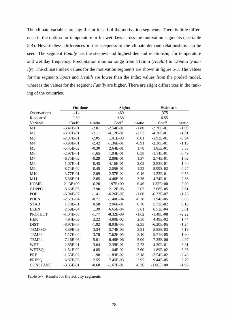
The climate variables are significant for all of the motivation segments. There is little differ-
ence in the optima for temperature or for wet days across the motivation segments (see table
5-4). Nevertheless, differences in the steepness of the climate-demand relationships can be
seen. The segment Family has the steepest and highest demand relationship for temperature
and wet day frequency. Precipitation minima range from 117mm (Health) to 139mm (Fam-
ily). The climate index values for the motivation segments are shown in figure 5-3. The values
for the segments Sport and Health are lower than the index values from the pooled model,
whereas the values for the segment Family are higher. There are slight differences in the rank-
ing of the countries.
Observations 414 460 375R-squared 0.59 0.58 0.55Variable Coeff. t-ratio Coeff. t-ratio Coeff. t-ratioM1 -3.47E-01 -2.01 -2.54E-01 -1.80 -2.36E-01 -1.09M2 -3.97E-01 -2.11 -4.12E-01 -2.53 -4.20E-01 -1.81M3 -2.87E-01 -2.05 1.01E-03 0.01 -1.92E-01 -0.94M4 -3.93E-01 -2.42 -1.36E-01 -0.91 -2.30E-01 -1.13M5 -5.45E-02 -0.30 2.64E-01 1.78 1.85E-01 0.83M6 -2.97E-01 -1.65 1.04E-01 0.58 -1.14E-01 -0.49M7 -6.75E-02 -0.29 2.89E-01 1.37 2.74E-01 1.02M8 1.07E-01 0.45 4.16E-01 2.02 3.83E-01 1.40M9 -8.74E-02 -0.45 2.05E-01 1.22 -5.99E-02 -0.27M10 -3.77E-01 -2.09 2.57E-02 0.16 -1.23E-01 -0.56M11 -5.36E-01 -2.65 -4.46E-01 -3.26 -4.74E-01 -2.86HOME 2.13E+00 6.20 1.97E+00 6.46 1.33E+00 3.30GDPPC 3.66E-05 2.90 2.12E-05 2.07 2.68E-05 2.61POP -6.94E-07 -1.41 -6.26E-07 -1.60 -6.33E-07 -1.25PDEN -2.61E-04 -0.71 -1.40E-04 -0.38 1.94E-05 0.05STAB 1.78E-01 0.58 2.06E-01 0.70 5.73E-02 0.18BLEN 2.69E-04 1.39 6.65E-04 3.61 6.51E-04 3.61PROTECT -1.04E-08 -1.77 -8.32E-09 -1.62 -1.48E-08 -2.22HER 4.94E-02 2.22 4.80E-02 2.50 4.49E-02 1.74DIST -8.97E-05 -1.92 -8.93E-05 -2.35 -6.20E-05 -1.24TEMPSQ 3.39E-03 3.34 3.74E-03 3.91 5.85E-03 5.19TEMP3 1.17E-04 3.78 7.62E-05 3.10 5.71E-05 1.90TEMP4 -7.16E-06 -5.01 -6.48E-06 -5.00 -7.35E-06 -4.97WET 2.86E-01 3.64 2.39E-01 2.73 4.20E-01 3.31WETSQ -1.31E-02 -4.85 -1.04E-02 -3.60 -1.89E-02 -3.96PRE -1.65E-02 -1.98 -1.83E-02 -2.18 -2.54E-02 -2.43PRESQ 6.87E-05 2.55 7.45E-05 2.95 9.44E-05 2.79CONSTANT -3.35E-01 -0.68 -1.67E-01 -0.36 -1.06E+00 -1.98
Sights SwimsunOutdoor
Table 5-7: Results for the activity segments
78
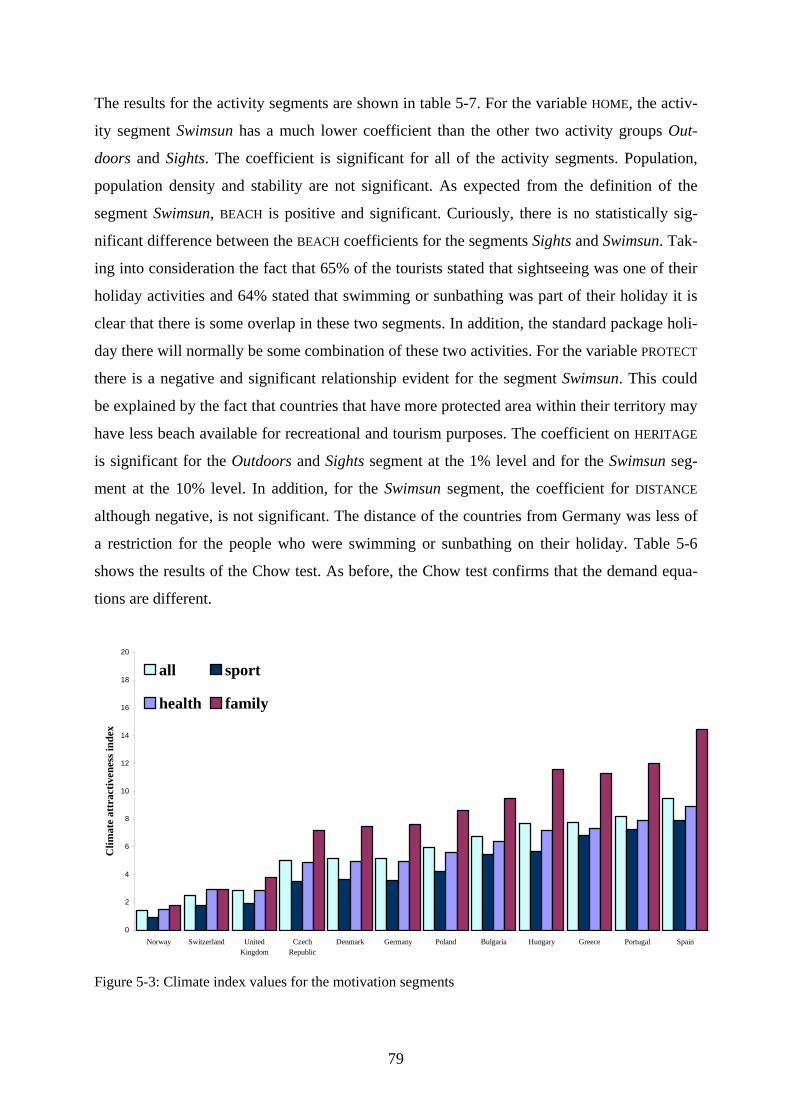
The results for the activity segments are shown in table 5-7. For the variable HOME, the activ-
ity segment Swimsun has a much lower coefficient than the other two activity groups Out-
doors and Sights. The coefficient is significant for all of the activity segments. Population,
population density and stability are not significant. As expected from the definition of the
segment Swimsun, BEACH is positive and significant. Curiously, there is no statistically sig-
nificant difference between the BEACH coefficients for the segments Sights and Swimsun. Tak-
ing into consideration the fact that 65% of the tourists stated that sightseeing was one of their
holiday activities and 64% stated that swimming or sunbathing was part of their holiday it is
clear that there is some overlap in these two segments. In addition, the standard package holi-
day there will normally be some combination of these two activities. For the variable PROTECT
there is a negative and significant relationship evident for the segment Swimsun. This could
be explained by the fact that countries that have more protected area within their territory may
have less beach available for recreational and tourism purposes. The coefficient on HERITAGE
is significant for the Outdoors and Sights segment at the 1% level and for the Swimsun seg-
ment at the 10% level. In addition, for the Swimsun segment, the coefficient for DISTANCE
although negative, is not significant. The distance of the countries from Germany was less of
a restriction for the people who were swimming or sunbathing on their holiday. Table 5-6
shows the results of the Chow test. As before, the Chow test confirms that the demand equa-
tions are different.
0
2
4
6
8
10
12
14
16
18
20
Norway Switzerland UnitedKingdom
CzechRepublic
Denmark Germany Poland Bulgaria Hungary Greece Portugal Spain
Clim
ate
attr
activ
enes
s ind
ex
all sport
health family
Figure 5-3: Climate index values for the motivation segments
79
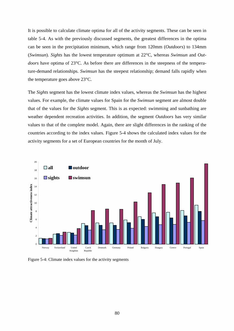
It is possible to calculate climate optima for all of the activity segments. These can be seen in
table 5-4. As with the previously discussed segments, the greatest differences in the optima
can be seen in the precipitation minimum, which range from 120mm (Outdoors) to 134mm
(Swimsun). Sights has the lowest temperature optimum at 22°C, whereas Swimsun and Out-
doors have optima of 23°C. As before there are differences in the steepness of the tempera-
ture-demand relationships. Swimsun has the steepest relationship; demand falls rapidly when
the temperature goes above 23°C.
The Sights segment has the lowest climate index values, whereas the Swimsun has the highest
values. For example, the climate values for Spain for the Swimsun segment are almost double
that of the values for the Sights segment. This is as expected: swimming and sunbathing are
weather dependent recreation activities. In addition, the segment Outdoors has very similar
values to that of the complete model. Again, there are slight differences in the ranking of the
countries according to the index values. Figure 5-4 shows the calculated index values for the
activity segments for a set of European countries for the month of July.
0
2
4
6
8
10
12
14
16
18
20
Norway Switzerland UnitedKingdom
CzechRepublic
Denmark Germany Poland Bulgaria Hungary Greece Portugal Spain
Clim
ate
attr
activ
enes
s ind
ex
all outdoor
sights swimsun
Figure 5-4: Climate index values for the activity segments
80
5.5 Discussion and conclusion
The aim of this chapter is to examine the climate-demand relationships of various segments,
in order to provide a quantitative basis for tourism scenarios, which can then be used in cli-
mate impact research. Expanding the work of the previous chapter, this chapter presents three
separate methods to segment the original data set and goes on to estimate the demand function
for these segments in terms of destination characteristics such as climate, natural and cultural
resources as well as socio-economic characteristics. Using a Chow test, the demand functions
of all of the 28 segments were found to be significantly different from that of the complete
model.
Certain variables were found to have a consistent relationship across all the segments. Domes-
tic tourism was a positive factor in all of the estimated equations. There were, however, dif-
ferences in size. For older tourists, those looking to do something for their health, those from
the East or those wanting to take part in outdoor activities domestic tourism is particularly
popular. For younger people, those motivated to participate in sport on their holiday or for
those who were sunbathing or swimming domestic tourism is less important. Beach length
was also an important factor for younger tourists. After younger tourists, the segments of tour-
ists from the North and the West of Germany had the highest coefficient for beach length. It is
not clear from this analysis if this is caused by the region of residence having beaches or be-
ing close to countries with beaches. The number of heritage sites also has a positive effect on
demand, especially for those tourists who went sightseeing.
The temperature optima ranged from 21°C to 24°C. There were, however, differences in the
steepness of the temperature-demand relationship. This was markedly so for the segments of
tourists with dependent children and for those whose activities included sunbathing and
swimming. Moving away from the optimal temperature leads to a sharp drop in demand, par-
ticularly for temperatures above the optimal. The optimal wet day frequency ranges from 11
to 13 wet days per month. Again, there were differences in the steepness of the relationship
with demand. Almost one third of month with a rain day may seem high for an optimal holi-
day climate. It must be borne in mind that a wet day is one where there is more than 1mm of
rain and a frequency of 11 days per month is normal for a central European summer or early
and late summer in southern Europe. Moreover, climate is not just a thermal or physical factor
it is also an aesthetic one, in that it affects, for example, the appearance and type of flora and
fauna, the appearance of the built environment and visibility. Occasional rain is not necessar-
81
ily detrimental for tourism demand. There are also some more practical effects of regular rain,
such as the water availability, which may be considered by the tourist.
The ranking of tourist destinations, using the climate index developed in chapter 4, did not
differ significantly across the segments. Nevertheless, the size of the climate index, on aver-
age and for the individual destinations, did differ. For the majority of the segments, the desti-
nation with the highest index value was Spain.
The results of this study confirm many of the results of previous segmentation studies. This
can be seen in the differences in preferences across the life cycle or across activities. Like
Mykletun et al. (2001), this study examines several kinds of segmentation and uses regression
analysis to provide detail on the different preferences of the different groups. Previous studies
that examined destination image preferences did so using a ranking of attributes. In this study,
demand for a destination has been estimated with respect to the environmental characteristics,
such as climate or beaches. This not only provides information on what is important for each
segment but also how this quantitatively affects demand.
For climate change impact studies, a segmentation approach can provide useful information.
Scenarios of population and economic change are only two aspects that will shape the devel-
opment of tourism in the future. New trends or structural changes in the population will also
affect demand. This study provides quantitative relationships, for different segments, such as
seniors, health tourists or from different geographic regions. It was shown that regions with a
warmer climate generate tourists that are more particular about their holiday destination cli-
mate. If this is applied to countries, it can be expected that warmer countries would also pro-
duce tourists that are less tolerant of temperatures away from the optimal. A similar result was
obtained by Bigano et al. (2006) in a study of global demand. This has implications for cli-
mate change impact studies. Climate change may result in many origin countries having a
climate closer to their optimal temperature, which combined with a preference, ceteris pari-
bus, for domestic tourism, would result in a reduction in international tourism. Moreover, as a
warmer climate becomes the norm, the tourists may also become more particular about their
holiday destination climates.
This study examines the destination choices of German tourists in a single year. To obtain a
more complete picture it would be useful to repeat the study for different years but also for
different countries or look at smaller regions. The results of this study, however, provide a
starting point for the development of quantitative tourism-climate scenarios.
82
Chapter 6
Coastal landscape and the hedonic price of accommodation*
6.1 Introduction
Studies on the impact of climate change on tourism focus on the relationship between climate
and demand. Ancillary effects, however, like sea-level rise, will also have an impact on de-
mand. Sea-level rise will result in the loss of low-lying islands, the loss of low-lying land at
the coast and the erosion of beaches and cliffs. Nevertheless, there is a range of adaptation
measures that can minimize these problems. In some cases, these measures will also change
the appearance of the coast. To calculate the cost of the impact of climate change on tourism
information is needed on the relationship between coastal morphology and tourism demand.
The importance of the coast for tourism demand can be seen in chapters 3, 4 and 5. But in
these chapters, different types of coastal landscape or morphology are not distinguished. This
chapter is the first study to link accommodation price with coastal and other landscape attrib-
utes.
The state of Schleswig-Holstein in Northern Germany has been chosen as the study area.
Schleswig-Holstein has two quite different coastlines: first, to the west there is the North Sea
coast and second, to the east there is the Baltic Sea coast. In addition, there is the coastline of
the river Elbe, which is heavily influenced by the North Sea. Tourism promotion in
Schleswig-Holstein is organised at the level of the Gemeinde or district. These are small ad-
ministration units at the level of LAU2.16 The coastal districts included in this study have an
average area of 21 km2, and the maximum area is 67 km2. The smallness of the districts al-
lows a high-resolution study of tourism in the region.
To examine the effect that landscape and in particular seascape have on tourism demand the
hedonic price method is used. The hedonic hypothesis is that goods are valued for their utility
bringing characteristics, and that this is reflected in the willingness to pay for these character-
istics and hence in the price. In tourism research, this method is not frequently used. Fleischer
* This chapter is based on Hamilton (in press). 16 LAU2 is the lowest of the administrative classes of the NUTS classification system of the EU.
83
and Tchetchik (2005), however, apply this method to the price of rural tourist accommodation
in Israel. They focus on whether tourists value that their accommodation is located on a work-
ing farm. In this study the focus is on whether tourists value their accommodation being lo-
cated in a district with certain coastal characteristics and if so by how much.
This chapter is structured as follows. In the second section, the study area is described. The
hedonic method is introduced in the third section. The data used in this study and the model
specifications are described in the fourth section. The fifth section presents the results of the
regression analysis. The implications of these are discussed in the sixth section, and the sev-
enth section concludes.
6.2 Study area
Schleswig-Holstein is the most northerly state in Germany, bordering Denmark in the North,
and its southern border is defined by the river Elbe and the City State of Hamburg. The east-
ern border is shared with the state of Mecklenburg-Western Pomerania.
The coastal zone of Schleswig-Holstein consists of three coastlines: at the North Sea, at the
Baltic Sea and along the River Elbe. The North Sea and Baltic Sea coast are quite different
from their coastal morphology. The North Sea coast was formed by post-glacial floods. This
resulted in low lying marshland, which may even be below sea level. The sandy moorland,
Geest, is higher than the coastal marshland. Overall, the North Sea coast is flat, although the
barrier islands of Sylt, Amrum and Föhr have moranic hills, cliffs and dunes (Kelletat, 1993).
These barrier islands as well as the marsh islands that were formerly part of the mainland lie
in the Schleswig-Holstein section of the Wadden Sea. The Wadden Sea is a large area of tidal
flats, tidal gullies, salt marshes and sandy barriers stretching from Denmark along the North
Sea coast of Germany to the Netherlands (Hofstede, 2003). The North Sea is salty with a sa-
linity of 25%-30% (Reese, 2003). The Baltic Sea coast was formed by glaciers resulting in
semi-enclosed inlets and fjords. There are also some stretches of coastline with cliffs. The
land surrounding the coast is slightly hilly. Compared to the North Sea the Baltic Sea is much
less salty. It has a salinity of 10% to 15% (Reese, 2003).
The main problem at the coast is the effect of storm floods. Around 24% of Schleswig-
Holstein lies in the flood prone area, which is below 5m in the west and 3m in the east
(Hofstede and Hammann, 2000). At the North Sea coast, these areas contain the main areas of
84
high population and of high economic value, which has resulted in the coastline being pro-
tected with dikes. Hard structures such as dikes are not the only protection measures used:
beach nourishment is also carried out on the barrier islands of Föhr and Sylt. This not only
stabilises the coastline of the islands but also provides protection for the mainland as well as
sandy beaches for recreation. The Baltic Sea coast has fewer stretches of dikes because of its
natural protection system of beach walls and spits.
Climate change will result in sea-level rise and increased storminess. This will mean that ex-
isting dikes will have to be strengthened and raised. Currently Schleswig-Holstein spends 24
million Euros per year on keeping present safety levels. Under a scenario of 25cm sea-level
rise by 2050, it is expected that the cost will rise by 5% to 15%. For the worst-case scenario
of 50cm sea-level rise by 2050, the costs are estimated at 42 million Euros per year (CPSL,
2001). Furthermore, sea-level rise will increase the volume of sand required for beach nour-
ishment.
3.1 million tourists spent their holiday at the coast and on the islands of Schleswig-Holstein in
2003. 10% of these tourists were from abroad. As a destination for German tourists,
Schleswig-Holstein has a market share equivalent to that of France or Greece (NIT, 2001). In
terms of its market share of tourism within Germany, Schleswig Holstein has a market share
of approximately 4%. Tourism is important economically for the state: 7% of all jobs are in
the tourism sector and 4.6% of the state income comes from tourism.
6.3 The hedonic price method
The hedonic price method, developed theoretically by Rosen (1974), is based on the idea that
any differentiated product can be seen as a bundle of characteristics. The value that consumers
attach to the characteristics will be reflected in the price of the differentiated product. The
price of an individual characteristic is called the implicit or shadow price.
Hedonic price analysis is widely used for different goods such as cars (Irandoust, 1998), com-
puter equipment (Doms and Forman, 2005) and agricultural products (Langyintuo et al.,
2004). The method has been extensively used for housing and in particular the valuation of
environmental amenities. Moreover, it has been used to examine the impact of climate change
on the price of housing in Italy (Maddison and Bigano, 2003), the UK (Rehdanz, 2006) and
Germany (Rehdanz and Maddison, 2004). In tourism research, it has been applied to package
85
tours (Clewer et al., 1992; Sinclair et al., 1990). Fleischer and Tchetchik (2005) have applied
the technique to estimate the value to tourists of rural accommodation being located on a
working farm. They find that an outstanding view from the tourist accommodation is posi-
tively related to price. Tourists are indifferent to the accommodation being located on a work-
ing farm.
Following Fleischer and Tchetchik’s (2005) hedonic price framework for rural accommoda-
tion, Pi represents the minimum price per person per night for a particular district and accom-
modation type. Xi is the matrix of attributes of the districts and the accommodation types. The
hedonic price equation is:
Equation 6-1: ( )i iP f X=
The effect of an incremental increase in the kth attribute on price, that is the implicit price, is
the partial derivative of Equation 6.1:
Equation 6-2: / ( ) /i i k iP X f X X i k∂ ∂ = ∂ ∂
6.4 Data and model specification
6.4.1 Data
The accommodation price data used in the analysis is taken from the tourist brochures of the
coastal districts. These brochures, as well as containing the marketing and promotional infor-
mation about the district, list all of the businesses providing accommodation with details on
the number of beds, price per room or per unit and the facilities of each accommodation unit.
From the 146 coastal districts, it was possible to calculate price data for 92 districts, which is
more than is available from the official statistics.17 The tourism marketing strategy of
Schleswig-Holstein divides the state in to four regions: the North Sea coast, the Baltic Sea
coast, inland and cities and large towns. As cities and large towns are marketed separately,
such districts were not included in the analysis.18 Furthermore, city or urban tourism is quite
different from the rural coastal tourism under examination here.
17 Official statistics only include business with more than nine beds, which leads to the exclusion of certain dis-tricts from the statistics. Data on accommodation prices is collected but not published. 18 This applied to the cities and towns of Kiel, Lübeck and Flensburg and to the districts Harrislee and Wedel, which are so close to cities that they have a suburb function.
86
The accommodation listings provide information on up to seven different types of accommo-
dation: hotel, hotel garni, guesthouse, bed and breakfast, rooms in private accommodation,
holiday homes and flats. Holiday homes and flats, which make up half of all the available
accommodation, show a great range in price dependent on the size of the unit and the quality
of the features. For this reason, the price data set was constructed only for the categories hotel
(including hotel garni), B&B (including guesthouse) and private rooms.
For each establishment the minimum price per person per night and the number of rooms was
recorded. It was not possible to calculate separate prices for the different seasons as many
establishments and individual districts have their own “seasons“ that deviate from the typical
high and low seasons. From the listed establishment price and capacity data the district aver-
age minimum price per person per night was calculated for the three groups of accommoda-
tion. The accommodation listings are from the years 2001 to 2005. The year 2002 was taken
as the base year. The prices for the other years were adjusted to 2002 prices using the German
consumer price index for accommodation and hospitality services (Statistiches Bundesamt,
2005). If there was no average price for 2002 then the price for 2003 was used and so on until
2005. If there was not a price available for 2005 then the data for 2001 was used. In this case,
the prices were converted from DM into Euro. The resulting dataset covers 92 coastal districts
and has 189 observations. Note that as there are three types of accommodation each district
may be represented by more than one observation. The 48 districts that are not covered in the
data set may have specialised in self-catering accommodation or tourism might not have de-
veloped there at all.19
In addition to the price data, data on landscape features of each district were collected. First,
for each district the area in hectares of sandy beach that extend beyond the main coastline was
measured using the 1:50000 topographical map from the TOP50 CD-Rom (Landesvermes-
sungsamt Schleswig-Holstein, 2005). Second, using maps showing coastal protection struc-
tures and coastal morphology from the Ministry of Coastal Protection (Ministerium für
ländliche Räume, Landesplanung, Landwirtschaft und Tourismus des Landes Schleswig-
Holstein, 2001) the length of dikes, cliffs and open coast in each district were measured using
MAPINFO. The area in hectares of water surface, heathland, moorland and agricultural land
19 In comparison, the official statistics report tourism data (but not price data) for 86 coastal districts, which means that for 54 districts data are not available.
87
were taken from the land use dataset of the state statistical office (Statistisches Landesamt
Schleswig-Holstein, 1999).
In chapters 4 and 5, population and population density were included in the model specifica-
tions. For this dataset, it is not possible to include population and population density as they
are highly correlated. Instead of using both, only population will be included as a variable
(POP). This is used as a proxy for the number of man-made attractions or for the amount of
infrastructure in each district. The source of the population data is the state statistical office
(Statistisches Landesamt Schleswig-Holstein, 2001).
Climate variables have been omitted, as the climate is largely homogenous over the small area
of Schleswig-Holstein.
Three regions are included in the dataset: the districts at the North Sea coast, the districts at
the Baltic coast and those at the Elbe.20 The North Sea districts border on the Wadden Sea
National Park. The flora and fauna of this unique area, as well as the national park’s facilities
for education are an attraction for tourists that can only be found at the North Sea. In addition,
the water at the North Sea is generally cooler than at the Baltic, and the waves tend to be
higher. To control for these effects a dummy variable, NORTH, has been created for the dis-
tricts at the North Sea coast. It is also possible, however, that this variable also picks up a
preference for the North Sea coast that has nothing to do with the coastal landscape, such as
the popularity of the distinctive Frisian culture.
Table 6-1 presents the variables used in this analysis, and table 6-2 presents the summary sta-
tistics of these variables.
20 The districts at the river Elbe belong to the marketing category “Inland”. In this analysis, however, they have been included as part of the coast, as the Elbe is strongly influenced by the tidal regime of the North Sea and the districts are part of the coastal defence programme.
88
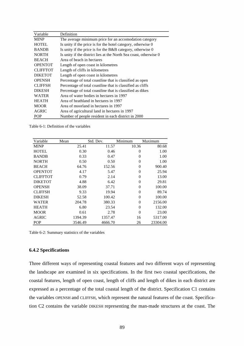
Variable DefinitionMINP The average minimum price for an accomodation category HOTEL Is unity if the price is for the hotel category, otherwise 0BANDB Is unity if the price is for the B&B category, otherwise 0NORTH Is unity if the district lies at the North Sea coast, otherwise 0BEACH Area of beach in hectaresOPENTOT Length of open coast in kilometresCLIFFTOT Length of cliffs in kilometresDIKETOT Length of open coast in kilometresOPENSH Percentage of total coastline that is classified as openCLIFFSH Percentage of total coastline that is classified as cliffsDIKESH Percentage of total coastline that is classified as dikesWATER Area of water bodies in hectares in 1997HEATH Area of heathland in hectares in 1997MOOR Area of moorland in hectares in 1997AGRIC Area of agricultural land in hectares in 1997POP Number of people resident in each district in 2000
Table 6-1: Definition of the variables
Table 6-2: Summary statistics of the variables
Variable Mean Std. Dev. Minimum MaximumMINP 25.41 11.57 10.36 80.68HOTEL 0.30 0.46 0 1.00BANDB 0.33 0.47 0 1.00NORTH 0.50 0.50 0 1.00BEACH 64.76 152.56 0 900.40OPENTOT 4.17 5.47 0 25.94CLIFFTOT 0.79 2.14 0 13.00DIKETOT 4.88 6.42 0 29.81OPENSH 38.09 37.71 0 100.00CLIFFSH 9.33 19.94 0 89.74DIKESH 52.58 100.42 0 100.00WATER 204.78 380.33 0 2156.00HEATH 6.80 23.54 0 132.00MOOR 0.61 2.78 0 23.00AGRIC 1394.39 1357.47 16 5317.00POP 3546.49 4666.70 26 23304.00
6.4.2 Specifications
Three different ways of representing coastal features and two different ways of representing
the landscape are examined in six specifications. In the first two coastal specifications, the
coastal features, length of open coast, length of cliffs and length of dikes in each district are
expressed as a percentage of the total coastal length of the district. Specification C1 contains
the variables OPENSH and CLIFFSH, which represent the natural features of the coast. Specifica-
tion C2 contains the variable DIKESH representing the man-made structures at the coast. The
89

third specification C3 contains all of the coastal variables expressed as absolute values
(OPENTOT, CLIFFTOT and DIKETOT).
The landscape of the districts can be described in different ways. There are many possible
variables, but because of multicolinearity only some could be included in the final specifica-
tions. The first landscape specification L1 uses land use data on the area of water surfaces
(WATER), the area of heathland (HEATH) and moorland (MOOR) in each district. In the second
landscape specification L2, these three variables are replaced with the area in each district
used for agriculture (AGRIC).
Combining the coastal and the landscape specifications gives six different specifications.
Each of these contains the dummy variables HOTEL, BANDB and NORTH and the continuous
variables BEACH and POP. (See Table 6-1 for the definitions of the variables and table 6-2 for
the summary statistics.)
6.4.3 Functional form and implicit prices
There is no theoretical guidance on the best functional form. Using the specifications de-
scribed above the linear, log linear and inverse functional forms were tested. The log-linear
functional form performs the best, and so only the results of this functional form will be pre-
sented here. The price equation is now written as:
Equation 6-3: ln i iP X iβ ε= +
Equation 6-4: ( )i ii
XP e β ε+=
Hence, the effect of an incremental increase is:
Equation 6-5: ( )/ i ii ik
XP X e β εkβ
+∂ ∂ = ⋅
Substituting equation 6-4 into equation 6-5 means that the implicit price is the real price mul-
tiplied by the coefficient of the variable that has increased.
90
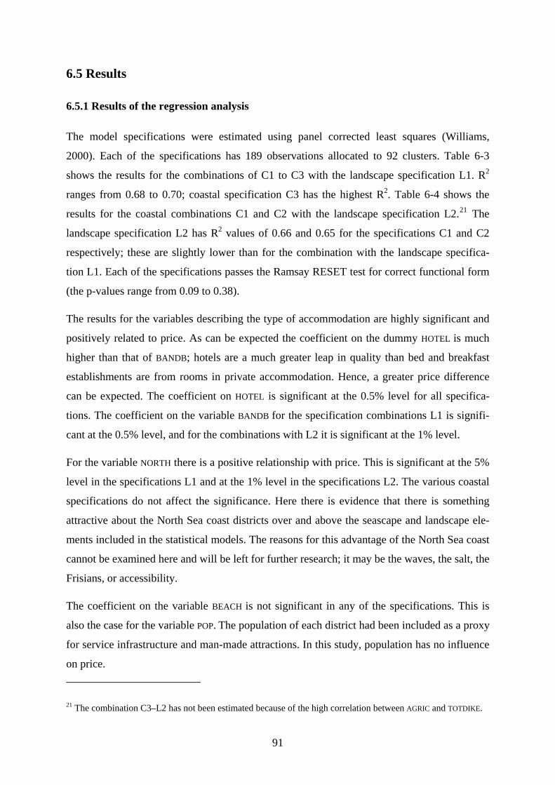
6.5 Results
6.5.1 Results of the regression analysis
The model specifications were estimated using panel corrected least squares (Williams,
2000). Each of the specifications has 189 observations allocated to 92 clusters. Table 6-3
shows the results for the combinations of C1 to C3 with the landscape specification L1. R2
ranges from 0.68 to 0.70; coastal specification C3 has the highest R2. Table 6-4 shows the
results for the coastal combinations C1 and C2 with the landscape specification L2.21 The
landscape specification L2 has R2 values of 0.66 and 0.65 for the specifications C1 and C2
respectively; these are slightly lower than for the combination with the landscape specifica-
tion L1. Each of the specifications passes the Ramsay RESET test for correct functional form
(the p-values range from 0.09 to 0.38).
The results for the variables describing the type of accommodation are highly significant and
positively related to price. As can be expected the coefficient on the dummy HOTEL is much
higher than that of BANDB; hotels are a much greater leap in quality than bed and breakfast
establishments are from rooms in private accommodation. Hence, a greater price difference
can be expected. The coefficient on HOTEL is significant at the 0.5% level for all specifica-
tions. The coefficient on the variable BANDB for the specification combinations L1 is signifi-
cant at the 0.5% level, and for the combinations with L2 it is significant at the 1% level.
For the variable NORTH there is a positive relationship with price. This is significant at the 5%
level in the specifications L1 and at the 1% level in the specifications L2. The various coastal
specifications do not affect the significance. Here there is evidence that there is something
attractive about the North Sea coast districts over and above the seascape and landscape ele-
ments included in the statistical models. The reasons for this advantage of the North Sea coast
cannot be examined here and will be left for further research; it may be the waves, the salt, the
Frisians, or accessibility.
The coefficient on the variable BEACH is not significant in any of the specifications. This is
also the case for the variable POP. The population of each district had been included as a proxy
for service infrastructure and man-made attractions. In this study, population has no influence
on price.
21 The combination C3–L2 has not been estimated because of the high correlation between AGRIC and TOTDIKE.
91
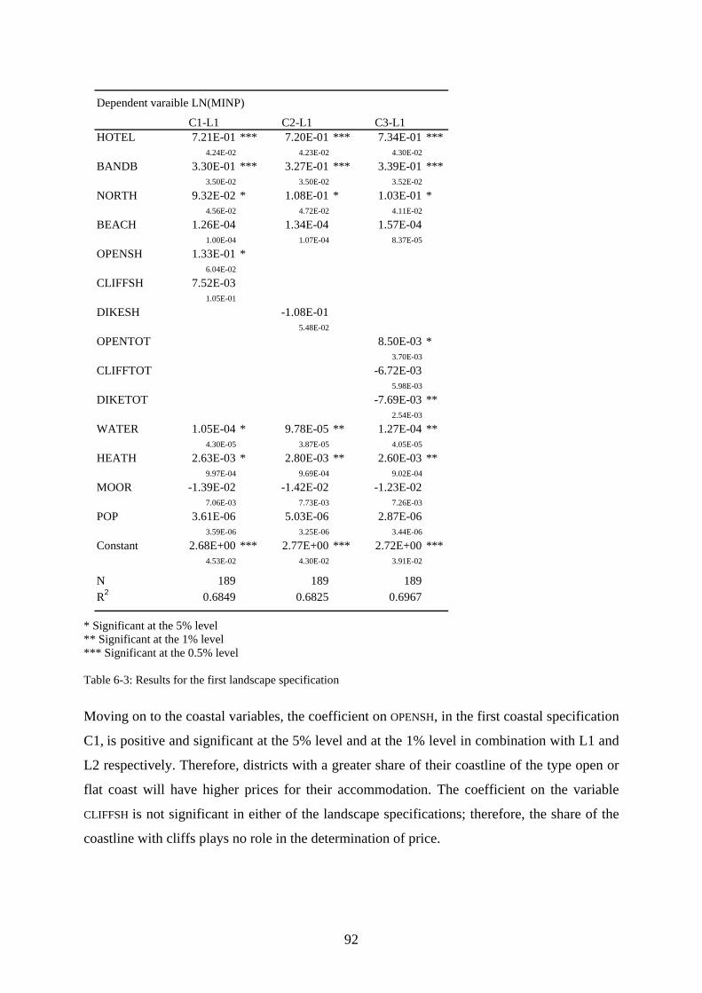
Dependent varaible LN(MINP)
C1-L1 C2-L1 C3-L1HOTEL 7.21E-01 *** 7.20E-01 *** 7.34E-01 ***
4.24E-02 4.23E-02 4.30E-02
BANDB 3.30E-01 *** 3.27E-01 *** 3.39E-01 ***3.50E-02 3.50E-02 3.52E-02
NORTH 9.32E-02 * 1.08E-01 * 1.03E-01 *4.56E-02 4.72E-02 4.11E-02
BEACH 1.26E-04 1.34E-04 1.57E-041.00E-04 1.07E-04 8.37E-05
OPENSH 1.33E-01 *6.04E-02
CLIFFSH 7.52E-031.05E-01
DIKESH -1.08E-015.48E-02
OPENTOT 8.50E-03 *3.70E-03
CLIFFTOT -6.72E-035.98E-03
DIKETOT -7.69E-03 **2.54E-03
WATER 1.05E-04 * 9.78E-05 ** 1.27E-04 **4.30E-05 3.87E-05 4.05E-05
HEATH 2.63E-03 * 2.80E-03 ** 2.60E-03 **9.97E-04 9.69E-04 9.02E-04
MOOR -1.39E-02 -1.42E-02 -1.23E-027.06E-03 7.73E-03 7.26E-03
POP 3.61E-06 5.03E-06 2.87E-063.59E-06 3.25E-06 3.44E-06
Constant 2.68E+00 *** 2.77E+00 *** 2.72E+00 ***4.53E-02 4.30E-02 3.91E-02
N 189 189 189R2 0.6849 0.6825 0.6967
* Significant at the 5% level ** Significant at the 1% level *** Significant at the 0.5% level Table 6-3: Results for the first landscape specification
Moving on to the coastal variables, the coefficient on OPENSH, in the first coastal specification
C1, is positive and significant at the 5% level and at the 1% level in combination with L1 and
L2 respectively. Therefore, districts with a greater share of their coastline of the type open or
flat coast will have higher prices for their accommodation. The coefficient on the variable
CLIFFSH is not significant in either of the landscape specifications; therefore, the share of the
coastline with cliffs plays no role in the determination of price.
92
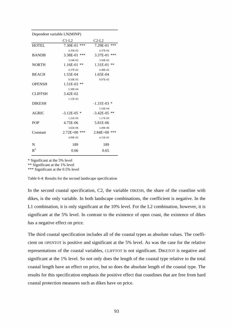
Dependent variable LN(MINP)
C1-L2 C2-L2HOTEL 7.30E-01 *** 7.29E-01 ***
4.35E-02 4.37E-02
BANDB 3.38E-01 *** 3.37E-01 ***3.54E-02 3.56E-02
NORTH 1.16E-01 ** 1.31E-01 **4.37E-02 4.48E-02
BEACH 1.55E-04 1.65E-049.50E-05 9.97E-05
OPENSH 1.51E-03 **5.39E-04
CLIFFSH 3.42E-021.15E-03
DIKESH -1.31E-03 *5.16E-04
AGRIC -3.12E-05 * -3.42E-05 **1.21E-05 1.17E-05
POP 4.75E-06 5.81E-063.65E-06 3.49E-06
Constant 2.72E+00 *** 2.84E+00 ***4.99E-02 4.15E-02
N 189 189R2 0.66 0.65
* Significant at the 5% level ** Significant at the 1% level *** Significant at the 0.5% level Table 6-4: Results for the second landscape specification
In the second coastal specification, C2, the variable DIKESH, the share of the coastline with
dikes, is the only variable. In both landscape combinations, the coefficient is negative. In the
L1 combination, it is only significant at the 10% level. For the L2 combination, however, it is
significant at the 5% level. In contrast to the existence of open coast, the existence of dikes
has a negative effect on price.
The third coastal specification includes all of the coastal types as absolute values. The coeffi-
cient on OPENTOT is positive and significant at the 5% level. As was the case for the relative
representations of the coastal variables, CLIFFTOT is not significant. DIKETOT is negative and
significant at the 1% level. So not only does the length of the coastal type relative to the total
coastal length have an effect on price, but so does the absolute length of the coastal type. The
results for this specification emphasis the positive effect that coastlines that are free from hard
coastal protection measures such as dikes have on price.
93

For the first landscape specification, there are very similar results across the coastal specifica-
tions. The coefficient of the variable WATER is positive and significant. For specification C1-
L1 it is significant at the 5% level. For the other two specifications, C2-L1 and C3-L1 water is
significant at the 1% level. Therefore, the more water features such as lakes and rivers in a
district the higher the price of accommodation will be. In addition, heathland in a district has a
positive effect on price: the coefficient on HEATH is positive and significant at the 5%, 1% and
1% level for C1-L1, C2-L1 and C3-L1 respectively. MOOR is not significant in any of the
specifications.
The second landscape specification has only one landscape variable AGRIC, which is negative
in all of the specifications and significant at least at the 5% level. The size of the coefficients
and their standard errors are similar for the specifications C1 and C2.
6.5.2 Hedonic prices of coastal and other landscape features
To recap on section 6.4.3, the hedonic price of a characteristic is calculated by multiplying the
coefficient by the price of the accommodation type in each district. The hedonic prices for the
significant variables for the landscape specifications L1 are shown in table 6-5. The hedonic
prices are calculated using the average, the minimum and the maximum price of all the dis-
tricts for one night in private accommodation. Table 6-6 shows the results for the specifica-
tions L2. As mentioned above it can be expected that hotel accommodation is valued higher
than B&B accommodation. Here, the hedonic price for hotel accommodation is double that of
B&B for all of the specifications. Dike share and absolute dike length have negative hedonic
prices; that is, they are a disamenity. On the other hand, the share of open coast and the abso-
lute length of open coast are amenities. Agricultural land use has a small but negative hedonic
price.
94
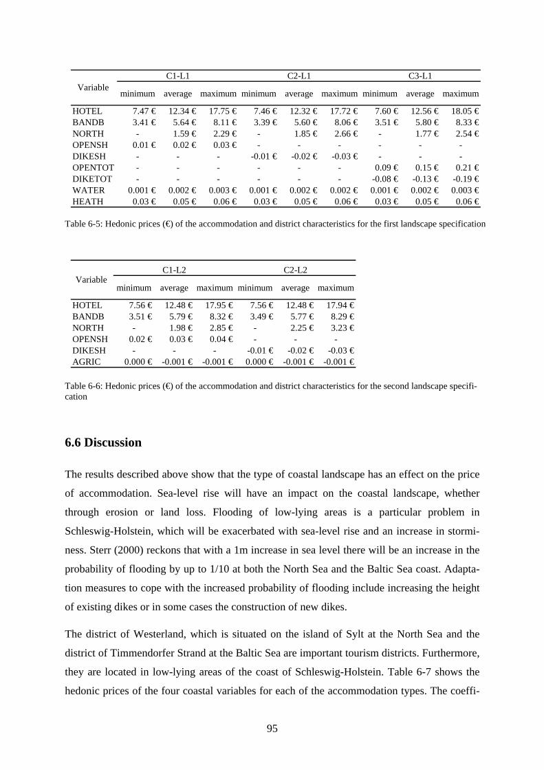
minimum average maximum minimum average maximum minimum average maximum
HOTEL 7.47 € 12.34 € 17.75 € 7.46 € 12.32 € 17.72 € 7.60 € 12.56 € 18.05 €BANDB 3.41 € 5.64 € 8.11 € 3.39 € 5.60 € 8.06 € 3.51 € 5.80 € 8.33 €NORTH - 1.59 € 2.29 € - 1.85 € 2.66 € - 1.77 € 2.54 €OPENSH 0.01 € 0.02 € 0.03 € - - - - - -DIKESH - - - -0.01 € -0.02 € -0.03 € - - -OPENTOT - - - - - - 0.09 € 0.15 € 0.21DIKETOT - - - - - - -0.08 € -0.13 € -0.19WATER 0.001 € 0.002 € 0.003 € 0.001 € 0.002 € 0.002 € 0.001 € 0.002 € 0.003 €HEATH 0.03 € 0.05 € 0.06 € 0.03 € 0.05 € 0.06 € 0.03 € 0.05 € 0.06 €
C1-L1 C2-L1 C3-L1Variable
€ €
Table 6-5: Hedonic prices (€) of the accommodation and district characteristics for the first landscape specification
Table 6-6: Hedonic prices (€) of the accommodation and district characteristics for the second landscape specifi-cation
minimum average maximum minimum average maximum
HOTEL 7.56 € 12.48 € 17.95 € 7.56 € 12.48 € 17.94 €BANDB 3.51 € 5.79 € 8.32 € 3.49 € 5.77 € 8.29 €NORTH - 1.98 € 2.85 € - 2.25 € 3.23 €OPENSH 0.02 € 0.03 € 0.04 € - - -DIKESH - - - -0.01 € -0.02 € -0.03 €AGRIC 0.000 € -0.001 € -0.001 € 0.000 € -0.001 € -0.001 €
Variable C1-L2 C2-L2
6.6 Discussion
The results described above show that the type of coastal landscape has an effect on the price
of accommodation. Sea-level rise will have an impact on the coastal landscape, whether
through erosion or land loss. Flooding of low-lying areas is a particular problem in
Schleswig-Holstein, which will be exacerbated with sea-level rise and an increase in stormi-
ness. Sterr (2000) reckons that with a 1m increase in sea level there will be an increase in the
probability of flooding by up to 1/10 at both the North Sea and the Baltic Sea coast. Adapta-
tion measures to cope with the increased probability of flooding include increasing the height
of existing dikes or in some cases the construction of new dikes.
The district of Westerland, which is situated on the island of Sylt at the North Sea and the
district of Timmendorfer Strand at the Baltic Sea are important tourism districts. Furthermore,
they are located in low-lying areas of the coast of Schleswig-Holstein. Table 6-7 shows the
hedonic prices of the four coastal variables for each of the accommodation types. The coeffi-
95
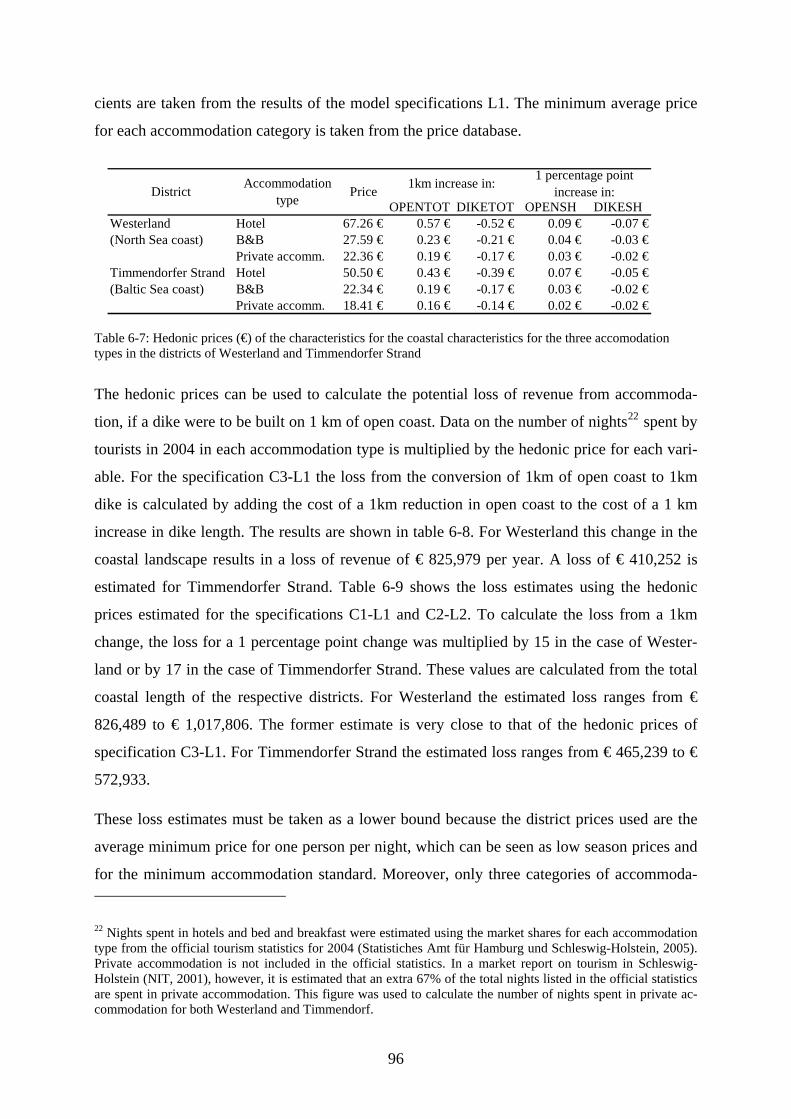
cients are taken from the results of the model specifications L1. The minimum average price
for each accommodation category is taken from the price database.
OPENTOT DIKETOT OPENSH DIKESHWesterland Hotel 67.26 € 0.57 € -0.52 € 0.09 € -0.07 €(North Sea coast) B&B 27.59 € 0.23 € -0.21 € 0.04 € -0.03 €
Private accomm. 22.36 € 0.19 € -0.17 € 0.03 € -0.02 €Timmendorfer Strand Hotel 50.50 € 0.43 € -0.39 € 0.07 € -0.05 €(Baltic Sea coast) B&B 22.34 € 0.19 € -0.17 € 0.03 € -0.02 €
Private accomm. 18.41 € 0.16 € -0.14 € 0.02 € -0.02 €
1 percentage point increase in:District Accommodation
type Price 1km increase in:
Table 6-7: Hedonic prices (€) of the characteristics for the coastal characteristics for the three accomodation types in the districts of Westerland and Timmendorfer Strand
The hedonic prices can be used to calculate the potential loss of revenue from accommoda-
tion, if a dike were to be built on 1 km of open coast. Data on the number of nights22 spent by
tourists in 2004 in each accommodation type is multiplied by the hedonic price for each vari-
able. For the specification C3-L1 the loss from the conversion of 1km of open coast to 1km
dike is calculated by adding the cost of a 1km reduction in open coast to the cost of a 1 km
increase in dike length. The results are shown in table 6-8. For Westerland this change in the
coastal landscape results in a loss of revenue of € 825,979 per year. A loss of € 410,252 is
estimated for Timmendorfer Strand. Table 6-9 shows the loss estimates using the hedonic
prices estimated for the specifications C1-L1 and C2-L2. To calculate the loss from a 1km
change, the loss for a 1 percentage point change was multiplied by 15 in the case of Wester-
land or by 17 in the case of Timmendorfer Strand. These values are calculated from the total
coastal length of the respective districts. For Westerland the estimated loss ranges from €
826,489 to € 1,017,806. The former estimate is very close to that of the hedonic prices of
specification C3-L1. For Timmendorfer Strand the estimated loss ranges from € 465,239 to €
572,933.
These loss estimates must be taken as a lower bound because the district prices used are the
average minimum price for one person per night, which can be seen as low season prices and
for the minimum accommodation standard. Moreover, only three categories of accommoda-
22 Nights spent in hotels and bed and breakfast were estimated using the market shares for each accommodation type from the official tourism statistics for 2004 (Statistiches Amt für Hamburg und Schleswig-Holstein, 2005). Private accommodation is not included in the official statistics. In a market report on tourism in Schleswig-Holstein (NIT, 2001), however, it is estimated that an extra 67% of the total nights listed in the official statistics are spent in private accommodation. This figure was used to calculate the number of nights spent in private ac-commodation for both Westerland and Timmendorf.
96
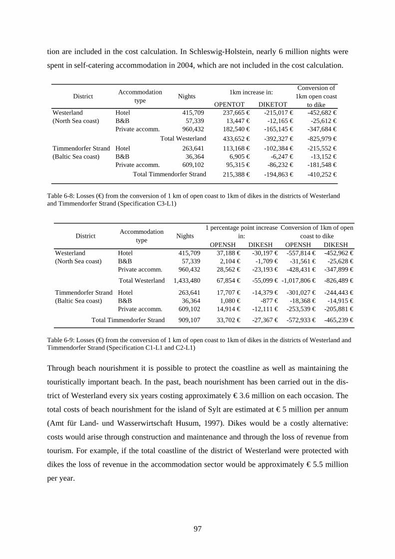
tion are included in the cost calculation. In Schleswig-Holstein, nearly 6 million nights were
spent in self-catering accommodation in 2004, which are not included in the cost calculation.
OPENTOT DIKETOTWesterland Hotel 415,709 237,665 € -215,017 € -452,682 €(North Sea coast) B&B 57,339 13,447 € -12,165 € -25,612 €
Private accomm. 960,432 182,540 € -165,145 € -347,684 €433,652 € -392,327 € -825,979 €
Timmendorfer Strand Hotel 263,641 113,168 € -102,384 € -215,552 €(Baltic Sea coast) B&B 36,364 6,905 € -6,247 € -13,152 €
Private accomm. 609,102 95,315 € -86,232 € -181,548 €215,388 € -194,863 € -410,252 €
Total Westerland
Total Timmendorfer Strand
Conversion of 1km open coast
to dikeDistrict Accommodation
type Nights 1km increase in:
Table 6-8: Losses (€) from the conversion of 1 km of open coast to 1km of dikes in the districts of Westerland and Timmendorfer Strand (Specification C3-L1)
Table 6-9: Losses (€) from the conversion of 1 km of open coast to 1km of dikes in the districts of Westerland and Timmendorfer Strand (Specification C1-L1 and C2-L1)
OPENSH DIKESH OPENSH DIKESHWesterland Hotel 415,709 37,188 € -30,197 € -557,814 € -452,962 €(North Sea coast) B&B 57,339 2,104 € -1,709 € -31,561 € -25,628 €
Private accomm. 960,432 28,562 € -23,193 € -428,431 € -347,899 €
1,433,480 67,854 € -55,099 € -1,017,806 € -826,489 €
Timmendorfer Strand Hotel 263,641 17,707 € -14,379 € -301,027 € -244,443 €(Baltic Sea coast) B&B 36,364 1,080 € -877 € -18,368 € -14,915 €
Private accomm. 609,102 14,914 € -12,111 € -253,539 € -205,881 €
909,107 33,702 € -27,367 € -572,933 € -465,239 €
Conversion of 1km of open coast to dike
Total Westerland
Total Timmendorfer Strand
1 percentage point increase in:District Accommodation
type Nights
Through beach nourishment it is possible to protect the coastline as well as maintaining the
touristically important beach. In the past, beach nourishment has been carried out in the dis-
trict of Westerland every six years costing approximately € 3.6 million on each occasion. The
total costs of beach nourishment for the island of Sylt are estimated at € 5 million per annum
(Amt für Land- und Wasserwirtschaft Husum, 1997). Dikes would be a costly alternative:
costs would arise through construction and maintenance and through the loss of revenue from
tourism. For example, if the total coastline of the district of Westerland were protected with
dikes the loss of revenue in the accommodation sector would be approximately € 5.5 million
per year.
97

6.7 Conclusion
This chapter has provided a way of examining the value that tourists attach to different coastal
attributes. Districts with open coast accrue higher accommodation prices than districts with
other coastal types. The hedonic prices of the different coastal types produced from this study
can be used along with other tourism data in a cost-benefit analysis when considering the best
adaptation measures to sea-level rise. Nevertheless, this study categorises coastal type in a
very simple manner. Dikes are not the only hard engineering structures than can be used to
protect the coast. In addition, tetrapods, groynes and revetments can be used; all of which
change the appearance of the landscape. In this study, stretches of the coastline that have such
structures in place still fall under the category of open coast.
Although this study examines tourism at a very high resolution, it would be an interesting
extension to increase the resolution even further. Instead of the district average price, the
prices of individual accommodation units can be used. At a higher resolution and with a
smaller focus area, it would be possible to include measurements such as distance to the near-
est beach and the area of coastline that has tetrapods or other such structures. Such an exten-
sion, however, would depend on the availability of appropriate GIS data.
Here the focus has been on only one of the coastal states of Germany. The other coastal states,
Mecklenburg-Western Pomerania and Lower Saxony, have large tourism industries. Although
the broad coastal types that can be found in these states can also be found in Schleswig-
Holstein, a comprehensive study of coastal accommodation prices in Germany would be use-
ful both for integrated coastal zone management as well as for tourism planning and market-
ing. This method and the results presented in this study are a good starting point for future
research.
98
Chapter 7
Climate change and international tourism: a simulation study*
7.1 Introduction
Chapter 2 drew attention to the lack of a larger, global assessment of push and pull factors of
international tourism. The study presented in this chapter is an attempt to fill that gap.
If one wants to estimate the implications of climate change for a particular tourist destination,
then one would not only want to know how the attractiveness of that place is changing – as is
done in some of literature discussed in chapter 2. Rather, one would need to know how cli-
mate change affects the attractiveness of that place relative to its competitors. If, for instance,
Switzerland loses half of its snow, but other European skiing destinations lose all – then Swit-
zerland’s position may well be strengthened as the only place in Europe with natural snow.
Similarly, one would need the change in behaviour of all tourists, and not just of those from
Germany, the Netherlands and the UK. Like the studies on climate attractiveness, this chapter
uses attractiveness indicators, albeit ones that are based on observed behaviour. In combining
country demand studies and attractiveness studies, it was necessary to simplify. The novelty
of this study lies in the interactions of push and pull factors at a global scale, not in the details.
Section 7.2 presents the model, its calibration and the base results. Section 7.3 discusses the
sensitivity of the model. Section 7.4 concludes.
From the review of climate and tourism literature in chapter 2, the following gaps are evident.
Firstly, the possibility of substitution between destinations has been neglected in all studies.
Secondly, the studies have focussed on particular areas or particular origin nationalities; the
global picture has yet to be filled in. Thirdly, in the forecasting literature, environmental char-
acteristics are assumed to be fixed, and only economic variables are seen as varying over
time. Climate as a “push” factor has also been largely overlooked. A global study of flows
from origin countries to destination countries that includes the climate of countries as a factor
* This chapter is based on Hamilton et al. (2005a).
99
in both the estimation of demand to travel as well as the demand for a particular destination
would fill this gap, as well as allowing an examination of the substitution process.
7.2 The model and basic results
7.2.1 Model structure
A model of international tourist flows from 207 countries to 207 countries was constructed.
The purpose of the model is not to understand the current pattern of international tourism; for
that, more detailed information than is currently available would be needed. Rather, the pur-
pose of the model is to analyse how the current pattern may change under not-implausible
scenarios of future population growth, economic growth and, particularly, climate change.
The inputs to the patterns and their changes are the empirical regularities reported in section
7.2.2. The exact details are given below.
The basis of the model is the matrix of bilateral tourism flows. This matrix is perturbed with
scenarios of population growth, economic growth and climate change. The perturbations on
the supply side are perturbations on the relative attractiveness of holiday destinations. The
perturbations on the demand side are perturbations on the number of tourists from origin
countries. For these perturbations, the same relationships are used that were used to construct
the bilateral tourism flow matrix.
Note that data on international tourism is available only at the national level. This implies a
distortion of reality, particularly for large and diverse countries for which a representative
climate and a representative income have to be assumed. This is obviously problematic for the
USA, but also for France, the most popular destination, where tourism is concentrated in Paris
and the south. Similarly, data are reported per year. Seasonal tourism flows are not accounted
for.
7.2.2 Baseline
The model is calibrated against the international arrivals and departures data of 1995 con-
tained in the World Resources Databases (WRI, 2000).23 There are three major problems with
23 The reported departures from the Czech Republic were divided by 10; comparison to earlier and later years shows that the 1995 data have a typographical error.
100

this dataset. Firstly, for some countries, the reported data is for arrivals and departures for
tourism only. For other countries, the data is for arrivals and departures for all purposes. Un-
fortunately, it is impossible to correct for this.24 Secondly, the data is on total arrivals and
total departures; there is no data on the origin of the arrivals or the destination of the depar-
tures. Consequently, a database on bilateral tourism flows for all pairs of countries was con-
structed. Thirdly, there are missing observations, particularly with regard to departures.
For arrivals, 181 countries have data but 26 do not. The missing observations were filled with
a statistical model, viz:
Equation 7-1: 7 3 2 5
0.97 0.96 0.07 2.21 3.03 0.09
2
ln 5.97 2.05 10 0.22 7.91 10 7.15 10 0.80 ln
139; 0.54
d d d d d
adj
dA G T T C
N R
− − −= + ⋅ + − ⋅ + ⋅ +
= =
Y
where A denotes total arrivals, G is land area (in square kilometres); T is annual average tem-
perature for 1961-1990 (in degrees Celsius) averaged over the country, C is length of coast-
line (in kilometres), and Y is per capita income; d indexes destination country. This model is
the best fit25 to the observations for the countries for which there is data.26 The total number
of tourists increases from 55.2 million (observed) to 56.5 million (observed + modelled). The
26 missing observations constitute only 2% of the international tourism market.
For departures, the data problem is more serious: 107 countries report but 99 do not27; 46.5
million departures are reported, against 56.5 million arrivals, so that 18% of all international
tourists have an unknown origin. Again, the missing observations were filled with a statistical
model, viz:
24 However, the Polish departure data was corrected. According to Statistic Poland, only 12% of the reported international departures are tourists (Central Statistical Office Poland, 2002) 25 The estimation procedure started with a large number of explanatory variables, including precipitation, num-ber of world heritage sites, political stability and a range of other indicators. Explanatory variables that are indi-vidually and jointly insignificant were eliminated. Different representations of temperature (e.g., temperature of the hottest month) were experimented with; the annual average temperature describes the data best. 26 The data on per capita income were taken from WRI (2000), supplemented with data from CIA (2002); the data on area and the length of international borders are from CIA (2002); the data on temperature from New et al. (1999). All data can be found at http://www.uni-hamburg.de/Wiss/FB/15/Sustainability. 27 These are mostly African countries and small dependencies; however, data from Pakistan and Taiwan are also missing. Luxemburg is the only OECD country without departures data.
101

Equation 7-2:
3 2 2
17.05 0.17 16.82 4.22 0.09 0.13
2
ln 1.51 0.18 4.83 10 5.56 10 0.86 ln 0.23ln
99; 0.66
oo o o o
o
adj
DT T B Y
P
N R
− −= − + ⋅ − ⋅ + −
= =
oG
where D denotes departures (in number), P denotes population (in thousands) and B is the
number of countries with shared land borders; o indexes the country of origin. Again, this
model is the best fit28 to the observations for the countries for which there is data,29 but al-
though the fit is better than for arrivals, the uncertainty about the parameters is larger. This
leads to a total number of departures of 48.2 million, so all departures30 were scaled up by
17% so that the total number of observed and modelled departures equals the total number of
observed and modelled arrivals.
Note that most results below are given relative to 1995 or relative to the base scenario, which
itself is relative to 1995. The fact that the data had to be adjusted should not distort the quali-
tative results.
Bilateral tourism flows were derived as follows. In keeping with the model described below, a
general attractiveness index for each country was constructed.31 The tourists of each country
are allocated to other countries according to a country-of-origin-specific attractiveness index
that is equal to the general attractiveness index times the distance between the two capital
cities raised to the power -1.7·10-4.32 That is, tourists are allocated to destinations based on the
general attractiveness of the destinations and the distance to these destinations. In this man-
ner, the model reproduces the 1995 pattern of total departures and arrivals (see Figures 7-1
28 The estimation procedure started with a large number of explanatory variables. Explanatory variables that are individually and jointly insignificant were eliminated. 29 The data on population were taken from WRI (2000), the data on the number of land borders were taken from CIA (2002). 30 Scaling up only the interpolated departures leads to distortions, as many small countries do not report departures data. Besides, countries have less of an interest in counting departures than in counting arrivals, so departures are probably underreported even if there are data available. Note that by equating total arrivals and total departures num-bers, it is assumed that tourists visit one country per trip only. 31 The general attractiveness index was adjusted in an iterative calibration. In the first iteration, the attractiveness index equals the market share of each country in world tourism. The ratio between predicted and observed tourist arrivals was used to adjust the attractiveness index. Changes in the attractiveness index follow Equation 7-1. 32 Lise and Tol (2002) analyse tourism flows from selected OECD countries to selected OECD countries. This allows them to estimate a distance elasticity. The number reported here is the average of their estimates.
102
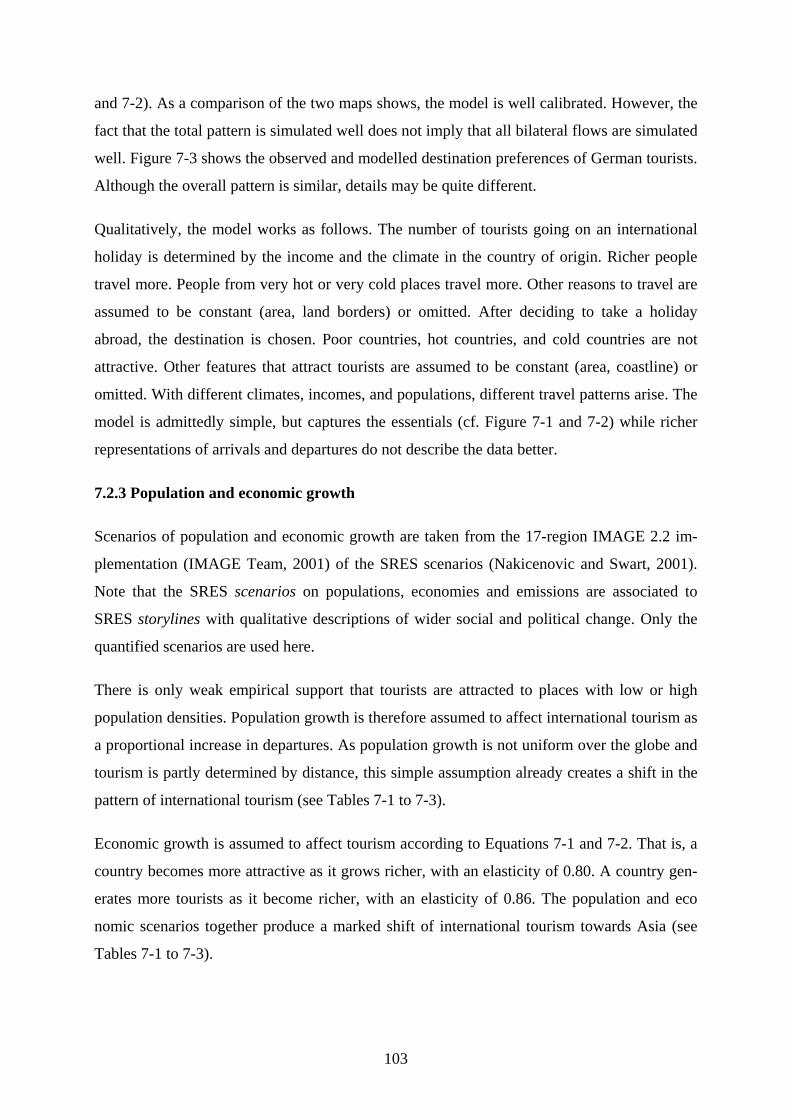
and 7-2). As a comparison of the two maps shows, the model is well calibrated. However, the
fact that the total pattern is simulated well does not imply that all bilateral flows are simulated
well. Figure 7-3 shows the observed and modelled destination preferences of German tourists.
Although the overall pattern is similar, details may be quite different.
Qualitatively, the model works as follows. The number of tourists going on an international
holiday is determined by the income and the climate in the country of origin. Richer people
travel more. People from very hot or very cold places travel more. Other reasons to travel are
assumed to be constant (area, land borders) or omitted. After deciding to take a holiday
abroad, the destination is chosen. Poor countries, hot countries, and cold countries are not
attractive. Other features that attract tourists are assumed to be constant (area, coastline) or
omitted. With different climates, incomes, and populations, different travel patterns arise. The
model is admittedly simple, but captures the essentials (cf. Figure 7-1 and 7-2) while richer
representations of arrivals and departures do not describe the data better.
7.2.3 Population and economic growth
Scenarios of population and economic growth are taken from the 17-region IMAGE 2.2 im-
plementation (IMAGE Team, 2001) of the SRES scenarios (Nakicenovic and Swart, 2001).
Note that the SRES scenarios on populations, economies and emissions are associated to
SRES storylines with qualitative descriptions of wider social and political change. Only the
quantified scenarios are used here.
There is only weak empirical support that tourists are attracted to places with low or high
population densities. Population growth is therefore assumed to affect international tourism as
a proportional increase in departures. As population growth is not uniform over the globe and
tourism is partly determined by distance, this simple assumption already creates a shift in the
pattern of international tourism (see Tables 7-1 to 7-3).
Economic growth is assumed to affect tourism according to Equations 7-1 and 7-2. That is, a
country becomes more attractive as it grows richer, with an elasticity of 0.80. A country gen-
erates more tourists as it become richer, with an elasticity of 0.86. The population and eco
nomic scenarios together produce a marked shift of international tourism towards Asia (see
Tables 7-1 to 7-3).
103
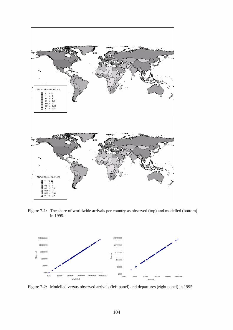
Figure 7-1: The share of worldwide arrivals per country as observed (top) and modelled (bottom) in 1995.
Figure 7-2: Modelled versus observed arrivals (left panel) and departures (right panel) in 1995
1000
10000
100000
1000000
10000000
100000000
1000 10000 100000 1000000 10000000 100000000
Modelled
Obs
erve
d
1000
10000
100000
1000000
10000000
100000000
1000 10000 100000 1000000 10000000 100000000
Modelled
Obs
erve
d
104

0
2
4
6
8
10
12
14
Spain
France
Italy
Czech R
ep
Hunga
ry UKGree
ceUSA
Turkey
Portug
al
Belgium
Canad
a
Irelan
d
Austral
iaJap
an
New Zeal
and
Icelan
d
Mill
ions
of v
isito
rs
ObservedM odelled
Figure 7-3: The most popular destinations of German tourists as observed and as modelled
1995 2025a
P P+E P+E+C France 10.79 10.62 7.73 7.67United States 7.53 7.60 5.63 5.88Spain 7.07 7.00 5.09 4.84Italy 5.58 5.52 4.10 3.89United Kingdom 4.23 4.18 3.07 3.17Hungary 3.76 3.71 5.63 5.70Mexico 3.50 3.59 3.71 3.16Poland 3.46 3.40 5.25 5.52China 3.41 3.44 7.25 8.17Austria 3.09 3.04 2.25 2.43Czech Rep 3.01 2.95 4.51 4.75Canada 2.96 3.01 1.96 2.90Germany 2.65 2.63 2.01 2.09Switzerland 2.08 2.04 1.49 1.62Greece 1.83 1.82 1.37 1.26Hong Kong 1.71 1.75 2.60 2.22Portugal 1.71 1.70 1.22 1.13Russian Federation 1.66 1.65 2.20 3.11Turkey 1.28 1.27 1.29 1.28Malaysia 1.27 1.29 1.76 1.55Netherlands 1.19 1.17 0.85 0.86Thailand 1.17 1.21 1.69 1.49Singapore 1.07 1.11 1.17 1.05Belgium 1.01 0.98 0.71 0.72Ireland 0.87 0.85 0.61 0.62a Three scenarios are distinguished for 2025: population growth (P); population and per capita income growth (P+E); population and per capita income growth and climate change (P+E+C). Population and per capita income growth is according to the SRES A1B scenario (Nakicenovic and Swart, 2001; IMAGE Team, 2001) in 2025. Climate change is a 1˚C global warming; the spatial pattern is the average over 14 GCMs (Schlesinger and Wil-liams, 1998).
Table 7-1: Market share of arrivals
105
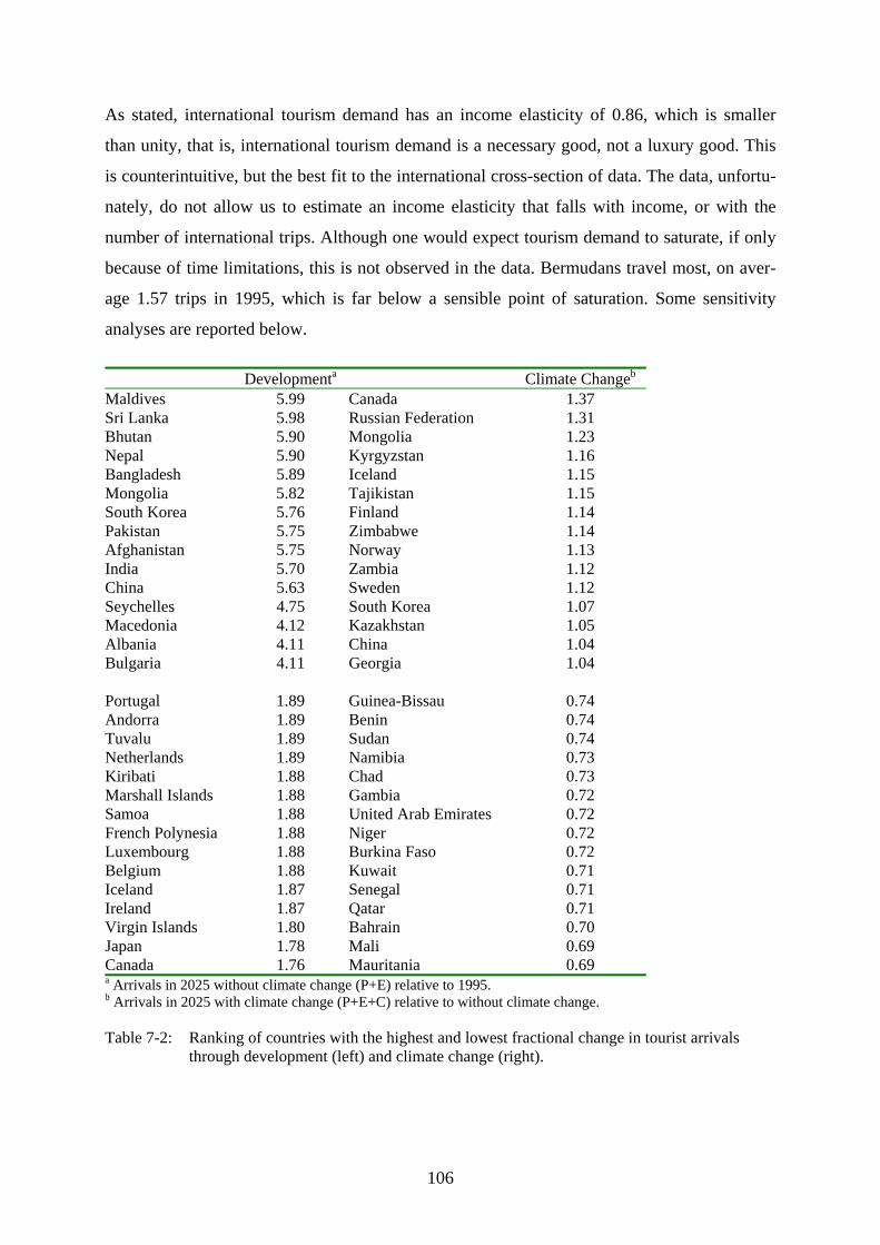
As stated, international tourism demand has an income elasticity of 0.86, which is smaller
than unity, that is, international tourism demand is a necessary good, not a luxury good. This
is counterintuitive, but the best fit to the international cross-section of data. The data, unfortu-
nately, do not allow us to estimate an income elasticity that falls with income, or with the
number of international trips. Although one would expect tourism demand to saturate, if only
because of time limitations, this is not observed in the data. Bermudans travel most, on aver-
age 1.57 trips in 1995, which is far below a sensible point of saturation. Some sensitivity
analyses are reported below.
Developmenta Climate Changeb
Maldives 5.99 Canada 1.37 Sri Lanka 5.98 Russian Federation 1.31 Bhutan 5.90 Mongolia 1.23 Nepal 5.90 Kyrgyzstan 1.16 Bangladesh 5.89 Iceland 1.15 Mongolia 5.82 Tajikistan 1.15 South Korea 5.76 Finland 1.14 Pakistan 5.75 Zimbabwe 1.14 Afghanistan 5.75 Norway 1.13 India 5.70 Zambia 1.12 China 5.63 Sweden 1.12 Seychelles 4.75 South Korea 1.07 Macedonia 4.12 Kazakhstan 1.05 Albania 4.11 China 1.04 Bulgaria 4.11 Georgia 1.04 Portugal 1.89 Guinea-Bissau 0.74 Andorra 1.89 Benin 0.74 Tuvalu 1.89 Sudan 0.74 Netherlands 1.89 Namibia 0.73 Kiribati 1.88 Chad 0.73 Marshall Islands 1.88 Gambia 0.72 Samoa 1.88 United Arab Emirates 0.72 French Polynesia 1.88 Niger 0.72 Luxembourg 1.88 Burkina Faso 0.72 Belgium 1.88 Kuwait 0.71 Iceland 1.87 Senegal 0.71 Ireland 1.87 Qatar 0.71 Virgin Islands 1.80 Bahrain 0.70 Japan 1.78 Mali 0.69 Canada 1.76 Mauritania 0.69 a Arrivals in 2025 without climate change (P+E) relative to 1995. b Arrivals in 2025 with climate change (P+E+C) relative to without climate change.
Table 7-2: Ranking of countries with the highest and lowest fractional change in tourist arrivals through development (left) and climate change (right).
106
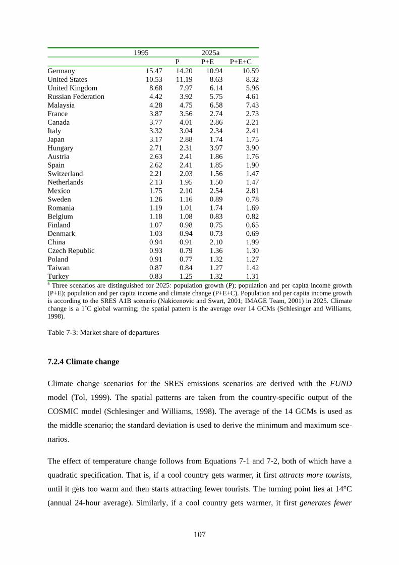
1995 2025a P P+E P+E+C Germany 15.47 14.20 10.94 10.59United States 10.53 11.19 8.63 8.32United Kingdom 8.68 7.97 6.14 5.96Russian Federation 4.42 3.92 5.75 4.61Malaysia 4.28 4.75 6.58 7.43France 3.87 3.56 2.74 2.73Canada 3.77 4.01 2.86 2.21Italy 3.32 3.04 2.34 2.41Japan 3.17 2.88 1.74 1.75Hungary 2.71 2.31 3.97 3.90Austria 2.63 2.41 1.86 1.76Spain 2.62 2.41 1.85 1.90Switzerland 2.21 2.03 1.56 1.47Netherlands 2.13 1.95 1.50 1.47Mexico 1.75 2.10 2.54 2.81Sweden 1.26 1.16 0.89 0.78Romania 1.19 1.01 1.74 1.69Belgium 1.18 1.08 0.83 0.82Finland 1.07 0.98 0.75 0.65Denmark 1.03 0.94 0.73 0.69China 0.94 0.91 2.10 1.99Czech Republic 0.93 0.79 1.36 1.30Poland 0.91 0.77 1.32 1.27Taiwan 0.87 0.84 1.27 1.42Turkey 0.83 1.25 1.32 1.31a Three scenarios are distinguished for 2025: population growth (P); population and per capita income growth (P+E); population and per capita income and climate change (P+E+C). Population and per capita income growth is according to the SRES A1B scenario (Nakicenovic and Swart, 2001; IMAGE Team, 2001) in 2025. Climate change is a 1˚C global warming; the spatial pattern is the average over 14 GCMs (Schlesinger and Williams, 1998).
Table 7-3: Market share of departures
7.2.4 Climate change
Climate change scenarios for the SRES emissions scenarios are derived with the FUND
model (Tol, 1999). The spatial patterns are taken from the country-specific output of the
COSMIC model (Schlesinger and Williams, 1998). The average of the 14 GCMs is used as
the middle scenario; the standard deviation is used to derive the minimum and maximum sce-
narios.
The effect of temperature change follows from Equations 7-1 and 7-2, both of which have a
quadratic specification. That is, if a cool country gets warmer, it first attracts more tourists,
until it gets too warm and then starts attracting fewer tourists. The turning point lies at 14°C
(annual 24-hour average). Similarly, if a cool country gets warmer, it first generates fewer
107
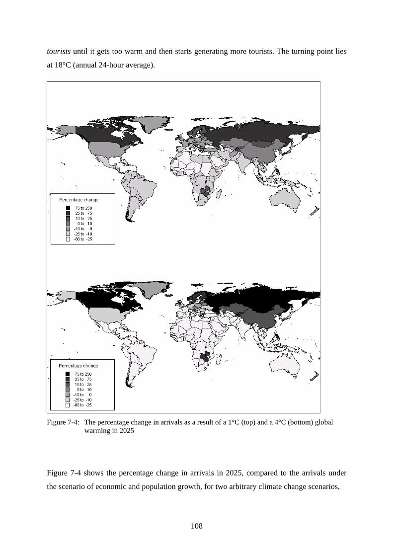
tourists until it gets too warm and then starts generating more tourists. The turning point lies
at 18°C (annual 24-hour average).
Figure 7-4: The percentage change in arrivals as a result of a 1°C (top) and a 4°C (bottom) global warming in 2025
Figure 7-4 shows the percentage change in arrivals in 2025, compared to the arrivals under
the scenario of economic and population growth, for two arbitrary climate change scenarios,
108
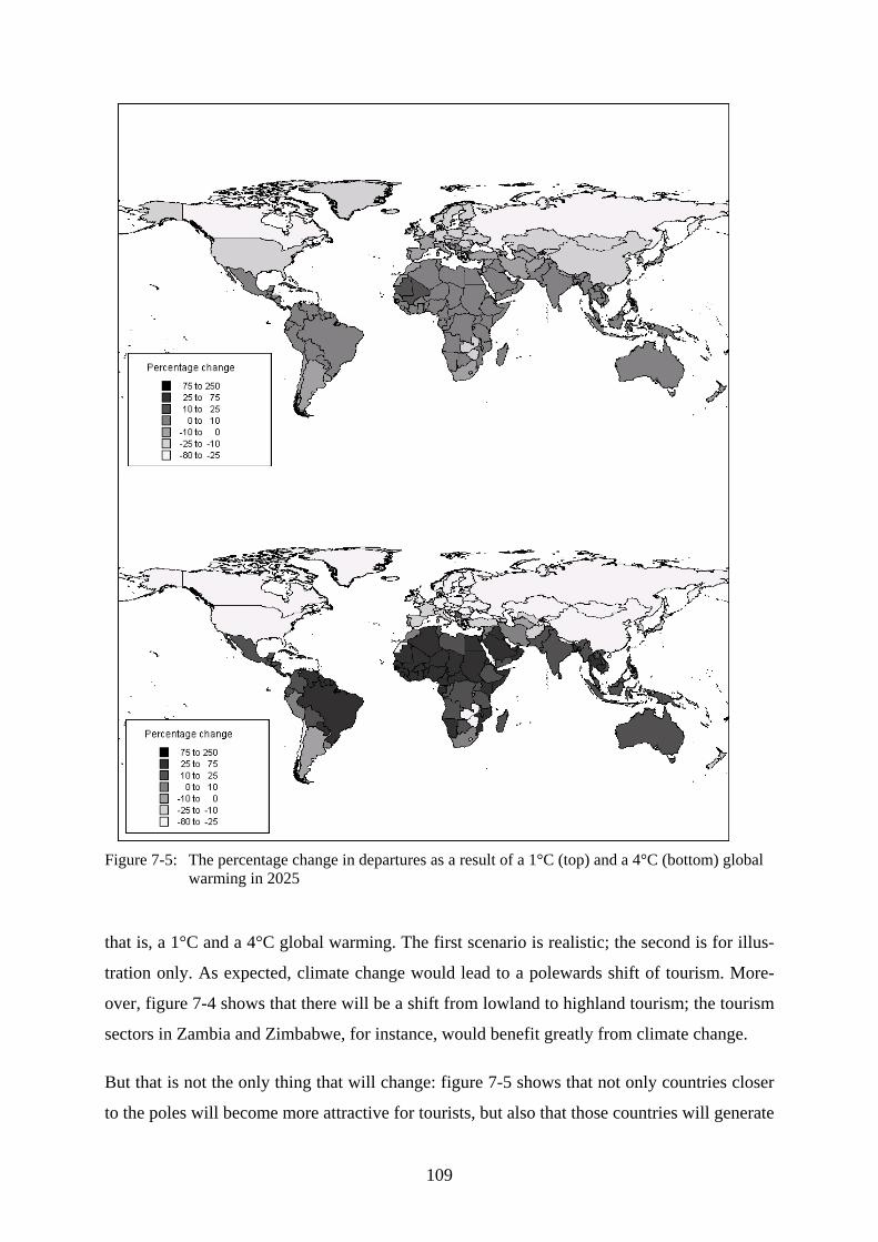
Figure 7-5: The percentage change in departures as a result of a 1°C (top) and a 4°C (bottom) global warming in 2025
that is, a 1°C and a 4°C global warming. The first scenario is realistic; the second is for illus-
tration only. As expected, climate change would lead to a polewards shift of tourism. More-
over, figure 7-4 shows that there will be a shift from lowland to highland tourism; the tourism
sectors in Zambia and Zimbabwe, for instance, would benefit greatly from climate change.
But that is not the only thing that will change: figure 7-5 shows that not only countries closer
to the poles will become more attractive for tourists, but also that those countries will generate
109
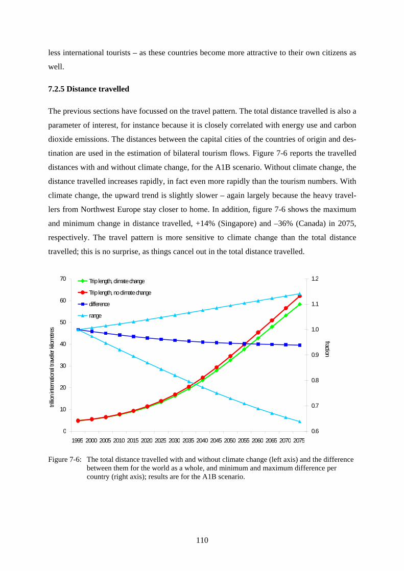
less international tourists – as these countries become more attractive to their own citizens as
well.
7.2.5 Distance travelled
The previous sections have focussed on the travel pattern. The total distance travelled is also a
parameter of interest, for instance because it is closely correlated with energy use and carbon
dioxide emissions. The distances between the capital cities of the countries of origin and des-
tination are used in the estimation of bilateral tourism flows. Figure 7-6 reports the travelled
distances with and without climate change, for the A1B scenario. Without climate change, the
distance travelled increases rapidly, in fact even more rapidly than the tourism numbers. With
climate change, the upward trend is slightly slower – again largely because the heavy travel-
lers from Northwest Europe stay closer to home. In addition, figure 7-6 shows the maximum
and minimum change in distance travelled, +14% (Singapore) and –36% (Canada) in 2075,
respectively. The travel pattern is more sensitive to climate change than the total distance
travelled; this is no surprise, as things cancel out in the total distance travelled.
0
10
20
30
40
50
60
70
1995 2000 2005 2010 2015 2020 2025 2030 2035 2040 2045 2050 2055 2060 2065 2070 2075
trillio
n inte
rnati
onal
trave
ller k
ilome
tres
0.6
0.7
0.8
0.9
1.0
1.1
1.2
fraction
Trip length, climate change Trip length, no climate change difference range
Figure 7-6: The total distance travelled with and without climate change (left axis) and the difference between them for the world as a whole, and minimum and maximum difference per country (right axis); results are for the A1B scenario.
110
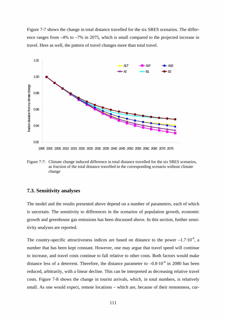
Figure 7-7 shows the change in total distance travelled for the six SRES scenarios. The differ-
ence ranges from –4% to –7% in 2075, which is small compared to the projected increase in
travel. Here as well, the pattern of travel changes more than total travel.
0.92
0.94
0.96
0.98
1.00
1.02
1995 2000 2005 2010 2015 2020 2025 2030 2035 2040 2045 2050 2055 2060 2065 2070 2075
fracti
on de
viatio
n fro
m no
clim
ate ch
ange
A1T A1F A1B A2 B1 B2
Figure 7-7: Climate change induced difference in total distance travelled for the six SRES scenarios, as fraction of the total distance travelled in the corresponding scenario without climate change
7.3. Sensitivity analyses
The model and the results presented above depend on a number of parameters, each of which
is uncertain. The sensitivity to differences in the scenarios of population growth, economic
growth and greenhouse gas emissions has been discussed above. In this section, further sensi-
tivity analyses are reported.
The country-specific attractiveness indices are based on distance to the power –1.7·10-4, a
number that has been kept constant. However, one may argue that travel speed will continue
to increase, and travel costs continue to fall relative to other costs. Both factors would make
distance less of a deterrent. Therefore, the distance parameter to –0.8·10-4 in 2080 has been
reduced, arbitrarily, with a linear decline. This can be interpreted as decreasing relative travel
costs. Figure 7-8 shows the change in tourist arrivals, which, in total numbers, is relatively
small. As one would expect, remote locations – which are, because of their remoteness, cur-
111
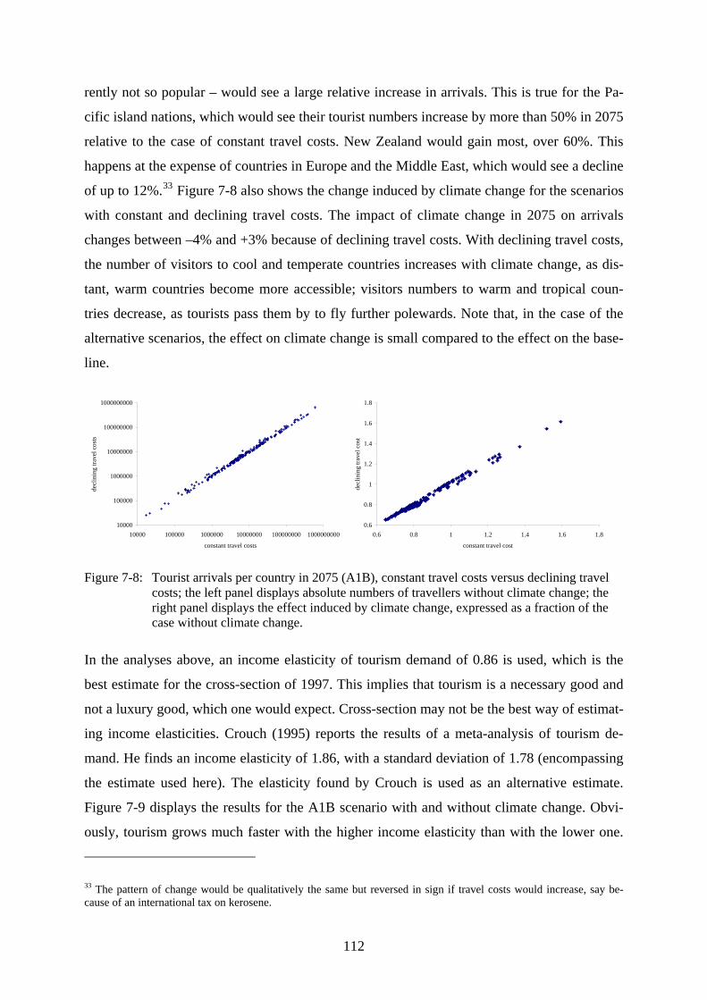
rently not so popular – would see a large relative increase in arrivals. This is true for the Pa-
cific island nations, which would see their tourist numbers increase by more than 50% in 2075
relative to the case of constant travel costs. New Zealand would gain most, over 60%. This
happens at the expense of countries in Europe and the Middle East, which would see a decline
of up to 12%.33 Figure 7-8 also shows the change induced by climate change for the scenarios
with constant and declining travel costs. The impact of climate change in 2075 on arrivals
changes between –4% and +3% because of declining travel costs. With declining travel costs,
the number of visitors to cool and temperate countries increases with climate change, as dis-
tant, warm countries become more accessible; visitors numbers to warm and tropical coun-
tries decrease, as tourists pass them by to fly further polewards. Note that, in the case of the
alternative scenarios, the effect on climate change is small compared to the effect on the base-
line.
10000
100000
1000000
10000000
100000000
1000000000
10000 100000 1000000 10000000 100000000 1000000000
constant travel costs
decl
inin
g tra
vel c
osts
0.6
0.8
1
1.2
1.4
1.6
1.8
0.6 0.8 1 1.2 1.4 1.6 1.8
constant travel cost
decl
inin
g tra
vel c
ost
Figure 7-8: Tourist arrivals per country in 2075 (A1B), constant travel costs versus declining travel costs; the left panel displays absolute numbers of travellers without climate change; the right panel displays the effect induced by climate change, expressed as a fraction of the case without climate change.
In the analyses above, an income elasticity of tourism demand of 0.86 is used, which is the
best estimate for the cross-section of 1997. This implies that tourism is a necessary good and
not a luxury good, which one would expect. Cross-section may not be the best way of estimat-
ing income elasticities. Crouch (1995) reports the results of a meta-analysis of tourism de-
mand. He finds an income elasticity of 1.86, with a standard deviation of 1.78 (encompassing
the estimate used here). The elasticity found by Crouch is used as an alternative estimate.
Figure 7-9 displays the results for the A1B scenario with and without climate change. Obvi-
ously, tourism grows much faster with the higher income elasticity than with the lower one.
33 The pattern of change would be qualitatively the same but reversed in sign if travel costs would increase, say be-cause of an international tax on kerosene.
112
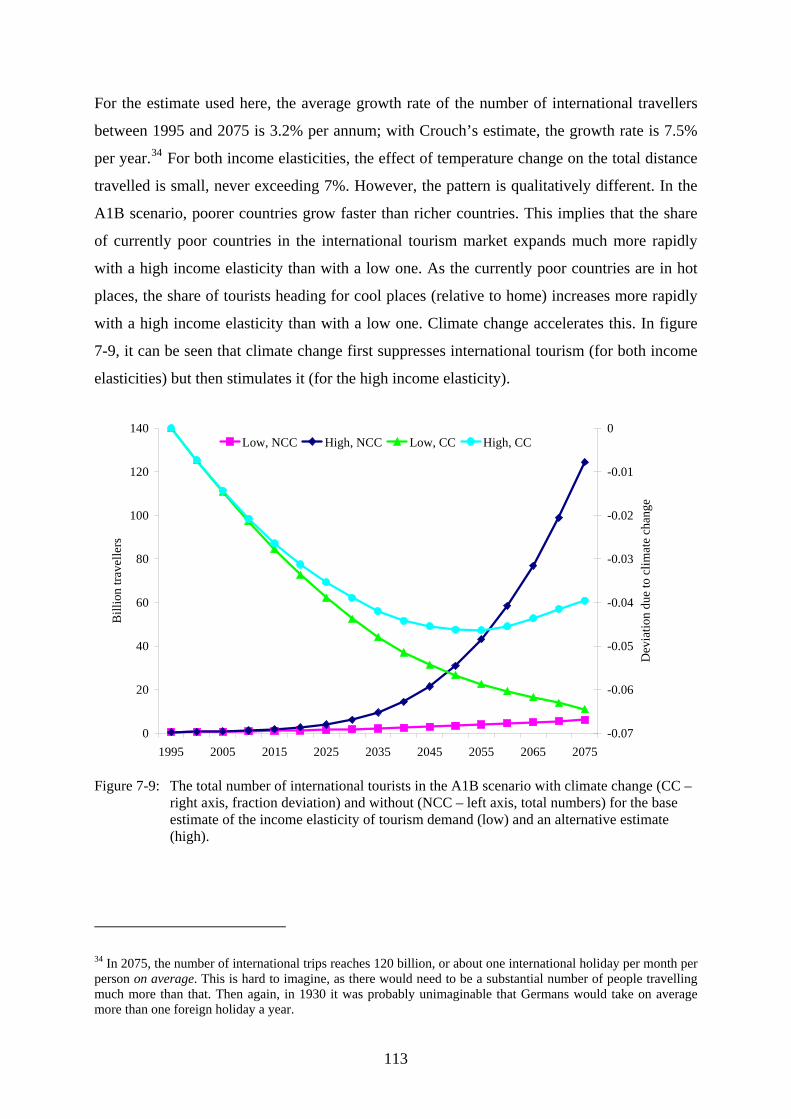
For the estimate used here, the average growth rate of the number of international travellers
between 1995 and 2075 is 3.2% per annum; with Crouch’s estimate, the growth rate is 7.5%
per year.34 For both income elasticities, the effect of temperature change on the total distance
travelled is small, never exceeding 7%. However, the pattern is qualitatively different. In the
A1B scenario, poorer countries grow faster than richer countries. This implies that the share
of currently poor countries in the international tourism market expands much more rapidly
with a high income elasticity than with a low one. As the currently poor countries are in hot
places, the share of tourists heading for cool places (relative to home) increases more rapidly
with a high income elasticity than with a low one. Climate change accelerates this. In figure
7-9, it can be seen that climate change first suppresses international tourism (for both income
elasticities) but then stimulates it (for the high income elasticity).
0
20
40
60
80
100
120
140
1995 2005 2015 2025 2035 2045 2055 2065 2075
Bill
ion
trave
llers
-0.07
-0.06
-0.05
-0.04
-0.03
-0.02
-0.01
0
Dev
iatio
n du
e to
clim
ate
chan
ge
Low, NCC High, NCC Low, CC High, CC
Figure 7-9: The total number of international tourists in the A1B scenario with climate change (CC – right axis, fraction deviation) and without (NCC – left axis, total numbers) for the base estimate of the income elasticity of tourism demand (low) and an alternative estimate (high).
34 In 2075, the number of international trips reaches 120 billion, or about one international holiday per month per person on average. This is hard to imagine, as there would need to be a substantial number of people travelling much more than that. Then again, in 1930 it was probably unimaginable that Germans would take on average more than one foreign holiday a year.
113
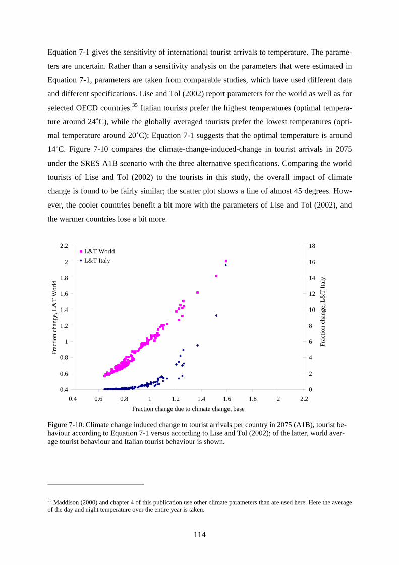
Equation 7-1 gives the sensitivity of international tourist arrivals to temperature. The parame-
ters are uncertain. Rather than a sensitivity analysis on the parameters that were estimated in
Equation 7-1, parameters are taken from comparable studies, which have used different data
and different specifications. Lise and Tol (2002) report parameters for the world as well as for
selected OECD countries.35 Italian tourists prefer the highest temperatures (optimal tempera-
ture around 24˚C), while the globally averaged tourists prefer the lowest temperatures (opti-
mal temperature around 20˚C); Equation 7-1 suggests that the optimal temperature is around
14˚C. Figure 7-10 compares the climate-change-induced-change in tourist arrivals in 2075
under the SRES A1B scenario with the three alternative specifications. Comparing the world
tourists of Lise and Tol (2002) to the tourists in this study, the overall impact of climate
change is found to be fairly similar; the scatter plot shows a line of almost 45 degrees. How-
ever, the cooler countries benefit a bit more with the parameters of Lise and Tol (2002), and
the warmer countries lose a bit more.
0.4
0.6
0.8
1
1.2
1.4
1.6
1.8
2
2.2
0.4 0.6 0.8 1 1.2 1.4 1.6 1.8 2 2.2Fraction change due to climate change, base
Frac
tion
chan
ge, L
&T
Wor
ld
0
2
4
6
8
10
12
14
16
18
Frac
tion
chan
ge, L
&T
Italy
L&T WorldL&T Italy
Figure 7-10: Climate change induced change to tourist arrivals per country in 2075 (A1B), tourist be-haviour according to Equation 7-1 versus according to Lise and Tol (2002); of the latter, world aver-age tourist behaviour and Italian tourist behaviour is shown.
35 Maddison (2000) and chapter 4 of this publication use other climate parameters than are used here. Here the average of the day and night temperature over the entire year is taken.
114
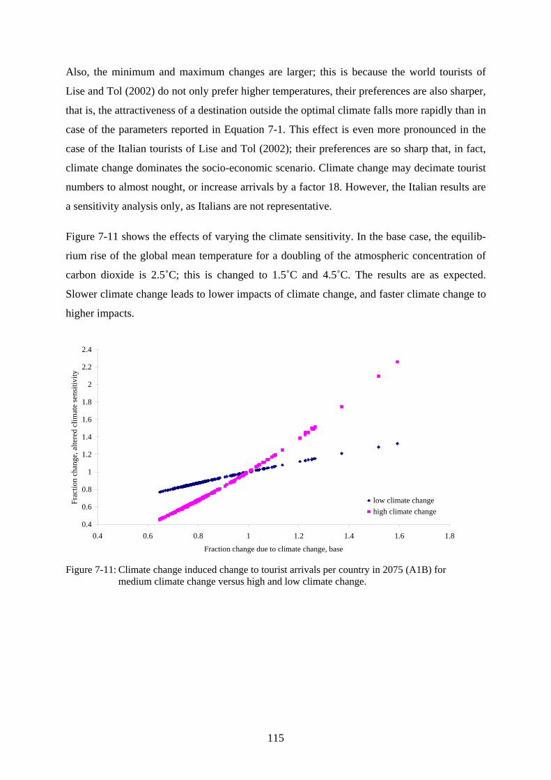
Also, the minimum and maximum changes are larger; this is because the world tourists of
Lise and Tol (2002) do not only prefer higher temperatures, their preferences are also sharper,
that is, the attractiveness of a destination outside the optimal climate falls more rapidly than in
case of the parameters reported in Equation 7-1. This effect is even more pronounced in the
case of the Italian tourists of Lise and Tol (2002); their preferences are so sharp that, in fact,
climate change dominates the socio-economic scenario. Climate change may decimate tourist
numbers to almost nought, or increase arrivals by a factor 18. However, the Italian results are
a sensitivity analysis only, as Italians are not representative.
Figure 7-11 shows the effects of varying the climate sensitivity. In the base case, the equilib-
rium rise of the global mean temperature for a doubling of the atmospheric concentration of
carbon dioxide is 2.5˚C; this is changed to 1.5˚C and 4.5˚C. The results are as expected.
Slower climate change leads to lower impacts of climate change, and faster climate change to
higher impacts.
0.4
0.6
0.8
1
1.2
1.4
1.6
1.8
2
2.2
2.4
0.4 0.6 0.8 1 1.2 1.4 1.6 1
Fraction change due to climate change, base
Frac
tion
chan
ge, a
ltere
d cl
imat
e se
nsiti
vity
.8
low climate changehigh climate change
Figure 7-11: Climate change induced change to tourist arrivals per country in 2075 (A1B) for medium climate change versus high and low climate change.
115
7.4 Discussion and conclusion
In this chapter, a simulation model of international tourism has been presented, and scenarios
of changes in international arrivals and departures have been developed corresponding to
changes in population numbers, per capita income, and climate change. A model like this is
for testing sensitivities rather than making predictions. Results are qualitative, not quantita-
tive.
The model shows that the past growth of international tourism may well continue unabated in
the medium to long term. The main driver is economic growth, and the growth of interna-
tional tourism will therefore be concentrated in those regions with the highest economic
growth; had a higher income elasticity been used, this conclusion would have been even
stronger. Although intercontinental tourism will also grow, mass tourism is likely to continue
to prefer destinations closer to home. Uncertainties about future population and economic
growth, and uncertainties about elasticities and future travel costs make the projections of
international tourist numbers very uncertain.
Climate change would lead to a gradual shift of tourist destinations towards higher latitudes
and altitudes. Climate change would also imply that the currently dominant group of interna-
tional tourists – sun and beach lovers from Western Europe – would stay closer to home, im-
plying a relatively small fall of total international tourist numbers and total distance travelled.
The changes in the patterns are greater than the changes in the aggregate numbers. The
changes induced by climate change are generally much smaller than those resulting from
population and economic growth are.
116
Chapter 8
The impact of climate change on domestic and international tourism:
a simulation study*
8.1 Introduction
In Chapter 7 the first version of HTM, a model for international tourism is presented.
However, domestic tourism is not explicitly modelled there. In fact, there it is assumed that
the change in the absolute numbers of domestic tourists equals the change in the absolute
numbers of international departures, without considering the actual number of domestic
tourists. Recently collected data on domestic tourism (Bigano et al., 2005b) allows us to
consider this aspect and explicitly model the trade-off between holidays in the home country
and abroad. Domestic tourists comprise 86% of the total tourist numbers (Bigano et al.,
2005b).
Compared to international tourism, there are relatively few studies on domestic tourism.
There are some studies, however, that examine the trends in domestic tourism for particular
countries: for example, Australia (Faulkner, 1988), China (Wen, 1997) and Germany (Coles,
2003). In some developing countries, domestic tourism has been increasing rapidly (Wen,
1997; Ghimire, 2001), whereas in developed countries such as Australia and Germany
domestic tourism is relatively stable. The geographical spread of domestic tourists is different
from international tourists and domestic tourists and from domestic holidaymakers and those
visiting friends and relatives (see, for example, Seaton and Palmer, 1997 and Seckelmann,
2002). Some studies argue that tourists behave differently on a domestic holiday compared to
an international holiday (see Carr, 2002). Few attempts have been made to estimate demand
functions for domestic tourism. In a study carried out for the North East of England, the
demand function is restricted to the price of tourism in the region, the price of substitutes and
the income of tourists (Seddighi and Shearing, 1997).
Another major shortcoming of earlier versions of HTM was that it stopped at tourist numbers.
In this chapter, the model is extended to include tourist expenditures. This allows us to
* This chapter is based on Bigano et al. (2005a).
117
estimate the economic implications of climate-change-induced changes in tourism. Berrittella
et al. (2006) do this for HTM, version 1.0, but only for six world regions, using a computable
general equilibrium model. Our economic approach is far simpler, but it does include all
countries individually.
This chapter proceeds as follows. Section 8.2 discusses the data. Section 8.3 presents the
model, its calibration and validation. Section 8.4 shows the base results and sensitivity
analyses. Section 8.5 concludes.
8.2 The data
In this section, the domestic tourism data and the procedures to fill missing observations are
described and discussed. The data used for international arrivals and departures is the same as
that presented in chapter 7, section 7.2.2.
8.2.1 Domestic tourism
For most countries, the volume of domestic tourist flows is derived using 1997 data contained
in the Euromonitor (2002) database. For some other countries, alternative sources, such as
national statistical offices, other governmental institutions or trade associations, are relied
upon. Data are mostly in the form of number of trips to destinations beyond a non-negligible
distance from the place of residence, and involve at least one overnight stay. For some
countries, data in this format were not available, and so either the number of registered guests
in hotels, campsites, hostels etc., or the ratio between the number of overnight stays and the
average length of stay was used. The latter formats underestimate domestic tourism by
excluding trips to friends and relatives; nevertheless, such data for completeness have been
included for completeness, relying on the fact that dropping them did not lead to any dramatic
change.
In general, the number of domestic tourists is less than the regional population. ´However in
22 countries, residents were domestic tourists more than once per year. An examination of the
characteristics of such countries shows that these are in general rich countries, endowed with
plenty of opportunities for domestic tourism and large (or at least medium-sized). This
definition fits in particular Scandinavian countries (e.g., 4.8 domestic trips per resident in
118

Sweden) but also Canada, Australia, and the USA.36 In the USA, the combination of a large
national area, a large number of tourist sites and high income per capita contribute to explain
why, on average, an average American took a domestic holiday 3.7 times in 1997. Distance
from the rest of the world is also important, and this is most probably the explanation for the
many domestic holidays in Australia and New Zealand.
The missing observations were filled using two regressions. Total tourist numbers, D+H,
where H is the number of domestic tourists, were interpolated using
Equation 8-1: 0.83 0.10
2
ln 1.67 0.93ln
63; 0.60
o oo
o
adj
D HY
P
N R
+= − +
= =
Note that equation 8-1 is not limited from above. The number of tourists may exceed the
number of people, which implies that people take a holiday more than once a year. Note that
population numbers are measured in thousands. The parameters imply that people with an
income of $10,000 per person per year take one holiday per year.
The ratio of domestic to total holidays was interpolated using
Equation 8-2: ( )
1 1 1
1.19 0.42 0.30 0.32 1.11
7
0.12 1.24
2
ln 3.75 0.83 10 ln 0.93 10 ln 0.16 10 0.29 10
0.16 4.43 10 ln
63; 0.36
oo o o
o o
o o
adj
HG C T
D H
Y Y
N R
− − −
−
= − + ⋅ + ⋅ + ⋅ − ⋅+
+ − ⋅
= =
3 2oT−
The individual temperature parameters are not statistically significant from zero at the 5%
level, but they are jointly significant. “Observations” for 1995 were derived from 1997
observations by dividing the latter by the population and per capita income growth between
1995 and 1997, correcting the latter for the income elasticity of equations 8-1 and 8-2. The
income elasticity of domestic holidays is positive for countries with low incomes but falls as
income grows and eventually goes negative. See Figure 8-1. Qualitatively, this pattern is not
surprising. In very poor countries, only the upper income class have holidays and they prefer
to travel abroad, also because domestic holidays may be expensive too (cf. Equation 8-4). As
a country gets richer, the middle-income class have holidays too, and they first prefer cheap,
36 Poland, ranking 8th, is particularly active notwithstanding substantially lower per capita income than the rest of the top 10 countries.
119
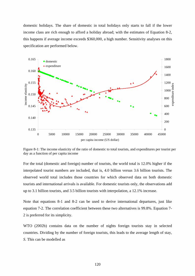
domestic holidays. The share of domestic in total holidays only starts to fall if the lower
income class are rich enough to afford a holiday abroad; with the estimates of Equation 8-2,
this happens if average income exceeds $360,000, a high number. Sensitivity analyses on this
specification are performed below.
0.135
0.140
0.145
0.150
0.155
0.160
0.165
0 5000 10000 15000 20000 25000 30000 35000 40000 45000
per capita income (US dollar)
inco
me
elas
ticity
0
200
400
600
800
1000
1200
1400
1600
1800
expe
nditu
re in
dex
domesticexpenditure
Figure 8-1: The income elasticity of the ratio of domestic to total tourists, and expenditures per tourist per day as a function of per capita income
For the total (domestic and foreign) number of tourists, the world total is 12.0% higher if the
interpolated tourist numbers are included, that is, 4.0 billion versus 3.6 billion tourists. The
observed world total includes those countries for which observed data on both domestic
tourists and international arrivals is available. For domestic tourists only, the observations add
up to 3.1 billion tourists, and 3.5 billion tourists with interpolation, a 12.1% increase.
Note that equations 8-1 and 8-2 can be used to derive international departures, just like
equation 7-2. The correlation coefficient between these two alternatives is 99.8%. Equation 7-
2 is preferred for its simplicity.
WTO (2002b) contains data on the number of nights foreign tourists stay in selected
countries. Dividing by the number of foreign tourists, this leads to the average length of stay,
S. This can be modelled as
120
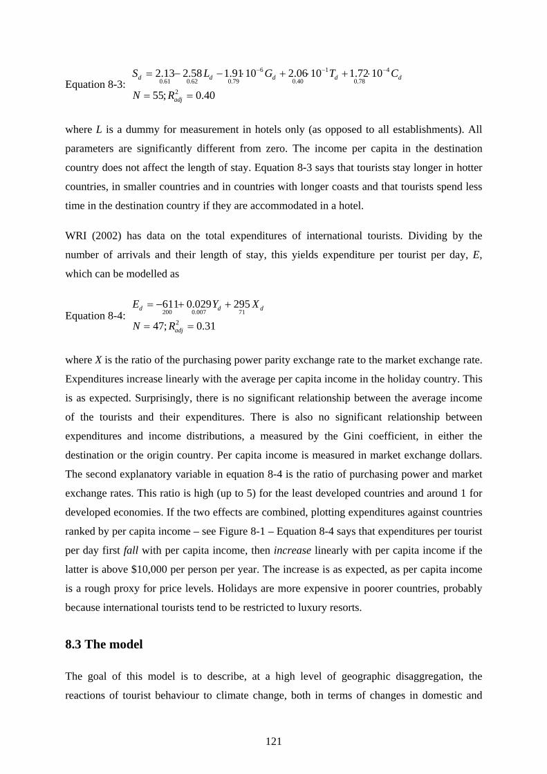
Equation 8-3: 6 1
0.61 0.62 0.79 0.40 0.78
2
2.13 2.58 1.91 10 2.06 10 1.72 10
55; 0.40
d d d d
adj
S L G T
N R
− −= − − ⋅ + ⋅ + ⋅
= =
4dC−
dX
where L is a dummy for measurement in hotels only (as opposed to all establishments). All
parameters are significantly different from zero. The income per capita in the destination
country does not affect the length of stay. Equation 8-3 says that tourists stay longer in hotter
countries, in smaller countries and in countries with longer coasts and that tourists spend less
time in the destination country if they are accommodated in a hotel.
WRI (2002) has data on the total expenditures of international tourists. Dividing by the
number of arrivals and their length of stay, this yields expenditure per tourist per day, E,
which can be modelled as
Equation 8-4: 200 0.007 712
611 0.029 295
47; 0.31
d d
adj
E Y
N R
= − + +
= =
where X is the ratio of the purchasing power parity exchange rate to the market exchange rate.
Expenditures increase linearly with the average per capita income in the holiday country. This
is as expected. Surprisingly, there is no significant relationship between the average income
of the tourists and their expenditures. There is also no significant relationship between
expenditures and income distributions, a measured by the Gini coefficient, in either the
destination or the origin country. Per capita income is measured in market exchange dollars.
The second explanatory variable in equation 8-4 is the ratio of purchasing power and market
exchange rates. This ratio is high (up to 5) for the least developed countries and around 1 for
developed economies. If the two effects are combined, plotting expenditures against countries
ranked by per capita income – see Figure 8-1 – Equation 8-4 says that expenditures per tourist
per day first fall with per capita income, then increase linearly with per capita income if the
latter is above $10,000 per person per year. The increase is as expected, as per capita income
is a rough proxy for price levels. Holidays are more expensive in poorer countries, probably
because international tourists tend to be restricted to luxury resorts.
8.3 The model
The goal of this model is to describe, at a high level of geographic disaggregation, the
reactions of tourist behaviour to climate change, both in terms of changes in domestic and
121
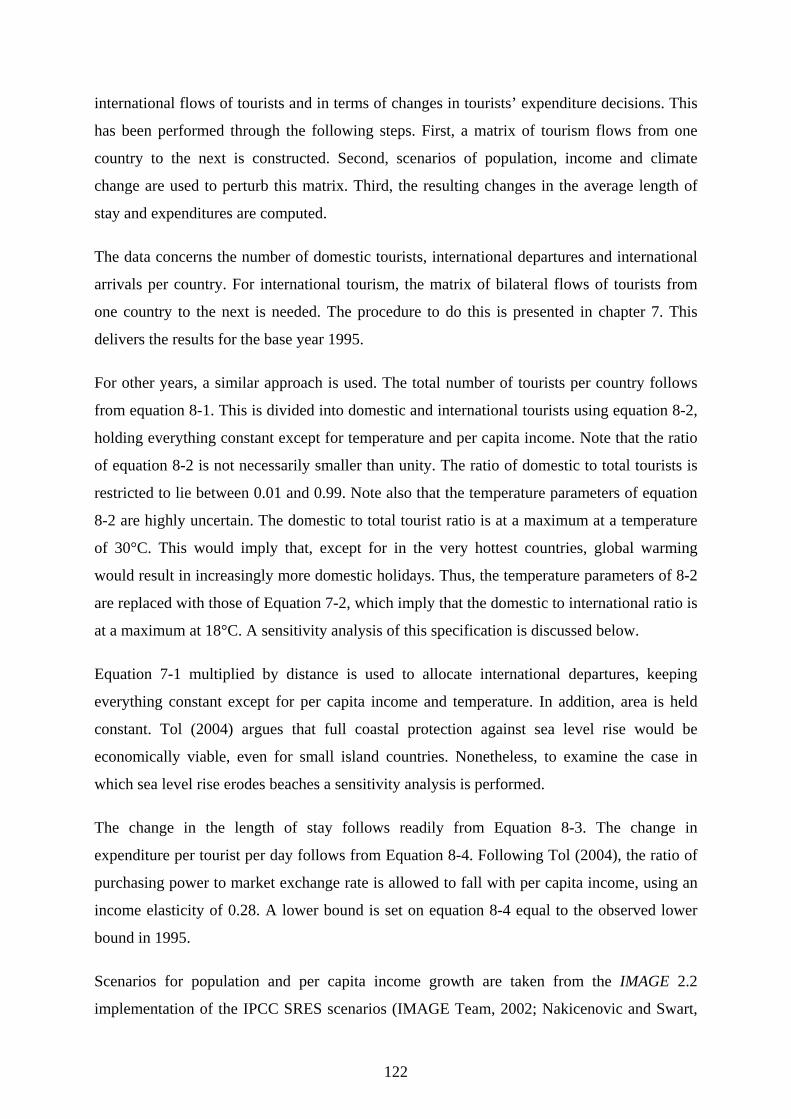
international flows of tourists and in terms of changes in tourists’ expenditure decisions. This
has been performed through the following steps. First, a matrix of tourism flows from one
country to the next is constructed. Second, scenarios of population, income and climate
change are used to perturb this matrix. Third, the resulting changes in the average length of
stay and expenditures are computed.
The data concerns the number of domestic tourists, international departures and international
arrivals per country. For international tourism, the matrix of bilateral flows of tourists from
one country to the next is needed. The procedure to do this is presented in chapter 7. This
delivers the results for the base year 1995.
For other years, a similar approach is used. The total number of tourists per country follows
from equation 8-1. This is divided into domestic and international tourists using equation 8-2,
holding everything constant except for temperature and per capita income. Note that the ratio
of equation 8-2 is not necessarily smaller than unity. The ratio of domestic to total tourists is
restricted to lie between 0.01 and 0.99. Note also that the temperature parameters of equation
8-2 are highly uncertain. The domestic to total tourist ratio is at a maximum at a temperature
of 30°C. This would imply that, except for in the very hottest countries, global warming
would result in increasingly more domestic holidays. Thus, the temperature parameters of 8-2
are replaced with those of Equation 7-2, which imply that the domestic to international ratio is
at a maximum at 18°C. A sensitivity analysis of this specification is discussed below.
Equation 7-1 multiplied by distance is used to allocate international departures, keeping
everything constant except for per capita income and temperature. In addition, area is held
constant. Tol (2004) argues that full coastal protection against sea level rise would be
economically viable, even for small island countries. Nonetheless, to examine the case in
which sea level rise erodes beaches a sensitivity analysis is performed.
The change in the length of stay follows readily from Equation 8-3. The change in
expenditure per tourist per day follows from Equation 8-4. Following Tol (2004), the ratio of
purchasing power to market exchange rate is allowed to fall with per capita income, using an
income elasticity of 0.28. A lower bound is set on equation 8-4 equal to the observed lower
bound in 1995.
Scenarios for population and per capita income growth are taken from the IMAGE 2.2
implementation of the IPCC SRES scenarios (IMAGE Team, 2002; Nakicenovic and Swart,
122
2001). The original scenarios are specified for 17 world regions. The growth rates of countries
in each region are assumed equal to the regional growth rate. Scenarios for the global mean
temperature are derived from the FUND model (Tol, 2002), using the same population and
economic scenarios and the corresponding scenarios for energy efficiency improvements and
decarbonisation. The global mean temperature change is downscaled to national means using
the COSMIC model (Schlesinger and Williams, 1995).
The 1995 model values for the total number of tourists, the number of domestic tourists, the
length of stay, and the expenditures are as observed. Data is not available for other years to
validate this part of the model. It is possible, however, to validate international arrivals and
departures. Figure 8-2 compares the model results for international arrivals to the
observations for 1980, 1985, 1990 and 1995. The correlation between observed and modelled
international arrivals in 1995 is almost perfect, largely because of calibration. For the other
years, the correspondence between observations and modelled values is never below 92%.
R2 = 0.92831000
10000
100000
1000000
10000000
100000000
1000 10000 100000 1000000 10000000 100000000
observed
mod
elle
d
1980
R2 = 0.92471000
10000
100000
1000000
10000000
100000000
1000 10000 100000 1000000 10000000 100000000
observed
mod
elle
d
1985
R2 = 0.94921000
10000
100000
1000000
10000000
100000000
1000 10000 100000 1000000 10000000 100000000
observed
mod
elle
d
1990
R2 = 0.99961000
10000
100000
1000000
10000000
100000000
1000 10000 100000 1000000 10000000 100000000
observed
mod
elle
d
1995
Figure 8-2: Observed versus modelled international arrivals in 1980, 1985, 1990 and 1995.
Figure 8-3 compares model results and data for international departures. Between 1985 and
1995, the correspondence between observations and model results is between 91% and 94%.
For 1980, this drops to 79%, which is still a reasonable performance given the fact that data
are patchy, not just for international tourism, but also for per capita income.
123
R2 = 0.79091000
10000
100000
1000000
10000000
100000000
1000 10000 100000 1000000 10000000 100000000
observed
mod
elle
d1980
R2 = 0.9391000
10000
100000
1000000
10000000
100000000
1000 10000 100000 1000000 10000000 100000000
observed
mod
elle
d
1985
R2 = 0.93391000
10000
100000
1000000
10000000
100000000
1000 10000 100000 1000000 10000000 100000000
observed
mod
elle
d
1990
R2 = 0.91421000
10000
100000
1000000
10000000
100000000
1000 10000 100000 1000000 10000000 100000000
observed
mod
elle
d
1995
Figure 8-3: Observed versus modelled international departures in 1980, 1985, 1990 and 1995.
8.4 Results
8.4.1 Base results
Figure 8-4 shows some characteristics of the A1B scenario without climate change for 16
major world regions. Currently, the OECD (the regions at the bottom of the graph) dominates
tourism, with over half of world tourists but only a fraction of the world population.
Nevertheless, the OECD share has been declining over the last 20 years, and will continue to
do so. For most of the 21st century, tourism will be predominantly Asian. Within Asia, East
Asia leads at first, but South Asia will take over after a few decades. The dominance of the
rich countries in international departures is stronger than it is in domestic holidays, and this
dominance will decline more gradually. Asia (Africa) has a bigger (smaller) share of
international tourism than of domestic tourism, because it has several large (many small)
countries. The difference between Europe and North America can be explained in the same
way. The pattern of international arrivals is similar to, but smoother than, the pattern of
international departures; international tourists cross borders, but prefer to travel shorter
distances. The pattern of receipts from domestic and international tourists is different. Here,
the OECD first expands its market share as expenditures per tourist per day fall as the poorer
124
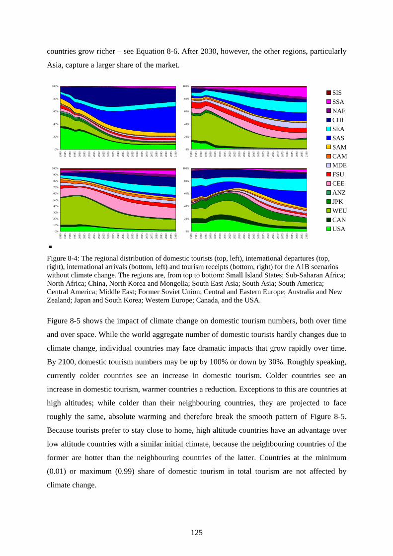
countries grow richer – see Equation 8-6. After 2030, however, the other regions, particularly
Asia, capture a larger share of the market.
0
%
20
0
%
1980
2045
SISSSANAFCHISEASASSAMCAMMDEFSUCEEANZJPKWEUCANUSA
0%
20%
40%
60%
80%
100%
1980
1985
1990
1995
2000
2005
2010
2015
2020
2025
2030
2035
2040
2045
2050
2055
2060
2065
2070
2075
2080
2085
2090
2095
2100
0%
20%
40%
60%
80%
100%
1980
1985
1990
1995
2000
2005
2010
2015
2020
2025
2030
2035
2040
2045
2050
2055
2060
2065
2070
2075
2080
2085
2090
2095
2100
0%
10%
20%
30%
40%
50%
60%
70%
80%
90%
100%
1980
1985
1990
1995
2000
2005
2010
2015
2020
2025
2030
2035
2040
2045
2050
2055
2060
2065
2070
2075
2080
2085
2090
2095
2100
0%
20%
40%
60%
80%
100%
1980
1985
1990
1995
2000
2005
2010
2015
2020
2025
2030
2035
2040
2045
2050
2055
2060
2065
2070
2075
2080
2085
2090
2095
2100
Figure 8-4: The regional distribution of domestic tourists (top, left), international departures (top, right), international arrivals (bottom, left) and tourism receipts (bottom, right) for the A1B scenarios without climate change. The regions are, from top to bottom: Small Island States; Sub-Saharan Africa; North Africa; China, North Korea and Mongolia; South East Asia; South Asia; South America; Central America; Middle East; Former Soviet Union; Central and Eastern Europe; Australia and New Zealand; Japan and South Korea; Western Europe; Canada, and the USA.
Figure 8-5 shows the impact of climate change on domestic tourism numbers, both over time
and over space. While the world aggregate number of domestic tourists hardly changes due to
climate change, individual countries may face dramatic impacts that grow rapidly over time.
By 2100, domestic tourism numbers may be up by 100% or down by 30%. Roughly speaking,
currently colder countries see an increase in domestic tourism. Colder countries see an
increase in domestic tourism, warmer countries a reduction. Exceptions to this are countries at
high altitudes; while colder than their neighbouring countries, they are projected to face
roughly the same, absolute warming and therefore break the smooth pattern of Figure 8-5.
Because tourists prefer to stay close to home, high altitude countries have an advantage over
low altitude countries with a similar initial climate, because the neighbouring countries of the
former are hotter than the neighbouring countries of the latter. Countries at the minimum
(0.01) or maximum (0.99) share of domestic tourism in total tourism are not affected by
climate change.
125
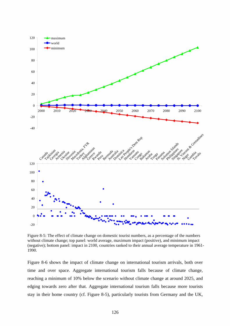
-40
-20
0
20
40
60
80
100
120
2000 2010 2020 2030 2040 2050 2060 2070 2080 2090 2100
maximumworldminimum
-20
0
20
40
60
80
100
120Can
ada
Tajikis
tan
Georgi
a
Armen
ia
Ukraine
Sloven
ia
Macedo
nia, F
YR
Turkey
Afghan
istan
Greece
Rwanda
Peru Bermud
a
Austral
ia
Domini
ca
Lao Peo
ple's D
em Rep
Hondu
ras
Vanua
tu
CongoBah
amas
ArubaTon
gaPan
ama
Solomon
Islan
ds
Philipp
ines
Singap
ore
St. Vinc
ent &
Gren
adine
s
NigerGam
bia
Tuvalu
Figure 8-5: The effect of climate change on domestic tourist numbers, as a percentage of the numbers without climate change; top panel: world average, maximum impact (positive), and minimum impact (negative); bottom panel: impact in 2100, countries ranked to their annual average temperature in 1961-1990.
Figure 8-6 shows the impact of climate change on international tourism arrivals, both over
time and over space. Aggregate international tourism falls because of climate change,
reaching a minimum of 10% below the scenario without climate change at around 2025, and
edging towards zero after that. Aggregate international tourism falls because more tourists
stay in their home country (cf. Figure 8-5), particularly tourists from Germany and the UK,
126
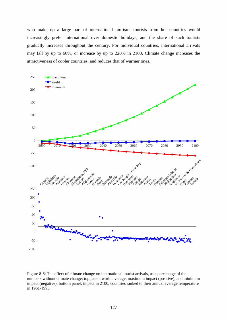
who make up a large part of international tourism; tourists from hot countries would
increasingly prefer international over domestic holidays, and the share of such tourists
gradually increases throughout the century. For individual countries, international arrivals
may fall by up to 60%, or increase by up to 220% in 2100. Climate change increases the
attractiveness of cooler countries, and reduces that of warmer ones.
-100
-50
0
50
100
150
200
250
2000 2010 2020 2030 2040 2050 2060 2070 2080 2090 2100
maximumworldminimum
-100
-50
0
50
100
150
200
250Can
ada
Tajikis
tan
Georgi
a
Armen
ia
Ukraine
Sloven
ia
Macedo
nia, F
YR
Turkey
Afghan
istan
Greece
Rwanda
Peru Bermud
a
Austral
ia
Domini
ca
Lao Peo
ple's D
em Rep
Hondu
ras
Vanua
tu
CongoBah
amas
ArubaTon
gaPan
ama
Solomon
Islan
ds
Philipp
ines
Singap
ore
St. Vinc
ent &
Gren
adine
s
NigerGam
bia
Tuvalu
Figure 8-6: The effect of climate change on international tourist arrivals, as a percentage of the numbers without climate change; top panel: world average, maximum impact (positive), and minimum impact (negative); bottom panel: impact in 2100, countries ranked to their annual average temperature in 1961-1990.
127
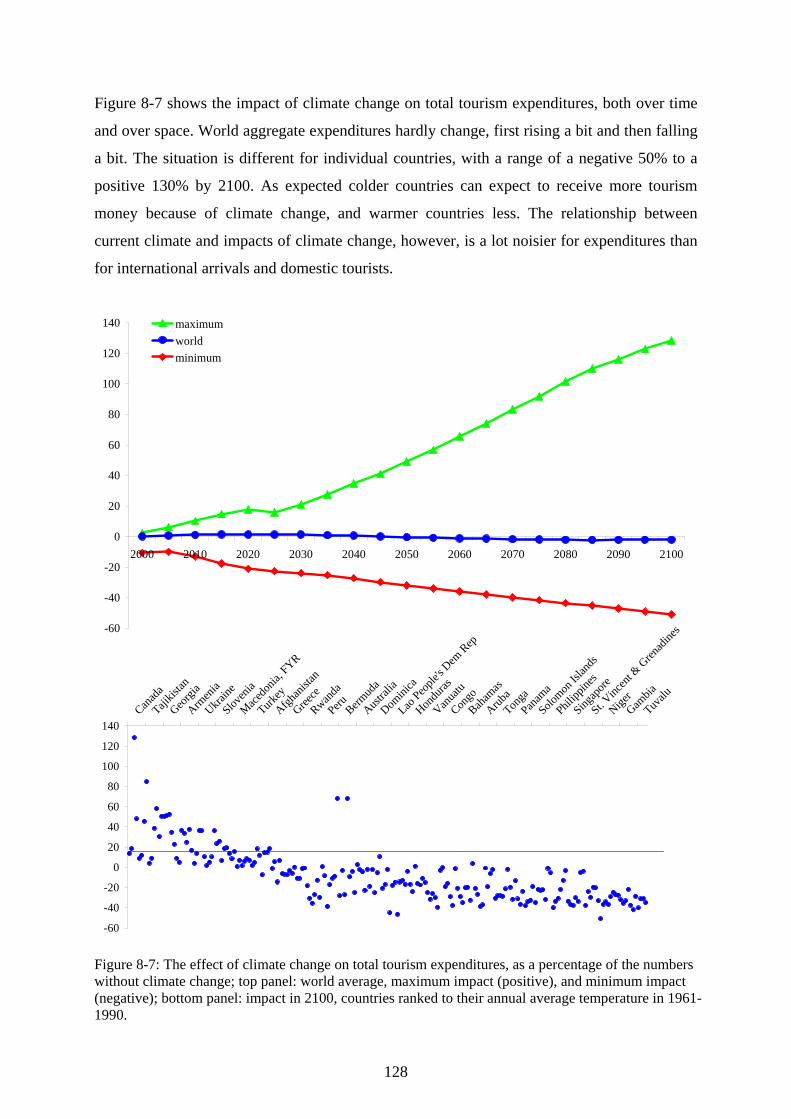
Figure 8-7 shows the impact of climate change on total tourism expenditures, both over time
and over space. World aggregate expenditures hardly change, first rising a bit and then falling
a bit. The situation is different for individual countries, with a range of a negative 50% to a
positive 130% by 2100. As expected colder countries can expect to receive more tourism
money because of climate change, and warmer countries less. The relationship between
current climate and impacts of climate change, however, is a lot noisier for expenditures than
for international arrivals and domestic tourists.
-60
-40
-20
0
20
40
60
80
100
120
140
2000 2010 2020 2030 2040 2050 2060 2070 2080 2090 2100
maximumworldminimum
-60
-40
-20
0
20
40
60
80
100
120
140Can
ada
Tajikis
tan
Georgi
a
Armen
ia
Ukraine
Sloven
ia
Macedo
nia, F
YR
Turkey
Afghan
istan
Greece
Rwanda
Peru Bermud
a
Austral
ia
Domini
ca
Lao Peo
ple's D
em Rep
Hondu
ras
Vanua
tu
CongoBah
amas
ArubaTon
gaPan
ama
Solomon
Islan
ds
Philipp
ines
Singap
ore
St. Vinc
ent &
Gren
adine
s
NigerGam
bia
Tuvalu
Figure 8-7: The effect of climate change on total tourism expenditures, as a percentage of the numbers without climate change; top panel: world average, maximum impact (positive), and minimum impact (negative); bottom panel: impact in 2100, countries ranked to their annual average temperature in 1961-1990.
128
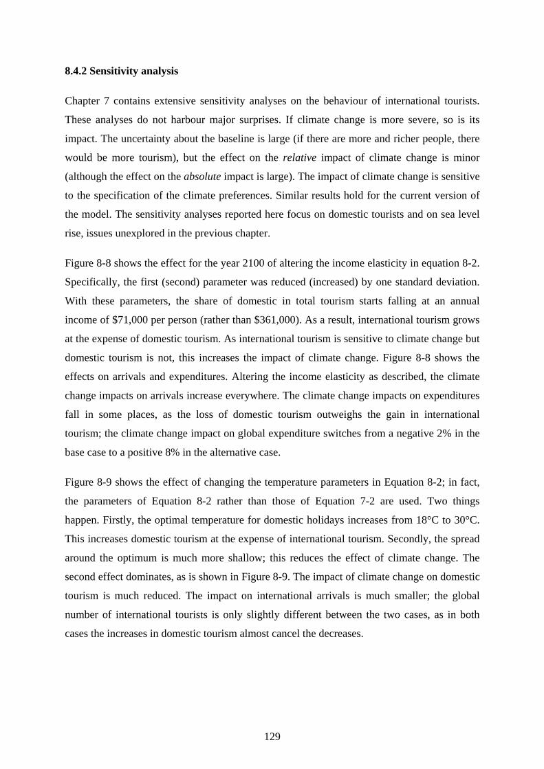
8.4.2 Sensitivity analysis
Chapter 7 contains extensive sensitivity analyses on the behaviour of international tourists.
These analyses do not harbour major surprises. If climate change is more severe, so is its
impact. The uncertainty about the baseline is large (if there are more and richer people, there
would be more tourism), but the effect on the relative impact of climate change is minor
(although the effect on the absolute impact is large). The impact of climate change is sensitive
to the specification of the climate preferences. Similar results hold for the current version of
the model. The sensitivity analyses reported here focus on domestic tourists and on sea level
rise, issues unexplored in the previous chapter.
Figure 8-8 shows the effect for the year 2100 of altering the income elasticity in equation 8-2.
Specifically, the first (second) parameter was reduced (increased) by one standard deviation.
With these parameters, the share of domestic in total tourism starts falling at an annual
income of $71,000 per person (rather than $361,000). As a result, international tourism grows
at the expense of domestic tourism. As international tourism is sensitive to climate change but
domestic tourism is not, this increases the impact of climate change. Figure 8-8 shows the
effects on arrivals and expenditures. Altering the income elasticity as described, the climate
change impacts on arrivals increase everywhere. The climate change impacts on expenditures
fall in some places, as the loss of domestic tourism outweighs the gain in international
tourism; the climate change impact on global expenditure switches from a negative 2% in the
base case to a positive 8% in the alternative case.
Figure 8-9 shows the effect of changing the temperature parameters in Equation 8-2; in fact,
the parameters of Equation 8-2 rather than those of Equation 7-2 are used. Two things
happen. Firstly, the optimal temperature for domestic holidays increases from 18°C to 30°C.
This increases domestic tourism at the expense of international tourism. Secondly, the spread
around the optimum is much more shallow; this reduces the effect of climate change. The
second effect dominates, as is shown in Figure 8-9. The impact of climate change on domestic
tourism is much reduced. The impact on international arrivals is much smaller; the global
number of international tourists is only slightly different between the two cases, as in both
cases the increases in domestic tourism almost cancel the decreases.
129
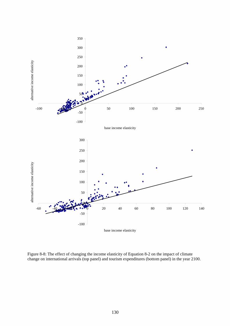
-100
-50
0
50
100
150
200
250
300
350
-100 -50 0 50 100 150 200 250
base income elasticity
alte
rnat
ive
inco
me
elas
ticity
-100
-50
0
50
100
150
200
250
300
-60 -40 -20 0 20 40 60 80 100 120 140
base income elasticity
alte
rnat
ive
inco
me
elas
ticity
Figure 8-8: The effect of changing the income elasticity of Equation 8-2 on the impact of climate change on international arrivals (top panel) and tourism expenditures (bottom panel) in the year 2100.
130
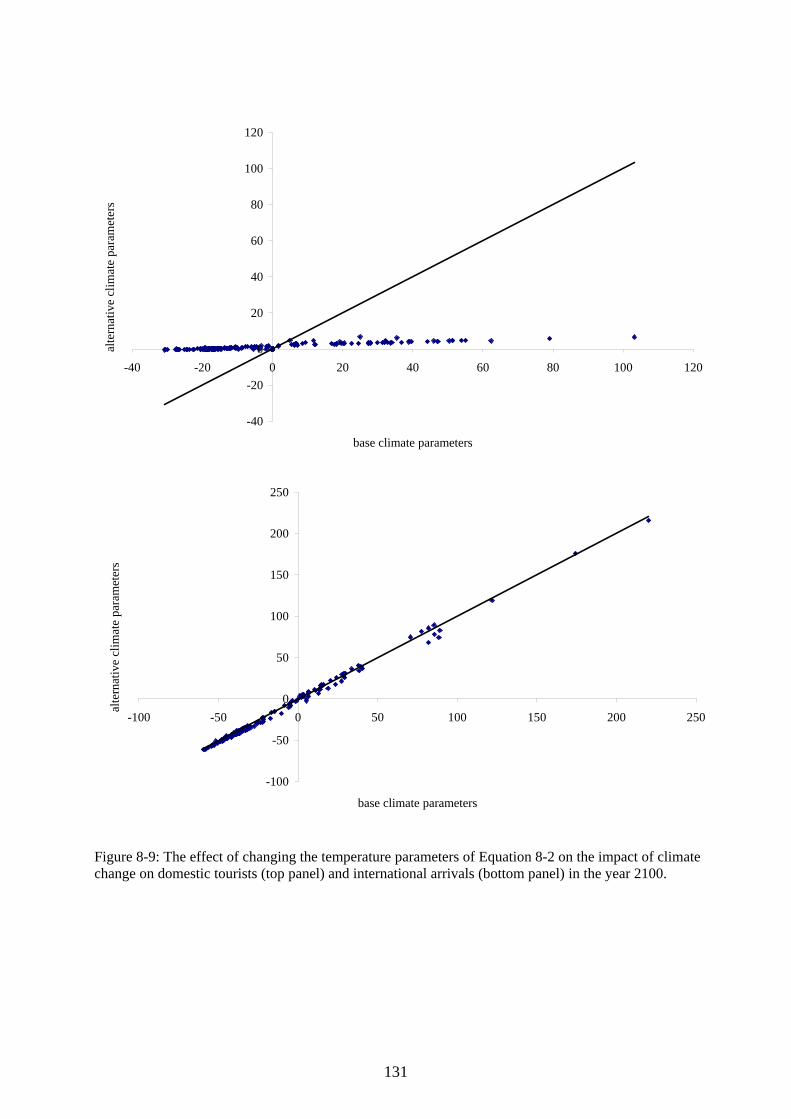
-40
-20
0
20
40
60
80
100
120
-40 -20 0 20 40 60 80 100 120
base climate parameters
alte
rnat
ive
clim
ate
para
met
ers
-100
-50
0
50
100
150
200
250
-100 -50 0 50 100 150 200 250
base climate parameters
alte
rnat
ive
clim
ate
para
met
ers
Figure 8-9: The effect of changing the temperature parameters of Equation 8-2 on the impact of climate change on domestic tourists (top panel) and international arrivals (bottom panel) in the year 2100.
131
-100
-80
-60
-40
-20
0
20
40
60
80
100
120
-40 -20 0 20 40 60 80 100 1
without sea level rise
with
sea
leve
l ris
e
20
-100
-50
0
50
100
150
200
250
-100 -50 0 50 100 150 200 250
without sea level rise
with
sea
leve
l ris
e
Figure 8-10: The effect of including sea level rise on the impact of climate change on domestic tourists (top panel) and international arrivals (bottom panel) in the year 2100.
132
Figure 8-10 shows the effect of including sea level rise. Taking the sea level rise scenario that
corresponds to the temperature scenario used elsewhere in this chapter and the national land
losses, without coastal protection, from Hoozemans et al. (1993; see also Tol, 2004), domestic
tourism and the attractiveness to international tourists are scaled according to the proportional
land loss. That is, if the Maldives loses 78% of its territory to sea level rise (this is what the
scenario says), than its domestic to total tourism ratio and its international attractiveness index
both fall by 78%. This crude approach serves only to illustrate the qualitative effect of sea
level rise; more sophisticated analyses would take account of the interaction of beach and sun,
and deliberate efforts to maintain commercially attractive beach in the face of sea level rise
induced erosion. In most countries, the effect of sea level rise on domestic tourism is minimal,
as the land loss is minimal. In some countries, however, the effect is dramatic. The same
pattern can be seen in international arrivals; most countries gain a little, and some lose a lot.
No country gains particularly from the partial loss of the small island states.
8.5 Discussion and conclusion
This chapter presents an updated and extended version of the Hamburg Tourism Model
(HTM). As in chapter 7, it is found that climate change would shift patterns of tourism
towards higher altitudes and latitudes. Domestic tourism may double in colder countries and
fall by 20% in warmer countries (relative to the baseline without climate change). For some
countries, international tourism may treble whereas for others it may cut in half. International
tourism is more (less) important than is domestic tourism in colder (warmer) places.
Therefore, climate change may double tourist expenditures in colder countries, and halve
them in warmer countries.
However, in most places, the impact of climate change is small compared to the impact of
population and economic growth.
The quantitative results are sensitive to parameter choices, both for the baseline and the
impact of climate change. The qualitative pattern is robust, however. Interestingly, one
finding is that climate change has a larger impact on tourism than sea level rise has. This is
because the latter heavily affects only a few places and beach nourishment for tourism is a
viable option in many countries.
133
The model described in this chapter and in chapter 7 is, to our knowledge, one in its kind. As
all early models, it leaves much to be desired. Although the model is reasonably good at
reproducing current and past patterns of international tourism, long-term and global studies of
tourism demand are rare – and the empirical basis of the model is therefore weak. This is even
truer for the effects of climate change on tourist destination choice, where the model is based
on only a few studies from a limited set of similar countries. The projections neglect that
changes in preferences, age structure, working hours and life styles would also affect tourist
behaviour. The spatial resolution (national) of the model is crude, as is the temporal resolution
(annual). A seasonal resolution would allow for the separate analysis of sun and snow seekers,
and would allow tourists to shift their holidays not only in space (as they do in the current
model) but also in time (from summer to spring and autumn). The economic impact does not
extend beyond tourist expenditures. Improving on all this is deferred to future research. The
results presented here demonstrate that this is a fruitful line of research.
Another potential application of the model is to sustainability analysis. On the one hand,
tourists exert substantial pressure on the environment (Gössling, 2002) while ecotourism
supports conservation (Gössling, 1999; Wilson and Tisdell, 2001). Immediate applications
include an analysis of the relocation effects due to restrictions on tourist numbers in a
particular country (e.g., Bhutan). In Hamilton et al. (2005b), carbon dioxide emissions from
international travel are projected, but other emissions and resource use can be readily added
(if the data are available) now that the model includes the length of stay as well. The
implications of constraints on emissions and resource use could then be analysed too. In this
model, the attractiveness of a tourist destination consists of a climate component, which
changes, and a second, unspecific component, which is kept constant. Splitting the latter
would allow for the analysis of other environmental changes – for example, the establishment
of national parks. The analysis of price instruments to change the behaviour of tourists would
require adding costs to the attractiveness index, and splitting “distance” into its price and time
components. These are important topics for future research.
This chapter demonstrates that, erratic as individual tourists may be, mass tourist movements
can be modelled and projected into the future. As tourism is an important driving force of
global environmental change, this is a step towards the prediction of human impacts on the
environment and, via climate change for example, of environmental change on human
behaviour.
134
Chapter 9
Conclusion
Measuring the impacts of climate change on tourism necessitates a quantitative appraisal of
the relationship between tourism demand and climate as well as other natural attractions, such
as the coastal zone, which will be affected by climate change. In the young but growing field
of research on tourism and climate change, quantitative studies are scarce. To go some way to
reducing the scarcity and so improve the basis for climate change impact assessment for tour-
ism, this thesis examines how demand, with particular reference to the coastal zone, will
change in response to climate change. The realisation of the aims of this thesis, which were
set out in the first chapter, is summarised below. This is followed by a discussion of the im-
plications for the research field of tourism and climate change, for the tourism industry and
for policy.
9.1 Realisation of aims
The first aim of this thesis, to review the historical evidence and the contemporary scientific
literature on the importance of climate and the coastal zone for tourism demand, was met in
chapter 2. A review of studies on the history of tourism shows that climate has been an impor-
tant factor in the spatial and temporal location of holidays throughout history. Nevertheless,
enjoying the sunshine first became the main purpose of a holiday in the 1920s. The coast,
however, was not always appreciated: in fact, during the 17th century it was seen as being dis-
gusting. By the beginning of the 19th century, this had changed and the coast became the focus
of tourism in the industrialised nations. Contemporary studies show that climate is one of the
decisive factors in destination choice; this can be seen in destination image studies as well as
in studies of tourism demand. There are fewer studies on tourism and the coast. Nevertheless,
the coast and the sea, in particular beaches, are important factors for tourists. In the review of
the studies that have been carried out on the impact of climate change and tourism, it can be
seen that there are fewer quantitative studies than qualitative ones. In the existing quantitative
studies, there are several gaps. First, the coverage of countries and activities has been piece-
meal. Second, substitution between countries has not properly been considered. Third, exist-
ing studies focus on particular origin countries or on particular destinations: the global picture
135
is neglected. Fourth, there have not been any studies that examine directly and in a quantita-
tive way the impact of sea-level rise on coastal tourism. Hence, a comprehensive assessment
of the costs of climate change in the tourism sector is difficult.
The second aim, which was to provide quantitative evidence that climate and the coast are
important destination characteristics that affect tourists’ decisions for a particular destination,
was achieved in chapter 3. For a survey of German tourists, it is found that climate is the most
important factor in the decision for a particular destination. Access to the sea and lakes is
found to be the second most important of the characteristics before other aspects such as
price, cultural and historical attractions and landscape. This is the first study of its kind to
provide quantitative evidence of climate’s importance, which has been speculated on in many
of the articles and books on climate and tourism, but which has not been backed up by survey
data. Furthermore, the results confirm the use of temperature as the main determining variable
in demand studies (for example, chapters 4, 5, 7 and 8 of this publication) and in the composi-
tion of tourism climate indices, such as that of Amelung et al. (forthcoming). Other, non-
temperature variables were also important, which provides support for the use of several vari-
ables in the Tourism Climate Index (TCI). Nevertheless, there is no support for the specific
combination of variables in the TCI.
Establishing quantitative relationships between climate and tourism demand as well as be-
tween coastal characteristics and tourism demand was the third aim, and this was met in chap-
ters 4,5 and 6 with the focus on demand from Germany. In chapter 4 demand is estimated
using, among other things, climate variables and beach length. Here demand for countries is
found to peak when the average monthly temperature is 24°C. Furthermore, beach length is
found to be positively related to demand. Using the estimated coefficients, an index of cli-
matic attractiveness for destinations is calculated. Although the concept of an index of cli-
matic attractiveness is not new, the index method developed in chapter 4 has an advantage
over the TCI and other climate indices for tourism, since its composition is based on the ob-
served behaviour of tourists and not on expert judgement. Index values for the main tourist
generating countries as well as for the main receiving countries are calculated for the month
of August. The most attractive climate is that of Spain closely followed by Greece and Portu-
gal. The northern European countries have the least attractive climate. It must be borne in
mind, however, that these values are for the demand from Germany as a whole; different ac-
tivities, different lifestyles or the health status of tourists, for example may all affect prefer-
136
ences for climate and so different climatic indices would be necessary. And it is exactly this
point that chapter 5 deals with. In that study, the tourism demand data used in chapter 4 is
segmented according to phase in the life cycle, region of origin and activities and motivation.
The optimal temperature, that is where demand peaks, ranges from 22°C to 24°C across the
segments. More interestingly, the steepness of the temperature demand relationship is differ-
ent for different segments. Even though the temperature optima are similar, changes in tem-
perature will have a larger effect on demand depending on the steepness of the demand curve.
Chapter 6 examines the role that the coastal landscape has on the price of accommodation.
Price reflects the interaction of supply and demand. Thus, this study does not solely estimate
the relationship between demand and the coastal landscape. Nonetheless, chapter 6 estimates
the value that tourists attach to various coastal types. It is found that an increase in the length
of dikes in a given district would result in a reduction in the average price of accommodation.
An increase in the length of open coast results in an increase in the average price of accom-
modation. The length of cliffs in a district has no effect on price.
The fourth aim was to use the relationships estimated in chapter 4 and 6 to examine the ef-
fects of climate change on tourism. In addition, chapters 7 and 8 examine the impact of cli-
mate change but do not directly use the results from chapters 4 to 6. In chapter 4, the effect of
climate change on the estimated climatic attractiveness of countries is twofold. First, attrac-
tiveness increases for those countries whose average monthly temperature is below the calcu-
lated optimal. Second, attractiveness decreases for countries whose average temperature
moves beyond the optimal value. The results for August show that Northern Europe will be-
come climatically more attractive. Countries in Southern Europe will experience a relatively
small increase in attractiveness compared to those in the north, and Greece and Portugal will
even experience a reduction in attractiveness. In addition, chapter 4 shows that demand is
positively related to the length of beach in a country. Therefore, if sea-level rise causes ero-
sion of beaches in a particular country then demand for the affected country will fall unless
measures are taken to prevent erosion. Another important finding of chapter 4 is the prefer-
ence for domestic holidays, which combined with increasing climatic attractiveness in the
major source markets of Northern Europe will weaken demand for the main destination coun-
tries and shift it to the source countries.
Chapters 7 and 8 examine the impact of climate change on global tourism, and the results of
these chapters largely reflect those of chapter 4. The Hamburg Tourism Model predicts that
137
climate change will lead to an increasing popularity of destinations in higher latitudes and
altitudes. Nevertheless, the increases from climate change are relatively small compared to
those resulting from economic and population growth. Domestic tourism is incorporated into
the model in chapter 8. Domestic tourism is particularly important as the results of chapter 4
show. Compared to the baseline situation, climate change will cause domestic tourism to dou-
ble in relatively cooler countries and, at the other extreme, to reduce by up to a fifth and rela-
tively hot countries. In terms of tourism expenditures, the model predicts that changes in total
expenditures will range from a doubling in the currently cooler countries to being halved in
the relatively hot countries.
Turning to the impact of climate change on the coastal zone, chapter 6 examines the impact of
sea-level rise, more specifically adaptation to sea-level rise, on accommodation prices. It is
found that purely in terms of the impact on accommodation revenues, beach nourishment
rather than dike construction is the more beneficial adaptation measure. The simulation results
of chapter 8 are also used to explore the impact of sea-level rise. Proportional land loss is used
to scale the number of tourists from a country as well as the numbers of tourists visiting that
country. Even without considering coastal protection measures, the impact for the majority of
countries is minimal. There are, however, some exceptions, such as the Maldives, which will
experience a drastic reduction in the number of tourists.
The final aim, which was to examine the impact of climate change at various destination and
source market spatial scales, was met in chapters 4 through to 8. In terms of destination
scales, this ranged from districts within one of the coastal states of Germany (chapter 6) to
groups of countries (chapter 4). Source market scales ranged from regions of Germany (chap-
ter 5) to all countries of the world (chapters 7 and 8). The detail of the smaller scale studies
provides contrast to the general nature of the country scale studies. Not only that, the results
of the small-scale studies could be incorporated into the general models. For example, it was
found in chapter 5 that the climate-demand relationship of tourists from the warmer parts of
Germany is steeper than that of tourists from cooler areas of Germany. That is, demand is
more responsive to changes in temperature. Bigano et al. (2006) find the same result for coun-
tries. The results could be used to differentiate the global model.
138
9.2 Relevance to the research field of tourism and climate change
The results summarised above are relevant to the research field. But it is the extension of ex-
isting methods and the application of new techniques that is of particular interest. Although
surveys have been used elsewhere in the field of tourism and climate change research, chapter
3 is the first study to provide a comprehensive examination of climate and climate informa-
tion in the tourists’ decision-making process. It would be worthwhile to replicate this study
for other times of the year – this study was carried out in the summer – and for other nations.
A problem of the study was making sure that climate and weather are understood as distinct
concepts by the respondents of the questionnaire. This blurring of concepts could be over-
come in subsequent studies by verbally administering the questionnaire. An additional use of
the survey method could be to investigate tourists’ images of a destination’s climate and if
these diverge from the actual climate. Data on this was collected as part of the study in chap-
ter 3, but an examination of this aspect is deferred for future research.
Segmentation, the hedonic price method and simulation modelling are new methodologies for
research on climate change and tourism. Segmentation of tourism datasets provides informa-
tion that can be used to quantify tourism scenarios. For example, using different climate- de-
mand relationships for different age groups it would be possible to examine the effect that
ageing populations - in the main source market countries - have on the flows of tourists. The
major restriction to this is the availability of data that is detailed enough to allow segmenta-
tion. Nevertheless, segmentation could be applied to existing studies such as the study pre-
sented in chapter 3 or other tourism demand studies.
The hedonic price method was applied to the issue of coastal landscape change. However, this
method could also be a fruitful way to estimate the willingness to pay for a certain climate.
Package tours are one of the largest markets in tourism demand. Price, accommodation, loca-
tion and climate data can be easily collected from the brochures produced by tour operators.
Of course, it would be time consuming to prepare such a dataset. With the assistance of tour
operators, however, it may be possible to access such data in digital form. The research net-
work of éCLAT is trying to establish contacts with the tourism industry to procure tourism
data and to provide information for the industry about climate change. It is also particularly
important to gain empirical knowledge of the preference of tourists from such countries as
Brazil, China and India. The fast-growing middle class will become an increasingly important
player in the tourism market.
139
So far, the Hamburg Tourism Model, a global tourism demand simulation model, is the sole
global model for predicting the effect of climate change on tourism. It would be useful if
other global models were developed. Perhaps these could incorporate different representations
of climate or different environmental attributes. It would then be possible to compare different
scenario results and so give the tourism industry and policy-makers a better assessment of the
likely range of impacts.
9.3 Relevance to the tourism industry
The results of chapters 7 and 8 show that population growth and economic growth will result
in an absolute increase in the number of tourists travelling, both domestically and internation-
ally, and that all countries will experience an increase in the number of tourists spending holi-
days within their borders. These results are projections of demand assuming that supply will
expand to meet it. Expansion may not be physically possible or it may be restricted politically
because of detrimental effects to other sectors or to the environment.
The discussion in this thesis has been about the effect of climate change on tourism demand.
It has been shown that tourists will substitute one destination for another and one season for
another. It is likely that this will also be the case for types of activities. For example, if skiing
is no longer possible then another activity will gain in popularity. But, what will the change in
demand mean for the tourism industry? The majority of the tourism industry consists of small
to medium sized enterprises (SMEs), and many of these are family run businesses (Cooper et
al., 1998). As well as accounting for a large share of the employment in tourism and sustain-
ing many communities’ livelihoods, the SMEs generate one third of total tourism revenue
(Getz and Nilsson, 2004). In addition, the industry has high fixed costs, particularly in the
accommodation and transport sectors. Changes in the patterns of demand, even over longer
periods, will therefore be an important consideration in investment decisions. One of the re-
sults of this thesis is that climate change will reduce the attractiveness of certain countries
during the hottest months but increase the attractiveness during the shoulder season. In other
words, the season will lengthen. For countries that are relatively cool, climate change will
increase the attractiveness of all of the seasons; again, there will be an increase in the length
of the tourist season. Therefore, the seasonality of employment is reduced, which is likely to
increase the amount of permanent positions available in the industry. In addition, facilities
will have longer use periods, which will increase the owner’s return on their investment.
140
Other parts of the tourist industry, intermediaries and large diversified suppliers with short
payback times on their investment, are less vulnerable to climate change. They would have to
adjust their behaviour, but profits would not be affected to the same extent as is likely to be
the case for the small to medium sized enterprises.
9.4 Relevance to policy
Tourism development has considerable environmental, economic and social impacts at the
local level. The task of tourism planning, to balance the positive and negative impacts of de-
velopment, requires demand forecasts at the local and regional – not just at the national level.
If the results of chapters 7 and 8 could be disaggregated further than individual countries. It
would be highly useful for policy-making at the local level. For the supply of tourism services
to meet demand, it is likely that the accommodation sector will have to expand, which implies
the construction of new accommodation or the conversion of existing building stock. In other
words, there will be land-use changes, which in turn will effect demand. Being able to esti-
mate demand or accommodation prices using environmental characteristics makes it possible
to weigh up the costs as well as benefits of the expansion of tourism services.
Tourism currently contributes to roughly 5% of CO2 emissions (Gössling, 2002), and the bulk
of this comes from emissions from transport both to and at the destination. Chapters 7 and 8
show that demand will continue to grow, which implies a growth in transport emissions. It
was also shown in chapter 8 that climate change will increase domestic tourism in many of
the main source markets, which will lead to a fall in the distance travelled. Nevertheless, the
reduction in potential emissions will depend on the mode of transport that is used for domes-
tic tourism. Short-haul flights have a much higher rate of emissions per passenger kilometre,
as take off and landing involve considerable amounts of fuel. Therefore, reducing the distance
travelled does not proportionally reduce the amount of emissions. Assessments of the impact
on transport demand will be needed for both transport and tourism planning as well as climate
change policies.
9.5 Outlook
This thesis has contributed to the research on tourism and climate change as well as the more
general issue of incorporating the environmental characteristics of destinations into the under-
standing of tourist decision-making, tourism demand and the price of tourism services. The
141

results and the methodologies developed are useful not only for climate change impact re-
search but also more practically for the tourism industry and policy-makers at the local as
well as national levels. In this thesis, the focus has mainly been on the direct impact of cli-
mate change and more specifically the expected increase in temperature. The ancillary effect
of sea-level rise has also been examined. There are, however, other direct and indirect effects
of climate change, such as a decrease in water availability, eutrophication or changes in land-
scape and ecosystems that are likely to have an effect on tourism demand. The methodologies
and results presented in this thesis provide a good starting point to examine such issues.
142
References
Abegg, B. (1996) Klimaänderung und Tourismus – Klimafolgenforschung am Beispiel des
Wintertourismus in den Schweizer Alpen. Zurich: vdf Hochschuleverlag an der ETH.
Adler, J. (1989) Origins of sightseeing. Annals of Tourism Research, 16(1), 7-29.
Agnew, M.D. and Palutikof, J.P. (2001) Climate impacts on the demand for tourism. In: A.
Matzarakis and C. de Freitas (eds.), International Society of Biometeorology Proceedings
of the First International Workshop on Climate, Tourism and Recreation. Retrieved from
http://www.mif.uni-freiburg.de/isb/ws/report.htm.
Ahmed, Z.U. (1991) The influence of the components of a state’s tourist image on product
positioning strategy. Tourism Management, 12(4), 331-340.
Amelung, B., Nicholls, S. and Viner, D. (forthcoming) Implications of global climate change for
tourism flows and seasonality. Journal of Travel Research.
Amt für Land- und Wasserwirtschaft Husum (1997) Fachplan Küstenschutz Sylt. Husum: Amt
für Land- und Wasserwirtschaft.
Baloglu, S. and Mangaloglu, M. (2001) Tourism destination images of Turkey, Egypt, Greece,
and Italy as perceived by US-Based tour operators and travel agents. Tourism
Management, 22, 1-9.
Baloglu, S. and McCleary K.W. (1999) A model of destination image formation. Annals of
Tourism Research, 28(4), 868-897.
Becken, S. and Simmons, D.G. (2005) Tourism, fossil fuel consumption and the impact on the
global climate. In: C.M Hall and J. Higham (eds.), Tourism, recreation and climate
change. Clevedon: Channel View Publications, 44-60.
Beerli, A and Martin, J.D. (2004) Tourists’ characteristics and the perceived image of tourist
destinations: a quantitative analysis – a case study of Lanzarote, Spain. Tourism
Management, 25(5), 623-626.
Bell, F.W. and Leeworthy, V.R. (1990) Recreational demand by tourists for saltwater beach
days. Journal of Environmental Economics and Management, 18, 189-205.
Berritella, M., Bigano, A. Roson, R. and Tol, R.S.J. (2006) A general equilibrium analysis of
climate change impacts on tourism. Tourism Management, 27(5), 913-924.
143
Bethencourt, M., Diaz, F, Alvarez, T.A. and Gonzalez, O. (2002) The segmentation of the
Canarian tourism market with regard to expenditure: an empirical study of La Palma.
Congress CD-Rom of the 42nd Congress of the European Regional Science Association
Dortmund ERSA 2002.
Bigano, A., Hamilton, J. M. and Tol, R.S.J. (2006) The impact of climate on holiday destination
choice. Climatic Change, 76(3-4), 389-406
Bigano, A., Hamilton, J. M. and Tol, R.S.J. (2005a) The impact of climate change on domestic
and international tourism: a simulation study. Research Unit Sustainability and Global
Change Working Paper FNU-58, Hamburg: Hamburg University and Centre for Marine
and Atmospheric Science.
Bigano, A., Hamilton, J. M., Lau, M., Tol, R.S.J. and Zhou, Y. (2005b) A global database of
domestic and international tourist numbers at national and subnational level. Fondazione
Eni E. Mattei Working Papers n. 3.05. Milan: FEEM.
Boyer, M. (2001) Tourism in the French Mediterranean. In: Y. Apostolopoulos, P. Loukissas
and L. Leontidou (eds.), Mediterranean tourism: facets of socio-economic development
and change. London: Routledge, 39-51.
Brandenburg, C. and Arnberger, A. (2001) The influence of the weather upon recreation
activities. In: A. Matzarakis and C. de Freitas (eds.), International Society of
Biometeorology Proceedings of the First International Workshop on Climate, Tourism and
Recreation. Retrieved from http://www.mif.uni-freiburg.de/isb/ws/report.htm.
Breiling, M. and Charamza, P. (1999) The impact of global warming on winter tourism and
skiing: a regionalised model for Austrian snow conditions. Regional Environmental
Change, 1(1), 4-14.
Brown, G.M. and Pollakowski, H.O. (1979) Economic valuation of shoreline. The Review of
Economics and Statistics, 61(4), 635-36.
Butler, R.W. (2001) Seasonality in tourism: issues and implications. In: T. Baum and S.
Lundtorp (eds.), Seasonality in tourism. Amsterdam: Pergamon, 6-21.
Carr, N. (2002) A comparative analysis of the behaviour of domestic and international young
tourists. Tourism Management, 23, 321-325.
Central Statistical Office Poland (2002) Tourism statistics [online]. Warsaw: Central Statistical
Office Poland. Retrieved from:
http://www.stat.gov.pl/english/serwis/polska/rocznik11/turyst.htm
144
Chaudhary, M. (2000) India’s image as a tourist destination – a perspective of foreign tourists.
Tourism Management, 21, 293-297.
Chen,W., Hong, H., Liu, Y., Zhang, L., Hou, X. and Raymond, M. (2004) Recreation demand
and economic value: An application of travel cost method for Xiamen Island. China
Economic Review, 15(4), 398-406.
CIA (2002) The World Factbook 2002 [online]. Washington, D.C.: Central Intelligence Agency.
Retrieved from: http://www.cia.gov/cia/publications/factbook
Clawson, M. and Knetsch, J.L. (1966) Economics of Outdoor Recreation. Johns Hopkins Press,
Baltimore. Cited in: Fridgen, J.D. (1984) Environmental psychology and tourism. Annals
of Tourism Research, 11(1) 19-39.
Clewer, A., Pack, A. and Sinclair, M.T. (1992) Price competitiveness and inclusive tour holidays
in European cities. In: P. Johnson and B. Thomas (eds.), Choice and Demand in Tourism,
London: Mansell. 123-143.
Coles, T. (2003) The emergent tourism industry in eastern Germany a decade after unification.
Tourism Management, 24, 217-226.
Collins, D. and Tisdell, C. (2002) Age-related lifecycles: Purpose variations. Annals of Tourism
Research, 29(3), 801-818.
Cooper, C., Fletcher, J., Wanhill, S., Gilbert, D. and Shepherd, R. (1998) Tourism: Principles
and Practice. London: Longman.
Corbin, A. (1999) Meereslust: Das Abendland und die Entdeckung der Küste. Frankfurt am
Main: Fischer Verlag.
CPSL (2001) Coastal Protection and Sea-Level Rise. Wilhelmshaven: Common Wadden Sea
Secretariat.
Crouch, G.I. (1995) A meta-analysis of tourism demand. Annals of Tourism Research, 22(1),
103-118.
Dann, G.M.S. (1993) Limitations in the use of `nationality` and `country of residence` variables.
In: D.G. Pearce and R.W. Butler (eds.), Tourism research: Critiques and challenges.
London: Routledge. 88-112
de Freitas, C.R. (1990) Recreation climate assessment. International Journal of Climatology,
10, 89-103.
145
de Freitas, C.R. (2001) Theory, concepts and methods in tourism climate research. In: A.
Matzarakis and C. de Freitas (eds.), International Society of Biometeorology Proceedings
of the First International Workshop on Climate, Tourism and Recreation. Retrieved from
http://www.mif.uni-freiburg.de/isb/ws/report.htm.
de Freitas, C.R. (2003) Tourism climatology: evaluating environmental information for decision
making and business planning in the recreation and tourism sector. International Journal
of Biometeorology, 48, 45-54.
Defert, P. (1966) La localisation touristique. Publications de l’Association internationale
d’experts scientifiques du tourisme. Berne. Cited in: Mieczkowski, Z. (1990) World
Trends in Tourism and Recreation. New York: Peter Lang Publishing.
Delft Hydraulics (1990) Strategies for adaptation to sea level rise: Report of the coastal zone
management subgroup for WMO and UNEP. The Hague: Ministry of Transport and Public
Works.
Doms, M. and Forman, C. (2005) Prices for local area network equipment. Information
Economics and Policy, 17(3), 365-388.
Dwyer, J.F. (1988) Predicting daily use of urban forest recreation sites. Landscape and Urban
Planning, 15(1-2), 127-138.
Elsasser, H. and Messerli, P. (2001) The vulnerability of the snow industry in the Swiss Alps.
Journal of Mountain Research and Development, 21(4), 335-339.
Englin, J. and Moeltner, K. (2004) The value of snowfall to skiers and boarders. Environmental
and Resource Economics, 29(1), 123-136.
Euromonitor (2002) Global Market Information Database [online]. London: Euromonitor.
Retrieved from http://www.euromonitor.com/gmid/default.asp
Faulkner, B. (1988) Tourism demand patterns-Australia. International Journal of Hospitality
Management, 7(4), 333-341.
Fleischer, A. & Pizam, A. (2002) Tourism Constraints among Israeli seniors. Annals of Tourism
Research, 29(1), 106-122.
Fleischer, A. and Tchetchik, A. (2005) Does rural tourism benefit from agriculture? Tourism
Management, 26 (4), 493-501.
Fodness, D. and Murray, B. (1998) A typology of tourist information search strategies. Journal
of Travel Research, 37 (2), 108-119.
146
Fodness, D. and Murray, B. (1999) A model of tourist information search behaviour. Journal of
Travel Research, 37 (3), 220-230.
FUR (Forschungsgemeinschaft Urlaub und Reisen e.V.) (1998) Die Reiseanalyse RA 98 [CD-
ROM]. Köln: Zentralarchiv für empirische Sozialforschung.
FUR (Forschungsgemeinschaft Urlaub und Reisen e.V.) (2004) Reiseanalyse Aktuell [online].
Retrieved from http://www.fur.de/downloads/Reiseanalyse_2004.pdf
Freeman, A. M. (1993) The measurement of environmental and resource values: theory and
methods. Washington, D.C.: Resources for the Future.
Fridgen, J.D. (1984) Environmental psychology and tourism. Annals of Tourism Research,
11(1), 19-39.
Gable, F. J. (1997) Climate change impacts on Caribbean coastal areas and tourism. Journal of
Coastal Research, 27, 49-70.
Gallarza, M.G., Saura I.G. and Garcia, H.C. (2002) Destination image: towards a conceptual
framework. Annals of Tourism Research, 29(1), 56-78.
Getz, D. and Nilsson, P.A. (2004) Responses of family businesses to extreme seasonality in
demand: the case of Bornholm, Denmark. Tourism Management, 25(1), 17-30.
Ghimire, K.B. (2001) The Native Tourist. London: Earthscan.
Gibson, H. & Yiannakis, A. (2002) Tourist roles: needs and the lifecourse. Annals of Tourism
Research, 29(2), 358-383.
Gössling, S. (1999) Ecotourism: a means to safeguard biodiversity and ecosystem functions.
Ecological Economics, 29, 303-320.
Gössling, S. (2002) Global environmental consequences of tourism. Global Environmental
Change, 12, 283-302.
Gössling, S., Bredberg, M., Randow, A., Svensson, P. and Swedlin, E. (2006) Tourist
perceptions of climate change. Current Issues in Tourism, 9 (4-5), 419-435.
Gunn, C.A. (1989) Vacationscape: Designing Tourist Regions (2nd ed.). New York: Van
Nostrand Reinhold, pp. 23–38. Cited in: Ahmed, Z.U., (1991) The influence of the
components of a state’s tourist image on product positioning strategy. Tourism
Management, 12(4), 331-340.
Hamilton, J.M. (2003) Climate and the destination choice of German tourists, Research Unit
Sustainability and Global Change Working Paper FNU-15 (revised). Hamburg: Hamburg
University and Centre for Marine and Climate Research.
147
Hamilton, J.M. (in press) Coastal landscape and the hedonic price of accommodation.
Ecological Economics.
Hamilton, J.M. and Lau, M.A. (2005) The Role of Climate Information in Tourist Destination
Choice Decision-Making. In: Gössling, S. and C.M. Hall (eds.), Tourism and Global
Environmental Change. London, Routledge
Hamilton, J.M. and Tol, R.S.J. (forthcoming) The impacts of climate change on tourism and
recreation. In: Schlesinger, M. (ed.), Human-Induced Climate Change - An
Interdisciplinary Assessment, Cambridge, Cambridge University Press.
Hamilton, J.M., Maddison, D.J. and Tol, R.S.J. (2005a) Climate change and international
tourism: a simulation study. Global Environmental Change Part A, 15(3), 253-266.
Hamilton, J.M., Maddison, D.J. and Tol, R.S.J. (2005b) The effects of climate change on
international tourism. Climate Research, 29, 255-268.
Hamilton, J.M., Maddison, D.J. and Tol, R.S.J. (2005c) Climate preferences and destination
choice a segmentation approach Research Unit Sustainability and Global Change Working
Paper FNU-90. Hamburg: Hamburg University and Centre for Marine and Climate
Research.
Harrison, S.J., Winterbottom S.J. and Shephard, C. (1999) The potential effects of climate
change on the Scottish tourist industry. Tourism Management, 20, 203-211.
Hofstede, J. (2003) Integrated management of artificially created salt marshes in the Wadden
Sea of Schleswig-Holstein, Germany. Wetlands Ecology and Management, 11(3), 183-
194.
Hofstede, J. and Hammann, M. (2000) Wertermittlung sturmgefährdeter Gebiete in Schleswig-
Holstein. Mitteilungen des Franzius-Instituts für Wasserbau und Küsteningenieurwesen,
Heft 85/2000, 106-112.
Holloway, J.C. (1998) The Business of Tourism. London: Longman.
Hoozemans, F.M.J., Marchand, M. and Pennekamp, H.A. (1993) A Global Vulnerability
Analysis: Vulnerability Assessment for Population, Coastal Wetlands and Rice Production
and a Global Scale (2nd edition). Delft: Delft Hydraulics.
Houghton, J. T., Ding, Y., Griggs, D.J., Noguer, M., van der Linden, P.J. and Xiaosu, D. (eds.)
(2001) Climate Change 2001: The Scientific Basis. Cambridge: Cambridge University
Press.
148
Hu, Y. and Ritchie, J.B.R. (1993) Measuring destination attractiveness: A contextual approach.
Journal of Travel Research, 32 (2), 25-34.
IMAGE Team (2001) The IMAGE 2.2 Implementation of the SRES Scenarios: A Comprehensive
Analysis of Emissions, Climate Change and Impacts in the 21st Century [CD-ROM]
RIVM CD-ROM Publication 481508018. Bilthoven: National Institute for Public Health
and the Environment.
IPCC (2004) 16 Years of Scientific Assessment in Support of the Climate Convention [online].
Retrieved from http://www.ipcc.ch/about/about.htm
Irandoust, M. (1998) Pricing Policy in the Swedish Automobile Market. Journal of Economics
and Business, 50 (3), 309-317.
Kaufmann, D., Kraay, A. & Zoido-Lobaton, P. (1999) Governance Matters. Policy Research
Working Paper 2196, Washington: World Bank.
Kelletat, D. (1993) Coastal Geomorphology and tourism in the north sea coast. In: P.P. Wong
(ed.) (1994) Tourism vs. environment: the case for coastal areas. Dordrecht: Kluwer, 139-
165.
Kozak, M. (2002) Comparative analysis of tourist motivations by nationality and destinations.
Tourism Management, 23, 221-232.
Krupp, C. (1997) Klimaänderungen und die Folgen: eine exemplarische Fallstudie über die
Möglichkeiten und Grenzen einer interdisziplinären Klimafolgenforschung. Berlin: edition
Sigma.
Kuoppamaeki, P. (1996) Impacts of Climate Change from a Small Nordic Open Economy
Perspective -- The Potential Impacts of Climate Change on the Finnish Economy.
Helsinki: ETLA.
Lambert, G.W., Reid, C., Kaye, D.M., Jennings, G.L. and Esler, M.D. (2002) Effect of sunlight
and season on serotonin turnover in the brain, The Lancet, 360, 1840-1842.
Lancaster, K.J. (1966) A New Approach to Consumer Theory. Journal of Political Economy, 74,
132–157. Cited in: Um, S. and Crompton, J.L. (1990) Attitude determinants in tourism
destination choice. Annals of Tourism Research, 17, 432-448.
Landesvermessungsamt Schleswig-Holstein (2005) CD Top50 Schleswig-Holstein/Hamburg
(Version 3) [CD-ROM].
149
Langyintuo, A.S., Ntoukam, G., Murdock, L., Lowenberg-DeBoer, J. and Miller, D.J. (2004)
Consumer preferences for cowpea in Cameroon and Ghana. Agricultural Economics 30
(3), 203-213.
Lawson, R. (1991) Patterns of tourist expenditures and types of vacation across the family life
cycle. Journal of Travel Research, 29 4, 12-18.
Leiper, N. (1979) The framework of tourism: towards a definition of tourism, tourist, and the
tourist industry. Annals of Tourism Research, 6 (4), 390-407.
Lim, C. (1995) Review of international tourism demand models. Annals of Tourism Research,
24(4), 835-849.
Lise, W. and Tol, R.S.J. (2002) Impact of climate on tourism demand. Climatic Change, 55(4),
429-449.
Lohmann, M. and Kaim, E. (1999) Weather and holiday destination preferences, image attitude
and experience. The Tourist Review, 2, 54-64.
Loomis, J.B. and J. Crespi, (1999) Estimated effects of climate change on selected outdoor
recreation activities in the United States. In: R. Mendelsohn and J.E. Neumann (eds.) The
Impact of Climate Change on the United States Economy. Cambridge: CUP, 289-314.
Maddison, D. (2001) In search of warmer climates? The impact of climate change on flows of
British tourists. Climatic Change, 49, 103-208.
Maddison, D. and Bigano, A. (2003) The amenity value of the Italian climate. Journal of
Environmental Economics and Management, 45(2), 319-332.
Mansfeld, N. (1992) From motivation to actual travel. Annals of Tourism Research, 19, 399-
419.
McCarthy, J.J., Canziani, O.F., Leary, N.A., Dokken, D.J. and White, K.S. (eds.) (2001) Climate
Change 2001: Impacts, Adaptation, and Vulnerability. Cambridge: Cambridge University
Press.
Mendelsohn, R and Markowski, M. (1999) The impact of climate change on outdoor recreation.
In: R. Mendelsohn and J.E. Neumann (eds.) The Impact of Climate Change on the United
States Economy. Cambridge: CUP, 267-288.
Mieczokowski, Z. (1990) World Trends in Tourism and Recreation. New York: Peter Lang
Publishing.
150
Ministerium für ländliche Räume, Landesplanung, Landwirtschaft und Tourismus des Landes
Schleswig-Holstein (2001) Generalplan Küstenschutz: Integriertes
Küstenschutzmanagement in Schleswig-Holstein. Kiel: Landesregierung Schleswig-
Holstein.
Mitchell, T.D., Carter, T.R., Jones, P.D., Hulme,M. and New, M. (2003) A comprehensive set
of high-resolution grids of monthly climate for Europe and the globe: the observed record
(1901-2000) and 16 scenarios (2001-2100). Journal of Climate: submitted.
Mitchell, T.D., Hulme, M., and New, M. (2002) Climate Data for Political Areas. Area, 34, 109-
112.
Mok, C. and Iverson, T.J. (2000) Expenditure-based segmentation: Taiwanese tourists to Guam.
Tourism Management, 21(3), 299-305.
Morley, C.L. (1992) A microeconomic theory of international tourism demand. Annals of
Tourism Research. 19, 250-267.
Mykletun, R.J., Crotts, J.C. and Mykletun, A. (2001) Positioning an island destination in the
peripheral area of the Baltics: a flexible approach to market segmentation. Tourism
Management, 22 (5), 493-500.
Nakicenovic, N. and Swart, R.J. (2001) IPCC Special Report on Emissions Scenarios.
Cambridge: Cambridge University Press.
New, M., Hulme, M. and Jones, P.D. (1999) Representing twentieth century space-time climate
variability. Part 1: development of a 1961-90 mean monthly terrestrial climatology.
Journal of Climate, 12, 829-856.
Nicholls, R.J. and Hoozemans, F.M.J. (1996) The Mediterranean: vulnerability to coastal
implications of climate change. Ocean and Coastal Management, 31, 105-132.
NIT (2001) Marktanalyse Schleswig-Holstein-Tourismus. Kiel: Institut für Tourismus- und
Bäderforschung in Nordeuropa GmbH.
Oppermann, M. (1992) Intranational tourist flows in Malaysia. Annals of Tourism Research, 19,
482-500.
Oppermann, M. (1994) Relevance of nationality in tourism research. Annals of Tourism
Research, 21(1), 165-168.
Oppermann, M. (1995) Travel life cycle. Annals of Tourism Research, 22(3), 535-552.
Papatheodorou, A. (2001) Why people travel to different places. Annals of Tourism Research,
28, 164-179.
151
Parker, P. (2001) Physioeconomics: The Basis for Long-Run Economic Growth. Cambridge,
USA: The MIT Press.
Perez, E.A. and Sampol, C.J. (2000) Tourist expenditure for mass tourism markets. Annals of
Tourism Research, 27(3), 624-637.
Perry, A. (2000) Impacts of climate change on tourism in the Mediterranean: adaptive
responses. Fondazione Eni E. Mattei Working Papers n 35.2000. Milan: FEEM
Perry, A. and Thompson, R.D. (1997) Applied Climatology: Principles and Practice. London:
Routledge.
Phelps, A. (1986) Holiday destination image – the problem of assessment: an example
developed in Menorca. Tourism Management, 7 (3), 168-180.
Piga, C.A.G. (2003) Pigouvian Taxation in Tourism. Environmental and Resource Economics,
26, 343-359.
Pike, S. (2002) Destination image analysis – a review of 142 papers from 1973 to 2000. Tourism
Management, 23, 541-549.
Reese, S. (2003) Vulnerabilität des schleswig-holsteinischen Küstenraumes durch Sturmfluten.
Fallstudien von der Nord- und Ostseeküste. Berichte aus dem Forschungs- und
Technologiezentrum Westküste der Universität Kiel, Bd. 30. Kiel: Christian-Albrechts-
Universität.
Rehdanz, K. (2006) Hedonic Pricing of Climate Change Impacts to Households in Great Britain.
Climatic Change, 74(4) 413-434.
Rehdanz, K. and Maddison, D. (2004) The Amenity Value of Climate to German Households.
Research Unit Sustainability and Global Change Working Paper FNU-20. Hamburg:
Hamburg University and Centre for Marine and Climate Research.
Richardson, R.B. and J.B. Loomis, (2004) Adaptive recreation planning and climate change: a
contingent visitation approach. Ecological Economics, 50 (1-2), 83-99.
Rosen, S. (1974) Hedonic prices and implicit markets: Product differentiation in pure competition.
Journal of Political Economy, 82, 34–55.
Ryan, C. (2003) Recreational Tourism: Demands and Impacts. Clevedon: Channel View
Publications.
Schlesinger, M.E. and Williams, L.J. (1998) COSMIC 1.1 Country-Specific Model for
Intertemporal Climate. Palo Alto: Electric Power Research Institute.
152
Scott, D., McBoyle, G. and Schwartzentruber, N. (2004) Climate change and the distribution of
climatic resources for tourism in North America, Climate Research 27, 105-117
Scott, D., McBoyle, G., Mills, B. and G. Wall, G. (2001) Assessing the vulnerability of the
alpine skiing industry in Lakelands Tourism Region of Ontario, Canada to climate
variability and change. In: A. Matzarakis and C. de Freitas (eds.) International Society of
Biometeorology Proceedings of the First International Workshop on Climate, Tourism and
Recreation. Retrieved from http://www.mif.uni-freiburg.de/isb/ws/report.htm
Scott, D., Wall, G and McBoyle, G. (2005) The evolution of the climate change issue in the
tourism sector. In: C.M Hall and J. Higham, (eds.) Tourism, recreation and climate
change. Clevedon: Channel View Publications, pp 44-60.
Seaton, A.V. and Palmer, C. (1997) Understanding VFR tourism behaviour: the first five years
of the United Kingdom tourism survey. Tourism Management, 18(6), 345-355.
Seckelmann, A. (2002) Domestic tourism – a chance for regional development in Turkey.
Tourism Management, 23, 85-92.
Seddighi, H.R. and Shearing, D.F. (1997) The demand for tourism in North East England with
special reference to Northumbria: an empirical analysis. Tourism Management, 18(8),
499-511.
Sharpley, R. (1994) Tourism, Tourists and Society. Huntingdon: Elm Publications.
Shoemaker, S. (1989) Segmentation of the senior pleasure travel market. Journal of Travel
Research, 27(3), 14-19.
Shoemaker, S. (1994) Segmenting the U.S. travel market according to benefits realized, Journal
of Travel Research, 32 (3), 8-21.
Sinclair, M.T., Clewer, A. and Pack, A. (1990) Hedonic prices and the marketing of package
holidays. In: G. Ashworth and B. Goodall (eds.) Marketing Tourism Places. London and
New York: Routledge.
Sirakaya, E. and Woodside, A.G. (2005) Building and testing theories of decision making by
travellers. Tourism Management, 26 (6), 815-832
Smith, S. L. J. (1988) Defining tourism a supply-side view. Annals of Tourism Research, 15 (2),
179-190.
153
Statistisches Amt für Hamburg und Schleswig-Holstein (2005) Statistischer Bericht Ankünfte,
Übernachtungen und Aufenthaltsdauer der Gäste in Beherbergungsstätten mit 9 und mehr
Betten und auf Campingplätzen (ohne Dauercamping) in ausgewählten Gemeinden in
Schleswig-Holstein [online]. Retrieved from: http://www.statistik-
nord.de/fileadmin/download/Tourismus_SH_0506.pdf
Statistisches Bundesamt (2005) Verbraucherpreisindex für Deutschland [online]. Retrieved
from http://www.destatis.de/indicators/d/vpi103ad.htm
Statistisches Landesamt Schleswig-Holstein (1999) Statistischer Bericht A V 1 Bodenflächen
nach Art der tatsächlichen Nutzung 1997. Kiel: Statistisches Landesamt Schleswig-
Holstein.
Statistisches Landesamt Schleswig-Holstein (2001) Statistischer Bericht A I 2 Bevölkerung der
Gemeinde 2000. Kiel: Statistisches Landesamt Schleswig-Holstein.
Sterr, H. (2000) Implications of accelerated sea-level rise for Germany. In: A.C. de la Vega-
Leinert, R.J. Nicholls & R.S.J. Tol (eds.) Proceedings of SURVAS Expert Workshop on:
"European Vulnerability & Adaptation to impacts of Accelerated Sea-Level Rise” (ASLR)"
Hamburg: University of Hamburg.
Thorsson, S., Lindqvist, M. and Lindqvist, S. (2004) Thermal bioclimatic conditions and
patterns of behaviour in an urban park in Göteborg, Sweden. International Journal of
Biometeorology, 48, 149-156.
Tol, R.S.J. (1999) Spatial and temporal efficiency in climate policy: applications of FUND,
Environmental and Resource Economics, 14(1), 33-49.
Tol, R.S.J. (2002) Welfare specification and optimal control of climate change: an application of
FUND’, Energy Economics, 24(4), 367-376.
Tol, R.S.J. (2004) The double trade-off between adaptation and mitigation for sea level rise: an
application of FUND. Research Unit Sustainability and Global Change Working Paper
FNU-48. Hamburg: Hamburg University and Centre for Marine and Climate Research.
Towner, J. (1985) The grand tour: A key phase in the history of tourism. Annals of Tourism
Research, 12(3), 297-333.
Towner, J. (1996) An Historical Geography of Recreation and Tourism in the Western World
1540–1940. Chichester: John Wiley.
Um, S. and Crompton, J.L. (1990) Attitude determinants in tourism destination choice. Annals
of Tourism Research, 17, 432-448.
154
UNESCO (2001) The World Heritage List {online]. Paris: UNESCO. Retrieved from:
http://www.unesco.org/whc/heritage.htm
Van Raaij, W.F. (1986) Consumer research on tourism: mental and behavioral constructs.
Annals of Tourism Research, 13, 1-9.
Viner, D. and Agnew, M. (1999) Climate change and its impacts on tourism. Report prepared
for WWF-UK. Godalming: WWF.
Walton, J.K. (1997) The seaside resorts of Western Europe, 1750-1939. In: S. Fisher (ed.),
Recreation and the sea. Exeter: University of Exeter Press, 36-56.
Watson, R.T., Zinyowera, M.C. and Moss, R.H. (eds.) (1997) The regional impacts of climate
change - an assessment of vulnerability: A special report of IPCC working group II.
Cambridge: Cambridge University Press.
Wen, Z. (1997) China’s domestic tourism: impetus development and trends. Tourism
Management, 18(8), 565-571.
Wickens, E. (2002) The sacred and the profane: A tourist typology. Annals of Tourism
Research, 29(3), 834-851.
Williams, R.L. (2000) A note on robust variance estimation for cluster-correlated data.
Biometrics, 56, 645-646.
Wilson, C. and Tisdell, C. (2001) Sea turtles as a non-consumptive resource especially in
Australia. Tourism Management, 23, 279-288.
Witt, S.F. and Witt, C.A. (1995) Forecasting tourism demand: A review of empirical research.
International Journal of Forecasting, 11, 447-475.
Wong, P.P. (ed.) (1994) Tourism vs. environment: the case for coastal areas. Dordrecht:
Kluwer.
WCMC (World Conservation Monitoring Centre) (2002) Protected Areas Information: 1996
Global Protected Areas Summary Statistics [online]. Cambridge: UNEP-WCMC.
Retrieved from http://www.unep-wcmc.org/protectedareas/data/summstat.html.
WRI (World Resources Institute) (2000) World Resources Database 2000-2001. Washington,
D.C.: World Resources Institute.
WRI (2002) World Resources Database 2002-2003. Washington D.C: World Resources Institute.
WTO (World Tourism Organization) (2000) Basic reference on tourism statistics [online]. Madrid:
WTO. Retrieved from Retrieved from http://www.world-
tourism.org/statistics/tsa_project/basic_references/index-en.htm
155

WTO (2001a) Tourism 2020 Vision – East Asia and the Pacific. Madrid: WTO.
WTO (2001b) Tourism 2020 Vision – Europe. Madrid: WTO.
WTO (2002a) Definition of tourism [online]. Madrid: WTO. Retrieved from http://www.world-
tourism.org/statistics/tsa_project/TSA_in_depth/chapters/ch3-1.htm
WTO (2002b) Yearbook of Tourism Statistics. Madrid: WTO.
WTO (2003a) Climate Change and Tourism. Proceedings of the First International Conference
on Climate Change and Tourism, Djerba 9-11 April [online]. Madrid: WTO. Retrieved
from http://www.world-tourism.org/sustainable/climate/decdjerba-eng.pdf
WTO (2003b) Yearbook of Tourism Statistics. Madrid: WTO.
WTO (2005a) Long-term Prospects: Tourism 2020 Vision [online]. Madrid: WTO. Retrieved
from http://www.world-tourism.org/facts/2020.html
WTO (2005b) Tourism Market Trends [online]. Madrid:WTO. Retrieved from
http://www.world-tourism.org/facts/tmt.html
Yuan, S. and MacDonald, C. (1990) Motivational determinants of international pleasure time.
Journal of Travel Research, 29 (1), 42-44.
FNU Working Papers can be downloaded here:
http://www.uni-hamburg.de/Wiss/FB/15/Sustainability/Working_Papers.htm
Fondazione Eni E. Mattei Working Papers can be downloaded here:
http://www.feem.it/Feem/Pub/Publications/WPapers/default.htm
156
Summary
Climate change, whether through increased temperatures or sea-level rise, is likely to affect
the spatial and temporal pattern of tourism demand. Despite the cultural and economic
importance of tourism and its overwhelming dependence on climatic factors, relatively few
studies have tackled the impact of climate change on tourism. In particular there are few
quantitative studies on the effect that climate change will have on tourism. The aim of this
thesis is to fill the research gap and so provide information for the tourism industry and policy
makers.
Following a brief thematic introduction and statement of the aims of the thesis in chapter 1,
chapter 2 provides background information on tourism, climate, the coast and climate change.
Along with a sketch of the historical development of tourism with particular reference to
climate and coast, chapter 2 reviews the contemporary literature on the relationships between
tourism and climate and tourism and the coastal zone. Contemporary studies show that
climate is one of the decisive factors in destination choice; this can be seen in destination
image studies as well as in studies of tourism demand. The perspective is then shifted to the
future. The causes and impacts of climate change are briefly discussed. A review of the
literature on the impacts of climate change on tourism highlights the following gaps: First, the
coverage of countries and activities has been piecemeal. Second, substitution between
countries has not properly been considered. Third, existing studies focus on particular origin
countries or on particular destinations: the global picture is neglected. Fourth, there have not
been any studies that look directly at the impact of sea-level rise on coastal tourism.
The focus of chapter 3 is the role that information about the climate of destinations plays in
the destination choice of tourists. Using data from a survey of German tourists it is examined
if tourists actively inform themselves about the climate of their planned destination. The
majority of tourists did inform themselves about climate, and the most common phase for
doing this was during the planning of their holiday. In addition, preferred information sources
and types of information are established. Another aspect of the survey is the ranking of the
most important characteristics of the destination that were crucial for the tourist’s decision to
go to the chosen destination. It was found that climate is the most important factor in the
decision for a particular destination followed by access to the sea and lakes.
157
Chapter 4 contains an application of the pooled travel cost model using data on the destination
choices of German tourists. Tourism data from a representative survey of German citizens
combined with data on climate, beach length and indicators of cultural, natural resource and
economic attractiveness of the destination countries is used to estimate the destination
demand function. Demand for countries was found to peak when the average monthly
temperature is 24°C. Furthermore, beach length is found to be positively related to demand.
Using the results of the statistical analysis, an index of climatic attractiveness is calculated.
Under a scenario of climate change, in August Northern Europe will become climatically
more attractive whereas the countries in Southern Europe will experience a relatively small
increase in attractiveness and in some cases attractiveness will even reduce.
In chapter 5 the data set used in chapter 4 is segmented using phase in the life cycle; second,
holiday motivation and holiday activities and region of residency. The optimal temperature,
that is where demand peaks, ranges from 22°C to 24°C across the segments. More
interestingly, the steepness of the temperature demand relationship is different for different
segments. Even though the temperature optima are similar, changes in temperature will have a
larger effect on demand depending on the steepness of the temperature-demand relationship.
The climate index values are different across the segments: the segment containing those
tourists who were swimming and sunbathing while on holiday has the highest index values of
all of the segments.
Chapter 6 examines the role that coastal and other landscape features have on the
attractiveness of destinations for tourism. In this study, the relationship between the average
price of accommodation in the coastal districts of Schleswig-Holstein and the characteristics
of these districts is examined using the hedonic price technique. An increase in the length of
dikes in a given district would result in a reduction in the average price of accommodation.
An increase in the length of open coast results in an increase in the average price of
accommodation. The impact of sea-level rise is examined through an assessment of the
financial losses in the accommodation sector through the modification of the coastline caused
by the construction of different coastal protection measures. It was found that, purely in terms
of accommodation revenues, beach nourishment rather than dike construction is the more
beneficial adaptation measure.
Returning to the international scale, chapters 7 and 8 extend the examination of the impacts of
climate change to global tourism, modelling both the demand from countries and the demand
158

for countries. In chapter 7, the Hamburg Tourism Model (HTM), a simulation model of
international tourism, is introduced. The current pattern of international tourist flows is
modelled using 1995 data on departures and arrivals for 207 countries. Using this basic
model, the impact on arrivals and departures of different scenarios of population and per
capita income growth and climate change is analysed. The HTM predicts that climate change
will lead to an increasing popularity of destinations in higher latitudes and altitudes.
Nevertheless, the increases from climate change are relatively small compared to those
resulting from economic and population growth.
In chapter 8, the HTM is extended to include domestic tourism and tourist expenditures.
Compared to the baseline situation, climate change will cause domestic tourism to double in
relatively cooler countries and, at the other extreme, to reduce by up to a fifth and relatively
hot countries. In terms of tourism expenditures, the model predicts that changes in the total
expenditures will range from a doubling in the currently cooler countries to being halved in
the relatively hot countries.
In the final chapter, the results of the previous chapters are summarized, and their relevance to
the research field of tourism and climate change, to the tourism industry and to policy is
discussed.
159

Zusammenfassung
Klimawandel, ob durch steigende Temperaturen oder den Anstieg des Meeresspiegels, wird
das räumliche und zeitliche Muster der touristischen Nachfrage verändern. Trotz der
kulturellen und ökonomischen Bedeutung des Tourismus und dessen unmittelbarer
Abhängigkeit vom Klima, befassen sich erst wenige Studien mit den Auswirkungen des
Klimawandels auf den Tourismus. Insbesondere gibt es kaum quantitativen Studien. Diese
Forschungslücke soll mit dieser Arbeit geschlossen werden und dadurch Informationen für
die Tourismusindustrie und politische Entscheidungsträger zur Verfügung gestellt werden.
Nach inhaltlicher Einführung und Zielsetzung in Kapitel 1 führt das Kapitel 2 in die Thematik
ein und bietet Hintergrundinformationen zu den Themen Tourismus, Klima, Küste und
Klimawandel. Neben einem Abriss der historischen Entwicklung des Tourismus in Bezug auf
Klima und Landschaft wird in Kapitel 2 die gegenwärtige Literatur zu den Themen
Tourismus und Klima sowie Tourismus und Küste besprochen. Wie sowohl Destination-
Image-Studien als auch Nachfrageanalysen zeigen, ist das Klima einer der ausschlaggebenden
Faktoren bei der Entscheidung von Touristen für ein bestimmtes Reiseziel. Im Anschluss
werden die Ursachen und Auswirkungen des Klimawandels diskutiert. Die Auswertung der
Literatur zu den Auswirkungen vom Klimawandel auf den Tourismus deckt die folgenden
Aspekte auf: Erstens, die Erfassung von Ländern und Aktivitäten ist nur stückweise erfolgt.
Zweitens, die Substitution zwischen Ländern wurde nicht berücksichtigt. Drittens, Studien
berücksichtigen nur ausgewählte Länder oder Ziele: das globale Bild fehlt. Viertens, es gibt
bislang keine Untersuchungen, welche die Auswirkungen eines steigenden Meeresspiegels
auf den Küstentourismus untersucht haben.
Der Fokus von Kapitel 3 ist die Rolle von Klimainformationen im touristischen
Entscheidungsprozess. Anhand von Umfragedaten wird untersucht, ob Touristen sich aktiv
über das Klima ihres Reisezieles informiert hatten. Die Mehrheit der befragten Touristen hatte
sich tatsächlich informiert und dies passierte am häufigsten während der konkreten Planung
des Urlaubes. Ergänzend wurden die bevorzugten Informationsquellen und Informationstypen
ermittelt. Ein weiterer Aspekt der Umfrage ist die Rangordnung der Eigenschaften des
Ziellandes, in der sie für die Wahl des Reisezieles ausschlaggebend waren. Es wurde
festgestellt, dass das Klima der wichtigste Faktor für die Entscheidung war gefolgt von der
Zugänglichkeit zum Meer oder zu Seen.
160

Kapitel 4 beschreibt die Anwendung der Reisekostenmethode auf Umfragedaten deutscher
Touristen. Tourismusdaten aus einer repräsentativen Umfrage deutscher Staatsbürger wurden
mit Daten zu Klima, Strandlänge, Kultur-, Umwelt- und Wirtschaftsindikatoren von
Reiseländern verknüpft, um die Nachfragefunktion zu schätzen. Die Nachfrage für ein Land
ist am höchsten, wenn die monatliche Durchschnittstemperatur 24°C beträgt. Ferner wirkt die
Länge der Strände positiv auf die Nachfrage. Die Ergebnisse der statistischen Analyse bilden
die Grundlage, um einen Index der klimatischen Attraktivität für die heutigen Klimadaten
sowie für ein Zukunftsszenario zu errechnen. Ergebnisse des Klimawandelszenarios zeigen
für den Monat August eine Steigerung der Attraktivität Nordeuropas, für die südeuropäischen
Länder ist nur bei einigen Ländern eine relativ kleine Steigung zu verzeichnen, andere werden
an Attraktivität verlieren.
In Kapitel 5 wird der Datensatz nach Alter und Familienstatus, Urlaubsmotivation und
Aktivitäten sowie Herkunftsregion segmentiert. Für die einzelnen Segmente ergibt sich eine
Spannbreite der attraktivsten monatlichen Durchschnittstemperatur von 22°C bis 24°C.
Interessanterweise ist die Steilheit der Temperatur-Nachfrage-Beziehung unterschiedlich für
die einzelnen Segmente. Auch wenn die Temperaturoptima ähnlich sind, werden
Temperaturänderungen eine größere Wirkung auf die Nachfrage haben, wenn die Temperatur-
Nachfrage-Beziehung steil ist. Die Werte des Index der Klimaattraktivität sind am höchsten
für das Segment der Touristen, die Baden und Sonnenbaden als Urlaubsaktivität angegeben
haben.
Kapitel 6 untersucht die Rolle von Küsten- und anderen Landschaftsattribute in der
Attraktivität von Reisezielen. Mit Hilfe der Methode der hedonischen Preise wird die
Beziehung zwischen den Durchschnittspreisen für Unterkünfte in Küstengemeinden
Schleswig-Holsteins und der Attribute dieser Gemeinden analysiert. Eine Ausweitung der
Deiche in einer Gemeinde verursacht beispielsweise eine Minderung des
Durchschnittspreises. Andererseits verursacht die Ausweitung der offenen Küste eine
Erhöhung des Durchschnittspreises. Die Auswirkung des Meeresspiegelanstiegs wird durch
eine Bewertung der monetären Verluste in der Unterkunftsbranche für zwei Typen von
Küstenschutzmassnahmen analysiert. Es wurde festgestellt, dass aus touristischer Betrachtung
Strandvorspülungen dem Deichbau vorzuziehen sind.
Zurück auf der globalen Ebene erweitern Kapitel 7 und 8 die Analyse der Auswirkungen des
Klimawandels auf den weltweiten Tourismus, indem die Nachfrage von und nach allen
161

Ländern der Welt modelliert wird. In Kapitel 7 wird das Hamburg Tourismus Modell (HTM),
ein Simulationsmodell, vorgestellt. Dieses simuliert das gegenwärtige Muster der
internationalen Tourismusströme anhand von Daten über die An- und Abfahrten nach und von
207 Ländern im Jahr 1995. Anhand dieses Basismodells wird durch unterschiedliche
Szenarien von Bevölkerungs-, Wirtschaftswachstum und Klimawandel der Einfluss auf An-
und Abreisen analysiert. Das HTM prognostiziert, dass der Klimawandel zu einem
Nachfragezuwachs für die Zielländer in höheren Breitengraden sowie in höher gelegenen
Ländern führt. Dennoch ist der Zuwachs klein im Vergleich zu den von Bevölkerungs- und
Wirtschaftswachstum verursachten Zunahmen.
In Kapitel 8 wird das HTM erweitert, um Inlandstourismus und touristische Ausgaben
einzuschließen. Im Vergleich zum Trendszenario wird der Klimawandel den Inlandstourismus
in relativ kühle Länder verdoppeln und in relativ warme Länder um ein Fünftel reduzieren.
Für Ausgaben sagt das Model, dass die Änderung der Gesamtausgaben pro Land von einer
Verdoppelung bis zu einer Halbierung reichen wird.
Im letzten Kapitel werden die Ergebnisse der vorherigen Kapitel zusammengefasst und deren
Bedeutung für Forschung, Tourismusindustrie und Politik diskutiert.
162

Curriculum Vitae
Personal details Name: Jacqueline Margaret Hamilton Date of Birth: 8th of March 1973 Place of Birth: Greenock, Scotland Nationality: British
Education and Qualifications
June 2001 - Nov 2005 University of Hamburg, Germany – Dr. rer. pol. Department of Economics Doctoral Thesis “Tourism, Climate Change and the Coastal Zone”
Mar 1999 - Sept 1999 University of Bochum, Germany - DSH Proficiency in German Language Certificate
Oct 1995 - Sept 1997 University of Liverpool, UK - MCD Master of Civic Design in Town and Regional Planning Two year full scholarship from the ESRC
Oct 1991 - June 1995 University of Glasgow, UK – MA (Hons) Master of Arts in Political Economy - Upper Second Class Honours Joint winner of the Murray Johnstone Essay Prize
Professional Experience
October 2005 - present Department of Wood Science, University of Hamburg
Research Assistant on the BMBF funded project: NEWAL-Net
Jan 2005 - Jan 2006 Freelance work with Prof. Richard Tol for Metroeconomica, UK.
June 2001 - Dec 2004 Research Unit Sustainability and Global Change, Hamburg University,
Germany
Part-time Research Assistant on the EU Project DINAS-COAST
Nov 1999 - April 2001 ARGUS Town and Transport Planning, Hamburg, Germany
Engineer/Planner
Oct 1998 - Oct 1999 Rahs Planning Consultancy, Duisburg, Germany
Research Assistant
Mai 1998 - Sept 1998 Placements at bms Town Planning, Bochum and Rahs Planning
Consultancy, Duisburg, Germany
Oct 1997 - Oct 1999 Inlingua Language School, Essen, Germany
Language Tutor for English and Business English Courses
Recommended