Embed Size (px)
Citation preview
”A Generalized Framework for Multi-Scale Simulation ofComplex Crystallization Processes”
Von der Fakultat fur Maschinenwesen der Rheinisch-WestfalischenTechnischen Hochschule Aachen zur Erlangung des akademischen Grades
eines Doktors der Ingenieurwissenschaften genehmigte Dissertation
vorgelegt von
Viacheslav Kulikov
Berichter: Universitatsprofessor Dr.-Ing. Wolfgang MarquardtUniversitatsprofessor Dr.-Ing. Heiko Briesen
Tag der mundlichen Prufung: 20. September 2010
Diese Dissertation ist auf den Internetseiten der Hochschulbibliothek online verfugbar.

Contents
Preface VIII
Summary IX
Kurzfassung XI
1 Introduction 1
2 Fundamentals of crystallization and fluid dynamics modeling 42.1 Crystallization . . . . . . . . . . . . . . . . . . . . . . . . . . . . . . . . . . 4
2.1.1 Characterization of particles . . . . . . . . . . . . . . . . . . . . . . . 42.1.2 Population balance . . . . . . . . . . . . . . . . . . . . . . . . . . . . 62.1.3 Crystallization kinetics . . . . . . . . . . . . . . . . . . . . . . . . . . 72.1.4 Solution of population balance models . . . . . . . . . . . . . . . . . 11
2.2 Fluid dynamics . . . . . . . . . . . . . . . . . . . . . . . . . . . . . . . . . . 142.2.1 Modeling of fluid dynamics problems . . . . . . . . . . . . . . . . . . 142.2.2 Methods of computational fluid dynamics . . . . . . . . . . . . . . . . 16
2.3 Multi-physics and multi-scale problems . . . . . . . . . . . . . . . . . . . . . 172.3.1 Classification of complexities . . . . . . . . . . . . . . . . . . . . . . 172.3.2 Interplay between CFD and crystallization . . . . . . . . . . . . . . . 182.3.3 Models with structural complexity: CFD and process simulation . . . . 192.3.4 Multi-scale modeling . . . . . . . . . . . . . . . . . . . . . . . . . . 202.3.5 Simulation approaches for fluid dynamics – population balance prob-
lems . . . . . . . . . . . . . . . . . . . . . . . . . . . . . . . . . . . 22
3 Simulation of process flowsheets 243.1 Flowsheet representation and simulation approaches . . . . . . . . . . . . . . 24
3.1.1 Flowsheet representation . . . . . . . . . . . . . . . . . . . . . . . . 253.1.2 Overview of the simulation approaches . . . . . . . . . . . . . . . . . 27
II
CONTENTS III
3.2 Modular dynamic simulation . . . . . . . . . . . . . . . . . . . . . . . . . . . 293.2.1 Iteration in function space . . . . . . . . . . . . . . . . . . . . . . . . 293.2.2 Iteration in modular flowsheet simulation . . . . . . . . . . . . . . . . 303.2.3 Time discretization and integration intervals . . . . . . . . . . . . . . 343.2.4 Modular dynamic simulation algorithm . . . . . . . . . . . . . . . . . 37
3.3 Software implementation . . . . . . . . . . . . . . . . . . . . . . . . . . . . . 393.3.1 Requirements for software tool integration . . . . . . . . . . . . . . . 393.3.2 Simulation software tools . . . . . . . . . . . . . . . . . . . . . . . . 393.3.3 Tool integration solutions . . . . . . . . . . . . . . . . . . . . . . . . . 41
3.4 Case study: pentaerythritol crystallization . . . . . . . . . . . . . . . . . . . . 433.4.1 Problem description . . . . . . . . . . . . . . . . . . . . . . . . . . . 433.4.2 Choice of software tools . . . . . . . . . . . . . . . . . . . . . . . . . 473.4.3 Simulation results . . . . . . . . . . . . . . . . . . . . . . . . . . . . 48
3.5 Discussion . . . . . . . . . . . . . . . . . . . . . . . . . . . . . . . . . . . . . 50
4 Coupled simulation of fluid dynamics and crystallization 534.1 Example problem: tubular crystallizer . . . . . . . . . . . . . . . . . . . . . . 534.2 Generalized process flowsheet modeling and simulation . . . . . . . . . . . . 56
4.2.1 Problem decomposition . . . . . . . . . . . . . . . . . . . . . . . . . 564.2.2 Multi-scale problem discretization: fine grid and compartments . . . . 584.2.3 Scale integration . . . . . . . . . . . . . . . . . . . . . . . . . . . . . 61
4.2.3.1 Operations of scale integration . . . . . . . . . . . . . . . . 614.2.3.2 Spatial aggregation . . . . . . . . . . . . . . . . . . . . . . 614.2.3.3 Spatial disaggregation in the cells . . . . . . . . . . . . . . 624.2.3.4 Spatial disaggregation on the surfaces . . . . . . . . . . . . 664.2.3.5 Scale integration in the generalized flowsheet . . . . . . . . 67
4.2.4 Auxiliary modeling and disaggregation of source terms . . . . . . . . 674.2.5 Choice and treatment of coupling variables . . . . . . . . . . . . . . . 694.2.6 Multi-scale problem decomposition . . . . . . . . . . . . . . . . . . . 724.2.7 Subproblem setup in software tools . . . . . . . . . . . . . . . . . . . 774.2.8 Overdetermined problems and built-in relations . . . . . . . . . . . . 794.2.9 Modular dynamic simulation algorithm for generalized flowsheet . . . 79
4.3 Analysis of the generalized flowsheet . . . . . . . . . . . . . . . . . . . . . . 824.3.1 Characterization of errors in the simulation . . . . . . . . . . . . . . . 824.3.2 Model consistency . . . . . . . . . . . . . . . . . . . . . . . . . . . . 83
4.3.2.1 Consistency of generalized flowsheet model . . . . . . . . . 834.3.2.2 Equivalence of crystallization subproblem equation terms . . 84
IV CONTENTS
4.3.2.3 Equivalence in the fluid dynamics subproblem . . . . . . . . 88
4.3.3 Scale integration errors . . . . . . . . . . . . . . . . . . . . . . . . . 88
4.3.4 Numerical consistency error . . . . . . . . . . . . . . . . . . . . . . . 89
4.3.5 Reference error . . . . . . . . . . . . . . . . . . . . . . . . . . . . . . 90
4.3.6 Sources of error in the coupled simulation . . . . . . . . . . . . . . . 90
4.3.6.1 Numerical integration error in software tools . . . . . . . . . 90
4.3.6.2 Approaches to estimation of discretization error . . . . . . . 91
4.3.6.3 Approaches to evaluation of error propagation . . . . . . . . 92
4.3.6.4 Conclusions on error estimation . . . . . . . . . . . . . . . . 93
4.3.7 Convergence of modular simulation . . . . . . . . . . . . . . . . . . . 94
4.4 Case study: Simulation of tubular crystallizer . . . . . . . . . . . . . . . . . . 94
4.4.1 Setup of simulation experiments . . . . . . . . . . . . . . . . . . . . . 95
4.4.2 Dynamic simulation results . . . . . . . . . . . . . . . . . . . . . . . 97
4.4.3 Simulations with different coupling variables . . . . . . . . . . . . . . 104
4.4.4 Effect of the turbulent diffusion . . . . . . . . . . . . . . . . . . . . . 112
4.4.5 Simulations with different number of compartments . . . . . . . . . . 114
4.4.6 Simulations with different disaggregation methods . . . . . . . . . . . 115
4.4.7 Computational performance . . . . . . . . . . . . . . . . . . . . . . . 117
4.5 Discussion . . . . . . . . . . . . . . . . . . . . . . . . . . . . . . . . . . . . 120
5 Simulation with adaptive compartment selection 1235.1 Compartment adaptation with heuristic criteria . . . . . . . . . . . . . . . . . 124
5.1.1 Adaptation in generalized flowsheet simulation . . . . . . . . . . . . . 124
5.1.2 Formulation of compartment adaptation problem . . . . . . . . . . . . 125
5.1.3 Adaptation criteria . . . . . . . . . . . . . . . . . . . . . . . . . . . . 125
5.1.3.1 Adaptation criteria based on single variable . . . . . . . . . 126
5.1.3.2 Composite adaptation criteria . . . . . . . . . . . . . . . . . 128
5.1.4 Adaptation procedure . . . . . . . . . . . . . . . . . . . . . . . . . . 128
5.1.4.1 Delta-algorithm for compartment selection . . . . . . . . . . 128
5.1.4.2 Split-merge adaptation procedure . . . . . . . . . . . . . . . 130
5.1.5 Software-technical implementation of adaptation . . . . . . . . . . . . 135
5.2 Simulation of the tubular crystallizer with compartment adaptation . . . . . . . 135
5.2.1 Adaptation with different simulation criteria . . . . . . . . . . . . . . 136
5.2.2 Evolution of topology in dynamic simulation . . . . . . . . . . . . . . 142
5.3 Discussion . . . . . . . . . . . . . . . . . . . . . . . . . . . . . . . . . . . . . 144
CONTENTS V
6 Case study 1466.1 Forced Circulation crystallizer . . . . . . . . . . . . . . . . . . . . . . . . . . 146
6.2 Modeling of the FC crystallizer . . . . . . . . . . . . . . . . . . . . . . . . . 148
6.2.1 Structure and model assumptions . . . . . . . . . . . . . . . . . . . . 149
6.2.2 Model of the crystallizer vessel . . . . . . . . . . . . . . . . . . . . . 150
6.2.2.1 Fluid dynamics model . . . . . . . . . . . . . . . . . . . . . 150
6.2.2.2 Population balance model . . . . . . . . . . . . . . . . . . . 151
6.2.2.3 Particle growth model . . . . . . . . . . . . . . . . . . . . . 151
6.2.2.4 Particle settling model . . . . . . . . . . . . . . . . . . . . . 152
6.2.3 Model of the pump . . . . . . . . . . . . . . . . . . . . . . . . . . . . 154
6.2.4 Model of the heat exchanger . . . . . . . . . . . . . . . . . . . . . . . 157
6.2.5 Reference experimental data . . . . . . . . . . . . . . . . . . . . . . . 158
6.3 Coupled simulation of the FC crystallizer with a MSMPR assumption . . . . . 158
6.4 Coupled simulation of the FC crystallizer with a compartment model . . . . . 161
6.5 Coupled simulation of the FC crystallizer with compartment adaptation . . . . 168
6.6 Evaluation of performance of the coupled simulation . . . . . . . . . . . . . . 171
6.7 Discussion . . . . . . . . . . . . . . . . . . . . . . . . . . . . . . . . . . . . . 174
7 Conclusions 176
List of variables 186
A Software-technical implementation in CHEOPS 191A.1 Communication and tool interface standards . . . . . . . . . . . . . . . . . . . 191
A.2 Integration platform CHEOPS . . . . . . . . . . . . . . . . . . . . . . . . . . 192
A.3 FLUENT Wrapper . . . . . . . . . . . . . . . . . . . . . . . . . . . . . . . . 197
A.4 Parsival Wrapper . . . . . . . . . . . . . . . . . . . . . . . . . . . . . . . . . 201
A.5 MATLAB Wrapper . . . . . . . . . . . . . . . . . . . . . . . . . . . . . . . . 204
A.6 Aspen and HYSYS Wrappers . . . . . . . . . . . . . . . . . . . . . . . . . . . 205
A.7 lptNumerics: a general-purpose solver library . . . . . . . . . . . . . . . . . . 206
A.8 Wrapper for gPROMS ESO . . . . . . . . . . . . . . . . . . . . . . . . . . . 207
B Models of pentaerythritol flowsheet problem 208B.1 Crystallization kinetics . . . . . . . . . . . . . . . . . . . . . . . . . . . . . . 208
B.2 Model of hydrocyclone . . . . . . . . . . . . . . . . . . . . . . . . . . . . . . 209
C Derivation of the residence time transport equation 213

VI CONTENTS
D Forced Circulation crystallizer 216D.1 Material properties of the ammonium sulphate-water system . . . . . . . . . . 216D.2 Specification of pump characteristics . . . . . . . . . . . . . . . . . . . . . . 217
Bibliography 219

Preface
The present thesis summarizes my work in the crystallization group of the Chair of ProcessSystems Engineering (LPT) of RWTH Aachen University from 2002 to 2007. The goals ofthe project were to establish the algorithmic and software-technical integration (coupling) ofspecialized simulation software tools for the multi-physics simulation of complex processes,in particular fluid dynamics and crystallization, to develop the methods of such multi-physicssimulation, and to apply this approach to the complex crystallization problems of practicalimportance.
Due to the large scope of the research field, as well as the limitations posed by the actualavailable set of software tools, it was not possible to explore all the opportunities available fora chemical engineer by combination of software tool coupling and multi-physics simulationmethods. The focus of the practical part of the thesis is thus left on the simulation of thecrystallization and fluid dynamics. The broad scope of further applications and extensions isleft to future research.
The project was funded by the VerMoS collaborative research project of the state of NorthRhine-Westfalia, and by the German Research Foundation (DFG) in the framework of the Leib-niz research program.
I would like to thank Prof. Dr. Wolfgang Marquardt for enabling the project and carryingout the scientific supervision of the project, Prof. Dr. Heiko Briesen for fruitful discussions andhis scientific collaboration, Dr. Robert Grosch for sharing his competence in crystallizationmodeling, Dr. Lars von Wedel and Dr. Aidong Yang for their support in application and furtherdevelopment of the CHEOPS software, as well as all the other colleagues who helped me duringmy work at LPT. Special thanks are addressed to Dr. Michael Wulkow for his assistance inhandling complex crystallization models, his willingness to answer my questions and to provideuseful suggestions on the use of the software simulator Parsival.
I also owe very special thanks to my wife Maria.
VIII
Summary
The objective of the presented thesis is the development of a software-technical and algorithmicsolution for the dynamic simulation of complex multi-scale problems in the field of crystalliza-tion and fluid dynamic process modeling. In the thesis, all aspects of the problem solution areconsidered. The proposed solution is based on the representation of the complex problem in theform of a generalized process flowsheet. This flowsheet is solved by the specialized softwaresimulation tools coupled by means of an integration platform CHEOPS. CHEOPS supports rep-resentation of the process flowsheet and includes the algorithms for the flowsheet simulation.The units of the flowsheet (usually, the apparatuses) are represented by externally stored mathe-matical models and solved by the simulation software. To enable integration into the flowsheetmodel, interfaces to a number of external software tools such as FLUENT, Parsival, gPROMS,MATLAB and HYSYS have been implemented in CHEOPS.
The modular dynamic simulation algorithm for the solution of the flowsheet problem wasdeveloped and tested first on the illustrative example, which represents a crystallization processflowsheet. The developed coupled simulation approach is further applied to the solution of themulti-scale problem, which involves a fluid dynamics subproblem and crystallization subprob-lem described with the population balance and the crystallization kinetics. This multi-scaleproblem is represented as a generalized flowsheet, where process phenomena are representedas flowsheet units. Different decomposition options and choices of the coupling variables to betransferred between the subproblems are analyzed. As the considered phenomena have differ-ent scales, discretization grids for the individual subproblems have to be chosen. The problemdecomposition is performed such that for each subproblem, the best matching spatial grid isdetermined. The fine spatial grid is introduced for the fluid dynamics, and the coarse grid(compartments) is introduced for the crystallization subproblem. Scale integration techniquesto bridge between the grids are implemented and evaluated. The error sources in the coupledsimulation are discussed and the problems that arise in the error estimation are formulated.
The method was successfully applied to an illustrative example, for which the validationusing a reduced approach (Method of Moments) was possible, and the errors can be evaluated. Itwas found that the two major causes of deviation from the reference solution are inconsistencies
IX
X Summary
in the problem formulation between the subproblems, which can not always be avoided, and thechoice of the coarse grid, which introduces discretization error for the quantities within thecompartments.
Further development of the method was done by introducing a compartment adaptation,where the compartment boundaries are adjusted according to specified criteria during runtimeusing the adaptation procedure developed in the study. Simulations with adaptation were per-formed for different choices of criteria. The adaptation method showed ambiguous results de-pending on the choice of criteria. In particular, the predictions improved when both the kineticsand the residence times were accounted for.
The developed generalized flowsheet method was applied for the complex case study wherethe crystallization and the fluid dynamics models were solved for a lab-scale crystallizer andstate-of-the-art models of the process kinetics, taken from the literature. The method succeededto simulate this model as a generalized flowsheet and can be used for the other problems withsimilar complexity. However, due to large differences of time scales of the subproblems, thesimulation time was large, thus the model solution was found to be dependent on small distur-bances, and the simulation accuracy was insufficient.
Kurzfassung
Die vorgestellte Arbeit verfolgt das Ziel der Entwicklung einer softwaretechnischen und algo-rithmischen Losung fur die dynamische Simulation komplexer Multiskalenprobleme mit mehrerenPhanomenen, die auf der Darstellung dieser Probleme als verallgemeinerte Prozessfließbildersowie auf der Kopplung spezialisierter Simulationssoftware basiert. In der Arbeit sind alle As-pekte dieser Losung vorgestellt. Die softwaretechnische und algorithmische Losung umfasstdie Anwendung einer Integrationsplattform CHEOPS zur Reprasentation der Prozessfließbilderund der dynamischen Simulation dieser Fließbilder mit Hilfe der internen Algorithmen vonCHEOPS. Die Apparate, aus denen das Prozessfließbild besteht, sind als Module des Fließ-bilds abgebildet. Die Module werden durch die mathematischen Modelle oder Modelle inexternen Simulationswerkzeugen beschrieben. Die Schnittstellen zu verschiedenen externenSimulationswerkzeugen wie FLUENT, Parsival, gPROMS, MATLAB und HYSYS wurden imRahmen von CHEOPS implementiert. Algorithmen fur die modulare dynamische Simulationwurden entwickelt und zur Losung eines einfachen Kristallisationsprozesses verwendet.
Der entwickelte, gekoppelte Simulationsansatz wurde fur die Losung eines Kristallisation-Fluiddynamik-Problems eingesetzt, wobei die Kristallisation mit einem Populationsbilanzmod-ell und mit kinetischen Gleichungen beschrieben wurde. Dafur wurde die Darstellung einesMultiskalenproblems mit mehreren Phanomenen als ein verallgemeinertes Fließbild vorgeschla-gen, wobei die Phanomene als Subprobleme interpretiert werden und als Module des Fließ-bilds dargestellt werden. Es wurden mehrere Alternativen fur die Dekomposition des gesamtenProblems in die Subprobleme und fur die Auswahl der Variablen fur die Kopplung zwischenden Subproblemen diskutiert. Weil die betrachteten Phanomene verschiedene charakteristischeSkalen besitzen, wurden fur die entsprechenden Subprobleme verschiedene Diskretisierungenverwendet, was ebenfalls die Dekompositionsstrategie beeinflusste, so dass in jedem Subprob-lem die am besten passende Diskretisierung verwendet wurde. Fur das Fluiddynamikproblemwurde ein feines raumliches Gitter, und fur das Kristallisationsproblem wurden entsprechendgrobskalige Kompartmente definiert. Verschiedene Methoden fur die Skalenintegration zwis-chen verschiedenen raumlichen Gittern wurden implementiert. Die Fehlerquellen fur die vor-gestellte Methode und die Schwierigkeiten der Fehlerschatzung fur das betrachtete Problem
XI
XII Kurzfassung
wurden diskutiert.Die entwickelte Methode wurde fur eine Fallstudie eingesetzt, die eine Validierung der
Losung mittels gekoppelter Simulation mit Hilfe der Momentenmethode ermoglichte. DieHauptquellen der Fehler sind Inkonsistenzen zwischen den Problemformulierungen auf denverschiedenen Gittern sowie die Losungsfehler auf dem groben Gitter, die durch die Mittelungder Variablen in den Kompartmenten entstehen.
Um die Mittelungsfehler zu verringern, wurde die Adaptation der groben Gitter vorgeschla-gen, so dass die Grenzen der Kompartmente wahrend der Laufzeit entsprechend den vordefinier-ten Kriterien geandert werden. Eine Methode fur die Laufzeitadaptation wurde dabei entwick-elt. Die Simulationen wurden mit verschiedener Wahl der Kriterien ausgefuhrt. Die Ergebnisseder adaptiven Simulation waren stark von der Kriterienwahl abhangig. Eine Verbesserung derErgebnisse im Vergleich mit der nicht adaptiven Losung konnte bei Betrachtung der Kinetikzusammen mit der Verweilzeit im Apparat erreicht werden.
Die entwickelte Methode wurde fur die Simulation einer komplexen Kristallisationsfall-studie erfolgreich eingesetzt. Dabei wurde ein Labor-Kristallisator durch ein komplexes Modellbeschrieben, das aus dem Fluiddynamikmodell, dem Populationsbilanzmodell und den aus derLiteratur entnommenen Modellen der Kristallisationskinetiken besteht. Das gesamte Modellwurde im Rahmen des Ansatzes als verallgemeinertes Fließbild dargestellt und gelost. Aller-dings fuhrte der große Unterschied in den charakteristischen Zeitskalen zu langen Rechenzeiten,die Losung wurde oft durch Schwierigkeiten der numerischen Simulation gestort, und die erre-ichte Genauigkeit war nicht zufriedenstellend.
Chapter 1
Introduction
Process simulation as a means to gain information about the process behavior continuouslyevolved from the beginning of the computer age in the early 1960s and established as a rea-sonable and cheaper alternative to the experimental analysis in chemical engineering researchand design. The first applications of process simulation in industry focused on steady-stateprocesses, but continuing interest in the modeling of transient processes quickly lead to the im-plementation of numerous dynamic process simulators. A review of the simulation packagesavailable by the end of the 1980s has been provided by Marquardt (1991).
Facing the complexity of the process models, the developers pursued different approachesto dynamic process simulation already by that time. One of these approaches involves thedevelopment of general-purpose simulators for large classes of problems, typically describedby differential-algebraic equation (DAE) systems. The problem in these simulation codes wastypically set up by specification of its equations and initial/boundary conditions using a for-mal modeling language. The problems were solved using general numerical methods suchas Runge-Kutta or backward differentiation. Marquardt (1991) described a range of general-purpose solver codes such as DASSL (Petzold, 1983), LIMEX (Deuflhardt et al., 1987), andmodeling environments such as DIVA (Gilles et al., 1988), SpeedUp (Pantelides, 1988).
Other developers focused on special-purpose simulation codes for complex problem classes,which could not be represented accurately as a DAE system. A classic example is the fluid dy-namics problem where the system of partial differential algebraic equations (PDAE) is obtainedinstead of DAE system, and the solver has to use proper discretization techniques (e.g. finiteelements) to solve it. Specialized user-friendly codes were developed in many industries andacademic institutions.
Along with the simulation of single processes, another common problem in chemical en-gineering is the modeling and simulation of process flowsheets consisting of multiple unit op-erations. The process flowsheeting problem and the major solution approaches are introduced
1
2 Chapter 1. Introduction
by Westerberg (1979) (see Section 3.1.2 of this thesis). Marquardt (1991) listed several com-mercial flowsheet simulators like Aspen+, PRO/II and FLOWPACK available by the end of the1980s. They marked a major step to the industrial application of the solution of the flowsheetingproblems.
The recent evolution of computer technology dramatically increased available computa-tional power. A series of advanced software simulation tools of all types, involving both general-purpose and specialized simulators (gPROMS, FLUENT), steady-state and dynamic flowsheetsimulators (Aspen+, HYSYS) and many more became available. The use of these software toolsfor increasingly complex and intertwined problems draw attention to the problem of collabo-ration between the software tools from different developers. Solving this problem (commonlyreferred to as software tool integration) would enable the simulation of complex process flow-sheets using rigorous models and effective numerics of specialized tools, applying a top-levelalgorithm to obtain the overall process solution. Simulation can be carried out without reimple-mentation of all unit models in a single simulator and without loss in accuracy. In the thesis,this approach is referred to as a coupled simulation.
While the technical realization of the tool integration for the coupled simulation of processesand process flowsheets is possible in many ways (Section 3.3.2), many issues remain open inthe setup of the problem in the tools, integration and convergence to the final solution. Con-sideration of the convergence and accuracy of a coupled simulation is particularly importantfor the modeling of multi-physics processes with intertwined phenomena, since tightly coupledproblems may show a slow convergence. The favored first-principle modeling of the phenom-ena ought to take into account their characteristic spatial and temporal scales. This requiresapplication of special techniques for the simulation of problems with different temporal and/orspatial process scales, which are known as multi-scale methods (Section 2.3.4 and referencestherein) and are currently under development.
The present thesis focuses on the coupled dynamic simulation as a method to handle com-plex multi-physics process models. One objective of the thesis is the systematic developmentof the software-technical and algorithmic solution for the coupled dynamic simulation of multi-physics and multi-scale processes on spatial grids with different resolution, which are adjustableduring runtime. Another objective is the realization and evaluation of such a coupled solutionfor the particular problem of non-stationary mass crystallization and fluid dynamics, which is acommon example of a multi-physics and, in a broader sense, multi-scale problem.
In the thesis, all stages of the problem solution are considered, from the problem setup andsoftware development to the adaptation and error estimation. The chosen problem does notallow exploration of all relevant research questions. Thus, the work is focused on the issuesrelevant for the mass crystallization-fluid dynamics problem. The proposed solution approachfor the considered coupled problem contains a lot of heuristics, but the author expects that the
3
presented guidelines are valid for a larger class of problems.
Structure of the thesisThe thesis is organized in seven chapters. Chapter 2 describes the fundamentals and the mod-
eling of crystallization and fluid dynamics. It discusses the interplay between these phenomenaaccording to the reviewed literature.
Chapter 3 explains the principles and algorithmic implementation of the flowsheet simula-tion. The modular dynamic simulation algorithm employed is discussed in detail. The chapterincludes an illustrative example of the solution of a crystallization flowsheet by means of themodular dynamic simulation strategy.
Chapter 4 focuses on the application of the coupled simulation methodology to the multi-physics CFD-crystallization problem. A simple case study for the illustration of the method isintroduced. Handling a multi-physics problem is different from handling a flowsheet, since thephysical phenomena now occur in the same spatial domain, but on different scales, and sincethe choice of the variables to appear on the flowsheet level is no more dictated by the physicalstreams. The choice of grids is discussed and the compartments for solving the populationbalance are introduced. Scale integration methods to bridge between the grids are discussedand evaluated for the sample problem. A generalized flowsheet for the coupled simulation isbuilt employing different choices of flowsheet-level variables. The error sources in the coupledsimulation are discussed and the problems arising in the error estimation are formulated. Theillustrative case study is validated using a reduced approach (the Method of Moments) for thecrystallization model.
In Chapter 5, the coupled simulation is further developed by introducing grid adaptation.The boundaries of the compartments are adjusted according to the specified criteria. The cou-pled simulation with adaptation is evaluated for the same sample problem, and the conclusionson the choice of criteria and the efficiency of the adaptation are derived.
Chapter 6 presents a complex case study with a laboratory-scale crystallizer and state-of-the-art kinetics. The case study data are taken from the research work carried out at the DelftUniversity of Technology (Bermingham, 2003; Neumann, 2001).
The conclusions are presented in Chapter 7.Appendices provide extra detail on the modeling and software-technical realization of the
simulation environment. In particular, the integration platform CHEOPS developed at Chair ofProcess Systems Engineering for component-based flowsheet simulation, which was employedin the present thesis, and the software-technical solution for software tool communication withCHEOPS are presented in Appendix A.
Chapter 2
Fundamentals of crystallization and fluiddynamics modeling
Mass crystallization under non-stationary fluid dynamics is the target application of the ap-proach developed in the present thesis. This chapter provides a short review of modeling fun-damentals of mass crystallization and fluid dynamics processes.
2.1 Crystallization
Although mass crystallization from solutions is a common separation process in industry, its de-tailed first-principles modeling is still a topic of scientific interest. The complexity of this prob-lem has several sources. First, it is the complexity of particle characterization, since the particlephase cannot be completely described using only scalar quantities such as density, viscosityand concentration in case of fluid phase processes. Second, it is the complexity and variety ofkinetic phenomena in crystallization, and the lack of reliable, first-principle based mathemat-ical descriptions of these phenomena. Third, the modeling of crystallization should take intoaccount the behavior of the fluid phase surrounding particles and its effect on crystallizationprocesses. The ideal mixing assumption typically used in the modeling of crystallization, isoften not correct for industrial scale processes (Mullin, 2001). Therefore, fluid dynamics has tobe incorporated into the rigorous process model. All these complexities are subject of ongoingresearch in the field of crystallization modeling.
2.1.1 Characterization of particles
Unlike the continuous phase, the particle phase consists of many solid particles dispersed in thefluid, which cannot be characterized only with the phase volume. The particles are described by
4
2.1. Crystallization 5
particle size as well as by a number of additional properties (morphology, polymorphic form,presence of impurities, etc.). They are represented in the particle phase space, which consistsof external system coordinates characterizing the physical position x, and of internal systemcoordinates characterizing the particle properties L.
Introducing the assumption that the particle size L is the only variable characterizing particlecoordinate1, the dispersed phase is characterized by the particle size distribution, PSD (alsoreferred to as crystal size distribution, CSD), represented as a number-density function n(L),which is defined for the number of particles Ni of each size Li per unit volume as follows(Randolph and Larson, 1988):
n(L) = lim∆Li→0∆Ni
∆Li
(2.1)
From this function, many other properties of the dispersed phase can be directly computed.Integration of this function over L from 0 to ∞ gives the total number of particles; integrationfrom L1 to L2 produces the number of particles with sizes within the range [L1, L2], i.e.
Ntotal =
∫ ∞
0
n(L)dL; Npartial =
∫ L2
L1
n(L)dL.
The moments of the particle size distribution are defined as
µ(p) =
∫ ∞
0
Lpn(L)dL, p = 0, 1, 2, ... (2.2)
They have a direct physical interpretation for p < 4. The zeroth moment µ(0) is the totalnumber of particles. The second moment µ(2) is proportional to the total surface of the dis-persed phase, and the third moment µ(3) is proportional to the volume of the dispersed phaserelated to total volume. The proportionality constants are the surface form factor ka = Apart
L2
for µ(2) and the volumetric form factor kv = Vpart
L3 for µ(3). The relation of the moments µ(1)
µ(0)
characterizes the mean particle size L. Another characterization of the mean particle size isthe value of L50, which is the median of the distribution, i.e., the size where the conditionF = 1
Ntotal
∫ L50
0n(L)dL = 0.5 is fulfilled.
For practical purposes, the particle size distribution of the product crystals should be asnarrow and uniform as possible to simplify further processing of the particles (Mullin, 2001).
1The assumption implies that the crystals have the same particle shape, do not differ in morphology and have noimpurities. This is usually not satisfied even for the particles of the same substance with the same crystalline struc-ture. In this case, multi-dimensional population balances would result. To reduce the problem to one-dimensionalpopulation balances presented here, a constant volumetric form factor kv is used to characterize the shape ofparticles, and the presence of impurities is neglected.
6 Chapter 2. Fundamentals of crystallization and fluid dynamics modeling
2.1.2 Population balance
Differential population balanceThe evolution of the particle population in the process is described by the population balance,
which is the balance equation for the particle size distribution (Randolph and Larson, 1988):
∂n(x, L, t)
∂t+
∂ (G(x, L, t)n(x, L, t))
∂L+∇· (v n(x, L, t)) = B(x, L, t)−D(x, L, t). (2.3)
In this equation, the terms on the left-hand side refer to the accumulation of particles, particlegrowth G = dL
dt(movement along the internal particle size coordinate), and transport in the
physical space coordinates x with velocity v. The terms on the right-hand side, the birth termB and the death term D, refer to the generation and removal of particles in the process. Ingeneral, G, B and D are functions of both physical space coordinates x and particle size L.Equation (2.3) is derived under the assumptions of negligible diffusive transport of particlesand the absence of particle growth rate dispersion.
The equation needs to be supplied with initial and boundary conditions. The initial conditionis the state of the population at the initial point in time, n(x, L, t = 0) = n0(x, L). Theboundary conditions have to be provided on the boundaries of the domain. The conditions withrespect to spatial coordinates x specify the PSD or its flux at the geometrical boundaries of thedomain, its inlets and outlets. The boundary condition with respect to particle size L is usuallyspecified for the left boundary n(x, L = L0, t). The PSD at the left boundary can be set to zero,or alternatively, the nucleation rate at the left boundary can be specified.
To close the population model, the solute mass and energy balances, and the constitutiveequations for the kinetics of crystallization (Section 2.1.3) have to be provided.
Dimensional reduction and integral population balanceThe analytical way for the simplification of Eq. (2.3) is the reduction of (some or all) spatial
coordinates x in the coordinate system employed. The distributed scalar quantity φ is replacedby its mean value φ, computed by the integration over one or more coordinates to be eliminatedbetween the minimum and maximum values or over the equivalent surface or volume (Mar-quardt, 2005). Integration of the differential population balance (2.3) over the constant volumeV yields an integral population balance, which contains no spatial coordinates2:
V∂n(L, t)
∂t+ V
∂ (G(L, t)n(L, t))
∂L−
∑p
Vp,innp,in(L, t) +∑
p
Vp,outn(L, t)
= V (B(L, t)−D(L, t)) . (2.4)
2An overbar is omitted. In case of non-constant domain volume V , an extra term nd(log V )dt has to be added on
the left-hand side of the equation.
2.1. Crystallization 7
The initial conditions n(t = 0) = n0(L) and the boundary conditions with respect to the particlesize n(L = Lmin, t) are also averaged over the volume V . Boundary conditions for the spatialcoordinates are eliminated. The integral population balance is used to compute the particle sizedistribution, averaged over the spatial domain with volume V .
2.1.3 Crystallization kinetics
Crystallization from the solution is a interplay between a number of inter-phase mass transferphenomena and mechanistic phenomena on the solid phase surface.
Mass transfer in crystallization occurs under the effect of a driving force – the supersatura-tion. It is the excess concentration above the solubility of a solute in the given solvent.3 Thesolubility c∗ is a material system property and is typically described by empirical correlations,and in fewer cases, by the first-principle models (Mullin, 2001). Several different expressionsfor the supersaturation can be found in process kinetics relations (Mersmann, 1995), includingthe following:
s = ∆c = c− c∗
s =c
c∗
s = σ =∆c
c∗
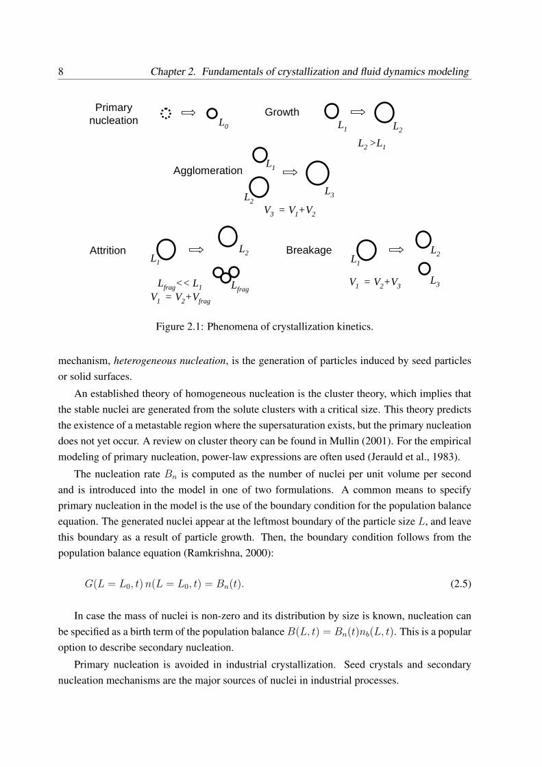
The major kinetic phenomenon is particle growth caused by mass transfer from the solutioninto the solid phase. It leads to an increase of particle size and amount of solid phase, andto a reduction of the supersaturation. The primary nucleation involves mass transfer from thesolution to the new nuclei, but the depleted mass is very small. The other kinetic phenomenasuch as aggregation, attrition, breakage and secondary nucleation are primarily caused by me-chanical effects, e.g. by impacts of particles with other particles, the walls of the vessel and theimpeller, or by the shear effect of the fluid. Although the effect of the mechanistic phenomena isoften undesired, they are unavoidable in an industrial process. These phenomena do not changethe amount of the solid phase, but modify the distribution of particles. The effect of variousphenomena of crystallization kinetics on the particle size distribution is illustrated in Fig. 2.1.
Primary nucleationPrimary nucleation describes the generation of particles from the mother solution without
any influence of the crystalline phase. If particles are spontaneously generated from the super-saturated crystal-free liquor, the mechanism is called homogeneous nucleation. An alternative
3In theory, the supersaturation should be written in activities instead of concentrations, but in practice, concen-trations are usually used.
8 Chapter 2. Fundamentals of crystallization and fluid dynamics modeling
L1 L2
GrowthPrimarynucleation L0
L2 >L1
Agglomeration
Attrition Breakage
L3
V3 = V1+V2
L1
L2
L1 L1
L2
L3V1 = V2+V3
L2
Lfrag<< L1
V1 = V2+Vfrag
Lfrag
Figure 2.1: Phenomena of crystallization kinetics.
mechanism, heterogeneous nucleation, is the generation of particles induced by seed particlesor solid surfaces.
An established theory of homogeneous nucleation is the cluster theory, which implies thatthe stable nuclei are generated from the solute clusters with a critical size. This theory predictsthe existence of a metastable region where the supersaturation exists, but the primary nucleationdoes not yet occur. A review on cluster theory can be found in Mullin (2001). For the empiricalmodeling of primary nucleation, power-law expressions are often used (Jerauld et al., 1983).
The nucleation rate Bn is computed as the number of nuclei per unit volume per secondand is introduced into the model in one of two formulations. A common means to specifyprimary nucleation in the model is the use of the boundary condition for the population balanceequation. The generated nuclei appear at the leftmost boundary of the particle size L, and leavethis boundary as a result of particle growth. Then, the boundary condition follows from thepopulation balance equation (Ramkrishna, 2000):
G(L = L0, t) n(L = L0, t) = Bn(t). (2.5)
In case the mass of nuclei is non-zero and its distribution by size is known, nucleation canbe specified as a birth term of the population balance B(L, t) = Bn(t)nb(L, t). This is a popularoption to describe secondary nucleation.
Primary nucleation is avoided in industrial crystallization. Seed crystals and secondarynucleation mechanisms are the major sources of nuclei in industrial processes.
2.1. Crystallization 9
Secondary nucleationSecondary nucleation is the generation of nuclei from the crystals of the solute already present
in the suspension. Randolph and Larson (1988) classify the variety of mechanisms of secondarynucleation into several groups: initial breeding in the seeded systems, nucleation by fracture ofeasily breaking crystals in dense suspensions, nucleation by attrition due to crystal collisionsand fluid shear in highly turbulent media. The dominating source of secondary nuclei is thecollision-induced attrition and fracture. The major part of new secondary nuclei (about 90%)are produced by the collision of crystals with the impeller (Liiri et al., 2002), and their numberis proportional to the agitation power input (Gahn and Mersmann, 1997). The second importantsource is the collision of crystals with the bottom of the vessel (Liiri et al., 2002). Crystal-wallcollisions produce a weaker effect. The effect of crystal-crystal collisions is small in dilutemediums, but higher in dense suspensions and fluidized beds.
Secondary nucleation is modeled together with attrition or breakage kinetics by means ofbirth and death terms of the population balance.
GrowthCrystal growth is the result of mass transfer of the solute to the particle. Growth kinetics are
characterized by the growth rate G, which is measured in[
ms
]and is equivalent to a velocity
in the direction of the particle size coordinate. Crystal growth is commonly described in theframework of the diffusion-reaction theory, which states that the two main steps of the processare diffusion of the solute to the crystal surface through its boundary, and consequent integrationinto the crystal lattice.4 The overall growth kinetics is determined by the slowest of thesetwo steps. Growth is called diffusion-controlled, if diffusion is the slower kinetic step, andintegration-controlled, if surface integration is slower.
In the framework of the diffusion-reaction theory, growth can be described by the masstransfer equation using the concentration difference as a driving force. The following equationtypically describes the overall growth rate (though different supersaturation expressions couldbe used):
G =dL
dt= kG(c− c∗)p. (2.6)
Here, p is the order of the process kinetics, the growth rate coefficient kG is a function ofdiffusive mass transfer (kd) and surface integration (kr) coefficients (Mullin, 2001).
If growth is diffusion-limited, kG is not a function of particle size. A further assumption ofisotropic crystal growth leads to well-known McCabe’s law of size-independent crystal growth.Diffusion-controlled growth shows only a first-order dependency on supersaturation. With in-creasing supersaturation, diffusion ceases to be the limiting step, and theories describing the
4See Mullin (1993) for detailed discussion on growth mechanisms.
10 Chapter 2. Fundamentals of crystallization and fluid dynamics modeling
surface integration step have to be used. Integration-controlled growth depends on particle size,the properties of the crystal lattice and other factors. Thus, the overall growth rate can be size-dependent and may show growth rate dispersion. A number of competing theories for this step(adsorption layer theory, surface nucleation theory, etc.) are discussed in the literature (Mullin(2001) and references therein); a predictive, first-principle based growth theory has not yet beenfully developed. In engineering practice, expressions of the form of Eq. (2.6) are widely used,where the kinetic coefficient kG and the kinetic order coefficient p are estimated from experi-mental data.
Attrition and breakageAs already mentioned, attrition and breakage are caused by the collisions of crystals with
the impeller, the crystallizer hull and other crystals. They have the same origin, but differ inmodeling. In case of breakage, a particle is broken into a finite number of smaller particles. Incase of attrition, a fraction of crystal volume displaced from the crystal forms a distribution ofsmall nuclei, which contribute to the secondary nucleation.
Attrition appears in the population balance in form of several terms: a death term for parti-cles, which undergo attrition, Datt, a birth term for the same particles after attrition, Batt, anda birth term for the fragment distribution, Bfrag (see also Eq. (6.43) in Section 6.2.3). Theseterms are complex functions of the material properties and the collision frequency/efficiencycharacteristics. Until recently, attrition was modeled using empirical or semi-empirical models;some overview of such models can be found in O Meadhra et al (1996a). Only the recent publi-cation by Gahn and Mersmann (1999a) presented a comprehensive first principles mechanisticmodel of attrition due to collisions with the impeller.
AgglomerationAgglomeration is a phenomenon by which crystals after collision adhere to each other and
subsequently grow further as a single particle or agglomerate. It is modelled by means of birthand death terms written in terms of particle volume or particle sizes, where the agglomerationkernel β(L) characterizes the agglomeration rate (Ramkrishna, 2000):
B(L) =L2
2
∫ L
0
β(L, λ)n([L3 − λ3]1/3)n(λ)
(L3 − λ3)2/3dλ, (2.7)
D(L) = n(L)
∫ ∞
0
β(L, λ)n(λ)dλ. (2.8)
The agglomeration kernel is a function of both the collision characteristics and the super-saturation. It is more pronounced in highly supersaturated systems, and in systems with slowfluid motion. It is often observed during precipitation of substances with low solubility; mass
2.1. Crystallization 11
crystallization of soluble substances usually operates under conditions where agglomeration isnegligible. Agglomeration widens the particle size distribution and is often undesired.
Classification of particlesParticle classification occurs under action of external body forces such as gravity or centrifu-
gal force. In this case, the velocity of particles differs from the velocity of the liquid phase byvpart = vliq + vslip, where vslip is the slip velocity. The stationary slip velocity is evaluatedby equating the body force fb and the drag resistance force. In case of gravitational settling inlaminar flow, the expression for the slip velocity is known as Stokes’ law.
Crystallization typically involves several of these processes occurring simultaneously, whichall need to be incorporated into the population balance model. A very general form of the popu-lation balance with all effects incorporated into a single equation is presented in Hounslow et al.(2005). In many cases the kinetics of these simultaneously occurring crystallization phenomenacannot be isolated in a single experiment. Rather, a series of complex experiments has to be car-ried out to identify the phenomena and their kinetics. As a result, rigorous kinetic models andaccurate kinetic parameters are often not available for a specific system of interest. Therefore,the vast majority of available models is empirical or semi-empirical.
2.1.4 Solution of population balance models
A population balance model is a complex equation system consisting of a partial integro-differential population balance equation (2.3) (in the differential form) or (2.4) (in the integralform) and the set of constitutive (usually algebraic) equations, which can in turn depend on thePSD. The system is generally not solvable analytically and requires numerical methods.
A major challenge is the proper discretization of the population balance. Discretizationmethods are used to transform a complex PIDAE system to a large system of DAEs on thechosen set of discretization elements, which is further solved with the numerical methods forthe solution of DAE systems, such as Newton-Raphson or Runge-Kutta methods. A numberof discretization techniques are proposed in the literature (Grosch et al., 2007; Hounslow et al.,2005; McGraw, 1997; Ramkrishna, 2000; Randolph and Larson, 1988; Wulkow et al., 2001).Below, the techniques relevant to the thesis are briefly discussed, and the reader is referred tothe literature for details.
Model reduction by the Method of Moments and its extensionsModel reduction can be performed if the user is not interested in the complete particle size
distribution, but only in statistically aggregated characteristics. A commonly used reductionmethod is the Method of Moments, which reduces the population balance to the set of equations
12 Chapter 2. Fundamentals of crystallization and fluid dynamics modeling
for the moments of the distribution (Randolph and Larson, 1988), from which aggregated PSDcharacteristics can be computed. A reduction to the p-th order distribution moment is performedby integrating both sides of the population balance equation (2.4) according to
∫∞0
Lp • dL.Assuming constant density, constant volume V , independency of growth rate on particle size,the following equation is obtained for the integral moment balance:
∂µ(p)
∂t= 0p ·Bn + pGµ(p−1) −
∑
k
Vkµ(p)k
V+ B
(p)
µ −D(p)
µ , p = 0, 1, ... (2.9)
B(p)
µ and D(p)
µ refer to the birth and death terms. Derivation of these terms is possible, if thepopulation balance birth and death functions can be expressed by a finite number of distributionmoments (Randolph and Larson, 1988).
Similarly, a moment transformation of the differential population balance (2.3) yields
∂µ(p)(x, t)
∂t+∇ · (v(x, t)µ(p)(x, t)) = 0p ·Bn(x, t) + pG(x, t)µ(p−1)(x, t)
+ B(p)
µ (x, t)−D(p)
µ (x, t). (2.10)
To provide closure for the Method of Moments, the Quadrature Method of Moments hasbeen recently introduced by McGraw (1997), which uses a quadrature approximation for thePSD using 2p moments for p-th order approximation. The method has been applied to crys-tallization processes including size-dependent kinetics (Marchisio et al., 2003a) as well as toagglomeration and breakage problems (Marchisio et al., 2003b). A comprehensive analysis ofthe computational accuracy of QMOM with respect to the crystallization kinetics and PSD hasbeen presented by Grosch et al. (2007).
However, both the Method of Moments and the Quadrature Method of Moments do notprovide details on the shape of the particle size distribution, which needs to be reconstructedassuming a certain shape (Gaussian, bimodal, etc.). A recent publication by John et al. (2007)reviews popular techniques for reconstructing distributions from the moments, and notes thatthis problem is ill-posed.
Detailed discretization of population balanceThe numerical solution of full population balance requires its discretization using a finite
number of discrete points, finite elements or other entities to obtain a large system of DAEs,which can be solved by conventional numerical integration techniques. Different discretizationtechniques are illustrated in Fig. 2.2.
A pivot-based discretization evaluates the particle size distribution at certain points (pivots).A fixed pivot discretization (also known as sectional model) uses a finite number of fixed pointswith particle sizes LI = (L1, L2, ..., LNI
), which split the particle size domain into sections
2.1. Crystallization 13
Fixed pivot discretization
Moving pivot discretization
Finite element discretization(Wulkow et al., 2001)
L
n(L)
pivot
shifted pivot
4 4 4 4 4 5 5Order of FE polynomial
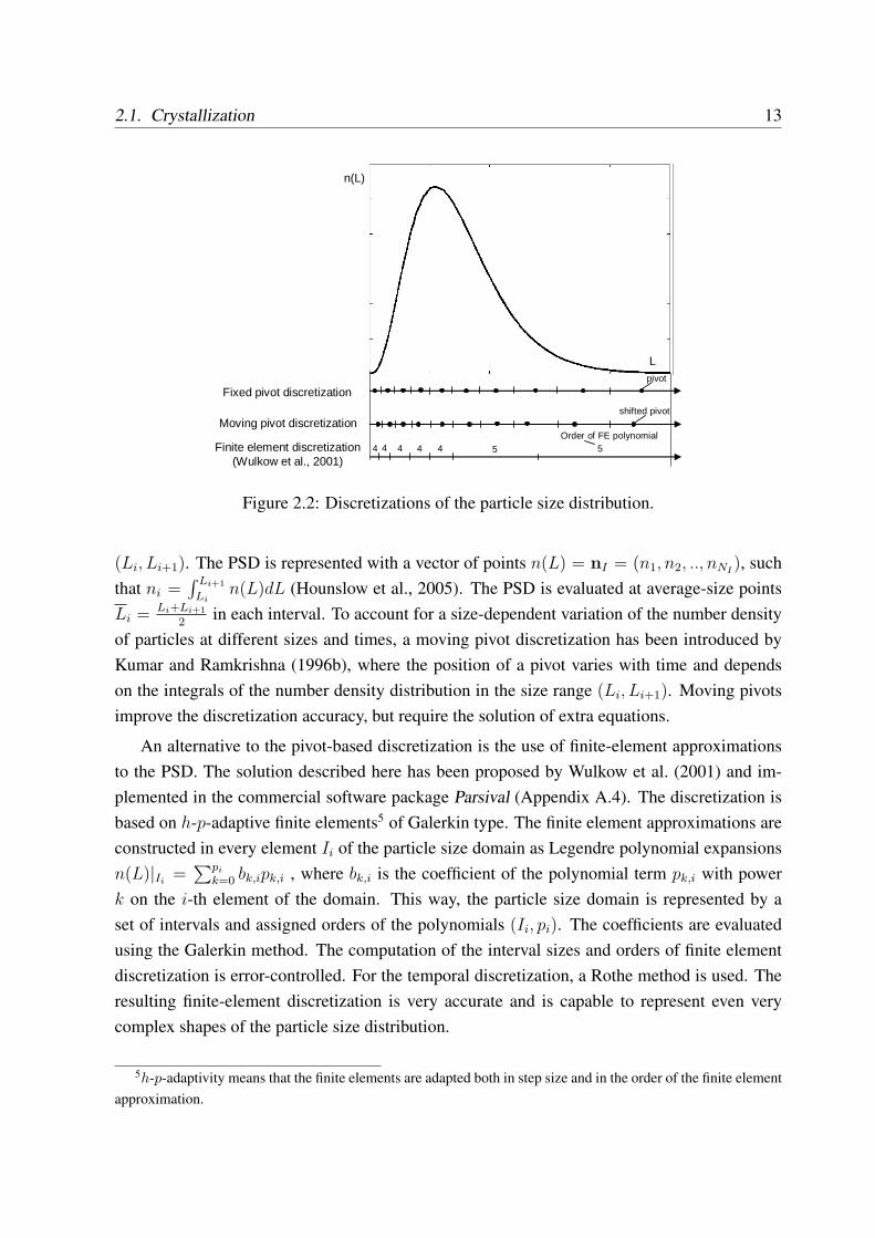
Figure 2.2: Discretizations of the particle size distribution.
(Li, Li+1). The PSD is represented with a vector of points n(L) = nI = (n1, n2, .., nNI), such
that ni =∫ Li+1
Lin(L)dL (Hounslow et al., 2005). The PSD is evaluated at average-size points
Li = Li+Li+1
2in each interval. To account for a size-dependent variation of the number density
of particles at different sizes and times, a moving pivot discretization has been introduced byKumar and Ramkrishna (1996b), where the position of a pivot varies with time and dependson the integrals of the number density distribution in the size range (Li, Li+1). Moving pivotsimprove the discretization accuracy, but require the solution of extra equations.
An alternative to the pivot-based discretization is the use of finite-element approximationsto the PSD. The solution described here has been proposed by Wulkow et al. (2001) and im-plemented in the commercial software package Parsival (Appendix A.4). The discretization isbased on h-p-adaptive finite elements5 of Galerkin type. The finite element approximations areconstructed in every element Ii of the particle size domain as Legendre polynomial expansionsn(L)|Ii
=∑pi
k=0 bk,ipk,i , where bk,i is the coefficient of the polynomial term pk,i with powerk on the i-th element of the domain. This way, the particle size domain is represented by aset of intervals and assigned orders of the polynomials (Ii, pi). The coefficients are evaluatedusing the Galerkin method. The computation of the interval sizes and orders of finite elementdiscretization is error-controlled. For the temporal discretization, a Rothe method is used. Theresulting finite-element discretization is very accurate and is capable to represent even verycomplex shapes of the particle size distribution.
5h-p-adaptivity means that the finite elements are adapted both in step size and in the order of the finite elementapproximation.
14 Chapter 2. Fundamentals of crystallization and fluid dynamics modeling
2.2 Fluid dynamics
2.2.1 Modeling of fluid dynamics problems
Fluid dynamics is a general term for a range of transport and mass/energy transfer problemsin the continuous media, such as flow of fluids, mixtures, films, particles in the fluid, turbu-lent transport, reactions in fluid, etc. The solution of the fluid dynamics problem is a field ofvelocity vectors, fluid and mixture properties in the physical domain, defined in the spatial coor-dinates. Common coordinate systems in fluid dynamics problems are Cartesian 3d-coordinatesand cylindrical 2d-coordinates with axial symmetry.
The fluid dynamics models in this section comply with the FLUENT 6.0 User Manual(2005). The reader is also referred to the literature on computational fluid dynamics (Birdet al., 2002; Ferziger and Peric, 1997).
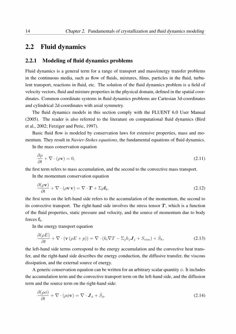
Basic fluid flow is modeled by conservation laws for extensive properties, mass and mo-mentum. They result in Navier-Stokes equations, the fundamental equations of fluid dynamics.
In the mass conservation equation
∂ρ
∂t+∇ · (ρv) = 0, (2.11)
the first term refers to mass accumulation, and the second to the convective mass transport.In the momentum conservation equation
∂(ρv)
∂t+∇ · (ρv v) = ∇ · T + Σρfb, (2.12)
the first term on the left-hand side refers to the accumulation of the momentum, the second toits convective transport. The right-hand side involves the stress tensor T , which is a functionof the fluid properties, static pressure and velocity, and the source of momentum due to bodyforces fb.
In the energy transport equation
∂(ρE)
∂t+∇ · (v (ρE + p)) = ∇ · (kt∇T − ΣjhjJ j + Svisc) + Sh, (2.13)
the left-hand side terms correspond to the energy accumulation and the convective heat trans-fer, and the right-hand side describes the energy conduction, the diffusive transfer, the viscousdissipation, and the external source of energy.
A generic conservation equation can be written for an arbitrary scalar quantity φ. It includesthe accumulation term and the convective transport term on the left-hand side, and the diffusionterm and the source term on the right-hand side:
∂(ρφ)
∂t+∇ · (ρφv) = ∇ · Jφ + Sφ. (2.14)
2.2. Fluid dynamics 15
All presented equations can be derived from the generic conservation equation by substitu-tion of general variables by appropriate specific quantities (see Marquardt (2005) and referencestherein).
Modeling mixtures and multi-phase flowsReal flows in crystallization processes involve two phases, liquid and solid, and several com-
ponents in the liquid phase (solute and solvent). The transport of every phase and every com-ponent of the mixture has to be described by an extra equation.
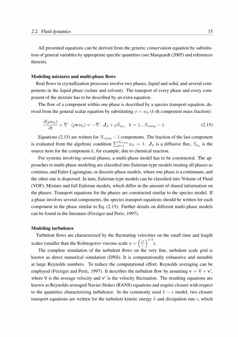
The flow of a component within one phase is described by a species transport equation, de-rived from the general scalar equation by substituting φ = wk (k-th component mass fraction):
∂(ρwk)
∂t+∇ · (ρvwk) = −∇ · Jk + ρSwk
, k = 1...Ncomp − 1. (2.15)
Equations (2.15) are written for Ncomp − 1 components. The fraction of the last componentis evaluated from the algebraic condition
∑Ncomp
k=1 wk = 1. Jk is a diffusive flux, Swkis the
source term for the component k, for example, due to chemical reaction.For systems involving several phases, a multi-phase model has to be constructed. The ap-
proaches to multi-phase modeling are classified into Eulerian-type models treating all phases ascontinua, and Euler-Lagrangian, or discrete-phase models, where one phase is a continuum, andthe other one is dispersed. In turn, Eulerian-type models can be classified into Volume of Fluid(VOF), Mixture and full Eulerian models, which differ in the amount of shared information onthe phases. Transport equations for the phases are constructed similar to the species model. Ifa phase involves several components, the species transport equations should be written for eachcomponent in the phase similar to Eq. (2.15). Further details on different multi-phase modelscan be found in the literature (Ferziger and Peric, 1997).
Modeling turbulenceTurbulent flows are characterized by the fluctuating velocities on the small time and length
scales (smaller than the Kolmogorov viscous scale η =(
ν3
ε
)1/4
).The complete simulation of the turbulent flows on the very fine, turbulent scale grid is
known as direct numerical simulation (DNS). It is computationally exhaustive and unstableat large Reynolds numbers. To reduce the computational effort, Reynolds averaging can beemployed (Ferziger and Peric, 1997). It describes the turbulent flow by assuming v = v + v′,where v is the average velocity and v′ is the velocity fluctuation. The resulting equations areknown as Reynolds-averaged Navier-Stokes (RANS) equations and require closure with respectto the quantities characterizing turbulence. In the commonly used k − ε model, two closuretransport equations are written for the turbulent kinetic energy k and dissipation rate ε, which
16 Chapter 2. Fundamentals of crystallization and fluid dynamics modeling
characterize the local intensity of turbulence. An alternative way to model turbulence is largeeddy simulation (LES), where large turbulent eddies are explicitly resolved in the simulation,so that the major turbulent transport is accounted for.
2.2.2 Methods of computational fluid dynamics
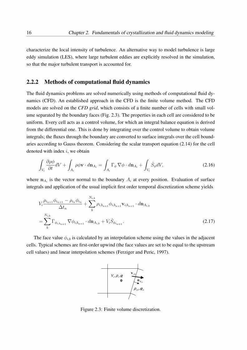
The fluid dynamics problems are solved numerically using methods of computational fluid dy-namics (CFD). An established approach in the CFD is the finite volume method. The CFDmodels are solved on the CFD grid, which consists of a finite number of cells with small vol-ume separated by the boundary faces (Fig. 2.3). The properties in each cell are considered to beuniform. Every cell acts as a control volume, for which an integral balance equation is derivedfrom the differential one. This is done by integrating over the control volume to obtain volumeintegrals; the fluxes through the boundary are converted to surface integrals over the cell bound-aries according to Gauss theorem. Considering the scalar transport equation (2.14) for the celldenoted with index i, we obtain
∫
Vi
∂ρφ
∂tdV +
∫
Ai
ρφv · dnAi=
∫
Ai
Γφ∇φ · dnAi+
∫
Vi
SφdV, (2.16)
where nAiis the vector normal to the boundary Ai at every position. Evaluation of surface
integrals and application of the usual implicit first order temporal discretization scheme yields
Vi
ρin+1φin+1 − ρinφin
∆tn+
Ni,b∑
b
ρi,bn+1φi,bn+1
vi,bn+1· dnAi,b
=
Ni,b∑
b
Γφi,bn+1∇φi,bn+1
· dnAi,b+ ViSφin+1
. (2.17)
The face value φi,b is calculated by an interpolation scheme using the values in the adjacentcells. Typical schemes are first-order upwind (the face values are set to be equal to the upstreamcell values) and linear interpolation schemes (Ferziger and Peric, 1997).
biA ,n
iiiV φρ ,,
bibi ,, ,φρ
bi,v
Figure 2.3: Finite volume discretization.
2.3. Multi-physics and multi-scale problems 17
2.3 Multi-physics and multi-scale problems
2.3.1 Classification of complexities
In industrial processes, crystallization (Section 2.1) and fluid dynamics (Section 2.2) phenom-ena occur simultaneously within the same domain and ultimately affect each other. Such prob-lems can be denoted as phenomenologically complex.
A mathematical model of a phenomenologically complex problem can have several com-plexity aspects: complexity of the heterogeneous structure of the mathematical model, of mul-tiple dimensions and of multiple scales.
Structural complexity refers to the heterogeneity of the structure of the model equations.The model is structurally complex if its governing equations belong to different mathematicaltypes, inconvertible to fit each other’s form. To handle structural complexity, a suitable problemdecomposition into subproblems with a more homogeneous structure may be appropriate.
Multi-dimensional complexity arises in the systems described by models with multiple in-dependent coordinates, on which the discretization of the model has to be performed. This dra-matically increases the number of nodes or elements for the numerical solution of the model.To reduce this complexity, coordinate transformation and dimensional reduction can be used.
Length, L[m]
Nanoscale Microscale Mesoscale Macroscale
10-9 10-6 10-3 100
atomisticmodels
turbulent fluctuations,molecular dynamics
particle transport,CFD, large eddies
population evolution,bulk flow
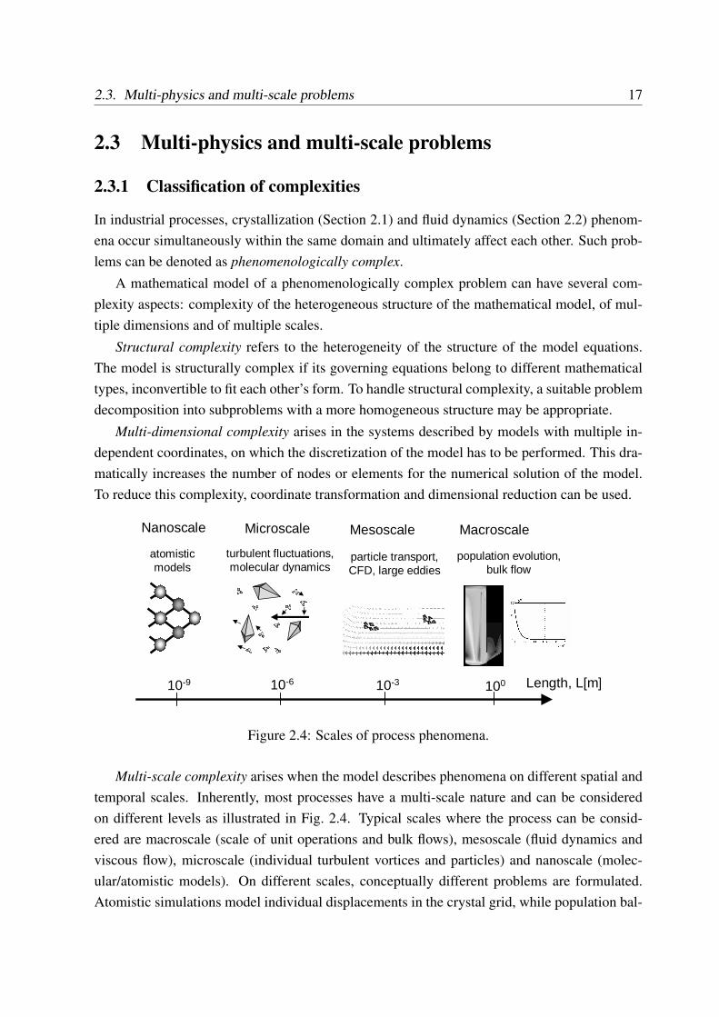
Figure 2.4: Scales of process phenomena.
Multi-scale complexity arises when the model describes phenomena on different spatial andtemporal scales. Inherently, most processes have a multi-scale nature and can be consideredon different levels as illustrated in Fig. 2.4. Typical scales where the process can be consid-ered are macroscale (scale of unit operations and bulk flows), mesoscale (fluid dynamics andviscous flow), microscale (individual turbulent vortices and particles) and nanoscale (molec-ular/atomistic models). On different scales, conceptually different problems are formulated.Atomistic simulations model individual displacements in the crystal grid, while population bal-
18 Chapter 2. Fundamentals of crystallization and fluid dynamics modeling
ances on the macro-scale compute macroscopic product characteristics. If the process phenom-ena considered are modeled on different characteristic scales, multi-scale simulation has to beemployed and multi-scale complexity emerges. To resolve such phenomena on different scaleswith comparable accuracy, different resolution in space and time (up to several orders) for theproblem parts (subproblems) or grid subspaces is necessary. Application of standard simulationapproaches where overall performance is determined by the smallest grid and time step sizes iscomputationally prohibitive. Multi-scale complexity has to be handled by means of multi-scalemethods.
2.3.2 Interplay between CFD and crystallization
The need to consider crystallization and fluid dynamics as a phenomenologically complex pro-cess has been illustrated by Marchisio et al. (2006). The simulations of a Taylor-Couette shearcell and a stirred tank showed that a simplified homogeneous model could be used if aggrega-tion and breakage processes were much slower than mixing. When the phenomena occurredon comparable time scales, the use of a lumped model leads to errors in the identification ofthe process kinetics, so the modeling of interplay between fluid dynamics and crystallizationbecomes necessary. However, since there is still a shortcoming of reliable quantitative modelsfor the physics of such interplay effects, they are usually described qualitatively based on theexperimental results.
The influence of local fluid dynamics on crystallization is two-fold. First, the kinetic coeffi-cients of a crystallization process can directly depend on the fluid dynamics characteristics suchas turbulence or shear rate. An example is the dependence of growth rate on turbulence (Mullin,2001): the thickness of the particle boundary layer is reduced in turbulent flows, acceleratingthe diffusion to the surface and making growth integration-controlled. Turbulence and shearrates also affect the collision frequency (increases with increasing shear rate) and efficiency(decreases with increasing shear rate) of the particle collisions governing the mechanical crys-tallization phenomena, in particular, agglomeration. A complex dependency of agglomerationkinetics on the shear rate was shown in an analysis of calcium oxalate aggregation (Mumtaz etal., 1997). A recent model for gibbsite agglomeration related the agglomeration kinetics withviscosity, impeller speed and fluid shear rate (Ilievsky and Livk, 2006). Highly turbulent flowsmay force particles to disaggregate (Synowiec et al., 1993). Fragmentation of particles is pre-dominantly caused by the particle-impeller or particle-wall collisions, the energy and efficiencyof which depend on the streamlines and the particle velocity (Gahn and Mersmann, 1999a).
The flow field can also indirectly affect the crystallization because of the anisotropy of theflow field and, therefore, the inhomogeneity of the suspension properties in the vessel. Anindustrial-scale vessel is always inhomogeneous (Mullin, 2001). Mersmann (1995) mentions
2.3. Multi-physics and multi-scale problems 19
a range of effects contributing to local inhomogeneity, such as macro-/micromixing quality,6
particularly in the vicinity of the feed and the impeller, poor mixing regions, boundary layers,position of a product outlet, particle classification, local energy input and turbulence, etc. Shaand Palosaari (2000) showed that the profile of solid phase concentration along the height ofthe vessel is not uniform and is affected by macromixing, convective transport, gravitationalsettling of particles and the impeller type. In mass crystallization, micromixing is not of aprimary concern due to much slower rate of crystallization kinetics compared to fluid dynamics.However, in the systems with fast chemical reactions or precipitation, micromixing is often agoverning factor to determine the number of nuclei, and hence, the particle size distribution(Baldyga and Bourne, 1999; Barresi et al., 1999; Zauner and Jones, 2002).
Inhomogeneities affect crystallization kinetics through local variations in concentration,temperature and particle content. Reversely, locally varying crystallization rates produce lo-cal variations of suspension composition, density and viscosity. This can be considered as afeedback mechanism of crystallization on fluid dynamics. It increases with an increasing frac-tion of solids; large particle content results in swarm behavior.
2.3.3 Models with structural complexity: CFD and process simulation
Structurally complex problems of fluid dynamics and process simulation have been a topicof extensive studies in the recent years. Bezzo (2002) modeled the behavior of a bioreactorcoupling the bioprocess model with the CFD model. Bauer and Eigenberger (2001) studiedthe behavior of bubble columns emphasizing the effect of the hydrodynamics. Some of theseproblems such as the modeling of reacting systems and the transport of particle clouds can betreated in commercial CFD packages (such as FLUENT or CFX). More complex problems,such as the modeling of particulate systems and emulsions together with fluid dynamics, stillneed more attention, particularly due to their multi-dimensional and multi-scale nature.
In case of particulate systems, much attention is focused on precipitation. The interplay be-tween precipitation and fluid dynamics was extensively studied in the literature for a number ofsystems such as barium sulphate-water (Baldyga and Orciuch, 2001; Wei et al., 2001) or gibb-site precipitation from caustic solution (Ilievsky et al., 2001; Ilievsky and Livk, 2006), wherethe modeling of precipitation and in some cases the estimation of the precipitation kinetics wasstudied. The problem of fluid dynamics and mass crystallization from solution attracts less at-tention; for ammonium sulphate-water system, it has been partially investigated in Kramer etal. (2000) and other publications of this author (see Section 6).
6Depending on the characteristic scales of mixing, macromixing (bulk convective transport), mesomixing (localcoarse-scale turbulent and large eddy transport on the CFD grid scale) and micromixing (diffusive and viscous-convective transport on the turbulence scale below CFD grid) are distinguished (Baldyga and Bourne, 1999).
20 Chapter 2. Fundamentals of crystallization and fluid dynamics modeling
Similar problems involving fluid dynamics and the population balance are the droplet dis-tribution modeling (Vikhansky and Kraft, 2004), population models for the polymerization re-actors (Wells and Ray, 2001) or complex multiphase reactors (Rigopoulos and Jones, 2003).
2.3.4 Multi-scale modeling
There are a variety of formulations for multi-scale problems, but no commonly recognizedclassification exists. Several classifications have been introduced in reviews of Brandt (1999),Liu et al. (2004), Ingram et al. (2004) and Fish (2006).
Spatial and temporal multi-scale problems need to be distinguished. Spatial multi-scaleproblems involve more than one spatial scale for the solution of the subproblems. Temporalmulti-scale problems have different characteristic temporal scales of the subproblems. A com-plex problem may be multi-scale in both space and time.
A classification of multi-scale problems can be based on the continuity types of fine andcoarse scale models. Multi-scale problems can be formulated for (a) problems with discretefine and coarse scales (e.g. atomistic simulations); (b) problems with a continuous coarse anda discrete fine scale (e.g. molecular simulations of the continuous phase); (c) problems with alocally continuous fine scale coupled with a globally continuous coarse scale (e.g. processes inbubbles or drops in the continuous medium); and (d) problems with globally continuous coarseand fine scales (simulation of processes with different scales on the same domain).
Ingram et al. (2004) introduce a classification based on the type of integrating framework,that determines the way the models are coupled, and the information flows between them. Dif-ferent types of integrating frameworks have been introduced, such as the multidomain, paralleland embedded frameworks.
Liu et al. (2004) classify multi-scale problems into hierarchical (or information-passing)and concurrent. Hierarchical multi-scale problems allow full decomposition of the problemby scales to formulate closed equation systems for the subproblems. The fine-scale subprob-lems are defined within an element of a coarse-scale grid or independently of the coarse grid.Concurrent multi-scale problems define different scales and their respective subproblems simul-taneously in different parts of the considered domain.
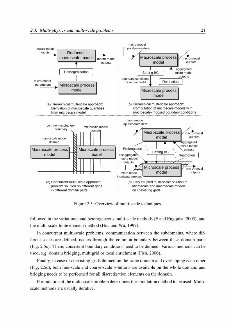
Fig. 2.5 presents a simple classification following Liu et al. (2004). Hierarchical multi-scaleproblems can be solved using two kinds of methods. For discrete models and molecular dynam-ics simulation (Fig. 2.5a), a popular analytical approach is homogenization, where the contin-uum equations are constructed from the discrete fine-scale equations to compute macroscopicquantities (Liu et al., 2004). For continuous coarse-scale models with discrete or continuousfine-scale models, a multi-scale simulation can be performed by solving a fine-scale subprob-lem with boundary conditions set by the coarse-scale subproblem (Fig. 2.5b). This strategy is
2.3. Multi-physics and multi-scale problems 21
(a) Hierarchical multi-scale approach: Derivation of macroscale quantitiesfrom microscale model
Spatial multi-scale problems
(b) Hierarchical multi-scale approach:Computation of microscale models with macroscale-imposed boundary conditions
(c) Concurrent multi-scale approach:problem solution on different grids in different domain parts
(d) Fully coupled multi-scale: solution of microscale and macroscale modelson coexisting grids
Microscale processmodel
Homogenization
macro-modelinputs
Microscale processmodel
Macroscale processmodel
Restriction
Reduced macroscale model
micro-model parameters
macro-modeloutputs
macro-model inputs/parameters
Setting BC
boundary conditionsfor micro-model
aggregatedmicro-model
outputs
macro-model outputs
Macroscale processmodel
Microscale processmodel
common (exchange) boundary
microscale modeldomain
macroscale modeldomain
Microscale processmodel
Macroscale processmodel
Prolongation
Restriction
aggregatedmicro-model
outputsSetting BC
macro-model outputs
macro-model inputs/parameters
disaggregatedmacro-model
outputs
micro-model outputsmicro-model
inputs/parameters
Figure 2.5: Overview of multi-scale techniques.
followed in the variational and heterogeneous multi-scale methods (E and Engquist, 2003), andthe multi-scale finite element method (Hou and Wu, 1997).
In concurrent multi-scale problems, communication between the subdomains, where dif-ferent scales are defined, occurs through the common boundary between these domain parts(Fig. 2.5c). There, consistent boundary conditions need to be defined. Various methods can beused, e.g. domain bridging, multigrid or local enrichment (Fish, 2006).
Finally, in case of coexisting grids defined on the same domain and overlapping each other(Fig. 2.5d), both fine-scale and coarse-scale solutions are available on the whole domain, andbridging needs to be performed for all discretization elements on the domain.
Formulation of the multi-scale problem determines the simulation method to be used. Multi-scale methods are usually iterative.
22 Chapter 2. Fundamentals of crystallization and fluid dynamics modeling
Although multi-scale methods emerged in molecular dynamics and are most often used forthe exploration of the microscale, their scope of application is enormous. In this thesis, multi-scale approaches are discussed in the context of the coupled crystallization and fluid dynamicsproblem.
2.3.5 Simulation approaches for fluid dynamics – population balance prob-lems
Problem complexityAccording to the above discussion, mass crystallization under non-stationary fluid dynamics
conditions should ideally be modeled with a differential population balance (2.3) with constitu-tive crystallization kinetics, initial and boundary conditions, the general fluid dynamic equations(2.11)-(2.13), and the species equation (2.15) formulated for a multi-phase system.
Such a coupled problem shows all kinds of complexities discussed in Section 2.3.1. Com-parison of the Navier-Stokes equations (partial differential equations in Euclidean spatial co-ordinates and time) and the population balance (a partial (integro-)differential equation withintegral birth/death terms in spatial coordinates, the internal particle size coordinate and time)shows the structural and multi-dimensional complexity. Besides, the process in the consideredmodel formulation is inherently of multi-scale nature. A typical CFD model based on Reynolds-averaging performs computations on the viscous scale resolved by the CFD discretization. It isin the order of Kolmogorov scale η = 10−3− 10−4m. The matching temporal scale is in the or-der of seconds. On the other hand, mass crystallization from solutions is a macroscopic process,the residence time in a crystallizer is in the order of minutes/hours (102-103s) (Mullin, 2001).The process scales with respect to space and time differ by two to three orders of magnitude.The application of a turbulence model would further expand the scale range considered.
Solution approaches and model reductionThe presented multi-dimensional and multi-scale complexity of the coupled fluid dynamics-
crystallization problem makes its numerical simulation computationally expensive. Discretiza-tion of the particle size distribution into Nc classes by the method of lines results in a systemof Nc + 1 discretized population balance equations, 5− 7 transport equations and the complex,often PSD dependent crystallization kinetics in every element of the CFD grid (Hounslow et al.,2005). Solving such a system requires a high computational cost. Sectional models with a smallnumber of particle classes and fixed pivots (Sha and Palosaari, 2000) may also be inaccurate,since the PSD varies with time in non-stationary processes, and the small number of particleclasses can not accurately reflect such a variation (Ramkrishna, 2000). The solvers also need tohandle a problem of consistency in the numerical evaluation of integrals in the source terms of
2.3. Multi-physics and multi-scale problems 23
population balance (Ramkrishna, 2000). Furthermore, the statistical foundations of the popula-tion balance can be violated on the CFD grid scale, especially for large particles, compared tothe size of a CFD grid element.
A practical solution to solve the fluid dynamics-crystallization problem ought to reducecomplexity and computational effort to an acceptable level, but to retain as much informationand accuracy as possible. Model reduction reduces the computational costs by disregardingsome information content and by reducing accuracy requirements. This can be done by intro-ducing assumptions and subsequent analytical reduction of the model dimensions.
For the fluid dynamics-crystallization problem, the spatially distributed population balance(2.3) provides the maximum complexity and needs to be reduced. The most popular solutionapproach is model reduction by the Method of Moments or Quadrature Method of Moments(Section 2.1.4). Marchisio et al. (2003b) implemented QMOM in FLUENT for the aggregation-breakage problems and tracked the aggregated characteristics of the PSD in dynamic CFD sim-ulation. Further developments of this approach, such as Sectional QMOM (Attarakih et al.,2006), are aimed at accurate definition of the quadratures for population balance problems withpreservation of the integral quantities, and still remain an active research field. For reactiveprecipitation, probability density function (PDF) based methods were developed by Wang andFox (2004). However, these methods do not provide detailed information on the PSD and mayshow errors in case of complex process kinetics compared to the methods working with the fullPSD (Grosch et al., 2007).
An alternative solution, followed in the present thesis, is based on the use of coarse-scalecompartments for the crystallization model. This solution is known as the compartment-basedapproach, which has been used in the literature for different processes. The compartments canbe chosen a priori by the user (Kramer et al., 2000; Zauner and Jones, 2002) or identified basedon steady-state CFD simulation (Bezzo et al., 2004b; Wells and Ray, 2001). In the compart-ments, the spatial coordinates are eliminated, and the model equations are formulated in anintegral form.
This thesis presents a general compartment-based solution within a framework of modeldecomposition into submodels with different grids and characteristic scales to facilitate thecoupled dynamic simulation of the resulting flowsheet incorporating both CFD and crystalliza-tion process models. The solution is described and applied to a mass crystallization process inSection 4. Prior to that, the simulation methods and software-technical solution are discussedin Section 3.
Chapter 3
Simulation of process flowsheets
3.1 Flowsheet representation and simulation approaches
Prior to the discussion of simulation approaches for process flowsheets, several definitions ofthe process flowsheeting terminology used in the thesis need to be introduced.
A complex process is understood to involve multiple process phenomena and/or apparatuses,with every phenomenon or process apparatus described by means of a mathematical model.The whole process is represented by the process flowsheet consisting of units defined by a unitmodel and a set of variables, and connecting streams, which represent material and energyflows. Process flowsheeting operates with physical units and material streams. However, amathematical model can also describe a single process phenomenon. In this case, the streamsmay represent information flows between the process phenomena models, carrying informationabout the quantities relevant to these phenomena.
Coupling (of the phenomena) is the formalized interplay between several processes or pro-cess phenomena of a complex process.1 Such phenomena are denoted as coupled phenomena,and the description of the complete process as a coupled problem. The coupling between thephenomena can be direct, if the relations between the quantities characterizing the phenomenacan be explicitly formulated in the model, or indirect if there is an implicit influence throughsome third quantities.
Coupling is characterized by the strength of coupling. According to Matthies et al. (2002),a weak coupling requires a single iteration on every coupling to reach the problem solution, anda strong coupling necessitates an iterative process. The strength of coupling differs betweendifferent units. It can be evaluated by formulating the closure equations to represent the effects
1In the context of the software-technical solution, the term coupling is also used to refer to a software-technicalimplementation of an actual connection between the units/phenomena of a complex process, independently ofwhether it represents a physical stream or an information flow.
24
3.1. Flowsheet representation and simulation approaches 25
of the other unit/phenomena models on the variables in the considered unit/phenomena, andevaluating the respective sensitivities (Bezzo, 2002).
Coupled simulation is defined here as a simulation approach where the units/phenomenamodels of a complex process are coupled by means of an explicit set of connections. Simula-tion approaches differ by the techniques of setting up and handling such couplings to establishand solve the model of the complete process. Simulation of complex processes with coupledphenomena of different nature is referred to as a multi-physics simulation in this work and canbe treated as a specific case of coupled simulation.
3.1.1 Flowsheet representation
Abstract unit modelAn abstract mathematical DAE model for the q-th unit of the flowsheet can be written as
follows (Gilles et al., 1988):
xq = f q(t, xq(t),zq(t),uq(t),pq(t))
0 = gq(t, xq(t),zq(t),uq(t),pq(t)) (3.1)
yq = hq(t, xq(t),zq(t),pq(t)).
Here xq and zq are the vectors of differential and algebraic state variables in the q-th unit,uq is the vector of unit inputs, yq is the vector of unit outputs and pq is the vector of modelparameters. All variables are time-dependent and evaluated at time t. The function vectors f q,gq and hq refer to the sets of differential equations, algebraic equations and output equations,respectively. The resulting DAE system should have a differential index of one2. Consistentinitial conditions xq(t0) must be provided to fully specify the model.
The full vector of states is defined as xq =(
xq
zq
)and composed of both differential and
algebraic states, and the vector of functions fq =(
f q
gq
)is composed of differential and al-
gebraic equations of the system. For practical considerations, the outputs yq are (wheneverpossible) defined as a subset of the state variables xq. Then, hq are identity relations that can berepresented as an output permutation matrix Py,q.
An abstract explicit formulation of a unit model can be written as
yq = gq(uq,pq), (3.2)
where g is the set of explicit equations equivalent to (3.1).3
2Should the DAE system have an index greater than 1, index reduction methods need to be applied prior tosolution; see Marquardt (1995) for details.
3In order to find the equivalent g and to represent the model in an explicit form, the analytical solution ofthe model is required. E.g. for a simple ODE f(x) = x − f(x) the equivalent explicit iterative formulation isx(t) = x(t0) +
∫ t
0f(x(t′))dt′.
26 Chapter 3. Simulation of process flowsheets
Abstract model of a process flowsheetThe flowsheet model is constructed by aggregation of the models of the flowsheet units using
the streams between every two connected units. Using the introduced vectors of states xq andfunctions fq, the model of a flowsheet with Nq units can be written as
fq(xq,uq,pq) = 0, ∀q = 1..Nq, (3.3)
yq = Py,qxq, ∀q = 1..Nq,
up = Ppqyq, ∀(p, q). (3.4)
Eq. (3.3) represents the collection of the models of individual units. Eq. (3.4) refers to theexpressions for the streams between every pair of connected units in the flowsheet written asidentity relations between the unit variables.
Matrix Ppq represents a coupling from the output variables of the upstream unit (in columns)to the input variables of the downstream unit (in rows). An element of this matrix pij equals1 if a respective identity equation ui = yj is provided, and 0 otherwise. A collection of thematrices for all couplings produces the permutation matrix P = ∪p=1..Nq ,q=1..NqPpq which isa convenient way to represent the topology of all couplings in the flowsheet. Since an outputvariable can not be assigned twice, the permutation matrix can always be transformed to adiagonal form. Fig. 3.1a and Fig. 3.1b illustrate the correspondence between the flowsheetscheme and the entries of the permutation matrix.
Incidence matricesThe structure of the equation system Eq. (3.1) can be described by constructing an incidence
matrix Λq = [λij]q where each row corresponds to an equation from the vector of equationsf , and each column to a variable from the vector of states x. The element λij of the incidencematrix is marked as × if the j-th variable or any of its derivatives appears in the i-th equation,and is not marked otherwise. An incidence matrix Λ for the flowsheet model Eq. (3.3)–Eq. (3.4)is built by collecting the unit incidence matrices Λq and adding identity relations for unit con-nections (Westerberg, 1979). The resulting incidence matrix is shown in Fig. 3.1c. Note thatthe outputs yq are set equal to the respective states and are eliminated from this matrix.
Incidence matrices illustrate the dependencies of equation systems on variables and are con-veniently used to solve a number of problems of DAE numerics. One such problem is outputassignment, i.e., the determination, which variables can be computed from which equations. Anelement of the incidence matrix, that marks that a variable is computed from the specific equa-tion is marked as ⊗. For DAE systems of index 1, the differential quantities are obtained fromthe respective differential equations in canonical form and can be marked directly4; the output
4Similar consideration is valid for PDAE systems.
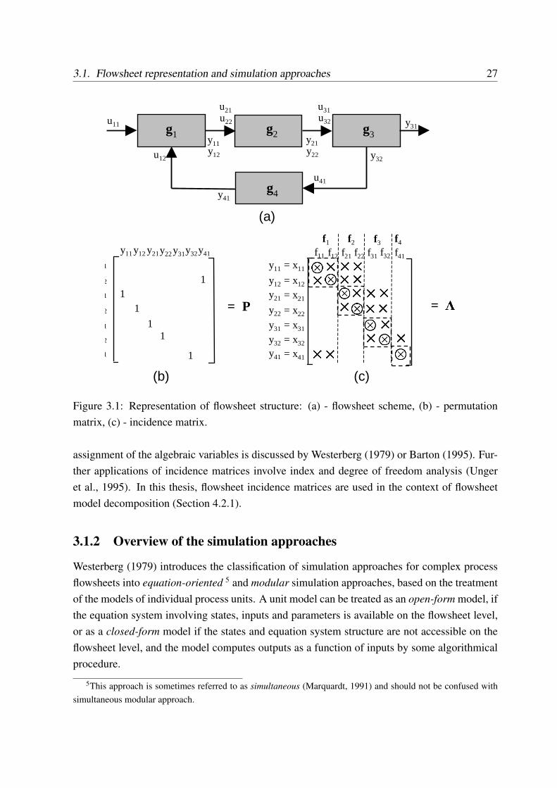
3.1. Flowsheet representation and simulation approaches 27
u11
u12
g1 g2 g3
g4
y11y12
u21u22
y21y22
u31u32 y31
y32
u41
y41
= P
u11
u12
u21
u22
u31
u32
u41
y11 y12 y21y22 y31y32y41
11
11
1
1
f1 f2 f3 f4
= x11
= x12
= x21
= x22
= x31
= x32
= x41
��f11 f12 f21 f22 f31 f32 f41������y11
y12
y21
y22
y31
y32
y41 ��������������� � = Λ(a)
(b) (c)
Figure 3.1: Representation of flowsheet structure: (a) - flowsheet scheme, (b) - permutationmatrix, (c) - incidence matrix.
assignment of the algebraic variables is discussed by Westerberg (1979) or Barton (1995). Fur-ther applications of incidence matrices involve index and degree of freedom analysis (Ungeret al., 1995). In this thesis, flowsheet incidence matrices are used in the context of flowsheetmodel decomposition (Section 4.2.1).
3.1.2 Overview of the simulation approaches
Westerberg (1979) introduces the classification of simulation approaches for complex processflowsheets into equation-oriented 5 and modular simulation approaches, based on the treatmentof the models of individual process units. A unit model can be treated as an open-form model, ifthe equation system involving states, inputs and parameters is available on the flowsheet level,or as a closed-form model if the states and equation system structure are not accessible on theflowsheet level, and the model computes outputs as a function of inputs by some algorithmicalprocedure.
5This approach is sometimes referred to as simultaneous (Marquardt, 1991) and should not be confused withsimultaneous modular approach.
28 Chapter 3. Simulation of process flowsheets
Equation-oriented simulation approachAn equation-oriented approach treats unit models as equation systems and combines them
into a single flowsheet equation system (which is typically of DAE, PDAE or PIDAE type fordynamic models). Couplings between units or phenomena are directly added to the processequation system by means of identity relations between the respective variables. This system isthen solved simultaneously by a general-purpose solver. The solution is a set of variable valuesfor the steady-state simulation, and a set of variable trajectories over time in case of dynamicsimulation.
An overview of the numerical methods to solve DAE systems (BDF, Runge-Kutta, etc.) hasbeen given by Marquardt (1995). Sparse methods are often applied to improve performance.PDAE and PIDAE systems are usually transformed into large DAE systems using generic meth-ods such as the method of lines.
A prerequisite for the use of the equation-oriented approach is the full access to the mathe-matical model of each unit, i.e., to the states, residuals and Jacobian information. DAE solversalso expect consistent initial conditions, the determination of which is not trivial (Marquardt,1995).
Modular simulation approachA modular approach is based on the concept that the models are present in a closed form,
each unit solves its mathematical model autonomously by means of a dedicated solver andexchanges only input and output information with the flowsheet. This effectively splits thetask of solving a large process model of complicated structure into two levels. The unit levelsolves unit models, which are smaller in size compared to the full process model. Specializedsolvers can be applied, which utilize the known equation structure of the unit models to obtainan accurate solution and reduce computational costs (Gilles et al., 1988). Given unit inputs andparameters, unit states and outputs are computed.
The flowsheet level fulfils the coordination task to transfer data between the units accordingto the flowsheet specification, and to converge the solutions of the individual unit models tothe solution of the whole process model. On this level, an iterative algorithm is usually em-ployed. Convergence of the modular simulation can be proven for most problems without astrong nonlinear behavior (Helget, 1997; Liu and Brosilow, 1987). The modular approach iswell suited for cases when the unit models are implemented in the software tools, which onlyprovide interfaces to access their inputs and outputs.
In case of dynamic simulation, the variables vary with time and need to be converged atevery time point. Therefore, the coordination algorithm and the tear stream update procedureperform the convergence of variable trajectories in time instead of the scalar variable values.
3.2. Modular dynamic simulation 29
3.2 Modular dynamic simulation
3.2.1 Iteration in function space
The modular dynamic simulation approach discussed in this section uses an iterative algorithmon the flowsheet level to converge the variable trajectories in time to the final solution.
Convergence propertiesAssume that an iterative process is described as xk+1 = ϕ(xk), where xk is the set of state
variables at iteration k, ϕ(xk) is an explicit representation of the model f(x) = 0 for the solutionwith an iterative process. An iterative process is converged if a fixed point x∗ is reached fork → ∞ such that x∗ = ϕ(x∗). Convergence is characterized by the order of convergencedefined by
||xk+1 − x∗|| ≤ C||xk − x∗||p, (3.5)
where C > 0 and p is the order of convergence. The norm ||xk − x∗|| is a measure of thedeviation at the k-th iteration from the unknown fixed point.
An iterative process that operates on functions x(t) instead of single-valued variables iscalled iteration in function space. Its converged solution is a trajectory described by the functionx∗(t).
Classification of iterations in function spaceHelget (1997) classified the iteration processes in function space into successive approxima-
tion, waveform relaxation and Newton-type iterations, by analogy to the respective approachesto the iterative solution of algebraic equation systems.6
A fixed point iteration (successive approximation) in function space is analogous to a Gauss-Jacobi iteration in linear algebra. The trajectories xk(t) evaluated at the k-th iteration are sub-stituted as inputs to compute the trajectory at the (k + 1)-th iteration:
xk+1(t) = ϕ(xk(t)). (3.6)
The uniqueness of a fixed point x∗ and the convergence of an iterative process is treated bythe Banach fixed point theorem (also known as contraction mapping theorem), which states thatthe iteration process xk = ϕ(xk−1) converges to the same fixed point x∗ for all initial conditionsprovided that Lipschitz condition
||ϕ(x1)− ϕ(x2)|| ≤ q||x1 − x2|| (3.7)6The classification is introduced by Helget (1997) for ODE and DAE systems of differential index 1, but can
be also extended to general systems (Steindorf, 2002).
30 Chapter 3. Simulation of process flowsheets
holds. The Lipschitz constant q must lie in the open interval 0 < q < 1 for the iteration toconverge. Convergence of a fixed point iteration is thus conditional and relies on the propertiesof the iteration function ϕ(x): the function must be smooth, and its graphic should not be steeperthat the graphic of its inputs (Lipschitz smoothness). Strongly nonlinear functions, which donot obey Lipschitz conditions, will not be converged by a fixed point iteration.
The theorem also states that the fixed point iteration provides only first-order convergence.The theorem is valid without modification for the iterations in function spaces where x1(t),x2(t) are functions of time (Helget, 1997).
A waveform relaxation in function space performs a sequential evaluation of the modelequations using the values at the k-th iteration xk(t) for evaluation of the first equation. Everyfollowing equation uses the values at the (k + 1)-th iteration for already computed variables,and the values at the k-th iteration for the others. The iteration is described as
xk+1(t) = ϕw(xk+1(t),xk(t)), (3.8)
ϕwi= ϕi(x
k+11 , .., xk+1
i−1 , xki , ..., x
kn). (3.9)
Waveform relaxation is analogous to a Gauss-Seidel iteration of linear algebra, and alsoshows first-order convergence (Helget, 1997).
A modification of waveform relaxation is block-waveform relaxation where the model is firstdecomposed into equation blocks. The equations within the blocks are solved simultaneously,while the blocks are computed sequentially.
A Newton-waveform iteration can be defined analogously to the Newton iteration as
xk+1(t) = xk(t)− J−1(xk(t)− ϕ(xk(t))
), (3.10)
where J is the Jacobian of the considered iterative system. Helget (1997) shows that for contin-uously differentiable functions, the Newton approach shows second-order convergence. Simi-larly to block-waveform relaxation, a block-Newton iteration can be defined.
3.2.2 Iteration in modular flowsheet simulation
In the framework of modular simulation, the states of the units remain unavailable for the mod-ular algorithm on the flowsheet level, which has to operate with unit inputs u(t) and outputsy(t) only. Hence, the update procedure, e.g. the iteration function ϕ(u(t)), has to be written interms of inputs and is a complex functional of the models of the individual units and couplingsbetween them.
The flowsheet model (3.3) is written in explicit form as
yq(t) = gq(uq(t),pq), ∀q = 1..Nq, (3.11)
up(t) = Ppqyq(t), ∀(p, q). (3.12)
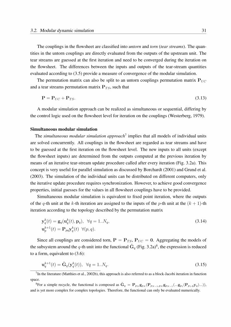
3.2. Modular dynamic simulation 31
The couplings in the flowsheet are classified into untorn and torn (tear streams). The quan-tities in the untorn couplings are directly evaluated from the outputs of the upstream unit. Thetear streams are guessed at the first iteration and need to be converged during the iteration onthe flowsheet. The differences between the inputs and outputs of the tear-stream quantitiesevaluated according to (3.5) provide a measure of convergence of the modular simulation.
The permutation matrix can also be split to an untorn couplings permutation matrix PUC
and a tear streams permutation matrix PTS , such that
P = PUC + PTS. (3.13)
A modular simulation approach can be realized as simultaneous or sequential, differing bythe control logic used on the flowsheet level for iteration on the couplings (Westerberg, 1979).
Simultaneous modular simulationThe simultaneous modular simulation approach7 implies that all models of individual units
are solved concurrently. All couplings in the flowsheet are regarded as tear streams and haveto be guessed at the first iteration on the flowsheet level. The new inputs to all units (exceptthe flowsheet inputs) are determined from the outputs computed at the previous iteration bymeans of an iterative tear-stream update procedure called after every iteration (Fig. 3.2a). Thisconcept is very useful for parallel simulation as discussed by Borchardt (2001) and Grund et al.(2003). The simulation of the individual units can be distributed on different computers, onlythe iterative update procedure requires synchronization. However, to achieve good convergenceproperties, initial guesses for the values in all flowsheet couplings have to be provided.
Simultaneous modular simulation is equivalent to fixed point iteration, where the outputsof the q-th unit at the k-th iteration are assigned to the inputs of the p-th unit at the (k + 1)-thiteration according to the topology described by the permutation matrix
ykq (t) = gq(u
kq(t),pq), ∀q = 1..Nq, (3.14)
uk+1p (t) = Ppqy
kq (t) ∀(p, q).
Since all couplings are considered torn, P = PTS , PUC = 0. Aggregating the models ofthe subsystem around the q-th unit into the functional Gq (Fig. 3.2a)8, the expression is reducedto a form, equivalent to (3.6):
uk+1q (t) = Gq(y
kq (t)), ∀q = 1..Nq. (3.15)
7In the literature (Matthies et al., 2002b), this approach is also referred to as a block-Jacobi iteration in functionspace.
8For a simple recycle, the functional is composed as Gq = PpN gpN (PpN−1,pN gpN−1(...gp1(Pp1,qyq)...)),and is yet more complex for complex topologies. Therefore, the functional can only be evaluated numerically.
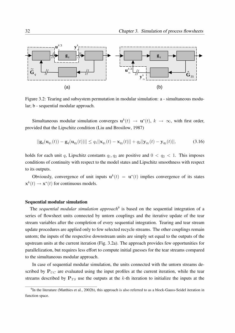
32 Chapter 3. Simulation of process flowsheets
(a) (b)
qG~
qg
TSG1+k
TSu
k
TSy
1+k
qu k
qy
qg
Figure 3.2: Tearing and subsystem permutation in modular simulation: a - simultaneous modu-lar; b - sequential modular approach.
Simultaneous modular simulation converges uk(t) → u∗(t), k → ∞, with first order,provided that the Lipschitz condition (Liu and Brosilow, 1987)
||gq(uq1(t))− gq(uq2(t))|| ≤ q1||xq1(t)− xq2(t)||+ q2||yq1(t)− yq2(t)||, (3.16)
holds for each unit q, Lipschitz constants q1, q2 are positive and 0 < q2 < 1. This imposesconditions of continuity with respect to the model states and Lipschitz smoothness with respectto its outputs.
Obviously, convergence of unit inputs uk(t) = u∗(t) implies convergence of its statesxk(t) → x∗(t) for continuous models.
Sequential modular simulationThe sequential modular simulation approach9 is based on the sequential integration of a
series of flowsheet units connected by untorn couplings and the iterative update of the tearstream variables after the completion of every sequential integration. Tearing and tear streamupdate procedures are applied only to few selected recycle streams. The other couplings remainuntorn; the inputs of the respective downstream units are simply set equal to the outputs of theupstream units at the current iteration (Fig. 3.2a). The approach provides few opportunities forparallelization, but requires less effort to compute initial guesses for the tear streams comparedto the simultaneous modular approach.
In case of sequential modular simulation, the units connected with the untorn streams de-scribed by PUC are evaluated using the input profiles at the current iteration, while the tearstreams described by PTS use the outputs at the k-th iteration to initialize the inputs at the
9In the literature (Matthies et al., 2002b), this approach is also referred to as a block-Gauss-Seidel iteration infunction space.
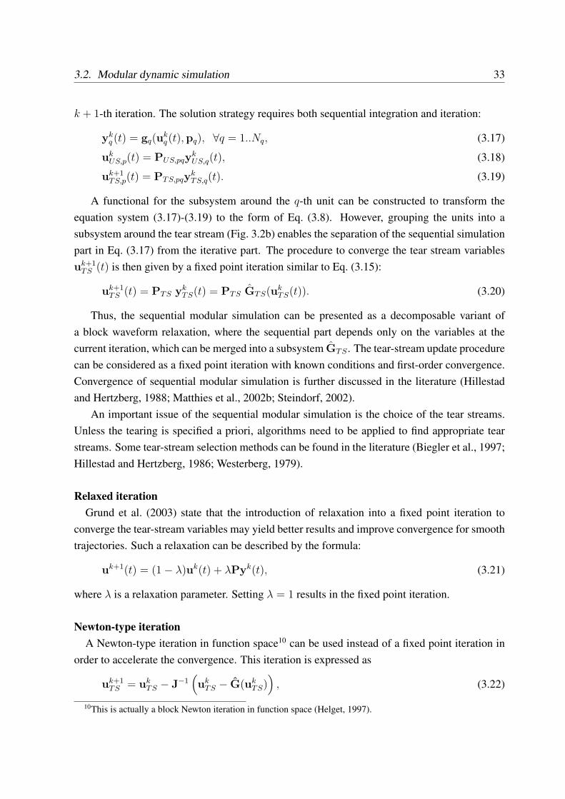
3.2. Modular dynamic simulation 33
k + 1-th iteration. The solution strategy requires both sequential integration and iteration:
ykq (t) = gq(u
kq(t),pq), ∀q = 1..Nq, (3.17)
ukUS,p(t) = PUS,pqy
kUS,q(t), (3.18)
uk+1TS,p(t) = PTS,pqy
kTS,q(t). (3.19)
A functional for the subsystem around the q-th unit can be constructed to transform theequation system (3.17)-(3.19) to the form of Eq. (3.8). However, grouping the units into asubsystem around the tear stream (Fig. 3.2b) enables the separation of the sequential simulationpart in Eq. (3.17) from the iterative part. The procedure to converge the tear stream variablesuk+1
TS (t) is then given by a fixed point iteration similar to Eq. (3.15):
uk+1TS (t) = PTS yk
TS(t) = PTS GTS(ukTS(t)). (3.20)
Thus, the sequential modular simulation can be presented as a decomposable variant ofa block waveform relaxation, where the sequential part depends only on the variables at thecurrent iteration, which can be merged into a subsystem GTS . The tear-stream update procedurecan be considered as a fixed point iteration with known conditions and first-order convergence.Convergence of sequential modular simulation is further discussed in the literature (Hillestadand Hertzberg, 1988; Matthies et al., 2002b; Steindorf, 2002).
An important issue of the sequential modular simulation is the choice of the tear streams.Unless the tearing is specified a priori, algorithms need to be applied to find appropriate tearstreams. Some tear-stream selection methods can be found in the literature (Biegler et al., 1997;Hillestad and Hertzberg, 1986; Westerberg, 1979).
Relaxed iterationGrund et al. (2003) state that the introduction of relaxation into a fixed point iteration to
converge the tear-stream variables may yield better results and improve convergence for smoothtrajectories. Such a relaxation can be described by the formula:
uk+1(t) = (1− λ)uk(t) + λPyk(t), (3.21)
where λ is a relaxation parameter. Setting λ = 1 results in the fixed point iteration.
Newton-type iterationA Newton-type iteration in function space10 can be used instead of a fixed point iteration in
order to accelerate the convergence. This iteration is expressed as
uk+1TS = uk
TS − J−1(uk
TS − G(ukTS)
), (3.22)
10This is actually a block Newton iteration in function space (Helget, 1997).
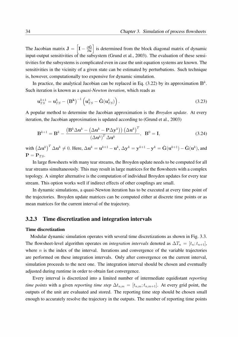
34 Chapter 3. Simulation of process flowsheets
The Jacobian matrix J =[I− ∂G
∂u
]is determined from the block diagonal matrix of dynamic
input-output sensitivities of the subsystem (Grund et al., 2003). The evaluation of these sensi-tivities for the subsystems is complicated even in case the unit equation systems are known. Thesensitivities in the vicinity of a given state can be estimated by perturbations. Such techniqueis, however, computationally too expensive for dynamic simulation.
In practice, the analytical Jacobian can be replaced in Eq. (3.22) by its approximation Bk.Such iteration is known as a quasi-Newton iteration, which reads as
uk+1TS = uk
TS −(Bk
)−1(uk
TS − G(ukTS)
). (3.23)
A popular method to determine the Jacobian approximation is the Broyden update. At everyiteration, the Jacobian approximation is updated according to (Grund et al., 2003)
Bk+1 = Bk −(Bk∆uk − (
∆uk −P∆yk)) (
∆uk)T
(∆uk)T ∆uk, B0 = I, (3.24)
with(∆uk
)T∆uk 6= 0. Here, ∆uk = uk+1−uk, ∆yk = yk+1−yk = G(uk+1)− G(uk), and
P = PTS .In large flowsheets with many tear streams, the Broyden update needs to be computed for all
tear streams simultaneously. This may result in large matrices for the flowsheets with a complextopology. A simpler alternative is the computation of individual Broyden updates for every tearstream. This option works well if indirect effects of other couplings are small.
In dynamic simulations, a quasi-Newton iteration has to be executed at every time point ofthe trajectories. Broyden update matrices can be computed either at discrete time points or asmean matrices for the current interval of the trajectory.
3.2.3 Time discretization and integration intervals
Time discretizationModular dynamic simulation operates with several time discretizations as shown in Fig. 3.3.
The flowsheet-level algorithm operates on integration intervals denoted as ∆Tn = [tn; tn+1],where n is the index of the interval. Iterations and convergence of the variable trajectoriesare performed on these integration intervals. Only after convergence on the current interval,simulation proceeds to the next one. The integration interval should be chosen and eventuallyadjusted during runtime in order to obtain fast convergence.
Every interval is discretized into a limited number of intermediate equidistant reportingtime points with a given reporting time step ∆tn,m = [tn,m; tn,m+1]. At every grid point, theoutputs of the unit are evaluated and stored. The reporting time step should be chosen smallenough to accurately resolve the trajectory in the outputs. The number of reporting time points
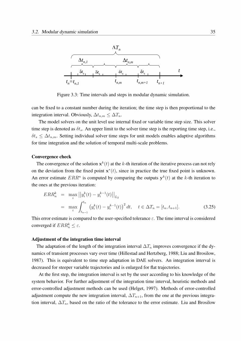
3.2. Modular dynamic simulation 35∆Tn
tn tn+1
t
∆tn,m
tn,m tn,m+1
δts
=tn,1
δts
∆tn,1δts δts
Figure 3.3: Time intervals and steps in modular dynamic simulation.
can be fixed to a constant number during the iteration; the time step is then proportional to theintegration interval. Obviously, ∆tn,m ≤ ∆Tn.
The model solvers on the unit level use internal fixed or variable time step size. This solvertime step is denoted as δts. An upper limit to the solver time step is the reporting time step, i.e.,δts ≤ ∆tn,m. Setting individual solver time steps for unit models enables adaptive algorithmsfor time integration and the solution of temporal multi-scale problems.
Convergence checkThe convergence of the solution xk(t) at the k-th iteration of the iterative process can not rely
on the deviation from the fixed point x∗(t), since in practice the true fixed point is unknown.An error estimate ERRn is computed by comparing the outputs yk(t) at the k-th iteration tothe ones at the previous iteration:
ERRkn = max
i
∣∣∣∣yki (t)− yk−1
i (t)∣∣∣∣
L2
= maxi
∫ tn
tn−1
(yk
i (t)− yk−1i (t)
)2dt, t ∈ ∆Tn = [tn, tn+1]. (3.25)
This error estimate is compared to the user-specified tolerance ε. The time interval is consideredconverged if ERRk
n ≤ ε.
Adjustment of the integration time intervalThe adaptation of the length of the integration interval ∆Tn improves convergence if the dy-
namics of transient processes vary over time (Hillestad and Hertzberg, 1988; Liu and Brosilow,1987). This is equivalent to time step adaptation in DAE solvers. An integration interval isdecreased for steeper variable trajectories and is enlarged for flat trajectories.
At the first step, the integration interval is set by the user according to his knowledge of thesystem behavior. For further adjustment of the integration time interval, heuristic methods anderror-controlled adjustment methods can be used (Helget, 1997). Methods of error-controlledadjustment compute the new integration interval, ∆Tn+1, from the one at the previous integra-tion interval, ∆Tn, based on the ratio of the tolerance to the error estimate. Liu and Brosilow
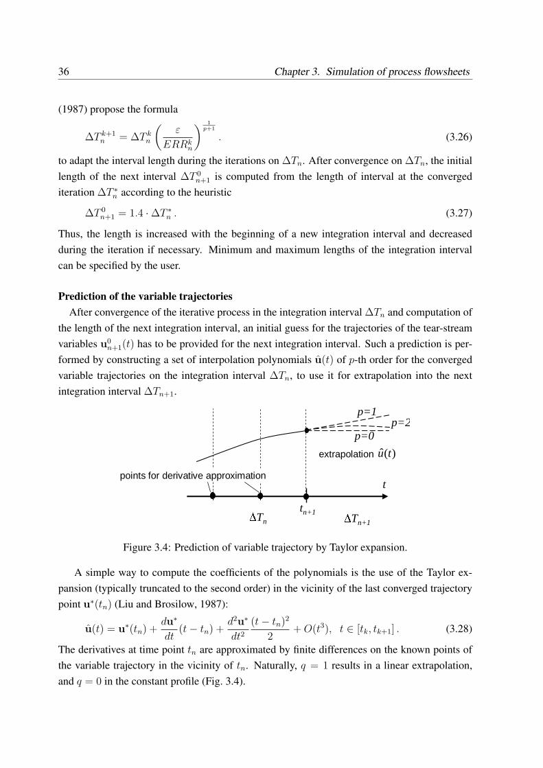
36 Chapter 3. Simulation of process flowsheets
(1987) propose the formula
∆T k+1n = ∆T k
n
(ε
ERRkn
) 1p+1
. (3.26)
to adapt the interval length during the iterations on ∆Tn. After convergence on ∆Tn, the initiallength of the next interval ∆T 0
n+1 is computed from the length of interval at the convergediteration ∆T ∗
n according to the heuristic
∆T 0n+1 = 1.4 ·∆T ∗
n . (3.27)
Thus, the length is increased with the beginning of a new integration interval and decreasedduring the iteration if necessary. Minimum and maximum lengths of the integration intervalcan be specified by the user.
Prediction of the variable trajectoriesAfter convergence of the iterative process in the integration interval ∆Tn and computation of
the length of the next integration interval, an initial guess for the trajectories of the tear-streamvariables u0
n+1(t) has to be provided for the next integration interval. Such a prediction is per-formed by constructing a set of interpolation polynomials u(t) of p-th order for the convergedvariable trajectories on the integration interval ∆Tn, to use it for extrapolation into the nextintegration interval ∆Tn+1.
tn+1
t∆Tn ∆Tn+1
points for derivative approximation
p=0p=2
p=1
extrapolation )(ˆ tu
Figure 3.4: Prediction of variable trajectory by Taylor expansion.
A simple way to compute the coefficients of the polynomials is the use of the Taylor ex-pansion (typically truncated to the second order) in the vicinity of the last converged trajectorypoint u∗(tn) (Liu and Brosilow, 1987):
u(t) = u∗(tn) +du∗
dt(t− tn) +
d2u∗
dt2(t− tn)2
2+ O(t3), t ∈ [tk, tk+1] . (3.28)
The derivatives at time point tn are approximated by finite differences on the known points ofthe variable trajectory in the vicinity of tn. Naturally, q = 1 results in a linear extrapolation,and q = 0 in the constant profile (Fig. 3.4).
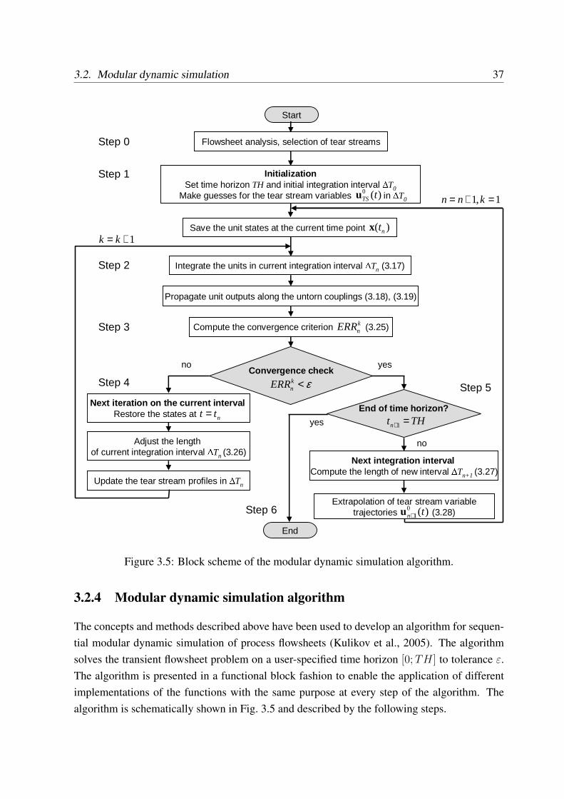
3.2. Modular dynamic simulation 37
Next iteration on the current interval Restore the states at
Flowsheet analysis, selection of tear streams
End of time horizon?
Next integration interval Compute the length of new interval ∆Tn+1 (3.27)
Convergence check
Save the unit states at the current time point
yesno
yes
no
InitializationSet time horizon TH and initial integration interval ∆T0
Make guesses for the tear stream variables in ∆T0
Integrate the units in current integration interval ∆Tn (3.17)
Compute the convergence criterion (3.25)
Extrapolation of tear stream variabletrajectories (3.28)
Update the tear stream profiles in ∆Tn
Adjust the length of current integration interval ∆Tn (3.26)
Propagate unit outputs along the untorn couplings (3.18), (3.19)
Start
End
ε<knERR
THtn =+1
knERR
ntt =
)(0 tTSu
)( ntx
)(01 tn+u
Step 0
Step 1
Step 2
Step 3
Step 4 Step 5
Step 6
1,1 =+= knn
1+= kk
Figure 3.5: Block scheme of the modular dynamic simulation algorithm.
3.2.4 Modular dynamic simulation algorithm
The concepts and methods described above have been used to develop an algorithm for sequen-tial modular dynamic simulation of process flowsheets (Kulikov et al., 2005). The algorithmsolves the transient flowsheet problem on a user-specified time horizon [0; TH] to tolerance ε.The algorithm is presented in a functional block fashion to enable the application of differentimplementations of the functions with the same purpose at every step of the algorithm. Thealgorithm is schematically shown in Fig. 3.5 and described by the following steps.
38 Chapter 3. Simulation of process flowsheets
Algorithm: sequential modular dynamic simulation
Step 0. The simulation is preceded with flowsheet analysis where the closed recycles in theflowsheet are identified, and tear streams (one stream per recycle) are chosen by means ofheuristics (Hillestad and Hertzberg, 1988) or a graph analysis algorithm (Westerberg, 1979).The step is omitted if the user defines the set of tear streams a priori.
Step 1. Before the start of the integration, the total time horizon and the initial integrationinterval ∆T0 = [t0; t1] are set, the external inputs are initialized, and initial guesses for thetrajectories of the tear stream variables u0
TS(t) on the interval ∆T0 are provided.
Step 2. With this information, the sequential integration of the units along the untorn cou-plings is carried out for the integration interval ∆Tn (Eq. (3.17)-(3.18)), until all unit outputsto the tear streams yk
TS(t) are computed.
Step 3. After completion of the sequential integration, an estimate of the convergence errorERRk (3.25) is computed for all tear stream variables in the current integration interval(Section 3.2.3). The obtained values are compared to the tolerance ε.
Step 4. If the error is larger than the tolerance ε, the convergence criterion is not fulfilled,and another iteration on the current integration interval ∆Tn is performed. A tear-streamupdate procedure (Section 3.2.2) is applied to all tear-stream variables to compute their es-timates uk+1
TS (t) at the next iteration. After the trajectories of the tear-stream variables areupdated, the sequential integration on the interval (Step 2) is repeated. To facilitate conver-gence, an adjustment of the integration interval length can be performed before starting withthe k + 1-th iteration (Section 3.2.3).
Step 5. Otherwise, if the convergence criterion is met, the iteration on the current integrationinterval is considered converged. Then, the next integration interval ∆Tn+1 is initialized,with the length adjusted according to the strategy discussed in Section 3.2.3. To proceedwith the integration on the next interval, initial guesses for the trajectories of the tear-streamvariables u0
TSn+1(t) have to be predicted by means of extrapolation (Section 3.2.3). Then,
sequential integration (Step 2) is performed for the next integration interval.
Step 6. The integration continues until the end of the simulation time horizon is reached.
The modular simulation algorithm is implemented in the integration platform CHEOPS.CHEOPS is a software platform for heterogeneous process modeling developed at the Lehrstuhlfur Prozesstechnik starting from 1997 (Schopfer et al., 2004; Schopfer, 2005; von Wedel andMarquardt, 1999). The architecture and functions of CHEOPS are described in Appendix A.
3.3. Software implementation 39
3.3 Software implementation
This section and Appendix A discuss the software-technical solution for the modular simulationof the complex flowsheets using the integration platform CHEOPS and simulation softwaretools.
3.3.1 Requirements for software tool integration
Integration of software tools becomes necessary when a problem scope is beyond the limits offunctionality of a single software tool, but is likely to be solved by a combination of differenttools that are not directly connected to each other. Tool integration solution should execute twoequally important tasks, namely
• to provide mechanisms for automatic data exchange and consistent data translation be-tween the software tools, and
• to provide a command interface to control tool execution and data exchange.
In order to employ a software tool in the coupled simulation, the tool must comply with thefollowing requirements:
• A software tool has to solve the declared model with an appropriate solver coupled to themodel. If the tool only provides a model declaration, it has to be coupled to an externalsolver before integration.
• A documentation of the model equations solved in the software tool has to be available.
• A standard control interface to enable the external client to execute the simulation.
• A documented data interface to provide access to the model data, configurable duringruntime.
3.3.2 Simulation software tools
Model sourceA model implemented in the software tool is denoted as model source in the text. An open-
form model source provides the full information on the states, residuals and Jacobian of themodel. In a closed-form model source, only inputs and outputs of the model can be accessed.
40 Chapter 3. Simulation of process flowsheets
Classification of simulation software toolsThe range of software tools available for process modeling and simulation can be roughly
classified into several groups.Modeling environments are used for the development of models in a formalized modeling
language, where the model variables, equations and initial/boundary conditions can be repre-sented. Examples of modeling languages are Modelica,11 CapeML (Bischof et al., 2005) andgPROMS modeling language (Barton, 1992; Pantelides, 1996). Modeling environments providedeclarative model representations and open-form model sources.
General-purpose simulators are software packages that, given a formalized mathematicalmodel or an open-form model source, solve it using the built-in general-purpose solution al-gorithm. Such solvers are developed to solve a broad class of mathematical problems (e.g.DAE systems of differential index 1) using generally applicable numerical methods (such asNewton-type iteration, Runge-Kutta methods, sparse matrix techniques, etc.). The solvers canbe implemented within modeling environments (gPROMS12, MATLAB13), as separate simula-tors (e.g. DIVA, Marquardt et al. (1990)), as legacy code libraries or their components (e.g.LIMEX, Ehrig et al. (1998); lptNumerics, Schopfer et al (2005)). They provide open-form orclosed-form model sources to an external client.
Special-purpose simulators are developed for the simulation of specific processes repre-sented by the mathematical models with an a priori known structure. They apply specializedalgorithms tailored to specific problem classes, or algorithms with improved accuracy or conver-gence properties. Special-purpose simulators are available as commercial or academic softwaretools, and as legacy codes. Commercial special-purpose simulators often provide a user-friendlygraphical user interface, where the formalization of the mathematical model’s equation system,its assumptions and constitutive relations is transparent to the user. The tool’s capabilities tomodify the models are thus developer-restricted. Examples are CFD solvers (FLUENT14, CFX,etc.) process simulation tools like e.g. Parsival15 for crystallization problems, etc. Commercialsimulators usually provide only closed-form model sources.
Flowsheet simulators (such as Aspen+16) perform the simulation of a process flowsheetusing modules and models available in the simulator. Flowsheet simulators usually use estab-lished, intrinsic models of the unit operations, although some simulators support user-providedmodels in explicit form. The use of flowsheet simulators is reasonable if the intrinsic models inthe simulator are sufficient; otherwise, general-purpose or specialized simulation tools have to
11OpenModelica project: http://www.ida.liu.se/labs/pelab/modelica/OpenModelica.html (accessed 05.02.07).12Developer: Process System Enterprise, www.psenterprise.com.13Developer: Mathworks Inc., www.matlab.com.14Developer: Fluent Inc., www.fluent.com.15Developer: CiT GmbH, www.cit-wulkow.com.16Developer: Aspen Technology Inc., www.aspentech.com.
3.3. Software implementation 41
be employed. Flowsheet simulators provide closed-form model sources.
Software tool roles in the simulationA software tool can be used in the tool integration
• in the role of a simulation service, when it declares the external communication inter-face that enables the external client to access the tool data and to set up and control theexecution of the simulation;
• in the role of data/model source provider, when its external interface only supports accessto the internal data or model information, but not the execution of commands;
• in the role of master, when the tool acts as an external client, i.e., establishes connection,accesses data and controls the simulation in the other tool acting as a simulation service.
3.3.3 Tool integration solutions
There are several possible options of tool integration.Tool-to-tool coupling is employed if a dedicated solution is developed for the coupling be-
tween two specific tools. One tool acts as a master, controls the simulation and performs calls tothe second tool acting as a simulation service. If two tools have compatible interfaces, a directcoupling can be established (Fig. 3.6a).
However, most commercial software tool developers provide incompatible tool-specificlegacy interfaces. Therefore, a dedicated software component called tool wrapper has to bedeveloped. It covers the tool with a wrapper’s own interface, and acts as a ”transparent” medi-ator to translate data and interface commands between the formats supported by both the tooland the client. Such a wrapper can be developed for a specific combination of two softwaretools (Fig. 3.6b). This wrapper is usually tool- and problem-specific and does not use standardinterfaces. This solution is widely employed for problem-focused researches.
If the master tools use a standard interface, it is sufficient to have a single tool wrapperfor a software tool to be used for integration with any other master tool, instead of developinga dedicated wrapper for each pair of simulators. An example of such a standard interface isCAPE-OPEN (Appendix A).
For problems such as flowsheet simulation, where multiple models are employed, the cou-pling with integration platform can be used (Fig. 3.6c). A special top-level software (integrationplatform) is employed as a master. An integration platform is a special software that acts as amaster and executes the top-level coordination of the simulation. For the flowsheet simula-tion problems, it implements flowsheet-level functionality such as setup of the flowsheet and
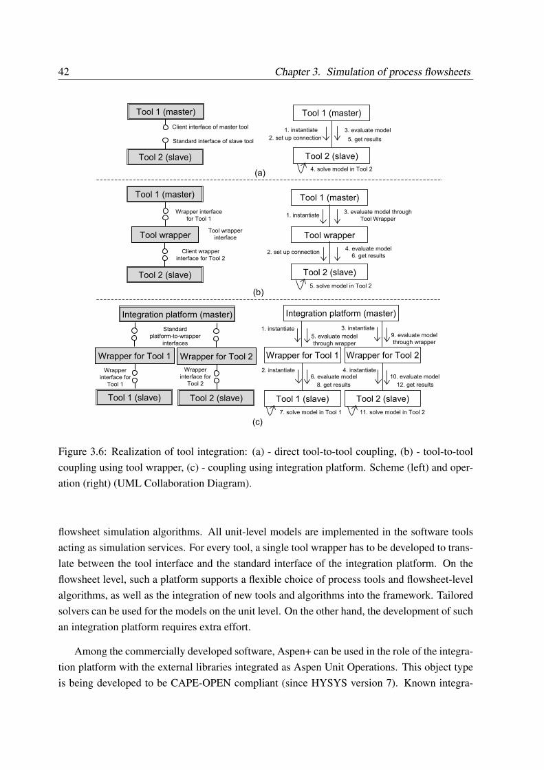
42 Chapter 3. Simulation of process flowsheets
(b)
(a)
(c)
Tool 1 (master)
Tool 2 (slave)
Tool wrapperTool wrapper
interface
Client wrapper
interface for Tool 2
Tool 1 (master)
Tool wrapper
Tool 2 (slave)
1. instantiate
2. set up connection
3. evaluate model through
Tool Wrapper
4. evaluate model
6. get results
Tool 1 (master)
Tool 2 (slave)
Standard interface of slave tool
Tool 1 (master)
Tool 2 (slave)
1. instantiate 3. evaluate model
2. set up connection 5. get results
Integration platform (master)
Wrapper for Tool 1
Tool 1 (slave)
Wrapper for Tool 2
Tool 2 (slave)
Integration platform (master)
Standard
platform-to-wrapper
interfaces
Wrapper
interface for
Tool 1
Wrapper for Tool 1
Tool 1 (slave)
Wrapper for Tool 2
Tool 2 (slave)
Wrapper
interface for
Tool 2
1. instantiate
2. instantiate
5. evaluate model
through wrapper
6. evaluate model
3. instantiate
4. instantiate
9. evaluate model
through wrapper
10. evaluate model
5. solve model in Tool 2
4. solve model in Tool 2
7. solve model in Tool 1 11. solve model in Tool 2
8. get results 12. get results
Client interface of master tool
Wrapper interface
for Tool 1
Figure 3.6: Realization of tool integration: (a) - direct tool-to-tool coupling, (b) - tool-to-toolcoupling using tool wrapper, (c) - coupling using integration platform. Scheme (left) and oper-ation (right) (UML Collaboration Diagram).
flowsheet simulation algorithms. All unit-level models are implemented in the software toolsacting as simulation services. For every tool, a single tool wrapper has to be developed to trans-late between the tool interface and the standard interface of the integration platform. On theflowsheet level, such a platform supports a flexible choice of process tools and flowsheet-levelalgorithms, as well as the integration of new tools and algorithms into the framework. Tailoredsolvers can be used for the models on the unit level. On the other hand, the development of suchan integration platform requires extra effort.
Among the commercially developed software, Aspen+ can be used in the role of the integra-tion platform with the external libraries integrated as Aspen Unit Operations. This object typeis being developed to be CAPE-OPEN compliant (since HYSYS version 7). Known integra-
3.4. Case study: pentaerythritol crystallization 43
tion platforms of academic origin include MpCCI,17 specialized in the structural coupling forthe simulation of complex multi-phase processes, and CHEOPS. CHEOPS and the respectivesoftware tool wrappers are described in more detail in Appendix A and are used in the presentthesis as the flowsheet-level integration platform.
3.4 Case study: pentaerythritol crystallization
Application of modular dynamic simulation employing the CHEOPS integration platform to aflowsheeting problem is illustrated by means of a case study of the crystallization of pentaery-thritol from aqueous solution. The goal is the rigorous prediction of the crystal size distributionin the product stream during the transient process. The process flowsheet is simulated withrigorous unit models, such as a particle population balance model with process kinetics for thecrystallizer. The simulation framework poses no limitations on the complexity of the modelsand the flowsheet. However, the illustrative case study presents a significantly simplified flow-sheet compared to real industrial processes. Nevertheless, such dynamic simulation alreadyprovides insight to the process behavior, based on which sophisticated representations of theprocess can be developed.
3.4.1 Problem description
The illustrative case study presented in this section describes the evaporative crystallization ofpentaerythritol (PE, tetramethylolmethan, C(CH2OH)4), a compound used in the productionof alkyd resins, lacquers and additives. It is produced by means of chemical reaction betweenformaldehyde and acetaldehyde in a base environment with subsequent crystallization. Thephysico-chemical properties of PE are available in the chemical data bases. Experiments for thecrystallization kinetics of PE and its modeling were carried out by a number of authors. Mostrecent studies have been published by Chianese et al. (1995a), Chianese et al. (1995b) and OMeadhra et al. (1996b).
Process flowsheetThe investigated process flowsheet in Figure 3.7 (Kulikov et al., 2005) comprises the major
steps of a typical crystallization process: (a) preparation of the concentrated solution; (b) crys-tallization; (c) separation of the product. The flowsheet consists of four units: an evaporator(1), a crystallizer (2), a hydrocyclone (3), and a mixer (4). It employs one recycle stream toincrease the product yield. In the evaporator, the solution is heated to 102◦C and is partially
17See http://www.scai.fraunhofer.de/mpcci.html for details (accessed 05.02.07).
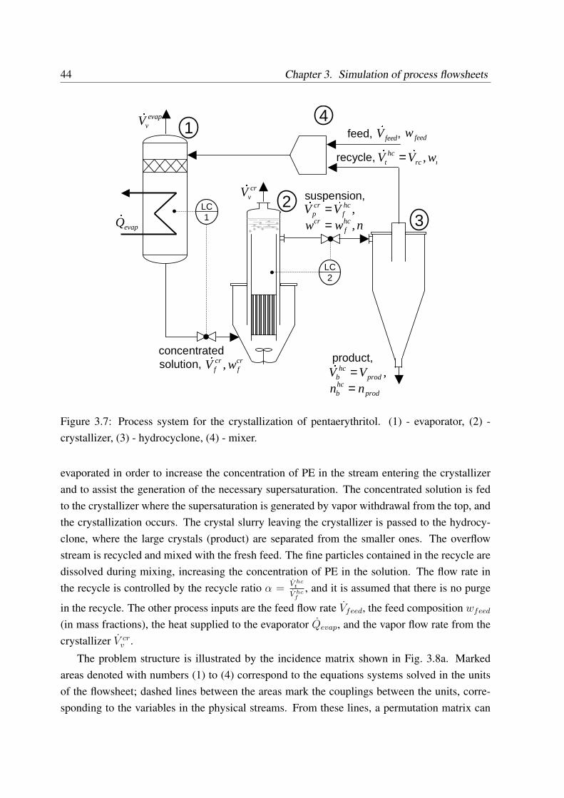
44 Chapter 3. Simulation of process flowsheets
feed, ,
suspension,
product,concentrated solution,
1
3
4
LC2
recycle,
evapvV&
evapQ&crf
crf wV ,&
2LC1
crvV&
nwwVV
hcf
cr
hcf
crp
,,
== && feedV&
rcrchc
t wVV ,&& =
prodhcb
prodhc
b
nnVV
== ,&
feedw
Figure 3.7: Process system for the crystallization of pentaerythritol. (1) - evaporator, (2) -crystallizer, (3) - hydrocyclone, (4) - mixer.
evaporated in order to increase the concentration of PE in the stream entering the crystallizerand to assist the generation of the necessary supersaturation. The concentrated solution is fedto the crystallizer where the supersaturation is generated by vapor withdrawal from the top, andthe crystallization occurs. The crystal slurry leaving the crystallizer is passed to the hydrocy-clone, where the large crystals (product) are separated from the smaller ones. The overflowstream is recycled and mixed with the fresh feed. The fine particles contained in the recycle aredissolved during mixing, increasing the concentration of PE in the solution. The flow rate inthe recycle is controlled by the recycle ratio α =
V hct
V hcf
, and it is assumed that there is no purge
in the recycle. The other process inputs are the feed flow rate Vfeed, the feed composition wfeed
(in mass fractions), the heat supplied to the evaporator Qevap, and the vapor flow rate from thecrystallizer V cr
v .
The problem structure is illustrated by the incidence matrix shown in Fig. 3.8a. Markedareas denoted with numbers (1) to (4) correspond to the equations systems solved in the unitsof the flowsheet; dashed lines between the areas mark the couplings between the units, corre-sponding to the variables in the physical streams. From these lines, a permutation matrix can
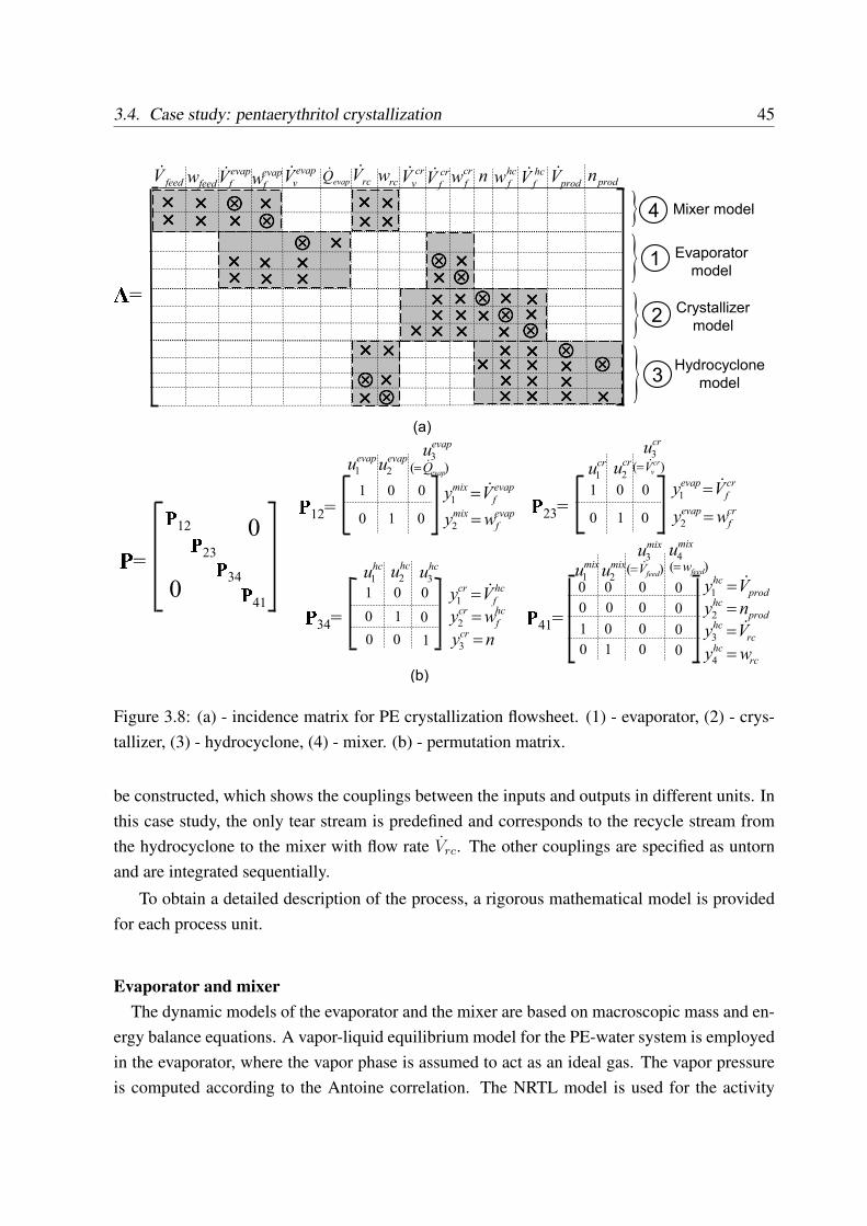
3.4. Case study: pentaerythritol crystallization 45
feedV& n hc
fw�=
evap
vV& cr
fV& cr
fwfeedw rcwrcV& hc
fV&
prodV&evapQ& prodnevap
fV& evap
fw
��������
����
����
����
�������� ���� ����
��������
��������
��������
���� ���� ��������
��������
����
���� ���� ����
���������������� ����
cr
vV&
����
��������
��������
������������ ����
����
����
���� ������������
�������� ����
������������
����
���� ���� ����
���� ����
��������
����
}
}}
}
Mixer model
Evaporator
model
Crystallizer
model
Hydrocyclone
model
4
1
2
3
�=
(a)�12�
23�34�
41
0
0
�12=
evap
f
mix Vy &=1
evap
f
mix wy =2
evapu1evapu2
evapu3)( evapQ&=
1
1
0
0
0
0
�23=
cr
f
evap Vy &=1
cr
f
evap wy =2
cru1cru2
cru3)( cr
vV&=
1
1
0
0
0
0�34=
hc
f
cr Vy &=1hc
f
cr wy =2
hcu1hcu2
hcu31
1
0
0
0
0
0 0 1 nycr =3
�41=
prod
hc Vy &=1
prod
hc ny =2
mixu1mixu2
mixu3
0
0
0
0
0
0
1 0 0rc
hc Vy &=3
0 1 0
mixu4
0
0
0
0
)( feedV&= )( feedw=
rc
hc wy =4
(b)
Figure 3.8: (a) - incidence matrix for PE crystallization flowsheet. (1) - evaporator, (2) - crys-tallizer, (3) - hydrocyclone, (4) - mixer. (b) - permutation matrix.
be constructed, which shows the couplings between the inputs and outputs in different units. Inthis case study, the only tear stream is predefined and corresponds to the recycle stream fromthe hydrocyclone to the mixer with flow rate Vrc. The other couplings are specified as untornand are integrated sequentially.
To obtain a detailed description of the process, a rigorous mathematical model is providedfor each process unit.
Evaporator and mixerThe dynamic models of the evaporator and the mixer are based on macroscopic mass and en-
ergy balance equations. A vapor-liquid equilibrium model for the PE-water system is employedin the evaporator, where the vapor phase is assumed to act as an ideal gas. The vapor pressureis computed according to the Antoine correlation. The NRTL model is used for the activity
46 Chapter 3. Simulation of process flowsheets
coefficients in the liquid phase. The other model parameters are taken from the property databank available in the employed software.
CrystallizerThe crystallizer is modeled by means of a population balance model, which computes the
particle size distribution n(L, t) in the crystallizer under the assumption of constant volume Vcr
and ideal mixing within the crystallizer. The kinetic relations are adopted from O Meadhra etal. (1996b), and were validated with industrial process data by Placido et al. (2002). The em-ployed crystallization kinetics involve particle growth and secondary nucleation due to attrition.Primary nucleation is neglected. The crystal growth rate, Gkin(σ, L), is a function of the super-saturation of the solution and the crystal size. The attrition is described by a negative growthrate Gatt(L), which accounts for abrasion of large crystals, and the nucleation rate B(σ, L),which introduces the attrition fragments. The effective growth rate Geff (σ, L) is a sum of crys-tal growth rate and negative growth rate due to attrition. The population balance is augmentedby solute mass and unit energy balances.
A detailed description of the model is presented in Appendix B.1 and by Kulikov et al.(2005).
HydrocycloneA hydrocyclone is used for liquid-solid separation of suspensions with large flow rates. The
suspension enters at the top of the hydrocyclone in tangential direction, which forces the liquidin the volume of the apparatus to rotation. The centrifugal force in the arising eddy moves largerparticles to the outer wall of the apparatus, where they settle down to the product stream. Small,lightweight particles are removed through the apex tube from the top of the apparatus, and aredirected to the recycle stream.
The separation process in the hydrocyclone unit is characterized by grade efficiency curvesthat relate mass density of particles of a certain size in the bottom product stream (mass recov-ery) to the mass density in the feed. For a known grade efficiency curve, particle distributionsin the overflow (the recycle stream) and underflow (the product stream) can be computed. Anoverview of some modeling approaches to obtain the curve is presented by Braun (1989) andreferences therein.
In this study, a three-compartment quasi-stationary model developed by Braun (1989) isemployed. The model describes particle separation as a result of the interplay of settling inthe centrifugal force field and turbulent diffusion. The population balance model is formulatedas partial differential equations representing particle transport along the axial coordinate ofthe hydrocyclone and between the regions with bottom-directed and top-directed flow. Theequations are discretized into a system of differential equations for a fixed number of particle
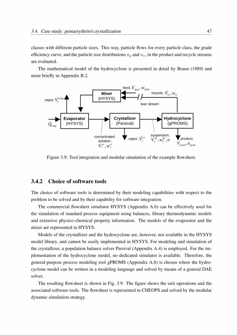
3.4. Case study: pentaerythritol crystallization 47
classes with different particle sizes. This way, particle flows for every particle class, the gradeefficiency curve, and the particle size distributions np and nrc in the product and recycle streamsare evaluated.
The mathematical model of the hydrocyclone is presented in detail by Braun (1989) andmore briefly in Appendix B.2.
suspension,product,
vapor,
concentrated solution,
recycle,
feed, ,
Crystallizer(Parsival)
Hydrocyclone(gPROMS)
Evaporator(HYSYS)
Mixer(HYSYS)
vapor,
tear stream
evapvV&
evapQ&crf
crf wV ,& cr
vV&feedV&
rcrc wV ,&,hc
fV&prodprod nV ,&
feedw
nwhcf ,
Figure 3.9: Tool integration and modular simulation of the example flowsheet.
3.4.2 Choice of software tools
The choice of software tools is determined by their modeling capabilities with respect to theproblem to be solved and by their capability for software integration.
The commercial flowsheet simulator HYSYS (Appendix A.6) can be effectively used forthe simulation of standard process equipment using balances, library thermodynamic modelsand extensive physico-chemical property information. The models of the evaporator and themixer are represented in HYSYS.
Models of the crystallizer and the hydrocyclone are, however, not available in the HYSYSmodel library, and cannot be easily implemented in HYSYS. For modeling and simulation ofthe crystallizer, a population balance solver Parsival (Appendix A.4) is employed. For the im-plementation of the hydrocyclone model, no dedicated simulator is available. Therefore, thegeneral-purpose process modeling tool gPROMS (Appendix A.8) is chosen where the hydro-cyclone model can be written in a modeling language and solved by means of a general DAEsolver.
The resulting flowsheet is shown in Fig. 3.9. The figure shows the unit operations and theassociated software tools. The flowsheet is represented in CHEOPS and solved by the modulardynamic simulation strategy.
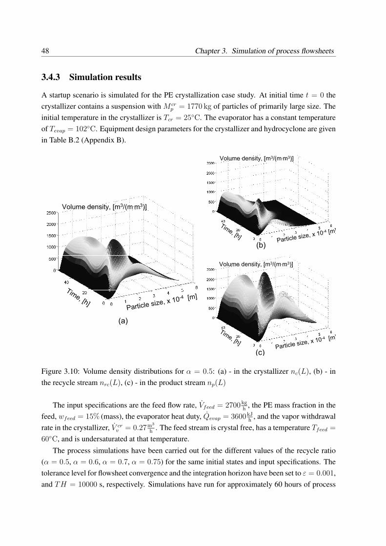
48 Chapter 3. Simulation of process flowsheets
3.4.3 Simulation results
A startup scenario is simulated for the PE crystallization case study. At initial time t = 0 thecrystallizer contains a suspension with M cr
p = 1770 kg of particles of primarily large size. Theinitial temperature in the crystallizer is Tcr = 25◦C. The evaporator has a constant temperatureof Tevap = 102◦C. Equipment design parameters for the crystallizer and hydrocyclone are givenin Table B.2 (Appendix B).
(a)
Time, [h]
Volume density, [m3/(m.m3)]
(c)
(b)Particle
size, x 10
-4 [m]Time, [h]
Volume density, [m3/(m.m3)]
Particle size, x
10-4 [m]
Particle size, x
10-4 [m]
Time, [h]
Volume density, [m3/(m.m3)]
Figure 3.10: Volume density distributions for α = 0.5: (a) - in the crystallizer nc(L), (b) - inthe recycle stream nrc(L), (c) - in the product stream np(L)
The input specifications are the feed flow rate, Vfeed = 2700kgh
, the PE mass fraction in thefeed, wfeed = 15% (mass), the evaporator heat duty, Qevap = 3600kJ
h, and the vapor withdrawal
rate in the crystallizer, V crv = 0.27m3
h. The feed stream is crystal free, has a temperature Tfeed =
60◦C, and is undersaturated at that temperature.
The process simulations have been carried out for the different values of the recycle ratio(α = 0.5, α = 0.6, α = 0.7, α = 0.75) for the same initial states and input specifications. Thetolerance level for flowsheet convergence and the integration horizon have been set to ε = 0.001,and TH = 10000 s, respectively. Simulations have run for approximately 60 hours of process
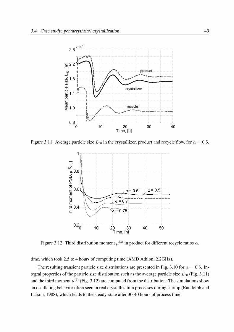
3.4. Case study: pentaerythritol crystallization 49
0 5 10 15 20 25 30 35 400.6
0.8
1
1.2
1.4
1.6
1.8
2
2.2
2.4
2.6x 10
-4
Time, h
Average particle size d50
crystallizer
product
recycle
Time, [h]0 10 20 30 40
2.6
2.2
1.8
1.4
1.0
0.6
Mean particle size, L50, [m
]
Figure 3.11: Average particle size L50 in the crystallizer, product and recycle flow, for α = 0.5.
0 10 20 30 40 500.2
0.4
0.6
0.8
1
Time, [h]
Third moment of PSD, µ(3) , [ ] � = 0.5 � = 0.6 � = 0.7 � = 0.75
Figure 3.12: Third distribution moment µ(3) in product for different recycle ratios α.
time, which took 2.5 to 4 hours of computing time (AMD Athlon, 2.2GHz).
The resulting transient particle size distributions are presented in Fig. 3.10 for α = 0.5. In-tegral properties of the particle size distribution such as the average particle size L50 (Fig. 3.11)and the third moment µ(3) (Fig. 3.12) are computed from the distribution. The simulations showan oscillating behavior often seen in real crystallization processes during startup (Randolph andLarson, 1988), which leads to the steady-state after 30-40 hours of process time.
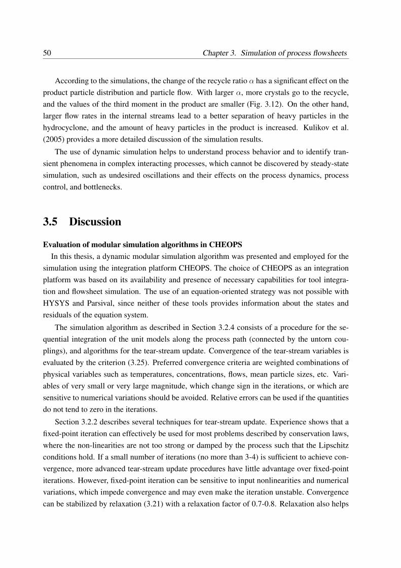
50 Chapter 3. Simulation of process flowsheets
According to the simulations, the change of the recycle ratio α has a significant effect on theproduct particle distribution and particle flow. With larger α, more crystals go to the recycle,and the values of the third moment in the product are smaller (Fig. 3.12). On the other hand,larger flow rates in the internal streams lead to a better separation of heavy particles in thehydrocyclone, and the amount of heavy particles in the product is increased. Kulikov et al.(2005) provides a more detailed discussion of the simulation results.
The use of dynamic simulation helps to understand process behavior and to identify tran-sient phenomena in complex interacting processes, which cannot be discovered by steady-statesimulation, such as undesired oscillations and their effects on the process dynamics, processcontrol, and bottlenecks.
3.5 Discussion
Evaluation of modular simulation algorithms in CHEOPSIn this thesis, a dynamic modular simulation algorithm was presented and employed for the
simulation using the integration platform CHEOPS. The choice of CHEOPS as an integrationplatform was based on its availability and presence of necessary capabilities for tool integra-tion and flowsheet simulation. The use of an equation-oriented strategy was not possible withHYSYS and Parsival, since neither of these tools provides information about the states andresiduals of the equation system.
The simulation algorithm as described in Section 3.2.4 consists of a procedure for the se-quential integration of the unit models along the process path (connected by the untorn cou-plings), and algorithms for the tear-stream update. Convergence of the tear-stream variables isevaluated by the criterion (3.25). Preferred convergence criteria are weighted combinations ofphysical variables such as temperatures, concentrations, flows, mean particle sizes, etc. Vari-ables of very small or very large magnitude, which change sign in the iterations, or which aresensitive to numerical variations should be avoided. Relative errors can be used if the quantitiesdo not tend to zero in the iterations.
Section 3.2.2 describes several techniques for tear-stream update. Experience shows that afixed-point iteration can effectively be used for most problems described by conservation laws,where the non-linearities are not too strong or damped by the process such that the Lipschitzconditions hold. If a small number of iterations (no more than 3-4) is sufficient to achieve con-vergence, more advanced tear-stream update procedures have little advantage over fixed-pointiterations. However, fixed-point iteration can be sensitive to input nonlinearities and numericalvariations, which impede convergence and may even make the iteration unstable. Convergencecan be stabilized by relaxation (3.21) with a relaxation factor of 0.7-0.8. Relaxation also helps
3.5. Discussion 51
to filter out minor numerical integration errors in the solution trajectory.A major improvement in convergence can be achieved by the quasi-Newton method (3.23).
The estimation of the Jacobian matrix can be done by the Broyden method (3.24). However, theapplication of this method in CHEOPS met some difficulties, such as the time dependency ofthe coefficients of the Broyden matrix, their variation at the end of the integration interval, andthe necessity to calculate the Broyden matrix for all tear-stream variables simultaneously, whichis in conflict with the architecture of the simulation algorithm implementation. Application ofquasi-Newton iteration with Broyden update showed that the number of iterations is signifi-cantly reduced if fixed-point iterations converge slowly (four or more iterations per interval),but in some cases oscillations at the ends of the integration interval are produced.
The method for adjustment of the size of the integration interval ∆Tn proposed by Liu andBrosilow (1987) has to be evaluated critically. Simulations show that an adjustment of the timeinterval during the iterations has a negative effect on performance. Hence, the adjustment ofthe integration interval in the intermediate iterations was disabled. The size of the interval wasonly adjusted at the beginning of new integration intervals (as shown in Fig. 3.5). A restrictionwas set on the maximum error value in the converged iterations, so that the time interval is onlyadjusted if ERR∗
n < εad < ε. The heuristics (3.27) to adjust the size of the next integrationinterval should be replaced with a better expression. The time interval adjustment should notdepend on the absolute value of the convergence criterion, but rather on its rate of change.
The choice of the limit sizes of the integration intervals has to be considered carefully.Too short intervals require too many intermediate intervals in the horizon, even if few callsare necessary for a single interval. Simulations with long intervals converge slowly, increasingoverall computational time and reducing stability, and are more sensitive to the initial guess ofthe tear-stream variables.
Simulations also showed that the most stable prediction of the tear stream variable trajec-tories on the new integration intervals is a constant profile or an extrapolation of linear order.Taylor expansion or interpolation of higher orders may fail to provide a good estimation by pro-ducing too stiff trajectories or violating the bounds of the physical variables for long integrationintervals. A more accurate prediction of the tear-stream variable trajectory can be done if thesensitivities of the tear streams are available to be used in an extrapolation model for the variabletrajectory, and a formulation similar to quasi-Newton update is employed. The development ofsuch a procedure remains outside of the scope of the present thesis.
Restrictions and accuracy of modular dynamic simulationIn the reviewed literature on modular simulation, little attention is paid to other factors affect-
ing convergence of the modular algorithm. Obviously, convergence of the modular simulation islimited by the convergence of the unit-level integration. Several kinds of errors may arise here.
52 Chapter 3. Simulation of process flowsheets
The integration in a unit may diverge or produce a physically meaningless, strongly nonlineartrajectory. In particular, this can happen if the complex DAE system is solved with inconsis-tent initial values. Hence, consistent initial values had to be computed at the beginning of thesimulation, and reset to the last converged trajectory point at the beginning of every integrationinterval. The numerical simulation of a unit model may produce numerical errors representedas large peaks or oscillations. Extrapolation methods and simulation failures may result in vi-olation of the limits of physical variables. All mentioned effects retard the convergence on theflowsheet level.
These cases have to be accounted for in the modular dynamic simulation algorithm. Toreduce the effect of numerical errors, filtering functions and relaxation can be used at the inter-mediate iterations. To detect divergence of the simulation in a unit, dedicated procedures basedon gradient analysis, variable limit detection or error evaluation need to be developed. Thesimulation on a diverged interval should be restarted with a different initial guess, or a softwareexception has to be thrown in case such divergence is permanent.
Another problem of algorithmic implementation is the control of the simulation accuracyand performance. A possible measure is the change of the error tolerance of the unit integrationduring the iterations on a single time interval. A reduction of the accuracy for the first iterationenables a quick computation of the approximate variable trajectories, which are improved dur-ing the following iterations employing a tighter tolerance. As a result, the overall simulationtime can be reduced.
A significant issue is the accuracy of function representations over time. In CHEOPS, thevariable values are stored at discrete reporting time points. The accuracy of the transient sim-ulations is affected by the number and position of these reporting points and by the quality ofpolynomial interpolation between these points. A small number of reporting points results in alower accuracy in the computation of intermediate points. A large number is time and memoryconsuming and is often unnecessary for smooth variable trajectories.
Future development of modular simulation algorithms should address the discussed prob-lems and opportunities in order to improve and effectively apply the developed method.
Chapter 4
Coupled simulation of fluid dynamics andcrystallization
The solution of the flowsheeting problem by the modular dynamic simulation techniques dis-cussed in the previous chapter can be applied to the simulation of complex processes involvingseveral coupled physico-chemical phenomena. The phenomena are represented as units of ageneralized flowsheet, where a unit represents a process entity described by a mathematicalmodel, such as a physical apparatus, phenomenon or part of the process domain. The unitsof the generalized flowsheet are connected by information streams responsible for informationexchange between the units. Scale integration methods are implemented to bridge between thescales of the coupled CFD-crystallization problem. For the simulation of each of the units, thesimulation capabilities of existing software tools can be employed. The software componentsof the integration platform CHEOPS developed for the process flowsheet simulation (Chap-ter 3) can be reused. Hence, a significant effort to develop a dedicated solver for the consideredproblem can be spared.
A case study for illustration of the methodological development of modular simulation ofmulti-physics problems is presented in Section 4.1. The approach to construct a generalizedflowsheet for the multi-physics problem is developed in Section 4.2. It is analyzed for errors inSection 4.3 and applied to the considered case study in Section 4.4.
4.1 Example problem: tubular crystallizer
For the methodological development, the example problem of ammonium sulphate crystalliza-tion from solution in a tubular crystallizer was chosen, where the problem complexity is prag-matically limited to the major factors and simple geometry.
The crystallization occurs in a tube with length l = 1.27m and radius r = 0.05m (see
53
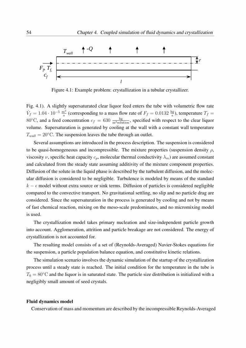
54 Chapter 4. Coupled simulation of fluid dynamics and crystallization
Ff, Tf,
cf
-QTwall
l
r
Figure 4.1: Example problem: crystallization in a tubular crystallizer.
Fig. 4.1). A slightly supersaturated clear liquor feed enters the tube with volumetric flow rateVf = 1.04 · 10−5 m3
s(corresponding to a mass flow rate of Ff = 0.0132 kg
s), temperature Tf =
80◦C, and a feed concentration cf = 630 kgm3solution
, specified with respect to the clear liquorvolume. Supersaturation is generated by cooling at the wall with a constant wall temperatureTwall = 20◦C. The suspension leaves the tube through an outlet.
Several assumptions are introduced in the process description. The suspension is consideredto be quasi-homogeneous and incompressible. The mixture properties (suspension density ρ,viscosity ν, specific heat capacity cp, molecular thermal conductivity λm) are assumed constantand calculated from the steady state assuming additivity of the mixture component properties.Diffusion of the solute in the liquid phase is described by the turbulent diffusion, and the molec-ular diffusion is considered to be negligible. Turbulence is modeled by means of the standardk − ε model without extra source or sink terms. Diffusion of particles is considered negligiblecompared to the convective transport. No gravitational settling, no slip and no particle drag areconsidered. Since the supersaturation in the process is generated by cooling and not by meansof fast chemical reaction, mixing on the meso-scale predominates, and no micromixing modelis used.
The crystallization model takes primary nucleation and size-independent particle growthinto account. Agglomeration, attrition and particle breakage are not considered. The energy ofcrystallization is not accounted for.
The resulting model consists of a set of (Reynolds-Averaged) Navier-Stokes equations forthe suspension, a particle population balance equation, and constitutive kinetic relations.
The simulation scenario involves the dynamic simulation of the startup of the crystallizationprocess until a steady state is reached. The initial condition for the temperature in the tube isT0 = 80◦C and the liquor is in saturated state. The particle size distribution is initialized with anegligibly small amount of seed crystals.
Fluid dynamics modelConservation of mass and momentum are described by the incompressible Reynolds-Averaged
4.1. Example problem: tubular crystallizer 55
Navier-Stokes equations (see Eq. (2.11)-(2.12)) as
∇ · v = 0, (4.1)∂v
∂t+∇ · (vv) = −1
ρ∇p + (ν + νt)∇ · (∇v) . (4.2)
The vector of Reynolds-averaged velocities, the static pressure and turbulent viscosity are de-noted by v, p and νt, respectively. Turbulent viscosity νt is computed by the k − ε turbulencemodel (FLUENT 6.0 User Manual).
The energy balance (2.13) can be written as
∂T
∂t+∇ · (vT ) =
λ
cpρ∇ · (∇T ) . (4.3)
The thermal conductivity λ is dominated by the turbulent component λt computed by the k − ε
model with a (default) Prandtl number of 0.85.Inlet flow Vf , its temperature Tf and the temperature at the walls Twall are set as boundary
conditions.
Crystallization modelTo model the crystallization process, a population balance is employed. The particles are
described by the particle size distribution n(L,x, t). The introduced assumptions result in G 6=G(L), Dm,p = 0, Dt,p = 0, B = D = 0. The general differential population balance equation(2.3) reduces to
∂n(L,x, t)
∂t+ G
∂n(L,x, t)
∂L+∇ · (vn(L,x, t)) = 0. (4.4)
The initial conditions for the PSD and the concentration of solute c (in kgm3solution
) are given by
n(L, t = 0) = 0; c(t = 0) = c0. (4.5)
The crystallization kinetics applied in the study is analogous to the model of Jerauld et al.(1983). Nucleation is accounted for as a left boundary condition for the population balanceequation, expressed by Volmers power law,
n(L = 0,x, t) =Bn
G,Bn = (1− αs)k2 exp
− k3(
cc∗(T )
− 1)2
, (4.6)
where αs is the volume fraction of solids. The kinetic parameters k1 = 2.81 · 10−8, k2 =
2.21 · 106, and k3 = 1.29 · 10−3 are adopted from Chiu and Christofides (1999).
56 Chapter 4. Coupled simulation of fluid dynamics and crystallization
The growth rate G is independent of particle size and shows a first-order dependency onsupersaturation s = c− c∗ of the form
G = k1(c− c∗(T )), (4.7)
where c∗ is the saturation concentration of solute in the solution, evaluated according to a fittedapproximation:
c∗(T ) = 980.2 + 1297 ∗ exp
(−268
T
). (4.8)
To close the crystallization model, a mass balance for the solute is provided
∂ρc
∂t+∇ · (vρc)−Dc∇ · (∇ρc) = −Sc , (4.9)
where ρc is the concentration of the solute in the suspension1 (in kgm3suspension
), Dc is the effectivediffusion coefficient for the solute, equal to the sum of molecular and turbulent diffusion of thesolute, Dm,c and Dt,c, respectively. The turbulent diffusion is determined from the k− ε model.The concentration sink term due to the depletion of supersaturation during particle growth −Sc
(in kgm3(susp) s
) is calculated as
Sc = 3ρSkvG
∫ ∞
0
nL2dL . (4.10)
ρS and kv are the solids density and the particle shape factor. For spherical particles kv = π6.
In summary, modeling of the multi-physics problem covering crystallization and fluid dy-namics leads to a complex partial-integro-differential-algebraic equation (PIDAE) system. Theproblem contains partial differential equations formulated in external spatial coordinates x, oneinternal coordinate (particle size) L and the time coordinate t.
4.2 Generalized process flowsheet modeling and simulation
4.2.1 Problem decomposition
Modular simulation of complex multi-physics processes requires the decomposition of the pro-cess model into the models of process phenomena and couplings between them. The full pro-cess model is reformulated as the set of Nq submodels and coupling equations, which make upa generalized flowsheet simulation problem, similar to the flowsheet problem in Chapter 3:
yq = gq(uq,pq), q = 1, ..., Nq (4.11)
up = Pp,qyq, q = 1, ..., Nq, p = 1, ..., Np, p 6= q. (4.12)
1We distinguish the concentration in the solution c and the partial density, or the concentration in the suspensionρc. They are related by ρc = c (1− αs), where αs is the volume fraction of solids.
4.2. Generalized process flowsheet modeling and simulation 57
Here, gq denotes the explicit form of the submodel equation system for the q-th subproblem,and Pp,q is the coupling permutation matrix.
The decomposition into submodels needs to be defined by the user. The modular simulationapproach can only be effective if the complexity of the submodels is reduced compared to thecomplexity of the original model. Some principles of decomposition can be formulated:
• Each of the submodels must be mathematically simpler than the original model, in termsof structure and the number of equations solved.
• At least one of the submodels must be specified at the finest scale defined to resolve thephenomena of interest and to provide the requested process information.
• The decomposition should be consistent, i.e., the submodels should be defined such thatthey assemble into the complete and consistent process model, identical to the originalmodel or converging to its solution by the modular simulation, subject to the assumptionstaken.
• The decomposition should provide good convergence properties. The connection topol-ogy of the generalized flowsheet and the number of coupling variables have to be deter-mined to minimize the number of iterations in the modular simulation necessary to reachconvergence.
With these often contradictory requirements, model decomposition is largely a design deci-sion. The decision process can be supported by variable-equation incidence matrices as intro-duced in Section 3.1.1 for the flowsheet problem. Model decomposition can be performed inthe following sequence:
• Write down a complete model with constitutive equations, and an incidence matrix Λ.
• Identify the phenomena and their set of balance equations.
• Perform an initial output assignment for the balance equations (Westerberg, 1979) andfind out the list of variables to be determined from these equations.
• Perform an initial identification of the subproblems. A subproblem is initially identifiedto include the set of balance equations and respective variables which describe a singlephenomenon. It is a valid option to collect a group of phenomena with the same structureof the balance equations (e.g. fluid transport) in a single subproblem.
• Identify subproblem dimensions and scales. High-dimensional variables and the respec-tive balance equations are recommended to be collected in one high-dimensional sub-problem. Similarly, in multi-scale problems, variables defined on a certain scale shouldbe computed in the subproblem, which described processes on this specific scale.
58 Chapter 4. Coupled simulation of fluid dynamics and crystallization
• Perform the causal analysis of the balance equations of every subproblem model. Thecausal analysis (Iwasaki, 1988; Skorstad, 1990) builds an oriented graph of causal depen-dencies of the model variables obtained from the incidence matrix and output assignment.A graph node is a variable, an edge of the graph corresponds to a direct effect of the inputvariable to the output variable in a model equation. The analysis begins with the outputvariables computed by the balance equations and is performed in the ”causally upstream”fashion. For every input variable in the balance equation, which is not determined fromanother balance equation and not provided as an external input, a phenomenological equa-tion computing it as an output variable has to be provided in the model. The inputs of thisequation and their effects to the output variable are added to the graph, and the inputs arein turn analyzed. The analysis is performed recursively for all phenomenological equa-tions until all model equations have been analyzed, the output assignment is completed,and a full causal dependency graph is constructed.
• Assign the phenomenological equations to the subproblems and choose coupling vari-ables. Coupling variables are computed within one subproblem, transferred by the cou-plings and used as inputs in the other subproblems. The assignment of phenomenologicalequations and the choice of coupling variables requires the user’s expert decision. Severalheuristics are given in Section 4.2.5.
4.2.2 Multi-scale problem discretization: fine grid and compartments
Discretization of Navier-Stokes equationsThe spatial discretization of the Navier-Stokes equations of the fluid dynamics subproblem
(4.1)-(4.3) uses the Finite Volume method. For time discretization, an implicit scheme is em-ployed. The resulting discretized Navier-Stokes equations have a form similar to Eq. (2.17).2
Reduction of population balanceAs discussed in Section 2.3.5, the CFD and crystallization phenomena subproblems are
defined on the same spatial domain, but on different scales within the domain. Such multi-dimensional and multi-scale complexity of the model leads to a large number of discretizationnodes, and to a large computational demand. It can be reduced by a reduction of the number ofdiscretization elements.
Section 2.3.5 discusses two generally employed approaches to reduce the population balanceof the crystallization subproblem. The population balance can be reduced in the particle size
2To distinguish discretized forms of the fluid dynamics equations from their non-discretized forms, the dis-cretized equations will be referred to as (4.1)d, (4.2)d, (4.3)d, etc.
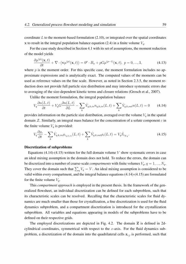
4.2. Generalized process flowsheet modeling and simulation 59
coordinate L to the moment-based formulation (2.10), or integrated over the spatial coordinatesx to result in the integral population balance equation (2.4) in a finite volume Vq.
For the case study described in Section 4.1 with its set of assumptions, the moment reductionof the model yields
∂µ(p)(x, t)
∂t+∇ · (vµ(p)(x, t)) = 0p ·Bn + pGµ(p−1)(x, t), p = 0, ..., 3, (4.13)
where p is the moment order. For this specific case, the moment formulation includes no ap-proximate expressions and is analytically exact. The computed values of the moments can beused as reference values on the fine scale. However, as noted in Section 2.3.5, the moment re-duction does not provide full particle size distribution and may introduce systematic errors dueto averaging of the size-dependent kinetic terms and closure relations (Grosch et al., 2007).
Unlike the moment formulation, the integral population balance
Vq∂n(L, t)
∂t+ VqG
∂n(L, t)
∂L−
∑
k
Vq,k,innq,k,in(L, t) +∑
k
Vq,k,outn(L, t) = 0 (4.14)
provides information on the particle size distribution, averaged over the volume Vq in the spatialdomain Z . Similarly, an integral mass balance for the concentration of a solute component c inthe finite volume Vq is provided:
Vq∂ρc
∂t−
∑
k
Vq,k,inρcq,k,in(L, t) +
∑
k
Vq,k,outρc(L, t) = VqScKq. (4.15)
Discretization of subproblemsEquations (4.14)-(4.15) written for the full domain volume V show systematic errors in case
an ideal mixing assumption in the domain does not hold. To reduce the errors, the domain canbe discretized into a number of coarse-scale compartments with finite volumes Vq, q = 1, ..., Nq.They cover the domain such that
∑q Vq = V . An ideal mixing assumption is considered to be
valid within every compartment, and the integral balance equations (4.14)-(4.15) are formulatedfor the finite volume Vq.
This compartment approach is employed in the present thesis. In the framework of the gen-eralized flowsheet, an individual discretization can be defined for each subproblem, such thatits characteristic scales can be resolved. Recalling that the characteristic scales for fluid dy-namics are much smaller than those for crystallization, a fine discretization is used for the fluiddynamics subproblem, and a compartment discretization is introduced for the crystallizationsubproblem. All variables and equations appearing in models of the subproblems have to bedefined on their respective grids.
The employed discretizations are depicted in Fig. 4.2. The domain Z is defined in 2d-cylindrical coordinates, symmetrical with respect to the x-axis. For the fluid dynamics sub-problem, a discretization of the domain into the quadrilateral cells zi,j is performed, such that
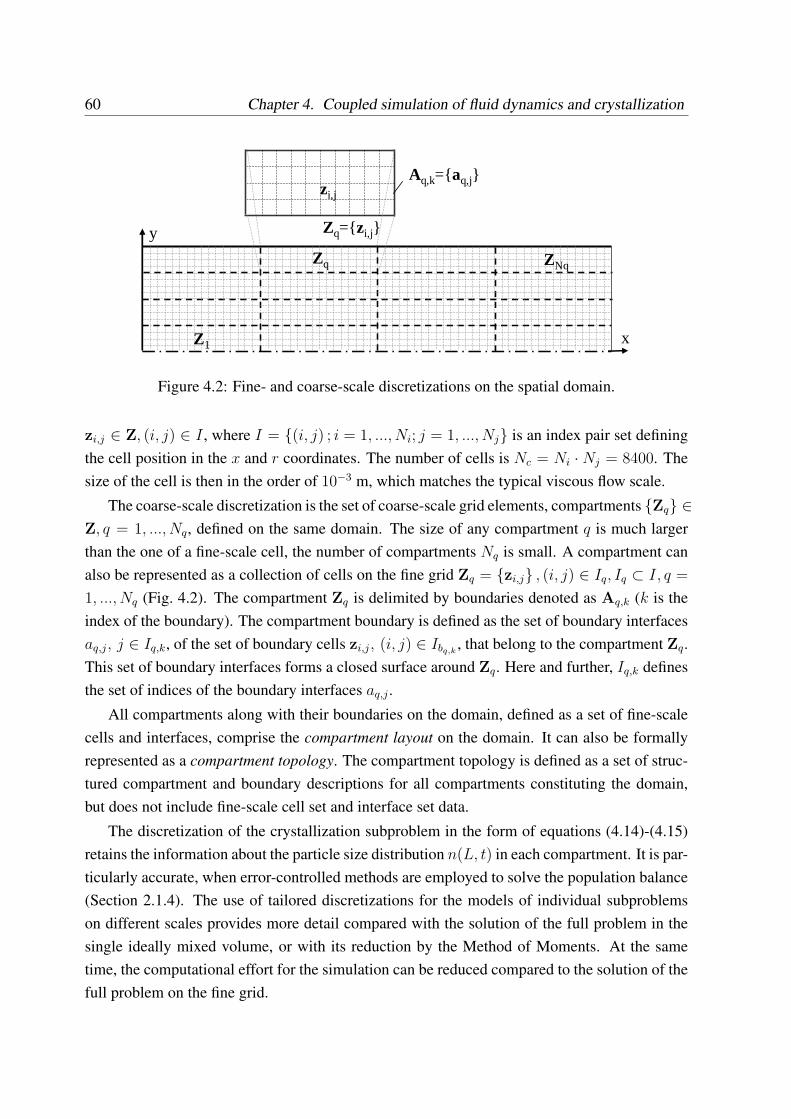
60 Chapter 4. Coupled simulation of fluid dynamics and crystallization
Zq={zi,j}
zi,j
Z1
Zq ZNq
x
y
Aq,k={aq,j}
Figure 4.2: Fine- and coarse-scale discretizations on the spatial domain.
zi,j ∈ Z, (i, j) ∈ I , where I = {(i, j) ; i = 1, ..., Ni; j = 1, ..., Nj} is an index pair set definingthe cell position in the x and r coordinates. The number of cells is Nc = Ni ·Nj = 8400. Thesize of the cell is then in the order of 10−3 m, which matches the typical viscous flow scale.
The coarse-scale discretization is the set of coarse-scale grid elements, compartments {Zq} ∈Z, q = 1, ..., Nq, defined on the same domain. The size of any compartment q is much largerthan the one of a fine-scale cell, the number of compartments Nq is small. A compartment canalso be represented as a collection of cells on the fine grid Zq = {zi,j} , (i, j) ∈ Iq, Iq ⊂ I, q =
1, ..., Nq (Fig. 4.2). The compartment Zq is delimited by boundaries denoted as Aq,k (k is theindex of the boundary). The compartment boundary is defined as the set of boundary interfacesaq,j, j ∈ Iq,k, of the set of boundary cells zi,j, (i, j) ∈ Ibq,k
, that belong to the compartment Zq.This set of boundary interfaces forms a closed surface around Zq. Here and further, Iq,k definesthe set of indices of the boundary interfaces aq,j .
All compartments along with their boundaries on the domain, defined as a set of fine-scalecells and interfaces, comprise the compartment layout on the domain. It can also be formallyrepresented as a compartment topology. The compartment topology is defined as a set of struc-tured compartment and boundary descriptions for all compartments constituting the domain,but does not include fine-scale cell set and interface set data.
The discretization of the crystallization subproblem in the form of equations (4.14)-(4.15)retains the information about the particle size distribution n(L, t) in each compartment. It is par-ticularly accurate, when error-controlled methods are employed to solve the population balance(Section 2.1.4). The use of tailored discretizations for the models of individual subproblemson different scales provides more detail compared with the solution of the full problem in thesingle ideally mixed volume, or with its reduction by the Method of Moments. At the sametime, the computational effort for the simulation can be reduced compared to the solution of thefull problem on the fine grid.
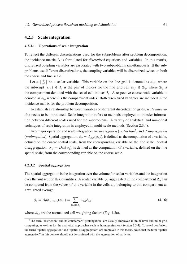
4.2. Generalized process flowsheet modeling and simulation 61
4.2.3 Scale integration
4.2.3.1 Operations of scale integration
To reflect the different discretizations used for the subproblems after problem decomposition,the incidence matrix Λ is formulated for discretized equations and variables. In this matrix,discretized coupling variables are associated with two subproblems simultaneously. If the sub-problems use different discretizations, the coupling variables will be discretized twice, on boththe coarse and fine scale.
Let φ[
#m3
]be a scalar variable. This variable on the fine grid is denoted as φi,j , where
the subscript (i, j) ∈ Iq is the pair of indices for the fine grid cell zi,j ∈ Zq, where Zq isthe compartment dentoted with the set of cell indices Iq. A respective coarse-scale variable isdenoted as φq, where q is the compartment index. Both discretized variables are included in theincidence matrix for the problem decomposition.
To establish a relationship between variables on different discretization grids, scale integra-tion needs to be introduced. Scale integration refers to methods employed to transfer informa-tion between different scales used for the subproblems. A variety of analytical and numericaltechniques of scale integration is employed in multi-scale methods (Section 2.3.4).
Two major operations of scale integration are aggregation (restriction3) and disaggregation(prolongation). Spatial aggregation, φq = Agg(φi,j), is defined as the computation of a variable,defined on the coarse spatial scale, from the corresponding variable on the fine scale. Spatialdisaggregation, φi,j = Dis(φq), is defined as the computation of a variable, defined on the finespatial scale, from the corresponding variable on the coarse scale.
4.2.3.2 Spatial aggregation
The spatial aggregation is the integration over the volume for scalar variables and the integrationover the surface for flux quantities. A scalar variable φq aggregated in the compartment Zq canbe computed from the values of this variable in the cells zi,j belonging to this compartment asa weighted average,
φq = Agg(i,j)∈Iq(φi,j) =∑
(i,j)∈Iq
ωi,jφi,j, (4.16)
where ωi,j are the normalized cell weighting factors (Fig. 4.3a).
3The term ”restriction” and its counterpart ”prolongation” are usually employed in multi-level and multi-gridcomputing, as well as for the analytical approaches such as homogenization (Section 2.3.4). To avoid confusion,the terms ”spatial aggregation” and ”spatial disaggregation” are employed in this thesis. Note, that the term ”spatialaggregation” in this context should not be confused with the aggregation of particles.
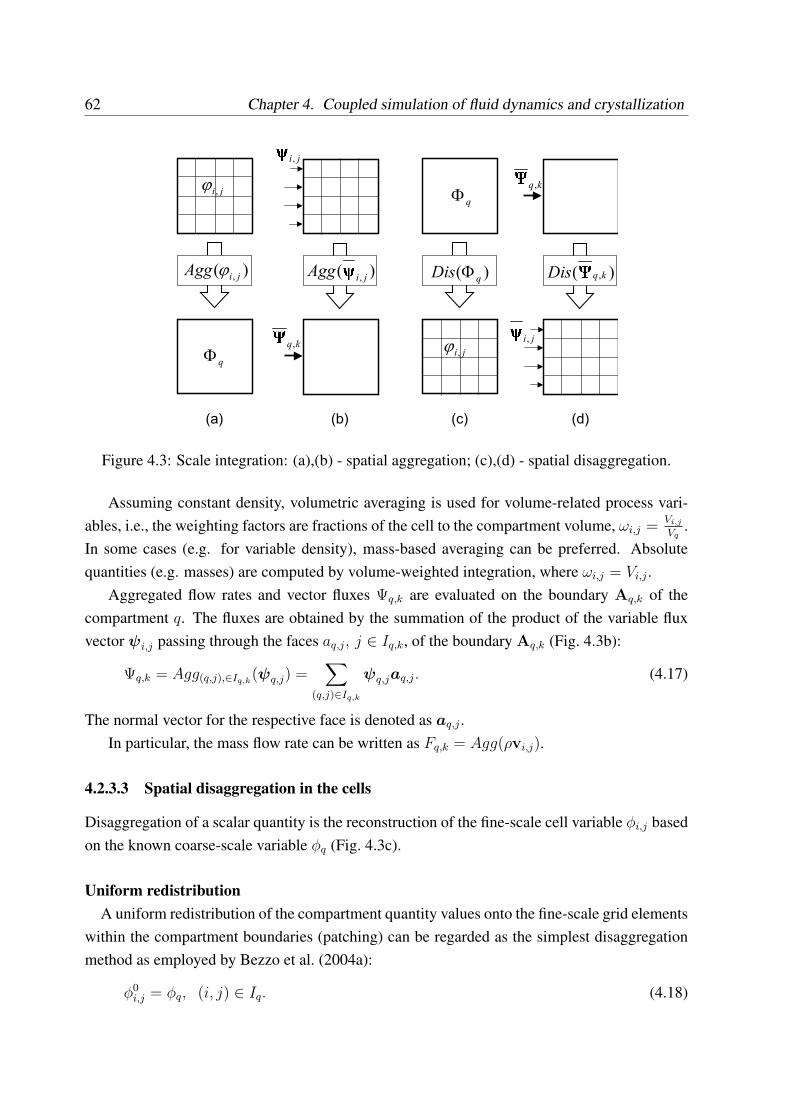
62 Chapter 4. Coupled simulation of fluid dynamics and crystallization
)( , jiAgg ϕ
ji,ϕ
qΦ
(a)
)(, jiAgg
�kq,
�(b)
ji,
�)( qDis Φ
ji,ϕ
qΦ
(c)
)( ,kqDis �kq,
�
(d)
ji,
�Figure 4.3: Scale integration: (a),(b) - spatial aggregation; (c),(d) - spatial disaggregation.
Assuming constant density, volumetric averaging is used for volume-related process vari-ables, i.e., the weighting factors are fractions of the cell to the compartment volume, ωi,j =
Vi,j
Vq.
In some cases (e.g. for variable density), mass-based averaging can be preferred. Absolutequantities (e.g. masses) are computed by volume-weighted integration, where ωi,j = Vi,j .
Aggregated flow rates and vector fluxes Ψq,k are evaluated on the boundary Aq,k of thecompartment q. The fluxes are obtained by the summation of the product of the variable fluxvector ψi,j passing through the faces aq,j, j ∈ Iq,k, of the boundary Aq,k (Fig. 4.3b):
Ψq,k = Agg(q,j),∈Iq,k(ψq,j) =
∑
(q,j)∈Iq,k
ψq,jaq,j. (4.17)
The normal vector for the respective face is denoted as aq,j .In particular, the mass flow rate can be written as Fq,k = Agg(ρvi,j).
4.2.3.3 Spatial disaggregation in the cells
Disaggregation of a scalar quantity is the reconstruction of the fine-scale cell variable φi,j basedon the known coarse-scale variable φq (Fig. 4.3c).
Uniform redistributionA uniform redistribution of the compartment quantity values onto the fine-scale grid elements
within the compartment boundaries (patching) can be regarded as the simplest disaggregationmethod as employed by Bezzo et al. (2004a):
φ0i,j = φq, (i, j) ∈ Iq. (4.18)
4.2. Generalized process flowsheet modeling and simulation 63
This technique provides no information gain and leads to discontinuities at the compartmentboundaries that result in computational problems if the disaggregated values are used as initialstate or input to the fine-scale simulation. However, expression (4.18) can be used to provide aninitial approximation of the disaggregated fine-scale quantities (denoted by the upper index 0).
Disaggregation with smoothing filterThe discontinuities in φ0
i,j can be dampened by a smoothing procedure realized by means ofa Gaussian convolution filter. Convolution filters are extensively used in image processing tocarry out operations like blurring, edge and gradient detection (Young et al., 1998). Convolutionfilters adjust the value in a given central point using the values in the neighboring cells fallinginto the ”window” represented by the convolution kernel. For a rectangular grid, a generalconvolution filter in two-dimensional space in a discrete formulation can be written as
φ∗i,j = φ0i,j ⊗Hi,j =
ni∑
i′=−ni
nj∑
j′=−nj
hi′,j′ · φi−i′,j−j′ , (4.19)
where φ0i,j is the scalar quantity in the cell zi,j and Hi,j is the (2ni + 1)(2nj + 1) matrix of a
convolution kernel for the cell. Indices i′ and j′ are zero for the central element of the matrix.A commonly used filtering approach is the Gaussian smoothing, where the convolution
kernel is based on the Gaussian distribution
hGi′,j′ =
1
2πσ2exp−
i′2+j′22σ2 , (4.20)
and σ is the standard deviation controlling the degree of smoothing. It affects the size of theGaussian convolution kernel and the area affected by the smoothing. The Gaussian kernel isoften truncated at the distance of 3σ from the mean. For example, for σ = 1.0 the 5x5 kernelcan be constructed as:
HG =1
273
[1 4 7 4 14 16 26 16 47 26 41 26 74 16 26 16 41 4 7 4 1
]. (4.21)
The Gaussian smoothing is not performed at the external boundaries.
Disaggregation with bicubic spline interpolationAn alternative option to reconstruct the fine-scale variables from their aggregated values is
the use of interpolation techniques. A fine-scale variable profile is assumed to be describedby an interpolation polynomial of certain type, which reconstructs the fine-scale profile usingknown aggregated values in the compartment. In two-dimensional problems, the interpolationof the variables can be done by means of bicubic splines. Bicubic splines are well established
64 Chapter 4. Coupled simulation of fluid dynamics and crystallization
in data processing to approximate continuous two-dimensional functions between their knownvalues at the nodes.
A bicubic spline is a two-dimensional polynomial function with a maximum power of 3. Itis written for the interpolation in arbitrary q-th compartment as:
Pq(x, y) =3∑
px=0
3∑py=0
bq,px,py(x− x0q)
px(y − y0q )
py , q = 1, ..., Nq, (4.22)
where bq,px,py is the set of 16 spline coefficients for the q-th compartment, (x0q, y
0q ) are the coor-
dinates of the node – a point with the known variable value. A bicubic spline is constructed tosatisfy C2-continuity conditions everywhere in the domain, including all compartment bound-aries. After the spline is constructed, the variable value in the cell zi,j with coordinates (xi, yj)
is evaluated as φi,j = Pq(xi, yj).
Assume that a rectangular grid is chosen on the coarse scale with Nx+1 nodes in x-directionand Ny + 1 nodes in y-direction (Fig. 4.4a), located at the corners of the compartments. Then,Nq = NxNy. To specify the bicubic spline problem, where the spline in every compartment isdescribed by Eq. (4.22), 16NxNy conditions should be provided.
Continuity requirements for the bicubic spline on this grid result in the following conditions:
• C2-continuity at all compartment boundaries. This results in the 15NxNy−3Nx−3Ny−9
conditions of the form:
∂α+βPq1(xb, yb)
∂xα∂yβ=
∂α+βPq2(xb, yb)
∂xα∂yβ, ∀q1, q2, s.t. Zq1 ∩ Zq2 6= 0. (4.23)
Here, α = 0, .., 2, β = 0, .., 2 are integer numbers, points (xb, yb) belong to a commonboundary between the compartments Zq1 and Zq2 and q1 and q2 are the respective indicesfor the compartments that have a common boundary.
• ”Natural spline” conditions at the external boundaries of the domain impose zero secondderivatives (Press et al., 1992):
∂2Pq
∂x2= 0, at the external boundaries in x-direction;
∂2Pq
∂y2= 0, at the external boundaries in y-direction;
∂2Pq
∂x∂y= 0, at the corners of the domain in the x-y-plane.
The number of conditions is 2(Nx + Ny) + 8.
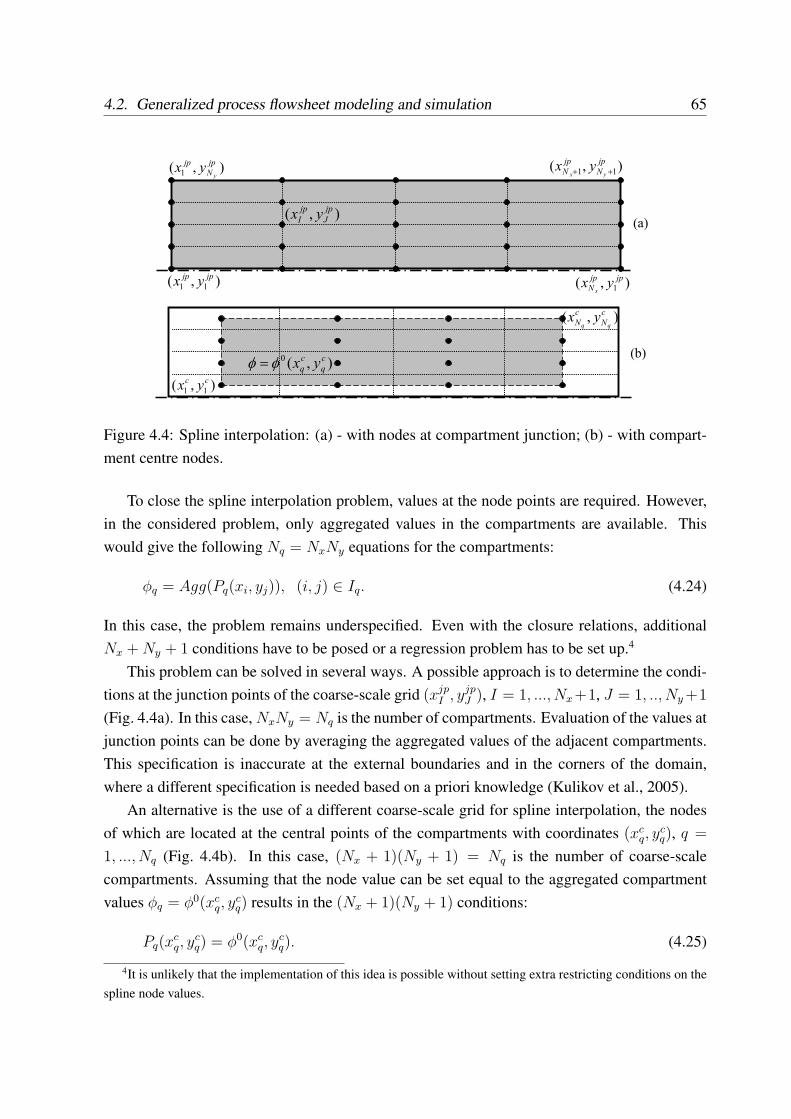
4.2. Generalized process flowsheet modeling and simulation 65
(a)
(b)
),( 11
ccyx
),( c
N
c
N qqyx
),( 11
jpjpyx
),( 1
jp
N
jp
yyx
),( 1
jpjp
N yxx
),( 11
jp
N
jp
N yxyx ++
),(0 c
q
c
q yxφφ =
),(jp
J
jp
I yx
Figure 4.4: Spline interpolation: (a) - with nodes at compartment junction; (b) - with compart-ment centre nodes.
To close the spline interpolation problem, values at the node points are required. However,in the considered problem, only aggregated values in the compartments are available. Thiswould give the following Nq = NxNy equations for the compartments:
φq = Agg(Pq(xi, yj)), (i, j) ∈ Iq. (4.24)
In this case, the problem remains underspecified. Even with the closure relations, additionalNx + Ny + 1 conditions have to be posed or a regression problem has to be set up.4
This problem can be solved in several ways. A possible approach is to determine the condi-tions at the junction points of the coarse-scale grid (xjp
I , yjpJ ), I = 1, ..., Nx+1, J = 1, .., Ny +1
(Fig. 4.4a). In this case, NxNy = Nq is the number of compartments. Evaluation of the values atjunction points can be done by averaging the aggregated values of the adjacent compartments.This specification is inaccurate at the external boundaries and in the corners of the domain,where a different specification is needed based on a priori knowledge (Kulikov et al., 2005).
An alternative is the use of a different coarse-scale grid for spline interpolation, the nodesof which are located at the central points of the compartments with coordinates (xc
q, ycq), q =
1, ..., Nq (Fig. 4.4b). In this case, (Nx + 1)(Ny + 1) = Nq is the number of coarse-scalecompartments. Assuming that the node value can be set equal to the aggregated compartmentvalues φq = φ0(xc
q, ycq) results in the (Nx + 1)(Ny + 1) conditions:
Pq(xcq, y
cq) = φ0(xc
q, ycq). (4.25)
4It is unlikely that the implementation of this idea is possible without setting extra restricting conditions on thespline node values.
66 Chapter 4. Coupled simulation of fluid dynamics and crystallization
This reduces the spline interpolation problem to the traditional formulation. However, the cen-tral point assumption does not necessarily hold even for the rectangular coarse-scale grid. Be-sides, the boundary of the interpolated area (shown in dashed lines) is not the domain boundary,such that extrapolation has to be used in the ”outer” compartments of the domain outside theinterpolated area boundary.
With the node conditions given by either of two alternatives presented above, the bicubicspline interpolation problem for a disaggregated variable is fully specified and has a uniquesolution. To solve this problem, a standard solver code developed by Press et al. (1992) isemployed.
In the simulations, the central-point and junction-point approaches have been compared.The simulations showed that although the central-point assumption was somewhat more ac-curate in the profile prediction, no significant difference between the two alternatives was ob-served. However, the use of spline interpolation procedure results in a much smoother profilecompared to the Gaussian filtering approach, although it can introduce an additional error to theoverall problem.
Conservation of a disaggregated quantityConservation of the values of a quantity φ in the disaggregation is a necessary consistency
check. Conservation is provided if the aggregation of disaggregated fine-scale variable valueson the domain results in the original coarse-scale variable value. Conservation in a compartmentis achieved, if the same is valid for a single compartment:
φq = Agg(Dis(φq)) = φq (4.26)
In case of Gaussian smoothing, the symmetry of the Gaussian kernel provides the con-servation of disaggregated variable on the domain for equivolumetric cells, but does not pro-vide exact conservation of the disaggregated variable in the compartment because of the cross-compartment smoothing. In case of spline interpolation, conservation of disaggregated quantityboth on the domain and in the compartment is provided if Eq. (4.24) is valid. In case of reducedmethods, exact conservation is not achieved.
Therefore, a consistent disaggregation method, which provides both conservation of vari-ables and fine-scale variable profile reconstruction – disaggregation of source terms – for arbi-trary compartments has been implemented in the thesis and described in Section 4.2.4.
4.2.3.4 Spatial disaggregation on the surfaces
Spatial disaggregation on surfaces is performed for the boundary conditions at the spatial do-main, which can change during runtime. They are typically the inlet stream properties, wherethe flow rate, the temperature and the component concentrations may change in each iteration.
4.2. Generalized process flowsheet modeling and simulation 67
By default, the boundary conditions for the physical properties such as temperature andconcentration at the faces of a considered boundary are set equal to their aggregated value at thisboundary (Fig. 4.3d). The fluxes through the faces of the boundary are obtained by assuming auniform velocity profile in the inlet zone, such that the fluxes are proportional to the face areaψq,b,i = Ψq,k
aq,b,i
Aq,k. More complex profiles, e.g. turbulent velocity in the inlet, are possible, but
have not been employed in the illustrative example.
4.2.3.5 Scale integration in the generalized flowsheet
Scale integration equations replace the standard coupling identity equations in the model of ageneralized flowsheet. Assuming that unit Q has a coarse-scale discretization, and unit P afine-scale discretization, scale integration Agg(yP ), Dis(yQ) is applied to all discretizationelements of the respective units,
Agg(yP ) =
(Agg(yPi,j
), (i,j)∈I1...
Agg(yPi,j), (i,j)∈INq
); Dis(yQ) =
(Dis(yQ1
),...
Dis(yQNq)
).
The scale integration equations in the generalized flowsheet are
uQ = PQ,P Agg(yP ), (4.27)
uP = Dis(PP,QyQ), (4.28)
where uQ =( u1
...uNq
), yQ =
( y1...
yNq
)in the unit Q with coarse-scale discretization, and uP =
(ui,j), yP = (yi,j) in the unit P with fine-scale discretization. Since the incidence matrix iswritten for coarse-scale variables to avoid excessive information flow in the coupling variables,disaggregation is executed after transferring the outputs yQ to the inputs of unit P .
4.2.4 Auxiliary modeling and disaggregation of source terms
The methods of disaggregation of a coarse-scale variable φq described above are not sufficientto recover information on the fine grid. The constant value disaggregation provides no extrainformation compared to the coarse scale and leads to discontinuities. Spline interpolationmethods compute a fine-scale profile of a variable, but its accuracy can not be controlled. Theeffect of the known fine-scale variables on the disaggregated variable φi,j is not accounted for.Disaggregation errors can be introduced. Consistency with the other fine-scale variables andphysical interpretation of the results on the fine scale is not guaranteed.
In order to consistently compute an accurate profile of a variable to be disaggregated onthe fine grid, auxiliary modeling is proposed. In this method, the disaggregation relation forthe variable φ is replaced with an auxiliary model. This is an equation or a set of equations to
68 Chapter 4. Coupled simulation of fluid dynamics and crystallization
compute the fine-scale variable φi,j from the other fine-scale variables and the changes of thevariable φ caused by the phenomena described in the coarse-scale subproblem.
In the fluid dynamics subproblem, an auxiliary model for a scalar variable φ reflects the fine-scale phenomena of fluid dynamics. Therefore, it has the same structure as the Navier-Stokesequations and is a convection-dominated transport equation written for φ:
∂φ
∂t+∇ · vφ = Sφ. (4.29)
The overall change of the fine-scale variable φi,j is described by the convective transportterm, which involves only fine-scale variables, and the change of the variable in the coarse-scale process phenomena, which appears in the auxiliary equation as the source term Sφ. Thesource term has the units of scalar variable per time. It is evaluated using an extra expressionin the coarse-scale subproblem and is disaggregated using one of the methods described inSection 4.2.3.3.
The use of a source term computed in the coarse-scale subproblem to reflect the change ofvariable in the coarse-scale phenomena, and its further disaggregation for use in the auxiliarymodel on the fine scale, is referred to as disaggregation of a source term. It has a numberof advantages over the disaggregation of a variable. The behavior of a variable φ on the finescale is fully described using a fine-scale balance equation, which accounts for the physicalphenomena acting on that scale, considers actual values of the other fine-scale variables suchas velocity and guarantees the conservation of the fine-scale variable. The effects of the coarse-scale phenomena are consistently accounted for, and no other balance equation for φ on thecoarse scale is necessary. Discontinuities at the compartment boundaries do not occur.
When using this method, attention must be paid on the consistency of the auxiliary model,correct derivation and implementation of the source term expression on the coarse scale, con-sistent disaggregation on the fine scale and possible overdetermination of the problem that mayarise due to use of auxiliary modeling (Section 4.2.8).
Considering the fluid dynamics-crystallization problem, assume that the scalar variable ofinterest is the concentration (partial density) of a solute component in the suspension, i.e. φ =
ρK , where K is the component index in the suspension. The auxiliary model uses the transportequation for a component concentration:
∂ρK
∂t+∇ · vρK = SρK
, K = 1, ..., NK , (4.30)
where the source term SρKis defined as the component concentration change in the crystal-
lization process. The change of concentration of the solute component is determined in thecoarse-scale subproblem as:
Scq =dρcq
dt= −3ρSkvGq
∫ ∞
0
nq(L)L2dL. (4.31)
4.2. Generalized process flowsheet modeling and simulation 69
The coarse-scale source term is then disaggregated on the fine scale employing one of the de-scribed disaggregation methods:
Sci,j= Dis
(Scq
). (4.32)
Similarly to the solute concentration, the solid component concentration ρs can be computedusing the transport equation, where the change of the solute concentration is obtained as Sρsq
=
−Scq , assuming that the mass of the solvent does not change in the crystallization process.
4.2.5 Choice and treatment of coupling variables
Choice of coupling variables in multi-scale problemsIdeally, coupling variables should be chosen to fulfil the following conditions:
• All subproblems should be determined and should produce a convergent solution consis-tent with the solution of the other subproblems. The coupling variables should be chosento provide such consistency to the extent possible (see Section 4.3.2.1).
• The coupling variables need to be chosen such that during the iterations, the convergenceconditions for the employed procedure are fulfilled at every point of the trajectory (Lip-schitz conditions for the fixed-point iteration).
Full consistency of subproblems, although desirable, may be violated in practice, because itmay be impossible to evaluate certain model variables or equation terms due to model assump-tions, limitations of solver capabilities or excessive computational demand. Furthermore, in anunconverged iteration, the solution is not consistent since some input variable values are takenfrom the previous iteration. Only when the iteration converges, the condition of solution con-sistency should be satisfied. Choice of inputs and outputs of a subproblem can be also restrictedby the interfaces of the employed software tools. These considerations may require to revisethe choice of coupling variables at the stage of the problem setup in the software tools.
In determined problems, only a few decomposition options are available. In overdeterminedproblems, where extra equations are explicitly or implicitly added to the subproblem, the num-ber of available decomposition options increases. On the basis of expertise gained during themethodological development, the heuristics presented below have been identified. They can actas practical guidelines to perform decomposition and to choose coupling variables in a general-ized flowsheet, where different design options are available.
• Reduce the total number of coupling variables. A modular simulation can be compu-tationally expensive, when several iterations have to be performed on all units to reachconvergence. A larger number of coupling variables leads to an increase of computational
70 Chapter 4. Coupled simulation of fluid dynamics and crystallization
effort and slower convergence (in particular, if variables with fast dynamics are involved).Besides, this requires better initial guesses for the variable trajectories.
• Avoid using unaggregated fine-scale variables as coupling variables. The use of aggre-gated scalar quantities as coupling variables is recommended. Scale integration shouldbe executed in the fine-scale subproblem. It is also recommended to avoid using full par-ticle size distributions as coupling variables whenever the transfer of aggregated scalarquantities suffices.
• Include into the subproblem phenomenological equations to compute causally ”upstream”variables, in order to reduce the number of coupling variables and complexity of the in-teractions on the flowsheet level, particularly, if the aggregation error is small, or if thephenomenological equation shows a strong coupling between the variables, which leadsto significant increase of computational effort if they are computed in different subprob-lems.
• Use phenomenological equations to compute variables on the fine grid when this is pos-sible without significant increase of the computational effort and without making the con-vergence worse. This reduces inconsistencies in the equation inputs, caused by the use ofaggregated quantities.
• Prefer variables computed by the models with better consistency, as determined by theconsistency analysis for a given decomposition (see Section 4.3.2). Inconsistency canyield systematic deviations in the solution, which will propagate further along the flow-sheet and may appear in the converged solution.
• Avoid computation of variables, which appear in one and the same term of a balanceequation, in different subproblems. This is necessary to ensure the consistency of themodel. For example, in a product mass balance the overall flow Vq,k and the concentrationof product in the flow ρKq,k are used to compute the product mass flow FKq,k = Vq,kρKq,k.If these variables are evaluated in different subproblems, inconsistencies between thesubproblems may lead to an error in the computation of this integral term and to theviolation of the product balance in the convergent solution. Therefore, it is recommendedto compute the product concentration in the same subproblem where the overall flow isevaluated.
• Prefer coupling variables with slow dynamics in order to damp local inconsistencies andnumerical disturbances during the iteration, which may violate stability and result in fail-ure of the simulation or its oscillatory behavior. Conversely, highly fluctuating variablesshould be avoided, since they may lead to large errors and convergence problems.
4.2. Generalized process flowsheet modeling and simulation 71
• Use auxiliary model equations with disaggregated source terms Sφ instead of disaggre-gation of scalar variable values φ whenever it is possible to represent the effects of thephenomena on a scalar process variable as a source term of the auxiliary transport equa-tion for this scalar variable on the fine grid. This is a consistent way to account forchange of a variable in all subproblems, and removes discontinuities at the boundaries ofthe coarse grid. This also enables a better postprocessing to obtain fine-grid variable data.
Handling of coupling variables in the subproblemsThe coupling variables have a different meaning in the subproblems of a generalized flow-
sheet. A coupling variable can be interpreted as an input variable on the subproblem’s respectivegrid, as a grid-independent parameter, as a term in an equation of the subproblem model, or asan initial or boundary condition at the domain.
Coupling variables interpreted as input variables are assigned at every point of time duringthe integration of the subproblem model. They act as the inputs to the subproblem equationsand have to use the same discretization as in the destination subproblem. Scale integration hasto be used if necessary. Coupling variables interpreted as parameters are used as scalar valuesand do not require scale integration.
Initial conditions are required for all differential variables of the subproblem. Global initialconditions are set once at the beginning of the simulation. Interval initial conditions are setonce at the beginning of the integration on every new interval; if they are not specified, the lastconverged state of the variable is taken as an initial condition. Coupling variables interpreted asinitial conditions are assigned to the associated variables in the destination subproblem,
x∣∣t=t0
= uIC
∣∣t=t0
. (4.33)
Initial conditions can be used either in discretized form or as scalar values. For a discretizedinitial condition, scale integration may have to be used.
Boundary conditions are required for the simulation of a subproblem involving a PDE. Theyare set on the domain boundaries. A coupling variable that refers to such a boundary condition inthe spatial coordinates will be assigned to the right-hand side of a respective boundary conditionequation, which has to be specified in the destination subproblem. For these variables, scaleintegration on surfaces has to be performed.
x∣∣aq,k
= uBC = Dis(yBC
∣∣aq,k
) (4.34)
The number of boundary conditions for a grid element is determined by the topology. Innergrid elements usually do not have specific boundary conditions.
The boundary conditions with respect to internal coordinates not present in the source sub-problem (particle size) are transferred as inputs and are assigned to the corresponding boundarycondition equations in the destination subproblem. They may undergo scale integration in cells.
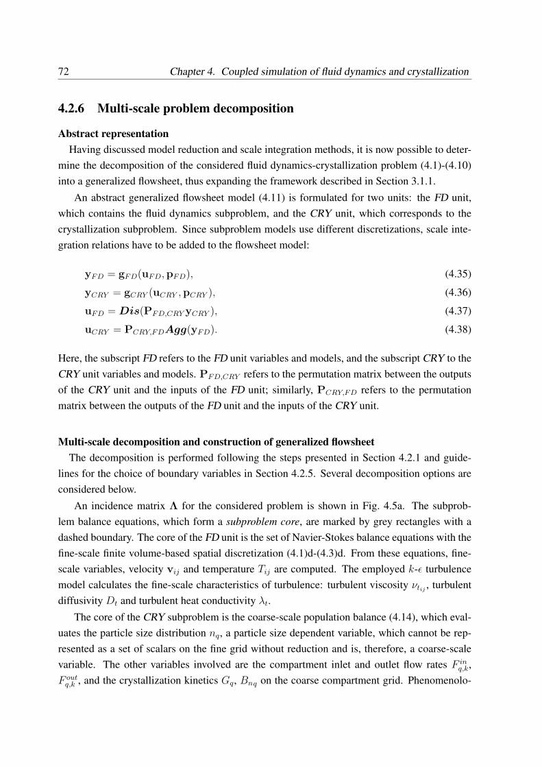
72 Chapter 4. Coupled simulation of fluid dynamics and crystallization
4.2.6 Multi-scale problem decomposition
Abstract representationHaving discussed model reduction and scale integration methods, it is now possible to deter-
mine the decomposition of the considered fluid dynamics-crystallization problem (4.1)-(4.10)into a generalized flowsheet, thus expanding the framework described in Section 3.1.1.
An abstract generalized flowsheet model (4.11) is formulated for two units: the FD unit,which contains the fluid dynamics subproblem, and the CRY unit, which corresponds to thecrystallization subproblem. Since subproblem models use different discretizations, scale inte-gration relations have to be added to the flowsheet model:
yFD = gFD(uFD,pFD), (4.35)
yCRY = gCRY (uCRY ,pCRY ), (4.36)
uFD = Dis(PFD,CRY yCRY ), (4.37)
uCRY = PCRY,FDAgg(yFD). (4.38)
Here, the subscript FD refers to the FD unit variables and models, and the subscript CRY to theCRY unit variables and models. PFD,CRY refers to the permutation matrix between the outputsof the CRY unit and the inputs of the FD unit; similarly, PCRY,FD refers to the permutationmatrix between the outputs of the FD unit and the inputs of the CRY unit.
Multi-scale decomposition and construction of generalized flowsheetThe decomposition is performed following the steps presented in Section 4.2.1 and guide-
lines for the choice of boundary variables in Section 4.2.5. Several decomposition options areconsidered below.
An incidence matrix Λ for the considered problem is shown in Fig. 4.5a. The subprob-lem balance equations, which form a subproblem core, are marked by grey rectangles with adashed boundary. The core of the FD unit is the set of Navier-Stokes balance equations with thefine-scale finite volume-based spatial discretization (4.1)d-(4.3)d. From these equations, fine-scale variables, velocity vij and temperature Tij are computed. The employed k-ε turbulencemodel calculates the fine-scale characteristics of turbulence: turbulent viscosity νtij , turbulentdiffusivity Dt and turbulent heat conductivity λt.
The core of the CRY subproblem is the coarse-scale population balance (4.14), which eval-uates the particle size distribution nq, a particle size dependent variable, which cannot be rep-resented as a set of scalars on the fine grid without reduction and is, therefore, a coarse-scalevariable. The other variables involved are the compartment inlet and outlet flow rates F in
q,k,F out
q,k , and the crystallization kinetics Gq, Bnq on the coarse compartment grid. Phenomenolo-
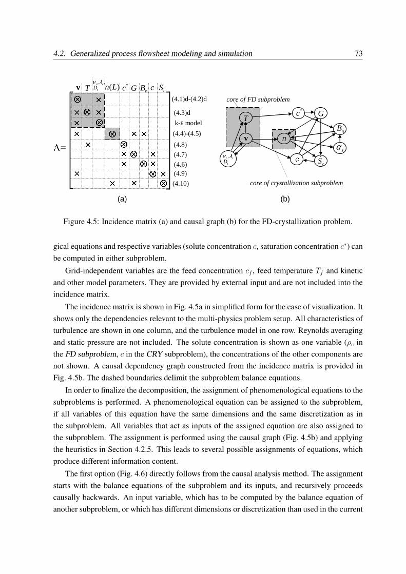
4.2. Generalized process flowsheet modeling and simulation 73
v T t
ttD
,,λν*c)(Ln c cS&G nB���� � �� �� �
(a) (b)
��Λ= � � �� ��� � v
t
ttD
λν ,
T
n сcS&*c G
nB
sα
core of FD subproblem
core of crystallization subproblem
(4.1)d-(4.2)d
(4.3)d
(4.4)-(4.5)
(4.7)
(4.6)
�(4.9)
(4.10)
�� �� (4.8)
k-ε model
Figure 4.5: Incidence matrix (a) and causal graph (b) for the FD-crystallization problem.
gical equations and respective variables (solute concentration c, saturation concentration c∗) canbe computed in either subproblem.
Grid-independent variables are the feed concentration cf , feed temperature Tf and kineticand other model parameters. They are provided by external input and are not included into theincidence matrix.
The incidence matrix is shown in Fig. 4.5a in simplified form for the ease of visualization. Itshows only the dependencies relevant to the multi-physics problem setup. All characteristics ofturbulence are shown in one column, and the turbulence model in one row. Reynolds averagingand static pressure are not included. The solute concentration is shown as one variable (ρc inthe FD subproblem, c in the CRY subproblem), the concentrations of the other components arenot shown. A causal dependency graph constructed from the incidence matrix is provided inFig. 4.5b. The dashed boundaries delimit the subproblem balance equations.
In order to finalize the decomposition, the assignment of phenomenological equations to thesubproblems is performed. A phenomenological equation can be assigned to the subproblem,if all variables of this equation have the same dimensions and the same discretization as inthe subproblem. All variables that act as inputs of the assigned equation are also assigned tothe subproblem. The assignment is performed using the causal graph (Fig. 4.5b) and applyingthe heuristics in Section 4.2.5. This leads to several possible assignments of equations, whichproduce different information content.
The first option (Fig. 4.6) directly follows from the causal analysis method. The assignmentstarts with the balance equations of the subproblem and its inputs, and recursively proceedscausally backwards. An input variable, which has to be computed by the balance equation ofanother subproblem, or which has different dimensions or discretization than used in the current
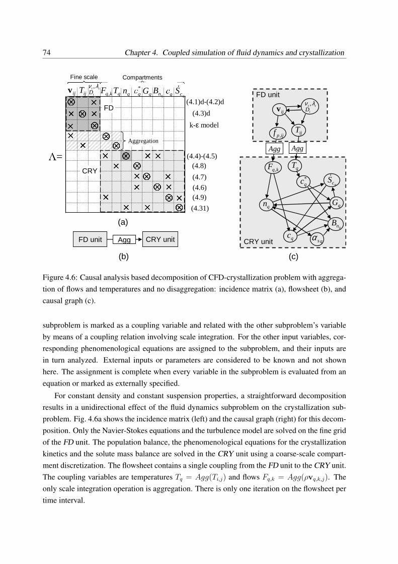
74 Chapter 4. Coupled simulation of fluid dynamics and crystallization
ijv
ijT
qn
FD unit
CRY unit
qT
ijpf ,
kqF ,
Agg
FD unit CRY unit
k-ε model
ijv ijT *qсqn qс qcS&qG
qnB��� � � �� �� ���Λ= � � �� ��� �
(4.1)d-(4.2)d
(4.3)d
(4.4)-(4.5)
(4.7)
(4.6)
�(4.9)
(4.31)
�� ��Agg
kqF , qT��� � Aggregation
qc
qcS&*qc
qG
qnB
qsα
FD
CRY
48476Fine scale 444444 8444444 76 Compartments
(b) (c)
(4.8)
t
ttD
λν ,
t
ttD
λν ,
Agg
(a)
Figure 4.6: Causal analysis based decomposition of CFD-crystallization problem with aggrega-tion of flows and temperatures and no disaggregation: incidence matrix (a), flowsheet (b), andcausal graph (c).
subproblem is marked as a coupling variable and related with the other subproblem’s variableby means of a coupling relation involving scale integration. For the other input variables, cor-responding phenomenological equations are assigned to the subproblem, and their inputs arein turn analyzed. External inputs or parameters are considered to be known and not shownhere. The assignment is complete when every variable in the subproblem is evaluated from anequation or marked as externally specified.
For constant density and constant suspension properties, a straightforward decompositionresults in a unidirectional effect of the fluid dynamics subproblem on the crystallization sub-problem. Fig. 4.6a shows the incidence matrix (left) and the causal graph (right) for this decom-position. Only the Navier-Stokes equations and the turbulence model are solved on the fine gridof the FD unit. The population balance, the phenomenological equations for the crystallizationkinetics and the solute mass balance are solved in the CRY unit using a coarse-scale compart-ment discretization. The flowsheet contains a single coupling from the FD unit to the CRY unit.The coupling variables are temperatures Tq = Agg(Ti,j) and flows Fq,k = Agg(ρvq,k,j). Theonly scale integration operation is aggregation. There is only one iteration on the flowsheet pertime interval.
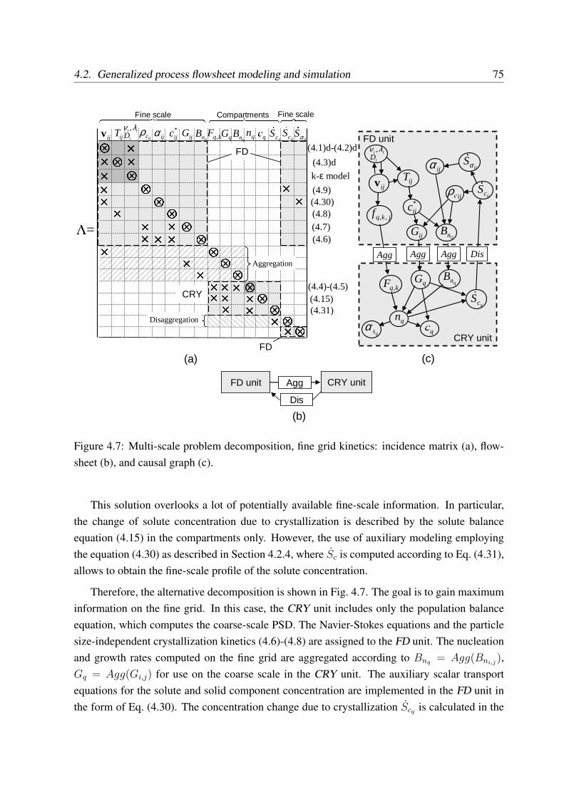
4.2. Generalized process flowsheet modeling and simulation 75444 8444 76ijv ijT
qnqс qcS&
*ijc
ijGijnB
qsα
FD unit
CRY unit
jkqf ,,
kqF ,
ijv ijT *ijc qn
ijcρqcS&ijG
ijnB����� � ���Λ=
� � ��� (4.1)d-(4.2)d
(4.3)d
(4.4)-(4.5)
(4.7)(4.6)� (4.9)� �� ijсρ ijcS&ijcS&
�����
Disaggregation
CRY
FD
ijα ijSα&
qG qnB
qсijα qGqnB
ijSα&
� � ��kqF ,
Aggregation� � ������ ����� � (4.30)
(4.15)(4.31)
FD unit CRY unitAgg
Dis
�� 44444 844444 76 Fine scale Compartments Fine scale48476k-ε model
t
ttD
λν ,
(4.8)
(a)
Agg Agg Agg Dis
t
ttD
λν ,
(c)
(b)
FD
Figure 4.7: Multi-scale problem decomposition, fine grid kinetics: incidence matrix (a), flow-sheet (b), and causal graph (c).
This solution overlooks a lot of potentially available fine-scale information. In particular,the change of solute concentration due to crystallization is described by the solute balanceequation (4.15) in the compartments only. However, the use of auxiliary modeling employingthe equation (4.30) as described in Section 4.2.4, where Sc is computed according to Eq. (4.31),allows to obtain the fine-scale profile of the solute concentration.
Therefore, the alternative decomposition is shown in Fig. 4.7. The goal is to gain maximuminformation on the fine grid. In this case, the CRY unit includes only the population balanceequation, which computes the coarse-scale PSD. The Navier-Stokes equations and the particlesize-independent crystallization kinetics (4.6)-(4.8) are assigned to the FD unit. The nucleationand growth rates computed on the fine grid are aggregated according to Bnq = Agg(Bni,j
),Gq = Agg(Gi,j) for use on the coarse scale in the CRY unit. The auxiliary scalar transportequations for the solute and solid component concentration are implemented in the FD unit inthe form of Eq. (4.30). The concentration change due to crystallization Scq is calculated in the
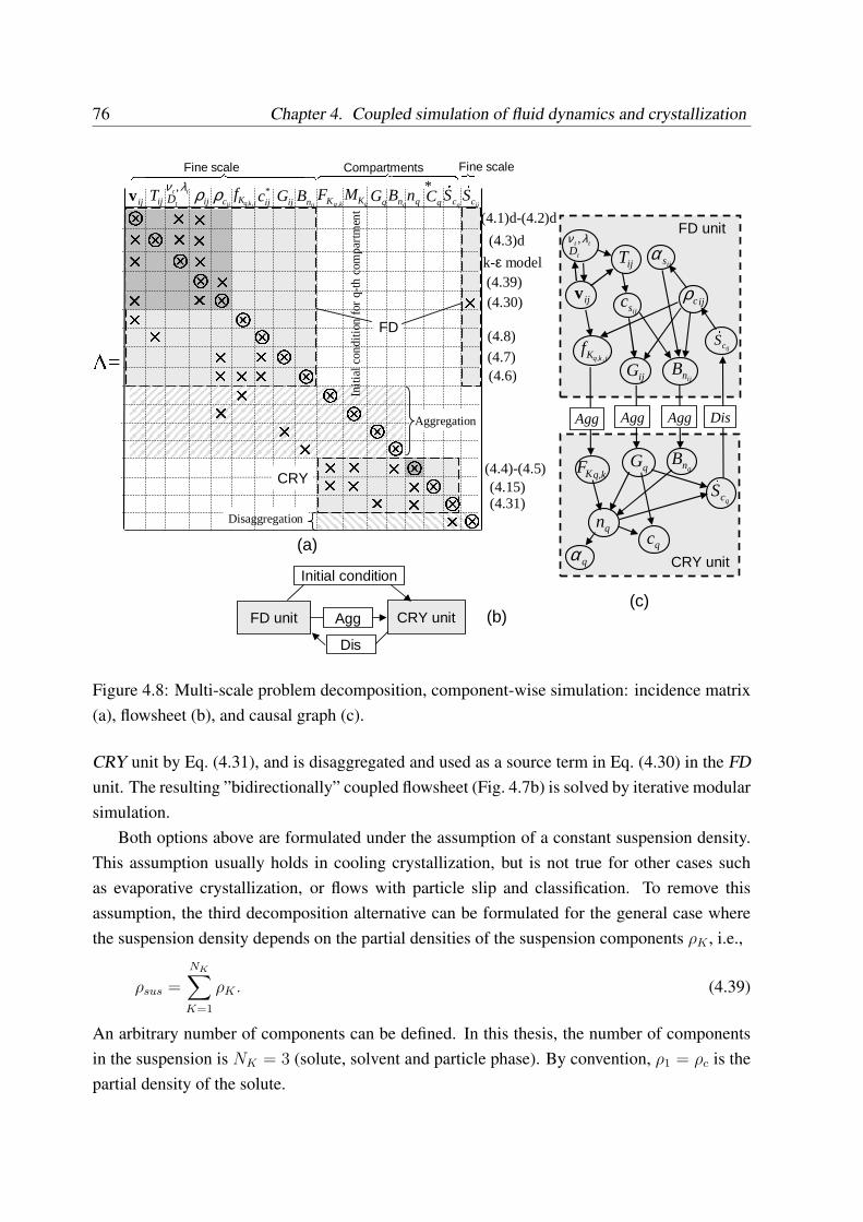
76 Chapter 4. Coupled simulation of fluid dynamics and crystallization44444 844444 76ijv ijT *
ijc qnijcρ
qcS&ijGijnB���� � � �
��Λ=� � ��� (4.1)d-(4.2)d
(4.3)d
(4.4)-(4.5)
(4.7)(4.6)� (4.30)���
ijcS&����
Disaggregation
FD
ijv
ijT
qnqc
qcS&ijsc
ijGijnB
qα
FD unit
CRY unit
kqKF ,
ijcρ
ijcS&ijsα
qGqnB
qCqGqnB
� ��kqKF
,
� � � � �� � � �����
(4.15)(4.31)
�� *44444 844444 76 Fine scale Compartments Fine scale}
jkqKf ,, qKM
��CRY
Aggregation
Initi
al c
ondi
tion
for
q-t
hco
mpa
rtm
ent
jkqKf ,,
FD unit CRY unitAgg
Dis
Initial condition
ijρ� ����� (4.39)
(a)
(c)(b)
t
ttD
λν ,
Agg Agg Agg Dis
t
ttD
λν ,
k-ε model
(4.8)
Figure 4.8: Multi-scale problem decomposition, component-wise simulation: incidence matrix(a), flowsheet (b), and causal graph (c).
CRY unit by Eq. (4.31), and is disaggregated and used as a source term in Eq. (4.30) in the FDunit. The resulting ”bidirectionally” coupled flowsheet (Fig. 4.7b) is solved by iterative modularsimulation.
Both options above are formulated under the assumption of a constant suspension density.This assumption usually holds in cooling crystallization, but is not true for other cases suchas evaporative crystallization, or flows with particle slip and classification. To remove thisassumption, the third decomposition alternative can be formulated for the general case wherethe suspension density depends on the partial densities of the suspension components ρK , i.e.,
ρsus =
NK∑K=1
ρK . (4.39)
An arbitrary number of components can be defined. In this thesis, the number of componentsin the suspension is NK = 3 (solute, solvent and particle phase). By convention, ρ1 = ρc is thepartial density of the solute.
4.2. Generalized process flowsheet modeling and simulation 77
In this case, the FD unit includes Navier-Stokes equations for mass, momentum and energy,the species transport equations (4.30) for the suspension components together with the consti-tutive equation (4.39) and the crystallization kinetics. The CRY unit includes the populationbalance. The incidence matrix of the decomposition is shown in Fig. 4.8. The species transportis part of the FD subproblem and solved for all components but one. Instead of overall massflows Fq,k, the mass flows of suspension components FKq,k
through the compartment boundariesare used as coupling variables. This allows to abandon a mixed product removal assumptionand specify different outlet flows for the components.
An important issue is the initial conditions setup for the variables defined on both grids.These initial conditions are first set at the beginning of the simulation. During the simulation,the initial variable profiles in the FD unit are always set equal to the converged state at theprevious interval. The initial conditions for the component partial densities on the coarse gridin the CRY unit are set depending on the decomposition option used. If the first option isused, the component partial densities are only evaluated in the coarse-scale CRY unit, and thesimulation on the new interval continues from the last converged state. If other decompositionsare used, the initial conditions for the partial densities are calculated as integrals of the fine-gridconcentration in the FD unit (component masses MKq(tn)) and updated in the CRY unit at thestart of the new time interval.
4.2.7 Subproblem setup in software tools
Choice of software toolsAfter problem decomposition, the resulting subproblems need to be set up in the associated
software tools. The choice of software tools for the simulation of the subproblems is tightly re-lated to the problem decomposition. In fact, these two steps need to be performed concurrently:the definition of the subproblems provides guidelines for the choice of the simulation tools, andreversely, the capabilities of the available simulation tools should be considered already duringthe definition of the subproblems. The simulation tools chosen should efficiently solve the bal-ance equations of the subproblems, support the grids, on which the subproblems are defined,and the information exchange.
For the fluid dynamics-crystallization problem, FLUENT (Appendix A.3) was chosen tosolve the CFD subproblem.5 Parsival (Appendix A.4) was employed for the crystallization sub-problem for its adaptive population balance solution algorithm, representation of the kineticsand support of multiple interconnected ideally mixed compartments. Fig. 4.9 shows the re-
5Besides FLUENT, there are a number of alternative CFD codes like CFX or the open-source CFD solverOpenFOAM, available at www.opencfd.co.uk (Accessed: 12.03.2009). However, for these solvers, no dedicatedwrapper has yet been developed in CHEOPS.
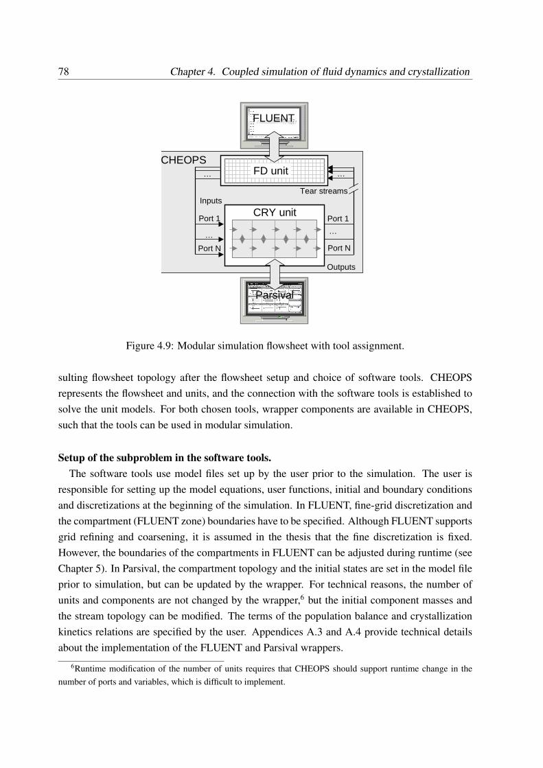
78 Chapter 4. Coupled simulation of fluid dynamics and crystallization
FD unit
CRY unit
…
Port N
…
FLUENT
Parsival
CHEOPS
Port 1
…
Port 1
Port N
…
Inputs
Outputs
Tear streams
Figure 4.9: Modular simulation flowsheet with tool assignment.
sulting flowsheet topology after the flowsheet setup and choice of software tools. CHEOPSrepresents the flowsheet and units, and the connection with the software tools is established tosolve the unit models. For both chosen tools, wrapper components are available in CHEOPS,such that the tools can be used in modular simulation.
Setup of the subproblem in the software tools.The software tools use model files set up by the user prior to the simulation. The user is
responsible for setting up the model equations, user functions, initial and boundary conditionsand discretizations at the beginning of the simulation. In FLUENT, fine-grid discretization andthe compartment (FLUENT zone) boundaries have to be specified. Although FLUENT supportsgrid refining and coarsening, it is assumed in the thesis that the fine discretization is fixed.However, the boundaries of the compartments in FLUENT can be adjusted during runtime (seeChapter 5). In Parsival, the compartment topology and the initial states are set in the model fileprior to simulation, but can be updated by the wrapper. For technical reasons, the number ofunits and components are not changed by the wrapper,6 but the initial component masses andthe stream topology can be modified. The terms of the population balance and crystallizationkinetics relations are specified by the user. Appendices A.3 and A.4 provide technical detailsabout the implementation of the FLUENT and Parsival wrappers.
6Runtime modification of the number of units requires that CHEOPS should support runtime change in thenumber of ports and variables, which is difficult to implement.
4.2. Generalized process flowsheet modeling and simulation 79
4.2.8 Overdetermined problems and built-in relations
Commercial tools, particularly specialized simulators, usually aid the user in constructing themodel not only by providing a user interface for setting up model equations and their parame-ters, but also by automatically applying typical assumptions and constitutive equations requiredfor model closure. Built-in tool assumptions can usually not be modified by the user. Built-inconstitutive equations are added by the tool to close the equation system without an explicituser specification, and they can not be set or removed from the equation system by the user.
Automatic problem closure is very convenient if the user works with a stand-alone simulator.However, in case the simulator solves only a subproblem model, some built-in closure relationsfor a certain variable may duplicate equations computing the same variable in the other subprob-lem. This introduces redundancy and renders the full problem overdetermined. An example ofsuch a relation is the built-in solute mass balance in the CRY unit solver Parsival (Eq. (4.15))which is redundant to the species transport equation in the FD unit (Eq. (4.30)) and computesthe solute concentration in compartment ρcq , which can also be evaluated by aggregation fromthe fine-scale concentration as Agg(ρci,j
).
Problem overdetermination introduces inconcistencies discussed in Section 4.3.2.2. Toeliminate them, the user has to define only one equation to compute the variable in the fullproblem, eliminating the other redundant equations for the same variable, and disabling thebuilt-in relations if possible. Alternatively, the user can employ the redundant equations in theanalysis of the overall problem to check consistency and subproblem deviations (Section 4.3.2).
4.2.9 Modular dynamic simulation algorithm for generalized flowsheet
To perform the simulation of the generalized flowsheet, a modular dynamic simulation al-gorithm is employed. Application of this algorithm to the simulation of a fluid dynamics-crystallization problem represented by a generalized flowsheet requires several steps to be per-formed by the user, and several extensions of the modular simulation algorithm (Section 3.2.4)as described below.
Setup of the generalized flowsheetThese steps must be followed by the user to set up the simulation of a generalized flowsheet.
The setup procedure is illustrated in Fig. 4.10 and includes the following major steps.
Step 1. The procedure starts with the decomposition of the problem into subproblems (Sec-tion 4.2.1), causal analysis, identification of coupling variables and construction of the flow-sheet, as described in Section 4.2.6. This step defines the subproblems and their respective
80 Chapter 4. Coupled simulation of fluid dynamics and crystallization
scales, subproblem equation systems, the list of coupling variables and their association withsubproblem inputs, initial and boundary conditions.
Step 2. The user chooses software tools and implements the subproblems in the chosentools. The user identifies built-in constitutive relations and redundant equations. He canreturn to Step 1 to change the subproblem decomposition to eliminate redundant equations.The user defines the initial discretization in all employed subproblems, and determines,which initial and boundary conditions will be set by the algorithm. After this step, thediscretizations of the subproblems are determined, the problem decomposition is finalized,and model files for the subproblems in the simulation tool’s format are completed.
Step 3. The user compiles the XML configuration file to define the generalized flowsheet inCHEOPS, where the number of units, their couplings and coupling variables are specified.The user also configures the mapping between the CHEOPS variables and internal variablesof the tools as a mapping XML file for each tool (see also Appendices A.3–A.5). Finally,the solver parameters are specified. Then, the generalized flowsheet is fully specified andready for simulation.
Modular simulation algorithmThe modular dynamic simulation algorithm for the process flowsheets was described in Sec-
tion 3.2.4. To use this algorithm for the simulation of generalized flowsheets for spatial multi-scale problems, the existing framework was extended to support scale integration, topologyhandling and setting of initial and boundary conditions. The major steps of the updated algo-rithm are described below:
Step 0. Flowsheet analysis. If the problem involves few subproblems, the simulation se-quence and the torn couplings are specified by the user.
Step 1. As in Section 3.2.4, the total time horizon and the initial integration interval ∆T0 =
[t0; t1] are set, the external inputs are initialized, the guesses for the tear-stream variabletrajectories u0
TS(t) are done.
Step 2. Sequential integration for the interval ∆Tn is performed as described in Sec-tion 3.2.2. During the propagation through the coupling between the units with differentdiscretization, scale integration relations are evaluated at every reporting time point (Sec-tion 4.2.3).
Step 3. The convergence error ERRkcv is evaluated and compared with the convergence tol-
erance ε according to Section 3.2.3 after completion of sequential integration in the current
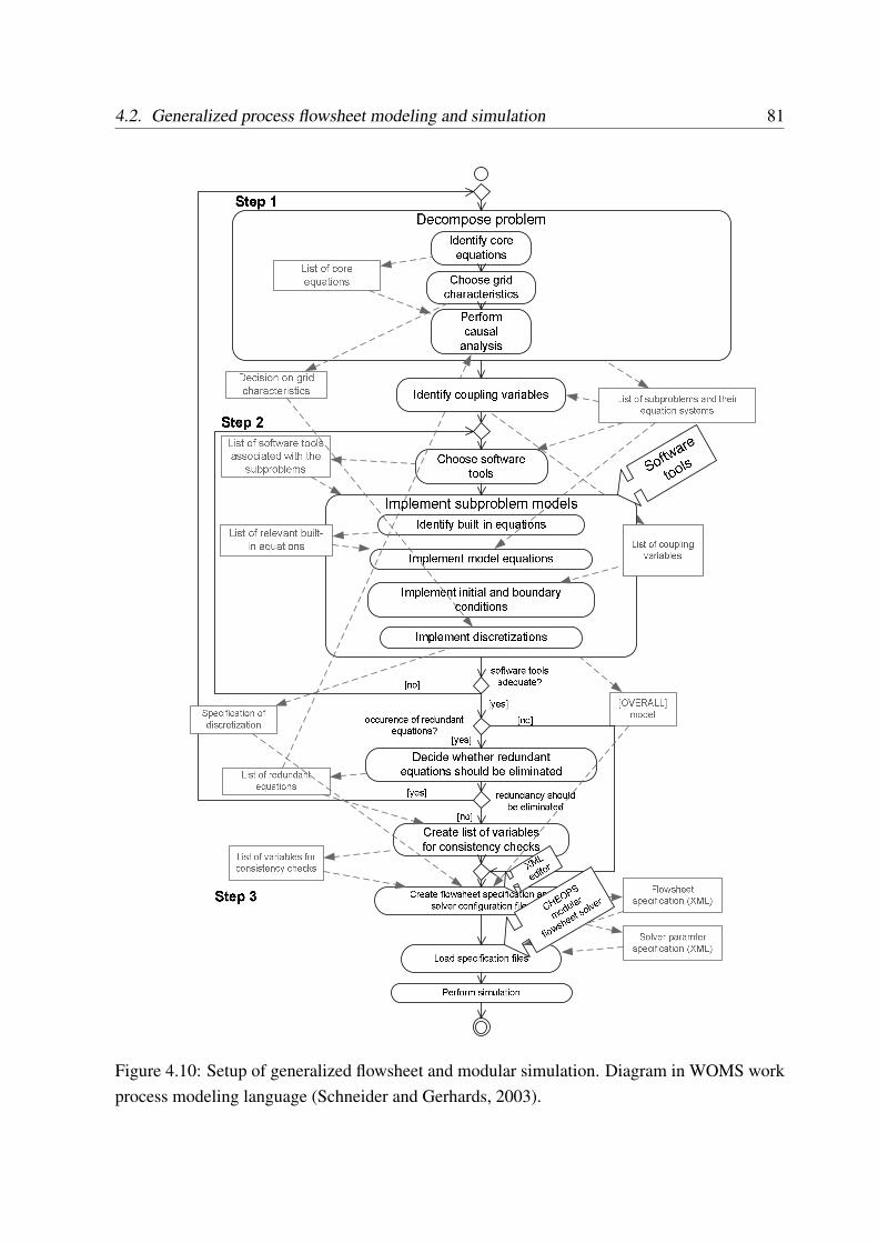
4.2. Generalized process flowsheet modeling and simulation 81
Figure 4.10: Setup of generalized flowsheet and modular simulation. Diagram in WOMS workprocess modeling language (Schneider and Gerhards, 2003).
82 Chapter 4. Coupled simulation of fluid dynamics and crystallization
iteration on the interval. For overdetermined problems, the equation term consistency error(Section 4.3.2) ERRt can be computed as the difference between the trajectories computedin different subproblems and compared to the consistency tolerance εt.
Step 4. If the iteration is not converged, another iteration on the same interval is startedas described in Section 3.2.4. Since scale integration is implemented in the unit with finediscretization, the updated variables in the tear stream are defined on the coarse grid.
Step 5. After a converged iteration, the next integration interval ∆Tn+1 is initialized, and ini-tial guesses for the trajectories of the tear-stream variables are predicted as in Section 3.2.4.The initial conditions for the next interval are updated. Depending on the problem setup,they can be set equal to the converged state at the end of the previous interval, or can beprovided by an external input or by a different unit. After the update of the tear streams andthe initial conditions, sequential integration (Step 2) is performed for the next integrationinterval.
Step 6. The integration continues until the end of the simulation time horizon is reached.
4.3 Analysis of the generalized flowsheet
4.3.1 Characterization of errors in the simulation
The process model implemented as a generalized flowsheet in the framework of modular cou-pled simulation needs to be checked for consistency and numerical errors in the simulations.
The deviation of the solution of the numerically solved discretized model from the truesolution is denoted as an overall simulation error ERR. It can be defined as the norm of thedeviation of the subproblem outputs from the true solution on the considered time interval ∆Tn:
ERR = ‖y∗(t)− y(t)‖ , ∈ (tn; tn+1) . (4.40)
The overall simulation error is a function of the discretization and of the solver tolerance.The tolerance is the convergence condition and determines the numerical integration errorERRnum, which characterizes the accuracy of the numerical methods in the employed sim-ulation tools. The sources of this error are discussed in Section 4.3.6.1. The deviation of aperfectly convergent solution (with tolerance approaching zero) from the true solution is thediscretization error ERRd. It is caused by the discrete representation of the continuous modelequations, its terms and inputs, and depends on the discretization and grid topology employed.
The considered problem is decomposed into two subproblems with different discretizations.Hence, two discretization errors exist for these subproblems, ERRFD
d and ERRCRYd .
4.3. Analysis of the generalized flowsheet 83
Discretization error cannot be computed without knowledge of the analytical true solutionand its outputs y. Evaluation of discretization error requires specific mathematical methods ofa posteriori error estimation, which have been developed only for limited problem classes andstandard discretizations. A further complexity is the propagation of all errors in the modular dy-namic simulation along the grid, between the subproblems, and in temporal coordinates. Somediscussion about the discretization error estimation approaches is provided in Section 4.3.6.2.
However, it is possible to characterize the discretization error by several error quantities:
• The equation terms consistency error ERRt represents the error between the discretizedmodel equation of a subproblem and its counterpart, represented analytically or in a fine-scale discretization. This is a measure of consistency of the model representation in thesubproblems, and should ideally be zero.
• The scale integration errors are caused by the aggregation (ERRagg) or the disaggrega-tion (ERRdis) where the input and output quantities are discretized using different grids.The aggregation error characterizes non-uniformity of the fine-grid profile, and so, thecontribution to the discretization error because of the model inputs aggregation in onecoarse-grid element.
• The consistency error ERRc is a numerically evaluated deviation in the solution of thediscretized model equations in different subproblems and on different grids, computedusing the same inputs. If the numerical and the equation terms consistency error are zero,this error can be used as an approximate of the discretization error.
The reference error ERRref is defined as a deviation between the computed solution andthe reference solution that contains no analytical errors. This can be used as the measure of theoverall error.
Finally, the convergence error (ERRkcv,n) is defined similarly to Section 3.2.3 as the devi-
ation between the values at iteration k and k − 1, in order to check convergence during theiteration process (Section 4.3.7).
4.3.2 Model consistency
4.3.2.1 Consistency of generalized flowsheet model
A generalized flowsheet model of a complex process is considered consistent if its discreterepresentations in the subproblems passes the consistency check, which includes:
• consistent choice of assumptions and parameters in all subproblems;
84 Chapter 4. Coupled simulation of fluid dynamics and crystallization
• equivalence of the inputs and equation terms of the discretized balance equations em-ployed in different subproblems and tools;
• equivalence of the discretized subproblem closure equations (particularly, the tool built-inclosures) employed in different subproblems and tools.
The first condition implies that an assumption about a variable (or an equation) should beequivalent in the subproblem where it is computed and in that where it is used, and the sameparameter values should be used. If different assumptions are employed, subproblem balanceequations will not be written in equivalent forms, and a systematic error follows. For example,a constant density assumption should hold both in the FD and in the CRY unit, and the densitiesmust be equal.
To verify equivalence for subproblem inputs and equation terms, the input terms, initial andboundary conditions, and equations are analytically derived for the considered discretization,and compared with the respective terms in the discretized subproblem equations actually em-ployed in the tools. A non-equivalence in the subproblem inputs inevitably leads to systematicerrors and should be, whenever possible, minimized by adjusting the set of assumptions, equa-tions and coupling variables. Similarly, non-equivalence in the built-in constitutive relationsresults in inconcictency between the variables computed from such consistutive relations indifferent subproblems and also violates subproblem consistency.
To identify these issues, equation consistency errors can be evaluated prior to the simulation.Such analysis for the fluid dynamics-crystallization problem is done in next section.
4.3.2.2 Equivalence of crystallization subproblem equation terms
Population balance equationThe equivalence is checked for the crystallization subproblem on the coarse-scale compart-
ment grid, defined by the integral balance equations and solved in the population balance solverParsival. The integral population balance equation (4.14)
Vq∂nq(L, t)
∂t+ Vq
∂(Gq(L, t)nq(L, t))
∂L−
∑
k
Vq,k,innq,k,in(L, t) +∑
k
Vq,k,outnq,k,out(L, t)
= VqBq(L, t)− VqDq(L, t).
(4.41)
is actually solved in Parsival for an ideally mixed unit with constant volume Vq. To checkequivalence, the terms of the differential PB equation (2.3) are individually integrated for a
4.3. Analysis of the generalized flowsheet 85
coarse-grid compartment to result in
(1)
∫
Vq
∂n
∂tdV = Vq
∂nq
∂t;
(2)
∫
Vq
∂(Gn)
∂LdV = Vq
∂((Gn)q
)
∂L;
(3)
∫
Vq
∇ · (vn)dV =
∫
Aq
vqnqnAqdA =∑
k
Vq,knq,k =∑
k
fn(L, t)q,k
(4)
∫
Vq
(B(L, t)−D(L, t))dV = VqBq(L, t)− VqDq(L, t).
The terms of the coarse-scale population balance equation are the particle transport along the
particle size coordinate,∂((Gn)q)
∂L, the inlet and outlet particle flows averaged over the flow cross
sections (compartment boundaries) q, k,∑
k fn(L, t)q,k =∑
k Vq,knq,k(L, t), and the volume-averaged birth and death kinetics terms Bq(L, t) and Dq(L, t). These terms are not fully equiv-alent to those of the population balance for an ideally mixed unit in (4.41). In particular, theproduct of volume-averaged growth rate and PSD Gqnq is not equivalent to the volume-averagedtransport along the particle size coordinate (Gn)q even in case G 6= G(L). The birth and deathterms are nonlinear functions, usually dependent on the PSD. Since nq(L, t) is available onlyon the coarse grid, these functions always produce deviations during the volumetric averaging(B(nq) 6= B(nq(L, t)) and D(nq) 6= D(nq(L, t))).
In the considered problem, the birth and death kinetics rates are both zero. Inconsistenciesin the equation terms ERRt representing the crystallization kinetics of the considered problem(4.1)-(4.10) can be summarized as
ERRt,Gnq=
∥∥∥(G(L, t)n(L, t))q −Gq(L, t)nq(L, t)∥∥∥ 6= 0; (4.42)
ERRt,Bq=
∥∥∥B (nq(L, t))−B(nq(L, t)
)∥∥∥ = 0; (4.43)
ERRt,Dq=
∥∥∥D (nq(L, t))−D(nq(L, t)
)∥∥∥ = 0. (4.44)
Mixed product removal modelThe particle flow fn(L, t)q,k is the product of the flux through a cross section of the compart-
ment boundary Aq,k and the respective PSD, integrated over the cross section. On the coarsegrid it is computed as the product of the inlet/outlet volumetric flow rate Vq,k and the volumetricflow averaged PSD in the boundary cross section, i.e., Vq,knq,k.
Since nq,k is not available on the fine grid, it should be approximated. A popular practicalsimplification is the mixed product removal assumption, implemented in the simulation toolssuch as Parsival as a default option. It assumes that a scalar quantity or distribution at the outlet
86 Chapter 4. Coupled simulation of fluid dynamics and crystallization
compartment boundary has the same value as within the compartment, i.e., nq,out(L) = nq(L),ρcq,out = ρcq . This is not consistent with the true values at the outlet, if gradients within thecompartment are present. In particular, Vq,knq,k(L) 6= Vq,k nq(L) and
ERRt,Fnq,k,MPR =∥∥∥fn(L, t)q,k − Vq,knq(L)
∥∥∥ > ERRt,Fnq,k. (4.45)
In the considered problem, where consistency of the states within the discretization cells of bothgrids is important for a successful simulation, the mixed product removal assumption introducessignificant errors into the solution. It can be written as an error in the equation term for particletransport as
ERRt,Fnq,k=
∥∥∥fn(L, t)q,k − Vq,knq(L)∥∥∥ . (4.46)
Component flows modelTo improve the consistency of the particle flow term, component flows (discussed in the
decomposition option 3 in Section 4.2.6) are used instead of overall flows. The flow ratesfor each component of the suspension FKq,k
= Vq,kcKq,kand specifically for the particle flow
Fn,q,k = Vq,knq,k(L) are evaluated. They are used as exact terms in the integral componentbalance equations in the compartment (4.30).
Use of the component flows in the population balance yields Vq,knq,k(L) = Vnq,knnorm
q,k (L),where Vnq,k
is the particle flow. The particle flow is exact, and its use does not introduce errorsinto the mass balance of particles. The only remaining inconsistency is the normalized par-ticle size distribution nnorm
q,k (L), which should be aggregated over the boundary Aq,k. Sincethe PSD is not defined on the fine grid, the normalized boundary PSD has to be approxi-mated on the coarse compartment grid. An assumption of mixed PSD removal implies thatnnorm,out
q,k (L) = nnormq (L); it can be considered accurate in case of slow kinetics and absence of
particle classification. Alternatively, a classification model for the PSD at the respective outletcan be provided.
If the component flows model is used, the following error is produced in the equation termfor particle transport:
ERRt,Fnq,k=
{ ∥∥∥fn(L, t)q,k − Vnq,knnorm
q (L)∥∥∥ (no classification),∥∥∥fn(L, t)q,k − Vnq,k
houtq,k (L)nnorm
q (L)∥∥∥ (with classification).
(4.47)
Solute component balanceA built-in balance equation is automatically solved in Parsival for the concentration ρKq of
each liquid phase component K in the compartment q (4.30):
∂ρKq
∂t=
∑
k
V inq,kρ
inKq,k
−∑
k
V outq,k ρKq + SρKq
, K = 1, 2.
4.3. Analysis of the generalized flowsheet 87
This equation is redundant to the species transport equations (4.9), which compute concen-trations ρKi,j on the fine grid if they are specified. These concentrations are related to theconcentrations in the compartment by the aggregation relation, ρKq = Agg(ρKi,j
).Integration of the terms of the balance equation (4.9) for the solute concentration ρc on the
fine grid results in:
(1)
∫
Vq
∂ρc
∂tdV = Vq
∂ρcq
∂t;
(2)
∫
Vq
∇ · (vρc)dV =
∫
Aq,k
vq,kρcq,kdA = Vq,kρcq,k
= Fcq,k;
(3)
∫
Vq
ScdV = VqScq .
The coarse scale solute balance incorporates term for the solute mass flow rate through thecross section of the k-th boundary Fcq,k
and an averaged source of the solute component in
compartment q, Scq . The mass flow rates of the solute component Fcq,kare represented exactly,
while the use of the total flow rate Vq,k would lead to an inconsistency because of Vq,kρcq,k6=
Vq,kρcq,k. Hence,
ERRt,F cq,k=
{∣∣∣Fcq,k− Vq,kρcq,k
∣∣∣ , (in case of total flow),
0, (in case of component flows),(4.48)
The solute component source term Scq is the mass transfer due to crystallization. It is nonlin-early dependent on the PSD and the growth rate (4.10). It has to be computed in the crystalliza-tion subproblem. Integration reveals the inconsistency in the concentration source term even incase G 6= G(L):
ERRt,Scq=
∣∣∣Sc (G(L), n(L))− Sc(Gq(L), nq(L))∣∣∣
=
∣∣∣∣3kvρS
∫ ∞
0
(Gn(L))qL2dL− 3kvρSGqµ
(2)q
∣∣∣∣ 6= 0. (4.49)
Since n(L) is only available on the coarse scale, this deviation can not be corrected, and consis-tent formulations cannot be achieved. Furthermore, disaggregation of Scq to produce the inputs
for the component balance on the fine scale ˜Sci,jintroduces a disaggregation error. The two
errors can not be completely corrected without knowledge of the true PSD on the fine grid, andremain in the solution.
Initial and boundary conditionsThe crystallization subproblem is specified with initial and boundary conditions. Initial con-
ditions, e.g. initial masses of components and initial PSD in the coarse-scale compartments,
88 Chapter 4. Coupled simulation of fluid dynamics and crystallization
are computed by the integration over the volume and are always consistent. A boundary con-dition is set at the left boundary for the particle size as a nucleation rate (4.6). Nucleation isdescribed by a nonlinear term, depending on concentration. Hence, deviations may occur dueto Bn(cq) 6= Bn(cq),
ERRt,Bnq=
∥∥∥Bn (cq)−Bn (cq)∥∥∥ . (4.50)
The discussion in this section shows that the terms of the compartment population balanceare not equivalent to those of the fine-scale population balance without knowledge of the fine-scale PSD. But a partial correction is possible by a proper spatial averaging and by representingthe streams as component flows instead of employing a mixed product removal assumption.
4.3.2.3 Equivalence in the fluid dynamics subproblem
The discretized forms of the equations in the fluid dynamics subproblem equations are deter-mined by the employed discretization scheme on the fine scale (Section 2.2.2). Similar errorterms as in the above section can be derived for the fine-scale cells. However, the deviationsbetween the analytical equations of the fluid dynamics subproblem and their finite volume dis-cretization are orders of magnitude smaller than the similar deviations in the crystallizationsubproblem, and can be ignored.
4.3.3 Scale integration errors
Aggregation errorThe integration of the discretized function between different scales inevitably introduces an
error, since the profiles within the discretization element are averaged during the aggregation orapproximated during the disaggregation.
The aggregation error for a scalar quantity φ is defined here as a norm of a deviation betweenthe fine-grid values of this quantity φi,j in the cells zi,j and its averaged value in the coarse-scalecompartment Zq, which contains these cells, φq = Agg(i,j)∈Iq(φi,j):
ERRagg,q(φ) =
∫
Vq
∥∥φ− φq
∥∥ ∼=∑
(i,j)∈Iq
∥∥φi,j − φq
∥∥ . (4.51)
This aggregation error characterizes the inhomogeneity of the spatial profile of the quantityφ in the coarse-scale compartment Zq. This error can be directly evaluated numerically forany quantity φ. The larger the aggregation error, the larger deviations can be expected in thesolution of discretized model equations on the coarse scale. Hence, it is an implicit indicationof the discretization error.
The aggregation error (4.51) does not characterize the deviation of an aggregated quantityfrom its true value.
4.3. Analysis of the generalized flowsheet 89
Disaggregation errorDisaggregation computes the fine-grid profile of a quantity from its coarse-grid values by
introducing a certain approximation function evaluated on the fine grid. It is thus a simplifiedimplementation of the inverse problem of the profile reconstruction. The approximation doesnot correctly reflect the true profiles of this quantity on the fine grid, thus an error is introduced.
If the true fine-scale solution, φi,j or its accurate estimate is available, the error in the disag-gregated scalar quantity φi,j can be evaluated as
ERRdis,q =∑
(i,j)∈Iq
∥∥∥φi,j − φi,j
∥∥∥ , (4.52)
under the condition Agg(φi,j) = Agg(φi,j).
The disaggregated quantity contains all other errors already present in the outputs of thecoarse-scale subproblem, including aggregation errors of the coarse-scale subproblem inputs,consistency errors and effects of error propagation. An isolation of the disaggregation errorsource is a complicated inverse problem and has not been addressed in the thesis. However,the comparison of disaggregation methods is possible by evaluating Eq. (4.52) for solutionsobtained using different methods (Section 4.4.6).
4.3.4 Numerical consistency error
Characterization of the numerical consistency error ERRc can be done for the problems overde-termined on the flowsheet level using the outputs of the simulation. The same variable is eval-uated in subproblems P and Q at the n-th time step (index omitted) and at the k-th iterationaccording to:
ERRkc =
∥∥ykP (t)− yk
Q(t)∥∥ = max
i
1
tn − tn−1
∫ tn
tn−1
(yP
ki (t)− yQ
ki (t)
)2dt. (4.53)
The numerical consistency error at the converged iteration, ERR∗c , is determined by the spa-
tial and temporal discretization of the subproblems, consistency of the inputs for the discretizedmodel, and consistency of the subproblem formulations. The change of ERR∗
c with differentsubproblem formulations, using the same discretizations and the same inputs, can be interpretedas the measure of consistency between the subproblems. Smaller ERR∗
c indicates a better con-sistency. However, ERR∗
c is usually non-zero even if the input variables and formulations areconsistent and the system states convergence error ERR∗
cv approaches zero. The remaining er-ror is caused by discretization. Therefore, it is possible to use the numerical consistency errorat the converged iteration ERR∗
c as a characteristics of the problem discretization error ERRd.
90 Chapter 4. Coupled simulation of fluid dynamics and crystallization
4.3.5 Reference error
The reference error ERRref is defined here as the deviation between the simulated and thereference solutions, which is obtained by a more accurate method and is a good estimate forthe true solution. It is evaluated in this study for the coarse-grid variables according to theexpression:
ERRrefq = φq − φrefq .
To obtain an error term, |ERRrefq | should be used.
4.3.6 Sources of error in the coupled simulation
As discussed in Section 4.3.1, the overall error in the simulation is determined by the discretiza-tion error ERRd of the subproblems, the numerical integration error ERRn and the propagationof the errors in the simulation.
4.3.6.1 Numerical integration error in software tools
Simulation software tools usually perform numerical iteration on the discretized problem untilthe solution is converged to the specified error tolerance. The tolerance is usually set in thesimulation tools. The user can specify spatial and time discretization schemes, which maydiffer in accuracy.
A typical solution in FLUENT is the first-order upwind spatial discretization and first-orderimplicit time discretization with fixed solver time steps δts ≤ ∆tn,m. Fig. 4.11 shows thediscretized values of a trajectory for different solver time steps, δts = ∆tn,m (points A,B) andδts = ∆tn,m/2 (points A,C,B) in the FD subproblem. A further improvement can be achievedby the evaluation of the input trajectories at the midpoints of each step (points D,E). If the solverstep sizes are chosen well, the numerical integration error in FLUENT is controlled by the errortolerances for the balance equations.
Parsival performs an adaptive, error-controlled simulation of the compartment populationbalance problem based on finite element discretization for the particle size coordinate (Sec-tion 2.1.4). It uses adaptive steps in time, which are smaller than the reporting time step, andare chosen such that the overall numerical integration error remains controlled (points A,C,D,Bin the CRY subproblem in Fig. 4.11). Thus, the error of the numerical integration can be con-sidered as tolerance controlled in both subproblems. With high tolerance levels, the numericalerror ERRn is considered small.
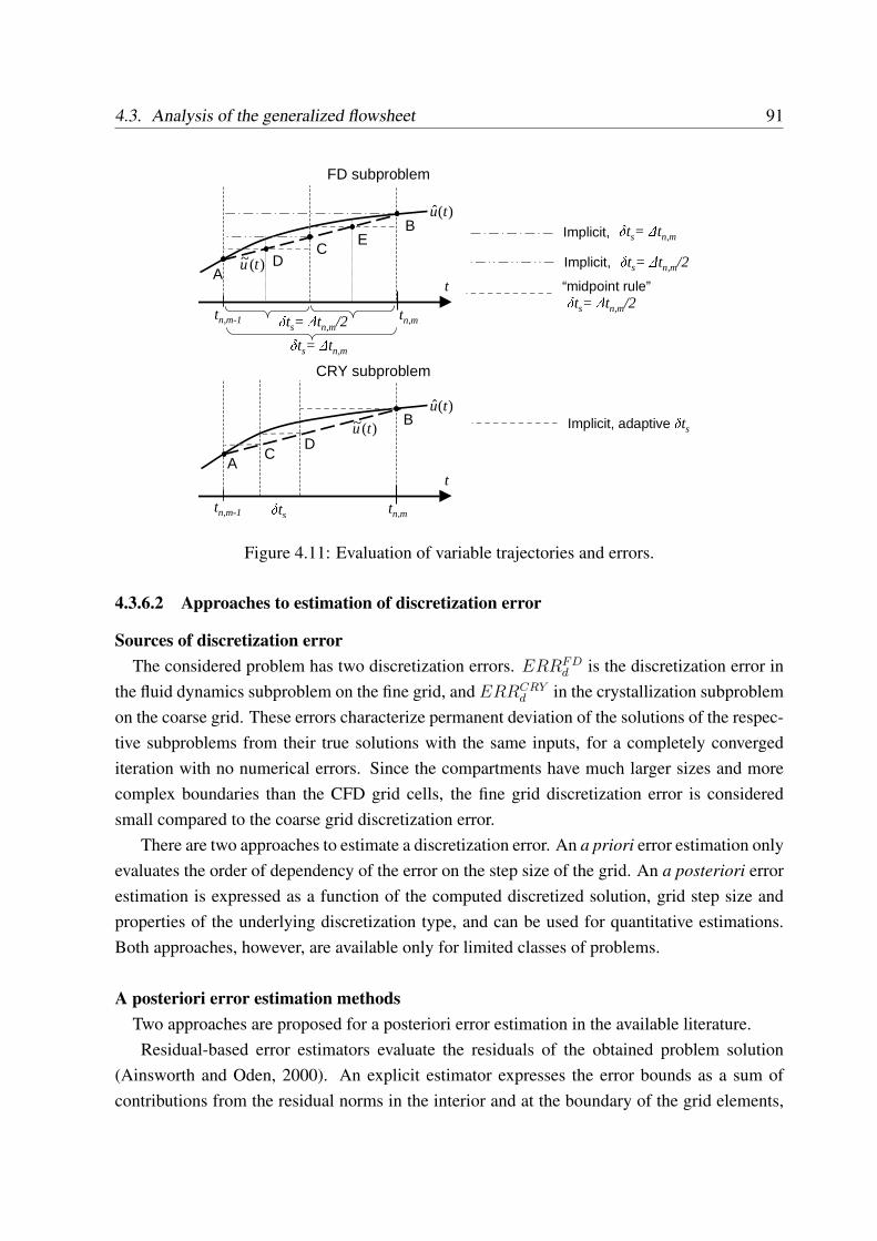
4.3. Analysis of the generalized flowsheet 91
tn,m
t
)(ˆ tu
tn,m-1
CRY subproblem
tn,m
t
)(ˆ tu
tn,m-1
δts= ∆tn,m/2δts= ∆tn,m
)(~ tu
“midpoint rule”
Implicit, δts= ∆tn,m
Implicit, δts= ∆tn,m/2δts= ∆tn,m/2
δts
)(~ tu
FD subproblem
Implicit, adaptive δts
A
B
CD
E
A
B
CD
Figure 4.11: Evaluation of variable trajectories and errors.
4.3.6.2 Approaches to estimation of discretization error
Sources of discretization errorThe considered problem has two discretization errors. ERRFD
d is the discretization error inthe fluid dynamics subproblem on the fine grid, and ERRCRY
d in the crystallization subproblemon the coarse grid. These errors characterize permanent deviation of the solutions of the respec-tive subproblems from their true solutions with the same inputs, for a completely convergediteration with no numerical errors. Since the compartments have much larger sizes and morecomplex boundaries than the CFD grid cells, the fine grid discretization error is consideredsmall compared to the coarse grid discretization error.
There are two approaches to estimate a discretization error. An a priori error estimation onlyevaluates the order of dependency of the error on the step size of the grid. An a posteriori errorestimation is expressed as a function of the computed discretized solution, grid step size andproperties of the underlying discretization type, and can be used for quantitative estimations.Both approaches, however, are available only for limited classes of problems.
A posteriori error estimation methodsTwo approaches are proposed for a posteriori error estimation in the available literature.Residual-based error estimators evaluate the residuals of the obtained problem solution
(Ainsworth and Oden, 2000). An explicit estimator expresses the error bounds as a sum ofcontributions from the residual norms in the interior and at the boundary of the grid elements,
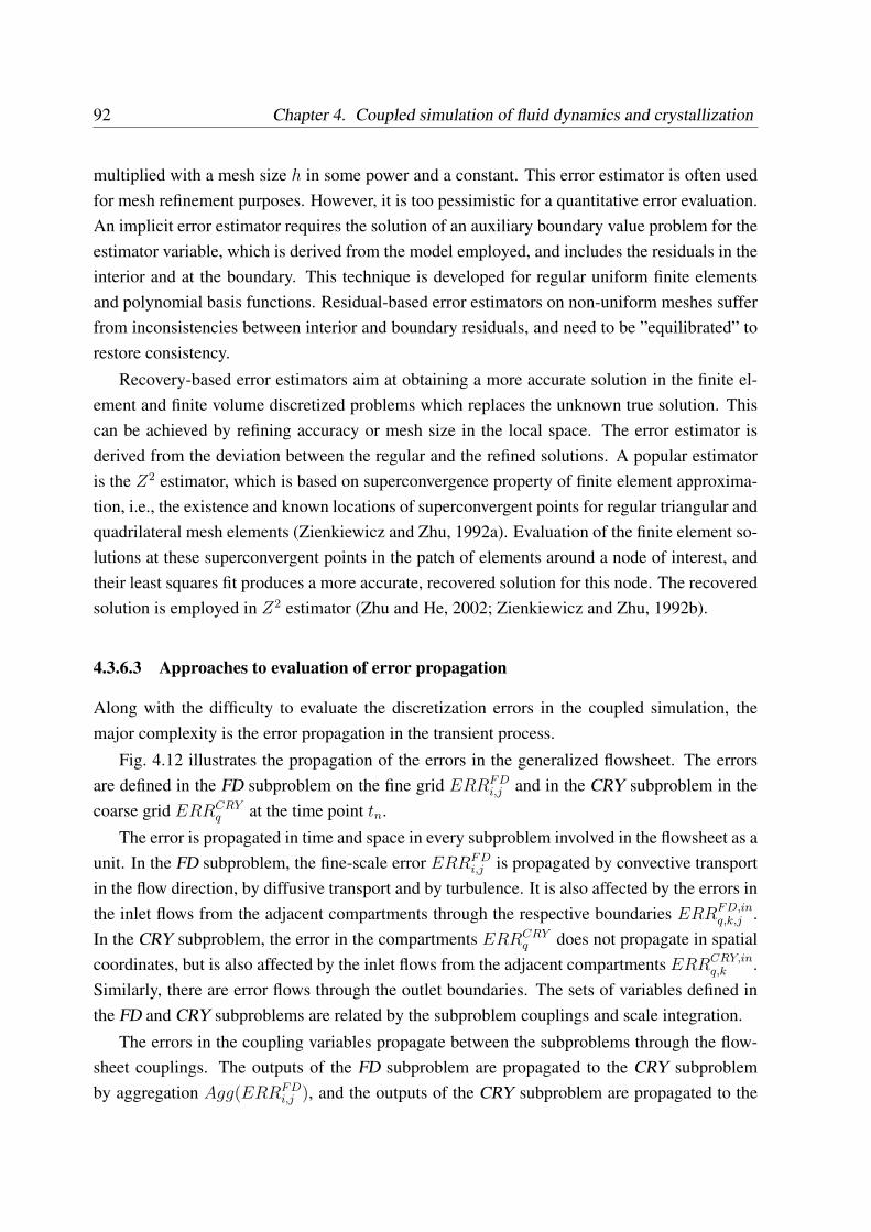
92 Chapter 4. Coupled simulation of fluid dynamics and crystallization
multiplied with a mesh size h in some power and a constant. This error estimator is often usedfor mesh refinement purposes. However, it is too pessimistic for a quantitative error evaluation.An implicit error estimator requires the solution of an auxiliary boundary value problem for theestimator variable, which is derived from the model employed, and includes the residuals in theinterior and at the boundary. This technique is developed for regular uniform finite elementsand polynomial basis functions. Residual-based error estimators on non-uniform meshes sufferfrom inconsistencies between interior and boundary residuals, and need to be ”equilibrated” torestore consistency.
Recovery-based error estimators aim at obtaining a more accurate solution in the finite el-ement and finite volume discretized problems which replaces the unknown true solution. Thiscan be achieved by refining accuracy or mesh size in the local space. The error estimator isderived from the deviation between the regular and the refined solutions. A popular estimatoris the Z2 estimator, which is based on superconvergence property of finite element approxima-tion, i.e., the existence and known locations of superconvergent points for regular triangular andquadrilateral mesh elements (Zienkiewicz and Zhu, 1992a). Evaluation of the finite element so-lutions at these superconvergent points in the patch of elements around a node of interest, andtheir least squares fit produces a more accurate, recovered solution for this node. The recoveredsolution is employed in Z2 estimator (Zhu and He, 2002; Zienkiewicz and Zhu, 1992b).
4.3.6.3 Approaches to evaluation of error propagation
Along with the difficulty to evaluate the discretization errors in the coupled simulation, themajor complexity is the error propagation in the transient process.
Fig. 4.12 illustrates the propagation of the errors in the generalized flowsheet. The errorsare defined in the FD subproblem on the fine grid ERRFD
i,j and in the CRY subproblem in thecoarse grid ERRCRY
q at the time point tn.
The error is propagated in time and space in every subproblem involved in the flowsheet as aunit. In the FD subproblem, the fine-scale error ERRFD
i,j is propagated by convective transportin the flow direction, by diffusive transport and by turbulence. It is also affected by the errors inthe inlet flows from the adjacent compartments through the respective boundaries ERRFD,in
q,k,j .In the CRY subproblem, the error in the compartments ERRCRY
q does not propagate in spatialcoordinates, but is also affected by the inlet flows from the adjacent compartments ERRCRY,in
q,k .Similarly, there are error flows through the outlet boundaries. The sets of variables defined inthe FD and CRY subproblems are related by the subproblem couplings and scale integration.
The errors in the coupling variables propagate between the subproblems through the flow-sheet couplings. The outputs of the FD subproblem are propagated to the CRY subproblemby aggregation Agg(ERRFD
i,j ), and the outputs of the CRY subproblem are propagated to the
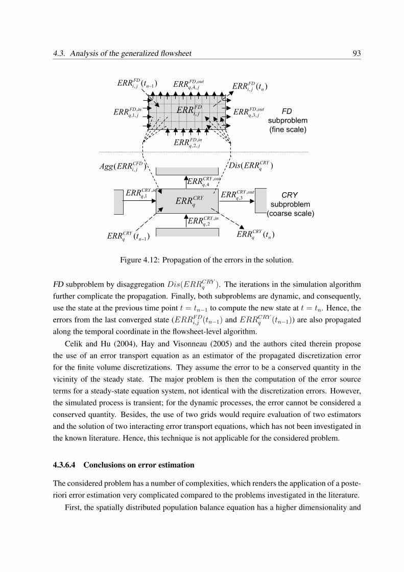
4.3. Analysis of the generalized flowsheet 93
FD
jiERR ,inFD
jqERR,
,1,
inFD
jqERR,
,2,
outFD
jqERR,
,3,
outFD
jqERR,
,4,
)( ,
CFD
jiERRAgg )( CRY
qERRDis
inCRY
qERR,
1, CRY
qERR
inCRY
qERR,
2,
outCRY
qERR,
4,
outCRY
qERR,
3,
)( 1−n
CRY
q tERR )( nCRY
q tERR
)( 1, −n
FD
ji tERR )(, n
FD
ji tERR
FD
subproblem
(fine scale)
CRY
subproblem
(coarse scale)
Figure 4.12: Propagation of the errors in the solution.
FD subproblem by disaggregation Dis(ERRCRYq ). The iterations in the simulation algorithm
further complicate the propagation. Finally, both subproblems are dynamic, and consequently,use the state at the previous time point t = tn−1 to compute the new state at t = tn. Hence, theerrors from the last converged state (ERRFD
i,j (tn−1) and ERRCRYq (tn−1)) are also propagated
along the temporal coordinate in the flowsheet-level algorithm.
Celik and Hu (2004), Hay and Visonneau (2005) and the authors cited therein proposethe use of an error transport equation as an estimator of the propagated discretization errorfor the finite volume discretizations. They assume the error to be a conserved quantity in thevicinity of the steady state. The major problem is then the computation of the error sourceterms for a steady-state equation system, not identical with the discretization errors. However,the simulated process is transient; for the dynamic processes, the error cannot be considered aconserved quantity. Besides, the use of two grids would require evaluation of two estimatorsand the solution of two interacting error transport equations, which has not been investigated inthe known literature. Hence, this technique is not applicable for the considered problem.
4.3.6.4 Conclusions on error estimation
The considered problem has a number of complexities, which renders the application of a poste-riori error estimation very complicated compared to the problems investigated in the literature.
First, the spatially distributed population balance equation has a higher dimensionality and
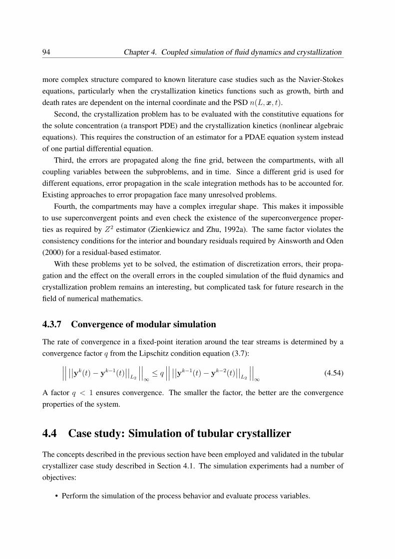
94 Chapter 4. Coupled simulation of fluid dynamics and crystallization
more complex structure compared to known literature case studies such as the Navier-Stokesequations, particularly when the crystallization kinetics functions such as growth, birth anddeath rates are dependent on the internal coordinate and the PSD n(L, x, t).
Second, the crystallization problem has to be evaluated with the constitutive equations forthe solute concentration (a transport PDE) and the crystallization kinetics (nonlinear algebraicequations). This requires the construction of an estimator for a PDAE equation system insteadof one partial differential equation.
Third, the errors are propagated along the fine grid, between the compartments, with allcoupling variables between the subproblems, and in time. Since a different grid is used fordifferent equations, error propagation in the scale integration methods has to be accounted for.Existing approaches to error propagation face many unresolved problems.
Fourth, the compartments may have a complex irregular shape. This makes it impossibleto use superconvergent points and even check the existence of the superconvergence proper-ties as required by Z2 estimator (Zienkiewicz and Zhu, 1992a). The same factor violates theconsistency conditions for the interior and boundary residuals required by Ainsworth and Oden(2000) for a residual-based estimator.
With these problems yet to be solved, the estimation of discretization errors, their propa-gation and the effect on the overall errors in the coupled simulation of the fluid dynamics andcrystallization problem remains an interesting, but complicated task for future research in thefield of numerical mathematics.
4.3.7 Convergence of modular simulation
The rate of convergence in a fixed-point iteration around the tear streams is determined by aconvergence factor q from the Lipschitz condition equation (3.7):
∣∣∣∣∣∣∣∣∣∣yk(t)− yk−1(t)
∣∣∣∣L2
∣∣∣∣∣∣∞≤ q
∣∣∣∣∣∣∣∣∣∣yk−1(t)− yk−2(t)
∣∣∣∣L2
∣∣∣∣∣∣∞
(4.54)
A factor q < 1 ensures convergence. The smaller the factor, the better are the convergenceproperties of the system.
4.4 Case study: Simulation of tubular crystallizer
The concepts described in the previous section have been employed and validated in the tubularcrystallizer case study described in Section 4.1. The simulation experiments had a number ofobjectives:
• Perform the simulation of the process behavior and evaluate process variables.
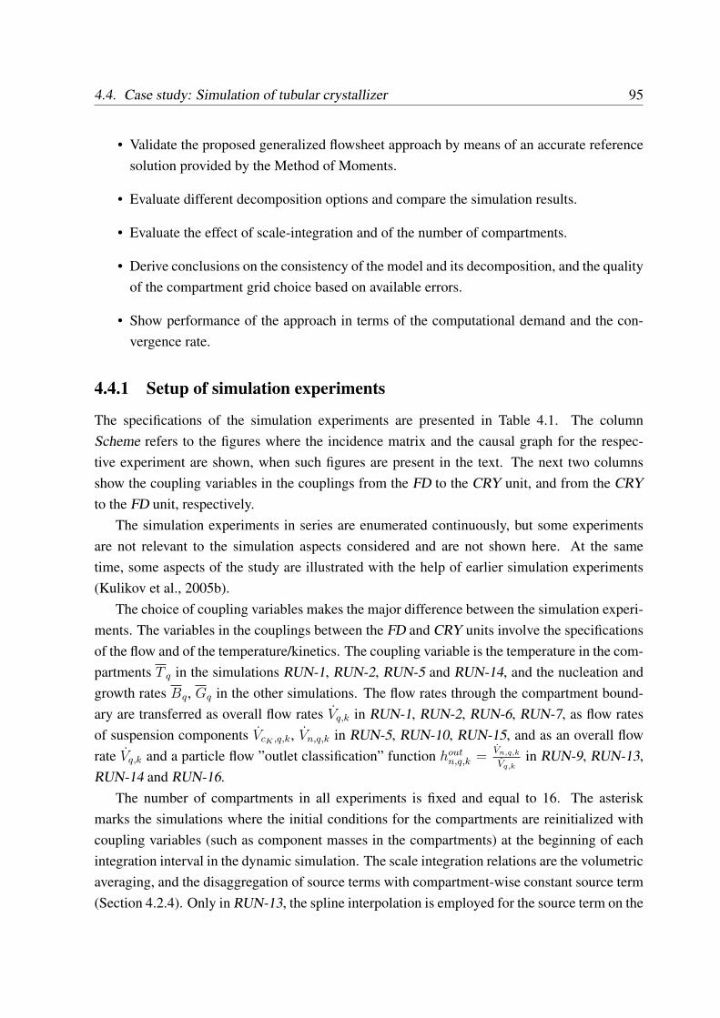
4.4. Case study: Simulation of tubular crystallizer 95
• Validate the proposed generalized flowsheet approach by means of an accurate referencesolution provided by the Method of Moments.
• Evaluate different decomposition options and compare the simulation results.
• Evaluate the effect of scale-integration and of the number of compartments.
• Derive conclusions on the consistency of the model and its decomposition, and the qualityof the compartment grid choice based on available errors.
• Show performance of the approach in terms of the computational demand and the con-vergence rate.
4.4.1 Setup of simulation experiments
The specifications of the simulation experiments are presented in Table 4.1. The columnScheme refers to the figures where the incidence matrix and the causal graph for the respec-tive experiment are shown, when such figures are present in the text. The next two columnsshow the coupling variables in the couplings from the FD to the CRY unit, and from the CRYto the FD unit, respectively.
The simulation experiments in series are enumerated continuously, but some experimentsare not relevant to the simulation aspects considered and are not shown here. At the sametime, some aspects of the study are illustrated with the help of earlier simulation experiments(Kulikov et al., 2005b).
The choice of coupling variables makes the major difference between the simulation experi-ments. The variables in the couplings between the FD and CRY units involve the specificationsof the flow and of the temperature/kinetics. The coupling variable is the temperature in the com-partments T q in the simulations RUN-1, RUN-2, RUN-5 and RUN-14, and the nucleation andgrowth rates Bq, Gq in the other simulations. The flow rates through the compartment bound-ary are transferred as overall flow rates Vq,k in RUN-1, RUN-2, RUN-6, RUN-7, as flow ratesof suspension components VcK ,q,k, Vn,q,k in RUN-5, RUN-10, RUN-15, and as an overall flowrate Vq,k and a particle flow ”outlet classification” function hout
n,q,k =Vn,q,k
Vq,kin RUN-9, RUN-13,
RUN-14 and RUN-16.The number of compartments in all experiments is fixed and equal to 16. The asterisk
marks the simulations where the initial conditions for the compartments are reinitialized withcoupling variables (such as component masses in the compartments) at the beginning of eachintegration interval in the dynamic simulation. The scale integration relations are the volumetricaveraging, and the disaggregation of source terms with compartment-wise constant source term(Section 4.2.4). Only in RUN-13, the spline interpolation is employed for the source term on the
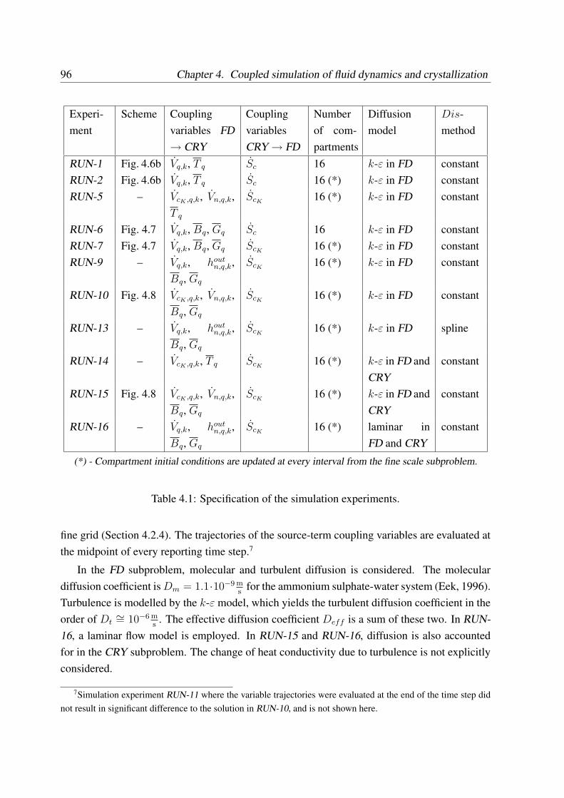
96 Chapter 4. Coupled simulation of fluid dynamics and crystallization
Experi-ment
Scheme Couplingvariables FD→ CRY
CouplingvariablesCRY → FD
Numberof com-partments
Diffusionmodel
Dis-method
RUN-1 Fig. 4.6b Vq,k, T q Sc 16 k-ε in FD constantRUN-2 Fig. 4.6b Vq,k, T q Sc 16 (*) k-ε in FD constantRUN-5 – VcK ,q,k, Vn,q,k,
T q
ScK16 (*) k-ε in FD constant
RUN-6 Fig. 4.7 Vq,k, Bq, Gq Sc 16 k-ε in FD constantRUN-7 Fig. 4.7 Vq,k, Bq, Gq ScK
16 (*) k-ε in FD constantRUN-9 – Vq,k, hout
n,q,k,Bq, Gq
ScK16 (*) k-ε in FD constant
RUN-10 Fig. 4.8 VcK ,q,k, Vn,q,k,Bq, Gq
ScK16 (*) k-ε in FD constant
RUN-13 – Vq,k, houtn,q,k,
Bq, Gq
ScK16 (*) k-ε in FD spline
RUN-14 – VcK ,q,k, T q ScK16 (*) k-ε in FD and
CRYconstant
RUN-15 Fig. 4.8 VcK ,q,k, Vn,q,k,Bq, Gq
ScK16 (*) k-ε in FD and
CRYconstant
RUN-16 – Vq,k, houtn,q,k,
Bq, Gq
ScK16 (*) laminar in
FD and CRYconstant
(*) - Compartment initial conditions are updated at every interval from the fine scale subproblem.
Table 4.1: Specification of the simulation experiments.
fine grid (Section 4.2.4). The trajectories of the source-term coupling variables are evaluated atthe midpoint of every reporting time step.7
In the FD subproblem, molecular and turbulent diffusion is considered. The moleculardiffusion coefficient is Dm = 1.1·10−9 m
sfor the ammonium sulphate-water system (Eek, 1996).
Turbulence is modelled by the k-ε model, which yields the turbulent diffusion coefficient in theorder of Dt
∼= 10−6 ms
. The effective diffusion coefficient Deff is a sum of these two. In RUN-16, a laminar flow model is employed. In RUN-15 and RUN-16, diffusion is also accountedfor in the CRY subproblem. The change of heat conductivity due to turbulence is not explicitlyconsidered.
7Simulation experiment RUN-11 where the variable trajectories were evaluated at the end of the time step didnot result in significant difference to the solution in RUN-10, and is not shown here.
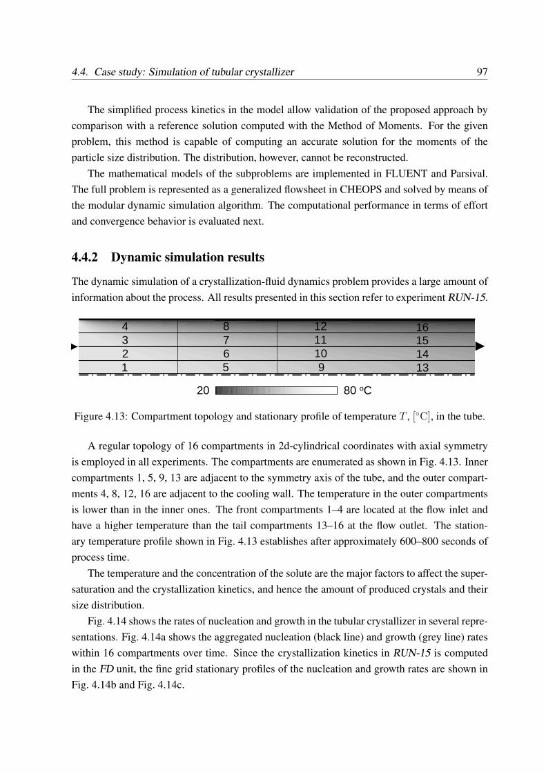
4.4. Case study: Simulation of tubular crystallizer 97
The simplified process kinetics in the model allow validation of the proposed approach bycomparison with a reference solution computed with the Method of Moments. For the givenproblem, this method is capable of computing an accurate solution for the moments of theparticle size distribution. The distribution, however, cannot be reconstructed.
The mathematical models of the subproblems are implemented in FLUENT and Parsival.The full problem is represented as a generalized flowsheet in CHEOPS and solved by means ofthe modular dynamic simulation algorithm. The computational performance in terms of effortand convergence behavior is evaluated next.
4.4.2 Dynamic simulation results
The dynamic simulation of a crystallization-fluid dynamics problem provides a large amount ofinformation about the process. All results presented in this section refer to experiment RUN-15.
20 80 oC
1234
5678
9101112
13141516
Figure 4.13: Compartment topology and stationary profile of temperature T , [◦C], in the tube.
A regular topology of 16 compartments in 2d-cylindrical coordinates with axial symmetryis employed in all experiments. The compartments are enumerated as shown in Fig. 4.13. Innercompartments 1, 5, 9, 13 are adjacent to the symmetry axis of the tube, and the outer compart-ments 4, 8, 12, 16 are adjacent to the cooling wall. The temperature in the outer compartmentsis lower than in the inner ones. The front compartments 1–4 are located at the flow inlet andhave a higher temperature than the tail compartments 13–16 at the flow outlet. The station-ary temperature profile shown in Fig. 4.13 establishes after approximately 600–800 seconds ofprocess time.
The temperature and the concentration of the solute are the major factors to affect the super-saturation and the crystallization kinetics, and hence the amount of produced crystals and theirsize distribution.
Fig. 4.14 shows the rates of nucleation and growth in the tubular crystallizer in several repre-sentations. Fig. 4.14a shows the aggregated nucleation (black line) and growth (grey line) rateswithin 16 compartments over time. Since the crystallization kinetics in RUN-15 is computedin the FD unit, the fine grid stationary profiles of the nucleation and growth rates are shown inFig. 4.14b and Fig. 4.14c.
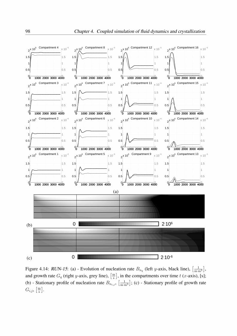
98 Chapter 4. Coupled simulation of fluid dynamics and crystallization
0 1000 2000 3000 40000
0.5
1
1.5
2x 10⁶ Compartment 4
0 1000 2000 3000 40000
0.5
1
1.5
x 10−6
0 1000 2000 3000 40000
0.5
1
1.5
2x 10⁶ Compartment 8
0 1000 2000 3000 40000
0.5
1
1.5
x 10−6
0 1000 2000 3000 40000
0.5
1
1.5
2x 10⁶ Compartment 12
0 1000 2000 3000 40000
0.5
1
1.5
x 10−6
0 1000 2000 3000 40000
0.5
1
1.5
2x 10⁶ Compartment 16
0 1000 2000 3000 40000
0.5
1
1.5
x 10−6
0 1000 2000 3000 40000
0.5
1
1.5
2x 10⁶ Compartment 3
0 1000 2000 3000 40000
0.5
1
1.5
x 10−6
0 1000 2000 3000 40000
0.5
1
1.5
2x 10⁶ Compartment 7
0 1000 2000 3000 40000
0.5
1
1.5
x 10−6
0 1000 2000 3000 40000
0.5
1
1.5
2x 10⁶ Compartment 11
0 1000 2000 3000 40000
0.5
1
1.5
x 10−6
0 1000 2000 3000 40000
0.5
1
1.5
2x 10⁶ Compartment 15
0 1000 2000 3000 40000
0.5
1
1.5
x 10−6
0 1000 2000 3000 40000
0.5
1
1.5
2x 10⁶ Compartment 2
0 1000 2000 3000 40000
0.5
1
1.5
x 10−6
0 1000 2000 3000 40000
0.5
1
1.5
2x 10⁶ Compartment 6
0 1000 2000 3000 40000
0.5
1
1.5
x 10−6
0 1000 2000 3000 40000
0.5
1
1.5
2x 10⁶ Compartment 10
0 1000 2000 3000 40000
0.5
1
1.5
x 10−6
0 1000 2000 3000 40000
0.5
1
1.5
2x 10⁶ Compartment 14
0 1000 2000 3000 40000
0.5
1
1.5
x 10−6
0 1000 2000 3000 40000
0.5
1
1.5
2x 10⁶ Compartment 1
0 1000 2000 3000 40000
0.5
1
1.5
x 10−6
0 1000 2000 3000 40000
0.5
1
1.5
2x 10⁶ Compartment 5
0 1000 2000 3000 40000
0.5
1
1.5
x 10−6
0 1000 2000 3000 40000
0.5
1
1.5
2x 10⁶ Compartment 9
0 1000 2000 3000 40000
0.5
1
1.5
x 10−6
0 1000 2000 3000 40000
0.5
1
1.5
2x 10⁶ Compartment 13
0 1000 2000 3000 40000
0.5
1
1.5
x 10−6
(a)
(b) 0 2.106
(c) 0 2.10-6
Figure 4.14: RUN-15: (a) - Evolution of nucleation rate Bnq (left y-axis, black line),[
1m·m3
],
and growth rate Gq (right y-axis, grey line),[
ms
], in the compartments over time t (x-axis), [s];
(b) - Stationary profile of nucleation rate Bni,j,[
1m·m3
]; (c) - Stationary profile of growth rate
Gi,j ,[
ms
].
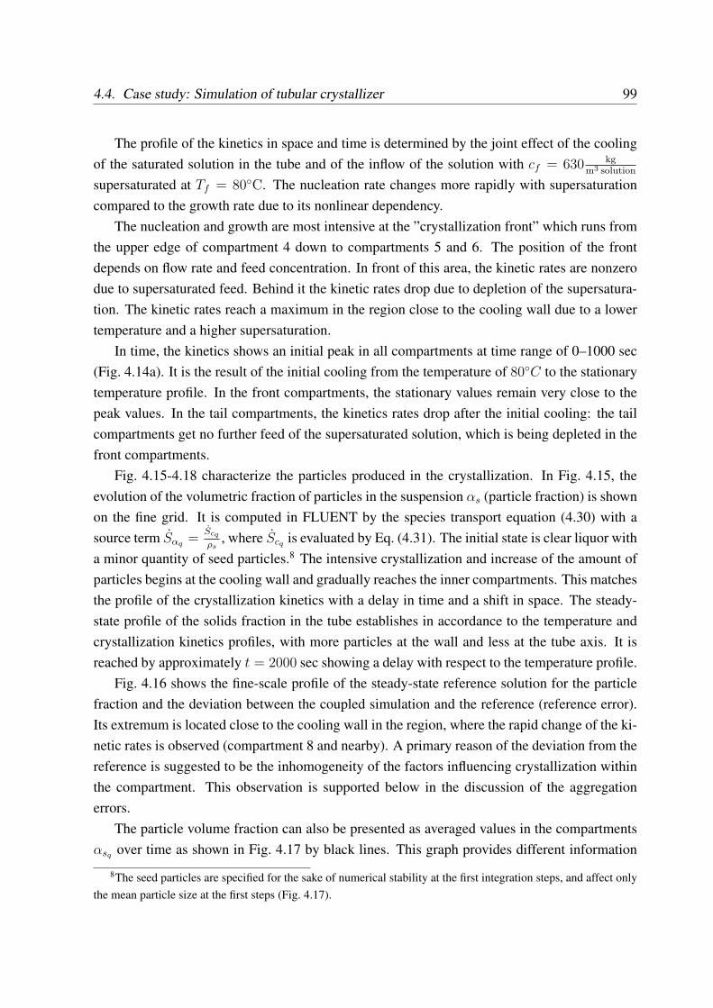
4.4. Case study: Simulation of tubular crystallizer 99
The profile of the kinetics in space and time is determined by the joint effect of the coolingof the saturated solution in the tube and of the inflow of the solution with cf = 630 kg
m3 solution
supersaturated at Tf = 80◦C. The nucleation rate changes more rapidly with supersaturationcompared to the growth rate due to its nonlinear dependency.
The nucleation and growth are most intensive at the ”crystallization front” which runs fromthe upper edge of compartment 4 down to compartments 5 and 6. The position of the frontdepends on flow rate and feed concentration. In front of this area, the kinetic rates are nonzerodue to supersaturated feed. Behind it the kinetic rates drop due to depletion of the supersatura-tion. The kinetic rates reach a maximum in the region close to the cooling wall due to a lowertemperature and a higher supersaturation.
In time, the kinetics shows an initial peak in all compartments at time range of 0–1000 sec(Fig. 4.14a). It is the result of the initial cooling from the temperature of 80◦C to the stationarytemperature profile. In the front compartments, the stationary values remain very close to thepeak values. In the tail compartments, the kinetics rates drop after the initial cooling: the tailcompartments get no further feed of the supersaturated solution, which is being depleted in thefront compartments.
Fig. 4.15-4.18 characterize the particles produced in the crystallization. In Fig. 4.15, theevolution of the volumetric fraction of particles in the suspension αs (particle fraction) is shownon the fine grid. It is computed in FLUENT by the species transport equation (4.30) with asource term Sαq =
Scq
ρs, where Scq is evaluated by Eq. (4.31). The initial state is clear liquor with
a minor quantity of seed particles.8 The intensive crystallization and increase of the amount ofparticles begins at the cooling wall and gradually reaches the inner compartments. This matchesthe profile of the crystallization kinetics with a delay in time and a shift in space. The steady-state profile of the solids fraction in the tube establishes in accordance to the temperature andcrystallization kinetics profiles, with more particles at the wall and less at the tube axis. It isreached by approximately t = 2000 sec showing a delay with respect to the temperature profile.
Fig. 4.16 shows the fine-scale profile of the steady-state reference solution for the particlefraction and the deviation between the coupled simulation and the reference (reference error).Its extremum is located close to the cooling wall in the region, where the rapid change of the ki-netic rates is observed (compartment 8 and nearby). A primary reason of the deviation from thereference is suggested to be the inhomogeneity of the factors influencing crystallization withinthe compartment. This observation is supported below in the discussion of the aggregationerrors.
The particle volume fraction can also be presented as averaged values in the compartmentsαsq over time as shown in Fig. 4.17 by black lines. This graph provides different information
8The seed particles are specified for the sake of numerical stability at the first integration steps, and affect onlythe mean particle size at the first steps (Fig. 4.17).
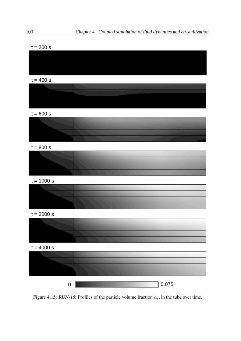
100 Chapter 4. Coupled simulation of fluid dynamics and crystallization
0
t = 200 s
t = 400 s
0.075
t = 600 s
t = 1000 s
t = 2000 s
t = 4000 s
t = 800 s
Figure 4.15: RUN-15: Profiles of the particle volume fraction αs, in the tube over time.
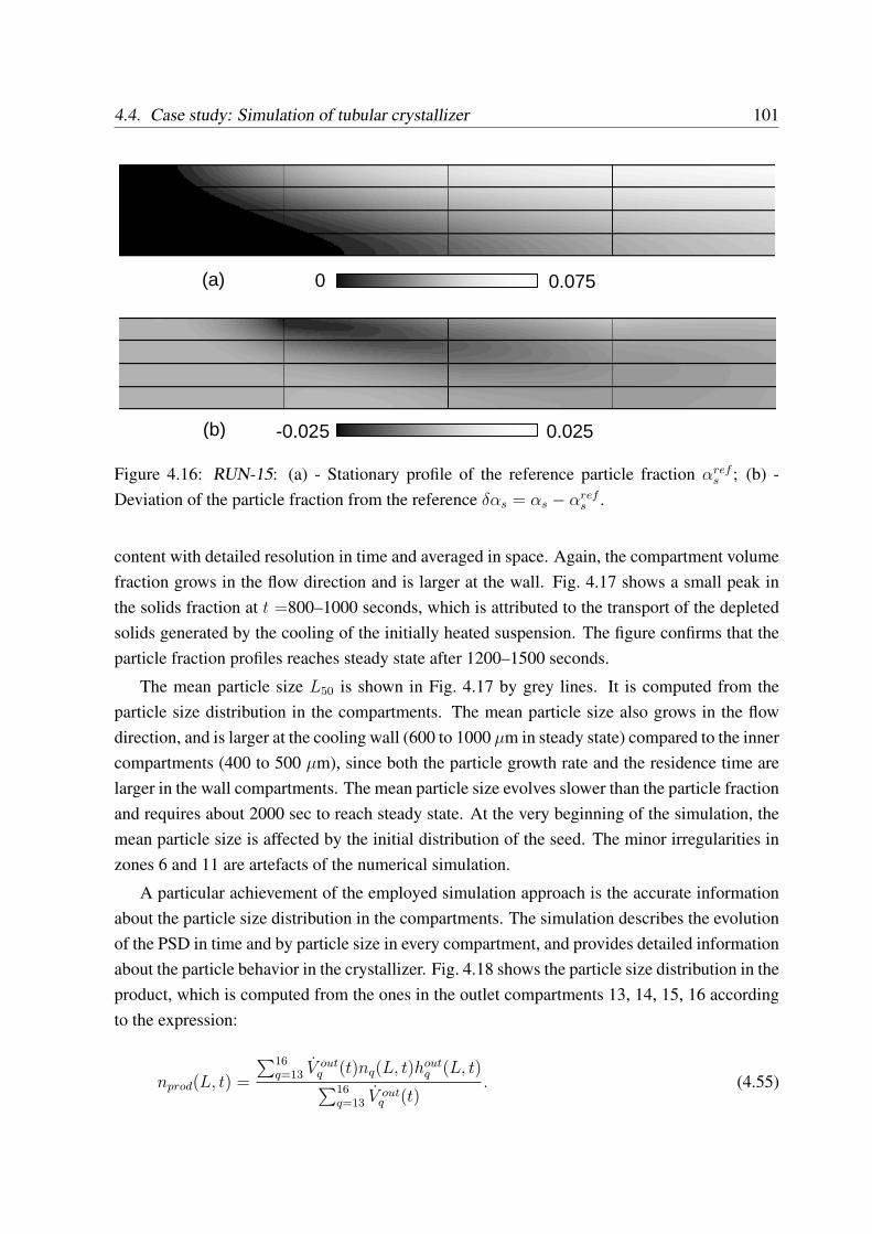
4.4. Case study: Simulation of tubular crystallizer 101
0 0.075
-0.025 0.025
(a)
(b)
Figure 4.16: RUN-15: (a) - Stationary profile of the reference particle fraction αrefs ; (b) -
Deviation of the particle fraction from the reference δαs = αs − αrefs .
content with detailed resolution in time and averaged in space. Again, the compartment volumefraction grows in the flow direction and is larger at the wall. Fig. 4.17 shows a small peak inthe solids fraction at t =800–1000 seconds, which is attributed to the transport of the depletedsolids generated by the cooling of the initially heated suspension. The figure confirms that theparticle fraction profiles reaches steady state after 1200–1500 seconds.
The mean particle size L50 is shown in Fig. 4.17 by grey lines. It is computed from theparticle size distribution in the compartments. The mean particle size also grows in the flowdirection, and is larger at the cooling wall (600 to 1000 µm in steady state) compared to the innercompartments (400 to 500 µm), since both the particle growth rate and the residence time arelarger in the wall compartments. The mean particle size evolves slower than the particle fractionand requires about 2000 sec to reach steady state. At the very beginning of the simulation, themean particle size is affected by the initial distribution of the seed. The minor irregularities inzones 6 and 11 are artefacts of the numerical simulation.
A particular achievement of the employed simulation approach is the accurate informationabout the particle size distribution in the compartments. The simulation describes the evolutionof the PSD in time and by particle size in every compartment, and provides detailed informationabout the particle behavior in the crystallizer. Fig. 4.18 shows the particle size distribution in theproduct, which is computed from the ones in the outlet compartments 13, 14, 15, 16 accordingto the expression:
nprod(L, t) =
∑16q=13 V out
q (t)nq(L, t)houtq (L, t)
∑16q=13 V out
q (t). (4.55)
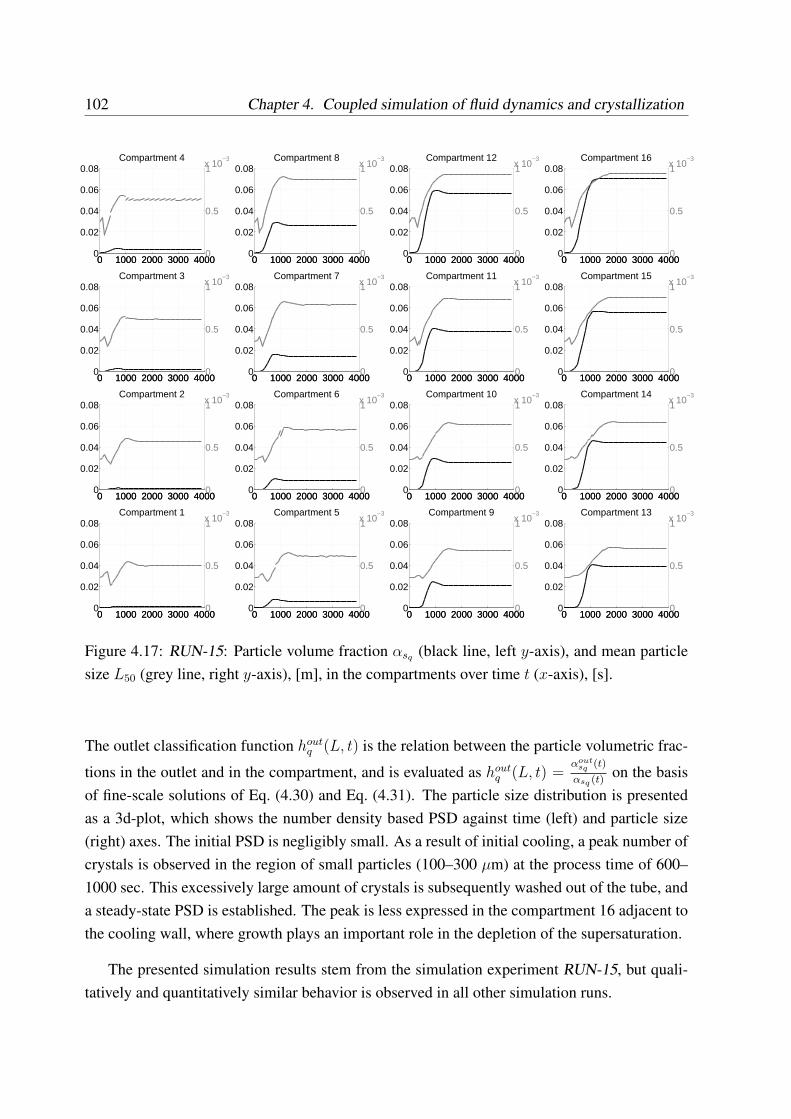
102 Chapter 4. Coupled simulation of fluid dynamics and crystallization
0 1000 2000 3000 40000
0.02
0.04
0.06
0.08Compartment 4
0 1000 2000 3000 40000
0.5
1x 10⁻³
0 1000 2000 3000 40000
0.02
0.04
0.06
0.08Compartment 8
0 1000 2000 3000 40000
0.5
1x 10⁻³
0 1000 2000 3000 40000
0.02
0.04
0.06
0.08Compartment 12
0 1000 2000 3000 40000
0.5
1x 10⁻³
0 1000 2000 3000 40000
0.02
0.04
0.06
0.08Compartment 16
0 1000 2000 3000 40000
0.5
1x 10⁻³
0 1000 2000 3000 40000
0.02
0.04
0.06
0.08Compartment 3
0 1000 2000 3000 40000
0.5
1x 10⁻³
0 1000 2000 3000 40000
0.02
0.04
0.06
0.08Compartment 7
0 1000 2000 3000 40000
0.5
1x 10⁻³
0 1000 2000 3000 40000
0.02
0.04
0.06
0.08Compartment 11
0 1000 2000 3000 40000
0.5
1x 10⁻³
0 1000 2000 3000 40000
0.02
0.04
0.06
0.08Compartment 15
0 1000 2000 3000 40000
0.5
1x 10⁻³
0 1000 2000 3000 40000
0.02
0.04
0.06
0.08Compartment 2
0 1000 2000 3000 40000
0.5
1x 10⁻³
0 1000 2000 3000 40000
0.02
0.04
0.06
0.08Compartment 6
0 1000 2000 3000 40000
0.5
1x 10⁻³
0 1000 2000 3000 40000
0.02
0.04
0.06
0.08Compartment 10
0 1000 2000 3000 40000
0.5
1x 10⁻³
0 1000 2000 3000 40000
0.02
0.04
0.06
0.08Compartment 14
0 1000 2000 3000 40000
0.5
1x 10⁻³
0 1000 2000 3000 40000
0.02
0.04
0.06
0.08Compartment 1
0 1000 2000 3000 40000
0.5
1x 10⁻³
0 1000 2000 3000 40000
0.02
0.04
0.06
0.08Compartment 5
0 1000 2000 3000 40000
0.5
1x 10⁻³
0 1000 2000 3000 40000
0.02
0.04
0.06
0.08Compartment 9
0 1000 2000 3000 40000
0.5
1x 10⁻³
0 1000 2000 3000 40000
0.02
0.04
0.06
0.08Compartment 13
0 1000 2000 3000 40000
0.5
1x 10⁻³
Figure 4.17: RUN-15: Particle volume fraction αsq (black line, left y-axis), and mean particlesize L50 (grey line, right y-axis), [m], in the compartments over time t (x-axis), [s].
The outlet classification function houtq (L, t) is the relation between the particle volumetric frac-
tions in the outlet and in the compartment, and is evaluated as houtq (L, t) =
αoutsq (t)
αsq (t)on the basis
of fine-scale solutions of Eq. (4.30) and Eq. (4.31). The particle size distribution is presentedas a 3d-plot, which shows the number density based PSD against time (left) and particle size(right) axes. The initial PSD is negligibly small. As a result of initial cooling, a peak number ofcrystals is observed in the region of small particles (100–300 µm) at the process time of 600–1000 sec. This excessively large amount of crystals is subsequently washed out of the tube, anda steady-state PSD is established. The peak is less expressed in the compartment 16 adjacent tothe cooling wall, where growth plays an important role in the depletion of the supersaturation.
The presented simulation results stem from the simulation experiment RUN-15, but quali-tatively and quantitatively similar behavior is observed in all other simulation runs.
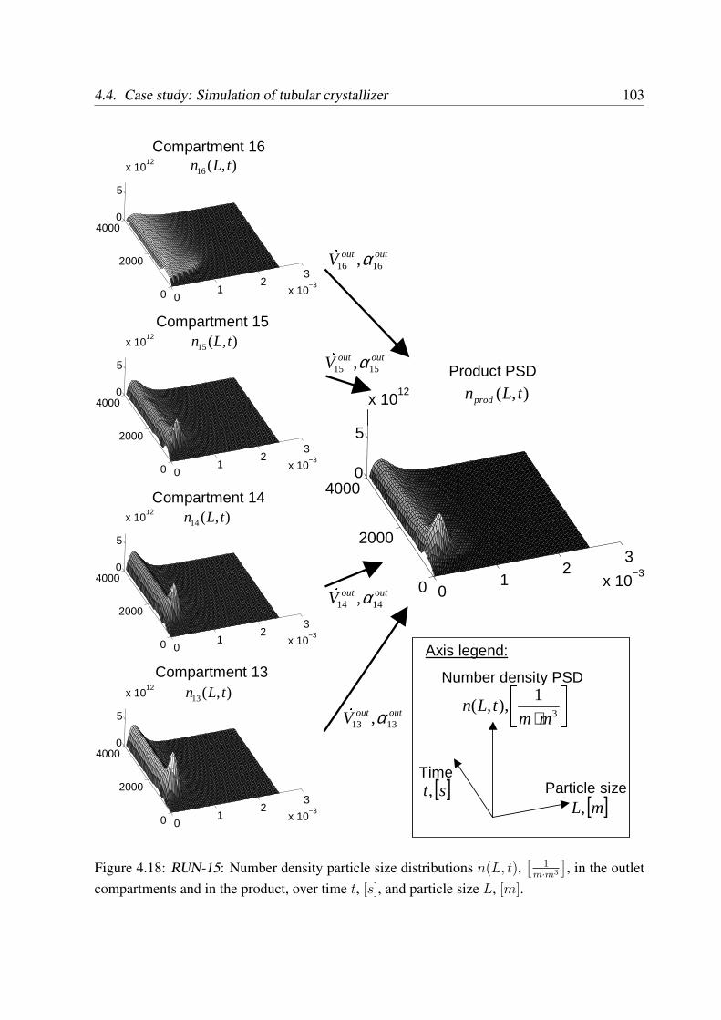
4.4. Case study: Simulation of tubular crystallizer 103
01
23
x 10−3
0
2000
40000
5
x 1012
Product
01
23
x 10−3
0
2000
40000
5
x 1012
Zone 13
01
23
x 10−3
0
2000
40000
5
x 1012
Zone 14
01
23
x 10−3
0
2000
40000
5
x 1012
Zone 15
01
23
x 10−3
0
2000
40000
5
x 1012
Zone 16
Particle sizeTime
outoutV 1616 ,α&outoutV 1515 ,α&outoutV 1414 ,α&
outoutV 1313 ,α&
),(16 tLnCompartment 16
Compartment 15
Compartment 14
Compartment 13
Product PSD
),(15 tLn
),(14 tLn
),(13 tLn
),( tLnprod
Axis legend:
Number density PSD ⋅ 3
1),,(
mmtLn
[ ]st,[ ]mL,
Figure 4.18: RUN-15: Number density particle size distributions n(L, t),[
1m·m3
], in the outlet
compartments and in the product, over time t, [s], and particle size L, [m].
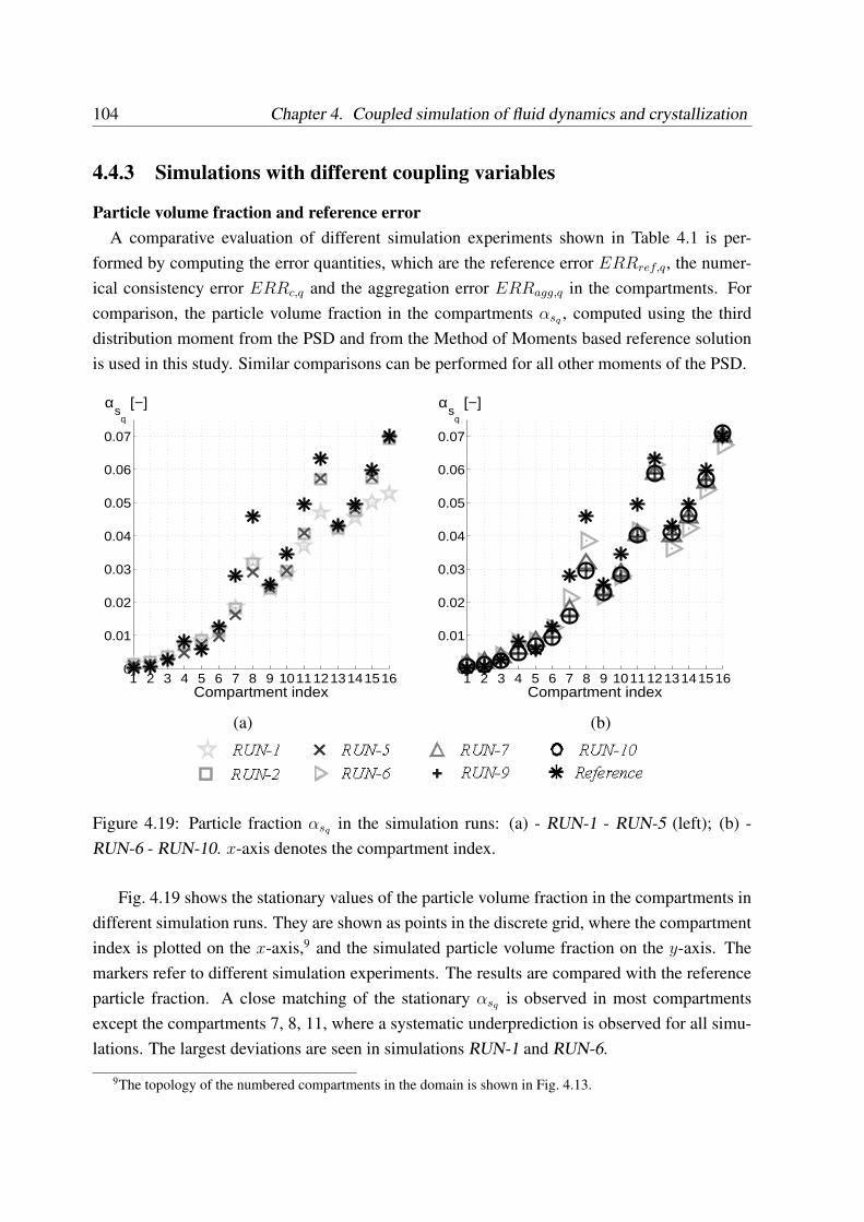
104 Chapter 4. Coupled simulation of fluid dynamics and crystallization
4.4.3 Simulations with different coupling variables
Particle volume fraction and reference errorA comparative evaluation of different simulation experiments shown in Table 4.1 is per-
formed by computing the error quantities, which are the reference error ERRref,q, the numer-ical consistency error ERRc,q and the aggregation error ERRagg,q in the compartments. Forcomparison, the particle volume fraction in the compartments αsq , computed using the thirddistribution moment from the PSD and from the Method of Moments based reference solutionis used in this study. Similar comparisons can be performed for all other moments of the PSD.
1 2 3 4 5 6 7 8 9 101112131415160
0.01
0.02
0.03
0.04
0.05
0.06
0.07
Compartment index
αs
q
[−]
1 2 3 4 5 6 7 8 9 101112131415160
0.01
0.02
0.03
0.04
0.05
0.06
0.07
Compartment index
αs
q
[−]
(a) (b)
Figure 4.19: Particle fraction αsq in the simulation runs: (a) - RUN-1 - RUN-5 (left); (b) -RUN-6 - RUN-10. x-axis denotes the compartment index.
Fig. 4.19 shows the stationary values of the particle volume fraction in the compartments indifferent simulation runs. They are shown as points in the discrete grid, where the compartmentindex is plotted on the x-axis,9 and the simulated particle volume fraction on the y-axis. Themarkers refer to different simulation experiments. The results are compared with the referenceparticle fraction. A close matching of the stationary αsq is observed in most compartmentsexcept the compartments 7, 8, 11, where a systematic underprediction is observed for all simu-lations. The largest deviations are seen in simulations RUN-1 and RUN-6.
9The topology of the numbered compartments in the domain is shown in Fig. 4.13.
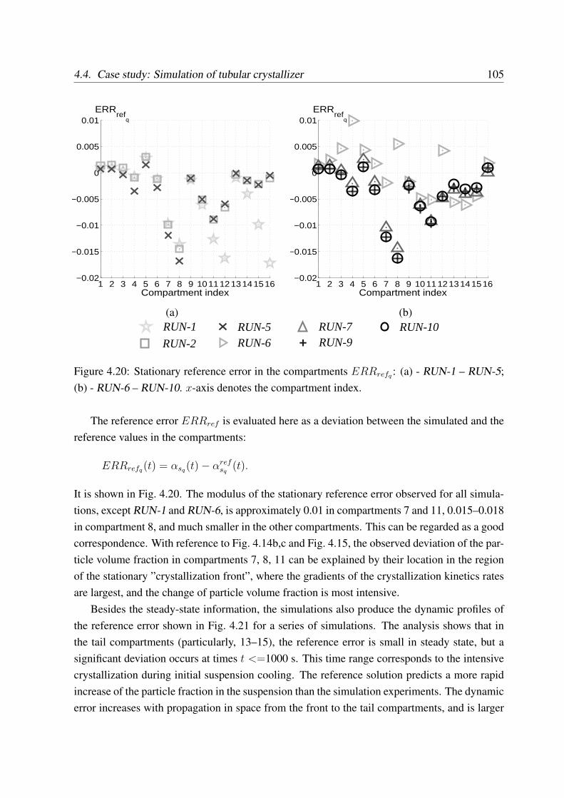
4.4. Case study: Simulation of tubular crystallizer 105
1 2 3 4 5 6 7 8 9 10111213141516−0.02
−0.015
−0.01
−0.005
0
0.005
0.01
Compartment index
ERRref
q
1 2 3 4 5 6 7 8 9 10111213141516−0.02
−0.015
−0.01
−0.005
0
0.005
0.01
Compartment index
ERRref
q
(a) (b)RUN-1
RUN-2
RUN-5RUN-6
RUN-7
+ RUN-9RUN-10
Figure 4.20: Stationary reference error in the compartments ERRrefq : (a) - RUN-1 – RUN-5;(b) - RUN-6 – RUN-10. x-axis denotes the compartment index.
The reference error ERRref is evaluated here as a deviation between the simulated and thereference values in the compartments:
ERRrefq(t) = αsq(t)− αrefsq
(t).
It is shown in Fig. 4.20. The modulus of the stationary reference error observed for all simula-tions, except RUN-1 and RUN-6, is approximately 0.01 in compartments 7 and 11, 0.015–0.018in compartment 8, and much smaller in the other compartments. This can be regarded as a goodcorrespondence. With reference to Fig. 4.14b,c and Fig. 4.15, the observed deviation of the par-ticle volume fraction in compartments 7, 8, 11 can be explained by their location in the regionof the stationary ”crystallization front”, where the gradients of the crystallization kinetics ratesare largest, and the change of particle volume fraction is most intensive.
Besides the steady-state information, the simulations also produce the dynamic profiles ofthe reference error shown in Fig. 4.21 for a series of simulations. The analysis shows that inthe tail compartments (particularly, 13–15), the reference error is small in steady state, but asignificant deviation occurs at times t <=1000 s. This time range corresponds to the intensivecrystallization during initial suspension cooling. The reference solution predicts a more rapidincrease of the particle fraction in the suspension than the simulation experiments. The dynamicerror increases with propagation in space from the front to the tail compartments, and is larger
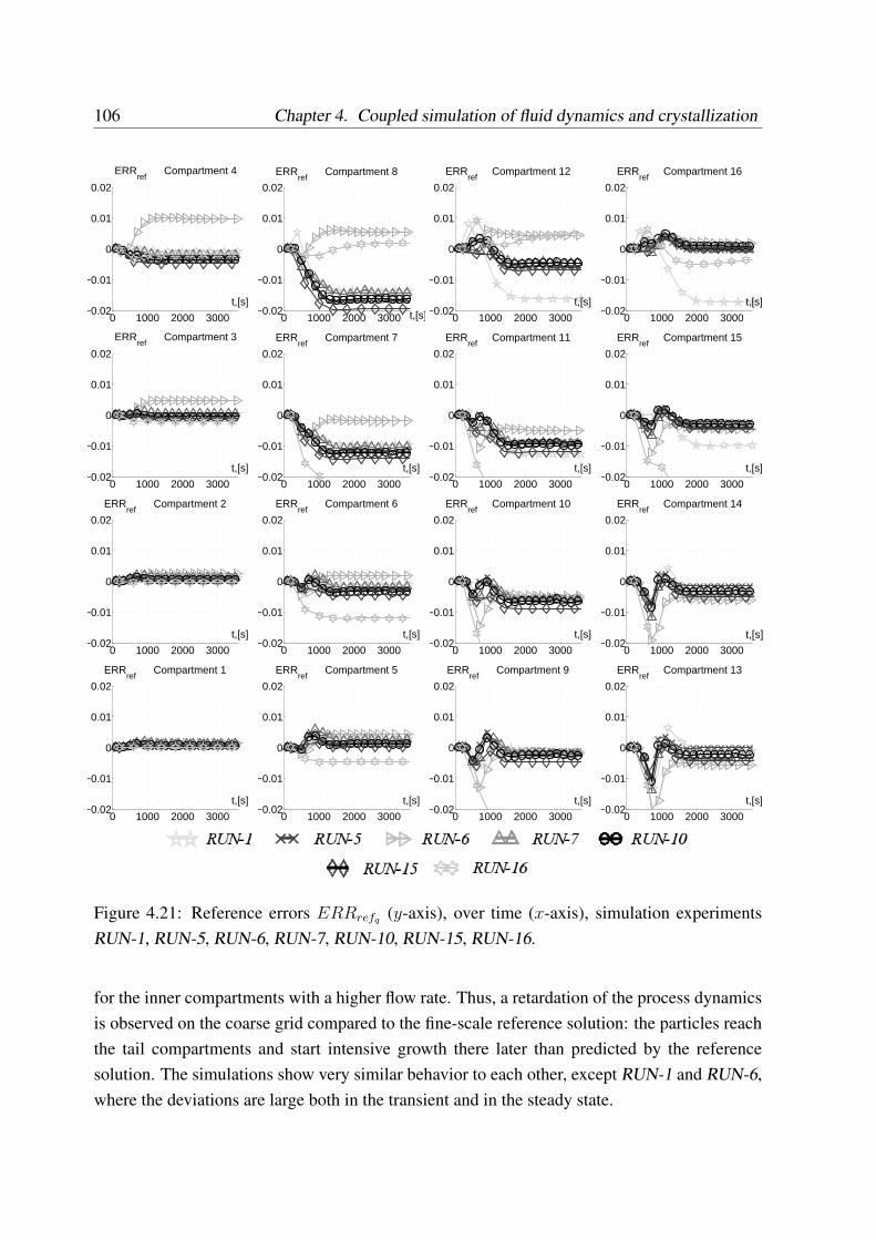
106 Chapter 4. Coupled simulation of fluid dynamics and crystallization
0 1000 2000 3000−0.02
−0.01
0
0.01
0.02
ERRref
Compartment 4
t,[s]
0 1000 2000 3000−0.02
−0.01
0
0.01
0.02
ERRref
Compartment 8
t,[s] 0 1000 2000 3000−0.02
−0.01
0
0.01
0.02
ERRref
Compartment 12
t,[s]
0 1000 2000 3000−0.02
−0.01
0
0.01
0.02
ERRref
Compartment 16
t,[s]
0 1000 2000 3000−0.02
−0.01
0
0.01
0.02
ERRref
Compartment 3
t,[s]
0 1000 2000 3000−0.02
−0.01
0
0.01
0.02
ERRref
Compartment 7
t,[s]
0 1000 2000 3000−0.02
−0.01
0
0.01
0.02
ERRref
Compartment 11
t,[s]
0 1000 2000 3000−0.02
−0.01
0
0.01
0.02
ERRref
Compartment 15
t,[s]
0 1000 2000 3000−0.02
−0.01
0
0.01
0.02
ERRref
Compartment 2
t,[s]
0 1000 2000 3000−0.02
−0.01
0
0.01
0.02
ERRref
Compartment 6
t,[s]
0 1000 2000 3000−0.02
−0.01
0
0.01
0.02
ERRref
Compartment 10
t,[s]
0 1000 2000 3000−0.02
−0.01
0
0.01
0.02
ERRref
Compartment 14
t,[s]
0 1000 2000 3000−0.02
−0.01
0
0.01
0.02
ERRref
Compartment 1
t,[s]
0 1000 2000 3000−0.02
−0.01
0
0.01
0.02
ERRref
Compartment 5
t,[s]
0 1000 2000 3000−0.02
−0.01
0
0.01
0.02
ERRref
Compartment 9
t,[s]
0 1000 2000 3000−0.02
−0.01
0
0.01
0.02
ERRref
Compartment 13
t,[s]
Figure 4.21: Reference errors ERRrefq (y-axis), over time (x-axis), simulation experimentsRUN-1, RUN-5, RUN-6, RUN-7, RUN-10, RUN-15, RUN-16.
for the inner compartments with a higher flow rate. Thus, a retardation of the process dynamicsis observed on the coarse grid compared to the fine-scale reference solution: the particles reachthe tail compartments and start intensive growth there later than predicted by the referencesolution. The simulations show very similar behavior to each other, except RUN-1 and RUN-6,where the deviations are large both in the transient and in the steady state.
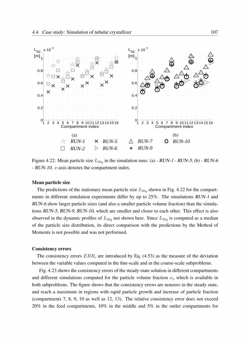
4.4. Case study: Simulation of tubular crystallizer 107
1 2 3 4 5 6 7 8 9 101112131415160
0.2
0.4
0.6
0.8
1
x 10−3
Compartment index
L50
[m]
1 2 3 4 5 6 7 8 9 101112131415160
0.2
0.4
0.6
0.8
1
x 10−3
Compartment index
L50
[m]
(a) (b)RUN-1
RUN-2
RUN-5RUN-6
RUN-7
+ RUN-9RUN-10
Figure 4.22: Mean particle size L50q in the simulation runs: (a) - RUN-1 - RUN-5, (b) - RUN-6- RUN-10. x-axis denotes the compartment index.
Mean particle sizeThe predictions of the stationary mean particle size L50q shown in Fig. 4.22 for the compart-
ments in different simulation experiments differ by up to 25%. The simulations RUN-1 andRUN-6 show larger particle sizes (and also a smaller particle volume fraction) than the simula-tions RUN-5, RUN-9, RUN-10, which are smaller and closer to each other. This effect is alsoobserved in the dynamic profiles of L50q not shown here. Since L50q is computed as a medianof the particle size distribution, its direct comparison with the predictions by the Method ofMoments is not possible and was not performed.
Consistency errorsThe consistency errors ERRc are introduced by Eq. (4.53) as the measure of the deviation
between the variable values computed in the fine-scale and in the coarse-scale subproblems.
Fig. 4.23 shows the consistency errors of the steady-state solution in different compartmentsand different simulations computed for the particle volume fraction αs which is available inboth subproblems. The figure shows that the consistency errors are nonzero in the steady state,and reach a maximum in regions with rapid particle growth and increase of particle fraction(compartments 7, 8, 9, 10 as well as 12, 13). The relative consistency error does not exceed20% in the feed compartments, 10% in the middle and 5% in the outlet compartments for
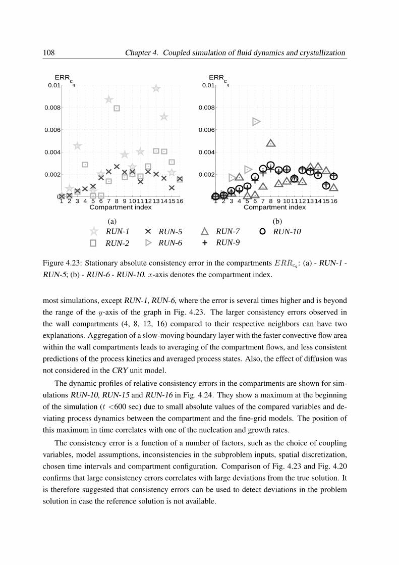
108 Chapter 4. Coupled simulation of fluid dynamics and crystallization
1 2 3 4 5 6 7 8 9 101112131415160
0.002
0.004
0.006
0.008
0.01
Compartment index
ERRc
q
1 2 3 4 5 6 7 8 9 101112131415160
0.002
0.004
0.006
0.008
0.01
Compartment index
ERRc
q
(a) (b)RUN-1
RUN-2
RUN-5RUN-6
RUN-7
+ RUN-9RUN-10
Figure 4.23: Stationary absolute consistency error in the compartments ERRcq : (a) - RUN-1 -RUN-5; (b) - RUN-6 - RUN-10. x-axis denotes the compartment index.
most simulations, except RUN-1, RUN-6, where the error is several times higher and is beyondthe range of the y-axis of the graph in Fig. 4.23. The larger consistency errors observed inthe wall compartments (4, 8, 12, 16) compared to their respective neighbors can have twoexplanations. Aggregation of a slow-moving boundary layer with the faster convective flow areawithin the wall compartments leads to averaging of the compartment flows, and less consistentpredictions of the process kinetics and averaged process states. Also, the effect of diffusion wasnot considered in the CRY unit model.
The dynamic profiles of relative consistency errors in the compartments are shown for sim-ulations RUN-10, RUN-15 and RUN-16 in Fig. 4.24. They show a maximum at the beginningof the simulation (t <600 sec) due to small absolute values of the compared variables and de-viating process dynamics between the compartment and the fine-grid models. The position ofthis maximum in time correlates with one of the nucleation and growth rates.
The consistency error is a function of a number of factors, such as the choice of couplingvariables, model assumptions, inconsistencies in the subproblem inputs, spatial discretization,chosen time intervals and compartment configuration. Comparison of Fig. 4.23 and Fig. 4.20confirms that large consistency errors correlates with large deviations from the true solution. Itis therefore suggested that consistency errors can be used to detect deviations in the problemsolution in case the reference solution is not available.
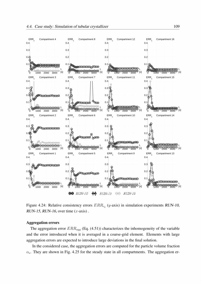
4.4. Case study: Simulation of tubular crystallizer 109
0 1000 2000 30000
0.1
0.2
0.3
0.4
ERRc Compartment 4
t,[s] 0 1000 2000 3000
0
0.1
0.2
0.3
0.4
ERRc Compartment 8
t,[s] 0 1000 2000 3000
0
0.1
0.2
0.3
0.4
ERRc Compartment 12
t,[s] 0 1000 2000 3000
0
0.1
0.2
0.3
0.4
ERRc Compartment 16
t,[s]
0 1000 2000 30000
0.1
0.2
0.3
0.4
ERRc Compartment 3
t,[s] 0 1000 2000 3000
0
0.1
0.2
0.3
0.4
ERRc Compartment 7
t,[s] 0 1000 2000 3000
0
0.1
0.2
0.3
0.4
ERRc Compartment 11
t,[s] 0 1000 2000 3000
0
0.1
0.2
0.3
0.4
ERRc Compartment 15
t,[s]
0 1000 2000 30000
0.1
0.2
0.3
0.4
ERRc Compartment 2
t,[s] 0 1000 2000 3000
0
0.1
0.2
0.3
0.4
ERRc Compartment 6
t,[s] 0 1000 2000 3000
0
0.1
0.2
0.3
0.4
ERRc Compartment 10
t,[s] 0 1000 2000 3000
0
0.1
0.2
0.3
0.4
ERRc Compartment 14
t,[s]
0 1000 2000 30000
0.1
0.2
0.3
0.4
ERRc Compartment 1
t,[s] 0 1000 2000 3000
0
0.1
0.2
0.3
0.4
ERRc Compartment 5
t,[s] 0 1000 2000 3000
0
0.1
0.2
0.3
0.4
ERRc Compartment 9
t,[s] 0 1000 2000 3000
0
0.1
0.2
0.3
0.4
ERRc Compartment 13
t,[s]
Figure 4.24: Relative consistency errors ERRcq (y-axis) in simulation experiments RUN-10,RUN-15, RUN-16, over time (x-axis) .
Aggregation errorsThe aggregation error ERRagg (Eq. (4.51)) characterizes the inhomogeneity of the variable
and the error introduced when it is averaged in a coarse-grid element. Elements with largeaggregation errors are expected to introduce large deviations in the final solution.
In the considered case, the aggregation errors are computed for the particle volume fractionαs. They are shown in Fig. 4.25 for the steady state in all compartments. The aggregation er-
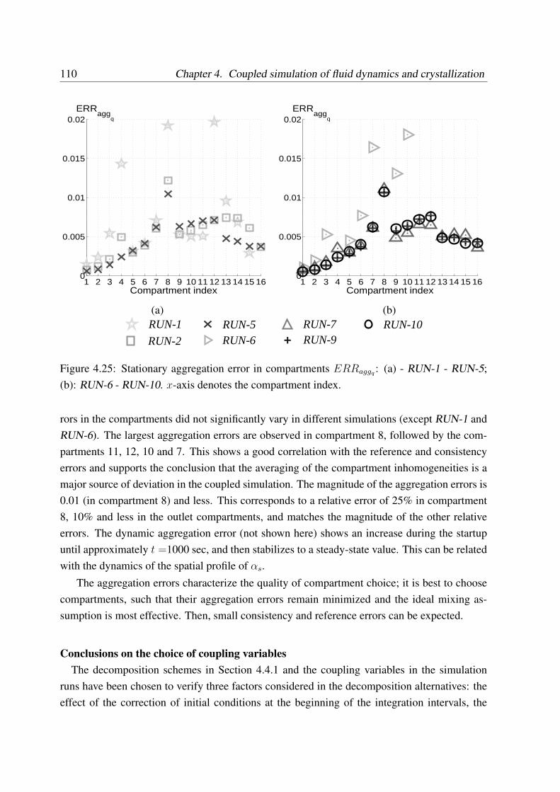
110 Chapter 4. Coupled simulation of fluid dynamics and crystallization
1 2 3 4 5 6 7 8 9 10 11 12 13 14 15 160
0.005
0.01
0.015
0.02
Compartment index
ERRagg
q
1 2 3 4 5 6 7 8 9 10 11 12 13 14 15 160
0.005
0.01
0.015
0.02
Compartment index
ERRagg
q
(a) (b)RUN-1
RUN-2
RUN-5RUN-6
RUN-7
+ RUN-9RUN-10
Figure 4.25: Stationary aggregation error in compartments ERRaggq : (a) - RUN-1 - RUN-5;(b): RUN-6 - RUN-10. x-axis denotes the compartment index.
rors in the compartments did not significantly vary in different simulations (except RUN-1 andRUN-6). The largest aggregation errors are observed in compartment 8, followed by the com-partments 11, 12, 10 and 7. This shows a good correlation with the reference and consistencyerrors and supports the conclusion that the averaging of the compartment inhomogeneities is amajor source of deviation in the coupled simulation. The magnitude of the aggregation errors is0.01 (in compartment 8) and less. This corresponds to a relative error of 25% in compartment8, 10% and less in the outlet compartments, and matches the magnitude of the other relativeerrors. The dynamic aggregation error (not shown here) shows an increase during the startupuntil approximately t =1000 sec, and then stabilizes to a steady-state value. This can be relatedwith the dynamics of the spatial profile of αs.
The aggregation errors characterize the quality of compartment choice; it is best to choosecompartments, such that their aggregation errors remain minimized and the ideal mixing as-sumption is most effective. Then, small consistency and reference errors can be expected.
Conclusions on the choice of coupling variablesThe decomposition schemes in Section 4.4.1 and the coupling variables in the simulation
runs have been chosen to verify three factors considered in the decomposition alternatives: theeffect of the correction of initial conditions at the beginning of the integration intervals, the
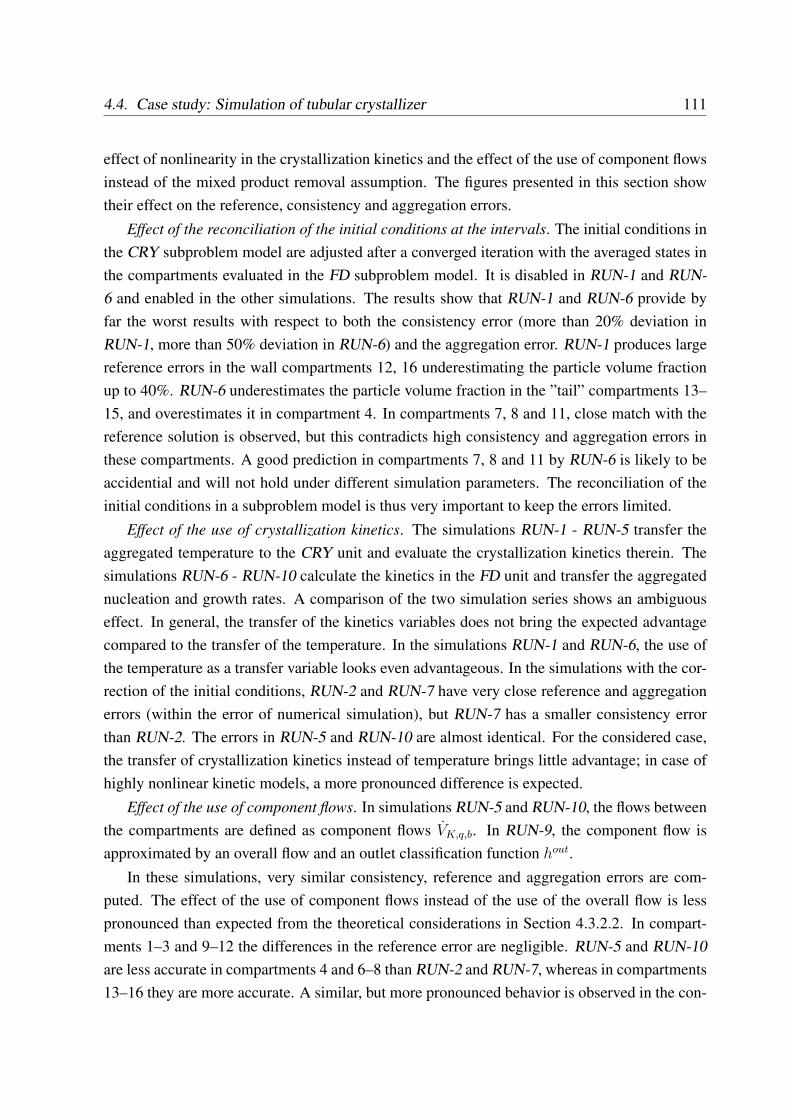
4.4. Case study: Simulation of tubular crystallizer 111
effect of nonlinearity in the crystallization kinetics and the effect of the use of component flowsinstead of the mixed product removal assumption. The figures presented in this section showtheir effect on the reference, consistency and aggregation errors.
Effect of the reconciliation of the initial conditions at the intervals. The initial conditions inthe CRY subproblem model are adjusted after a converged iteration with the averaged states inthe compartments evaluated in the FD subproblem model. It is disabled in RUN-1 and RUN-6 and enabled in the other simulations. The results show that RUN-1 and RUN-6 provide byfar the worst results with respect to both the consistency error (more than 20% deviation inRUN-1, more than 50% deviation in RUN-6) and the aggregation error. RUN-1 produces largereference errors in the wall compartments 12, 16 underestimating the particle volume fractionup to 40%. RUN-6 underestimates the particle volume fraction in the ”tail” compartments 13–15, and overestimates it in compartment 4. In compartments 7, 8 and 11, close match with thereference solution is observed, but this contradicts high consistency and aggregation errors inthese compartments. A good prediction in compartments 7, 8 and 11 by RUN-6 is likely to beaccidential and will not hold under different simulation parameters. The reconciliation of theinitial conditions in a subproblem model is thus very important to keep the errors limited.
Effect of the use of crystallization kinetics. The simulations RUN-1 - RUN-5 transfer theaggregated temperature to the CRY unit and evaluate the crystallization kinetics therein. Thesimulations RUN-6 - RUN-10 calculate the kinetics in the FD unit and transfer the aggregatednucleation and growth rates. A comparison of the two simulation series shows an ambiguouseffect. In general, the transfer of the kinetics variables does not bring the expected advantagecompared to the transfer of the temperature. In the simulations RUN-1 and RUN-6, the use ofthe temperature as a transfer variable looks even advantageous. In the simulations with the cor-rection of the initial conditions, RUN-2 and RUN-7 have very close reference and aggregationerrors (within the error of numerical simulation), but RUN-7 has a smaller consistency errorthan RUN-2. The errors in RUN-5 and RUN-10 are almost identical. For the considered case,the transfer of crystallization kinetics instead of temperature brings little advantage; in case ofhighly nonlinear kinetic models, a more pronounced difference is expected.
Effect of the use of component flows. In simulations RUN-5 and RUN-10, the flows betweenthe compartments are defined as component flows VK,q,b. In RUN-9, the component flow isapproximated by an overall flow and an outlet classification function hout.
In these simulations, very similar consistency, reference and aggregation errors are com-puted. The effect of the use of component flows instead of the use of the overall flow is lesspronounced than expected from the theoretical considerations in Section 4.3.2.2. In compart-ments 1–3 and 9–12 the differences in the reference error are negligible. RUN-5 and RUN-10are less accurate in compartments 4 and 6–8 than RUN-2 and RUN-7, whereas in compartments13–16 they are more accurate. A similar, but more pronounced behavior is observed in the con-
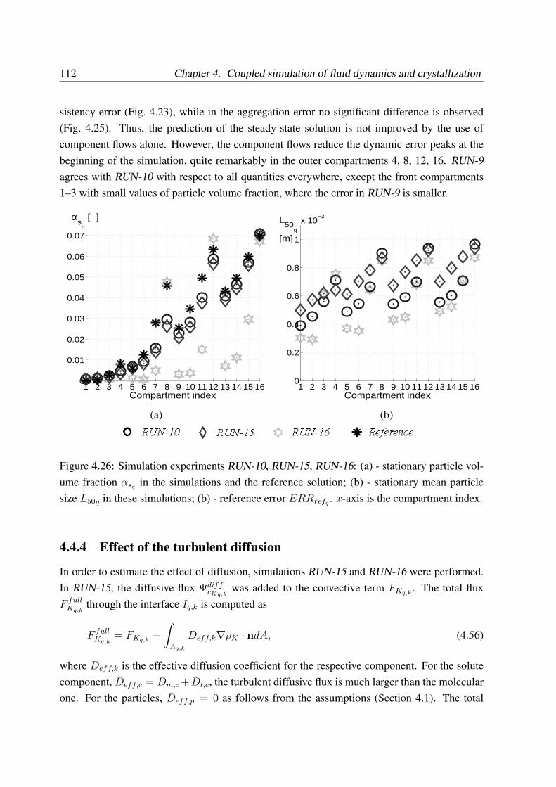
112 Chapter 4. Coupled simulation of fluid dynamics and crystallization
sistency error (Fig. 4.23), while in the aggregation error no significant difference is observed(Fig. 4.25). Thus, the prediction of the steady-state solution is not improved by the use ofcomponent flows alone. However, the component flows reduce the dynamic error peaks at thebeginning of the simulation, quite remarkably in the outer compartments 4, 8, 12, 16. RUN-9agrees with RUN-10 with respect to all quantities everywhere, except the front compartments1–3 with small values of particle volume fraction, where the error in RUN-9 is smaller.
1 2 3 4 5 6 7 8 9 10 11 12 13 14 15 160
0.01
0.02
0.03
0.04
0.05
0.06
0.07
Compartment index
αs
q
[−]
1 2 3 4 5 6 7 8 9 10 11 12 13 14 15 160
0.2
0.4
0.6
0.8
1
x 10−3
Compartment index
L50
q
[m]
(a) (b)
Figure 4.26: Simulation experiments RUN-10, RUN-15, RUN-16: (a) - stationary particle vol-ume fraction αsq in the simulations and the reference solution; (b) - stationary mean particlesize L50q in these simulations; (b) - reference error ERRrefq . x-axis is the compartment index.
4.4.4 Effect of the turbulent diffusion
In order to estimate the effect of diffusion, simulations RUN-15 and RUN-16 were performed.In RUN-15, the diffusive flux Ψdiff
cKq,kwas added to the convective term FKq,k
. The total fluxF full
Kq,kthrough the interface Iq,k is computed as
F fullKq,k
= FKq,k−
∫
Aq,k
Deff,k∇ρK · ndA, (4.56)
where Deff,k is the effective diffusion coefficient for the respective component. For the solutecomponent, Deff,c = Dm,c +Dt,c, the turbulent diffusive flux is much larger than the molecularone. For the particles, Deff,p = 0 as follows from the assumptions (Section 4.1). The total
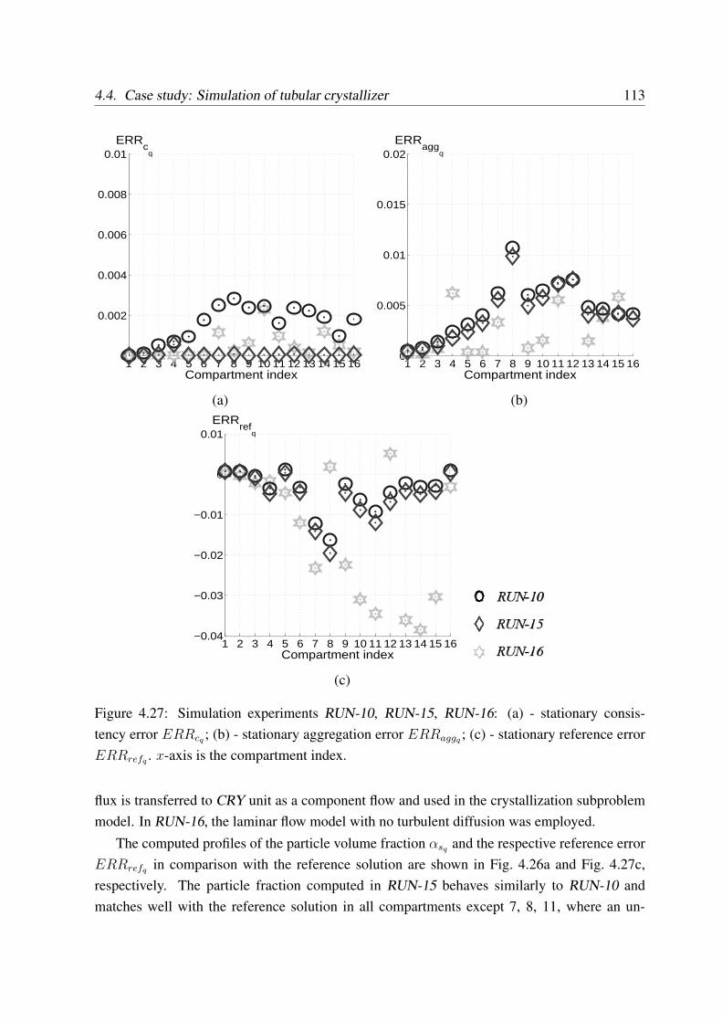
4.4. Case study: Simulation of tubular crystallizer 113
1 2 3 4 5 6 7 8 9 10 11 12 13 14 15 160
0.002
0.004
0.006
0.008
0.01
Compartment index
ERRc
q
1 2 3 4 5 6 7 8 9 10 11 12 13 14 15 160
0.005
0.01
0.015
0.02
Compartment index
ERRagg
q
(a) (b)
1 2 3 4 5 6 7 8 9 10 11 12 13 14 15 16−0.04
−0.03
−0.02
−0.01
0
0.01
Compartment index
ERRref
q
(c)
Figure 4.27: Simulation experiments RUN-10, RUN-15, RUN-16: (a) - stationary consis-tency error ERRcq ; (b) - stationary aggregation error ERRaggq ; (c) - stationary reference errorERRrefq . x-axis is the compartment index.
flux is transferred to CRY unit as a component flow and used in the crystallization subproblemmodel. In RUN-16, the laminar flow model with no turbulent diffusion was employed.
The computed profiles of the particle volume fraction αsq and the respective reference errorERRrefq in comparison with the reference solution are shown in Fig. 4.26a and Fig. 4.27c,respectively. The particle fraction computed in RUN-15 behaves similarly to RUN-10 andmatches well with the reference solution in all compartments except 7, 8, 11, where an un-
114 Chapter 4. Coupled simulation of fluid dynamics and crystallization
derprediction is observed. In RUN-16, strong underprediction is observed in all compartmentsexcept the outer compartments 4, 8, 12, 16, where the reference value is matched well.
The mean particle size L50q is shown in Fig. 4.26b. In RUN-15, where turbulent diffusionis modeled, the particle sizes are larger than those in RUN-10 for all compartments except theouter ones. They are smaller in RUN-16 with a laminar flow model. In the outer compartmentsthe effect of diffusion on the particle size is less pronounced.
The consistency and aggregation errors for these simulations are shown in Fig. 4.27a andFig. 4.27b, respectively. The consistency error is dramatically reduced in both simulations. InRUN-15, it is negligibly small. Thus, the best equivalency of the subproblem formulations canbe concluded when the effect of diffusion is accounted for in the CRY subproblem. The aggre-gation error, however, is only slightly smaller in RUN-15 than in RUN-10, which illustrates thatthe inhomogeneity in the compartments does not change significantly. In RUN-16, the aggre-gation error is smaller than in RUN-10 everywhere except in the outer compartments 4, 8, 12,16, where the aggregation error is several times larger due to the much stronger gradient of theparticle volume fraction in the boundary layer in case the diffusion is neglected.
RUN-15 has the smallest consistency error and a minimal deviation from the reference so-lution. The remaining deviation is determined by the compartment configuration.
4.4.5 Simulations with different number of compartments
The effect of the number of compartments on the solution was evaluated by Kulikov et al. (2006)for the coupled simulation with 8, 16 and 32 compartments in the tube with regular topology.A MSMPR-assumption was made in the compartments. The coupling variables transferredfrom the FD to the CRY unit were the temperature Tq and the flow rates Vq,k, and the couplingvariables from the CRY to the FD unit were the terms of mass transfer in crystallization Scq .The simulation setup is similar to RUN-1, but initial and boundary conditions were chosendifferently, such that a direct comparison with the results from RUN-1 cannot be performed.More details are provided in Kulikov et al. (2006).
The moments µ(p) of the PSD and the mean particle size L were evaluated in the CRYunit at the suspension outlet and presented in Fig. 4.28. The third distribution moment at theoutlet is predicted with good accuracy for simulations with 16 and 32 compartments, while asignificant overestimation of the third moment is observed if only 8 compartments are used.Similarly, the steady-state mean particle size at the outlet, L
out, is predicted well with 16 and
32 compartments, but is overestimated in the simulation with 8 compartments.The results show that the 16-compartment model is more accurate than the 8-compartment
model. However, further model refinement to 32 compartments does not provide a reasonablepayoff in accuracy for the double computational time.
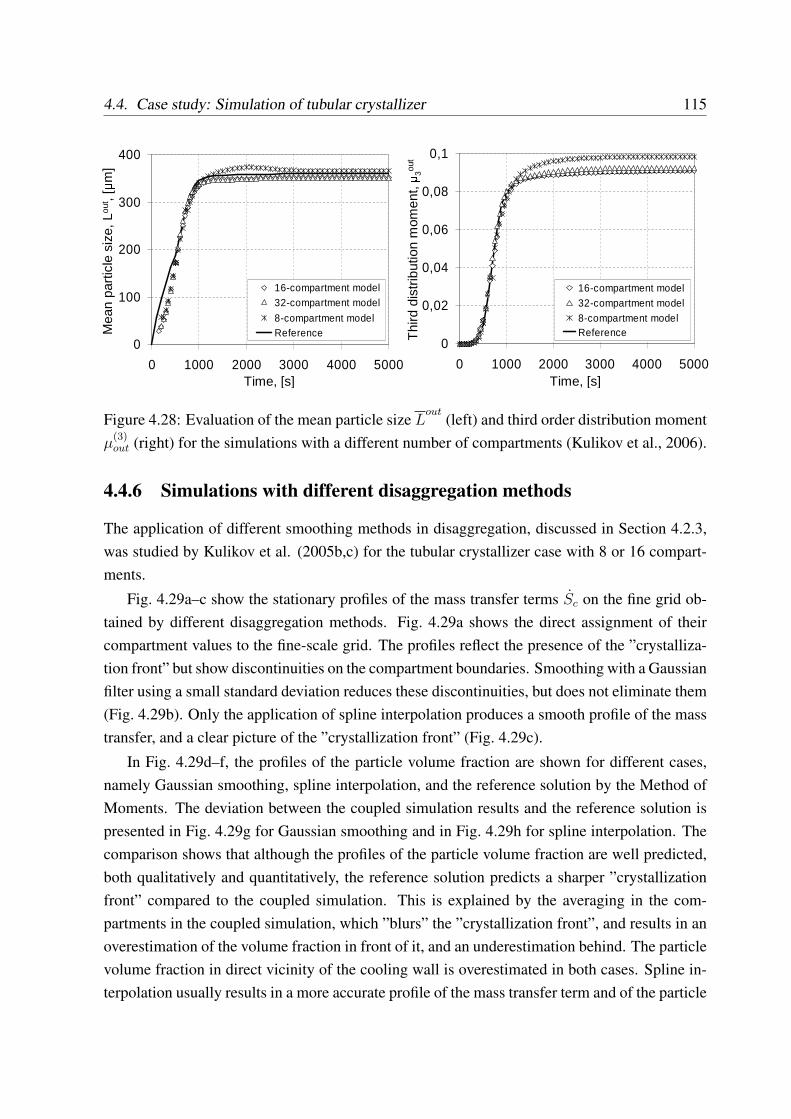
4.4. Case study: Simulation of tubular crystallizer 115
0
100
200
300
400
0 1000 2000 3000 4000 5000
16-compartment model32-compartment model
8-compartment modelReference
Time, [s]
Mea
n pa
rtic
le s
ize,
Lou
t , [µm]
0
0,02
0,04
0,06
0,08
0,1
0 1000 2000 3000 4000 5000
16-compartment model32-compartment model8-compartment modelReference
Time, [s]
Thi
rd d
istr
ibut
ion
mom
ent,
µ3out
Figure 4.28: Evaluation of the mean particle size Lout
(left) and third order distribution momentµ
(3)out (right) for the simulations with a different number of compartments (Kulikov et al., 2006).
4.4.6 Simulations with different disaggregation methods
The application of different smoothing methods in disaggregation, discussed in Section 4.2.3,was studied by Kulikov et al. (2005b,c) for the tubular crystallizer case with 8 or 16 compart-ments.
Fig. 4.29a–c show the stationary profiles of the mass transfer terms Sc on the fine grid ob-tained by different disaggregation methods. Fig. 4.29a shows the direct assignment of theircompartment values to the fine-scale grid. The profiles reflect the presence of the ”crystalliza-tion front” but show discontinuities on the compartment boundaries. Smoothing with a Gaussianfilter using a small standard deviation reduces these discontinuities, but does not eliminate them(Fig. 4.29b). Only the application of spline interpolation produces a smooth profile of the masstransfer, and a clear picture of the ”crystallization front” (Fig. 4.29c).
In Fig. 4.29d–f, the profiles of the particle volume fraction are shown for different cases,namely Gaussian smoothing, spline interpolation, and the reference solution by the Method ofMoments. The deviation between the coupled simulation results and the reference solution ispresented in Fig. 4.29g for Gaussian smoothing and in Fig. 4.29h for spline interpolation. Thecomparison shows that although the profiles of the particle volume fraction are well predicted,both qualitatively and quantitatively, the reference solution predicts a sharper ”crystallizationfront” compared to the coupled simulation. This is explained by the averaging in the com-partments in the coupled simulation, which ”blurs” the ”crystallization front”, and results in anoverestimation of the volume fraction in front of it, and an underestimation behind. The particlevolume fraction in direct vicinity of the cooling wall is overestimated in both cases. Spline in-terpolation usually results in a more accurate profile of the mass transfer term and of the particle
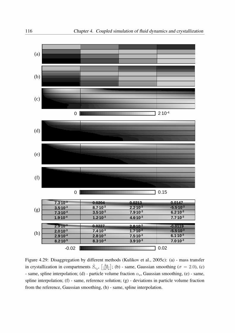
116 Chapter 4. Coupled simulation of fluid dynamics and crystallization
8.2.10-5
7.3.10-43.5.10-37.3.10-3
1.2.10-33.5.10-3
1.9.10-4
8.7.10-30.0204
4.6.10-3
7.9.10-32.2.10-30.0213
7.7.10-36.2.10-3-5.5.10-30.0147
2.9.10-42.0.10-32.9.10-3
8.3.10-42.8.10-37.4.10-30.0227
3.9.10-37.5.10-31.7.10-3
7.0.10-36.1.10-3-5.5.10-3-0.01192.8.10-3
(a)
(b)
(c)
(d)
(e)
(f)
(g)
(h)
0 2.10-4
0 0.15
-0.02 0.02
Figure 4.29: Disaggregation by different methods (Kulikov et al., 2005c): (a) - mass transferin crystallization in compartments Scq ,
[kg
m3s
]; (b) - same, Gaussian smoothing (σ = 2.0), (c)
- same, spline interpolation; (d) - particle volume fraction αs, Gaussian smoothing, (e) - same,spline interpolation; (f) - same, reference solution; (g) - deviations in particle volume fractionfrom the reference, Gaussian smoothing, (h) - same, spline interpolation.
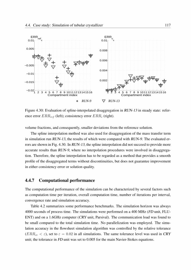
4.4. Case study: Simulation of tubular crystallizer 117
1 2 3 4 5 6 7 8 9 10111213141516−0.02
−0.015
−0.01
−0.005
0
0.005
0.01
Compartment index
ERRref
q
1 2 3 4 5 6 7 8 9 101112131415160
0.002
0.004
0.006
0.008
0.01
Compartment index
ERRc
q
+ RUN-9 RUN-13
Figure 4.30: Evaluation of spline-interpolated disaggregation in RUN-13 in steady state: refer-ence error ERRref (left); consistency error ERRc (right).
volume fractions, and consequently, smaller deviations from the reference solution.The spline interpolation method was also used for disaggregation of the mass transfer term
in simulation run RUN-13, the results of which were compared with RUN-9. The evaluated er-rors are shown in Fig. 4.30. In RUN-13, the spline interpolation did not succeed to provide moreaccurate results than RUN-9, where no interpolation procedures were involved in disaggrega-tion. Therefore, the spline interpolation has to be regarded as a method that provides a smoothprofile of the disaggregated terms without discontinuities, but does not guarantee improvementin either consistency error or solution quality.
4.4.7 Computational performance
The computational performance of the simulation can be characterized by several factors suchas computation time per iteration, overall computation time, number of iterations per interval,convergence rate and simulation accuracy.
Table 4.2 summarizes some performance benchmarks. The simulation horizon was always4000 seconds of process time. The simulations were performed on a 400 MHz (FD unit, FLU-ENT) and on a 1.6GHz computer (CRY unit, Parsival). The communication load was found tobe small compared to the total simulation time. No parallelization was employed. The simu-lation accuracy in the flowsheet simulation algorithm was controlled by the relative tolerance(ERRcv < ε), set to ε = 0.02 in all simulations. The same tolerance level was used in CRYunit; the tolerance in FD unit was set to 0.005 for the main Navier-Stokes equations.
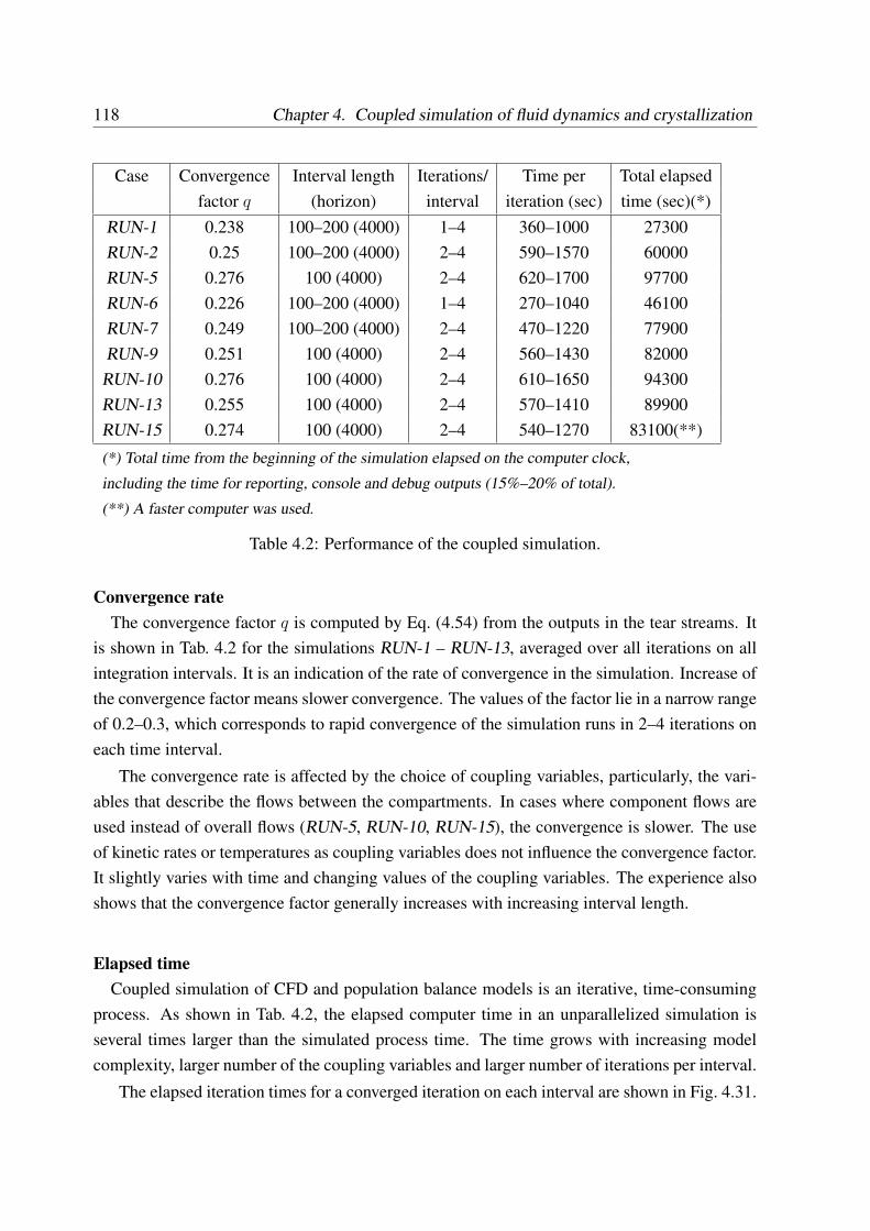
118 Chapter 4. Coupled simulation of fluid dynamics and crystallization
Case Convergence Interval length Iterations/ Time per Total elapsedfactor q (horizon) interval iteration (sec) time (sec)(*)
RUN-1 0.238 100–200 (4000) 1–4 360–1000 27300RUN-2 0.25 100–200 (4000) 2–4 590–1570 60000RUN-5 0.276 100 (4000) 2–4 620–1700 97700RUN-6 0.226 100–200 (4000) 1–4 270–1040 46100RUN-7 0.249 100–200 (4000) 2–4 470–1220 77900RUN-9 0.251 100 (4000) 2–4 560–1430 82000
RUN-10 0.276 100 (4000) 2–4 610–1650 94300RUN-13 0.255 100 (4000) 2–4 570–1410 89900RUN-15 0.274 100 (4000) 2–4 540–1270 83100(**)
(*) Total time from the beginning of the simulation elapsed on the computer clock,
including the time for reporting, console and debug outputs (15%–20% of total).
(**) A faster computer was used.
Table 4.2: Performance of the coupled simulation.
Convergence rateThe convergence factor q is computed by Eq. (4.54) from the outputs in the tear streams. It
is shown in Tab. 4.2 for the simulations RUN-1 – RUN-13, averaged over all iterations on allintegration intervals. It is an indication of the rate of convergence in the simulation. Increase ofthe convergence factor means slower convergence. The values of the factor lie in a narrow rangeof 0.2–0.3, which corresponds to rapid convergence of the simulation runs in 2–4 iterations oneach time interval.
The convergence rate is affected by the choice of coupling variables, particularly, the vari-ables that describe the flows between the compartments. In cases where component flows areused instead of overall flows (RUN-5, RUN-10, RUN-15), the convergence is slower. The useof kinetic rates or temperatures as coupling variables does not influence the convergence factor.It slightly varies with time and changing values of the coupling variables. The experience alsoshows that the convergence factor generally increases with increasing interval length.
Elapsed timeCoupled simulation of CFD and population balance models is an iterative, time-consuming
process. As shown in Tab. 4.2, the elapsed computer time in an unparallelized simulation isseveral times larger than the simulated process time. The time grows with increasing modelcomplexity, larger number of the coupling variables and larger number of iterations per interval.
The elapsed iteration times for a converged iteration on each interval are shown in Fig. 4.31.
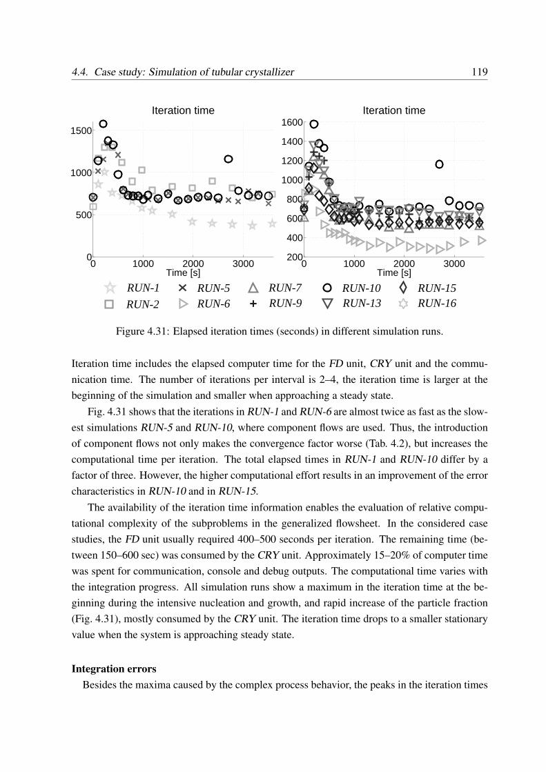
4.4. Case study: Simulation of tubular crystallizer 119
0 1000 2000 30000
500
1000
1500
Time [s]
Iteration time
0 1000 2000 3000200
400
600
800
1000
1200
1400
1600
Time [s]
Iteration time
RUN-1
RUN-2
RUN-5RUN-6
RUN-7
+ RUN-9RUN-10RUN-13
RUN-15RUN-16
Figure 4.31: Elapsed iteration times (seconds) in different simulation runs.
Iteration time includes the elapsed computer time for the FD unit, CRY unit and the commu-nication time. The number of iterations per interval is 2–4, the iteration time is larger at thebeginning of the simulation and smaller when approaching a steady state.
Fig. 4.31 shows that the iterations in RUN-1 and RUN-6 are almost twice as fast as the slow-est simulations RUN-5 and RUN-10, where component flows are used. Thus, the introductionof component flows not only makes the convergence factor worse (Tab. 4.2), but increases thecomputational time per iteration. The total elapsed times in RUN-1 and RUN-10 differ by afactor of three. However, the higher computational effort results in an improvement of the errorcharacteristics in RUN-10 and in RUN-15.
The availability of the iteration time information enables the evaluation of relative compu-tational complexity of the subproblems in the generalized flowsheet. In the considered casestudies, the FD unit usually required 400–500 seconds per iteration. The remaining time (be-tween 150–600 sec) was consumed by the CRY unit. Approximately 15–20% of computer timewas spent for communication, console and debug outputs. The computational time varies withthe integration progress. All simulation runs show a maximum in the iteration time at the be-ginning during the intensive nucleation and growth, and rapid increase of the particle fraction(Fig. 4.31), mostly consumed by the CRY unit. The iteration time drops to a smaller stationaryvalue when the system is approaching steady state.
Integration errorsBesides the maxima caused by the complex process behavior, the peaks in the iteration times
120 Chapter 4. Coupled simulation of fluid dynamics and crystallization
can show the intervals where numerical difficulties or integration failures were encountered.If an integration fails, sudden sharp peaks in the consistency errors and the iteration time areobserved at the position of failure. An example of such peak can be seen in the simulation runRUN-10 at t = 2700 sec (Fig. 4.31 and Fig. 4.24). The propagation of the disturbance to thedownstream compartments is quickly corrected in the following intervals, and the steady state isnot affected. It is a failure of the numerical integration, which disturbs the values of the particlefraction in compartment 7. Analysis of this sudden deviation identifies the cause of error: anincorrect reinitialization of the PSD occurred in compartment 7 in RUN-10 at t =2700 seconds,not reported by the tool. This example shows that the monitoring of dynamic consistency errorsand iteration times is an appropriate instrument to detect numerical errors in the integration, andhence to avoid erroneous solutions.
4.5 Discussion
Generalized flowsheet and decompositionThe algorithmic and technical framework described in Section 3 was further developed to
support generalized flowsheets and applied to the simulation of complex multi-scale and multi-physics processes such as the coupled simulation of fluid dynamics and crystallization. Thegeneralized flowsheet contains unit operations, which may involve process units, unit areas orprocess phenomena, and streams, which can be physical streams or couplings.
The formulation of the generalized flowsheet requires a decomposition of the problem,which is a model design problem. The design decisions determine the decomposition schemeand the resulting generalized flowsheet. The main steps of the decomposition are the choice ofcore equations and grids, the choice of assumptions used in the subproblems, and the choice ofcoupling variables (Fig. 4.10). The capabilities of the simulation tools are accounted for.
The key concept in the problem decomposition employed is the use of different discretiza-tions in the subproblems of the generalized flowsheet. Simulations were performed employinga fixed fine-scale grid in the FD unit and 16 coarse-scale compartments with a regular layout inthe CRY unit. The studies discussed by Kulikov et al. (2006) showed that the use of 16 com-partments can be regarded as satisfactory, while the simulation with 8 compartments showedsignificant error, and the simulation with 32 compartments was very time-consuming withoutsignificant improvement of the simulation quality.
The set of Navier-Stokes equations is the core for the FD unit and the population balancefor the CRY unit. Therefore, the particle size distributed variables are allocated to the CRYunit. Because of different discretizations in the subproblems, the coupling variables transferredfrom the FD to the CRY unit undergo aggregation by volumetric averaging, while the variables
4.5. Discussion 121
transferred from the CRY to the FD unit are disaggregated onto the FD grid using a dedicatedprocedure.
The choice of coupling variables aggregated from the FD to the CRY unit is a design deci-sion. Simulations were performed with various sets of the coupling variables and were analyzedfor consistency and accuracy. The most accurate results were achieved using the auxiliary mod-eling in the disaggregation. This implies that the mass transfer term due to crystallization isevaluated in the compartment model and used as a source term in the fine-scale species trans-port equations to produce the fine-scale profiles of the suspension components, while keepingthe component mass balance correct. Approaches to improve the disaggregation procedure byapplication of smoothing methods to the disaggregated source term to generate its continuousprofile show ambiguous results.
A further improvement in accuracy was achieved by considering the diffusion flows alongwith the convective flows in the comparment models. The other design decisions involved thereconciliation of initial conditions in the CRY unit at the beginning of the iteration, the use ofoverall or component flows in the CRY unit, and the transfer of temperature or the crystallizationkinetics to the CRY unit.
Evaluation of simulationsThe simulation runs with various choices of the coupling variables are compared to the ref-
erence solution by the Method of Moments to evaluate the model design decisions. To evaluatethe quality of the simulation, three kinds of errors were computed in all compartments on ev-ery integration time interval: the reference error (deviation from the reference solution), theconsistency error (deviation between the same quantities from different subproblems) and theaggregation error (fine-grid profile inhomogeneity). In most simulations, the stationary valuesof the errors did not exceed 20% in the compartments, which can be regarded as a good approx-imation. The observed errors are higher in regions close to the ”crystallization front” where theintensive crystallization occurs. During the transient, all error quantities show a maximum atthe beginning of the simulations, since the cooling of the saturated suspension results in rapidcrystallization.
The reference error shows that a significant improvement is obtained if the reconciliationof initial conditions is employed on every time interval. The use of component flows insteadof overall flows results in a minor improvement in accuracy, but in a better consistency of themodel. The effect of computation of the crystallization kinetics in the FD rather than in the CRYunit is ambiguous for a considered model with simple kinetics. For the most compartments, theprofiles and the steady-state values produced by different simulation runs are close to each other,but show a systematic deviation from the reference solution.
In the considered model, the effect of the compartment choice and of the consistency of the
122 Chapter 4. Coupled simulation of fluid dynamics and crystallization
assumptions appears to be more important than the effect of the choice of coupling variables.In contrast, this choice has a pronounced effect in the simulations of the forced circulationcrystallizer with a more complex model (Section 6.1).
In all simulation cases, a correlation between the consistency and reference error was ob-served. Smaller consistency errors are usually correlated with smaller deviations from the refer-ence solution. A reduction of the consistency error to the minimum leads to the ”best” coupledsimulation solution. In the considered case, this ”best” solution is produced in RUN-15, wherethe correction of initial conditions, component flows and the correction for turbulent diffusionare employed. However, the reference error shows that systematic deviations are present evenin the ”best” solution. The source of the remaining deviations is the compartment discretiza-tion, which introduces a discretization error, dependent on the choice of the coarse grid. Thisis illustrated by the observed correlation between the reference and the aggregation errors: botherrors are larger for the compartments with highly non-uniform profiles. In conclusion, a properchoice and a run-time adaptation of the compartments to render more homogeneous profiles inthe compartments should be a major contribution to reduce the remaining solution error.
The author is convinced that an a posteriori error estimation using one of the approachessketched in Section 4.3.6.2 enables derivation of an accurate error criteria to replace the usuallyunknown reference error. However, such a derivation is challenging and remained outside thescope of the present thesis.
Numerical integration and performanceThe simulation of the FD subproblem on a fine grid and the population balance on a coarse-
scale compartment grid enabled the direct application of specialized simulation tools and algo-rithms implemented therein. There are no technical limitations in CHEOPS for the simulationof a generalized flowsheet with a predefined fixed discretization. The chosen software toolsfor the simulation of the FD unit (FLUENT) and the CRY unit (Parsival), and the CHEOPSwrappers for these tools support the required functionality, with some limitations discussed inSection 4.2.7 and in Appendix A.
However, large computational times of iterations on the complex models make the coupledsimulation of generalized flowsheets inappropriate for fast simulations. For small models, thecommunication overhead becomes a significant factor. The proposed coupled simulation isuseful as an instrument to handle complex models with large simulation times, which are notsolvable in a single tool, but can be decomposed into moderately complex subproblems.
Section 4.4.7 also illustrates that the analysis of the consistency errors and iteration times inthe coupled simulation enables easy detection of the errors in the numerical integration.
Chapter 5
Simulation with adaptive compartmentselection
The term adaptation has a number of different meanings. In this work, adaptation is employedfor an algorithmic runtime adjustment of the model discretization. It belongs to algorithmicadaptation methods, according to Marquardt (2002). The objectives of this adaptation can beformulated as follows:
• local refinement of the discretization in regions of interest or in regions with large gra-dients to preserve simulation accuracy while minimizing the increase of computationaleffort;
• coarsening of the discretization outside regions of interest and in regions with small gra-dients to reduce computational effort while minimizing the loss of solution accuracy;
• specification of the local region for a detailed submodel or a submodel for the specificprocess.
The adaptation target is a discretization element in space, time or internal coordinate vari-ables. The discretization of the spatial grid is characterized by a step h; for finite-elementdiscretization, the order p of the finite element basis can also be adjusted. For a spatial grid cellwith complex topology, the boundary of the cell can be adjusted. Temporal discretizations canbe adjusted by changing the time step ∆t to be used for the integration of the dynamic problem.
The adaptation criterion χ is a locally evaluated function which is compared with a thresh-old value χcrit to determine whether an adaptation has to be performed for the given grid cell.An a posteriori quality criterion ζ can be formulated in some cases to evaluate the quality ofthe solution after adaptation compared to the reference simulation results.
123
124 Chapter 5. Simulation with adaptive compartment selection
5.1 Compartment adaptation with heuristic criteria
5.1.1 Adaptation in generalized flowsheet simulation
In the considered generalized flowsheet simulation framework, adaptation of different targets ishandled in different blocks of the algorithm. Discretization in internal coordinates is adaptedwithin the respective tools (Parsival). Adaptation of temporal discretization can be done both inthe simulation tools (internal time step adaptation is supported by Parsival and FLUENT) and inthe flowsheet simulation algorithm to adjust the length of the integration interval (Section 3.2.3).
Spatial adaptation in the generalized flowsheet with individual spatial discretizations in thesubproblems can be used for both the fine and coarse grids. Adaptation of the fine grid of theCFD subproblems is a typical task covered in many books on the computational fluid dynamics,and can be executed by most CFD solvers (Ferziger and Peric, 1997; Hay and Visonneau, 2005).In the present study, we assume that the fine grid is accurate enough for modeling the flowdynamics in the considered mass crystallization problems.
Therefore, adaptation of the coarse-grid compartments is discussed exclusively. This adap-tation modifies the compartment layout to reduce the errors introduced by the coarse compart-ment discretization. To characterize them, we have defined reference, aggregation and con-sistency errors in Section 4.3. Only the aggregation errors ERRagg characterizing the inho-mogeneity in the profiles of selected process quantities can be immediately evaluated in thenumerical simulation. They can be used in the adaptation criterion χ to decide on the compart-ments to be adapted (Section 5.1.3.1).
After adaptation, an improvement of the simulation quality can be expected. If a referencesolution is available for the problem, the reference error ERRref can be employed to check this.Alternatively, an a posteriori quality criterion ζ can be employed. In absence of reference errorinformation, the aggregation error ERRagg and the consistency errors ERRc can be employed,assuming that a reduction of these errors is correlated with an improvement of the solutionaccuracy.
In the following subsections, the formulation and implementation of an adaptation proce-dure for a generalized flowsheet in CHEOPS are discussed. The concepts are illustrated inSection 5.2 with the tubular crystallizer case study introduced in Section 4.1, where spatialadaptation of the compartments is performed during the simulation. On the basis of this study,the hypothesis of applicability of error quantities to evaluate the simulation quality will bechecked.
5.1. Compartment adaptation with heuristic criteria 125
5.1.2 Formulation of compartment adaptation problem
Compartment adaptation can be formulated as an optimization problem to minimize the adap-tation criterion χ within the chosen compartments formulated for a relevant process quantity φ
or its function.Assume φ is the chosen quantity, available on the fine grid, φq = Agg(φi,j) is its aggre-
gated value in compartment q with Zq = {zi,j}, (i, j) ∈ Iq. Iq refers to the set of indices ofcells belonging to the compartment q, and defines its spatial domain. A general compartmentadaptation problem can be formulated as follows:
Find (i, j) ∈ Iq, ∀q = 1, ..., Nq, such thatχ =
∑Nq
q=1 χq(φ) → min, χq = ‖φi,j‖p, (i, j) ∈ Iq
subject to the constraintsVq ≥ Vmin, ∀q = 1, ..., Nq (constraint for compartment volume Vq);Cα,q(φ) ≥ 0, α = 1, .., Nα,q, ∀q = 1, ..., Nq (other compartment constraints if used).
The adaptation criterion χq = ‖φi,j‖p is defined as the norm to evaluate compartment inho-mogeneity with respect to the specified quantity φ. The symbol p denotes the type of the norm.Several types of norms, such as ∞-, 1- and 2-norms, and min-max criterion can be used foradaptation:
min-max criterion χq = |φq,max − φq,min| =∣∣maxi,j∈Iq φi,j −mini,j∈Iq φi,j
∣∣,∞-norm χq =
∥∥φi,j − φq
∥∥∞ = max(i,j)∈Iq
(|φi,j − φq|), (i, j) ∈ Iq,
1-norm χq =∥∥φi,j − φq
∥∥1
=∑
i,j∈Iq
(|φi,j − φq|)
= ERRagg,q(φ), (i, j) ∈ Iq,
2-norm χq =∥∥φi,j − φq
∥∥2
=√∑
i,j∈Iq
(φi,j − φq
)2, (i, j) ∈ Iq .
All norms except the min-max-criterion are evaluated with respect to the aggregated quantityφq. The 1-norm is identical to the aggregation error ERRagg,q(φ). A min-max-criterion directlyevaluates the deviation between the minimum and maximum values of the quantity φ within thecompartment.
Minimum volume constraints require the compartment volume Vq to be larger than the min-imum threshold volume Vmin. This provides a limit for the minimum residence time in thecompartment and is useful for the stability of the computations. Further constraints can beadded to specify other restrictions on the allowed compartment topology.
The optimization problem is solved by an algorithm which manipulates the index sets(i, j) ∈ Iq to modify the location and the boundaries of the compartments.
5.1.3 Adaptation criteria
The formulation of the adaptation criterion χ and the choice of the relevant quantities φ are themajor factors that determine the quality of the adaptation of the compartments.
126 Chapter 5. Simulation with adaptive compartment selection
Ideally, the adaptation criterion should be an error estimator and involve the compartmentvariables at the end of the considered time interval ∆Tn in the converged state y∗(tn+1). Ob-viously, this is not possible, because an explicit expression for the aggregation error in thesevariables at tn+1 can only be obtained after the interval convergence, and because the com-partment outputs are not available on the fine grid, where the aggregation error is evaluated.Therefore, the adaptation criterion has to involve only the variables available on the fine grid atthe beginning of the considered time interval tn, such as
• the inputs to the compartment on the fine grid (φ = ui,j(tn));
• the computed fine-scale quantities, equivalent to the compartment outputs (φ = yi,j(tn));
• the quantities, computed as functions of these inputs or outputs;
A criterion can be composite and involve several quantities of the above type.
5.1.3.1 Adaptation criteria based on single variable
Relevant inputsThe inputs to the compartment are obtained by a causal analysis of decomposition (Sec-
tion 4.2.6). In the context of the generalized flowsheet problem, the adaptation criterion, eval-uated on the fine grid, should involve one or several coupling variables, acting as inputs to thefine grid subproblem, or variables located causally upstream of them. For the considered fluiddynamics-crystallization problem, such quantities are shown in Fig. 5.1 by circles with a thickboundary line.
Temperature, T . The temperature is directly computed from the energy balance in the finegrid FD subproblem (4.3). It affects the saturation concentration c∗ and hence the supersatu-ration s (which usually increases if temperature decreases). In turn, the supersaturation deter-mines the nucleation and growth rates. In the considered model, growth rate shows a lineardependency on temperature, while nucleation rate shows a nonlinear dependency. The temper-ature can be used as a primary criterion if a significant temperature change in the process isobserved.
Residence time, τ . The residence time in the compartment is a characteristic of the flow inthe process. It affects the number of emerging crystals and the amount of mass transfer fromthe solute to the crystals. It depends on the flow velocity and the topology of the compartments.A transport equation for the residence time can be derived as
∇ · (vτ) = 1, (5.1)
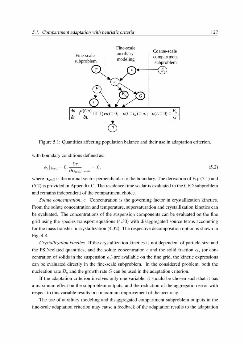
5.1. Compartment adaptation with heuristic criteria 127
.)0(;)(;0)()(
00 G
BLnnttnn
L
Gn
t
n n=====⋅∇+∂
∂+∂∂
v
s
GqnBF
n
T c
τ
Fine-scale subproblem
Coarse-scale compartmentsubproblem
cS&Fine-scaleauxiliary modeling
Figure 5.1: Quantities affecting population balance and their use in adaptation criterion.
with boundary conditions defined as:
φτ |feed = 0;∂τ
∂nwall
∣∣∣wall
= 0, (5.2)
where nwall is the normal vector perpendicular to the boundary. The derivation of Eq. (5.1) and(5.2) is provided in Appendix C. The residence time scalar is evaluated in the CFD subproblemand remains independent of the compartment choice.
Solute concentration, c. Concentration is the governing factor in crystallization kinetics.From the solute concentration and temperature, supersaturation and crystallization kinetics canbe evaluated. The concentrations of the suspension components can be evaluated on the finegrid using the species transport equations (4.30) with disaggregated source terms accountingfor the mass transfer in crystallization (4.32). The respective decomposition option is shown inFig. 4.8.
Crystallization kinetics. If the crystallization kinetics is not dependent of particle size andthe PSD-related quantities, and the solute concentration c and the solid fraction αs (or con-centration of solids in the suspension ρs) are available on the fine grid, the kinetic expressionscan be evaluated directly in the fine-scale subproblem. In the considered problem, both thenucleation rate Bn and the growth rate G can be used in the adaptation criterion.
If the adaptation criterion involves only one variable, it should be chosen such that it hasa maximum effect on the subproblem outputs, and the reduction of the aggregation error withrespect to this variable results in a maximum improvement of the accuracy.
The use of auxiliary modeling and disaggregated compartment subproblem outputs in thefine-scale adaptation criterion may cause a feedback of the adaptation results to the adaptation
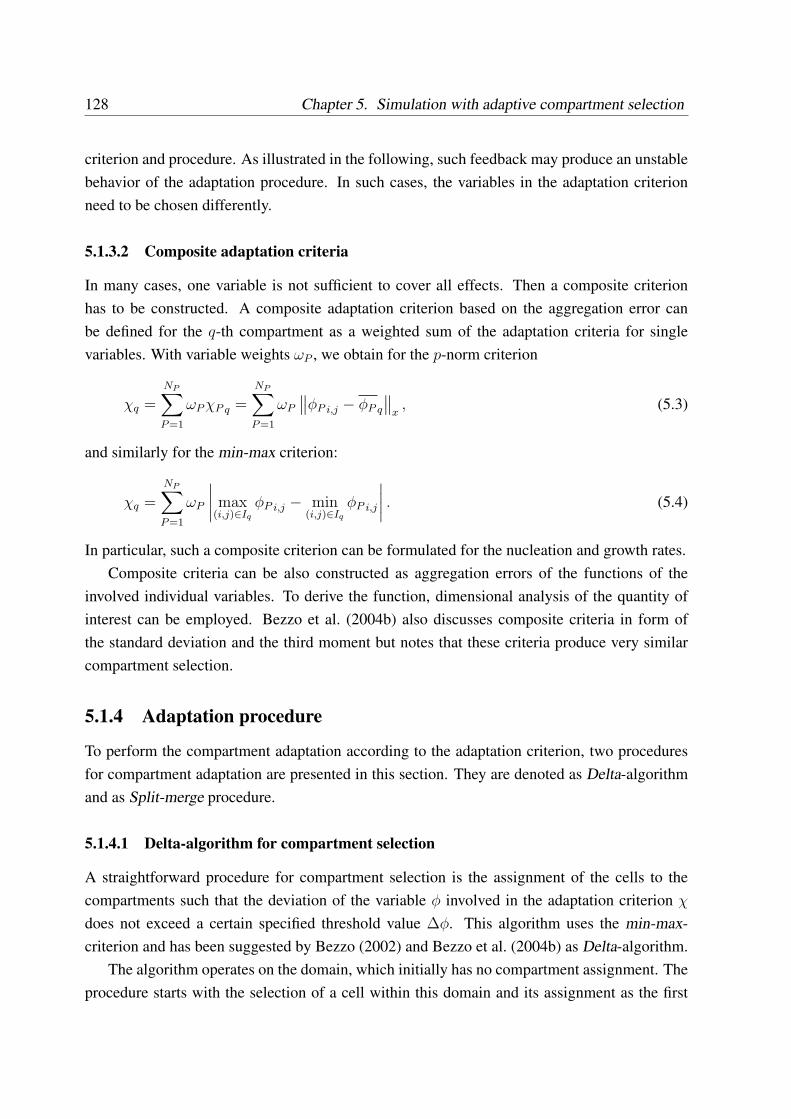
128 Chapter 5. Simulation with adaptive compartment selection
criterion and procedure. As illustrated in the following, such feedback may produce an unstablebehavior of the adaptation procedure. In such cases, the variables in the adaptation criterionneed to be chosen differently.
5.1.3.2 Composite adaptation criteria
In many cases, one variable is not sufficient to cover all effects. Then a composite criterionhas to be constructed. A composite adaptation criterion based on the aggregation error canbe defined for the q-th compartment as a weighted sum of the adaptation criteria for singlevariables. With variable weights ωP , we obtain for the p-norm criterion
χq =
NP∑P=1
ωP χP q =
NP∑P=1
ωP
∥∥φP i,j − φP q
∥∥x, (5.3)
and similarly for the min-max criterion:
χq =
NP∑P=1
ωP
∣∣∣∣ max(i,j)∈Iq
φP i,j − min(i,j)∈Iq
φP i,j
∣∣∣∣ . (5.4)
In particular, such a composite criterion can be formulated for the nucleation and growth rates.Composite criteria can be also constructed as aggregation errors of the functions of the
involved individual variables. To derive the function, dimensional analysis of the quantity ofinterest can be employed. Bezzo et al. (2004b) also discusses composite criteria in form ofthe standard deviation and the third moment but notes that these criteria produce very similarcompartment selection.
5.1.4 Adaptation procedure
To perform the compartment adaptation according to the adaptation criterion, two proceduresfor compartment adaptation are presented in this section. They are denoted as Delta-algorithmand as Split-merge procedure.
5.1.4.1 Delta-algorithm for compartment selection
A straightforward procedure for compartment selection is the assignment of the cells to thecompartments such that the deviation of the variable φ involved in the adaptation criterion χ
does not exceed a certain specified threshold value ∆φ. This algorithm uses the min-max-criterion and has been suggested by Bezzo (2002) and Bezzo et al. (2004b) as Delta-algorithm.
The algorithm operates on the domain, which initially has no compartment assignment. Theprocedure starts with the selection of a cell within this domain and its assignment as the first
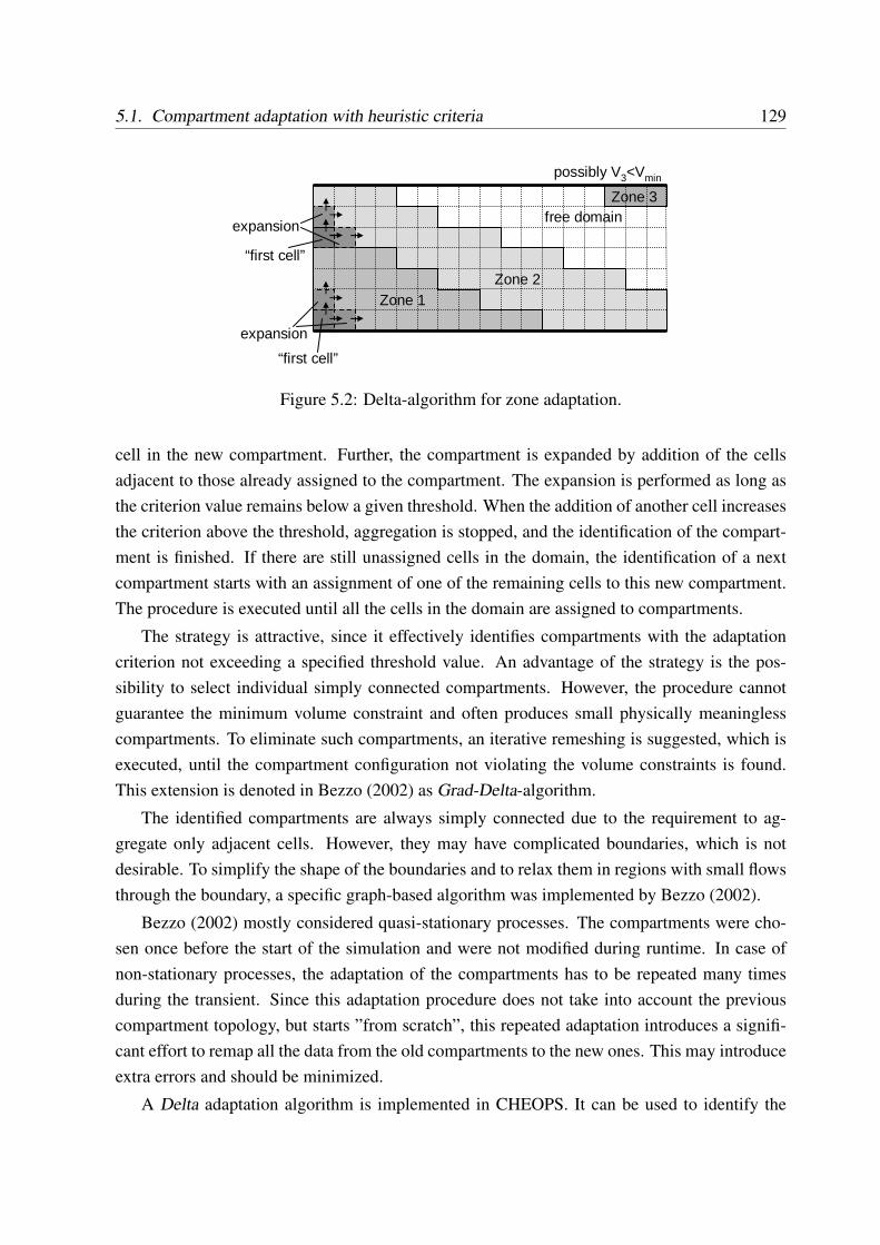
5.1. Compartment adaptation with heuristic criteria 129
free domain
Zone 1Zone 2
“first cell”
expansion
“first cell”
expansion
Zone 3
possibly V3<Vmin
Figure 5.2: Delta-algorithm for zone adaptation.
cell in the new compartment. Further, the compartment is expanded by addition of the cellsadjacent to those already assigned to the compartment. The expansion is performed as long asthe criterion value remains below a given threshold. When the addition of another cell increasesthe criterion above the threshold, aggregation is stopped, and the identification of the compart-ment is finished. If there are still unassigned cells in the domain, the identification of a nextcompartment starts with an assignment of one of the remaining cells to this new compartment.The procedure is executed until all the cells in the domain are assigned to compartments.
The strategy is attractive, since it effectively identifies compartments with the adaptationcriterion not exceeding a specified threshold value. An advantage of the strategy is the pos-sibility to select individual simply connected compartments. However, the procedure cannotguarantee the minimum volume constraint and often produces small physically meaninglesscompartments. To eliminate such compartments, an iterative remeshing is suggested, which isexecuted, until the compartment configuration not violating the volume constraints is found.This extension is denoted in Bezzo (2002) as Grad-Delta-algorithm.
The identified compartments are always simply connected due to the requirement to ag-gregate only adjacent cells. However, they may have complicated boundaries, which is notdesirable. To simplify the shape of the boundaries and to relax them in regions with small flowsthrough the boundary, a specific graph-based algorithm was implemented by Bezzo (2002).
Bezzo (2002) mostly considered quasi-stationary processes. The compartments were cho-sen once before the start of the simulation and were not modified during runtime. In case ofnon-stationary processes, the adaptation of the compartments has to be repeated many timesduring the transient. Since this adaptation procedure does not take into account the previouscompartment topology, but starts ”from scratch”, this repeated adaptation introduces a signifi-cant effort to remap all the data from the old compartments to the new ones. This may introduceextra errors and should be minimized.
A Delta adaptation algorithm is implemented in CHEOPS. It can be used to identify the
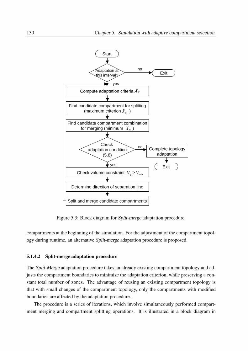
130 Chapter 5. Simulation with adaptive compartment selection
Start
Compute adaptation criteria
Find candidate compartment for splitting(maximum criterion )
Find candidate compartment combinationfor merging (minimum )
sqχ
Check adaptation condition
(5.8)
Exit
no
yes
Complete topologyadaptation
Determine direction of separation line
Split and merge candidate compartments
mχ
Adaptation atthis interval?
no
yes
Exit
Check volume constraint
qχ
minVVq ≥
Figure 5.3: Block diagram for Split-merge adaptation procedure.
compartments at the beginning of the simulation. For the adjustment of the compartment topol-ogy during runtime, an alternative Split-merge adaptation procedure is proposed.
5.1.4.2 Split-merge adaptation procedure
The Split-Merge adaptation procedure takes an already existing compartment topology and ad-justs the compartment boundaries to minimize the adaptation criterion, while preserving a con-stant total number of zones. The advantage of reusing an existing compartment topology isthat with small changes of the compartment topology, only the compartments with modifiedboundaries are affected by the adaptation procedure.
The procedure is a series of iterations, which involve simultaneously performed compart-ment merging and compartment splitting operations. It is illustrated in a block diagram in
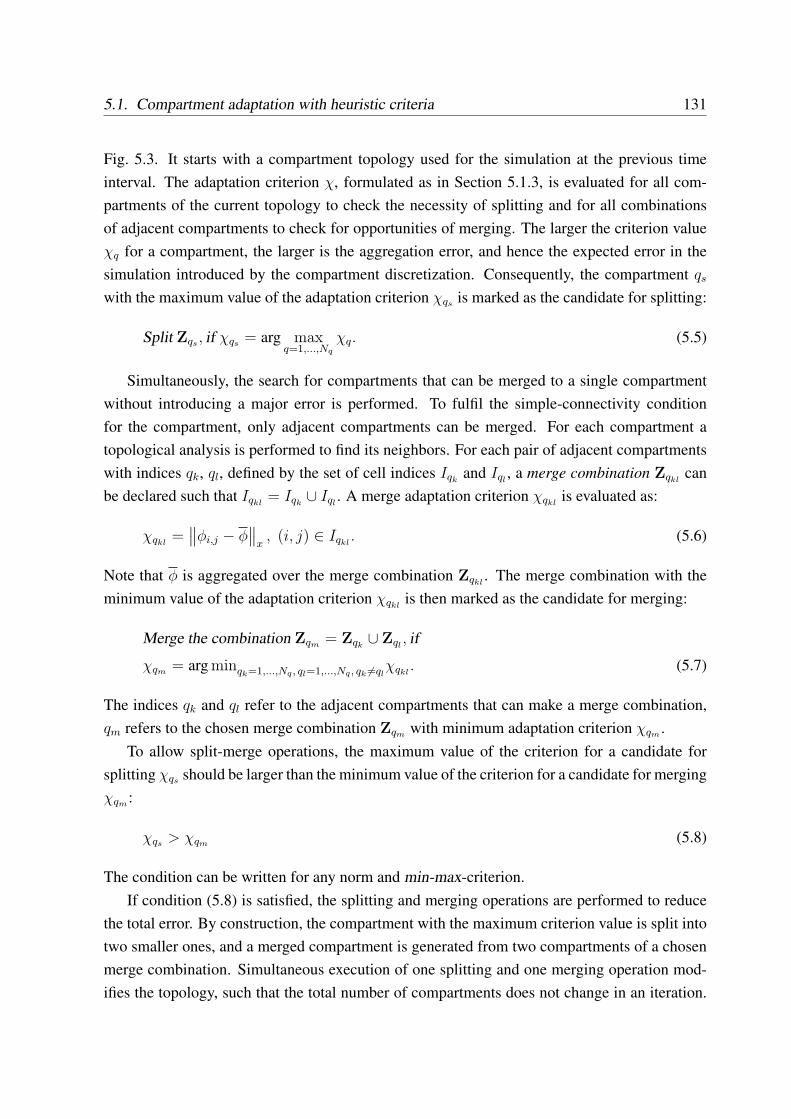
5.1. Compartment adaptation with heuristic criteria 131
Fig. 5.3. It starts with a compartment topology used for the simulation at the previous timeinterval. The adaptation criterion χ, formulated as in Section 5.1.3, is evaluated for all com-partments of the current topology to check the necessity of splitting and for all combinationsof adjacent compartments to check for opportunities of merging. The larger the criterion valueχq for a compartment, the larger is the aggregation error, and hence the expected error in thesimulation introduced by the compartment discretization. Consequently, the compartment qs
with the maximum value of the adaptation criterion χqs is marked as the candidate for splitting:
Split Zqs , if χqs = arg maxq=1,...,Nq
χq. (5.5)
Simultaneously, the search for compartments that can be merged to a single compartmentwithout introducing a major error is performed. To fulfil the simple-connectivity conditionfor the compartment, only adjacent compartments can be merged. For each compartment atopological analysis is performed to find its neighbors. For each pair of adjacent compartmentswith indices qk, ql, defined by the set of cell indices Iqk
and Iql, a merge combination Zqkl
canbe declared such that Iqkl
= Iqk∪ Iql
. A merge adaptation criterion χqklis evaluated as:
χqkl=
∥∥φi,j − φ∥∥
x, (i, j) ∈ Iqkl
. (5.6)
Note that φ is aggregated over the merge combination Zqkl. The merge combination with the
minimum value of the adaptation criterion χqklis then marked as the candidate for merging:
Merge the combination Zqm = Zqk∪ Zql
, if
χqm = arg minqk=1,...,Nq , ql=1,...,Nq , qk 6=qlχqkl
. (5.7)
The indices qk and ql refer to the adjacent compartments that can make a merge combination,qm refers to the chosen merge combination Zqm with minimum adaptation criterion χqm .
To allow split-merge operations, the maximum value of the criterion for a candidate forsplitting χqs should be larger than the minimum value of the criterion for a candidate for mergingχqm:
χqs > χqm (5.8)
The condition can be written for any norm and min-max-criterion.If condition (5.8) is satisfied, the splitting and merging operations are performed to reduce
the total error. By construction, the compartment with the maximum criterion value is split intotwo smaller ones, and a merged compartment is generated from two compartments of a chosenmerge combination. Simultaneous execution of one splitting and one merging operation mod-ifies the topology, such that the total number of compartments does not change in an iteration.
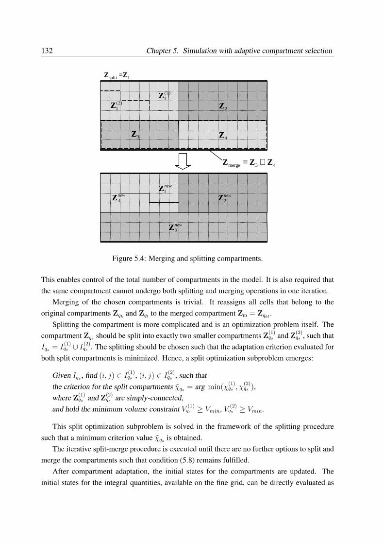
132 Chapter 5. Simulation with adaptive compartment selection
Zsplit =Z1
43merge ZZZ ∪=
)1(`1Ζ
)2(1Ζ 2Ζ
3Ζ 4Ζnew1Ζ
new4Ζ new
2Ζnew3Ζ
Figure 5.4: Merging and splitting compartments.
This enables control of the total number of compartments in the model. It is also required thatthe same compartment cannot undergo both splitting and merging operations in one iteration.
Merging of the chosen compartments is trivial. It reassigns all cells that belong to theoriginal compartments Zqk
and Zqlto the merged compartment Zm = Zqkl
.Splitting the compartment is more complicated and is an optimization problem itself. The
compartment Zqs should be split into exactly two smaller compartments Z(1)qs and Z
(2)qs , such that
Iqs = I(1)qs ∪ I
(2)qs . The splitting should be chosen such that the adaptation criterion evaluated for
both split compartments is minimized. Hence, a split optimization subproblem emerges:
Given Iqs , find (i, j) ∈ I(1)qs , (i, j) ∈ I
(2)qs , such that
the criterion for the split compartments χqs = arg min(χ(1)qs , χ
(2)qs ),
where Z(1)qs and Z
(2)qs are simply-connected,
and hold the minimum volume constraint V(1)qs ≥ Vmin, V
(2)qs ≥ Vmin.
This split optimization subproblem is solved in the framework of the splitting proceduresuch that a minimum criterion value χqs is obtained.
The iterative split-merge procedure is executed until there are no further options to split andmerge the compartments such that condition (5.8) remains fulfilled.
After compartment adaptation, the initial states for the compartments are updated. Theinitial states for the integral quantities, available on the fine grid, can be directly evaluated as
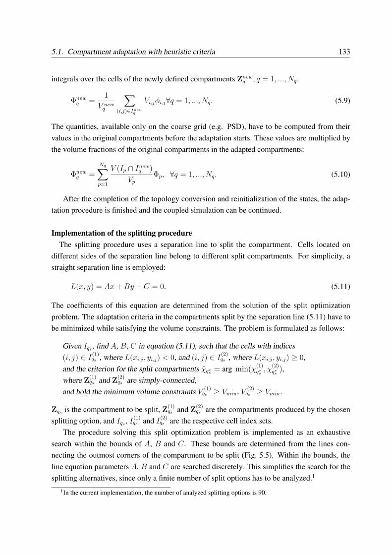
5.1. Compartment adaptation with heuristic criteria 133
integrals over the cells of the newly defined compartments Znewq , q = 1, ..., Nq.
Φnewq =
1
V newq
∑
(i,j)∈Inewq
Vi,jφi,j∀q = 1, ..., Nq. (5.9)
The quantities, available only on the coarse grid (e.g. PSD), have to be computed from theirvalues in the original compartments before the adaptation starts. These values are multiplied bythe volume fractions of the original compartments in the adapted compartments:
Φnewq =
Nq∑p=1
V (Ip ∩ Inewq )
Vp
Φp, ∀q = 1, ..., Nq. (5.10)
After the completion of the topology conversion and reinitialization of the states, the adap-tation procedure is finished and the coupled simulation can be continued.
Implementation of the splitting procedureThe splitting procedure uses a separation line to split the compartment. Cells located on
different sides of the separation line belong to different split compartments. For simplicity, astraight separation line is employed:
L(x, y) = Ax + By + C = 0. (5.11)
The coefficients of this equation are determined from the solution of the split optimizationproblem. The adaptation criteria in the compartments split by the separation line (5.11) have tobe minimized while satisfying the volume constraints. The problem is formulated as follows:
Given Iqs , find A, B, C in equation (5.11), such that the cells with indices(i, j) ∈ I
(1)qs , where L(xi,j, yi,j) < 0, and (i, j) ∈ I
(2)qs , where L(xi,j, yi,j) ≥ 0,
and the criterion for the split compartments χq∗s = arg min(χ(1)q∗s , χ
(2)q∗s ),
where Z(1)qs and Z
(2)qs are simply-connected,
and hold the minimum volume constraints V(1)qs ≥ Vmin, V
(2)qs ≥ Vmin.
Zqs is the compartment to be split, Z(1)qs and Z
(2)qs are the compartments produced by the chosen
splitting option, and Iqs , I(1)qs and I
(2)qs are the respective cell index sets.
The procedure solving this split optimization problem is implemented as an exhaustivesearch within the bounds of A, B and C. These bounds are determined from the lines con-necting the outmost corners of the compartment to be split (Fig. 5.5). Within the bounds, theline equation parameters A, B and C are searched discretely. This simplifies the search for thesplitting alternatives, since only a finite number of split options has to be analyzed.1
1In the current implementation, the number of analyzed splitting options is 90.
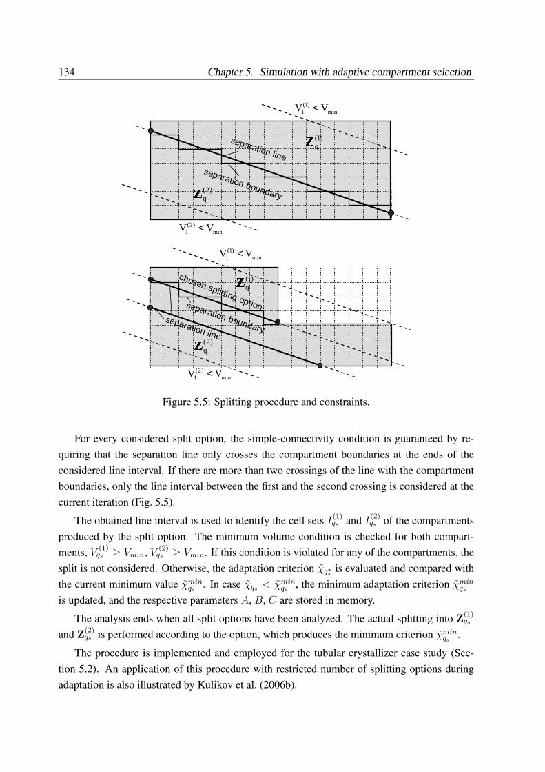
134 Chapter 5. Simulation with adaptive compartment selection
min)1(
1 VV <
)2(qΖ )1(
qΖmin
)1(1 VV <
min)2(
1 VV <
separation line
min)2(
1 VV <
separation boundary
separation boundary
)1(qΖ
)2(qΖchosen splitting option
separation line
Figure 5.5: Splitting procedure and constraints.
For every considered split option, the simple-connectivity condition is guaranteed by re-quiring that the separation line only crosses the compartment boundaries at the ends of theconsidered line interval. If there are more than two crossings of the line with the compartmentboundaries, only the line interval between the first and the second crossing is considered at thecurrent iteration (Fig. 5.5).
The obtained line interval is used to identify the cell sets I(1)qs and I
(2)qs of the compartments
produced by the split option. The minimum volume condition is checked for both compart-ments, V
(1)qs ≥ Vmin, V
(2)qs ≥ Vmin. If this condition is violated for any of the compartments, the
split is not considered. Otherwise, the adaptation criterion χq∗s is evaluated and compared withthe current minimum value χmin
qs. In case χqs < χmin
qs, the minimum adaptation criterion χmin
qs
is updated, and the respective parameters A, B, C are stored in memory.
The analysis ends when all split options have been analyzed. The actual splitting into Z(1)qs
and Z(2)qs is performed according to the option, which produces the minimum criterion χmin
qs.
The procedure is implemented and employed for the tubular crystallizer case study (Sec-tion 5.2). An application of this procedure with restricted number of splitting options duringadaptation is also illustrated by Kulikov et al. (2006b).
5.2. Simulation of the tubular crystallizer with compartment adaptation 135
5.1.5 Software-technical implementation of adaptation
The adaptation procedure is integrated into the modular dynamic simulation algorithm for gen-eralized flowsheets, which is described in Section 4.2.9. The main steps of the algorithm remainthe same, but they are expanded to support the modification of the compartment layout and toaccommodate its adaptation.
Adaptation is performed at every Nad-th integration interval, prior to starting the first itera-tion on the interval (i.e. before Step 2 in Section 4.2.9). The parameter Nad is configured in thesetup file. During the iterations on the interval, the compartment layout is not adapted becauseconvergence cannot be measured for the problems with changing compartment layout.
In the software, the adaptation procedure is implemented in two parts. The first part isthe evaluation of the existing compartment layout according to the adaptation criterion anddetermination of a new layout by means of Split-Merge algorithm described in the previoussection. This part of the adaptation procedure is implemented as a function within the fine-grid subproblem, and is called by the respective tool wrapper if the adaptation is enabled forthe problem. In the particular case, where FLUENT is employed to solve the fluid dynamcissubproblem, it is implemented as a FLUENT user-defined function.
After the new compartment layout has been determined, the actual discretization employedby the tools to perform the calculations needs to be modified to match the new compartmentlayout. This is performed by the wrapper components. First, the FLUENT wrapper marksthe fine-grid cells and the cell boundaries, which are incorporated into the new compartments.These marks are used to compute the flows and average quantities through the compartmentboundaries from the fine-scale variables. Then, the new compartment topology is reportedto the other subproblems. The respective wrappers receive the new topology and update thetopology in the tools used for the solution of the subproblem models. The initial states for thenewly configured compartments are recomputed by these wrappers according to the equations(5.9) and (5.10).
To run the adaptation in a specific case study, it should be enabled in the setup file.
5.2 Simulation of the tubular crystallizer with compartmentadaptation
In this section, a series of simulations is presented to illustrate the adaptation concept. Thesimulations are performed for the same tubular crystallizer model presented in Section 4.1,with regular 16 coarse-scale compartments. The initial layout of the compartments is the sameas in Fig. 4.13. The decomposition of the problem and the choice of coupling variables was
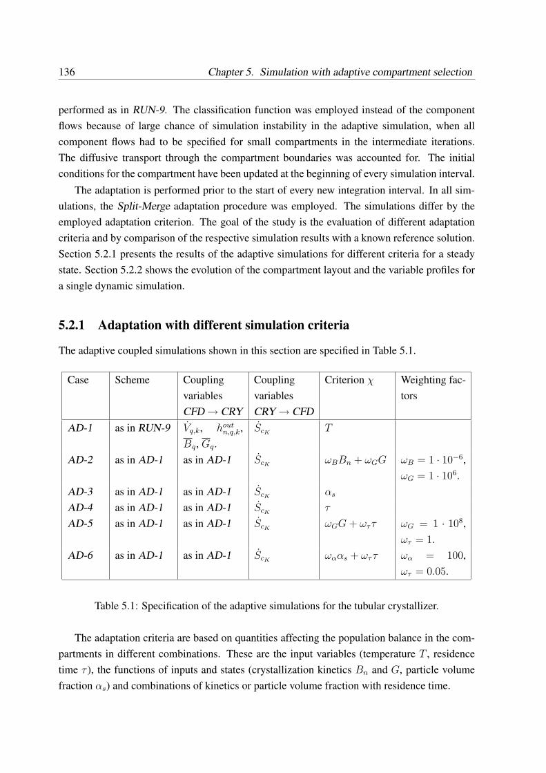
136 Chapter 5. Simulation with adaptive compartment selection
performed as in RUN-9. The classification function was employed instead of the componentflows because of large chance of simulation instability in the adaptive simulation, when allcomponent flows had to be specified for small compartments in the intermediate iterations.The diffusive transport through the compartment boundaries was accounted for. The initialconditions for the compartment have been updated at the beginning of every simulation interval.
The adaptation is performed prior to the start of every new integration interval. In all sim-ulations, the Split-Merge adaptation procedure was employed. The simulations differ by theemployed adaptation criterion. The goal of the study is the evaluation of different adaptationcriteria and by comparison of the respective simulation results with a known reference solution.Section 5.2.1 presents the results of the adaptive simulations for different criteria for a steadystate. Section 5.2.2 shows the evolution of the compartment layout and the variable profiles fora single dynamic simulation.
5.2.1 Adaptation with different simulation criteria
The adaptive coupled simulations shown in this section are specified in Table 5.1.
Case Scheme CouplingvariablesCFD → CRY
CouplingvariablesCRY → CFD
Criterion χ Weighting fac-tors
AD-1 as in RUN-9 Vq,k, houtn,q,k,
Bq, Gq.ScK
T
AD-2 as in AD-1 as in AD-1 ScKωBBn + ωGG ωB = 1 · 10−6,
ωG = 1 · 106.AD-3 as in AD-1 as in AD-1 ScK
αs
AD-4 as in AD-1 as in AD-1 ScKτ
AD-5 as in AD-1 as in AD-1 ScKωGG + ωττ ωG = 1 · 108,
ωτ = 1.AD-6 as in AD-1 as in AD-1 ScK
ωααs + ωττ ωα = 100,ωτ = 0.05.
Table 5.1: Specification of the adaptive simulations for the tubular crystallizer.
The adaptation criteria are based on quantities affecting the population balance in the com-partments in different combinations. These are the input variables (temperature T , residencetime τ ), the functions of inputs and states (crystallization kinetics Bn and G, particle volumefraction αs) and combinations of kinetics or particle volume fraction with residence time.
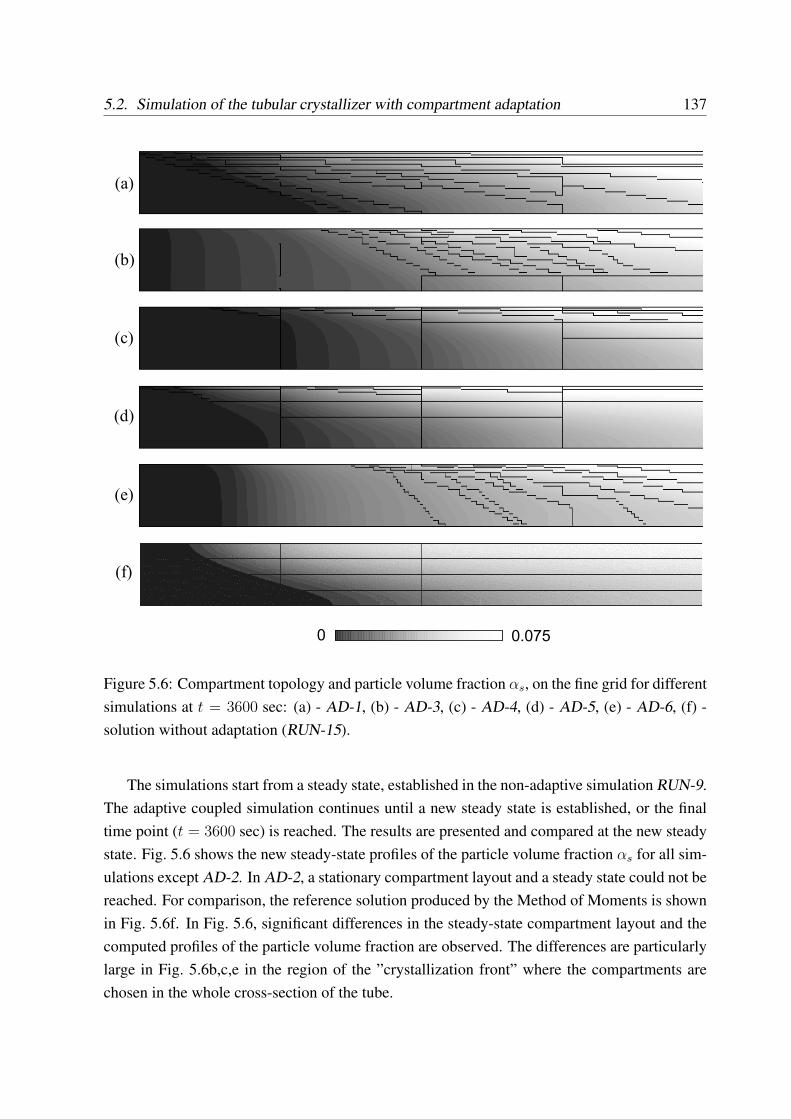
5.2. Simulation of the tubular crystallizer with compartment adaptation 137
(a)
(b)
(c)
(d)
(e)
(f)
0 0.075
Figure 5.6: Compartment topology and particle volume fraction αs, on the fine grid for differentsimulations at t = 3600 sec: (a) - AD-1, (b) - AD-3, (c) - AD-4, (d) - AD-5, (e) - AD-6, (f) -solution without adaptation (RUN-15).
The simulations start from a steady state, established in the non-adaptive simulation RUN-9.The adaptive coupled simulation continues until a new steady state is established, or the finaltime point (t = 3600 sec) is reached. The results are presented and compared at the new steadystate. Fig. 5.6 shows the new steady-state profiles of the particle volume fraction αs for all sim-ulations except AD-2. In AD-2, a stationary compartment layout and a steady state could not bereached. For comparison, the reference solution produced by the Method of Moments is shownin Fig. 5.6f. In Fig. 5.6, significant differences in the steady-state compartment layout and thecomputed profiles of the particle volume fraction are observed. The differences are particularlylarge in Fig. 5.6b,c,e in the region of the ”crystallization front” where the compartments arechosen in the whole cross-section of the tube.
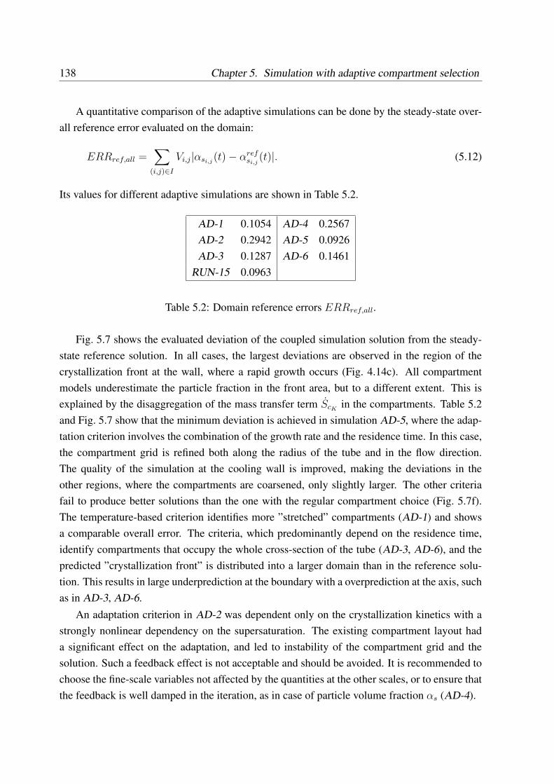
138 Chapter 5. Simulation with adaptive compartment selection
A quantitative comparison of the adaptive simulations can be done by the steady-state over-all reference error evaluated on the domain:
ERRref,all =∑
(i,j)∈I
Vi,j|αsi,j(t)− αref
si,j(t)|. (5.12)
Its values for different adaptive simulations are shown in Table 5.2.
AD-1 0.1054 AD-4 0.2567AD-2 0.2942 AD-5 0.0926AD-3 0.1287 AD-6 0.1461
RUN-15 0.0963
Table 5.2: Domain reference errors ERRref,all.
Fig. 5.7 shows the evaluated deviation of the coupled simulation solution from the steady-state reference solution. In all cases, the largest deviations are observed in the region of thecrystallization front at the wall, where a rapid growth occurs (Fig. 4.14c). All compartmentmodels underestimate the particle fraction in the front area, but to a different extent. This isexplained by the disaggregation of the mass transfer term ScK
in the compartments. Table 5.2and Fig. 5.7 show that the minimum deviation is achieved in simulation AD-5, where the adap-tation criterion involves the combination of the growth rate and the residence time. In this case,the compartment grid is refined both along the radius of the tube and in the flow direction.The quality of the simulation at the cooling wall is improved, making the deviations in theother regions, where the compartments are coarsened, only slightly larger. The other criteriafail to produce better solutions than the one with the regular compartment choice (Fig. 5.7f).The temperature-based criterion identifies more ”stretched” compartments (AD-1) and showsa comparable overall error. The criteria, which predominantly depend on the residence time,identify compartments that occupy the whole cross-section of the tube (AD-3, AD-6), and thepredicted ”crystallization front” is distributed into a larger domain than in the reference solu-tion. This results in large underprediction at the boundary with a overprediction at the axis, suchas in AD-3, AD-6.
An adaptation criterion in AD-2 was dependent only on the crystallization kinetics with astrongly nonlinear dependency on the supersaturation. The existing compartment layout hada significant effect on the adaptation, and led to instability of the compartment grid and thesolution. Such a feedback effect is not acceptable and should be avoided. It is recommended tochoose the fine-scale variables not affected by the quantities at the other scales, or to ensure thatthe feedback is well damped in the iteration, as in case of particle volume fraction αs (AD-4).
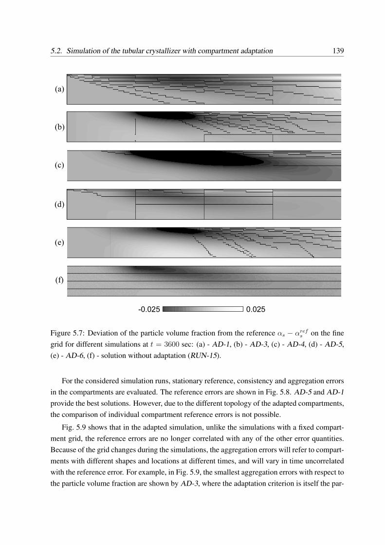
5.2. Simulation of the tubular crystallizer with compartment adaptation 139
(a)
(b)
(c)
(d)
(e)
(f)
-0.025 0.025
Figure 5.7: Deviation of the particle volume fraction from the reference αs − αrefs on the fine
grid for different simulations at t = 3600 sec: (a) - AD-1, (b) - AD-3, (c) - AD-4, (d) - AD-5,(e) - AD-6, (f) - solution without adaptation (RUN-15).
For the considered simulation runs, stationary reference, consistency and aggregation errorsin the compartments are evaluated. The reference errors are shown in Fig. 5.8. AD-5 and AD-1provide the best solutions. However, due to the different topology of the adapted compartments,the comparison of individual compartment reference errors is not possible.
Fig. 5.9 shows that in the adapted simulation, unlike the simulations with a fixed compart-ment grid, the reference errors are no longer correlated with any of the other error quantities.Because of the grid changes during the simulations, the aggregation errors will refer to compart-ments with different shapes and locations at different times, and will vary in time uncorrelatedwith the reference error. For example, in Fig. 5.9, the smallest aggregation errors with respect tothe particle volume fraction are shown by AD-3, where the adaptation criterion is itself the par-
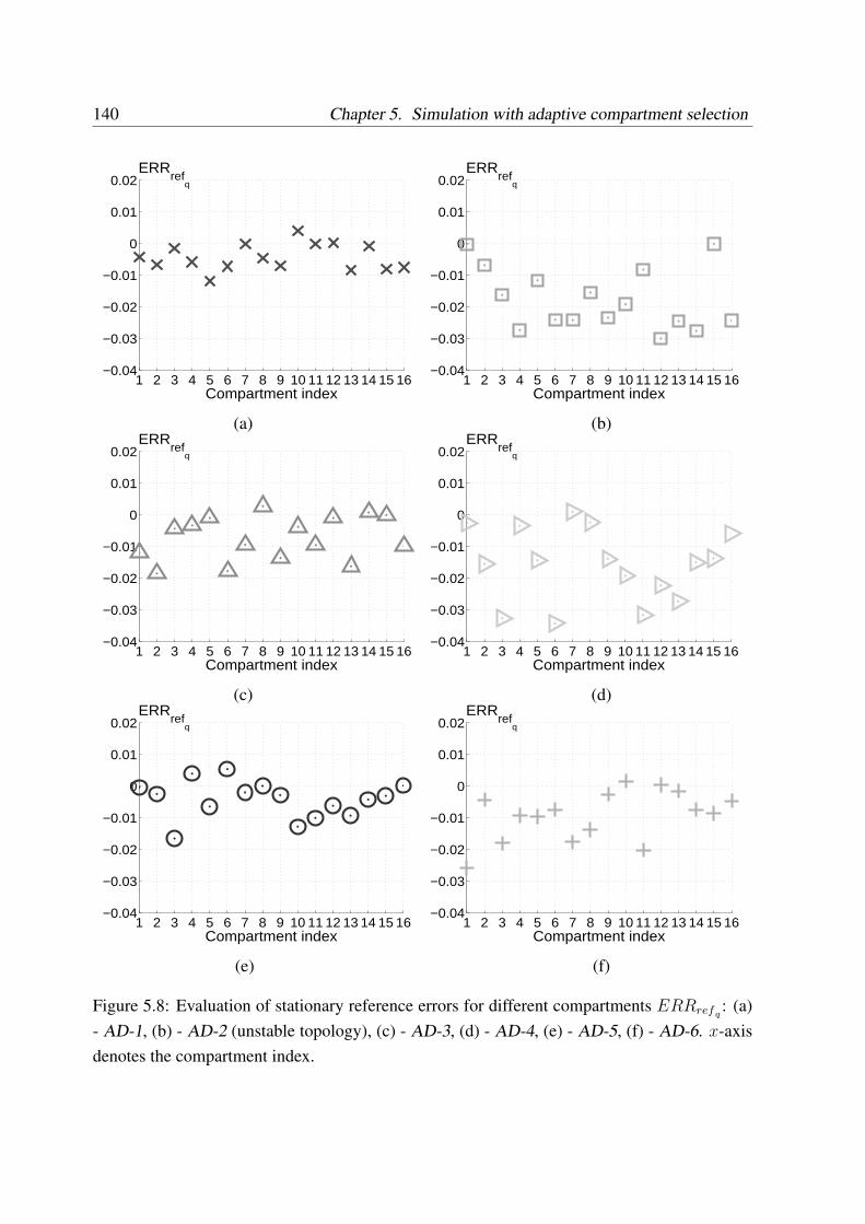
140 Chapter 5. Simulation with adaptive compartment selection
1 2 3 4 5 6 7 8 9 10 11 12 13 14 15 16−0.04
−0.03
−0.02
−0.01
0
0.01
0.02
Compartment index
ERRref
q
1 2 3 4 5 6 7 8 9 10 11 12 13 14 15 16−0.04
−0.03
−0.02
−0.01
0
0.01
0.02
Compartment index
ERRref
q
(a) (b)
1 2 3 4 5 6 7 8 9 10 11 12 13 14 15 16−0.04
−0.03
−0.02
−0.01
0
0.01
0.02
Compartment index
ERRref
q
1 2 3 4 5 6 7 8 9 10 11 12 13 14 15 16−0.04
−0.03
−0.02
−0.01
0
0.01
0.02
Compartment index
ERRref
q
(c) (d)
1 2 3 4 5 6 7 8 9 10 11 12 13 14 15 16−0.04
−0.03
−0.02
−0.01
0
0.01
0.02
Compartment index
ERRref
q
1 2 3 4 5 6 7 8 9 10 11 12 13 14 15 16−0.04
−0.03
−0.02
−0.01
0
0.01
0.02
Compartment index
ERRref
q
(e) (f)
Figure 5.8: Evaluation of stationary reference errors for different compartments ERRrefq: (a)
- AD-1, (b) - AD-2 (unstable topology), (c) - AD-3, (d) - AD-4, (e) - AD-5, (f) - AD-6. x-axisdenotes the compartment index.
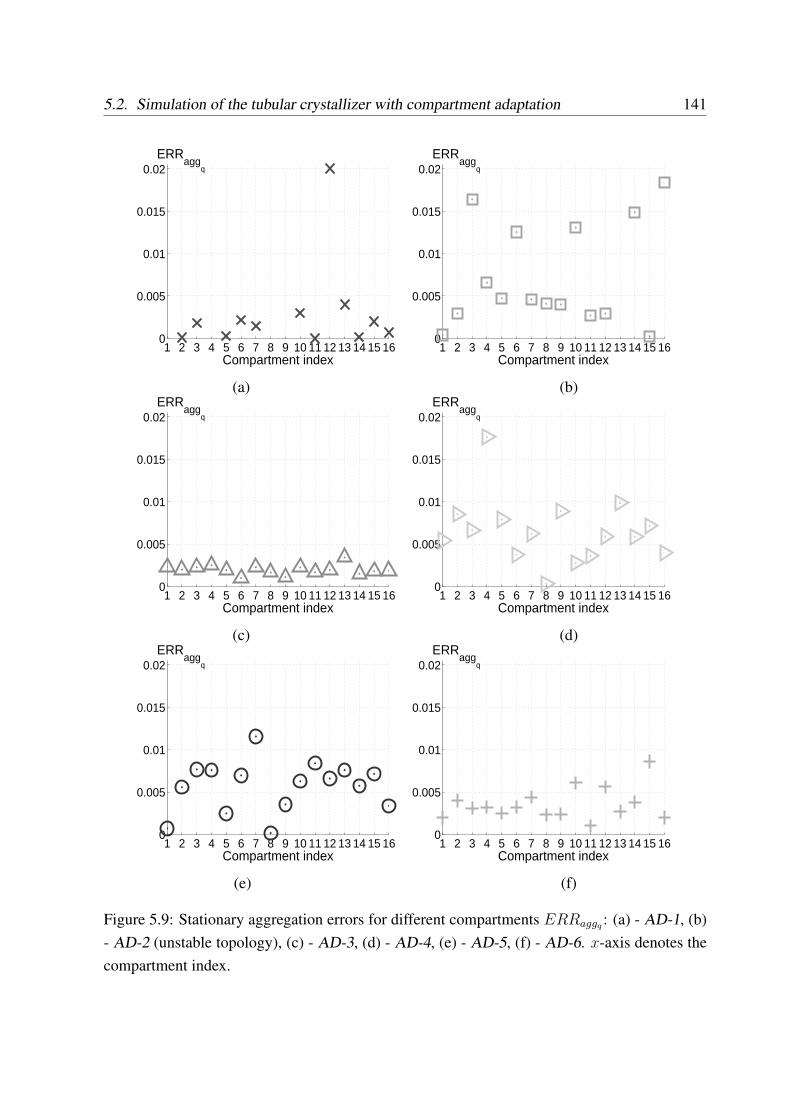
5.2. Simulation of the tubular crystallizer with compartment adaptation 141
1 2 3 4 5 6 7 8 9 10 11 12 13 14 15 160
0.005
0.01
0.015
0.02
Compartment index
ERRagg
q
1 2 3 4 5 6 7 8 9 10 11 12 13 14 15 160
0.005
0.01
0.015
0.02
Compartment index
ERRagg
q
(a) (b)
1 2 3 4 5 6 7 8 9 10 11 12 13 14 15 160
0.005
0.01
0.015
0.02
Compartment index
ERRagg
q
1 2 3 4 5 6 7 8 9 10 11 12 13 14 15 160
0.005
0.01
0.015
0.02
Compartment index
ERRagg
q
(c) (d)
1 2 3 4 5 6 7 8 9 10 11 12 13 14 15 160
0.005
0.01
0.015
0.02
Compartment index
ERRagg
q
1 2 3 4 5 6 7 8 9 10 11 12 13 14 15 160
0.005
0.01
0.015
0.02
Compartment index
ERRagg
q
(e) (f)
Figure 5.9: Stationary aggregation errors for different compartments ERRaggq : (a) - AD-1, (b)- AD-2 (unstable topology), (c) - AD-3, (d) - AD-4, (e) - AD-5, (f) - AD-6. x-axis denotes thecompartment index.
142 Chapter 5. Simulation with adaptive compartment selection
ticle volume fraction. However, this is not the closest match to the reference solution. Similarly,the consistency error also shows no correlation with the reference error in the compartments.It can only be used to analyze the consistency of the assumptions, model and data in the sub-models. For the adaptive simulations with complex compartment shapes, the consistency erroris generally larger than for the simulations with a regular topology.
As a conclusion, the adaptation of the compartment boundaries in the simulations makesit impossible to directly use the aggregation or consistency errors in the compartments as in-dicators of the quality of the final solution. A complex analysis on the fine grid using errorestimation techniques is necessary.
5.2.2 Evolution of topology in dynamic simulation
To show that the adaptation of the compartments also works in the dynamic simulations, andthat the compartment topology is actually changing during the integration to match the evolv-ing profiles of the relevant quantities in the adaptation criteria, the full dynamic simulation ofthe process startup (AD-7) is performed and presented in this section. Similarly to AD-5, theemployed criterion is the combination of the particle residence time τ (time elapsed from theinlet) and the particle growth rate G, i.e. χ = ωGG + ωττ , with ωG = 1 · 108, ωτ = 0.25.
The evolution of the compartment grid and the volume fraction in the tube is shown inFig. 5.10 for different times. Initially, a regular mesh of 16 compartments is employed as inSection 4.4. At the beginning of the simulation, the grid is largely adapted by the profile ofresidence time (Fig. 5.11a), which does not change during the runtime and has a strong gradientin the radial direction. At t =600 sec and further, the effect of the growth rate increases, andthe adaptation depends on both the residence time and the growth rate profiles (Fig. 5.11b). Thegrowth rate profile changes with the process time. With the values of the criterion variablesreaching a steady state, the topology is no longer adapted. Fig. 5.11a,b show the steady-stateprofiles of the criterion variables. The steady-state deviation from the reference solution isshown in Fig. 5.11c. Similar to AD-5, this deviation also shows a minimum behind the crystal-lization front.
The evolution of the overall reference error ERRref,all in Fig. 5.12 in the dynamics illus-trates an ambiguous effect of the adaptive simulation with the employed criterion and algorithm.In some regions of the domain the algorithm failed to adapt compartment boundaries and to finda more optimal compartment topology, since the factors in the adaptation criterion had a similarweight and counterweighed each other. The global optimum was not found by the procedurewith this criterion, and the final compartment grid still does not provide the closest match toa reference solution. More simulations with improved criteria and algorithm are necessary todraw conclusions about the capabilities of the adaptive dynamic simulation.
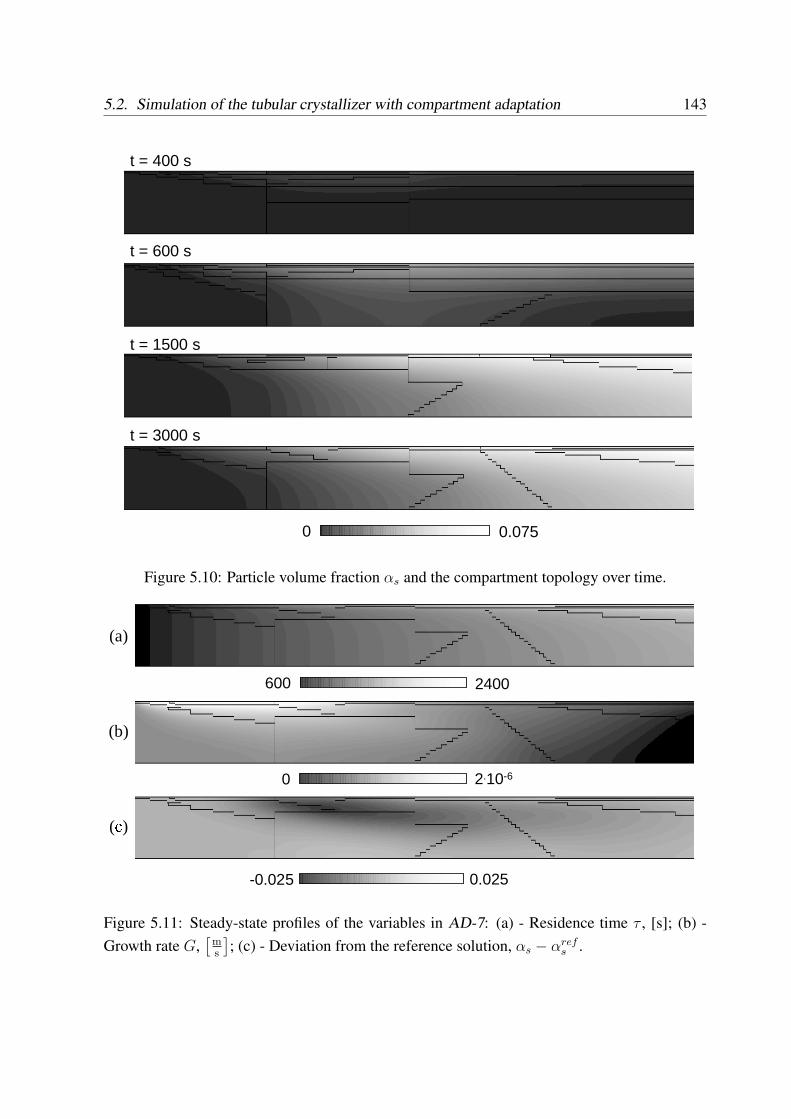
5.2. Simulation of the tubular crystallizer with compartment adaptation 143
t = 400 s
t = 600 s
t = 1500 s
t = 3000 s
0 0.075
Figure 5.10: Particle volume fraction αs and the compartment topology over time.
(a)
(b)
600 2400
0 2.10-6
-0.025 0.025
(с)
Figure 5.11: Steady-state profiles of the variables in AD-7: (a) - Residence time τ , [s]; (b) -Growth rate G,
[ms
]; (c) - Deviation from the reference solution, αs − αref
s .
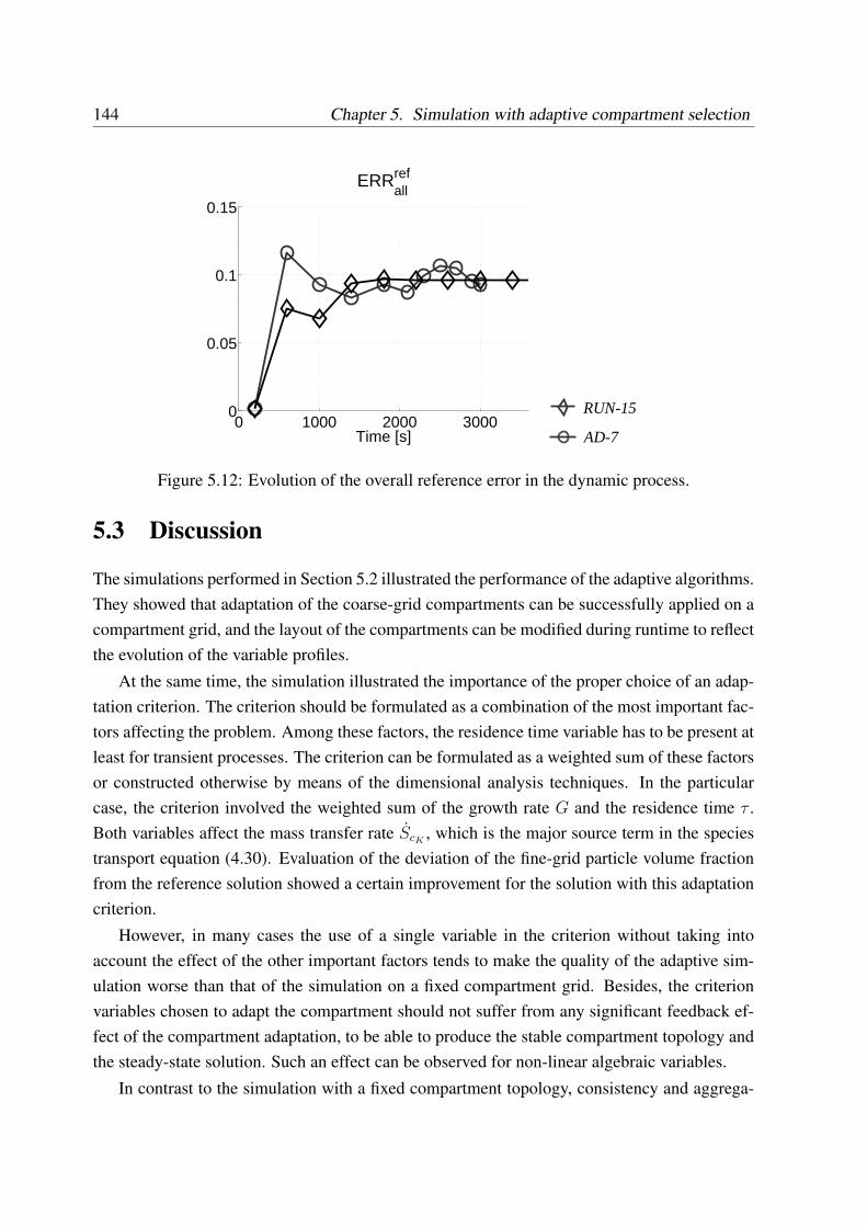
144 Chapter 5. Simulation with adaptive compartment selection
0 1000 2000 30000
0.05
0.1
0.15
Time [s]
ERRrefall
AD-7
RUN-15
Figure 5.12: Evolution of the overall reference error in the dynamic process.
5.3 Discussion
The simulations performed in Section 5.2 illustrated the performance of the adaptive algorithms.They showed that adaptation of the coarse-grid compartments can be successfully applied on acompartment grid, and the layout of the compartments can be modified during runtime to reflectthe evolution of the variable profiles.
At the same time, the simulation illustrated the importance of the proper choice of an adap-tation criterion. The criterion should be formulated as a combination of the most important fac-tors affecting the problem. Among these factors, the residence time variable has to be present atleast for transient processes. The criterion can be formulated as a weighted sum of these factorsor constructed otherwise by means of the dimensional analysis techniques. In the particularcase, the criterion involved the weighted sum of the growth rate G and the residence time τ .Both variables affect the mass transfer rate ScK
, which is the major source term in the speciestransport equation (4.30). Evaluation of the deviation of the fine-grid particle volume fractionfrom the reference solution showed a certain improvement for the solution with this adaptationcriterion.
However, in many cases the use of a single variable in the criterion without taking intoaccount the effect of the other important factors tends to make the quality of the adaptive sim-ulation worse than that of the simulation on a fixed compartment grid. Besides, the criterionvariables chosen to adapt the compartment should not suffer from any significant feedback ef-fect of the compartment adaptation, to be able to produce the stable compartment topology andthe steady-state solution. Such an effect can be observed for non-linear algebraic variables.
In contrast to the simulation with a fixed compartment topology, consistency and aggrega-
5.3. Discussion 145
tion errors did not correlate with the reference errors in the adaptive simulation. Aggregationerrors with respect to output variables and consistency errors were both strongly affected by thechoice of the compartments, varied with compartment adaptation and could not be used to drawany conclusions on the deviation of the solution from the true reference solution. The derivationof an error estimator (Section 4.3.6.2), as well as its modification to handle compartments ofarbitrary shapes, are absolutely necessary to evaluate the accuracy of the simulation and theperformance of the compartment adaptation algorithm.
The employed Split-Merge adaptation algorithm as well as the Delta algorithm search for thelocal minima of the criterion. The Split-Merge algorithm starts from the last reached compart-ment configuration and is better suited for the adaptation during runtime. The Delta algorithmstarts at some a priori chosen initial point and can be used for initial compartment selection.Both algorithms depend on the compartment topology at the previous state, and are likely notto find the globally optimal compartment topology.
The development of an adaptation method based on the global optimization and formaliza-tion of the criterion selection rules can improve the quality of the adaptive coupled simulation.After assessment of the above problems, the use of the compartment adaptation algorithms inthe modular coupled simulation can reduce deviations from the reference solution compared tothe simulations without compartment adaptation. However, they still could not be fully elimi-nated.
Chapter 6
Case study
In this section, the software-technical and algorithmic framework of the coupled simulationwith generalized flowsheet and adaptation, developed in the previous sections, is applied to acrystallization process carried out in an industrial-type equipment. The crystallizer is describedby first principles models, which cover the fluid dynamics in the apparatus, the population bal-ance and the crystallization kinetics. The goal of the section is the application of the introducedcoupled simulation techniques to a crystallization process of realistic complexity.
Due to methodological orientation of the thesis, the major criterion for the choice of thecase study was the availability of sufficient information on the crystallization kinetics. For thisreason, the ammonium sulphate - water system was chosen. The experimental investigationand modeling of this system was reported in a number of publications by a group at DelftUniversity of Technology (e.g. Eek et al. (1995), Eek (1996), Kramer et al. (2000), Neumann(2001), Bermingham (2003) and earlier references therein).
In this thesis, the coupled simulation framework was employed to simulate the crystalliza-tion of the ammonium sulphate from aqueous solution in a forced circulation (FC) crystallizer.
6.1 Forced Circulation crystallizer
The forced circulation (FC) crystallizer is a common type of industrial crystallizer. The crystal-lizer is shown in Fig. 6.1. It consists of a crystallizer vessel and an external recirculation conduitwith a pump, a heat exchanger, a feed inlet and a product outlet. In the crystallizer vessel, apart of the liquid is evaporated under vacuum. This generates the supersaturation and inducescrystallization. The suspension is pumped through the recirculation conduit, where part of it isremoved as the product, and fresh liquor is added; it is heated in the heat exchanger to replacethe loss of energy during evaporation. The axial pump provides the energy to push the suspen-sion through the recirculation conduit. The friction in the pump results in intensive attrition and
146
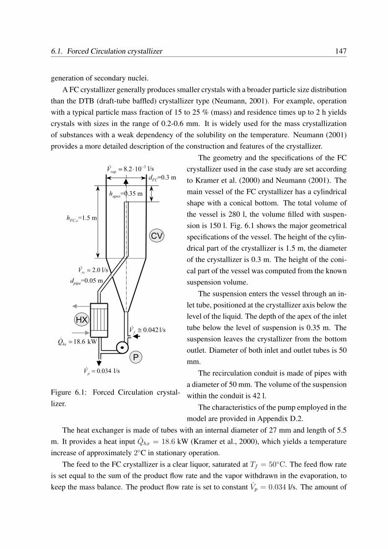
6.1. Forced Circulation crystallizer 147
generation of secondary nuclei.A FC crystallizer generally produces smaller crystals with a broader particle size distribution
than the DTB (draft-tube baffled) crystallizer type (Neumann, 2001). For example, operationwith a typical particle mass fraction of 15 to 25 % (mass) and residence times up to 2 h yieldscrystals with sizes in the range of 0.2-0.6 mm. It is widely used for the mass crystallizationof substances with a weak dependency of the solubility on the temperature. Neumann (2001)provides a more detailed description of the construction and features of the crystallizer.
dFC=0.3 m
hapex=0.35 m
hFC,c=1.5 m
dpipe=0.05 m
6.18=hxQ&
034.0=pV&
kW
P
CV
HX
l/s
042.0≅fV& l/s
3102.8
−⋅=vapV& l/s
0.2=rcV& l/s
Figure 6.1: Forced Circulation crystal-lizer.
The geometry and the specifications of the FCcrystallizer used in the case study are set accordingto Kramer et al. (2000) and Neumann (2001). Themain vessel of the FC crystallizer has a cylindricalshape with a conical bottom. The total volume ofthe vessel is 280 l, the volume filled with suspen-sion is 150 l. Fig. 6.1 shows the major geometricalspecifications of the vessel. The height of the cylin-drical part of the crystallizer is 1.5 m, the diameterof the crystallizer is 0.3 m. The height of the coni-cal part of the vessel was computed from the knownsuspension volume.
The suspension enters the vessel through an in-let tube, positioned at the crystallizer axis below thelevel of the liquid. The depth of the apex of the inlettube below the level of suspension is 0.35 m. Thesuspension leaves the crystallizer from the bottomoutlet. Diameter of both inlet and outlet tubes is 50mm.
The recirculation conduit is made of pipes witha diameter of 50 mm. The volume of the suspensionwithin the conduit is 42 l.
The characteristics of the pump employed in themodel are provided in Appendix D.2.
The heat exchanger is made of tubes with an internal diameter of 27 mm and length of 5.5m. It provides a heat input Qhx = 18.6 kW (Kramer et al., 2000), which yields a temperatureincrease of approximately 2◦C in stationary operation.
The feed to the FC crystallizer is a clear liquor, saturated at Tf = 50◦C. The feed flow rateis set equal to the sum of the product flow rate and the vapor withdrawn in the evaporation, tokeep the mass balance. The product flow rate is set to constant Vp = 0.034 l/s. The amount of
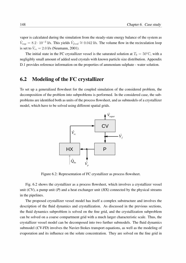
148 Chapter 6. Case study
vapor is calculated during the simulation from the steady-state energy balance of the system asVvap = 8.2 · 10−3 l/s. This yields Vfeed
∼= 0.042 l/s. The volume flow in the recirculation loopis set to Vrc = 2.0 l/s (Neumann, 2001).
The initial state in the FC crystallizer vessel is the saturated solution at T0 = 50◦C, with anegligibly small amount of added seed crystals with known particle size distribution. AppendixD.1 provides reference information on the properties of ammonium sulphate - water solution.
6.2 Modeling of the FC crystallizer
To set up a generalized flowsheet for the coupled simulation of the considered problem, thedecomposition of the problem into subproblems is performed. In the considered case, the sub-problems are identified both as units of the process flowsheet, and as submodels of a crystallizermodel, which have to be solved using different spatial grids.
CV
PHX
fV&pV&hxQ& rcV& vaporV&
Figure 6.2: Representation of FC crystallizer as process flowsheet.
Fig. 6.2 shows the crystallizer as a process flowsheet, which involves a crystallizer vesselunit (CV), a pump unit (P) and a heat exchanger unit (HX) connected by the physical streamsin the pipelines.
The proposed crystallizer vessel model has itself a complex substructure and involves thedescription of the fluid dynamics and crystallization. As discussed in the previous sections,the fluid dynamics subproblem is solved on the fine grid, and the crystallization subproblemcan be solved on a coarse compartment grid with a much larger characteristic scale. Thus, thecrystallizer vessel model can be decomposed into two further submodels. The fluid dynamicssubmodel (CV-FD) involves the Navier-Stokes transport equations, as well as the modeling ofevaporation and its influence on the solute concentration. They are solved on the fine grid in
6.2. Modeling of the FC crystallizer 149
the geometry of the crystallizer vessel together with the other balances. The crystallizationsubmodel (CV-CRY) involves the solution of the population balance with the respective crys-tallization kinetics. Both submodels can also be defined as subproblems and solved by meansof dynamic simulation.
Three cases with increasing complexity were considered and simulated: a) an ideally mixedcrystallizer vessel, where no FD model had to be solved; b) a decomposition of the vessel modelinto a FD and a crystallization subproblems, with different fixed grids; and c) a decompositionof the vessel model into a FD and a crystallization subproblems, with compartment adaptationduring runtime.
Based on the model equations, the assignment of the constitutive equations to the subprob-lems and the final formulation of the subproblems solved in the study are presented in thefollowing sections.
6.2.1 Structure and model assumptions
The models for the units of the process flowsheet of the FC crystallizer are presented in thissection. The assumptions used in the development of the process models can be summarized asfollows:
• The crystallization is described by a population balance model.
• The FD model is solved only for the crystallizer vessel. The models of the other units donot involve the solution of FD models.
• The FD model assumes an incompressible liquid, a single quasi-homogeneous phase. Thesuspension is modeled as a mixture of three components, solvent, solute and particles.k − ε model is employed to model turbulence.
• The crystallization phenomena considered are size-dependent crystal growth, attrition andsecondary nucleation.
• The majority of attrition and secondary nucleation occurs in the circulation pump, thegrowth of the attrition fragments is specifically accounted for in the growth model. Attri-tion occurs neither in the other units nor in the pipeline.
• The attrition process in the pump is quasi-stationary.
• Growth occurs only in the crystallizer vessel, but does not take place in either the pipelinesor the pump.
150 Chapter 6. Case study
• Gravity induces particle classification and enhanced settling of large particles in the ves-sel. It is not accounted for in the other units.
• Primary nucleation, particle breakage and agglomeration are neglected.
• The heat of crystallization is negligible.
Some of these assumptions are taken from the works of Kramer and Bermingham (Krameret al., 2000), while others (such as the modeling of the suspension as a component mixture)were introduced in this study to simplify the implementation of the model.
6.2.2 Model of the crystallizer vessel
As follows from the set of assumptions, the crystallizer vessel is described by a FD model forthe three-component mixture coupled to a particle population balance and evaporation, sedi-mentation (particle classification) and particle growth models.
6.2.2.1 Fluid dynamics model
The FD model is solved on the fine FD grid as a set of Navier-Stokes equations for mass (2.11),momentum (2.12) and energy (2.13) as well as for the transport of the components of the suspen-sion (2.15) (species transport). The source terms in these equations Sm, Sh and ScK
correspondto the change of mass, energy and component concentration in the process. They need to bespecified by constitutive relations.
The sources of mass Sm and energy Sh are zero everywhere except in the vicinity of thephase boundary where they are introduced to reflect the evaporation process. The mass sourcedue to evaporation is the mass flow of evaporated water Sm,evap. The energy source due toevaporation is computed from the total energy balance of the system:
ρf Vf∆Hf − ρpVp∆Hp − Sh,evap + Qhx = 0. (6.1)
∆Hf and ∆Hp refer to the specific enthalpies in the feed and product streams computed fromthe component enthalpies and the mixture composition. Qhx is the specified energy input inthe heat exchanger. From the energy source due to evaporation Sh,evap and the known enthalpyof water vaporization ∆Hevap, the mass flow of evaporated water Sm,evap and the vapor streamVvap can be evaluated by Sh,evap = Sm,evap∆Hevap, Sm,evap = ρvapVvap.
The concentration source term ScKis evaluated in the crystallization model.
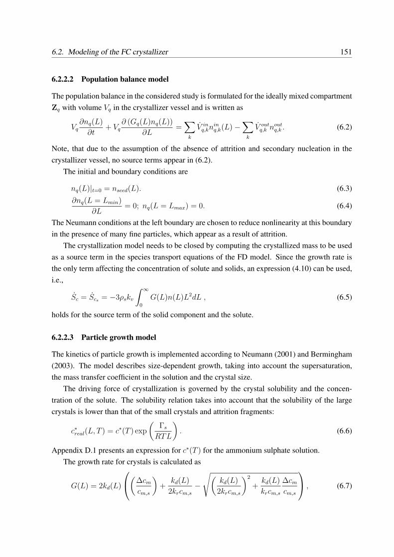
6.2. Modeling of the FC crystallizer 151
6.2.2.2 Population balance model
The population balance in the considered study is formulated for the ideally mixed compartmentZq with volume Vq in the crystallizer vessel and is written as
Vq∂nq(L)
∂t+ Vq
∂ (Gq(L)nq(L))
∂L=
∑
k
V inq,kn
inq,k(L)−
∑
k
V outq,k nout
q,k . (6.2)
Note, that due to the assumption of the absence of attrition and secondary nucleation in thecrystallizer vessel, no source terms appear in (6.2).
The initial and boundary conditions are
nq(L)|t=0 = nseed(L). (6.3)
∂nq(L = Lmin)
∂L= 0; nq(L = Lmax) = 0. (6.4)
The Neumann conditions at the left boundary are chosen to reduce nonlinearity at this boundaryin the presence of many fine particles, which appear as a result of attrition.
The crystallization model needs to be closed by computing the crystallized mass to be usedas a source term in the species transport equations of the FD model. Since the growth rate isthe only term affecting the concentration of solute and solids, an expression (4.10) can be used,i.e.,
Sc = Scs = −3ρskv
∫ ∞
0
G(L)n(L)L2dL , (6.5)
holds for the source term of the solid component and the solute.
6.2.2.3 Particle growth model
The kinetics of particle growth is implemented according to Neumann (2001) and Bermingham(2003). The model describes size-dependent growth, taking into account the supersaturation,the mass transfer coefficient in the solution and the crystal size.
The driving force of crystallization is governed by the crystal solubility and the concen-tration of the solute. The solubility relation takes into account that the solubility of the largecrystals is lower than that of the small crystals and attrition fragments:
c∗real(L, T ) = c∗(T ) exp
(Γs
RTL
). (6.6)
Appendix D.1 presents an expression for c∗(T ) for the ammonium sulphate solution.The growth rate for crystals is calculated as
G(L) = 2kd(L)
(∆cm
cm,s
)+
kd(L)
2krcm,s
−√(
kd(L)
2krcm,s
)2
+kd(L)
krcm,s
∆cm
cm,s
, (6.7)
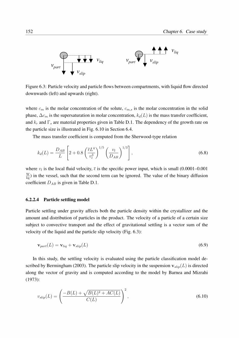
152 Chapter 6. Case study
vliqvpart
vslip
vliq
vpart vslip
regularliqV ,&
slippartV,
&
regularpartV,
& regularliqV ,&
slippartV,
&
regularpartV,
&Figure 6.3: Particle velocity and particle flows between compartments, with liquid flow directeddownwards (left) and upwards (right).
where cm is the molar concentration of the solute, cm,s is the molar concentration in the solidphase, ∆cm is the supersaturation in molar concentration, kd(L) is the mass transfer coefficient,and kr and Γs are material properties given in Table D.1. The dependency of the growth rate onthe particle size is illustrated in Fig. 6.10 in Section 6.4.
The mass transfer coefficient is computed from the Sherwood-type relation
kd(L) =DAB
L
[2 + 0.8
(εL4
v3l
)1/5 (vl
DAB
)1/3]
, (6.8)
where vl is the local fluid velocity, ε is the specific power input, which is small (0.0001–0.001Wkg
) in the vessel, such that the second term can be ignored. The value of the binary diffusioncoefficient DAB is given in Table D.1.
6.2.2.4 Particle settling model
Particle settling under gravity affects both the particle density within the crystallizer and theamount and distribution of particles in the product. The velocity of a particle of a certain sizesubject to convective transport and the effect of gravitational settling is a vector sum of thevelocity of the liquid and the particle slip velocity (Fig. 6.3):
vpart(L) = vliq + vslip(L) (6.9)
In this study, the settling velocity is evaluated using the particle classification model de-scribed by Bermingham (2003). The particle slip velocity in the suspension vslip(L) is directedalong the vector of gravity and is computed according to the model by Barnea and Mizrahi(1973):
vslip(L) =
(−B(L) +
√B(L)2 + AC(L)
C(L)
)2
, (6.10)
6.2. Modeling of the FC crystallizer 153
where
A =√
α1,
B(L) = 0.5√
α2α4,
C(L) =√
α2α3,
α1 = gρs − ρl
ρs + ρl
,
α2(L) =3
4
1 + (1− ε)1/3
(ρs + ρl)L2ε,
α3(L) = 0.63√
Lρl,
α4 = 4.8√
ηl exp
(5
6
1− ε
ε
).
A rigorous consideration of particle settling under gravity would require an evaluation ofthe slip velocity in every cell of the fine grid for particles of all sizes. However, the particle sizedistributions are not available in the FD model, and the settling of particles has to be describedon the coarse compartment grid. Bermingham (2003) uses a classification function for thecompartment outlets to account for the particle settling in the compartments,
hout(L) =nout(L)
n(L)=
vliq + vslip(L)
vsus,out
, (6.11)
where vsus,out is a superficial velocity defined as
vsus,out = vliq +
∫ ∞
0
vslip(L)nout(L)L3dL. (6.12)
This model can be written in an alternative formulation using component-wise specificationof the streams at the compartment outlets:
Vq,k = Vliqq,k+ Vpartq,k
, (6.13)
Vliqq,k= Aq,kvliqq,k
(1− αoutsq,k
), (6.14)
Vpartq,k= Aq,kvliqq,k
αoutsq,k
+ Vslipq,k, (6.15)
Vslipq,k= Aq,kvslipq,k
αoutsq,k
. (6.16)
Here, Vq,k is the overall volumetric stream, Vliqq,kand Vpartq,k
are the liquid and particle volu-metric streams through the k-th boundary of the q-th compartment with area Aq,k, vslipq,k
is theslip velocity vector, vliqq,k
is the liquid stream velocity vector, and αoutsq,k
is the volume fractionof solids at the k-th boundary of the q-th compartment.
154 Chapter 6. Case study
6.2.3 Model of the pump
Attrition and secondary nucleation are considered to occur in the pump. They are described bymeans of the attrition model by Gahn (Gahn and Mersmann, 1999a, 1999b), where the model ofmechanical collisions was based on the work of Ploß et al. (1989). The model was successfullyapplied for the modeling of the ammonium sulphate-water system by Bermingham (2003).
The model assumes that the prevailing attrition occurs due to the collisions of particles withthe impeller blades. To compute the attrition rate and the amount of fragments generated duringcollision, the collision rate φcol,e/f (L, r) and energy Ep,e/b(L, r) are evaluated as functions ofthe particle size L and the distance from the impeller rotation axis r. They are used to computethe number of attrited fragments from a collision Nfrag(L, r), their volume Vatt(L, r) and theirsize distribution nfrag(L, r, Lf ). Integration over r and evaluation of birth (n+,1
att (L), n+,2att (L))
and death (n−att(L)) terms yields the particle size distribution at the outlet of the pump nP,out.
Collision efficiencyCollisions of particles with impeller blades are characterized by two major factors: collision
rate and collision efficiency. They are functions of the particle size L and the distance from theimpeller axis r.
Collision efficiency ηcol,e/f (L, r) is computed as a product of geometric efficiency ηgeom,e/f (r)
and target efficiency ηtarget,e/f (L, r) of collisions:
ηcol,e/f (L, r) = ηgeom,e/f (r)ηtarget,e/f (L, r). (6.17)
The geometric efficiency is the ratio of the effective area of collision to the pump shaftcross-section area:
ηgeom,e/b(r) =4Te/b(r)Nb
πd2dtsin(α(r))
. (6.18)
The effective area of collision for edge and face targets:
Te(r) = lecos(β − α(r)), (6.19)
Tb(r) = lb|sin(β − α(r))|. (6.20)
The angle of particle approach:
α(r) = arctan
(vax
vrad(r)
). (6.21)
The fluid velocity along the impeller axis:
vax =4Nvnpd
3p
πd2dt
=4V
πd2dt
, (6.22)
6.2. Modeling of the FC crystallizer 155
where ddt is the diameter of the draft tube or pump shaft, taken from the pump properties (TableD.2).
The impeller radial velocity:
vrad(r) = 2πnpr. (6.23)
The target efficiency is computed from the assumption of a flowing particle approaching acylinder-shaped body as proposed by Ploß et al. (1989):
ηtarget,e/b(L, r) =
(Ψe/b(L, r)
0.32 + Ψe/b(L, r)
)2.1
(6.24)
with the modified Stokes number
Ψe/b(L, r) =(ρs − ρl)vrelL
2
18ηlTe/b
, (6.25)
and the relative velocity
vrel =√
v2ax + v2
rad. (6.26)
Collision rate, velocity and energyThe collision rate of crystals φcol,e/f (L, r) of size L with the face and edges of the impeller
at the distance from the impeller axis r is given by
φcol,e/f (L, r) = n(L)ηcol,e/f (L, r)V . (6.27)
The collision impact velocity is calculated as
vcoll,e/b(L, r) = ηtarget,e/b(L, r)vrel,⊥,e/b(L, r), (6.28)
with the velocity components
vrel,⊥,e(L, r) = vrel,e(L, r)cos(β − α), (6.29)
vrel,⊥,b(L, r) = vrel,b(L, r)|sin(β − α)|. (6.30)
The collision impact energy is
Ep,e/b(L, r) =1
2ρskvL
3v2coll,e/b(L, r). (6.31)
and the minimum impact energy for effective collision leading to attrition, Ep,min is given by
Ep,min = 64µ3
s
H3s
(Γ
Kr
)6
=64
1000Wc, (6.32)
156 Chapter 6. Case study
where Wc, µs, Hs, ΓKr
are material properties provided in Table D.1.The number of effective collisions of size L with the face and edges of the impeller at the
distance from the impeller axis r per unit volume is
Ncol,e/f (L, r) = n(L)ηcol,e/f (L, r)h(Ep − Ep,min), (6.33)
where the term h(Ep − Ep,min) is a Heaviside function introduced to account for effectivecollisions only.
Number, volume and distribution of the attrited fragmentsThe volume of attrited fragments is calculated as
Vatt(L, r) = CE4/3p (L, r), (6.34)
if the impact energy exceeds its minimum value Ep,min. The attrition constant C is provided inTable D.1.
The minimum and maximum size of attrited fragments is computed from
Lfrag,min =32
30
(WC
Hs
)1/3
; Lfrag,max =1
2
(H
2/3s
µs
Kr
Γ
)1/3
E4/9p (L, r). (6.35)
The number of attrited fragments from a single collision, Nfrag(L, r) is
Nfrag(L, r) =π
21
H1/2s
Kvµ3/4s
(Kr
Γ
)3/4 (L−2.25
frag,min − L−2.25frag,max
)Ep(L, r). (6.36)
and the distribution of the attrited fragments nfrag(L, r, Lf ) is given by
nfrag(L, r, Lf ) =
{2.25L−3.25
frag
L−2.25frag,min−L−2.25
frag,max(L,r), Lfrag,min < Lfrag(L, r) < Lfrag,max(L, r),
= 0, Lfrag(L, r) ≤ Lfrag,min, Lfrag(L, r) ≥ Lfrag,max(L, r).(6.37)
Particle size distribution after pumpThere are three effects of collisions on the PSD: removal of collided particles, addition of
smaller collided particles and addition of small attrited fragments. These three effects are eva-luated from the number of effective collisions with the impeller integrated over r, assuming thatthe process is quasi-stationary.
The removal of collided particles per unit volume is given by
n−att(L) =
∫ d/2
r=0
Ncol,e(L, r)dr|e +
∫ d/2
r=0
Ncol,f (L, r)dr|f . (6.38)
6.2. Modeling of the FC crystallizer 157
The addition of smaller collided particles with size L∗ per unit volume is
n+,1att (L) =
∫ d/2
r=0
∫ ∞
L′=L
δ(L− L∗(L′, r))Ncol,e(L′, r)dL′dr|e
+
∫ d/2
r=0
∫ ∞
L′=L
δ(L− L∗(L′, r))Ncol,f (L′, r)dL′dr|f . (6.39)
The addition of small attrited fragments per unit volume is computed from
n+,2att (L) =
∫ d/2
r=0
∫ ∞
L′=L
[h(L− Lfrag,min)− h(L− Lfrag,max)]
Ncol,e(L′, r)Nfrag(L
′, r)nfrag(L′, r, L)dL′dr|e
+
∫ d/2
r=0
∫ ∞
L′=L
[h(L− Lfrag,min)− h(L− Lfrag,max)]
Ncol,f (L′, r)Nfrag(L
′, r)nfrag(L′, r, L)dL′dr|f . (6.40)
Here, L′ is the size of the attrition fragment, while L∗ is the size of a smaller crystal afterattrition:
L∗ = 3
√((1
6πL3
)− Vatt(L)
)6
π. (6.41)
From these quantities, the overall secondary nucleation term,
B+ =
∫ ∞
L=0
(n+,1
att (L) + n+,2att (L)
)dL, (6.42)
and the particle size distribution after the pump nP,out,
nP,out(L) = nP,in(L)− τp
[n−att(L) + n+,1
att (L) + n+,2att (L)
], (6.43)
can be computed. We refer to Appendix D.2 for the characteristics of the employed pump, andto Table D.1 for the material properties of the substances.
6.2.4 Model of the heat exchanger
The temperature change in the heat exchanger ∆T is calculated from the known energy flow inthe heat exchanger Qhx using the standard expression
∆T =Qhx
cpsuspρVrc
, (6.44)
where Vrc is the current flow rate in the recycle, and cpsusp is the specific heat capacity of thesuspension with known composition. The temperature is increased by about 2◦C. This changeaffects the solubility and the supersaturation. However, since it is assumed that no crystalliza-tion or dissolution occurs in the heat exchanger and pipelines, the effect of the temperatureincrease on the crystallization is observed only in the crystallizer vessel.
158 Chapter 6. Case study
6.2.5 Reference experimental data
The reference data for the considered ammonuim sulphate-water system undergoing crystalliza-tion are available from a series of experiments carried out by the Delft University of Technology.The experiments were performed for different crystallizers, such as a 970-l Draft Tube Baffled(DTB) crystallizer, a 150-l Forced Circulation (FC) crystallizer and a 22-l Draft Tube (DT)crystallizer. Relevant experimental data have been given by Kramer et al. (2000), Neumann(2001) and Bermingham (2003). These data can be used for an approximate validation of themodel of the coupled simulation. They include:
• the reference particle volume fraction from the steady-state mass balance around the crys-tallizer αref
s = 0.121;
• the range of mean (median) particle size Lref50 ≈ 500− 550µm (Neumann, 2001), L
ref
4/3 =
568µm1 (Kramer et al., 2000);
• the stationary birth rate in the pump due to secondary nucleation Brefn ≈ 2.6 · 107 1
m3·s(Kramer et al., 2000);
• the stationary particle growth rate, averaged in the vessel Gref ≈ 3.2 · 10−8 ms
(Kramer etal., 2000).
The steady-state values are reached after 6–8 hours of the process time (Neumann, 2001).
6.3 Coupled simulation of the FC crystallizer with a MSMPRassumption
Setup of the simulationThe simplest option, widely used in industrial practice, introduces an ideal mixing assump-
tion for the full volume of the crystallizer vessel, and mixed product removal at the outlet(MSMPR assumption). No fluid dynamics and gravitational settling models are used.
The flowsheet in this simulation consists of the crystallizer vessel (CRY) and the periph-erial equipment (MAT) unit (Fig. 6.4). It is equivalent to the process flowsheet in Fig. 6.2,where the pump and the heat exchanger are merged to a single MAT unit. The CRY unit in-volves the full population balance model with growth kinetics (6.2)-(6.8). As inputs, the unitobtains the specification of the recirculation stream entering the vessel (flow rate Vrc, com-ponent concentrations crc, temperature Trc, particle size distribution nrc). The MAT unit in-
1In Kramer et al. (2000), the mean particle size is defined as L4/3 = µ(4)
µ(3) .
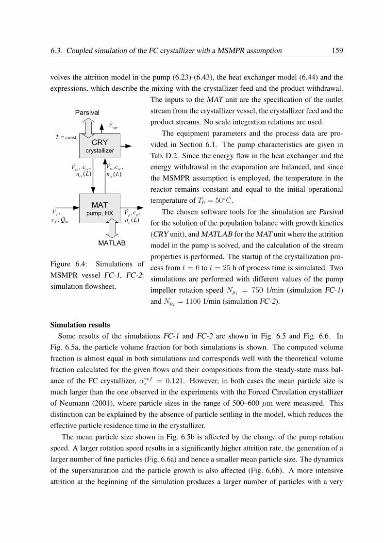
6.3. Coupled simulation of the FC crystallizer with a MSMPR assumption 159
volves the attrition model in the pump (6.23)-(6.43), the heat exchanger model (6.44) and theexpressions, which describe the mixing with the crystallizer feed and the product withdrawal.
CRYcrystallizer
MATpump, HX
MATLAB
,fV&
,fc
=T
hxQ&
,pV& ,pc
)(Lnp
)(Lncv )(Lnrc
,rcV& ,rcc,cvV
& ,cvc
const
Parsival
vapV&
Figure 6.4: Simulations ofMSMPR vessel FC-1, FC-2:simulation flowsheet.
The inputs to the MAT unit are the specification of the outletstream from the crystallizer vessel, the crystallizer feed and theproduct streams. No scale integration relations are used.
The equipment parameters and the process data are pro-vided in Section 6.1. The pump characteristics are given inTab. D.2. Since the energy flow in the heat exchanger and theenergy withdrawal in the evaporation are balanced, and sincethe MSMPR assumption is employed, the temperature in thereactor remains constant and equal to the initial operationaltemperature of T0 = 50◦C.
The chosen software tools for the simulation are Parsivalfor the solution of the population balance with growth kinetics(CRY unit), and MATLAB for the MAT unit where the attritionmodel in the pump is solved, and the calculation of the streamproperties is performed. The startup of the crystallization pro-cess from t = 0 to t = 25 h of process time is simulated. Twosimulations are performed with different values of the pumpimpeller rotation speed Np1 = 750 1/min (simulation FC-1)and Np2 = 1100 1/min (simulation FC-2).
Simulation resultsSome results of the simulations FC-1 and FC-2 are shown in Fig. 6.5 and Fig. 6.6. In
Fig. 6.5a, the particle volume fraction for both simulations is shown. The computed volumefraction is almost equal in both simulations and corresponds well with the theoretical volumefraction calculated for the given flows and their compositions from the steady-state mass bal-ance of the FC crystallizer, αref
s = 0.121. However, in both cases the mean particle size ismuch larger than the one observed in the experiments with the Forced Circulation crystallizerof Neumann (2001), where particle sizes in the range of 500–600 µm were measured. Thisdistinction can be explained by the absence of particle settling in the model, which reduces theeffective particle residence time in the crystallizer.
The mean particle size shown in Fig. 6.5b is affected by the change of the pump rotationspeed. A larger rotation speed results in a significantly higher attrition rate, the generation of alarger number of fine particles (Fig. 6.6a) and hence a smaller mean particle size. The dynamicsof the supersaturation and the particle growth is also affected (Fig. 6.6b). A more intensiveattrition at the beginning of the simulation produces a larger number of particles with a very
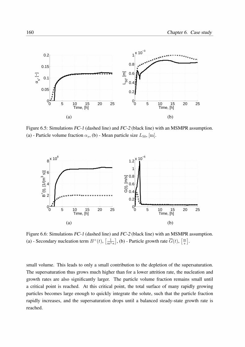
160 Chapter 6. Case study
0 5 10 15 20 250
0.05
0.1
0.15
0.2
Time, [h]
α s, [−
]
0 5 10 15 20 250
0.2
0.4
0.6
0.8
1x 10
−3
Time, [h]
L 50, [
m]
(a) (b)
Figure 6.5: Simulations FC-1 (dashed line) and FC-2 (black line) with an MSMPR assumption.(a) - Particle volume fraction αs, (b) - Mean particle size L50, [m].
0 5 10 15 20 250
2
4
6
8x 10
8
Time, [h]
B+(t
), [1
/(m
3 s)]
0 5 10 15 20 250
0.2
0.4
0.6
0.8
1
1.2x 10
−6
Time, [h]
G(t
), [m
/s]
(a) (b)
Figure 6.6: Simulations FC-1 (dashed line) and FC-2 (black line) with an MSMPR assumption.(a) - Secondary nucleation term B+(t),
[1
m3·s], (b) - Particle growth rate G(t),
[ms
].
small volume. This leads to only a small contribution to the depletion of the supersaturation.The supersaturation thus grows much higher than for a lower attrition rate, the nucleation andgrowth rates are also significantly larger. The particle volume fraction remains small untila critical point is reached. At this critical point, the total surface of many rapidly growingparticles becomes large enough to quickly integrate the solute, such that the particle fractionrapidly increases, and the supersaturation drops until a balanced steady-state growth rate isreached.
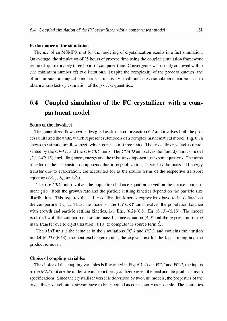
6.4. Coupled simulation of the FC crystallizer with a compartment model 161
Performance of the simulationThe use of an MSMPR unit for the modeling of crystallization results in a fast simulation.
On average, the simulation of 25 hours of process time using the coupled simulation frameworkrequired approximately three hours of computer time. Convergence was usually achieved within(the minimum number of) two iterations. Despite the complexity of the process kinetics, theeffort for such a coupled simulation is relatively small, and these simulations can be used toobtain a satisfactory estimation of the process quantities.
6.4 Coupled simulation of the FC crystallizer with a com-partment model
Setup of the flowsheetThe generalized flowsheet is designed as discussed in Section 6.2 and involves both the pro-
cess units and the units, which represent submodels of a complex mathematical model. Fig. 6.7ashows the simulation flowsheet, which consists of three units. The crystallizer vessel is repre-sented by the CV-FD and the CV-CRY units. The CV-FD unit solves the fluid dynamics model(2.11)-(2.15), including mass, energy and the mixture component transport equations. The masstransfer of the suspension components due to crystallization, as well as the mass and energytransfer due to evaporation, are accounted for as the source terms of the respective transportequations (ScK
, Sm and Sh).The CV-CRY unit involves the population balance equation solved on the coarse compart-
ment grid. Both the growth rate and the particle settling kinetics depend on the particle sizedistribution. This requires that all crystallization kinetics expressions have to be defined onthe compartment grid. Thus, the model of the CV-CRY unit involves the population balancewith growth and particle settling kinetics, i.e., Eqs. (6.2)-(6.8), Eq. (6.13)-(6.16). The modelis closed with the compartment solute mass balance equation (4.9) and the expression for themass transfer due to crystallization (4.10) to compute the source term Sc.
The MAT unit is the same as in the simulations FC-1 and FC-2, and contains the attritionmodel (6.23)-(6.43), the heat exchanger model, the expressions for the feed mixing and theproduct removal.
Choice of coupling variablesThe choice of the coupling variables is illustrated in Fig. 6.7. As in FC-1 and FC-2, the inputs
to the MAT unit are the outlet stream from the crystallizer vessel, the feed and the product streamspecifications. Since the crystallizer vessel is described by two unit models, the properties of thecrystallizer vessel outlet stream have to be specified as consistently as possible. The heuristics
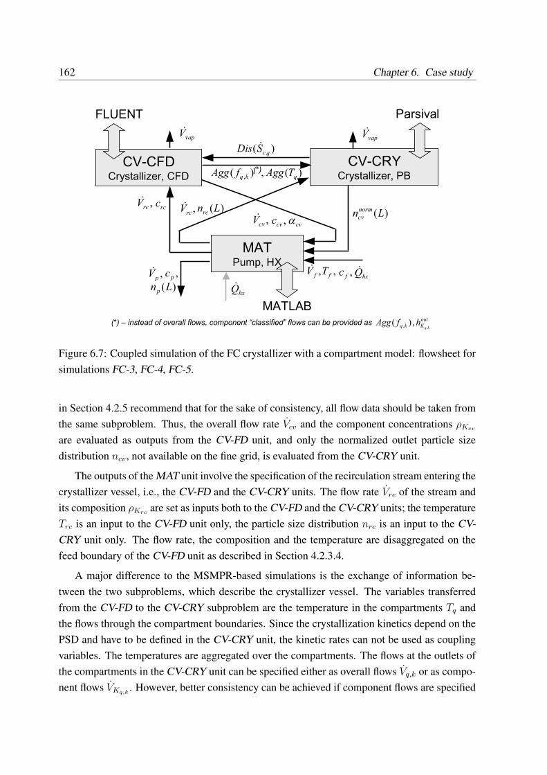
162 Chapter 6. Case study
CV-CRYCrystallizer, PB
MATPump, HX
,fV&
,pV&
hxQ&
,rcV&
vapV&
CV-CFDCrystallizer, CFD
,pc
)(Lnp
,fc,fT hxQ&
,rcV& )(Lnrcrcc
)(,)( , qkq TAggfAgg
)(qc
SDis &vapV&
,cvV& ,cvc cvα
)(Lnnormcv
ParsivalFLUENT
MATLAB
(*)
(*) – instead of overall flows, component “classified” flows can be provided as out
Kkq kqhfAgg
,,)( ,
Figure 6.7: Coupled simulation of the FC crystallizer with a compartment model: flowsheet forsimulations FC-3, FC-4, FC-5.
in Section 4.2.5 recommend that for the sake of consistency, all flow data should be taken fromthe same subproblem. Thus, the overall flow rate Vcv and the component concentrations ρKcv
are evaluated as outputs from the CV-FD unit, and only the normalized outlet particle sizedistribution ncv, not available on the fine grid, is evaluated from the CV-CRY unit.
The outputs of the MAT unit involve the specification of the recirculation stream entering thecrystallizer vessel, i.e., the CV-FD and the CV-CRY units. The flow rate Vrc of the stream andits composition ρKrc are set as inputs both to the CV-FD and the CV-CRY units; the temperatureTrc is an input to the CV-FD unit only, the particle size distribution nrc is an input to the CV-CRY unit only. The flow rate, the composition and the temperature are disaggregated on thefeed boundary of the CV-FD unit as described in Section 4.2.3.4.
A major difference to the MSMPR-based simulations is the exchange of information be-tween the two subproblems, which describe the crystallizer vessel. The variables transferredfrom the CV-FD to the CV-CRY subproblem are the temperature in the compartments Tq andthe flows through the compartment boundaries. Since the crystallization kinetics depend on thePSD and have to be defined in the CV-CRY unit, the kinetic rates can not be used as couplingvariables. The temperatures are aggregated over the compartments. The flows at the outlets ofthe compartments in the CV-CRY unit can be specified either as overall flows Vq,k or as compo-nent flows VKq,k
. However, better consistency can be achieved if component flows are specified
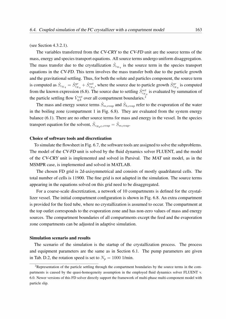
6.4. Coupled simulation of the FC crystallizer with a compartment model 163
(see Section 4.3.2.1).The variables transferred from the CV-CRY to the CV-FD unit are the source terms of the
mass, energy and species transport equations. All source terms undergo uniform disaggregation.The mass transfer due to the crystallization ScKq
is the source term in the species transportequations in the CV-FD. This term involves the mass transfer both due to the particle growthand the gravitational settling. Thus, for both the solute and particles component, the source termis computed as ScKq
= SgrcKq
+ SsetcKq
, where the source due to particle growth SgrcKq
is computedfrom the known expression (6.8). The source due to settling Sset
cKqis evaluated by summation of
the particle settling flow V setq,k over all compartment boundaries.2
The mass and energy source terms Sm,evap and Sh,evap refer to the evaporation of the waterin the boiling zone (compartment 1 in Fig. 6.8). They are evaluated from the system energybalance (6.1). There are no other source terms for mass and energy in the vessel. In the speciestransport equation for the solvent, ScH2O,evap = Sm,evap.
Choice of software tools and discretizationTo simulate the flowsheet in Fig. 6.7, the software tools are assigned to solve the subproblems.
The model of the CV-FD unit is solved by the fluid dynamics solver FLUENT, and the modelof the CV-CRY unit is implemented and solved in Parsival. The MAT unit model, as in theMSMPR case, is implemented and solved in MATLAB.
The chosen FD grid is 2d-axisymmetrical and consists of mostly quadrilateral cells. Thetotal number of cells is 11900. The fine grid is not adapted in the simulation. The source termsappearing in the equations solved on this grid need to be disaggregated.
For a coarse-scale discretization, a network of 10 compartments is defined for the crystal-lizer vessel. The initial compartment configuration is shown in Fig. 6.8. An extra compartmentis provided for the feed tube, where no crystallization is assumed to occur. The compartment atthe top outlet corresponds to the evaporation zone and has non-zero values of mass and energysources. The compartment boundaries of all compartments except the feed and the evaporationzone compartments can be adjusted in adaptive simulation.
Simulation scenario and resultsThe scenario of the simulation is the startup of the crystallization process. The process
and equipment parameters are the same as in Section 6.1. The pump parameters are givenin Tab. D.2, the rotation speed is set to Np = 1000 1/min.
2Representation of the particle settling through the compartment boundaries by the source terms in the com-partments is caused by the quasi-homogeneity assumption in the employed fluid dynamics solver FLUENT v.6.0. Newer versions of this FD solver directly support the framework of multi-phase multi-component model withparticle slip.
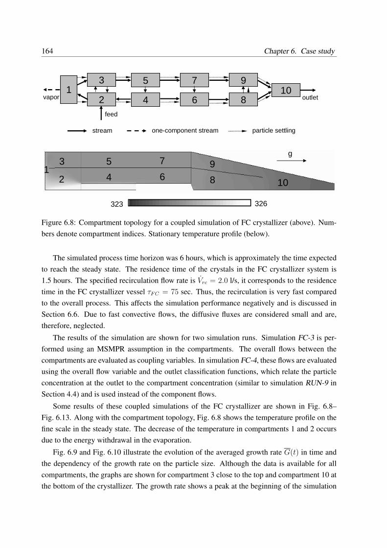
164 Chapter 6. Case study
12
3
4
5
6
7
8
9
10
323 326
2
31
4
5
6
7
8
910
g
stream particle settlingone-component stream
feed
vapor outlet
Figure 6.8: Compartment topology for a coupled simulation of FC crystallizer (above). Num-bers denote compartment indices. Stationary temperature profile (below).
The simulated process time horizon was 6 hours, which is approximately the time expectedto reach the steady state. The residence time of the crystals in the FC crystallizer system is1.5 hours. The specified recirculation flow rate is Vrc = 2.0 l/s, it corresponds to the residencetime in the FC crystallizer vessel τFC = 75 sec. Thus, the recirculation is very fast comparedto the overall process. This affects the simulation performance negatively and is discussed inSection 6.6. Due to fast convective flows, the diffusive fluxes are considered small and are,therefore, neglected.
The results of the simulation are shown for two simulation runs. Simulation FC-3 is per-formed using an MSMPR assumption in the compartments. The overall flows between thecompartments are evaluated as coupling variables. In simulation FC-4, these flows are evaluatedusing the overall flow variable and the outlet classification functions, which relate the particleconcentration at the outlet to the compartment concentration (similar to simulation RUN-9 inSection 4.4) and is used instead of the component flows.
Some results of these coupled simulations of the FC crystallizer are shown in Fig. 6.8–Fig. 6.13. Along with the compartment topology, Fig. 6.8 shows the temperature profile on thefine scale in the steady state. The decrease of the temperature in compartments 1 and 2 occursdue to the energy withdrawal in the evaporation.
Fig. 6.9 and Fig. 6.10 illustrate the evolution of the averaged growth rate G(t) in time andthe dependency of the growth rate on the particle size. Although the data is available for allcompartments, the graphs are shown for compartment 3 close to the top and compartment 10 atthe bottom of the crystallizer. The growth rate shows a peak at the beginning of the simulation
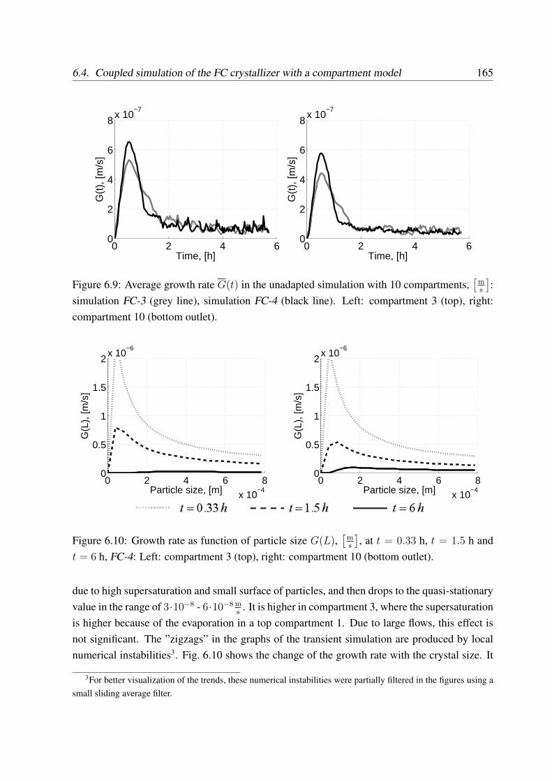
6.4. Coupled simulation of the FC crystallizer with a compartment model 165
0 2 4 60
2
4
6
8x 10
−7
Time, [h]
G(t
), [m
/s]
0 2 4 60
2
4
6
8x 10
−7
Time, [h]
G(t
), [m
/s]
Figure 6.9: Average growth rate G(t) in the unadapted simulation with 10 compartments,[
ms
]:
simulation FC-3 (grey line), simulation FC-4 (black line). Left: compartment 3 (top), right:compartment 10 (bottom outlet).
0 2 4 6 8
x 10−4
0
0.5
1
1.5
2x 10
−6
Particle size, [m]
G(L
), [m
/s]
0 2 4 6 8
x 10−4
0
0.5
1
1.5
2x 10
−6
Particle size, [m]
G(L
), [m
/s]
Figure 6.10: Growth rate as function of particle size G(L),[
ms
], at t = 0.33 h, t = 1.5 h and
t = 6 h, FC-4: Left: compartment 3 (top), right: compartment 10 (bottom outlet).
due to high supersaturation and small surface of particles, and then drops to the quasi-stationaryvalue in the range of 3·10−8 - 6·10−8 m
s. It is higher in compartment 3, where the supersaturation
is higher because of the evaporation in a top compartment 1. Due to large flows, this effect isnot significant. The ”zigzags” in the graphs of the transient simulation are produced by localnumerical instabilities3. Fig. 6.10 shows the change of the growth rate with the crystal size. It
3For better visualization of the trends, these numerical instabilities were partially filtered in the figures using asmall sliding average filter.
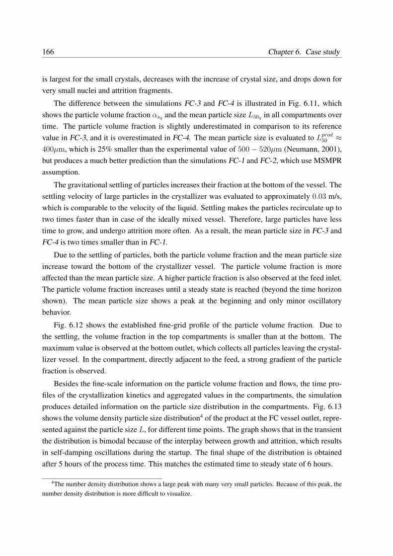
166 Chapter 6. Case study
is largest for the small crystals, decreases with the increase of crystal size, and drops down forvery small nuclei and attrition fragments.
The difference between the simulations FC-3 and FC-4 is illustrated in Fig. 6.11, whichshows the particle volume fraction αsq and the mean particle size L50q in all compartments overtime. The particle volume fraction is slightly underestimated in comparison to its referencevalue in FC-3, and it is overestimated in FC-4. The mean particle size is evaluated to Lprod
50 ≈400µm, which is 25% smaller than the experimental value of 500− 520µm (Neumann, 2001),but produces a much better prediction than the simulations FC-1 and FC-2, which use MSMPRassumption.
The gravitational settling of particles increases their fraction at the bottom of the vessel. Thesettling velocity of large particles in the crystallizer was evaluated to approximately 0.03 m/s,which is comparable to the velocity of the liquid. Settling makes the particles recirculate up totwo times faster than in case of the ideally mixed vessel. Therefore, large particles have lesstime to grow, and undergo attrition more often. As a result, the mean particle size in FC-3 andFC-4 is two times smaller than in FC-1.
Due to the settling of particles, both the particle volume fraction and the mean particle sizeincrease toward the bottom of the crystallizer vessel. The particle volume fraction is moreaffected than the mean particle size. A higher particle fraction is also observed at the feed inlet.The particle volume fraction increases until a steady state is reached (beyond the time horizonshown). The mean particle size shows a peak at the beginning and only minor oscillatorybehavior.
Fig. 6.12 shows the established fine-grid profile of the particle volume fraction. Due tothe settling, the volume fraction in the top compartments is smaller than at the bottom. Themaximum value is observed at the bottom outlet, which collects all particles leaving the crystal-lizer vessel. In the compartment, directly adjacent to the feed, a strong gradient of the particlefraction is observed.
Besides the fine-scale information on the particle volume fraction and flows, the time pro-files of the crystallization kinetics and aggregated values in the compartments, the simulationproduces detailed information on the particle size distribution in the compartments. Fig. 6.13shows the volume density particle size distribution4 of the product at the FC vessel outlet, repre-sented against the particle size L, for different time points. The graph shows that in the transientthe distribution is bimodal because of the interplay between growth and attrition, which resultsin self-damping oscillations during the startup. The final shape of the distribution is obtainedafter 5 hours of the process time. This matches the estimated time to steady state of 6 hours.
4The number density distribution shows a large peak with many very small particles. Because of this peak, thenumber density distribution is more difficult to visualize.
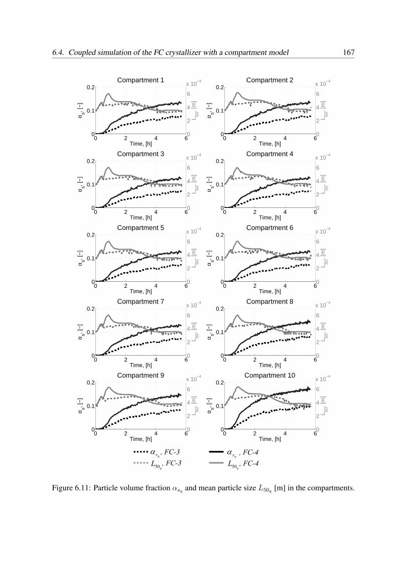
6.4. Coupled simulation of the FC crystallizer with a compartment model 167
0 2 4 60
0.1
0.2Compartment 1
Time, [h]
α s, [−
]
0
2
4
6
x 10−4
L 50, [
m]
0 2 4 60
0.1
0.2Compartment 2
Time, [h]
α s, [−
]
0
2
4
6
x 10−4
L 50, [
m]
0 2 4 60
0.1
0.2Compartment 3
Time, [h]
α s, [−
]
0
2
4
6
x 10−4
L 50, [
m]
0 2 4 60
0.1
0.2Compartment 4
Time, [h]
α s, [−
]0
2
4
6
x 10−4
L 50, [
m]
0 2 4 60
0.1
0.2Compartment 5
Time, [h]
α s, [−
]
0
2
4
6
x 10−4
L 50, [
m]
0 2 4 60
0.1
0.2Compartment 6
Time, [h]
α s, [−
]
0
2
4
6
x 10−4
L 50, [
m]
0 2 4 60
0.1
0.2Compartment 7
Time, [h]
α s, [−
]
0
2
4
6
x 10−4
L 50, [
m]
0 2 4 60
0.1
0.2Compartment 8
Time, [h]
α s, [−
]
0
2
4
6
x 10−4
L 50, [
m]
0 2 4 60
0.1
0.2Compartment 9
Time, [h]
α s, [−
]
0
2
4
6
x 10−4
L 50, [
m]
0 2 4 60
0.1
0.2Compartment 10
Time, [h]
α s, [−
]
0
2
4
6
x 10−4
L 50, [
m]
, FC-3q
L50
, FC-4
, FC-3qs
α , FC-4qs
α
qL50
Figure 6.11: Particle volume fraction αsq and mean particle size L50q [m] in the compartments.
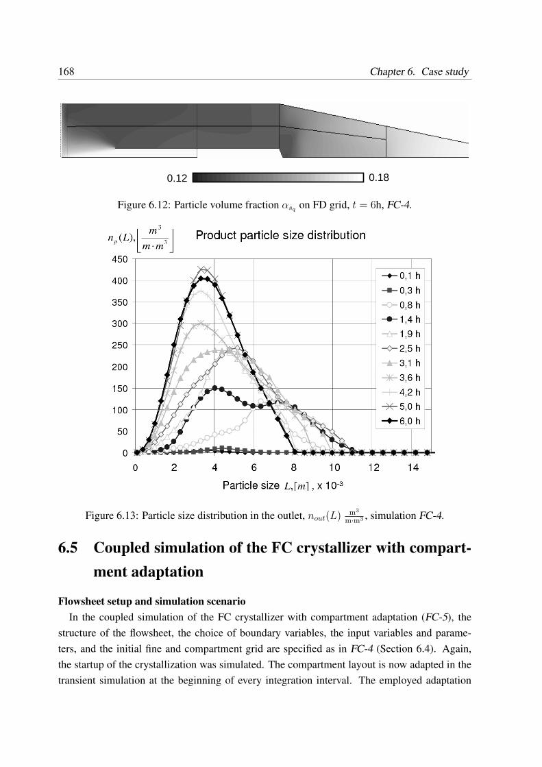
168 Chapter 6. Case study
0.12 0.18
Figure 6.12: Particle volume fraction αsq on FD grid, t = 6h, FC-4.
Figure 6.13: Particle size distribution in the outlet, nout(L) m3
m·m3 , simulation FC-4.
6.5 Coupled simulation of the FC crystallizer with compart-ment adaptation
Flowsheet setup and simulation scenarioIn the coupled simulation of the FC crystallizer with compartment adaptation (FC-5), the
structure of the flowsheet, the choice of boundary variables, the input variables and parame-ters, and the initial fine and compartment grid are specified as in FC-4 (Section 6.4). Again,the startup of the crystallization was simulated. The compartment layout is now adapted in thetransient simulation at the beginning of every integration interval. The employed adaptation
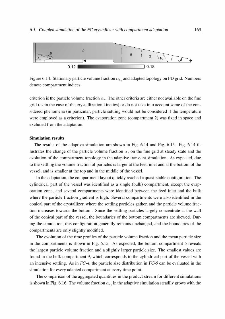
6.5. Coupled simulation of the FC crystallizer with compartment adaptation 169
0.12 0.18
1
9
2
710
6
5
83
4
Figure 6.14: Stationary particle volume fraction αsq and adapted topology on FD grid. Numbersdenote compartment indices.
criterion is the particle volume fraction αs. The other criteria are either not available on the finegrid (as in the case of the crystallization kinetics) or do not take into account some of the con-sidered phenomena (in particular, particle settling would not be considered if the temperaturewere employed as a criterion). The evaporation zone (compartment 2) was fixed in space andexcluded from the adaptation.
Simulation resultsThe results of the adaptive simulation are shown in Fig. 6.14 and Fig. 6.15. Fig. 6.14 il-
lustrates the change of the particle volume fraction αs on the fine grid at steady state and theevolution of the compartment topology in the adaptive transient simulation. As expected, dueto the settling the volume fraction of particles is larger at the feed inlet and at the bottom of thevessel, and is smaller at the top and in the middle of the vessel.
In the adaptation, the compartment layout quickly reached a quasi-stable configuration. Thecylindrical part of the vessel was identified as a single (bulk) compartment, except the evap-oration zone, and several compartments were identified between the feed inlet and the bulkwhere the particle fraction gradient is high. Several compartments were also identified in theconical part of the crystallizer, where the settling particles gather, and the particle volume frac-tion increases towards the bottom. Since the settling particles largely concentrate at the wallof the conical part of the vessel, the boundaries of the bottom compartments are skewed. Dur-ing the simulation, this configuration generally remains unchanged, and the boundaries of thecompartments are only slightly modified.
The evolution of the time profiles of the particle volume fraction and the mean particle sizein the compartments is shown in Fig. 6.15. As expected, the bottom compartment 5 revealsthe largest particle volume fraction and a slightly larger particle size. The smallest values arefound in the bulk compartment 9, which corresponds to the cylindrical part of the vessel withan intensive settling. As in FC-4, the particle size distribution in FC-5 can be evaluated in thesimulation for every adapted compartment at every time point.
The comparison of the aggregated quantities in the product stream for different simulationsis shown in Fig. 6.16. The volume fraction αsq in the adaptive simulation steadily grows with the
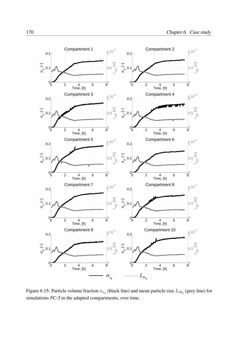
170 Chapter 6. Case study
0 2 4 6 80
0.1
0.2Compartment 1
Time, [h]
α s, [−
]
0
0.5
1x 10
−3
L 50, [
m]
0 2 4 6 80
0.1
0.2Compartment 2
Time, [h]
α s, [−
]
0
0.5
1x 10
−3
L 50, [
m]
0 2 4 6 80
0.1
0.2Compartment 3
Time, [h]
α s, [−
]
0
0.5
1x 10
−3
L 50, [
m]
0 2 4 6 80
0.1
0.2Compartment 4
Time, [h]
α s, [−
]
0
0.5
1x 10
−3
L 50, [
m]
0 2 4 6 80
0.1
0.2Compartment 5
Time, [h]
α s, [−
]
0
0.5
1x 10
−3
L 50, [
m]
0 2 4 6 80
0.1
0.2Compartment 6
Time, [h]
α s, [−
]
0
0.5
1x 10
−3
L 50, [
m]
0 2 4 6 80
0.1
0.2Compartment 7
Time, [h]
α s, [−
]
0
0.5
1x 10
−3
L 50, [
m]
0 2 4 6 80
0.1
0.2Compartment 8
Time, [h]
α s, [−
]
0
0.5
1x 10
−3
L 50, [
m]
0 2 4 6 80
0.1
0.2Compartment 9
Time, [h]
α s, [−
]
0
0.5
1x 10
−3
L 50, [
m]
0 2 4 6 80
0.1
0.2Compartment 10
Time, [h]
α s, [−
]
0
0.5
1x 10
−3
L 50, [
m]
Figure 6.15: Particle volume fraction αsq (black line) and mean particle size L50q (grey line) forsimulations FC-5 in the adapted compartments, over time.
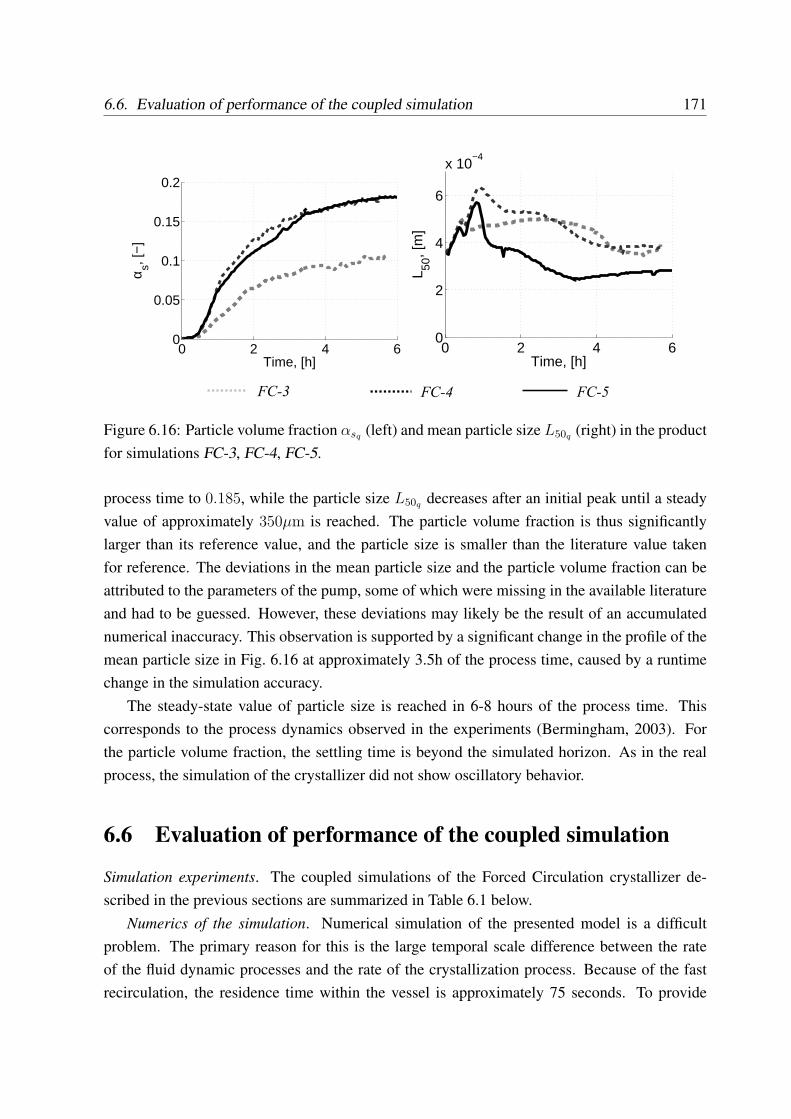
6.6. Evaluation of performance of the coupled simulation 171
0 2 4 60
0.05
0.1
0.15
0.2
Time, [h]
α s, [−
]
0 2 4 60
2
4
6
x 10−4
Time, [h]
L 50, [
m]
FC-3 FC-4 FC-5
Figure 6.16: Particle volume fraction αsq (left) and mean particle size L50q (right) in the productfor simulations FC-3, FC-4, FC-5.
process time to 0.185, while the particle size L50q decreases after an initial peak until a steadyvalue of approximately 350µm is reached. The particle volume fraction is thus significantlylarger than its reference value, and the particle size is smaller than the literature value takenfor reference. The deviations in the mean particle size and the particle volume fraction can beattributed to the parameters of the pump, some of which were missing in the available literatureand had to be guessed. However, these deviations may likely be the result of an accumulatednumerical inaccuracy. This observation is supported by a significant change in the profile of themean particle size in Fig. 6.16 at approximately 3.5h of the process time, caused by a runtimechange in the simulation accuracy.
The steady-state value of particle size is reached in 6-8 hours of the process time. Thiscorresponds to the process dynamics observed in the experiments (Bermingham, 2003). Forthe particle volume fraction, the settling time is beyond the simulated horizon. As in the realprocess, the simulation of the crystallizer did not show oscillatory behavior.
6.6 Evaluation of performance of the coupled simulation
Simulation experiments. The coupled simulations of the Forced Circulation crystallizer de-scribed in the previous sections are summarized in Table 6.1 below.
Numerics of the simulation. Numerical simulation of the presented model is a difficultproblem. The primary reason for this is the large temporal scale difference between the rateof the fluid dynamic processes and the rate of the crystallization process. Because of the fastrecirculation, the residence time within the vessel is approximately 75 seconds. To provide
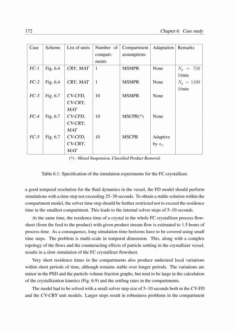
172 Chapter 6. Case study
Case Scheme List of units Number ofcompart-ments
Compartmentassumptions
Adaptation Remarks
FC-1 Fig. 6.4 CRY, MAT 1 MSMPR None Np = 750
1/minFC-2 Fig. 6.4 CRY, MAT 1 MSMPR None Np = 1100
1/minFC-3 Fig. 6.7 CV-CFD,
CV-CRY,MAT
10 MSMPR None
FC-4 Fig. 6.7 CV-CFD,CV-CRY,MAT
10 MSCPR(*) None
FC-5 Fig. 6.7 CV-CFD,CV-CRY,MAT
10 MSCPR Adaptiveby αs
(*) - Mixed Suspension, Classified Product Removal.
Table 6.1: Specification of the simulation experiments for the FC-crystallizer.
a good temporal resolution for the fluid dynamics in the vessel, the FD model should performsimulations with a time step not exceeding 25–30 seconds. To obtain a stable solution within thecompartment model, the solver time step should be further restricted not to exceed the residencetime in the smallest compartment. This leads to the internal solver steps of 5–10 seconds.
At the same time, the residence time of a crystal in the whole FC crystallizer process flow-sheet (from the feed to the product) with given product stream flow is estimated to 1.5 hours ofprocess time. As a consequence, long simulation time horizons have to be covered using smalltime steps. The problem is multi-scale in temporal dimension. This, along with a complextopology of the flows and the counteracting effects of particle settling in the crystallizer vessel,results in a slow simulation of the FC crystallizer flowsheet.
Very short residence times in the compartments also produce undesired local variationswithin short periods of time, although remains stable over longer periods. The variations areminor in the PSD and the particle volume fraction graphs, but tend to be large in the calculationof the crystallization kinetics (Fig. 6.9) and the settling rates in the compartments.
The model had to be solved with a small solver step size of 5–10 seconds both in the CV-FDand the CV-CRY unit models. Larger steps result in robustness problems in the compartment
6.6. Evaluation of performance of the coupled simulation 173
model of the CV-CRY unit. The employed reporting time step was 20–25 seconds. The size ofan integration interval was limited to 100–150 seconds.
The robustness and convergence of the simulation are worsened in case the flows are speci-fied by every component. Such a fixed specification of the flows leaves no room for the processparameters to vary in the unconverged iterations. The component masses in the compartmentsare rapidly changing because of large recirculation flows. This has a nonlinear effect on the pro-cess kinetics, and thus, ruins stability. A simulation employing the component flows (similar toRUN-10 in Section 4.4) failed due to divergence. To avoid this, a classification function had tobe employed instead of component flows.
Accuracy of the simulation. The incompleteness of the specification of the FC crystallizerin the available literature, and specifically, of the axial pump data, and insufficient detail ofavailable experimental data makes it impossible to use the FC crystallizer case study to evaluatethe accuracy of the simulation. The simulation results only match the order of the availablereference results. The inaccuracies can be attributed both to the inaccurate parameters of theemployed axial pump model and to the numerical inconsistencies of the model. For the samereason, the effect of the compartment boundary adaptation on the accuracy of the simulationcould not be evaluated numerically.
The average consistency errors with respect to the particle volume fraction in the compart-ments αsq in the converged iterations of FC-3, FC-4 and FC-5 do not generally exceed 6% inrelative numbers and are 1% or less in the majority of the compartments. The largest deviationis observed in compartment 8 in FC-3 and FC-4, and in the feed compartment 7 in FC-5 wherethe observed gradients of αs are higher.
Computational times. Due to the complexity of the model and the numerical difficultyof the simulation, the computational time is very large. In FC-3, the simulation of 6 hoursof process time required approximately 70 hours of computer time with the main simulationrunning on a 400 MHz computer, and the simulation of the CV-CRY unit in Parsival on a 1.6GHz computer. Approximately 20% of the simulation time was elapsed for the console outputand communication, and over 50% of the simulation time was spent for the simulation of thepopulation balance in the compartments in Parsival. The introduction of a classification functionfurther increased the computational time in Parsival by approximately 30%.
Large computational times make it nearly infeasible to solve the problem with high ormedium accuracy. The compartment model of the crystallizer had to be solved with a rela-tively low tolerance. This leads to an accumulation of numerical errors in the solution.
Adaptation does not cause any significant increase in computational time.Adaptivity in algorithms. During the simulations, several attempts to tune the adaptivity
of the PSD representation in the crystallization subproblem in Parsival were performed. Theyshowed that a high level of adaptivity of the finite elements, which contribute to the PSD, gener-
174 Chapter 6. Case study
ally renders the simulation much slower and is undesired for this kind of simulation. The effectof simultaneous adaptation of different aspects of discretization is rather negative than positive,if such adaptations are performed independently of each other, since the result of one kind ofadaptation has a cross-effect on the other kind of adaptation. For example, an optimal high-order adaptive representation of a PSD in a compartment will no longer be optimal when theboundaries of a compartment have changed at the next time interval. Furthermore, interactionsbetween the compartments with differently adapted PSD in the complex compartment topologyhave to be accounted for. The efficiency of methods where two different kinds of adaptation areperformed at the same time has to be carefully analyzed.
The presented case study effectively demonstrates both the capabilities of the employedmethod and the simulation software, and their computational feasibility limits.
6.7 Discussion
The case study illustrates that the coupled simulation approach enables the simulation of in-dustrial crystallization processes with multiple process units and multiple phenomena withinthe units, described by high-complexity models. A decomposition results in a heterogeneousflowsheet, where both process units and process phenomena models can be represented as unitsof the flowsheet. The method was successfully applied to the simulation of a forced circulationcrystallizer with a size-dependent growth model, settling in the main vessel, and attrition in thepump within the recirculation conduit. Several model formulations, resulting in different flow-sheets and different sets of coupling variables, were investigated and compared with each otherand with the experimental data by Bermingham (2003).
In FC-1 and FC-2, the use of a simple MSMPR vessel with a growth model, where theparticle settling and inhomogeneity in the vessel are ignored, leads to a high overestimation ofthe mean particle size. Although the simulation required no FD evaluation and was fast, thissimulation cannot be used for the prediction of suspension properties.
In FC-3, the full model with fluid dynamics, crystallization kinetics, particle settling andrecirculation was simulated. The MSMPR assumption was employed for the compartments ofthe coarse compartment grid in the crystallizer vessel. The grid consisted of 10 compartments.Simulation FC-3 provided a good prediction of the mean particle size, some underestimation ofthe particle volume fraction, and a satisfactory prediction of the crystallization kinetics in thevessel.
The addition of a classification function in FC-4, which specifies that the values for theparticle volume fractions differ from the compartment-averaged values, resulted in an overesti-mation of the particle volume fraction, with a good prediction of the mean particle size and the
6.7. Discussion 175
crystallization kinetics. With exception of compartment 8, this solution has small consistencyerrors, which indicates a good match between the submodels. The use of component flows inthe coupled simulation lead to simulation instability.
The chosen compartment topology produces a meaningful fine-scale profile of the particlevolume fraction, except for a region at the base of the conical section. To improve the com-partment selection, an adaptive simulation was employed (FC-5). This simulation produced areasonable choice of compartments with more compartments chosen at the bottom and at thefeed. As a result, adaptation resulted in an improvement of the fine-scale profile of the particlevolume fraction. However, no further improvement was achieved with respect to aggregatedquantities compared to FC-4.
Because of absence of a reference solution with only a few reference process values avail-able and a lack of data on the model parameters, an evaluation of the simulation accuracy is notpossible. All simulations, where 10 compartments are used and where particle settling is takeninto account, are by far more accurate than FC-1 and FC-2 with only an MSMPR assumptionin the vessel. The simulation FC-4 is more consistent than FC-3, but there are not enough argu-ments to evaluate its accuracy. The adaptation in FC-5 seems to work well to find the optimalcompartment layout, which produces correct profiles of the fine-scale variables. It is likely that,once found, this layout can be used in the simulation without further adaptation. Similarly, thereare not enough arguments to evaluate the accuracy of FC-5 and the adaptation criteria selected.
The FC crystallizer case study is difficult for numerical simulation due to its temporal multi-scale properties. Fast flow rates in the vessel caused by recirculation require small time stepsin the population balance solver, otherwise the solver shows a non-robust behavior in responseto minor changes in the inputs, and even fails to converge. At the same time, the small productflow rate results in a large residence time in the flowsheet. This results in problem stiffness,long simulation times and high chances of local instabilities of the solution. It is also likely thatsmall numerical errors accumulate and produce much larger deviations in the long run.
The difficulty to handle such temporal multi-scale problems is a limitation of the whole cou-pled simulation approach. To handle temporal multi-scale process, its modification is requiredto decompose the generalized flowsheet problem by the time scales. A possible approach wouldbe an isolation of the fast-scale subproblems into a subflowsheet in order to solve it using asmaller time step, which guarantees robustness, for a part of a time interval. For the rest of theinterval, extrapolation and correction steps would have to be performed. The main flowsheetwould then be solved using a larger time step. However, this modification remains outside ofthe scope of the present thesis.
Chapter 7
Conclusions
In the present thesis, two objectives were formulated. The first objective was the development ofa solution strategy for dynamic coupled simulation of a complex multi-physics and multi-scaleprocess on spatial grids with different resolution. The objective was reached by introducing theconcept of a generalized flowsheet, where the units represent both process unit operations andprocess phenomena models, and the couplings between these units are process material streamsas well as information flows. A modular dynamic simulation algorithm was developed andemployed for the simulation of this generalized flowsheet. A software-technical solution wasrealized using the integration platform CHEOPS, which implements the modular simulationalgorithm and executes the communication with the external software tools. These softwaretools were used for the simulation of the individual unit or phenomena models.
The second objective was the application and evaluation of the implemented coupled sim-ulation for the problem of non-stationary mass crystallization and fluid dynamics simulation.This problem is considered in the study as an example of a multi-physics and in a larger sensea multi-scale problem. The setup and simulation of such a problem required the use of spatialgrids with different resolution for the representation of the process phenomena as units of ageneralized flowsheet. The spatial grids were either chosen fixed or were adapted over timeaccording to the specified criteria. Both a simplified evaluation and a case study of a lab-scalecrystallizer unit with state-of-the-art models were performed. The application of the method isregarded as successful. However, both the overall performance and the accuracy of the simula-tion method have to be evaluated as moderate.
Evaluation of coupled simulation approach
The modular simulation algorithm (Chapter 3) could be successfully applied to the gener-alized flowsheet problems. Conceptually, a simulation problem of high complexity, both in
176
177
multi-physics and multi-scale sense, can be tackled by decomposition into subproblems (pro-cess units or phenomena models, defined on a single scale or a domain part), subproblem im-plementation in the appropriate software simulators and application of the modular simulationfor the resulting generalized flowsheet.
The approach is attractive for the simulation of phenomenologically complex processes, theproblems with moderately strong couplings between the process units or phenomena, whichusually converge in several iterations on an interval. It is slower if a fixed point iteration isused, and faster if a Broyden-type update is employed. Very strong couplings between the unitsmay lead to a difficult decomposition and slow convergence behavior. The structure of thegeneralized flowsheet is determined by user design decisions on the choice of the decomposi-tion scheme and the coupling variables. Several guidelines to perform the decomposition arepresented in Section 4.2.5.
A further advantage of the modular simulation is the possibility to reuse existing models,specialized software tools and the numerical methods implemented therein to solve the sub-problems of the full problem. Implementation of specialized solvers can be avoided.
The disadvantages of the approach are the dependency on the tool performance, the neces-sity of subproblem reformulation to match the problem setup in the software tools, inaccurateor inconsistent solutions, which may arise in case of inappropriate decomposition, and longsimulation times because of multiple iterations on the same integration interval. The use of ex-isting simulation tools requires the implementation of specific software tool wrappers to providecommunication.
Handling of multi-scale complexity
The simulation approach in the thesis was developed to handle a class of spatial multi-scaleproblems (Chapter 4). Different grids can be defined for the subproblems. If these grids areseparated in space, the subproblems are defined as separate units of a generalized flowsheet.
In the problem considered in the thesis, the fluid dynamics subproblem with a fine-scalegrid and the crystallization subproblem with a coarse compartment grid are defined on the samedomain. The modular simulation algorithm is extended to support scale integration methods forthe information transfer between the subproblems with different discretizations. This methodenables the simulation of spatial multi-scale problems without having to implement specializedmulti-scale solvers.
No temporal multi-scale methods are implemented. Integration of all units is performedusing the same integration interval and reporting time steps. The unit models are evaluated atevery reporting time point. The choice of the internal solver time step for the unit models isperformed by the respective software simulators.
178 Chapter 7. Conclusions
Evaluation of CHEOPS
The integration platform CHEOPS (Section A.2) is an appropriate software-technical so-lution for the modular simulation of generalized flowsheets based on the integration of softwaresimulators. The platform provides the structures for the flowsheet and variable representation,a hierarchy of model representation classes, including both steady-state and dynamic models.CHEOPS communicates with the external software tools to solve the models of the subprob-lems. It implements wrappers to a number of software simulation tools (e.g. gPROMS, Aspen+)and has a direct access to the library of numerical solvers lptNumerics. The flowsheet-level al-gorithms are implemented in the application modules of CHEOPS.
CHEOPS requires a full model specification, where for every CHEOPS unit, the set of inputand output couplings and coupling variables is specified. This set cannot be modified duringruntime. The coupling variables are defined as time profiles of scalar (temperatures, flows, etc.)or distributed quantities (PSD).
CHEOPS is an extendable platform with respect to all types of components. New compo-nents (application modules, model representation types, tool wrappers) can be integrated intoCHEOPS, provided that they comply to the standard CHEOPS interfaces. For the present thesis,CHEOPS was extended to include the modular dynamic simulation algorithm, the support ofdistributed quantities, the tool wrappers for a number of external simulators, such as HYSYS,FLUENT, Parsival and MATLAB, by the generalized flowsheet formulations and the adaptationprocedure (Appendix A).
CHEOPS was also upgraded to support the transfer of grid topology information. This solu-tion is currently implemented in FLUENT and Parsival wrappers for the coarse-scale grids. Thecoupling variable data is transferred as the values in the coarse-grid compartments, and the flowvariables are computed on their boundaries. The adaptation of the coarse-scale compartmentboundaries in the simulation has been implemented. CHEOPS does not support the treatmentof fine-scale grids.
Evaluation of the employed software tools
Throughout the thesis, FLUENT was employed for the solution of the fluid dynamics sub-problems, and Parsival was used for the crystallization subproblems. They are specialized com-mercial simulators with an external command and data interface, which makes them capable oftool integration.
FLUENT is a CFD solver, which supports flexible fluid dynamics problem formulation. Itdefines the model on the fine-scale FD grid and supports the selection of process zones. Theexternal interface of FLUENT allows the execution of all FLUENT commands. However, only
179
the major access and reporting functions have been implemented by the FLUENT wrapper.
Parsival is a specialized tool for the crystallization problems, which provides modeling andsimulation capabilities for population balance equations to compute the accurate representationof the PSD, accounting for various crystallization kinetics and phenomena. Parsival supportsmultiple interconnected crystallizer units, this enables the representation of a coarse-scale gridtopology. Parsival has somewhat restricted communication capabilities; while most output vari-ables and user functions can be reported, the problem setup and specification of the input datarequires editing of the model file and eventually the library of user functions.
Specialized commercial tools do not provide access to the equation systems, and often useautomatic problem closures. This is convenient for the user, but may pose problems for coupledflowsheets, where this closure may be provided by another unit. This may lead to problemoverdetermination, when the same variable is computed twice in the flowsheet. For example,Parsival uses such an automatic closure to compute the solute concentration (Section 4.2.8).
Consistent decomposition and subproblem specification
Decomposition involves the assignment of the model equations to the subproblems and re-spective discretization grids, and choice of coupling variables. A consistent decompositionrequires consideration of all relevant process phenomena and use of equivalent subproblem for-mulations, especially for overdetermined problems.
For the fluid dynamics-crystallization problem (Section 4.1), a consistent decompositionwas achieved and shown in Section 4.4. A FD subproblem on the fine grid involved the trans-port equations for each suspension component, turbulent diffusion and the expressions for thecrystallization kinetics. A crystallization subproblem, formulated in the coarse-grid compart-ments, involved the population balance in the compartments, the calculation of the source termsdue to crystallization and an update of the compartment topology and the initial states at thebeginning of an integration interval.
The coupling variables transferred from the FD to the crystallization subproblem involvedaggregated crystallization kinetics and component flows through all boundaries, including dif-fusive flux. The component mass source/sink terms due to the crystallization were transferredfrom the crystallization to the FD subproblem and uniformly disaggregated. The affected con-centrations were computed by the transport equations added to the FD subproblem, which in-clude these source/sink terms. This solution is the most rigorous disaggregation option and wasemployed in all simulations.
A MSMPR assumption used by default in many crystallization models results in inconsistentinputs to the compartment submodel and hence to a systematic error (Section 4.3.2.1).
180 Chapter 7. Conclusions
Accuracy and performance on fixed grids
The accuracy of the proposed method is affected both by the consistency between the sub-problems and by the selection of the coarse-grid compartment layout.
In the simulations, the consistency error and aggregation error could be evaluated. The con-sistency error is a norm of deviation of the values of the same quantity computed in differentsubproblems, and characterizes the equivalency of subproblem input formulations. It variesfor different decomposition schemes, employed assumptions, choices of coupling variables andcompartment layouts. The consistency error should be minimized by choosing appropriatecoupling variables. The aggregation error characterizes the profile uniformity within a com-partment. It can be used as a measure of quality of the compartment selection. The error inthe disaggregation of quantities on the fine grid could not be evaluated without knowledge of areference solution.
The error of numerical integration was considered to be controlled.A reference solution for the considered problem can only be provided for the simplest cases.
Such a solution was produced by the Method of Moments for the example study of a tubularcrystallizer. It enabled the evaluation of the difference between the computed and the referencesolution with respect to the particle volume fraction.
Subproblem inconsistencies and the choice of boundary variables showed a noticeable effecton the deviation from the reference solution. It was also found in the aggregation and consis-tency errors. A positive correlation between the consistency, aggregation and reference errorwas found, if the same compartment layout was employed. Reduction of the consistency errorin a compartment usually corresponded to the reduction of the deviation from the reference so-lution. Thus, reduction of consistency and aggregation errors can be used as an indication ofthe approximation to the true solution. A certain minimum reference error was found even forthe fully consistent formulations due to the discretization error in the solution in the coarse-gridcompartments.
The discretization error and the error propagation were the two major problems of the ap-proach. To evaluate the discretization error, an a posteriori error estimator needs to be con-structed for the population balance with the constitutive relations, discretized in the finite vol-ume compartments with complex shapes. The known Z2 and finite element-based estimatorscould not be directly used for the PDAE systems and the compartment grid with irregular com-partment shapes (Section 4.3.6.2). The error propagation should be performed in time, withinthe spatial domain and between all the subproblems of the flowsheet during the iterations. Itcan not be evaluated without a known local error production term, and in the absence of recon-struction of its behavior in the iterative processes. The evaluation of a mathematically rigorousa posteriori error estimator for the considered problem was, therefore, not possible in the frame-
181
work of the thesis. The author considers the absence of an error estimator for the compartmentsas a disadvantage of the approach.
The simulation approach is computationally expensive, but provides a large amount of pro-cess information (such as fine-grid profiles of flows, components and process kinetics, as wellas the PSD in the compartments), compared to the time-saving reduced methods. The com-putational time is affected by the number of iterations required for convergence, the quantityof coupling variables (increases with increasing number of coupling variables), the choice ofdecomposition scheme (increases with the strength of coupling, e.g. the specification of com-ponent flows makes the convergence slower), the compartment topology (increases non-linearlyfor more complex topologies), etc. A balance between the computational effort and the amountof information produced in the simulation has to be found.
Selection and adaptation of grids and compartments
The choice of compartments is very important and seriously affects the results. Adaptivesimulations (Chapter 5) can improve the solution with respect to unadapted simulations, whichuse the same decomposition scheme. A good choice of the adaptation criterion is a major fac-tor of the adaptation success. The criterion should be formulated as a combination of majorvariables affecting the solution and the output quantity of interest. Among these factors, theresidence time variable or a similar quantity characterizing the process dynamics should bepresent at least for the transient processes to avoid highly scattered residence times in the com-partments. The other criteria in case of crystallization can involve the crystallization kinetics,temperature or the fine-scale profiles of the output variables such as the particle volume fraction(Section 5.1.3).
In case of an inappropriate criterion selection, the results of adaptive simulations could beworse than those of unadapted simulations. Adaptation may also produce instabilities in thesolution if the primary factors in the adaptation criterion are the variables, which experience astrong feedback correlation with the choice of the compartments, such as nucleation rate. For anefficient adaptation, a stable sharp variable profile or gradient without a significant dependencyon the compartment choice and variables in the other subproblems is desired.
Both implemented compartment boundary identification procedures (Delta and Split-Merge)were designed to search for a local optimum. Although a search for the local optimum may suf-fice, the choice of starting points or the previous compartment layout affect the adaptation, suchthat the globally optimal compartment layout may not be found by the procedure.
The adaptation of the compartment boundary makes the evaluation of the simulation qualityin the absence of a reference solution difficult. Neither consistency error nor the aggregationerror can be used as a measure of convergence to the reference solution. In case the reference
182 Chapter 7. Conclusions
solution is not available, even the relative quality of adaptation is difficult to evaluate. Derivationof an error estimator for the discretization error is necessary, but remains a yet more complexproblem since the compartment layout will change during the transient.
In the considered cases, the adaptation itself was fast compared to the simulation of thesubproblems. However, complex compartment topology increases the computational time ofthe simulation.
Forced Circulation crystallizer
Application of the approach to the Forced Circulation crystallizer with the state-of-the-artmodels (Chapter 6) effectively shows possibilities and limitations of the employed approach.The generalized flowsheet has a mixed structure and contained both the process units (pump,heat exchanger) and the phenomena models (fluid dynamics and crystallization in the vesselas separate subproblems). Simulation involved the size-dependent growth and particle gravita-tional settling within the crystallization subproblem in Parsival, fluid dynamics and evaporationeffect within the FD subproblem in FLUENT and attrition in the pump unit (MATLAB). Despiteits strong coupling, the simulation was convergent within 3–5 iterations in the non-stationaryprocess, and within 1–2 iterations in the vicinity of the steady state. The simulation produceddetailed information on the system, including the PSD in the compartments.
Consistent decomposition of this problem into subproblems was a complicated task dueto restrictions of the employed software tools, particularly with respect to the size-dependentparticle settling, not directly supported by FLUENT or Parsival.
The FC crystallizer is a recirculating system with long residence times of a particle in thesystem, but fast flows in the pipe conduit and small residence time in the vessel. This is aspatial and temporal multi-scale problem with different process dynamics on the same domainand time interval. The FD modeling and the stability of the solution of the population balancein the compartments required small steps, with which a large simulation horizon had to becovered. The simulation requires a high computational effort and may be locally unstable,although remains globally convergent. The simulation is also sensitive to the problem boundaryconditions and the compartment adaptation. The case study demonstrates the capabilities of theemployed method and its computational feasibility limits.
It was not possible to evaluate the deviation with respect to the true solution in the absenceof a quantitative error estimator.
Scope of application
The application of a coupled simulation and a generalized flowsheet framework is a pow-
183
erful tool for the dynamic simulation of detailed models of complex processes, which can beimplemented and solved in general-purpose tools or specialized simulators with an externalclient interface. Simulations can be successfully performed for different kinds of processes:
• All kinds of multi-stage processes, represented with a flowsheet with detailed, customizedmodels of the unit operations involved, which are implemented in the simulators.
• Multi-physics processes, where individual process phenomena can be isolated in spaceand represented as separate models, and the regions with the specific dominating processphenomena can be determined by evaluation of an appropriate criterion during runtime.
• Multi-physics processes on the same spatial domain with weak or moderately strong cou-pling, where the subproblems representing the process phenomena can be identified dur-ing problem decomposition, and the number of coupling variables in the couplings be-tween these phenomena models is not large.
• Multi-scale multi-physics problems, where the process phenomena occur on the samedomain, but on different spatial scales, such that an easy scale separation is possible. Ageneralized flowsheet can involve subproblems defined on different grids.
• ”Heterogeneous” multi-stage and multi-physics problems with weak or moderately strongcoupling, which involve both different process unit operations and multiple process phe-nomena within the units and which can be decomposed into subproblems in spatial do-main or by spatial scales.
The approach in the presented formulation is generally not appropriate for problem classeswith the following features:
• Flowsheet simulations with standard unit models, which are available in the existing flow-sheet simulators such as Aspen+ or HYSYS or can be easily integrated there. The effortneeded for the flowsheet setup and the communication overhead in the coupled simulationare excessive compared to those needed to set up a model in such a simulator.
• Complex processes with already established specialized simulator, which use effectivesolution algorithms: they are likely to surpass the coupled simulation in terms of bothaccuracy and performance.
• Multi-physics problems with strong coupling between the phenomena on the same spatialscale. The decomposition of the problem may be unsuccessful, and the convergence maybe too slow or not achieved at all. A specialized solver may need to be employed.
184 Chapter 7. Conclusions
• Transient problems with a temporal multi-scale behavior within the subproblems on thesame spatial domain and the same time intervals, where neither the subproblems can beconsidered quasi-stationary, nor the time scales can be directly separated into individualsubproblems. This is a case similar to strongly coupled spatial multi-scale problems on asingle domain. They require development of temporal decomposition techniques, whichare not present in this framework.
The following difficulties of the approach can hinder the simulation during runtime:
• Inconsistency in the problem formulation due to improper decomposition or tool restric-tions may produce a solution with systematic errors, and even a non-convergent solution.
• Improper compartment layout is likely to produce an inaccurate solution.
An accurate reconstruction of the true solution cannot be guaranteed and not even be as-sessed in the absence of a reference solution. The systematic error in the converged solution iscaused by the discretization. Error estimators have not been developed for the problems of suchcomplexity in the known literature.
Consistently decomposed problems have a minimum error possible with the given dis-cretization. The chosen coarse-scale discretization can be improved by adaptation of the coarse-grid compartments. However, an adaptation criterion has to be properly chosen to generate thecompartment layout, simulation on which improves the solution.
Some problems, where the application of the coupled simulation of generalized flowsheetslooks attractive, involve the simulation of a 2d-population balance in inhomogeneous environ-ment, simulation of reactive precipitation processes with a fine grid model in the vicinity of thefeed, population balance described crystallization in specific regions of a crystallizer.
Future development
Further development of a proposed solution should follow several ways. First, the supportof arbitrary spatial grids with a changing number of elements, boundaries and variables withinthe grids has to be implemented in the integration platform CHEOPS to lift current limitationson the ports and variables. Second, decomposition of the problem into subproblems by tem-poral scale and specific algorithms to handle such temporal multi-scale problems need to bedeveloped. Such algorithms should run a fast subproblem with different step sizes and inter-vals than the slow subproblem. Adaptation of the coarse grid compartment boundaries requiresfurther development to look for a global optimum instead of local ones, and the rules of adap-tation criterion choice have to be proposed such that a good adaptation criterion improving thesolution could be quickly found if the model is known. Adaptation of grids can also be very

185
useful for parallel computations of large-scale problems on computer clusters. The support ofparallelization has to be implemented in the simultaneous modular simulation algorithm in thiscase. Finally, the problem of error estimation with respect to the true solution, caused by dis-cretization and error propagation, was not solved in the present thesis and remains a problemfor future research. With the proposed developments, the potential of the generalized frame-work for coupled multi-physics simulation can be exploited in a full extent for various kinds ofmulti-physics and multi-scale problems.
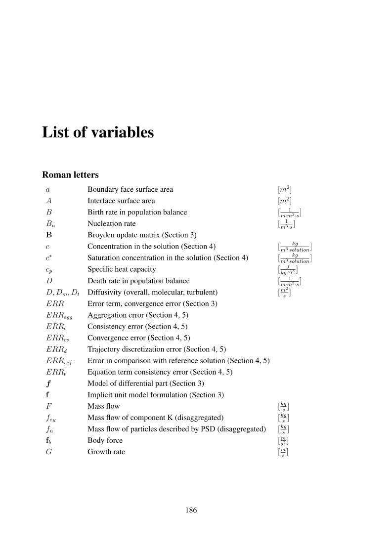
List of variables
Roman lettersa Boundary face surface area [m2]
A Interface surface area [m2]
B Birth rate in population balance [ 1m·m3·s ]
Bn Nucleation rate [ 1m3·s ]
B Broyden update matrix (Section 3)c Concentration in the solution (Section 4) [ kg
m3 solution]
c∗ Saturation concentration in the solution (Section 4) [ kgm3 solution
]
cp Specific heat capacity [ Jkg·◦C ]
D Death rate in population balance [ 1m·m3·s ]
D,Dm, Dt Diffusivity (overall, molecular, turbulent) [m2
s]
ERR Error term, convergence error (Section 3)ERRagg Aggregation error (Section 4, 5)ERRc Consistency error (Section 4, 5)ERRcv Convergence error (Section 4, 5)ERRd Trajectory discretization error (Section 4, 5)ERRref Error in comparison with reference solution (Section 4, 5)ERRt Equation term consistency error (Section 4, 5)f Model of differential part (Section 3)f Implicit unit model formulation (Section 3)F Mass flow [kg
s]
fcKMass flow of component K (disaggregated) [kg
s]
fn Mass flow of particles described by PSD (disaggregated) [kgs]
fb Body force [ms2 ]
G Growth rate [ms]
186
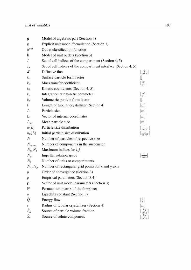
List of variables 187
g Model of algebraic part (Section 3)g Explicit unit model formulation (Section 3)hout Outlet classification functionh Model of unit outlets (Section 3)I Set of cell indices of the compartment (Section 4, 5)Ib Set of cell indices of the compartment interface (Section 4, 5)J Diffusive flux [ #
m2·s ]
ka Surface particle form factor []
kd Mass transfer coefficient [ms]
ki Kinetic coefficients (Section 4, 5)kr Integration rate kinetic parameter [m
s]
kv Volumetric particle form factor []
l Length of tubular crystallizer (Section 4) [m]
L Particle size [m]
L Vector of internal coordinates [m]
L50 Mean particle size [m]
n(L) Particle size distribution [ 1m·m3 ]
n0(L) Initial particle size distribution [ 1m·m3 ]
N Number of particles of respective sizeNcomp Number of components in the suspensionNi, Nj Maximum indices for i,jNp Impeller rotation speed [ 1
min]
Nq Number of units or compartmentsNx, Ny Number of rectangular grid points for x and y axisp Order of convergence (Section 3)p Empirical parameters (Section 3.4)p Vector of unit model parameters (Section 3)P Permutation matrix of the flowsheetq Lipschitz constant (Section 3)Q Energy flow [J
s]
r Radius of tubular crystallizer (Section 4) [m]
Sα Source of particle volume fraction [ kgm3·s ]
Sc Source of solute component [ kgm3·s ]
188 List of variables
ScKSource of component K [ kg
m3·s ]
Sm Source of mass [ kgm3·s ]
Sh Source of energy [ Jm3·s ]
Sφ Source of a scalar quantity [ [#]m3·s ]
t Time coordinate [s]
T Temperature [K] or [◦C]
∆Tn Integration interval [s]
δts Solver time step [s]
u Inputs of unit model (Section 3)v Velocity [m/s]
vliq Liquid velocity in settling model [m/s]
vpart Particle velocity in settling model [m/s]
vslip Slip velocity in settling model [m/s]
V Volume [m3]
V Volumetric flow [m3
s]
w Mass fraction [ kgkg mixture
]
x Spatial coordinate [m]
x Vector of spatial coordinates [m]
x Differential states of unit model (Section 3)x Vector of states of unit model (Section 3)y Outputs (Section 3)z Algebraic states (Section 3)Z Domain in spatial coordinatesz CellZ CompartmentZsplit Split candidate compartmentZmerge Merge candidate combination of compartments
Greek lettersα Reflux ratio (Section 3.4) []
αs Volume fraction of solids []
β Agglomeration kernelβsurf Angle of velocity with respect to normal to surface [◦]
Γ/Kr Effective fracture surface energy [ Jm2 ]
Γs Surface-related energy increase [J ·mmol
]
List of variables 189
ε Void fraction in the suspension (mathematical models) []
ε Tolerance (iterations and error measurement)ε Power input [J
s]
Λ Incidence matrix for the flowsheet modelµ(p) p-th moment of particle size distribution [ mp
m·m3 ]
ν Viscosity [Pa · s]ρ Density [ kg
m3 ]
ρK Partial density (concentration) of component K [ kgm3 suspension
]
ρc,ρs Partial density (concentration) of solute/solids in suspension [ kgm3 suspension
]
ρS Density of particles [ kgm3 ]
φ Distributed scalar quantity [#]
φ True solution of the scalar quantity [#]
φ Disaggregated scalar quantity [#]
Φ Aggregated scalar quantity in spatial coordinates [#]
ψ Distributed vector quantity [#]
Ψ Aggregated vector quantity in spatial coordinates [#]
τ Residence time [s]
χ Criterion of spatial adaptation
Subscripts
att Attritionb Compartment boundary or its faces in 2d-meshed domainCFD Unit for the CFD subproblem (Chapter 4, 5)cr CrystallizerCRY Unit for the crystallization subproblem (Chapter 4, 5)e Edge collision in attrition model (Chapter 6)eff Effective kinetic ratef, feed Feedf Face collision in attrition model (Chapter 6)frag Attrition fragmentshx Heat exchanger (Chapter 6)i Index by particle size (Chapter 2)i, b Indices by CFD faces of the compartment boundary in 2d-meshed domaini, j Indices by CFD cell in 2d-meshed domain
190 List of variables
k Index of mixture component in one-phase flowK Index of mixture component in multi-phase flowm Index of time stepn Index of time discretizationp Order of process kinetics (Chapter 2)p Product (Chapter 6)q Unit index (Chapter 3)q Compartment index (Chapter 4)q, k Compartment boundary index (Chapter 4)qk,ql Indices of compartments in candidate compartment combination for merge (Chapter 5)q∗k,q∗l Indices of optimal candidate compartment combination for merge (Chapter 5)qs Index of candidate compartment for splitting (Chapter 5)q∗s Indices of optimal candidate compartment for splitting (Chapter 5)rc Recirculation stream (Chapter 6)s Solid phase (particles)TS Tear stream (Chapter 3)UC Untorn coupling (Chapter 3)vap Vapor (Chapter 6)
Superscripts
∗ Converged iteration index in iterative processcr Crystallizer (Section 3.4)evap Evaporator (Section 3.4)hc Hydrocyclone (Section 3.4)in Input termk Iteration indexmix Mixer unit (Section 3.4)out Output termref Reference solution value(p) Moment index of particle size distribution
Appendix A
Software-technical implementation inCHEOPS
In this appendix, the software-technical architecture and implementation of the integration plat-form CHEOPS and the wrapper components for the software tool integration are discussedbriefly. A more detailed description of CHEOPS has been presented by Schopfer (2005).
A.1 Communication and tool interface standards
The software-technical basis of the tool integration is a communication middleware, which isnecessary to establish connections between tools and wrappers, as well as between wrappers andthe client. Two common middleware standards are COM1 and CORBA.2 The external interfacesof many Windows-based commercial software simulators are based on COM (e.g. MATLAB,Aspen+, Parsival). CORBA is designed for the communication between software tools runningon different computer platforms and operation systems. It is used in the tools such as gPROMS.Both middleware standards have a well-documented set of functions and methods to establishand maintain communication between the software tools. A tool wrapper must support thecommunication middleware used in the tool interface. If the client uses a middleware differentfrom the tool, the tool wrapper has to provide a bridge between them.
Unlike the software-technical interface standards, the high-level semantic description ofinterfaces of simulation tools does not often use established standards. Due to continuing de-
1Component Object Model, an interprocess communication middleware developed for Microsoft Windowsapplications. Based on COM, specific middleware standards such as OLE, ActiveX, etc., have been developed.
2Common Object Request Broker Architecture, an interprocess and interplatform communication middle-ware standard defined by OMG (Object Management Group). Description of the standard is available athttp://www.omg.org, accessed 12.03.09. See also Henning and Vinoski (1999).
191
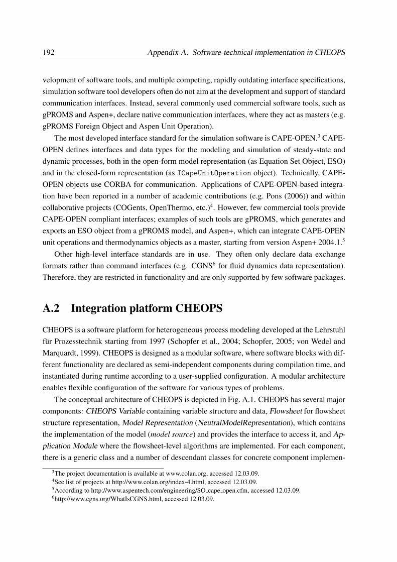
192 Appendix A. Software-technical implementation in CHEOPS
velopment of software tools, and multiple competing, rapidly outdating interface specifications,simulation software tool developers often do not aim at the development and support of standardcommunication interfaces. Instead, several commonly used commercial software tools, such asgPROMS and Aspen+, declare native communication interfaces, where they act as masters (e.g.gPROMS Foreign Object and Aspen Unit Operation).
The most developed interface standard for the simulation software is CAPE-OPEN.3 CAPE-OPEN defines interfaces and data types for the modeling and simulation of steady-state anddynamic processes, both in the open-form model representation (as Equation Set Object, ESO)and in the closed-form representation (as ICapeUnitOperation object). Technically, CAPE-OPEN objects use CORBA for communication. Applications of CAPE-OPEN-based integra-tion have been reported in a number of academic contributions (e.g. Pons (2006)) and withincollaborative projects (COGents, OpenThermo, etc.)4. However, few commercial tools provideCAPE-OPEN compliant interfaces; examples of such tools are gPROMS, which generates andexports an ESO object from a gPROMS model, and Aspen+, which can integrate CAPE-OPENunit operations and thermodynamics objects as a master, starting from version Aspen+ 2004.1.5
Other high-level interface standards are in use. They often only declare data exchangeformats rather than command interfaces (e.g. CGNS6 for fluid dynamics data representation).Therefore, they are restricted in functionality and are only supported by few software packages.
A.2 Integration platform CHEOPS
CHEOPS is a software platform for heterogeneous process modeling developed at the Lehrstuhlfur Prozesstechnik starting from 1997 (Schopfer et al., 2004; Schopfer, 2005; von Wedel andMarquardt, 1999). CHEOPS is designed as a modular software, where software blocks with dif-ferent functionality are declared as semi-independent components during compilation time, andinstantiated during runtime according to a user-supplied configuration. A modular architectureenables flexible configuration of the software for various types of problems.
The conceptual architecture of CHEOPS is depicted in Fig. A.1. CHEOPS has several majorcomponents: CHEOPS Variable containing variable structure and data, Flowsheet for flowsheetstructure representation, Model Representation (NeutralModelRepresentation), which containsthe implementation of the model (model source) and provides the interface to access it, and Ap-plication Module where the flowsheet-level algorithms are implemented. For each component,there is a generic class and a number of descendant classes for concrete component implemen-
3The project documentation is available at www.colan.org, accessed 12.03.09.4See list of projects at http://www.colan.org/index-4.html, accessed 12.03.09.5According to http://www.aspentech.com/engineering/SO cape open.cfm, accessed 12.03.09.6http://www.cgns.org/WhatIsCGNS.html, accessed 12.03.09.
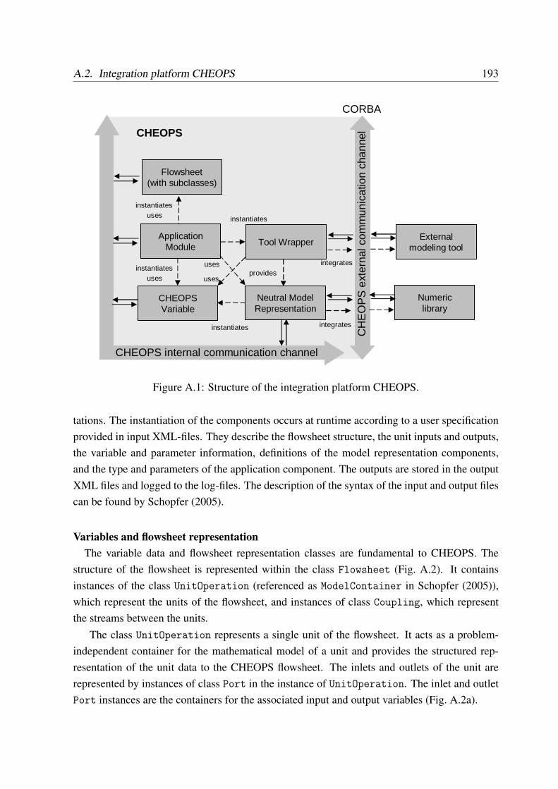
A.2. Integration platform CHEOPS 193
CHEOPS internal communication channelC
HE
OP
S e
xter
nal c
omm
unic
atio
n ch
anne
l
CORBA
Neutral ModelRepresentation
ApplicationModule Tool Wrapper
Flowsheet(with subclasses)
CHEOPSVariable
Externalmodeling tool
providesintegrates
instantiatesuses
instantiates
instantiatesuses
instantiates
uses
Numericlibrary
integrates
CHEOPS
uses
Figure A.1: Structure of the integration platform CHEOPS.
tations. The instantiation of the components occurs at runtime according to a user specificationprovided in input XML-files. They describe the flowsheet structure, the unit inputs and outputs,the variable and parameter information, definitions of the model representation components,and the type and parameters of the application component. The outputs are stored in the outputXML files and logged to the log-files. The description of the syntax of the input and output filescan be found by Schopfer (2005).
Variables and flowsheet representationThe variable data and flowsheet representation classes are fundamental to CHEOPS. The
structure of the flowsheet is represented within the class Flowsheet (Fig. A.2). It containsinstances of the class UnitOperation (referenced as ModelContainer in Schopfer (2005)),which represent the units of the flowsheet, and instances of class Coupling, which representthe streams between the units.
The class UnitOperation represents a single unit of the flowsheet. It acts as a problem-independent container for the mathematical model of a unit and provides the structured rep-resentation of the unit data to the CHEOPS flowsheet. The inlets and outlets of the unit arerepresented by instances of class Port in the instance of UnitOperation. The inlet and outletPort instances are the containers for the associated input and output variables (Fig. A.2a).
194 Appendix A. Software-technical implementation in CHEOPS
Unit Operation
Model Representation
Inputs Outputs
Port 1
Port 2
Port 3
Port 4
Coupling 3
Coupling 4
Coupling 1
Coupling 2
Variable 1
Variable 2
Variable n
Variable Instances
Flowsheet
Unit Operation Coupling
Model Representation Port
CHEOPS VariableUntorn Coupling
Torn Coupling
(a)
(b)1..n1..n
1..n 1..n
1..n1..n11
11
1 1
Figure A.2: Flowsheet classes in CHEOPS: a) scheme; b) UML diagram.
The variables are represented as instances of subclasses derived form the base CHEOPSVariable class. Steady-state and dynamic problems require different variable subclasses.In steady-state problems, ScalarVariable and DiscreteVector are used for scalar quan-tities and vectors of scalars, respectively. For dynamic problems, two most important sub-classes are InterpolationVariable, which represents the variable trajectory in time, andDistributionVariable, which represents the profile of a variable distributed along an inde-pendent coordinate in time.
A Coupling connects the outlet port of one unit to the inlet port of another unit, and containsreferences to the respective Port instances. The ports participating in a coupling must havevariables of identical types. A subclass Torn Coupling derived from Coupling represents atear stream in modular simulation. The treatment of the couplings by the algorithm depends onthe coupling type and the simulation approach employed (Section A.2).
Model sources and model representationsA unit model in CHEOPS is represented by an instance of a subclass derived from the gen-
eral class ModelRepresentation. It is associated with the respective UnitOperation objectduring runtime initialization. It is responsible for the evaluation of the model and for modeldata storage.
CHEOPS supports both the open-form representation of a model source as in Eq. (3.3) and
A.2. Integration platform CHEOPS 195
the closed-form representation as in Eq. (3.11). The same type must be used for the modelrepresentations for all units in the flowsheet. An open-form model representation is used for theequation-oriented simulation, and should comply to the requirements of the DAE solver (i.e.,states, residuals and Jacobian entries of a DAE system must be provided by the model source).An implementation of open-form model type is the class OpenFormModelRepresentation.An open-form model source in CHEOPS is typically a CAPE-OPEN ESO object, from gPROMS(Appendix A.8) or another software tool.
The closed-form model representation class ClosedFormModelRepresentation is em-ployed in the modular simulation. This model source is usually implemented in an externalsoftware tool. It encapsulates the solver and only provides the input and output information andthe solver command interface. Since the variable types and command interface differ for thesteady-state and the dynamic modular simulation, corresponding subclasses are derived fromthe class ClosedFormModelRepresentation for the steady-state and the dynamic simulation.
Tool wrappers are special components for communication between CHEOPS and externaltools employed in the simulation. The ToolWrapper base classes are derived from the afore-mentioned closed-form steady-state and dynamic model representation classes and declare theabstract functionality expected by CHEOPS. Specific software tool wrapper components arederived from these base classes and comply to their interfaces, but differ in the tool-specific im-plementation of the functions. A brief description of the tool wrappers employed in the presentthesis can be found further in this Appendix.
Implementation of simulation algorithmsThe flowsheet-level algorithms are implemented and executed by the Application Module
component of CHEOPS. The classes containing specific flowsheet-level algorithms are derivedfrom the base class ApplicationModule. SteadyStateEquationOrientedSimulation-
Module and DynamicEquationOrientedSimulationModule are dedicated classes for, re-spectively, steady-state and dynamic equation-oriented simulation algorithms. They constructa flowsheet equation system object by aggregating the unit ESOs provided by the open-formmodel representations. It is then solved by an appropriate solver from the CHEOPS solverlibrary lptNumerics (Schopfer, 2005). Couplings between the units are specified as identityrelations in the flowsheet ESO.
Class DynamicSequentialModularSimulationModule implements of the sequential mod-ular algorithm for dynamic flowsheet simulation as described in Section 3.2.4. It uses severalauxiliary classes where specific steps of the algorithm are implemented. Class DAEIntegration-RangeAdjuster is responsible for the adjustment of the length of an integration interval accord-ing to Eq. (3.26)–(3.27). Class DAETornCouplingHandler performs the convergence check(3.25) for every torn coupling. Class DAETornCouplingUpdater implements the tear stream
196 Appendix A. Software-technical implementation in CHEOPS
update procedure for every torn coupling (Section 3.2.2). Class DAETornCouplingNewProfile-Generator predicts the trajectory of the variables in the torn coupling on the next integrationinterval according to Eq. (3.28). This component-wise design and the runtime instantiationof the auxiliary algorithm components enables flexible configuration of the dynamic modularsimulation algorithm, and its easy extension with the further methods.
Class SteadyStateSequentialModularSimulationModule implements a sequential mod-ular simulation algorithm for steady-state problems (Schopfer, 2005). Further application classesinvolve steady-state parameter estimation and simulation of the flowsheets with ”grey box”models.
Specifying a simulation in CHEOPSA specification of a flowsheet case study in CHEOPS involves
• the specification of the flowsheet structure in CHEOPS;
• the specification of the mapping files, which contain the mapping to the model sourcevariables and functions;
• the specification of the inputs and outputs of each unit;
• the specification of the flowsheet solver type and its options;
• the specification of the tool wrapper and solver options.
The specifications are read from the XML files with a documented formatting.
Handling of compartment topology in CHEOPSCHEOPS variables do not contain information about their spatial discretization and location
in the domain. The architecture of CHEOPS dictates that CHEOPS variables are always definedin a specific unit, port and compartment. This poses some restrictions on handling discretiza-tions and compartment adaptation in CHEOPS. At present, only coarse-scale (compartment)information can be transferred, and the number of compartments cannot be changed. However,the compartment layout, the number of interfaces and their topology may change during adap-tation. To set up the adapted topology in the other CHEOPS units, the topology is transferredthere by means of CHEOPS topology data files.
The topology data file has an XML-format and contains the volume and masses of suspen-sion components in the compartment, list of compartment interfaces and their properties, list ofadjacent compartments and the origin (previous) compartment layout. The list of interfaces andtheir adjacent zones is used to set up the new compartment and stream topology. To take intoaccount the changing number and names of the interfaces, the template tags in the XML-file
A.3. FLUENT Wrapper 197
are employed to indicate that respective interface names must be substituted during runtime.The information on the origin compartment layout is used to compute new initial states in theadapted compartments for the variables not available from the fine-scale grid (such as PSD)by evaluating V new
q φnewq =
∑NQ
q′=1 V originq,q′ φorigin
q , where q and q′ are indices of the adapted andorigin compartment, respectively.
Extending CHEOPSThe base components discussed in the previous sections (variable, flowsheet, model repre-
sentation and application components) form the core of CHEOPS. The core is compiled as asingle library. Calls within the core are performed by standard C++ mechanisms.
CHEOPS can be easily extended by developing further variable types, application algo-rithms, model representations and tool wrapper components conforming to the interfaces of thebase components. All but tool wrapper components need to be incorporated into the CHEOPScore. Tool wrapper components can be compiled as separate libraries accessed using C++ orCORBA-calls.
A.3 FLUENT Wrapper
FLUENT is a popular solver for fluid dynamics problems with a broad range of applications.FLUENT can solve continuity, momentum, energy, turbulence, species and user-defined scalartransport equations. The user can specify phenomena and source terms to be included into themodel. The computation is performed on a continuous domain meshed into a large number ofcells separated by the interfaces. The cells are treated as finite volumes, on which the modelequations are discretized and solved (Section 2.2.2). The cells can be grouped to compartments,which boundaries can be determined by the user. The user can modify the type of compartmentand its boundary (”transparent”, wall, inlet, etc.), and change the phenomena models included,respective source terms, inputs and boundary conditions.
The specifications can be done using both the graphics user interface and the commandconsole interface. The command console interface uses FLUENT text commands based onScheme language. The list of console commands is provided in FLUENT Text Command Guideand by Javurek (2004).
A powerful feature of FLUENT is the support of user-defined terms and functions. User-defined terms involve user-defined scalars (UDS), for which transport equations are solved,and user-defined memory (UDM). FLUENT defines several types of user-defined functions(see FLUENT User’s Guide for a full list). Important function types are DEFINE SOURCE -definition of a source term for a given FLUENT variable; DEFINE INIT - initialization of a
198 Appendix A. Software-technical implementation in CHEOPS
FLUENT variable; DEFINE ADJUST - update of a FLUENT variable during the iterations; andDEFINE PROFILE - specification of the variable profile at a boundary. User-defined functionsare written in C and can access many FLUENT variables using internal macros. They can beprecompiled to a library and loaded together with the model case file.
FLUENT can be considered as a special-purpose simulator that defines a closed-form modelsource in terms of CHEOPS. All physical state variables and user-defined quantities can be setas inputs and accessed as outputs, but no information about the equation structure and respectiveJacobians is available.
Software-technical implementation of the FLUENT WrapperThe implementation of the FLUENT Wrapper used for communication between CHEOPS
and FLUENT in this thesis refers to FLUENT v.6.0.FLUENT is designed for use as stand-alone software. There is no officially released external
interface for FLUENT. There are, however, several ways to connect to FLUENT. Bezzo (2002)uses a coupling mechanism with the FLUENT solver code in his work on coupling betweenFLUENT and gPROMS. This requires access to FLUENT solver code, which was not availablein this thesis.
The solution employed in this work makes use of an undocumented feature of the UNIX-platform version of FLUENT, where console inputs and outputs can be redirected to the UNIXpipes, a special kind of file in UNIX-based systems. Communication through the pipes createdby the wrapper during initialization enables full control over the program by the wrapper. Theinput pipe provides the console input to FLUENT as text and Scheme commands. The consoleoutputs are stored in the output pipe and are parsed by the wrapper.
FLUENT console commands are used to execute control over the simulation, to set initialand boundary conditions for the compartments and perform standard reporting for the variablesin the zones. The tasks, which are performed during the integration, or which require accessto the fine grid information, have to be implemented in user-defined functions. These tasks in-volve complex reporting, analysis of the compartment topology, update of model source terms,boundary conditions and profiles. When a series of commands has to be executed at one time,journal files containing a prescribed series of FLUENT console commands are executed.
The structure of the FLUENT wrapper thus consists of two layers (Fig. A.3). The ”upper”wrapper layer is a descendant of the ToolWrapper component of CHEOPS and is implementedin C++ as a library in CHEOPS. It communicates with FLUENT via pipes, executes FLUENTconsole commands and parses their outputs. The ”lower” wrapper layer functions are imple-mented in a UDF library, which is developed in C++ as a separate code, compiled and loadedin FLUENT together with the case file. The case file contains references to the functions of thisUDF library used. Some ”lower” layer functions are called from the ”upper” layer using Exe-
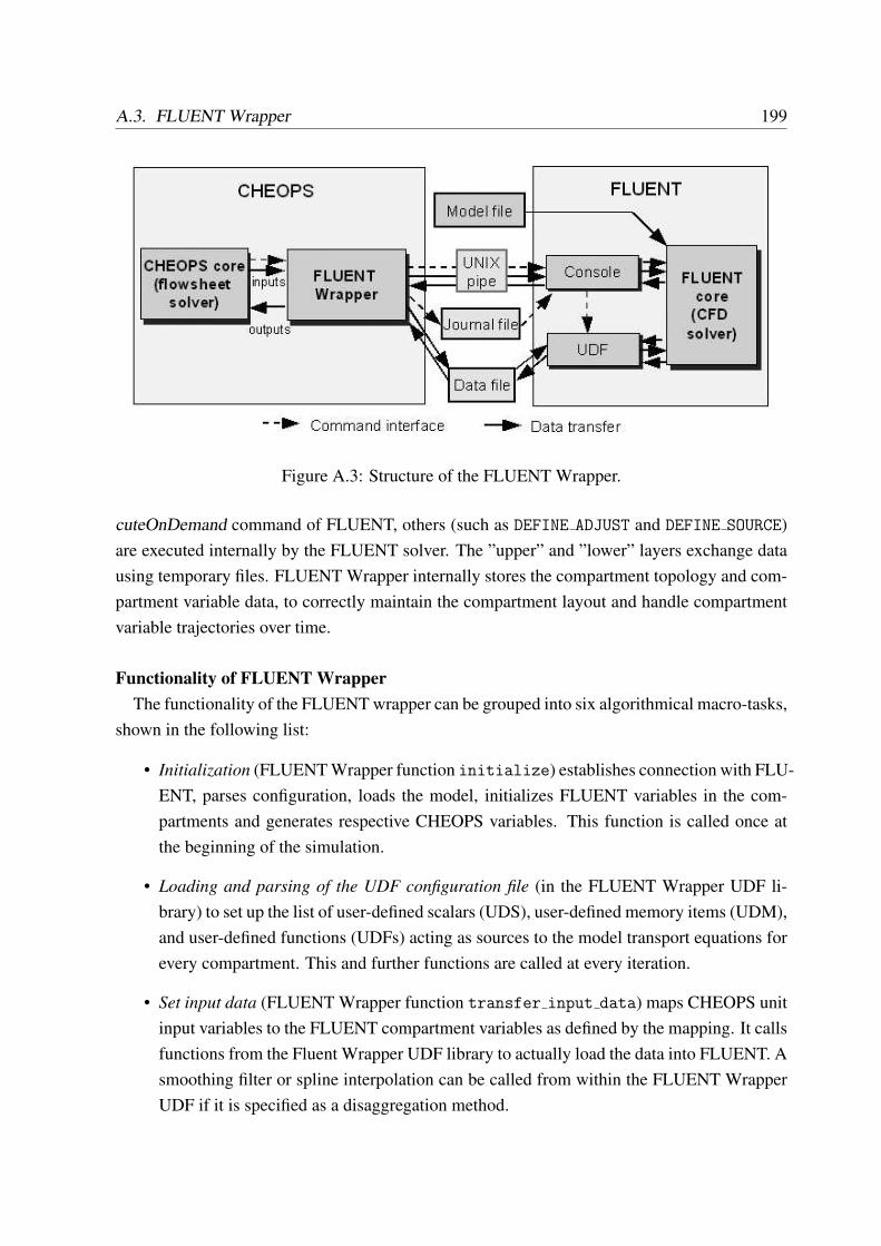
A.3. FLUENT Wrapper 199
Figure A.3: Structure of the FLUENT Wrapper.
cuteOnDemand command of FLUENT, others (such as DEFINE ADJUST and DEFINE SOURCE)are executed internally by the FLUENT solver. The ”upper” and ”lower” layers exchange datausing temporary files. FLUENT Wrapper internally stores the compartment topology and com-partment variable data, to correctly maintain the compartment layout and handle compartmentvariable trajectories over time.
Functionality of FLUENT WrapperThe functionality of the FLUENT wrapper can be grouped into six algorithmical macro-tasks,
shown in the following list:
• Initialization (FLUENT Wrapper function initialize) establishes connection with FLU-ENT, parses configuration, loads the model, initializes FLUENT variables in the com-partments and generates respective CHEOPS variables. This function is called once atthe beginning of the simulation.
• Loading and parsing of the UDF configuration file (in the FLUENT Wrapper UDF li-brary) to set up the list of user-defined scalars (UDS), user-defined memory items (UDM),and user-defined functions (UDFs) acting as sources to the model transport equations forevery compartment. This and further functions are called at every iteration.
• Set input data (FLUENT Wrapper function transfer input data) maps CHEOPS unitinput variables to the FLUENT compartment variables as defined by the mapping. It callsfunctions from the Fluent Wrapper UDF library to actually load the data into FLUENT. Asmoothing filter or spline interpolation can be called from within the FLUENT WrapperUDF if it is specified as a disaggregation method.
200 Appendix A. Software-technical implementation in CHEOPS
• Simulation control (function compute) sets the solver time step and its parameters, ini-tializes the simulation and performs integration on the interval. During the integration,DEFINE ADJUST functions from the FLUENT Wrapper UDF library, used in the model,are automatically evaluated by FLUENT to update the values of the input variables atthe current time and current iteration, and to calculate expressions involving FLUENTvariables (e.g. growth rate computed as a function of temperature and component con-centration).
• Get output data (function transfer output data) evaluates the output FLUENT vari-ables in the compartments at every reporting time step and stores their trajectory into theCHEOPS unit output variables as defined by the mapping. It calls FLUENT reportingcommands to compute integrals and compartment-averaged values for these variables.This code, therefore, implements the aggregation.
• Saving and restoring solution at given time point is done by FLUENT Wrapper functionssave current state and restore state by tag.
• Adaptation (function adapt zones) performs adaptation of the compartment layout. It isperformed in two steps. First, the adaptation criterion is computed for all compartmentsby a FLUENT Wrapper UDF, to identify compartments to be adapted and find out the newcompartment layout. Second, the compartment layout is actually modified in FLUENTby executing respective FLUENT commands from the FLUENT Wrapper. The boundaryconditions of the new compartments in the topology are inherited from the respective oldtopology compartments. The updated topology is saved to an external file to be availableto other CHEOPS units.
Mapping specificationThe mapping between CHEOPS variable and FLUENT variable is provided as an XML file
for all CHEOPS variables. Every input variable of the CHEOPS unit is referred to by its portname, variable tag and type. It is mapped to a respective FLUENT variable, referred to byits compartment name, FLUENT variable name, as well as the UDF function type if the vari-able data is a trajectory over time, updated in FLUENT during the iterations. The respectiveUDF function type is DEFINE ADJUST for the trajectories of all compartment variables (suchas temperatures, concentrations or source terms), and DEFINE PROFILE for the trajectories ofcompartment boundary variables such as fluxes.
Similarly, every output variable of the CHEOPS unit is referred to by its port name, vari-able tag and type. The mapping on the FLUENT side is, however, different for compartmentvariables and compartment boundary variables. In case of the compartment variables, we need
A.4. Parsival Wrapper 201
to specify the compartment name, variable name and name of the FLUENT or UDF reportingfunction, which calculates the aggregated value of the specified variable in the compartment(volumetric integral, volumetric average, etc.). In case of compartment boundary variables, wealso need to specify the boundary index, and eventually map it to the interface between com-partments in the CHEOPS topology. If the index of an interface is not known, e.g. because ofadaptation, a mechanism of automatic enumeration is employed. Reporting functions can beused to calculate variable fluxes through the compartment boundary, which are evaluated eitherto the currently mapped or to another specified reference compartment.
FLUENT Wrapper accepts a number of optional parameters to control options such as num-ber of iterations, number of solver time steps, topology adaptation flag, etc.
A.4 Parsival Wrapper
Parsival is a special-purpose simulator for crystallization processes modeled by means of pop-ulation balance equations. The crystallization process is represented in Parsival by means ofkinetic modules for a large set of crystallization kinetics phenomena, including primary nucle-ation, growth, attrition, agglomeration, breakage and crystal dissolution. Using these modules,Parsival internally formulates an integral dynamic population balance equation (2.4) assumingideal mixing within the unit, and solves it to compute the change of the particle size distributionover time. The user is responsible for writing the functions to compute the rates of the specifiedprocess kinetics. Along with the population balance, a solute concentration and overall massbalance are intrinsically calculated. Parsival employs the condition of mixed product removalunless a classification function is used.
Parsival does not provide information on the solved equation system, its states and deriva-tives, and is a closed-form model source in terms of CHEOPS.
Software-technical implementation of Parsival WrapperIn normal operation, a Parsival model is defined by the user in the Parsival GUI and then
solved by the tool. The outputs are shown in graphs, which can be exported from Parsival.
Parsival supports a communication interface based on the COM technology to communicatewith an external software application. This interface provides a number of functions to controlthe simulation and get outputs during the runtime, but has limited capabilities to set inputs.
The Parsival model file has a readable text format, and contains a description of the units,streams, kinetic modules and initial states of the system. The evolution of the inputs over time,the initial PSD and the feed PSD can be given by external files. This enables the wrapper tomodify the model and data files prior to the start of the simulation to update the initial states
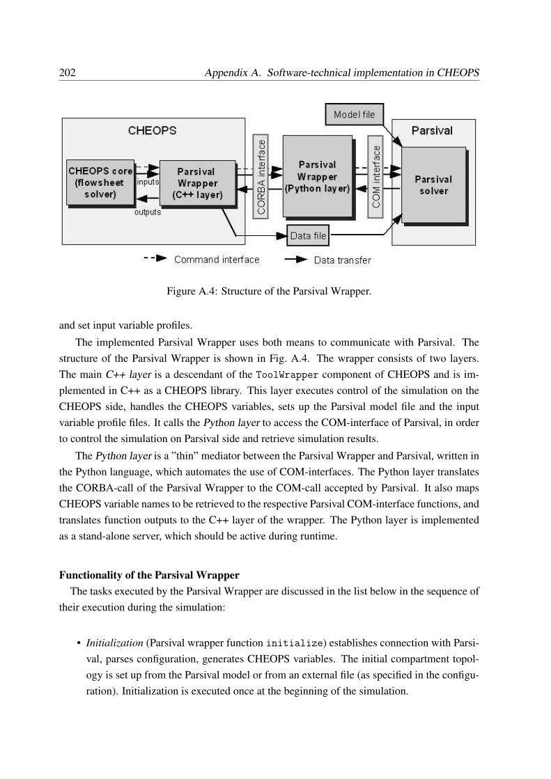
202 Appendix A. Software-technical implementation in CHEOPS
Figure A.4: Structure of the Parsival Wrapper.
and set input variable profiles.
The implemented Parsival Wrapper uses both means to communicate with Parsival. Thestructure of the Parsival Wrapper is shown in Fig. A.4. The wrapper consists of two layers.The main C++ layer is a descendant of the ToolWrapper component of CHEOPS and is im-plemented in C++ as a CHEOPS library. This layer executes control of the simulation on theCHEOPS side, handles the CHEOPS variables, sets up the Parsival model file and the inputvariable profile files. It calls the Python layer to access the COM-interface of Parsival, in orderto control the simulation on Parsival side and retrieve simulation results.
The Python layer is a ”thin” mediator between the Parsival Wrapper and Parsival, written inthe Python language, which automates the use of COM-interfaces. The Python layer translatesthe CORBA-call of the Parsival Wrapper to the COM-call accepted by Parsival. It also mapsCHEOPS variable names to be retrieved to the respective Parsival COM-interface functions, andtranslates function outputs to the C++ layer of the wrapper. The Python layer is implementedas a stand-alone server, which should be active during runtime.
Functionality of the Parsival WrapperThe tasks executed by the Parsival Wrapper are discussed in the list below in the sequence of
their execution during the simulation:
• Initialization (Parsival wrapper function initialize) establishes connection with Parsi-val, parses configuration, generates CHEOPS variables. The initial compartment topol-ogy is set up from the Parsival model or from an external file (as specified in the configu-ration). Initialization is executed once at the beginning of the simulation.
A.4. Parsival Wrapper 203
• Update of the compartment topology is performed at the first iteration on every interval ifthe topology update flag is set in the configuration. The compartment topology informa-tion is updated from the file provided by CHEOPS. The list of compartments, connectingstreams and the kinetic modules in the Parsival model file are updated by the ParsivalWrapper to match the loaded compartment topology.
• Set input data (function update input variables) maps CHEOPS unit input variablesto Parsival model variables as defined by the mapping, updates their initial states andstores the variable trajectories in the data files referenced by the model. After this, themodel loaded into Parsival has an updated topology, initial states and all input variabletrajectories. This and further tasks are executed at every iteration.
• Simulation control (function compute) loads the model in Parsival, configures the solvertime step and the solver parameters in Parsival, initializes simulation, calls the runtimeupdate of input variables and performs integration for all reporting time steps in the inter-val.
• Runtime update (function update runtime variables) updates the Parsival input vari-ables at every reporting time step with data from the mapped CHEOPS input variables.However, it is preferred to use set input data instead.
• Get output data (function get output variables) evaluates the requested Parsival vari-ables at every reporting time step and stores the trajectory in CHEOPS unit output vari-ables as defined by the mapping.
• Save state and restore state are executed by tool wrapper functions save current state
and restore state by tag.
Mapping specification and wrapping optionsSimilarly to the FLUENT wrapper, the mapping between CHEOPS and FLUENT variables is
provided as an XML file with a specified format, common for both the inputs and outputs. TheCHEOPS variables are referred to by their port name, variable tag and type, and mapped to theParsival variables specified by their names in the Parsival model file. An additional parameterspecifies the method used to transfer variable data between CHEOPS and Parsival, e.g. inputvariable trajectory saving (in set input data task) or runtime update for the input variables. Forevery variable, the function of the Parsival COM-interface to be called is internally determinedby the Parsival wrapper based on the specified data transfer method and the variable name in theParsival model file. It is also possible to get an output from a user-specified function in Parsival.
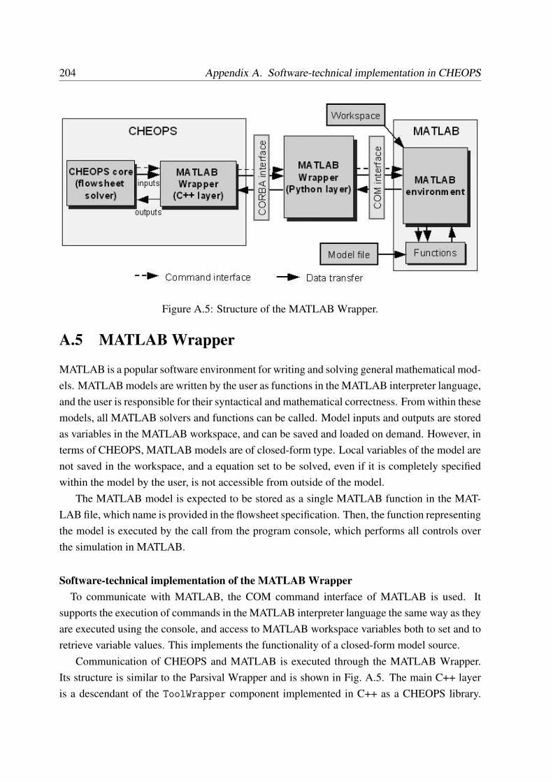
204 Appendix A. Software-technical implementation in CHEOPS
Figure A.5: Structure of the MATLAB Wrapper.
A.5 MATLAB Wrapper
MATLAB is a popular software environment for writing and solving general mathematical mod-els. MATLAB models are written by the user as functions in the MATLAB interpreter language,and the user is responsible for their syntactical and mathematical correctness. From within thesemodels, all MATLAB solvers and functions can be called. Model inputs and outputs are storedas variables in the MATLAB workspace, and can be saved and loaded on demand. However, interms of CHEOPS, MATLAB models are of closed-form type. Local variables of the model arenot saved in the workspace, and a equation set to be solved, even if it is completely specifiedwithin the model by the user, is not accessible from outside of the model.
The MATLAB model is expected to be stored as a single MATLAB function in the MAT-LAB file, which name is provided in the flowsheet specification. Then, the function representingthe model is executed by the call from the program console, which performs all controls overthe simulation in MATLAB.
Software-technical implementation of the MATLAB WrapperTo communicate with MATLAB, the COM command interface of MATLAB is used. It
supports the execution of commands in the MATLAB interpreter language the same way as theyare executed using the console, and access to MATLAB workspace variables both to set and toretrieve variable values. This implements the functionality of a closed-form model source.
Communication of CHEOPS and MATLAB is executed through the MATLAB Wrapper.Its structure is similar to the Parsival Wrapper and is shown in Fig. A.5. The main C++ layeris a descendant of the ToolWrapper component implemented in C++ as a CHEOPS library.
A.6. Aspen and HYSYS Wrappers 205
Similar to the Parsival Wrapper, the C++ layer handles the CHEOPS variables and executescontrol over the simulation. The Python layer is a ”thin” mediator written in Python, whichtranslates between the CORBA-calls made by the C++ layer of the MATLAB Wrapper and theCOM-communication with MATLAB. It is also implemented as a separate server and shouldbe active during the runtime.
Functionality of the MATLAB WrapperSince MATLAB provides direct access to all workspace variables by their names through
the COM-interface, no handling of complex objects and specialized functions is necessary, andthe code for the MATLAB Wrapper is much simpler than for the FLUENT or the ParsivalWrappers.
The MATLAB Wrapper fulfils the usual tasks of tool wrappers, such as initialization, trans-fer of input variables, control over the simulation and retrieval of output variables. Initialization(function initialize) establishes connection with MATLAB through the Python layer, parsesconfiguration and generates CHEOPS variables. The transfer of input data is done by a call tothe MATLAB COM-function for specified input variables. It stores the current value of thesevariables in the MATLAB workspace. The names of the workspace variables are specified inthe mapping. The function is executed at every reporting time step for the inputs and at thebeginning of each interval for the CHEOPS variables marked as parameters. After all variablesare set, the compute function executes the model, calling it as a MATLAB function with thelist of MATLAB workspace variables acting as its inputs and outputs. The outputs are retrievedby requesting the current values of the output MATLAB workspace variables via MATLABCOM-interface. MATLAB Wrapper also supports saving and restoring the current workspace.
Mapping specificationThe mapping between the CHEOPS and MATLAB variables is given by an XML file. Each
CHEOPS variable is referred to by their port name, variable tag and type, and mapped to theMATLAB workspace variable specified by its name. The mapping file is concluded with twolines that provide the input and output argument list for the MATLAB model function. Inputarguments are MATLAB variable names or numbers; output arguments are MATLAB variablenames. The user is responsible for the correctness of the variable names, which appear asarguments in the mapping.
A.6 Aspen and HYSYS Wrappers
Aspen+ and HYSYS belong to the family of commercial flowsheet simulators. They are popu-lar for the simulation of flowsheets with units represented by standard models. Aspen+ typically
206 Appendix A. Software-technical implementation in CHEOPS
performs steady-state simulation of the flowsheet, while AspenDynamics and HYSYS are usu-ally used for the dynamic simulation. The tools are particularly well suited for fluid-phaseprocess modeling with established models. A useful feature is the built-in data bank of sub-stance properties. The tools can be conveniently used in modular simulation with CHEOPS forthe representation of those process subsystems where detailed models are not necessary.
Both, Aspen+ and HYSYS act as closed-form model sources in terms of CHEOPS. Theysupport the access to the physical variables (states, input and outputs), and the commands nec-essary to control the simulation through their intrinsic COM-interface.
The technical solution for the HYSYS Wrapper is very similar to the solution employed forthe MATLAB Wrapper. It involves a C++ layer on the CHEOPS side to control the simulationand to transfer the input and output data between CHEOPS and HYSYS through the ”thin”mediator in Python. The mapping in HYSYS involves the specification of the unit, port andvariables in the port, which may bear the same names as the CHEOPS ports and variables.
The wrapper for Aspen+ is written in a similar way. It is not used in the present thesis.
A.7 lptNumerics: a general-purpose solver library
General-purpose solver libraries are composed of available solvers for various classes of math-ematical problems, usually of academic origin. These solvers can be developed internally or areavailable under public license. They are often used as alternatives to the commercial softwaretools.
LPT uses an internally developed library lptNumerics. The library is developed to providethe functionality for processing and solving unit or flowsheet models provided as equation sys-tems in form of a CAPE-OPEN ESO (Schopfer et al, 2005). It contains a number of solvers andtheir respective wrapper components, which implement the mapping between the objects andinterfaces of the solver code and CHEOPS interfaces. The library contains solvers and wrappersfor the steady-state simulation of large algebraic equation systems (NLEQ1s, NLEQ2) (Nowakand Weinmann, 1991), and for the dynamic simulation of DAE systems (LIMEX, Deuflhardt etal. (1987)). The solver LIMEX is used in the present thesis.
Besides the solvers and their wrappers, lptNumerics provides a number of auxiliary classesactively employed in CHEOPS, in particular, for the support of operations (aggregation, externalspecification, etc.) with ESO objects. Schopfer et al (2005) provide further details on the use oflptNumerics in CHEOPS applications.
A.8. Wrapper for gPROMS ESO 207
A.8 Wrapper for gPROMS ESO
The commercial modeling environment and general-purpose solver gPROMS has been devel-oped for the representation and solution of mathematical models, involving steady-state anddynamic DAE and PDAE systems, discrete and continuous models, etc. The models are writ-ten as equations in the gPROMS modeling language. Consistency and well-posedness of theequation system is the responsibility of the user, but gPROMS verifies them before starting thesolver.
A gPROMS model is usually solved by gPROMS internal DAE solver. However, gPROMSis capable to provide a CAPE-OPEN ESO object, which is an open-form model source in termsof CHEOPS. The ESO object is wrapped in CHEOPS by the OpenFormModelRepresentationclass and can be used for the equation-oriented simulation of the flowsheet. Then, the flowsheetsimulation algorithm in CHEOPS calls necessary solver codes from the solver library lptNu-merics. The CHEOPS Programmer’s Guide provides details about wrapping of an ESO objectin CHEOPS.
Alternatively, the ESO can be transformed to closed form for use in the modular simulation,by employing the Open-to-Closed Form Bridge component (Schopfer, 2005), where a DAEsolver from the CHEOPS solver library is attached to the ESO as its solving procedure. Thissolution is employed in the present thesis.
Appendix B
Models of pentaerythritol flowsheetproblem
B.1 Crystallization kinetics
A population balance model for the considered crystallizer model under the assumption of con-stant volume and ideal mixing within the crystallizer is formulated as:
Vcr∂n(L, t)
∂t+ Vcr
∂Geff (σ, L)n(L, t)
∂l+ V cr
p n(L, t) = Vcr B(σ, L). (B.1)
The initial condition is n(L, 0) = n0(L), the boundary condition is n(0, t) = 0.
The kinetic phenomena in Eq. (B.1) are growth, attrition and secondary nucleation. Theattrition is modeled by a negative growth rate Gatt(L), which accounts for abrasion of largecrystals, and the nucleation rate B(σ, L), which introduces the attrited fragments. The crystalsare also subject to the kinetic growth rate Gkin(σ, L). Hence, an effective growth rate of thecrystals Geff (σ, L) is
Geff (σ, L) = Gkin(σ, L)−Gatt(L). (B.2)
The crystal growth rate, Gkin(σ, L), is a function of the supersaturation of the solution andthe crystal size:
Gkin(σ, L) = kkinσ
(1− exp
(− L
p1
)p2)
. (B.3)
The supersaturation is defined as σ = wws− 1, where w is a mass fraction of the solute, and
ws is its value in the saturated solution. p1 and p2 are empirical parameters.
208
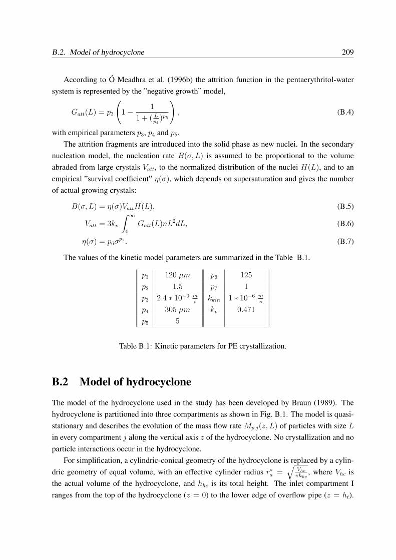
B.2. Model of hydrocyclone 209
According to O Meadhra et al. (1996b) the attrition function in the pentaerythritol-watersystem is represented by the ”negative growth” model,
Gatt(L) = p3
(1− 1
1 + ( Lp4
)p5
), (B.4)
with empirical parameters p3, p4 and p5.The attrition fragments are introduced into the solid phase as new nuclei. In the secondary
nucleation model, the nucleation rate B(σ, L) is assumed to be proportional to the volumeabraded from large crystals Vatt, to the normalized distribution of the nuclei H(L), and to anempirical ”survival coefficient” η(σ), which depends on supersaturation and gives the numberof actual growing crystals:
B(σ, L) = η(σ)VattH(L), (B.5)
Vatt = 3kv
∫ ∞
0
Gatt(L)nL2dL, (B.6)
η(σ) = p6σp7 . (B.7)
The values of the kinetic model parameters are summarized in the Table B.1.
p1 120 µm p6 125
p2 1.5 p7 1
p3 2.4 ∗ 10−9 ms
kkin 1 ∗ 10−6 ms
p4 305 µm kv 0.471
p5 5
Table B.1: Kinetic parameters for PE crystallization.
B.2 Model of hydrocyclone
The model of the hydrocyclone used in the study has been developed by Braun (1989). Thehydrocyclone is partitioned into three compartments as shown in Fig. B.1. The model is quasi-stationary and describes the evolution of the mass flow rate Mp,j(z, L) of particles with size L
in every compartment j along the vertical axis z of the hydrocyclone. No crystallization and noparticle interactions occur in the hydrocyclone.
For simplification, a cylindric-conical geometry of the hydrocyclone is replaced by a cylin-dric geometry of equal volume, with an effective cylinder radius r∗a =
√Vhc
πhhc, where Vhc is
the actual volume of the hydrocyclone, and hhc is its total height. The inlet compartment Iranges from the top of the hydrocyclone (z = 0) to the lower edge of overflow pipe (z = ht).
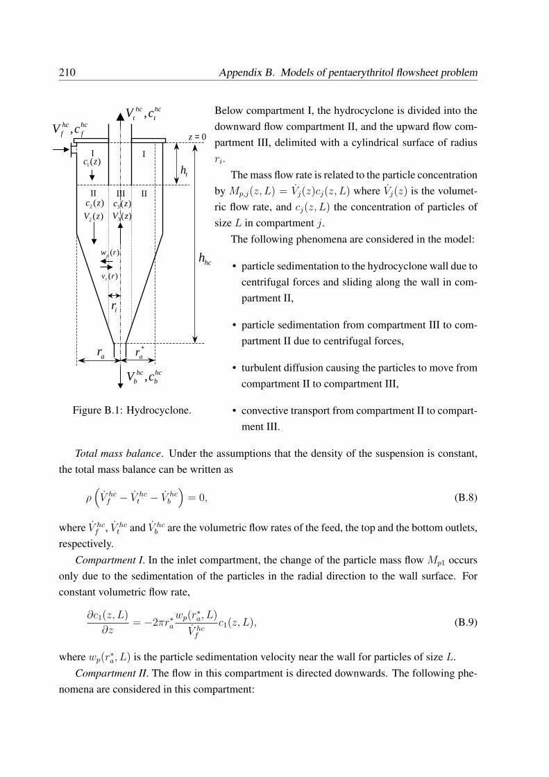
210 Appendix B. Models of pentaerythritol flowsheet problem
th
hch
*arar
I I
II IIIII
ir
hcf
hcf cV ,
)(1 zc
hct
hct cV ,
)(2 zc )(3 zc
)(2 zV )(3 zV
hcb
hcb cV ,
0=z
)(rwp
)(rvr
Figure B.1: Hydrocyclone.
Below compartment I, the hydrocyclone is divided into thedownward flow compartment II, and the upward flow com-partment III, delimited with a cylindrical surface of radiusri.
The mass flow rate is related to the particle concentrationby Mp,j(z, L) = Vj(z)cj(z, L) where Vj(z) is the volumet-ric flow rate, and cj(z, L) the concentration of particles ofsize L in compartment j.
The following phenomena are considered in the model:
• particle sedimentation to the hydrocyclone wall due tocentrifugal forces and sliding along the wall in com-partment II,
• particle sedimentation from compartment III to com-partment II due to centrifugal forces,
• turbulent diffusion causing the particles to move fromcompartment II to compartment III,
• convective transport from compartment II to compart-ment III.
Total mass balance. Under the assumptions that the density of the suspension is constant,the total mass balance can be written as
ρ(V hc
f − V hct − V hc
b
)= 0, (B.8)
where V hcf , V hc
t and V hcb are the volumetric flow rates of the feed, the top and the bottom outlets,
respectively.Compartment I. In the inlet compartment, the change of the particle mass flow Mp1 occurs
only due to the sedimentation of the particles in the radial direction to the wall surface. Forconstant volumetric flow rate,
∂c1(z, L)
∂z= −2πr∗a
wp(r∗a, L)
V hcf
c1(z, L), (B.9)
where wp(r∗a, L) is the particle sedimentation velocity near the wall for particles of size L.
Compartment II. The flow in this compartment is directed downwards. The following phe-nomena are considered in this compartment:
B.2. Model of hydrocyclone 211
• particle sedimentation and counteracting convective transport in the radial direction withvelocity vr(ri),
mp32(z, L) = 2πri(wp(ri, L)− vr(ri))c3(z, L), (B.10)
• turbulent diffusion counteracting particle sedimentation in the radial direction,
mp23(z, L) = 2πriDp(L)
(r∗a − ri)(c2(z, L)− c3(z, L)), (B.11)
• particle removal from the compartment at the outer wall of the hydrocyclone due to sedi-mentation in axial direction,
mp2(z, L) = 2πr∗awp(r∗a, L)c2(z, L). (B.12)
The particle mass flow Mp2 is determined as
∂Mp2(z, L)
∂z= −mp2(z, L)− mp23(z, L) + mp32(z, L). (B.13)
The volumetric flow rate V2(z) in compartment II is calculated as
V2(z) = V hcf +
V hcb − V hc
f
hhc − ht
(z − ht). (B.14)
The differential equation for the particle concentration in compartment II is
∂c2(z, L)
∂z=
1
V2(z)
[− V hc
b − V hcf
hhc − ht
c2(z, L)− 2πr∗awp(r∗a, L)c2(z, L)−
−2πriDp(L)
r∗a − ri
(c2(z, L)− c3(z, L)
)+
+2πric3(z, L)(wp(ri, L)− vr(ri)
)]. (B.15)
The particle sedimentation velocity wp(ri, L) and the fluid radial velocity vr(ri) are evaluatedat the surface delimiting compartments II and III. Dp(L) is a turbulent diffusion coefficient forthe particles. Braun (1989) provides guidelines for computation of these quantities.
Compartment III. The flow in compartment III is directed upwards. Thus, the local particlebalance for the compartment is computed as
−∂Mp3(z, L)
∂z= mp23(z, L)− mp32(z, L). (B.16)
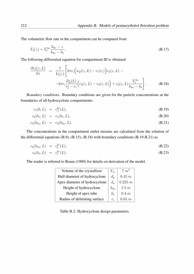
212 Appendix B. Models of pentaerythritol flowsheet problem
The volumetric flow rate in the compartment can be computed from
V3(z) = V hct
hhc − z
hhc − ht
. (B.17)
The following differential equation for compartment III is obtained:
∂c3(z, L)
∂z=
1
V3(z)
[2πri
(wp(ri, L)− vr(ri)
)c3(z, L)−
−2πriDp(L)
r∗a − ri
(c2(z, L)− c3(z, L)
)+ c3(z, L)
V hct
hhc − ht
]. (B.18)
Boundary conditions. Boundary conditions are given for the particle concentrations at theboundaries of all hydrocyclone compartments:
c1(0, L) = chcf (L), (B.19)
c2(ht, L) = c1(ht, L), (B.20)
c3(hhc, L) = c2(hhc, L). (B.21)
The concentrations in the compartment outlet streams are calculated from the solution ofthe differential equations (B.9), (B.15), (B.18) with boundary conditions (B.19-B.21) as
c2(hhc, L) = chcb (L), (B.22)
c3(ht, L) = chct (L). (B.23)
The reader is referred to Braun (1989) for details on derivation of the model.
Volume of the crystallizer Vcr 7 m3
Hull diameter of hydrocyclone dp 0.45 m
Apex diameter of hydrocyclone da 0.225 m
Height of hydrocyclone hhc 1.5 m
Height of apex tube ht 0.4 m
Radius of delimiting surface ri 0.05 m
Table B.2: Hydrocyclone design parameters.
Appendix C
Derivation of the residence time transportequation
Residence time distributionThe residence time distribution (RTD) of a vessel is often obtained using a tracer experiment.
The tracer is injected at the inlet with known concentration profile cin(τ). Its concentrationis measured at the location of interest (typically at the output) to obtain cout(τ). From thisresponse, the residence time distribution can be easily computed.
In case the inlet tracer concentration is given by c0 multiplied to the Heaviside function,H(τ) which is equal to 1 if τ ≥ 0, and 0 otherwise, the dimensionless response functionis calculated as F (τ) = cout(τ)
c0and is a cumulative residence time distribution with τ as a
residence time coordinate. The residence time distribution density function (RTD) E(τ) with∫∞0
E(τ)dτ = 1 is then obtained by differentiation:
E(τ) =dF (τ)
dτ=
1
c0
dcout(τ)
dτ. (C.1)
If the RTD is known, mean residence time is computed from it as its first moment (Danck-werts, 1953):
τ =
∫ ∞
0
τE(τ)dτ. (C.2)
Assuming that the tracer concentration profile has a finite time to steady-state, E(τ) = 0 forτ > τs, and therefore
τ =
∫ τs
0
τE(τ)dτ. (C.3)
213
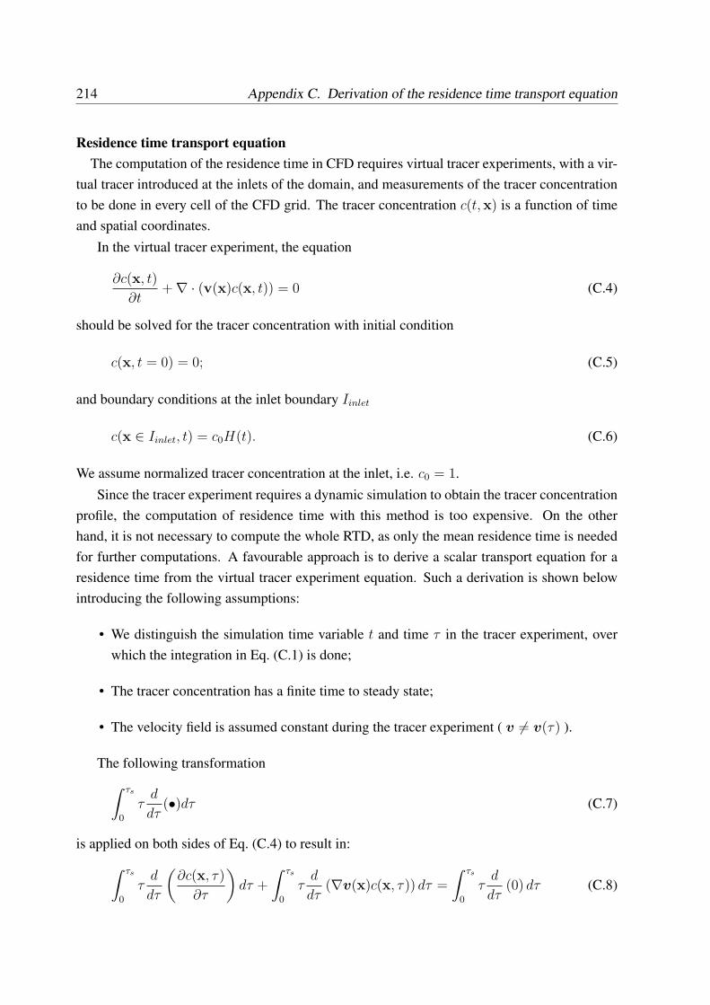
214 Appendix C. Derivation of the residence time transport equation
Residence time transport equationThe computation of the residence time in CFD requires virtual tracer experiments, with a vir-
tual tracer introduced at the inlets of the domain, and measurements of the tracer concentrationto be done in every cell of the CFD grid. The tracer concentration c(t,x) is a function of timeand spatial coordinates.
In the virtual tracer experiment, the equation
∂c(x, t)
∂t+∇ · (v(x)c(x, t)) = 0 (C.4)
should be solved for the tracer concentration with initial condition
c(x, t = 0) = 0; (C.5)
and boundary conditions at the inlet boundary Iinlet
c(x ∈ Iinlet, t) = c0H(t). (C.6)
We assume normalized tracer concentration at the inlet, i.e. c0 = 1.Since the tracer experiment requires a dynamic simulation to obtain the tracer concentration
profile, the computation of residence time with this method is too expensive. On the otherhand, it is not necessary to compute the whole RTD, as only the mean residence time is neededfor further computations. A favourable approach is to derive a scalar transport equation for aresidence time from the virtual tracer experiment equation. Such a derivation is shown belowintroducing the following assumptions:
• We distinguish the simulation time variable t and time τ in the tracer experiment, overwhich the integration in Eq. (C.1) is done;
• The tracer concentration has a finite time to steady state;
• The velocity field is assumed constant during the tracer experiment ( v 6= v(τ) ).
The following transformation∫ τs
0
τd
dτ(•)dτ (C.7)
is applied on both sides of Eq. (C.4) to result in:
∫ τs
0
τd
dτ
(∂c(x, τ)
∂τ
)dτ +
∫ τs
0
τd
dτ(∇v(x)c(x, τ)) dτ =
∫ τs
0
τd
dτ(0) dτ (C.8)
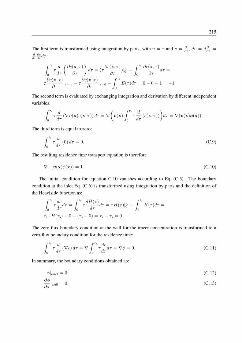
215
The first term is transformed using integration by parts, with u = τ and v = ∂c∂τ
, dv = d ∂c∂τ
=ddτ
∂c∂τ
dτ :
∫ τs
0
τd
dτ
(∂c(x, τ)
∂τ
)dτ = (τ
∂c(x, τ)
∂τ)|τs
0 −∫ τs
0
∂c(x, τ)
∂τdτ =
τ∂c(x, τ)
∂τ|τ=τs − τ
∂c(x, τ)
∂τ|τ=0 −
∫ τs
0
E(τ)dτ = 0− 0− 1 = −1.
The second term is evaluated by exchanging integration and derivation by different independentvariables.
∫ τs
0
τd
dτ(∇v(x)c(x, τ)) dτ = ∇
(v(x)
∫ τs
0
τd
dτ(c(x, τ))
)dτ = ∇(v(x)φ(x)).
The third term is equal to zero:∫ τs
0
τd
dτ(0) dτ = 0. (C.9)
The resulting residence time transport equation is therefore
∇ · (v(x)φ(x)) = 1. (C.10)
The initial condition for equation C.10 vanishes according to Eq. (C.5). The boundarycondition at the inlet Eq. (C.6) is transformed using integration by parts and the definition ofthe Heaviside function as:
∫ τs
0
τdc
dτdτ =
∫ τs
0
τdH(τ)
dτdτ = τH(τ)|τs
0 −∫ τs
0
H(τ)dτ =
τs ·H(τs)− 0− (τs − 0) = τs − τs = 0.
The zero-flux boundary condition at the wall for the tracer concentration is transformed to azero-flux boundary condition for the residence time:
∫ τs
0
τd
dτ(∇c) dτ = ∇
∫ τs
0
τdc
dτdτ = ∇φ = 0. (C.11)
In summary, the boundary conditions obtained are
φ|inlet = 0; (C.12)∂φ
∂x|wall = 0. (C.13)
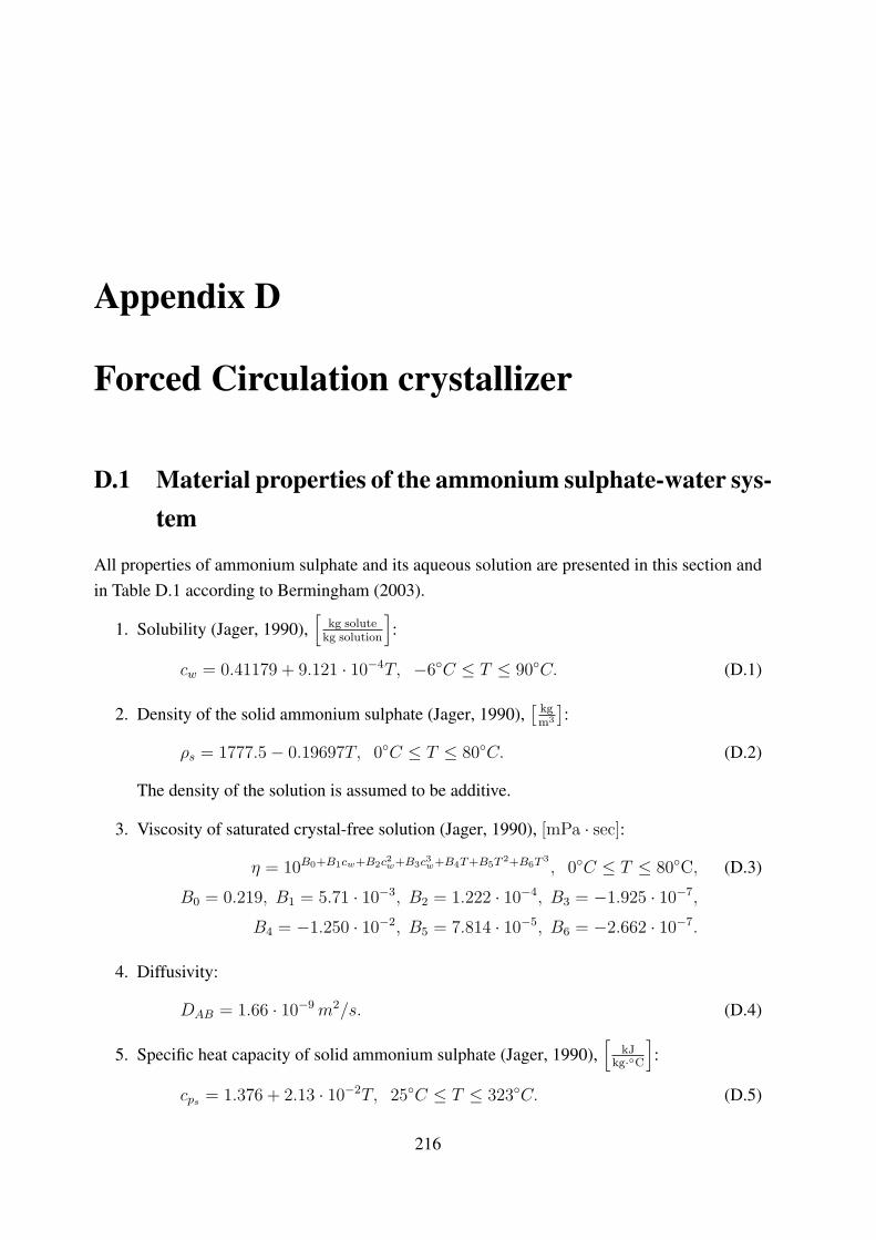
Appendix D
Forced Circulation crystallizer
D.1 Material properties of the ammonium sulphate-water sys-tem
All properties of ammonium sulphate and its aqueous solution are presented in this section andin Table D.1 according to Bermingham (2003).
1. Solubility (Jager, 1990),[
kg solutekg solution
]:
cw = 0.41179 + 9.121 · 10−4T, −6◦C ≤ T ≤ 90◦C. (D.1)
2. Density of the solid ammonium sulphate (Jager, 1990),[
kgm3
]:
ρs = 1777.5− 0.19697T, 0◦C ≤ T ≤ 80◦C. (D.2)
The density of the solution is assumed to be additive.
3. Viscosity of saturated crystal-free solution (Jager, 1990), [mPa · sec]:
η = 10B0+B1cw+B2c2w+B3c3w+B4T+B5T 2+B6T 3
, 0◦C ≤ T ≤ 80◦C, (D.3)
B0 = 0.219, B1 = 5.71 · 10−3, B2 = 1.222 · 10−4, B3 = −1.925 · 10−7,
B4 = −1.250 · 10−2, B5 = 7.814 · 10−5, B6 = −2.662 · 10−7.
4. Diffusivity:
DAB = 1.66 · 10−9 m2/s. (D.4)
5. Specific heat capacity of solid ammonium sulphate (Jager, 1990),[
kJkg·◦C
]:
cps = 1.376 + 2.13 · 10−2T, 25◦C ≤ T ≤ 323◦C. (D.5)
216
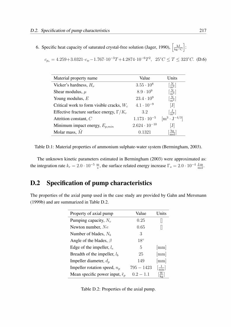
D.2. Specification of pump characteristics 217
6. Specific heat capacity of saturated crystal-free solution (Jager, 1990),[
kJkg·◦C
]:
cps = 4.259+3.0321·cw−1.767·10−3T +4.2874·10−6T 2, 25◦C ≤ T ≤ 323◦C. (D.6)
Material property name Value UnitsVicker’s hardness, Hν 3.55 · 108 [ N
m2 ]
Shear modulus, µ 8.9 · 109 [ Nm2 ]
Young modulus, E 23.4 · 109 [ Nm2 ]
Critical work to form visible cracks, Wc 4.1 · 10−9 [J]
Effective fracture surface energy, Γ/Kr 3.2 [ Jm2 ]
Attrition constant, C 1.173 · 10−5 [m3 · J−4/3]
Minimum impact energy, Ep,min 2.624 · 10−10 [J]
Molar mass, M 0.1321 [ kgmol
]
Table D.1: Material properties of ammonium sulphate-water system (Bermingham, 2003).
The unknown kinetic parameters estimated in Bermingham (2003) were approximated as:the integration rate kr = 2.0 · 10−5 m
s, the surface related energy increase Γs = 2.0 · 10−4 J·m
mol.
D.2 Specification of pump characteristics
The properties of the axial pump used in the case study are provided by Gahn and Mersmann(1999b) and are summarized in Table D.2.
Property of axial pump Value UnitsPumping capacity, Nv 0.25 []
Newton number, Ne 0.65 []
Number of blades, Nb 3
Angle of the blades, β 18◦
Edge of the impeller, le 5 [mm]
Breadth of the impeller, lb 25 [mm]
Impeller diameter, dp 149 [mm]
Impeller rotation speed, np 795− 1423 [ 1min
]
Mean specific power input, εp 0.2− 1.1 [Wkg
]
Table D.2: Properties of the axial pump.
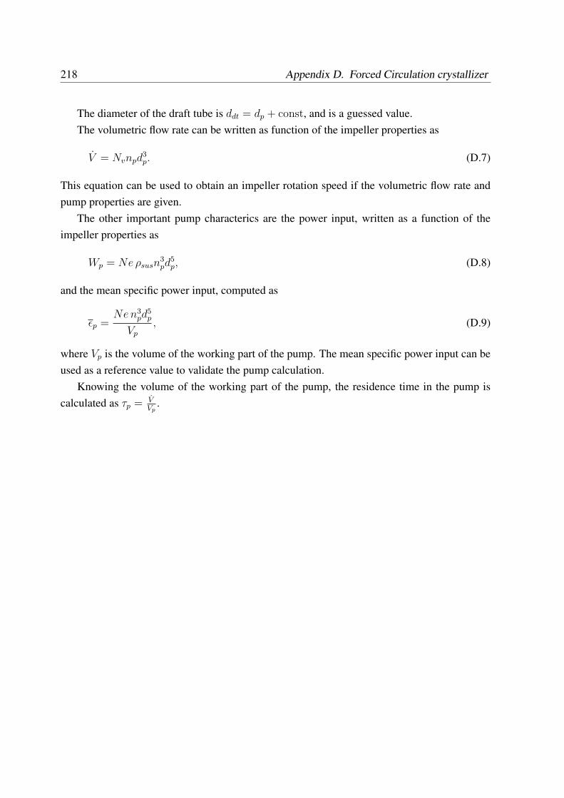
218 Appendix D. Forced Circulation crystallizer
The diameter of the draft tube is ddt = dp + const, and is a guessed value.The volumetric flow rate can be written as function of the impeller properties as
V = Nvnpd3p. (D.7)
This equation can be used to obtain an impeller rotation speed if the volumetric flow rate andpump properties are given.
The other important pump characterics are the power input, written as a function of theimpeller properties as
Wp = Ne ρsusn3pd
5p, (D.8)
and the mean specific power input, computed as
εp =Ne n3
pd5p
Vp
, (D.9)
where Vp is the volume of the working part of the pump. The mean specific power input can beused as a reference value to validate the pump calculation.
Knowing the volume of the working part of the pump, the residence time in the pump iscalculated as τp = V
Vp.
Bibliography
M. Ainsworth, J.T. Oden. A Posteriori Error Estimation in Finite Element Analysis. Wiley, NewYork, 2000.
M.M. Attarakih, H.J. Bart, N.M. Faqir. Solution of population balance equations using the sec-tional quadrature method of moments (SQMOM). Computer Aided Chemical Engineering,21 (2006), 209–214.
J. Baldyga, J.R. Bourne. Turbulent Mixing and Chemical Reactions. Wiley, New York, 1999.
J. Baldyga, W. Orciuch. Barium sulphate precipitation in a pipe – an experimental study and aCFD modeling. Chemical Engineering Science, 56 (2001), 2435–2444.
E. Barnea, J. Mizrahi. A generalized approach to fluid dynamics of particulate systems. TheChemical Engineering Journal, 5 (1973), 171–189.
A.A. Barresi, D. Marchisio, G. Baldi. On the role of micro- and mesomixing in a continuousCouette-type precipitator. Chemical Engineering Science, 54 (1999), 2339–2349.
P.I. Barton. The modelling and simulation of combined discrete/continuous processes. Ph.D.Thesis. Imperial College of Science Technology and Medicine, London, 1992.
P.I. Barton. Structural analysis of systems of equations. Internal report, Massachusetts Instituteof Technology, Cambridge, 1995.
M. Bauer, G. Eigenberger. Multiscale modeling of hydrodynamics, mass transfer and reactionin bubble column reactors. Chemical Engineering Science, 56 (2001), 1067–1074.
S.K. Bermingham. A design procedure and predictive models for solution crystallization pro-cesses. Ph.D. Thesis, Technical University of Delft, 2003.
F. Bezzo. Design of a general architecture for integration of process engineering simulationand computational fluid dynamics. Ph.D. Thesis. Imperial College of Science Technologyand Medicine, London, 2002.
219
220 BIBLIOGRAPHY
F. Bezzo, S. Macchietto, C.C.Pantelides. A general methodology for hybrid multizonal/CFDmodels - Part I. Theoretical framework. Computers and Chemical Engineering, 28 (2004),501–511.
F. Bezzo, S. Macchietto, C.C.Pantelides. A general methodology for hybrid multizonal/CFDmodels - Part II. Automatic zoning. Computers and Chemical Engineering, 28 (2004), 513–525.
L.T. Biegler, I.E. Grossmann, A.W. Westerberg. Systematic methods of chemical process design,13. Prentice Hall, Upper Saddle River, New Jersey, USA, 1997.
R.B. Bird, W.E. Stewart, E.N. Lightfoot. Transport Phenomena. 2nd edition. Wiley, New York,2002.
C. Bischof, H. M. Bucker, W. Marquardt, M. Petera, J. Wyes. Transforming Equation-basedModels in Process Engineering. In: M. Buecker, G. Corliss, P. Hovland, U. Naumann, B.Norris (Eds.): Automatic Differentiation: Applications, Theory, and Tools, Springer, Vol. 50(2005), 189-198.
J. Borchardt. Newton-type decomposition methods in large scale dynamic process simulation.Computers and Chemical Engineering, 25 (2001), 951–961.
A. Brandt. Multiscale scientific computation: six years research summary. Internal report,Gauss Center for Scientific Computation, The Weizmann Institute of Science, Israel, 1999.1
B. Braun. Theoretische und experimentelle Untersuchungen des Einflusses der Feststoffkonzen-tration und der Partikelgrosseverteilung auf das Trennverhalten von Hydrozyklonen. Disser-tation, Universitat Braunschweig, 1989.
K.E. Brenan, S.L. Campbell, L.R. Petzold. Numerical Solution of Initial-Value Problems inDifferential-Algebraic Equations, North-Holland, New York, 1989.
I.Celik, G. Hu. Single grid error estimation using error transport equation. Transactions of theASME, 126 (2004), 778–790.
A. Chianese, B. Mazzarotta, M. Karel. Nucleation kinetics of pentaerythritol. The ChemicalEngineering Journal, 58 (1995), 209–214.
A. Chianese, B. Mazzarotta, M. Karel. Crystal growth kinetics of pentaerythritol. The ChemicalEngineering Journal, 58 (1995), 215–221.
1Available online at: http://www.wisdom.weizmann.ac.il/ achi/gmc.html (accessed 16.05.2007)
BIBLIOGRAPHY 221
T. Chiu, P.D. Christofides. Nonlinear control of particulate processes. AIChE Journal, 45(1999), 1279–1297.
CHEOPS User’s Guide, Lehrstuhl fur Prozesstechnik, RWTH Aachen University, 2007.
D. Clancy, B. Kuipers. Model decomposition and simulation. In: Proceedings of 8th Int. Work-shop on Qualitative Reasoning, Nara, Japan, 1994.
P. Deufhardt, E. Hairer, J. Zugk. One-step and extrapolation methods for differential-algebraicsystems. Numerical Mathematics, 51 (1987), 501–516.
W. E, B. Engquist. The heterogeneous multiscale methods. Communications in MathematicalSciences, 1 (2003), 87-132.
R. A. Eek, S. Dijkstra, G.M. van Rosmalen. Dynamic modeling of suspension crystallizersusing experimental data. AIChE Journal, 41 (1995), 571–584.
R.A. Eek. Control and dynamic modelling of industrial suspension crystallizers. Ph.D. Thesis,Technical University of Delft, 1995.
R. Ehrig, U. Nowak, P. Deuflhard. Massively parallel linearly-implicit extrapolation algorithmsas a powerful tool in process simulation. In: E.H. D’Hollander et al. (Eds.), Advances inParallel Computing, Vol. 12 (1998): Parallel computing: Fundamentals, applications andnew directions, Elsevier, 517–524.
J.H. Ferziger, M. Peric. Computational Methods for Fluid Dynamics. Springer-Verlag, Berlin,1997.
J. Fish. Bridging the scales in nano engineering and science. Journal of Nanoparticle Research,8 (2006), 577–594.
FLUENT 6.0 User Manual, Fluent Inc., 2005.
C. Gahn, A. Mersmann. Theoretical prediction and experimental determination of attrition rates.Chemical Engineering Research and Design, 75 (1997), 125–131.
C. Gahn, A. Mersmann. Brittle fracture in crystallization processes. Part A. Attrition and abra-sion of brittle solids. Chemical Engineering Science, 54 (1999), 1273–1282.
C. Gahn, A. Mersmann. Brittle fracture in crystallization processes. Part B. Growth of fragmentsand scale-up of suspension crystallizers. Chemical Engineering Science, 54 (1999), 1283–1292.
222 BIBLIOGRAPHY
W. Geffers, L. von Wedel, J. Wyes, W. Marquardt. Integration von deklarativen undausfuhrbaren Modellen in offenen Simulationsumgebungen In: K. Panreck, F. Dorrscheidt(Hrsg.): 15. Symposium Simulationstechnik, Paderborn, 11-14 September 2001, 579–586.
E.D. Gilles, P. Holl, W. Marquardt. The dynamic simulation of complex chemical processes.International Chemical Engineering, 28 (1988), 579–592.
R. Grosch, H. Briesen. Getting started with Parsival. A tutorial introduction. Chair of ProcessSystems Engineering, RWTH Aachen, Germany, 2004.
R. Grosch, H. Briesen, W. Marquardt, M. Wulkow. Generalization and numerical investigationof QMOM. AIChE Journal, 53 (2007), 207-227.
F. Grund, K. Ehrhardt, J. Borchardt, D. Horn. Heterogeneous dynamic process flowsheet sim-ulation of chemical plants. In: Jager, W., Krebs, H.-J.(Eds.), Mathematics - Key Technologyfor the Future, Springer-Verlag, Berlin, 2003, 184–193.
A. Hay, M. Visonneau. Error estimation using the error transport equation for finite-volumemethods and arbitrary meshes. International Journal of Computational Fluid Dynamics, 20(2006), 463–479.
Helget, A. Modulare Simulation verfahrentechnischer Anlagen. VDI-Fortschritt-Bericht 251,Reihe 20, VDI Verlag, Dusseldorf, 1997.
M. Henning, S. Vinoski. Advanced CORBA Programming with C++. Addison-Wesley, Read-ing, MA, USA, 1999.
M. Hillestad, T. Hertzberg. Dynamic simulation of chemical engineering systems by the se-quential modular approach. Computers and Chemical Engineering, 10 (1986), 377–388.
M. Hillestad, T. Hertzberg. Convergence and stability of the sequential modular approach todynamic process simulation. Computers and Chemical Engineering, 12 (1988), 407–414.
T.Y. Hou, X.-H. Wu. A multiscale finite element method for elliptic problems in compositematerials and porous media. Journal of Computational Physics, 134 (1997), 169–189.
M.J. Hounslow, A.E. Lewis, S.J. Sanders, R. Bondy. Generic crystallizer model: I. A modelframework for a well-mixed compartment. Particle Technnology and Fluidization, 51 (2005),2942–2955.
M.J. Hounslow, G.K. Reynolds. Product engineering for crystal size distribution. AIChE Jour-nal, 52 (7), 2507–2517.
BIBLIOGRAPHY 223
D. Ilievsky, M. Rudman, G. Metcalfe. The separate roles of shear rate and mixing on gibbsiteprecipitation. Chemical Engineering Science, 56 (2001), 2521–2530.
D. Ilievsky, I. Livk. An agglomeration efficiency model for gibbsite precipitation in a turbulentlystiffed vessel. Chemical Engineering Science, 61 (2006), 2010–2022.
G.D. Ingram, I.T. Cameron, K.M. Hangos. Classification and analysis of integrating frameworksin multiscale modelling. Chemical Engineering Science, 59 (2004), 2171–2187.
Y. Iwasaki. Causal ordering in a mixed structure. Proceedings of the 7th National Conferenceon Artificial Intelligence, Saint Paul, USA, 1988, 313–318.
J. Jager. Control of industrial crystallizers – the physical aspects. Ph.D. Thesis, Delft Universityof Technology, 1990.
M. Javurek, Scheme-Programmierung in FLUENT 5 & 6. Internal Report, Institut fuerStromungsprozesse und Warmeubertragung, Johannes Kepler Universitat, Linz, 2004.2
G.R. Jerauld, Y. Vasatis, M.F. Doherty. Simple conditions for the appearance of sustained oscil-lations in continuous crystallizers. Chemical Engineering Science, 38 (1983), 1675–1681.
V. John, I.Angelov, A.A. Oncul, D. Thevenin. Techniques for reconstructing a distribution froma finite number of its moments. Chemical Engineering Science, 62 (2007), 2890–2904.
P. Koumoutsakos. Multiscale flow simulations using particles. Annual Reviews of Fluid Me-chanics, 37 (2005), 457–487.
H.J.M. Kramer, J.W. Dijkstra, P.J.T. Verheijen, G.M. van Rosmalen. Modeling of industrialcrystallizers for control and design purposes, Powder technology, 108 (2000), 185–191.
V. Kulikov, H. Briesen, R. Grosch, A. Yang, L. von Wedel, W. Marquardt. Modular dynamicsimulation of integrated process flowsheets by means of tool integration. Chemical Engineer-ing Science, 60 (2005), 2069–2083.
V. Kulikov, H. Briesen, W. Marquardt. Scale integration for the coupled simulation of crystal-lization and fluid dynamics. Chemical Engineering Research and Design, 83 (2005), 706–717.
V. Kulikov, H. Briesen, W. Marquardt. Scale integration for the coupled simulation of crystal-lization and fluid dynamics. Presentation at the 5th World Congress of Chemical Enginnering,Glasgow, 9-15 July 2005.
2Available online at: http://fluid.jku.at/personen/javurek/pdf/scheme.pdf (accessed 03.09.2007).
224 BIBLIOGRAPHY
V. Kulikov, H. Briesen, W. Marquardt. A framework for the simulation of mass crystallizationconsidering the effect of fluid dynamics. Chemical Engineering and Processing, 45 (2006),886–899.
V. Kulikov, H. Briesen, W. Marquardt. Adaptive compartment selection for the coupled simu-lation of population balance and fluid dynamics. Proceedings of CHISA-2006, 28-31 August2006, Prague.
S. Kumar, D. Ramkrishna. On the solution of population balance equations by discretization –I. A fixed pivot technique. Chemical Engineering Science, 51 (1996), 1311–1332.
S. Kumar, D. Ramkrishna. On the solution of population balance equations by discretization –II. A moving pivot technique. Chemical Engineering Science, 51 (1996), 1333–1342.
T.S. Li, I. Livk, G. Lane, D. Ilievsky. Dynamic compartmental models of uniformly-mixed andinhomogeneously-mixed gibbsite crystallizers. Chemical Engineering and Technology, 26(2003), 369–376.
M. Liiri, T. Koiranen, J. Attamaa. Secondary nucleation due to crystal-impeller and crystal-vessel collisions by population balances in CFD modelling. Journal of Crystal Growth, 237-239 (2002), 2188–2193.
W.K. Liu, E.G. Karpov, S. Zhang, H.S. Park. An introduction to computational nanomechanicsand materials. Computer Methods in Applied Mechanics and Engineering, 193 (2004), 1529–1578, 2004.
Y.C. Liu, C.B. Brosilow. Simulation of large scale dynamic systems - I. Modular integrationmethods. Computers and Chemical Engineering, 11 (1987), 241–253.
D.L. Marchisio, J.T. Pikturna, R.O. Fox, R.D. Vigil, A.A. Barresi. Quadrature method of mo-ments for population-balance equations. AIChE Journal, 49 (2003), 1266–1276.
D.L. Marchisio, R.D. Vigil, R.O. Fox. Implementation of the quadrature method of moments inCFD codes for aggregation-breakage problems. Chemical Engineering Science, 58 (2003),3337–3351.
D.L. Marchisio, M. Soos, J. Sefcik, M. Morbidelli, A.A. Barresi, G. Baldi. Effect of fluid dy-namics on particle size distribution in particulate processes. Chemical Engineering and Tech-nology, 29 (2006), 191-199.
W. Marquardt, M. Wurst, P. Holl, E.D. Gilles. DIVA - An open architecture for dynamic simu-lation. Computers and Chemical Engineering, 14 (1990), 1289–1295.
BIBLIOGRAPHY 225
W. Marquardt. Dynamic process simulation - recent trends and future challenges. In: Arkun, Y.,Ray, W.H. (Eds.), Chemical Process Control CPC-IV, CACHE Publications, Austin, 1991,131–180.
W. Marquardt. Numerical methods for the simulation of differential-algebraic process models.In: R. Berber: Methods of Model Based Control, NATO-ASI Ser. E, Applied Sciences, Vol.293, Kluwer Academic Pub., Dordrecht, 1995, 42–79.
W. Marquardt. Adaptivity in process systems modeling In: J. Grievink, J. v. Schijndel (Eds.):European Symposium on Computer Aided Process Engineering - 12, Elsevier, 2002, 42–56.
W. Marquardt. Modellbildung und Analyse verfahrenstechnischer Prozesse. Lecture script,Lehrstuhl fur Prozesstechnik, RWTH Aachen University, 2005.
H.G. Matthies, J. Steindorf. Fully coupled fluid-structure interaction using weak coupling. Pro-ceedings in Applied Mathematics and Mechanics, 1 (2002), 37-38.
H.G. Matthies, R. Niekamp, J. Steindorf. Algorithms for strong coupling procedures. ComputerMethods in Applied Mechanics and Engineering, 195 (2002), 2028–2049.
R. McGraw. Description of aerosol dynamics by the quadrature method of moments. AerosolScience and Technology, 27 (1997), 255–265.
A. Mersmann. Crystallization Technology Handbook. Dekker, New York, 1995.
Mini-Workshop: Numerical Upscaling. Org.: Achi Brandt, Richard E. Ewing and Oleg Iliev.Mathematisches Forschungsinstitut Oberwolfach, 1.-7.05.2005. In: Oberwolfach Reports, 2(2), 2005, 11271176.
MpCCI 3.0.4 Technical Reference, Fraunhofer Institute for Algorithms and Scientific Comput-ing, 2005.
J.W. Mullin. Crystallization, Fourth Edition. Butterworth-Heinemann, Oxford, 2001.
H.S. Mumtaz, M.J. Hounslow, N.A. Seaton, W.R. Paterson. Orthokinetic aggregation duringprecipitation. Transactions of Institution of Chemical Engineers, 75 (1997), 152–159.
A. Neumann. Characterizing indistrial crystallizers of different scale and type. Ph.D. Thesis,Technical University of Delft, 2001.
O. Neumann, Integration von Werkzeugen in heterogene, prozessgesteuerte Software-Entwicklungumgebungen - Tool integration concept. Dissertation, Universitat Paderborn,2002.
226 BIBLIOGRAPHY
U. Nowak, L. Weinmann. A family of newton codes for systems of highly nonlinear equations.Technical Report TR-91-10, Konrad-Zuse-Zentrum fur Infomationstechnik, Berlin, 1991. 3
R. O Meadhra, H.J.M. Kramer, G.M. van Rosmalen. Model for secondary nucleation in a sus-pension crystallizer. AIChE Journal, 42 (1996), 973–982.
R. O Meadhra, H.J.M. Kramer, G.M. van Rosmalen. Crystallization kinetics of pentaerythritol.Journal of Crystal Growth, 166 (1996), 1046–1052.
C.C. Pantelides. SpeedUp - recent advances in process simulation. Computers and ChemicalEngineering, 12 (1988), 745–755.
C.C. Pantelides. An advanced tool for process modelling, simulation and optimisation. Pre-sented at: CHEMPUTERS EUROPE III, Frankfurt, Germany, 29-30 October 1996.
H.S. Park, W.K. Liu. An introduction and tutorial on multiple-scale analysis in solids. Computermethods in applied mechanics and engineering, 193 (2004), 1733–1772.
L.R. Petzold. A description of DASSL: A differential/algebraic system solver. In: Stepleman,R.S., et al. (Eds.), Scientific Computing. North-Holland, Amsterdam, 1983, 65–68.
J. Placido, R. Guardani, M.M. Seckler, S. Derenzo, M. Giulietti. Simulation of a pentaerythritolindustrial DT crystallizer. Proceedings of 15th International Symposium on Industrial Crys-tallization, Sorrento, Italy, 15-18 September 2002, 1371-1376.
R. Ploß, T. Tengler, A. Mersmann. A new model on the effect of stirring intensity on the rate ofsecondary nucleation. Chemical Engineering and Technology, 12 (1989), 137–146.
M. Pons. A summary of CAPE-OPEN activities. Available online at:http://www.chemicalprocessing.com/articles/2006/014.html (accessed 03.09.2007).
W.H. Press, S.A. Teukolsky, W.T. Vetterling, B.P.Flannery. Numerical Recipes in C. 2nd Edi-tion. Cambridge University Press, Cambridge, 1992.
D. Ramkrishna. Population balances. Academic Press, San Diego, 2000.
A.D. Randolph, M.A. Larson. Theory of Particulate Processes, Second Edition. AcademicPress, San Diego, 1988.
S. Rigopoulos, A. Jones. A hybrid CFD-reaction engineering framework for multiphase reactormodeling: basic concept and application to bubble column reactors. Chemical EngineeringScience, 58 (2003), 3077–3089.3Available online at: www.zib.de/Publications/Reports/TR-91-10.ps.Z. Accessed 04.07.2007
BIBLIOGRAPHY 227
R. Schneider, S. Gerhards. WOMS - Ein Werkzeug zur Modellierung von Arbeitsablaufen. In:M. Nagl, B. Westfechtel, (Eds.): Modelle, Werkzeuge und Infrastrukturen zur Unterstutzungvon Entwicklungsprozessen, Wiley VCH, Weinheim, 2003, 375-376.
G. Schopfer, A. Yang, L. von Wedel, W. Marquardt. CHEOPS: a tool integration platformfor chemical process modelling and simulation. International Journal on Software Tools forTechnology Transfer, 6 (2004), 186–202.
G. Schopfer. A framework for tool integration in chemical process modeling. Dissertation,RWTH Aachen University, 2005.
G. Schopfer, J. Wyes, W. Marquardt, L. von Wedel. A Library for Equation System Processingbased on the CAPE-OPEN ESO Interface. In: L. Puigjaner and A. Espuna (Eds.), Proceed-ings of ESCAPE 15, Barcelona, Spain, 2005.
Z. Sha, S. Palosaari. Mixing and crystallization in suspensions. Chemical Engineering Science,55 (2000), 1797–1806.
G. Skorstad. Clustered causal ordering. In: Proceedings of 4th International Workshop on Qual-itative Physics, 1990, 290–299. 4
J. Steindorf. Partitionierte Verfahren fur Probleme der Fluid-Struktur Wechselwirkung. Disser-tation, Technische Universitat Braunschweig, 2002. 5
P. Synowiec, A.G. Jones, P.A. Shamlou. Crystal break-up in dilute turbulently agitated suspen-sions. Chemical Engineering Science, 48 (1993), 3485–3495.
J. Unger, A. Kroner, W. Marquardt. Structural analysis of differential-algebraic equation sys-tems – theory and applications. Computers and Chemical Engineering, 19 (1995), 867–882.
A. Vikhansky, M. Kraft. Modelling of a RDC using a combined CFD-population balance ap-proach. Chemical Engineering Science, 59 (2004), 2597–2606.
L. von Wedel, W. Marquardt. CHEOPS: A case study in component-based process simulation.In: Malone, M.F., Trainham, J.A., Carnahan, B. (Eds.), Foundations of Computer-AidedProcess Design, No. 323 in AIChE Symposium Series, AIChE, 1999, 494–497.
L. Wang, R.O. Fox. Comparison of micromixing models for CFD simulation of nanoparticleformation. AIChE Journal, 50 (2004), 2217–2232.4Available online at: http://www.qrg.northwestern.edu/papers/Files/qrworkshops/QP90/Index QP90.htm (ac-
cessed 16.05.2007).5Available online at: http://www.wire.tu-bs.de/forschung/d berichte.html (accessed 03.09.2007).
228 BIBLIOGRAPHY
H. Wei, W. Zhou, J. Garside. Computational fluid dynamics modeling of the precipitation pro-cess in a semibatch crystallizer. Industrial and Engineering Chemistry Research, 40 (2001),5255-5261.
G.J. Wells, W.H. Ray. Investigation of imperfect mixing effects in the LDPE autoclave reactorusing CFD and compartment models. In: DECHEMA Monographs, Vol. 137 (2001), WILEY-VCH, 49–59.
A.W. Westerberg, H.P. Hutchison, R.L. Motard, P. Winter. Process Flowsheeting. CambridgeUniversity Press, Cambridge, 1979.
M. Wulkow, A. Gerstlauer, U. Nieken. Modeling and simulation of crystallization processesusing Parsival. Chemical Engineering Science, 56 (2001), 2575–2588.
I.T. Young, J.J. Gerbrands and L.J. van Vliet. Lecture notes: Fundamentals of Image Processing.Delft University of Technology, Delft, The Netherlands, 1998.6
R. Zauner, A.G. Jones. On the influence of mixing on crystal precipitation processes - applica-tion of the segregated feed model. Chemical Engineering Science, 57 (2002), 821–831.
J.Z.Zhu, G.He. Error estimation and uncertainty propagation in computational fluid mechanics.ICASE Interim Report No. 41, 2002.7
O.C. Zienkiewicz, J.H. Zhu. Superconvergent patch recovery and a posteriori error estimates.Part I: The recovery technique. International Journal for Numerical Methods in Engineering,33 (1992), 1331–1364.
O.C. Zienkiewicz, J.H. Zhu. Superconvergent patch recovery and a posteriori error estimates.Part II: Error estimates and adaptivity. International Journal for Numerical Methods in Engi-neering, 33 (1992), 1365–1382.
6Available online at: http://www.freetechbooks.com/about384.html. Accessed 04.09.2007.7Available online at: http://ntrs.nasa.gov/archive/nasa/casi.ntrs.nasa.gov/20020074979 2002123158.pdf. Ac-
cessed 04.09.2007.