A Sodar-based Investigation of the Atmospheric Boundary Layer

Berichte des Meteorologischen Institutes der Universität Freiburg

Nr. 8

Mahmoud El-Nouby Adam Haggagy

A Sodar-based Investigation of the Atmospheric Boundary Layer

Freiburg, September 2003

b

ISSN 1435-618X

Alle Rechte, insbesondere die Rechte der Vervielfältigung und Verbreitung sowie der

Übersetzung vorbehalten.

Eigenverlag des Meteorologischen Instituts der Albert-Ludwigs-Universität Freiburg

Druck: Druckerei der Albert-Ludwigs-Universität Freiburg

Herausgeber: Prof. Dr. Helmut Mayer und PD Dr. Andreas Matzarakis Meteorologisches Institut der Universität Freiburg Werderring 10, D-79085 Freiburg Tel.: 0049/761/203-3590; Fax: 0049/761/203-3586 e-mail: [email protected]

Dokumentation: Ber. Meteor. Inst. Univ. Freiburg Nr. 8, 2003, 259 S.

Dissertation an der Fakultät für Forst- und Umweltwissenschaften der Albert-Ludwigs-

Universität Freiburg

ACKNOWLEDGEMENTS

First of all, I wish to express my gratitude to God for guiding me and giving me strength

in my efforts to acquaint more knowledge.

In what follows, I would like to express my gratitude to all those who contributed to my

Ph.D. thesis:

My deepest appreciation gave to Prof. Dr. Helmut Mayer, Head of the Meteorological

Institute, University of Freiburg, Germany, for suggesting the problem, supervising me

and providing all the necessary supports throughout the course of this work. I am ex-

tremely grateful to him for his kindness and encouragement, which kept me going dur-

ing the study period.

I wish to express my deep gratitude to the Mission Department - Ministry of Higher

Education and Scientific Research (Egypt) for providing the scholarship that covered

my living expenses during the study period. I would also like to thank the German Fed-

eral Ministry of Education and Research for funding the Atmospheric Research Pro-

gramme AFO2000, in the framework of which my study (VERTIKO-ALUF1) was con-

ducted.

My cordial thanks to my colleagues at the Meteorological Institute, who assisted me to

solve many problems during the analysis of data for my study. They also created a

good atmosphere for my daily works. In particular, Dirk Schindler, who assisted me with

software-related problems during the analysis of my data.

I wish to express my gratitude to the secretarial and technical staffs of the Meteorologi-

cal Institute for creating a friendly and stimulating atmosphere, which made my stay in

Freiburg very enjoyable and worthwhile.

Thanks to my friend Dr. Moses Iziomon (presently in Canada), who assisted me a lot

during his stay in Freiburg to start my work. I appreciate his efforts at checking my the-

sis manuscript.

I am most grateful to Prof. em. Dr. Abdelazeem M. Abdelmegeed, Department of Phys-

ics, Faculty of Science, Qena - South Valley University (Egypt), and Prof. Dr. Sayed M.

El-Shazly, Professor of Atmospheric Physics and vice Dean for post graduate studies

II

and researches, Faculty of Science, Qena - South Valley University (Egypt), for their

moral support.

Furthermore, I'm grateful to everybody who gave me a hand during this study.

Finally, special thanks to my dear wife for her love, encouragement and support as well

as her patience to be separated from her extended family during our stay in Germany.

This work is dedicated to those who loved me. First and foremost, to the memory of my

mother, who gave so much and asked for so little.

Mahmoud Haggagy

Freiburg, Germany 10 May 2003

III

TABLE OF CONTENTS

Acknowledgements I

Table of contents III

Summary X

Zusammenfassung XVII

1 Introduction 1

2 Literature review 5

2.1 Acoustic remote sensing 5

2.2 Sodar studies of atmospheric stability 6

2.3 Turbulence of the atmospheric boundary layer 8

3 Objectives and applications of the present study 11

3.1 Necessity of the present study 12

3.2 Objectives of the present study 13

3.3 Application of the present work 14

4 Theoretical concepts 16

4.1 Atmospheric boundary layer 16

4.1.1 Wind and flow 17

4.1.2 Turbulence 18

4.1.2.1 Turbulence kinetic energy 19

4.1.2.2 Turbulence intensity 22

IV

4.1.2.3 Free and forced convection 23

4.1.3 Depth and structure of the atmospheric boundary layer 25

4.1.3.1 Mixed layer 26

4.1.3.2 Residual layer 28

4.1.3.3 Stable boundary layer 28

4.1.4 Atmospheric stability 29

4.1.5 Micrometeorological variables 30

4.1.5.1 Friction velocity 30

4.1.5.2 Monin-Obukhov length 31

4.1.5.3 Convective velocity scale 32

4.1.5.4 Roughness length 32

4.2 Sound propagation in the atmosphere 33

4.3 Theory of the sodar measurement 38

4.3.1 Physical principle of the method 38

4.3.2 Sodar system configurations 41

5 Measurements, data processing and experimental sites 43

5.1 Measurements 43

5.1.1 Principles of sodar measurement 43

5.1.1.1 Beam pattern 43

5.1.1.2 Backscatter 44

5.1.1.3 Doppler shift 44

5.1.1.4 Height determination 45

5.1.1.5 Signal analysis 46

5.1.1.6 Limitation of sodar operation 47

V

5.1.2 Accuracy of sodar measurements 47

5.1.3 Instrumentation: Description of the FAS64 49

5.1.4 Description of the software: FASrun program 53

5.2 Data processing 54

5.3 Experimental sites 57

6 Results 59

6.1 Hartheim: Scots pine forest 60

6.1.1 Global solar radiation, wind direction, and wind speed variation 60

6.1.1.1 Global solar radiation 60

6.1.1.2 Wind direction 61

6.1.1.3 Horizontal wind speed 61

6.1.1.4 Vertical wind speed component 61

6.1.2 Atmospheric stability classification 61

6.1.3 Variance of horizontal and vertical wind speed 68

6.1.4 Turbulence kinetic energy 68

6.1.5 Turbulence intensity 69

6.1.5.1 Variation of turbulence intensity with wind directions under

neutral conditions 69

6.1.5.2 Turbulence intensity under different stratifications 69

6.1.6 Relationship between normalized standard deviations

of velocity components and z/L 69

6.2 Bremgarten: Grassland 80



6.2.1.2 Wind direction speed 80

VI







6.2.5.1 Variation of turbulence intensity with wind directions

under neutral conditions 88




6.3 Blankenhornsberg: Vineyard 100













6.3.5.3 Relationship between normalized standard deviations


VII

6.4 Oberbärenburg: Norway spruce forest 120















6.5 Melpitz: Grassland 139










VIII




6.6 Freiburg: Urban area 158








7 General discussion 171

7.1 Global solar radiation, wind direction, and wind speed variation 171

7.1.1 Global solar radiation 171

7.1.2 Wind direction 172

7.1.3 Wind speed components 173

7.2 Atmospheric stability classification 174

7.3 Variance of horizontal and vertical wind speed 174

7.4 Turbulence kinetic energy 176

7.5 Turbulence intensity components 178

7.5.1 Variation of turbulence intensity components with

wind directions under neutral conditions 179

7.5.2 Turbulence intensity under different stratifications 181

7.6 Relationship between normalized standard deviations of

velocity components and z/L under unstable conditions 183

IX

7.6.1 Horizontal component 183

7.6.2 Vertical component 185

7.7 Profile of normalized variance of vertical wind speed component 185

8 Conclusions 202

References 207

List of abbreviations and symbols 219

List of captions for figures 223

List of captions for tables 231

Curriculum vitae

X

SUMMARY

On one hand, environmental studies need information and forecasts on the state,

trends and impacts of air pollutant concentrations on different scales. On the other

hand, air pollution control needs information on parameters of the atmospheric bound-

ary layer (ABL), with reference to accumulation, dispersion and transport of air pollut-

ants. Turbulence is one of the important transport processes, and is also used some-

times to define the ABL. The ABL is the layer where interactions take place between

the earth’s surface (which captures most of the incoming solar energy and redistributes

it in different forms) and the large scale atmospheric flow (which is driven by this en-

ergy). This transfer of energy is partly accomplished by turbulent eddies which are pro-

duced by two different mechanisms, namely wind shear and buoyancy.

The investigation presented here deals with the experimental determination of main

atmospheric variables affecting the ABL structure over different land use types in Ger-

many by use of a FAS64 sodar (sonic detecting and ranging) from the Scintec Com-

pany (Tübingen, Germany). The investigation has been carried out at the Meteorologi-

cal Institute, University of Freiburg, Germany, and performed as project ALUF1 within

the scope of the AFO2000 network VERTIKO (Vertical Transports of Energy and Trace

Gases at Anchor Stations and their Spatial/Temporal Extrapolation under Complex

Natural Conditions). Forest, urban and agricultural areas are land use types which are

typical of the small-scale heterogeneity in many parts of Germany. Among all types of

surfaces, the aerodynamic roughness of an urban area is almost constant. Forests and

urban areas are associated with comparatively high values of aerodynamic roughness.

Aerodynamic surface roughness of forests shows a long-term dependence on growth

dynamics. In contrast to that, aerodynamic surface roughness of agricultural areas is

smaller and has an annual pattern, which depends on plant growth.

The experimental sites of this investigation are located at Hartheim (47° 56` N, 07° 36`

E, 201 m a.s.l.), Bremgarten (47° 54` N, 07° 37` E, 200 m a.s.l.), Blankenhornsberg

(48° 03` N, 07° 36` E, 285 m a.s.l.), Oberbärenburg (50° 47` N, 13° 43` E, 735 m a.s.l.),

Melpitz (51° 31` N, 12° 55` E, 86 m a.s.l.) and Freiburg (48° 56` N, 07° 50` E, 272 m

a.s.l.). These sites represent different land use types: grassland (Bremgarten and

Melpitz), vineyard (Blankenhornsberg), forest (Hartheim and Oberbärenburg), and ur-

ban area (Freiburg).

XI

The data from the FAS64 sodar, such as wind speed components, wind direction and

turbulence parameters (particularly standard deviation of the vertical wind speed), are

30-min mean values. They were measured at each site within the same range of height

(20-500 m a.g.l.), but at different times. The measurement extends in Hartheim from 30

March, 2000 to 25 April, 2000, in Bremgarten from 10 July, 2001 to 26 July, 2001, in

Blankenhornsberg from 01 August, 2001 to 22 August, 2001, in Oberbärenburg from 29

August, 2001 to 24 September, 2001, in Melpitz from 26 September, 2001 to 12 Octo-

ber, 2001, and in Freiburg from 16 November, 2001 to 19 November, 2001. Due to the

acoustic noise produced by the sodar and acting as disturbance for people, the meas-

urement campaign in Freiburg has to be broken off after a short period.

Global solar radiation was necessary to interpret the results of the sodar measure-

ments. For Hartheim, Bremgarten and Blankenhornsberg it was taken over from the

forest-meteorological site Hartheim that is operated by the Meteorological Institute,

University of Freiburg. However, it is located 3.5 km and 9 km far from Bremgarten and

Blankenhornsberg, respectively. In addition, global solar radiation data for Oberbären-

burg and Melpitz were provided by the weather stations at Rotherdbach (1 km from

Oberbärenburg) and Melpitz, respectively. For Freiburg, global radiation was taken

over from the urban climate experimental site, which is run by the Meteorological Insti-

tute, University of Freiburg, on a high-rise building (approximately 51 m a.g.l.) in the

northern downtown of Freiburg. Moreover, the German Weather Service (DWD) pro-

vided some data on fog, precipitation and cloud fraction.

Besides directly monitoring meteorological variables such as wind speed components,

wind direction, and the standard deviations of the wind direction and wind speed com-

ponents, the application of a number of methods and algorithms enabled the estimation

of features of the atmospheric turbulence such as Pasquill-Gifford (P-G) stability

classes, Monin-Obukhov length, and friction velocity, which are all crucial for both

straightforward meteorological applications and as inputs to atmospheric pollutant dis-

persion models. In particular, a typical sodar-related method has been used to classify

atmospheric stability over the sites of the study through the periods of the measure-

ments. Such a stability classification is the first step for applying a number of traditional

algorithms aiming at estimating the main atmospheric parameters that typically de-

XII

scribe the ABL structure (e.g. Monin-Obukhov length, friction velocity and mixing

height) in dependence on land use, weather as well as time of day and year.

This investigation focuses on the study of turbulence characteristics within the ABL

over different land use types: grassland, vineyard, forest and urban area. Thereby, the

main purpose of this study is to analyze the influences of thermal and roughness

changes on the properties of turbulence within the ABL over these land use types. To

fulfill the objectives of this investigation, the following points were taken into account:

∗∗ An overall measure of the intensity of turbulence is the turbulent kinetic energy

per unit mass (TKE). It is usually produced at the scale of the ABL depth. The

quantity σ3w/z (σw: standard deviation of the vertical wind speed at a height z) is

connected to the production terms of convective and mechanical origin of TKE.

Hence the behavior of this quantity was studied to explain the influence of ther-

mal and roughness changes on the characteristics of the TKE. In addition, the

mean kinetic energy per unit mass (MKE) has a considerable role on the values

of TKE. Therefore, it was considered in this study. Moreover, daily midday-hour-

(11:00-14:00 CET) and midnight-hour- (23:00-02:00 CET) averages of σ3w/z,

MKE, and TKE at different levels were calculated for two cloudless and two

cloudy days at each of the sites.

∗∗ The components Iu, Iv and Iw of the turbulence intensity depend on measuring

height, surface roughness and atmospheric stability. Therefore, they were in-

cluded in this investigation.

∗∗ For the sites Hartheim, Bremgarten, Blankenhornsberg and Oberbärenburg,

mean values of the normalized (by the friction velocity u∗) standard deviations of

the wind speed components, σi/u∗ (i=u,v,w), in the surface layer were discussed

as a function of the stability parameter (z/L) under unstable conditions. In con-

trast to σw, the determination of σu and σv from sodar measurements is ex-

tremely problematic due to the measuring method. The manufacturer (Scintec

Company) of the FAS64 sodar, however, states, that half-hourly mean values of

σu and σv are utilizable for further calculations even if their accuracy is lower

than for σw. Mean values of σu/u∗, σv/u∗ and σw/u∗ in the range of -z/L from 0.86 to

XIII

3.66 in the surface layer over the land use types under investigation are com-

pared with analogous values from previous studies at flat and complex terrain.

∗∗ The variation of the normalized (by the square of the convective velocity w∗2)

variance of the vertical wind speed component, σ2w/w∗

2, with the normalized (by

the mixing height zi) height z/zi was discussed for the grassland site Bremgarten.

In order to explain the influence of thermal and roughness changes on the characteris-

tics of TKE and turbulence intensity components, background information on the be-

havior of global radiation, wind direction and its standard deviation, horizontal and ver-

tical wind speed components, and the variance of horizontal and vertical wind speed

components was provided for each site during the measurement campaigns.

The results of this investigation can be summarized as follows:

∗∗ Using only sodar data, the atmospheric stability (according to P-G stability clas-

sification) was determined at four levels a.g.l. at Hartheim (50-80, 80-110, 140-

170, and 200-230 m), Bremgarten (40-60, 60-100, 100-180, and 180-260 m),

Blankenhornsberg (40-60, 80-120, 120-160, and 160-240 m), Oberbärenburg

(50-80, 80-110, 140-170, and 200-230 m), and Melpitz (50-80, 80-110, 140-170,

and 200-230 m). In order to optimize the sodar measurements, its setup varied

between the measurement campaigns. Therefore, the graduation of layers is

slightly different between the sites. Land use-specific values of the frequency

distribution of the P-G stability classes A to F within the range, approximately,

from 40 to 260 m a.g.l. were A (1%, 5%, 5%, 1%, 1%), B (3%, 15%, 19%, 6%,

3%), C (21%, 22%, 26%, 34%, 21%), D (72%, 41%, 33%, 55%, 72%), E (2%,

7%, 5%, 1%, 2%), and F (1%, 10%, 10%, 2%, 1%) for Scots pine forest (Hart-

heim), grassland (Bremgarten), vineyard (Blankenhornsberg), Norway spruce

forest (Oberbärenburg), and grassland (Melpitz), respectively. Considering the

period of the year for every site, these results seem to be reliable.

∗∗ Case studies showed that half-hourly mean values of σ3w/z under various stabil-

ity conditions (neutral, stable and unstable) decreased with height. This was due

to the increasing of the mechanical and buoyancy turbulence production in the

surface layer. In addition, the analysis of daily mean values of σ3w/z at different

levels within the surface layer on cloudless and cloudy conditions revealed lower

XIV

values at the upper level than at the lower level: 44% (cloudless) and 64%

(cloudy) at Hartheim (80-110 m compared to 20-50 m a.g.l.), 60% (cloudless)

and 64% (cloudy) at Bremgarten (60-100 m compared to 20-30 m a.g.l.), 76%

(cloudless) and 65% (cloudy) at Blankenhornsberg (80-120 m compared to 20-

30 m a.g.l.), 33% (cloudless) and 64% (cloudy) at Oberbärenburg (80-110 m

compared to 20-50 m a.g.l.), 48% (cloudless) and 51% (cloudy) at Melpitz (80-

110 m compared to 20-50 m a.g.l.), as well as 61% (cloudless) and 45%

(cloudy) at Freiburg (60-80 m compared to 20-30 m a.g.l.).

∗∗ The values of σ3w/z during cloudless conditions throughout the night were lower

even in the presence of wind shear. This reflected the effect of the global radia-

tion on σ3w/z in the daytime, especially when the wind speed is relatively low. In

addition, this effect could be obviously seen by comparing the average values of

σ3w/z at the midday (11:00-14:00 CET) and midnight hours (23:00-02:00 CET)

during cloudless conditions. The decrease of the mean values of σ3w/z for three

levels within the range approximately from 20 to 110 m a.g.l. in the midnight

hours (23:00-02:00 CET) were 93%, 72%, 56%, 84%, 85% and 62% at Hart-

heim, Bremgarten, Blankenhornsberg, Oberbärenburg, Melpitz and Freiburg, re-

spectively. At cloudy conditions, the effect of the mechanical turbulence on the

values of σ3w/z became apparent, especially when the values of the horizontal

wind speed were relatively high (for example in Bremgarten). The midnight

hours (23:00-02:00 CET) average of σ3w/z was greater than those for the midday

hours (11:00-14:00 CET). The increases of the midnight hours (23:00-02:00

CET) average of σ3w/z were 3% at the level of 20-30 m and 6% at the level of

40-60 m a.g.l.. However the average values of the horizontal wind speed at the

level of 20-30 m and 40-60 m a.g.l. were 1.4 and 2.7 m/s for the midnight hours

(23:00-02:00 CET) and 0.2 and 0.3 m/s for the midday hours (11:00-14:00 CET).

∗∗ Under neutral conditions, the variations of the aerodynamic roughness over the

study areas for various fetch conditions due to various wind directions affect the

turbulence intensity components (Iu, Iv, Iw). This behavior appeared qualitatively

by the study of the variation of the Iu, Iv and Iw with the angular sectors at

Bremgarten, Blankenhornsberg, Oberbärenburg and Melpitz. At Hartheim and

Freiburg, there were not enough data to carry out this study. The results show,

XV

for example, at Bremgarten a small fluctuation in the values of Iu, Iv and Iw from

one angular sector to another. This behaviour was expected, because the sur-

rounding of the sodar at this site was not completely symmetric.

∗∗ It is known that the turbulence intensity components (Iu, Iv, Iw) show a depend-

ence on P-G stability classes and increase with increasing instability. This be-

havior was illustrated qualitatively by the investigation of the variation of the Iu, Iv

and Iw with the P-G stability classes for the sites Hartheim, Bremgarten,

Blankenhornsberg, Oberbärenburg and Melpitz. At Freiburg, there were not

enough data to perform this study. To reduce the effect of the change of the

roughness, this relationship was investigated for angular sectors of 30°. As a re-

sult the horizontal turbulence intensities increased faster with increasing instabil-

ity contrary to the vertical turbulence intensity.

∗∗ The turbulence intensity components (Iu, Iv, Iw) decreased with the increase of

the observation height. This dependence could be determined analyzing the

characteristics of Iu, Iv and Iw for various fetch conditions arising under various

wind directions at different level and under neutral conditions. At the Scots pine

forest site Hartheim, the values of Iu, Iv and Iw for the angular sector of 180-210°

at the level of 200-230 m a.g.l. were lower than those at the level of 50-80 m

a.g.l. (21%, 51% and 47% respectively). At the grassland site Bremgarten, the

values of Iu, Iv and Iw for some angular sectors at the level of 180-260 m a.g.l.

were lower than those at the level of 40-60 m a.g.l. (64%, 63% and 82% for 180-

210° and 30%, 37% and 72% for 210-240° respectively). At the vineyard site

Blankenhornsberg, the values of Iv and Iw at the levels of 160–240 m a.g.l. were

lower than those for 40-60 m a.g.l. (15% and 72% for 150-180° and 35% and

75% for 180-210° respectively), while the values of Iu at the levels of 160–240 m

a.g.l. were higher than those for 40-60 m a.g.l. (57% and 21% for the angular

sectors 150-180° and 180-210° respectively). This may be due to the difference

between the number of observations in both levels and the inhomogeneous ter-

rain. At the grassland site Melpitz, the values of Iu, Iv and Iw at the level of 200-

230 m a.g.l. were lower than those for 50-80 m a.g.l. (47%, 46% and 50% for

180-210° and 30%, 38% and 44% for 210-240° respectively). At the Norway

spruce site Oberbärenburg, the mean value of Iu, Iv and Iw calculated for some

XVI

angular sectors (210-330°) at the level of 200-230 m a.g.l. were lower than those

values at the levels of 50-80 m a.g.l. (61%, 50% and 85% respectively).

∗∗ Under unstable conditions, the mean values of σu/u∗, σv/u∗ and σw/u∗ were func-

tions of (z/L)1/3. σu/u∗ and σv/u∗ were strongly affected by the change in the sur-

face roughness. For -z/L within the range 0.86 to 3.66, the mean values of σu/u∗

and σv/u∗ over the grassland site were approximately in the same magnitude as

over the vineyard site, but they were lower (34% and 52% respectively) than

those observed over the forest sites. The change of surface roughness between

the investigated land use types did not apparently influence the properties of σw

/u∗.

∗∗ The profile of the normalized (by the square of the convective velocity w2∗) vari-

ance of the vertical wind speed component, σ2w/w∗

2 under free convective condi-

tions over grassland (Bremgarten) increased with height and reached maximum

values (≈ 0.46) within the mixed layer at z = 0.32 zi. After it these values de-

creased with height and were very small.

XVII

ZUSAMMENFASSUNG

Untersuchung der atmosphärischen Grenzschicht mit einem Sodar

Umweltstudien erfordern Daten über Konzentrationen von Luftverunreinigungen in der

atmosphärischen Grenzschicht (ABL), ihre Niveaus, Trends und Auswirkungen, wobei

die Skalenebenen räumlich und zeitlich variieren. In der Kausalkette der Luftverunreini-

gungen wird ihre Ausbreitung und Verdünnung in der ABL wesentlich von meteorologi-

schen Parametern beeinflusst. Der turbulente Luftmassenaustausch stellt dabei einen

bedeutenden Transportprozess dar. Ursache für den turbulenten Luftmassenaustausch

in der ABL sind zwei verschiedene Prozesse, die dynamisch bedingte Turbulenz und

die thermisch bedingte Turbulenz.

Zur Definition der ABL werden oft Eigenschaften der Turbulenz herangezogen. Die at-

mosphärische Grenzschicht, die im Mittel die untersten 1000 m der Atmosphäre um-

fasst, bildet die Schicht, in der Wechselwirkungen zwischen der Erdoberfläche - in ihrer

Funktion als Umsetzungsfläche für Strahlung, Wärme, Wasser, Stoffe und Impuls - und

der übergeordneten Strömung in der Atmosphäre stattfinden.

In der vorliegenden experimentellen Untersuchung werden bedeutende meteorologi-

sche Parameter zur Kennzeichnung der ABL über verschiedenen Landnutzungen an

ausgewählten Standorten in Deutschland bestimmt. Für die in diesem Zusammenhang

notwendigen Messungen wurde ein FAS64 Sodar (sonic detecting and ranging) der

Firma Scintec (Tübingen) eingesetzt. Diese Untersuchung wurde am Meteorologischen

Institut der Universität Freiburg als Teilprojekt ALUF1 im Rahmen des AFO2000 Ver-

bundprojektes VERTIKO durchgeführt.

Wälder, Stadtflächen und landwirtschaftlich genutzte Flächen stellen Landnutzungs-

formen dar, die für die kleinteilige Heterogenität in vielen Teilen Deutschlands typisch

sind. Wälder und Stadtflächen weisen eine große aerodynamische Oberflächenrauhig-

keit auf. Während sie bei Stadtflächen fast konstant ist, zeigt sie bei Wäldern eine lang-

fristige Abhängigkeit von ihrer Wuchsdynamik. Im Gegensatz dazu nimmt die aerody-

namische Oberflächenrauhigkeit von landwirtschaftlich genutzten Flächen kleinere

Werte an und ist zusätzlich durch eine Jahresvariabilität gekennzeichnet, die vom

Pflanzenwachstum abhängt.

XVIII

Die Standorte für die Sodarmessungen waren in Hartheim (47° 56` N, 07° 36` E, 201 m

ü. NN), Bremgarten (47° 54` N, 07° 37` E, 200 m ü. NN), Blankenhornsberg (48° 03` N,

07° 36` E, 285 m ü. NN), Oberbärenburg (50° 47` N, 13° 43` E, 735 m ü. NN), Melpitz

(51° 31` N, 12° 55` E, 86 m ü. NN) und Freiburg (48° 56` N, 07° 50` E, 272 m ü. NN).

Die Standorte repräsentieren die Landnutzungeformen Grasland (Bremgarten und

Melpitz), Weingarten (Blankenhornsberg), Wald (Hartheim und Oberbärenburg) und

Stadt (Freiburg).

Die Sodarmessungen lieferten im Höhenbereich zwischen 20 und 500 m ü. Grund 30-

Minuten-Mittelwerte der drei Komponenten des Windvektors sowie von Windrichtung

und Turbulenzparametern, insbesondere der Standardabweichung der vertikalen

Windvektorkomponente. Da nur ein Sodarsystem zur Verfügung stand, konnten die

Sodarmessungen an den einzelnen Standorten nicht parallel, sondern nur in sequen-

tieller Abfolge durchgeführt werden. Sie fanden zu folgenden Terminen statt:

** Hartheim, Landnutzung Waldkiefern (Pinus sylvestris): 30. Mai bis 25. April 2000; ** Bremgarten, Landnutzung Grasland: 10. bis 26. Juli 2001, ** Blankenhornsberg, Landnutzung Weingarten: 1. bis 22. August 2001, ** Oberbärenburg, Landnutzung Fichten (Picea abies): 29. August bis 24. September

2001, ** Melpitz, Landnutzung Grasland: 26. September bis 12. Oktober 2001, ** Freiburg, Landnutzung Stadt: 16. bis 19. November 2001.

Wegen der Schallemissionen des Sodars und der damit verbundenen Lärmbelästigung

für Menschen mussten die Sodarmessungen in Freiburg schon nach relativ kurzer Zeit

abgebrochen werden.

Zur Interpretation der Ergebnisse aus den Sodarmessungen waren Globalstrahlungs-

werte erforderlich. Für die Standorte Hartheim, Bremgarten and Blankenhornsberg

wurden sie von der Forstmeteorologischen Messstelle Hartheim des Meteorologischen

Instituts der Universität Freiburg übernommen. Dabei musste allerdings beachtet wer-

den, dass sich diese Messstelle 3.5 km von Bremgarten und 9 km von Blankenhorns-

berg entfernt befindet. Globalstrahlungswerte für den Standort Oberbärenburg konnten

von der 1 km entfernten Station Rotherdbach übernommen werden. Am Standort Mel-

pitz wurde die parallel zu den Sodarmessungen erfasste Globalstrahlung vom Institut

für Troposphärenforschung bereit gestellt. Für den Standort Freiburg konnten Werte

XIX

der Globalstrahlung von der Meteorologischen Stadtstation verwendet werden, die das

Meteorologische Institut der Universität Freiburg auf dem Dach des Chemiehochhau-

ses (51 m ü. Grund) betreibt. Zusätzlich wurden vom Deutschen Wetterdienst Daten

über Nebel, Niederschlag und Himmelsbedeckung zur Verfügung gestellt.

Die direkt über Sodarmessungen bestimmten meteorologischen Variablen bilden die

Grundlage für die Anwendung von verschiedenen Methoden, über die sich Kennzei-

chen der atmosphärischen Turbulenz in ihrer landnutzungsspezifischen Ausprägung

ableiten lassen. Dazu zählen u.a. die Pasquill-Gifford (P-G) Stabilitätsklassen, Monin-

Obukhov Länge und Schubspannungsgeschwindigkeit. Sie sind wichtig für direkte me-

teorologische Anwendungen, bilden aber auch Eingangsgrößen für atmosphärische

Ausbreitungsmodelle. In dieser Untersuchung wurde eine spezielle Methode angewen-

det, die auf Sodardaten beruht und damit eine Klassifizierung der thermischen Schich-

tung in der ABL während der Sodarmessungen an den einzelnen Standorten ermög-

licht. Solch eine Stabilitätsklassifizierung ist notwendig, um traditionelle Algorithmen zur

Bestimmung von Parametern (u.a. Monin-Obukhov Länge, Schubspannungsgeschwin-

digkeit oder Mischungsschichthöhe) anwenden zu können, die die Struktur der ABL in

ihrer vielfältigen Abhängigkeit (u.a. Landnutzung, Wetterlage, Tages- und Jahreszeit)

beschreiben.

Diese Untersuchung hat als Zielsetzung die Charakterisierung der Kenngrößen der

Turbulenz in der atmosphärischen Grenzschicht, wobei der Schwerpunkt auf den ther-

misch- und oberflächenrauhigkeitsbedingten Auswirkungen der ausgewählten Land-

nutzungen Grasland, Weingarten, Wald und Stadt liegt. Zur Erreichung dieser Zielset-

zung wurde folgende Fakten berücksichtigt:

∗∗ Ein allgemeines Maß für die Intensität der Turbulenz in der ABL stellt die turbu-

lente kinetische Energie pro Masseneinheit (TKE) dar. Die Größe σ3w/z (σw:

Standardabweichung der vertikalen Windgeschwindigkeit in der Höhe z) bezieht

sich auf die Produktionsterme von TKE konvektiven und mechanischen Ur-

sprungs. Daher wurde diese Größe analysiert, um die Einflüsse thermischer und

rauhigkeitsbedingter Änderungen auf TKE zu erklären. Die mittlere kinetische

Energie pro Masseneinheit (MKE) weist Zusammenhänge mit TKE auf und wur-

de deshalb in diese Untersuchung aufgenommen. Zur Berücksichtigung der

Auswirkungen von Tageszeit und Wetterbedingungen wurden Mittelwerte von

XX

σ3w/z, MKE und TKE zur Mittagszeit (11:00-14:00 Uhr MEZ) und um Mitternacht

(23:00-02:00 Uhr MEZ) in verschiedenen Höhenschichten berechnet, und zwar

je Messkampagne für zwei wolkenlose Tage und zwei bedeckte Tage.

** Die Komponenten Iu, Iv und Iw der Turbulenzintensität hängen von aerodynami-

scher Oberflächenrauhigkeit, thermischer Schichtung und Bezugsniveau ab und

wurden daher in diese Untersuchung einbezogen.

** Mittelwerte der mit der Schubspannungsgeschwindigkeit u∗ normierten Stan-

dardabweichungen der Windgeschwindigkeitskomponenten σi/u∗ (i= u,v,w) in der

Surface Layer werden bei instabilen Bedingungen in Abhängigkeit vom Stabili-

tätsparameter z/L an den Standorten Hartheim, Bremgarten, Blankenhornsberg

und Oberbärenburg diskutiert. Dabei wird auch auf die im Gegensatz zu σw be-

stehende Problematik der Bestimmung von σu und σv aus Sodarmessungen ein-

gegangen. Beim Scintec Sodar FAS64 gibt der Hersteller an, dass Halbstun-

denmittelwerte von σu und σv für weitere Analysen verwendbar sind, auch wenn

ihre Genauigkeit messtechnisch bedingt deutlich unter derjenigen von σw liegt.

Hier erzielte Mittelwerte von σu/u∗, σv/u∗ und σw/u∗ im Bereich von –z/L zwischen

0.86 und 3.66 werden vergleichend diskutiert und Ergebnissen aus anderen Un-

tersuchungen gegenübergestellt.

** Für den Grasland-Standort Bremgarten wurde die Variation der mit der quadrier-

ten konvektiven Geschwindigkeit w∗2 normierten Varianz der vertikalen Windge-

schwindigkeit σ2w/w∗

2 in Abhängigkeit von der mit der Mischungsschichthöhe zi

normierten Höhe z/zi diskutiert.

Als Grundlage für die Analyse der direkten und indirekten Ergebnisse aus den einzel-

nen Sodarmesskampagnen wurden für jeden Standort die Wetterbedingungen im

Messzeitraum anhand von Daten für Globalstrahlung, Windrichtung einschließlich

Standardabweichung sowie horizontale und vertikale Windgeschwindigkeit einschließ-

lich ihrer Standardabweichungen beschrieben.

Die Ergebnisse dieser Untersuchung lassen sich wie folgt zusammenfassen:

** Die thermische Schichtung in der ABL nach den P-G Stabilitätsklassen wurde

allein aus Sodardaten abgeleitet und für jeweils vier Höhenschichten bestimmt:

XXI

Hartheim (50-80, 80-110, 140-170 und 200-230 m ü. Grund), Bremgarten (40-

60, 60-100, 100-180 and 180-260 m ü. Grund), Blankenhornsberg (40-60, 80-

120, 120-160 und 160-240 m ü. Grund), Oberbärenburg (50-80, 80-110, 140-

170 und 200-230 m ü. Grund) und Melpitz (50-80, 80-110, 140-170 and 200-230

m ü. Grund). Da das Sodar-Setup aus Optimierungsgründen bei den Messkam-

pagnen nicht immer identisch war, gibt es zwischen den einzelnen Standorten

Unterschiede in der Schichteneinteilung. Die standortsspezifischen Häufigkeiten

der P-G Stabilitätsklassen A bis F in der Schicht zwischen ca. 40 und 260 m ü.

Grund betrugen an den Standorten Hartheim (Waldkiefer), Bremgarten (Gras-

land), Blankenhornsberg (Weingarten), Oberbärenburg (Fichte) und Melpitz

(Grasland): A (1%, 5%, 5%, 1%, 1%), B (3%, 15%, 19%, 6%, 3%), C (21%,

22%, 26%, 34%, 21%), D (72%, 41%, 33%, 55%, 72%), E (2%, 7%, 5%, 1%,

2%) und F (1%, 10%, 10%, 2%, 1%).

∗∗ In Fallbeispielen wurde gezeigt, dass Halbstundenmittelwerte von σ3w/z bei un-

terschiedlicher atmosphärischer Schichtung (neutral, stabil und labil) mit anstei-

gender Höhe abnahmen, was durch die Produktion von mechanischer und

thermischer Turbulenz in der Surface Layer bedingt war. Bei wolkenlosen und

bedeckten Bedingungen erbrachte die Analyse der Tagesmittel von σ3w/z in ver-

schiedenen Höhenschichten innerhalb der Surface Layer niedrigere Werte im

oberen Bereich dieser Schicht: 44% (wolkenlos) und 64% (bedeckt) in Hartheim

(80-110 m bezogen auf to 20-50 m ü. Grund), 60% (wolkenlos) und 64% (be-

deckt) in Bremgarten (60-100 m bezogen auf 20-30 m ü. Grund), 76% (wolken-

los) und 65% (bedeckt) in Blankenhornsberg (80-120 m bezogen auf 20-30 m ü.

Grund), 33% (wolkenlos) und 64% (bedeckt) in Oberbärenburg (80-110 m bezo-

gen auf 20-50 m ü. Grund), 48% (wolkenlos) und 51% (bedeckt) in Melpitz (80-

110 m bezogen auf 20-50 m ü. Grund) sowie 61% (wolkenlos) und 45% (be-

deckt) in Freiburg (60-80 m bezogen auf 20-30 m ü. Grund).

∗∗ Während wolkenloser Bedingungen war σ3w/z in der Nacht, auch bei vorhande-

ner Windscherung, kleiner als tagsüber, was die Wirkung der Globalstrahlung

aufzeigt, insbesondere wenn die Windgeschwindigkeit klein ist. Die Tag- und

Nachtunterschiede von σ3w/z ließen sich systematischer bei der Analyse von

Mittagsmittelwerten (11:00-14:00 Uhr MEZ) und Mitternachtsmittelwerten (23:00-

XXII

02:00 Uhr MEZ) an Strahlungstagen erkennen. Bezogen auf Mittelwerte über

drei Schichten zwischen ca. 20 und 110 m ü. Grund betrugen die Mitternachts-

mittelwerte von σ3w/z, bezogen auf die Mittagsmittelwerte, in Hartheim 93%,

Bremgarten 72%, Blankenhornsberg 56%, Oberbärenburg 84%, Melpitz 85%

und Freiburg 62%. Bei bedecktem Himmel erhöhte sich der Effekt der mechani-

schen Turbulenz auf σ3w/z, und zwar insbesondere bei großer horizontaler

Windgeschwindigkeit. So war dann z.B. in Bremgarten der Mitternachtsmittel-

wert von σ3w/z größer als der Mittagsmittelwert; die relative Erhöhung des Mit-

ternachtsmittelwertes von σ3w/z betrug 3% in der Schicht 20-30 m und 6 % in der

Schicht 40-60 m ü. Grund. Die Mitternachtsmittelwerte der horizontalen Windge-

schwindigkeit beliefen sich auf 1.4 m/s in der Schicht 20-30 m und 2.7 m/s in der

Schicht 40-60 m ü. Grund. Die analogen Mittagsmittelwerte erreichten nur 0.2

m/s in der Schicht 20-30 m und 0.3 m/s in der Schicht 40-60 m ü. Grund.

∗∗ Die Komponenten (Iu, Iv, Iw) der Turbulenzintensität wurden von der aerodynami-

schen Oberflächenrauhigkeit im Luv des Sodars beeinflusst. Diese Abhängigkeit

ließ sich qualitativ über die Variation von Iu, Iv und Iw bei differierenden Windrich-

tungssektoren (jeweils 30°) für die Landnutzungen an den Standorten Bremgar-

ten, Blankenhornsberg, Oberbärenburg und Melpitz bestätigen. In Bremgarten

zeigte sich z.B. nur eine geringe sektorspezifische Variabilität der Werte für Iu, Iv

und Iw, weil an diesem ebenem Grasland-Standort relativ gute horizontal homo-

gene Bedingungen vorhanden sind.

∗∗ Die Abhängigkeit der Komponenten (Iu, Iv, Iw) der Turbulenzintensität von der

atmosphärischen Schichtung, die in dieser Untersuchung über die P-G Stabili-

tätsklassen repräsentiert wurde, konnte für die Landnutzungen an den Standor-

ten Hartheim, Bremgarten, Blankenhornsberg, Oberbärenburg und Melpitz

nachgewiesen werden, wobei sich die bekannte Zunahme von Iu, Iv und Iw mit

ansteigender Instabilität widerspiegelte. Sie war bei Iu und Iv starker als bei Iw

ausgeprägt.

∗∗ Für neutrale Schichtung und verschiedene standortsspezifische Anströmungs-

bedingungen konnte gezeigt werden, dass die Komponenten (Iu, Iv, Iw) der Tur-

bulenzintensität mit ansteigender Höhe über Grund abnahmen. Am Kiefernwald-

XXIII

Standort Hartheim waren im Richtungssektor 180-210° die Werte von Iu, Iv und Iw

in der Schicht 200-230 m ü. Grund um 21%, 51% bzw. 47% kleiner als in der

Schicht 50-80 m ü. Grund. Für den Grasland-Standort Bremgarten wurde der

zusätzliche Einfluss der Anströmungsbedingungen auf Iu, Iv und Iw aufgezeigt. So

ergaben sich Werte für Iu, Iv und Iw in der Schicht 180-260 m ü. Grund, die rich-

tungsspezifisch variabel unter denjenigen für die Schicht 40-60 m ü. Grund la-

gen (64%, 63% und 82% im Sektor 180-210° sowie 30%, 37% and 72% im Sek-

tor 210-240°). Am Weingarten-Standort Blankenhornsberg waren die Werte für Iv

und Iw in der Schicht 160–240 m ü. Grund niedriger als in der Schicht 40-60 m ü.

Grund (15% und 72% im Sektor 150-180° sowie 35% und 75% im Sektor 180-

210°). Dagegen erreichte Iu an diesem Standort in der Schicht 160–240 m ü.

Grund höhere Werte als in der Schicht 40-60 m ü. Grund (57% im Sektor 150-

180° und 21% im Sektor 180-210°). Gründe dafür waren ein unterschiedlich gro-

ßes Datenkollektiv in den beiden Schichten und das inhomogene Gelände an

diesem Standort. Am Grasland-Standort Melpitz waren die Werte für Iu, Iv und Iw

in der Schicht 200-230 m ü. Grund kleiner als in der Schicht 50-80 m ü. Grund

(47%, 46% and 50% im Sektor 180-210° sowie 30%, 38% and 44% im Sektor

210-240°). Für den Fichtenwald-Standort Oberbärenburg ergaben sich über

mehrere Sektoren (210-330°) Mittelwerte von Iu, Iv und Iw , die in der Schicht 200-

230 m ü. Grund ebenfalls unter den Vergleichswerten in der Schicht 50-80 m ü.

Grund lagen (61%, 50% and 85%).

∗∗ Für instabile Bedingungen ließen sich die Mittelwerte von σu/u∗, σv/u∗ und σw/u∗

als Funktionen von (z/L)1/3 darstellen. Dabei zeigte sich der ausgeprägte Ein-

fluss der Oberflächenrauhigkeit auf σu/u∗ und σv/u∗. Im Bereich von –z/L zwi-

schen 0.86 und 3.66 erreichten die Mittelwerte von σu/u∗ und σv/u∗ an den Gras-

land-Standorten in etwa die gleiche Größenordnung wie am Weingarten-

Standort, waren aber niedriger (34% und 52%) als an den Wald-Standorten. Bei

den Eigenschaften von σw /u∗ konnte für die untersuchten Landnutzungen keine

Abhängigkeit von der Oberflächenrauhigkeit festgestellt werden.

∗∗ Bei freier Konvektion stieg am Grasland-Standort Bremgarten die mit dem

Quadrat der konvektiven Geschwindigkeit (w2∗) normierte Varianz der vertikalen

Windgeschwindigkeit (σ2w/w∗

2) mit der Höhe an, erreichte maximale Werte (um

XXIV

0.46) in der Mischungsschicht bei der relativen Höhe z/zi = 0.32 und nahm an-

schließend mit der Höhe auf sehr kleine Werte ab.

1

1 INTRODUCTION

Sunrise-sunset-sunrise, the daily cycle of radiative heating causes a daily cycle of sen-

sible and latent heat fluxes between the earth and the air. These fluxes cannot directly

reach the whole atmosphere, but they are confined by the troposphere to a shallow

layer near the ground. This layer is called the atmospheric boundary layer, ABL (Stull,

2000). It is defined as the part of the troposphere that is directly influenced by the pres-

ence of earth’s surface and responds to surface forcings with a timescale of about an

hour or less. These forcings include the fractional drag, evaporation and transpiration,

heat transfer, pollutant emission, and terrain induced flow modification (Stull, 1988).

Within this layer most of the human activities takes place. Processes of the boundary

layer are of extreme importance both for the large-scale atmospheric dynamics and for

a large number of meteorological applications such as agriculture, air pollution studies,

urban planning, etc (McBean et al., 1979).

The ABL thickness is quite variable in time and space, ranging from hundreds of me-

ters to a few kilometers (Stull, 1988). Indirectly, the whole troposphere can change in

response to surface characteristics, but this response is relatively slow outside of the

ABL. Hence, the definition of the ABL includes a statement about one-hour time scales.

This does not imply that the boundary reaches an equilibrium in that time, but that al-

terations have at least begun. The study of the ABL involves the study of micro-scale

processes. However, phenomena in ABL are with space scales smaller than about 3

km and with time scales shorter than about 1 hour (Stull, 1988).

As mentioned before, the importance of ABL studies is founded on two main reasons. It

is the pathway for fluxes of momentum, heat and water vapor to reach the free atmos-

phere and give it the energy responsible for large-scale circulation. Moreover, it is the

place where most of human activities (with their consequences) take place. The infor-

mation on the “open” structure of ABL is of great importance since it may have an im-

pact on future weather prediction methods. In addition, the knowledge of the “close”

structure associated with the stable case should assist in predicting the strength and

the duration of air pollution events (Brown, 1987).

Sensors used for ABL measurements fall into two broad categories:

2

** in situ sensors that can be mounted at the ground, on masts or towers as well as

tethered balloons, free balloons, or aircrafts;

** remote sensors, ground-based or aircraft-mounted, that infer atmospheric prop-

erties through their effects on acoustic, microwave and optical signals propagat-

ing through the air.

In situ sensors are the traditional instruments of choice for surface and lower boundary

layer studies, being the only ones capable of the accuracy and resolution needed for

quantitative work. Remote sensors have the advantage of increased range and spatial

scanning capability, but the constraints on minimum range and spatial resolution limit

their usefulness for surface layer measurements. Used in combination, however, the

two types of sensors provide a more complete description of the flow field being studied

than either of the two can provide separately. New remote sensors with shorter mini-

mum ranges and finer range resolutions are now becoming available for boundary layer

applications (Kaimal and Finnigan, 1994).

In addition to observing the ABL, another important area of research involves the nu-

merical simulation of boundary-layer structure and behaviour. This allows experimenta-

tion under carefully controlled conditions and thus offers an advantage over real-word

field experiments where no such control is possible. The effects of radiation, atmos-

pheric composition, clouds, orography, the earth’s rotation, surface friction, gravity

waves and turbulence are taken into account in order to derive realistic fields for wind,

temperature, humidity and pressure (Garratt, 1992).

The increasing knowledge about atmospheric turbulence has made it possible to physi-

cally model important aspects of ABL. Consequently, many numerical models have al-

ready been developed for a wide range of applications with different degrees of sophisti-

cation. The demands on the models vary as well as the formulation, or parameterization,

of basic physical processes. Numerical models of the ABL are today capable of simulat-

ing, or coping with, a number of different aspects of atmospheric motions. Very sophisti-

cated models are used in testing new hypotheses about the ABL structure. Others try to

deal with air pollution dispersion and diffusion, for prediction, local weather forecasting,

etc (McBean et al., 1979).

3

In this study one of the remote sensing methods was used. Therefore, a brief descrip-

tion of the general characteristics of these sensors, especially the ground-based re-

mote sensing, is given. In the ABL, considered as a three-dimensional fluid, remote

sensing means measuring the characteristics of some region in the fluid with instru-

mentation that does not have a sensing element in or surrounding the volume of inter-

est. Remote sensing of ABL variables can be done actively or passively (Schwiesow,

1986).

Active measurements involve transmitting acoustic or electromagnetic radiation to the

region of interest and measuring the portion of the radiation that is returned from the

region to the instrument (for example; sodar, radar, lidar). However, Tyndall (1874) in

England investigated acoustic scattering in the atmosphere before the turn of the cen-

tury but Gilman et al. (1946) started the modern era of sodar. Radar returns from the

ionosphere were obtained by Appleton and Barnett (1925), but the development of

shorter-wavelength radars with steerable antennas during World War II made ABL

measurements practical (for more details see Marshall et al., 1947; Wexler, 1947 and

Hardy et al., 1966). Lidar at first used large, modulated searchlights separated from the

receiver location and scanned in elevation angle to intersect a vertically pointing re-

ceiver beam at various altitudes up to 60 km (Elterman, 1951). Fiocco and Smullin

(1963) demonstrated a lidar based on a ruby laser and since then many different types

of lasers have been used for lidar (Schwiesow, 1986).

Passive measurements involve receiving and analyzing radiation naturally emitted from

the atmosphere. Visual observations and infrared radiometry are examples of passive

remote-sensing technique. For more details about the applications of sodar, radar and

Lidar as well as the passive microwave radiometry and other passive techniques, see

Schwiesow (1986) and Chadwick and Gossard (1986).

There is no doubt that the sodar is of great significance in the ABL investigations. Al-

though by itself it may not be able to give a complete description of ABL, it measures

the wind profile, one of the most important mean quantities characterizing the ABL.

Moreover this quantity is particularly useful to monitor the vertical diffusion and the

transport processes that are of paramount importance to the study and the modeling of

pollution (Mastrantonio et al., 1994, 1996). The knowledge of the diffusion mechanism

and of the circulation pattern in these cases is very important since severe pollution

4

episode may be associated to these circulations. Moreover, they may have harmful

effects since recirculation of pollutants is made more dangerous by chemical changes,

as in the case of breezes (Lalas et al., 1983), or by converging the pollutants in the

center of urban areas, as it may happen with the toroidal heat island circulation (Ben-

nett and Saab, 1982). As a consequence, the knowledge of the local circulation and of

the associated dispersion mechanisms is a first step toward a possibility to forecast

conditions in which severe pollution episodes may be expected. The sodar may reveal

its usefulness also in the characterization of urban ABL (Melas et al., 1998).

Beside wind, temperature and depth of the ABL, the most important parameters in the

ABL are the surface heat flux and the surface momentum flux, which are required to

define the parameter z/L (needed to estimate the atmospheric stability). Furthermore,

some statistics turbulent parameters such as the standard deviations of wind speed are

used to assess dispersions of plumes (Melas et al., 1998).

In conclusion, although with some limitations due to an incomplete coverage of the full

ABL extension sometimes and to the acoustic pollution, the acoustic remote sensing

represent a powerful, relatively cheap technique for ABL investigations (Melas et al.,

1998) and it is a new “eye” looking from a different point of view into the atmosphere

(Graber, 1993).

The data for this study were provided from measurement campaigns based on a Flat

Array Sodar (FAS64) operated by the Meteorology Institute, University of Freiburg, over

different sites in Germany. The campaigns were performed as project ALUF1 within the

framework of the AFO2000 research network VERTIKO (Vertical Transports of Energy

and Trace Gases at Anchor Stations and their Spatial/Temporal Extrapolation under

Complex Natural Conditions).

5

2 LITERATURE REVIEW

2.1 Acoustic remote sensing

An English physicist Tyndall (1874) was apparently the first who observed sound scat-

tering from turbulence when studying the propagation of acoustic signals through the

sea fog to determine the potentialities of acoustic beacons. On the cloudless day of 27

October 1873, he observed echo-signals from a height of 200 m. His contemporaries,

in particular, Rayleigh (1877) did not accept his hypothesis and considered refraction to

be responsible for this effect (Kalistratova, 1997).

A theoretical problem of sound scattering by turbulence was first formulated and gen-

erally solved by Obukhov in 1941, who applied the theory of locally isotropic turbulence

that he had developed together with Kolmogorov at that time. During the following two

decades the fundamental theory of sound wave scattering was independently devel-

oped in Russia by Obukhov (1943), Blokhintsev (1946a, 1946b), Tatarskii (1959, 1967),

Monin (1962), and in the USA by Pekeris (1947), Kraichnan (1953), Lighthill (1953),

Batchelor (1957).

The first time the term “sodar” acronym of sonic detection and ranging, appears in the

literature is in a paper by Gilman et al. (1946). In this paper, to study the radar signal

fading in particular atmospheric conditions an “acoustic radar” was realized that al-

lowed them to correlate large acoustic echoes to the presence of thermal inversion and

radar signal fading. In this system the acoustic echo intensity was displayed by means

of an oscilloscope. By analyzing the same problem McAllister (1968) and McAllister et

al. (1969a, 1969b) carried out the prototype of the modern sodars: the key novelty of

the McAllister system is the facsimile recording of echo intensity that allows to have a

picture of the thermal structure of the ABL as well as the sonars trace of the sea bottom

on ships. Ever since, with the technology progress and the capability to measure in

real-time the wind profile and other quantities of geophysical interest, acoustic remote

sensing technique has increased in popularity also due to the relatively inexpensive

cost and its capability to continuously monitor the first 500-1000 m of the atmosphere

(Melas et al., 1998).

The theoretical and experimental papers of the 1960’s contained everything necessary

for performing acoustic sounding as a way of probing the lower troposphere. The deci-

6

sive step in this direction was made in 1969 by Little (1969) who generalized the ex-

perience gained by Russian, American and Australian researchers and analyzed sys-

tematically the potentialities of the new method. These works have been analyzed in

the perfect review by Brown and Hall (1978) and in the papers by Neff and Coulter

(1986), Singal (1988, 1990), Weill and Lehmann (1990) and Kallistratova (1994).

Kallistratova (1997), Kleppe (1997) and Melas et al. (1998) have described a brief his-

tory of acoustic sensing and its developments. Singal (1997) is just one of numerous

investigators, who showed the acoustic remote sensing applications. Moreover, Coulter

(1998) has explained the place of acoustic sensing in a high technology environment.

The development of basic physical concepts of influence of turbulent inhomogeneities

on acoustic wave propagation and scattering in the atmosphere was surveyed briefly

by Kallistratova (2000). However, the main theoretical and experimental results ob-

tained per the last decades were summarized and the analysis of fundamental prob-

lems, requiring solution for practical applications of sound waves in the atmospheric

researches, was given.

Singal (2000) has introduced shortly a notice about the developments of the acoustic

sensing and the history of the International Society for Acoustic Remote Sensing (IS-

ARS). However, for 20 years the biennial symposiums organized by the ISARS have

been held in different countries of the world. The role of ISRS symposiums in develop-

ment of acoustic sounding of the atmosphere has been outlined by Kallistratova (2002).

2.2 Sodar studies of atmospheric stability

Pasquill (1962) divided the ABL into six categories of stability from A to F which can be

classified on the basis of data of surface wind speed, wind direction, daytime insulation,

nighttime sky conditions and temperature lapse rate etc. Singal et al. (1983, 1984, 1985

and 1990) developed an approach based on sodar echo patterns to classify Pasquill

stability categories. Using standard deviation of horizontal wind direction fluctuations to

represent the various stability categories, Singal et al. (1985) have worked out a

scheme to determine Pasquill stability categories based on different types of signatures

traced on sodar records under varying atmospheric conditions (Singal et al., 1994).

7

Singal (1993), has done a brief description of the remote sensing technique and a re-

view of the work done during the last two decades to determine the various air quality

related to meteorological parameters. However, amongst the early works, Beran et al.

(1972) were the first to demonstrate the potential of the acoustic sounding device for

making continuous meso-scale measurements in critical air pollution situations. Subse-

quently, Tombach et al. (1973) showed relevance of the acoustic sounding technique to

obtain information on atmospheric stability. In this paper, he referred to the works done

to determine Pasquill stability category based on sodar data during this period.

Singal et al. (1997) explained the role of sodar in studying the characteristics of haz-

ardous situations in air pollution and communication. This work also outlined the impor-

tance of atmospheric stability for air quality studies, as well as the role of sodar in de-

termining the stability categories. Singal et al. (1997), has referred to the numerous

techniques which categorized Pasquill stability on the basis of meteorological meas-

urements made close to the ground and by sodar.

Marzorati and Anfossi (1993) determined Pasquil stability categories from sodar data,

using a method proposed by Thomas (1986). However, in this paper, Thomas com-

pared the standard deviations of the vertical wind angle [vertical angle = arctg(σw/vh);

where σw is the standard deviation of the vertical component of the wind speed and vh

is the horizontal wind speed] obtained by sodar, to the same values obtained by a vec-

tor vane. Capanni et al. (1999) as well as Capanni and Gualtieri (1999) used also the

same methods to do a classifying of the atmospheric stability. The results that they ob-

tained, if one considers the period of the year, were reliable.

In the present study a method proposed by Thomas (1988) was used to determine the

Pasquill stability categories. Thomas (1988) used the standard deviation of the horizon-

tal wind direction to determine the Pasquill stability categories. He found the correlation

between the values of the standard deviation of wind direction at the tower and by the

sodar increases with the wind speed and height of measurement.

Although, Thomas (1988) used the standard deviation of the wind direction obtained by

sodar to carry out the Pasquill stability classification. Best et al. (1986) found that the

use of the standard deviation of the wind direction for stability determination could be

misleading in all but very flat and uniform terrain. They preferred to use the turbulence

8

parameter, σw/vh, at Stanwell (Australia). Gland (1980) also considered using turbu-

lence intensity parameter, σw/vh, for the stability classification. He, however, found

(Gland, 1981) that it was leading to unrealistic results in cases of weak wind associated

with strong atmospheric stability (Singal et al., 1997).

2.3 Turbulence of the atmospheric boundary layer

Beginning with the pioneering work of Osborne Reynolds (1876), meteorologists first

become interested in turbulence in 1915 (Taylor). They have reviewed the develop-

ments of the study of the turbulence and the important literatures. Panofsky and Dutton

(1984) and Garratt (1992) surveyed the history of atmospheric turbulence and ABL

studies. Here the recent important results through this time are summarized.

In the 1950s and into 1960s major advances took place in the ability to interpret obser-

vations in the understanding of the role of buoyancy in modifying the wind profile and in

modifying flux-gradient relations in general. This involved the surface-layer similarity

theory of Monin and Obukhov (1954) and ABL similarity theory of Kazanski and Monin

(1960, 1961). Many of the observations are associated with the major field experiments

of 1950s to 1970s. From the late 1960s to the present day, major advances in the

knowledge of ABL structure have taken place through the use of numerical modeling to

simulate the ABL, and the application of higher-order closure theory for representing

the effects of turbulence more realistically (Garratt, 1992).

Since the 1960s the rapid development of atmospheric instrumentation and computers

has made it possible to examine the characteristics of atmospheric turbulence in more

detail. The turbulence characteristics over a homogeneous surface are well understood

(Haugen, 1973; Panofsky and Dutton, 1984). Moreover, several models have been de-

veloped by Panofsky and Townsed (1964), Peterson (1969), Peterson et al. (1976) and

Højstrup (1981) to describe the development of wind profiles and surface stress pro-

files. However the study of turbulence parameters over complex surfaces (with varying

topography and roughness) helps in dealing with problems of wind energy conversion

system, pollutant transfer, etc (AL-Jiboori et al., 2001).

Zhang et al. (2001), have shown briefly the nature of the relationship between the nor-

malized (by the friction velocity, u∗) standard deviation of the wind velocity component,

9

σu,v,w/u∗ and the stability parameter z/L (L: Monin-Obukhov length) under unstable con-

ditions. However, under unstable conditions, the normalized standard deviations of

horizontal velocity, σu,v/u∗ follow the similarity hypotheses (Roth, 1993):

31

*

, )6.11(5.2 Luvu −=

σ (2.1)

Experimental data from the homogeneous surface layer of the horizontal wind compo-

nent are usually less supportive of the Monin-Obukhov similarity prediction and it is of-

ten argued and also observed that u and v scales can be better fitted with mixed-layer

variables. It is often unclear whether z or zi is the better scaling variable (Roth, 1993).

Panofsky and Dotton (1984) showed that σu,v/u∗ scale with zi/L rather than with z/L and

suggested that (under unstable conditions):

31

*

, )5.012(Lz

uivu −=

σ (2.2)

Also, the analysis from large-eddy simulations shows that the horizontal wind compo-

nents scale with zi, and not with z (Khanna and Brasseur, 1998). Although, the values

of zi affect σu,v/u∗ in unstable conditions, the values of σu,v/u∗ are almost constant and

not influenced by zi in near neutral conditions. The relationship between the normalized

standard deviations of horizontal velocity σu,v/u∗ and stability z/L may involve the sur-

face roughness as well.

The relationship between the normalized standard deviations of vertical velocity σw/u∗

and stability z/L shows a similar form over homogeneous surfaces (under unstable

conditions), as given in (Panofsky et al., 1977):

31

*

)31(3.1Lz

uw −=

σ (2.3)

The result over a suburban surface condition from Roth (1993) is similar to this equa-

tion but the empirical constants are slightly different:

31

*

)5.21(2.1Lz

uw −=

σ (2.4)

10

Meanwhile, Roth (1993) quoted other reports to prove this equation and pointed out

that the relationship between the normalized standard deviations of vertical velocity

σw/u∗ and stability z/L varies with observation site. Roth (1993) and Yersel and Goble

(1986) showed that the normalized standard deviations decrease with an increase of

the roughness length z0 and that the influence of roughness on horizontal components

of wind deviations is larger than that on the vertical component.

In the last years, few articles have appeared comparing behavior of the turbulence pa-

rameters over different land use types (e.g. Zhang et al., 2001; AL-Jiboori et al., 2001).

However, Zhang et al. (2001) have surveyed the developments of the relationship be-

tween σu/u∗, σv/u∗ and σw/u∗, and the stability parameter z/L under the unstable condi-

tions. Furthermore, they have done a comprehensive study of this relationship under

unstable conditions over a desert, grassland, suburban and urban sites. The turbulence

data was measured at the four sites with the same instrumentation (sonic anemometer-

thermometer), but the observational periods and measurements heights are different.

This study indicated that under unstable conditions, the normalized standard deviation

of the wind velocity components (σu/u∗, σv/u∗ and σw/u∗) are functions of (z/L)1/3.

In addition, AL-Jiboori et al. (2001) have studied the characteristics of the atmospheric

turbulence over flat and complex terrain for various fetch conditions arising under vari-

ous wind directions, and different atmospheric stability. In this study a sonic anemome-

ter-thermometer was used. However, they compared the results with those reported by

Miyake et al. (1970), Kaimal et al. (1972), Bradley (1980), Panofsky et al. (1977) and

Xu et al. (1993). These studies indicated that, in unstable conditions, the normalized

standard deviation of the wind velocity components (σu/u∗, σv/u∗ and σw/u∗) were func-

tions of (z/L)1/3. The study of AL-Jiboori et al. (2001) referred to the strong dependence

of the characteristics of turbulence on the upwind change of roughness of the surface.

Moreover the values of σu/u∗ and σv/u∗ were strongly affected by the change in the sur-

face roughness, while that for vertical velocity (σw/u∗) was almost not influenced.

11

3 OBJECTIVES AND APPLICATIONS OF THE PRESENT STUDY

The turbulence characteristics in the surface layer over flat, homogeneous surface and

under various atmospheric stratifications are well understood (Kaimal et al., 1972; Roth

and Oke, 1993). Since the 1960s several models were developed to describe the modi-

fication of wind profiles and surface stress profiles downstream a change in surface

roughness from a smooth to a rough surface (Panofsky and Townsend, 1964; Peter-

son, 1969; Peterson et al., 1976; Højstrup, 1981). The study of turbulence parameters

over complex surfaces (heterogeneous topography and roughness) has special fea-

tures in dealing with problems of wind energy conversion system, pollutant transfer, etc

(AL-Jiboori et al., 2001).

Until now there are few studies comparing the behavior of turbulence parameters over

different land use types (e.g. AL-Jiboori et al., 2001 ; Zhang et al., 2001). Both studies

used a three-dimensional sonic anemometer-thermometer instrument (Kaijo-Denki Dat-

300, path 0.2 m). In the first study, AL-Jiboori et al. (2001), the instrument was installed

on mast of height 4.9 m above the ground on August 16, 1992. The observation dura-

tion for each run was half an hour. The experimental site is located in a Gobi Desert

(west China) and surrounded by different topography. Under south to northwest wind

direction, conditions can be considered as being locally flat terrain, while for the other

wind directions it should be regarded as complex. In the second one, Zhang et al.

(2001), the instruments were installed in the same way at the four experimental sites

(desert, grassland, suburban and urban) but the observational periods and the meas-

urement height were different. The measurement heights at the four sites were 4.9,

3.45, 75.0 and 47.0 m a.g.l. for the periods Aug.6-17.1992, Aug. 13-19, 1993, Sept.2-

14, 1994 and May 13-27,1993 respectively.

In this study a Scintec FAS64 sodar was used to investigate turbulence characteristics

in the ABL over different land use types. However, with some limitations due to incom-

plete coverage of the full ABL extension and sometimes to the acoustic pollution, the

acoustic remote sensing represents a powerful, relatively cheap technique for ABL in-

vestigations (Melas et al., 1998).

Hence a need for these studies was given to enrich the knowledge of the characteris-

tics of the turbulence over the study areas and to detect and quantify the impact of for-

12

ested, urban, and agricultural land use type on the structure of ABL. Forests and urban

areas are associated with comparatively high values of aerodynamic roughness.

Among all types of surfaces, aerodynamic roughness of urban is almost constant.

Aerodynamic surface roughness of forests shows a short-term dependence on growth

dynamics. In contrast to that, aerodynamic surface roughness of agricultural areas is

smaller and has an annual pattern which depends on plant growth.

In addition air pollution control needs the information on parameters of the ABL, with

impact on accumulation, dispersion and transport of pollutants (Pekour et al., 1993).

3.1 Necessity of the present study

During a weak advection, the nature of convection and turbulence is controlled by wind

speed, incoming solar radiation (insulation), cloud shading and time of day or night.

Pasquill and Gifford suggested a practical way to estimate the nature of convection,

based on these forcings (Stull, 2000). Hence a better knowledge about these parame-

ters is significant in order to understand the nature of the turbulence in the ABL. In ad-

dition, in this study a particular attention will be given to the variance of the horizontal

wind speed σ2h and the variance of the vertical wind speed component σ2

w, because

the velocity variances represent the turbulent kinetic energy per unit mass (TKE) and a

measure of the intensity of turbulence (Stull, 2000).

However the stability classification of the atmosphere is the first step to applying a

number of traditional algorithms aiming at estimating the main atmospheric parameters

which typically describe the ABL structure such as Monin-Obukhov length, friction ve-

locity and the ABL height (Capanni and Gualtieri, 1999). A method, starting from sodar

data only, is applied to determine the P-G stability classes. However many authors

used the sodar to determine the atmospheric stability. Section (2.2) explained a litera-

ture review about the use of sodar to determine P-G stability classes. This method is

the one proposed by Thomas (1988). He used σdd to determine the P-G stability

classes. Section (5.3) explains the algorithms necessary for calculating the parameters

which are used in this study such as Monin-Obukhov length (L), friction velocity (u∗),

convective velocity (w∗), turbulent kinetic energy per unit mass (TKE), mean kinetic en-

ergy per unit mass (MKE), production of turbulent kinetic energy of convective and me-

13

chanical origin (σ3w/z) and turbulence intensity components for longitudinal, lateral and

vertical wind speed components (Iu, Iv, Iw respectively).

3.2 Objectives of the present study

This work focuses on the study of characteristics of turbulence of the ABL over the dif-

ferent land use types grassland, vineyard, forest and urban area. But the main purpose

of this study is to analyze the influence of thermal and roughness changes on proper-

ties of turbulence within the ABL over these land use types. The following investiga-

tions are necessary to fulfill the objectives of this work:

∗∗ determination of characteristics of vertical profiles and diurnal courses (at differ-

ent heights a.g.l.) of σ3w/z, MKE and TKE under various sky conditions within the

areas of investigation,

∗∗ performing a comparative study between the mid-day hours and midnight hours

averages of σ3w/z, MKE, and TKE on cloudless and cloudy days within the areas

of investigation,

∗∗ determination of characteristics of the turbulence intensity components over the

study areas during the study periods as experienced for various fetch conditions

arising under various wind directions and different atmospheric stability at differ-

ent levels,

∗∗ analysis of mean values of the normalized standard deviations of the wind speed

components, σi/u∗ (i=u,v,w), as functions of the stability parameter (z/L) under

unstable conditions in the surface layer,

∗∗ comparison of the mean values of σu/u∗, σv/u∗ and σw/u∗ in the range of -z/L from

0.86 to 3.66 in the surface layer over different land use types with some previous

studies at flat and complex terrain,

∗∗ analysis of vertical profiles of the normalized values σ2w/w∗

2.

14

3.3 Application of the present work

The ABL plays an important role in many fields such as air pollution, dispersal of pollut-

ants, agricultural meteorology, hydrology, aeronautical meteorology, mesoscale mete-

orology, weather forecasting and climate (Garratt, 1992). The investigation of the at-

mospheric processes affecting transport and removal of pollutants in the ABL is gener-

ally performed with models. The quality of the models is strongly influenced by their

meteorological input. Therefore, the meteorological input has to comprise the meteoro-

logical factors that have a direct effect on the dispersion of a pollutant that is emitted

into the atmosphere. Here some of these factors are summarized (Melas et al, 1998):

wind (determines where the pollutant goes and how fast), atmospheric turbulence (de-

termines turbulent dispersion) and air temperature (affects the rise of a buoyant plume).

A few of the problems are summarized for which the knowledge of characteristics of

turbulence within the ABL is important (Garratt, 1992):

∗∗ The control and management of air quality is closely associated with the trans-

port and dispersal of atmospheric pollutants. In this field, the research on the

atmospheric turbulent is very important.

∗∗ Urban meteorology is associated with low-level urban environment and air pollu-

tion including air pollution episodes, photochemical smog and accidental re-

leases of dangerous gases. The dispersal of smog and low-level pollutant de-

pends strongly on meteorological conditions.

∗∗ Agricultural meteorological and hydrology are concerned with processes such as

dry deposition of natural gases and pollutants to crops, evaporation, dewfall and

frost formation. The last three are intimately associated with the state of the

ABL, with the intensity of turbulence and with the energy balance at the surface.

∗∗ The wind shears in the lower part of ABL can be dangerous for landing and

taken-off of heavy aircrafts. So information on wind conditions and also turbu-

lence in the ABL are of great importance to air traffic safety (Kallistratova, 1997).

∗∗ Numerical weather predication (NWP) and climate simulation based on dynami-

cal models of the atmosphere depend on the realistic representation of the

Earth’s surface and the major physical processes occurring in the atmosphere. It

15

has been said that no general circulation model is conceptually complete without

the inclusion of ABL effects (Stewart, 1979), and that no predication model can

succeed without a sufficiently accurate inclusion of the influence of the bound-

ary.

∗∗ In the last years, the need to develop new sources of energy has largely increased

in order to solve a part of the energy demand problem. The wind is one of the en-

ergy sources which reduce the environmental pollution and the costs associated.

In addition, it represents one of the most promising renewable source of energy.

For these applications, not only a good and accurate knowledge of the wind data

are required but also the investigation of the turbulence intensity is necessary for

the design of these systems (Axel and Klug, 1995; van Dam and Werkhoven,

1999).

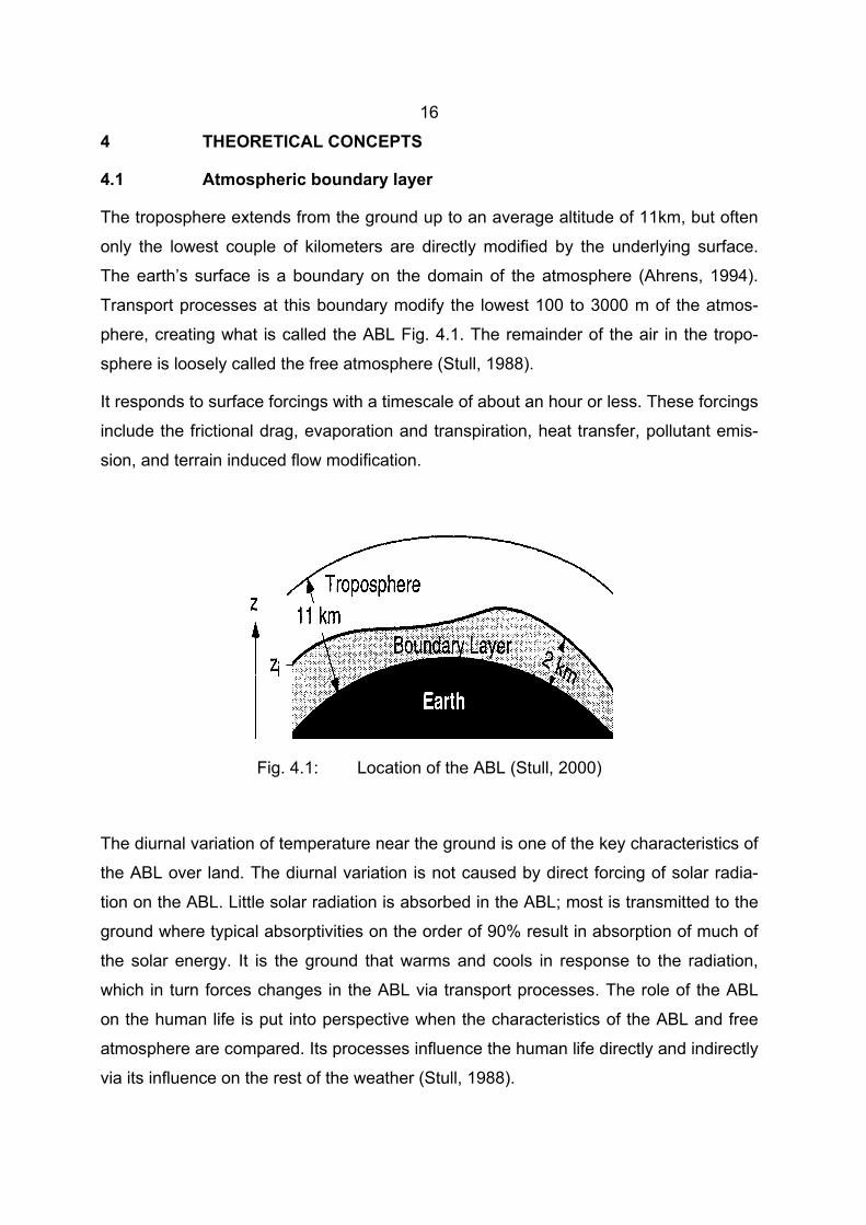
16

4 THEORETICAL CONCEPTS

4.1 Atmospheric boundary layer

The troposphere extends from the ground up to an average altitude of 11km, but often

only the lowest couple of kilometers are directly modified by the underlying surface.

The earth’s surface is a boundary on the domain of the atmosphere (Ahrens, 1994).

Transport processes at this boundary modify the lowest 100 to 3000 m of the atmos-

phere, creating what is called the ABL Fig. 4.1. The remainder of the air in the tropo-

sphere is loosely called the free atmosphere (Stull, 1988).

It responds to surface forcings with a timescale of about an hour or less. These forcings

include the frictional drag, evaporation and transpiration, heat transfer, pollutant emis-

sion, and terrain induced flow modification.

Fig. 4.1: Location of the ABL (Stull, 2000)

The diurnal variation of temperature near the ground is one of the key characteristics of

the ABL over land. The diurnal variation is not caused by direct forcing of solar radia-

tion on the ABL. Little solar radiation is absorbed in the ABL; most is transmitted to the

ground where typical absorptivities on the order of 90% result in absorption of much of

the solar energy. It is the ground that warms and cools in response to the radiation,

which in turn forces changes in the ABL via transport processes. The role of the ABL

on the human life is put into perspective when the characteristics of the ABL and free

atmosphere are compared. Its processes influence the human life directly and indirectly

via its influence on the rest of the weather (Stull, 1988).

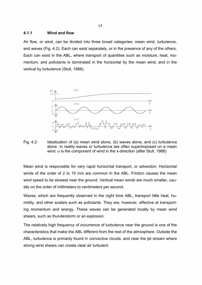
17

4.1.1 Wind and flow

Air flow, or wind, can be divided into three broad categories: mean wind, turbulence,

and waves (Fig. 4.2). Each can exist separately, or in the presence of any of the others.

Each can exist in the ABL, where transport of quantities such as moisture, heat, mo-

mentum, and pollutants is dominated in the horizontal by the mean wind, and in the

vertical by turbulence (Stull, 1988).

Fig. 4.2: Idealization of (a) mean wind alone, (b) waves alone, and (c) turbulence alone. In reality waves or turbulence are often superimposed on a mean wind. u is the component of wind in the x-direction (after Stull, 1988)

Mean wind is responsible for very rapid horizontal transport, or advection. Horizontal

winds of the order of 2 to 10 m/s are common in the ABL. Friction causes the mean

wind speed to be slowest near the ground. Vertical mean winds are much smaller, usu-

ally on the order of millimeters to centimeters per second.

Waves, which are frequently observed in the night time ABL, transport little heat, hu-

midity, and other scalars such as pollutants. They are, however, effective at transport-

ing momentum and energy. These waves can be generated locally by mean wind

shears, such as thunderstorm or an explosion.

The relatively high frequency of occurrence of turbulence near the ground is one of the

characteristics that make the ABL different from the rest of the atmosphere. Outside the

ABL, turbulence is primarily found in convective clouds, and near the jet stream where

strong wind shears can create clear air turbulent.

18

There is an easy way to isolate the large-scale variations from the turbulent ones. By

averaging wind speed measurements over a period of 30 minutes to one hour, the

positive and negative deviations of the turbulent velocities about the mean can be

eliminated or “averaged out”. Knowing the mean velocity, u, for any time period, it can

be subtracted from the actual instantaneous velocity, u`, to give just the turbulent part

(u`-u). The term u`-u can be illustrated as the gust that is superimposed on the mean

wind. It represents the part of flow that varies with periods shorter than about one hour.

The mean, u, represents the part that varies with a period longer than about one hour

(Stull, 1988).

4.1.2 Turbulence

Turbulence may be regarded as a complex assembly of locally organized but unsteady

velocity patterns which interact strongly with each other as they move with the flow.

Thus turbulence is a random, three-dimensional state of motion which is characterized

by high degree of chaotic velocity. Unstable and stable flows tend to remain in the

same state unless there is an imbalance between the paired destabilizing and stabiliz-

ing force acting on the flow. If the net effect of destabilizing factor is more than the net

effect of stabilizing factor, then turbulence will occur. It is governed mainly by the non-

linear terms of the equation of motion with strong interaction between motion on differ-

ent spatial and temporal scales. Only statistical average correlated in time and space

describe turbulence. Turbulence structure is considered to be made up of eddies of

various sizes which interact with each other and with the mean flow. The eddy interac-

tion cascades the energy to smaller and smaller eddy sizes until the energy is essen-

tially lost by the action of viscosity. Thus turbulence is dissipative and diffusive in char-

acter to a high enough degree which cannot be accounted for by the molecular diffu-

sivities and the mean strain rate. The diameter of eddies whose influence is predomi-

nant under any conditions roughly defines the scale of turbulence. There are two major

types of turbulence in the ABL; mechanical due to the instability of the vertical wind

shear and thermal due to the buoyancy forces in the atmosphere. The combination of

wind and temperature stratification, therefore, plays an important role in characterizing

the stability of the atmosphere and the generation and nature of turbulence (Singal et

al., 1997).

19

In the atmosphere, the flow near the ground is almost always turbulent up to a height 1

km or more in the daytime over land, to 100 m or so over land at night, and to a few

hundred meters over the ocean. At larger heights, turbulence occurs in the cumulus

clouds and in layers with strong changes in average wind speed or direction (Panofsky

and Dutton, 1984).

Here the three reasons can be formally listed why atmospheric scientists and engineers

are concerned with the properties of turbulence; turbulence imposes forces on build-

ings, bridges, towers, airplanes, and other structures; turbulence mixes air with different

properties and creates fluxes of important physical quantities, and turbulence creates

spatial and temporal variations of refractive index and thus leads to scattering of elec-

tromagnetic and acoustic radiation (Panofsky and Dutton, 1984).

4.1.2.1 Turbulence kinetic energy

Generally, the usual definition of kinetic energy (KE) is KE=0.5 m M2 (kg m2/s2), where

m is mass (kg) and M is the magnitude of wind (m/s). When dealing with a fluid such as

air it is more convenient to talk about kinetic energy per unit mass, which is just 0.5M2

(Stull, 1988).

It is enticing to partition the kinetic energy of the flow into a portion associated with the

mean wind, and a portion associated with turbulence. By taking the advantage of the

mean and turbulent parts of velocity, as reported in section (4.1.1), the equations of the

mean kinetic energy per unit mass (MKE, m2/s2) and the turbulence kinetic energy per

unit mass (TKE, m2/s2) can be immediately written. Moreover, the energy that is me-

chanically produced as turbulence is lost from the mean flow, and vice versa (Stull,

1988).

( )222

21 wvuMKE ++= (4.1)

( )222

21

wvuTKE σσσ ++= (4.2)

where σ2u , σ2

v and σ2w (m2/s2) are the variances of the wind velocity components in

the east (u), north (v) and vertical (w) directions (m/s) respectively.

20

TKE is one of the most important variables in micrometeorology, because it is a meas-

ure of the intensity of turbulence. It is directly related to the momentum, heat and mois-

ture transport through the ABL (Stull, 1988).

The tendency of TKE to increase or decrease is given by the following TKE budget

equation (Stull, 2000):

ε−+++=∆

∆rTBSA

tTKE (4.3)

where

A: advection of TKE by the mean wind (m2/s3),

S: shear generation (m2/s3),

B: buoyant production or consumption (m2/s3),

Tr: transport by turbulent motions and pressure (m2/s3),

ε: viscous dissipation rate (m2/s3).

The individual terms in the TKE budget equation describe physical processes that gen-

erate turbulence. The relative balance of these processes determines the ability of the

flow to maintain turbulence or become turbulent, and indicates flow stability (Stull,

1988)

Mean wind blows TKE from one location to another. The advection term is given by:

zTKEw

yTKEv

xTKEuA

∆∆

−∆

∆−

∆∆

−= (4.4)

Thus, turbulence can increase (or decrease) at any location if the wind is blowing in

higher (or lower) values of TKE from somewhere else.

Wind shear generates turbulence near the ground according to:

zMuS

∆∆

= 2* (4.5)

In the surface layer, where *u is the friction velocity (m/s), and zM

∆∆ is the wind shear

(1/s). To good approximation:

213aMS ≈ (4.6)

where a ≅ 2∗10-5 m-1 for wind speed measured at standard height of z =10 m above the

ground. Greater wind speeds at near the ground cause greater wind shear, and gener-

ate more turbulence.

Buoyancy can either increase or decrease turbulence. When thermals are rising from a

warm surface, they generate TKE. Conversely, when the ground is cold and the ABL is

statically stable, buoyancy opposes vertical motion and consumes TKE. The rate of

buoyant production or consumption of TKE is:

0HTgBv

= (4.7)

where

g : acceleration due to gravity (m/s2),

H0: kinematic surface heat flux (positive when the ground is warmer than the air)

(K.m/s). Over land, H0 and B are usually positive during the daytime, and nega-

tive at night.

Tv: absolute virtual air temperature near the ground (K).

Turbulence can advect or transport itself. For example, if turbulence is produced by

shear near the ground (in the surface layer), then turbulence motions will tend to move

the excess TKE from the surface layer to location higher in the ABL. Pressure fluctua-

tions can have a similar effect, because turbulent pressure forces can generate turbu-

lence motions. These terms are here grouped with the turbulent transport term, Tr.

Molecular viscosity dissipates turbulent motions into heat. The amount of heating is

small, but the amount of damping of TKE is large. The dissipation is always a loss:

ε

εL

TKE 23

≈ (4.8)

where Lε is a dissipation length scale (m).

The ratio of buoyancy to shear terms of TKE equation is called the flux Richardson

number, Rf, which is approximately equal to the gradient or bulk Richardson number:

22

300 )/()/(

aMHTg

zMu

HTgSBR vv

f−

≈

∆∆

−≈

−= (4.9)

4.1.2.2 Turbulence intensity

Generally, the standard deviation can be interpreted as a measure of magnitude of the

spread or dispersion of the original data from its mean. For this reason, it is used as a

measure of the intensity of turbulence. Near the ground, the turbulence intensity might

be expected to increase as the mean wind speed, M, increases. For this reason a di-

mensionless measure of the turbulence intensity, I, is often defined as (Stull, 1988):

MI Mσ

= (4.10)

where σM is the standard deviation and M the average of M (m/s). For mechanically

generated turbulence, one might expect σM to be a simple function of M.

The wind profile in general can be given by (Yersel and Goble, 1986):

)]([ln)(0

*

Lz

zz

kuzM ψ−= (4.11)

where k is von Kármán constant and ψ is some function of z/L.

The turbulence intensities may then be expressed as:

)]([ln0

* Lz

zzu

kI M

ψ

σ

−= (4.12)

In line with section 4.1.2.1, the standard deviations of the wind speed components, σi

(i=u,v,w), are intimately related to the turbulent kinetic energy, it is to be anticipated that

the intensity of turbulence should be related to the processes generating this energy.

Richardson (1920) shows these to be mainly shearing stresses and buoyancy forces.

The shearing stresses are to a large degree functions of surface roughness, which may

be taking as dependent on wind direction (Brook, 1972).

From equation (4.12), the nature of turbulence intensity depends on the height of ob-

servation, the surface roughness and the atmospheric stability (Roth, 1993). But at

23

near-neutral condition as z/L → 0, the turbulence intensity components are function of z

and z0 (Yersel and Goble, 1986).

The turbulence intensity components are defined as the ratio of the standard deviations

of the respective wind component to the mean wind speed, namely, the turbulence in-

tensity components for the along-wind (Iu), crosswind (Iv) and the vertical (Iw) wind

components are given by (Roth, 1993);

MI uu

σ= ,

MI vv

σ= and

MI ww

σ= (4.13)

4.1.2.3 Free and forced convection

The nature of turbulence, and therefore the nature of pollutant dispersion, changes with

the relative magnitudes of terms in the TKE budget. Two terms of interest are the shear

S and buoyancy B terms (Stull, 2000).

When 3/SB < , the atmosphere is said to be in a state of forced convection (Fig. 4.3).

These conditions are typical of windy overcast days, and are associated with near neu-

tral static stability. Turbulence is nearly isotropic. Smoke plumes disperse at nearly

equal rates in the vertical and lateral, which is called coning. The sign of B is not impor-

tant here- only the magnitude.

When B is positive and SB 3> , the atmosphere is said to be in a state of free convec-

tion. Thermals are typical in this situation, and the ABL is statically unstable. These

conditions often happen in the daytime over land, and during periods of cold-air advec-

tion over warmer surfaces. Turbulence is anisotropic, with more energy in the vertical,

and smoke plumes loop up and down in a pattern called looping.

When B is negative and SB > , static stability is so strong that turbulence cannot ex-

ist. During these conditions, there is virtually no dispersion while the smoke blows

downwind. Buoyancy waves (gravity waves) are possible, and appear as waves in the

smoke plumes. For values of SB ≅ , breaking Kelvin-Helmholtz waves can occur,

which cause some dispersion.

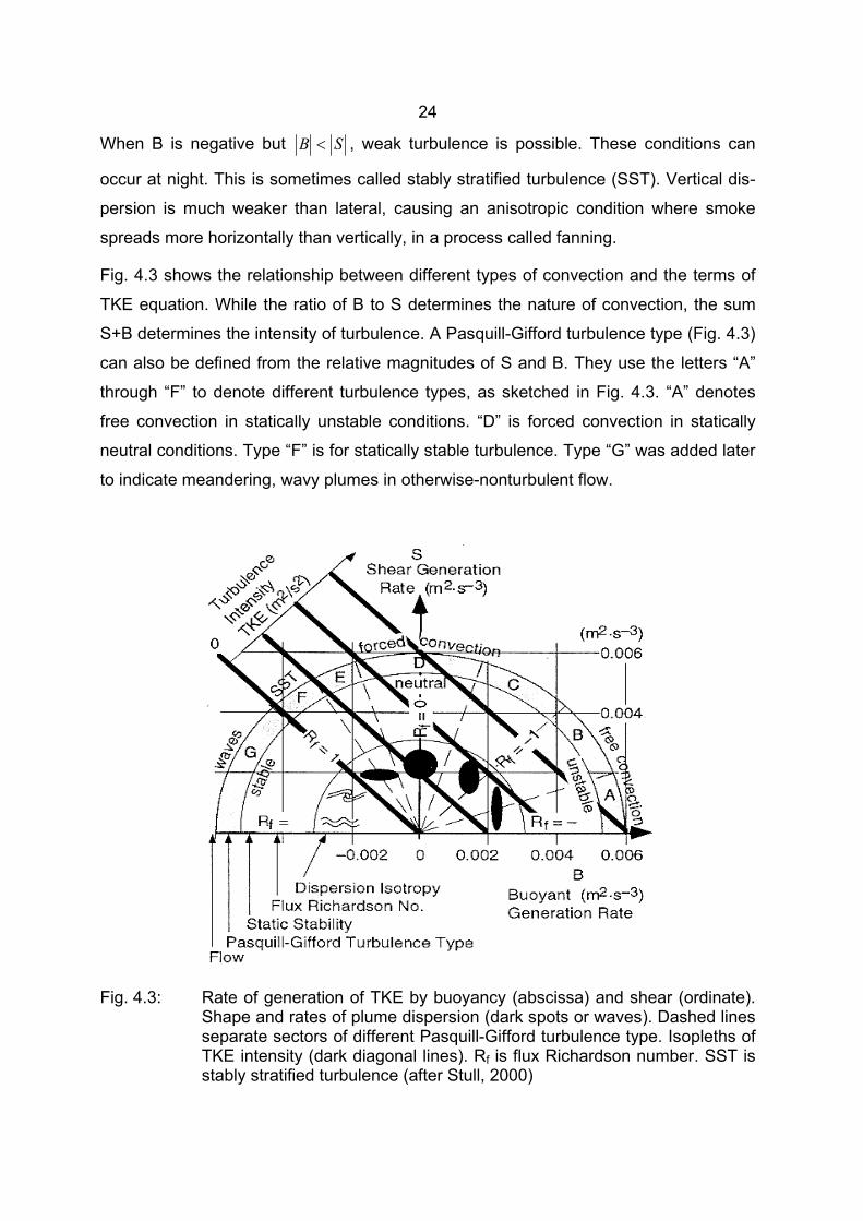
24

When B is negative but SB < , weak turbulence is possible. These conditions can

occur at night. This is sometimes called stably stratified turbulence (SST). Vertical dis-

persion is much weaker than lateral, causing an anisotropic condition where smoke

spreads more horizontally than vertically, in a process called fanning.

Fig. 4.3 shows the relationship between different types of convection and the terms of

TKE equation. While the ratio of B to S determines the nature of convection, the sum

S+B determines the intensity of turbulence. A Pasquill-Gifford turbulence type (Fig. 4.3)

can also be defined from the relative magnitudes of S and B. They use the letters “A”

through “F” to denote different turbulence types, as sketched in Fig. 4.3. “A” denotes

free convection in statically unstable conditions. “D” is forced convection in statically

neutral conditions. Type “F” is for statically stable turbulence. Type “G” was added later

to indicate meandering, wavy plumes in otherwise-nonturbulent flow.

Fig. 4.3: Rate of generation of TKE by buoyancy (abscissa) and shear (ordinate). Shape and rates of plume dispersion (dark spots or waves). Dashed lines separate sectors of different Pasquill-Gifford turbulence type. Isopleths of TKE intensity (dark diagonal lines). Rf is flux Richardson number. SST is stably stratified turbulence (after Stull, 2000)

25

4.1.3 Depth and structure of the atmospheric boundary layer

The depth of ABL depends on many factors including surface character, time of day,

atmospheric stability (e.g. the type of air mass), and insulation of the surface. In low

pressure regions the upward motions carry boundary-layer air away from the ground to

large altitudes throughout the troposphere. It is difficult to define a boundary-layer top

for these situations. Cloud base is often used as an arbitrary cut-off for the ABL studies

in these cases. Thus the region studies by ABL meteorologists may actually be thinner

in low-pressure regions than in high-pressure ones. But over land surfaces in high-

pressure regions the ABL has a well-defined structure that evolves with the diurnal cy-

cle. The three major components of this structure are the mixed layer, the residual

layer, and the stable ABL. When clouds are present in the mixed layer, it is further sub-

divided into a cloud layer and subcloud layer Fig. 4.4 (Stull, 1988).

The surface layer is the region at the bottom of the ABL where turbulent fluxes and

stress vary by less than 10% of their magnitude. Thus, the bottom 10% of the ABL is

called the surface layer, regardless of whether it is part of a mixed layer or stable ABL.

Finally, a thin layer called a micrometer or interfacial layer has been identified in the

lowest centimeters of air, where molecular transport dominates over turbulence trans-

port. For more details about the structure of the ABL, see Stull (1988).

The thickness of the ABL can be characterised in a number of ways. First, the depth of

the ABL can be defined by h, the thickness of the turbulent region next to the ground.

This is also called the depth of the mixed layer or the mixing depth, since atmospheric

properties are well mixed within it (Panofsky and Dutton, 1984).

Another height used to describe the thickness of the ABL in the daytime or at night over

heated surfaces is the height zi of the lowest inversion. Roughly, h and zi are the same

at the daytime. Actually, however, h tends to be 10% or so larger than zi, because the

lowest part of the inversion is still turbulent, partly because of the overshooting from

below and partly because there is often strong wind shear in the inversion (Panofsky

and Dutton, 1984).

At night, an inversion often extends to the ground, because the ground cools rapidly by

emitting infrared radiation (IR). When the wind is strong, mechanical turbulence is cre-

ated and heat is lost to the ground by turbulent mixing through the ABL. However, on

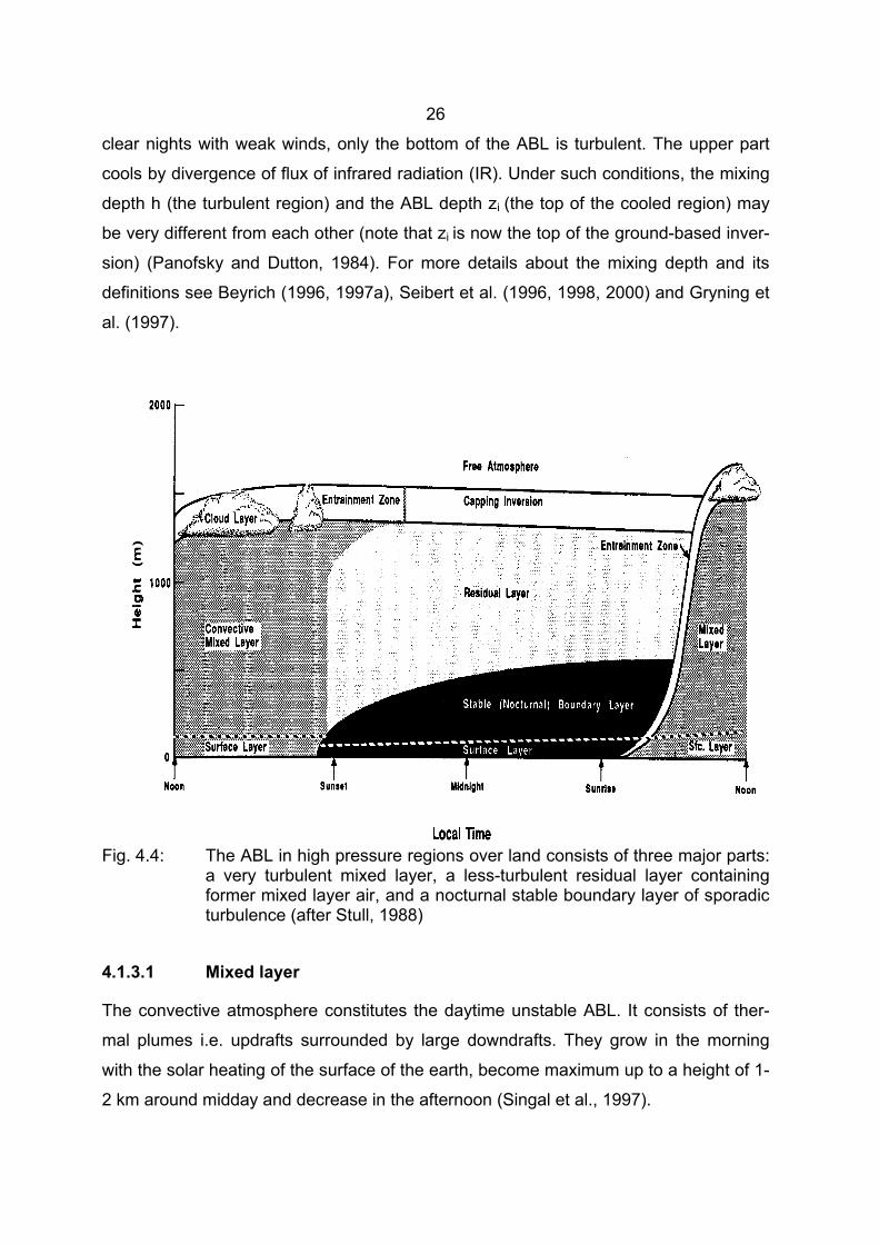
26

clear nights with weak winds, only the bottom of the ABL is turbulent. The upper part

cools by divergence of flux of infrared radiation (IR). Under such conditions, the mixing

depth h (the turbulent region) and the ABL depth zi (the top of the cooled region) may

be very different from each other (note that zi is now the top of the ground-based inver-

sion) (Panofsky and Dutton, 1984). For more details about the mixing depth and its

definitions see Beyrich (1996, 1997a), Seibert et al. (1996, 1998, 2000) and Gryning et

al. (1997).

Fig. 4.4: The ABL in high pressure regions over land consists of three major parts: a very turbulent mixed layer, a less-turbulent residual layer containing former mixed layer air, and a nocturnal stable boundary layer of sporadic turbulence (after Stull, 1988)

4.1.3.1 Mixed layer

The convective atmosphere constitutes the daytime unstable ABL. It consists of ther-

mal plumes i.e. updrafts surrounded by large downdrafts. They grow in the morning

with the solar heating of the surface of the earth, become maximum up to a height of 1-

2 km around midday and decrease in the afternoon (Singal et al., 1997).

27

After Driedonks and Tennekes (1984), three layers can be identified within the convec-

tive boundary layer as shown in Fig. 4.4 (Stull, 1988):

∗∗ the surface layer in the bottom 5 to 10%,

∗∗ the mixed layer (ML) composing the middle 35 to 80%,

∗∗ the entrainment zone in the top 10 to 60%.

In the unstable surface layer there are small-scale structures such as buoyant vertical

plumes, convergence lines, sheets of rising air, and dust devils. Higher in the mixed

layer, larger-diameter thermals, horizontal roll vortices, and mesoscale cellular convec-

tion patterns are observed. In the entrainment zone at the top of the mixed layer, these

are intermittent turbulence, overshooting thermals, Kelvin-Helmholtz waves, internal

gravity waves, and sometimes clouds. Often the whole convective ABL is called the

mixed layer. The mixed layer is so named because intense vertical mixing tends to

leave conserved variables such as potential temperature and humidity nearly constant

with height. Sometimes the mixed layer is called the well-mixed layer (Stull, 1988).

Mixing can be generated mechanically by shears, or convectively by buoyancy. Buoy-

antly generated MLs tends to be more uniformly mixed than ones driven mechanically,

because anisotropy in convection favors vertical motions, while shear anisotropy fa-

vours horizontal motions. Shears near the ground are usually more important for gen-

erating mixing than shears across the top of the ML, for atmospheric situations. Shears

at the ML top, however, can cause a separate layer to form. A mixed layer dominated

by buoyant turbulence generation is called a convective boundary layer (CBL) or con-

vective mixed layer (Stull, 1988).

During the early morning the mixed layer is shallow, starting with a depth on the order

of tens of meters for calm situations to the depth of a couple of hundred meters for

windier situations. By the late morning, for many cases, the cool nocturnal air warms to

a temperature near that of the residual layer, and the top of the ML moves up to the

residual layer base. When the thermals reach the capping inversion at the top of the

residual layer, they meet resistance to vertical motion again and the ML growth rate

rabidly decrease (Stull, 1988). At the sunset, the generation rate of the convective tur-

bulence decrease to the point where turbulence cannot be maintained against dissipa-

tion (Nieuwstadt and Brost, 1986). In the absence of the mechanical forcings, turbu-

28

lence in the ML decays completely, causing us to reclassify that layer as a residual

layer. Temperature fluctuations decay the fastest, while turbulence kinetic energy de-

cays more slowly. During this decay process the last few weak thermals may still be

rising in the upper part of the ML and can still cause entrainment, while the surface

layer has already become stably stratified (Stull and Driedonks, 1987).

4.1.3.2 Residual layer

About a half hour before sunset the thermals cease to form (in the absence of cold air

advection), allowing turbulence to decay in the formerly well-mixed layer. The resulting

layer of air is sometimes called residual layer because its initial mean state variables

and concentration variables are the same those of the recently decayed mixed layer.

Non-passive pollutants may react with other constituents during the night to create

compounds that were not originally emitted from the ground. Sometimes gaseous

chemicals may react to form aerosols or particulates which can precipitate out. The

Residual layer (RL) often exists for a while in the mornings being entrained into the ML.

During this time solar radiation may trigger photochemical reactions among the con-

stituents in the RL. Variables such as virtual potential temperature usually decrease

slowly during the night because of radiation divergence (Stull, 1988).

The RL does not have direct contact with the ground. During the night, the nocturnal

stable layer gradually increases in thickness by modifying the bottom of the RL. Thus,

the remainder of the RL is not affected by turbulent transport of surface-related proper-

ties and hence does not really fall within the definition of ABL (Stull, 1988).

4.1.3.3 Stable boundary layer

As the night progresses, the bottom portion of the residual layer is transformed by its

contact with the ground into a stable boundary layer. The ABL can become stably

stratified whenever the surface is colder than the air. This stable boundary layer (SBL)

often forms at night over land, where it is known as a nocturnal boundary layer (NBL). It

also forms by advection of warmer air over a cooler surface. This layer is characterized

by statically stable air with weaker, sporadic turbulence. Although the wind at ground

level frequently becomes lighter or calm at night, the winds aloft may accelerate to su-

29

pergeostrophic speeds in a phenomenon that is called the low-level jet or nocturnal jet.

The statically stable air tends to suppress turbulence, while the developing nocturnal jet

enhances wind shears that tend to generate turbulence. As a result, turbulence some-

times occurs in relatively short bursts that can cause mixing throughout the SBL. Dur-

ing the nonturbulent periods, the flow becomes essentially decoupled from the surface

(Stull, 1988).

As opposed to the daytime ML which has a clearly defined top, the SBL has a poorly

defined top that smoothly blends into the RL above. The top of the ML is defined as the

base of stable layer, while the SBL top is defined as the top of the stable layer or the

height where turbulence intensity is a small fraction of its surface value. SBLs can also

form during the day, as long as the underlying surface is colder than the air. These

situations often occur during warm-air advection over a colder surface, such as after a

warm frontal passage or near shorelines (Stull, 1988).

4.1.4 Atmospheric stability

Unstable flows become or remain turbulent. Stable flows become or remain laminar.

There are many factors that can cause laminar flow to become turbulent, and other fac-

tors that tend to stabilize flows. If the net effect of all the destabilizing factors exceeds

the net effect of the stabilizing factors, then turbulence will occur. These factors can be

interpreted as terms in the turbulence kinetic energy budget equation. To simplify the

concept of the atmospheric stability, investigators have historically paired one destabi-

lizing factor with one stabilizing factor, and expressed these factors as a dimensionless

ratio. Some other stability parameters such as static stability are not expressed in di-

mensionless form (Stull, 1988).

The stability is static, if it does not depend on wind but it is a measure of capability for

buoyant convection. In this case, it is determined by the local lapse rate. Even if the air

is statically stable, wind shears may be able to generate turbulence dynamically. This is

called dynamic stability (Stull, 1988).

In the ABL the air flow is turbulent because of two different mechanisms: friction with

the surface and surface heating by the sun. The airflow follows the non-slip condition at

the surface. The result is a vertical velocity gradient (wind shear). Turbulence is gener-

30

ated and energy from the mean shear is obtained. The resulting turbulent atmospheric

flow is called a mechanically generated flow (or neutral condition). On the other hand,

at daytime, the sun warms up the earth surface and the heat is molecularly transferred

to the first few centimeters of air above the ground and then further transported by tur-

bulence processes. A positive vertical temperature gradient develops and results in

vertical acceleration of air parcels (thermals). The resulting turbulent atmospheric flow

is called a buoyancy generated flow (or unstable condition). Rise of a thermal depends

whether the parcel of air is less dense than the surrounding. But, at nighttime, before

the sunset the soil starts to release heat by long wave radiation and becomes cooler

than the overlaying air. In this way vertical upward motions are suppressed. The result-

ing atmospheric flow is called stable (Melas et al., 1998).

Atmospheric stability can be characterized by several methods or parameters (Zannetti,

1990):

∗∗ empirical methods, such as the Pasquill and Turner methods,

∗∗ Monin-Obukhov length L (1/L < 0 for unstable conditions, ≅0 for neutral condi-

tions, and > 0 for stable conditions),

∗∗ Richardson number Ri, the ratio of the rate of dissipation (or production) of tur-

bulence by buoyancy to the rate of creation of turbulence by shear (Ri < 0 for

unstable conditions, Ri = 0 for neutral conditions, and Ri > 0 for stable condi-

tions).

4.1.5 Micrometeorological variables

4.1.5.1 Friction velocity

Friction velocity as one of the fundamental scaling parameters of boundary-layer mete-

orology is not uniquely defined in the literature. A survey of several textbooks on mete-

orology and of some recent research articles on ABL meteorology was made by Weber

(1999) to show the different definitions of friction velocity.

Since turbulence is often generated by wind shear at the base of the ABL, the magni-

tude of the Reynolds’ stress (turbulent momentum flux) in the surface layer turns out to

be very important. The Reynolds’ stress (τ , kg/ms2) is given by:

31

{ }21

222)´´´´( ss wvwu +−= ρτ (4.14)

where ρ is the average density of air (in kg/m3), u´, v´ and w´ are Cartesian compo-

nents of instantaneous wind (in m/s) and the subscript "s" denotes a quantity measured

at the surface.

This magnitude of Reynolds’ stress is used to calculate a natural velocity scale, the

friction velocity (u∗). The friction velocity gives a measure of the vertical kinematic flux

of the horizontal momentum in the surface layer. When horizontal winds flow over

roughness elements protruding from a surface, drag slows wind speeds near the sur-

face relative to those aloft, creating vertical wind shear. Wind shear produces eddies

that exchange momentum, energy, gases, and aerosols vertically. The greater the

height, the roughness elements protrude from a surface, and the greater the horizontal

wind speed, the greater the resulting wind shear and the mechanical turbulence. The

greater the mechanical turbulence, the greater is friction velocity, and the faster mo-

mentum, energy, and pollutants from aloft are mixed with surface air. Typical rough-

ness elements at the surface include rocks, trees, buildings, grass, and sand. The fric-

tion velocity, can be parameterized or found from the following (Jacobson, 1999):

{ }ρτ

ρ =+−= 21

2222* )´´´´( ss wvwuu (4.15)

4.1.5.2 Monin-Obukhov length

The Monin-Obukhov length L is a parameter that characterizes the stability of the sur-

face layer and is calculated from ground-level measurements. It is computed from

(Stull, 2000):

0

3*

)( HTgk

uL

v

−= (4.16)

where:

g : acceleration due to gravity,

32

H0: kinematic surface heat flux (positive when the ground is warmer than the air),

Tv: absolute virtual air temperature near the ground.

L has the unit “m” and it can refer to the atmospheric stability, 1/L < 0 for unstable con-

ditions, ≅ 0 for neutral conditions, and > 0 for stability conditions (Zannetti, 1990).

4.1.5.3 Convective velocity scale

The strong diurnal cycle in solar heating creates a strong heat flux into the air from the

earth’s surface. The buoyancy associated with this flux fuels the thermals. A buoyancy

flux can be defined as ))(/( vv wg θθ ′′ . Although the surface buoyancy flux could be used

directly as scaling variable, it is usually more convenient to generate a velocity scale

instead, using the two variables being important in free convection: buoyancy flux at the

surface, and zi. Combining these yields a velocity scale known as free convection scal-

ing velocity, w∗; also sometimes called the convective velocity scale for short (Stull,

1988):

31

* )(

′′= sv

v

i wgzw θθ

(4.17)

where vθ is the virtual potential temperature (K) and )( vw θ ′′ is the kinematic virtual po-

tential temperature flux in the vertical (K m/s).

Free convection and forced convection are names for states of turbulence in the ABL.

The ABL is said to be in free convection if buoyant convection dominates, and in forced

convection if mechanically generated turbulence dominates. Note that for forced con-

vection, u∗ is likely to be a more appropriate length scaling parameter than w* (Stull,

1988):

4.1.5.4 Roughness length

Roughness parameter represents the direct effect of the surface on the wind above and

is thus a very useful concept. Normally, within the layer of air near the ground viscosity

predominates. However, as the wind speed (shearing stress) increases over a given

33

surface, i.e. departure from the ground level, or as the surface becomes increasingly

rough at a constant wind speed, the shearing stress becomes partly turbulent and

partly viscous. Soon a stage is reached at which the pure viscous stress of the surface

is outweighed by the effect of pressure forces associated with the eddying wakes from

the roughness elements i.e. at this stage the viscosity ceases to influence the wind pro-

file and thus the shearing stress primarily defines the turbulence motions. Such an

aerodynamically rough stage where the flow is practically zero is characteristic of the

surface roughness and gives a measure of the roughness parameter z0 of the surface

(Melas et al.1998).

z0 is defined as the height at which the wind speed becomes zero. It is generally not

the same as surface height. For example z0 for a forest is always greater than z0 for

short grass. Although z0 is usually inferred from wind speed measurements at the

measurement height, Lettau (1969) suggests that it can be estimated from:

)/(5.0 *0 ls sshz = (4.18)

where:

h∗ average vertical extent of roughness elements,

ss average cross section presented to wind by each element,

sl total ground surface area / number of elements.

From the point of view of surface layer ground based measurements, z0 is useful in

estimating the effect of the ground on the flow. Especially, large values of z0 give larger

mean eddy sizes.

4.2 Sound propagation in the atmosphere

Sound energy propagates in the atmosphere as a longitudinal pressure wave. The at-

tenuation of the sound wave as it propagates is frequency dependent. Since the varia-

tion of attenuation with frequency is a smooth step less continuous curve, the decrease

in intensity of a plane sound wave in a small frequency interval can be expressed as an

exponential decay function (DIN-VDI, 1999):

)exp(0 lII α−= (4.19)

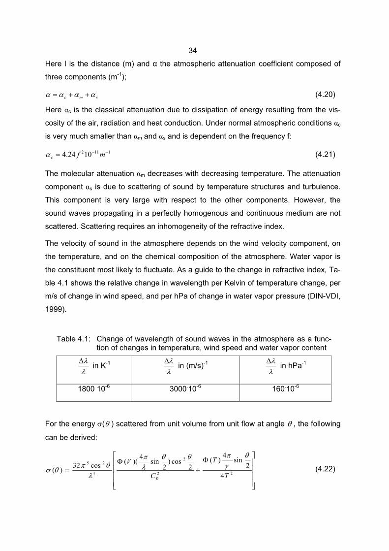
34

Here l is the distance (m) and α the atmospheric attenuation coefficient composed of

three components (m-1);

smc αααα ++= (4.20)

Here αc is the classical attenuation due to dissipation of energy resulting from the vis-

cosity of the air, radiation and heat conduction. Under normal atmospheric conditions αc

is very much smaller than αm and αs and is dependent on the frequency f:

11121024.4 −−= mfcα (4.21)

The molecular attenuation αm decreases with decreasing temperature. The attenuation

component αs is due to scattering of sound by temperature structures and turbulence.

This component is very large with respect to the other components. However, the

sound waves propagating in a perfectly homogenous and continuous medium are not

scattered. Scattering requires an inhomogeneity of the refractive index.

The velocity of sound in the atmosphere depends on the wind velocity component, on

the temperature, and on the chemical composition of the atmosphere. Water vapor is

the constituent most likely to fluctuate. As a guide to the change in refractive index, Ta-

ble 4.1 shows the relative change in wavelength per Kelvin of temperature change, per

m/s of change in wind speed, and per hPa of change in water vapor pressure (DIN-VDI,

1999).

Table 4.1: Change of wavelength of sound waves in the atmosphere as a func-

tion of changes in temperature, wind speed and water vapor content

λλ∆ in K-1

λλ∆ in (m/s)-1

λλ∆ in hPa-1

1800 10-6 3000.10-6 160.10-6

For the energy σ(θ ) scattered from unit volume from unit flow at angle θ , the following

can be derived:

Φ+

Φ= 22

0

2

4

25

42

sin4)(2

cos)2

sin4)((cos32)(T

T

C

Vθ

γπθθ

λπ

λθπθσ (4.22)

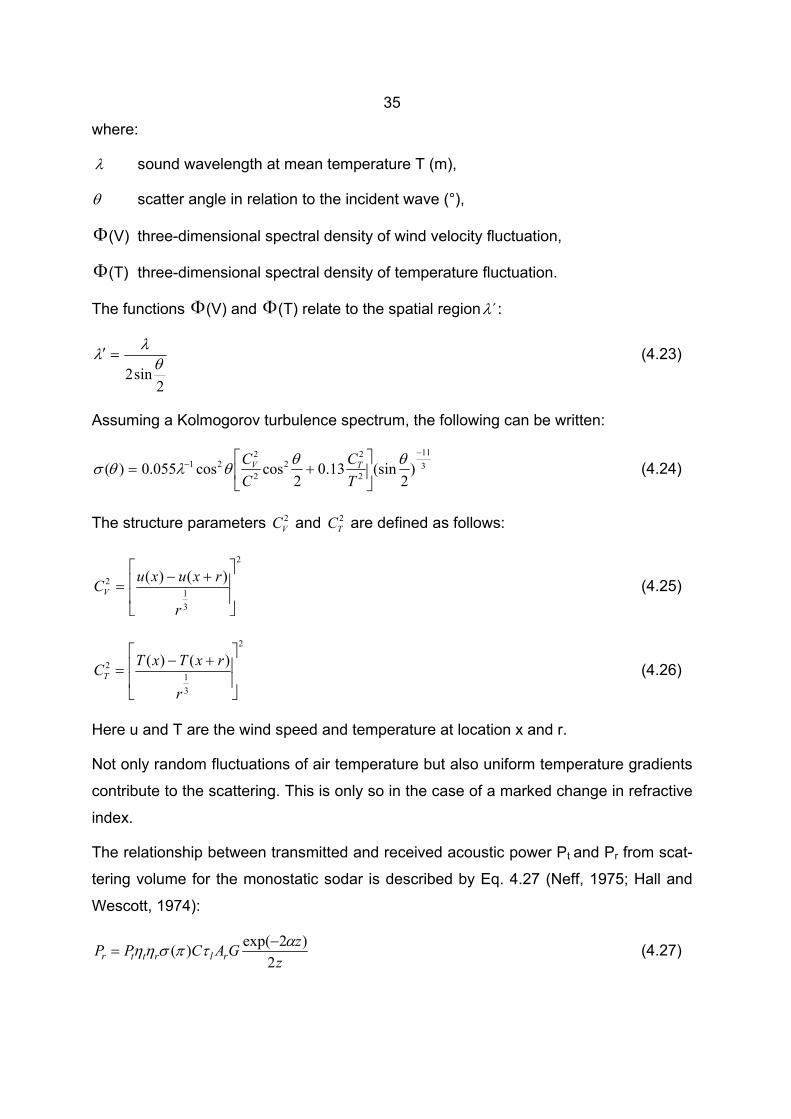
35

where:

λ sound wavelength at mean temperature T (m),

θ scatter angle in relation to the incident wave (°),

Φ(V) three-dimensional spectral density of wind velocity fluctuation,

Φ(T) three-dimensional spectral density of temperature fluctuation.

The functions Φ(V) and Φ(T) relate to the spatial region ´λ :

2sin2 θλλ =′ (4.23)

Assuming a Kolmogorov turbulence spectrum, the following can be written:

311

2

22

2

221 )

2(sin13.0

2coscos055.0)(

−−

+=

θθθλθσTC

CC TV (4.24)

The structure parameters 2VC and 2

TC are defined as follows:

2

31

2 )()(

+−=

r

rxuxuCV (4.25)

2

31

2 )()(

+−=

r

rxTxTCT (4.26)

Here u and T are the wind speed and temperature at location x and r.

Not only random fluctuations of air temperature but also uniform temperature gradients

contribute to the scattering. This is only so in the case of a marked change in refractive

index.

The relationship between transmitted and received acoustic power Pt and Pr from scat-

tering volume for the monostatic sodar is described by Eq. 4.27 (Neff, 1975; Hall and

Wescott, 1974):

zzGACPP rlrttr 2)2exp()( ατπσηη −

= (4.27)

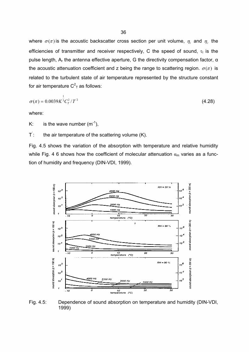
36

where )(πσ is the acoustic backscatter cross section per unit volume, tη and rη the

efficiencies of transmitter and receiver respectively, C the speed of sound, τl is the

pulse length, Ar the antenna effective aperture, G the directivity compensation factor, α

the acoustic attenuation coefficient and z being the range to scattering region. )(πσ is

related to the turbulent state of air temperature represented by the structure constant

for air temperature C2T as follows:

2`231

/0039.0)( TCK T=πσ (4.28)

where:

K: is the wave number (m-1),

T`: the air temperature of the scattering volume (K).

Fig. 4.5 shows the variation of the absorption with temperature and relative humidity

while Fig. 4 6 shows how the coefficient of molecular attenuation αm varies as a func-

tion of humidity and frequency (DIN-VDI, 1999).

Fig. 4.5: Dependence of sound absorption on temperature and humidity (DIN-VDI, 1999)

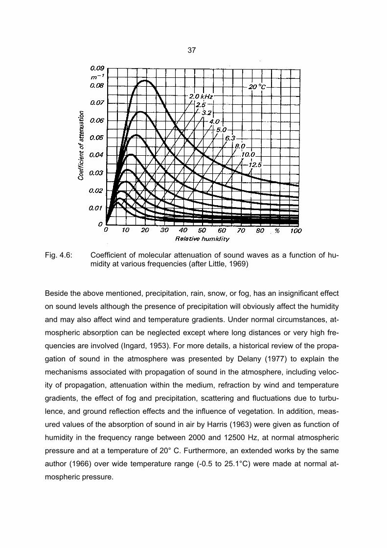
37

Fig. 4.6: Coefficient of molecular attenuation of sound waves as a function of hu-

midity at various frequencies (after Little, 1969)

Beside the above mentioned, precipitation, rain, snow, or fog, has an insignificant effect

on sound levels although the presence of precipitation will obviously affect the humidity

and may also affect wind and temperature gradients. Under normal circumstances, at-

mospheric absorption can be neglected except where long distances or very high fre-

quencies are involved (Ingard, 1953). For more details, a historical review of the propa-

gation of sound in the atmosphere was presented by Delany (1977) to explain the

mechanisms associated with propagation of sound in the atmosphere, including veloc-

ity of propagation, attenuation within the medium, refraction by wind and temperature

gradients, the effect of fog and precipitation, scattering and fluctuations due to turbu-

lence, and ground reflection effects and the influence of vegetation. In addition, meas-

ured values of the absorption of sound in air by Harris (1963) were given as function of

humidity in the frequency range between 2000 and 12500 Hz, at normal atmospheric

pressure and at a temperature of 20° C. Furthermore, an extended works by the same

author (1966) over wide temperature range (-0.5 to 25.1°C) were made at normal at-

mospheric pressure.

38

4.3 Theory of sodar measurement

Acoustic sensing is based on the sound wave scattering by turbulent air inhomogenei-

ties that are always present in the atmosphere. This technique does not differ basically

from clear air radiolocation. However, the former has some specific properties (Kallis-

tratova, 1997):

∗∗ The speed of sound is more sensitive to temperature variations than that of elec-

tromagnetic waves. For the same temperature variations the changes in the val-

ues of the refractive index for sound waves are 1000 times greater than those in

the values of the refractive index for electromagnetic waves. Therefore a cross-

section of acoustic scattering from the atmospheric temperature inhomogenei-

ties is about a million times greater than that of electromagnetic waves. As a re-

sult of this fact, sodar is simpler in design than clear air radar and its prime cost

is much lower.

∗∗ The speed of sound is responsive to changes in wind velocity. Therefore sodar

provides a more detailed information on dynamic properties of turbulence.

∗∗ The velocity of sound propagation is a million times lower than that of electro-

magnetic waves. Due to this fact the processing sodar information is considera-

bly simplified, moreover, a better spatial resolution and a short dead zone can

be reached.

∗∗ Acoustic waves of both centimeter and decimeter bands used usually in sodars

are readily absorbed in the air. Therefore the altitude range for acoustic sound-

ing is rather low and bounded to the heights of the order of 1 km.

4.3.1 Physical principle of the method

Adiabatic speed of sound C in motionless air is determined from the Laplace formula

(Kallistratova, 1997):

ργPC = (4.29)

where P is the air pressure (hPa), ρ the air density (kg/m3), and γ =1.4 is the ratio of

39

heat capacities for constant pressure and constant volume. Using the equation for ideal

gases condition:

RTP=

ρ (4.30)

Eq. (4.29) can be rewritten in the form:

µγRTC = (4.31)

where T is the mean temperature (K), R the universal gas constant (JK-1.kg-1), and µ

the molecular weight of the mixture of gases that are constituents of air (g/mol). In the

real atmosphere, water vapor is always present and the values of ρ , µ and γ depend

on water vapor concentration. Fluctuations of sound speed in wet air are due to both

adiabatic changes in density when air temperature varies, and changes in density ow-

ing to turbulent fluctuations in water vapor concentration q.

In the atmosphere, the phase sound velocity Cph, that governs the process of scatter-

ing, depends also on the projection of wind velocity vector Vr

(m/s) on the normal to the

wave front:

KKVCCph r

rr

+= (4.32)

where Kr

is the wave vector. In what follows, just a phase sound speed will be implied,

the subscript ph being omitted. Atmospheric turbulence results in random fluctuations

of T, q and Vr

that are responsible for fluctuations of the sound refractive index:

CCn 0= (4.33)

where C0 is the mean speed of sound. The intensity of a scattered wave carries infor-

mation of the intensity of turbulent fluctuations n´= n – 1.

Characteristic frequencies of turbulent fluctuations are below audio frequencies; there-

fore not temporal fluctuations but a spatial field of random inhomogeneities n´ is essen-

tial for audio sound scattering. Only those inhomogeneities, whose characteristic scales

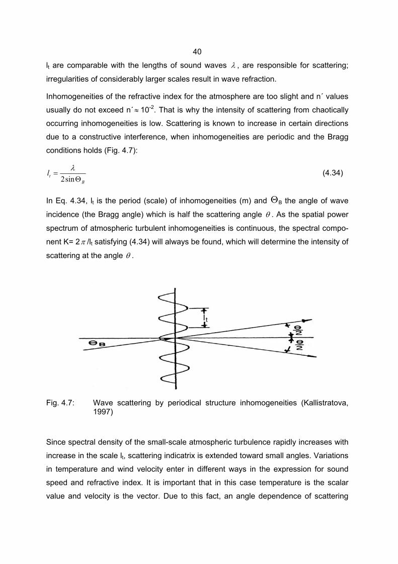
40

lt are comparable with the lengths of sound waves λ , are responsible for scattering;

irregularities of considerably larger scales result in wave refraction.

Inhomogeneities of the refractive index for the atmosphere are too slight and n´ values

usually do not exceed n´ ≈ 10-2. That is why the intensity of scattering from chaotically

occurring inhomogeneities is low. Scattering is known to increase in certain directions

due to a constructive interference, when inhomogeneities are periodic and the Bragg

conditions holds (Fig. 4.7):

Btl Θ

=sin2

λ (4.34)

In Eq. 4.34, lt is the period (scale) of inhomogeneities (m) and ΘB the angle of wave

incidence (the Bragg angle) which is half the scattering angle θ . As the spatial power

spectrum of atmospheric turbulent inhomogeneities is continuous, the spectral compo-

nent K= 2π /lt satisfying (4.34) will always be found, which will determine the intensity of

scattering at the angle θ .

Fig. 4.7: Wave scattering by periodical structure inhomogeneities (Kallistratova, 1997)

Since spectral density of the small-scale atmospheric turbulence rapidly increases with

increase in the scale lt, scattering indicatrix is extended toward small angles. Variations

in temperature and wind velocity enter in different ways in the expression for sound

speed and refractive index. It is important that in this case temperature is the scalar

value and velocity is the vector. Due to this fact, an angle dependence of scattering

41

intensity is different for temperature and velocity fluctuations. In particular, backscat-

tering (at θ =180°) occurs only from temperature and humidity inhomegenieties. This

fact offers a possibility to determine separately the fluctuations of scalar parameters

and wind velocity from the measurement of sound scattering at different angles.

Mean wind flows that carry small-scale inhomogeneities are always present in the at-

mosphere. The time of transfer of such inhomogeneities by wind flows through the so-

dar beam is usually quite less than the characteristic time of their evolution. Therefore it

is possible to consider that the spatial, the field of scatters moves as a frozen one. In

this case, the frequency of the received scattered signal fs is shifted from the radiation

frequency f0 due to the Doppler effect. At backscattering:

fs = f0 (1-2υ r/C) (4.35)

where υ r is the projection of wind velocity in the direction of sounder beam. Thus, us-

ing a Doppler sodar it is possible to determine a beam component of the mean wind

velocity and using a three-component sodar it is possible to determine the whole vector

of wind velocity Vr

.

4.3.2 Sodar system configurations

The principle of acoustic sounding is based on the detection of the backscattered signal

from acoustic refractive index discontinuities or disturbances in the atmosphere. Based

on the equations (4.24), two elementary configurations are possible (Melas et al., 1998;

for more details about the basic design of Doppler sodar, see Ito 1997):

Monostatic: the same antenna is used for the acoustic tone emission and for the echo

reception. There are some disadvantages to take into account when using this configu-

ration:

∗∗ The echo intensity, having only the contribution from thermal fluctuations, is

weaker than in the bistatic configuration and vanishes when the temperature

lapse rate approaches to adiabatic. That may happen in the period following the

sunset and leads to a systematic lack of data in some parts of the day.

∗∗ The estimates of the wind values at each range gate derive from radial vertical

component measured at three different positions in space. This problem is usu-

42

ally overcome by averaging over several scans. However this can be a severe

limitation even for mean wind estimates (Neff and Coulter, 1986) in high horizon-

tal dishomogeneity conditions such as for example over complex terrain or land-

water interfaces.

Bistatic: at least two antenna are needed, one to emit the tone, the other to receive the

echo. This configuration, using bistatic scattering, rely on a more continuous signal for

Doppler wind estimate since echo is present also when the temperature lapse rate is

close to adiabatic. Moreover in this configuration the sodar is the only remote sensor

directly sensitive to the small-scale velocity field (Neff and Coulter, 1986). Several dis-

advantages, however, are associated with this configuration.

∗∗ Bistatic systems usually require 100 to 300 m base lines with all the related ca-

bling.

∗∗ There are ground clutter problems because of the refraction and reflection of the

signal going through the broad beams from low objects.

The need to measure the wind components in several directions for the wind profile

retrieving leads to multi-axes (bistatic and /or monostatic) sodar systems.

In the last decade the increasing computing power of PC's and the possibility to plug in

their bus DSP (Digital Signal Processing) cards permitted the setting-up of configura-

tions that allows for simultaneous monostatic and bistatic modes of operation (Mastran-

tonio et al. 1986). In this case each of the antennas radiates a different frequency, and

each is allowed to receive and process signals at three frequencies.

More recently to make systems easy to move, array antennas have been developed,

that is antennas resulting from a set of elementary microphones (typically between 25

and 220 elements) that radiate the acoustic tones simultaneously. The control of the

relative phase of each emitter permits the beam steering in the desired direction; the

alternately transmitting along three different directions, after an appropriate averaging

period, allows retrieval of the wind profile (Melas et al., 1998).

43

5 MEASUREMENTS, DATA PROCESSING AND EXPERIMENTAL SITES

5.1 Measurements

5.1.1 Principles of sodar measurement

The sodar emits short pulses of sound which are backscattered by temperature and

velocity inhomogeneities in the atmosphere. The sodar measures the return time, the

amplitude as well as the frequency distribution of echoed pulse. The time of travel is

used to evaluate the distance of the scattering volume the frequency shift to calculate

its velocity and the amplitude of the returned signal to obtain information about the

structure of the inhomogeneity.

5.1.1.1 Beam pattern

The sodar uses a single antenna system to both transmit acoustic signals upward into

the atmosphere and to measure the reflection of those signals back from small scale

turbulence caused by small scale thermal and wind velocity fluctuations in the air.

Three beam axes (not in the same plane) are required for wind measurements. Usu-

ally, there is one in the vertical beam and two tilted beams, but three tilted beams also

work. Standard measurements are made by transmitting a pulse along the first beam

path and its symmetrical (if tilted) beam path, then waiting a few seconds for all re-

flected energy from the atmosphere to be received back at the antenna and processed,

then transmitting on the second third beam paths in the same manner as the first. The

cycle is repeated continuously to accumulate measurements for further averaging dur-

ing the automated data process. In the sodar (FAS64) of the Meteorological Institute,

University of Freiburg, which was used within this investigation, the antenna pointing

directions include one vertical beam and many tilted beams. The direction cycle can be

individually defined by the user and it can emit beams in 9 different directions which are

as following (Scintec, 2002):

∗∗ 0° vertically,

∗∗ 9° east, 22° west

∗∗ 29° north, 22° south

∗∗ 29° west, 22° east

∗∗ 29° south, 22° north

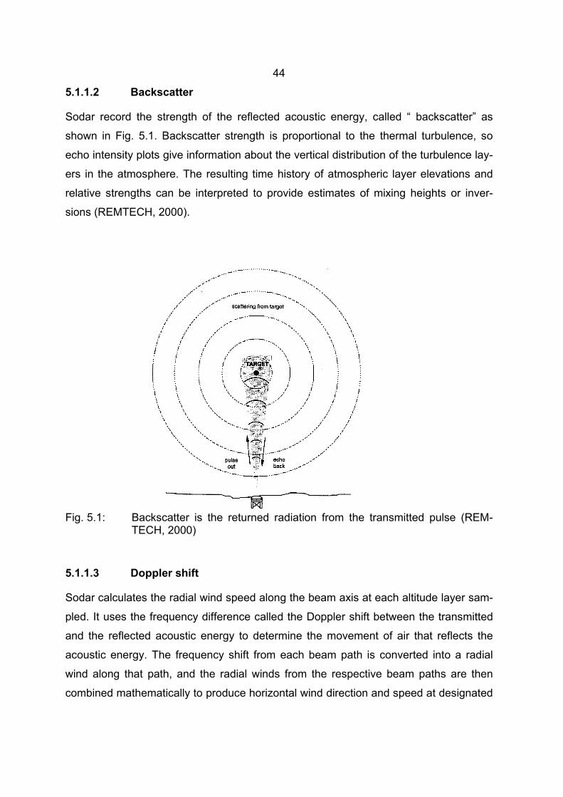
44

5.1.1.2 Backscatter

Sodar record the strength of the reflected acoustic energy, called “ backscatter” as

shown in Fig. 5.1. Backscatter strength is proportional to the thermal turbulence, so

echo intensity plots give information about the vertical distribution of the turbulence lay-

ers in the atmosphere. The resulting time history of atmospheric layer elevations and

relative strengths can be interpreted to provide estimates of mixing heights or inver-

sions (REMTECH, 2000).

Fig. 5.1: Backscatter is the returned radiation from the transmitted pulse (REM-TECH, 2000)

5.1.1.3 Doppler shift

Sodar calculates the radial wind speed along the beam axis at each altitude layer sam-

pled. It uses the frequency difference called the Doppler shift between the transmitted

and the reflected acoustic energy to determine the movement of air that reflects the

acoustic energy. The frequency shift from each beam path is converted into a radial

wind along that path, and the radial winds from the respective beam paths are then

combined mathematically to produce horizontal wind direction and speed at designated

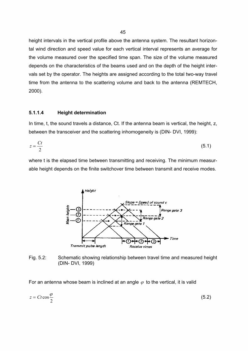
45

height intervals in the vertical profile above the antenna system. The resultant horizon-

tal wind direction and speed value for each vertical interval represents an average for

the volume measured over the specified time span. The size of the volume measured

depends on the characteristics of the beams used and on the depth of the height inter-

vals set by the operator. The heights are assigned according to the total two-way travel

time from the antenna to the scattering volume and back to the antenna (REMTECH,

2000).

5.1.1.4 Height determination

In time, t, the sound travels a distance, Ct. If the antenna beam is vertical, the height, z,

between the transceiver and the scattering inhomogeneity is (DIN- DVI, 1999):

2Ctz = (5.1)

where t is the elapsed time between transmitting and receiving. The minimum measur-

able height depends on the finite switchover time between transmit and receive modes.

Fig. 5.2: Schematic showing relationship between travel time and measured height (DIN- DVI, 1999)

For an antenna whose beam is inclined at an angle ϕ to the vertical, it is valid

2cosϕCtz = (5.2)

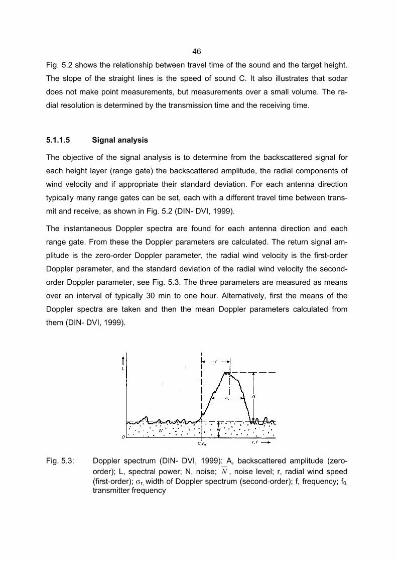
46

Fig. 5.2 shows the relationship between travel time of the sound and the target height.

The slope of the straight lines is the speed of sound C. It also illustrates that sodar

does not make point measurements, but measurements over a small volume. The ra-

dial resolution is determined by the transmission time and the receiving time.

5.1.1.5 Signal analysis

The objective of the signal analysis is to determine from the backscattered signal for

each height layer (range gate) the backscattered amplitude, the radial components of

wind velocity and if appropriate their standard deviation. For each antenna direction

typically many range gates can be set, each with a different travel time between trans-

mit and receive, as shown in Fig. 5.2 (DIN- DVI, 1999).

The instantaneous Doppler spectra are found for each antenna direction and each

range gate. From these the Doppler parameters are calculated. The return signal am-

plitude is the zero-order Doppler parameter, the radial wind velocity is the first-order

Doppler parameter, and the standard deviation of the radial wind velocity the second-

order Doppler parameter, see Fig. 5.3. The three parameters are measured as means

over an interval of typically 30 min to one hour. Alternatively, first the means of the

Doppler spectra are taken and then the mean Doppler parameters calculated from

them (DIN- DVI, 1999).

Fig. 5.3: Doppler spectrum (DIN- DVI, 1999): A, backscattered amplitude (zero-order); L, spectral power; N, noise; N , noise level; r, radial wind speed (first-order); σr, width of Doppler spectrum (second-order); f, frequency; f0, transmitter frequency

47

The horizontal and vertical wind velocity and the horizontal wind direction are calcu-

lated from the first-order parameters. The standard deviations of the wind values can

be calculated from the instantaneous values of the first order parameters or from the

second-order parameter. For each antenna and each range gate, it is possible to calcu-

late: Doppler spectrum; return signal amplitude, A; radial wind velocity; vertical wind

velocity, w; horizontal wind velocity, horizontal wind directions, standard deviations of

horizontal wind velocity and standard deviation of horizontal wind direction.

5.1.1.6 Limitation of sodar operation

The limitation to a sodar's operation stem principally from the use of acoustics as a

probing technique (Atmospheric Research Pty. Ltd., 2000):

∗∗ Range: Sound is attenuated in the atmosphere. At higher frequency, sound is

attenuated much more than lower frequencies. With increasing temperatures,

and/or lower relative humidity, the attenuation of sound increases. The height

performance of a sodar in a hot, dry, desert may only be 60% of the same in-

strument in a cool and damp location.

∗∗ Audible sound: The use of sound can limit its use in built-up areas.

∗∗ Background noise: The background noise where a sodar is operating can also

limit a sodar’s performance. In general sodars should not be operated in areas

where the noise level (at the frequency of operation of the sodar) is high.

∗∗ Local structures: Sodars should not be installed near structures (or vegetation)

which can produce fixed echoes.

5.1.2 Accuracy of sodar measurements

The ability of Doppler sodar to measure profiles of mean wind speed with good accu-

racy and reliability is well proved (Shurygin et al., 2000). Comparisons with tower in-

struments, tethersondes, and pilot balloons have shown that Doppler sodars offer a

reliable estimations of the mean wind speed and wind direction (e.g. Balser et al., 1976;

Caughey et al., 1976; Asimakopoulos et al., 1978; Kaimal et al., 1980; Congeduti et al.,

48

1981; Gaynor and Korrell, 1981; Thomas et al., 1983; Kaimal et al., 1984; Helmis et al.,

1985; Kallistratova et al., 1985; Tsvang et al., 1985; Finkelstein et al., 1986; Gaynor

and Kristensen, 1986; Ito et al., 1986; Santovasi, 1986; Kallistratova et al., 1987; Tho-

mas, 1988; Chintawongvanisch et al., 1989; Ito et al., 1989; Keder et al., 1989; Gaynor

et al., 1990; Thomas and Vogt, 1990, 1993; Kurzeja, 1994; Piringer, 1994; Vogt and

Thomas, 1994; Beyrich, 1997b; Ito, 1997b; Peters et al., 1998; Reitebuch and Emeis,

1998; Seibert et al., 2000; Emeis, 2001; Görsdorf et al., 2002; Kramer and Kouznetsov,

2002). Doppler sodar configurations examined in these studies included bistatic,

monostatic and phased-array sodars, but only Ito et al. (1989); Gaynor et al. (1990) -

Xontech phased-array sodar; Vogt and Thomas (1994) - Remtech phased-array sodar;

Kurzeja (1994) - Xontech phased-array sodar; Piringer (1994) - Remtech phased-array

sodar - and Ito (1997b) have used phased-array sodars. The results of most studies

that have made quantitative comparisons of sodar-data against those obtained by in

situ instruments and other ground-based remote sensing methods were compiled by

Grescenti (1997). He summarized a brief descriptions of all published sodar compari-

son studies over the last 20 years and the statistical measures which were used in

these studies.

Some results of these investigations are: the sodar-derived wind speed and wind direc-

tion are highly correlated against reference measurements (correlation coefficient r ≈

0.92) with precision of 1.1 m/s and 21.5°, respectively. Correlations of sodar-derived

values of σw were not quite as good (r ≈ 0.81) with an average precision of 0.18 m/s.

Past studies have shown that σw accuracies vary significantly from day (convective

conditions) to night (stable conditions). Very few data values were available for σdd,

which had a poor correlation of r ≈ 0.57 and precision of 10.7°. The conclusions from

many of these studies have shown that Doppler sodars can accurately obtain the mean

wind speed and wind direction. Sodar-derived values of σw show much promise, espe-

cially in the more recent studies; however, caution is still recommended with their use

(Grescenti, 1997).

With regard to the standard deviations of the longitudinal and lateral wind speed, σu

and σv, only a poor correlation exists with other methods (Gaynor, 1992). Unfortu-

nately, sodar-derived σu and σv values have very large uncertainties that make them

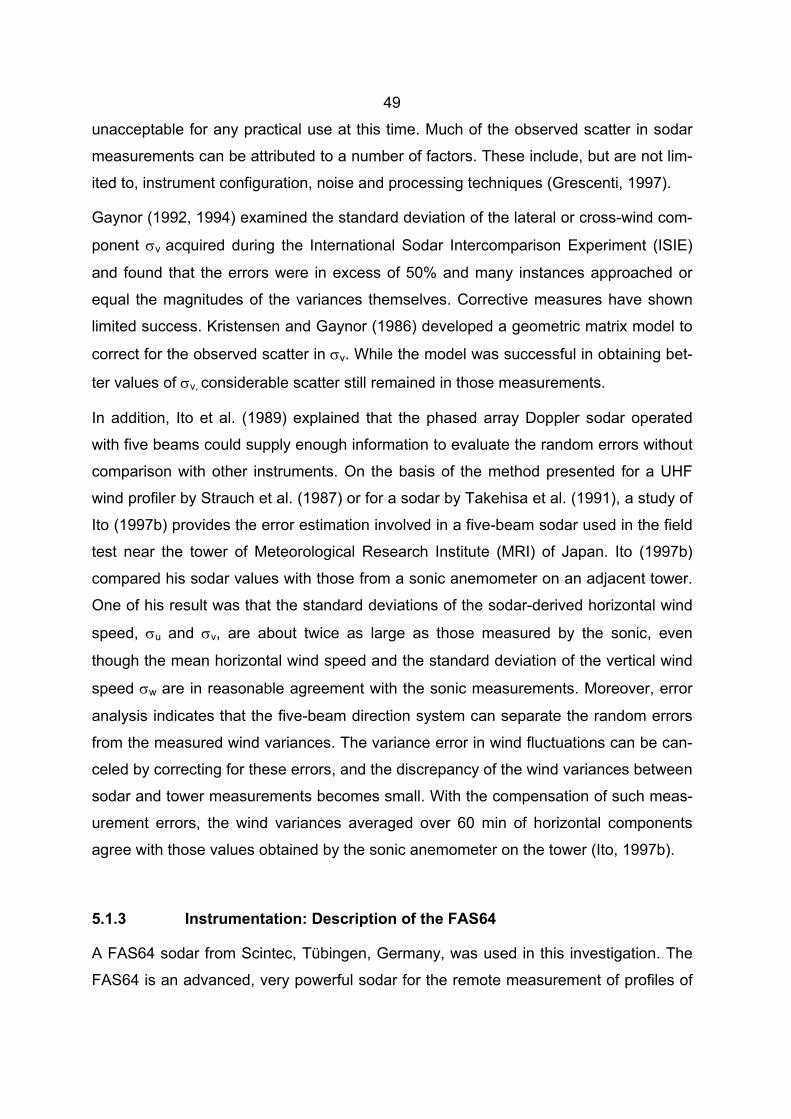
49

unacceptable for any practical use at this time. Much of the observed scatter in sodar

measurements can be attributed to a number of factors. These include, but are not lim-

ited to, instrument configuration, noise and processing techniques (Grescenti, 1997).

Gaynor (1992, 1994) examined the standard deviation of the lateral or cross-wind com-

ponent σv acquired during the International Sodar Intercomparison Experiment (ISIE)

and found that the errors were in excess of 50% and many instances approached or

equal the magnitudes of the variances themselves. Corrective measures have shown

limited success. Kristensen and Gaynor (1986) developed a geometric matrix model to

correct for the observed scatter in σv. While the model was successful in obtaining bet-

ter values of σv, considerable scatter still remained in those measurements.

In addition, Ito et al. (1989) explained that the phased array Doppler sodar operated

with five beams could supply enough information to evaluate the random errors without

comparison with other instruments. On the basis of the method presented for a UHF

wind profiler by Strauch et al. (1987) or for a sodar by Takehisa et al. (1991), a study of

Ito (1997b) provides the error estimation involved in a five-beam sodar used in the field

test near the tower of Meteorological Research Institute (MRI) of Japan. Ito (1997b)

compared his sodar values with those from a sonic anemometer on an adjacent tower.

One of his result was that the standard deviations of the sodar-derived horizontal wind

speed, σu and σv, are about twice as large as those measured by the sonic, even

though the mean horizontal wind speed and the standard deviation of the vertical wind

speed σw are in reasonable agreement with the sonic measurements. Moreover, error

analysis indicates that the five-beam direction system can separate the random errors

from the measured wind variances. The variance error in wind fluctuations can be can-

celed by correcting for these errors, and the discrepancy of the wind variances between

sodar and tower measurements becomes small. With the compensation of such meas-

urement errors, the wind variances averaged over 60 min of horizontal components

agree with those values obtained by the sonic anemometer on the tower (Ito, 1997b).

5.1.3 Instrumentation: Description of the FAS64

A FAS64 sodar from Scintec, Tübingen, Germany, was used in this investigation. The

FAS64 is an advanced, very powerful sodar for the remote measurement of profiles of

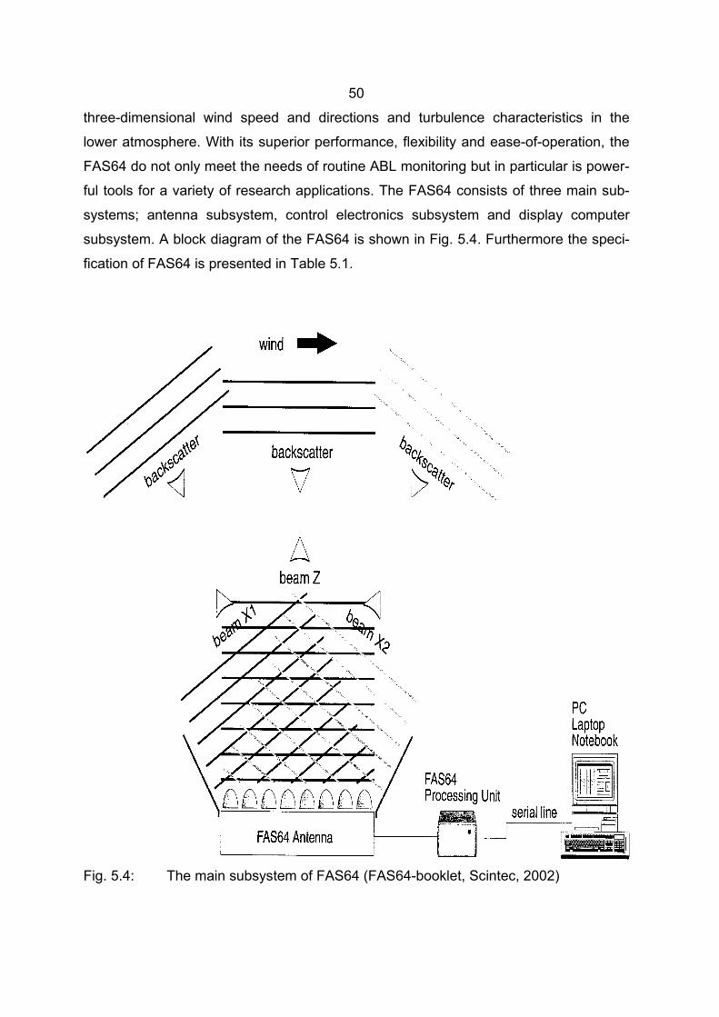
50

three-dimensional wind speed and directions and turbulence characteristics in the

lower atmosphere. With its superior performance, flexibility and ease-of-operation, the

FAS64 do not only meet the needs of routine ABL monitoring but in particular is power-

ful tools for a variety of research applications. The FAS64 consists of three main sub-

systems; antenna subsystem, control electronics subsystem and display computer

subsystem. A block diagram of the FAS64 is shown in Fig. 5.4. Furthermore the speci-

fication of FAS64 is presented in Table 5.1.

Fig. 5.4: The main subsystem of FAS64 (FAS64-booklet, Scintec, 2002)

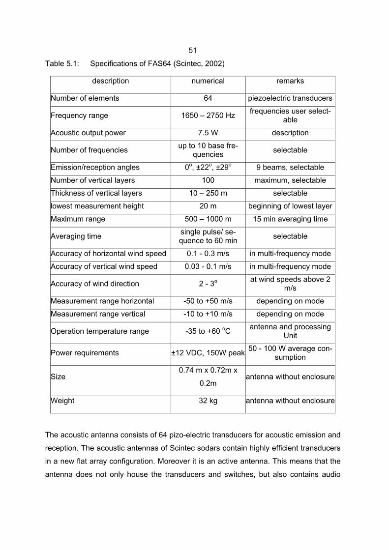
51

Table 5.1: Specifications of FAS64 (Scintec, 2002)

description numerical remarks

Number of elements 64 piezoelectric transducers

Frequency range 1650 – 2750 Hz frequencies user select-able

Acoustic output power 7.5 W description

Number of frequencies up to 10 base fre-quencies selectable

Emission/reception angles 0o, ±22o, ±29o 9 beams, selectable

Number of vertical layers 100 maximum, selectable

Thickness of vertical layers 10 – 250 m selectable

lowest measurement height 20 m beginning of lowest layer

Maximum range 500 – 1000 m 15 min averaging time

Averaging time single pulse/ se-quence to 60 min selectable

Accuracy of horizontal wind speed 0.1 - 0.3 m/s in multi-frequency mode

Accuracy of vertical wind speed 0.03 - 0.1 m/s in multi-frequency mode

Accuracy of wind direction 2 - 3o at wind speeds above 2 m/s

Measurement range horizontal -50 to +50 m/s depending on mode

Measurement range vertical -10 to +10 m/s depending on mode

Operation temperature range -35 to +60 oC antenna and processing Unit

Power requirements ±12 VDC, 150W peak 50 - 100 W average con-sumption

Size 0.74 m x 0.72m x

0.2m antenna without enclosure

Weight 32 kg antenna without enclosure

The acoustic antenna consists of 64 pizo-electric transducers for acoustic emission and

reception. The acoustic antennas of Scintec sodars contain highly efficient transducers

in a new flat array configuration. Moreover it is an active antenna. This means that the

antenna does not only house the transducers and switches, but also contains audio

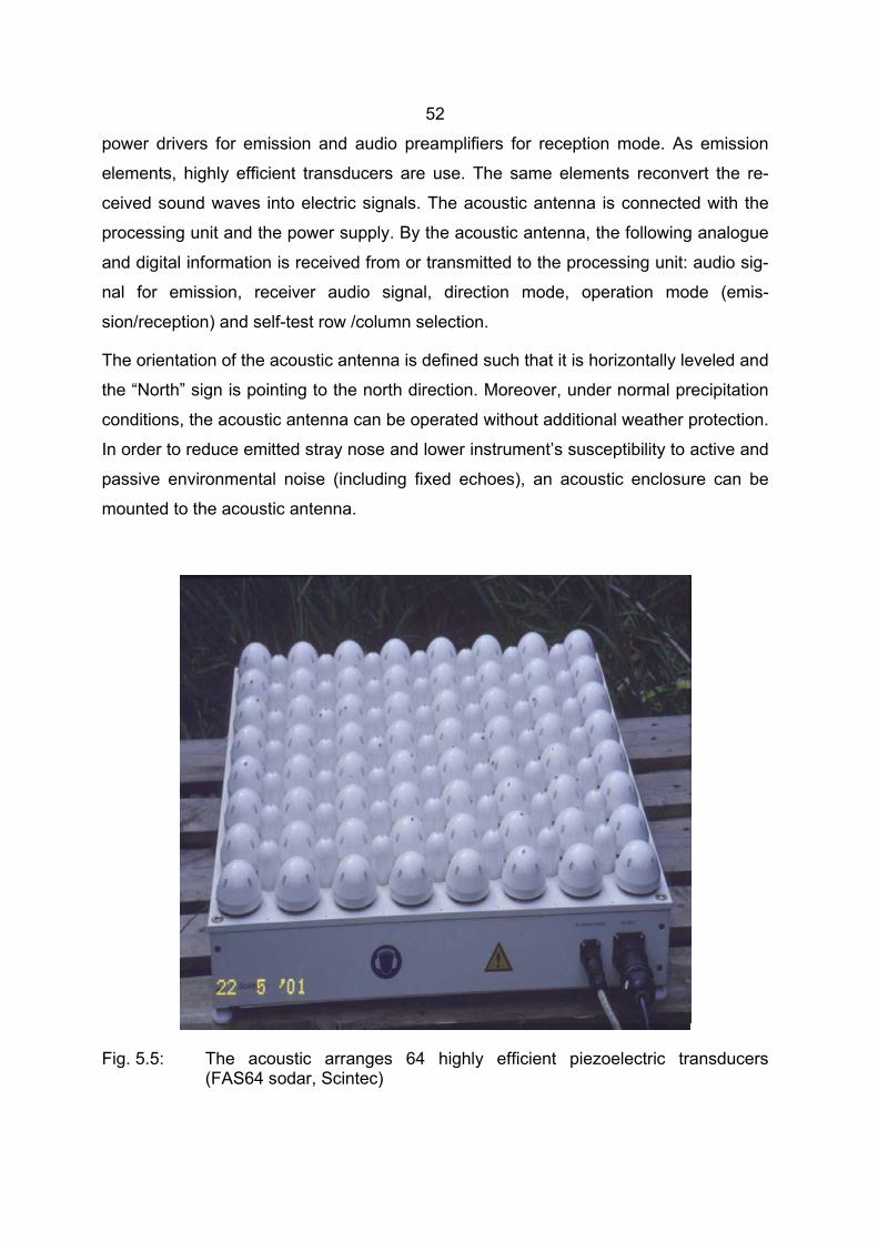
52

power drivers for emission and audio preamplifiers for reception mode. As emission

elements, highly efficient transducers are use. The same elements reconvert the re-

ceived sound waves into electric signals. The acoustic antenna is connected with the

processing unit and the power supply. By the acoustic antenna, the following analogue

and digital information is received from or transmitted to the processing unit: audio sig-

nal for emission, receiver audio signal, direction mode, operation mode (emis-

sion/reception) and self-test row /column selection.

The orientation of the acoustic antenna is defined such that it is horizontally leveled and

the “North” sign is pointing to the north direction. Moreover, under normal precipitation

conditions, the acoustic antenna can be operated without additional weather protection.

In order to reduce emitted stray nose and lower instrument’s susceptibility to active and

passive environmental noise (including fixed echoes), an acoustic enclosure can be

mounted to the acoustic antenna.

Fig. 5.5: The acoustic arranges 64 highly efficient piezoelectric transducers (FAS64 sodar, Scintec)

53

5.1.4 Description of the software: FASrun program

The FAS64 sodar system is operated with the FASrun software. This software must be

installed on an IBM compatible PC with a Pentium or higher Processor, Windows 3x,

Windows 95, Windows 98, Windows NT operating system, a minimum of 8MB free

RAM, and a minimum of 12 MB free hard-disk space. It allows the user to set the pa-

rameters for emission and reception. It also displays the measured data. All output data

files are written in ASCII format. The actual data can be viewed during the measure-

ment to verify the parameters with respect to consistency. The received spectra, the

wind speeds and their standard deviations, the gains and the backscatter of signal are

visualized. If the wind data are calibrated with the sensible heat flux, the program dis-

plays the values of the temperature structure function, CT, and other atmospheric pa-

rameters like the stability parameter and eddy diffusivity (an input for z0 is required to

obtain correct estimates of the eddy diffusivity).

The “received spectra” window shows the received frequency distribution normalized to

the emitted frequencies as function of the altitude. It also displays the fitted frequency

function, which used by the program for determining the wind speed.

The “wind speed” window displays for each height the three wind speed components,

the resulting horizontal wind speed and its direction and the standard deviations of the

three wind components (not the accuracy of the wind speed measurement).

In the “gain” window the actual automatically fitted gains are shown.

The “sodargram” window displays the backscatter of the emitted signal. The data

represents the absolute signal returned by the system at all frequencies used.

These values can also be viewed after the measurement. But it is not possible to dis-

play the gains and the fitted spectra.

The parameters for the emission and reception govern the frequencies and their dura-

tion in an emitted sequence, the vertical resolution and the averaging time. Setting

these parameters also controls some algorithms.

The vertical resolutions set the average ranging of the returned signal. The user sets

ranges in meters and not the time which the sound needs for this distance. The relation

between the range and the time through the velocity of sound is done by the process-

54

ing units. The program needs the temperature and air pressure at ground for this rela-

tion. The vertical resolution should correlate with the structure of the ABL, if it is known.

To achieve good results even in higher altitudes, the resolution is reduced with increas-

ing height, so that more information is retrieved from a given average.0

The composition of the emitted frequencies can be independent for each direction. Up

to ten frequencies can be emitted in one sequence.

In this study, only the main data output files (extensions *.mnd) were used which can

be converted to other software to make other treatment of these results. For more de-

tails about the FASrun program, see the user’s manual of Flat Array Sodars, Scintec

(2002) and Pavel Schilinsky (2000).

5.2 Data processing

In this study, the FAS64 provided the following data in the range from 20 m to 500 m

a.g.l. for all investigated land use types in form of vertical layer related mean values

over 30 minutes: longitudinal (u), lateral (v) and vertical (w) wind speed; horizontal wind

speed (vh); wind direction (dd); standard deviations of all wind speed components (σi;

i=u,v,w) and standard deviations of the wind direction (σdd). Although the variances of

horizontal wind speed, σ2u and σ2

v, measured by the phased-sodar may be about twice

as large as those measured at the tower (Ito, 1997b), these variables were used in this

study, because the manufacturer of the FAS64 Sodar gave a physically based declara-

tion for the use of σu and σv. In addition, the shape of the variation of σu/u∗ and σv/u∗

with increasing instability (-z/L) in the surface layer showed the same behavior as in

other studies, which used sonic anemometer-thermometer instruments such as AL-

Jiboori et al., 2001 (see figures 6.1.14, 6.2.15, 6.3.15 and 6.4.14).

Besides directly monitoring such meteorological variables as u, v, w, vh, dd, σi (i=u,v,w),

σdd, the application of a number of methods and algorithms enabled the estimation of

features of the atmospheric turbulence were calculated. These can be concluded as

follows:

∗∗ P-G stability classes: Such a stability classification is the first step for applying a

number of traditional algorithms aiming at estimating the main atmospheric pa-

55

rameters which typically describe the ABL structure such as Monin-Obukhov

length (L) and friction velocity (u∗) (Capanni and Gualtieri, 1999). A method,

starting from sodar data only, was applied to determine the P-G stability classes.

This method is the one proposed by Thomas (1988). He used the standard de-

viations of the horizontal wind speed (σdd) by measurements of a tower (at 100

m a.g.l.) and sodar (at 60, 100, 160, 200 m a.g.l.) to determine the P-G stability

classes. The class limits of the σdd-values measured at these heights by the so-

dar have been compiled in table 5. 2.

∗∗ Stability parameter (z/L), the Monin-Obukhov length could be calculated from the

empirical method developed by Liu et al. (1976) and Irwin (1979), as described

in Zannetti (1990), by using power law functions of z0 as:

bazL 01

= (5.3)

where a and b are empirical coefficients and their values have been compiled in

table 5. 3.

∗∗ Turbulent kinetic energy per unit mass, TKE, could be calculated from Eq. (4.2).

∗∗ Mean kinetic energy per unit mass, MKE, can be calculated from Eq. (4.1).

∗∗ The production of turbulent kinetic energy of convective and mechanical origin

can be represented by the σ3w/z (Weill et al., 1980) and can be calculated from

the data of sodar.

∗∗ The turbulence intensity components for longitudinal, lateral and vertical wind

speed components, Iu, Iv, Iw, could be calculated from Eq. (4.13).

∗∗ The standard deviations of the wind speed components normalized by the fric-

tion velocity, σi/u∗ (i=u,v,w), in the surface layer and under unstable conditions:

σi could be obtained from the sodar’s data. The friction velocity, u∗, under unsta-

ble conditions and in the surface layer, could be calculated from the similarity re-

lationship (Stull, 1988):

31

* )(9.1

−

−=Lzu wσ (5.4)

56

∗∗ The variance of the vertical component of the wind speed scaled by the square

value of the convective velocity, σ2w/w∗

2 , under the free convective weather. The

convective velocity was given by (Melas, 1993):

6.0*wmw σ

= (5.5)

where σwm is the average of σw between 100 m and the uppermost sodar level.

∗∗ The data of mixed layer, zi, are not available in this study but a rough estimate of

zi could be obtained from the σ2w profile. However, σ2

w has a maximum at

zm ≈ 0.35zi. Measurements in the CBL show that zm occurs in the range 0.3zi-

0.6zi (Caughey, 1982). A good compromise is therefore (Melas, 1993):

mi zz 8.2≈ (5.6)

Table 5.2: Method of stability classification (class limits) (Thomas, 1988)

height P-G stability classes

F E D C B A

60 m 4.6° 9.1 22.6 44.0 67.6

100 m 4.3° 6.9 15.1 27.9 51.3

160 m 2.0° 4.7 14.4 30.5 52.7

200 m 2.3° 4.4 13.2 30.4 54.5

Table 5.3: The values of coefficient a and b (Liu et al., 1976; Irwin, 1979)

P-G stability

classes

A B C D E F

A -0.08750 -0.03849 -0.00807 0.0 0.00807 0.03849

B -0.1029 -0.1714 -0.3049 0.0 -0.3049 -0.1714

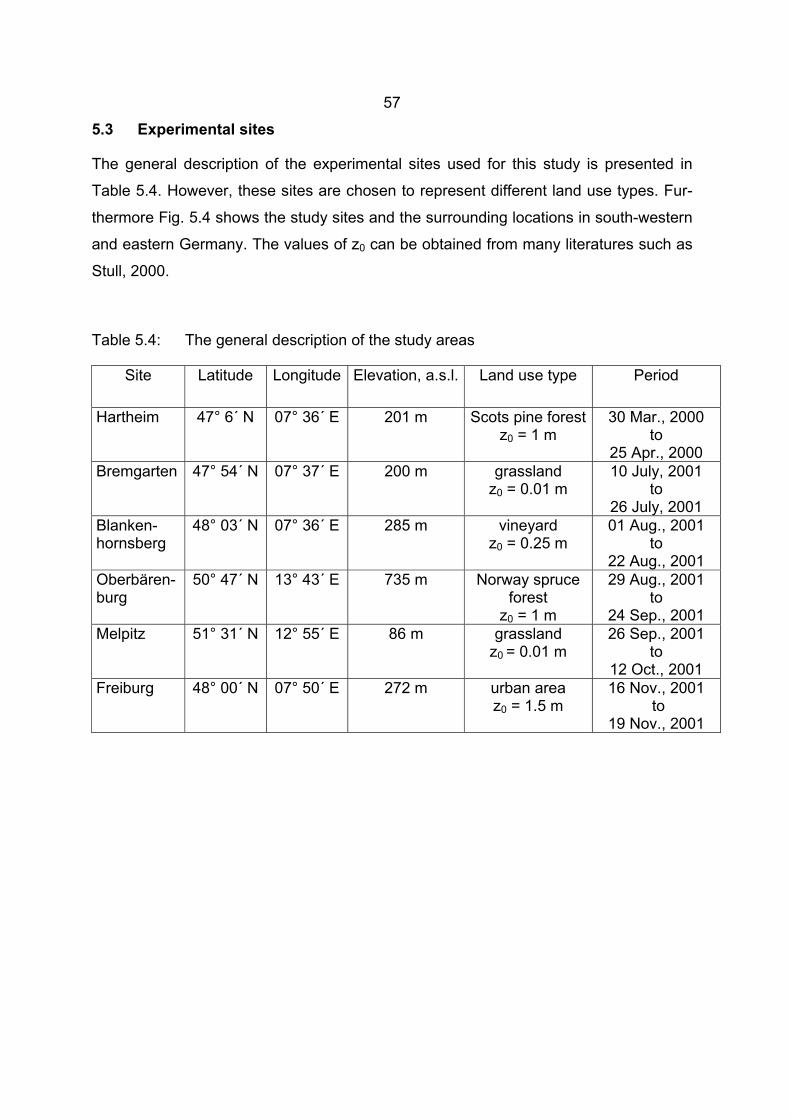
57

5.3 Experimental sites

The general description of the experimental sites used for this study is presented in

Table 5.4. However, these sites are chosen to represent different land use types. Fur-

thermore Fig. 5.4 shows the study sites and the surrounding locations in south-western

and eastern Germany. The values of z0 can be obtained from many literatures such as

Stull, 2000.

Table 5.4: The general description of the study areas

Site Latitude Longitude Elevation, a.s.l. Land use type Period

Hartheim 47° 6´ N 07° 36´ E 201 m Scots pine forest z0 = 1 m

30 Mar., 2000 to

25 Apr., 2000 Bremgarten 47° 54´ N 07° 37´ E 200 m grassland

z0 = 0.01 m 10 July, 2001

to 26 July, 2001

Blanken-hornsberg

48° 03´ N 07° 36´ E 285 m vineyard z0 = 0.25 m

01 Aug., 2001 to

22 Aug., 2001 Oberbären-burg

50° 47´ N 13° 43´ E 735 m Norway spruce forest

z0 = 1 m

29 Aug., 2001 to

24 Sep., 2001 Melpitz 51° 31´ N 12° 55´ E 86 m grassland

z0 = 0.01 m 26 Sep., 2001

to 12 Oct., 2001

Freiburg 48° 00´ N 07° 50´ E 272 m urban area z0 = 1.5 m

16 Nov., 2001 to

19 Nov., 2001

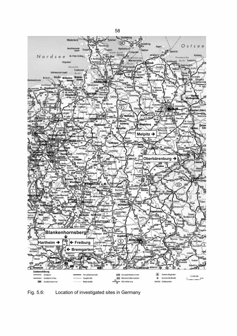
58

Fig. 5.6: Location of investigated sites in Germany

Oberbärenburg

Melpitz

Blankenhornsberg

Freiburg

Bremgarten

Hartheim

59

6 RESULTS

In this section a description of some measurements is given for the investigation sites

concerning incoming solar radiation, wind direction and its standard deviation, wind

speed components (horizontal and vertical), atmospheric stability (except for Freiburg),

variances of the horizontal and vertical wind speed, turbulent kinetic energy, and turbu-

lence intensity. Although the variances of horizontal wind speed, σ2u and σ2

v, measured

by a phased-sodar may be about twice as large as those measured by sonics at towers

(Ito, 1997b), these variables were used in this study as mentioned before.

Table 5.4 summarizes some of the information about the sites of this study. For every

site included in this study, the following results are shown:

∗∗ characteristic of the global solar radiation G received on a horizontal surface on

two cloudless and two cloudy days (except for: Melpitz with one cloudless day

and two cloudy days and Freiburg with one cloudless day and one cloudy day),

∗∗ wind roses at different levels during the period of the study,

∗∗ atmospheric stability classification at different levels,

∗∗ profiles of dd, σdd, vh, w, σ2h, σ2

w, σ3w/z, MKE and TKE under various atmos-

pheric conditions in the range 20 to 500 m a.g.l. (except for Oberbärenburg); the

weather was cloudy, rainy and foggy most times at Freiburg during the meas-

urement campaign from 16 November, 2001 to 19 November, 2001; thus sodar

data above 100 m a.g.l. were not available,

∗∗ diurnal course of two days mean of σdd, vh, w, σ2h, σ2

w, σ3w/z, MKE and TKE in

cloudless and cloudy sky conditions (except for: Melpitz with one cloudless day

and two cloudy days and Freiburg with one cloudless day and one cloudy day),

∗∗ characteristics of the turbulence intensity components (Iu, Iv, Iw) over the study

areas for various fetch conditions arising under various wind direction and differ-

ent atmospheric stability at different levels,

∗∗ behavior of the relationship between the standard deviations of the velocity

components normalized by the u∗, σi/u∗ (i=u,v,w), and z/L in the surface layer

60

and under the unstable atmospheric conditions (except for Melpitz and

Freiburg).

The used data, such as wind speed components, wind direction and the turbulence

parameters are 30-min mean values and are measured by the same instrumentation

within the same range of the height (20-500 m a.g.l.) but the periods of the observa-

tions differ (see Table 5.4).

The global solar radiation measurements at Hartheim, Bremgarten and Blankenhorns-

berg were collected at a forest-meteorological experimental site Hartheim which is op-

erated by the Meteorological Institute, Freiburg University (Mayer et al., 2000). How-

ever, it is 3.5 km and 9 km far from Bremgarten and Blankenhornsberg respectively.

The global solar radiation data for Oberbärenburg and Melpitz were provided by the

weather stations at Rotherdbach (one km from Oberbärenburg) and Melpitz respec-

tively. In Freiburg, the data were collected from the urban climate station, operated by

the Meteorological Institute, University of Freiburg, at the top of a high-rise building (ap-

proximately 50 m a.g.l.) in the northern downtown of Freiburg.

6.1 Hartheim: Scots pine forest

6.1.1 Global solar radiation, wind direction, and wind speed variation

6.1.1.1 Global solar radiation

The diurnal variation of the global solar radiation G received on a horizontal surface at

Hartheim on two cloudless days (21/22 April, 2000) and two cloudy days (17/18 April,

2000) is given by Fig. 6.1.1. In which the maximum values are recorded around the

noon hours (11:00-14:00 CET) with average values >600 W/m2 in the cloudless and

approximately <300 W/m2 at the cloudy days.

6.1.1.3 Wind direction

The frequency distribution of the wind direction at different levels, 20-50 m, 230-260 m

and 470-500 m a.g.l. at Hartheim during the day and night, the daytime (6:00–18:00

CET) and the nighttime (18:00–6:00 CET) through the period from 30 March, 2000 to

25 April, 2000 is shown in Fig. 6.1.2. In addition, the profile of the wind direction, dd,

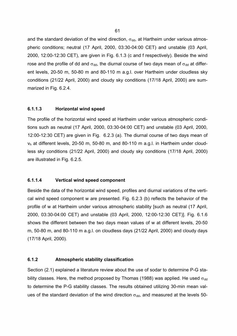
61

and the standard deviation of the wind direction, σdd, at Hartheim under various atmos-

pheric conditions; neutral (17 April, 2000, 03:30-04:00 CET) and unstable (03 April,

2000, 12:00-12:30 CET), are given in Fig. 6.1.3 (c and f respectively). Beside the wind

rose and the profile of dd and σdd, the diurnal course of two days mean of σdd at differ-

ent levels, 20-50 m, 50-80 m and 80-110 m a.g.l. over Hartheim under cloudless sky

conditions (21/22 April, 2000) and cloudy sky conditions (17/18 April, 2000) are sum-

marized in Fig. 6.2.4.

6.1.1.3 Horizontal wind speed

The profile of the horizontal wind speed at Hartheim under various atmospheric condi-

tions such as neutral (17 April, 2000, 03:30-04:00 CET) and unstable (03 April, 2000,

12:00-12:30 CET) are given in Fig. 6.2.3 (a). The diurnal course of two days mean of

vh at different levels, 20-50 m, 50-80 m, and 80-110 m a.g.l. in Hartheim under cloud-

less sky conditions (21/22 April, 2000) and cloudy sky conditions (17/18 April, 2000)

are illustrated in Fig. 6.2.5.

6.1.1.4 Vertical wind speed component

Beside the data of the horizontal wind speed, profiles and diurnal variations of the verti-

cal wind speed component w are presented. Fig. 6.2.3 (b) reflects the behavior of the

profile of w at Hartheim under various atmospheric stability [such as neutral (17 April,

2000, 03:30-04:00 CET) and unstable (03 April, 2000, 12:00-12:30 CET)]. Fig. 6.1.6

shows the different between the two days mean values of w at different levels, 20-50

m, 50-80 m, and 80-110 m a.g.l. on cloudless days (21/22 April, 2000) and cloudy days

(17/18 April, 2000).

6.1.2 Atmospheric stability classification

Section (2.1) explained a literature review about the use of sodar to determine P-G sta-

bility classes. Here, the method proposed by Thomas (1988) was applied. He used σdd

to determine the P-G stability classes. The results obtained utilizing 30-min mean val-

ues of the standard deviation of the wind direction σdd, and measured at the levels 50-

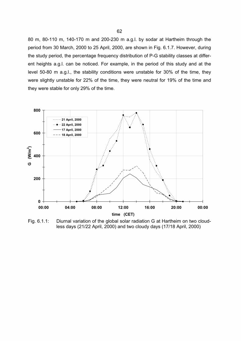
62

80 m, 80-110 m, 140-170 m and 200-230 m a.g.l. by sodar at Hartheim through the

period from 30 March, 2000 to 25 April, 2000, are shown in Fig. 6.1.7. However, during

the study period, the percentage frequency distribution of P-G stability classes at differ-

ent heights a.g.l. can be noticed. For example, in the period of this study and at the

level 50-80 m a.g.l., the stability conditions were unstable for 30% of the time, they

were slightly unstable for 22% of the time, they were neutral for 19% of the time and

they were stable for only 29% of the time.

Fig. 6.1.1: Diurnal variation of the global solar radiation G at Hartheim on two cloud-less days (21/22 April, 2000) and two cloudy days (17/18 April, 2000)

0

200

400

600

800

00:00 04:00 08:00 12:00 16:00 20:00 00:00time (CET)

G

(W/m

2 )

21 April, 200022 April, 200017 April, 200018 April, 2000

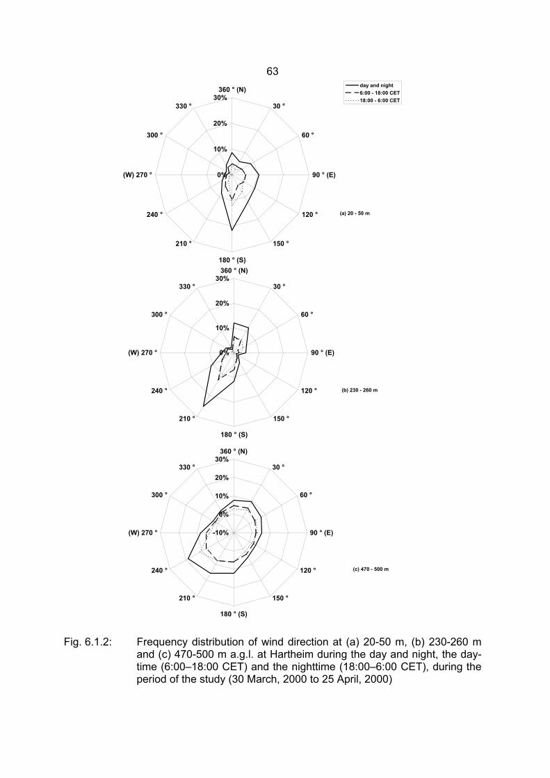
63

Fig. 6.1.2: Frequency distribution of wind direction at (a) 20-50 m, (b) 230-260 m

and (c) 470-500 m a.g.l. at Hartheim during the day and night, the day-time (6:00–18:00 CET) and the nighttime (18:00–6:00 CET), during the period of the study (30 March, 2000 to 25 April, 2000)

0%

10%

20%

30%360 ° (N)

30 °

60 °

90 ° (E)

120 °

150 °

180 ° (S)

210 °

240 °

(W) 270 °

300 °

330 °

day and night6:00 - 18:00 CET18:00 - 6:00 CET

(a) 20 - 50 m

0%

10%

20%

30%360 ° (N)

30 °

60 °

90 ° (E)

120 °

150 °

180 ° (S)

210 °

240 °

(W) 270 °

300 °

330 °

(b) 230 - 260 m

-10%

0%

10%

20%

30%360 ° (N)

30 °

60 °

90 ° (E)

120 °

150 °

180 ° (S)

210 °

240 °

(W) 270 °

300 °

330 °

(c) 470 - 500 m

64

Fig. 6.1.3: Profile of vh, w, dd, σ2h, σ2

w, σdd, TKE, MKE and σ3w/z at Hartheim under

various atmospheric conditions; neutral (17 April, 2000, 03:30-04:00 CET) and unstable (03 April, 2000, 12:00-12:30 CET)

vh (m/s) w (m/s) dd ( ° )

σ2h (m2/s2) σ2

w (m2/s2) σdd ( ° )

TKE (m2/s2) MKE (m2/s2) σ3w/z (m2/s3)

(a)

0

100

200

300

400

500

0 5 10

z (

m) (b)

-0.5 0.5

(c)

0 360

(d)

0

100

200

300

400

500

0 3 6 9

z (

m)

(e)

0 0.5 1

(f)

0 40 80

(g)

0

100

200

300

400

500

0 5 10

z (

m) (h)

0 25 50 75

(i)

0.00 0.01 0.02

neutral unstable

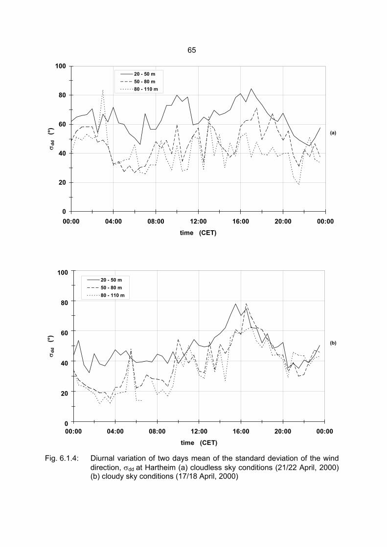
65

Fig. 6.1.4: Diurnal variation of two days mean of the standard deviation of the wind direction, σdd at Hartheim (a) cloudless sky conditions (21/22 April, 2000) (b) cloudy sky conditions (17/18 April, 2000)

0

20

40

60

80

100

00:00 04:00 08:00 12:00 16:00 20:00 00:00

time (CET)

σdd

(°

)

20 - 50 m50 - 80 m80 - 110 m

(a)

0

20

40

60

80

100

00:00 04:00 08:00 12:00 16:00 20:00 00:00

time (CET)

σdd

(°

)

20 - 50 m50 - 80 m80 - 110 m

(b)

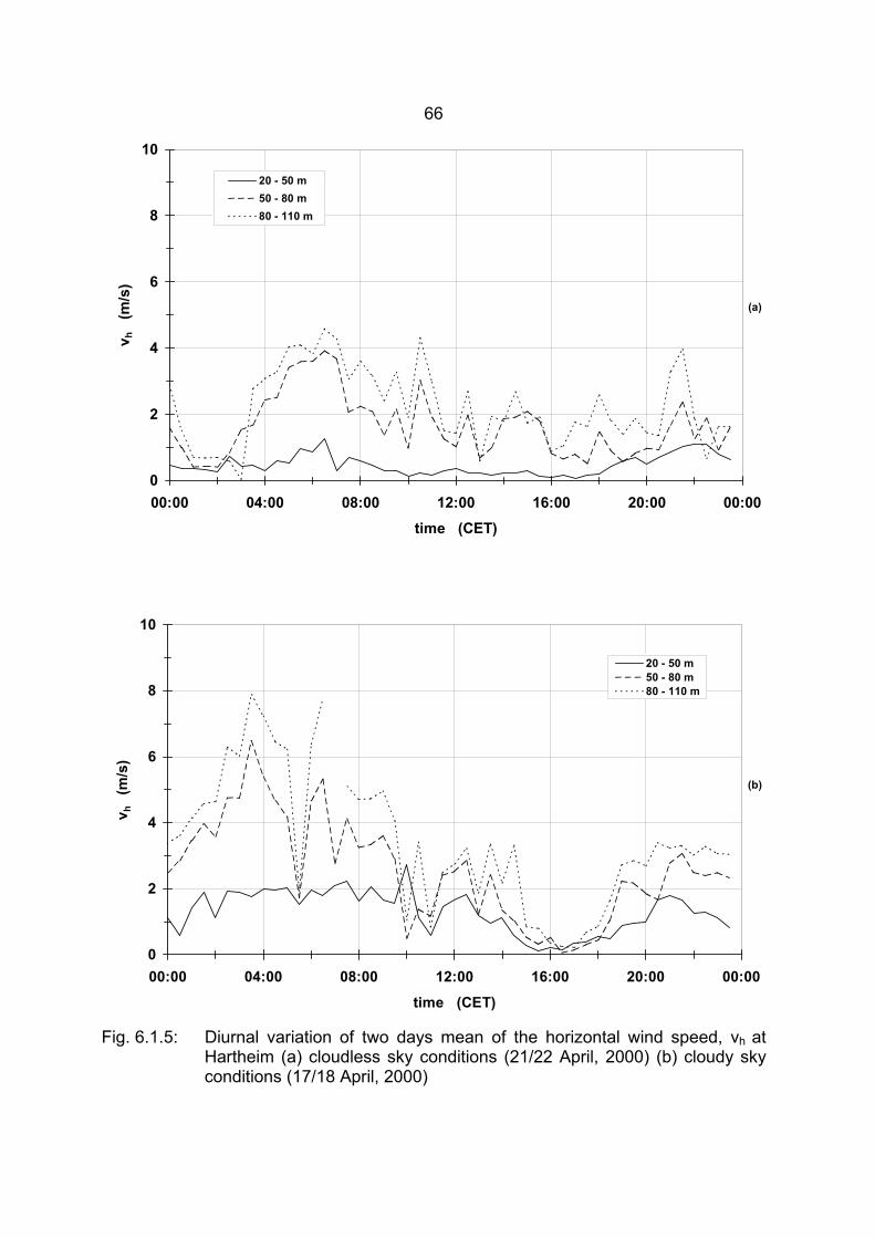
66

Fig. 6.1.5: Diurnal variation of two days mean of the horizontal wind speed, vh at Hartheim (a) cloudless sky conditions (21/22 April, 2000) (b) cloudy sky conditions (17/18 April, 2000)

0

2

4

6

8

10

00:00 04:00 08:00 12:00 16:00 20:00 00:00time (CET)

v h

(m/s

)

20 - 50 m50 - 80 m80 - 110 m

(a)

0

2

4

6

8

10

00:00 04:00 08:00 12:00 16:00 20:00 00:00

time (CET)

v h

(m/s

)

20 - 50 m50 - 80 m80 - 110 m

(b)

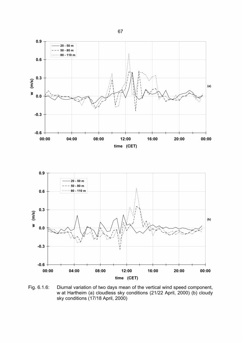
67

Fig. 6.1.6: Diurnal variation of two days mean of the vertical wind speed component, w at Hartheim (a) cloudless sky conditions (21/22 April, 2000) (b) cloudy sky conditions (17/18 April, 2000)

-0.6

-0.3

0.0

0.3

0.6

0.9

00:00 04:00 08:00 12:00 16:00 20:00 00:00

time (CET)

w

(m/s

)

20 - 50 m50 - 80 m80 - 110 m

(a)

-0.6

-0.3

0.0

0.3

0.6

0.9

00:00 04:00 08:00 12:00 16:00 20:00 00:00time (CET)

w

(m/s

)

20 - 50 m50 - 80 m80 - 110 m

(b)

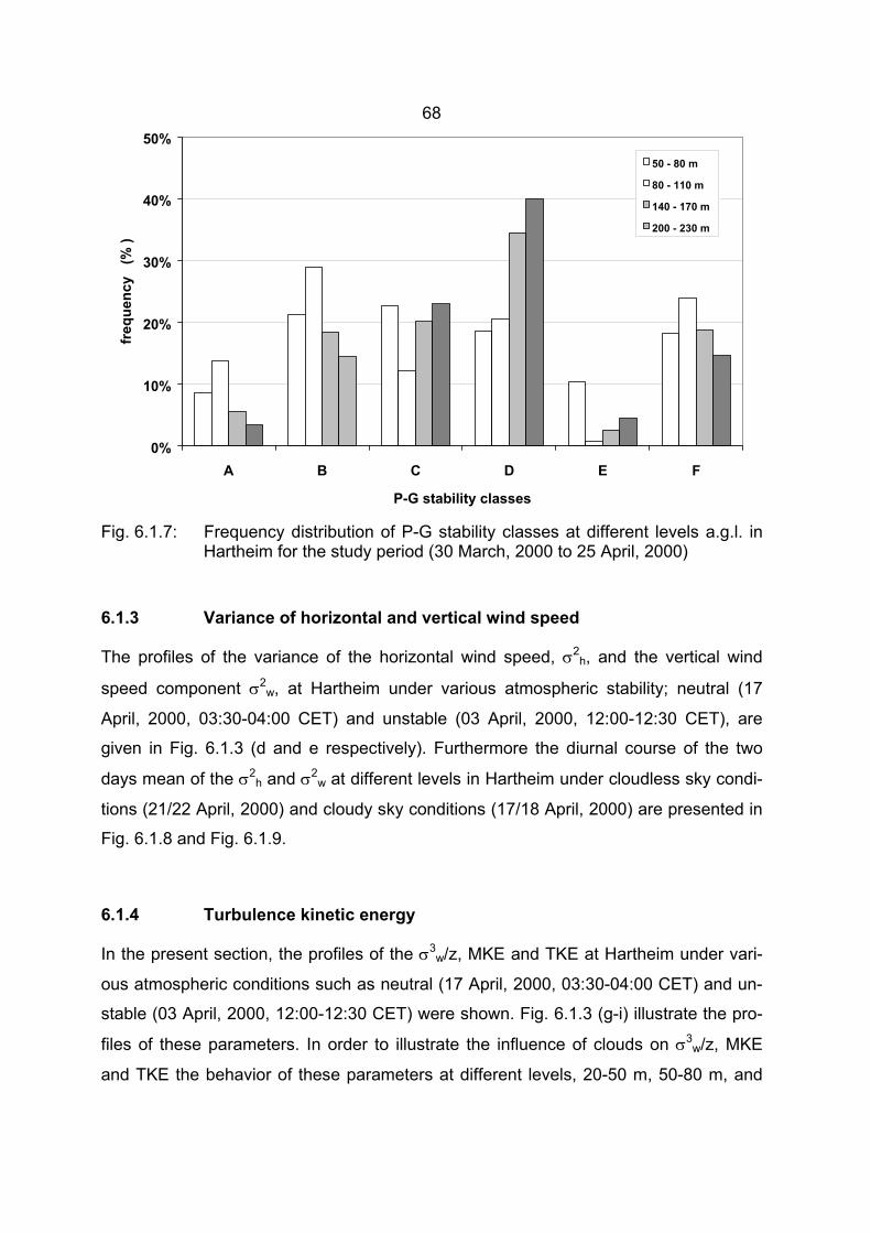
68

Fig. 6.1.7: Frequency distribution of P-G stability classes at different levels a.g.l. in Hartheim for the study period (30 March, 2000 to 25 April, 2000)

6.1.3 Variance of horizontal and vertical wind speed

The profiles of the variance of the horizontal wind speed, σ2h, and the vertical wind

speed component σ2w, at Hartheim under various atmospheric stability; neutral (17

April, 2000, 03:30-04:00 CET) and unstable (03 April, 2000, 12:00-12:30 CET), are

given in Fig. 6.1.3 (d and e respectively). Furthermore the diurnal course of the two

days mean of the σ2h and σ2

w at different levels in Hartheim under cloudless sky condi-

tions (21/22 April, 2000) and cloudy sky conditions (17/18 April, 2000) are presented in

Fig. 6.1.8 and Fig. 6.1.9.

6.1.4 Turbulence kinetic energy

In the present section, the profiles of the σ3w/z, MKE and TKE at Hartheim under vari-

ous atmospheric conditions such as neutral (17 April, 2000, 03:30-04:00 CET) and un-

stable (03 April, 2000, 12:00-12:30 CET) were shown. Fig. 6.1.3 (g-i) illustrate the pro-

files of these parameters. In order to illustrate the influence of clouds on σ3w/z, MKE

and TKE the behavior of these parameters at different levels, 20-50 m, 50-80 m, and

0%

10%

20%

30%

40%

50%

A B C D E F

P-G stability classes

freq

uenc

y (

% )

50 - 80 m

80 - 110 m

140 - 170 m

200 - 230 m

69

80-110 m a.g.l. over Hartheim in the case of cloudless sky conditions (21/22 April,

2000) and cloudy sky conditions (17 April, 2000 and 18 April 2000) were studied. Fig.

6.1.10-Fig. 6.1.12 present a comparative study between the diurnal course of two days

mean of σ3w/z, MKE and TKE in the cloudless and cloudy sky conditions.

6.1.5 Turbulence intensity 6.1.5.1 Variation of turbulence intensity with wind directions under neutral

conditions During neutral conditions, the variation of turbulence intensity components, Iu, Iv and Iw,

with the angular sectors can be investigated to illustrate the effect of the roughness in

the values of the turbulent intensity components. Table 6.1.1 shows the mean, stan-

dard deviations and the number of the observation of the turbulence intensity compo-

nents, Iu, Iv and Iw, at different levels, 50-80 m, 80-110 m, 140-170 m, and 200-230 m

a.g.l. under neutral conditions, grouped by wind direction, during the period of this

study (30 March, 2000 to 25 April, 2000).

6.1.5.2 Turbulence intensity under different stratifications

The turbulence intensity components, Iu, Iv and Iw, can be analyzed according to P-G

stability classes for the angular sector 180-210° at different levels. This angular sector

has been chosen for this study since the major wind directions are approximately ob-

served to be between 180° and 210°. Table 6.1.2 summarizes the mean, standard de-

viations and the number of observations of the turbulence intensity components, Iu, Iv

and Iw, at different levels, 50-80 m, 80-110 m, 140-170 m, and 200-230 m a.g.l. in Hart-

heim during the period from 30 March, 2000 to 25 April, 2000. These data were

grouped according to P-G stability classes for the angular sector 210-240° and the

mean values are schown in Fig. 6.1.13.

6.1.6 Relationship between normalized standard deviations of velocity components and z/L

The mean values of the standard deviations of the velocity components were normal-

ized by u∗, σi/u∗ (i=u,v,w), and the dependence of the normalized values on the stability

70

parameter (-z/L) under the unstable stratified would be explained. Fig. 6.1.14 shows the

behavior of σu/u∗, σv/u∗ and σw/u∗ as a function of -z/L under the unstable conditions

(0.28 <-z/L<8.31) at Hartheim during the period from 30 March, 2000 to 25 April, 2000.

This data was collected in the surface layer (less than 110 m a.g.l.).

The shape of the variation of σu/u∗, σv/u∗ and σw/u∗ with increasing instability (-z/L) have

the same variation of the following general function (after Al-Jiboori et al., 2001):

31

*

)1(Lzba

u iii +=

σ (6.1)

where ai and bi are empirical constants. In this study they were found to be 2.95, 2.99

and 1.1, and 2.2, 2.7 and 4 for u, v and w components respectively.

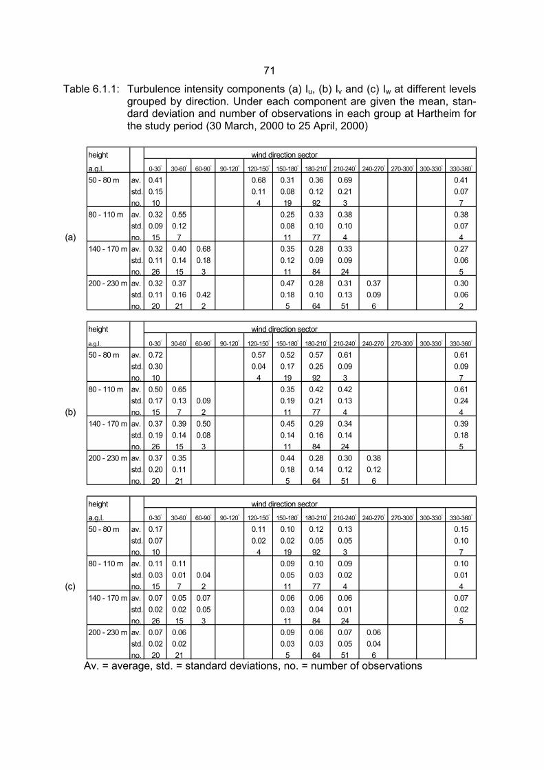
71

Table 6.1.1: Turbulence intensity components (a) Iu, (b) Iv and (c) Iw at different levels grouped by direction. Under each component are given the mean, stan-dard deviation and number of observations in each group at Hartheim for the study period (30 March, 2000 to 25 April, 2000)

Av. = average, std. = standard deviations, no. = number of observations

height wind direction sector

a.g.l. 0-30° 30-60° 60-90° 90-120° 120-150° 150-180° 180-210° 210-240° 240-270° 270-300° 300-330° 330-360°

50 - 80 m av. 0.41 0.68 0.31 0.36 0.69 0.41std. 0.15 0.11 0.08 0.12 0.21 0.07no. 10 4 19 92 3 7

80 - 110 m av. 0.32 0.55 0.25 0.33 0.38 0.38std. 0.09 0.12 0.08 0.10 0.10 0.07

(a) no. 15 7 11 77 4 4140 - 170 m av. 0.32 0.40 0.68 0.35 0.28 0.33 0.27

std. 0.11 0.14 0.18 0.12 0.09 0.09 0.06no. 26 15 3 11 84 24 5

200 - 230 m av. 0.32 0.37 0.47 0.28 0.31 0.37 0.30std. 0.11 0.16 0.42 0.18 0.10 0.13 0.09 0.06no. 20 21 2 5 64 51 6 2


a.g.l. 0-30° 30-60° 60-90° 90-120° 120-150° 150-180° 180-210° 210-240° 240-270° 270-300° 300-330° 330-360°

50 - 80 m av. 0.72 0.57 0.52 0.57 0.61 0.61std. 0.30 0.04 0.17 0.25 0.09 0.09no. 10 4 19 92 3 7

80 - 110 m av. 0.50 0.65 0.35 0.42 0.42 0.61std. 0.17 0.13 0.09 0.19 0.21 0.13 0.24

(b) no. 15 7 2 11 77 4 4140 - 170 m av. 0.37 0.39 0.50 0.45 0.29 0.34 0.39

std. 0.19 0.14 0.08 0.14 0.16 0.14 0.18no. 26 15 3 11 84 24 5

200 - 230 m av. 0.37 0.35 0.44 0.28 0.30 0.38std. 0.20 0.11 0.18 0.14 0.12 0.12no. 20 21 5 64 51 6


a.g.l. 0-30° 30-60° 60-90° 90-120° 120-150° 150-180° 180-210° 210-240° 240-270° 270-300° 300-330° 330-360°

50 - 80 m av. 0.17 0.11 0.10 0.12 0.13 0.15std. 0.07 0.02 0.02 0.05 0.05 0.10no. 10 4 19 92 3 7

80 - 110 m av. 0.11 0.11 0.09 0.10 0.09 0.10std. 0.03 0.01 0.04 0.05 0.03 0.02 0.01

(c) no. 15 7 2 11 77 4 4140 - 170 m av. 0.07 0.05 0.07 0.06 0.06 0.06 0.07

std. 0.02 0.02 0.05 0.03 0.04 0.01 0.02no. 26 15 3 11 84 24 5

200 - 230 m av. 0.07 0.06 0.09 0.06 0.07 0.06std. 0.02 0.02 0.03 0.03 0.05 0.04no. 20 21 5 64 51 6

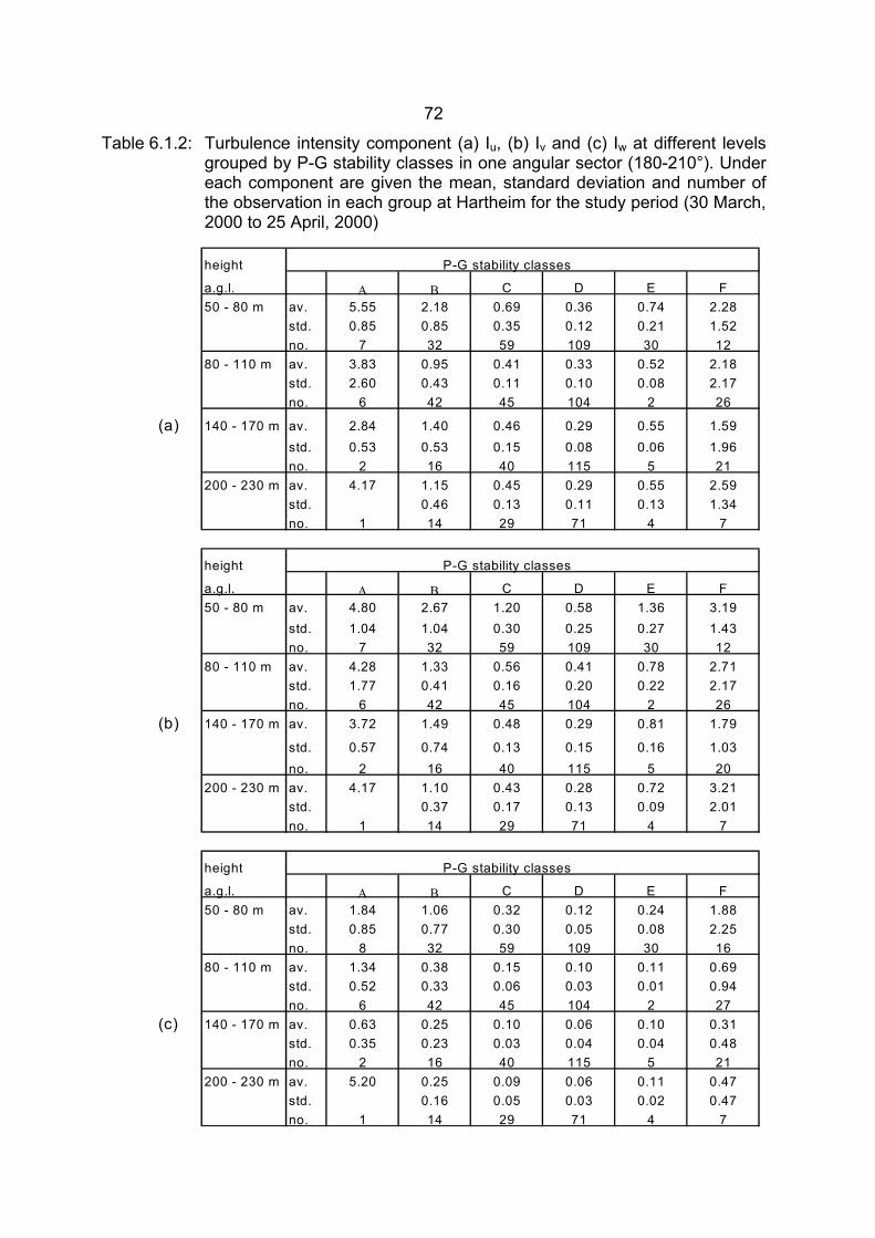
72

Table 6.1.2: Turbulence intensity component (a) Iu, (b) Iv and (c) Iw at different levels grouped by P-G stability classes in one angular sector (180-210°). Under each component are given the mean, standard deviation and number of the observation in each group at Hartheim for the study period (30 March, 2000 to 25 April, 2000)


a.g.l. Α Β C D E F50 - 80 m av. 5.55 2.18 0.69 0.36 0.74 2.28

std. 0.85 0.85 0.35 0.12 0.21 1.52no. 7 32 59 109 30 12

80 - 110 m av. 3.83 0.95 0.41 0.33 0.52 2.18std. 2.60 0.43 0.11 0.10 0.08 2.17no. 6 42 45 104 2 26

(a) 140 - 170 m av. 2.84 1.40 0.46 0.29 0.55 1.59std. 0.53 0.53 0.15 0.08 0.06 1.96no. 2 16 40 115 5 21

200 - 230 m av. 4.17 1.15 0.45 0.29 0.55 2.59std. 0.46 0.13 0.11 0.13 1.34no. 1 14 29 71 4 7


a.g.l. Α Β C D E F50 - 80 m av. 4.80 2.67 1.20 0.58 1.36 3.19

std. 1.04 1.04 0.30 0.25 0.27 1.43no. 7 32 59 109 30 12

80 - 110 m av. 4.28 1.33 0.56 0.41 0.78 2.71std. 1.77 0.41 0.16 0.20 0.22 2.17no. 6 42 45 104 2 26

(b) 140 - 170 m av. 3.72 1.49 0.48 0.29 0.81 1.79

std. 0.57 0.74 0.13 0.15 0.16 1.03no. 2 16 40 115 5 20

200 - 230 m av. 4.17 1.10 0.43 0.28 0.72 3.21std. 0.37 0.17 0.13 0.09 2.01no. 1 14 29 71 4 7


a.g.l. Α Β C D E F50 - 80 m av. 1.84 1.06 0.32 0.12 0.24 1.88

std. 0.85 0.77 0.30 0.05 0.08 2.25no. 8 32 59 109 30 16

80 - 110 m av. 1.34 0.38 0.15 0.10 0.11 0.69std. 0.52 0.33 0.06 0.03 0.01 0.94no. 6 42 45 104 2 27

(c) 140 - 170 m av. 0.63 0.25 0.10 0.06 0.10 0.31std. 0.35 0.23 0.03 0.04 0.04 0.48no. 2 16 40 115 5 21

200 - 230 m av. 5.20 0.25 0.09 0.06 0.11 0.47std. 0.16 0.05 0.03 0.02 0.47no. 1 14 29 71 4 7

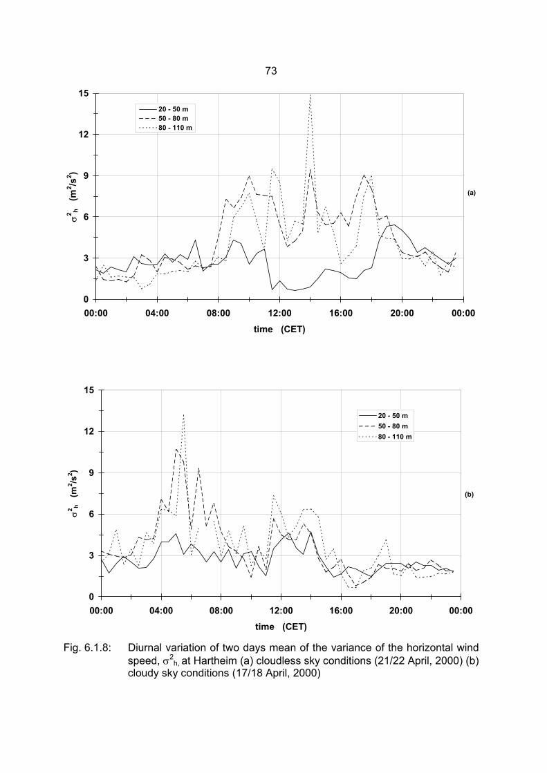
73

Fig. 6.1.8: Diurnal variation of two days mean of the variance of the horizontal wind speed, σ2

h, at Hartheim (a) cloudless sky conditions (21/22 April, 2000) (b) cloudy sky conditions (17/18 April, 2000)

0

3

6

9

12

15

00:00 04:00 08:00 12:00 16:00 20:00 00:00

time (CET)

σ2 h

(m2 /s

2 )

20 - 50 m50 - 80 m80 - 110 m

(a)

0

3

6

9

12

15

00:00 04:00 08:00 12:00 16:00 20:00 00:00time (CET)

σ2 h

(m2 /s

2 )

20 - 50 m50 - 80 m80 - 110 m

(b)

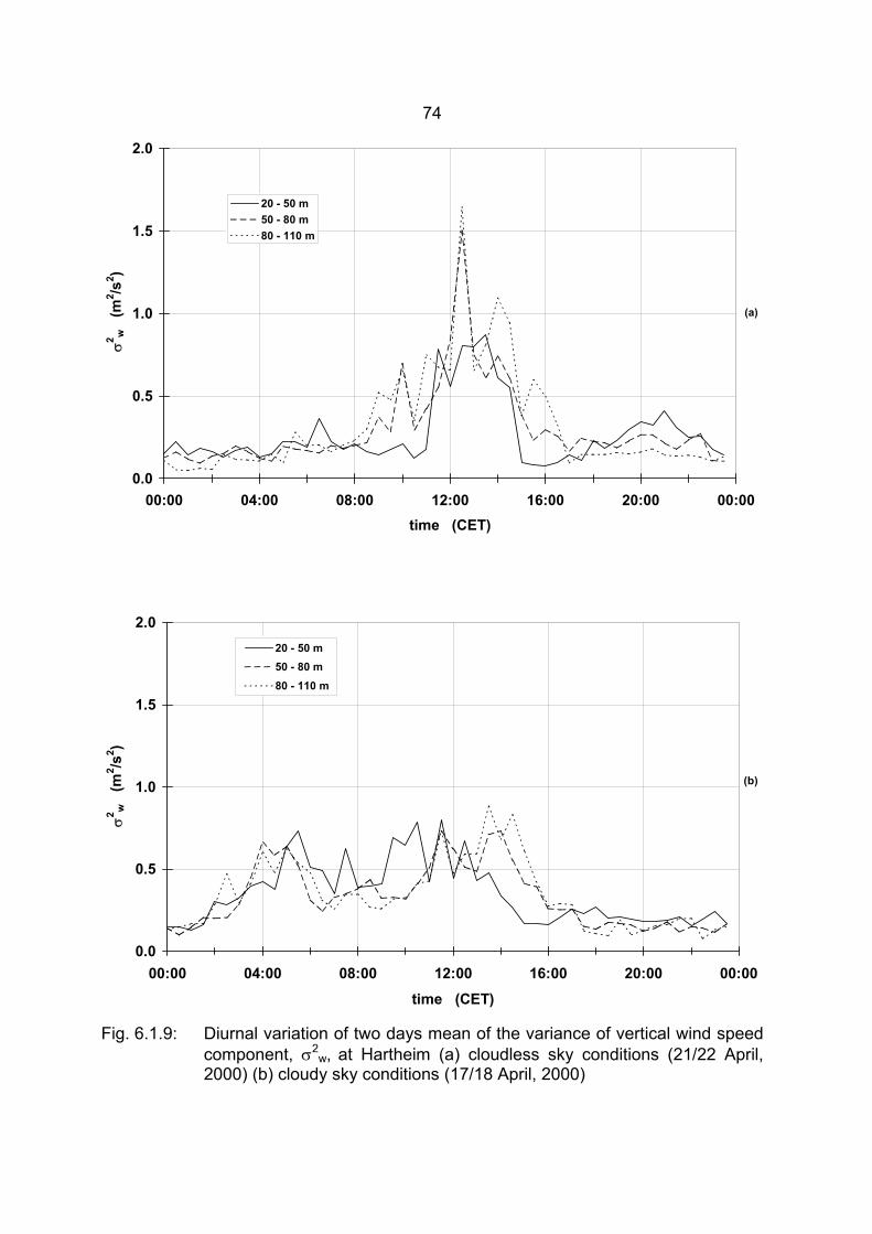
74

Fig. 6.1.9: Diurnal variation of two days mean of the variance of vertical wind speed component, σ2

w, at Hartheim (a) cloudless sky conditions (21/22 April, 2000) (b) cloudy sky conditions (17/18 April, 2000)

0.0

0.5

1.0

1.5

2.0

00:00 04:00 08:00 12:00 16:00 20:00 00:00

time (CET)

σ2 w

(m

2 /s2 )

20 - 50 m50 - 80 m80 - 110 m

(b)

0.0

0.5

1.0

1.5

2.0

00:00 04:00 08:00 12:00 16:00 20:00 00:00time (CET)

σ2 w

(m2 /s

2 )

20 - 50 m50 - 80 m80 - 110 m

(a)

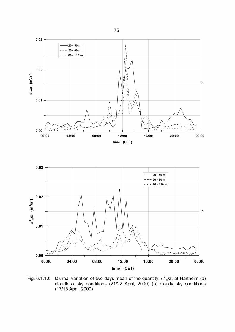
75

Fig. 6.1.10: Diurnal variation of two days mean of the quantity, σ3w/z, at Hartheim (a)

cloudless sky conditions (21/22 April, 2000) (b) cloudy sky conditions (17/18 April, 2000)

0.00

0.01

0.02

0.03

00:00 04:00 08:00 12:00 16:00 20:00 00:00

time (CET)

σ3 w

/z

(m2 /s

3 )

20 - 50 m50 - 80 m80 - 110 m

(a)

0.00

0.01

0.02

0.03

00:00 04:00 08:00 12:00 16:00 20:00 00:00time (CET)

σ3 w

/z

(m2 /s

3 )

20 - 50 m50 - 80 m80 - 110 m

(b)

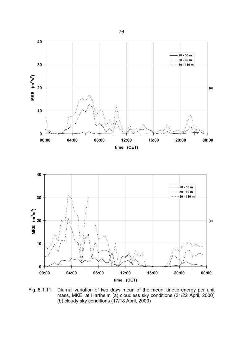
76

Fig. 6.1.11: Diurnal variation of two days mean of the mean kinetic energy per unit mass, MKE, at Hartheim (a) cloudless sky conditions (21/22 April, 2000) (b) cloudy sky conditions (17/18 April, 2000)

0

10

20

30

40

00:00 04:00 08:00 12:00 16:00 20:00 00:00

time (CET)

MK

E (

m2 /s

2 )

20 - 50 m50 - 80 m80 - 110 m

(a)

0

10

20

30

40

00:00 04:00 08:00 12:00 16:00 20:00 00:00

time (CET)

MK

E (

m2 /s

2 )

20 - 50 m50 - 80 m80 - 110 m

(b)

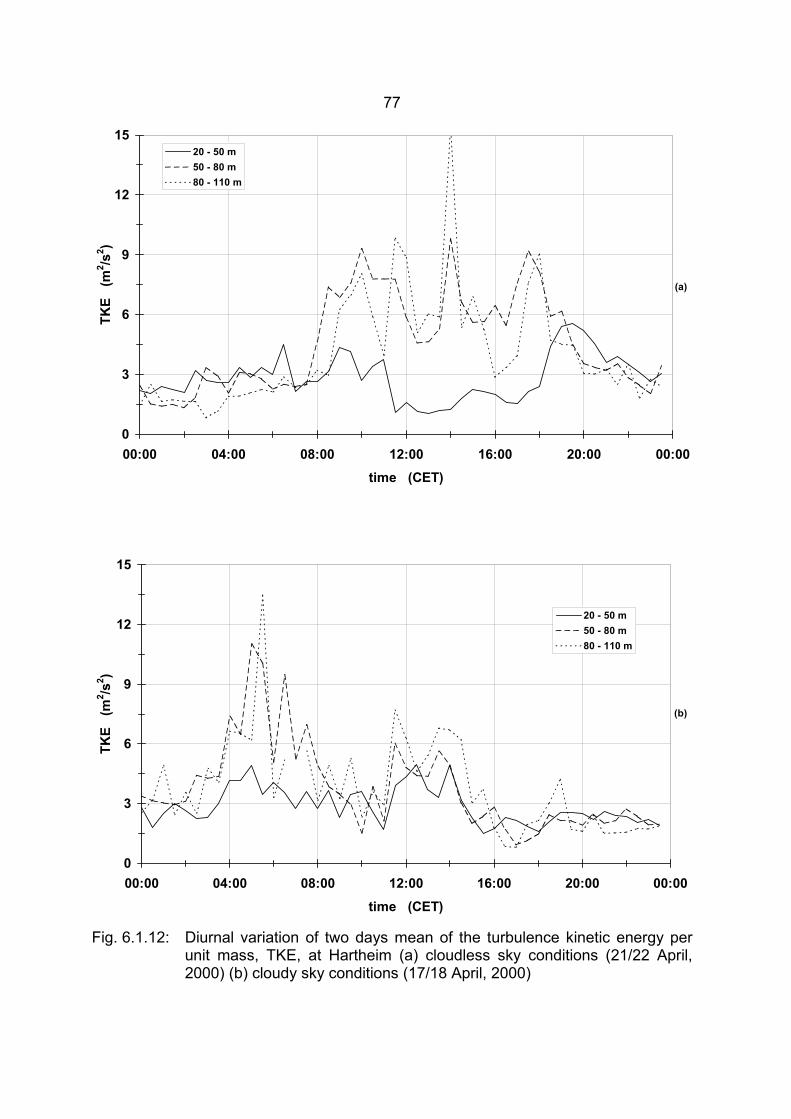
77

Fig. 6.1.12: Diurnal variation of two days mean of the turbulence kinetic energy per unit mass, TKE, at Hartheim (a) cloudless sky conditions (21/22 April, 2000) (b) cloudy sky conditions (17/18 April, 2000)

0

3

6

9

12

15

00:00 04:00 08:00 12:00 16:00 20:00 00:00time (CET)

TKE

(m

2 /s2 )

20 - 50 m50 - 80 m80 - 110 m

(a)

0

3

6

9

12

15

00:00 04:00 08:00 12:00 16:00 20:00 00:00

time (CET)

TKE

(m

2 /s2 )

20 - 50 m50 - 80 m80 - 110 m

(b)

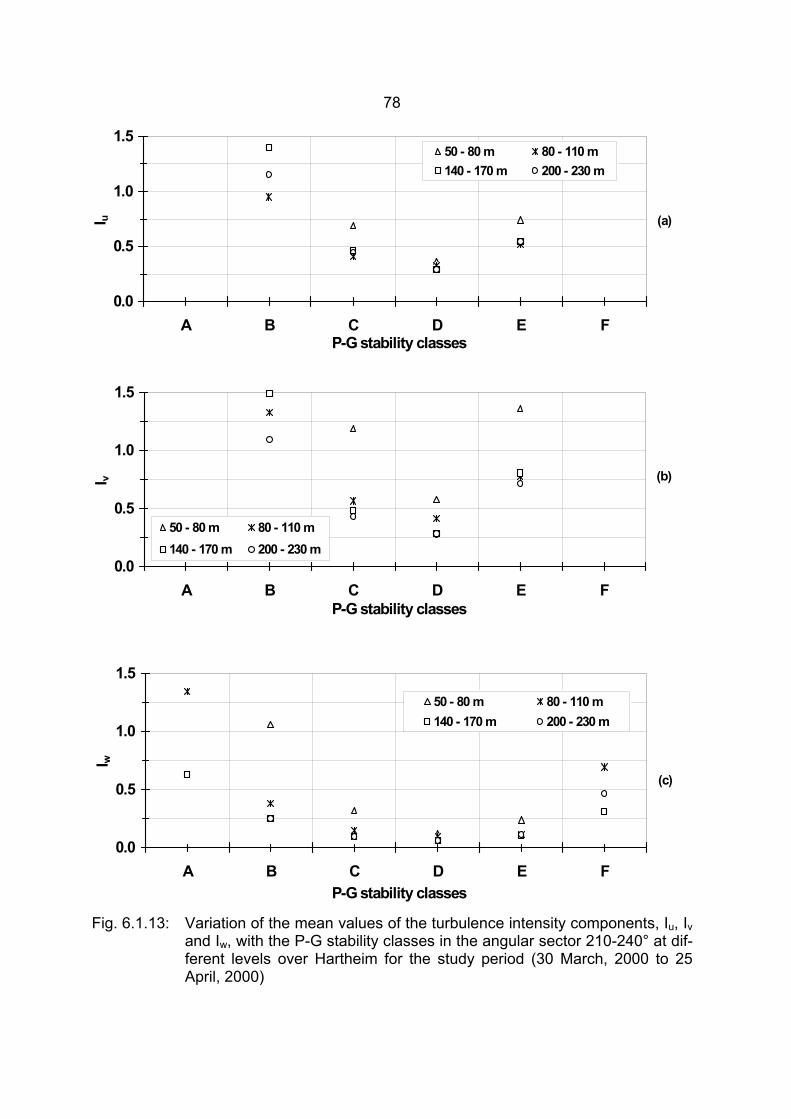
78

Fig. 6.1.13: Variation of the mean values of the turbulence intensity components, Iu, Iv and Iw, with the P-G stability classes in the angular sector 210-240° at dif-ferent levels over Hartheim for the study period (30 March, 2000 to 25 April, 2000)

0.0

0.5

1.0

1.5

A B C D E FP-G stability classes

I u

50 - 80 m 80 - 110 m 140 - 170 m 200 - 230 m

(a)

0.0

0.5

1.0

1.5


I v

50 - 80 m 80 - 110 m 140 - 170 m 200 - 230 m

(b)

0.0

0.5

1.0

1.5


I w

50 - 80 m 80 - 110 m 140 - 170 m 200 - 230 m

(c)

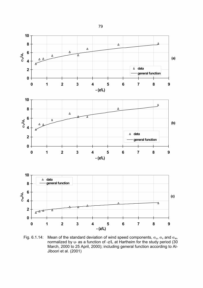
79

Fig. 6.1.14: Mean of the standard deviation of wind speed components, σu, σv and σw, normalized by u* as a function of -z/L at Hartheim for the study period (30 March, 2000 to 25 April, 2000); including general function according to Al-Jiboori et al. (2001)

0

2

4

6

8

10

0 1 2 3 4 5 6 7 8 9- (z/L)

σ u/u

∗

datageneral function

(a)

0

2

4

6

8

10

0 1 2 3 4 5 6 7 8 9- (z/L)

σ v/u

∗


(b)

0

2

4

6

8

10

0 1 2 3 4 5 6 7 8 9- (z/L)

σ w/u

∗


(c)

80

6.2 Bremgarten: Grassland



The characteristics of the global solar radiation G received on a horizontal surface at

Hartheim (approximately 3.5 km far from Bremgarten) on two cloudless days (22/23

July, 2001) and two cloudy days (14/15 July, 2001) are presented in Fig. 6.2.1. The

highest G was recorded around the noon hours (11:00-13:00 CET) with average values

greater than 800 W/m2 in the cloudless days and lower than 210 W/m2 in the cloudy

ones.


A general note about the frequency distribution of the wind direction is presented for

different levels (20-30 m, 180-260 m and 320-500 m a.g.l.) in Bremgarten during the

day and night, the daytime (6:00–18:00 CET), and nighttime (18:00–6:00 CET) through

the period from 10 July, 2001 to 26 July, 2001. Fig. 6.2.2 illustrates the wind rose at

these levels.

The profiles of the wind direction, dd, and the standard deviation of the wind direction,

σdd, at Bremgarten under various atmospheric stratification such as neutral (14 July,

2001, 22:30-23:00 CET), stable (16 July, 2001, 23:00-23:30 CET) and unstable (22

July, 2001, 11:30-12:00 CET) are presented in Fig. 6.2.3 (c and f respectively). Fur-

thermore the diurnal course of two days mean of σdd at different levels, 20-30 m, 40-60

m, and 60-100 m a.g.l. over Bremgarten are summarized in Fig. 6.2.4, to show the

various characteristics on cloudless (22/23 July, 2001) and cloudy days (14/15 July,

2001)


The profile of the horizontal wind speed vh at Bremgarten under various atmospheric

conditions such as neutral (14 July, 2001, 22:30-23:00 CET), stable (16 July, 2001,

23:00-23:30 CET) and unstable (22 July, 2001, 11:30-12:00 CET) is given by Fig. 6.2.3

(a). Moreover, the diurnal course of two mean days of vh at different levels, 20-30 m,

81

40-60 m, and 60-100 m a.g.l. in Bremgarten on cloudless days (22/23 July, 2001) and

cloudy days (14/15 July, 2001) is illustrated in Fig. 6.2.5.


The effect of the atmospheric stability on the profile of the vertical component of the

wind speed, w, at Bremgarten under various atmospheric conditions such as neutral

(14 July, 2001,22:30-23:00 CET), stable (16 July, 2001, 23:00-23:30 CET) and unsta-

ble (22 July, 2001, 11:30-12:00 CET) is given by Fig. 6.2.6 (b). In addition, the differ-

ence between the diurnal variation of the two days mean values of w at various levels,

20-30 m, 40-60 m, and 60-100 m a.g.l. at Bremgarten on cloudless days (22/23 July,

2001) and cloudy days (14/15 July, 2001) is presented in Fig. 6.2.6.


Similar to section 6.1.2, the P-G stability classes were determined according to Thomas

(1988). The results that obtained utilizing 30-min mean values of the standard deviation

of the wind direction, σdd, measured at the levels 40-60 m, 60-100 m, 100-180 m and

180-260 m a.g.l. by sodar are shown in Fig. 6.2.7.

However, during the study period (10 July, 2001 to 26 July, 2001) the percentage fre-

quency distribution of P-G stability classes at different heights a.g.l. could be noticed.

For example, in the period of this study and at the level 40-60 m a.g.l. the stability con-

ditions were unstable for 16% of the time, they were slightly unstable for 18% of the

time, they were neutral for 48% of the time and they were stable for only 18% of the

time.



speed component, σ2w, at Bremgarten under various atmospheric conditions such as

neutral (14 July, 2001,22:30-23:00 CET), stable (16 July, 2001, 23:00-23:30 CET) and

unstable (22 July, 2001, 11:30-12:00 CET) are given in Fig. 6.2.3 (d and e respec-

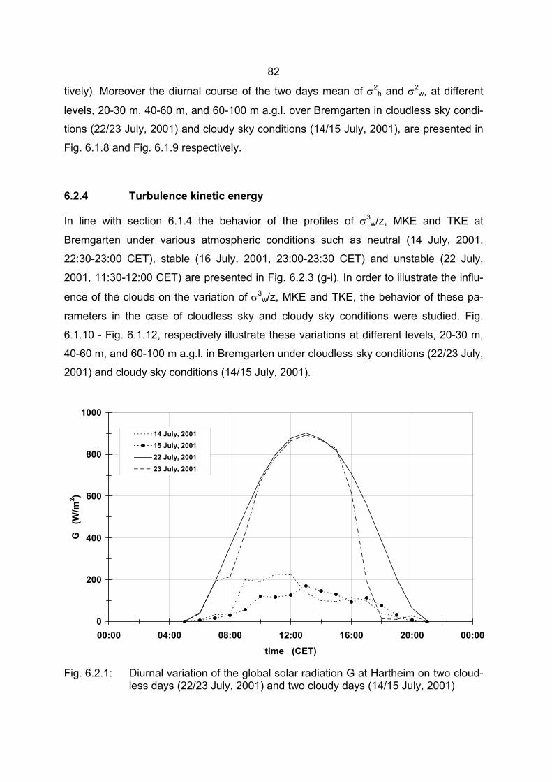
82

tively). Moreover the diurnal course of the two days mean of σ2h and σ2

w, at different

levels, 20-30 m, 40-60 m, and 60-100 m a.g.l. over Bremgarten in cloudless sky condi-

tions (22/23 July, 2001) and cloudy sky conditions (14/15 July, 2001), are presented in

Fig. 6.1.8 and Fig. 6.1.9 respectively.


In line with section 6.1.4 the behavior of the profiles of σ3w/z, MKE and TKE at

Bremgarten under various atmospheric conditions such as neutral (14 July, 2001,

22:30-23:00 CET), stable (16 July, 2001, 23:00-23:30 CET) and unstable (22 July,

2001, 11:30-12:00 CET) are presented in Fig. 6.2.3 (g-i). In order to illustrate the influ-

ence of the clouds on the variation of σ3w/z, MKE and TKE, the behavior of these pa-

rameters in the case of cloudless sky and cloudy sky conditions were studied. Fig.

6.1.10 - Fig. 6.1.12, respectively illustrate these variations at different levels, 20-30 m,

40-60 m, and 60-100 m a.g.l. in Bremgarten under cloudless sky conditions (22/23 July,

2001) and cloudy sky conditions (14/15 July, 2001).

Fig. 6.2.1: Diurnal variation of the global solar radiation G at Hartheim on two cloud-less days (22/23 July, 2001) and two cloudy days (14/15 July, 2001)

0

200

400

600

800

1000

00:00 04:00 08:00 12:00 16:00 20:00 00:00time (CET)

G

(W/m

2 )

14 July, 200115 July, 200122 July, 200123 July, 2001

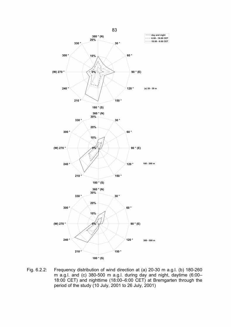
83

Fig. 6.2.2: Frequency distribution of wind direction at (a) 20-30 m a.g.l. (b) 180-260

m a.g.l. and (c) 380-500 m a.g.l. during day and night, daytime (6:00–18:00 CET) and nighttime (18:00–6:00 CET) at Bremgarten through the period of the study (10 July, 2001 to 26 July, 2001)

0%

10%

20%360 ° (N)

30 °

60 °

90 ° (E)

120 °

150 °

180 ° (S)

210 °

240 °

(W) 270 °

300 °

330 °


(a) 20 - 30 m

0%

10%

20%

30%360 ° (N)

30 °

60 °

90 ° (E)

120 °

150 °

180 ° (S)

210 °

240 °

(W) 270 °

300 °

330 °

180 - 260 m

0%

10%

20%

30%360 ° (N)

30 °

60 °

90 ° (E)

120 °

150 °

180 ° (S)

210 °

240 °

(W) 270 °

300 °

330 °

380 - 500 m

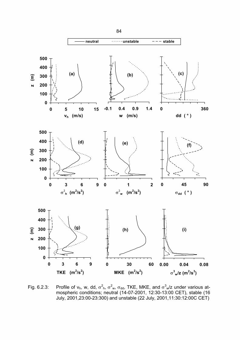
84


w, σdd, TKE, MKE, and σ3w/z under various at-

mospheric conditions; neutral (14-07-2001, 12:30-13:00 CET), stable (16 July, 2001,23:00-23:300) and unstable (22 July, 2001,11:30:12:00C CET)

vh (m/s) w (m/s) dd ( ° )

σ2h (m2/s2) σ2

w (m2/s2) σdd ( ° )


(a)

0

100

200

300

400

500

0 5 10 15

z (

m) (b)

-0.1 0.4 0.9 1.4

(c)

0 360

(d)

0

100

200

300

400

500

0 3 6 9

z (

m)

(e)

0 1 2

(f)

0 45 90

(g)

0

100

200

300

400

500

0 3 6 9

z (

m) (h)

0 30 60

(i)

0.00 0.04 0.08

neutral unstable stable

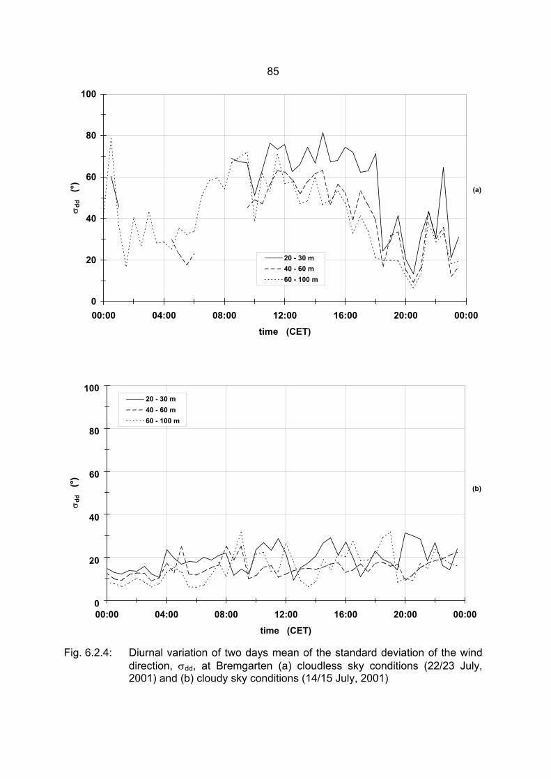
85

Fig. 6.2.4: Diurnal variation of two days mean of the standard deviation of the wind direction, σdd, at Bremgarten (a) cloudless sky conditions (22/23 July, 2001) and (b) cloudy sky conditions (14/15 July, 2001)

0

20

40

60

80

100

00:00 04:00 08:00 12:00 16:00 20:00 00:00time (CET)

σdd

(°

)

20 - 30 m40 - 60 m60 - 100 m

(a)

0

20

40

60

80

100

00:00 04:00 08:00 12:00 16:00 20:00 00:00

time (CET)

σdd

(°

)

20 - 30 m40 - 60 m60 - 100 m

(b)

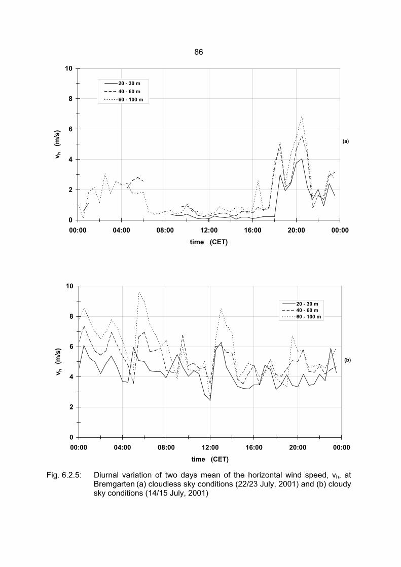
86

Fig. 6.2.5: Diurnal variation of two days mean of the horizontal wind speed, vh, at Bremgarten (a) cloudless sky conditions (22/23 July, 2001) and (b) cloudy sky conditions (14/15 July, 2001)

0

2

4

6

8

10

00:00 04:00 08:00 12:00 16:00 20:00 00:00time (CET)

v h

(m/s

)

20 - 30 m40 - 60 m60 - 100 m

(a)

0

2

4

6

8

10

00:00 04:00 08:00 12:00 16:00 20:00 00:00

time (CET)

v h

(m/s

)

20 - 30 m40 - 60 m60 - 100 m

(b)

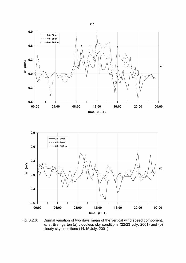
87

Fig. 6.2.6: Diurnal variation of two days mean of the vertical wind speed component, w, at Bremgarten (a) cloudless sky conditions (22/23 July, 2001) and (b) cloudy sky conditions (14/15 July, 2001)

-0.6

-0.3

0.0

0.3

0.6

0.9

00:00 04:00 08:00 12:00 16:00 20:00 00:00

time (CET)

w

(m/s

)

20 - 30 m40 - 60 m60 - 100 m

(a)

-0.6

-0.3

0.0

0.3

0.6

0.9

00:00 04:00 08:00 12:00 16:00 20:00 00:00time (CET)

w

(m/s

)

20 - 30 m40 - 60 m60 - 100 m

(b)

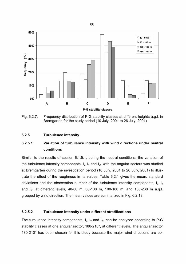
88

Fig. 6.2.7: Frequency distribution of P-G stability classes at different heights a.g.l. in Bremgarten for the study period (10 July, 2001 to 26 July, 2001)

6.2.5 Turbulence intensity

6.2.5.1 Variation of turbulence intensity with wind directions under neutral conditions

Similar to the results of section 6.1.5.1, during the neutral conditions, the variation of

the turbulence intensity components, Iu, Iv and Iw, with the angular sectors was studied

at Bremgarten during the investigation period (10 July, 2001 to 26 July, 2001) to illus-

trate the effect of the roughness in its values. Table 6.2.1 gives the mean, standard

deviations and the observation number of the turbulence intensity components, Iu, Iv

and Iw, at different levels, 40-60 m, 60-100 m, 100-180 m, and 180-260 m a.g.l.

grouped by wind direction. The mean values are summarized in Fig. 6.2.13.


The turbulence intensity components, Iu, Iv and Iw, can be analyzed according to P-G

stability classes at one angular sector, 180-210°, at different levels. The angular sector

180-210° has been chosen for this study because the major wind directions are ob-

0%

10%

20%

30%

40%

50%

A B C D E F


freq

uenc

y (

% )

40 - 60 m

60 - 100 m

100 - 180 m

180 - 260 m

89

served to be between 180° and 210°. Table 6.2.2 summarizes the mean and standard

deviations of the turbulence intensity components, Iu, Iv and Iw, at different levels, 40-60

m, 60-100 m, 100-180 m, and 180-260 m a.g.l. in Bremgarten grouped according to P-

G stability classes for the angular sector 180-210°. The mean values are summarized

in Fig. 6.2.14.


The mean values of the standard deviations of the velocity components normalized by

u∗, σi/u∗ (i=u,v,w), and the dependence of the normalized values on the stability pa-

rameter (-z/L) under the unstable stratified will be explained.

Fig. 6.1.15 shows the behavior of σu/u∗, σv/u∗ and σw/u∗ as a function of -z/L under the

unstable conditions (0.82<-z/L <11.24) at Bremgarten during the period from 10 July,

2001 to 26 July, 7-2001. This data was collected in the surface layer (less than 100 m

a.g.l.).

The shape of the variation of σu/u∗, σv/u∗ and σw/u∗ with the increasing of the instability

(-z/L) have the same variation of the Eq. (6.1), but the empirical constants ai and bi at

this site are found to be 1.7, 1.7 and 1.2, and 1.6, 1.5 and 4 for u, v and w components

respectively.

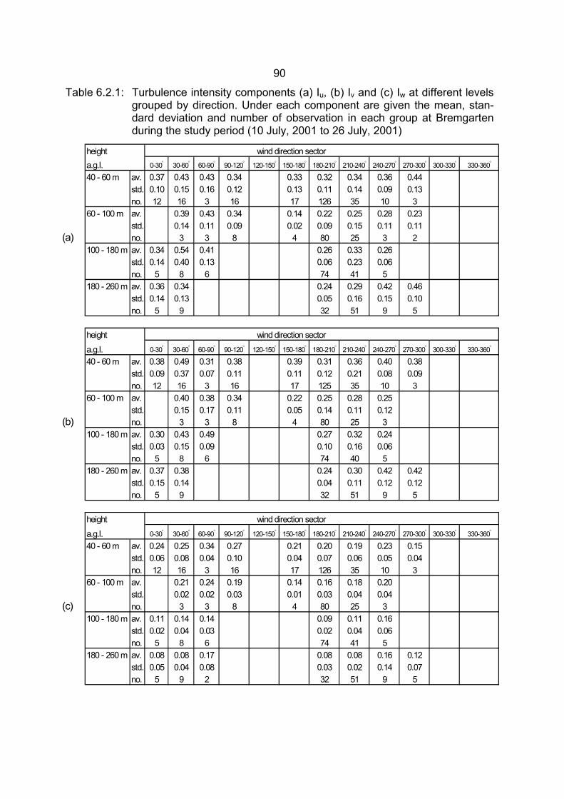
90

Table 6.2.1: Turbulence intensity components (a) Iu, (b) Iv and (c) Iw at different levels grouped by direction. Under each component are given the mean, stan-dard deviation and number of observation in each group at Bremgarten during the study period (10 July, 2001 to 26 July, 2001)

height wind direction sector a.g.l. 0-30° 30-60° 60-90° 90-120° 120-150° 150-180° 180-210° 210-240° 240-270° 270-300° 300-330° 330-360°

40 - 60 m av. 0.37 0.43 0.43 0.34 0.33 0.32 0.34 0.36 0.44std. 0.10 0.15 0.16 0.12 0.13 0.11 0.14 0.09 0.13no. 12 16 3 16 17 126 35 10 3

60 - 100 m av. 0.39 0.43 0.34 0.14 0.22 0.25 0.28 0.23std. 0.14 0.11 0.09 0.02 0.09 0.15 0.11 0.11

(a) no. 3 3 8 4 80 25 3 2100 - 180 m av. 0.34 0.54 0.41 0.26 0.33 0.26

std. 0.14 0.40 0.13 0.06 0.23 0.06no. 5 8 6 74 41 5

180 - 260 m av. 0.36 0.34 0.24 0.29 0.42 0.46std. 0.14 0.13 0.05 0.16 0.15 0.10no. 5 9 32 51 9 5


a.g.l. 0-30° 30-60° 60-90° 90-120° 120-150° 150-180° 180-210° 210-240° 240-270° 270-300° 300-330° 330-360°

40 - 60 m av. 0.38 0.49 0.31 0.38 0.39 0.31 0.36 0.40 0.38std. 0.09 0.37 0.07 0.11 0.11 0.12 0.21 0.08 0.09no. 12 16 3 16 17 125 35 10 3

60 - 100 m av. 0.40 0.38 0.34 0.22 0.25 0.28 0.25std. 0.15 0.17 0.11 0.05 0.14 0.11 0.12

(b) no. 3 3 8 4 80 25 3100 - 180 m av. 0.30 0.43 0.49 0.27 0.32 0.24

std. 0.03 0.15 0.09 0.10 0.16 0.06no. 5 8 6 74 40 5

180 - 260 m av. 0.37 0.38 0.24 0.30 0.42 0.42std. 0.15 0.14 0.04 0.11 0.12 0.12no. 5 9 32 51 9 5


a.g.l. 0-30° 30-60° 60-90° 90-120° 120-150° 150-180° 180-210° 210-240° 240-270° 270-300° 300-330° 330-360°

40 - 60 m av. 0.24 0.25 0.34 0.27 0.21 0.20 0.19 0.23 0.15std. 0.06 0.08 0.04 0.10 0.04 0.07 0.06 0.05 0.04no. 12 16 3 16 17 126 35 10 3

60 - 100 m av. 0.21 0.24 0.19 0.14 0.16 0.18 0.20std. 0.02 0.02 0.03 0.01 0.03 0.04 0.04

(c) no. 3 3 8 4 80 25 3100 - 180 m av. 0.11 0.14 0.14 0.09 0.11 0.16

std. 0.02 0.04 0.03 0.02 0.04 0.06no. 5 8 6 74 41 5

180 - 260 m av. 0.08 0.08 0.17 0.08 0.08 0.16 0.12std. 0.05 0.04 0.08 0.03 0.02 0.14 0.07no. 5 9 2 32 51 9 5

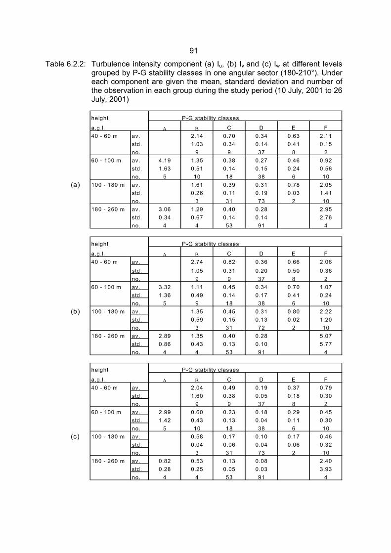
91

Table 6.2.2: Turbulence intensity component (a) Iu, (b) Iv and (c) Iw at different levels grouped by P-G stability classes in one angular sector (180-210°). Under each component are given the mean, standard deviation and number of the observation in each group during the study period (10 July, 2001 to 26 July, 2001)


a.g.l. Α Β C D E F40 - 60 m av. 2.14 0.70 0.34 0.63 2.11

std. 1.03 0.34 0.14 0.41 0.15no. 9 9 37 8 2

60 - 100 m av. 4.19 1.35 0.38 0.27 0.46 0.92std. 1.63 0.51 0.14 0.15 0.24 0.56no. 5 10 18 38 6 10

(a) 100 - 180 m av. 1.61 0.39 0.31 0.78 2.05std. 0.26 0.11 0.19 0.03 1.41no. 3 31 73 2 10

180 - 260 m av. 3.06 1.29 0.40 0.28 2.95std. 0.34 0.67 0.14 0.14 2.76no. 4 4 53 91 4


a.g.l. Α Β C D E F40 - 60 m av. 2.74 0.82 0.36 0.66 2.06

std. 1.05 0.31 0.20 0.50 0.36no. 9 9 37 8 2

60 - 100 m av. 3.32 1.11 0.45 0.34 0.70 1.07std. 1.36 0.49 0.14 0.17 0.41 0.24no. 5 9 18 38 6 10

(b) 100 - 180 m av. 1.35 0.45 0.31 0.80 2.22std. 0.59 0.15 0.13 0.02 1.20no. 3 31 72 2 10

180 - 260 m av. 2.89 1.35 0.40 0.28 5.07std. 0.86 0.43 0.13 0.10 5.77no. 4 4 53 91 4


a.g.l. Α Β C D E F40 - 60 m av. 2.04 0.49 0.19 0.37 0.79

std. 1.60 0.38 0.05 0.18 0.30no. 9 9 37 8 2

60 - 100 m av. 2.99 0.60 0.23 0.18 0.29 0.45std. 1.42 0.43 0.13 0.04 0.11 0.30no. 5 10 18 38 6 10

(c) 100 - 180 m av. 0.58 0.17 0.10 0.17 0.46std. 0.04 0.06 0.04 0.06 0.32no. 3 31 73 2 10

180 - 260 m av. 0.82 0.53 0.13 0.08 2.40std. 0.28 0.25 0.05 0.03 3.93no. 4 4 53 91 4

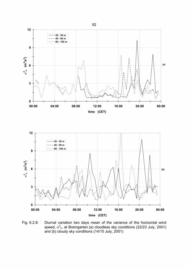
92

Fig. 6.2.8: Diurnal variation two days mean of the variance of the horizontal wind speed, σ2

h, at Bremgarten (a) cloudless sky conditions (22/23 July, 2001) and (b) cloudy sky conditions (14/15 July, 2001)

0

3

6

9

12

00:00 04:00 08:00 12:00 16:00 20:00 00:00

time (CET)

σ2 h

(m2 /s

2 )

20 - 30 m40 - 60 m60 - 100 m

(a)

0

3

6

9

12

00:00 04:00 08:00 12:00 16:00 20:00 00:00time (CET)

σ2 h

(m2 /s

2 )

20 - 30 m40 - 60 m60 - 100 m

(b)

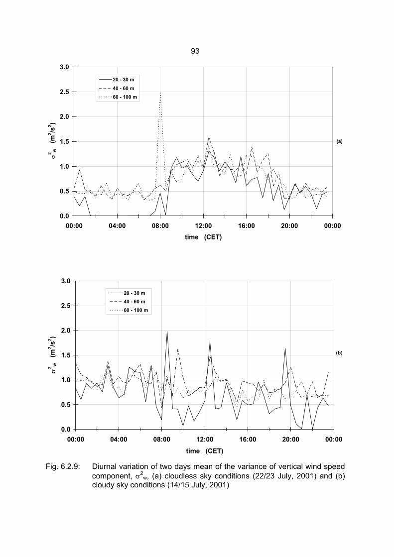
93


w, (a) cloudless sky conditions (22/23 July, 2001) and (b) cloudy sky conditions (14/15 July, 2001)

0.0

0.5

1.0

1.5

2.0

2.5

3.0

00:00 04:00 08:00 12:00 16:00 20:00 00:00

time (CET)

σ2 w

(m

2 /s2 )

20 - 30 m40 - 60 m60 - 100 m

(b)

0.0

0.5

1.0

1.5

2.0

2.5

3.0

00:00 04:00 08:00 12:00 16:00 20:00 00:00time (CET)

σ2 w

(m2 /s

2 )

20 - 30 m

40 - 60 m

60 - 100 m

(a)

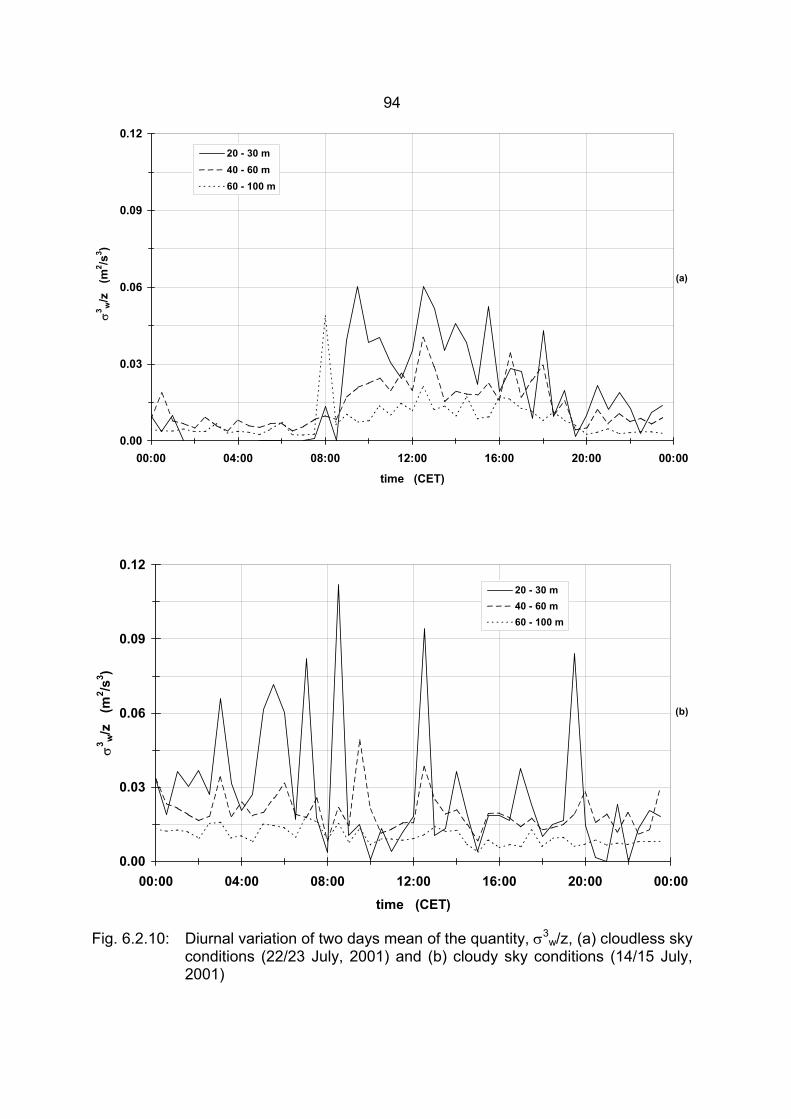
94

Fig. 6.2.10: Diurnal variation of two days mean of the quantity, σ3w/z, (a) cloudless sky

conditions (22/23 July, 2001) and (b) cloudy sky conditions (14/15 July, 2001)

0.00

0.03

0.06

0.09

0.12

00:00 04:00 08:00 12:00 16:00 20:00 00:00

time (CET)

σ3 w

/z

(m2 /s

3 )

20 - 30 m40 - 60 m60 - 100 m

(a)

0.00

0.03

0.06

0.09

0.12

00:00 04:00 08:00 12:00 16:00 20:00 00:00time (CET)

σ3 w

/z

(m2 /s

3 )

20 - 30 m40 - 60 m60 - 100 m

(b)

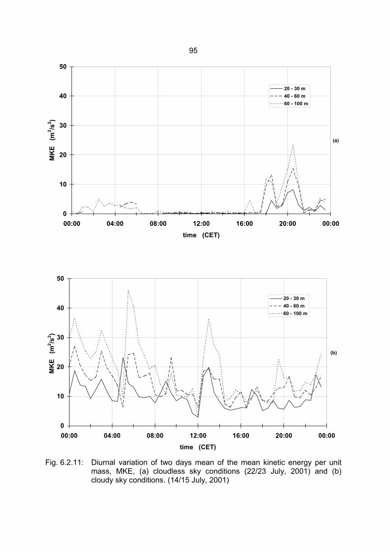
95

Fig. 6.2.11: Diurnal variation of two days mean of the mean kinetic energy per unit mass, MKE, (a) cloudless sky conditions (22/23 July, 2001) and (b) cloudy sky conditions. (14/15 July, 2001)

0

10

20

30

40

50

00:00 04:00 08:00 12:00 16:00 20:00 00:00

time (CET)

MK

E (

m2 /s

2 )

20 - 30 m40 - 60 m60 - 100 m

(a)

0

10

20

30

40

50

00:00 04:00 08:00 12:00 16:00 20:00 00:00

time (CET)

MK

E (

m2 /s

2 )

20 - 30 m40 - 60 m60 - 100 m

(b)

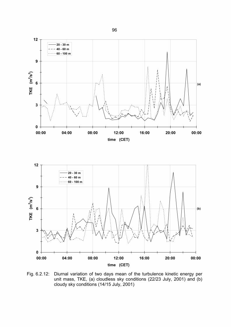
96

Fig. 6.2.12: Diurnal variation of two days mean of the turbulence kinetic energy per unit mass, TKE, (a) cloudless sky conditions (22/23 July, 2001) and (b) cloudy sky conditions (14/15 July, 2001)

0

3

6

9

12

00:00 04:00 08:00 12:00 16:00 20:00 00:00time (CET)

TKE

(m

2 /s2 )

20 - 30 m40 - 60 m60 - 100 m

(a)

0

3

6

9

12

00:00 04:00 08:00 12:00 16:00 20:00 00:00

time (CET)

TKE

(m

2 /s2 )

20 - 30 m40 - 60 m60 - 100 m

(b)

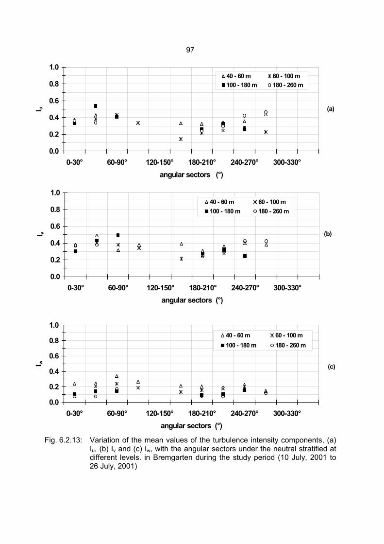
97

Fig. 6.2.13: Variation of the mean values of the turbulence intensity components, (a) Iu, (b) Iv and (c) Iw, with the angular sectors under the neutral stratified at different levels. in Bremgarten during the study period (10 July, 2001 to 26 July, 2001)

0.0

0.2

0.4

0.6

0.8

1.0

0-30° 60-90° 120-150° 180-210° 240-270° 300-330°angular sectors (°)

I u

40 - 60 m 60 - 100 m100 - 180 m 180 - 260 m

(a)

0.0

0.2

0.4

0.6

0.8

1.0

0-30° 60-90° 120-150° 180-210° 240-270° 300-330°angular sectors (°)

I v

40 - 60 m 60 - 100 m100 - 180 m 180 - 260 m

(b)

0.0

0.2

0.4

0.6

0.8

1.0

0-30° 60-90° 120-150° 180-210° 240-270° 300-330°angular sectors (°)

I w

40 - 60 m 60 - 100 m100 - 180 m 180 - 260 m

(c)

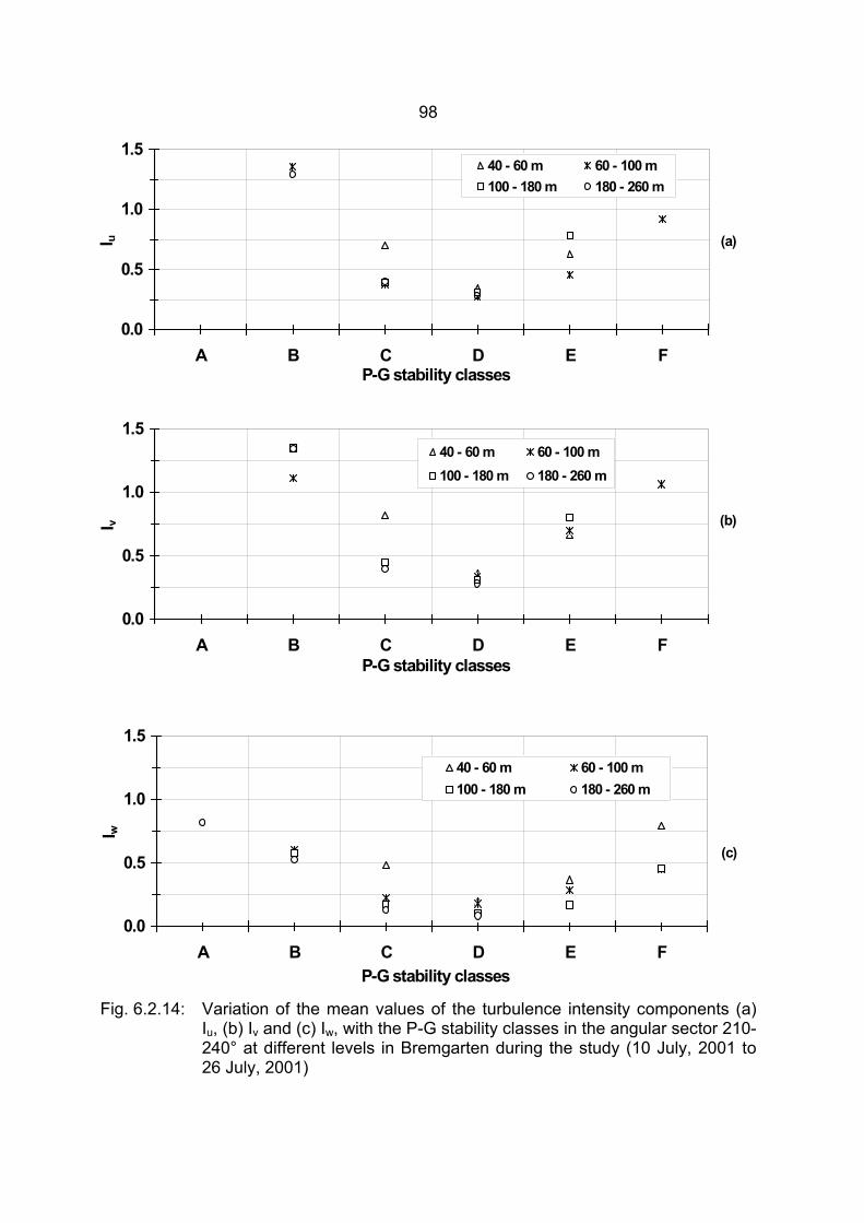
98

Fig. 6.2.14: Variation of the mean values of the turbulence intensity components (a) Iu, (b) Iv and (c) Iw, with the P-G stability classes in the angular sector 210-240° at different levels in Bremgarten during the study (10 July, 2001 to 26 July, 2001)

0.0

0.5

1.0

1.5


I u

40 - 60 m 60 - 100 m100 - 180 m 180 - 260 m

(a)

0.0

0.5

1.0

1.5


I v

40 - 60 m 60 - 100 m100 - 180 m 180 - 260 m

(b)

0.0

0.5

1.0

1.5


I w

40 - 60 m 60 - 100 m100 - 180 m 180 - 260 m

(c)

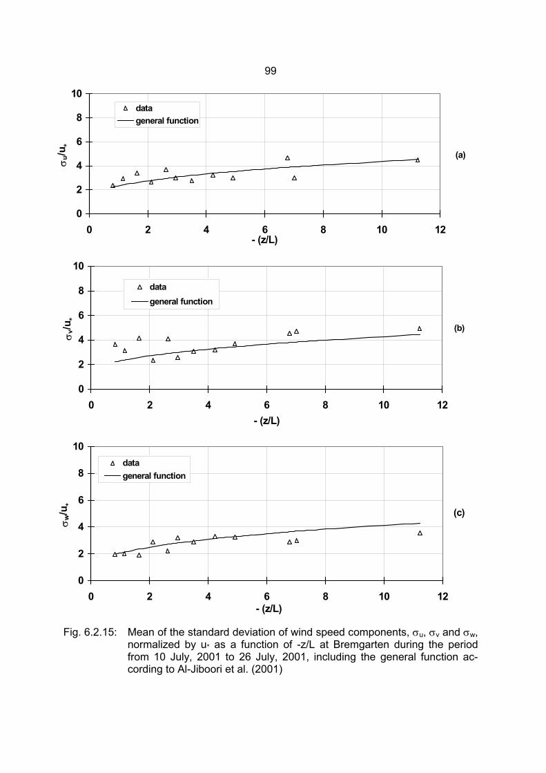
99

Fig. 6.2.15: Mean of the standard deviation of wind speed components, σu, σv and σw, normalized by u* as a function of -z/L at Bremgarten during the period from 10 July, 2001 to 26 July, 2001, including the general function ac-cording to Al-Jiboori et al. (2001)

0

2

4

6

8

10

0 2 4 6 8 10 12- (z/L)

σu/u

∗


(a)

0

2

4

6

8

10

0 2 4 6 8 10 12- (z/L)

σv/u

∗


(b)

0

2

4

6

8

10

0 2 4 6 8 10 12- (z/L)

σw/u

∗


(c)

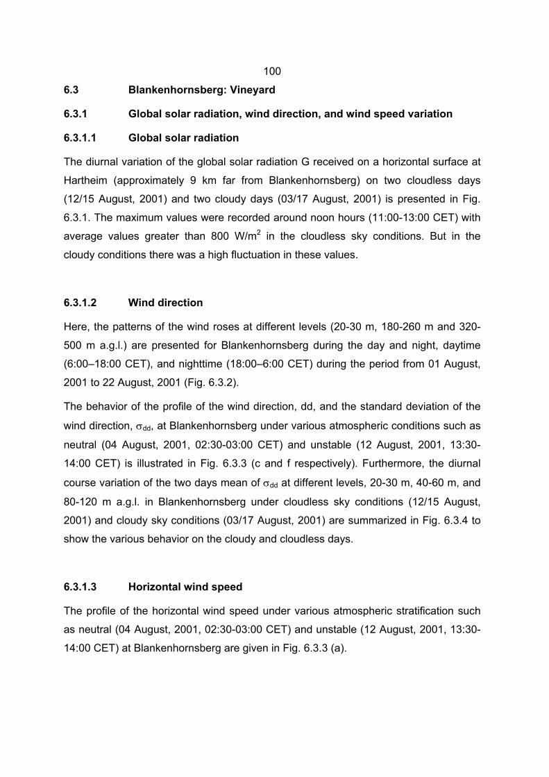
100

6.3 Blankenhornsberg: Vineyard




Hartheim (approximately 9 km far from Blankenhornsberg) on two cloudless days

(12/15 August, 2001) and two cloudy days (03/17 August, 2001) is presented in Fig.

6.3.1. The maximum values were recorded around noon hours (11:00-13:00 CET) with

average values greater than 800 W/m2 in the cloudless sky conditions. But in the

cloudy conditions there was a high fluctuation in these values.


Here, the patterns of the wind roses at different levels (20-30 m, 180-260 m and 320-

500 m a.g.l.) are presented for Blankenhornsberg during the day and night, daytime

(6:00–18:00 CET), and nighttime (18:00–6:00 CET) during the period from 01 August,

2001 to 22 August, 2001 (Fig. 6.3.2).

The behavior of the profile of the wind direction, dd, and the standard deviation of the

wind direction, σdd, at Blankenhornsberg under various atmospheric conditions such as

neutral (04 August, 2001, 02:30-03:00 CET) and unstable (12 August, 2001, 13:30-

14:00 CET) is illustrated in Fig. 6.3.3 (c and f respectively). Furthermore, the diurnal

course variation of the two days mean of σdd at different levels, 20-30 m, 40-60 m, and

80-120 m a.g.l. in Blankenhornsberg under cloudless sky conditions (12/15 August,

2001) and cloudy sky conditions (03/17 August, 2001) are summarized in Fig. 6.3.4 to

show the various behavior on the cloudy and cloudless days.


The profile of the horizontal wind speed under various atmospheric stratification such

as neutral (04 August, 2001, 02:30-03:00 CET) and unstable (12 August, 2001, 13:30-

14:00 CET) at Blankenhornsberg are given in Fig. 6.3.3 (a).

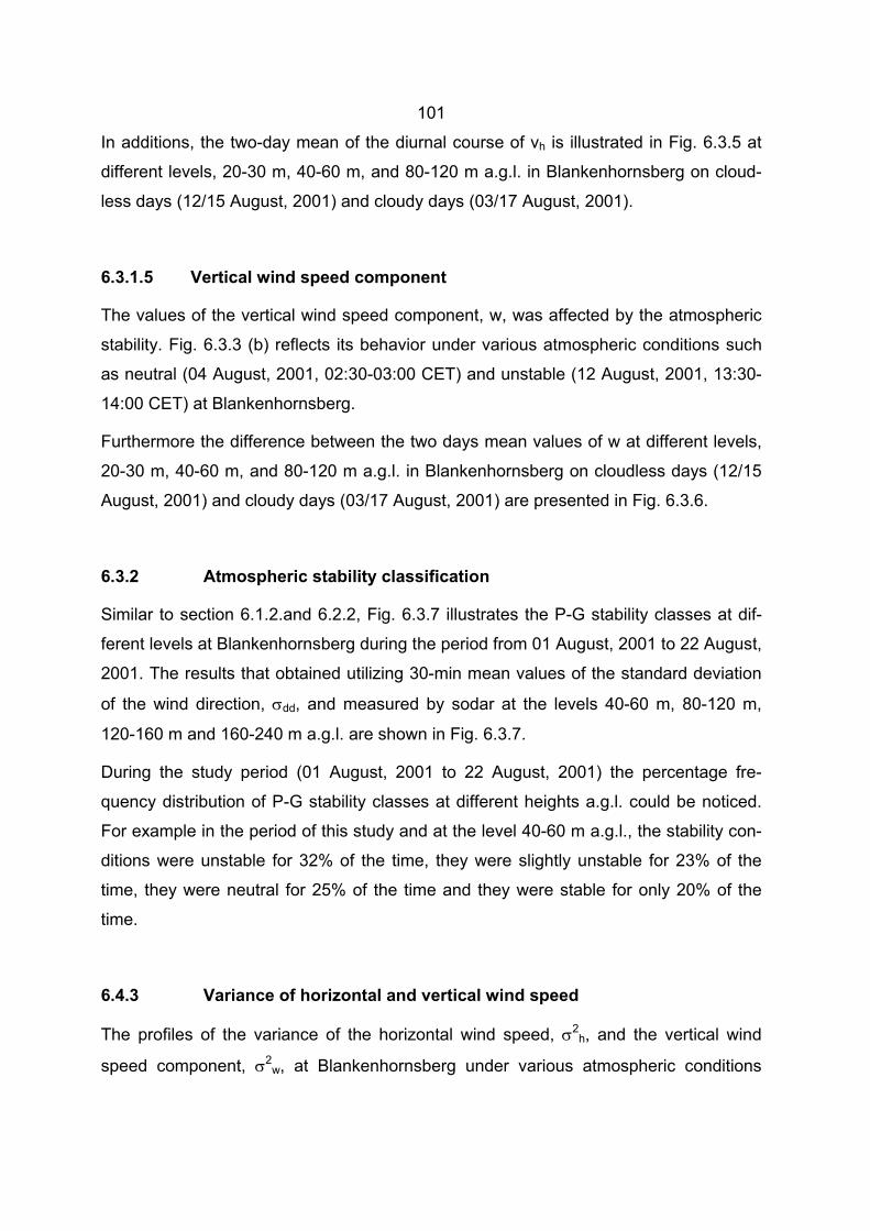
101

In additions, the two-day mean of the diurnal course of vh is illustrated in Fig. 6.3.5 at

different levels, 20-30 m, 40-60 m, and 80-120 m a.g.l. in Blankenhornsberg on cloud-

less days (12/15 August, 2001) and cloudy days (03/17 August, 2001).


The values of the vertical wind speed component, w, was affected by the atmospheric

stability. Fig. 6.3.3 (b) reflects its behavior under various atmospheric conditions such

as neutral (04 August, 2001, 02:30-03:00 CET) and unstable (12 August, 2001, 13:30-

14:00 CET) at Blankenhornsberg.

Furthermore the difference between the two days mean values of w at different levels,

20-30 m, 40-60 m, and 80-120 m a.g.l. in Blankenhornsberg on cloudless days (12/15

August, 2001) and cloudy days (03/17 August, 2001) are presented in Fig. 6.3.6.


Similar to section 6.1.2.and 6.2.2, Fig. 6.3.7 illustrates the P-G stability classes at dif-

ferent levels at Blankenhornsberg during the period from 01 August, 2001 to 22 August,

2001. The results that obtained utilizing 30-min mean values of the standard deviation

of the wind direction, σdd, and measured by sodar at the levels 40-60 m, 80-120 m,

120-160 m and 160-240 m a.g.l. are shown in Fig. 6.3.7.

During the study period (01 August, 2001 to 22 August, 2001) the percentage fre-

quency distribution of P-G stability classes at different heights a.g.l. could be noticed.

For example in the period of this study and at the level 40-60 m a.g.l., the stability con-

ditions were unstable for 32% of the time, they were slightly unstable for 23% of the

time, they were neutral for 25% of the time and they were stable for only 20% of the

time.



speed component, σ2w, at Blankenhornsberg under various atmospheric conditions

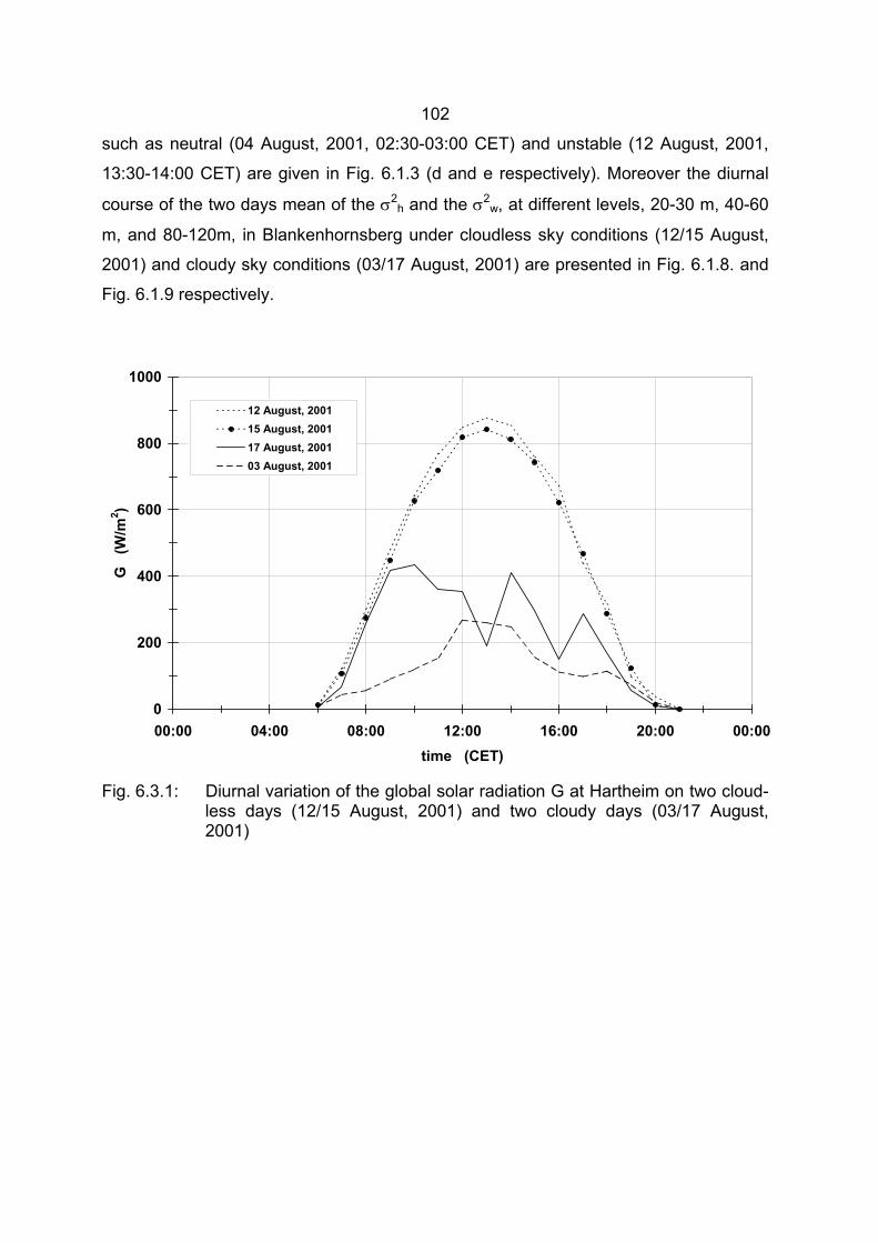
102

such as neutral (04 August, 2001, 02:30-03:00 CET) and unstable (12 August, 2001,

13:30-14:00 CET) are given in Fig. 6.1.3 (d and e respectively). Moreover the diurnal

course of the two days mean of the σ2h and the σ2

w, at different levels, 20-30 m, 40-60

m, and 80-120m, in Blankenhornsberg under cloudless sky conditions (12/15 August,

2001) and cloudy sky conditions (03/17 August, 2001) are presented in Fig. 6.1.8. and

Fig. 6.1.9 respectively.

Fig. 6.3.1: Diurnal variation of the global solar radiation G at Hartheim on two cloud-less days (12/15 August, 2001) and two cloudy days (03/17 August, 2001)

0

200

400

600

800

1000

00:00 04:00 08:00 12:00 16:00 20:00 00:00time (CET)

G

(W/m

2 )

12 August, 200115 August, 200117 August, 200103 August, 2001

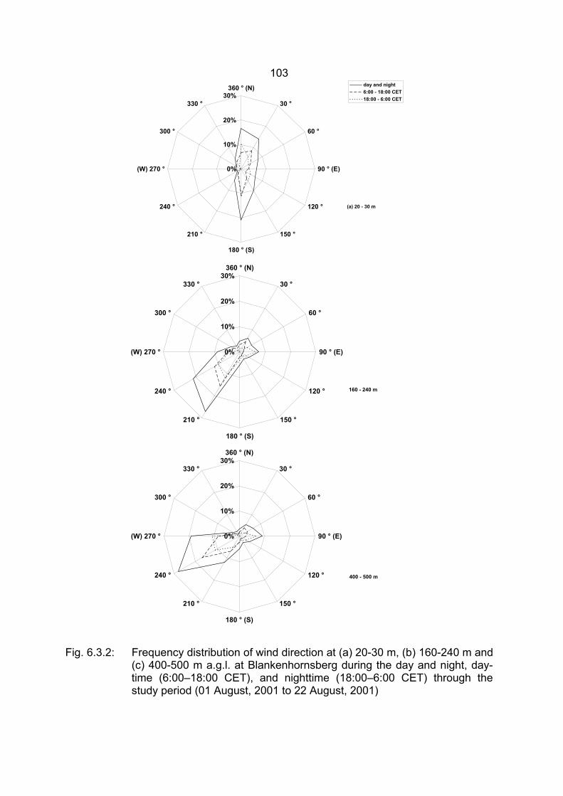
103

Fig. 6.3.2: Frequency distribution of wind direction at (a) 20-30 m, (b) 160-240 m and

(c) 400-500 m a.g.l. at Blankenhornsberg during the day and night, day-time (6:00–18:00 CET), and nighttime (18:00–6:00 CET) through the study period (01 August, 2001 to 22 August, 2001)

0%

10%

20%

30%360 ° (N)

30 °

60 °

90 ° (E)

120 °

150 °

180 ° (S)

210 °

240 °

(W) 270 °

300 °

330 °


(a) 20 - 30 m

0%

10%

20%

30%360 ° (N)

30 °

60 °

90 ° (E)

120 °

150 °

180 ° (S)

210 °

240 °

(W) 270 °

300 °

330 °

160 - 240 m

0%

10%

20%

30%360 ° (N)

30 °

60 °

90 ° (E)

120 °

150 °

180 ° (S)

210 °

240 °

(W) 270 °

300 °

330 °

400 - 500 m

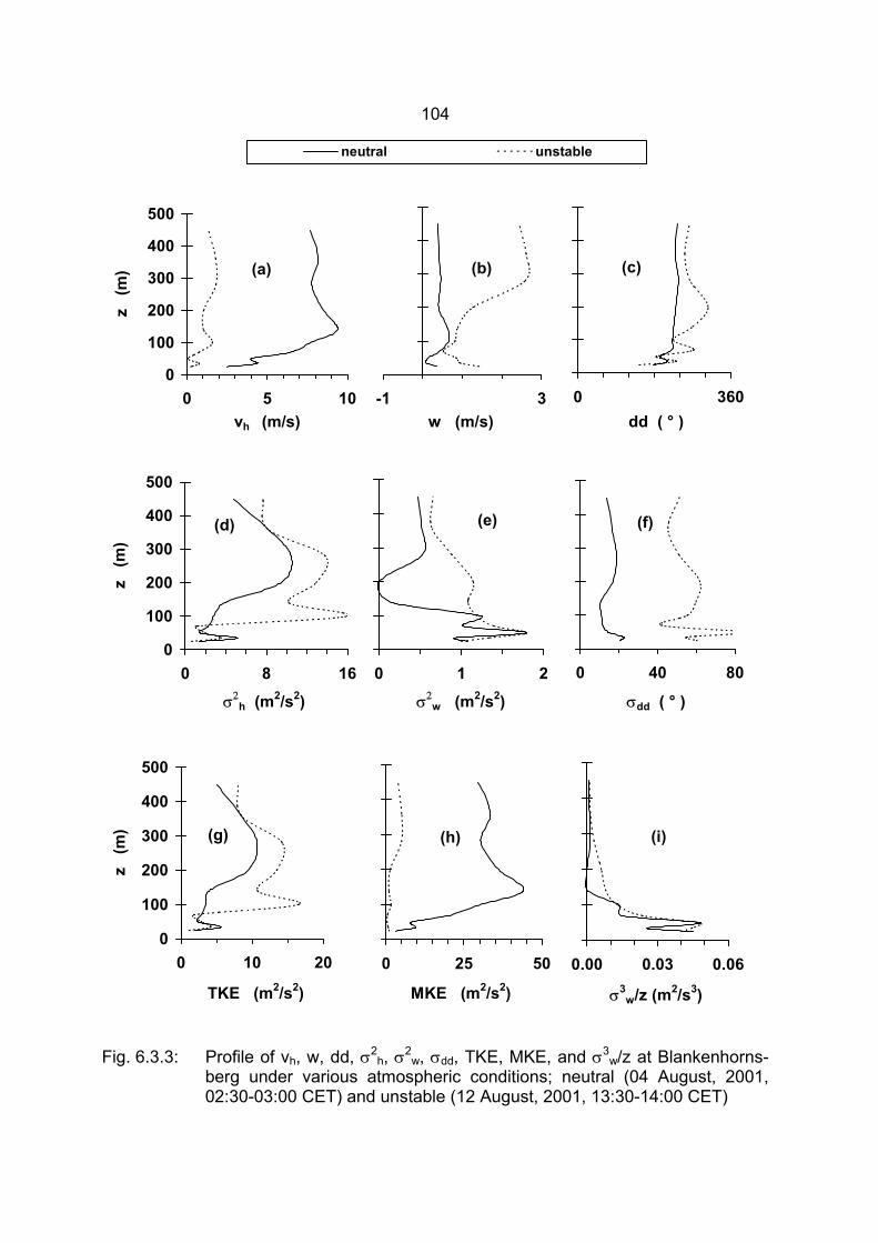
104


w, σdd, TKE, MKE, and σ3w/z at Blankenhorns-

berg under various atmospheric conditions; neutral (04 August, 2001, 02:30-03:00 CET) and unstable (12 August, 2001, 13:30-14:00 CET)

vh (m/s) w (m/s) dd ( ° )

σ2h (m2/s2) σ2

w (m2/s2) σdd ( ° )


(a)

0

100

200

300

400

500

0 5 10

z (

m) (b)

-1 3

(c)

0 360

(d)

0

100

200

300

400

500

0 8 16

z (

m)

(e)

0 1 2

(f)

0 40 80

(g)

0

100

200

300

400

500

0 10 20

z (

m) (h)

0 25 50

(i)

0.00 0.03 0.06

neutral unstable

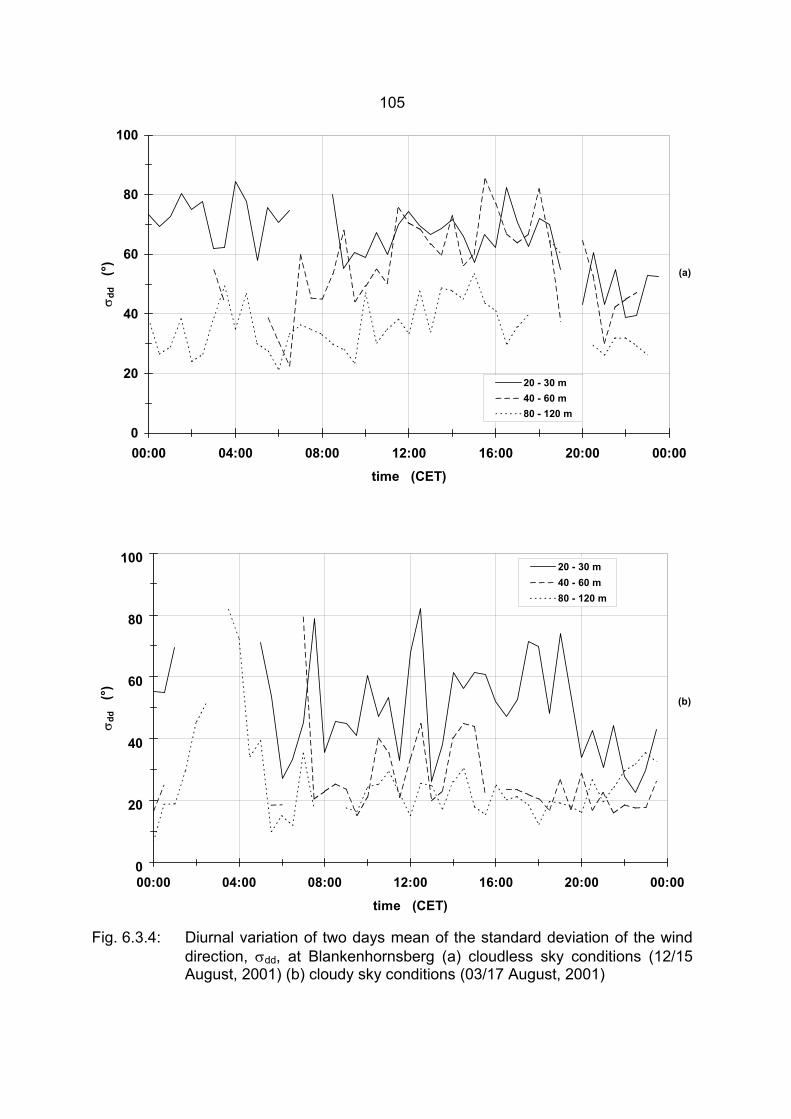
105

Fig. 6.3.4: Diurnal variation of two days mean of the standard deviation of the wind direction, σdd, at Blankenhornsberg (a) cloudless sky conditions (12/15 August, 2001) (b) cloudy sky conditions (03/17 August, 2001)

0

20

40

60

80

100

00:00 04:00 08:00 12:00 16:00 20:00 00:00time (CET)

σdd

(°

)

20 - 30 m40 - 60 m80 - 120 m

(a)

0

20

40

60

80

100

00:00 04:00 08:00 12:00 16:00 20:00 00:00

time (CET)

σdd

(°

)

20 - 30 m40 - 60 m80 - 120 m

(b)

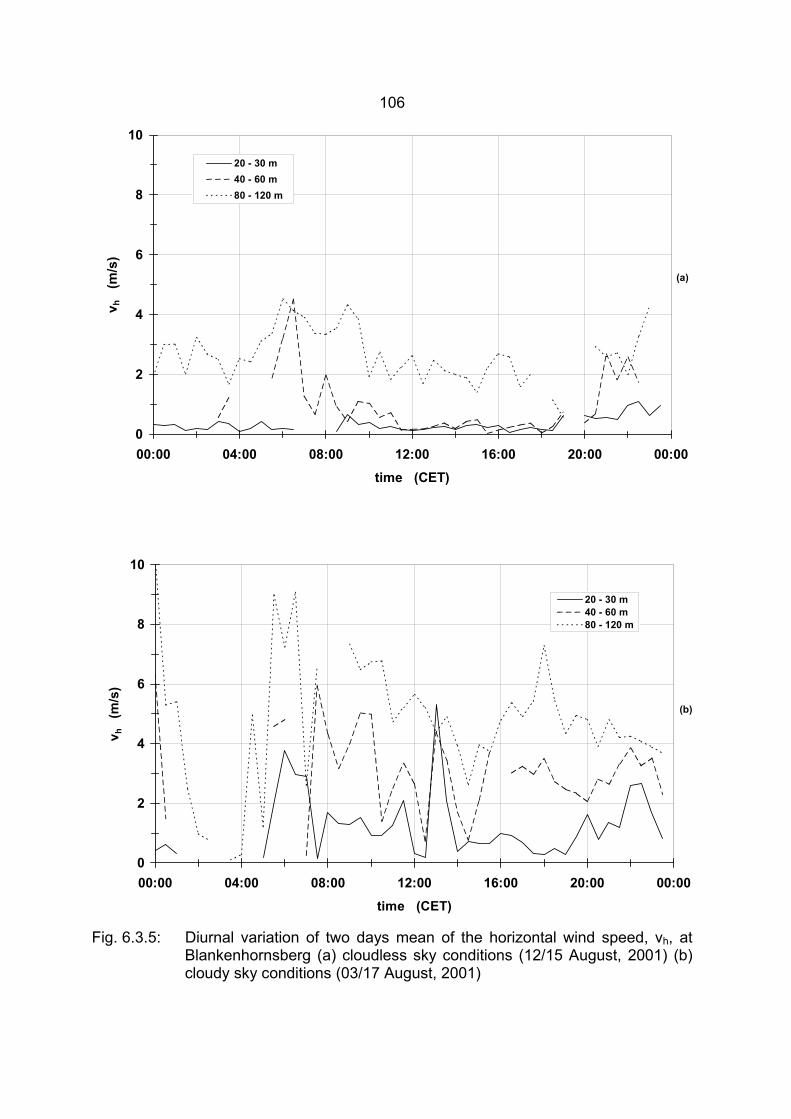
106

Fig. 6.3.5: Diurnal variation of two days mean of the horizontal wind speed, vh, at Blankenhornsberg (a) cloudless sky conditions (12/15 August, 2001) (b) cloudy sky conditions (03/17 August, 2001)

0

2

4

6

8

10

00:00 04:00 08:00 12:00 16:00 20:00 00:00time (CET)

v h

(m/s

)

20 - 30 m40 - 60 m80 - 120 m

(a)

0

2

4

6

8

10

00:00 04:00 08:00 12:00 16:00 20:00 00:00time (CET)

v h

(m/s

)

20 - 30 m40 - 60 m80 - 120 m

(b)

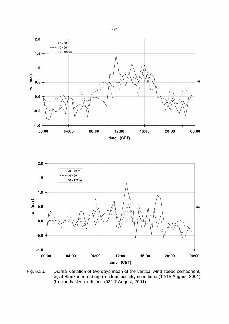
107

Fig. 6.3.6: Diurnal variation of two days mean of the vertical wind speed component, w, at Blankenhornsberg (a) cloudless sky conditions (12/15 August, 2001) (b) cloudy sky conditions (03/17 August, 2001)

-1.0

-0.5

0.0

0.5

1.0

1.5

2.0

00:00 04:00 08:00 12:00 16:00 20:00 00:00

time (CET)

w

(m/s

)

20 - 30 m40 - 60 m80 - 120 m

(a)

-1.0

-0.5

0.0

0.5

1.0

1.5

2.0

00:00 04:00 08:00 12:00 16:00 20:00 00:00time (CET)

w

(m/s

)

20 - 30 m40 - 60 m80 - 120 m

(b)

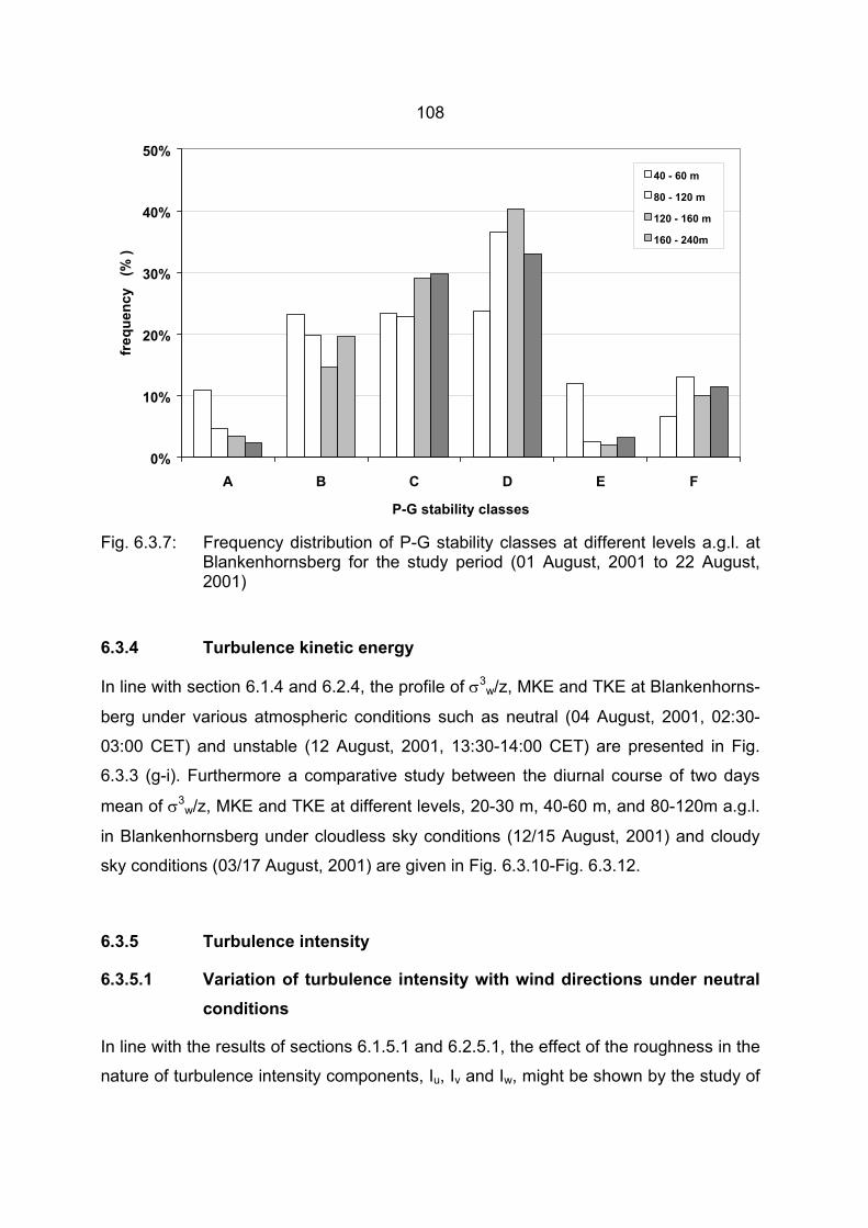
108

Fig. 6.3.7: Frequency distribution of P-G stability classes at different levels a.g.l. at Blankenhornsberg for the study period (01 August, 2001 to 22 August, 2001)


In line with section 6.1.4 and 6.2.4, the profile of σ3w/z, MKE and TKE at Blankenhorns-

berg under various atmospheric conditions such as neutral (04 August, 2001, 02:30-

03:00 CET) and unstable (12 August, 2001, 13:30-14:00 CET) are presented in Fig.

6.3.3 (g-i). Furthermore a comparative study between the diurnal course of two days

mean of σ3w/z, MKE and TKE at different levels, 20-30 m, 40-60 m, and 80-120m a.g.l.

in Blankenhornsberg under cloudless sky conditions (12/15 August, 2001) and cloudy

sky conditions (03/17 August, 2001) are given in Fig. 6.3.10-Fig. 6.3.12.



In line with the results of sections 6.1.5.1 and 6.2.5.1, the effect of the roughness in the

nature of turbulence intensity components, Iu, Iv and Iw, might be shown by the study of

0%

10%

20%

30%

40%

50%

A B C D E F


freq

uenc

y (

% )

40 - 60 m

80 - 120 m

120 - 160 m

160 - 240m

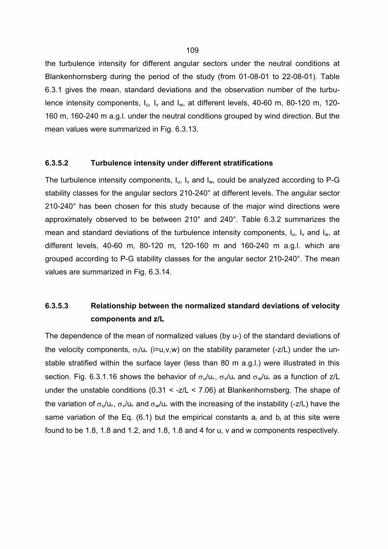
109

the turbulence intensity for different angular sectors under the neutral conditions at

Blankenhornsberg during the period of the study (from 01-08-01 to 22-08-01). Table

6.3.1 gives the mean, standard deviations and the observation number of the turbu-

lence intensity components, Iu, Iv and Iw, at different levels, 40-60 m, 80-120 m, 120-

160 m, 160-240 m a.g.l. under the neutral conditions grouped by wind direction. But the

mean values were summarized in Fig. 6.3.13.


The turbulence intensity components, Iu, Iv and Iw, could be analyzed according to P-G

stability classes for the angular sectors 210-240° at different levels. The angular sector

210-240° has been chosen for this study because of the major wind directions were

approximately observed to be between 210° and 240°. Table 6.3.2 summarizes the

mean and standard deviations of the turbulence intensity components, Iu, Iv and Iw, at

different levels, 40-60 m, 80-120 m, 120-160 m and 160-240 m a.g.l. which are

grouped according to P-G stability classes for the angular sector 210-240°. The mean

values are summarized in Fig. 6.3.14.

6.3.5.3 Relationship between the normalized standard deviations of velocity components and z/L

The dependence of the mean of normalized values (by u*) of the standard deviations of

the velocity components, σi/u∗ (i=u,v,w) on the stability parameter (-z/L) under the un-

stable stratified within the surface layer (less than 80 m a.g.l.) were illustrated in this

section. Fig. 6.3.1.16 shows the behavior of σu/u∗, σv/u∗ and σw/u∗ as a function of z/L

under the unstable conditions (0.31 < -z/L < 7.06) at Blankenhornsberg. The shape of

the variation of σu/u∗, σv/u∗ and σw/u∗ with the increasing of the instability (-z/L) have the

same variation of the Eq. (6.1) but the empirical constants ai and bi at this site were

found to be 1.8, 1.8 and 1.2, and 1.8, 1.8 and 4 for u, v and w components respectively.

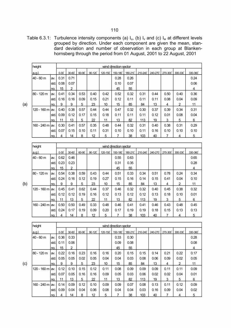
110

Table 6.3.1: Turbulence intensity components (a) Iu, (b) Iv and (c) Iw at different levels grouped by direction. Under each component are given the mean, stan-dard deviation and number of observation in each group at Blanken-hornsberg through the period from 01 August, 2001 to 22 August, 2001


a.g.l. 0-30° 30-60° 60-90° 90-120° 120-150° 150-180° 180-210° 210-240° 240-270° 270-300° 300-330° 330-360°

40 - 60 m av. 0.31 0.71 0.28 0.26 0.24std. 0.08 0.07 0.10 0.07 0.06no. 15 2 45 55 4

80 - 120 m av. 0.41 0.34 0.53 0.40 0.42 0.52 0.32 0.31 0.44 0.50 0.40 0.36std. 0.16 0.16 0.09 0.15 0.21 0.12 0.11 0.11 0.11 0.08 0.04 0.09

(a) no. 9 9 5 23 10 15 85 84 13 4 2 11120 - 160 m av. 0.40 0.38 0.57 0.44 0.44 0.47 0.32 0.30 0.37 0.39 0.34 0.31

std. 0.09 0.12 0.17 0.15 0.18 0.11 0.11 0.11 0.12 0.01 0.08 0.04no. 11 13 5 22 11 13 82 113 19 3 5 6

160 - 240 m av. 0.30 0.41 0.57 0.35 0.48 0.44 0.32 0.31 0.40 0.38 0.31 0.29std. 0.07 0.15 0.10 0.11 0.31 0.10 0.10 0.11 0.16 0.10 0.10 0.10no. 4 14 8 12 5 7 38 103 40 7 4 5


a.g.l. 0-30° 30-60° 60-90° 90-120° 120-150° 150-180° 180-210° 210-240° 240-270° 270-300° 300-330° 330-360°

40 - 60 m av. 0.62 0.46 0.55 0.63 0.65std. 0.23 0.23 0.31 0.35 0.28no. 15 2 45 55 4

80 - 120 m av. 0.54 0.38 0.59 0.43 0.44 0.51 0.33 0.34 0.51 0.78 0.24 0.34std. 0.24 0.16 0.12 0.19 0.27 0.15 0.16 0.14 0.15 0.41 0.04 0.10

(b) no. 9 9 5 23 10 15 85 84 13 4 2 11120 - 160 m av. 0.45 0.41 0.62 0.44 0.37 0.46 0.32 0.32 0.40 0.45 0.38 0.32

std. 0.12 0.12 0.19 0.16 0.12 0.13 0.12 0.12 0.13 0.18 0.10 0.01no. 11 13 5 22 11 13 82 113 19 3 5 6

160 - 240 m av. 0.50 0.50 0.49 0.33 0.48 0.46 0.41 0.41 0.46 0.43 0.48 0.45std. 0.24 0.17 0.19 0.09 0.20 0.17 0.19 0.19 0.18 0.15 0.13 0.13no. 4 14 8 12 5 7 38 103 40 7 4 5


a.g.l. 0-30° 30-60° 60-90° 90-120° 120-150° 150-180° 180-210° 210-240° 240-270° 270-300° 300-330° 330-360°

40 - 60 m av. 0.36 0.33 0.33 0.30 0.28std. 0.11 0.06 0.09 0.08 0.08no. 15 2 45 55 4

80 - 120 m av. 0.22 0.16 0.23 0.16 0.16 0.20 0.15 0.15 0.14 0.21 0.22 0.17std. 0.05 0.05 0.02 0.05 0.04 0.04 0.03 0.08 0.06 0.09 0.02 0.05

(c) no. 9 9 5 23 10 15 85 84 13 4 2 11120 - 160 m av. 0.12 0.10 0.15 0.12 0.11 0.08 0.09 0.09 0.09 0.11 0.11 0.09

std. 0.07 0.05 0.16 0.16 0.09 0.05 0.03 0.06 0.02 0.02 0.04 0.01no. 11 13 5 22 11 13 82 113 19 3 5 6

160 - 240 m av. 0.14 0.09 0.12 0.10 0.09 0.09 0.07 0.08 0.13 0.11 0.12 0.09std. 0.09 0.04 0.04 0.06 0.08 0.04 0.04 0.03 0.16 0.09 0.04 0.02no. 4 14 8 12 5 7 38 103 40 7 4 5

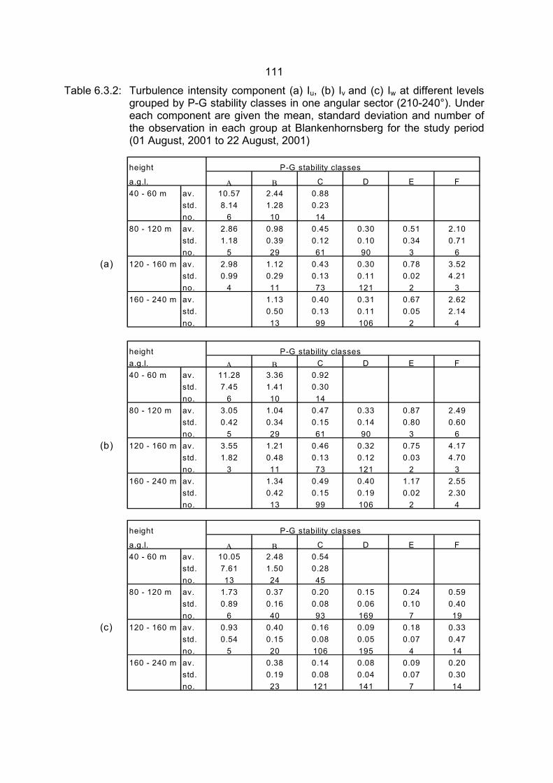
111

Table 6.3.2: Turbulence intensity component (a) Iu, (b) Iv and (c) Iw at different levels grouped by P-G stability classes in one angular sector (210-240°). Under each component are given the mean, standard deviation and number of the observation in each group at Blankenhornsberg for the study period (01 August, 2001 to 22 August, 2001)


a.g.l. Α Β C D E F40 - 60 m av. 10.57 2.44 0.88

std. 8.14 1.28 0.23no. 6 10 14

80 - 120 m av. 2.86 0.98 0.45 0.30 0.51 2.10std. 1.18 0.39 0.12 0.10 0.34 0.71no. 5 29 61 90 3 6

(a) 120 - 160 m av. 2.98 1.12 0.43 0.30 0.78 3.52std. 0.99 0.29 0.13 0.11 0.02 4.21no. 4 11 73 121 2 3

160 - 240 m av. 1.13 0.40 0.31 0.67 2.62std. 0.50 0.13 0.11 0.05 2.14no. 13 99 106 2 4

height P-G stability classesa.g.l. Α Β C D E F40 - 60 m av. 11.28 3.36 0.92

std. 7.45 1.41 0.30no. 6 10 14

80 - 120 m av. 3.05 1.04 0.47 0.33 0.87 2.49std. 0.42 0.34 0.15 0.14 0.80 0.60no. 5 29 61 90 3 6

(b) 120 - 160 m av. 3.55 1.21 0.46 0.32 0.75 4.17std. 1.82 0.48 0.13 0.12 0.03 4.70no. 3 11 73 121 2 3

160 - 240 m av. 1.34 0.49 0.40 1.17 2.55std. 0.42 0.15 0.19 0.02 2.30no. 13 99 106 2 4


a.g.l. Α Β C D E F40 - 60 m av. 10.05 2.48 0.54

std. 7.61 1.50 0.28no. 13 24 45

80 - 120 m av. 1.73 0.37 0.20 0.15 0.24 0.59std. 0.89 0.16 0.08 0.06 0.10 0.40no. 6 40 93 169 7 19

(c) 120 - 160 m av. 0.93 0.40 0.16 0.09 0.18 0.33std. 0.54 0.15 0.08 0.05 0.07 0.47no. 5 20 106 195 4 14

160 - 240 m av. 0.38 0.14 0.08 0.09 0.20std. 0.19 0.08 0.04 0.07 0.30no. 23 121 141 7 14

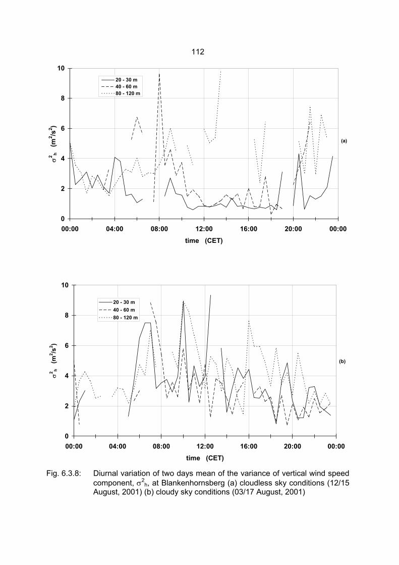
112


h, at Blankenhornsberg (a) cloudless sky conditions (12/15 August, 2001) (b) cloudy sky conditions (03/17 August, 2001)

0

2

4

6

8

10

00:00 04:00 08:00 12:00 16:00 20:00 00:00

time (CET)

σ2 h

(m2 /s

2 )

20 - 30 m40 - 60 m80 - 120 m

(a)

0

2

4

6

8

10

00:00 04:00 08:00 12:00 16:00 20:00 00:00time (CET)

σ2 h

(m2 /s

2 )

20 - 30 m40 - 60 m80 - 120 m

(b)

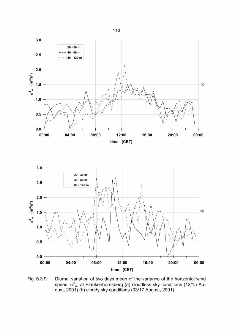
113


w, at Blankenhornsberg (a) cloudless sky conditions (12/15 Au-gust, 2001) (b) cloudy sky conditions (03/17 August, 2001)

0.0

0.5

1.0

1.5

2.0

2.5

3.0

00:00 04:00 08:00 12:00 16:00 20:00 00:00

time (CET)

σ2 w

(m

2 /s2 )

20 - 30 m40 - 60 m80 - 120 m

(b)

0.0

0.5

1.0

1.5

2.0

2.5

3.0

00:00 04:00 08:00 12:00 16:00 20:00 00:00time (CET)

σ2 w

(m2 /s

2 )

20 - 30 m

40 - 60 m

80 - 120 m

(a)

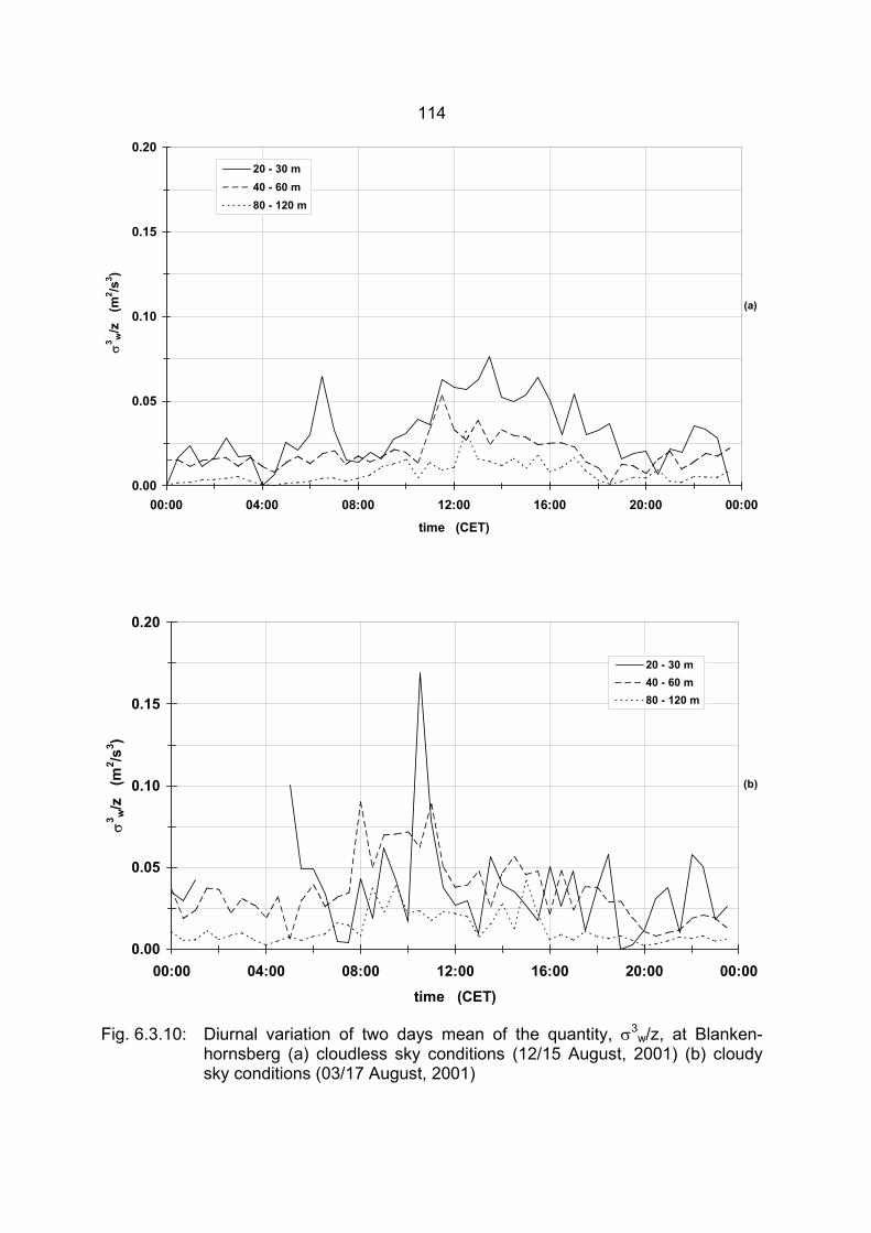
114

Fig. 6.3.10: Diurnal variation of two days mean of the quantity, σ3w/z, at Blanken-

hornsberg (a) cloudless sky conditions (12/15 August, 2001) (b) cloudy sky conditions (03/17 August, 2001)

0.00

0.05

0.10

0.15

0.20

00:00 04:00 08:00 12:00 16:00 20:00 00:00

time (CET)

σ3 w

/z

(m2 /s

3 )

20 - 30 m40 - 60 m80 - 120 m

(a)

0.00

0.05

0.10

0.15

0.20

00:00 04:00 08:00 12:00 16:00 20:00 00:00time (CET)

σ3 w

/z

(m2 /s

3 )

20 - 30 m40 - 60 m80 - 120 m

(b)

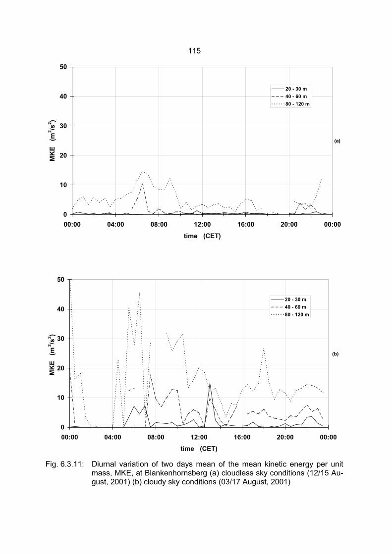
115

Fig. 6.3.11: Diurnal variation of two days mean of the mean kinetic energy per unit mass, MKE, at Blankenhornsberg (a) cloudless sky conditions (12/15 Au-gust, 2001) (b) cloudy sky conditions (03/17 August, 2001)

0

10

20

30

40

50

00:00 04:00 08:00 12:00 16:00 20:00 00:00

time (CET)

MK

E (

m2 /s

2 )

20 - 30 m40 - 60 m80 - 120 m

(a)

0

10

20

30

40

50

00:00 04:00 08:00 12:00 16:00 20:00 00:00

time (CET)

MK

E (

m2 /s

2 )

20 - 30 m40 - 60 m80 - 120 m

(b)

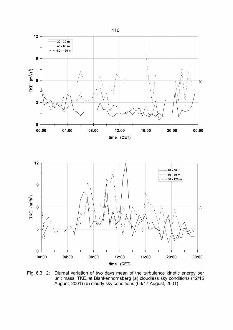
116

Fig. 6.3.12: Diurnal variation of two days mean of the turbulence kinetic energy per unit mass, TKE, at Blankenhornsberg (a) cloudless sky conditions (12/15 August, 2001) (b) cloudy sky conditions (03/17 August, 2001)

0

3

6

9

12

00:00 04:00 08:00 12:00 16:00 20:00 00:00time (CET)

TKE

(m

2 /s2 )

20 - 30 m40 - 60 m80 - 120 m

(a)

0

3

6

9

12

00:00 04:00 08:00 12:00 16:00 20:00 00:00

time (CET)

TKE

(m

2 /s2 )

20 - 30 m40 - 60 m80 - 120 m

(b)

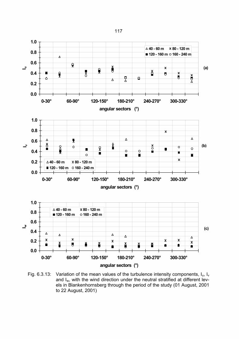
117

Fig. 6.3.13: Variation of the mean values of the turbulence intensity components, Iu, Iv and Iw, with the wind direction under the neutral stratified at different lev-els in Blankenhornsberg through the period of the study (01 August, 2001 to 22 August, 2001)

0.0

0.2

0.4

0.6

0.8

1.0

0-30° 60-90° 120-150° 180-210° 240-270° 300-330°angular sectors (°)

I u

40 - 60 m 80 - 120 m 120 - 160 m 160 - 240 m

(a)

0.0

0.2

0.4

0.6

0.8

1.0

0-30° 60-90° 120-150° 180-210° 240-270° 300-330°angular sectors (°)

I v

40 - 60 m 80 - 120 m 120 - 160 m 160 - 240 m

(b)

0.0

0.2

0.4

0.6

0.8

1.0

0-30° 60-90° 120-150° 180-210° 240-270° 300-330°angular sectors (°)

I w

40 - 60 m 80 - 120 m 120 - 160 m 160 - 240 m

(c)

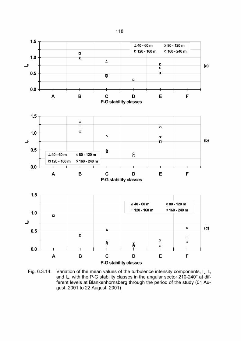
118

Fig. 6.3.14: Variation of the mean values of the turbulence intensity components, Iu, Iv and Iw, with the P-G stability classes in the angular sector 210-240° at dif-ferent levels at Blankenhornsberg through the period of the study (01 Au-gust, 2001 to 22 August, 2001)

0.0

0.5

1.0

1.5


I u

40 - 60 m 80 - 120 m 120 - 160 m 160 - 240 m

(a)

0.0

0.5

1.0

1.5


I v

40 - 60 m 80 - 120 m 120 - 160 m 160 - 240 m

(b)

0.0

0.5

1.0

1.5


I w

40 - 60 m 80 - 120 m 120 - 160 m 160 - 240 m

(c)

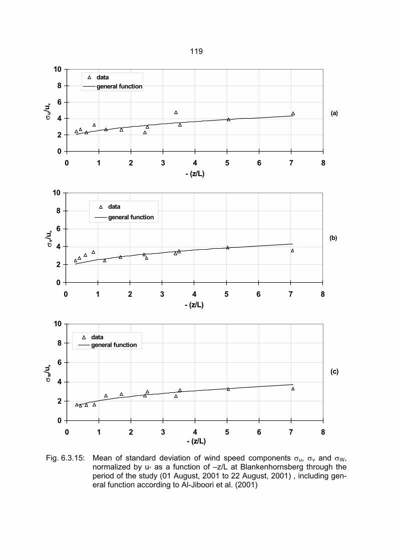
119

Fig. 6.3.15: Mean of standard deviation of wind speed components σu, σv and σW, normalized by u* as a function of –z/L at Blankenhornsberg through the period of the study (01 August, 2001 to 22 August, 2001) , including gen-eral function according to Al-Jiboori et al. (2001)

0

2

4

6

8

10

0 1 2 3 4 5 6 7 8- (z/L)

σu/u

∗


(a)

0

2

4

6

8

10

0 1 2 3 4 5 6 7 8- (z/L)

σv/u

∗


(b)

0

2

4

6

8

10

0 1 2 3 4 5 6 7 8- (z/L)

σw/u

∗


(c)

120

6.4 Oberbärenburg: Norway Spruce forest




Rotherdbach (one km from Oberbärenburg) on two cloudless days (30 August, 2001

and 23 September, 2001) and two cloudy days (31 August, 2001 and 01 September,

2001) is presented in Fig. 6.4.1. The maximum values were recorded around the noon

hours with average values greater than 600 W/m2 on the cloudless days and approxi-

mately lower than 200 W/m2 on the cloudy days.


A preliminary analysis of wind rose at different heights, 20-50 m, 230-260 m and 470-

500 m a.g.l. at Oberbärenburg during the day and night, daytime (6:00-8:00 CET) and

the nighttime (18:00-6:00 CET), through the period from 29 August, 2001 to 24 Sep-

tember, 2001, are presented in Fig. 6.4.2. The diurnal course of two days mean of σdd

at different levels 20-50 m, 50-80 m, 80-110 m a.g.l. at Oberbärenburg in cloudless sky

conditions (30 August, 2001 and 23 September, 2001) and cloudy sky conditions (31

August, 2001 and 01 September, 2001), are shown in Fig. 6.4.3.


The two days mean of the diurnal variation of vh is illustrated in Fig. 6.4.4 at different

levels, 20-50 m, 50-80 m, and 80-110 m a.g.l. in Oberbärenburg on cloudless days (30

August, 2001 and 23 September, 2001) and cloudy days (31 August, 2001 and 01 Sep-

tember, 2001).


Besides the data of the horizontal wind speed, diurnal variation of the vertical wind

speed component, w, at Oberbärenburg is shown. Fig. 6.4.5 presents the different be-

tween the two days mean values of w on cloudless days (30 August, 2001 and 23 Sep-

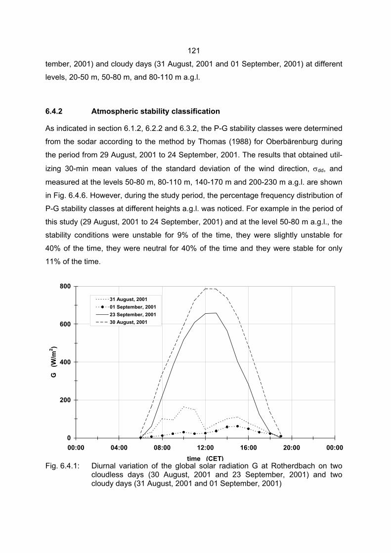
121

tember, 2001) and cloudy days (31 August, 2001 and 01 September, 2001) at different

levels, 20-50 m, 50-80 m, and 80-110 m a.g.l.


As indicated in section 6.1.2, 6.2.2 and 6.3.2, the P-G stability classes were determined

from the sodar according to the method by Thomas (1988) for Oberbärenburg during

the period from 29 August, 2001 to 24 September, 2001. The results that obtained util-

izing 30-min mean values of the standard deviation of the wind direction, σdd, and

measured at the levels 50-80 m, 80-110 m, 140-170 m and 200-230 m a.g.l. are shown

in Fig. 6.4.6. However, during the study period, the percentage frequency distribution of

P-G stability classes at different heights a.g.l. was noticed. For example in the period of

this study (29 August, 2001 to 24 September, 2001) and at the level 50-80 m a.g.l., the

stability conditions were unstable for 9% of the time, they were slightly unstable for

40% of the time, they were neutral for 40% of the time and they were stable for only

11% of the time.

Fig. 6.4.1: Diurnal variation of the global solar radiation G at Rotherdbach on two cloudless days (30 August, 2001 and 23 September, 2001) and two cloudy days (31 August, 2001 and 01 September, 2001)

0

200

400

600

800

00:00 04:00 08:00 12:00 16:00 20:00 00:00time (CET)

G

(W/m

2 )

31 August, 200101 September, 200123 September, 200130 August, 2001

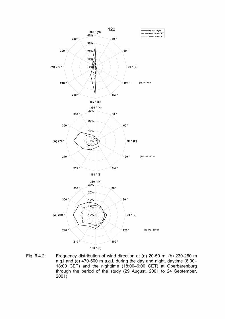
122

Fig. 6.4.2: Frequency distribution of wind direction at (a) 20-50 m, (b) 230-260 m

a.g.l and (c) 470-500 m a.g.l. during the day and night, daytime (6:00–18:00 CET) and the nighttime (18:00–6:00 CET) at Oberbärenburg through the period of the study (29 August, 2001 to 24 September, 2001)

0%

10%

20%

30%

40%360 ° (N)

30 °

60 °

90 ° (E)

120 °

150 °

180 ° (S)

210 °

240 °

(W) 270 °

300 °

330 °


(a) 20 - 50 m

0%

10%

20%

30%360 ° (N)

30 °

60 °

90 ° (E)

120 °

150 °

180 ° (S)

210 °

240 °

(W) 270 °

300 °

330 °

(b) 230 - 260 m

-10%

0%

10%

20%

30%360 ° (N)

30 °

60 °

90 ° (E)

120 °

150 °

180 ° (S)

210 °

240 °

(W) 270 °

300 °

330 °

(c) 470 - 500 m

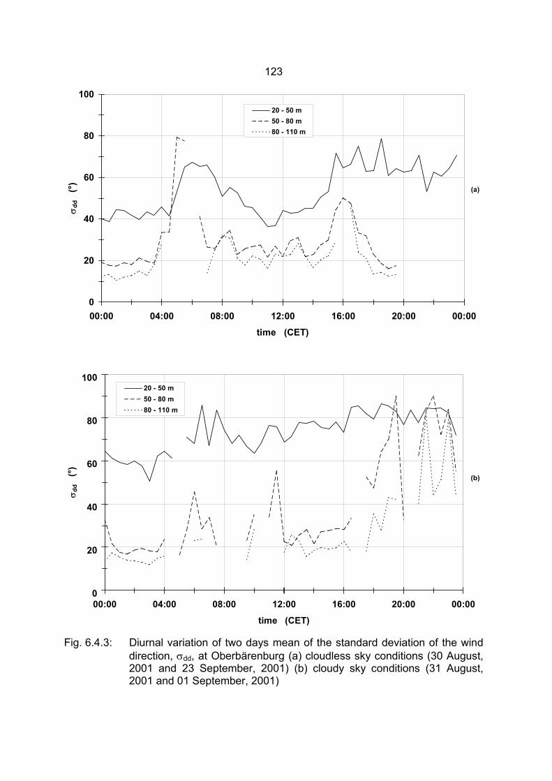
123

Fig. 6.4.3: Diurnal variation of two days mean of the standard deviation of the wind direction, σdd, at Oberbärenburg (a) cloudless sky conditions (30 August, 2001 and 23 September, 2001) (b) cloudy sky conditions (31 August, 2001 and 01 September, 2001)

0

20

40

60

80

100

00:00 04:00 08:00 12:00 16:00 20:00 00:00

time (CET)

σdd

(°

)

20 - 50 m50 - 80 m80 - 110 m

(a)

0

20

40

60

80

100

00:00 04:00 08:00 12:00 16:00 20:00 00:00

time (CET)

σdd

(°

)

20 - 50 m50 - 80 m80 - 110 m

(b)

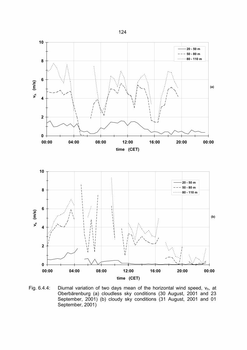
124

Fig. 6.4.4: Diurnal variation of two days mean of the horizontal wind speed, vh, at Oberbärenburg (a) cloudless sky conditions (30 August, 2001 and 23 September, 2001) (b) cloudy sky conditions (31 August, 2001 and 01 September, 2001)

0

2

4

6

8

10

00:00 04:00 08:00 12:00 16:00 20:00 00:00time (CET)

v h

(m/s

)

20 - 50 m50 - 80 m80 - 110 m

(a)

0

2

4

6

8

10

00:00 04:00 08:00 12:00 16:00 20:00 00:00

time (CET)

v h

(m/s

)

20 - 50 m50 - 80 m80 - 110 m

(b)

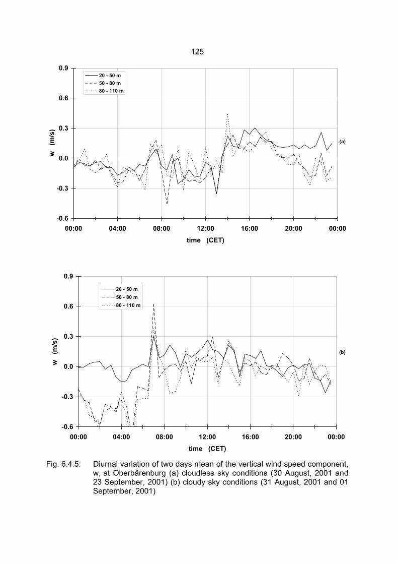
125

Fig. 6.4.5: Diurnal variation of two days mean of the vertical wind speed component, w, at Oberbärenburg (a) cloudless sky conditions (30 August, 2001 and 23 September, 2001) (b) cloudy sky conditions (31 August, 2001 and 01 September, 2001)

-0.6

-0.3

0.0

0.3

0.6

0.9

00:00 04:00 08:00 12:00 16:00 20:00 00:00

time (CET)

w

(m/s

)

20 - 50 m50 - 80 m80 - 110 m

(a)

-0.6

-0.3

0.0

0.3

0.6

0.9

00:00 04:00 08:00 12:00 16:00 20:00 00:00time (CET)

w

(m/s

)

20 - 50 m50 - 80 m80 - 110 m

(b)

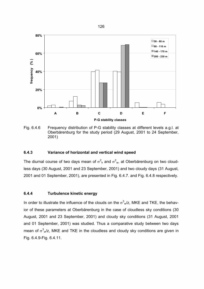
126

Fig. 6.4.6 Frequency distribution of P-G stability classes at different levels a.g.l. at Oberbärenburg for the study period (29 August, 2001 to 24 September, 2001)


The diurnal course of two days mean of σ2h and σ2

w, at Oberbärenburg on two cloud-

less days (30 August, 2001 and 23 September, 2001) and two cloudy days (31 August,

2001 and 01 September, 2001), are presented in Fig. 6.4.7. and Fig. 6.4.8 respectively.


In order to illustrate the influence of the clouds on the σ3w/z, MKE and TKE, the behav-

ior of these parameters at Oberbärenburg in the case of cloudless sky conditions (30

August, 2001 and 23 September, 2001) and cloudy sky conditions (31 August, 2001

and 01 September, 2001) was studied. Thus a comparative study between two days

mean of σ3w/z, MKE and TKE in the cloudless and cloudy sky conditions are given in

Fig. 6.4.9-Fig. 6.4.11.

0%

20%

40%

60%

80%

A B C D E F


freq

uenc

y (

% )

50 - 80 m

80 - 110 m

140 - 170 m

200 - 230 m

127



As indicated in sections 6.1.5.1, 6.2.5.1 and 6.3.5.1, the variations of the turbulence

intensity components, Iu, Iv and Iw, with the angular sectors were investigated under the

neutral conditions to illustrate the effect of the roughness in their values. Table 6.4.1

illustrates the mean, standard deviations and the observation number of the turbulence

intensity components, Iu, Iv and Iw, at different levels, 50-80 m, 80-110 m, 140-170 m,

200-230 m a.g.l. under the neutral conditions, grouped by the wind direction at Ober-

bärenburg through the period of the study (from 29 August, 2001 to 24 September,

2001). The mean values are summarized in Fig. 6.4.12.



stability classes at the angular sector 180-210° at different levels. The angular sector


approximately observed to be between 180° and 210° at these levels. Table 6.4.2 sum-

marizes the mean, standard deviations and the number of the observations of the tur-

bulence intensity components, Iu, Iv and Iw, at different levels, 50-80 m, 80-110 m, 140-

170 m, 200-230 m a.g.l. in Oberbärenburg during the period from 29 August, 2001 to

24 September, 2001. These data are grouped according to P-G stability classes for the

angular sector 180-210° and the mean values are illustrated in Fig. 6.4.13.


The dependence of the mean of the standard deviations of the velocity components

normalized by u∗, σi/u∗ (i=u,v,w), on the stability parameter (-z/L) under the unstable

conditions would be studied. Fig. 6.4.14 shows the behavior of σu/u∗, σv/u∗ and σw/u∗ as

a function of -z/L (0.28 < -z/L <8.31) under the unstable conditions at Oberbärenburg

128

during the period. from 29 August, 2001 to 24 September, 2001. However, this data

was collected within the surface layer (less than 110 m a.g.l.).

The shape of the variation of σu/u∗, σv/u∗ and σw/u∗ with the increasing of the instability

(-z/L) have the same variation of the Eq. (6.1), but the empirical constants ai and bi at

this site were found to be 2.6, 2.5 and 1.25, and 1.8, 3.5 and 4.1 for u, v and w compo-

nents respectively.

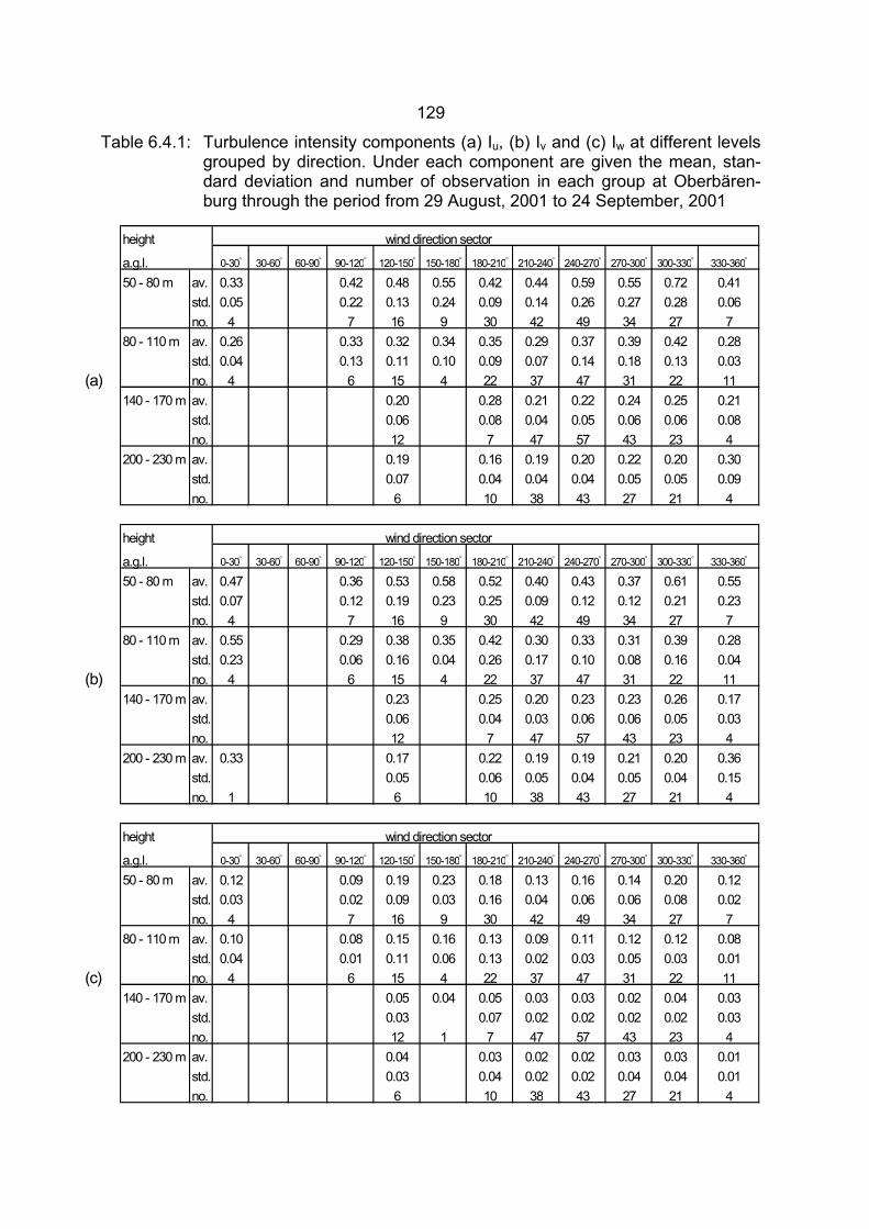
129

Table 6.4.1: Turbulence intensity components (a) Iu, (b) Iv and (c) Iw at different levels grouped by direction. Under each component are given the mean, stan-dard deviation and number of observation in each group at Oberbären-burg through the period from 29 August, 2001 to 24 September, 2001


a.g.l. 0-30° 30-60° 60-90° 90-120° 120-150° 150-180° 180-210° 210-240° 240-270° 270-300° 300-330° 330-360°

50 - 80 m av. 0.33 0.42 0.48 0.55 0.42 0.44 0.59 0.55 0.72 0.41std. 0.05 0.22 0.13 0.24 0.09 0.14 0.26 0.27 0.28 0.06no. 4 7 16 9 30 42 49 34 27 7

80 - 110 m av. 0.26 0.33 0.32 0.34 0.35 0.29 0.37 0.39 0.42 0.28std. 0.04 0.13 0.11 0.10 0.09 0.07 0.14 0.18 0.13 0.03

(a) no. 4 6 15 4 22 37 47 31 22 11140 - 170 m av. 0.20 0.28 0.21 0.22 0.24 0.25 0.21

std. 0.06 0.08 0.04 0.05 0.06 0.06 0.08no. 12 7 47 57 43 23 4

200 - 230 m av. 0.19 0.16 0.19 0.20 0.22 0.20 0.30std. 0.07 0.04 0.04 0.04 0.05 0.05 0.09no. 6 10 38 43 27 21 4


a.g.l. 0-30° 30-60° 60-90° 90-120° 120-150° 150-180° 180-210° 210-240° 240-270° 270-300° 300-330° 330-360°

50 - 80 m av. 0.47 0.36 0.53 0.58 0.52 0.40 0.43 0.37 0.61 0.55std. 0.07 0.12 0.19 0.23 0.25 0.09 0.12 0.12 0.21 0.23no. 4 7 16 9 30 42 49 34 27 7

80 - 110 m av. 0.55 0.29 0.38 0.35 0.42 0.30 0.33 0.31 0.39 0.28std. 0.23 0.06 0.16 0.04 0.26 0.17 0.10 0.08 0.16 0.04

(b) no. 4 6 15 4 22 37 47 31 22 11140 - 170 m av. 0.23 0.25 0.20 0.23 0.23 0.26 0.17

std. 0.06 0.04 0.03 0.06 0.06 0.05 0.03no. 12 7 47 57 43 23 4

200 - 230 m av. 0.33 0.17 0.22 0.19 0.19 0.21 0.20 0.36std. 0.05 0.06 0.05 0.04 0.05 0.04 0.15no. 1 6 10 38 43 27 21 4


a.g.l. 0-30° 30-60° 60-90° 90-120° 120-150° 150-180° 180-210° 210-240° 240-270° 270-300° 300-330° 330-360°

50 - 80 m av. 0.12 0.09 0.19 0.23 0.18 0.13 0.16 0.14 0.20 0.12std. 0.03 0.02 0.09 0.03 0.16 0.04 0.06 0.06 0.08 0.02no. 4 7 16 9 30 42 49 34 27 7

80 - 110 m av. 0.10 0.08 0.15 0.16 0.13 0.09 0.11 0.12 0.12 0.08std. 0.04 0.01 0.11 0.06 0.13 0.02 0.03 0.05 0.03 0.01

(c) no. 4 6 15 4 22 37 47 31 22 11140 - 170 m av. 0.05 0.04 0.05 0.03 0.03 0.02 0.04 0.03

std. 0.03 0.07 0.02 0.02 0.02 0.02 0.03no. 12 1 7 47 57 43 23 4

200 - 230 m av. 0.04 0.03 0.02 0.02 0.03 0.03 0.01std. 0.03 0.04 0.02 0.02 0.04 0.04 0.01no. 6 10 38 43 27 21 4

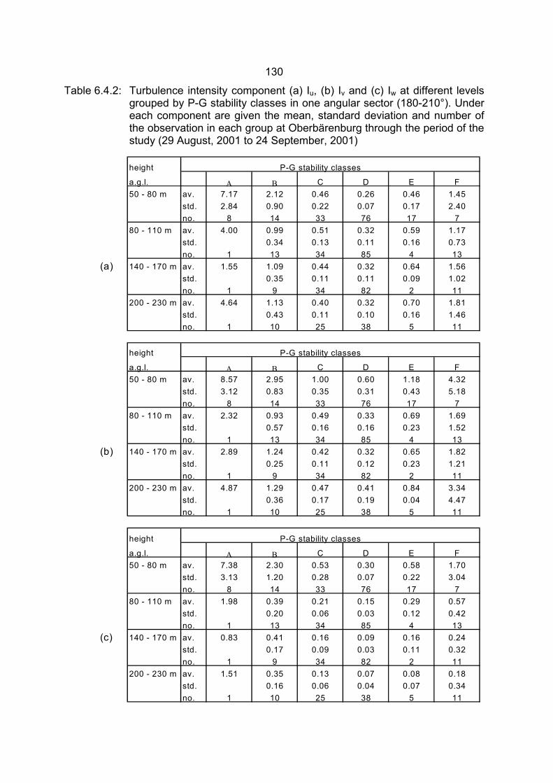
130

Table 6.4.2: Turbulence intensity component (a) Iu, (b) Iv and (c) Iw at different levels grouped by P-G stability classes in one angular sector (180-210°). Under each component are given the mean, standard deviation and number of the observation in each group at Oberbärenburg through the period of the study (29 August, 2001 to 24 September, 2001)


a.g.l. Α Β C D E F50 - 80 m av. 7.17 2.12 0.46 0.26 0.46 1.45

std. 2.84 0.90 0.22 0.07 0.17 2.40no. 8 14 33 76 17 7

80 - 110 m av. 4.00 0.99 0.51 0.32 0.59 1.17std. 0.34 0.13 0.11 0.16 0.73no. 1 13 34 85 4 13

(a) 140 - 170 m av. 1.55 1.09 0.44 0.32 0.64 1.56std. 0.35 0.11 0.11 0.09 1.02no. 1 9 34 82 2 11

200 - 230 m av. 4.64 1.13 0.40 0.32 0.70 1.81std. 0.43 0.11 0.10 0.16 1.46no. 1 10 25 38 5 11


a.g.l. Α Β C D E F50 - 80 m av. 8.57 2.95 1.00 0.60 1.18 4.32

std. 3.12 0.83 0.35 0.31 0.43 5.18no. 8 14 33 76 17 7

80 - 110 m av. 2.32 0.93 0.49 0.33 0.69 1.69std. 0.57 0.16 0.16 0.23 1.52no. 1 13 34 85 4 13

(b) 140 - 170 m av. 2.89 1.24 0.42 0.32 0.65 1.82std. 0.25 0.11 0.12 0.23 1.21no. 1 9 34 82 2 11

200 - 230 m av. 4.87 1.29 0.47 0.41 0.84 3.34std. 0.36 0.17 0.19 0.04 4.47no. 1 10 25 38 5 11


a.g.l. Α Β C D E F50 - 80 m av. 7.38 2.30 0.53 0.30 0.58 1.70

std. 3.13 1.20 0.28 0.07 0.22 3.04no. 8 14 33 76 17 7

80 - 110 m av. 1.98 0.39 0.21 0.15 0.29 0.57std. 0.20 0.06 0.03 0.12 0.42no. 1 13 34 85 4 13

(c) 140 - 170 m av. 0.83 0.41 0.16 0.09 0.16 0.24std. 0.17 0.09 0.03 0.11 0.32no. 1 9 34 82 2 11

200 - 230 m av. 1.51 0.35 0.13 0.07 0.08 0.18std. 0.16 0.06 0.04 0.07 0.34no. 1 10 25 38 5 11

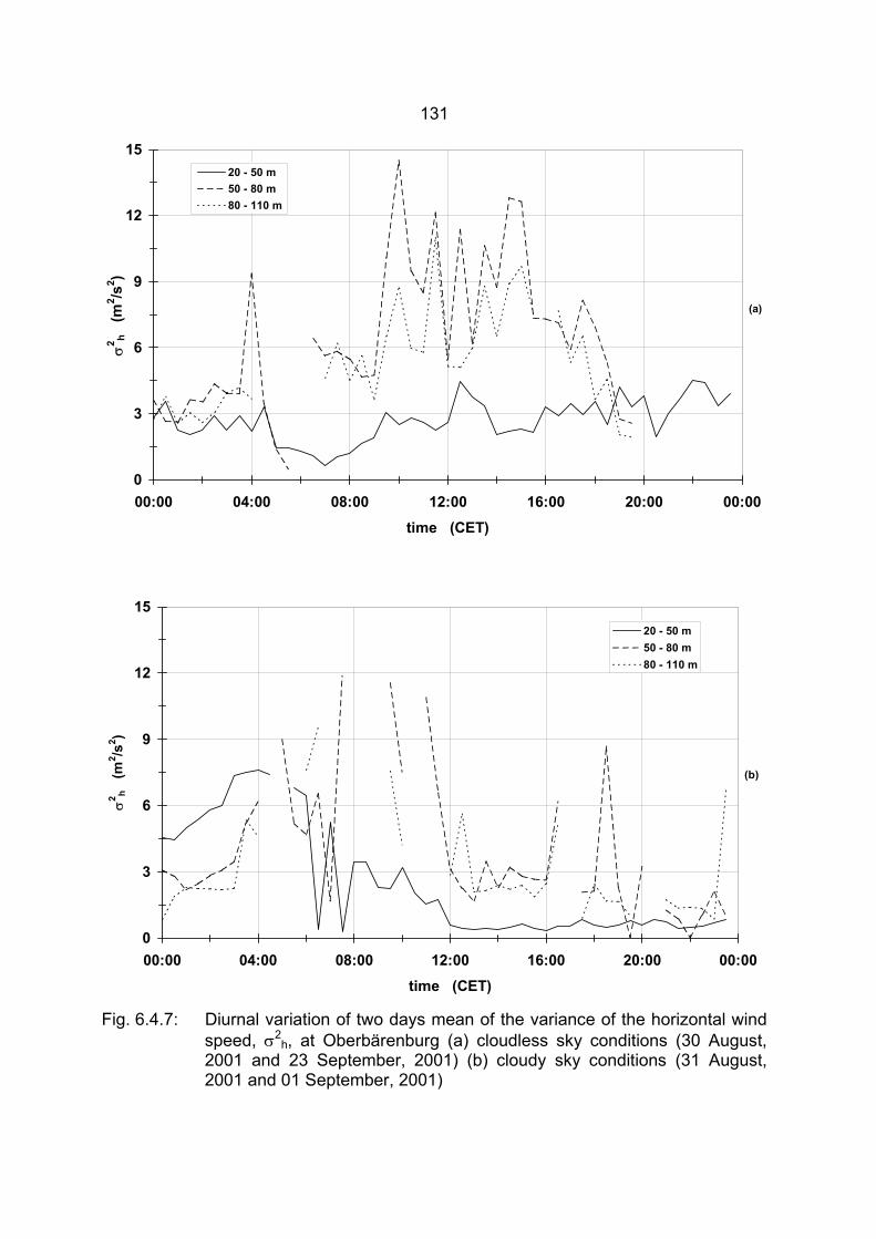
131


h, at Oberbärenburg (a) cloudless sky conditions (30 August, 2001 and 23 September, 2001) (b) cloudy sky conditions (31 August, 2001 and 01 September, 2001)

0

3

6

9

12

15

00:00 04:00 08:00 12:00 16:00 20:00 00:00

time (CET)

σ2 h

(m2 /s

2 )

20 - 50 m50 - 80 m80 - 110 m

(a)

0

3

6

9

12

15

00:00 04:00 08:00 12:00 16:00 20:00 00:00time (CET)

σ2 h

(m2 /s

2 )

20 - 50 m50 - 80 m80 - 110 m

(b)

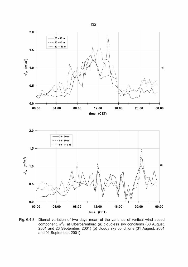
132


w, at Oberbärenburg (a) cloudless sky conditions (30 August, 2001 and 23 September, 2001) (b) cloudy sky conditions (31 August, 2001 and 01 September, 2001)

0.0

0.5

1.0

1.5

2.0

00:00 04:00 08:00 12:00 16:00 20:00 00:00

time (CET)

σ2 w

(m

2 /s2 )

20 - 50 m50 - 80 m80 - 110 m

(b)

0.0

0.5

1.0

1.5

2.0

00:00 04:00 08:00 12:00 16:00 20:00 00:00time (CET)

σ2 w

(m2 /s

2 )

20 - 50 m

50 - 80 m

80 - 110 m

(a)

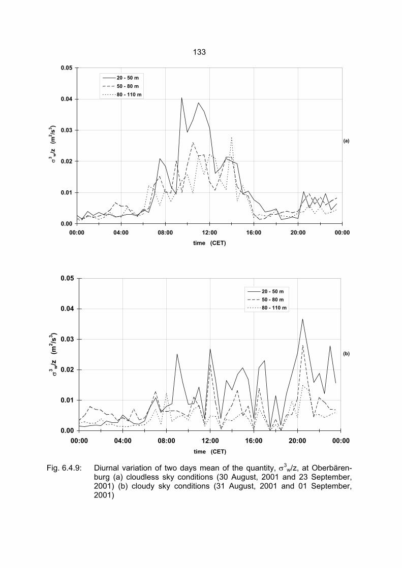
133

Fig. 6.4.9: Diurnal variation of two days mean of the quantity, σ3w/z, at Oberbären-

burg (a) cloudless sky conditions (30 August, 2001 and 23 September, 2001) (b) cloudy sky conditions (31 August, 2001 and 01 September, 2001)

0.00

0.01

0.02

0.03

0.04

0.05

00:00 04:00 08:00 12:00 16:00 20:00 00:00

time (CET)

σ3 w

/z

(m2 /s

3 )

20 - 50 m50 - 80 m80 - 110 m

(a)

0.00

0.01

0.02

0.03

0.04

0.05

00:00 04:00 08:00 12:00 16:00 20:00 00:00time (CET)

σ3 w

/z

(m2 /s

3 )

20 - 50 m50 - 80 m80 - 110 m

(b)

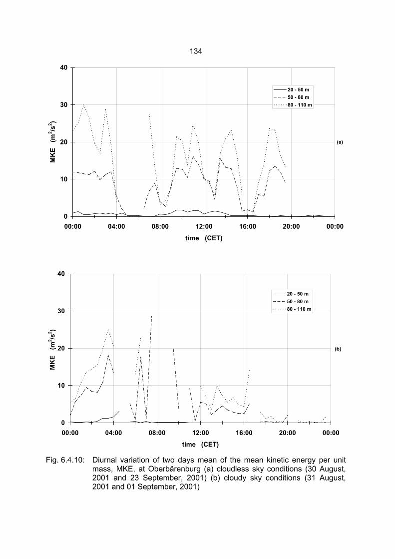
134

Fig. 6.4.10: Diurnal variation of two days mean of the mean kinetic energy per unit mass, MKE, at Oberbärenburg (a) cloudless sky conditions (30 August, 2001 and 23 September, 2001) (b) cloudy sky conditions (31 August, 2001 and 01 September, 2001)

0

10

20

30

40

00:00 04:00 08:00 12:00 16:00 20:00 00:00

time (CET)

MK

E (

m2 /s

2 )

20 - 50 m50 - 80 m80 - 110 m

(a)

0

10

20

30

40

00:00 04:00 08:00 12:00 16:00 20:00 00:00

time (CET)

MK

E (

m2 /s

2 )

20 - 50 m50 - 80 m80 - 110 m

(b)

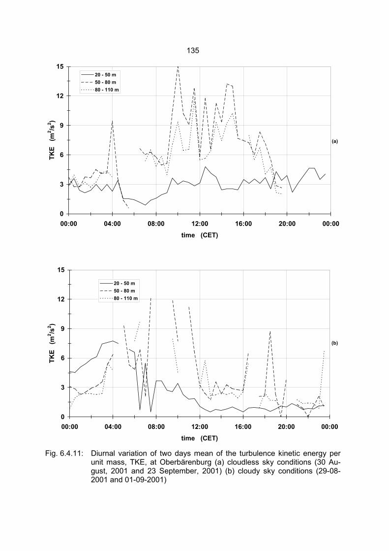
135

Fig. 6.4.11: Diurnal variation of two days mean of the turbulence kinetic energy per unit mass, TKE, at Oberbärenburg (a) cloudless sky conditions (30 Au-gust, 2001 and 23 September, 2001) (b) cloudy sky conditions (29-08-2001 and 01-09-2001)

0

3

6

9

12

15

00:00 04:00 08:00 12:00 16:00 20:00 00:00time (CET)

TKE

(m

2 /s2 )

20 - 50 m50 - 80 m80 - 110 m

(a)

0

3

6

9

12

15

00:00 04:00 08:00 12:00 16:00 20:00 00:00

time (CET)

TKE

(m

2 /s2 )

20 - 50 m50 - 80 m80 - 110 m

(b)

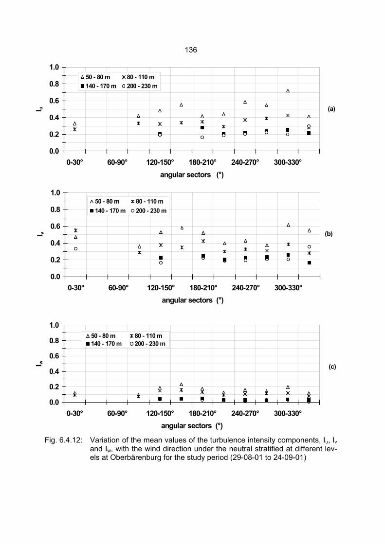
136

Fig. 6.4.12: Variation of the mean values of the turbulence intensity components, Iu, Iv and Iw, with the wind direction under the neutral stratified at different lev-els at Oberbärenburg for the study period (29-08-01 to 24-09-01)

0.0

0.2

0.4

0.6

0.8

1.0

0-30° 60-90° 120-150° 180-210° 240-270° 300-330°angular sectors (°)

I u

50 - 80 m 80 - 110 m 140 - 170 m 200 - 230 m

(a)

0.0

0.2

0.4

0.6

0.8

1.0

0-30° 60-90° 120-150° 180-210° 240-270° 300-330°angular sectors (°)

I v

50 - 80 m 80 - 110 m 140 - 170 m 200 - 230 m

(b)

0.0

0.2

0.4

0.6

0.8

1.0

0-30° 60-90° 120-150° 180-210° 240-270° 300-330°angular sectors (°)

I w

50 - 80 m 80 - 110 m 140 - 170 m 200 - 230 m

(c)

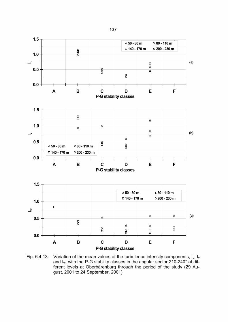
137

Fig. 6.4.13: Variation of the mean values of the turbulence intensity components, Iu, Iv and Iw, with the P-G stability classes in the angular sector 210-240° at dif-ferent levels at Oberbärenburg through the period of the study (29 Au-gust, 2001 to 24 September, 2001)

0.0

0.5

1.0

1.5


I u

50 - 80 m 80 - 110 m 140 - 170 m 200 - 230 m

(a)

0.0

0.5

1.0

1.5


I v

50 - 80 m 80 - 110 m 140 - 170 m 200 - 230 m

(b)

0.0

0.5

1.0

1.5


I w

50 - 80 m 80 - 110 m 140 - 170 m 200 - 230 m

(c)

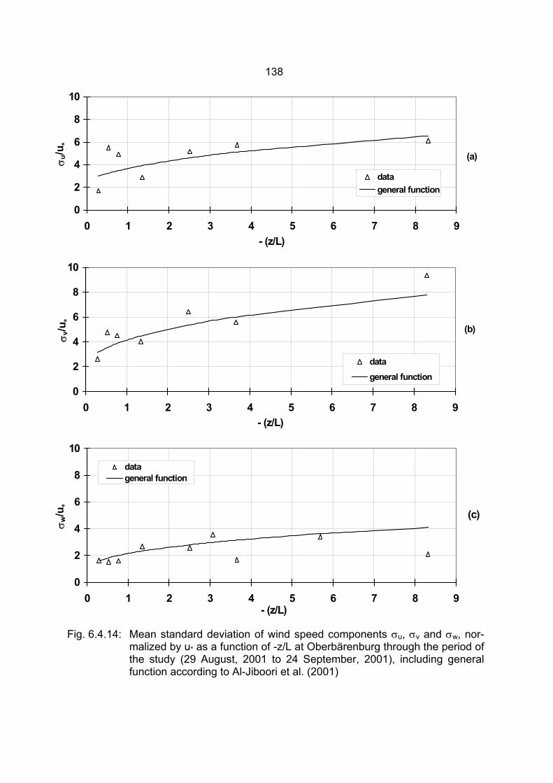
138

Fig. 6.4.14: Mean standard deviation of wind speed components σu, σv and σw, nor-malized by u* as a function of -z/L at Oberbärenburg through the period of the study (29 August, 2001 to 24 September, 2001), including general function according to Al-Jiboori et al. (2001)

0

2

4

6

8

10

0 1 2 3 4 5 6 7 8 9- (z/L)

σ u/u

∗


(a)

0

2

4

6

8

10

0 1 2 3 4 5 6 7 8 9- (z/L)

σ v/u

∗


(b)

0

2

4

6

8

10

0 1 2 3 4 5 6 7 8 9- (z/L)

σ w/u

∗


(c)

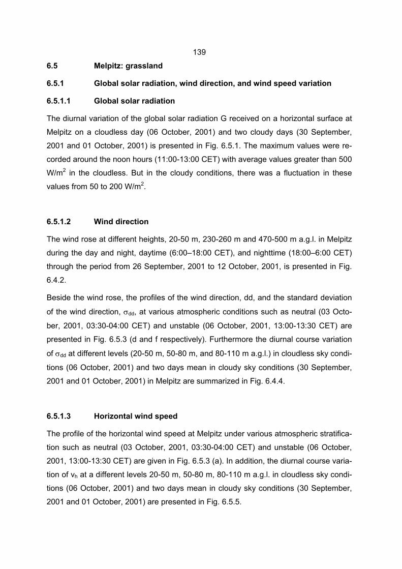
139

6.5 Melpitz: grassland




Melpitz on a cloudless day (06 October, 2001) and two cloudy days (30 September,

2001 and 01 October, 2001) is presented in Fig. 6.5.1. The maximum values were re-

corded around the noon hours (11:00-13:00 CET) with average values greater than 500

W/m2 in the cloudless. But in the cloudy conditions, there was a fluctuation in these

values from 50 to 200 W/m2.


The wind rose at different heights, 20-50 m, 230-260 m and 470-500 m a.g.l. in Melpitz

during the day and night, daytime (6:00–18:00 CET), and nighttime (18:00–6:00 CET)

through the period from 26 September, 2001 to 12 October, 2001, is presented in Fig.

6.4.2.

Beside the wind rose, the profiles of the wind direction, dd, and the standard deviation

of the wind direction, σdd, at various atmospheric conditions such as neutral (03 Octo-

ber, 2001, 03:30-04:00 CET) and unstable (06 October, 2001, 13:00-13:30 CET) are

presented in Fig. 6.5.3 (d and f respectively). Furthermore the diurnal course variation

of σdd at different levels (20-50 m, 50-80 m, and 80-110 m a.g.l.) in cloudless sky condi-

tions (06 October, 2001) and two days mean in cloudy sky conditions (30 September,

2001 and 01 October, 2001) in Melpitz are summarized in Fig. 6.4.4.


The profile of the horizontal wind speed at Melpitz under various atmospheric stratifica-

tion such as neutral (03 October, 2001, 03:30-04:00 CET) and unstable (06 October,

2001, 13:00-13:30 CET) are given in Fig. 6.5.3 (a). In addition, the diurnal course varia-

tion of vh at a different levels 20-50 m, 50-80 m, 80-110 m a.g.l. in cloudless sky condi-

tions (06 October, 2001) and two days mean in cloudy sky conditions (30 September,

2001 and 01 October, 2001) are presented in Fig. 6.5.5.

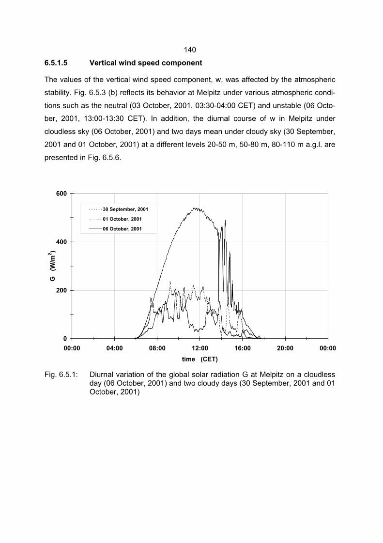
140


The values of the vertical wind speed component, w, was affected by the atmospheric

stability. Fig. 6.5.3 (b) reflects its behavior at Melpitz under various atmospheric condi-

tions such as the neutral (03 October, 2001, 03:30-04:00 CET) and unstable (06 Octo-

ber, 2001, 13:00-13:30 CET). In addition, the diurnal course of w in Melpitz under

cloudless sky (06 October, 2001) and two days mean under cloudy sky (30 September,

2001 and 01 October, 2001) at a different levels 20-50 m, 50-80 m, 80-110 m a.g.l. are

presented in Fig. 6.5.6.

Fig. 6.5.1: Diurnal variation of the global solar radiation G at Melpitz on a cloudless day (06 October, 2001) and two cloudy days (30 September, 2001 and 01 October, 2001)

0

200

400

600

00:00 04:00 08:00 12:00 16:00 20:00 00:00time (CET)

G

(W/m

2 )

30 September, 2001

01 October, 2001

06 October, 2001

141

Fig. 6.5.2: Frequency distribution of wind direction at (a) 20-50 m, (b) 230-260 m and

m, (c) 470-500 m a.g.l. during the day and night, daytime (6:00–18:00 CET) and the nighttime (18:00–6:00 CET) at Melpitz through the period of the study (26 September, 2001 to 12 October, 2001)

0%

10%

20%

30%360 ° (N)

30 °

60 °

90 ° (E)

120 °

150 °

180 ° (S)

210 °

240 °

(W) 270 °

300 °

330 °


(a) 20 - 50 m

0%

10%

20%

30%

40%360 ° (N)

30 °

60 °

90 ° (E)

120 °

150 °

180 ° (S)

210 °

240 °

(W) 270 °

300 °

330 °

(b) 230 - 260 m

-10%

0%

10%

20%

30%360 ° (N)

30 °

60 °

90 ° (E)

120 °

150 °

180 ° (S)

210 °

240 °

(W) 270 °

300 °

330 °

(c) 470 - 500 m

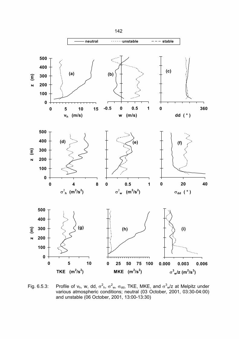
142


w, σdd, TKE, MKE, and σ3w/z at Melpitz under

various atmospheric conditions; neutral (03 October, 2001, 03:30-04:00) and unstable (06 October, 2001, 13:00-13:30)

vh (m/s) w (m/s) dd ( ° )

σ2h (m2/s2) σ2

w (m2/s2) σdd ( ° )


(a)

0

100

200

300

400

500

0 5 10 15

z (

m) (b)

-0.5 0 0.5 1

(c)

0 360

(d)

0

100

200

300

400

500

0 4 8

z (

m)

(e)

0 0.5 1

(f)

0 20 40

(g)

0

100

200

300

400

500

0 5 10

z (

m) (h)

0 25 50 75 100

(i)

0.000 0.003 0.006

neutral unstable stable

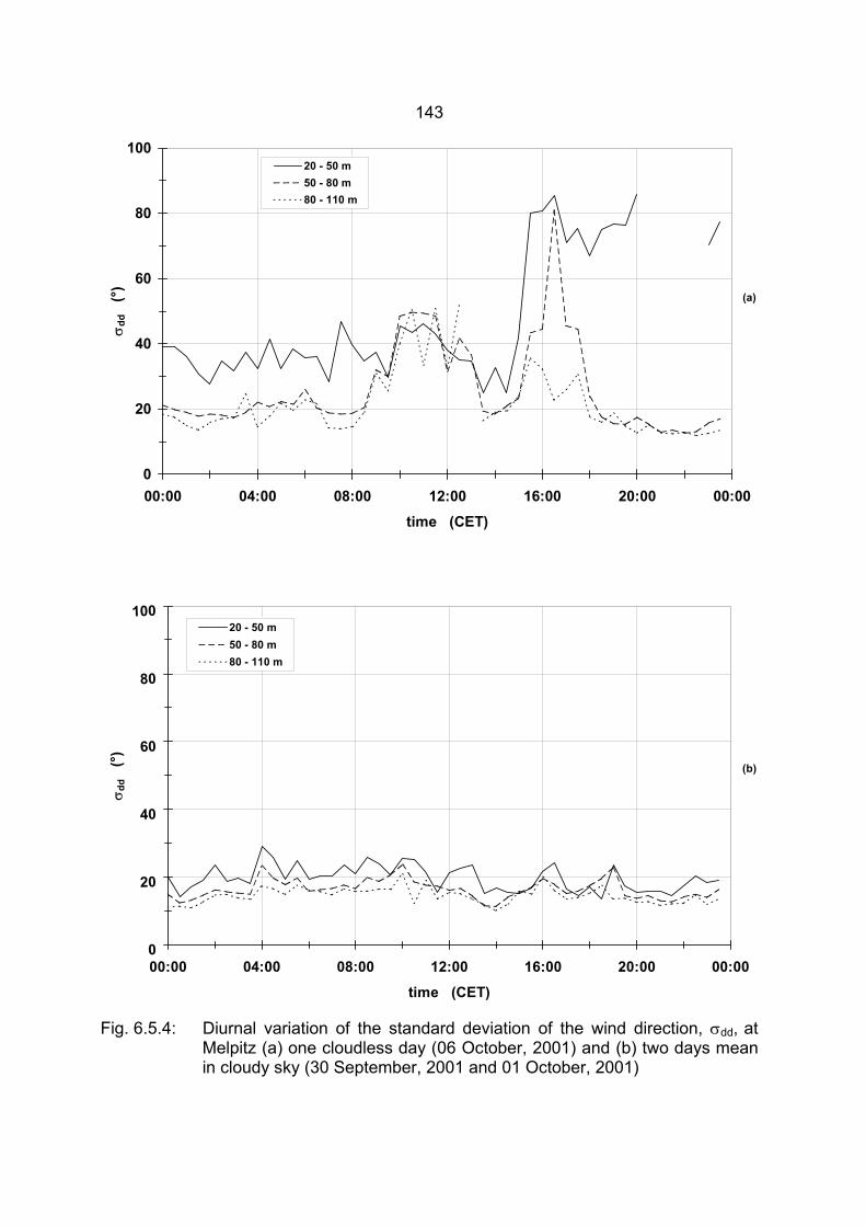
143

Fig. 6.5.4: Diurnal variation of the standard deviation of the wind direction, σdd, at Melpitz (a) one cloudless day (06 October, 2001) and (b) two days mean in cloudy sky (30 September, 2001 and 01 October, 2001)

0

20

40

60

80

100

00:00 04:00 08:00 12:00 16:00 20:00 00:00

time (CET)

σdd

(°

)

20 - 50 m50 - 80 m80 - 110 m

(a)

0

20

40

60

80

100

00:00 04:00 08:00 12:00 16:00 20:00 00:00

time (CET)

σdd

(°

)

20 - 50 m50 - 80 m80 - 110 m

(b)

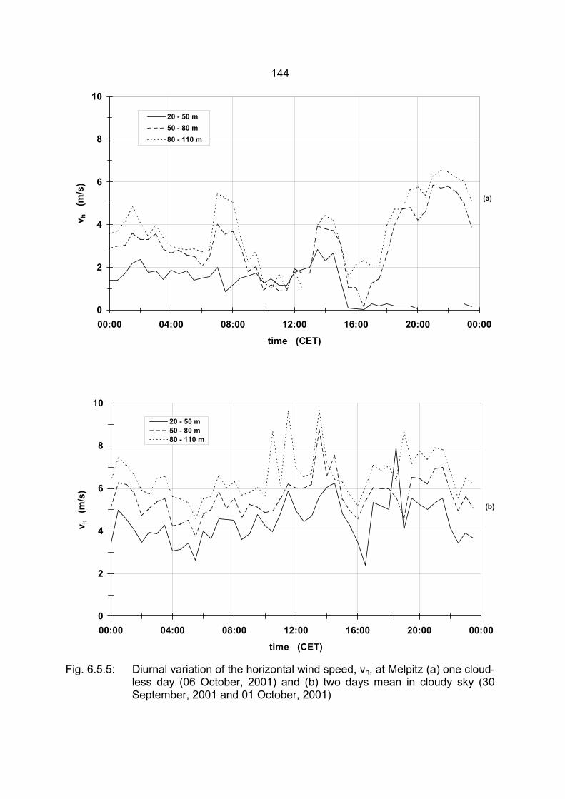
144

Fig. 6.5.5: Diurnal variation of the horizontal wind speed, vh, at Melpitz (a) one cloud-less day (06 October, 2001) and (b) two days mean in cloudy sky (30 September, 2001 and 01 October, 2001)

0

2

4

6

8

10

00:00 04:00 08:00 12:00 16:00 20:00 00:00time (CET)

v h

(m/s

)

20 - 50 m50 - 80 m80 - 110 m

(a)

0

2

4

6

8

10

00:00 04:00 08:00 12:00 16:00 20:00 00:00

time (CET)

v h

(m/s

)

20 - 50 m50 - 80 m80 - 110 m

(b)

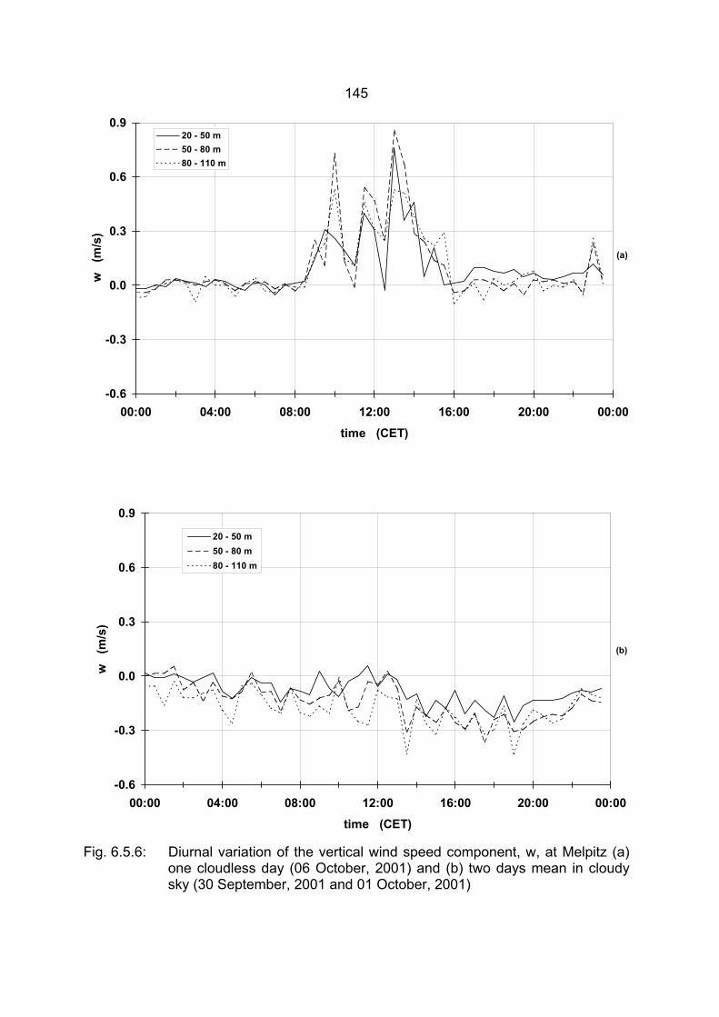
145

Fig. 6.5.6: Diurnal variation of the vertical wind speed component, w, at Melpitz (a) one cloudless day (06 October, 2001) and (b) two days mean in cloudy sky (30 September, 2001 and 01 October, 2001)

-0.6

-0.3

0.0

0.3

0.6

0.9

00:00 04:00 08:00 12:00 16:00 20:00 00:00

time (CET)

w

(m/s

)

20 - 50 m50 - 80 m80 - 110 m

(a)

-0.6

-0.3

0.0

0.3

0.6

0.9

00:00 04:00 08:00 12:00 16:00 20:00 00:00time (CET)

w

(m/s

)

20 - 50 m50 - 80 m80 - 110 m

(b)

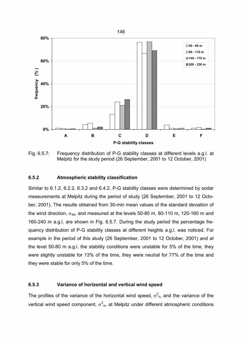
146

Fig. 6.5.7: Frequency distribution of P-G stability classes at different levels a.g.l. at Melpitz for the study period (26 September, 2001 to 12 October, 2001)


Similar to 6.1.2, 6.2.2, 6.3.2 and 6.4.2, P-G stability classes were determined by sodar

measurements at Melpitz during the period of study (26 September, 2001 to 12 Octo-

ber, 2001). The results obtained from 30-min mean values of the standard deviation of

the wind direction, σdd, and measured at the levels 50-80 m, 80-110 m, 120-160 m and

160-240 m a.g.l. are shown in Fig. 6.5.7. During the study period the percentage fre-

quency distribution of P-G stability classes at different heights a.g.l. was noticed. For

example in the period of this study (26 September, 2001 to 12 October, 2001) and at

the level 50-80 m a.g.l. the stability conditions were unstable for 5% of the time, they

were slightly unstable for 13% of the time, they were neutral for 77% of the time and

they were stable for only 5% of the time.


The profiles of the variance of the horizontal wind speed, σ2h, and the variance of the

vertical wind speed component, σ2w, at Melpitz under different atmospheric conditions

0%

20%

40%

60%

80%


freq

uenc

y (

% )

50 - 80 m

80 - 110 m

140 - 170 m

200 - 230 m

147

such as the neutral (03 October, 2001, 03:30-04:00 CET) and unstable (06 October,

2001, 13:00-13:30 CET) are given in Fig. 6.5.3 (d and e respectively).

In addition, the diurnal course variation of σh and σw at different levels (20-50 m, 50-80

m, and 80-110 m a.g.l.) in cloudless sky conditions (06 October, 2001) and two days

mean in cloudy sky conditions (30 September, 2001 and 01 October, 2001) are pre-

sented in Fig. 6.5.8. and Fig. 6.5.9 respectively.


The behavior of the profiles of σ3w/z, MKE and TKE at Melpitz under various atmos-

pheric conditions such as neutral (03 October, 2001, 03:30-04:00 CET) and unstable

(06 October, 2001, 13:00-13:30 CET) is presented in Fig. 6.5.3 (g-i).

Moreover a comparative study between the values of σ3w/z, MKE and TKE at different

levels, 20-50 m, 50-80 m, 80-110 m a.g.l in Melpitz for cloudless (06 October, 2001)

and a two days means in cloudy sky conditions (30 September, 2001 and 01 October,

2001) are given in Fig. 6.5.10 - Fig. 6.5.12.



In line with the sections 6.1.5.1, 6.2.5.1, 6.3.5.1 and 6.4.5.1, the effect of the roughness

in the nature of the turbulence intensity components, Iu, Iv and Iw, might be shown by

the study of the intensity components, Iu, Iv and Iw, at different angular sectors under

the neutral conditions over Melpitz during the period of the study (26 September, 2001

to 12 October, 2001).

Table 6.5.1 gives the mean, standard deviations and the observation number of the

turbulence intensity components, Iu, Iv and Iw, at different levels (50-80 m, 80-110 m,

120-160 m, and 160-240 m a.g.l.) under the neutral conditions, grouped by wind direc-

tion. But the mean values are summarized in Fig. 6.5.13.

148



stability classes for the angular sectors 210-240° at different levels. The angular sector


approximately observed to be between 210 and 240°. Table 6.5.2 summarizes the

mean and standard deviations of the turbulence intensity components Iu, Iv and Iw at

different levels (50-80 m, 80-110 m, 120-160 m, 160-240 m a.g.l.) grouped according to

P-G stability classes for the angular sector 210-240°. The mean values are illustrated in

Fig. 6.5.14.

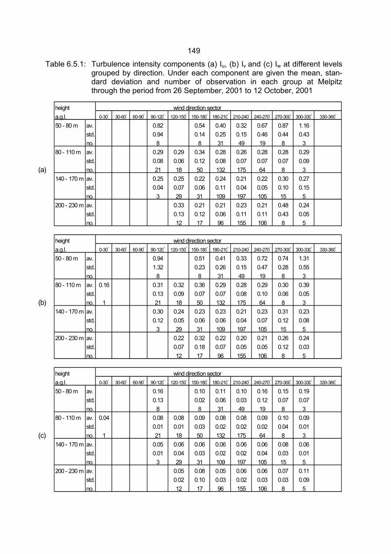
149

Table 6.5.1: Turbulence intensity components (a) Iu, (b) Iv and (c) Iw at different levels grouped by direction. Under each component are given the mean, stan-dard deviation and number of observation in each group at Melpitz through the period from 26 September, 2001 to 12 October, 2001


50 - 80 m av. 0.82 0.54 0.40 0.32 0.67 0.87 1.16std. 0.94 0.14 0.25 0.15 0.46 0.44 0.43no. 8 8 31 49 19 8 3

80 - 110 m av. 0.29 0.29 0.34 0.28 0.26 0.28 0.28 0.29std. 0.08 0.06 0.12 0.08 0.07 0.07 0.07 0.09

(a) no. 21 18 50 132 175 64 8 3140 - 170 m av. 0.25 0.25 0.22 0.24 0.21 0.22 0.30 0.27

std. 0.04 0.07 0.06 0.11 0.04 0.05 0.10 0.15no. 3 29 31 109 197 105 15 5

200 - 230 m av. 0.33 0.21 0.21 0.23 0.21 0.48 0.24std. 0.13 0.12 0.06 0.11 0.11 0.43 0.05no. 12 17 96 155 106 8 5


50 - 80 m av. 0.94 0.51 0.41 0.33 0.72 0.74 1.31std. 1.32 0.23 0.26 0.15 0.47 0.28 0.55no. 8 8 31 49 19 8 3

80 - 110 m av. 0.16 0.31 0.32 0.36 0.29 0.28 0.29 0.30 0.39std. 0.13 0.09 0.07 0.07 0.08 0.10 0.06 0.05

(b) no. 1 21 18 50 132 175 64 8 3140 - 170 m av. 0.30 0.24 0.23 0.23 0.21 0.23 0.31 0.23

std. 0.12 0.05 0.06 0.06 0.04 0.07 0.12 0.08no. 3 29 31 109 197 105 15 5

200 - 230 m av. 0.22 0.32 0.22 0.20 0.21 0.26 0.24std. 0.07 0.18 0.07 0.05 0.05 0.12 0.03no. 12 17 96 155 106 8 5


50 - 80 m av. 0.16 0.10 0.11 0.10 0.16 0.15 0.19std. 0.13 0.02 0.06 0.03 0.12 0.07 0.07no. 8 8 31 49 19 8 3

80 - 110 m av. 0.04 0.08 0.08 0.09 0.08 0.08 0.09 0.10 0.09std. 0.01 0.01 0.03 0.02 0.02 0.02 0.04 0.01

(c) no. 1 21 18 50 132 175 64 8 3140 - 170 m av. 0.05 0.06 0.06 0.06 0.06 0.06 0.08 0.06

std. 0.01 0.04 0.03 0.02 0.02 0.04 0.03 0.01no. 3 29 31 109 197 105 15 5

200 - 230 m av. 0.05 0.08 0.05 0.06 0.06 0.07 0.11std. 0.02 0.10 0.03 0.02 0.03 0.03 0.09no. 12 17 96 155 106 8 5

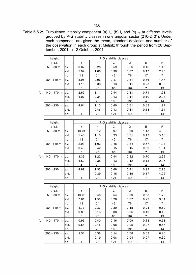
150

Table 6.5.2: Turbulence intensity component (a) Iu, (b) Iv and (c) Iw at different levels grouped by P-G stability classes in one angular sector (210-240°). Under each component are given the mean, standard deviation and number of the observation in each group at Melpitz through the period from 26 Sep-tember, 2001 to 12 October, 2001

height P-G stability classesa.g.l. Α Β C D E F

50 - 80 m av. 8.82 2.25 0.59 0.26 0.46 1.45std. 5.92 1.06 0.30 0.07 0.17 2.40no. 13 24 45 76 17 7

80 - 110 m av. 3.05 0.96 0.47 0.31 0.56 1.47std. 1.15 0.36 0.13 0.11 0.23 0.83no. 6 40 93 169 7 19

(a) 140 - 170 m av. 2.69 1.11 0.44 0.31 0.71 1.98std. 1.07 0.31 0.13 0.11 0.10 2.05no. 5 20 106 195 4 14

200 - 230 m av. 4.64 1.13 0.40 0.31 0.69 1.77std. 0.46 0.13 0.11 0.13 1.34no. 1 23 121 141 7 14


50 - 80 m av. 10.01 3.12 0.97 0.60 1.18 4.32std. 5.45 1.10 0.33 0.31 0.43 5.18no. 13 24 45 76 17 7

80 - 110 m av. 2.93 1.02 0.48 0.34 0.77 1.94std. 0.48 0.42 0.15 0.15 0.50 1.34no. 6 40 93 169 7 19

(b) 140 - 170 m av. 3.39 1.22 0.44 0.32 0.70 2.32std. 1.52 0.38 0.13 0.12 0.15 2.35no. 4 20 106 195 4 14

200 - 230 m av. 4.87 1.32 0.48 0.41 0.93 2.93std. 0.39 0.16 0.19 0.17 4.02no. 1 23 121 141 7 14


50 - 80 m av. 10.05 2.48 0.54 0.30 0.58 1.70std. 7.61 1.50 0.28 0.07 0.22 3.04no. 13 24 45 76 17 7

80 - 110 m av. 1.73 0.37 0.20 0.15 0.24 0.59std. 0.89 0.16 0.08 0.06 0.10 0.40no. 6 40 93 169 7 19

(c) 140 - 170 m av. 0.93 0.40 0.16 0.09 0.18 0.33std. 0.54 0.15 0.08 0.05 0.07 0.47no. 5 20 106 195 4 14

200 - 230 m av. 1.51 0.38 0.14 0.08 0.09 0.20std. 0.19 0.08 0.04 0.07 0.30no. 1 23 121 141 7 14

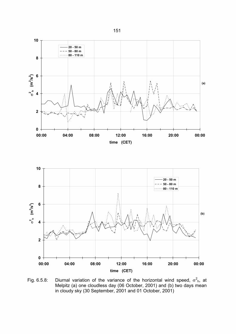
151

Fig. 6.5.8: Diurnal variation of the variance of the horizontal wind speed, σ2h, at

Melpitz (a) one cloudless day (06 October, 2001) and (b) two days mean in cloudy sky (30 September, 2001 and 01 October, 2001)

0

2

4

6

8

10

00:00 04:00 08:00 12:00 16:00 20:00 00:00

time (CET)

σ2 h

(m2 /s

2 )

20 - 50 m50 - 80 m80 - 110 m

(a)

0

2

4

6

8

10

00:00 04:00 08:00 12:00 16:00 20:00 00:00time (CET)

σ2 h

(m2 /s

2 )

20 - 50 m50 - 80 m80 - 110 m

(b)

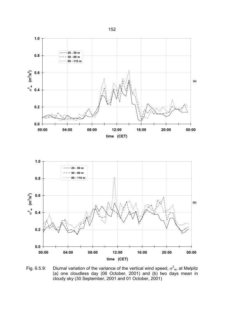
152

Fig. 6.5.9: Diurnal variation of the variance of the vertical wind speed, σ2w, at Melpitz

(a) one cloudless day (06 October, 2001) and (b) two days mean in cloudy sky (30 September, 2001 and 01 October, 2001)

0.0

0.2

0.4

0.6

0.8

1.0

00:00 04:00 08:00 12:00 16:00 20:00 00:00

time (CET)

σ2 w

(m

2 /s2 )

20 - 50 m50 - 80 m80 - 110 m

(b)

0.0

0.2

0.4

0.6

0.8

1.0

00:00 04:00 08:00 12:00 16:00 20:00 00:00time (CET)

σ2 w

(m2 /s

2 )

20 - 50 m50 - 80 m80 - 110 m

(a)

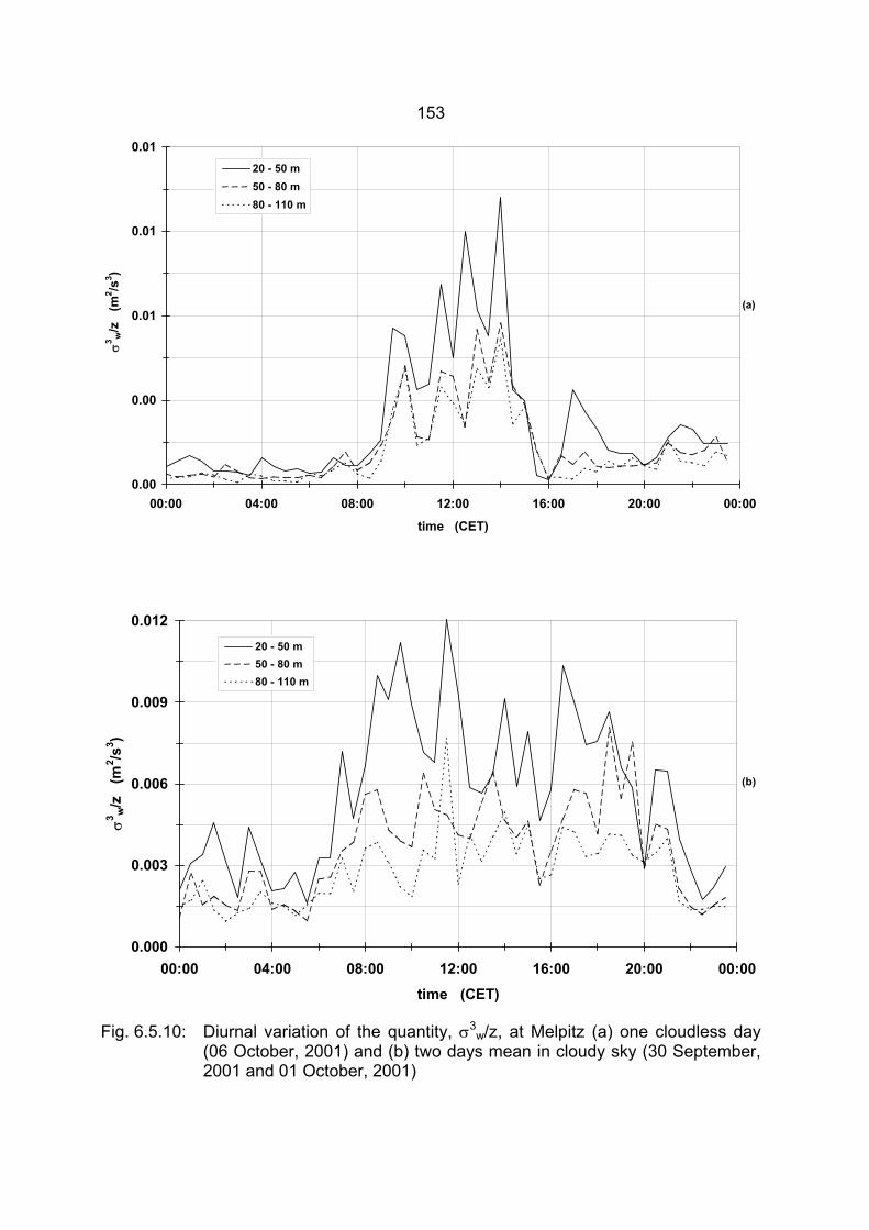
153

Fig. 6.5.10: Diurnal variation of the quantity, σ3w/z, at Melpitz (a) one cloudless day

(06 October, 2001) and (b) two days mean in cloudy sky (30 September, 2001 and 01 October, 2001)

0.00

0.00

0.01

0.01

0.01

00:00 04:00 08:00 12:00 16:00 20:00 00:00

time (CET)

σ3 w

/z

(m2 /s

3 )

20 - 50 m50 - 80 m80 - 110 m

(a)

0.000

0.003

0.006

0.009

0.012

00:00 04:00 08:00 12:00 16:00 20:00 00:00time (CET)

σ3 w

/z

(m2 /s

3 )

20 - 50 m50 - 80 m80 - 110 m

(b)

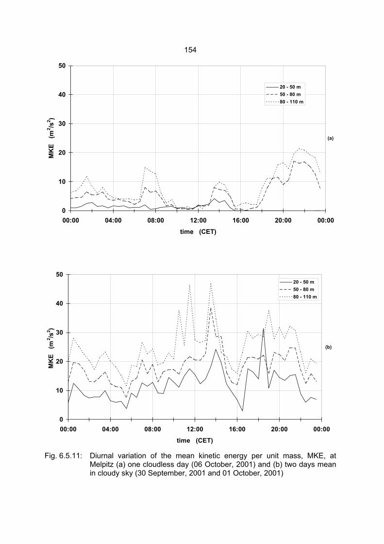
154

Fig. 6.5.11: Diurnal variation of the mean kinetic energy per unit mass, MKE, at Melpitz (a) one cloudless day (06 October, 2001) and (b) two days mean in cloudy sky (30 September, 2001 and 01 October, 2001)

0

10

20

30

40

50

00:00 04:00 08:00 12:00 16:00 20:00 00:00

time (CET)

MK

E (

m2 /s

2 )

20 - 50 m50 - 80 m80 - 110 m

(a)

0

10

20

30

40

50

00:00 04:00 08:00 12:00 16:00 20:00 00:00

time (CET)

MK

E (

m2 /s

2 )

20 - 50 m50 - 80 m80 - 110 m

(b)

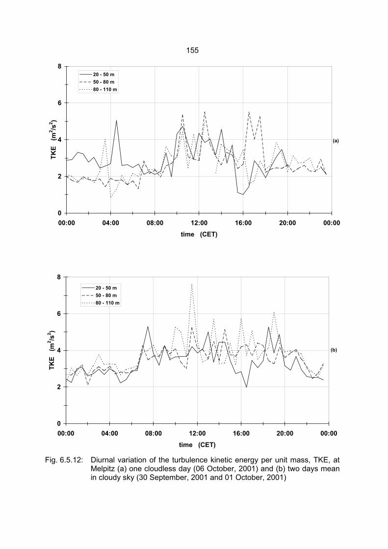
155

Fig. 6.5.12: Diurnal variation of the turbulence kinetic energy per unit mass, TKE, at Melpitz (a) one cloudless day (06 October, 2001) and (b) two days mean in cloudy sky (30 September, 2001 and 01 October, 2001)

0

2

4

6

8

00:00 04:00 08:00 12:00 16:00 20:00 00:00time (CET)

TKE

(m

2 /s2 )

20 - 50 m50 - 80 m80 - 110 m

(a)

0

2

4

6

8

00:00 04:00 08:00 12:00 16:00 20:00 00:00

time (CET)

TKE

(m

2 /s2 )

20 - 50 m50 - 80 m80 - 110 m

(b)

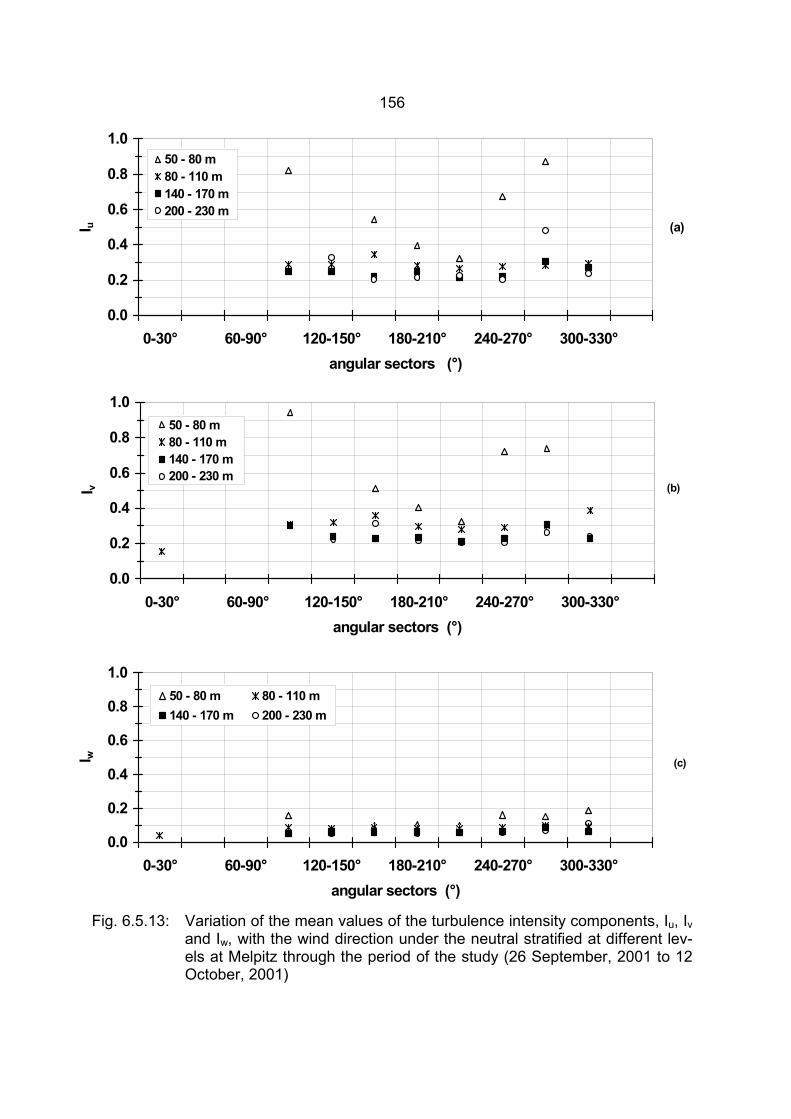
156

Fig. 6.5.13: Variation of the mean values of the turbulence intensity components, Iu, Iv and Iw, with the wind direction under the neutral stratified at different lev-els at Melpitz through the period of the study (26 September, 2001 to 12 October, 2001)

0.0

0.2

0.4

0.6

0.8

1.0

0-30° 60-90° 120-150° 180-210° 240-270° 300-330°angular sectors (°)

I u

50 - 80 m 80 - 110 m 140 - 170 m 200 - 230 m

(a)

0.0

0.2

0.4

0.6

0.8

1.0

0-30° 60-90° 120-150° 180-210° 240-270° 300-330°angular sectors (°)

I v

50 - 80 m 80 - 110 m 140 - 170 m 200 - 230 m

(b)

0.0

0.2

0.4

0.6

0.8

1.0

0-30° 60-90° 120-150° 180-210° 240-270° 300-330°angular sectors (°)

I w

50 - 80 m 80 - 110 m 140 - 170 m 200 - 230 m

(c)

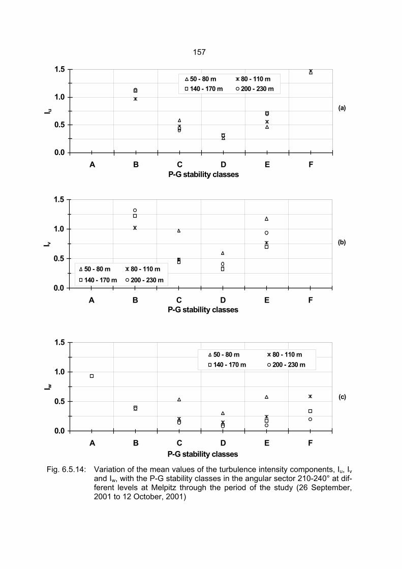
157

Fig. 6.5.14: Variation of the mean values of the turbulence intensity components, Iu, Iv and Iw, with the P-G stability classes in the angular sector 210-240° at dif-ferent levels at Melpitz through the period of the study (26 September, 2001 to 12 October, 2001)

0.0

0.5

1.0

1.5


I u

50 - 80 m 80 - 110 m 140 - 170 m 200 - 230 m

(a)

0.0

0.5

1.0

1.5


I v

50 - 80 m 80 - 110 m 140 - 170 m 200 - 230 m

(b)

0.0

0.5

1.0

1.5


I w

50 - 80 m 80 - 110 m 140 - 170 m 200 - 230 m

(c)

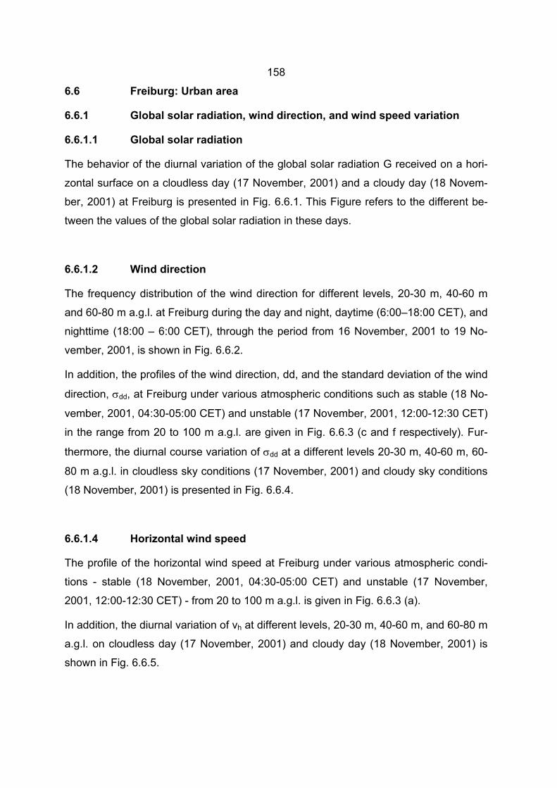
158

6.6 Freiburg: Urban area



The behavior of the diurnal variation of the global solar radiation G received on a hori-

zontal surface on a cloudless day (17 November, 2001) and a cloudy day (18 Novem-

ber, 2001) at Freiburg is presented in Fig. 6.6.1. This Figure refers to the different be-

tween the values of the global solar radiation in these days.


The frequency distribution of the wind direction for different levels, 20-30 m, 40-60 m

and 60-80 m a.g.l. at Freiburg during the day and night, daytime (6:00–18:00 CET), and

nighttime (18:00 – 6:00 CET), through the period from 16 November, 2001 to 19 No-

vember, 2001, is shown in Fig. 6.6.2.

In addition, the profiles of the wind direction, dd, and the standard deviation of the wind

direction, σdd, at Freiburg under various atmospheric conditions such as stable (18 No-

vember, 2001, 04:30-05:00 CET) and unstable (17 November, 2001, 12:00-12:30 CET)

in the range from 20 to 100 m a.g.l. are given in Fig. 6.6.3 (c and f respectively). Fur-

thermore, the diurnal course variation of σdd at a different levels 20-30 m, 40-60 m, 60-

80 m a.g.l. in cloudless sky conditions (17 November, 2001) and cloudy sky conditions

(18 November, 2001) is presented in Fig. 6.6.4.


The profile of the horizontal wind speed at Freiburg under various atmospheric condi-

tions - stable (18 November, 2001, 04:30-05:00 CET) and unstable (17 November,

2001, 12:00-12:30 CET) - from 20 to 100 m a.g.l. is given in Fig. 6.6.3 (a).

In addition, the diurnal variation of vh at different levels, 20-30 m, 40-60 m, and 60-80 m

a.g.l. on cloudless day (17 November, 2001) and cloudy day (18 November, 2001) is

shown in Fig. 6.6.5.

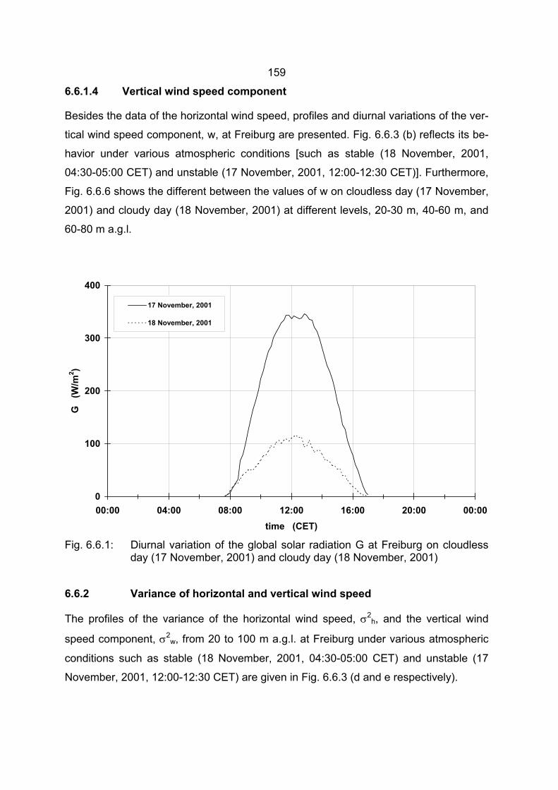
159


Besides the data of the horizontal wind speed, profiles and diurnal variations of the ver-

tical wind speed component, w, at Freiburg are presented. Fig. 6.6.3 (b) reflects its be-

havior under various atmospheric conditions [such as stable (18 November, 2001,

04:30-05:00 CET) and unstable (17 November, 2001, 12:00-12:30 CET)]. Furthermore,

Fig. 6.6.6 shows the different between the values of w on cloudless day (17 November,

2001) and cloudy day (18 November, 2001) at different levels, 20-30 m, 40-60 m, and

60-80 m a.g.l.

Fig. 6.6.1: Diurnal variation of the global solar radiation G at Freiburg on cloudless day (17 November, 2001) and cloudy day (18 November, 2001)



speed component, σ2w, from 20 to 100 m a.g.l. at Freiburg under various atmospheric

conditions such as stable (18 November, 2001, 04:30-05:00 CET) and unstable (17

November, 2001, 12:00-12:30 CET) are given in Fig. 6.6.3 (d and e respectively).

0

100

200

300

400

00:00 04:00 08:00 12:00 16:00 20:00 00:00time (CET)

G

(W/m

2 )

17 November, 2001

18 November, 2001

160

Moreover, the diurnal courses of σ2h and σ2

w, at different levels, 20-30 m, 40-60 m, and

60-80 m a.g.l. in Freiburg under cloudless sky conditions (17 November, 2001) and

cloudy sky conditions (18 November, 2001) are presented in Fig. 6.6.7 and Fig. 6.6.8

respectively.


In line with section 6.1.4, 6.2.4, 6.3.4, 6.4.4 and 6.5.4, profiles of the σ3w/z, MKE and

TKE at Freiburg are shown under various atmospheric conditions such as stable (18

November, 2001, 04:30-05:00 CET) and unstable (17 November, 2001, 12:00-12:30

CET). Moreover the diurnal courses of the σ3w/z, MKE and TKE at different levels, 20-

30 m, 40-60 m, 60-80 m a.g.l. under cloudless (17 November, 2001) and cloudy (18

November, 2001) sky conditions at Freiburg are shown in Fig. 6.6.9-Fig. 6.6.11.

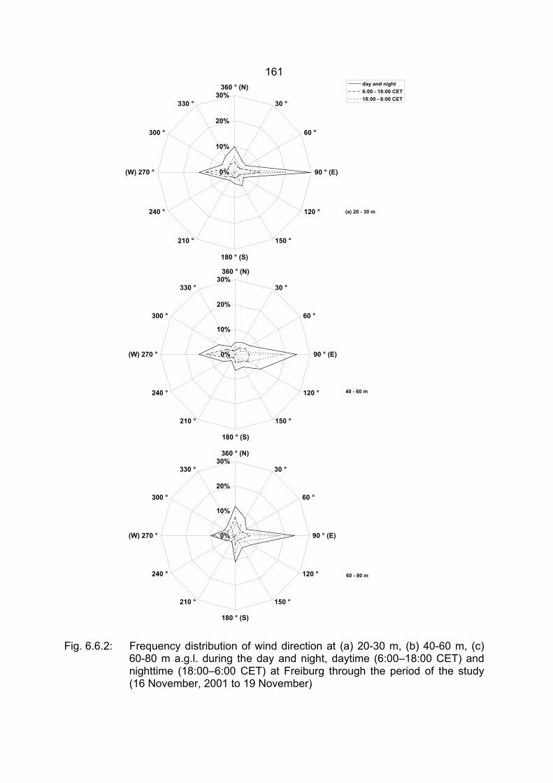
161

Fig. 6.6.2: Frequency distribution of wind direction at (a) 20-30 m, (b) 40-60 m, (c)

60-80 m a.g.l. during the day and night, daytime (6:00–18:00 CET) and nighttime (18:00–6:00 CET) at Freiburg through the period of the study (16 November, 2001 to 19 November)

0%

10%

20%

30%360 ° (N)

30 °

60 °

90 ° (E)

120 °

150 °

180 ° (S)

210 °

240 °

(W) 270 °

300 °

330 °


(a) 20 - 30 m

0%

10%

20%

30%360 ° (N)

30 °

60 °

90 ° (E)

120 °

150 °

180 ° (S)

210 °

240 °

(W) 270 °

300 °

330 °

40 - 60 m

0%

10%

20%

30%360 ° (N)

30 °

60 °

90 ° (E)

120 °

150 °

180 ° (S)

210 °

240 °

(W) 270 °

300 °

330 °

60 - 80 m

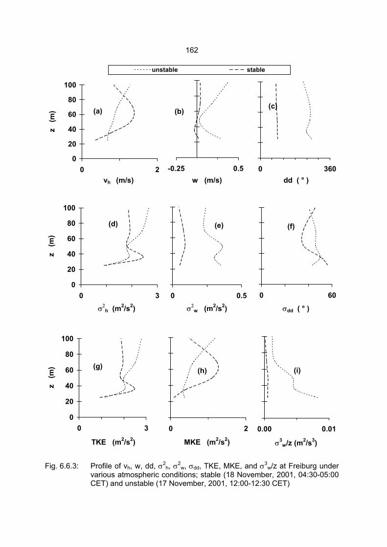
162


w, σdd, TKE, MKE, and σ3w/z at Freiburg under

various atmospheric conditions; stable (18 November, 2001, 04:30-05:00 CET) and unstable (17 November, 2001, 12:00-12:30 CET)

vh (m/s) w (m/s) dd ( ° )

σ2h (m2/s2) σ2

w (m2/s2) σdd ( ° )


(a)

0

20

40

60

80

100

0 2

z (

m) (b)

-0.25 0.5

(c)

0 360

(d)

0

20

40

60

80

100

0 3

z (

m)

(e)

0 0.5

(f)

0 60

(g)

0

20

40

60

80

100

0 3

z (

m) (h)

0 2

(i)

0.00 0.01

unstable stable

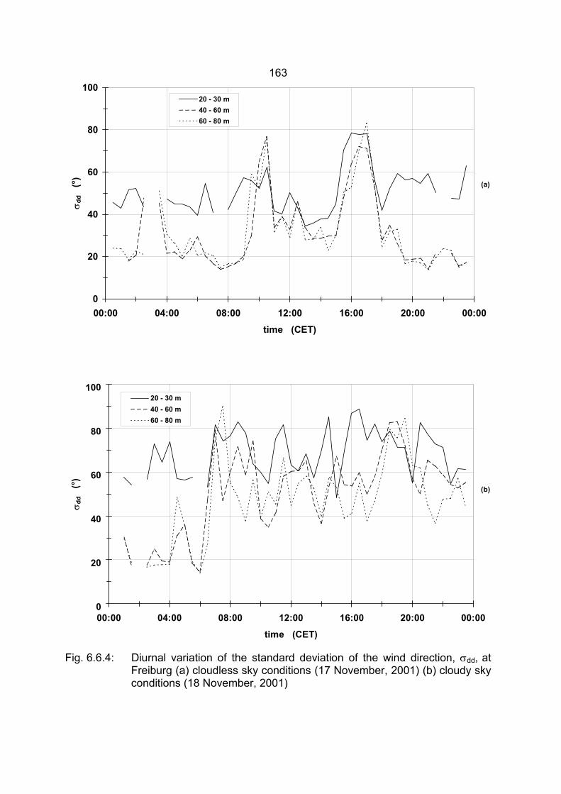
163

Fig. 6.6.4: Diurnal variation of the standard deviation of the wind direction, σdd, at Freiburg (a) cloudless sky conditions (17 November, 2001) (b) cloudy sky conditions (18 November, 2001)

0

20

40

60

80

100

00:00 04:00 08:00 12:00 16:00 20:00 00:00

time (CET)

σdd

(°

)

20 - 30 m40 - 60 m60 - 80 m

(a)

0

20

40

60

80

100

00:00 04:00 08:00 12:00 16:00 20:00 00:00

time (CET)

σdd

(°

)

20 - 30 m40 - 60 m60 - 80 m

(b)

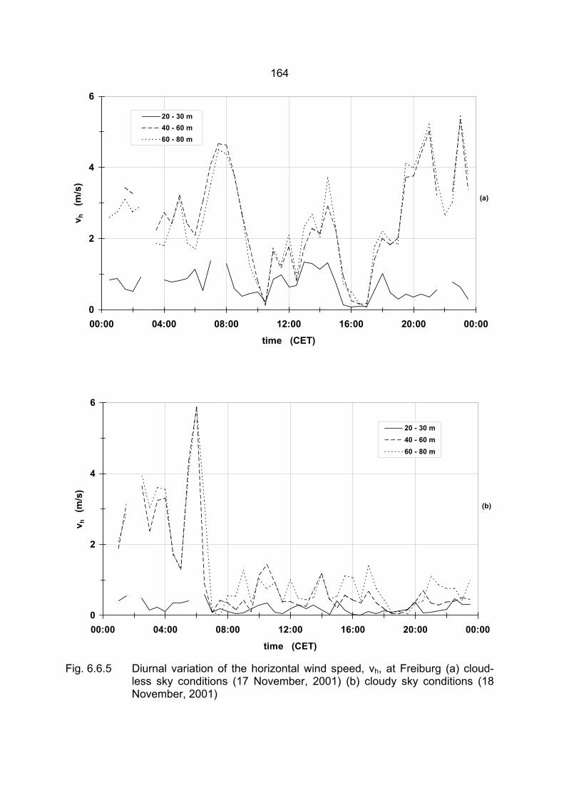
164

Fig. 6.6.5 Diurnal variation of the horizontal wind speed, vh, at Freiburg (a) cloud-less sky conditions (17 November, 2001) (b) cloudy sky conditions (18 November, 2001)

0

2

4

6

00:00 04:00 08:00 12:00 16:00 20:00 00:00time (CET)

v h

(m/s

)

20 - 30 m40 - 60 m60 - 80 m

(a)

0

2

4

6

00:00 04:00 08:00 12:00 16:00 20:00 00:00

time (CET)

v h

(m/s

)

20 - 30 m40 - 60 m60 - 80 m

(b)

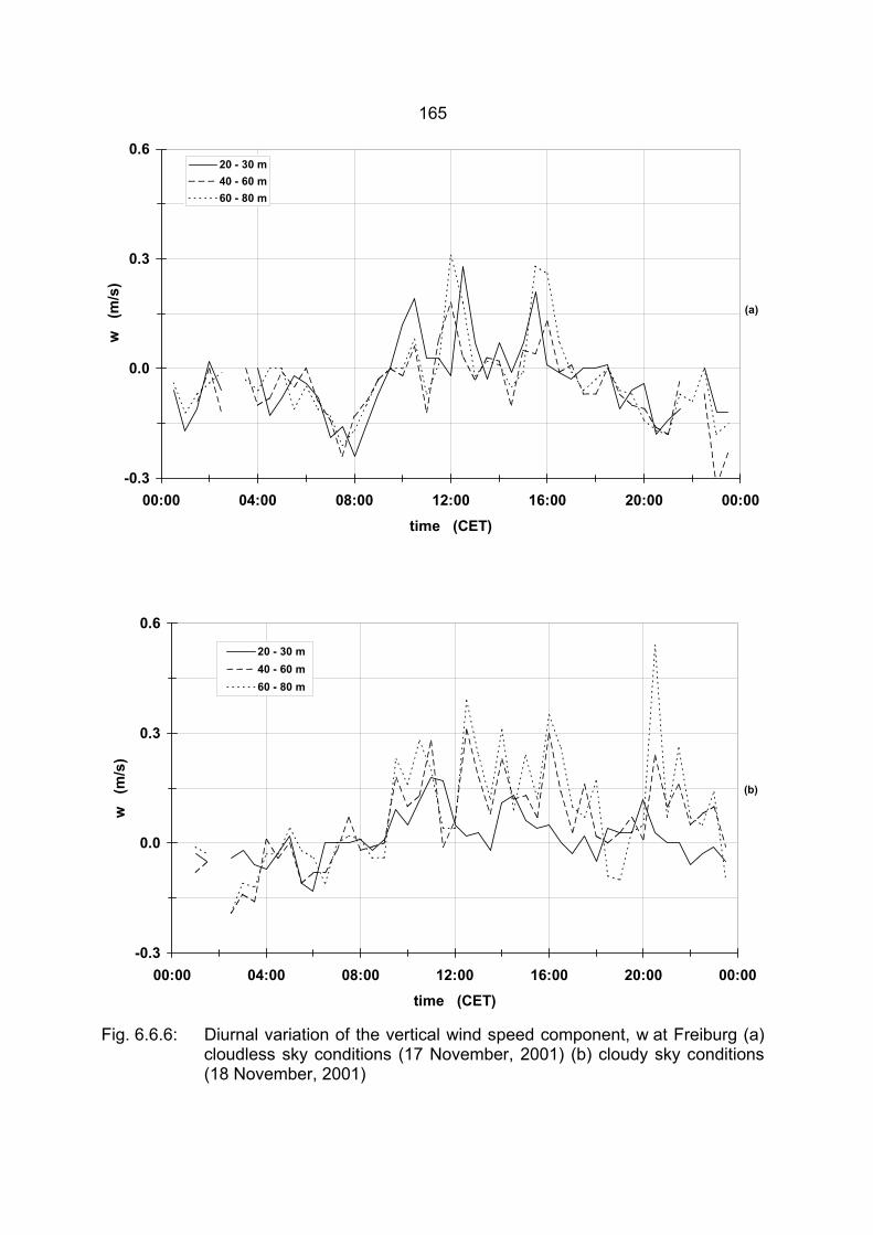
165

Fig. 6.6.6: Diurnal variation of the vertical wind speed component, w at Freiburg (a) cloudless sky conditions (17 November, 2001) (b) cloudy sky conditions (18 November, 2001)

-0.3

0.0

0.3

0.6

00:00 04:00 08:00 12:00 16:00 20:00 00:00

time (CET)

w

(m/s

)

20 - 30 m40 - 60 m60 - 80 m

(a)

-0.3

0.0

0.3

0.6

00:00 04:00 08:00 12:00 16:00 20:00 00:00time (CET)

w

(m/s

)

20 - 30 m40 - 60 m60 - 80 m

(b)

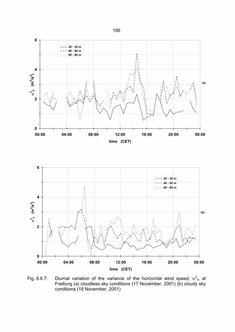
166


Freiburg (a) cloudless sky conditions (17 November, 2001) (b) cloudy sky conditions (18 November, 2001)

0

2

4

6

00:00 04:00 08:00 12:00 16:00 20:00 00:00

time (CET)

σ2 h

(m2 /s

2 )

20 - 30 m40 - 60 m60 - 80 m

(a)

0

2

4

6

00:00 04:00 08:00 12:00 16:00 20:00 00:00time (CET)

σ2 h

(m2 /s

2 )

20 - 30 m40 - 60 m60 - 80 m

(b)

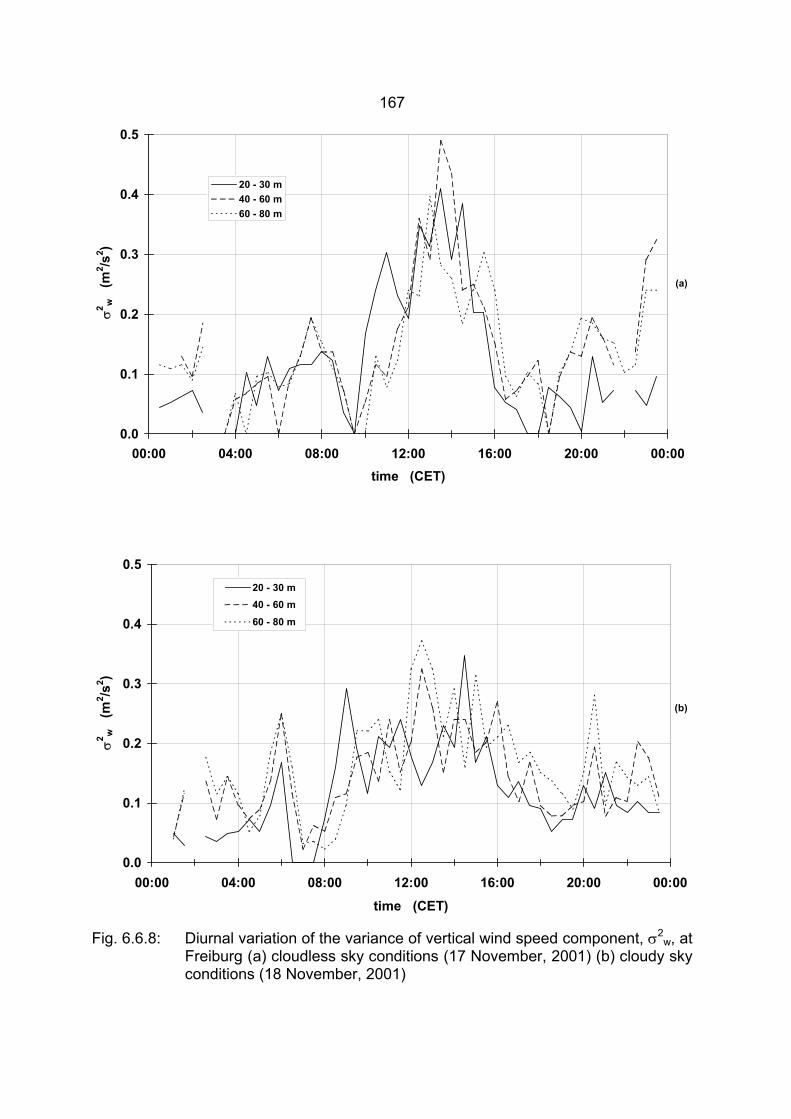
167

Fig. 6.6.8: Diurnal variation of the variance of vertical wind speed component, σ2w, at


0.0

0.1

0.2

0.3

0.4

0.5

00:00 04:00 08:00 12:00 16:00 20:00 00:00

time (CET)

σ2 w

(m

2 /s2 )

20 - 30 m40 - 60 m60 - 80 m

(b)

0.0

0.1

0.2

0.3

0.4

0.5

00:00 04:00 08:00 12:00 16:00 20:00 00:00time (CET)

σ2 w

(m2 /s

2 )

20 - 30 m40 - 60 m60 - 80 m

(a)

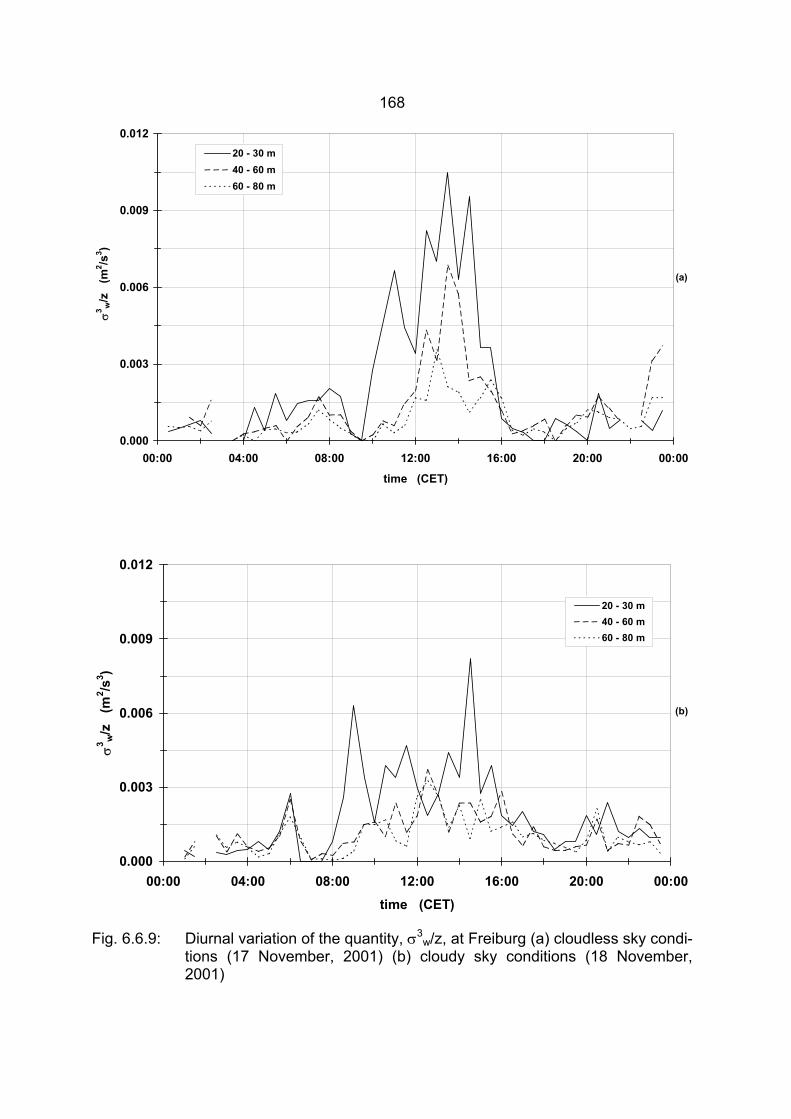
168

Fig. 6.6.9: Diurnal variation of the quantity, σ3w/z, at Freiburg (a) cloudless sky condi-

tions (17 November, 2001) (b) cloudy sky conditions (18 November, 2001)

0.000

0.003

0.006

0.009

0.012

00:00 04:00 08:00 12:00 16:00 20:00 00:00

time (CET)

σ3 w

/z

(m2 /s

3 )

20 - 30 m40 - 60 m60 - 80 m

(a)

0.000

0.003

0.006

0.009

0.012

00:00 04:00 08:00 12:00 16:00 20:00 00:00time (CET)

σ3 w

/z

(m2 /s

3 )

20 - 30 m40 - 60 m60 - 80 m

(b)

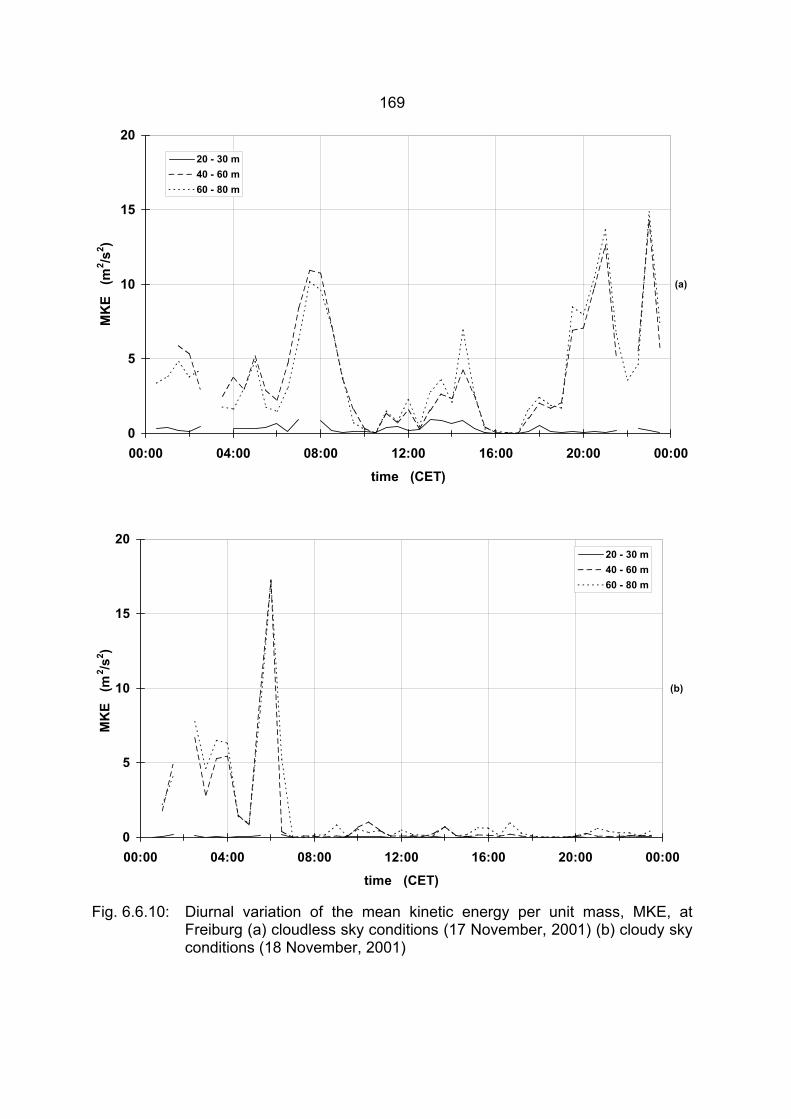
169

Fig. 6.6.10: Diurnal variation of the mean kinetic energy per unit mass, MKE, at Freiburg (a) cloudless sky conditions (17 November, 2001) (b) cloudy sky conditions (18 November, 2001)

0

5

10

15

20

00:00 04:00 08:00 12:00 16:00 20:00 00:00

time (CET)

MK

E (

m2 /s

2 )

20 - 30 m40 - 60 m60 - 80 m

(a)

0

5

10

15

20

00:00 04:00 08:00 12:00 16:00 20:00 00:00

time (CET)

MK

E (

m2 /s

2 )

20 - 30 m40 - 60 m60 - 80 m

(b)

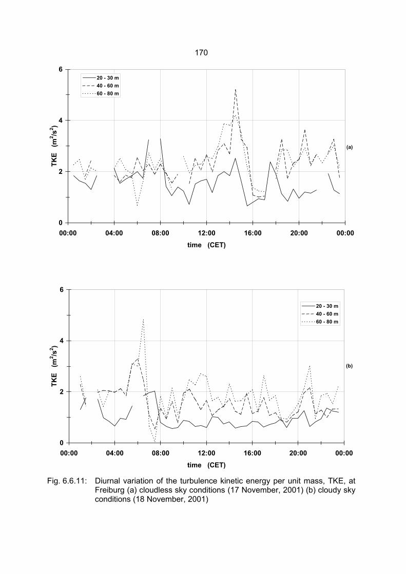
170

Fig. 6.6.11: Diurnal variation of the turbulence kinetic energy per unit mass, TKE, at Freiburg (a) cloudless sky conditions (17 November, 2001) (b) cloudy sky conditions (18 November, 2001)

0

2

4

6

00:00 04:00 08:00 12:00 16:00 20:00 00:00time (CET)

TKE

(m

2 /s2 )

20 - 30 m40 - 60 m60 - 80 m

(a)

0

2

4

6

00:00 04:00 08:00 12:00 16:00 20:00 00:00

time (CET)

TKE

(m

2 /s2 )

20 - 30 m40 - 60 m60 - 80 m

(b)

171

7 GENERAL DISCUSSION

7.1 Global solar radiation, wind direction, and wind speed variation

To explain the influence of thermal and roughness changes on the characteristics of

the turbulent parameters such as turbulent kinetic energy per unit mass (TKE), turbu-

lence intensity components (Iu, Iv, Iw) and the mean values of the normalized (by the

friction velocity) standard deviations of the velocity components, σi/u∗ (i=u,v,w) over the

sites of this study, the characteristics of the incoming solar radiation, wind direction and

its standard deviation, horizontal and vertical wind speed components, and the vari-

ances of horizontal and vertical wind speed components are briefly discussed for all

study sites through the periods of the measurements. The importance of these meas-

urements for this study is due to their effects in the turbulence of the atmosphere. Dur-

ing weak advection, the nature of convection and turbulence are controlled by the wind

speed, incoming solar radiation (insulation) cloud shading and time of day and night

(Stull, 2000).

7.1.1 Global solar radiation

Within the ABL, there are significant daily variations of temperature, winds, static stabil-

ity, and turbulence. These variations are driven by the diurnal cycle of solar heating

during day and IR cooling at night (Stull, 2000). The knowledge of the variability of G

gives an insight the effect of thermal in the behavior of the turbulence parameters in the

cloudless and cloudy sky conditions. Sections 6.1.1.1, 6.2.1.1, 6.3.1.1, 6.4.1.1, 6.5.1.1

and 6.6.1.1 summarize the results of the global solar radiation on the days in which the

turbulence parameters are investigated over Hartheim, Bremgarten, Blankenhornsberg,

Oberbärenburg, Melpitz and Freiburg respectively. These results reflect the effect of

clouds in the quantity of the incoming solar radiation. The difference between the mid-

day hours (11:00-14:00 CET) average of G on two cloudless and cloudy days (except

for Melpitz: one cloudless day, and Freiburg: one cloudless and one cloudy day) were,

respectively, 67%, 82%, 66%, 86%, 78% and 73% at Hartheim, Bremgarten, Blanken-

hornsberg, Oberbärenburg, Melpitz and Freiburg.

In addition, a high difference of the midday hours (11:00-14:00 CET) average of G on

cloudless and cloudy days were noticed from one site to another. These values were

172

701, 857, 817, 690, 495, and 381 (cloudless days), and 230, 156, 280, 94, 110 and 102

W/m2 (cloudy days) at Hartheim, Bremgarten, Blankenhornsberg, Oberbärenburg,

Melpitz and Freiburg respectively. This is due to the seasonal effect of the incoming

solar radiation, as the measurements were gathered in a different periods of the year

(Table 5.4). The high difference in G from the cloudless days to the cloudy ones, as

well from one site to another, were important to show the effect of the incoming solar

radiation on some turbulence parameters (such as σw and σ3w/z) which are affected by

the thermal variation.

7.1.2 Wind direction

As reported in Stull (2000) the wind shear is one process of the production of the turbu-

lence of the boundary layer and it is associated with the change of wind speed or wind

direction with the height. Moreover the values of σdd were used to determine the P-G

stability classes, according to Thomas (1988). Profiles of σdd under different atmos-

pheric conditions and the diurnal course of σdd during cloudless and cloudy sky condi-

tions are presented in the sections 6.1.1.2, 6.2.1.2, 6.3.1.2, 6.4.1.2, 6.5.1.2, and

6.6.1.2. As well these sections included the wind rose at different levels during the pe-

riod of the study at Hartheim, Bremgarten, Blankenhornsberg, Oberbärenburg, Melpitz

and Freiburg respectively. From these results, it can be concluded:

∗∗ The pattern of the wind rose varies for the different levels at the whole site of this

study but this change varies from one sites to another.

∗∗ There are high values of σdd at the low levels than those values of the high levels

at the whole sites of this study (see Figures 6.1.4, 6.2.4, 6.3.4, 6.4.3, 6.5.4 and

6.6.4). But these differences between the low and the high levels vary from one

site to another in both cases of cloudless and cloudy sky conditions.

In addition, the daily, midday hours (11:00-14:00 CET) and midnight hours (23:00-

02:00 CET) averages of σdd at different levels were calculated on two cloudless and

cloudy days (except for Melpitz and Freiburg: there were no many cloudless days) over

the sites of this study. Tables 7.1 - 7.6 summarize these averages and the standard

deviations at the sites of this study.

173

7.1.3 Wind speed components

Each local has a unique landscape that creates or modifies the wind. The change of

wind speed or wind direction with height leads to the wind shear which is one process

of the production of the turbulence of the atmospheric boundary layer. Furthermore, the

study of the MKE relates to the values of the wind speed components. Thus, profiles of

the horizontal and vertical wind speed under different atmospheric conditions as well as

the diurnal course at different levels in cloudless and cloudy sky conditions over all the

sites of this investigation are shown. Sections 6.1.1.3 , 6.2.1.3, 6.3.1.3, 6.4.1.3, 6.5.1.3

and 6.6.1.3 summarize the results of vh at Hartheim, Bremgarten, Blankenhornsberg,

Oberbärenburg, Melpitz and Freiburg respectively. Moreover, sections 6.1.1.4 , 6.2.1.4,

6.3.1.4, 6.4.1.4, 6.5.1.4 and 6.6.1.4 summarize the results of w at the same site respec-

tively. From these results it can be concluded:

∗∗ The values of w under unstable conditions were greater than those under the

neutral conditions which were greater than those under stable conditions (see

Fig. 6.1.3(b), 6.2.3(b), 6.3.3(b), 6.5.3(b), and 6.1.3(b)). This is an expected be-

havior, however, the high instability causes a strong upward and downward mo-

tion of the air.

∗∗ There is a vibration of the values of w in cloudless and cloudy conditions. In the

first case (cloudless sky conditions), the values of w fluctuate through the most

time of the day and night with a high fluctuation values in the daytime. This is

due to the effect of the incoming solar radiation.

∗∗ At the two cases (cloudless and cloudy conditions), there is a difference of the

values of w from level to level. This is a result of the effect of the warming and

cooling of the earth’s surface in the upward and downward motion of the air.

In addition to the above remarks, the daily, midday hours (11:00-14:00 CET) and mid-

night hours (23:00-02:00 CET) averages of vh and w at different levels were calculated

on two cloudless and cloudy days (except for Melpitz and Freiburg: there is no many

cloudless days) over the sites of this study. Tables 7.1-Table 7.6 summarize these av-

erages and the standard deviations at Hartheim, Bremgarten, Blankenhornsberg,

Oberbärenburg, Melpitz and Freiburg respectively. Moreover a comparison study be-

174

tween the midday-hours and midnight-hours-averages of vh and w on cloudless and

cloudy days are presented in Fig. 7.1-Fig. 7.6.

7.2 Atmospheric stability classification

The stability classification of the atmosphere is the first step for applying a number of

traditional algorithms aiming at estimating the main atmospheric parameters which

typically describe the boundary layer structure such as: Monin-Obukhov length, friction

velocity and the boundary layer height (Capanni and Gualtieri, 1999). The atmospheric

stability according to P-G stability classification was determined at four levels a.g.l, at

Hartheim (50-80, 80-110, 140-170, and 200-230 m), Bremgarten (40-60, 60-100, 100-

180, and 180-260 m), Blankenhornsberg (40-60, 80-120, 120-160, and 160-240 m),

Oberbärenburg (50-80, 80-110, 140-170, and 200-230 m), and Melpitz (50-80, 80-110,

140-170, and 200-230 m) for the study period. The mean value of the percentage fre-

quency distribution for each class within the range, approximately, from 40 to 260 m

a.g.l, were respectively: A (1%, 5%, 5%, 1%, 1%), B (3%, 15%, 19%, 6%, 3%), C (21%,

22%, 26%, 34%, 21%), D (72%, 41%, 33%, 55%, 72%), E (2%, 7%, 5%, 1%, 2%), and

F (1%, 10%, 10%, 2%, 1%) at Hartheim, Bremgarten, Blankenhornsberg, Oberbären-

burg, and Melpitz. If one considers the period of the year for every site, these results

seem reliable.

7.3 Variance of horizontal and vertical wind speed

Turbulence is a quasi-random phenomenon that can be described by statistics. Velocity

variances represent TKE and a measure of the intensity of turbulence (Stull, 2000). As

σ2u , σ2

v and σ2w are intimately related to the turbulent kinetic energy, it is to be antici-

pated that the intensity of turbulence should be related to the processes generating this

energy. Richardson (1920) showed these to be mainly shearing stresses and buoyancy

forces. Hence a particular attention will be given to the variance of the horizontal wind

speed, σ2h, and the variance of the vertical wind speed component, σ2

w, in order to un-

derstand the nature of TKE and the turbulence intensity components.

175

The profiles of σ2h and σ2

w under different atmospheric conditions, as well as, the diur-

nal course at different levels in cloudless and cloudy sky conditions over all the sites of

this study, are presented in sections 6.1.3, 6.2.3, 6.3.3, 6.4.3, 6.5.3 and 6.6.2 at Hart-

heim, Bremgarten, Blankenhornsberg, Oberbärenburg, Melpitz and Freiburg respec-

tively. From these results the following facts can be summarized:

∗∗ The fluctuations of the profile of σ2h and σ2

w in the lower part are relatively higher

than those of the above part through the range of the FAS64 (20-500 m a.g.l.)

under the whole stability conditions (especially neutral and unstable conditions).

The nature of this fluctuation varies from one sites to the other ones. This may

be due to the increase of the mechanically and buoyancy production which oc-

curs intensively in the surface layer,

∗∗ The general feature of the diurnal variation of both σ2h and σ2

w under the two

cases have various variability from level to level and from hour to hour with

some peaks at different time,

∗∗ The effect of the solar radiation in the σ2w is obviously at the day-time, espe-

cially, during interval from 11:00 to 13:00 CET under the cloudless sky condi-

tions,

∗∗ Sometime there is a high fluctuation in the values of σ2w under the cloudy sky

conditions (such as at the interval from 04:00 to 12:00 CET, Fig. 6.1.8), this may

be due to the downward and upward motion of the atmosphere through this in-

terval as it illustrated in the variation of w, see Fig. 6.1.6.

Beside the above notice, the daily, midday hours (11:00-14:00 CET) and midnight

hours (23:00-02:00 CET) averages of σ2h and σ2

w at different levels were calculated on

two cloudless and cloudy days (except for Melpitz and Freiburg: there is no many

cloudless days) over the sites of this study. Tables 7.1 - 7.6 summarize these averages

and the standard deviations at Hartheim, Bremgarten, Blankenhornsberg, Oberbären-

burg, Melpitz and Freiburg respectively. Moreover a comparison between the midday

hours and midnight hours averages of σ2h and σ2

w on cloudless and cloudy days are

presented in Fig. 7.1 - Fig. 7.6.

176

7.4 Turbulence kinetic energy

In line with section (4.1.2.1), the value of TKE depends on: advection by the mean

wind, shear generation, buoyancy production, transport by turbulent motions and pres-

sure, and viscous dissipation rate. This means, the nature of the changes of TKE varies

with the relative change of the magnitudes of these terms. But two terms of interest are

the shear and buoyancy terms (Stull, 2000). Moreover σ2w is connected to the produc-

tion terms of convective and mechanical origin (σ3w/z), appearing in the equation of tur-

bulent energy balance (Weill et al., 1980). Hence a particular attention will be given to

this quantity (σ3w/z) in this work.

To explain the influence of thermal and roughness changes on the properties of TKE

turbulence of the atmospheric boundary layer over the sites of this study, the profiles of

σ3w/z, MKE and TKE under different atmospheric stability conditions as well as the di-

urnal course at different levels in cloudless and cloudy sky conditions over the whole

sites of this study, were presented in sections 6.1.4, 6.2.4, 6.3.4, 6.4.4, 6.5.4 and 6.6.3

at Hartheim, Bremgarten, Blankenhornsberg, Oberbärenburg, Melpitz and Freiburg re-

spectively. The following features can be summarized from these results:

∗∗ At the whole site of this study, the vertical profiles of σ3w/z show that, the values

at the surface layer are higher than those at the rest range under the neutral and

unstable conditions. As well under the neutral and unstable atmospheric condi-

tions, the values of σ3w/z are greater than those under the stable conditions, see

Fig. 6.1.3 (i), 6.2.3 (i), 6.3.3 (i), 6.5.3 (i) and 6.6.3 (i). Moreover, the variation of

σ3w/z is similar to the change of σ2

w and depends on the buoyancy and the me-

chanical turbulence which occur intensively at the surface layer (Weill et al.,

1980).

∗∗ During cloudless conditions throughout the night, the values of the quantity σ3w/z

are low, even in the presence of wind shear. The effect of the incoming solar ra-

diation is obvious in the day-time. But in the case of cloudy conditions, there are

some high peaks in the first level which correspond to the high values of σ2w

(see Fig. 6.1.10, 6.2.10, 6.3.10, 6.4.9, 6.5.10, and 6.6.9).

∗∗ However, the quantity σ3w/z is conducted by the mechanical and buoyancy tur-

bulence production which occurs intensively in the surface layer. Hence the high

177

values of σ3w/z can be noticed at the low levels in the case of cloudless and

cloudy conditions.

∗∗ At the whole sites of this study, the values of MKE depend on the values of the

horizontal and vertical wind speed components and it has the same shape of the

variation of horizontal wind speed. This is obvious by the comparison of the

change of the profile and diurnal course of MKE and vh. Moreover the values of

MKE have a noticeable influence on TKE, as reported in Stull (1988), in which

the energy that is mechanically produced as turbulence is lost from the mean

flow and vice versa.

∗∗ As a result of the change of σ3w/z and MKE, the values of TKE vary too but this

change is not identical with these parameters. This is due to the fact that the

values of TKE do not depend on σ3w/z and MKE only but also on other parame-

ters, see section 4.1.2.1. This change conduct with the behavior of σ2h and σ2

w,

in which the effect of the σ2h is obvious because its values are relatively greater

than σ2w.

Beside the above remarks, the daily, midday hours (11:00-14:00 CET) and midnight

hours (23:00-02:00 CET) average of σ3w/z, MKE, and TKE at different levels are calcu-

lated on two cloudless and cloudy days (except for Melpitz and Freiburg: there were not

many cloudless days) over the sites of this study. Tables 7.1 - Table 7.6 summarize

these averages and the standard deviations at Hartheim, Bremgarten, Blankenhorns-

berg, Oberbärenburg, Melpitz and Freiburg respectively. Moreover a comparative study

between the midday-hours and midnight-hours-averages of σ3w/z, MKE, and TKE on

cloudless and cloudy days is presented in Fig. 7.1 - Fig. 7.6. The following conclusions

can be drawn from the figures:

∗∗ The effect of the incoming solar radiation on σ3w/z is obviously by the compari-

son of the difference between its average values at the midday hours (11:00-

14:00 CET) and midnight hours (23:00-02:00 CET) on cloudless and cloudy

days. However the difference between the average values of the quantity σ3w/z

of the midday hours (11:00-14:00 CET) and midnight hours (23:00-02:00 CET)

for the whole levels in the sites of the study on the cloudless days are greater

than those on the cloudy days. Sometimes on cloudy days, these average val-

178

ues at midnight hours (23:00-02:00 CET) are equal to those at midday hours

(11:00-14:00 CET). For example in Bremgarten, for the whole levels under

cloudy conditions the average values at the midday and midnight hours are the

same, because the average of the wind speeds at the midday hours are smaller

than those at the midnight hours and the average global solar radiation is small

(~ 150 W/m2). This possibly suggests that, in the presence of developed convec-

tion, as at (11:00–14:00 CET), especially when the wind shear is less intense

(the horizontal wind speed is <1 m/s), the mechanical production term contribut-

ing to σ3w/z is negligible with respect to the buoyancy term (Greenhut et al.

1989). But the effect of the mechanical term on σ3w/z at the midnight hours and

under the cloudy days can be seen, especially in the low levels, when the values

of the horizontal wind speed are relatively high in this time.

∗∗ The midday hours (11:00-14:00 CET) and midnight hours (23:00-02:00 CET)

averages of MKE depend on the values of the horizontal and vertical wind speed

components and it has the same shape of the variation of the horizontal wind

speed. However, the values of the horizontal wind speed are greater than the

values of the vertical wind speed.

∗∗ The values of TKE do not depend on σ3w/z and MKE only but also on some

other parameters (see section 4.1.2.1). The variation of the midday hours

(11:00-14:00 CET) and midnight hours (23:00-02:00 CET) averages of TKE vary

and this variations are not identical with the variations of σ3w/z and MKE. But the

change of TKE is related to the behavior of σ2h and σ2

w, in which the effect of the

σ2h is obvious because its values are relatively greater than σ2

w. One can see

this behavior by the comparison of the values of TKE with the values of σ3w/z,

MKE, σ2h and σ2

w in Fig. 7.1 - Fig. 7.6.

7.5 Turbulence intensity components

The turbulence intensity components, Iu, Iv and Iw, are the important variables for diffu-

sion modeling and depend on the height of observation, the surface roughness and the

stability (Roth, 1993). Characteristics of the turbulence intensity components, Iu, Iv and

Iw, are shown over the study areas and investigation periods for various fetch condi-

179

tions arising under various wind directions, and different atmospheric stability at differ-

ent levels.

7.5.2 Variation of turbulence intensity components with wind directions under neutral conditions

In line with section 4.1.2.2, during the neutral conditions, the variation of the turbulence

intensity components, Iu, Iv and Iw, with the angular sectors are explained to illustrate

the effect of the roughness in the values of the turbulent intensity components. Table

6.1.1, 6.2.1, 6.3.1, 6.4.1 and 6.5.1 show the mean, standard deviations and the obser-

vation number of the turbulence intensity components, Iu , Iv and Iw, at different levels

under the neutral conditions, grouped by wind direction in Hartheim, Bremgarten,

Blankenhornsberg, Oberbärenburg and Melpitz respectively. In addition, the mean val-

ues are summarized in Fig. 6.2.13, 6.3.13, 6.4.12, and 6.5.13 in Bremgarten, Blanken-

hornsberg, Oberbärenburg and Melpitz respectively (this analysis could not be done for

Freiburg because the period of study was very short, 16 November, 2001 to 19 No-

vember, 2001). These tables and figures summarize the following:

∗∗ Generally the most frequent wind direction in the wind rose at the different levels

in the range of sodar for every site in this study are not the same for the whole

angular sectors and sometime there are no data in a number of angular sectors.

Consequently, the variation of the turbulence intensity components at the whole

angular sectors could not be analyzed. Also, these values could not be com-

pared together, but this comparison could be made for the angular sectors for

which a considerable number of observations are available. For example, at

Hartheim (Table 6.1.1) results of the turbulence intensity components, Iu, Iv and

Iw, could not be compared at all angular sectors. But for the angular sector 180-

210°, the number of observation was suitable (92, 77, 84, and 28 at the heights

50-80 m, 80-110 m, 140-170 m and 200-230 m respectively). Thus, the depend-

ence of the turbulence intensity components on the height of observation could

be analyzed. It shows a decrease with increasing height. The decrease of the

values of Iu, Iv and Iw were 21%, 51% and 47% respectively between the level

50-80 m and 200-230 m a.g.l..

180

∗∗ At Bremgarten, there is a small fluctuation in the values of Iu , Iv and Iw from one

angular sector to another as illustrated in Fig. 6.2.13. This behavior is expected,

as the surrounding of the sodar in this site is not completely symmetric. This

may be due to the presence of some trees with an average height 11 m (125 m

far from the site of sodar in the north-east direction), houses with an average

height 12 m (500 m far from the site of the sodar in the north-east and south-

east) and a big group of trees in the west direction with an average height 10 m

(1800 m far from the site of the sodar). Beside the non-symmetric of the sur-

rounding of the sodar, the high difference in the number of observations for the

wind direction sectors can play a considerable role in this variation. Furthermore,

the values of Iu, Iv and Iw decrease with the altitude (see Table 6.2.1 and Fig.

6.2.13). The decrease of the values of Iu, Iv and Iw from the level of 40-60 m to

180-260 m a.g.l. was calculated for the angular sectors which have a consider-

able number of observation such as 180-210° and 210-240°. The decrease of

the values of Iu, Iv and Iw were 64%, 63% and 82% for 180-210° and 30%, 37%

and 72% respectively for 210-240°. But some discrepancies in the results (such

as in the angular sectors 240-270° and 270-300°) may be due to the difference

between the number of the observations.

∗∗ At Blankenhornsberg and Melpitz, generally there is a very small fluctuation in

the values of Iu, Iv and Iw as it is illustrated in Fig. 6.3.13 and Fig. 6.5.14. This

fluctuation in the data is due to the non-symmetry of the surrounding and the

high difference of the number of the observations between the wind direction

sectors. Moreover the values of Iu, Iv and Iw decrease with the altitude (see Table

6.3.1 and 6.5.1). At Blankenhornsberg, the decrease of the values of Iu, Iv and Iw

from the level 40-60 m to 160-240 m a.g.l. was calculated for the angular sectors

(which have a considerable number of observation such as 150-180° and 180-

210°). The decrease of the values of Iv and Iw were 15% and 72% for 150-180°

and 35% and 75% respectively for 180-210°. There is a discrepancy in the val-

ues of Iu (its value increase 57% and 21% for the angular sectors 150-180° and

180-210° respectively). This may be due to the difference of the number of ob-

servations between the level 40-60 m a.g.l. (45 and 55) and the level 160-240 m

a.g.l. (7 and 38). At Melpitz, the values of Iu, Iv and Iw decrease with the increase

181

of the height for the angular sectors (which have a considerable number of ob-

servation such as 180-210° and 210-240°). The decrease of the values of Iu, Iv

and Iw were 47%, 46% and 50% respectively for 180-210°, and 30%, 38% and

44% respectively for 210-240°.

∗∗ At Oberbärenburg (Fig. 6.1.12), there is a variation of the values of the turbu-

lence intensity component Iu, Iv and Iw with angular sector. This may be due to

the variation of the nature of the surface from sector to sector. Moreover, this

variation is high at the level 50-80 m a.g.l. and decrease with the increase of the

height a.g.l.. The mean value of the decrease of the values of Iu, Iv and Iw from

the level 50-80 m to 200-230 m a.g.l. was calculated for some angular sectors

(210-330°). The mean decrease of the values of Iu, Iv and Iw were 61%, 50% and

85% for this angular sector. This is an expected behavior. However, the nature

of turbulence intensity depends on the height of observation, the surface rough-

ness (Roth, 1993).

From the previous remarks, the effect of the roughness index in the turbulence intensity

can be obviously seen when the surrounding of the sodar is not symmetric, as ex-

plained in the study of Brook (1972), which indicated the variation of the turbulence in-

tensity components for various wind sector at different level in a complex terrain. More-

over, it can be seen that the intensity of turbulence is significantly different from the alti-

tude above the ground level. This type of studies needs a large number of observations

to provide more reliable results.

7.5.2 Turbulence intensity under different stratifications

In order to study the effect of the height of observation and stability on turbulence in-

tensity components, Iu, Iv and Iw, their values according to P-G stability classes were

analyzed at one angular sector at different levels for each site. This study was done at

one angular sector to reduce the change of z0. This led to its value approximately fixed

and only the effect of the stability on the turbulence intensity components could be in-

vestigated. Sections 6.1.5.2, 6.2.5.2, 6.3.5.2, 6.4.5.2 and 6.5.5.2 summarize the results

of this study at Hartheim, Bremgarten, Blankenhornsberg, Oberbärenburg and Melpitz

182

respectively (however at Freiburg there were not enough data to do this study). These

results led to the following:

∗∗ At all the sites of the study a high difference between the number of observa-

tions from class to class was observed, especially for A, E, F and sometimes for

B. Thus, these data were neglected in the discussion, because they are not rep-

resentative data. Regardless of the number of observation at the stable condi-

tions (E and F), the values of the turbulence intensity components are less reli-

able than for the neutral (D) and unstable (A, B and C) case. This behavior has

been observed by Smith and Abbott (1961), as well, McBean (1971) found a

less reliable data for σi/u*(i=u,v,w) under the stable than the unstable conditions.

Panofsky and Dutton (1984) explained that for a strong stability the quantities

σi/u∗ (i=u,v,w), σu/vh and σv/vh increase and become extremely variable. They

show that, the large standard deviations are produced by low-frequency fluctua-

tions, not associated with turbulence.

∗∗ At all the sites of the study the nature of the relationship between turbulence in-

tensity components, Iu, Iv and Iw, and the atmospheric stability was investigated

in the range from the class B (unstable) to class D (neutral). The values of the

turbulence intensity components, Iu, Iv and Iw, increase with the increase of the

instability from the neutral conditions (D) to the unstable (B). The values of the

turbulence intensity components Iu, Iv and Iw vary from level to level but they

have the same shape of variation. The relationship between turbulence intensity

components, Iu, Iv and Iw, and the atmospheric stability reflects high values of the

horizontal components of the turbulence intensity with respect to the vertical

component.

Similar to these results are those of Clarke et al. (1982), who also observed that values

increased with the increase of instability (for -1.6 < z/L < 0.8) and they reported higher

turbulence intensities for the horizontal components. Roth (1993) obtained similar re-

sults. On the other hand, Ramsdell (1975) (for -2.5 < z/L > 0.17; 1 < z < 50 m in an ur-

ban residential area), Högström et al. (1982) and Rotach (1991) could not observe any

relationship.

183

7.6 Relationship between normalized standard deviations of velocity components and z/L under unstable conditions

In the present study, the mean values of the normalized standard deviations of the ve-

locity components, σi/u∗ (i=u,v,w) as functions of the stability parameter (z/L) under the

unstable conditions over Hartheim (Scots pine forest), Bremgarten (grassland),

Blankenhornsberg (vineyard) and Oberbärenburg (Norway spruce forest), are summa-

rized in Fig. 7.7 and compared to the results of other studies, which used sonic ane-

mometer-thermometer instrument, over complex and flat terrain. The relationship be-

tween the mean values of the σi/u∗ (i=u,v,w) and z/L showed the same behavior over all

the sites and was in good agreement with the general function given by AL-Jiboori et al.

(2001).

31

*

)1(Lzba

u iii +=

σ 7.8

where i = u, v, w as well as ai and bi are empirical constants. Table 7.7 summarizes the

values of ai and bi for this study and shows values of ai and bi as applied in this study

for different sites. Fig. 7.7 (a and b) and Table 7.7 show the increase of the mean val-

ues of σu/u∗ and σv/u∗ with increasing -z/L. The values of the empirical constant au,v and

bu,v at grassland and vineyard were smaller than those given by AL-Jiboori et al.

(2001). The values of au,v and bu,v at Scots pine forest, Norway spruce forest were

higher than those of AL-Jiboori et al. (2001). The mean values of σw/u∗ at the all sites

showed an increase with increasing instability (Fig. 7.7 c). Changes of aw and bw were

very small.

7.6.1 Horizontal components

The results of Scots pine forest (Hartheim), grassland (Bremgarten), vineyard

(Blankenhornsberg) and Norway spruce forest (Oberbärenburg) show the behavior that

the variation of the values of σu/u∗ and σv/u∗ increases with the increasing -z/L and has

the same trends described by Eq. (7.8) and Fig. (7.7). Previous studies such as AL-

Jiboori et al., 2001 found the dependence of σu/u∗ and σv/u∗ on the stability parameter

z/L under unstable condition. Moreover, Monin and Obukhov (1954) hypothesized that

184

any dimensionless characteristic of the turbulence can depend only upon u∗, z, g/Tv,

H0, i.e. upon z/L (Garratt, 1992). The model proposed by Højstrup (1982), obtained by

integration of a model spectrum of horizontal variance, acknowledges a dependence of

σu/u∗ and σv/u∗ on both zi/L and z/L (Zhang et al., 2001).

In addition, Garratt (1992) pointed out that the relationships between σu/u∗ and σv/u∗

and -z/L show no height-dependence throughout the surface layer, even under very

unstable conditions, i.e. Monin-Obukhov scaling does not apply under these conditions,

and the mixed layer height zi becomes the relevant scaling height. But the mixing

height data, zi, are not available in the present study, thus the present results are un-

able to discriminate as to whether the horizontal components scale better with zi/L

rather than z/L as suggested by Panofsky et al. (1977) and Wyngaard and Cotè (1974).

To illustrate the effect of surface roughness on σu/u∗ and σv/u∗, the behavior of the rela-

tionship between these parameters and -z/L was compared for the different four sites

(Scots pine forest, grassland, vineyard and Norway spruce forest) as well as the data of

AL-Jiboori et al., 2001 for flat and complex terrain (Fig. 7.7, a and b). Furthermore, the

variation of the mean values of σu/u∗ and σv/u∗ in the same range of -z/L (0.86 to 3.86)

at the four sites and compares the results to the data of AL-Jiboori et al., 2001 for flat

and complex terrain will be discussed (Table 7.8).

Under unstable conditions, it is of interest to show that the data points of σu/u∗ and σv/u∗

were separated for different values of Scots pine forest, grassland, vineyard and Nor-

way spruce forest. The lower values are from grassland and vineyard, while the higher

values upper points are from Scots pine forest and Norway spruce forest. This is in

good agreement with the result of AL-Jiboori et al., 2001. On the other hand, other

studies such as Zhang et al., 2001 compared the values of σu/u∗ and σv/u∗ over rough

surface (suburban and urban area) and a smooth surface (desert an grassland site).

The result gives a reduction for the rough site compared to the smooth surface condi-

tion for a given z/L. Garratt (1992) pointed out that the relationship between σu,v /u∗ and

-z/L shows no height-dependence throughout the surface layer, even in highly unstable

conditions, so Monin-Obukhov scaling does not apply, and the mixed layer height zi

becomes the relevant scaling height. These results revealed a dependence on the ob-

servational height. Zhang et al. (2001) have interpreted this behavior as follows: during

185

the course of a day the variation in zi may be small compared to the corresponding

variation in L and the measurements over various surface conditions were taken at dif-

ferent heights, so an apparent variation of σu/u∗ and σv/u∗ with height will results. But

the data were gathered with approximately a small difference in the height range, more-

over the data of Al-Jiboori et al. 2001 were gathered at the same height (4.9 m a.g.l.).

Table 7.8 display the variation of the mean values of σu/u∗ and σv/u∗ in the same range

of -z/L (0.86 to 3.86) at the four sites and compares the results to the data of AL-Jiboori

et al., 2001 for flat and complex terrain. σu/u∗ and σv/u∗ differ from site to site and in-

crease with increasing of the roughness length z0. The difference between the values

of σu/u∗ and σv/u∗ over flat terrain are smaller than those over complex terrain.

7.6.1 Vertical component

The vertical component σw/u∗ also showed an increase with increasing instability (Fig.

7.7c) which is in an agreement with results over flat (Al-Jiboori et al., 2001; Panofsky et

al., 1977; Xu et al., 1993; Zhang et al., 2001), and complex terrain (Al-Jiboori et al.,

2001; Founda et al., 1997; Zhang et al., 2001). The change of the surface roughness

does not seem to influence the properties of σw/u∗ (Fig. 7.7, c and Table 7.8). This

might be due to the fact that vertical velocity fluctuations are produced by small eddies

which rapidly adjust to changing surface properties (Panofsky and Dutton, 1984).

7.7 Profile of normalized variance of vertical wind speed component

Argentini et al. (1999) discussed the behavior of the normalized variances σ2w/w∗

2 as a

function of the normalized height z/zi. They did this work in Milan (Italy) in the center

part of Po Valley, a densely populated and industrialized flat area of approximately 400

x 200 km2 surrounded on three sides by mountain but on the eastern part, the Po Val-

ley is open to the Adriatic sea. They obtained a scatter data corresponding to the scal-

ing:

232

2*

2

)8.01()(ii

w

zz

zzc

w−=

σ 7.9

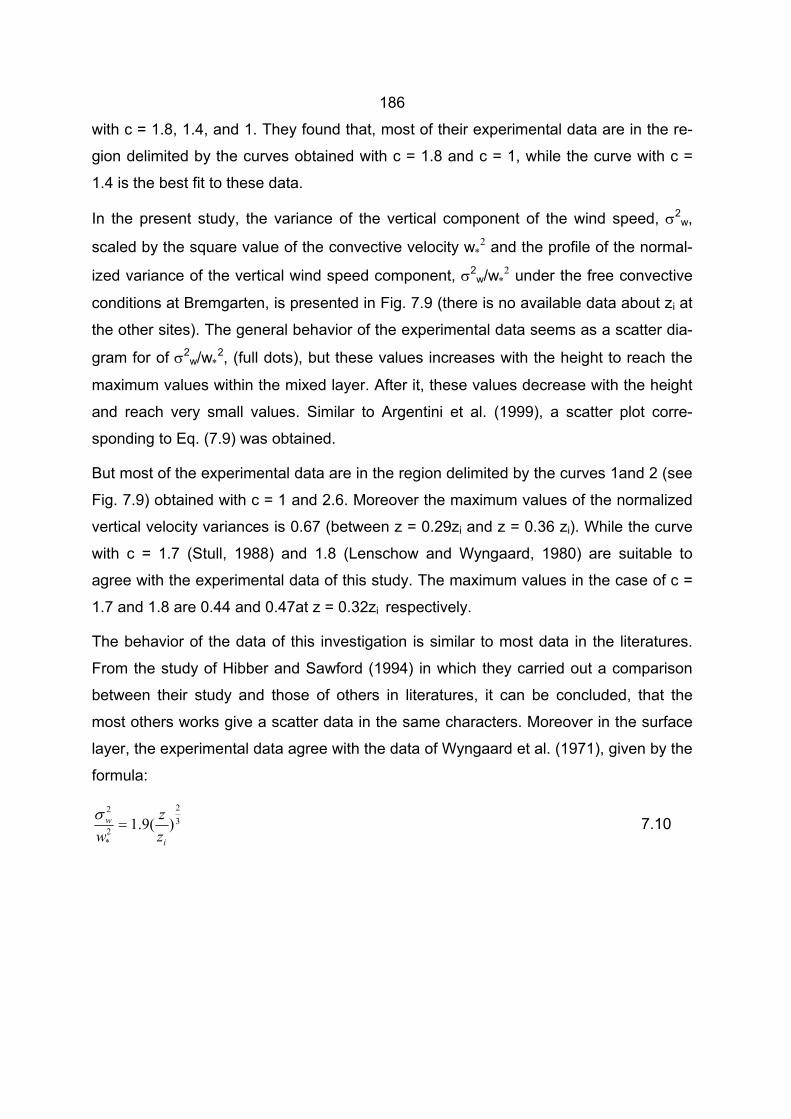
186

with c = 1.8, 1.4, and 1. They found that, most of their experimental data are in the re-

gion delimited by the curves obtained with c = 1.8 and c = 1, while the curve with c =

1.4 is the best fit to these data.

In the present study, the variance of the vertical component of the wind speed, σ2w,

scaled by the square value of the convective velocity w∗2 and the profile of the normal-

ized variance of the vertical wind speed component, σ2w/w∗

2 under the free convective

conditions at Bremgarten, is presented in Fig. 7.9 (there is no available data about zi at

the other sites). The general behavior of the experimental data seems as a scatter dia-

gram for of σ2w/w∗

2, (full dots), but these values increases with the height to reach the

maximum values within the mixed layer. After it, these values decrease with the height

and reach very small values. Similar to Argentini et al. (1999), a scatter plot corre-

sponding to Eq. (7.9) was obtained.

But most of the experimental data are in the region delimited by the curves 1and 2 (see

Fig. 7.9) obtained with c = 1 and 2.6. Moreover the maximum values of the normalized

vertical velocity variances is 0.67 (between z = 0.29zi and z = 0.36 zi). While the curve

with c = 1.7 (Stull, 1988) and 1.8 (Lenschow and Wyngaard, 1980) are suitable to

agree with the experimental data of this study. The maximum values in the case of c =

1.7 and 1.8 are 0.44 and 0.47at z = 0.32zi respectively.

The behavior of the data of this investigation is similar to most data in the literatures.

From the study of Hibber and Sawford (1994) in which they carried out a comparison

between their study and those of others in literatures, it can be concluded, that the

most others works give a scatter data in the same characters. Moreover in the surface

layer, the experimental data agree with the data of Wyngaard et al. (1971), given by the

formula:

32

2*

2

)(9.1i

w

zz

w=

σ 7.10

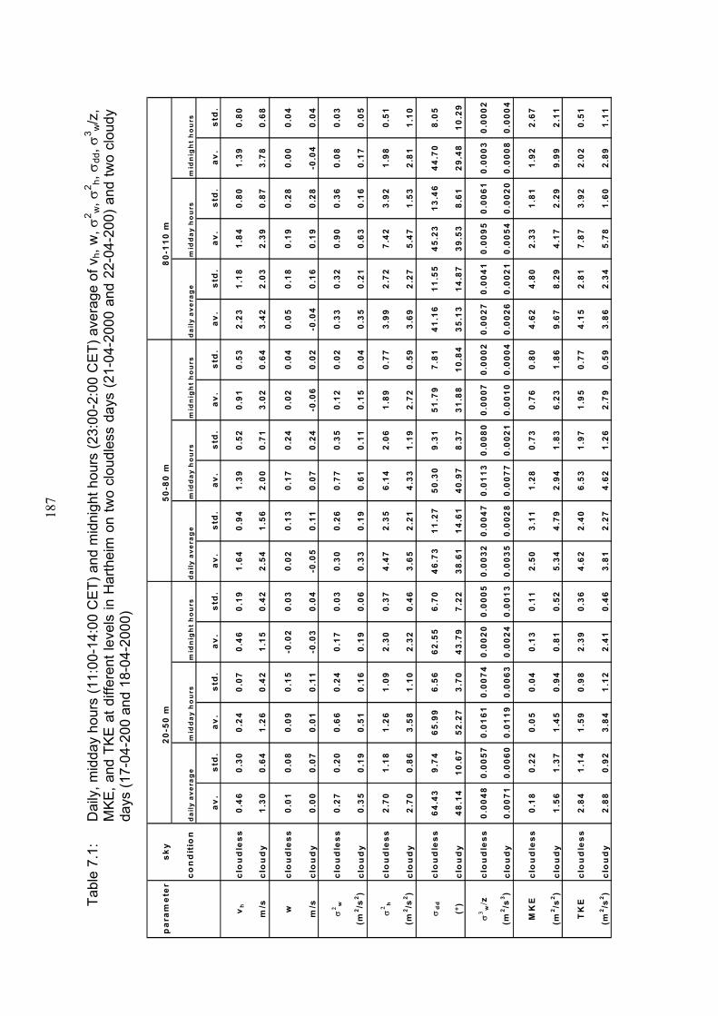
18

7

Tabl

e 7.

1:

Dai

ly, m

idda

y ho

urs

(11:

00-1

4:00

CE

T) a

nd m

idni

ght h

ours

(23:

00-2

:00

CE

T) a

vera

ge o

f vh,

w, σ

2 w, σ

2 h, σ d

d, σ3 w

/z,

MKE

, and

TK

E a

t diff

eren

t lev

els

in H

arth

eim

on

two

clou

dles

s da

ys (2

1-04

-200

0 an

d 22

-04-

200)

and

two

clou

dy

days

(17-

04-2

00 a

nd 1

8-04

-200

0)

par

amet

ersk

y20

-50

m50

-80

m80

-110

m

con

dit

ion

dai

ly a

vera

ge

mid

day

ho

urs

m

idn

igh

t h

ou

rs

dai

ly a

vera

ge

mid

day

ho

urs

m

idn

igh

t h

ou

rs

dai

ly a

vera

ge

mid

day

ho

urs

m

idn

igh

t h

ou

rs

av.

std

.av

.st

d.

av.

std

.av

.st

d.

av.

std

.av

.st

d.

av.

std

.av

.st

d.

av.

std

.

vh

clo

ud

less

0.46

0.30

0.24

0.07

0.46

0.19

1.64

0.94

1.39

0.52

0.91

0.53

2.23

1.18

1.84

0.80

1.39

0.80

m/s

clo

ud

y1.

300.

641.

260.

421.

150.

422.

541.

562.

000.

713.

020.

643.

422.

032.

390.

873.

780.

68

wcl

ou

dle

ss0.

010.

080.

090.

15-0

.02

0.03

0.02

0.13

0.17

0.24

0.02

0.04

0.05

0.18

0.19

0.28

0.00

0.04

m/s

clo

ud

y0.

000.

070.

010.

11-0

.03

0.04

-0.0

50.

110.

070.

24-0

.06

0.02

-0.0

40.

160.

190.

28-0

.04

0.04

σ2

wcl

ou

dle

ss0.

270.

200.

660.

240.

170.

030.

300.

260.

770.

350.

120.

020.

330.

320.

900.

360.

080.

03

(m2 /s

2 )cl

ou

dy

0.35

0.19

0.51

0.16

0.19

0.06

0.33

0.19

0.61

0.11

0.15

0.04

0.35

0.21

0.63

0.16

0.17

0.05

σ2

hcl

ou

dle

ss2.

701.

181.

261.

092.

300.

374.

472.

356.

142.

061.

890.

773.

992.

727.

423.

921.

980.

51

(m2 /s

2 )cl

ou

dy

2.70

0.86

3.58

1.10

2.32

0.46

3.65

2.21

4.33

1.19

2.72

0.59

3.69

2.27

5.47

1.53

2.81

1.10

σd

dcl

ou

dle

ss64

.43

9.74

65.9

96.

5662

.55

6.70

46.7

311

.27

50.3

09.

3151

.79

7.81

41.1

611

.55

45.2

313

.46

44.7

08.

05

(°)

clo

ud

y48

.14

10.6

752

.27

3.70

43.7

97.

2238

.61

14.6

140

.97

8.37

31.8

810

.84

35.1

314

.87

39.5

38.

6129

.48

10.2

9

σ3

w/z

cl

ou

dle

ss0.

0048

0.00

570.

0161

0.00

740.

0020

0.00

050.

0032

0.00

470.

0113

0.00

800.

0007

0.00

020.

0027

0.00

410.

0095

0.00

610.

0003

0.00

02

(m2 /s

3 )cl

ou

dy

0.00

710.

0060

0.01

190.

0063

0.00

240.

0013

0.00

350.

0028

0.00

770.

0021

0.00

100.

0004

0.00

260.

0021

0.00

540.

0020

0.00

080.

0004

MK

Ecl

ou

dle

ss0.

180.

220.

050.

040.

130.

112.

503.

111.

280.

730.

760.

804.

624.

802.

331.

811.

922.

67

(m2 /s

2 )cl

ou

dy

1.56

1.37

1.45

0.94

0.81

0.52

5.34

4.79

2.94

1.83

6.23

1.86

9.67

8.29

4.17

2.29

9.99

2.11

TK

Ecl

ou

dle

ss2.

841.

141.

590.

982.

390.

364.

622.

406.

531.

971.

950.

774.

152.

817.

873.

922.

020.

51

(m2 /s

2 )cl

ou

dy

2.88

0.92

3.84

1.12

2.41

0.46

3.81

2.27

4.62

1.26

2.79

0.59

3.86

2.34

5.78

1.60

2.89

1.11

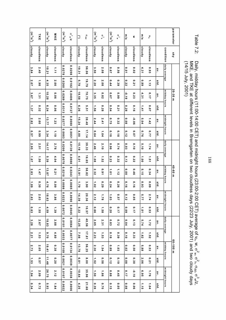
188

Table 7.2: D

aily, midday hours (11:00-14:00 C

ET) and m

idnight hours (23:00-2:00 CE

T) average of vh , w

, σ2w , σ

2h , σdd , σ

3w /z, M

KE, and TK

E at different levels in B

remgarten on tw

o cloudless days (22/23 July, 2001) and two cloudy days

(14/15 July, 2001)

param

etersky

20-30 m40-60 m

60-100 m

con

ditio

nd

aily average

mid

day h

ou

rs m

idn

igh

t ho

urs

daily averag

em

idd

ay ho

urs

mid

nig

ht h

ou

rs d

aily average

mid

day h

ou

rs m

idn

igh

t ho

urs

av.std

.av.

std.

av.std

.av.

std.

av.std

.av.

std.

av.std

.av.

std.

av.std

.

vh

clou

dless

0.931.13

0.170.07

1.420.77

1.741.51

0.340.09

2.740.53

1.721.52

0.530.21

1.761.04

m/s

clou

dy

4.310.89

4.311.41

5.040.76

5.101.00

5.150.93

5.771.01

5.741.62

5.882.06

6.951.15

wclo

ud

less0.02

0.210.23

0.16-0.06

0.070.10

0.220.46

0.160.05

0.170.13

0.330.50

0.30-0.10

0.06

m/s

clou

dy

0.010.22

-0.190.28

0.080.12

0.030.13

0.000.16

0.120.09

0.040.10

0.020.08

0.170.08

σ2w

clou

dless

0.560.39

0.990.21

0.320.18

0.740.32

1.120.26

0.570.17

0.720.39

1.030.19

0.450.05

(m2/s

2)clo

ud

y0.67

0.440.67

0.540.75

0.180.96

0.231.01

0.241.03

0.200.83

0.180.89

0.120.88

0.15

σ2h

clou

dless

2.082.08

0.820.28

2.411.04

2.101.52

0.910.29

1.781.58

2.311.53

1.540.58

1.860.70

(m2/s

2)clo

ud

y3.50

2.203.35

1.562.44

0.642.46

1.082.32

1.022.12

0.662.85

2.232.30

1.521.50

0.39

σd

dclo

ud

less56.06

19.7970.75

5.5139.48

17.1439.33

16.6558.82

3.9020.36

10.5740.56

17.8156.25

8.0035.96

21.68

(°)clo

ud

y19.31

5.7919.58

6.2615.24

4.0015.19

4.0113.91

1.7914.39

5.2215.25

7.0813.79

6.8110.64

4.25

σ3w

/z clo

ud

less0.0208

0.01820.0406

0.01270.0080

0.00510.0139

0.00880.0243

0.00850.0090

0.00450.0084

0.00770.0134

0.00390.0038

0.0006

(m2/s

3)clo

ud

y0.0278

0.02600.0269

0.03130.0277

0.00830.0200

0.00780.0210

0.00860.0223

0.00720.0101

0.00330.0109

0.00210.0107

0.0022

MK

Eclo

ud

less1.11

2.000.06

0.061.23

1.192.78

4.040.21

0.093.86

1.392.88

4.600.38

0.202.12

1.84

(m2/s

2)clo

ud

y10.21

4.3510.28

6.2413.77

3.3414.17

5.3913.87

4.7618.63

4.5918.83

9.7019.41

11.4626.75

5.93

TK

Eclo

ud

less2.40

1.981.31

0.322.60

0.992.51

1.501.47

0.302.03

1.552.67

1.532.05

0.572.09

0.72

(m2/s

2)clo

ud

y3.84

2.073.67

1.372.82

0.572.95

1.072.83

1.092.63

0.633.28

2.212.73

1.531.94

0.34

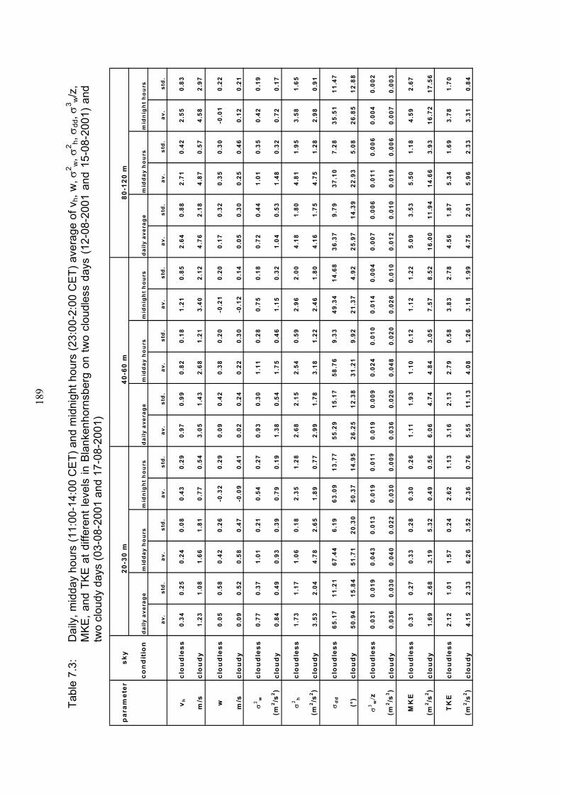
18

9

Tabl

e 7.

3:

Dai

ly, m

idda

y ho

urs

(11:

00-1

4:00

CE

T) a

nd m

idni

ght h

ours

(23:

00-2

:00

CE

T) a

vera

ge o

f vh,

w, σ

2 w, σ

2 h, σ d

d, σ3 w

/z,

MKE

, and

TK

E a

t diff

eren

t lev

els

in B

lank

enho

rnsb

erg

on tw

o cl

oudl

ess

days

(12

-08-

2001

and

15-

08-2

001)

and

tw

o cl

oudy

day

s (0

3-08

-200

1 an

d 17

-08-

2001

)

par

amet

ersk

y20

-30

m40

-60

m80

-120

m

con

dit

ion

dai

ly a

vera

ge

mid

day

ho

urs

m

idn

igh

t h

ou

rs

dai

ly a

vera

ge

mid

day

ho

urs

m

idn

igh

t h

ou

rs

dai

ly a

vera

ge

mid

day

ho

urs

m

idn

igh

t h

ou

rs

av.

std

.av

.st

d.

av.

std

.av

.st

d.

av.

std

.av

.st

d.

av.

std

.av

.st

d.

av.

std

.

v hcl

ou

dle

ss0.

340.

250.

240.

080.

430.

290.

970.

990.

820.

181.

210.

852.

640.

882.

710.

422.

550.

83

m/s

clo

ud

y1.

231.

081.

661.

810.

770.

543.

051.

432.

681.

213.

402.

124.

762.

184.

870.

574.

582.

97

wcl

ou

dle

ss0.

050.

580.

420.

26-0

.32

0.29

0.09

0.42

0.38

0.20

-0.2

10.

200.

170.

320.

350.

30-0

.01

0.22

m/s

clo

ud

y0.

090.

520.

580.

47-0

.09

0.41

0.02

0.24

0.22

0.30

-0.1

20.

140.

050.

300.

250.

460.

120.

21

σ2 w

clo

ud

less

0.77

0.37

1.01

0.21

0.54

0.27

0.93

0.30

1.11

0.28

0.75

0.18

0.72

0.44

1.01

0.35

0.42

0.19

(m2 /s

2 )cl

ou

dy

0.84

0.49

0.93

0.39

0.79

0.19

1.38

0.54

1.75

0.46

1.15

0.32

1.04

0.53

1.48

0.32

0.72

0.17

σ2 h

clo

ud

less

1.73

1.17

1.06

0.18

2.35

1.28

2.68

2.15

2.54

0.59

2.96

2.00

4.18

1.80

4.81

1.95

3.58

1.65

(m2 /s

2 )cl

ou

dy

3.53

2.04

4.78

2.65

1.89

0.77

2.99

1.78

3.18

1.22

2.46

1.80

4.16

1.75

4.75

1.28

2.98

0.91

σd

dcl

ou

dle

ss65

.17

11.2

167

.44

6.19

63.0

913

.77

55.2

915

.17

58.7

69.

3349

.34

14.6

836

.37

9.79

37.1

07.

2835

.51

11.4

7

(°)

clo

ud

y50

.94

15.8

451

.71

20.3

050

.37

14.9

526

.25

12.3

831

.21

9.92

21.3

74.

9225

.97

14.3

922

.93

5.08

26.8

512

.88

σ3 w

/z

clo

ud

less

0.03

10.

019

0.04

30.

013

0.01

90.

011

0.01

90.

009

0.02

40.

010

0.01

40.

004

0.00

70.

006

0.01

10.

006

0.00

40.

002

(m2 /s

3 )cl

ou

dy

0.03

60.

030

0.04

00.

022

0.03

00.

009

0.03

60.

020

0.04

80.

020

0.02

60.

010

0.01

20.

010

0.01

90.

006

0.00

70.

003

MK

Ecl

ou

dle

ss0.

310.

270.

330.

280.

300.

261.

111.

931.

100.

121.

121.

225.

093.

535.

501.

184.

592.

67

(m2 /s

2 )cl

ou

dy

1.69

2.68

3.19

5.32

0.49

0.56

6.06

4.74

4.84

3.05

7.57

8.52

16.0

011

.94

14.6

63.

9316

.72

17.5

6

TK

Ecl

ou

dle

ss2.

121.

011.

570.

242.

621.

133.

162.

132.

790.

583.

832.

784.

561.

875.

341.

693.

781.

70

(m2 /s

2 )cl

ou

dy

4.15

2.33

6.26

3.52

2.36

0.76

5.55

11.1

34.

081.

263.

181.

994.

752.

015.

962.

333.

310.

84

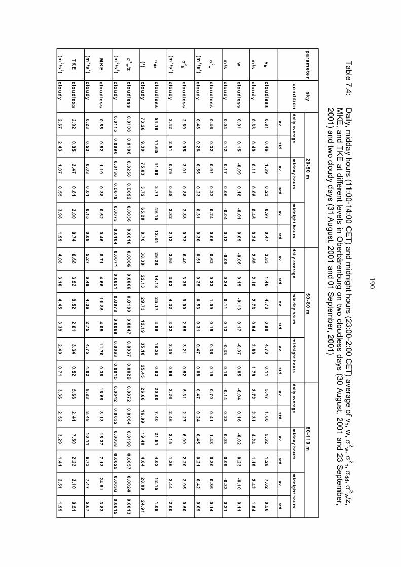
190

Table 7.4: D


ET) and m



, σ2w , σ

2h , σdd , σ

3w /z, M

KE, and TK

E at different levels in O

berbärenburg on two cloudless days (30 A

ugust, 2001 and 23 Septem

ber, 2001) and tw

o cloudy days (31 August, 2001 and 01 S

eptember, 2001)

param

etersky

20-50 m50-80 m

80-110 m

con

ditio

nd

aily average

mid

day h

ou

rs m

idn

igh

t ho

urs

daily averag

em

idd

ay ho

urs

mid

nig

ht h

ou

rs d

aily average

mid

day h

ou

rs m

idn

igh

t ho

urs

av.std

.av.

std.

av.std

.av.

std.

av.std

.av.

std.

av.std

.av.

std.

av.std

.

vh

clou

dless

0.810.46

1.390.23

0.970.47

3.831.46

4.730.90

4.700.11

5.471.60

5.321.28

7.020.56

m/s

clou

dy

0.330.40

0.110.05

0.460.24

2.692.10

2.730.94

2.601.79

3.722.31

4.241.19

3.421.94

wclo

ud

less0.01

0.15-0.09

0.18-0.01

0.09-0.06

0.15-0.13

0.17-0.07

0.05-0.04

0.16-0.02

0.23-0.10

0.11

m/s

clou

dy

0.040.12

0.170.06

-0.040.12

-0.090.24

0.110.13

-0.330.18

-0.140.23

0.030.09

-0.330.21

σ2w

clou

dless

0.460.32

0.910.22

0.240.06

0.620.33

1.090.19

0.360.19

0.700.41

1.430.30

0.360.14

(m2/s

2)clo

ud

y0.48

0.260.56

0.230.31

0.300.51

0.250.53

0.310.47

0.080.47

0.240.45

0.210.42

0.09

σ2h

clou

dless

2.690.95

3.010.88

2.880.73

6.403.39

9.002.55

3.210.52

5.312.27

6.902.20

2.950.50

(m2/s

2)clo

ud

y2.42

2.510.79

0.583.82

2.133.95

3.034.32

3.322.35

0.693.26

2.463.15

1.362.44

2.00

σd

dclo

ud

less54.19

11.6541.90

3.7149.15

12.8429.28

14.1825.17

3.8918.25

0.8320.00

7.4021.61

4.0212.15

1.09

(°)clo

ud

y73.26

9.3075.03

3.7265.28

8.7638.38

22.1329.73

12.1935.18

25.4526.66

16.9919.40

4.0428.09

24.91

σ3w

/ z clo

ud

less0.0108

0.01080.0258

0.00920.0036

0.00160.0086

0.00660.0180

0.00470.0037

0.00290.0072

0.00640.0190

0.00570.0024

0.0013

(m2/s

3)clo

ud

y0.0115

0.00900.0136

0.00790.0073

0.01040.0071

0.00510.0078

0.00680.0063

0.00150.0042

0.00320.0038

0.00250.0036

0.0015

MK

Eclo

ud

less0.55

0.521.19

0.380.62

0.468.71

4.6611.85

4.0511.70

0.3816.69

8.1315.37

7.1324.81

3.83

(m2/s

2)clo

ud

y0.23

0.530.03

0.010.15

0.085.27

6.494.36

2.754.75

4.028.83

8.4810.11

6.737.47

5.67

TK

Eclo

ud

less2.92

0.953.47

0.813.00

0.746.68

3.529.52

2.613.34

0.525.66

2.417.50

2.233.10

0.51

(m2/s

2)clo

ud

y2.67

2.431.07

0.553.98

1.994.08

3.104.45

3.392.40

0.713.36

2.523.29

1.412.51

1.99

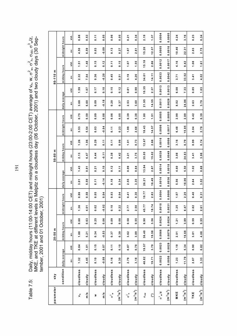
19

1

Tabl

e 7.

5:

Dai

ly, m

idda

y ho

urs

(11:

00-1

4:00

CE

T) a

nd m

idni

ght h

ours

(23:

00-2

:00

CE

T) a

vera

ge o

f vh,

w, σ

2 w, σ

2 h, σ d

d, σ3 w

/z,

MKE

, and

TK

E a

t diff

eren

t lev

els

in M

elpi

tz o

n a

clou

dles

s da

y (0

6 O

ctob

er, 2

001)

and

two

clou

dy d

ays

(30

Sep

-te

mbe

r, 20

01 a

nd 0

1 O

ctob

er, 2

001)

par

amet

ersk

y20

-50

m50

-80

m80

-110

m

con

dit

ion

dai

ly a

vera

ge

mid

day

ho

urs

m

idn

igh

t h

ou

rs

dai

ly a

vera

ge

mid

day

ho

urs

m

idn

igh

t h

ou

rs

dai

ly a

vera

ge

mid

day

ho

urs

m

idn

igh

t h

ou

rs

av.

std

.av

.st

d.

av.

std

.av

.st

d.

av.

std

.av

.st

d.

av.

std

.av

.st

d.

av.

std

.

v hcl

ou

dle

ss1.

320.

841.

880.

601.

360.

863.

011.

432.

131.

263.

530.

753.

681.

592.

321.

514.

500.

88

m/s

clo

ud

y4.

451.

015.

210.

634.

010.

585.

590.

916.

471.

065.

540.

596.

601.

077.

541.

486.

590.

53

wcl

ou

dle

ss0.

100.

150.

340.

250.

020.

050.

110.

210.

440.

290.

030.

090.

090.

170.

360.

150.

030.

11

m/s

clo

ud

y-0

.08

0.07

-0.0

30.

06-0

.02

0.04

-0.1

40.

10-0

.11

0.11

-0.0

40.

08-0

.18

0.10

-0.2

00.

12-0

.09

0.05

σ2 w

clo

ud

less

0.16

0.11

0.37

0.09

0.10

0.03

0.18

0.12

0.38

0.11

0.11

0.06

0.20

0.15

0.45

0.11

0.13

0.06

(m2 /s

2 )cl

ou

dy

0.30

0.10

0.39

0.08

0.22

0.04

0.34

0.11

0.42

0.06

0.23

0.05

0.37

0.12

0.51

0.15

0.27

0.05

σ2 h

clo

ud

less

2.79

0.87

3.62

0.58

2.77

0.41

2.55

0.99

3.21

1.01

1.99

0.39

2.53

0.81

3.19

1.07

1.97

0.21

(m2 /s

2 )cl

ou

dy

3.18

0.78

3.89

0.55

2.50

0.30

3.35

0.64

3.75

0.73

2.68

0.38

3.60

0.98

4.26

1.55

2.61

0.34

σd

dcl

ou

dle

ss46

.82

19.5

736

.40

6.90

45.7

719

.77

26.2

113

.94

35.0

512

.67

18.4

31.

8021

.95

10.3

534

.01

15.1

815

.20

2.19

(°)

clo

ud

y19

.71

3.79

19.5

83.

5618

.74

2.83

16.4

92.

8715

.02

2.66

14.5

71.

5114

.55

2.37

14.1

12.

8612

.37

1.37

σ3 w

/z

clo

ud

less

0.00

220.

0023

0.00

660.

0024

0.00

100.

0004

0.00

140.

0014

0.00

380.

0016

0.00

060.

0005

0.00

110.

0013

0.00

330.

0012

0.00

050.

0004

(m2 /s

3 )cl

ou

dy

0.00

560.

0028

0.00

790.

0024

0.00

310.

0008

0.00

360.

0018

0.00

490.

0008

0.00

170.

0005

0.00

280.

0013

0.00

420.

0017

0.00

160.

0005

MK

Ecl

ou

dle

ss1.

231.

192.

011.

211.

251.

075.

564.

603.

083.

166.

482.

998.

026.

083.

714.

1610

.46

4.24

(m2 /s

2 )cl

ou

dy

11.7

95.

3416

.68

3.89

8.47

2.25

18.0

65.

5024

.63

6.79

15.8

52.

8924

.86

7.33

33.5

29.

4222

.31

3.16

TK

Ecl

ou

dle

ss2.

870.

903.

810.

592.

820.

402.

641.

023.

410.

992.

040.

422.

630.

853.

411.

082.

030.

23

(m2 /s

2 )cl

ou

dy

3.33

0.82

4.08

0.55

2.61

0.31

3.52

0.68

3.98

0.74

2.79

0.39

3.79

1.03

4.52

1.61

2.75

0.34

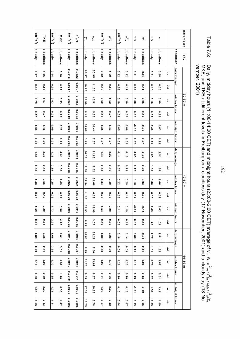
192

Table 7.6: D


ET) and m



, σ2w , σ

2h , σdd , σ

3w /z, M

KE, and TK

E at different levels in Freiburg on a cloudless day (17 N

ovember, 2001) and a cloudy day (18 N

o-vem

ber, 2001)

param

etersky

20-30 m40-60 m

60-80 m

con

ditio

nd

aily average

mid

day h

ou

rs m

idn

igh

t ho

urs

daily averag

em

idd

ay ho

urs

mid

nig

ht h

ou

rs d

aily average

mid

day h

ou

rs m

idn

igh

t ho

urs

av.std

.av.

std.

av.std

.av.

std.

av.std

.av.

std.

av.std

.av.

std.

av.std

.

vh

clou

dless

0.680.36

0.990.28

0.630.22

2.511.34

1.660.52

3.621.01

2.511.32

1.870.61

3.411.09

m/s

clou

dy

0.210.16

0.180.09

0.400.11

1.051.30

0.600.36

1.491.28

1.271.31

0.700.32

1.591.09

wclo

ud

less-0.03

0.110.06

0.10-0.09

0.07-0.05

0.090.03

0.09-0.14

0.13-0.03

0.110.06

0.13-0.10

0.06

m/s

clou

dy

0.010.07

0.080.08

-0.030.02

0.050.12

0.160.12

-0.020.07

0.080.15

0.190.13

-0.010.09

σ2w

clou

dless

0.120.11

0.300.07

0.060.02

0.150.11

0.290.14

0.190.11

0.140.09

0.230.10

0.150.07

(m2/s

2)clo

ud

y0.12

0.080.19

0.040.05

0.030.14

0.070.22

0.060.11

0.050.16

0.080.26

0.100.10

0.04

σ2h

clou

dless

1.500.58

1.520.27

1.430.27

2.220.76

2.400.38

2.200.60

2.280.69

2.790.66

2.220.42

(m2/s

2)clo

ud

y0.92

0.420.69

0.181.35

0.271.49

0.581.34

0.261.54

0.491.80

0.781.97

0.511.90

0.57

σd

dclo

ud

less50.95

11.0040.51

5.3650.44

7.0731.63

17.0234.66

6.0818.99

3.0731.27

17.0033.67

6.6720.23

3.78

(°)clo

ud

y68.57

10.7667.99

8.4858.66

3.4950.38

18.5852.54

11.1038.93

18.2346.85

18.4951.75

9.0537.39

16.75

σ3w

/ z clo

ud

less0.0022

0.00270.0066

0.00230.0006

0.00030.0014

0.00150.0034

0.00230.0018

0.00150.0008

0.00070.0017

0.00110.0009

0.0006

(m2/s

3)clo

ud

y0.0018

0.00170.0034

0.00100.0005

0.00040.0012

0.00080.0022

0.00090.0008

0.00050.0010

0.00080.0019

0.00100.0005

0.0003

MK

Eclo

ud

less0.30

0.270.53

0.280.22

0.134.01

3.561.49

0.816.96

4.204.01

3.611.92

1.106.33

4.42

(m2/s

2)clo

ud

y0.04

0.040.03

0.010.09

0.051.38

3.190.25

0.261.73

2.251.66

3.250.32

0.251.71

1.81

TK

Eclo

ud

less1.56

0.581.67

0.271.46

0.262.30

0.782.55

0.402.29

0.612.35

0.712.90

0.692.29

0.43

(m2/s

2)clo

ud

y0.97

0.390.79

0.171.38

0.261.56

0.581.46

0.251.59

0.461.89

0.792.10

0.501.95

0.55

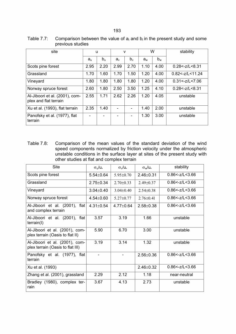
193

Table 7.7: Comparison between the value of ai and bi in the present study and some previous studies

u v W site

au bu av bv aw bw

stability

Scots pine forest 2.95 2.20 2.99 2.70 1.10 4.00 0.28<-z/L<8.31

Grassland 1.70 1.60 1.70 1.50 1.20 4.00 0.82<-z/L<11.24

Vineyard 1.80 1.80 1.80 1.80 1.20 4.00 0.31<-z/L<7.06

Norway spruce forest 2.60 1.80 2.50 3.50 1.25 4.10 0.28<-z/L<8.31

Al-Jiboori et al. (2001), com-plex and flat terrain

2.55 1.71 2.62 2.26 1.20 4.05 unstable

Xu et al. (1993), flat terrain 2.35 1.40 - - 1.40 2.00 unstable

Panofsky et al. (1977), flat terrain

- - - - 1.30 3.00 unstable

Table 7.8: Comparison of the mean values of the standard deviation of the wind

speed components normalized by friction velocity under the atmospheric unstable conditions in the surface layer at sites of the present study with other studies at flat and complex terrain

Site σu/u∗ σv/u∗ σw/u∗ stability

Scots pine forest 5.54±0.64 5.95±0.70 2.46±0.31 0.86<-z/L<3.66

Grassland 2.75±0.34 2.70±0.33 2.49±0.37 0.86<-z/L<3.66

Vineyard 3.04±0.40 3.04±0.40 2.54±0.38 0.86<-z/L<3.66

Norway spruce forest 4.54±0.60 5.27±0.77 2.76±0.41 0.86<-z/L<3.66

Al-Jiboori et al. (2001), flat and complex terrain

4.31±0.54 4.77±0.64 2.58±0.38 0.86<-z/L<3.66

Al-Jiboori et al. (2001), flat terrain(I)

3.57 3.19 1.66 unstable

Al-Jiboori et al. (2001), com-plex terrain (Oasis to flat II)

5.90 6.70 3.00 unstable

Al-Jiboori et al. (2001), com-plex terrain (Oasis to flat III)

3.19 3.14 1.32 unstable

Panofsky et al. (1977), flat terrain

- - 2.56±0.36 0.86<-z/L<3.66

Xu et al. (1993) 2.46±0.32 0.86<-z/L<3.66

Zhang et al. (2001), grassland 2.29 2.12 1.18 near-neutral

Bradley (1980), complex ter-rain

3.67 4.13 2.73 unstable

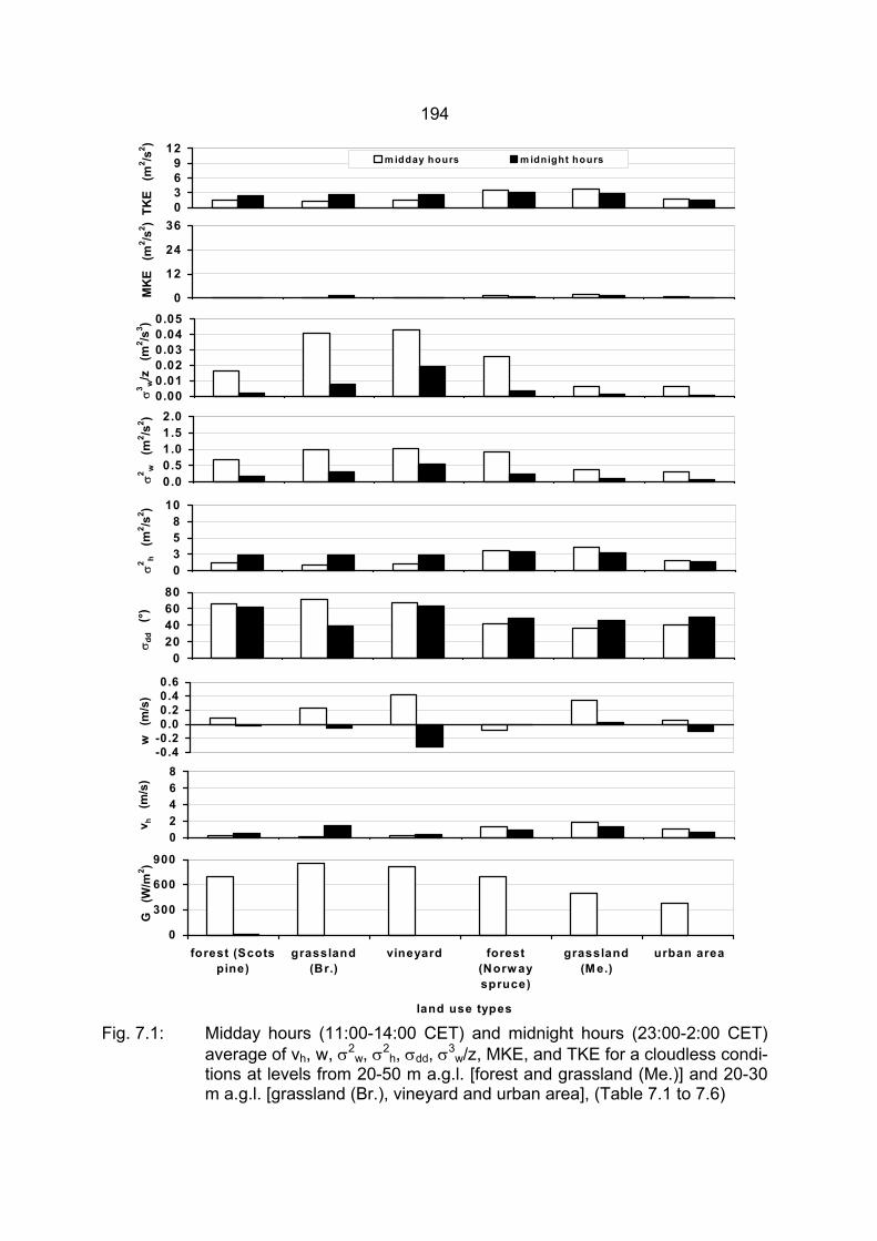
194

Fig. 7.1: Midday hours (11:00-14:00 CET) and midnight hours (23:00-2:00 CET) average of vh, w, σ2

w, σ2h, σdd, σ3

w/z, MKE, and TKE for a cloudless condi-tions at levels from 20-50 m a.g.l. [forest and grassland (Me.)] and 20-30 m a.g.l. [grassland (Br.), vineyard and urban area], (Table 7.1 to 7.6)

0369

12TK

E (

m2 /s

2 )m idday hours m idnight hours

0

12

24

36

MK

E (

m2 /s

2 )

0 .000.010.020.030.040.05

σ3 w/z

(m

2 /s3 )

0 .00.51.01.52.0

σ2 w

(m2 /s

2 )

0358

10

σ2 h (m

2 /s2 )

020406080

σ dd

(°)

-0 .4-0.20.00.20.40.6

w

(m/s

)

02468

v h

(m/s

)

0

300

600

900

forest (Scotspine)

grassland(Br.)

vineyard forest(Norw ayspruce)

grassland(M e.)

urban area

land use types

G

(W/m

2 )

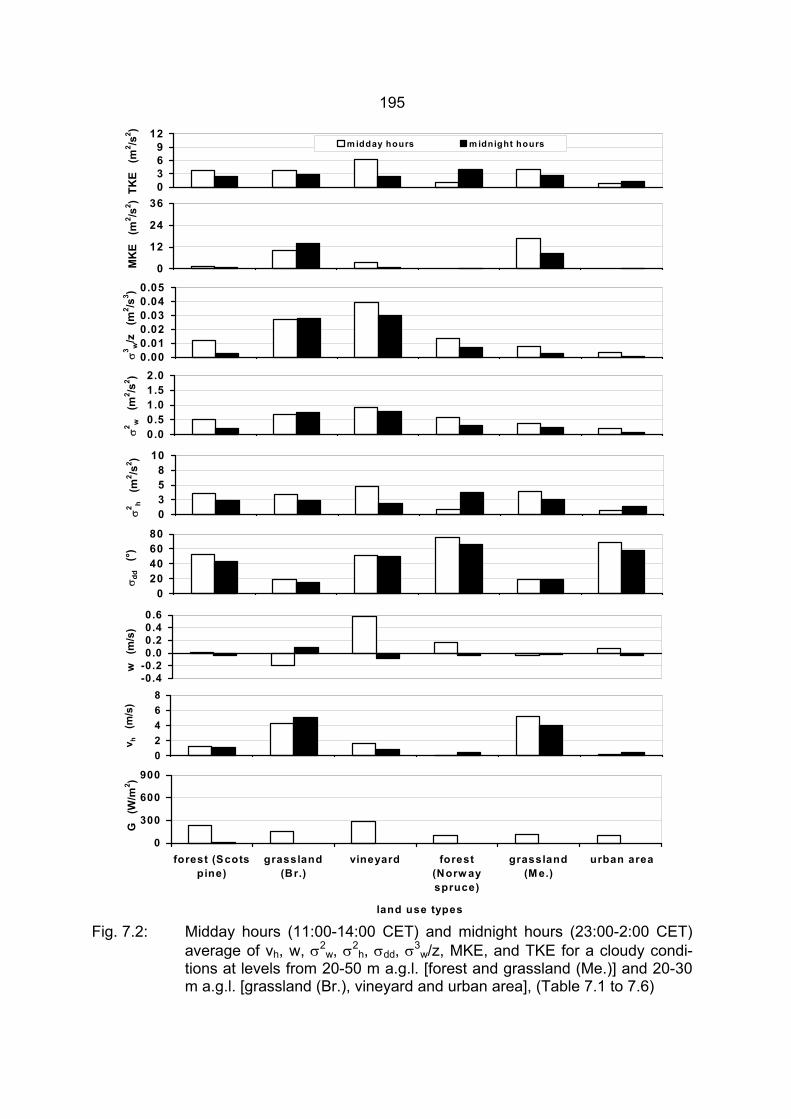
195


w, σ2h, σdd, σ3

w/z, MKE, and TKE for a cloudy condi-tions at levels from 20-50 m a.g.l. [forest and grassland (Me.)] and 20-30 m a.g.l. [grassland (Br.), vineyard and urban area], (Table 7.1 to 7.6)

0369

12TK

E (

m2 /s


0

12

24

36

MK

E (

m2 /s

2 )

0 .000.010.020.030.040.05

σ3 w/z

(m

2 /s3 )

0 .00.51.01.52.0

σ2 w

(m2 /s

2 )

0358

10

σ2 h (m

2 /s2 )

020406080

σ dd

(°)

-0.4-0.20.00.20.40.6

w

(m/s

)

02468

v h

(m/s

)

0

300

600

900

forest (Scotspine)

grassland(Br.)


grassland(M e.)

urban area

land use types

G

(W/m

2 )

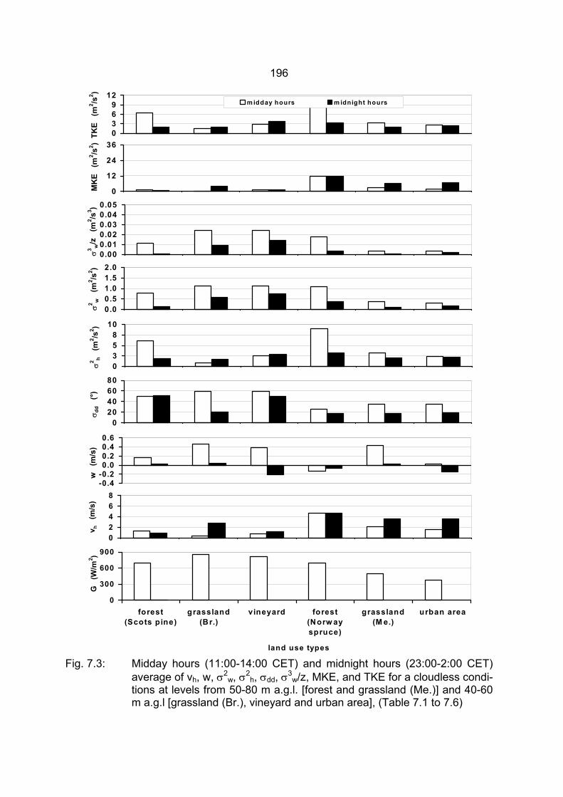
196


w, σ2h, σdd, σ3

w/z, MKE, and TKE for a cloudless condi-tions at levels from 50-80 m a.g.l. [forest and grassland (Me.)] and 40-60 m a.g.l [grassland (Br.), vineyard and urban area], (Table 7.1 to 7.6)

0369

12TK

E (

m2 /s


0

12

24

36

MK

E (

m2 /s

2 )

0 .000.010.020.030.040.05

σ3 w/z

(m

2 /s3 )

0 .00.51.01.52.0

σ2 w

(m2 /s

2 )

0358

10

σ2 h (m

2 /s2 )

020406080

σ dd

(°)

-0.4-0.20.00.20.40.6

w

(m/s

)

02468

v h

(m/s

)

0

300

600

900

forest(Scots pine)

grassland(Br.)


grassland(M e.)

urban area

land use types

G

(W/m

2 )

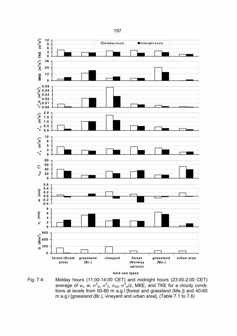
197


w, σ2h, σdd, σ3

w/z, MKE, and TKE for a cloudy condi-tions at levels from 50-80 m a.g.l [forest and grassland (Me.)] and 40-60 m a.g.l [grassland (Br.), vineyard and urban area], (Table 7.1 to 7.6)

0369

12TK

E (

m2 /s


0

12

24

36

MK

E (

m2 /s

2 )

0 .000.010.020.030.040.05

σ3 w/z

(m

2 /s3 )

0 .00.51.01.52.0

σ2 w

(m2 /s

2 )

0358

10

σ2 h (m

2 /s2 )

020406080

σ dd

(°)

-0.4-0.20.00.20.40.6

w

(m/s

)

02468

v h

(m/s

)

0

300

600

900

forest (Scotspine)

grassland(Br.)


grassland(M e.)

urban area

land use types

G

(W/m

2 )

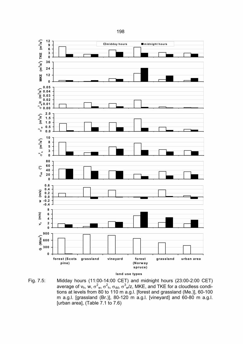
198


w, σ2h, σdd, σ3

w/z, MKE, and TKE for a cloudless condi-tions at levels from 80 to 110 m a.g.l. [forest and grassland (Me.)], 60-100 m a.g.l. [grassland (Br.)], 80-120 m a.g.l. [vineyard] and 60-80 m a.g.l. [urban area], (Table 7.1 to 7.6)

0369

12TK

E (

m2 /s


0

12

24

36

MK

E (

m2 /s

2 )

0 .000.010.020.030.040.05

σ3 w/z

(m

2 /s3 )

0 .00.51.01.52.0

σ2 w

(m2 /s

2 )

0358

10

σ2 h (m

2 /s2 )

020406080

σ dd

(°)

-0 .4-0.20.00.20.40.6

w

(m/s

)

02468

v h

(m/s

)

0

300

600

900

forest (S cotspine)

grassland vineyard forest(N orw ayspruce)

grassland urban area

land use types

G

(W/m

2 )

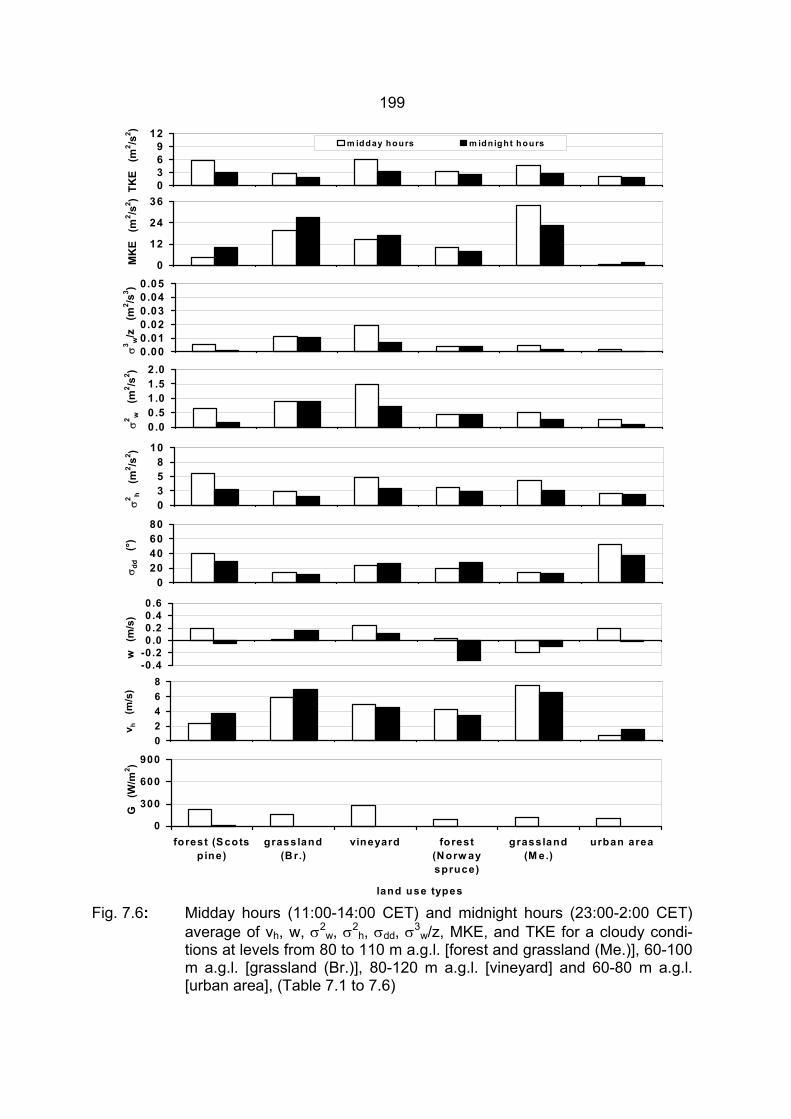
199


w, σ2h, σdd, σ3

w/z, MKE, and TKE for a cloudy condi-tions at levels from 80 to 110 m a.g.l. [forest and grassland (Me.)], 60-100 m a.g.l. [grassland (Br.)], 80-120 m a.g.l. [vineyard] and 60-80 m a.g.l. [urban area], (Table 7.1 to 7.6)

0369

12TK

E (

m2 /s


0

12

24

36

MK

E (

m2 /s

2 )

0 .000.010.020.030.040.05

σ3 w/z

(m

2 /s3 )

0 .00.51.01.52.0

σ2 w

(m2 /s

2 )

0358

10

σ2 h (m

2 /s2 )

020406080

σ dd

(°)

-0 .4-0.20.00.20.40.6

w

(m/s

)

02468

v h

(m/s

)

0

300

600

900

forest (S cotspine)

grassland(B r.)

vineyard forest(N orw ayspruce)

grassland(M e.)

urban area

land use types

G

(W/m

2 )

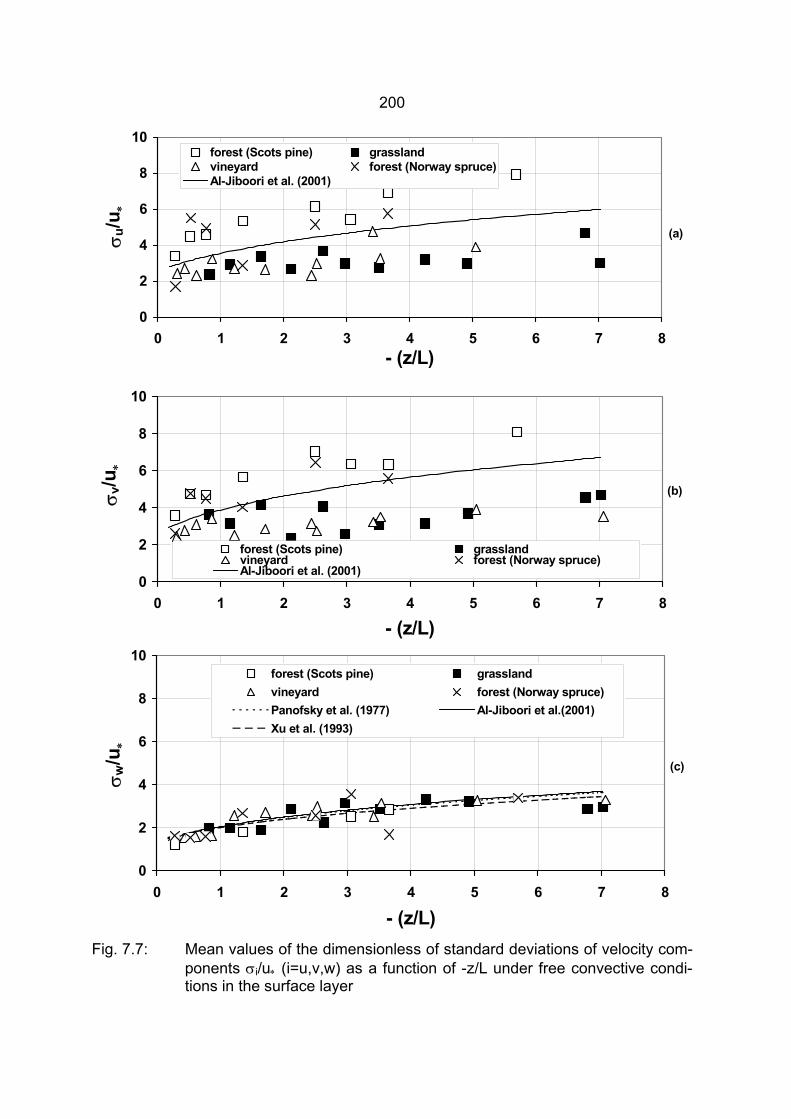
200

Fig. 7.7: Mean values of the dimensionless of standard deviations of velocity com-ponents σi/u∗ (i=u,v,w) as a function of -z/L under free convective condi-tions in the surface layer

0

2

4

6

8

10

0 1 2 3 4 5 6 7 8- (z/L)

σ u/u

∗

forest (Scots pine) grasslandvineyard forest (Norway spruce)Al-Jiboori et al. (2001)

(a)

0

2

4

6

8

10

0 1 2 3 4 5 6 7 8

- (z/L)

σ w/u

∗

forest (Scots pine) grasslandvineyard forest (Norway spruce)Panofsky et al. (1977) Al-Jiboori et al.(2001)Xu et al. (1993)

(c)

0

2

4

6

8

10

0 1 2 3 4 5 6 7 8

- (z/L)

σ v/u

∗

forest (Scots pine) grasslandvineyard forest (Norway spruce)Al-Jiboori et al. (2001)

(b)

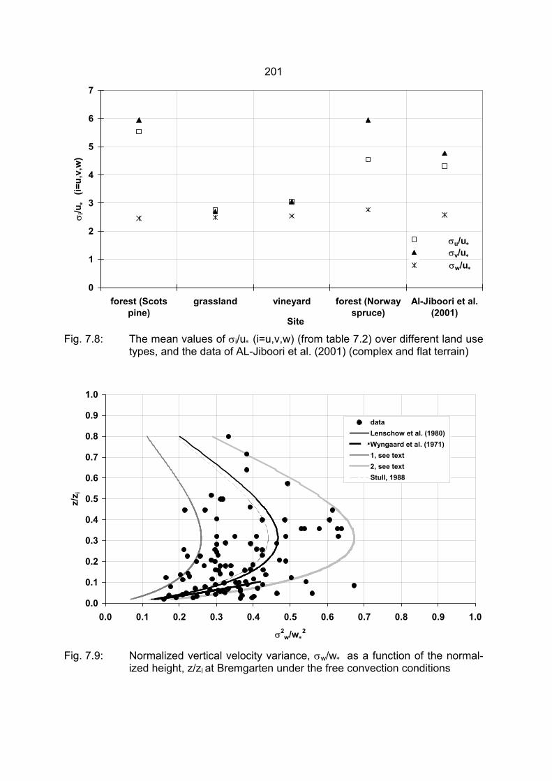
201

Fig. 7.8: The mean values of σi/u∗ (i=u,v,w) (from table 7.2) over different land use types, and the data of AL-Jiboori et al. (2001) (complex and flat terrain)

Fig. 7.9: Normalized vertical velocity variance, σw/w∗ as a function of the normal-ized height, z/zi at Bremgarten under the free convection conditions

0

1

2

3

4

5

6

7

forest (Scotspine)

grassland vineyard forest (Norwayspruce)

Al-Jiboori et al.(2001)

Site

σ i/u

∗ (

i=u,

v,w

)

σu/u∗

σv/u∗

σw/u∗

0.0

0.1

0.2

0.3

0.4

0.5

0.6

0.7

0.8

0.9

1.0

0.0 0.1 0.2 0.3 0.4 0.5 0.6 0.7 0.8 0.9 1.0

σ2w/w∗

2

z/z i

dataLenschow et al. (1980)Wyngaard et al. (1971)1, see text2, see textStull, 1988

202

8 CONCLUSIONS

The Scintec FAS64 sodar was used to study the influence of thermal and roughness

changes on the characteristics of the turbulent parameters such as turbulent kinetic

energy per unit mass (TKE), turbulence intensity components (Iu, Iv, Iw), and the mean

values of the normalized (by the friction velocity) standard deviations of the velocity

components, σi/u∗ (i=u,v,w) over different land use types such as grassland, forest

vineyard and urban sites. To explain the influence of thermal and roughness changes

on the characteristics of these parameters, the characteristics of incoming solar radia-

tion (G), wind direction (dd) and its standard deviation (σdd), horizontal and vertical wind

speed components (vh and w respectively), and the variances of horizontal and vertical

wind speed components (σ2h and σ2

w) are briefly discussed for the whole study sites

through the periods of the measurements. The importance of these measurements for

this study are due to their effects in the turbulence of the atmosphere. As reported in

Stull (2000), during weak advection, the nature of convection and turbulence are con-

trolled by the wind speed, incoming solar radiation (insulation) cloud shading and time

of day and night.

Besides directly monitoring such meteorological variables as vh, w, dd, σdd, σh and σw,

the application of a number of methods and algorithms enabled the estimation of fea-

tures of the atmospheric turbulence such as Pasquill-Gifford (P-G) stability classes,

Monin-Obukhov length (L), friction velocity (u∗), and convective velocity scale (w∗). In

particular, a typical sodar-related method has been used to classify atmospheric stabil-

ity over the sites of the study through the periods of the measurements (except for

Freiburg). The variable used σdd was used to determine the P-G stability classes ac-

cording to Thomas (1988). Such a stability classification is the first step for applying a

number of traditional algorithms aiming at estimating the main atmospheric parameters

which typically describe the ABL structure such as L, u∗ and zi. For every site of the

study the following results were obtained:

∗∗ characteristic of the global solar radiation G received on a horizontal surface on

two cloudless and two cloudy days (except for Melpitz: one cloudless day and

two cloudy days, and Freiburg: one cloudless day and one cloudy day),

∗∗ wind roses at different levels during the period of the study,

203

∗∗ atmospheric stability classification at different levels,

∗∗ profiles of dd, σdd, vh, w, σ2h, σ2

w, σ3w/z, MKE and TKE under various atmos-

pheric conditions (stable, neutral and unstable) in the range from 20 to 500 m

a.g.l. (except for Oberbärenburg, there was not enough result). But at Freiburg

the weather was cloudy, rainy and foggy most of the time during the measure-

ment campaign from 16 November, 2001 to 19 November, 2001. Thus, no sodar

data are available in the range above 100 m a.g.l.,

∗∗ diurnal course of two days mean of σdd, vh, w, σ2h, σ2

w, σ3w/z, MKE and TKE in

cloudless and cloudy sky conditions (except for: Melpitz; with one cloudless day

and two cloudy days and Freiburg; with one cloudless day and one cloudy day),

∗∗ characteristics of the turbulence intensity components (Iu, Iv, Iw) over the study

areas for various fetch conditions arising under various wind direction and differ-

ent atmospheric stability at different levels (except for Freiburg: there was not

enough result),

∗∗ behavior of the relationship between the standard deviations of the velocity

components normalized by the u∗, σi/u∗ (i=u,v,w) and z/L in the surface layer

under the unstable atmospheric conditions (except for Melpitz and Freiburg),

∗∗ variation of the normalized (by the square value of the convective velocity, w∗2)

variance of the vertical wind speed component, σ2w,/w∗

2, with the normalized (by

the mixing height) height, z/zi.

This study yielded the following results:

∗∗ By using sodar data only, the atmospheric stability according to P-G stability

classification was quantified at different levels at Hartheim, Bremgarten,

Blankenhornsberg, Oberbärenburg, and Melpitz through the periods of the stud-

ies. If one considers the period of the year for every site these results seem reli-

able.

∗∗ The profile of σ3w/z under the various stability conditions (neutral, stable and un-

stable) showed a decline with the height a.g.l.. This is due to the increasing of

the mechanical and buoyancy turbulence production which is intensively present

in the surface layer.

204

∗∗ The values of the quantity σ3w/z, at the cloudless conditions, throughout the

night, were low even in the presence of wind shear. This reflects the effect of the

incoming solar radiation of σ3w/z which appears in the daytime, especially when

the value of the wind speed is relatively small. As well this effect could be obvi-

ously seen in the comparison of the difference between the average values of

σ3w/z at the midday hours (11:00-14:00 CET) and midnight hours (23:00-02:00

CET) on cloudless conditions. But on the cloudy conditions, the role of the me-

chanical turbulence increases, especially when the value of the horizontal wind

speed is relatively high.

∗∗ Under neutral conditions, the variations of the roughness over the study areas

for various fetch conditions arising for various wind directions have impact on the

turbulence intensity components (Iu, Iv, Iw). This behavior appeared qualitatively

by the study of the variation of the Iu, Iv and Iw with the angular sectors at

Bremgarten, Blankenhornsberg, Oberbärenburg and Melpitz. But at Hartheim

and Freiburg there is no enough data to do this study.

∗∗ The turbulence intensity components (Iu, Iv, Iw) showed dependence on P-G sta-

bility classes and increase with increasing of instability. This behavior was illus-

trated qualitatively by the study of the variation of the Iu, Iv and Iw with the P-G

stability classes over Hartheim, Bremgarten, Blankenhornsberg, Oberbärenburg

and Melpitz. But at Freiburg there is no enough data to do this study. To reduce

the effect of the change of the roughness, this relationship has been investigated

at small angular sector (30°). The turbulence intensities for horizontal compo-

nents increased faster with increasing instability incomparable with vertical com-

ponent.

∗∗ The turbulence intensity components (Iu, Iv, Iw) decreased with the increasing of

the height of the observation. This dependence was determined by the study of

the characteristics of Iu, Iv and Iw for various fetch conditions arising under vari-

ous wind directions, and different atmospheric stability at different level.

∗∗ Under unstable conditions, the mean values σu/u∗, σv/u∗ and σw/u∗ are functions

of (z/L)1/3. σu/u∗ and σv/u∗ are strongly affected by the change in the surface

roughness. In the range of -z/L (0.86 to 3.66), σu/u∗ and σv/u∗ over the grassland

205

site were approximately in the same magnitude as over the vineyard site, but

they were smaller (34% and 52% respectively) than those observed over forest.

But the change of surface roughness does not seem to influence the properties

of σw/u∗.

∗∗ The profile of the normalized (by the square value of the convective velocity w2∗)

variance of the vertical wind speed component, σ2w/w∗

2 under the free convec-

tive conditions over grassland (Bremgarten) increases with the height to reach

the maximum equal to 0.46 within the mixed layer at z = 0.32 zi. After that these

values decrease with the height to reach a very small values. The behavior of

this results is similar to most data in the literatures (For example: Argentini et al.,

1999; Hibber and Sawford, 1994; Lenschow and Wyngaard, 1980).

All these above conclusions indicate that this study has given a quantitatively variation

of the effect of the thermal and roughness change in some turbulence parameters such

as σu/u∗, σv/u∗ and σw/u∗ in the surface layer over grassland, vineyard and forest under

unstable conditions. In addition, a qualitatively variation of the effect of the thermal and

roughness change in the intensity components (Iu, Iv, Iw) in the surface layer and the

lower part of the mixed layer over grassland, vineyard and forest under the all stability

conditions (neutral, stable and unstable). Furthermore, It determined the height at

which σw is maximum (0.32 zi) under the free convective conditions over grassland

(Bremgarten). This study can be resumed to investigate quantitatively the following:

∗∗ the relationship between the turbulence intensity components Iu, Iv and Iw and z0

under the neutral stability conditions,

∗∗ the relationship between the turbulence intensity components Iu, Iv and Iw and

z/L at different z/z0 over flat and complex terrain,

∗∗ the dependence of σu/u∗, σv/u∗ and σw/u∗ on the thermal and roughness change

under neutral and near-neutral stability conditions,

∗∗ some terms in the turbulence kinetic energy (TKE) budget such as dissipation

rate, buoyancy production, shear production and vertical transport of the TKE

over flat and complex terrain,

206

∗∗ the characteristics of normalized (by variance / covariance) spectra / cospectra

of the wind speed components and some turbulence parameters.

207

REFERENCES Ahrens, C. D., 1994: Meteorology today: An introduction to weather, climate, and the

environment. Fifth edition. New York, West Publishing Company. Al-Jiboori, M. H.; Xu, Y.; Yongfu, Q., 2001: Turbulence characteristics over complex

terrain in west China. Boundary Layer Meteorol., 101, 109-126. Appleton, E. V.; Barnett, M. A. F., 1925: On some direct evidence for downward at-

mospheric reflection of electric rays. Proc. R. Soc. London, A109, 621-640. Argentini, S.; Mastrantonio, G.; Lena, F., 1999: Case studies of the winter time convec-

tive boundary layer structure in the urban area of Milan, Italy. Boundary Layer Me-teorol., 93, 253-267.

Asimakopoulos, D. N.; Cole, R. S.; Crease, B. A.; Caughey, J., 1978: A comparison of acoustic Doppler vertical velocity power spectra with direct measurements. Atmos. Environ., 12, 1951–1956.

Atmospheric Research Pty Ltd, 2000: SODAR. http://www. a-research. com. au/ Axel, A.; Klug, H., 1995: The use of sodars in respect to wind energy applications.

DEWI-Magazin, 7, 57-61. Balser, M.; McNary, C. A.; Nagy, A. E.; Loveland, R.; Dickson, D., 1976: Remote wind

sensing by acoustic radar. J. Appl. Meteorol., 15, 50–58. Batchelor, G. K., 1957: Wave scattering due to turbulence. In: Symp. on Naval

Hydraulics (Ed.: F. S. Sherman), National Academy of Sciences, Washington, D. C., 409-423.

Bennet, M.; Saab, A. E., 1982: Modeling of the urban heat island and of its interaction with pollutant dispersal. Atmos. Environ.,16, 1797-1822.

Beran, D. W.; Hall, F. F.; Wescott, Jr. J. W.; Neff, W. D., 1972: Application of an acous-tic sounder to air pollution monitoring . In: Proc. Symp. on air pollution turbulence and diffusion (Eds.: H. W. Church; R. E Luna), Sandia Laboratories, Albuquerque.

Best, P. R.; Kanowski, M.; Stumer, L.; Green, D., 1986: Convective dispersion model-ing utilizing acoustic sounder information. Atmos. Res., 20.

Beyrich, F., 1996: Mixing height estimation from sodar data-a review. In: Proc. 8th int. Symp. on acoustic remote sensing and associated techniques of the atmosphere and oceans, Moscow, Russia, May 27-31.

Beyrich, F., 1997a: Mixing height determination using remote sensing systems -general remark. In: The determination of the mixing Height – Current progress and prob-lems (Eds.: S. E. Gryning; F. Beyrich; E. Batchvarova), EURASAP Workshop pro-ceedings, RisØ National Laboratory, 71-74.

Beyrich, F., 1997b: Mixing height estimation from sodar data – a critical discussion. Atmos. Environ., 31, 3941-3953.

Blokhintzev, D., 1946a: The propagation of sound in an inhomogeneous and moving medium I, II, Acoustic. Soc. Amer., 18, 322-334.

208

Blokhintzev, D., 1946b: Acoustics of inhomogeneous moving medium. 2nd Ed. Moscow, Nauka, 206, (in Russian).

Bradley, E. F., 1980: An experimental study of the profiles of the wind speed, shearing stress and Turbulence at the crest of a large hill. Q. J. Roy. Meteorol., Soc., 106, 101-124.

Brook, R. R., 1972: The measurement of turbulence in a city environment. J. Appl. Me-teorol., 11, 443-450.

Brown, E. H., 1987: Atmospheric acoustics. Encyclopedia of Physical Science and Technology, 2, 147-163.

Brown, E. H.; Hall, F. F., 1978: Advances in atmospheric acoustics. Rev. Geophys. and Space Phys., 16, 47-110.

Caughey, S. J., 1982: In: Atmospheric turbulence and air pollution Modeling (Eds.: F.T.M. Nieuwstadt; H. Van Dop), Reidel, Dordrecht, 107-158.

Caughey, S. J.; Crease, B. A.; Asimakopoulos, D. N.; Cole, R. S., 1976: A comparison of acoustic Doppler vertical velocities with direct measurements in the atmos-pheric boundary layer. Nature, 262, 274–276.

Chadwick, R. B.; Gossard, E. E., 1986: Radar probing and measurement of the plane-tary boundary layer. In: Probing the atmospheric boundary layer (Ed.: D. H. Len-schow), Boston, Amer. Meteorol. Soc., 201-239.

Chintawongvanich, P.; Olsen, R.; Biltoft, C. A., 1989: Intercomparison of wind meas-urements from two acoustic Doppler sodars, a laser Doppler lidar, and in situ sen-sors. J. Atmos. Oceanic Technol., 6, 785–797.

Capanni, A.; Gualtieri, G., 1999: Sodar application for estimating boundary layer pa-rameters. In: Proc. EUROPTO series: Optics in atmospheric propagation and adaptive systems III. Florence, Italy, Sept., 23-24.

Capanni, A.; Gualtieri, G.; Meneguzzo, F.; Zipoli, G., 1999: Sodar Un metodo di classi-ficazione della stabilità basto su misure sodar. Rivista italiana di Telerilevamento, 14/15, 3-12 (in Italian).

Clarke, J. F.; Ching, J. K. S.; Godowitch, J. M., 1982: An experimental study of turbu-lence in urban environment. Tech. Rep. U. S. E. P. A., Research Triangle Park, N. C., NMS PB 226085.

Congeduti, F.; Fiocco, G.; Adriani, A.; Guarrella, C., 1981: Vertical wind velocity meas-urements by a Doppler lidar and comparisons with a Doppler sodar. Appl. Opt., 20, 2048–2054.

Coulter, R. L, 1998: The place for sodars in a high-technology environment. In: Proc. 9th Int. Symp. on acoustic remote sensing of the atmosphere and oceans (Ed.: E. Murch-Radlgruber; P. Seibert), Vienna, Austria, July, 6-10.

Delany, M. E., 1977: Sound propagation in the atmosphere- a historical review. Acustica, 38, 201-223.

DIN-VDI, 1999: Environmental meteorology, determination of the vertical wind prophile by Doppler sodar systems. In: Part I- Wind, air temperature, air humidity and pre-cipitation. Handbock, Berlin, Beuth Verlag, VDI, 3786, 212-231.

209

Driedonks, A. G. M.; Tennekes, H., 1984: Entrainment effects in the well-mixed atmospheric boundary layer. Boundary Layer Meteorol., 30, 75-105.

Eltermann, L., 1951: The measurement of stratospheric density distribution with the searchlight technique. J. Geophys. Res., 56, 509-520.

Emeis, S., 2001: Vertical variation of frequency distributions of wind speed in and above the surface layer observed by Sodar. Meteorol. Z., 10, 141-149.

Finkelstein, P. L.; Kaimal, J. C.; Gaynor, J. E.; Graves, M. E.; Lockhart, T. J., 1986b: Comparison of wind monitoring systems. Part II: Doppler sodars. J. Atmos. Oce-anic Technol., 3, 594–604.

Fiocco, G.; Smullin, L. D., 1963: Detection of scattering layers in upper atmosphere. Nature, 199, 1275-1276.

Founda, D.; Tombrou, M.; Lalas, D.P.; Asimakopoulos, D. N., 1997: Some measure-ments of turbulence characteristics over complex terrain. Boundary Layer Meteo-rol., 83, 221-245.

Garratt, A. J., 1992: The atmospheric boundary layer. Cambridge, University Press. Gaynor, J. E., 1992: Quantifying errors in sodar wind variance measurements. Proc.

Sixth Int. Symp. on Acoustic Remote Sensing, Athens, Greece, Int. Soc. Acoust. Remote Sens., 47–52.

Gaynor, J. E., 1994: Accuracy of sodar wind variance measurements. Int. J. Remot. Sens., 15, 313–324.

Gaynor, J. E., Korrell, J. A., 1981: Instrument intercomparisons at the Boulder Atmos-pheric Observatory during 1980. NOAA Tech. Memo. ERL WPL-69, 38 pp. [Avail-able from National Technical Information Service, 5285 Port Royal Road, Spring-field, VA 22161.]

Gaynor, J. E., Kristensen, L., 1986: Errors in second moments estimated from monostatic Doppler sodar winds. Part II: Application to field measurements. J. At-mos. Oceanic Technol., 3, 529–534.

Gaynor, J. E.; Baker, C. B.; Kaimal, J. C., 1990: The international sodar Intercompari-son experiment. Proc. Fifth Int. Symp. on Acoustic Remote Sensing, New Delhi, India, Int. Soc. Acoust. Remote Sens., 67–74.

Gilman, G. W.; Coxhead, H. B.; Willis, F. H., 1946: Reflection of sound signals in the troposphere. J. Acoust. Soc. Amer., 18, 274-283.

Gland, H., 1980: Experiments with a Doppler sounder. Report HE/32-80. 24, French electricity board, department of aquatic and atmospheric environment, division of applied Meteorology and air pollution, Paris, France, 35.

Gland, H., 1981: Qualifying test on a three dimensional Doppler sodar. Report HE/32-81. 9, French electricity board, department of aquatic and atmospheric environ-ment, division of applied Meteorology and air pollution, Paris, France, 35.

Görsdorf, U.; Beyrich, F.; Dier, H.; Leiterer, U., 2002: Composite wind and temperature profiles obtained from a complex of in-situ and remote sensing measurement sys-tems for the forcing of a boundary layer model. Theor. Appl. Climatol., 73, 97-105.

210

Graber, W. K., 1993: Sodar monitoring of the atmosphere – recent developments. Appl. Phys. B, 57, 1-2.

Greenhut, G. K.; Mastrantonio, G., 1989: Turbulence kinetic energy budget profiles de-rived from Doppler sodar measurements. J. Appl. Meteorol., 28, 99-106

Crescenti, G., H., 1997: A Look back on two decades of Doppler Sodar comparison studies. Bulletin of the Amer. Meteorolo., Soc., 78, 651- 673.

Gryning, S.; Beyrich, F.; Batchvarova, E., 1997: The determination of mixing height- Current progress and problems. EURASAP Workshop proceedings. RisØ National laboratory, October, 1-3.

Hall, F. F.; Wescott, J. W., 1974: Acoustic Antennas for atmospheric echo sounding. J. Acoustic. Soc. Amer., 56, 1376-1382.

Hardy, K. R.; Atlas, D.; Glover, K. M., 1966: Multi-wavelength back-scatter from the clear atmosphere. J. Geophys. Res., 71, 1537-1552.

Harris, C. M., 1963: Absorption of sound in air in the audio-frequency range. J. Acous-tic. Soc. Amer., 35, 11-17.

Harris, C. M., 1966: Absorption of sound in air versus humidity and temperature. J. Acoustic. Soc. Amer.,40, 148-159.

Haugen, D. A., 1973: Workshop on micrometeorology. Amer. Meteorol. Soc., Boston, 34-52.

Helmis, C. G.; Asimakopoulos, D. N.; Cole, R. S., 1985: A low-level atmospheric verti-cal velocity comparison between a high-resolution acoustic sounder and a turbu-lence probe. IEEE Trans. Geosci. Remote Sens., GE-23, 164–170.

Hibberd, M. F.; Sawford, B. L., 1994: A saline laboratory model of the planetary convective boundary layer. Boundary-Layer Meteorol., 67, 229-250.

Högström, U.; Bergström, H.; Alexandersson, H., 1982: Turbulence characteristics in a near neutrally stratified urban atmosphere. Boundary Layer Meteorol., 23, 229-250.

Højstrup, J., 1981: A simple model for the adjustment of velocity spectra in unstable conditions downstream of an abrupt change in roughness and heat flux. Boundary Layer Meteorol., 21, 341-356.

Højstrup, J., 1982: Velocity spectra in the unstable planetary boundary layer. J. atmos. Sci., 39, 2239-2248.

Ingard, U., 1953: A review of the influence of meteorological conditions on sound propagation. J. Acoustic. Soc. Amer., 25, 405.

Irwin, J. S., 1979: Estimating plume dispersion: A recommended generalised scheme. In: Proc. of the 4th AMS Symp. on turbulence and diffusion, Reno, NE, USA.

Ito, Y.; Kobori, Y.; Horiguchi, M.; Takehisa, M.; Mitsuta, Y.,1989: Development of wind profiling sodar. Atmos. Oceanic Technol., 6, 779-784.

Ito, Y., 1997a: Design of a Tri-Monostatic Doppler sodar system. In: Acoustic remote sensing applications (Ed.: S. P. Singal), New Delhi, India, Narosa Publishing House, 85-105.

211

Ito, Y., 1997b: Errors in wind measurements estimated by five-beam phased array Doppler sodar. J. Atmos. Oceanic Technol., 14, 792-801.

Jacobson, M. Z., 1999: Fundamentals of atmospheric modelling. London, Cambridge University Press.

Kaimal, J. C.; Finnigan, J. J., 1994: Atmospheric boundary layer and flows, their struc-ture and measurement. Oxford University Press.

Kaimal, J. C.; Baynton, B., N.; Gaynor, J. E., 1980: The Boulder low-level intercompari-son experiment. BAO Rep. 2, Wave Propagation Laboratory, NOAA/ERL, 189 pp. [Available from National Technical Information Service, 5285 Port Royal Road, Springfield, VA 22161.].

Kaimal, J. C.; Wyngaard, J. C.; Izumi, Y.; Coté, O. R., 1972: Spectra characteristics of surface layer turbulence. Q. J. Roy. Meteorol. Soc., 98, 563-589.

Kaimal, J. C.; Gaynor, J. E.; Finkelstein, P. L.; Graves, M. E.; Lockhart, T. J., 1984: An evaluation of wind measurements by four Doppler sodars. BAO Rep. 5, Wave Propagation Laboratory, NOAA/ERL, 110 pp. [Available from National Technical Information Service, 5285 Port Royal Road, Springfield, VA22161.]

Kallistratova, M. A., 1994: Acoustic and radio-acoustic remote sensing studies in C:I:S: (Former U:S:S:R:)-current statues. Int. J. Remot. Sens., 15, 251-266.

Kallistratova, M. A., 1997: Physical grounds for acoustic remote sensing of the atmos-pheric boundary layer. In: Acoustic remote sensing applications (Ed.: S. P. Sin-gal), New Delhi, India, Narosa Publishing House, 3-34.

Kallistratova, M. A., 2000: Propagation and scattering of acoustic waves in turbulent atmospheres. In: Proc. 10th Int. Symp. on acoustic remote sensing of the atmos-phere and oceans (Ed.: S. Bradley), Auckland, New Zealand, November, 27- De-cember,1.

Kallistratova, M. A., 2002: The role of ISARS Symposiums in development of acoustic sounding of the atmosphere (Review). In: Proc. 11th Int. Symp. on acoustic remote sensing of the atmosphere and oceans (Eds.: S. Argentini; G. Mastrantonio; I. Pe-tenko,), Rome, Italy, June, 24-28.

Kallistratova, M. A.; Keder, J.; Petenko, I. V., Tieme, N., 1985: Average wind velocity profile measurements by a sodar anemometer [Doppler sounder] in the lower tro-posphere under inversion and convective conditions. Izv. Atmos. Oceanic Phys., 21, 380–383.

Kallistratova, M. A.; Petenko, I. V.; Shurygin, Y. A., 1987: Sodar studies of the wind velocity field in the lower troposphere. Izv. Atmos. Oceanic Phys., 23, 339–346.

Kalthoff, N., 2003: Das Sodar als Messsystem zur Analyse mesoskaliger meteorologi-scher Phänomene. Prepr. 2. Fachgespräch Sodar, 19:/20. März 2003, Neuher-berg, BfS-ISH (in German).

Kazanski, A. B.; Monin, A. S., 1960: A turbulent regime above the ground atmosphere layer. Bull. (Izv.) Acad. Sci. USSR, Geophys. Ser. 110-12.

Kazanski, A. B.; Monin, A. S., 1961: On the dynamic interaction between the atmos-phere and Earth’s surface. Bull. (Izv.) Acad. Sci. USSR, Geophys. Ser., 514-15.

212

Keder, J., Foken, T.; Gerstmann, W; Schindler, V., 1989: Measurement of wind pa-rameters and heat flux with the Sensitron Doppler sodar. Boundary Layer Meteo-rol., 46, 195–204.

Khanna, S.; Brasseur, J. G., 1998: Three dimensional buoyancy and shear induced local structure of atmospheric boundary layer. J. Atmos. Sci., 55, 710-743.

Kleppe, J. A., 1997: An overview of the technological development of atmospheric echosounders. In: Acoustic remote sensing applications (Ed.: S. P. Singal), New Delhi, India, Narosa Publishing House, 35-85.

Kraichnan, R. H., 1953: The scattering of sound in a turbulent medium. J. Acoustic. Soc. Amer., 25, 1096-1104.

Kramer, V., F.; Kouznetsov, R. D., 2002: A new concept for estimation of turbulent pa-rameter profiles in the ABL using sodar data. J. Atmos. Oceanic Technol., 19, 1216-1224.

Kristensen, L.; Gaynor, J. E., 1986: Errors in second moments estimated from monostatic Doppler sodar winds. Part I: Theoretical description. J. Atmos. Oceanic Technol., 3, 523–528.

Kurzeja, R. J., 1994: Comparison of a Doppler sodar with bivanes and cup anemome-ters. J. Atmos. Oceanic Technol., 11, 192–199.

Lalas, D. P.; Asimakopoulos, D. N.; Deligiorgi, D. G; Helmis, C. G., 1983: Sea breeze circulation and photochemical pollution in Athens, Greece. Atmos. Environment, 17, 1621-1632.

Lenschow, D. H.; Wyngaard, J. C. ,1980: Mean-Field and second-moment budgets in a baroclinic, convective boundary layer. J. Atmos. Sci., 37, 1313-1326.

Lettau, H., 1969: Note on aerodynamic roughness –parameter estimation on the basis of roughness-element description. J. Appl. Meteorol., 8, 828-832.

Lighthill, M. J., 1953: On the energy scattered from the interaction of turbulence with sound or shock waves. Proc. Cambridge Phil. Soc., 49, 531-555.

Little, C. G., 1969: Acoustic methods for the remote probing of the lower atmosphere. Proc. IEEE, 57, 571-578.

Liu, M.; Whitney, D.C.; Roth, P.M., 1976: Effects of atmospheric parameters on the concentration of photochemical air pollutants. J. Appl. Meteorol., 15, 829-835.

Marshall, J. S.; Langille, R. C.; Palmer, W. M., 1947: Measurement of rainfall by radar. J. Meteorol., 4, 186-192.

Marzorati, A.; Anfossi, D., 1993: Doppler sodar measurements and evaluations in com-plex terrain. Il. Nupvo Cimento, 16, 141-154.

Mastrantonio G.; Fiocco G.; Marzorati A., 1986: Simultaneous operation of a sodar sys-tem in monostatic and bistatic modes: “preliminary results". Atmos. Res, 20, 213-223.

Mastrantonio, G.; Viola A.; Argentini, A.; Fiocco, G.; Giannini, L.; Rossini, L.; Abbate, G.; Ocone, R.; Casonato, M., 1994: Observations of sea breeze events in Rome

213

and the surrounding area by a network of Doppler sodars. Boundary Layer Meteo-rol., 71, 67- 80.

Mastrantonio, G.; Rossini, L.; Argentini, S.; Viola, A. P.; Giannini, L.; Fiocco, G., 1996: Rome urban heat island effect of served by a network of sodars. In: Proc. 8th int. Symp. on acoustic remote sensing and associated techniques of the atmosphere and oceans, Moscow, Russia, May 27-31.

Mayer, H.; Jaeger, L.; Fernbach, G.; Redepenning, D., 2000: Forstmeteorologische Messstelle Hartheim des Meteorologischen Institutes der Universität Freiburg. In: Prof Dr. Albrecht Kessler zum 70. Geburtstag (Ed.: H. Mayer), Freiburg.

McAllister, L. G., 1968: Acoustic sounding of the lower troposphere. J. Atmos. Terr. Phys, 30, 1439-1440.

McAllister, L. G.; Pollard, J. R., 1969a: Acoustic sounding of the lower atmosphere. In: Proc. of the 6th Int. Symp. on remote sensing of the environment, University of Michigan Press, 436-450.

McAllister, L. G.; Pollard, J. R.; Mahoney, A. R.; Shaw, P. J. R., 1969b: Acoustic sound-ing–a new approach to the study of atmospheric structure. Proc. IEEE, 57, 579-587.

McBean, G. A.; Miyake, M., 1971: Turbulent transfer Mechanisms in the atmospheric surface layer. Q. J. Roy. Meteorol. Soc.

McBean, G. A.; Bernhardt, K.; Bodin, S.; Litynska, Z.; Van Ulden, A. P.; Wyngaard, J. C., 1979: The Planetary boundary layer (Ed.: G. A. McBean), WMO-No. 530, Ge-neva- Switzerland.

Melas, D., 1993: Similarity methods to derive turbulence quantities and mixed layer depth from sodar measurements in the convective boundary layer: A review. Appl. Phys. B , 57, 11-17.

Melas, D.; Mastrantonio, G.; Argentini, S.; Sempreviva, A.; Viola, A; Kambezidis, A.; Lavagini. A, 1998: Using information from acoustic sounders in urban air quality management. Intermediate technical report. Italy, February,19-18.

Miyake, M.; Stewart, R. W.; Burling, R. W., 1970: Spectra and cospectra of turbulence over water. Q. J. Roy. Meteorol. Soc., 96, 138-143.

Monin, A. S., 1962: Characteristics of the scattering of sound in a turbulent atmosphere. Sov. Phys. Acoust., Engl. Transl., 7, 370-373.

Monin, A.S.; Obukhov, A. M., 1954. Basic laws of turbulent mixing in the ground layer of the atmosphere. Trans. Geophys. Inst. Akad., Nauk USSR 151, 163-187.

Neff, W. D., 1975: Quantitative evaluation of acoustic echoes from the planetary boundary layer. Technical Report ERL 322-WPL 38, NOAA, Boulder, Co., 34.

Neff, W. D.; Coulter, R. L., 1986: Acoustic remote sensing. In: Probing the Atmospheric Boundary Layer (Ed.: D. H. Lenschow), Boston, American Meteorological Society, 201-240.

Nieuwstadt, F. T. M.; Brost, R. A, 1986: The decay of convective turbulence. J. Atmos. Sci., 43, 532-546.

214

Obukhov, A. M., 1941: On sound propagation in vertical flow. Dokl. Akad. Nauk. SSSR, 39, 46-49 (in Russian).

Obukhov, A. M., 1943: Scattering of sound in turbulent flow. Dokl. Akad. Nauk. SSSR, 30, 611-614 (in Russian).

Panofsky, H. A.; Dutton, J. A., 1984: Atmospheric turbulence. New Yourk, Wiley & Sons, Inc.

Panofsky, H. A.; Townsed, A. A., 1964: Change of terrain roughness and the wind pro-file. Q. J. Roy. Meteorol. Soc., 90, 147-155.

Panofsky, H. A.; Tennekes, H.; Lenschow, D. H.; Wyngaard, J. C., 1977: The charac-teristics of turbulent velocity components in the surface layer under convective conditions. Boundary Layer Meteorol., 11, 355-361.

Pasquill, F, 1962: Atmospheric Diffusion. London, D. Van Nostrand Co. Ltd. Pavel Schilinsky, A. P., 2000: Investigation of the boundary layer at an Atlantic coastal

site using Flat array sodar. http://www. pmnet. uni-oldenburg. de/~ivopavel/sodar. PDF

Pekour, M. S.; Kallistratova, M. A., 1993: Sodar study of the boundary layer over Moscow for air-pollution application. Appl. Phys. B, 57, 49-55.

PeKeris, C. L., 1947: Note on scattering in an homogeneous medium. Phys. Rev., 71, 286.

Peters, G.; Fischer, B.; Kirtzel, H. J., 1998: One-year operational measurements with a sonic anemometer-thermometer and a Doppler Sodar. J. Atmos. Oceanic Tech-nol., 15, 18-28.

Peterson, E. W., 1969: Modification of mean flow and turbulent energy by a change in surface roughness under conditions of neutral stability. Q. J. Roy. Meteorol. Soc., 95, 561-575.

Peterson, E. W.; Kristensen, L.; Su, C. C., 1976: Some observation and analysis of wind over non uniform terrain. Q. J. Roy. Meteorol. Soc., 102, 887-869.

Piringer, M., 1994: Selected results of a sodar intercomparison experiment. Meteorol. Z., 3, 132–137.

Ramsdell, J. V., 1975: Wind and turbulence information for vertical and short take-off and landing (V/STOL) operations in built-up areas-results of meteorological survey. Battelle, Pacific North west Laboratories, Richland, Washington, FAA-RD-75-94, Final Report.

Rayleigh, J. W., 1877: The theory of Sound. Macmillan, New York, (American editor, Dover, New York, 1945).

Reitebuch, O.; Emeis, S., 1998: Sodar measurements for atmospheric research and environmental monitoring. Meteorol. Z., 7, 11-14.

REMTECH, 2000: The operation and maintenance manual for the PA1, PA2, PA1-LR, and RASS. Prepared by REMTECH and Radian Electronic Systems. REMTECH, S:A:, 78143 Vélizy Cedex-France.

215

Reynolds, O., 1876: On the refraction of sound in the atmosphere. Phil. Trans. Roy. Soc. London, 166, 315.

Richardson, L. F., 1920: The supply of energy from and to atmospheric eddies. Proc. Roz. Soc. London, A97, 354-373.

Rotach, M. W., 1991: Turbulence within and above an urban canopy. Zürcher Geogr. Schrift, 45.

Roth, M., 1993: Turbulent transfer relationships over an urban surface. Q. J. R. Meteo-rolo. Soc., 119, 1105-1120.

Roth, M.; Oke, T. R., 1993: Turbulent transfer relationships over an urban surface. I: Spectra characteristics. Q. J. R. Meteorolo. Soc., 119, 1071-1104.

Santovasi, J. A., 1986: Meteorological monitoring using sodar for electric utility air qual-ity applications. J. Air Pollut. Control Assoc., 36, 1130–1137.

Schwiesow, R. L., 1986: A comparative overview of active remote-sensing techniques. In: Probing the atmospheric boundary layer (Ed.: D. H. Lenschow ), Boston, Mas-sachusetts, Amer. Meteorol. Soc., 129-138.

Scintec, 2002: User’s manual (SFAS, MFAS and XFAS). Scintec Atmospheräen-messtechnik AG, Europaplatz 3, 72072 Tübingen, Germany.

Seibert, P., 1996: The role of ground remote sensing techniques in providing meteoro-logical input to modern dispersion models. In: Proc. 8th Int. Symp. on acoustic re-mote sensing and associated techniques of the atmosphere and Ocean, Moscow, May 27-31.

Seibert, P.; Beyrich, F.; Gryning, S. E.; Joffre, S.; Rasmussen, A.; Trcier, P., 1998: Mix-ing layer depth determination for dispersion modelling. In cost Action 710- final re-port (EUR): Harmonisation of the pre-processing of meteorological data for at-mospheric dispersion models (Eds.: B.E.A. Fisher; J.J. Erbrink, S. Finardi; P. Jeannet; S. Joffre; M. G. Morselli; U. Pechinger; P. Seibert; D. J. Thoson), ISBN 92-828-3302-x, Luxembourg.

Seibert, P.; Beyrich, F.; Gryning. S. E.; Joffre, S.; Rasmussen, A.; Trcier, P., 2000: Re-view and intercomparison of operational methods for determination of the mixing height. Atmos. Environ., 34, 1001-1027.

Shurygin, E. A.; Kallistratova, M. A.; Petenko, I. V.; Zubkovski, S. L., 2000: Comparison of measurements of turbulent kinetic energy by sodar and sonic anemometer. In: Proc. 10th Int. Symp. on acoustic remote sensing of the atmosphere and oceans (Ed.: S. Bradley), Auckland, New Zealand, November, 27- December,1.

Singal, S. P., 1988: The use of an acoustic sounder in air quality studies, J. Scient. Ind. Res. 47, 520-533.

Singal, S. P., 1990: Current status of air quality related boundary layer metrology studies using sodar. In: Proceedings 5th International Symp. on Acoustic Remote Sensing the atmosphere and Ocean, 453-476.

Singal, S. P., 1993: Monitoring air pollution related meteorology using sodar. Applied Physics B, 57, 65-82.

216

Singal, S. P., 1997: Acoustic remote sensing applications, New Delhi, India, Narosa Publishing House.

Singal, S. P., 2000: Reflections on ISARS: A history of 10 ISARS symposia. In: Proc. 10th Int. Symp. on acoustic remote sensing of the atmosphere and oceans. (Ed.: S. Bradley), Auckland, New Zealand, November,27-December,1.

Singal, S. P.; Gera, B. S.; Aggarwal, S. K., 1983: Studies of the boundary layer at Delhi using sodar. In: Proc. second Int. Symp. on acoustic remote sensing of the atmos-phere and oceans, Rome, Italy.

Singal, S. P.; Gera, B. S., Aggarwal, S. K., 1984: Nowcasting by acoustic remote sensing: Experience with the systems established at the National Physical Laboratory, New Delhi. J. Sci. Ind. Res. 4, 469-488.

Singal, S. P ; Gera, B. S.; Pahwa, D. R., 1994: Application of sodar to air pollution mete-orology. Int. J. Remote sensing, 15, 427-441.

Singal, S. P.; Gera, B. S; Saxena, N. 1997: Sodar, a tool to characterize hazardous situations in air pollution and communication. In: Acoustic remote sensing applica-tions (Ed.: S. P. Singal), New Delhi, India, Narosa Publishing House, 334-352.

Singal, S. P.; Aggarwal, S. K.; Pahwa, D. R.; Gera, B. S., 1985: Atmos. Environ., 19, 221. Smith, F. B.; Abbott, P. F., 1961: Statistics of lateral gustiness at 16 m above the

ground. Q. J. R. Meteorol. Soc. 87, 548-561. Stewart, R. W., 1979: The atmospheric boundary layer. WMO No. 523, World Meteor-

ology Organization, Geneva, 44. Strauch, R. G.; Weber, B. L.; Frish, A. S.; Little, C. G.; Merritt, D. A.; Moran, K. P.;

Welsh, D. C., 1987: The precision and relative accuracy of profiler wind measure-ments. J. Atmos. Oceanic Technol., 4, 563-571.

Stull, R. B., 1988: An Introduction to boundary layer meteorology. Dordrecht, Kluwer Academic Publishishers.

Stull R. B., 2000: Meteorology for scientists and engineers. Brooks/Cole. Stull, R. B.; Driedonks, A. G. M., 1987: Applications of the transient turbulence parame-

terization to atmospheric boundary layer simulation. Boundary Layer Meteorol., 40, 209-239

Takehisa, M.; Ito, Y.; Mitsuta, Y., 1991: Precision and relative accuracy of phased array Doppler sodar. Preprints, Seventh Symp. On Meteorological Observations and In-strumentation, New Orleans, LA, Amer. Meteor. Soc., 405-408.

Tatarskii, V. I., 1959: Wave propagation in a turbulent medium. Translated from Rus-sian by R. A. Silverman, Dover, New York.

Tatarskii, V. I., 1967: The effects of the turbulent atmosphere on wave propagation. Translated from Russian by J. W. Strohbehn, Israel Program for Scientific Transla-tions, Jerusalem. (Available from National Technical Information Service, Spring-field, Va. ).

Taylor, G. I., 1915: Eddy motion in the atmosphere. Phil. Trans. R. Soc. London Ser. A 215, 1-26.

217

Thomas, P., 1986: Stability classification by acoustic remote sensing. Atmos. Res., 20, 165-172.

Thomas, P., 1988: Measurement of the standard deviation of wind direction by sodar and tower instruments. Proc. Fourth Int. Symp. on Acoustic Remote Sensing, Canberra, Australia, Int. Soc. Acoust. Remote Sens., 1–17.

Thomas, P.; Vogt, S., 1990: Measurement of wind data by Doppler sodar and tower instruments: An intercomparison. Meteor. Rundsch., 42, 161–165.

Thomas, P., Vogt, S., 1993: Intercomparison of turbulence data measured by sodar and sonic anemometers. Bound.-Layer Meteor., 62, 353–359.

Thomas, P.; von Holleuffer-Kypke, R.; Hübschmann, W., P., 1983: Doppler acoustic sounding performance tests. Proc. Second Int. Symp. on Acoustic Remote Sens-ing, Rome, Italy, Int. Soc. Acoust. Remote Sens., XII-1–XII-17.

Tombach, I.; Mac Cready, P. B.; Baboolal, L., 1973: Use of monostatic sounder in air pollution diffusion estimates. J. Instrum. Soc. Am., 139-149.

Tsvang, L. R.; Zubkovskii, S. L.; Kader, B. A.; Kallistratova, M. A.; Foken, T.; Gerstmann, V.; Przadka, A.; Pretel, Ya.; Zeleny, Ya.; Keder, J., 1985: International turbulence comparison experiment (ITCE-81). Bound.-Layer Meteor., 31, 325–348.

Tyndall, J., 1874: On the atmosphere as a vehicle of sound. Phil. Trans. Roy. Soc., London, ser. A, 164, 183-244.

Van Dam, J. J. D.; Werkhoven, E. J., 1999: Mini-sodar for wind energy applications (Explorative experimentation). ECN-C-99-034, Energy Centre, Netherlands.

Vogt, S.; Thomas, P., 1994: Test of a phased array sodar by intercomparison with tower data. J. Atmos. Oceanic. Technol., 11, 94–102.

Weber, R. O., 1999: Remarks on the definition and estimation of friction velocity. Boundary Layer Meteorol., 93, 197-200.

Weill, A.; Lehmann, H. R., 1990: Twenty years of acoustic sounding - a review and some applications. Z. Meteorol. 40, 241-250.

Weill, A.; Klapisz, C.; Strauss, B.; Baudin, F.; Jaupart, C.; Grunderbeeck, P.; VanGoutorbe, J. P., 1980: Mea-surface heat flux and structure functions of temperature fluctuations. J. Appl. Meteorol., 19, 199-205.

Wexler, R., 1947: Radar detection of a frontal storm 18 June 1946. J. Meteorol. 4, 38-44. Wyngaard, J. C.; Coté, O. R., 1971: The budgets of turbulent kinetic energy and

temperature variance in the atmospheric surface layer. J. Atmos. Sci. 28, 190-201. Wyngaard, J. C.; Coté, O. R., 1974. The evaluation of a convective planetary boundary

layer-a higher order closure model study. Boundary Layer Meteorol. 7, 289-308. Xu, Y; Chaofu, Zhou; Zhenhua, Li; Zongkai, L., 1993: Microstructure and spectral char-

acteristics of turbulence in the surface layer Atmosphere over Guanzhou. Scientia Atmospherica Sinica 17, 338-348.

Yersel, M.; Gobal, R., 1986: Roughness effects on urban turbulence parameters. Boundary Layer Meteorol., 37, 271-284.

218

Zannetti, P., 1990: Air pollution modeling. New York, NY; USA, Computational mechan-ics publications, Van nostrand Reinhold.

Zhang, H.; Chen, J., 2001: Turbulence structure in unstable conditions over various surfaces. Boundary Layer Meteorol., 100, 243-261.

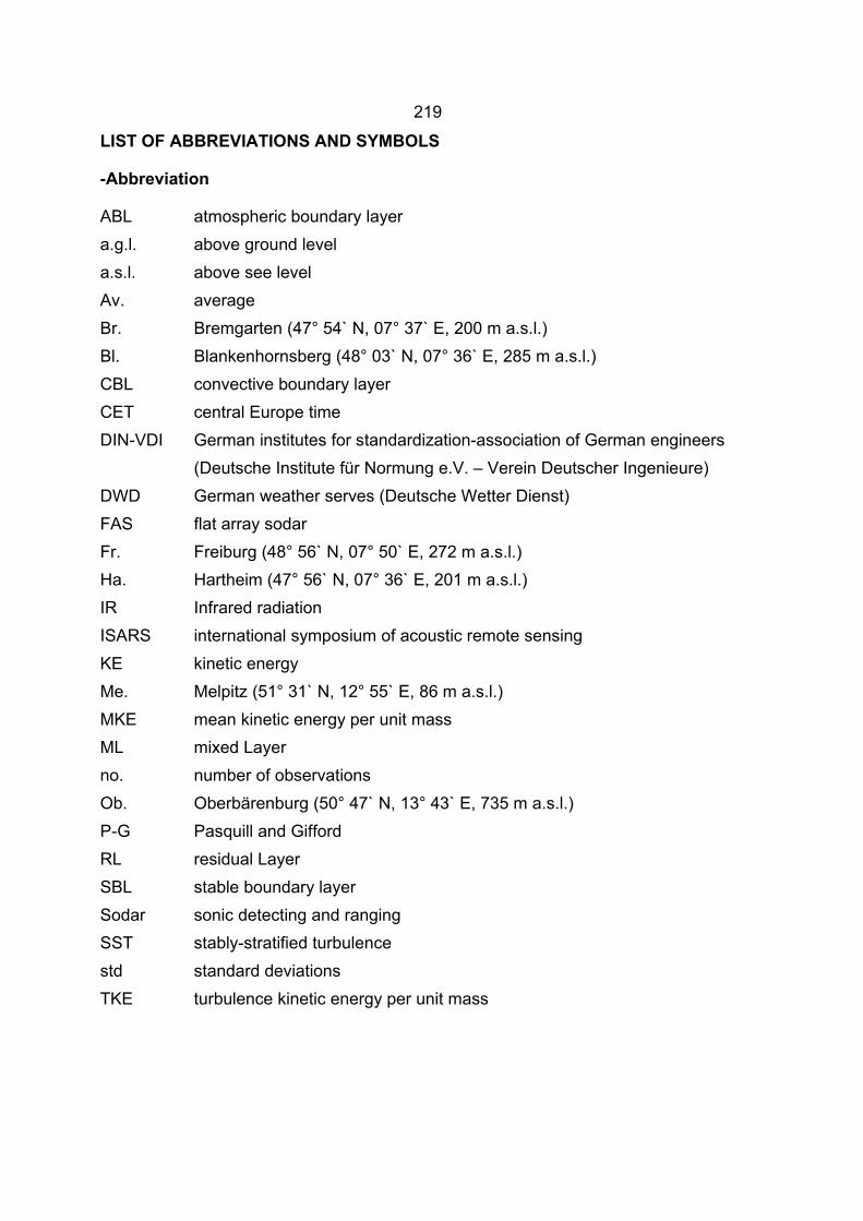
219

LIST OF ABBREVIATIONS AND SYMBOLS

-Abbreviation

ABL a.g.l. a.s.l. Av. Br. Bl. CBL CET DIN-VDI DWD FAS Fr. Ha. IR ISARS KE Me. MKE ML no. Ob. P-G RL SBL Sodar SST std TKE

atmospheric boundary layer above ground level above see level average Bremgarten (47° 54` N, 07° 37` E, 200 m a.s.l.) Blankenhornsberg (48° 03` N, 07° 36` E, 285 m a.s.l.) convective boundary layer central Europe time German institutes for standardization-association of German engineers (Deutsche Institute für Normung e.V. – Verein Deutscher Ingenieure) German weather serves (Deutsche Wetter Dienst) flat array sodar Freiburg (48° 56` N, 07° 50` E, 272 m a.s.l.) Hartheim (47° 56` N, 07° 36` E, 201 m a.s.l.) Infrared radiation international symposium of acoustic remote sensing kinetic energy Melpitz (51° 31` N, 12° 55` E, 86 m a.s.l.) mean kinetic energy per unit mass mixed Layer number of observations Oberbärenburg (50° 47` N, 13° 43` E, 735 m a.s.l.) Pasquill and Gifford residual Layer stable boundary layer sonic detecting and ranging stably-stratified turbulence standard deviations turbulence kinetic energy per unit mass

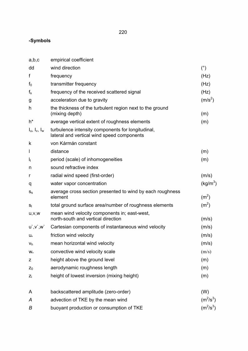
220

-Symbols

a,b,c empirical coefficient dd wind direction (°) f frequency (Hz) f0 transmitter frequency (Hz) fs frequency of the received scattered signal (Hz) g acceleration due to gravity (m/s2) h the thickness of the turbulent region next to the ground

(mixing depth) (m) h* average vertical extent of roughness elements (m) Iu, Iv, Iw turbulence intensity components for longitudinal,

lateral and vertical wind speed components k von Kármán constant l distance (m) lt period (scale) of inhomogeneities (m) n sound refractive index r radial wind speed (first-order) (m/s) q water vapor concentration (kg/m3) ss average cross section presented to wind by each roughness

element (m2) sl total ground surface area/number of roughness elements (m2) u,v,w mean wind velocity components in; east-west,

north-south and vertical direction (m/s) u`,v`,w` Cartesian components of instantaneous wind velocity (m/s)

u∗ friction wind velocity (m/s) vh mean horizontal wind velocity (m/s)

w∗ convective wind velocity scale (m/s) z height above the ground level (m) z0 aerodynamic roughness length (m) zi height of lowest inversion (mixing height) (m) A backscattered amplitude (zero-order) (W) A advection of TKE by the mean wind (m2/s3) B buoyant production or consumption of TKE (m2/s3)

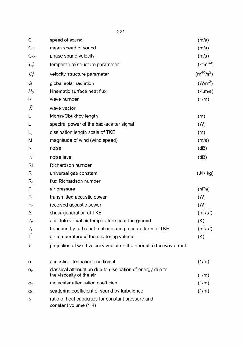
221

C speed of sound (m/s) C0 mean speed of sound (m/s) Cph phase sound velocity (m/s)

2TC temperature structure parameter (k2m2/3) 2VC velocity structure parameter (m4/3/s2)

G global solar radiation (W/m2) H0 kinematic surface heat flux (K.m/s) K wave number (1/m)

Kr

wave vector L Monin-Obukhov length (m) L spectral power of the backscatter signal (W)

Lε dissipation length scale of TKE (m) M magnitude of wind (wind speed) (m/s) N noise (dB)

N noise level (dB)

Ri Richardson number R universal gas constant (J/K.kg) Rf flux Richardson number P air pressure (hPa) Pt transmitted acoustic power (W) Pr received acoustic power (W) S shear generation of TKE (m2/s3) Tv absolute virtual air temperature near the ground (K) Tr transport by turbulent motions and pressure term of TKE (m2/s3) T` air temperature of the scattering volume (K)

Vr

projection of wind velocity vector on the normal to the wave front

α acoustic attenuation coefficient (1/m) αc classical attenuation due to dissipation of energy due to

the viscosity of the air (1/m) αm molecular attenuation coefficient (1/m) αs scattering coefficient of sound by turbulence (1/m)

γ ratio of heat capacities for constant pressure and constant volume (1.4)

222

ε viscous dissipation rate of TKE (m2/s3)

tη efficiency of transmitter of the acoustic wave

rη efficiency of receiver of the acoustic wave

θ scatter angle in relation to the incident wave (°)

ΘB angle of wave incidence (Bragg angle) which is half the scattering angle θ (°)

vθ virtual potential temperature (K)

λ sound wavelength at mean temperature T (m)

µ molecular weight of the mixture of gases that are constituents of air (g/mol)

υ r projection of wind velocity in the direction of sounder beam

ρ air density (kg/m3)

ρ average density of air (kg/m3)

σdd standard deviation of the wind direction (°)

σi standard deviation of the wind speed components (i=u,v,w) (m/s)

σ2i variance of the wind speed components (i=u,v,w) (m2/s2)

σ2h variance of the horizontal wind speed (m2/s2)

σr width of Doppler spectrum (second-order)

σwm average of σw between 100 m and the uppermost sodar level (m/s)

τl pulse length (m)

τ magnitude of the Reynolds’ stress (turbulent momentum flux) in the surface layer (kg/ms2)

zM

∆∆ wind shear (1/s)

Lz stability parameter

zw3σ represent of the quantity of convective and mechanical

production origin of TKE (m2/s3)

223

LIST OF CAPTIONS FOR FIGURES Figure Caption Page Fig. 4.1: Location of the atmospheric boundary layer Fig. 4.2: Idealization of (a) mean wind alone, (b) waves alone, and (c) turbu-

lence alone Fig. 4.3: Rate of generation of TKE by buoyancy, shear. As well as shape and

rates of plume dispersion, separate sectors of different Pasquill-Gifford turbulence type

Fig. 4.4: The boundary layer in high pressure regions over land consists of three major parts

Fig. 4.5: Dependence of sound absorption on temperature and humidity Fig. 4 6: Coefficient of molecular attenuation of sound waves as a function of

humidity at various frequencies Fig. 4.7: Wave scattering by periodical structure inhomogeneities Fig. 5.1: Backscatter is the returned radiation from the transmitted pulse Fig. 5.2: Schematic showing relationship between travel time and measured

height Fig. 5.3: Doppler spectrum Fig. 5.4: The main subsystem of FAS64 Fig. 5.5: The acoustic arranges 64 highly efficient piezoelectric transducers Fig. 5.6: Location of investigated sites in Germany Fig. 6.1.1: Diurnal variation of the global solar radiation G at Hartheim on two

cloudless days (21/22 April, 2000) and two cloudy days (17/18 April, 2000)

Fig. 6.1.2: Frequency distribution of wind direction at (a) 20-50 m, (b) 230-260 m and (c) 470-500 m a.g.l. at Hartheim during the day and night, the daytime (6:00–18:00 CET) and the nighttime (18:00–6:00 CET), dur-ing the period of the study (30 March, 2000 to 25 April, 2000)


w, σdd, TKE, MKE and σ3w/z at Hartheim un-

der various atmospheric conditions; neutral (17 April, 2000, 03:30-04:00 CET) and unstable (03 April, 2000, 12:00-12:30 CET)

Fig. 6.1.4: Diurnal variation of two days mean of the standard deviation of the wind direction, σdd at Hartheim (a) cloudless sky conditions (21/22 April, 2000) (b) cloudy sky conditions (17/18 April, 2000)

Fig. 6.1.5: Diurnal variation of two days mean of the horizontal wind speed, vh at Hartheim (a) cloudless sky conditions (21/22 April, 2000) (b) cloudy sky conditions (17/18 April, 2000)

1617

24

26

3637

404445

4650525862

63

64

65

66

224

Fig. 6.1.6: Diurnal variation of two days mean of the vertical wind speed compo-nent, w at Hartheim (a) cloudless sky conditions (21/22 April, 2000) (b) cloudy sky conditions (17/18 April, 2000)

Fig. 6.1.7: Frequency distribution of P-G stability classes at different levels a.g.l. in Hartheim for the study period (30 March, 2000 to 25 April, 2000)


h, at Hartheim (a) cloudless sky conditions (21/22 April, 2000) (b) cloudy sky conditions (17/18 April, 2000)


w, at Hartheim (a) cloudless sky conditions (21/22 April, 2000) (b) cloudy sky conditions (17/18 April, 2000)

Fig. 6.1.10: Diurnal variation of two days mean of the quantity, σ3w/z, at Hartheim

(a) cloudless sky conditions (21/22 April, 2000) (b) cloudy sky condi-tions (17/18 April, 2000)

Fig. 6.1.11: Diurnal variation of two days mean of the mean kinetic energy per unit mass, MKE, at Hartheim (a) cloudless sky conditions (21/22 April, 2000) (b) cloudy sky conditions (17/18 April, 2000)

Fig. 6.1.12: Diurnal variation of two days mean of the turbulence kinetic energy per unit mass, TKE, at Hartheim (a) cloudless sky conditions (21/22 April, 2000) (b) cloudy sky conditions (17/18 April, 2000)

Fig. 6.1.13: Variation of the mean values of the turbulence intensity components, Iu, Iv and Iw, with the P-G stability classes in the angular sector 210-240° at different levels over Hartheim for the study period (30 March, 2000 to 25 April, 2000)

Fig. 6.1.14: Mean of the standard deviation of wind speed components, σu, σv and σw, normalized by u* as a function of –z/L at Hartheim for the study pe-riod (30 March, 2000 to 25 April, 2000); including general function ac-cording to Al-Jiboori et al. (2001)

Fig. 6.2.1: Diurnal variation of the global solar radiation G at Hartheim on two cloudless days (22/23 July, 2001) and two cloudy days (14/15 July, 2001)

Fig. 6.2.2: Frequency distribution of wind direction at (a) 20-30 m a.g.l. (b) 180-260 m a.g.l. and (c) 380-500 m a.g.l. during day and night, daytime (6:00–18:00 CET) and nighttime (18:00–6:00 CET) at Bremgarten through the period of the study (10 July, 2001 to 26 July, 2001)


w, σdd, TKE, MKE, and σ3w/z under various

atmospheric conditions; neutral (14-07-2001, 12:30-13:00 CET), sta-ble (16 July, 2001,23:00-23:300) and unstable (22 July, 2001,11:30:12:00C CET)

Fig. 6.2.4: Diurnal variation of two days mean of the standard deviation of the wind direction, σdd, at Bremgarten (a) cloudless sky conditions (22/23 July, 2001) and (b) cloudy sky conditions (14/15 July, 2001)

Fig. 6.2.5: Diurnal variation of two days mean of the horizontal wind speed, vh, at

67

68

73

74

75

76

77

78

79

82

83

84

85

86

225

Bremgarten (a) cloudless sky conditions (22/23 July, 2001) and (b) cloudy sky conditions (14/15 July, 2001)

Fig. 6.2.6: Diurnal variation of two days mean of the vertical wind speed compo-nent, w, at Bremgarten (a) cloudless sky conditions (22/23 July, 2001) and (b) cloudy sky conditions (14/15 July, 2001)

Fig. 6.2.7: Frequency distribution of P-G stability classes at different heights a.g.l. in Bremgarten for the study period (10 July, 2001 to 26 July, 2001)

Fig. 6.2.8: Diurnal variation two days mean of the variance of the horizontal wind speed, σ2

h, at Bremgarten (a) cloudless sky conditions (22/23 July, 2001) and (b) cloudy sky conditions (14/15 July, 2001)


w, (a) cloudless sky conditions (22/23 July, 2001) and (b) cloudy sky conditions (14/15 July, 2001)

Fig. 6.2.10: Diurnal variation of two days mean of the quantity, σ3w/z, (a) cloudless

sky conditions (22/23 July, 2001) and (b) cloudy sky conditions (14/15 July, 2001)

Fig. 6.2.11: Diurnal variation of two days mean of the mean kinetic energy per unit mass, MKE, (a) cloudless sky conditions (22/23 July, 2001) and (b) cloudy sky conditions. (14/15 July, 2001)

Fig. 6.2.12: Diurnal variation of two days mean of the turbulence kinetic energy per unit mass, TKE, (a) cloudless sky conditions (22/23 July, 2001) and (b) cloudy sky conditions (14/15 July, 2001)

Fig. 6.2.13: Variation of the mean values of the turbulence intensity components, (a) Iu, (b) Iv and (c) Iw, with the angular sectors under the neutral strati-fied at different levels. in Bremgarten during the study period (10 July, 2001 to 26 July, 2001)

Fig. 6.2.14: Variation of the mean values of the turbulence intensity components (a) Iu, (b) Iv and (c) Iw, with the P-G stability classes in the angular sec-tor 210-240° at different levels in Bremgarten during the study (10 July, 2001 to 26 July, 2001)

Fig. 6.2.15: Mean of the standard deviation of wind speed components, σu, σv and σw, normalized by u* as a function of -z/L at Bremgarten during the pe-riod from 10 July, 2001 to 26 July, 2001, including the general function according to Al-Jiboori et al. (2001)

Fig. 6.3.1: Diurnal variation of the global solar radiation G at Hartheim on two cloudless days (12/15 August, 2001) and two cloudy days (03/17 Au-gust, 2001)

Fig. 6.3.2: Frequency distribution of wind direction at (a) 20-30 m, (b) 160-240 m and (c) 400-500 m a.g.l. at Blankenhornsberg during the day and night, daytime (6:00–18:00 CET), and nighttime (18:00–6:00 CET) through the study period (01 August, 2001 to 22 August, 2001)


w, σdd, TKE, MKE, and σ3w/z at Blanken-

hornsberg under various atmospheric conditions; neutral (04 August,

87

88

92

93

94

95

96

97

98

99

102

103

104

226

2001, 02:30-03:00 CET) and unstable (12 August, 2001, 13:30-14:00 CET)

Fig. 6.3.4: Diurnal variation of two days mean of the standard deviation of the wind direction, σdd, at Blankenhornsberg (a) cloudless sky conditions (12/15 August, 2001) (b) cloudy sky conditions (03/17 August, 2001)

Fig. 6.3.5: Diurnal variation of two days mean of the horizontal wind speed, vh, at Blankenhornsberg (a) cloudless sky conditions (12/15 August, 2001) (b) cloudy sky conditions (03/17 August, 2001)

Fig. 6.3.6: Diurnal variation of two days mean of the vertical wind speed compo-nent, w, at Blankenhornsberg (a) cloudless sky conditions (12/15 Au-gust, 2001) (b) cloudy sky conditions (03/17 August, 2001)

Fig. 6.3.7: Frequency distribution of P-G stability classes at different levels a.g.l. at Blankenhornsberg for the study period (01 August, 2001 to 22 Au-gust, 2001)


h, at Blankenhornsberg (a) cloudless sky condi-tions (12/15 August, 2001) (b) cloudy sky conditions (03/17 August, 2001)


w, at Blankenhornsberg (a) cloudless sky conditions (12/15 August, 2001) (b) cloudy sky conditions (03/17 August, 2001)

Fig. 6.3.10: Diurnal variation of two days mean of the quantity, σ3w/z, at Blanken-

hornsberg (a) cloudless sky conditions (12/15 August, 2001) (b) cloudy sky conditions (03/17 August, 2001)

Fig. 6.3.11: Diurnal variation of two days mean of the mean kinetic energy per unit mass, MKE, at Blankenhornsberg (a) cloudless sky conditions (12/15 August, 2001) (b) cloudy sky conditions (03/17 August, 2001)

Fig. 6.3.12: Diurnal variation of two days mean of the turbulence kinetic energy per unit mass, TKE, at Blankenhornsberg (a) cloudless sky conditions (12/15 August, 2001) (b) cloudy sky conditions (03/17 August, 2001)

Fig. 6.3.13: Variation of the mean values of the turbulence intensity components, Iu, Iv and Iw, with the wind direction under the neutral stratified at dif-ferent levels in Blankenhornsberg through the period of the study (01 August, 2001 to 22 August, 2001)

Fig. 6.3.14: Variation of the mean values of the turbulence intensity components, Iu, Iv and Iw, with the P-G stability classes in the angular sector 210-240° at different levels at Blankenhornsberg through the period of the study (01 August, 2001 to 22 August, 2001)

Fig. 6.3.15: Mean of standard deviation of wind speed components σu, σv and σW, normalized by u* as a function of –z/L at Blankenhornsberg through the period of the study (01 August, 2001 to 22 August, 2001), includ-ing general function according to Al-Jiboori et al. (2001)

Fig. 6.4.1: Diurnal variation of the global solar radiation G at Rotherdbach on two

105

106

107

108

112

113

114

115

116

117

118

119

121

227

cloudless days (30 August, 2001 and 23 September, 2001) and two cloudy days (31 August, 2001 and 01 September, 2001)

Fig. 6.4.2: Frequency distribution of wind direction at (a) 20-50 m, (b) 230-260 m a.g.l. and (c) 470-500 m a.g.l. during the day and night, daytime (6:00–18:00 CET) and the nighttime (18:00–6:00 CET) at Oberbären-burg through the period of the study (29 August, 2001 to 24 Septem-ber, 2001)

Fig. 6.4.3: Diurnal variation of two days mean of the standard deviation of the wind direction, σdd, at Oberbärenburg (a) cloudless sky conditions (30 August, 2001 and 23 September, 2001) (b) cloudy sky conditions (31 August, 2001 and 01 September, 2001)

Fig. 6.4.4: Diurnal variation of two days mean of the horizontal wind speed, vh, at Oberbärenburg (a) cloudless sky conditions (30 August, 2001 and 23 September, 2001) (b) cloudy sky conditions (31 August, 2001 and 01 September, 2001)

Fig. 6.4.5: Diurnal variation of two days mean of the vertical wind speed compo-nent, w, at Oberbärenburg (a) cloudless sky conditions (30 August, 2001 and 23 September, 2001) (b) cloudy sky conditions (31 August, 2001 and 01 September, 2001)

Fig. 6.4.6 Frequency distribution of P-G stability classes at different levels a.g.l. at Oberbärenburg for the study period (29 August, 2001 to 24 Sep-tember, 2001)


h, at Oberbärenburg (a) cloudless sky conditions (30 August, 2001 and 23 September, 2001) (b) cloudy sky conditions (31 August, 2001 and 01 September, 2001)


w, at Oberbärenburg (a) cloudless sky conditions (30 August, 2001 and 23 September, 2001) (b) cloudy sky conditions (31 August, 2001 and 01 September, 2001)

Fig. 6.4.9: Diurnal variation of two days mean of the quantity, σ3w/z, at Ober-

bärenburg (a) cloudless sky conditions (30 August, 2001 and 23 Sep-tember, 2001) (b) cloudy sky conditions (31 August, 2001 and 01 Sep-tember, 2001)

Fig. 6.4.10: Diurnal variation of two days mean of the mean kinetic energy per unit mass, MKE, at Oberbärenburg (a) cloudless sky conditions (30 Au-gust, 2001 and 23 September, 2001) (b) cloudy sky conditions (31 August, 2001 and 01 September, 2001)

Fig. 6.4.11: Diurnal variation of two days mean of the turbulence kinetic energy per unit mass, TKE, at Oberbärenburg (a) cloudless sky conditions (30 August, 2001 and 23 September, 2001) (b) cloudy sky conditions (29-08-2001 and 01-09-2001)

Fig. 6.4.12: Variation of the mean values of the turbulence intensity components, Iu, Iv and Iw, with the wind direction under the neutral stratified at dif-

122

123

124

125

126

131

132

133

134

135

136

228

ferent levels at Oberbärenburg for the study period (29-08-01 to 24-09-01)

Fig. 6.4.13: Variation of the mean values of the turbulence intensity components, Iu, Iv and Iw, with the P-G stability classes in the angular sector 210-240° at different levels at Oberbärenburg through the period of the study (29 August, 2001 to 24 September, 2001)

Fig. 6.4.14: Mean standard deviation of wind speed components σu, σv and σw, normalized by u* as a function of -z/L at Oberbärenburg through the period of the study (29 August, 2001 to 24 September, 2001), includ-ing general function according to Al-Jiboori et al. (2001)

Fig. 6.5.1: Diurnal variation of the global solar radiation G at Melpitz on a cloud-less day (06 October, 2001) and two cloudy days (30 September, 2001 and 01 October, 2001)

Fig. 6.5.2: Frequency distribution of wind direction at (a) 20-50 m, (b) 230-260 m and m, (c) 470-500 m a.g.l. during the day and night, daytime (6:00–18:00 CET) and the nighttime (18:00–6:00 CET) at Melpitz through the period of the study (26 September, 2001 to 12 October, 2001)


w, σdd, TKE, MKE, and σ3w/z at Melpitz under

various atmospheric conditions; neutral (03 October, 2001, 03:30-04:00) and unstable (06 October, 2001, 13:00-13:30).

Fig. 6.5.4: Diurnal variation of the standard deviation of the wind direction, σdd, at Melpitz (a) one cloudless day (06 October, 2001) and (b) two days mean in cloudy sky (30 September, 2001 and 01 October, 2001)

Fig. 6.5.5: Diurnal variation of the horizontal wind speed, vh, at Melpitz (a) one cloudless day (06 October, 2001) and (b) two days mean in cloudy sky (30 September, 2001 and 01 October, 2001)

Fig. 6.5.6: Diurnal variation of the vertical wind speed component, w, at Melpitz (a) one cloudless day (06 October, 2001) and (b) two days mean in cloudy sky (30 September, 2001 and 01 October, 2001)

Fig. 6.5.7: Frequency distribution of P-G stability classes at different levels a.g.l. at Melpitz for the study period (26 September, 2001 to 12 October, 2001)



Fig. 6.5.9: Diurnal variation of the variance of the vertical wind speed, σ2w, at


Fig. 6.5.10: Diurnal variation of the quantity, σ3w/z, at Melpitz (a) one cloudless day

(06 October, 2001) and (b) two days mean in cloudy sky (30 Septem-ber, 2001 and 01 October, 2001)

Fig. 6.5.11: Diurnal variation of the mean kinetic energy per unit mass, MKE, at Melpitz (a) one cloudless day (06 October, 2001) and (b) two days

137

138

140

141

142

143

144

145

146

151

152

153

154

229

mean in cloudy sky (30 September, 2001 and 01 October, 2001) Fig. 6.5.12: Diurnal variation of the turbulence kinetic energy per unit mass, TKE,

at Melpitz (a) one cloudless day (06 October, 2001) and (b) two days mean in cloudy sky (30 September, 2001 and 01 October, 2001)

Fig. 6.5.13: Variation of the mean values of the turbulence intensity components, Iu, Iv and Iw, with the wind direction under the neutral stratified at dif-ferent levels at Melpitz through the period of the study (26 September, 2001 to 12 October, 2001)

Fig. 6.5.14: Variation of the mean values of the turbulence intensity components, Iu, Iv and Iw, with the P-G stability classes in the angular sector 210-240° at different levels at Melpitz through the period of the study (26 September, 2001 to 12 October, 2001)

Fig. 6.6.1: Diurnal variation of the global solar radiation G at Freiburg on cloud-less day (17 November, 2001) and cloudy day (18 November, 2001)

Fig. 6.6.2: Frequency distribution of wind direction at (a) 20-30 m, (b) 40-60 m, (c) 60-80 m a.g.l. during the day and night, daytime (6:00–18:00 CET) and nighttime (18:00–6:00 CET) at Freiburg through the period of the study (16 November, 2001 to 19 November)


w, σdd, TKE, MKE, and σ3w/z at Freiburg un-

der various atmospheric conditions; stable (18 November, 2001, 04:30-05:00 CET) and unstable (17 November, 2001, 12:00-12:30 CET)

Fig. 6.6.4: Diurnal variation of the standard deviation of the wind direction, σdd, at Freiburg (a) cloudless sky conditions (17 November, 2001) (b) cloudy sky conditions (18 November, 2001)

Fig. 6.6.5 Diurnal variation of the horizontal wind speed, vh, at Freiburg (a) cloudless sky conditions (17 November, 2001) (b) cloudy sky condi-tions (18 November, 2001)

Fig. 6.6.6: Diurnal variation of the vertical wind speed component, w at Freiburg (a) cloudless sky conditions (17 November, 2001) (b) cloudy sky con-ditions (18 November, 2001)



Fig. 6.6.8: Diurnal variation of the variance of vertical wind speed component, σ2

w, at Freiburg (a) cloudless sky conditions (17 November, 2001) (b) cloudy sky conditions (18 November, 2001)

Fig. 6.6.9: Diurnal variation of the quantity, σ3w/z, at Freiburg (a) cloudless sky

conditions (17 November, 2001) (b) cloudy sky conditions (18 Novem-ber, 2001)

Fig. 6.6.10: Diurnal variation of the mean kinetic energy per unit mass, MKE, at Freiburg (a) cloudless sky conditions (17 November, 2001) (b) cloudy

155

156

157

159

161

162

163

164

165

166

167

168

169

230

sky conditions (18 November, 2001) Fig. 6.6.11: Diurnal course of the turbulence kinetic energy per unit mass, TKE, at



w, σ2h, σdd, σ3

w/z, MKE, and TKE for a cloud-less conditions at levels from 20-50 m a.g.l. [forest and grassland (Me.)] and 20-30 m a.g.l. [grassland (Br.), vineyard and urban area], (Table 7.1 to 7.6)


w, σ2h, σdd, σ3

w/z, MKE, and TKE for a cloudy conditions at levels from 20-50 m a.g.l. [forest and grassland (Me.)] and 20-30 m a.g.l. [grassland (Br.), vineyard and urban area], (Table 7.1 to 7.6)


w, σ2h, σdd, σ3

w/z, MKE, and TKE for a cloud-less conditions at levels from 50-80 m a.g.l. [forest and grassland (Me.)] and 40-60 m a.g.l [grassland (Br.), vineyard and urban area], (Table 7.1 to 7.6)


w, σ2h, σdd, σ3

w/z, MKE, and TKE for a cloudy conditions at levels from 50-80 m a.g.l [forest and grassland (Me.)] and 40-60 m a.g.l [grassland (Br.), vineyard and urban area], (Table 7.1 to 7.6)


w, σ2h, σdd, σ3

w/z, MKE, and TKE for a cloud-less conditions at levels from 80 to 110 m a.g.l. [forest and grassland (Me.)], 60-100 m a.g.l. [grassland (Br.)], 80-120 m a.g.l. [vineyard] and 60-80 m a.g.l. [urban area], (Table 7.1 to 7.6)


w, σ2h, σdd, σ3

w/z, MKE, and TKE for a cloudy conditions at levels from 80 to 110 m a.g.l. [forest and grassland (Me.)], 60-100 m a.g.l. [grassland (Br.)], 80-120 m a.g.l. [vineyard] and 60-80 m a.g.l. [urban area], (Table 7.1 to 7.6)

Fig. 7.7: Mean values of the dimensionless of standard deviations of velocity components σi/u∗ (i=u,v,w) as a function of –z/L under free convective conditions in the surface layer

Fig. 7.8: The mean values of σi/u∗ (i=u,v,w) (from table 7.2) over different land use types, and the data of AL-Jiboori et al. (2001) (complex and flat terrain)

Fig. 7.9: Normalized vertical velocity variance, σw/w∗ as a function of the nor-malized height, z/zi at Bremgarten under the free convection condi-tions

170

194

195

196

197

198

199

200

201

201

231

LIST OF CAPTIONS FOR TABLES Table Caption Page

Table 4.1: Change of wavelength of sound waves in the atmosphere as a function of changes in temperature, wind speed and water vapor content.

Table 5.1: Specifications of FAS64 Table 5.2: Method of stability classification (class limits) Table 5.3: The values of coefficient a and b (Liu et al., 1976 and Irwin,

1979) Table 5.4: The general description of the study areas. Table 6.1.1: Turbulence intensity components (a) Iu, (b) Iv and (c) Iw at differ-

ent levels grouped by direction. Under each component are given the mean, standard deviation and number of observations in each group at Hartheim for the study period (30 March, 2000 to 25 April, 2000)

Table 6.1.2: Turbulence intensity component (a) Iu, (b) Iv and (c) Iw at differ-ent levels grouped by P-G stability classes in one angular sector (180-210°). Under each component are given the mean, stan-dard deviation and number of the observation in each group at Hartheim for the study period (30 March, 2000 to 25 April, 2000)

Table 6.2.1: Turbulence intensity components (a) Iu, (b) Iv and (c) Iw at differ-ent levels grouped by direction. Under each component are given the mean, standard deviation and number of observation in each group at Bremgarten during the study period (10 July, 2001 to 26 July, 2001)

Table 6.2.2: Turbulence intensity component (a) Iu, (b) Iv and (c) Iw at different levels grouped by P-G stability classes in one angular sector (180-210°). Under each component are given the mean, stan-dard deviation and number of the observation in each group dur-ing the study period (10 July, 2001 to 26 July, 2001)

Table 6.3.1: Turbulence intensity components (a) Iu, (b) Iv and (c) Iw at differ-ent levels grouped by direction. Under each component are given the mean, standard deviation and number of observation in each group at Blankenhornsberg through the period from 01 August, 2001 to 22 August, 2001

Table 6.3.2: Turbulence intensity component (a) Iu, (b) Iv and (c) Iw at different levels grouped by P-G stability classes in one angular sector (210-240°).Under each component are given the mean, stan-dard deviation and number of the observation in each group at Blankenhornsberg for the study period (01 August, 2001 to 22

34

515656

5771

72

90

91

110

111

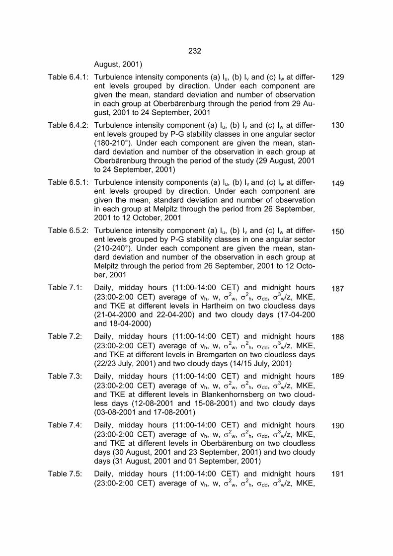
232

August, 2001) Table 6.4.1: Turbulence intensity components (a) Iu, (b) Iv and (c) Iw at differ-

ent levels grouped by direction. Under each component are given the mean, standard deviation and number of observation in each group at Oberbärenburg through the period from 29 Au-gust, 2001 to 24 September, 2001

Table 6.4.2: Turbulence intensity component (a) Iu, (b) Iv and (c) Iw at differ-ent levels grouped by P-G stability classes in one angular sector (180-210°). Under each component are given the mean, stan-dard deviation and number of the observation in each group at Oberbärenburg through the period of the study (29 August, 2001 to 24 September, 2001)

Table 6.5.1: Turbulence intensity components (a) Iu, (b) Iv and (c) Iw at differ-ent levels grouped by direction. Under each component are given the mean, standard deviation and number of observation in each group at Melpitz through the period from 26 September, 2001 to 12 October, 2001

Table 6.5.2: Turbulence intensity component (a) Iu, (b) Iv and (c) Iw at differ-ent levels grouped by P-G stability classes in one angular sector (210-240°). Under each component are given the mean, stan-dard deviation and number of the observation in each group at Melpitz through the period from 26 September, 2001 to 12 Octo-ber, 2001

Table 7.1: Daily, midday hours (11:00-14:00 CET) and midnight hours (23:00-2:00 CET) average of vh, w, σ2

w, σ2h, σdd, σ3

w/z, MKE, and TKE at different levels in Hartheim on two cloudless days (21-04-2000 and 22-04-200) and two cloudy days (17-04-200 and 18-04-2000)


w, σ2h, σdd, σ3

w/z, MKE, and TKE at different levels in Bremgarten on two cloudless days (22/23 July, 2001) and two cloudy days (14/15 July, 2001)


w, σ2h, σdd, σ3

w/z, MKE, and TKE at different levels in Blankenhornsberg on two cloud-less days (12-08-2001 and 15-08-2001) and two cloudy days (03-08-2001 and 17-08-2001)


w, σ2h, σdd, σ3

w/z, MKE, and TKE at different levels in Oberbärenburg on two cloudless days (30 August, 2001 and 23 September, 2001) and two cloudy days (31 August, 2001 and 01 September, 2001)


w, σ2h, σdd, σ3

w/z, MKE,

129

130

149

150

187

188

189

190

191

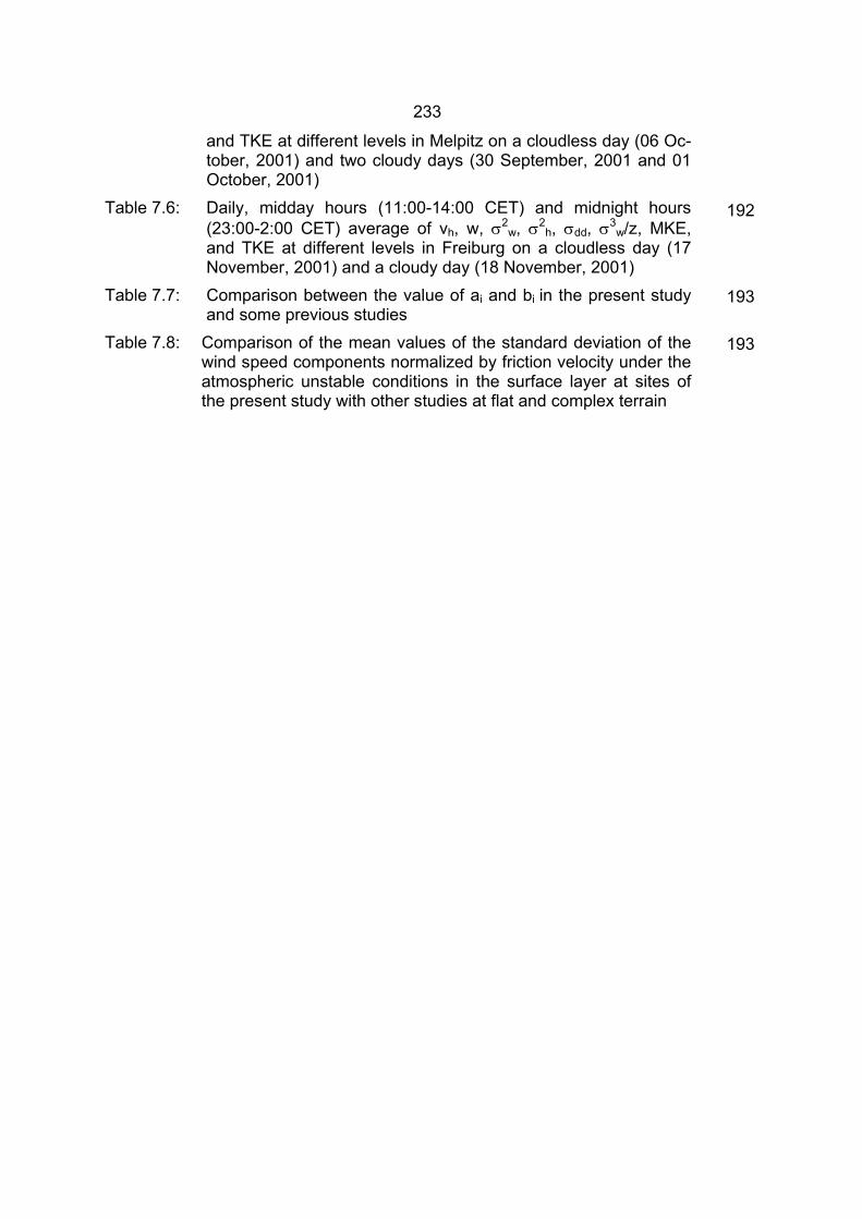
233

and TKE at different levels in Melpitz on a cloudless day (06 Oc-tober, 2001) and two cloudy days (30 September, 2001 and 01 October, 2001)


w, σ2h, σdd, σ3

w/z, MKE, and TKE at different levels in Freiburg on a cloudless day (17 November, 2001) and a cloudy day (18 November, 2001)

Table 7.7: Comparison between the value of ai and bi in the present study and some previous studies

Table 7.8: Comparison of the mean values of the standard deviation of the wind speed components normalized by friction velocity under the atmospheric unstable conditions in the surface layer at sites of the present study with other studies at flat and complex terrain

192

193

193

234

235

Berichte des Meteorologischen Institutes der Universität Freiburg

Nr. 1: Fritsch, J.: Energiebilanz und Verdunstung eines bewaldeten Hanges. Juni

1998.

Nr.2: Gwehenberger, J.: Schadenpotential über den Ausbreitungspfad Atmosphäre

bei Unfällen mit Tankfahrzeugen zum Transport von Benzin, Diesel, Heizöl o-

der Flüssiggas. August 1998.

Nr. 3: Thiel, S.: Einfluß von Bewölkung auf die UV-Strahlung an der Erdoberfläche

und ihre ökologische Bedeutung. August 1999.

Nr. 4: Iziomon, M.G.: Characteristic variability, vertical profile and modelling of sur-

face radiation budget in the southern Upper Rhine valley region. Juli 2000.

Nr. 5: Mayer, H. (Hrsg.): Festschrift „Prof. Dr. Albrecht Kessler zum 70. Geburtstag“.

Oktober 2000.

Nr. 6: Matzarakis, A.: Die thermische Komponente des Stadtklimas. Juli 2001.

Nr. 7: Kirchgäßner, A.: Phänoklimatologie von Buchenwäldern im Südwesten der

Schwäbischen Alb. Dezember 2001

Nr. 8: Haggagy, M.: A sodar-based investigation of the atmospheric boundary layer.

September 2003

236

Documents

A Sodar-based Investigation of the Atmospheric Boundary Layer