and Physics Simulation of stratospheric water vapor trends: … · 2016-01-11 · For exam-ple, Rosenlof et al. (2001) combined ten different data sets between 1954 and 2000, and

Atmos. Chem. Phys., 5, 1257–1272, 2005www.atmos-chem-phys.org/acp/5/1257/SRef-ID: 1680-7324/acp/2005-5-1257European Geosciences Union

AtmosphericChemistry

and Physics

Simulation of stratospheric water vapor trends: impact onstratospheric ozone chemistry

A. Stenke and V. Grewe

Deutsches Zentrum fur Luft- und Raumfahrt (DLR), Institut fur Physik der Atmosphare, Oberpfaffenhofen, 82230 Weßling,Germany

Received: 16 August 2004 – Published in Atmos. Chem. Phys. Discuss.: 14 October 2004Revised: 7 February 2005 – Accepted: 16 April 2005 – Published: 31 May 2005

Abstract. A transient model simulation of the 40-year timeperiod 1960 to 1999 with the coupled climate-chemistrymodel (CCM) ECHAM4.L39(DLR)/CHEM shows a strato-spheric water vapor increase over the last two decades of0.7 ppmv and, additionally, a short-term increase after ma-jor volcanic eruptions. Furthermore, a long-term decrease inglobal total ozone as well as a short-term ozone decline in thetropics after volcanic eruptions are modeled. In order to un-derstand the resulting effects of the water vapor changes onlower stratospheric ozone chemistry, different perturbationsimulations were performed with the CCM ECHAM4.L39-(DLR)/CHEM feeding the water vapor perturbations only tothe chemistry part. Two different long-term perturbations oflower stratospheric water vapor, +1 ppmv and +5 ppmv, and ashort-term perturbation of +2 ppmv with an e-folding time oftwo months were applied. An additional stratospheric watervapor amount of 1 ppmv results in a 5–10% OH increase inthe tropical lower stratosphere between 100 and 30 hPa. Asa direct consequence of the OH increase the ozone destruc-tion by the HOx cycle becomes 6.4% more effective. Cou-pling processes between the HOx-family and the NOx/ClOx-family also affect the ozone destruction by other catalyticreaction cycles. The NOx cycle becomes 1.6% less effec-tive, whereas the effectiveness of the ClOx cycle is againslightly enhanced. A long-term water vapor increase doesnot only affect gas-phase chemistry, but also heterogeneousozone chemistry in polar regions. The model results indicatean enhanced heterogeneous ozone depletion during antarc-tic spring due to a longer PSC existence period. In contrast,PSC formation in the northern hemisphere polar vortex andtherefore heterogeneous ozone depletion during arctic springare not affected by the water vapor increase, because of theless PSC activity. Finally, this study shows that 10% of theglobal total ozone decline in the transient model run can

Correspondence to:A. Stenke([email protected])

be explained by the modeled water vapor increase, but thesimulated tropical ozone decrease after volcanic eruptions iscaused dynamically rather than chemically.

1 Introduction

Water vapor in the upper troposphere (UT) and lower strato-sphere (LS) plays a key role in atmospheric chemistry. Theoxidation of H2O and CH4 by excited oxygen O(1D) is theprimary source of hydrogen oxides (HOx=OH+HO2) (Reac-tionsR1–R2, see Appendix), which are involved in importantcatalytic reaction cycles that control the production and de-struction of ozone in the LS. The importance of the catalyticHOx-cycles for the photochemistry of stratospheric O3 hasalready been identified in 1950 byBates and Nicolet. Ad-ditionally, OH is important for changing the partitioning ofthe nitrogen and the halogen family which are crucial for theO3 removal in the stratosphere.

Several studies discussed an increase in stratospheric wa-ter vapor (e.g.Evans et al., 1998; Michelsen et al., 2000;Nedoluha et al., 1998; Rosenlof et al., 2001). For exam-ple, Rosenlof et al.(2001) combined ten different data setsbetween 1954 and 2000, and estimated a water vapor trendof +1%/yr. Several reasons like enhanced methane oxi-dation, increased aircraft emission in the LS, a warmingof the tropical tropopause, volcanic eruptions and large-scale changes in stratospheric circulation and troposphere-stratosphere-exchange have been discussed, but the observedstratospheric water vapor increase is not yet understood(Evans et al., 1998, and references therein). In contrast, trop-ical tropopause temperatures have been found to decrease(Zhou et al., 2001).

Oltmans et al.(2000) analyzed 20 years of water vapormeasurements with the NOAA Climate Monitoring and Di-agnostics Laboratory (CMDL) frostpoint hygrometer overBoulder, CO, and reported a +1%/yr (+0.05 ppmv/yr) trend

© 2005 Author(s). This work is licensed under a Creative Commons License.

1258 A. Stenke and V. Grewe: Impact of stratospheric water vapor trends on ozone chemistry

1980 1982 1984 1986 1988 1990 1992 1994 1996 1998 2000

Wate

r vapor

mix

ing r

atio 8

2

6

4

2002

8

2

6

4

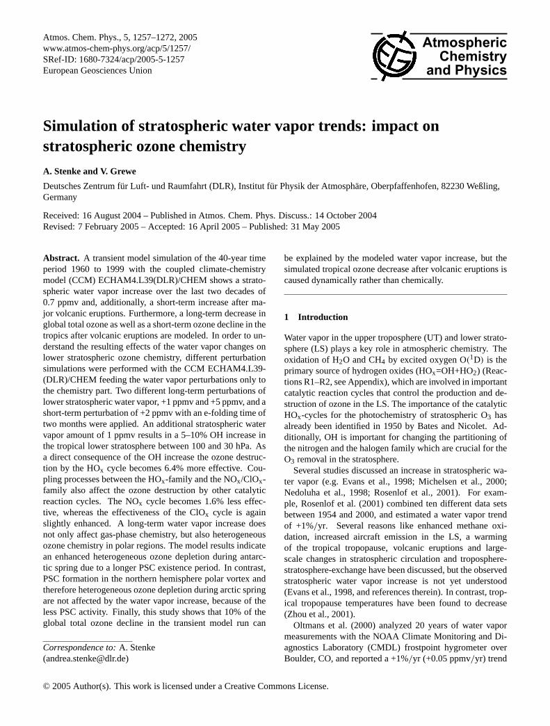
Fig. 1. Time series of individual water vapor soundings with theCMDL frostpoint hygrometer between 24 and 26 km at Boulder,CO (black) (Oltmans et al., 2000), and of monthly mean watervapor mixing ratios from ECHAM4.L39(DLR)/CHEM at 40◦ N,20 hPa (red) (Dameris et al., 2005). The linear trend with the95% confidence interval is 0.044±0.012 ppmv/yr for Boulder and0.029±0.007 ppmv/yr for the model simulation.

in the LS. Figure1 shows a comparison of this time se-ries with a corresponding water vapor time series froma transient model simulation with ECHAM4.L39(DLR)-/CHEM (Dameris et al., 2005). Over the 20 year pe-riod between 1980 and 1999 both time series show a pos-itive trend. However, over the 40 year period from 1960to 1999 the model results do not show a sustained posi-tive trend (seeDameris et al., 2005, for further informa-tion). The water vapor trend over Boulder (24–26 km) is+0.044±0.012 ppmv/yr (Oltmans et al., 2000). The simu-lated water vapor trend is about 35% weaker, it amounts to+0.029±0.007 ppmv/yr (the given uncertainties are the 95%confidence intervals using the t-statistic). A current studyof Randel et al.(2004) reports a great disparity between theBoulder dataset and HALOE satellite data near Boulder re-garding the decadal water vapor changes for the period 1992–2002. For the period 1992–1996 both datasets show a reason-able agreement. After 1997 the Boulder balloon data furtherincrease in time, while HALOE stays relatively constant, sothat HALOE shows small or even negative water vapor trendsin the LS for 1992–2002. However, after 2001 both datasetsagain show a good agreement with remarkably low and per-sistent water vapor anomalies. Taking into account the abovementioned uncertainties in stratospheric water vapor trendsthe magnitude of the modeled water vapor increase is compa-rable with observations. The modeled water vapor increase ismainly associated with a warming of the tropical tropopause,which is in contrast to the observations where water vaporchanges and changes of the tropical tropopause temperatureare apparently in disagreement, and to some extent (≈30%)with the methane increase.

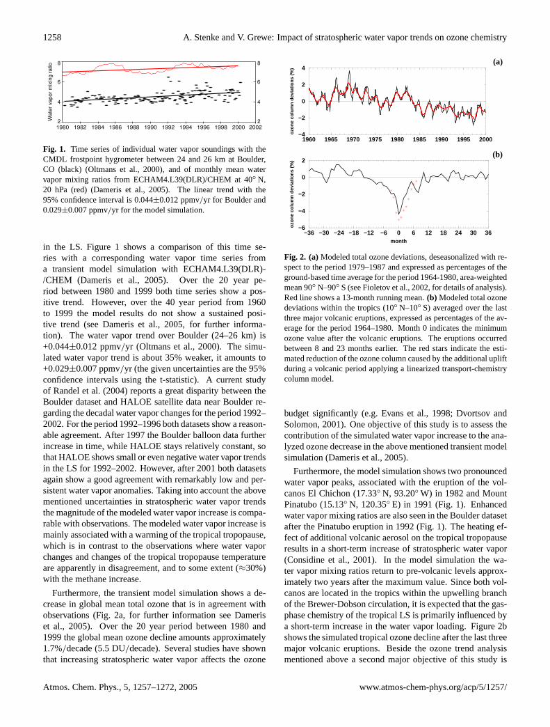
Furthermore, the transient model simulation shows a de-crease in global mean total ozone that is in agreement withobservations (Fig.2a, for further information see Dameriset al., 2005). Over the 20 year period between 1980 and1999 the global mean ozone decline amounts approximately1.7%/decade (5.5 DU/decade). Several studies have shownthat increasing stratospheric water vapor affects the ozone

1960 1965 1970 1975 1980 1985 1990 1995 2000−4

−2

0

2

4

ozon

e co

lum

n de

viat

ions

(%

)

(a)

−36 −30 −24 −18 −12 −6 0 6 12 18 24 30 36month

−6

−4

−2

0

2

ozon

e co

lum

n de

viat

ions

(%

)

(b)

Fig. 2. (a)Modeled total ozone deviations, deseasonalized with re-spect to the period 1979–1987 and expressed as percentages of theground-based time average for the period 1964-1980, area-weightedmean 90◦ N–90◦ S (seeFioletov et al., 2002, for details of analysis).Red line shows a 13-month running mean.(b) Modeled total ozonedeviations within the tropics (10◦ N–10◦ S) averaged over the lastthree major volcanic eruptions, expressed as percentages of the av-erage for the period 1964–1980. Month 0 indicates the minimumozone value after the volcanic eruptions. The eruptions occurredbetween 8 and 23 months earlier. The red stars indicate the esti-mated reduction of the ozone column caused by the additional upliftduring a volcanic period applying a linearized transport-chemistrycolumn model.

budget significantly (e.g.Evans et al., 1998; Dvortsov andSolomon, 2001). One objective of this study is to assess thecontribution of the simulated water vapor increase to the ana-lyzed ozone decrease in the above mentioned transient modelsimulation (Dameris et al., 2005).

Furthermore, the model simulation shows two pronouncedwater vapor peaks, associated with the eruption of the vol-canos El Chichon (17.33◦ N, 93.20◦ W) in 1982 and MountPinatubo (15.13◦ N, 120.35◦ E) in 1991 (Fig.1). Enhancedwater vapor mixing ratios are also seen in the Boulder datasetafter the Pinatubo eruption in 1992 (Fig.1). The heating ef-fect of additional volcanic aerosol on the tropical tropopauseresults in a short-term increase of stratospheric water vapor(Considine et al., 2001). In the model simulation the wa-ter vapor mixing ratios return to pre-volcanic levels approx-imately two years after the maximum value. Since both vol-canos are located in the tropics within the upwelling branchof the Brewer-Dobson circulation, it is expected that the gas-phase chemistry of the tropical LS is primarily influenced bya short-term increase in the water vapor loading. Figure2bshows the simulated tropical ozone decline after the last threemajor volcanic eruptions. Beside the ozone trend analysismentioned above a second major objective of this study is

Atmos. Chem. Phys., 5, 1257–1272, 2005 www.atmos-chem-phys.org/acp/5/1257/

A. Stenke and V. Grewe: Impact of stratospheric water vapor trends on ozone chemistry 1259

to investigate whether these short-term ozone changes arisefrom a short-term water vapor increase.

In this paper we investigate the impact of stratospheric wa-ter vapor perturbations on ozone chemistry by model simula-tions with the coupled climate-chemistry model ECHAM4-.L39(DLR)/CHEM. We use a special method to prevent afeedback of the simulated water vapor increase to the modeldynamics in order to separate the chemical effect. A shortmodel description is given in the next section. Section3 de-scribes the applied tracer approach. The results of our studyare presented in Sects.4.1and4.2, followed by a discussionin Sect.4.3. A summary is given in the last section.

2 Model description

The coupled climate-chemistry model ECHAM4.L39(DLR)-/CHEM (Hein et al., 2001, hereafter referred to as E39/C)consists of the dynamic part ECHAM4.L39(DLR) (E39) andthe chemistry module CHEM. E39 is a spectral general circu-lation model, based on the climate model ECHAM4 (Roeck-ner et al., 1996), and has a vertical resolution of 39 levelsup to the top layer centered at 10 hPa (Land et al., 1999).A horizontal resolution of T30 (≈6◦ isotropic resolution) isused in this study. The tracer transport, parameterizations ofphysical processes and the chemistry are calculated on thecorresponding Gaussian transform grid with a grid size of3.75◦

×3.75◦. Water vapor, cloud water and chemical speciesare advected by a so-called semi-Lagrangian scheme.

The chemistry module CHEM (Steil et al., 1998) is basedon the family concept. It includes stratospheric homoge-neous and heterogeneous ozone chemistry and the most rel-evant chemical processes for describing the troposphericbackground NOx-CH4-CO-HOx-O3 chemistry with 107 pho-tochemical reactions, 37 chemical species and 4 heteroge-neous reactions (R12–R15) on polar stratospheric clouds(PSCs) and on sulfate aerosols. CHEM does not yet considerbromine chemistry. Mixing ratios of methane (CH4), nitrousoxide (N2O) and carbon monoxide (CO) are prescribed atthe surface followingIPCC (2001) for the year 2000. Zon-ally averaged monthly mean concentrations of chlorofluo-rocarbons (CFCs) and upper boundary conditions for totalchlorine and total nitrogen are taken from the 2-D model ofBruhl and Crutzen(1993). Nitrogen oxide emissions at thesurface (natural and anthropogenic sources), from lightningand aircraft are considered. The model set-up followsHeinet al.(2001) except for the total amounts of emissions, light-ning NOx, which is parameterized according toGrewe et al.(2001), and a more detailed sulfate aerosol chemistry.

The model E39/C can be run in two different modes: with-and without-feedback. In the without-feedback mode theconcentrations of the radiatively active gases H2O, O3, N2O,and CFCs calculated by CHEM do not feed back to the radia-tive scheme of E39. Prescribed climatological mixing ratiosof the radiatively active gases are used as input for the radia-

tive scheme instead (Hein et al., 2001). Note that the tran-sient model simulation reported byDameris et al.(2005), onthe other hand, was integrated in the with-feedback mode in-cluding the chemical feedbacks on radiatively active gases.

2.1 Model climatology

The model climatology was extensively validated inHeinet al. (2001). Generally, the model offers a reasonable de-scription of dynamic and chemical processes and of the pa-rameter distributions in the troposphere and LS. In particular,the modeled dynamics in the northern hemisphere LS are ingood agreement with observations. The model is able to re-produce the high interannual dynamic variability includingthe occurrence of stratospheric warmings. The subsidenceof air masses inside the arctic polar vortex is also repro-duced by the model. However,Hein et al.(2001) have alsomentioned some model weaknesses which seem to be linkedto a cold temperature bias in the southern hemisphere polarstratosphere. This temperature bias leads to a too cold andtoo stable polar vortex and, therefore, influences the antarcticozone chemistry. This “cold-pole” problem is often consid-ered as being an effect of the low model top at 10 hPa, butit should be mentioned that this problem is also present ina number of middle atmosphere models (e.g.Pawson et al.,2000). Sometimes, even the use of this kind of models forcoupled chemistry-climate simulations is questioned (Austinet al., 1997). Nevertheless, the results ofHein et al.(2001)and further studies ofSchnadt et al.(2002) show that CCMswith a model top centered at 10 hPa and an adequate verti-cal resolution in the UT/LS region are appropriate to inves-tigate chemistry-climate interactions in the LS. Furthermore,a recent inter-comparison of different CCMs byAustin et al.(2003) revealed that low top models reproduce the observedtotal ozone distribution as well as high top models. Possi-ble effects of the above mentioned model weaknesses on theresults of our study will be discussed in the concluding dis-cussion.

2.1.1 Water vapor

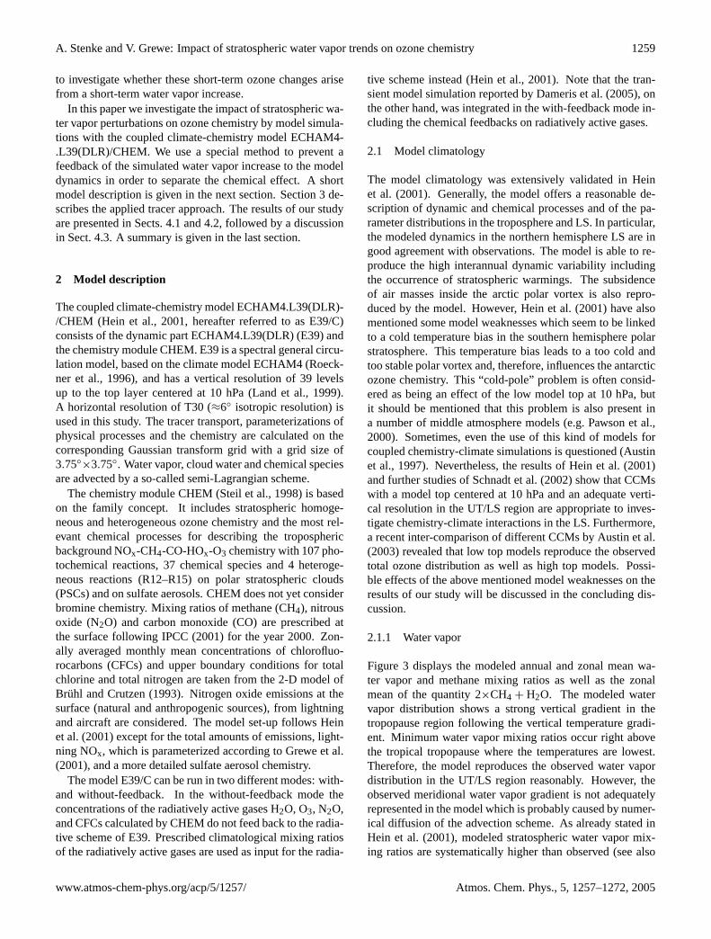
Figure3 displays the modeled annual and zonal mean wa-ter vapor and methane mixing ratios as well as the zonalmean of the quantity 2×CH4 + H2O. The modeled watervapor distribution shows a strong vertical gradient in thetropopause region following the vertical temperature gradi-ent. Minimum water vapor mixing ratios occur right abovethe tropical tropopause where the temperatures are lowest.Therefore, the model reproduces the observed water vapordistribution in the UT/LS region reasonably. However, theobserved meridional water vapor gradient is not adequatelyrepresented in the model which is probably caused by numer-ical diffusion of the advection scheme. As already stated inHein et al.(2001), modeled stratospheric water vapor mix-ing ratios are systematically higher than observed (see also

www.atmos-chem-phys.org/acp/5/1257/ Atmos. Chem. Phys., 5, 1257–1272, 2005


4

56

6

6

6

7

7

7

7

7

7

88

89

9910

101015

Pre

ssur

e [h

Pa]

90˚S 60˚S 30˚S Equator 30˚N 60˚N 90˚N150120100

70

504030

20

10a)

1.2

1.21.3

1.3

1.31.4

1.4

1.4

1.5

1.5

1.5

1.5

1.6

1.6

1.6

1.6

Pre

ssur

e [h

Pa]

90˚S 60˚S 30˚S Equator 30˚N 60˚N 90˚N150120100

70

504030

20

10b)

7

8

9

9

9

1010

10

10

10

1515

15

Pre

ssur

e [h

Pa]

90˚S 60˚S 30˚S Equator 30˚N 60˚N 90˚N150120100

70

504030

20

10c)

Fig. 3. Annual average of(a) zonal mean water vapor mixing ra-tios (ppmv), (b) zonal mean methane mixing ratios (ppmv) and(c) zonal mean 2×CH4 + H2O (ppmv). Averaged over the last10 years (1990–1999) of the transient model simulation (Dameriset al., 2005).

Fig. 1). A comparison between modeled temperatures andECMWF reanalysis reveals a warm temperature bias nearthe model’s tropical tropopause (Land et al., 1999), whichresults in enhanced entry level mixing ratios [H2O]e (mod-eled: 5.9 ppmv, observed: 3.6–4.1 ppmv;SPARC, 2000).The southern polar stratosphere is characterized by strongdehydration in antarctic winter which is overestimated in themodel. This behavior can be directly attributed to the toocold and too stable antarctic polar vortex (Hein et al., 2001).

The modeled methane distribution is shown in Fig.3b. Inthe tropics the methane mixing ratio decreases from about1.65 ppmv to 1.2 ppmv near 10 hPa which is in good agree-ment with HALOE observations (Rosenlof, 2002). Themeridional gradient of methane is slightly underestimated in

the model. As mentioned inHein et al.(2001) this might betaken as an indication for an effect of the low upper bound-ary.

In order to exclude an upper boundary effect on the mod-eled water vapor distribution Fig.3c shows the zonal meanmixing ratio of the quantity 2×CH4 + H2O. The quan-tity 2×CH4 + H2O should be nearly uniform throughout thestratosphere away from regions of dehydration in the winterpolar vortex. The distribution of the quantity 2×CH4 + H2Ois dominated by the modeled water vapor distribution. Awayfrom the southern polar region the distribution is nearlyconstant, whereas northern hemispheric values are slightlyhigher than in the southern hemisphere which is caused bythe water vapor distribution. Figure3c does not show a sub-stantial increase of the quantity 2×CH4 + H2O towards themodel top. Therefore, an upper boundary effect on the mod-eled water vapor is not expected.

2.1.2 Hydroxyl radical

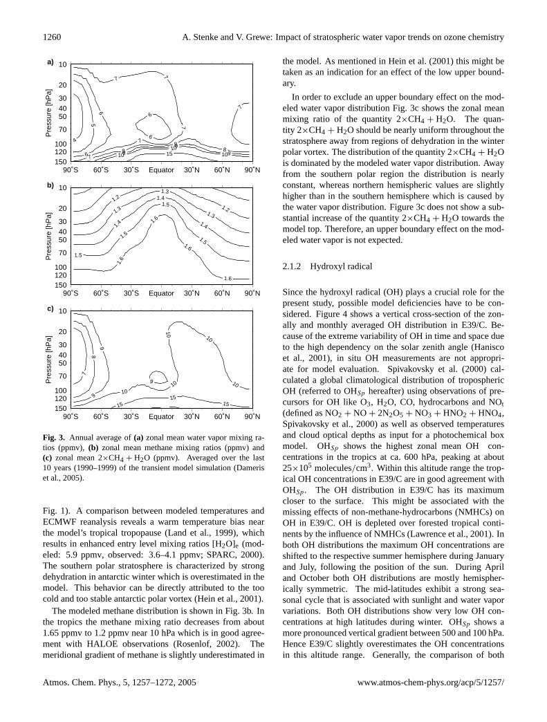
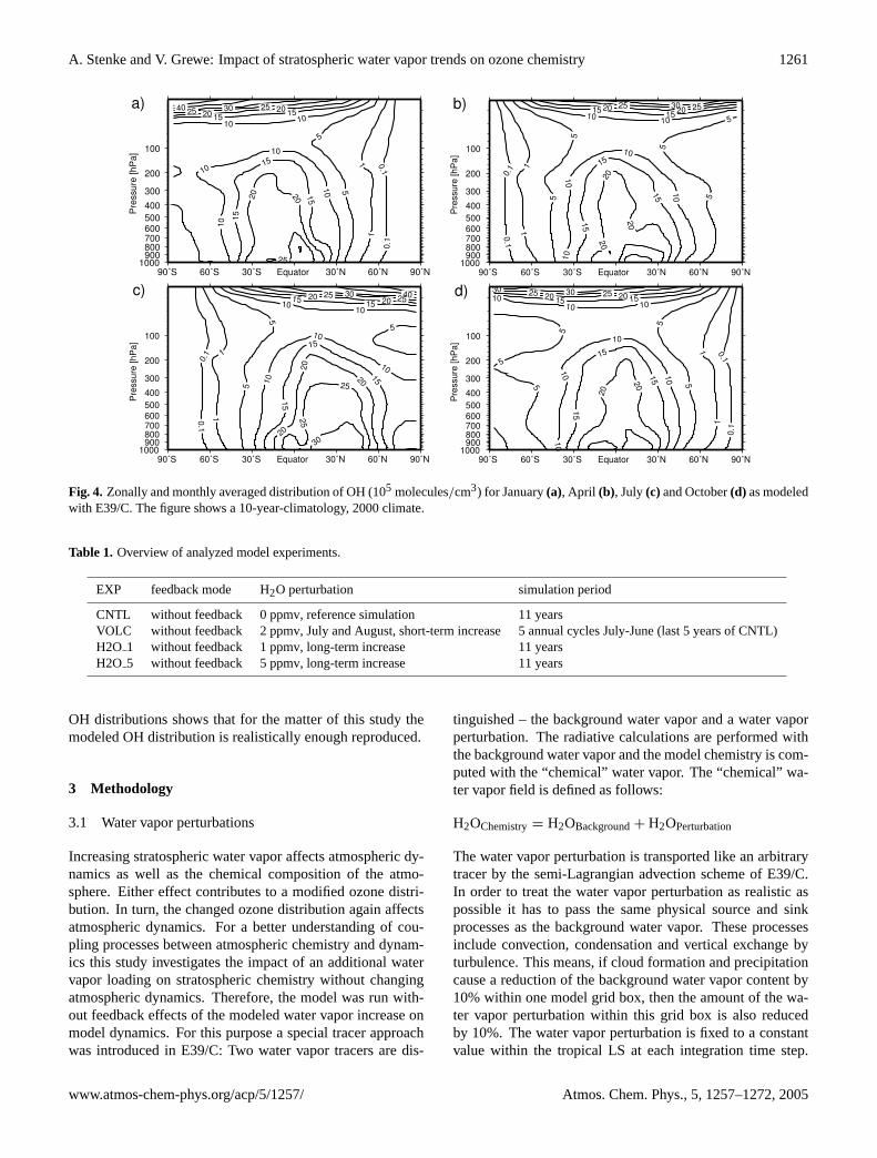
Since the hydroxyl radical (OH) plays a crucial role for thepresent study, possible model deficiencies have to be con-sidered. Figure4 shows a vertical cross-section of the zon-ally and monthly averaged OH distribution in E39/C. Be-cause of the extreme variability of OH in time and space dueto the high dependency on the solar zenith angle (Haniscoet al., 2001), in situ OH measurements are not appropri-ate for model evaluation.Spivakovsky et al.(2000) cal-culated a global climatological distribution of troposphericOH (referred to OHSp hereafter) using observations of pre-cursors for OH like O3, H2O, CO, hydrocarbons and NOt(defined as NO2 + NO + 2N2O5 + NO3 + HNO2 + HNO4,Spivakovsky et al., 2000) as well as observed temperaturesand cloud optical depths as input for a photochemical boxmodel. OHSp shows the highest zonal mean OH con-centrations in the tropics at ca. 600 hPa, peaking at about25×105 molecules/cm3. Within this altitude range the trop-ical OH concentrations in E39/C are in good agreement withOHSp. The OH distribution in E39/C has its maximumcloser to the surface. This might be associated with themissing effects of non-methane-hydrocarbons (NMHCs) onOH in E39/C. OH is depleted over forested tropical conti-nents by the influence of NMHCs (Lawrence et al., 2001). Inboth OH distributions the maximum OH concentrations areshifted to the respective summer hemisphere during Januaryand July, following the position of the sun. During Apriland October both OH distributions are mostly hemispher-ically symmetric. The mid-latitudes exhibit a strong sea-sonal cycle that is associated with sunlight and water vaporvariations. Both OH distributions show very low OH con-centrations at high latitudes during winter. OHSp shows amore pronounced vertical gradient between 500 and 100 hPa.Hence E39/C slightly overestimates the OH concentrationsin this altitude range. Generally, the comparison of both



0.1

0.1

1

1

5

5

1010

10

10

10

10

1515

15

15

15

2020

2020

2525

25

3040

100

200

300

400

500600700800900

1000

Pre

ssu

re [

hP

a]

90˚S 60˚S 30˚S Equator 30˚N 60˚N 90˚N

0.1

0.1

1

1

5

5 5

5

51010

10

10

10

10

1515

15

15

15

20 20

20

20

20

25 2530

100

200

300

400

500600700800900

1000

Pre

ssu

re [

hP

a]

90˚S 60˚S 30˚S Equator 30˚N 60˚N 90˚N

0.1

0.1

1

1

5

5

5

1010

10

10

10

1515

15

15

15

2020

20

20

20

25 25

25

25

30

30

40

100

200

300

400

500600700800900

1000

Pre

ssu

re [

hP

a]

90˚S 60˚S 30˚S Equator 30˚N 60˚N 90˚N

0.1

0.1

1

1

5

55

5

5

101010

10

10

10

10

1515

15

15

15

2020

20

20

2525 3030

100

200

300

400

500600700800900

1000P

ressu

re [

hP

a]

90˚S 60˚S 30˚S Equator 30˚N 60˚N 90˚N

a) b)

c) d)

Fig. 4. Zonally and monthly averaged distribution of OH (105 molecules/cm3) for January(a), April (b), July(c) and October(d) as modeledwith E39/C. The figure shows a 10-year-climatology, 2000 climate.

Table 1. Overview of analyzed model experiments.

EXP feedback mode H2O perturbation simulation period

CNTL without feedback 0 ppmv, reference simulation 11 yearsVOLC without feedback 2 ppmv, July and August, short-term increase 5 annual cycles July-June (last 5 years of CNTL)H2O 1 without feedback 1 ppmv, long-term increase 11 yearsH2O 5 without feedback 5 ppmv, long-term increase 11 years

OH distributions shows that for the matter of this study themodeled OH distribution is realistically enough reproduced.

3 Methodology

3.1 Water vapor perturbations

Increasing stratospheric water vapor affects atmospheric dy-namics as well as the chemical composition of the atmo-sphere. Either effect contributes to a modified ozone distri-bution. In turn, the changed ozone distribution again affectsatmospheric dynamics. For a better understanding of cou-pling processes between atmospheric chemistry and dynam-ics this study investigates the impact of an additional watervapor loading on stratospheric chemistry without changingatmospheric dynamics. Therefore, the model was run with-out feedback effects of the modeled water vapor increase onmodel dynamics. For this purpose a special tracer approachwas introduced in E39/C: Two water vapor tracers are dis-

tinguished – the background water vapor and a water vaporperturbation. The radiative calculations are performed withthe background water vapor and the model chemistry is com-puted with the “chemical” water vapor. The “chemical” wa-ter vapor field is defined as follows:

H2OChemistry= H2OBackground+ H2OPerturbation

The water vapor perturbation is transported like an arbitrarytracer by the semi-Lagrangian advection scheme of E39/C.In order to treat the water vapor perturbation as realistic aspossible it has to pass the same physical source and sinkprocesses as the background water vapor. These processesinclude convection, condensation and vertical exchange byturbulence. This means, if cloud formation and precipitationcause a reduction of the background water vapor content by10% within one model grid box, then the amount of the wa-ter vapor perturbation within this grid box is also reducedby 10%. The water vapor perturbation is fixed to a constantvalue within the tropical LS at each integration time step.



0.0

0.2

0.4

0.6

0.8

1.0

1.2

1.4

1.6

1.8

2.0

Jul Aug Sep Oct Nov Dec Jan Feb Mar Apr May Jun

89 hPa, 30˚N

89 hPa, 30˚S

0.0

0.1

0.2

0.3

0.4

0.5

0.6

0.7

0.8

0.9

1.0


89 hPa, 60˚N

89 hPa, 60˚S

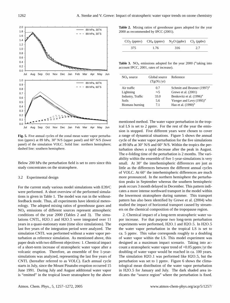
Fig. 5. Five annual cycles of the zonal mean water vapor perturba-tion (ppmv) at 89 hPa, 30◦ N/S (upper panel) and 60◦ N/S (lowerpanel) of the simulation VOLC. Solid line: northern hemisphere;dashed line: southern hemisphere.

Below 200 hPa the perturbation field is set to zero since thisstudy concentrates on the stratosphere.

3.2 Experimental design

For the current study various model simulations with E39/Cwere performed. A short overview of the performed simula-tions is given in Table1. The model was run in the without-feedback mode. Thus, all experiments have identical meteo-rology. The adopted mixing ratios of greenhouse gases andNOx emissions of different sources represent atmosphericconditions of the year 2000 (Tables2 and 3). The simu-lations CNTL, H2O1 and H2O5 were integrated over 11years in a quasi-stationary state (time slice simulations). Thelast five years of the integration period were analyzed. Thesimulation CNTL was performed without a water vapor per-turbation as reference simulation. As mentioned above, thispaper deals with two different objectives: 1. Chemical impactof a short-term increase of stratospheric water vapor after avolcanic eruption. Therefore, an ensemble of five 1-year-simulations was analyzed, representing the last five years ofCNTL (hereafter referred to as VOLC). Each annual cyclestarts in July, since the Mount Pinatubo eruption occurred 15June 1991. During July and August additional water vaporis “emitted” in the tropical lower stratosphere by the above

Table 2. Mixing ratios of greenhouse gases adopted for the year2000 as recommended byIPCC(2001).

CO2 (ppmv) CH4 (ppmv) N2O (ppbv) Cly (ppbv)

375 1.76 316 2.7

Table 3. NOx emissions adopted for the year 2000 (∗taking intoaccountIPCC, 2001, rates of increase).

NOx source Global source Reference(Tg(N)/yr)

Air traffic 0.7 Schmitt and Brunner(1997)∗

Lightning ≈5 Grewe et al.(2001)Industry, Traffic 33.0 Benkovitz et al.(1996)∗

Soils 5.6 Yienger and Levy(1995)∗

Biomass burning 7.1 Hao et al.(1990)∗

mentioned method. The water vapor perturbation in the trop-ical LS is set to 2 ppmv. For the rest of the year the emis-sion is stopped. Five different years were chosen to covera range of dynamical situations. Figure5 shows the annualcycle of the water vapor perturbation for the five simulationsat 89 hPa at 30◦ N/S and 60◦ N/S. Within the tropics the per-turbation shows a rapid decrease after the peak in August.The e-folding time of the perturbation is 2 months. The vari-ability within the ensemble of five 1-year-simulations is verysmall. At 30◦ the interhemispheric differences are just aslittle as the differences between the different annual cyclesof VOLC. At 60◦ the interhemispheric differences are muchmore pronounced. In the northern hemisphere the perturba-tion peaks in September whereas the southern hemisphericpeak occurs 3 month delayed in December. This pattern indi-cates a more intense northward transport in the model withinthe lowermost stratosphere during summer. This transportpattern has also been identified byGrewe et al.(2004) whostudied the impact of horizontal transport caused by stream-ers on the chemical composition of the tropopause region.

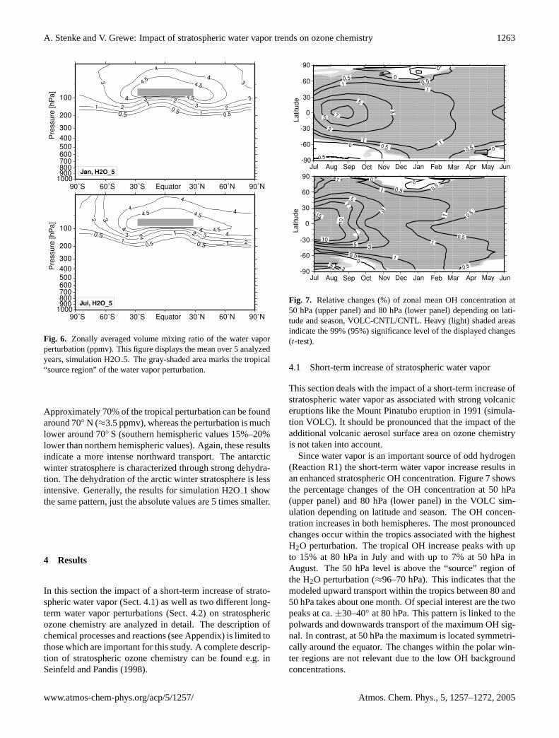
2. Chemical impact of a long-term stratospheric water va-por increase. For that purpose two long-term perturbationexperiments were performed, H2O1 and H2O5. In H2O 5the water vapor perturbation in the tropical LS is set toca. 5 ppmv. This value corresponds roughly to a doublingof water vapor within the LS. This model experiment wasdesigned as a maximum impact scenario. Taking into ac-count a stratospheric water vapor trend of +0.05 ppmv/yr thedoubling of water vapor would be reached in ca. 100 years.The simulation H2O1 was performed like H2O5, but theperturbation was set to 1 ppmv. Figure6 shows the clima-tological mean distribution of the water vapor perturbationin H2O 5 for January and July. The dark shaded area in-dicates the “source region” where the perturbation is fixed.



0.50.50.5 1

11 2

2

2

3

33

3

3

4

4

4

4.54.5

4.5100

200

300

400500600700800900

1000

Pre

ssu

re [

hP

a]

90˚S 60˚S 30˚S Equator 30˚N 60˚N 90˚N

Jan, H2O_5

0.50.5

0.5

1

11

2

22

2

3

3 3 444

4

4

4

4.5

4.54.5

100

200

300

400500600700800900

1000

Pre

ssu

re [

hP

a]

90˚S 60˚S 30˚S Equator 30˚N 60˚N 90˚N

Jul, H2O_5

Fig. 6. Zonally averaged volume mixing ratio of the water vaporperturbation (ppmv). This figure displays the mean over 5 analyzedyears, simulation H2O5. The gray-shaded area marks the tropical“source region” of the water vapor perturbation.

Approximately 70% of the tropical perturbation can be foundaround 70◦ N (≈3.5 ppmv), whereas the perturbation is muchlower around 70◦ S (southern hemispheric values 15%–20%lower than northern hemispheric values). Again, these resultsindicate a more intense northward transport. The antarcticwinter stratosphere is characterized through strong dehydra-tion. The dehydration of the arctic winter stratosphere is lessintensive. Generally, the results for simulation H2O1 showthe same pattern, just the absolute values are 5 times smaller.

4 Results

In this section the impact of a short-term increase of strato-spheric water vapor (Sect.4.1) as well as two different long-term water vapor perturbations (Sect.4.2) on stratosphericozone chemistry are analyzed in detail. The description ofchemical processes and reactions (see Appendix) is limited tothose which are important for this study. A complete descrip-tion of stratospheric ozone chemistry can be found e.g. inSeinfeld and Pandis(1998).

00

0

0

0.5

0.50.5

0.5

0.5

11

11

3

3

5

57

-90

-60

-30

0

30

60

90

Latitu

de


0

00

0.5

0.5

0.5

0.5

0.50.5

1

1

1

1

1

3

3

3

5

5

5

7

7

10

10

-90

-60

-30

0

30

60

90

Latitu

de


15

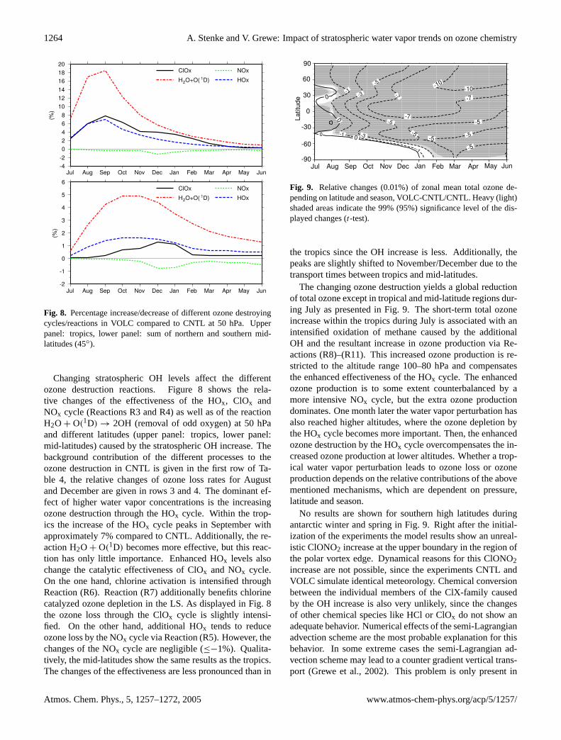
Fig. 7. Relative changes (%) of zonal mean OH concentration at50 hPa (upper panel) and 80 hPa (lower panel) depending on lati-tude and season, VOLC-CNTL/CNTL. Heavy (light) shaded areasindicate the 99% (95%) significance level of the displayed changes(t-test).

4.1 Short-term increase of stratospheric water vapor

This section deals with the impact of a short-term increase ofstratospheric water vapor as associated with strong volcaniceruptions like the Mount Pinatubo eruption in 1991 (simula-tion VOLC). It should be pronounced that the impact of theadditional volcanic aerosol surface area on ozone chemistryis not taken into account.

Since water vapor is an important source of odd hydrogen(ReactionR1) the short-term water vapor increase results inan enhanced stratospheric OH concentration. Figure7 showsthe percentage changes of the OH concentration at 50 hPa(upper panel) and 80 hPa (lower panel) in the VOLC sim-ulation depending on latitude and season. The OH concen-tration increases in both hemispheres. The most pronouncedchanges occur within the tropics associated with the highestH2O perturbation. The tropical OH increase peaks with upto 15% at 80 hPa in July and with up to 7% at 50 hPa inAugust. The 50 hPa level is above the “source” region ofthe H2O perturbation (≈96–70 hPa). This indicates that themodeled upward transport within the tropics between 80 and50 hPa takes about one month. Of special interest are the twopeaks at ca.±30–40◦ at 80 hPa. This pattern is linked to thepolwards and downwards transport of the maximum OH sig-nal. In contrast, at 50 hPa the maximum is located symmetri-cally around the equator. The changes within the polar win-ter regions are not relevant due to the low OH backgroundconcentrations.



-4

-2

0

2

4

6

8

10

12

14

16

18

20

(%)


ClOx

H2O+O( 1D)

NOx

HOx

-2

-1

0

1

2

3

4

5

6

(%)


ClOx

H2O+O( 1D)

NOx

HOx

Fig. 8. Percentage increase/decrease of different ozone destroyingcycles/reactions in VOLC compared to CNTL at 50 hPa. Upperpanel: tropics, lower panel: sum of northern and southern mid-latitudes (45◦).

Changing stratospheric OH levels affect the differentozone destruction reactions. Figure8 shows the rela-tive changes of the effectiveness of the HOx, ClOx andNOx cycle (ReactionsR3 andR4) as well as of the reactionH2O + O(1D) → 2OH (removal of odd oxygen) at 50 hPaand different latitudes (upper panel: tropics, lower panel:mid-latitudes) caused by the stratospheric OH increase. Thebackground contribution of the different processes to theozone destruction in CNTL is given in the first row of Ta-ble 4, the relative changes of ozone loss rates for Augustand December are given in rows 3 and 4. The dominant ef-fect of higher water vapor concentrations is the increasingozone destruction through the HOx cycle. Within the trop-ics the increase of the HOx cycle peaks in September withapproximately 7% compared to CNTL. Additionally, the re-action H2O + O(1D) becomes more effective, but this reac-tion has only little importance. Enhanced HOx levels alsochange the catalytic effectiveness of ClOx and NOx cycle.On the one hand, chlorine activation is intensified throughReaction (R6). Reaction (R7) additionally benefits chlorinecatalyzed ozone depletion in the LS. As displayed in Fig.8the ozone loss through the ClOx cycle is slightly intensi-fied. On the other hand, additional HOx tends to reduceozone loss by the NOx cycle via Reaction (R5). However, thechanges of the NOx cycle are negligible (≤−1%). Qualita-tively, the mid-latitudes show the same results as the tropics.The changes of the effectiveness are less pronounced than in

-10-10

-7

-7

-7

-5

-5-5

-5

-5

-3

-3

-1

-1

-1

0

0

00

-90

-60

-30

0

30

60

90

La

titu

de


-5

-5

Fig. 9. Relative changes (0.01%) of zonal mean total ozone de-pending on latitude and season, VOLC-CNTL/CNTL. Heavy (light)shaded areas indicate the 99% (95%) significance level of the dis-played changes (t-test).

the tropics since the OH increase is less. Additionally, thepeaks are slightly shifted to November/December due to thetransport times between tropics and mid-latitudes.

The changing ozone destruction yields a global reductionof total ozone except in tropical and mid-latitude regions dur-ing July as presented in Fig.9. The short-term total ozoneincrease within the tropics during July is associated with anintensified oxidation of methane caused by the additionalOH and the resultant increase in ozone production via Re-actions (R8)–(R11). This increased ozone production is re-stricted to the altitude range 100–80 hPa and compensatesthe enhanced effectiveness of the HOx cycle. The enhancedozone production is to some extent counterbalanced by amore intensive NOx cycle, but the extra ozone productiondominates. One month later the water vapor perturbation hasalso reached higher altitudes, where the ozone depletion bythe HOx cycle becomes more important. Then, the enhancedozone destruction by the HOx cycle overcompensates the in-creased ozone production at lower altitudes. Whether a trop-ical water vapor perturbation leads to ozone loss or ozoneproduction depends on the relative contributions of the abovementioned mechanisms, which are dependent on pressure,latitude and season.

No results are shown for southern high latitudes duringantarctic winter and spring in Fig.9. Right after the initial-ization of the experiments the model results show an unreal-istic ClONO2 increase at the upper boundary in the region ofthe polar vortex edge. Dynamical reasons for this ClONO2increase are not possible, since the experiments CNTL andVOLC simulate identical meteorology. Chemical conversionbetween the individual members of the ClX-family causedby the OH increase is also very unlikely, since the changesof other chemical species like HCl or ClOx do not show anadequate behavior. Numerical effects of the semi-Lagrangianadvection scheme are the most probable explanation for thisbehavior. In some extreme cases the semi-Lagrangian ad-vection scheme may lead to a counter gradient vertical trans-port (Grewe et al., 2002). This problem is only present in



Table 4. Ozone destroying cycles/reactions at 50 hPa, different latitudes and seasons. CNTL: Contribution of each reaction to the total ozonedestruction [%]. VOLC, H2O1 and H2O5: Changes compared to CNTL [%]. The term O3-Loss includes all ozone destroying reactionsconsidered in E39/C.

Annual Mean, Tropics (5◦N-5◦S) Annual Mean, Mid-Latitudes (45◦N/S)O3-Loss HOx NOx ClOx H2O + O(1D) O3-Loss HOx NOx ClOx H2O + O(1D)

CNTL – 77.1 14.0 1.4 2.9 – 60.8 19.6 8.4 1.4H2O 1 +5.1 +6.4 −1.6 +7.8 +17.0 +2.4 +4.1 -2.2 +2.7 +12.7H2O 5 +25.8 +29.0 −7.7 +114.9 +86.0 +11.0 +19.0 −7.0 +3.4 +64.0

VOLC (Aug) +5.0 +6.0 −0.2 +5.9 +17.0 +0.6 +0.9 -0.07 +0.03 +2.6VOLC (Dec) +1.8 +2.3 −1.2 +4.0 +5.6 +0.9 +1.5 −0.8 +1.3 +4.4

Arctic Spring (April), 80–90◦N Antarctic Spring (October), 80–90◦SO3-Loss HOx NOx ClOx H2O + O(1D) O3-Loss HOx NOx ClOx H2O + O(1D)

CNTL – 26.8 47.7 7.9 0.3 – 6.7 4.0 88.7 0.07H2O 1 −0.9 +5.6 −6.7 +12.4 +10.5 +38.9 −3.4 −47.4 +46.4 +4.3H2O 5 −1.5 +23.3 −17.5 +16.5 +55.7 +126.6 −22.8 −94.9 +149.1 +35.9

simulation VOLC. The long-term experiments are not af-fected.

Interestingly, the most pronounced total ozone reductiontakes place at northern high latitudes during spring/earlysummer. Since the chemical ozone destruction is onlyslightly enhanced in VOLC during arctic spring this resultseems to be associated with the transport of air masses withreduced ozone content from the tropics to northern high lat-itudes during winter.Grewe et al.(2004) studied the large-scale transport of tropical air masses to higher latitudes atpressure levels between 100 hPa and 30 hPa with the climate-chemistry model E39/C. Low ozone air masses are trans-ported from the tropics to higher latitudes by wave breakingevents, so-called streamers.Grewe et al.(2004) showed thatstreamers cause a 30% (50%) decrease of ozone at the extra-tropical tropopause of the summer (winter) hemisphere.

The changes displayed in Fig.9 are statistically significantalthough the changes are less than 1%. For this study onlythe variability of the chemical signal and not the variability ofthe dynamical signal is used for thet-test, taking advantageof the applied methodology (Sect.3) which leads to identicalmeteorology in all simulations.

Unfortunately, no observational data are available for theperiod right after the Mount Pinatubo eruption, suitable for acomparison with model results. Following the volcanic erup-tion, SAGE II (Stratospheric Aerosol and Gas Experiment)ozone values were systematically overestimated due to thePinatubo aerosol. SAGE II ozone values below 22 km al-titude are affected by aerosol for approximately 2 years af-ter the Pinatubo eruption (SPARC, 1998). HALOE (Halo-gen Occultation Experiment) and MLS (Microwave LimbSounder) satellite data are available since October 1991,i.d. no pre-Pinatubo observations are available for compar-ison.

4.2 Long-term increase of stratospheric water vapor

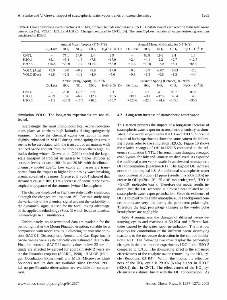
This section presents the impact of a long-term increase ofstratospheric water vapor on stratospheric chemistry as simu-lated in the model experiments H2O1 and H2O5. Since theresults of both experiments show the same pattern the follow-ing figures refer to the simulation H2O5. Figure10 showsthe relative changes of OH in H2O5 compared to the ref-erence simulation CNTL. The zonal mean changes, averagedover 5 years, for July and January are displayed. As expectedthe additional water vapor results in an elevated stratosphericOH concentration (ReactionR1). The highest OH increaseoccurs in the tropical LS. An additional stratospheric watervapor content of 5 ppmv (1 ppmv) results in a 50% (10%) in-crease in OH (≈20×105

−25×105 molecules/cm3, H2O 1:≈5×105 molecules/cm3). Therefore our model results in-dicate that the OH response is almost linear related to thestratospheric water vapor perturbation. Since the existence ofOH is coupled to the sunlit atmosphere, OH background con-centrations are very low during the permanent polar night.Therefore the high percentage changes in the winter polarhemispheres are negligible.

Table 4 summarizes the changes of different ozone de-stroying cycles and reactions at 50 hPa and different lati-tudes caused by the water vapor perturbation. The first rowdisplays the contribution of the different ozone destroyingreactions to the net ozone destruction in the control simula-tion CNTL. The following two rows display the percentagechanges in the perturbation experiments H2O1 and H2O5compared to CNTL. The dominating effect is the enhancedeffectiveness of the catalytic ozone removal by the HOx cy-cle (ReactionsR3–R4). Within the tropics the effective-ness of the HOx cycle is 29.0% (6.4%) higher in H2O5(H2O 1) than in CNTL. The effectiveness of the HOx cy-cle increases almost linear with the OH concentration. As



1

1

1

1

1

1

111

1

5

5

55

5

5

10

10

10

1010

10

25

2525

2525

25

50

Jan, H2O_5

100

200

300

400500600700800900

1000

Pre

ssu

re [

hP

a]

90˚S 60˚S 30˚S Equator 30˚N 60˚N 90˚N

1

1

1

1

1

1

1

1

1

5

5

5

5

5

5

5

5

510

10

10

10

1010 25

2525

25

2525

2525

5075100

Jul, H2O_5

100

200

300

400500600700800900

1000

Pre

ssu

re [

hP

a]

90˚S 60˚S 30˚S Equator 30˚N 60˚N 90˚N

Fig. 10. Zonally and monthly averaged changes of OH (%) com-pared to the simulation CNTL for January and July, simulationH2O 5. Heavy (light) shaded areas indicate the 99% (95%) sig-nificance level of the displayed changes (t-test).

already mentioned in the previous section enhanced HOx lev-els further facilitates the ClOx related ozone destruction(via ReactionsR6–R7), whereas the ozone loss through theNOx cycle is reduced via Reaction (R5). The changes of theNOx cycle and the removal of excited oxygen by the reactionwith water vapor also show a linear behavior with increasingOH. The last mentioned process plays only a minor role inthe ozone destruction. In contrast, the ClOx cycle shows astrong non-linear behavior. The ClOx cycle is 7.8% more ef-fective in H2O1, but above 100% more effective in H2O5.However, the contribution of the ClOx cycle in the tropics isvery small. Within the mid-latitudes the different ozone de-struction cycles show qualitatively the same pattern exceptthe ClOx cycle which increases only slightly with increasingOH.

As already stated the OH increase does not only affectozone destruction, it also results in an enhanced ozone pro-duction in the methane oxidation chain (ReactionsR8–R11).Furthermore, as stratospheric ozone declines, ultraviolet ra-diation penetrates deeper into the stratosphere which leads toan enhanced ozone production by the Chapman mechanism.This process affects mainly the tropical LS, but the ozoneproduction by the Chapman mechanism is only slightly en-hanced (less than 5% in H2O5). However, the increasedozone production can not compensate the enhanced ozonedestruction.

The above mentioned results deal with gas-phase chem-istry and do not consider heterogeneous reactions on polarstratospheric clouds (PSCs). PSCs occur between 15 and25 km at temperatures below≈195 K (pressure dependent)and promote the release of active chlorine from the reser-voir species HCl and ClONO2. At sunrise, activated chlo-rine compounds are easily photolyzed and catalytic ozone de-struction starts. CHEM uses the classical theory ofHansonand Mauersberger(1988) for the formation of PSCs, basedon modeled temperatures and mixing ratios of HNO3 andH2O, and differentiates between PSCs Type I (NAT, nitricacid trihydrate) and PSCs Type II (ice). Four heterogeneousreactions on PSCs and sulfate aerosols (ReactionsR12–R15)are considered in CHEM.

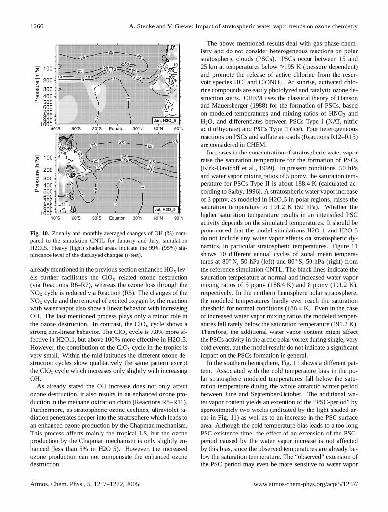
Increases in the concentration of stratospheric water vaporraise the saturation temperature for the formation of PSCs(Kirk-Davidoff et al., 1999). In present conditions, 50 hPaand water vapor mixing ratios of 5 ppmv, the saturation tem-perature for PSCs Type II is about 188.4 K (calculated ac-cording toSalby, 1996). A stratospheric water vapor increaseof 3 ppmv, as modeled in H2O5 in polar regions, raises thesaturation temperature to 191.2 K (50 hPa). Whether thehigher saturation temperature results in an intensified PSCactivity depends on the simulated temperatures. It should bepronounced that the model simulations H2O1 and H2O5do not include any water vapor effects on stratospheric dy-namics, in particular stratospheric temperatures. Figure11shows 10 different annual cycles of zonal mean tempera-tures at 80◦ N, 50 hPa (left) and 80◦ S, 50 hPa (right) fromthe reference simulation CNTL. The black lines indicate thesaturation temperature at normal and increased water vapormixing ratios of 5 ppmv (188.4 K) and 8 ppmv (191.2 K),respectively. In the northern hemisphere polar stratosphere,the modeled temperatures hardly ever reach the saturationthreshold for normal conditions (188.4 K). Even in the caseof increased water vapor mixing ratios the modeled temper-atures fall rarely below the saturation temperature (191.2 K).Therefore, the additional water vapor content might affectthe PSCs activity in the arctic polar vortex during single, verycold events, but the model results do not indicate a significantimpact on the PSCs formation in general.

In the southern hemisphere, Fig.11 shows a different pat-tern. Associated with the cold temperature bias in the po-lar stratosphere modeled temperatures fall below the satu-ration temperature during the whole antarctic winter periodbetween June and September/October. The additional wa-ter vapor content yields an extention of the “PSC-period” byapproximately two weeks (indicated by the light shaded ar-eas in Fig.11) as well as to an increase in the PSC surfacearea. Although the cold temperature bias leads to a too longPSC existence time, the effect of an extension of the PSC-period caused by the water vapor increase is not affectedby this bias, since the observed temperatures are already be-low the saturation temperature. The “observed” extension ofthe PSC period may even be more sensitive to water vapor



170

180

190

200

210

220

230

240

T (

K)

Time (Month)

170

180

190

200

210

220

230

240

T (

K)

Time (Month)

J F M A M J J A S O N D170

180

190

200

210

220

230

240

T (

K)

Time (Month)

J A S O N D J F M A M J

Fig. 11. Modeled temperature at 80◦N, 50 hPa (left) and 80◦S, 50 hPa (right) from the reference simulation CNTL. The colors indicate10 different model years. The dashed lines indicate mean analyzed temperatures based on long-term observations (1979–2004) from theNational Center for Environmental Prediction (NCEP, data can be accessed viahttp://hyperion.gsfc.nasa.gov). The black lines mark thesaturation temperature at water vapor mixing ratios of 5 ppmv (188.4 K) and 8 ppmv (191.2 K). The gray shaded areas indicate the extensionof the PSC existence period associated with the raised saturation temperature (light: E39/C, dark: NCEP reanalysis).

changes, since the temperature changes are smaller in June-July-August compared to March and October (indicated bythe dark shaded areas in Fig.11).

In contrast to the formation of PSCs Type II, which de-pends on temperature and water vapor mixing ratios, the for-mation of PSCs Type I additionally depends on the mixingratio of HNO3. The model results indicate a small increase ofPSCs Type I in the early winter of the northern (November)as well as the southern hemisphere (May) associated with theadditional water vapor (not shown). This enhanced PSC ac-tivity intensifies the denitrification of the polar stratospherein early winter which results in a slightly less NAT forma-tion during the remaining winter. Nevertheless, the dominat-ing effect in the southern polar stratosphere is the enhancedformation of PSCs Type II. In the northern hemisphere nosignificant increase in PSC surface area is detected.

Table 4 displays the percentage changes of the differentozone destruction rates at 50 hPa in polar regions duringspring. The model results show a remarkable interhemi-spheric difference: The additional water vapor yields an in-crease in ozone loss during antarctic spring by≈39% in sim-ulation H2O1 and≈127% in simulation H2O5, whereasthe spring-time ozone loss in the arctic stratosphere staysnearly constant. The most important changes during antarc-tic spring concern the ClOx cycle which is the most impor-tant ozone destruction cycle during antarctic spring. Theenhanced PSC activity during antarctic winter intensifieschlorine activation and results in a pronounced ozone lossthrough the ClOx cycle in spring (+47% in H2O1, +150% inH2O 5). Additionally, it leads to an enhanced denitrificationof the antarctic stratosphere which further supports chlorinecatalyzed ozone destruction (no re-formation of ClONO2).Associated with the denitrification the NOx cycle becomes≈50% less effective in H2O1 and is almost vanished inH2O 5. Finally, the ozone loss through the HOx cycle isslightly reduced, but this effect is less important. In con-

trast, the additional stratospheric water vapor has no impacton PSC activity and heterogeneous ozone destruction duringnorthern polar spring. The ozone destruction rate in generalremains nearly unchanged, but the contribution of the differ-ent ozone destroying reactions is shifted with more effectiveHOx and ClOx cycles and a less effective NOx cycle.

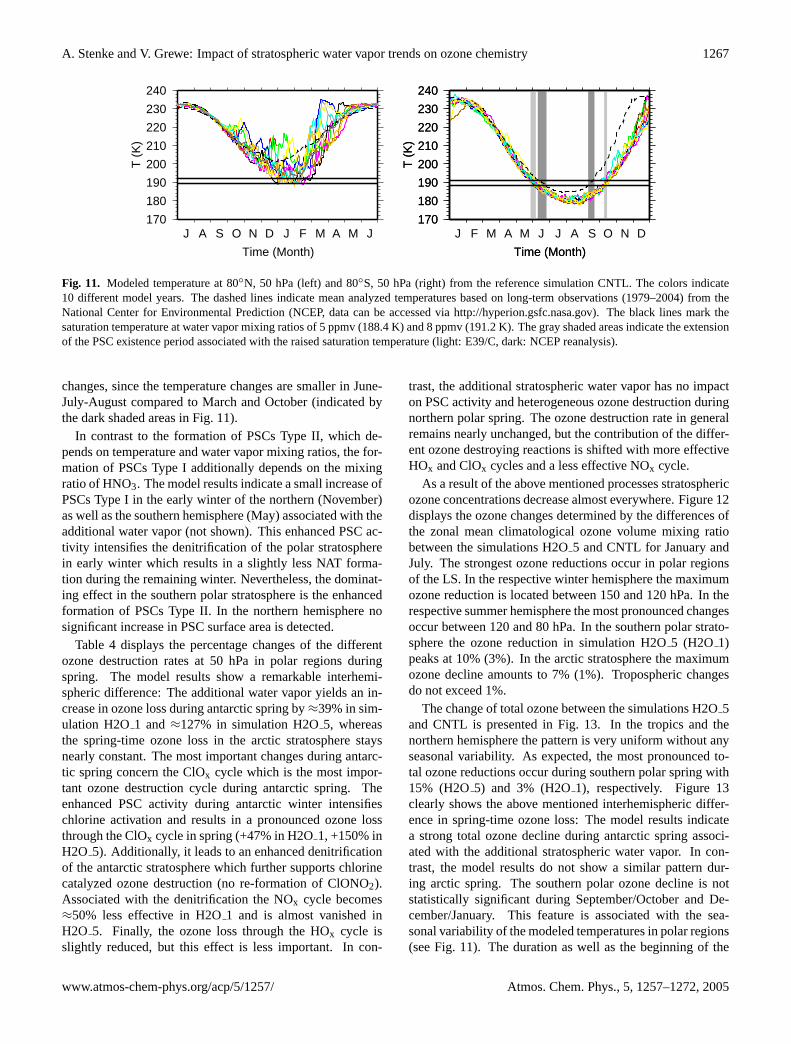
As a result of the above mentioned processes stratosphericozone concentrations decrease almost everywhere. Figure12displays the ozone changes determined by the differences ofthe zonal mean climatological ozone volume mixing ratiobetween the simulations H2O5 and CNTL for January andJuly. The strongest ozone reductions occur in polar regionsof the LS. In the respective winter hemisphere the maximumozone reduction is located between 150 and 120 hPa. In therespective summer hemisphere the most pronounced changesoccur between 120 and 80 hPa. In the southern polar strato-sphere the ozone reduction in simulation H2O5 (H2O 1)peaks at 10% (3%). In the arctic stratosphere the maximumozone decline amounts to 7% (1%). Tropospheric changesdo not exceed 1%.

The change of total ozone between the simulations H2O5and CNTL is presented in Fig.13. In the tropics and thenorthern hemisphere the pattern is very uniform without anyseasonal variability. As expected, the most pronounced to-tal ozone reductions occur during southern polar spring with15% (H2O5) and 3% (H2O1), respectively. Figure13clearly shows the above mentioned interhemispheric differ-ence in spring-time ozone loss: The model results indicatea strong total ozone decline during antarctic spring associ-ated with the additional stratospheric water vapor. In con-trast, the model results do not show a similar pattern dur-ing arctic spring. The southern polar ozone decline is notstatistically significant during September/October and De-cember/January. This feature is associated with the sea-sonal variability of the modeled temperatures in polar regions(see Fig.11). The duration as well as the beginning of the


http://hyperion.gsfc.nasa.gov


1

1

-1

-1

-1

-1

-1

-1

-3

-3

-3

-3-3

-3

-3-3-3

-5

-5

-5

-5

-5 -7

-7

-7

-7

-10

-10

Jan, H2O_5

100

200

300

400500600700800900

1000

Pre

ssu

re [

hP

a]

90˚S 60˚S 30˚S Equator 30˚N 60˚N 90˚N

1-1

-1

-1

-1

-1

-3

-3

-3 -3

-3

-3-3

-3-3

-5

-5-5-5

-5

-5-5

-7

-7

-7

-7-7

Jul, H2O_5

100

200

300

400500600700800900

1000

Pre

ssu

re [

hP

a]

90˚S 60˚S 30˚S Equator 30˚N 60˚N 90˚N

Fig. 12. Zonally and monthly averaged changes of O3 (%) com-pared to the simulation CNTL for January and July, simulationH2O 5. Heavy (light) shaded areas indicate the 99% (95%) sig-nificance level of the displayed changes (t-test).

PSC-period in the antarctic winter LS varies from year toyear, resulting in a non-uniform ozone depletion pattern. Acomparison between simulation H2O1 and H2O5 reveals anearly linear ozone response to the stratospheric water vaporperturbation (not shown).

4.3 Discussion

The analysis of the model simulation VOLC (see Sect.4.1)indicates an almost negligible impact of short-term water va-por perturbations on total ozone in the tropics (Fig.9). There-fore, the short-term ozone decline after volcanic eruptions of≈4% as modeled in the transient model simulation (Fig.2b)can not only be explained through the short-term water vaporincrease. The additional volcanic aerosol heats the strato-sphere and amplifies tropical ascent by roughly 20%, leadingto an additional uplift during a volcanic period of roughly1.2 km, which compares reasonably with the uplift of thePinatubo aerosol cloud by 1.8 km (DeFoor et al., 1992; Kinneet al., 1992). Applying a linearized transport-chemistry col-umn model and using E39/C values for uplift, ozone pro-duction and destruction rates of ozone, the simulated ver-tical ozone profile can be reproduced within 5 to 25% ac-curacy. Introducing an additional uplift of 1.2 km over 8months produces a vertical displacement of the ozone pro-

-10-7-5

-4

-3-3

-3-3

-2-2

-2

-2

-2-2

-2

-90

-60

-30

0

30

60

90

Latitu

de

H2O_5

Jan Feb Mar Apr May Jun Jul Aug Sep Oct Nov Dec

Fig. 13. Relative changes (%) of climatological zonal mean to-tal ozone depending on latitude and season, simulation H2O5-CNTL/CNTL. Heavy (light) shaded areas indicate the 99% (95%)significance level of the displayed changes (t-test).

file and a reduction of the ozone column of 5% (red starsin Fig. 2b), agreeing well with the findings ofKinne et al.(1992). This indicates that the ozone decline simulated aftervolcanic eruptions (Fig.2b) is dominated by dynamic effects.

A comparison between the simulated short-term (VOLC)and long-term water vapor perturbations (H2O1 and H2O5)reveals various differences. VOLC shows a small increase intotal ozone within the tropics during July and August. Duringthis period of the simulation VOLC the water vapor perturba-tion is not yet evenly distributed and the OH increase is con-centrated on the lowermost stratosphere, resulting in a totalozone increase caused by an enhanced ozone production inthe methane oxidation chain (ReactionsR8–R11). Later onthe water vapor perturbation and the associated OH increasereach higher altitudes where the HOx cycle becomes moreimportant. At that time the enhanced ozone loss through theHOx cycle dominates over the enhanced ozone production inthe lowermost stratosphere, resulting in a total ozone reduc-tion. The model simulations H2O1 and H2O5 do not showa similar total ozone increase since the water vapor pertur-bation has reached a steady distribution and the raised ozoneloss through the HOx cycle is the dominating effect. Further-more, simulation VOLC as well as simulation H2O1 showa 7% increase in OH at 50 hPa within the tropics duringAugust. Despite similar water vapor and OH perturbationsVOLC and H2O1 show different ozone changes within thisregion. The ozone reduction in H2O1 amounts to 1%, butonly 0.07% in VOLC. At this altitude the ozone concentra-tion is dynamically controlled (Seinfeld and Pandis, 1998,p. 170). Thus, the effect of a short-term change in localchemistry is less important than the impact of a long-termchange resulting in different ozone transport.

In a previous studyDvortsov and Solomon(2001) ana-lyzed the response of stratospheric temperatures and ozone topast and future increases in stratospheric humidity (1%/yr)with a 2-D radiative-chemical-dynamical model, also sepa-rating the radiation effects of water vapor trends on ozonefrom the photochemical effects. The study ofDvortsov and



Solomon(2001) concentrated on ozone changes at northernmid-latitudes, water vapor effects on PSC formation and het-erogeneous chemistry in polar regions have not been con-sidered. Their results show an additional depletion of mid-latitude total ozone of 0.2%/decade caused by the strato-spheric water vapor increase. In this regard our results are ingood agreement with the findings ofDvortsov and Solomon(2001).

The effect of increasing stratospheric water vapor onozone chemistry has also been discussed within the scope ofsupersonic aircraft emission studies. WithinIPCC(1999) theeffects of a future (year 2015) supersonic aircraft fleet (500aircraft) on stratospheric O3, H2O and other species was con-ducted with various 2-D and 3-D CTMs (chemistry transportmodel). The maximum H2O perturbations caused by super-sonic aircraft emissions occurred in the northern hemisphereLS (≈20 km) with values between 0.4 ppmv and 0.7 ppmv.The calculated total ozone reduction averaged over the north-ern hemisphere was in the range between 0.3 and 0.6%. Thisscenario included only H2O emissions, NOx emissions wereexcluded (EI(NOx)=0). Performing further scenarios withdifferent EI(NOx) all models predicted that the most signif-icant supersonic impact on ozone is caused by the water va-por emissions and that the addition of NOx emissions leadsto less ozone depletion (IPCC, 1999). The modeled watervapor perturbation in H2O1 in the northern hemisphere LS(≈50 hPa) range from 0.5 ppmv to 0.8 ppmv, depending onseason (Fig.6). The resulting total ozone reduction averagedover the northern hemisphere is≈0.5%. In this respect theresults of H2O1 are within the range ofIPCC(1999).

5 Conclusions

The impact of different idealized stratospheric water vaporperturbations on the stratospheric ozone chemistry withoutany feedback on atmospheric dynamics was studied withthe coupled climate-chemistry model ECHAM4.L39(DLR)-/CHEM. To prevent any feedback of the modeled water va-por perturbations a special tracer approach was applied, dif-ferentiating between a background water vapor field and thewater vapor perturbation. Two different long-term perturba-tions (+1 ppmv and +5 ppmv) as well as a short-term increase(“volcanic eruption”, +2 ppmv, 2 month e-folding time) ofstratospheric water vapor were simulated. The impact of wa-ter vapor perturbations on the effectiveness of different ozonedestroying reactions as well as coupling effects between dif-ferent chemical processes were analyzed in detail.

A stratospheric water vapor increase leads to an enhancedOH concentration which results primarily in an enhancedozone depletion by the HOx cycle. The coupling of theHOx cycle with the NOx and ClOx cycle leads to a less ef-fective NOx cycle and a slightly enhanced effectiveness ofthe ClOx cycle. Furthermore, increasing stratospheric wa-ter vapor concentrations raise the saturation temperature of

PSCs by 0.8 K/ppmv (at 50 hPa,≈6 ppmv H2O) (Kirk-Davidoff et al., 1999). Therefore, a stratospheric water va-por increase is supposed to enhance PSCs activity and het-erogeneous ozone loss. In this regard the model results haveindicated a strong asymmetry between arctic and antarctic re-gions: Within the antarctic polar vortex the increase in strato-spheric water vapor causes an enhanced PSC formation. As-sociated with the higher PSC activity the release of activechlorine from reservoir species is intensified which leads to amore effective heterogeneous ozone destruction through theClOx cycle. In contrast, the simulated stratospheric watervapor increase does not affect PSC formation in the arcticstratosphere during winter. This interhemispheric differenceis linked to the modeled stratospheric temperatures in thetwo polar regions. In the arctic polar vortex modeled tem-peratures fall rarely below the saturation temperature, evenin case of the raised saturation temperature. In the southernhemisphere polar vortex the modeled temperatures are gen-erally lower than in the northern hemisphere polar vortex andfall below the saturation temperature during the whole win-ter. Therefore, the additional stratospheric water vapor yieldsan extention the PSC-period by two weeks and an increasein PSCs surface area. The simulated short-term water vaporperturbation does not affect PSCs activity and heterogeneousozone chemistry.

A comparison with NCEP (National Center for Environ-mental Prediction) reanalysis shows that the modeled tem-peratures in the northern polar stratosphere are generally ingood agreement with the NCEP data, only the mean winterminimum temperature is slightly lower (≈3 K) in the model(Hein et al., 2001, see also Fig.11). Regarding to the NCEPdata the temperatures in the northern polar stratosphere donot fall below the PSC Type II formation temperature dur-ing winter. Therefore, neglecting any radiation effect of thewater vapor increase, an increase in stratospheric water va-por is not to be expected to cause a general increase in PSCactivity and heterogeneous ozone loss in the northern polarstratosphere. To cause a significant increase in PSC activity astrong cooling of the arctic stratosphere would be necessary.However, the magnitude of stratospheric cooling caused byincreasing greenhouse gases as well as the contribution ofincreasing stratospheric water vapor is still unclear (WMO,2003, chapter 3).

In the southern hemisphere polar stratosphere the mod-eled mean winter temperature is significantly lower (≈10 K)than in the NCEP data (Hein et al., 2001, see also Fig.11).However, the observed temperatures also fall below the for-mation temperature for PSC Type II between June and Au-gust. Therefore, it is to be expected that an increase in strato-spheric water vapor results in an enhanced PSC Type II for-mation in the southern polar stratosphere. The raised PSCformation temperature may even lead to a larger extension ofthe PSC existence period than modeled (indicated by the grayshaded areas in Fig.11), because the temporal temperaturechanges at the end and beginning of PSC existence time are



larger in the model simulation than in the observations. Theexpected radiation effect of a water vapor increase (Forsterand Shine, 1999, 2002) would further extend the PSC period.However, the magnitude of the resulting ozone loss dependsnot only on water vapor concentrations and PSC activity, bute.g. also on the stratospheric chlorine and bromine loading.For example, a model study ofSchnadt et al.(2002) on thefuture chemical composition and climate has shown a slightincrease in antarctic ozone depletion due to larger PSC activ-ity, despite a reduced stratospheric chlorine loading.

A comparison between the two different long-term wa-ter vapor perturbations (H2O1 and H2O5) has shown thatthe ozone reduction increases almost linearly with increasingstratospheric water vapor. This linear ozone response agreeswell with the results ofDvortsov and Solomon(2001) whoalso found a linear relationship between ozone response andwater vapor perturbation. The results of a transient modelsimulation (Dameris et al., 2005) with a modeled water vaporincrease of 0.029 ppmv/yr between 1980 and 1999 (Fig.1)correspond to a stratospheric water vapor perturbation of ap-proximately 0.6 ppmv. According to the linear behavior ofthe ozone response, at least on hemispheric scales, a pertur-bation of 0.6 ppmv leads to a global total ozone reductionof 0.5%. The simulated global ozone decline between 1980and 1999 amounts 3.4%, considering the increasing chlorineloading and climate change. Therefore, the results of thisstudy indicate that 10% of the ozone decline in the transientmodel run is linked to the simulated water vapor increase.

Several studies discussed an increase in stratospheric wa-ter vapor concentrations over the last decades (e.g.Nedoluhaet al., 1998; Oltmans et al., 2000; Rosenlof, 2002). An in-crease in stratospheric water vapor would affect stratosphericozone in several ways: The stratosphere is expected to coolas water vapor increases (Forster and Shine, 1999, 2002)which results in an more pronounced PSC formation (Kirk-Davidoff et al., 1999). Furthermore, increasing OH concen-trations cause an enhanced homogeneous ozone loss (e.g.Dvortsov and Solomon, 2001). However, a recent analysis ofdifferent water vapor observations shows great discrepanciesin lower stratospheric water vapor trends between the differ-ent data sets (Randel et al., 2004), so that the discussion onstratospheric water vapor trends is re-opened. Furthermore,the observations show remarkably low water vapor concen-trations in the LS since 2001. Nevertheless, this and previ-ous model studies indicate a not negligible impact of watervapor on stratospheric ozone that must be kept in mind dis-cussing the future development of stratospheric ozone con-centrations.

Appendix: Chemical reactions

Oxidation of H2O and CH4:

O(1D) + H2O → 2OH (R1)

O(1D) + CH4 → OH + CH3 (R2)

Catalytic ozone destruction cycle:

X + O3 → XO + O2

XO + O → X + O2

O3 + O → O2 + O2, (R3)

where X can be one of the free radicals H, OH, NO, Cl orBr.

Additional HOx-cycle:

OH + O3 → HO2 + O2

HO2 + O3 → OH + O2 + O2

O3 + O3 → O2 + O2 + O2 (R4)

Coupling of HOx and NOx cycle:

OH + NO2 + M → HNO3 + M (R5)

Coupling of HOx and ClOx cycle:

OH + HCl → H2O + Cl (R6)

HO2 + ClO → HOCl + O2 (R7)

Ozone production in methane oxidation chain:

CH3O2 + NO → CH3O + NO2 (R8)

or

HO2 + NO → OH + NO2 (R9)

NO2hν→ NO + O (R10)

O2 + O → O3 (R11)

Heterogeneous reactions on PSCs and sulfate aerosols inCHEM:

HCl + ClONO2 → Cl2 + HNO3 (R12)

H2O + ClONO2 → HOCl + HNO3 (R13)

HOCl + HCl → Cl2 + H2O (R14)

N2O5 + H2O → 2HNO3 (R15)



Acknowledgements.This study was partially funded by the EUproject SCENIC. The model simulations were performed on theNEC SX-6 high performance computer of the German ClimateComputing Centre (DKRZ), Hamburg. We thank M. Ponater forhis helpful answers concerning the “last secrets” of the model EC-HAM4.L39(DLR)/CHEM and H. Vomel for providing the Boulderwater vapor dataset. J. Austin, P. Haynes and an anonymous refereeare kindly acknowledged for their constructive reviews and helpfulsuggestions.

Edited by: P. H. Haynes

References

Austin, J., Butchart, N., and Swinbank, R. S.: Sensitivity of ozoneand temperature to vertical resolution in a GCM with coupledstratospheric chemistry, Q. J. R. Meteorol. Soc., 123, 1405–1431,1997.

Austin, J., Shindell, D., Beagley, S. R., Bruhl, C., Dameris, M.,Manzini, E., Nagashima, T., Newman, P., Pawson, S., Pitari, G.,Rozanov, E., Schnadt, C., and Shepherd, T. G.: Uncertaintiesand assessments of chemistry-climate models of the stratosphere,Atmos. Chem. Phys., 3, 1–27, 2003,SRef-ID: 1680-7324/acp/2003-3-1.

Bates, D. R. and Nicolet, M.: The photochemistry of atmosphericwater vapor, J. Geophys. Res., 55, 301–327, 1950.

Benkovitz, C. M., Scholtz, M. T., Pacyna, J., Tarrason, L., Dignon,J., Voldner, E. C., Spiro, P. A., Logan, J. A., and Graedel, T. E.:Global gridded inventories of anthropogenic emissions of sulfurand nitrogen, J. Geophys. Res., 101, 29 239–29 253, 1996.

Bruhl, C. and Crutzen, P. J.: MPIC two-dimensional model, in Theatmospheric effects of stratospheric aircraft: Report of the 1992models and measurement workshop, edited by: Prather, M. andRemsberg, E., NASA Reference Publ. 1292, pp. 703–706, Wash-ington, DC, 1993.

Considine, D. B., Rosenfield, J. E., and Fleming, E. L.: An in-teractive model study of the influence of the Mount Pinatuboaerosol on stratospheric methane and water trends, J. Geophys.Res., 106, 27 711–27 727, 2001.

Dameris, M., Grewe, V., Ponater, M., Deckert, R., Eyring, V.,Mager, F., Matthes, S., Schnadt, C., Stenke, A., Steil, B., Bruhl,C., and Giorgetta, M. A.: Long-term changes and variability in atransient simulation with a chemistry-climate model employingrealistic forcing, Atmos. Chem. Phys. Discuss., 5, 2297–2353,2005,SRef-ID: 1680-7375/acpd/2005-5-2297.

DeFoor, T. E., Robinson, E., and Ryan, S.: Early lidar observationsof the June ’91 Pinatubo eruption plume at Mauna Loa Observa-tory, Hawaii, Geophys. Res. Lett., 19, 187–190, 1992.

Dvortsov, V. L. and Solomon, S.: Response of the stratospheric tem-peratures and ozone to past and future increases in stratospherichumidity, J. Geophys. Res., 106, 7505–7514, 2001.

Evans, S. J., Toumi, R., Harries, J. E., Chipperfield, M. P., and Rus-sell III, J. M.: Trends in the stratospheric humidity and the sensi-tivity of ozone to these trends, J. Geophys. Res., 103, 8715–8725,1998.

Fioletov, V. E., Bodeker, G. E., Miller, A. J., McPeters, R. D., andStolarski, R.: Global and zonal total ozone variations estimated

from ground-based and satellite measurements: 1964–2000, J.Geophys. Res., 107, 4647, doi:10.1029/2001JD001350, 2002.

Forster, P. M. de F. and Shine, K. P.: Stratospheric water vapourchanges as a possible contributor to observed stratospheric cool-ing, Geophys. Res. Lett., 26, 3309–3312, 1999.

Forster, P. M. de F. and Shine, K. P.: Assessing the climate impactof trends in stratospheric water vapor, Geophys. Res. Lett., 29,1086, doi:10.1029/2001GL013909, 2002.

Grewe, V., Brunner, D., Dameris, M., Grenfell, J. L., Hein, R., Shin-dell, D., and Staehelin, J.: Origin and variability of upper tro-pospheric nitrogen oxides and ozone at northern mid-latitudes,Atmos. Environ., 35, 3421–3433, 2001.

Grewe, V., Dameris, M., Fichter, C., and Sausen, R.: Impact ofaircraft NOx emissions. Part 1: Interactively coupled climate-chemistry simulations and sensitivities to climate-chemistryfeedback, lightning and model resolution, Meteorol. Z., 3, 177–186, 2002.

Grewe, V., Shindell, D. T., and Eyring, V.: The impact of horizontaltransport on the chemical composition in the tropopause region:Lightning NOx and streamers, Adv. Space Res., 33, 1058–1061,2004.

Hanisco, T. F., Lanzendorf, E. J., Wennberg, P. O., Perkins, K. K.,Stimpfle, R. M., Voss, P. B., Anderson, J. G., Cohen, R. C., Fa-hey, D. W., Gao, R. S., Hintsa, E. J., Salawitch, R. J., Margitan,J. J., McElroy, C. T., and Midwinter, C.: Sources, sinks and thedistribution of OH in the lower stratosphere, J. Phys. Chem. A,105, 1543–1553, 2001.

Hanson, D. and Mauersberger, K.: Laboratory studies of nitric acidtrihydrate: Implications for the south polar stratosphere, Geo-phys. Res. Lett., 15, 855–858, 1988.

Hao, W. M., Liu, M.-H., and Crutzen, P. J.: Estimates of annual andregional releases of CO2 and other trace gases to the atmospherefrom fires in the tropics, based on the FAO statistics for the pe-riod 1975–1980, Vol. 84 of Fire in the Tropical Biota, EcologicalStudies, pp. 440–462, Springer-Verlag, New York, 1990.

Hein, R., Dameris, M., Schnadt, C., Land, C., Grewe, V., Kohler,I., Ponater, M., Sausen, R., Steil, B., Landgraf, J., and Bruhl,C.: Results of an interactively coupled atmospheric chemistry–general circulation model: comparison with oberservations, Ann.Geophys., 19, 435–457, 2001,SRef-ID: 1432-0576/ag/2001-19-435.

IPCC (Intergovernmental Panel on Climate Change): Aviation andthe global atmosphere, 373 pp., Cambridge University Press,Cambridge, UK, 1999.

IPCC (Intergovernmental Panel on Climate Change): ClimateChange 2001 – The scientific basis, 881 pp., Cambridge Uni-versity Press, New York, USA, 2001.

Kinne, S., Toon, O. B., and Prather, M. J.: Buffering of stratosphericcirculation by changing amounts of tropical ozone – a Pinatubocase study, Geophys. Res. Lett., 19, 1927–1930, 1992.

Kirk-Davidoff, D. B., Hintsa, E. J., Anderson, J. G., and Keith,D. W.: The effect of climate change on ozone depletion throughchanges in stratospheric water vapour, Nature, 402, 399–401,1999.

Land, C., Ponater, M., Sausen, R., and Roeckner, E.: TheECHAM4.L39(DLR) atmosphere GCM – Technical descriptionand model climatology, DLR Forschungsbericht 1999-31, ISSN1434-8454, Koln, 1999.

Lawrence, M. G., Jockel, P., and von Kuhlmann, R.: What does the


http://direct.sref.org/1680-7324/acp/2003-3-1

http://direct.sref.org/1680-7375/acpd/2005-5-2297

http://direct.sref.org/1432-0576/ag/2001-19-435


global mean OH concentration tell us?, Atmos. Chem. Phys., 1,37–49, 2001,SRef-ID: 1680-7324/acp/2001-1-37.

Michelsen, H. A., Irion, F. W., Manney, G. L., Toon, G. C.,and Gunson, M. R.: Features and trends in Atmospheric TraceMolecule Spectroscopy (ATMOS) version 3 stratospheric wa-ter vapor and methane measurements, J. Geophys. Res., 105,22 713–22 724, 2000.

Nedoluha, G. E., Bevilacqua, R. M., Gomez, R. M., Siskind, D. E.,Hicks, B. C., Russell III, J. M., and Connor, B. J.: Increasesin middle atmospheric water vapor as observed by the Halo-gen Occultation Experiment and the ground-based Water VaporMillimeter-wave Spectrometer from 1991 to 1997, J. Geophys.Res., 103, 3531–3543, 1998.

Oltmans, S. J., Vomel, H., Hofmann, D. J., Rosenlof, K. H., andKley, D.: The increase in stratospheric water vapor from bal-loonborne frostpoint hygrometer measurements at WashingtonD.C., and Boulder, Colorado, Geophys. Res. Lett., 27, 3453–3456, 2000.

Pawson, S., Kodera, K., Hamilton, K., Shepherd, T. G., Beagley,S. R., Boville, B. A., Farrara, J. D., Fairlie, T. D. A., Kitoh, A.,Lahoz, W. A., Langematz, U., Manzini, E., Rind, D. H., Scaife,A. A., Shibata, K., Simon, P., Swinbank, R., Takacs, L., Wil-son, R. J., Al-Saadi, J. A., Amodei, M., Chiba, M., Coy, L., deGrandpre, J., Eckman, R. S., Fiorino, M., Grose, W. L., Koide,H., Koshyk, J. N., Li, D., Lerner, J., Mahlman, J. D., McFarlane,N. A., Mechoso, C. R., Molod, A., O’Neill, A., Pierce, R. B.,Randel, W. J., Rood, R. B., and Wu, F.: The GCM-reality inter-comparison project of SPARC (GRIPS): scientific issues and ini-tial results, Bull. Am. Meteorol. Soc., 81, 781–796, 2000.

Randel, W. J., Wu, F., Oltmans, S. J., Rosenlof, K., and Nedoluha,G. E.: Interannual changes of stratospheric water vapor and cor-relations with tropical tropopause temperatures, J. Atmos. Sci.,61, 2133–2148, 2004.

Roeckner, E., Arpe, K., Bengtsson, L., Christoph, M., Claussen,M., Dumenil, L., Esch, M., Giorgetta, M., Schlese, U., andSchulzweida, U.: The atmospheric general circulation modelECHAM-4: Model description and simulation of present-dayclimate, Report No. 218, Max-Planck-Institut fur Meteorologie,Hamburg, 1996.

Rosenlof, K. H.: Transport changes inferred from HALOE wa-ter and methane measurements, J. Met. Soc. Jap., 80, 831–848,2002.

Rosenlof, K. H., Oltmans, S. J., Kley, D., Russell III, J. M., Chiou,E.-W., Chu, W. P., Johnson, D. G., Kelly, K. K., Michelsen,H. A., Nedoluha, G. E., Remsberg, E. E., Toon, G. C., and Mc-Cormick, M. P.: Stratospheric water vapor increases over the pasthalf-century, Geophys. Res. Lett., 28, 1195–1198, 2001.

Salby, M. L.: Fundamentals of Atmospheric Physics, 627 pp., Aca-demic Press, San Diego, Calif., 1996.

Schnadt, C., Dameris, M., Ponater, M., Hein, R., Grewe, V., andSteil, B.: Interaction of atmospheric chemistry and climate andits impact on stratospheric ozone, Clim. Dyn., 17, 501–517,2002.

Schmitt, A. and Brunner, D.: Emissions from aviation and theirdevelopment over time, in: Pollutants from air traffic – resultsof atmospheric research 1992–1997, edited by: Schumann, U.,Chloud, A., Ebel, A., Karcher, B., Pak, H., Schlager, H., Schmitt,A., and Wendling, P., Vol. 97-04 of DLR-Mitt., 37–52, DLRKoln, Germany, 1997.

Seinfeld, J. H. and Pandis, S. N.: Atmospheric chemistry andphysics: From air pollution to climate change, 1360 pp., JohnWiley & Sons, Inc., New York, NY, 1998.

SPARC: Assessment of trends in the vertical distribution of ozone,SPARC Report #1, WMO Ozone Research and MonitoringProject Report #43, 1998.

SPARC: Assessment of upper tropospheric and stratospheric wa-ter vapour, WCRP #113, WMO/TD #1043, SPARC Report #2,2000.

Spivakovsky, C. M., Logan, J. A., Montzka, S. A., Balkanski, Y. J.,Foreman-Fowler, M., Jones, D. B. A., Horowitz, L. W., Fusco,A. C., Brenninkmeijer, C. A. M., Prather, M. J., Wofsy, S. C., andMcElroy, M. B.: Three-dimensional climatological distributionof tropospheric OH: Update and evaluation, J. Geophys. Res.,105, 8931–8980, 2000.

Steil, B., Dameris, M., Bruhl, C., Crutzen, P. J., Grewe, V., Ponater,M., and Sausen, R.: Development of a chemistry module forGCMs: first results of a multiannual integration, Ann. Geophys.,16, 205–228, 1998,SRef-ID: 1432-0576/ag/1998-16-205.

WMO (World Meteorological Organization): Scientific assessmentof ozone depletion: 2002, Report No. 47, 498 pp., Geneva, 2003.

Yienger, J. J. and Levy, H.: Empirical model of global soil-biogenicNOx emissions, J. Geophys. Res., 100, 11 447–11 464, 1995.

Zhou, X., Geller, M. A., and Zhang, M.: Cooling trend of the trop-ical cold point tropopause temperatures and its implications, J.Geophys. Res., 106, 1511–1522, 2001.


http://direct.sref.org/1680-7324/acp/2001-1-37

http://direct.sref.org/1432-0576/ag/1998-16-205

Documents

and Physics Simulation of stratospheric water vapor trends: … · 2016-01-11 · For exam-ple, Rosenlof et al. (2001) combined ten different data sets between 1954 and 2000, and