Max-Planck-Institut fur Physik komplexer Systeme

Biaxial Nematic Order in Liver Tissue

D I S S E R T A T I O N

zur Erlangung des akademischen Grades

Doctor rerum naturalium

(Dr. rer. nat.)

vorgelegt

dem Bereich Mathematik und Naturwissenschaften

der Technischen Universitat Dresden

von

Dipl.-Phys. Andre Scholich

geboren am 17. Dezember 1986 in Crivitz

Dresden, 2018

Betreuender Hochschullehrer: Prof. Dr. Frank Julicher

Eingereicht am 5. Februar 2018

Gutachter:

• Prof. Dr. Frank Julicher

• Prof. Dr. Stephan Grill

• Prof. Dr. Samuel Safran

Prufungskommission:

• Prof. Dr. Clemens Laubschat (Vorsitz)

• Prof. Dr. Frank Julicher

• Prof. Dr. Stefan Grill

• Dr. Benjamin Friedrich

Verteidigt am 30. Mai 2018 in Dresden

ii

Abstract

Understanding how biological cells organize to form complex functional tissues is

a question of key interest at the interface between biology and physics. The liver is

a model system for a complex three-dimensional epithelial tissue, which performs

many vital functions. Recent advances in imaging methods provide access to

experimental data at the subcellular level. Structural details of individual cells

in bulk tissues can be resolved, which prompts for new analysis methods. In

this thesis, we use concepts from soft matter physics to elucidate and quantify

structural properties of mouse liver tissue.

Epithelial cells are structurally anisotropic and possess a distinct apico-basal cell

polarity that can be characterized, in most cases, by a vector. For the parenchymal

cells of the liver (hepatocytes), however, this is not possible. We therefore develop

a general method to characterize the distribution of membrane-bound proteins in

cells using a multipole decomposition. We first verify that simple epithelial cells

of the kidney are of vectorial cell polarity type and then show that hepatocytes

are of second order (nematic) cell polarity type. We propose a method to quan-

tify orientational order in curved geometries and reveal lobule-level patterns of

aligned cell polarity axes in the liver. These lobule-level patterns follow, on av-

erage, streamlines defined by the locations of larger vessels running through the

tissue. We show that this characterizes the liver as a nematic liquid crystal with

biaxial order. We use the quantification of orientational order to investigate the

effect of specific knock-down of the adhesion protein Integrin-β1.

Building upon these observations, we study a model of nematic interactions.

We find that interactions among neighboring cells alone cannot account for the

observed ordering patterns. Instead, coupling to an external field yields cell po-

larity fields that closely resemble the experimental data. Furthermore, we analyze

the structural properties of the two transport networks present in the liver (sinu-

soids and bile canaliculi) and identify a nematic alignment between the anisotropy

of the sinusoid network and the nematic cell polarity of hepatocytes. We propose

a minimal lattice-based model that captures essential characteristics of network

organization in the liver by local rules. In conclusion, using data analysis and

minimal theoretical models, we found that the liver constitutes an example of a

living biaxial liquid crystal.

iii

Contents

1. Introduction 1

1.1. From molecules to cells, tissues and organisms: multi-scale hierar-

chical organization in animals . . . . . . . . . . . . . . . . . . . . . . . . . . . . . . . . 1

1.2. The liver as a model system of complex three-dimensional tissue . . 2

1.3. Biology of tissues . . . . . . . . . . . . . . . . . . . . . . . . . . . . . . . . . . . . . . . . . . 5

1.4. Physics of tissues . . . . . . . . . . . . . . . . . . . . . . . . . . . . . . . . . . . . . . . . . . . 9

1.4.1. Continuum descriptions . . . . . . . . . . . . . . . . . . . . . . . . . . . . . . . 11

1.4.2. Discrete models . . . . . . . . . . . . . . . . . . . . . . . . . . . . . . . . . . . . . . 11

1.4.3. Two-dimensional case study: planar cell polarity in the fly

wing . . . . . . . . . . . . . . . . . . . . . . . . . . . . . . . . . . . . . . . . . . . . . . . . 15

1.4.4. Challenges of three-dimensional models for liver tissue . . . . . 16

1.5. Liquids, crystals and liquid crystals . . . . . . . . . . . . . . . . . . . . . . . . . . . 16

1.5.1. The uniaxial nematic order parameter . . . . . . . . . . . . . . . . . . . 19

1.5.2. The biaxial nematic ordering tensor . . . . . . . . . . . . . . . . . . . . . 21

1.5.3. Continuum theory of nematic order . . . . . . . . . . . . . . . . . . . . . 23

1.5.4. Smectic order . . . . . . . . . . . . . . . . . . . . . . . . . . . . . . . . . . . . . . . . 25

1.6. Three-dimensional imaging of liver tissue . . . . . . . . . . . . . . . . . . . . . . 26

1.7. Overview of the thesis . . . . . . . . . . . . . . . . . . . . . . . . . . . . . . . . . . . . . . 28

2. Characterizing cellular anisotropy 31

2.1. Classifying protein distributions on cell surfaces . . . . . . . . . . . . . . . . 31

2.1.1. Mode expansion to characterize distributions on the unit

sphere . . . . . . . . . . . . . . . . . . . . . . . . . . . . . . . . . . . . . . . . . . . . . . 31

2.1.2. Vectorial and nematic classes of surface distributions . . . . . . 33

2.1.3. Cell polarity on non-spherical surfaces . . . . . . . . . . . . . . . . . . 34

2.2. Cell polarity in kidney and liver tissues . . . . . . . . . . . . . . . . . . . . . . . 36

2.2.1. Kidney cells exhibit vectorial polarity . . . . . . . . . . . . . . . . . . . 36

2.2.2. Hepatocytes exhibit nematic polarity . . . . . . . . . . . . . . . . . . . 37

2.3. Local network anisotropy . . . . . . . . . . . . . . . . . . . . . . . . . . . . . . . . . . . . 40

2.4. Summary . . . . . . . . . . . . . . . . . . . . . . . . . . . . . . . . . . . . . . . . . . . . . . . . . 41

iv

3. Order parameters for tissue organization 43

3.1. Orientational order: quantifying biaxial phases . . . . . . . . . . . . . . . . . 43

3.1.1. Biaxial nematic order parameters . . . . . . . . . . . . . . . . . . . . . . . 45

3.1.2. Co-orientational order parameters . . . . . . . . . . . . . . . . . . . . . . 51

3.1.3. Invariants of moment tensors . . . . . . . . . . . . . . . . . . . . . . . . . . 52

3.1.4. Relation between these three schemes . . . . . . . . . . . . . . . . . . . 53

3.1.5. Example: nematic coupling to an external field . . . . . . . . . . . 55

3.2. A tissue-level reference field . . . . . . . . . . . . . . . . . . . . . . . . . . . . . . . . . 59

3.3. Orientational order in inhomogeneous systems . . . . . . . . . . . . . . . . . 62

3.4. Positional order: identifying signatures of smectic and columnar

order . . . . . . . . . . . . . . . . . . . . . . . . . . . . . . . . . . . . . . . . . . . . . . . . . . . . . 64

3.5. Summary . . . . . . . . . . . . . . . . . . . . . . . . . . . . . . . . . . . . . . . . . . . . . . . . . 67

4. The liver lobule exhibits biaxial liquid-crystal order 69

4.1. Coarse-graining reveals nematic cell polarity patterns on the lobule-

level . . . . . . . . . . . . . . . . . . . . . . . . . . . . . . . . . . . . . . . . . . . . . . . . . . . . . . 69

4.2. Coarse-grained patterns match tissue-level reference field . . . . . . . . 73

4.3. Apical and basal nematic cell polarity are anti-correlated . . . . . . . . 74

4.4. Co-orientational order: nematic cell polarity is aligned with net-

work anisotropy . . . . . . . . . . . . . . . . . . . . . . . . . . . . . . . . . . . . . . . . . . . . 76

4.5. RNAi knock-down perturbs orientational order in liver tissue . . . . . 78

4.6. Signatures of smectic order in liver tissue . . . . . . . . . . . . . . . . . . . . . . 81

4.7. Summary . . . . . . . . . . . . . . . . . . . . . . . . . . . . . . . . . . . . . . . . . . . . . . . . . 86

5. Effective models for cell and network polarity coordination 89

5.1. Discretization of a uniaxial nematic free energy . . . . . . . . . . . . . . . . . 89

5.2. Discretization of a biaxial nematic free energy . . . . . . . . . . . . . . . . . . 91

5.3. Application to cell polarity organization in liver tissue . . . . . . . . . . . 92

5.3.1. Spatial profile of orientational order in liver tissue . . . . . . . . 93

5.3.2. Orientational order from neighbor-interactions and bound-

ary conditions . . . . . . . . . . . . . . . . . . . . . . . . . . . . . . . . . . . . . . . 94

5.3.3. Orientational order from coupling to an external field . . . . . 99

5.4. Biaxial interaction model . . . . . . . . . . . . . . . . . . . . . . . . . . . . . . . . . . . . 101

5.5. Summary . . . . . . . . . . . . . . . . . . . . . . . . . . . . . . . . . . . . . . . . . . . . . . . . . 105

v

6. Network self-organization in a liver-inspired lattice model 107

6.1. Cubic lattice geometry motivated by liver tissue . . . . . . . . . . . . . . . . 107

6.2. Effective energy for local network segment interactions . . . . . . . . . . 110

6.3. Characterizing network structures in the cubic lattice geometry . . . 113

6.4. Local interaction rules generate macroscopic network structures . . 115

6.5. Effect of mutual repulsion between unlike segment types on network

structure . . . . . . . . . . . . . . . . . . . . . . . . . . . . . . . . . . . . . . . . . . . . . . . . . . 118

6.6. Summary . . . . . . . . . . . . . . . . . . . . . . . . . . . . . . . . . . . . . . . . . . . . . . . . . 121

7. Discussion and Outlook 123

A. Appendix 127

A.1. Mean field theory fo the isotropic-uniaxial nematic transition . . . . 127

A.2. Distortions of the Mollweide projection . . . . . . . . . . . . . . . . . . . . . . . . 129

A.3. Shape parameters for basal membrane around hepatocytes . . . . . . . 130

A.4. Randomized control for network segment anisotropies . . . . . . . . . . . 130

A.5. The dihedral symmetry group D2h . . . . . . . . . . . . . . . . . . . . . . . . . . . . 131

A.6. Relation between orientational order parameters and elements of

the super-tensor . . . . . . . . . . . . . . . . . . . . . . . . . . . . . . . . . . . . . . . . . . . . 134

A.7. Formal separation of molecular asymmetry and orientation . . . . . . 134

A.8. Order parameters under action of axes permutation . . . . . . . . . . . . . 137

A.9. Minimal integrity basis for symmetric traceless tensors . . . . . . . . . . 139

A.10. Discretization of distortion free energy on cubic lattice . . . . . . . . . . 141

A.11. Metropolis Algorithm for uniaxial cell polarity coordination . . . . . . 142

A.12. States in the zero-noise limit of the nearest-neighbor interaction

model . . . . . . . . . . . . . . . . . . . . . . . . . . . . . . . . . . . . . . . . . . . . . . . . . . . . 143

A.13. Metropolis Algorithm for network self-organization . . . . . . . . . . . . . 144

A.14. Structural quantifications for varying values of mutual network seg-

ment repulsion . . . . . . . . . . . . . . . . . . . . . . . . . . . . . . . . . . . . . . . . . . . . . 146

A.15. Structural quantifications for varying values of self-attraction of

network segments . . . . . . . . . . . . . . . . . . . . . . . . . . . . . . . . . . . . . . . . . . 148

A.16. Structural quantifications for varying values of cell demand . . . . . . 150

Bibliography 152

Acknowledgements 175

vi

1. Introduction

The study of biaxial liquid crystal order in liver tissue, as presented in this thesis,

is an interdisciplinary endeavor at the interface between biology and physics and

contributes to the broader topic of how cells organize into complex functional

tissues. Over the past decades, the study of physical principles in biology has

been developed into a research field of its own. The capability of living matter

to self-organize and replicate makes it an especially appealing research topic. The

present introduction provides an overview over the key concepts of biology and

physics of tissues that the main part of the thesis is founded on.

1.1. From molecules to cells, tissues and organisms:

multi-scale hierarchical organization in animals

The structural organization of animals spans multiple scales ranging from molecules

on the nano-meter scale to whole organisms on the order of meters (cf. Fig. 1.1).

Over these scales, the cell takes a prominent role, as it forms the basic building

block of all living organisms [1].

A cell’s interior, the cytoplasm, consists of biomolecules such as proteins, lipids

and nucleic acids. These molecular constituents organize into sub-cellular struc-

tures. In eukaryotic1 cells, important examples of sub-cellular structures are the

nucleus, mitochondria, vesicles, the cytoskeleton and the cell membrane. Each of

these organelles provide a specific function to the cell. The cell membrane, for

example, forms the interface between the cytoplasm and the cell’s environment. It

consists of a lipid bilayer and membrane-bound proteins that regulate exchange of

chemicals and mediate mechanical interactions with the cell’s environment [1, 2].

This chemical and mechanical interaction is important for the formation of tissues.

A tissue is a higher-level structure consisting of multiple cells with identical or

complementary function. The proper function of a tissue requires cells to be con-

nected or associated in a specific way and is an important step in the formation of

complex, multi-cellular organisms [3]. There are four basic types of animal tissue:

connective, muscle, nervous and epithelial tissue [4]. The connection between cells

1Cells of eukaryotic organisms are distinguished from prokaryotic ones, in that they possessorganelles enclosed within membranes, especially a nucleus.

1

1. Introduction

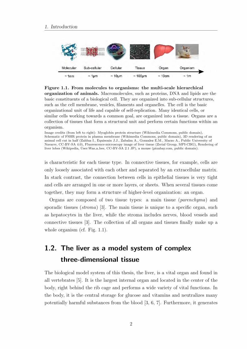
Figure 1.1. From molecules to organisms: the multi-scale hierarchicalorganization of animals. Macromolecules, such as proteins, DNA and lipids are thebasic constituents of a biological cell. They are organized into sub-cellular structures,such as the cell membrane, vesicles, filaments and organelles. The cell is the basicorganizational unit of life and capable of self-replication. Many identical cells, orsimilar cells working towards a common goal, are organized into a tissue. Organs are acollection of tissues that form a structural unit and perform certain functions within anorganism.Image credits (from left to right): Myoglobin protein structure (Wikimedia Commons, public domain),Schematic of FSHR protein in plasma membrane (Wikimedia Commons, public domain), 3D rendering of ananimal cell cut in half (Zaldua I., Equisoain J.J., Zabalza A., Gonzalez E.M., Marzo A., Public University ofNavarre, CC-BY-SA 4.0), Fluorescence-microscopy image of liver tissue (Zerial Group, MPI-CBG), Rendering ofliver lobes (Wikipedia, User:Was a bee, CC-BY-SA 2.1 JP), a mouse (pixabay.com, public domain).

is characteristic for each tissue type. In connective tissues, for example, cells are

only loosely associated with each other and separated by an extracellular matrix.

In stark contrast, the connection between cells in epithelial tissues is very tight

and cells are arranged in one or more layers, or sheets. When several tissues come

together, they may form a structure of higher-level organization: an organ.

Organs are composed of two tissue types: a main tissue (parenchyma) and

sporadic tissues (stroma) [3]. The main tissue is unique to a specific organ, such

as hepatocytes in the liver, while the stroma includes nerves, blood vessels and

connective tissues [3]. The collection of all organs and tissues finally make up a

whole organism (cf. Fig. 1.1).

1.2. The liver as a model system of complex

three-dimensional tissue

The biological model system of this thesis, the liver, is a vital organ and found in

all vertebrates [5]. It is the largest internal organ and located in the center of the

body, right behind the rib cage and performs a wide variety of vital functions. In

the body, it is the central storage for glucose and vitamins and neutralizes many

potentially harmful substances from the blood [3, 6, 7]. Furthermore, it generates

2

1.2. The liver as a model system of complex three-dimensional tissue

many different hormones, enzymes and blood clotting factors, as well as immune

molecules [3, 8–11]. All these important functions demand a proper working of

the liver at all times, which possesses astonishing regenerative capabilities: after

removal of more than two thirds of the liver, it can grow back to its original

mass and work as well as before [12]. This remarkable ability to regenerate is

demanded by the liver’s pivotal role in blood detoxification, making liver tissue

particularly susceptible to intoxication damage. Because the liver is the entry

point of many medical drugs, it is of great interest to understand the underlying

mechanisms that play into toxicity damage and how recovery is enabled. While,

for example the kidney can be substituted by dialysis, the function of the liver can

so far not be substituted by mechanical devices. This is partly due to the complex

architecture of the liver, which remains a great challenge for building in-vitro

systems that could be used in pharmaceutical applications [13–18]. Furthermore,

how regeneration and liver development [19] is orchestrated is not well understood

in terms of molecular and physical mechanisms. This thesis takes a step towards

that understanding by charactering the so-far unrecognized orientational order

of cell polarity in the liver, which might serve as a structural benchmark during

liver development and regeneration and by that help in unraveling the underlying

mechanisms.

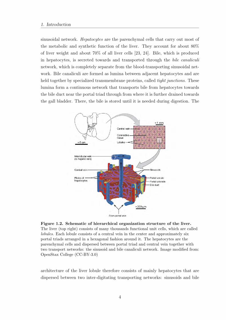
We now describe the main anatomical features of the liver. When examining

the liver as a whole it appears as a homogeneous, dark reddish brown tissue [20].

Upon closer examination, a subdivision into functional subunits called lobules,

with typical size of about 1 mm, is observed. They are shown, schematically, in

Fig. 1.2. Each lobule consists of a central vein in the middle and approximately

six portal triads arranged in a hexagonal fashion around it. A portal triad con-

sists of a proper hepatic artery (also portal arteriole), hepatic portal vein and a

bile duct [21, 22]. The hepatic artery supplies oxygen-rich blood directly from

the heart, whereas the portal vein delivers blood, which contains toxins and nu-

trients from other organs. The blood from these two afferent vessels mixes in a

region close to the portal triad. It then flows through a network of fenestrated2

blood vessels, called sinusoids towards the central vein in the center of the lobule,

from where it is drained towards the heart [21, 22]. On the way through the si-

nusoidal network, blood flows past hepatocytes, which are immersed between the

2Fenestration means that sinusoids contain “holes” or “windows”, which enable efficientexchange of blood with hepatocytes.

3

1. Introduction

sinusoidal network. Hepatocytes are the parenchymal cells that carry out most of

the metabolic and synthetic function of the liver. They account for about 80%

of liver weight and about 70% of all liver cells [23, 24]. Bile, which is produced

in hepatocytes, is secreted towards and transported through the bile canaliculi

network, which is completely separate from the blood-transporting sinusoidal net-

work. Bile canaliculi are formed as lumina between adjacent hepatocytes and are

held together by specialized transmembrane proteins, called tight junctions. These

lumina form a continuous network that transports bile from hepatocytes towards

the bile duct near the portal triad through from where it is further drained towards

the gall bladder. There, the bile is stored until it is needed during digestion. The

Figure 1.2. Schematic of hierarchical organization structure of the liver.The liver (top right) consists of many thousands functional unit cells, which are calledlobules. Each lobule consists of a central vein in the center and approximately sixportal triads arranged in a hexagonal fashion around it. The hepatocytes are theparenchymal cells and dispersed between portal triad and central vein together withtwo transport networks: the sinusoid and bile canaliculi network. Image modified from:OpenStax College (CC-BY-3.0)

architecture of the liver lobule therefore consists of mainly hepatocytes that are

dispersed between two inter-digitating transporting networks: sinusoids and bile

4

1.3. Biology of tissues

canaliculi3. Because hepatocytes are of epithelial origin, the liver can be regarded

as an epithelial tissue but with a complex three-dimension organization. In the

following sections of this introduction, we therefore review fundamental aspects of

epithelia tissue architecture and cell polarity and discuss previous approaches to

describe biological tissues.

1.3. Biology of tissues

As a complex organ, the liver as a whole does not fall into a single category of

the four basic tissue types (connective, muscle, nervous and epithelial), mentioned

above. However, the main characteristic of the liver is that of an exocrine gland [3].

Glandular tissues derive from epithelium and the parenchymal cells of the liver

(hepatocytes) share important features of epithelial cells [3]. We therefore review

relevant aspects of epithelial tissues now.

Epithelial tissues are found at the surface of the body or body cavities, such

as the gut, the airway lumen, or the skin. They are lining tissues and typically

separate the outside or a lumen from the inside of the body or an underlying tissue.

Their main functions are absorption, filtration and the organization of directed

transport of macromolecules. The cells that form the epithelium are tightly joined,

so that almost no inter-cellular space is left. These cell-cell connections are realized

by tight junctions, which effectively seal the lumen-facing side from the rest of the

tissue [3]. This enables the epithelium to serve as a gatekeeper and a protective

shield of the underlying tissue. It can regulate transport from one side to the

other or perform more complex sorting tasks, e.g. taking in material from one

side, processing it and directing the products to either side in a controlled way.

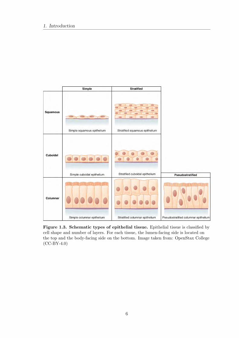
Epithelial tissue is classified by the number of cell layers and the shape of individ-

ual cells, see Fig. 1.3. One can distinguish three principal cell shapes: squamous,

cuboidal and columnar. Squamous cells are wider than they are tall, cuboid cells

are cube-like and columnar cells are taller than they are wide. Using a coordi-

nate system, where the epithelial sheet lies in the xy-plane, simple epithelia are

single-layered, and multi-layered epithelia are called stratified. When nuclei of a

simple epithelium appear on different heights, they might be confused with strat-

ified epithelia. For these cases there is the separate category of pseudo-stratified

3Other parts of the stroma of the liver, e.g. Kupffer cells and stellate cells, are not consideredin this thesis.

5

1. Introduction

Figure 1.3. Schematic types of epithelial tissue. Epithelial tissue is classified bycell shape and number of layers. For each tissue, the lumen-facing side is located onthe top and the body-facing side on the bottom. Image taken from: OpenStax College(CC-BY-4.0)

6

1.3. Biology of tissues

epithelia.

It is important to note that the three-dimensional organization of epithelial

tissue can be more intricate than the picture of stacked flat sheets shown above.

Kidney collecting ducts, for example, are simple epithelia that form cylindrical

structures [20, plate 1133][3]. Hepatocytes of the liver are cuboidal epithelial cells

that exhibit a peculiar three-dimensional arrangement that was first described

by Hans Elias around 1950 [25, 26]. He proposed that hepatocytes are arranged

into sheets, one cell thick, spanning the space between portal triad and central

vein [3, 25, 26]. These cell sheets are branched and regularly anastomose with

neighboring sheets. This peculiar arrangement of cells does not fit any of the

classical categories of epithelial sheets mentioned above and is also reflected in the

apicobasal cell polarity of hepatocytes.

Apicobasal polarity of epithelial cells. For proper function of epithelial tissue,

it is important for specific proteins to be located at the correct region of the mem-

brane of the epithelial cells. Imagine a protein pump that selectively transports

material from the cell’s cytoplasma into a lumen. This pump must be in the part

of the membrane facing the lumen as otherwise the material would be transported

into the wrong direction. Junctions forming connection between cells, specifi-

cally tight junctions, inhibit lateral diffusion of membrane proteins and thereby

facilitate the compartmentalization of the membrane into distinct domains [1, 2].

Specifically, apical domains form on the sides of the tissue that faces the outside

of a body or lumen of a cavity and are separated from other domains by tight

junctions [3, 27]. Lateral domains provide cell-cell adhesion and basal domains

form the interface with the basement membrane and extracellular matrix [3, 28,

29]. This anisotropic distribution of apical and basal membrane domains on the

surface of cells is termed apicobasal cell polarity [2]. The locations of these func-

tional domains have been found to respond to cues from the environment around

a cell [30]. Disruption of the organization of membrane proteins leads to serious

problems for cell function within a tissue, such as misdirection of transport [31–

33], mis-specification [34, 35], or errors in cell sorting [36] and is implicated in the

onset of diseases such as choleostasis [37], multiple sclerosis [33] and cancer [35,

38].

7

1. Introduction

The term “cell polarity”. Cells that exhibit anisotropies in physical properties,

such as the distribution of membrane-bound proteins, are said to be polarized.

At this point, it is imperative to be precise about the usage of the terms polar

and polarity. In physics, the term polarity usually refers to vectorial quantities

describing, for example, electric or magnetic fields. This needs to be distinguished

from the term cell polarity used in biology, where the term is used in a broader

sense to describe differences in cell shape, structure or function of cells, that are

not necessarily vectorial [2]. The present thesis deals specifically with anisotropic

distributions of membrane proteins on the surfaces of cells and will thus use the

term cell polarity to denote this particular form of cellular anisotropy, unless stated

otherwise. To avoid confusion, we will be explicit about the type of polarity and

will not equate polar with vectorial.

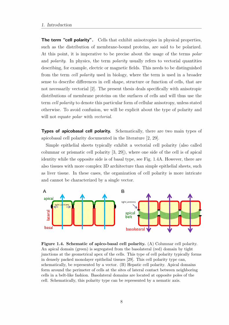
Types of apicobasal cell polarity. Schematically, there are two main types of

apicobasal cell polarity documented in the literature [2, 29].

Simple epithelial sheets typically exhibit a vectorial cell polarity (also called

columnar or prismatic cell polarity [3, 29]), where one side of the cell is of apical

identity while the opposite side is of basal type, see Fig. 1.4A. However, there are

also tissues with more complex 3D architecture than simple epithelial sheets, such

as liver tissue. In these cases, the organization of cell polarity is more intricate

and cannot be characterized by a single vector.

Figure 1.4. Schematic of apico-basal cell polarity. (A) Columnar cell polarity.An apical domain (green) is segregated from the basolateral (red) domain by tightjunctions at the geometrical apex of the cells. This type of cell polarity typically formsin densely packed monolayer epithelial tissues [29]. This cell polarity type can,schematically, be represented by a vector. (B) Hepatic cell polarity. Apical domainsform around the perimeter of cells at the sites of lateral contact between neighboringcells in a belt-like fashion. Basolateral domains are located at opposite poles of thecell. Schematically, this polarity type can be represented by a nematic axis.

8

1.4. Physics of tissues

One example of this type of multi-faceted cell polarity are hepatocytes of the

liver. Each hepatocyte possesses multiple apical membrane domains forming nar-

row lumina with adjacent cells, into which bile is excreted. Together, these lumina

constitute the lobule-spanning bile canaliculi network (cf. section 1.2). Addition-

ally, each hepatocyte has multiple basal domains that face the blood-transporting

sinusoidal network [29]. This type of apicobasal cell polarity is referred to as “hep-

atic cell polarity” in the literature [29] and schematically shown in Fig. 1.4B. This

picture of hepatic cell polarity is certainly oversimplified and will be investigated

systematically in chapter 2.

The schematic is nevertheless useful to illustrate the qualitative difference be-

tween columnar and hepatic cell polarity with respect to the symmetry of the

protein distribution. As indicated in Fig. 1.4 columnar cell polarity can be de-

scribed by a single vector pointing from the basal to the apical side of the cell.

In contrast to that, the idealized hepatic cell polarity can be described by an

undirected axis connecting both basal sides. In this simple case, this axis is also

perpendicular to the ring of apical domain. The undirected axis of this idealized

picture represents a nematic object that is invariant with respect to mirroring on

a plane perpendicular to it [39]. The formalization and systematic study of this

intuition will be a core subject in the present thesis.

1.4. Physics of tissues

Tissues are a form of complex matter that share common characteristics. The

physics of tissues aims to find general laws describing these systems of living mat-

ter. The study of the physics of tissues is a broad field and we only provide a

coarse overview here and highlight some particularly useful examples.

The physics of tissues includes inter-cellular processes of cells and the mechan-

ical and chemical interaction between them. From the perspective of physics, a

cell can be regarded as a complex machinery that, among other tasks, converts

chemical energy from fuel molecules (e.g. ATP) into useful work [1]. This work

can drive different processes, including cell migration [40–42], inter-cellular traf-

ficking processes [43], and cell division [44–46]. On the sub-cellular scale, processes

such as DNA replication and transcription [47] and the physics of the acto-myosin

cytoskeleton [48, 49], as well as the emergent mechanical properties of the cell

as a whole [50, 51] have been studied. Cells in the tissue constantly consume

9

1. Introduction

chemical energy, which keeps the system from reaching thermodynamic equilib-

rium and requires the characterization of the material as active matter [52]. A

complete description of all degrees of freedom in a tissue is neither achievable nor

desirable [52]. Instead, it is useful to apply global principles, such as conservation

laws and symmetries, to constrain the possible dynamics of the system [52]. The

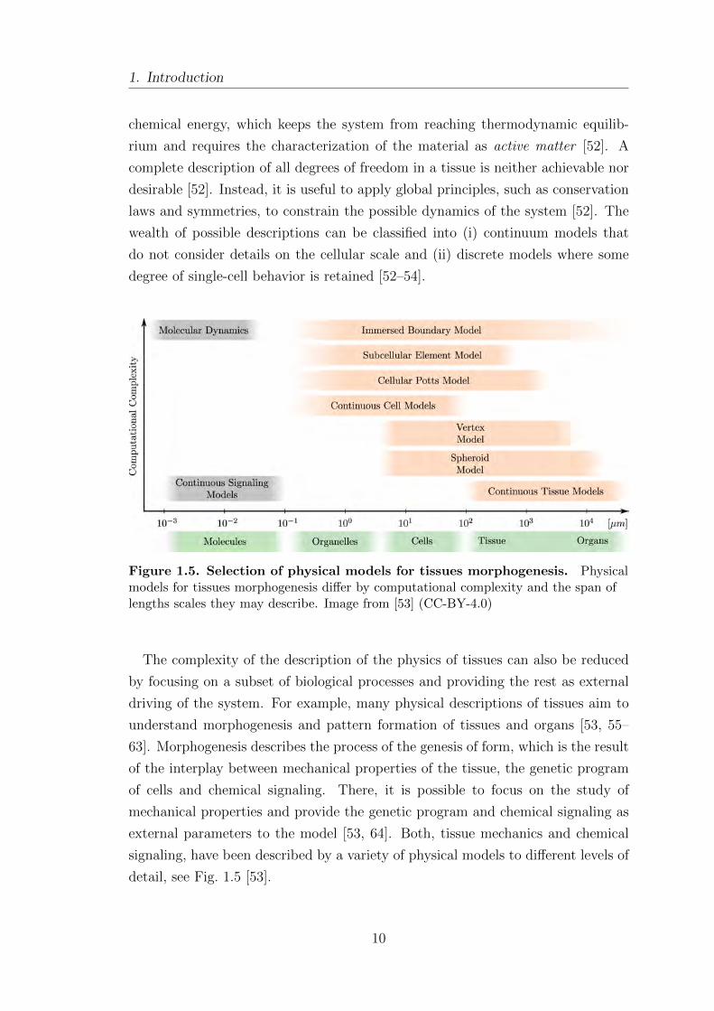
wealth of possible descriptions can be classified into (i) continuum models that

do not consider details on the cellular scale and (ii) discrete models where some

degree of single-cell behavior is retained [52–54].

Figure 1.5. Selection of physical models for tissues morphogenesis. Physicalmodels for tissues morphogenesis differ by computational complexity and the span oflengths scales they may describe. Image from [53] (CC-BY-4.0)

The complexity of the description of the physics of tissues can also be reduced

by focusing on a subset of biological processes and providing the rest as external

driving of the system. For example, many physical descriptions of tissues aim to

understand morphogenesis and pattern formation of tissues and organs [53, 55–

63]. Morphogenesis describes the process of the genesis of form, which is the result

of the interplay between mechanical properties of the tissue, the genetic program

of cells and chemical signaling. There, it is possible to focus on the study of

mechanical properties and provide the genetic program and chemical signaling as

external parameters to the model [53, 64]. Both, tissue mechanics and chemical

signaling, have been described by a variety of physical models to different levels of

detail, see Fig. 1.5 [53].

10

1.4. Physics of tissues

1.4.1. Continuum descriptions

At the coarsest level, a tissue can be described as a macroscopic continuous ma-

terial with potentially viscous, elastic and plastic properties, depending on the

timescale of interest [53, 65–67]. The tissue is characterized by a constitutive

equation that describes how “slow” hydrodynamic variables respond to external

stimuli, such as forces or other applied fields. These hydrodynamic variables are

given by conservation laws or, in the case of ordered systems, by “continuous bro-

ken symmetries” and represent collective modes that describe the long-wavelength,

long-time scale relaxation towards thermodynamic equilibrium after an initial per-

turbation [68]. The constitutive equation can either be determined phenomenolog-

ically [69–71] or derived from an underlying “microscopic description” of cellular

processes, such as directed cell division, extrusion, migration and adhesion [72].

Given the mathematical form of the constitutive equation, the material parame-

ters are determined by comparison to experimental data or result directly from

coarse-grained “microscopic” interaction parameters between individual cells [52,

72]. The resulting ordinary or partial differential equations are typically solved

using finite element methods in general, and analytical tools in special cases [52,

53, 72]. Continuum models are particularly useful for the study of processes on

large time and length scales, when the separation of tissue into individual cells can

be neglected. Coarse-graining a realistic microscopic description is difficult and

typically involves simplifications and approximations [52].

In the context of liver tissue, continuum models have been used to study fluid

flow and deformation of decellularized liver tissue [73, 74] and for the development

of surgery simulation systems [75].

1.4.2. Discrete models

Discrete models typically retain the cell as a structural unit of a tissue and by that

possess many more degrees of freedom than continuum descriptions [53]. There

are many variants of discrete models (see Fig. 1.5) and only a subset, namely the

vertex model, spheroid model and cellular Potts model, is discussed here. For

more detailed reviews, see [53, 76, 77].

The vertex and spheroid models consider the cell as the smallest unit in a tissue.

In the (two-dimensional) vertex model, cells are described as polygons [78–80]. The

interface between neighboring cells is represented by a common edge and the points

11

1. Introduction

of intersection are the location of graph vertices. Stable and stationary network

configurations result from force balance on each vertex. Given NC polygonal cells,

numbered by α = 1, . . . , NC and NV vertices, numbered i = 1, . . . , NV , the force

balance corresponds to a local minimum of an energy function [79]

E(ri) =∑α

Kα

2

(Aα − A(0)

α

)2+∑〈i,j〉

Λijlij +∑α

Γα2L2α . (1.1)

Thus, fi = −∂E/∂ri is the total force acting on vertex i. This energy func-

tion describes forces due to cell elasticity, actin-myosin bundles and adhesion

molecules [79, 81]. The first term on the right hand side describes area elas-

ticity of cells with elastic coefficients Kα and preferred cell area A(0)α . The second

term describes line tensions on the edges 〈i, j〉 of the graph with line-tension co-

efficient Λij and edge length lij. Line tensions result from cell-cell adhesion and

activity of actin-myosin bundles [79]. Actin-myosin bundles are combinations of

actin filaments with myosin molecular motors that generate contractile forces [82].

These bundles are found at the interfaces between cells and may thus be respon-

sible for line tensions on the edges in the vertex model. The third term describes

the contractility of the cell perimeter Lα by a coefficient Γα. It is motivated by the

observation of an actin-myosin ring around the perimeter of many epithelial cells.

Vertex models have been used to study epithelial morphogenesis [79, 83, 84], cell

sorting [85–87] and planar cell polarity [67, 88]. Interstitial space between cells

is not described by the model, which makes it a good approximation for tightly

packed epithelia.

Spheroid models are built on conceptual analogies to colloidal particles and a cell

is represented by a homogeneous isotropic elastic sticky object, which is capable

of migration, growth, division and change of orientation [76]. Cell adhesion has

recently been shown to be well explained by Johnson-Kendall-Roberts theory of

adhesive spheres [89], which includes a hysteresis effect in that the distance where

cells are pulled apart is larger than the distance an initial contact is formed [53].

The JKR theory and other variants, such as the Hertz contact model [90], harmonic

interaction potentials [91] and dashpot-spring elements [92] have been used in

spheroids models [53, 76]. Cell movement in this framework is described by over-

damped dynamics with stochastic contributions and multiple schemes to treat

them in the statistical context of Langevin equations can be derived [76]. A variant

of the spheroid model has been used to describe liver regeneration after intoxication

12

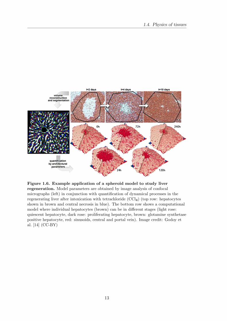
1.4. Physics of tissues

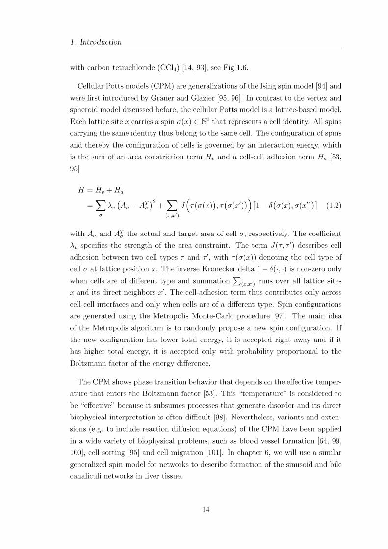
Figure 1.6. Example application of a spheroid model to study liverregeneration. Model parameters are obtained by image analysis of confocalmicrographs (left) in conjunction with quantification of dynamical processes in theregenerating liver after intoxication with tetrachloride (CCl4) (top row: hepatocytesshown in brown and central necrosis in blue). The bottom row shows a computationalmodel where individual hepatocytes (brown) can be in different stages (light rose:quiescent hepatocyte, dark rose: proliferating hepatocyte, brown: glotamine synthetasepositive hepatocyte, red: sinusoids, central and portal vein). Image credit: Godoy etal. [14] (CC-BY)

13

1. Introduction

with carbon tetrachloride (CCl4) [14, 93], see Fig 1.6.

Cellular Potts models (CPM) are generalizations of the Ising spin model [94] and

were first introduced by Graner and Glazier [95, 96]. In contrast to the vertex and

spheroid model discussed before, the cellular Potts model is a lattice-based model.

Each lattice site x carries a spin σ(x) ∈ N0 that represents a cell identity. All spins

carrying the same identity thus belong to the same cell. The configuration of spins

and thereby the configuration of cells is governed by an interaction energy, which

is the sum of an area constriction term Hv and a cell-cell adhesion term Ha [53,

95]

H = Hv +Ha

=∑σ

λv(Aσ − ATσ

)2+∑(x,x′)

J(τ(σ(x)

), τ(σ(x′)

))[1− δ

(σ(x), σ(x′)

)](1.2)

with Aσ and ATσ the actual and target area of cell σ, respectively. The coefficient

λv specifies the strength of the area constraint. The term J(τ, τ ′) describes cell

adhesion between two cell types τ and τ ′, with τ(σ(x)) denoting the cell type of

cell σ at lattice position x. The inverse Kronecker delta 1− δ(·, ·) is non-zero only

when cells are of different type and summation∑

(x,x′) runs over all lattice sites

x and its direct neighbors x′. The cell-adhesion term thus contributes only across

cell-cell interfaces and only when cells are of a different type. Spin configurations

are generated using the Metropolis Monte-Carlo procedure [97]. The main idea

of the Metropolis algorithm is to randomly propose a new spin configuration. If

the new configuration has lower total energy, it is accepted right away and if it

has higher total energy, it is accepted only with probability proportional to the

Boltzmann factor of the energy difference.

The CPM shows phase transition behavior that depends on the effective temper-

ature that enters the Boltzmann factor [53]. This “temperature” is considered to

be “effective” because it subsumes processes that generate disorder and its direct

biophysical interpretation is often difficult [98]. Nevertheless, variants and exten-

sions (e.g. to include reaction diffusion equations) of the CPM have been applied

in a wide variety of biophysical problems, such as blood vessel formation [64, 99,

100], cell sorting [95] and cell migration [101]. In chapter 6, we will use a similar

generalized spin model for networks to describe formation of the sinusoid and bile

canaliculi networks in liver tissue.

14

1.4. Physics of tissues

1.4.3. Two-dimensional case study: planar cell polarity in the

fly wing

As stated in section 1.3, this thesis deals with the peculiar cell polarity of hepato-

cytes in liver tissue. Organization of cell polarity has been studied previously in

the context of planar cell polarity (PCP) in the planar simple epithelium of the

fly wing. Proper establishment of PCP is an important prerequisite in control-

ling the direction of hair growth in the developing fly. In contrast to apicobasal

cell polarity, PCP describes the anisotropic localization of proteins of the Frizzled

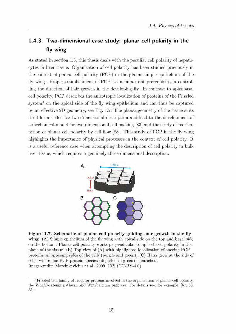
system4 on the apical side of the fly wing epithelium and can thus be captured

by an effective 2D geometry, see Fig. 1.7. The planar geometry of the tissue suits

itself for an effective two-dimensional description and lead to the development of

a mechanical model for two-dimensional cell packing [83] and the study of reorien-

tation of planar cell polarity by cell flow [88]. This study of PCP in the fly wing

highlights the importance of physical processes in the context of cell polarity. It

is a useful reference case when attempting the description of cell polarity in bulk

liver tissue, which requires a genuinely three-dimensional description.

Figure 1.7. Schematic of planar cell polarity guiding hair growth in the flywing. (A) Simple epithelium of the fly wing with apical side on the top and basal sideon the bottom. Planar cell polarity works perpendicular to apico-basal polarity in theplane of the tissue. (B) Top view of (A) with highlighted localization of specific PCPproteins on opposing sides of the cells (purple and green). (C) Hairs grow at the side ofcells, where one PCP protein species (depicted in green) is enriched.Image credit: Marcinkevicius et al. 2009 [102] (CC-BY-4.0)

4Frizzled is a family of receptor proteins involved in the organization of planar cell polarity,the Wnt/β-catenin pathway and Wnt/calcium pathway. For details see, for example, [67, 83,88].

15

1. Introduction

1.4.4. Challenges of three-dimensional models for liver tissue

Many studies investigating physical principles in tissues have been performed on

simple epithelial sheets [2, 55, 60, 83, 88, 103, 104], because they are experimentally

more easily accessible than bulk tissue. The study of complex three-dimensional

organs, such as the liver [105], has become feasible only recently due to advances

in microscopy techniques, such as fluorescence microscopy with its many improve-

ments and variants (confocal, two-photon and light sheet microscopy [106, 107]),

as well as advances in protocols that render tissue optically transparent to enable

imaging of relatively thick specimen [108, 109]. The newfound wealth of data

demand for appropriate biophysical descriptions.

So far, physical descriptions of liver tissue have involved organ-level continuum

models [73, 75, 110, 111] and spheroid-based lobule-level models [93, 112]. In this

thesis, we first categorize the liver as a biaxial nematic liquid crystal. We then

use a discrete model of nematic cell orientations to describe the observed order.

Building on this, we then develop a generalized spin model to study the formation

of transport networks in the liver. In both cases, an interaction energy, similar in

spirit to the vertex model and CPM, is formulated and configurations are sampled

using the Monte-Carlo approach.

Biological tissues represent complex, amorphous materials with mesoscopic struc-

ture conferring interesting physical properties. From a physical point of view, their

structure and order lies between the limiting cases of isotropic liquids and three-

dimensional crystals. Another type of mesoscopic material, liquid crystals, falls

into the same range and the concepts developed there are likely to be suitable for

the description of biological tissues as well.

1.5. Liquids, crystals and liquid crystals

The solid, liquid, and gas phase are the three classical phases of matter, one is

very much familiar with from everyday experience. Solids are rigid objects with

definite shape and volume, due to strong attractive forces among their molecular

constituents. In liquids and gases, inter-molecular forces are weaker and the mate-

rial is able to adapt to the shape of a container and they are collectively referred to

as fluids. Between liquids and crystalline solids, there exists a range of mesophases

that can be distinguished with respect to their mechanical and symmetry proper-

ties [39].

16

1.5. Liquids, crystals and liquid crystals

According to Chandrasekhar, the first observations of liquid crystalline behav-

ior were made by Reinitzer and Lehmann at the end of the 19th century [113].

The common characteristic of liquid crystalline states is that they are strongly

anisotropic in certain properties, while retaining a substantial amount of fluidity

in others. This macroscopic property originates in the typical shape of the con-

stituent molecules that form liquid crystal phases, which are geometrically highly

anisotropic, like a rod or a disc [113]. There is a wide variety of liquid-crystal

phases, which have been classified by different experimental techniques, including

refractive index studies, NMR spectroscopy as well as X-ray and Neutron scat-

tering [114]. A liquid crystal system may be driven through multiple nematic

phases by changes in temperature (thermotropic) or by the influence of solvents

(lyotropic) before arriving at the isotropic liquid state.

It is instructive to review the limiting cases of crystalline order and liquids and

place the liquid crystal mesophases therein. In crystals, the constituents (atoms,

molecules or groups of molecules) are arranged on a three-dimensional periodic

lattice. Liquids, on the other hand, flow easily and do not display a periodic

arrangement. The regular ordering in crystals is reflected by the fact that, if

a primitive pattern (or basis) is located at a point r0, the probability to find an

equivalent pattern at a point r = r0 +n1a1 +n1a2 +n1a3 with ni ∈ N0, i ∈ 1, 2, 3and ai the basis vectors of the crystal, remains finite even for large separations

|r−r0| → ∞ [39]. This leads to sharp Bragg reflections in X-ray diffraction patterns

that are characteristic for a given crystal and reflect the limiting behavior of the

density-density correlation function [39]

lim|r−r′|→∞

〈ρ(r)ρ(r′)〉 = F (r− r′) , (1.3)

which approaches a periodic function F (r− r′) of the crystal lattice basis vectors

ai. Liquids, on the other hand, flow easily and individual constituents can pass

each other and change neighbor relations. Liquids are isotropic and show trans-

lational symmetry in all three spatial directions. The density-density correlation

function [39]

lim|r−r′|→∞

〈ρ(r)ρ(r′)〉 = ρ2 (1.4)

therefore approaches the square of the average density ρ. In a liquid, there is an

isotropic length scale ξ over which correlations between constituents are lost.

17

1. Introduction

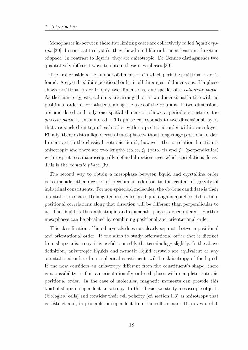
Mesophases in-between these two limiting cases are collectively called liquid crys-

tals [39]. In contrast to crystals, they show liquid-like order in at least one direction

of space. In contrast to liquids, they are anisotropic. De Gennes distinguishes two

qualitatively different ways to obtain these mesophases [39].

The first considers the number of dimensions in which periodic positional order is

found. A crystal exhibits positional order in all three spatial dimensions. If a phase

shows positional order in only two dimensions, one speaks of a columnar phase.

As the name suggests, columns are arranged on a two-dimensional lattice with no

positional order of constituents along the axes of the columns. If two dimensions

are unordered and only one spatial dimension shows a periodic structure, the

smectic phase is encountered. This phase corresponds to two-dimensional layers

that are stacked on top of each other with no positional order within each layer.

Finally, there exists a liquid crystal mesophase without long-range positional order.

In contrast to the classical isotropic liquid, however, the correlation function is

anisotropic and there are two lengths scales, ξ|| (parallel) and ξ⊥ (perpendicular)

with respect to a macroscopically defined direction, over which correlations decay.

This is the nematic phase [39].

The second way to obtain a mesophase between liquid and crystalline order

is to include other degrees of freedom in addition to the centers of gravity of

individual constituents. For non-spherical molecules, the obvious candidate is their

orientation in space. If elongated molecules in a liquid align in a preferred direction,

positional correlations along that direction will be different than perpendicular to

it. The liquid is thus anisotropic and a nematic phase is encountered. Further

mesophases can be obtained by combining positional and orientational order.

This classification of liquid crystals does not clearly separate between positional

and orientational order. If one aims to study orientational order that is distinct

from shape anisotropy, it is useful to modify the terminology slightly. In the above

definition, anisotropic liquids and nematic liquid crystals are equivalent as any

orientational order of non-spherical constituents will break isotropy of the liquid.

If one now considers an anisotropy different from the constituent’s shape, there

is a possibility to find an orientationally ordered phase with complete isotropic

positional order. In the case of molecules, magnetic moments can provide this

kind of shape-independent anisotropy. In this thesis, we study mesoscopic objects

(biological cells) and consider their cell polarity (cf. section 1.3) as anisotropy that

is distinct and, in principle, independent from the cell’s shape. It proves useful,

18

1.5. Liquids, crystals and liquid crystals

and will be done in this thesis, to reserve the term nematic for orientational order

and use the term anisotropic liquid for anisotropic positional correlations.

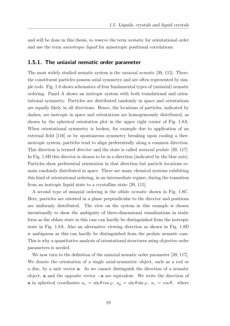
1.5.1. The uniaxial nematic order parameter

The most widely studied nematic system is the uniaxial nematic [39, 115]. There,

the constituent particles possess axial symmetry and are often represented by sim-

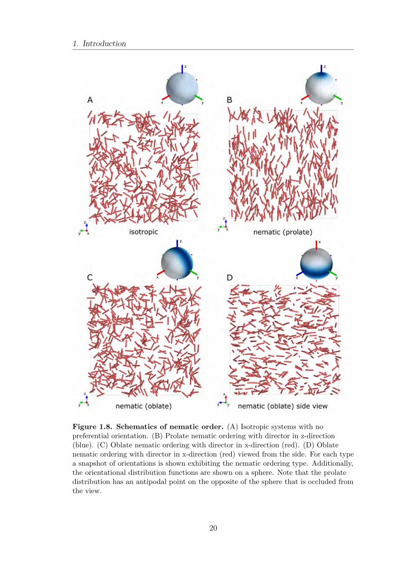
ple rods. Fig. 1.8 shows schematics of four fundamental types of (uniaxial) nematic

ordering. Panel A shows an isotropic system with both translational and orien-

tational symmetry. Particles are distributed randomly in space and orientations

are equally likely in all directions. Hence, the locations of particles, indicated by

dashes, are isotropic in space and orientations are homogeneously distributed, as

shown by the spherical orientation plot in the upper right corner of Fig. 1.8A.

When orientational symmetry is broken, for example due to application of an

external field [116] or by spontaneous symmetry breaking upon cooling a ther-

motropic system, particles tend to align preferentially along a common direction.

This direction is termed director and the state is called uniaxial prolate [39, 117].

In Fig. 1.8B this director is chosen to be in z-direction (indicated by the blue axis).

Particles show preferential orientation in that direction but particle locations re-

main randomly distributed in space. There are many chemical systems exhibiting

this kind of orientational ordering, in an intermediate regime, during the transition

from an isotropic liquid state to a crystalline state [39, 115].

A second type of uniaxial ordering is the oblate nematic shown in Fig. 1.8C.

Here, particles are oriented in a plane perpendicular to the director and positions

are uniformly distributed. The view on the system in this example is chosen

intentionally to show the ambiguity of three-dimensional visualizations in static

form as the oblate state in this case can hardly be distinguished from the isotropic

state in Fig. 1.8A. Also an alternative viewing direction as shown in Fig. 1.8D

is ambiguous as this can hardly be distinguished from the prolate nematic case.

This is why a quantitative analysis of orientational structures using objective order

parameters is needed.

We now turn to the definition of the uniaxial nematic order parameter [39, 117].

We denote the orientation of a single axial-symmetric object, such as a rod or

a disc, by a unit vector a. As we cannot distinguish the direction of a nematic

object, a and the opposite vector −a are equivalent. We write the direction of

a in spherical coordinates ax = sin θ cosϕ, ay = sin θ sinϕ, az = cos θ, where

19

1. Introduction

Figure 1.8. Schematics of nematic order. (A) Isotropic systems with nopreferential orientation. (B) Prolate nematic ordering with director in z-direction(blue). (C) Oblate nematic ordering with director in x-direction (red). (D) Oblatenematic ordering with director in x-direction (red) viewed from the side. For each typea snapshot of orientations is shown exhibiting the nematic ordering type. Additionally,the orientational distribution functions are shown on a sphere. Note that the prolatedistribution has an antipodal point on the opposite of the sphere that is occluded fromthe view.

20

1.5. Liquids, crystals and liquid crystals

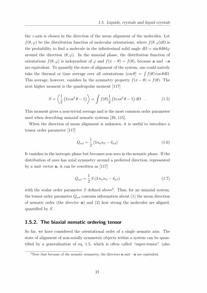
the z-axis is chosen in the direction of the mean alignment of the molecules. Let

f(θ, ϕ) be the distribution function of molecular orientations, where f(θ, ϕ)dΩ is

the probability to find a molecule in the infinitesimal solid angle dΩ = sin θdθdϕ

around the direction (θ, ϕ). In the uniaxial phase, the distribution function of

orientations f(θ, ϕ) is independent of ϕ and f(π − θ) = f(θ), because a and −a

are equivalent. To quantify the state of alignment of the system, one could naively

take the thermal or time average over all orientations 〈cos θ〉 =∫f(θ) cos θdΩ.

This average, however, vanishes by the symmetry property f(π − θ) = f(θ). The

next higher moment is the quadrupolar moment [117]

S =

⟨1

2

(3 cos2 θ − 1

)⟩=

∫f(θ)

1

2

(3 cos2 θ − 1

)dΩ . (1.5)

This moment gives a non-trivial average and is the most common order parameter

used when describing uniaxial nematic systems [39, 115].

When the direction of mean alignment is unknown, it is useful to introduce a

tensor order parameter [117]

Qαβ =1

2〈3 aαaβ − δαβ〉 (1.6)

It vanishes in the isotropic phase but becomes non-zero in the nematic phase. If the

distribution of axes has axial symmetry around a preferred direction, represented

by a unit vector n, it can be rewritten as [117]

Qαβ =1

2S (3nαnβ − δαβ) (1.7)

with the scalar order parameter S defined above5. Thus, for an uniaxial system,

the tensor order parameter Qαβ contains information about (1) the mean direction

of nematic order (the director n) and (2) how strong the molecules are aligned,

quantified by S.

1.5.2. The biaxial nematic ordering tensor

So far, we have considered the orientational order of a single nematic axis. The

state of alignment of non-axially symmetric objects within a system can be quan-

tified by a generalization of eq. 1.5, which is often called “super-tensor” (also

5Note that because of the nematic symmetry, the directors n and −n are equivalent.

21

1. Introduction

“ordering tensor” or “ordering matrix”) [39, 115, 118]

Sijαβ =1

2〈3iαjβ − δαβδij〉 , (1.8)

where jα denotes the direction cosine jα = ej ·Eα between object axes ej = a,b, c

and laboratory axes Eα = x,y, z. Further, δαβ and δij are Kronecker symbols and

the brackets denote the thermal average. This ordering matrix is, by construction,

real-valued, symmetric in both i, j and α, β, and traceless in either index pair,

specifically Sijαα = 0 and Siiαβ = 0. It therefore diagonalizes for a special choice of

the orthogonal reference frame, which we call l, m, n [39]. In its eigenframe, Sijαβhas nine non-zero components Siiαα, which are not independent and can be reduced

to four orientational order parameters. This is discussed in section 3.1.1, where we

make explicit use of the symmetries of the individual constituents and the biaxial

nematic phase [115, 119].

For objects that are axially-symmetric around one axis (e.g. a), the only non-

zero components of the super-tensor are

Qαβ = Saaαβ =1

2〈3 aαaβ − δαβ〉 (1.9)

which is exactly the form given in equation (1.6) for axially-symmetric objects. If

the distribution of object axes a does not possess axial symmetry (as was assumed

in eq. (1.7)), an additional order parameter P , measuring the deviation from axial

symmetry of the orientational distribution, becomes non-zero and the ordering

tensor is given by

Qαβ = S nαnβ −S + P

2mαmβ −

S − P2

lαlβ (1.10)

with a primary director n and secondary director m. The third director l is

given by the orthogonality relation of the reference frame l, m, n in which Qαβ

is diagonal. While in the uniaxial case there is only one symmetry axis, in the

biaxial case there is some ambiguity about which axis to choose as the primary

and which to choose as the secondary director. We will discuss this issue in more

detail in section 3.1.1

22

1.5. Liquids, crystals and liquid crystals

1.5.3. Continuum theory of nematic order

We review important aspects of orientational order in the context of liquid crystals.

This will provide us with the necessary tools that are applied to biological tissue

in subsequent chapters.

Let us consider a uniaxial nematic, which is characterized by a scalar order

parameter S and a nematic director n. The total free energy ET of this nematic

can be split in into two parts

ET = Eu + Ed (1.11)

where Eu is the free energy of a uniformly aligned nematic and Ed denotes the

contribution to the free energy due to gradients in the director field n(r). Typically,

the uniform state is the ground state of a nematic system and therefore distortions

of the director field lead to an increase of the free energy of the system [39, 120,

121]. These gradual changes may be due to constraints on the limiting surfaces of

the sample (e.g. walls of a container) or external fields.

For a uniaxial system, described by a spatially varying director field n(r), the

so-called Frank free energy6 is given by [39]

Ed =

∫d3r

1

2K1 (∇ · n)2 +

1

2K2 [n · (∇× n)]2 +

1

2K3 |n× (∇× n)|2 , (1.12)

with three elastic constants that correspond to three bending modes: splay (K1),

twist (K2) and bend (K3). Previous measurements on nematic materials have

shown that the elastic constants are of equal order of magnitude [39]. In situations,

where the relative values of the elastic constants are unknown, it is therefore a good

approximation to set the three elastic constants equal to K := K1 = K2 = K3.

This is known as the one-constant approximation7, which is adopted here. In this

case, the Frank free energy simplifies to (neglecting surface terms) [39]

Ed =

∫d3r

K

2∂αnβ∂αnβ . (1.13)

6Named after Frederick Charles Frank and also called distortion free energy. In this formula-tion of the distortion free energy, it is assumed that the overall nematic alignment, characterizedby the order parameter S, is not influenced by the distortions of the director n and constantthroughout the system.

7The elastic constants have also been calculated for a lattice model [122, 123] and usingdensity functional theory [124]. There, equal constants correspond to an isotropic two-particlecorrelation function.

23

1. Introduction

An important feature of the one-constant approximation is that the distortion free

energy is now invariant under simultaneous rotation of all individual nematic spins

n while keeping their positions fixed8. For unequal elastic constants, the Frank

free energy is invariant only under simultaneous rotation of both nematic axes and

their respective positions [39]. This equation forms the starting point of the theory

developed in chapter 5. There, we will discretize the continuum equations and use

them to study nematic cell polarity in the liver.

Above, we assumed that nematic order is generated through some process and is

constant throughout the system. The relevant contribution to the free energy then

results from gradients in the director field n(r). As a side note, we now briefly

mention existing statistical theories describing the emergence of nematic order in

the first place (typically assuming a spatially uniform system and by that ignoring

gradient terms). One can broadly distinguish macroscopic and microscopic ap-

proaches. First, axially-symmetric nematogens subject to steric interactions have

been considered by Onsager in 1949 [126]. Later, in 1958, Meier and Saupe for-

mulated a mean-field theory for the same axially-symmetric system and showed

the existence of a first-order transition from the isotropic to the uniaxial nematic

state [127]. This theory was extended by Freiser in 1970 to include non-axially

symmetric (biaxial) nematogens [128]. For a short summary of the Meier-Saupe

theory and its extension to biaxial systems, see appendix A.1.

An Onsager-type theory for the steric interaction between rigid plates was pro-

vided in 1974 by Straley [119], which was later extended to investigate the ef-

fect of polydispersity of particle sizes [129, 130]. Also, mixtures of rod-like and

plate-like molecules were studied [131–134]. In these cases, stable biaxial mixtures

are unlikely due to demixing prior to the biaxial phase [134–137]. Furthermore,

Laundau-type phenomenological theories have been developed for both uniaxial

and biaxial systems [39, 118, 138–142]. Complementary, computer simulations

(typically using Monte-Carlo methods) have been performed to study more com-

plex systems that go beyond analytical and perturbative treatments mentioned

above [133, 134, 143–147].

8The form of the free energy in one-constant approximation is also equivalent to a cubicHeisenberg ferromagnet [125, §39][39]

24

1.5. Liquids, crystals and liquid crystals

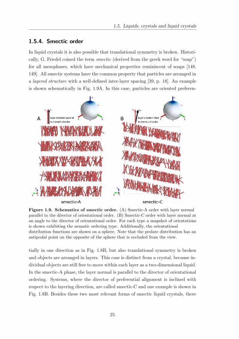
1.5.4. Smectic order

In liquid crystals it is also possible that translational symmetry is broken. Histori-

cally, G. Friedel coined the term smectic (derived from the greek word for “soap”)

for all mesophases, which have mechanical properties reminiscent of soaps [148,

149]. All smectic systems have the common property that particles are arranged in

a layered structure with a well-defined inter-layer spacing [39, p. 18]. An example

is shown schematically in Fig. 1.9A. In this case, particles are oriented preferen-

Figure 1.9. Schematics of smectic order. (A) Smectic-A order with layer normalparallel to the director of orientational order. (B) Smectic-C order with layer normal atan angle to the director of orientational order. For each type a snapshot of orientationsis shown exhibiting the nematic ordering type. Additionally, the orientationaldistribution functions are shown on a sphere. Note that the prolate distribution has anantipodal point on the opposite of the sphere that is occluded from the view.

tially in one direction as in Fig. 1.8B, but also translational symmetry is broken

and objects are arranged in layers. This case is distinct from a crystal, because in-

dividual objects are still free to move within each layer as a two-dimensional liquid.

In the smectic-A phase, the layer normal is parallel to the director of orientational

ordering. Systems, where the director of preferential alignment is inclined with

respect to the layering direction, are called smectic-C and one example is shown in

Fig. 1.8B. Besides these two most relevant forms of smectic liquid crystals, there

25

1. Introduction

are more variants of smectic order (see for example Chandrasekhar [113] Table

5.1.1.).

1.6. Three-dimensional imaging of liver tissue

Imaging biological tissues across multiple length-scales is a continuing challenge

within the life sciences. The data used throughout this thesis was acquired in

the group of Marino Zerial at the Max Planck Institute of Molecular Cell Biology

and Genetics (MPI-CBG) in Dresden. This section briefly reviews the parts of

the data acquisition pipeline relevant for the purpose of this thesis. Details of

the experimental procedure and computational segmentation of the images can

be found in [105]. The workflow of the image acquisition pipeline is: (1) tissue

preparation, (2) confocal microscopy of the tissue, and (3) computational analysis

of the acquired data.

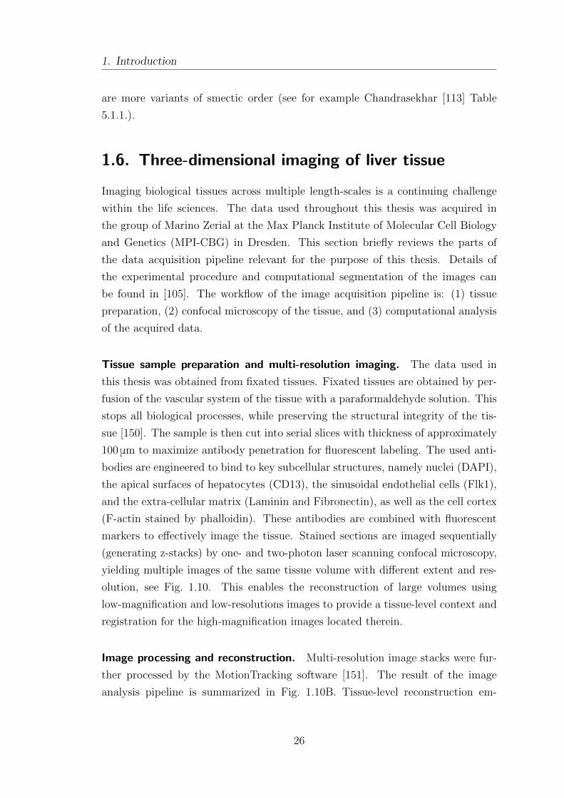
Tissue sample preparation and multi-resolution imaging. The data used in

this thesis was obtained from fixated tissues. Fixated tissues are obtained by per-

fusion of the vascular system of the tissue with a paraformaldehyde solution. This

stops all biological processes, while preserving the structural integrity of the tis-

sue [150]. The sample is then cut into serial slices with thickness of approximately

100 μm to maximize antibody penetration for fluorescent labeling. The used anti-

bodies are engineered to bind to key subcellular structures, namely nuclei (DAPI),

the apical surfaces of hepatocytes (CD13), the sinusoidal endothelial cells (Flk1),

and the extra-cellular matrix (Laminin and Fibronectin), as well as the cell cortex

(F-actin stained by phalloidin). These antibodies are combined with fluorescent

markers to effectively image the tissue. Stained sections are imaged sequentially

(generating z-stacks) by one- and two-photon laser scanning confocal microscopy,

yielding multiple images of the same tissue volume with different extent and res-

olution, see Fig. 1.10. This enables the reconstruction of large volumes using

low-magnification and low-resolutions images to provide a tissue-level context and

registration for the high-magnification images located therein.

Image processing and reconstruction. Multi-resolution image stacks were fur-

ther processed by the MotionTracking software [151]. The result of the image

analysis pipeline is summarized in Fig. 1.10B. Tissue-level reconstruction em-

26

1.6. Three-dimensional imaging of liver tissue

Figure 1.10. Overview of the data acquisition pipeline. (A) Low-resolution(1 μm× 1 μm× 1 μm per voxel) and high-resolution (0.3 μm× 0.3 μm× 0.3 μm per voxel)images of fixated and fluorescently stained slices of liver tissue are taken withfluorescence microscopy. (B) Segmentation, using the MotionTracking software,provides reconstructions of biological structure on different length-scales. Most notableare the reconstructions of the afferent vessels (portal veins, PV, orange) and efferentvessels (central veins, CV, cyan), hepatocytes (middle panel, colored meshes) andsinusoid and bile canaliculi networks (middle panel, magenta and green, respectively).The surface distribution of basal (magenta) and apical (green) membrane domains ofeach individual cell can be reconstructed (right panel). Image credit:Morales-Navarrete et al. [105] (CC-BY 4.0)

27

1. Introduction

ploys the low-resolution images to identify large vessels, namely portal veins and

central veins to provide landmarks to identify the liver lobule (cf. section 1.2).

Within these vessel structures, the high-resolution images are registered. The

high-resolution images are then used for reconstruction on the cellular level (mid-

dle panel). This yields a triangulated mesh for each cell, the sinusoidal endothelial

network and the bile canalicular network [152]. Due to the high-quality of the

imaging it is even possible to identify distributions of polarity proteins on the cell

surface, namely domains of apical and basal membrane. We take this opportunity

to also introduce a color-scheme that is used throughout this thesis to denote cer-

tain structures of the liver lobule. Central veins are shown in cyan, portal veins are

shown in orange, bile canaliculi in green and the sinusoidal network in magenta.

On the surface of hepatocytes, the apical domains are shown in green and basal

domains in magenta (cf. Fig. 1.10B).

1.7. Overview of the thesis

At the heart of this thesis is the characterization of biaxial nematic order in liver

tissue. We first turn to individual cells and establish a systematic method for the

analysis of protein patterns on cell surfaces in chapter 2. There, we introduce

the notion of vectorial and nematic cell polarity. As a reference case for vectorial

cell polarity found in simple epithelia tissue, we apply this method to cells of the

proximal and distal tubules of the kidney. Next, we turn to the main study subject

of this thesis, the hepatocytes of the liver, and find them to be of predominantly

nematic cell polarity type. Each hepatocyte in the liver is in close contact with

the sinusoidal and bile canalicli network. We therefore also characterize the local

network around hepatocytes by a method that is analogous to the characterization

of cell surface polarity. Having established the concept of nematic cell polarity for

individual hepatocytes, we next turn to the tissue level.

In chapter 3, we introduce order parameters for tissues based on concepts from

liquid crystal theory. There, we focus on characterizing orientational order of

nematic objects and introduce scalar order parameters and invariants of moment

tensors. At the end of the chapter, we turn to characterization of translational

order, showcasing the relevant signatures of smectic and columnar order.

We use the tissue-level order parameters to study the structure of liver tissue

in chapter 4. We find that the orientational order of nematic cell polarity in the

28

1.7. Overview of the thesis

liver corresponds to a biaxial liquid crystal. Furthermore, we observe co-alignment

between nematic cell polarity and the structure of the sinusoid transport network.

The translational order of cells in the liver shows signatures of smectic order.

We show that cell layers are co-localized with the bile canaliculi network and

alternate with layers of high sinusoid network density. We report alterations of

tissue polarity pattern in genetic knock-down experiments and quantify them using

orientational order parameters. The specific form of the structural alterations hint

at bi-directional cell communication with its environment.

We develop a simple nematic interaction model in chapter 5, to study the emer-

gence of orientational order found in the liver lobule. We first discuss a uniaxial

interaction model and test two hypothetical mechanisms: a global alignment field

and surface anchoring. We provide evidence that a global alignment field is more

consistent with observations in the liver. We then proceed to describe the biaxial

co-alignment between nematic cell polarity and an alignment field given by the

local sinusoid network around hepatocytes. In chapter 6, we devise a generalized

lattice-based Ising model, which shares some characteristics with cellular Potts

models, to study network generation in liver tissue. We show that this provides

a possible mechanism for the spontaneous emergence of layered order from local

rules.

29

2. Characterizing cellular anisotropy

It is crucial for proper functioning of a cell that proteins in the membrane are ag-

gregated into functional domains (cf. section 1.3). It is therefore of great interest

to quantitatively characterize the spatial distribution of membrane proteins on the

surfaces of cells. In this chapter, we present a general method to systematically

characterize cellular anisotropy. We first consider the case of surface distributions

on the unit sphere, which are expanded into spherical modes (section 2.1.1). The

power spectrum of these modes is used to characterize the anisotropy and classify

it into two classes: vectorial and nematic, as shown in section 2.1.2. In section 2.1.3

we turn to biological cells, which are, in general, non-spherical and discuss pro-

jection methods of the membrane protein distribution on the cell surface onto a

sphere. We then apply the developed classification technique by mode expansion

to experimental data of kidney and liver cells in section 2.2. In the last section

of this chapter, we extend the analysis to encompass the immediate environment

around a cell and show how to quantify the anisotropy of transport networks in

the vicinity of a cell.

2.1. Classifying protein distributions on cell surfaces

We first illustrate how to characterize surface distributions on a sphere, and after-

wards show how membrane protein distributions of cells with non-spherical shape

can be treated.

2.1.1. Mode expansion to characterize distributions on the unit

sphere

Let us first assume that cells were unit spheres. Let further f(θ, ϕ) represent a

binary surface density of the unit sphere, with polar angle θ and azimuthal angle ϕ.

Similar to the two-dimensional Fourier transform for functions defined on a plane,

we decompose f(θ, ϕ) into spherical harmonics

f(θ, ϕ) =∞∑l=0

l∑m=−l

fml Yml (θ, ϕ) , (2.1)

31

2. Characterizing cellular anisotropy

with Y ml (θ, ϕ) denoting the spherical harmonic of degree l and order m normalized

to unity. Using the ortho-normality of the spherical harmonics, the expansion co-

efficients fml are given by fml =∫S2 dΩ f(θ, ϕ)Y m∗

l (θ, ϕ). Here, integration is over

the unit sphere S2, the star denotes the complex conjugate and dΩ = sin θ dθdϕ

the differential solid angle. We also introduce orthogonal modes Fl for each degree

l of the spherical harmonics, given by

Fl(θ, ϕ) =l∑

m=−l

fml Yml (θ, ϕ) . (2.2)

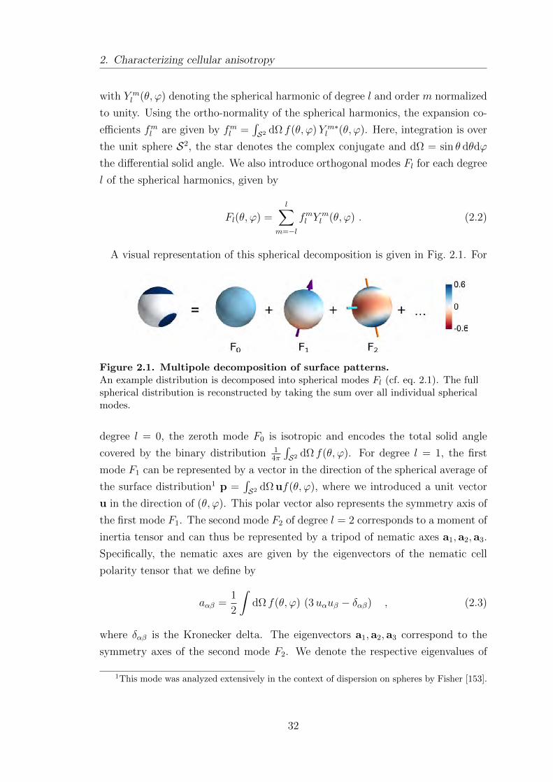
A visual representation of this spherical decomposition is given in Fig. 2.1. For

Figure 2.1. Multipole decomposition of surface patterns.An example distribution is decomposed into spherical modes Fl (cf. eq. 2.1). The fullspherical distribution is reconstructed by taking the sum over all individual sphericalmodes.

degree l = 0, the zeroth mode F0 is isotropic and encodes the total solid angle

covered by the binary distribution 14π

∫S2 dΩ f(θ, ϕ). For degree l = 1, the first

mode F1 can be represented by a vector in the direction of the spherical average of

the surface distribution1 p =∫S2 dΩ uf(θ, ϕ), where we introduced a unit vector

u in the direction of (θ, ϕ). This polar vector also represents the symmetry axis of

the first mode F1. The second mode F2 of degree l = 2 corresponds to a moment of

inertia tensor and can thus be represented by a tripod of nematic axes a1, a2, a3.

Specifically, the nematic axes are given by the eigenvectors of the nematic cell

polarity tensor that we define by

aαβ =1

2

∫dΩ f(θ, ϕ) (3uαuβ − δαβ) , (2.3)

where δαβ is the Kronecker delta. The eigenvectors a1, a2, a3 correspond to the

symmetry axes of the second mode F2. We denote the respective eigenvalues of

1This mode was analyzed extensively in the context of dispersion on spheres by Fisher [153].

32

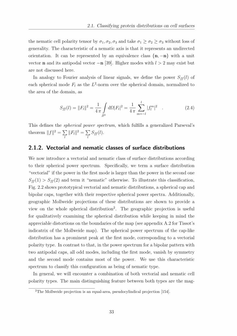
2.1. Classifying protein distributions on cell surfaces

the nematic cell polarity tensor by σ1, σ2, σ3 and take σ1 ≥ σ2 ≥ σ3 without loss of

generality. The characteristic of a nematic axis is that it represents an undirected

orientation. It can be represented by an equivalence class n,−n with a unit

vector n and its antipodal vector −n [39]. Higher modes with l > 2 may exist but

are not discussed here.

In analogy to Fourier analysis of linear signals, we define the power Sff (l) of

each spherical mode Fl as the L2-norm over the spherical domain, normalized to

the area of the domain, as

Sff (l) = ‖Fl‖2 =1

4 π

∫S2

dΩ|Fl|2 =1

4 π

l∑m=−l

|fml |2 . (2.4)

This defines the spherical power spectrum, which fulfills a generalized Parseval’s

theorem ‖f‖2 =∑l

‖Fl‖2 =∑l

Sff (l).

2.1.2. Vectorial and nematic classes of surface distributions

We now introduce a vectorial and nematic class of surface distributions according

to their spherical power spectrum. Specifically, we term a surface distribution

“vectorial” if the power in the first mode is larger than the power in the second one

Sff (1) > Sff (2) and term it “nematic” otherwise. To illustrate this classification,

Fig. 2.2 shows prototypical vectorial and nematic distributions, a spherical cap and

bipolar caps, together with their respective spherical power spectra. Additionally,

geographic Mollweide projections of these distributions are shown to provide a

view on the whole spherical distribution2. The geographic projection is useful

for qualitatively examining the spherical distribution while keeping in mind the

appreciable distortions on the boundaries of the map (see appendix A.2 for Tissot’s

indicatrix of the Mollweide map). The spherical power spectrum of the cap-like

distribution has a prominent peak at the first mode, corresponding to a vectorial

polarity type. In contrast to that, in the power spectrum for a bipolar pattern with

two antipodal caps, all odd modes, including the first mode, vanish by symmetry

and the second mode contains most of the power. We use this characteristic

spectrum to classify this configuration as being of nematic type.

In general, we will encounter a combination of both vectorial and nematic cell

polarity types. The main distinguishing feature between both types are the mag-

2The Mollweide projection is an equal-area, pseudocylindical projection [154].

33

2. Characterizing cellular anisotropy

nitudes of the first and second mode of the power spectrum.

Figure 2.2. Idealized cases of vectorial and nematic surface pattern.(A) The spherical cap is shown as a prototypical example of a vectorial surface patterndistribution, which is characterized by a peak at first mode in the spherical powerspectrum. It can be represented by a vector pointing towards the center of the cap asindicated in the schematic on the left. (B) Two opposing (bipolar) spherical caps areshown as a prototypical example of a nematic surface pattern distribution. Thissurface distribution is characterized by a peak at the second mode in the sphericalpower spectrum. Additionally, all odd modes vanish by symmetry. It can berepresented by a dash (an undirected line segment) pointing from the center of one capto the center of the other as indicated in the schematic on the left.

2.1.3. Cell polarity on non-spherical surfaces

In general, the surfaces of cells are not unit spheres and we need to decide for

a projection method when analyzing protein distributions on non-spherical cells.

We restrict our treatment to three-dimensional volumes that are star-convex with

respect to their center of mass3. To simplify notation, we choose the origin of our

coordinate system to be at the center of mass of the volume. Then, by definition of

a star-convex volume, for every point r on the surface, there exists a line segment

from the origin to r that does not include any point from the surface other than r.

The restriction to star-convex shapes of this type is useful, because every point r on

the surface can be mapped bijectively on a point on the unit sphere, characterized

by a polar angle θ and an azimuthal angle ϕ.

3A volume V in R3 is called star convex, if there exists a point x0 ∈ V such that every linesegment from x0 to any point in V is contained in V . Note that every non-empty convex volumeis also star-convex.

34

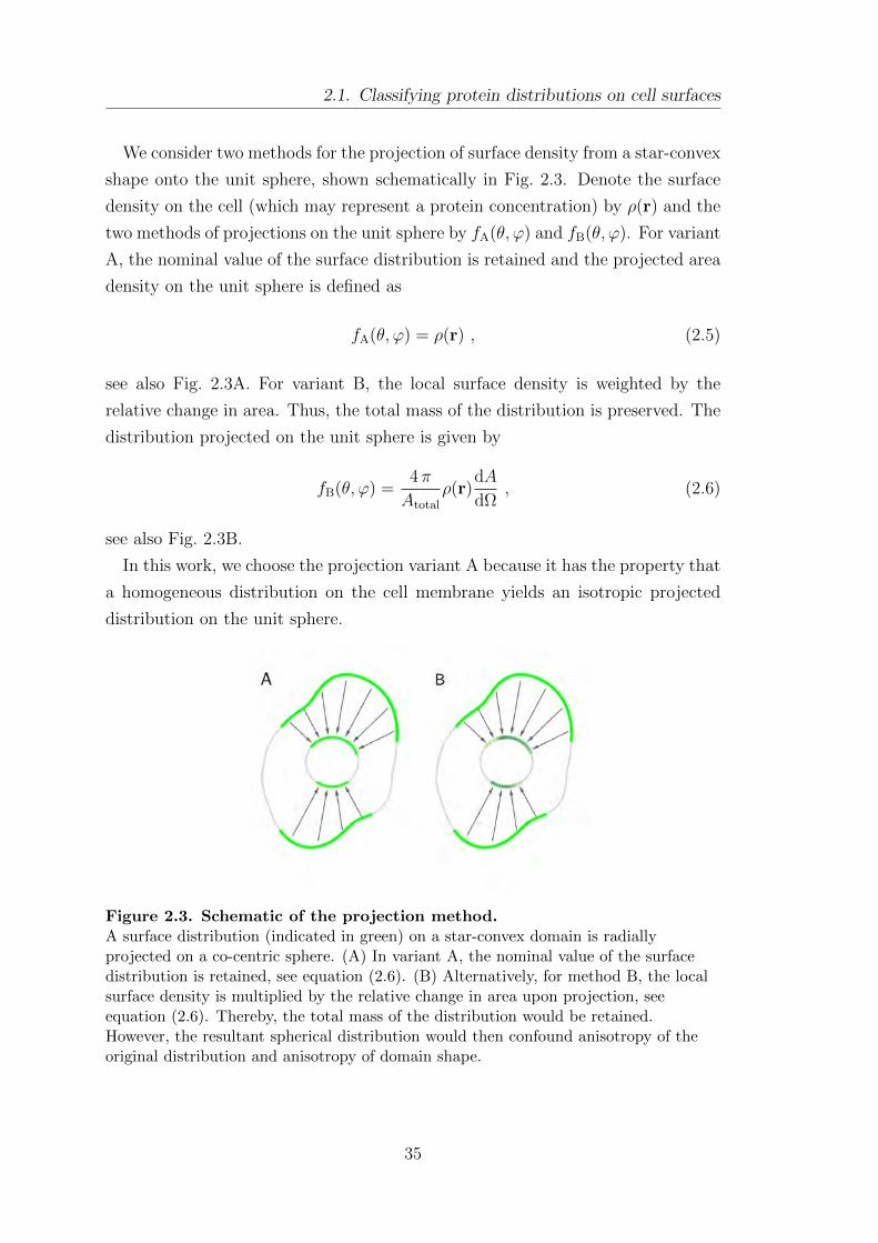
2.1. Classifying protein distributions on cell surfaces

We consider two methods for the projection of surface density from a star-convex

shape onto the unit sphere, shown schematically in Fig. 2.3. Denote the surface

density on the cell (which may represent a protein concentration) by ρ(r) and the

two methods of projections on the unit sphere by fA(θ, ϕ) and fB(θ, ϕ). For variant

A, the nominal value of the surface distribution is retained and the projected area

density on the unit sphere is defined as

fA(θ, ϕ) = ρ(r) , (2.5)

see also Fig. 2.3A. For variant B, the local surface density is weighted by the

relative change in area. Thus, the total mass of the distribution is preserved. The

distribution projected on the unit sphere is given by

fB(θ, ϕ) =4π

Atotal

ρ(r)dA

dΩ, (2.6)

see also Fig. 2.3B.

In this work, we choose the projection variant A because it has the property that

a homogeneous distribution on the cell membrane yields an isotropic projected

distribution on the unit sphere.

Figure 2.3. Schematic of the projection method.A surface distribution (indicated in green) on a star-convex domain is radiallyprojected on a co-centric sphere. (A) In variant A, the nominal value of the surfacedistribution is retained, see equation (2.6). (B) Alternatively, for method B, the localsurface density is multiplied by the relative change in area upon projection, seeequation (2.6). Thereby, the total mass of the distribution would be retained.However, the resultant spherical distribution would then confound anisotropy of theoriginal distribution and anisotropy of domain shape.

35

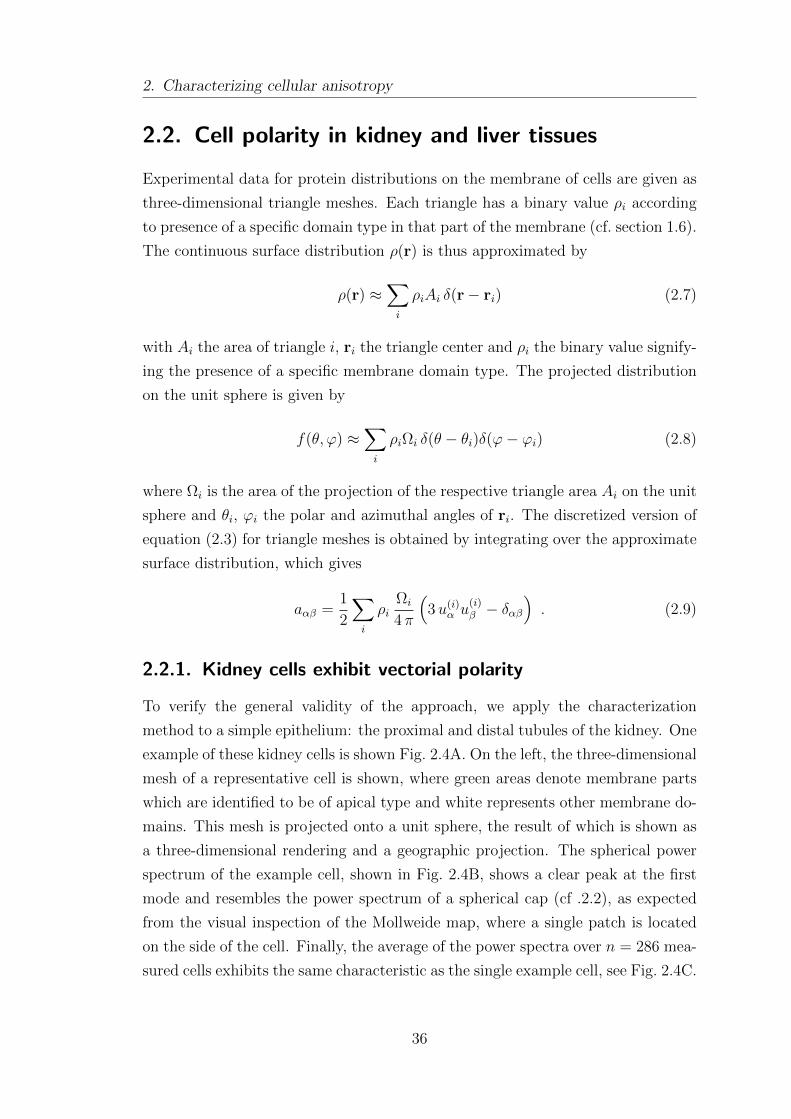
2. Characterizing cellular anisotropy

2.2. Cell polarity in kidney and liver tissues

Experimental data for protein distributions on the membrane of cells are given as

three-dimensional triangle meshes. Each triangle has a binary value ρi according

to presence of a specific domain type in that part of the membrane (cf. section 1.6).

The continuous surface distribution ρ(r) is thus approximated by

ρ(r) ≈∑i

ρiAi δ(r− ri) (2.7)

with Ai the area of triangle i, ri the triangle center and ρi the binary value signify-

ing the presence of a specific membrane domain type. The projected distribution

on the unit sphere is given by

f(θ, ϕ) ≈∑i

ρiΩi δ(θ − θi)δ(ϕ− ϕi) (2.8)

where Ωi is the area of the projection of the respective triangle area Ai on the unit

sphere and θi, ϕi the polar and azimuthal angles of ri. The discretized version of

equation (2.3) for triangle meshes is obtained by integrating over the approximate

surface distribution, which gives

aαβ =1

2

∑i

ρiΩi

4π

(3u(i)

α u(i)β − δαβ

). (2.9)

2.2.1. Kidney cells exhibit vectorial polarity

To verify the general validity of the approach, we apply the characterization

method to a simple epithelium: the proximal and distal tubules of the kidney. One

example of these kidney cells is shown Fig. 2.4A. On the left, the three-dimensional

mesh of a representative cell is shown, where green areas denote membrane parts

which are identified to be of apical type and white represents other membrane do-

mains. This mesh is projected onto a unit sphere, the result of which is shown as

a three-dimensional rendering and a geographic projection. The spherical power

spectrum of the example cell, shown in Fig. 2.4B, shows a clear peak at the first

mode and resembles the power spectrum of a spherical cap (cf .2.2), as expected

from the visual inspection of the Mollweide map, where a single patch is located

on the side of the cell. Finally, the average of the power spectra over n = 286 mea-

sured cells exhibits the same characteristic as the single example cell, see Fig. 2.4C.

36

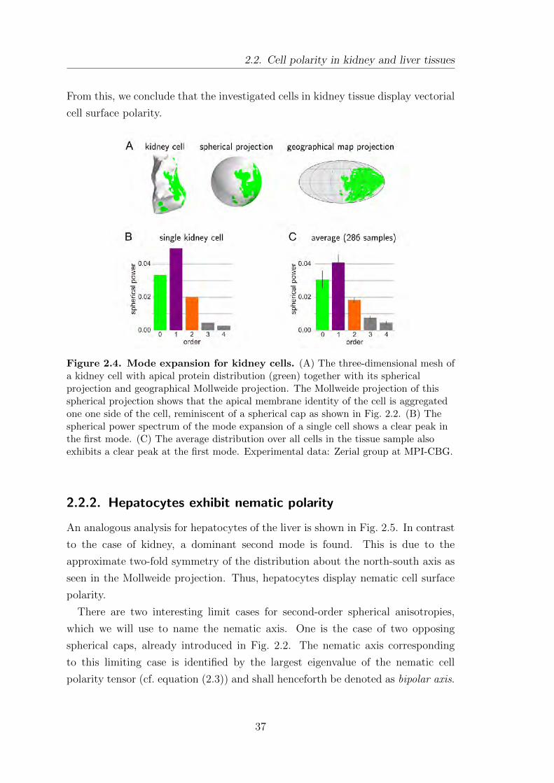
2.2. Cell polarity in kidney and liver tissues

From this, we conclude that the investigated cells in kidney tissue display vectorial

cell surface polarity.

Figure 2.4. Mode expansion for kidney cells. (A) The three-dimensional mesh ofa kidney cell with apical protein distribution (green) together with its sphericalprojection and geographical Mollweide projection. The Mollweide projection of thisspherical projection shows that the apical membrane identity of the cell is aggregatedone one side of the cell, reminiscent of a spherical cap as shown in Fig. 2.2. (B) Thespherical power spectrum of the mode expansion of a single cell shows a clear peak inthe first mode. (C) The average distribution over all cells in the tissue sample alsoexhibits a clear peak at the first mode. Experimental data: Zerial group at MPI-CBG.

2.2.2. Hepatocytes exhibit nematic polarity

An analogous analysis for hepatocytes of the liver is shown in Fig. 2.5. In contrast

to the case of kidney, a dominant second mode is found. This is due to the

approximate two-fold symmetry of the distribution about the north-south axis as

seen in the Mollweide projection. Thus, hepatocytes display nematic cell surface

polarity.

There are two interesting limit cases for second-order spherical anisotropies,

which we will use to name the nematic axis. One is the case of two opposing

spherical caps, already introduced in Fig. 2.2. The nematic axis corresponding

to this limiting case is identified by the largest eigenvalue of the nematic cell

polarity tensor (cf. equation (2.3)) and shall henceforth be denoted as bipolar axis.

37

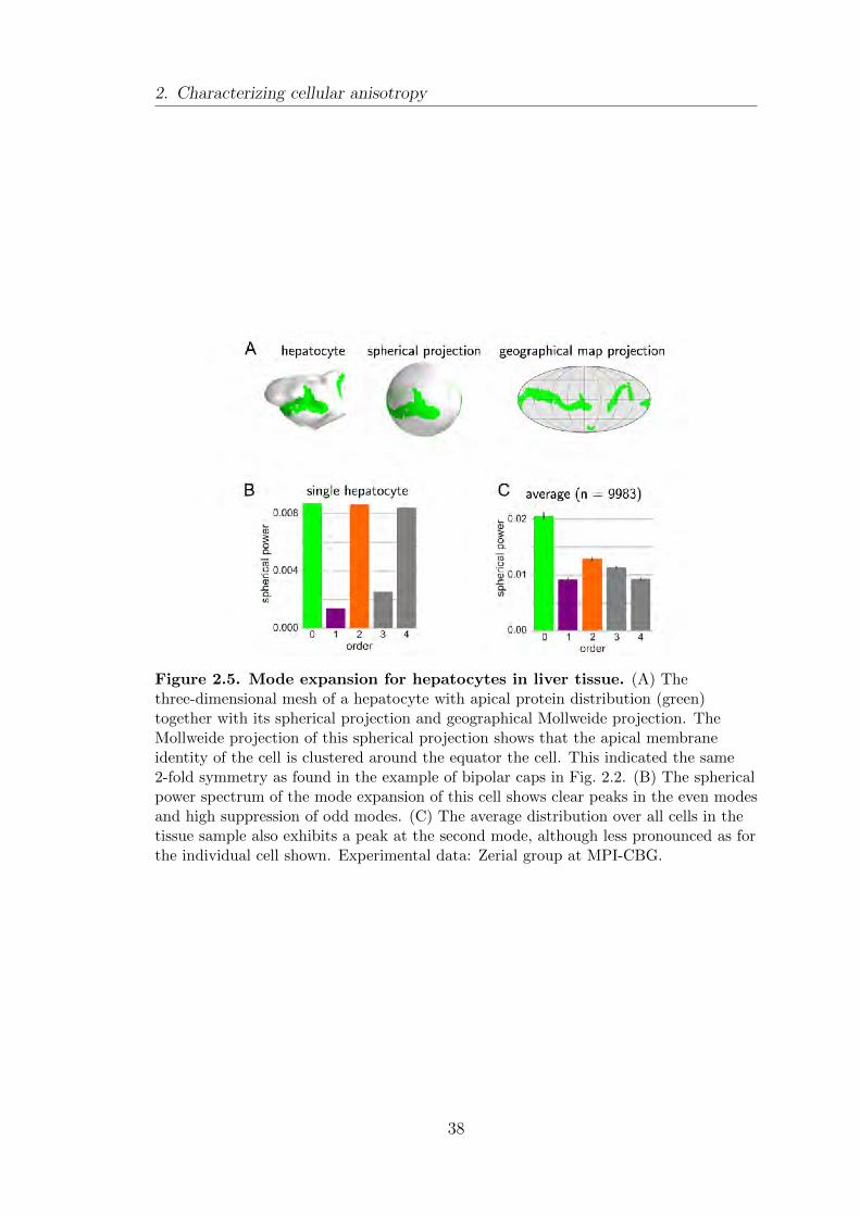
2. Characterizing cellular anisotropy

Figure 2.5. Mode expansion for hepatocytes in liver tissue. (A) Thethree-dimensional mesh of a hepatocyte with apical protein distribution (green)together with its spherical projection and geographical Mollweide projection. TheMollweide projection of this spherical projection shows that the apical membraneidentity of the cell is clustered around the equator the cell. This indicated the same2-fold symmetry as found in the example of bipolar caps in Fig. 2.2. (B) The sphericalpower spectrum of the mode expansion of this cell shows clear peaks in the even modesand high suppression of odd modes. (C) The average distribution over all cells in thetissue sample also exhibits a peak at the second mode, although less pronounced as forthe individual cell shown. Experimental data: Zerial group at MPI-CBG.

38

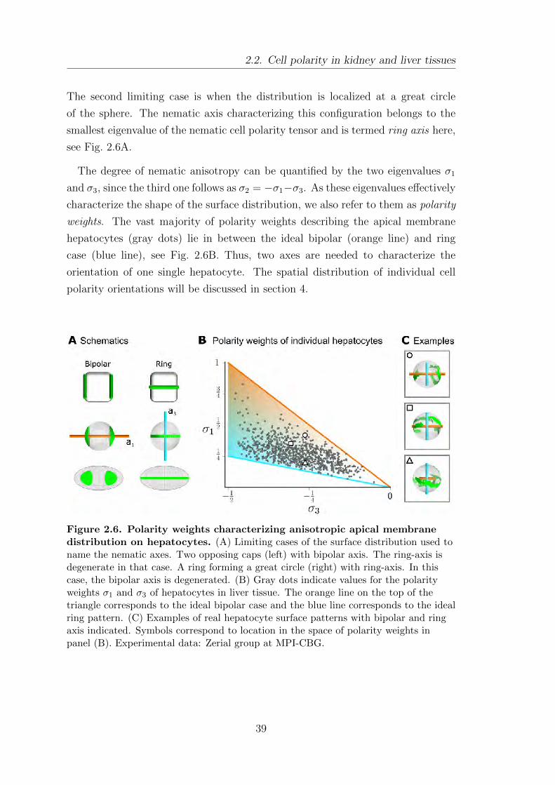
2.2. Cell polarity in kidney and liver tissues

The second limiting case is when the distribution is localized at a great circle

of the sphere. The nematic axis characterizing this configuration belongs to the

smallest eigenvalue of the nematic cell polarity tensor and is termed ring axis here,

see Fig. 2.6A.

The degree of nematic anisotropy can be quantified by the two eigenvalues σ1

and σ3, since the third one follows as σ2 = −σ1−σ3. As these eigenvalues effectively

characterize the shape of the surface distribution, we also refer to them as polarity

weights. The vast majority of polarity weights describing the apical membrane

hepatocytes (gray dots) lie in between the ideal bipolar (orange line) and ring

case (blue line), see Fig. 2.6B. Thus, two axes are needed to characterize the

orientation of one single hepatocyte. The spatial distribution of individual cell

polarity orientations will be discussed in section 4.

Figure 2.6. Polarity weights characterizing anisotropic apical membranedistribution on hepatocytes. (A) Limiting cases of the surface distribution used toname the nematic axes. Two opposing caps (left) with bipolar axis. The ring-axis isdegenerate in that case. A ring forming a great circle (right) with ring-axis. In thiscase, the bipolar axis is degenerated. (B) Gray dots indicate values for the polarityweights σ1 and σ3 of hepatocytes in liver tissue. The orange line on the top of thetriangle corresponds to the ideal bipolar case and the blue line corresponds to the idealring pattern. (C) Examples of real hepatocyte surface patterns with bipolar and ringaxis indicated. Symbols correspond to location in the space of polarity weights inpanel (B). Experimental data: Zerial group at MPI-CBG.

39

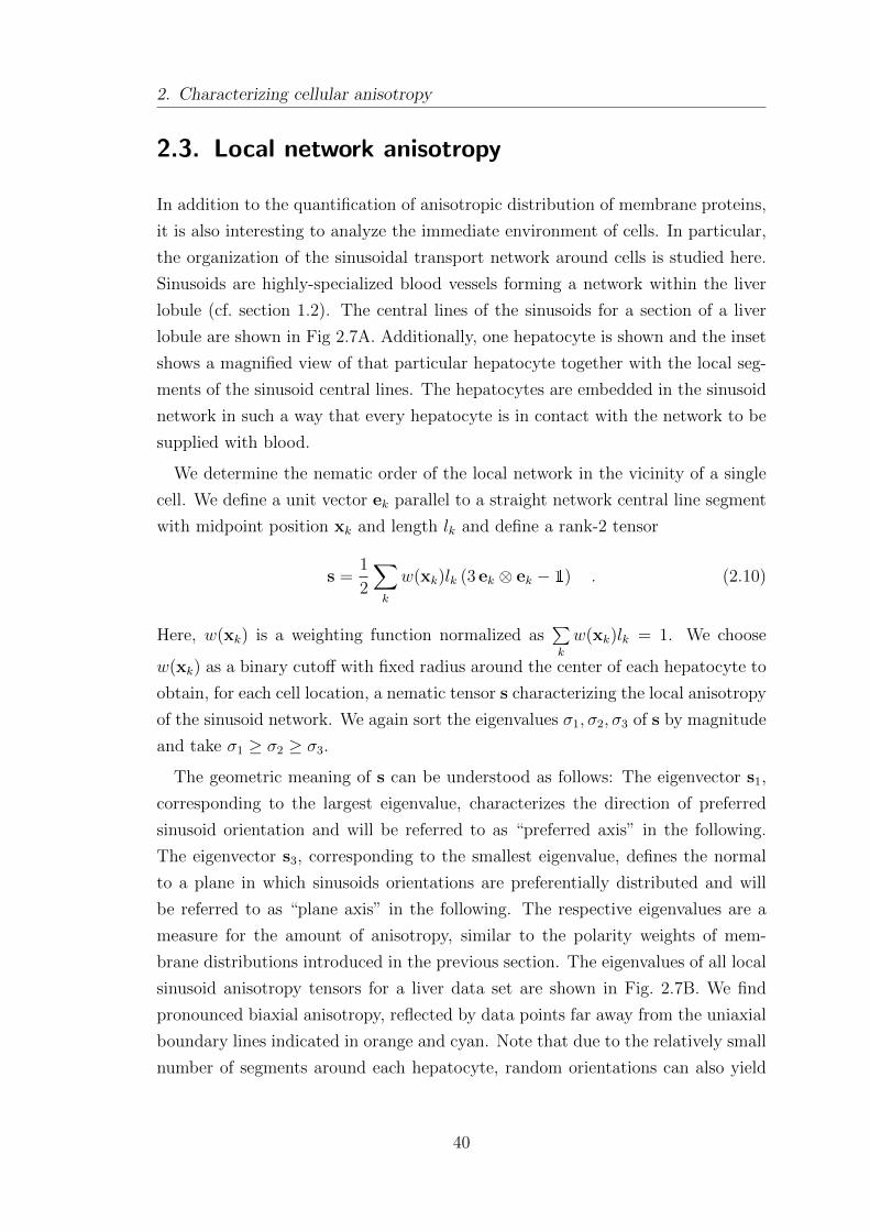
2. Characterizing cellular anisotropy

2.3. Local network anisotropy

In addition to the quantification of anisotropic distribution of membrane proteins,

it is also interesting to analyze the immediate environment of cells. In particular,

the organization of the sinusoidal transport network around cells is studied here.

Sinusoids are highly-specialized blood vessels forming a network within the liver

lobule (cf. section 1.2). The central lines of the sinusoids for a section of a liver

lobule are shown in Fig 2.7A. Additionally, one hepatocyte is shown and the inset

shows a magnified view of that particular hepatocyte together with the local seg-

ments of the sinusoid central lines. The hepatocytes are embedded in the sinusoid

network in such a way that every hepatocyte is in contact with the network to be

supplied with blood.

We determine the nematic order of the local network in the vicinity of a single

cell. We define a unit vector ek parallel to a straight network central line segment

with midpoint position xk and length lk and define a rank-2 tensor

s =1

2

∑k

w(xk)lk (3 ek ⊗ ek − 1) . (2.10)

Here, w(xk) is a weighting function normalized as∑k

w(xk)lk = 1. We choose

w(xk) as a binary cutoff with fixed radius around the center of each hepatocyte to

obtain, for each cell location, a nematic tensor s characterizing the local anisotropy

of the sinusoid network. We again sort the eigenvalues σ1, σ2, σ3 of s by magnitude

and take σ1 ≥ σ2 ≥ σ3.

The geometric meaning of s can be understood as follows: The eigenvector s1,

corresponding to the largest eigenvalue, characterizes the direction of preferred

sinusoid orientation and will be referred to as “preferred axis” in the following.

The eigenvector s3, corresponding to the smallest eigenvalue, defines the normal

to a plane in which sinusoids orientations are preferentially distributed and will

be referred to as “plane axis” in the following. The respective eigenvalues are a

measure for the amount of anisotropy, similar to the polarity weights of mem-

brane distributions introduced in the previous section. The eigenvalues of all local

sinusoid anisotropy tensors for a liver data set are shown in Fig. 2.7B. We find

pronounced biaxial anisotropy, reflected by data points far away from the uniaxial

boundary lines indicated in orange and cyan. Note that due to the relatively small

number of segments around each hepatocyte, random orientations can also yield

40

2.4. Summary

non-zero anisotropies. These are, however, much smaller than the ones observed

in actual liver data, see appendix A.4 for details.

Figure 2.7. Local network anisotropy around cells. (A) Central lines of thesinusoid network (cf. section 1.6) shown for a section of a liver lobule between centralvein (cyan) and portal vein (orange). Inset shows one hepatocyte together with thesegments of the central lines with node positions within a sphere of 20 μm around thecenter of the hepatocyte. (B) Eigenvalues of the nematic tensor s for local sinusoidnetwork around hepatocytes that characterize the amount of nematic anisotropy.Experimental data: Zerial group at MPI-CBG.

2.4. Summary

In this chapter, we defined and characterized two types of cell polarity: vectorial

and nematic. These types represent symmetry types of surface patterns of (apical)

membrane proteins. We showed that the cells of the kidney exhibit vectorial

apico-basal cell polarity and cells in the liver exhibit nematic cell polarity. This

is, to our knowledge, the first time that nematic cell polarity of hepatocytes has

been quantified systematically in this way. Furthermore, we introduced a tool to

quantify nematic anisotropy of networks around cells. These methods open up

new possibilities to analyze structure order in tissue and will be applied to liver

tissue in chapter 4 to identify biaxial liquid crystal ordering of apical nematic cell

polarity of hepatocytes.

41

3. Order parameters for tissue

organization

For individual cells, we established in chapter 2 that membrane protein distribu-

tions around individual cells of kidney and liver tissue are anisotropic. We now

consider many cells that together constitute a biological tissue and study transla-

tional and orientational order of this composite material. In the present chapter,

we introduce the necessary tools for this structural analysis. These tools will be

applied to the study of liver tissue in chapter 4.

Regarding orientational order, we discuss two approaches: (i) scalar order pa-

rameters used in liquid crystal theory (cf. section 1.5.3) and (ii) invariants of tensor

fields. We then extend the description to treat orientational order in curved ge-

ometries. This generalization is motivated by the lobular structure of liver tissue

(cf. section 1.2). Complementary to this, we propose the concept of co-orientational

order to compare two biaxial nematic fields within the same system. This approach

will prove useful in the analysis of orientational order in tissues with spatially vary-

ing director fields, presented in chapter 4. In the last section of this chapter, we

turn to translational order by providing concepts to quantify smectic and columnar

order.

3.1. Orientational order: quantifying biaxial phases

In this section, we characterize orientational order of homogeneous systems by

two methods: (i) four orientational order parameters S, P,D,C and (ii) invariants

of moment tensors Ik. This analysis of orientational order of nematic objects

is motivated by the finding that hepatocytes of the liver exhibit a second-order

anisotropy that is captured by the nematic tensor aαβ (cf. equation (2.3)), which

was presented in section 2.2.2. The analysis of orientational order outlined below is

not specific to cell polarity but instead more general. We therefore use the generic

term “object” to refer to individual constituents and denote the corresponding

nematic tensor by tαβ (cf. Fig. 3.1).

We denote the tripod of ortho-normalized eigenvectors of this tensor by l,m,n

with respective eigenvalues σl, σm, σn. The eigenvectors l,m,n are only defined up

43

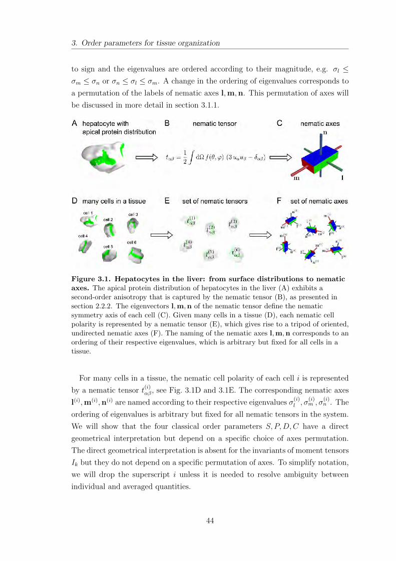
3. Order parameters for tissue organization

to sign and the eigenvalues are ordered according to their magnitude, e.g. σl ≤σm ≤ σn or σn ≤ σl ≤ σm. A change in the ordering of eigenvalues corresponds to

a permutation of the labels of nematic axes l,m,n. This permutation of axes will

be discussed in more detail in section 3.1.1.

Figure 3.1. Hepatocytes in the liver: from surface distributions to nematicaxes. The apical protein distribution of hepatocytes in the liver (A) exhibits asecond-order anisotropy that is captured by the nematic tensor (B), as presented insection 2.2.2. The eigenvectors l,m,n of the nematic tensor define the nematicsymmetry axis of each cell (C). Given many cells in a tissue (D), each nematic cellpolarity is represented by a nematic tensor (E), which gives rise to a tripod of oriented,undirected nematic axes (F). The naming of the nematic axes l,m,n corresponds to anordering of their respective eigenvalues, which is arbitrary but fixed for all cells in atissue.

For many cells in a tissue, the nematic cell polarity of each cell i is represented

by a nematic tensor t(i)αβ, see Fig. 3.1D and 3.1E. The corresponding nematic axes

l(i),m(i),n(i) are named according to their respective eigenvalues σ(i)l , σ

(i)m , σ

(i)n . The

ordering of eigenvalues is arbitrary but fixed for all nematic tensors in the system.

We will show that the four classical order parameters S, P,D,C have a direct

geometrical interpretation but depend on a specific choice of axes permutation.

The direct geometrical interpretation is absent for the invariants of moment tensors

Ik but they do not depend on a specific permutation of axes. To simplify notation,

we will drop the superscript i unless it is needed to resolve ambiguity between

individual and averaged quantities.

44

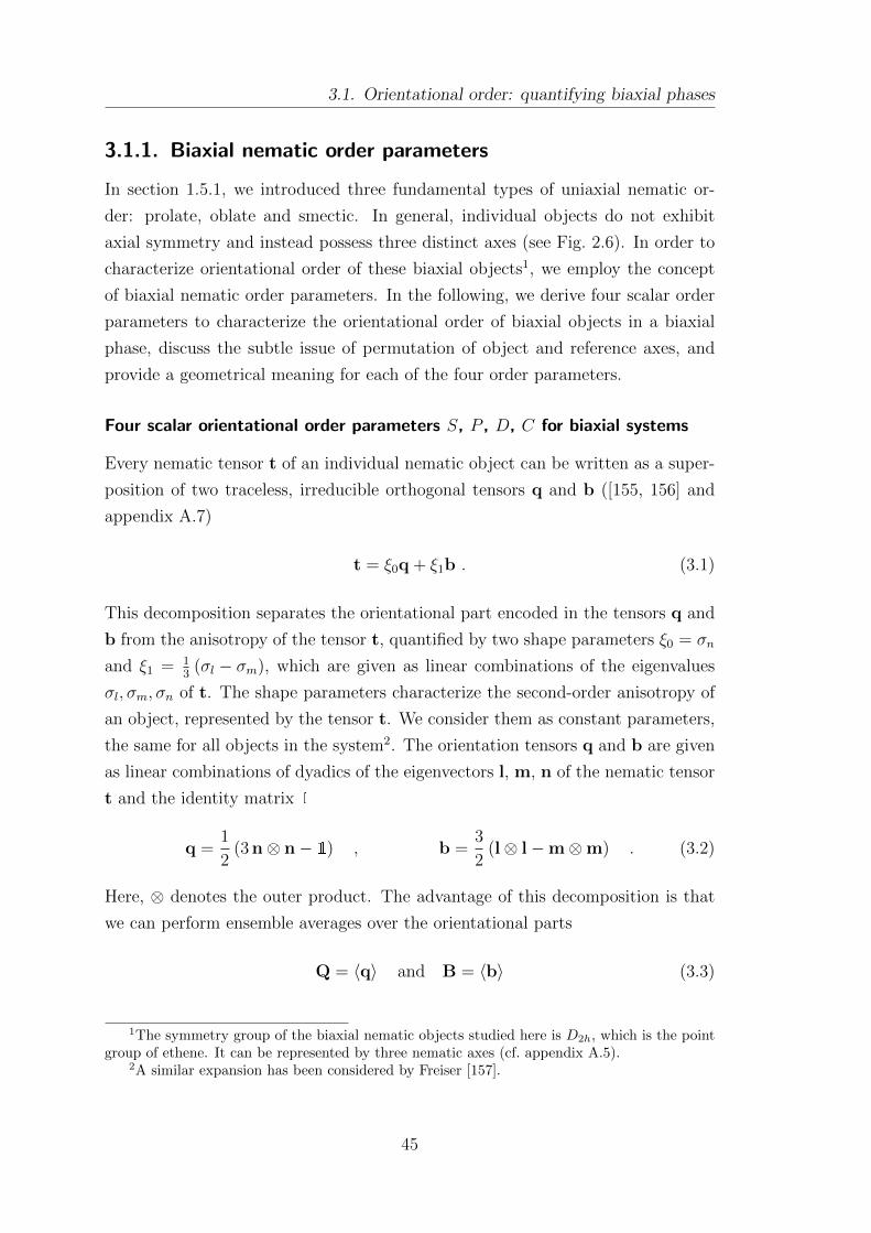
3.1. Orientational order: quantifying biaxial phases

3.1.1. Biaxial nematic order parameters

In section 1.5.1, we introduced three fundamental types of uniaxial nematic or-

der: prolate, oblate and smectic. In general, individual objects do not exhibit

axial symmetry and instead possess three distinct axes (see Fig. 2.6). In order to

characterize orientational order of these biaxial objects1, we employ the concept

of biaxial nematic order parameters. In the following, we derive four scalar order

parameters to characterize the orientational order of biaxial objects in a biaxial

phase, discuss the subtle issue of permutation of object and reference axes, and

provide a geometrical meaning for each of the four order parameters.

Four scalar orientational order parameters S, P , D, C for biaxial systems

Every nematic tensor t of an individual nematic object can be written as a super-

position of two traceless, irreducible orthogonal tensors q and b ([155, 156] and

appendix A.7)

t = ξ0q + ξ1b . (3.1)

This decomposition separates the orientational part encoded in the tensors q and

b from the anisotropy of the tensor t, quantified by two shape parameters ξ0 = σn

and ξ1 = 13

(σl − σm), which are given as linear combinations of the eigenvalues

σl, σm, σn of t. The shape parameters characterize the second-order anisotropy of

an object, represented by the tensor t. We consider them as constant parameters,

the same for all objects in the system2. The orientation tensors q and b are given

as linear combinations of dyadics of the eigenvectors l, m, n of the nematic tensor

t and the identity matrix 1

q =1

2(3 n⊗ n− 1) , b =

3

2(l⊗ l−m⊗m) . (3.2)

Here, ⊗ denotes the outer product. The advantage of this decomposition is that

we can perform ensemble averages over the orientational parts

Q = 〈q〉 and B = 〈b〉 (3.3)

1The symmetry group of the biaxial nematic objects studied here is D2h, which is the pointgroup of ethene. It can be represented by three nematic axes (cf. appendix A.5).

2A similar expansion has been considered by Freiser [157].

45

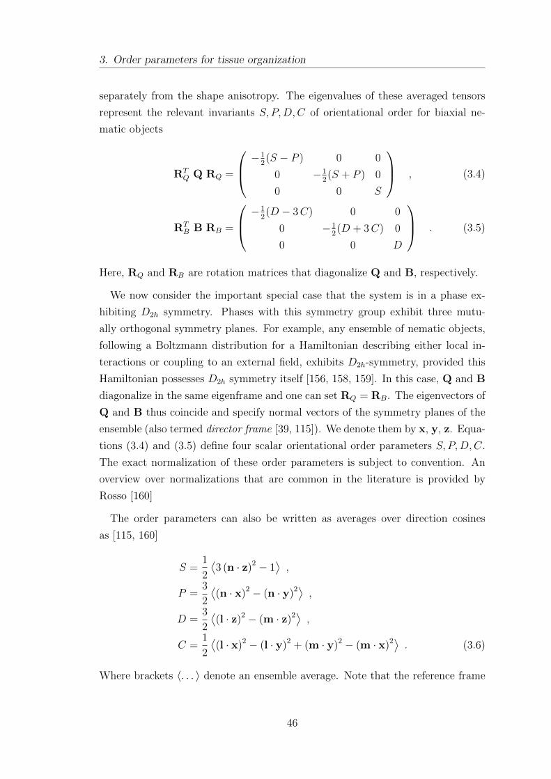
3. Order parameters for tissue organization

separately from the shape anisotropy. The eigenvalues of these averaged tensors

represent the relevant invariants S, P,D,C of orientational order for biaxial ne-

matic objects

RTQ Q RQ =

−12(S − P ) 0 0

0 −12(S + P ) 0

0 0 S

, (3.4)

RTB B RB =

−12(D − 3C) 0 0

0 −12(D + 3C) 0

0 0 D

. (3.5)

Here, RQ and RB are rotation matrices that diagonalize Q and B, respectively.

We now consider the important special case that the system is in a phase ex-

hibiting D2h symmetry. Phases with this symmetry group exhibit three mutu-

ally orthogonal symmetry planes. For example, any ensemble of nematic objects,

following a Boltzmann distribution for a Hamiltonian describing either local in-

teractions or coupling to an external field, exhibits D2h-symmetry, provided this

Hamiltonian possesses D2h symmetry itself [156, 158, 159]. In this case, Q and B

diagonalize in the same eigenframe and one can set RQ = RB. The eigenvectors of

Q and B thus coincide and specify normal vectors of the symmetry planes of the

ensemble (also termed director frame [39, 115]). We denote them by x, y, z. Equa-

tions (3.4) and (3.5) define four scalar orientational order parameters S, P,D,C.

The exact normalization of these order parameters is subject to convention. An

overview over normalizations that are common in the literature is provided by

Rosso [160]

The order parameters can also be written as averages over direction cosines

as [115, 160]

S =1

2

⟨3 (n · z)2 − 1

⟩,

P =3

2

⟨(n · x)2 − (n · y)2⟩ ,

D =3

2

⟨(l · z)2 − (m · z)2⟩ ,

C =1

2

⟨(l · x)2 − (l · y)2 + (m · y)2 − (m · x)2⟩ . (3.6)

Where brackets 〈. . . 〉 denote an ensemble average. Note that the reference frame

46

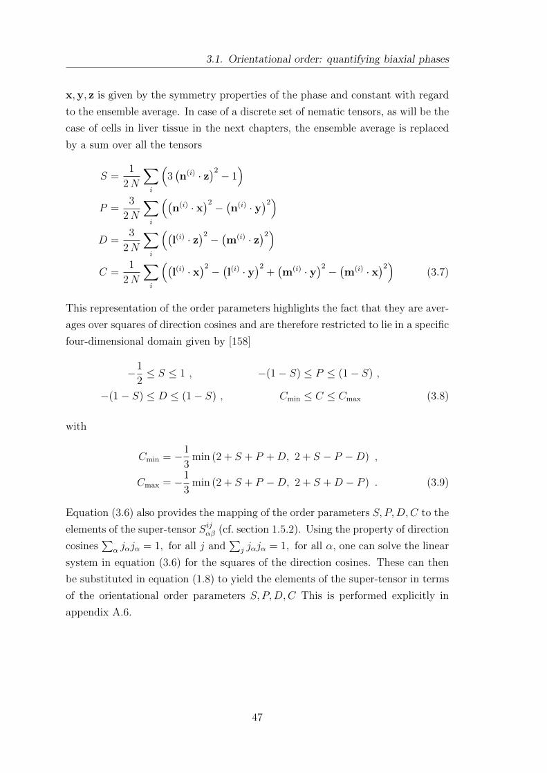
3.1. Orientational order: quantifying biaxial phases

x,y, z is given by the symmetry properties of the phase and constant with regard

to the ensemble average. In case of a discrete set of nematic tensors, as will be the

case of cells in liver tissue in the next chapters, the ensemble average is replaced

by a sum over all the tensors

S =1

2N

∑i

(3(n(i) · z

)2 − 1)

P =3

2N

∑i

((n(i) · x

)2 −(n(i) · y

)2)

D =3

2N

∑i

((l(i) · z

)2 −(m(i) · z

)2)

C =1

2N

∑i

((l(i) · x

)2 −(l(i) · y

)2+(m(i) · y

)2 −(m(i) · x

)2)

(3.7)

This representation of the order parameters highlights the fact that they are aver-

ages over squares of direction cosines and are therefore restricted to lie in a specific

four-dimensional domain given by [158]

−1

2≤ S ≤ 1 , −(1− S) ≤ P ≤ (1− S) ,

−(1− S) ≤ D ≤ (1− S) , Cmin ≤ C ≤ Cmax (3.8)

with

Cmin = −1

3min (2 + S + P +D, 2 + S − P −D) ,

Cmax = −1

3min (2 + S + P −D, 2 + S +D − P ) . (3.9)

Equation (3.6) also provides the mapping of the order parameters S, P,D,C to the

elements of the super-tensor Sijαβ (cf. section 1.5.2). Using the property of direction

cosines∑

α jαjα = 1, for all j and∑

j jαjα = 1, for all α, one can solve the linear

system in equation (3.6) for the squares of the direction cosines. These can then

be substituted in equation (1.8) to yield the elements of the super-tensor in terms

of the orientational order parameters S, P,D,C This is performed explicitly in

appendix A.6.

47

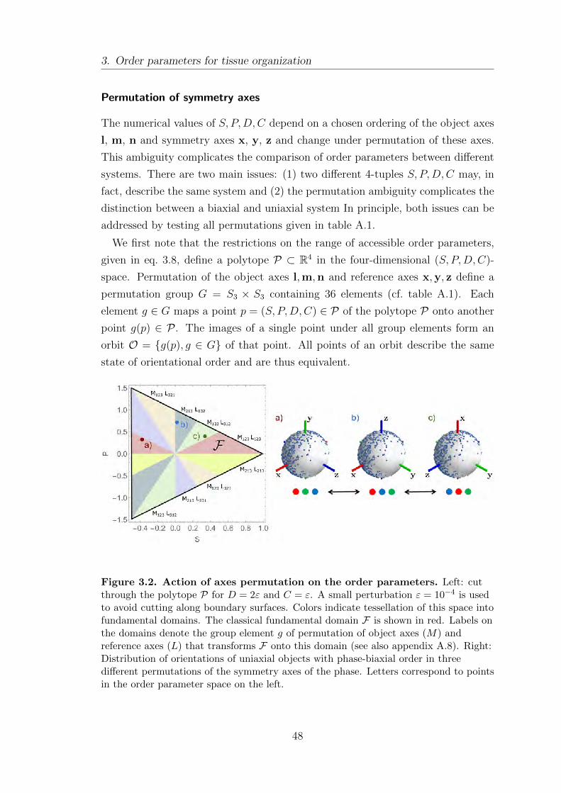
3. Order parameters for tissue organization

Permutation of symmetry axes

The numerical values of S, P,D,C depend on a chosen ordering of the object axes

l, m, n and symmetry axes x, y, z and change under permutation of these axes.

This ambiguity complicates the comparison of order parameters between different

systems. There are two main issues: (1) two different 4-tuples S, P,D,C may, in

fact, describe the same system and (2) the permutation ambiguity complicates the

distinction between a biaxial and uniaxial system In principle, both issues can be

addressed by testing all permutations given in table A.1.

We first note that the restrictions on the range of accessible order parameters,

given in eq. 3.8, define a polytope P ⊂ R4 in the four-dimensional (S, P,D,C)-

space. Permutation of the object axes l,m,n and reference axes x,y, z define a

permutation group G = S3 × S3 containing 36 elements (cf. table A.1). Each

element g ∈ G maps a point p = (S, P,D,C) ∈ P of the polytope P onto another

point g(p) ∈ P . The images of a single point under all group elements form an

orbit O = g(p), g ∈ G of that point. All points of an orbit describe the same

state of orientational order and are thus equivalent.

Figure 3.2. Action of axes permutation on the order parameters. Left: cutthrough the polytope P for D = 2ε and C = ε. A small perturbation ε = 10−4 is usedto avoid cutting along boundary surfaces. Colors indicate tessellation of this space intofundamental domains. The classical fundamental domain F is shown in red. Labels onthe domains denote the group element g of permutation of object axes (M) andreference axes (L) that transforms F onto this domain (see also appendix A.8). Right:Distribution of orientations of uniaxial objects with phase-biaxial order in threedifferent permutations of the symmetry axes of the phase. Letters correspond to pointsin the order parameter space on the left.

48

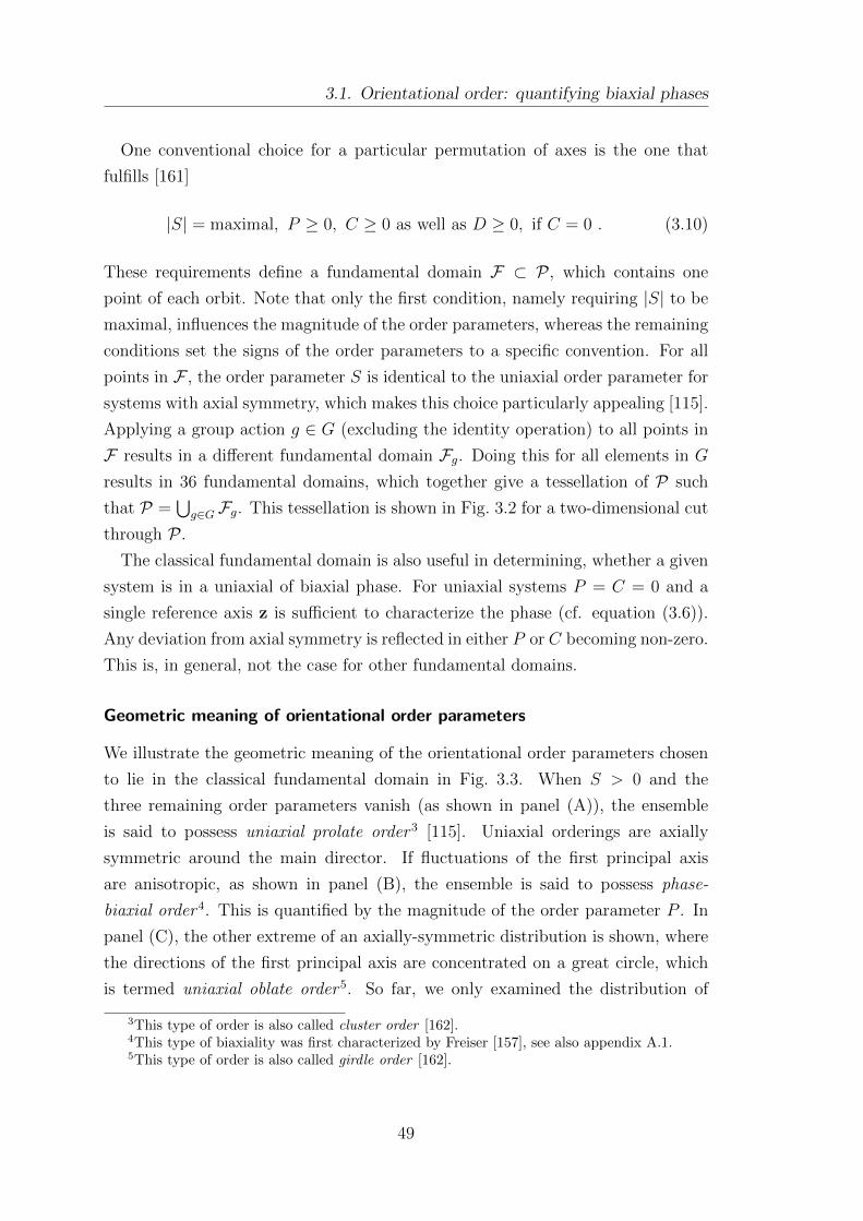
3.1. Orientational order: quantifying biaxial phases

One conventional choice for a particular permutation of axes is the one that

fulfills [161]

|S| = maximal, P ≥ 0, C ≥ 0 as well as D ≥ 0, if C = 0 . (3.10)

These requirements define a fundamental domain F ⊂ P , which contains one

point of each orbit. Note that only the first condition, namely requiring |S| to be

maximal, influences the magnitude of the order parameters, whereas the remaining

conditions set the signs of the order parameters to a specific convention. For all

points in F , the order parameter S is identical to the uniaxial order parameter for

systems with axial symmetry, which makes this choice particularly appealing [115].

Applying a group action g ∈ G (excluding the identity operation) to all points in

F results in a different fundamental domain Fg. Doing this for all elements in G

results in 36 fundamental domains, which together give a tessellation of P such

that P =⋃g∈GFg. This tessellation is shown in Fig. 3.2 for a two-dimensional cut

through P .

The classical fundamental domain is also useful in determining, whether a given

system is in a uniaxial of biaxial phase. For uniaxial systems P = C = 0 and a

single reference axis z is sufficient to characterize the phase (cf. equation (3.6)).

Any deviation from axial symmetry is reflected in either P or C becoming non-zero.

This is, in general, not the case for other fundamental domains.

Geometric meaning of orientational order parameters

We illustrate the geometric meaning of the orientational order parameters chosen

to lie in the classical fundamental domain in Fig. 3.3. When S > 0 and the

three remaining order parameters vanish (as shown in panel (A)), the ensemble

is said to possess uniaxial prolate order 3 [115]. Uniaxial orderings are axially

symmetric around the main director. If fluctuations of the first principal axis

are anisotropic, as shown in panel (B), the ensemble is said to possess phase-

biaxial order 4. This is quantified by the magnitude of the order parameter P . In

panel (C), the other extreme of an axially-symmetric distribution is shown, where

the directions of the first principal axis are concentrated on a great circle, which

is termed uniaxial oblate order 5. So far, we only examined the distribution of

3This type of order is also called cluster order [162].4This type of biaxiality was first characterized by Freiser [157], see also appendix A.1.5This type of order is also called girdle order [162].

49

3. Order parameters for tissue organization

Figure 3.3. Schematics to illustrate orientational order parameters. (A)Distribution of a single axis with prolate nematic order relative to the main directoraxis (blue). Sample axes are indicated by pairs of antipodal blue points. (B) Exampleof a phase biaxial distribution with nematic alignment (towards the main director) andstrong anisotropic fluctuations with bias towards the medium director (red). (C)Distribution of a single axis with oblate nematic order around a great circle about themain director. (D) Distribution of a tripod of axes with prolate nematic order of thefirst principal axis (blue) and no additional order of the second principal axis (red),third axis not shown. (E) Example of biaxial order measured by the order parameterC, where the first principal axis displays prolate nematic order as in panel (D) whilethe second principal axis (red) is additionally biased towards the minor director(green). (F) Illustration of molecular biaxiality, where the first principal axis (bluedots) exhibits nematic order with respect to the blue director, while fluctuations of thesecond principal axis (red dots) are biased in the direction of the same reference axesto an extent measured by D. In this case, the biaxial nature of individual objects isnot reflected in the phase, which remains uniaxial.

50

3.1. Orientational order: quantifying biaxial phases

one principal axis of the object’s anisotropy, which is quantified by the two order

parameters S and P . We now turn to the full description of biaxial nematic order,

characterizing the distribution of a tripod of axes for each individual object. For

that we show in panels (D), (E), and (F) the effect of an additional ordering of

a second principal axis indicated by red points on the sphere and explain how

this effects the remaining two order parameters D and C. Fig. 3.3D shows the

reference case in which a sample of an uniaxial prolate distribution is shown in

blue. In absence of any additional ordering, the second principal axis (drawn in

red) is in the uniaxial oblate state, as it is required to be perpendicular to the

main axis6.

We now consider the case of an additional ordering on the second principal axis

in panels (E) and (F). In panel (E), the second principal axis is biased towards

a direction perpendicular to the main director. This breaks the axial symmetry

around the main director for the second principal axis (red) but not for the first

principal axis (blue). Therefore, the order parameter P describing the phase biaxi-

ality of the first principal axis remains zero but the molecular biaxiality parameter

C becomes nonzero. The parameter C therefore describes the deviation from axial

symmetry of the distribution of the second principal axis around the main direc-

tor. In contrast to that, it is possible that both nematic axes of individual objects

compete for the same director as shown in panel (F) while their distribution re-

mains axially symmetric around that axis. This case is captured by both P and C

being zero and the competition is quantified by the molecular ordering parameter

D being non-zero7. In this case, the phase remains axially symmetric but two

molecular axes compete for alignment with the same director.

3.1.2. Co-orientational order parameters

The reference axes x,y, z used in the calculation of the orientational order param-

eters S, P,D,C are determined by the symmetry axes of a phase of biaxial objects.

In a similar manner, we can consider the case where the reference axes are given

by a second biaxial field. We now introduce the concept of co-orientational or-

der parameters. For that, we consider two sets of nematic tensors T(i)αβ and K

(i)αβ.

The basic idea is to calculate the orientational order parameters of one field in

6This example also demonstrates that the type of order (prolate or oblate) depends on thechoice of which axis is taken as the first principal axis.

7This type of “molecular” biaxiality was first considered by Alben, McColl and Shih in [163]

51

3. Order parameters for tissue organization

the reference frame provided by the other. Formally, this is achieved by replacing

the symmetry axes of the phase x,y, z in equation (3.6) by the object axes frame

of the second tensor field. Specifically, denoting by l(i),m(i),n(i) the eigenvectors

of tensor T(i)αβ with an arbitrary but fixed ordering of their respective eigenval-

ues and u(i),v(i),w(i) the respective eigenvectors of tensor K(i)αβ, we define the

co-orientational order parameters analogously to equation (3.6)

co-S =1

2N

∑i

(3(n(i) ·w(i)

)2 − 1)

co-P =3

2N

∑i

((n(i) · u(i)

)2 −(n(i) · v(i)

)2)

co-D =3

2N

∑i

((l(i) ·w(i)

)2 −(m(i) ·w(i)

)2)

co-C =1

2N

∑i

((l(i) · u(i)

)2 −(l(i) · v(i)

)2+(m(i) · v(i)

)2 −(m(i) · u(i)

)2)(3.11)

where we explicitly noted the index i, which runs over allN pairs of nematic tensors

(T(i)αβ , K

(i)αβ). This highlights the main difference to the classical orientational order

parameters (cf. equation (3.6)). There, the reference axes x,y, z were given by the

symmetry of the biaxial phase and were the same for all nematic objects in the

system. In contrast to that, for co-orientational order parameters, the reference

axes are given by a second tripod of nematic axes u(i),v(i),w(i), which need not

be constant throughout the system.

3.1.3. Invariants of moment tensors

An alternative to the classical order parameters introduced above is to quantify

the state of orientational order of a nematic tensor field by constructing invariants

of its moment tensors. The benefit of this approach is that tensor invariants are

independent of the choice of ordering of axes. Here, we focus on the invariants of

the first three moment tensors. The moment tensors are given by

first moment: Tαβ = 〈tαβ〉

second moment: Vαβγδ = 〈tαβtγδ〉

third moment: Kαβγδεν = 〈tαβtγδtεν〉 . (3.12)

52

3.1. Orientational order: quantifying biaxial phases

Note that, because nematic tensors of individual objects tαβ are traceless (tγγ = 0),

only some contractions are non-zero. Specifically, the only non-vanishing contrac-

tion of the second moment is Vαβ = Vαγγβ. From these moment tensors, invariants

can be constructed as

Tαα , TαβTβα , TαβTβγTγα , Vαα , VαβVβα , TαβVβα , . . .

When the ordered phase exhibits at least D2h symmetry, the average tensor and

its higher moments diagonalize in the same eigenframe (see appendix A.5). The

invariants are then given by polynomials of the eigenvalues of the averaged tensor

and higher moments. Specifically, denoting the eigenvalues of Tαβ by σ1, σ2, σ3 and

Vαγγβ by µ1, µ2, µ3, the invariants defined above are given as

I1 = Tαα =∑i

σi, I2 = TαβTβα =∑i

σ2i , I3 = TαβTβγTγα =

∑i

σ3i ,

I4 = Vαα =∑i

µi, I5 = VαβVβα =∑i

µ2i , I6 = VαβVβγVγα =

∑i

µ3i ,

I7 = TαβVαβ =∑i

σiµi, I8 = TαβTβγVγα =∑i

σ2i µi, I9 = TαβVβγVγα =

∑i

σiµi,

. . . (3.13)

In turn, the eigenvalues can either be determined by diagonalization of Tαβ and Vαβ

or by solving a polynomial system of the tensor invariants. In general, infinitely

many invariants can be constructed from the series of moment tensors. However,

a finite number of them is sufficient to describe biaxial nematic systems (cf. ap-

pendix A.9). We will address this issue in detail when comparing the approach of

tensor invariants with the approach of scalar order parameters in the next section.

3.1.4. Relation between these three schemes

Above, we introduced three methods to characterize the orientational order of a

field of nematic tensors: (1) by four orientational order parameters S, P , D, C, (2)

by co-orientational order parameters co-S, co-P , co-D, co-C, and (3) by invariants

Ik of moment tensors. The main difference between the classical order parameters

S, P , D, C and the co-orientational order parameters co-S, co-P , co-D, co-C is

that with the former, the permutation of symmetry axes is obtained by bounds on

the values of the order parameters, whereas in the second method, the permutation

53

3. Order parameters for tissue organization

is postulated a priori (cf. section 3.1.2). The relation between the order parameters

S, P , D, C and tensor invariants Ik is less obvious and will be discussed now.

For identical object anisotropies ξ0 and ξ1, as considered here, the averaged

nematic tensor Tαβ is related to the averaged orientation tensors Qαβ and Bαβ by

〈tαβ〉 = Tαβ = ξ0Qαβ + ξ1Bαβ . (3.14)

Because qαβ, bαβ, and δαβ span the space of symmetric traceless tensors in three

dimensions (cf. appendix A.7 and [156]), the second moment can also be given as

a linear combination and reads Vαβ = ξ′0Qαβ +ξ′1Bαβ +ξ′cδαβ with ξ′0 = 12(ξ2

0−3 ξ21),

ξ′1 = −ξ0ξ1 and ξ′c = 12(ξ2

0 + 3 ξ21). A similar statement also holds for higher

moments. Because of the linearity of the trace operation, the invariants of the

moment tensors Ik can be expressed by the invariants of the ordering tensors Qαβ

and Bαβ. Note that due to the vanishing trace of the nematic tensor, I1 = Tαα = 0

and I4 = Vαα = 3ξ′c are independent of the orientational order of the system.

The eigenvalues of the first and second moment of the tensor field can be ex-

pressed in terms of the orientational order parameters as

2σ1 = −ξ0S + ξ0P − ξ1D + 3 ξ1C

2σ2 = −ξ0S − ξ0P − ξ1D − 3 ξ1C

2µ1 = −ξ′0S + ξ′0P − ξ′1D + 3 ξ′1C + ξ′c

2µ2 = −ξ′0S − ξ′0P − ξ′1D − 3 ξ′1C + ξ′c (3.15)

This system can be inverted to express the scalar orientational order parameters

S, P,D,C in terms of invariants of the tensor field. Note that this shows explicitly

that the average of the tensor field Tαβ is not sufficient to quantify the state of

biaxial nematic order. To determine all four scalar order parameters, at least the

second moment tensor is needed8. It is now interesting to understand the relative

benefits and downsides of both approaches.

As shown in section 3.1.1, the order parameters S, P,D,C have a direct geo-

metrical meaning, which is not apparent for the invariants of moment tensors. On

the other hand, the invariants of the moments tensors respect the permutation

symmetry of the system and can be used directly for the construction of a Landau

free energy. It is, however, possible to construct invariants from the scalar order

8If the nematic shape parameters are such that ξ′0 = ξ0 and ξ′1 = ξ1, the third moment hasto be considered in order to arrive at four linearly independent equations.

54

3.1. Orientational order: quantifying biaxial phases

parameters as well. In fact, Matteis [140] pointed out that there are at most eight

independent invariants of the two ordering tensors Qαβ = 〈qαβ〉 and Bαβ = 〈bαβ〉,because both are symmetric traceless tensors. The arguments for that upper limit

are summarized in appendix A.9.

3.1.5. Example: nematic coupling to an external field

We now show orientational order parameters, co-orientational order parameters

and invariants of moment tensors for systems of biaxial objects subject to an ex-

ternally applied field, to highlight the differences between these methods. The

three-dimensional orientation of the external field is described by a tripod of

ortho-normalized axes ek = ex, ey, ez. The interaction of the nematic axes mi =

m1,m2,m3 of each individual object with that external field is described by a

nematic interaction term (mi · ek)2 that is invariant under a flip of any molecular

axis mi → −mi or an external field axis ek → −ek. The interaction strength is

controlled by coupling constants αik and the free energy of a single nematic object

in an external field is given by

Fint = −U0

∑ik

αik (mi · ek)2 , (3.16)

with an overall interaction strength U0 > 0. The sign is chosen such that positive

values of the coupling constants αik favor alignment of the specific axis with the re-

spective reference axis. A particular realization of this biaxial nematic interaction

model of molecules in an external field was considered by Carlsson and Leslie [116]

in a theoretical study of nematogenic molecules in electric and magnetic fields.

We assume that the statistics of the system can be described by the Boltzmann

distribution9

f(ϕ, θ, ψ) =1

Ze−Fint(ϕ,θ,ψ)/ν , (3.17)

where ν controls the noise strength, which induces disorder in the system, and

Z is the partition sum. Observables of the system, such as the order parame-

ters S, P,D,C and invariants of moment tensors Ik, are given by averages over

9Note that the Boltzmann distribution describes canonical ensembles in thermodynamic equi-librium. Therefore, the statistical ensemble of the orientational distributions discussed here areequivalent to a system of particles interacting with an external field according to equation (3.16),coupled to a heat bath at temperature ν.

55

3. Order parameters for tissue organization

this orientational distribution function, which we determine numerically by dis-

cretizing the space of orientations ϕ, θ, ψ. We can now study how the microscopic

interaction parameters αik influence the macroscopic phase of the system and how

this is reflected in the orientational order parameters S, P,D,C and invariants of

the moment tensors Ik. We will consider four cases: (A) uniaxial objects in an

uniaxial phase, (B) uniaxial objects in a biaxial phase, (C) biaxial objects in a

uniaxial phase and (D) biaxial objects in a biaxial phase. The classical order pa-

rameters S, P,D,C for these cases are shown in Fig. 3.4. To simplify notation, the

Figure 3.4. Classical order parameters S, P,D,C for four types of externalbiaxial fields. (A) Uniaxial ordering of uniaxial objects. (B) Biaxial phase of uniaxialobjects. (C) Uniaxial phase of biaxial objects. (D) Biaxial phase of biaxial objects.

coefficients αik are given in units of U0/ν.

(A) Uniaxial ordering of uniaxial objects. We start with the simplest case of

one axis of the objects interacting with one axis of the reference frame. Hence,

we have α3z 6= 0 and set all other interaction parameters to zero. The result is

a uniaxial phase, characterized by the single non-zero uniaxial order parameter

56

3.1. Orientational order: quantifying biaxial phases

S. For negative values of α3z, the interaction between the object’s axis and the

external field axis is repulsive and the resulting orientational order is oblate (S <

0). For positive values of α3z, the interaction between the object’s axis and the

external field axis is attractive and the resulting orientational order is prolate

(S > 0).

(B) Phase biaxial ordering of uniaxial objects. If a single object axis interacts

with more than one reference axes, the observed phase becomes biaxial. We illus-

trate this by setting α3z = 5 and varying α3x instead. For α3x = 0 the system is in

a uniaxial phase but for increasing α3x it becomes phase biaxial, characterized by

the order parameter P . The dominant order is prolate, meaning, that the object

axis is preferentially aligned with the z-direction. This is captured by a positive

order parameter S. When α3x crosses a threshold value. the dominant order be-

comes oblate, which means that the object axes is preferentially in the xz-plane.

This is characterized by a negative value of S. At this point, the maximum of the

phase biaxiality is reached. When α3x is increased further and approaches α3z = 5,

the phase biaxiality decreases and for the point α3x = α3z = 5 the system is in the

uniaxial oblate phase. Upon further increase of the second interaction parameter

α3x, phase biaxiality increases again and the dominant order type switches back

to prolate but with alignment preferential in the x-direction. Phase biaxiality

decreases asymptotically to zero for α3x → ∞, because the deviation from axial

symmetry is only possible in non-perfectly ordered systems.

(C) Uniaxial ordering of biaxial objects. If two axes of the object interact with

a single reference axis, the microscopic biaxiality is not propagated to the phase,

which remains uniaxial. This is achieved by setting α3z = 5 and varying α1z.

An increase of α1z leads to a competition of two molecular axes about aligning

with the reference z-direction, which reduces the dominant ordering parameter S.

When both interaction parameters are of comparable magnitude, the dominant

order type switches to be oblate, characterized by negative values of S. This case

is very similar to the one of phase biaxial ordering in that they are mapped onto

each other by exchange of the roles of biaxial object and reference axes.

(D) Biaxial ordering of biaxial objects. If two axes of the object interact with

two reference axes in a non-competing way, the molecular biaxiality is translated

to the phase, which then also become biaxial. This is markedly different from the

57

3. Order parameters for tissue organization

case of phase biaxiality, where a single axis interacts with a two reference axis.

Here, we set α3z = 5 and change α1y. Again, starting at the uniaxial prolate

phase an increase of α1y changes the dominant order type characterized by S only

slightly. Instead, the biaxial order parameter C becomes non-zero, characteristic

of this phase. Interestingly, also the order parameters D and P become non-zero

through the additional interaction parameter. However, both D and P approach

zero in the limit of perfect biaxial ordering, whereas S and C approach unity.

The convention to choose the order parameters S, P,D,C in the classical fun-

damental domain has the drawback that these order parameters may jump dis-

continuously, although the orientational order of the system changes continuously.

The co-orientational order parameters, however, do not change discontinuously. A

direct comparison between both values is given in Fig. 3.5 for the case of phase

biaxiality. We can see that for this particular choice of axes ordering in the co-

Figure 3.5. Direct comparison of classical order parameters,co-orientational order parameters and invariants of moment tensors forphase biaxial order. (A) Classical order parameters and (B) co-orientational orderparameter for phase biaxial system. The classical order parameters may jumpdiscontinuously upon a continuous change of the microscopic interaction parameters,whereas the co-orientational order parameters vary smoothly.

58

3.2. A tissue-level reference field

orientational order parameters, they are identical to the classical order parameters

for small values of α3x. At the point where the orientational order parameters

have a discontinuity, however, the co-orientational order parameters vary smoothly,

which makes them more suitable to describe orientational order for systems, where

a control parameter is varied continuously. Their geometrical meaning, however,

is less transparent then for the conventional order parameters. The same applies

to the invariants of moment tensors.

3.2. A tissue-level reference field

We introduce the concept of a tissue-level reference field, which will be useful to an-

alyze biological data in chapter 4. Spatially varying director fields are often related

to structural landmarks that either provide boundary conditions [164] or are the

organizing centers for external ordering fields, such as morphogen gradients [60].

In the liver, a tissue-level reference field has so far not been observed directly.

However, the locations of afferent (portal veins and arteries) and efferent (central

veins) blood vessels provide natural candidates for organizing centers. We therefore

define a reference coordinate system that encodes a relative distance between the

locations of portal and central veins.

To that end, we construct a scalar potential χ(r) as a solution to Laplace’s

equation

∆χ(r) = 0 (3.18)

with boundary conditions f(r) on the surfaces of the portal and central veins as

defined below. This generic equation describes phenomena ranging from electro-

statics to stationary diffusion profiles. As explained in section 1.6 the locations of

the veins are given as triangulated meshes. We therefore describe the boundary

conditions f(r) as a superposition of point sources and sinks. Specifically, point

sources are placed at locations of triangle centers ri of meshes belonging to affer-

ent vessels (portal veins) with magnitude proportional to the relative area of the

triangle with respect to the total area of the corresponding vessel qi = Ai/∑

iAi.

Correspondingly, point sinks with magnitude qj = Aj/∑

j Aj are placed on the tri-

angle centers rj of efferent vessels (central veins). We therefore define the boundary

59

3. Order parameters for tissue organization

conditions f(r) on a discrete set of points as

f(r) = −4π∑i∈IPV

qi δ(r− ri) + 4π∑j∈ICV

qj δ(r− rj) , (3.19)

where the index i ∈ IPV runs over the triangles of the mesh constituting portal

veins and j ∈ ICV runs over triangles constituting the mesh of central veins.

The Green’s function G(r, r′) = −|r−r′|−1/4π of the Laplace operator describes

the response of the system to a unit point source ∆G(r, r′) = δ(r− r′). The total

field χ is then given as a superposition

χ(r) =∑i∈IPV

qi|r− ri|

−∑j∈ICV

qj|r− rj|

. (3.20)

The value at a specific location is a measure of distance between the two vessel

types. Positive values correspond to positions near the portal veins, whereas neg-

ative values indicate closeness to the central vein. The gradient of this scalar field,

∇χ gives a reference direction throughout the lobule represented by the unit vector

eχ = ∇χ/|∇χ|. To illustrate the resulting tissue-level reference field, we show the

streamlines of this vector field ∇χ for a simple configuration of cylindrical vessels

in Fig. 3.6. In an analogy with potential flow in fluid dynamics, these streamlines

correspond to paths that particles in an incompressible fluid would take, where the

velocity field of the flow is given by v(r) = ∇χ(r). In this analogy, the boundary

conditions introduced above represent sources and sinks of the flow field.

60

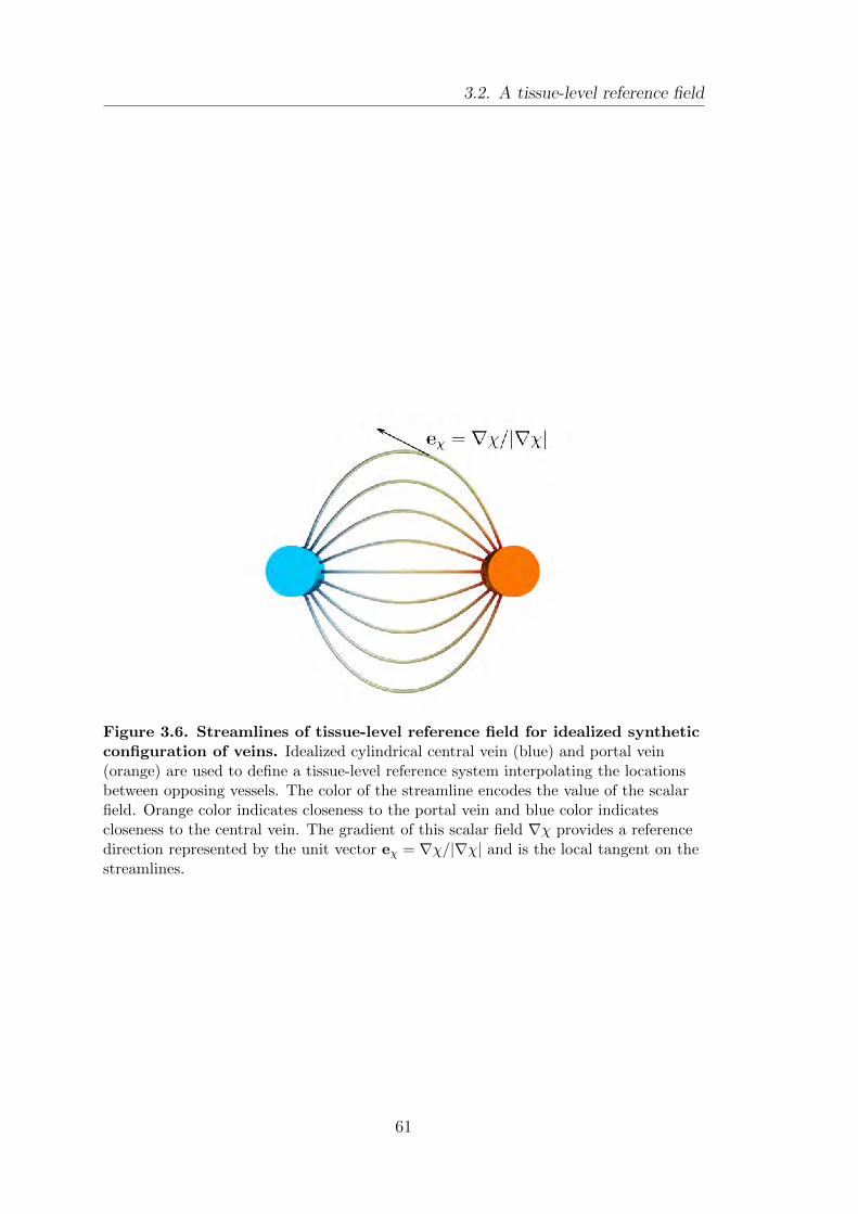
3.2. A tissue-level reference field

Figure 3.6. Streamlines of tissue-level reference field for idealized syntheticconfiguration of veins. Idealized cylindrical central vein (blue) and portal vein(orange) are used to define a tissue-level reference system interpolating the locationsbetween opposing vessels. The color of the streamline encodes the value of the scalarfield. Orange color indicates closeness to the portal vein and blue color indicatescloseness to the central vein. The gradient of this scalar field ∇χ provides a referencedirection represented by the unit vector eχ = ∇χ/|∇χ| and is the local tangent on thestreamlines.

61

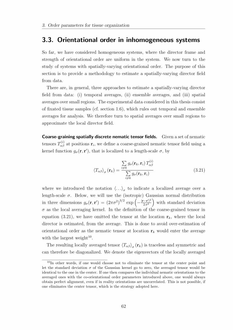
3. Order parameters for tissue organization

3.3. Orientational order in inhomogeneous systems

So far, we have considered homogeneous systems, where the director frame and

strength of orientational order are uniform in the system. We now turn to the

study of systems with spatially-varying orientational order. The purpose of this

section is to provide a methodology to estimate a spatially-varying director field

from data.

There are, in general, three approaches to estimate a spatially-varying director

field from data: (i) temporal averages, (ii) ensemble averages, and (iii) spatial

averages over small regions. The experimental data considered in this thesis consist

of fixated tissue samples (cf. section 1.6), which rules out temporal and ensemble

averages for analysis. We therefore turn to spatial averages over small regions to

approximate the local director field.

Coarse-graining spatially discrete nematic tensor fields. Given a set of nematic

tensors T(i)αβ at positions ri, we define a coarse-grained nematic tensor field using a

kernel function gσ(r, r′), that is localized to a length-scale σ, by

〈Tαβ〉σ (rk) =

∑i6=k

gσ(rk, ri)T(i)αβ∑

i6=kgσ(rk, ri)

(3.21)

where we introduced the notation 〈. . .〉σ to indicate a localized average over a

length-scale σ. Below, we will use the (isotropic) Gaussian normal distribution

in three dimensions gσ(r, r′) = (2πσ2)3/2

exp(− |r−r

′|22σ2

)with standard deviation

σ as the local averaging kernel. In the definition of the coarse-grained tensor in

equation (3.21), we have omitted the tensor at the location rk, where the local

director is estimated, from the average. This is done to avoid over-estimation of

orientational order as the nematic tensor at location rk would enter the average

with the largest weight10.

The resulting locally averaged tensor 〈Tαβ〉σ (rk) is traceless and symmetric and

can therefore be diagonalized. We denote the eigenvectors of the locally averaged

10In other words, if one would choose not to eliminate the tensor at the center point andlet the standard deviation σ of the Gaussian kernel go to zero, the averaged tensor would beidentical to the one in the center. If one then compares the individual nematic orientations to theaveraged ones with the co-orientational order parameters introduced above, one would alwaysobtain perfect alignment, even if in reality orientations are uncorrelated. This is not possible, ifone eliminates the center tensor, which is the strategy adopted here.

62

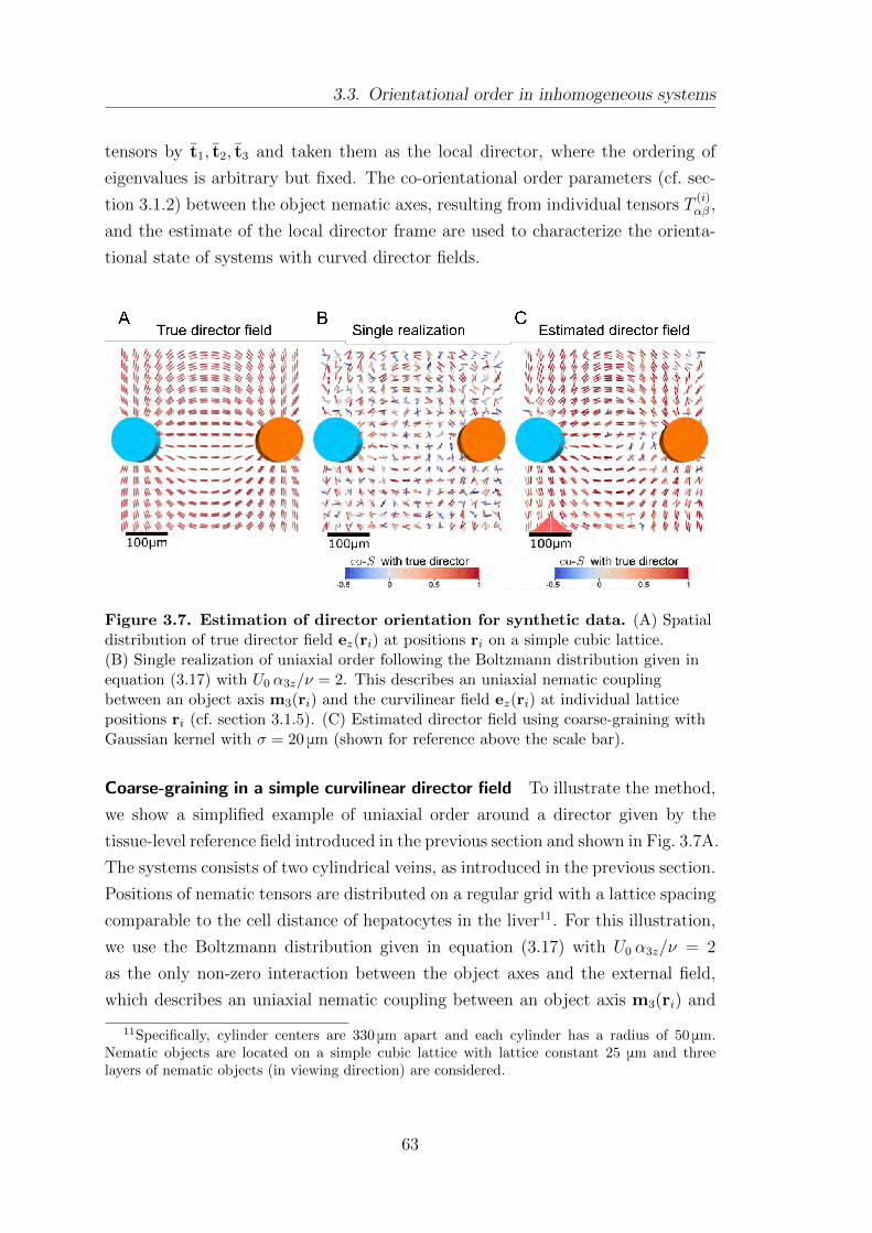
3.3. Orientational order in inhomogeneous systems

tensors by t1, t2, t3 and taken them as the local director, where the ordering of

eigenvalues is arbitrary but fixed. The co-orientational order parameters (cf. sec-

tion 3.1.2) between the object nematic axes, resulting from individual tensors T(i)αβ ,

and the estimate of the local director frame are used to characterize the orienta-

tional state of systems with curved director fields.

Figure 3.7. Estimation of director orientation for synthetic data. (A) Spatialdistribution of true director field ez(ri) at positions ri on a simple cubic lattice.(B) Single realization of uniaxial order following the Boltzmann distribution given inequation (3.17) with U0 α3z/ν = 2. This describes an uniaxial nematic couplingbetween an object axis m3(ri) and the curvilinear field ez(ri) at individual latticepositions ri (cf. section 3.1.5). (C) Estimated director field using coarse-graining withGaussian kernel with σ = 20 μm (shown for reference above the scale bar).

Coarse-graining in a simple curvilinear director field To illustrate the method,

we show a simplified example of uniaxial order around a director given by the

tissue-level reference field introduced in the previous section and shown in Fig. 3.7A.

The systems consists of two cylindrical veins, as introduced in the previous section.

Positions of nematic tensors are distributed on a regular grid with a lattice spacing

comparable to the cell distance of hepatocytes in the liver11. For this illustration,

we use the Boltzmann distribution given in equation (3.17) with U0 α3z/ν = 2

as the only non-zero interaction between the object axes and the external field,

which describes an uniaxial nematic coupling between an object axis m3(ri) and

11Specifically, cylinder centers are 330 μm apart and each cylinder has a radius of 50 μm.Nematic objects are located on a simple cubic lattice with lattice constant 25 μm and threelayers of nematic objects (in viewing direction) are considered.

63

3. Order parameters for tissue organization

the curvilinear field ez(ri) at individual lattice positions ri. Sample configurations

are obtained by inverse transform sampling on a discretization of orientation space.

A single realization is shown in Fig. 3.7B. There, the order is not prevalent and

the director field cannot be made out visually. Nevertheless, using the estimation

procedure introduced above it is possible to get an estimated director field that

closely follows the true director field from just a single realization, as shown in

Fig. 3.7C.

The choice of coarse-graining length scale σ depends on the specific system at

hand. It should be large enough to achieve a good statistic for the local director

estimate. On the other hand, σ should be chosen small enough, in order to describe

spatial variations of the local director.

3.4. Positional order: identifying signatures of

smectic and columnar order

We use the structure function to characterize positional order of tissue structures.

The structure function is a central quantity in the classification of matter [165].

It is used to discriminate between liquids and crystals and the mesophases be-

tween them (see section 1.5). One can distinguish four broad classes of positional

order: liquids, columnar liquid crystals, smectic liquid crystals and crystals [39,

pp. 34, 409]. In liquids, there is no long-range positional order, whereas in crystals,

constituents are arranged on a three-dimensional lattice [165]. If positional order

is present in one dimension, we speak of a smectic phase and when positional order

is observed in two dimensions a columnar phase is encountered [39].

The structure function is the Fourier transform of the two-point density-density

correlation function 〈ρ(r)ρ(r′)〉 [165]

I(q) =

∫e−iq·(r−r

′) 〈ρ(r)ρ(r′)〉 d3r d3r′ . (3.22)

The data to be analyzed consists of binarized voxel12 images, where the value

indicates the presence or absence of a cell. The density is therefore given as

n(r) =∑α

δ(r − rα), where rα is the set of voxel locations, where cells are

present.

12Voxels are the three-dimensional generalizations of pixels, familiar from two-dimensionalimages.

64

3.4. Positional order: identifying signatures of smectic and columnar order

In this case, the structure function simplifies to the absolute square of the Fourier

transform of the number density

I(q) ∝ S(q) =

⟨∑α,β

e−iq·(rα−rβ)

⟩=

⟨∑α

e−iq·rα∑β

eiq·rβ

⟩=⟨|ρ(q)|2

⟩(3.23)

with the Fourier transform13 of the density ρ(q). Periodic structures in the distri-

bution of cells14 lead to characteristic peaks of the structure function at non-zero

wave-vectors q. The peaks form a lattice in the reciprocal space of wave-vectors

and the dimensionality of this lattice reflects the type of positional order between

a liquid and a crystal, as detailed above.

Three-dimensional structure functions cannot be easily visualized and inter-

preted. We therefore project the densities along different directions and calculate

the two-dimensional structure function of these images. We subtract the mean of

the input images to avoid the otherwise dominating peak at zero wave-vector.

To illustrate this approach to structural analysis on voxelized binary data, we

consider idealized arrangements of smectic and columnar order. In Fig. 3.8A, three

orthogonal cut-planes through an idealized system of smectic order is shown. Cells

(red voxels) are arranged into layers, which are stacked in z-direction. There is no

positional order of cells within each layer. The cube is summed along each axis

individually and the two-dimensional structure function is calculated. The layered

order is characterized by two peaks in the structure function for the summed

densities in x- and y-direction. The absence of order within the layers is quantified

by a diffuse peak at the center of the structure function when considering the

density summed in z-direction.

In the idealized case of columnar order, shown in Fig. 3.8B, cells are arranged

into columns on a two-dimensional grid, with no positional order along the direc-

tion of the columns. Again, this order is reflected in the structure functions of

the summed densities. The two-dimensional grid is easily visible in x-direction,

whereas an apparent layered order is seen in the other two directions.

13We write the Fourier transform as ρ(q) =∫n(r)e−iq·rd3r, which yields for a discrete set

of voxel locations, as considered above, ρ(q) =∑α e−iq·rα . Taking the absolute square of this

leads to the last equality in equation (3.23).14Note that, due to the limitation of experimental imaging to fixated samples (cf. section1.6),

we are not able to perform an ensemble average and instead perform the analysis on singlerealizations of the system.

65

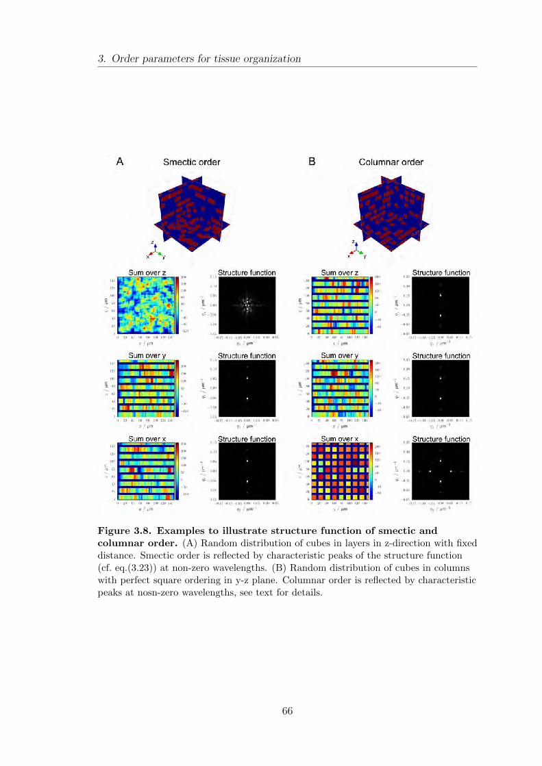
3. Order parameters for tissue organization

Figure 3.8. Examples to illustrate structure function of smectic andcolumnar order. (A) Random distribution of cubes in layers in z-direction with fixeddistance. Smectic order is reflected by characteristic peaks of the structure function(cf. eq.(3.23)) at non-zero wavelengths. (B) Random distribution of cubes in columnswith perfect square ordering in y-z plane. Columnar order is reflected by characteristicpeaks at nosn-zero wavelengths, see text for details.

66

3.5. Summary

By this analysis, signatures of smectic and columnar order can be identified in

binarized voxelized cell distributions.

3.5. Summary

In the present chapter, we introduced mathematical tools for the subsequent anal-

ysis of structural order of liver tissue in chapter 4. We addressed orientational

and positional order. To characterize orientational order in spatially homogeneous

systems, we reviewed classical orientational order parameters S, P,D,C, and in-

troduced invariants of moment tensors Ik and co-orientational order parameters

co-S, co-P, co-D, co-C as alternative measures. We showed that all three schemes

are directly related for systems in which all objects have identical anisotropies. To

showcase how uniaxial and biaxial orientational order is captured by these three

different types of order parameters, we used a simple model of nematic coupling

to an external field15. We showed that the classical orientational order parame-

ters provide an intuitive geometrical interpretation at the expense of discontinuous

jumps16 upon gradual changes of orientational order (cf. Fig. 3.4). In contrast, the

tensor invariants do not jump discontinuously but in turn lack an intuitive geomet-

ric interpretation (cf. Fig. 3.5). Finally, with a suitable choice of nematic reference

frame, the co-orientational order parameters change continuously and also yield a

geometrical meaning through their relation to the classical order parameters.

Equipped with these orientational order parameters for homogeneous systems,

we turned to characterize orientational order in curved geometries. The basic

approach is to find a suitable nematic reference field to define co-orientational order

parameters. In this chapter, we introduced two possibilities. First, we defined a

tissue-level reference field based on locations of landmarks, e.g. large blood vessels,

within a tissue17. Secondly, we introduced a coarse-graining procedure to obtain

estimates for a local director in systems with curved directors. Additionally to

the two presented options, the nematic reference field can be given by other tissue

structures, e.g. orientation of anisotropy of transport networks surrounding the

15We will return to this model in section 5.4, where we study biaxial alignment of cell polaritywith local anisotropy of the sinusoid network in liver tissue.

16The reason for these jumps is their restriction to a specific fundamental domain in the pa-rameters space, which is motivated by the equivalence with the common uniaxial order parameterS (see section 3.1.1).

17Evaluating the direction of the gradient of this field at the positions of cells provides anematic reference axis.

67

3. Order parameters for tissue organization

cells (cf. section 2.3), which are co-located with the positions of cells. These three

variants of co-orientational order are used in the next chapter for the analysis of

cell polarity in liver tissue.

In the last section of the present chapter, we introduced a method to identify sig-

natures of smectic and columnar order from experimental data using the structure

function.

68

4. The liver lobule exhibits biaxial

liquid-crystal order

In chapter 2, we saw that the distribution of membrane-bound proteins on cell

surfaces is anisotropic. In particular, hepatocytes of the liver exhibit a nematic

cell polarity characterized by a dominant second mode in the spherical power

spectrum. This anisotropy defines an orientation of a cell within the tissue that is

characterized by a tripod of nematic cell polarity axes. In this chapter, we study

orientational order of hepatocytes within the liver, using concepts from liquid-

crystal theory introduced in chapter 3. Our analysis identifies so far unrecognized

tissue-level ordering patterns within liver tissue. We relate these ordering patterns

to positions of anatomical landmarks in the liver lobule. Section 4.4 compares these

newly found nematic cell polarity fields with fields of anisotropies of the blood-

supplying sinusoid network around hepatocytes. This provides a comprehensive

view on both the global and relative orientational order of cell polarity within

the liver. Section 4.5 deals with the analysis of experiments involving genetic

perturbations. The knock-down of a cell-adhesion protein (Integrin-β1) reduces

orientational order of the liver in a characteristic way that indicates a bi-directional

feedback between cell polarity organization and sinusoidal network structure. The

chapter closes with a discussion of translational order, where we find evidence

for smectic order of liver tissue. All experimental data shown in this chapter

was obtained and pre-processed (cf. section 1.6) by members of the Zerial lab at

the Max Planck Institute of Molecular Cell Biology and Genetics (MPI-CBG) in

Dresden, Germany.

4.1. Coarse-graining reveals nematic cell polarity

patterns on the lobule-level

In this section, we analyze the spatial distribution of nematic tensors as defined

in equation 2.3, which characterizes the distribution of apical membrane proteins

on the hepatocyte surfaces. To get a visual impression of the spatial distribution

of nematic cell polarity, we employ two complementary three-dimensional visual-

izations approaches: individual nematic cell polarity axes and colored cubes. We

69

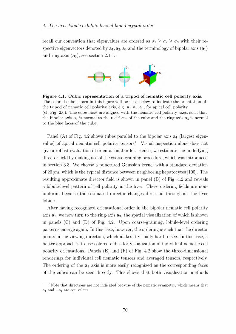
4. The liver lobule exhibits biaxial liquid-crystal order

recall our convention that eigenvalues are ordered as σ1 ≥ σ2 ≥ σ3 with their re-

spective eigenvectors denoted by a1, a2, a3 and the terminology of bipolar axis (a1)

and ring axis (a3), see section 2.1.1.

Figure 4.1. Cubic representation of a tripod of nematic cell polarity axis.The colored cube shown in this figure will be used below to indicate the orientation ofthe tripod of nematic cell polarity axis, e.g. a1,a2,a3, for apical cell polarity(cf. Fig. 2.6). The cube faces are aligned with the nematic cell polarity axes, such thatthe bipolar axis a1 is normal to the red faces of the cube and the ring axis a3 is normalto the blue faces of the cube.

Panel (A) of Fig. 4.2 shows tubes parallel to the bipolar axis a1 (largest eigen-

value) of apical nematic cell polarity tensors1. Visual inspection alone does not

give a robust evaluation of orientational order. Hence, we estimate the underlying

director field by making use of the coarse-graining procedure, which was introduced

in section 3.3. We choose a punctured Gaussian kernel with a standard deviation

of 20 μm, which is the typical distance between neighboring hepatocytes [105]. The

resulting approximate director field is shown in panel (B) of Fig. 4.2 and reveals

a lobule-level pattern of cell polarity in the liver. These ordering fields are non-

uniform, because the estimated director changes direction throughout the liver

lobule.

After having recognized orientational order in the bipolar nematic cell polarity

axis a1, we now turn to the ring-axis a3, the spatial visualization of which is shown

in panels (C) and (D) of Fig. 4.2. Upon coarse-graining, lobule-level ordering

patterns emerge again. In this case, however, the ordering is such that the director

points in the viewing direction, which makes it visually hard to see. In this case, a

better approach is to use colored cubes for visualization of individual nematic cell

polarity orientations. Panels (E) and (F) of Fig. 4.2 show the three-dimensional

renderings for individual cell nematic tensors and averaged tensors, respectively.

The ordering of the a3 axis is more easily recognized as the corresponding faces

of the cubes can be seen directly. This shows that both visualization methods

1Note that directions are not indicated because of the nematic symmetry, which means thata1 and −a1 are equivalent.

70

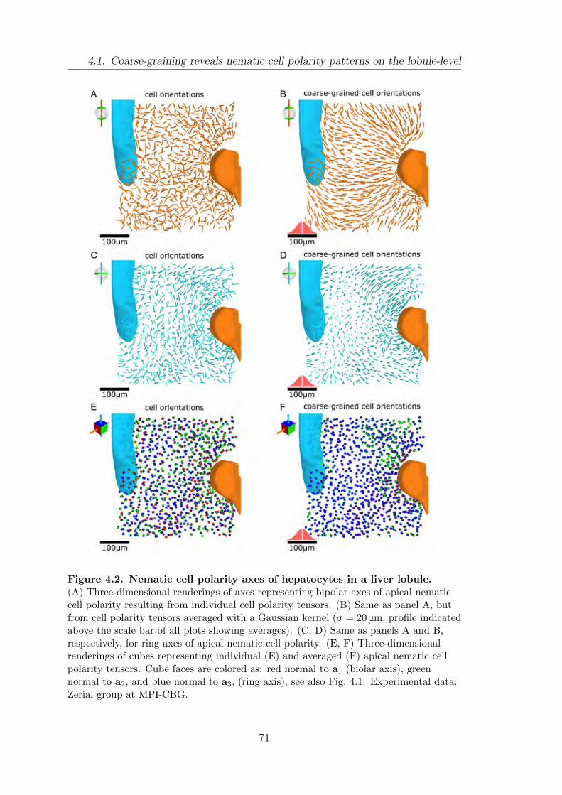
4.1. Coarse-graining reveals nematic cell polarity patterns on the lobule-level

Figure 4.2. Nematic cell polarity axes of hepatocytes in a liver lobule.(A) Three-dimensional renderings of axes representing bipolar axes of apical nematiccell polarity resulting from individual cell polarity tensors. (B) Same as panel A, butfrom cell polarity tensors averaged with a Gaussian kernel (σ = 20 μm, profile indicatedabove the scale bar of all plots showing averages). (C, D) Same as panels A and B,respectively, for ring axes of apical nematic cell polarity. (E, F) Three-dimensionalrenderings of cubes representing individual (E) and averaged (F) apical nematic cellpolarity tensors. Cube faces are colored as: red normal to a1 (biolar axis), greennormal to a2, and blue normal to a3, (ring axis), see also Fig. 4.1. Experimental data:Zerial group at MPI-CBG.

71

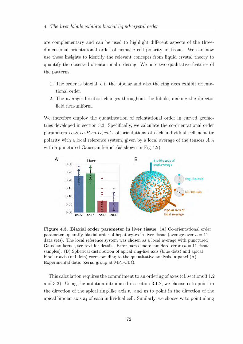
4. The liver lobule exhibits biaxial liquid-crystal order

are complementary and can be used to highlight different aspects of the three-

dimensional orientational order of nematic cell polarity in tissue. We can now

use these insights to identify the relevant concepts from liquid crystal theory to

quantify the observed orientational ordering. We note two qualitative features of

the patterns:

1. The order is biaxial, e.i. the bipolar and also the ring axes exhibit orienta-

tional order.

2. The average direction changes throughout the lobule, making the director

field non-uniform.

We therefore employ the quantification of orientational order in curved geome-

tries developed in section 3.3. Specifically, we calculate the co-orientational order

parameters co-S, co-P, co-D, co-C of orientations of each individual cell nematic

polarity with a local reference system, given by a local average of the tensors Aαβ

with a punctured Gaussian kernel (as shown in Fig 4.2).

Figure 4.3. Biaxial order parameter in liver tissue. (A) Co-orientational orderparameters quantify biaxial order of hepatocytes in liver tissue (average over n = 11data sets). The local reference system was chosen as a local average with puncturedGaussian kernel, see text for details. Error bars denote standard error (n = 11 tissuesamples). (B) Spherical distribution of apical ring-like axis (blue dots) and apicalbipolar axis (red dots) corresponding to the quantitative analysis in panel (A).Experimental data: Zerial group at MPI-CBG.

This calculation requires the commitment to an ordering of axes (cf. sections 3.1.2

and 3.3). Using the notation introduced in section 3.1.2, we choose n to point in

the direction of the apical ring-like axis a3 and m to point in the direction of the

apical bipolar axis a1 of each individual cell. Similarly, we choose w to point along

72

4.2. Coarse-grained patterns match tissue-level reference field

the direction of ring axis a3 and v to point along the bipolar axis a1 of the local

averaged cell polarity tensor (cf. section 3.3).

With this choice, we compute the four co-orientational order parameters co-S,

co-P , co-D, co-C as shown in Fig 4.3A. To further illustrate the order of nematic

cell polarity in liver tissue, we show the distribution of the nematic axes of cell

polarity relative to the local reference system as a spherical distribution plot in

Fig 4.3B. We observe that the ring-like axes (blue dots) are clustered around the

blue reference axis. This is reflected by the scalar order parameter co-S being

larger than zero. Additionally, we find a significant phase biaxiality quantified by

non-zero values of co-P , which is also apparent in the spherical distribution plot of

Fig 4.3B. The second principal axis m = a1 (bipolar axis, red dots) also exhibits a

weak ordering, which becomes apparent in the non-zero values of co-D and co-C.

Thus, using co-orientational order parameters that compare nematic axes with a

local average (omitting the central cell), we have quantified biaxial orientational

ordering in the presence of curved director fields.

4.2. Coarse-grained patterns match tissue-level

reference field

In the previous section, we studied coarse-grained patterns of apical nematic cell

polarity. By visual inspection, a clear resemblance with the lobule-wide reference

field is apparent as is shown in Fig. 4.4 for one example data set. As shown in

section 3.2, the locations of the central and portal veins in the lobule can be used

to define a tissue-level reference coordinate system. In this chapter, we use the

term lobule-level reference system to refer to the specific realization for a given

geometrical configuration of large veins in liver tissue, as shown in Fig. 4.4B.

Additionally, a quantification of the alignment of the coarse-grained directors with

the lobule-level reference frame is shown in panel (C) of Fig. 4.4. There, a color-

coding is used to distinguish between parallel (red) and perpendicular alignment

(blue). The coarse-grained cell polarity pattern matches the reference system

well throughout most parts of the lobule (indicated by red color in the figure).

Deviations from the parallel alignment are most notable near the portal vein and

at the boundary of the imaging volume. We will return to this spatial dependence

of orientational order throughout the lobule in section 5.3.3, where we compare

a minimal model of nematic order generation to the orientational order found in

73

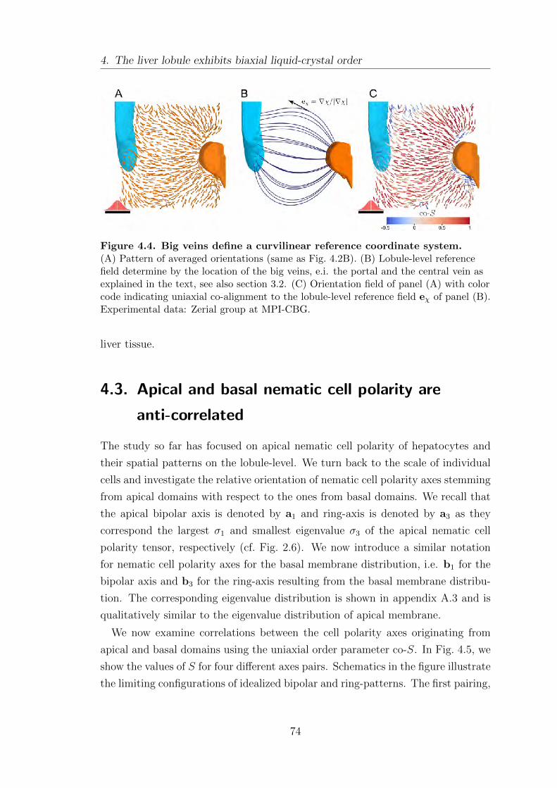
4. The liver lobule exhibits biaxial liquid-crystal order

Figure 4.4. Big veins define a curvilinear reference coordinate system.(A) Pattern of averaged orientations (same as Fig. 4.2B). (B) Lobule-level referencefield determine by the location of the big veins, e.i. the portal and the central vein asexplained in the text, see also section 3.2. (C) Orientation field of panel (A) with colorcode indicating uniaxial co-alignment to the lobule-level reference field eχ of panel (B).Experimental data: Zerial group at MPI-CBG.

liver tissue.

4.3. Apical and basal nematic cell polarity are

anti-correlated

The study so far has focused on apical nematic cell polarity of hepatocytes and

their spatial patterns on the lobule-level. We turn back to the scale of individual

cells and investigate the relative orientation of nematic cell polarity axes stemming

from apical domains with respect to the ones from basal domains. We recall that

the apical bipolar axis is denoted by a1 and ring-axis is denoted by a3 as they

correspond the largest σ1 and smallest eigenvalue σ3 of the apical nematic cell

polarity tensor, respectively (cf. Fig. 2.6). We now introduce a similar notation

for nematic cell polarity axes for the basal membrane distribution, i.e. b1 for the

bipolar axis and b3 for the ring-axis resulting from the basal membrane distribu-

tion. The corresponding eigenvalue distribution is shown in appendix A.3 and is

qualitatively similar to the eigenvalue distribution of apical membrane.

We now examine correlations between the cell polarity axes originating from

apical and basal domains using the uniaxial order parameter co-S. In Fig. 4.5, we

show the values of S for four different axes pairs. Schematics in the figure illustrate

the limiting configurations of idealized bipolar and ring-patterns. The first pairing,

74

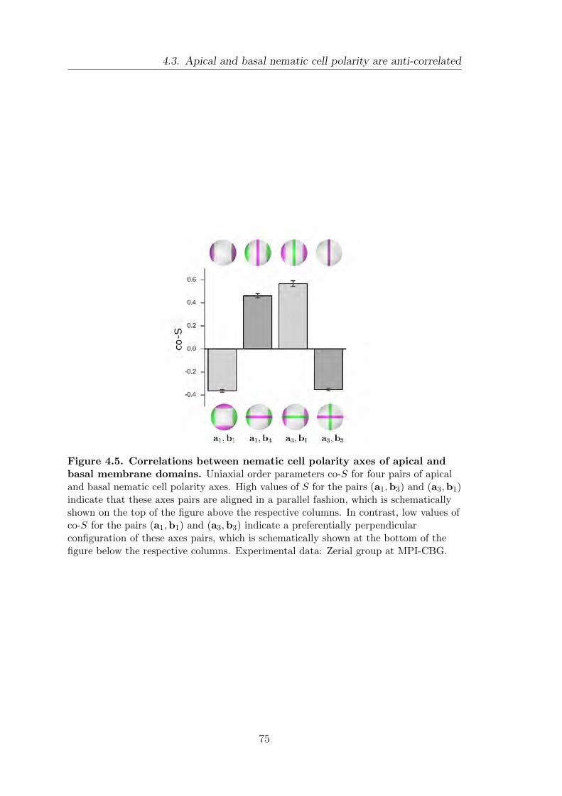
4.3. Apical and basal nematic cell polarity are anti-correlated

Figure 4.5. Correlations between nematic cell polarity axes of apical andbasal membrane domains. Uniaxial order parameters co-S for four pairs of apicaland basal nematic cell polarity axes. High values of S for the pairs (a1,b3) and (a3,b1)indicate that these axes pairs are aligned in a parallel fashion, which is schematicallyshown on the top of the figure above the respective columns. In contrast, low values ofco-S for the pairs (a1,b1) and (a3,b3) indicate a preferentially perpendicularconfiguration of these axes pairs, which is schematically shown at the bottom of thefigure below the respective columns. Experimental data: Zerial group at MPI-CBG.

75

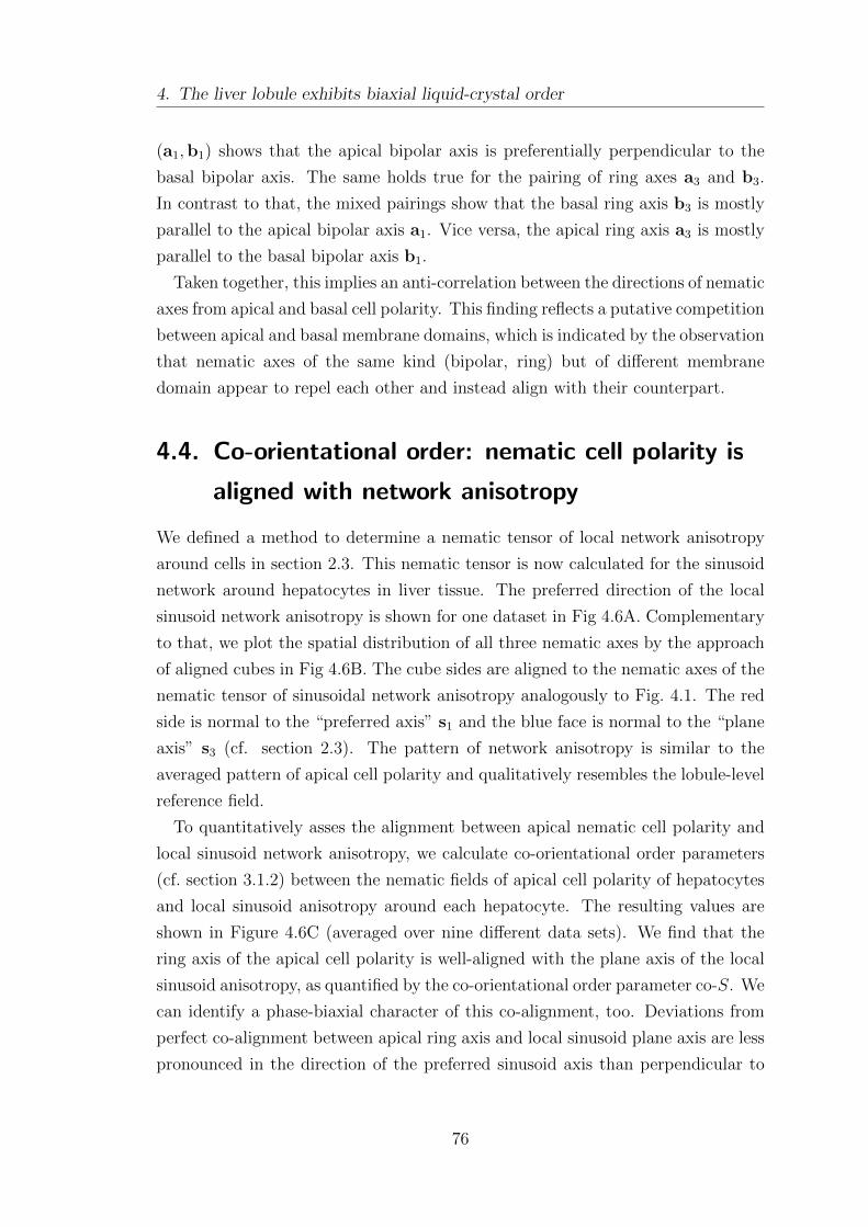
4. The liver lobule exhibits biaxial liquid-crystal order

(a1,b1) shows that the apical bipolar axis is preferentially perpendicular to the

basal bipolar axis. The same holds true for the pairing of ring axes a3 and b3.

In contrast to that, the mixed pairings show that the basal ring axis b3 is mostly

parallel to the apical bipolar axis a1. Vice versa, the apical ring axis a3 is mostly

parallel to the basal bipolar axis b1.

Taken together, this implies an anti-correlation between the directions of nematic

axes from apical and basal cell polarity. This finding reflects a putative competition

between apical and basal membrane domains, which is indicated by the observation

that nematic axes of the same kind (bipolar, ring) but of different membrane

domain appear to repel each other and instead align with their counterpart.

4.4. Co-orientational order: nematic cell polarity is

aligned with network anisotropy

We defined a method to determine a nematic tensor of local network anisotropy

around cells in section 2.3. This nematic tensor is now calculated for the sinusoid

network around hepatocytes in liver tissue. The preferred direction of the local

sinusoid network anisotropy is shown for one dataset in Fig 4.6A. Complementary

to that, we plot the spatial distribution of all three nematic axes by the approach

of aligned cubes in Fig 4.6B. The cube sides are aligned to the nematic axes of the

nematic tensor of sinusoidal network anisotropy analogously to Fig. 4.1. The red

side is normal to the “preferred axis” s1 and the blue face is normal to the “plane

axis” s3 (cf. section 2.3). The pattern of network anisotropy is similar to the

averaged pattern of apical cell polarity and qualitatively resembles the lobule-level

reference field.

To quantitatively asses the alignment between apical nematic cell polarity and

local sinusoid network anisotropy, we calculate co-orientational order parameters

(cf. section 3.1.2) between the nematic fields of apical cell polarity of hepatocytes

and local sinusoid anisotropy around each hepatocyte. The resulting values are

shown in Figure 4.6C (averaged over nine different data sets). We find that the

ring axis of the apical cell polarity is well-aligned with the plane axis of the local

sinusoid anisotropy, as quantified by the co-orientational order parameter co-S. We

can identify a phase-biaxial character of this co-alignment, too. Deviations from

perfect co-alignment between apical ring axis and local sinusoid plane axis are less

pronounced in the direction of the preferred sinusoid axis than perpendicular to

76

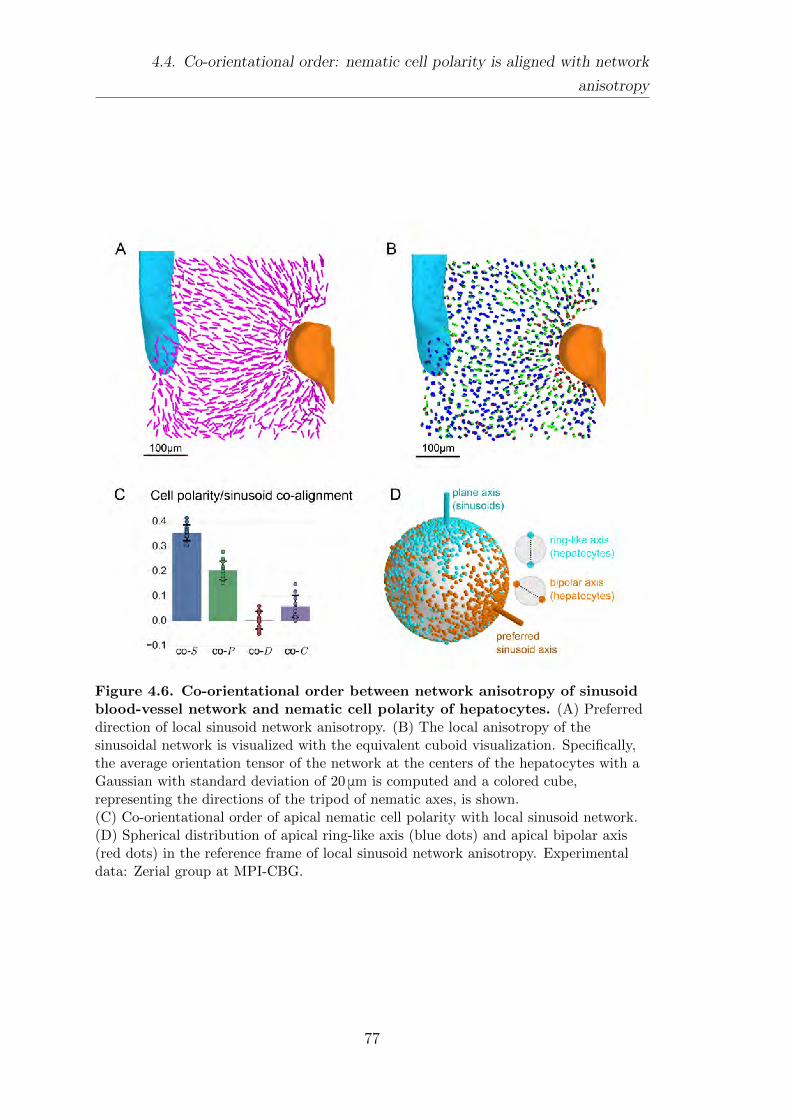
4.4. Co-orientational order: nematic cell polarity is aligned with network

anisotropy

Figure 4.6. Co-orientational order between network anisotropy of sinusoidblood-vessel network and nematic cell polarity of hepatocytes. (A) Preferreddirection of local sinusoid network anisotropy. (B) The local anisotropy of thesinusoidal network is visualized with the equivalent cuboid visualization. Specifically,the average orientation tensor of the network at the centers of the hepatocytes with aGaussian with standard deviation of 20 μm is computed and a colored cube,representing the directions of the tripod of nematic axes, is shown.(C) Co-orientational order of apical nematic cell polarity with local sinusoid network.(D) Spherical distribution of apical ring-like axis (blue dots) and apical bipolar axis(red dots) in the reference frame of local sinusoid network anisotropy. Experimentaldata: Zerial group at MPI-CBG.

77

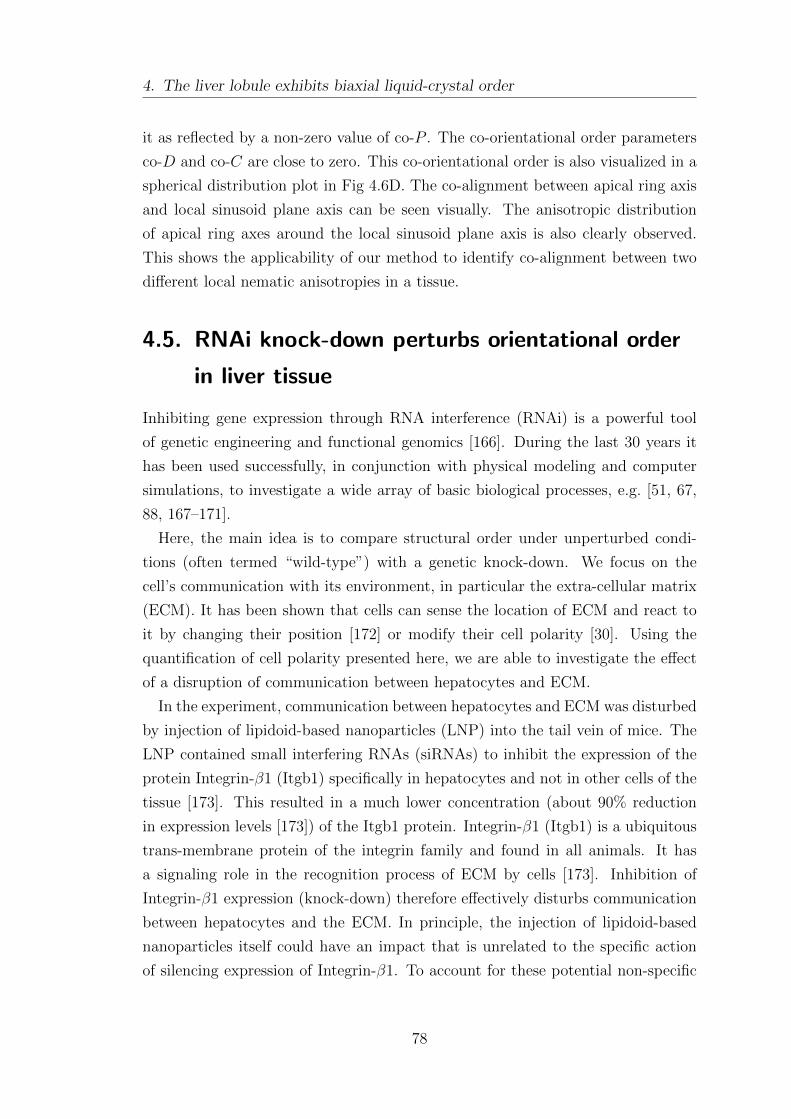
4. The liver lobule exhibits biaxial liquid-crystal order

it as reflected by a non-zero value of co-P . The co-orientational order parameters

co-D and co-C are close to zero. This co-orientational order is also visualized in a

spherical distribution plot in Fig 4.6D. The co-alignment between apical ring axis

and local sinusoid plane axis can be seen visually. The anisotropic distribution

of apical ring axes around the local sinusoid plane axis is also clearly observed.

This shows the applicability of our method to identify co-alignment between two

different local nematic anisotropies in a tissue.

4.5. RNAi knock-down perturbs orientational order

in liver tissue

Inhibiting gene expression through RNA interference (RNAi) is a powerful tool

of genetic engineering and functional genomics [166]. During the last 30 years it

has been used successfully, in conjunction with physical modeling and computer

simulations, to investigate a wide array of basic biological processes, e.g. [51, 67,

88, 167–171].

Here, the main idea is to compare structural order under unperturbed condi-

tions (often termed “wild-type”) with a genetic knock-down. We focus on the

cell’s communication with its environment, in particular the extra-cellular matrix

(ECM). It has been shown that cells can sense the location of ECM and react to

it by changing their position [172] or modify their cell polarity [30]. Using the

quantification of cell polarity presented here, we are able to investigate the effect

of a disruption of communication between hepatocytes and ECM.

In the experiment, communication between hepatocytes and ECM was disturbed

by injection of lipidoid-based nanoparticles (LNP) into the tail vein of mice. The

LNP contained small interfering RNAs (siRNAs) to inhibit the expression of the

protein Integrin-β1 (Itgb1) specifically in hepatocytes and not in other cells of the

tissue [173]. This resulted in a much lower concentration (about 90% reduction

in expression levels [173]) of the Itgb1 protein. Integrin-β1 (Itgb1) is a ubiquitous

trans-membrane protein of the integrin family and found in all animals. It has

a signaling role in the recognition process of ECM by cells [173]. Inhibition of

Integrin-β1 expression (knock-down) therefore effectively disturbs communication

between hepatocytes and the ECM. In principle, the injection of lipidoid-based

nanoparticles itself could have an impact that is unrelated to the specific action

of silencing expression of Integrin-β1. To account for these potential non-specific

78

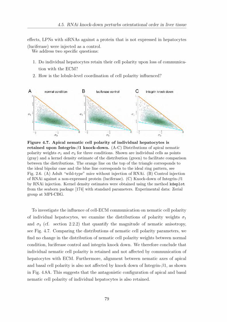
4.5. RNAi knock-down perturbs orientational order in liver tissue

effects, LPNs with siRNAs against a protein that is not expressed in hepatocytes

(luciferase) were injected as a control.We address two specific questions:

1. Do individual hepatocytes retain their cell polarity upon loss of communica-

tion with the ECM?

2. How is the lobule-level coordination of cell polarity influenced?

Figure 4.7. Apical nematic cell polarity of individual hepatocytes isretained upon Integrin-β1 knock-down. (A-C) Distributions of apical nematicpolarity weights σ1 and σ3 for three conditions. Shown are individual cells as points(gray) and a kernel density estimate of the distribution (green) to facilitate comparisonbetween the distributions. The orange line on the top of the triangle corresponds tothe ideal bipolar case and the blue line corresponds to the ideal ring pattern, seeFig. 2.6. (A) Adult “wild-type” mice without injection of RNAi. (B) Control injectionof RNAi against a non-expressed protein (luciferase). (C) Knock-down of Integrin-β1by RNAi injection. Kernel density estimates were obtained using the method kdeplot

from the seaborn package [174] with standard parameters. Experimental data: Zerialgroup at MPI-CBG.

To investigate the influence of cell-ECM communication on nematic cell polarity

of individual hepatocytes, we examine the distributions of polarity weights σ1

and σ3 (cf. section 2.2.2) that quantify the magnitude of nematic anisotropy,

see Fig. 4.7. Comparing the distributions of nematic cell polarity parameters, we

find no change in the distribution of nematic cell polarity weights between normal

condition, luciferase control and integrin knock down. We therefore conclude that

individual nematic cell polarity is retained and not affected by communication of

hepatocytes with ECM. Furthermore, alignment between nematic axes of apical

and basal cell polarity is also not affected by knock down of Integrin-β1, as shown

in Fig. 4.8A. This suggests that the antagonistic configuration of apical and basal

nematic cell polarity of individual hepatocytes is also retained.

79

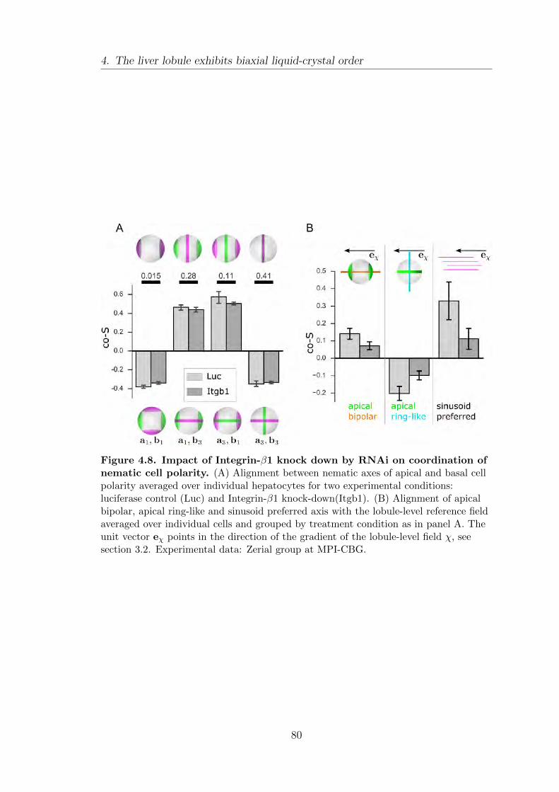
4. The liver lobule exhibits biaxial liquid-crystal order

Figure 4.8. Impact of Integrin-β1 knock down by RNAi on coordination ofnematic cell polarity. (A) Alignment between nematic axes of apical and basal cellpolarity averaged over individual hepatocytes for two experimental conditions:luciferase control (Luc) and Integrin-β1 knock-down(Itgb1). (B) Alignment of apicalbipolar, apical ring-like and sinusoid preferred axis with the lobule-level reference fieldaveraged over individual cells and grouped by treatment condition as in panel A. Theunit vector eχ points in the direction of the gradient of the lobule-level field χ, seesection 3.2. Experimental data: Zerial group at MPI-CBG.

80

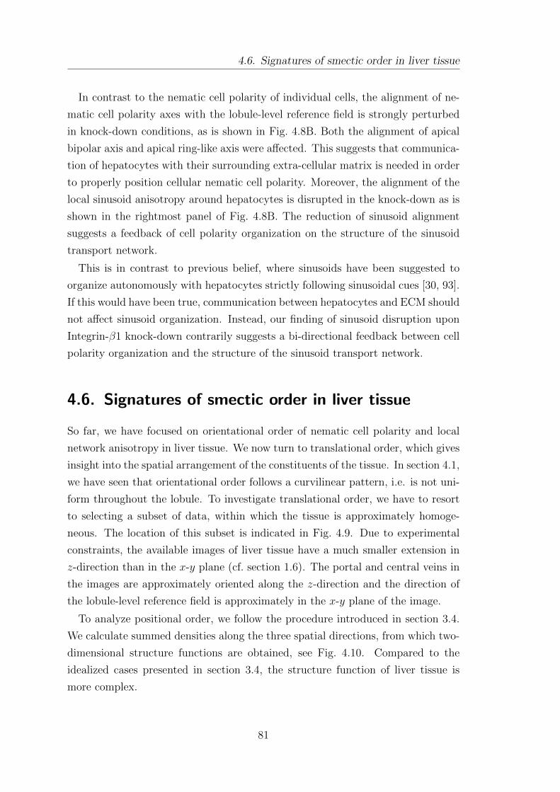
4.6. Signatures of smectic order in liver tissue

In contrast to the nematic cell polarity of individual cells, the alignment of ne-

matic cell polarity axes with the lobule-level reference field is strongly perturbed

in knock-down conditions, as is shown in Fig. 4.8B. Both the alignment of apical

bipolar axis and apical ring-like axis were affected. This suggests that communica-

tion of hepatocytes with their surrounding extra-cellular matrix is needed in order

to properly position cellular nematic cell polarity. Moreover, the alignment of the

local sinusoid anisotropy around hepatocytes is disrupted in the knock-down as is

shown in the rightmost panel of Fig. 4.8B. The reduction of sinusoid alignment

suggests a feedback of cell polarity organization on the structure of the sinusoid

transport network.

This is in contrast to previous belief, where sinusoids have been suggested to

organize autonomously with hepatocytes strictly following sinusoidal cues [30, 93].

If this would have been true, communication between hepatocytes and ECM should

not affect sinusoid organization. Instead, our finding of sinusoid disruption upon

Integrin-β1 knock-down contrarily suggests a bi-directional feedback between cell

polarity organization and the structure of the sinusoid transport network.

4.6. Signatures of smectic order in liver tissue

So far, we have focused on orientational order of nematic cell polarity and local

network anisotropy in liver tissue. We now turn to translational order, which gives

insight into the spatial arrangement of the constituents of the tissue. In section 4.1,

we have seen that orientational order follows a curvilinear pattern, i.e. is not uni-

form throughout the lobule. To investigate translational order, we have to resort

to selecting a subset of data, within which the tissue is approximately homoge-

neous. The location of this subset is indicated in Fig. 4.9. Due to experimental

constraints, the available images of liver tissue have a much smaller extension in

z-direction than in the x-y plane (cf. section 1.6). The portal and central veins in

the images are approximately oriented along the z-direction and the direction of

the lobule-level reference field is approximately in the x-y plane of the image.

To analyze positional order, we follow the procedure introduced in section 3.4.

We calculate summed densities along the three spatial directions, from which two-

dimensional structure functions are obtained, see Fig. 4.10. Compared to the

idealized cases presented in section 3.4, the structure function of liver tissue is

more complex.

81

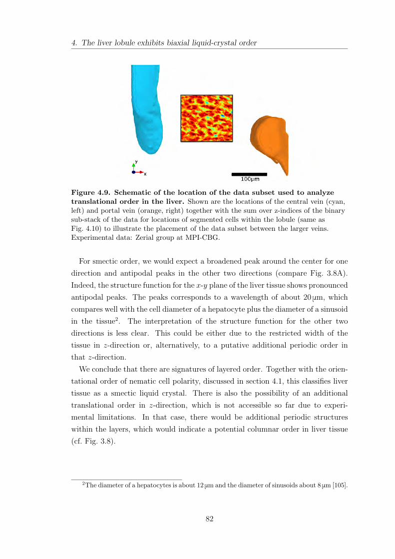
4. The liver lobule exhibits biaxial liquid-crystal order

Figure 4.9. Schematic of the location of the data subset used to analyzetranslational order in the liver. Shown are the locations of the central vein (cyan,left) and portal vein (orange, right) together with the sum over z-indices of the binarysub-stack of the data for locations of segmented cells within the lobule (same asFig. 4.10) to illustrate the placement of the data subset between the larger veins.Experimental data: Zerial group at MPI-CBG.

For smectic order, we would expect a broadened peak around the center for one

direction and antipodal peaks in the other two directions (compare Fig. 3.8A).

Indeed, the structure function for the x-y plane of the liver tissue shows pronounced

antipodal peaks. The peaks corresponds to a wavelength of about 20 μm, which

compares well with the cell diameter of a hepatocyte plus the diameter of a sinusoid

in the tissue2. The interpretation of the structure function for the other two

directions is less clear. This could be either due to the restricted width of the

tissue in z-direction or, alternatively, to a putative additional periodic order in

that z-direction.

We conclude that there are signatures of layered order. Together with the orien-

tational order of nematic cell polarity, discussed in section 4.1, this classifies liver

tissue as a smectic liquid crystal. There is also the possibility of an additional

translational order in z-direction, which is not accessible so far due to experi-

mental limitations. In that case, there would be additional periodic structures

within the layers, which would indicate a potential columnar order in liver tissue

(cf. Fig. 3.8).

2The diameter of a hepatocytes is about 12 μm and the diameter of sinusoids about 8 μm [105].

82

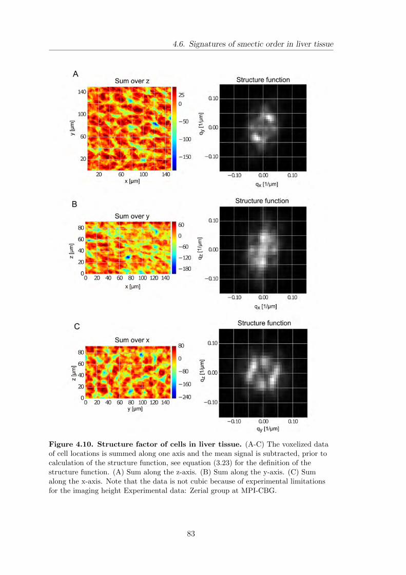
4.6. Signatures of smectic order in liver tissue

Figure 4.10. Structure factor of cells in liver tissue. (A-C) The voxelized dataof cell locations is summed along one axis and the mean signal is subtracted, prior tocalculation of the structure function, see equation (3.23) for the definition of thestructure function. (A) Sum along the z-axis. (B) Sum along the y-axis. (C) Sumalong the x-axis. Note that the data is not cubic because of experimental limitationsfor the imaging height Experimental data: Zerial group at MPI-CBG.

83

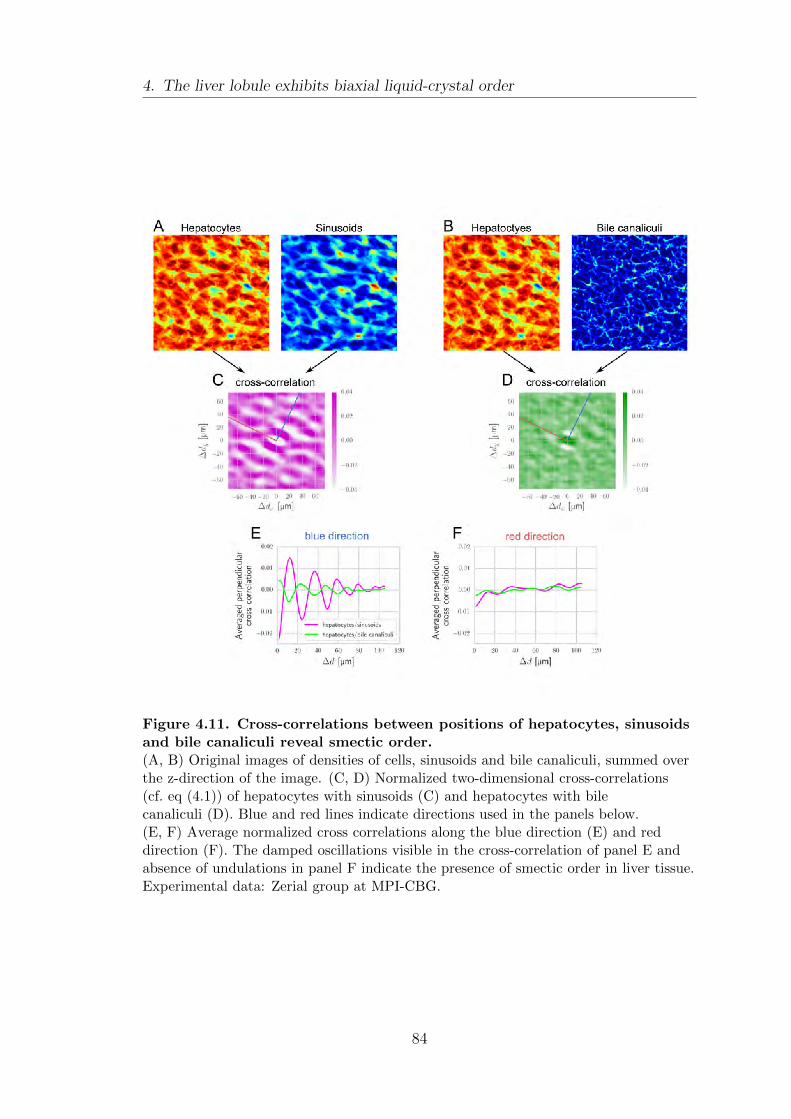
4. The liver lobule exhibits biaxial liquid-crystal order

Figure 4.11. Cross-correlations between positions of hepatocytes, sinusoidsand bile canaliculi reveal smectic order.(A, B) Original images of densities of cells, sinusoids and bile canaliculi, summed overthe z-direction of the image. (C, D) Normalized two-dimensional cross-correlations(cf. eq (4.1)) of hepatocytes with sinusoids (C) and hepatocytes with bilecanaliculi (D). Blue and red lines indicate directions used in the panels below.(E, F) Average normalized cross correlations along the blue direction (E) and reddirection (F). The damped oscillations visible in the cross-correlation of panel E andabsence of undulations in panel F indicate the presence of smectic order in liver tissue.Experimental data: Zerial group at MPI-CBG.

84

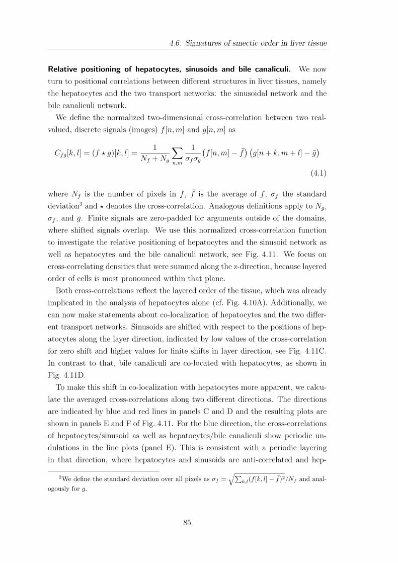
4.6. Signatures of smectic order in liver tissue

Relative positioning of hepatocytes, sinusoids and bile canaliculi. We now

turn to positional correlations between different structures in liver tissues, namely

the hepatocytes and the two transport networks: the sinusoidal network and the

bile canaliculi network.

We define the normalized two-dimensional cross-correlation between two real-

valued, discrete signals (images) f [n,m] and g[n,m] as

Cfg[k, l] = (f ? g)[k, l] =1

Nf +Ng

∑n,m

1

σfσg

(f [n,m]− f

) (g[n+ k,m+ l]− g

)(4.1)

where Nf is the number of pixels in f , f is the average of f , σf the standard

deviation3 and ? denotes the cross-correlation. Analogous definitions apply to Ng,

σf , and g. Finite signals are zero-padded for arguments outside of the domains,

where shifted signals overlap. We use this normalized cross-correlation function

to investigate the relative positioning of hepatocytes and the sinusoid network as

well as hepatocytes and the bile canaliculi network, see Fig. 4.11. We focus on

cross-correlating densities that were summed along the z-direction, because layered

order of cells is most pronounced within that plane.

Both cross-correlations reflect the layered order of the tissue, which was already

implicated in the analysis of hepatocytes alone (cf. Fig. 4.10A). Additionally, we

can now make statements about co-localization of hepatocytes and the two differ-

ent transport networks. Sinusoids are shifted with respect to the positions of hep-

atocytes along the layer direction, indicated by low values of the cross-correlation

for zero shift and higher values for finite shifts in layer direction, see Fig. 4.11C.

In contrast to that, bile canaliculi are co-located with hepatocytes, as shown in

Fig. 4.11D.

To make this shift in co-localization with hepatocytes more apparent, we calcu-

late the averaged cross-correlations along two different directions. The directions

are indicated by blue and red lines in panels C and D and the resulting plots are

shown in panels E and F of Fig. 4.11. For the blue direction, the cross-correlations

of hepatocytes/sinusoid as well as hepatocytes/bile canaliculi show periodic un-

dulations in the line plots (panel E). This is consistent with a periodic layering

in that direction, where hepatocytes and sinusoids are anti-correlated and hep-

3We define the standard deviation over all pixels as σf =√∑

k,l(f [k, l]− f)2/Nf and anal-

ogously for g.

85

4. The liver lobule exhibits biaxial liquid-crystal order

atocytes and bile canaliculi are co-localization. In the red direction (panel F of

Fig. 4.11), the undulation is more irregular and has lower amplitude, which is con-

sistent with a direction perpendicular to normal direction of putative layers. This

implies the presence of alternating layers of sinusoid and bile canaliculi networks

in the liver, which is consistent with the finding that apical and basal nematic cell

polarity are anti-correlated (cf. section 4.3).

The layer distance derived from the maximum-to-maximum distance in the line

plot of hepatocyte/sinusoid cross-correlation is approximately 24 μm. This com-

pares well with the value of 20 μm obtained by the structure function of hepato-

cytes shown in Fig. 4.10A. The structure function is the inverse Fourier transform

of the cross-correlation of an input signal with itself (also called auto-correlation),

which is also known as the Wiener-Kinchin theorem [175, 176]. The different rep-

resentations highlight distinct features of the tissue structure. While the structure

function is useful to access the general presence of layered order in the system, the

cross-correlations emphasizes the relative phase between different structures. The

quantification of the layer spacing distance of both approaches give comparable

results that are close to the value of the sum of one hepatocyte diameter plus one

sinusoid diameter4.

4.7. Summary

This chapter investigated the structural properties of liver tissue with focus on

orientational order of nematic cell polarity. We found that apical nematic cell

polarity of hepatocytes exhibit lobule-level patterns in liver tissue. We used tools

from liquid crystal theory to quantify the orientational order and found it to be

phase biaxial. We showed that the coarse-grained patterns of apical nematic cell

polarity match a curvilinear reference field that is given by the locations of larger

vessels in the liver lobule.

We then investigated co-orientational order between different types of cellu-

lar anisotropies. We found that apical and basal nematic cell polarity are anti-

correlated, which indicates a putative competition between apical and basal mem-

brane domains. The co-orientational order of apical cell polarity and local sinusoid

anisotropy was found to be of phase biaxial type. These quantifications of co-

orientational order between different cell anisotropies was then used to investigate

4The diameter of a hepatocytes is about 12 μm and the diameter of sinusoids about 8 μm [105].

86

4.7. Summary

genetic knock-down experiments.

We found that the knock-down of Integrin-β1, a protein involved in cell adhesion

and recognition, has no impact on apical-basal anti-correlation but does disrupt

the co-orientational order between apical cell polarity and local sinusoid network

anisotropy. This finding, together with the previously known influence of exter-

nal cues on hepatic cell polarity, indicates a bi-directional feedback between cell

polarity organization and sinusoidal network structure.

In the last section of this chapter, we examined the translational order of hepa-

tocytes and found evidence for smectic order. Furthermore, we investigated cross

correlations and found indications for alternating layers of sinusoids and bile canal-

iuli.

87

5. Effective models for cell and

network polarity coordination

In this chapter, we investigate physical principles underlying the observed architec-

ture in the liver, which was presented in chapter 4. Motivated by the observation

of biaxial nematic liquid crystal order of cell polarity made there, we first derive a

minimal nematic interaction model1 by discretizing a continuum theory of nematic

elasticity (cf. section 1.5.3). This procedure yields a uniaxial nematic interaction

model and we show how it naturally generalizes to the biaxial case.

We then apply this nematic interaction model to the case of coordinated nematic

cell polarity found in liver tissue. Using the uniaxial variant of the model, we ad-

dress two basic mechanisms to coordinate nematic cell polarity axes throughout

the liver lobule: neighbor-interaction and coupling to an external ordering field.

We show that both mechanisms are, in principle, able to generate ordered patterns

reminiscent of the cell polarity fields in liver but only the external field mecha-

nism is consistent with spatial profiles of orientational order found in liver tissue.

Building on this observation, we focus the external field mechanism and use its

biaxial variant to study co-orientational order between apical nematic cell polarity

and local sinusoid around hepatocytes. This reproduces the observed phase-biaxial

order of apical cell polarity in liver tissue, which was shown in section 4.4.

The work presented in this section was done in collaboration with Simon Syga.

Some preliminary results of the uniaxial interaction model were published in his

Bachelor thesis titled “Nematic Order in Complex Tissues” [179].

5.1. Discretization of a uniaxial nematic free energy

Starting from a continuum theory of nematic liquid crystals, we obtain a discretiza-

tion, which we will use to describe the discrete organization of cells in tissues. For

this, we restate the Frank free energy in one-constant approximation (cf. eq. (1.13)

1Meier and Saupe [127, 177, 178] derived a formally equivalent nematic interaction model byexpanding dispersion forces between individual molecules up to second order.

89

5. Effective models for cell and network polarity coordination

and [39])

Fd =

∫d3r

K

2(∂αnβ)(∂αnβ) , (5.1)

which describes the contribution of gradients in the uniaxial director field n(r)

with n2 = 1 to the total free energy. We now discretize this continuum energy,

which will yield a sum over pairwise nematic interactions. For this, it is convenient

to rewrite it in tensorial form. We introduce the tensor Nαβ = nαnβ as the dyadic

product of the nematic director n with itself. Using that n is a unit vector, we

can also write [121]

Fd =

∫d3r

K

4(∂γNαβ) (∂γNαβ) . (5.2)

The tensorial form of the Frank free energy, eq. (5.2), has the advantage that

it allows for a straight-forward discretization. This is due to the fact that the

individual gradient ∂γNαβ = nα∂γnβ + nβ∂γnα is invariant under the nematic

symmetry operation n → −n. In contrast, only the square of the gradient of the

nematic director ∂αnβ is invariant under the nematic symmetry operation. We

first consider discretization on a cubic lattice with lattice constant a, which yields

(cf. appendix A.10)

Fd ≈ −K a

2

∑〈i,j〉

N(i)αβN

(j)αβ (5.3)

where 〈i, j〉 runs over all pairs of neighbors on the cubic lattice and N(i)αβ denotes

the dyadic tensor of the nematic director located at lattice point i. The parameter

K controls the interaction strength between neighboring nematic tensors.

The discretized distortion free energy, eq (5.3), can be restated2 in terms of the

nematic director n and the second Legendre polynomial P2(x) =1

2(3x2 − 1)

Fd ≈ −ε∑〈i,j〉

P2

(n(i) · n(j)

)(5.4)

with ε = K a/3. This form is known as the Lebwohl-Lasher model in the lit-

erature [180–182] and resembles the definition of the uniaxial order parameter

2Here, we ignored an irrelevant additive constant to the interaction energy.

90

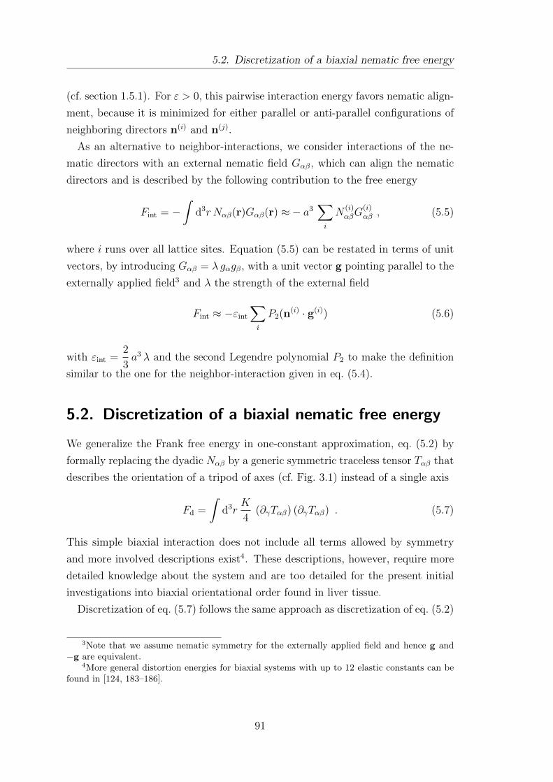
5.2. Discretization of a biaxial nematic free energy

(cf. section 1.5.1). For ε > 0, this pairwise interaction energy favors nematic align-

ment, because it is minimized for either parallel or anti-parallel configurations of

neighboring directors n(i) and n(j).

As an alternative to neighbor-interactions, we consider interactions of the ne-

matic directors with an external nematic field Gαβ, which can align the nematic

directors and is described by the following contribution to the free energy

Fint = −∫

d3r Nαβ(r)Gαβ(r) ≈− a3∑i

N(i)αβG

(i)αβ , (5.5)

where i runs over all lattice sites. Equation (5.5) can be restated in terms of unit

vectors, by introducing Gαβ = λ gαgβ, with a unit vector g pointing parallel to the

externally applied field3 and λ the strength of the external field

Fint ≈ −εint

∑i

P2(n(i) · g(i)) (5.6)

with εint =2

3a3 λ and the second Legendre polynomial P2 to make the definition

similar to the one for the neighbor-interaction given in eq. (5.4).

5.2. Discretization of a biaxial nematic free energy

We generalize the Frank free energy in one-constant approximation, eq. (5.2) by

formally replacing the dyadic Nαβ by a generic symmetric traceless tensor Tαβ that

describes the orientation of a tripod of axes (cf. Fig. 3.1) instead of a single axis

Fd =

∫d3r

K

4(∂γTαβ) (∂γTαβ) . (5.7)

This simple biaxial interaction does not include all terms allowed by symmetry

and more involved descriptions exist4. These descriptions, however, require more

detailed knowledge about the system and are too detailed for the present initial

investigations into biaxial orientational order found in liver tissue.

Discretization of eq. (5.7) follows the same approach as discretization of eq. (5.2)

3Note that we assume nematic symmetry for the externally applied field and hence g and−g are equivalent.

4More general distortion energies for biaxial systems with up to 12 elastic constants can befound in [124, 183–186].

91

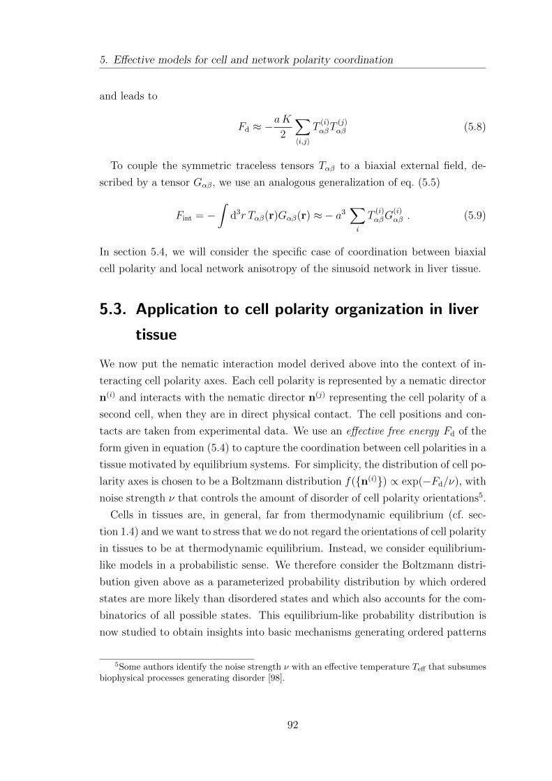
5. Effective models for cell and network polarity coordination

and leads to

Fd ≈ −aK

2

∑〈i,j〉

T(i)αβT

(j)αβ (5.8)

To couple the symmetric traceless tensors Tαβ to a biaxial external field, de-

scribed by a tensor Gαβ, we use an analogous generalization of eq. (5.5)

Fint = −∫

d3r Tαβ(r)Gαβ(r) ≈− a3∑i

T(i)αβG

(i)αβ . (5.9)

In section 5.4, we will consider the specific case of coordination between biaxial

cell polarity and local network anisotropy of the sinusoid network in liver tissue.

5.3. Application to cell polarity organization in liver

tissue

We now put the nematic interaction model derived above into the context of in-

teracting cell polarity axes. Each cell polarity is represented by a nematic director

n(i) and interacts with the nematic director n(j) representing the cell polarity of a

second cell, when they are in direct physical contact. The cell positions and con-

tacts are taken from experimental data. We use an effective free energy Fd of the

form given in equation (5.4) to capture the coordination between cell polarities in a

tissue motivated by equilibrium systems. For simplicity, the distribution of cell po-

larity axes is chosen to be a Boltzmann distribution f(n(i)) ∝ exp(−Fd/ν), with

noise strength ν that controls the amount of disorder of cell polarity orientations5.

Cells in tissues are, in general, far from thermodynamic equilibrium (cf. sec-

tion 1.4) and we want to stress that we do not regard the orientations of cell polarity

in tissues to be at thermodynamic equilibrium. Instead, we consider equilibrium-

like models in a probabilistic sense. We therefore consider the Boltzmann distri-

bution given above as a parameterized probability distribution by which ordered

states are more likely than disordered states and which also accounts for the com-

binatorics of all possible states. This equilibrium-like probability distribution is

now studied to obtain insights into basic mechanisms generating ordered patterns

5Some authors identify the noise strength ν with an effective temperature Teff that subsumesbiophysical processes generating disorder [98].

92

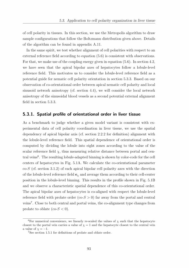
5.3. Application to cell polarity organization in liver tissue

of cell polarity in tissues. In this section, we use the Metropolis algorithm to draw

sample configurations that follow the Boltzmann distribution given above. Details

of the algorithm can be found in appendix A.11.

In the same spirit, we test whether alignment of cell polarities with respect to an

external reference field according to equation (5.6) is consistent with observations.

For that, we make use of the coupling energy given in equation (5.6). In section 4.2,

we have seen that the apical bipolar axes of hepatocytes follow a lobule-level

reference field. This motivates us to consider the lobule-level reference field as a

potential guide for nematic cell polarity orientation in section 5.3.3. Based on our

observation of co-orientational order between apical nematic cell polarity and local

sinusoid network anisotropy (cf. section 4.4), we will consider the local network

anisotropy of the sinusoidal blood vessels as a second potential external alignment

field in section 5.3.3.

5.3.1. Spatial profile of orientational order in liver tissue

As a benchmark to judge whether a given model variant is consistent with ex-

perimental data of cell polarity coordination in liver tissue, we use the spatial

dependency of apical bipolar axis (cf. section 2.2.2 for definition) alignment with

the lobule-level reference field. This spatial dependence of orientational order is

computed by dividing the lobule into eight zones according to the value of the

scalar reference field χ, thus measuring relative distance between portal and cen-

tral veins6. The resulting lobule-adapted binning is shown by color-code for the cell

centers of hepatocytes in Fig. 5.1A. We calculate the co-orientational parameter

co-S (cf. section 3.1.2) of each apical bipolar cell polarity axes with the direction

of the lobule-level reference field eχ and average them according to their cell-center

position in the lobule-level binning. This results in the profile shown in Fig. 5.1B

and we observe a characteristic spatial dependence of this co-orientational order.

The apical bipolar axes of hepatocytes is co-aligned with respect the lobule-level

reference field with prolate order (co-S > 0) far away from the portal and central

veins7. Close to both central and portal veins, the co-alignment type changes from

prolate to oblate (co-S < 0).

6For numerical convenience, we linearly re-scaled the values of χ such that the hepatocyteclosest to the portal vein carries a value of χ = 1 and the hepatocyte closest to the central veina value of χ = −1.

7See section 1.5.1 for definitions of prolate and oblate order.

93

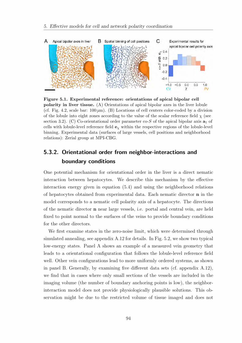
5. Effective models for cell and network polarity coordination

Figure 5.1. Experimental reference: orientations of apical bipolar cellpolarity in liver tissue. (A) Orientations of apical bipolar axes in the liver lobule(cf. Fig. 4.2, scale bar: 100 μm). (B) Locations of cell centers color-coded by a divisionof the lobule into eight zones according to the value of the scalar reference field χ (seesection 3.2). (C) Co-orientational order parameter co-S of the apical bipolar axis a1 ofcells with lobule-level reference field eχ within the respective regions of the lobule-levelbinning. Experimental data (surfaces of large vessels, cell positions and neighborhoodrelations): Zerial group at MPI-CBG.

5.3.2. Orientational order from neighbor-interactions and

boundary conditions

One potential mechanism for orientational order in the liver is a direct nematic

interaction between hepatocytes. We describe this mechanism by the effective

interaction energy given in equation (5.4) and using the neighborhood relations

of hepatocytes obtained from experimental data. Each nematic director n in the

model corresponds to a nematic cell polarity axis of a hepatocyte. The directions

of the nematic director n near large vessels, i.e. portal and central vein, are held

fixed to point normal to the surfaces of the veins to provide boundary conditions

for the other directors.

We first examine states in the zero-noise limit, which were determined through

simulated annealing, see appendix A.12 for details. In Fig. 5.2, we show two typical

low-energy states. Panel A shows an example of a measured vein geometry that

leads to a orientational configuration that follows the lobule-level reference field

well. Other vein configurations lead to more uniformly ordered systems, as shown

in panel B. Generally, by examining five different data sets (cf. appendix A.12),

we find that in cases where only small sections of the vessels are included in the

imaging volume (the number of boundary anchoring points is low), the neighbor-

interaction model does not provide physiologically plausible solutions. This ob-

servation might be due to the restricted volume of tissue imaged and does not

94

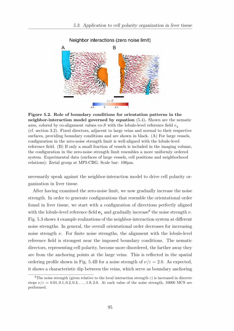
5.3. Application to cell polarity organization in liver tissue

Figure 5.2. Role of boundary conditions for orientation patterns in theneighbor-interaction model governed by equation (5.4). Shown are the nematicaxes, colored by co-alignment values co-S with the lobule-level reference field eχ(cf. section 3.2). Fixed directors, adjacent to large veins and normal to their respectivesurfaces, providing boundary conditions and are shown in black. (A) For large vessels,configuration in the zero-noise strength limit is well-aligned with the lobule-levelreference field. (B) If only a small fraction of vessels is included in the imaging volume,the configuration in the zero-noise strength limit resembles a more uniformly orderedsystem. Experimental data (surfaces of large vessels, cell positions and neighborhoodrelations): Zerial group at MPI-CBG. Scale bar: 100μm.

necessarily speak against the neighbor-interaction model to drive cell polarity or-

ganization in liver tissue.

After having examined the zero-noise limit, we now gradually increase the noise

strength. In order to generate configurations that resemble the orientational order

found in liver tissue, we start with a configuration of directions perfectly aligned

with the lobule-level reference field eχ and gradually increase8 the noise strength ν.

Fig. 5.3 shows 4 example realizations of the neighbor-interaction system at different

noise strengths. In general, the overall orientational order decreases for increasing

noise strength ν. For finite noise strengths, the alignment with the lobule-level

reference field is strongest near the imposed boundary conditions. The nematic

directors, representing cell polarity, become more disordered, the farther away they

are from the anchoring points at the large veins. This is reflected in the spatial

ordering profile shown in Fig. 5.4B for a noise strength of ν/ε = 2.0. As expected,

it shows a characteristic dip between the veins, which serve as boundary anchoring

8The noise strength (given relative to the local interaction strength ε) is increased in discretesteps ν/ε = 0.01, 0.1, 0.2, 0.3, . . . , 1.9, 2.0. At each value of the noise strength, 10000 MCS areperformed.

95

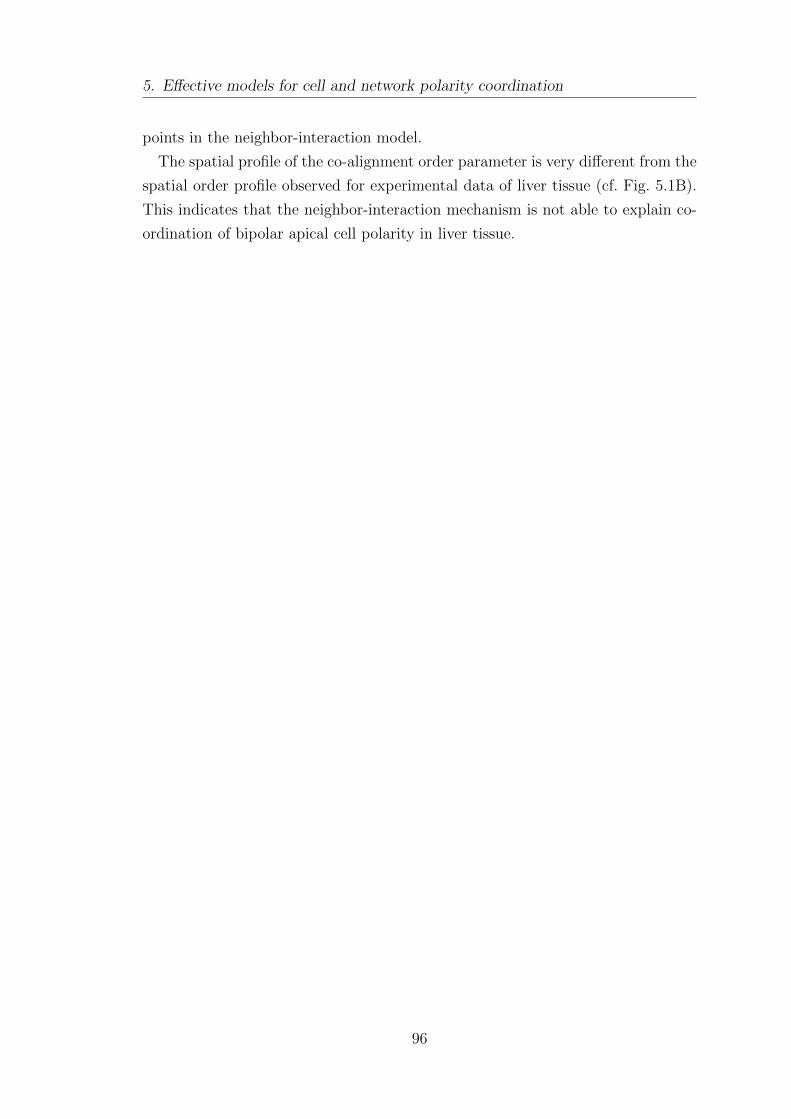
5. Effective models for cell and network polarity coordination

points in the neighbor-interaction model.

The spatial profile of the co-alignment order parameter is very different from the

spatial order profile observed for experimental data of liver tissue (cf. Fig. 5.1B).

This indicates that the neighbor-interaction mechanism is not able to explain co-

ordination of bipolar apical cell polarity in liver tissue.

96

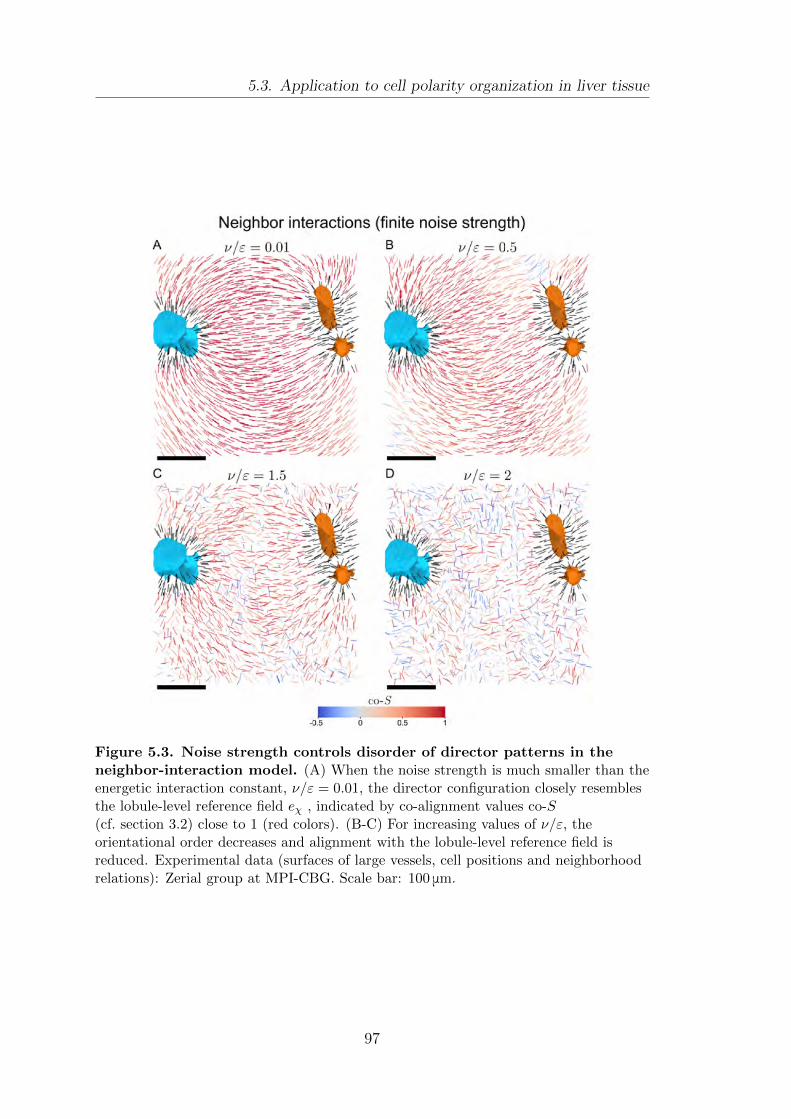
5.3. Application to cell polarity organization in liver tissue

Figure 5.3. Noise strength controls disorder of director patterns in theneighbor-interaction model. (A) When the noise strength is much smaller than theenergetic interaction constant, ν/ε = 0.01, the director configuration closely resemblesthe lobule-level reference field eχ , indicated by co-alignment values co-S(cf. section 3.2) close to 1 (red colors). (B-C) For increasing values of ν/ε, theorientational order decreases and alignment with the lobule-level reference field isreduced. Experimental data (surfaces of large vessels, cell positions and neighborhoodrelations): Zerial group at MPI-CBG. Scale bar: 100 μm.

97

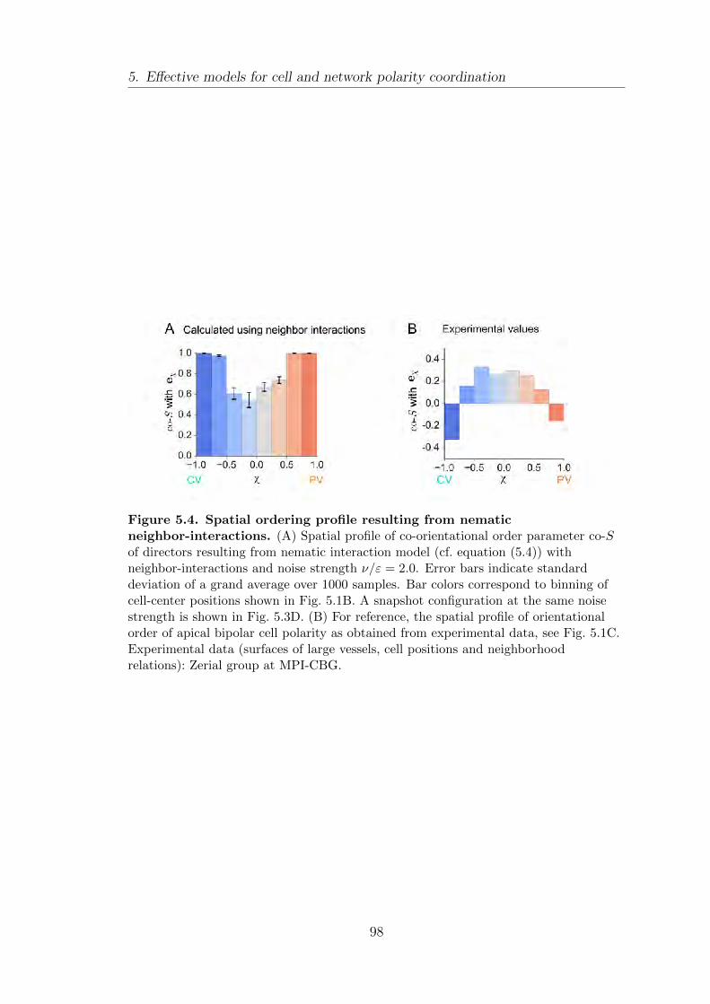
5. Effective models for cell and network polarity coordination

Figure 5.4. Spatial ordering profile resulting from nematicneighbor-interactions. (A) Spatial profile of co-orientational order parameter co-Sof directors resulting from nematic interaction model (cf. equation (5.4)) withneighbor-interactions and noise strength ν/ε = 2.0. Error bars indicate standarddeviation of a grand average over 1000 samples. Bar colors correspond to binning ofcell-center positions shown in Fig. 5.1B. A snapshot configuration at the same noisestrength is shown in Fig. 5.3D. (B) For reference, the spatial profile of orientationalorder of apical bipolar cell polarity as obtained from experimental data, see Fig. 5.1C.Experimental data (surfaces of large vessels, cell positions and neighborhoodrelations): Zerial group at MPI-CBG.

98

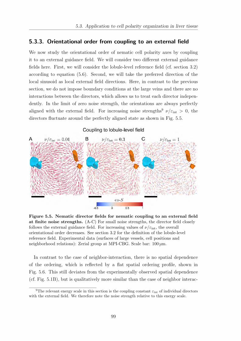
5.3. Application to cell polarity organization in liver tissue

5.3.3. Orientational order from coupling to an external field

We now study the orientational order of nematic cell polarity axes by coupling

it to an external guidance field. We will consider two different external guidance

fields here. First, we will consider the lobule-level reference field (cf. section 3.2)

according to equation (5.6). Second, we will take the preferred direction of the

local sinusoid as local external field directions. Here, in contrast to the previous

section, we do not impose boundary conditions at the large veins and there are no

interactions between the directors, which allows us to treat each director indepen-

dently. In the limit of zero noise strength, the orientations are always perfectly

aligned with the external field. For increasing noise strengths9 ν/εint > 0, the

directors fluctuate around the perfectly aligned state as shown in Fig. 5.5.

Figure 5.5. Nematic director fields for nematic coupling to an external fieldat finite noise strengths. (A-C) For small noise strengths, the director field closelyfollows the external guidance field. For increasing values of ν/εint, the overallorientational order decreases. See section 3.2 for the definition of the lobule-levelreference field. Experimental data (surfaces of large vessels, cell positions andneighborhood relations): Zerial group at MPI-CBG. Scale bar: 100 μm.

In contrast to the case of neighbor-interaction, there is no spatial dependence

of the ordering, which is reflected by a flat spatial ordering profile, shown in

Fig. 5.6. This still deviates from the experimentally observed spatial dependence

(cf. Fig. 5.1B), but is qualitatively more similar than the case of neighbor interac-

9The relevant energy scale in this section is the coupling constant εint of individual directorswith the external field. We therefore note the noise strength relative to this energy scale.

99

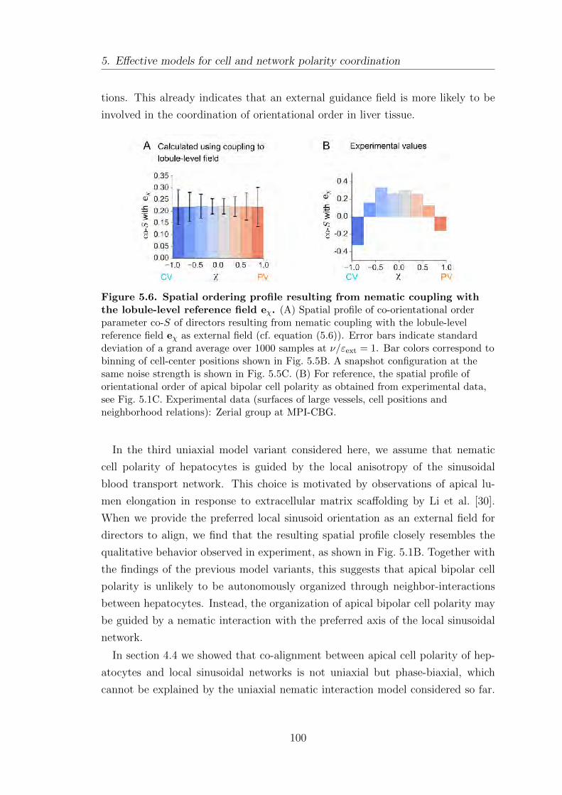
5. Effective models for cell and network polarity coordination

tions. This already indicates that an external guidance field is more likely to be

involved in the coordination of orientational order in liver tissue.

Figure 5.6. Spatial ordering profile resulting from nematic coupling withthe lobule-level reference field eχ. (A) Spatial profile of co-orientational orderparameter co-S of directors resulting from nematic coupling with the lobule-levelreference field eχ as external field (cf. equation (5.6)). Error bars indicate standarddeviation of a grand average over 1000 samples at ν/εext = 1. Bar colors correspond tobinning of cell-center positions shown in Fig. 5.5B. A snapshot configuration at thesame noise strength is shown in Fig. 5.5C. (B) For reference, the spatial profile oforientational order of apical bipolar cell polarity as obtained from experimental data,see Fig. 5.1C. Experimental data (surfaces of large vessels, cell positions andneighborhood relations): Zerial group at MPI-CBG.

In the third uniaxial model variant considered here, we assume that nematic

cell polarity of hepatocytes is guided by the local anisotropy of the sinusoidal

blood transport network. This choice is motivated by observations of apical lu-

men elongation in response to extracellular matrix scaffolding by Li et al. [30].

When we provide the preferred local sinusoid orientation as an external field for

directors to align, we find that the resulting spatial profile closely resembles the

qualitative behavior observed in experiment, as shown in Fig. 5.1B. Together with

the findings of the previous model variants, this suggests that apical bipolar cell

polarity is unlikely to be autonomously organized through neighbor-interactions

between hepatocytes. Instead, the organization of apical bipolar cell polarity may

be guided by a nematic interaction with the preferred axis of the local sinusoidal

network.

In section 4.4 we showed that co-alignment between apical cell polarity of hep-

atocytes and local sinusoidal networks is not uniaxial but phase-biaxial, which

cannot be explained by the uniaxial nematic interaction model considered so far.

100

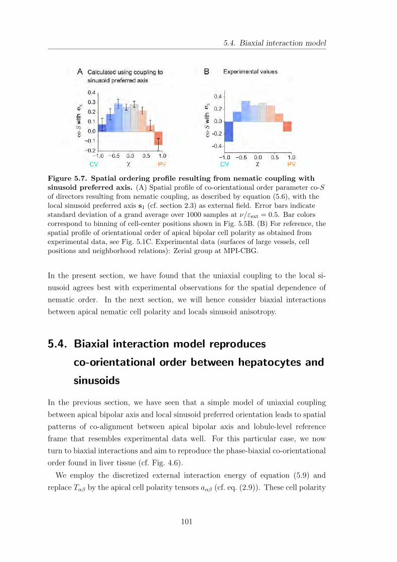
5.4. Biaxial interaction model

Figure 5.7. Spatial ordering profile resulting from nematic coupling withsinusoid preferred axis. (A) Spatial profile of co-orientational order parameter co-Sof directors resulting from nematic coupling, as described by equation (5.6), with thelocal sinusoid preferred axis s1 (cf. section 2.3) as external field. Error bars indicatestandard deviation of a grand average over 1000 samples at ν/εext = 0.5. Bar colorscorrespond to binning of cell-center positions shown in Fig. 5.5B. (B) For reference, thespatial profile of orientational order of apical bipolar cell polarity as obtained fromexperimental data, see Fig. 5.1C. Experimental data (surfaces of large vessels, cellpositions and neighborhood relations): Zerial group at MPI-CBG.

In the present section, we have found that the uniaxial coupling to the local si-

nusoid agrees best with experimental observations for the spatial dependence of

nematic order. In the next section, we will hence consider biaxial interactions

between apical nematic cell polarity and locals sinusoid anisotropy.

5.4. Biaxial interaction model reproduces

co-orientational order between hepatocytes and

sinusoids

In the previous section, we have seen that a simple model of uniaxial coupling

between apical bipolar axis and local sinusoid preferred orientation leads to spatial

patterns of co-alignment between apical bipolar axis and lobule-level reference

frame that resembles experimental data well. For this particular case, we now

turn to biaxial interactions and aim to reproduce the phase-biaxial co-orientational

order found in liver tissue (cf. Fig. 4.6).

We employ the discretized external interaction energy of equation (5.9) and

replace Tαβ by the apical cell polarity tensors aαβ (cf. eq. (2.9)). These cell polarity

101

5. Effective models for cell and network polarity coordination

tensors are subject to an external field Gαβ = λ/a3 sαβ given as the product of a

field strength λ and the anisotropy sαβ of the local sinusoid network (cf. eq. (2.10)).

This leads to the interaction energy

Fint = −λ∑i

a(i)αβ s

(i)αβ =

∑i

F(i)int . (5.10)

The interaction strength10 λ with the external field effectively controls the coupling

between the orientation of the biaxial cell anisotropy, described by aαβ, and the

orientation of the sinusoid network anisotropy sαβ, which takes the role of an exter-

nal field11. Again, we assume that the probability of finding a relative orientation

between an apical cell polarity and a respective local sinusoid is proportional to

the Boltzmann distribution at a noise strength ν that subsumes dynamic processes

that reduce spatial order. For simplicity, we introduce the normalized interaction

strength λ = λν

as the parameter that controls the overall amount of order in

the system. As we consider only the coupling to an external reference field here,

the directions of apical nematic cell polarity of individual cells decouple and we

can obtain the co-orientational parameters by direct numerical integration without

needing to resort to Monte-Carlo methods.

We now use the minimal biaxial interaction model to study co-orientational order

between apical nematic cell polarity and local sinusoid anisotropy of hepatocytes

10Here, we defined the coupling in a way that the field strength λ has units of energy.11To show this more explicitly, each tensor contraction in (5.10) can be written in terms of the

principle axis of the apical cell polarity tensor aαβ and the sinusoid network anisotropy tensorsαβ . For simplicity, we assume all cells and network anisotropies to be identical. and consideronly a single cell subject to the external field and drop the superscript i. Denoting the eigenvaluesof aαβ by σa1 , σa2 , σa3 and the respective eigenvectors by a1, a2, a3 and an analogous naming forthe eigenvalues and eigenvectors of tensor s, we note

F(1)int = λa : s = λ

(∑i

σai ai ⊗ ai

):

(∑k

σsk sk ⊗ sk

)= λ

∑ik

σai σak (ai ⊗ ai) : (sk ⊗ sk)

= λ∑ik

σai σsk (ai · sk)2 =

∑ik

αik (ai · sk)2 . (5.11)

Comparison with equation (3.16) shows that the functional form is similar to the case of a biaxialobject in an external field discussed in section 3.1.5. Both descriptions become equivalent, whenthe eigenvectors of the tensor s take the role of the external reference frame and the interactionparameters αik are given by the eigenvalues of a and s as αik = λσai σ

sk. The biaxial nematic

interaction energy thus depends on the eigenvalues of both tensors, encoded in the interactionparameters αik as well as the mutual orientation of the eigenframes of the tensors given bydirection cosines ai · sk.

102

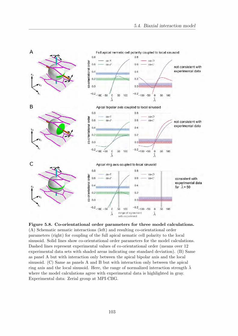
5.4. Biaxial interaction model

Figure 5.8. Co-orientational order parameters for three model calculations.(A) Schematic nematic interactions (left) and resulting co-orientational orderparameters (right) for coupling of the full apical nematic cell polarity to the localsinusoid. Solid lines show co-orientational order parameters for the model calculations.Dashed lines represent experimental values of co-orientational order (means over 12experimental data sets with shaded areas indicating one standard deviation). (B) Sameas panel A but with interaction only between the apical bipolar axis and the localsinusoid. (C) Same as panels A and B but with interaction only between the apicalring axis and the local sinusoid. Here, the range of normalized interaction strength λwhere the model calculations agree with experimental data is highlighted in gray.Experimental data: Zerial group at MPI-CBG.

103

5. Effective models for cell and network polarity coordination

in the liver. For that, the averaged eigenvalues of the apical nematic cell polarity

tensor and local sinusoid tensor are used for aαβ and sαβ, respectively. Below, we

will consider three variants of the model. While the first two cannot explain the

experimental data, the third compares very well.

Let us first consider the case, where the biaxial interaction parameters are de-

rived from the full (averaged) apical nematic cell polarity tensor. The resulting

co-orientational order parameters for varying values of the normalized interaction

strength λ are shown in Fig. 5.8A together with a schematic of an apical cell

polarity interacting with its local sinusoid. Because the sign of the interaction

energy (5.10) is not know a priori, both positive and negative values of the con-

trol parameter are considered. For comparison, the mean co-orientational order

parameters for liver tissue (cf. Fig. 4.6) averaged over 12 data sets are shown by a

dashed line. The shaded area around the dashed line indicates one standard devia-

tion of the experimental values. It can be seen that for no value of the normalized

interaction strength λ consistency with the experimental values is achieved. In

particular, for the region in which co-S is in agreement with experiment, the other

co-orientational order parameters are much higher in the model calculations than

what is observed in liver tissue.

This leads us to test an intermediate approach between the uniaxial and biaxial

model, where only one axis of apical cell polarity interacts with the local sinu-

soid. For an interaction of only the bipolar nematic axis with the local sinusoid

anisotropy, we formally set σa2 = σa3 = 0, see schematic in Fig. 5.8B. Likewise, to let

only the apical the ring axis interact with the local sinusoid anisotropy, we formally

set σa1 = σa2 = 0, see schematic in Fig. 5.8C. The resulting co-orientational order

parameters are shown in panels B and C of Fig. 5.8, respectively. In the case of

coupling the apical bipolar axis with the local sinusoid, again, the co-orientational

order parameters of the model calculations (solid lines) are different from the

experimental values observed in liver data (dashed lines) for all values of the nor-

malized interaction strength λ. However, for the last considered variant, where

the apical ring axis of cell polarity interacts with the local sinusoid anisotropy, we

observe a range of normalized interaction strengths λ, where the co-orientational

order parameters obtained from the model calculations (solid lines) are in good

agreement with experimental results (dashed lines).

This indicates that the interaction of the ring-axis of apical nematic cell polarity

with the local sinusoid network is sufficient to account for the experimentally

104

5.5. Summary

observed co-orientational order, which motivates the schematic picture of sinusoid-

hepatocyte co-alignment in liver tissue shown in Fig 5.8C. There, we propose a

simplified view of co-alignment with the ring-axis of apical nematic cell polarity of

hepatocytes aligned preferentially parallel to the plane axis of the local sinusoid s3

(see section 2.3 for definition). Fluctuations break axial symmetry and are biased

towards the corresponding network axis s2.

5.5. Summary

In this chapter, we investigated potential mechanisms that could underly orienta-

tional order of nematic cell polarity found in liver tissue (cf. chapter 4). With a

uniaxial nematic interaction model (derived by discretizing the Frank distortion

free energy) we studied neighbor-interactions and coupling to an external field.

We showed that, for certain boundary conditions, the orientations obtained in the

zero-noise strength limit of the uniaxial nematic neighbor-interactions agree with

the lobule-level reference field, which can be seen as an idealization of the orienta-

tional order of cell polarity found in liver tissue (see section 4.2). For finite noise

strength, however, the spatial distribution of orientational order of cell polarity,

as found in liver data, could not be reproduced. Coupling to an external refer-

ence field, given by the lobule-level reference field, gave slightly better agreement

(cf. section 5.3.3). By far the best agreement with experimental data was obtained

using the preferential direction of the local sinusoid network as a global alignment

field. This indicates that nematic cell polarity of hepatocytes is spontaneous, yet

requires global alignment cues for correct lobule-level organization, which may be

provided by the anisotropy of the local sinusoid network. Building on these obser-

vations, we considered a biaxial nematic interaction model that couples anisotropy

of the local sinusoid network and nematic cell polarity of hepatocytes. This last

model was able to reproduce the phase biaxial co-orientational order between both

structures.

105

6. Network self-organization in a

liver-inspired lattice model

The main focus of this short chapter are the two transport networks of the liver,

namely the sinusoid and bile canaliculi network, which were introduced in sec-

tion 1.2. One important aspect of the bile canaliculi network is that it is formed

directly as a lumen between two adjacent cells, which is hold together by tight

junctions (cf. section 1.3). It is therefore not possible that the sinusoid and bile

canaliculi networks cross each other. Furthermore, all hepatocytes are in contact

with both transport networks and each network is by itself fully connected.

The aim of the present chapter is to reproduce the basic principles of these three

biological observations of the two transport networks in liver tissue in a minimal

model. For that, we devise a simple lattice-based model, which is a generalized

Ising model. The proposed energetic interactions are similar to the one in the

Cellular Potts Model introduced in section 1.4.2, which is able to spontaneously

generate ordered structures.

6.1. Cubic lattice geometry motivated by liver tissue

We propose a simple and abstract model to study the generation of the network

structure observed in liver tissue. As a first simplification, we neglect all dynamic

rearrangement of cells, such as cell movement or cell division. We further simplify

the arrangement of cells by regarding them as cubes arranged on a simple cubic

lattice. On the surfaces of these cubes, which represent cells in an abstract way,

we allow network segments to form in a particular fashion. Specifically, network

segments representing sinusoids may form on the edges of the cube and will be

referred to as edge segments below. Network segments representing bile canaliculi

connect midpoints of opposing edges on the faces of the cube and are termed face

segments, see Fig. 6.1. This peculiar topology is chosen because it is relatively

simple, while retaining the number of cells adjacent to each segment found in real

liver tissue. We now provide analysis of experimental data to support that claim.

In the cubic model, it is apparent that each edge segment, representing a sinu-

soid, is surrounded by four different hepatocytes, while each face segment, repre-

107

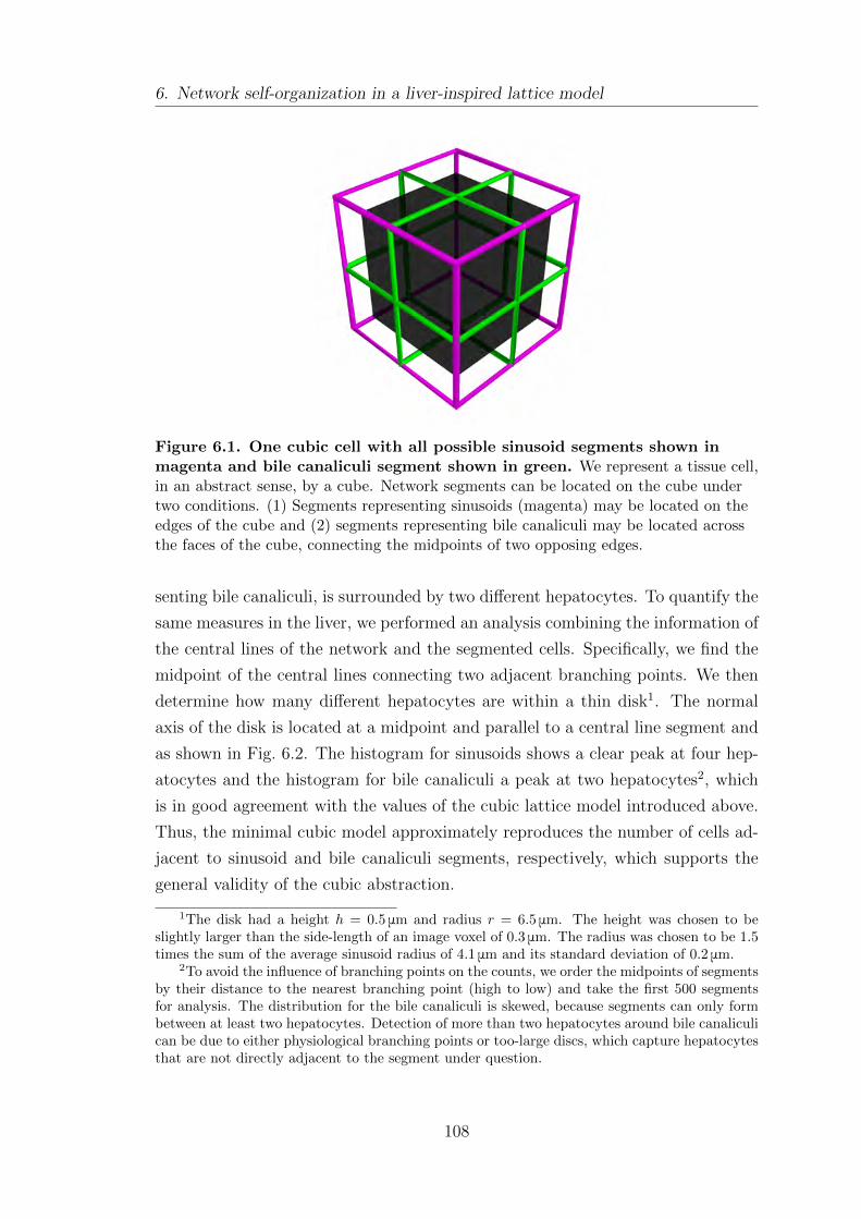
6. Network self-organization in a liver-inspired lattice model

Figure 6.1. One cubic cell with all possible sinusoid segments shown inmagenta and bile canaliculi segment shown in green. We represent a tissue cell,in an abstract sense, by a cube. Network segments can be located on the cube undertwo conditions. (1) Segments representing sinusoids (magenta) may be located on theedges of the cube and (2) segments representing bile canaliculi may be located acrossthe faces of the cube, connecting the midpoints of two opposing edges.

senting bile canaliculi, is surrounded by two different hepatocytes. To quantify the

same measures in the liver, we performed an analysis combining the information of

the central lines of the network and the segmented cells. Specifically, we find the

midpoint of the central lines connecting two adjacent branching points. We then

determine how many different hepatocytes are within a thin disk1. The normal

axis of the disk is located at a midpoint and parallel to a central line segment and

as shown in Fig. 6.2. The histogram for sinusoids shows a clear peak at four hep-

atocytes and the histogram for bile canaliculi a peak at two hepatocytes2, which

is in good agreement with the values of the cubic lattice model introduced above.

Thus, the minimal cubic model approximately reproduces the number of cells ad-

jacent to sinusoid and bile canaliculi segments, respectively, which supports the

general validity of the cubic abstraction.

1The disk had a height h = 0.5 μm and radius r = 6.5 μm. The height was chosen to beslightly larger than the side-length of an image voxel of 0.3 μm. The radius was chosen to be 1.5times the sum of the average sinusoid radius of 4.1 μm and its standard deviation of 0.2 μm.

2To avoid the influence of branching points on the counts, we order the midpoints of segmentsby their distance to the nearest branching point (high to low) and take the first 500 segmentsfor analysis. The distribution for the bile canaliculi is skewed, because segments can only formbetween at least two hepatocytes. Detection of more than two hepatocytes around bile canaliculican be due to either physiological branching points or too-large discs, which capture hepatocytesthat are not directly adjacent to the segment under question.

108

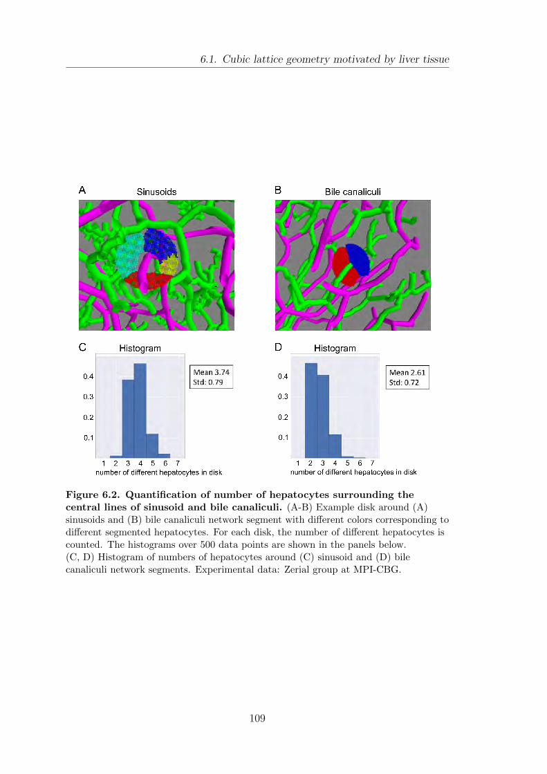
6.1. Cubic lattice geometry motivated by liver tissue

Figure 6.2. Quantification of number of hepatocytes surrounding thecentral lines of sinusoid and bile canaliculi. (A-B) Example disk around (A)sinusoids and (B) bile canaliculi network segment with different colors corresponding todifferent segmented hepatocytes. For each disk, the number of different hepatocytes iscounted. The histograms over 500 data points are shown in the panels below.(C, D) Histogram of numbers of hepatocytes around (C) sinusoid and (D) bilecanaliculi network segments. Experimental data: Zerial group at MPI-CBG.

109

6. Network self-organization in a liver-inspired lattice model

We can further estimate the number of segments per cube in the model that

would correspond to the network density found in liver tissue. From experimental

data, we calculate the length density and obtain for the bile canaliculi network 5.8

m / mm3 and 4.4 m / mm3 for the sinusoid network. We assume that the cubic cell

has a side-length of a = 20 μm, which corresponds to approximately one hepatocyte

diameter3. With that, we estimate the density of network segments to be 2.32 bile

canalicui segments per cubic volume and 1.72 sinusoid segments per cubic volume.

6.2. Effective energy for local network segment

interactions

The geometric lattice model introduced above is now supplemented with an ef-

fective energy to describe local interactions between network segments that are

motivated by observations in liver tissue. The resulting effective energy is for-

mally equivalent to a Hamiltonian of a generalized Ising model. The interaction

parameter, however, do not describe actual physical interactions between the net-

work segments but are instead used to maker biologically plausible neighborhood

relations more preferable. In particular, neighboring segments of the same type

should be favored while segments of different type should repel each other4. The

conceptual novelty of the approach presented here is the biologically motivated

constraint for each species of network segments to be bound to a disjoint subset of

the lattice, e.i. sinusoids to “edge segments” and bile canaliculi to “face segments”.

We write the effective energy of the network configuration as a sum of pair-wise

interaction between network segments Epair and an energy Ecell favoring a specific

number of segments per cell

Etotal = Epair + Ecell . (6.1)

The probability to find a specific configuration of network segments at a noise

strength ν shall be given by the Boltzmann distribution f ∝ exp(−Etotal/ν). Here,

we regard the noise strength ν as an abstract measure of how strongly biological

processes generate disorder.

3This value also compares well with the layer spacing found in section 4.6.4This type of local interaction is similar to the cellular Potts model introduced in section 1.4.2.

They were also studied in the context of binary mixtures of liquids [187, 188], which were usedby Steinberg to formulate the differential adhesion hypothesis for cell sorting [189].

110

6.2. Effective energy for local network segment interactions

Energetic contribution of neighboring network segments. To formulate the

effective pair interaction between network segments, we introduce an occupation

list σi = 0, 1, where i sequentially numbers all segments of the lattice and segment

i is empty if σi = 0 and occupied if σi = 1. Denoting the energetic interaction

between segment i and segment j by Jij, we write the interaction energy

Epair =∑ij

Jij σiσj . (6.2)

While this formulation is appealing due to its simplicity, it is impractical to allow

for arbitrary interaction energies between any segments in the whole lattice. We

therefore modify the generic formulation above to make explicit use of the topology

of the lattice. Specifically, we separate the occupation list into two parts, σSi and

σBj , where the index i runs over all edge segments of the lattice, i ∈ IE, and the

index j runs over all face segments of the lattice j ∈ IF. With this, we effectively

separated the energetic contributions from segments of the same type, JSS and

JBB, and of different types JBS, yielding Epair =∑

i,j∈IEJSSij σ

Si σ

Sj +

∑i,j∈IF

JBBij σ

Bi σ

Bj +∑

i∈IF,j∈IEJBSij σ

Bi σ

Sj . The total number of occupied network segments representing

sinusoids is thus given by NS =∑

i σSi , and the number of occupied network

segments representing bile canaliculi is given by NB =∑

i σBi .

We further impose that the energetic interactions are the same for all neigh-

bors defined by adjacency matrices KSS, KBB, KBS. Hence, we can write JSS =εSS2KSS, JBB = εBB

2KBB, JBS = εBS

2KBS, which gives for the effective interaction

energy

Epair =εSS

2

∑i,j∈IE

KSSij σ

Si σ

Sj +

εBB

2

∑i,j∈IF

KBBij σ

Bi σ

Bj + εBS

∑i∈IF,j∈IE

KBSij σ

Bi σ

Sj . (6.3)

We have thus separated the parameters for the energetic interaction from the

topology of the lattice. The topology of the lattice is incorporated solely in the

set of adjacency matrices KSS, KBB, KBS. The constraint of segments represent-

ing sinusoids being located on the edges of cubes and segments representing bile

canaliculi on the face of cubes leads to particular neighborhood relations between

different segment types. To illustrate that we show the 4 possible neighborhoods

that are encoded in the adjacency matrices KSS, KBB, KBS in Fig. 6.3.

111

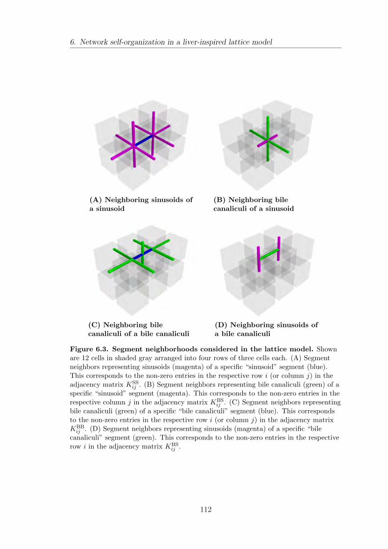
6. Network self-organization in a liver-inspired lattice model

(A) Neighboring sinusoids ofa sinusoid

(B) Neighboring bilecanaliculi of a sinusoid

(C) Neighboring bilecanaliculi of a bile canaliculi

(D) Neighboring sinusoids ofa bile canaliculi

Figure 6.3. Segment neighborhoods considered in the lattice model. Shownare 12 cells in shaded gray arranged into four rows of three cells each. (A) Segmentneighbors representing sinusoids (magenta) of a specific “sinusoid” segment (blue).This corresponds to the non-zero entries in the respective row i (or column j) in theadjacency matrix KSS

ij . (B) Segment neighbors representing bile canaliculi (green) of aspecific “sinusoid” segment (magenta). This corresponds to the non-zero entries in therespective column j in the adjacency matrix KBS

ij . (C) Segment neighbors representingbile canaliculi (green) of a specific “bile canaliculi” segment (blue). This correspondsto the non-zero entries in the respective row i (or column j) in the adjacency matrixKBBij . (D) Segment neighbors representing sinusoids (magenta) of a specific “bile

canaliculi” segment (green). This corresponds to the non-zero entries in the respectiverow i in the adjacency matrix KBS

ij .

112

6.3. Characterizing network structures in the cubic lattice geometry

Energetic contribution to favor a given network segment number per cell.

As every cell needs to be in contact with both types of network it is useful to

introduce a cell-based control parameter to enforce this requirement. We choose

an energy contribution similar to the area constraint of the cellular Potts model

(cf. equation 1.2).

Ecell =∑α

λSα

(nSα − cS

α

)2

+∑α

λBα

(nBα − cB

α

)2

. (6.4)

Here, we introduced the index α that runs over all Ncells cubes that represent cells

in the abstract lattice model. For a compact notation, we defined shorthands for

the number of occupied segments representing sinusoids nSα =

∑i∈CSα

σSi and the

number occupied segments representing bile canaliculi nBα =

∑i∈CBα

σBi that are

adjacent to the cube α. The set CSα includes all edge segments and the set CB

α holds

all face segments adjacent to the cube α. The parameter cSα is the target number

of occupied edge segments representing sinusoids and cBα is the target number of

face segments representing bile canaliculi for cube α. Any deviation of the actual

number of occupied segments around cube α from their respective target number

yields a unfavorable contribution to the total effective energy. The parameters

λSα ≥ 0 and λB

α ≥ 0 control the strength of the energetic penalty. For simplicity,

we assume that all cells share the same preference for the number of surrounding

segments. Thus, we set λS,Bα = λS,B and cS,B

α = cS,B in equation (6.4).

6.3. Characterizing network structures in the cubic

lattice geometry

For the analysis of network structures on the cubic lattice employed here, we

define suitable order parameters. Motivated by the observations in liver data, we

are interested in the amount of connectivity between the two transport networks

(sinusoids and bile canaliculi) and structural order parameters, such as cell polarity

and smectic order of the cell-network density correlations (cf. section 4.6).

From liver data, we know that each cell has an interface with both types of

networks. In the cubic lattice model, we therefore investigate the fraction of cells

that is in contact with at least one segment representing a sinusoid and the fraction

of cells that is in contact with at least one segment representing a bile canaliculi.

113

6. Network self-organization in a liver-inspired lattice model

When both of theses numbers are one, every cell has a contact to both network

types, which corresponds to the results found in liver tissue. Fractions lower than

one indicate that some cubes in the model are not connected to the networks.

Next, we observe in experimental data of liver tissue that the sinusoid and bile

canaliculi networks are both fully connected. In the abstract cubic lattice model,

we calculate the number of connected components as well as the relative size of

the largest one. When this relative size is one, all the segments form one giant

component, which is then similar to the observations in liver tissue.

From liver data, we are also aware of the impossibility of crossings between

sinusoid and bile canaliculi network. We therefore count the number of crossings

in segment configurations in the cubic lattice model. Any deviation from zero

indicates a deviation from typical liver structure.

Finally, we calculate a structural anisotropy parameter similar to identify layered

structures, for which we found evidence in liver tissue (cf. section 4.6). Due to

the underlying specific geometry of a cubic lattice, we now introduce a layering

order parameter for this specific case. To that end, we consider a binary array p

of dimension 2nx × 2ny × 2nz, where nx, ny, nz are the numbers of cubes in the

respective spatial direction. The indices of that array represent all node positions

of both network types and the midpoints of the cubes they surround. Each network

segment is thus associated with three indices in that array, corresponding to its

endpoints and midpoint. Starting at a zero-array, we iterate through all segments

of a given network type (either edge of face segments) and all occupied nodes from

zero to one. We then calculate an intermediate quantity

qx =∑

ix∈[0,2,3,...,2nx−2]

2ny−1,2nz−1∑iy ,iz=0

pix,iy ,iz + pix+2,iy ,iz − 2 pix+1,iy ,iz

and analogous values qy and qz for the other spatial directions. We sort these

intermediate values as q1 ≤ q2 ≤ q3 and take

q = q3 −1

2(q2 + q1) (6.5)

as the layering order parameter. In accordance with the notation introduced for

the interaction energy between network segments, we term the layering order pa-

rameter for the edge network representing sinusoids qS and the respective layering

order parameter for the face network representing bile canaliculi qB.

114

6.4. Local interaction rules generate macroscopic network structures

6.4. Local interaction rules generate macroscopic

network structures

We now introduce the effects of the individual contributions of the interaction

parameters on the qualitative properties of the structure of the resulting transport

networks. For simplicity, we fix the total number of sinusoid NS and bile canaliculi

segments NB in the system. To avoid non-integer values for the number of occupied

edge segments per cell cS and occupied face segments per cell cB, we round the

respective segment numbers estimate from liver data (cf. section 6.1) to their

nearest integer values, which yields 2 bile segments (located on cube faces) per

cube and 2 sinusoid segments (located on cube edges) per cube5.

To get a qualitative picture of the how different local rules lead to differ-

ent types of order in the cubic lattice model presented above, we first examine

only self-attraction, only mutual repulsion and then their combined action. Af-

ter that, we add the cell demand (cf. equation (6.4)), which will lead to lay-

ered network structures. To that end, we employ a Monte-Carlo method (see

appendix A.13 for details) to sample configurations from the Boltzmann distribu-

tion f ∝ exp(−Etotal/ν). For each set of parameters, we gradually decrease6 the

noise strength ν to obtain states that correspond to (local) energetic minima. We

then compare the types of order found in the network configurations corresponding

to these (local) energetic minima.

We first confirm that in the absence of network segment pair interactions, ran-

dom configurations are found, see Fig 6.4B. For non-zero self-attraction parameters

εSS < 0, we find that network segments of the same type aggregat into fully-

connected clusters, see Fig. 6.4C. In other words, all segments of one type are part

of a single connected component. The locations of the two clusters are arbitrary

and they may overlap. The layering order parameters qS = 0.1 and qB = 0.13 for

this structure are small. We now consider the case of only repulsive interaction

between un-like network segment types. This corresponds to εBS > 0 being the

5Due to the different total numbers of face segments and edge segments, this leads to twothirds of the edge segments (representing sinusoids) and one third of the face segments (repre-senting bile canaliculi) being occupied. Note that the rounding has an opposite effect in bothnetwork types.

6The noise strength ν was first set to 100 to allow for equilibration in a highly unorderedregime. It was then reduced in steps of 1 from 10 to 5 and then further reduced in steps of 0.1from 5 to 0. For each value of the noise strength, 5000 MCS were performed. A single annealingrun took about 4h on a machine with an Intel Xeon CPU with 2.5 GHz.

115

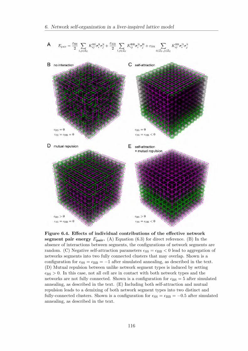
6. Network self-organization in a liver-inspired lattice model

Figure 6.4. Effects of individual contributions of the effective networksegment pair energy Epair. (A) Equation (6.3) for direct reference. (B) In theabsence of interactions between segments, the configurations of network segments arerandom. (C) Negative self-attraction parameters εSS = εBB < 0 lead to aggregation ofnetworks segments into two fully connected clusters that may overlap. Shown is aconfiguration for εSS = εBB = −1 after simulated annealing, as described in the text.(D) Mutual repulsion between unlike network segment types is induced by settingεBS > 0. In this case, not all cell are in contact with both network types and thenetworks are not fully connected. Shown is a configuration for εBS = 5 after simulatedannealing, as described in the text. (E) Including both self-attraction and mutualrepulsion leads to a demixing of both network segment types into two distinct andfully-connected clusters. Shown is a configuration for εSS = εBB = −0.5 after simulatedannealing, as described in the text.

116

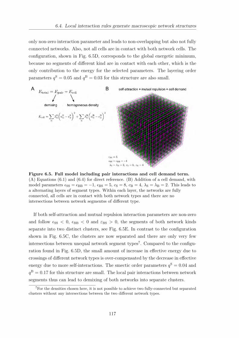
6.4. Local interaction rules generate macroscopic network structures

only non-zero interaction parameter and leads to non-overlapping but also not fully

connected networks. Also, not all cells are in contact with both network cells. The

configuration, shown in Fig. 6.5D, corresponds to the global energetic minimum,

because no segments of different kind are in contact with each other, which is the

only contribution to the energy for the selected parameters. The layering order

parameters qS = 0.05 and qB = 0.03 for this structure are also small.

Figure 6.5. Full model including pair interactions and cell demand term.(A) Equations (6.1) and (6.4) for direct reference. (B) Addition of a cell demand, withmodel parameters εSS = εBB = −1, εBS = 5, cS = 8, cB = 4, λS = λB = 2. This leads toa alternating layers of segment types. Within each layer, the networks are fullyconnected, all cells are in contact with both network types and there are nointersections between network segmentss of different type.

If both self-attraction and mutual repulsion interaction parameters are non-zero

and follow εSS < 0, εBB < 0 and εBS > 0, the segments of both network kinds

separate into two distinct clusters, see Fig. 6.5E. In contrast to the configuration

shown in Fig. 6.5C, the clusters are now separated and there are only very few

intersections between unequal network segment types7. Compared to the configu-

ration found in Fig. 6.5D, the small amount of increase in effective energy due to

crossings of different network types is over-compensated by the decrease in effective

energy due to more self-interactions. The smectic order parameters qS = 0.04 and

qB = 0.17 for this structure are small. The local pair interactions between network

segments thus can lead to demixing of both networks into separate clusters.

7For the densities chosen here, it is not possible to achieve two fully-connected but separatedclusters without any intersections between the two different network types.

117

6. Network self-organization in a liver-inspired lattice model

In the liver, we also find that both networks are ”demixed” in that there are

no overlaps between sinusoids and bile canaliculi. However, the demixing occurs

locally and still each cell is in contact with both network types. For this, we

now also include the cell demand Ecell (cf. equation (6.4)). The addition of a

non-zero cell demand with λS > 0 and λB > 0 generates alternating layers of

sinusoid and bile canaliculi networks, see Fig. 6.5B. Here, we chose the cell segment

numbers per cell cS = 8 and cB = 4 to be compatible with the fixed numbers of

respective network segments in the system. Within the layers, both networks are

fully connected but individual layers are not connected with each other. This

configuration has the, qualitatively, best agreement with properties found in liver

tissue. In particular, there are no intersection points between the two, mutually

exclusive, networks. All cells are in contact with both network types and both

networks are (within each layer) fully connected. The smectic order parameters

qS = 1 and qB = 1 correspond to perfect layering and are thus much larger than

in the other three examples shown.

While these layered structures in the cubic lattice model in the low-noise strength

limit are much more regular than the networks found in liver tissue, they share

common characteristics and open the possibility of reproducing general features of

liver tissue for finite noise strengths.

6.5. Effect of mutual repulsion between unlike

segment types on network structure

The analysis above shows that simple local rules can generate different types of

interesting order in the cubic lattice model that can be compared to properties of

liver tissue. To get more insight into the parameter space and how the qualita-

tively different structures are placed therein, we scans through different sections

of the parameter space can be performed. An exhaustive scan is unfeasible at

the moment. However, for an initial analysis, we perform a line scan through the

parameter space to explore the feasibility and to learn how the ordered structures

change in dependence of the repulsion parameter εBS and for varying values of the

noise strength ν.

For that, we take the values used to obtain the layered structure in Fig. 6.5B

118

6.5. Effect of mutual repulsion between unlike segment types on network

structure

and change the repulsion parameter8 εBS from εBS = 0 to εBS = 4 in steps of 0.2.

For each value of the repulsion parameter ε, simulated annealing9 was done 10

times and a grand average over the averaged values over 20 measurements of a

single realization at each noise strength was taken.

The resulting values for the number of intersection events between unequal net-

work types are shown in Fig. 6.6A and four regimes can be identified10. The first,

“R1”, is encountered for high values of the noise strength and low values of the

repulsion parameter εBS. A representative example is shown in Fig. 6.6D1. This

corresponds to a random configuration of both networks, which features many in-

tersections between both network types. For decreasing values of the noise strength

ν, the structure becomes more ordered. In particular, the face segments represent-

ing bile canaliculi (green) representing bile canaliculi arrange into layers. This

is quantified by the network order parameter S = −0.5 for these structures, see

Fig. 6.6B, which means that alls occupied face segments lie in a single plane11.

The edge segments representing sinusoids, however, form a structure not yet en-

countered. It can be best described by envisioning a fully occupied edge segment

network and then removing every second layer in one direction, see Fig. 6.6D2.

This is captured by the smectic order parameter qS = 0.25, see Fig. 6.6C, which

is clearly non-zero but far from its maximum value of 1. For increasing values of

the repulsion parameter (1 < ε < 2), the number of intersection events between

unequal segment types decreases and the bile canaliculi layers change into more

line-like configurations, which is indicated by positive values of S in Fig. 6.6B. Fi-

nally, for large values of the repulsion parameter ε > 2, the layered configuration

already encountered in the qualitative analysis, see Fig. 6.5B, is found.

We now raise the question, whether the final configurations after the annealing

procedure may be the ground states for the specific parameter. For that, we

compare the configuration found through simulated annealing at a specific value of

the repulsion parameter ε with all other configurations encountered after simulated

annealing with different values of the repulsion parameter. For high values εBS >

8The other interaction parameters are kept constant at εSS = εBB = −1, cS = 8, cB = 4 andλS = λB = 2.

9The noise strength ν was first set to 100 to allow for equilibration in a highly unorderedregime. It was then reduced in steps of 1 from 10 to 5 and then further reduced in steps of 0.1from 5 to 0. For each value of the noise strength, 20000 MCS were performed for equilibration.Then, 20 numerical measurements were taken with 100 MCS between each measurement.

10Other structural quantities can be found in appendix A.1411The smectic order parameter for face segments representing bile canaliclui is qB = 1 in this

case, see appendix A.14.

119

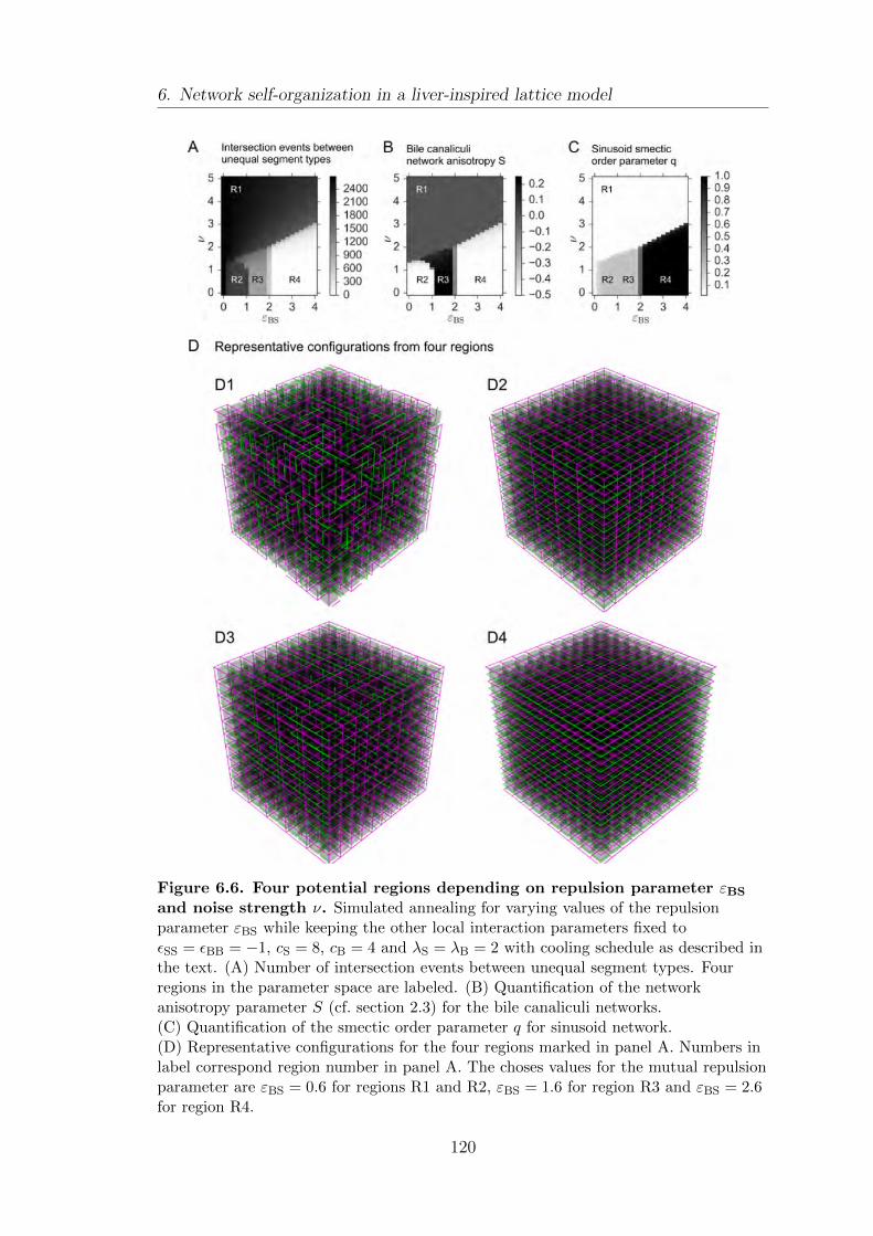
6. Network self-organization in a liver-inspired lattice model

Figure 6.6. Four potential regions depending on repulsion parameter εBS

and noise strength ν. Simulated annealing for varying values of the repulsionparameter εBS while keeping the other local interaction parameters fixed toεSS = εBB = −1, cS = 8, cB = 4 and λS = λB = 2 with cooling schedule as described inthe text. (A) Number of intersection events between unequal segment types. Fourregions in the parameter space are labeled. (B) Quantification of the networkanisotropy parameter S (cf. section 2.3) for the bile canaliculi networks.(C) Quantification of the smectic order parameter q for sinusoid network.(D) Representative configurations for the four regions marked in panel A. Numbers inlabel correspond region number in panel A. The choses values for the mutual repulsionparameter are εBS = 0.6 for regions R1 and R2, εBS = 1.6 for region R3 and εBS = 2.6for region R4.

120

6.6. Summary

2 and low values εBS < 1 of the repulsion parameter, the configuration found

through annealing had indeed the lowest energy among all the other proposed

configurations. For repulsion parameters in the intermediate regime 1 < εBS <

2, however, the annealing procedure for was not able to find the lowest energy

configuration. In this parameter range, the layered configuration had lower total

energy than the one found through simulated annealing. We therefore speculate

that the annealing procedure was trapped in a potentially metastable state and the

layered configuration is assumed to be the ground state in that parameter range.

Given the densities, the values for the network segment self-attraction and cell

demand as above, the face segments representing bile canaliculi form layers even in

the absence of mutual repulsion while the edge segments representing sinusoids do

not. Therefore, mutual repulsion is mandatory to obtain a smectic configuration of

network segments. For an intermediate region of repulsion 1 < ε < 2, the layered

configuration has the lowest energy but is not reliably found through simulated

annealing, indicating other, possibly metastable, configurations. Only for larger

values ε > 2, the layered configuration is found in all the simulated annealing

trials.

6.6. Summary

In this last chapter of the thesis, we have presented an abstract model to condense

the complex three-dimensional structure of liver tissue into a simplified cubic ge-

ometry. We have shown that this abstract geometry conserves the number of cells

that surround the segments of the transport networks to good approximation.

On this cubic geometry, we defined a generalization of the Ising model for net-

work self-organization, which is similar to the cellular Potts model introduced in

section 1.4.2. For a specific choice of local interaction parameters, we were able to

reproduce three key observations from biology: connectedness of both networks,

avoidance of crossings between different network types and the connection of all

cells to both network types. The configuration that reproduced these features was

also smectic, and network segments of different type were organized into alter-

nating layers. Building on this observation we tested, whether repulsion between

segments is necessary for the emergence of this type of order. While for the face

segment network representing bile canaliculi, the repulsion was not needed to gen-

erate a layered structure, it was indeed necessary for the formation of edge segment

121

6. Network self-organization in a liver-inspired lattice model

layers representing sinusoids. This serves as a proof-of-concept and opens inter-

esting avenues to explore in future.

One interesting future research is to characterize different kinds of phase sepa-

rations in the system. Also, on a more technical note, it is not obvious how to best

compare the simulation results on the abstract cubic geometry to experimental

data of liver tissue. Alternatively to using coarse-grained data, as done here, it

might provide useful to extend a mapping procedure of fluorescence data onto a

lattice geometry, as proposed by Breuer et al. [190] for the two-dimensional case,

to the three-dimensional geometry used here. A further future research direction

is to use the cubic lattice geometry to model growth processes of the networks

that may include feedback from the hepatocytes. From a biological perspective,

there are indications that hepatocytes control the local density of sinusoid and

bile canaliculi in liver tissue by either regulating the number of proteins involved

in the formation of membrane domains that create bile canaliculi [29, 37, 191], or

through chemical signaling by growth factors, such as VEGF, which was previously

reported for the sinusoidal network [192–194]. Some of these approaches have been

investigated in the master thesis of Marius Asal [195] on a modified version of the

cubic lattice model presented here.

122

7. Discussion and Outlook

The over-arching question underlying this thesis is how cells organize into complex

functional tissues. To address this question, we selected the liver as a model organ

because of three main features: (1) it is a vital organ of vertebrates performing

a wide variety of functions, (2) it is inherently three-dimensional in its structural

organization and (3) novel experimental imaging methods have recently become

available to provide a detailed view on the organization of cells with sub-cellular

resolution. By that, the liver qualifies as being complex in both the function it

provides for body homeostasis as well as in the architecture needed to provide

this function. Using data analysis of high-resolution images of liver data1 and

theoretical modeling, the present thesis arrived at four important results.

The first important result of this thesis, laid out in chapter 2, is the identifi-

cation of a nematic cell polarity of hepatocytes in the liver. In this context, cell

polarity refers to the inhomogeneous distribution of membrane-bound proteins on

the surface of cells. While this has been implicated before [29], we provide a rigor-

ous quantification of this type of cell polarity by means of a multipole expansion.

We showed that cell polarity of hepatocytes is best described by a nematic cell

polarity, the orientation of which is represented by a tripod of undirected axes. In

the future, it will be interesting to see this method applied to other tissues types

and investigate, what dominant type of protein configurations are found there.

The second important result of this thesis is that the orientations of these in-

dividual nematic cell polarities are coordinated among many cells throughout the

tissue. Furthermore, the patterns of oriented nematic cell polarity were found to be

correlated with a lobule-level reference field that is defined by the locations of large

vessels within the tissue (cf. section 4.1). We applied the structural analysis frame-

work, which consists of analyzing single cell protein patterns and the orientational

order of the thus identified nematic cell polarity, to genetic knock-down experi-

ments, which highlights the usefulness of the quantification. We could show that

the inhibition of a specific signaling protein (integrin beta1) reduces the amount of

cellular coordination, making the orientational alignment less pronounced, while

leaving nematic cell polarity of individual cells unchanged (cf. section 4.5). This

1The acquisition of experimental data of mice livers as well as image segmentation wasperformed by collaborators in the lab of Marino Zerial at the Max Planck Institute of MolecularCell Biology and Genetics, Dresden.

123

7. Discussion and Outlook

indicates a bi-directional feedback between cell polarity organization and network

structures, which is contrary to previous belief. Future studies of liver tissue may

use the structural benchmark presented here and investigate its changes during

liver development and regeneration. The tools underlying this liver-specific anal-

ysis are generic and are summarized in a separate chapter 3. In the future, they

may provide useful in their own right as they can be readily applied to other tis-

sues to investigate phenotypes induced by genetic knock down, chemical damage

or disease conditions.

The third important result of this thesis is that the coordination of nematic cell

polarity is best reproduced by a theoretical model that couples cell polarity to

the anisotropy of the local sinusoid network. This conclusion involved three steps.

We first showed that uniaxial nematic nearest-neighbor interactions (known as

the Lebwohl-Lascher model) was unable to reproduce the spatial distribution of

orientational order of cell polarity in liver tissue, and coupling to the lobule-level

reference field gave more agreeable results (cf. section 5.3.3). The best agreement

with experimental data was obtained using the preferential direction of the local

sinusoid network as a global alignment field. This indicates that nematic cell po-

larity of hepatocytes is spontaneous, yet requires global alignment cues for correct

lobule-level organization, which may be provided by the anisotropy of the local

sinusoid network. Building on these observations, we considered a biaxial nematic

interaction model that couples anisotropy of the local sinusoid network and ne-

matic cell polarity of hepatocytes. This last model was able to reproduce the

phase biaxial co-orientational between both structures. This implicates that an

autonomous organization of orientational order of cell polarity of hepatocytes in

the liver is unlikely and guidance by the sinusoidal network is necessary. Whether

the sinusoidal network is the only driver of structural organization in the liver or

whether there is a more intricate interplay between the network structures and the

cell polarity of hepatocytes, as indicated by the genetic knock-down experiments

presented in section 4.5, is an interesting question for future research.

The fourth important result of this thesis is that local interaction rules can

self-organize into biologically sensible transport networks on a simplified cubic

tissue geometry. We mapped the complex three-dimensional structure of liver

tissue to a simplified cubic geometry, which preserves typical network-cell neighbor-

relations present in liver tissue. We showed that a generalized Ising model is able

to reproduce three key observations from biology: connectedness of both networks,

124

avoidance of crossings between different network types and the connection of all

cells to both network types, for a specific choice of local interaction parameters.

This serves as a proof-of-concept and opens interesting avenues to explore in future

work, e.g. efficient simulation of networks to study robustness and the action of

morphogenetic cues.

In conclusion, this thesis used structural analysis of biological tissues to reveal

biaxial nematic order in liver tissue. Furthermore, using theoretical modeling, we

showed that networks on an abstract cubic lattice can self-organize into sensible

structures by local rules alone. Using a nematic interaction model, we showed

that it is reasonable to assume that the networks in turn influence the arrange-

ment of cell polarity in liver tissue. A potential feedback of cell polarity on the

network structure, as indicated by experimental data, opens new avenues for future

explorations.

125

A. Appendix

A.1. Mean field theory fo the isotropic-uniaxial

nematic transition

The first molecular field theory for the (uniaxial) nematic phase was developed by

Wilhelm Meier and Alfred Saupe in 1959 [177]. The theory features an effective

orientational potential for a single particle derived by a molecular field approxi-

mation of the van der Waals forces between molecules [117, 196]

U(cos θ) = −u2 S1

2

(3 cos2 θ − 1

)(A.1)

where θ is the angle between the molecular symmetry axis and the director. The

order parameter S is one given in equation 1.5 and u2 includes the averaged

anisotropic interaction parameters. In general, u2 may depend on pressure and

temperature. Following the original assumption by Meier and Saupe and for sake

of simplicity, this dependence is neglected here. In equilibrium, the angular dis-

tribution function given by the interaction energy (A.1) follows the Boltzmann

distribution f(θ) = exp (−U/kT ) /Z with partition function Z as the normaliza-

tion factor Z =∫ π/2

0dθ sin θ exp (−U/kT ). The order parameter S is given as the

average second moment of the distribution (see eq. (1.5)). Inserting the Boltzmann

distribution for the orientational distribution function into eq. (1.5) yields

S = −1

2+

3

2Z

1∫0

x2e12u2S(3x2−1)/kTdx . (A.2)

where we substituted x = cos θ. In order for equation (A.2) to be self-consistent,

the values of the order parameter on the left-hand side and on the right-hand

side must be equal. The solution to this self-consistency equation can be deter-

mined numerically. The Meier-Saupe theory predicts a first-order transition from

an isotropic fluid to the nematic state at a critical temperature T = Tc, where

the order parameter goes discontinuously from zero to Sc = S(Tc) = 0.44 [39].

Despite the simplicity of the interaction potential and assumption of axially sym-

metric molecules, the theory is in reasonable agreement with experimental ob-

127

A. Appendix

servations (see Fig. 2.3 in [39] and [196]). The theory of Meier and Saupe was

extended to also include steric interactions between molecules, higher rank in-

teractions and deviations from molecular cylindrical symmetry that yield better

quantitative agreement with experimental data [196–198].

Extensions to biaxial nematics The molecular-field theory of Meier and Saupe,

describing the uniaxial nematic phase, was extended by Freiser to non-cylindrically

symmetric molecules [128, 157, 199]. Specifically, the orientational part of the

interaction energy between molecules i and j is written as

wij = −Trace(RTQRQ

)(A.3)

where R is the orthogonal rotation matrix that transforms the axes of molecule i

into those of molecule j, and Q characterizes the second-order molecular anisotropy

of the molecules. Assuming molecules that possess dihedral symmetry (see ap-

pendix A.5), Q is assumed to be symmetric and traceless. It can thus always be

diagonalized, yielding two shape parameters. One parameter, Q, characterizes the

uniaxial anisotropy of the molecule and the second, q, characterizes the deviation

of the molecular shape from axial symmetry. Using the Schwartz inequality, he

first shows that all molecules are perfectly aligned in the ground state. Two ori-

entational order parameters can be defined from the averaged quantity 〈Q〉 over

the orientational distribution function f(Ω) = f(α, β, γ), that are related to the

uniaxial order parameter S and the phase biaxiality parameter P that are dis-

cussed in section 3.1.1. Applying the molecular field approximation, a successive

transition from the isotropic to uniaxial towards the biaxial state upon cooling is

found. The isotropic to uniaxial transition is shown to be of first order, whereas

the uniaxial to biaxial transition is continuous. For axially symmetric molecules

(q = 0) the theory reduces to the one of Meier and Saupe.

Shortly after Freiser, Straley proposed the use of two more order parameters

(corresponding to D and C in section 3.1.1) to properly characterize the biaxial

phase [119]. This revealed a richer phase diagram than the one predicted by Freiser.

In particular, a direct isotropic-to-biaxial transition of either first or second order,

depending on the molecular anisotropy, was found. This view was adopted by

subsequent authors and formalized in considering a so-called “supertensor”[39] or

two molecular tensors [200], which can be shown to be equivalent descriptions

of orientational order of biaxial molecules in a biaxial phase [160]. Using this

128

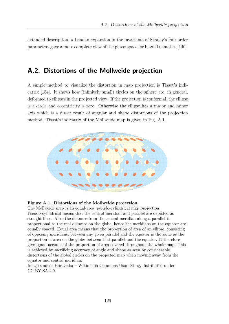
A.2. Distortions of the Mollweide projection

extended description, a Landau expansion in the invariants of Straley’s four order

parameters gave a more complete view of the phase space for biaxial nematics [140].

A.2. Distortions of the Mollweide projection

A simple method to visualize the distortion in map projection is Tissot’s indi-

catrix [154]. It shows how (infinitely small) circles on the sphere are, in general,

deformed to ellipses in the projected view. If the projection is conformal, the ellipse

is a circle and eccentricity is zero. Otherwise the ellipse has a major and minor

axis which is a direct result of angular and shape distortions of the projection

method. Tissot’s indicatrix of the Mollweide map is given in Fig. A.1.

Figure A.1. Distortions of the Mollweide projection.The Mollweide map is an equal-area, pseudo-cylindrical map projection.Pseudo-cylindrical means that the central meridian and parallel are depicted asstraight lines. Also, the distance from the central meridian along a parallel isproportional to the real distance on the globe, hence the meridians on the equator areequally spaced. Equal area means that the proportion of area of an ellipse, consistingof opposing meridians, between any given parallel and the equator is the same as theproportion of area on the globe between that parallel and the equator. It thereforegives good account of the proportion of area covered throughout the whole map. Thisis achieved by sacrificing accuracy of angle and shape as seen by considerabledistortions of the global circles on the projected map when moving away from theequator and central meridian.Image source: Eric Gaba – Wikimedia Commons User: Sting, distributed underCC-BY-SA 4.0.

129

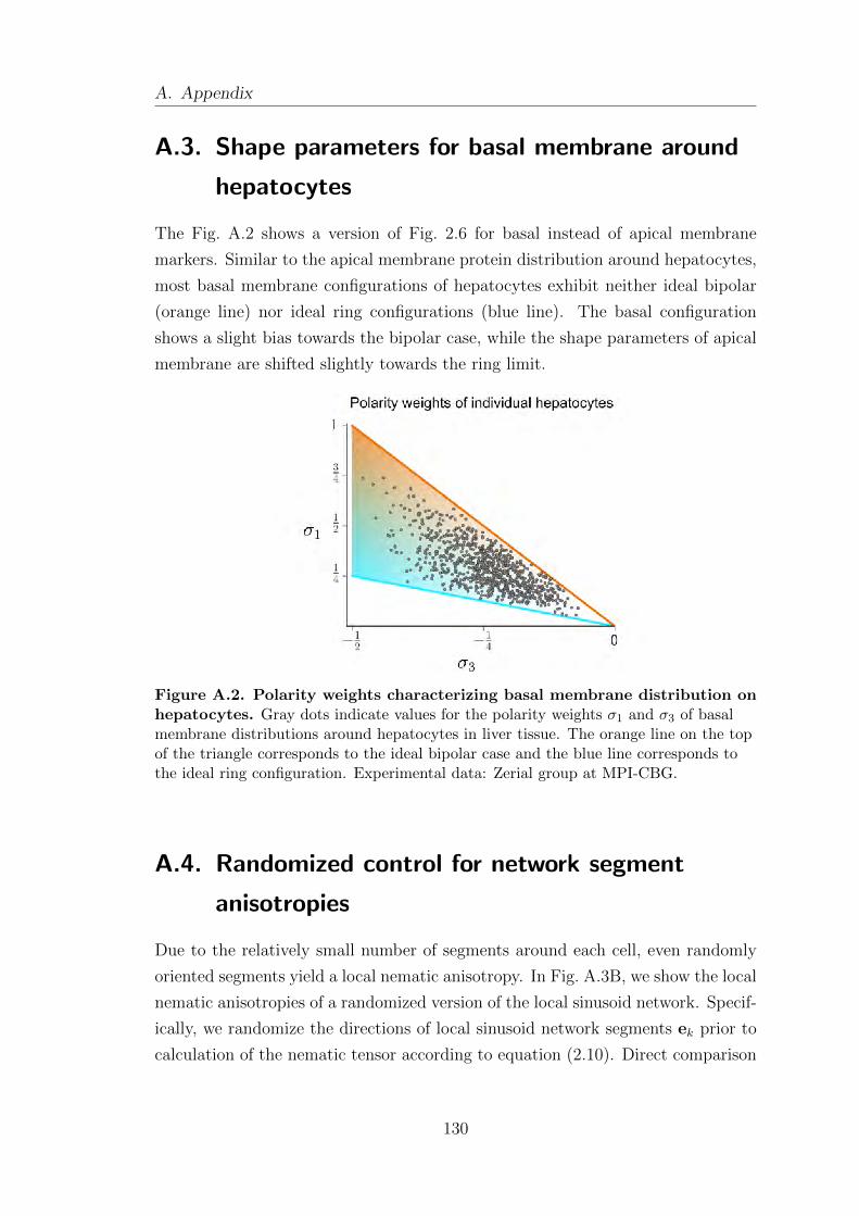
A. Appendix

A.3. Shape parameters for basal membrane around

hepatocytes

The Fig. A.2 shows a version of Fig. 2.6 for basal instead of apical membrane

markers. Similar to the apical membrane protein distribution around hepatocytes,

most basal membrane configurations of hepatocytes exhibit neither ideal bipolar

(orange line) nor ideal ring configurations (blue line). The basal configuration

shows a slight bias towards the bipolar case, while the shape parameters of apical

membrane are shifted slightly towards the ring limit.

Figure A.2. Polarity weights characterizing basal membrane distribution onhepatocytes. Gray dots indicate values for the polarity weights σ1 and σ3 of basalmembrane distributions around hepatocytes in liver tissue. The orange line on the topof the triangle corresponds to the ideal bipolar case and the blue line corresponds tothe ideal ring configuration. Experimental data: Zerial group at MPI-CBG.

A.4. Randomized control for network segment

anisotropies

Due to the relatively small number of segments around each cell, even randomly

oriented segments yield a local nematic anisotropy. In Fig. A.3B, we show the local

nematic anisotropies of a randomized version of the local sinusoid network. Specif-

ically, we randomize the directions of local sinusoid network segments ek prior to

calculation of the nematic tensor according to equation (2.10). Direct comparison

130

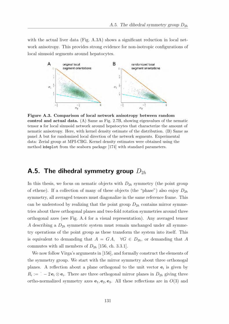
A.5. The dihedral symmetry group D2h

with the actual liver data (Fig. A.3A) shows a significant reduction in local net-

work anisotropy. This provides strong evidence for non-isotropic configurations of

local sinusoid segments around hepatocytes.

Figure A.3. Comparison of local network anisotropy between randomcontrol and actual data. (A) Same as Fig. 2.7B, showing eigenvalues of the nematictensor s for local sinusoid network around hepatocytes that characterize the amount ofnematic anisotropy. Here, with kernel density estimate of the distribution. (B) Same aspanel A but for randomized local direction of the network segments. Experimentaldata: Zerial group at MPI-CBG. Kernel density estimates were obtained using themethod kdeplot from the seaborn package [174] with standard parameters.

A.5. The dihedral symmetry group D2h

In this thesis, we focus on nematic objects with D2h symmetry (the point group

of ethene). If a collection of many of these objects (the “phase”) also enjoy D2h

symmetry, all averaged tensors must diagonalize in the same reference frame. This

can be understood by realizing that the point group D2h contains mirror symme-

tries about three orthogonal planes and two-fold rotation symmetries around three

orthogonal axes (see Fig. A.4 for a visual representation). Any averaged tensor

A describing a D2h symmetric system must remain unchanged under all symme-

try operations of the point group as these transform the system into itself. This

is equivalent to demanding that A = GA, ∀G ∈ D2h, or demanding that A

commutes with all members of D2h [156, ch. 3.3.1].

We now follow Virga’s arguments in [156], and formally construct the elements of

the symmetry group. We start with the mirror symmetry about three orthonogal

planes. A reflection about a plane orthogonal to the unit vector ei is given by

Ri := 1− 2 ei ⊗ ei. There are three orthogonal mirror planes in D2h giving three

ortho-normalized symmetry axes e1, e2, e3. All these reflections are in O(3) and

131

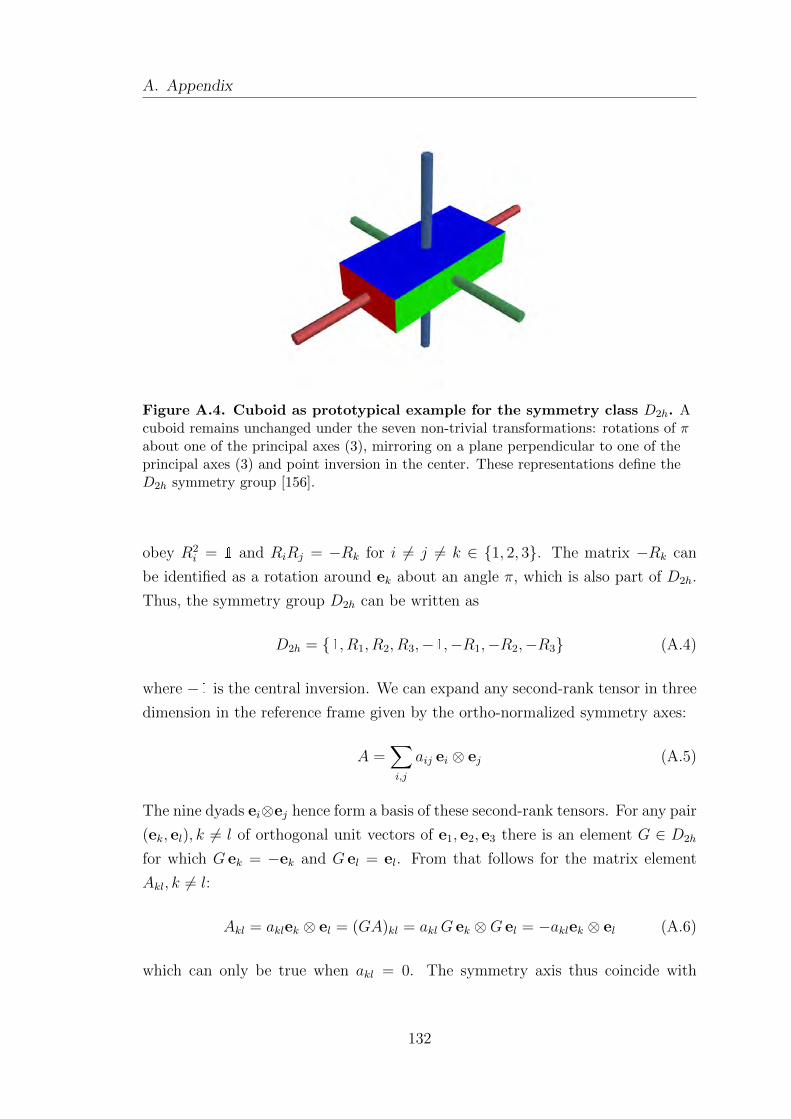
A. Appendix

Figure A.4. Cuboid as prototypical example for the symmetry class D2h. Acuboid remains unchanged under the seven non-trivial transformations: rotations of πabout one of the principal axes (3), mirroring on a plane perpendicular to one of theprincipal axes (3) and point inversion in the center. These representations define theD2h symmetry group [156].

obey R2i = 1 and RiRj = −Rk for i 6= j 6= k ∈ 1, 2, 3. The matrix −Rk can

be identified as a rotation around ek about an angle π, which is also part of D2h.

Thus, the symmetry group D2h can be written as

D2h = 1, R1, R2, R3,−1,−R1,−R2,−R3 (A.4)

where −1 is the central inversion. We can expand any second-rank tensor in three

dimension in the reference frame given by the ortho-normalized symmetry axes:

A =∑i,j

aij ei ⊗ ej (A.5)

The nine dyads ei⊗ej hence form a basis of these second-rank tensors. For any pair

(ek, el), k 6= l of orthogonal unit vectors of e1, e2, e3 there is an element G ∈ D2h

for which G ek = −ek and G el = el. From that follows for the matrix element

Akl, k 6= l:

Akl = aklek ⊗ el = (GA)kl = aklG ek ⊗G el = −aklek ⊗ el (A.6)

which can only be true when akl = 0. The symmetry axis thus coincide with

132

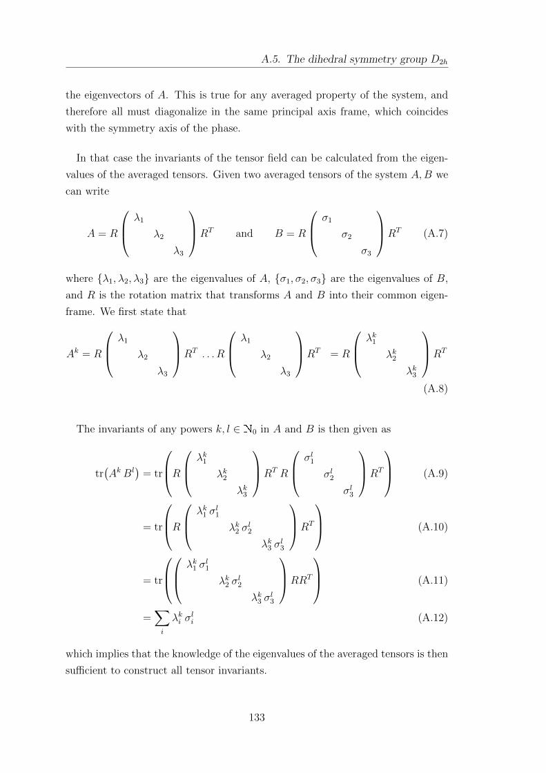
A.5. The dihedral symmetry group D2h

the eigenvectors of A. This is true for any averaged property of the system, and

therefore all must diagonalize in the same principal axis frame, which coincides

with the symmetry axis of the phase.

In that case the invariants of the tensor field can be calculated from the eigen-

values of the averaged tensors. Given two averaged tensors of the system A,B we

can write

A = R

λ1

λ2

λ3

RT and B = R

σ1

σ2

σ3

RT (A.7)

where λ1, λ2, λ3 are the eigenvalues of A, σ1, σ2, σ3 are the eigenvalues of B,

and R is the rotation matrix that transforms A and B into their common eigen-

frame. We first state that

Ak = R

λ1

λ2

λ3

RT . . . R

λ1

λ2

λ3

RT = R

λk1

λk2

λk3

RT

(A.8)

The invariants of any powers k, l ∈ N0 in A and B is then given as

tr(Ak Bl

)= tr

R λk1

λk2

λk3

RT R

σl1

σl2

σl3

RT

(A.9)

= tr

R λk1 σ

l1

λk2 σl2

λk3 σl3

RT

(A.10)

= tr

λk1 σ

l1

λk2 σl2

λk3 σl3

RRT

(A.11)

=∑i

λki σli (A.12)

which implies that the knowledge of the eigenvalues of the averaged tensors is then

sufficient to construct all tensor invariants.

133

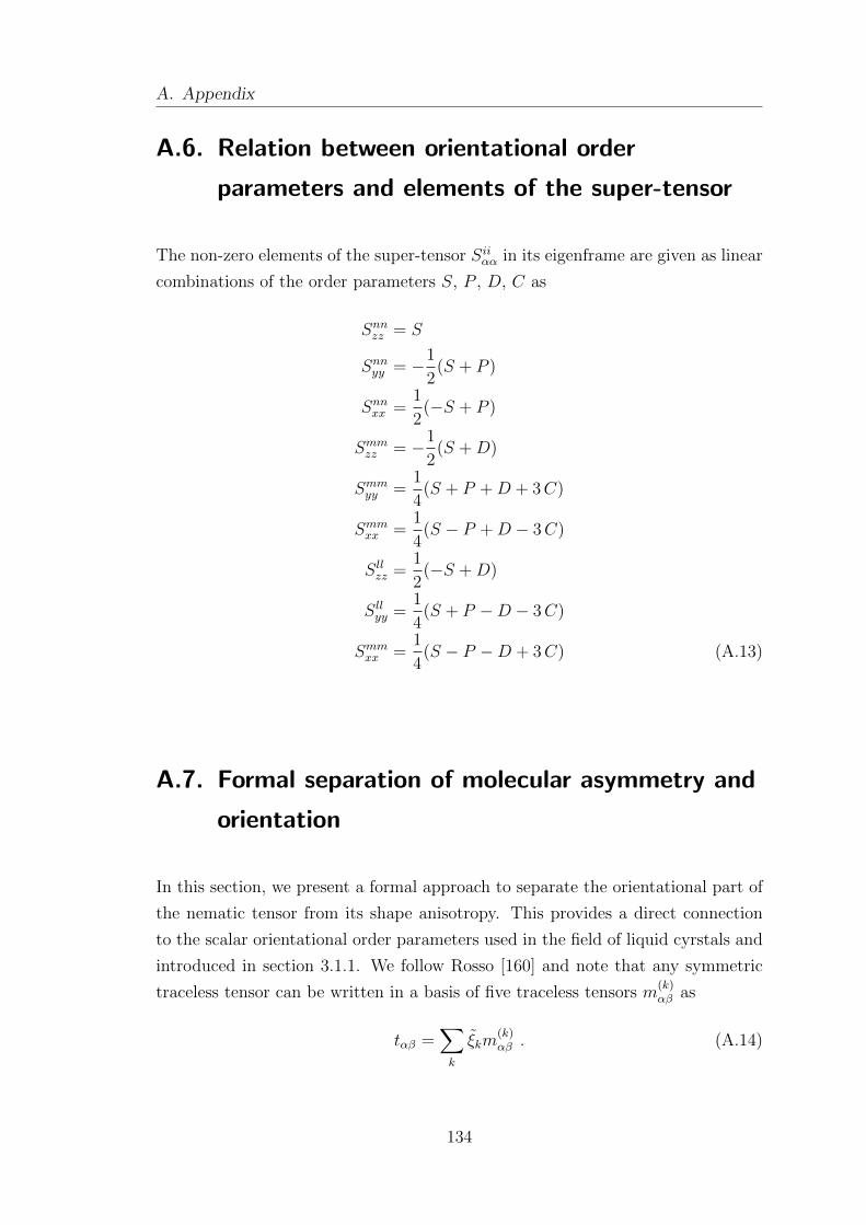
A. Appendix

A.6. Relation between orientational order

parameters and elements of the super-tensor

The non-zero elements of the super-tensor Siiαα in its eigenframe are given as linear

combinations of the order parameters S, P , D, C as

Snnzz = S

Snnyy = −1

2(S + P )

Snnxx =1

2(−S + P )

Smmzz = −1

2(S +D)

Smmyy =1

4(S + P +D + 3C)

Smmxx =1

4(S − P +D − 3C)

Sllzz =1

2(−S +D)

Sllyy =1

4(S + P −D − 3C)

Smmxx =1

4(S − P −D + 3C) (A.13)

A.7. Formal separation of molecular asymmetry and

orientation

In this section, we present a formal approach to separate the orientational part of

the nematic tensor from its shape anisotropy. This provides a direct connection

to the scalar orientational order parameters used in the field of liquid cyrstals and

introduced in section 3.1.1. We follow Rosso [160] and note that any symmetric

traceless tensor can be written in a basis of five traceless tensors m(k)αβ as

tαβ =∑k

ξkm(k)αβ . (A.14)

134

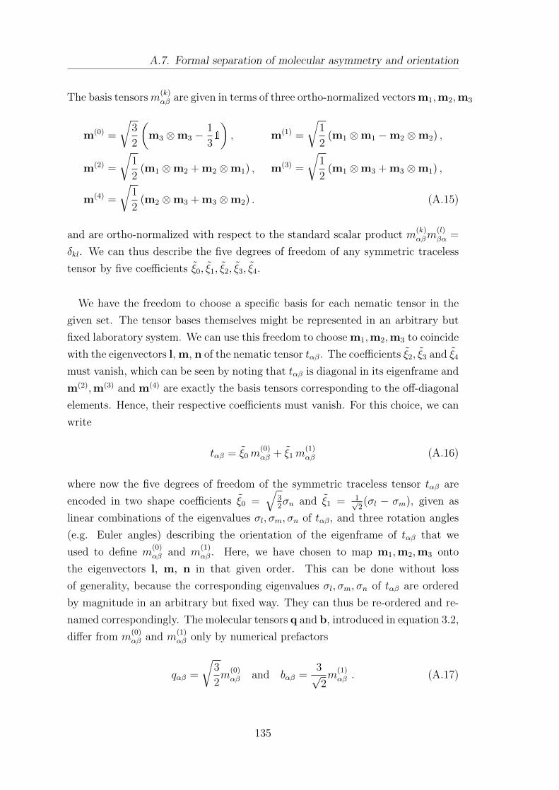
A.7. Formal separation of molecular asymmetry and orientation

The basis tensorsm(k)αβ are given in terms of three ortho-normalized vectors m1,m2,m3

m(0) =

√3

2

(m3 ⊗m3 −

1

31

), m(1) =

√1

2(m1 ⊗m1 −m2 ⊗m2) ,

m(2) =

√1

2(m1 ⊗m2 + m2 ⊗m1) , m(3) =

√1

2(m1 ⊗m3 + m3 ⊗m1) ,

m(4) =

√1

2(m2 ⊗m3 + m3 ⊗m2) . (A.15)

and are ortho-normalized with respect to the standard scalar product m(k)αβm

(l)βα =

δkl. We can thus describe the five degrees of freedom of any symmetric traceless

tensor by five coefficients ξ0, ξ1, ξ2, ξ3, ξ4.

We have the freedom to choose a specific basis for each nematic tensor in the

given set. The tensor bases themselves might be represented in an arbitrary but

fixed laboratory system. We can use this freedom to choose m1,m2,m3 to coincide

with the eigenvectors l, m, n of the nematic tensor tαβ. The coefficients ξ2, ξ3 and ξ4

must vanish, which can be seen by noting that tαβ is diagonal in its eigenframe and

m(2),m(3) and m(4) are exactly the basis tensors corresponding to the off-diagonal

elements. Hence, their respective coefficients must vanish. For this choice, we can

write

tαβ = ξ0m(0)αβ + ξ1m

(1)αβ (A.16)

where now the five degrees of freedom of the symmetric traceless tensor tαβ are

encoded in two shape coefficients ξ0 =√

32σn and ξ1 = 1√

2(σl − σm), given as

linear combinations of the eigenvalues σl, σm, σn of tαβ, and three rotation angles

(e.g. Euler angles) describing the orientation of the eigenframe of tαβ that we

used to define m(0)αβ and m

(1)αβ . Here, we have chosen to map m1,m2,m3 onto

the eigenvectors l, m, n in that given order. This can be done without loss

of generality, because the corresponding eigenvalues σl, σm, σn of tαβ are ordered

by magnitude in an arbitrary but fixed way. They can thus be re-ordered and re-

named correspondingly. The molecular tensors q and b, introduced in equation 3.2,

differ from m(0)αβ and m

(1)αβ only by numerical prefactors

qαβ =

√3

2m

(0)αβ and bαβ =

3√2m

(1)αβ . (A.17)

135

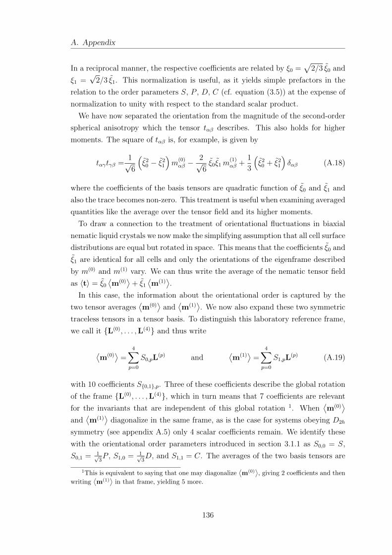
A. Appendix

In a reciprocal manner, the respective coefficients are related by ξ0 =√

2/3 ξ0 and

ξ1 =√

2/3 ξ1. This normalization is useful, as it yields simple prefactors in the

relation to the order parameters S, P , D, C (cf. equation (3.5)) at the expense of

normalization to unity with respect to the standard scalar product.

We have now separated the orientation from the magnitude of the second-order

spherical anisotropy which the tensor tαβ describes. This also holds for higher

moments. The square of tαβ is, for example, is given by

tαγtγβ =1√6

(ξ2

0 − ξ21

)m

(0)αβ −

2√6ξ0ξ1m

(1)αβ +

1

3

(ξ2

0 + ξ21

)δαβ (A.18)

where the coefficients of the basis tensors are quadratic function of ξ0 and ξ1 and

also the trace becomes non-zero. This treatment is useful when examining averaged

quantities like the average over the tensor field and its higher moments.

To draw a connection to the treatment of orientational fluctuations in biaxial

nematic liquid crystals we now make the simplifying assumption that all cell surface

distributions are equal but rotated in space. This means that the coefficients ξ0 and

ξ1 are identical for all cells and only the orientations of the eigenframe described

by m(0) and m(1) vary. We can thus write the average of the nematic tensor field

as 〈t〉 = ξ0

⟨m(0)

⟩+ ξ1

⟨m(1)

⟩.

In this case, the information about the orientational order is captured by the

two tensor averages⟨m(0)

⟩and

⟨m(1)

⟩. We now also expand these two symmetric

traceless tensors in a tensor basis. To distinguish this laboratory reference frame,

we call it L(0), . . . ,L(4) and thus write

⟨m(0)

⟩=

4∑p=0

S0,pL(p) and

⟨m(1)

⟩=

4∑p=0

S1,pL(p) (A.19)

with 10 coefficients S0,1,p. Three of these coefficients describe the global rotation

of the frame L(0), . . . ,L(4), which in turn means that 7 coefficients are relevant

for the invariants that are independent of this global rotation 1. When⟨m(0)

⟩and

⟨m(1)

⟩diagonalize in the same frame, as is the case for systems obeying D2h

symmetry (see appendix A.5) only 4 scalar coefficients remain. We identify these

with the orientational order parameters introduced in section 3.1.1 as S0,0 = S,

S0,1 = 1√3P , S1,0 = 1√

3D, and S1,1 = C. The averages of the two basis tensors are

1This is equivalent to saying that one may diagonalize⟨m(0)

⟩, giving 2 coefficients and then

writing⟨m(1)

⟩in that frame, yielding 5 more.

136

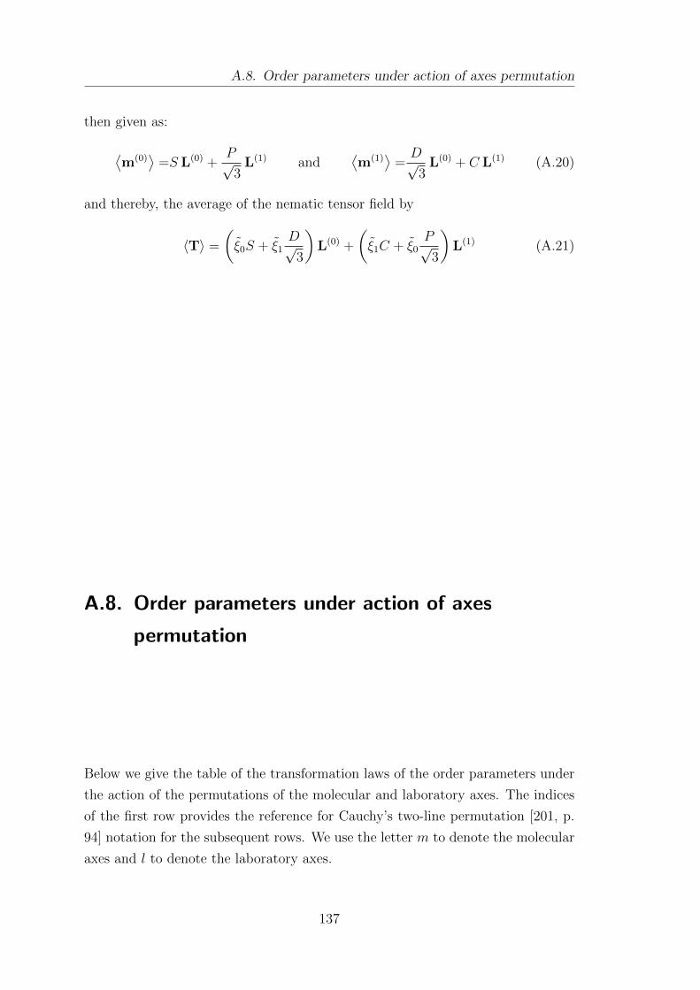
A.8. Order parameters under action of axes permutation

then given as:

⟨m(0)

⟩=S L(0) +

P√3

L(1) and⟨m(1)

⟩=D√

3L(0) + C L(1) (A.20)

and thereby, the average of the nematic tensor field by

〈T〉 =

(ξ0S + ξ1

D√3

)L(0) +

(ξ1C + ξ0

P√3

)L(1) (A.21)

A.8. Order parameters under action of axes

permutation

Below we give the table of the transformation laws of the order parameters under

the action of the permutations of the molecular and laboratory axes. The indices

of the first row provides the reference for Cauchy’s two-line permutation [201, p.

94] notation for the subsequent rows. We use the letter m to denote the molecular

axes and l to denote the laboratory axes.

137

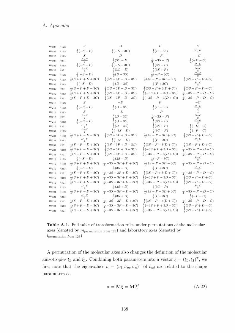
A. Appendix

m123 l123 S D P C

m123 l13212

(−S − P ) 12

(−D − 3C) 12

(P − 3S) C−D2

m123 l213 S D −P −Cm123 l231

P−S2

12

(3C −D) 12

(−3S − P ) 12

(−D − C)

m123 l31212

(−S − P ) 12

(−D − 3C) 12

(3S − P ) D−C2

m123 l321P−S

212

(3C −D) 12

(3S + P ) D+C2

m132 l12312

(−S −D) 12

(D − 3S) 12

(−P − 3C) C−P2

m132 l13214

(S + P +D + 3C) 14

(3S + 3P −D − 3C) 14

(3S − P + 3D − 3C) 14

(3S − P −D + C)

m132 l21312

(−S −D) 12

(D − 3S) 12

(P + 3C) P−C2

m132 l23114

(S − P +D − 3C) 14

(3S − 3P −D + 3C) 14

(3S + P + 3(D + C)) 14

(3S + P −D − C)

m132 l31214

(S + P +D + 3C) 14

(3S + 3P −D − 3C) 14

(−3S + P − 3D + 3C) 14

(−3S + P +D − C)

m132 l32114

(S − P +D − 3C) 14

(3S − 3P −D + 3C) 14

(−3S − P − 3(D + C)) 14

(−3S − P +D + C)

m213 l123 S −D P −Cm213 l132

12

(−S − P ) 12

(D + 3C) 12

(P − 3S) D−C2

m213 l213 S −D −P C

m213 l231P−S

212

(D − 3C) 12

(−3S − P ) D+C2

m213 l31212

(−S − P ) 12

(D + 3C) 12

(3S − P ) C−D2

m213 l321P−S

212

(D − 3C) 12

(3S + P ) 12

(−D − C)

m231 l123D−S

212

(−3S −D) 12

(3C − P ) 12

(−P − C)

m231 l13214

(S + P −D − 3C) 14

(3S + 3P +D + 3C) 14

(3S − P − 3D + 3C) 14

(3S − P +D − C)

m231 l213D−S

212

(−3S −D) 12

(P − 3C) P+C2

m231 l23114

(S − P −D + 3C) 14

(3S − 3P +D − 3C) 14

(3S + P − 3(D + C)) 14

(3S + P +D + C)

m231 l31214

(S + P −D − 3C) 14

(3S + 3P +D + 3C) 14

(−3S + P + 3D − 3C) 14

(−3S + P −D + C)

m231 l32114

(S − P −D + 3C) 14

(3S − 3P +D − 3C) 14

(−3S − P + 3(D + C)) 14

(−3S − P −D − C)

m312 l12312

(−S −D) 12

(3S −D) 12

(−P − 3C) P−C2

m312 l13214

(S + P +D + 3C) 14

(−3S − 3P +D + 3C) 14

(3S − P + 3D − 3C) 14

(−3S + P +D − C)

m312 l21312

(−S −D) 12

(3S −D) 12

(P + 3C) C−P2

m312 l23114

(S − P +D − 3C) 14

(−3S + 3P +D − 3C) 14

(3S + P + 3(D + C)) 14

(−3S − P +D + C)

m312 l31214

(S + P +D + 3C) 14

(−3S − 3P +D + 3C) 14

(−3S + P − 3D + 3C) 14

(3S − P −D + C)

m312 l32114

(S − P +D − 3C) 14

(−3S + 3P +D − 3C) 14

(−3S − P − 3(D + C)) 14

(3S + P −D − C)

m321 l123D−S

212

(3S +D) 12

(3C − P ) P+C2

m321 l13214

(S + P −D − 3C) 14

(−3S − 3P −D − 3C) 14

(3S − P − 3D + 3C) 14

(−3S + P −D + C)

m321 l213D−S

212

(3S +D) 12

(P − 3C) 12

(−P − C)

m321 l23114

(S − P −D + 3C) 14

(−3S + 3P −D + 3C) 14

(3S + P − 3(D + C)) 14

(−3S − P −D − C)

m321 l31214

(S + P −D − 3C) 14

(−3S − 3P −D − 3C) 14

(−3S + P + 3D − 3C) 14

(3S − P +D − C)

m321 l32114

(S − P −D + 3C) 14

(−3S + 3P −D + 3C) 14

(−3S − P + 3(D + C)) 14

(3S + P +D + C)

Table A.1. Full table of transformation rules under permutations of the molecularaxes (denoted by mpermutation from 123) and laboratory axes (denoted bylpermutation from 123)

A permutation of the molecular axes also changes the definition of the molecular

anisotropies ξ0 and ξ1. Combining both parameters into a vector ξ = (ξ0, ξ1)T , we

first note that the eigenvalues σ = (σl, σm, σn)T of tαβ are related to the shape

parameters as

σ = Mξ = M′ξ′ (A.22)

138

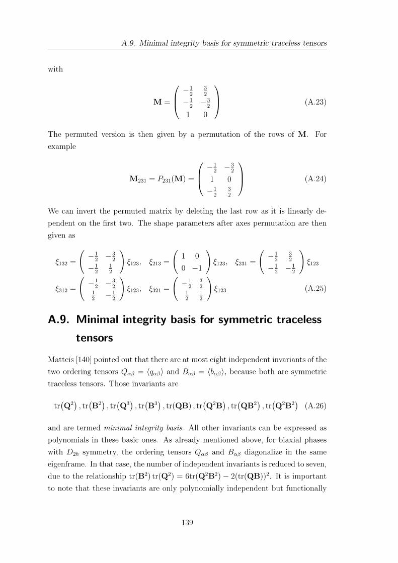
A.9. Minimal integrity basis for symmetric traceless tensors

with

M =

−12

32

−12−3

2

1 0

(A.23)

The permuted version is then given by a permutation of the rows of M. For

example

M231 = P231(M) =

−12−3

2

1 0

−12

32

(A.24)

We can invert the permuted matrix by deleting the last row as it is linearly de-

pendent on the first two. The shape parameters after axes permutation are then

given as

ξ132 =

(−1

2−3

2

−12

12

)ξ123, ξ213 =

(1 0

0 −1

)ξ123, ξ231 =

(−1

232

−12−1

2

)ξ123

ξ312 =

(−1

2−3

212−1

2

)ξ123, ξ321 =

(−1

232

12

12

)ξ123 (A.25)

A.9. Minimal integrity basis for symmetric traceless

tensors

Matteis [140] pointed out that there are at most eight independent invariants of the

two ordering tensors Qαβ = 〈qαβ〉 and Bαβ = 〈bαβ〉, because both are symmetric

traceless tensors. Those invariants are

tr(Q2), tr(B2), tr(Q3), tr(B3), tr(QB) , tr

(Q2B

), tr(QB2

), tr(Q2B2

)(A.26)

and are termed minimal integrity basis. All other invariants can be expressed as

polynomials in these basic ones. As already mentioned above, for biaxial phases

with D2h symmetry, the ordering tensors Qαβ and Bαβ diagonalize in the same

eigenframe. In that case, the number of independent invariants is reduced to seven,

due to the relationship tr(B2) tr(Q2) = 6tr(Q2B2) − 2(tr(QB))2. It is important

to note that these invariants are only polynomially independent but functionally

139

A. Appendix

dependent. The functional dependence results from the fact that they can be given

as polynomials in the four order parameters S, P,D,C. These seven invariants are

thus particular polynomials in S, P,D,C from which any function that obeys the

D2h symmetry of the objects and the phase can be constructed.

The averaged moment tensors T and V (cf. section 3.1.3) can be written as a

linear combination of the ordering tensors Qαβ, Bαβ and the identity matrix, as

shown in section 3.1.4. The minimal number of moments needed to describe the

system is met, when they can express all elements of the minimal integrity basis.

In general, taking the first and second moment is sufficient (cf. equation (3.15)).

140

A.10. Discretization of distortion free energy on cubic lattice

A.10. Discretization of distortion free energy on

cubic lattice

The Frank distortion free energy in tensorial form is given by (cf. equation (5.2))

Fd =

∫d3r

1

4K (∂γNαβ)2 . (A.27)

To discretize this free energy, we approximate the partial derivatives with finite

differences

∂γNαβ =Nαβ(r + a eγ)−Nαβ(r)

a(A.28)

which yields for the squared gradient term

(∂γNαβ)2 = − 2

a2

∑αβγ

Nαβ(r + a eγ)Nαβ(r) + const . (A.29)

Aligning the cubic lattice with the directions of the reference frame a ex, a ey, a ezand further approximating the volume integral by a sum over lattice vectors r with

substituting∫

d3r −→ a3∑

r, we see that

Fd =

∫d3r

1

4K (∂γNαβ)2 ≈− K a

2

∑r

∑αβγ

Nαβ(r + a eγ)Nαβ(r) + const

=− K a

2

∑<i,j>

N(i)αβN

(j)αβ + const (A.30)

where < i, j > runs over all pairs of neighbors on the cubic lattice.

141

A. Appendix

A.11. Metropolis Algorithm for uniaxial cell polarity

coordination

The Metropolis algorithm was first published by Nicholas Metropolis et al. in

1953 [202]. It is used to create a Markov chain and with it the states of a system

according to the Boltzmann distribution. The new state of the system does only

depend on the current state. The definition of the algorithm as it is used here, can

be found below. Note, that the unit vector n′ created in step 3 must be chosen

from the uniform distribution on the surface of the unit sphere. The random value

r in step 6 must be chosen from the uniform distribution in the interval [0, 1].

Algorithm 1 (Metropolis algorithm for uniaxial interaction model)

1. Choose an initial state

2. Choose a random lattice site i that is not fixed by boundaries

3. Generate a random unit vector n′

4. Calculate the energy change ∆F that results if the vector n(i) at site i is

replaced by the new direction n′.

5. If ∆F ≤ 0, accept the proposed new direction n′ for the lattice site i and go

to step 2

6. If ∆F > 0, draw r from the uniform distribution in the interval [0, 1]

7. If r < exp(−∆Fν

), accept the proposed new direction n′ for the lattice site i

8. Go to step 2

Unit vectors with isotropic orientational distribution are generated by obtaining

three independent coordinates from the normal distribution and then normalizing

the resulting vector to unit length. One Monte-Carlo step (MCS) is defined as

N Metropolis steps, where N denotes the number of lattice sites excluding those

fixed by boundary conditions. One Metropolis step is defined as one proposed new

direction (doing steps 2 to 7 of algorithm 1 once). Note that a rejected proposal

is counted as one Metropolis step as well.

142

A.12. States in the zero-noise limit of the nearest-neighbor interaction model

A.12. States in the zero-noise limit of the

nearest-neighbor interaction model

This section provides details of the algorithms used to find the states in the

zero-noise strength limit of the uniaxial nearest-neighbor interaction model pre-

sented in section 5.3.2. Namely, two strategies were used. First, the system

was initialized with random director orientations and gradually “cooled” down

towards smaller noise strengths. The steps of noise strength used were ν/ε =

10., 5.0, 2.0, 1.0, 0.5, 0.2, 0.1, 0.05, 0.02, 0.01. For each value of the noise strength,

25000 Monte Carlo steps (MCS) were performed2 and the last configuration at one

noise strength was used as the first configuration for the subsequent lower noise

strength. In the second strategy, the system was initialized with all the directors

aligned to the lobule-level reference field eχ. Then, 50000 MCS were performed

at a relatively small noise strength of ν/ε = 0.01. This procedure provided two

candidates for the potential states for the zero-noise strength limit of the system.

In general, it is not guaranteed that the found state corresponds to the smallest

effective energy of the system. However, for sake of practicality, we refer to the

lower-energy state of the two candidates as the state for the zero-noise strength

limit. An overview over the resulting energies for different data sets is provided in

Fig. A.5.

2One MCS consists of N Metropolis steps, where N is the number of free directors in thesystem, see section A.11 for details.

143

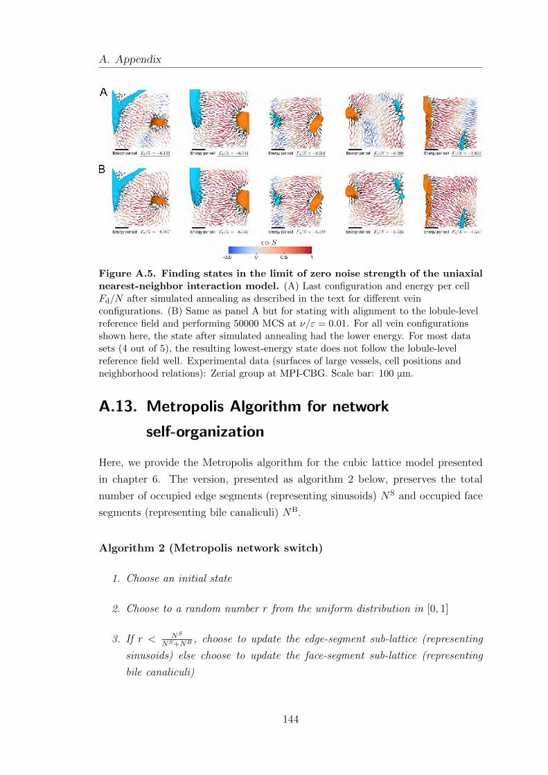
A. Appendix

Figure A.5. Finding states in the limit of zero noise strength of the uniaxialnearest-neighbor interaction model. (A) Last configuration and energy per cellFd/N after simulated annealing as described in the text for different veinconfigurations. (B) Same as panel A but for stating with alignment to the lobule-levelreference field and performing 50000 MCS at ν/ε = 0.01. For all vein configurationsshown here, the state after simulated annealing had the lower energy. For most datasets (4 out of 5), the resulting lowest-energy state does not follow the lobule-levelreference field well. Experimental data (surfaces of large vessels, cell positions andneighborhood relations): Zerial group at MPI-CBG. Scale bar: 100 μm.

A.13. Metropolis Algorithm for network

self-organization

Here, we provide the Metropolis algorithm for the cubic lattice model presented

in chapter 6. The version, presented as algorithm 2 below, preserves the total

number of occupied edge segments (representing sinusoids) NS and occupied face

segments (representing bile canaliculi) NB.

Algorithm 2 (Metropolis network switch)

1. Choose an initial state

2. Choose to a random number r from the uniform distribution in [0, 1]

3. If r < NS

NS+NB , choose to update the edge-segment sub-lattice (representing

sinusoids) else choose to update the face-segment sub-lattice (representing

bile canaliculi)

144

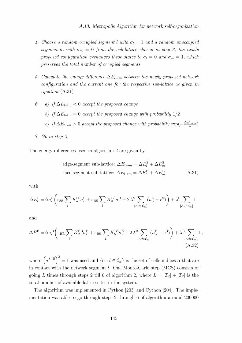
A.13. Metropolis Algorithm for network self-organization

4. Choose a random occupied segment l with σl = 1 and a random unoccupied

segment m with σm = 0 from the sub-lattice chosen in step 3, the newly

proposed configuration exchanges these states to σl = 0 and σm = 1, which

preserves the total number of occupied segments

5. Calculate the energy difference ∆El→m between the newly proposed network

configuration and the current one for the respective sub-lattice as given in

equation (A.31)

6. a) If ∆El→m < 0 accept the proposed change

b) If ∆El→m = 0 accept the proposed change with probability 1/2

c) If ∆El→m > 0 accept the proposed change with probability exp(−∆El→mν

)

7. Go to step 2

The energy differences used in algorithm 2 are given by

edge-segment sub-lattice: ∆El→m = ∆ESl + ∆ES

m

face-segment sub-lattice: ∆El→m = ∆EBl + ∆EB

m (A.31)

with

∆ESl =∆σS

l

(εSS

∑i

KSSil σ

Si + εBS

∑i

KBSil σ

Bi + 2λS

∑α:l∈Cα

(nSα − cS)

)+ λS

∑α:l∈Cα

1

and

∆EBl =∆σB

l

(εBB

∑i

KBBil σ

Bi + εBS

∑i

KBSli σ

Si + 2λB

∑α:l∈Cα

(nBα − cB)

)+ λB

∑α:l∈Cα

1 ,

(A.32)

where(σS, Bl

)2

= 1 was used and α : l ∈ Cα is the set of cells indices α that are

in contact with the network segment l. One Monte-Carlo step (MCS) consists of

going L times through steps 2 till 6 of algorithm 2, where L = |IE| + |IF| is the

total number of available lattice sites in the system.

The algorithm was implemented in Python [203] and Cython [204]. The imple-

mentation was able to go through steps 2 through 6 of algorithm around 200000

145

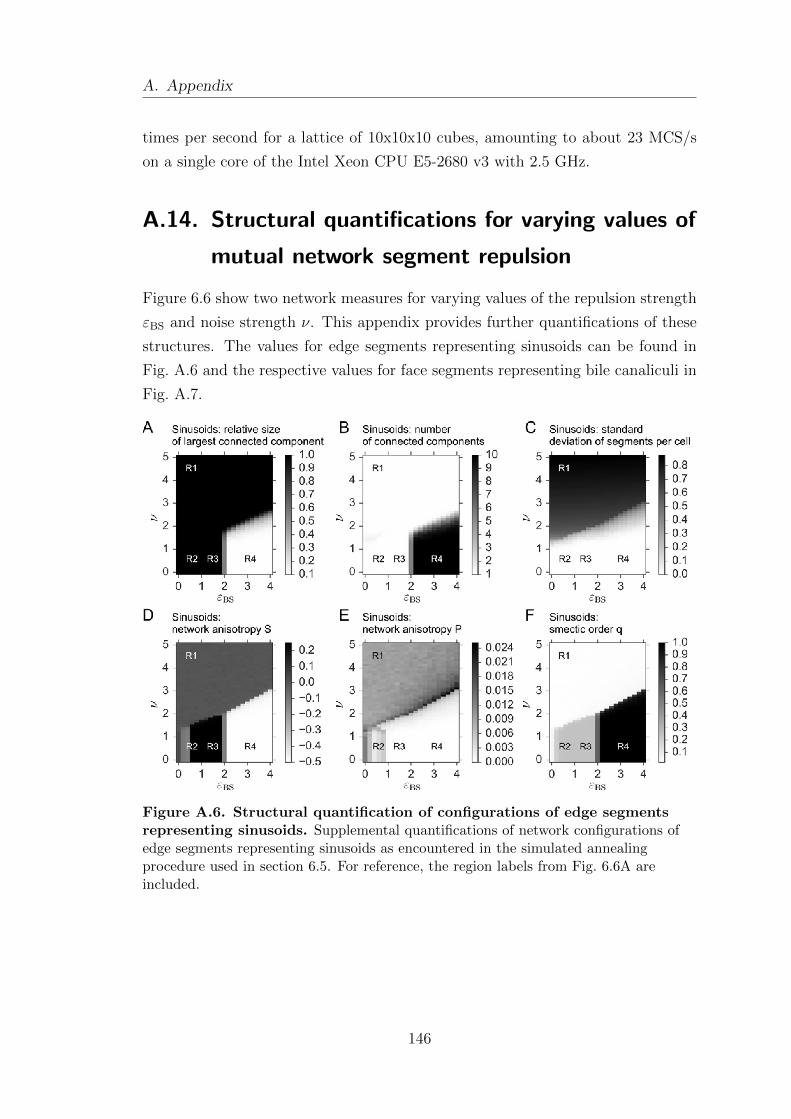
A. Appendix

times per second for a lattice of 10x10x10 cubes, amounting to about 23 MCS/s

on a single core of the Intel Xeon CPU E5-2680 v3 with 2.5 GHz.

A.14. Structural quantifications for varying values of

mutual network segment repulsion

Figure 6.6 show two network measures for varying values of the repulsion strength

εBS and noise strength ν. This appendix provides further quantifications of these

structures. The values for edge segments representing sinusoids can be found in

Fig. A.6 and the respective values for face segments representing bile canaliculi in

Fig. A.7.

Figure A.6. Structural quantification of configurations of edge segmentsrepresenting sinusoids. Supplemental quantifications of network configurations ofedge segments representing sinusoids as encountered in the simulated annealingprocedure used in section 6.5. For reference, the region labels from Fig. 6.6A areincluded.

146

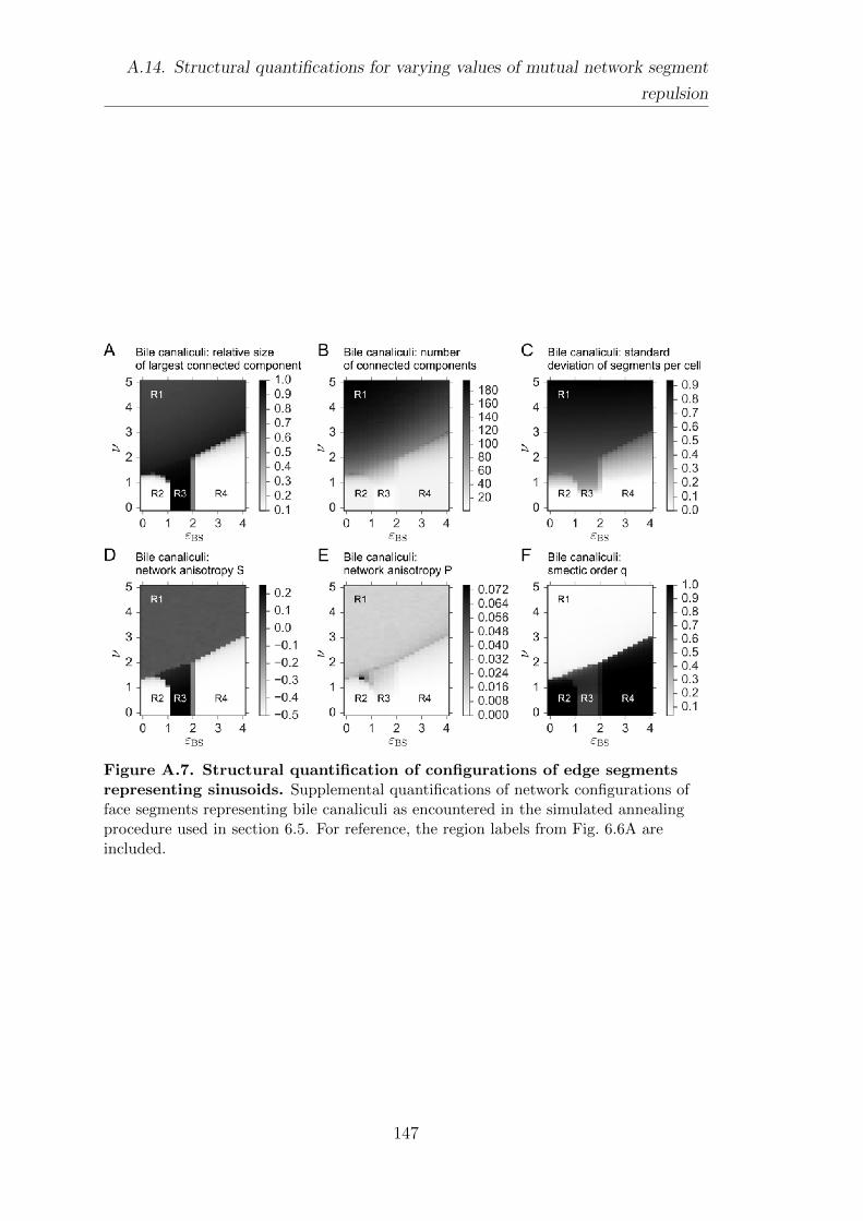
A.14. Structural quantifications for varying values of mutual network segment

repulsion

Figure A.7. Structural quantification of configurations of edge segmentsrepresenting sinusoids. Supplemental quantifications of network configurations offace segments representing bile canaliculi as encountered in the simulated annealingprocedure used in section 6.5. For reference, the region labels from Fig. 6.6A areincluded.

147

A. Appendix

A.15. Structural quantifications for varying values of

self-attraction of network segments

This appendix provides network measures for varying values of the self-attraction

parameters εSS = εBB and noise strength ν. The values for edge segments rep-

resenting sinusoids can be found in Fig. A.8 and the respective values for face

segments representing bile canaliculi in Fig. A.9.

Figure A.8. Structural quantification of configurations of edge segmentsrepresenting sinusoids. Quantifications of network configurations of edge segmentsrepresenting sinusoids as encountered in a simulated annealing procedure as explainedin section 6.5. Here, the interaction parameter for self-attraction εSS = εBB are variedinstead.

148

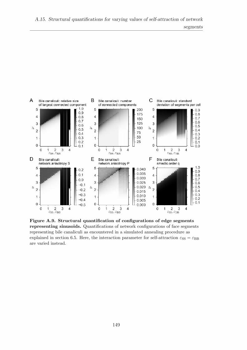
A.15. Structural quantifications for varying values of self-attraction of network

segments

Figure A.9. Structural quantification of configurations of edge segmentsrepresenting sinusoids. Quantifications of network configurations of face segmentsrepresenting bile canaliculi as encountered in a simulated annealing procedure asexplained in section 6.5. Here, the interaction parameter for self-attraction εSS = εBB

are varied instead.

149

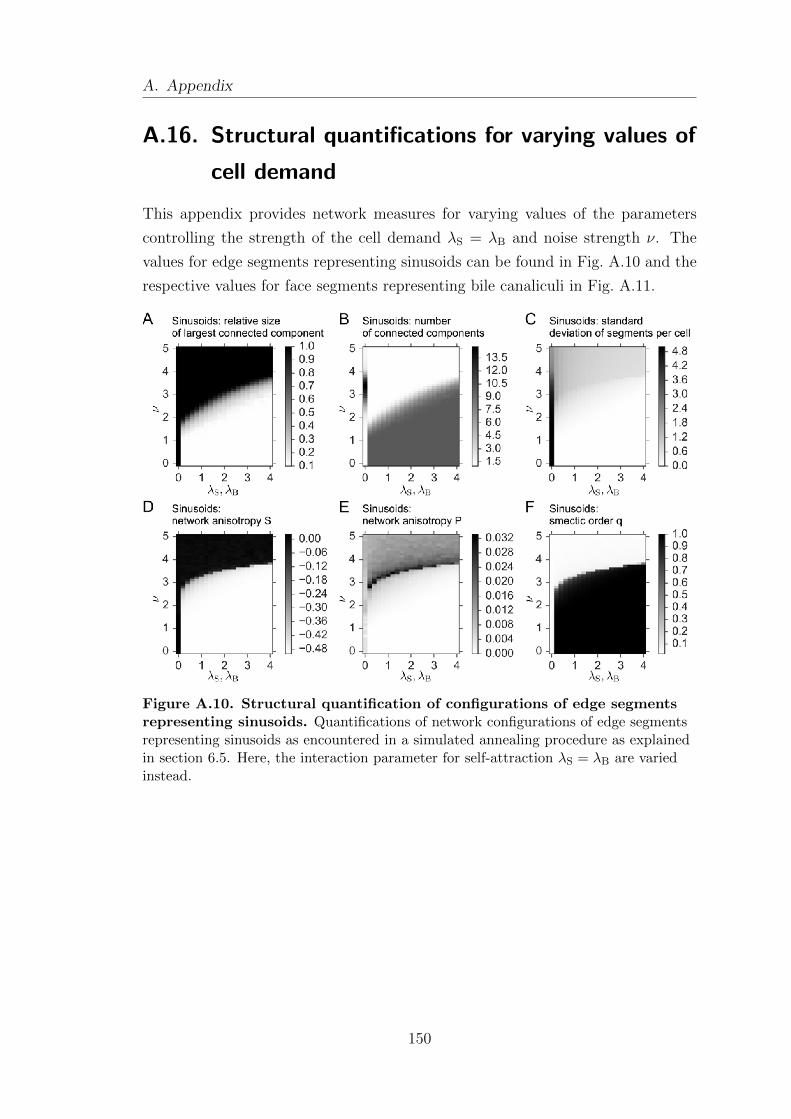
A. Appendix

A.16. Structural quantifications for varying values of

cell demand

This appendix provides network measures for varying values of the parameters

controlling the strength of the cell demand λS = λB and noise strength ν. The

values for edge segments representing sinusoids can be found in Fig. A.10 and the

respective values for face segments representing bile canaliculi in Fig. A.11.

Figure A.10. Structural quantification of configurations of edge segmentsrepresenting sinusoids. Quantifications of network configurations of edge segmentsrepresenting sinusoids as encountered in a simulated annealing procedure as explainedin section 6.5. Here, the interaction parameter for self-attraction λS = λB are variedinstead.

150

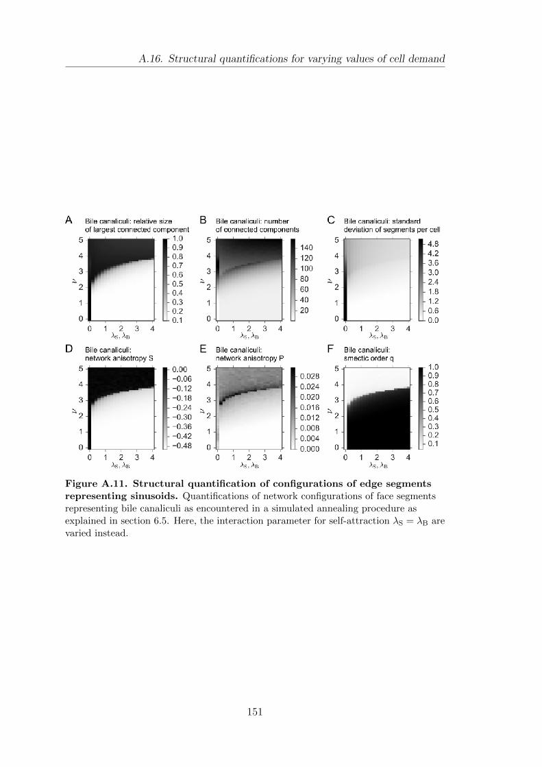
A.16. Structural quantifications for varying values of cell demand

Figure A.11. Structural quantification of configurations of edge segmentsrepresenting sinusoids. Quantifications of network configurations of face segmentsrepresenting bile canaliculi as encountered in a simulated annealing procedure asexplained in section 6.5. Here, the interaction parameter for self-attraction λS = λB arevaried instead.

151

Bibliography

1. Alberts, B., Johnson, A., Lewis, J., Raff, M., Roberts, K. & Walter, P.

Molecular Biology of the Cell 4th ed.

(Garland Science, New York, NY, USA, 2002) (cit. on pp. 1, 7, 9).

2. Bryant, D. M. & Mostov, K. E.

From cells to organs: building polarized tissue.

Nature Reviews Molecular Cell Biology 9. doi:10.1038/nrm2523 (2008)

(cit. on pp. 1, 7, 8, 16).

3. Van Lommel, A. T. L. From Cells to Organs

doi:10.1007/978-1-4615-0353-8 (Springer US, Boston, MA, 2003)

(cit. on pp. 1–3, 5, 7, 8).

4. OpenStax. Anatomy and Physiology 2016.

https://opentextbc.ca/anatomyandphysiology/ (2017) (cit. on p. 1).

5. Elias, H. & Bengelsdorf, H. The Structure of the Liver of Vertebrates.

Cells Tissues Organs 14. doi:10.1159/000140715 (1952) (cit. on p. 2).

6. Hendriks, H., Verhoofstad, W., Brouwer, A., De Leeuw, A. & Knook, D.

Perisinusoidal fat-storing cells are the main vitamin A storage sites in rat

liver. Experimental Cell Research 160.

doi:10.1016/0014-4827(85)90243-5 (1985) (cit. on p. 2).

7. Schleicher, J., Tokarski, C., Marbach, E., Matz-Soja, M., Zellmer, S.,

Gebhardt, R. & Schuster, S. Zonation of hepatic fatty acid metabolism —

The diversity of its regulation and the benefit of modeling. Biochimica et

Biophysica Acta (BBA) - Molecular and Cell Biology of Lipids 1851.

doi:10.1016/j.bbalip.2015.02.004 (2015) (cit. on p. 2).

8. Yamamoto, M. et al. SIRT1 regulates adaptive response of the growth

hormone–insulin-like growth factor-I axis under fasting conditions in liver.

Proceedings of the National Academy of Sciences 110.

doi:10.1073/pnas.1220606110 (2013) (cit. on p. 3).

152

9. Van den Eynden, G. G. et al. The Multifaceted Role of the

Microenvironment in Liver Metastasis: Biology and Clinical Implications.

Cancer Research 73. doi:10.1158/0008-5472.CAN-12-3931 (2013)

(cit. on p. 3).

10. Zorn. Liver Development. StemBook. doi:10.3824/stembook.1.25.1

(2008) (cit. on p. 3).

11. Boyer, J. L. Bile Formation and Secretion. In Comprehensive Physiology

(John Wiley & Sons, Inc., Hoboken, NJ, USA, 2013).

doi:10.1002/cphy.c120027 (cit. on p. 3).

12. Michalopoulos, G. K. Liver Regeneration after Partial Hepatectomy.

The American Journal of Pathology 176.

doi:10.2353/ajpath.2010.090675 (2010) (cit. on p. 3).

13. Thomas, R. J., Bhandari, R., Barrett, D. A., Bennett, A. J., Fry, J. R.,

Powe, D., Thomson, B. J. & Shakesheff, K. M.

The Effect of Three-Dimensional Co-Culture of Hepatocytes and Hepatic

Stellate Cells on Key Hepatocyte Functions in vitro.

Cells Tissues Organs 181. doi:10.1159/000091096 (2005) (cit. on p. 3).

14. Godoy, P. et al. Recent advances in 2D and 3D in vitro systems using

primary hepatocytes, alternative hepatocyte sources and non-parenchymal

liver cells and their use in investigating mechanisms of hepatotoxicity, cell

signaling and ADME. Archives of Toxicology 87.

doi:10.1007/s00204-013-1078-5 (2013) (cit. on pp. 3, 13, 14).

15. Baptista, P. M., Siddiqui, M. M., Lozier, G., Rodriguez, S. R., Atala, A. &

Soker, S. The use of whole organ decellularization for the generation of a

vascularized liver organoid. Hepatology 53. doi:10.1002/hep.24067 (2011)

(cit. on p. 3).

16. Ho, C.-T. et al. Liver-cell patterning Lab Chip: mimicking the morphology

of liver lobule tissue. Lab on a Chip 13. doi:10.1039/c3lc50402f (2013)

(cit. on p. 3).

17. Montanez-Sauri, S. I., Beebe, D. J. & Sung, K. E.

Microscale screening systems for 3D cellular microenvironments: platforms,

advances, and challenges. Cellular and Molecular Life Sciences 72.

doi:10.1007/s00018-014-1738-5 (2015) (cit. on p. 3).

153

18. Deharde, D. et al.

Bile canaliculi formation and biliary transport in 3D sandwich-cultured

hepatocytes in dependence of the extracellular matrix composition.

Archives of Toxicology 90. doi:10.1007/s00204-016-1758-z (2016)

(cit. on p. 3).

19. Gordillo, M., Evans, T. & Gouon-Evans, V.

Orchestrating liver development. Development 142.

doi:10.1242/dev.114215 (2015) (cit. on p. 3).

20. Gray, H. Anatomy of the human body 20th ed. (ed Lewis, W. H.)

(Lea & Febiger, Philadelphia, 1918) (cit. on pp. 3, 7).

21. Elias, H. & Petty, D.

Gross anatomy of the blood vessels and ducts within the human liver.

American Journal of Anatomy 90. doi:10.1002/aja.1000900104 (1952)

(cit. on p. 3).

22. Mescher, A. L. Junqueira’s Basic Histology: Text and Atlas 13th ed.

doi:ark:/13960/t62553f36 (McGraw-Hill Education, 2013) (cit. on p. 3).

23. Si-Tayeb, K., Lemaigre, F. P. & Duncan, S. A.

Organogenesis and Development of the Liver. Developmental Cell 18.

doi:10.1016/j.devcel.2010.01.011 (2010) (cit. on p. 4).

24. Miyaoka, Y. & Miyajima, A.

To divide or not to divide: revisiting liver regeneration. Cell Division 8.

doi:10.1186/1747-1028-8-8 (2013) (cit. on p. 4).

25. Elias, H. A re-examination of the structure of the mammalian liver. II.

The hepatic lobule and its relation to the vascular and biliary systems.

American Journal of Anatomy 85. doi:10.1002/aja.1000850303. (2014)

(1949) (cit. on p. 7).

26. Elias, H. & Petty, D.

Gross anatomy of the blood vessels and ducts within the human liver.

American Journal of Anatomy 90. doi:10.1002/aja.1000900104. (2013)

(1952) (cit. on p. 7).

154

27. Matter, K. & Mellman, I.

Mechamisms of cell polarity: sorting and transport in epithelial cells.

Current Opinion in Cell Biology 6. doi:10.1016/0955-0674(94)90075-2

(1994) (cit. on p. 7).

28. Simons, K. & Fuller, S. D. Cell Surface Polarity in Epithelia.

Annual Review of Cell Biology 1.

doi:10.1146/annurev.cb.01.110185.001331 (1985) (cit. on p. 7).

29. Treyer, A. & Musch, A. Hepatocyte Polarity. Comprehensive Physiology 3.

doi:10.1002/cphy.c120009 (2013) (cit. on pp. 7–9, 122, 123).

30. Li, Q. et al. Extracellular matrix scaffolding guides lumen elongation by

inducing anisotropic intercellular mechanical tension.

Nature Cell Biology 18. doi:10.1038/ncb3310 (2016)

(cit. on pp. 7, 78, 81, 100).

31. Schiff, J. M., Fisher, M. M. & Underdown, B. J. Receptor-mediated biliary

transport of immunoglobulin A and asialoglycoprotein: sorting and

missorting of ligands revealed by two radiolabeling methods.

The Journal of Cell Biology 98. doi:10.1083/jcb.98.1.79 (1984)

(cit. on p. 7).

32. Babbey, C. M., Ahktar, N., Wang, E., Chen, C. C.-H., Grant, B. D. &

Dunn, K. W. Rab10 Regulates Membrane Transport through Early

Endosomes of Polarized Madin-Darby Canine Kidney Cells.

Molecular Biology of the Cell 17. doi:10.1091/mbc.E05-08-0799 (2006)

(cit. on p. 7).

33. Wolburg-Buchholz, K., Mack, A. F., Steiner, E., Pfeiffer, F.,

Engelhardt, B. & Wolburg, H.

Loss of astrocyte polarity marks blood–brain barrier impairment during

experimental autoimmune encephalomyelitis. Acta Neuropathologica 118.

doi:10.1007/s00401-009-0558-4 (2009) (cit. on p. 7).

34. Miller, J. R. & Moon, R. T. Signal transduction through beta-catenin and

specification of cell fate during embryogenesis. Genes & Development 10.

doi:10.1101/gad.10.20.2527 (1996) (cit. on p. 7).

155

35. Lee, M. & Vasioukhin, V. Cell polarity and cancer - cell and tissue polarity

as a non-canonical tumor suppressor. Journal of Cell Science 121.

doi:10.1242/jcs.016634 (2008) (cit. on p. 7).

36. Cerchiari, A. E. et al. A strategy for tissue self-organization that is robust

to cellular heterogeneity and plasticity.

Proceedings of the National Academy of Sciences 112.

doi:10.1073/pnas.1410776112. (2015) (2015) (cit. on p. 7).

37. Wang, L. & Boyer, J. L.

The maintenance and generation of membrane polarity in hepatocytes.

Hepatology 39. doi:10.1002/hep.20039 (2004) (cit. on pp. 7, 122).

38. Wodarz, A. & Nathke, I. Cell polarity in development and cancer.

Nature Cell Biology 9. doi:10.1038/ncb433 (2007) (cit. on p. 7).

39. De Gennes, P. G. & Prost, J. The Physics of Liquid Crystals 2nd ed.

(Oxford University Press, New York, NY, USA, 1993)

(cit. on pp. 9, 16–19, 21–25, 33, 46, 64, 90, 127, 128).

40. Kress, H., Stelzer, E. H. K., Holzer, D., Buss, F., Griffiths, G. &

Rohrbach, A. Filopodia act as phagocytic tentacles and pull with discrete

steps and a load-dependent velocity.

Proceedings of the National Academy of Sciences 104.

doi:10.1073/pnas.0702449104 (2007) (cit. on p. 9).

41. Riedel-Kruse, I. H., Hilfinger, A., Howard, J. & Julicher, F.

How molecular motors shape the flagellar beat. HFSP Journal 1.

doi:10.2976/1.2773861 (2007) (cit. on p. 9).

42. Howard, J. Mechanics of Motor Proteins & the Cytoskeleton

(Sinauer Associates, 2001) (cit. on p. 9).

43. Kressmann, S., Campos, C., Castanon, I., Furthauer, M. &

Gonzalez-Gaitan, M. Directional Notch trafficking in Sara endosomes

during asymmetric cell division in the spinal cord. Nature Cell Biology 17.

doi:10.1038/ncb3119 (2015) (cit. on p. 9).

44. Grill, S. W., Kruse, K. & Julicher, F.

Theory of Mitotic Spindle Oscillations. Physical Review Letters 94.

doi:10.1103/PhysRevLett.94.108104 (2005) (cit. on p. 9).

156

45. Zumdieck, A., Kruse, K., Bringmann, H., Hyman, A. A. & Julicher, F.

Stress Generation and Filament Turnover during Actin Ring Constriction.

PLoS ONE 2. doi:10.1371/journal.pone.0000696 (2007) (cit. on p. 9).

46. Robinson, D. N., Cavet, G., Warrick, H. M. & Spudich, J. A.

Quantitation of the distribution and flux of myosin-II during cytokinesis.

BMC Cell Biology 3. doi:10.1186/1471-2121-3-4 (2002) (cit. on p. 9).

47. Depken, M., Galburt, E. A. & Grill, S. W.

The Origin of Short Transcriptional Pauses. Biophysical Journal 96.

doi:10.1016/j.bpj.2008.12.3918 (2009) (cit. on p. 9).

48. Julicher, F., Kruse, K., Prost, J. & Joanny, J.-F.

Active behavior of the Cytoskeleton. Physics Reports 449.

doi:10.1016/j.physrep.2007.02.018 (2007) (cit. on p. 9).

49. Friedrich, B. M. & Safran, S. A. How cells feel their substrate: spontaneous

symmetry breaking of active surface stresses. Soft Matter 8.

doi:10.1039/c2sm06450b (2012) (cit. on p. 9).

50. Otto, O. et al.

Real-time deformability cytometry: on-the-fly cell mechanical phenotyping.

Nature Methods 12. doi:10.1038/nmeth.3281 (2015) (cit. on p. 9).

51. Fischer-Friedrich, E., Toyoda, Y., Cattin, C. J., Muller, D. J.,

Hyman, A. A. & Julicher, F.

Rheology of the Active Cell Cortex in Mitosis. Biophysical Journal 111.

doi:10.1016/j.bpj.2016.06.008 (2016) (cit. on pp. 9, 78).

52. Marchetti, M. C., Joanny, J. F., Ramaswamy, S., Liverpool, T. B.,

Prost, J., Rao, M. & Simha, R. A. Hydrodynamics of soft active matter.

Reviews of Modern Physics 85. doi:10.1103/RevModPhys.85.1143 (2013)

(cit. on pp. 10, 11).

53. Tanaka, S. Simulation Frameworks for Morphogenetic Problems.

Computation 3. doi:10.3390/computation3020197 (2015)

(cit. on pp. 10–12, 14).

54. Ranft, J. M.

Mechanics of Growing Tissues : A Continuum Description Approach

PhD thesis (Technical University Dresden & Pierre and Marie Curie

University Paris, 2012) (cit. on p. 10).

157

55. Lecuit, T. & Le Goff, L.

Orchestrating size and shape during morphogenesis. Nature 450.

doi:10.1038/nature06304 (2007) (cit. on pp. 10, 16).

56. Steinberg, M. S. Differential adhesion in morphogenesis: a modern view.

Current Opinion in Genetics & Development 17.

doi:10.1016/j.gde.2007.05.002 (2007) (cit. on p. 10).

57. Turing, A. M. The Chemical Basis of Morphogenesis.

Philosophical Transactions of the Royal Society B 237.

doi:10.1098/rstb.1952.0012 (1952) (cit. on p. 10).

58. Newman, S. a. & Comper, W. D.

’Generic’ physical mechanisms of morphogenesis and pattern formation.

Development 110 (1990) (cit. on p. 10).

59. Sampathkumar, A., Yan, A., Krupinski, P. & Meyerowitz, E. M.

Physical Forces Regulate Plant Development and Morphogenesis.

Current Biology 24. doi:10.1016/j.cub.2014.03.014 (2014)

(cit. on p. 10).

60. Wartlick, O., Mumcu, P., Julicher, F. & Gonzalez-Gaitan, M.

Understanding morphogenetic growth control — lessons from flies.

Nature Reviews Molecular Cell Biology 12. doi:10.1038/nrm3169 (2011)

(cit. on pp. 10, 16, 59).

61. Wartlick, O., Julicher, F. & Gonzalez-Gaitan, M. Growth control by a

moving morphogen gradient during Drosophila eye development.

Development 141. doi:10.1242/dev.105650 (2014) (cit. on p. 10).

62. Werner, S., Stuckemann, T., Beiran Amigo, M., Rink, J. C., Julicher, F. &

Friedrich, B. M. Scaling and Regeneration of Self-Organized Patterns.

Physical Review Letters 114. doi:10.1103/PhysRevLett.114.138101

(2015) (cit. on p. 10).

63. Boehm, B., Westerberg, H., Lesnicar-Pucko, G., Raja, S., Rautschka, M.,

Cotterell, J., Swoger, J. & Sharpe, J. The role of spatially controlled cell

proliferation in limb bud morphogenesis. PLoS Biology 8.

doi:10.1371/journal.pbio.1000420 (2010) (cit. on p. 10).

158

64. Scianna, M., Bell, C. & Preziosi, L.

A review of mathematical models for the formation of vascular networks.

Journal of Theoretical Biology 333. doi:10.1016/j.jtbi.2013.04.037

(2013) (cit. on pp. 10, 14).

65. Verdier, C., Etienne, J., Duperray, A. & Preziosi, L.

Review: Rheological properties of biological materials.

Comptes Rendus Physique 10. doi:10.1016/j.crhy.2009.10.003 (2009)

(cit. on p. 11).

66. Rodriguez, E. K., Hoger, A. & McCulloch, A. D.

Stress-dependent finite growth in soft elastic tissues.

Journal of Biomechanics 27. doi:10.1016/0021-9290(94)90021-3 (1994)

(cit. on p. 11).

67. Merkel, M. From cells to tissues: Remodeling and polarity reorientation in

epithelial tissues

PhD thesis (Technical University Dresden, Dresden, 2014)

(cit. on pp. 11, 12, 15, 78).

68. Martin, P. C., Parodi, O. & Pershan, P. S.

Unified hydrodynamic theories of Crystals. Physical Review A 6.

doi:10.1103/PhysRevA.6.2401 (1972) (cit. on p. 11).

69. Ramaswamy, S. The Mechanics and Statistics of Active Matter.

Annual Review of Condensed Matter Physics 1.

doi:10.1146/annurev-conmatphys-070909-104101 (2010) (cit. on p. 11).

70. Perepelyuk, M., Chin, L., Cao, X., van Oosten, A., Shenoy, V. B.,

Janmey, P. A. & Wells, R. G.

Normal and Fibrotic Rat Livers Demonstrate Shear Strain Softening and

Compression Stiffening: A Model for Soft Tissue Mechanics.

PLOS ONE 11. doi:10.1371/journal.pone.0146588 (2016)

(cit. on p. 11).

71. Miller, K. Constitutive modelling of abdominal organs.

Journal of Biomechanics 33. doi:10.1016/S0021-9290(99)00196-7

(2000) (cit. on p. 11).

159

72. Popovic, M., Nandi, A., Merkel, M., Etournay, R., Eaton, S., Julicher, F.

& Salbreux, G. Active dynamics of tissue shear flow.

New Journal of Physics 19. doi:10.1088/1367-2630/aa5756 (2017)

(cit. on p. 11).

73. Nishii, K., Reese, G., Moran, E. C. & Sparks, J. L.

Multiscale computational model of fluid flow and matrix deformation in

decellularized liver.

Journal of the Mechanical Behavior of Biomedical Materials 57.

doi:10.1016/j.jmbbm.2015.11.033 (2016) (cit. on pp. 11, 16).

74. Debbaut, C., Monbaliu, D. & Segers, P.

Engineering Point of View on Liver Transplantation Strategies:

Multi-Level Modeling of Hepatic Perfusion.

Transplantation Proceedings 46.

doi:10.1016/j.transproceed.2014.09.167 (2014) (cit. on p. 11).

75. Schwartz, J.-M., Denninger, M., Rancourt, D., Moisan, C. &

Laurendeau, D. Modelling liver tissue properties using a non-linear

visco-elastic model for surgery simulation. Medical Image Analysis 9.

doi:10.1016/j.media.2004.11.002 (2005) (cit. on pp. 11, 16).

76. Anderson, A. R. A., Chaplain, M. A. J., Rejniak, K. A. & Fozard, J. A.

Single-cell-based models in biology and medicine.

Mathematical Medicine and Biology 25. doi:10.1093/imammb/dqn008

(2008) (cit. on pp. 11, 12).

77. Smallwood, R. Computational modeling of epithelial tissues.

Wiley Interdisciplinary Reviews: Systems Biology and Medicine 1.

doi:10.1002/wsbm.18 (2009) (cit. on p. 11).

78. Farhadifar, R.

Dynamics of Cell Packing and Polar Order in Developing Epithelia

PhD thesis (Technical University Dresden, Dresden, 2009) (cit. on p. 11).

79. Farhadifar, R., Roper, J.-C., Aigouy, B., Eaton, S. & Julicher, F.

The Influence of Cell Mechanics, Cell-Cell Interactions, and Proliferation

on Epithelial Packing. Current Biology 17.

doi:10.1016/j.cub.2007.11.049 (2007) (cit. on pp. 11, 12).

160

80. Hufnagel, L., Teleman, A. A., Rouault, H., Cohen, S. M. & Shraiman, B. I.

On the mechanism of wing size determination in fly development.

Proceedings of the National Academy of Sciences 104.

doi:10.1073/pnas.0607134104 (2007) (cit. on p. 11).

81. Kruse, K. & Julicher, F.

Self-organization and mechanical properties of active filament bundles.

Physical Review E 67. doi:10.1103/PhysRevE.67.051913 (2003)

(cit. on p. 12).

82. Lodish, H., Berk, A., Zipursky, S. L., Matsudaira, P., Baltimore, D. &

Darnell, J. Molecular Cell Biology 4th ed.

(W. H. Freeman, New York, NY, USA, 2000) (cit. on p. 12).

83. Staple, D. B., Farhadifar, R., Roper, J.-C., Aigouy, B., Eaton, S. &

Julicher, F. Mechanics and remodelling of cell packings in epithelia.

The European Physical Journal E 33. doi:10.1140/epje/i2010-10677-0

(2010) (cit. on pp. 12, 15, 16).

84. Alt, S., Ganguly, P. & Salbreux, G.

Vertex models: from cell mechanics to tissue morphogenesis.

Philosophical Transactions of the Royal Society B 372.

doi:10.1098/rstb.2015.0520 (2017) (cit. on p. 12).

85. Landsberg, K. P. et al. Increased Cell Bond Tension Governs Cell Sorting

at the Drosophila Anteroposterior Compartment Boundary.

Current Biology 19. doi:10.1016/j.cub.2009.10.021 (2009)

(cit. on p. 12).

86. Aliee, M., Roper, J.-C., Landsberg, K. P., Pentzold, C., Widmann, T. J.,

Julicher, F. & Dahmann, C. Physical Mechanisms Shaping the Drosophila

Dorsoventral Compartment Boundary. Current Biology 22.

doi:10.1016/j.cub.2012.03.070 (2012) (cit. on p. 12).

87. Aliee, M.

Dynamics and mechanics of compartment boundaries in developing tissues

PhD thesis (Technical University Dresden, 2013) (cit. on p. 12).

88. Aigouy, B., Farhadifar, R., Staple, D. B., Sagner, A., Roper, J.-C.,

Julicher, F. & Eaton, S. Cell Flow Reorients the Axis of Planar Polarity in

161

the Wing Epithelium of Drosophila. Cell 142.

doi:10.1016/j.cell.2010.07.042 (2010) (cit. on pp. 12, 15, 16, 78).

89. Chu, Y.-S., Dufour, S., Thiery, J. P., Perez, E. & Pincet, F.

Johnson-Kendall-Roberts Theory Applied to Living Cells.

Physical Review Letters 94. doi:10.1103/PhysRevLett.94.028102 (2005)

(cit. on p. 12).

90. Drasdo, D., Hoehme, S. & Block, M.

On the role of physics in the growth and pattern formation of multi-cellular

systems: What can we learn from individual-cell based models?

Journal of Statistical Physics 128. doi:10.1007/s10955-007-9289-x

(2007) (cit. on p. 12).

91. Drasdo, D., Kree, R. & McCaskill, J. S.

Monte Carlo approach to tissue-cell populations. Physical Review E 52.

doi:10.1103/PhysRevE.52.6635 (1995) (cit. on p. 12).

92. Palsson, E.

A three-dimensional model of cell movement in multicellular systems.

Future Generation Computer Systems 17.

doi:10.1016/S0167-739X(00)00062-5 (2001) (cit. on p. 12).

93. Hoehme, S. et al.

Prediction and validation of cell alignment along microvessels as order

principle to restore tissue architecture in liver regeneration.

Proceedings of the National Academy of Sciences 107.

doi:10.1073/pnas.0909374107 (2010) (cit. on pp. 14, 16, 81).

94. Ising, E. Beitrag zur Theorie des Ferromagnetismus.

Zeitschrift fur Physik 31. doi:10.1007/BF02980577 (1925) (cit. on p. 14).

95. Graner, F. & Glazier, J. A. Simulation of biological cell sorting using a

two-dimensional extended Potts model. Physical Review Letters 69.

doi:10.1103/PhysRevLett.69.2013 (1992) (cit. on p. 14).

96. Glazier, J. A. & Graner, F. Simulation of the differential adhesion driven

rearrangement of biological cells. Physical Review E 47.

doi:10.1103/PhysRevE.47.2128 (1993) (cit. on p. 14).

162

97. Metropolis, N., Rosenbluth, A. W., Rosenbluth, M. N., Teller, A. H. &

Teller, E. Equation of State Calculations by Fast Computing Machines.

The Journal of Chemical Physics 21. doi:10.1063/1.1699114 (1953)

(cit. on p. 14).

98. Ben-Isaac, E., Park, Y., Popescu, G., Brown, F. L. H., Gov, N. S. &

Shokef, Y.

Effective Temperature of Red-Blood-Cell Membrane Fluctuations.

Physical Review Letters 106. doi:10.1103/PhysRevLett.106.238103

(2011) (cit. on pp. 14, 92).

99. Merks, R. M., Brodsky, S. V., Goligorksy, M. S., Newman, S. A. &

Glazier, J. A. Cell elongation is key to in silico replication of in vitro

vasculogenesis and subsequent remodeling. Developmental Biology 289.

doi:10.1016/j.ydbio.2005.10.003 (2006) (cit. on p. 14).

100. Kohn-Luque, A., de Back, W., Yamaguchi, Y., Yoshimura, K.,

Herrero, M. A. & Miura, T.

Dynamics of VEGF matrix-retention in vascular network patterning.

Physical Biology 10. doi:10.1088/1478-3975/10/6/066007 (2013)

(cit. on p. 14).

101. Segerer, F. J., Thuroff, F., Piera Alberola, A., Frey, E. & Radler, J. O.

Emergence and Persistence of Collective Cell Migration on Small Circular

Micropatterns. Physical Review Letters 114.

doi:10.1103/PhysRevLett.114.228102 (2015) (cit. on p. 14).

102. Marcinkevicius, E., Fernandez-Gonzalez, R. & Zallen, J. A.

Q&A: Quantitative approaches to planar polarity and tissue organization.

Journal of Biology 8. doi:10.1186/jbiol191 (2009) (cit. on p. 15).

103. Salbreux, G., Barthel, L. K., Raymond, P. A. & Lubensky, D. K.

Coupling Mechanical Deformations and Planar Cell Polarity to Create

Regular Patterns in the Zebrafish Retina. PLoS Computational Biology 8.

doi:10.1371/journal.pcbi.1002618 (2012) (cit. on p. 16).

104. Bielmeier, C., Alt, S., Weichselberger, V., La Fortezza, M., Harz, H.,

Julicher, F., Salbreux, G. & Classen, A.-K. Interface Contractility between

Differently Fated Cells Drives Cell Elimination and Cyst Formation.

Current Biology 26. doi:10.1016/j.cub.2015.12.063 (2016)

(cit. on p. 16).

163

105. Morales-Navarrete, H. et al. A versatile pipeline for the multi-scale digital

reconstruction and quantitative analysis of 3D tissue architecture. eLife 4.

doi:10.7554/eLife.11214 (2015) (cit. on pp. 16, 26, 27, 70, 82, 86).

106. Yuste, R. Fluorescence microscopy today. Nature Methods 2.

doi:10.1038/nmeth1205-902 (2005) (cit. on p. 16).

107. Hoyer, P. et al. Breaking the diffraction limit of light-sheet fluorescence

microscopy by RESOLFT.

Proceedings of the National Academy of Sciences 113.

doi:10.1073/pnas.1522292113 (2016) (cit. on p. 16).

108. Chung, K. & Deisseroth, K. CLARITY for mapping the nervous system.

Nature Methods 10. doi:10.1038/nmeth.2481 (2013) (cit. on p. 16).

109. Ke, M.-T., Fujimoto, S. & Imai, T.

SeeDB: a simple and morphology-preserving optical clearing agent for

neuronal circuit reconstruction. Nature Neuroscience 16.

doi:10.1038/nn.3447 (2013) (cit. on p. 16).

110. Debbaut, C. et al. Perfusion Characteristics of the Human Hepatic

Microcirculation Based on Three-Dimensional Reconstructions and

Computational Fluid Dynamic Analysis.

Journal of Biomechanical Engineering 134. doi:10.1115/1.4005545

(2012) (cit. on p. 16).

111. Debbaut, C., Vierendeels, J., Siggers, J. H., Repetto, R., Monbaliu, D. &

Segers, P. A 3D porous media liver lobule model: the importance of

vascular septa and anisotropic permeability for homogeneous perfusion.

Computer Methods in Biomechanics and Biomedical Engineering 17.

doi:10.1080/10255842.2012.744399 (2014) (cit. on p. 16).

112. Schliess, F. et al.

Integrated metabolic spatial-temporal model for the prediction of

ammonia detoxification during liver damage and regeneration.

Hepatology 60. doi:10.1002/hep.27136 (2014) (cit. on p. 16).

113. Chandrasekhar, S. Liquid Crystals doi:10.1017/CBO9780511622496

(Cambridge University Press, Cambridge, 1992) (cit. on pp. 17, 26).

164

114. Dierking, I., Palangana, A. J., Vij, J. K., Kocot, A., Madsen, L. A. &

Davidson, P. Characterisation. In Biaxial Nematic Liquid Crystals

(John Wiley & Sons, Ltd, Chichester, UK, 2015).

doi:10.1002/9781118696316.ch10 (cit. on p. 17).

115. Luckhurst, G. R. & Sluckin, T. J. Introduction.

In Biaxial Nematic Liquid Crystals

(John Wiley & Sons, Ltd, Chichester, UK, 2015).

doi:10.1002/9781118696316.ch1 (cit. on pp. 19, 21, 22, 46, 49).

116. Carlsson, T. & Leslie, F. M. Behaviour of biaxial nematics in the presence

of electric and magnetic fields. Liquid Crystals 10.

doi:10.1080/02678299108026279 (1991) (cit. on pp. 19, 55).

117. Doi, M. Soft Matter Physics

(Oxford University Press, New York, NY, USA, 2013)

(cit. on pp. 19, 21, 127).

118. Allender, D. W. & Lee, M. A.

Landau Theory of Biaxial Nematic Liquid Crystals.

Molecular Crystals and Liquid Crystals 110.

doi:10.1080/00268948408074514 (1984) (cit. on pp. 22, 24).

119. Straley, J. P. Ordered phases of a liquid of biaxial particles.

Physical Review A 10. doi:10.1103/PhysRevA.10.1881 (1974)

(cit. on pp. 22, 24, 128).

120. Beris, A. N. & Edwards, B. J.

Thermodynamics of flowing systems with internal microstructure

(Oxford University Press, 1994) (cit. on p. 23).

121. Selinger, J. V. Introduction to the Theory of Soft Matter

doi:10.1007/978-3-319-21054-4 (2016) (cit. on pp. 23, 90).

122. Cleaver, D. J. & Allen, M. P.

Computer simulations of the elastic properties of liquid crystals.

Physical Review A 43. doi:10.1103/PhysRevA.43.1918 (1991)

(cit. on p. 23).

165

123. Priest, R. G.

A Calculation of the Elastic Constants of a Nematic Liquid Crystal.

Molecular Crystals and Liquid Crystals 17.

doi:10.1080/15421407208083836 (1972) (cit. on p. 23).

124. Singh, Y., Rajesh, K., Menon, V. J. & Singh, S. Molecular theory of elastic

constants of liquid crystals. II. Application to the biaxial nematic phase.

Physical Review E 49. doi:10.1103/PhysRevE.49.501 (1994)

(cit. on pp. 23, 91).

125. Landau, L. D. & Lifshitz, E. M. Electrodynamics of Continuous Media

(Pergamon Press, Oxford, 1960) (cit. on p. 24).

126. Onsager, L. The Effects of Shape on the Interaction of Colloidal Particles.

Annals of the New York Academy of Sciences 51.

doi:10.1111/j.1749-6632.1949.tb27296.x (1949) (cit. on p. 24).

127. Maier, W. & Saupe, A. Eine einfache molekulare Theorie des nematischen

kristallinflussigen Zustandes. Zeitschrift fur Naturforschung A 13.

doi:10.1515/zna-1958-0716 (1958) (cit. on pp. 24, 89).

128. Freiser, M. J. Ordered States of a Nematic Liquid.

Physical Review Letters 24. doi:10.1103/PhysRevLett.24.1041 (1970)

(cit. on pp. 24, 128).

129. Belli, S., Patti, A., Dijkstra, M. & van Roij, R.

Polydispersity Stabilizes Biaxial Nematic Liquid Crystals.

Physical Review Letters 107. doi:10.1103/PhysRevLett.107.148303

(2011) (cit. on p. 24).

130. Bates, M. A. & Frenkel, D. Influence of polydispersity on the phase

behavior of colloidal liquid crystals: A Monte Carlo simulation study.

Journal of Chemical Physics 109. doi:10.1063/1.477248 (1998)

(cit. on p. 24).

131. Alben, R. Liquid crystal phase transitions in mixtures of rodlike and

platelike molecules. The Journal of Chemical Physics 59.

doi:10.1063/1.1680625 (1973) (cit. on p. 24).

166

132. Stroobants, A. & Lekkerkerker, H. N. W. Liquid crystal phase transitions

in a solution of rodlike and disklike particles.

The Journal of Physical Chemistry 88. doi:10.1021/j150660a058 (1984)

(cit. on p. 24).

133. Masters, A. J. Hard Particle Theories. In Biaxial Nematic Liquid Crystals

(John Wiley & Sons, Ltd, Chichester, UK, 2015).

doi:10.1002/9781118696316.ch4 (cit. on p. 24).

134. Vroege, G. J. Colloidal Systems. In Biaxial Nematic Liquid Crystals

(John Wiley & Sons, Ltd, Chichester, UK, 2015).

doi:10.1002/9781118696316.ch12 (cit. on p. 24).

135. Van Roij, R. & Mulder, B. Demixing in a hard rod-plate mixture.

Journal de Physique II 4. doi:10.1051/jp2:1994110 (1994)

(cit. on p. 24).

136. Camp, P. J., Allen, M. P., Bolhuis, P. G. & Frenkel, D.

Demixing in hard ellipsoid rod-plate mixtures.

The Journal of Chemical Physics 106. doi:10.1063/1.474012 (1997)

(cit. on p. 24).

137. Varga, S., Galindo, A. & Jackson, G. Phase behavior of symmetric

rod–plate mixtures revisited: Biaxiality versus demixing.

The Journal of Chemical Physics 117. doi:10.1063/1.1519536 (2002)

(cit. on p. 24).

138. Alben, R. Phase Transitions in a Fluid of Biaxial Particles.

Physical Review Letters 30. doi:10.1103/PhysRevLett.30.778 (1973)

(cit. on p. 24).

139. Allender, D. W., Lee, M. A. & Hafiz, N.

Landau Theory of Biaxial and Uniaxial Nematic Liquid Crystals.

Molecular Crystals and Liquid Crystals 124.

doi:10.1080/00268948508079464 (1985) (cit. on p. 24).

140. Matteis, G. D.

Continuum Landau Model for Biaxial Nematic Liquid Crystals.

Molecular Crystals and Liquid Crystals 500.

doi:10.1080/15421400802713678 (2009) (cit. on pp. 24, 55, 129, 139).

167

141. Majumdar, A. Equilibrium order parameters of nematic liquid crystals in

the Landau-de Gennes theory.

European Journal of Applied Mathematics 21.

doi:10.1017/S0956792509990210 (2010) (cit. on p. 24).

142. Longa, L. Landau Theory of Nematic Phases.

In Biaxial Nematic Liquid Crystals

(John Wiley & Sons, Ltd, Chichester, UK, 2015).

doi:10.1002/9781118696316.ch5 (cit. on p. 24).

143. Eppenga, R. & Frenkel, D. Monte Carlo study of the isotropic and nematic

phases of infinitely thin hard platelets. Molecular Physics 52.

doi:10.1080/00268978400101951 (1984) (cit. on p. 24).

144. Pasini, P. & Zannoni, C.

Advances in the Computer Simulatons of Liquid Crystals

(eds Pasini, P. & Zannoni, C.) doi:10.1007/978-94-011-4225-0

(Springer Netherlands, Dordrecht, 2000) (cit. on p. 24).

145. Bates, M. A. & Luckhurst, G. R. Biaxial nematic phases and V-shaped

molecules: A Monte Carlo simulation study. Physical Review E 72.

doi:10.1103/PhysRevE.72.051702 (2005) (cit. on p. 24).

146. Nguyen, K. T., Sciortino, F. & De Michele, C.

Self-Assembly-Driven Nematization. Langmuir 30.

doi:10.1021/la500127n (2014) (cit. on p. 24).

147. Avendano, C., Jackson, G., Muller, E. A. & Escobedo, F. A.

Assembly of porous smectic structures formed from interlocking

high-symmetry planar nanorings.

Proceedings of the National Academy of Sciences 113.

doi:10.1073/pnas.1604717113 (2016) (cit. on p. 24).

148. Friedel, G. Les etats mesomorphes de la matiere. Annales de Physique 9.

doi:10.1051/anphys/192209180273 (1922) (cit. on p. 25).

149. Frank, F. C. I. Liquid crystals. On the theory of liquid crystals.

Discussions of the Faraday Society 25. doi:10.1039/df9582500019 (1958)

(cit. on p. 25).

168

150. Gage, G. J., Kipke, D. R. & Shain, W.

Whole Animal Perfusion Fixation for Rodents.

Journal of Visualized Experiments. doi:10.3791/3564 (2012)

(cit. on p. 26).

151. Kalaidzidis, Y., Kalaidzidis, A., Marsico, G., Chernykh, M.,

Morales-Navarrete, H. & Klukowski, P. MotionTracking 2017.

http://motiontracking.mpi-cbg.de (cit. on p. 26).

152. Morales-Navarrete, H. et al. A versatile pipeline for the multi-scale digital

reconstruction and quantitative analysis of 3D tissue architecture. eLife 4.

doi:10.7554/eLife.11214. (2016) (2015) (cit. on p. 28).

153. Fisher, R. Dispersion on a Sphere. Proceedings of the Royal Society of

London A: Mathematical, Physical and Engineering Sciences 217.

doi:10.1098/rspa.1953.0064. (2016) (1953) (cit. on p. 32).

154. Snyder, J. P. Map projections–A working manual (2016)

(US Government Printing Office, Washington, 1987) (cit. on pp. 33, 129).

155. Matteis, G. D., Sonnet, A. M. & Virga, E. G. Landau theory for biaxial

nematic liquid crystals with two order parameter tensors.

Continuum Mechanics and Thermodynamics 20.

doi:10.1007/s00161-008-0086-9 (2008) (cit. on p. 45).

156. Virga, E. G. Molecular Field Theory. In Biaxial Nematic Liquid Crystals

(John Wiley & Sons, Ltd, Chichester, UK, 2015).

doi:10.1002/9781118696316.ch3 (cit. on pp. 45, 46, 54, 131, 132).

157. Freiser, M. J. Successive Transitions in a Nematic Liquid.

Molecular Crystals and Liquid Crystals 14.

doi:10.1080/15421407108083564 (1971) (cit. on pp. 45, 49, 128).

158. De Matteis, G., Bisi, F., Virga, E. G., Matteis, G. D., Bisi, F. &

Virga, E. G. Constrained stability for biaxial nematic phases.

Continuum Mechanics and Thermodynamics 19.

doi:10.1007/s00161-007-0041-1 (2007) (cit. on pp. 46, 47).

159. Luckhurst, G. R.

Biaxial Nematics: Order Parameters and Distribution Functions.

In Biaxial Nematic Liquid Crystals

169

(John Wiley & Sons, Ltd, Chichester, UK, 2015).

doi:10.1002/9781118696316.ch2 (cit. on p. 46).

160. Rosso, R.

Orientational order parameters in biaxial nematics: Polymorphic notation.

Liquid Crystals 34. doi:10.1080/02678290701284303 (2007)

(cit. on pp. 46, 128, 134).

161. Berardi, R. & Zannoni, C. Computer Simulations of Biaxial Nematics.

In Biaxial Nematic Liquid Crystals

(John Wiley & Sons, Ltd, Chichester, UK, 2015).

doi:10.1002/9781118696316.ch6 (cit. on p. 49).

162. Fisher, N. I., Lewis, T. & Embleton, B. J. J.

Statistical analysis of spherical data doi:10.1017/CBO9780511623059

(Cambridge University Press, Cambridge, 1987) (cit. on p. 49).

163. Alben, R., McColl, J. & Shih, C.

The characterization of order in nematic liquid crystals.

Solid State Communications 11. doi:10.1016/0038-1098(72)90325-0

(1972) (cit. on p. 51).

164. Lewis, A. H. et al. Colloidal liquid crystals in rectangular confinement:

theory and experiment. Soft Matter 10. doi:10.1039/C4SM01123F (2014)

(cit. on p. 59).

165. Chaikin, P. M. & Lubensky, T. C. Principles of Condensed Matter Physics

(Cambridge University Press, 2000) (cit. on p. 64).

166. Saurabh, S., Vidyarthi, A. S. & Prasad, D.

RNA interference: concept to reality in crop improvement. Planta 239.

doi:10.1007/s00425-013-2019-5 (2014) (cit. on p. 78).

167. Stuckemann, T. et al.

Antagonistic Self-Organizing Patterning Systems Control Maintenance and

Regeneration of the Anteroposterior Axis in Planarians.

Developmental Cell 40. doi:10.1016/j.devcel.2016.12.024 (2017)

(cit. on p. 78).

168. Gilleron, J. et al. Image-based analysis of lipid nanoparticle–mediated

siRNA delivery, intracellular trafficking and endosomal escape.

Nature Biotechnology 31. doi:10.1038/nbt.2612 (2013) (cit. on p. 78).

170

169. Elbaum-Garfinkle, S., Kim, Y., Szczepaniak, K., Chen, C. C.-H.,

Eckmann, C. R., Myong, S. & Brangwynne, C. P.

The disordered P granule protein LAF-1 drives phase separation into

droplets with tunable viscosity and dynamics.

Proceedings of the National Academy of Sciences 112.

doi:10.1073/pnas.1504822112 (2015) (cit. on p. 78).

170. Broadhead, R. et al. Flagellar motility is required for the viability of the

bloodstream trypanosome. Nature 440. doi:10.1038/nature04541 (2006)

(cit. on p. 78).

171. Pan, Y., Heemskerk, I., Ibar, C., Shraiman, B. I. & Irvine, K. D.

Differential growth triggers mechanical feedback that elevates Hippo

signaling. Proceedings of the National Academy of Sciences 113.

doi:10.1073/pnas.1615012113 (2016) (cit. on p. 78).

172. Cerchiari, A. E. et al. A strategy for tissue self-organization that is robust

to cellular heterogeneity and plasticity.

Proceedings of the National Academy of Sciences 112.

doi:10.1073/pnas.1410776112 (2015) (cit. on p. 78).

173. Bogorad, R. L., Yin, H., Zeigerer, A., Nonaka, H., Ruda, V. M., Zerial, M.,

Anderson, D. G. & Koteliansky, V. Nanoparticle-formulated siRNA

targeting integrins inhibits hepatocellular carcinoma progression in mice.

Nature Communications 5. doi:10.1038/ncomms4869 (2014)

(cit. on p. 78).

174. Waskom, M. et al. seaborn: v0.7.1 (June 2016).

doi:10.5281/ZENODO.54844 (2016) (cit. on pp. 79, 131).

175. Weisstein, E. W. Cross-Correlation Theorem

http://mathworld.wolfram.com/Cross-CorrelationTheorem.html

(2017) (cit. on p. 86).

176. Champeney, D. C. A Handbook of Fourier Theorems

(Cambridge University Press, Cambridge, UK, 1987) (cit. on p. 86).

177. Maier, W. & Saupe, A. Eine einfache molekular-statistische Theorie der

nematischen kristallinflussigen Phase. Teil l.

Zeitschrift fur Naturforschung A 14. doi:10.1515/zna-1959-1005 (1959)

(cit. on pp. 89, 127).

171

178. Maier, W. & Saupe, A. Eine einfache molekular-statistische Theorie der

nematischen kristallinflussigen Phase. Teil II.

Zeitschrift fur Naturforschung A 15. doi:10.1515/zna-1960-0401 (1960)

(cit. on p. 89).

179. Syga, S. Nematic Order in Complex Tissues

Bachelor Thesis (Technical University Dresden, 2014) (cit. on p. 89).

180. Lebwohl, P. a. & Lasher, G.

Nematic-Liquid-Crystal Order—A Monte Carlo Calculation.

Physical Review A 6. doi:10.1103/PhysRevA.6.426 (1972) (cit. on p. 90).

181. Pasini, P., Chiccoli, C. & Zannoni, C.

Liquid Crystal Lattice Models I. Bulk Systems.

In Advances in the Computer Simulatons of Liquid Crystals

(eds Pasini, P. & Zannoni, C.) (Springer Netherlands, Dordrecht, 2000).

doi:10.1007/978-94-011-4225-0_5 (cit. on p. 90).

182. Marguta, R. G., Martınez-Raton, Y., Almarza, N. G. & Velasco, E.

Theory and simulation of the confined Lebwohl-Lasher model.

Physical Review E 83. doi:10.1103/PhysRevE.83.041701 (2011)

(cit. on p. 90).

183. Saupe, A. Elastic and flow properties of biaxial nematics.

The Journal of Chemical Physics 75. doi:10.1063/1.441903 (1981)

(cit. on p. 91).

184. Vissenberg, M. C. J. M., Stallinga, S. & Vertogen, G. Generalized

Landau–de Gennes theory of uniaxial and biaxial nematic liquid crystals.

Physical Review E 55. doi:10.1103/PhysRevE.55.4367 (1997)

(cit. on p. 91).

185. Longa, L., Stelzer, J. & Dunmur, D. Density functional approach to study

the elastic constants of biaxial nematic liquid crystals.

The Journal of Chemical Physics 109. doi:10.1063/1.476707 (1998)

(cit. on p. 91).

186. Stewart, I. W. Continuum Theory of Biaxial Nematic Liquid Crystals.

In Biaxial Nematic Liquid Crystals

(John Wiley & Sons, Ltd, Chichester, UK, 2015).

doi:10.1002/9781118696316.ch7 (cit. on p. 91).

172

187. Safran, S. A.

Statistical Thermodynamics of Surfaces, Interfaces and Membranes

(Addison-Wesley Publishing Company, Reading, MA, 1994)

(cit. on p. 110).

188. Barrat, J.-L. & Hansen, J.-P.

Basic Concepts for Simple and Complex Liquids

(Cambridge University Press, Cambridge, UK, 2003) (cit. on p. 110).

189. Steinberg, M. S. Reconstruction of Tissues by Dissociated Cells.

Science 141. doi:10.1126/science.141.3579.401 (1963) (cit. on p. 110).

190. Breuer, D., Ivakov, A., Sampathkumar, A., Hollandt, F., Persson, S. &

Nikoloski, Z. Quantitative analyses of the plant cytoskeleton reveal

underlying organizational principles.

Journal of The Royal Society Interface 11. doi:10.1098/rsif.2014.0362

(2014) (cit. on p. 122).

191. Hua, M., Zhang, W., Li, W., Li, X., Liu, B., Lu, X. & Zhang, H.

Molecular mechanisms regulating the establishment of hepatocyte polarity

during human hepatic progenitor cell differentiation into a functional

hepatocyte-like phenotype. Journal of Cell Science 125.

doi:10.1242/jcs.110551 (2012) (cit. on p. 122).

192. Taniguchi, E., Sakisaka, S., Matsuo, K., Tanikawa, K. & Sata, M.

Expression and Role of Vascular Endothelial Growth Factor in Liver

Regeneration After Partial Hepatectomy in Rats.

Journal of Histochemistry & Cytochemistry 49.

doi:10.1177/002215540104900112 (2001) (cit. on p. 122).

193. Coultas, L., Chawengsaksophak, K. & Rossant, J.

Endothelial cells and VEGF in vascular development. Nature 438.

doi:10.1038/nature04479 (2005) (cit. on p. 122).

194. Sugiyama, Y., Takabe, Y., Nakakura, T., Tanaka, S., Koike, T. &

Shiojiri, N. Sinusoid development and morphogenesis may be stimulated

by VEGF-Flk-1 signaling during fetal mouse liver development.

Developmental Dynamics 239. doi:10.1002/dvdy.22162 (2010)

(cit. on p. 122).

173

195. Asal, M. Self-organization of biological transport networks

Master thesis (Technical University Dresden, 2017) (cit. on p. 122).

196. Luckhurst, G. R. & Zannoni, C.

Why is the Maier–Saupe theory of nematic liquid crystals so successful?

Nature 267. doi:10.1038/267412b0 (1977) (cit. on pp. 127, 128).

197. Humphries, R. L., James, P. G. & Luckhurst, G. R.

Molecular field treatment of nematic liquid crystals.

Journal of the Chemical Society, Faraday Transactions 2 68.

doi:10.1039/f29726801031 (1972) (cit. on p. 128).

198. Luckhurst, G., Zannoni, C., Nordio, P. & Segre, U.

A molecular field theory for uniaxial nematic liquid crystals formed by

non-cylindrically symmetric molecules. Molecular Physics 30.

doi:10.1080/00268977500102881 (1975) (cit. on p. 128).

199. Galerne, Y. Biaxial Nematics. Molecular Crystals and Liquid Crystals

Incorporating Nonlinear Optics 165. doi:10.1080/00268948808082199

(1988) (cit. on p. 128).

200. Sonnet, A. M., Virga, E. G. & Durand, G. E. Dielectric shape dispersion

and biaxial transitions in nematic liquid crystals. Phys. Rev. E 67.

doi:10.1103/PhysRevE.67.061701 (2003) (cit. on p. 128).

201. Wussing, H. The Genesis of the Abstract Group Concept (ed Grant, H.)

(Dover Publications, Inc., Mineola, New York, USA, 2007) (cit. on p. 137).

202. Metropolis, N., Rosenbluth, A. W., Rosenbluth, M. N., Teller, A. H. &

Teller, E. Equation of State Calculations by Fast Computing Machines.

The Journal of Chemical Physics 21. doi:10.1063/1.1699114 (1953)

(cit. on p. 142).

203. Jones, E., Oliphant, T., Peterson, P., et al.

SciPy: Open source scientific tools for Python 2001–.

http://www.scipy.org/ (cit. on p. 145).

204. Behnel, S., Bradshaw, R., Citro, C., Dalcin, L., Seljebotn, D. S. &

Smith, K. Cython: The Best of Both Worlds.

Computing in Science & Engineering 13. doi:10.1109/MCSE.2010.118

(2011) (cit. on p. 145).

174

Acknowledgements

First and foremost I wish to express my deepest appreciation and gratitude towards

Benjamin Friedrich and Frank Julicher for offering continuous guidance, motivation

and encouragement throughout the development of this dissertation project.

The work presented in this thesis would not have been possible without the

experimental data obtained in the group of Marino Zerial at the Max Planck In-

stitute of Molecular Cell Biology and Genetics. In particular, I want to thank Hi-

denori Nonaka, Kirstin Meyer, Hernan Andres Morales Navarrete, Fabian Segovia

Miranda and Yannis Kalaidzidis for their expertise, stimulating discussions and

introductions to the biological concepts related to this work. While pursing my

PhD, I also had the opportunity to guide a Bachelor student, Simon Syga and

a Master student, Marius Asal, through their projects. I sincerely thank them

for their trust, their contributions and new perspectives to the overall research

project. For a critical reading of the thesis’ manuscript, I thank Benjamin, Paul,

Silvanus, Yannic, Jens, Gary, Annelie, Fabian and Tajana.

A core strength of the groups are the many scientific and not-so-scientific dis-

cussions going on with the brilliant people around. I would therefore like to thank

all my colleagues at the two Max Planck Institutes, many of whom became true

friends and made my stay a special, memorable and growing experience. In par-

ticular, I want to thank Christoph, who is not only an advocate of nurturing the

mind but also of training the body. Silvanus, for giving me interesting problems

to think about. The 1pm lunch group, which was always good for fun discussion

about mushrooms, medieval history, politics and much more. Stephan and the

non-linear dynamics guys for their weird but very intriguing topics. Franzi, Ben

and Tom for the music we did together, which never failed to warm my heart.

Finally, I thank my parents, my sister and my friends for their continuing support

and guidance in life. You are awesome and I should let you know that more often.

175

Eigenstandigkeitserklarung

Hiermit versichere ich, dass ich die vorliegende Arbeit ohne unzulassige Hilfe Drit-

ter und ohne Benutzung anderer als der angegebenen Hilfsmittel angefertigt habe;

die aus fremden Quellen direkt oder indirekt ubernommenen Gedanken sind als

solche kenntlich gemacht. Die Arbeit wurde bisher weder im Inland noch im Aus-

land in gleicher oder ahnlicher Form einer anderen Prufungsbehorde vorgelegt.

Die vorliegende Arbeit wurde im Zeitraum zwischen Mai 2013 und Januar 2018

unter der Betreuung von Prof. Dr. Frank Julicher und Dr. Benjamin Friedrich am

Max-Planck-Institut fur Physik komplexer Systeme in Dresden angefertigt.

Ich versichere, dass ich bisher kein erfolgloses Promotionsverfahren unternommen

habe. Ich erkenne die Promotionsordnung der Fakultat Mathematik und Natur-

wissenschaften der Technischen Universitat an.

Dresden,