Embed Size (px)
Citation preview
M A S T E R A R B E I T
Automatic Audio Segmentation:Segment Boundary and Structure Detection in
Popular Music
Ausgeführt am
Institut für Softwaretechnik und Interaktive Systeme (E188)
der Technischen Universität Wien
unter der Anleitung von
Ao.Univ.Prof. Dipl.-Ing. Dr.techn. Andreas Rauber
und
Dipl.-Ing. Thomas Lidy
durch
Ewald PeiszerFrauenkirchnerstraße 22
A-7141 Podersdorf am See, Österreich
Wien, im August 2007.
Acknowledgements
I gratefully acknowledge Andrei Grecu’s support with Digital Signal Processing, as well as the
various opportunities for fruitful professional exchange. Additionally, he contributed annota-
tions for a couple of songs and proofread a draft version of my thesis.
I wish to thank Jouni Paulus et al. and Mark Levy et al. for sharing their groundtruth files and
Chris Harte for passing on his HCDF Matlab code.
The short audiosamples used for demonstration songs were spoken by Angelika Schneider. Also,
credit goes to her for getting me acquainted with the desktop publishing software I used to create
the thesis poster, and for assistance in improving print quality.
Finally, I’d like to thank my parents and friends for their support during exhausting, engrossing
weeks.
ii
Abstract, Kurzfassung
Abstract
Automatic Audio Segmentation aims at extracting information on a song’s structure, i.e., seg-
ment boundaries, musical form and semantic labels like verse, chorus, bridge etc. This informa-
tion can be used to create representative song excerpts or summaries, to facilitate browsing in
large music collections or to improve results of subsequent music processing applications like,
e.g., query by humming.
This thesis features algorithms that extract both segment boundaries and recurrent structures
of everyday pop songs. Numerous experiments are carried out to improve performance. For
evaluation a large corpus is used that comprises various musical genres. The evaluation process
itself is discussed in detail and a reasonable and versatile evaluation system is presented and
documented at length to promote a common basis that makes future results more comparable.
Kurzfassung
Automatische Segmentierung von Musikstücken zielt darauf ab, Informationen über die Struktur
eines Musikstücks maschinell zu extrahieren. Diese Informationen umfassen die Zeitpunkte von
Segmentgrenzen, den allgemeinen musikalischen Aufbau eines Liedes und semantisch sinnvol-
le Bezeichnungen (Strophe, Refrain, Bridge, u.a.) für viele oder alle Segmente. Mithilfe dieser
Daten können repräsentative Hörbeispiele aus Liedern generiert werden um die Navigation in
großen Musikkollektionen zu erleichtern. Weiters können dadurch Ergebnisse von nachgeschal-
teten Anwendungen wie z.B. Query-by-humming verbessert werden.
Die vorliegende Masterarbeit präsentiert Verfahren, die einerseits die Segmentgrenzen bestim-
men und andererseits die Liedstruktur schematisch abbilden. Zahlreiche Experimente zur Per-
formanzverbesserung und deren Auswirkung auf die Resultate werden beschrieben. Zur Eva-
luierung der Ergebnisse wird ein großer Korpus verwendet, der verschiedenartige Musikgenres
umfasst. Der Evaluierungsprozess selbst wird ausführlich beschrieben. Dies soll die Etablierung
eines einheitlichen Prozesses fördern, um zukünftige Ergebnisse besser miteinander vergleichen
zu können.
iii

Contents
Acknowledgments ii
Abstract, Kurzfassung iii
1 Intro 1
1.1 Applications . . . . . . . . . . . . . . . . . . . . . . . . . . . . . . . . . . . . 2
1.2 Related work . . . . . . . . . . . . . . . . . . . . . . . . . . . . . . . . . . . 3
1.2.1 Tasks and goals . . . . . . . . . . . . . . . . . . . . . . . . . . . . . . 4
1.2.2 Features . . . . . . . . . . . . . . . . . . . . . . . . . . . . . . . . . . 4
1.2.3 Techniques . . . . . . . . . . . . . . . . . . . . . . . . . . . . . . . . 5
1.2.4 Corpora . . . . . . . . . . . . . . . . . . . . . . . . . . . . . . . . . . 8
1.2.5 Musical domain knowledge . . . . . . . . . . . . . . . . . . . . . . . 8
1.3 Musical segmentation . . . . . . . . . . . . . . . . . . . . . . . . . . . . . . . 11
1.3.1 Ambiguity . . . . . . . . . . . . . . . . . . . . . . . . . . . . . . . . 11
1.3.2 Musicology . . . . . . . . . . . . . . . . . . . . . . . . . . . . . . . . 12
1.4 Contributions . . . . . . . . . . . . . . . . . . . . . . . . . . . . . . . . . . . 15
1.5 Conventions . . . . . . . . . . . . . . . . . . . . . . . . . . . . . . . . . . . . 16
1.6 Summary . . . . . . . . . . . . . . . . . . . . . . . . . . . . . . . . . . . . . 16
2 Evaluation setup 18
2.1 Groundtruth . . . . . . . . . . . . . . . . . . . . . . . . . . . . . . . . . . . . 18
2.1.1 Adaption . . . . . . . . . . . . . . . . . . . . . . . . . . . . . . . . . 19
2.1.2 Quality of audio signal . . . . . . . . . . . . . . . . . . . . . . . . . . 20
2.2 Performance measures . . . . . . . . . . . . . . . . . . . . . . . . . . . . . . 21
2.2.1 Level 1 - Boundaries . . . . . . . . . . . . . . . . . . . . . . . . . . . 21
2.2.2 Level 2 - Structure . . . . . . . . . . . . . . . . . . . . . . . . . . . . 22
2.3 Evaluation system . . . . . . . . . . . . . . . . . . . . . . . . . . . . . . . . . 24
iv
Contents
2.3.1 Audio segmentation file format . . . . . . . . . . . . . . . . . . . . . 24
2.3.2 Evaluation procedure . . . . . . . . . . . . . . . . . . . . . . . . . . . 28
2.4 Ambiguity revisited . . . . . . . . . . . . . . . . . . . . . . . . . . . . . . . . 40
2.5 Additional coding . . . . . . . . . . . . . . . . . . . . . . . . . . . . . . . . . 41
2.6 Summary . . . . . . . . . . . . . . . . . . . . . . . . . . . . . . . . . . . . . 42
3 Boundary detection 43
3.1 Algorithm . . . . . . . . . . . . . . . . . . . . . . . . . . . . . . . . . . . . . 44
3.2 Experiments . . . . . . . . . . . . . . . . . . . . . . . . . . . . . . . . . . . . 46
3.3 Results . . . . . . . . . . . . . . . . . . . . . . . . . . . . . . . . . . . . . . . 54
3.4 Discussion . . . . . . . . . . . . . . . . . . . . . . . . . . . . . . . . . . . . . 58
3.5 Summary . . . . . . . . . . . . . . . . . . . . . . . . . . . . . . . . . . . . . 63
4 Structure detection 65
4.1 Algorithm . . . . . . . . . . . . . . . . . . . . . . . . . . . . . . . . . . . . . 65
4.1.1 Clustering approaches . . . . . . . . . . . . . . . . . . . . . . . . . . 66
4.2 Experiments . . . . . . . . . . . . . . . . . . . . . . . . . . . . . . . . . . . . 68
4.2.1 Finding the correct number of clusters . . . . . . . . . . . . . . . . . . 68
4.3 Results . . . . . . . . . . . . . . . . . . . . . . . . . . . . . . . . . . . . . . . 74
4.4 Discussion . . . . . . . . . . . . . . . . . . . . . . . . . . . . . . . . . . . . . 77
4.5 Summary . . . . . . . . . . . . . . . . . . . . . . . . . . . . . . . . . . . . . 79
5 Outro 81
5.1 Cross validation . . . . . . . . . . . . . . . . . . . . . . . . . . . . . . . . . . 81
5.2 Test with additional songs . . . . . . . . . . . . . . . . . . . . . . . . . . . . 82
5.3 Case studies: evaluation of selected songs . . . . . . . . . . . . . . . . . . . . 84
5.4 Conclusions and future work . . . . . . . . . . . . . . . . . . . . . . . . . . . 85
5.5 Summary . . . . . . . . . . . . . . . . . . . . . . . . . . . . . . . . . . . . . 89
A Appendix 93
A.1 Software used . . . . . . . . . . . . . . . . . . . . . . . . . . . . . . . . . . . 93
A.2 SegmXML example file and schema definition file . . . . . . . . . . . . . . . . 94
A.3 Corpus . . . . . . . . . . . . . . . . . . . . . . . . . . . . . . . . . . . . . . . 98
Bibliography 103
v
List of Figures
1.1 Groundtruth ambiguity . . . . . . . . . . . . . . . . . . . . . . . . . . . . . . 13
2.1 Boundary evaluation . . . . . . . . . . . . . . . . . . . . . . . . . . . . . . . 21
2.2 Overview of the evaluation system . . . . . . . . . . . . . . . . . . . . . . . . 25
2.3 Two levels of segmentation . . . . . . . . . . . . . . . . . . . . . . . . . . . . 28
2.4 An example of differing segmentations . . . . . . . . . . . . . . . . . . . . . . 31
2.5 Creating subparts structure . . . . . . . . . . . . . . . . . . . . . . . . . . . . 32
2.6 Perfect matches . . . . . . . . . . . . . . . . . . . . . . . . . . . . . . . . . . 33
2.7 HTML report, head . . . . . . . . . . . . . . . . . . . . . . . . . . . . . . . . 37
2.8 HTML report, genre / corpus summary . . . . . . . . . . . . . . . . . . . . . . 38
2.9 HTML report, body . . . . . . . . . . . . . . . . . . . . . . . . . . . . . . . . 39
2.10 Data flow diagram of core algorithm and additional conversion routines . . . . 41
3.1 Gaussian kernel . . . . . . . . . . . . . . . . . . . . . . . . . . . . . . . . . . 45
3.2 Boundary detection in KC and the Sunshine Band: That’s the Way I Like It . . . 47
3.3 Boundary detection in Chumbawamba: Thubthumping . . . . . . . . . . . . . 48
3.4 Boundary detection in Eminem: Stan . . . . . . . . . . . . . . . . . . . . . . . 49
3.5 Boundaries of Chumbawamba: Thubthumping . . . . . . . . . . . . . . . . . . 51
3.6 Effect of boundary removing heuristic . . . . . . . . . . . . . . . . . . . . . . 52
3.7 Comparison of parameter settings . . . . . . . . . . . . . . . . . . . . . . . . 56
3.8 Evaluation results with different values for w . . . . . . . . . . . . . . . . . . 58
3.9 Comparison of P , R and Pabd, Rabd . . . . . . . . . . . . . . . . . . . . . . . 59
3.10 Evaluation numbers from different sources . . . . . . . . . . . . . . . . . . . . 60
3.11 Alternative evaluation numbers from different sources . . . . . . . . . . . . . . 61
4.1 Clustering approaches . . . . . . . . . . . . . . . . . . . . . . . . . . . . . . . 69
4.2 Performance numbers against k . . . . . . . . . . . . . . . . . . . . . . . . . . 70
vi
List of Figures
4.3 Histograms related to segment types . . . . . . . . . . . . . . . . . . . . . . . 71
4.4 Fixed k versus various ranges for k to choose from . . . . . . . . . . . . . . . 73
4.5 Segmentations of Eminem: Stan . . . . . . . . . . . . . . . . . . . . . . . . . 74
4.6 Results of structure detection . . . . . . . . . . . . . . . . . . . . . . . . . . . 75
4.7 Comparison of results using groundtruth boundaries and computed boundaries. 76
4.8 Histogram of rf values . . . . . . . . . . . . . . . . . . . . . . . . . . . . . . 77
5.1 Segmentations of Coolio: The Devil is Dope . . . . . . . . . . . . . . . . . . . 84
5.2 Segmentations of Beatles: Help! . . . . . . . . . . . . . . . . . . . . . . . . . 85
5.3 Segmentations of Björk: It’s Oh So Quiet . . . . . . . . . . . . . . . . . . . . 86
vii
List of Tables
1.1 Overview of feature sets used and subtasks of individual papers. . . . . . . . . 6
1.2 Overview of corpora and evaluation methods used in the literature . . . . . . . 9
3.1 Results of experiments . . . . . . . . . . . . . . . . . . . . . . . . . . . . . . 50
3.2 Parameter value sets . . . . . . . . . . . . . . . . . . . . . . . . . . . . . . . . 55
3.3 List of evaluation numbers from different sources . . . . . . . . . . . . . . . . 57
4.1 Comparison of mean I values for different (fixed) k . . . . . . . . . . . . . . . 78
5.1 Results of five-fold cross validation . . . . . . . . . . . . . . . . . . . . . . . 82
5.2 Parameter value set . . . . . . . . . . . . . . . . . . . . . . . . . . . . . . . . 83
5.3 Evaluation results of the independent test set . . . . . . . . . . . . . . . . . . . 83
A.1 Programs used for this thesis . . . . . . . . . . . . . . . . . . . . . . . . . . . 93
A.2 94 song corpus for experiments and parameter selection . . . . . . . . . . . . . 98
A.3 Additional songs of the corpus (“test set”) . . . . . . . . . . . . . . . . . . . . 102
viii
Chapter 1
Intro
In the last years there has been a significant change in how music is distributed to, organized by
and listened to by individuals. With the advent of large amounts of electronic storage capacity
at a cheap rate, the internet and MPEG Layer 3 as a de-facto standard for transparent music
compression, Music Information Retrieval (MIR) as a new research field has emerged.
As in related Information Retrieval research fields MIR aims at providing computational models,
techniques and algorithms that can handle digital audio streams (e.g., mp3 files) in an “intelli-
gent” way. Audio files may have textual meta-information attached to it like song title, artist,
album title, genre and year of release. Mostly, however, MIR techniques do not rely on these but
instead use the audio signal directly which is of course always available.
This thesis’ topic, Automatic Audio Segmentation (AAS), is a subfield that aims at extracting
information on the musical structure of songs in terms of segment boundaries, recurrent form
(e.g., ABCBDBA, where each distinct letter stands for one segment type) and appropriate segment
labels like intro, verse, chorus, refrain, bridge, etc.
The document is organized as follows. The remainder of this chapter discusses applications
of AAS, informs about related literature as well as about audio segmentation in musicology
literature and last but not least gives a list of my contributions.
Chapter 2 presents the evaluation system. It includes considerations about how evaluation should
deal with ambiguity, details about the corpus used and how the performance measures are com-
puted.
Chapters 3 and 4 comprise the algorithms, experiments and results for segment boundary and
structure detection, respectively.
1
Chapter 1 Intro
Finally, Chapter 5 presents results of a five-fold cross validation and of an independent test set.
A few case studies of automatically extracted segmentations are discussed, the major aspects of
the thesis are concluded and a number of directions for future work are mentioned.
The appendix contains additional resources like an overview of software used for this thesis and
a detailed description of the corpus used.
Groundtruth segmentations, HTML reports, source code and demonstration songs where infor-
mation about segment boundaries and types is included in the audio stream can be accessed
through the thesis’ webpage1.
1.1 Applications
Automatically extracted structural information about songs can be useful in various ways.
Browsing of digital music collections Many online music or CD stores allow you to listen to a
short excerpt of each audio piece that is available. It seems reasonable to select this excerpt
according to the musical structure in such a way that it starts at a segment boundary and
is somehow “representative” for the whole song. Facing the enormous amount of music
available nowadays, this cannot be done manually. Of course, there will hardly ever be
an ideal excerpt but musical structure extraction can help to provide a better-than-random
song extract. This field of application is often referred to as audio thumbnailing, chorus
detection or music summarization.
Music file seeking New features for audio playback devices are possible, such as skipping in-
dividual song segments or exclusively listening to segments of the same type to have a
direct comparison between them, e.g., for practicing purposes.
Reduction of computational effort MIR algorithms more and more move from research insti-
tutes’ computers where they are developed to portable electronic devices where they are
used. Since mobile phones (so far) have significantly less computational power than an
average home computer it is desirable to make the algorithms computationally less expen-
sive. One possibility is to restrict expensive processing steps to one chorus section as it is
probably a good representation of the entire song. Maybe results are even superior as the
1http://www.ifs.tuwien.ac.at/mir/audiosegmentation/
2
Chapter 1 Intro
algorithms are not ‘distracted’ by irrelevant parts of the song. (Irrelevant to the application
at hand, that is, not to the human listener.)
Basis for subsequent MIR tasks There are also other advantages if only one chorus section
has to be considered instead of the whole song: less storage capacity is required for music
databases, the accuracy of query-by-humming systems could be higher because most of
the time the user will hum part of the chorus as this typically is the most catchiest and
rememberable part of the song. In addition the musical form itself could explicitly be
modeled as a song’s feature, leading to more accurate song similarity estimations.
Finally, structural information could generally help on tasks like music transcription and align-
ment, or lyrics identification and extraction.
1.2 Related work
What research has been undertaken in this field so far?
Ong [Ong05] provides a comprehensive overview describing different approaches at length. I
recommend that paper as an introductory text. Here, I shall only give a short summary of meth-
ods used. The main part of this section deals with details I have compiled from my references
in a summarizing, comparative and tabular way I find handy. This can be useful to you if, e.g.,
you are about to employ chromagram features in your work and you are interested in comparing
your results with already published ones where the same type of features have been used.
Although I cite quite a number of articles, PhD theses and technical reports as literature related to
Automatic Audio Segmentation, the final outcome or purpose is not the same. Some concentrate
on finding repeated patterns (so they do not care about sections that occur only once), some try
to attach semantically meaningful labels to the sections found (whereas others concentrate on
finding correct boundaries).
All those procedures start with a feature extraction step where the audio stream is split into a
number of snippets (“frames”) from which feature vectors are calculated. These are taken as a
representation of the respective audio snippet. The subsequent steps, however, depend on the
procedure and on the goals that are to be reached.
3
Chapter 1 Intro
1.2.1 Tasks and goals
Possible tasks are:
Segmentation Finds begin and end time points of segments, i.e., the segment boundaries.
Structure / musical form detection Assigns generic identifiers like A, B or C to each segment.
Segments of same type and/or function get the same identifiers. Thus, the musical form
of a song can be written as a string like ABCBDBA.
Audio summary extraction Often referred to as Audio Thumbnailing, the output of this task is
an excerpt that should contain all segment types once. In this sense, the excerpt summa-
rizes the whole song.
Key phrase / chorus detection Finds the most significant part of the song which is basically
the chorus section.
Semantic label assignment Assigns semantically meaningful labels like verse, chorus, bridge,
intro, etc., to each segment.
Vocal / instrumental section detection The information whether a segment contains voice or
not helps with semantic label assignment.
It is not possible to give a fixed order in which these tasks are performed. For example, algo-
rithms which produce an audio summary do not necessarily compute segment boundaries or the
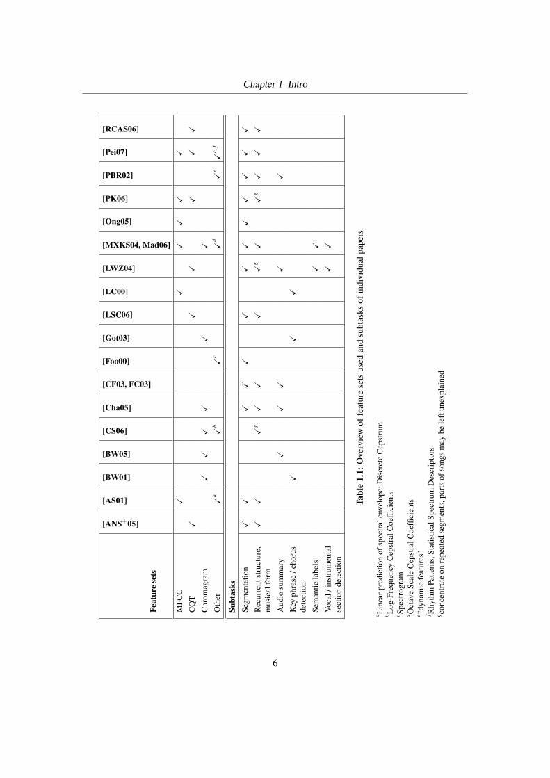
musical form. Table 1.1 gives an overview about which subtasks are dealt with in which paper.
For convenience, this thesis is referred to as [Pei07] in this and subsequent tables.
1.2.2 Features
Quite a number of different feature sets are used throughout related literature. Many of them are
well-known in the MIR community and I shall not repeat their definitions here.
Many authors do not rely on the ubiquitous Mel-Frequency Cepstrum Coefficients (MFCCs)
when tackling the specific task of audio segmentation because they are known to rather describe
timbre content and hence the feature set values of one chorus featuring distorted guitar play
and of another one lacking guitar sound would differ quite a lot. So a range of feature sets is
proposed that should capture the melody, or harmony, of a song.
4

Chapter 1 Intro
Table 1.1 gives a survey of various feature sets used. For their mathematical definitions and to
learn how to compute them please refer to the respective publication.
Constant Q transform (CQT) [LWZ04, ANS+05] can be used to directly map pitch height to
western twelve semitone scale if appropriate values for minimal frequency f0 (e.g., 130.8 Hz
as the pitch of note C3) and the number of semitones per octave b are chosen. Most papers set
b = 12 whereas other ones extract 36 values per octave. The size of the feature vector is the
product of b and the number of octaves.
Chromagram, also called Pitch Class Profile (PCP) [BW01, Got03], is essentially a generaliza-
tion of the twelve bin CQT feature set. All pitch values are collapsed into a feature vector of size
twelve, corresponding to twelve semitones, disregarding the octave of a note.
Octave Scale Cepstral Coefficients (OSCCs) and Log-Frequency Cepstral Coefficients (LFCCs)
[MXKS04, Mad06] are similar to MFCCs. Instead of calculating cepstral coefficients from Mel
scaled filter bank, the frequency band is divided into eight subbands (OSCC) or a logarithmic
filter bank is applied (LFCC) before the coefficients are extracted.
Discrete Cepstrum [AS01] is a method to estimate the spectral envelope of a signal. It uses
discrete points on the frequency/amplitude plane. These points originate from spectral peaks.
The “Dynamic Features” proposed in [PBR02] basically comprise those STFT coefficients of
a Mel filter bank filtered audio signal that maximize Mutual Information, “represent[ing] the
variation of the signal energy in different frequency bands.”
Rhythm Patterns (RP) [RPM02], also called Fluctuation Patterns, and Statistical Spectrum De-
scriptors (SSD) [LR05] both represent fluctuations on critical bands (a part of RP comprise
“rhythm” in a narrow sense). The first feature set uses a matrix representation whereas the latter
one is a more compact “summary”, employing statistical moments.
1.2.3 Techniques
The methods and mathematical models used in Automatic Audio Segmentation are widely-used
in MIR, pattern recognition and image processing.
Self-Similarity Analysis Foote [Foo00] was the first to use a two-dimensional self-similarity
matrix (autocorrelation matrix) where a song’s frames are matched against themselves
5
Chapter 1 Intro
Feat
ure
sets
[ANS+05]
[AS01]
[BW01]
[BW05]
[CS06]
[Cha05]
[CF03, FC03]
[Foo00]
[Got03]
[LSC06]
[LC00]
[LWZ04]
[MXKS04, Mad06]
[Ong05]
[PK06]
[PBR02]
[Pei07]
[RCAS06]
MFC
CX
XX
XX
X
CQ
TX
XX
XX
X
Chr
omag
ram
XX
XX
XX
Oth
erX
aX
bX
cX
dX
eX
c,f
Subt
asks
Segm
enta
tion
XX
XX
XX
XX
XX
XX
X
Rec
urre
ntst
ruct
ure,
mus
ical
form
XX
Xg
XX
XX
gX
Xg
XX
X
Aud
iosu
mm
ary
XX
XX
X
Key
phra
se/c
horu
sde
tect
ion
XX
X
Sem
antic
labe
lsX
X
Voca
l/in
stru
men
tal
sect
ion
dete
ctio
nX
X
Tabl
e1.
1:O
verv
iew
offe
atur
ese
tsus
edan
dsu
btas
ksof
indi
vidu
alpa
pers
.
a Lin
earp
redi
ctio
nof
spec
tral
enve
lope
;Dis
cret
eC
epst
rum
b Log
-Fre
quen
cyC
epst
ralC
oeffi
cien
tsc Sp
ectr
ogra
md O
ctav
eSc
ale
Cep
stra
lCoe
ffici
ents
e "dyn
amic
feat
ures
"f R
hyth
mPa
ttern
s,St
atis
tical
Spec
trum
Des
crip
tors
g conc
entr
ate
onre
peat
edse
gmen
ts,p
arts
ofso
ngs
may
bele
ftun
expl
aine
d
6

Chapter 1 Intro
(Figure 3.2 top). One characteristic trait are the longer and shorter diagonal lines parallel
to the main diagonal ranging from white to different shades of gray. These indicate seg-
ments of a song that are repeated at different positions, i.e., with a time lag. This inspired a
restructured matrix called time-lag matrix [BW01], where these lines become horizontal,
for an easier extraction of repeated segments.
Some researchers [Ong05, LWZ04] apply the basic morphological operations dilation and
erosion to the matrix to improve extraction results. (If a combination of these operations
are applied to the matrix the lines mentioned above become more distinct.)
Dynamic time warping (DTW) Given the self similarity matrix Chai [Cha05] uses DTW to find
both segment transitions and segment repetitions. DTW computes a cost matrix from
where the optimal alignment of two sequences can be derived. It is assumed that the
alignment cost of a pair of similar song sections is significantly lower than average cost
values.
Singular Value Decomposition (SVD) SVD is employed by some researchers [FC03, CF03]
to factor a segment-indexed similarity matrix (the frame-indexed counterpart would be
computationally intractable) in order to form groups of similar segments.
Hidden Markov Models (HMM) An HMM is a Markov model whose states cannot be directly
observed but must be estimated by the output produced. This approach has been employed
quite a few times in [ANS+05, ASRC06, AS01, LC00, Mad06, RCAS06, LSC06, LS06].
Feature vectors are parametrized using Gaussian Mixture Models (GMM). These param-
eters are used as the HMM’s output values.
First, both the transition probability matrix and the emission probability matrix are esti-
mated using the Baum-Welch algorithm. Second, the most likely state sequence is Viterbi
decoded. Then, there are two ways to continue. Some authors use the HMM states di-
rectly as segment types, often resulting in a very fragmented song structure that has to
be smoothed out afterwards. Another possibility is to use a sliding window to create
short-term HMM state histograms that, in turn, are clustered using a standard clustering
technique to derive the final segment type assignment. The latter approach is explained in
detail in [RCAS06].
7
Chapter 1 Intro
1.2.4 Corpora
One of the chronologically first tasks I performed was a detailed survey on annotated music
corpora used so far for AAS. To my surprise there is no common corpus that has been used to
evaluate the different approaches. Also, in previous Music Information Retrieval Evaluation eX-
change (MIREX) benchmark contests, AAS was not considered as an evaluation task. Rather,
institutes and research centers investigating audio segmentation have their own corpus, some-
times a subset of databases like RWC [GHNO02] or MUSIC [Hei03]. The annotations have
apparently not been shared among fellow researchers outside the own institute.
Besides, the evaluation methods are not consistent. Some authors compare the mere number of
segments found and segments annotated, whereas others use an elaborate roll-up procedure to
take a hierarchical structure of repeated patterns into account.
Table 1.2 shows a summary of corpora and evaluation methods used.
1.2.5 Musical domain knowledge
Belonging to the general research field of Music Information Retrieval, the task of segmenting
contemporary popular songs into their constituents like chorus, verse or bridge is quite specific.
Thus, it seems advisable to take advantage of domain knowledge, i.e., musical knowledge about
structure and other properties that most or all pop songs have in common. In practice such
knowledge means constraints for the solution space or heuristic rules to avoid a computational
intractable exhaustive search. While the use of such knowledge may narrow the range of poten-
tial songs an algorithm can successfully process, the overall improvement is probably worth it.
This section summarizes domain knowledge that has been used in the literature.
After deriving a great deal of information about the song, musical form detection and semantic
label assignment in [MXKS04, Mad06] finally is a matter of strict rules and a few case descrip-tions. The rules govern the overall song structure, the number and length of verses and choruses
and the “middle eight” section. The following is an example of one case for verse/chorus detec-
tion:
“Case 1. The system finds two melody-based similarity regions. In this case, the
song has the structure described in item 1a [Intro, verse 1, chorus, verse 2, chorus,
chorus, outro]. If the gap between verses 1 and 2 is equal and more than 24 bars,
8
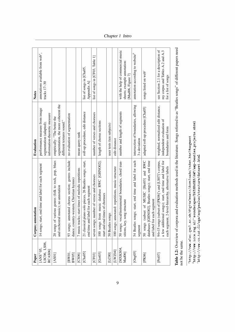
Chapter 1 IntroPa
per
Cor
pus;
anno
tatio
nE
valu
atio
nN
otes
[AN
S+05
,L
SC06
,L
S06,
RC
AS0
6]
14so
ngs;
star
t,en
dtim
ean
dla
belf
orea
chse
gmen
tpe
rfor
man
cem
easu
refr
omim
age
segm
enta
tion
(ada
pted
);in
form
atio
n-th
eore
ticm
easu
re
anno
tatio
nsav
aila
ble
from
web
a ,tr
acks
17–3
0
[AS0
1]20
song
sof
vari
ous
genr
es(f
olk
toro
ck,
pop,
blue
san
dor
ches
tral
mus
ic);
noan
nota
tion
empi
rica
lly:“
The
bette
rthe
segm
enta
tion,
the
mor
eco
here
ntth
edi
ffer
entt
extu
res
soun
d.”
[BW
01,
BW
05]
93so
ngs;
anno
tate
dch
orus
sect
ion;
genr
esin
clud
eda
nce,
coun
try-
wes
tern
,Chr
istia
nhy
mns
)no
eval
uatio
nof
segm
enta
tion
[CS0
6]7
mus
ictr
acks
;sta
rttim
esof
mel
odic
repe
titio
nsm
ean
quer
yra
nk
[Cha
05]
21cl
assi
calp
iano
solo
piec
es,2
6B
eatle
sso
ngs;
star
t,en
dtim
ean
dla
belf
orea
chse
gmen
tro
ll-up
proc
edur
e,ed
itdi
stan
celis
tofs
ongs
in[C
ha05
,A
ppen
dix
A]
[CF0
3]se
ven
song
s;nu
mbe
rofv
erse
san
dch
orus
esnu
mbe
rofv
erse
san
dch
orus
eslis
tofs
ongs
in[C
F03,
Tabl
e1]
[Got
03]
100
song
sfr
omm
usic
data
base
RW
C[G
HN
O02
];st
arta
nden
dtim
esof
chor
uses
leng
thof
chor
usse
ctio
ns
[LC
00]
50B
eatle
sso
ngs
user
test
s(t
ensu
bjec
ts)
[LW
Z04
]10
0so
ngs;
anno
tate
d:re
petit
ions
,mus
icst
ruct
ure
edit
dist
ance
[MX
KS0
4,M
ad06
]50
song
s;vo
cal/i
nstr
umen
tal
boun
dari
es,c
hord
tran
-si
tions
,key
,son
gst
ruct
ure
num
bera
ndle
ngth
ofse
gmen
tsw
ithth
ehe
lpof
com
mer
cial
mus
icsh
eets
;exa
mpl
ean
nota
tion:
[Mad
06,F
igur
e7]
[Ong
05]
54B
eatle
sso
ngs;
star
t,en
dtim
ean
dla
bel
for
each
segm
ent
inte
rsec
tion
ofbo
unda
ries
,allo
win
g3
sde
viat
ion
anno
tatio
nac
cord
ing
tow
ebsi
teb
[PK
06]
50so
ngs
(sub
set
ofM
USI
C[H
ei03
]an
dR
WC
data
base
s[G
HN
O02
],B
eatle
sso
ngs)
;sta
rt,e
ndtim
ean
dla
belf
orea
chse
gmen
t
adap
ted
roll-
uppr
oced
ure
[Cha
05]
song
slis
ted
onw
ebc
[Pei
07]
94+1
5so
ngs
(sub
seto
f[PK
06]’
san
d[L
S07]
’sco
rpus
,a
few
addi
tiona
lson
gs);
star
t,en
dtim
ean
dla
belf
orea
chse
gmen
t,2-
leve
l-hi
erar
chy,
alte
rnat
ive
labe
ls
wei
ghte
d,no
rmal
ized
edit
dist
ance
,in
depe
nden
teva
luat
ion
ofbo
unda
ries
and
form
see
Sect
ion
2.1
fora
desc
ript
ion
ofm
yco
rpus
and
Tabl
esA
.2an
dA
.3fo
ralis
tofs
ongs
Tabl
e1.
2:O
verv
iew
ofco
rpor
aan
dev
alua
tion
met
hods
used
inth
elit
erat
ure.
Song
sre
ferr
edto
as“B
eatle
sso
ngs”
ofdi
ffer
entp
aper
sne
edno
tbe
the
sam
e.
a http://www.elec.qmul.ac.uk/digitalmusic/downloads/index.html#segment
b http://www.icce.rug.nl/~soundscapes/DATABASES/AWP/awp-beatles_projects.shtml
c http://www.cs.tut.fi/sgn/arg/paulus/structure/dataset.html
9
Chapter 1 Intro
both the verse and chorus are 16 bars long each. If the gap is less than 16 bars, both
the verse and chorus are 8 bars long.”
In [LSC06] the authors state that conventional pop music
“follows an extremely simple structure, dictated by the verse-chorus form of the
lyrics and very predictable phrase-lengths, so that segments are a simple multiple
of a basic eight-bar phrase.”
Hence, a function z is presented that models the deviations of the detected segment boundaries
from the nearest fixed phrase-length position. z is minimized over appropriate values and
the detected boundaries are adapted. As you will see in Section 3.2 I also employed this idea,
however, without success.
Whereas most researchers use common distance functions like Euclidean or cosine distance
for their similarity matrices, Lu et al. propose a novel one, coined Structure-based distance[LWZ04]. It is based on the observation that difference vectors (that is, the differences vd =vi−vj between two feature vectors) exhibit different structure properties depending on whether
the note or the timbre varies. Difference vectors between the same notes but with different tim-
bres have peaks that are spaced with some regular interval corresponding to semitones. The
authors report a performance improvement over using common distance measures. The statisti-
cal significance, however, has not been tested.
Besides, the authors use a simple rule to assign the labels intro, interlude/bridge and outro/coda
to instrumental sections, depending on their relative positions in the song.
Paulus et al. come up with an interesting assumption about segment types [PK06]. It is assumed
that the durations of two segments of the same type lies within the duration ratio r = [56 , 65 ].
Also the converse is supposed to hold: segment pairs of duration ratio within r are of the same
type. Although this frequently is indeed the case it is not difficult to present a counterexample:
Portishead: Wandering Star contains both verse and chorus sections of a duration of approxi-
mately 24 s whereas the instrumental sections at [01:48, 02:24], [03:24, 03:36], [03:36, 04:25]
and [04:25, 04:48] are of different length.
In some pop songs one of the chorus segments (mostly at the end of the song) is transposeda number of semitones upwards to increase tension and make the song more interesting2. This
2There is a (slightly ironic) website devoted to this phenomenon: http://www.gearchange.org/index.asp
10
Chapter 1 Intro
causes problems as extracted features may not be similar to those of original repetitions. Goto
explicitly takes care of this stylistic element by defining twelve kinds of extended similarities
that correspond to the twelve possible semitone transpositions [Got03].
In the same paper Goto also formulates three assumptions about song structure, dealing with
the length of the chorus section (limiting from 7.7 to 40 s), its relative position and its internal
structure (tends to have two half-length repeated sub-sections). Results were best when all three
assumptions were enabled.
Abdallah et al. introduce an explicit segment duration prior function to overcome the problem
of very short and fragmented segments [ASRC06]. The prior function rises steeply from 5 s to
a peak at 20 s, from where it starts to go down gradually to reach a value of half the peak value
at 60 s. Thus, segments with a length of 0 to approximately 10 seconds are unlikely; 20 s is the
duration with the highest probability.
1.3 Musical segmentation
Segmenting pieces of music into sections is ambiguous. People with little musical background
will come to different results than professional musicians (provided that they are willing to
engage in such an activity at all); people on the same level of ‘musical proficiency’ are likely to
dispute each other’s suggestion.
This is supported by both experiments with my groundtruth annotations and musicology litera-
ture.
1.3.1 Ambiguity
To assess the ambiguity of segmentations I compared groundtruth annotations from different
subjects against each other.
The corpus data I received from other researchers contained three duplicate songs, i.e., I re-
ceived three songs each having two groundtruth annotations done by two subjects. In addition, I
annotated a few songs myself when taking over the annotations (see Section 2.1 on page 18 for
details). This was the case when I could not agree with the received annotations at all.
11
Chapter 1 Intro
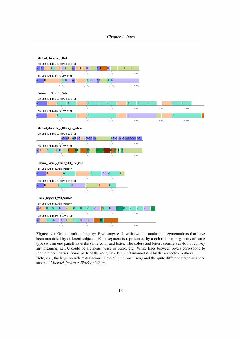
Figure 1.1 shows five songs each with two “groundtruth” segmentations. The annotations have
been done by two different subjects. You can clearly see that the two segmentations of the same
song differ from each other in terms of segment boundaries and/or musical form.
1.3.2 Musicology
The question of musical structure analysis is also dealt with in the musicology literature. This
section gives a brief overview of some approaches (following [Mid90]).
Information theory was applied for analyzing the surface structure of music [Mid90]:
“This, in a sense, however, simply rewrites older assumptions about pattern, ex-
pectation, and the relationship of unity to variety, in terms of allegedly quantifiable
probabilities; style is defined in terms of measurable ‘information’, product of the
relative proportions of ‘originality’ and ‘redundancy’.”
This approach is heavily criticized because of its oversimplification of musical parameters and
its disregard of both the listening act and the participant input. Besides, it regards repetition as
negative because it has no information value; an attitude that certainly does not coincide with
the “real world”.
Then, methods and terms from Structural linguistics were adopted and applied to musical anal-
ysis. For example, it is argued that motives (in music) correspond to morphemes (in linguistics),
called musemes, and that notes correspond to phonemes.
Another example is Steedman’s approach [Ste84] which is a quite formal one. He employs
generative grammar that recursively generates all recognizably well-formed transformations in
a certain kind of jazz music. This naturally produces a hierarchical segmentation. Of course,
this method can only be applied to music that somehow ‘follows’ the rules of the grammar.
Paradigmatic analysis
As to Ruwet [Ruw87], repetition and varied repetition, transformation, are the central charac-
teristics of musical syntax. His analytical method, named paradigmatic analysis by others,
defines
12
Chapter 1 Intro
Figure 1.1: Groundtruth ambiguity: Five songs each with two “groundtruth” segmentations that havebeen annotated by different subjects. Each segment is represented by a colored box, segments of sametype (within one panel) have the same color and letter. The colors and letters themselves do not conveyany meaning, i.e., C could be a chorus, verse or outro, etc. White lines between boxes correspond tosegment boundaries. Some parts of the song have been left unannotated by the respective authors.Note, e.g., the large boundary deviations in the Shania Twain song and the quite different structure anno-tation of Michael Jackson: Black or White.
13
Chapter 1 Intro
“anything repeated (straight or varied) (. . . ) as an unit, and this is true on all levels,
from sections through phrases, presumably down as far as individual sounds. This
means that in principal he can segment a piece without reference to its meaning,
purely on the basis of the internal grammar of its expression plane. There are some
problems, however. (. . . ) What is the criteria for a judgment that two entities are
sufficiently similar to be considered equivalent?”
In a nutshell, an analyst using Ruwet’s method works iteratively: he breaks the song down to
its constituent units of each structural level. Units of one level have roughly the same length.
[Mid90, Examples 6.3–6.5] show the result of this method applied to George Gershwin’s song
‘A Foggy Day’.
While this method sounds quite concrete many questions remain open.
“Are these the minimal units in the tune? And are they phonemic or morphemic?”
Or in other words: which level is the last level? Which level’s units are the shortest that still
convey some sort of meaning?
According to Middleton, Ruwet’s method cannot answer these questions. He also shows that
there are different criteria that can be applied to break up segments into smaller pieces. It is also
not clearly defined how different one segment must be to another in order not to be regarded as
a transformation but rather as a contrast to the other segment.
Schenker analysis
Middleton also discusses the application of Schenker analysis (which actually comes from
classical music) to pop music. Generally, this method concentrates on tonality, cadences and
harmonic structure and neglects ‘motivic’ structure and rhythm. See [Mid90, Example 6.10]
for a Schenker analyzed ‘A Foggy Day’: The basic V-I cadence and the centrality of the tonic
triad notes are revealed. Critics argue, however, that the Schenkerian principles are (too) ax-
iomatic, according to them all valid music styles are seen essentially the same: “Thus, Schenke-
rian ‘tonalism’ could not be satisfactorily applied to much Afro-American and rock music, in
which pentatonic and modal structures are important, and where harmonic structure (...) plays a
comparatively small role.”
14
Chapter 1 Intro
Relevance for this thesis
When reading musicology literature I realized, not very surprisingly, that I lack music know-
ledge to really use the information and knowledge presented there. On the other hand I learned
that comprehensive music knowledge would not necessarily simplify my work: I would not be
better in judging whether one segmentation is superior to the other, whether two segments can
be regarded as identical, as transformation of each other or contrasting to each other. Just as one
might expect, even (or especially?) among experts these questions cannot be answered unam-
biguously. (One symptom of this is the fact that Middleton poses more questions in this book
than he answers.)
For this thesis, I regard Ruwet’s method as the most relevant. I think, intuitively I had some idea
of his propositions in the back of the head when I prepared the ground truth for my corpus. Also,
this method is not as strict regarding tonality and cadences as other ones. This is just the way
my algorithm works because of the limited possibility to extract correct notes, chords and thus
cadences from multi-instrumental audio files.
Paradigmatic analysis, however, can also be of direct use: One can assure that the ground truth
annotations of a corpus are as homogeneous as possible if Ruwet’s method is applied to each
song using the same criteria and then the same level of segmentation is chosen for all songs.
1.4 Contributions
The contributions of this thesis can be summarized as follow:
Evaluation system I invested a significant amount of time in careful considerations about “good”
evaluation in this case, the design and implementation of an easy-to-use evaluation pro-
gram that produces both appealing and informative HTML reports. I defined a novel
XML based file format for groundtruth files that is more expressive than other formats.
(Chapter 2)
Large corpus The corpus on which this work is based contains 94 songs of various genres.
Final evaluation runs are conducted on a 109 song corpus which is the largest corpus used
so far in this research field. (Sections 2.1 and A.3)
15
Chapter 1 Intro
Boundary detection I used the classic similarity matrix / novelty score approach [Foo00]. In
addition, I carried out quite a few experiments to improve performance (various fea-
ture sets and parameter settings, boundary removing heuristic, boundary shifting post-
processing [LSC06], Harmonic Change Detection Function HCDF [HSG06]). (Chapter 3)
Structure detection I focused on the complete annotation of all parts of the songs both with
sequential-unaware approaches and an approach that takes temporal information into ac-
count. I employed cluster validity indices to find the correct number of segment types for
each song. (Chapter 4)
Statistical significance All evaluation results are statistically well grounded by calculating and
publishing confidence intervals from which statistical (in)significance can be derived.
1.5 Conventions
In pseudo code notation algorithms I use the following non-standard symbols.
· string concatenation
© empty string
hash{key} hash array access
string\c removes all occurrences of character c from string
? special label with the meaning “not annotated”
Statistical significance Statements about statistical significance refer to confidence intervals
calculated for each algorithm run. If the intervals of two runs do not overlap the difference
of the mean values is said to be a statistically significant. I use Student’s T distribution and a
significance level of α = 0.05.
1.6 Summary
This chapter introduced the reader to Automatic Audio Segmentation (AAS). I explained some
prospective fields of application for this task, e.g., how AAS can facilitate the browsing in large
digital music collections.
16
Chapter 1 Intro
Next, I gave an overview of related work. I introduced various tasks and goals that are sub-
sumed as AAS (boundary detection, structure detection, audio thumbnailing, semantic label
assignment, etc.) I briefly explained mathematical models used (e.g., self-similarity analysis and
Hidden Markov Models). Then, corpora and feature sets employed have been clearly arranged
in tabular form. I pointed out that there is no common corpus so far. One section summarized
different pieces of musical domain knowledge that are employed either explicitly or implicitly
by authors of related literature.
The subsequent section dealt with musical segmentation as a task that generally leads to am-
biguous results. I presented examples of “ground truth” annotations that differed to a certain
degree. The chapter is topped off with a survey on how segmentation is perceived and discussed
in musicology literature. I pointed out why Ruwet’s method is the most relevant for my thesis.
Finally, I gave an overview of my contributions in this thesis.
17
Chapter 2
Evaluation setup
In my opinion evaluation of output of algorithms is, at least in the research phase, as important
as the algorithm itself. If the evaluation procedure does not produce useful and applicable per-
formance numbers any effort to optimize an algorithm becomes futile. In fact you would not
know whether algorithm A performs better than algorithm B.
Thus, I decided to devote a significant part of my work to my evaluation system.
From my experience with similar work I know it is very handy if there is a simple-to-use proce-
dure that automatically produces both optical appealing and informative reports. This makes it
possible to have rapid feedback loops in a phase where you adjust the large number of degrees
of freedoms, i.e., algorithm parameters, to get an optimal result.
This chapter describes the corpus I used, defines performance measures, introduces a new XML
format for groundtruth files and explains the evalution algorithm in detail.
2.1 Groundtruth
To be able to compare results of various research studies the algorithms should run on the same
corpus. Therefore I tried to collect as much annotation data as possible that has already been
used in prior studies. I asked the authors of [Mad06, LWZ04, Cha05, Ong05, PK06] whether
they would share their annotations. Finally I could base my work upon data used in [PK06]
(50 songs, “Paulus/Klapuri corpus”) and in [LS07]1 (60 songs, “qmul2 corpus”), respectively.
1http://www.elec.qmul.ac.uk/digitalmusic/downloads/index.html#segment2The annotators of this corpus are from the Centre for Digital Music, Queen Mary, University of London
18
Chapter 2 Evaluation setup
A subset of the latter corpus has been used in [RCAS06, CS06, LSC06, AS01, ANS+05], too
(“qmul14 corpus”).
As the corpora overlap and because I could not obtain all songs my corpus which I used for
my experiments finally contained 94 distinct songs. This is a multiple of some researchers’
corpora and one of the largest used so far in this field. At the end I enlarged the corpus by fifteen
additional songs which eventually led to the largest corpus against which an AAS algorithm has
ever been evaluated. I included the corpus information (“this song belongs to which corpora?”)
in the groundtruth files to get also corpus-specific performance measures.
See Section A.3 for the complete list of songs I used.
2.1.1 Adaption
When I received other researcher’s annotation data I had to decide if I use it ‘as is’ or if I adapt
it.
As a matter of fact the results are less comparable if you change something at the test set used
for evaluation. On the other hand the expressiveness of performance measure numbers is limited
if the underlying ground truth annotations are inconsistent due to the fact that they come from
several different sources.
Because of this and the fact that I introduced a novel XML audio segmentation format that is
more expressive and flexible and can be used by other researchers in future studies and evalua-
tions I decided to look through the data and carefully make some changes if necessary.
Essentially, the adaptions I made fell into two main groups:
• I introduced hierarchical segmentation and alternative labels where appropriate.
• Adjustments of start and end times of segments that are probably due to different offsets
when encoding the audio file from CD, i.e., when all boundaries seemed to be shifted by
a fixed offset. (I had to collect the audio files by myself because of copyright issues.)
• There were a number of songs where parts have been left unannotated.
19

Chapter 2 Evaluation setup
2.1.2 Quality of audio signal
Like in other Information Retrieval tasks the quality of the output (classifications, algorithms)
highly depends on the quality of the input, i.e., training data and test data. Of course, this is not
clearly visible at first sight. Even if only a small and inaccurate data set was being used, the
evaluation procedure would still yield perfect looking performance measure numbers with quite
a few decimal places. One could be tempted to use and publish them without have a proper look
at what is behind these numbers.
Thus, I took some consideration on the input data at the beginning of my work.
Lossy compression
By far the most widely used audio file format nowadays is MPEG-1 Audio Layer 3, commonly
referred to as mp3. While the compressed audio should not sound different from the original
one (if an appropriate bitrate is used), it certainly changes the spectrogram and extracted audio
features to some degree. I wondered whether the results would be distorted when using mp3
files as input.
I did some experiments with two versions of the same song: one version was extracted from
CD as uncompressed wav file, while the other one was encoded to mp3 at the rather low bitrate
of 128 kbit/s. The experiments showed that, e.g., the novelty score plot was almost congruent.
Thus, I decided not to exclude mp3 files as input data, especially because typically my mp3 files
have a bitrate of at least 192 or even 320 kbit/s.
Sample frequency
I decided to downsample audio files to mono, 22,050 Hz as this is a good trade-off between input
data quality and reduction in computation time. Ad-hoc experiments with 44,100 Hz audio files
showed almost no change of results.
20
Chapter 2 Evaluation setup
2.2 Performance measures
2.2.1 Level 1 - Boundaries
Evaluating segment boundaries is straight forward. Following the approach used, e.g., in [Cha05]
I calculate precision P , recall R and F-measure F . Let the sets Balgo and Bgt denote begin and
end times of automatic generated segments and ground truth segments respectively, then P , R
and F are calculated as follows:
P =Balgo ∩ Bgt
Balgo(2.1)
R =Balgo ∩ Bgt
Bgt(2.2)
F =2RP
R + P(2.3)
A parameter w determines how far two boundaries can be apart but still count as one boundary.
A typical value is 3 s, i.e., all boundaries within the range of three seconds before to three
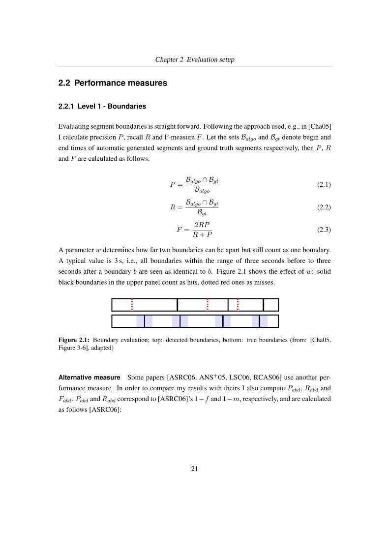
seconds after a boundary b are seen as identical to b. Figure 2.1 shows the effect of w: solid
black boundaries in the upper panel count as hits, dotted red ones as misses.
Figure 2.1: Boundary evaluation; top: detected boundaries, bottom: true boundaries (from: [Cha05,Figure 3-6], adapted)
Alternative measure Some papers [ASRC06, ANS+05, LSC06, RCAS06] use another per-
formance measure. In order to compare my results with theirs I also compute Pabd, Rabd and
Fabd. Pabd and Rabd correspond to [ASRC06]’s 1−f and 1−m, respectively, and are calculated
as follows [ASRC06]:
21
Chapter 2 Evaluation setup
“Considering the measurement M [computed segmentation] as a sequence of seg-
ments SiM , and the ground truth G likewise as segments Sj
G, we compute a direc-
tional Hamming distance dGM by finding for each SiM the segment Sj
G with the
maximum overlap, and then summing the difference,
dGM =∑Si
M
∑Sk
G 6=SjG
|SiM ∩ Sk
G|
where | · | denotes the duration of a segment.”
Then,
Pabd = 1− dMG/dur (2.4)
Rabd = 1− dGM/dur (2.5)
Fabd =2RabdPabd
Rabd + Pabd(2.6)
where dur is the duration of the song.
The main advantage of the alternative measures is that they somehow reflect how much the two
segmentations differ from each other: If a boundary b from computed segmentation is apart more
than w from the corresponding one in the ground truth b0, it does not count for P or R, regardless
of how far they are apart (since b /∈ Balgo ∩ Bgt). In contrast, Pabd and Rabd will rise depending
on the distance between b and b0 since these measures are not based on the boundaries directly
but rather on (overlapping) segments between them.
If applied to the same machine segmentations, I saw that mean Fabd is generally about 0.1higher than mean F . In my opinion this is due to the "binaryness" of P and R as explained
in the previous paragraph (either a boundary belongs to the intersection Balgo ∩ Bgt or not).
Distances between "corresponding" boundaries from Balgo and Bgt are frequently a bit larger
than w, leading to quite bad P and R.
2.2.2 Level 2 - Structure
Following Chai’s notion I use the formal distance metric f which basically is the edit distance ed
between strings representing the two structures, independent of the actual naming of the distinct
22
Chapter 2 Evaluation setup
segments as long as segments with the same label get the same character. That is,
f(ABABCCCABB, ABCBBBBACC) = 3 (2.7)
because
ed(ABABCCCABB, A CBCCCC A BB ) = 3 (2.8)
(in the second argument B and C have been swapped). To relate f to the song duration durs I
use the formal distance ratio
rf = 1− f/durs (2.9)
Details about the string representation are discussed in Section 2.3.2.
Alternative measures Another interesting performance measure can be computed following
an information-theoretic approach. In [ANS+05, ASRC06] “conditional entropies” and “mutual
information” are calculated, treating the joint distribution of label sequences as a probability
distribution. Mutual information I (in bits) measures the amount of information contained in
both the computed and the groundtruth segmentation. The conditional entropies H(algo|gt)and H(gt|algo) gives an impression about the amount of “spurious” information in computed
segmentation and about how much of the groundtruth information is missing there, respectively.
I is optimal and maximal if each segment type in the groundtruth segmentation is mapped to
one and only one segment type in the computed segmentation. If so, both H(algo|gt) and
H(gt|algo) are zero.
In my opinion this measure has one clear flaw. I increases monotonically with the number of
k-means clusters k. Even if the extracted structure has obviously too many (spurious) segment
types, and formal distance ratio already declines, I still ascends further. This behavior is dis-
tinctly visible in Figure 4.2.
The performance numbers for level 2 using the proposed method are independent of the bound-
ary accuracy. This gives us the possibility to judge structure extraction performance indepen-
dently from segment boundary performance.
23

Chapter 2 Evaluation setup
2.3 Evaluation system
Figure 2.2 depicts the architecture of my evaluation system. It uses XML, XSD, XSLT and Perl
to produce an HTML file from both automatic generated and hand made song segmentations.
The system is OS independent, I used it both on Windows (XP) and Linux (Debian Sarge).
The following subsections describe each part in some detail.
2.3.1 Audio segmentation file format
I introduced a new file format describing audio segmentations. Both ground truth annotations
and automatically generated ones are encoded in this format. I decided to use Extensible Markup
Language (XML) to model the information because it is a well established standard that is ex-
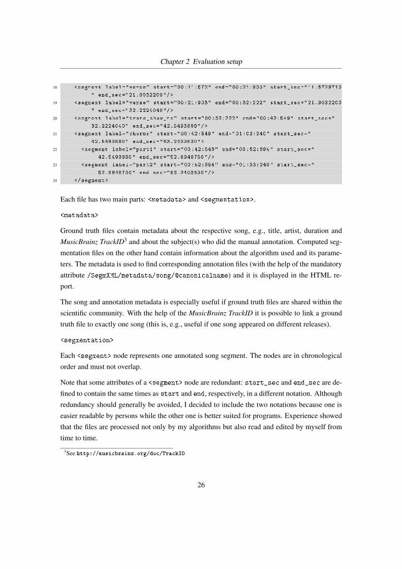
pressive enough for this application and still human readable. The file format is called Segm-XML which is also the name of the files’ root node.
Listing 2.1 shows an excerpt of an example XML file (the complete file can be seen in List-
ing A.1).
Listing 2.1: Britney_Spears_-_Hit_Me_Baby_One_More_Time.xml (excerpt) – segmentation XML filefor Hit Me Baby One More Time by Britney Spears
1 <?xml version="1.0" encoding="UTF -8"?>
2 <SegmXML version="1.0">
3 <metadata >
4 <song canonicalname="Britney_Spears_ -_Hit_Me_Baby_One_More_Time">
5 <title>Hit Me Baby One More Time</title>
6 <artist >Britney Spears </artist >
7 <album year="">Hit Me Baby One More Time</album>
8 <musicbrainz_trackID/>
9 <duration duration_sec="212">03:32</duration >
10 <genre>Rock/Pop/Dance</genre></song>
11 <annotation source="ground truth">
12 <done_by note="primary author(s)">Mark Levy/Geoffroy Peeters/Katy Noland </
done_by >
13 <done_by timestamp="2007 -02 -24" note="adapted by">Ewald Peiszer </done_by >
14 </annotation >
15 </metadata >
16 <segmentation >
17 <segment label="intro" start="00 :00:000" end="00 :11:572" start_sec="0.0000000"
end_sec="11.5729710"/>
24

Chapter 2 Evaluation setup
According to XML schema definition file
XSDComputed segmentation
SegmXML
Groundtruth segmentation
SegmXML
Evaluation report
EvalXML
report.xslt
XSLT
report.css
css
report.html
HTML
Evaluation algorithm
Level 1 – Boundaries
Level 2 – Form
Perl
XSLT-Engine
Xalan-J
Browser
Figure 2.2: Overview of the evaluation system
25
Chapter 2 Evaluation setup
18 <segment label="verse" start="00 :11:572" end="00 :21:903" start_sec="11.5729710
" end_sec="21.9032200"/>
19 <segment label="verse" start="00 :21:903" end="00 :32:222" start_sec="21.9032200
" end_sec="32.2224040"/>
20 <segment label="trans_show_me" start="00 :32:222" end="00 :42:549" start_sec="
32.2224040" end_sec="42.5493880"/>
21 <segment label="chorus" start="00 :42:549" end="01 :03:240" start_sec="
42.5493880" end_sec="63.2403630">
22 <segment label="part1" start="00 :42:549" end="00 :52:894" start_sec="
42.5493880" end_sec="52.8948750"/>
23 <segment label="part2" start="00 :52:894" end="01 :03:240" start_sec="
52.8948750" end_sec="63.2403630"/>
24 </segment >
Each file has two main parts: <metadata> and <segmentation>.
<metadata>
Ground truth files contain metadata about the respective song, e.g., title, artist, duration and
MusicBrainz TrackID3 and about the subject(s) who did the manual annotation. Computed seg-
mentation files on the other hand contain information about the algorithm used and its parame-
ters. The metadata is used to find corresponding annotation files (with the help of the mandatory
attribute /SegmXML/metadata/song/@canonicalname) and it is displayed in the HTML re-
port.
The song and annotation metadata is especially useful if ground truth files are shared within the
scientific community. With the help of the MusicBrainz TrackID it is possible to link a ground
truth file to exactly one song (this is, e.g., useful if one song appeared on different releases).
<segmentation>
Each <segment> node represents one annotated song segment. The nodes are in chronological
order and must not overlap.
Note that some attributes of a <segment> node are redundant: start_sec and end_sec are de-
fined to contain the same times as start and end, respectively, in a different notation. Although
redundancy should generally be avoided, I decided to include the two notations because one is
easier readable by persons while the other one is better suited for programs. Experience showed
that the files are processed not only by my algorithms but also read and edited by myself from
time to time.
3See http://musicbrainz.org/doc/TrackID
26
Chapter 2 Evaluation setup
A <segment> node can contain the two additional optional attributes instrumental and fade
where further information about this segment can be annotated. In this thesis I do not make
use of these attributes. The main label of a segment is defined by its attribute label; for each
alternative label a subnode alt_label is inserted. A <segment> node can contain <segment>
subnodes only if it is a child node of <segmentation>, i.e., subsubnodes are disallowed in order
not to make the annotation and adaption process too complicated.
There are several positions where <remark> nodes can be inserted. These can contain infor-
mational text that is rendered into the HTML report. As an example, remarks for segments are
inserted as tooltips.
To make it easy for research colleagues who may want to use this file format as well, I created
a corresponding XML schema definition file that contains the schema in a formal notation, c.f.
Listing A.2.
Flexibility
It is hardly possible to decide upon the one and only correct song segmentation (see Section 1.3).
This means that even if two subjects segment the same song, quite a different structure could
emerge. As a matter of fact this was true for the songs that are contained in both the Paulus/Kla-
puri corpus [PK06] and the Queen Mary corpus [RCAS06, CS06, LSC06, AS01, ANS+05].
From this perspective I decided to add flexibility to my file format. This includes
hierarchical segments Following considerations from Section 1.3, a segment can be divided
into subsegments. Figure 2.3 shows two song segmentations, one where only the super-
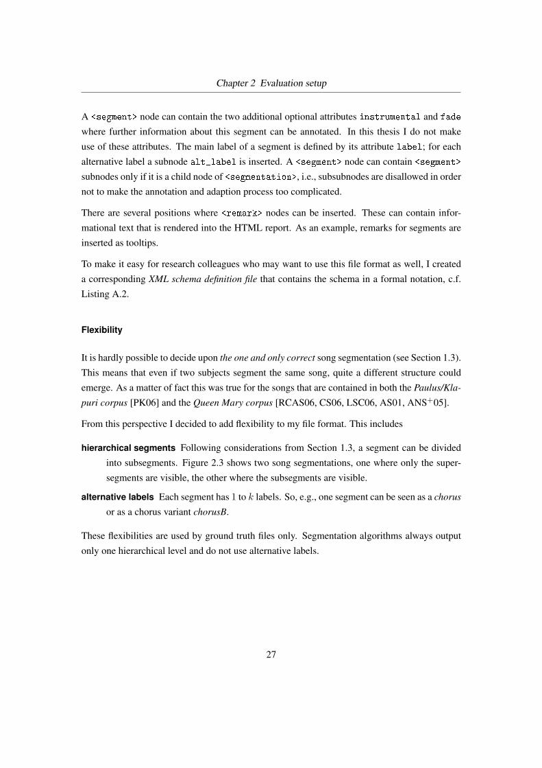
segments are visible, the other where the subsegments are visible.
alternative labels Each segment has 1 to k labels. So, e.g., one segment can be seen as a chorus
or as a chorus variant chorusB.
These flexibilities are used by ground truth files only. Segmentation algorithms always output
only one hierarchical level and do not use alternative labels.
27
Chapter 2 Evaluation setup
Figure 2.3: Two levels of segmentation: one with subsegments (top), the other one without (bottom).Both variants are included in one ground truth file. Segments of same color correspond to same segmentlabel.
2.3.2 Evaluation procedure
The procedure itself is implemented in Perl. Because of the above mentioned flexibility of the
SegmXML file format one ground truth file actually contains several ground truth variants.
The evaluation procedure is executed for each pair of computed segmentation and ground truth
variant that can be extracted from the corresponding ground truth file. It consists of two stages
or levels. The performance numbers are output into one XML file, including mean values and
confidence intervals, as well as remarks, debug output and warnings if appropriate.
Semantics
Basically, I consider the segmentation with and without subsegments. Moreover, the alternative
labels have impact. I do not, however, consider all permutations of them. For example, if
there are segments that have two labels (i.e., one alternative label), either all main labels or all
alternative labels are used, but they are not mixed. As a motivation for this behavior consider
the following case.
Several segments of a song can be regarded as chorus segments. On the other hand some cho-
ruses are modulated in such a way that it can be argued to label them differently (e.g., chorusB).
Now we would like to consider both annotation possibilities as valid, but we do not want to
28
Chapter 2 Evaluation setup
mix them: Either all chorus-like segments are labeled chorus or the original ones are labeled
chorus and all modulated ones are labeled chorusB.
As an example, the following ground truth variants can be extracted from XML Listing A.1.
Segment labels that differ between variants are emphasized.
Algorithm 1 shows the algorithm in pseudo code.
ground truth variant 'with subsegments, variant 0'.
intro - verse - verse - trans_show_me - part1 - part2 - verse - verse -
trans_show_me - part1 - part2 - intro - verse - verse - part1 - part2 -
part1 - part2 - part1 - part2
ground truth variant 'with subsegments, variant 1 '.
intro - verse - verse - trans_show_me - part1 - part2 - verse - verse -
trans_show_me - part1 - part2 - intro - verse2 - verse2 - part1 - part2 -
part1 - part2 - part1 - part2
ground truth variant ' only main segments, variant 0'.
intro - verse - verse - trans_show_me - chorus - verse - verse -
trans_show_me - chorus - intro - verse - verse - chorus
ground truth variant 'only main segments, variant 1'.
intro - verse - verse - trans_show_me - chorus - verse - verse -
trans_show_me - chorus - intro - verse2 - verse2 - chorus2
The performance of each pair of computed and ground truth segmentation file is the maximum
of all performance numbers of the extracted ground truth variants, i.e., always the best matching
variant is chosen.
Addressing hierarchy
The discussion on hierarchical song segmentation variants suggests to build an evaluation pro-
cedure that yields high performance numbers for two segmentations that are on different hierar-
chical levels. Chai was the first to take this into account and proposed a roll-up process followed
by a drill-down process [Cha05]. Later, Paulus proposed a similar approach in [PK06].
29
Chapter 2 Evaluation setup
Algorithm 1 getSegmentationVariants
Parameters: S // set of segments having up to k labels
1: levelmax ← max |Si{labels}| ∀i ∈ (0 . . . |S|)2: for j ← 0 to levelmax do
3: maxV ariantsj ← max getNumberOfLabelVariants(Si, j)4: end for
5: variants←∑
maxV ariantsj
6: for v ← 0 to variants do
7: for i← 0 to |S| do8: segmentationvariantsi
v ← Si
9: if |Si{labels}| = levelmax then
10: segmentationvariantsiv{label} ← Si{labels}min v,levelmax
11: else
12: segmentationvariantsiv{label} ← Si{labels}v mod |S|
13: end if
14: end for
15: end for
16: return segmentationvariants
Algorithm 2 getNumberOfLabelVariants
Parameters: segment, level1: if level = 0 ∨ |segment{labels}| = 1 ∨ |segment{labels}| > level then2: return 13: else
4: return |segment{labels}|5: end if
30
Chapter 2 Evaluation setup
Although these methods are an advance over not considering hierarchical levels at all, in my
opinion there are some problems and pitfalls.
1. If the computed and/or the ground truth segmentation are changed by the evaluation pro-
cess there is the danger that knowledge is added to it that is neither part of the algorithmic
output nor of the manually annotated ground truth. This would mean that the data has
been falsified and that as a matter of fact the evaluation output would no longer be ap-
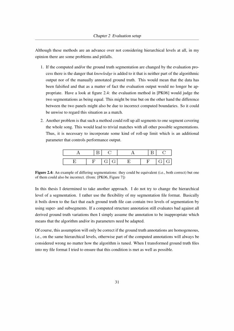
propriate. Have a look at figure 2.4: the evaluation method in [PK06] would judge the
two segmentations as being equal. This might be true but on the other hand the difference
between the two panels might also be due to incorrect computed boundaries. So it could
be unwise to regard this situation as a match.
2. Another problem is that such a method could roll up all segments to one segment covering
the whole song. This would lead to trivial matches with all other possible segmentations.
Thus, it is necessary to incorporate some kind of roll-up limit which is an additional
parameter that controls performance output.
Figure 2.4: An example of differing segmentations: they could be equivalent (i.e., both correct) but oneof them could also be incorrect. (from: [PK06, Figure 7])
In this thesis I determined to take another approach. I do not try to change the hierarchical
level of a segmentation. I rather use the flexibility of my segmentation file format. Basically
it boils down to the fact that each ground truth file can contain two levels of segmentation by
using super- and subsegments. If a computed structure annotation still evaluates bad against all
derived ground truth variations then I simply assume the annotation to be inappropriate which
means that the algorithm and/or its parameters need be adapted.
Of course, this assumption will only be correct if the ground truth annotations are homogeneous,
i.e., on the same hierarchical levels, otherwise part of the computed annotations will always be
considered wrong no matter how the algorithm is tuned. When I transformed ground truth files
into my file format I tried to ensure that this condition is met as well as possible.
31
Chapter 2 Evaluation setup
String representation
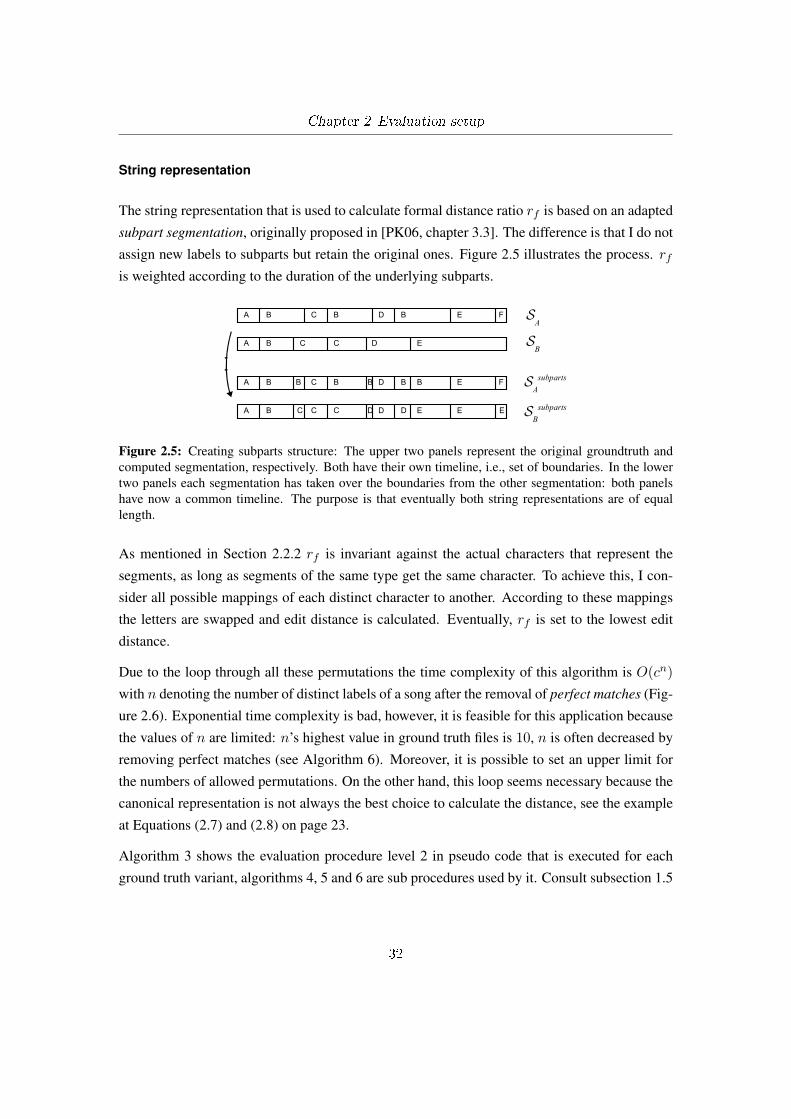
The string representation that is used to calculate formal distance ratio rf is based on an adapted
subpart segmentation, originally proposed in [PK06, chapter 3.3]. The difference is that I do not
assign new labels to subparts but retain the original ones. Figure 2.5 illustrates the process. rf
is weighted according to the duration of the underlying subparts.
A B C B D B E F
A B C C D E
A B B C B B D B B E F
A B C C C D D E EED
SA
SAsubparts
SB
SBsubparts
Figure 2.5: Creating subparts structure: The upper two panels represent the original groundtruth andcomputed segmentation, respectively. Both have their own timeline, i.e., set of boundaries. In the lowertwo panels each segmentation has taken over the boundaries from the other segmentation: both panelshave now a common timeline. The purpose is that eventually both string representations are of equallength.
As mentioned in Section 2.2.2 rf is invariant against the actual characters that represent the
segments, as long as segments of the same type get the same character. To achieve this, I con-
sider all possible mappings of each distinct character to another. According to these mappings
the letters are swapped and edit distance is calculated. Eventually, rf is set to the lowest edit
distance.
Due to the loop through all these permutations the time complexity of this algorithm is O(cn)with n denoting the number of distinct labels of a song after the removal of perfect matches (Fig-
ure 2.6). Exponential time complexity is bad, however, it is feasible for this application because
the values of n are limited: n’s highest value in ground truth files is 10, n is often decreased by
removing perfect matches (see Algorithm 6). Moreover, it is possible to set an upper limit for
the numbers of allowed permutations. On the other hand, this loop seems necessary because the
canonical representation is not always the best choice to calculate the distance, see the example
at Equations (2.7) and (2.8) on page 23.
Algorithm 3 shows the evaluation procedure level 2 in pseudo code that is executed for each
ground truth variant, algorithms 4, 5 and 6 are sub procedures used by it. Consult subsection 1.5
32
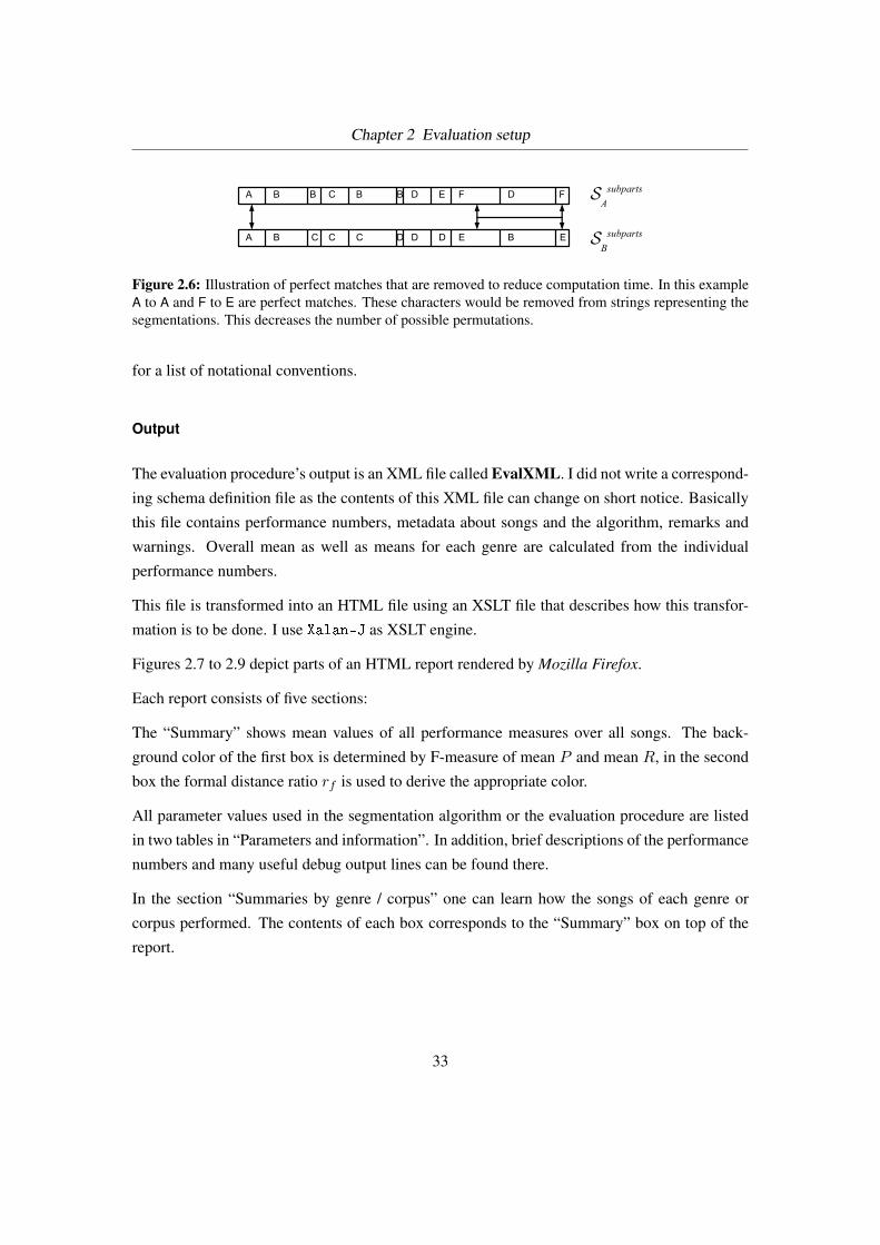
Chapter 2 Evaluation setup
SAsubparts
SBsubparts
A B B C B B D E F D F
A B C C C D D E EBD
Figure 2.6: Illustration of perfect matches that are removed to reduce computation time. In this exampleA to A and F to E are perfect matches. These characters would be removed from strings representing thesegmentations. This decreases the number of possible permutations.
for a list of notational conventions.
Output
The evaluation procedure’s output is an XML file called EvalXML. I did not write a correspond-
ing schema definition file as the contents of this XML file can change on short notice. Basically
this file contains performance numbers, metadata about songs and the algorithm, remarks and
warnings. Overall mean as well as means for each genre are calculated from the individual
performance numbers.
This file is transformed into an HTML file using an XSLT file that describes how this transfor-
mation is to be done. I use Xalan-J as XSLT engine.
Figures 2.7 to 2.9 depict parts of an HTML report rendered by Mozilla Firefox.
Each report consists of five sections:
The “Summary” shows mean values of all performance measures over all songs. The back-
ground color of the first box is determined by F-measure of mean P and mean R, in the second
box the formal distance ratio rf is used to derive the appropriate color.
All parameter values used in the segmentation algorithm or the evaluation procedure are listed
in two tables in “Parameters and information”. In addition, brief descriptions of the performance
numbers and many useful debug output lines can be found there.
In the section “Summaries by genre / corpus” one can learn how the songs of each genre or
corpus performed. The contents of each box corresponds to the “Summary” box on top of the
report.
33
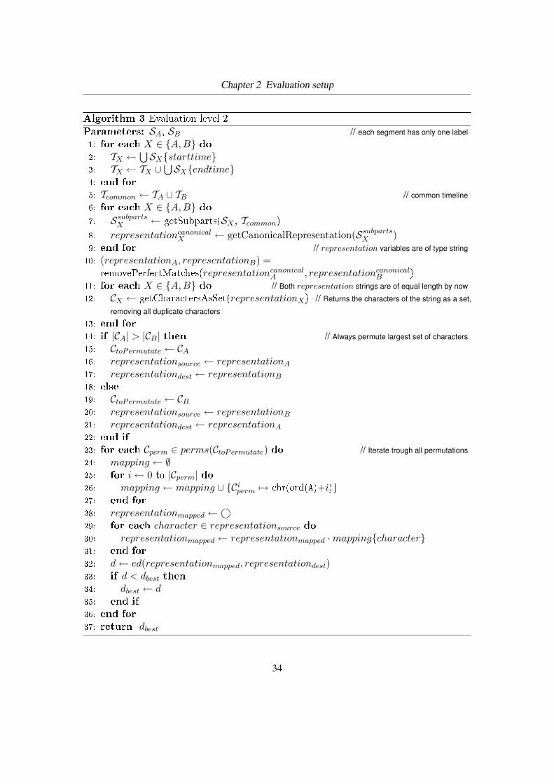
Chapter 2 Evaluation setup
Algorithm 3 Evaluation level 2
Parameters: SA, SB // each segment has only one label
1: for each X ∈ {A,B} do2: TX ←
⋃SX{starttime}
3: TX ← TX ∪⋃SX{endtime}
4: end for
5: Tcommon ← TA ∪ TB // common timeline
6: for each X ∈ {A,B} do7: Ssubparts
X ← getSubparts(SX , Tcommon)
8: representationcanonicalX ← getCanonicalRepresentation(Ssubparts
X )9: end for // representation variables are of type string
10: (representationA, representationB) =removePerfectMatches(representationcanonical
A , representationcanonicalB )
11: for each X ∈ {A,B} do // Both representation strings are of equal length by now
12: CX ← getCharactersAsSet(representationX) // Returns the characters of the string as a set,
removing all duplicate characters
13: end for
14: if |CA| > |CB| then // Always permute largest set of characters
15: CtoPermutate ← CA16: representationsource ← representationA
17: representationdest ← representationB
18: else
19: CtoPermutate ← CB20: representationsource ← representationB
21: representationdest ← representationA
22: end if
23: for each Cperm ∈ perms(CtoPermutate) do // Iterate trough all permutations
24: mapping ← ∅25: for i← 0 to |Cperm| do26: mapping ← mapping ∪ {Ci
perm 7→ chr(ord(A)+i)}27: end for
28: representationmapped ←©29: for each character ∈ representationsource do
30: representationmapped ← representationmapped ·mapping{character}31: end for
32: d← ed(representationmapped, representationdest)33: if d < dbest then
34: dbest ← d35: end if
36: end for
37: return dbest
34
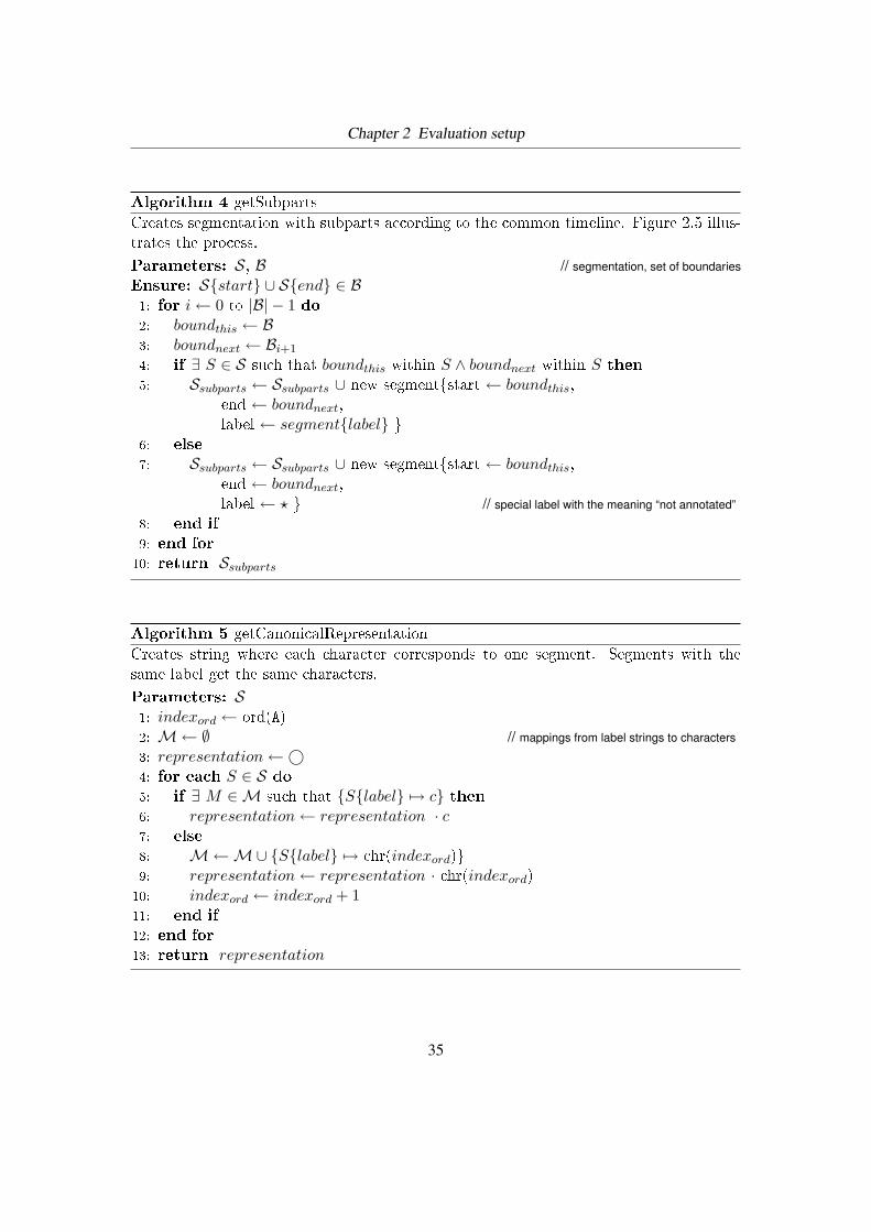
Chapter 2 Evaluation setup
Algorithm 4 getSubparts
Creates segmentation with subparts according to the common timeline. Figure 2.5 illus-trates the process.
Parameters: S, B // segmentation, set of boundaries
Ensure: S{start} ∪ S{end} ∈ B1: for i← 0 to |B| − 1 do
2: boundthis ← B3: boundnext ← Bi+1
4: if ∃ S ∈ S such that boundthis within S ∧ boundnext within S then
5: Ssubparts ← Ssubparts ∪ new segment{start ← boundthis,end ← boundnext,label ← segment{label} }
6: else
7: Ssubparts ← Ssubparts ∪ new segment{start ← boundthis,end ← boundnext,label ← ? } // special label with the meaning “not annotated”
8: end if
9: end for
10: return Ssubparts
Algorithm 5 getCanonicalRepresentation
Creates string where each character corresponds to one segment. Segments with thesame label get the same characters.
Parameters: S1: indexord ← ord(A)2: M← ∅ // mappings from label strings to characters
3: representation←©4: for each S ∈ S do
5: if ∃ M ∈M such that {S{label} 7→ c} then6: representation← representation · c7: else
8: M←M∪ {S{label} 7→ chr(indexord)}9: representation← representation · chr(indexord)
10: indexord ← indexord + 111: end if
12: end for
13: return representation
35
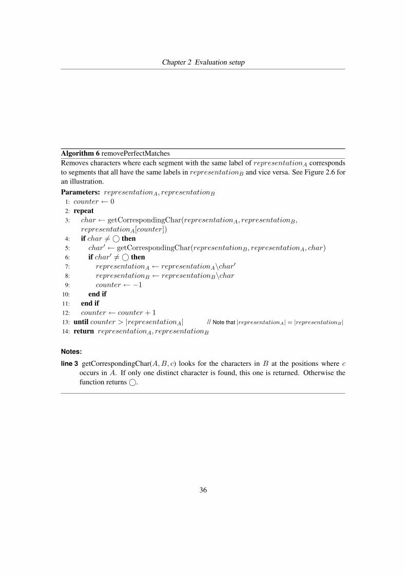
Chapter 2 Evaluation setup
Algorithm 6 removePerfectMatchesRemoves characters where each segment with the same label of representationA correspondsto segments that all have the same labels in representationB and vice versa. See Figure 2.6 foran illustration.Parameters: representationA, representationB
1: counter ← 02: repeat3: char ← getCorrespondingChar(representationA, representationB,
representationA[counter])4: if char 6=© then5: char′ ← getCorrespondingChar(representationB, representationA, char)6: if char′ 6=© then7: representationA ← representationA\char′
8: representationB ← representationB\char9: counter ← −1
10: end if11: end if12: counter ← counter + 113: until counter > |representationA| // Note that |representationA| = |representationB |14: return representationA, representationB
Notes:
line 3 getCorrespondingChar(A,B, c) looks for the characters in B at the positions where coccurs in A. If only one distinct character is found, this one is returned. Otherwise thefunction returns©.
36
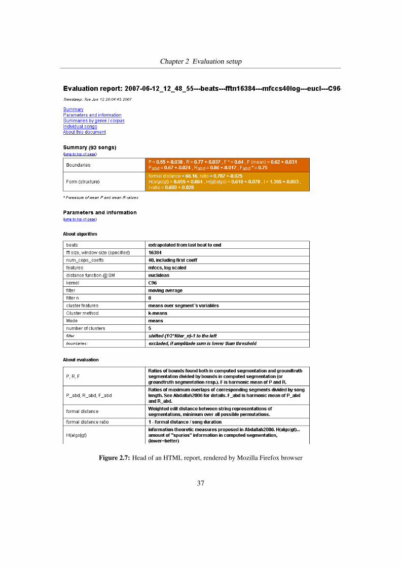
Chapter 2 Evaluation setup
Figure 2.7: Head of an HTML report, rendered by Mozilla Firefox browser
37
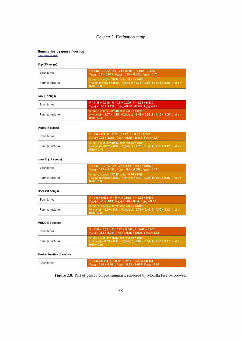
Chapter 2 Evaluation setup
Figure 2.8: Part of genre / corpus summary, rendered by Mozilla Firefox browser
38
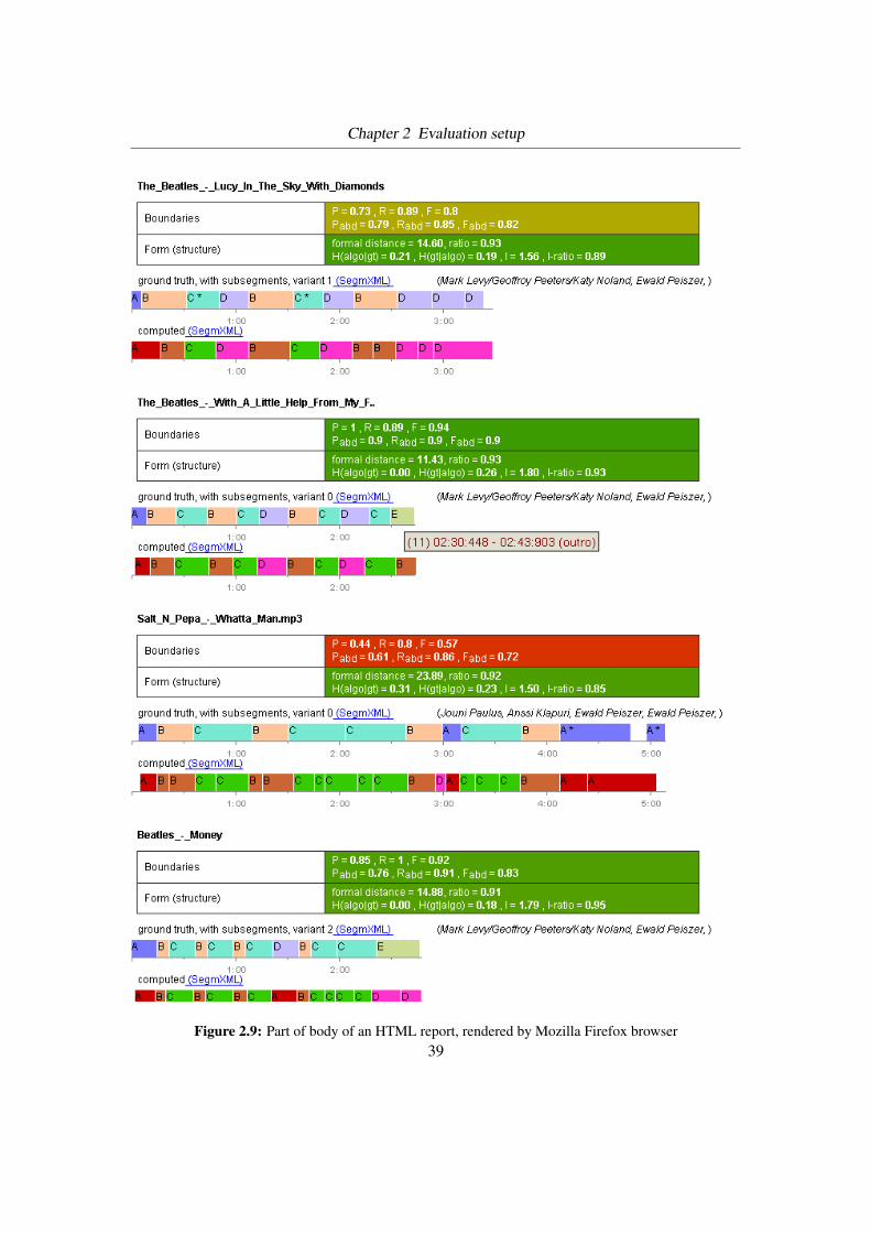
Chapter 2 Evaluation setup
Figure 2.9: Part of body of an HTML report, rendered by Mozilla Firefox browser39
Chapter 2 Evaluation setup
The largest part of the report gives you information about each individual song: performance
numbers, debug output, information about the groundtruth file and last but not least a graphical
representation of both the groundtruth annotation and the computed segmentation. Segments
with the same label have the same color, each segment has a tooltip with information about start
and end time, label and an optional comment which is indicated by an asterisk. Hyperlinks make
the underlying SegmXML files directly accessible.
The footer of the report contains general information about the document.
The colors of the boxes range from red (if the respective performance number is lower than 0.6)
over yellow (if around 0.75) to green (if greater than 0.9).
2.4 Ambiguity revisited
As already stated in Section 1.3.1, it can happen that two annotators produce different segmen-
tations for the same songs. In Figure 1.1 we saw five examples of that situation.
On the other hand, it must be noted that not all segmentations differ that much. This leads to the
conclusion that some songs have a more ambiguous structure than others. One idea would be
to determine an upper limit for the performance measures for each song individually and scale
results according to this limit. This limit could be the mean of performance numbers that result
if various manual segmentations are evaluated against each other. Let F gt and rgtf denote these
limits for boundary evaluation and musical form evaluation, respectively.
Example (Michael Jackson: Black or White) rgtf values if evaluating Paulus corpus ground-
truth and Queen Mary corpus groundtruth against my official (flexible, two-level) annotation are
0.84 and 0.68, the mean is 0.76. This can be considered to be the upper limit for this song: rf
of computed structure against groundtruth need not be any higher. One result of a computed
annotation for this song is rf = 0.66. If you scale it according to the upper groundtruth limit the
resulting r0.76f = 0.868.
I do not have different groundtruth segmentations for the majority of the songs, and the number
of different annotations available for the rest is not large enough to derive well-grounded F gt
and rgtf values. Thus, I decided not to scale evaluation numbers.
40
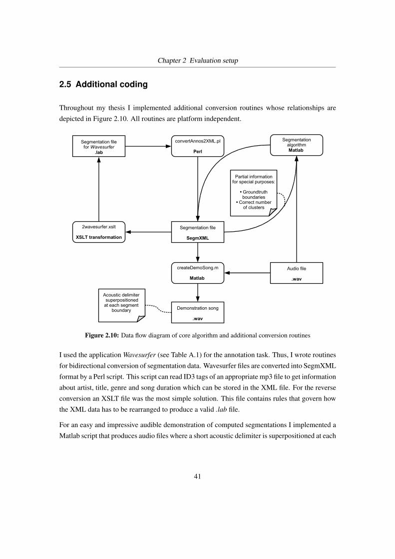
Chapter 2 Evaluation setup
2.5 Additional coding
Throughout my thesis I implemented additional conversion routines whose relationships are
depicted in Figure 2.10. All routines are platform independent.
convertAnnos2XML.pl
Perl
Segmentation filefor Wavesurfer
.lab
2wavesurfer.xslt
XSLT transformation
SegmentationalgorithmMatlab
Partial informationfor special purposes:
● Groundtruthboundaries
● Correct numberof clusters
Audio file
.wav
Demonstration song
.wav
Acoustic delimiter superpositioned
at each segment boundary
Segmentation file
SegmXML
createDemoSong.m
Matlab
Figure 2.10: Data flow diagram of core algorithm and additional conversion routines
I used the application Wavesurfer (see Table A.1) for the annotation task. Thus, I wrote routines
for bidirectional conversion of segmentation data. Wavesurfer files are converted into SegmXML
format by a Perl script. This script can read ID3 tags of an appropriate mp3 file to get information
about artist, title, genre and song duration which can be stored in the XML file. For the reverse
conversion an XSLT file was the most simple solution. This file contains rules that govern how
the XML data has to be rearranged to produce a valid .lab file.
For an easy and impressive audible demonstration of computed segmentations I implemented a
Matlab script that produces audio files where a short acoustic delimiter is superpositioned at each
41
Chapter 2 Evaluation setup
segment boundary. This delimiter also indicates the segment type of the respective subsequent
segment (“one”, “two”, “three”, etc.).
2.6 Summary
This chapter discussed how evaluation has been carried out in this thesis.
First, I described the groundtruth corpus which is one of the largest used so far in this research
field. Together with the additional “test set” songs it is indeed the largest one.
Since annotation file formats used so far seemed too strict to me for the purpose at hand I
introduced a novel file format based on XML (SegmXML) that can contain two hierarchical
levels of segmentation as well as alternative labels for each segment. Besides, song metadata
can be stored to ease the retrieval of specific song recordings (e.g., with the help of MusicBrainz
TrackID). I explained how this flexible annotation format is used by the evaluation algorithm.
Performance measures for both algorithm tasks have been defined. For the first phase, boundary
detection, these are precision P , recall R and F-measure F , as well as alternative measures
Pabd, Rabd and Fabd which express similar concepts but have different properties. The second
phase, structure extraction, makes use of formal distance ratio rf and the alternative information-
theoretic measure “mutual information” I . Especially the measure for the second phase has
been motivated thoroughly as musical form evaluation is quite sophisticated and not as straight
forward as one might think in the beginning (see the discussion on hierarchical segmentations in
Section 2.2.2).
I included the most important sub functions of the evaluation algorithm in pseudo code notation
and explained all relevant parts of the evaluation reports that are generated by the system.
One section presented an idea how the inherent segmentation ambiguity can be used explicitely
to get more accurate evaluation numbers. As noted, this would require a number of groundtruth
annotations for each song and is thus not feasible for this thesis.
The chapter ended with a brief overview of additional coding that has been carried out, e.g., to
convert annotation data from one file format to another or to produce audio files for acoustic
demonstration.
42
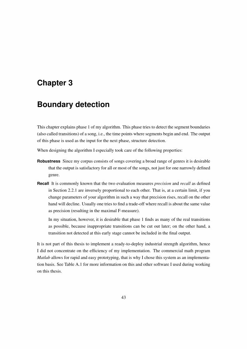
Chapter 3
Boundary detection
This chapter explains phase 1 of my algorithm. This phase tries to detect the segment boundaries
(also called transitions) of a song, i.e., the time points where segments begin and end. The output
of this phase is used as the input for the next phase, structure detection.
When designing the algorithm I especially took care of the following properties:
Robustness Since my corpus consists of songs covering a broad range of genres it is desirable
that the output is satisfactory for all or most of the songs, not just for one narrowly defined
genre.
Recall It is commonly known that the two evaluation measures precision and recall as defined
in Section 2.2.1 are inversely proportional to each other. That is, at a certain limit, if you
change parameters of your algorithm in such a way that precision rises, recall on the other
hand will decline. Usually one tries to find a trade-off where recall is about the same value
as precision (resulting in the maximal F-measure).
In my situation, however, it is desirable that phase 1 finds as many of the real transitions
as possible, because inappropriate transitions can be cut out later; on the other hand, a
transition not detected at this early stage cannot be included in the final output.
It is not part of this thesis to implement a ready-to-deploy industrial strength algorithm, hence
I did not concentrate on the efficiency of my implementation. The commercial math program
Matlab allows for rapid and easy prototyping, that is why I chose this system as an implementa-
tion basis. See Table A.1 for more information on this and other software I used during working
on this thesis.
43
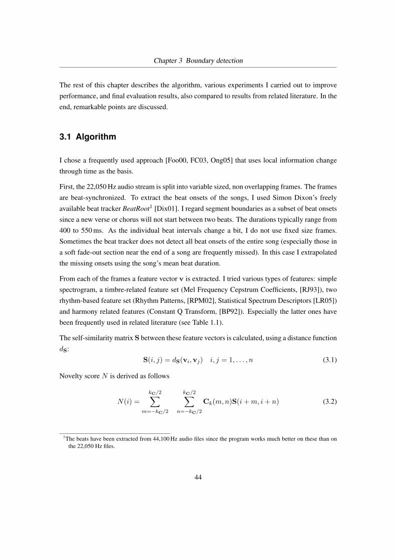
Chapter 3 Boundary detection
The rest of this chapter describes the algorithm, various experiments I carried out to improve
performance, and final evaluation results, also compared to results from related literature. In the
end, remarkable points are discussed.
3.1 Algorithm
I chose a frequently used approach [Foo00, FC03, Ong05] that uses local information change
through time as the basis.
First, the 22,050 Hz audio stream is split into variable sized, non overlapping frames. The frames
are beat-synchronized. To extract the beat onsets of the songs, I used Simon Dixon’s freely
available beat tracker BeatRoot1 [Dix01]. I regard segment boundaries as a subset of beat onsets
since a new verse or chorus will not start between two beats. The durations typically range from
400 to 550 ms. As the individual beat intervals change a bit, I do not use fixed size frames.
Sometimes the beat tracker does not detect all beat onsets of the entire song (especially those in
a soft fade-out section near the end of a song are frequently missed). In this case I extrapolated
the missing onsets using the song’s mean beat duration.
From each of the frames a feature vector v is extracted. I tried various types of features: simple
spectrogram, a timbre-related feature set (Mel Frequency Cepstrum Coefficients, [RJ93]), two
rhythm-based feature set (Rhythm Patterns, [RPM02], Statistical Spectrum Descriptors [LR05])
and harmony related features (Constant Q Transform, [BP92]). Especially the latter ones have
been frequently used in related literature (see Table 1.1).
The self-similarity matrix S between these feature vectors is calculated, using a distance function
dS:
S(i, j) = dS(vi,vj) i, j = 1, . . . , n (3.1)
Novelty score N is derived as follows
N(i) =kC/2∑
m=−kC/2
kC/2∑n=−kC/2
Ck(m,n)S(i + m, i + n) (3.2)
1The beats have been extracted from 44,100 Hz audio files since the program works much better on these than onthe 22,050 Hz files.
44

Chapter 3 Boundary detection
where Ck denotes a Gaussian tapered checkerboard kernel of size kC, radially symmetric and
centered on 0, 0 (Figure 3.1). S is zero padded.
Figure 3.1: Gaussian kernel of size kC = 80. (from: [FC03])
Since N appears to be quite jagged I applied a low-pass filter H to get a smoother novelty score
HN , this reduces the number of local maxima. I used a moving average filter with a sliding
window size of nH . This type of filter is optimal for this task: noise reduction while retaining a
sharp step response [Smi97, Chapter 15].
HN (i) = 1/nH
nH/2∑j=−nH/2
N(i + j) (3.3)
Empirically, I found out that if there is a local maximum during a period of low amplitude it
should not be considered as a segment boundary. Thus, I introduced an amplitude threshold
45

Chapter 3 Boundary detection
Tampl: maxima in a region with an amplitude a < Tampl will not be regarded as segment
boundaries. This step removes approximately one to four boundaries mainly from the beginning
and end of a song (fade-in and fade-out).
Finally, I set up an interval restriction that prevents two boundaries that are closer than a thresh-
old Tclose (in this case the maximum with the higher HN value is chosen). For Tclose = 6seconds about only 60 to 80 per cent of the original boundaries remain.
The process described produces a set of possible segment boundaries B1.
Figures 3.2 to 3.4 illustrate this process for three songs with varying output quality.
3.2 Experiments
The algorithm description indicates that there are many parameters or degrees of freedom that
have to be adjusted: choice of feature set, feature set related parameters, dS, kC, type and
parameters of H , etc.
These parameters span a high dimensional solution space, the exhaustive search for the best
parameter settings seems intractable to me. Therefore I systematically investigated this space by
two methods. In the first place I acted at my own discretion, using comments from the literature,
common music knowledge and machine learning experience as basis to set parameters to values
that might lead to good results. For example, since two choruses are more likely to share the
same melody than the same instruments, the use of CQT features seemed advisable.
Secondly I fixed all parameters but one and let the mutable variable loop through an appropriate
value range to see whether the results would change significantly.
From all feature sets I used MFCC features provided the best results. This is surprising since
CQT features (when using appropriate values for f0, fmax and bins) would model the proper-
ties of musical signals more specifically than the widely used MFCCs that actually come from
speech processing: Bartsch et al. report better results with ‘harmony aware’ features than with
MFCC [BW05]. Aucouturier et al., however, report MFCC to be superior if 8–10 coefficients
are taken [AS01]. I found that ten coefficients are too little, even results with 30 coefficients are
(insignificantly) inferior to those with 40 (c.f. Figure 3.7).
46

Chapter 3 Boundary detection
Figure 3.2: Boundary detection in KC and the Sunshine Band: That’s the Way I Like It. Vertical dottedlines indicate groundtruth boundaries, subsegment boundaries are in parentheses. These are also clearlyvisible in the similarity matrix. Result for this computation is P = R = F = 1 for w = 3.
47
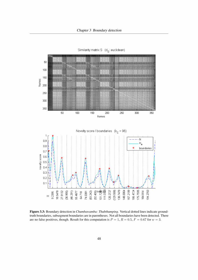
Chapter 3 Boundary detection
Figure 3.3: Boundary detection in Chumbawamba: Thubthumping. Vertical dotted lines indicate ground-truth boundaries, subsegment boundaries are in parentheses. Not all boundaries have been detected. Thereare no false positives, though. Result for this computation is P = 1, R = 0.5, F = 0.67 for w = 3.
48
Chapter 3 Boundary detection
Figure 3.4: Boundary detection in Eminem: Stan. Vertical dotted lines indicate groundtruth boundaries,subsegment boundaries are in parentheses. Y axis is cropped to interval [0, 0.3]. HN exhibits manypeaks that do not correspond to true boundaries. Each detected bound, however, is correct. Result for thiscomputation is P = 0.27, R = 1, F = 0.42 for w = 3.
49
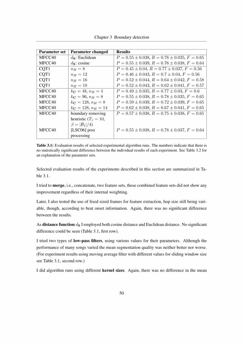
Chapter 3 Boundary detection
Parameter set Parameter changed ResultsMFCC40 dS: Euclidean P = 0.55± 0.038, R = 0.78± 0.035, F = 0.65MFCC40 dS: cosine P = 0.55± 0.039, R = 0.76± 0.038, F = 0.64CQT1 nH = 8 P = 0.45± 0.04, R = 0.77± 0.037, F = 0.56CQT1 nH = 12 P = 0.46± 0.043, R = 0.7± 0.04, F = 0.56CQT1 nH = 16 P = 0.52± 0.044, R = 0.64± 0.042, F = 0.58CQT1 nH = 18 P = 0.52± 0.043, R = 0.62± 0.041, F = 0.57MFCC40 kC = 48, nH = 4 P = 0.49± 0.035, R = 0.77± 0.03, F = 0.6MFCC40 kC = 96, nH = 8 P = 0.55± 0.038, R = 0.78± 0.035, F = 0.65MFCC40 kC = 128, nH = 8 P = 0.59± 0.039, R = 0.72± 0.039, F = 0.65MFCC40 kC = 128, nH = 14 P = 0.62± 0.038, R = 0.67± 0.041, F = 0.65MFCC40 boundary removing
heuristic (T1 = 10,β = |B1|/4)
P = 0.57± 0.038, R = 0.75± 0.038, F = 0.65
MFCC40 [LSC06] postprocessing
P = 0.55± 0.038, R = 0.78± 0.037, F = 0.64
Table 3.1: Evaluation results of selected experimental algorithm runs. The numbers indicate that there isno statistically significant difference between the individual results of each experiment. See Table 3.2 foran explanation of the parameter sets.
Selected evaluation results of the experiments described in this section are summarized in Ta-
ble 3.1.
I tried to merge, i.e., concatenate, two feature sets, these combined feature sets did not show any
improvement regardless of their internal weighting.
Later, I also tested the use of fixed sized frames for feature extraction, hop size still being vari-
able, though, according to beat onset information. Again, there was no significant difference
between the results.
As distance function dS I employed both cosine distance and Euclidean distance. No significant
difference could be seen (Table 3.1, first row).
I tried two types of low-pass filters, using various values for their parameters. Although the
performance of many songs varied the mean segmentation quality was neither better nor worse.
(For experiment results using moving average filter with different values for sliding window size
see Table 3.1, second row.)
I did algorithm runs using different kernel sizes. Again, there was no difference in the mean
50
Chapter 3 Boundary detection
performance. Finally, I decided to take kC = 96 beats which corresponds to approx. 38 seconds,
depending on the beat length of course. Figure 3.5 and the third row of Table 3.1 show the effect
of various kernel sizes.
Figure 3.5: Novelty scores and resulting boundaries of Chumbawamba: Thubthumping when usingdifferent kernel sizes. Although the latter kernel is more than five times larger than the first one there arenot that many more segment boundaries as one might expect because many peaks are very close to eachother and hence are not regarded as boundaries. kC = 48: P = 0.93, R = 0.7, F = 0.8; kC = 256:P = 1, R = 0.65, F = 0.79.
I employed Principal Component Analysis (PCA) to reduce the size of the feature vectors for
the subsequent calculation steps. Most of the time, however, this step neither reduced the overall
runtime very much nor improved the results.
I tried a boundary removing heuristic to improve performance of the worst songs: From some
songs (for instance Eminem: Stan, see Figure 3.4) too many peaks of HN are interpreted as
boundaries. I computed the bounds per minute ratio rbm = |B1|/dur, dur being the song’s
duration in minutes, and compared it with a threshold T1 (e.g., T1 = 10). If rbm > T1 then
β boundaries with the lowest corresponding HN values are removed (e.g., β = |B1|/4). This
heuristic worked well for the Eminem song (F rose by 0.13), the overall results were not better,
though (Table 3.1, fourth row). In my opinion there are two reasons for that.
First, there are also songs which natively have a high rbm in their groundtruth annotation. These
songs’ performance declines. Second, sometimes it is indeed the case that segments begin or
51

Chapter 3 Boundary detection
end at positions where HN is low. So this heuristic would remove correct boundaries, resulting
in an even lower precision value. See Figure 3.6 for two example songs.
(a) Segmentations of The Roots: You Got Me. Ground truth (top); computed (middle), F = 0.61; computed withheuristic applied (bottom), F = 0.73.
(b) Segmentations of Britney Spears: Hit Me Baby One More Time. Ground truth (top); computed (middle), F =0.80; computed with heuristic applied (bottom), F = 0.67.
Figure 3.6: Effect of boundary removing heuristic (T1 = 10, β = |B1|/4) applied to two songs. Whitevertical lines within dark gray panels indicate segment boundaries.Figure (a) shows a song where applying the heuristic improved F . Figure (b), on the contrary, showsan example of a song where the F-measure has declined. Checking the novelty score, I saw that it wasindeed the case that HN had rather low values at some positions where correct boundaries are located.
Another attempt to cope with low precision can be called two-iterations-approach. Since songs
like the above mentioned Eminem: Stan produce way too many computed boundaries one should
regard them only as boundary candidates from which the final boundaries can be selected by a
second S / N / HN iteration. This means in fact that the “segments” from the first iteration are
considered to be the “frames” for the second one: each “frame” now comprises a longer period
of time. Naturally this leads to less boundaries.
52
Chapter 3 Boundary detection
Unfortunately even the outcome of Eminem’s song was not better using this approach. I noticed
that the similarity matrix resolution for the second pass was very low (one discreet time step
was about 7 s), thus, novelty score computation could not be performed properly. Especially the
low-pass filter had problems with the low time resolution.
Levy et al. proposed a post-processing method which takes musical domain knowledge into
account [LSC06]. The idea is to restrict the possible locations where a segment boundary may
be to downbeat locations (i.e., where a measure starts) since it is unlikely that a segment begins
within a measure. The authors employed a brute-force algorithm to find a phrase-length m and
an offset o such that the squared differences between detected boundaries and positions matching
m and o becomes minimal. o should eventually correspond to the position of the first downbeat;
m can be regarded as the length of one measure.
I tried two value ranges for m. First, I let m iterate trough values close (± 16 ) to half of the mean
segment length. Results were statistically insignificantly worse. Then I chose a value range
around 4, 8 and 16 times the mean beat length. The results were almost equal to the results
without this post-processing method (Table 3.1, fourth row).
One reason for this is the fact that most of the incorrectly detected boundaries are a greater period
of time away from the closest groundtruth boundary than half of the measure (for a measure of
eight beats this would be approximately 1.6 s, depending on the beat lengths). So the possibly
largest shift correction could not turn these incorrect transitions into correct ones. It is also quite
common that some computed boundaries are actually superfluous and should be deleted, not
shifted, further decreasing the potential positive effect of this method in my case.
As one of the last attempts to improve results I employed a recently presented method called
Harmonic Change Detection Function (HCDF) [HSG06]. Here, twelve bin chroma vectors
are mapped into a 6 D polytop (i.e., six dimensional generalization of a polygon) based on the
Harmonic Network or Tonnetz which is a representation of pitch relations. Using the original
Matlab code written by the authors it appeared that the results were significantly worse than
already obtained ones, also after some experimenting with HCDF parameters. One reason might
be that HCDF is originally used for chord detection, an application that needs a higher resolution
of the harmonic changes. The HCDF can probably be adapted to work for audio segmentation
as well. In view of the very low performance numbers, their robustness against various HCDF
parameters settings and the experience with previous unsuccessful improvement attempts I did
not go any further into adapting the HCDF.
53
Chapter 3 Boundary detection
3.3 Results
Figure 3.7 depicts the results of my segment boundary detection algorithm using different pa-
rameter sets. For the specifications of these parameter sets please refer to Table 3.2.
Evaluation results depend on the allowed deviation w between computed and groundtruth bound-
aries. Figure 3.8 shows the effect of different values for w.
In Figure 3.9 P and Pabd of each song is plotted against the respective R and Rabd values.
Baseline As baseline results I generated four sets of segmentations. Each segmentation con-
sists of segments of equal length l ∈ {10, 15, 20, 30}. The position of the first boundary was
l/2. Following my expectations these results were pretty bad.
Comparison In Table 3.3, Figures 3.10 and 3.11 performance of my output is compared to
performance measures that have been published in related literature.
Both Lu et al. [LWZ04] and Levy et al. [LSC06] include a histogram over distances of computed
boundaries from the nearest groundtruth boundary. Since the precise numbers are not included I
can only estimate the evaluation number precision.
Chai [Cha05] and Ong [Ong05] publish results in terms of precision and recall, defined in the
same way as I did in Section 2.2.1.
Please note, however, that not all mentioned papers use the same corpus, thus the comparability
of the numbers is limited. To overcome this limitation I included results based on qmul14 corpus
that has been used in [LWZ04] and [LSC06].
If you look at mean P and F , disregarding the confidence interval, you can notice that qmul14
results are (much) higher (Figure 3.10, last two columns). This shows one fact very impres-
sively: The evaluation numbers depend to a larger degree on the corpus than on the algorithm
or parameters. This again emphasizes the importance of carefully selecting songs for a common
corpus if an audio segmentation benchmark evaluation is going to take place. You can also see
how important it is to compute and publish proper confidence intervals: the mean values alone
could be misleading.
54
Chapter 3 Boundary detection
Parameters SPEC MFCC10 MFCC30 MFCC40feature set spectrogram MFCCs, 10 / 30 / 40 coefficients, included first
coefficient, log scaledframe size 1 beat 740ms (214 points)hop size 1 beatdS EuclideankC 96H Moving average with nH sized sliding windownH 8Tampl 0.2Parameters RP SSD CQT1 CQT2feature set Rhythm Patterns Statistical
SpectrumDescriptor
CQT withf0 = 64.4,bins = 12,fmax = 7902.1
CQT withf0 = 64.4,bins = 12,fmax = 988.7
frame size Approx. 6 s (217 points) 370 ms (8096 points)hop size 2 beats 1 beatdS EuclideankC 48 64 96H Moving average with nH sized sliding windownH 4 2 8Tampl 0.2Parameters MRG1 MRG2feature sets,frame size,hop size
mergedMFCC40 andRP; weighted2:1
mergedMFCC40 andCQT1; weighted3:1
dS EuclideankC 48 96H Moving average with nH sized sliding windownH 4 8Tampl 0.2
Table 3.2: Parameter value sets that are referenced in figures
55
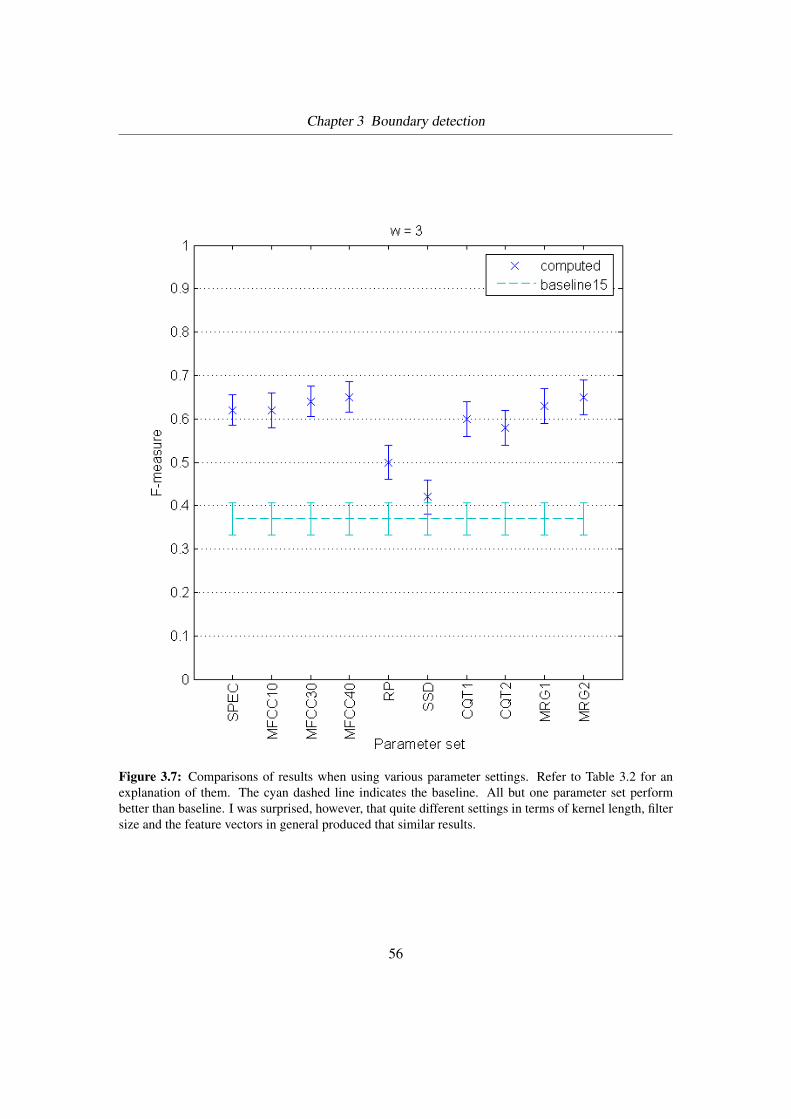
Chapter 3 Boundary detection
Figure 3.7: Comparisons of results when using various parameter settings. Refer to Table 3.2 for anexplanation of them. The cyan dashed line indicates the baseline. All but one parameter set performbetter than baseline. I was surprised, however, that quite different settings in terms of kernel length, filtersize and the feature vectors in general produced that similar results.
56
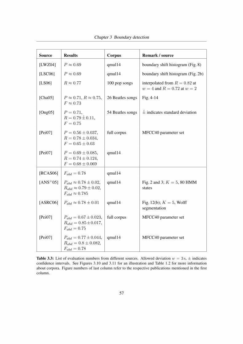
Chapter 3 Boundary detection
Source Results Corpus Remark / source
[LWZ04] P ≈ 0.69 qmul14 boundary shift histogram (Fig. 8)
[LSC06] P ≈ 0.69 qmul14 boundary shift histogram (Fig. 2b)
[LS06] R ≈ 0.77 100 pop songs interpolated from R = 0.82 atw = 4 and R = 0.72 at w = 2
[Cha05] P ≈ 0.71, R ≈ 0.75,F ≈ 0.73
26 Beatles songs Fig. 4-14
[Ong05] P = 0.71,R = 0.79 ±̂ 0.11,F = 0.75
54 Beatles songs ±̂ indicates standard deviation
[Pei07] P = 0.56± 0.037,R = 0.78± 0.034,F = 0.65± 0.03
full corpus MFCC40 parameter set
[Pei07] P = 0.69± 0.085,R = 0.74± 0.124,F = 0.68± 0.069
qmul14
[RCAS06] Fabd = 0.78 qmul14
[ANS+05] Pabd ≈ 0.78± 0.02,Rabd ≈ 0.79± 0.02,Fabd ≈ 0.785
qmul14 Fig. 2 and 3; K = 5, 80 HMMstates
[ASRC06] Pabd ≈ 0.78± 0.01 qmul14 Fig. 12(b); K = 5, Wolffsegmentation
[Pei07] Pabd = 0.67± 0.023,Rabd = 0.85±0.017,Fabd = 0.75
full corpus MFCC40 parameter set
[Pei07] Pabd = 0.77± 0.044,Rabd = 0.8± 0.082,Fabd = 0.78
qmul14 MFCC40 parameter set
Table 3.3: List of evaluation numbers from different sources. Allowed deviation w = 3 s, ± indicatesconfidence intervals. See Figures 3.10 and 3.11 for an illustration and Table 1.2 for more informationabout corpora. Figure numbers of last column refer to the respective publications mentioned in the firstcolumn.
57

Chapter 3 Boundary detection
Figure 3.8: Evaluation results with different values for w, error bars indicate the confidence interval.At w = 6 P values are identical with baseline. At w = 3 precision of MFCC40 is significantly betterthan the baseline whereas precision of RP is not.
3.4 Discussion
I would say that automatic segment boundary extraction results are quite acceptable if you con-
sider that
• the algorithm operates exclusively on local information, i.e., it does not take large scale
data into account.
• it does not make use of domain knowledge which means that there is also no restriction
about the songs that can be processed.
• the corpus contains songs of various different genres.
• the evaluation numbers have not been related to the songs’ “inherent” ambiguity that can
make it impossible to reach the perfect value of F = 1 (see Sections 1.3.1 and 2.4).
It can be noticed that computed segmentations tend to have too many boundaries which leads to
a rather low precision value. Reasons for that may be:
58
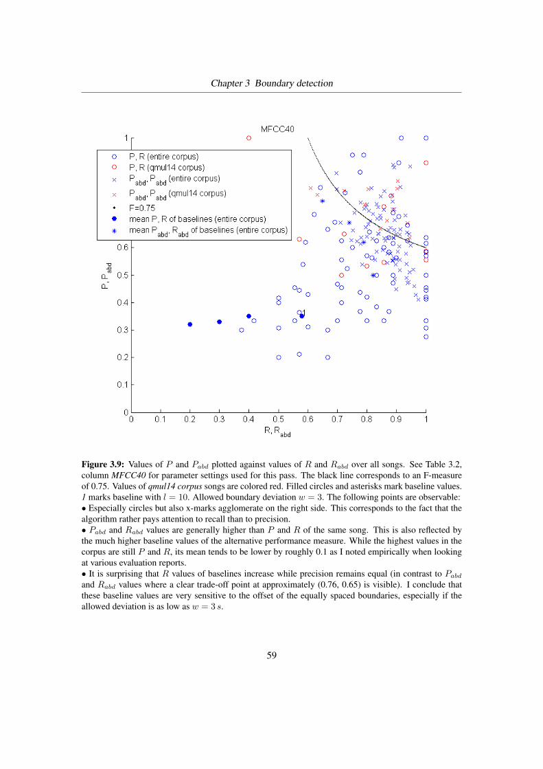
Chapter 3 Boundary detection
Figure 3.9: Values of P and Pabd plotted against values of R and Rabd over all songs. See Table 3.2,column MFCC40 for parameter settings used for this pass. The black line corresponds to an F-measureof 0.75. Values of qmul14 corpus songs are colored red. Filled circles and asterisks mark baseline values.1 marks baseline with l = 10. Allowed boundary deviation w = 3. The following points are observable:• Especially circles but also x-marks agglomerate on the right side. This corresponds to the fact that thealgorithm rather pays attention to recall than to precision.• Pabd and Rabd values are generally higher than P and R of the same song. This is also reflected bythe much higher baseline values of the alternative performance measure. While the highest values in thecorpus are still P and R, its mean tends to be lower by roughly 0.1 as I noted empirically when lookingat various evaluation reports.• It is surprising that R values of baselines increase while precision remains equal (in contrast to Pabd
and Rabd values where a clear trade-off point at approximately (0.76, 0.65) is visible). I conclude thatthese baseline values are very sensitive to the offset of the equally spaced boundaries, especially if theallowed deviation is as low as w = 3 s.
59
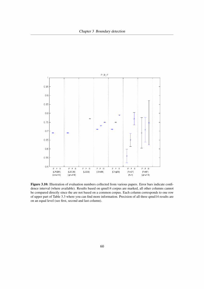
Chapter 3 Boundary detection
Figure 3.10: Illustration of evaluation numbers collected from various papers. Error bars indicate confi-dence interval (where available). Results based on qmul14 corpus are marked, all other columns cannotbe compared directly since the are not based on a common corpus. Each column corresponds to one rowof upper part of Table 3.3 where you can find more information. Precision of all three qmul14 results areon an equal level (see first, second and last column).
60
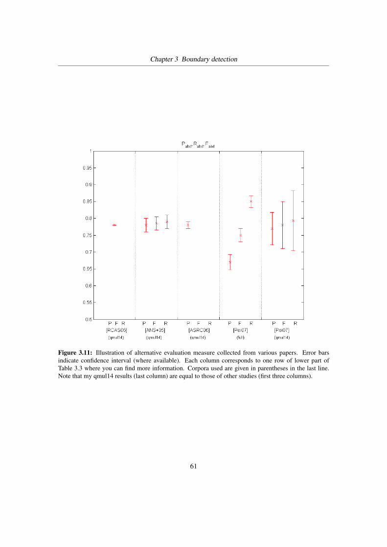
Chapter 3 Boundary detection
Figure 3.11: Illustration of alternative evaluation measure collected from various papers. Error barsindicate confidence interval (where available). Each column corresponds to one row of lower part ofTable 3.3 where you can find more information. Corpora used are given in parentheses in the last line.Note that my qmul14 results (last column) are equal to those of other studies (first three columns).
61
Chapter 3 Boundary detection
• Frequently there is a novelty score peak at the change of instrument, e.g., in soli, leading
to false positives.
• Boundaries in slow and soft songs are often shifted some time from the correct positions
since the edges in the similarity matrix are not that distinct (for instance in Sinhead O
Connor: Nothing Compares To You).
• On the other hand, non-melodic audio parts like in rap songs exhibit fast changing feature
vector distances leading to a jagged Novelty Score and too many boundaries.
• Also, songs with dense, distorted guitar sound seem to perform worse than melodic ones.
• The values of N or HN themselves cannot be used to distinguish between correct and
incorrect boundaries.
In view of the fact that my improvement attempts did not produce significantly better results I
got a feeling that it might not possible to further improve segmentation. A plausible reason may
be that the data set contains a certain amount of noise which is due to the ambiguity of song
segmentations as discussed in Sections 1.3.1 and 2.4.
I learned from the evaluation reports that it were not always the same songs which performed
badly. There are, of course, songs that generally are easier to segment, e.g., KC and the Sunshine
Band: That’s the Way I Like It, but the songs on the lower end change according to the feature
set used and other parameters.
To find a clue about which “type” of songs perform better with which feature set I compared the
24 worst performing songs (which is a quarter of the entire corpus) of one algorithm run with
those of another. Consecutively, I built the intersection between these two sets. The idea was to
find some similarity between the bad performing songs not contained in the intersection.
For clarification please have a look at the following example.
First I ran the algorithm using MFCC features, the second run was based on CQT features. The
intersection of each run’s 24 worst performing songs contained 17 songs. This means that there
are seven songs for which MFCC features work better and seven other songs for which CQT
features are the better choice. The songs of these two sets are, in no special order:
62
Chapter 3 Boundary detection
Set 1 (performs better with MFCC features):
The Beatles: Within You Without You, The Beatles: Being For The Benefit Of Mr. Kite,
Britney Spears: Oops I Did It Again, Faith No More: Epic, The Beatles: Help, The Beatles:
Sgt. Peppers Lonely Hearts Club Band, Beatles: Till There Was You
Set 2 (performs better with CQT features):
The Beatles: She’s Leaving Home, Björk: It’s Oh So Quiet, Simply Red: Stars, Red Hot
Chili Peppers: Parallel Universe, Depeche Mode: It’s no good, Artful Dodger Craig David:
Rewind, A-HA: Take on me
It can be said that Set 2 is quite melodic and does not contain strong guitar sound, whereas most
of the songs of Set 1 exhibit a strong rhythm and dominant guitar timbre. On the other hand
there are also rather melodic songs in Set 1 (Oops I Did It Again, Till There Was You). In this
light it might be the case that MFCC features are better suited for rock songs. This conclusion
is, however, not evidenced by the mean performance numbers of rock genre in the respective
evaluation reports: those numbers do not differ significantly.
I repeated this ad-hoc investigation a few times, however, without finding strong evidence. Thus,
I suggest to do a systematically analysis on this matter in subsequent studies.
Finally, to summarize the results verbally one can state that every other computed segment
boundary is correct and that three quarters of the boundaries are detected automatically with-
out human interaction across a diverse set of songs.
3.5 Summary
This chapter dealt with the first phase of my audio segmentation algorithm, which is automatic
boundary extraction. Its output is a set of time points where song segments start or end.
The approach I used is the quite traditional similarity matrix / novelty score method introduced
in [Foo00]. There, differences between neighbouring feature vectors are used to detect more or
less sudden changes in the song.
63
Chapter 3 Boundary detection
Then, I mentioned and explained numerous experiments I carried out to improve performance
(various feature sets and parameter settings, boundary removing heuristic, boundary shifting
post-processing, Harmonic Change Detection Function HCDF). Some of those attempts have
been illustrated by examples, and the change in performance results of selected algorithm runs
have been summarized in a table. Several times I pointed out that all these experiments did not
produce statistically significant changes in the mean performance, one exception being HCDF
whose results were significantly inferior. (I stated, however, that this may be because HCDF is
intended for chord detection rather than for boundary detection.)
I presented final results in various figures, also comparing them to already published numbers.
These latter figures (3.10 and 3.11) showed that my results of qmul14 corpus subset can be as-
sumed to be equal to those of other authors. However, no statistically grounded statement can be
made since other papers lack confidence intervals. It was clearly visible that mean performance
numbers depend to a large degree on the underlying corpus. Another interesting observation was
the fact that the alternative performance measures whose definitions I took over from related lit-
erature tend to be more positive than the ones I decided to use (c.f. Figure 3.9).
At the end, I could state that boundary detection results are quite acceptable if some points are
taken into account (no domain knowledge used, the theoretically optimal result of F = 1 is
probably inherently unreachable, etc.). Melodic songs which lack rap passages and prominent
distorted guitar sound and which do not have a too slow rhythm perform best.
64

Chapter 4
Structure detection
This chapter explains phase 2 of my algorithm. This phase tries to detect the structure of the
song, also referred to as musical form, i.e., a label is assigned to each segment where segments
of the same type (verse, chorus, intro, etc.) get the same label. The labels themselves are single
characters like A, B, C, etc., and thus not semantically meaningful.
4.1 Algorithm
The algorithm takes B1, a set of prospective segment boundaries, from phase 1 as the input. The
set of prospective segments S1 is created by setting
S1 = {Sn|Sn.start, Sn.end ∈ {1, dur} ∪ B1 ∧ Sn.start < Sn.end ∧
b /∈ B1|Sn.start < b < Sn.end} (4.1)
where dur denotes the song duration. That is, the gaps between the time points are regarded as
segments, including the first segment starting at the beginning of the song and the last segment
ending at the song’s end.
As stated in the previous chapter there is a possibility that B1 contains too many segment tran-
sitions. Therefore, boundaries between two segments whose distance is lower than a threshold
Tmerge are removed and the consecutive segments are merged.
I assume that segments of the same type are represented by similar features. Thus, I employ
unsupervised clustering in four variations.
65
Chapter 4 Structure detection
4.1.1 Clustering approaches
Means-of-frames Each segment is represented by a feature vector that contains the mean val-
ues over all frame feature vectors of the segment. This approach discards any temporal informa-
tion. The resulting feature vectors are clustered using a standard k-means approach. The cluster
centroids are initialized by choosing some feature vectors at random. Since the initial setting
is important for k-means the clustering is repeated ten times and the solution with the lowest
within-cluster sums of point-to-centroid distances is chosen. Since k-means expects the number
of cluster centers k as input parameter I investigated some heuristics and cluster validity indices.
See Section 4.2 for details.
Agglomerative Hierarchical Clustering The segment representation is the same as before but
this time I employ a hierarchical clustering approach. With this method in each step the two
most similar clusters (starting with the individual data points) are merged, eventually leading
to one cluster that comprise all data points. This process is frequently visualized using a den-
drogram. After some initial algorithm runs I decided to use complete linkage function, i.e.,
the cluster-to-cluster distance is seen as the maximum of the distances between any data points
of the respective clusters. Single linkage function results were inferior to those with complete
linkage.
It can, however, be problematic to just take the mean of the feature vectors over all frames of a
segment. Imagine a song segment S1 that actually somehow lies between two segment types.
Looking at the mean values it is likely that the clustering process assigns one centroid exclu-
sively to this segment. This has two disadvantages: First, the number of available clusters for
the remaining segments is lower and thus maybe to little. Second, it is likely that S1 belongs to
one of the neighboring segment types and is not a type of its own. Thus, S1 would be misclas-
sified, resulting in a lower performance. To avoid this effect I moved on to an approach called
“voting”.
Voting The clustering process is employed to cluster all frame feature vectors together, again
using k-means clustering. Then the segment type of each segment is assumed to be the cluster
number that is assigned to most of its frames. This approach still does not take temporal in-
formation into account but it allows more freedom in terms of number of clusters k. Setting k
66
Chapter 4 Structure detection
to a higher number than existent segment types is not much of a problem because only a few
frames will be assigned to the “superfluous” clusters and these frames will be disregarded in this
“first-past-the-post” voting system. K-means is repeated 100 times for each song since there are
many more points to cluster with this approach.
Glancing at real-world elections I introduced the concept of “run-off polls”: If the percentage of
the most frequently occurring cluster number is lower than a threshold Trunoff then all frames
“vote” again but this time only the two most frequently occurring clusters are allowed. This
should avoid that some distracting frames turn the election result upside down.
Dynamic Time Warping The forth approach uses Dynamic Time Warping (DTW) to compute
a segment-indexed similarity matrix Ssegs of size (m, m). From this matrix a configuration
matrix is calculated by classical multidimensional scaling (MDS), such that this matrix contains
points in the m dimensional space (one point per segment) whose distances correspond to the
distances in Ssegs.
DTW is also widely used in speech processing and recognition to allow approximate matching
of two audio streams (or, in the general case, two sequences of values) U = u1u2 . . . um and
V = v1v2 . . . vn that may vary in terms of tempo. This can also be the case in popular music
where tempo can change or where some break beats that extend a chorus section by two beats can
be introduced as a stylistic element. DTW is carried out by a dynamic programming approach
and produces a cost matrix C whose (i, j)th element denote the cost of aligning u1u2 . . . ui with
v1v2 . . . vj . Thus, C(m,n) is used to calculate the distance between a pair of segments Si, Sj ,
adapting [Cha05, Eq. 4-6]:
Ssegs(i, j) =C(m,n)
min {‖Si‖ , ‖Sj‖} ·√|Si|2 + |Sj |2
(4.2)
Inspired by [PK06], the DTW distance is normalized by an additional factor. Imagine two chorus
segments where one is significantly longer than the other. Their DTW distance C(m,n) will be
quite high although their frames’ feature vectors are probably similar. To avoid a high Ssegs(·, ·)value the DTW distance is divided by the length of the C diagonal to account for this situation.
To compute the frame-level similarity matrices I use cosine distance. Tests showed that the final
clustering result is not affected by the choice of Euclidean distance at this step. Prior to MDS
Ssegs is log-scaled to smooth out large values.
67
Chapter 4 Structure detection
Figure 4.1 shows similarity matrices and clustering results for the song KC and the Sunshine
Band: That’s the Way I Like It of all three approaches. It must be mentioned that this song
performs well in general.
I used Dan Ellis’ freely available Matlab code for DTW1.
4.2 Experiments
Again, I list and describe ideas, experiments and adjustments carried out and note whether they
had a positive or negative effect on the overall performance. In order not to depend on B1 I fre-
quently did not use computed segment boundaries but rather loaded them from the groundtruth
XML files to fully concentrate on musical form detection.
I tried to find the most suitable value for the above mentioned threshold Tmerge by performing
multiple algorithm passes using groundtruth boundaries. I increased Tmerge step-by-step to find
the value where the F-measure of boundary evaluation starts to decline. The assumption is that
groundtruth boundaries are ideal and perfect boundaries that should not be removed by this
heuristic. Since F started to decline at Tmerge = 0.18 (Tmerge = 0.05 : F = 1, Tmerge = 0.1 :F = 0.996, Tmerge = 0.18 : F = 0.965, Tmerge = 0.26 : F = 0.932) I set Tmerge = 0.16 for
further algorithm runs.
In addition to taking the mean of all frames of a segment I tried to take mean and standard de-viation of the segments’ feature vectors. Those results, however, proved to be inferior compared
to taking the mean values alone.
4.2.1 Finding the correct number of clusters
Let us introduce some variables that will be referred to in this section. Let Ls be the set of
(distinct) labels of song s, thus |Ls| is the number of segment types. Lgts and Lalgo
s refer to the
groundtruth and computed segmentation, respectively. Let durs be the duration of song s.
One open problem that remained is how to find the appropriate input parameter for k-means
and hierarchical clustering, the number of cluster centroids k (as for voting approach the exact
1http://www.ee.columbia.edu/~dpwe/resources/matlab/
68
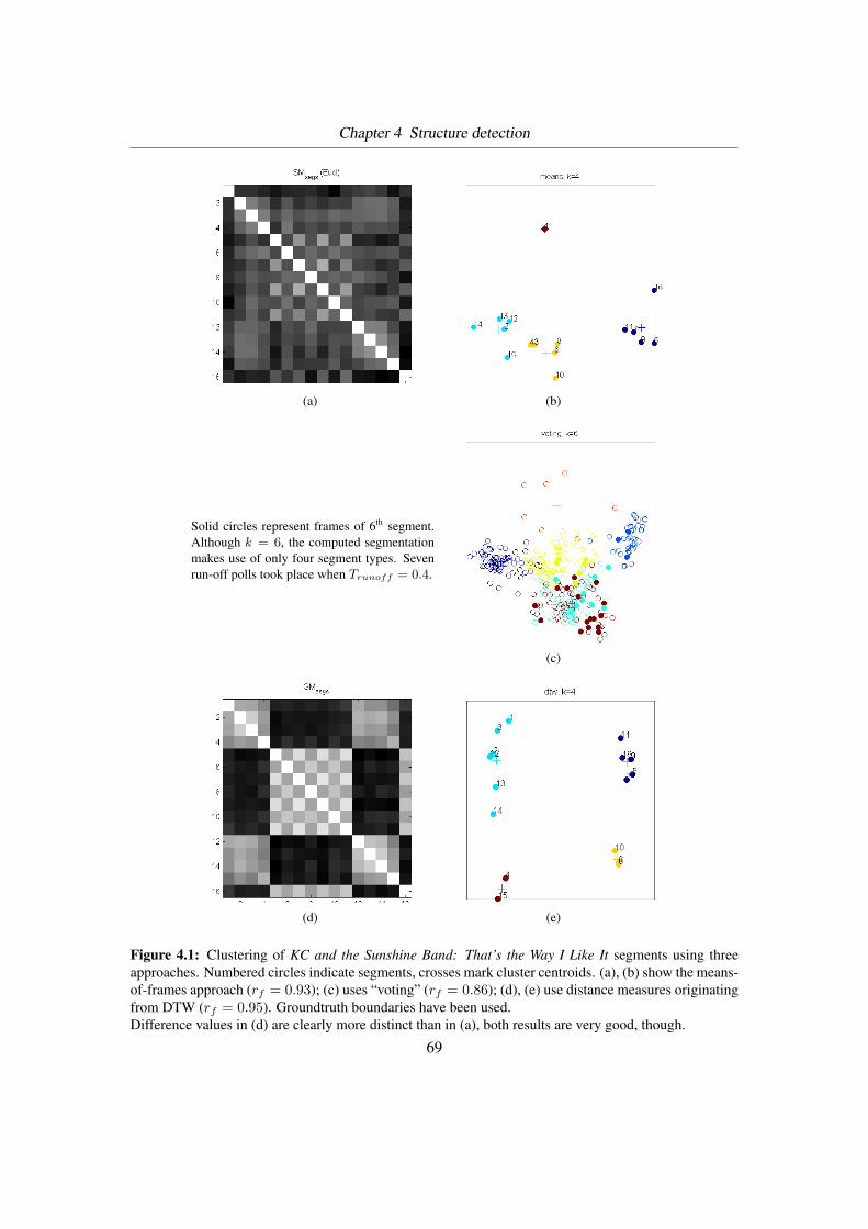
Chapter 4 Structure detection
(a) (b)
Solid circles represent frames of 6th segment.Although k = 6, the computed segmentationmakes use of only four segment types. Sevenrun-off polls took place when Trunoff = 0.4.
(c)
(d) (e)
Figure 4.1: Clustering of KC and the Sunshine Band: That’s the Way I Like It segments using threeapproaches. Numbered circles indicate segments, crosses mark cluster centroids. (a), (b) show the means-of-frames approach (rf = 0.93); (c) uses “voting” (rf = 0.86); (d), (e) use distance measures originatingfrom DTW (rf = 0.95). Groundtruth boundaries have been used.Difference values in (d) are clearly more distinct than in (a), both results are very good, though.
69
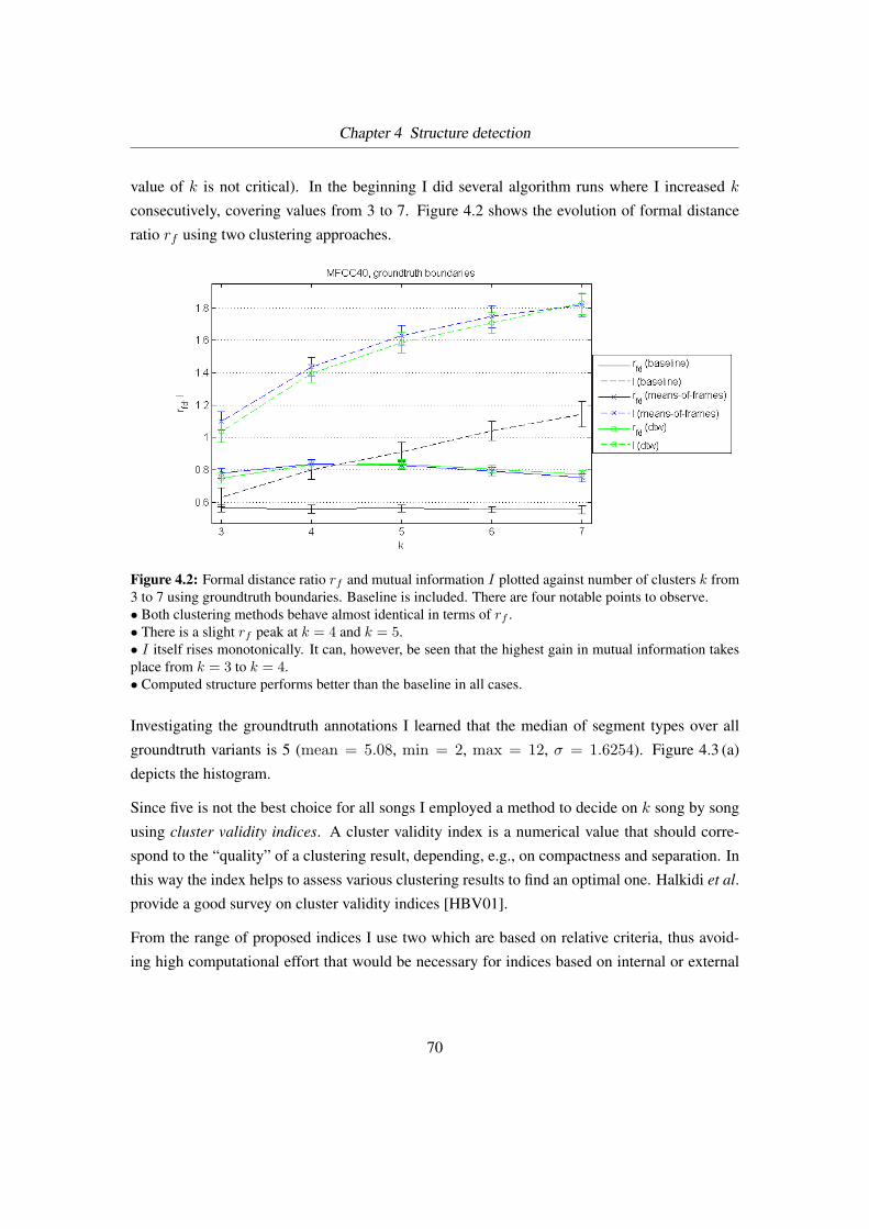
Chapter 4 Structure detection
value of k is not critical). In the beginning I did several algorithm runs where I increased k
consecutively, covering values from 3 to 7. Figure 4.2 shows the evolution of formal distance
ratio rf using two clustering approaches.
Figure 4.2: Formal distance ratio rf and mutual information I plotted against number of clusters k from3 to 7 using groundtruth boundaries. Baseline is included. There are four notable points to observe.• Both clustering methods behave almost identical in terms of rf .• There is a slight rf peak at k = 4 and k = 5.• I itself rises monotonically. It can, however, be seen that the highest gain in mutual information takesplace from k = 3 to k = 4.• Computed structure performs better than the baseline in all cases.
Investigating the groundtruth annotations I learned that the median of segment types over all
groundtruth variants is 5 (mean = 5.08, min = 2, max = 12, σ = 1.6254). Figure 4.3 (a)
depicts the histogram.
Since five is not the best choice for all songs I employed a method to decide on k song by song
using cluster validity indices. A cluster validity index is a numerical value that should corre-
spond to the “quality” of a clustering result, depending, e.g., on compactness and separation. In
this way the index helps to assess various clustering results to find an optimal one. Halkidi et al.
provide a good survey on cluster validity indices [HBV01].
From the range of proposed indices I use two which are based on relative criteria, thus avoid-
ing high computational effort that would be necessary for indices based on internal or external
70
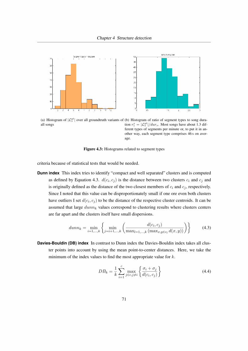
Chapter 4 Structure detection
(a) Histogram of |Lgts | over all groundtruth variants of
all songs(b) Histogram of ratio of segment types to song dura-tion rs
1 = |Lgts |/durs. Most songs have about 1.3 dif-
ferent types of segments per minute or, to put it in an-other way, each segment type comprises 46 s on aver-age.
Figure 4.3: Histograms related to segment types
criteria because of statistical tests that would be needed.
Dunn index This index tries to identify “compact and well separated” clusters and is computed
as defined by Equation 4.3. d(ci, cj) is the distance between two clusters ci and cj and
is originally defined as the distance of the two closest members of ci and cj , respectively.
Since I noted that this value can be disproportionately small if one ore even both clusters
have outliers I set d(ci, cj) to be the distance of the respective cluster centroids. It can be
assumed that large dunnk values correspond to clustering results where clusters centers
are far apart and the clusters itself have small dispersions.
dunnk = mini=1,...,k
{min
j=i+1,...,k
(d(ci, cj)
maxl=1,...,k (maxx,y∈cld(x, y))
)}(4.3)
Davies-Bouldin (DB) index In contrast to Dunn index the Davies-Bouldin index takes all clus-
ter points into account by using the mean point-to-center distances. Here, we take the
minimum of the index values to find the most appropriate value for k.
DBk =1k
c∑i=1
maxj∈c,j 6=i
{σi + σj
d(ci, cj)
}(4.4)
71
Chapter 4 Structure detection
where σi = 1/ci∑
y∈cid(y, µi) is the measure of “scatterness” of a cluster i, i.e., the
mean distance to the cluster center µi.
Hence, clustering is performed several times for each song with k iterating through a range of
values, then the best value for k is chosen. The first few algorithm runs, however, showed that
both indices frequently favor either very few classes (k = 2) or too many classes (k is about the
number of segments). Thus, a limitation of the range such that kmin ≤ k ≤ kmax was advisable,
also in respect to computation time.
I decided to use the ratio of number of segment types to song duration in minutes rs1 = |Lgt
s |/durs
to estimate the range for k for each song. Figure 4.3 (b) shows the distribution of rs1 over all
groundtruth variants. First I chose the lower and upper quartile (1.16 and 1.79). Since the mean
of the differences between |Lgts | and actually chosen number of segment types |Lalgo
s | turned out
to be as high as about 1.5 I extended the limit to the range from 15 percentile to 85 percentile rs1
values (1 to 1.97).
Results showed very clearly that increasing k’s range even decreases formal distance ratio rf
(which is bad). Therefore I tried a third run setting the range to [4, 5] which provided best re-
sults, however, without statistical significance. Figure 4.4 summarizes the performance measure
values obtained by various settings for kmin and kmax, compared with the result using a fixed
k = 5.
Semi-supervised approach [LS06] states that
“research into parallel problems in image segmentation suggests that a small amount
of supervision may offer large gains in segmentation accuracy.”
In this sense I set up an experimental algorithm run where the “user” is required to set k to an
appropriate value for each song. In real life this situation can easily be imagined: the user wants
a song segmentation and enters the number of distinct segment types he/she wants to obtain into
his device. This allows him or her to request different segmentations that differ in granularity.
Finally, the user can select the most appropriate suggestion for the purpose at hand.
In fact I extracted the number of distinct segment labels from each groundtruth annotation. The
algorithm then loaded this value for each song and used it for clustering. I tried three variants:
1. groundtruth without subsegments
72
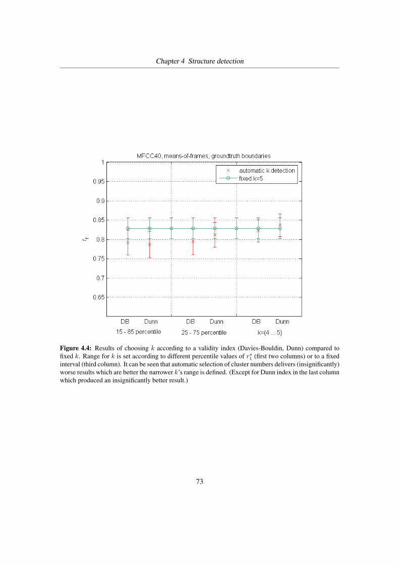
Chapter 4 Structure detection
Figure 4.4: Results of choosing k according to a validity index (Davies-Bouldin, Dunn) compared tofixed k. Range for k is set according to different percentile values of rs
1 (first two columns) or to a fixedinterval (third column). It can be seen that automatic selection of cluster numbers delivers (insignificantly)worse results which are better the narrower k’s range is defined. (Except for Dunn index in the last columnwhich produced an insignificantly better result.)
73

Chapter 4 Structure detection
Figure 4.5: Segmentations of Eminem: Stan. Top panel: groundtruth, bottom panel: computed structure.Note the spurious boundaries especially between the C segments of the bottom panel.
2. groundtruth with subsegments
3. rounded mean of variants 1 and 2.
The results were similar for all three variants, being insignificantly better than results without
simulated user input: rf = 0.717 ± 0.028 (variant 3) in contrast to rf = 0.707 ± 0.025 (fixed
k = 5).
Boundary post processing Looking at some machine segmentations like the one in Fig-
ure 4.5 it seems to be a prospective idea to remove all or most of the boundaries between two
segments of the same segment type.
As expected, mean precision rose quite a lot, whereas mean recall declined, so that eventually
the F-measure was insignificantly higher. Here are the full details:
• All boundaries between segments of same type removed: P = 0.68 ± 0.045, R = 0.64 ±0.045, F = 0.66
• Boundaries between segments of same type removed if the distance between the two adja-
cent segments is lower than the mean distance between all consecutive segments of same
type: P = 0.61 ± 0.039, R = 0.72 ± 0.041, F = 0.66
• No post processing: P = 0.55 ± 0.038, R = 0.77 ± 0.037, F = 0.64
4.3 Results
Figure 4.6 informs about results of algorithm runs with various feature sets.
74
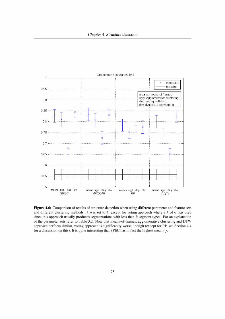
Chapter 4 Structure detection
Figure 4.6: Comparison of results of structure detection when using different parameter and feature setsand different clustering methods. k was set to 4, except for voting approach where a k of 6 was usedsince this approach usually produces segmentations with less than k segment types. For an explanationof the parameter sets refer to Table 3.2. Note that means-of-frames, agglomerative clustering and DTWapproach perform similar, voting approach is significantly worse, though (except for RP, see Section 4.4for a discussion on this). It is quite interesting that SPEC has in fact the highest mean rf .
75

Chapter 4 Structure detection
Figure 4.7: Comparison of rf values using groundtruth boundaries and computed boundaries. Theparameter set used is MFCC40, k = 4 except for voting where again k = 6. The decline of rf is clearlyvisible in all four cases. The DTW result based on computed boundaries, however, is much lower thanthe respective result using groundtruth. See the following section for a dicussion about that.
As one might expect rf is lower if automatically obtained segment boundaries are used and not
the groundtruth boundaries (which can be seen as “perfect” boundaries). Figure 4.7 illustrates
this decline in performance.
A histogram of the formal distance ratios if the groundtruth is not used in any way is shown as
Figure 4.8.
Baseline Two types of baseline have been calculated where the first one can actually be con-
sidered as a special case of the second one. First I assigned the same label to each segment,
second I selected one of k segment types at random (k ∈ (2, . . . , 6)). For baseline calculation I
used groundtruth boundary positions. Values of rf were around 0.56 which again is pretty bad
compared to the algorithmic results.
76
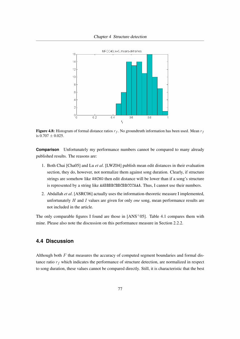
Chapter 4 Structure detection
Figure 4.8: Histogram of formal distance ratios rf . No groundtruth information has been used. Mean rf
is 0.707 ± 0.025.
Comparison Unfortunately my performance numbers cannot be compared to many already
published results. The reasons are:
1. Both Chai [Cha05] and Lu et al. [LWZ04] publish mean edit distances in their evaluation
section, they do, however, not normalize them against song duration. Clearly, if structure
strings are somehow like ABCBD then edit distance will be lower than if a song’s structure
is represented by a string like AABBBBCBBCBBCCCAAA. Thus, I cannot use their numbers.
2. Abdallah et al. [ASRC06] actually uses the information-theoretic measure I implemented,
unfortunately H and I values are given for only one song, mean performance results are
not included in the article.
The only comparable figures I found are those in [ANS+05]. Table 4.1 compares them with
mine. Please also note the discussion on this performance measure in Section 2.2.2.
4.4 Discussion
Although both F that measures the accuracy of computed segment boundaries and formal dis-
tance ratio rf which indicates the performance of structure detection, are normalized in respect
to song duration, these values cannot be compared directly. Still, it is characteristic that the best
77
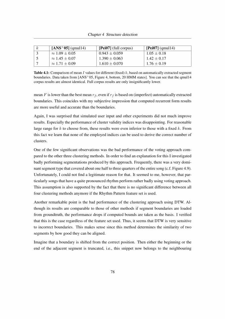
Chapter 4 Structure detection
k [ANS+05] (qmul14) [Pei07] (full corpus) [Pei07] (qmul14)3 ≈ 1.09 ± 0.05 0.943 ± 0.059 1.05 ± 0.185 ≈ 1.45 ± 0.07 1.390 ± 0.063 1.42 ± 0.177 ≈ 1.71 ± 0.09 1.610 ± 0.070 1.76 ± 0.19
Table 4.1: Comparison of mean I values for different (fixed) k, based on automatically extracted segmentboundaries. Data taken from [ANS+05, Figure 4, bottom, 20 HMM states]. You can see that the qmul14corpus results are almost identical. Full corpus results are only insignificantly lower.
mean F is lower than the best mean rf , even if rf is based on (imperfect) automatically extracted
boundaries. This coincides with my subjective impression that computed recurrent form results
are more useful and accurate than the boundaries.
Again, I was surprised that simulated user input and other experiments did not much improve
results. Especially the performance of cluster validity indices was disappointing. For reasonable
large range for k to choose from, these results were even inferior to those with a fixed k. From
this fact we learn that none of the employed indices can be used to derive the correct number of
clusters.
One of the few significant observations was the bad performance of the voting approach com-
pared to the other three clustering methods. In order to find an explanation for this I investigated
badly performing segmentations produced by this approach. Frequently, there was a very domi-
nant segment type that covered about one half to three quarters of the entire song (c.f. Figure 4.9).
Unfortunately, I could not find a legitimate reason for that. It seemed to me, however, that par-
ticularly songs that have a quite pronounced rhythm perform rather badly using voting approach.
This assumption is also supported by the fact that there is no significant difference between all
four clustering methods anymore if the Rhythm Pattern feature set is used.
Another remarkable point is the bad performance of the clustering approach using DTW. Al-
though its results are comparable to those of other methods if segment boundaries are loaded
from groundtruth, the performance drops if computed bounds are taken as the basis. I verified
that this is the case regardless of the feature set used. Thus, it seems that DTW is very sensitive
to incorrect boundaries. This makes sense since this method determines the similarity of two
segments by how good they can be aligned.
Imagine that a boundary is shifted from the correct position. Then either the beginning or the
end of the adjacent segment is truncated, i.e., this snippet now belongs to the neighbouring
78

Chapter 4 Structure detection
Figure 4.9: Evaluation of Portishead: Wandering Star. Top panel: groundtruth, bottom panel: computedsegmentation. Voting approach has been used for segment clustering: note that B segments cover half ofthe song although these segments are actually of different types. Therefore formal distance ratio is quitelow (rf = 0.59). (Boundaries have been loaded from groundtruth.)
segment). Thus, the alignment process starts actually somewhere in the middle of a segment and
will therefore not deliver a good result.
Carefully reading through a number of evaluation reports generated I frequently noted that a
finer structure is extracted, especially if sections are subdivided by “incorrect” boundaries. As
Goto assumed in [Got03] many chorus sections contain two subsegments. If phase 1 finds
this boundary phase 2 sometimes assigns two different segment types to those segments. This
decreases performance numbers but informally it is obvious that the extracted segmentations can
still be useful.
4.5 Summary
The current chapter presented my work on another AAS subtask: structure detection, also re-
ferred to as musical form extraction. This phase outputs a string like ABCBDBA which represents
the song structure. Each character stands for one segment, segments of the same type get the
same character. Note that these letters do not indicate whether the respective song segment is a
chorus or verse section, etc.
I employed clustering in four variants to group segments according to their similarity: k-means
and hierarchical clustering with the segments being represented by one mean feature vector,
79
Chapter 4 Structure detection
“voting” approach, and k-means with the segment similarity being computed using Dynamic
Time Warping (DTW).
In the experiments section I explained how I employed cluster validity indices (Davies-Bouldin
and Dunn) to find the correct number of cluster centroids, i.e., segment types, for each song.
This, however, had no positive effect on the mean performance. Besides, I investigated a semi-
supervised approach where this parameter is loaded from groundtruth, simulating a possible user
input.
The last experiment was the removal of boundaries whose adjacent segments were of the same
type. I pointed out that these experiments did produce statistically insignificantly better results
only.
I provided evaluation numbers of various algorithm runs, grouped by parameter set used and
clustering approach. From these figures it could be seen that most of the time (except for RP
parameter set) the voting approach was inferior to other methods. Another remarkable point
was that the DTW approach was very sensitive to the correctness of the segment boundaries.
Unfortunately, I could compare my results with those of only one other paper. The comparison
showed that my qmul14 corpus results are equal to those of the other study.
80
Chapter 5
Outro
In this chapter I present the results of a five-fold cross validation to measure a possible bias in
my corpus. Besides, I conducted an algorithm run on a test set of fifteen additional songs that
have not been used for parameter selection so far. After a few case studies I conclude the major
aspects of the thesis and address possible future work. The chapter ends with a summary of the
entire thesis.
5.1 Cross validation
In order to assess the bias of the data I performed a five-fold cross validation. For this example
I tried to find an optimal value for parameter nH which is the size of the sliding window for the
low-pass filter employed in boundary detection. I let nH iterate through values from 1 to 20,
nH ∈ {1, 2, 4, 6, 8, 10, 12, 16, 20}.
Cross validation is a technique to avoid training and validation on the very same data while still
using as much of the data available as possible. In my case of a five-fold cross validation I
partitioned the music files into five disjoint subsets. The union of four of these subsets (“training
set”) are used for finding the optimal value for nH while the fifth one (“validation set”) is used
to perform evaluation. This procedure is repeated five times, each subset acting as the validation
set exactly once.
Table 5.1 summarizes the results.
Quite surprisingly, the evaluation results of the validation sets are almost the same as those of
the training sets. This indicates that there is not much bias in the data. The optimal value for nH
81
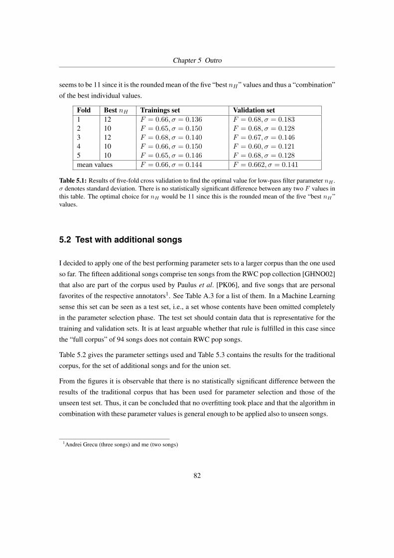
Chapter 5 Outro
seems to be 11 since it is the rounded mean of the five “best nH” values and thus a “combination”
of the best individual values.
Fold Best nH Trainings set Validation set1 12 F = 0.66, σ = 0.136 F = 0.68, σ = 0.1832 10 F = 0.65, σ = 0.150 F = 0.68, σ = 0.1283 12 F = 0.68, σ = 0.140 F = 0.67, σ = 0.1464 10 F = 0.66, σ = 0.150 F = 0.60, σ = 0.1215 10 F = 0.65, σ = 0.146 F = 0.68, σ = 0.128mean values F = 0.66, σ = 0.144 F = 0.662, σ = 0.141
Table 5.1: Results of five-fold cross validation to find the optimal value for low-pass filter parameter nH .σ denotes standard deviation. There is no statistically significant difference between any two F values inthis table. The optimal choice for nH would be 11 since this is the rounded mean of the five “best nH”values.
5.2 Test with additional songs
I decided to apply one of the best performing parameter sets to a larger corpus than the one used
so far. The fifteen additional songs comprise ten songs from the RWC pop collection [GHNO02]
that also are part of the corpus used by Paulus et al. [PK06], and five songs that are personal
favorites of the respective annotators1. See Table A.3 for a list of them. In a Machine Learning
sense this set can be seen as a test set, i.e., a set whose contents have been omitted completely
in the parameter selection phase. The test set should contain data that is representative for the
training and validation sets. It is at least arguable whether that rule is fulfilled in this case since
the “full corpus” of 94 songs does not contain RWC pop songs.
Table 5.2 gives the parameter settings used and Table 5.3 contains the results for the traditional
corpus, for the set of additional songs and for the union set.
From the figures it is observable that there is no statistically significant difference between the
results of the traditional corpus that has been used for parameter selection and those of the
unseen test set. Thus, it can be concluded that no overfitting took place and that the algorithm in
combination with these parameter values is general enough to be applied also to unseen songs.
1Andrei Grecu (three songs) and me (two songs)
82
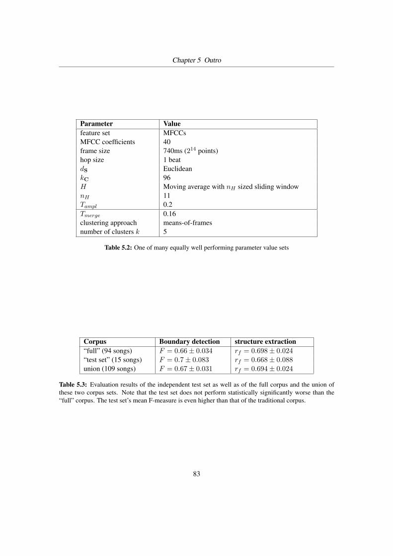
Chapter 5 Outro
Parameter Valuefeature set MFCCsMFCC coefficients 40frame size 740ms (214 points)hop size 1 beatdS EuclideankC 96H Moving average with nH sized sliding windownH 11Tampl 0.2Tmerge 0.16clustering approach means-of-framesnumber of clusters k 5
Table 5.2: One of many equally well performing parameter value sets
Corpus Boundary detection structure extraction“full” (94 songs) F = 0.66± 0.034 rf = 0.698± 0.024“test set” (15 songs) F = 0.7± 0.083 rf = 0.668± 0.088union (109 songs) F = 0.67± 0.031 rf = 0.694± 0.024
Table 5.3: Evaluation results of the independent test set as well as of the full corpus and the union ofthese two corpus sets. Note that the test set does not perform statistically significantly worse than the“full” corpus. The test set’s mean F-measure is even higher than that of the traditional corpus.
83
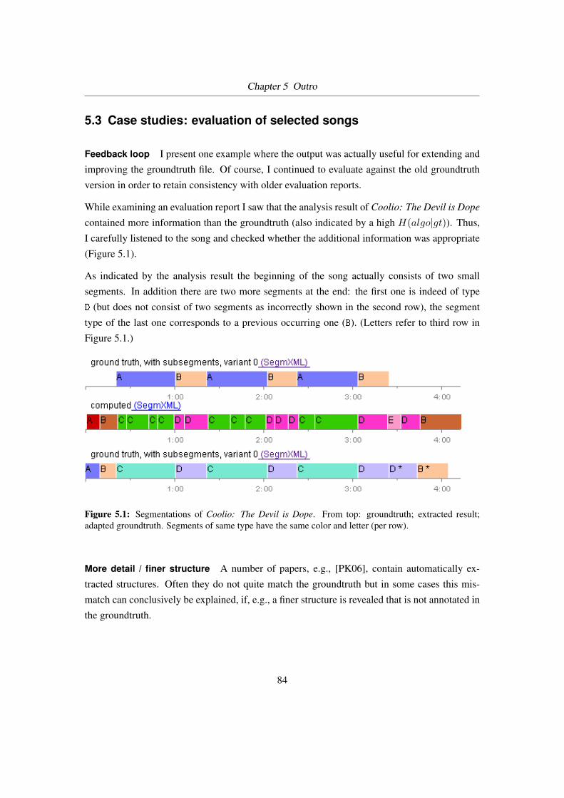
Chapter 5 Outro
5.3 Case studies: evaluation of selected songs
Feedback loop I present one example where the output was actually useful for extending and
improving the groundtruth file. Of course, I continued to evaluate against the old groundtruth
version in order to retain consistency with older evaluation reports.
While examining an evaluation report I saw that the analysis result of Coolio: The Devil is Dope
contained more information than the groundtruth (also indicated by a high H(algo|gt)). Thus,
I carefully listened to the song and checked whether the additional information was appropriate
(Figure 5.1).
As indicated by the analysis result the beginning of the song actually consists of two small
segments. In addition there are two more segments at the end: the first one is indeed of type
D (but does not consist of two segments as incorrectly shown in the second row), the segment
type of the last one corresponds to a previous occurring one (B). (Letters refer to third row in
Figure 5.1.)
Figure 5.1: Segmentations of Coolio: The Devil is Dope. From top: groundtruth; extracted result;adapted groundtruth. Segments of same type have the same color and letter (per row).
More detail / finer structure A number of papers, e.g., [PK06], contain automatically ex-
tracted structures. Often they do not quite match the groundtruth but in some cases this mis-
match can conclusively be explained, if, e.g., a finer structure is revealed that is not annotated in
the groundtruth.
84

Chapter 5 Outro
One example from my work can be seen in Figure 5.2. Both verse and chorus sections (B and C
in the upper panel) consist of two smaller parts. The parts of the chorus sections do indeed differ
from each other such that the assignment of two different segment labels (C and A in the lower
panel) seems to be justified. In addition it can also be stated that the intro sounds much like the
second part of each chorus.
Figure 5.2: Groundtruth (top panel) and computed segmentation (bottom panel) of Beatles: Help!. Samecolor and letter within one panel correspond to same segment type.
Soft song As already mentioned slow and soft songs perform rather bad. If you have a look
at the computed segmentation of Figure 5.3 you see that many boundaries are missed and hence
clustering feature sets have been blurred so that the result looks degenerated.
The bad boundary extraction result is due to an inappropriate value of threshold Tampl. (NH
peaks in song sections with an amplitude lower than this threshold are ignored.) Changing this
value globally does lead to worse mean performance, though. Thus, an adaptive threshold setting
method is advisable.
5.4 Conclusions and future work
As already stated in previous chapters, automatically segmenting songs into their constituents
is somehow feasible. It works well especially for songs where segment types differ in terms of
spectral content or timbre.
85

Chapter 5 Outro
(a) Segmentations of Björk: It’s Oh So Quiet. Top panel: groundtruth; bottom panel: extracted result. Same colorand letter within one panel correspond to same segment type. Note the low F-measure F = 0.5.
(b) Novelty score plot of Björk: It’s Oh So Quiet. For illustration purposes, amplitude values (thick green line) witha sliding average lower than Tampl = 0.2 are not visible. Note that only six boundaries remain although there arequite a few HN peaks that would lead to correct boundaries.
Figure 5.3: Investigation of bad performance of Björk: It’s Oh So Quiet. For this song a Tampl value of0.2 is clearly too high.
86

Chapter 5 Outro
On the other hand the algorithm presented has problems with slow songs that do not have a
distinct transition between their segments, as well as with not-quite-melodic audio content like
rap songs.
I was surprised that the large number of experiments and heuristics I tried did not lead to a
significant mean performance improvement. As already mentioned one heuristic typically im-
proves segmentation of a subset of songs and impairs results of the rest, leading to almost the
same mean performance measure. One reason could be that the groundtruth annotations I used
are not consistent enough. Another possibility is that there is noise in terms of segmentation
ambiguity which cannot be eliminated. This is supported by tests I carried out as described in
Section 2.4.
Results of both phases, boundary detection and structure extraction, are distinctly better than the
respective baselines, though.
As to musical form extraction we can conclude that a certain amount of extraction error is not
due to using the incorrect number of cluster centers k for k-means. The experiment where k is
provided as “minimal user input” showed that even if k is correct, evaluation results show only
a modest improvement. Thus, further investigation into more reliable cluster validity indices
(which aim at finding correct values for k) seems not too promising.
Again, I would like to note that it is not easy to compare the published performance numbers to
results in other papers. We saw that the choice of the underlying corpus has a larger effect on the
final evaluation numbers than the change of algorithm parameters and the use of heuristics.
Similarly, it is not obvious how evaluation should take place. As stated, the two performance
measures F and Fabd produce different results, the latter normally being a bit higher. Consid-
eration must especially be given to the ambiguity of song segmentations. I decided to model it
explicitly in the groundtruth annotation data.
Finally, I give the following suggestions for further research:
Chords Chord transcription can be used to obtain the chord sequence of a song. It can be
investigated whether this chord representation used as feature vectors improves results over using
audio signal feature vectors directly.
87

Chapter 5 Outro
Select parameter values song-by-song Since the songs that perform poorly are different for
various parameter configurations it seems advisable to develop a procedure or criterion to be
able to select an appropriate parameter setting from a pool for each song individually (e.g., for
Tampl as noted in Björk: It’s Oh So Quiet case study in Section 5.3).
User input The potential improvement of minimal user input can further be looked into.
Maybe results become even better if the system works iteratively, reacting on user input. Possi-
bilities of simple user input include: indication of beginning and end of one section; rejection of
individual incorrect segment boundaries; etc.
Evaluation (Consistent groundtruth) The groundtruth annotations I used are a bit ad-hoc. It
is desirable to have a well-founded groundtruth, e.g., by consistently employing always the same
musicology approach (Section 1.3.2) to all songs. In addition, the performance numbers could
be related to the mean evaluation results among groundtruth annotations from different subjects
as suggested in Section 2.4.
Simplify Facing the unsuccessful improvement attempts one could also try the other way and
simplify the algorithm as much as possible to make a potential implementation in mobile devices
easier.
Plugins One obvious practical task is the development of audio player plugins that make use of
structure information, e.g., for XMMS, Winamp or Audacity. These plugins could offer features
like skipping back and forth between segment boundaries or just visualize the structure.
Statistical evaluation At this place I like to make an appeal to fellow researches to encour-
age them to compute and publish not the mere mean values of performance measures but also
statistical information like confidence intervals.
Flexer compiled a survey on evaluation performance figures published in ISMIR proceedings
articles [Fle06]. He states that not even 4 % of articles that publish mean values also report
statistical information like significance tests results or confidence intervals that would
88
Chapter 5 Outro
“allow us to express the amount of uncertainty that comes with every experiment.
They also enable use to compare the outcome of experiments under different con-
ditions.”
The different conditions could be different corpora in our case. Remember Figure 3.10 on
page 60 where confidence intervals clearly indicate the high variability of qmul14 corpus re-
sults. Mean values alone would be misleading.
Working together It can be fruitful for this research field to consult the musical expertise of
professional musicians in an interdisciplinary manner.
5.5 Summary
In the first chapter the reader was introduced to the research field of Automatic Audio Segmen-
tation (AAS).
As a motivation I explained some prospective fields of application for this task, e.g., how AAS
can facilitate the browsing in large digital music collections. Next, I gave an overview of related
work. I introduced various tasks and goals that are subsumed as AAS (boundary detection, struc-
ture detection, audio thumbnailing, semantic label assignment, etc.) I briefly explained mathe-
matical models used (e.g., self-similarity analysis and Hidden Markov Models). Then, corpora
and feature sets used in the individual papers have been compared. I pointed out that there is no
common corpus so far for benchmark evaluation in this field.
At the end of the first chapter, I showed that musical segmentation is a task that generally leads to
ambiguous results and summarized how segmentation is perceived and discussed in musicology
literature.
In the next chapter I discussed how evaluation has been carried out in this thesis.
First, I desribed the groundtruth corpus which is one of the largest used so far in this research
field. It contains 94 songs collected from two sources. The corpus contains contemporary pop-
ular songs of different genres (dance, rock, pop, rap, R&B, etc.).
89
Chapter 5 Outro
A novel annotation file format based on XML (SegmXML) has been described. This format is
flexible, i.e., it can contain two hierarchical levels of segmentation as well as alternative labels
for each song segment.
Performance measures for both algorithm tasks have been defined: For the first phase, boundary
detection, these are precision P , recall R and F-measure F . The second phase, structure ex-
traction, uses formal distance ratio rf which is based on edit distance. Besides, also alternative
measures have been introduced and discussed. In subsequent chapters these have been used to
compare my figures with those of other studies.
I discussed the problem of hierarchical segmentations (two annotations may actually be equiva-
lent but on a different hierarchical level) and described how the evaluation process handles such
cases. I decided to explicitely include two levels of segmentation into the groundtruth files.
The evaluation algorithm which is implemented in Perl has been defined in pseudo code nota-
tion. At the end of the evaluation process HTML reports are generated. These reports contain
performance numbers (mean values over the entire corpus, mean values grouped by genre /
corpus and the values of the individual songs), metadata about songs as well as algorithm and
evaluation parameter settings and visual representations of each segmentation.
The subsequent two chapters dealt with the algorithm I implemented. It has a segment boundary
detection phase followed by a structure extraction phase. The first phase outputs a set of time
points where song segments start or end, whereas the output of the second phase is a string like
ABCBDBA which represents the song structure. Each character stands for one segment, segments
of the same type get the same character. Note that these letters do not indicate whether the
respective song segment is a chorus or verse section, etc.
For the boundary detection task I used the traditional similarity matrix / novelty score method.
There, the similarity between feature vectors of neighbouring song frames are used to compute
a novelty score whose peaks indicate more or less sudden changes in the song.
I carried out a number of experiments to improve performance (various feature sets and parame-
ter settings, boundary removing heuristic, boundary shifting post-processing, Harmonic Change
Detection Function HCDF). I, however, had to point out that none of these experiments did
improve the mean performance in a statistically significant way.
90
Chapter 5 Outro
When comparing my figures to those of other studies it could be seen that they were on an equal
level. From these figures we could also see that mean performance numbers depend to a large
degree on the underlying corpus.
At the end, I could state that boundary detection results are quite acceptable if some points are
taken into account (no domain knowledge used, the theoretically optimal result of F = 1 is
probably inherently unreachable, etc.). Melodic songs which lack rap passages and prominent
distorted guitar sound and which do not have a too slow rhythm perform better than other ones.
Turning to musical form detection, I employed clustering in four variants to group segments
according to their similarity: k-means and hierarchical clustering with the segments being repre-
sented by one mean feature vector, “voting” approach, and k-means with the segment similarity
being computed using Dynamic Time Warping (DTW). Evaluation of various algorithm runs
showed that the “voting” and DTW approaches are inferior to the other ones if automatically
extracted segment boundaries are used.
I explained how I employed cluster validity indices (Davies-Bouldin and Dunn) to find the cor-
rect number of cluster centroids, i.e., segment types, for each song. This, however, had no
positive effect on the mean performance. Besides, I investigated a semi-supervised approach
where this parameter is loaded from groundtruth, simulating a possible user input. The last
experiment was the removal of boundaries whose adjacent segments were of the same type. I
pointed out that these experiments did produce statistically insignificant better results only.
Again, I compared my evaluation results with those of another paper. The comparison showed
that my qmul14 corpus results, again, are equal to the already published numbers.
In the last chapter I presented the results of a five-fold cross validation. Those numbers indicated
that the training set (four fifth of the corpus) had no bias: evaluation results of both the training
set and the validation set did not differ.
Also, I did one algorithm run on a test set of fifteen additional songs that have not been used
for parameter selection so far. Again, the results were not significantly different and thus quite
promising: It seems that no overfitting took place and the algorithm together with (at least) this
parameter set is general enough to apply it to new songs.
Next, I presented two case studies where computed segmentation actually delivered more infor-
mation than the respective groundtruth annotation files contained. This is a good sign for the
practical application of the algorithm.
91
Chapter 5 Outro
There are, however, open issues: the case study of a rather soft and slow song revealed that it
is advisable for some parameters not to set them to a fixed value for all songs but to make them
change adaptively. This and other suggestions for future work have been listed in the last section
of this chapter.
You can find groundtruth annotations, HTML reports, segmented songs for acoustic demon-
stration purposes as well as Perl and Matlab source code at http://www.ifs.tuwien.ac.at/
mir/audiosegmentation/.
92

Appendix A
Appendix
A.1 Software used
Name Used for URLWavesurfer manual segmentation http://www.speech.kth.se/
wavesurfer/
Matlab 7.0.1 feature extraction, prototyping. http://www.mathworks.com/
products/matlab/
Signal ProcessingToolbox
feature extraction included in Matlab 7.0.1
Dan Ellis’ DTWtoolbox
similarity matrix, DynamicTime Warping
http://www.ee.columbia.edu/
~dpwe/resources/matlab/
Somtoolbox k-means clustering, DB clustervalidity index
http://www.cis.hut.fi/
projects/somtoolbox/
LATEX(Miktex) typesetting http://www.miktex.org/
Default.aspx
TeXnicCenter editor http://www.toolscenter.org/
Perl evaluation system, conversionscripts
http://www.perl.com
Xalan-J XSLT engine http://xml.apache.org/
xalan-j/
Table A.1: Programs used for this thesis
93
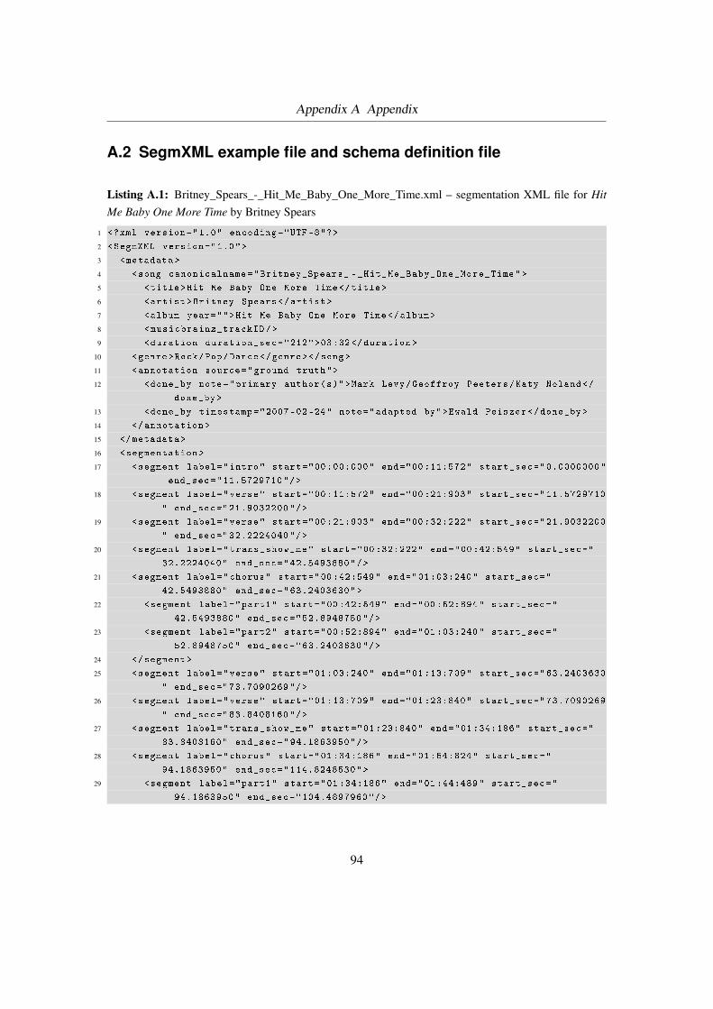
Appendix A Appendix
A.2 SegmXML example file and schema definition file
Listing A.1: Britney_Spears_-_Hit_Me_Baby_One_More_Time.xml – segmentation XML file for HitMe Baby One More Time by Britney Spears
1 <?xml version="1.0" encoding="UTF -8"?>
2 <SegmXML version="1.0">
3 <metadata >
4 <song canonicalname="Britney_Spears_ -_Hit_Me_Baby_One_More_Time">
5 <title>Hit Me Baby One More Time</title>
6 <artist >Britney Spears </artist >
7 <album year="">Hit Me Baby One More Time</album>
8 <musicbrainz_trackID/>
9 <duration duration_sec="212">03:32</duration >
10 <genre>Rock/Pop/Dance</genre></song>
11 <annotation source="ground truth">
12 <done_by note="primary author(s)">Mark Levy/Geoffroy Peeters/Katy Noland </
done_by >
13 <done_by timestamp="2007 -02 -24" note="adapted by">Ewald Peiszer </done_by >
14 </annotation >
15 </metadata >
16 <segmentation >
17 <segment label="intro" start="00 :00:000" end="00 :11:572" start_sec="0.0000000"
end_sec="11.5729710"/>
18 <segment label="verse" start="00 :11:572" end="00 :21:903" start_sec="11.5729710
" end_sec="21.9032200"/>
19 <segment label="verse" start="00 :21:903" end="00 :32:222" start_sec="21.9032200
" end_sec="32.2224040"/>
20 <segment label="trans_show_me" start="00 :32:222" end="00 :42:549" start_sec="
32.2224040" end_sec="42.5493880"/>
21 <segment label="chorus" start="00 :42:549" end="01 :03:240" start_sec="
42.5493880" end_sec="63.2403630">
22 <segment label="part1" start="00 :42:549" end="00 :52:894" start_sec="
42.5493880" end_sec="52.8948750"/>
23 <segment label="part2" start="00 :52:894" end="01 :03:240" start_sec="
52.8948750" end_sec="63.2403630"/>
24 </segment >
25 <segment label="verse" start="01 :03:240" end="01 :13:709" start_sec="63.2403630
" end_sec="73.7090269"/>
26 <segment label="verse" start="01 :13:709" end="01 :23:840" start_sec="73.7090269
" end_sec="83.8408160"/>
27 <segment label="trans_show_me" start="01 :23:840" end="01 :34:186" start_sec="
83.8408160" end_sec="94.1863950"/>
28 <segment label="chorus" start="01 :34:186" end="01 :54:824" start_sec="
94.1863950" end_sec="114.8248530">
29 <segment label="part1" start="01 :34:186" end="01 :44:489" start_sec="
94.1863950" end_sec="104.4897960"/>
94

Appendix A Appendix
30 <segment label="part2" start="01 :44:489" end="01 :54:824" start_sec="
104.4897960" end_sec="114.8248530"/>
31 </segment >
32 <segment label="intro" start="01 :54:824" end="02 :05:136" start_sec="
114.8248530" end_sec="125.1361450"/>
33 <segment label="verse" start="02 :05:136" end="02 :15:239" start_sec="
125.1361450" end_sec="135.2390183">
34 <alt_label >verse2 </alt_label >
35 </segment >
36 <segment label="verse" start="02 :15:239" end="02 :25:801" start_sec="
135.2390183" end_sec="145.8019950">
37 <alt_label >verse2 </alt_label >
38 </segment >
39 <segment label="chorus" start="02 :25:801" end="03 :28:551" start_sec="
145.8019950" end_sec="208.5515650">
40 <alt_label >chorus2 </alt_label >
41 <segment label="part1" start="02 :25:801" end="02 :36:307" start_sec="
145.8019950" end_sec="156.3073933"/>
42
43 <segment label="part2" start="02 :36:307" end="02 :46:467" start_sec="
156.3073933" end_sec="166.4679370"/>
44 <segment label="part1" start="02 :46:467" end="02 :56:753" start_sec="
166.4679370" end_sec="176.7531970"/>
45 <segment label="part2" start="02 :56:753" end="03 :07:189" start_sec="
176.7531970" end_sec="187.1892060"/>
46
47 <segment label="part1" start="03 :07:189" end="03 :17:631" start_sec="
187.1892060" end_sec="197.6319782"/>
48
49 <segment label="part2" start="03 :17:631" end="03 :28:551" start_sec="
197.6319782" end_sec="208.5515650"/>
50 </segment >
51 </segmentation >
52 </SegmXML >
Listing A.2: XML Schema Definition for SegmXML files version 1.0
1 <?xml version="1.0"?>
2 <xs:schema xmlns="http: // thesis.ewald -peiszer.com" xmlns:xs="http://www.w3.org
/2001/ XMLSchema" targetNamespace="http:// thesis.ewald -peiszer.com">
3 <xs:element name="SegmXML">
4 <xs:complexType >
5 <xs:sequence >
6 <xs:element name="metadata">
7 <xs:complexType >
8 <xs:sequence >
9 <xs:element name="song">
10 <xs:complexType >
95
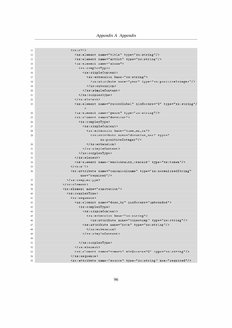
Appendix A Appendix
11 <xs:all >
12 <xs:element name="title" type="xs:string"/>
13 <xs:element name="artist" type="xs:string"/>
14 <xs:element name="album">
15 <xs:complexType >
16 <xs:simpleContent >
17 <xs:extension base="xs:string">
18 <xs:attribute name="year" type="xs:positiveInteger"/>
19 </xs:extension >
20 </xs:simpleContent >
21 </xs:complexType >
22 </xs:element >
23 <xs:element name="recordlabel" minOccurs="0" type="xs:string"/
>
24 <xs:element name="genre" type="xs:string"/>
25 <xs:element name="duration">
26 <xs:complexType >
27 <xs:simpleContent >
28 <xs:extension base="time_mm_ss">
29 <xs:attribute name="duration_sec" type="
xs:positiveInteger"/>
30 </xs:extension >
31 </xs:simpleContent >
32 </xs:complexType >
33 </xs:element >
34 <xs:element name="musicbrainz_trackID" type="xs:token"/>
35 </xs:all >
36 <xs:attribute name="canonicalname" type="xs:normalizedString"
use="required"/>
37 </xs:complexType >
38 </xs:element >
39 <xs:element name="annotation">
40 <xs:complexType >
41 <xs:sequence >
42 <xs:element name="done_by" maxOccurs="unbounded">
43 <xs:complexType >
44 <xs:simpleContent >
45 <xs:extension base="xs:string">
46 <xs:attribute name="timestamp" type="xs:string"/>
47 <xs:attribute name="note" type="xs:string"/>
48 </xs:extension >
49 </xs:simpleContent >
50
51 </xs:complexType >
52 </xs:element >
53 <xs:element name="remark" minOccurs="0" type="xs:string"/>
54 </xs:sequence >
55 <xs:attribute name="source" type="xs:string" use="required"/>
96

Appendix A Appendix
56 </xs:complexType >
57 </xs:element >
58 </xs:sequence >
59 </xs:complexType >
60 </xs:element >
61 <xs:element name="segmentation">
62 <xs:complexType >
63 <xs:sequence >
64 <xs:element name="segment" maxOccurs="unbounded">
65 <xs:complexType >
66 <xs:sequence >
67 <xs:element name="alt_label" minOccurs="0" type="xs:string"/>
68 <xs:element name="remark" minOccurs="0" type="xs:string"/>
69 <xs:element name="segment" minOccurs="0" maxOccurs="unbounded"
>
70 <xs:complexType >
71 <xs:attribute name="label" type="xs:string" use="required"
/>
72 <xs:attribute name="start" type="time_mm_ss_millis" use="
required"/>
73 <xs:attribute name="end" type="time_mm_ss_millis" use="
required"/>
74 <xs:attribute name="start_sec" type="xs:decimal" use="
required"/>
75 <xs:attribute name="end_sec" type="xs:decimal" use="
required"/>
76 <xs:attribute name="instrumental" type="xs:boolean"/>
77 <xs:attribute name="fade" type="T_fade"/>
78 </xs:complexType >
79 </xs:element >
80 </xs:sequence >
81 <xs:attribute name="label" type="xs:string" use="required"/>
82 <xs:attribute name="start" type="time_mm_ss_millis" use="
required"/>
83 <xs:attribute name="end" type="time_mm_ss_millis" use="required"
/>
84 <xs:attribute name="start_sec" type="xs:decimal" use="required"/
>
85 <xs:attribute name="end_sec" type="xs:decimal" use="required"/>
86 <xs:attribute name="instrumental" type="xs:boolean"/>
87 <xs:attribute name="fade" type="T_fade"/>
88 </xs:complexType >
89 </xs:element >
90 </xs:sequence >
91 </xs:complexType >
92 </xs:element >
93 </xs:sequence >
94 <xs:attribute name="version" type="xs:decimal" use="required"/>
97
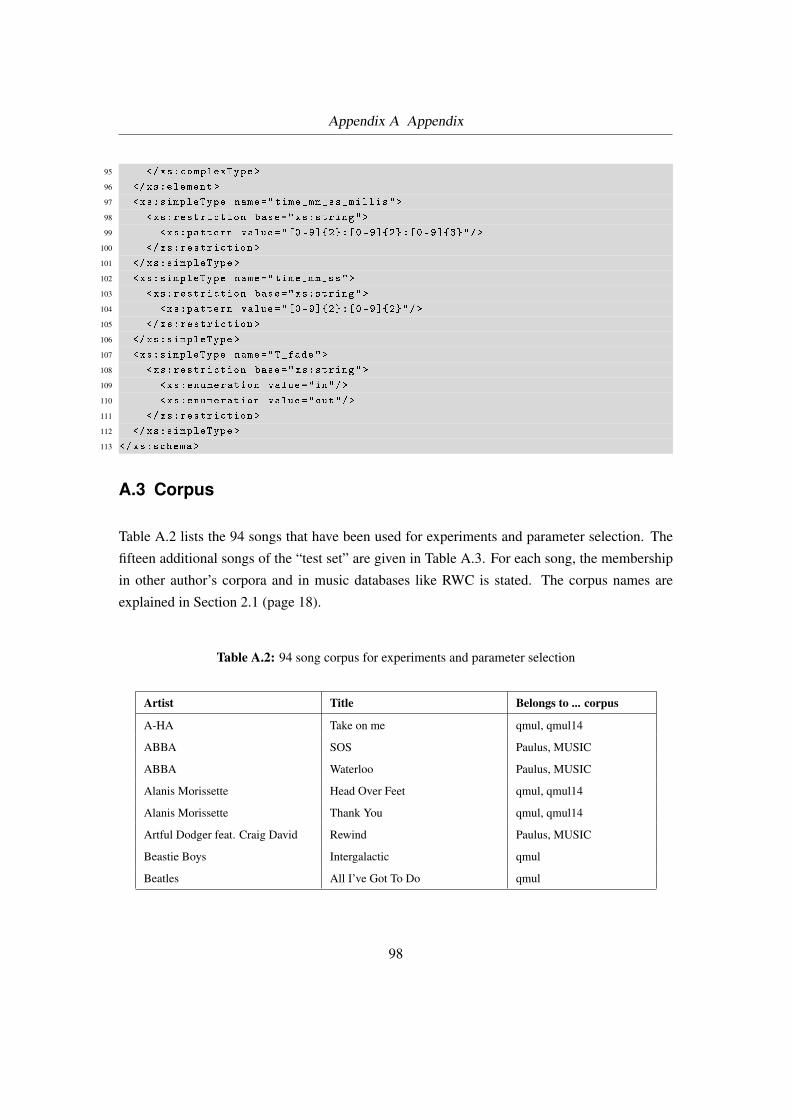
Appendix A Appendix
95 </xs:complexType >
96 </xs:element >
97 <xs:simpleType name="time_mm_ss_millis">
98 <xs:restriction base="xs:string">
99 <xs:pattern value="[0 -9]{2}:[0 -9]{2}:[0 -9]{3}"/>
100 </xs:restriction >
101 </xs:simpleType >
102 <xs:simpleType name="time_mm_ss">
103 <xs:restriction base="xs:string">
104 <xs:pattern value="[0 -9]{2}:[0 -9]{2}"/>
105 </xs:restriction >
106 </xs:simpleType >
107 <xs:simpleType name="T_fade">
108 <xs:restriction base="xs:string">
109 <xs:enumeration value="in"/>
110 <xs:enumeration value="out"/>
111 </xs:restriction >
112 </xs:simpleType >
113 </xs:schema >
A.3 Corpus
Table A.2 lists the 94 songs that have been used for experiments and parameter selection. The
fifteen additional songs of the “test set” are given in Table A.3. For each song, the membership
in other author’s corpora and in music databases like RWC is stated. The corpus names are
explained in Section 2.1 (page 18).
Table A.2: 94 song corpus for experiments and parameter selection
Artist Title Belongs to ... corpus
A-HA Take on me qmul, qmul14
ABBA SOS Paulus, MUSIC
ABBA Waterloo Paulus, MUSIC
Alanis Morissette Head Over Feet qmul, qmul14
Alanis Morissette Thank You qmul, qmul14
Artful Dodger feat. Craig David Rewind Paulus, MUSIC
Beastie Boys Intergalactic qmul
Beatles All I’ve Got To Do qmul
98
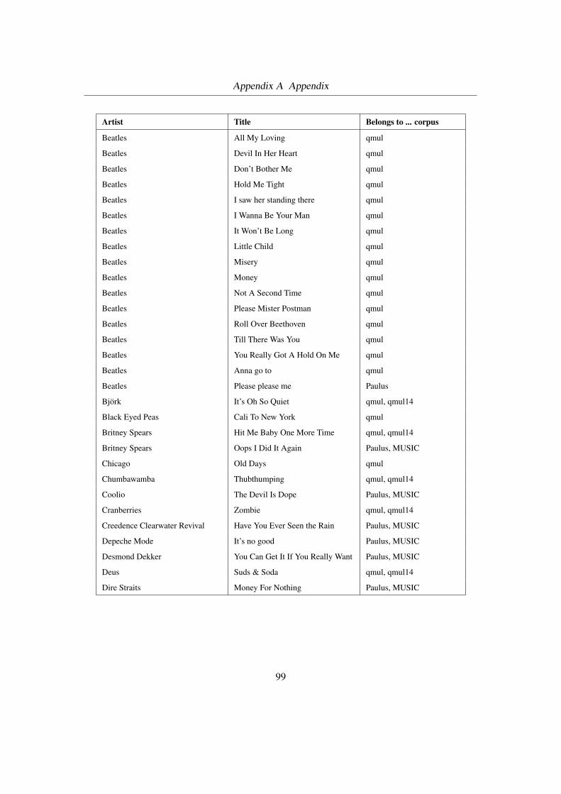
Appendix A Appendix
Artist Title Belongs to ... corpus
Beatles All My Loving qmul
Beatles Devil In Her Heart qmul
Beatles Don’t Bother Me qmul
Beatles Hold Me Tight qmul
Beatles I saw her standing there qmul
Beatles I Wanna Be Your Man qmul
Beatles It Won’t Be Long qmul
Beatles Little Child qmul
Beatles Misery qmul
Beatles Money qmul
Beatles Not A Second Time qmul
Beatles Please Mister Postman qmul
Beatles Roll Over Beethoven qmul
Beatles Till There Was You qmul
Beatles You Really Got A Hold On Me qmul
Beatles Anna go to qmul
Beatles Please please me Paulus
Björk It’s Oh So Quiet qmul, qmul14
Black Eyed Peas Cali To New York qmul
Britney Spears Hit Me Baby One More Time qmul, qmul14
Britney Spears Oops I Did It Again Paulus, MUSIC
Chicago Old Days qmul
Chumbawamba Thubthumping qmul, qmul14
Coolio The Devil Is Dope Paulus, MUSIC
Cranberries Zombie qmul, qmul14
Creedence Clearwater Revival Have You Ever Seen the Rain Paulus, MUSIC
Depeche Mode It’s no good Paulus, MUSIC
Desmond Dekker You Can Get It If You Really Want Paulus, MUSIC
Deus Suds & Soda qmul, qmul14
Dire Straits Money For Nothing Paulus, MUSIC
99
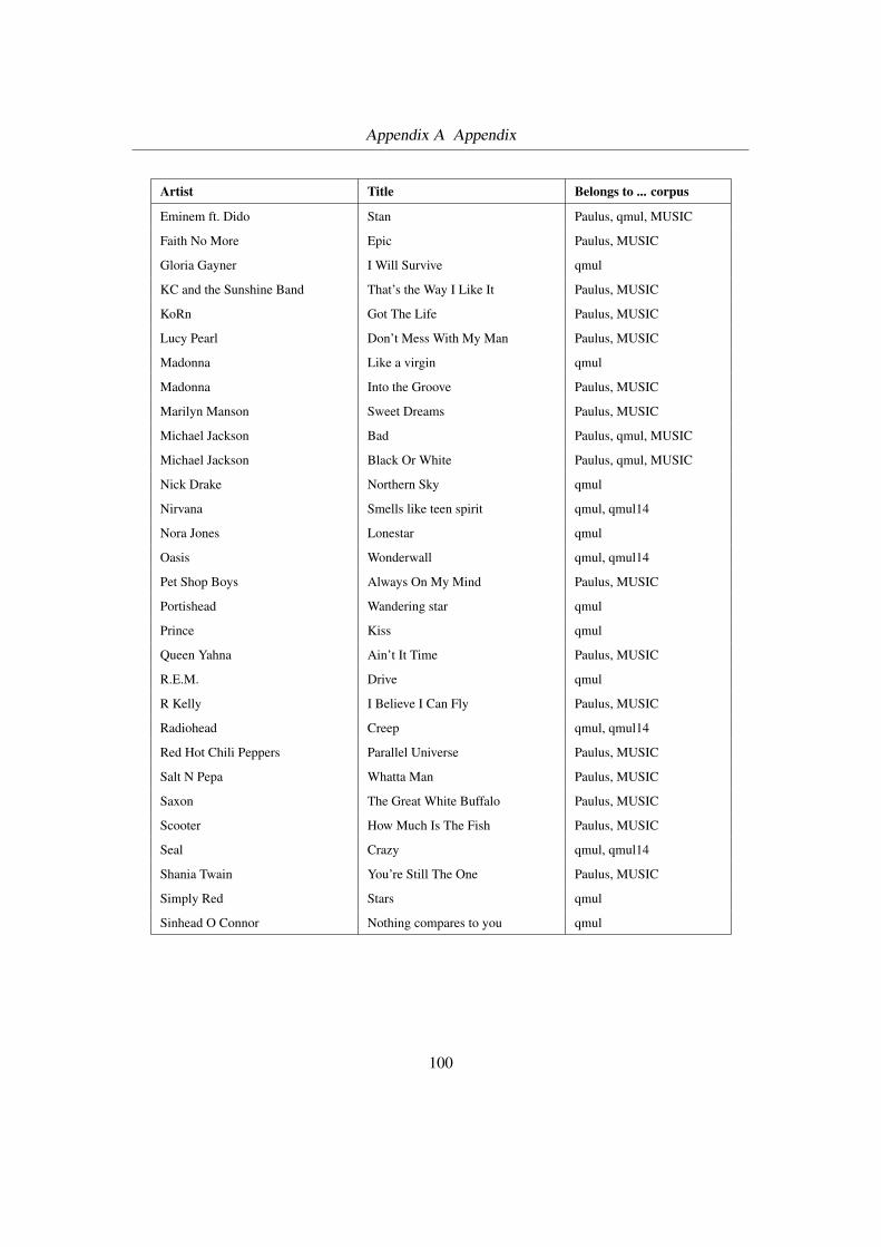
Appendix A Appendix
Artist Title Belongs to ... corpus
Eminem ft. Dido Stan Paulus, qmul, MUSIC
Faith No More Epic Paulus, MUSIC
Gloria Gayner I Will Survive qmul
KC and the Sunshine Band That’s the Way I Like It Paulus, MUSIC
KoRn Got The Life Paulus, MUSIC
Lucy Pearl Don’t Mess With My Man Paulus, MUSIC
Madonna Like a virgin qmul
Madonna Into the Groove Paulus, MUSIC
Marilyn Manson Sweet Dreams Paulus, MUSIC
Michael Jackson Bad Paulus, qmul, MUSIC
Michael Jackson Black Or White Paulus, qmul, MUSIC
Nick Drake Northern Sky qmul
Nirvana Smells like teen spirit qmul, qmul14
Nora Jones Lonestar qmul
Oasis Wonderwall qmul, qmul14
Pet Shop Boys Always On My Mind Paulus, MUSIC
Portishead Wandering star qmul
Prince Kiss qmul
Queen Yahna Ain’t It Time Paulus, MUSIC
R.E.M. Drive qmul
R Kelly I Believe I Can Fly Paulus, MUSIC
Radiohead Creep qmul, qmul14
Red Hot Chili Peppers Parallel Universe Paulus, MUSIC
Salt N Pepa Whatta Man Paulus, MUSIC
Saxon The Great White Buffalo Paulus, MUSIC
Scooter How Much Is The Fish Paulus, MUSIC
Seal Crazy qmul, qmul14
Shania Twain You’re Still The One Paulus, MUSIC
Simply Red Stars qmul
Sinhead O Connor Nothing compares to you qmul
100
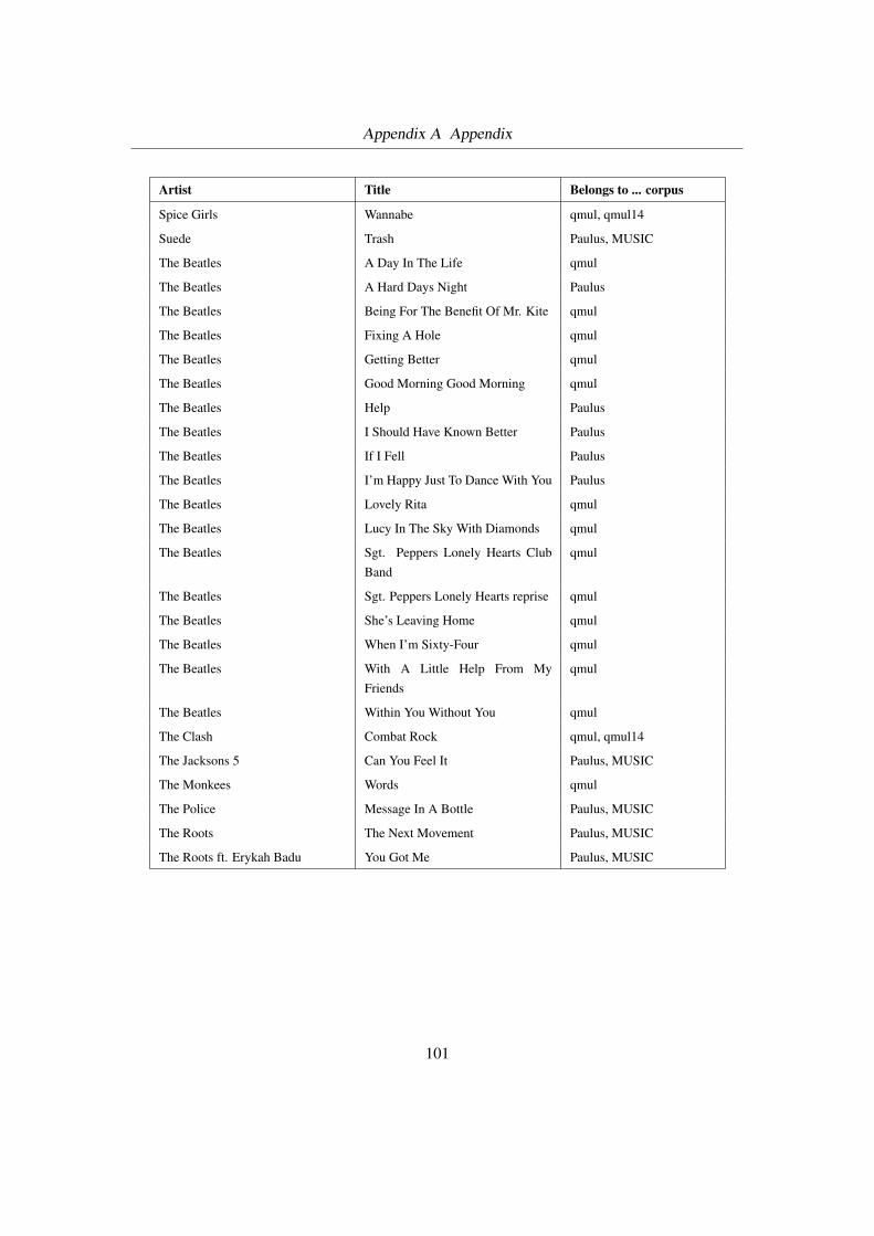
Appendix A Appendix
Artist Title Belongs to ... corpus
Spice Girls Wannabe qmul, qmul14
Suede Trash Paulus, MUSIC
The Beatles A Day In The Life qmul
The Beatles A Hard Days Night Paulus
The Beatles Being For The Benefit Of Mr. Kite qmul
The Beatles Fixing A Hole qmul
The Beatles Getting Better qmul
The Beatles Good Morning Good Morning qmul
The Beatles Help Paulus
The Beatles I Should Have Known Better Paulus
The Beatles If I Fell Paulus
The Beatles I’m Happy Just To Dance With You Paulus
The Beatles Lovely Rita qmul
The Beatles Lucy In The Sky With Diamonds qmul
The Beatles Sgt. Peppers Lonely Hearts ClubBand
qmul
The Beatles Sgt. Peppers Lonely Hearts reprise qmul
The Beatles She’s Leaving Home qmul
The Beatles When I’m Sixty-Four qmul
The Beatles With A Little Help From MyFriends
qmul
The Beatles Within You Without You qmul
The Clash Combat Rock qmul, qmul14
The Jacksons 5 Can You Feel It Paulus, MUSIC
The Monkees Words qmul
The Police Message In A Bottle Paulus, MUSIC
The Roots The Next Movement Paulus, MUSIC
The Roots ft. Erykah Badu You Got Me Paulus, MUSIC
101
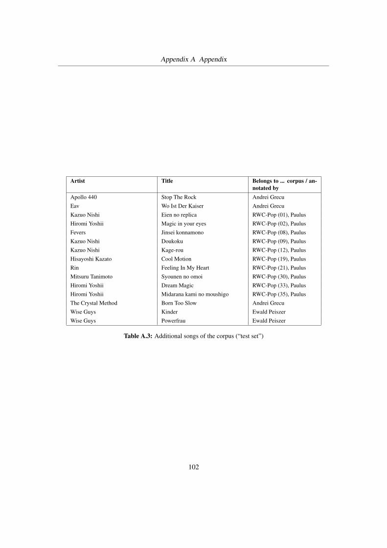
Appendix A Appendix
Artist Title Belongs to ... corpus / an-notated by
Apollo 440 Stop The Rock Andrei Grecu
Eav Wo Ist Der Kaiser Andrei Grecu
Kazuo Nishi Eien no replica RWC-Pop (01), Paulus
Hiromi Yoshii Magic in your eyes RWC-Pop (02), Paulus
Fevers Jinsei konnamono RWC-Pop (08), Paulus
Kazuo Nishi Doukoku RWC-Pop (09), Paulus
Kazuo Nishi Kage-rou RWC-Pop (12), Paulus
Hisayoshi Kazato Cool Motion RWC-Pop (19), Paulus
Rin Feeling In My Heart RWC-Pop (21), Paulus
Mitsuru Tanimoto Syounen no omoi RWC-Pop (30), Paulus
Hiromi Yoshii Dream Magic RWC-Pop (33), Paulus
Hiromi Yoshii Midarana kami no moushigo RWC-Pop (35), Paulus
The Crystal Method Born Too Slow Andrei Grecu
Wise Guys Kinder Ewald Peiszer
Wise Guys Powerfrau Ewald Peiszer
Table A.3: Additional songs of the corpus (“test set”)
102
Bibliography
[ANS+05] S. Abdallah, K. Noland, M. Sandler, M. Casey, and C. Rhodes. Theory and evalua-
tion of a Bayesian music structure extractor. In Proceedings of the 6th International
Conference on Music Information Retrieval (ISMIR 2005), pages 420–425, London,
UK, 2005.
[AS01] J.J. Aucouturier and M. Sandler. Segmentation of musical signals using Hidden
Markov Models. In Proceedings of the 110th Audio Engineering Society Conven-
tion (AES), Amsterdam, The Netherlands, 2001. Preprint Number: 5379.
[ASRC06] S. Abdallah, M. Sandler, C. Rhodes, and M. Casey. Using duration models to reduce
fragmentation in audio segmentation. Machine Learning, 65(2):485–515, 2006.
[BP92] J. C. Brown and M. S. Puckette. An efficient algorithm for the calculation of a con-
stant Q transform. The Journal of the Acoustical Society of America, 92(5):2698–
2701, 1992.
[BW01] M.A. Bartsch and G.H. Wakefield. To catch a chorus: using chroma-based rep-
resentations for audiothumbnailing. In Proceedings of the IEEE Workshop on the
Applications of Signal Processing to Audio and Acoustics (WASPAA 2001), pages
15–18, New Paltz, New York, USA, 2001.
[BW05] M.A. Bartsch and G.H. Wakefield. Audio thumbnailing of popular music using
chroma-based representations. IEEE Transactions on Multimedia, 7(1):96–104,
2005.
[CF03] M. Cooper and J. Foote. Summarizing popular music via structural similarity anal-
ysis. In Proceedings of the IEEE Workshop on Applications of Signal Processing to
Audio and Acoustics (WASPAA 2003), pages 127–130, New Paltz, New York, USA,
2003.
103
Bibliography
[Cha05] W. Chai. Automated analysis of musical structure. PhD thesis, Massachusetts
Institute of Technology, MA, USA, September 2005.
[CS06] M. Casey and M. Slaney. The importance of sequences in musical similarity. In
Proceedings of the IEEE International Conference on Acoustics, Speech and Signal
Processing (ICASSP 2006), volume 5, Toulouse, France, 2006.
[Dix01] S. Dixon. Automatic extraction of tempo and beat from expressive performances.
Journal of New Music Research, 30(1):39–58, 2001.
[FC03] J. Foote and M. Cooper. Media segmentation using self-similarity decomposition.
In Proceedings of the SPIE Storage and Retrieval for Media Databases, volume
5021, pages 167–175, Santa Clara, California, USA, 2003.
[Fle06] A. Flexer. Statistical evaluation of music information retrieval experiments. Journal
of New Music Research, 35(2):113–120, June 2006.
[Foo00] J. Foote. Automatic audio segmentation using a measure of audio novelty. In
Proceedings of the IEEE International Conference on Multimedia and Expo (ICME
2000), volume 1, New York City, New York, USA, 2000.
[GHNO02] M. Goto, H. Hashiguchi, T. Nishimura, and R. Oka. RWC music database: popular,
classical, and jazz music databases. In Proceedings of the 3rd International Confer-
ence on Music Information Retrieval (ISMIR 2002), pages 287–288, Paris, France,
2002.
[Got03] M. Goto. A chorus-section detecting method for musical audio signals. In Pro-
ceedings of the IEEE International Conference on Acoustics, Speech and Signal
Processing (ICASSP 2003), volume 5, Hong Kong, China, 2003.
[HBV01] M. Halkidi, Y. Batistakis, and M. Vazirgiannis. On clustering validation techniques.
Journal of Intelligent Information Systems, 17(2-3):107–145, 2001.
[Hei03] T. Heittola. Automatic classification of music signals. Master’s thesis, Tampere
University of Technology, 2003.
[HSG06] C. Harte, M. Sandler, and M. Gasser. Detecting harmonic change in musical au-
dio. In Proceedings of the 1st ACM Workshop on Audio and Music Computing for
Multimedia (AMCMM 2006), pages 21–26, Santa Barbara, California, USA, 2006.
ACM Press New York, New York, USA.
104
Bibliography
[LC00] B. Logan and S. Chu. Music summarization using key phrases. In Proceedings
of the IEEE International Conference on Acoustics, Speech and Signal Processing
(ICASSP 2000), volume 2, Istanbul, Turkey, 2000.
[LR05] T. Lidy and A. Rauber. Evaluation of feature extractors and psycho-acoustic trans-
formations for music genre classification. In Proceedings of the 6th International
Conference on Music Information Retrieval (ISMIR 2005), pages 34–41, London,
UK, 2005.
[LS06] M. Levy and M. Sandler. New methods in structural segmentation of musical au-
dio. In Proceedings of European Signal Processing Conference (EUSIPCO 2006),
Florence, Italy, 2006.
[LS07] M. Levy and M. Sandler. Structural segmentation of musical audio by constrained
clustering. 2007. Submitted to IEEE Transactions on Audio, Speech and Language
Processing.
[LSC06] M. Levy, M. Sandler, and M. Casey. Extraction of high-level musical structure
from audio data and its application to thumbnail generation. In Proceedings of
the IEEE International Conference on Acoustics, Speech and Signal Processing
(ICASSP 2006), Toulouse, France, 2006.
[LWZ04] L. Lu, M. Wang, and H.J. Zhang. Repeating pattern discovery and structure analysis
from acoustic music data. In Proceedings of the 6th ACM SIGMM International
Workshop on Multimedia Information Retrieval (MIR 2004), pages 275–282, New
York, New York, USA, 2004. ACM Press New York, New York, USA.
[Mad06] N.C. Maddage. Automatic structure detection for popular music. IEEE Transac-
tions on Multimedia, 13(1):65–77, 2006.
[Mid90] R. Middleton. Studying Popular Music. Open University Press, Philadelphia, 1990.
[MXKS04] N.C. Maddage, C. Xu, M.S. Kankanhalli, and X. Shao. Content-based music struc-
ture analysis with applications to music semantics understanding. In Proceedings
of the 12th Annual ACM International Conference on Multimedia, pages 112–119,
New York, New York, USA, 2004. ACM Press New York, New York, USA.
[Ong05] B.S. Ong. Towards automatic music structural analysis: identifying characteristic
within-song excerpts in popular music. PhD thesis, Universitat Pompeu Fabra,
2005.
105
Bibliography
[PBR02] G. Peeters, A. La Burthe, and X. Rodet. Toward automatic music audio summary
generation from signal analysis. In Proceedings of the 3rd International Conference
on Music Information Retrieval (ISMIR 2002), Paris, France, 2002.
[Pei07] E. Peiszer. Automatic audio segmentation: Algorithm, experiments and evaluation.
Master’s thesis, Vienna University of Technology, Vienna, Austria, 2007. (self-
reference to this thesis for convenience).
[PK06] J. Paulus and A. Klapuri. Music structure analysis by finding repeated parts. In
Proceedings of the 1st ACM Workshop on Audio and Music Computing for Multi-
media (AMCMM 2006), pages 59–68, Santa Barbara, California, USA, 2006. ACM
Press New York, New York, USA.
[RCAS06] C. Rhodes, M. Casey, S. Abdallah, and M. Sandler. A Markov-chain Monte-Carlo
approach to musical audio segmentation. In Proceedings of the IEEE International
Conference on Acoustics, Speech and Signal Processing (ICASSP 2006), Toulouse,
France, 2006.
[RJ93] L. Rabiner and B.-H. Juang. Fundamentals of speech recognition. Prentice-Hall,
Inc., Upper Saddle River, New Jersey, USA, 1993.
[RPM02] A. Rauber, E. Pampalk, and D. Merkl. Using psycho-acoustic models and self-
organizing maps to create a hierarchical structuring of music by musical styles. In
Proceedings of the 3rd International Symposium on Music Information Retrieval,
pages 71–80, Paris, France, October 13-17 2002.
[Ruw87] N. Ruwet. Methods of analysis in musicology. Music Analysis, 6(1/2):11–36, 1987.
[Smi97] S. W. Smith. The Scientist and Engineer’s Guide to Digital Signal Processing.
California Technical Publishing, 1997. Available at http://www.dspguide.com.
[Ste84] M. Steedman. A generative grammar for jazz chord sequences. Music Perception,
2(1):52–77, 1984.
106