Embed Size (px)
Citation preview
Chiral Dynamics of Heavy-Light Mesons
by
Michael AltenbuchingerDecember, 2013

Physik Department
Institut für Theoretische Physik T39
Univ.-Prof. Dr. Wolfram Weise
Chiral Dynamics of Heavy-Light Mesons
Dipl.-Phys. (Univ.) Michael Christoph Altenbuchinger
Vollständiger Abdruck der von der Fakultät für Physik der Technischen Universität München zur Erlangung
des akademischen Grades eines
Doktors der Naturwissenschaften (Dr. rer. nat.)
genehmigten Dissertation.
Vorsitzender: Univ.-Prof. Dr. Stephan Paul
Prüfer der Dissertation: 1. Univ.-Prof. Dr. Wolfram Weise
2. Univ.-Prof. Dr. Nora Brambilla
Die Dissertation wurde am 02.01.2014 bei der Technischen Universität München eingereicht und durch die
Fakultät für Physik am 21.01.2014 angenommen.

Abstract
This thesis focuses on the physics of heavy-light mesons, i.e. quark-antiquark systems com-
posed of a heavy (𝑐 or 𝑏) and a light (𝑢, 𝑑 or 𝑠) quark. The light-quark sector is treated within the
framework of chiral effective field theory. Recent lattice QCD computations have progressed in de-
termining the decay constants of charmed mesons and the scattering lengths of Nambu-Goldstone
bosons (pions, kaons) off 𝐷 mesons. These computations are performed for light quark masses
larger than the physical ones. A chiral extrapolation down to physical masses is necessary. It
is commonly performed using chiral perturbation theory. The related systematical uncertainties
have to be examined carefully. In this thesis it is shown how these uncertainties can be reduced
significantly by taking into account relativistic effects in the chiral extrapolations. As a byprod-
uct, estimates are presented for several physical quantities that are related by heavy-quark spin
and flavor symmetry. Furthermore, the investigation of the light-quark mass dependence of the
scattering lengths of Nambu-Goldstone bosons off 𝐷 mesons provides important information on
the nature of one of the intriguing newly discovered resonances, the 𝐷*𝑠0(2317). It is shown that
this resonance can be dynamically generated from the coupled-channels 𝐷𝐾 interaction without
a priori assumption of its existence. Finally we demonstrate how the underlying framework, uni-
tarized chiral perturbation theory, can be improved by the inclusion of intermediate states with
off-the-mass-shell kinematics.
5

Zusammenfassung
Diese Arbeit befasst sich mit der Physik von so genannten Heavy-Light Mesonen. Dabei han-
delt es sich um Quark-Antiquark Systeme, die sich aus einem schweren (𝑐 oder 𝑏) und einem
leichten (𝑢, 𝑑 oder 𝑠) Quark zusammensetzen. Die leichten Quarks lassen sich im Rahmen der
Chiralen Effektiven Theorie beschreiben. Aktuelle Gitter QCD Simulationen haben in den letzten
Jahren große Fortschritte gemacht. Sie bieten Ergebnisse für Zerfallskonstanten von 𝐷 Meso-
nen sowie für die Streuung von Nambu-Goldstone Bosonen (Pionen, Kaonen) an 𝐷 Mesonen.
Diese Simulationen werden für 𝑢 und 𝑑 Quarks durchgeführt, die deutlich schwerer sind als die
tatsächlichen physikalischen Quarks. Dies erfordert eine chirale Extrapolation zu physikalischen
Quarkmassen, was üblicherweise im Rahmen der Chiralen Effektiven Theorie durchgeführt wird.
Die damit verbundenen systematischen Unsicherheiten müssen jedoch gründlich untersucht wer-
den. In dieser Arbeit wird gezeigt, wie sie sich im Rahmen einer relativistischen Theorie sig-
nifikant reduzieren lassen. Ausserdem ist es uns möglich für mehrere physikalische Größen,
unter Verwendung der Spin- und Flavor-Symmetrie des schweren Quarks, Vorhersagen zu tref-
fen. Angewendet auf die Streuung von Nambu-Goldstone Bosonen an 𝐷 Mesonen geben diese
Rechnungen wichtige Hinweise auf die Zusammensetzung einer der meist diskutierten neu ent-
deckten Resonanzen, bezeichnet als 𝐷*𝑠0(2317). Es wird gezeigt, dass sie dynamisch generiert
werden kann durch die 𝐷𝐾 Wechselwirkung in gekoppelten Kanälen, wobei keine Annahmen
über die Existenz dieser Resonanz erforderlich sind. Abschließend wird demonstriert wie die zu-
grundeliegende Theorie, die Unitarisierte Chirale Störungstheorie, verbessert werden kann. Dabei
werden Zwischenzustände berücksichtigt, die sich nicht auf der Massenschale befinden.
7

Contents
1 Introduction 11
2 Heavy-quark symmetry 15
2.1 The physical picture . . . . . . . . . . . . . . . . . . . . . . . . . . . . . . . . . . . . . . . . 15
2.2 The heavy-quark limit of QCD . . . . . . . . . . . . . . . . . . . . . . . . . . . . . . . . . . 16
2.3 Spectroscopical implications . . . . . . . . . . . . . . . . . . . . . . . . . . . . . . . . . . . 18
3 The chiral effective Lagrangian 19
3.1 Chiral perturbation theory . . . . . . . . . . . . . . . . . . . . . . . . . . . . . . . . . . . . . 19
3.2 Representation of heavy-light meson fields . . . . . . . . . . . . . . . . . . . . . . . . . . . . 20
3.3 Covariant Lagrangian for heavy-light mesons . . . . . . . . . . . . . . . . . . . . . . . . . . 22
4 SU(3) breaking corrections to the D, D*, B, and B* decay constants 25
4.1 Light quark mass dependence of the 𝐷 and 𝐷𝑠 decay constants . . . . . . . . . . . . . . . . . 25
4.1.1 Theoretical framework . . . . . . . . . . . . . . . . . . . . . . . . . . . . . . . . . . 27
4.1.2 The extended-on-mass-shell (EOMS) scheme . . . . . . . . . . . . . . . . . . . . . . 31
4.1.3 Results and discussion . . . . . . . . . . . . . . . . . . . . . . . . . . . . . . . . . . 33
4.2 Predictions on 𝑓𝐷*𝑠 /𝑓𝐷* , 𝑓𝐵𝑠/𝑓𝐵 , and 𝑓𝐵*𝑠 /𝑓𝐵* in NNLO covariant ChPT . . . . . . . . . . . 36
5 Scattering of Nambu-Goldstone bosons off heavy-light mesons 45
5.1 Introduction . . . . . . . . . . . . . . . . . . . . . . . . . . . . . . . . . . . . . . . . . . . . 45
5.2 The T-matrix, unitarity, and the Bethe-Salpeter equation . . . . . . . . . . . . . . . . . . . . . 47
5.2.1 The S- and T-matrix . . . . . . . . . . . . . . . . . . . . . . . . . . . . . . . . . . . 47
5.2.2 The Bethe-Salpeter equation . . . . . . . . . . . . . . . . . . . . . . . . . . . . . . . 48
5.2.3 Partial-wave and isospin decomposition . . . . . . . . . . . . . . . . . . . . . . . . . 51
5.3 Chiral potentials . . . . . . . . . . . . . . . . . . . . . . . . . . . . . . . . . . . . . . . . . . 53
5.3.1 Off-shell potentials . . . . . . . . . . . . . . . . . . . . . . . . . . . . . . . . . . . . 53
5.3.2 Partial-wave projected on-shell potentials . . . . . . . . . . . . . . . . . . . . . . . . 57
5.4 The scattering of Nambu-Goldstone bosons off heavy-light mesons in the HQS scheme . . . . 62
5.4.1 Renormalization scheme motivated by heavy-quark symmetry . . . . . . . . . . . . . 62
5.4.2 Results and discussions . . . . . . . . . . . . . . . . . . . . . . . . . . . . . . . . . . 65
9
10 Contents
5.5 Off-shell effects on the light-quark mass evolution of scattering lengths . . . . . . . . . . . . 78
5.5.1 Framework . . . . . . . . . . . . . . . . . . . . . . . . . . . . . . . . . . . . . . . . 78
5.5.2 Results and discussions . . . . . . . . . . . . . . . . . . . . . . . . . . . . . . . . . . 84
6 Summary and conclusions 87
7 Acknowledgements 89
A Appendix 91A.1 Loop functions . . . . . . . . . . . . . . . . . . . . . . . . . . . . . . . . . . . . . . . . . . 91
A.2 Partial wave decomposition for 𝑃 *𝜑 scattering . . . . . . . . . . . . . . . . . . . . . . . . . . 93
A.3 “Renormalization” of the BS equation . . . . . . . . . . . . . . . . . . . . . . . . . . . . . . 98
A.4 Charmed and bottomed mesons from PDG [1] . . . . . . . . . . . . . . . . . . . . . . . . . . 99
Chapter 1
Introduction
The study of charm and bottom hadrons has provided numerous constraints on the parameters of the Standard
Model. Their weak decays offer the most direct way to determine the weak mixing angles, to test the unitarity of
the Cabibbo-Kobayashi-Maskawa (CKM) matrix and to study CP violation. Furthermore, they have constrained
many scenarios of physics beyond the Standard Model and hopefully they will give some hints for new physics
in ongoing or upcoming experiments. For a review see [1] and references therein.
The elements of the CKM matrix are fundamental parameters of the Standard Model. A few of them
are determined to high accuracy, as for instance |𝑉𝑢𝑑|, |𝑉𝑢𝑠| and |𝑉𝑐𝑠|, with errors mainly governed by our
knowledge of form factors. For |𝑉𝑢𝑑|, this is 𝑔𝐴 = 𝐺𝐴/𝐺𝑉 , known to high precision [2]. For |𝑉𝑐𝑠|, it is the
𝐷𝑠 meson decay constant 𝑓𝐷𝑠 , and for |𝑉𝑢𝑠| it is the form factor entering the semi-leptonic decays of kaons
to pions. Those form factors can be calculated accurately in unquenched Lattice Quantum Chromodynamics
(LQCD) computations [2, 3]. On the other hand, CKM matrix elements involving top or bottom quarks are
less certain. The extraction of |𝑉𝑢𝑏| requires an accurate knowledge of the 𝐵 meson decay constant, 𝑓𝐵 , or
of some form factors in semi-leptonic decays of bottomed hadrons. The matrix elements |𝑉𝑡𝑠| and |𝑉𝑡𝑑| are
extracted from 𝐵0 − ��0 mixing, which requires a good knowledge of 𝑓𝐵𝑠
√��𝐵𝑠 and 𝑓𝐵𝑑
√��𝐵𝑑
, where �� is
the non-perturbative QCD bag parameter. All these quantities are difficult to determine in experiment and input
from LQCD is needed. This, however, has significant statistical and systematical errors and accounts for the
main uncertainty of these CKM matrix elements. Several supplementary methods further constrain the CKM
matrix. For instance, taking the ratio |𝑉𝑡𝑠|/|𝑉𝑡𝑑|, depending on 𝜉 = (𝑓𝐵𝑠
√��𝐵𝑠)/(𝑓𝐵𝑑
√��𝐵𝑑
), reduces errors
from LQCD significantly. A comprehensive review can be found in [1].
LQCD calculations obviously play a key role in constraining the Standard Model. Their uncertainties,
however, have to be examined carefully. Lattice QCD calculations are performed on a discrete Euclidean
lattice in a finite box. They need to be translated to Minkowski space, infinite volume and infinitesimally
small lattice spacings. Additionally, most of the calculations are performed for larger than physical light-quark
masses. This reduces computation costs but requires a chiral extrapolation to physical masses. A very powerful
tool employed in this context is chiral effective theory, c.f. [4] for an overview. Investigating the dependence
of LQCD results on pion mass, volume and lattice spacing, offers a unique opportunity to constrain many
unknown low-energy constants (LECs) of chiral effective field theory. This enables us to be predictive. In
11
12 Chapter 1. Introduction
this theses, for instance, we use the light-quark mass dependence of the decay constants 𝑓𝐷 and 𝑓𝐷𝑠 to make
predictions for the ratios 𝑓𝐵𝑠/𝑓𝐵 , 𝑓𝐷*𝑠 /𝑓𝐷* and 𝑓𝐵*𝑠 /𝑓𝐵* .
Concerning the measurements of the CKM matrix and tests of its unitarity, most of the attention has been
devoted to bottom physics, whereas charm physics has long been considered as less attractive. However, this
has started to change in recent years. One of the reasons is the discovery of 𝐷0− ��0 oscillations with a mixing
rate higher than expected. This rate, intriguing by itself, gives access to CP violation in the charm sector and
hence complementary information to the intensely studied 𝐾0 − ��0 and 𝐵0 − ��0 oscillations. Another reason
relates to recent discoveries in spectroscopy. This development has been driven by a number of newly observed
states at CLEO, BaBar, Belle and LHCb [5]. These states are the still mysterious charmonium-like states,
known as 𝑋 , 𝑌 and 𝑍 particles, or the numerous new open charm states. Many of these states cannot be easily
understood in terms of conventional quark models. Multi-quark components have to be taken into account in
addition to the basic quark structure. The persisting problem is, however, that a clear description in terms of an
effective field theory is not yet available, leading to ongoing discussions about the nature of these new states.
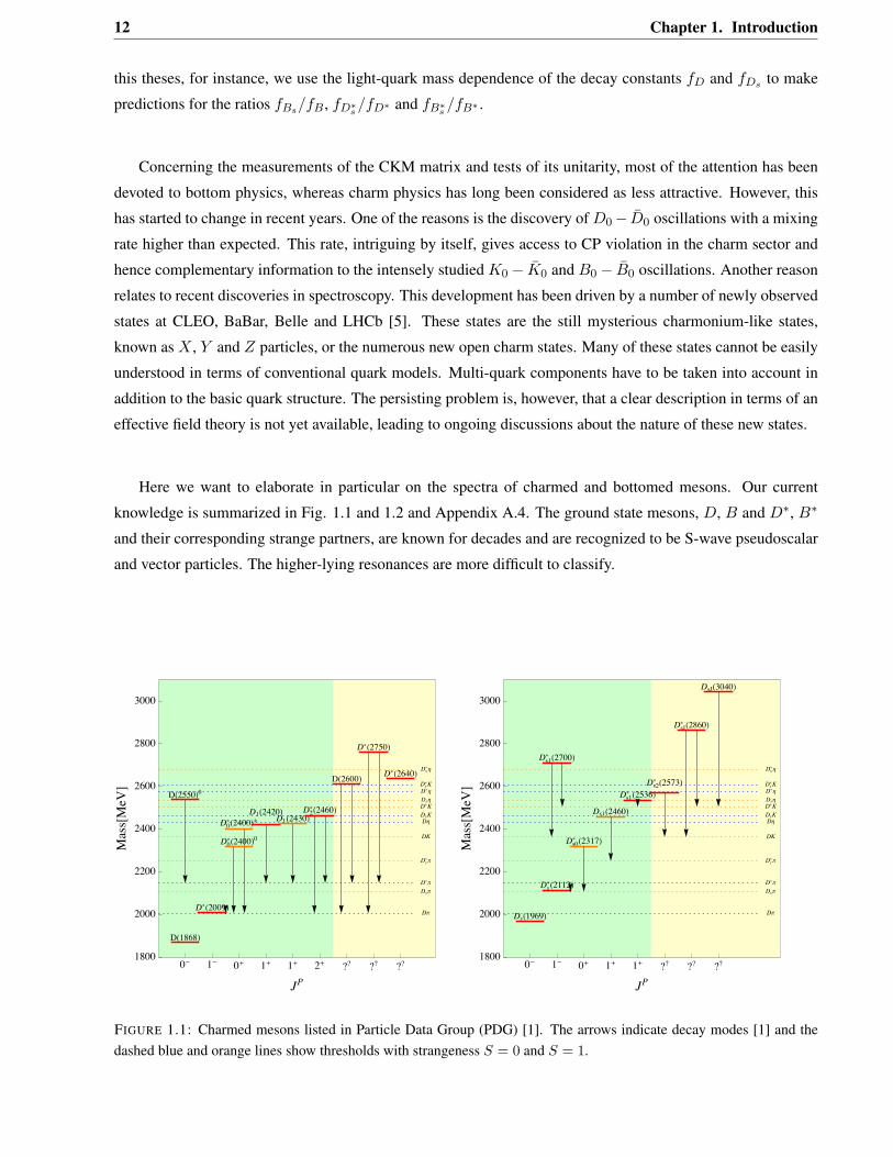
Here we want to elaborate in particular on the spectra of charmed and bottomed mesons. Our current
knowledge is summarized in Fig. 1.1 and 1.2 and Appendix A.4. The ground state mesons, 𝐷, 𝐵 and 𝐷*, 𝐵*
and their corresponding strange partners, are known for decades and are recognized to be S-wave pseudoscalar
and vector particles. The higher-lying resonances are more difficult to classify.
DsK
DK
Ds!
Ds"
D"
D!
Ds#K
D#K
Ds#!
Ds#"
D#"
D#!
D!1868"D#!2009"
D0#!2400"0D0#!2400"$D1!2420"D1!2430"D2#!2460"
D!2550"0 D!2600" D#!2640"D#!2750"
0% 1% 0& 1& 1& 2& ?? ?? ??1800
2000
2200
2400
2600
2800
3000
JP
Mass#MeV
$
DsK
DK
Ds!
Ds"
D"
D!
Ds#K
D#K
Ds#!
Ds#"
D#"
D#!
Ds!1969"Ds#!2112"
Ds0# !2317"Ds1!2460"Ds1
# !2536"Ds2# !2573"Ds1# !2700"
DsJ# !2860"DsJ!3040"
0% 1% 0& 1& 1& ?? ?? ??1800
2000
2200
2400
2600
2800
3000
JP
Mass#MeV
$
FIGURE 1.1: Charmed mesons listed in Particle Data Group (PDG) [1]. The arrows indicate decay modes [1] and thedashed blue and orange lines show thresholds with strangeness 𝑆 = 0 and 𝑆 = 1.
13
BsK
BK
Bs!
Bs"
B"
B!
Bs#K
B#K
Bs#!
Bs#"
B#"
B#!
B!5280" B#!5325"
BJ#!5732"B2#!5747"0B1#!5721"0
0$ 1$ 1% 2% ??
5300
5400
5500
5600
5700
5800
5900
6000
JP
Mass#MeV
$BsK
BK
Bs!
Bs"
B"
B!
Bs#K
B#K
Bs#!
Bs#"
B#"
B#!
Bs!5337"Bs#!5416"
Bs1# !5830"Bs2# !5840"0 BsJ# !5850"
0$ 1$ 1% 2% ??
5300
5400
5500
5600
5700
5800
5900
6000
JP
Mass#MeV
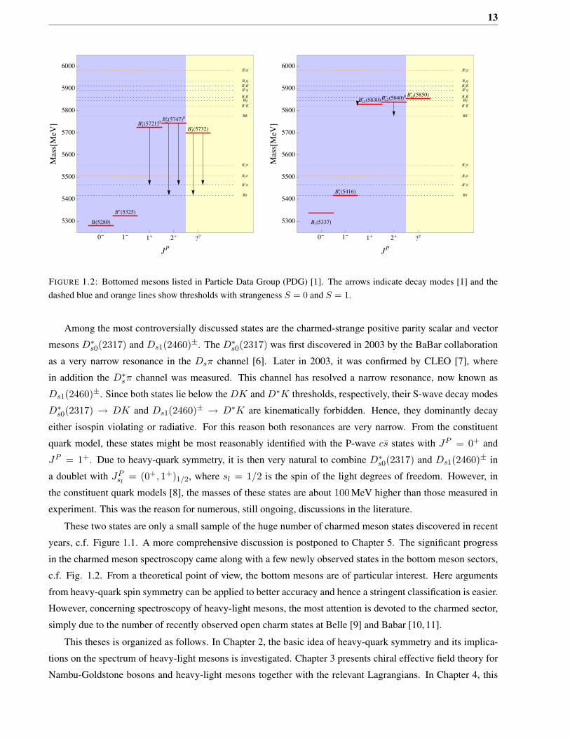
$FIGURE 1.2: Bottomed mesons listed in Particle Data Group (PDG) [1]. The arrows indicate decay modes [1] and thedashed blue and orange lines show thresholds with strangeness 𝑆 = 0 and 𝑆 = 1.
Among the most controversially discussed states are the charmed-strange positive parity scalar and vector
mesons 𝐷*𝑠0(2317) and 𝐷𝑠1(2460)±. The 𝐷*𝑠0(2317) was first discovered in 2003 by the BaBar collaboration
as a very narrow resonance in the 𝐷𝑠𝜋 channel [6]. Later in 2003, it was confirmed by CLEO [7], where
in addition the 𝐷*𝑠𝜋 channel was measured. This channel has resolved a narrow resonance, now known as
𝐷𝑠1(2460)±. Since both states lie below the 𝐷𝐾 and 𝐷*𝐾 thresholds, respectively, their S-wave decay modes
𝐷*𝑠0(2317) → 𝐷𝐾 and 𝐷𝑠1(2460)± → 𝐷*𝐾 are kinematically forbidden. Hence, they dominantly decay
either isospin violating or radiative. For this reason both resonances are very narrow. From the constituent
quark model, these states might be most reasonably identified with the P-wave 𝑐𝑠 states with 𝐽𝑃 = 0+ and
𝐽𝑃 = 1+. Due to heavy-quark symmetry, it is then very natural to combine 𝐷*𝑠0(2317) and 𝐷𝑠1(2460)± in
a doublet with 𝐽𝑃𝑠𝑙
= (0+, 1+)1/2, where 𝑠𝑙 = 1/2 is the spin of the light degrees of freedom. However, in
the constituent quark models [8], the masses of these states are about 100 MeV higher than those measured in
experiment. This was the reason for numerous, still ongoing, discussions in the literature.
These two states are only a small sample of the huge number of charmed meson states discovered in recent
years, c.f. Figure 1.1. A more comprehensive discussion is postponed to Chapter 5. The significant progress
in the charmed meson spectroscopy came along with a few newly observed states in the bottom meson sectors,
c.f. Fig. 1.2. From a theoretical point of view, the bottom mesons are of particular interest. Here arguments
from heavy-quark spin symmetry can be applied to better accuracy and hence a stringent classification is easier.
However, concerning spectroscopy of heavy-light mesons, the most attention is devoted to the charmed sector,
simply due to the number of recently observed open charm states at Belle [9] and Babar [10, 11].
This theses is organized as follows. In Chapter 2, the basic idea of heavy-quark symmetry and its implica-
tions on the spectrum of heavy-light mesons is investigated. Chapter 3 presents chiral effective field theory for
Nambu-Goldstone bosons and heavy-light mesons together with the relevant Lagrangians. In Chapter 4, this
14 Chapter 1. Introduction
theory is applied. In the first part of this chapter, it is demonstrated how covariant calculations can significantly
improve chiral extrapolations. The second part is devoted to predictions on the ratios 𝑓𝐷*𝑠 /𝑓𝐷* , 𝑓𝐵𝑠/𝑓𝐵 , and
𝑓𝐵*𝑠 /𝑓𝐵* . Chapter 5 investigates the scattering of Nambu-Goldstone bosons off heavy-light mesons. In this
chapter we first present the prerequisites of unitarized chiral perturbation theory in Section 5.2. These are the
unitarity conditions for the T matrix, the Bethe-Salpeter equation and partial-wave projections. The chiral po-
tentials up to next-to-leading order are presented in Section 5.3. Finally, unitarized chiral perturbation theory
is applied starting from Section 5.4 in combination with recent lattice computations [12]. This allows us to
predict numerous states of charm and bottom mesons by use of heavy-quark spin and flavor symmetry. The
next part, Section 5.5, shows some alternative results, obtained by solving the Bethe-Salpeter equation for fully
momentum dependent potentials, i.e. without employing the on-shell approximation. This is shown to improve
the leading order resummations significantly. A short conclusion and summary is given in Chapter 6.
Chapter 2
Heavy-quark symmetry
2.1 The physical picture
Among the six different quark flavors, three can be identified as heavy compared to the fundamental scale of
Quantum Chromodynamics (QCD), ΛQCD ∼ 0.3 GeV. These are 𝑐, 𝑏, 𝑡 with masses of roughly 1.5 GeV, 5 GeV
and 175 GeV. We concentrate on heavy-light hadrons, which are composed of one heavy quark surrounded by
light (anti-)quarks and gluons. Such systems exhibit additional symmetries in the limit ΛQCD/𝑚𝑄 → 0, where
𝑚𝑄 is the mass of the heavy quark 𝑄. These are the heavy-quark flavor and heavy-quark spin symmetry. There
a numerous review articles and lecture notes investigating these symmetries, c.f. [13–17], to name just the few
of which this section did benefit most.
The physical picture of heavy-light hadrons is similar to the hydrogen atom. There the proton acts in a
first approximation as a static source of electromagnetic fields: it emits and absorbs photons, whereas all recoil
effects are negligible. In heavy-light hadrons, the role of the proton is played by the heavy quark and the role of
the electron cloud by the light degrees of freedom of QCD1. The light degrees of freedom carry momenta of the
order of ΛQCD and the momenta transferred to the heavy quark are therefore of the same order of magnitude.
The momentum of the heavy quark can be decomposed as
𝑝𝑄 = 𝑚𝑄𝑣 + 𝑘, (2.1)
where 𝑣 is the velocity of the heavy quark, with 𝑣2 = 1, and 𝑘 is a small residual momentum of the order
of ΛQCD. Even if the momentum of the heavy quark can be changed by orders of ΛQCD, its velocity 𝑣 is
only altered by orders ΛQCD/𝑚𝑄 ≪ 1. Hence, in the limit 𝑚𝑄 → ∞, the heavy quark becomes a static color
source, where all recoil effects from the emission or absorption of gluons can be neglected. The dynamics of the
surrounding cloud is still governed by non-perturbative interactions among its constituents, but its interaction
with the heavy quark has simplified tremendously. From this picture it becomes clear that in this limit, the light
degrees of freedom do not see the exact mass of the heavy quark (since it is static), i.e. their wave-function
does not depend on the heavy-quark mass. This is heavy-quark flavor symmetry.
1By “light degrees of freedom” we mean the complex many-body system, consisting of the light quarks and antiquarks, and gluons,that surrounds the heavy quark. Frequently, the notation “brown muck” is used in this context [13, 14].
15
16 Chapter 2. Heavy-quark symmetry
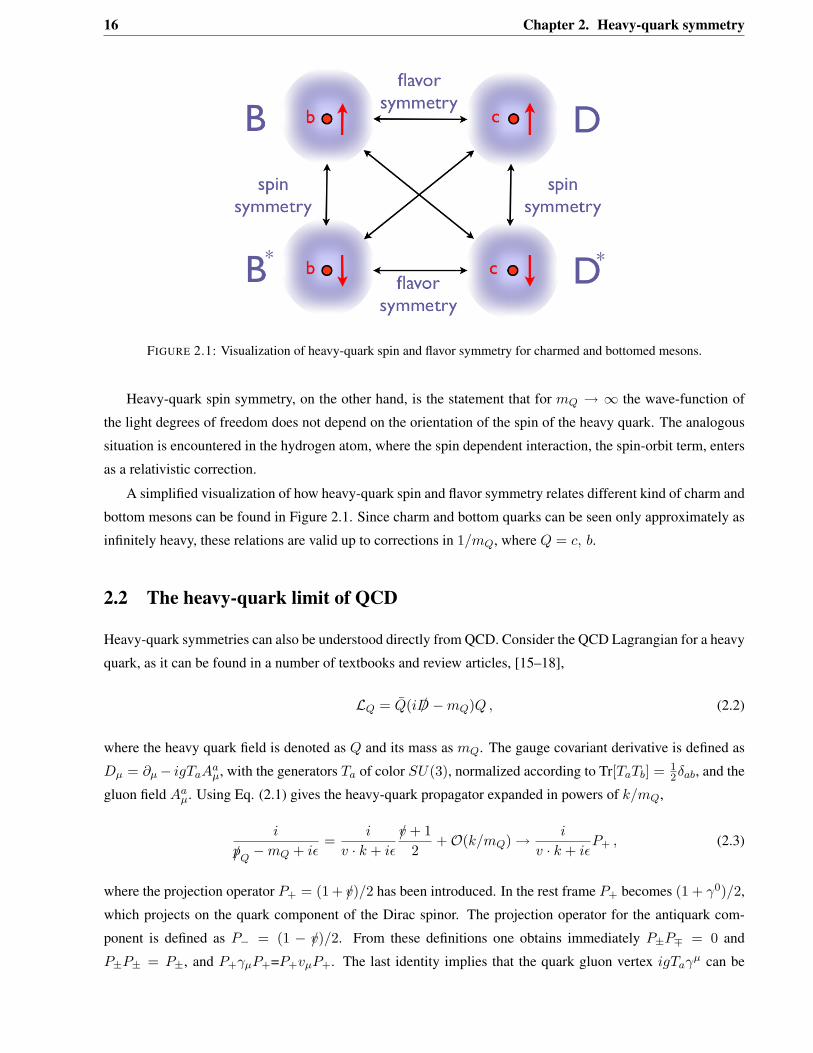
FIGURE 2.1: Visualization of heavy-quark spin and flavor symmetry for charmed and bottomed mesons.
Heavy-quark spin symmetry, on the other hand, is the statement that for 𝑚𝑄 → ∞ the wave-function of
the light degrees of freedom does not depend on the orientation of the spin of the heavy quark. The analogous
situation is encountered in the hydrogen atom, where the spin dependent interaction, the spin-orbit term, enters
as a relativistic correction.
A simplified visualization of how heavy-quark spin and flavor symmetry relates different kind of charm and
bottom mesons can be found in Figure 2.1. Since charm and bottom quarks can be seen only approximately as
infinitely heavy, these relations are valid up to corrections in 1/𝑚𝑄, where 𝑄 = 𝑐, 𝑏.
2.2 The heavy-quark limit of QCD
Heavy-quark symmetries can also be understood directly from QCD. Consider the QCD Lagrangian for a heavy
quark, as it can be found in a number of textbooks and review articles, [15–18],
ℒ𝑄 = ��(𝑖 /𝐷 −𝑚𝑄)𝑄 , (2.2)
where the heavy quark field is denoted as 𝑄 and its mass as 𝑚𝑄. The gauge covariant derivative is defined as
𝐷𝜇 = 𝜕𝜇− 𝑖𝑔𝑇𝑎𝐴𝑎𝜇, with the generators 𝑇𝑎 of color 𝑆𝑈(3), normalized according to Tr[𝑇𝑎𝑇𝑏] = 1
2𝛿𝑎𝑏, and the
gluon field 𝐴𝑎𝜇. Using Eq. (2.1) gives the heavy-quark propagator expanded in powers of 𝑘/𝑚𝑄,
𝑖
/𝑝𝑄−𝑚𝑄 + 𝑖𝜖
=𝑖
𝑣 · 𝑘 + 𝑖𝜖
/𝑣 + 12
+𝒪(𝑘/𝑚𝑄) → 𝑖
𝑣 · 𝑘 + 𝑖𝜖𝑃+ , (2.3)
where the projection operator 𝑃+ = (1 + /𝑣)/2 has been introduced. In the rest frame 𝑃+ becomes (1 + 𝛾0)/2,
which projects on the quark component of the Dirac spinor. The projection operator for the antiquark com-
ponent is defined as 𝑃− = (1 − /𝑣)/2. From these definitions one obtains immediately 𝑃±𝑃∓ = 0 and
𝑃±𝑃± = 𝑃±, and 𝑃+𝛾𝜇𝑃+=𝑃+𝑣𝜇𝑃+. The last identity implies that the quark gluon vertex 𝑖𝑔𝑇𝑎𝛾𝜇 can be
2.2. The heavy-quark limit of QCD 17
replaced by
𝑖𝑔𝑇𝑎𝑣𝜇 (2.4)
at leading order in 1/𝑚𝑄. One notices that both limits, Eq. (2.3) and Eq. (2.4), do not refer to the mass of the
heavy quark, in accordance with our intuitive picture of heavy-quark flavor symmetry. The coefficient 𝑃+ in
Eq. (2.3) projects on the upper (quark) component of the spinor, whereas the remaining part of the propagator
is diagonal in spin, i.e. it does not depend on the spin of the quark or antiquark field. Obviously, Eq. (2.4)
is diagonal in spin space, too. Therefore the interaction does not depend on the spin orientation of the heavy
quark, in accordance with heavy-quark spin symmetry.
Heavy-quark symmetries can be implemented at the Lagrangian level. This is done in the language of
heavy-quark-effective theory (HQET), which is directly derived from the generating functional of QCD. There
the heavy degrees of freedom can be identified and integrated out, resulting in a non-local action. Expanding
in a series of local terms gives the Lagrangian of HQET [19]. Equivalently, one can perform a number of field
redefinitions, Foldy-Wouthuysen transformations, to transform away the couplings to the small components of
the spinors, as described in [20]. At leading order the Lagrangian of HQET can be also obtained directly from
Eq. (2.2) by redefining the heavy-quark field,
𝑄(𝑥) = exp(−𝑖𝑚𝑄𝑣 · 𝑥)(ℎ𝑣(𝑥) + 𝐻𝑣(𝑥)) , (2.5)
with
ℎ𝑣(𝑥) = exp(𝑖𝑚𝑄𝑣 · 𝑥)1 + /𝑣
2𝑄(𝑥) ,
𝐻𝑣(𝑥) = exp(𝑖𝑚𝑄𝑣 · 𝑥)1− /𝑣
2𝑄(𝑥) , (2.6)
where the quark component is denoted by ℎ𝑣(𝑥) and the antiquark component by 𝐻𝑣(𝑥). The exponential
factor ensures that derivatives applied to ℎ𝑣(𝑥) produce only momenta of the order 𝑘. Inserting Eq. (2.5)
into the QCD lagrangian Eq. (2.2), and retaining only the quark component ℎ𝑣(𝑥), gives the leading order
lagrangian of HQET,
ℒeff = ℎ𝑣 𝑖𝑣 ·𝐷 ℎ𝑣 = ℎ𝑣(𝑖𝑣𝜇𝜕𝜇 + 𝑔𝑇𝑎𝑣𝜇𝐴𝜇𝑎)ℎ𝑣 . (2.7)
Taking into account also the antiquark part 𝐻𝑣(𝑥) produces corrections of higher order in 1/𝑚𝑄, as can be
shown by employing the equations of motion to express 𝐻𝑣(𝑥) in terms of ℎ𝑣(𝑥). The Feynman rules derived
from this Lagrangian are in accordance with Eq. (2.3) and Eq. (2.4). The Lagrangian (2.7) does not have
a heavy-quark mass term, as a manifestation of heavy-quark flavor symmetry. Further, one notices that the
Lagrangian is invariant under spin rotations,
ℎ𝑣(𝑥) → (1 + 𝑖𝜖 · 𝑆)ℎ𝑣(𝑥) , with 𝑆𝑖 =12
(𝜎𝑖 00 𝜎𝑖
), (2.8)
where 𝜎𝑖 are the Pauli matrices, i.e. it possesses heavy-quark spin symmetry. Breaking effects to these symme-
tries start at order 1/𝑚𝑄.
18 Chapter 2. Heavy-quark symmetry
I3
Y
+12!1
2
+1
D+D0
D+s
JP = 0!
I3
Y
+12!1
2
+1
D"+D"0
D"+s
JP = 1!
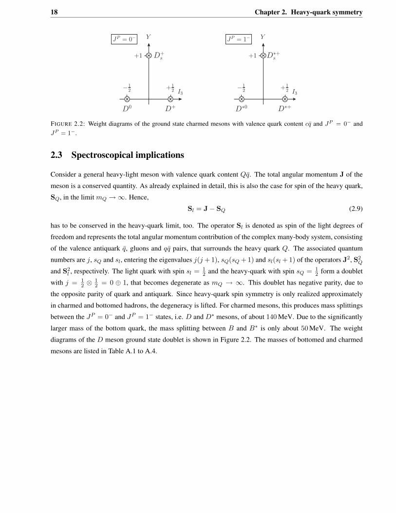
FIGURE 2.2: Weight diagrams of the ground state charmed mesons with valence quark content 𝑐𝑞 and 𝐽𝑃 = 0− and𝐽𝑃 = 1−.
2.3 Spectroscopical implications
Consider a general heavy-light meson with valence quark content 𝑄𝑞. The total angular momentum J of the
meson is a conserved quantity. As already explained in detail, this is also the case for spin of the heavy quark,
S𝑄, in the limit 𝑚𝑄 →∞. Hence,
S𝑙 = J− S𝑄 (2.9)
has to be conserved in the heavy-quark limit, too. The operator S𝑙 is denoted as spin of the light degrees of
freedom and represents the total angular momentum contribution of the complex many-body system, consisting
of the valence antiquark 𝑞, gluons and 𝑞𝑞 pairs, that surrounds the heavy quark 𝑄. The associated quantum
numbers are 𝑗, 𝑠𝑄 and 𝑠𝑙, entering the eigenvalues 𝑗(𝑗 + 1), 𝑠𝑄(𝑠𝑄 + 1) and 𝑠𝑙(𝑠𝑙 + 1) of the operators J2, S2𝑄
and S2𝑙 , respectively. The light quark with spin 𝑠𝑙 = 1
2 and the heavy-quark with spin 𝑠𝑄 = 12 form a doublet
with 𝑗 = 12 ⊗ 1
2 = 0 ⊕ 1, that becomes degenerate as 𝑚𝑄 → ∞. This doublet has negative parity, due to
the opposite parity of quark and antiquark. Since heavy-quark spin symmetry is only realized approximately
in charmed and bottomed hadrons, the degeneracy is lifted. For charmed mesons, this produces mass splittings
between the 𝐽𝑃 = 0− and 𝐽𝑃 = 1− states, i.e. 𝐷 and 𝐷* mesons, of about 140 MeV. Due to the significantly
larger mass of the bottom quark, the mass splitting between 𝐵 and 𝐵* is only about 50 MeV. The weight
diagrams of the 𝐷 meson ground state doublet is shown in Figure 2.2. The masses of bottomed and charmed
mesons are listed in Table A.1 to A.4.
Chapter 3
The chiral effective Lagrangian
3.1 Chiral perturbation theory
The three quark flavors 𝑢, 𝑑 and 𝑠, can be considered as light compared to the fundamental scale of QCD,
ΛQCD ∼ 0.3 GeV. This classification is obvious for 𝑢 and 𝑑, whereas the mass of the strange quark 𝑠 is almost
of the same order of magnitude as ΛQCD, but still reasonably small. In the limit of vanishing light quark masses,
𝑚𝑢 = 𝑚𝑑 = 𝑚𝑠 = 0, the Lagrangian of QCD possesses the symmetries 𝑆𝑈(3)𝐿 ⊗ 𝑆𝑈(3)𝑅 ⊗ 𝑈(1)𝑉 . These
are spontaneously broken down to 𝑆𝑈(3)𝑉 ⊗𝑈(1)𝑉 , leading to eight massless Nambu-Goldstone bosons which
correspond to eight broken generators. As a consequence of the explicit chiral symmetry breaking, 𝑚𝑢,𝑑,𝑠 = 0,
these bosons acquire a mass and can be identified with the light pseudoscalar meson octet consisting of pions,
kaons and the eta meson. The theory describing the interaction of these low-energy degrees of freedom is
called chiral effective field theory [21, 22]. In the following we summarize the most important ingredients of
this theory and refer to [23] and the references therein for more details.
The most general Lagrangian describing the interaction of Nambu-Goldstone bosons consists of an infinite
amount of terms. To be predictive anyway, we have to specify power counting rules: the masses 𝑚𝜑 of the
Nambu-Goldstone bosons 𝜑 and the field gradients 𝜕𝜇𝜑 are counted as 𝒪(𝑝), where 𝑝 is a small momentum
compared to the characteristic scale of the theory, 4𝜋𝑓0 ≈ 1.2 GeV. To given chiral order only a finite number
of terms enters the Lagrangian and therefore the theory becomes predictive. In our analysis it is sufficient to
consider only the leading chiral order.
We introduce the field Σ = exp(
𝑖Φ𝑓0
)∈ 𝑆𝑈(3), where 𝑓0 is the pion decay constant in the chiral limit and
Φ collects the light pseudoscalar meson octet,
Φ = Λ𝑎𝜑𝑎 =√
2
⎛⎜⎜⎜⎜⎝
𝜋0√
2+ 𝜂√
6𝜋+ 𝐾+
𝜋− − 𝜋0√
2+ 𝜂√
6𝐾0
𝐾− ��0 − 2√6𝜂
⎞⎟⎟⎟⎟⎠
. (3.1)
19
20 Chapter 3. The chiral effective Lagrangian
This field transforms under flavor 𝑆𝑈(3)𝐿 × 𝑆𝑈(3)𝑅 as
Σ → 𝐿Σ𝑅† , (3.2)
where 𝐿 ∈ 𝑆𝑈(3)𝐿 and 𝑅 ∈ 𝑆𝑈(3)𝑅.
We use the field 𝜉 defined by 𝜉2 = Σ = exp(
𝑖Φ𝑓0
). As can be seen from (3.2), it has to transforms as
𝜉 → 𝐿𝜉𝑈 † = 𝑈𝜉𝑅† (3.3)
under 𝑆𝑈(3)𝐿 × 𝑆𝑈(3)𝑅, where 𝑈 is a unitary matrix depending on 𝐿, 𝑅 and the meson fields Φ(𝑥). With
these ingredients, the most general Lagrangian consistent with the symmetries of the theory is [23]
ℒ(2) =𝑓20
4⟨𝜕𝜇Σ𝜕𝜇Σ†⟩+
𝑓20
4⟨𝜒+⟩ , (3.4)
at leading chiral order. The brackets ⟨. . .⟩ stand for the trace over flavor indices. The superscript (2) gives
the order of the Lagrangian and 𝜒+ = 𝜉†ℳ𝜉† + 𝜉ℳ𝜉. The light-quark mass matrix, responsible for explicit
chiral symmetry breaking, is defined as ℳ = 2𝐵0 Diag(𝑚𝑢, 𝑚𝑑, 𝑚𝑠), where the new parameter 𝐵0 can be
related to the chiral quark condensate by 3𝑓20 𝐵0 = −⟨𝑞𝑞⟩ = −⟨��𝑢 + 𝑑𝑑 + 𝑠𝑠⟩. For exact isospin symmetry,
𝑚 ≡ 𝑚𝑢 = 𝑚𝑑, the masses of the Nambu-Goldstone bosons can be expressed in terms of the light quark
masses by
𝑚2𝜋 = 2𝐵0𝑚 , (3.5)
𝑚2𝐾 = 𝐵0(𝑚 + 𝑚𝑠) , (3.6)
𝑚2𝜂 =
23𝐵0(𝑚 + 2𝑚𝑠) , (3.7)
at leading chiral order. These equations, together with their relation to the chiral quark condensate, are known as
the Gell-Mann, Oakes, and Renner relations [24]. As a direct consequence, one obtains the Gell-Mann-Okubo
relation
4𝑚2𝐾 = 3𝑚2
𝜂 + 𝑚2𝜋 , (3.8)
which is used throughout our analysis to express the mass of the 𝜂 meson. The mass matrix can be written as
ℳ = (𝑚2𝜋, 𝑚2
𝜋, 2𝑚2𝐾 −𝑚2
𝜋), where equations (3.5) to (3.7) have been used.
3.2 Representation of heavy-light meson fields
It is convenient to impose heavy-quark spin symmetry on the level of the Lagrangian. This is done by repre-
senting the 𝑄𝑞 mesons by a field 𝐻 , that contains both, pseudoscalar and vector meson ground states. These
ground states become degenerate as the mass of the heavy quark goes to infinity, 𝑚𝑄 →∞.
3.2. Representation of heavy-light meson fields 21
The field 𝐻 has to transform as a bispinor under Lorentz transformations [17],
𝐻 ′(𝑥′) = 𝐷(Λ)𝐻(𝑥)𝐷(Λ)−1 , 𝑥′ = Λ𝑥 , (3.9)
where 𝐷(Λ) is the Lorentz transformation for spinors and Λ for coordinates. Equivalently,
𝐻(𝑥) → 𝐻 ′(𝑥) = 𝐷(Λ)𝐻(Λ−1𝑥)𝐷(Λ)−1 . (3.10)
This field can be expressed as a linear combination of a pseudoscalar meson field 𝑃 and a vector meson field
𝑃 *𝜇,
𝐻 =𝑖 /𝒟 + 𝑚𝑃
2𝑚𝑃(𝛾𝜇𝑃 *𝜇 + 𝑖𝑃𝛾5) , (3.11)
where 𝑚𝑃 is the characteristic mass of the heavy-light meson. The field 𝐻 is a scalar under Lorentz transfor-
mations since 𝛾5 multiplies the pseudoscalar meson field 𝑃 and 𝛾𝜇 the vector field 𝑃 *𝜇. The phase between 𝑃
and 𝑃 *𝜇 is arbitrary. Under parity, 𝐻 transforms as
𝐻(𝑥) → 𝛾0𝐻(𝑥𝑃 )𝛾0 , with 𝑥𝑃 = (𝑥0,−x) . (3.12)
The covariant derivative 𝒟𝜇 in Eq. (3.11) has been introduced with respect to triplets under flavor 𝑆𝑈(3).
For 𝐷 mesons (𝑄 = 𝑐), they are 𝑃 = (𝐷0, 𝐷+, 𝐷+𝑠 ) and 𝑃 *𝜇 = (𝐷*0, 𝐷*+, 𝐷*+𝑠 )𝜇 and for �� mesons (𝑄 = 𝑏),
they are 𝑃 = (𝐵−, ��0, ��0𝑠 ) and 𝑃 *𝜇 = (𝐵*−, ��*0, ��0*
𝑠 )𝜇. Then, 𝐻 transforms as
𝐻𝑎 → 𝐻𝑏𝑈†𝑏𝑎 (3.13)
under 𝑆𝑈(3)𝐿×𝑆𝑈(3)𝑅, where 𝑎(𝑏) are the flavor indices. This transformation is not the only possible choice.
It has, however, the advantage that the transformation under parity takes the simple form of Eq. (3.12)1. For
more details we refer to [17]. The covariant derivative is defined as
𝒟𝜇𝑃𝑎 = 𝜕𝜇𝑃𝑎 − Γ𝑏𝑎𝜇 𝑃𝑏 , 𝒟𝜇𝑃 †𝑎 = 𝜕𝜇𝑃 †𝑎 + Γ𝜇
𝑎𝑏𝑃†𝑏 , (3.14)
with the vector current Γ𝜇 = 12(𝜉†𝜕𝜇𝜉 + 𝜉𝜕𝜇𝜉†). With this definition
𝒟𝜇𝐻𝑎 → (𝒟𝜇𝐻𝑏)𝑈†𝑏𝑎 (3.15)
under 𝑆𝑈(3)𝐿 × 𝑆𝑈(3)𝑅. In the limit 𝑚𝑃 → ∞, the coefficient (𝑖 /𝒟 + 𝑚𝑃 )/(2𝑚𝑃 ) in Eq. (3.11) becomes
a projection operator, as can be understood by decomposing the momentum of the heavy-light meson as 𝑝𝜇𝑃 =
𝑚𝑃 𝑣𝜇 + 𝑘𝜇, with the static part 𝑚𝑃 𝑣𝜇 and the small residual momentum 𝑘𝜇. The velocity is normalized as
𝑣2 = 1. In the static limit (𝑖 /𝒟+𝑚𝑃 )/(2𝑚𝑃 ) → (1+/𝑣)/2, where the interaction terms with Nambu-Goldstone
1This ambiguity can be translated to the freedom of choosing different interpolating fields 𝐻 . Therefore, physical predictions arestill unique.
22 Chapter 3. The chiral effective Lagrangian
bosons are neglected. The operators 𝑃+ = (1 + /𝑣)/2 and 𝑃− = (1 − /𝑣)/2 project on quark and antiquark
component of the heavy quark [17], respectively. Their properties are summarized in Section 2.2.
With respect to rotations of the spins, the field 𝐻 transforms as a (1/2, 1/2) representation under 𝑆𝑄 ⊗ 𝑆𝑙.
Under finite rotations of the heavy-quark spin, this field transforms as
𝐻 → 𝐷(𝑅)𝑄𝐻, (3.16)
where 𝐷(𝑅)𝑄 is a rotation matrix in the spinor representation for a rotation 𝑅, applied to the heavy quark 𝑄.
As for the Lorentz transformations, the relation 𝛾0𝐷(𝑅)†𝑄𝛾0 = 𝐷(𝑅)−1𝑄 holds.
In the heavy-quark flavor space, the field 𝐻 transforms as
√𝑚𝑃𝑖𝐻
(𝑄𝑖) → 𝑈 𝑖𝑗𝑄√
𝑚𝑃𝑗𝐻(𝑄𝑗) , (3.17)
with the unitary transformation 𝑈𝑄. The superscript (𝑄𝑖) has been added to indicate the heavy quark of flavor
𝑄𝑖. The characteristic mass of the 𝑄𝑖𝑞 meson is denoted by 𝑚𝑃𝑖 . One should notice that our convention
deviates from standard heavy meson chiral perturbation theory, where the pre-factors √𝑚𝑃𝑖 in (3.17) are not
present. This is due to our definition of fields, which are chosen to carry mass dimension 1, in contrast to the
standard choice 3/2.
The conjugate field is introduced as
�� = 𝛾0𝐻†𝛾0 = (𝛾𝜇𝑃 *†𝜇 + 𝑖𝑃 †𝛾5)−𝑖←/𝒟 + 𝑚𝑃
2𝑚𝑃, (3.18)
with 𝑃 †𝑎←𝒟𝜇 ≡ 𝒟𝜇𝑃 †𝑎 . The field �� transforms also as a bispinor under Lorentz transformations
�� ′(𝑥) = 𝐷(Λ)��(Λ−1𝑥)𝐷(Λ)−1 , (3.19)
since 𝛾0𝐷(Λ)†𝛾0 = 𝐷(Λ)−1. Under chiral 𝑆𝑈(3)𝐿 × 𝑆𝑈(3)𝑅 it transforms as
��𝑎 → 𝑈𝑎𝑏��𝑏 and 𝒟𝜇��𝑎 → 𝑈𝑎𝑏(𝒟𝜇��𝑏) . (3.20)
3.3 Covariant Lagrangian for heavy-light mesons
In this section we construct the chiral effective Lagrangian describing the interaction of Nambu-Goldstone
bosons with heavy-light pseudoscalar and vector mesons. The power-counting rules from Section 3.1 are
supplemented by field gradients 𝜕𝜇𝑃 , 𝜕𝜇𝑃 *𝜈 and masses 𝑚𝑃 and 𝑚𝑃 * , both counted as𝒪(1). Employing these
rules together with Lorentz covariance, hermiticity, chiral symmetry and invariance under parity and charge
3.3. Covariant Lagrangian for heavy-light mesons 23
conjugation, gives the leading order (LO) Lagrangian
ℒ(1)𝐴 = 𝒟𝜇𝑃𝒟𝜇𝑃 † −𝑚2
𝑃 𝑃𝑃 † −𝒟𝜇𝑃 *𝜈𝒟𝜇𝑃 *†𝜈 + 𝑚2𝑃 *𝑃
*𝜈𝑃 *†𝜈
+𝑖𝑔𝑃𝑃 *𝜑
(𝑃 *𝜇𝑢𝜇𝑃 † − 𝑃𝑢𝜇𝑃 *†𝜇
)+
𝑔𝑃 *𝑃 *𝜑
2
(𝑃 *𝜇𝑢𝛼𝜕𝛽𝑃 *†𝜈 − 𝜕𝛽𝑃 *𝜇𝑢𝛼𝑃 *†𝜈
)𝜖𝜇𝜈𝛼𝛽 . (3.21)
The masses of the 𝑃 and 𝑃 * mesons in the chiral limit are denoted as 𝑚𝑃 and 𝑚𝑃 * and the axial current is
defined as 𝑢𝜇 = 𝑖(𝜉†𝜕𝜇𝜉 − 𝜉𝜕𝜇𝜉†). The coupling constant 𝑔𝑃𝑃 *𝜑 has mass dimension 1, whereas 𝑔𝑃 *𝑃 *𝜑 is
dimensionless. As described in Section 3.2, heavy-quark spin symmetry can be imposed by use of the combined
field 𝐻 . In terms of this field, the LO Lagrangian is given by
ℒ(1) = −12
Tr[𝒟𝜇��𝑎𝒟𝜇𝐻𝑎] +12𝑚2
𝑃 Tr[��𝑎𝐻𝑎] +𝑔
2Tr[��𝑏𝐻𝑎/𝑢𝑎𝑏𝛾5] , (3.22)
where the trace Tr[. . .] is taken in Dirac space and the indices 𝑎(𝑏) are flavor indices which are summed over
implicitly. As previously, this form is restricted by the symmetries of the theory. The corresponding transfor-
mation properties were summarized in Section 3.2. Evaluating the traces in (3.22) gives a number of terms
which are partially of higher order in 1/𝑚𝑃 . These terms can be easily identified by integrating by parts and
using the equations of motion. Neglecting these terms gives the LO Lagrangian (3.21) with 𝑚𝑃 = 𝑚𝑃 * and
𝑔 = 𝑔𝑃𝑃 *𝜑 = 𝑚𝑃 𝑔𝑃 *𝑃 *𝜑. These identities hold up to corrections in 1/𝑚𝑃 .
The coupling 𝑔𝐷𝐷*𝜑 is known from experiment. It can be determined from the decay width Γ𝐷*+ =
(96 ± 22) keV together with the branching ratio 𝐵𝑅𝐷*+→𝐷0𝜋+ = (67.7 ± 0.5)%. At tree level, we obtain
Γ𝐷*+→𝐷0𝜋+ = 112𝜋
𝑔2𝐷𝐷*𝜑
𝑓20
|𝑞𝜋 |3𝑚2
𝐷*+, which gives 𝑔𝐷𝐷*𝜑 = (1177 ± 137) MeV. Since not much information is
available on 𝑔𝐷*𝐷*𝜑, we use throughout our analysis its relation to the coupling 𝑔𝐷𝐷*𝜑, keeping in mind that
there could be sizable deviations of higher order in 1/𝑚𝐷. The couplings 𝑔𝐵𝐵*𝜑 and 𝑔𝐵*𝐵*𝜑 can be related
to their 𝐷 counterparts through heavy-quark flavor symmetry. On the other hand, the masses of both, 𝑃 and
𝑃 * mesons, are known to high accuracy. Therefore we use physical masses for 𝑚𝑃 and 𝑚𝑃 * , wherever we are
working at sufficient order.
In a similar way, we can construct the covariant next-to-leading-order (NLO) Lagrangian
ℒ(2) = −2[𝑐0𝑃𝑃 †⟨𝜒+⟩ − 𝑐1𝑃𝜒+𝑃 † − 𝑐2𝑃𝑃 †⟨𝑢𝜇𝑢𝜇⟩ − 𝑐3𝑃𝑢𝜇𝑢𝜇𝑃 †
+𝑐4
𝑚2𝑃
𝒟𝜇𝑃𝒟𝜈𝑃†⟨{𝑢𝜇, 𝑢𝜈}⟩+
𝑐5
𝑚2𝑃
𝒟𝜇𝑃{𝑢𝜇, 𝑢𝜈}𝒟𝜈𝑃† +
𝑐6
𝑚2𝑃
𝒟𝜇𝑃 [𝑢𝜇, 𝑢𝜈 ]𝒟𝜈𝑃†]
+2[𝑐0𝑃*𝜇𝑃 *𝜇†⟨𝜒+⟩ − 𝑐1𝑃
*𝜇𝜒+𝑃 *𝜇† − 𝑐2𝑃
*𝜇𝑃 *𝜇†⟨𝑢𝜇𝑢𝜇⟩ − 𝑐3𝑃
*𝜈 𝑢𝜇𝑢𝜇𝑃 *𝜈†
+𝑐4
𝑚2𝑃 *𝒟𝜇𝑃 *𝛼𝒟𝜈𝑃
*𝛼†⟨{𝑢𝜇, 𝑢𝜈}⟩+𝑐5
𝑚2𝑃 *𝒟𝜇𝑃 *𝛼{𝑢𝜇, 𝑢𝜈}𝒟𝜈𝑃
*𝛼†
+𝑐6
𝑚2𝑃 *𝒟𝜇𝑃 *𝛼[𝑢𝜇, 𝑢𝜈 ]𝒟𝜈𝑃
*𝛼†] , (3.23)
where we have introduced the low energy constants 𝑐𝑖 and 𝑐𝑖 with 𝑖 = 0, . . . 6. These constants have to be
determined by comparison with experiment or lattice QCD. In the limit of exact heavy-quark spin symmetry,
24 Chapter 3. The chiral effective Lagrangian
the Lagrangian is written in terms of the combined field 𝐻 as
ℒ(2) = 𝑐0Tr[��𝑎𝐻𝑎](𝜒+)𝑏𝑏 − 𝑐1Tr[��𝑎𝐻𝑏](𝜒+)𝑏𝑎 − 𝑐2Tr[��𝑎𝐻𝑎](𝑢𝜇𝑢𝜇)𝑏𝑏
−𝑐3Tr[��𝑎𝐻𝑏](𝑢𝜇𝑢𝜇)𝑏𝑎 +𝑐4
𝑚2𝑃
Tr[𝒟𝜇��𝑎𝒟𝜈𝐻𝑎]({𝑢𝜇, 𝑢𝜈})𝑏𝑏
+Tr[𝒟𝜇��𝑎𝒟𝜈𝐻𝑏](
𝑐5
𝑚2𝑃
({𝑢𝜇, 𝑢𝜈})𝑏𝑎 +𝑐6
𝑚2𝑃
([𝑢𝜇, 𝑢𝜈 ])𝑏𝑎
). (3.24)
Evaluating the traces and removing terms suppressed in 1/𝑚𝑃 , gives Lagrangian (3.23) with 𝑐𝑖 = 𝑐𝑖 for
𝑖 = 0, . . . 6 and 𝑚𝑃 = 𝑚𝑃 * . As a first estimate of the size of spin-symmetry breaking effects, we can determine
the constants 𝑐1 and 𝑐1 from the masses of strange and non-strange 𝐷 and 𝐷* mesons. At next-to-leading chiral
order, the masses of the 𝐷, 𝐷𝑠, 𝐷* and 𝐷*𝑠 meson are given by
𝑚2𝐷 = 𝑚2
𝐷,0 + 4𝑐0(𝑚2𝜋 + 2𝑚2
𝐾)− 4𝑐1𝑚2𝜋 , (3.25)
𝑚2𝐷𝑠
= 𝑚2𝐷,0 + 4𝑐0(𝑚2
𝜋 + 2𝑚2𝐾) + 4𝑐1(𝑚2
𝜋 − 2𝑚2𝐾) , (3.26)
𝑚2𝐷* = 𝑚2
𝐷*,0 + 4𝑐0(𝑚2𝜋 + 2𝑚2
𝐾)− 4𝑐1𝑚2𝜋 , (3.27)
𝑚2𝐷*𝑠
= 𝑚2𝐷*,0 + 4𝑐0(𝑚2
𝜋 + 2𝑚2𝐾) + 4𝑐1(𝑚2
𝜋 − 2𝑚2𝐾) , (3.28)
where the 𝐷(𝐷*) meson mass in the chiral limit is denoted as 𝑚𝐷,0(𝑚𝐷*,0). Inserting the physical masses
listed in Table 4.1 leads to 𝑐1 = −0.214 and 𝑐1 = −0.236. Repeating the same argument for the �� mesons, we
obtain 𝑐1(𝐵) = −0.513 and 𝑐1(𝐵) = −0.534. The heavy-quark flavor symmetry dictates that 𝑐1(𝑐1)/𝑀HL =
const. Using an SU(3) averaged mass for 𝑀HL for each sector, we find 𝑐1/��𝐷 = −0.113 GeV−1, 𝑐1/��𝐷* =
−0.116 GeV−1, 𝑐1(𝐵)/��𝐵 = −0.097 GeV−1, and 𝑐1(𝐵)/��𝐵* = −0.100 GeV−1. These numbers provide
a hint about the expected order of magnitude for the breaking of heavy-quark spin and flavor symmetry: about
3% between 𝐷 vs. 𝐷* and 𝐵 vs. 𝐵*, whereas it amounts to about 16% between 𝐷 vs. 𝐵 and 𝐷* vs. 𝐵*.
Chapter 4
SU(3) breaking corrections to the D, D*, B,and B* decay constants
4.1 Light quark mass dependence of the 𝐷 and 𝐷𝑠 decay constants
In this section, we study the light-quark mass dependence of the 𝐷 and 𝐷𝑠 meson decay constants, 𝑓𝐷 and
𝑓𝐷𝑠 , using a covariant formulation of chiral perturbation theory (ChPT). Using the HPQCD lattice results for
the 𝐷(𝐷𝑠) decay constants as a benchmark we show that covariant ChPT can describe the HPQCD results [25]
better than heavy meson ChPT (HMChPT).
The decay constants of charged pseudoscalar mesons 𝜋±, 𝐾±, 𝐷±, 𝐷±𝑠 and 𝐵± play an important role
in our understanding of strong interaction physics, e.g., in measurements of the Cabibbo-Kobayashi-Maskawa
(CKM) matrix elements [1] and in the search for signals of physics beyond the Standard Model (SM). At lowest
order, the decay width of a charged pseudoscalar 𝑃± with valence quark content 𝑞1𝑞2 decaying into a charged
lepton pair (ℓ±𝜈ℓ) via a virtual 𝑊± meson is given by [26]
Γ(𝑃± → ℓ±𝜈ℓ) =𝐺2
𝐹
8𝜋𝑓2
𝑃 𝑚2ℓ𝑀𝑃
(1− 𝑚2
ℓ
𝑀2𝑃
)2
|𝑉𝑞1𝑞2 |2, (4.1)
where 𝑚ℓ is the ℓ± mass, |𝑉𝑞1𝑞2 | is the CKM matrix element between the constituent quarks 𝑞1𝑞2 in 𝑃±, and
𝐺𝐹 is the Fermi constant. The parameter 𝑓𝑃 is the decay constant, related to the wave function overlap of
the 𝑞1𝑞2 pair. Measurements of purely leptonic decay branching fractions and lifetimes allow an experimental
determination of the product |𝑉𝑞1𝑞2𝑓𝑃 |. A good knowledge of the value of either |𝑉𝑞1𝑞2 | or 𝑓𝑃 can then be used
to determine the value of the other.
These decay constants can be accessed both experimentally and through Lattice Quantum Chromodynamics
(LQCD) simulations. While for 𝑓𝜋, 𝑓𝐾 , 𝑓𝐷, experimental measurements agree well with lattice QCD calcu-
lations, a discrepancy is seen for the value of 𝑓𝐷𝑠 : The 2008 PDG average for 𝑓𝐷𝑠 is 273 ± 10 MeV [27],
about 3𝜎 larger than the most precise 𝑁𝑓 = 2 + 1 LQCD result from the HPQCD/UKQCD collaboration [25],
241 ± 3 MeV. On the other hand, experiments and LQCD calculations agree very well with each other on the
value of 𝑓𝐷, 𝑓𝐷(expt) = 205.8± 8.9 MeV and 𝑓𝐷(LQCD) = 207± 4 MeV. The discrepancy concerning 𝑓𝐷𝑠
25
26 Chapter 4. SU(3) breaking corrections to the D, D*, B, and B* decay constants
is quite puzzling because whatever systematic errors have affected the LQCD calculation of 𝑓𝐷, they should
also be expected for the calculation of 𝑓𝐷𝑠 . In this context, constraints imposed by this discrepancy on new
physics were seriously discussed (see, e.g., Ref. [34]).
However, the situation has changed recently. With the new (updated) data from CLEO [35–37] and
Babar [38], together with the Belle measurement [39], the latest PDG average is 𝑓𝐷𝑠 = 257.5±6.1 MeV [40]1.
The discrepancy is reduced to 2.4𝜎. Lately the HPQCD collaboration has also updated its study of the 𝐷𝑠
decay constant [42]. By including additional results at smaller lattice spacing along with improved determina-
tions of the lattice spacing and improved tuning of the charm and strange quark masses, a new value for the 𝐷𝑠
decay constant has been reported2: 𝑓𝐷𝑠 = 248.0 ± 2.5 MeV. With the updated results from both the experi-
mental side and the HPQCD collaboration, the window for possible new physics in this quantity is significantly
reduced [42].
An important part of the uncertainties in heavy quark LQCD simulations comes from chiral extrapolations
that are needed in order to extrapolate LQCD simulations, performed with larger-than-physical light-quark
masses, down to the physical point. Recent LQCD studies of the 𝐷 (𝐷𝑠) decay constants, both for 𝑁𝑓 =
2 + 1 [25,44] and 𝑁𝑓 = 2 [45], have adopted the one-loop heavy-meson chiral perturbation theory (HMChPT)
(including its partially-quenched and staggered counterparts) to perform chiral extrapolations. In particular, the
HPQCD collaboration has used the standard continuum chiral expansions through first order but augmented by
second- and third-order polynomial terms in 𝑥𝑞 = 𝐵0𝑚𝑞/8(𝜋𝑓𝜋)2 where 𝐵0 ≡ 𝑚2𝜋/(𝑚𝑢 + 𝑚𝑑) to leading
order in ChPT, arguing that the polynomial terms are required by the precision of the data. It is clear that the
NLO HMChPT alone fails to describe its data.
HMChPT [33, 46, 47] has been widely employed not only in extrapolating LQCD simulations but also in
phenomenology studies and has been remarkably successful over the decades (see Ref. [48] for a partial review
of early applications). In Ref. [49], it was argued that a covariant formulation of ChPT may be a better choice
for studying heavy-meson phenomenology and LQCD simulations. This was based on the observation that the
counterpart in the SU(3) baryon sector, heavy baryon ChPT, converges very slowly and often fails to describe
both phenomenology and lattice data (particularly the latter), e.g., in the description of the lattice data for the
masses of the lowest-lying baryons [50, 51]. On the other hand, covariant baryon ChPT was shown to provide
a much improved description of the same data [52]. Indeed, in Ref. [49] it was shown that for the scattering
lengths of light pseudoscalar mesons interacting with 𝐷 mesons, recoil corrections are non-negligible. Given
the important role played by 𝑓𝐷 (𝑓𝐷𝑠) in our understanding of strong-interaction physics and the importance of
chiral extrapolations in LQCD simulations, it is timely to examine how covariant ChPT works in conjunction
with the HPQCD 𝑓𝐷 (𝑓𝐷𝑠) data.
In this section we study the light quark mass dependence of the HPQCD 𝑓𝐷 and 𝑓𝐷𝑠 results [25]3 using
a covariant formulation of ChPT. It is not our purpose to reanalyze the raw LQCD data because the HPQCD
1The October 2010 average from the Heavy Flavor Averaging Group (HFAG) is similar: 𝑓𝐷𝑠 = 257.3± 5.3 MeV [41].2A slightly different but less precise value of 𝑓𝐷𝑠 = 250.2± 3.6 MeV was obtained in Ref. [43] as a byproduct from the study of
the 𝐷 → 𝐾 ℓ 𝜈 semileptonic decay scalar form factor by the same collaboration.3Although the HPQCD collaboration has updated its study of the 𝑓𝐷𝑠 decay constant, it has not done the same for the 𝑓𝐷 decay
constant, and therefore its 𝑓𝐷𝑠/𝑓𝐷 ratio remains the same but with a slightly larger uncertainty. For our purposes, it is enough to studythe HPQCD 2007 data [25].
4.1. Light quark mass dependence of the 𝐷 and 𝐷𝑠 decay constants 27
collaboration has performed a comprehensive study. Repeating such a process using a different formulation of
ChPT will not likely yield any significantly different results. Instead, we will focus on their final results in the
continuum limit as a function of 𝑚𝑞/𝑚𝑠, with 𝑚𝑞 the average of up and down quark masses and 𝑚𝑠 the strange
quark mass. These results can be treated as quasi-original lattice data because, for chiral extrapolations, the
HPQCD collaboration has used the NLO HMChPT result plus two polynomials of higher chiral order. There-
fore, any inadequacy of the NLO HMChPT should have been remedied by fine-tuning the two polynomials.
Accordingly the extrapolations should be reliable, apart from the fact that the connection with an order-by-order
ChPT analysis is lost. This section tries to close this gap. Using the HPQCD continuum limits as a benchmark
instead of the raw data not only greatly simplifies our analysis but also highlights the point we wish to make,
namely that the covariant formulation of ChPT is more suitable for chiral extrapolations of LQCD data than the
HMChPT, at least in the present case.
4.1.1 Theoretical framework
The decay constants of heavy-light pseudoscalar and vector mesons with quark content 𝑞𝑄, with 𝑞 one of the
𝑢, 𝑑, and 𝑠 quarks and 𝑄 either the 𝑐 or 𝑏 quark, are defined by
⟨0|𝑞𝛾𝜇𝛾5𝑄(0)|𝑃𝑞(𝑝)⟩ = −𝑖𝑓𝑃𝑞𝑝𝜇, (4.2)
⟨0|𝑞𝛾𝜇𝑄(0)|𝑃 *𝑞 (𝑝, 𝜖)⟩ = 𝐹𝑃 *𝑞 𝜖𝜇, (4.3)
where 𝑃𝑞 denotes a pseudoscalar meson and 𝑃 *𝑞 a vector meson. In this convention, 𝑓𝑃𝑞 has mass dimension
one and 𝐹𝑃 *𝑞 has mass dimension two [17]. From now on, we concentrate on the charm sector, 𝐷, 𝐷𝑠, 𝐷*, and
𝐷*𝑠 . The formalism can easily be extended to the bottom sector.
The coupling of the 𝐷 (𝐷𝑠) mesons to the vacuum or to Nambu-Goldstone bosons through the left-handed
current is described by the following leading order chiral Lagrangian:
ℒ(1)source = 𝛼(𝑐′𝑃 *𝜇 −
𝜕𝜇𝑃
𝑚𝑃)𝜉†𝐽𝜇, (4.4)
where 𝛼 is a normalization constant with mass dimension two, 𝐽𝜇 = (𝐽𝑐𝑢𝜇 , 𝐽𝑐𝑑
𝜇 , 𝐽𝑐𝑠𝜇 )𝑇 with the weak current
𝐽𝑐𝑞𝜇 = 𝑐𝛾𝜇(1 − 𝛾5)𝑞, and 𝑃 = (𝐷0, 𝐷+, 𝐷+
𝑠 ), 𝑃 *𝜇 = (𝐷*0, 𝐷*+, 𝐷*+𝑠 ), where 𝑚𝑃 is the characteristic mass
of the 𝑃 triplet introduced to conserve heavy-quark spin symmetry in the 𝑚𝑄 →∞ limit, i.e., ��𝐷 at NLO and
𝑚𝐷 at NNLO (see Table 4.1). We have introduced a dimensionless coefficient 𝑐′ to distinguish the vector and
pseudoscalar fields, which is 1 if heavy-quark spin symmetry is exact. We need to stress that in our covariant
formulation of ChPT we do not keep track of explicit 1/𝑚𝑄 corrections that break heavy-quark spin and flavor
symmetry, instead we focus on SU(3) breaking. This implies that different couplings have to be used for
𝐷(𝐷*) and 𝐵(𝐵*) mesons. In this section we only need to make such a differentiation in calculating diagram
Fig. (4.1d). In Eq. (4.25) we have therefore explicitly pointed out that 𝑐′ may be different from 1. In all the
other places, we will simply set 𝑐′ equal to 1.
The leading-order (LO) SU(3) breaking of the 𝐷 meson decay constants is described by the following
28 Chapter 4. SU(3) breaking corrections to the D, D*, B, and B* decay constants
next-to-leading order (NLO) chiral Lagrangian
ℒ(3) = − 𝛼
2Λ𝜒
[𝑏𝐷(𝑃 *𝜇 −
𝜕𝜇𝑃
𝑚𝑃)(𝜒+𝜉†)𝐽𝜇 + 𝑏𝐴(𝑃 *𝜇 −
𝜕𝜇𝑃
𝑚𝑃)𝜉†𝐽𝜇⟨𝜒+⟩
], (4.5)
where 𝑏𝐷 and 𝑏𝐴 are two LECs.
To study the NLO SU(3) breaking, one has to take into account the 𝐷𝐷* (𝐷𝑠𝐷*𝑠 ) and 𝐷𝐷𝑠 (𝐷*𝐷*𝑠 ) mass
splittings. Experimentally the 𝐷𝐷* and 𝐷𝑠𝐷*𝑠 splittings are similar:
Δ𝐷𝐷* = 141.4 MeV and Δ𝐷𝑠𝐷*𝑠 = 143.8 MeV. (4.6)
Therefore in our calculation we will take an average of these two splittings, i.e., Δ = (Δ𝐷𝐷* + Δ𝐷𝑠𝐷*𝑠 )/2 =
142.6 MeV. It should be noted that the 𝐷𝐷* mass splitting is of sub-leading order in the 1/𝑚𝑄 expansion of
heavy quark effective theory. The numbers above show that SU(3) breaking of this quantity is less than 2%.
The mass splitting in principle can also depend on the light-quark masses but we expect that the dependence of
this “hyperfine” splitting should be much weaker than that of the 𝐷 mass4, 𝑚𝐷, which we discuss below.
At NLO, the following Lagrangian is responsible for generating SU(3) breaking between the 𝐷 and 𝐷𝑠
masses [49]:
ℒ(2) = −2𝑐0𝑃𝑃 †⟨𝜒+⟩+ 2𝑐1𝑃𝜒+𝑃 †, (4.7)
which yields the NLO mass formulas Eq. (3.25) and (3.26). One may implement this mass splitting in two
different ways by either using the HPQCD continuum limits on the 𝐷 and 𝐷𝑠 masses [25] to fix the three
LECs: 𝑚𝐷,0, 𝑐0, and 𝑐1, or taking into account only the 𝐷𝐷𝑠 mass splitting
−8𝑐1(𝑚2𝐾 −𝑚2
𝜋) = (𝑚2𝐷𝑠−𝑚2
𝐷 + 𝑚2𝐷*𝑠−𝑚2
𝐷*)/2 ≈ Δ𝑠(𝑚𝐷 + 𝑚𝐷𝑠 + 𝑚𝐷* + 𝑚𝐷*𝑠 )/2, (4.8)
where we have introduced Δ𝑠 ≡ 𝑚𝐷𝑠 −𝑚𝐷 ≈ 𝑚𝐷*𝑠 −𝑚𝐷* ≈ (𝑚𝐷𝑠 −𝑚𝐷 + 𝑚𝐷*𝑠 −𝑚𝐷*)/2. In the second
approach, using the experimental data for 𝑚𝐷, 𝑚𝐷𝑠 , 𝑚𝐷* , and 𝑚𝐷*𝑠 , one obtains 𝑐1 = −0.225. We found
that the HPQCD continuum limits on the 𝐷 and 𝐷* masses can be described very well using Eqs. (3.25,3.26).
We also found that using Eqs. (3.25,3.26) or Eq. (4.8) gives very similar results in our analysis of the 𝐷 (𝐷𝑠)
decay constants. The results shown below are obtained using Eq. (4.8) to implement the SU(3) breaking and
light-quark mass evolution of the 𝐷 (𝐷𝑠) masses.
In order to calculate loop diagrams contributing to the decay constants one needs to know the coupling,
𝑔𝐷𝐷*𝜑, with 𝜑 denoting a Nambu-Goldstone boson. This is provided at the leading chiral order by the following
part of Lagrangian (3.21):
ℒ(1) = 𝑖𝑔��𝐷
(𝑃 *𝜇𝑢𝜇𝑃 † − 𝑃𝑢𝜇𝑃 *†𝜇
)(4.9)
where 𝑢𝜇 = 𝑖(𝜉†𝜕𝜇𝜉 − 𝜉𝜕𝜇𝜉†) and ��𝐷 is the average of 𝐷, 𝐷𝑠, 𝐷*, and 𝐷*𝑠 masses. The dimensionless
coupling 𝑔 ≡ 𝑔/��𝐷, determined from the 𝐷*+ → 𝐷0𝜋+ decay width, is 𝑔𝐷𝐷*𝜋 = 0.60 ± 0.07 [49]. At the
chiral order we are working, one can take 𝑔𝐷𝐷*𝜑 = 𝑔𝐷𝐷*𝜋. If heavy-quark flavor symmetry is exact, we expect
4This seems to be supported by quenched LQCD calculations, see, e.g., Refs. [53, 54].
4.1. Light quark mass dependence of the 𝐷 and 𝐷𝑠 decay constants 29
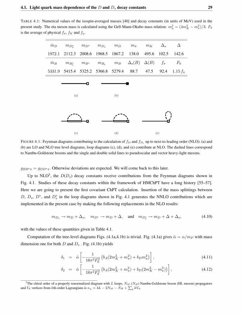
TABLE 4.1: Numerical values of the isospin-averaged masses [40] and decay constants (in units of MeV) used in thepresent study. The eta meson mass is calculated using the Gell-Mann-Okubo mass relation: 𝑚2
𝜂 = (4𝑚2𝐾 −𝑚2
𝜋)/3. 𝐹0
is the average of physical 𝑓𝜋 , 𝑓𝐾 and 𝑓𝜂 .
��𝐷 𝑚𝐷*𝑠 𝑚𝐷* 𝑚𝐷𝑠 𝑚𝐷 𝑚𝜋 𝑚𝐾 Δ𝑠 Δ
1972.1 2112.3 2008.6 1968.5 1867.2 138.0 495.6 102.5 142.6
��𝐵 𝑚𝐵*𝑠 𝑚𝐵* 𝑚𝐵𝑠 𝑚𝐵 Δ𝑠(𝐵) Δ(𝐵) 𝑓𝜋 𝐹0
5331.9 5415.4 5325.2 5366.8 5279.4 88.7 47.5 92.4 1.15 𝑓𝜋
(a) (b)
(c) (d) (e)
FIGURE 4.1: Feynman diagrams contributing to the calculation of 𝑓𝐷 and 𝑓𝐷𝑠up to next-to-leading order (NLO): (a) and
(b) are LO and NLO tree level diagrams, loop diagrams (c), (d), and (e) contribute at NLO. The dashed lines correspondto Nambu-Goldstone bosons and the single and double solid lines to pseudoscalar and vector heavy-light mesons.
𝑔𝐵𝐵*𝜋 = 𝑔𝐷𝐷*𝜋. Otherwise deviations are expected. We will come back to this later.
Up to NLO5, the 𝐷(𝐷𝑠) decay constants receive contributions from the Feynman diagrams shown in
Fig. 4.1. Studies of these decay constants within the framework of HMChPT have a long history [55–57].
Here we are going to present the first covariant ChPT calculation. Insertion of the mass splittings between
𝐷, 𝐷𝑠, 𝐷*, and 𝐷*𝑠 in the loop diagrams shown in Fig. 4.1 generates the NNLO contributions which are
implemented in the present case by making the following replacements in the NLO results:
𝑚𝐷𝑠 → 𝑚𝐷 + Δ𝑠, 𝑚𝐷* → 𝑚𝐷 + Δ, and 𝑚𝐷*𝑠 → 𝑚𝐷 + Δ + Δ𝑠, (4.10)
with the values of these quantities given in Table 4.1.
Computation of the tree-level diagrams Figs. (4.1a,4.1b) is trivial. Fig. (4.1a) gives �� = 𝛼/𝑚𝑃 with mass
dimension one for both 𝐷 and 𝐷𝑠 . Fig. (4.1b) yields
𝛿1 = ��
[− 1
16𝜋2𝐹 20
(𝑏𝐴(2𝑚2
𝐾 + 𝑚2𝜋) + 𝑏𝐷𝑚2
𝜋
)], (4.11)
𝛿2 = ��
[− 1
16𝜋2𝐹 20
(𝑏𝐴(2𝑚2
𝐾 + 𝑚2𝜋) + 𝑏𝐷(2𝑚2
𝐾 −𝑚2𝜋))]
, (4.12)
5The chiral order of a properly renormalized diagram with 𝐿 loops, 𝑁𝑀 (𝑁𝐻 ) Nambu-Goldstone boson (HL meson) propagatorsand 𝑉𝑘 vertices from 𝑘th-order Lagrangians is 𝑛𝜒 = 4𝐿− 2𝑁𝑀 −𝑁𝐻 +
∑𝑘 𝑘𝑉𝑘.
30 Chapter 4. SU(3) breaking corrections to the D, D*, B, and B* decay constants
where 𝛿1 is for 𝐷 and 𝛿2 for 𝐷𝑠.
Diagram Fig. (4.1c) represents the wave function renormalization, from which one can calculate the wave
function renormalization constants, which can be written as
𝑍𝑖 =∑
𝑗,𝑘
𝜉𝑖,𝑗,𝑘
𝑑 𝜑𝑤(𝑝2𝑖 , 𝑚
2𝑗 , 𝑚
2𝑘)
𝑑 𝑝2𝑖
|𝑝2𝑖 =𝑚2
𝑖, (4.13)
where 𝑝𝑖 denotes the four-momentum of 𝐷 (𝐷𝑠), 𝑚𝑖 the mass of 𝐷 (𝐷𝑠), 𝑚𝑗 the mass of 𝐷* (𝐷*𝑠 ), and 𝑚𝑘 the
mass of 𝜋, 𝜂, and 𝐾. The coefficients 𝜉𝑖,𝑗,𝑘 are given in Table 4.2. The function 𝜑𝑤 is defined as6
𝜑𝑤(𝑝2𝑖 , 𝑚
2𝑉 , 𝑚2
𝑀 ) =(𝑔��𝐷)2
4𝐹 20 𝑚2
𝑉
[ (−2𝑚2
𝑀
(𝑝2
𝑖 + 𝑚2𝑉
)+(𝑚2
𝑉 − 𝑝2𝑖
)2 + 𝑚4
𝑀
)𝐵0
(𝑝2
𝑖 , 𝑚2𝑀 , 𝑚2
𝑉
)
+𝐴0
(𝑚2
𝑉
) (−𝑝2
𝑖 + 𝑚2𝑀 −𝑚2
𝑉
)+ 𝐴0
(𝑚2
𝑀
) (−𝑝2
𝑖 + 3𝑚2𝑀 + 𝑚2
𝑉
) ], (4.14)
where the functions 𝐴0 and 𝐵0 are defined in the Appendix A.1.
Diagram Fig. (4.1d) provides current renormalization, which has the following form
𝐶𝑖 = ��𝑐′∑
𝑗,𝑘
𝜉𝑖,𝑗,𝑘𝜑𝑐(𝑚2𝑖 , 𝑚
2𝑗 , 𝑚
2𝑘), (4.15)
where 𝜉𝑖,𝑗,𝑘 are given in Table 4.2 with 𝑖 running over 𝐷 and 𝐷𝑠, 𝑗 over 𝐷* and 𝐷*𝑠 , and 𝑘 over 𝜋, 𝜂, 𝐾. The
function 𝜑𝑐 is defined as
𝜑𝑐(𝑚2𝑖 , 𝑚
2𝑉 , 𝑚2
𝑀 ) = − (𝑔��𝐷)𝑚𝑃
8𝐹 20 𝑚2
𝑖 𝑚2𝑉
[ (𝑚2
𝑀 −𝑚2𝑉
) (𝑚2
𝑖 −𝑚2𝑀 + 𝑚2
𝑉
)𝐵0
(0, 𝑚2
𝑀 , 𝑚2𝑉
)− 2𝑚2
𝑖 𝐴0
(𝑚2
𝑀
)
+(−2𝑚2
𝑖
(𝑚2
𝑀 + 𝑚2𝑉
)+ 𝑚4
𝑖 +(𝑚2
𝑀 −𝑚2𝑉
)2)𝐵0
(𝑚2
𝑖 , 𝑚2𝑀 , 𝑚2
𝑉
) ]. (4.16)
It should be noted that 𝐶𝑖 vanishes in NLO HMChPT but plays an important role in covariant ChPT.
Diagram Fig. (4.1e) also provides current correction
𝑇𝑖 = ��∑
𝑗=𝜋,𝜂,𝐾
𝜁𝑖,𝑗𝐴0(𝑚2𝑗 )/𝐹 2
0 , (4.17)
with 𝜁𝑖,𝑗 given in Table 4.3.
The total results are then
𝑓𝑖 = ��(1 + 𝑍𝑖/2) + 𝛿𝑖 + 𝑇𝑖 + 𝐶𝑖. (4.18)
6To be consistent, the product 𝑔��𝐷 is only appropriate for NLO. At NNLO, it has to be replaced by 𝑔′𝑚𝐷 with 𝑔′ = 𝑔��𝐷/𝑚𝐷 ≈0.63 before performing expansions in terms of 1/𝑚𝐷 either to obtain the HMChPT results or to remove the power-counting-breakingpieces. The same applies to the calculation of 𝐶𝑖 [see Eq. (4.15)].
4.1. Light quark mass dependence of the 𝐷 and 𝐷𝑠 decay constants 31
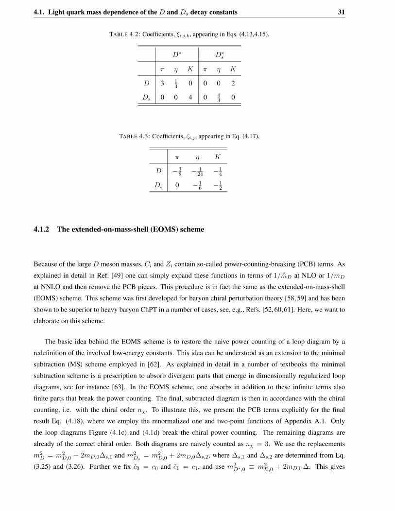
TABLE 4.2: Coefficients, 𝜉𝑖,𝑗,𝑘, appearing in Eqs. (4.13,4.15).
𝐷* 𝐷*𝑠
𝜋 𝜂 𝐾 𝜋 𝜂 𝐾
𝐷 3 13 0 0 0 2
𝐷𝑠 0 0 4 0 43 0
TABLE 4.3: Coefficients, 𝜁𝑖,𝑗 , appearing in Eq. (4.17).
𝜋 𝜂 𝐾
𝐷 −38 − 1
24 −14
𝐷𝑠 0 −16 −1
2
4.1.2 The extended-on-mass-shell (EOMS) scheme
Because of the large 𝐷 meson masses, 𝐶𝑖 and 𝑍𝑖 contain so-called power-counting-breaking (PCB) terms. As
explained in detail in Ref. [49] one can simply expand these functions in terms of 1/��𝐷 at NLO or 1/𝑚𝐷
at NNLO and then remove the PCB pieces. This procedure is in fact the same as the extended-on-mass-shell
(EOMS) scheme. This scheme was first developed for baryon chiral perturbation theory [58, 59] and has been
shown to be superior to heavy baryon ChPT in a number of cases, see, e.g., Refs. [52,60,61]. Here, we want to
elaborate on this scheme.
The basic idea behind the EOMS scheme is to restore the naive power counting of a loop diagram by a
redefinition of the involved low-energy constants. This idea can be understood as an extension to the minimal
subtraction (MS) scheme employed in [62]. As explained in detail in a number of textbooks the minimal
subtraction scheme is a prescription to absorb divergent parts that emerge in dimensionally regularized loop
diagrams, see for instance [63]. In the EOMS scheme, one absorbs in addition to these infinite terms also
finite parts that break the power counting. The final, subtracted diagram is then in accordance with the chiral
counting, i.e. with the chiral order 𝑛𝜒. To illustrate this, we present the PCB terms explicitly for the final
result Eq. (4.18), where we employ the renormalized one and two-point functions of Appendix A.1. Only
the loop diagrams Figure (4.1c) and (4.1d) break the chiral power counting. The remaining diagrams are
already of the correct chiral order. Both diagrams are naively counted as 𝑛𝜒 = 3. We use the replacements
𝑚2𝐷 = 𝑚2
𝐷,0 + 2𝑚𝐷,0Δ𝑠,1 and 𝑚2𝐷𝑠
= 𝑚2𝐷,0 + 2𝑚𝐷,0Δ𝑠,2, where Δ𝑠,1 and Δ𝑠,2 are determined from Eq.
(3.25) and (3.26). Further we fix 𝑐0 = 𝑐0 and 𝑐1 = 𝑐1, and use 𝑚2𝐷*,0 ≡ 𝑚2
𝐷,0 + 2𝑚𝐷,0 Δ. This gives
32 Chapter 4. SU(3) breaking corrections to the D, D*, B, and B* decay constants
𝑚2𝐷* = 𝑚2
𝐷,0 +2𝑚𝐷,0 (Δ+Δ𝑠,1) and 𝑚2𝐷*𝑠
= 𝑚2𝐷,0 +2𝑚𝐷,0 (Δ+Δ𝑠,2). Expanding finally in 1/𝑚𝐷,0 gives
𝐶1 =��𝑐′𝑔
24𝜋2𝑓20
[𝑐1
(3(𝑚𝐾
2 −𝑚𝜋2) log
( 𝜇2
𝑚2𝐷,0
)− 2
(3𝑚𝐾
2 + 𝑚𝜋2) )
+ 4𝑚𝐷,0 Δ
−𝑚𝐷,0 (2𝑚𝐷,0 + 2Δ) log( 𝜇2
𝑚2𝐷,0
)+ 8𝑐0
(2𝑚𝐾
2 + 𝑚𝜋2) ]
+𝒪(𝑛𝜒 = 3)
𝐶2 =��𝑐′𝑔
24𝜋2𝑓20
[− 2𝑐1
(3(𝑚𝐾
2 −𝑚𝜋2) log
( 𝜇2
𝑚2𝐷,0
)+ 2
(𝑚𝐾
2 + 𝑚𝜋2) )
+ 4𝑚𝐷,0 Δ
−𝑚𝐷,0 (2𝑚𝐷,0 + 2Δ) log( 𝜇2
𝑚2𝐷,0
)+ 8𝑐0
(2𝑚𝐾
2 + 𝑚𝜋2) ]
+𝒪(𝑛𝜒 = 3)
��𝑍1/2 =��𝑔2
24𝜋2𝑓20
[𝑐1
(6(𝑚𝜋
2 −𝑚𝐾2)log( 𝜇2
𝑚2𝐷,0
)− 3𝑚𝐾
2 + 7𝑚𝜋2)
+ 2𝑚𝐷,0 Δ
+𝑚𝐷,0(𝑚𝐷,0 + 4Δ) log( 𝜇2
𝑚2𝐷,0
)− 4𝑐0
(2𝑚𝐾
2 + 𝑚𝜋2) ]
+𝒪(𝑛𝜒 = 3)
��𝑍2/2 =��𝑔2
24𝜋2𝑓20
[2𝑐1
(6(𝑚𝐾
2 −𝑚𝜋2) log
( 𝜇2
𝑚2𝐷,0
)+ 7𝑚𝐾
2 − 5𝑚𝜋2)
+ 2𝑚𝐷,0 Δ
+𝑚𝐷,0(𝑚𝐷,0 + 4Δ) log( 𝜇2
𝑚2𝐷,0
)− 4𝑐0
(2𝑚𝐾
2 + 𝑚𝜋2) ]
+𝒪(𝑛𝜒 = 3) (4.19)
where we have inserted the explicit form of Δ𝑠,1 and Δ𝑠,2.
These terms are the PCB terms, depending on three parameters, 𝑏𝐴, 𝑏𝐷 and ��. If only the NLO result
is considered, the mass 𝑚𝐷,0 has to be replaced by ��𝐷 in the previous expansion. The terms that do not
depend on 𝑚𝜋 and 𝑚𝐾 are equal for 𝑖 = 1 and 𝑖 = 2 and can therefore be directly absorbed into the low-
energy constant ��. The terms that are proportional to 𝑐0 and 𝑐1, on the other hand, require a redefinition of the
low-energy constants 𝑏𝐷 and 𝑏𝐴. Introducing new constants 𝑏𝐴,𝑟 and 𝑏𝐷,𝑟 by the replacements
𝑏𝐴 → −𝑐1𝑔[− 𝑐′
(log( 𝜇2
𝑚2𝐷,0
)− 2)
+ 2𝑔 log( 𝜇2
𝑚2𝐷,0
)+ 𝑔]
+ 𝑏𝐴,𝑟 −83𝑐0𝑔(𝑔 − 2𝑐′
),
𝑏𝐷 → 13𝑐1𝑔[𝑐′(2− 9 log
( 𝜇2
𝑚2𝐷,0
))+ 𝑔(18 log
( 𝜇2
𝑚2𝐷,0
)+ 17
)]+ 𝑏𝐷,𝑟 , (4.20)
removes the remaining PCB terms. Equivalently, we have expanded the results by use of equation (4.10) in
powers of 1/𝑚𝐷 and have removed the PCB terms directly from 𝐶𝑖 and 𝑍𝑖, keeping in mind that the low-
energy-constants 𝑏𝐴, 𝑏𝐷 and �� are now to be understood as the renormalized constants. These subtracted
functions are denoted by 𝐶𝑖 and 𝑍𝑖 and have a proper power-counting as described in Ref. [49]. At the end one
finds
𝑓𝑖 = ��(1 + 𝑍𝑖/2) + 𝛿𝑖 + 𝑇𝑖 + 𝐶𝑖, (4.21)
the expression that is used in the actual calculations. By expanding 𝑍𝑖 and 𝐶𝑖 in terms of 1/��𝐷 at NLO
or 1/𝑚𝐷 at NNLO and keeping the lowest order in 1/��𝐷 (1/𝑚𝐷) one can easily obtain the corresponding
HMChPT results.
4.1. Light quark mass dependence of the 𝐷 and 𝐷𝑠 decay constants 33
4.1.3 Results and discussion
Before presenting the numerical results, we should make it clear that in our present formulation of ChPT we
have focused on SU(3) breaking in the context of the chiral expansions but we have not utilized explicitly heavy
quark symmetry that relates the couplings of the 𝐷 mesons with those of the 𝐷*, 𝐵, and 𝐵* mesons.
In the present case, we encounter three LECs: 𝑎, 𝑏𝐷, and 𝑏𝐴. At this point, light-quark mass dependent
LQCD results are extremely useful. By a least-squares fit to the HPQCD results, one can fix those three LECs
appearing in our calculation.
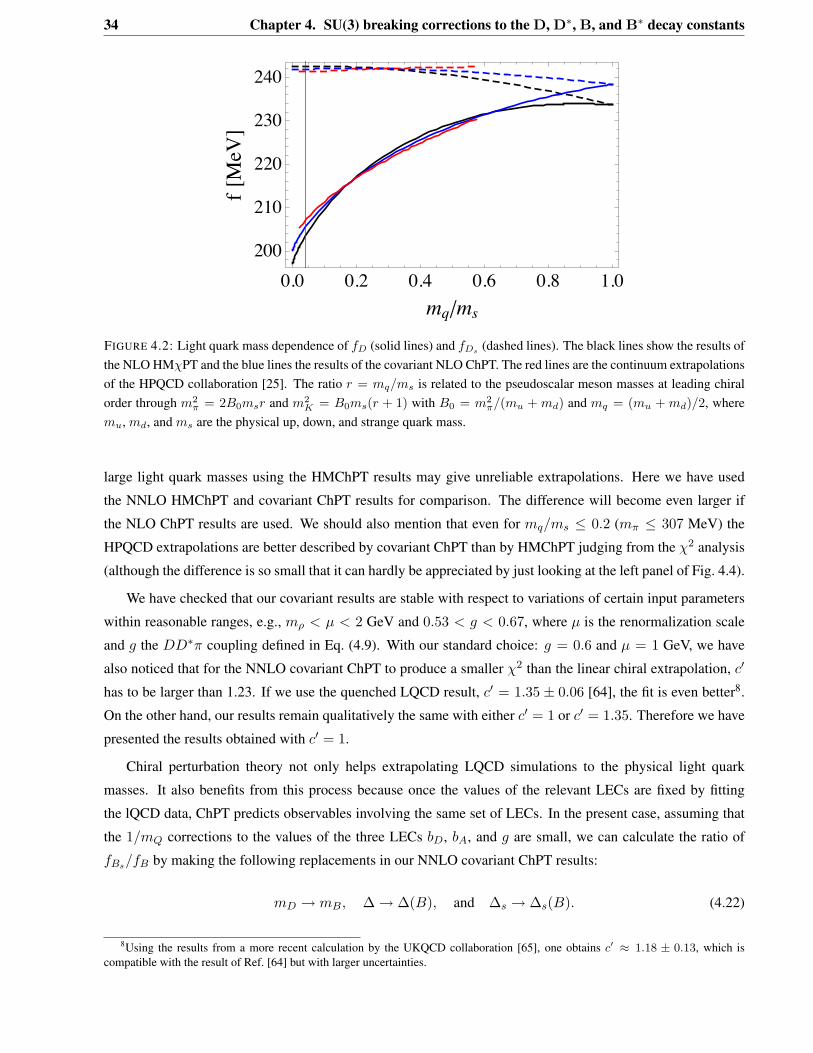
First we treat the 𝐷, 𝐷𝑠, 𝐷*, and 𝐷*𝑠 mesons as degenerate, i.e., we work up to NLO. The corresponding
results are shown in Fig. 4.2, where the HMChPT results are obtained by expanding our covariant results in
terms of 1/��𝐷 and keeping only the lowest-order terms. It is clear that the covariant results (with 𝜒2=41) are
in much better agreement with the HPQCD continuum limits than the HMChPT results (with 𝜒2 = 201) 7. This
is not surprising because as we mentioned earlier the HPQCD collaboration has added second and third order
polynomial terms in 𝑥𝑞 to perform their extrapolation. Furthermore one can notice that at larger light quark
masses the difference between the covariant ChPT and the HMChPT results becomes larger. This highlights the
importance of using a covariant formulation of ChPT in order to make chiral extrapolations if lattice simulations
are performed with relatively large light quark masses. Similar conclusions have been reached in studying the
light quark mass dependence of the lowest-lying octet and decuplet baryon masses [52].
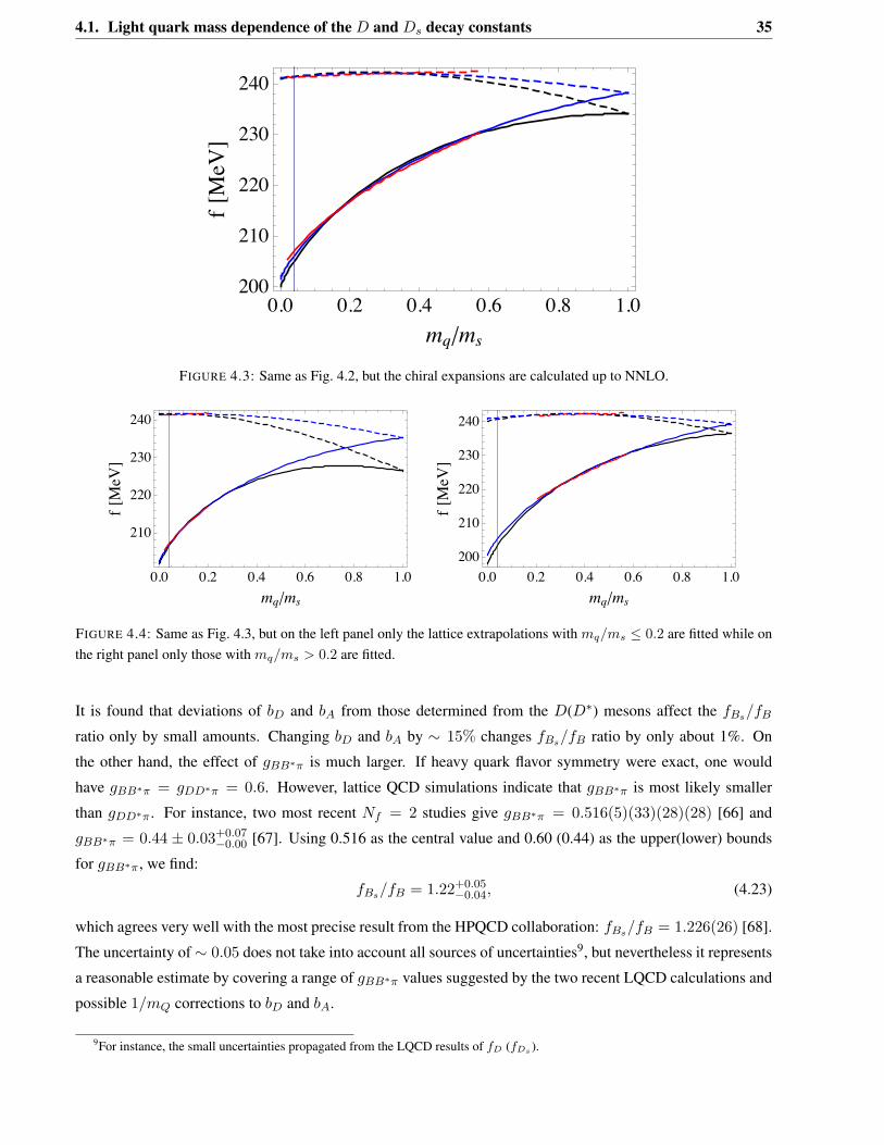
Taking into account the mass splittings between 𝐷, 𝐷𝑠, 𝐷*, and 𝐷*𝑠 as prescribed by Eq. (4.10) one obtains
the NNLO ChPT results. Fitting them to the HPQCD extrapolations, one finds the results shown in Fig. 4.3.
Compared to Fig. 4.2, it is clear that the agreement between the covariant ChPT results with the HPQCD
extrapolations becomes even better. Furthermore the covariant 𝜒PT results (with 𝜒2 = 16) is still visibly better
than the HMChPT results (with 𝜒2 = 59), but now the difference between the covariant and the HMChPT
results becomes smaller. The three LECs in the NNLO covariant ChPT have the following values: �� = 208
MeV, 𝑏𝐷 = 0.318, 𝑏𝐴 = 0.166.
If we had fitted the HPQCD extrapolations by neglecting the loop contributions, we would have obtained
a even better agreement (𝜒2 = 9). In Ref. [52] we also found that the lattice baryon mass data could be fitted
better with the LO (linear in 𝑚𝑞) chiral extrapolation. But there we found that the NLO chiral results in fact
describe the experimental data better than the LO (linear) chiral extrapolation. This just shows that the lattice
baryon mass data behave more linearly as a function of light quark masses at large light quark masses and chiral
logarithms play a more relevant role at smaller light quark masses, as one naively expects.
Another way of understanding the importance of chiral logarithms is to perform separate fits for lattice
simulations obtained at different light quark masses. One expects that at smaller light quark masses (e.g.,
𝑚𝜋 < 300 MeV) covariant ChPT and HM ChPT results should perform more or less similarly. On the other
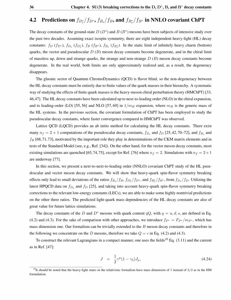
hand, if the light quark masses are larger, covariant ChPT should be a better choice. In Fig. 4.4, we show the
fitted results obtained from fitting the HPQCD extrapolations in two different regions of light quark masses,
𝑚𝑞/𝑚𝑠 ≤ 0.2 (left panel) and 𝑚𝑞/𝑚𝑠 > 0.2 (right panel). It is clearly seen that fitting lattice data with
7It should be noted that the absolute value of 𝜒2 as defined here does not have a clear-cut physical meaning. It only reflects to whatextent the chiral results agree with the HPQCD extrapolations.
34 Chapter 4. SU(3) breaking corrections to the D, D*, B, and B* decay constants
0.0 0.2 0.4 0.6 0.8 1.0200
210
220
230
240
mq!ms
f"MeV#
FIGURE 4.2: Light quark mass dependence of 𝑓𝐷 (solid lines) and 𝑓𝐷𝑠(dashed lines). The black lines show the results of
the NLO HM𝜒PT and the blue lines the results of the covariant NLO ChPT. The red lines are the continuum extrapolationsof the HPQCD collaboration [25]. The ratio 𝑟 = 𝑚𝑞/𝑚𝑠 is related to the pseudoscalar meson masses at leading chiralorder through 𝑚2
𝜋 = 2𝐵0𝑚𝑠𝑟 and 𝑚2𝐾 = 𝐵0𝑚𝑠(𝑟 + 1) with 𝐵0 = 𝑚2
𝜋/(𝑚𝑢 + 𝑚𝑑) and 𝑚𝑞 = (𝑚𝑢 + 𝑚𝑑)/2, where𝑚𝑢, 𝑚𝑑, and 𝑚𝑠 are the physical up, down, and strange quark mass.
large light quark masses using the HMChPT results may give unreliable extrapolations. Here we have used
the NNLO HMChPT and covariant ChPT results for comparison. The difference will become even larger if
the NLO ChPT results are used. We should also mention that even for 𝑚𝑞/𝑚𝑠 ≤ 0.2 (𝑚𝜋 ≤ 307 MeV) the
HPQCD extrapolations are better described by covariant ChPT than by HMChPT judging from the 𝜒2 analysis
(although the difference is so small that it can hardly be appreciated by just looking at the left panel of Fig. 4.4).
We have checked that our covariant results are stable with respect to variations of certain input parameters
within reasonable ranges, e.g., 𝑚𝜌 < 𝜇 < 2 GeV and 0.53 < 𝑔 < 0.67, where 𝜇 is the renormalization scale
and 𝑔 the 𝐷𝐷*𝜋 coupling defined in Eq. (4.9). With our standard choice: 𝑔 = 0.6 and 𝜇 = 1 GeV, we have
also noticed that for the NNLO covariant ChPT to produce a smaller 𝜒2 than the linear chiral extrapolation, 𝑐′
has to be larger than 1.23. If we use the quenched LQCD result, 𝑐′ = 1.35 ± 0.06 [64], the fit is even better8.
On the other hand, our results remain qualitatively the same with either 𝑐′ = 1 or 𝑐′ = 1.35. Therefore we have
presented the results obtained with 𝑐′ = 1.
Chiral perturbation theory not only helps extrapolating LQCD simulations to the physical light quark
masses. It also benefits from this process because once the values of the relevant LECs are fixed by fitting
the lQCD data, ChPT predicts observables involving the same set of LECs. In the present case, assuming that
the 1/𝑚𝑄 corrections to the values of the three LECs 𝑏𝐷, 𝑏𝐴, and 𝑔 are small, we can calculate the ratio of
𝑓𝐵𝑠/𝑓𝐵 by making the following replacements in our NNLO covariant ChPT results:
𝑚𝐷 → 𝑚𝐵, Δ → Δ(𝐵), and Δ𝑠 → Δ𝑠(𝐵). (4.22)
8Using the results from a more recent calculation by the UKQCD collaboration [65], one obtains 𝑐′ ≈ 1.18 ± 0.13, which iscompatible with the result of Ref. [64] but with larger uncertainties.
4.1. Light quark mass dependence of the 𝐷 and 𝐷𝑠 decay constants 35
0.0 0.2 0.4 0.6 0.8 1.0200
210
220
230
240
mq!ms
f"MeV#
FIGURE 4.3: Same as Fig. 4.2, but the chiral expansions are calculated up to NNLO.
0.0 0.2 0.4 0.6 0.8 1.0
210
220
230
240
mq!ms
f"MeV#
0.0 0.2 0.4 0.6 0.8 1.0200
210
220
230
240
mq!ms
f"MeV#
FIGURE 4.4: Same as Fig. 4.3, but on the left panel only the lattice extrapolations with 𝑚𝑞/𝑚𝑠 ≤ 0.2 are fitted while onthe right panel only those with 𝑚𝑞/𝑚𝑠 > 0.2 are fitted.
It is found that deviations of 𝑏𝐷 and 𝑏𝐴 from those determined from the 𝐷(𝐷*) mesons affect the 𝑓𝐵𝑠/𝑓𝐵
ratio only by small amounts. Changing 𝑏𝐷 and 𝑏𝐴 by ∼ 15% changes 𝑓𝐵𝑠/𝑓𝐵 ratio by only about 1%. On
the other hand, the effect of 𝑔𝐵𝐵*𝜋 is much larger. If heavy quark flavor symmetry were exact, one would
have 𝑔𝐵𝐵*𝜋 = 𝑔𝐷𝐷*𝜋 = 0.6. However, lattice QCD simulations indicate that 𝑔𝐵𝐵*𝜋 is most likely smaller
than 𝑔𝐷𝐷*𝜋. For instance, two most recent 𝑁𝑓 = 2 studies give 𝑔𝐵𝐵*𝜋 = 0.516(5)(33)(28)(28) [66] and
𝑔𝐵𝐵*𝜋 = 0.44 ± 0.03+0.07−0.00 [67]. Using 0.516 as the central value and 0.60 (0.44) as the upper(lower) bounds
for 𝑔𝐵𝐵*𝜋, we find:
𝑓𝐵𝑠/𝑓𝐵 = 1.22+0.05−0.04, (4.23)
which agrees very well with the most precise result from the HPQCD collaboration: 𝑓𝐵𝑠/𝑓𝐵 = 1.226(26) [68].
The uncertainty of∼ 0.05 does not take into account all sources of uncertainties9, but nevertheless it represents
a reasonable estimate by covering a range of 𝑔𝐵𝐵*𝜋 values suggested by the two recent LQCD calculations and
possible 1/𝑚𝑄 corrections to 𝑏𝐷 and 𝑏𝐴.
9For instance, the small uncertainties propagated from the LQCD results of 𝑓𝐷 (𝑓𝐷𝑠 ).
36 Chapter 4. SU(3) breaking corrections to the D, D*, B, and B* decay constants
4.2 Predictions on 𝑓𝐷*𝑠/𝑓𝐷*, 𝑓𝐵𝑠
/𝑓𝐵, and 𝑓𝐵*𝑠/𝑓𝐵* in NNLO covariant ChPT
The decay constants of the ground-state 𝐷 (𝐷*) and 𝐵 (𝐵*) mesons have been subjects of intensive study over
the past two decades. Assuming exact isospin symmetry, there are eight independent heavy-light (HL) decay
constants: 𝑓𝐷 (𝑓𝐷*), 𝑓𝐷𝑠 (𝑓𝐷*𝑠 ), 𝑓𝐵 (𝑓𝐵*), 𝑓𝐵𝑠 (𝑓𝐵*𝑠 ). In the static limit of infinitely heavy charm (bottom)
quarks, the vector and pseudoscalar 𝐷 (𝐵) meson decay constants become degenerate, and in the chiral limit
of massless up, down and strange quarks, the strange and non-strange 𝐷 (𝐵) meson decay constants become
degenerate. In the real world, both limits are only approximately realized and, as a result, the degeneracy
disappears.
The gluonic sector of Quantum ChromoDynamics (QCD) is flavor blind, so the non-degeneracy between
the HL decay constants must be entirely due to finite values of the quark masses in their hierarchy. A systematic
way of studying the effects of finite quark masses is the heavy-meson chiral perturbation theory (HMChPT) [33,
46,47]. The HL decay constants have been calculated up to next-to-leading order (NLO) in the chiral expansion,
and to leading-order (LO) [55, 56] and NLO [57, 69] in 1/𝑚𝐻 expansion, where 𝑚𝐻 is the generic mass of
the HL systems. In the previous section, the covariant formulation of ChPT has been employed to study the
pseudoscalar decay constants, where faster convergence compared to HMChPT was observed.
Lattice QCD (LQCD) provides an ab initio method for calculating the HL decay constants. There exist
many 𝑛𝑓 = 2 + 1 computations of the pseudoscalar decay constants, 𝑓𝐷𝑠 and 𝑓𝐷 [25, 42, 70–72], and 𝑓𝐵𝑠 and
𝑓𝐵 [68,71,73], motivated by the important role they play in determinations of the CKM matrix elements and in
tests of the Standard Model (see, e.g., Ref. [34]). On the other hand, for the vector meson decay constants, most
existing simulations are quenched [65,74,75], except for Ref. [76] where 𝑛𝑓 = 2. Simulations with 𝑛𝑓 = 2+1
are underway [77].
In this section, we present a next-to-next-to-leading order (NNLO) covariant ChPT study of the HL pseu-
doscalar and vector meson decay constants. We will show that heavy-quark spin-flavor symmetry breaking
effects only lead to small deviations of the ratios 𝑓𝐵𝑠/𝑓𝐵 , 𝑓𝐷*𝑠 /𝑓𝐷* , and 𝑓𝐵*𝑠 /𝑓𝐵* , from 𝑓𝐷𝑠/𝑓𝐷. Utilizing the
latest HPQCD data on 𝑓𝐷𝑠 and 𝑓𝐷 [25], and taking into account heavy-quark spin-flavor symmetry breaking
corrections to the relevant low-energy constants (LECs), we are able to make some highly nontrivial predictions
on the other three ratios. The predicted light-quark mass dependencies of the HL decay constants are also of
great value for future lattice simulations.
The decay constants of the 𝐷 and 𝐷* mesons with quark content 𝑞𝑄, with 𝑞 = 𝑢, 𝑑, 𝑠, are defined in Eq.
(4.2) and (4.3). For the sake of comparison with other approaches, we introduce 𝑓𝑃 * = 𝐹𝑃 */𝑚𝑃 * , which has
mass dimension one. Our formalism can be trivially extended to the 𝐵 meson decay constants and therefore in
the following we concentrate on the 𝐷 mesons, therefore we take 𝑄 = 𝑐 in Eq. (4.2) and (4.3).
To construct the relevant Lagrangians in a compact manner, one uses the fields10 Eq. (3.11) and the current
as in Ref. [47]:
𝐽 =12𝛾𝜇(1− 𝛾5)𝐽𝜇, (4.24)
10It should be noted that the heavy-light states in the relativistic formalism have mass dimension of 1 instead of 3/2 as in the HMformulation.
4.2. Predictions on 𝑓𝐷*𝑠 /𝑓𝐷* , 𝑓𝐵𝑠/𝑓𝐵 , and 𝑓𝐵*𝑠 /𝑓𝐵* in NNLO covariant ChPT 37
(a) (b)
(c) (d) (e)
(f) (g) (h)
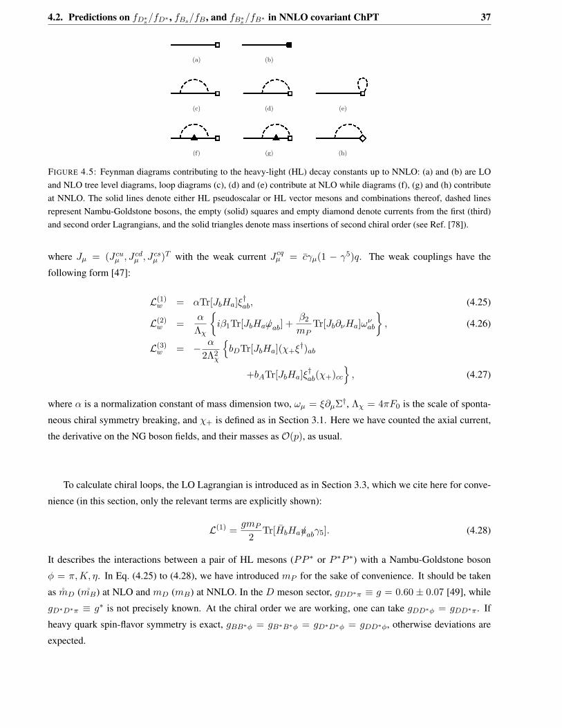
FIGURE 4.5: Feynman diagrams contributing to the heavy-light (HL) decay constants up to NNLO: (a) and (b) are LOand NLO tree level diagrams, loop diagrams (c), (d) and (e) contribute at NLO while diagrams (f), (g) and (h) contributeat NNLO. The solid lines denote either HL pseudoscalar or HL vector mesons and combinations thereof, dashed linesrepresent Nambu-Goldstone bosons, the empty (solid) squares and empty diamond denote currents from the first (third)and second order Lagrangians, and the solid triangles denote mass insertions of second chiral order (see Ref. [78]).
where 𝐽𝜇 = (𝐽𝑐𝑢𝜇 , 𝐽𝑐𝑑
𝜇 , 𝐽𝑐𝑠𝜇 )𝑇 with the weak current 𝐽𝑐𝑞
𝜇 = 𝑐𝛾𝜇(1 − 𝛾5)𝑞. The weak couplings have the
following form [47]:
ℒ(1)𝑤 = 𝛼Tr[𝐽𝑏𝐻𝑎]𝜉
†𝑎𝑏, (4.25)
ℒ(2)𝑤 =
𝛼
Λ𝜒
{𝑖𝛽1Tr[𝐽𝑏𝐻𝑎/𝜔𝑎𝑏] +
𝛽2
𝑚𝑃Tr[𝐽𝑏𝜕𝜈𝐻𝑎]𝜔𝜈
𝑎𝑏
}, (4.26)
ℒ(3)𝑤 = − 𝛼
2Λ2𝜒
{𝑏𝐷Tr[𝐽𝑏𝐻𝑎](𝜒+𝜉†)𝑎𝑏
+𝑏𝐴Tr[𝐽𝑏𝐻𝑎]𝜉†𝑎𝑏(𝜒+)𝑐𝑐
}, (4.27)
where 𝛼 is a normalization constant of mass dimension two, 𝜔𝜇 = 𝜉𝜕𝜇Σ†, Λ𝜒 = 4𝜋𝐹0 is the scale of sponta-
neous chiral symmetry breaking, and 𝜒+ is defined as in Section 3.1. Here we have counted the axial current,
the derivative on the NG boson fields, and their masses as 𝒪(𝑝), as usual.
To calculate chiral loops, the LO Lagrangian is introduced as in Section 3.3, which we cite here for conve-
nience (in this section, only the relevant terms are explicitly shown):
ℒ(1) =𝑔𝑚𝑃
2Tr[��𝑏𝐻𝑎/𝑢𝑎𝑏𝛾5]. (4.28)
It describes the interactions between a pair of HL mesons (𝑃𝑃 * or 𝑃 *𝑃 *) with a Nambu-Goldstone boson
𝜑 = 𝜋, 𝐾, 𝜂. In Eq. (4.25) to (4.28), we have introduced 𝑚𝑃 for the sake of convenience. It should be taken
as ��𝐷 (𝑚𝐵) at NLO and 𝑚𝐷 (𝑚𝐵) at NNLO. In the 𝐷 meson sector, 𝑔𝐷𝐷*𝜋 ≡ 𝑔 = 0.60 ± 0.07 [49], while
𝑔𝐷*𝐷*𝜋 ≡ 𝑔* is not precisely known. At the chiral order we are working, one can take 𝑔𝐷𝐷*𝜑 = 𝑔𝐷𝐷*𝜋. If
heavy quark spin-flavor symmetry is exact, 𝑔𝐵𝐵*𝜑 = 𝑔𝐵*𝐵*𝜑 = 𝑔𝐷*𝐷*𝜑 = 𝑔𝐷𝐷*𝜑, otherwise deviations are
expected.
38 Chapter 4. SU(3) breaking corrections to the D, D*, B, and B* decay constants
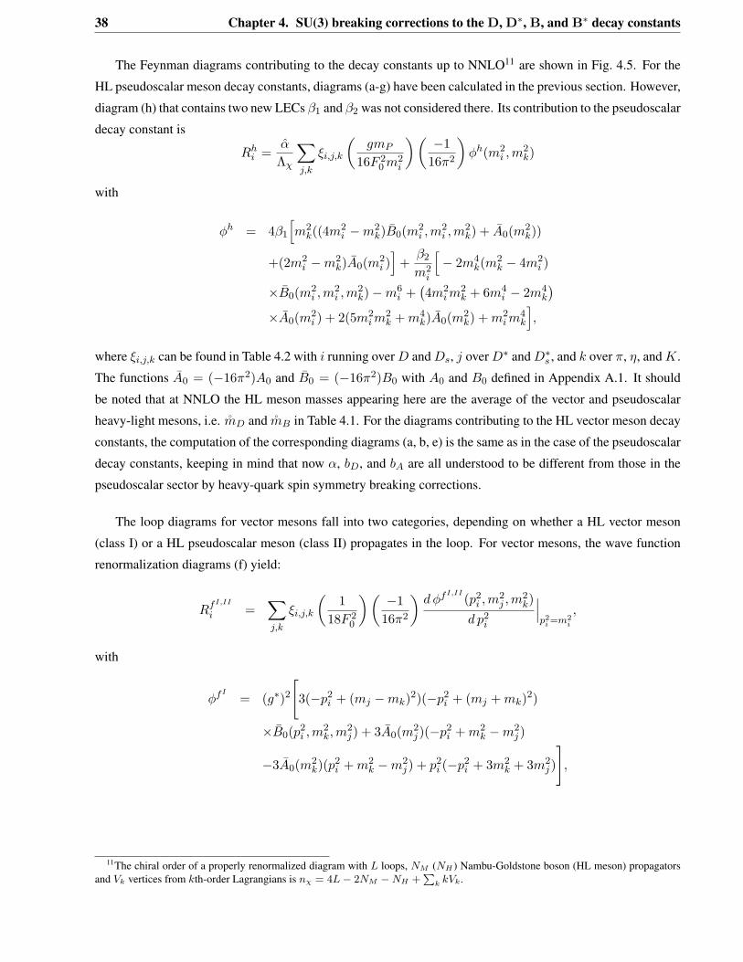
The Feynman diagrams contributing to the decay constants up to NNLO11 are shown in Fig. 4.5. For the
HL pseudoscalar meson decay constants, diagrams (a-g) have been calculated in the previous section. However,
diagram (h) that contains two new LECs 𝛽1 and 𝛽2 was not considered there. Its contribution to the pseudoscalar
decay constant is
𝑅ℎ𝑖 =
��
Λ𝜒
∑
𝑗,𝑘
𝜉𝑖,𝑗,𝑘
(𝑔𝑚𝑃
16𝐹 20 𝑚2
𝑖
)( −116𝜋2
)𝜑ℎ(𝑚2
𝑖 , 𝑚2𝑘)
with
𝜑ℎ = 4𝛽1
[𝑚2
𝑘((4𝑚2𝑖 −𝑚2
𝑘)��0(𝑚2𝑖 , 𝑚
2𝑖 , 𝑚
2𝑘) + 𝐴0(𝑚2
𝑘))
+(2𝑚2𝑖 −𝑚2
𝑘)𝐴0(𝑚2𝑖 )]
+𝛽2
𝑚2𝑖
[− 2𝑚4
𝑘(𝑚2𝑘 − 4𝑚2
𝑖 )
×��0(𝑚2𝑖 , 𝑚
2𝑖 , 𝑚
2𝑘)−𝑚6
𝑖 +(4𝑚2
𝑖 𝑚2𝑘 + 6𝑚4
𝑖 − 2𝑚4𝑘
)
×𝐴0(𝑚2𝑖 ) + 2(5𝑚2
𝑖 𝑚2𝑘 + 𝑚4
𝑘)𝐴0(𝑚2𝑘) + 𝑚2
𝑖 𝑚4𝑘
],
where 𝜉𝑖,𝑗,𝑘 can be found in Table 4.2 with 𝑖 running over 𝐷 and 𝐷𝑠, 𝑗 over 𝐷* and 𝐷*𝑠 , and 𝑘 over 𝜋, 𝜂, and 𝐾.
The functions 𝐴0 = (−16𝜋2)𝐴0 and ��0 = (−16𝜋2)𝐵0 with 𝐴0 and 𝐵0 defined in Appendix A.1. It should
be noted that at NNLO the HL meson masses appearing here are the average of the vector and pseudoscalar
heavy-light mesons, i.e. ��𝐷 and ��𝐵 in Table 4.1. For the diagrams contributing to the HL vector meson decay
constants, the computation of the corresponding diagrams (a, b, e) is the same as in the case of the pseudoscalar
decay constants, keeping in mind that now 𝛼, 𝑏𝐷, and 𝑏𝐴 are all understood to be different from those in the
pseudoscalar sector by heavy-quark spin symmetry breaking corrections.
The loop diagrams for vector mesons fall into two categories, depending on whether a HL vector meson
(class I) or a HL pseudoscalar meson (class II) propagates in the loop. For vector mesons, the wave function
renormalization diagrams (f) yield:
𝑅𝑓𝐼,𝐼𝐼
𝑖 =∑
𝑗,𝑘
𝜉𝑖,𝑗,𝑘
(1
18𝐹 20
)( −116𝜋2
)𝑑 𝜑𝑓𝐼,𝐼𝐼
(𝑝2𝑖 , 𝑚
2𝑗 , 𝑚
2𝑘)
𝑑 𝑝2𝑖
𝑝2
𝑖 =𝑚2𝑖
,
with
𝜑𝑓𝐼= (𝑔*)2
[3(−𝑝2
𝑖 + (𝑚𝑗 −𝑚𝑘)2)(−𝑝2𝑖 + (𝑚𝑗 + 𝑚𝑘)2)
×��0(𝑝2𝑖 , 𝑚
2𝑘, 𝑚
2𝑗 ) + 3𝐴0(𝑚2
𝑗 )(−𝑝2𝑖 + 𝑚2
𝑘 −𝑚2𝑗 )
−3𝐴0(𝑚2𝑘)(𝑝
2𝑖 + 𝑚2
𝑘 −𝑚2𝑗 ) + 𝑝2
𝑖 (−𝑝2𝑖 + 3𝑚2
𝑘 + 3𝑚2𝑗 )
],
11The chiral order of a properly renormalized diagram with 𝐿 loops, 𝑁𝑀 (𝑁𝐻 ) Nambu-Goldstone boson (HL meson) propagatorsand 𝑉𝑘 vertices from 𝑘th-order Lagrangians is 𝑛𝜒 = 4𝐿− 2𝑁𝑀 −𝑁𝐻 +
∑𝑘 𝑘𝑉𝑘.
4.2. Predictions on 𝑓𝐷*𝑠 /𝑓𝐷* , 𝑓𝐵𝑠/𝑓𝐵 , and 𝑓𝐵*𝑠 /𝑓𝐵* in NNLO covariant ChPT 39
𝜑𝑓𝐼𝐼= −𝑚2
𝑃
2𝑝2𝑖
𝑔2[− 3(−2𝑚2
𝑘(𝑝2𝑖 + 𝑚2
𝑗 ) + (𝑚2𝑗 − 𝑝2
𝑖 )2 + 𝑚4
𝑘)
×��0(𝑝2𝑖 , 𝑚
2𝑘, 𝑚
2𝑗 ) + 3𝐴0(𝑚2
𝑘)(𝑝2𝑖 + 𝑚2
𝑘 −𝑚2𝑗 )
+3𝐴0(𝑚2𝑗 )(𝑝
2𝑖 −𝑚2
𝑘 + 𝑚2𝑗 ) + 6𝑝2
𝑖 (𝑚2𝑘 + 𝑚2
𝑗 )− 2𝑝4𝑖
],
where 𝑖 denotes (𝐷*, 𝐷*𝑠) and 𝑗 denotes either (𝐷*, 𝐷*𝑠) or (𝐷,𝐷𝑠).
Diagrams (g) yield 𝑅𝑔𝐼= 0 and
𝑅𝑔𝐼𝐼=∑
𝑗,𝑘
𝜉𝑖,𝑗,𝑘
(𝛼𝑔
72𝐹 20 𝑚2
𝑖
)( −116𝜋2
)𝜑𝑔𝐼𝐼
(𝑚2𝑖 , 𝑚
2𝑗 , 𝑚
2𝑘)
with
𝜑𝑔𝐼𝐼= −3((𝑚𝑖 −𝑚𝑘)2 −𝑚2
𝑗 )((𝑚𝑖 + 𝑚𝑘)2 −𝑚2𝑗 )
×��0(𝑚2𝑖 , 𝑚
2𝑗 , 𝑚
2𝑘) + 3𝐴0(𝑚2
𝑗 )(𝑚2𝑖 + 𝑚2
𝑗 −𝑚2𝑘)
+3𝐴0(𝑚2𝑘)(𝑚
2𝑖 −𝑚2
𝑗 + 𝑚2𝑘)− 2𝑚2
𝑖 (𝑚2𝑖 − 3(𝑚2
𝑗 + 𝑚2𝑘)).
Diagrams (h) give
𝑅ℎ𝐼,𝐼𝐼=
𝛼
Λ𝜒
∑
𝑗,𝑘
𝜉𝑖,𝑗,𝑘
(𝑔𝑚𝑃
144𝐹 20 𝑚2
𝑖
)( −116𝜋2
)𝜑ℎ𝐼,𝐼𝐼
(𝑚2𝑖 , 𝑚
2𝑘)
with
𝜑ℎ𝐼= 8𝛽1
𝑚2𝑖
𝑚2𝑃
𝑔*
𝑔
[(6𝑚2
𝑖 − 3𝑚2𝑘)𝐴0(𝑚2
𝑖 )− 3𝑚2𝑖 𝑚
2𝑘 − 2𝑚4
𝑖
+3𝑚2𝑘
[(4𝑚2
𝑖 −𝑚2𝑘)��0(𝑚2
𝑖 , 𝑚2𝑖 , 𝑚
2𝑘) + 𝐴0(𝑚2
𝑘)]]
,
𝜑ℎ𝐼𝐼= 4𝛽1
[3𝑚2
𝑘((4𝑚2𝑖 −𝑚2
𝑘)��0(𝑚2𝑖 , 𝑚
2𝑖 , 𝑚
2𝑘)
+𝐴0(𝑚2𝑘)) + (6𝑚2
𝑖 − 3𝑚2𝑘)𝐴0(𝑚2
𝑖 ) + 6𝑚2𝑖 𝑚
2𝑘
+4𝑚4𝑖
]+
𝛽2
𝑚2𝑃
[− 6𝑚4
𝑘(𝑚2𝑘 − 4𝑚2
𝑖 )��0(𝑚2𝑖 , 𝑚
2𝑖 , 𝑚
2𝑘)
+6(3𝑚2𝑖 −𝑚2
𝑘)(𝑚2𝑖 + 𝑚2
𝑘)𝐴0(𝑚2𝑖 ) + 8𝑚4
𝑖 𝑚2𝑘
+21𝑚2𝑖 𝑚
4𝑘 + 9𝑚6
𝑖 + 6(3𝑚2𝑖 𝑚
2𝑘 + 𝑚4
𝑘)𝐴0(𝑚2𝑘)].
As explained in Section 4.1, mass insertions in diagrams (c, d) generate NNLO contributions. Therefore,
using 𝑚𝐷𝑠 → 𝑚𝐷 +Δ𝑠, 𝑚𝐷* → 𝑚𝐷 +Δ, and 𝑚𝐷*𝑠 → 𝑚𝐷 +Δ+Δ𝑠 for the HL meson masses in diagrams
(f, g), one obtains the full NNLO results of these diagrams. The complete NNLO results for the pseudoscalar
40 Chapter 4. SU(3) breaking corrections to the D, D*, B, and B* decay constants
and vector HL decay constants are
𝑓𝑖 = ��(1 + 𝑍𝑖/2) + 𝛿𝑖 + 𝑇𝑖 + 𝐶𝑖 + ��ℎ𝑖 ,
𝐹 *𝑖 = 𝛼(1 + (��𝑓𝐼
𝑖 + ��𝑓𝐼𝐼
𝑖 )/2) + 𝑚𝑃 𝛿*𝑖 + 𝑅𝑒𝑖 + ��𝑔𝐼𝐼
𝑖 + ��ℎ𝐼
𝑖 + ��ℎ𝐼𝐼
𝑖 ,
where �� = 𝛼/𝑚𝑃 and 𝑍𝑖, 𝑇𝑖, and 𝐶𝑖 can be found in Section 4.1 and 𝑅𝑒𝑖 = 𝑚𝑃 𝑇𝑖. The NLO tree level
𝛿*𝑖 equals 𝛿𝑖, where 𝑏𝐴 and 𝑏𝐷 are replaced by the low-energy constants from the vector meson sector of the
theory 𝑏*𝐴 and 𝑏*𝐷. The Lagrangian Eq. (4.27) implies 𝑏𝐴 = 𝑏*𝐴 and 𝑏𝐷 = 𝑏*𝐷, which has to be modified by
finite subtractions, as explained in the following. As previously, the “tilde” indicates that one has to perform a
subtraction to remove the power-counting-breaking terms that are inherent of covariant ChPT involving heavy
hadrons whose masses do not vanish at the chiral limit (for details see Refs. [49, 78]). Furthermore, a second
subtraction is needed to ensure that heavy-quark spin symmetry is exact in the limit of infinite heavy quark
masses. This means 𝐹 *𝑖 = 𝑚𝑃 𝑓𝑖 should hold for 𝑚𝑃 → ∞. In order to achieve this, the NNLO low-energy
constants 𝑏*𝐴 and 𝑏*𝐷 have to be shifted by finite parts (equivalently one can also shift 𝑏𝐴 and 𝑏𝐷). We impose
at order 𝑛𝜒 = 3 for 𝑚𝑃 →∞:
𝑚𝑃 𝛿*𝑖 + 𝛼(��𝑓𝐼
𝑖 + ��𝑓𝐼𝐼
𝑖 )/2 + ��𝑔𝐼𝐼
𝑖 −𝑚𝑃 𝛿𝑖 − 𝛼(𝑍𝑖/2)−𝑚𝑃 𝐶𝑖!= 0 (4.29)
This can be achieved by shifting the NNLO low-energy constant 𝑏*𝐴 and 𝑏*𝐷 according to
𝑏*𝐴 → 172
(11(𝑔 − 2)𝑔 log
(𝑚2
𝐷,0
𝜇2
)+ 72 𝑏𝐴 − 22(𝑔 − 1)𝑔
)
𝑏*𝐷 → 124
(5(𝑔 − 2)𝑔 log
(𝑚2
𝐷,0
𝜇2
)+ 24 𝑏𝐷 − 10(𝑔 − 1)𝑔
)(4.30)
After these subtractions (or redefinition of low-energy constants) the results can be expanded in the inverse
heavy-light meson mass. In the limit 𝑚𝑃 →∞ the lowest order HMChPT results are recovered. The covariant
approach, being fully relativistic, sums all powers of contributions in 1/𝑚𝑃 , which are of higher order in
HMChPT. Such a relativistic formulation is not only formally appealing. It also converges faster than non-
relativistic formulations, such as HMChPT and HBChPT. This has been recently demonstrated in the one-
baryon sector and in heavy-light systems for a number of observables (see, e.g., Refs. [49, 78]. It should
be stressed that the loop functions are divergent and the infinities have been removed as previously or as in
Ref. [78].
Now we are in a position to perform numerical studies. We first fix the five LECs, 𝛼, 𝑏𝐷, 𝑏𝐴, 𝛽1, and
𝛽2, by fitting the HPQCD 𝑓𝐷𝑠/𝑓𝐷 extrapolations [25]. The results are shown in Fig. (4.6a). The NNLO
ChPT fits the chiral and continuum extrapolated lattice QCD results remarkably well, keeping in mind that
the HPQCD extrapolations were obtained using the NLO HMChPT results supplemented with higher-order
analytical terms [25].
In addition to providing the NNLO ChPT results that should be useful for future lattice simulations of
the HL decay constants, a primary aim of the present study is to predict quantitatively the SU(3) breaking
4.2. Predictions on 𝑓𝐷*𝑠 /𝑓𝐷* , 𝑓𝐵𝑠/𝑓𝐵 , and 𝑓𝐵*𝑠 /𝑓𝐵* in NNLO covariant ChPT 41
corrections to 𝑓𝐷*𝑠 /𝑓𝐷* , 𝑓𝐵𝑠/𝑓𝐵 , and 𝑓𝐵*𝑠 /𝑓𝐵* from that of the 𝑓𝐷𝑠/𝑓𝐷. To achieve this, one must take into
account heavy-quark spin-flavor symmetry breaking corrections to the LECs: 𝛼, 𝑏𝐷, 𝑏𝐴, 𝛽1, 𝛽2, and 𝑔𝑃𝑃 *𝜑
(𝑔𝑃 *𝑃 *𝜑).
The LEC 𝛼 is only relevant for the absolute value of the decay constants, therefore it does not appear in
the SU(3) breaking ratios. However, in the Lagrangian of Eqs. (4.25,4.26), one implicitly assumes heavy-quark
spin symmetry, i.e., 𝑐′ = 𝑓𝑃*√
𝑚𝑃*𝑓𝑃√
𝑚𝑃= 1, which affects the computation of loop diagrams (g) for pseudoscalars
and (g, h) for vector mesons (see Ref. [78] for details). Recent quenched LQCD simulations suggest that 𝑐′ is
within the range of 1.0 ∼ 1.2 [65,74]. To be conservative we allow 𝑐′ to vary within 0.8 ∼ 1.2. For 𝑏𝐷, 𝑏𝐴, 𝛽1,
and 𝛽2, no LQCD data are available. However, the corrections to those constants from heavy-quark spin-flavor
symmetry breaking are expected to be . 20%.
The LECs that affect the predicted ratios most prominently turn out to be 𝑔 and 𝑔*, which determine the
size of chiral loop contributions. In the present case 𝑔𝐷𝐷*𝜋 is determined by reproducing the 𝐷* meson decay
width. Recent 𝑛𝑓 = 2 LQCD simulations suggest that 𝑔𝐵𝐵*𝜋 is in the range of 0.4 ∼ 0.6 [66, 67, 79]. We
therefore take the central value of 0.516 from Ref. [66] and assign a 20% uncertainty. Studies based on QCD
sum rules indicate that 𝑔 and 𝑔* could differ by 10 ∼ 20% [80, 81]. We take this into account in our study.
With heavy-quark spin-flavor symmetry breaking effects on the relevant LECs taken into account as de-
scribed above, we can now make predictions for the ratios of 𝑓𝐵𝑠/𝑓𝐵 , 𝐹𝐷*𝑠 /𝐹𝐷* , and 𝐹𝐵*𝑠 /𝐹𝐵* and their
light-quark mass dependencies. The results are shown in Figs. (4.6b,4.6c,4.6d). The differences between the
four ratios are small, at the order of a few percent. Interestingly, the ratios of the B meson decay constants
are found to be larger than those of their D counterparts, in agreement with the HPQCD results [25, 68]. Fully
dynamical lattice simulations of the vector meson decay constants should provide a stringent test of our pre-
dictions. It should be stressed that the bands shown in Fig. 4.6 reflect the estimated effects of heavy-quark
spin-flavor symmetry breaking from the change of the relevant LECs, in addition to those induced by the co-
variant formulation of ChPT, the use of physical mass splittings and different 𝑔𝐷𝐷*𝜑 (𝑔𝐵𝐵*𝜑). The same is true
for the uncertainties of our results given in Table 4.4.
Our predicted ratios at the physical point are compared in Table 4.4 with the results from a number of
other approaches, including the lattice simulations [65, 74, 76], the relativistic quark model (RQM) [83], the
light-front quark model (LFQM) [84], and the field correlator method (FCM) [82].12 Our predictions for the
relative magnitude of the 𝑓𝑃 *𝑠 /𝑓𝑃 * vs. 𝑓𝑃𝑠/𝑓𝑃 ratios agree with those of the FCM [82], the RQM [83] and
LFQM [84]. It should be noted that the results in Fig. 4.6 are obtained with a renormalization scale of 1
GeV [78]. Uncertainties have been estimated changing this scale between 𝜇 = 𝑚𝐷 and 𝜇 = 𝑚𝐵 for the
calculation of 𝐷 and 𝐵 decay constants, respectively. The changes turn out to be small and are taken into
account in the results shown in Table 4.4.
In summary, we have calculated the pseudoscalar and vector decay constants of the 𝐵 and 𝐷 mesons using
a covariant formulation of chiral perturbation theory up to next-to-next-to-leading order and found that it can
describe well the HPQCD 𝑛𝑓 = 2+1 data on 𝑓𝐷𝑠/𝑓𝐷 . Taking into account heavy-quark spin-flavor symmetry
breaking effects on the relevant LECs, we have made predictions for the ratios of 𝑓𝐵𝑠/𝑓𝐵 , 𝑓𝐷*𝑠 /𝑓𝐷* , and
12It should be mentioned that the NNLO ChPT predictions cover the NLO predictions within uncertainties.
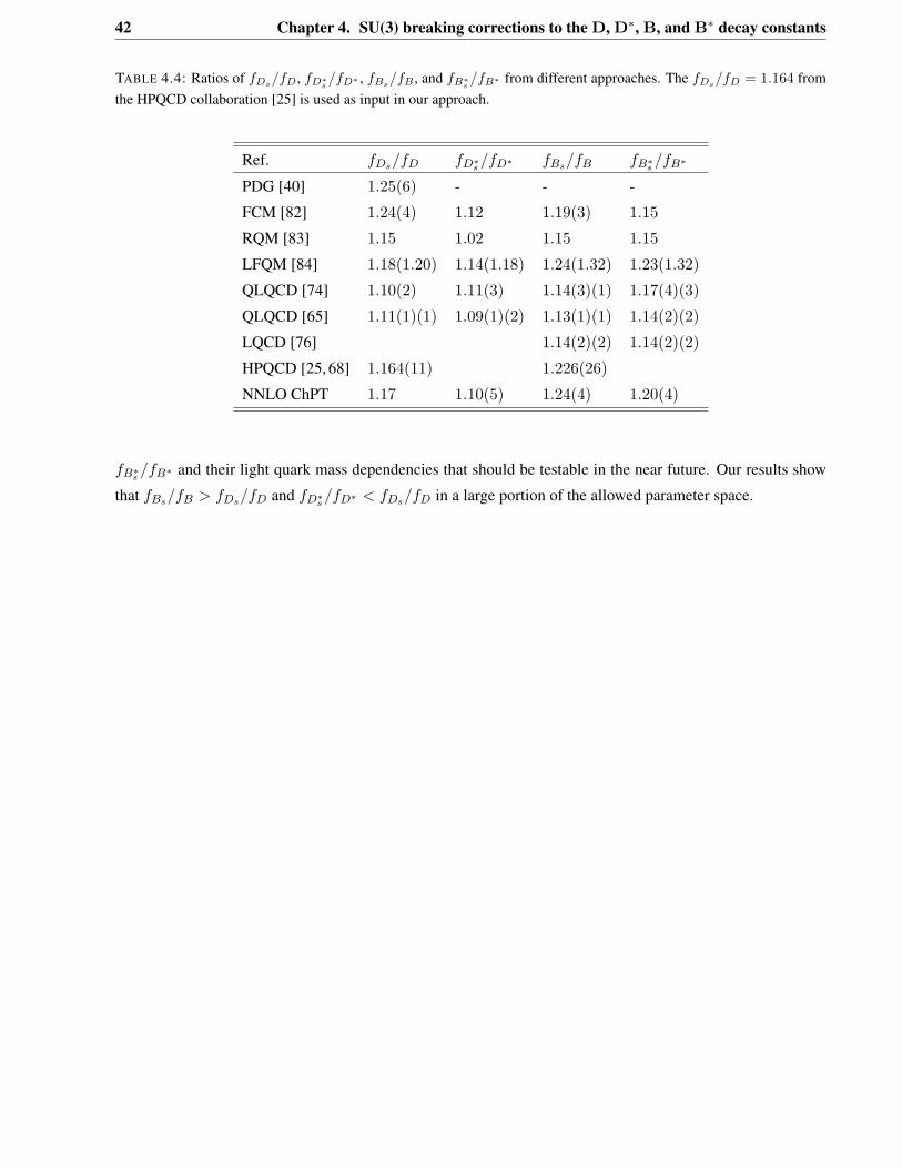
42 Chapter 4. SU(3) breaking corrections to the D, D*, B, and B* decay constants
TABLE 4.4: Ratios of 𝑓𝐷𝑠/𝑓𝐷, 𝑓𝐷*𝑠
/𝑓𝐷* , 𝑓𝐵𝑠/𝑓𝐵 , and 𝑓𝐵*𝑠
/𝑓𝐵* from different approaches. The 𝑓𝐷𝑠/𝑓𝐷 = 1.164 from
the HPQCD collaboration [25] is used as input in our approach.
Ref. 𝑓𝐷𝑠/𝑓𝐷 𝑓𝐷*𝑠 /𝑓𝐷* 𝑓𝐵𝑠/𝑓𝐵 𝑓𝐵*𝑠 /𝑓𝐵*
PDG [40] 1.25(6) - - -
FCM [82] 1.24(4) 1.12 1.19(3) 1.15
RQM [83] 1.15 1.02 1.15 1.15
LFQM [84] 1.18(1.20) 1.14(1.18) 1.24(1.32) 1.23(1.32)
QLQCD [74] 1.10(2) 1.11(3) 1.14(3)(1) 1.17(4)(3)
QLQCD [65] 1.11(1)(1) 1.09(1)(2) 1.13(1)(1) 1.14(2)(2)
LQCD [76] 1.14(2)(2) 1.14(2)(2)
HPQCD [25, 68] 1.164(11) 1.226(26)
NNLO ChPT 1.17 1.10(5) 1.24(4) 1.20(4)
𝑓𝐵*𝑠 /𝑓𝐵* and their light quark mass dependencies that should be testable in the near future. Our results show
that 𝑓𝐵𝑠/𝑓𝐵 > 𝑓𝐷𝑠/𝑓𝐷 and 𝑓𝐷*𝑠 /𝑓𝐷* < 𝑓𝐷𝑠/𝑓𝐷 in a large portion of the allowed parameter space.
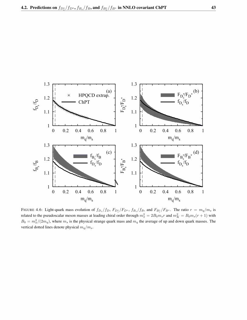
4.2. Predictions on 𝑓𝐷*𝑠 /𝑓𝐷* , 𝑓𝐵𝑠/𝑓𝐵 , and 𝑓𝐵*𝑠 /𝑓𝐵* in NNLO covariant ChPT 43
1
1.1
1.2
1.3
0 0.2 0.4 0.6 0.8 1
f Ds/f D
mq/ms
(a)HPQCD extrap.ChPT
1
1.1
1.2
1.3
0 0.2 0.4 0.6 0.8 1
F D* s/F
D*
mq/ms
(b)FD*
s/FD*
fDs/fD
1
1.1
1.2
1.3
0 0.2 0.4 0.6 0.8 1
f Bs/f B
mq/ms
(c)fBs
/fBfDs
/fD
1
1.1
1.2
1.3
0 0.2 0.4 0.6 0.8 1
F B* s/F
B*
mq/ms
(d)FB*
s/FB*
fDs/fD
FIGURE 4.6: Light-quark mass evolution of 𝑓𝐷𝑠/𝑓𝐷, 𝐹𝐷*𝑠
/𝐹𝐷* , 𝑓𝐵𝑠/𝑓𝐵 , and 𝐹𝐵*𝑠
/𝐹𝐵* . The ratio 𝑟 = 𝑚𝑞/𝑚𝑠 isrelated to the pseudoscalar meson masses at leading chiral order through 𝑚2
𝜋 = 2𝐵0𝑚𝑠𝑟 and 𝑚2𝐾 = 𝐵0𝑚𝑠(𝑟 + 1) with
𝐵0 = 𝑚2𝜋/(2𝑚𝑞), where 𝑚𝑠 is the physical strange quark mass and 𝑚𝑞 the average of up and down quark masses. The
vertical dotted lines denote physical 𝑚𝑞/𝑚𝑠.
44 Chapter 4. SU(3) breaking corrections to the D, D*, B, and B* decay constants
Chapter 5
Scattering of Nambu-Goldstone bosons offheavy-light mesons
5.1 Introduction
Measurements of hadronic states with charm quarks such as the 𝐷*𝑠0(2317) have led to extensive and still
ongoing discussions about our deeper understanding of mesons and baryons [6, 7, 85], traditionally thought to
be composed of a pair of quark and anti-quark or three quarks in the naive quark model. With its mass (𝑀 =
2317.8±0.6 MeV) about 100 MeV lower than the lowest 𝑐𝑠 scalar state in the naive quark model, the 𝐷*𝑠0(2317)
cannot be a conventional 𝑞𝑞 state [86–99]. One possible interpretation is that of a compound dynamically
generated by the strong 𝐷𝐾 interaction in coupled-channels dynamics [96–98]. Such approaches have provided
many useful insights into the nature of some most intriguing new resonances (see, e.g., Refs. [100,101] for some
recent applications).
In order to clarify the nature of the 𝐷*𝑠0(2317), or of any other meson of similar kind, it is useful to study
such objects from various perspectives and compare the results with experimental and lattice QCD (LQCD)
data. In this respect, it has been argued that the isospin-breaking decay width 𝐷*𝑠0(2317) → 𝐷𝑠𝜋 [102, 103],
the light-quark mass dependence [104], and the volume dependence [105] of 𝐷*𝑠0(2317) properties can provide
valuable information on its nature. At the same time it should also be noted that, in addition to the 𝐷*𝑠0(2317),
coupled-channels unitary dynamics predicts several other states in sectors/channels related to the 𝐷*𝑠0(2317) by
heavy-quark spin and flavor symmetry and (approximate) chiral symmetry (or broken SU(4) symmetry) [96–98,
106, 107]. Once the mass and width of the 𝐷*𝑠0(2317) are fixed, so are those of the other related states. Future
experiments in search for those resonances in the predicted energy regions are therefore strongly encouraged.
All these predictions are subject to potentially sizable symmetry breaking corrections. In particular, a com-
prehensive study is necessary to estimate the impact of recoil corrections. For the scattering Length of the
Nambu-Goldstone bosons off the 𝐷 mesons, such a study was performed in [49], showing that these effects
are sizable1. In Chapter 4, or Refs. [78, 109], covariant chiral perturbation theory (ChPT), supplemented with
the extended-on-mass-shell (EOMS) scheme, was applied to study the decay constants of the 𝐷(𝐷*)/𝐵(𝐵*)
1See Ref. [108] for a related discussion on the scattering lengths of the pseudoscalar mesons off the heavy-light vector mesons.
45
46 Chapter 5. Scattering of Nambu-Goldstone bosons off heavy-light mesons
mesons. It was shown that the covariant ChPT converges faster than its non-relativistic (heavy-meson) coun-
terpart. These findings can, to some extent, be deemed as repercussions of the one-baryon sector. For instance,
it has been shown that the EOMS formulation of the baryon ChPT is capable of better describing three-flavor
observables and their light-quark mass evolutions than its non-relativistic (heavy-baryon) counterpart, see, e.g.,
Refs. [52, 60, 110] and references cited therein.
In the present chapter we study the interactions of the heavy-light mesons (𝐷, 𝐷*, 𝐵, 𝐵* and their strange
counterparts) with Nambu-Goldstone bosons (the octet of the lightest pseudoscalar mesons) in covariant ChPT
and its unitary version. We calculate the interaction potentials up to next-to-leading order (NLO) and perform
an iteration of these potentials to all orders using the Bethe-Salpeter equation. It was pointed out that in the
covariant calculation of the loop function appearing in the Bethe-Salpeter equation, one looses the heavy-quark
spin and flavor symmetry [104]. We study this problem in detail and propose a new renormalization scheme,
similar in spirit to the EOMS scheme widely used in the one-baryon sector [58, 59, 110] and also used in
Refs. [49, 78, 109], to recover heavy-quark spin and flavor symmetry up to 1/𝑚𝐻 corrections, where 𝑚𝐻 is a
generic heavy-light meson mass. We apply our approach to describe the most recent fully dynamical LQCD
simulations for the scattering lengths of Nambu-Goldstone bosons off the 𝐷 mesons [12] and fix the relevant
low-energy and subtraction constants. We then solve the corresponding Bethe-Salpeter equations and search
for poles in the complex energy plane, identified as dynamically generated states. We show that a number of 0+
and 1+ states emerge naturally, including the 𝐷*𝑠0(2317), the 𝐷*𝑠1(2460) and their bottom-quark counterparts2.
This chapter is organized as follows. In Section 5.2 we give the basic ingredients of unitarized chiral pertur-
bation theory (UChPT). Starting from Section 5.3 we apply this theory to the scattering of Nambu-Goldstone
bosons off heavy-light mesons. Subsections 5.3.1 and 5.3.2 give the driving potentials up to NLO. In Subsection
5.4.1 we propose a new renormalization scheme to be used in the Bethe-Salpeter equation, which manifestly
satisfies the chiral power counting rules and heavy-quark spin and flavor symmetries. We discuss the advantage
of this scheme in comparison with others widely used in unitarized ChPT in Subsection 5.4.2. In this subsection
we give also predictions for a number of dynamically generated resonances in both the charm and the bottom
sectors. In Section 5.5 we finally investigate off-shell effects on the scattering of Nambu-Goldstone bosons off
𝐷 mesons.
2A similar strategy was adopted in Refs. [12, 111], but both studies are limited to the 0+ charm sector, and in addition Ref. [111]studied the preliminary LQCD results of Ref. [112].
5.2. The T-matrix, unitarity, and the Bethe-Salpeter equation 47
5.2 The T-matrix, unitarity, and the Bethe-Salpeter equation
5.2.1 The S- and T-matrix
The operator 𝑆-matrix is defined through [18]
out⟨p3p4|p1p2⟩in ≡ ⟨p3p4|𝑆|p1p2⟩ , (5.1)
where two-particle initial and final states are chosen for better readability. The generalization to more particles
is straight forward. The 𝑖𝑛 and 𝑜𝑢𝑡 states are defined in the Heisenberg picture, i.e. the two states have a
nontrivial overlap. The states |p1p2⟩ and ⟨p3p4| represent states in the interaction picture, where the 𝑆 matrix
serves as the time evolution operator. Previous definition implies the unitarity of the 𝑆 matrix, 𝑆†𝑆 = 1, which
is equivalent to the conservation of probability.
The 𝑆-matrix is related to the 𝑇 -matrix by
𝑆 = 1− 𝑖𝑇 , (5.2)
where 1 represents the part where the two initial particles pass each other without interaction. The part that is
responsible for the interaction is denoted as 𝑇 . This definition together with the unitarity condition, 𝑆†𝑆 = 1,
gives
𝑖((𝑇 − 𝑇 †) = 𝑇 †𝑇 . (5.3)
Due to momentum conservation, the matrix elements of 𝑇 can be expressed as
⟨p3p4|𝑇 |p1p2⟩ = (2𝜋)4𝛿(4)(𝑝1 + 𝑝2 − 𝑝3 − 𝑝4)𝒯 (𝑝1𝑝2 → 𝑝3𝑝4) , (5.4)
where 𝒯 is the invariant matrix element or scattering amplitude. Using this definition in Eq. (5.3) gives the
identity
𝒯 (𝑝1𝑝2 → 𝑝3𝑝4)− 𝒯 *(𝑝3𝑝4 → 𝑝1𝑝2)
= −𝑖∑
𝑛
(𝑛∏
𝑖=1
∫𝑑3𝑞𝑖
(2𝜋)31
2𝐸𝑖
)𝒯 *(𝑝3𝑝4 → {𝑞𝑖})𝒯 (𝑝1𝑝2 → {𝑞𝑖})(2𝜋)4𝛿(4)(𝑝1 + 𝑝2 −
∑
𝑖
𝑞𝑖) ,
(5.5)
where we have inserted a complete set of intermediate states with particle number 𝑛 and momenta 𝑞𝑖 for
𝑖 = 1, ..., 𝑛. It relates the imaginary part of the forward scattering amplitude to the total cross section3. This
special case of equation (5.5) is known as optical theorem.
We concentrate on two particle intermediate states with momenta 𝑞1 ≡ −�� and 𝑞2 = �� + 𝑃 . Then Eq.
3Our normalization of 𝒯 is chosen such that the differential cross section in the center of mass frame is given by 𝑑𝜎𝑑ΩCM
=1
64𝜋2𝑠
𝑝𝑓
𝑝𝑖|𝒯 (𝑝1𝑝2 → 𝑝3𝑝4)|2, where 𝑝𝑖 and 𝑝𝑓 are the center of mass momenta of the initial and final particles, 𝑝𝑖 =
12√
𝑠𝜆1/2(𝑠, 𝑚2
1, 𝑚22) and 𝑝𝑓 = 1
2√
𝑠𝜆1/2(𝑠, 𝑚2
3, 𝑚24), with the mass 𝑚𝑘 of particle 𝑘. The total momentum squared is denoted as
𝑠 = 𝑃 2 and 𝜆(𝑥, 𝑦, 𝑧) = 𝑥2 + 𝑦2 + 𝑧2 − 2𝑥𝑦 − 2𝑥𝑧 − 2𝑦𝑧 is the Källen function.
48 Chapter 5. Scattering of Nambu-Goldstone bosons off heavy-light mesons
(5.5) reads
𝒯 (𝑝1𝑝2 → 𝑝3𝑝4)− 𝒯 *(𝑝3𝑝4 → 𝑝1𝑝2)
= −𝑖
∫𝑑4��
(2𝜋)4𝒯 *(𝑝3𝑝4 → −��, �� + 𝑃 )𝒯 (𝑝1𝑝2 → −��, �� + 𝑃 )
×(2𝜋)2𝛿+((𝑃 + ��)2 −𝑚2)𝛿+((−��)2 −𝑀2) , (5.6)
with 𝛿+(𝑞2𝑖 − 𝑚2) = Θ(𝑞0
𝑖 )𝛿(𝑞2𝑖 − 𝑚2) for 𝑖 = 1, 2. The total momentum is 𝑃 = 𝑝1 + 𝑝2 = 𝑝3 + 𝑝4
and the masses of the particles with momenta 𝑞1 and 𝑞2 are denoted as 𝑀 and 𝑚. This relation is the two-
particle unitarity requirement. As will be shown, this relation is fulfilled by solutions of the Bethe-Salpeter
(BS) equation. In other words: solutions of the BS equation conserve probability to all orders, not only on a
perturbative level.
5.2.2 The Bethe-Salpeter equation
BS equation for 𝑃𝜑 scattering
The Bethe-Salpeter equation [113] for scattering a Nambu-Goldstone boson 𝜑 off a pseudoscalar heavy-light
meson 𝑃 reads
𝒯𝑃 (𝑞, 𝑄) = 𝒱𝑃 (𝑞, 𝑄)− 𝑖
∫𝑑4��
(2𝜋)4𝒱𝑃 (𝑞, ��)Δℎ(��)Δ𝑙(�� + 𝑃 )𝒯𝑃 (��, 𝑄) , (5.7)
where the propagator of the heavy-light meson is denoted by Δℎ and the propagator of the light Nambu-
Goldstone boson by Δ𝑙. The scattering amplitude is abbreviated as 𝒯𝑃 (𝑞, 𝑄) ≡ 𝒯 (𝑃 (𝑝1)𝜑(𝑝2) → 𝑃 (𝑝3)𝜑(𝑝4)),
where the momenta are related by 𝑝1 = −𝑞, 𝑝2 = 𝑞 + 𝑃 , 𝑝3 = −𝑄 and 𝑝4 = 𝑄 + 𝑃 . In accordance with this
convention the potential is denoted by 𝒱𝑃 (𝑞, 𝑄). Diagrammatically, the BS equation is shown in Figure 5.1. It
is straight forward to include channel coupling effects by promoting 𝒯𝑃 and 𝒱𝑃 to matrices. The multiplication
in (5.7) is then understood as matrix multiplication and the propagators become diagonal matrices. Explicitly,
equation (5.7) becomes
(𝒯𝑃 (𝑞, 𝑄)
)𝑖𝑗
=(𝒱𝑃 (𝑞, 𝑄)
)𝑖𝑗− 𝑖
∫𝑑4��
(2𝜋)4(𝒱𝑃 (𝑞, ��)
)𝑖𝑘
Δℎ,𝑘(��)Δ𝑙,𝑘(�� + 𝑃 )(𝒯𝑃 (��, 𝑄)
)𝑘𝑗
,
(5.8)
where Δℎ,𝑘 and Δ𝑙,𝑘 are the propagators corresponding to the two-particle state 𝑘. From now on channel
coupling effects are treated implicitly as far as possible.
Inserting the exact propagators together with the exact two-particle irreducible amplitude (the potential)
into equation (5.7) gives access to the exact scattering amplitude. However, since both are not exactly known,
one has to rely on approximations. We use the free propagators
Δℎ(𝑞) =𝑖
𝑞2 −𝑀2 + 𝑖𝜖, Δ𝑙(𝑞) =
𝑖
𝑞2 −𝑚2 + 𝑖𝜖, (5.9)
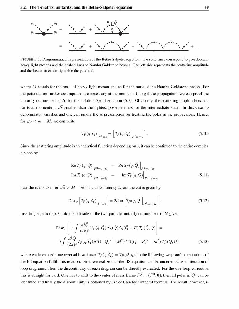
5.2. The T-matrix, unitarity, and the Bethe-Salpeter equation 49
p4
p3p1
p2
!Q
P + QP + Q
!Q
= +
+
+ . . .
=
+
FIGURE 5.1: Diagrammatical representation of the Bethe-Salpeter equation. The solid lines correspond to pseudoscalarheavy-light mesons and the dashed lines to Nambu-Goldstone bosons. The left side represents the scattering amplitudeand the first term on the right side the potential.
where 𝑀 stands for the mass of heavy-light meson and 𝑚 for the mass of the Nambu-Goldstone boson. For
the potential no further assumptions are necessary at the moment. Using these propagators, we can proof the
unitarity requirement (5.6) for the solution 𝒯𝑃 of equation (5.7). Obviously, the scattering amplitude is real
for total momentum√
𝑠 smaller than the lightest possible mass for the intermediate state. In this case no
denominator vanishes and one can ignore the 𝑖𝜖 prescription for treating the poles in the propagators. Hence,
for√
𝑠 < 𝑚 + 𝑀 , we can write
𝒯𝑃 (𝑞, 𝑄)𝑃 2=𝑠
=[𝒯𝑃 (𝑞, 𝑄)
𝑃 2=𝑠*
]*. (5.10)
Since the scattering amplitude is an analytical function depending on 𝑠, it can be continued to the entire complex
𝑠 plane by
Re 𝒯𝑃 (𝑞, 𝑄)𝑃 2=𝑠+𝑖𝜖
= Re 𝒯𝑃 (𝑞, 𝑄)𝑃 2=𝑠−𝑖𝜖
Im 𝒯𝑃 (𝑞, 𝑄)𝑃 2=𝑠+𝑖𝜖
= −Im 𝒯𝑃 (𝑞, 𝑄)𝑃 2=𝑠−𝑖𝜖
(5.11)
near the real 𝑠 axis for√
𝑠 > 𝑀 + 𝑚. The discontinuity across the cut is given by
Disc𝑠
[𝒯𝑃 (𝑞, 𝑄)
𝑃 2=𝑠
]= 2𝑖 Im
[𝒯𝑃 (𝑞, 𝑄)
𝑃 2=𝑠+𝑖𝜖
]. (5.12)
Inserting equation (5.7) into the left side of the two-particle unitarity requirement (5.6) gives
Disc𝑠
[−𝑖
∫𝑑4��
(2𝜋)4𝒱𝑃 (𝑞, ��)Δℎ(��)Δ𝑙(�� + 𝑃 )𝒯𝑃 (��, 𝑄)
]=
−𝑖
∫𝑑4��
(2𝜋)2𝒯𝑃 (𝑞, ��) 𝛿+((−��)2 −𝑀2) 𝛿+((�� + 𝑃 )2 −𝑚2) 𝒯 *𝑃 (𝑄, ��) , (5.13)
where we have used time reversal invariance, 𝒯𝑃 (𝑞,𝑄) = 𝒯𝑃 (𝑄, 𝑞). In the following we proof that solutions of
the BS equation fulfill this relation. First, we realize that the BS equation can be understood as an iteration of
loop diagrams. Then the discontinuity of each diagram can be directly evaluated. For the one-loop correction
this is straight forward. One has to shift to the center of mass frame 𝑃𝜇 = (𝑃 0,0), then all poles in ��0 can be
identified and finally the discontinuity is obtained by use of Cauchy’s integral formula. The result, however, is
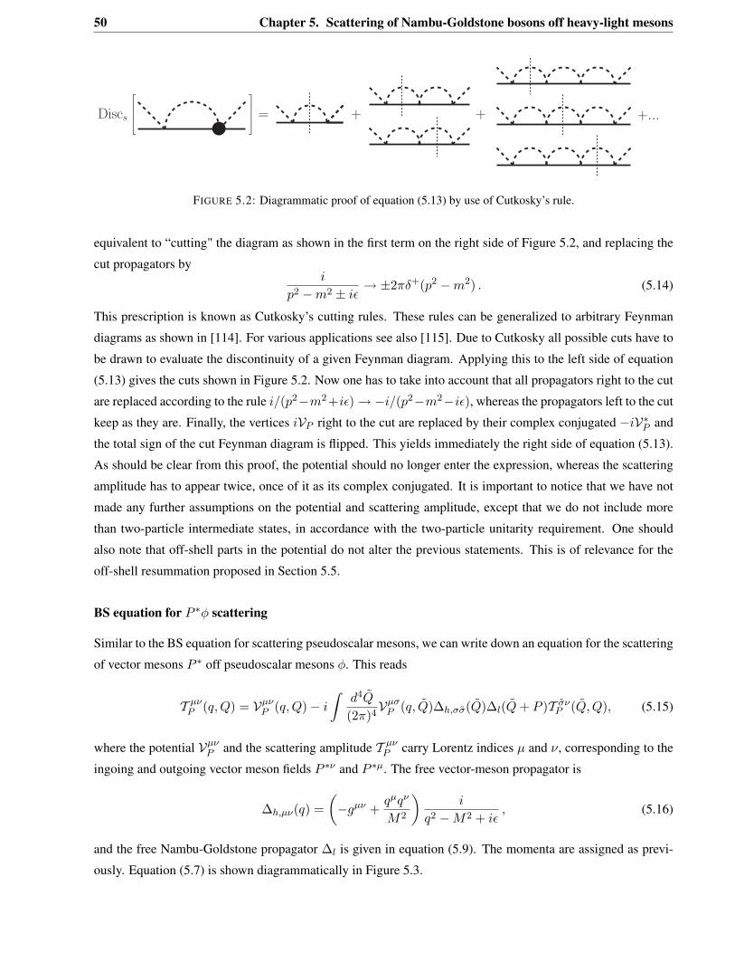
50 Chapter 5. Scattering of Nambu-Goldstone bosons off heavy-light mesons
Discs
!""#
$%%& = + + +...
FIGURE 5.2: Diagrammatic proof of equation (5.13) by use of Cutkosky’s rule.
equivalent to “cutting" the diagram as shown in the first term on the right side of Figure 5.2, and replacing the
cut propagators by𝑖
𝑝2 −𝑚2 ± 𝑖𝜖→ ±2𝜋𝛿+(𝑝2 −𝑚2) . (5.14)
This prescription is known as Cutkosky’s cutting rules. These rules can be generalized to arbitrary Feynman
diagrams as shown in [114]. For various applications see also [115]. Due to Cutkosky all possible cuts have to
be drawn to evaluate the discontinuity of a given Feynman diagram. Applying this to the left side of equation
(5.13) gives the cuts shown in Figure 5.2. Now one has to take into account that all propagators right to the cut
are replaced according to the rule 𝑖/(𝑝2−𝑚2+𝑖𝜖) → −𝑖/(𝑝2−𝑚2−𝑖𝜖), whereas the propagators left to the cut
keep as they are. Finally, the vertices 𝑖𝒱𝑃 right to the cut are replaced by their complex conjugated −𝑖𝒱*𝑃 and
the total sign of the cut Feynman diagram is flipped. This yields immediately the right side of equation (5.13).
As should be clear from this proof, the potential should no longer enter the expression, whereas the scattering
amplitude has to appear twice, once of it as its complex conjugated. It is important to notice that we have not
made any further assumptions on the potential and scattering amplitude, except that we do not include more
than two-particle intermediate states, in accordance with the two-particle unitarity requirement. One should
also note that off-shell parts in the potential do not alter the previous statements. This is of relevance for the
off-shell resummation proposed in Section 5.5.
BS equation for 𝑃 *𝜑 scattering
Similar to the BS equation for scattering pseudoscalar mesons, we can write down an equation for the scattering
of vector mesons 𝑃 * off pseudoscalar mesons 𝜑. This reads
𝒯 𝜇𝜈𝑃 (𝑞, 𝑄) = 𝒱𝜇𝜈
𝑃 (𝑞, 𝑄)− 𝑖
∫𝑑4��
(2𝜋)4𝒱𝜇𝜎
𝑃 (𝑞, ��)Δℎ,𝜎��(��)Δ𝑙(�� + 𝑃 )𝒯 ��𝜈𝑃 (��, 𝑄), (5.15)
where the potential 𝒱𝜇𝜈𝑃 and the scattering amplitude 𝒯 𝜇𝜈
𝑃 carry Lorentz indices 𝜇 and 𝜈, corresponding to the
ingoing and outgoing vector meson fields 𝑃 *𝜈 and 𝑃 *𝜇. The free vector-meson propagator is
Δℎ,𝜇𝜈(𝑞) =(−𝑔𝜇𝜈 +
𝑞𝜇𝑞𝜈
𝑀2
)𝑖
𝑞2 −𝑀2 + 𝑖𝜖, (5.16)
and the free Nambu-Goldstone propagator Δ𝑙 is given in equation (5.9). The momenta are assigned as previ-
ously. Equation (5.7) is shown diagrammatically in Figure 5.3.
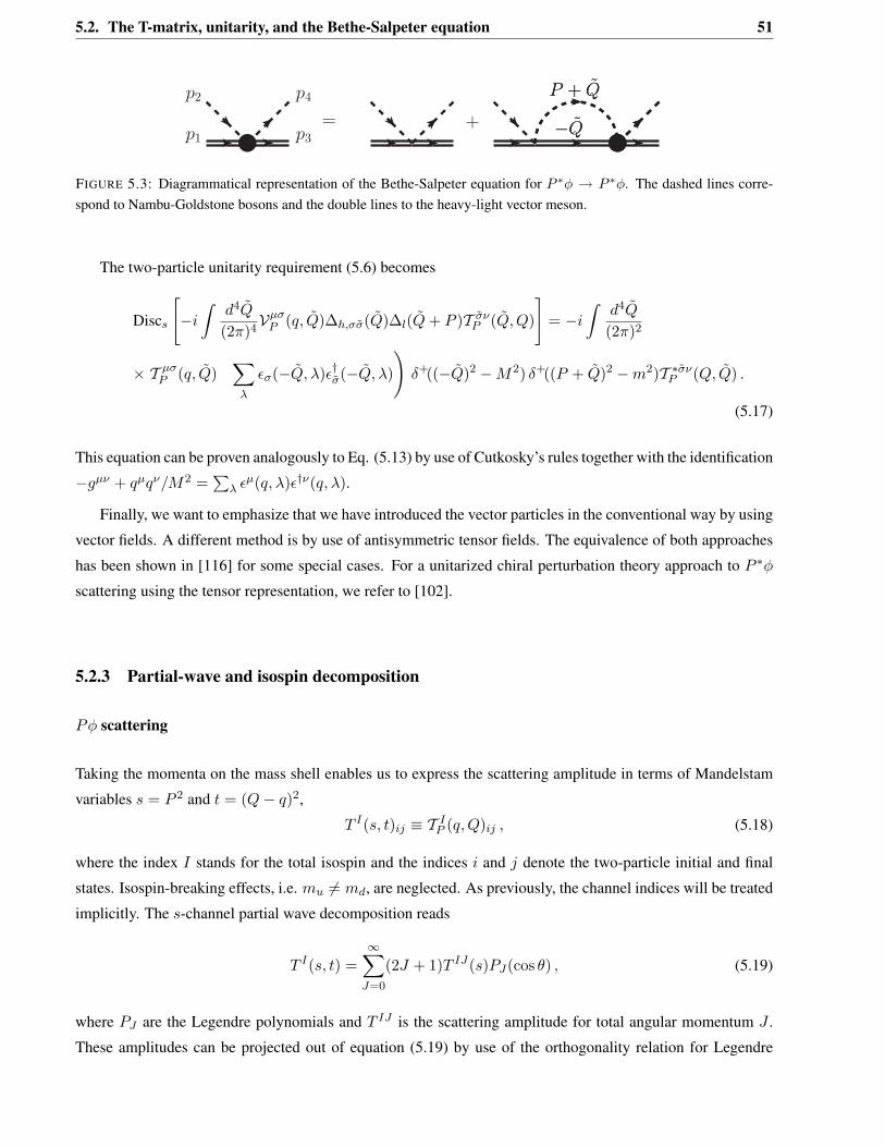
5.2. The T-matrix, unitarity, and the Bethe-Salpeter equation 51
= +
p4
p3p1
p2
!Q
P + Q
!Q
P + Q
FIGURE 5.3: Diagrammatical representation of the Bethe-Salpeter equation for 𝑃 *𝜑 → 𝑃 *𝜑. The dashed lines corre-spond to Nambu-Goldstone bosons and the double lines to the heavy-light vector meson.
The two-particle unitarity requirement (5.6) becomes
Disc𝑠
[−𝑖
∫𝑑4��
(2𝜋)4𝒱𝜇𝜎
𝑃 (𝑞, ��)Δℎ,𝜎��(��)Δ𝑙(�� + 𝑃 )𝒯 ��𝜈𝑃 (��, 𝑄)
]= −𝑖
∫𝑑4��
(2𝜋)2
× 𝒯 𝜇𝜎𝑃 (𝑞, ��)
(∑
𝜆
𝜖𝜎(−��, 𝜆)𝜖†��(−��, 𝜆)
)𝛿+((−��)2 −𝑀2) 𝛿+((𝑃 + ��)2 −𝑚2)𝒯 *��𝜈
𝑃 (𝑄, ��) .
(5.17)
This equation can be proven analogously to Eq. (5.13) by use of Cutkosky’s rules together with the identification
−𝑔𝜇𝜈 + 𝑞𝜇𝑞𝜈/𝑀2 =∑
𝜆 𝜖𝜇(𝑞, 𝜆)𝜖†𝜈(𝑞, 𝜆).
Finally, we want to emphasize that we have introduced the vector particles in the conventional way by using
vector fields. A different method is by use of antisymmetric tensor fields. The equivalence of both approaches
has been shown in [116] for some special cases. For a unitarized chiral perturbation theory approach to 𝑃 *𝜑
scattering using the tensor representation, we refer to [102].
5.2.3 Partial-wave and isospin decomposition
𝑃𝜑 scattering
Taking the momenta on the mass shell enables us to express the scattering amplitude in terms of Mandelstam
variables 𝑠 = 𝑃 2 and 𝑡 = (𝑄− 𝑞)2,
𝑇 𝐼(𝑠, 𝑡)𝑖𝑗 ≡ 𝒯 𝐼𝑃 (𝑞, 𝑄)𝑖𝑗 , (5.18)
where the index 𝐼 stands for the total isospin and the indices 𝑖 and 𝑗 denote the two-particle initial and final
states. Isospin-breaking effects, i.e. 𝑚𝑢 = 𝑚𝑑, are neglected. As previously, the channel indices will be treated
implicitly. The 𝑠-channel partial wave decomposition reads
𝑇 𝐼(𝑠, 𝑡) =∞∑
𝐽=0
(2𝐽 + 1)𝑇 𝐼𝐽(𝑠)𝑃𝐽(cos 𝜃) , (5.19)
where 𝑃𝐽 are the Legendre polynomials and 𝑇 𝐼𝐽 is the scattering amplitude for total angular momentum 𝐽 .
These amplitudes can be projected out of equation (5.19) by use of the orthogonality relation for Legendre
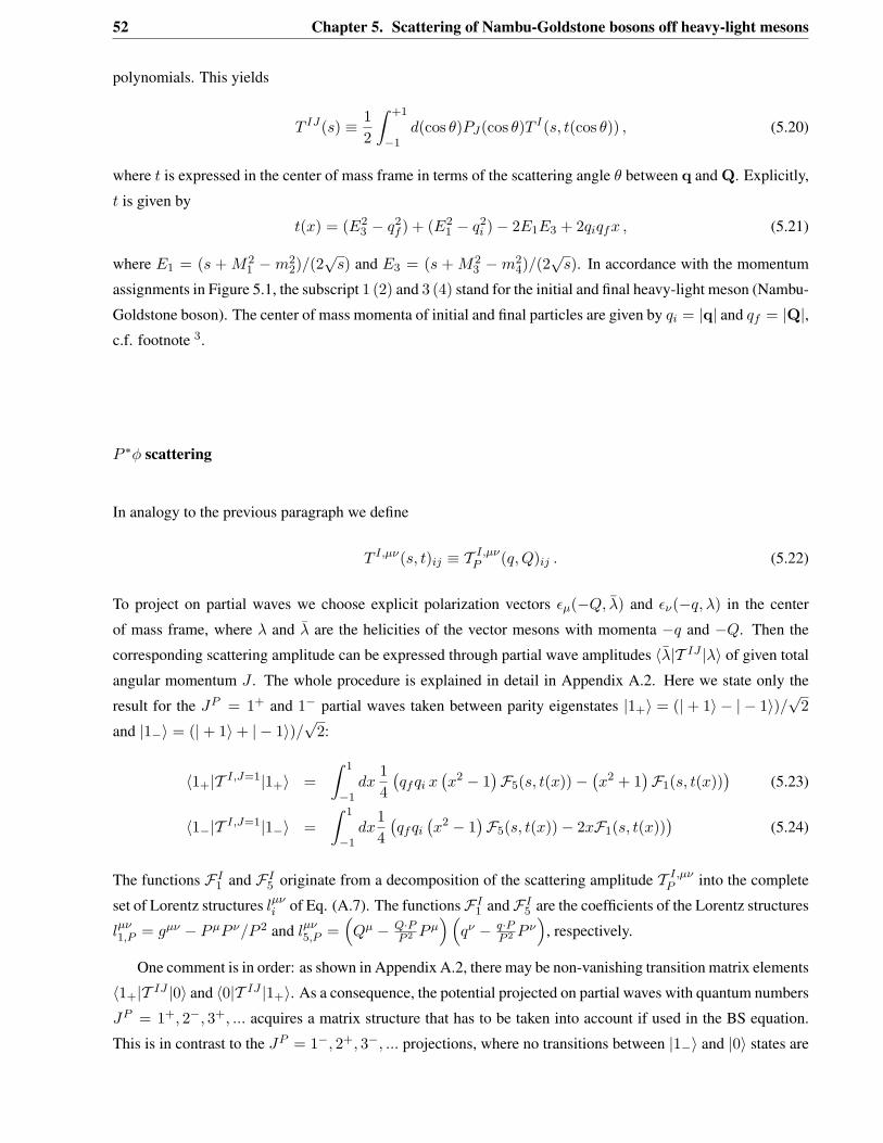
52 Chapter 5. Scattering of Nambu-Goldstone bosons off heavy-light mesons
polynomials. This yields
𝑇 𝐼𝐽(𝑠) ≡ 12
∫ +1
−1𝑑(cos 𝜃)𝑃𝐽(cos 𝜃)𝑇 𝐼(𝑠, 𝑡(cos 𝜃)) , (5.20)
where 𝑡 is expressed in the center of mass frame in terms of the scattering angle 𝜃 between q and Q. Explicitly,
𝑡 is given by
𝑡(𝑥) = (𝐸23 − 𝑞2
𝑓 ) + (𝐸21 − 𝑞2
𝑖 )− 2𝐸1𝐸3 + 2𝑞𝑖𝑞𝑓𝑥 , (5.21)
where 𝐸1 = (𝑠 + 𝑀21 −𝑚2
2)/(2√
𝑠) and 𝐸3 = (𝑠 + 𝑀23 −𝑚2
4)/(2√
𝑠). In accordance with the momentum
assignments in Figure 5.1, the subscript 1 (2) and 3 (4) stand for the initial and final heavy-light meson (Nambu-
Goldstone boson). The center of mass momenta of initial and final particles are given by 𝑞𝑖 = |q| and 𝑞𝑓 = |Q|,c.f. footnote 3.
𝑃 *𝜑 scattering
In analogy to the previous paragraph we define
𝑇 𝐼,𝜇𝜈(𝑠, 𝑡)𝑖𝑗 ≡ 𝒯 𝐼,𝜇𝜈𝑃 (𝑞, 𝑄)𝑖𝑗 . (5.22)
To project on partial waves we choose explicit polarization vectors 𝜖𝜇(−𝑄, ��) and 𝜖𝜈(−𝑞, 𝜆) in the center
of mass frame, where 𝜆 and �� are the helicities of the vector mesons with momenta −𝑞 and −𝑄. Then the
corresponding scattering amplitude can be expressed through partial wave amplitudes ⟨��|𝒯 𝐼𝐽 |𝜆⟩ of given total
angular momentum 𝐽 . The whole procedure is explained in detail in Appendix A.2. Here we state only the
result for the 𝐽𝑃 = 1+ and 1− partial waves taken between parity eigenstates |1+⟩ = (|+ 1⟩ − | − 1⟩)/√
2
and |1−⟩ = (|+ 1⟩+ | − 1⟩)/√
2:
⟨1+|𝒯 𝐼,𝐽=1|1+⟩ =∫ 1
−1𝑑𝑥
14(𝑞𝑓𝑞𝑖 𝑥
(𝑥2 − 1
)ℱ5(𝑠, 𝑡(𝑥))−
(𝑥2 + 1
)ℱ1(𝑠, 𝑡(𝑥))
)(5.23)
⟨1−|𝒯 𝐼,𝐽=1|1−⟩ =∫ 1
−1𝑑𝑥
14(𝑞𝑓𝑞𝑖
(𝑥2 − 1
)ℱ5(𝑠, 𝑡(𝑥))− 2𝑥ℱ1(𝑠, 𝑡(𝑥))
)(5.24)
The functions ℱ𝐼1 and ℱ𝐼
5 originate from a decomposition of the scattering amplitude 𝒯 𝐼,𝜇𝜈𝑃 into the complete
set of Lorentz structures 𝑙𝜇𝜈𝑖 of Eq. (A.7). The functionsℱ𝐼
1 andℱ𝐼5 are the coefficients of the Lorentz structures
𝑙𝜇𝜈1,𝑃 = 𝑔𝜇𝜈 − 𝑃𝜇𝑃 𝜈/𝑃 2 and 𝑙𝜇𝜈
5,𝑃 =(𝑄𝜇 − 𝑄·𝑃
𝑃 2 𝑃𝜇)(
𝑞𝜈 − 𝑞·𝑃𝑃 2 𝑃 𝜈
), respectively.
One comment is in order: as shown in Appendix A.2, there may be non-vanishing transition matrix elements
⟨1+|𝒯 𝐼𝐽 |0⟩ and ⟨0|𝒯 𝐼𝐽 |1+⟩. As a consequence, the potential projected on partial waves with quantum numbers
𝐽𝑃 = 1+, 2−, 3+, ... acquires a matrix structure that has to be taken into account if used in the BS equation.
This is in contrast to the 𝐽𝑃 = 1−, 2+, 3−, ... projections, where no transitions between |1−⟩ and |0⟩ states are
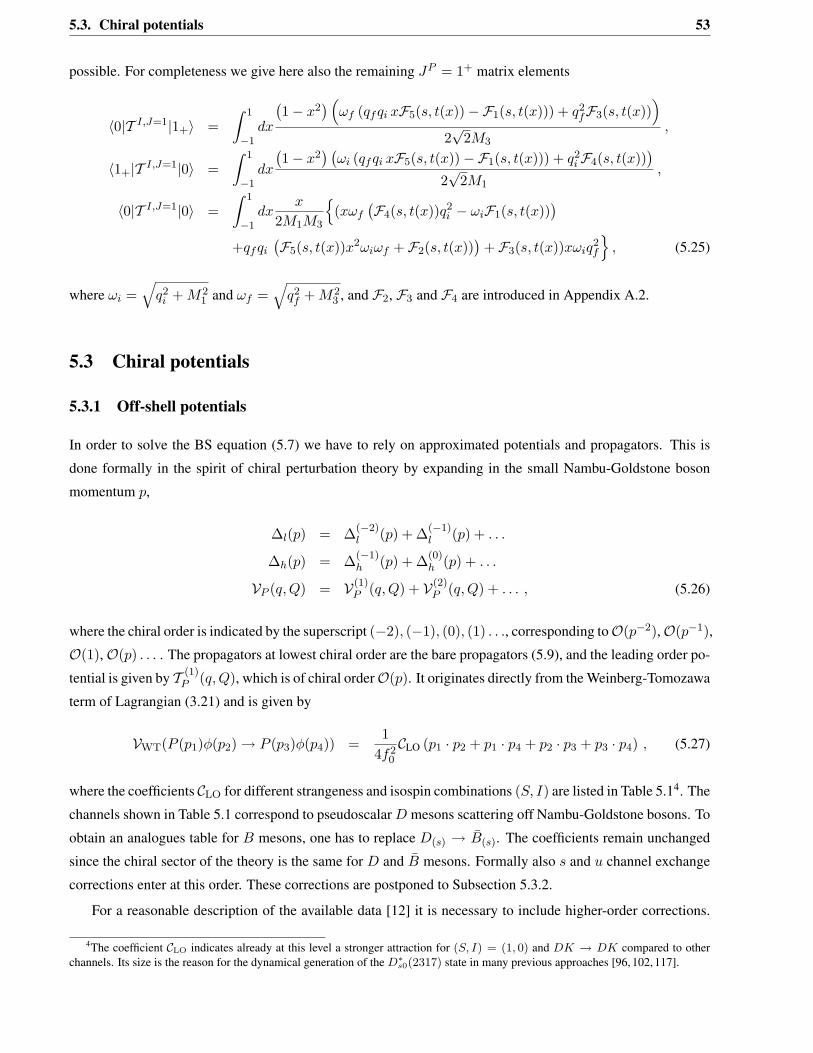
5.3. Chiral potentials 53
possible. For completeness we give here also the remaining 𝐽𝑃 = 1+ matrix elements
⟨0|𝒯 𝐼,𝐽=1|1+⟩ =∫ 1
−1𝑑𝑥
(1− 𝑥2
) (𝜔𝑓 (𝑞𝑓𝑞𝑖 𝑥ℱ5(𝑠, 𝑡(𝑥))−ℱ1(𝑠, 𝑡(𝑥))) + 𝑞2
𝑓ℱ3(𝑠, 𝑡(𝑥)))
2√
2𝑀3
,
⟨1+|𝒯 𝐼,𝐽=1|0⟩ =∫ 1
−1𝑑𝑥
(1− 𝑥2
) (𝜔𝑖 (𝑞𝑓𝑞𝑖 𝑥ℱ5(𝑠, 𝑡(𝑥))−ℱ1(𝑠, 𝑡(𝑥))) + 𝑞2
𝑖ℱ4(𝑠, 𝑡(𝑥)))
2√
2𝑀1
,
⟨0|𝒯 𝐼,𝐽=1|0⟩ =∫ 1
−1𝑑𝑥
𝑥
2𝑀1𝑀3
{(𝑥𝜔𝑓
(ℱ4(𝑠, 𝑡(𝑥))𝑞2
𝑖 − 𝜔𝑖ℱ1(𝑠, 𝑡(𝑥)))
+𝑞𝑓𝑞𝑖
(ℱ5(𝑠, 𝑡(𝑥))𝑥2𝜔𝑖𝜔𝑓 + ℱ2(𝑠, 𝑡(𝑥))
)+ ℱ3(𝑠, 𝑡(𝑥))𝑥𝜔𝑖𝑞
2𝑓
}, (5.25)
where 𝜔𝑖 =√
𝑞2𝑖 + 𝑀2
1 and 𝜔𝑓 =√
𝑞2𝑓 + 𝑀2
3 , and ℱ2, ℱ3 and ℱ4 are introduced in Appendix A.2.
5.3 Chiral potentials
5.3.1 Off-shell potentials
In order to solve the BS equation (5.7) we have to rely on approximated potentials and propagators. This is
done formally in the spirit of chiral perturbation theory by expanding in the small Nambu-Goldstone boson
momentum 𝑝,
Δ𝑙(𝑝) = Δ(−2)𝑙 (𝑝) + Δ(−1)
𝑙 (𝑝) + . . .
Δℎ(𝑝) = Δ(−1)ℎ (𝑝) + Δ(0)
ℎ (𝑝) + . . .
𝒱𝑃 (𝑞, 𝑄) = 𝒱(1)𝑃 (𝑞, 𝑄) + 𝒱(2)
𝑃 (𝑞, 𝑄) + . . . , (5.26)
where the chiral order is indicated by the superscript (−2), (−1), (0), (1) . . ., corresponding to𝒪(𝑝−2),𝒪(𝑝−1),
𝒪(1),𝒪(𝑝) . . . . The propagators at lowest chiral order are the bare propagators (5.9), and the leading order po-
tential is given by 𝒯 (1)𝑃 (𝑞, 𝑄), which is of chiral order𝒪(𝑝). It originates directly from the Weinberg-Tomozawa
term of Lagrangian (3.21) and is given by
𝒱WT(𝑃 (𝑝1)𝜑(𝑝2) → 𝑃 (𝑝3)𝜑(𝑝4)) =1
4𝑓20
𝒞LO (𝑝1 · 𝑝2 + 𝑝1 · 𝑝4 + 𝑝2 · 𝑝3 + 𝑝3 · 𝑝4) , (5.27)
where the coefficients 𝒞LO for different strangeness and isospin combinations (𝑆, 𝐼) are listed in Table 5.14. The
channels shown in Table 5.1 correspond to pseudoscalar 𝐷 mesons scattering off Nambu-Goldstone bosons. To
obtain an analogues table for 𝐵 mesons, one has to replace 𝐷(𝑠) → ��(𝑠). The coefficients remain unchanged
since the chiral sector of the theory is the same for 𝐷 and �� mesons. Formally also 𝑠 and 𝑢 channel exchange
corrections enter at this order. These corrections are postponed to Subsection 5.3.2.
For a reasonable description of the available data [12] it is necessary to include higher-order corrections.
4The coefficient 𝒞LO indicates already at this level a stronger attraction for (𝑆, 𝐼) = (1, 0) and 𝐷𝐾 → 𝐷𝐾 compared to otherchannels. Its size is the reason for the dynamical generation of the 𝐷*
𝑠0(2317) state in many previous approaches [96, 102, 117].
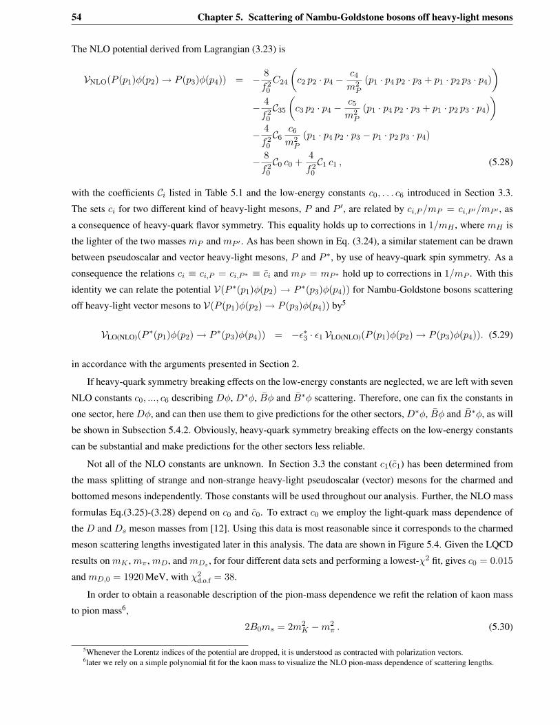
54 Chapter 5. Scattering of Nambu-Goldstone bosons off heavy-light mesons
The NLO potential derived from Lagrangian (3.23) is
𝒱NLO(𝑃 (𝑝1)𝜑(𝑝2) → 𝑃 (𝑝3)𝜑(𝑝4)) = − 8𝑓20
𝐶24
(𝑐2 𝑝2 · 𝑝4 −
𝑐4
𝑚2𝑃
(𝑝1 · 𝑝4 𝑝2 · 𝑝3 + 𝑝1 · 𝑝2 𝑝3 · 𝑝4))
− 4𝑓20
𝒞35
(𝑐3 𝑝2 · 𝑝4 −
𝑐5
𝑚2𝑃
(𝑝1 · 𝑝4 𝑝2 · 𝑝3 + 𝑝1 · 𝑝2 𝑝3 · 𝑝4))
− 4𝑓20
𝒞6𝑐6
𝑚2𝑃
(𝑝1 · 𝑝4 𝑝2 · 𝑝3 − 𝑝1 · 𝑝2 𝑝3 · 𝑝4)
− 8𝑓20
𝒞0 𝑐0 +4𝑓20
𝒞1 𝑐1 , (5.28)
with the coefficients 𝒞𝑖 listed in Table 5.1 and the low-energy constants 𝑐0, . . . 𝑐6 introduced in Section 3.3.
The sets 𝑐𝑖 for two different kind of heavy-light mesons, 𝑃 and 𝑃 ′, are related by 𝑐𝑖,𝑃 /𝑚𝑃 = 𝑐𝑖,𝑃 ′/𝑚𝑃 ′ , as
a consequence of heavy-quark flavor symmetry. This equality holds up to corrections in 1/𝑚𝐻 , where 𝑚𝐻 is
the lighter of the two masses 𝑚𝑃 and 𝑚𝑃 ′ . As has been shown in Eq. (3.24), a similar statement can be drawn
between pseudoscalar and vector heavy-light mesons, 𝑃 and 𝑃 *, by use of heavy-quark spin symmetry. As a
consequence the relations 𝑐𝑖 ≡ 𝑐𝑖,𝑃 = 𝑐𝑖,𝑃 * ≡ 𝑐𝑖 and 𝑚𝑃 = 𝑚𝑃 * hold up to corrections in 1/𝑚𝑃 . With this
identity we can relate the potential 𝒱(𝑃 *(𝑝1)𝜑(𝑝2) → 𝑃 *(𝑝3)𝜑(𝑝4)) for Nambu-Goldstone bosons scattering
off heavy-light vector mesons to 𝒱(𝑃 (𝑝1)𝜑(𝑝2) → 𝑃 (𝑝3)𝜑(𝑝4)) by5
𝒱LO(NLO)(𝑃 *(𝑝1)𝜑(𝑝2) → 𝑃 *(𝑝3)𝜑(𝑝4)) = −𝜖*3 · 𝜖1 𝒱LO(NLO)(𝑃 (𝑝1)𝜑(𝑝2) → 𝑃 (𝑝3)𝜑(𝑝4)). (5.29)
in accordance with the arguments presented in Section 2.
If heavy-quark symmetry breaking effects on the low-energy constants are neglected, we are left with seven
NLO constants 𝑐0, ..., 𝑐6 describing 𝐷𝜑, 𝐷*𝜑, ��𝜑 and ��*𝜑 scattering. Therefore, one can fix the constants in
one sector, here 𝐷𝜑, and can then use them to give predictions for the other sectors, 𝐷*𝜑, ��𝜑 and ��*𝜑, as will
be shown in Subsection 5.4.2. Obviously, heavy-quark symmetry breaking effects on the low-energy constants
can be substantial and make predictions for the other sectors less reliable.
Not all of the NLO constants are unknown. In Section 3.3 the constant 𝑐1(𝑐1) has been determined from
the mass splitting of strange and non-strange heavy-light pseudoscalar (vector) mesons for the charmed and
bottomed mesons independently. Those constants will be used throughout our analysis. Further, the NLO mass
formulas Eq.(3.25)-(3.28) depend on 𝑐0 and 𝑐0. To extract 𝑐0 we employ the light-quark mass dependence of
the 𝐷 and 𝐷𝑠 meson masses from [12]. Using this data is most reasonable since it corresponds to the charmed
meson scattering lengths investigated later in this analysis. The data are shown in Figure 5.4. Given the LQCD
results on 𝑚𝐾 , 𝑚𝜋, 𝑚𝐷, and 𝑚𝐷𝑠 , for four different data sets and performing a lowest-𝜒2 fit, gives 𝑐0 = 0.015
and 𝑚𝐷,0 = 1920 MeV, with 𝜒2d.o.f = 38.
In order to obtain a reasonable description of the pion-mass dependence we refit the relation of kaon mass
to pion mass6,
2𝐵0𝑚𝑠 = 2𝑚2𝐾 −𝑚2
𝜋 . (5.30)
5Whenever the Lorentz indices of the potential are dropped, it is understood as contracted with polarization vectors.6later we rely on a simple polynomial fit for the kaon mass to visualize the NLO pion-mass dependence of scattering lengths.
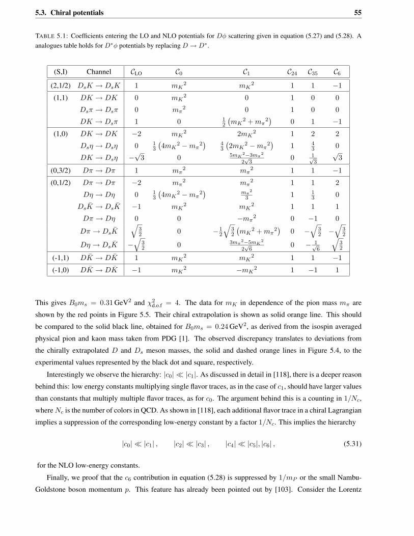
5.3. Chiral potentials 55
TABLE 5.1: Coefficients entering the LO and NLO potentials for 𝐷𝜑 scattering given in equation (5.27) and (5.28). Aanalogues table holds for 𝐷*𝜑 potentials by replacing 𝐷 → 𝐷*.
(S,I) Channel 𝒞LO 𝒞0 𝒞1 𝒞24 𝒞35 𝒞6
(2,1/2) 𝐷𝑠𝐾 → 𝐷𝑠𝐾 1 𝑚𝐾2 𝑚𝐾
2 1 1 −1
(1,1) 𝐷𝐾 → 𝐷𝐾 0 𝑚𝐾2 0 1 0 0
𝐷𝑠𝜋 → 𝐷𝑠𝜋 0 𝑚𝜋2 0 1 0 0
𝐷𝐾 → 𝐷𝑠𝜋 1 0 12
(𝑚𝐾
2 + 𝑚𝜋2)
0 1 −1
(1,0) 𝐷𝐾 → 𝐷𝐾 −2 𝑚𝐾2 2𝑚𝐾
2 1 2 2
𝐷𝑠𝜂 → 𝐷𝑠𝜂 0 13
(4𝑚𝐾
2 −𝑚𝜋2)
43
(2𝑚𝐾
2 −𝑚𝜋2)
1 43 0
𝐷𝐾 → 𝐷𝑠𝜂 −√
3 0 5𝑚𝐾2−3𝑚𝜋
2
2√
30 1√
3
√3
(0,3/2) 𝐷𝜋 → 𝐷𝜋 1 𝑚𝜋2 𝑚𝜋
2 1 1 −1
(0,1/2) 𝐷𝜋 → 𝐷𝜋 −2 𝑚𝜋2 𝑚𝜋
2 1 1 2
𝐷𝜂 → 𝐷𝜂 0 13
(4𝑚𝐾
2 −𝑚𝜋2)
𝑚𝜋2
3 1 13 0
𝐷𝑠�� → 𝐷𝑠�� −1 𝑚𝐾2 𝑚𝐾
2 1 1 1
𝐷𝜋 → 𝐷𝜂 0 0 −𝑚𝜋2 0 −1 0
𝐷𝜋 → 𝐷𝑠��√
32 0 −1
2
√32
(𝑚𝐾
2 + 𝑚𝜋2)
0 −√
32 −
√32
𝐷𝜂 → 𝐷𝑠�� −√
32 0 3𝑚𝜋
2−5𝑚𝐾2
2√
60 − 1√
6
√32
(-1,1) 𝐷�� → 𝐷�� 1 𝑚𝐾2 𝑚𝐾
2 1 1 −1
(-1,0) 𝐷�� → 𝐷�� −1 𝑚𝐾2 −𝑚𝐾
2 1 −1 1
This gives 𝐵0𝑚𝑠 = 0.31 GeV2 and 𝜒2d.o.f = 4. The data for 𝑚𝐾 in dependence of the pion mass 𝑚𝜋 are
shown by the red points in Figure 5.5. Their chiral extrapolation is shown as solid orange line. This should
be compared to the solid black line, obtained for 𝐵0𝑚𝑠 = 0.24 GeV2, as derived from the isospin averaged
physical pion and kaon mass taken from PDG [1]. The observed discrepancy translates to deviations from
the chirally extrapolated 𝐷 and 𝐷𝑠 meson masses, the solid and dashed orange lines in Figure 5.4, to the
experimental values represented by the black dot and square, respectively.
Interestingly we observe the hierarchy: |𝑐0| ≪ |𝑐1|. As discussed in detail in [118], there is a deeper reason
behind this: low energy constants multiplying single flavor traces, as in the case of 𝑐1, should have larger values
than constants that multiply multiple flavor traces, as for 𝑐0. The argument behind this is a counting in 1/𝑁𝑐,
where 𝑁𝑐 is the number of colors in QCD. As shown in [118], each additional flavor trace in a chiral Lagrangian
implies a suppression of the corresponding low-energy constant by a factor 1/𝑁𝑐. This implies the hierarchy
|𝑐0| ≪ |𝑐1| , |𝑐2| ≪ |𝑐3| , |𝑐4| ≪ |𝑐5|, |𝑐6| , (5.31)
for the NLO low-energy constants.
Finally, we proof that the 𝑐6 contribution in equation (5.28) is suppressed by 1/𝑚𝑃 or the small Nambu-
Goldstone boson momentum 𝑝. This feature has already been pointed out by [103]. Consider the Lorentz
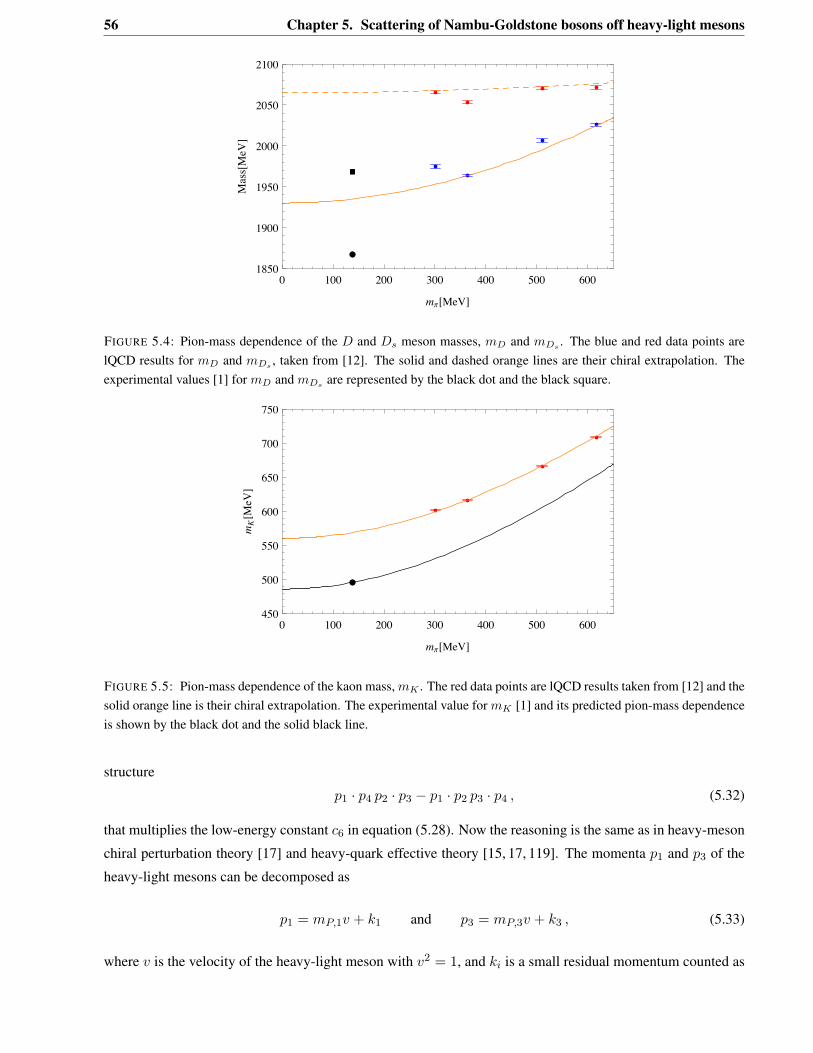
56 Chapter 5. Scattering of Nambu-Goldstone bosons off heavy-light mesons
0 100 200 300 400 500 6001850
1900
1950
2000
2050
2100
m!!MeV"Mass!MeV
"
FIGURE 5.4: Pion-mass dependence of the 𝐷 and 𝐷𝑠 meson masses, 𝑚𝐷 and 𝑚𝐷𝑠. The blue and red data points are
lQCD results for 𝑚𝐷 and 𝑚𝐷𝑠 , taken from [12]. The solid and dashed orange lines are their chiral extrapolation. Theexperimental values [1] for 𝑚𝐷 and 𝑚𝐷𝑠 are represented by the black dot and the black square.
0 100 200 300 400 500 600450
500
550
600
650
700
750
m!!MeV"
mK!MeV
"
FIGURE 5.5: Pion-mass dependence of the kaon mass, 𝑚𝐾 . The red data points are lQCD results taken from [12] and thesolid orange line is their chiral extrapolation. The experimental value for 𝑚𝐾 [1] and its predicted pion-mass dependenceis shown by the black dot and the solid black line.
structure
𝑝1 · 𝑝4 𝑝2 · 𝑝3 − 𝑝1 · 𝑝2 𝑝3 · 𝑝4 , (5.32)
that multiplies the low-energy constant 𝑐6 in equation (5.28). Now the reasoning is the same as in heavy-meson
chiral perturbation theory [17] and heavy-quark effective theory [15, 17, 119]. The momenta 𝑝1 and 𝑝3 of the
heavy-light mesons can be decomposed as
𝑝1 = 𝑚𝑃,1𝑣 + 𝑘1 and 𝑝3 = 𝑚𝑃,3𝑣 + 𝑘3 , (5.33)
where 𝑣 is the velocity of the heavy-light meson with 𝑣2 = 1, and 𝑘𝑖 is a small residual momentum counted as
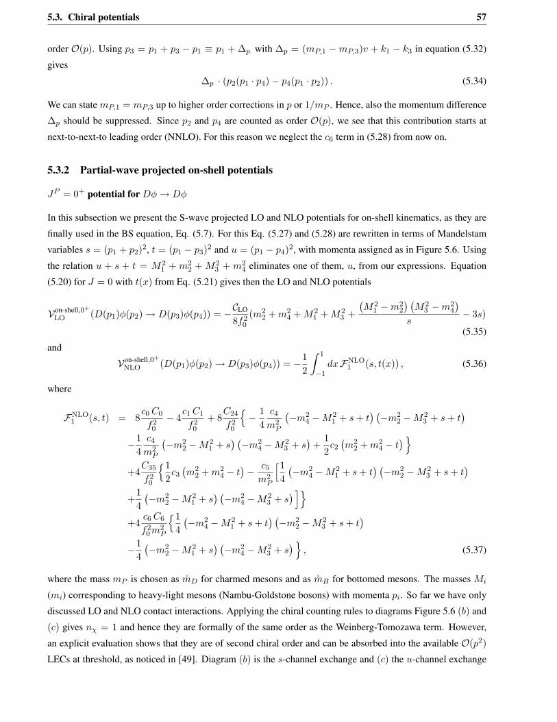
5.3. Chiral potentials 57
order 𝒪(𝑝). Using 𝑝3 = 𝑝1 + 𝑝3 − 𝑝1 ≡ 𝑝1 + Δ𝑝 with Δ𝑝 = (𝑚𝑃,1 −𝑚𝑃,3)𝑣 + 𝑘1 − 𝑘3 in equation (5.32)
gives
Δ𝑝 · (𝑝2(𝑝1 · 𝑝4)− 𝑝4(𝑝1 · 𝑝2)) . (5.34)
We can state 𝑚𝑃,1 = 𝑚𝑃,3 up to higher order corrections in 𝑝 or 1/𝑚𝑃 . Hence, also the momentum difference
Δ𝑝 should be suppressed. Since 𝑝2 and 𝑝4 are counted as order 𝒪(𝑝), we see that this contribution starts at
next-to-next-to leading order (NNLO). For this reason we neglect the 𝑐6 term in (5.28) from now on.
5.3.2 Partial-wave projected on-shell potentials
𝐽𝑃 = 0+ potential for 𝐷𝜑 → 𝐷𝜑
In this subsection we present the S-wave projected LO and NLO potentials for on-shell kinematics, as they are
finally used in the BS equation, Eq. (5.7). For this Eq. (5.27) and (5.28) are rewritten in terms of Mandelstam
variables 𝑠 = (𝑝1 + 𝑝2)2, 𝑡 = (𝑝1 − 𝑝3)2 and 𝑢 = (𝑝1 − 𝑝4)2, with momenta assigned as in Figure 5.6. Using
the relation 𝑢 + 𝑠 + 𝑡 = 𝑀21 + 𝑚2
2 + 𝑀23 + 𝑚2
4 eliminates one of them, 𝑢, from our expressions. Equation
(5.20) for 𝐽 = 0 with 𝑡(𝑥) from Eq. (5.21) gives then the LO and NLO potentials
𝒱on-shell,0+
LO (𝐷(𝑝1)𝜑(𝑝2) → 𝐷(𝑝3)𝜑(𝑝4)) = −𝒞LO
8𝑓20
(𝑚22 + 𝑚2
4 + 𝑀21 + 𝑀2
3 +
(𝑀2
1 −𝑚22
) (𝑀2
3 −𝑚24
)
𝑠− 3𝑠)
(5.35)
and
𝒱on-shell,0+
NLO (𝐷(𝑝1)𝜑(𝑝2) → 𝐷(𝑝3)𝜑(𝑝4)) = −12
∫ 1
−1𝑑𝑥ℱNLO
1 (𝑠, 𝑡(𝑥)) , (5.36)
where
ℱNLO1 (𝑠, 𝑡) = 8
𝑐0 𝐶0
𝑓20
− 4𝑐1 𝐶1
𝑓20
+ 8𝐶24
𝑓20
{− 1
4𝑐4
𝑚2𝑃
(−𝑚2
4 −𝑀21 + 𝑠 + 𝑡
) (−𝑚2
2 −𝑀23 + 𝑠 + 𝑡
)
−14
𝑐4
𝑚2𝑃
(−𝑚2
2 −𝑀21 + 𝑠
) (−𝑚2
4 −𝑀23 + 𝑠
)+
12𝑐2
(𝑚2
2 + 𝑚24 − 𝑡
)}
+4𝐶35
𝑓20
{12𝑐3
(𝑚2
2 + 𝑚24 − 𝑡
)− 𝑐5
𝑚2𝑃
[14(−𝑚2
4 −𝑀21 + 𝑠 + 𝑡
) (−𝑚2
2 −𝑀23 + 𝑠 + 𝑡
)
+14(−𝑚2
2 −𝑀21 + 𝑠
) (−𝑚2
4 −𝑀23 + 𝑠
) ]}
+4𝑐6 𝐶6
𝑓20 𝑚2
𝑃
{14(−𝑚2
4 −𝑀21 + 𝑠 + 𝑡
) (−𝑚2
2 −𝑀23 + 𝑠 + 𝑡
)
−14(−𝑚2
2 −𝑀21 + 𝑠
) (−𝑚2
4 −𝑀23 + 𝑠
)}, (5.37)
where the mass 𝑚𝑃 is chosen as ��𝐷 for charmed mesons and as ��𝐵 for bottomed mesons. The masses 𝑀𝑖
(𝑚𝑖) corresponding to heavy-light mesons (Nambu-Goldstone bosons) with momenta 𝑝𝑖. So far we have only
discussed LO and NLO contact interactions. Applying the chiral counting rules to diagrams Figure 5.6 (𝑏) and
(𝑐) gives 𝑛𝜒 = 1 and hence they are formally of the same order as the Weinberg-Tomozawa term. However,
an explicit evaluation shows that they are of second chiral order and can be absorbed into the available 𝒪(𝑝2)
LECs at threshold, as noticed in [49]. Diagram (𝑏) is the 𝑠-channel exchange and (𝑐) the 𝑢-channel exchange
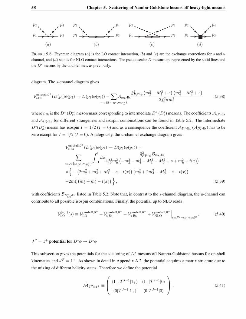
58 Chapter 5. Scattering of Nambu-Goldstone bosons off heavy-light mesons
p3
p4
p1
p2
p1
p2
p3
p4
(b) (c)(a)
p3
p4
p1
p2
(d)
p3
p4
p1
p2
FIGURE 5.6: Feynman diagram (𝑎) is the LO contact interaction, (𝑏) and (𝑐) are the exchange corrections for 𝑠 and 𝑢
channel, and (𝑑) stands for NLO contact interactions. The pseudoscalar 𝐷 mesons are represented by the solid lines andthe 𝐷* mesons by the double lines, as previously.
diagram. The 𝑠-channel diagram gives
𝒱on-shell,0+
s-Ex (𝐷(𝑝1)𝜑(𝑝2) → 𝐷(𝑝3)𝜑(𝑝4)) =∑
𝑚ℎ∈{𝑚𝐷* ,𝑚𝐷*𝑠 }
𝒜𝑚ℎ-Ex𝑔2𝑃𝑃 *𝜑
(𝑚2
2 −𝑀21 + 𝑠
) (𝑚2
4 −𝑀23 + 𝑠
)
2𝑓20 𝑠 𝑚2
ℎ
(5.38)
where 𝑚ℎ is the 𝐷* (𝐷*𝑠 ) meson mass corresponding to intermediate 𝐷* (𝐷*𝑠 ) mesons. The coefficients𝒜𝐷*-Ex
and 𝒜𝐷*𝑠 -Ex for different strangeness and isospin combinations can be found in Table 5.2. The intermediate
𝐷*(𝐷*𝑠 ) meson has isospin 𝐼 = 1/2 (𝐼 = 0) and as a consequence the coefficient 𝒜𝐷*-Ex (𝒜𝐷*𝑠 -Ex) has to be
zero except for 𝐼 = 1/2 (𝐼 = 0). Analogously, the 𝑢-channel exchange diagram gives
𝒱on-shell,0+
u-Ex (𝐷(𝑝1)𝜑(𝑝2) → 𝐷(𝑝3)𝜑(𝑝4)) =∑
𝑚ℎ∈{𝑚𝐷* ,𝑚𝐷*𝑠 }
∫ 1
−1𝑑𝑥
𝑔2𝑃𝑃 *𝜑 ℬ𝑚ℎ-Ex
4𝑓20 𝑚2
ℎ
(−𝑚2
2 −𝑚24 −𝑀2
1 −𝑀23 + 𝑠 + 𝑚2
ℎ + 𝑡(𝑥))
×{−(2𝑚2
2 + 𝑚24 + 𝑀2
1 − 𝑠− 𝑡(𝑥)) (
𝑚22 + 2𝑚2
4 + 𝑀23 − 𝑠− 𝑡(𝑥)
)
+2𝑚2ℎ
(𝑚2
2 + 𝑚24 − 𝑡(𝑥)
)}, (5.39)
with coefficients ℬ𝐷*(𝑠)
-Ex listed in Table 5.2. Note that, in contrast to the 𝑠-channel diagram, the 𝑢-channel can
contribute to all possible isospin combinations. Finally, the potential up to NLO reads
𝒱(𝑆,𝐼)LO (𝑠) ≡ 𝒱on-shell,0+
LO + 𝒱on-shell,0+
s-Ex + 𝒱on-shell,0+
u-Ex + 𝒱on-shell,0+
NLO
𝑠≡𝑃 2=(𝑝1+𝑝2)2
, (5.40)
𝐽𝑃 = 1+ potential for 𝐷*𝜑 → 𝐷*𝜑
This subsection gives the potentials for the scattering of 𝐷* mesons off Nambu-Goldstone bosons for on-shell
kinematics and 𝐽𝑃 = 1+. As shown in detail in Appendix A.2, the potential acquires a matrix structure due to
the mixing of different helicity states. Therefore we define the potential
ℳ𝐽𝑃 =1+ ≡
⎛⎜⎝⟨1+|𝒯 𝐽=1|1+⟩ ⟨1+|𝒯 𝐽=1|0⟩
⟨0|𝒯 𝐽=1|1+⟩ ⟨0|𝒯 𝐽=1|0⟩
⎞⎟⎠ , (5.41)
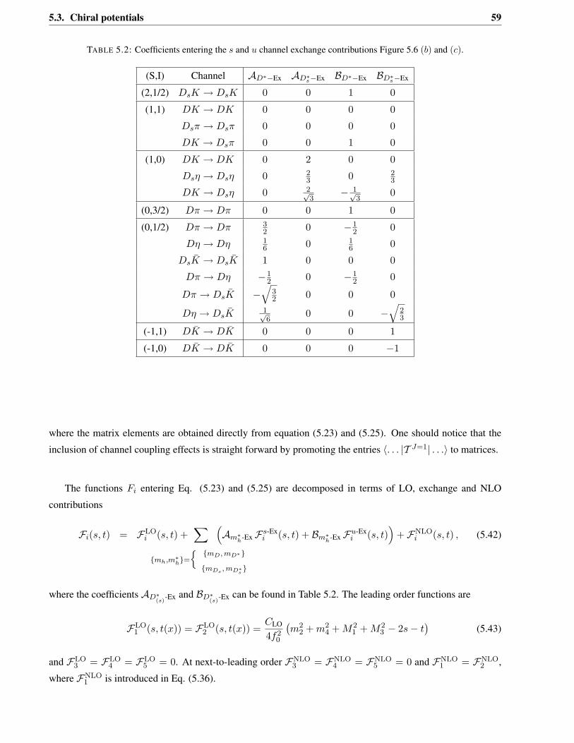
5.3. Chiral potentials 59
TABLE 5.2: Coefficients entering the 𝑠 and 𝑢 channel exchange contributions Figure 5.6 (𝑏) and (𝑐).
(S,I) Channel 𝒜𝐷*−Ex 𝒜𝐷*𝑠−Ex ℬ𝐷*−Ex ℬ𝐷*𝑠−Ex
(2,1/2) 𝐷𝑠𝐾 → 𝐷𝑠𝐾 0 0 1 0
(1,1) 𝐷𝐾 → 𝐷𝐾 0 0 0 0
𝐷𝑠𝜋 → 𝐷𝑠𝜋 0 0 0 0
𝐷𝐾 → 𝐷𝑠𝜋 0 0 1 0
(1,0) 𝐷𝐾 → 𝐷𝐾 0 2 0 0
𝐷𝑠𝜂 → 𝐷𝑠𝜂 0 23 0 2
3
𝐷𝐾 → 𝐷𝑠𝜂 0 2√3
− 1√3
0
(0,3/2) 𝐷𝜋 → 𝐷𝜋 0 0 1 0
(0,1/2) 𝐷𝜋 → 𝐷𝜋 32 0 −1
2 0
𝐷𝜂 → 𝐷𝜂 16 0 1
6 0
𝐷𝑠�� → 𝐷𝑠�� 1 0 0 0
𝐷𝜋 → 𝐷𝜂 −12 0 −1
2 0
𝐷𝜋 → 𝐷𝑠�� −√
32 0 0 0
𝐷𝜂 → 𝐷𝑠��1√6
0 0 −√
23
(-1,1) 𝐷�� → 𝐷�� 0 0 0 1
(-1,0) 𝐷�� → 𝐷�� 0 0 0 −1
where the matrix elements are obtained directly from equation (5.23) and (5.25). One should notice that the
inclusion of channel coupling effects is straight forward by promoting the entries ⟨. . . |𝒯 𝐽=1| . . .⟩ to matrices.
The functions 𝐹𝑖 entering Eq. (5.23) and (5.25) are decomposed in terms of LO, exchange and NLO
contributions
ℱ𝑖(𝑠, 𝑡) = ℱLO𝑖 (𝑠, 𝑡) +
∑
{𝑚ℎ,𝑚*ℎ}={ {𝑚𝐷, 𝑚𝐷*}
{𝑚𝐷𝑠 , 𝑚𝐷*𝑠 }
(𝒜𝑚*
ℎ-Exℱ𝑠-Ex𝑖 (𝑠, 𝑡) + ℬ𝑚*
ℎ-Exℱ𝑢-Ex𝑖 (𝑠, 𝑡)
)+ ℱNLO
𝑖 (𝑠, 𝑡) , (5.42)
where the coefficients 𝒜𝐷*(𝑠)
-Ex and ℬ𝐷*(𝑠)
-Ex can be found in Table 5.2. The leading order functions are
ℱLO1 (𝑠, 𝑡(𝑥)) = ℱLO
2 (𝑠, 𝑡(𝑥)) =𝐶LO
4𝑓20
(𝑚2
2 + 𝑚24 + 𝑀2
1 + 𝑀23 − 2𝑠− 𝑡
)(5.43)
and ℱLO3 = ℱLO
4 = ℱLO5 = 0. At next-to-leading order ℱNLO
3 = ℱNLO4 = ℱNLO
5 = 0 and ℱNLO1 = ℱNLO
2 ,
where ℱNLO1 is introduced in Eq. (5.36).
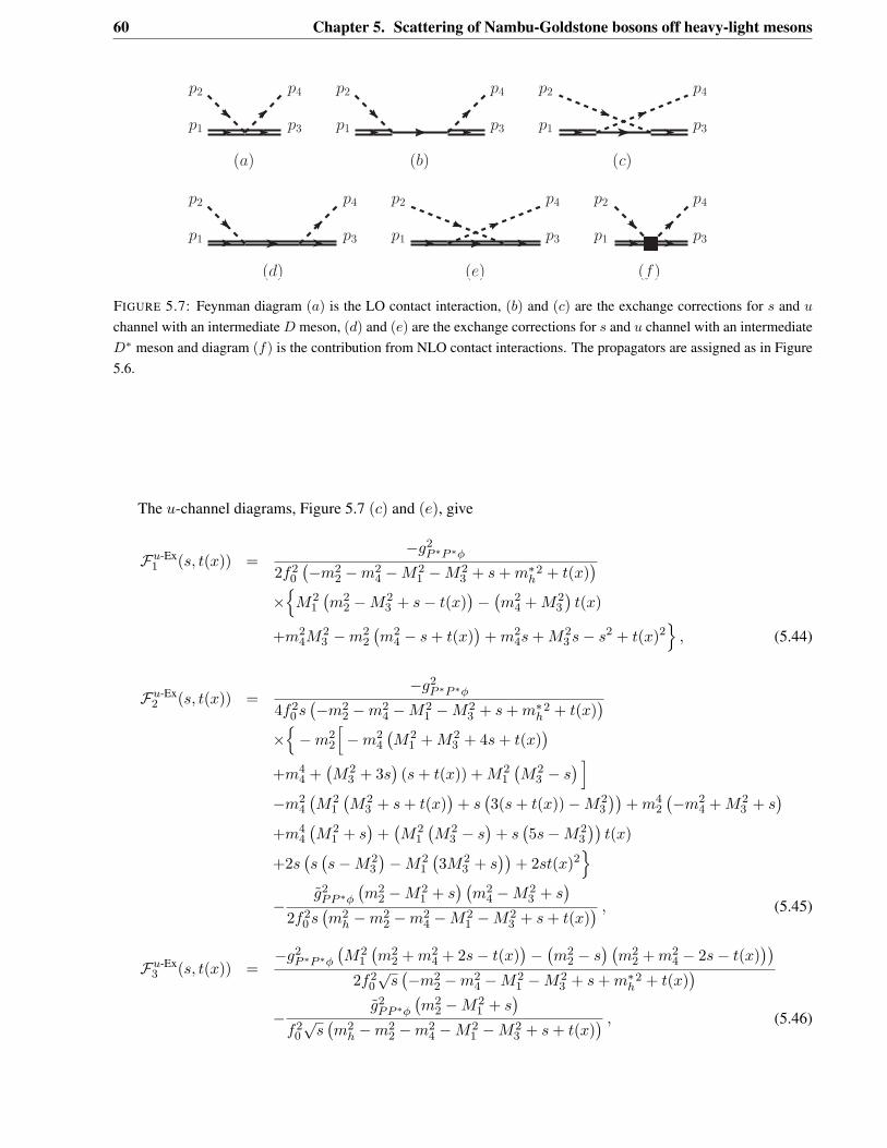
60 Chapter 5. Scattering of Nambu-Goldstone bosons off heavy-light mesons
p1
p2
(d)
p3
p4
p1
p2
(b)
p3
p4
p1
p2
p3
p4
(c)(a)
p1
p2
p3
p4
p1
p2
p3
p4
(e) (f)
p1
p2
p3
p4
FIGURE 5.7: Feynman diagram (𝑎) is the LO contact interaction, (𝑏) and (𝑐) are the exchange corrections for 𝑠 and 𝑢
channel with an intermediate 𝐷 meson, (𝑑) and (𝑒) are the exchange corrections for 𝑠 and 𝑢 channel with an intermediate𝐷* meson and diagram (𝑓) is the contribution from NLO contact interactions. The propagators are assigned as in Figure5.6.
The 𝑢-channel diagrams, Figure 5.7 (𝑐) and (𝑒), give
ℱ𝑢-Ex1 (𝑠, 𝑡(𝑥)) =
−𝑔2𝑃 *𝑃 *𝜑
2𝑓20
(−𝑚2
2 −𝑚24 −𝑀2
1 −𝑀23 + 𝑠 + 𝑚*ℎ
2 + 𝑡(𝑥))
×{
𝑀21
(𝑚2
2 −𝑀23 + 𝑠− 𝑡(𝑥)
)−(𝑚2
4 + 𝑀23
)𝑡(𝑥)
+𝑚24𝑀
23 −𝑚2
2
(𝑚2
4 − 𝑠 + 𝑡(𝑥))
+ 𝑚24𝑠 + 𝑀2
3 𝑠− 𝑠2 + 𝑡(𝑥)2}
, (5.44)
ℱ𝑢-Ex2 (𝑠, 𝑡(𝑥)) =
−𝑔2𝑃 *𝑃 *𝜑
4𝑓20 𝑠(−𝑚2
2 −𝑚24 −𝑀2
1 −𝑀23 + 𝑠 + 𝑚*ℎ
2 + 𝑡(𝑥))
×{−𝑚2
2
[−𝑚2
4
(𝑀2
1 + 𝑀23 + 4𝑠 + 𝑡(𝑥)
)
+𝑚44 +
(𝑀2
3 + 3𝑠)(𝑠 + 𝑡(𝑥)) + 𝑀2
1
(𝑀2
3 − 𝑠) ]
−𝑚24
(𝑀2
1
(𝑀2
3 + 𝑠 + 𝑡(𝑥))
+ 𝑠(3(𝑠 + 𝑡(𝑥))−𝑀2
3
))+ 𝑚4
2
(−𝑚2
4 + 𝑀23 + 𝑠
)
+𝑚44
(𝑀2
1 + 𝑠)
+(𝑀2
1
(𝑀2
3 − 𝑠)
+ 𝑠(5𝑠−𝑀2
3
))𝑡(𝑥)
+2𝑠(𝑠(𝑠−𝑀2
3
)−𝑀2
1
(3𝑀2
3 + 𝑠))
+ 2𝑠𝑡(𝑥)2}
−𝑔2𝑃𝑃 *𝜑
(𝑚2
2 −𝑀21 + 𝑠
) (𝑚2
4 −𝑀23 + 𝑠
)
2𝑓20 𝑠(𝑚2
ℎ −𝑚22 −𝑚2
4 −𝑀21 −𝑀2
3 + 𝑠 + 𝑡(𝑥)) , (5.45)
ℱ𝑢-Ex3 (𝑠, 𝑡(𝑥)) =
−𝑔2𝑃 *𝑃 *𝜑
(𝑀2
1
(𝑚2
2 + 𝑚24 + 2𝑠− 𝑡(𝑥)
)−(𝑚2
2 − 𝑠) (
𝑚22 + 𝑚2
4 − 2𝑠− 𝑡(𝑥)))
2𝑓20
√𝑠(−𝑚2
2 −𝑚24 −𝑀2
1 −𝑀23 + 𝑠 + 𝑚*ℎ
2 + 𝑡(𝑥))
−𝑔2𝑃𝑃 *𝜑
(𝑚2
2 −𝑀21 + 𝑠
)
𝑓20
√𝑠(𝑚2
ℎ −𝑚22 −𝑚2
4 −𝑀21 −𝑀2
3 + 𝑠 + 𝑡(𝑥)) , (5.46)
5.3. Chiral potentials 61
ℱ𝑢-Ex4 (𝑠, 𝑡(𝑥)) =
−𝑔2𝑃 *𝑃 *𝜑
2𝑓20
√𝑠(−𝑚2
2 −𝑚24 −𝑀2
1 −𝑀23 + 𝑠 + 𝑚*ℎ
2 + 𝑡(𝑥))
×(𝑀2
3
(𝑚2
4 + 2𝑠− 𝑡(𝑥))
+ 𝑚22
(−𝑚2
4 + 𝑀23 + 𝑠
)−(𝑚2
4 − 𝑠) (
𝑚24 − 2𝑠− 𝑡(𝑥)
))
−𝑔2𝑃𝑃 *𝜑
(𝑚2
4 −𝑀23 + 𝑠
)
𝑓20
√𝑠(𝑚2
ℎ −𝑚22 −𝑚2
4 −𝑀21 −𝑀2
3 + 𝑠 + 𝑡(𝑥)) , (5.47)
ℱ𝑢-Ex5 (𝑠, 𝑡(𝑥)) =
−𝑔2𝑃 *𝑃 *𝜑
(𝑚2
2 + 𝑚24 − 𝑡(𝑥)
)
𝑓20
(𝑚2
2 + 𝑚24 + 𝑀2
1 + 𝑀23 − 𝑠−𝑚*ℎ
2 − 𝑡(𝑥))
−2𝑔2
𝑃𝑃 *𝜑
𝑓20
(𝑚2
ℎ −𝑚22 −𝑚2
4 −𝑀21 −𝑀2
3 + 𝑠 + 𝑡(𝑥)) . (5.48)
and the 𝑠-channel diagrams do not contribute for 𝐽𝑃 = 1+, as can be confirmed by an explicit calculation.
Potentials in heavy-meson 𝜒PT
In the HM𝜒PT, the LO potential reduces to
𝒱on-shell,0+
LO =1
4𝑓20
2𝑀(𝐸2 + 𝐸4)𝒞LO (5.49)
after 𝑆-wave projection, with 𝑀 chosen as ��𝐷 for charmed mesons and as ��𝐵 for bottomed mesons, c.f.
Table 4.1. At NLO, with the on-shell approximation and for 𝑆-wave interactions, effectively only four of the
six low-energy constants contribute, i.e.,
𝒱on-shell,0+
NLO = − 8𝑓20
𝐶24 𝑐24 𝐸2𝐸4 −4𝑓20
𝒞35 𝑐35 𝐸2𝐸4 −8𝑓20
𝒞0 𝑐0 +4𝑓20
𝒞1 𝑐1 , (5.50)
where 𝑐24 = 𝑐2 − 2𝑐4 and 𝑐35 = 𝑐3 − 2𝑐5 (see, e.g., Ref. [104]). The LO exchange diagrams start contributing
at NLO and hence do not have to be considered within HM𝜒PT.
The potential for the scattering of Nambu-Goldstone bosons off heavy-light vector meson can be easily
derived by Eq.(5.41). In the infinite heavy-quark limit we have 𝜖*3 · 𝜖1 = −1, which leads to
𝒱LO(NLO)(𝑃 *(𝑝1)𝜑(𝑝2) → 𝑃 *(𝑝3)𝜑(𝑝4)) = 𝒱LO(NLO)(𝑃 (𝑝1)𝜑(𝑝2) → 𝑃 (𝑝3)𝜑(𝑝4)) (5.51)
(see also, e.g., Ref. [120]). One should notice that the different helicity states do not mix in the heavy-quark
limit, reducing the potentials to the simplified form Eq. (5.51).
62 Chapter 5. Scattering of Nambu-Goldstone bosons off heavy-light mesons
5.4 The scattering of Nambu-Goldstone bosons off heavy-light mesons in theHQS scheme
5.4.1 Renormalization scheme motivated by heavy-quark symmetry
It is well known that perturbation theory at any finite order cannot generate bound states or resonances. One way
to proceed is to perform an infinite summation of a leading subclass of diagrams to all orders using the Bethe-
Salpeter (or Lippmann-Schwinger) equation, Eq. (5.7). In combination with coupled-channels dynamics,
this approach has turned out to be quite successful in describing a multitude of low-energy strong-interaction
phenomena (see, e.g., Refs. [121–129] for early references and Refs. [100, 101] for some recent applications).
To simplify the calculations, the so-called on-shell approximation [122, 123] is often introduced, with the
argument that the off-shell effects are relegated to higher orders. Schematically, the Bethe-Salpeter equation
(5.7) can then be written as
𝑇 = 𝑉 + 𝑉 𝐺𝑇, (5.52)
where 𝑉 is the potential and 𝐺 is a loop function defined in the following way
𝐺(𝑠, 𝑀2, 𝑚2) ≡ 𝑖
∫𝑑𝑛𝑞
(2𝜋)𝑛
1[(𝑃 − 𝑞)2 −𝑚2 + 𝑖𝜖](𝑞2 −𝑀2 + 𝑖𝜖)
, (5.53)
where 𝑃 = (√
𝑠, 0, 0, 0) is the total momentum of the two particles. 𝑀 and 𝑚 are the masses of the heavy-light
meson and of the Nambu-Goldstone boson, respectively, in the two-particle intermediate state. According to
the power counting rule specified in Section 4, the loop function 𝐺 counts as of 𝒪(𝑝). An explicit evaluation
in 𝑛 = 4 dimensions with the modified minimal subtraction scheme yields
𝐺MS(𝑠, 𝑀2, 𝑚2) =
116𝜋2
{𝑚2 −𝑀2 + 𝑠
2𝑠log(
𝑚2
𝑀2
)
− 𝑞√𝑠
{log[2𝑞
√𝑠 + 𝑚2 −𝑀2 − 𝑠] + log[2𝑞
√𝑠−𝑚2 + 𝑀2 − 𝑠]
− log[2𝑞√
𝑠 + 𝑚2 −𝑀2 + 𝑠]− log[2𝑞√
𝑠−𝑚2 + 𝑀2 + 𝑠]}
+(
log(
𝑀2
𝜇2
)− 2)}
, (5.54)
where 𝑞 =√
(𝑠−(𝑚+𝑀)2)(𝑠−(𝑚−𝑀)2)
2√
𝑠is the centre of mass (three) momentum. It is easily seen that the un-
derlined term in the loop function (5.54) breaks the chiral power counting. In addition, the heavy-quark flavor
symmetry and, to a less extent, the heavy-quark spin symmetry are also broken in the covariant loop function,
as noticed in Ref. [104]. The ambiguity in choosing the finite part of the loop function is reflected in the appear-
ance of the renormalization scale 𝜇. In perturbation theory up to some given order, these ambiguities are well
understood. All divergent parts can be absorbed into the low-energy constants of the theory and the dependence
on the renormalization scale is compensated by the scale dependence of the low-energy constants. However,
our solution of the BS equation does not correspond to a consistent perturbation theory calculation. As a conse-
quence, the ambiguity of the loop integral is reflected in the final results, i.e. the scattering amplitude depends
5.4. The scattering of Nambu-Goldstone bosons off heavy-light mesons in the HQS scheme 63
on the renormalization scale 𝜇. There are different approaches to arrive at reasonable predictions anyway. The
most common way is to consider 𝜇 as an additional parameter of the theory. This is usually done by replacing
the underlined term −2 in Eq. (5.54) by the so-called subtraction constant, 𝑎(𝜇), which we will refer to as
the MS scheme from now on. Another method is the 𝜒−BS(3) approach proposed by [121, 130], as has been
applied to heavy-light mesons in [96, 131]. This approach has the appealing feature that crossing symmetry is
restored at a given kinematical point.
In the following we propose a renormalization scheme that restores the chiral power counting and ensures
that the loop function 𝐺 has a well defined behavior in the 𝑀 → ∞ limit. To achieve this, we turn to the HM
ChPT. In the static limit the momentum of the heavy-light meson is decomposed as 𝑝𝑃 = 𝑚𝑃 𝑣 + 𝑘, where 𝑣 is
the constant velocity (𝑣2 = 1) and 𝑚𝑃 the mass of the heavy-light meson in the chiral limit. The small residual
momentum is denoted by 𝑘. Using momentum conservation and expanding in 1/𝑚𝑃 gives for the heavy-light
meson propagator the replacement
1𝑝2
𝑃 −𝑀2 + 𝑖𝜖→ 1
2𝑚𝑃 𝑣 · 𝑘 + 2𝑚𝑃 Δ𝑃 + 𝑖𝜖(5.55)
at leading order in 1/𝑚𝑃 . The mass splitting Δ𝑃 is defined as Δ𝑃 ≡ 𝑚𝑃−𝑀 . This gives the loop function
in HM𝜒PT, (see, e.g., Refs. [23, 104]),
𝐺HM(𝑠, 𝑀2, 𝑚2) =1
16𝜋2𝑀
{2√
Δ2HM −𝑚2
(arccosh
(ΔHM
𝑚
)− 𝜋𝑖
)+ ΔHM
(log(
𝑚2
𝜇2
)+ 𝑎
)},
(5.56)
where 𝑀 is the chiral limit value of the heavy-light meson mass appearing in the loop and ΔHM =√
𝑠 −𝑀 .
Comparing 𝐺HM with the loop function of Eq. (5.54) expanded up to order 1/𝑀 ,
𝐺(𝑠, 𝑀2, 𝑚2) =1
16𝜋2
(log
(𝑀2
𝜇2
)− 2
)+
+1
16𝜋2𝑀
{2√
Δ2HM −𝑚2
(arccosh
(ΔHM
𝑚
)− 𝜋𝑖
)+ ΔHM log
(𝑚2
𝑀2
)}, (5.57)
one is tempted to introduce the following renormalization scheme:
𝐺HQS(𝑠, 𝑀2, 𝑚2) ≡ 𝐺(𝑠, 𝑀2, 𝑚2)
− 116𝜋2
(log
(𝑀2
𝜇2
)− 2
)+
𝑚sub
16𝜋2𝑀
(log
(𝑀2
𝜇2
)+ 𝑎
), (5.58)
where 𝑚sub = 𝑚. From now on, we will refer to this loop function as the heavy-quark symmetry (HQS)
inspired loop function. It should be noted that in Eq. (5.58) we have chosen to renormalize the loop function at
the threshold of√
𝑠 = 𝑀 + 𝑚, where ΔHM = 𝑚(𝑚sub). It is easily seen that the renormalized loop function
𝐺HQS satisfies the chiral power counting and also exhibits a well-defined behavior in the 𝑀 → ∞ limit.7 At
7If we drop the non-perturbative term 𝑚
16𝜋2𝑀
(log
(𝑀2
𝜇2
)+ 𝑎
), it can be easily seen that our proposed renormalization scheme is
64 Chapter 5. Scattering of Nambu-Goldstone bosons off heavy-light mesons
fixed 𝑀 and 𝑚sub the ansatz we propose is equivalent to the MS approach widely used in UChPT, but it has
the advantage of manifestly satisfying the (approximate) heavy-quark spin and flavor symmetries at threshold.
In our study of the scattering lengths of Nambu-Goldstone boson bosons off the 𝐷 mesons, the subtraction
constant 𝑎 can in principle vary from channel to channel, depending on the intermediate Nambu-Goldstone
boson. A reasonable alternative is to use for 𝑚sub an SU(3) average mass, e.g., 𝑚sub = (3𝑚𝜋 + 4𝑚𝐾 +
𝑚𝜂)/8 = 0.3704 GeV, and have a common subtraction constant 𝑎 for all channels. A variation of this value
from 𝑚𝜋 to 𝑚𝜂 can serve as an estimate of uncertainties as one tries to connect physics of the 𝐷 and 𝐵 sectors.
It should be stressed that using the mass of the intermediate Nambu-Goldstone boson in the subtraction but
keeping a common subtraction constant for all channels will introduce sizable uncontrolled SU(3) breaking
corrections that should be avoided.
In Fig. 5.8, we show the dependence of the loop functions calculated in the HQS, HM and MS schemes with
the renormalization scale 𝜇 = 1 GeV 8 , 𝑀 = 𝑀 , 𝑚 = 𝑚𝜋 = 0.138 GeV,√
𝑠 = 𝑀 + 𝑚, and 𝑚sub = 0.3704
GeV. For the sake of comparison, we have plotted the loop function defined in the chiral SU(3) scheme of
Ref. [121], which has the following form
𝐺𝜒−SU(3) = 𝐺MS(𝑠, 𝑀2, 𝑚2)−𝐺MS(𝑀
2, 𝑀2, 𝑚2). (5.59)
This approach has the appealing feature that crossing symmetry is restored at a given kinematical point, here
for√
𝑠 = 𝑀 . For this case all loop corrections vanish and only the potential remains, which is obviously
crossing symmetric by construction. For Fig. 5.8 the subtraction constants in the HM, HQS, and MS schemes
are adjusted to reproduce the 𝐺𝜒−SU(3) at 𝑀 = 2 GeV. From Eq. (5.56) one can see that 𝐺HM is inversely
proportional to 𝑀 and therefore 𝑀𝐺 is a constant for the HM loop function. On the other hand, the 𝐺 function
in the HQS scheme is slightly upward curved while the 𝐺 function in the 𝜒-SU(3) downward curved. The naive
MS scheme, on the other hand, changes rapidly with 𝑀 . It is clear that without readjusting 𝑎 for different 𝑀 ,
which could correspond to either a heavy-light 𝐵 meson or 𝐷 meson, heavy-quark flavor symmetry is lost as
pointed out in Ref. [104].
So far, we have concentrated on the 1/𝑀 scaling of the loop function 𝐺 in different schemes, but have not
paid much attention to the chiral series or SU(3) breaking effects. In terms of 1/𝑀 scaling, the HM, HQS,
and 𝜒-SU(3) approaches all seem reasonable, as shown in Fig. 5.8. On the other hand, compared to the HM
ChPT or the 𝜒-SU(3) approach, the subtraction constant in the HQS scheme has the simplest form consistent
with the chiral power counting and 1/𝑀 scaling. We will see in the following subsection that such a choice
seems to play a non-negligible role in describing the light-quark mass dependence of the scattering lengths of
the Nambu-Goldstone bosons off the 𝐷 mesons.
in the spirit of the EOMS scheme to remove the power-counting-breaking terms.8From a theoretical point of view, the renormalization scale 𝜇 should be the chiral-symmetry breaking scale, Λ𝜒 ≈ 4𝜋𝑓0 ≈ 1.2
GeV, which can be immediately seen by examining the HM ChPT loop function of Eq. (5.56).
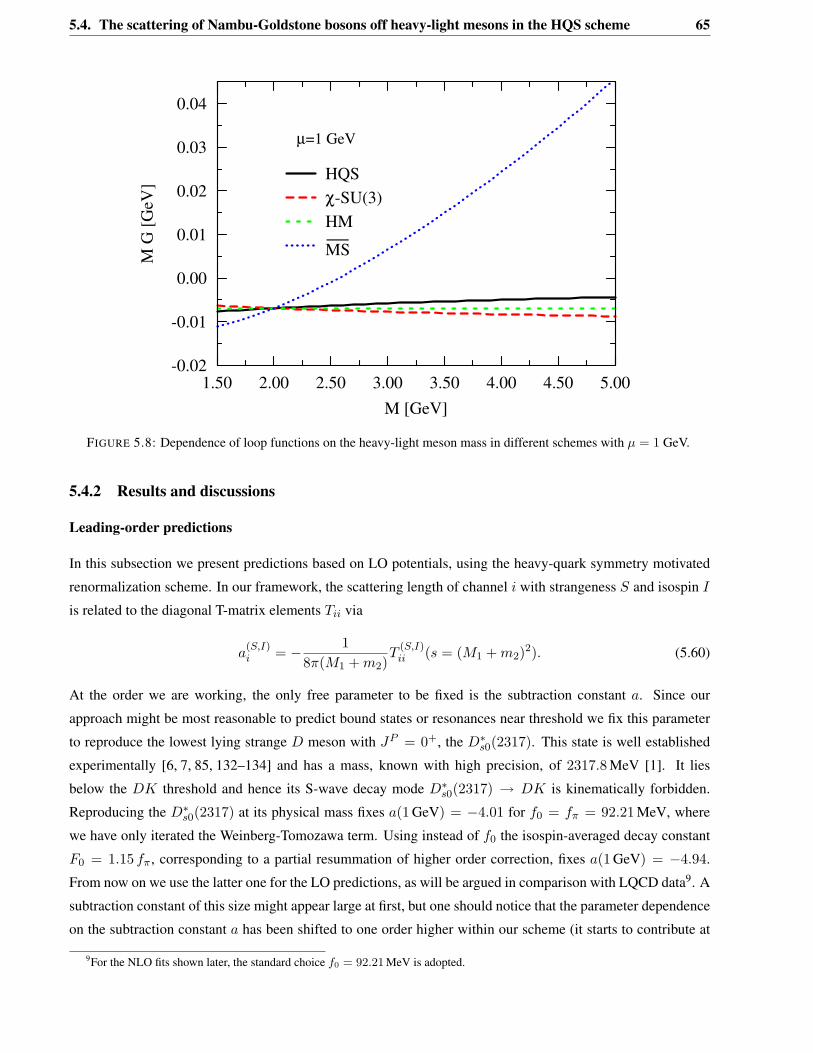
5.4. The scattering of Nambu-Goldstone bosons off heavy-light mesons in the HQS scheme 65
-0.02
-0.01
0.00
0.01
0.02
0.03
0.04
1.50 2.00 2.50 3.00 3.50 4.00 4.50 5.00
M G
[G
eV]
M [GeV]
µ=1 GeV
HQS
!-SU(3)
HM
MS"
FIGURE 5.8: Dependence of loop functions on the heavy-light meson mass in different schemes with 𝜇 = 1 GeV.
5.4.2 Results and discussions
Leading-order predictions
In this subsection we present predictions based on LO potentials, using the heavy-quark symmetry motivated
renormalization scheme. In our framework, the scattering length of channel 𝑖 with strangeness 𝑆 and isospin 𝐼
is related to the diagonal T-matrix elements 𝑇𝑖𝑖 via
𝑎(𝑆,𝐼)𝑖 = − 1
8𝜋(𝑀1 + 𝑚2)𝑇
(𝑆,𝐼)𝑖𝑖 (𝑠 = (𝑀1 + 𝑚2)2). (5.60)
At the order we are working, the only free parameter to be fixed is the subtraction constant 𝑎. Since our
approach might be most reasonable to predict bound states or resonances near threshold we fix this parameter
to reproduce the lowest lying strange 𝐷 meson with 𝐽𝑃 = 0+, the 𝐷*𝑠0(2317). This state is well established
experimentally [6, 7, 85, 132–134] and has a mass, known with high precision, of 2317.8 MeV [1]. It lies
below the 𝐷𝐾 threshold and hence its S-wave decay mode 𝐷*𝑠0(2317) → 𝐷𝐾 is kinematically forbidden.
Reproducing the 𝐷*𝑠0(2317) at its physical mass fixes 𝑎(1 GeV) = −4.01 for 𝑓0 = 𝑓𝜋 = 92.21 MeV, where
we have only iterated the Weinberg-Tomozawa term. Using instead of 𝑓0 the isospin-averaged decay constant
𝐹0 = 1.15 𝑓𝜋, corresponding to a partial resummation of higher order correction, fixes 𝑎(1 GeV) = −4.94.
From now on we use the latter one for the LO predictions, as will be argued in comparison with LQCD data9. A
subtraction constant of this size might appear large at first, but one should notice that the parameter dependence
on the subtraction constant 𝑎 has been shifted to one order higher within our scheme (it starts to contribute at
9For the NLO fits shown later, the standard choice 𝑓0 = 92.21 MeV is adopted.
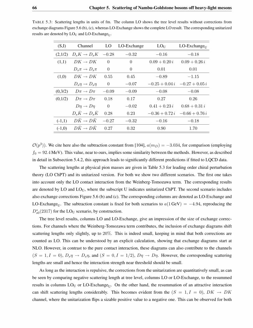
66 Chapter 5. Scattering of Nambu-Goldstone bosons off heavy-light mesons
TABLE 5.3: Scattering lengths in units of fm. The column LO shows the tree level results without corrections fromexchange diagrams Figure 5.6 (b), (c), whereas LO-Exchange shows the complete LO result. The corresponding unitarizedresults are denoted by LOU and LO-ExchangeU.
(S,I) Channel LO LO-Exchange LOU LO-ExchangeU
(2,1/2) 𝐷𝑠𝐾 → 𝐷𝑠𝐾 −0.28 −0.32 −0.16 −0.18
(1,1) 𝐷𝐾 → 𝐷𝐾 0 0 0.09 + 0.20 𝑖 0.09 + 0.26 𝑖
𝐷𝑠𝜋 → 𝐷𝑠𝜋 0 0 0.01 0.01
(1,0) 𝐷𝐾 → 𝐷𝐾 0.55 0.45 −0.89 −1.15
𝐷𝑠𝜂 → 𝐷𝑠𝜂 0 −0.07 −0.25 + 0.04 𝑖 −0.27 + 0.05 𝑖
(0,3/2) 𝐷𝜋 → 𝐷𝜋 −0.09 −0.09 −0.08 −0.08
(0,1/2) 𝐷𝜋 → 𝐷𝜋 0.18 0.17 0.27 0.26
𝐷𝜂 → 𝐷𝜂 0 −0.02 0.41 + 0.23 𝑖 0.68 + 0.31 𝑖
𝐷𝑠�� → 𝐷𝑠�� 0.28 0.23 −0.36 + 0.72 𝑖 −0.66 + 0.76 𝑖
(-1,1) 𝐷�� → 𝐷�� −0.27 −0.32 −0.16 −0.18
(-1,0) 𝐷�� → 𝐷�� 0.27 0.32 0.90 1.70
𝒪(𝑝3)). We cite here also the subtraction constant from [104], 𝑎(𝑚𝐷) = −3.034, for comparison (employing
𝑓0 = 92.4 MeV). This value, near to ours, implies some similarity between the methods. However, as described
in detail in Subsection 5.4.2, this approach leads to significantly different predictions if fitted to LQCD data.
The scattering lengths at physical pion masses are given in Table 5.3 for leading order chiral perturbation
theory (LO ChPT) and its unitarized version. For both we show two different scenarios. The first one takes
into account only the LO contact interaction from the Weinberg-Tomozawa term. The corresponding results
are denoted by LO and LOU, where the subscript U indicates unitarized ChPT. The second scenario includes
also exchange corrections Figure 5.6 (b) and (c). The corresponding columns are denoted as LO-Exchange and
LO-ExchangeU. The subtraction constant is fixed for both scenarios to 𝑎(1 GeV) = −4.94, reproducing the
𝐷*𝑠0(2317) for the LOU scenario, by construction.
The tree level results, columns LO and LO-Exchange, give an impression of the size of exchange correc-
tions. For channels where the Weinberg-Tomozawa term contributes, the inclusion of exchange diagrams shift
scattering lengths only slightly, up to 20%. This is indeed small, keeping in mind that both corrections are
counted as LO. This can be understood by an explicit calculation, showing that exchange diagrams start at
NLO. However, in contrast to the pure contact interaction, these diagrams can also contribute to the channels
(𝑆 = 1, 𝐼 = 0), 𝐷𝑠𝜂 → 𝐷𝑠𝜂, and (𝑆 = 0, 𝐼 = 1/2), 𝐷𝜂 → 𝐷𝜂. However, the corresponding scattering
lengths are small and hence the interaction strength near threshold should be small.
As long as the interaction is repulsive, the corrections from the unitarization are quantitatively small, as can
be seen by comparing negative scattering length at tree level, columns LO or LO-Exchange, to the resummed
results in columns LOU or LO-ExchangeU. On the other hand, the resummation of an attractive interaction
can shift scattering lengths considerably. This becomes evident from the (𝑆 = 1, 𝐼 = 0), 𝐷𝐾 → 𝐷𝐾
channel, where the unitarization flips a sizable positive value to a negative one. This can be observed for both
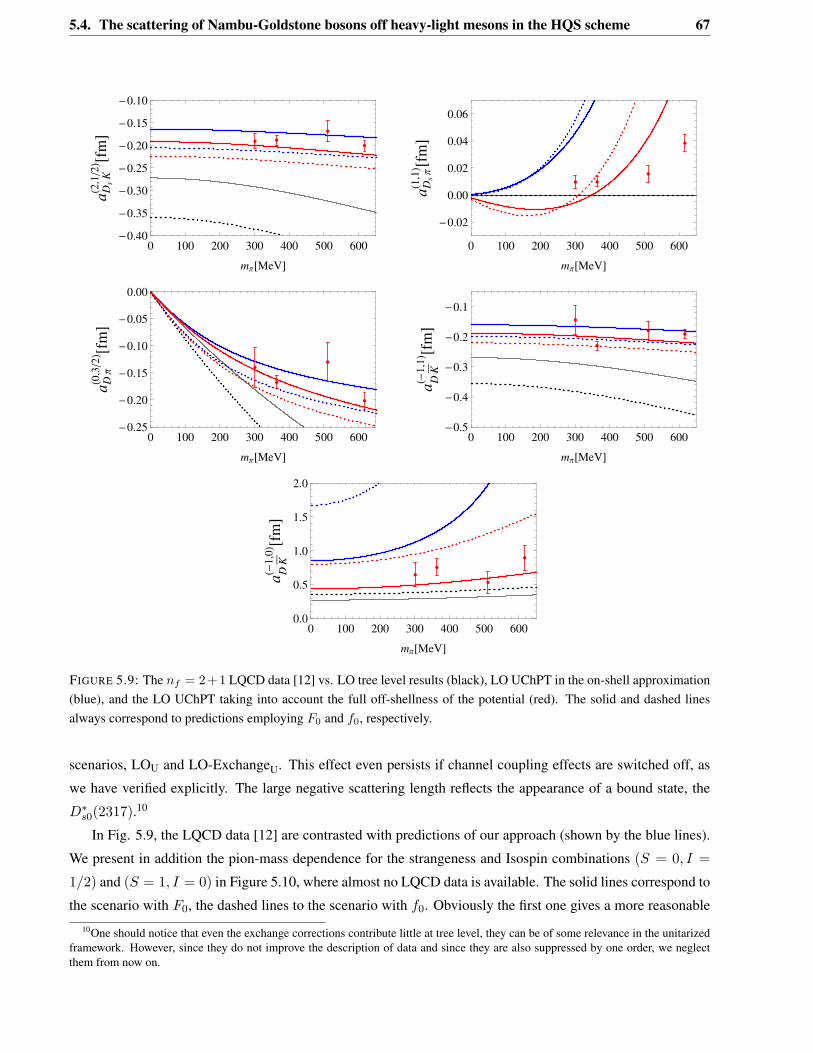
5.4. The scattering of Nambu-Goldstone bosons off heavy-light mesons in the HQS scheme 67
0 100 200 300 400 500 600-0.40
-0.35
-0.30
-0.25
-0.20
-0.15
-0.10
mΠ@MeVD
aD
sK
H2,1
�2L@fm
D
0 100 200 300 400 500 600
-0.02
0.00
0.02
0.04
0.06
mΠ@MeVD
aD
sΠ
H1,1
L @fmD
0 100 200 300 400 500 600-0.25
-0.20
-0.15
-0.10
-0.05
0.00
mΠ@MeVD
aD
ΠH0,3
�2L@fm
D
0 100 200 300 400 500 600-0.5
-0.4
-0.3
-0.2
-0.1
mΠ@MeVDa
DKH-1
,1L @fm
D
0 100 200 300 400 500 6000.0
0.5
1.0
1.5
2.0
mΠ@MeVD
aD
KH-1,0
L @fmD
FIGURE 5.9: The 𝑛𝑓 = 2+1 LQCD data [12] vs. LO tree level results (black), LO UChPT in the on-shell approximation(blue), and the LO UChPT taking into account the full off-shellness of the potential (red). The solid and dashed linesalways correspond to predictions employing 𝐹0 and 𝑓0, respectively.
scenarios, LOU and LO-ExchangeU. This effect even persists if channel coupling effects are switched off, as
we have verified explicitly. The large negative scattering length reflects the appearance of a bound state, the
𝐷*𝑠0(2317).10
In Fig. 5.9, the LQCD data [12] are contrasted with predictions of our approach (shown by the blue lines).
We present in addition the pion-mass dependence for the strangeness and Isospin combinations (𝑆 = 0, 𝐼 =
1/2) and (𝑆 = 1, 𝐼 = 0) in Figure 5.10, where almost no LQCD data is available. The solid lines correspond to
the scenario with 𝐹0, the dashed lines to the scenario with 𝑓0. Obviously the first one gives a more reasonable
10One should notice that even the exchange corrections contribute little at tree level, they can be of some relevance in the unitarizedframework. However, since they do not improve the description of data and since they are also suppressed by one order, we neglectthem from now on.
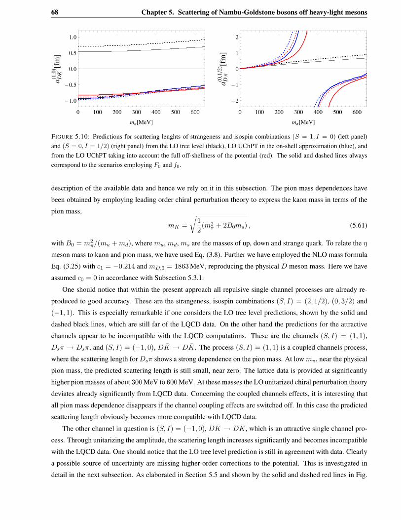
68 Chapter 5. Scattering of Nambu-Goldstone bosons off heavy-light mesons
0 100 200 300 400 500 600
-1.0
-0.5
0.0
0.5
1.0
mΠ@MeVD
aD
KH1,0
L @fmD
0 100 200 300 400 500 600
-2
-1
0
1
2
mΠ@MeVD
aD
ΠH0,1
�2L@fm
D
FIGURE 5.10: Predictions for scattering lenghts of strangeness and isospin combinations (𝑆 = 1, 𝐼 = 0) (left panel)and (𝑆 = 0, 𝐼 = 1/2) (right panel) from the LO tree level (black), LO UChPT in the on-shell approximation (blue), andfrom the LO UChPT taking into account the full off-shellness of the potential (red). The solid and dashed lines alwayscorrespond to the scenarios employing 𝐹0 and 𝑓0.
description of the available data and hence we rely on it in this subsection. The pion mass dependences have
been obtained by employing leading order chiral perturbation theory to express the kaon mass in terms of the
pion mass,
𝑚𝐾 =
√12(𝑚2
𝜋 + 2𝐵0𝑚𝑠) , (5.61)
with 𝐵0 = 𝑚2𝜋/(𝑚𝑢 + 𝑚𝑑), where 𝑚𝑢, 𝑚𝑑, 𝑚𝑠 are the masses of up, down and strange quark. To relate the 𝜂
meson mass to kaon and pion mass, we have used Eq. (3.8). Further we have employed the NLO mass formula
Eq. (3.25) with 𝑐1 = −0.214 and 𝑚𝐷,0 = 1863 MeV, reproducing the physical 𝐷 meson mass. Here we have
assumed 𝑐0 = 0 in accordance with Subsection 5.3.1.
One should notice that within the present approach all repulsive single channel processes are already re-
produced to good accuracy. These are the strangeness, isospin combinations (𝑆, 𝐼) = (2, 1/2), (0, 3/2) and
(−1, 1). This is especially remarkable if one considers the LO tree level predictions, shown by the solid and
dashed black lines, which are still far of the LQCD data. On the other hand the predictions for the attractive
channels appear to be incompatible with the LQCD computations. These are the channels (𝑆, 𝐼) = (1, 1),
𝐷𝑠𝜋 → 𝐷𝑠𝜋, and (𝑆, 𝐼) = (−1, 0), 𝐷�� → 𝐷��. The process (𝑆, 𝐼) = (1, 1) is a coupled channels process,
where the scattering length for 𝐷𝑠𝜋 shows a strong dependence on the pion mass. At low 𝑚𝜋, near the physical
pion mass, the predicted scattering length is still small, near zero. The lattice data is provided at significantly
higher pion masses of about 300 MeV to 600 MeV. At these masses the LO unitarized chiral perturbation theory
deviates already significantly from LQCD data. Concerning the coupled channels effects, it is interesting that
all pion mass dependence disappears if the channel coupling effects are switched off. In this case the predicted
scattering length obviously becomes more compatible with LQCD data.
The other channel in question is (𝑆, 𝐼) = (−1, 0), 𝐷�� → 𝐷��, which is an attractive single channel pro-
cess. Through unitarizing the amplitude, the scattering length increases significantly and becomes incompatible
with the LQCD data. One should notice that the LO tree level prediction is still in agreement with data. Clearly
a possible source of uncertainty are missing higher order corrections to the potential. This is investigated in
detail in the next subsection. As elaborated in Section 5.5 and shown by the solid and dashed red lines in Fig.
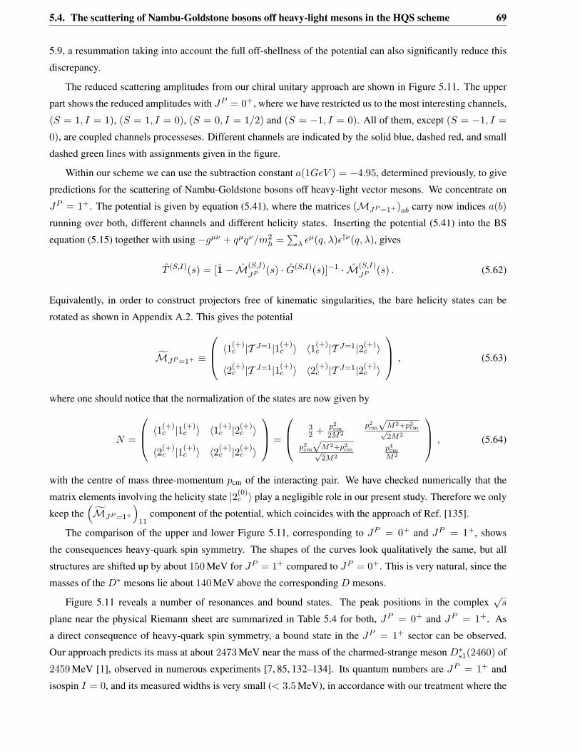
5.4. The scattering of Nambu-Goldstone bosons off heavy-light mesons in the HQS scheme 69
5.9, a resummation taking into account the full off-shellness of the potential can also significantly reduce this
discrepancy.
The reduced scattering amplitudes from our chiral unitary approach are shown in Figure 5.11. The upper
part shows the reduced amplitudes with 𝐽𝑃 = 0+, where we have restricted us to the most interesting channels,
(𝑆 = 1, 𝐼 = 1), (𝑆 = 1, 𝐼 = 0), (𝑆 = 0, 𝐼 = 1/2) and (𝑆 = −1, 𝐼 = 0). All of them, except (𝑆 = −1, 𝐼 =
0), are coupled channels processeses. Different channels are indicated by the solid blue, dashed red, and small
dashed green lines with assignments given in the figure.
Within our scheme we can use the subtraction constant 𝑎(1𝐺𝑒𝑉 ) = −4.95, determined previously, to give
predictions for the scattering of Nambu-Goldstone bosons off heavy-light vector mesons. We concentrate on
𝐽𝑃 = 1+. The potential is given by equation (5.41), where the matrices (ℳ𝐽𝑃 =1+)𝑎𝑏 carry now indices 𝑎(𝑏)
running over both, different channels and different helicity states. Inserting the potential (5.41) into the BS
equation (5.15) together with using −𝑔𝜇𝜈 + 𝑞𝜇𝑞𝜈/𝑚2ℎ =
∑𝜆 𝜖𝜇(𝑞, 𝜆)𝜖†𝜈(𝑞, 𝜆), gives
𝑇 (𝑆,𝐼)(𝑠) = [1− ℳ(𝑆,𝐼)
𝐽𝑃 (𝑠) · ��(𝑆,𝐼)(𝑠)]−1 · ℳ(𝑆,𝐼)
𝐽𝑃 (𝑠) . (5.62)
Equivalently, in order to construct projectors free of kinematic singularities, the bare helicity states can be
rotated as shown in Appendix A.2. This gives the potential
ℳ𝐽𝑃 =1+ ≡
⎛⎜⎝⟨1(+)
𝑐 |𝒯 𝐽=1|1(+)𝑐 ⟩ ⟨1(+)
𝑐 |𝒯 𝐽=1|2(+)𝑐 ⟩
⟨2(+)𝑐 |𝒯 𝐽=1|1(+)
𝑐 ⟩ ⟨2(+)𝑐 |𝒯 𝐽=1|2(+)
𝑐 ⟩
⎞⎟⎠ , (5.63)
where one should notice that the normalization of the states are now given by
𝑁 =
⎛⎜⎝⟨1(+)
𝑐 |1(+)𝑐 ⟩ ⟨1(+)
𝑐 |2(+)𝑐 ⟩
⟨2(+)𝑐 |1(+)
𝑐 ⟩ ⟨2(+)𝑐 |2(+)
𝑐 ⟩
⎞⎟⎠ =
⎛⎜⎝
32 + 𝑝2
cm2𝑀2
𝑝2cm
√𝑀2+𝑝2
cm√2𝑀2
𝑝2cm
√𝑀2+𝑝2
cm√2𝑀2
𝑝4cm
𝑀2
⎞⎟⎠ , (5.64)
with the centre of mass three-momentum 𝑝cm of the interacting pair. We have checked numerically that the
matrix elements involving the helicity state |2(0)𝑐 ⟩ play a negligible role in our present study. Therefore we only
keep the(ℳ𝐽𝑃 =1+
)11
component of the potential, which coincides with the approach of Ref. [135].
The comparison of the upper and lower Figure 5.11, corresponding to 𝐽𝑃 = 0+ and 𝐽𝑃 = 1+, shows
the consequences heavy-quark spin symmetry. The shapes of the curves look qualitatively the same, but all
structures are shifted up by about 150 MeV for 𝐽𝑃 = 1+ compared to 𝐽𝑃 = 0+. This is very natural, since the
masses of the 𝐷* mesons lie about 140 MeV above the corresponding 𝐷 mesons.
Figure 5.11 reveals a number of resonances and bound states. The peak positions in the complex√
𝑠
plane near the physical Riemann sheet are summarized in Table 5.4 for both, 𝐽𝑃 = 0+ and 𝐽𝑃 = 1+. As
a direct consequence of heavy-quark spin symmetry, a bound state in the 𝐽𝑃 = 1+ sector can be observed.
Our approach predicts its mass at about 2473 MeV near the mass of the charmed-strange meson 𝐷*𝑠1(2460) of
2459 MeV [1], observed in numerous experiments [7, 85, 132–134]. Its quantum numbers are 𝐽𝑃 = 1+ and
isospin 𝐼 = 0, and its measured widths is very small (< 3.5 MeV), in accordance with our treatment where the
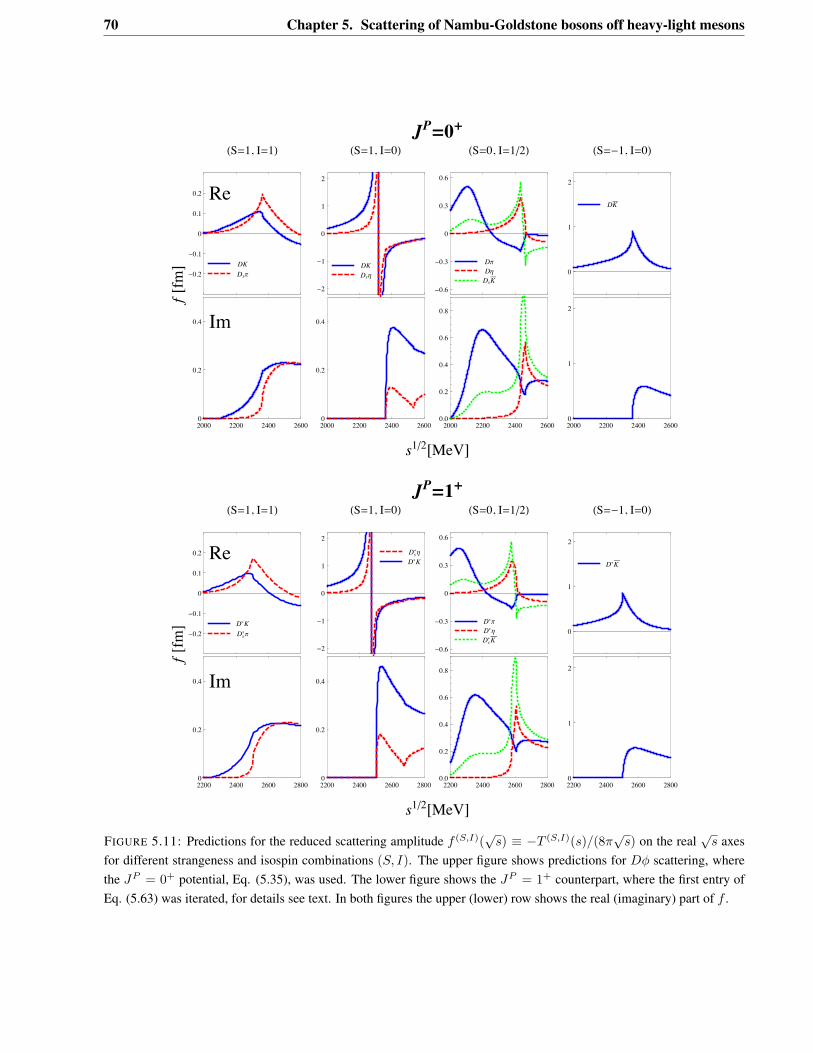
70 Chapter 5. Scattering of Nambu-Goldstone bosons off heavy-light mesons
Re
DKDs!
0
0.1
0.2
"0.1
"0.2
!S#1, I#1"
DKDs$
0
1
2
"1
"2
!S#1, I#0"
D!D$DsK
0
0.3
0.6
"0.3
"0.6
!S#0, I#1#2"DK
0
1
2
!S#"1, I#0"
Im
2000 2200 2400 26000
0.2
0.4
2000 2200 2400 26000
0.2
0.4
2000 2200 2400 26000.0
0.2
0.4
0.6
0.8
2000 2200 2400 26000
1
2
JP!0"
s1#2$MeV%
f$fm%
Re
D!KDs!"
0
0.1
0.2
#0.1
#0.2
!S$1, I$1"D!KDs!%
0
1
2
#1
#2
!S$1, I$0"
D!"D!%Ds!K
0
0.3
0.6
#0.3
#0.6
!S$0, I$1#2"D!K
0
1
2
!S$#1, I$0"
Im
2200 2400 2600 28000
0.2
0.4
2200 2400 2600 28000
0.2
0.4
2200 2400 2600 28000.0
0.2
0.4
0.6
0.8
2200 2400 2600 28000
1
2
JP!1"
s1#2$MeV%
f$fm%
FIGURE 5.11: Predictions for the reduced scattering amplitude 𝑓 (𝑆,𝐼)(√
𝑠) ≡ −𝑇 (𝑆,𝐼)(𝑠)/(8𝜋√
𝑠) on the real√
𝑠 axesfor different strangeness and isospin combinations (𝑆, 𝐼). The upper figure shows predictions for 𝐷𝜑 scattering, wherethe 𝐽𝑃 = 0+ potential, Eq. (5.35), was used. The lower figure shows the 𝐽𝑃 = 1+ counterpart, where the first entry ofEq. (5.63) was iterated, for details see text. In both figures the upper (lower) row shows the real (imaginary) part of 𝑓 .
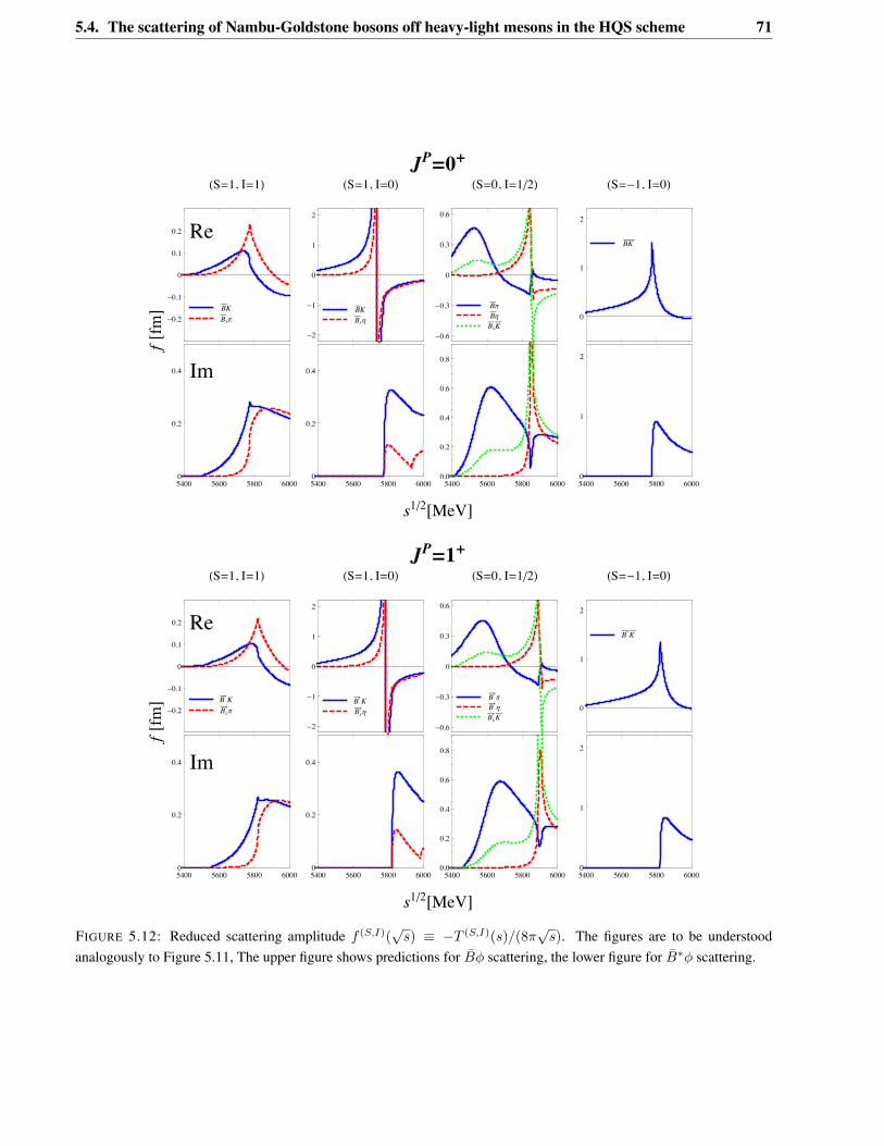
5.4. The scattering of Nambu-Goldstone bosons off heavy-light mesons in the HQS scheme 71
Re
BKBs!
0
0.1
0.2
"0.1
"0.2
!S#1, I#1"
BKBs$
0
1
2
"1
"2
!S#1, I#0"
B!B$BsK
0
0.3
0.6
"0.3
"0.6
!S#0, I#1#2"BK
0
1
2
!S#"1, I#0"
Im
5400 5600 5800 60000
0.2
0.4
5400 5600 5800 60000
0.2
0.4
5400 5600 5800 60000.0
0.2
0.4
0.6
0.8
5400 5600 5800 60000
1
2
JP!0"
s1#2$MeV%
f$fm%
Re
B!KBs!"
0
0.1
0.2
#0.1
#0.2
!S$1, I$1"
B!KBs!%
0
1
2
#1
#2
!S$1, I$0"
B!"B!%Bs!K
0
0.3
0.6
#0.3
#0.6
!S$0, I$1#2"B!K
0
1
2
!S$#1, I$0"
Im
5400 5600 5800 60000
0.2
0.4
5400 5600 5800 60000
0.2
0.4
5400 5600 5800 60000.0
0.2
0.4
0.6
0.8
5400 5600 5800 60000
1
2
JP!1"
s1#2$MeV%
f$fm%
FIGURE 5.12: Reduced scattering amplitude 𝑓 (𝑆,𝐼)(√
𝑠) ≡ −𝑇 (𝑆,𝐼)(𝑠)/(8𝜋√
𝑠). The figures are to be understoodanalogously to Figure 5.11, The upper figure shows predictions for ��𝜑 scattering, the lower figure for ��*𝜑 scattering.
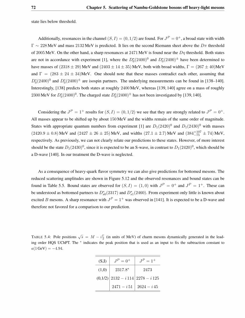
72 Chapter 5. Scattering of Nambu-Goldstone bosons off heavy-light mesons
state lies below threshold.
Additionally, resonances in the channel (𝑆, 𝐼) = (0, 1/2) are found. For 𝐽𝑃 = 0+, a broad state with width
Γ ∼ 228 MeV and mass 2132 MeV is predicted. It lies on the second Riemann sheet above the 𝐷𝜋 threshold
of 2005 MeV. On the other hand, a sharp resonances at 2471 MeV is found near the 𝐷𝜂 threshold. Both states
are not in accordance with experiment [1], where the 𝐷*0(2400)0 and 𝐷*0(2400)± have been determined to
have masses of (2318 ± 29) MeV and (2403 ± 14 ± 35) MeV, both with broad widths, Γ = (267 ± 40)MeV
and Γ = (283 ± 24 ± 34)MeV. One should note that these masses contradict each other, assuming that
𝐷*0(2400)0 and 𝐷*0(2400)± are isospin partners. The underlying measurements can be found in [138–140].
Interestingly, [138] predicts both states at roughly 2400 MeV, whereas [139, 140] agree on a mass of roughly
2300 MeV for 𝐷*0(2400)0. The charged state 𝐷*0(2400)± has not been investigated by [139, 140].
Considering the 𝐽𝑃 = 1+ results for (𝑆, 𝐼) = (0, 1/2) we see that they are strongly related to 𝐽𝑃 = 0+.
All masses appear to be shifted up by about 150 MeV and the widths remain of the same order of magnitude.
States with appropriate quantum numbers from experiment [1] are 𝐷1(2420)0 and 𝐷1(2430)0 with masses
(2420.9 ± 0.8) MeV and (2427 ± 26 ± 25) MeV, and widths (27.1 ± 2.7) MeV and (384+107−75 ± 74) MeV,
respectively. As previously, we can not clearly relate our predictions to these states. However, of more interest
should be the state 𝐷1(2430)0, since it is expected to be an S-wave, in contrast to 𝐷1(2420)0, which should be
a D-wave [140]. In our treatment the D-wave is neglected.
As a consequence of heavy-quark flavor symmetry we can also give predictions for bottomed mesons. The
reduced scattering amplitudes are shown in Figure 5.12 and the observed resonances and bound states can be
found in Table 5.5. Bound states are observed for (𝑆, 𝐼) = (1, 0) with 𝐽𝑃 = 0+ and 𝐽𝑃 = 1+. These can
be understood as bottomed partners to 𝐷*𝑠0(2317) and 𝐷*𝑠1(2460). From experiment only little is known about
excited 𝐵 mesons. A sharp resonance with 𝐽𝑃 = 1+ was observed in [141]. It is expected to be a D-wave and
therefore not favored for a comparison to our prediction.
TABLE 5.4: Pole positions√
𝑠 = 𝑀 − 𝑖Γ2 (in units of MeV) of charm mesons dynamically generated in the lead-
ing order HQS UChPT. The * indicates the peak position that is used as an input to fix the subtraction constant to𝑎(1 GeV) = −4.94.
(S,I) 𝐽𝑃 = 0+ 𝐽𝑃 = 1+
(1,0) 2317.8* 2473
(0,1/2) 2132− 𝑖 114 2278− 𝑖 125
2471− 𝑖 51 2624− 𝑖 45
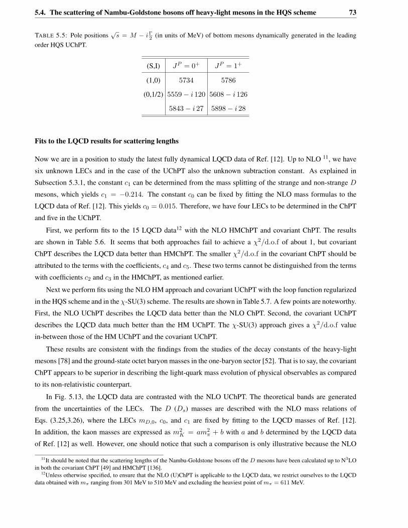
5.4. The scattering of Nambu-Goldstone bosons off heavy-light mesons in the HQS scheme 73
TABLE 5.5: Pole positions√
𝑠 = 𝑀 − 𝑖Γ2 (in units of MeV) of bottom mesons dynamically generated in the leading
order HQS UChPT.
(S,I) 𝐽𝑃 = 0+ 𝐽𝑃 = 1+
(1,0) 5734 5786
(0,1/2) 5559− 𝑖 120 5608− 𝑖 126
5843− 𝑖 27 5898− 𝑖 28
Fits to the LQCD results for scattering lengths
Now we are in a position to study the latest fully dynamical LQCD data of Ref. [12]. Up to NLO 11, we have
six unknown LECs and in the case of the UChPT also the unknown subtraction constant. As explained in
Subsection 5.3.1, the constant 𝑐1 can be determined from the mass splitting of the strange and non-strange 𝐷
mesons, which yields 𝑐1 = −0.214. The constant 𝑐0 can be fixed by fitting the NLO mass formulas to the
LQCD data of Ref. [12]. This yields 𝑐0 = 0.015. Therefore, we have four LECs to be determined in the ChPT
and five in the UChPT.
First, we perform fits to the 15 LQCD data12 with the NLO HMChPT and covariant ChPT. The results
are shown in Table 5.6. It seems that both approaches fail to achieve a 𝜒2/d.o.f of about 1, but covariant
ChPT describes the LQCD data better than HMChPT. The smaller 𝜒2/d.o.f in the covariant ChPT should be
attributed to the terms with the coefficients, 𝑐4 and 𝑐5. These two terms cannot be distinguished from the terms
with coefficients 𝑐2 and 𝑐3 in the HMChPT, as mentioned earlier.
Next we perform fits using the NLO HM approach and covariant UChPT with the loop function regularized
in the HQS scheme and in the 𝜒-SU(3) scheme. The results are shown in Table 5.7. A few points are noteworthy.
First, the NLO UChPT describes the LQCD data better than the NLO ChPT. Second, the covariant UChPT
describes the LQCD data much better than the HM UChPT. The 𝜒-SU(3) approach gives a 𝜒2/d.o.f value
in-between those of the HM UChPT and the covariant UChPT.
These results are consistent with the findings from the studies of the decay constants of the heavy-light
mesons [78] and the ground-state octet baryon masses in the one-baryon sector [52]. That is to say, the covariant
ChPT appears to be superior in describing the light-quark mass evolution of physical observables as compared
to its non-relativistic counterpart.
In Fig. 5.13, the LQCD data are contrasted with the NLO UChPT. The theoretical bands are generated
from the uncertainties of the LECs. The 𝐷 (𝐷𝑠) masses are described with the NLO mass relations of
Eqs. (3.25,3.26), where the LECs 𝑚𝐷,0, 𝑐0, and 𝑐1 are fixed by fitting to the LQCD masses of Ref. [12].
In addition, the kaon masses are expressed as 𝑚2𝐾 = 𝑎𝑚2
𝜋 + 𝑏 with 𝑎 and 𝑏 determined by the LQCD data
of Ref. [12] as well. However, one should notice that such a comparison is only illustrative because the NLO
11It should be noted that the scattering lengths of the Nambu-Goldstone bosons off the 𝐷 mesons have been calculated up to N3LOin both the covariant ChPT [49] and HMChPT [136].
12Unless otherwise specified, to ensure that the NLO (U)ChPT is applicable to the LQCD data, we restrict ourselves to the LQCDdata obtained with 𝑚𝜋 ranging from 301 MeV to 510 MeV and excluding the heaviest point of 𝑚𝜋 = 611 MeV.
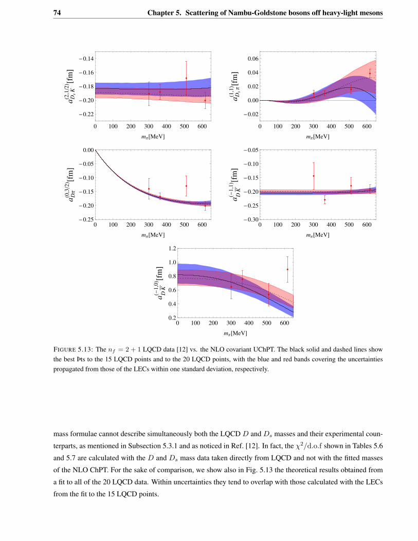
74 Chapter 5. Scattering of Nambu-Goldstone bosons off heavy-light mesons
0 100 200 300 400 500 600
-0.22
-0.20
-0.18
-0.16
-0.14
mΠ@MeVD
aD
sK
H2,1
�2L@fm
D
0 100 200 300 400 500 600
-0.02
0.00
0.02
0.04
0.06
mΠ@MeVD
aD
sΠ
H1,1
L @fmD
0 100 200 300 400 500 600-0.25
-0.20
-0.15
-0.10
-0.05
0.00
mΠ@MeVD
aD
ΠH0,3
�2L@fm
D
0 100 200 300 400 500 600-0.30
-0.25
-0.20
-0.15
-0.10
-0.05
mΠ@MeVDa
DKH-1
,1L @fm
D
0 100 200 300 400 500 6000.2
0.4
0.6
0.8
1.0
1.2
mΠ@MeVD
aD
KH-1,0
L @fmD
FIGURE 5.13: The 𝑛𝑓 = 2 + 1 LQCD data [12] vs. the NLO covariant UChPT. The black solid and dashed lines showthe best Þts to the 15 LQCD points and to the 20 LQCD points, with the blue and red bands covering the uncertaintiespropagated from those of the LECs within one standard deviation, respectively.
mass formulae cannot describe simultaneously both the LQCD 𝐷 and 𝐷𝑠 masses and their experimental coun-
terparts, as mentioned in Subsection 5.3.1 and as noticed in Ref. [12]. In fact, the 𝜒2/d.o.f shown in Tables 5.6
and 5.7 are calculated with the 𝐷 and 𝐷𝑠 mass data taken directly from LQCD and not with the fitted masses
of the NLO ChPT. For the sake of comparison, we show also in Fig. 5.13 the theoretical results obtained from
a fit to all of the 20 LQCD data. Within uncertainties they tend to overlap with those calculated with the LECs
from the fit to the 15 LQCD points.
5.4. The scattering of Nambu-Goldstone bosons off heavy-light mesons in the HQS scheme 75
TABLE 5.6: Low-energy constants and the 𝜒2/d.o.f from the best fits to the LQCD data [12] in the covariant ChPTand the HM ChPT up to NLO, where 𝑐24 = 𝑐2 − 2𝑐4 and 𝑐35 = 𝑐3 − 2𝑐5. The uncertainties of the LECs given in theparentheses correspond to one standard deviation.
𝑐24 𝑐35 𝑐4 𝑐5 𝜒2/d.o.fCovariant ChPT 0.153(35) −0.126(71) 0.760(186) −1.84(39) 2.01HM ChPT 0.012(6) 0.167(17) - - 3.10
TABLE 5.7: Low-energy constants, the subtraction constants, and the 𝜒2/d.o.f from the best fits to the LQCD data [12] inthe HQS UChPT, the 𝜒-SU(3) UChPT, and the HM UChPT. The renormalization scale 𝜇 is set at 1 GeV. The uncertaintiesof the LECs given in the parentheses correspond to one standard deviation.
𝑎 𝑐24 𝑐35 𝑐4 𝑐5 𝜒2/d.o.fHQS UChPT −4.13(40) −0.068(21) −0.011(31) 0.052(83) −0.96(30) 1.23
𝜒-SU(3) UChPT - −0.096(19) −0.0037(340) 0.22(8) −0.53(21) 1.57HM UChPT 2.52 (11) 4.86(30) −9.45(60) - - 2.69
Dynamically generated heavy-light mesons
Once the subtraction constant and the LECs are fixed, one can utilize the UChPT to study whether the interac-
tions between heavy-light mesons and Nambu-Goldstone bosons are strong enough to generate bound states or
resonances, by searching for poles in the complex√
𝑠 plane. We notice that the subtraction constant in the HM
UChPT given in Table 5.7 is positive, and as a result, there is no bound state generated in the (𝑆, 𝐼) = (1, 0)
channel. On the other hand, using covariant UChPT, a bound state is found at√
𝑠 = 2317 ± 10 MeV in the
complex plane. We identify this bound state as the 𝐷*𝑠0(2317). In addition, one more state is generated in
the (𝑆, 𝐼) = (0, 1/2) channel. All of them are tabulated in Table 5.8. In calculating the positions of these
states, we have used the physical masses listed in Table 4.1. The uncertainties in the positions of these states
are estimated by changing the LECs and the subtraction constant within their 1-𝜎 uncertainties given in Table
5.7. Furthermore, we predict the heavy quark spin partners of the 0+ states as well. The counterpart of the
𝐷*𝑠0(2317) appears at√
𝑠 = 2457 ± 17 MeV 13 , which we identify as the 𝐷𝑠1(2460). It is clear that the
heavy-quark spin symmetry is approximately conserved in the HQS ChPT approach.
One appealing feature of the renormalization scheme we propose in this work is that the heavy quark flavor
symmetry is conserved up to 1/𝑀HL, in contrast to the naive MS subtraction scheme. As such, we can calculate
the bottom partners of the 𝐷*𝑠0(2317) and 𝐷𝑠1(2460) in reasonable confidence. We tabulate in Table 5.9 the
bottom counterparts of the charm states of Table 5.8. It should be noted that the absolute positions of these
resonances are subject to corrections of a few tens of MeV because of the uncertainty related to the evolution
of the UChPT from the charm sector to the bottom sector. On the other hand, the mass differences between the
1+ states and their 0+ counterparts should be more stable, as has been argued in a number of different studies
(see, e.g., Ref. [104]).
13The uncertainties are propagated from the uncertainties of the LECs and the subtraction constant. In addition, we have assigned a10% uncertainty for relating the LECS in the 𝐷* sector with those in the 𝐷 sector by use of heavy-quark spin symmetry. To relate theLECs between 𝐷 and 𝐵 sectors, a 20% uncertainty is assumed, and 𝑚sub is varied from 𝑚𝜋 to 𝑚𝜂 .
76 Chapter 5. Scattering of Nambu-Goldstone bosons off heavy-light mesons
TABLE 5.8: Pole positions√
𝑠 = 𝑀 − 𝑖Γ2 (in units of MeV) of charm mesons dynamically generated in the HQS UChPT.
(S,I) 𝐽𝑃 = 0+ 𝐽𝑃 = 1+
(1,0) 2317± 10 2457± 17
(0,1/2) (2105± 4)− 𝑖(103± 7) (2248± 6)− 𝑖(106± 13)
TABLE 5.9: Pole positions√
𝑠 = 𝑀−𝑖Γ2 (in units of MeV) of bottom mesons dynamically generated in the HQS UChPT.
(S,I) 𝐽𝑃 = 0+ 𝐽𝑃 = 1+
(1,0) 5726± 28 5778± 26
(0,1/2) (5537± 14)− 𝑖(118± 22) (5586± 16)− 𝑖(124± 25)
TABLE 5.10: Dynamically generated 0+ and 1+ bottom states in (𝑆, 𝐼) = (1, 0) from different formulations of theUChPT. Masses of the states are in units of MeV.
𝐽𝑃 present work NLO HMChPT [104] LO UChPT [97] LO 𝜒-SU(3) [96]
0+ 5726± 28 5696± 36 5725± 39 56431+ 5778± 26 5742± 36 5778± 7 5690
In Table 5.10 we compare the predicted 0+ and 1+ states from several different formulations of UChPT in
the bottom sector. It is seen that the absolute positions can differ by as much as 80 MeV, which is not surprising
because the heavy-quark flavor symmetry was implemented differently.
It has been argued that the light-quark mass evolution of the masses of mesons and baryons can provide
important hints about their nature (see, e.g., Refs. [104, 142]). In the left panel of Fig. 5.14, we show how the
pole positions of the 𝐷*𝑠0(2317) and the 𝐷𝑠1(2460) evolve as a function of 𝑚𝜋. The strange-quark mass is fixed
to its physical value using leading-order ChPT. The light-quark mass dependences of the 𝐷(𝐷𝑠) and 𝐷*(𝐷*𝑠)
are given by the NLO ChPT formulas of Eqs. (3.25 to 3.28). The right panel of Fig. 5.14 shows the evolution of
the 𝐷*𝑠0(2317) and 𝐷𝑠1(2460) pole position as a function of the kaon mass (or equivalently the strange-quark
mass) as we fix the pion mass to its physical value. As has been argued in Ref. [104], the feature of being
dynamically generated dictates that the dependence of the masses of these states on 𝑚𝐾 are linear with a slope
close to unity, which can be clearly seen from Fig. 5.14.
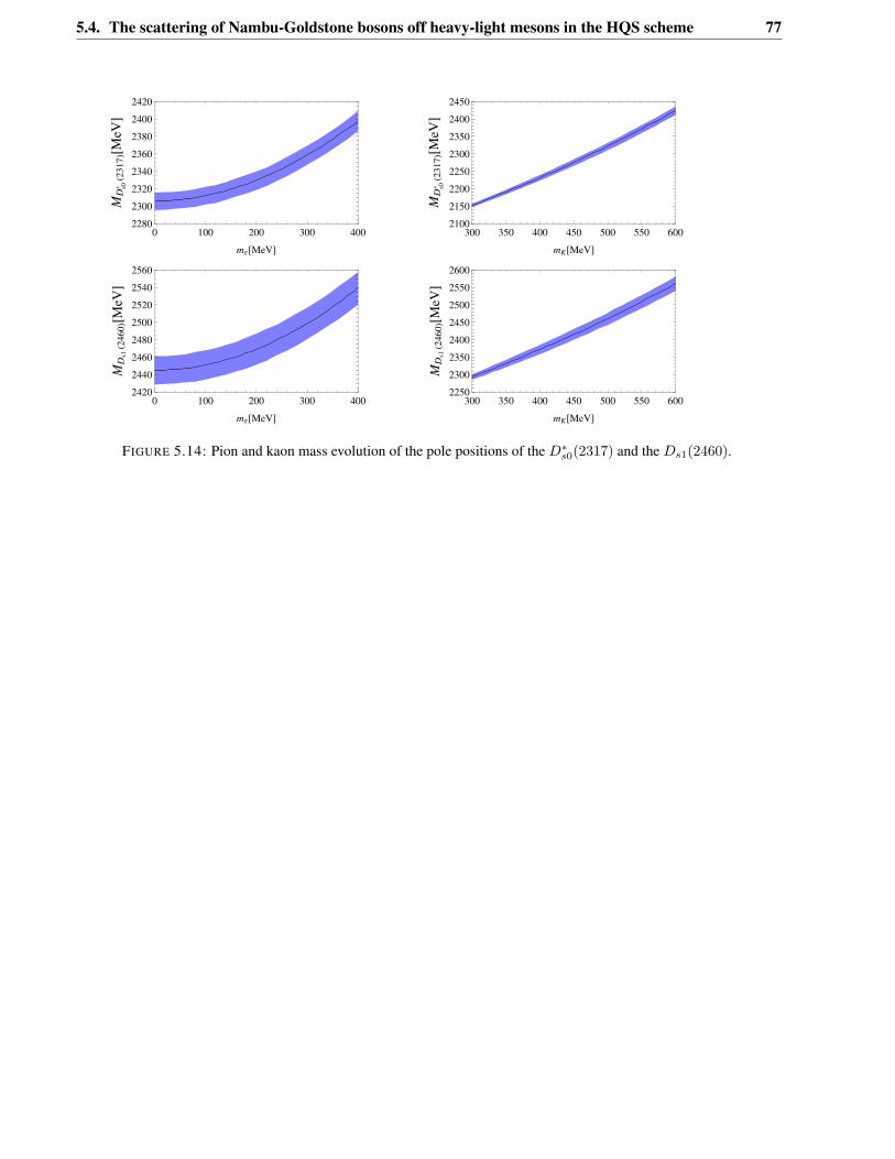
5.4. The scattering of Nambu-Goldstone bosons off heavy-light mesons in the HQS scheme 77
0 100 200 300 4002280
2300
2320
2340
2360
2380
2400
2420
mΠ@MeVD
MD
s0*H23
17
L@MeV
D
300 350 400 450 500 550 6002100
2150
2200
2250
2300
2350
2400
2450
mK@MeVD
MD
s0*H23
17
L@MeV
D0 100 200 300 400
2420
2440
2460
2480
2500
2520
2540
2560
mΠ@MeVD
MD
s1H24
60
L@MeV
D
300 350 400 450 500 550 6002250
2300
2350
2400
2450
2500
2550
2600
mK@MeVDM
Ds1
H2460
L@MeV
DFIGURE 5.14: Pion and kaon mass evolution of the pole positions of the 𝐷*
𝑠0(2317) and the 𝐷𝑠1(2460).
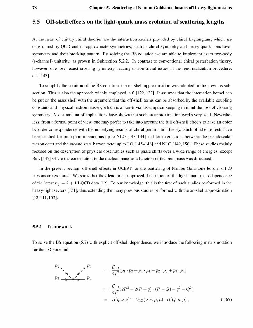
78 Chapter 5. Scattering of Nambu-Goldstone bosons off heavy-light mesons
5.5 Off-shell effects on the light-quark mass evolution of scattering lengths
At the heart of unitary chiral theories are the interaction kernels provided by chiral Lagrangians, which are
constrained by QCD and its approximate symmetries, such as chiral symmetry and heavy quark spin/flavor
symmetry and their breaking pattern. By solving the BS equation we are able to implement exact two-body
(s-channel) unitarity, as proven in Subsection 5.2.2. In contrast to conventional chiral perturbation theory,
however, one loses exact crossing symmetry, leading to non trivial issues in the renormalization procedure,
c.f. [143].
To simplify the solution of the BS equation, the on-shell approximation was adopted in the previous sub-
section. This is also the approach widely employed, c.f. [122, 123]. It assumes that the interaction kernel can
be put on the mass shell with the argument that the off-shell terms can be absorbed by the available coupling
constants and physical hadron masses, which is a non-trivial assumption keeping in mind the loss of crossing
symmetry. A vast amount of applications have shown that such an approximation works very well. Neverthe-
less, from a formal point of view, one may prefer to take into account the full off-shell effects to have an order
by order correspondence with the underlying results of chiral perturbation theory. Such off-shell effects have
been studied for pion-pion interactions up to NLO [143, 144] and for interactions between the pseudoscalar
meson octet and the ground state baryon octet up to LO [145–148] and NLO [149, 150]. These studies mainly
focused on the description of physical observables such as phase shifts over a wide range of energies, except
Ref. [147] where the contribution to the nucleon mass as a function of the pion mass was discussed.
In the present section, off-shell effects in UChPT for the scattering of Nambu-Goldstone bosons off 𝐷
mesons are explored. We show that they lead to an improved description of the light-quark mass dependence
of the latest 𝑛𝑓 = 2 + 1 LQCD data [12]. To our knowledge, this is the first of such studies performed in the
heavy-light sectors [151], thus extending the many previous studies performed with the on-shell approximation
[12, 111, 152].
5.5.1 Framework
To solve the BS equation (5.7) with explicit off-shell dependence, we introduce the following matrix notation
for the LO potential
p1
p2 p4
p3
=𝒞LO
4𝑓20
(𝑝1 · 𝑝2 + 𝑝1 · 𝑝4 + 𝑝2 · 𝑝3 + 𝑝3 · 𝑝4)
=𝒞LO
4𝑓20
(2𝑃 2 − 2(𝑃 + 𝑞) · (𝑃 + 𝑄)− 𝑞2 −𝑄2)
= 𝐵(𝑞, 𝜈, 𝜈)𝑇 · 𝑉LO(𝜈, 𝜈, 𝜇, ��) ·𝐵(𝑄, 𝜇, ��) , (5.65)
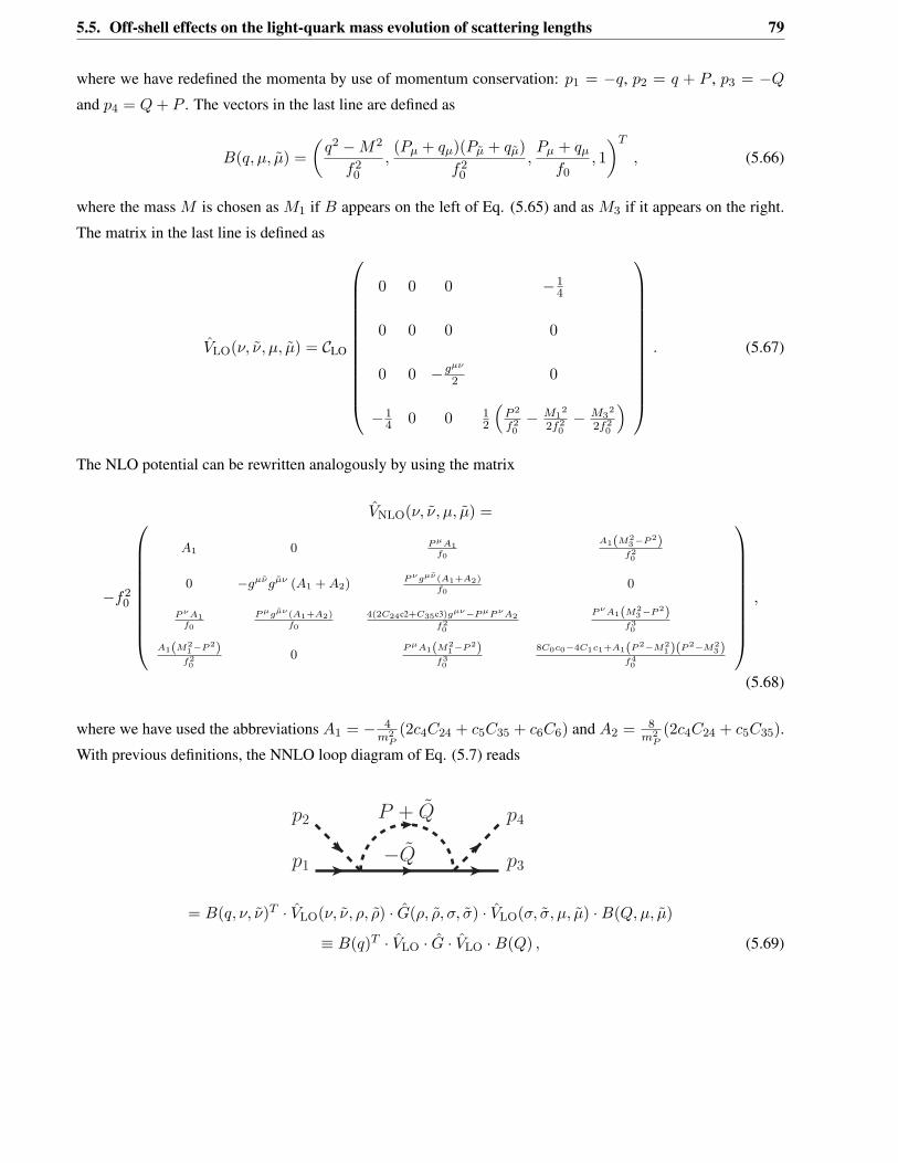
5.5. Off-shell effects on the light-quark mass evolution of scattering lengths 79
where we have redefined the momenta by use of momentum conservation: 𝑝1 = −𝑞, 𝑝2 = 𝑞 + 𝑃 , 𝑝3 = −𝑄
and 𝑝4 = 𝑄 + 𝑃 . The vectors in the last line are defined as
𝐵(𝑞, 𝜇, ��) =(
𝑞2 −𝑀2
𝑓20
,(𝑃𝜇 + 𝑞𝜇)(𝑃�� + 𝑞��)
𝑓20
,𝑃𝜇 + 𝑞𝜇
𝑓0, 1)𝑇
, (5.66)
where the mass 𝑀 is chosen as 𝑀1 if 𝐵 appears on the left of Eq. (5.65) and as 𝑀3 if it appears on the right.
The matrix in the last line is defined as
𝑉LO(𝜈, 𝜈, 𝜇, ��) = 𝒞LO
⎛⎜⎜⎜⎜⎜⎜⎜⎜⎜⎜⎜⎜⎝
0 0 0 −14
0 0 0 0
0 0 −𝑔𝜇𝜈
2 0
−14 0 0 1
2
(𝑃 2
𝑓20− 𝑀1
2
2𝑓20− 𝑀3
2
2𝑓20
)
⎞⎟⎟⎟⎟⎟⎟⎟⎟⎟⎟⎟⎟⎠
. (5.67)
The NLO potential can be rewritten analogously by using the matrix
𝑉NLO(𝜈, 𝜈, 𝜇, ��) =
−𝑓20
⎛⎜⎜⎜⎜⎜⎜⎜⎜⎜⎝
𝐴1 0 𝑃 𝜇𝐴1𝑓0
𝐴1(𝑀23−𝑃2)
𝑓20
0 −𝑔𝜇𝜈𝑔��𝜈 (𝐴1 + 𝐴2)𝑃 𝜈𝑔𝜇𝜈(𝐴1+𝐴2)
𝑓00
𝑃 𝜈𝐴1𝑓0
𝑃 𝜇𝑔��𝜈(𝐴1+𝐴2)𝑓0
4(2𝐶24c2+𝐶35c3)𝑔𝜇𝜈−𝑃 𝜇𝑃 𝜈𝐴2𝑓20
𝑃 𝜈𝐴1(𝑀23−𝑃2)
𝑓30
𝐴1(𝑀21−𝑃2)
𝑓20
0𝑃 𝜇𝐴1(𝑀2
1−𝑃2)𝑓30
8𝐶0𝑐0−4𝐶1𝑐1+𝐴1(𝑃2−𝑀21 )(𝑃2−𝑀2
3 )𝑓40
⎞⎟⎟⎟⎟⎟⎟⎟⎟⎟⎠
,
(5.68)
where we have used the abbreviations 𝐴1 = − 4𝑚2
𝑃(2𝑐4𝐶24 + 𝑐5𝐶35 + 𝑐6𝐶6) and 𝐴2 = 8
𝑚2𝑃
(2𝑐4𝐶24 + 𝑐5𝐶35).
With previous definitions, the NNLO loop diagram of Eq. (5.7) reads
p1
p2
!Q
P + Q p4
p3
= 𝐵(𝑞, 𝜈, 𝜈)𝑇 · 𝑉LO(𝜈, 𝜈, 𝜌, 𝜌) · ��(𝜌, 𝜌, 𝜎, ��) · 𝑉LO(𝜎, ��, 𝜇, ��) ·𝐵(𝑄, 𝜇, ��)
≡ 𝐵(𝑞)𝑇 · 𝑉LO · �� · 𝑉LO ·𝐵(𝑄) , (5.69)
80 Chapter 5. Scattering of Nambu-Goldstone bosons off heavy-light mesons
where we have defined the loop function as
��(𝜈, 𝜈, 𝜇, ��) ≡ 𝑖
∫𝑑𝑛��
(2𝜋)𝑛
1[(𝑃 + ��)2 −𝑚2]
1(��2 −𝑀2)
𝐵(��, 𝜈, 𝜈) ·𝐵(��, 𝜇, ��)𝑇
=
⎛⎜⎜⎜⎜⎜⎜⎜⎜⎜⎜⎜⎜⎝
𝐺1,1(𝑠) 𝐺1,2𝜇��(𝑠) 0 𝐺1,4(𝑠)
𝐺1,2𝜈𝜈 (𝑠) 𝐺2,2
𝜈𝜈𝜇��(𝑠) 𝐺2,3𝜈𝜈𝜇(𝑠) 𝐺2,4
𝜈𝜈 (𝑠)
0 𝐺2,3𝜈𝜇��(𝑠) 𝐺3,3
𝜈𝜇 (𝑠) 𝐺3,4𝜈 (𝑠)
𝐺1,4(𝑠) 𝐺2,4𝜇��(𝑠) 𝐺3,4
𝜇 (𝑠) 𝐺4,4(𝑠)
⎞⎟⎟⎟⎟⎟⎟⎟⎟⎟⎟⎟⎟⎠
, (5.70)
with the Functions 𝐺(𝑠 = 𝑃 2) listed in Appendix A.1, Eq. (A.3) to (A.5). In the last step we have introduced
a brief notation, keeping in mind that a summation over Lorentz indices is implicit.
An arbitrary diagram generated by the BS equation is simply calculated as
𝐵(𝑞)𝑇 · 𝑉(N)LO · �� · 𝑉(N)LO · �� · . . . · 𝑉(N)LO ·𝐵(𝑄) . (5.71)
For instance, the loop integral of Eq.(5.7) reads
𝐵(𝑞, 𝜈, 𝜈)𝑇 · 𝑉LO,NLO(𝜈, 𝜈, 𝜌, 𝜌) · ��(𝜌, 𝜌, 𝜎, ��) · 𝑇 (𝜎, ��, 𝜇, ��) ·𝐵(𝑄, 𝜇, ��)
≡ 𝐵(𝑞)𝑇 · 𝑉LO,NLO · �� · 𝑇 ·𝐵(𝑄) . (5.72)
The complete BS equation becomes
𝐵(𝑞)𝑇 · 𝑇 ·𝐵(𝑄) = 𝐵(𝑞)𝑇 · (𝑉 + 𝑉 · �� · 𝑇 ) ·𝐵(𝑄) , (5.73)
with 𝑉 = 𝑉LO + 𝑉NLO. As Ansatz for the scattering amplitude 𝑇 we use
𝑇 (𝜈, 𝜈 ′, 𝜇, 𝜇′) ≡⎛⎜⎜⎜⎜⎜⎜⎜⎜⎜⎝
𝑡11 𝑔𝜇𝜇′𝑡12𝑎 + 𝑃 𝜇𝑃 𝜇′𝑡12𝑏 𝑃 𝜇𝑡13 𝑡14
𝑔𝜈𝜈′𝑡21𝑎 + 𝑃 𝜈𝑃 𝜈′𝑡21𝑏 𝑃 𝜇𝑃 𝜈𝑃 𝜇′𝑃 𝜈′𝑡22𝑎 + 𝐴𝜈𝜈′𝜇𝜇′ + 𝐶𝜈𝜈′𝜇𝜇′ 𝑃 𝜇𝑃 𝜈𝑃 𝜈′𝑡23𝑎 + 𝐵𝜇𝜈𝜈′
23 𝑃 𝜈𝑃 𝜈′𝑡24𝑎 + 𝑔𝜈𝜈′𝑡24𝑏
𝑃 𝜈𝑡31 𝑃 𝜇𝑃 𝜈𝑃 𝜇′𝑡32𝑎 + 𝐵𝜈𝜇𝜇′
32 𝑔𝜇𝜈𝑡33𝑎 + 𝑃 𝜇𝑃 𝜈𝑡33𝑏 𝑃 𝜈𝑡34
𝑡41 𝑃 𝜇𝑃 𝜇′𝑡42𝑎 + 𝑔𝜇𝜇′𝑡42𝑏 𝑃 𝜇𝑡43 𝑡44
⎞⎟⎟⎟⎟⎟⎟⎟⎟⎟⎠
,
(5.74)
5.5. Off-shell effects on the light-quark mass evolution of scattering lengths 81
with the abbreviations
𝐶𝜈𝜈′𝜇𝜇′ = 𝑔𝜇𝜇′𝑔𝜈𝜈′𝑡22𝑏 + 𝑔𝜈𝜇′𝑔𝜈′𝜇𝑡22𝑐 + 𝑔𝜈𝜇𝑔𝜈′𝜇′𝑡22𝑑
𝐵𝜇𝜈𝜈′
23 = 𝑃 𝜈′𝑔𝜈𝜇𝑡23𝑏 + 𝑃 𝜈𝑔𝜈′𝜇𝑡23𝑐 + 𝑃𝜇𝑔𝜈𝜈′𝑡23𝑑
𝐵𝜈𝜇𝜇′
32 = 𝑃𝜇′𝑔𝜈𝜇𝑡32𝑏 + 𝑃 𝜈𝑔𝜇′𝜇𝑡32𝑐 + 𝑃𝜇𝑔𝜈𝜇′𝑡32𝑑
𝐴𝜈𝜈′𝜇𝜇′ = 𝑃𝜇′𝑃 𝜈′𝑔𝜈𝜇𝑡22𝑒 + 𝑃 𝜈𝑃 𝜈′𝑔𝜇𝜇′𝑡22𝑓 + 𝑃 𝜈𝑃𝜇′𝑔𝜈′𝜇𝑡22𝑔
+𝑃𝜇𝑃 𝜈′𝑔𝜈𝜇′𝑡22ℎ + 𝑃𝜇𝑃𝜇′𝑔𝜈𝜈′𝑡22𝑖 + 𝑃𝜇𝑃 𝜈𝑔𝜈′𝜇′𝑡22𝑗 . (5.75)
We have introduced a set of functions 𝑡𝑖 that depend on the total momentum squared 𝑠. These functions have
to be determined by solving the set of linear equations
𝑇 = 𝑉 + 𝑉 · �� · 𝑇 . (5.76)
As previously, the whole calculation can be simply extended to include coupled channels effects by increasing
the dimension of the matrices. The form of Eq. (5.73) makes obvious that the solutions of the BS equation,
Eq. (5.7), still correspond to a geometric series, even if off-shell effects are taken into account. Explicitly, the
matrix 𝑇 becomes
𝑇 = (1− 𝑉 · ��)−1 · 𝑉 . (5.77)
Some comments are in order: first, the potentials Eq. (5.67) and (5.68) could have been also written as a
3 × 3 matrix. This can be achieved by using the metric tensors 𝑔𝜇�� (𝑔𝜈𝜈) in the definition of 𝑉LO,NLO. Then
the two vectors (𝑞 + 𝑃 )𝜇 and (𝑞 + 𝑃 )��, ((𝑄 + 𝑃 )𝜈 and (𝑄 + 𝑃 )𝜈), entering Eq. (5.66), are contracted with
each other and Lorentz structures like 𝑞2 (𝑄2) can be created. Hence, the first component of the vector Eq.
(5.66) is no longer necessary. Performing this way, however, requires care in factorizing the potential from the
loop function (this should be done consistently in 𝐷 dimensions!). Secondly, our summation does not exactly
correspond to the result obtained in dimensional regularization, i.e. we insert the T matrix in four space-time
(not D) dimensions into the BS equation. This subtlety plays only a role for the contributions originating
from the 𝑐4, 𝑐5 and 𝑐6 terms in the NLO potential. As a last comment: usually one solves the BS equation
for potentials with off-shellness by some specific ansatz. Due to the previous subtleties in the dimensional
regularization of the loop integral, this can lead to a loss of time-reversal invariance. This happens only for the
iteration of the 𝑐4, 𝑐5 and 𝑐6 terms. All similar approaches listed so far circumvent this issue by either stopping
at sufficiently low order, or not relying on dimensional regularization. Our approach, on the other hand, keeps
time reversal invariance. This is an advantage of performing the resummation explicitly by iterating matrices.
Concerning the computation of the loop function, a few words are in order. Relativistic loop functions
involving a heavy particle, whose mass does not vanish in the chiral limit, contain power-counting-breaking
(PCB) term, as already encountered numerous times in this theses. In the one-baryon sector, various approaches
have been proposed to remove PCB terms, such as the heavy-baryon formulation [153], the infrared formulation
[154], and the extended-on-mass-shell approach [59] (see, Ref. [110] for a short review for their respective
advantages and limitations). Traditionally, in the UChPT with the on-shell approximation, no attention is paid
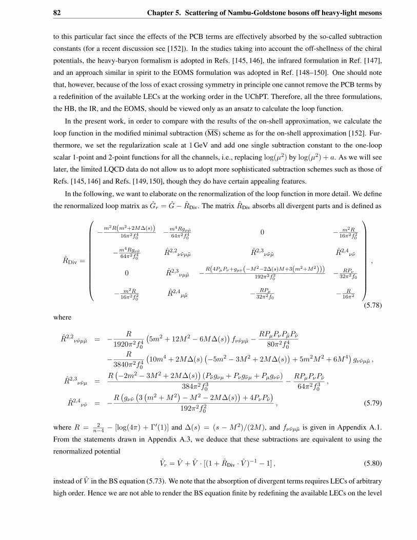
82 Chapter 5. Scattering of Nambu-Goldstone bosons off heavy-light mesons
to this particular fact since the effects of the PCB terms are effectively absorbed by the so-called subtraction
constants (for a recent discussion see [152]). In the studies taking into account the off-shellness of the chiral
potentials, the heavy-baryon formalism is adopted in Refs. [145, 146], the infrared formulation in Ref. [147],
and an approach similar in spirit to the EOMS formulation was adopted in Ref. [148–150]. One should note
that, however, because of the loss of exact crossing symmetry in principle one cannot remove the PCB terms by
a redefinition of the available LECs at the working order in the UChPT. Therefore, all the three formulations,
the HB, the IR, and the EOMS, should be viewed only as an ansatz to calculate the loop function.
In the present work, in order to compare with the results of the on-shell approximation, we calculate the
loop function in the modified minimal subtraction (MS) scheme as for the on-shell approximation [152]. Fur-
thermore, we set the regularization scale at 1 GeV and add one single subtraction constant to the one-loop
scalar 1-point and 2-point functions for all the channels, i.e., replacing log(𝜇2) by log(𝜇2) + 𝑎. As we will see
later, the limited LQCD data do not allow us to adopt more sophisticated subtraction schemes such as those of
Refs. [145, 146] and Refs. [149, 150], though they do have certain appealing features.
In the following, we want to elaborate on the renormalization of the loop function in more detail. We define
the renormalized loop matrix as ��𝑟 = ��− ��Div. The matrix ��Div absorbs all divergent parts and is defined as
��Div =
⎛⎜⎜⎜⎜⎜⎜⎜⎜⎜⎜⎜⎜⎝
−𝑚2𝑅(𝑚2+2𝑀Δ(𝑠))16𝜋2𝑓4
0−𝑚4𝑅𝑔𝜇��
64𝜋2𝑓40
0 − 𝑚2𝑅16𝜋2𝑓2
0
−𝑚4𝑅𝑔𝜈𝜈
64𝜋2𝑓40
��2,2𝜈𝜈𝜇�� ��2,3
𝜈𝜈�� ��2,4𝜈𝜈
0 ��2,3𝜈𝜇�� −𝑅(4𝑃𝜇𝑃𝜈+𝑔𝜇𝜈(−𝑀2−2Δ(𝑠)𝑀+3(𝑚2+𝑀2)))
192𝜋2𝑓20
− 𝑅𝑃𝜈32𝜋2𝑓0
− 𝑚2𝑅16𝜋2𝑓2
0��2,4
𝜇�� − 𝑅𝑃𝜇
32𝜋2𝑓0− 𝑅
16𝜋2
⎞⎟⎟⎟⎟⎟⎟⎟⎟⎟⎟⎟⎟⎠
,
(5.78)
where
��2,2𝜈𝜈𝜇�� = − 𝑅
1920𝜋2𝑓40
(5𝑚2 + 12𝑀2 − 6𝑀Δ(𝑠)
)𝑓𝜈𝜈𝜇�� −
𝑅𝑃𝜇𝑃𝜈𝑃��𝑃𝜈
80𝜋2𝑓40
− 𝑅
3840𝜋2𝑓40
(10𝑚4 + 2𝑀Δ(𝑠)
(−5𝑚2 − 3𝑀2 + 2𝑀Δ(𝑠)
)+ 5𝑚2𝑀2 + 6𝑀4
)𝑔𝜈𝜈𝜇�� ,
��2,3𝜈𝜈𝜇 =
𝑅(−2𝑚2 − 3𝑀2 + 2𝑀Δ(𝑠)
)(𝑃𝜈𝑔𝜈𝜇 + 𝑃𝜈𝑔𝜈𝜇 + 𝑃𝜇𝑔𝜈𝜈)
384𝜋2𝑓30
− 𝑅𝑃𝜇𝑃𝜈𝑃𝜈
64𝜋2𝑓30
,
��2,4𝜈𝜈 = −𝑅
(𝑔𝜈𝜈
(3(𝑚2 + 𝑀2
)−𝑀2 − 2𝑀Δ(𝑠)
)+ 4𝑃𝜈𝑃𝜈
)
192𝜋2𝑓20
, (5.79)
where 𝑅 = 2𝑛−4 − [log(4𝜋) + Γ′(1)] and Δ(𝑠) = (𝑠 − 𝑀2)/(2𝑀), and 𝑓𝜈𝜈𝜇�� is given in Appendix A.1.
From the statements drawn in Appendix A.3, we deduce that these subtractions are equivalent to using the
renormalized potential
𝑉𝑟 = 𝑉 + 𝑉 · [(1 + ��Div · 𝑉 )−1 − 1] , (5.80)
instead of 𝑉 in the BS equation (5.73). We note that the absorption of divergent terms requires LECs of arbitrary
high order. Hence we are not able to render the BS equation finite by redefining the available LECs on the level
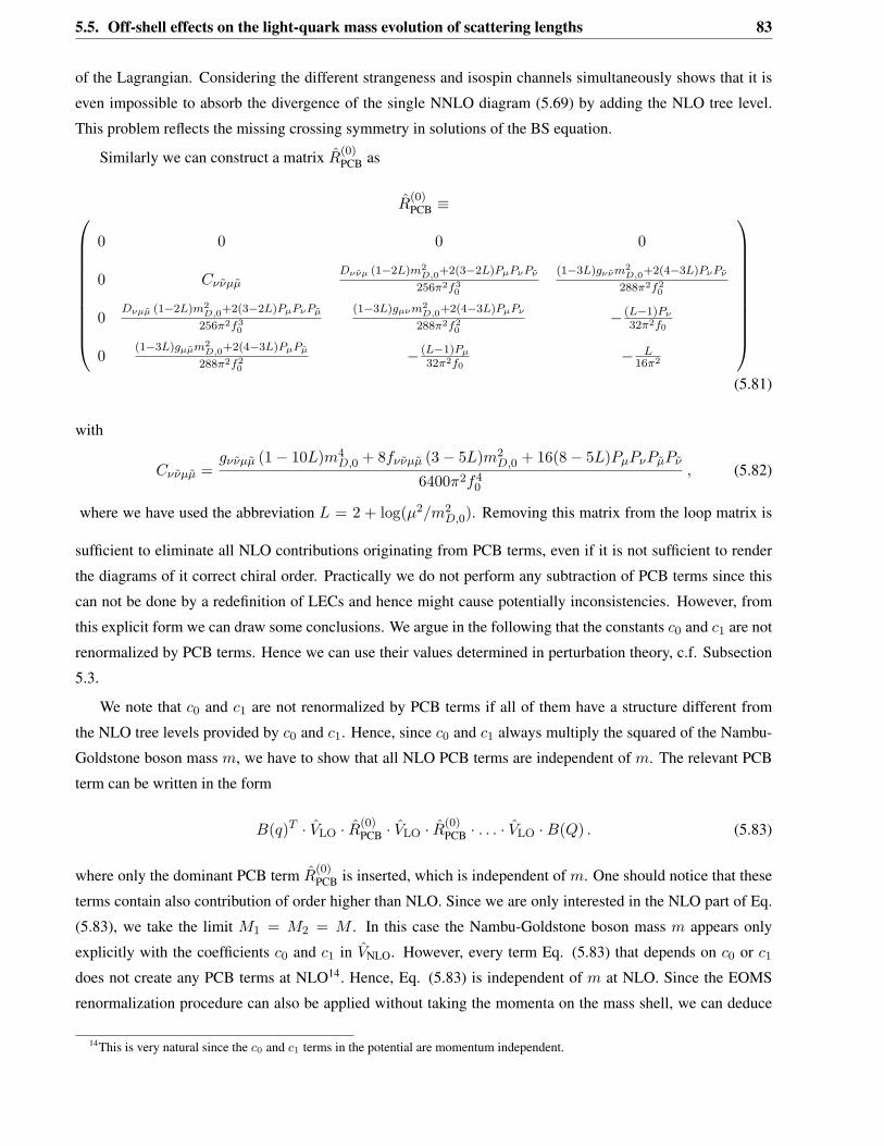
5.5. Off-shell effects on the light-quark mass evolution of scattering lengths 83
of the Lagrangian. Considering the different strangeness and isospin channels simultaneously shows that it is
even impossible to absorb the divergence of the single NNLO diagram (5.69) by adding the NLO tree level.
This problem reflects the missing crossing symmetry in solutions of the BS equation.
Similarly we can construct a matrix ��(0)PCB as
��(0)PCB ≡⎛
⎜⎜⎜⎜⎜⎜⎜⎜⎜⎜⎝
0 0 0 0
0 𝐶𝜈𝜈𝜇��𝐷𝜈𝜈𝜇 (1−2𝐿)𝑚2
𝐷,0+2(3−2𝐿)𝑃𝜇𝑃𝜈𝑃𝜈
256𝜋2𝑓30
(1−3𝐿)𝑔𝜈𝜈𝑚2𝐷,0+2(4−3𝐿)𝑃𝜈𝑃𝜈
288𝜋2𝑓20
0𝐷𝜈𝜇�� (1−2𝐿)𝑚2
𝐷,0+2(3−2𝐿)𝑃𝜇𝑃𝜈𝑃��
256𝜋2𝑓30
(1−3𝐿)𝑔𝜇𝜈𝑚2𝐷,0+2(4−3𝐿)𝑃𝜇𝑃𝜈
288𝜋2𝑓20
− (𝐿−1)𝑃𝜈
32𝜋2𝑓0
0(1−3𝐿)𝑔𝜇��𝑚2
𝐷,0+2(4−3𝐿)𝑃𝜇𝑃��
288𝜋2𝑓20
− (𝐿−1)𝑃𝜇
32𝜋2𝑓0− 𝐿
16𝜋2
⎞⎟⎟⎟⎟⎟⎟⎟⎟⎟⎟⎠
(5.81)
with
𝐶𝜈𝜈𝜇�� =𝑔𝜈𝜈𝜇�� (1− 10𝐿)𝑚4
𝐷,0 + 8𝑓𝜈𝜈𝜇�� (3− 5𝐿)𝑚2𝐷,0 + 16(8− 5𝐿)𝑃𝜇𝑃𝜈𝑃��𝑃𝜈
6400𝜋2𝑓40
, (5.82)
where we have used the abbreviation 𝐿 = 2 + log(𝜇2/𝑚2𝐷,0). Removing this matrix from the loop matrix is
sufficient to eliminate all NLO contributions originating from PCB terms, even if it is not sufficient to render
the diagrams of it correct chiral order. Practically we do not perform any subtraction of PCB terms since this
can not be done by a redefinition of LECs and hence might cause potentially inconsistencies. However, from
this explicit form we can draw some conclusions. We argue in the following that the constants 𝑐0 and 𝑐1 are not
renormalized by PCB terms. Hence we can use their values determined in perturbation theory, c.f. Subsection
5.3.
We note that 𝑐0 and 𝑐1 are not renormalized by PCB terms if all of them have a structure different from
the NLO tree levels provided by 𝑐0 and 𝑐1. Hence, since 𝑐0 and 𝑐1 always multiply the squared of the Nambu-
Goldstone boson mass 𝑚, we have to show that all NLO PCB terms are independent of 𝑚. The relevant PCB
term can be written in the form
𝐵(𝑞)𝑇 · 𝑉LO · ��(0)PCB · 𝑉LO · ��(0)
PCB · . . . · 𝑉LO ·𝐵(𝑄) . (5.83)
where only the dominant PCB term ��(0)PCB is inserted, which is independent of 𝑚. One should notice that these
terms contain also contribution of order higher than NLO. Since we are only interested in the NLO part of Eq.
(5.83), we take the limit 𝑀1 = 𝑀2 = 𝑀 . In this case the Nambu-Goldstone boson mass 𝑚 appears only
explicitly with the coefficients 𝑐0 and 𝑐1 in 𝑉NLO. However, every term Eq. (5.83) that depends on 𝑐0 or 𝑐1
does not create any PCB terms at NLO14. Hence, Eq. (5.83) is independent of 𝑚 at NLO. Since the EOMS
renormalization procedure can also be applied without taking the momenta on the mass shell, we can deduce
14This is very natural since the 𝑐0 and 𝑐1 terms in the potential are momentum independent.
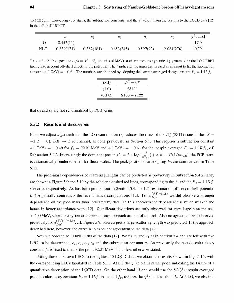
84 Chapter 5. Scattering of Nambu-Goldstone bosons off heavy-light mesons
TABLE 5.11: Low-energy constants, the subtraction constants, and the 𝜒2/d.o.f. from the best fits to the LQCD data [12]in the off-shell UChPT.
𝑎 𝑐2 𝑐3 𝑐4 𝑐5 𝜒2/d.o.fLO -0.452(11) 17.9
NLO 0.639(131) 0.382(181) 0.653(345) 0.597(92) -2.084(276) 0.79
TABLE 5.12: Pole positions√
𝑠 = 𝑀 − 𝑖Γ2 (in units of MeV) of charm mesons dynamically generated in the LO UChPT
taking into account off-shell effects in the potential. The * indicates the mass that is used as an input to fix the subtractionconstant, 𝑎(1 GeV) = −0.61. The numbers are obtained by adopting the isospin averaged decay constant 𝐹0 = 1.15 𝑓0.
(S,I) 𝐽𝑃 = 0+
(1,0) 2318*
(0,1/2) 2155− 𝑖 122
that 𝑐0 and 𝑐1 are not renormalized by PCB terms.
5.5.2 Results and discussions
First, we adjust 𝑎(𝜇) such that the LO resummation reproduces the mass of the 𝐷*𝑠0(2317) state in the (𝑆 =
−1, 𝐼 = 0), 𝐷�� → 𝐷�� channel, as done previously in Section 5.4. This requires a subtraction constant
𝑎(1 GeV) = −0.49 for 𝑓0 = 92.21 MeV and 𝑎(1 GeV) = −0.61 for the isospin averaged 𝐹0 = 1.15 𝑓0, c.f.
Subsection 5.4.2. Interestingly the dominant part in 𝐵0 = 2 + log( 𝜇2
𝑚2𝐷,0
) + 𝑎(𝜇) +𝒪(1/𝑚𝐷,0), the PCB term,
is automatically rendered small for those scales. The peak positions for adopting 𝐹0 are summarized in Table
5.12.
The pion-mass dependences of scattering lengths can be predicted as previously in Subsection 5.4.2. They
are shown in Figure 5.9 and 5.10 by the solid and dashed red lines, corresponding to the 𝑓0 and the 𝐹0 = 1.15 𝑓0
scenario, respectively. As has been pointed out in Section 5.4, the LO resummation of the on-shell potential
(5.40) partially contradicts the recent lattice computations [12]. For 𝑎(𝑆,𝐼)=(1,1)𝐷𝑠𝜋 we did observe a stronger
dependence on the pion mass than indicated by data. In this approach the dependence is much weaker and
hence in better accordance with [12]. Significant deviations are only observed for very large pion masses,
> 500 MeV, where the systematic errors of our approach are out of control. Also no agreement was observed
previously for 𝑎(𝑆,𝐼)=(−1,0)
𝐷��, c.f. Figure 5.9, where a pretty large scattering length was predicted. In the approach
described here, however, the curve is in excellent agreement to the data [12].
Now we proceed to LO/NLO fits of the data [12]. We fix 𝑐0 and 𝑐1 as in Section 5.4 and are left with five
LECs to be determined, 𝑐2, 𝑐3, 𝑐4, 𝑐5 and the subtraction constant 𝑎. As previously the pseudoscalar decay
constant 𝑓0 is fixed to that of the pion, 92.21 MeV [1], unless otherwise stated.
Fitting these unknown LECs to the lightest 15 LQCD data, we obtain the results shown in Fig. 5.15, with
the corresponding LECs tabulated in Table 5.11. At LO the 𝜒2/d.o.f. is rather poor, indicating the failure of a
quantitative description of the LQCD data. On the other hand, if one would use the 𝑆𝑈(3) isospin averaged
pseudoscalar decay constant 𝐹0 = 1.15𝑓0 instead of 𝑓0, reduces the 𝜒2/d.o.f. to about 5. At NLO, we obtain a
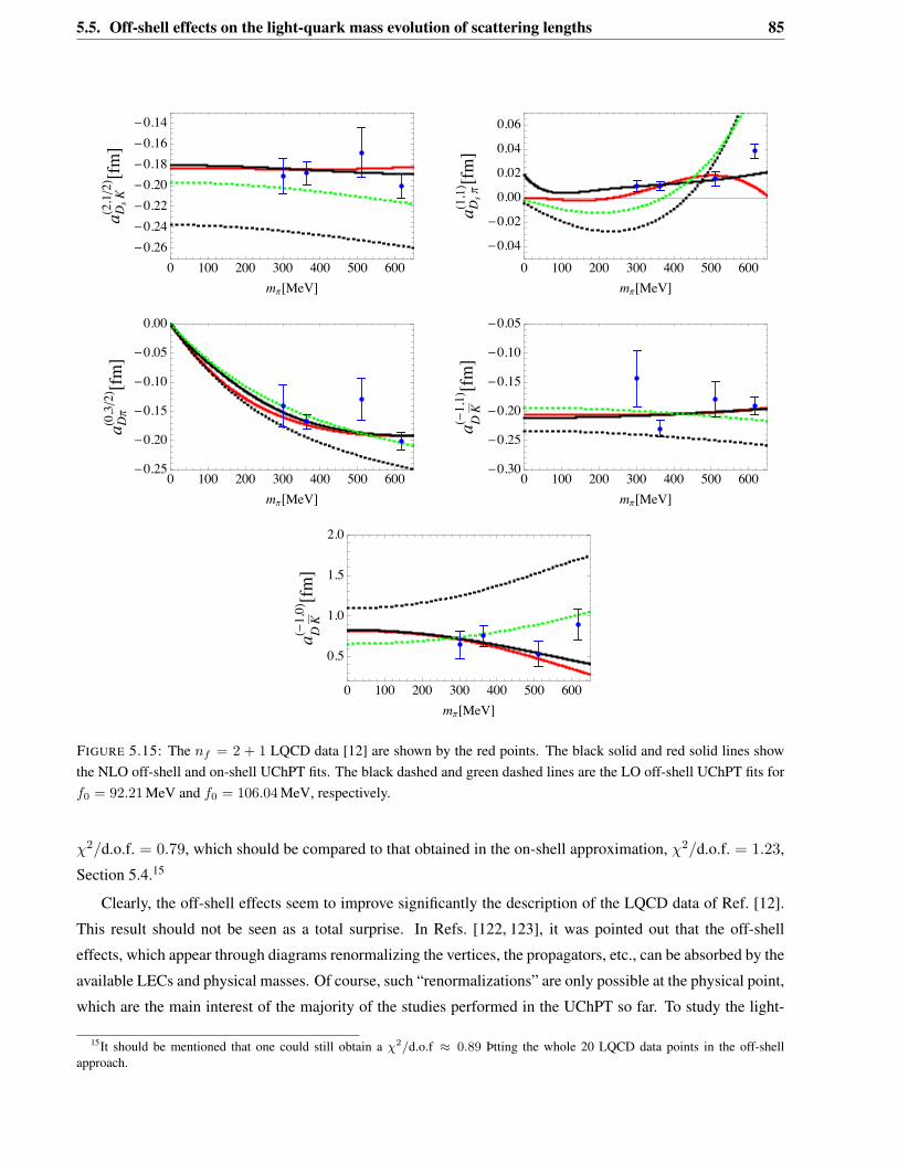
5.5. Off-shell effects on the light-quark mass evolution of scattering lengths 85
0 100 200 300 400 500 600!0.26!0.24!0.22!0.20!0.18!0.16!0.14
m"!MeV"
a DsK#2,1$2% !fm"
0 100 200 300 400 500 600!0.04
!0.02
0.00
0.02
0.04
0.06
m"!MeV"
a Ds"#1,1% !fm"
0 100 200 300 400 500 600!0.25
!0.20
!0.15
!0.10
!0.05
0.00
m"!MeV"
a D"#0,3$2% !fm"
0 100 200 300 400 500 600!0.30
!0.25
!0.20
!0.15
!0.10
!0.05
m"!MeV"a D
K#!1,1% !fm"
0 100 200 300 400 500 600
0.5
1.0
1.5
2.0
m"!MeV"
a DK#!1,0% !fm"
FIGURE 5.15: The 𝑛𝑓 = 2 + 1 LQCD data [12] are shown by the red points. The black solid and red solid lines showthe NLO off-shell and on-shell UChPT fits. The black dashed and green dashed lines are the LO off-shell UChPT fits for𝑓0 = 92.21 MeV and 𝑓0 = 106.04 MeV, respectively.
𝜒2/d.o.f. = 0.79, which should be compared to that obtained in the on-shell approximation, 𝜒2/d.o.f. = 1.23,
Section 5.4.15
Clearly, the off-shell effects seem to improve significantly the description of the LQCD data of Ref. [12].
This result should not be seen as a total surprise. In Refs. [122, 123], it was pointed out that the off-shell
effects, which appear through diagrams renormalizing the vertices, the propagators, etc., can be absorbed by the
available LECs and physical masses. Of course, such “renormalizations” are only possible at the physical point,
which are the main interest of the majority of the studies performed in the UChPT so far. To study the light-
15It should be mentioned that one could still obtain a 𝜒2/d.o.f ≈ 0.89 Þtting the whole 20 LQCD data points in the off-shellapproach.
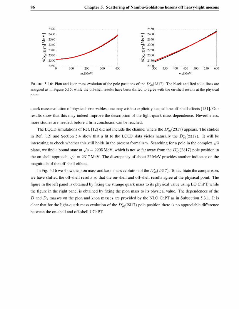
86 Chapter 5. Scattering of Nambu-Goldstone bosons off heavy-light mesons
0 100 200 300 40022802300232023402360238024002420
m!!MeV"
MDs0"#2317
$!MeV"
300 350 400 450 500 550 60021002150220022502300235024002450
mK!MeV"
MDs0"#2317
$!MeV"
FIGURE 5.16: Pion and kaon mass evolution of the pole positions of the 𝐷*𝑠0(2317). The black and Red solid lines are
assigned as in Figure 5.15, while the off-shell results have been shifted to agree with the on-shell results at the physicalpoint.
quark mass evolution of physical observables, one may wish to explicitly keep all the off-shell effects [151]. Our
results show that this may indeed improve the description of the light-quark mass dependence. Nevertheless,
more studies are needed, before a firm conclusion can be reached.
The LQCD simulations of Ref. [12] did not include the channel where the 𝐷*𝑠0(2317) appears. The studies
in Ref. [12] and Section 5.4 show that a fit to the LQCD data yields naturally the 𝐷*𝑠0(2317). It will be
interesting to check whether this still holds in the present formalism. Searching for a pole in the complex√
𝑠
plane, we find a bound state at√
𝑠 = 2295 MeV, which is not so far away from the 𝐷*𝑠0(2317) pole position in
the on-shell approach,√
𝑠 = 2317 MeV. The discrepancy of about 22 MeV provides another indicator on the
magnitude of the off-shell effects.
In Fig. 5.16 we show the pion mass and kaon mass evolution of the 𝐷*𝑠0(2317). To facilitate the comparison,
we have shifted the off-shell results so that the on-shell and off-shell results agree at the physical point. The
figure in the left panel is obtained by fixing the strange quark mass to its physical value using LO ChPT, while
the figure in the right panel is obtained by fixing the pion mass to its physical value. The dependences of the
𝐷 and 𝐷𝑠 masses on the pion and kaon masses are provided by the NLO ChPT as in Subsection 5.3.1. It is
clear that for the light-quark mass evolution of the 𝐷*𝑠0(2317) pole position there is no appreciable difference
between the on-shell and off-shell UChPT.
Chapter 6
Summary and conclusions
Lattice QCD computations have made remarkable progress in recent years. Nowadays, they offer an accurate
method to calculate a variety of physical quantities governed by non-perturbative strong interaction physics.
For “gold plated” quantities, such as the decay constants studied in this work, the overall uncertainties have
been reduced to a few percent. Obviously, chiral perturbation theory plays an important role in understanding
some of the systematic errors, such as those from finite volume and extrapolations of the light quark masses to
their physical values.
In the first part of this theses we have investigated the light-quark mass dependence of the HPQCD lattice
QCD data [25] for the decay constants 𝑓𝐷 and 𝑓𝐷𝑠 . This is done in the framework of covariant chiral per-
turbation theory (ChPT). This analysis reveals that the covariant ChPT describes the HPQCD extrapolations
considerably better than the standard heavy meson ChPT at a given order, although both approaches show
improvement when going from next-to-leading to next-to-next-to leading order. Our studies show that if the
lattice simulations are performed with relatively large light quark masses (e.g., 𝑚𝜋 > 300 MeV), a covariant
formulation of ChPT is a better choice for chiral extrapolations, particularly at low chiral orders.
On the other hand, precise lattice data are valuable to fix some of the low energy constants of our the-
ory. These constants can be used to predict physical observables involving the same low-energy-constants, or
constants that are related by symmetries. In the present work, we give predictions for the ratios of 𝑓𝐵𝑠/𝑓𝐵 ,
𝑓𝐷*𝑠 /𝑓𝐷* , and 𝑓𝐵*𝑠 /𝑓𝐵* and their light-quark mass dependencies, where the low-energy-constants have been
determined by employing the lattice QCD data of Ref. [25]. These predictions should be testable in the near
future. Our results show that the relations 𝑓𝐵𝑠/𝑓𝐵 > 𝑓𝐷𝑠/𝑓𝐷 and 𝑓𝐷*𝑠 /𝑓𝐷* < 𝑓𝐷𝑠/𝑓𝐷 should hold in a large
portion of the allowed parameter space.
The second part of this theses, starting from Chapter 5, has investigated the interactions of the heavy-
light mesons (𝐷, 𝐷*, 𝐵, 𝐵* and their strange counterparts) with Nambu-Goldstone bosons (the octet of the
lightest pseudoscalar mesons). These interactions have been iterated by a unitarization procedure, i.e. solving
a Bethe-Salpeter equation, which has the appealing feature that various higher-lying charm/bottom states can
be studied. In order to fix the relevant low-energy constant up to next-to-leading order we have fitted the
latest fully dynamical lattice QCD simulations for the scattering lengths of Nambu-Goldstone bosons off 𝐷
mesons of Ref. [12]. As in the first part of this theses we have relied on the covariant formulation of chiral
87
88 Chapter 6. Summary and conclusions
perturbation theory. This calculation shows, as previously for the study of the decay constants 𝑓𝐷 and 𝑓𝐷𝑠 , that
the covariant (unitarized) ChPT describes the lattice QCD data better than its non-relativistic (heavy-meson)
counterpart. In addition, we show that the 𝐷*𝑠0(2317) can be dynamically generated without a priori assumption
of its existence, where the predicted mass is in excellent agreement with experiment. This success indicates
that the nearby 𝐷𝐾 threshold can not be neglected in terms of naive constituent quark models.
To employ the determined low-energy constants in other sectors of heavy-light mesons, 𝐷*, 𝐵 and 𝐵*,
we have proposed a new subtraction scheme to ensure that the loop function appearing in the Bethe-Salpeter
equation satisfies the chiral power counting rule and has a well defined behavior in the limit of infinite heavy
quark mass. It has been shown that this scheme has a similar 1/𝑀HL scaling as the heavy-meson ChPT loop
function, but provides a better description of the light-quark mass dependence of the lattice QCD scattering
lengths. With such a scheme, we have predicted the counterparts of the 𝐷*𝑠0(2317) in the 𝐽𝑃 = 1+ sector and
in the bottom sector. The experimental confirmation of the dynamically generated states in the bottom sector
can serve as a stringent test of our theoretical model and the interpretation of the 𝐷*𝑠0(2317) as a dynamically
generated state from the strong 𝐷𝐾 interaction.
Apart from the successes of such a unitarization procedure, its range of applicability is very limited. States
more distant to the lowest lying threshold are usually not reproduced to good accuracy. These apparent problems
motivated us to test the validity of a simplification usually employed in the unitarization procedure. This
is the use of potentials taken on the mass shell. This widely accepted approximation is understood to be
legitimate, since all effects coming from the off-shellness of the potential should be absorbable into the low-
energy constants of the theory, even if these constants enter at arbitrarily high order. This is a highly nontrivial
statement since the results produced by unitarization do no longer respect crossing symmetry. A consequence
of this is the loss of renormalizability, even at a given chiral order.
In the end of Chapter 5 we have solved the Bethe-Salpeter equation in unitary chiral perturbation theory
by taking into account the full off-shellness of the chiral potentials up to next-to-leading order. To quantify
the magnitude and impact of the off-shell effects, we have studied the light-quark mass dependence of the
scattering lengths of the Nambu-Goldstone bosons off the 𝐷 mesons from Ref. [12]. In comparison with
the widely used on-shell approximation, we have shown that taking into account off-shell effects can indeed
improve the description of the lattice QCD data, in terms of light-quark mass evolution. On the other hand,
both descriptions look qualitatively similar, at least for the observables we studied. Therefore, unless the lattice
QCD data becomes more precise, the on-shell approximation may still be confidently used, given its simplicity.
On the other hand we have shown that predictions obtained by employing only the leading order potential can
significantly differ within these two approaches, as demonstrated in Section 5.4. There we have observed that
the results taking into account the full off-shellness of the potential are clearly favored by the lattice QCD data.
So far, even if we can not yet draw a final statement concerning the quality of the on-shell approximation, our
procedure can be seen as a step towards improving the standard unitarization techniques.
Chapter 7
Acknowledgements
Finally, I want to thank a number of people that contributed significantly to this theses
∙ Prof. Dr. Wolfram Weise for giving me the opportunity to write this theses in his group T39, and for
numerous discussions and constructive feedback over the last few years.
∙ Prof. Dr. Lisheng Geng for the fruitful collaboration. I want to thank him for his active contributions, his
numerous ideas and the verification of most parts of the present work.
∙ Prof. Dr. Norbert Kaiser for enlightening discussions.
∙ all members of T39 for the very nice working atmosphere. I also want to thank a number of former
members of T39: Maximilian Duell, Salvatore Fiorilla, Thomas Hell and Alexander Laschka.
∙ and last but not least my family for supporting me over all the years.
For the financial support, I would like to thank the German Bundesministerium für Bildung und Forschung
(BMBF), the DFG Cluster of Excellence “Origin and Structure of the Universe”, and the Sino-German CRC
110 “Symmetries and Emergence of Structure in QCD” by DFG and NSFC.
89
90 Chapter 7. Acknowledgements
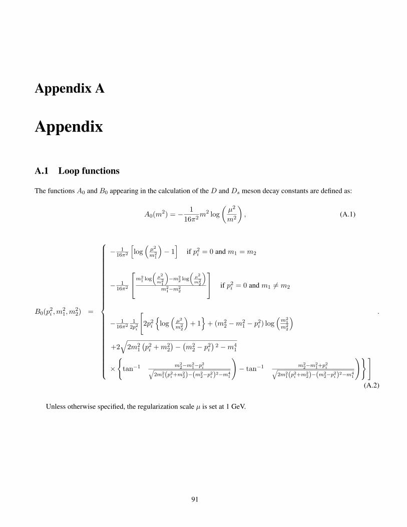
Appendix A
Appendix
A.1 Loop functions
The functions 𝐴0 and 𝐵0 appearing in the calculation of the 𝐷 and 𝐷𝑠 meson decay constants are defined as:
𝐴0(𝑚2) = − 116𝜋2
𝑚2 log(
𝜇2
𝑚2
), (A.1)
𝐵0(𝑝2𝑖 , 𝑚
21, 𝑚
22) =
⎧⎪⎪⎪⎪⎪⎪⎪⎪⎪⎪⎪⎪⎪⎪⎪⎪⎪⎪⎪⎪⎪⎪⎪⎪⎪⎨⎪⎪⎪⎪⎪⎪⎪⎪⎪⎪⎪⎪⎪⎪⎪⎪⎪⎪⎪⎪⎪⎪⎪⎪⎪⎩
− 116𝜋2
[log(
𝜇2
𝑚21
)− 1]
if 𝑝2𝑖 = 0 and 𝑚1 = 𝑚2
− 116𝜋2
⎡⎣
𝑚21 log
(𝜇2
𝑚21
)−𝑚2
2 log
(𝜇2
𝑚22
)𝑚2
1−𝑚22
⎤⎦ if 𝑝2
𝑖 = 0 and 𝑚1 = 𝑚2
− 116𝜋2
12𝑝2
𝑖
[2𝑝2
𝑖
{log(
𝜇2
𝑚22
)+ 1}
+ (𝑚22 −𝑚2
1 − 𝑝2𝑖 ) log
(𝑚2
1
𝑚22
)
+2√
2𝑚21
(𝑝2
𝑖 + 𝑚22
)−(𝑚2
2 − 𝑝2𝑖
)2 −𝑚4
1
×{
tan−1
(𝑚2
2−𝑚21−𝑝2
𝑖√2𝑚2
1(𝑝2𝑖 +𝑚2
2)−(𝑚22−𝑝2
𝑖 )2−𝑚41
)− tan−1
(𝑚2
2−𝑚21+𝑝2
𝑖√2𝑚2
1(𝑝2𝑖 +𝑚2
2)−(𝑚22−𝑝2
𝑖 )2−𝑚41
)}]
.
(A.2)
Unless otherwise specified, the regularization scale 𝜇 is set at 1 GeV.
91
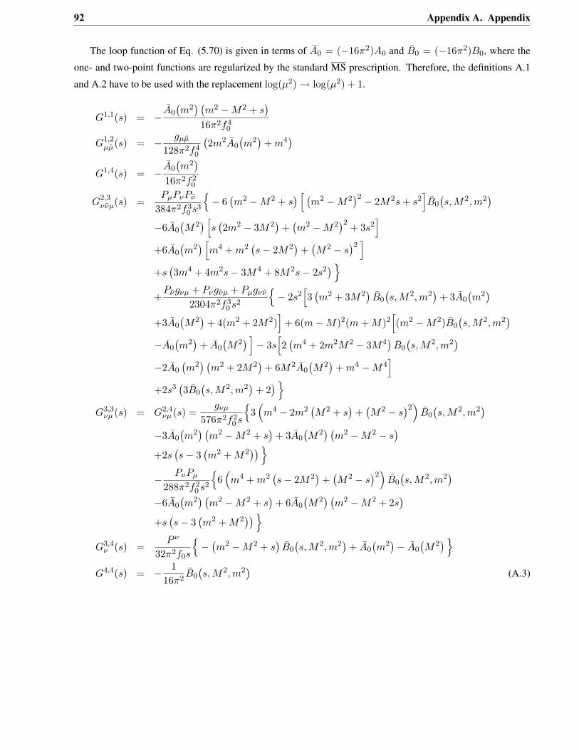
92 Appendix A. Appendix
The loop function of Eq. (5.70) is given in terms of 𝐴0 = (−16𝜋2)𝐴0 and ��0 = (−16𝜋2)𝐵0, where the
one- and two-point functions are regularized by the standard MS prescription. Therefore, the definitions A.1
and A.2 have to be used with the replacement log(𝜇2) → log(𝜇2) + 1.
𝐺1,1(𝑠) = −𝐴0
(𝑚2) (
𝑚2 −𝑀2 + 𝑠)
16𝜋2𝑓40
𝐺1,2𝜇��(𝑠) = − 𝑔𝜇��
128𝜋2𝑓40
(2𝑚2𝐴0
(𝑚2)
+ 𝑚4)
𝐺1,4(𝑠) = −𝐴0
(𝑚2)
16𝜋2𝑓20
𝐺2,3𝜈𝜈𝜇(𝑠) =
𝑃𝜇𝑃𝜈𝑃𝜈
384𝜋2𝑓30 𝑠3
{− 6
(𝑚2 −𝑀2 + 𝑠
) [ (𝑚2 −𝑀2
)2 − 2𝑀2𝑠 + 𝑠2]��0
(𝑠, 𝑀2, 𝑚2
)
−6𝐴0
(𝑀2) [
𝑠(2𝑚2 − 3𝑀2
)+(𝑚2 −𝑀2
)2 + 3𝑠2]
+6𝐴0
(𝑚2) [
𝑚4 + 𝑚2(𝑠− 2𝑀2
)+(𝑀2 − 𝑠
)2 ]
+𝑠(3𝑚4 + 4𝑚2𝑠− 3𝑀4 + 8𝑀2𝑠− 2𝑠2
)}
+𝑃𝜈𝑔𝜈𝜇 + 𝑃𝜈𝑔𝜈𝜇 + 𝑃𝜇𝑔𝜈𝜈
2304𝜋2𝑓30 𝑠2
{− 2𝑠2
[3(𝑚2 + 3𝑀2
)��0
(𝑠, 𝑀2, 𝑚2
)+ 3𝐴0
(𝑚2)
+3𝐴0
(𝑀2)
+ 4(𝑚2 + 2𝑀2)]
+ 6(𝑚−𝑀)2(𝑚 + 𝑀)2[(𝑚2 −𝑀2)��0
(𝑠, 𝑀2, 𝑚2
)
−𝐴0
(𝑚2)
+ 𝐴0
(𝑀2) ]− 3𝑠
[2(𝑚4 + 2𝑚2𝑀2 − 3𝑀4
)��0
(𝑠, 𝑀2, 𝑚2
)
−2𝐴0
(𝑚2) (
𝑚2 + 2𝑀2)
+ 6𝑀2𝐴0
(𝑀2)
+ 𝑚4 −𝑀4]
+2𝑠3(3��0
(𝑠, 𝑀2, 𝑚2
)+ 2)}
𝐺3,3𝜈𝜇 (𝑠) = 𝐺2,4
𝜈𝜇 (𝑠) =𝑔𝜈𝜇
576𝜋2𝑓20 𝑠
{3(𝑚4 − 2𝑚2
(𝑀2 + 𝑠
)+(𝑀2 − 𝑠
)2)��0
(𝑠, 𝑀2, 𝑚2
)
−3𝐴0
(𝑚2) (
𝑚2 −𝑀2 + 𝑠)
+ 3𝐴0
(𝑀2) (
𝑚2 −𝑀2 − 𝑠)
+2𝑠(𝑠− 3
(𝑚2 + 𝑀2
))}
− 𝑃𝜈𝑃𝜇
288𝜋2𝑓20 𝑠2
{6(𝑚4 + 𝑚2
(𝑠− 2𝑀2
)+(𝑀2 − 𝑠
)2)��0
(𝑠, 𝑀2, 𝑚2
)
−6𝐴0
(𝑚2) (
𝑚2 −𝑀2 + 𝑠)
+ 6𝐴0
(𝑀2) (
𝑚2 −𝑀2 + 2𝑠)
+𝑠(𝑠− 3
(𝑚2 + 𝑀2
))}
𝐺3,4𝜈 (𝑠) =
𝑃 𝜈
32𝜋2𝑓0𝑠
{−(𝑚2 −𝑀2 + 𝑠
)��0
(𝑠, 𝑀2, 𝑚2
)+ 𝐴0
(𝑚2)−𝐴0
(𝑀2)}
𝐺4,4(𝑠) = − 116𝜋2
��0
(𝑠, 𝑀2, 𝑚2
)(A.3)
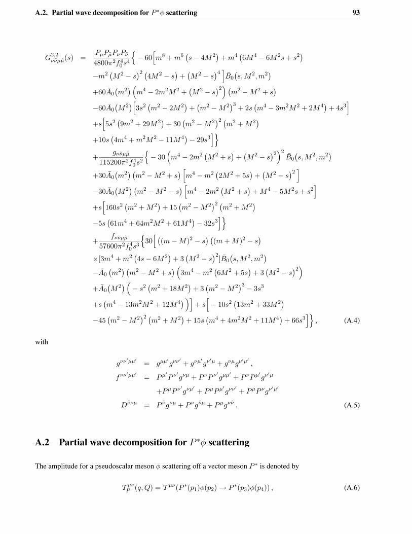
A.2. Partial wave decomposition for 𝑃 *𝜑 scattering 93
𝐺2,2𝜈𝜈𝜇��(𝑠) =
𝑃𝜇𝑃��𝑃𝜈𝑃𝜈
4800𝜋2𝑓40 𝑠4
{− 60
[𝑚8 + 𝑚6
(𝑠− 4𝑀2
)+ 𝑚4
(6𝑀4 − 6𝑀2𝑠 + 𝑠2
)
−𝑚2(𝑀2 − 𝑠
)2 (4𝑀2 − 𝑠)
+(𝑀2 − 𝑠
)4 ]��0
(𝑠, 𝑀2, 𝑚2
)
+60𝐴0
(𝑚2) (
𝑚4 − 2𝑚2𝑀2 +(𝑀2 − 𝑠
)2) (𝑚2 −𝑀2 + 𝑠
)
−60𝐴0
(𝑀2)[
3𝑠2(𝑚2 − 2𝑀2
)+(𝑚2 −𝑀2
)3 + 2𝑠(𝑚4 − 3𝑚2𝑀2 + 2𝑀4
)+ 4𝑠3
]
+𝑠[5𝑠2(9𝑚2 + 29𝑀2
)+ 30
(𝑚2 −𝑀2
)2 (𝑚2 + 𝑀2
)
+10𝑠(4𝑚4 + 𝑚2𝑀2 − 11𝑀4
)− 29𝑠3
]}
+𝑔𝜈𝜈𝜇��
115200𝜋2𝑓40 𝑠2
{− 30
(𝑚4 − 2𝑚2
(𝑀2 + 𝑠
)+(𝑀2 − 𝑠
)2)2��0
(𝑠, 𝑀2, 𝑚2
)
+30𝐴0
(𝑚2) (
𝑚2 −𝑀2 + 𝑠) [
𝑚4 −𝑚2(2𝑀2 + 5𝑠
)+(𝑀2 − 𝑠
)2 ]
−30𝐴0
(𝑀2) (
𝑚2 −𝑀2 − 𝑠) [
𝑚4 − 2𝑚2(𝑀2 + 𝑠
)+ 𝑀4 − 5𝑀2𝑠 + 𝑠2
]
+𝑠[160𝑠2
(𝑚2 + 𝑀2
)+ 15
(𝑚2 −𝑀2
)2 (𝑚2 + 𝑀2
)
−5𝑠(61𝑚4 + 64𝑚2𝑀2 + 61𝑀4
)− 32𝑠3
]}
+𝑓𝜈𝜈𝜇��
57600𝜋2𝑓40 𝑠3
{30[ (
(𝑚−𝑀)2 − 𝑠) (
(𝑚 + 𝑀)2 − 𝑠)
×[3𝑚4 + 𝑚2(4𝑠− 6𝑀2
)+ 3
(𝑀2 − 𝑠
)2]��0
(𝑠, 𝑀2, 𝑚2
)
−𝐴0
(𝑚2) (
𝑚2 −𝑀2 + 𝑠) (
3𝑚4 −𝑚2(6𝑀2 + 5𝑠
)+ 3
(𝑀2 − 𝑠
)2)
+𝐴0
(𝑀2) (
− 𝑠2(𝑚2 + 18𝑀2
)+ 3
(𝑚2 −𝑀2
)3 − 3𝑠3
+𝑠(𝑚4 − 13𝑚2𝑀2 + 12𝑀4
) )]+ 𝑠[− 10𝑠2
(13𝑚2 + 33𝑀2
)
−45(𝑚2 −𝑀2
)2 (𝑚2 + 𝑀2
)+ 15𝑠
(𝑚4 + 4𝑚2𝑀2 + 11𝑀4
)+ 66𝑠3
]}, (A.4)
with
𝑔𝜈𝜈′𝜇𝜇′ = 𝑔𝜇𝜇′𝑔𝜈𝜈′ + 𝑔𝜈𝜇′𝑔𝜈′𝜇 + 𝑔𝜈𝜇𝑔𝜈′𝜇′ ,
𝑓𝜈𝜈′𝜇𝜇′ = 𝑃𝜇′𝑃 𝜈′𝑔𝜈𝜇 + 𝑃 𝜈𝑃 𝜈′𝑔𝜇𝜇′ + 𝑃 𝜈𝑃𝜇′𝑔𝜈′𝜇
+𝑃𝜇𝑃 𝜈′𝑔𝜈𝜇′ + 𝑃𝜇𝑃𝜇′𝑔𝜈𝜈′ + 𝑃𝜇𝑃 𝜈𝑔𝜈′𝜇′
𝐷𝜈𝜈𝜇 = 𝑃 𝜈𝑔𝜈𝜇 + 𝑃 𝜈𝑔𝜈𝜇 + 𝑃𝜇𝑔𝜈𝜈 . (A.5)
A.2 Partial wave decomposition for 𝑃 *𝜑 scattering
The amplitude for a pseudoscalar meson 𝜑 scattering off a vector meson 𝑃 * is denoted by
𝒯 𝜇𝜈𝑃 (𝑞,𝑄) = 𝒯 𝜇𝜈(𝑃 *(𝑝1)𝜑(𝑝2) → 𝑃 *(𝑝3)𝜑(𝑝4)) , (A.6)
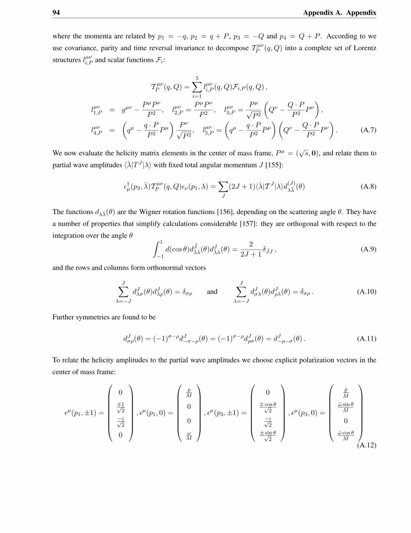
94 Appendix A. Appendix
where the momenta are related by 𝑝1 = −𝑞, 𝑝2 = 𝑞 + 𝑃 , 𝑝3 = −𝑄 and 𝑝4 = 𝑄 + 𝑃 . According to we
use covariance, parity and time reversal invariance to decompose 𝒯 𝜇𝜈𝑃 (𝑞, 𝑄) into a complete set of Lorentz
structures 𝑙𝜇𝜈𝑖,𝑃 and scalar functions ℱ𝑖:
𝒯 𝜇𝜈𝑃 (𝑞, 𝑄) =
5∑
𝑖=1
𝑙𝜇𝜈𝑖,𝑃 (𝑞, 𝑄)ℱ𝑖,𝑃 (𝑞, 𝑄) ,
𝑙𝜇𝜈1,𝑃 = 𝑔𝜇𝜈 − 𝑃𝜇𝑃 𝜈
𝑃 2, 𝑙𝜇𝜈
2,𝑃 =𝑃𝜇𝑃 𝜈
𝑃 2, 𝑙𝜇𝜈
3,𝑃 =𝑃𝜇
√𝑃 2
(𝑄𝜈 − 𝑄 · 𝑃
𝑃 2𝑃 𝜈
),
𝑙𝜇𝜈4,𝑃 =
(𝑞𝜇 − 𝑞 · 𝑃
𝑃 2𝑃𝜇
)𝑃 𝜈
√𝑃 2
, 𝑙𝜇𝜈5,𝑃 =
(𝑞𝜇 − 𝑞 · 𝑃
𝑃 2𝑃𝜇
)(𝑄𝜈 − 𝑄 · 𝑃
𝑃 2𝑃 𝜈
). (A.7)
We now evaluate the helicity matrix elements in the center of mass frame, 𝑃𝜇 = (√
𝑠,0), and relate them to
partial wave amplitudes ⟨��|𝑇 𝐽 |𝜆⟩ with fixed total angular momentum 𝐽 [155]:
𝜖†𝜇(𝑝3, ��)𝒯 𝜇𝜈𝑃 (𝑞, 𝑄)𝜖𝜈(𝑝1, 𝜆) =
∑
𝐽
(2𝐽 + 1)⟨��|𝒯 𝐽 |𝜆⟩𝑑(𝐽)
𝜆��(𝜃) (A.8)
The functions 𝑑𝜆��(𝜃) are the Wigner rotation functions [156], depending on the scattering angle 𝜃. They have
a number of properties that simplify calculations considerable [157]: they are orthogonal with respect to the
integration over the angle 𝜃 ∫ 1
−1𝑑(cos 𝜃)𝑑𝐽
��𝜆(𝜃)𝑑𝐽��𝜆(𝜃) =
22𝐽 + 1
𝛿𝐽𝐽 , (A.9)
and the rows and columns form orthonormal vectors
𝐽∑
𝜆=−𝐽
𝑑𝐽𝜆𝜎(𝜃)𝑑𝐽
𝜆𝜌(𝜃) = 𝛿𝜎𝜌 and𝐽∑
𝜆=−𝐽
𝑑𝐽𝜎𝜆(𝜃)𝑑𝐽
𝜌𝜆(𝜃) = 𝛿𝜎𝜌 . (A.10)
Further symmetries are found to be
𝑑𝐽𝜎𝜌(𝜃) = (−1)𝜎−𝜌𝑑𝐽
−𝜎−𝜌(𝜃) = (−1)𝜎−𝜌𝑑𝐽𝜌𝜎(𝜃) = 𝑑𝐽
−𝜌−𝜎(𝜃) . (A.11)
To relate the helicity amplitudes to the partial wave amplitudes we choose explicit polarization vectors in the
center of mass frame:
𝜖𝜇(𝑝1,±1) =
⎛⎜⎜⎜⎜⎜⎜⎜⎝
0
∓1√2
−𝑖√2
0
⎞⎟⎟⎟⎟⎟⎟⎟⎠
, 𝜖𝜇(𝑝1, 0) =
⎛⎜⎜⎜⎜⎜⎜⎜⎝
𝑝𝑀
0
0
𝜔𝑀
⎞⎟⎟⎟⎟⎟⎟⎟⎠
, 𝜖𝜇(𝑝3,±1) =
⎛⎜⎜⎜⎜⎜⎜⎜⎝
0
∓ cos 𝜃√2
−𝑖√2
± sin 𝜃√2
⎞⎟⎟⎟⎟⎟⎟⎟⎠
, 𝜖𝜇(𝑝3, 0) =
⎛⎜⎜⎜⎜⎜⎜⎜⎝
𝑝��
�� sin 𝜃��
0
�� cos 𝜃��
⎞⎟⎟⎟⎟⎟⎟⎟⎠
(A.12)
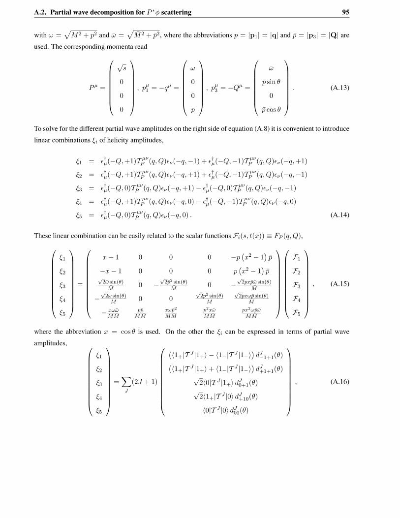
A.2. Partial wave decomposition for 𝑃 *𝜑 scattering 95
with 𝜔 =√
𝑀2 + 𝑝2 and �� =√
��2 + 𝑝2, where the abbreviations 𝑝 = |p1| = |q| and 𝑝 = |p3| = |Q| are
used. The corresponding momenta read
𝑃𝜇 =
⎛⎜⎜⎜⎜⎜⎜⎜⎝
√𝑠
0
0
0
⎞⎟⎟⎟⎟⎟⎟⎟⎠
, 𝑝𝜇1 = −𝑞𝜇 =
⎛⎜⎜⎜⎜⎜⎜⎜⎝
𝜔
0
0
𝑝
⎞⎟⎟⎟⎟⎟⎟⎟⎠
, 𝑝𝜇3 = −𝑄𝜇 =
⎛⎜⎜⎜⎜⎜⎜⎜⎝
��
𝑝 sin 𝜃
0
𝑝 cos 𝜃
⎞⎟⎟⎟⎟⎟⎟⎟⎠
. (A.13)
To solve for the different partial wave amplitudes on the right side of equation (A.8) it is convenient to introduce
linear combinations 𝜉𝑖 of helicity amplitudes,
𝜉1 = 𝜖†𝜇(−𝑄, +1)𝒯 𝜇𝜈𝑃 (𝑞, 𝑄)𝜖𝜈(−𝑞,−1) + 𝜖†𝜇(−𝑄,−1)𝒯 𝜇𝜈
𝑃 (𝑞, 𝑄)𝜖𝜈(−𝑞, +1)
𝜉2 = 𝜖†𝜇(−𝑄, +1)𝒯 𝜇𝜈𝑃 (𝑞, 𝑄)𝜖𝜈(−𝑞, +1) + 𝜖†𝜇(−𝑄,−1)𝒯 𝜇𝜈
𝑃 (𝑞,𝑄)𝜖𝜈(−𝑞,−1)
𝜉3 = 𝜖†𝜇(−𝑄, 0)𝒯 𝜇𝜈𝑃 (𝑞, 𝑄)𝜖𝜈(−𝑞, +1)− 𝜖†𝜇(−𝑄, 0)𝒯 𝜇𝜈
𝑃 (𝑞, 𝑄)𝜖𝜈(−𝑞,−1)
𝜉4 = 𝜖†𝜇(−𝑄, +1)𝒯 𝜇𝜈𝑃 (𝑞, 𝑄)𝜖𝜈(−𝑞, 0)− 𝜖†𝜇(−𝑄,−1)𝒯 𝜇𝜈
𝑃 (𝑞,𝑄)𝜖𝜈(−𝑞, 0)
𝜉5 = 𝜖†𝜇(−𝑄, 0)𝒯 𝜇𝜈𝑃 (𝑞, 𝑄)𝜖𝜈(−𝑞, 0) . (A.14)
These linear combination can be easily related to the scalar functions ℱ𝑖(𝑠, 𝑡(𝑥)) ≡ 𝐹𝑃 (𝑞, 𝑄),
⎛⎜⎜⎜⎜⎜⎜⎜⎜⎜⎜⎝
𝜉1
𝜉2
𝜉3
𝜉4
𝜉5
⎞⎟⎟⎟⎟⎟⎟⎟⎟⎟⎟⎠
=
⎛⎜⎜⎜⎜⎜⎜⎜⎜⎜⎜⎝
𝑥− 1 0 0 0 −𝑝(𝑥2 − 1
)𝑝
−𝑥− 1 0 0 0 𝑝(𝑥2 − 1
)𝑝
√2�� sin(𝜃)
��0 −
√2𝑝2 sin(𝜃)
��0 −
√2𝑝𝑥𝑝�� sin(𝜃)
��
−√
2𝜔 sin(𝜃)𝑀 0 0
√2𝑝2 sin(𝜃)
𝑀
√2𝑝𝑥𝜔𝑝 sin(𝜃)
𝑀
− 𝑥𝜔��𝑀��
𝑝𝑝𝑀��
𝑥𝜔𝑝2
𝑀��𝑝2𝑥��𝑀��
𝑝𝑥2𝜔𝑝��𝑀��
⎞⎟⎟⎟⎟⎟⎟⎟⎟⎟⎟⎠
⎛⎜⎜⎜⎜⎜⎜⎜⎜⎜⎜⎝
ℱ1
ℱ2
ℱ3
ℱ4
ℱ5
⎞⎟⎟⎟⎟⎟⎟⎟⎟⎟⎟⎠
, (A.15)
where the abbreviation 𝑥 = cos 𝜃 is used. On the other the 𝜉𝑖 can be expressed in terms of partial wave
amplitudes, ⎛⎜⎜⎜⎜⎜⎜⎜⎜⎜⎜⎝
𝜉1
𝜉2
𝜉3
𝜉4
𝜉5
⎞⎟⎟⎟⎟⎟⎟⎟⎟⎟⎟⎠
=∑
𝐽
(2𝐽 + 1)
⎛⎜⎜⎜⎜⎜⎜⎜⎜⎜⎜⎝
(⟨1+|𝒯 𝐽 |1+⟩ − ⟨1−|𝒯 𝐽 |1−⟩
)𝑑𝐽−1+1(𝜃)
(⟨1+|𝒯 𝐽 |1+⟩+ ⟨1−|𝒯 𝐽 |1−⟩
)𝑑𝐽
+1+1(𝜃)√
2⟨0|𝒯 𝐽 |1+⟩ 𝑑𝐽0+1(𝜃)
√2⟨1+|𝒯 𝐽 |0⟩ 𝑑𝐽
+10(𝜃)
⟨0|𝒯 𝐽 |0⟩ 𝑑𝐽00(𝜃)
⎞⎟⎟⎟⎟⎟⎟⎟⎟⎟⎟⎠
, (A.16)
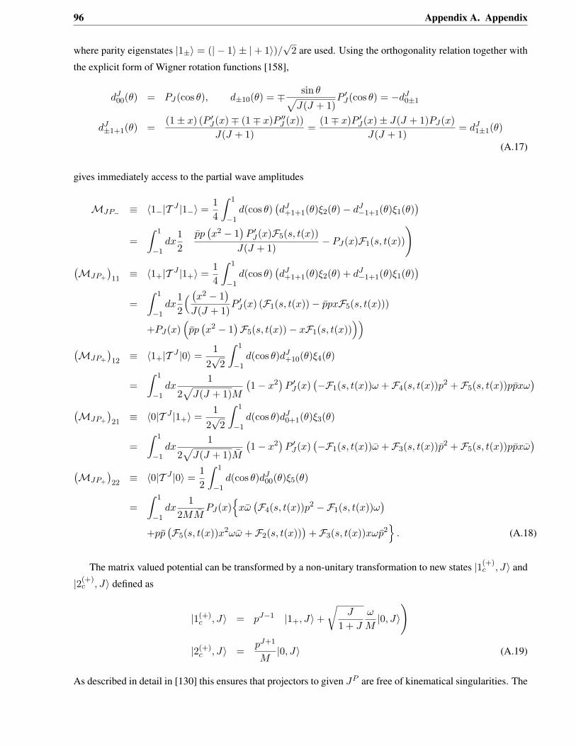
96 Appendix A. Appendix
where parity eigenstates |1±⟩ = (| − 1⟩ ± |+ 1⟩)/√
2 are used. Using the orthogonality relation together with
the explicit form of Wigner rotation functions [158],
𝑑𝐽00(𝜃) = 𝑃𝐽(cos 𝜃), 𝑑±10(𝜃) = ∓ sin 𝜃√
𝐽(𝐽 + 1)𝑃 ′𝐽(cos 𝜃) = −𝑑𝐽
0±1
𝑑𝐽±1+1(𝜃) =
(1± 𝑥) (𝑃 ′𝐽(𝑥)∓ (1∓ 𝑥)𝑃 ′′𝐽 (𝑥))𝐽(𝐽 + 1)
=(1∓ 𝑥)𝑃 ′𝐽(𝑥)± 𝐽(𝐽 + 1)𝑃𝐽(𝑥)
𝐽(𝐽 + 1)= 𝑑𝐽
1±1(𝜃)
(A.17)
gives immediately access to the partial wave amplitudes
ℳ𝐽𝑃− ≡ ⟨1−|𝒯 𝐽 |1−⟩ =14
∫ 1
−1𝑑(cos 𝜃)
(𝑑𝐽
+1+1(𝜃)𝜉2(𝜃)− 𝑑𝐽−1+1(𝜃)𝜉1(𝜃)
)
=∫ 1
−1𝑑𝑥
12
(𝑝𝑝(𝑥2 − 1
)𝑃 ′𝐽(𝑥)ℱ5(𝑠, 𝑡(𝑥))
𝐽(𝐽 + 1)− 𝑃𝐽(𝑥)ℱ1(𝑠, 𝑡(𝑥))
)
(ℳ𝐽𝑃+
)11
≡ ⟨1+|𝒯 𝐽 |1+⟩ =14
∫ 1
−1𝑑(cos 𝜃)
(𝑑𝐽
+1+1(𝜃)𝜉2(𝜃) + 𝑑𝐽−1+1(𝜃)𝜉1(𝜃)
)
=∫ 1
−1𝑑𝑥
12
( (𝑥2 − 1)
𝐽(𝐽 + 1)𝑃 ′𝐽(𝑥) (ℱ1(𝑠, 𝑡(𝑥))− 𝑝𝑝𝑥ℱ5(𝑠, 𝑡(𝑥)))
+𝑃𝐽(𝑥)(𝑝𝑝(𝑥2 − 1
)ℱ5(𝑠, 𝑡(𝑥))− 𝑥ℱ1(𝑠, 𝑡(𝑥))
))
(ℳ𝐽𝑃+
)12
≡ ⟨1+|𝒯 𝐽 |0⟩ =1
2√
2
∫ 1
−1𝑑(cos 𝜃)𝑑𝐽
+10(𝜃)𝜉4(𝜃)
=∫ 1
−1𝑑𝑥
12√
𝐽(𝐽 + 1)𝑀
(1− 𝑥2
)𝑃 ′𝐽(𝑥)
(−ℱ1(𝑠, 𝑡(𝑥))𝜔 + ℱ4(𝑠, 𝑡(𝑥))𝑝2 + ℱ5(𝑠, 𝑡(𝑥))𝑝𝑝𝑥𝜔
)
(ℳ𝐽𝑃+
)21
≡ ⟨0|𝒯 𝐽 |1+⟩ =1
2√
2
∫ 1
−1𝑑(cos 𝜃)𝑑𝐽
0+1(𝜃)𝜉3(𝜃)
=∫ 1
−1𝑑𝑥
12√
𝐽(𝐽 + 1)��
(1− 𝑥2
)𝑃 ′𝐽(𝑥)
(−ℱ1(𝑠, 𝑡(𝑥))�� + ℱ3(𝑠, 𝑡(𝑥))𝑝2 + ℱ5(𝑠, 𝑡(𝑥))𝑝𝑝𝑥��
)
(ℳ𝐽𝑃+
)22
≡ ⟨0|𝒯 𝐽 |0⟩ =12
∫ 1
−1𝑑(cos 𝜃)𝑑𝐽
00(𝜃)𝜉5(𝜃)
=∫ 1
−1𝑑𝑥
12𝑀��
𝑃𝐽(𝑥){
𝑥��(ℱ4(𝑠, 𝑡(𝑥))𝑝2 −ℱ1(𝑠, 𝑡(𝑥))𝜔
)
+𝑝𝑝(ℱ5(𝑠, 𝑡(𝑥))𝑥2𝜔�� + ℱ2(𝑠, 𝑡(𝑥))
)+ ℱ3(𝑠, 𝑡(𝑥))𝑥𝜔𝑝2
}. (A.18)
The matrix valued potential can be transformed by a non-unitary transformation to new states |1(+)𝑐 , 𝐽⟩ and
|2(+)𝑐 , 𝐽⟩ defined as
|1(+)𝑐 , 𝐽⟩ = 𝑝𝐽−1
(|1+, 𝐽⟩+
√𝐽
1 + 𝐽
𝜔
𝑀|0, 𝐽⟩
)
|2(+)𝑐 , 𝐽⟩ =
𝑝𝐽+1
𝑀|0, 𝐽⟩ (A.19)
As described in detail in [130] this ensures that projectors to given 𝐽𝑃 are free of kinematical singularities. The
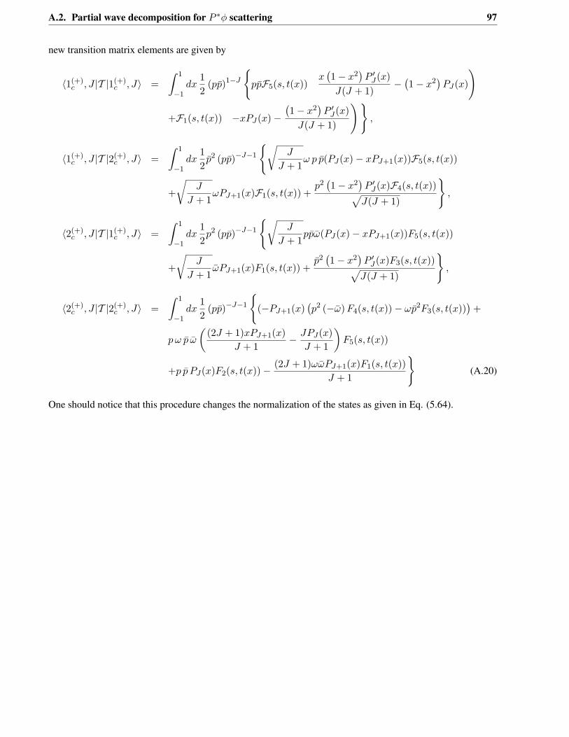
A.2. Partial wave decomposition for 𝑃 *𝜑 scattering 97
new transition matrix elements are given by
⟨1(+)𝑐 , 𝐽 |𝒯 |1(+)
𝑐 , 𝐽⟩ =∫ 1
−1𝑑𝑥
12
(𝑝𝑝)1−𝐽
{𝑝𝑝ℱ5(𝑠, 𝑡(𝑥))
(𝑥(1− 𝑥2
)𝑃 ′𝐽(𝑥)
𝐽(𝐽 + 1)−(1− 𝑥2
)𝑃𝐽(𝑥)
)
+ℱ1(𝑠, 𝑡(𝑥))
(−𝑥𝑃𝐽(𝑥)−
(1− 𝑥2
)𝑃 ′𝐽(𝑥)
𝐽(𝐽 + 1)
)},
⟨1(+)𝑐 , 𝐽 |𝒯 |2(+)
𝑐 , 𝐽⟩ =∫ 1
−1𝑑𝑥
12𝑝2 (𝑝𝑝)−𝐽−1
{√𝐽
𝐽 + 1𝜔 𝑝 𝑝(𝑃𝐽(𝑥)− 𝑥𝑃𝐽+1(𝑥))ℱ5(𝑠, 𝑡(𝑥))
+
√𝐽
𝐽 + 1𝜔𝑃𝐽+1(𝑥)ℱ1(𝑠, 𝑡(𝑥)) +
𝑝2(1− 𝑥2
)𝑃 ′𝐽(𝑥)ℱ4(𝑠, 𝑡(𝑥))√𝐽(𝐽 + 1)
},
⟨2(+)𝑐 , 𝐽 |𝒯 |1(+)
𝑐 , 𝐽⟩ =∫ 1
−1𝑑𝑥
12𝑝2 (𝑝𝑝)−𝐽−1
{√𝐽
𝐽 + 1𝑝𝑝��(𝑃𝐽(𝑥)− 𝑥𝑃𝐽+1(𝑥))𝐹5(𝑠, 𝑡(𝑥))
+
√𝐽
𝐽 + 1��𝑃𝐽+1(𝑥)𝐹1(𝑠, 𝑡(𝑥)) +
𝑝2(1− 𝑥2
)𝑃 ′𝐽(𝑥)𝐹3(𝑠, 𝑡(𝑥))√
𝐽(𝐽 + 1)
},
⟨2(+)𝑐 , 𝐽 |𝒯 |2(+)
𝑐 , 𝐽⟩ =∫ 1
−1𝑑𝑥
12
(𝑝𝑝)−𝐽−1
{(−𝑃𝐽+1(𝑥)
(𝑝2 (−��) 𝐹4(𝑠, 𝑡(𝑥))− 𝜔𝑝2𝐹3(𝑠, 𝑡(𝑥))
)+
𝑝 𝜔 𝑝 ��
((2𝐽 + 1)𝑥𝑃𝐽+1(𝑥)
𝐽 + 1− 𝐽𝑃𝐽(𝑥)
𝐽 + 1
)𝐹5(𝑠, 𝑡(𝑥))
+𝑝 𝑝 𝑃𝐽(𝑥)𝐹2(𝑠, 𝑡(𝑥))− (2𝐽 + 1)𝜔��𝑃𝐽+1(𝑥)𝐹1(𝑠, 𝑡(𝑥))𝐽 + 1
}(A.20)
One should notice that this procedure changes the normalization of the states as given in Eq. (5.64).
98 Appendix A. Appendix
A.3 “Renormalization” of the BS equation
The BS equation can be rewritten as
𝑇 = 𝑉 + 𝑉 · �� · 𝑇 = 𝑉 + 𝑉 · �� · 𝑉 + 𝑉 · �� · 𝑉 · �� · 𝑉 + ... , (A.21)
where we assume that the potential 𝑉 can be factorized from the loop function ��. Effects from coupled
channels and from off-shell terms are encoded in the symbolical way of writing this equation1. Now we
decompose 𝑉 = 𝑉0 +𝑉1, where 𝑉0 is the potential and 𝑉1 is a correction up to arbitrary order. In the following
we determine 𝑉1 such that all divergences from an iteration of 𝑉0 are cancelled. We decompose �� = ��𝑟 + ��,
where ��𝑟 is the finite renormalized loop function and �� is the divergent part. We make the Ansatz
𝑉1 = 𝑉0 ·∞∑
𝑖=1
(−�� · 𝑉0)𝑖 = 𝑉0 · [(1 + �� · 𝑉0)−1 − 1] . (A.22)
This sum renormalizes the iteration of the potential 𝑉0, as can be seen as follows
𝑇 = (1− 𝑉 · ��)−1 · 𝑉 (A.23)
= [1− (𝑉0 + 𝑉1) · (��𝑟 + ��)]−1 · (𝑉0 + 𝑉1)
=[(1 + �� · 𝑉0) · 𝑉 −1
0 · [1− 𝑉0 · (1 + �� · 𝑉0)−1 · (��𝑟 + ��)]]−1
=[[(𝑉 −1
0 + ��)− (��𝑟 + ��)]]−1
= [1− 𝑉0 · ��𝑟]−1𝑉0 . (A.24)
Therefore it is practically sufficient to replace the divergent loop matrix �� by the finite renormalized ��𝑟 and 𝑉
by 𝑉0.
An equivalent proof can be obtained by demanding
𝑑
𝑑𝜖𝑇 = 0, (A.25)
where the part to be subtracted is rewritten as �� ≡ 𝜖��0, where ��0 is a matrix that contains all divergences.
Inserting the solution (A.21) into equation (A.25) gives
𝑉 ′ + (𝑉 ′ · (��𝑟 + 𝜖��0) + 𝑉 · ��0) · [1− 𝑉 · (��𝑟 + 𝜖��0)]−1 · 𝑉 = 0 (A.26)
where the derivative has been abbreviated by (𝑉 ′ = 𝑑𝑑𝜖𝑉 ). This identity implies
𝑉 = 𝑐 · (1 + 𝜖��0 · 𝑐)−1 , (A.27)
where 𝑐 = 𝑉0 in accordance with the right side of equation (A.21). This sum obeys Eq. (A.25), as can be easily
seen by using
𝑉 ′(𝜖) = −𝑐 · (1 + 𝜖��0 · 𝑐)−1 ·𝑅0 · 𝑐 · (1 + 𝜖��0 · 𝑐)−1 = −𝑉 · ��0 · 𝑉 (A.28)1It should be clear from Section 5.5 that not all potentials can be cast into this factorized form
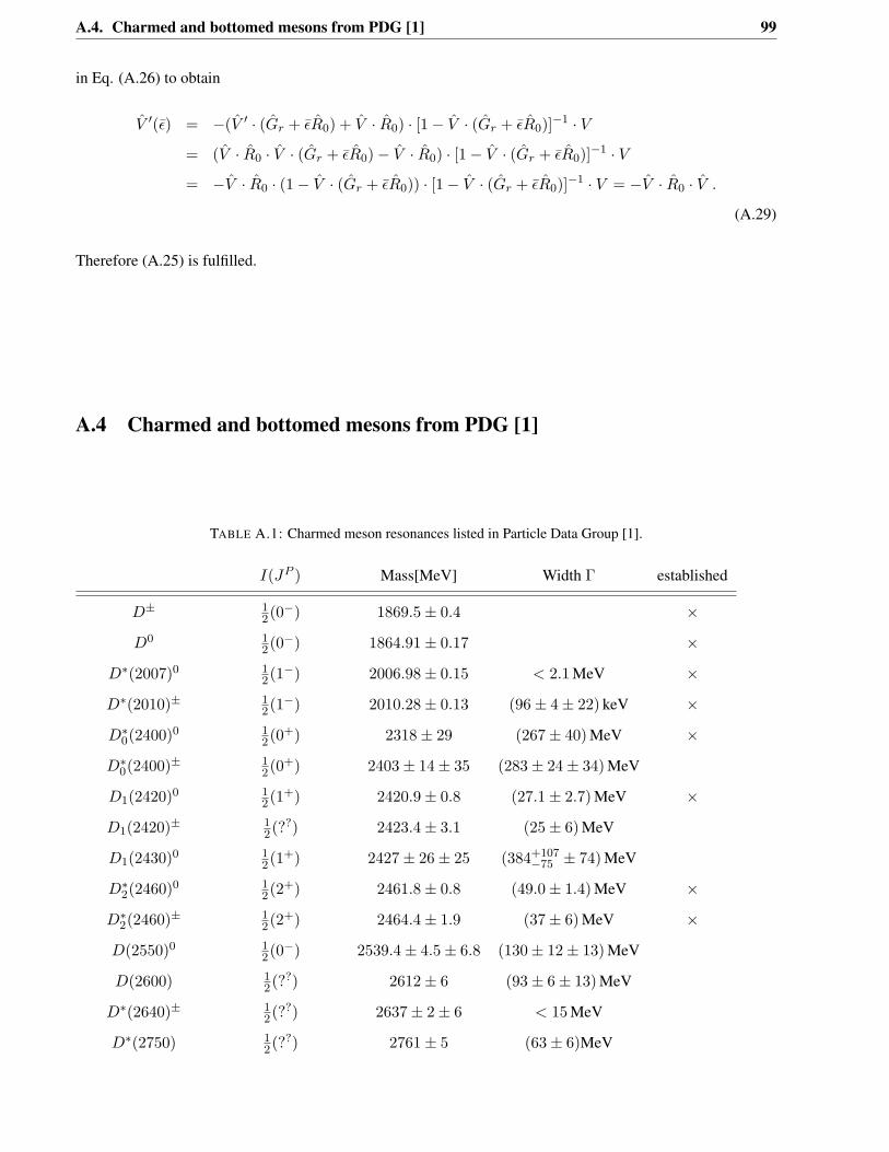
A.4. Charmed and bottomed mesons from PDG [1] 99
in Eq. (A.26) to obtain
𝑉 ′(𝜖) = −(𝑉 ′ · (��𝑟 + 𝜖��0) + 𝑉 · ��0) · [1− 𝑉 · (��𝑟 + 𝜖��0)]−1 · 𝑉= (𝑉 · ��0 · 𝑉 · (��𝑟 + 𝜖��0)− 𝑉 · ��0) · [1− 𝑉 · (��𝑟 + 𝜖��0)]−1 · 𝑉= −𝑉 · ��0 · (1− 𝑉 · (��𝑟 + 𝜖��0)) · [1− 𝑉 · (��𝑟 + 𝜖��0)]−1 · 𝑉 = −𝑉 · ��0 · 𝑉 .
(A.29)
Therefore (A.25) is fulfilled.
A.4 Charmed and bottomed mesons from PDG [1]
TABLE A.1: Charmed meson resonances listed in Particle Data Group [1].
𝐼(𝐽𝑃 ) Mass[MeV] Width Γ established
𝐷± 12(0−) 1869.5± 0.4 ×
𝐷0 12(0−) 1864.91± 0.17 ×
𝐷*(2007)0 12(1−) 2006.98± 0.15 < 2.1 MeV ×
𝐷*(2010)± 12(1−) 2010.28± 0.13 (96± 4± 22) keV ×
𝐷*0(2400)0 12(0+) 2318± 29 (267± 40) MeV ×
𝐷*0(2400)± 12(0+) 2403± 14± 35 (283± 24± 34) MeV
𝐷1(2420)0 12(1+) 2420.9± 0.8 (27.1± 2.7) MeV ×
𝐷1(2420)± 12(??) 2423.4± 3.1 (25± 6) MeV
𝐷1(2430)0 12(1+) 2427± 26± 25 (384+107
−75 ± 74) MeV
𝐷*2(2460)0 12(2+) 2461.8± 0.8 (49.0± 1.4) MeV ×
𝐷*2(2460)± 12(2+) 2464.4± 1.9 (37± 6) MeV ×
𝐷(2550)0 12(0−) 2539.4± 4.5± 6.8 (130± 12± 13) MeV
𝐷(2600) 12(??) 2612± 6 (93± 6± 13) MeV
𝐷*(2640)± 12(??) 2637± 2± 6 < 15 MeV
𝐷*(2750) 12(??) 2761± 5 (63± 6)MeV
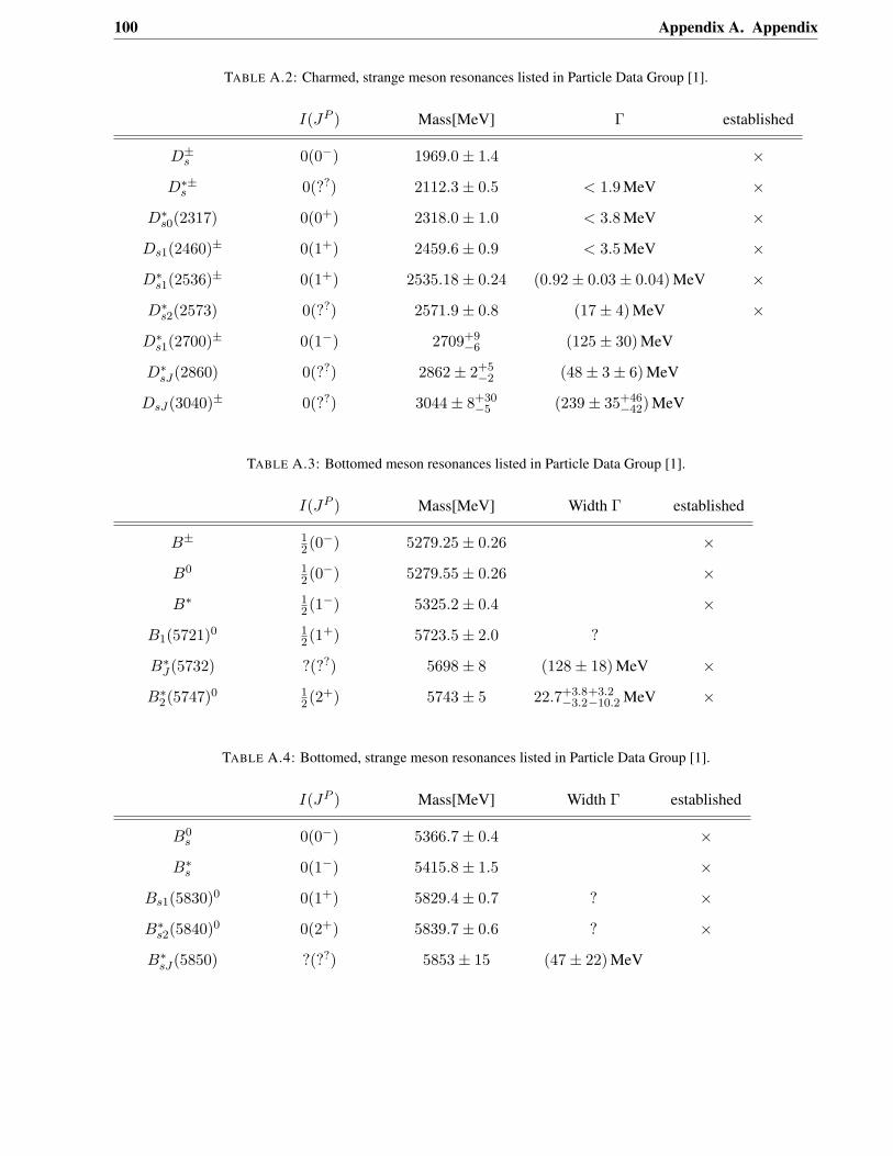
100 Appendix A. Appendix
TABLE A.2: Charmed, strange meson resonances listed in Particle Data Group [1].
𝐼(𝐽𝑃 ) Mass[MeV] Γ established
𝐷±𝑠 0(0−) 1969.0± 1.4 ×
𝐷*±𝑠 0(??) 2112.3± 0.5 < 1.9 MeV ×𝐷*𝑠0(2317) 0(0+) 2318.0± 1.0 < 3.8 MeV ×
𝐷𝑠1(2460)± 0(1+) 2459.6± 0.9 < 3.5 MeV ×
𝐷*𝑠1(2536)± 0(1+) 2535.18± 0.24 (0.92± 0.03± 0.04) MeV ×𝐷*𝑠2(2573) 0(??) 2571.9± 0.8 (17± 4) MeV ×
𝐷*𝑠1(2700)± 0(1−) 2709+9−6 (125± 30) MeV
𝐷*𝑠𝐽(2860) 0(??) 2862± 2+5−2 (48± 3± 6) MeV
𝐷𝑠𝐽(3040)± 0(??) 3044± 8+30−5 (239± 35+46
−42) MeV
TABLE A.3: Bottomed meson resonances listed in Particle Data Group [1].
𝐼(𝐽𝑃 ) Mass[MeV] Width Γ established
𝐵± 12(0−) 5279.25± 0.26 ×
𝐵0 12(0−) 5279.55± 0.26 ×
𝐵* 12(1−) 5325.2± 0.4 ×
𝐵1(5721)0 12(1+) 5723.5± 2.0 ?
𝐵*𝐽(5732) ?(??) 5698± 8 (128± 18) MeV ×𝐵*2(5747)0 1
2(2+) 5743± 5 22.7+3.8−3.2
+3.2−10.2 MeV ×
TABLE A.4: Bottomed, strange meson resonances listed in Particle Data Group [1].
𝐼(𝐽𝑃 ) Mass[MeV] Width Γ established
𝐵0𝑠 0(0−) 5366.7± 0.4 ×
𝐵*𝑠 0(1−) 5415.8± 1.5 ×𝐵𝑠1(5830)0 0(1+) 5829.4± 0.7 ? ×
𝐵*𝑠2(5840)0 0(2+) 5839.7± 0.6 ? ×
𝐵*𝑠𝐽(5850) ?(??) 5853± 15 (47± 22) MeV
Bibliography
[1] J. Beringer et al. (Particle Data Group), Phys. Rev. D86, 010001 (2012)
[2] E. Blucher and W.J. Marciano, “Vud, Vus, the Cabibbo Angle and CKM Unitarity,” (Particle Data
Group), Phys. Rev. D86, 010001 (2012)
[3] J. Laiho, E. Lunghi and R. S. Van de Water, Phys. Rev. D 81 (2010) 034503 [arXiv:0910.2928 [hep-ph]].
[4] M. Golterman, arXiv:0912.4042 [hep-lat].
[5] http://www.lepp.cornell.edu/Research/EPP/CLEO/, http://belle.kek.jp/,
http://www.slac.stanford.edu/BF/, http://lhcb.web.cern.ch/lhcb/ .
[6] B. Aubert et al. [BaBar Collaboration], Phys. Rev. Lett. 90 (2003) 242001 [hep-ex/0304021].
[7] D. Besson et al. [CLEO Collaboration], Phys. Rev. D 68 (2003) 032002 [Erratum-ibid. D 75 (2007)
119908] [hep-ex/0305100].
[8] S. Godfrey and R. Kokoski, Phys. Rev. D 43, 1679 (1991); S. Godfrey and N. Isgur, Phys. Rev. D 32,
189 (1985); M. Di Pierro and E. Eichten, Phys. Rev. D 64, 114004 (2001).
[9] J. Brodzicka et al. [Belle Collaboration], Phys. Rev. Lett. 100 (2008) 092001 [arXiv:0707.3491 [hep-
ex]].
[10] B. Aubert et al. [BaBar Collaboration], Phys. Rev. D 80 (2009) 092003 [arXiv:0908.0806 [hep-ex]].
[11] B. Aubert et al. [BaBar Collaboration], Phys. Rev. Lett. 97 (2006) 222001 [hep-ex/0607082].
[12] L. Liu, K. Orginos, F. -K. Guo, C. Hanhart and U. -G. Meissner, Phys. Rev. D 87 (2013) 014508
[arXiv:1208.4535 [hep-lat]].
[13] N. Isgur and M. B. Wise, Adv. Ser. Direct. High Energy Phys. 10 (1992) 549.
[14] H. Georgi,“Heavy quark effective field theory,” HUTP-91-A039.
[15] M. Neubert, Phys. Rept. 245 (1994) 259 [hep-ph/9306320].
[16] F. Hussain and G. Thompson, hep-ph/9502241.
[17] A. V. Manohar, M. B. Wise, Camb. Monogr. Part. Phys. Nucl. Phys. Cosmol. 10, 1-191 (2000).
101
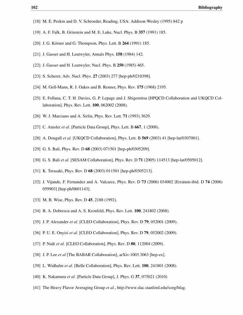
102 Bibliography
[18] M. E. Peskin and D. V. Schroeder, Reading, USA: Addison-Wesley (1995) 842 p
[19] A. F. Falk, B. Grinstein and M. E. Luke, Nucl. Phys. B 357 (1991) 185.
[20] J. G. Körner and G. Thompson, Phys. Lett. B 264 (1991) 185.
[21] J. Gasser and H. Leutwyler, Annals Phys. 158 (1984) 142.
[22] J. Gasser and H. Leutwyler, Nucl. Phys. B 250 (1985) 465.
[23] S. Scherer, Adv. Nucl. Phys. 27 (2003) 277 [hep-ph/0210398].
[24] M. Gell-Mann, R. J. Oakes and B. Renner, Phys. Rev. 175 (1968) 2195.
[25] E. Follana, C. T. H. Davies, G. P. Lepage and J. Shigemitsu [HPQCD Collaboration and UKQCD Col-
laboration], Phys. Rev. Lett. 100, 062002 (2008).
[26] W. J. Marciano and A. Sirlin, Phys. Rev. Lett. 71 (1993) 3629.
[27] C. Amsler et al. [Particle Data Group], Phys. Lett. B 667, 1 (2008).
[28] A. Dougall et al. [UKQCD Collaboration], Phys. Lett. B 569 (2003) 41 [hep-lat/0307001].
[29] G. S. Bali, Phys. Rev. D 68 (2003) 071501 [hep-ph/0305209].
[30] G. S. Bali et al. [SESAM Collaboration], Phys. Rev. D 71 (2005) 114513 [hep-lat/0505012].
[31] K. Terasaki, Phys. Rev. D 68 (2003) 011501 [hep-ph/0305213].
[32] J. Vijande, F. Fernandez and A. Valcarce, Phys. Rev. D 73 (2006) 034002 [Erratum-ibid. D 74 (2006)
059903] [hep-ph/0601143].
[33] M. B. Wise, Phys. Rev. D 45, 2188 (1992).
[34] B. A. Dobrescu and A. S. Kronfeld, Phys. Rev. Lett. 100, 241802 (2008).
[35] J. P. Alexander et al. [CLEO Collaboration], Phys. Rev. D 79, 052001 (2009).
[36] P. U. E. Onyisi et al. [CLEO Collaboration], Phys. Rev. D 79, 052002 (2009).
[37] P. Naik et al. [CLEO Collaboration], Phys. Rev. D 80, 112004 (2009).
[38] J. P. Lee et al [The BABAR Collaboration], arXiv:1003.3063 [hep-ex].
[39] L. Widhalm et al. [Belle Collaboration], Phys. Rev. Lett. 100, 241801 (2008).
[40] K. Nakamura et al. [Particle Data Group], J. Phys. G 37, 075021 (2010)
[41] The Heavy Flavor Averaging Group et al., http://www.slac.stanford.edu/xorg/hfag.
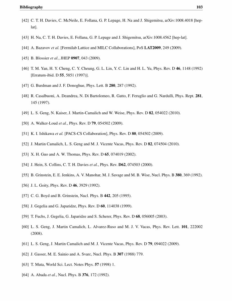
Bibliography 103
[42] C. T. H. Davies, C. McNeile, E. Follana, G. P. Lepage, H. Na and J. Shigemitsu, arXiv:1008.4018 [hep-
lat].
[43] H. Na, C. T. H. Davies, E. Follana, G. P. Lepage and J. Shigemitsu, arXiv:1008.4562 [hep-lat].
[44] A. Bazavov et al. [Fermilab Lattice and MILC Collaborations], PoS LAT2009, 249 (2009).
[45] B. Blossier et al., JHEP 0907, 043 (2009).
[46] T. M. Yan, H. Y. Cheng, C. Y. Cheung, G. L. Lin, Y. C. Lin and H. L. Yu, Phys. Rev. D 46, 1148 (1992)
[Erratum-ibid. D 55, 5851 (1997)].
[47] G. Burdman and J. F. Donoghue, Phys. Lett. B 280, 287 (1992).
[48] R. Casalbuoni, A. Deandrea, N. Di Bartolomeo, R. Gatto, F. Feruglio and G. Nardulli, Phys. Rept. 281,
145 (1997).
[49] L. S. Geng, N. Kaiser, J. Martin-Camalich and W. Weise, Phys. Rev. D 82, 054022 (2010).
[50] A. Walker-Loud et al., Phys. Rev. D 79, 054502 (2009).
[51] K. I. Ishikawa et al. [PACS-CS Collaboration], Phys. Rev. D 80, 054502 (2009).
[52] J. Martin Camalich, L. S. Geng and M. J. Vicente Vacas, Phys. Rev. D 82, 074504 (2010).
[53] X. H. Guo and A. W. Thomas, Phys. Rev. D 65, 074019 (2002).
[54] J. Hein, S. Collins, C. T. H. Davies et al., Phys. Rev. D62, 074503 (2000).
[55] B. Grinstein, E. E. Jenkins, A. V. Manohar, M. J. Savage and M. B. Wise, Nucl. Phys. B 380, 369 (1992).
[56] J. L. Goity, Phys. Rev. D 46, 3929 (1992).
[57] C. G. Boyd and B. Grinstein, Nucl. Phys. B 442, 205 (1995).
[58] J. Gegelia and G. Japaridze, Phys. Rev. D 60, 114038 (1999).
[59] T. Fuchs, J. Gegelia, G. Japaridze and S. Scherer, Phys. Rev. D 68, 056005 (2003).
[60] L. S. Geng, J. Martin Camalich, L. Alvarez-Ruso and M. J. V. Vacas, Phys. Rev. Lett. 101, 222002
(2008).
[61] L. S. Geng, J. Martin Camalich and M. J. Vicente Vacas, Phys. Rev. D 79, 094022 (2009).
[62] J. Gasser, M. E. Sainio and A. Svarc, Nucl. Phys. B 307 (1988) 779.
[63] T. Muta, World Sci. Lect. Notes Phys. 57 (1998) 1.
[64] A. Abada et al., Nucl. Phys. B 376, 172 (1992).
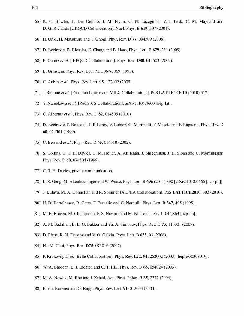
104 Bibliography
[65] K. C. Bowler, L. Del Debbio, J. M. Flynn, G. N. Lacagnina, V. I. Lesk, C. M. Maynard and
D. G. Richards [UKQCD Collaboration], Nucl. Phys. B 619, 507 (2001).
[66] H. Ohki, H. Matsufuru and T. Onogi, Phys. Rev. D 77, 094509 (2008).
[67] D. Becirevic, B. Blossier, E. Chang and B. Haas, Phys. Lett. B 679, 231 (2009).
[68] E. Gamiz et al. [ HPQCD Collaboration ], Phys. Rev. D80, 014503 (2009).
[69] B. Grinstein, Phys. Rev. Lett. 71, 3067-3069 (1993).
[70] C. Aubin et al., Phys. Rev. Lett. 95, 122002 (2005).
[71] J. Simone et al. [Fermilab Lattice and MILC Collaborations], PoS LATTICE2010 (2010) 317.
[72] Y. Namekawa et al. [PACS-CS Collaboration], arXiv:1104.4600 [hep-lat].
[73] C. Albertus et al., Phys. Rev. D 82, 014505 (2010).
[74] D. Becirevic, P. Boucaud, J. P. Leroy, V. Lubicz, G. Martinelli, F. Mescia and F. Rapuano, Phys. Rev. D
60, 074501 (1999).
[75] C. Bernard et al., Phys. Rev. D 65, 014510 (2002).
[76] S. Collins, C. T. H. Davies, U. M. Heller, A. Ali Khan, J. Shigemitsu, J. H. Sloan and C. Morningstar,
Phys. Rev. D 60, 074504 (1999).
[77] C. T. H. Davies, private communication.
[78] L. S. Geng, M. Altenbuchinger and W. Weise, Phys. Lett. B 696 (2011) 390 [arXiv:1012.0666 [hep-ph]].
[79] J. Bulava, M. A. Donnellan and R. Sommer [ALPHA Collaboration], PoS LATTICE2010, 303 (2010).
[80] N. Di Bartolomeo, R. Gatto, F. Feruglio and G. Nardulli, Phys. Lett. B 347, 405 (1995).
[81] M. E. Bracco, M. Chiapparini, F. S. Navarra and M. Nielsen, arXiv:1104.2864 [hep-ph].
[82] A. M. Badalian, B. L. G. Bakker and Yu. A. Simonov, Phys. Rev. D 75, 116001 (2007).
[83] D. Ebert, R. N. Faustov and V. O. Galkin, Phys. Lett. B 635, 93 (2006).
[84] H. -M. Choi, Phys. Rev. D75, 073016 (2007).
[85] P. Krokovny et al. [Belle Collaboration], Phys. Rev. Lett. 91, 262002 (2003) [hep-ex/0308019].
[86] W. A. Bardeen, E. J. Eichten and C. T. Hill, Phys. Rev. D 68, 054024 (2003).
[87] M. A. Nowak, M. Rho and I. Zahed, Acta Phys. Polon. B 35, 2377 (2004).
[88] E. van Beveren and G. Rupp, Phys. Rev. Lett. 91, 012003 (2003).
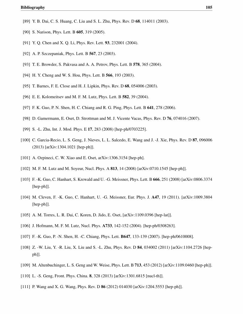
Bibliography 105
[89] Y. B. Dai, C. S. Huang, C. Liu and S. L. Zhu, Phys. Rev. D 68, 114011 (2003).
[90] S. Narison, Phys. Lett. B 605, 319 (2005).
[91] Y. Q. Chen and X. Q. Li, Phys. Rev. Lett. 93, 232001 (2004).
[92] A. P. Szczepaniak, Phys. Lett. B 567, 23 (2003).
[93] T. E. Browder, S. Pakvasa and A. A. Petrov, Phys. Lett. B 578, 365 (2004).
[94] H. Y. Cheng and W. S. Hou, Phys. Lett. B 566, 193 (2003).
[95] T. Barnes, F. E. Close and H. J. Lipkin, Phys. Rev. D 68, 054006 (2003).
[96] E. E. Kolomeitsev and M. F. M. Lutz, Phys. Lett. B 582, 39 (2004).
[97] F. K. Guo, P. N. Shen, H. C. Chiang and R. G. Ping, Phys. Lett. B 641, 278 (2006).
[98] D. Gamermann, E. Oset, D. Strottman and M. J. Vicente Vacas, Phys. Rev. D 76, 074016 (2007).
[99] S. -L. Zhu, Int. J. Mod. Phys. E 17, 283 (2008) [hep-ph/0703225].
[100] C. Garcia-Recio, L. S. Geng, J. Nieves, L. L. Salcedo, E. Wang and J. -J. Xie, Phys. Rev. D 87, 096006
(2013) [arXiv:1304.1021 [hep-ph]].
[101] A. Ozpineci, C. W. Xiao and E. Oset, arXiv:1306.3154 [hep-ph].
[102] M. F. M. Lutz and M. Soyeur, Nucl. Phys. A 813, 14 (2008) [arXiv:0710.1545 [hep-ph]].
[103] F. -K. Guo, C. Hanhart, S. Krewald and U. -G. Meissner, Phys. Lett. B 666, 251 (2008) [arXiv:0806.3374
[hep-ph]].
[104] M. Cleven, F. -K. Guo, C. Hanhart, U. -G. Meissner, Eur. Phys. J. A47, 19 (2011). [arXiv:1009.3804
[hep-ph]].
[105] A. M. Torres, L. R. Dai, C. Koren, D. Jido, E. Oset, [arXiv:1109.0396 [hep-lat]].
[106] J. Hofmann, M. F. M. Lutz, Nucl. Phys. A733, 142-152 (2004). [hep-ph/0308263].
[107] F. -K. Guo, P. -N. Shen, H. -C. Chiang, Phys. Lett. B647, 133-139 (2007). [hep-ph/0610008].
[108] Z. -W. Liu, Y. -R. Liu, X. Liu and S. -L. Zhu, Phys. Rev. D 84, 034002 (2011) [arXiv:1104.2726 [hep-
ph]].
[109] M. Altenbuchinger, L. S. Geng and W. Weise, Phys. Lett. B 713, 453 (2012) [arXiv:1109.0460 [hep-ph]].
[110] L. -S. Geng, Front. Phys. China. 8, 328 (2013) [arXiv:1301.6815 [nucl-th]].
[111] P. Wang and X. G. Wang, Phys. Rev. D 86 (2012) 014030 [arXiv:1204.5553 [hep-ph]].
106 Bibliography
[112] L. Liu, H. -W. Lin and K. Orginos, PoS LATTICE 2008, 112 (2008) [arXiv:0810.5412 [hep-lat]].
[113] E. E. Salpeter and H. A. Bethe, Phys. Rev. 84 (1951) 1232.
[114] R. E. Cutkosky, J. Math. Phys. 1 (1960) 429.
[115] G. ’t Hooft and M. J. G. Veltman, NATO Adv. Study Inst. Ser. B Phys. 4 (1974) 177.
[116] G. Ecker, J. Gasser, H. Leutwyler, A. Pich and E. de Rafael, Phys. Lett. B 223 (1989) 425.
[117] F. -K. Guo, C. Hanhart and U. -G. Meissner, Eur. Phys. J. A 40 (2009) 171 [arXiv:0901.1597 [hep-ph]].
[118] A. V. Manohar, hep-ph/9802419.
[119] H. Georgi, Phys. Lett. B 240 (1990) 447.
[120] L. M. Abreu, D. Cabrera, F. J. Llanes-Estrada and J. M. Torres-Rincon, Annals Phys. 326, 2737 (2011)
[arXiv:1104.3815 [hep-ph]].
[121] M. F. M. Lutz and E. E. Kolomeitsev, Nucl. Phys. A 700 (2002) 193 [nucl-th/0105042].
[122] J. A. Oller and E. Oset, Nucl. Phys. A 620 (1997) 438 [Erratum-ibid. A 652 (1999) 407] [hep-
ph/9702314].
[123] E. Oset and A. Ramos, Nucl. Phys. A 635 (1998) 99 [nucl-th/9711022].
[124] N. Kaiser, P. B. Siegel and W. Weise, Nucl. Phys. A 594, 325 (1995) [nucl-th/9505043].
[125] A. Dobado and J. R. Pelaez, Phys. Rev. D 56, 3057 (1997) [hep-ph/9604416].
[126] J. A. Oller, E. Oset and J. R. Pelaez, Phys. Rev. D 59, 074001 (1999) [Erratum-ibid. D 60, 099906
(1999)] [Erratum-ibid. D 75, 099903 (2007)] [hep-ph/9804209].
[127] N. Kaiser, Eur. Phys. J. A 3, 307 (1998).
[128] J. A. Oller and E. Oset, Phys. Rev. D 60, 074023 (1999) [hep-ph/9809337].
[129] J. A. Oller and U. G. Meissner, Phys. Lett. B 500, 263 (2001) [hep-ph/0011146].
[130] M. F. M. Lutz and E. E. Kolomeitsev, Nucl. Phys. A 730, 392 (2004) [nucl-th/0307039].
[131] E. E. Kolomeitsev and M. F. M. Lutz, AIP Conf. Proc. 717 (2004) 665 [hep-ph/0311205].
[132] K. Abe et al. [Belle Collaboration], Phys. Rev. Lett. 92 (2004) 012002 [hep-ex/0307052].
[133] B. Aubert et al. [BABAR Collaboration], Phys. Rev. D 69 (2004) 031101 [hep-ex/0310050].
[134] B. Aubert et al. [BABAR Collaboration], Phys. Rev. D 74 (2006) 032007 [hep-ex/0604030].
[135] L. Roca, E. Oset and J. Singh, Phys. Rev. D 72, 014002 (2005) [hep-ph/0503273].
Bibliography 107
[136] Y. -R. Liu, X. Liu and S. -L. Zhu, Phys. Rev. D 79, 094026 (2009) [arXiv:0904.1770 [hep-ph]].
[137] H. -B. Tang, hep-ph/9607436.
[138] J. M. Link et al. [FOCUS Collaboration], Phys. Lett. B 586 (2004) 11 [hep-ex/0312060].
[139] B. Aubert et al. [BABAR Collaboration], Phys. Rev. D 79 (2009) 112004 [arXiv:0901.1291 [hep-ex]].
[140] K. Abe et al. [Belle Collaboration], Phys. Rev. D 69 (2004) 112002 [hep-ex/0307021].
[141] T. Aaltonen et al. [CDF Collaboration], Phys. Rev. Lett. 100 (2008) 082001 [arXiv:0710.4199 [hep-ex]].
[142] C. Hanhart, J. R. Pelaez and G. Rios, Phys. Rev. Lett. 100, 152001 (2008) [arXiv:0801.2871 [hep-ph]].
[143] J. Nieves and E. Ruiz Arriola, Nucl. Phys. A 679 (2000) 57 [hep-ph/9907469].
[144] J. Nieves and E. Ruiz Arriola, Phys. Lett. B 455 (1999) 30 [nucl-th/9807035].
[145] J. Nieves and E. Ruiz Arriola, Phys. Rev. D 63 (2001) 076001 [hep-ph/0008034].
[146] J. Nieves and E. Ruiz Arriola, Phys. Rev. D 64 (2001) 116008 [hep-ph/0104307].
[147] D. Djukanovic, J. Gegelia and S. Scherer, Eur. Phys. J. A 29 (2006) 337 [hep-ph/0604164].
[148] B. Borasoy, P. C. Bruns, U. -G. Meissner and R. Nissler, Eur. Phys. J. A 34 (2007) 161 [arXiv:0709.3181
[nucl-th]].
[149] P. C. Bruns, M. Mai and U. G. Meissner, Phys. Lett. B 697 (2011) 254 [arXiv:1012.2233 [nucl-th]].
[150] M. Mai, P. C. Bruns and U. -G. Meissner, Phys. Rev. D 86 (2012) 094033 [arXiv:1207.4923 [nucl-th]].
[151] M. Altenbuchinger and L. -S. Geng, arXiv:1310.5224 [hep-ph].
[152] M. Altenbuchinger, L. -S. Geng and W. Weise, arXiv:1309.4743 [hep-ph].
[153] E. E. Jenkins and A. V. Manohar, Phys. Lett. B 255 (1991) 558.
[154] T. Becher and H. Leutwyler, Eur. Phys. J. C 9 (1999) 643 [hep-ph/9901384].
[155] M. Jacob and G. C. Wick, Annals Phys. 7 (1959) 404 [Annals Phys. 281 (2000) 774].
[156] A. R. Edmonds, “Angular Momentum in Quantum Mechanics," Princeton Univ. Press, Princeton, 1957.
[157] J. Pagaran et al., Computer Physics Communications 174 (2006) 616Ð630
[158] D. A. Varshalovich, A. N. Moskalev and V. K. Khersonsky, “Quantum Theory Of Angular Momentum:
Irreducible Tensors, Spherical Harmonics, Vector Coupling Coefficients, 3nj Symbols,” SINGAPORE,
SINGAPORE: WORLD SCIENTIFIC (1988) 514p