Embed Size (px)
Citation preview
econstor www.econstor.eu
Der Open-Access-Publikationsserver der ZBW – Leibniz-Informationszentrum WirtschaftThe Open Access Publication Server of the ZBW – Leibniz Information Centre for Economics
Standard-Nutzungsbedingungen:
Die Dokumente auf EconStor dürfen zu eigenen wissenschaftlichenZwecken und zum Privatgebrauch gespeichert und kopiert werden.
Sie dürfen die Dokumente nicht für öffentliche oder kommerzielleZwecke vervielfältigen, öffentlich ausstellen, öffentlich zugänglichmachen, vertreiben oder anderweitig nutzen.
Sofern die Verfasser die Dokumente unter Open-Content-Lizenzen(insbesondere CC-Lizenzen) zur Verfügung gestellt haben sollten,gelten abweichend von diesen Nutzungsbedingungen die in der dortgenannten Lizenz gewährten Nutzungsrechte.
Terms of use:
Documents in EconStor may be saved and copied for yourpersonal and scholarly purposes.
You are not to copy documents for public or commercialpurposes, to exhibit the documents publicly, to make thempublicly available on the internet, or to distribute or otherwiseuse the documents in public.
If the documents have been made available under an OpenContent Licence (especially Creative Commons Licences), youmay exercise further usage rights as specified in the indicatedlicence.
zbw Leibniz-Informationszentrum WirtschaftLeibniz Information Centre for Economics
Nell, Kevin S.
Working Paper
The Endogenous/Exogenous Nature of SouthAfrica's Money Supply Under Direct and IndirectMonetary Control Measures
Department of Economics Discussion Paper, University of Kent, No. 9912
Provided in Cooperation with:University of Kent, School of Economics
Suggested Citation: Nell, Kevin S. (1999) : The Endogenous/Exogenous Nature of SouthAfrica's Money Supply Under Direct and Indirect Monetary Control Measures, Department ofEconomics Discussion Paper, University of Kent, No. 9912
This Version is available at:http://hdl.handle.net/10419/105538
ISSN 1466-0814
THE ENDOGENOUS/EXOGENOUS NATURE OF SOUTH AFRICA’S MONEY
SUPPLY UNDER DIRECT AND INDIRECT MONETARY CONTROL MEASURES
Kevin S. Nell
November 1999
AbstractThe main purpose of this paper is to describe South Africa’s moneysupply process along several competing, but not mutually exclusive,theoretical paradigms over the period 1966-1997. The most importantconclusion to be drawn from the empirical results is that irrespectiveof the monetary system at the time, the money supply process in SouthAfrica is endogenously determined. The empirical analysis furthershows that the inability of the South African Reserve Bank (SARB) toreach predetermined M3 monetary growth targets on a consistent basissince the mid 1980s is the direct result of an endogenous moneysupply and not, as a previous study claims, because of an unstable M3velocity. Although the M3 velocity is stable over the whole period1966-1997, money income determined an endogenous money supply,so that the M3 money supply lost its effectiveness as a leadingindicator for monetary policy. The policy implication is that theSARB controlled the M3 money supply indirectly over the period1980-1997, through an increase in interest rates, and at the potentialcost of a slowdown in economic activity.
JEL Classification: C22, E51, E52, E58
Keywords: Exogenous/endogenous money supply, M3 velocity, Causality tests
Acknowledgements: I am indebted to Tony Thirlwall, Alan Carruth, Andy Dickerson, JockaFaria and Miguel Leon-Ledesma for valuable comments on an earlier draft of this paper. Theusual disclaimer applies.
Correspondence Address: Kevin Nell, Department of Economics, Keynes College,University of Kent at Canterbury, Canterbury, Kent CT2 7NP, UK. e-mail: [email protected];tel: +44 (0)1227 827651; fax: +44 (0)1227 827850.
1
THE ENDOGENOUS/EXOGENOUS NATURE OF SOUTH AFRICA’S MONEY
SUPPLY UNDER DIRECT AND INDIRECT MONETARY CONTROL MEASURES
I Introduction
Following the significant financial reforms in 1980, the South African Reserve Bank
(SARB) adopted a policy of setting predetermined monetary growth targets for M3 since the
mid 1980s1. In contrast to empirical studies which have found evidence of a stable M3 money
demand function2, Moll (1999) recently identified the presence of an unstable M3 velocity
over the period 1960-1996 as one of the underlying causes to explain the failure of the SARB
to reach predetermined monetary growth targets on a regular and consistent basis.
After the publication of Kaldor’s seminal work in 1982, it became apparent that
although a stable money demand function is a necessary condition for there to be a stable and
predictable link between money and money income, it does not necessarily validate the
monetarist contention that the money supply is causal in the process of inflation3. Thus, even
when velocity is perceived to be stable, one way causality from money income to money or
even bi-directional causality could provide alternative explanations why monetary growth
targeting was less successful in South Africa. A stable velocity implies that the relevant
1 It is important to note that monetary growth targeting since the mid 1980s has not beenbased on direct monetary control measures as proposed by the orthodox monetarist approach,but indirectly through the SARB’s interest rate policy. A more detailed discussion of thedifferent monetary systems that characterised the period 1966-1997 will be presented insection III.2 Hurn and Muscatelli (1992) provide evidence of a cointegrating relationship between M3,income, prices and interest rates. Nell (1999) finds evidence of a stable real M3 moneydemand function over the period 1965-1997.3 Hendry and Ericsson (1991), for example, find a stable real money demand function for theUnited Kingdom over the period 1878 to 1970, but at the same time show that money isendogenously determined. By applying the same methodology, Macdonald and Taylor (1992)find similar results for the United States.
2
monetary aggregate could serve as a broad indicator for monetary policy, but that it loses its
effectiveness as a leading indicator when the money supply is endogenous or partly
endogenously determined.
The main purpose of this paper is to describe South Africa’s money supply process
along several competing, but not mutually exclusive, theoretical paradigms over the period
1966-1997. The paper will show that M3 velocity is indeed stable over the period 1966-1997
when the broadest definition is considered, and that a stable velocity necessitates a
reassessment of the endogenous/exogenous nature of M3 money to provide a possible
explanation for the failure of monetary growth targeting in South Africa. According to Niggle
(1991), over a long period the money supply may be regarded as exogenous or endogenous
depending on the degree of financial development and the nature and conduct of monetary
policy. To determine the exogenous/endogenous nature of South Africa’s money supply over
the period 1966-1997, Niggle’s (1991) analysis suggests a periodisation over the sub-periods
1966-1979 and 1980-1997 to capture the impact of direct and more market-oriented monetary
control measures respectively. Such an analysis would seem important to capture the long-run
causes of inflation in South Africa.
The plan of the paper is as follows. Section II sets out the hypotheses to be tested in the
empirical section together with a theoretical overview to distinguish between the two main
competing theoretical paradigms on the endogenous/exogenous nature of the money supply. In
this section a distinction will also be drawn between the dissident views that remain within the
Post-Keynesian camp on the nature of the endogeneity of the money supply. Section III
provides an overview of the salient features of monetary policy in South Africa. Section IV
discusses the econometric methodology to test the hypotheses outlined in section II, while
section V presents the empirical results. Section VI ends with some conclusions and policy
implications.
3
II An Overview of the Main Theoretical Paradigms on the Exogenous/Endogenous
Nature of the Money Supply
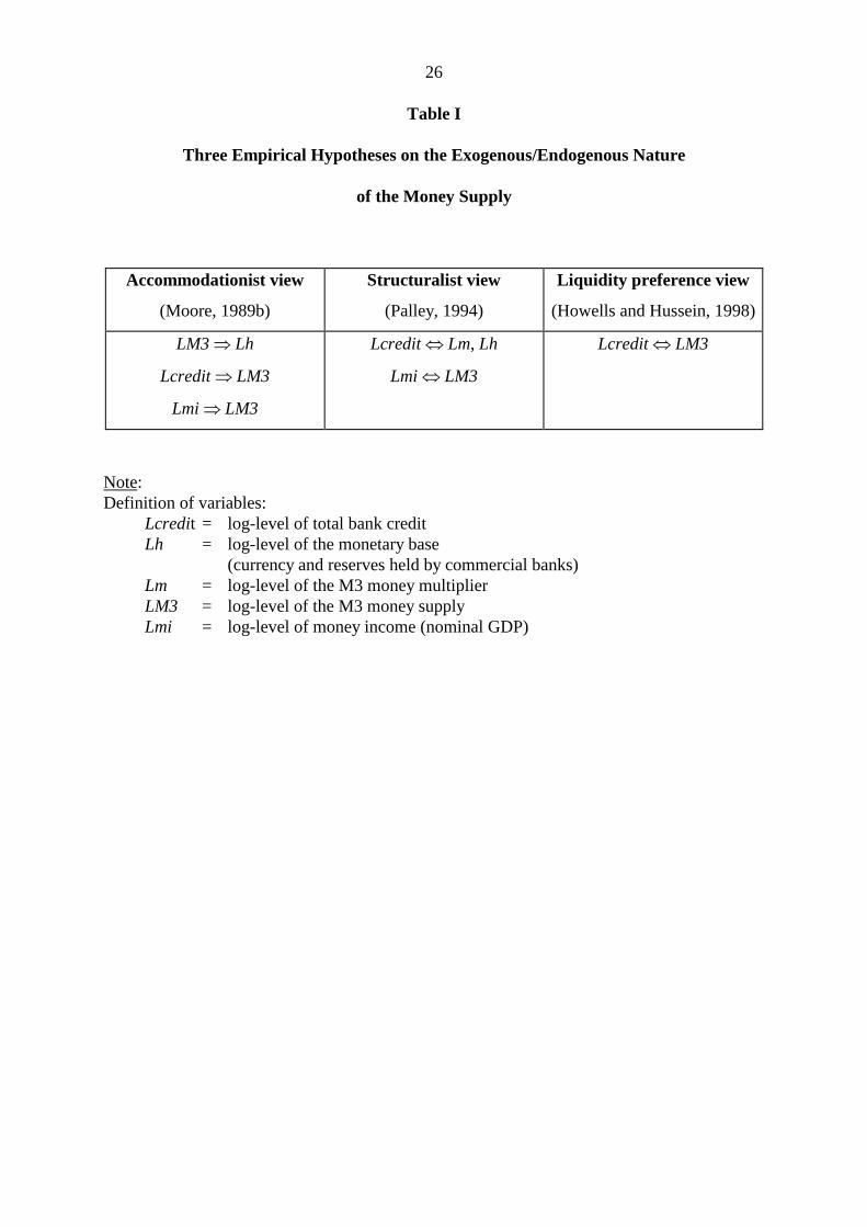
Table I summarises the hypotheses of three empirical studies which are representative of
three theoretical views on the exogenous/endogenous nature of the money supply. The main
empirical content of each study is based on Granger causality type tests.
[Table I here]
II.i The Accommodationist View versus the Monetarist View
The main exponents of the accommodationist view can be found in the writings of
Kaldor (1982); Kaldor and Trevithick (1981); and Moore (1988, 1989a). The
accommodationist view is a direct challenge to the orthodox monetarists’ approach who
believe that the money supply is some multiple of the monetary base. Reserves therefore make
deposits and the deposits that result from an increase in the monetary base are exogenously
determined by the monetary authorities. Explicit in this approach is that the money multiplier
is stable and predictable, so that restrictive (expansionary) monetary policy will not be offset
by an increase (decrease) in the money multiplier (Lavoie, 1984).
In direct contrast, the accommodationist view argues that the monetarist approach is
incompatible with the real world where commercial banks are price setters and quantity takers
(Moore, 1989b). If banks are in the business of selling credit, Central Banks inevitably play a
crucial role to supply the necessary currency and reserves on demand. According to Moore
(1989a, 1989c), reserves must always be provided on demand by Central Banks to ensure the
liquidity of the financial system and to fulfil their role as lender of last resort. If
accommodation occurs through the discount window, then banks will base their lending rates
as some mark-up over the cost of borrowing from the discount window. The money supply
process described by the accommodationist approach therefore implies that loans make
4
deposits and that the resulting deposits are endogenously determined. It follows that changes
in the money supply are a result and not a cause of changes in money income, and vary in
relation to prices and output (Kaldor and Trevithick, 1981).
If reserves are fully accommodated by the Central Bank and the loan supply schedule of
commercial banks is horizontal, then the empirical hypotheses of the accommodationist view
in Table I predict unidirectional causality from the M3 money supply (LM3) to base money
(Lh), and unidirectional causality from total bank credit (Lcredit) to LM3. Although not
explicitly included in Moore’s empirical study (1989b), the accommodationist approach
implies that there is unidirectional causality from money income (Lmi) to LM3.
II.ii The Structuralist View
Although it is fully acknowledged that the endogenous nature of the money supply
process has its origins in the views expressed by the accommodationist approach,
structuralists argue that full accommodation is an unrealistic real world assumption and assert
that the demand for credit is at least, to some extent, quantity constrained by the Central Bank
and commercial banks4. Structuralists such as Palley (1994) and Pollin (1991) argue that
accommodation depends on both the stance of the monetary authorities and the private
initiatives of banks5. Through open market operations, Central Banks have the option to place
significant quantity constraints on reserve availability (Pollin, 1991). In the structuralist view,
4 Davidson (1988) for example, associates an exogenous money supply with a perfectlyinelastic money supply function and an endogenous money supply with a less than perfectlyinelastic money supply function. Thus, an endogenous money supply does not necessary implythat the money supply function should always be perfectly elastic (Davidson, 1989; Goodhart,1989).5 A related idea presented by Dow (1996), although not prominent in the writings ofstructuralists, is that private banks express their liquidity preferences in terms of riskassessment. Credit rationing occurs with respect to particular classes of borrowers and duringthe downturn of the business cycle.
5
discount window borrowing is not a close substitute for nonborrowed funds restricted by open
market operations. Structuralists stress that the marginal cost of borrowing from the discount
window rises each time banks use this option, since the discount rate is positively related to
the level of borrowed funds (Palley, 1994). In contrast to the accommodationist approach, the
loan supply schedule of banks is positively sloped and not horizontal.
An important feature of the structuralist endogeneity approach is their emphasis on
liability management practices that allow banks to partly overcome reserve constraints
imposed by the Central Bank. Although liability management can go a long way to overcome
reserve constraints, structuralists emphasise that liability management need not necessarily
create an adequate supply of reserves to meet demand (Pollin, 1991)6.
The structuralist hypothesis in Table I can be described as a mixed model which
incorporates some of the ideas of the monetarist approach and the accommodationist view.
The accommodationist part of the model depicts causality from Lcredit (total bank credit) to
Lh and the monetarist part of the model causality from Lh to Lcredit. The monetarist part of
the model also depicts causality from the Lm (M3 money multiplier) to Lcredit. Although the
relations described by the accommodationist view in Table I could be used to test the
structuralist view, Palley’s (1994) relations test the monetarist version indirectly, where it is
assumed that excess reserves that result from expansionary monetary policy (Lh � LM3) are
lent out to the general public (i.e. Lh � Lcredit). If the structuralist view holds true, then an
additional test should indicate bi-directional causality between money income (Lmi) and LM3.
Finally, if Lh does not proportionately support an increase in the demand for Lcredit, i.e. a less
6 The accommodationist view also recognises the important role of liability managementpractices and the growth of off-balance-sheet items (loan commitments) to overcome reserveconstraints (Moore, 1989a). However, unlike structuralists, the accommodationists believethat these practices will fully offset any amount of reserve constraints.
6
than unitary long-run elasticity conditional on Lcredit being exogenous, then structuralists
identify liability management practices as an alternative to supplement the shortage in
reserves. Increased lending causes liability transformations so that Lcredit causes an increase
in Lm. Given that the main components of the money multiplier consist of the currency
deposit ratio (cd) and reserve deposit ratio (rd), Palley’s test implies that liability management
- bidding up rates to attract funds from demand deposits with high reserve requirements into
time deposits with lower reserve requirements - frees up reserves which subsequently alters cd
and rd7.
II.iii The Liquidity Preference View
This approach fully supports the accommodationists’ core theoretical arguments in
favour of an endogenously determined money supply. However, the liquidity preference
view’s main criticism is based on the assumption made by accommodationists that money can
never be in ‘excess’ supply, and hence that there is not an independent money demand
function that plays its traditional role (Arestis and Howells, 1996; Howells, 1995; Howells,
1997; Goodhart, 1989; Palley, 1991). According to Howells (1995), the main controversy
revolves around the identification of a reconciliation mechanism to ensure that the supply of
new deposits created by the flow of new net lending is just equal to the quantity demanded.
Kaldor and Trevithick (1981) identify the automatic repayment of loans as an appropriate
7 According to Pollin (1991), one way to describe liability management is by attracting fundsout of demand deposit accounts which have relatively high reserve requirements, intoinstruments within the short-term money market. When banks borrow short-term moneymarket instruments the reserve requirement associated with their liability will be lowercompared to demand deposits. One implication of liability management as described by Palley(1994) and Pollin (1991), is that the former case implies a rise in the velocity for a narrowdefinition of money while the latter case may be associated with a rise in velocity for abroader definition of money.
7
mechanism. Moore’s (1991) treatment is more explicit and states that since money is always
acceptable as a means of payment, the deposits that result from loans are willingly held by
new deposit holders8.
The empirical hypothesis of the liquidity preference view in Table I predicts causality
from Lcredit to LM3 if the money supply is endogenously determined. However, if the
demand for money and the demand for loans are independent, it follows that the supply of
deposits created by the net flow of new bank lending are not willingly held by new deposit
owners who have liquidity preferences about the amount of money they wish to hold. If this is
the case, then the demand for money places a constraint on the ability of loans to create
deposits so that causality can also be expected from LM3 to Lcredit9.
III Monetary Policy in South Africa over the period 1966-1997
This section provides a brief overview of the salient features that characterised monetary
policy over the sub-periods 1966-1979 and 1980-1997. An analysis of this nature will clearly
show why it is necessary to test the relations in Table I over two different sub-periods.
8 Also see the debate between Howells (1997) and Moore (1997) on an appropriatereconciliation mechanism.9 The reconciliation problem can be explained in terms of a demand for money function and ademand for loans function which both include prices and real income. Under an endogenouslydetermined money supply the demand for loans will be driven by prices and income. Withouta reconciliation problem we would expect identical price and income elasticities in the moneydemand and loan functions, so that the deposits created by loans are willingly held by depositholders. If the elasticities are not similar, then there is a reconciliation problem which mayinduce new deposit holders to dispose of any excess by either spending it or buying bonds.The actions by deposit holders could trigger further price and income changes so that thesupply of deposits is eventually reconciled with the demand for deposits. The reconciliationproblem is further exacerbated when it is considered that the individuals or agents whodemand loans, are different from the set of agents who eventually hold the deposits created byloans (Howells, 1995).
8
III.i Direct Control Measures: 1966-1979
Direct control measures were mainly based on credit ceilings, cash reserve
requirements, liquid asset reserve requirements and interest rate control measures. In its Final
Report, the De Kock Commission (1985) mentioned several reasons why monetary policy
based on direct control measures was less successful in moderating and controlling credit
expansion and money supply growth10.
First, it is widely acknowledged that liquid asset reserve requirements during this period
did not prevent large expansions in credit and money supply growth (Gidlow, 1995; Meijer,
1992). Second, direct control measures such as credit ceilings and liquid asset reserve
requirements, led to ‘disintermediation’ since the mid 1970s11. In addition to primary lenders
and ultimate borrowers, banks also participated in ‘disintermediation’ on a large scale by
entering money broking fields and arranging off-balance-sheet financing for their clients
(Black and Dollery, 1989).
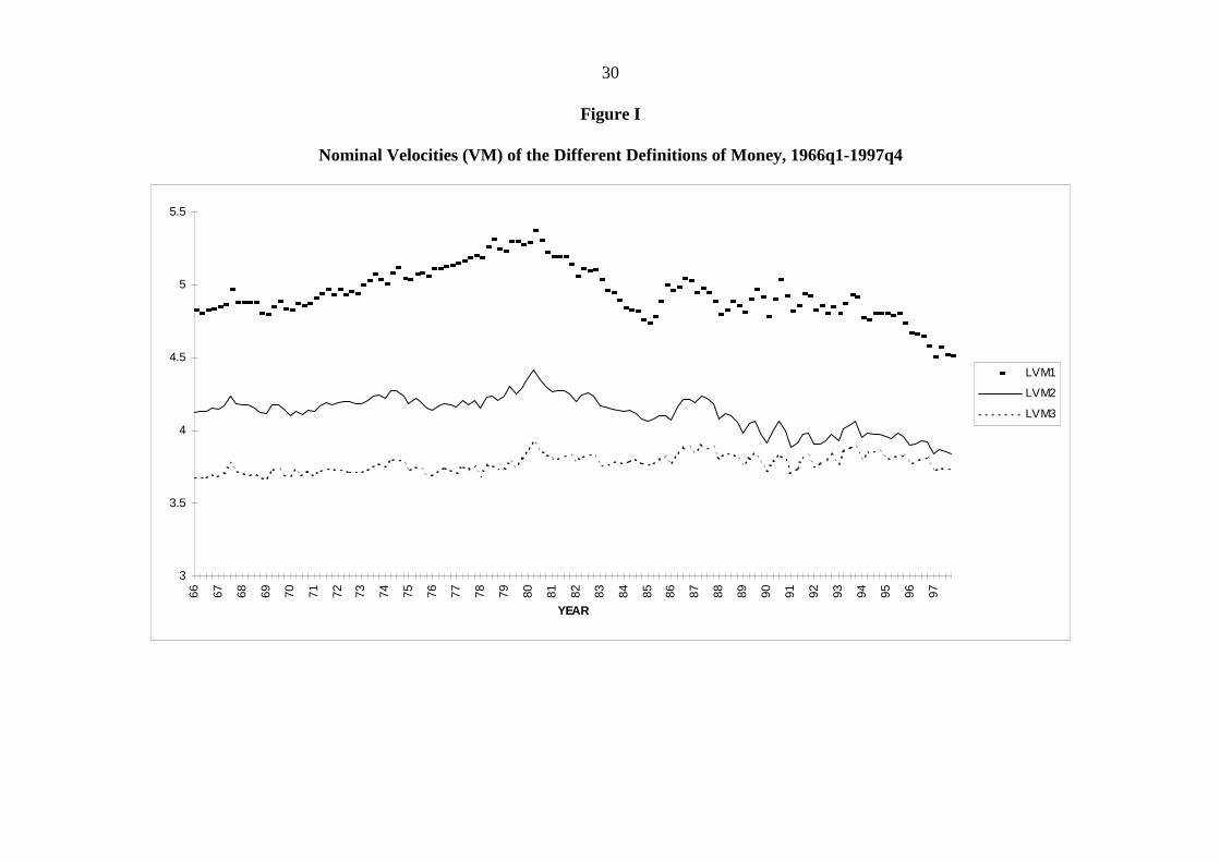
The ‘disintermediation’ phenomena is captured in Figure I by the movements in the
velocities (in logarithms) for the different monetary aggregates.
[Figure I here]
Two striking features stand out. First, Figure I shows a gradual increase in the M1 and M2
velocities (trended) during the 1960s, whereas the increases become more precipitous since
the mid 1970s. After the financial reforms in 1980, the decline in M1 and M2 velocities
10 See Black and Dollery (1989) for a summary of the Final Report.11 ‘Disintermediation’ refers to the replacement of credit normally extended by banks, by non-intermediated credit extended between primarily lenders and ultimate borrowers. Liquid assetreserve requirements forced banks to use some of their own deposits to buy low-yieldingstatutory liquid assets. This caused banks to offer a low interest on deposits and a highercharge to borrowers. Liquidity constraints imposed by banks through higher lending rates andadditional direct control measures such as credit ceilings, could largely explain the‘disintermediation’ phenomena experienced over the period 1976-1979.
9
describes the ‘reintermediation’ phenomena where credit extensions outside the banking
system returned to the balance sheets of banks. One implication is that the M1 and M2
velocities are not stable over the period 1966-1997, nor over the sub-periods 1966-1979 and
1980-1997. Second, the M3 velocity remains fairly stable along its trend value over the whole
period under analysis. The descriptive evidence strongly suggests that velocity becomes more
stable as we move from a narrow to a broader definition of money, and further implies that the
instability in the different velocities can be found in the demand for deposits and currency
components which define a narrow M1 definition of money12. It is of paramount importance
to note that a stable velocity over the period 1966-1997 will ultimately depend on whether we
use the broadest definition or not13.
The analysis thus far suggests that the unstable and stable velocities for M1, M2 and M3
respectively, may have an important bearing on the interpretation of the empirical hypotheses
described in Table I. Over the period of direct monetary control measures the relation between
the M3 money multiplier and total credit may not necessarily describe liability management,
12 More specifically, the rise in velocity can be described as an increase in nominal GDPrelative to currency and demand deposits that define a narrow definition of money. Using anextreme example, the decline in velocity following the financial reforms in 1980 is similar tomoving from a barter economy to one with a financial system. The visual evidence supportsthe main results of a previous study, which showed that the demand for real M1 and M2money balances display instability features following the financial reforms in 1980, while thedemand for real M3 money balances remain stable over the period 1965-1997 (Nell, 1999).13 The increase in the instability of velocity as we move from a M3 definition to a narrowdefinition, may well provide an explanation why Moll (1999) found no evidence of a stableM3 velocity. The M3 definition used in this study is obtained from the SARB’s historical dataset on the internet (http://www.resbank.co.za/Economics/econ.html), and defines the broadestmeasure of money in South Africa. In contrast, Moll’s (1999: 63) data are obtained fromInternational Financial Statistics, where M3 is defined as M1 plus time and savings deposits.According to Moll (1999) “…..the figure for M1 + time and savings deposits is closer to theSARB’s M3 than it is to the SARB’s M2” (p.64). Clearly as the visual evidence suggests,empirical support for a stable velocity will crucially depend on whether we use the broadestdefinition of money. Any definition which is M1, M2 or somewhere between M2 and M3,may yield unstable results.
10
but rather the growth of off-balance-sheet items. If credit extensions took place outside the
banking system to overcome reserve constraints imposed by the Central bank, then the
relevant question is what happens when the loans are spent? A possible answer is that some of
the funds find their way back to the balance sheet of banks and appear as deposits on the
liability side. The potential implication is that in the long-run banks can fulfil their role as
financial intermediaries despite loan arrangements initially taking place outside the banking
system. Thus, in the short-run we would expect that an increase in the demand for credit
causes the cd and rd ratios in the M3 money multiplier to rise (rise in velocity), so that an
increase in credit demand impacts negatively on the M3 money multiplier. In the long-run, if
some of the credits extended outside the banking system find their way back as deposits on the
balance sheet of banks, we would expect the cd and rd ratios in the M3 money multiplier to
fall (fall in velocity), so that credit demand impacts positively on the M3 money multiplier.
III.ii Indirect Monetary Control Measures: 1980-1997
Following the De Kock Commission’s recommendations in its Interim Report in 1978
and eventually its Final Report in 1985, the period after 1979 witnessed a significant change
in monetary policy from direct control measures to more market-oriented measures. Some of
the major changes included the abolition of deposit rate controls in March 1980, the abolition
of bank credit ceilings from September 1980, and lower liquid asset and cash reserve
requirements. In addition, the SARB abolished the direct link between its rediscount rate and
the prime overdraft rate of banks in 1982.
With the exception of some minor amendments over the period 1980-1997 (Schoombee,
1996), the SARB’s monetary policy was primarily based on the cost of borrowing from the
11
discount window14. Through its open market operations the SARB always ensures that
financial institutions remain indebted to it. When financial institutions seek accommodation at
the discount window, the SARB can charge an interest rate slightly above or equal to its
chosen bank rate (Whittaker, 1992). Short-term market interest rates will closely approximate
the discount rate since financial institutions will not lend at a rate which is below the discount
rate nor will they borrow at a rate which is higher than the prevailing discount rate15.
In 1985 the SARB adopted a policy of setting predetermined monetary growth targets
for M3. According to the SARB, however, monetary growth targeting has never been based
on a rigid monetary growth rule as proposed by monetarists, but could rather be described as a
more flexible approach (Mohr and Rogers, 1995).
It should be clear from the above that the market-oriented monetary policy measures
adopted since 1980 closely reflect an accommodationists’ view of how the banking system
operates (Rogers, 1985, 1986; Moore and Smit, 1986). The Central Bank will set the supply
price of reserves and be ready to supply any amount of reserves on demand. Commercial
banks, who are in the business of selling credit, will then base their lending rates as some
mark-up over the cost of borrowing from the discount window and supply any amount of
credit on demand. Structuralists, however, will argue that the marginal cost of borrowed funds
increases, which induces banks to seek alternative options such as liability management
practices.
14 In March 1998, the SARB adopted the repo rate system which is a more flexible systemcompared to the old system where the SARB set its lending rate at the discount window. Thecost of borrowing under this new system is determined by daily tenders, so that the cost ofborrowing ultimately depends on the amount of money the SARB is willing to make availableto commercial banks on a daily basis.15 Nel (1994) showed that after the gradual implementation of the current monetary policy inthe early 1980s, the SARB established a closer link between the bank rate and short-termmarket interest rates during the later part of the 1980s.
12
IV Econometric Methodology
To test the different models outlined in Table I, all the empirical tests will be based on
Granger causality type tests. By adopting the approach proposed by Granger (1988), the
empirical tests will not only detect short-run causality through the standard Granger
procedure, but also long-run causality through cointegration analysis. Given that all the
models in Table I are bivariate, it is important that the procedure used to estimate the single
cointegrating vectors complies with the basic criteria for efficient estimation (Gonzalo,
1994: 224)16. In this regard, the analysis will consider the Auto Regressive Distributed Lag
(ARDL) procedure developed by Pesaran and Shin (1999).
Consider the following ARDL(p,q) model when the underlying variables are I(1) and
there exists a stable long-run (cointegrating) relationship between yt and xt:
���
�
�
�
�
�����������
1
0
*
10 ,
q
ititit
p
iitit xxyy (1)
where xt is the I(1) variable and t� the disturbance term.
The long-run relationship between yt and xt solved from equation (1) is given by:
ttt xy ���� 1 , (2)
where 1 is the long-run parameter estimate of the constant, � is the long-run parameter
estimate of the variable tx , and t� is the long-run random disturbance term.
Pesaran and Shin (1999) have shown that even when the xt’s are endogenous, valid
asymptotic inferences on the short-run and long-run parameters can be drawn once an
appropriate choice of the order of the ARDL model is made. According to Pesaran (1997), the
Akaike Information Criterion (AIC) and Schwartz Bayesian Criterion (SBC) perform
16 Inder (1993), for example, shows that the omission of dynamics in the first-step static OLSprocedure may be detrimental to the performance of the estimator in finite samples.
13
relatively well in small samples, although the SBC is slightly superior to the AIC (Pesaran and
Shin, 1999).
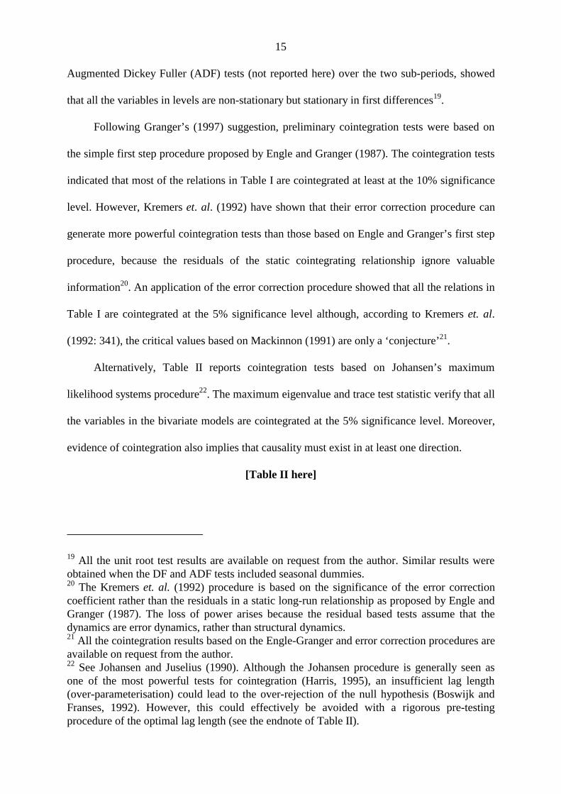
By utilising the residuals from equation (2) consider the following error correction
model:
� �� �
��� ����������
r
i
s
ittitxiityit xyy
1 0132 , (3)
where 1�� t is the lagged error correction term obtained from the residuals in equation (2) and
t is the short-run random disturbance term. From equation (3), the null hypothesis that x
does not Granger cause y would be rejected if the lagged coefficients of the xi� ’s are jointly
significant based on a standard F-test (or Wald test). Conversely, when �xt replaces �yt as the
left-side variable, then the null hypothesis that y does not cause x would be rejected if the
lagged coefficients of the yi� ’s are jointly significant.
The error correction term ( 1�� t ) in equation (3) provides a useful alternative to the
standard Granger causality test described above. The standard Granger causality procedure is
based on past changes in one variable explaining current changes in another. If, however,
variables share a common trend (long-run relationship), then current adjustments in y towards
its long-run equilibrium value are partly the result of current changes in x. Such causality can
be detected if the error correction term in equation (3) is statistically significant. So, if the
relevant variables are cointegrated, then causality must exist in at least one direction which is
not always detectable if the results are only based on the standard Granger procedure
(Granger, 1988)17.
17 The standard procedure to follow when testing for Granger causality is to difference non-stationary variables. However, after the publication of Engle and Granger’s (1987) two-stepprocedure it became apparent that these models could be misspecified, since they omit theerror correction term.
14
It is important to highlight some caveats related to the concepts of causality and
exogeneity. Standard Granger causality tests are only indicative of whether one variable
precedes another (Maddala, 1988; Urbain, 1992). In many empirical studies, causality through
the error correction term is used as a test for weak exogeneity, since it shows how the short-
run coefficients of the variables adjust towards their long-run equilibrium values (Engle and
Granger, 1987; Harris, 1995). Thus, in addition to first showing that a variable is weakly
exogenous through the error correction term, the definitions developed by Engle et. al. (1983)
can be used to determine whether a variable is strongly exogenous (Charemza and Deadman,
1997). So, if a variable is weakly exogenous through the error correction term and the lagged
values are also jointly significant, then the variable is said to be strongly exogenous. Since
weak exogeneity is a necessary condition for efficient estimation, more weight will be
attached to causality through the error correction term as opposed to causality through the
standard Granger procedure which only detects short-run causality.
V Empirical Results
All the data are quarterly and seasonally unadjusted over the sub-periods 1966q1-
1979q4 and 1980q1-1997q418. Before we apply the ARDL procedure outlined in the previous
section, it is first necessary to determine whether the variables in Table I are I(1) and whether
the I(1) variables cointegrate to form an I(0) time series. Standard Dickey Fuller (DF) and
18 The data are available from the SARB’s historical data series published on the internet.Data for the monetary base (see Table I) are obtained from International Financial Statistics(various issues). Based on Ericsson et. al’s (1994) assertion that variance dominance is notalways a necessary condition for encompassing, all the data are seasonally unadjusted.
15
Augmented Dickey Fuller (ADF) tests (not reported here) over the two sub-periods, showed
that all the variables in levels are non-stationary but stationary in first differences19.
Following Granger’s (1997) suggestion, preliminary cointegration tests were based on
the simple first step procedure proposed by Engle and Granger (1987). The cointegration tests
indicated that most of the relations in Table I are cointegrated at least at the 10% significance
level. However, Kremers et. al. (1992) have shown that their error correction procedure can
generate more powerful cointegration tests than those based on Engle and Granger’s first step
procedure, because the residuals of the static cointegrating relationship ignore valuable
information20. An application of the error correction procedure showed that all the relations in
Table I are cointegrated at the 5% significance level although, according to Kremers et. al.
(1992: 341), the critical values based on Mackinnon (1991) are only a ‘conjecture’21.
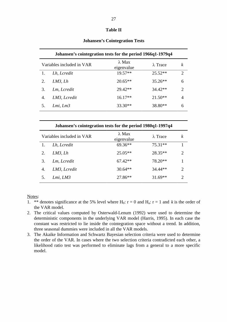
Alternatively, Table II reports cointegration tests based on Johansen’s maximum
likelihood systems procedure22. The maximum eigenvalue and trace test statistic verify that all
the variables in the bivariate models are cointegrated at the 5% significance level. Moreover,
evidence of cointegration also implies that causality must exist in at least one direction.
[Table II here]
19 All the unit root test results are available on request from the author. Similar results wereobtained when the DF and ADF tests included seasonal dummies.20 The Kremers et. al. (1992) procedure is based on the significance of the error correctioncoefficient rather than the residuals in a static long-run relationship as proposed by Engle andGranger (1987). The loss of power arises because the residual based tests assume that thedynamics are error dynamics, rather than structural dynamics.21 All the cointegration results based on the Engle-Granger and error correction procedures areavailable on request from the author.22 See Johansen and Juselius (1990). Although the Johansen procedure is generally seen asone of the most powerful tests for cointegration (Harris, 1995), an insufficient lag length(over-parameterisation) could lead to the over-rejection of the null hypothesis (Boswijk andFranses, 1992). However, this could effectively be avoided with a rigorous pre-testingprocedure of the optimal lag length (see the endnote of Table II).
16
V.i Empirical Results under Direct Control Measures: 1966q1-1979q4
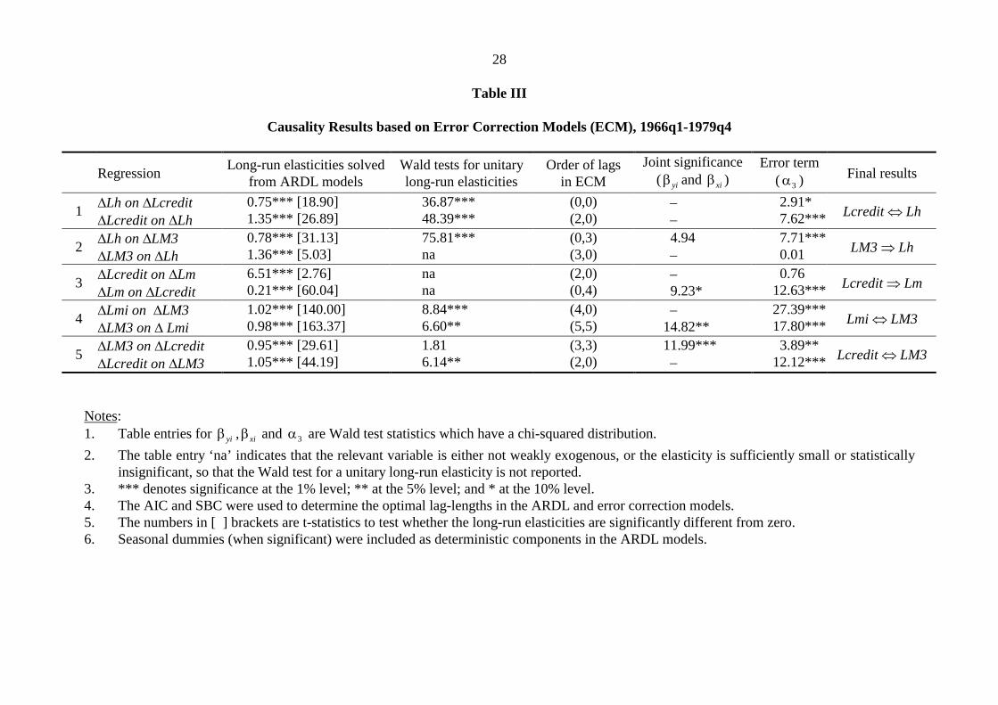
The long-run elasticity estimates and the corresponding error correction models based
on the ARDL procedure are reported in Table III23. From the first set of regressions it can be
seen that there is bi-directional causality between Lh and Lcredit. Thus, under direct control
measures, the monetary authorities managed to exert some direct influence on the expansion
of total credit through their control over the monetary base. However, even under direct
control measures, credit also determined the monetary base. The long-run elasticity estimate
shows that a one percent increase in Lcredit only leads to 0.75 percent increase in Lh. The
corresponding Wald test statistic indicates that the long-run elasticity estimate of 0.75 is
significantly different from unity (or less than proportionate), which supports the contention
that the monetary authorities exerted some direct control over the money supply.
[Table III here]
The second set of causality tests in Table III shows that there is unidirectional causality
from LM3 to Lh. This is an interesting result, given that the first and second set of causality
tests are theoretically equivalent, although the second set is a direct test of the money supply
process proposed by monetarists. The distinguishing feature between the first and second set
of causality tests could be that in the second set the money multiplier plays an important role,
whereas in the first set the role of the money multiplier is effectively circumvented. If the
money multiplier is unstable, causality will not be detected directly from Lh to LM3, but
indirectly from Lh to Lcredit. One important similarity between the first and second set of
23 The Johansen and ARDL procedures yielded almost identical long-run estimates over bothsub-periods. Alternatively, causality tests can also be based on Johansen’s cointegratingvectors by adopting a general-to-specific modelling approach in the error correction models.However, because we are also interested in the joint significance of the lagged values of thevariables, the ARDL procedure is used where the optimal lag length is determined by the AICand SBC in the ARDL and error correction models.
17
causality tests is that the 0.78 elasticity estimate in the second set, conditional on LM3 being
exogenous, again reflects that the amount of reserves was not enough to support increases in
the money supply.
The third set of tests in Table III shows unidirectional causality from Lcredit to Lm. In
addition, the joint significance of the lagged variables indicate that Lcredit is strongly
exogenous. From Table III, a one percent increase in total credit leads to a 0.21 percent
increase in the money multiplier. The importance of this test is that it may explain how agents
effectively avoided the direct control measures imposed by the monetary authorities. When
reserve shortages developed under direct control measures, loan arrangements initially took
place outside the banking system. Once the loans were spent, they re-entered the banking
system as deposits; reduced the cd and rd ratios in the money multiplier, and eventually led to
an increase in the money multiplier24. The 0.21 elasticity estimate therefore acts as a
supplement to the 0.75 elasticity estimate in the first regression (or the 0.78 elasticity in the
second regression), so that credit demand is supported by an almost proportionate increase in
the level of reserves.
The absence of causality from Lm to Lcredit, may support our previous contention that
the monetary authorities’ control over the money supply is not directly observable if the
regressions are based on the second set in Table III, but only indirectly through the first set of
regressions. This result does not imply that the monetary authorities had no direct control over
the money supply, but merely suggests that the money multiplier is unstable.
24 The negative coefficient in the error correction model (not reported here), reflects the short-run where credit extended outside the banking system initially increases the cd and rd ratios inthe money multiplier (see the theoretical discussion in section III). The positive long-runcoefficient is indicative of credit extended outside the banking system returning to the balancesheet of banks.
18
The fourth set of regressions provides a summary of the results obtained thus far. Bi-
directional causality between Lmi and LM3 first reiterates the direct control monetary
authorities exerted over the money supply. Second, through the mechanisms described
previously, agents effectively avoided direct control measures so that that Lmi also determines
LM3. The long-run elasticity estimates are very close to unity, although the Wald tests show
that the exogenous impact of the money supply is slightly higher than the exogenous impact of
money income. Also note that in addition to a significant error correction term, the joint
significance of the lagged variables indicates that Lmi is strongly exogenous.
The final causality tests in Table III supports the contention that the money supply is
endogenously determined, with Lcredit causing a proportionate increase in LM3 and Lcredit
also being strongly exogenous. Causality from LM3 to Lcredit may be interpreted in two
ways. First, it could reflect the exogenous influence of the monetary authorities on the money
supply. Second, the result may support the theoretical suppositions of the liquidity preference
view, where agents do not willingly absorb any amount of new deposits created by bank
lending. The result may therefore be interpreted as evidence of a demand for money function
which acts independently from a demand for loans function. Since the results earlier suggested
that the money multiplier is unstable, the cointegrating relationship between Lcredit and LM3
may well support the liquidity preference view, rather than being reflective of direct control by
the monetary authorities.
V.ii Empirical results under indirect control measures: 1980q1-1997q4
The long-run elasticity estimates and the corresponding causality results from the error
correction models for the second sub-period are given in Table IV. The results from the first
regressions reflect the significant change towards more market-oriented monetary policy
measures, with unidirectional causality from Lcredit to Lh.
19
[Table IV here]
Similarly, the second set of regressions shows unidirectional causality from LM3 to Lh,
while the elasticity estimate of 0.98 (and corresponding Wald test) indicates that reserves
proportionately supported increases in the money supply. Thus far, the results clearly support
the accommodationist view of how the banking system operates under indirect control
measures.
Although the third set of regressions in Table IV depicts unidirectional causality from
Lcredit to Lm, the magnitude of the long-run elasticity of 0.03 suggests that unlike the period
of direct control measures, more market-oriented monetary policy measures did not induce
agents to seek finance outside the banking system or encourage liability management
practices.
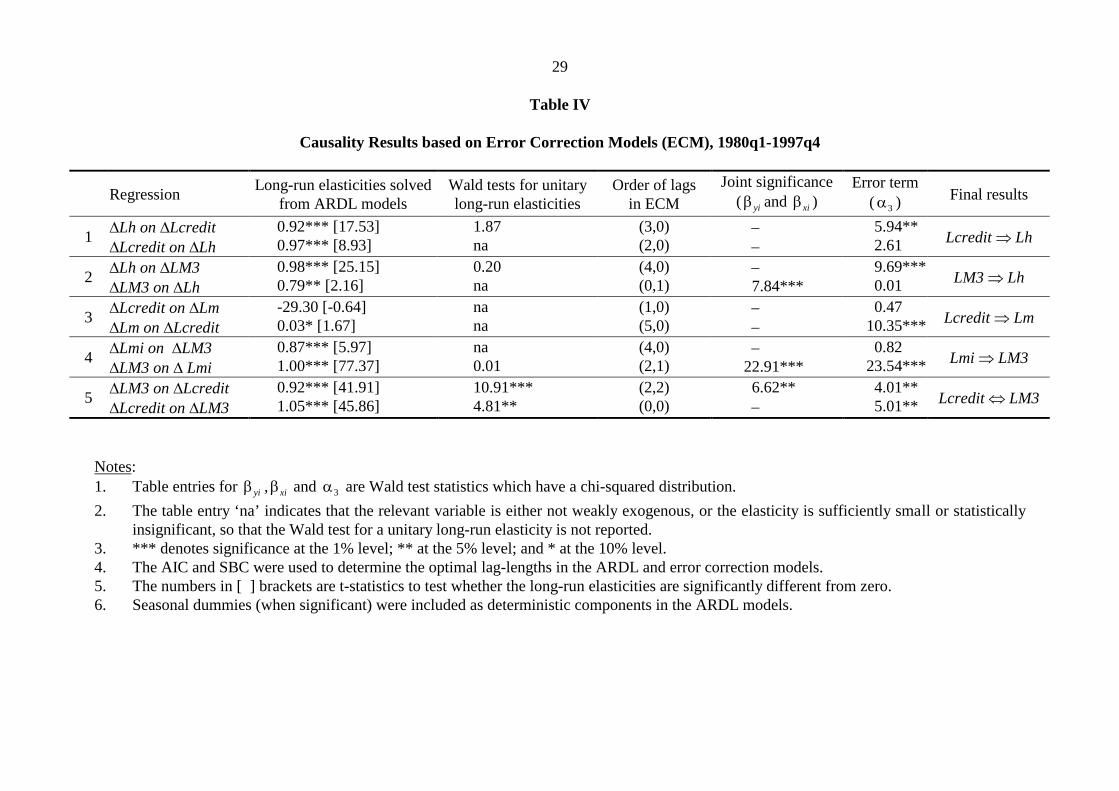
The fourth set of regressions in Table IV again provides a summary of the results
presented thus far. Unidirectional causality from Lmi to Lm3, conditional on Lmi being
strongly exogenous, reflects the endogenous nature of the money supply over the period of
more market-oriented monetary policy measures25.
Since the results unconditionally show that the SARB imposed no direct liquidity
constraints, bi-directional causality between LM3 and Lcredit in the fifth set of regressions
supports the theoretical propositions of the liquidity preference view. Causality from Lcredit
to LM3 with Lcredit being strongly exogenous emphasises the endogenous nature of the
money supply, while reverse causality can again be interpreted as evidence of an independent
money demand function.
25 The results for the first, second and fourth regressions all yield consistent results, insofar asthe null hypothesis of a unitary long-run elasticity cannot be rejected conditional on Lcredit,LM3 and Lmi as the exogenous variables.
20
VI Conclusions and Policy Implications
The different theoretical approaches tested in the empirical analysis have proved to be
most informative in describing South Africa’s money supply process over the periods of direct
and indirect monetary control measures. The analysis further suggests that it is a combination,
rather than a single approach, that enables us to draw some concrete conclusions on the
endogenous/exogenous nature of the money supply.
From a monetarist perspective, the inflationary impact of ‘excess’ money is only
relevant over the period of direct control measures. It remains an empirical matter to
determine whether excessive monetary expansion over this period can be regarded as one of
the underlying causes of inflation. This contention is borne out by the fact that the money
supply is also endogenously determined over this period.
Over the two sub-periods under analysis, the empirical results further show that even
under an endogenously determined money supply, ‘excess’ money may come into existence
because agents do not automatically absorb any amount of deposits created by the flow of new
bank lending. It is unlikely, however, that this process described by the liquidity preference
view could be regarded as an independent cause of inflation. The main causes of a self-
perpetuating inflationary process under an endogenously determined money supply are more
likely to be of a cost-push and/or structural nature.
The most important conclusion to be drawn from the empirical results is that
irrespective of the monetary system at the time, the money supply in South Africa is
endogenously determined over the period 1966-1997. ‘Disintermediation’, together with an
ineffective liquid asset reserve system, were some of the underlying reasons why the money
supply was mainly credit-driven and beyond the direct control of the SARB. In sharp contrast
to the period of direct control measures, more market-oriented measures over the period 1980-
21
1997 ensured that loan arrangements took place within the banking system. The SARB
fulfilled its role as lender of last resort and supplied reserves on demand.
One of the underlying reasons to explain the failure of the SARB to reach predetermined
M3 monetary growth targets on a consistent basis since the mid 1980s can be found in the
endogenous nature of the money supply and not, as Moll’s (1999) study claims, because of an
unstable M3 velocity. Although the M3 velocity is stable over the whole period under
analysis, the stable long-run relationship between money and money income is only valid
conditional on money income being exogenous, while it is invalid to regard money as
exogenous over the whole period 1966-199726. Over the period of monetary growth targeting,
money income determined an endogenous money supply, so that the M3 money supply lost its
effectiveness as a leading indicator for monetary policy. The most important policy
implication is that the SARB controlled the money supply indirectly during the period 1980-
1997, through an increase in interest rates, and at the potential cost of a slowdown in
economic activity.
26 The stable long-run relationship (cointegrating) between money and money income issupported by the empirical evidence over the two sub-periods. First, money income remainsexogenous to the M3 money supply irrespective of the monetary system. Second, the long-runelasticities of 0.98 and 1.00 conditional on money income being exogenous, are indicative ofparameter constancy over the whole period under analysis.
22
REFERENCES
Arestis, P. and Howells, P. (1996), Theoretical Reflections on Endogenous Money: theproblem with ‘convenience lending’, Cambridge Journal of Economics, 20, 539-551.
Black, P.A. and Dollery, B.E., (eds.), (1989), Monetary Policy in South Africa: Main findingsDe Kock Commission, in Leading Issues in South African Macroeconomics: selectedreadings, Johannesburg, Southern Book Publishers.
Boswijk, P. and Franses, P.H. (1992), Dynamic Specification and Cointegration, OxfordBulletin of Economics and Statistics, 54(3), 369-381.
Charemza, W.W. and Deadman, D.F. (1997), New Directions in Econometric Practice,second edition, UK, Edward Elgar.
Davidson, P. (1988), Endogenous Money, the Production Process, and Inflation Analysis,Economie Appliquee, XL1(1), 151-169.
Davidson, P. (1989), On the Endogeneity of Money once more, Journal of Post KeynesianEconomics, X1(3), 488-490.
Dow, S.C. (1996), Horizontalism: a critique, Cambridge Journal of Economics, 20, 497-508.
Engle, R.F. and Granger, W.J. (1987), Cointegration and Error Correction: representation,estimation, and testing, Econometrica, 55, 251-276.
Engle, R.F., Hendry, D.F. and Richard, J-F. (1983), Exogeneity, Econometrica, 51, 277-304.
Ericsson, N.R., Hendry, D.F. and Tran, H.-A. (1994), Cointegration, Seasonality,Encompassing, and the Demand for Money in the UK, in C.P. Hargreaves (ed.),Nonstationary Time Series Analysis and Cointegration, Chapter 7, Oxford, OxfordUniversity Press.
Gidlow, R.M. (1995), South African Reserve Bank Monetary Policies under dr. Gerhard deKock 1981-1989, Pretoria, South African Reserve Bank.
Gonzalo, J. (1994), Five Alternative Methods of Estimating Long-Run EquilibriumRelationships, Journal of Econometrics, 60, 203-233.
Goodhart, C.A.E. (1989), Has Moore Become Too Horizontal?, Journal of Post KeynesianEconomics, 12(1), 29-34.
Granger, C.W.J. (1988), Some Recent Developments in a Concept of Causality, Journal ofEconometrics, 39, 199-211.
Granger, C.W.J. (1997), On Modelling the Long Run in Applied Economics, The EconomicJournal, 107, 169-177.
Harris, R.I.D. (1995), Cointegration Analysis in Econometric Modelling, London, PrenticeHall.
23
Hendry, D.F. and N.R. Ericsson, (1991), An Econometric Analysis of U.K. Money Demand inMonetary Trends in the United States and the United Kingdom by Milton Friedman andAnna J. Schwartz, American Economic Review, 81, 8-38.
Howells, P.G.A. (1995). The demand for Endogenous Money, Journal of Post KeynesianEconomics, 18(1), 89-106.
Howells, P.G.A. (1997), The Demand for Endogenous Money: a rejoinder, Journal of PostKeynesian Economics, 19(3), 429-435.
Howells, P.G.A. and Hussein, K. (1998), The Endogeneity of Money: evidence from the G7,Scottish Journal of Political Economy, 45(3), 329-340.
Hurn, A.S. and Muscatelli, V.A. (1992), The Long-Run Properties of the Demand for M3 inSouth Africa, South African Journal of Economics, 60(2), 158-172.
Inder, B. (1993), Estimating Long-Run Relationships in Economics: a comparison of differentapproaches, Journal of Econometrics, 57, 53-68.
Johansen, S. and Juselius, K. (1990), Maximum Likelihood Estimation and Inference onCointegration - with application to the demand for money, Oxford Bulletin ofEconomics and Statistics, 52, 169-210.
Kaldor, N. (1982), The Scourge of Monetarism, New York, Oxford University Press.
Kaldor, N. and Trevithick, J.A. (1981), A Keynesian Perspective on Money, Lloyds BankReview, 139, 1-19.
Kremers, J.J.M., Ericsson, N.R. and Dolado, J.J. (1992), The Power of Cointegration Tests,Oxford Bulletin of Economics and Statistics, 54, 325-348.
Lavoie, M. (1984), The Endogenous Flow of Credit and the Post Keynesian Theory of Money,Journal of Economic Issues, XV111(3), 771-797.
Macdonald, R. and M.P. Taylor, (1992), A Stable US Money Demand Function, 1874-1975,Economics Letters, 39, 191-198.
MacKinnon, J. (1991), Critical Values for Cointegration Tests, Chapter 13 in R.F Engle andC.W. Granger (eds.), Long-Run Economic Relationships, Oxford University Press.
Maddala, G.S. (1988), Introduction to Econometrics, New York, Macmillan.
Meijer, J.H. (1992), Instruments of Monetary Policy, in LJ Fourie, HB Falkena, and WJ Kok(eds.), Fundamentals of the South African Financial System, Johannesburg, SouthernBook Publishers.
Mohr, P. and Rogers, C. (1995), Macro-Economics, third edition, Johannesburg, LexiconPublishers.
Moll, P.G. (1999), Money, Interest Rates, Income and Inflation in South Africa, South AfricanJournal of Economics, 67(1), 34-64.
24
Moore, B.J. (1988), Horizontalists and Verticalists, Cambridge, Cambridge University Press.
Moore, B.J. (1989a), A Simple Model of Bank Intermediation”, Journal of Post KeynesianEconomics, 12(1), 10-28.
Moore, B.J. (1989b), The Endogeneity of Credit Money, Review of Political Economy, 1(1),64-93.
Moore, B.J. (1989c), Does Money Supply Endogeneity Matter: a comment?, South AfricanJournal of Economics, 57(2), 194-200.
Moore, B.J. (1991), Has the Demand for Money been Mislaid? A reply to “Has MooreBecome too Horizontal?”, Journal of Post Keynesian Economics, 14(1), 125-133.
Moore, B.J. (1997), Reconciliation of the Supply and Demand for Endogenous Money,Journal of Post Keynesian Economics, 19(3), 423-428.
Moore, B.J. and Smit, B.W. (1986), Wages Money and Inflation, South African Journal ofEconomics, 54(1), 80-94.
Nel, H. (1994), Monetary Control and Interest Rates During the post-De Kock CommissionPeriod, South African Journal of Economics, 62(1), 14-27.
Nell, K.S. (1999), The Stability of Money Demand in South Africa, 1965-1997, University ofKent at Canterbury, Department of Economics, Studies in Economics, no.99/5.
Niggle, C.J. (1991), The Endogenous Money Supply Theory: an institutionalist appraisal,Journal of Economic Issues, XXV(1), 137-151.
Osterwald-Lenum, M. (1992), A Note with Quantiles of the Asymptotic Distribution of theML Cointegration Rank Test Statistics, Oxford Bulletin of Economics and Statistics, 54,461-472.
Palley, T.I. (1991), The Endogenous Money Supply: consensus and disagreement, Journal ofPost Keynesian Economics, 13(3), 397-403.
Palley, T.I. (1994), Competing Views of the Money Supply Process, Metroeconomica, 45(1),397-403.
Pesaran, M.H. (1997), The role of Economic Theory in Modelling the Long Run, TheEconomic Journal, 107(1), 178-191.
Pesaran, M.H. and Shin, Y. (1999), An Autoregressive Distributed Lag Modelling Approachto Cointegration Analysis, in S. Strom (ed.), Econometrics and Economic Theory in the20th Century. The Ragnar Frisch Centennial Symposium, 1998, Cambridge Universitypress, Cambridge, (forthcoming).
Pollin, R. (1991), Two Theories of Money Supply Endogeneity: some empirical evidence,Journal of Post Keynesian Economics, 13(3), 366-396.
25
Rogers, C. (1985), The monetary Control System of the South African Reserve Bank:Monetarist or Post-Keynesian?, South African Journal of Economics, 53(3), 241-247.
Rogers, (1986), The De Kock Report: A critical assessment of the theoretical issues, SouthAfrican Journal of Economics, 54(1), 66-79.
Schoombee, G.A. (1996), Recent Developments in Monetary Control Procedures in SouthAfrica, South African Journal of Economics, 64(1), 83-96.
Urbain, J. (1992), On the Weak Exogeneity in Error Correction Models, Oxford Bulletin ofEconomics and Statistics, 54(2), 187-207.
Whittaker, J. (1992), Monetary policy for economic growth, In: I. Abedian & B. Standish(eds.), Economic Growth in South Africa, Cape Town, Oxford University Press.
26
Table I
Three Empirical Hypotheses on the Exogenous/Endogenous Nature
of the Money Supply
Accommodationist view
(Moore, 1989b)
Structuralist view
(Palley, 1994)
Liquidity preference view
(Howells and Hussein, 1998)
LM3 � Lh
Lcredit � LM3
Lmi � LM3
Lcredit � Lm, Lh
Lmi � LM3
Lcredit � LM3
Note:Definition of variables:
Lcredit = log-level of total bank creditLh = log-level of the monetary base
(currency and reserves held by commercial banks)Lm = log-level of the M3 money multiplierLM3 = log-level of the M3 money supplyLmi = log-level of money income (nominal GDP)
27
Table II
Johansen’s Cointegration Tests
Johansen’s cointegration tests for the period 1966q1-1979q4
Variables included in VAR� Max
eigenvalue� Trace k
1. Lh, Lcredit
2. LM3, Lh
3. Lm, Lcredit
4. LM3, Lcredit
5. Lmi, Lm3
19.57**
20.65**
29.42**
16.17**
33.30**
25.52**
35.26**
34.42**
21.50**
38.80**
2
6
2
4
6
Johansen’s cointegration tests for the period 1980q1-1997q4
Variables included in VAR� Max
eigenvalue� Trace k
1. Lh, Lcredit
2. LM3, Lh
3. Lm, Lcredit
4. LM3, Lcredit
5. Lmi, LM3
69.36**
25.05**
67.42**
30.64**
27.86**
75.31**
28.35**
78.20**
34.44**
31.69**
1
2
1
2
2
Notes:1. ** denotes significance at the 5% level where H0: r = 0 and Ha: r = 1 and k is the order of
the VAR model.2. The critical values computed by Osterwald-Lenum (1992) were used to determine the
deterministic components in the underlying VAR model (Harris, 1995). In each case theconstant was restricted to lie inside the cointegration space without a trend. In addition,three seasonal dummies were included in all the VAR models.
3. The Akaike Information and Schwartz Bayesian selection criteria were used to determinethe order of the VAR. In cases where the two selection criteria contradicted each other, alikelihood ratio test was performed to eliminate lags from a general to a more specificmodel.
28
Table III
Causality Results based on Error Correction Models (ECM), 1966q1-1979q4
RegressionLong-run elasticities solved
from ARDL modelsWald tests for unitarylong-run elasticities
Order of lagsin ECM
Joint significance( yi� and xi� )
Error term( 3� ) Final results
1�Lh on �Lcredit�Lcredit on �Lh
0.75*** [18.90]1.35*** [26.89]
36.87***48.39***
(0,0)(2,0)
�
�
2.91*7.62*** Lcredit � Lh
2�Lh on �LM3�LM3 on �Lh
0.78*** [31.13]1.36*** [5.03]
75.81***na
(0,3)(3,0)
4.94�
7.71***0.01 LM3 � Lh
3�Lcredit on �Lm�Lm on �Lcredit
6.51*** [2.76]0.21*** [60.04]
nana
(2,0)(0,4)
�
9.23*0.76
12.63*** Lcredit � Lm
4�Lmi on �LM3�LM3 on � Lmi
1.02*** [140.00]0.98*** [163.37]
8.84***6.60**
(4,0)(5,5)
�
14.82**27.39***17.80*** Lmi � LM3
5�LM3 on �Lcredit�Lcredit on �LM3
0.95*** [29.61]1.05*** [44.19]
1.816.14**
(3,3)(2,0)
11.99***�
3.89**12.12*** Lcredit � LM3
Notes:1. Table entries for yi� , xi� and 3� are Wald test statistics which have a chi-squared distribution.
2. The table entry ‘na’ indicates that the relevant variable is either not weakly exogenous, or the elasticity is sufficiently small or statisticallyinsignificant, so that the Wald test for a unitary long-run elasticity is not reported.
3. *** denotes significance at the 1% level; ** at the 5% level; and * at the 10% level.4. The AIC and SBC were used to determine the optimal lag-lengths in the ARDL and error correction models.5. The numbers in [ ] brackets are t-statistics to test whether the long-run elasticities are significantly different from zero.6. Seasonal dummies (when significant) were included as deterministic components in the ARDL models.
29
Table IV
Causality Results based on Error Correction Models (ECM), 1980q1-1997q4
RegressionLong-run elasticities solved
from ARDL modelsWald tests for unitarylong-run elasticities
Order of lagsin ECM
Joint significance( yi� and xi� )
Error term( 3� ) Final results
1�Lh on �Lcredit�Lcredit on �Lh
0.92*** [17.53]0.97*** [8.93]
1.87na
(3,0)(2,0)
�
�
5.94**2.61 Lcredit � Lh
2�Lh on �LM3�LM3 on �Lh
0.98*** [25.15]0.79** [2.16]
0.20na
(4,0)(0,1)
�
7.84***9.69***0.01 LM3 � Lh
3�Lcredit on �Lm�Lm on �Lcredit
-29.30 [-0.64]0.03* [1.67]
nana
(1,0)(5,0)
�
�
0.4710.35*** Lcredit � Lm
4�Lmi on �LM3�LM3 on � Lmi
0.87*** [5.97]1.00*** [77.37]
na0.01
(4,0)(2,1)
�
22.91***0.82
23.54*** Lmi � LM3
5�LM3 on �Lcredit�Lcredit on �LM3
0.92*** [41.91]1.05*** [45.86]
10.91***4.81**
(2,2)(0,0)
6.62**�
4.01**5.01** Lcredit � LM3
Notes:1. Table entries for yi� , xi� and 3� are Wald test statistics which have a chi-squared distribution.
2. The table entry ‘na’ indicates that the relevant variable is either not weakly exogenous, or the elasticity is sufficiently small or statisticallyinsignificant, so that the Wald test for a unitary long-run elasticity is not reported.
3. *** denotes significance at the 1% level; ** at the 5% level; and * at the 10% level.4. The AIC and SBC were used to determine the optimal lag-lengths in the ARDL and error correction models.5. The numbers in [ ] brackets are t-statistics to test whether the long-run elasticities are significantly different from zero.6. Seasonal dummies (when significant) were included as deterministic components in the ARDL models.
30
Figure I
Nominal Velocities (VM) of the Different Definitions of Money, 1966q1-1997q4
3
3.5
4
4.5
5
5.5
66 67 68 69 70 71 72 73 74 75 76 77 78 79 80 81 82 83 84 85 86 87 88 89 90 91 92 93 94 95 96 97
YEAR
LVM1
LVM2
LVM3