Embed Size (px)
Citation preview
Computational Problems ofQuadratic Forms:
Complexity and CryptographicPerspectives
Dissertationzur Erlangung des Doktorgrades
der Naturwissenschaften
vorgelegt beim Fachbereich Informatik und Mathematikder Johann Wolfgang Goethe-Universitat
in Frankfurt am Main
von
Rupert Hartung
aus Oberwesel
Frankfurt am Main, 2007

Contents
Introduction vii
Table of Notation xvii
I Quadratic Forms and their Applications 1
1 Preliminaries 31.1 Computational Problems . . . . . . . . . . . . . . . . . . . . . . . 3
1.1.1 Model of computation . . . . . . . . . . . . . . . . . . . . 31.1.2 Problems . . . . . . . . . . . . . . . . . . . . . . . . . . . 41.1.3 Probabilistic Computation . . . . . . . . . . . . . . . . . . 51.1.4 Reductions . . . . . . . . . . . . . . . . . . . . . . . . . . 5
1.2 Quadratic Forms . . . . . . . . . . . . . . . . . . . . . . . . . . . 61.2.1 Quadratic Forms . . . . . . . . . . . . . . . . . . . . . . . 61.2.2 Representations . . . . . . . . . . . . . . . . . . . . . . . . 81.2.3 Properties of forms . . . . . . . . . . . . . . . . . . . . . . 91.2.4 Transformations . . . . . . . . . . . . . . . . . . . . . . . 91.2.5 Class structure over Important Rings . . . . . . . . . . . . 121.2.6 Classes and Genera . . . . . . . . . . . . . . . . . . . . . . 191.2.7 Reduction . . . . . . . . . . . . . . . . . . . . . . . . . . . 21
1.3 Problems of Quadratic Forms . . . . . . . . . . . . . . . . . . . . 211.3.1 Rings . . . . . . . . . . . . . . . . . . . . . . . . . . . . . 211.3.2 Encoding of properties . . . . . . . . . . . . . . . . . . . . 231.3.3 Representation problem . . . . . . . . . . . . . . . . . . . 241.3.4 Transformation problem . . . . . . . . . . . . . . . . . . . 261.3.5 Primitiveness . . . . . . . . . . . . . . . . . . . . . . . . . 261.3.6 Complexity assumption . . . . . . . . . . . . . . . . . . . 27
2 Cryptography 292.1 Randomization and Key Generation . . . . . . . . . . . . . . . . 292.2 An identification scheme . . . . . . . . . . . . . . . . . . . . . . . 31
2.2.1 Specification of the Protocol . . . . . . . . . . . . . . . . . 312.2.2 Proof of knowledge . . . . . . . . . . . . . . . . . . . . . . 322.2.3 Zero-knowledge property . . . . . . . . . . . . . . . . . . . 34
2.3 Long Challenges and Signatures . . . . . . . . . . . . . . . . . . . 352.3.1 Specification of the protocol . . . . . . . . . . . . . . . . . 352.3.2 Application to digital signatures . . . . . . . . . . . . . . 35
iii
iv CONTENTS
2.3.3 Security against Fraudulent Provers . . . . . . . . . . . . 362.3.4 Security against Fraudulent Verifiers . . . . . . . . . . . . 37
3 Localization and Decisional Complexity 393.1 Decision Problems . . . . . . . . . . . . . . . . . . . . . . . . . . 393.2 Forms over Finite Fields . . . . . . . . . . . . . . . . . . . . . . . 453.3 Forms over Local Rings . . . . . . . . . . . . . . . . . . . . . . . 47
4 Algorithms for Primes, Classes, and Genera 534.1 Algorithmic Prime Selection . . . . . . . . . . . . . . . . . . . . . 534.2 Construction of Genera . . . . . . . . . . . . . . . . . . . . . . . 59
4.2.1 Local representations . . . . . . . . . . . . . . . . . . . . . 594.2.2 Composition of square classes . . . . . . . . . . . . . . . . 624.2.3 Approximation . . . . . . . . . . . . . . . . . . . . . . . . 654.2.4 Main algorithm . . . . . . . . . . . . . . . . . . . . . . . . 68
II Classification with Respect to Complexity 73
5 Cases of Low Complexity 755.1 Singular Forms . . . . . . . . . . . . . . . . . . . . . . . . . . . . 755.2 Reducible Forms . . . . . . . . . . . . . . . . . . . . . . . . . . . 785.3 Definite Forms . . . . . . . . . . . . . . . . . . . . . . . . . . . . 825.4 Isotropic Ternary Forms . . . . . . . . . . . . . . . . . . . . . . . 83
6 The Impact of the Base Ring on Complexity 876.1 Forms over the Rational Numbers . . . . . . . . . . . . . . . . . 876.2 Rings of Formal Power Series . . . . . . . . . . . . . . . . . . . . 90
6.2.1 Introduction and summary of results . . . . . . . . . . . . 906.2.2 Upper bounds . . . . . . . . . . . . . . . . . . . . . . . . . 916.2.3 Lower bounds for representations . . . . . . . . . . . . . . 93
6.3 Polynomial Rings . . . . . . . . . . . . . . . . . . . . . . . . . . . 96
7 Complexity for Varying Dimension 1017.1 Dimension Shift to Ternary and Quaternary Forms . . . . . . . . 101
7.1.1 Introduction and result . . . . . . . . . . . . . . . . . . . 1017.1.2 Direct sum decomposition of isotropic forms . . . . . . . . 1027.1.3 Conclusion of the proof . . . . . . . . . . . . . . . . . . . 103
7.2 Binary Forms . . . . . . . . . . . . . . . . . . . . . . . . . . . . . 103
III Hardness and Interrelationship 107
8 Comparison with Factorization 1098.1 Introduction and Result . . . . . . . . . . . . . . . . . . . . . . . 1098.2 Spinor Norm and an Equivalence Criterion . . . . . . . . . . . . 1108.3 Conclusion of the Proof . . . . . . . . . . . . . . . . . . . . . . . 1128.4 Problem Modification . . . . . . . . . . . . . . . . . . . . . . . . 114
CONTENTS v
9 NP-Hardness Results 1159.1 Introduction and Summary of Results . . . . . . . . . . . . . . . 1159.2 From SAT to Squares . . . . . . . . . . . . . . . . . . . . . . . . 1219.3 The Special Cohen-Lenstra Heuristics . . . . . . . . . . . . . . . 1279.4 The Image of Binary Forms . . . . . . . . . . . . . . . . . . . . . 1309.5 The One-Class Condition . . . . . . . . . . . . . . . . . . . . . . 1319.6 Orbits of Representations . . . . . . . . . . . . . . . . . . . . . . 1329.7 Conclusion of the Proofs . . . . . . . . . . . . . . . . . . . . . . . 140
10 Relationship between the Problems 14510.1 Result and Proof Outline . . . . . . . . . . . . . . . . . . . . . . 14510.2 Construction of a Represented Form . . . . . . . . . . . . . . . . 14710.3 Construction of an Equivalent Form . . . . . . . . . . . . . . . . 14910.4 Reduction to Representations . . . . . . . . . . . . . . . . . . . . 151

vi CONTENTS
Introduction
I am the very model of a modern Major-General,I’ve information vegetable, animal, and mineral,[. . .]I’m very well acquainted, too, with matters mathematical,I understand equations, both the simple and quadratical[. . .].
(W. S. Gilbert, from: The Pirates of Penzance)
At least at first sight, quadratic equations seem to be much more difficultthan linear problems. This is what W. S. Gilbert may have had in mind whenwriting this verse for this self-assure officer; or so the juxtaposition between‘simple’ and ‘quadratical’ equations suggests. Roughly speaking, the aim of thisdissertation is to answer the question, how difficult the latter are.
Background. Quadratic forms play an important role in number theory aswell as in several related areas. They already aroused the interest of Fermat,Euler, Lagrange, and Legendre (see [Wei84], [Dic34b, ch. VI–X, XII, XIII],[Dic34c, ch. I–XI]). Perhaps one of their main appeals is their seeming simplicity:Being merely a slight abstraction from quadratic equations, quadratic forms areeasy to write down and ask questions about. More specifically, quadratic formsare just one step beyond linear ones, and the theory of linear forms (i. e. linearalgebra by any other name) is thouroughly explored and easily understandible– at least from today’s perspective. Curiously, this picture changes radicallywhen turning to exponent two. Another reason to study quadratic forms lies inthe fact that binary forms bear the structural information on quadratic numberfields, but in an easier accessible way.
The mathematical literature produced by the mid of the 19th century hasnot only contributed singnificantly to the knowledge about quadratic forms, butalso raised new questions. Especially Gauß’ work Disquisitiones Arithmeticae[Gau89] enjoyed immense popularity among the mathematicians of his and thefollowing generations: Not only did it mean a leap ahead in the theory, but ithas also shaped much of the area today known as algebraic number theory.
Probably, the flourishing of this reasearch area inspired Hilbert to discuss itin his famous speech at the International Congress of Mathematicians in Parisin 1900. The eleventh item on his famous list of mathematical problems for the20th century calls for a theory of quadratic forms over algebraic number fields.
vii
viii INTRODUCTION
The efforts initiated by Hilbert’s speech have given rise to the arithmetictheory of quadratic forms, which explores quadratic forms over local and globalfields and their respective rings of integers. Many question could be settled inthis area. The honor of having accomplished Hilbert’s task is usually grantedto H. Hasse for the famous Hasse Principle (see [Has24]).
It is this branch of the theory which will prove the most significant here.Some central results are discussed in Sect. 1.2.5.
Despite these enormous advances, algorithmic questions have hardly evercome into focus. This is even more suprising in view of the fact that most ofthe theory starts with two classical decision problems:
(A) Given two quadratic forms, are they equivalent?(B) Given a quadratic form and a scalar, can the scalar be repre-
sented by the form?
More than a century of research has provided us with comprehensive crite-ria for these questions. However, the algorithmic nature of such results is oftenbarely a theoretical possibility. This point deserves a closer look. In the lan-guage of computer science, the arithmetic theory can only prove that questions(A), (B) are decidable, while making no statement about running times. Arethese problems possibly polynomial-time decidable? In many important specialcases, the answer is ‘yes’, still thanks to arithmetic results, see Sect. 3.1. How-ever, these results do not extend to all forms. This gap is due to the complexityof the underlying computational problems:
(A’) Given two equivalent forms, compute an equivalence transform.(B’) Given a form f and a scalar m, solve the equation f(v) = m (if
possible).
An efficent method which produces an equivalence transform or representa-tion if it exists, obviously yields a procedure to decide their existence. But hereit seems that the only algorithm considered in the literature to find a transfor-mation is exhaustive search. This is most obvious when the attempt of Dicksonand Ross to decide equivalence of a particular pair of forms is discussed (see[Cas78, p. 132], [CS93, p. 403]). The restriction to trivial algorithms also be-comes explicit in Siegel’s famous bound on equivalence transformations [Sie72],which reproves the decidability of (A) using analytic techniques. More precisely,he shows that for each pairs f, g of equivalent forms there is a constant C > 0effectively computable from f, g such that there is a transformation from f tog whose coefficients are absolutely bounded by C. Siegel explicitly refers to theenumeration of all integral matrices up to some bound on the coefficients fortesting equivalence.
In dimension three, Siegel’s implicit bound has been made explicit and hasbeen improved to polynomial size by Dietmann [Die03]. Still using trivial enu-meration, this implies that problem (A) is in NP. Moreover, for problem (B),
ix
Grunewald and Segal [GS04] showed decidability by solving problem (B’) ifpossible. Their algorithm is more sophisticated, yet still involves steps of expo-nential enumeration.
I am aware of exactly one literature reference asking explicitly for a com-plexity analysis of problems (A), (B), (A’), (B’). At the end of [CS93, ch. 15],Conway and Sloane formulate both decisional and computational equivalenceand representation problems, along with a couple of additional questions, e. g.on class numbers. They mention several cases for which these problems areeasy. For indefinite forms over Z, they express their impression that “theredo not seem to be good algorithms”, and discuss the inefficiency of exhaustiveenumeration.
Thus it may be stated that algorithms on quadratic forms have hardly beenstudied, and even less so complexity issues.
Out of fairness, we ought to mention the main exceptions to this rule. In[Gau89], Gauß solves all problems (A),(B),(A’),(B’) for binary integral formsgiving concrete non-trivial algorithms along with a correctness analysis (seealso [Lag80], [BB97], [BV07] for improvements). His approach has been redis-covered by the founders of computational algebraic number theory, see [PZ89].In particular, Gauß’ algorithms and modifications thereof are employed for com-putations in quadratic and relative quadratic number fields, see [Coh93, ch. 5],[Coh00, sec. 2.6]. Still if forms are concerned these are mostly only binary ones.
Apart from the problems touched upon here, the old question how to solvethe Legendre equation
ax2 + by2 + cz2 = 0 (1)
non-trivially, if possible, has fascinated generations of mathematicians. Af-ter Legendre had discovered the conditions under which (1) is solvable, La-grange came up with a concrete solution method, see [Sma98, sec. 4.3.3], [Ser73,sec. 4.3]. A remarkable algorithm can also be found in [Gau89], recent im-provents include [CM98], [CR03] [Sim05b], and [Sim05a].
Finally, for definite forms algorithmic and complexity theoretic investiga-tions abound. Having a strong tradition in this particular field, computationalaspects have gained considerable momentum on the advent of the LLL-algorithm[LLL82]. Algorithms for definite forms, often formulated in the language oflattices, constitute a vivid domain of research. This may be due to the re-quirements of the domains where lattices are applied, as discrete optimization,cryptanalysis, and lattice cryptography (see below).
Motivation. In this thesis, I will explore the complexity of problems (A), (B),(A’), (B’). This follows a twofold motivation:
At first, in the age of highly-efficient computing devices, decidability is a veryweak notion. As computing capacities increased, the theory of computing hasbecome more and more demanding of the efficiency a problem is solvable with:From decidability, requirements have shifted to polynomial-time decidability,and are even further shifting towards efficient parallelizability. Thus Hilbert’squestion adapted to the concerns of this day and age could read:
‘Are equivalence and representability polynomial-time decidable over somering?’
x INTRODUCTION
or more generally:
‘What is the complexity of deciding equivalence and computingtransformations?’
We may arrive at similar questions if we apply similar reasoning to Hilbert’sTenth Problem on solvability of general Diophantine equations.
This leads us to our second approach to these questions: The hardness ofcomputational problems on indefinite quadratic forms allows to base crypto-graphic protocols on it, see Chapter 2. This follows the example of definiteforms, or lattices, which have been employed in cryptography, e. g. in [AD97],[GGH97], [HPS98], [HPS01], [HHGP+03]. The security of these crypto-schemesis based on the lattice problems SVP and CVP, whose hardness is illustrated by(partially randomized) NP-completeness results (see [MG02], [Kho05]). More-over, this is taken as a hint that this type of primitives may still be secure andapplicable in the (still hypothetical) age of quantum computers because quan-tum computers are considered unlikely to efficiently solve NP-complete problems(see [BBBV97]).
However, the hardness proofs use lattices of arbitrarily high dimension, whichcauses severe efficiency problems. In consequence, lattice cryptography plays aminor role in practice today. By contrast, for indefinite forms, we can provehardness in fixed small dimension (Theorem 7.1.1), and we discover the NP-hardness of closely related problems (Chapter 9). In cryptography, this wouldallow for smaller key sizes, and thus also faster protocols. Adopting the vision forthe future of lattice cryptography, we take this as an indication that quadraticform cryptography may be both suited for the post-quantum era as well asfeasible for traditional computers.
It should be noted that there are two further families of cryptosystems re-lated to quadratic forms or equations. At first, multivariate cryptography uti-lizes polynomial equation systems over finite fields, which are often quadratic.It was a scheme of Imai and Matsumoto [IM88] which became the igniter ofthis now fully developped and vivid branch of cryptography. Solving systems ofquadratic equations over F2 is already NP-hard; this is understood as an indica-tion that the concrete systems employed also are hard. However, NP-hardnessonly holds if the number of equations and variables is unbounded. This still re-quires relatively large keys, in contrast to our hardness results in small boundeddimension.
Furthermore, algorithmic problems of number fields have been employed incryptography. Important protocols are proposed in [BW90], [BBT94], [BMM00].This constitutes the branch of cryptography which is certainly closest to algo-rithmic algebraic number theory. As mentioned above, quadratic forms providea data type highly suitable for computation in number fields. This refers mostlyto binary forms, which are not useful in our context (see Sect. 7.2). Moreover,the underlying problems are often related to factoring, or discrete logarithms,while problems on higher-dimensional forms seem to be essentially harder.
xi
Main results. The cryptosystems reviewed in Chapter 2 are proposed forindefinite anisotropic quadratic forms over Z. This choice is the result of com-plexity investigations. The schemes themselves are quite flexible and could beimplemented, after minor modifications, for various types of forms over variousrings. The presentation in Chapter 2 emphasizes this flexibility. However, suchvariations usually have an impact on the security of the scheme.
Security relies on the hardness of problems (A’) and (B’), which will be calledTrafo and Repr (for formal definitions, see Sect. 1.3). These will be the mainobjects of study in this thesis.
The information that complexity theory can supply cryptography with is oftwo kinds: Efficient, or comparatively efficient algorithms rule out the instancesin question, while hardness results encourage the use of the respective problem.
In the latter respect, we prove that variants of the problems Trafo andRepr over Z are NP-complete under randomized reductions (Chapter 9). Moreprecisely, we ask for transformations and representations whose coefficients lie ingiven intervals. The hardness results refer to indefinite ternary quadratic forms(with several possible further restrictions). For isotropic forms, the results holdunconditionally, while for anisotropic forms it is subject to a number-theoreticassumption, which we call the special Cohen-Lenstra Heuristic (sCLH). Thisassumption claims class number one for ‘sufficiently many’ real quadratic fieldswith prime discriminant. It is inspired by and largely similar to the well-knownCohen-Lenstra Heuristic [CL84].
The proof of these theorems is based on a result of Adleman and Manders[MA78] who proved NP-completeness for solvability of the binary (inhomoge-neous) equations
x2 + by = a, |x| ≤ c
in integers x, y ∈ Z. We use a modification of this theorem with restrictionson a, b. The hardness of the representation proplem for isotropic forms fol-lows directly. For anisotropic forms, we have to construct a small family ofbinary quadratic forms some of which represents the (unknown) integer y withhigh probability. The correctness of our construction is proved using the sCLH.Finally, the results on transformation problems are derived from those on repre-sentations. This step requires a bound on the number of orbits of representationsunder the automorphism group of the representing form.
A reductionist hardness result, this time for the original problem Trafo, ispresented in Chapter 8. We show that computing transformations for equivalentindefinite forms over Z of any dimension n ≥ 3 is no easier than extracting asquare root of −1 modulo their determinant. The complexity of this task isclosely related to that of factoring. We again emphasize that we can restrict toanistropic forms (if n = 3 or 4).
This estimate is useful because it gives an explicit lower complexity bound forthe presumably hard problem Trafo. However, in the light of the NP-hardnessresults and for want of a subexponential algorithms for this problem, Trafoand factorization seem far from being polynomial-time equivalent. Thereforewe include the factorization of the determinants into the input for most of our
xii INTRODUCTION
investigations. In particular, the NP-hardness results are still valid for theproblems with the factorization given for free.
Perhaps our most suprising result reduces general Trafo instances over Zto such of small dimension. More precisely, the transformation problem (withfactorization given) in any fixed dimension can be solved using an oracle fortransformations in dimensions three and four. This holds for forms of oddsquarefree determinant.
This result justifies the use of low-dimensional forms in cryptography. Ifthe transformation problem is hard in any fixed dimension at all, then it isnecessarily hard in dimensions ≤ 4.
The proof works by splitting off (a lattice on) a ‘hyperbolic plane’ from bothforms in question, and reducing to the orthogonal complement.
Furthermore, we prove a result on the interrelationship between the trans-formation and representation problems. Here ‘interrelationship’ expresses a re-laxed version of polynomial-time equivalence. More explicitly, we reduce Reprto Trafo instances—both times with free factorization—at the cost of restric-tions on the determinants: The odd, squarefree determinant d of the form f ofdimension n in the Repr instance is lifted to its (n − 1)-th power under thisreduction.
Conversely, Trafo instances are solved using an oracle capable of computingsolutions to both Repr problems and Trafo problems of dimension n−1. Againthe Repr instances refer to forms of determinant dn−1. Most importantly, forn = 3 the oracle access for lower-dimensional Trafo solutions can be dispensedwith. Therefore we have some kind of mutual reductions of Trafo and Reprfor ternary forms, though not exactly polynomial-time equivalence.
The importance of this result is due to the signature scheme of Sect. 2.3.Its security requires that, beside Trafo, also the problem Repr is infeasible(whereas identification as in Sect. 2.2 is based on Trafo only). Equivalenceof Trafo and Repr would release us from the necessity to presuppose twounrelated cryptographic assumptions. Hence linking their complexity makesthe conjunction of these two hardness assumptions more plausible.
The proof employs Minkowski duality between representations of scalarsby f , and representations of (n − 1)-dimensional forms by the adjoint of f .Passing from such a representation to a transformation for given instances meansaugmenting a (n×(n−1))-matrix by a last column, subject to several linear andquadratic constraints. Very roughly, the reductions reflect the constructions ofthese missing coefficients.
Turning from lower to upper bounds on complexity, our first concern arebinary forms over Z. We learn that transformation problems can be solved intime polynomial in S, where S is any solution. This excludes the use of binaryforms in protocols as in Chapter 2 because this would allow for key extractionin time polynomial in the size of the secret key. Together with the result ofSect. 7.1.3 this prompts us to concentrate on forms of dimensions three andfour. Reference to solution size is necessary since in general, transformationsbetween binary forms need not even be of polynomial size. The statementfollows by analysis of an algorithm of Gauß.
xiii
An obvious variation of the computational problems consists in changing thebase ring. We prove various upper complexity bounds for other rings than Z.Over the rational number field Q, the problem Trafo can be closely linked tofactoring integers. For Trafo reduces to factoring the determinants of the formsinvolved, and conversely, Trafo is at least as hard as computing a modularsquare root of −1. As mentioned above, factoring and computing imaginaryroots seem to be similarly hard and may even be polynomial-time equivalent.Ignoring this gap and using the result from Chapter 8, we may heuristicallystate that the transformation problem over Z is no easier than over Q.
In Sects. 6.2 and 6.3, we explore rings of formal power series and polyno-mials in one variable, respectively. This setting is more general as we do notconcentrate on a concrete base ring, but compare complexity of Repr overthis ring with that over the ground field. For power series, it turns out thatboth decisional an computational problems are polynomial-time equivalent tothe respective problem over the ground field.
In the case of polynomials, we reduce it to the problem of finding simulta-neous representations over the ground field (which is much more general thansingle representations). Still, the solution over power series rings yields ‘ap-proximative’ solutions to representation problems with polynomial coefficients.Hence hard instances may only arise if ‘most’ representations modulo powers ofthe indeterminate do not lift to polynomials.
We thus learn that the use of power series rings in our applications does notpay, as it features roughly the same level of security at the cost of larger keys.The use of polynomial rings at least is not encouraged. Besides, a more preciseclassification of complexity over polynomial rings seems to depend heavily onthe ground field.
For finite fields, fields of p-adic numbers, and rings of p-adic integers, bothTrafo and Repr are polynomial time. This follows almost immediately fromclassification theorems.
By localization, we can also solve the decisional equivalence and repre-sentability problems over Z, for a large proportion of instances. For represen-tations, indefiniteness of the forms is required. If the computational problemsare hard, as we conjecture, this would establish an intriguing discrepancy phe-nomenon.
For definite forms in fixed dimension it is known that Trafo can be solved inpolynomial time. Isotopic ternary forms allow for subexponential algorithms forboth Trafo and Repr. These facts are collected in Chapter 5. There we alsoverify the decreasing effect of singularity and reducibility of forms on complexity.
Part of the results presented here have been published in[HS07b] and [Har07]. Another paper on this topic [HS07a] is in preparation.
Outline. In Chapter 1, we review the most important concepts from theoret-ical computer science that we are going to use. Then we introduce the basic
xiv INTRODUCTION
notions of quadratic forms and cite important known facts about them. Finallywe formulate and explain the computational problems Trafo and Repr, whichwe are going to analyze. This chapter contains prerequisites for the whole thesis.The other chapters are largely independent from each other.
In Chapter 2, we present an identification scheme by Schnorr which provesknowledge of an equivalence transformation. An enhanced scheme with longchallenges is suitable for digital signature generations, even if at the cost ofprovable security. These applications serves as our main motivation to studythe complexity of the underlying problem Trafo.
The impact of localization on complexity is studied in Chapter 3. We provepolynomial-time solvability of transformation and representation problems overall Fp, Zp, and Qp. These insights are used to demonstrate polynomial-timedecidability of equivalence and representability over Z. There will be severalreferences to these statements throughout the thesis, which explains why theyprecede its main parts.
Chapter 4 displays auxiliary algorithms. Section 4.1 is a survey on algorith-mic prime selection. In Sect. 4.2.4 we show how to construct an integral formsatisfying p-adic constraints. These methods will be needed in later chapters,particularly in Chapters 9 and 10.
In the second part of this thesis the reader may find results on several re-strictions of Trafo and Repr. At first, we discuss properties of forms and theirimpact on complexity (Chapter 5).
Chapter 6 contains those results on base rings other than Z which are notyet discussed in Chapter 3, i. e. it is concerned with Q, rings of formal powerseries, and of polynomials.
Finally, results with respect to the dimension can be found in Chapter 7;these are the reduction of the transformation problem to dimensions three andfour, and the feasibility of it for binary forms.
The third and last part of this thesis comprises the remaining lower-boundresults. It is opened by Chapter 8 which displays the imaginary root problemas a lower bound for Trafo. Then we present and prove NP-hardness results inChapter 9, and finally in Chapter 10, we establish the ‘near’ equivalence of theproblems Trafo and Repr.
Note that for the sake of convenience, the reader will find an overview of(non-standard) notation employed right after this introduction. Moreover, def-initions and conventions explained in the text can be easily looked up by use ofthe index at the end of this document.
Literature. Of the extremely comprehensive literature on quadratic forms,we will primarily need the arithmetic theory. If possible, we have cited [Cas78],since this textbook is particularly focussed on forms over Q and Z and theirlocalization. Other accounts of the arithmetic theory include [Bro06], [Jon50],[Eic52], [O’M63], [CS93, ch. 15], [Kne02], and [Kit93]. As far as local and globalfields are concerned, one can as well refer to [Ser73] and [Lam05].
xv
Acknowledgements. I would like to thank C.-P. Schnorr, my advisor, for allhis support during my work on this thesis, and for calling my attention to thealgorithmic aspects of quadratic forms in the first place.
I also wish to express my gratitude to all who have engaged in discussionswith me on the subject. In particular, I have benefitted from interested questionsand useful remarks on the part of A. Pfister, R. Scharlau, G. Schnitger, andD. Simon.
Thanks is also due to R. Dietmann, who introduced me to the the analytictheory of homogeneous forms. I also wish to thank J. Kluners and G. Malle fortheir comments on the sCLH (Sect. 9.3).

xvi INTRODUCTION
Table of Notation
|M | cardinality of a set M#M cardinality of a set M] disjoint unionQp field of p-adic numbersZp ring of p-adic integers
(by convention, Z∞ = Q∞ = R)
R∗ group of units of ring RR∗2 group of squares of units of ring R(ap
)Legendre symbol modulo odd prime p
ρp fixed element in Z∗p\Z∗
p2 see Sect. 1.2.5
ω(m) number of distinct prime factors of ma|b a divides ba 6 | b a does not divide bp|e∞ p is a prime dividing e, or p =∞
(see rem. after Theorem 1.2.8)νp(N) multiplicity of prime p in N ,
i. e. νp(N) = k ⇔ pk|N and pk+1 6 |N for N ∈ Zor Zp, νp(N) = νp(a)− νp(b) for N = a
b ∈ Q or Qp.By convention, νp(0) =∞.
gcd(a1, . . . , an) greatest common divisor of a1, . . . , an (in a UFD)
GLnR group of regular n-ary square matrices over ring R,i. e. GLnR = S ∈ Rn×n|det S ∈ R∗
SLnR special linear group over ring R,i. e. SLnR = S ∈ Rn×n|det S = 1
Sij (i, j)-entry of matrix SS∗j j-th column of matrix S (as a column vector)Si∗ i-th row of matrix S (as a row vector)St transpose of matrix (or vector) SS# Lagrange adjoint of matrix S
(with S#S = SS# = (det S)I)|S|∞ largest absolute value of the coefficients of matrix SIk identity matrix of dimension k
xvii
xviii TABLE OF NOTATION
ei i-th standard unit vector: ei = (0, . . . , 0, 1︸︷︷︸i
, 0, . . . , 0)t
f(·, ·) associated bilinear form of quadratic form f|f |∞ largest absolute value of the coefficients
of quadratic form f
〈a1, . . . , an〉 diagonal quadratic form∑
i aix2i (Sect. 1.2)
f ⊥ g orthogonal sum of quadratic forms f , g (Sect. 1.2)
f T quadratic form f transformed by matrix T , see Sect. 1.2.4f −→R m form f represents m over R
f∗−→R m form f represents m primitively over R
f∗−→R m form f represents m primitively over Z
(see Sect. 1.2.2)f
∗−→R g form f represents form g primitively over R
f∗−→ g form f represents form g primitively over Z
(see Sects. 10.1, 10.2)
ρ(f) reduction operator applied to form f see Sects. 1.2.7, 2.1
f ∼ g forms f and g are equivalent (over Z)f ∼R g forms f and g are equivalent over the ring R, see Sect. 1.2.4f ∼g g f and g belong to the same genus, see Sect. 1.2.6
sign f signature of form fcp(f) Hasse-Minkowski invariant of form f , see Sect. 1.2.5
OR(f) group of automorphisms of form f , i. e. O(f) =T ∈ GLnR | f T = f
O+R(f) group of proper automorphisms of f , i. e. O(f)
= T ∈ SLnR | f T = fR is suppressed in notation if R = Zshould not cause any confusion with the as-ymptotic symbol O
length (X) encoding length for object X (see Sect. 1.1)
CRT((a1,m1), . . . , (ak,mk)
)algorithmic call to the Chinese Remainder
Theorem, see p. 62
4 polynomial-time Turing reducible4na polynomial-time non-adaptively reducible41 polynomial-time Turing reducible with
(at most) one oracle call4K Cook-Karp reducible
for these reducibility notions, see Sect. 1.1.4
Part I
Quadratic Forms and theirApplications
1

Chapter 1
Preliminaries on QuadraticForms and ComputationalProblems
In this chapter we introduce definitions and theorems important for this wholethesis. We begin with collecting some concepts from theoretical computer sci-ence in Sect. 1.1. In Sect. 1.2, we review central aspects of the theory of qua-dratic forms. Finally, in Sect. 1.3, we discuss how to combine these topics, i. e.we define algorithmic problems of quadratic forms and begin with their analysis.
1.1 Computational Problems
1.1.1 Model of computation
We do not give many formal definitions in this section, but merely set up conven-tions. For more a detailed account, the interested reader is referred to [Pap94],[BDG88], [GJ79].
We generally use the computational model of a Turing machine. As weare only interested in complexity up to polynomial time, everthing done herecarries over to any model of computation polynomial-time equivalent to Turingmachines, e. g. polynomial-time k-string Turing machines.
For an algorithmic approach, the mathematical objects considered have tocome in a machine-readable format, i. e. an encoding in strings over a fixedalphabet. In some cases such an encoding is essentially canonic; for instance,integers can be presented in binary, and integral quadratic forms may be givenby its dimension and the array of its coefficients. Some more debatable casesare discussed in Sect. 1.3.1.
We will assume that some ‘sensible’ encoding has been chosen for each classof objects, and it will be kept fix. The length occupied by the encoding of an
3
4 CHAPTER 1. PRELIMINARIES
object ξ, i. e. the number of symbols (e. g. bits) used for it, will be denoted by
length (ξ) .
Analogously, we use probabilistic Turing machines as our model for random-ized algorithms, see Sect. 1.1.3 for more details.∗
We will write down algorithms as pseudocode programs, or merely sketchhow to write down such a program in proofs, without explicitly referring to aTuring machine.
1.1.2 Problems
For the considerations made in this thesis, an intuitive notion of decisional andcomputational problems suffices. However, a few remarks will be useful.
It is important for us not to restrict to decisional problems only.
A computational problem consists of a set of inputs, and for each input, aset of admissible outputs (solutions).
Note that in contrast to the usual decision problems, the output need notbe unique.
We can view decision problems as the special case of computational problemswhere all admissible answers are single bits. However, in this case we do requireuniqueness of the answer.
The computational model in which we seek for solutions of a problem isformally either the Turing machine, or the probabilistic Turing maching. Butfor easier understanding we formulate algorithms either in pseudo-programmingcode, or we indicate in the proofs how an algorithm should be programmed.
As we are mostly interested in the complexity of computational problemsup to (probabilistic) polynomial-time equivalence, we will often use the term“efficient” to mean ‘in (possibly probabilistic) polynomial time’.
We introduce problems with parameters. Here it is important to note thatthus define families of computational problems: For each value of the parame-ters, we obtain a new single problem to analyse.
Note that this definition also includes decision problems.As for inputs and solutions, we will later restrict the set of potential param-
eters to (the encodings of) suitable mathematical objects.
1.1.1 Example. Let M range over polynomial-time decidable subsets of N.Denote by Fact(M) the computational problem of factoring numbers from Minto their prime divisors (see Sect. 5.2). Then Fact is a problem with parame-ters. Obviously, its complexity can differ widely for differentM: IfM is the set
∗Speaking in a nit-picking fashion, there are two more exceptions: Whenever we speakof reductions, we implicitly make use of oracle machines; and the cryptographic protocols ofChapter 2 formally require interactive Turing machines.

1.1. COMPUTATIONAL PROBLEMS 5
of powers of two, for instance, then Fact(M) can be solved efficiently. However,Fact(N) is not believed to be solvable in polynomial time.
Note that this definition of the factorization problem was for illustrationalpurposes only. A more general variant will be analyzed in Sections 9.2 and 6.1;see also Chapter 8.
Problem union. For computational problems A,B define the problem unionA tB as follows: A tB takes inputs in
(0 × IA) ∪ (1 × IB)
where IA, IB is the set of inputs of A, B, respectively; and if the input was(0, i), then the admissible outputs are the admissible outputs of problem IAwith respect to input i, and anagolously for (1, i) and IB.
Heuristically, solving A tB means being able to solve both A and B.
1.1.3 Probabilistic Computation
As for general Turing machines, we will write down pseudo-code and identifysuch algorithms with probabilistic Turing machines. A probabilistic algorithmruns in polynomial-time if with probability ≥ 2
3 , it outputs a correct solution inpolynomial time; its behavior in other cases does not matter in the sense of thisdefinition. This makes sense since we can always break the computation afterpolynomially many steps and output a nonsense string.
We will use the terms “random polynomial time” and “probabilistic polyno-mial time” synonymously. In slightly colloquial contexts (as the rough discus-sion of proof ideas) we will use the term “efficient” unspecifically for ‘randompolynomial time’ and ‘deterministic polynomial time’.
1.1.4 Reductions
We write 4 for polynomial-time reductions of general computational problems,using polynomially many oracle calls. For decisional problems, this correspondsto a Turing reduction (see [Pap94, sec. 8.4]).
For decisional problems only, we denote by 4K a classical Karp reduction.
By 4na we denote non-adaptive reductions. It is the special case of a Turingreduction where first all questions have to be asked before the oracle gives itsanswers. For decisional problems, this type of reduction is often known as truthtable reduction. We will often write down reductions with successive oraclequeries for clarity, but mention non-adaptivety in statements if our reductioncan be easily transformed into a non-adaptive one.
6 CHAPTER 1. PRELIMINARIES
The symbol 41 denotes the special case of truth-table reduction where onlyone oracle call is permitted. For decision problems A,B, the reduction A 41 Bis equivalent to
A 4 B tK B,
where B denotes the complement of B.
The symbol 4r will be used for random reductions, i. e. the executing oraclemachine is probabilistic in the sense of Sect. 1.1.3. We combine it with theabove notation with obvious meanings, i. e. 4r,na, and 4r,1.
Finally, the notationA ≈∗ B
abbreviates the reductions
A 4∗ B and B 4∗ A,
for ∗ any legal combination of the discussed subscripts K, na, 1, r, none.
1.2 Quadratic Forms
Every mathematician who is not indifferent to number theoryhas felt the charm of Fermat’s theorem on the sum of two squaresof natural numbers. A psychologist of the Jungian school wouldprobably think that such diophantine problems are archetypal toa high degree.
(Yu. I. Manin in [Man74])
1.2.1 Quadratic Forms
Througout this thesis, let R be a commutative ring with unity in which 2 isnot a zero divisor. A quadratic form f (often simply called form) over R is ahomogeneous polynomial of degree two, i. e. a polynomial of the shape f =∑n
i,j=1 aijxixj where aii ∈ R and aij = aji ∈ 12R. The number n of variables is
called the dimension of f , denoted by dim f = n, and f is called an n-ary form.
If x = (x1, . . . , xn)t and A = (aij)ij , then we can also write f = xtAx.Conversely, via this formula any symmetric (n × n)-matrix A over 1
2R withdiagonal entries in R gives rise to a unique quadratic form. In this situation, Ais called the associated matrix of f .
If f is a form over Z (over Zp for some prime p), then f is called integral(p-adically integral). If the associated matrix of f has coefficients in R ratherthan 1
2R, then f is called classically integral ; this distinction is of course onlyrelevant if 2 /∈ R∗, thus, for R = Z and R = Z2
†. If R is a unique factorization†In the literature, the term ‘integral’ is sometimes used in the sense ‘classically integral’.
1.2. QUADRATIC FORMS 7
domain (UFD), f is classically integral and gcd(aii, 2aij | i 6= j) = 1, then f iscalled properly primitive. It is called improperly primitive if it is not properlyprimitive, but if it is classically integral and gcd(aii, aij | i 6= j) = 1. Finally, fis called primitive if it is either properly or improperly primitive.
Most of the time it will be enough to consider properly primitive and im-properly primitive forms. The reason is that for every classically integral formf , there is λ ∈ R such that 1
λf is still a form over R (‘integral’) and primitive.Moreover, if f is defined over R, but not classically integral, the 2f is (classi-cally integral and) improperly primitive. Hence, up to multiplication with ordivision by a scalar each form falls into one of two families. The last distictionremaining, namely between properly and improperly primitive forms, cannotbe easily removed; however, the phenomena observable within these families offorms do not differ too much.
We define det f := det A as the determinant of the quadratic form f . Ifdet f 6= 0 then f is called regular, otherwise singular. From now on, we willtacitly assume that all occurring forms are regular unless otherwise stated.
To every quadratic form f , there is an associated bilinear form: If A is theassociated matrix of f , then this bilinear form is given by (x, y) 7→ xtAy. Wewill denote this by f(x, y).
If ai ∈ R, then the form∑n
j=1 aix2i is abbreviated as
〈a1, . . . , an〉,
and such a form is called diagonal. Moreover, if f , g are forms with associatedmatrices A, B, then we define the form f ⊥ g, the orthogonal sum of f and g,by taking
A⊕B =(
A 00 B
)as its associated matrix. Obviously, we have
dim(f ⊥ g) = (dim f) + (dim g) and det(f ⊥ g) = (det f) · (det g).
For a symmetric matrix A consider its Laplace adjoint A# consisting ofsigned maximal minors of A, which satisfies
AA# = A#A = (det A)I.
Then A# is obviously symmetric as well, and hence the associated matrix of aquadratic form. This form, if A was the associated matrix of the form f , willbe called the adjoint form and denoted by f#.
8 CHAPTER 1. PRELIMINARIES
1.2.2 Representations
Let m ∈ Z. Then f is said to represent m if and only if there is u ∈ Rn\0such that f(u) = m. Write f −→R m, and call u a representation of m by f .In case R is a UFD and gcd(u1, . . . , un) = 1, then this representation is calledprimitive. This fact is denoted by f
∗−→R m. If R = Z we drop the subscriptand write f
∗−→ R.
In a general quadratic equation, one can get rid of linear terms, at the cost ofa linear congruence condition on the solution of the homogeneous problem. Thisis expressed in the following proposition. It serves to illustrate the usefulness ofstudying representations.
For the case n = 2 over Z, Proposition 1.2.1 is proven in [Gau89, art. 216];a similar generalization (for the case R = Z) can be found in [GS04]. Forconvenience, and according to Gauß, we use even linear terms without loss ofgenerality.
Proposition 1.2.1 Let R be a commutative ring. Let f be an n-ary quadraticform over R with associated matrix A, let det f =: d be not a zero divisor, andlet w ∈ Rn, h ∈ R.
Then the equationf(x) + 2wtx + h = 0 (1.1)
is solvable for x ∈ Rn if and only if the system
f(y) = −hd2 + d f#(w) and y ≡ A#w mod d (1.2)
is solvable for y ∈ Rn.
Note that if R is a field, the linear congruences are trivially fulfilled.
Proof : First let x be a solution to 1.1. Then
y := dx + A#w
satisfies y ≡ A#w mod d and
f(y) = ytAy = d2xtAx + 2dxtAA#w + wtA#AA#w
= d2(xtAx + 2xtw) + dwtA#w = −d2h + df#(w).
Conversely, let y satisfy 1.2. First note that the second condition means thatthere is x with y = dx + A#w. Thus it holds that
−hd2 + df#(w) = f(y) = f(dx + A#w) = d2(f(x) + 2xtw
)+ d f#(w),
which, as d is not a zero divisor, is equivalent to
f(x) + 2xtw + h = 0,
which was to be shown.
1.2. QUADRATIC FORMS 9
1.2.3 Properties of forms
Now we can define further properties of quadratic forms: A quadratic form iscalled reducible if it factors into two linear polynomials in R[x]. Reducible formsare studied in Sect. 5.2.
A form f is called isotropic if it represents zero, otherwise anisotropic.A vector v 6= 0 such that f(v) = 0 is then called an isotropic vector.
Now let there be a (canonical) embedding R → R. Typically, we think ofthe cases R = Z, Q, R here. Then a form over R is called indefinite if it (its realimage) represents both positive and negative values, and definite otherwise.Cleary every (regular) isotropic form is necessarily indefinite. Definite formscorrespond to lattices in Euclidean space and are not considered here.
1.2.4 Transformations
Let f be a quadratic form of dimension n with associated matrix A. Let S ∈GLnR, i. e. S is a (n× n)-matrix over R with |detS| ∈ R∗. Then f S := f(Sx)is a quadratic form with associated matrix StAS. If there is an S ∈ GLnRsuch that g = fS, then f, g are called equivalent over R, or R-equivalent,denoted by f ∼R g. It is easy to see that this in fact constitutes an equivalencerelation. If we talk about the R-class cls Rf of f , we always mean with respectto this relation. The equivalent forms f, g are called properly equivalent if theequivalence transformation S can be chosen with det S = 1. The equivalenceclasses with respect to to proper R-equivalence are called proper R-classes.
In all these defintions and notations, we drop the mention of the ring R ifwe are working over the rational integers.
Note the associative law
f (S T ) = (f S)T.
We fix for future reference the easy
Lemma 1.2.2 Let f, g be equivalent quadratic forms over a ring R.
(a) det g ∈ (det f) R∗2. In particular, for R = Z, the determinants of equiva-lent forms always coincide.
(b) If R is an integral domain, f is regular, and f T = g for T ∈ Rn×n, thenT ∈ GLnR.
10 CHAPTER 1. PRELIMINARIES
Proof : Let A (B) be the associated matrix of f (g, respectively).
(a) There is S ∈ GLnR such that f S = g, hence B = StAS and thus
det g = detB = (det S)2 det A = (det S)2 det f.
(b) From f T = g we conclude that
(detT )2(det f) = det g ∈ (det f) R∗2,
where the last equality is due to part a). As det f is not a zero divisor, itfollows that detT ∈ R∗ and thus T ∈ GLnR.
A key technique in classifying forms is the well-known
Lemma 1.2.3 (Completion of the square) Let R be either a field with en-coding of characteristic 6= 2, or R = Zp for an odd prime p. Then every qua-dratic form over R is equivalent to a diagonal form.
Moreover, if the dimension n of the forms is fixed, an equivalent diagonalform and a transformation can be computed in polynomial time.
Proof : See [Cas78, ch. 2, lm. 1.4 and ch. 8, thm. 3.1]. We briefly reviewthe arguments to estimate the algorithmic complexity.
For R a field, start by finding a vector v ∈ Rn with f(v) 6= 0. If none ofthe standard unit vectors satisfies this, choose a pair of standard unit vectorsei, ej (i 6= j) such that f(ei, ej) 6= 0, since then v := ei + ej satisfies f(v) =2f(ei, ej) 6= 0. Otherwise, the form f is identically zero, and the statement istrivial. Hence we have found a non-isotropic vector v, and if R is a field, thenv can be extended to a basis of Rn. Applying the base change matrix to f , wemay assume that f(e1) 6= 0. Let A = (aij)ij be the associated matrix of (thisupdated) f .
Now consider the matrix
T :=
1 −a12
a11. . . −a1n
a11
1. . . 0
0 1
.
Then f T = 〈a11〉 ⊥ f0 for some (n− 1)-ary form f0. Now employ induction forthe proof and perform a recursive self-call on f0 for the algorithm.
To estimate the complexity of this procedure, first note that the numberof arithmetic operations being constant as n is so. Note that finding a non-isotropic vector v (or detecting f as identically zero) requires only a completescan and 6= 0-tests through the coefficients of f . To form a basis with v, we canalso choose a subset of the e1, . . . , en.
Hence the most crucial part is controlling the growth of the coefficients.Let A(k) be the associated matrix of f after k iterations of the algorithm, i. e.
1.2. QUADRATIC FORMS 11
the first k rows and columns only have non-zero entries on the main diagonal.Moreover, for k = 1, . . . , n let
dk := det
a11 . . . a1k
......
a1k . . . akk
.
Note that this refers to the original (i. e. input) form f . By a straightforwardinduction one can see that the entries of dkA(k) are determinants of (k + 1) ×(k+1) submatrices of A(0). This implies that the coefficients of all intermediateforms in the algorithm are quotients of sums of at most n! products of at mostn of the input coefficients. As R is a field with encoding then the coefficientsare of polynomial size in the input length.
Consider the partial transformation Tk formed in one round of the algorithm.Its coefficients are, except zeros and ones, quotients of entries of A(k). Therefore,these are of polynomial size as well, and hence so is their product T , the outputtransformation.
If R = Zp, the algorithm follows roughly the same outline; however, insteadof a non-isotropic vector, we need v such that νp(f(v)) is minimal in Zn
p . Butthis can be accomplished by a coefficient scan as well, this time with keepingscore of the current minimal νp(aij) and the indices i, j.
The size estimates on the coefficients in this proof are highly exponentialin the dimension n. For instance, if we diagonalize a classically integral formover R = Q, the resuling diagonal form will have entries whose enumerator anddenominator are bounded by (n!)‖f‖n (Here ‖f‖ stands for the absolute valueof the absolutely largest coefficient of f). These bounds might not be sharp.However, the growth effect may incur severe efficiency problems in practice, see[Sim05b].
The same idea can be for slightly restricted problem over UFDs. Essen-tially the next lemma expresses that completion of the square is possible in thequotient field.
Lemma 1.2.4 Let f a quadratic form of dimension n ≥ 2 over the UFD withencoding R. If
f∗−→R t 6= 0,
then there are b2, . . . , bn ∈ R and a form f∗ of dimension n − 1 over R suchthat
tf = (tx1 + b2x2 + . . . + bnxn)2 + f∗(x2, . . . , xn);
in particular, then tf and 〈1〉 ⊥ f∗ are equivalent over the quotient field of R.Moreover, det f∗ = tn−2d.
Moreover, f∗ and the bi can be computed in polynomial time.
Proof : As in Lemma 1.2.3 we may assume without loss that f(e1) = t.Then perform the first step of the proof of Lemma 1.2.3 to annihilate the a1i,
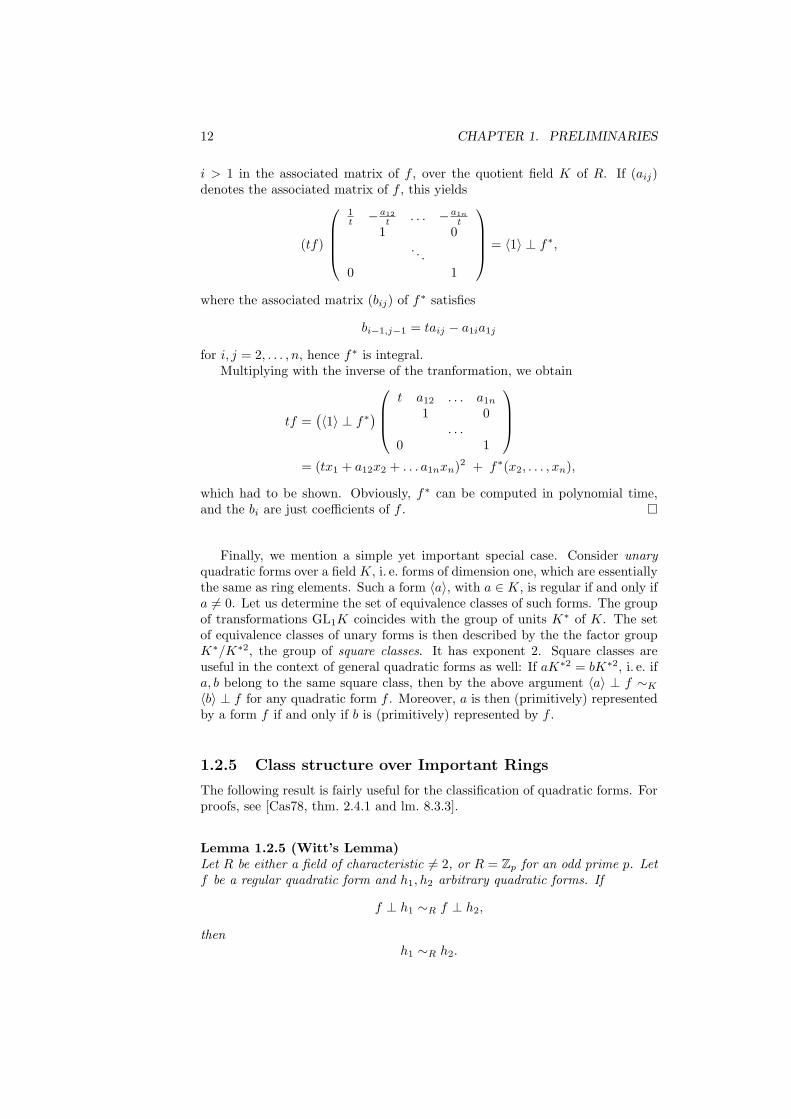
12 CHAPTER 1. PRELIMINARIES
i > 1 in the associated matrix of f , over the quotient field K of R. If (aij)denotes the associated matrix of f , this yields
(tf)
1t −a12
t . . . −a1n
t1 0
. . .0 1
= 〈1〉 ⊥ f∗,
where the associated matrix (bij) of f∗ satisfies
bi−1,j−1 = taij − a1ia1j
for i, j = 2, . . . , n, hence f∗ is integral.Multiplying with the inverse of the tranformation, we obtain
tf =(〈1〉 ⊥ f∗
)t a12 . . . a1n
1 0. . .
0 1
= (tx1 + a12x2 + . . . a1nxn)2 + f∗(x2, . . . , xn),
which had to be shown. Obviously, f∗ can be computed in polynomial time,and the bi are just coefficients of f .
Finally, we mention a simple yet important special case. Consider unaryquadratic forms over a field K, i. e. forms of dimension one, which are essentiallythe same as ring elements. Such a form 〈a〉, with a ∈ K, is regular if and only ifa 6= 0. Let us determine the set of equivalence classes of such forms. The groupof transformations GL1K coincides with the group of units K∗ of K. The setof equivalence classes of unary forms is then described by the the factor groupK∗/K∗2, the group of square classes. It has exponent 2. Square classes areuseful in the context of general quadratic forms as well: If aK∗2 = bK∗2, i. e. ifa, b belong to the same square class, then by the above argument 〈a〉 ⊥ f ∼K
〈b〉 ⊥ f for any quadratic form f . Moreover, a is then (primitively) representedby a form f if and only if b is (primitively) represented by f .
1.2.5 Class structure over Important Rings
The following result is fairly useful for the classification of quadratic forms. Forproofs, see [Cas78, thm. 2.4.1 and lm. 8.3.3].
Lemma 1.2.5 (Witt’s Lemma)Let R be either a field of characteristic 6= 2, or R = Zp for an odd prime p. Letf be a regular quadratic form and h1, h2 arbitrary quadratic forms. If
f ⊥ h1 ∼R f ⊥ h2,
thenh1 ∼R h2.
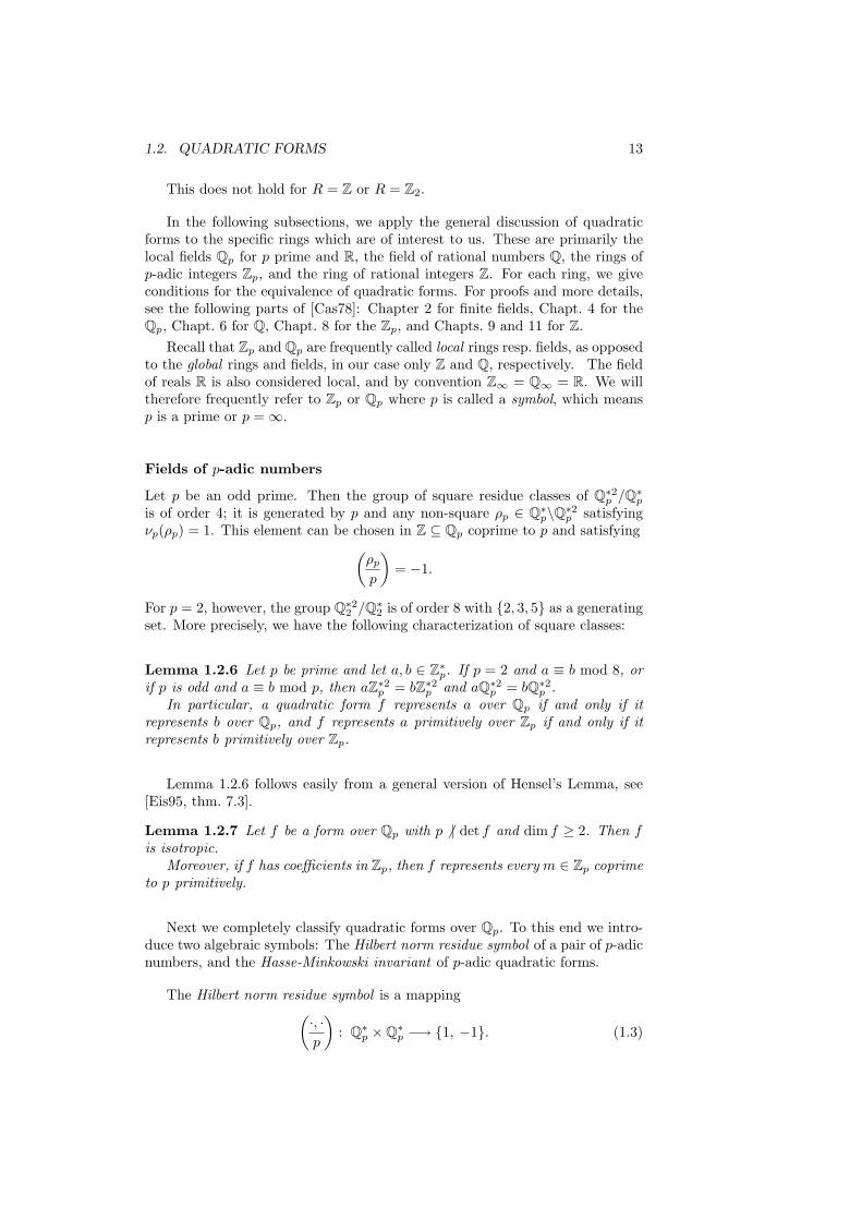
1.2. QUADRATIC FORMS 13
This does not hold for R = Z or R = Z2.
In the following subsections, we apply the general discussion of quadraticforms to the specific rings which are of interest to us. These are primarily thelocal fields Qp for p prime and R, the field of rational numbers Q, the rings ofp-adic integers Zp, and the ring of rational integers Z. For each ring, we giveconditions for the equivalence of quadratic forms. For proofs and more details,see the following parts of [Cas78]: Chapter 2 for finite fields, Chapt. 4 for theQp, Chapt. 6 for Q, Chapt. 8 for the Zp, and Chapts. 9 and 11 for Z.
Recall that Zp and Qp are frequently called local rings resp. fields, as opposedto the global rings and fields, in our case only Z and Q, respectively. The fieldof reals R is also considered local, and by convention Z∞ = Q∞ = R. We willtherefore frequently refer to Zp or Qp where p is called a symbol, which meansp is a prime or p =∞.
Fields of p-adic numbers
Let p be an odd prime. Then the group of square residue classes of Q∗2p /Q∗
p
is of order 4; it is generated by p and any non-square ρp ∈ Q∗p\Q∗2
p satisfyingνp(ρp) = 1. This element can be chosen in Z ⊆ Qp coprime to p and satisfying(
ρp
p
)= −1.
For p = 2, however, the group Q∗22 /Q∗
2 is of order 8 with 2, 3, 5 as a generatingset. More precisely, we have the following characterization of square classes:
Lemma 1.2.6 Let p be prime and let a, b ∈ Z∗p. If p = 2 and a ≡ b mod 8, or
if p is odd and a ≡ b mod p, then aZ∗2p = bZ∗2
p and aQ∗2p = bQ∗2
p .In particular, a quadratic form f represents a over Qp if and only if it
represents b over Qp, and f represents a primitively over Zp if and only if itrepresents b primitively over Zp.
Lemma 1.2.6 follows easily from a general version of Hensel’s Lemma, see[Eis95, thm. 7.3].
Lemma 1.2.7 Let f be a form over Qp with p 6 | det f and dim f ≥ 2. Then fis isotropic.
Moreover, if f has coefficients in Zp, then f represents every m ∈ Zp coprimeto p primitively.
Next we completely classify quadratic forms over Qp. To this end we intro-duce two algebraic symbols: The Hilbert norm residue symbol of a pair of p-adicnumbers, and the Hasse-Minkowski invariant of p-adic quadratic forms.
The Hilbert norm residue symbol is a mapping(·, ·p
): Q∗
p ×Q∗p −→ 1, −1. (1.3)
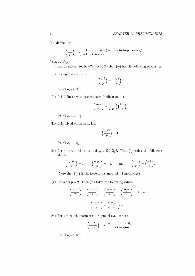
14 CHAPTER 1. PRELIMINARIES
It is defined by(a, b
p
)=
1 if ax21 + bx2
2 − x23 is isotropic over Qp,
−1 otherwise
for a, b ∈ Q∗p.
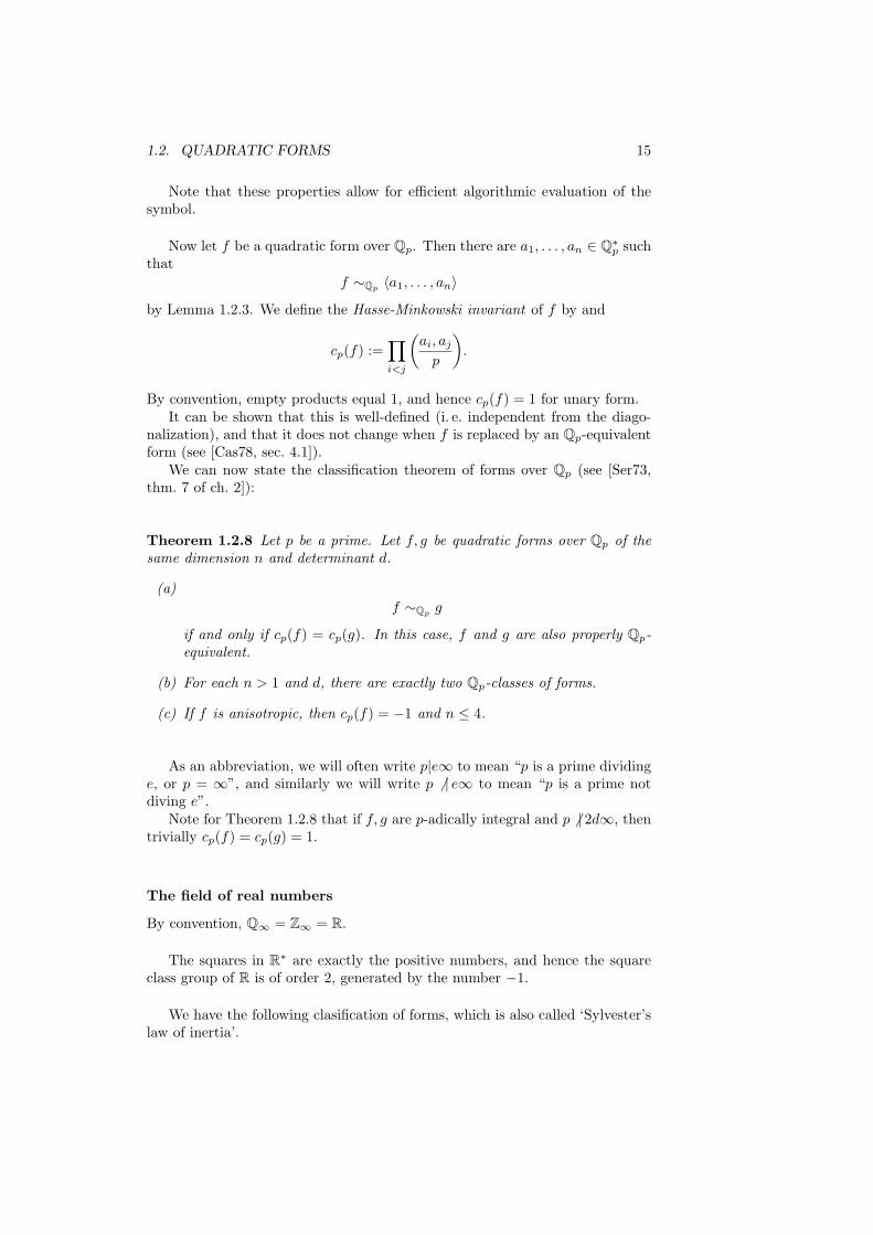
It can be shown (see [Cas78, sec. 3.2]) that(·,·
p
)has the following properties:
(i) It is symmetric, i. e. (a, b
p
)=(
b, a
p
)for all a, b ∈ Q∗.
(ii) It is bilinear with respect to multiplication, i. e.(ab, c
p
)=(
a, c
p
)(b, c
p
)for all a, b, c ∈ Q∗.
(iii) It is trivial on squares, i. e. (a, b2
p
)= 1
for all a, b ∈ Q∗p.
(iv) Let p be an odd prime and ρp ∈ Q∗p\Q∗2
p . Then(·,·
p
)takes the following
values:(ρp, ρp
p
)= 1,
(p, ρp
p
)= −1, and
(p, p
p
)=(−1p
).
(Note that(−1
p
)is the Legendre symbol of −1 modulo p.)
(v) Consider p = 2. Then(·,·
p
)takes the following values:(
5, 52
)=(
5, 72
)=(
2, 72
)=(
2, 22
)= 1 and
(7, 72
)=(
2, 52
)= −1.
(vi) For p =∞, the norm residue symbol evaluates to(a, b∞
)=−1 if a, b < 0,
1 otherwise
for all a, b ∈ R∗.
1.2. QUADRATIC FORMS 15
Note that these properties allow for efficient algorithmic evaluation of thesymbol.
Now let f be a quadratic form over Qp. Then there are a1, . . . , an ∈ Q∗p such
thatf ∼Qp
〈a1, . . . , an〉
by Lemma 1.2.3. We define the Hasse-Minkowski invariant of f by and
cp(f) :=∏i<j
(ai, aj
p
).
By convention, empty products equal 1, and hence cp(f) = 1 for unary form.It can be shown that this is well-defined (i. e. independent from the diago-
nalization), and that it does not change when f is replaced by an Qp-equivalentform (see [Cas78, sec. 4.1]).
We can now state the classification theorem of forms over Qp (see [Ser73,thm. 7 of ch. 2]):
Theorem 1.2.8 Let p be a prime. Let f, g be quadratic forms over Qp of thesame dimension n and determinant d.
(a)f ∼Qp
g
if and only if cp(f) = cp(g). In this case, f and g are also properly Qp-equivalent.
(b) For each n > 1 and d, there are exactly two Qp-classes of forms.
(c) If f is anisotropic, then cp(f) = −1 and n ≤ 4.
As an abbreviation, we will often write p|e∞ to mean “p is a prime dividinge, or p = ∞”, and similarly we will write p 6 | e∞ to mean “p is a prime notdiving e”.
Note for Theorem 1.2.8 that if f, g are p-adically integral and p 6 | 2d∞, thentrivially cp(f) = cp(g) = 1.
The field of real numbers
By convention, Q∞ = Z∞ = R.
The squares in R∗ are exactly the positive numbers, and hence the squareclass group of R is of order 2, generated by the number −1.
We have the following clasification of forms, which is also called ‘Sylvester’slaw of inertia’.
16 CHAPTER 1. PRELIMINARIES
Proposition 1.2.9 Let f be an n-ary form over R. Then there is a uniquelydetermined integer 0 ≤ s ≤ n such that
f ∼R 〈−1, . . . ,−1︸ ︷︷ ︸s
, 1, . . . , 1〉. (1.4)
s is called the signature of f and denoted by s = sign f .Two n-ary forms f, g are R-equivalent if and only if their signatures coincide.A transformation for the equivalence (1.4) can be computed efficiently (to
some desired precision).
Note that there are different definitions of the signature in the literature.
The rational number field
The square class group of Q is infinite. It is generated by the (positive) primenumbers and the number −1.
Perhaps the most prominent theorem in the theory of quadratic forms isthe Hasse principle. In rough words, it states that the Q-class of a rationalquadratic form is uniquely determined by its properties over the collection of alllocal fields Qp, where p ranges over all primes and the symbol ∞ (or for short:“for all symbols p”).
(These symbols represent the equivalence classes of non-trivial absolute val-ues of the field Q. They are also called “places” or “spots” of that field, em-ploying the ‘localization’ metaphor. This concept is required when dealing withalgebraic number fields in general. As we stay with the rationals, it seemsappropriate to treat these places simply as symbols.)
Theorem 1.2.10 (Minkowski) Let d ∈ Q\0 and n ≥ 2. Let fp be n-aryforms over Qp for all symbols p such that
det fp ∈ dQ∗2p .
Then there exists a rational quadratic form f satisfying
f ∼Qpfp
for all symbols p if and only if cp(fp) = −1 for only finitely many p, and∏all symbols p
cp(fp) = 1. (1.5)
Recall that by definition, cp(f) = 1 for all unary forms. The infinitude ofsymbols p is not an obstacle because for all but finitely many symbols p, theform fp satisfy cp(fp) = 1, and hence
fp ∼Qp〈1, . . . , 1, d〉
1.2. QUADRATIC FORMS 17
for all but finitely many symbols p. Therefore there is only a finite amount ofinformation about Qp-classes contained in the family (fp | p). We therefore donot lose generality when working with finitely many local forms In algorithms.
Theorem 1.2.11 (Rational Hasse Principle) Let f, g be rational quadraticforms. Then the following are equivalent:
1. f ∼Q g,
2. f ∼Qpg for all symbols p,
3. f ∼Qp g for all symbols p|2d∞ except possibly one.
From Theorems 1.2.11 and 1.2.8, one immediately obtains Meyer’s Theorem(see [Mey91]):
Theorem 1.2.12 (Meyer) Let f be an integral quadratic form of dimensionn ≥ 5. Then f is isotropic.
Rings of p-adic integers
Over the rings Zp of p-adic integers, there are many more classes of forms withthe same dimension and determinant than over Qp. More precisely, while overQp, p 6∈ 2,∞, there are exactly two classes of forms with determinant d anddimension n for each d ∈ Qp, n ≥ 2, the number of Zp-classes for fixed d, n isunbounded, depending on the multiplicity νp(d) of p in d. Fortunately, however,there exists an easy normal form classifying the classes of forms completely.
Theorem 1.2.13 Let f be a form over Zp, where p is an odd prime. Fixρ ∈ Z∗
p\Z∗2p (for example, ρ ∈ Z with
(ρp
)= −1).
Then f is properly Zp-equivalent to a form of the shape
f1 ⊥ . . . ⊥ fk,
wherefi = pei〈1, . . . , 1, ri︸ ︷︷ ︸
`i
〉
for i = 1, . . . , k, such that 0 < e1 < . . . ≤ ek, `i > 0, and ri ∈ 1, ρp.This normal form is uniquely determined by f and ρ. It can be computed in
polynomial time, given f , p, and ρ.Morever, a normal form with respect to some ρ ∈ Z∗
p\Z∗2p can be computed
in polynomial-time given only f as input.
18 CHAPTER 1. PRELIMINARIES
The last modification is important for keeping algorithms deterministic, sincethere is no unconditionally provable method known to produce a nonsquare ρwithout using randomness, see the remark after the proof of Theorem 3.2.1.
As a consequence of this classification, if det f = det g = d is coprime to p,then f ∼Zp g.
One simple case is useful to remember because it helps finding the normalform.
Lemma 1.2.14 Let p be an odd prime and ui ∈ Z∗p. Then
pe〈u1, . . . , un〉 ∼Zp pe〈1, . . . , 1, u1 . . . un〉.
The implied transformation can be computed in polynomial time.
Theorem 1.2.13 and Lemma 1.2.14 are classical results; they can be founde. g. in [Cas78, thm. 3.1, lm. 3.4 of ch. 8]. The algorithmic statement we addedis immediate from the proofs in the sources cited.
The case p = 2 is a bit more involved.
Theorem 1.2.15 There is a set S of forms over Z2 such that each f is properlyZ2-equivalent to one and only one form f0 ∈ S. This form f0 can be computedfrom f in polynomial time. The forms in S can be chosen rationally integral.
In particular, if f is properly primitive, dim f = 2 and det f is odd, then fis Z2-equivalent to exactly one of the forms
〈1, d〉, 〈3, 3〉, 〈3, 7〉 | d = 1, 3, 5, 7 .
Moreover, if f is properly primitive, n := dim f ≥ 3 and det f is odd, then f isZ2-equivalent to exactly one of the n-ary forms
〈1, . . . , 1, 1, 1, d〉, 〈1, . . . , 1, 1, 3, 3〉, 〈1, . . . , 1, 1, 3, 7〉,〈1, . . . , 1, 3, 3, 3〉, 〈1, . . . , 1, 3, 3, 7〉 | d = 1, 3, 5, 7
For details see [Wat76], [Jon44]. Perhaps easier a criterion of equivalence isgiven by congruence conditions rather than normal forms.
Proposition 1.2.16
(a) Let p an odd prime. If
f ≡ g mod pνp(d)+1,
then f ∼Zpg.
(b) Iff ≡ g mod 2ν2(d)+3,
then f ∼Z2 g.
1.2. QUADRATIC FORMS 19
1.2.6 Classes and Genera
Each class of forms is the union of one or two proper classes cls +f . Integralforms f and g are said to be in the same genus (denoted by gen f) if they areequivalent over all rings of p-adic integers Zp; here p ranges over all rationalprimes and the symbol ∞ (Z∞ = R by convention). Clearly every genus is aunion of classes.
If a statement is said to hold for all p, or all symbols p, then we include thecase p = ∞. It is excluded if p is called prime. All p|e∞ means p ranges overthe prime divisors of e and the symbol ∞.
We say that f and g lie in the same genus if
f ∼Zp g
for all symbols p. We denote this by
f ∼g g.
It is easy to see that
f ∼ g =⇒ f ∼g g =⇒ det f = det g
Lemma 1.2.17 Let f, g be integral forms with the same odd determinant d. Let
f ∼Zpg
for all p|d∞. Then f ∼g g.
Proof : By hypothesis, f ∼Zp g for all p|d∞. As noted after Theorem 1.2.15it follows that ⇒∼Zp g for all p except possibly p = 2. Hence ⇒∼Qp g for allp except possibly p = 2. Then by Theorem 1.2.11, also f ∼Q2 g. Since d is odd,Theorem 1.2.15 yields that also f ∼Z2 g.
One of the most important features of genera is that they coincide with theclasses in many interesting cases. The following criterion is taken from [Cas78,p. 202f.]. We will frequently employ it to prove equivalence of integral quadraticforms in cases a transformation cannot be written down explicitly.
We call an integer m k-power free if e ∈ Z, ek|m implies e = ±1. A rationalnumber a
b , a, b ∈ Z coprime, is k-power free if a is k-power free. The next resultcan be found in [Cas78, thm. 1.3 and 1.5 of ch. 9].
Theorem 1.2.18 (Eichler) Let f, g be integral quadratic forms of dimensionn ≥ 3 and determinant d which is n(n−1)
2 -power free and satisfies
2n(n−3)/2+b(n+1)/2c 6 | d
if f is classically integral. Then
f ∼ g ⇔ f ∼g g.
20 CHAPTER 1. PRELIMINARIES
cls +
cls
spn +
spn
gen
hhhhhhhhhhhhhh
XXXXXXXXX
HHHHH
cls Zp = cls +Zp
cls Zp′. . . cls R
order
cls Qp= cls +
Qpcls Qp′
. . . cls R
same determinant
JJ
JJ
JJ
cls Q = cls +Q
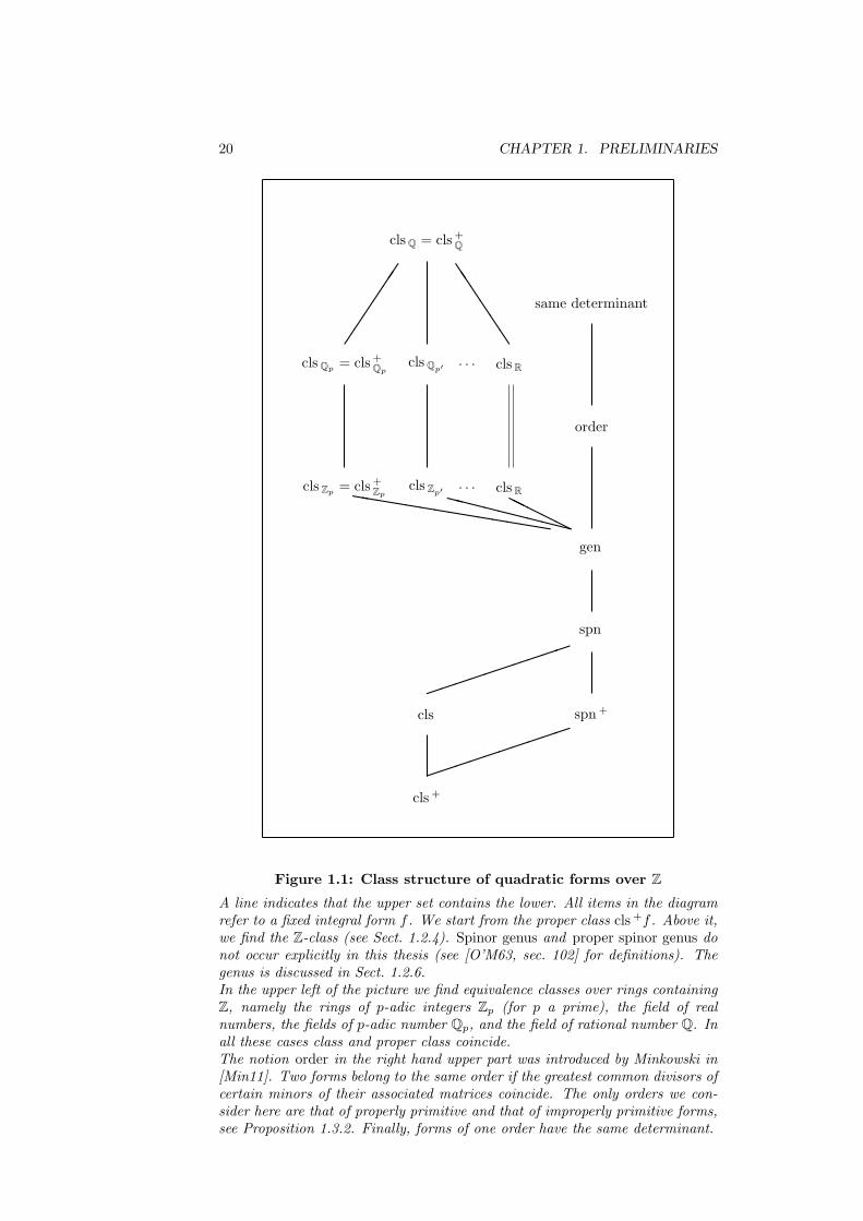
Figure 1.1: Class structure of quadratic forms over ZA line indicates that the upper set contains the lower. All items in the diagramrefer to a fixed integral form f . We start from the proper class cls +f . Above it,we find the Z-class (see Sect. 1.2.4). Spinor genus and proper spinor genus donot occur explicitly in this thesis (see [O’M63, sec. 102] for definitions). Thegenus is discussed in Sect. 1.2.6.In the upper left of the picture we find equivalence classes over rings containingZ, namely the rings of p-adic integers Zp (for p a prime), the field of realnumbers, the fields of p-adic number Qp, and the field of rational number Q. Inall these cases class and proper class coincide.The notion order in the right hand upper part was introduced by Minkowski in[Min11]. Two forms belong to the same order if the greatest common divisors ofcertain minors of their associated matrices coincide. The only orders we con-sider here are that of properly primitive and that of improperly primitive forms,see Proposition 1.3.2. Finally, forms of one order have the same determinant.
1.3. PROBLEMS OF QUADRATIC FORMS 21
1.2.7 Reduction
Following the case of definite forms, several concepts of reduction have beenproposed. We try to capture the main aspects in the following definition. Areduction theory is a pair (Ω, ρ) with the following properties:
(i) Ω is a set of quadratic forms such that every equivalence class of quadraticforms contains at least one, but at most finitely many elements of Ω.
(ii) Membership in Ω decidable in deterministic polynomial time.
(iii) Moreover, ρ is a (deterministic or probabilistic) polynomial-time algorithmwhich takes as input a quadratic form f and outputs a pair (f ′, T ) = ρ(f),where f ′ ∈ Ω, T ∈ GLnR, and f T = f ′; in particular, f and f ′ areequivalent.
(iv) Restricted to Ω, ρ operates as the identity.
The elements of Ω are called reduced forms. The procedure ρ is called thereduction algorithm of the reduction theory.
For R = Z, there are several concepts of reduction for indefinte quadraticforms. Most recently, variants of the LLL algorithm for definite forms (see[LLL82]) have been proposed by Simon [Sim05b], Ivanyos-Szanto [IAS96], andSchnorr [Sch07]. The main difficulty in generalizing LLL to indefinite forms isthe fact that the (analogue to the) length of orthogonalized basis vectors of alattice are simply values of the quadratic form in question at a rational non-zerovector. However, for indefinite forms this value may vanish, which thwarts theusual procedure of the algorithm, and in this event Simon’s algorithm breaks,as he is primarily interested in solutions to f(x) = 0 rather than reduction,while Ivanyos and Szanto work with a randomized perturbation of the vectorin question. However, these questions are irrelevant here because we are con-cerned mainly with anisotropic forms. So we may simply use the efficient, thencoinciding LLL-algorithms of Simon-Ivanyos-Szanto-Schnorr as our concept ofreduction. We denote the reduction operator by ρ(·); by (g, T ) = ρ(f) we meanthat g is LLL-reduced, the algorithm returns form g on input f , and f T = g.
1.3 Problems of Quadratic Forms
We will now define the computational problems dealing with quadratic formswhich will be of interest to us.
1.3.1 Rings
In the subsequent sections, we will define algorithmic problems on quadraticforms. This only makes sense if their coefficients can be specified in a (Turing-)machine readable format. In other words, we need an encoding of ring elements.We will use mainly the rings Z, Q, Zp, and Qp, including Z∞ = Q∞ = R. ForZ and Q, there are natural such encodings: Write the integers to some base b(e. g. b = 2)and represent rational numbers by pairs of integers (a, b) ∈ Z2 such
22 CHAPTER 1. PRELIMINARIES
that either (a, b) = (1, 0), or a, b coprime; here a, b indicate enumerator anddenominator of a fraction.
Using these representations, arithmetic operations can be evaluated effi-ciently, including the div and mod operations over Z. Consequently we canefficiently perform many standard tasks over these rings: For instance, polyno-mials can be efficiently evaluated, and over Q, systems of linear equations canbe efficiently tested for solubility, and for solvable linear systems, the generalsolution can be efficiently constructed.
Furthermore, for Z, the (extended) Euclidean Algorithm admits the compu-tation of greatest common divisors, and their representation as linear combina-tions. This also enables us to solve the analogous linear algebra tasks mentionedfor Q, compute least common multiples, find common denominators of fractions,check systems of vectors for primitivity and form bases of Zn out of them.
Moreover, we can as well perform all these arithmetic manipulations on thequotient rings Z/NZ.
Some of our results, especially in Sects. 5.1, 5.2, only rely on the efficiencyof such basic operations. We will call a ring a ring with encoding if there is arepresentation of ring elements by (binary) strings such that
(i) addition, subtraction/negation, multiplication, and division—if defined—are polynomial-time computable; and
(ii) it is polynomial-time decidable whehter a given string represents a ringelement, and whether it represents a unit.
As argued above, this also makes feasable many other basic tasks of arithmeticand linear algebra.
A field (UFD, integral domain) with encoding is a ring with encoding which isat the same time a field (UFD, integral domain). General fields with encoding,as opposed to the concrete fields Q, Qp, Fp with a canoncial encoding, will beemployed in Sects. 6.2 and 6.3. There we will study forms whose coefficientsare power series and polynomials in one variable, respectively, over an arbitraryfield with encoding of characteristic 6= 2.
Sometimes, this minimal arithmetic requirements do not suffice, and we needa closer similarity to Z above. In particular our results on singular and reducibleforms in Sects. 5.1, 5.2 refer to rings with a generalization of a Euclidean Algo-rithm.
Recall that a ring R is called a principal ideal domain (PID) if every idealof R is principal, i. e. generated by one element. Then a PID R is called acomputational principal ideal domain (cPID) if
(i) it is a ring with encoding, and if
(ii) given elements a, b ∈ R, we can efficiently compute a generator g of theideal aR + bR = gR, along with a λ, µ ∈ R such that
λa + µb = g.
1.3. PROBLEMS OF QUADRATIC FORMS 23
Note that item (ii) generalizes the Extended Euclidean Algorithm in Z. Moreprecisely, the existence of a polynomial-time computable Euclidean functionis sufficient for (ii), but seems not to be necessary: For instance, the ringsof integers in an algebraic number field of class number 1 are all cPIDs, thegeneralized gcd-algorithm being given by [Coh00, sec. 1.3]. In contrast, the vastmajority of these rings are not known to admit a Euclidean function, let alonean efficiently computable one (see [Lem95]).
It is obvious that as for the integers, this algorithm allows effient solution ofseveral related tasks, as the computation of least common multiples.
It remains to discuss the important local rings Zp, Qp, and R. At first sight,they seem inaccessible to computational encoding for Turing machines. This isbecause a generic element of Zp (Qp) involves an infinitude of coefficients from0, . . . , p− 1, and the exact representation of a real number requires infinitelymany (binary) digits.
For R the solution to this dilemma is obvious: All compuations are requiredonly up to a certain precision. For Zp, we mimick this approach: We say thata p-adic equation is satisfied to precision k if and only if it is satisfied modulopk+1.
Thus, talking about Zp we actually do the arithmetic in some Z/pk+1Z. Foralgorithmic purposes, we consider a problem over Zp efficiently solved if we cansolve it to arbitrary precision k in time polynomial in both the input length andk.
This convention naturally extends to Qp: An element∑∞
i=−n aipi of Qp is
known to precision k if the coefficients
a−n, a−k+1, . . . , a0, . . . , ak−1, ak
have been computed.(A similar notion of precision will be required in the context of formal power
series, see Sect. 6.2.)
1.3.2 Encoding of properties
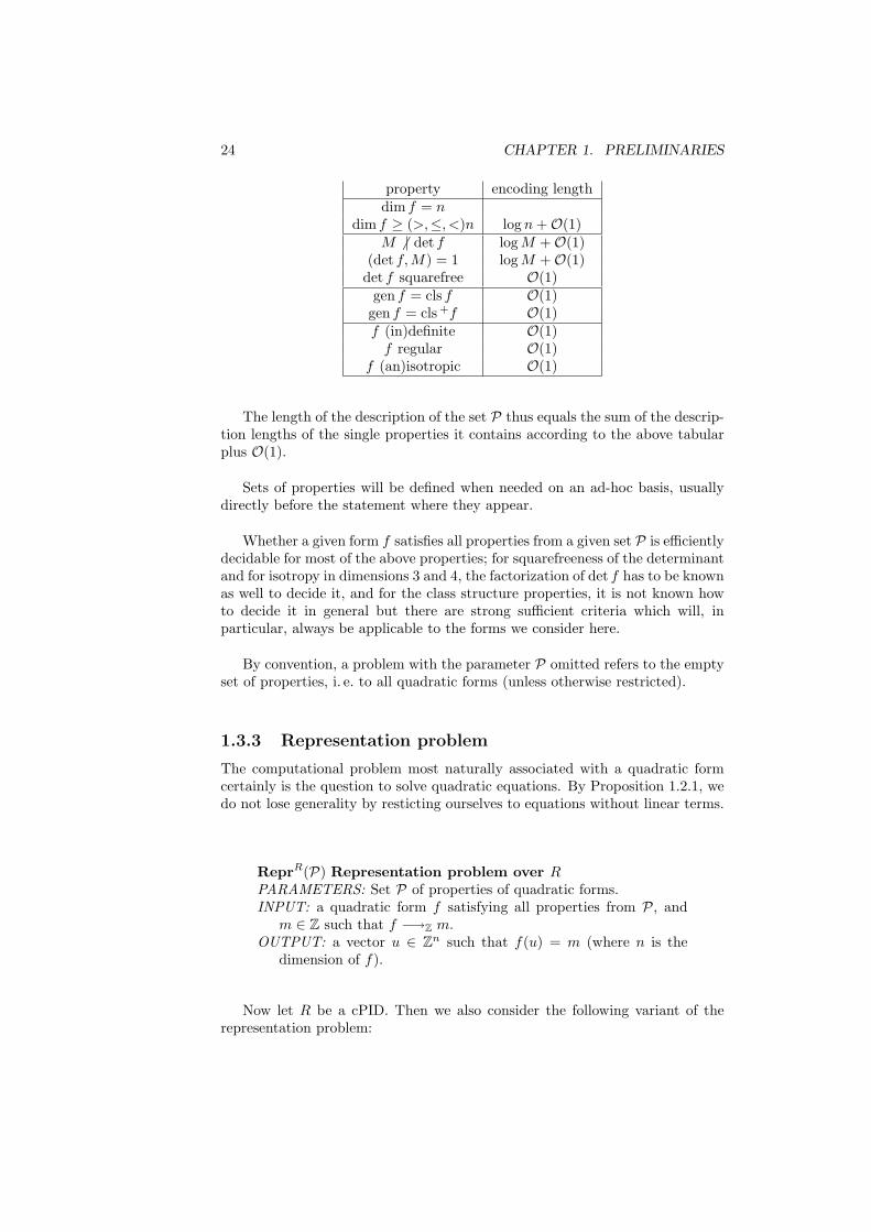
At times, we will want to restrict some of these problems to suitable subsets ofquadratic forms. To keep notation simple and short, we demand the specificationof a set P of properties of forms as a parameter of the problem. As far asthis work goes, we are primarily interested in restrictions on the dimension,the determinant, the class structure, the definiteness, the regularity, and theisotropy of the forms. Without agreeing on one concrete encoding of P, wedemand that the integers involved should be given in binary representation,and that the following bounds on the specification lengths hold:
24 CHAPTER 1. PRELIMINARIES
property encoding lengthdim f = n
dim f ≥ (>,≤, <)n log n +O(1)M 6 | det f log M +O(1)
(det f,M) = 1 log M +O(1)det f squarefree O(1)
gen f = cls f O(1)gen f = cls +f O(1)f (in)definite O(1)
f regular O(1)f (an)isotropic O(1)
The length of the description of the set P thus equals the sum of the descrip-tion lengths of the single properties it contains according to the above tabularplus O(1).
Sets of properties will be defined when needed on an ad-hoc basis, usuallydirectly before the statement where they appear.
Whether a given form f satisfies all properties from a given set P is efficientlydecidable for most of the above properties; for squarefreeness of the determinantand for isotropy in dimensions 3 and 4, the factorization of det f has to be knownas well to decide it, and for the class structure properties, it is not known howto decide it in general but there are strong sufficient criteria which will, inparticular, always be applicable to the forms we consider here.
By convention, a problem with the parameter P omitted refers to the emptyset of properties, i. e. to all quadratic forms (unless otherwise restricted).
1.3.3 Representation problem
The computational problem most naturally associated with a quadratic formcertainly is the question to solve quadratic equations. By Proposition 1.2.1, wedo not lose generality by resticting ourselves to equations without linear terms.
ReprR(P) Representation problem over RPARAMETERS: Set P of properties of quadratic forms.INPUT: a quadratic form f satisfying all properties from P, and
m ∈ Z such that f −→Z m.OUTPUT: a vector u ∈ Zn such that f(u) = m (where n is the
dimension of f).
Now let R be a cPID. Then we also consider the following variant of therepresentation problem:
1.3. PROBLEMS OF QUADRATIC FORMS 25
∗ReprR(P) Primitive representation problem over cPID RPARAMETERS: Set P of properties of quadratic forms.INPUT: a quadratic form f satisfying all properties from P, and
m ∈ Z such that f∗−→ m.
OUTPUT: a primitive vector u ∈ Zn such that f(u) = m (where nis the dimension of f).
This definition is motivated by the insight that for every representationf(x) = m, x 6= 0, there is an underlying primitive representation x = λx0, x0
primitive, andm = f(x) = f(x0) λ2.
As an algorithmic consequence, one can solve many general representationinstances by using an oracle for coprime representations, even if a coprime rep-resentation for the original instance does not exist. This is made precise by thefollowing proposition. Denote (for the next proposition and its proof) by Ω(m)the number of prime factors of the integers m (counted with multiplicities).
Proposition 1.3.1 Let c > 0 be fixed. Consider Repr-instances (f,m) over Zwhere m is presented fully factored and satisfies
Ω(m) ≤ c log log m.
Then there is a polynomial-time oracle algorithm which, given access to a∗Repr-oracle, computes a representation of m by f .
Moreover, this reduction is non-adaptive, and all oracle inquiries refer to theform f .
Proof : Sort the factors of m as
m = ±
(r∏
i=1
pi
)2 s∏j=1
qj (1.6)
where the qj , j = 1, . . . , s are pairwise distinct (positive) primes. For everyI ⊆ 1, . . . , r, ask the ∗ReprR-oracle for a representation of
m′ :=
(∏i∈I
pi
)2 s∏j=1
qj
by f . If the oracle finds v′ with f(v′) = m′, then
v :=
(∏i/∈I
pi
)v′
satisfies f(v) = m.
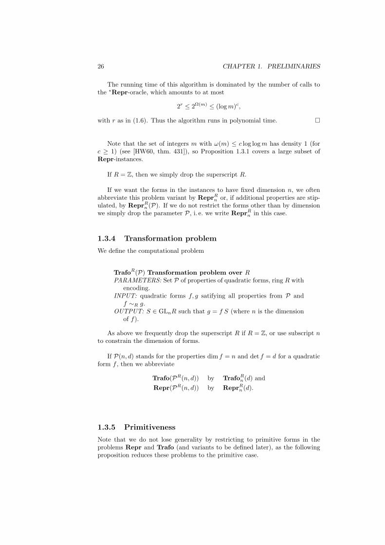
26 CHAPTER 1. PRELIMINARIES
The running time of this algorithm is dominated by the number of calls tothe ∗Repr-oracle, which amounts to at most
2r ≤ 2Ω(m) ≤ (log m)c,
with r as in (1.6). Thus the algorithm runs in polynomial time.
Note that the set of integers m with ω(m) ≤ c log log m has density 1 (forc ≥ 1) (see [HW60, thm. 431]), so Proposition 1.3.1 covers a large subset ofRepr-instances.
If R = Z, then we simply drop the superscript R.
If we want the forms in the instances to have fixed dimension n, we oftenabbreviate this problem variant by ReprR
n or, if additional properties are stip-ulated, by ReprR
n (P). If we do not restrict the forms other than by dimensionwe simply drop the parameter P, i. e. we write ReprR
n in this case.
1.3.4 Transformation problem
We define the computational problem
TrafoR(P) Transformation problem over RPARAMETERS: Set P of properties of quadratic forms, ring R with
encoding.INPUT: quadratic forms f, g satifying all properties from P and
f ∼R g.OUTPUT: S ∈ GLnR such that g = f S (where n is the dimension
of f).
As above we frequently drop the superscript R if R = Z, or use subscript nto constrain the dimension of forms.
If P(n, d) stands for the properties dim f = n and det f = d for a quadraticform f , then we abbreviate
Trafo(PR(n, d)) by TrafoRn (d) and
Repr(PR(n, d)) by ReprRn (d).
1.3.5 Primitiveness
Note that we do not lose generality by restricting to primitive forms in theproblems Repr and Trafo (and variants to be defined later), as the followingproposition reduces these problems to the primitive case.
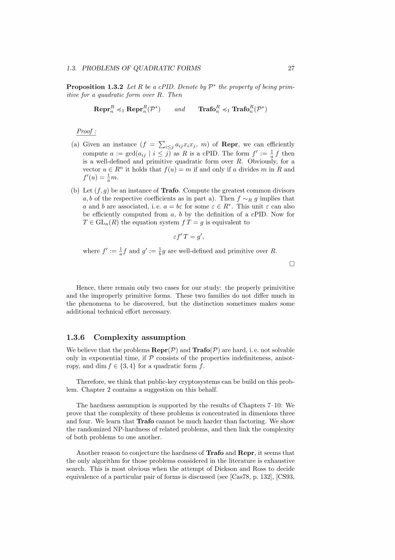
1.3. PROBLEMS OF QUADRATIC FORMS 27
Proposition 1.3.2 Let R be a cPID. Denote by P∗ the property of being prim-itive for a quadratic form over R. Then
ReprRn 41 ReprR
n (P∗) and TrafoRn 41 TrafoR
n (P∗)
Proof :
(a) Given an instance (f =∑
i≤j aijxixj , m) of Repr, we can efficientlycompute a := gcd(aij | i ≤ j) as R is a cPID. The form f ′ := 1
a f thenis a well-defined and primitive quadratic form over R. Obviously, for avector u ∈ Rn it holds that f(u) = m if and only if a divides m in R andf ′(u) = 1
am.
(b) Let (f, g) be an instance of Trafo. Compute the greatest common divisorsa, b of the respective coefficients as in part a). Then f ∼R g implies thata and b are associated, i. e. a = bε for some ε ∈ R∗. This unit ε can alsobe efficiently computed from a, b by the definition of a cPID. Now forT ∈ GLn(R) the equation system f T = g is equivalent to
εf ′ T = g′,
where f ′ := 1af and g′ := 1
b g are well-defined and primitive over R.
Hence, there remain only two cases for our study: the properly primivitiveand the improperly primitive forms. These two families do not differ much inthe phenomena to be discovered, but the distinction sometimes makes someadditional technical effort necessary.
1.3.6 Complexity assumption
We believe that the problems Repr(P) and Trafo(P) are hard, i. e. not solvableonly in exponential time, if P consists of the properties indefiniteness, anisot-ropy, and dim f ∈ 3, 4 for a quadratic form f .
Therefore, we think that public-key cryptosystems can be build on this prob-lem. Chapter 2 contains a suggestion on this behalf.
The hardness assumption is supported by the results of Chapters 7–10: Weprove that the complexity of these problems is concentrated in dimenions threeand four. We learn that Trafo cannot be much harder than factoring. We showthe randomized NP-hardness of related problems, and then link the complexityof both problems to one another.
Another reason to conjecture the hardness of Trafo and Repr, it seems thatthe only algorithm for those problems considered in the literature is exhaustivesearch. This is most obvious when the attempt of Dickson and Ross to decideequivalence of a particular pair of forms is discussed (see [Cas78, p. 132], [CS93,
28 CHAPTER 1. PRELIMINARIES
p. 403]). The restriction to trivial algorithms also becomes explicit in Siegel’sfamous bound on equivalence transformations [Sie72], which reproves the decid-ability of (A) using analytic techniques. More precisely, he shows that for eachpairs f, g of equivalent forms there is a constant C > 0 effectively computablefrom f, g such that there is a transformation from f to g whose coefficientsare absolutely bounded by C. Siegel explicitly refers to the enumeration of allintegral matrices up to some bound on the coefficients for testing equivalence.
In dimension three, Siegel’s implicit bound has been made explicit and hasbeen improved to polynomial size by Dietmann [Die03]. Still using trivial enu-meration, this implies that problem (A) is in NP. Moreover, for problem (B),Grunewald and Segal [GS04] showed decidability by solving problem (B’) ifpossible. Their algorithm is more sophisticated, yet still involves steps of expo-nential enumeration.
Apparently, the complexity of Trafo and Repr is hitherto discussed in theliterature only once. At the end of [CS93, ch. 15], Conway and Sloane formulateboth decisional and computational equivalence and representation problems,along with a couple of additional questions, e. g. on class numbers. They mentionseveral cases for which these problems are easy. For indefinite forms over Z, theyexpress their impression that “there do not seem to be good algorithms”, anddiscuss the inefficiency of exhaustive enumeration.
All this is an indication that we are at a loss if efficient algorithms arerequired for these problems.
Chapter 2
Cryptography
In this chapter we present cryptographic applications of indefinite quadraticforms. All of them are based on the Trafo problem: The public key is aninstance of Trafo, i. e. two equivalent forms f ∼ g, and a transformation S ∈GLnZ such that f S = g plays the role of the private key.
In Sect. 2.2, we present an identification scheme whose security is closelyrelated to the complexity of the underlying problem. However, its practicalusefulness is limited because it requires the sequential repetition of many rounds.This drawback is overcome in the signature scheme in Sect. 2.3. However, thesecurity against fraudulent provers cannot be rigorously proven. In both cases,security against fraudulent verifiers is heuristic. These two schemes have beenproposed in [HS07b] and [HS07a]. Before we turn to the protocols, we discusshow reduction theory can be used to randomize quadratic forms and unimodularmatrices. In particular, we explain how key generation is performed for allschemes.
2.1 Randomization and Key Generation
We define a probability distribution on the set of regular integer matrices andquadratic forms. We will use the following size function for matrices:
‖T‖ := maxi,j|Tij |.
Moreover, we fix the LLL reduction theory (Ω, ρ) from Sect. 1.2.7.
K is a security parameter. The notation
T ← UK
means that T ∈ Zn×n is selected uniformly at random such that |T |∞ ≤ K.Denote by
(g, T )← DK(f)
the process that a form g and a matrix T ∈ GLnZ satisfying g = f T are sampledat random according to the random distribution DK(f). The distribution mostinteresting for us is defined by the following procedure:
29
30 CHAPTER 2. CRYPTOGRAPHY
(g, T )← DK(f):
T ← UK ,(g, T ′) := ρ(f T ).
So the distribution of g in DK(f) takes as values (some of) the finitelymany reduced forms equivalent to f . It should not be expected that this isthe uniform distribution: For definite forms, it has been observed that LLL-reduced forms often have much smaller coefficients than theoretically guaranteed([LO85], [VV07]). This indicates that forms closer to the boundary of the set ofreduced forms (in Rn(n+1)/2) may have lower probability for this distribution;moreover, this effect might even intensify (see [Sim05b]).
Key generation can be accomplished as follows: A reduced form f−1 maybe fixed as a system parameter. Then using the distribution DK(f−1), we cangenerate random reduced forms fi = f−1 Si with i = 0, 1. We can use (f0, f1)as public and S := S−1
0 S1 as private key.
We denote by P[A] the probability of an event A. The statistical distancebetween two (discrete) random variables T0,T1 is defined as
∆(T0,T1) =12
∑T
∣∣∣P[T0 = T ]− P[T1 = T ]∣∣∣,
where T ranges over all objects which at least one of the Tj may attain. Notethat ∆(·, ·) takes values in [0, 1].
Two families T(K)0 ,T
(K)1 of random variables (K ∈ N) are called statistically
close for K →∞ if their statistical distance is negligible; i. e. if
∆(T(K)0 ,T
(K)1 ) = O
(1
P (K)
)for every polynomial P (·) (see [Gol01, sec. 3.2.2; def. 1.3.5] for details)∗.
Heuristically, it may seem convincing that if K is large enough, then thedistribution DK(f) does not depend too heavily on the reduced initial form ffrom a fixed equivalence class. Precisely, we state:
Heuristic 2.1.1 Let f−1 be a fixed quadratic form. Let f0, f1, S arise from thekey generation procedure above, i. e. the two pairs (fi, Si) are independent anddistributed according to DK(f−1, and S = S−1
0 S1. Then there is K ′ = K ′(K),depending polynomially on K, such that for K →∞ the following holds:
If (g0,T0) is randomly distributed according to DK′(f0) and if (g1,T1) is ran-domly distributed according to DK′(f1) then the distributions of T0 and S−1T1
are statistically close.
∗Note that narrower definitions of the term ‘negligible’ occur in the literature as well.
2.2. AN IDENTIFICATION SCHEME 31
2.2 An identification scheme
2.2.1 Specification of the Protocol
Let f0, f1 be integral indefinite quadratic forms of dimension n ≥ 3 and letS ∈ GLnZ satisfy f0 S = f1 (in particular, f0 and f1 are equivalent). Denoteby (P,V) the following protocol between prover P and verifier V:
public key (known to P and V): quadratic forms f0, f1
secret key (known to P only): S ∈ GLnZ such that f0 S = f1
P VProver Verifier
(g, T )← DK(f0)g−→i←− select i ∈ 0, 1 uniformly at random
R := S−i TR−→
check whether fi R?= g
In the next section, we will prove that this scheme is a proof of knowledge, i. e.it is secure against fraudulent provers. Thereafter, we show that (P,V) is zero-knowledge under Heuristic 2.1.1, which formalizes security against dishonestverifier. Combining these two concepts yields a strong notion of security. A zero-knowledge proof is secure as an identification scheme if and only if extracting asecret key from the public one is intractible.
In [HS07a] it is proposed that ‖T‖ ≈ 2100‖S‖ and that 100 rounds be per-formed. In contrast, we have here presented the scheme in more general form.The question arises whether modifications of it may render the scheme moreefficient while keeping the same level of security, or vice versa. More precisely,parameters which can be varied include
(i) the base ring of the forms,
(ii) restriction to forms with certain properties, and
(iii) the distribution of (g, T ) in step 1.
The protocol remains a proof of knowledge under all these modifications(see Sect. 2.2.2). Suppose that the new random distribution also preserves thezero-knowledge property. Then the modified protocol is secure if and only ifTrafo is still hard over the new base ring for the chosen type of forms. Most ofthis thesis, in particular Chapters 5, 6, 7, is devoted to the question for whichchoices of rings and form properties Trafo is still hard.
The results of those chapters do not recommend any other ring than Z.Moreover, by Sect. 7.1.3 we should take n = 3 or n = 4 for efficiency, and bySect. 5.4, Sect. 5.3 we should take indefinite anisotropic forms in these dimen-sions.
However, it seems possible to employ forms over rings OK of integers inalgebraic number fields K. Then forms should obey analogous constraints to
32 CHAPTER 2. CRYPTOGRAPHY
those over Z, namely they should be at least ternary, for dimensions 3,4 theyshould be anisotropic, and they must not be totally definite in case K is totallyreal. The complexity of the transformation problem for these sort of forms isbeyond the scope of this thesis. But many theorems formulated here for Z carryover to OK , because the the arithmetic theory reveals very similar behavior offorms over Z and OK (see [O’M63]). It is yet to be analyzed whether using,for instance, forms over the Gaussian integers Z[i], is advantageous over therational integers.
2.2.2 Proof of knowledge
We turn to proving that the seqential iteration of this identifiaction scheme isa proof of knowledge. Intuitively, this means that a fraudulent prover which isaccepted by the verifier with non-negligible probability must already know someprivate key fitting to the current public key. For a more thorough discussion ofthe following definitions see [Gol01, sec. 4.7].
An identification scheme is called complete if an honest prover with the secretkey at his disposal always makes the verifier accept.
Denote by x the public key and by w a witness, i. e. a potential private keyfitting to x of the scheme. Then the scheme is called proof of knowledge withknowledge error κ(x) if it is complete, and if there is a probabilistic polynomial-time algorithm X , the knowledge extractor, with the following property:
Let P be any probabilistic polynomial-time algorithm (a ‘dishonest prover’)which makes V accept on common input x with probability ε(x). Then there isc > 0 such that whenever ε(x) > κ(x), X outputs some correct w, on input x
and given rewindable black-box access to P, in expected time
O(
|x|c
ε(x)− κ(x)
).
Denote by (P,V)k the simultaneous execution of k independent copies of theprotocol (P,V).
Theorem 2.2.1 (P,V)k is a proof of knowlegde with knowledge error 2−k.
Proof : Obviously, (P,V) and hence (P,V)k is complete. To prove knowl-edge extractibility, consider first a single iteration of the protocol. The provercommits g and replies to challenge i ∈ 0, 1. If V accepts, rewind V and chal-lenge it with the complementary bit 1− i, but keep the old commitment g. LetRi be P’s reply to challenge i. If P is successful again, then
fi Ri = g for i = 1, 2 (2.1)
by specification of the protocol. This implies
f0 (R0R−11 ) = f1. (2.2)
2.2. AN IDENTIFICATION SCHEME 33
This means that we can compute a solution to the transformation instance(f0, f1) as soon as P is successful twice with respect to the same commitment.
Now suppose that P is successful with probability ε > 12 in (P,V). Then we
perform the following algorithm X :Make P commit a form g (first step of the protocol). Then challenge it with
bit b = 0, rewind it, and challenge it with bit b = 1 while keeping to the samecommitment g. If P passes both times, compute a transformation by (2.2).Otherwise, repeat until P succeeds on both challenges.
The expected number of iterations of X equals 1π , where π denotes the
probability that P passes on both challenges. We estimate π from below.Let πi be the probability that P passes on challenge i, i = 0, 1. Then
π ≥ π0 π1 (2.3)
andπ0 + π1 = 2ε. (2.4)
We can thus considerπ = π0(2ε− π0) (2.5)
as a quadratic function of π0. Since 0 ≤ πi ≤ 1 for i = 0, 1, Equation (2.4)implies that
2ε− 1 ≤ π0 ≤ 1. (2.6)
It is easy to check that π as a function of π0 as in (2.5) is concave and thereforetakes its minimum on the boundary of its range (2.6). For both boundary valuesπ0 = 1 and π0 = 2ε− 1 we obtain π = 2ε− 1. Hence we have established that
π ≥ 2ε− 1.
We infer that X needs at most
12ε− 1
=1/2
ε− 12
iterations in expectation, each of which takes polynomial time.
This shows that (P,V) is a proof of knowledge with knowledge error 12 .
Then by [Gol01, prop. 4.7.5], the protocol (P,V)k is a proof of knowledge withknowledge error 2−k.
Remark. Note that Theorem 2.2.1 and its proof remain valid if the randomdistributions DK , the base ring (here: Z), and the properties of the forms usedare replaced by other choices. This means that all these variations of (P,V)k
are secure against fraudulent provers if the public key is a hard Trafo-instance.
34 CHAPTER 2. CRYPTOGRAPHY
2.2.3 Zero-knowledge property
An interactive protocol is called stastistical zero-knowledge if for every (possiblydishonest) verifier (i. e. probabilistic polynomial-time algorithm) V, there is aprobabilistic polynomial-time algorithmM, the simulator, which produces ran-dom strings whose distribution is statistically close to that of the interactionbetween P and V. The simulator has no access to the secret key, but withrewindable black-box access to V (for details, see [Gol01]).
Theorem 2.2.2 Under heuristics 2.1.1, (P,V) and (P,V)k are statistical zero-knowledge protocols.
Proof : For (P,V), we specify a simulator S as follows:
repeatselect random j ∈ 0, 1;(g, T )← DK(fj)send g to V and wait for challenge i;
until i = jR := T ;output (g, j, R)
Obviously, the triples output by S are accepting interactions for (P,V).Moreover, the algorithm runs in expected polynomial-time because indepen-
dently from the distribution according to which V samples the challenge i, theprobability that i = j is at least 1
2 independently in each iteration. Therefore, Srequires at most two iterations of the repeat loop in expectation, which clearlyimplies expected polynomial running time.
Next, we have to show that under Heuristic 2.1.1, the distribution of S’soutput is statistically close to that of an interaction between an honest proverP and V. First, by construction of S, the distribution of j is exactly that ofthe challenge i from the interaction of P and V. Now conditionally on j = 0,the matrix R is distributed according to DK(f0), as is R sent by the prover inthe execution of the protocol. On the other hand, if j = 1, then the simulatoroutputs R according to DK(f1), whereas P chooses R according to S−1DK(f0).It is here where our heuristics 2.1.1 tells us that these two distributions arestatistically close. Finally, as the triples (g, j, R) are accepting interactions, gis uniquely determined by j, R since g = fj R. Therefore, the two distributionsin question are statistically close.
In constrast to the proof-of-knowlegde condition, the zero-knowledge prop-erty of the protocol depends heavily on the family of distributions DK .
The main disadvantage of (P,V) is, of course, its restriction to one-bit chal-lenges. To guarantee a certain level of security, one would have to run manycopies of it in parallel; to have the zero-knowledge property, we would evenneed the single applications of (P,V) to be run sequentially, which would makecommunication too costly.
2.3. LONG CHALLENGES AND SIGNATURES 35
2.3 Identification with Long Challenges and Sig-natures
2.3.1 Specification of the protocol
The major drawback of the scheme of Sect. 2.2 is its restriction to one-bitchallenges. Therfore security requires many sequential iterations (see Theorem2.2.1), which is too inefficient for practical purposes.
A potential solution of this issue is given here. We present an identificationscheme which admits arbitrarily long challenges (depending on key size andparameters). Therefore it is also suitable for the generation of digital signatures,see Sect. 2.3.2.
These advantages come at the price of provable security. In particular, per-haps it fails to be a proof of knowledge. This makes it harder to find out itsactual level of security. It may nevertheless be secure in practice, and we willgive heuristic arguments to support that claim.
The protocol relies on the hardness of both Trafo and Repr.
We denote the following protocol by (P,V)′. It was introduced in [HS07b],a refinement of it being proposed in [HS07a].
public key (known to P and V): quadratic forms f0, f1
secret key (known to P only): S ∈ GLnZ such that f0 S = f1
P VProver Verifier
(g, T )← DK(f0)g−→T ′←− (h, T ′)← DK(g)
e′1 := TT ′e1, e′4 := S−1TT ′e4e′1,e′4−→ check whether f0
?∼ g,f0(e′1)
?= h(e1), and f1(e′4)?= h(e4)
2.3.2 Application to digital signatures
We have now described an identification scheme where the number of possiblechallenges is an increasing function of the security parameter K. For this sit-uation there is a well-established technique to turn this identification protocolinto a digital signature scheme [BR93]: Namely, replace the verifier by a publichash function. Then the challenge in the scheme is a function of the messageto be signed. Of couse, this means that the hash function H has to take valuesin GL4Z. In the Bellare-Rogaway construction, H has to be collision resistant,i. e. it is hard to find messages m,m′ such that H(m) = H(m′); this conditioncan be slightly relaxed for this scheme (see [HS07a]). Moreover, H has to bea one-way function, as otherwise a fraudulent prover can choose a challenge,compute its preimage m, and compute a valid signature for m.
36 CHAPTER 2. CRYPTOGRAPHY
Conversely, consider the random oracle model (ROM), i. e. assume thatvalues of the hash function are retrieved from a public oracle which on newqueries computes a random output, but replies with the same answer to re-peated queries. Then it has been shown in [BR93] that the signature schemeobtained by replacing the verifier by a hash function in a zero-knowledge proof,is a non-interactive zero-knowledge proof in the random oracle model. The sameargument extends to statistical zero-knowledge.
The ROM was introduced into cryptography in [FS87]. It seems to be anappropriate model to analyse security of protocol which uses a collision-free one-way hash function, which is independent from the cryptographic primitive of theprotocol; The ROM is motivated by the impression that no useful structure canbe realized in the values of a well-designed hash-function, so that an attackerwould not have worse chances of success if H was replaced by a random oracle. Itshould be noted that the ROM was massively critized lately: Most prominently,[CGH98], examples of security flaws have been given for any concrete hashfunction, in cryptographic schemes secure in the ROM. However, as is argued in[KM07], these constructions contradict reasonable cryptographic practice, andcould even motivate to trust in the ROM more than before.
2.3.3 Security against Fraudulent Provers
There is the following heuristic argument for security against a fraudulent P: Inthe last step, P knows a transformation R = TT ′ satisfying f0 R = h. She hasto solve the equation f1(e′4) = h(e4) for e′4 ∈ Z4. Heuristically, there seem tobe essentially only two ways to solve such a problem: Either using an algorithmwhich solves the representation problem for f1 (the R is ignored), or finding atransformation S satisfying f0 S = f1, and computing e′4 := S−1Re4 as in theprotocol.
In the latter case, this would imply that P has knowledge of some transfor-mation from f0 to f1, which is our desired result. In the former case, P wouldstill have to solve a presumably hard problem, namely Repr.
However, the scheme is not known to be a proof of knowledge, in the sensethat passing as prover reduces to solving the Trafo-instance (f0, f1). One ob-stacle to such a proof is the following: We can construct a successful fraudulentprover if we have an algorithm which solves the representation problem for f0,f1. Namely, in this case it suffices to solve the verification equations for e′1, e
′4
in the last step. Therefore, (P,V)′ can only be a proof of knowledge if solvingrepresentations for f0, f1 reduces to solving for a transformation from f0 to f1.
It seems reasonable to expect that computing representations is not signif-icantly easier than computing transformations, even if there might not be acomplexity reduction in general. In later chapters, we find cases in which wecan reduce from a representation to a transformation problem; however, thesereductions do not refer to the same (equivalence class of ) forms (see the proofsof Theorems 9.1.8, 9.1.9 and Chapter 10 for complexity connections betweenTrafo and Repr).
2.3. LONG CHALLENGES AND SIGNATURES 37
2.3.4 Security against Fraudulent Verifiers
As with the proof-of-knowledge property, there is a major obstacle to the zero-knowledge property of (P,V)′. Namely a simulator S would have to producequintuples (g, T ′, T, e′1, e
′4) where (among other relations) f1(e′4) = f0(TT ′e4)
holds. As argued in Sect. 2.3.3, this implies that heuristically, S should be ableto either compute a transformation from f0 to f1, or to solve representationproblems for f1. Both tasks are presumably hard.
However, consider what we can learn about S if listening to the interactionof an honest prover P with a possibly fraudulent verifier V. We cannot gainany useful information if the distribution of e′4 does not reveal anything aboutS. This hypothesis is a heuristic similar to 2.1.1. Moreover, any informationobtained cannot be combined over several identifications as the matrices T arestatistically independent.

38 CHAPTER 2. CRYPTOGRAPHY
Chapter 3
Localization and DecisionalComplexity
In this chapter, we consider the transformation and representation problemsover the local rings Zp. At first, in Sect. 3.1, we analyze the decisional variantsof Trafo and Repr. It turns out that deciding equivalence and representabilityis feasible over the Zp, and in consequence of local-global priciples as Theorem1.2.18, these results extend to Z for a large set of instances.
Then we turn back to the computational problems. We show that these arealso tractable over finite fields and over the p-adic integers in Sections 3.2 and3.3, respectively.
3.1 Decision Problems
In computational complexity, the decisional and computational versions of prob-lems frequently turn out to be polynomial-time equivalent; in particular, thisholds for several NP-complete problems as SAT (cf. [GJ79, §§2.1, 5.1]).
Presumably, this is not the case with our problems of quadratic forms. Thearithmetic theory has produced easy-to-check sufficient criteria for representabil-ity and equivalence. This leads to Theorems 3.1.3 and 3.1.5. By contrast, Reprand ∗Repr seem to be computationally intractible, see Sect. 1.3.6.
Over Z, we let the decision problems include the factorization of the deter-minant into the input. This follows the general concept motivated in Chapter8. The letter F in the problem symbol reflects this modification.
DReprR Decisional representation problem over RINPUT: a quadratic form f over R and m ∈ R. DECIDE: whether
f represents m over R.
39
40 CHAPTER 3. LOCALIZATION AND DECISIONAL COMPLEXITY
DFRepr(P) Decisional representation problem with factor-ization
PARAMETERS: Set P of properties of quadratic forms.INPUT: a quadratic form f over Z satisfying all properties from P,
m ∈ R, factorization of det f .DECIDE: whether f represents m over Z.
To prove that DReprZp is in P, we first have to explore the image of binaryforms more closely.
Lemma 3.1.1Let p be an odd prime and
(ρp
)= −1.
(a) If p ≡ 1 mod 4, then 〈1, 1〉 ∗−→Zp a for all a ∈ Zp, and 〈1, ρ〉 ∗−→Zp a ∈ Zp
if and only if p 6 | a.
(b) If p ≡ 3 mod 4, then 〈1, ρ〉 ∗−→Zp a for all a ∈ Zp, and 〈1, 1〉 ∗−→Zp a ∈ Zp
if and only if p 6 | a.
Proof : Consider the form f := 〈1, r〉, where r ∈ 1, ρ, and let a ∈ Zp. Weanalyze the representation problem inductively mod pn, for n ∈ N.
At first, for n = 1, the equation x2 + ry2 = a is always solvable modulop because of a simple counting argument (see [Cas78, lemma 2.2.2]). If x ≡y ≡ 0 in this reprensentation, then it can obviously not be lifted to a primitiverepresentation over Zp. Otherwise, however, it guarantees the existence of aprimitive representation over Zp by Hensel’s lemma.
Thus f represents primitively at least all p-adic integers not divisible by p. Ifp|a, then, by the above argument, there is a primitive representation of a mod pif and only if f is isotropic over Fp. As f is binary, this occurs if and only if−det f = −r is a square in Fp by [Cas78, lm. 2.4 of ch. 4]. In the case r = 1this means that
(−1p
)= 1 or, equivalently, p ≡ 1 mod 4. In the case r = ρ it
implies(−1
p
)= −1 and thus p ≡ 3 mod 4.
Recall that the omission of the property set P stands for no restriction onthe forms at all.
Theorem 3.1.2Let p be a prime, or p =∞. Then
DReprZp
is solvable in polynomial time.
Remark. By a slight variation of the argument below we will as well be able
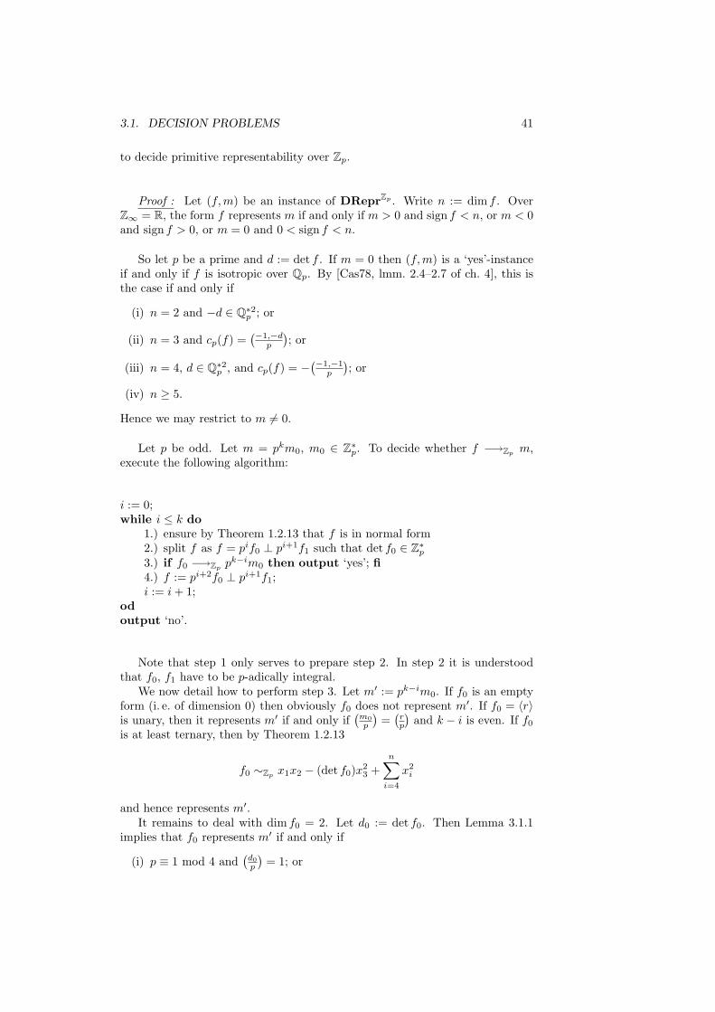
3.1. DECISION PROBLEMS 41
to decide primitive representability over Zp.
Proof : Let (f,m) be an instance of DReprZp . Write n := dim f . OverZ∞ = R, the form f represents m if and only if m > 0 and sign f < n, or m < 0and sign f > 0, or m = 0 and 0 < sign f < n.
So let p be a prime and d := det f . If m = 0 then (f,m) is a ‘yes’-instanceif and only if f is isotropic over Qp. By [Cas78, lmm. 2.4–2.7 of ch. 4], this isthe case if and only if
(i) n = 2 and −d ∈ Q∗2p ; or
(ii) n = 3 and cp(f) =(−1,−d
p
); or
(iii) n = 4, d ∈ Q∗2p , and cp(f) = −
(−1,−1p
); or
(iv) n ≥ 5.
Hence we may restrict to m 6= 0.
Let p be odd. Let m = pkm0, m0 ∈ Z∗p. To decide whether f −→Zp m,
execute the following algorithm:
i := 0;while i ≤ k do
1.) ensure by Theorem 1.2.13 that f is in normal form2.) split f as f = pif0 ⊥ pi+1f1 such that det f0 ∈ Z∗
p
3.) if f0 −→Zppk−im0 then output ‘yes’; fi
4.) f := pi+2f0 ⊥ pi+1f1;i := i + 1;
odoutput ‘no’.
Note that step 1 only serves to prepare step 2. In step 2 it is understoodthat f0, f1 have to be p-adically integral.
We now detail how to perform step 3. Let m′ := pk−im0. If f0 is an emptyform (i. e. of dimension 0) then obviously f0 does not represent m′. If f0 = 〈r〉is unary, then it represents m′ if and only if
(m0p
)=(
rp
)and k − i is even. If f0
is at least ternary, then by Theorem 1.2.13
f0 ∼Zpx1x2 − (det f0)x2
3 +n∑
i=4
x2i
and hence represents m′.It remains to deal with dim f0 = 2. Let d0 := det f0. Then Lemma 3.1.1
implies that f0 represents m′ if and only if
(i) p ≡ 1 mod 4 and(d0p
)= 1; or
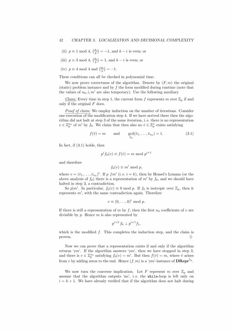
42 CHAPTER 3. LOCALIZATION AND DECISIONAL COMPLEXITY
(ii) p ≡ 1 mod 4,(d0p
)= −1, and k − i is even; or
(iii) p ≡ 3 mod 4,(d0p
)= 1, and k − i is even; or
(iv) p ≡ 4 mod 4 and(d0p
)= −1.
These conditions can all be checked in polynomial time.We now prove correctness of the algorithm. Denote by (F,m) the original
(static) problem instance and by f the form modified during runtime (note thatthe values of n0, i,m
′ are also temporary). Use the following auxiliary
Claim: Every time in step 1, the current form f represents m over Zp if andonly if the original F does.
Proof of claim: We employ induction on the number of iterations. Considerone execution of the modification step 4. If we have arrived there then the algo-rithm did not halt at step 3 of the same iteration, i. e. there is no representationv ∈ Zn0
p of m′ by f0. We claim that then also no v ∈ Znp exists satisfying
f(v) = m and gcdZp
(v1, . . . , vn0) = 1. (3.1)
In fact, if (3.1) holds, then
pif0(v) ≡ f(v) = m mod pi+1
and thereforef0(v) ≡ m′ mod p,
where v = (v1, . . . , vn0)t. If p 6 |m′ (i. e. i = k), then by Hensel’s Lemma (or the
above analysis of f0) there is a representation of m′ by f0, and we should havehalted in step 3, a contradiction.
So p|m′. In particular, f0(v) ≡ 0 mod p. If f0 is isotropic over Zp, then itrepresents m′, with the same contradiction again. Therefore
v ≡ (0, . . . , 0)t mod p.
If there is still a representation of m by f , then the first n0 coefficients of v aredivisible by p. Hence m is also represented by
pi+2 f0 ⊥ pi+1f1,
which is the modified f . This completes the induction step, and the claim isproven. ♦
Now we can prove that a representation exists if and only if the algorithmreturns ‘yes’. If the algorithm answers ‘yes’, then we have stopped in step 3,and there is v ∈ Zn0
p satisfying f0(v) = m′. But then f(v) = m, where v arisesfrom v by adding zeros to the end. Hence (f,m) is a ‘yes’-instance of DReprZp .
We now turn the converse implication. Let F represent m over Zp andassume that the algorithm outputs ‘no’, i. e. the while-loop is left only oni = k + 1. We have already verified that if the algorithm does not halt during
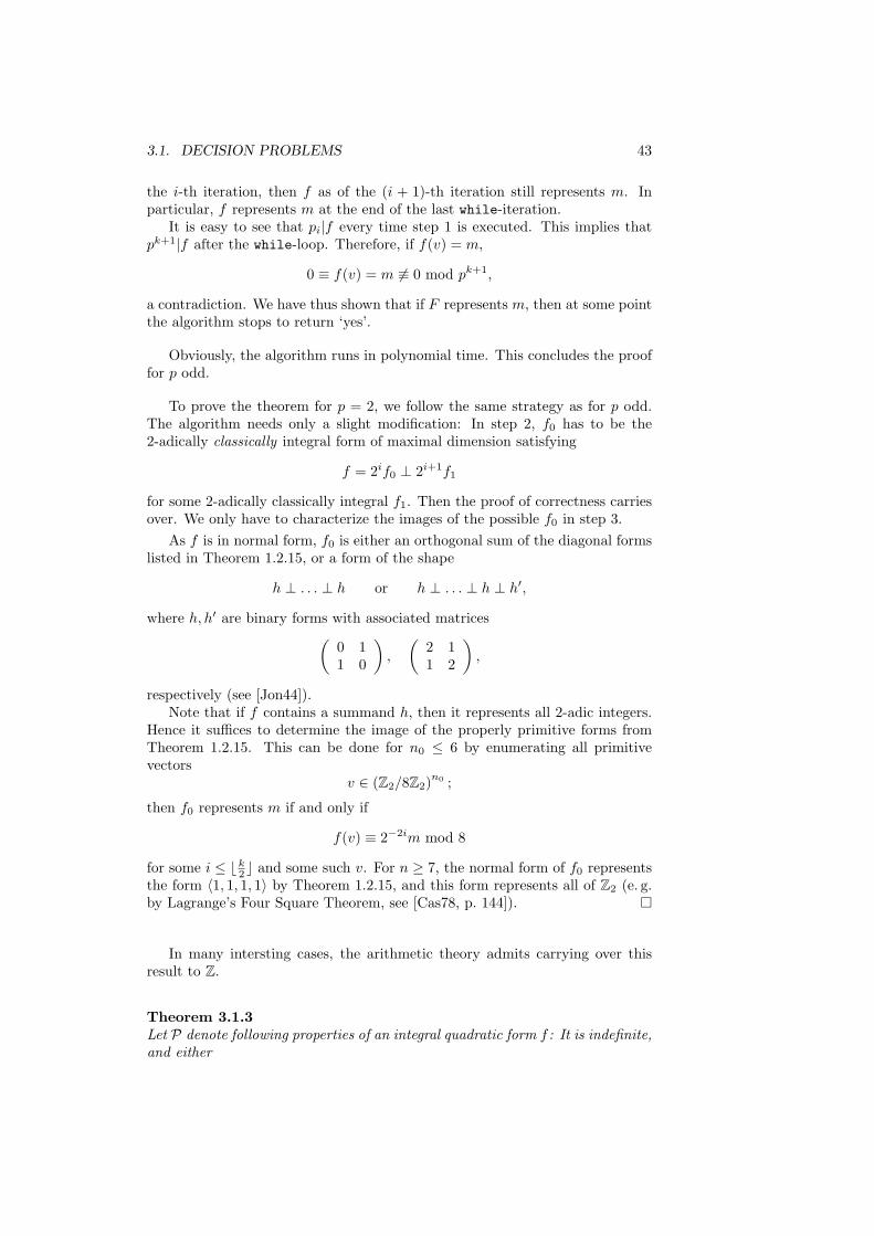
3.1. DECISION PROBLEMS 43
the i-th iteration, then f as of the (i + 1)-th iteration still represents m. Inparticular, f represents m at the end of the last while-iteration.
It is easy to see that pi|f every time step 1 is executed. This implies thatpk+1|f after the while-loop. Therefore, if f(v) = m,
0 ≡ f(v) = m 6≡ 0 mod pk+1,
a contradiction. We have thus shown that if F represents m, then at some pointthe algorithm stops to return ‘yes’.
Obviously, the algorithm runs in polynomial time. This concludes the prooffor p odd.
To prove the theorem for p = 2, we follow the same strategy as for p odd.The algorithm needs only a slight modification: In step 2, f0 has to be the2-adically classically integral form of maximal dimension satisfying
f = 2if0 ⊥ 2i+1f1
for some 2-adically classically integral f1. Then the proof of correctness carriesover. We only have to characterize the images of the possible f0 in step 3.
As f is in normal form, f0 is either an orthogonal sum of the diagonal formslisted in Theorem 1.2.15, or a form of the shape
h ⊥ . . . ⊥ h or h ⊥ . . . ⊥ h ⊥ h′,
where h, h′ are binary forms with associated matrices(0 11 0
),
(2 11 2
),
respectively (see [Jon44]).Note that if f contains a summand h, then it represents all 2-adic integers.
Hence it suffices to determine the image of the properly primitive forms fromTheorem 1.2.15. This can be done for n0 ≤ 6 by enumerating all primitivevectors
v ∈ (Z2/8Z2)n0 ;
then f0 represents m if and only if
f(v) ≡ 2−2im mod 8
for some i ≤ bk2 c and some such v. For n ≥ 7, the normal form of f0 represents
the form 〈1, 1, 1, 1〉 by Theorem 1.2.15, and this form represents all of Z2 (e. g.by Lagrange’s Four Square Theorem, see [Cas78, p. 144]).
In many intersting cases, the arithmetic theory admits carrying over thisresult to Z.
Theorem 3.1.3Let P denote following properties of an integral quadratic form f : It is indefinite,and either
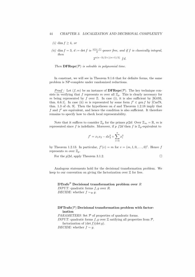
44 CHAPTER 3. LOCALIZATION AND DECISIONAL COMPLEXITY
(i) dim f ≥ 4, or
(ii) dim f = 3, d := det f is n(n−1)2 -power free, and if f is classically integral,
then2n(n−3)/2+b(n+1)/2c 6 | d.
Then DFRepr(P) is solvable in polynomial time.
In constrast, we will see in Theorem 9.1.6 that for definite forms, the sameproblem is NP-complete under randomized reductions.
Proof : Let (f,m) be an instance of DFRepr(P). The key technique con-sists in verifying that f represents m over all Zp. This is clearly necessary form being represented by f over Z. In case (i), it is also sufficient by [Kit93,thm. 6.6.1]. In case (ii) m is represented by some form f ′ ∈ gen f by [Cas78,thm. 1.3 of ch. 9]. Then the hypotheses on d and Theorem 1.2.18 imply thatf and f ′ are equivalent, and hence the condition is also sufficient. It thereforeremains to specify how to check local representability.
Note that it suffices to consider Zp for the primes p|2d: Over Z∞ = R, m isrepresented since f is indefinite. Moreover, if p 6 | 2d then f is Zp-equivalent to
f ′ = x1x2 − dx23 +
n∑i=4
x2i
by Theorem 1.2.13. In particular, f ′(v) = m for v = (m, 1, 0, . . . , 0)t. Hence frepresents m over Zp.
For the p|2d, apply Theorem 3.1.2.
Analogous statements hold for the decisional transformation problem. Wekeep to our convention on giving the factorization over Z for free.
DTrafoR Decisional transformation problem over RINPUT: quadratic forms f, g over R.DECIDE: whether f ∼R g.
DFTrafo(P) Decisional transformation problem with factor-ization
PARAMETERS: Set P of properties of quadratic forms.INPUT: quadratic forms f, g over Z satifying all properties from P,
factorization of (det f)(det g).DECIDE: whether f ∼ g.
3.2. FORMS OVER FINITE FIELDS 45
Theorem 3.1.4Let p be any symbol (i. e. a prime or ∞). Then
DTrafoZp
is solvable in polynomial time.
Proof : For p = ∞, forms f and g are R-equivalent if and only if theirsignatures coincide (Proposition 1.2.9). For p a prime, compute the normalforms of f , g. By Theorems 1.2.13, 1.2.15, f and g are Zp-equivalent if and onlyif their normal forms coincide. This can be checked in polynomial time.
Similarly, we have the following global result.
Theorem 3.1.5Let P denote following properties of an integral quadratic form f : It is indefinite,dim f ≥ 3, and d := det f is n(n−1)
2 -power free; and if f is classically integral,then
2n(n−3)/2+b(n+1)/2c 6 | d.
Then DFTrafo(P) is solvable in polynomial time.
Proof : Let (f, g) be an instance of DFTrafo(P). Without loss assumethat det f = det g =: d, as otherwise f 6∼ g. Then the hypotheses on det fand Theorem 1.2.18 imply that f, g lie in a one-class genus. Hence (f, g) is a‘yes’-instance if and only if f ∼g g; By Theorem 3.1.4, we can check whetherf ∼Zp g for all p|2d∞ in polynomial time. If this holds, f ∼g g by the remarkafter Theorem 1.2.13.
An analogous result holds over the rationals: Over Qp, classifying the imageof forms is even easier than over Zp; this is because there are at most twoequivalence classes of forms to be considered per dimension and determinant,and because every Qp-form is isotropic by Meyer’s theorem and hence representsall p-adic numbers (it is universal, see [Cas78, sec. 2.4]). The Strong HassePrinciple implies (see [Cas78, thm. 1.1, cor. 2 of ch. 6]) that m is representedby f over Q if and only if it is represented by f over all Qp, and again it sufficesto consider all p|2(det f)∞ in case f is integral.
3.2 Forms over Finite Fields
In this section, we consider the transformation and representation problems overfinite prime fields. The classification theorems of quadratic forms in Sect. 1.2.5show that the class structure of quadratic forms over the fields Fp is relativelysimple. We prove that the computational complexity of Repr, Trafo is alsoquite low, as they can be solved in random polynomial time.

46 CHAPTER 3. LOCALIZATION AND DECISIONAL COMPLEXITY
Theorem 3.2.1 Let p be an odd prime and let F be the finite field with p ele-ments. Then TrafoF is solvable in random polynomial time.
Proof : Let F-equivalent forms f, g over F be given. Use Lemma 1.2.3 totransform either of them into diagonal shape, say
f T1 = 〈a1, . . . , an〉 and g T2 = 〈b1, . . . , bn〉
with Ti ∈ SLnF. Then determine which of the ai, bi are squares in F. Thiscan be done in polynomial time by computing Jacobi symbols. Build a permu-tation matrix Πi for either form such that f T1Π1 = 〈s1, . . . , sk, qk+1, . . . , qn〉and g T2Π2 = 〈s′1, . . . , s′`, q′`+1, . . . , q
′n〉 such that all qi, q′i are squares and all si,
s′i are non-squares. Without loss we may assume that k ≥ `. Let s := s1 (ifk 6= 0). Then s−1
i s, (s′i)−1s are square for all i. By [CP01, sec. 2.3.2], we can
compute square roots
t2i = s−1i s for i = 1, . . . , k,
(t′i)2 = (s′i)
−1s for i = 1, . . . , `,
r2i = qi for i = k + 1, . . . , n, and
(r′i)2 = q′i for i = ` + 1, . . . , n.
in random polynomial time for all i for which the respective right hand side isdefined. Then
f ′ : = f T1Π1S1 = 〈s, . . . , s︸ ︷︷ ︸k times
, 1, . . . , 1︸ ︷︷ ︸n−k times
〉, and
g′ : = g T2Π2S2 = 〈s, . . . , s︸ ︷︷ ︸` times
, 1, . . . , 1︸ ︷︷ ︸n−` times
〉,
where
S1 =
t1 0. . .
tkrk+1
. . .0 rn
and
S2 =
t′1 0. . .
t′`r′`+1
. . .0 r′n
.
As f ′ and g′ are F-equivalent, their determinant may only differ by a square inF. Hence k− ` is even. Therefore it suffices for the completion of the algorithmto construct a transformation of the form 〈s, s〉 into the form 〈1, 1〉.
3.3. FORMS OVER LOCAL RINGS 47
Note that there are x, y ∈ F satisfying sx2 + sy2 = 1 by [Cas78, ch. 2,lm. 2.2]. Such a solution can be found efficiently using [AEM87]. Then findx′, y′ such that
det(
x x′
y y′
)= s−1
(e. g. by choosing x′ uniform at random and solving for y′, until success). Thenthe form
h := 〈s, s〉(
x x′
y y′
)has the right first coefficient and the right determinant. Therefore, anotherapplication of Lemma 1.2.3 transforms it into the form 〈1, 1〉. This completesthe description of the algorithm. As argued in the single steps, it runs in randompolynomial time.
It is easy to modify this procedure to obtain a proper transformation (ofdeterminant +1).
The reference [AEM87] used in this proof already shows that we can alsoefficiently find representations over prime fields. The algorithm of Adleman,Estes, and McCurley [AEM87] particularly makes sure that even probabilism,and the number-theoretic assumption as the Extended Riemann Hypothesis,can be avoided (cf. [PS87])∗.
Theorem 3.2.2 Let p be an odd prime and let F be the finite field with p ele-ments. If n ≥ 2, then ReprF
n is solvable in (deterministic) polynomial time.
Proof : See [AEM87].
It may seem peculiar that we had to exclude the case n = 1. For unary forms,the representation problem is equivalent to computing square roots in F. Thiscan be done efficiently in practice. However, it is not known to be possible indeterministic polynomial-time unless the Extended Riemann Hypothesis holds(see [CP01, sec. 2.3.2]).
3.3 Forms over Local Rings
Lemma 3.3.1 Let p be a prime, m ∈ Zp, and n, k ∈ N. Let f be a binaryquadratic form over Zp such that det f ∈ Z∗
p.If f represents m primitively over Zp, then one can construct, to precision
k, a primitive representation v ∈ Znp satisfying f(v) = m, in polynomial time.
∗Perhaps this result is even older. I am however not aware of a corresponding publication.The main objection of the authors of [AEM87] is to solve modular equations without havingto factor the modulus.
48 CHAPTER 3. LOCALIZATION AND DECISIONAL COMPLEXITY
Note that if f represents m and p2 6 |m, then f automatically represents mprimitively.
Proof : First assume that p 6 |m. By Lemma 1.2.3 we may assume that fhas been transformed into diagonal form, i. e.
f = 〈r1, r2〉.
We also have ri ∈ Z∗p, i = 1, 2 since p 6 |m and f has Zp-coefficients.
The requirement of precision k means that the have to find a vector v ∈(Z/pk+1Z)2 satisfying
f(v) ≡ m mod pk+1, (3.2)
such that v can be lifted to a global solution v ∈ Z2p, i. e.
⇒ (v) = m and v ≡ v mod pk+1.
A vector v satisfying (3.2) can be computed in (deterministic) polynomial-timeby [AEM87].
We claim that any such solution can be lifted to a solution over Zp. Firstnote that p 6 |m implies
p 6 | riv2i (3.3)
for at least one i ∈ 1, 2. Then
∂f(x)∂xi
∣∣∣x=v
= 2rivi
and thus
νp
(∂f(x)∂xi
∣∣∣x=v
)= 0
because of (3.3), and since p is odd. The solution can now be lifted by Hensel’sLemma [Eis95, thm. 7.3], since the solution v is correct modulo(
∂f(x)∂xi
∣∣∣x=v
)2
p.
This proves the lemma for p 6 |m.
Next consider p|m. Then f is (regular) isotropic modulo p. In particular, itis Fp-equivalent to the form 2x1x2. By Theorem 3.2.1, we can compute T ∈ Z2
p
such thatf T ≡ 2x1x2 mod p and det T 6≡ 0 mod p. (3.4)
Let
T =(
s tu q
).
Then (3.4) implies that p 6 | s and p 6 | t, or p 6 | u and p 6 | q. So after multiplyingT with the transposition matrix
(0 11 0
)we may assume that p 6 | t.
We claim that f is Zp-equivalent to the form 2x1x2; more prescisely, that Tcan be lifted to an equivalence transformation between these two. Let
T =(
s tu q
)and T t
(r1
r2
)T =
(a bb c
).
3.3. FORMS OVER LOCAL RINGS 49
Then the relation f T = 2x1x2 is equivalent to the three equations
r1s2 + r2u
2 = 0,
r1st + r2uq −1 = 0,
r1t2 + r2q
2 = 0
in the three indeterminates s, t, u. The Jacobi determinant of this equationsystem amounts to
det
2r1s r1t 00 r1s 2r1t
2r2u r2q 0
= −4r21r2t(detT ).
This value does not vanish modulo p if we sustitute s, t, u for s, t, u. Hencethe multidimensional variant of Hensel’s Lemma (see [Eis95, p. 209]) statesthat there is a matrix T ≡ T mod p such that f T = 2x1x2. Moreover, thecoefficients of T can inductively be computed to arbitrary precision.
Now that we know the transformation T to sufficient precision, we only needto find a representation of m by the form 2x1x2. But such is obviously given byx1 = 1, x2 = 1
2m. This concludes the proof for p|m.
For the discussion of [AEM87] see also Sect. 6.1.
Lemma 3.3.2 Let p be a prime, m ∈ Zp, and n, k ∈ N. Let f be a quadraticform over Zp such that
det f ∈ Z∗p and dim f ≥ 3.
Then f represents m primitively over Zp, and a primitive representation can beefficiently computed (to precision k).
Proof : After application of Lemma 1.2.3, we have
f = 〈r1, . . . , rn〉.
If p 6 |m, then m can be represented by 〈r1, r2〉 according to Lemma 3.1.1. Hencewe may choose x3 = . . . = xn = 0, whereas x1, x2 can be efficiently computedby use of Lemma 3.3.1.
If, however, p 6 |m, then let x3 = 1 and x4 = . . . = xn = 0. Then p 6 | r3 andtherefore p 6 |m−r3. Consequently, there is a representation of m−r3 by 〈r1, r2〉,which can be computed in polynomial time by Lemma 3.3.1. This representation(x1, x2) combines with x3, . . . , xn chosen so far to a representation of m by f ,as desired. All computations are to precision k.
Theorem 3.3.3 Let p be a prime or p =∞.Then
ReprZp and ∗ReprZp
are solvable in polynomial time.
50 CHAPTER 3. LOCALIZATION AND DECISIONAL COMPLEXITY
Proof : Proceed according to the following algorithm. All computations areperformed to the required precision.
i := 0;e := (0, . . . , 0)t ∈ Nn
0 ; ### exponents of p in the solution vectorcompute T ∈ GLnZp such that f T = 〈r1, . . . , rn〉 is in diagonal formwhile i ≤ k do
select the indices j1 ≤ . . . ≤ jk satisfying νp(rju) = i;
f0 := 〈p−irj1 , . . . , p−irjk
〉;if f0 −→Zp pk−im0 then
use Lemmata 3.1.1, 3.3.2 to compute w s.t. f0(w) = pk−im0;define v ∈ Zn
p by
vj :=
peju wjuif j = ju,
0 else;break ;
fifor u = 1, . . . , k do
redefine f : replace the ju-th diagonal coefficient, rju, by p2rju
;adjust exponent vector eju
:= eju+ 1;
odi := i + 1;
odoutput v.
This algorithm is similar in outline to the algorithm from the proof of The-orem 3.1.2. In particular, that proof also shows that the algorithm here willterminate with v defined if there is a representation of m by f . Moreover, wehave detailed there how to evaluate the if-query.
Letf = f0 ⊥ pf1 ⊥ . . . p`f`
with det fi ∈ Z∗p. The rationale for the above procedure is as follows: If m has
a representation by f with some variable belonging to f0 coprime to p, then itis represented by f0 only; this follows from reduction modulo p and Lemmata3.1.1, 3.3.2. If, however, all values of variables of f0 need to be divisible by p torepresent m, then we may replace f0 by p2f0 and its variables xj by pxj . Thisis what happens in the modification step after the while-loop. The correctnessof the algorithm then follows inductively.
Theorem 3.3.4 Let p be a prime or p =∞.Then TrafoZp is solvable in polynomial time.
Proof : Let an instance (f, g) of the transformation problem be given. ByTheorems 1.2.13, 1.2.15, and Proposition 1.2.9, both f and g can be efficientlytransformed into normal form, i. e. we can compute S, T ∈ GLnZp such that
f ′ := f S and g′ := g T
3.3. FORMS OVER LOCAL RINGS 51
are in normal form. Since normal forms are unique (see the results just cited),we must have f ′ = g′. Thus T−1S is a transformation from f to g.
As for the decisional problems in Sect. 3.1, similar results hold over the fieldsof p-adic numbers Qp. This is implicitly contained in the proof of Theorem 6.1.1.
52 CHAPTER 3. LOCALIZATION AND DECISIONAL COMPLEXITY
Chapter 4
Algorithms for Primes,Classes, and Genera
In this chapter we present some auxiliary algorithms needed in the later chap-ters, particularly in Chaps. 9 and 10.
In Sect. 4.1, we give an overview over methods to select primes with cer-tain properties. This constitutes an elementary but important algorithmic taskfor many algorithms in number theory. The polynomial-time primality test[AKS04] has simplified this significantly. In this thesis, prime selection is usedin Sect. 4.2.4 and in Chapter 9. Much of the results presented here may be con-sidered folklore; however, an overview over selection techniques in the light ofrecent primality tests seems to be missing in the literature. Hence this summarymay be as well of independent interest.
In Sect. 4.2.4, we show that the classical result on the existence of genera withlocally prescribed behavior can be made algorithmically efficient: We presentan algorithm which constructs a form f over Z which is p-adically integrallyequivalent to a finite set of given fp over Zp. The given forms fp have to be‘compatible’ in the sense that such a global form f exists. This will be appliedin the algorithms in Chaps. 9 and 10.
4.1 Algorithmic Prime Selection
In this section, we give an overview over prime selection algorithms. First weconsider the problem of finding the least prime, or any prime, exceeding a giveninteger; then we restrict to a coprime arithmetic progression. It turns out thatboth types of tasks can be accomplished in random polynomial time. For theunrestricted case, derandomization is possible under the Riemann hypothesis,whereas in the case of an arithmetic progression, we cannot give an analogousderandomization.
Prime selection has been a topic of profound investigation, in particularin connection with cryptographic key generation (e. g. see [Mih94]). Beforepolynomial-time primality tests have been known (see [AKS04]), the stumbling
53
54 CHAPTER 4. ALGORITHMS FOR PRIMES, CLASSES, AND GENERA
block was to guarantee that the output numbers were primes. “Probable primegenerators” became popular, which only claimed to output primes with a certainhigh probability. The “provable prime generators” had to produce a primalitycertificate for each prime.
The primality test [AKS04] has simplified this task extremely. The conse-quences for prime selection collected below can certainly be considered well-known. But as there seems to be no comprehensive study of them in the liter-ature, we decided to give an overview here.
We consider this question here because we will apply it in the next sextionas well as in later chapters (see Sect. 9.2). Prime selection, however, is a veryfundamental task both in cryptography and in algorithmic number theory, andtherefore it seemed to be worthwhile to ponder this topic a bit more closely.
Proposition 4.1.1 (a) For every ε > 0, there is a probabilistic polynomial-time algorithm which given an integer N , outputs some prime p > N suchthat
p = O(N ln1+ε N).
The implied constant only depends on ε.
(b) Assume the Riemann Hypothesis to be true. Then there is deterministicpolynomial-time algorithm which given an integer N , outputs the smallestprime p > N . It then holds that for every ε > 0 that
p = N +O((ln N)2(ln ln lnN)ε).
The implied constant only depends on ε.
Remark: To the best of my knowledge, there is, up to now, no deterministicand method known to produce a prime larger than a given number which canbe proven unconditionally to be polynomial time.
Proof : Recall that by [AKS04], a given integer can be proven or disprovento be prime in deterministic polynomial time. We shall use this primality testas a subroutine in the following algorithms.
(a) Whithout loss we may assume that lnN ≥ 2. Then perform the followingrandom selection algorithm:
success := false;while not success do
select uniformly at random p ∈ [N + 1, N ln1+ε N ] ∩ Zif p is prime then success := true;
odoutput p.
4.1. ALGORITHMIC PRIME SELECTION 55
The probability of success in one iteration of this algorithm amounts to
r =# primes in [N + 1, N ln1+ε N ]
N (ln1+ε N − 1). (4.1)
Let π(x) denote the number of primes less or equal to x. Then (4.1)implies
r ≥ π(N ln1+ε N)−N
N (ln1+ε N − 1).
If we assume without loss that ε < 1, the Prime Number Theorem thentells us that
r ≥
N ln1+ε N
lnN + (1 + ε) ln lnN−N +O
(N ln1+ε N
(lnN + (1 + ε) ln lnN)2
)N ln1+ε N
=1
lnN + (1 + ε) ln lnN− 1
ln1+ε N+O
(1
(lnN + (1 + ε) ln lnN)1+ε
)
=1
lnN+O
(1
ln1+ε N
).
(4.2)The last equality is due to the fact that
1lnN
− 1lnN + (1 + ε) ln lnN
= O(
1ln1+ε N
),
which follows from1
lnN− 1
lnN + (1 + ε) ln lnN= (1 + ε)
ln lnN
(lnN) (lnN + (1 + ε)(ln lnN))
= O(
ln lnN
ln2 N
).
Now turning to the general case of several iterations, we face a randomexperiment with respect to the geometric distribution, whose success prob-ability is bounded from below by (4.2). Therefore, the probability that ittakes more than t lnN iterations to obtain a prime does not exceed(
1lnN
+O(
1ln1+ε
))t ln N
=1
(lnN)t ln N+O
(2t ln N
(lnN)t ln N+ε
)= exp
(− (t lnN)(ln ln N)
)+O
(exp
(t lnN − t(1 + ε)(lnN)(ln lnN)
)).
(4.3)
Here the first equality is due to the fact that for every constant C > 0 andevery 1 ≤ k ≤ dt lnNe, it holds that
Ck
(lnN)t ln N+kε= O
(C
(lnN)t ln N+ε
), (4.4)
56 CHAPTER 4. ALGORITHMS FOR PRIMES, CLASSES, AND GENERA
and rounding t lnN to the next integer and applying the binomial theorem,we thus obtain
dt ln Ne∑i=1
(dt lnNe
i
)= 2dt ln Ne − 1
terms dominated by the right hand side of (4.4), apart from the mainterm.
But it easily seen that there are constants C1, C2 such that the rightmostside of (4.3) is stricly smaller than 1
2 if
t ≥ C1 − C2 ε.
Summing up, we find that after linearly many iterations, the algorithmreturns a prime with probability larger than 1
2 .
(b) Perform the following exhaustive search algorithm:
success := false;p := N ;while not success do
p := p + 1;if p is prime then success := true;
odoutput p.
By a result of Selberg [MSC96, §VII.13 a)], for any ε > 0 this procedureterminates successfully after at most (ln N)2(ln ln lnN)ε iterations con-ditionally on the Riemann Hypothesis, except for possibly finitely manyexceptions; hence certainly it succeeds after
O((lnN)2(ln ln lnN)ε
)iterations, and the returned prime p satisfies
p = N +O((lnN)2(ln ln lnN)ε
).
Remark. The choice of the factor (ln ln lnN)ε was somewhat arbitrary asSelberg’s theorem holds for arbitrary functions tending to infinity as N → ∞instead.
4.1. ALGORITHMIC PRIME SELECTION 57
Corollary 4.1.2 (a) For every ε > 0, there is a probabilistic algorithm whichgiven integers N and n (n fix), outputs some primes p1, . . . , pn satisfying
N < p1 < . . . < pn = O(N ln1+ε N)
in expected running time polynomial in n and log N .
(b) Assume the Riemann Hypothesis to be true. Then there is deterministicpolynomial-time algorithm which given integers N and n, outputs primesp1, . . . , pn such that p1 is the smallest prime exceeding N , and pi is thesmallest prime exceeding pi−1, for all i = 2, . . . , n.
It then holds that for every ε > 0 that
pn = N +O(n (lnN)2 (ln ln lnN)ε).
In either case, the implied constant only depends on ε.
Proof :
(a) Apply the algorithm of Proposition 4.1.1 a), but halt only when n distinctprimes have been found.
Suppose that k < n primes have already been found. Then the probabilitybound (4.2) that another prime is found in one more iteration changes bya summand
− k
N ln1+ε−N≥ − n
N ln1+ε−N.
As n is fixed, theO-term of (4.2) absorbs this summand, and the proceduresucceeds in polynomial time.
(b) Apply Proposition 4.1.1 b) itereratively n times.
Proposition 4.1.3 For every ε > 0, there is a probabilistic polynomial-timealgorithm which given C ∈ N and coprime positive integers q, a, outputs someprime p ≡ a mod q such that
p = O(q ln1+ε q).
Remark. Even if the Riemann hypothesis is true, an exhaustive searchalgorithm as in the proof of Proposition 4.1.1 will not succeed in polynomialtime because it is known that the least prime in an arithmetic progression is atleast linear in the modulus in the worst case, i. e. there are exponentially manynumbers to test. More precisely, [Erd49], [Pom80] give superlinear estimates inϕ(q), and [Pra61], presents a superlinear estimate in q, each for a large family ofexamples (see also [Wag79] for a heuristic argument why such examples occur sofrequently). Theoretically, however, there might be an alternative deterministic
58 CHAPTER 4. ALGORITHMS FOR PRIMES, CLASSES, AND GENERA
approach which succeeds in polynomial time.
Proof : Use the following algorithm (which is anagolous to the one from theproof of Proposition 4.1.1 a):
success := false;while not success do
select uniformly at random p ∈ [N + 1, N ln1+ε N ] ∩ (qZ + a)if p is prime then success := true;
odoutput p.
If r is the probability of success in one iteration and if π(x; q, a) denotes thenumber of primes p ≤ x with p ≡ a mod q, then
r =# p ∈ [N + 1, N ln1+ε N ] | p prime, p ≡ a mod q
N(ln1+ε N − 1)
≥ π(N ln1+ε N ; q, a)−N
N(ln1+ε N − 1.
(4.5)
The Bombieri-Vinogradov Theorem (see [MSC96, §VIII.6]), now states that
π(N ln1+ε N ; q, a) =N ln1+ε N
ϕ(q) ln(N ln1+ε N)+O
(N ln1+ε N
ϕ(q) ln2(N ln1+ε N)
)once q ≤
√N
lnB N, for some fixed B > 0; here ϕ(q) denotes Euler’s totient function.
Using (4.5) and ϕ(q) < q, it now follows that
r ≥ 1q lnN
+O(
1q ln1+ε N
)by the same computations as in the proof of Proposition 4.1.1 a). As then thereare constants C1, C2 such that we perform t lnN independent iterations, wheret ≥ C1 − C2 ε, then we obtain, as above, a chance of at least 1
2 that we thealgorithm succeeds within this time.
Moreover, for primes as well as for squarefree numbers, it is known that theleast a in the arithmetic progression with the desired properties may be expo-nentially large in the length of the modulus (see [MSC96, §§VI.23, VIII.5], thesearch for upper bounds is known as ‘Linnick’s question’). Therefore, the naıveexhaustive search approach of enumerating the integers in the progression in as-cending order, testing for primes (or squarefrees, if possible), and halting whena number of the desired type has been found, is doomed to run exponentiallylong. Moreover, to my knowledge there is no essentially different deterministicapproach known to attack this problem. Hence, it is not obvious at all whether,and if so, prime selection from an arithmetic progression can be efficiently de-randomized.
Obviously, an iterative version of this proposition could be established anal-ogously to Corollary 4.1.2.
4.2. CONSTRUCTION OF GENERA 59
4.2 Construction of Genera
In Sect. 1.2.5, we asked the following question: Given forms fp over Qp (for someset of symbols p ∈ P ), under which conditions does there exist a rational formf such that f ∼Qp
fp? We learned in Theorem 1.2.10 that there is essentiallyonly one condition, namely, that the product of the Hasse-Minkowski invariantsbe 1, see (1.5). Now we turn to an analogous question: Let the fp be p-adicallyintegral. Then we ask when a form f over Z exists such that f ∼Zp
fp; inother words, we ask whether the given fp define a genus over Z (see Sect. 1.2.6).Interestingly, the condition is no stronger than in the rational case (Theorem1.2.10).
Theorem 4.2.1 (Existence of Genera.) Let d ∈ Z\0. Let fp be formsover Zp such that
det fp ∈ dZ∗2p ,
for all p|2d∞, and ∏p|2d∞
cp(fp) = 1.
Then there exists an integral form f of determinant d such that
f ∼Zpfp
for all p.
We are now going to make this theorem algorithmic: Namely, we will proofthat given forms fp as in Theorem 4.2.1, one can efficiently construct the globalform f . The classical proof is constructive, and most of its steps can be turnedinto an algorithm directly. This is done in the subsequent subsections. The finalresult is recorded in Theorem 4.2.7.
4.2.1 Local representations
We first need a method to make p-adical representations p-adically integral at‘uninvolved’ primes p.
Proposition 4.2.2 Let n ≥ 3, k ∈ N0, m, d ∈ Z, and let p 6 | d be a prime.Then Algorithm 1 constructs β ∈ N0 and a primitive representation w of p2βmover Zp by the form
f := 〈1, . . . , 1︸ ︷︷ ︸n−1
, d〉
to precision k in polynomial time.
Proof : We first explain the rough outline of Algorithm 1. We always referto the form f := 〈1, . . . , 1, d〉 over Qp or Zp. In the first step, we construct an
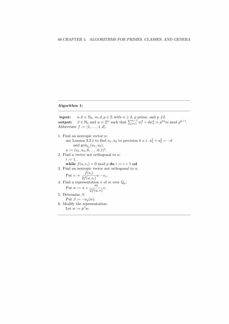
60 CHAPTER 4. ALGORITHMS FOR PRIMES, CLASSES, AND GENERA
Algorithm 1:
input: n, k ∈ N0, m, d, p ∈ Z with n ≥ 3, p prime, and p 6 | d.output: β ∈ N0 and w ∈ Zn such that
∑n−1i=1 w2
i + dw2n ≡ p2βm mod pk+1.
Abbreviate f := 〈1, . . . , 1, d〉.
1. Find an isotropic vector u:use Lemma 3.3.1 to find u1, u2 to precision k s. t. u2
1 + u22 = −d
and gcdZp(u1, u2),
u := (u1, u2, 0, . . . , 0, 1)t.2. Find a vector not orthogonal to u:
i := 1,while f(u, ei) = 0 mod p do i := i + 1 od
3. Find an isotropic vector not orthogonal to u:
Put v :=f(ei)
2f(u, ei)u− ei,
4. Find a representation x of m over Qp:Put w := u +
m
2f(u, v)v.
5. Determine β:Put β := −νp(w).
6. Modify the representation:Let w := pβw.
4.2. CONSTRUCTION OF GENERA 61
isotropic vector u ∈ Znp for f . In step 2, we find another vector e ∈ Zn
p suchthat f(u, e) 6= 0. This vector is used in step 3 to construct v ∈ Qn
p satisfyingf(v) = 0 and f(u, v) 6= 0. Then we have represented a ‘hyperbolic plane’ by fover Qp, i. e. a binary form with associated matrix(
0 11 0
),
see below. This subform allows us to find a representataion of m over Qp instep 4. In the last step, this representation and m are modified so that therepresentation will be p-adically integral and primitive.
Now we show that the algorithm is correct. Observe that steps 1 through 3construct a hyperbolic plane primitively represented by the form
f := 〈1, . . . , 1, d〉.
By Lemma 3.3.1, step 1 can be accomplished because the form 〈1, 1〉 repre-sents all p 6 | d over Zp (see [Cas78, ch. 2, lm. 2.2]). Obviously, then u is isotropicfor f .
Step 2 will succeed unless all standard unit vectors are orthogonal to u. Bylinearity, this implies that f(u, ·) is identically zero. As f is regular (over Qp),this can only happen for u = 0 [Cas78, ch. 2, lm. 1.2], which is excluded by step1.
Then step 3 yields an isotropic vector because
f(v) =f(ei)2
4 f(u, ei)2f(u) + f(ei) − 2 f(u, ei)
f(ei)2 f(u, ei)
= 0 + f(ei)− f(ei) = 0,
as f(u) = 0. Moreover, v is f -non-orthogonal to u, since
f(u, v) =f(ei)
2 f(u, ei)f(u) − f(u, ei) = −f(u, ei)
by step 2 and since u is isotropic.The vector x constructed in step 4 satisfies f(x) = m because
f(x) = f(u) +m2
4f(u, v)2f(v) + 2
m
2f(u, v)f(u, v) = m
as f(u) = f(v) = 0.For steps 5 and 6, it is obvious that the updated x′ = pβx is in Zn
p andprimitive by the choice of β. Finally, f(x′) = f(pβx) = p2βm.
It remains to bound the running time of the Algorithm 1. Step 1 terminatesin polynomial-time by Lemma 3.3.1. The while-loop in step 2 is repeated atmost n times. The remaining steps employ O(1) evaluations of the quadraticform f and its associated bilinear form to precision k, which amounts to O(n2)arithmetic operations modulo pk+1, and O(1) extra arithmetic operations mod-ulo pk+1.
62 CHAPTER 4. ALGORITHMS FOR PRIMES, CLASSES, AND GENERA
4.2.2 Composition of square classes
Our next subgoal is to find an integer t primitively represented by given lo-cal forms fp which are ‘compatible’ in the sense that they define a genus (seeTheorem 4.2.1).
Lemma 4.2.3 Let P be a finite set, containing primes and possibly the symbol∞. Let tp ∈ Z be given for all p ∈ P .
Then Algorithm 2 constructs a prime p0 and an integer t such that
(i) p0 is the only prime with p0|t and p0 /∈ P ; for this prime, p0|t and p20 6 | t,
(ii) tZ∗2p = tpZ∗2
p for all p ∈ P
in random polynomial time.
Denote byCRT
((a1,m1), . . . , (ak,mk)
)a call to an efficient routine realizing the Chinese Remainder Theorem. It re-turns an integer a such that
a ≡ ai mod mi ∀ i,
or fail if the system is unsolvable. Note that this task can be performed inpolynomial time.
Proof : For each p ∈ P\∞, let tp = εppsp . Algorithm 2 computes the
values sp, εp and takes care that for the output value t, it holds that
νp(t) = sp andt
pspZ∗2
p = εpZ∗2p . (4.6)
The number t is computed in the final step by
t = ±p0
∏p∈Pp6=∞
psp ,
which already implies statement (i). Then (4.6) is accomplished by the choiceof the prime p0:
By construction,
t
psp≡ εp mod p for p 6= 2, and
t
2s2≡ ε2 mod 8.
Then (4.6) follows from Lemma 1.2.6. Analogously, we have sign (t) = sign (t∞)and therefore tR+ = t∞R+ if ∞ ∈ P (recall that Z∗2
∞ = R∗2 = R+). Statement(ii) follows.
By Proposition 4.1.3, prime selection can be accomplished in random poly-nomial time. All other steps of the algorithm are trivially polynomial time.
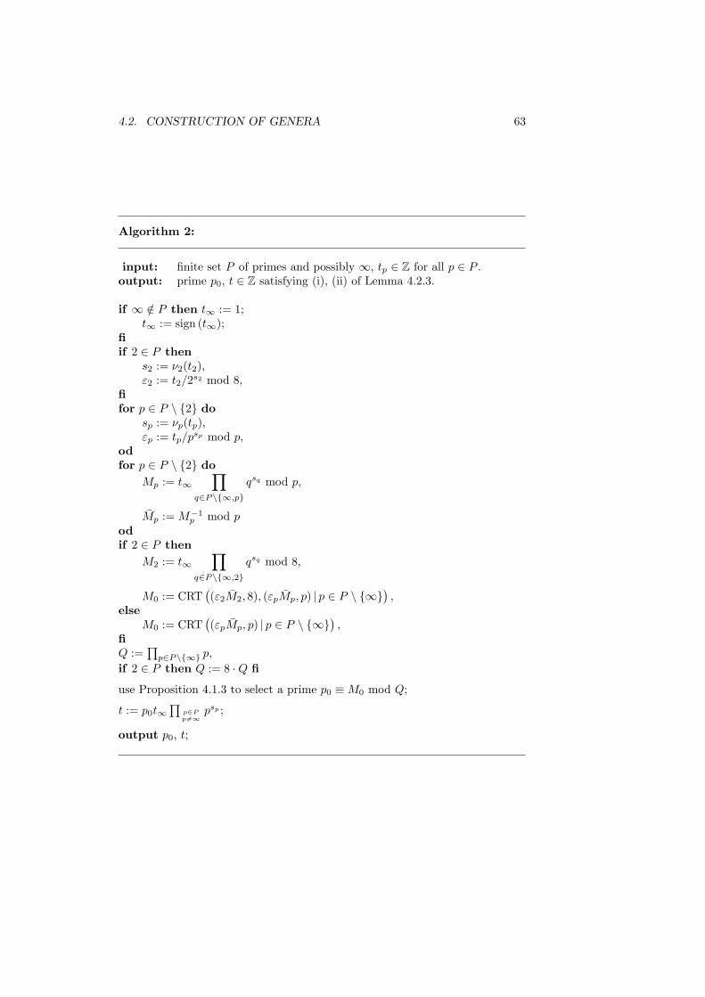
4.2. CONSTRUCTION OF GENERA 63
Algorithm 2:
input: finite set P of primes and possibly ∞, tp ∈ Z for all p ∈ P .output: prime p0, t ∈ Z satisfying (i), (ii) of Lemma 4.2.3.
if ∞ /∈ P then t∞ := 1;t∞ := sign (t∞);
fiif 2 ∈ P then
s2 := ν2(t2),ε2 := t2/2s2 mod 8,
fifor p ∈ P \ 2 do
sp := νp(tp),εp := tp/psp mod p,
odfor p ∈ P \ 2 do
Mp := t∞∏
q∈P\∞,p
qsq mod p,
Mp := M−1p mod p
odif 2 ∈ P then
M2 := t∞∏
q∈P\∞,2
qsq mod 8,
M0 := CRT((ε2M2, 8), (εpMp, p) | p ∈ P \ ∞
),
elseM0 := CRT
((εpMp, p) | p ∈ P \ ∞
),
fiQ :=
∏p∈P\∞ p,
if 2 ∈ P then Q := 8 ·Q fi
use Proposition 4.1.3 to select a prime p0 ≡M0 mod Q;
t := p0t∞∏
p∈Pp6=∞
psp ;
output p0, t;
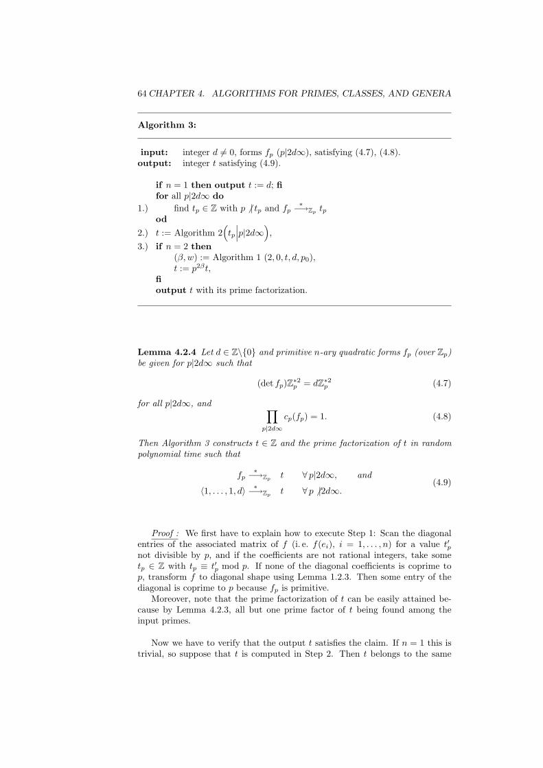
64 CHAPTER 4. ALGORITHMS FOR PRIMES, CLASSES, AND GENERA
Algorithm 3:
input: integer d 6= 0, forms fp (p|2d∞), satisfying (4.7), (4.8).output: integer t satisfying (4.9).
if n = 1 then output t := d; fifor all p|2d∞ do
1.) find tp ∈ Z with p 6 | tp and fp∗−→Zp
tpod
2.) t := Algorithm 2(tp
∣∣∣p|2d∞),
3.) if n = 2 then(β, w) := Algorithm 1 (2, 0, t, d, p0),t := p2βt,
fioutput t with its prime factorization.
Lemma 4.2.4 Let d ∈ Z\0 and primitive n-ary quadratic forms fp (over Zp)be given for p|2d∞ such that
(det fp)Z∗2p = dZ∗2
p (4.7)
for all p|2d∞, and ∏p|2d∞
cp(fp) = 1. (4.8)
Then Algorithm 3 constructs t ∈ Z and the prime factorization of t in randompolynomial time such that
fp∗−→Zp
t ∀ p|2d∞, and
〈1, . . . , 1, d〉 ∗−→Zp t ∀ p 6 |2d∞.(4.9)
Proof : We first have to explain how to execute Step 1: Scan the diagonalentries of the associated matrix of f (i. e. f(ei), i = 1, . . . , n) for a value t′pnot divisible by p, and if the coefficients are not rational integers, take sometp ∈ Z with tp ≡ t′p mod p. If none of the diagonal coefficients is coprime top, transform f to diagonal shape using Lemma 1.2.3. Then some entry of thediagonal is coprime to p because fp is primitive.
Moreover, note that the prime factorization of t can be easily attained be-cause by Lemma 4.2.3, all but one prime factor of t being found among theinput primes.
Now we have to verify that the output t satisfies the claim. If n = 1 this istrivial, so suppose that t is computed in Step 2. Then t belongs to the same
4.2. CONSTRUCTION OF GENERA 65
square class in Zp as tp by Lemma 4.2.3 (ii), and so
fp∗−→Zp
t (4.10)
holds for all p|2d∞ after step 2. If step 3 is executed, i. e. if n = 2, then thent is only modified by a square coprime to 2d, since p0 6 | 2d. Hence (4.10) stillholds at the end of the algorithm.
Now let p 6 | 2d∞. If additionally n ≥ 3, then gcd(t, d) = 1 because we havechose t ≡ tp 6≡ 0 mod p for all p|2d. Hence
〈1, . . . , 1, d〉 ∗−→Zp t (4.11)
is also satisfied for all p 6 | 2d∞ due to Lemma 1.2.7.Hence it remains to cover the case in which n = 2 and p 6 | 2d∞. Then fp
represents t primitively over Zp if and only if
fp ∼Zptx2 + bxy + cy2 (4.12)
for some b, c ∈ Zp, as every primitive vector can be extended to a regular matrix.If p 6 | t, then d
t ∈ Zp, and (4.12) holds with b = 0, c = dt because there is only
one class of binary quadratic forms of determinant d over Zp (see [Cas78, ch. 9,thm. 3.1]).
Now we are left with the case where p|t, but p 6 | 2d∞, and n = 2. By Lemma4.2.3, we then have p = p0. Moreover, in step 3 of Algorithm 3 the integer tis modified in such a way that t is primitively represented by f , according toProposition 4.2.2.
Finally, the algorithm terminates in polynomial-time because the subrou-tines called do.
Remark. For n ≥ 3, it would suffice in Algorithm 3 to combine the tp viathe Chinese Remainder Theorem and ignore all p 6 | 2d∞. The t would still beprimitively represented locally everywhere. However, it might then be harderto obtain the prime factorization of t.
4.2.3 Approximation
We prove a result (Corollary 4.2.6) which enables us to find a form f ‘close’ toeach of a given set of fp. Here ‘close’ refers to the topology of Zp; i. e. it meanscongruent to a high power of p (for p prime). This will help us in Theorem4.2.7 to guarantee the Zp-equivalence of forms obtained from modifying fp, f ,respectively.
Because of its topological interpretation, this method is also called ‘approx-imation’. Very roughly, the key lemma 4.2.5 allows for Chinese remainderingwith constraints.
Recall that a vector u = (ui)i ∈ Rn, where R is Z or some Zp, is calledprimitive if and only if gcdR(ui | i = 1, . . . , n) = 1.
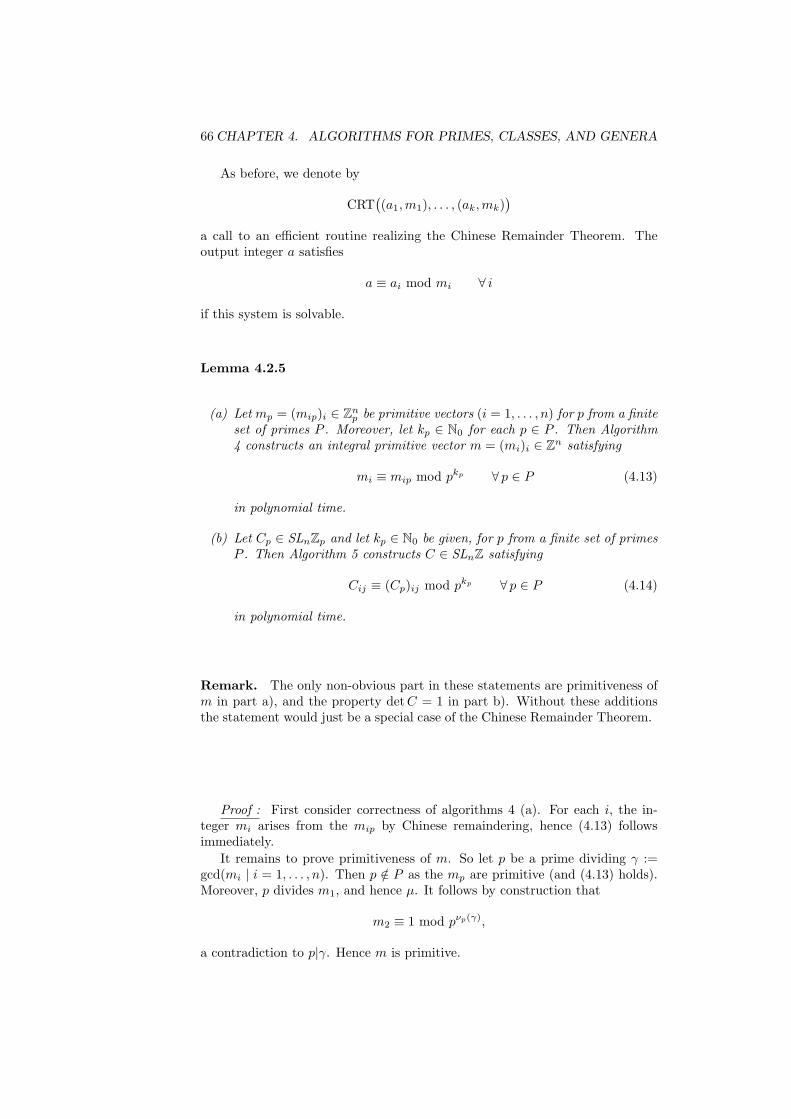
66 CHAPTER 4. ALGORITHMS FOR PRIMES, CLASSES, AND GENERA
As before, we denote by
CRT((a1,m1), . . . , (ak,mk)
)a call to an efficient routine realizing the Chinese Remainder Theorem. Theoutput integer a satisfies
a ≡ ai mod mi ∀ i
if this system is solvable.
Lemma 4.2.5
(a) Let mp = (mip)i ∈ Znp be primitive vectors (i = 1, . . . , n) for p from a finite
set of primes P . Moreover, let kp ∈ N0 for each p ∈ P . Then Algorithm4 constructs an integral primitive vector m = (mi)i ∈ Zn satisfying
mi ≡ mip mod pkp ∀ p ∈ P (4.13)
in polynomial time.
(b) Let Cp ∈ SLnZp and let kp ∈ N0 be given, for p from a finite set of primesP . Then Algorithm 5 constructs C ∈ SLnZ satisfying
Cij ≡ (Cp)ij mod pkp ∀ p ∈ P (4.14)
in polynomial time.
Remark. The only non-obvious part in these statements are primitiveness ofm in part a), and the property det C = 1 in part b). Without these additionsthe statement would just be a special case of the Chinese Remainder Theorem.
Proof : First consider correctness of algorithms 4 (a). For each i, the in-teger mi arises from the mip by Chinese remaindering, hence (4.13) followsimmediately.
It remains to prove primitiveness of m. So let p be a prime dividing γ :=gcd(mi | i = 1, . . . , n). Then p /∈ P as the mp are primitive (and (4.13) holds).Moreover, p divides m1, and hence µ. It follows by construction that
m2 ≡ 1 mod pνp(γ),
a contradiction to p|γ. Hence m is primitive.
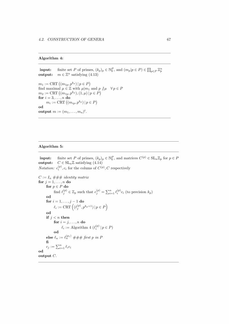
4.2. CONSTRUCTION OF GENERA 67
Algorithm 4:
input: finite set P of primes, (kp)p ∈ NP0 , and (mp|p ∈ P ) ∈
∏p∈P Zn
p
output: m ∈ Zn satisfying (4.13)
m1 := CRT((m1p, p
kp) | p ∈ P)
find maximal µ ∈ Z with µ|m1 and p 6 |µ ∀ p ∈ Pm2 := CRT
((m1p, p
kp), (1, µ) | p ∈ P)
for i = 3, . . . , n domi := CRT
((mip, p
kp) | p ∈ P)
odoutput m := (m1, . . . ,mn)t.
Algorithm 5:
input: finite set P of primes, (kp)p ∈ NP0 , and matrices C(p) ∈ SLnZp for p ∈ P
output: C ∈ SLnZ satisfying (4.14)Notation: c
(p)i , ci for the colums of C(p), C respectively
C := In ### identity matrixfor j = 1, . . . , n do
for p ∈ P dofind `
(p)j ∈ Zp such that c
(p)j =
∑ni=1 `
(p)i ci (to precision kp)
odfor i = 1, . . . , j − 1 do
`i := CRT((`(p)
j , pkp+1) | p ∈ P)
odif j < n then
for i = j, . . . , n do`i := Algorithm 4 (`(p)
i | p ∈ P )od
else `n := `(p1)n ### first p in P
ficj :=
∑ni=1 `ici
odoutput C.
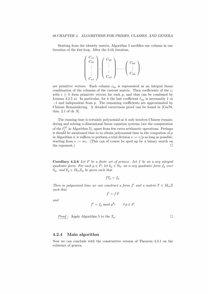
68 CHAPTER 4. ALGORITHMS FOR PRIMES, CLASSES, AND GENERA
Starting from the identity matrix, Algorithm 5 modifies one column in oneiteration of the for-loop. After the k-th iteration,
C11
C21
...
...Cn1
,
C22
...
...Cn2
, . . . ,
Ckk
...Cnk
,
are primitive vectors. Each column ckp is represented as an integral linearcombination of the columns of the current matrix. Then coefficients of the ci
with i ≥ k form primivite vectors for each p, and thus can be combined byLemma 4.2.5 a). In particular, for k the last coefficient `np is necessarily 1 or−1 and independent from p. The remaining coefficients are approximated byChinese Remaindering. A detailed correctness proof can be found in [Cas78,thm. 2.1 of ch. 9].
The running time is certainly polynomial as it only involves Chinese remain-dering and solving n-dimensional linear equation systems (see the computationof the `
(p)j in Algorithm 5), apart from few extra arithmetic operations. Perhaps
it should be mentioned that to to obtain polynomial time in the compution of µin Algorithm 4, it suffices to perform a trial division v := v/p as long as possible,starting from v := m1. (This can of course be sped up by a binary search onthe exponent.)
Corollary 4.2.6 Let P be a finite set of primes. Let f be an n-ary integralquadratic form. For each p ∈ P , let kp ∈ N0, an n-ary quadratic form fp overZp, and Tp ∈ SLnZp be given such that
fTp = fp.
Then in polynomial time we can construct a form f ′ and a matrix T ∈ SLnZsuch that
f ′ = f T
andf ′ = fp mod pkp ∀ p ∈ P.
Proof : Apply Algorithm 5 to the Tp.
4.2.4 Main algorithm
Now we can conclude with the constructive version of Theorem 4.2.1 on theexistence of genera.
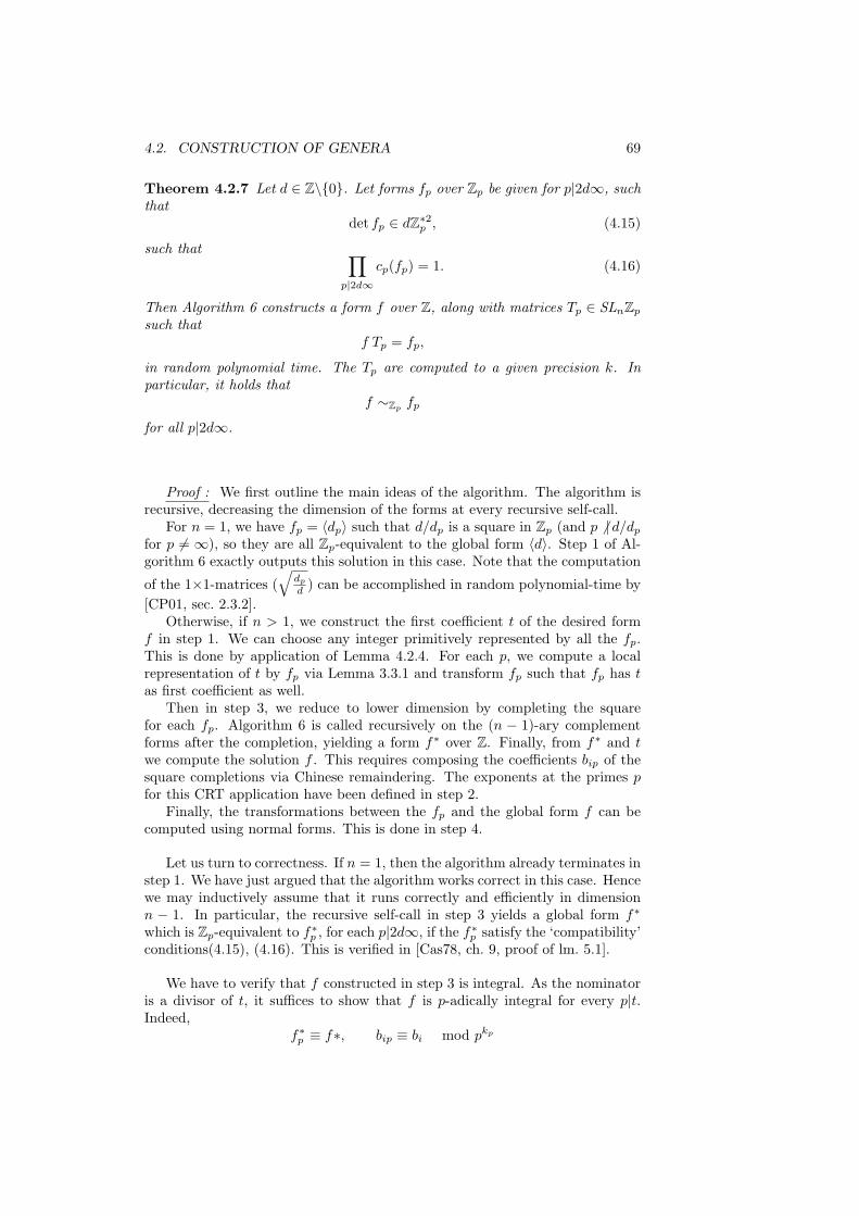
4.2. CONSTRUCTION OF GENERA 69
Theorem 4.2.7 Let d ∈ Z\0. Let forms fp over Zp be given for p|2d∞, suchthat
det fp ∈ dZ∗2p , (4.15)
such that ∏p|2d∞
cp(fp) = 1. (4.16)
Then Algorithm 6 constructs a form f over Z, along with matrices Tp ∈ SLnZp
such thatf Tp = fp,
in random polynomial time. The Tp are computed to a given precision k. Inparticular, it holds that
f ∼Zpfp
for all p|2d∞.
Proof : We first outline the main ideas of the algorithm. The algorithm isrecursive, decreasing the dimension of the forms at every recursive self-call.
For n = 1, we have fp = 〈dp〉 such that d/dp is a square in Zp (and p 6 | d/dp
for p 6= ∞), so they are all Zp-equivalent to the global form 〈d〉. Step 1 of Al-gorithm 6 exactly outputs this solution in this case. Note that the computation
of the 1×1-matrices (√
dp
d ) can be accomplished in random polynomial-time by[CP01, sec. 2.3.2].
Otherwise, if n > 1, we construct the first coefficient t of the desired formf in step 1. We can choose any integer primitively represented by all the fp.This is done by application of Lemma 4.2.4. For each p, we compute a localrepresentation of t by fp via Lemma 3.3.1 and transform fp such that fp has tas first coefficient as well.
Then in step 3, we reduce to lower dimension by completing the squarefor each fp. Algorithm 6 is called recursively on the (n − 1)-ary complementforms after the completion, yielding a form f∗ over Z. Finally, from f∗ and twe compute the solution f . This requires composing the coefficients bip of thesquare completions via Chinese remaindering. The exponents at the primes pfor this CRT application have been defined in step 2.
Finally, the transformations between the fp and the global form f can becomputed using normal forms. This is done in step 4.
Let us turn to correctness. If n = 1, then the algorithm already terminates instep 1. We have just argued that the algorithm works correct in this case. Hencewe may inductively assume that it runs correctly and efficiently in dimensionn − 1. In particular, the recursive self-call in step 3 yields a global form f∗
which is Zp-equivalent to f∗p , for each p|2d∞, if the f∗p satisfy the ‘compatibility’conditions(4.15), (4.16). This is verified in [Cas78, ch. 9, proof of lm. 5.1].
We have to verify that f constructed in step 3 is integral. As the nominatoris a divisor of t, it suffices to show that f is p-adically integral for every p|t.Indeed,
f∗p ≡ f∗, bip ≡ bi mod pkp
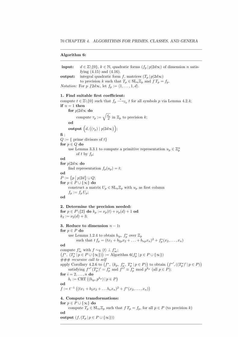
70 CHAPTER 4. ALGORITHMS FOR PRIMES, CLASSES, AND GENERA
Algorithm 6:
input: d ∈ Z\0, k ∈ N, quadratic forms (fp | p|2d∞) of dimension n satis-fying (4.15) and (4.16).
output: integral quadratic form f , matrices (Tp | p|2d∞)to precision k such that Tp ∈ SLnZp and f Tp = fp.
Notation: For p 6 | 2d∞, let fp := 〈1, . . . , 1, d〉.
1. Find suitable first coefficient:compute t ∈ Z\0 such that fp
∗−→Zp t for all symbols p via Lemma 4.2.4;if n = 1 then
for p|2d∞ do
compute τp :=√
dp
d in Zp to precision k;od
output(d,((τp) | p|2d∞
));
fi ;Q := prime divisors of tfor p ∈ Q do
use Lemma 3.3.1 to compute a primitive representation up ∈ Znp
of t by fp;odfor p|2d∞ do
find representation fp(up) = t;odP :=
p∣∣ p|2d
∪Q;
for p ∈ P ∪ ∞ doconstruct a matrix Up ∈ SLnZp with up as first columnfp := fp Up;
od
2. Determine the precision needed:for p ∈ P\2 do kp := νp(t) + νp(d) + 1 odk2 := ν2(d) + 3;
3. Reduce to dimension n− 1:for p ∈ P do
use Lemma 1.2.4 to obtain bip, f∗p over Zp
such that t fp = (tx1 + b2px2 + . . . + bnpxn)2 + f∗p (x2, . . . , xn)odcompute f∗∞ with f ∼R 〈t〉 ⊥ f∗∞;(f∗, (T ∗
p | p ∈ P ∪ ∞))
:= Algorithm 6(f∗p | p ∈ P ∪ ∞)### recursive call to selfapply Corollary 4.2.6 to
(f∗, (kp, f∗p , T ∗
p | p ∈ P ))
to obtain(f∗′, ((T ∗
p )′ | p ∈ P ))
satisfying f∗′ (T ∗p )′ = f∗p and f∗′ ≡ f∗p mod pkp (all p ∈ P );
for i = 2, . . . , n dobi := CRT
((bip, p
kp) | p ∈ P)
odf := t−1
((tx1 + b2x2 + . . . bnxn)2 + f∗(x2, . . . , xn)
)4. Compute transformations:for p ∈ P ∪ ∞ do
compute Tp ∈ SLnZp such that f Tp = fp, for all p ∈ P (to precision k)odoutput (f, (Tp | p ∈ P ∪ ∞))
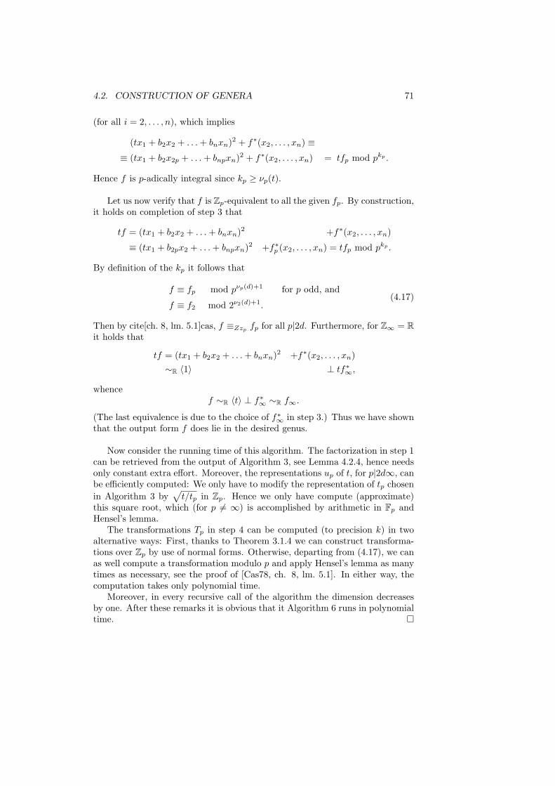
4.2. CONSTRUCTION OF GENERA 71
(for all i = 2, . . . , n), which implies
(tx1 + b2x2 + . . . + bnxn)2 + f∗(x2, . . . , xn) ≡≡ (tx1 + b2x2p + . . . + bnpxn)2 + f∗(x2, . . . , xn) = tfp mod pkp .
Hence f is p-adically integral since kp ≥ νp(t).
Let us now verify that f is Zp-equivalent to all the given fp. By construction,it holds on completion of step 3 that
tf = (tx1 + b2x2 + . . . + bnxn)2 +f∗(x2, . . . , xn)
≡ (tx1 + b2px2 + . . . + bnpxn)2 +f∗p (x2, . . . , xn) = tfp mod pkp .
By definition of the kp it follows that
f ≡ fp mod pνp(d)+1 for p odd, and
f ≡ f2 mod 2ν2(d)+1.(4.17)
Then by cite[ch. 8, lm. 5.1]cas, f ≡Zzpfp for all p|2d. Furthermore, for Z∞ = R
it holds that
tf = (tx1 + b2x2 + . . . + bnxn)2 +f∗(x2, . . . , xn)∼R 〈1〉 ⊥ tf∗∞,
whencef ∼R 〈t〉 ⊥ f∗∞ ∼R f∞.
(The last equivalence is due to the choice of f∗∞ in step 3.) Thus we have shownthat the output form f does lie in the desired genus.
Now consider the running time of this algorithm. The factorization in step 1can be retrieved from the output of Algorithm 3, see Lemma 4.2.4, hence needsonly constant extra effort. Moreover, the representations up of t, for p|2d∞, canbe efficiently computed: We only have to modify the representation of tp chosenin Algorithm 3 by
√t/tp in Zp. Hence we only have compute (approximate)
this square root, which (for p 6= ∞) is accomplished by arithmetic in Fp andHensel’s lemma.
The transformations Tp in step 4 can be computed (to precision k) in twoalternative ways: First, thanks to Theorem 3.1.4 we can construct transforma-tions over Zp by use of normal forms. Otherwise, departing from (4.17), we canas well compute a transformation modulo p and apply Hensel’s lemma as manytimes as necessary, see the proof of [Cas78, ch. 8, lm. 5.1]. In either way, thecomputation takes only polynomial time.
Moreover, in every recursive call of the algorithm the dimension decreasesby one. After these remarks it is obvious that it Algorithm 6 runs in polynomialtime.

72 CHAPTER 4. ALGORITHMS FOR PRIMES, CLASSES, AND GENERA
Part II
Classification with Respectto Complexity
73

Chapter 5
Cases of Low Complexity
In this chapter, we analyze various properties of quadratic forms and theirimpact on the complexity of the representation and transformation problems.In each case we will find that the properties in question either direclty reducecomplexity, or at least admit for polynomial-time reduction to smaller problems.
These findings serve as a confirmation that hard problems should be searchedfor among indefinite anisotropic forms, which are exactly those not occurringin this chapter; see Sect. 1.3.6. Therefore, the cryptographic applications ofChapter 2 have been proposed to use indefinite anisotropic forms.
Together with Chapters 6 and 7, this chapter forms the part of this thesiswhere we classify complexity of Repr and Trafo according to different ‘sorts’of forms: In Chapter 6, this is done with respect to the base ring, and in7 with respect to the dimension of forms. This and the mentioned chapterscomplement each other as forms with the properties studied here occur in everydimension, with the obvious exception of isotropic ternaries. Moreover, singularand reducible forms occur in every dimension over every base ring.
At first, in Sect. 5.1, we prove that the representation and transforma-tion problems for singular forms reduce to lower-dimensional problems. Subse-quently, in Sect. 5.2, the problems for reducible forms are reduced to factoriza-tion in the respective ring. These two sections are the only part of this theseswhere these two properties are not excluded, and they form the reason for thisrestriction. In Sect. 5.3, we explore complexity for definite forms, and finally inSect. 5.4 for isotropic (ternary) forms.
The definitions of the properties studied here can be found in Sect. 1.2.
5.1 Singular Forms
Recall that a form f is called singular if det f = 0. It is well-known (see[Gau89, art. 215] for forms over Z, [Cas78, ch. 2, sec. 6], [O’M63, §42C] forforms over a field) that singular forms actually arise as a lower-dimensionalform complemented by some linearly independent axes with value zero under
75
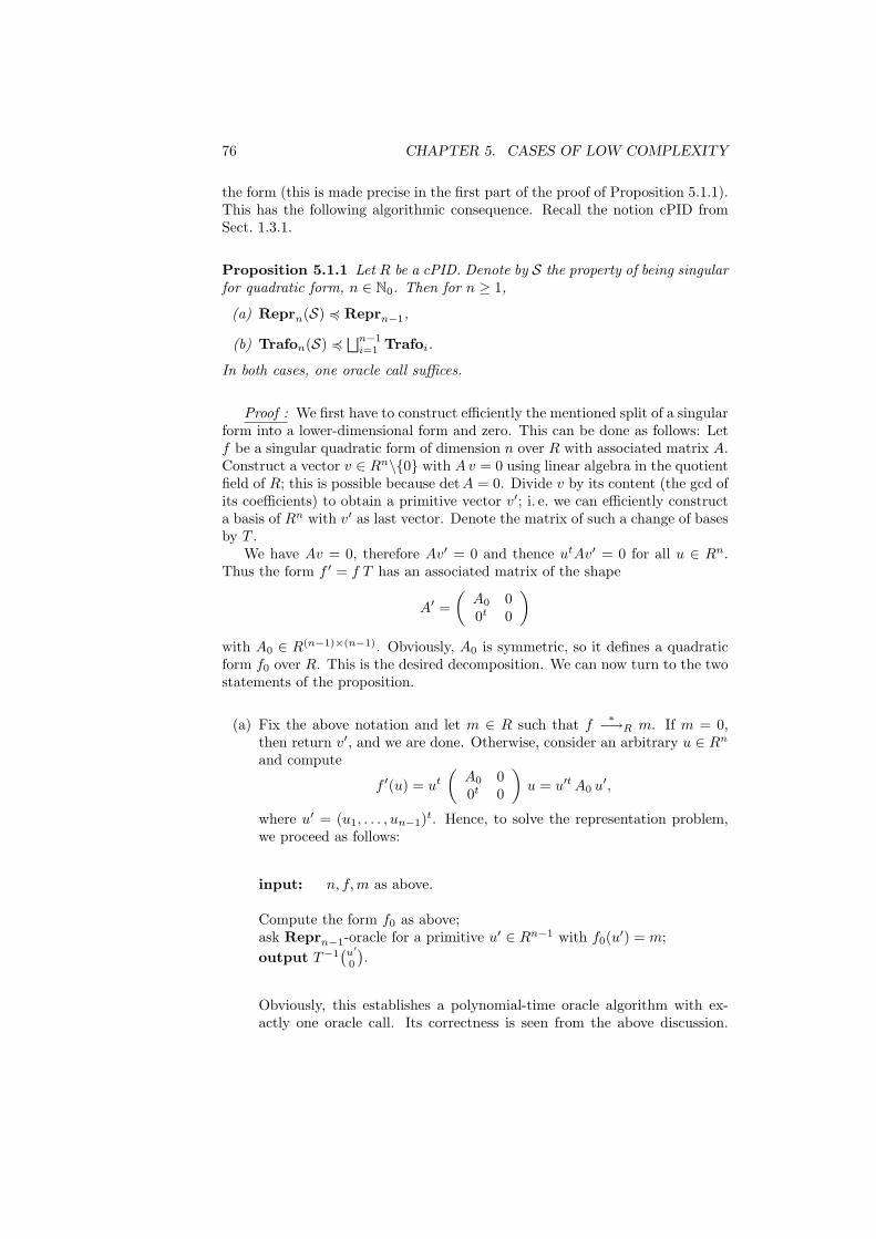
76 CHAPTER 5. CASES OF LOW COMPLEXITY
the form (this is made precise in the first part of the proof of Proposition 5.1.1).This has the following algorithmic consequence. Recall the notion cPID fromSect. 1.3.1.
Proposition 5.1.1 Let R be a cPID. Denote by S the property of being singularfor quadratic form, n ∈ N0. Then for n ≥ 1,
(a) Reprn(S) 4 Reprn−1,
(b) Trafon(S) 4⊔n−1
i=1 Trafoi.
In both cases, one oracle call suffices.
Proof : We first have to construct efficiently the mentioned split of a singularform into a lower-dimensional form and zero. This can be done as follows: Letf be a singular quadratic form of dimension n over R with associated matrix A.Construct a vector v ∈ Rn\0 with A v = 0 using linear algebra in the quotientfield of R; this is possible because det A = 0. Divide v by its content (the gcd ofits coefficients) to obtain a primitive vector v′; i. e. we can efficiently constructa basis of Rn with v′ as last vector. Denote the matrix of such a change of basesby T .
We have Av = 0, therefore Av′ = 0 and thence utAv′ = 0 for all u ∈ Rn.Thus the form f ′ = f T has an associated matrix of the shape
A′ =(
A0 00t 0
)with A0 ∈ R(n−1)×(n−1). Obviously, A0 is symmetric, so it defines a quadraticform f0 over R. This is the desired decomposition. We can now turn to the twostatements of the proposition.
(a) Fix the above notation and let m ∈ R such that f∗−→R m. If m = 0,
then return v′, and we are done. Otherwise, consider an arbitrary u ∈ Rn
and compute
f ′(u) = ut
(A0 00t 0
)u = u′t A0 u′,
where u′ = (u1, . . . , un−1)t. Hence, to solve the representation problem,we proceed as follows:
input: n, f, m as above.
Compute the form f0 as above;ask Reprn−1-oracle for a primitive u′ ∈ Rn−1 with f0(u′) = m;output T−1
(u′
0
).
Obviously, this establishes a polynomial-time oracle algorithm with ex-actly one oracle call. Its correctness is seen from the above discussion.
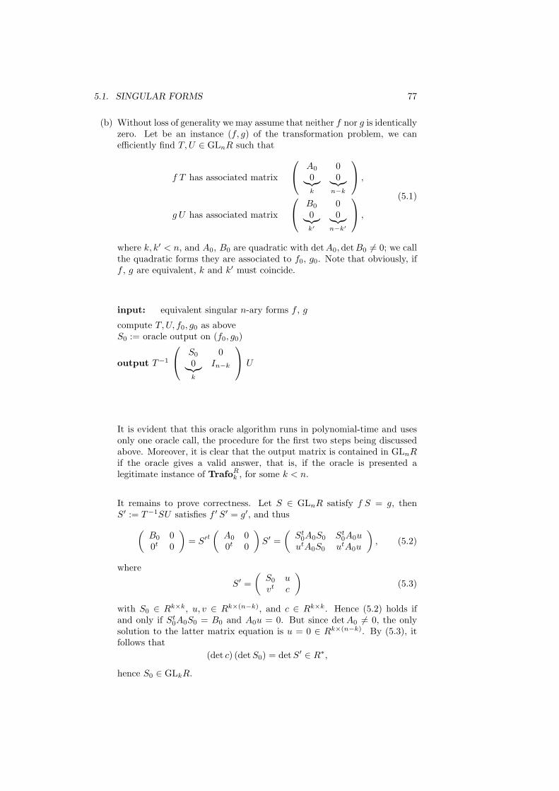
5.1. SINGULAR FORMS 77
(b) Without loss of generality we may assume that neither f nor g is identicallyzero. Let be an instance (f, g) of the transformation problem, we canefficiently find T,U ∈ GLnR such that
f T has associated matrix
A0 00︸︷︷︸k
0︸︷︷︸n−k
,
g U has associated matrix
B0 00︸︷︷︸k′
0︸︷︷︸n−k′
,
(5.1)
where k, k′ < n, and A0, B0 are quadratic with det A0,det B0 6= 0; we callthe quadratic forms they are associated to f0, g0. Note that obviously, iff , g are equivalent, k and k′ must coincide.
input: equivalent singular n-ary forms f , g
compute T,U, f0, g0 as aboveS0 := oracle output on (f0, g0)
output T−1
S0 00︸︷︷︸k
In−k
U
It is evident that this oracle algorithm runs in polynomial-time and usesonly one oracle call, the procedure for the first two steps being discussedabove. Moreover, it is clear that the output matrix is contained in GLnRif the oracle gives a valid answer, that is, if the oracle is presented alegitimate instance of TrafoR
k , for some k < n.
It remains to prove correctness. Let S ∈ GLnR satisfy f S = g, thenS′ := T−1SU satisfies f ′ S′ = g′, and thus(
B0 00t 0
)= S′
t(
A0 00t 0
)S′ =
(St
0A0S0 St0A0u
utA0S0 utA0u
), (5.2)
where
S′ =(
S0 uvt c
)(5.3)
with S0 ∈ Rk×k, u, v ∈ Rk×(n−k), and c ∈ Rk×k. Hence (5.2) holds ifand only if St
0A0S0 = B0 and A0u = 0. But since detA0 6= 0, the onlysolution to the latter matrix equation is u = 0 ∈ Rk×(n−k). By (5.3), itfollows that
(det c) (det S0) = det S′ ∈ R∗,
hence S0 ∈ GLkR.
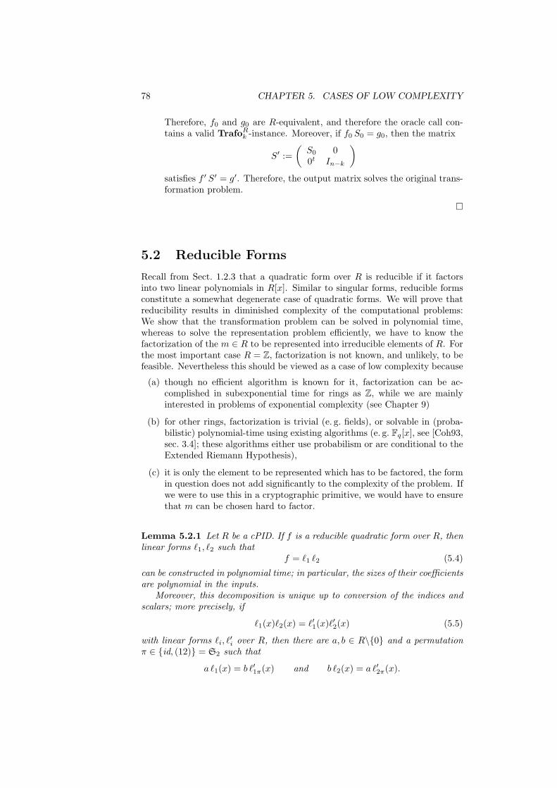
78 CHAPTER 5. CASES OF LOW COMPLEXITY
Therefore, f0 and g0 are R-equivalent, and therefore the oracle call con-tains a valid TrafoR
k -instance. Moreover, if f0 S0 = g0, then the matrix
S′ :=(
S0 00t In−k
)satisfies f ′ S′ = g′. Therefore, the output matrix solves the original trans-formation problem.
5.2 Reducible Forms
Recall from Sect. 1.2.3 that a quadratic form over R is reducible if it factorsinto two linear polynomials in R[x]. Similar to singular forms, reducible formsconstitute a somewhat degenerate case of quadratic forms. We will prove thatreducibility results in diminished complexity of the computational problems:We show that the transformation problem can be solved in polynomial time,whereas to solve the representation problem efficiently, we have to know thefactorization of the m ∈ R to be represented into irreducible elements of R. Forthe most important case R = Z, factorization is not known, and unlikely, to befeasible. Nevertheless this should be viewed as a case of low complexity because
(a) though no efficient algorithm is known for it, factorization can be ac-complished in subexponential time for rings as Z, while we are mainlyinterested in problems of exponential complexity (see Chapter 9)
(b) for other rings, factorization is trivial (e. g. fields), or solvable in (proba-bilistic) polynomial-time using existing algorithms (e. g. Fq[x], see [Coh93,sec. 3.4]; these algorithms either use probabilism or are conditional to theExtended Riemann Hypothesis),
(c) it is only the element to be represented which has to be factored, the formin question does not add significantly to the complexity of the problem. Ifwe were to use this in a cryptographic primitive, we would have to ensurethat m can be chosen hard to factor.
Lemma 5.2.1 Let R be a cPID. If f is a reducible quadratic form over R, thenlinear forms `1, `2 such that
f = `1 `2 (5.4)
can be constructed in polynomial time; in particular, the sizes of their coefficientsare polynomial in the inputs.
Moreover, this decomposition is unique up to conversion of the indices andscalars; more precisely, if
`1(x)`2(x) = `′1(x)`′2(x) (5.5)
with linear forms `i, `′i over R, then there are a, b ∈ R\0 and a permutation
π ∈ id, (12) = S2 such that
a `1(x) = b `′1π(x) and b `2(x) = a `′2π(x).
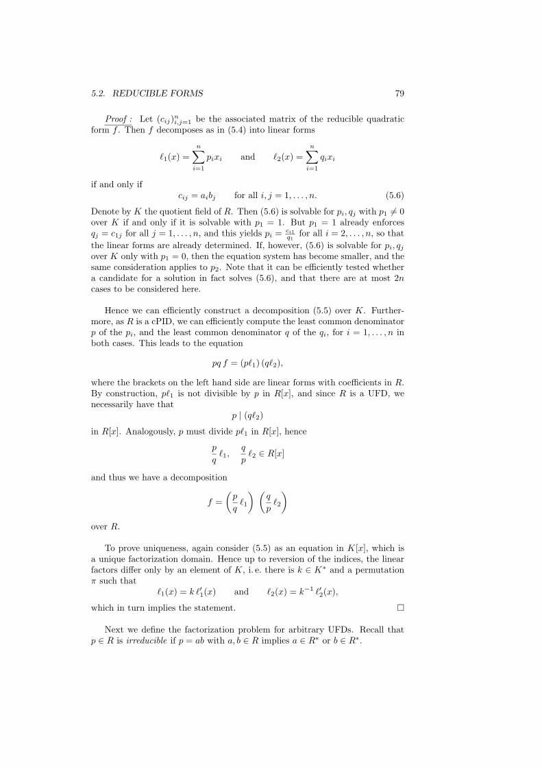
5.2. REDUCIBLE FORMS 79
Proof : Let (cij)ni,j=1 be the associated matrix of the reducible quadratic
form f . Then f decomposes as in (5.4) into linear forms
`1(x) =n∑
i=1
pixi and `2(x) =n∑
i=1
qixi
if and only ifcij = aibj for all i, j = 1, . . . , n. (5.6)
Denote by K the quotient field of R. Then (5.6) is solvable for pi, qj with p1 6= 0over K if and only if it is solvable with p1 = 1. But p1 = 1 already enforcesqj = c1j for all j = 1, . . . , n, and this yields pi = ci1
q1for all i = 2, . . . , n, so that
the linear forms are already determined. If, however, (5.6) is solvable for pi, qj
over K only with p1 = 0, then the equation system has become smaller, and thesame consideration applies to p2. Note that it can be efficiently tested whethera candidate for a solution in fact solves (5.6), and that there are at most 2ncases to be considered here.
Hence we can efficiently construct a decomposition (5.5) over K. Further-more, as R is a cPID, we can efficiently compute the least common denominatorp of the pi, and the least common denominator q of the qi, for i = 1, . . . , n inboth cases. This leads to the equation
pq f = (p`1) (q`2),
where the brackets on the left hand side are linear forms with coefficients in R.By construction, p`1 is not divisible by p in R[x], and since R is a UFD, wenecessarily have that
p | (q`2)
in R[x]. Analogously, p must divide p`1 in R[x], hence
p
q`1,
q
p`2 ∈ R[x]
and thus we have a decomposition
f =(
p
q`1
) (q
p`2
)over R.
To prove uniqueness, again consider (5.5) as an equation in K[x], which isa unique factorization domain. Hence up to reversion of the indices, the linearfactors differ only by an element of K, i. e. there is k ∈ K∗ and a permutationπ such that
`1(x) = k `′1(x) and `2(x) = k−1 `′2(x),
which in turn implies the statement.
Next we define the factorization problem for arbitrary UFDs. Recall thatp ∈ R is irreducible if p = ab with a, b ∈ R implies a ∈ R∗ or b ∈ R∗.
80 CHAPTER 5. CASES OF LOW COMPLEXITY
FactR Factorization problem over RPARAMETER: UFD R with encoding.INPUT: m ∈ R.OUTPUT: If m 6= 0 and m /∈ R∗, output r ∈ N, irreducible elements
pi ∈ R, and ei ∈ N, such that m =∏r
i=1 peii .
In particular, the existence of a polynomial-time algorithm for FactR impliesthat every m has a factorization where the sum of the encoding lengths of thepi and ei is polynomial in length (m); in particular, we must have
ω(m) = O(length (m)c) (5.7)
for some c > 0 (for R = Z, this condition holds with k = 1). By our conven-tion on oracles (see Sect. 1.1.4), any statement referring to a FactR-oracle isvacuously true if R fails to satisfy (5.7).
Moreover, recall that elements θ, η of a commutative ring R are called asso-ciated if there is a unit ε ∈ R∗ such that θ = εη. Obviously, this establishes anequivalence relation.
We can now formulate our result.
Proposition 5.2.2 Let R be a cPID. Denote by R the property of being re-ducible for a quadratic form. Then:
(a) TrafoR(R) is solvable in polynomial time.
(b) If R allows a polynomial-time algorithm which given a positive integer Cand a ring element θ ∈ R, enumerates all elements η ∈ R associated to θwith length (η) ≤ C, then
ReprR(R) 41 FactR.
Before turning to the proof let us discuss the additional condition of part(b), which stipulates efficient enumeration of associates. In particular, thisrequires the number of units is polynomially bounded. Obviously, cPIDs withonly finitely many units fulfill this property, as the rational integers Z, the ninerings of integers of imaginary quadratic fields (see Sect. 1.3.1), or the polynomialring in one variable over a finite field. Moreover, the criterion applies to ringswhose group of units possesses a finite set of generators from which the elementsgi, i = 1, . . . , r of infinite order satisfy the condition
length
(∏i
geii
)≥∑
i
eilength (gi) .
This criterion may be especially useful for the rings of integers of algebraicnumber fields.
It should also be noted that efficient enumeration of associates implies thatthere are only polynomially many for each θ ∈ R. But I am not aware of anyring in natural encoding where this condition is violated.
Proof :
5.2. REDUCIBLE FORMS 81
(a) Let f, g two equivalent reducible forms. By Lemma 5.2.1, we can efficientlyfactorize
f = `1 `2 and g = `′1 `′2.
Let T ∈ GLnR satisfy f T = g, which here means that
(`1 T ) (`2 T ) = `′1 `′2,
where (`i T )(x) := `i(Tx). The `i T are linear forms over R again; henceLemma 5.2.1 implies that there are a, b ∈ R\0 such that, without lossof generality,
a `1 T = b`′1 and b `2 T = a`′2. (5.8)
But for each a, b, this is just a system of 2n linear equations in n2 un-knowns. By hypothesis, it is solvable, and it can be efficiently solved overthe quotient field K of R with a, b as symbolic parameters. Finally, itcan be checked by computing least common denominators over R how thearising solutions can be lifted to R.
(b) For multiindices d = (d1, . . . , dr), e = (e1, . . . , er) ∈ Nr0 let us denote by
d ≤ e componentwise majorization of d by e, di ≤ ei for all i.
By Lemma 5.2.1, there is a polynomial P such that the lenghts of thecoefficients of the factors `1, `2 of f are bounded by P (length (f)). Con-sequently, if u ∈ Rn satisfies u ≤ K, then the sizes of `1, `2 are boundedby Q(length (f) + K) for some polynomial Q.
To hande the representation problem, perform the following algorithm:
input: reducible quadratic form f over R and m ∈ R.
decompose f = `1 `2 over R as in Lemma 5.2.1;factorize m =
∏ri=1 pei
i with ei ∈ N, pi pairwise non-associated primes in R;success := false; J := 1;while not success do
K :=⌈J (length (f) + length (m))J
⌉;
for α ∈ Nr0, α ≤ e do
put η :=∏r
i=1 qαii ;
for θ ∈ R associated to η s. t. length (θ) ≤ Q(length (f) + K) doif `1(u) = θ is not solvable for u in Rn then next; fi ;compute u(0), u(1), . . . , u(n−1) ∈ Rn s.t. u = u(0) +
∑n−1i=1 λiu
(i),with λi ∈ R, is the general solution of `1(u) = θ;
if mδ = `2(u(0)) +
∑n−1i=1 λi`2(u(i)) unsolvable for λi ∈ R then
next;else
fix a solution λi;success := true;
fi ;if success then fi ;
od ;
82 CHAPTER 5. CASES OF LOW COMPLEXITY
if success then fi ;od ;
if success then fi ;od ;output u := u(0) +
∑n−1i=1 λiu
(i).
Obviously this is a polynomial-time oracle algorithm with exactly oneFact-oracle call. To prove its correctness, note that in one iteration of thewhile loop, δ ranges exactly through all divisors of m of encoding lengthat most Q(length (f) + K) (for the current value of K). If
m = f(u) = `1(u) `2(u),
then obviously δ := `1(u) divides m in R, and
`1(x) = δ and `2(x) =m
δ. (5.9)
Moreover, as was discussed before the algorithm, if there is a solution uto the representation problem with length (u) ≤ K, then the encodinglength of δ from (5.9) is bounded by Q(length (f) + K) and thus occursin the enumeration.
Finally note that via the while loop, K attains any polynomial bound,and if there is a polynomial sized solution u, then the algorithm computesone after a constant number of while loop iterations.
5.3 Definite Forms
In this section, we report on the fact that for definite forms in fixed dimension,the transformation problem can be solved in polynomial time. The representa-tion problem, by contrast, stays hard, which can be seen from Theorem 9.1.6 andits discussion. The efficient solution of the transformation problem, however,already rules out the cryptographic applications from Chapter 2 for definiteforms.
The complexity of both the algorithm presented here as well as more recentimprovements depends heavily (i. e. more than simply exponentially) on n. Itis a vivid line of research to further reduce the running time (whithin exponen-tial bounds) in order to gradually increase the maximal dimension where suchalgorithms are still applicable in practice. But as we are primarily interested invery low fixed dimensions, mostly n ∈ 3, 4, the exact dependence on n doesnot make a difference for our applications; in addition to be polynomial-timein theory, the algorithms cited here run quite fast in practice still for higher
5.4. ISOTROPIC TERNARY FORMS 83
dimensions than 3,4 so that definite forms have to be ruled out for the schemesdiscussed in Chapter 2.
The first and essentially complete treatment of the problem to compute atransformation between given definite forms is given in [PP85] by Plesken andPohst. A discussion of this algorithm is also given in [PS85], where a majorimprovement, the fingerprint, is introduced. These publications are mainlyconcerned with the construction of nontrivial automorphisms of lattices, butessentially the same algorithms also work for transformations between differentequivalent lattices within the same time bounds.
These algorithms use as a subroutine the construction of a vector represent-ing the minimum of the form (a shortest vector), of which the first procedurewas given by Kannan [Kan87]; see [SH07] for current progressions in this field.
Together, these results show:
Theorem 5.3.1 (Plesken/Pohst/Souvignier) Let n ∈ N be fixed and de-note by D definiteness of a quadratic form. Then Trafon(D) is solvable inpolynomial time.
5.4 Isotropic Ternary Forms
Recall that a quadratic form is called isotropic if it represents zero. The Legen-dre equation
ax2 + by2 + cz2 = 0, (x, y, z) 6= 0
i. e. the problem of finding an isotropic vector for a ternary diagonal form, andthe question for a criterion for the isotropy of the form 〈a, b, c〉 have played animportant role in the history of the theory of quadratic forms.
As the results cited in this section show, the problems on isotropic three-dimensional forms are closely related to integer factorization with respect tocomplexity. This seems to be in striking contrast to anisotropic ternary andquaternary forms; cf. Sect. 7.1.3 and Chapter 9.
It should be noted that basic techniques of this section extend to higher-dimensional isotropic forms; however, they do not lead to complexity-theoreticimplications analogous to Theorem 5.4.3 beyond dimension three.
By convention, if a rational number u is written as u =∏
i peii with pi distinct
primes and ei ∈ Z, we will call this decomposition the factorization of u.In [Sim05a], Simon presents an algorithm which efficiently computes an iso-
tropic vector of an isotropic rational quadratic form once the factorization of itsdeterminant is given. For future reference, we write down a slight variant of hisresult adapted to our needs.
Theorem 5.4.1 (Simon) There is a polynomial-time algorithm which givenas input a rational isotropic quadratic form f of arbitrary dimension along withthe factorization of det f , constructs an integral isotropic vector for f .
84 CHAPTER 5. CASES OF LOW COMPLEXITY
Proof : Let k ∈ N be such that k f is an integral quadratic form. If k ischosen minimal, then obviously the knowledge of the factorization of det f alsoyields the factorization of det(kf). Moreover, a vector is isotropic for f if andonly if it is isotropic for k f .
Hence, we may apply Algorithm 7 from [Sim05a] which constructs an iso-tropic vector as desired.
Denote (temporarily) by Iso the problem of constructing an isotropic vec-tor of an input form. The problem of constructing an isotropic vector of aninput form is denoted Iso (see Sect. 1.3.3), where as usual, the missing ringsubscript is interpreted as referring to R = Z. Thus Simon’s algorithm boundsthe complexity of Iso from above by the complexity of factoring a rational num-ber, or, which is equivalent, integer factorization. We now turn to the oppositeargument, namely, a lower complexity bound for Iso, given by the problem ofextracting modular square roots. But as there seems to be no essentially betterway to extract square roots than to factor the module, and two essentially dif-ferent square roots yield a non-trivial factor of the module, the upper and lowerbounds we give on Iso can be considered close.
Sqrt Square root problemINPUT: N ∈ N such that −1 ∈ (Z/NZ)∗2.OUTPUT: s ∈ Z such that s2 ≡ −1 mod N .
Note that the condition on N can be rephrased as follows: Every odd primefactor p of N satisfies p ≡ 1 mod 4, and 4 6 |N .
Theorem 5.4.2 (Schnorr) There is a reduction Iso <1 Sqrt.More precisely, if −1 ∈ (Z/NZ)∗2, then the following problems are
polynomial-time equivalent:
1. compute a (nontrivial) isotropic vector of 〈1, 1,−N〉,
2. find a square root of −1 modulo N ,
3. represent N by the definite binary form 〈1, 1〉, i. e. as a sum of two squares.
Proof : See [Sch04a].
In the same paper it is shown, that
Theorem 5.4.3 (Schnorr)
(a) Let f be an isotropic ternary form representing m ∈ Z. If an isotropicvector is given, then a representation f(v) = m can be computed in poly-nomial time.
5.4. ISOTROPIC TERNARY FORMS 85
(b) Let f, g be equivalent isotropic ternary forms. If an isotropic vector isgiven for each of the two forms, then a transformation f S = g can becomputed in polynomial time.
Thus, in effect, both representation and transformation problems are at mostas hard as constructing an isotropic vector. Thus, the complexity of both prob-lems is close to that of factoring.
86 CHAPTER 5. CASES OF LOW COMPLEXITY
Chapter 6
The Impact of the BaseRing on Complexity
In this chapter, we will study the transformation and representation problemsover several rings different from the integers. We have already started whiththese investigations in Sections 3.2 and 3.3, concerning finite prime fields andthe rings of p-adic integers respectively.
We show that over the rational numbers, the complexity of the transfor-mation problem is closely related to factoring (as detailed in Sect. 6.1), andtherefore it can be solved in subexponential time.
Subsequently, we consider the representation problem over rings of formalpower series and polynomials. We analyse the question how closely the com-plexity of our problems is related to the complexity over the base field. Inparticular, for power series the problems are
6.1 Forms over the Rational Numbers
In this section, we will show that the transformation problem over the rationals isessentially equivalent to factoring the determinants of the forms involved. Moreprecisely, we show that TrafoQ is not harder than factoring, but at the sametime not easier that extracting square roots of −1 modulo some divisor of thedeterminant. This problem can be considered ‘almost equivalent’ to factoringbecause two essentially different square roots yield a non-trivial factor of themodulus, and because there seems to be no essentially better way to extractsquare roots than to factor the modulus.
Recall the definition of Fact, the factorization problem, from Sect. 5.2.
Let p, q ≡ 1 mod 4 be distinct primes, and let N := pq. Let us call such Ncounter-Blum integers (in analogy to the Blum integers N ′ = p′q′ with p′, q′ ≡3 mod 4). Recall that then the equation
x2 ≡ −1 mod N (6.1)
87
88 CHAPTER 6. THE IMPACT OF THE BASE RING ON COMPLEXITY
is solvable for every counter-Blum integer N . The integer factorization problemis not likely to become significantly easier if restricted to such numbers; compareit to the well-known hardness hypothesis for Blum integers [BBS86].
We will consider the problem of computing a solution x of (6.1). Note thatwe have considered a slightly more general problem in Sect. 5.4.
Imag Imaginary root problemINPUT: N ∈ N such that N = pq, with p, q primes ≡ 1 mod 4.OUTPUT: s ∈ Z such that s2 ≡ −1 mod N .
Theorem 6.1.1
(a) For n, s ∈ N, denote by I the properties f classically integral, binary,indefinite, and anisotropic for a quadratic form f . Then
Imag 1 TrafoQ(I).
(b)TrafoQ 41 FactZ.
For an instance (f, g) of TrafoQ, it suffices to call the oracle to factor(det f)(det g).
Proof :
(a) Let N be an instance of Imag, i. e. N = pq, with prime factors p, q ≡1 mod 4. Define
f := 〈1,−N〉, g := 〈−1, N〉.
Obviously, these are indefinite, and they are anisotropic since N is not aperfect square, see [Cas78, ch. 4, lm. 2.4]. We claim that f and g areQ-equivalent. Obviously, f and g are equivalent over the reals, as bothare R-equivalent to the form 〈1,−1〉. Moreover, we can compute Hasse-Minkowski invariants as follows. Recall the rules for the norm residuesymbols from Sect. 1.2.5. Let N = pq. Then
cp(f) =(
1, −N
p
)= 1,
and
cp(g) =(−1, N
p
)=(−1, p
p
) (−1, q
p
)︸ ︷︷ ︸
=1
=(−1p
)= 1.
An analogous computation works for q instead of p. Hence it follows fromthe Hasse Principle 1.2.11 that f ∼Q g.
Ask the oracle for S = (sij) ∈ GL2Q satisfying f S = g, i. e.
St
(1−N
)S =
(−1
N
),
6.1. FORMS OVER THE RATIONAL NUMBERS 89
whences211 − s2
21N = −1
Compute k ∈ N minimal such that σ11 := ks11, σ21 := ks21 are integers(via the Euclidean Algorithm). Write k = N `k0 with N 6 | k0. Then theequation
σ211 − σ2
21N = −k20 N2` (6.2)
holds in Z. We claim that we can assume ` = 0 without loss: Indeed,otherwise (6.2) implies σ11 = σ′11N for some σ′11 ∈ Z. Hence
(σ′11)2N − σ2
21 = −k20N
2`−1.
But now it follows that σ21 = σ′21N with σ′21 ∈ Z. Thus
(σ′11)2 − (σ′21)
2N = −k20 N2(`−1),
analogously to (6.2). Inductively we arrive at ` = 0.
Now (6.2) with ` = 0 implies
σ211 ≡ −k2
0 mod N. (6.3)
If γ := gcd(k0, N) 6= 1, then γ is p or q, and the factorization of N allowsto compute square roots of −1 modulo p and q, and combine them bymeans of the Chinese Remainder Theorem.
Otherwise, gcd(k0, N) = 1, and we can compute k ∈ Z such that k k0 ≡1 mod N . Then (6.3) implies that (σ11k)2 ≡ −1 mod N.
(b) Let (f, g) be an instance of TrafoQ, and let n := dim f . Then ϕ := f ⊥(−g) is isotropic.
Retrieve the factorization of det ϕ = (−1)n(det f)(det g) from the oracle.Then an algorithm by Simon ([Sim05a], see also [Sim05b]) constructs anisotropic vector (0, 0)t 6= (v1, v2)t ∈ Q2n for ϕ in deterministic polynomialtime. If f(v1) = 0 then also g(v2) = 0. At least one of the vi 6= 0, henceboth f and g are isotropic as f ∼ g. If v1 6= 0 6= v2, then these are isotropicvectors for f, g; if without loss v2 = 0, then the factorization of det g canbe employed again to construct a primitive isotropic vector v′2 for g. Nowif v1, v2 are isotropic vectors for f, g, it is easy and well-known that onecan find matrices Hi ∈ GLnQ with f H1 = h0 ⊥ f1 and g H2 = h0 ⊥ g1
for some (n− 2)-ary forms f1, g1, where h0 is the “hyperbolic plane” withassociated matrix
(0 11 0
), see [Cas78, ch. 2, lm. 2.1 and its cor. 1]. By Witt’s
lemma (Lemma 1.2.5), f1 ∼Q g1 holds. We recursively call the procedureoutlined here, yielding eventually a transformation f1S = g1. Then return
T := H1
11
S
H−12
since then f T = g.
90 CHAPTER 6. THE IMPACT OF THE BASE RING ON COMPLEXITY
If, however, a := f(v1) 6= 0, then also g(v2) = a. Find two bases of Qn withv1, respectively v2, as first vector. Thus we obtain matrices Ui ∈ GLnQwith
f U1 = 〈a〉 ⊥ f2 and g U2 = 〈a〉 ⊥ g2
for (n− 1)-ary forms f2,g2, and if the recursion produces f2S = g2,then output T := U1
(1 00 S
)U−1
2 .
Finally, this recursion will be called at most n times so that we haveestablished a polynomial-time algorithm.
We will reuse the technique from part a) in Chapter 8.
6.2 Rings of Formal Power Series
6.2.1 Introduction and summary of results
We have seen in Sections 3.2 and 6.1 that the transformation and representationproblems are relatively easy over the fields F and Q. It is natural to ask whetherthese problems are any harder over the polynomial rings F[x] or Q[x], or, moregenerally, over the polynomial ring of an arbitrary field K. We will come backto this question in Sect. 6.3; for now we show that over rings of formal powerseries, representations are no harder to compute than over the ground field.
Given a commutative ring R, the ring of formal power series over R, denotedR[[x]], is the set of all
∞∑i=0
aixi,
where ai ∈ R, and x /∈ R is a variable. We will not write out quadratic formsexplicitly in this section, so there should be not confusion with the variables ofthe quadratic form.
The algebraic operations are defined in the following natural way:( ∞∑i=0
aixi
)+
( ∞∑i=0
bixi
)=
∞∑i=0
(ai + bi)xi
and ( ∞∑i=0
aixi
) ( ∞∑i=0
bixi
)=
∞∑i=0
i∑j=0
ajbi−jxi.
Turning to algorithmic questions, power series are not directly suitable forfinite encoding because a single series involves an infinitude of coefficients. Butsimilar to real, or p-adic, numbers, we can approximate ring elements up to
6.2. RINGS OF FORMAL POWER SERIES 91
a certain desired precision. By convention, determining an element∑
i aixi ∈
R[[x]] to precision D ∈ N0 means to find its coefficients a0, . . . , aD.More generally, we can consider the question whether there is is an approxi-
mative solution to a problem up to precision D; this is equivalent to computingin the ring
R[[x]]/(xD+1) ∼= R[x]/(xD+1).
So if we talk about algorithms and computational problems over power seriesrings, we always assume that the input includes the specification of the desiredprecision D (e. g. by the unary string 1D). An algorithm may then read apolynomial number of coefficients of the input power series, where polynomialmeans polynomial in D.
On the other hand, we assume that we can do exact arithmetic in the groundfield. Therefore, the term ‘precision’ will have a unique meaning.
We first state our result on the ring of formal power series. Recall the defi-nition of the computational problems from Sect. 1.3 and that of their decisionalanalogues from Sect. 3.1.
Theorem 6.2.1 Let K be a field of characteristic 6= 2.
(a) Let D ∈ N0 be given. Then the decisional representation problems overK, and over K[[x]] to precision D are Karp-equivalent. Likewise, thecomputational representation problems are polynomial-time equivalent forone oracle call each. In other words:
DReprK[x]/(xD+1)n ≈K DReprK
n
andReprK[x]/(xD+1)
n ≈1 ReprKn .
(b) If K is infinite, then
DReprK[[x]]n ≈K DReprK
n and ReprK[[x]]n ≈1 ReprK
n .
6.2.2 Upper bounds
We start by proving the following arithmetic rules for matrices over rings ofpower series.
Lemma 6.2.2 Let R be a ring with encoding. Let X ∈ R[[x]]l1×l2 , Y ∈R[[x]]l2×l3 , Z ∈ R[[x]]l1×l3 and let
X =∞∑
i=0
Xixi, Y =
∞∑i=0
Yixi, Z =
∞∑i=0
Zixi
with Xi ∈ Rl1×l2 , Yi ∈ Rl2×l3 , and Zi ∈ Rl1×l3 for i ∈ N0.
92 CHAPTER 6. THE IMPACT OF THE BASE RING ON COMPLEXITY
(a) Let X Y = Z. Then
Zq =q∑
ν=0
XνYq−ν .
In particular, Z0 = X0 Y0.
(b) Let Xt =∑∞
i=0 X ′ix
i. Then X ′i = Xt
i for all i ∈ N0.
(c) Let XtY X = Z. Then
Zq =∑
λ,µ,ν∈N0λ+µ+ν=q
XtλYµXν .
Proof :
(a) Induction over q.
(b) Trivial.
(c) Follows from a) and b).
Note that it follows immediately from part b) that for associated matricesA =
∑∞p=0 Apx
p, Ap ∈ Rn×n of quadratic forms all Ap are symmetric.
Proposition 6.2.3Let K be a field with encoding, not of characteristic 2. Let n ∈ N. Then
(a) DReprKn 4K DReprK[[x]]
n ;
(b) ReprKn 41 ReprK[[x]]
n ;
(c) DTrafoKn 4K DTrafoK[[x]]
n ;
(d) TrafoKn 41 TrafoK[[x]]
n .
Proof :
a) and b) Let f be an n-ary form over R and let M ∈ R. Obviously, if f −→R M ,then also f −→R[[x]] M because R ⊆ R[[x]]. Conversely, let u ∈ R[[x]]n
with u =∑∞
p=0 upxp, up ∈ Rn, satisfy f(u) = M . If A is the associated
matrix of f , then, by Lemma 6.2.2, we have ut0Au0 = M and therefore
already f(u0) = M .
Thus we have shown that f −→R M if and only if f −→R[[x]] M . There-fore, to decide whether M is represented by f over R for part a), it sufficesto pass the instance over to the DReprR[x]
n -oracle, which can be done intime O(1).
In the same vein, on query (f,M), the ReprR[[x]]n -oracle will respond
with u =∑D
p=0 upxp (for some desired precision D ≥ 0), up ∈ Rn, with
f(u) = M . By the above argument, it follows that f(u0) = M .
6.2. RINGS OF FORMAL POWER SERIES 93
c) and d) Let f, g be n-ary forms over R. Obviously, if f ∼R g, then also f ∼R[[x]] g.Conversely, let T ∈ GLnR[[x]] with T =
∑∞p=0 Tpx
p, Tp ∈ Rn×n, satisfyf T = g. So if A,B are the associated matrices of f, g respectively, then,by Lemma 6.2.2, we have T t
0AT0 = B and therefore already f T0 = g.
Thus we have shown that f ∼R g holds if and only if f ∼R[[x]] g. Therefore,to decide equivalence over R for part c), it suffices to pass the instanceover to the DTrafoR[[x]]
n -oracle, which can be done in time O(1).
Pass (f, g) to the TrafoR[[x]]n -oracle. It will output T =
∑Dp=0 Tpx
p forsome D, Tp ∈ Rn×n, with f T = g. By the above argument, it holds thatf T0 = g. Finally note that T0 can be extracted from T in time linear inthe encoding length of T .
Remark. It can be read off from the proof that analogous assertions hold forgeneral representations of k-ary forms by n-ary forms, see [Min11]. Of these,we have covered the cases k = 1, i. e. representations in our (narrower) sense,and k = n, i. e. transformations.
6.2.3 Lower bounds for representations
We now turn to the more involved converse reductions.
Lemma 6.2.4 Let K be a field with encoding, not of characteristic 2. Let f bean n-dimensional quadratic form over K[[x]], let M ∈ K[[x]], q ∈ N, q < |K|and let u ∈ K[[x]]n satisfy
f(u) ≡M mod xq.
Then there is u ∈ K[x]n such that
f(u) ≡M mod xq+1 and u ≡ u mod xq.
The coefficient vectos at xq of all possible vectors u form an affine space overK. A parametrization of this affine space can be computed in polynomial-time(with respect to to the encodings of M , u, and f).
In particular, one such vector u can be computed in polynomial time.
Proof : Denote by
A =∞∑
p=0
Apxp
the associated matrix of the form f , Ap ∈ Kn×n symmetric. Similarly, let
M =∞∑
p=0
Mpxp and u =
∞∑p=0
upxp
94 CHAPTER 6. THE IMPACT OF THE BASE RING ON COMPLEXITY
with Mp ∈ K and up ∈ Kn for p ∈ N0. Then by Lemma 6.2.2, we have∑λ,µ,ν∈N0λ+µ+ν=q
utλAµuν = Mp
for all p = 0, . . . , D.We may assume that M0 6= 0. Namely, the statement holds for M if and
only if it holds for M replaced by the polynomial
M ′ :=q∑
i=0
Mixi.
So without loss M is a polynomial of degree at most q and not identically zero.Hence substituting q+1 arbitrary pairwise distinct values from K into M yieldsat most one t ∈ K for which M(t) 6= 0. But replacing A, M , and u by A(x− t),M(x− t), and u(x− t) leaves us with the case M0 6= 0 above. This is possiblesince q < |K|.
Now by hypothesis f(u) ≡ M mod xq with q ≥ 1, which by Lemma 6.2.2and equating coefficients yields
ut0A0u0 = M0 6= 0.
This implies that A0u0 6= 0, and hence that the bilinear form x 7→ xtA0u0 onKn is nondegenerate.
Let
U :=12
Mq −∑
λ+µ+ν=qλ, ν<q
utλAµuν
. (6.4)
By the last paragraph, there is v ∈ Kn such that
U = vtA0u0. (6.5)
Obviously, the set of all such v forms an affine space which can be computed bystandard efficient linear algebra.
For such a vector v, define u ∈ (K[x])n by
up :=
0 if p > q,v if p = q,up else.
(6.6)
Then by construction u is a polynomial (rather than a series),
u ≡ u mod xq,
and thereforef(u) ≡ f(u) ≡M mod xq. (6.7)
6.2. RINGS OF FORMAL POWER SERIES 95
Hence it only remains to compute the q-th coefficient of utAu. By Lemma 6.2.2,this coefficient equals∑
λ+µ+ν=q
uλAµuν = vtA0u0 + (vtA0u0)t +∑
λ+µ+ν=qλ, ν<q
utλAµuν
= 2U +∑
λ+µ+ν=qλ, ν<q
utλAµuν
= Mq,
the second equality being due to (6.5) and the last one to (6.4). Therefore
f(u) ≡M mod xq+1,
as was to be shown.
The same argument also shows that the set of q-th components of all possibleu satisfying the claim arise from the different solutions v of (6.5). As was arguedthere, this is is an affine space over K.
Proposition 6.2.5 Let K be a field not of characteristic 2.
(a) Given D ∈ N0, a quadratic form f over K[[x]], and M ∈ K[[x]]\0, andaccess to a DReprK
n -oracle, it can be decided in polynomial time whetherM can be represented up to precision D, and such an approximative rep-resentation can be computed in polynomial time; in other words:
DReprK[x]/(xD+1)n 4K DReprK
n and ReprK[x]/(xD+1)n 41 ReprK
n .
(b) If K is infinite, then
DReprK[[x]]n 4K DReprK
n and ReprK[[x]]n 41 ReprK
n .
Proof :
(a) First consider the computational problem. If D < |K|, ask the oracle forthe solution of the scalar problem modulo x. Then we can inductivelyapply Lemma 6.2.4 for D times to obtain a solution modulo xD+1. If,however, D ≥ |K|, then an exhaustive search on K[x]/(xD+1) takes onlypolynomial time.
For the decision problem, it follows directly from the last paragraph that ifD < |K|, then the problem modulo xD+1 is solvable if and only if the scalarproblem modulo x is (see Proposition 6.2.3). In case D ≥ |K|, perform anexhaustive search, and observe whether a solution can be found.
96 CHAPTER 6. THE IMPACT OF THE BASE RING ON COMPLEXITY
(b) If K is infinite, then a solution to the scalar problem modulo x can belifted inductively by Lemma 6.2.4 to arbitrarily high degrees; hence arepresentation over K[[x]] exists if and only if one exists for the scalarproblem (again see Proposition 6.2.3). Moreover, up to a given precisionD such a solution can be found by iterative application of Lemma 6.2.4.
Together with Proposition 6.2.3, this proves Theorem 6.2.1.
6.3 Polynomial Rings
In this section, we analyze the complexity of the representation problem whenreplacing the coefficient ring with its ring of polynomials (in some finite numberof variables). It turns out that as a lower bound, we can only give the problemof solving simultaneous quadratic equations.
Simultaneous representation problem over R, SReprRn
INPUT: r ∈ N, quadratic forms (fi | i = 1, . . . , r) of dimension n,and mi ∈ Rr such that there is u ∈ Rn\0 satisfying fi(u) = mi.
OUTPUT: Vector u ∈ Rn such that fi(u) = mi for all i.
Analogously, we define the decision problem DSReprRn .
It should be noted that DSRepr is undecidable over Z [Mat93, sec. 1.2], andthus also SRepr may be much harder than Repr for many rings R. However,this is not the case in general: For K an algebraically closed field, for instance,SReprK
n can be solved using techniques from algebraic geometry (cf. Bezout’sTheorem [Sha74, §IV.2.1]).
Theorem 6.3.1 Let K be a field with encoding, not of characteristic 2. Letn ∈ N. Then
(a) DSReprKn < DReprK[x]
n <K DReprKn ,
(b) SReprKn < ReprK[x]
n <1 ReprKn .
The remainder of this section is devoted to the proof of Theorem 6.3.1. Asfor power series, we can directly infer:
Proposition 6.3.2Let K be a field with encoding, not of characteristic 2. Let n ∈ N. Then
(a) DReprKn 4K DReprK[x]
n ;
(b) ReprKn 41 ReprK[x]
n , and one oracle call suffices;
6.3. POLYNOMIAL RINGS 97
(c) DTrafoKn 4K DTrafoK[x]
n ;
(d) TrafoKn 41 TrafoK[x]
n , where one oracle call suffices.
Proof : Analogous to Proposition 6.2.3.
As R[x] is a subring of R[[x]], Lemma 6.2.2 can still be applied to matriceswith polynomial coefficients. We can simply consider these polynomials as powerseries whose coefficients all vanish but finitely many.
Lemma 6.3.3 Let K be a field with encoding, not of characteristic 2. Let fbe an n-dimensional quadratic form over K[x], let M ∈ K[x], q, k ∈ N and letu ∈ K[x]n satisfy
f(u) ≡M mod xq.
Then there is u ∈ K[x]n such that
f(u) ≡M mod xq+k (6.8)
andu ≡ u mod xq. (6.9)
The set
uq
...uq+k−1
∈ Kk∣∣∣ u :=
q−1∑i=0
uixi +
r+k−1∑i=q
uixi
satisfies (6.8), (6.9)
=: M (6.10)
forms an affine space over K. A parametrization of this affine space can becomputed in polynomial time.
In particular, one such vector u can be computed in polynomial time.
Proof : The first statement follows from Lemma 6.2.4 by an easy inductionon k. We only have to show that M of (6.10) is an affine space over K.
From Lemma 6.2.4, we know that when lifting the exponent of x by one, weobtain an affine space as set of q-th components, i. e. the set of solutions of a(possibly inhomogeneous) system of linear equations.
Now employ induction on k again. Suppose we already know that
uq
...uq+k−2
∈ Kk−1∣∣∣ u :=
q−1∑i=0
uixi +
r+k−2∑i=q
uixi satisfies
f(u) ≡M mod xq+k−1 and (6.9)
=: M′ (6.11)
98 CHAPTER 6. THE IMPACT OF THE BASE RING ON COMPLEXITY
is an affine space over K, and that we know a parametrization
M′ = w + C Kk−1,
where w ∈ Kk−1 and C ∈ K(k−1)×(k−1), not necessarily regular. Proceedaccording to the proof of Lemma 6.2.4. The newly added component in (6.10)depends affine linearly jointly on all the the uq, . . . , uq+k−2, v = uq+k−1. Asthe composition of affine functions is affine, the set M from the statement isaffine-linear as well.
For the application of Lemma 6.3.3 to polynomials, we do not only have tolift to a correct solution modulo higher powers of the variable, but also to ensurethat this lifting process will terminate after some finite number of steps.
For a vector v ∈ K[x]n, define its degree by deg v := maxni=0 deg(vi). Anal-
ogously, we define the degree of a matrix over K[x]. By the degree deg f ofa form f we mean the degree of its associated matrix; this should lead to noconfusion since we only consider quadratic forms.
Lemma 6.3.4 Let K be a field with encoding, not of characteristic 2. Let f bean n-dimensional quadratic form over K[x], let M ∈ K[x], deg M ≤ q, k ∈ Nand let u ∈ K[x]n satisfy
f(u) ≡M mod xq.
Moreover, let u ∈ K[x]n with deg u ≤ q − 1 satisfy u ≡ u mod xq.
Then the equationf(u) = M
over K[x] is equivalent to a system of linear equations and (deg f) + q − 1 qua-dratic equations over K. These quadratic equations correspond to representationproblems for the forms f0, . . . , fdeg f via Proposition 1.2.1.
Proof : By the aid of Lemma 6.2.2, consider the (infinitely many) equationswhich arise by equating coefficients in f(u) = M at like powers of x. Byhypothesis, we have Mi = 0 and ui = 0 for all i ≥ q; hence it can be easilyverified that the equations are automatically satisfied from degree (deg f)+2q−1onwards. The remaining equations are, of course, at most quadratic; moreprecisely, they are quadratic up to degree (deg f) + q and linear afterwards.The homogeneous part of the quadratic ones are exactly the scalar forms fi,i = 1, . . . ,deg f , where
f =deg f∑i=0
fixi.
By Proposition 1.2.1, these conditions correspond to a system of linear equationsand representation problems with respect to the fi. Since we are working over
6.3. POLYNOMIAL RINGS 99
a field, the linear modular equations can be omitted.
This concludes the proof of the the lower bound in Theorem 6.3.1: To solveReprK[[x]], we ask the oracle for the solution of the scalar problem (a singlerepresentation problem over K), and lift this solution via Lemma 6.3.4, whichrequires another oracle call.
Together with Proposition 6.3.2, this proves Theorem 6.3.1.

100CHAPTER 6. THE IMPACT OF THE BASE RING ON COMPLEXITY
Chapter 7
Complexity for VaryingDimension
In this chapter, we turn back to quadratic forms over Z, and analyze howcomplexity of the transformation problem changes with varying dimension. Itwill turn out that if Trafo is hard, then it is still hard if restricted to ternaryand quaternary forms. This is particularly promising because this allows forsmall keys in cryptography, and because there are many anisotropic classes inthese dimensions which do not allow for an attack as in Sect. 5.4.
7.1 Dimension Shift to Ternary and QuaternaryForms
7.1.1 Introduction and result
In this section, we prove that in fixed dimension n ≥ 3, computing transforma-tions is no harder than in small dimension, i. e. three or four. This shows thatif computing transformations is hard for any bounded dimension n ≥ 3 at all,then it is necessarily hard in dimensions 3, 4.
Instead of Trafo, we will consider the problem FTrafo. They differ onlyby an additional input in FTrafo: For an instance (f, g), the factorization ofdet f is given for free. This modification will be motivated in Chapter 8. Wewill, however, suppress this extra information in writing down instances. Thisshould not lead to any confusion.
Theorem 7.1.1 Let n ≥ 5, and let d ∈ Z be odd and squarefree. Then
FTrafon(d) 1 FTrafon−2(d).
Remark. Note that the converse of Theorem 7.1.1 is not obvious: Suppose
101
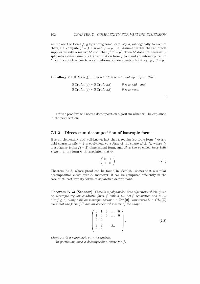
102 CHAPTER 7. COMPLEXITY FOR VARYING DIMENSION
we replace the forms f , g by adding some form, say h, orthogonally to each ofthem; i. e. compute f ′ = f ⊥ h and g′ = g ⊥ h. Assume further that an oraclesupplies us with a matrix S′ such that f ′ S′ = g′. Then S′ does not necessarilysplit into a direct sum of a transformation from f to g and an automorphism ofh, so it is not clear how to obtain information on a matrix S satisfying f S = g.
Corollary 7.1.2 Let n ≥ 5, and let d ∈ Z be odd and squarefree. Then
FTrafon(d) FTrafo3(d) if n is odd, andFTrafon(d) FTrafo4(d) if n is even.
For the proof we will need a decomposition algorithm which will be explainedin the next section.
7.1.2 Direct sum decomposition of isotropic forms
It is an elementary and well-known fact that a regular isotropic form f over afield characteristic 6= 2 is equivalent to a form of the shape H ⊥ f0, where f0
is a regular ((dim f) − 2)-dimensional form, and H is the so-called hyperbolicplane, i. e. the form with associated matrix(
0 11 0
). (7.1)
Theorem 7.1.3, whose proof can be found in [Sch04b], shows that a similardecomposition exists over Z; moreover, it can be computed efficiently in thecase of at least ternary forms of squarefree determinant.
Theorem 7.1.3 (Schnorr) There is a polynomial-time algorithm which, givenan isotropic regular quadratic form f with d := det f squarefree and n :=dim f ≥ 3, along with an isotropic vector v ∈ Zn\0, constructs U ∈ GLn(Z)such that the form f U has an associated matrix of the shape
0 1 0 . . . 01 0 0 . . . 00 0...
... A0
0 0
, (7.2)
where A0 is a symmetric (n× n)-matrix.In particular, such a decomposition exists for f .
7.2. BINARY FORMS 103
Remark. It is not usual to call the integral form H with associated ma-trix (7.1) a hyperbolic plane; this term is resticted to forms over fields. Thisdistinction is motivated by the fact that over a field of characteristic 6= 2, thehyperbolic plane is, up to equivalence, the only isotropic binary form of non-zero determinant. This does not hold for H over Z as there are infinitely many
such Z-classes (e. g. for all a ∈ N, the form with associated matrix(
0 aa 0
)).
However, binary isotropic forms over Z can be called “lattices on the (rational)hyperbolic plane”.
7.1.3 Conclusion of the proof
We can now finish the proof of Theorem 7.1.1.
Proof of Theorem 7.1.1: Let (f, g) be an instance ofFTrafon(d). If they are definite the problem can be solved by use of Theo-rem 5.3.1 (note that n is fixed). So suppose they are indefinite. By Meyer’sTheorem 1.2.12, the form f is isotropic since n ≥ 5.
By Simon’s algorithm ([Sim05a, Algorithm 7]), we can use our knowledge ofthe factorization of d = det f = det g to construct an isotropic vector for eachform. As d is squarefree, we can apply Theorem 7.1.3 to efficiently computeS1, S2 ∈ GLn(Z) with
f S1 = h ⊥ f0 and g S2 = h ⊥ g0
where h is the form with associated matrix (7.1). Now by Witt’s lemma forp-adic integers Lemma 1.2.5, f0 ∼Zp g0 for all symbols p 6= 2. Since d is odd, itfollows by Proposition 1.2.17 that f0 ∼g g0. Now we deduce that f ∼ g fromTheorem 1.2.18 because dim f0 ≥ 3 and d has no multiple prime divisors.
Obviously, if the oracle outputs T ∈ GLnZ with f0 T = g0, then a solutionS of the original problem is readily computed via S := S1(I2 ⊕ T )S−1
2 , whereI2 ∈ GL2Z is the identity matrix.
7.2 Binary Forms
In [Gau89, art. 171–182], Gauß gave an algorithm for the transformation prob-lem on indefinite binary quadratic forms. This algorithm has been extensivelystudied (see [Sha72], [Lag80], [Len82], [BB97]). It does not necessarily termi-nate in polynomial time; however, the running time is polynomial in the size ofa minimal solution.
In a crytographic setting as in Chapter 2, a solution to the Trafo-instance(f, g) is used as the secret key. An upper bound B on the length of the keysis a public parameter. Hence Gauß’ algorithm extracts the secret key from the
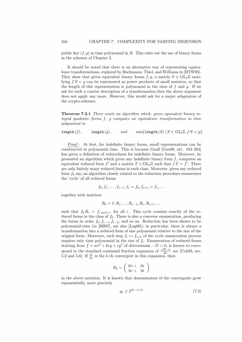
104 CHAPTER 7. COMPLEXITY FOR VARYING DIMENSION
public key (f, g) in time polynomial in B. This rules out the use of binary formsin the schemes of Chapter 2.
It should be noted that there is an alternative way of representing equiva-lence transformations, explored by Buchmann, Thiel, and Williams in [BTW95].They show that given equivalent binary forms f, g, a matrix S ∈ GL2Z satis-fying f S = g can be represented as power products of small matrices, so thatthe length of this representation is polynomial in the sizes of f and g. If weask for such a concise description of a transformation then the above argumentdoes not apply any more. However, this would ask for a major adaptation ofthe crypto-schemes.
Theorem 7.2.1 There exists an algorithm which, given equivalent binary in-tegral quadratic forms f , g computes an equivalence transformation in timepolynomial in
length (f) , length (g) , and minlength (S) |S ∈ GL2Z, f S = g.
Proof : At first, for indefinite binary forms, small representations can beconstructed in polynomial time. This is because Gauß [Gau89, art. 183–204]has given a definition of reducedness for indefinite binary forms. Moreover, hepresented an algorithm which given any indefinite binary form f , computes anequivalent reduced form f ′ and a matrix T ∈ GL2Z such that f T = f ′. Thereare only finitely many reduced forms in each class. Moreover, given any reducedform f0 say, an algorithm closely related to the reduction procedure enumeratesthe ‘cycle’ of all reduced forms
f0, f1, . . . , fe−1, fe = f0, fe+1 = f1, . . .
together with matrices
R0 = I,R1 . . . , Re−1, Re, Re+1 . . .
such that f0 Ri = fi mod e, for all i. This cycle consists exactly of the re-duced forms in the class of f0. There is also a converse enumeration, producingthe forms in order f0, fe−1, fe−2, and so on. Reduction has been shown to bepolynomial-time (in [BB97], see also [Lag80]); in particular, there is always atransformation into a reduced form of size polynomial relative to the size of theoriginal form. Moreover, each step fi 7→ fi+1 of the cycle enumeration processrequires only time polynomial in the size of fi. Enumeration of reduced formsstarting from f = ax2 + bxy + cy2 of determinant −D < 0, is known to corre-spond to the standard continued fraction expansion of
√D−b2a , see [Coh93, sec.
5.2 and 5.6]: If pk
qkis the k-th convergent in this expansion, then
Rk =(
pk−1 pk
qk−1 qk
)in the above notation. It is known that denominators of the convergents growexponentially, more precisely
qk ≥ 2(k−1)/2 (7.3)
7.2. BINARY FORMS 105
see [Per54]. Hence, the size of the Rk grows exponentially in k.Now let f , g be two equivalent indefinite binary forms linked by an (un-
known) transformation S. The reduction algorithm yields another two equiv-alent forms f ′, g′. By the above argument, there is a matrix S′ satisfyingf ′ S′ = g′ with the size of S′ polynomial in that of S. Then by (7.3), this occursif and only if f ′ and g′ are only logarithmically many steps apart in the cycle,relative to their size. Hence S′, and therefore S, can be computed by executinglinearly many enumeration steps in the size of S.
As this argument holds for all S, it certainly also holds for that of minimalencoding length.

106 CHAPTER 7. COMPLEXITY FOR VARYING DIMENSION
Part III
Hardness andInterrelationship
107

Chapter 8
Comparison withFactorization
8.1 Introduction and Result
This part of this thesis (Chapters 8–10) is devoted to results which support ourassumption that Trafo, Repr are computationally infeasible (see Sect. 1.3.6).In this short chapter, we show that finding transformations is not easier thancomputing
√−1 modulo a composite number of unknown factorization. As
argued in Sect. 6.1, this suggests that Trafo is at least as hard as factoring.This is an important result because it establishes a concrete lower bound for
the complexity of Trafo (and by Theorem 10.1.1, thus also of Repr). However,this result does not determine the exact complexity of these problems: Bycontrast, we conjectured that solving Trafo requires exponential time, whereasfactoring can be accomplished in subexponential time (see the discussion onp. 127). Moreover, factorization is closely related to TrafoQ by Theorem 6.1.1.Computing transformations over the integers seems a much more complicatetask, as may be illustrated by the much more complex structure of equivalenceclasses (see Sect. 1.2.5).
Recall from there that Imag stands for the problem of computing√−1
modulo a counter-Blum number.
Theorem 8.1.1
(a) For n, s ∈ N, denote by In,s the properties
f classically integral, dim f = n, sign f = s, and
gen f = cls +f
for a quadratic form f .
Then for every n ≥ 3 and 1 ≤ s ≤ n− 1, it holds that
Imag 1 Trafo(In,s).
109
110 CHAPTER 8. COMPARISON WITH FACTORIZATION
(b) For n, s ∈ N, denote by An,s the set of all properties from In,s, withanisotropy added.
Then for s ∈ 1, 2 and s′ ∈ 1, 2, 3 it holds that
Imag 1 Trafo(A3,s), Imag 1,r Trafo(A4,s′).
Remark.
(a) The theorem refers to indefinite forms only: This is guaranteed by thecondition that 1 ≤ s, s′ ≤ dim f − 1.
(b) All indefinite anistropic forms of dimension ≥ 3 occurr in part b) of thetheorem, as there are no indefinite anisotropic forms of dimension ≥ 5 byMeyer’s Theorem 1.2.12.
To prove our result, we employ a reduction similar to that of Sect. 6.1. Amajor point of the proof will be the verification that the forms constructedwill be integrally equivalent. To this end, we will need a more sophisticatedcriterion of equivalence, related to Theorem 1.2.18. This criterion is discussedin Sect. 8.2.
8.2 Spinor Norm and an Equivalence Criterion
In the proof of Theorem 8.1.1, we have to reduce to an instance (f, g) of Trafo.To show integral equivalence of these forms f, g, we need another notion, thespinor norm.
The elements of
OR(f) := T ∈ GLdim fR | f T = f
are called R-automorphims of f (where R a ring containing the coefficients off). Moreover, the group of proper automorphisms of f over R is defined as
O+R(f) := T ∈ SLdim fR | f T = f.
Let f be an n-ary form and let K be a field containing the coefficients off . Recall that f(·, ·) denotes the bilinear form associated to f , see Sect. 1.2.1.Let v ∈ Kn satisfy f(v) 6= 0. Then we can define an element τv ∈ OK(f), thesymmetry with respect to v, by
τv(u) = u− 2f(u, v)f(v)
v
for all v ∈ Kn.
8.2. SPINOR NORM AND AN EQUIVALENCE CRITERION 111
The spinor norm is a homomorphism
θ : OK(f) −→ K∗/K∗2
τv 7−→ f(v)
For details, in particular for well-definedness, see [O’M63, sec. 55]. We willemploy the spinor norm over the p-adic fields Qp.
With the help of this homomorphism, we can state a general sufficient cri-terion for the uniqueness of proper equivalence classes in a genus, whose proofcan be found in [O’M63, 102:9 and 102:10].
Criterion 8.2.1 Let f be a quadratic form over Z of dimension n ≥ 3 whichis indefinite. If
θ(O+Zp
(f)) ⊇ (Zp)∗
for all p|2 det f , thengen f = cls +f.
The crucial point is that there are sufficient criteria which are easier tocheck. The following results can be found (in much wider generality) in [O’M63,sec. 102,104].
Fact 8.2.2 Let p be a prime and f be an integral n-ary quadratic form. If
(a) p is odd, p 6 | det f and n ≥ 2, or
(b) p is odd, p3 6 | det f and n ≥ 3, or
(c) p = 2, p2 6 | det f and n ≥ 3,
then it holds thatθ(O+
Zp(f)) ⊇ (Zp)∗.
Lemma 8.2.3 Let f be a quadratic form over the commutative ring R andλ ∈ R not a zero divisor in R. Then
OR(f) = OR(λf) and O+R(f) = O+
R(λf).
Proof : Indeed, for T ∈ GLR(f), it holds that (λf)T = λ(fT ), so fT = f ifand only if (λf)T = λf .
112 CHAPTER 8. COMPARISON WITH FACTORIZATION
8.3 Conclusion of the Proof
Proof of Theorem 8.1.1: Let N be an instance of Imag. Let n ≥ 3 and1 ≤ s ≤ n− 1 be given. Choose a1, . . . , an−2 ∈ Z, each of them coprime to 2N ,with exactly s− 1 of them negative. Define
f := 〈 1, −N, a1N2, a2N
2, . . . , an−2N〉g := 〈 −1, N, a1N
2, a2N2, . . . , an−2N〉.
(8.1)
Obviously, these are forms of dimension n and signature s.
We claim that f ∼g g. As det f = det g is odd, it suffices if
f ∼Zp g for p|a1 . . . an−2N∞
by Lemma 1.2.17. Therefore it suffices to prove that
f ′ := 〈1,−N〉 ∼Zpg′ := 〈−1, N〉. (8.2)
Moreover, as det f ′ = det g′ = N , it even suffices to verify (8.2) for all p|N∞.
Obviously f ′ ∼R g′ holds. So let p|N be a prime. Then p is odd and −1 isa square modulo p since N is counter-Blum (see Sect. 6.1). This implies that
〈−1, N〉 ∼Zp〈1,−N〉.
This proves that f ∼g g. We will apply Criterion 8.2.1 to f, g. Let p|N .Then 〈N, a1N〉 is an orthogonal component of f since n ≥ 3. Hence
θ(O+Zp
(f)) ⊇ θ(O+Zp〈N, a1N〉)
= θ(O+Zp〈1, a1〉) by 8.2.3,
⊇ (Zq)∗ by 8.2.2.
Therefore, Criterion 8.2.1 yields gen f = cls +f . We already know that f ∼g g,whence f ∼ g.
Now ask the oracle for S = (sij) ∈ GLnZ satisfying f S = g. Then
St
1−N
a1N. . .
an−2N
S =
−1
Na1N
. . .an−2N
,
so that
s211 − s2
21N +n−2∑i=1
s22+i,1aiN
2 = −1
follows by evaluation the first matrix entry. In particular,
s211 ≡ −1 mod N,
8.3. CONCLUSION OF THE PROOF 113
and s11 is a solution of the original Imag-instance. This completes the proof ofpart a).
To verify part b), we follow the above reduction with a more specific choice ofthe ai. First consider the ternary case. Choose an arbitrary integer a′1 coprimeto N , and let
a1 ≡ −(a′1)2 mod N.
The sign of a1 has to be determined as above, depending on s. Then we claimthat f in (8.1) is anisotropic.
Let N = pq with p, q prime. We compute the Hasse-Minkowski invariant off with respect to p:
cp(f) =(
p,−a1p
p
)=(
p, p
p
)(p,−a1
p
)=(−1p
)(−a1
p
)= 1 · 1 = 1. (8.3)
Here we have used that −1 is a square modulo p by hypothesis, and that−a1 ≡ (a′1)
2 mod N is a square modulo p by construction. Moreover, we cancompute (
−1,−det f
p
)=(−1,−a1p
2
p
)=(−1,−a1
p
)= 1
as p 6 | a1. Together with (8.3) we have cp(f) =(−1,− det f
p
), which implies that
f is anisotropic by [Cas78, lm. 3.5 of ch. 4].
Finally consider the quaternary case. Find a prime r satisfying(Nr
)= −1. (8.4)
As N is not a perfect square in Z, we can find such a prime in random polyno-mial time; this follows from quadratic reciprocity and Proposition 4.1.3. Subse-quently, choose a′1, a
′2 ∈ Z coprime to N such that
a′1a′2 ≡ −N mod r, (8.5)
and such that exactly s′ − 1 of these two are negative (e. g. choose a′1 = ±1and a′2 = ±(r − λN), where λ ∈ Z is such that r < λN). Then set a1 := ra′1,a2 := ra′2.
We claim that f from (8.1) is anisotropic. Note that
det f = −a1a2N3 = (−N)(a′1a
′2)r
2N2 ∈ Q∗2r (8.6)
because of (8.5). Moreover, we have
f ∼Zr〈1,−N, r,−Nr〉
by Lemma 1.2.14, and therefore
cr(f) =(−N, r
r
)(−N,−Nr
r
)(r,−Nr
r
)=(
r, rr
)(r,−N
r
)=(−1r
)(−Nr
)= 1
114 CHAPTER 8. COMPARISON WITH FACTORIZATION
by (8.4). Together with (8.6), this shows that f is anisotropic, using [Cas78,lm. 2.6 of ch. 4].
8.4 Problem Modification
By Theorem 6.1.1 and Theorem 5.4.3, the complexity of the transformationproblems both over Q on the one hand and over Z for isotropic ternary formson the other, are both closely related to the factoring the determinants. Foranisotropic forms over Z, however, the problems seem to be much harder: Weconjecture that the complexity of the transformation and representation prob-lems over Z is exponential, see Sect. 1.3.6. In contrast, factorization can beaccomplished in subexponential time (see, for instance, [CP01, sec. 6.3]).
This suggests that the complexity of factoring does not really add to thehardness of Repr and Trafo; in other words: The knowledge of the primefactors of the determinant does not make these problems significantly easier.Consequently, we will henceforth consider the problems
FTrafo(P), FRepr(P), ∗FRepr(P)
which are defined analogously to Trafo(P), Repr(P), and ∗Repr(P) with thesole modification that the factorization of d is included in the input (see Sections1.3.3 and 1.3.4).
Note that these problems have already shown up in Theorems 3.1.3, 3.1.5,and 7.1.1.
For convenience, we will suppress the factorization in the notation of probleminstances. This should not cause any confusion as we always specify the exactproblem in question.
Chapter 9
NP-Hardness Results
9.1 Introduction and Summary of Results
In this chapter, we prove randomized NP-hardness of decisional variants ofthe problems Trafo and Repr. More precisely, these problems ask whethersolutions (i. e. transformations or representations) exist in a cuboid included inthe problem instance. We will see that hardness can already be achieved infixed dimension. Moreover, we prove that the decisional representation problemfor definite forms is NP-complete in dimensions n ≥ 5.
For the case of anisotropic forms, we will use a number-theoretic assumption,the special Cohen-Lenstra Heuristics (sCLH), which is discussed in Sect. 9.3.
We begin by introducing the decision problems we are going to examine.
IRepr Interval representation problemPARAMETERS: Set P of properties of quadratic forms.INPUT: n ∈ N, n-ary quadratic form f satifying all properties fromP, integer m, vectors v, w ∈ (Z∪±∞)n, factorization of det f .
OUTPUT: x ∈ Zn, vi ≤ xi ≤ wi for all i such that f(x) = m.
DIRepr Decisional interval representation problemPARAMETERS: Set P of properties of quadratic forms.INPUT: n ∈ N, n-ary quadratic form f satifying all properties fromP, integer m, vectors v, w ∈ (Z∪±∞)n, factorization of det f .
DECIDE: Whether there is x ∈ Zn such that vi ≤ xi ≤ wi for all iand f(x) = m.
Note that the factorization of the determinant is always included in theinput, as is justified in Chapter 8.
To motivate why we consider these constraint problems, note that for theproblems without interval restrictions the decisional variant seems to be sig-nificantly easier than the computational version, since DFRepr is efficiently
115
116 CHAPTER 9. NP-HARDNESS RESULTS
solvable for important special cases, namely for forms belonging to one-classgenera, see Theorem 3.1.3.
The next proposition sets up the equivalence between IRepr and DIRepr.This suggests that we may as well study IRepr if we are interested in thecomplexity of the computational problems. When proving NP-hardness, it isoften easier (and more natural) to deal with a decisional problem as opposed toa computational problem. Again, the unrestricted problems Repr and IReprare very unlikely to be equivalent.
Proposition 9.1.1Let P be a set of properties. Then IRepr(P) and DIRepr(P) are polyno-
mial-time equivalent.
Proof : Obviously DIRepr(P) 4 IRepr(P).
To reduce IRepr(P) to DIRepr(P), use the following divide-and-conqueralgorithm:
input: instance (n, f, v, w,m) of IRepr(P)output: vector x ∈ Zn: f(x) = m, v ≤ x ≤ wfor i = 1, . . . , n do
while wi − vi > 1 doif DIRepr-oracle accepts on input (n, f, (v1, . . . , vi−1, d 12 (vi + wi)e,
vi+1, . . . , vn), w, m thenvi := d 12 (vi + wi)e
else wi := b 12 (vi + wi)cfi
odxi := wi
odoutput x = (x1, . . . , xn).
Obviously, this algorithm constructs a solution, if one exists, in time O(n ·log(‖w − v‖∞)), which is polynomial. Moreover, as the same quadratic form fas in the input occurs in all the oracle calls, the properties P still hold.
We now give the list of our hardness theorems. The proofs will be given inthe subsequent sections.
Theorem 9.1.2 Let M ∈ N odd,n ∈ N, n ≥ 3 be fixed. Let P consist of theproperties
dim f = n, f indefinite isotropic, gen f = cls +f,
f improperly primitive, and (det f,M) = 1
for a quadratic form f . Then DIRepr(P) is NP-hard under randomized reduc-tions with one-sided error; precisely:
NP ⊆ RPDIRepr(P).
9.1. INTRODUCTION AND SUMMARY OF RESULTS 117
The proof of Theorem 9.1.2 is relatively easy, in comparison with Theorems9.1.2 and 9.1.8. Without the conditions (det f,M) = 1 and gen f = cls +f itwould follow directly from [MA78] (see the proof of Theorem 9.1.2 in Sect. 9.7,Proposition 9.2.1, and the discussion thereafter). More precisely, this wouldeven prove NP-hardness, without randomization.
To obtain an analogous result valid for primitive and anisotropic forms, wehave to use a number-theoretic assumption which we call the special Cohen-Lenstra Heuristics (sCLH). It will be defined and thouroughly discussed inSect. 9.3.
Recall that the complexity class RP (random polynomial time) consists of alldecicion problems for which there is a probabilistic worst-case polynomial-timealgorithm which accepts any ‘yes’-instances with probability ≥ 1
2 , and rejectsevery ‘no’-instance. Note that the success probability can be enlarged to ≥ 1−ε,for ε > 0, by iterating such a test d| log ε|e times independently, and acceptingif one of the executions accepts (see [Pap94] for details).
Theorem 9.1.3 Let M ∈ N be fixed. Let P ′M consist of the properties
dim f = 3, f indefinite anisotropic, gen f = cls +f,
f properly primitive, and (det f,M) = 1
for a quadratic form f . If the sCLH holds true, then DIRepr(P ′M ) is NP-hardunder randomized reductions with one-sided error; more precisely:
NP ⊆ RPDIRepr(P′M ).
The sCLH is employed to guarantee that we can, with high probability,represent every integer by some element of a small set of anisotropic quadraticforms to be constructed in the proof. This is much easier to ensure for isotropicforms.
Let us take a closer look at the properties constituting P of Theorem 9.1.2and P ′M of Theorem 9.1.3. At first, we have seen in Sect. 7.2 that for indefi-nite binary forms, small representations can be constructed in polynomial time.Therefore, dimension 3 is in this sense minimal for a hardness result. Besidethat, it is crucial that we actually have NP-hard problems in fixed dimension atall, in contrast to well-known lattice problems (see the beginning of this section).This also explains why we restrict ourselves to indefinite forms.
The fact that we can include the one-class condition as a hypothesis of thistheorems makes it clear that hardness of the problems on forms does by no meansdepend on the number of classes in the genera of the input forms. Moreover,one-class genera abound, so we also back our statement that hardness is not anexceptional phenomenon.
118 CHAPTER 9. NP-HARDNESS RESULTS
A remarkable share of the effort necessary to prove these Theorems 9.1.3and 9.1.9 is owed to including this property in the statements. It would followdirectly from classical results [Cas78, p. 202f.] if we could restrict to forms withsquarefree determinant in the reduction. However, our proof does not carry overto forms with squarefree determinant. See the discussion after Proposition 9.2.1for details.
Finally, coprimeness of the determinant to a given number M allows, forinstance, the restriction to determiants without small prime factors, and, mostimportantly, to odd determinant. In the arithmetic theory, a major difficultyin the classification of forms lies in the investigation of their behavior locally atthe prime 2 (see [O’M63, §§ 63, 93], [Cas78, sec. 8.4], [Wat76], [Jon44]). Ourtheorems 9.1.3, 9.1.2 imply that the computational complexity of our problemsis independent from the perfidies of dyadic arithmetic.
Under our reductions, ‘yes’-instances are mapped to representations of inte-gers coprime to the form determinant. This implies that Theorems 9.1.2, 9.1.3still hold if we restrict DIRepr to coprime representations (as in Sect. 1.3.3).
Corollary 9.1.4Suppose that the sCLH holds true. If DIRepr(P ′M ) is solvable in probabilisticpolynomial time, then so is every NP-problem.
Proof : This is the standard interpretation of NP-hardness.
The conclusion of Corollary 9.1.4, although potentially weaker than P=NP,seems unrealistic, which is a good hint to the intractibility of DIRepr. Forthe sake of completeness, we mention one of the most important cirteria un-der which deterministic and probabilistic reducibility coincide, and under whichtractibility of DIRepr(P ′M ) and validity of the sCLH would indeed imply thatP=NP. Recall that E denotes the set of decision problems solvable in determin-istic linear-exponential time, i. e. in time
O(2c `)
in the input length `, for some c > 0 (see [Pap94, ch. 20]). By the TimeHierarchy Theorem [Pap94, p. 145], there are problems in this set which requirehomogeneous circuits families of exponential size. Each of them may or maynot have a subexponential inhomogeneous circuit family.
Corollary 9.1.5 If there is a decision problem in E which has no subexponen-tional oracle ciruit family with access to a SAT-oracle, then DIRepr(P ′) isNP-hard.
Proof : This follows directly from the derandomization results in [IW97].
In a bit more colloquial terms, Corollary 9.1.5 can be rephrased as follows:DIRepr(P ′) is NP-hard unless non-uniformity admits remarkable savings incomplexity for every problem in E.
9.1. INTRODUCTION AND SUMMARY OF RESULTS 119
Let us note yet another interpretation of this problem: Theorem 9.1.3 refersto forms from one-class genera of dimension 3. We know that for such forms f ,it can be decided in polynomial-time whether f
∗−→ m once the factorizationof det f is given, see Theorem 3.1.2 and the remark thereafter. This allows usto reformulate Theorems 9.1.2 and 9.1.3 in the following way: Let a ternaryindefinite form f and an integer m be given. Then deciding whether all repre-sentations x ∈ Z3, f(x) = m lie outside the cuboid given by v, w ∈ (Z∪±∞)3is co-NP hard under randomized reductions, and hence also presumably hard.This still holds if we restrict to instances (f,m) for which a representation of mby f exists.
Moreover, almost as a by-result of the proof, we obtain the following resultfor the decisional representation problem on definite forms: The next theoremstates, in rough terms, that deciding whether a given lattice has a point on aorigin-centered sphere of given radius, is hard. Note that for this result we donot require interval constraints to the problems, unlike for all other theorems inthis section.
Theorem 9.1.6 Let M,n ∈ N, n ≥ 5 be fixed. Let D describe the followingproperties of a quadratic form f :
f positive definite, dim f = n, and (M,det f) = 1.
Then DRepr(D) is NP-complete.
Remember from Sect. 5.3 that for definite forms in constant dimension,transformations can efficiently be computed. Hence Theorem 9.1.6 highlightsa major difference between representations and transformations in the case ofdefinite forms. As we shall see now, this difference does not occur for a largeclass of indefinite forms.
Even more than in representations, we are interested in the hardness oftransformation problems. Modifying Trafo in the same spirit as Repr above,we obtain hardness results similar to Theorems 9.1.2 and 9.1.3.
ITrafo Interval transformation problemPARAMETERS: Set P of properties of quadratic forms.INPUT: n ∈ N, n-ary quadratic forms f, g satifying all properties
from P, matrices A,B ∈ (Z ∪ ±∞)n×n, factorization of det f .OUTPUT: T ∈ GLn(Z), Aij ≤ Tij ≤ Bij for all i, j such that
f T = g.
DITrafo Decisional interval transformation problemPARAMETERS: Set P of properties of quadratic forms.INPUT: n ∈ N, n-ary quadratic forms f, g satifying all properties
from P, matrices A,B ∈ (Z ∪ ±∞)n×n, factorization of det f .DECIDE: Whether there exists T ∈ GLn(Z), Aij ≤ Tij ≤ Bij for
all i, j such that f T = g.
120 CHAPTER 9. NP-HARDNESS RESULTS
Again, these problems turn out to be equivalent.
Proposition 9.1.7Let P be a set of properties. Then ITrafo(P) and DITrafo(P) are poly-
nomial-time equivalent.
Proof : Analogous to the proof of Proposition 9.1.1.
Theorem 9.1.8 Let an odd M ∈ N be fixed. Let PM consist of the properties
dim f = n, f indefinite isotropic, gen f = cls +f,
f improperly primitive, and (det f,M) = 1
for a quadratic form f . Then DITrafo(PM ) is NP-hard under randomizedreductions with one-sided error; precisely:
NP ⊆ RPDITrafo(PM ).
Finally, we obtain a result on transformations of anisotropic indefinite ternaryforms.
Theorem 9.1.9 Let M ∈ N be fixed. Let P ′M consist of the properties
dim f = 3, f indefinite anisotropic, gen f = cls +f,
f properly primitive, and (det f,M) = 1
for a quadratic form f . If the sCLH holds true, then DITrafo(P ′M ) is NP-hard under randomized reductions with one-sided error; precisely:
NP ⊆ RPDITrafo(P′M ).
This last theorem encourages us to use forms with properties P ′2 in ourapplications, see Chapter 2.
For all Theorems 9.1.2–9.1.5, 9.1.8, and 9.1.9, the interval restriction canbe chosen to be origin-symmetric, and to restrict only one component; this willturn out directly from the proof in Sect. 9.7. But as the proof of Proposition9.1.1 does not carry over directly to this special case we have chosen to definethe problems IRepr and DIRepr in greater generality.
The remainder of this chapter is organized as follows: The reductions estab-lishing the core of the proofs will be explicated in Sect. 9.2. Section 9.3 contains
9.2. FROM SAT TO SQUARES 121
statement and discussion of the special Cohen-Lenstra heuristics, the numbertheoretic assumption we are going to use. In Sect. 9.4 we digress slightly tostudy the set of numbers represented by certain binary forms, and in Sect. 9.5,it is confirmed that the one-class-genus property holds for the forms constructedin the proofs of Theorems 9.1.2, 9.1.3, and 9.1.8. To derive hardness of thetransformation problems from the theorems on DIRepr, we have to count andclassify orbits of representations under the automorphism group of a form. Thisis the content of Sect. 9.6. The final proofs are summarized in Sect. 9.7.
9.2 From SAT to Squares
As an intermediate step between the classical NP-hard problems and quadraticforms, we use the following problem on binary Diophantine equations.
MS Modular square problemPARAMETER: M ∈ N.INPUT: Integers a, b, c ∈ Z with c > 0, a odd, (a, b) = 1 = (ab,M),
and there is an odd prime p such that if u2|b, then u is a powerof p.
DECIDE: Whether there is x ∈ Z, |x| ≤ c such that x2 ≡ a mod b.
We also use the subproblem without the condition that a, b be coprime:
MS′ Narrow Modular Square ProblemPARAMETER: M ∈ N.INPUT: Integers a, b, c ∈ Z with c > 0, a odd, squarefree, such that
(ab,M) = 1 and there is an odd prime p such that if u2|b, thenu is a power of p.
DECIDE: Whether there is x ∈ Z, |x| ≤ c such that x2 ≡ a mod b.
Recall from Sect. 1.1.4 that 4 denotes a deterministic Karp reduction, and4r a probabilistic Karp reduction with one-sided error.
Proposition 9.2.1 Let M ∈ N be arbitrary. Then
(a) If the Riemann Hypthesis is true, then 3SAT 41 MS(M).
(b) 3SAT 4r,1 MS′(M) 41 MS(M).
Proposition 9.2.1 is similar to a result by Adleman and Manders [MA78], andwe follow in essence the outline of their proof. They proved NP-hardness (un-conditionally and without randomness) of the analogue of MS(1) without theconstraints imposed on a, b. In fact, their proof does not imply our proposition:They work with integers a, b (as in MS) such that b is divisible by unboundedlymany unboundedly high powers of odd primes, as well as unboundedly high
122 CHAPTER 9. NP-HARDNESS RESULTS
powers of 2. We will make essential use of the restrictions on a, b. Most impor-tantly, we will construct quadratic forms whose determinant is divisible by b,and the properties of b help ensuring the the one-class condition in Theorems9.1.3, 9.1.2, 9.1.9, and 9.1.8.
Proof of Proposition 9.2.1: Let Φ be a Boolean formula in 3-CNF. Withoutloss of generality Φ contains each possible clause at most once, and no clause ofΦ contains any variable both complemented and uncomplemented. Let ` be thenumber of variables in Φ. Choose an enumeration σ1, . . . , σm of all clauses inthe variables x1, . . . , x` with exactly three literals containing no variable bothcomplemented and uncomplemented, such that both the bijection i 7→ σi and itsinverse are polynomial-time (e. g. a suitable lexicographic enumeration). Denoteby σ ∈ Φ the assertion that clause σ occurs in Φ, and by xj ∈ σ (xj ∈ σ)that the j-th variable occurs uncomplemented (complemented) in clause σ. Letn = 2m + `.
For a fixed assignment to the boolean variables xi, we define
ri =
1 if xi =true,0 if xi =false, i = 1, . . . , `.
Moreover, for a clause σ, define
W (σ, r) =∑
i:xi∈σ
ri +∑
i:xi∈σ
(1− ri). (9.1)
For k = 1, . . . ,m, let furthermore
Rk :=
yk −W (σk, r) + 1 if σk∈ Φ,yk −W (σk, r) if σk /∈ Φ,
(9.2)
where yk are new variables, for k = 1, . . . ,m. Since Φ is in 3-CNF, we haveW (σk, r) = 0 if assignment r does not render clause σ true, and 1 ≤W (σk, r) ≤3 otherwise.
Hence the equation system
Rk = 0, k = 1, . . . ,m (9.3)
has a solutionr ∈ 0, 1`, y ∈ 0, 1, 2, 3m (9.4)
if and only if Φ is satisfiable.
Now choose a prime p ≥ 5 not dividing the M from the statement of thetheorem. As −3 ≤ Rk ≤ 4 for all choices (9.4) of the variables, (9.3) is equivalentto
m∑k=1
Rkpk = 0. (9.5)
We may estimate ∣∣∣∣∣m∑
k=1
Rkpk
∣∣∣∣∣ ≤ 4m∑
k=1
pk < pm+1 − 2
9.2. FROM SAT TO SQUARES 123
as p ≥ 5; hence (9.5) is equivalent to
m∑k=1
Rkpk ≡ 0 mod pm+1,
or, equivalently, as p is odd, with
m∑k=1
(2 Rk)pk ≡ 0 mod pm+1. (9.6)
Now replace the yk, k = 1, . . . ,m and the ri, i = 1, . . . , `, from (9.2) by newvariables αi, i = 1, . . . , n, each ranging independently over 1,−1, by theformula
yk =12((1− α2k−1) + 2((1− α2k)
),
ri =12(1− α2m+i),
(9.7)
which obviously induces a bijection between the sets over which the two se-quences of variables range.
After this change of variables the left hand side of (9.6) is still integral, andthus the congruence notation makes sense. Using (9.7) and collecting terms,(9.6) can be rephrased as
n∑j=1
cjαj ≡ τ ′ mod pm+1 (9.8)
for some cj , τ′ ∈ Z; explicitly, we have
−τ ′ =m∑
k=1
(5 −∑
i:xi∈σk
1 + 1σk∈Φ)pk,
c2k−1 = −pk,
c2k = −4pk,
c2m+i =m∑
k=1
(1xi∈σk− 1xi∈σk
)pk,
(9.9)
where k = 1, . . . ,m, i = 1, . . . , `, and
1Ψ =
1 if Ψ is true,0 if Ψ is false.
Without affecting solvability or the number of solutions, we may as wellintroduce an extra variable α0, define c0 := 1 and τ := τ ′ + 1, and write
n∑j=0
cjαj ≡ τ mod pm+1. (9.10)
Thus we have learnt that Φ was satisfiable if and only if (9.10) is solvable forα ∈ −1, 1n+1.
124 CHAPTER 9. NP-HARDNESS RESULTS
For later use, we verify that p 6 |τ : Indeed, τ ′ is divisible by p by (9.9); andthus
τ = τ ′ + 1 ≡ 1 mod p. (9.11)
Now define p0 to be some prime exceeding 4 ·pm+1(n+1), and let pj be someprime exceeding pj−1, for j = 1, . . . , n, such that all of them are of polynomialsize in pm; they can be found using Proposition 4.1.1 and Corollary 4.1.2. Forpart (a), we employ the Riemann Hypothesis, and randomness for part (b).
Choose θj , for j = 1, . . . , n, as the smallest positive integer satisfying
θj
≡ cj mod pm+1,≡ 0 mod
∏i 6=j pi,
6≡ 0 mod pj .; (9.12)
which can easily produced with the aid of the Chinese Remainder Theorem.Now we can reformulate (9.10) as follows: Φ is satisfiable if and only if there isα ∈ 1,−1n+1 such that
n∑j=0
θjαj ≡ τ mod pm+1. (9.13)
Finally, set K :=∏n
j=0 pj and c :=∑n
j=0 θj . Now we claim:
Claim: For x ∈ Z, the conditions |x| ≤ c and c2 ≡ x2 mod K hold if andonly if
x =n∑
j=0
θjαj (9.14)
for some α ∈ 1,−1n+1.
Proof of claim: By choice of the θj , every x of the shape (9.14) satisfiesc2 ≡ x2 mod K. Conversely, if c2 ≡ x2 mod K, or equivalently, 0 ≡ c2 − x2 =(c−x)(c+x) mod K, then for every j = 0, . . . , n, it holds that pj |c−x or pj |c+x.In fact, this disjunction is exclusive: Assume that pj |c−x and pj |c+x for somej. Then pj |2c, and thus pj |c as pj is an odd prime. But c ≡ θj 6≡ 0 mod pj byconstruction, which establishes the desired contradiction.
Thus for every j = 0, . . . , n, the prime pj divides either c+x or c−x. Hence
αj :=
1 if p|c− x,−1 if p|c + x.
is well-defined. Now set x′ :=∑n
j=0 αjθj . Then x ≡ x′ mod pj for all j, whence
x ≡ x′ mod K. (9.15)
Moreover, as |x′| ≤∑n
j=0 θj = c and as |x| ≤ c by hypothesis, we may concludethat
|x− x′| ≤ 2c. (9.16)
9.2. FROM SAT TO SQUARES 125
Now pj was chosen so that
2 · pm+1
pj≤ 1
2(n + 1). (9.17)
By construction of the θj ,
θjn∏
i=0i6=j
pi
= minθ ∈ N | θ 6≡ 0 mod pj , θ ≡ cj mod pm+1
< 2 · pm+1,
and therefore
θj < 2 · pm+1n∏
i=0i6=j
pi =2 · pm+1K
pj≤ K
2(n + 1)
by (9.17). Summing over all j, this yields
c <K
2, (9.18)
and with (9.16), this tells us that |x − x′| < K. But together with (9.15) thisimplies that x and x′ coincide. (end of proof of claim) ♦
Combining (9.14) and (9.13), we obtain that the 3SAT formula Φ has D ∈ N0
satisfying truth assignments if and only if there are D numbers x ∈ Z, |x| ≤ csuch that
c2 − x2 ≡ 0 mod K,
x ≡ τ mod pm+1.(9.19)
Now we take a closer look at the second condition of (9.19). Consider theequation
(τ − ξ) (τ + ξ) = τ2 − ξ2 ≡ 0 mod pm+1. (9.20)
If ξ ∈ Z solves it, then pk1 |τ − ξ and pk2 |τ + ξ for some k1, k2 ∈ N0 such thatk1 + k2 ≥ m + 1. Suppose at first that k1 ≤ k2. Then
pk1 |(τ − ξ) + (τ + ξ) = 2τ ≡ 2 mod p (9.21)
by (9.11). Thus (9.21) implies k1 = 0 and therefore k2 ≥ m + 1, which meansthat τ ≡ −ξ mod pm+1. Taking into account the analogous case k2 ≤ k1, weconclude that (9.20) is equivalent to
ξ ≡ τ mod pm+2 or ξ ≡ −τ mod pm+2. (9.22)
Now if ξ ≡ −τ mod pm+1, |ξ| ≤ c, and c2 − ξ2 ≡ 0 mod K, then clearlyx := −ξ obeys (9.19). All these considerations can be subsumed under thestatement that formula Φ is satisfiable if and only if there is an integer x with|x| ≤ c such that
c2 − x2 ≡ 0 mod K,
τ2 − x2 ≡ 0 mod pm+1.(9.23)
126 CHAPTER 9. NP-HARDNESS RESULTS
By the Chinese Remainder Theorem, the equations (9.23) are jointly equivalentto
pm+1(c2 − x2) + K(τ2 − x2) ≡ 0 mod pm+1K
which in turn is equivalent to
(pm+1 + K) x2 ≡ Kτ2 + pm+1c2 mod pm+1K.
But as K is prime to p by the construction of the pj , and pm+1 + K is prime toK, we finally reach the equation
x2 ≡ a mod b (9.24)
wherea ≡ (pm+1 + K)−1(Kτ2 + pm+1c2) mod pm+1K (9.25)
and b = pm+1K. Then (9.24) is solvable for x ∈ Z with |x| ≤ c if and only if Φis satisfiable. Now by construction, K is odd and squarefree, and a is odd andcoprime to b, so (a, b, c) is an instance of MS, and we have proven part (a) ofthe proposition.
Let us now justify part (b). By Proposition 4.1.3, we can select a prime pfrom the arithmetic progression (9.25) in random polynomial time. Of course,then a is squarefree. The second reduction is trivial.
Remark: In the final step of the proof of part b) we have selected a prime inan arithmetic progression. It would have sufficed to select any squarefree numberrather than a prime. One might hope that this could be done more efficientlyas sqarefree numbers are much more frequent than primes: By a theorem ofLandau (see [MSC96, §VI.37 1a)]), the fraction of squarefree numbers a ≤ xsatisfying (9.25) is bounded from below by
6π2 pm+1K
x +O(x).
Hence choosing x ≥ C (pm+2K)2 for some appropriate C > 0 and selecting arandom number a ≤ x from the arithmetic progression (9.25) yields a squarefreeinteger with probability not below 6
π2 . Unfortunately, we are not aware of anyefficient way to test whether a given integer is squarefree, the obvious strategyto accomplish this task resorting to its factorization. Therefore, it is not obviouswhether the use of primes can be discarded.
We may ask whether and how Proposition 9.2.1 can be further generalized.This interests us because the determinants of forms for which we can proveTheorems 9.1.3, 9.1.2, 9.1.8, and 9.1.8 depend on b. In the actual version, thenumber of distinct prime factors of b still grows arbitrarily large, as does themaximal multiplicity of a single prime factor. These two properties of b seemto play completely different roles in the hardness proofs:
On the one hand, if we impose a fixed upper bound B on the number ofdistinct prime factors of b, the problems analogous to MS and MS’ are un-likely to stay NP-hard. We can decide the existence of small square roots by
9.3. THE SPECIAL COHEN-LENSTRA HEURISTICS 127
computing all of them; this requires only the factorization of b, which can beachieved in subexponential time∗. Square roots modulo b are then computedby combining square roots modulo prime powers dividing b. The number of dif-ferent roots we have to consider is bounded by 2B . Now if B is constant B (orB = O(log log(b))), then the analogue of MS can be solved in subexponentialtime.
This means that the starting point of our reductions potentially becomeseasier. However, DITrafo and DIRepr for forms with at most B distict primedivisors of the determinant do not seem to be necessarily easier in general thanthe cases we consider. Therefore, it is an interesting question whether theseproblems still are NP-hard; but if so, an alternative proof outline is required.
On the other hand, we do not know how restricting the maximal multiplicityof single primes should affect the hardness of the MS problem. If we were ableto prove Proposition 9.2.1 for squarefree b, say, the reductions would carry over,and we would have generalized the theorems.
9.3 The Special Cohen-Lenstra Heuristics
In [CL84], Cohen and Lenstra suggested a very general heuristic framework forthe prediction of the average behavior of the class group of a number field K.The CLH strives to explain striking observations on class groups, as for instancethe abundance of class number one and the rareness of non-cyclic class groupsfor real-quadratic fields, and intends to give a convincing link between theseseemingly independent phenomena. Though still unproven, it has enjoyed avivid reception, and is thought of as a realistic way of extrapolating the long-run behavior of class numbers and groups. In particular, for real quadratic fieldsnumerical results suggest that large class numbers, even class numbers with oddpart larger than one are really rare.
We are going to exploit this empirical feature of class numbers. Namely,in the proof of Theorem 9.1.3 we have to ensure that every integer can berepresented by one of few binary indefinite forms constructed in the reduction.This is easy to verify locally over the Zp; to infer the same for representationsover Z, however, we need the condition that these forms belong to one-classgenera. If the negative determinant of these forms is prime, it suffices if thenumber field Q[
√−d] has class number one.
To argue like that, we need a variant of the CLH, which we will call specialCohen-Lenstra Heuristic (sCLH), as specified in 9.3.1. This assumption is re-stricted to real-quadratic fields only (as opposed to general number fields in the
∗Factoring can be achieved in random subexponential time by the algorithms of Dixon[Dix81] (see also [Pom87], [Val91]), or the class-group relation method of H. Lenstra andPomerance [LP92]. The running time of these algorithms has the shape
O(exp
((c + o(1))
√log N log log N
))for some c > 0, where N is the number we want to factor. Heuristically, the Elliptic CurveMethod [Len87] and the Quadratic Sieve [Pom82] achieve similar running times and the Num-ber Field Sieve [LL83], [LLMP90] even performs better, but up to now no useful bounds ontheir running times have been proven rigorously.
128 CHAPTER 9. NP-HARDNESS RESULTS
CLH) and makes a statement only for class number one (as opposed to manygeneral properties of number fields); however, it also contains a claim aboutthe rate of convergence to long-run behavior so that it is not a consequence ofthe original CLH. Note that according to [CL84], the unexplained abundanceof class number one was one of the key oberservations which led Cohen andLenstra to enunciate their heurisitic.
We cannot draw upon proven statements as the conjecture is still wide open;even our variant would imply that there are infinitely many real quadratic fieldswith class number 1, which is still unknown for number fields in general.
The remainder of this section is organized as follows: First we explain thegeneral philosophy the original CLH is based upon. Then we review some knownfacts and empirical observations on class groups of real quadratic fields. Weargue how these observations are explained by the CLH, and after that wediscuss our own modifications. Finally, we formulate our new assumption as9.3.1.
The method. The CLH is based on the thought experiment that, roughlyspeaking, all properties of class groups which are not determined a priori (e. g. bythe factorization of the discriminant of the field), develop according to a certainrandom model, they obtain a corresponding very comprehensive conjecture onthe distribution of such properties on large sets of discriminants.
More precisely, consider any (‘reasonable’) complex-valued functions f on theset of isomorphic classes of finite abelian groups (to Cohen and Lenstra, beingnon-negative suffices to be reasonable for a function). This function formalizesobservable ‘properties’ of the class groups; typical examples of such functionsbeing the group order, different sorts of ranks, the number of elements with agiven order, or the 1–0 indicator function of being cyclic, of having a certainisomophic class, or of having a certain order. Then
limx→∞
∑disc K≤x
f(C(K))∑disc K≤x
1
can be considered as an average of f on the groups C(K). Here K ranges overthe set of number fields with a fixed Galois group and signature. C(K) denotesthe prime-to-n part of the class group of K where n equals the degree of theGalois closure of K. The n-part of the class group is partially determined apriori. For the case of our interest, namely real quadratic fields, we will explainthis fact in detail in the subsequent paragraphs.
Class numbers of real quadratic forms. Recall that the class number ofa number field is defined as the order of its ideal class group (see [Neu92, sec.I.6]). To find all real quadratic fields Q[
√d], it suffices to let d run through all
squarefree positive integers 6= 1.
9.3. THE SPECIAL COHEN-LENSTRA HEURISTICS 129
The set F(d) of proper classes of primitive integral binary quadratic formsof determinant −d (with d odd and squarefree, for simplicity) also forms agroup under under composition. The class group of the number field Q[
√d] is
isomorphic to a factor group F(d)/I, where |I| ≤ 2 (see [Coh93, sec. 5.2]).By Gauß’ Principal Genus Theorem [Gau89, art. 247, 261, 286f.], the 2-rank
of F(d) equals 2ω(d), where ω(d) is the number of distint prime divisors of d;hence |F(d)| is divisible by 2ω(d). This power of two constitutes the ‘deterministicpart’ of the class number: It is determined by the prime factorization of d.
Beyond that part determined by genus theory, class numbers seem to behave‘randomly’. The CLH accounts for the empirical findings with the conjecturethat
limx→∞
∑D≤x
h26 (D)=1
1
∑D≤x
1= c0, (9.26)
see [CM87]. Here D ranges over all positive integers satisfying either D ≡1 mod 4 with D squarefree, or D ≡ 8 or 12 mod 16 with D
4 squarefree. Byh(D) we denote the class number of Q[
√D], and h26 (D) is its odd part, i. e.
h26 (D) is odd and h(D) = h26 (D) · 2t for some t (note that Q[√
d] = Q[√
4d]).Finally
c0 =1
2 (∏∞
i=2 ζ(i) )∏∞
i=1(1− 2−i)≈ 0.75446,
where ζ(·) is the Riemann ζ-function.
The total exclusion of the prime 2 in this conjecture seems to be over-cautious: If Cl(d) denotes the class group of Q[
√d], then only the index |Cl(d) :
Cl2(d)| is determined by Gauß theorem, but not the even part of |Cl2(d)|. It wasconjectured in [Ger84], [Ger87] and, in contrast to the large remaining part ofthe heuristics, it was proven in [FK06, thm. 3] that the 2-part of |Cl2(d)| behavesas random as conjectured for the odd part of the class number; in particular itwas shown that
limx→∞
∑D≤x
2 6| |Cl(D)2|
1
∑D≤x
1= c1 with c1 =
∞∏j=2
(1− 2−j) ≈ 0.57758. (9.27)
The special Cohen-Lenstra Heuristic. Now our variant of the CLH as-sumes that the probability of h(D) = 1 converges not too slowly to positivevalues, as in equations (9.26) and (9.27). Moreover, we implicitly assume thatthe convergencies (9.26) and (9.27) are compatible in the sense that the oddand the ”random” even parts of the class number are simultaneously trivialwith positive probability. Finally, we restrict the determinants to primes incertain arithmetic progressions.
At the same time, we relax our assumption by not insisting that the rate oftrivial class numbers among the h(Q[
√p]) be exactly c0c1 (with ci from (9.26),
(9.27)); instead, we settle for any positive constant. Precisely, we state:
130 CHAPTER 9. NP-HARDNESS RESULTS
Special Cohen Lenstra Heuristics 9.3.1 There are c, e > 0 and a polyno-mial F such that the following holds:
Let B > 0 and primes p1, . . . , pk be given, where k ≤ e log B. Then
#q ≤ F (B) | q prime,(
qpi
)= −1 ∀ i; |Cl(D(q))2| = 1 ≥ c
F (B)B log F (B)
.
Here D(q) = q if q ≡ 1 mod 4 and D(q) = 4q otherwise.
It should be noted that our restriction to primes, and further to primes inspecific residue classes, which is well supported by tables as [TW86], alreadypops up in the original publication (see [CL84, §9, II. C12]) and is explicitlyencouraged in [CM94, sec. 3].
9.4 The Image of Binary Forms
We will now characterize the image of certain binary forms over Zp and Z. Overfields, an elementary results states that every isotropic form is universal, i. e.it represents all field elements. In this section we try to imitate this result formore general rings.
These results will be used in Sect. 9.7 to guarantee that a small list ofquadratic forms represents an unknown fixed integer with high probability.
Lemma 9.4.1Let p be a prime satisfying
cls 〈1,−p〉 = gen 〈1,−p〉.
Let m ∈ Z be odd and satisfy(m
p
)= 1 and
(pq
)= −1 ∀ q prime, q|m.
(In particular, p 6 |m.) Then:
(a) Whether the form 〈1,−p〉 represents m primitively depends only on theresidue classes of p and m mod 8.
(b) If p ≡ 1 mod 4, then 〈1,−p〉 represents m primitively.
Proof : Let f := x2 − py2. We proceed by verifying the statement locallyfor all Zr and then deducing it over Z.
First consider f over Z/8Z evaluated at primitive vectors, which here meanstuples (x, y)t with at least one of x, y odd.
Obviously, the values it takes on primitive vectors depends only on p mod 8;moreover, if p ≡ 1 mod 4, then all odd classes modulo 8 are hit, as can becomputed directly.
9.5. THE ONE-CLASS CONDITION 131
Now by the Local Square Theorem [O’M63, thm. 63.1] (or a strong ver-sion of Hensel’s lemma as in [Eis95, p. 183ff.]), a ∈ Z2\8Z2 has a primitiverepresentation over Z2 if and only if it has one modulo 8.
Now consider the prime p. Obviously, f represents 1 primitively mod p;thus, by Hensel’s lemma, every square mod p is primitively represented, andconversely, if p 6 |m is represented, then
(mp
)= 1.
Next consider a prime q|m. By Lemma 3.1.1,
〈1,−p〉 ∗−→Zqm ⇔
(−1q
)= 1 = −
(−pq
)or(
−1q
)= −1 = −
(−pq
)⇔(
pq
)= −1.
We have used that(−1r
)= 1 ⇔ p ≡ 1 mod 4.
Furthermore, for an arbitrary prime r 6 | 2pm, we always have 〈1,−p〉 ∗−→Zr
m by Lemma 3.1.1.
Finally, as f is indefinite every integer is represented by f over R. Combiningthis information by means of the Chinese Remainder Theorem, we obtain that
〈1,−p〉 ∗−→Zrm for all symbols r ⇔ 〈1,−p〉 ∗−→Z2 m,
(m
p
)= 1, and
(q|m prime →
(pq
)= −1
).
(9.28)
By [Cas78, thm. 9.1.3], the left hand side of (9.28) holds if and only if mis represented by a form in the genus of f . But by hypothesis, there is onlyone equivalence classes of binary quadratic forms over Z in the genus of 〈1,−p〉.Therefore, it represents all integers obeying the criterion of (9.28), which wasto be proven.
9.5 The One-Class Condition
The aim of this section is to assert that the forms f constructed in the reductionsof Sect. 9.7 in fact satisfy gen f = cls +f . To show this, recall the one-classcriteria of Sect. 8.2. Again we denote the group of R-automorphisms of f byOR(f). We again employ the spinor norm
θ : OK(f) −→ K∗/K∗2
132 CHAPTER 9. NP-HARDNESS RESULTS
for K = Qp.
Proposition 9.5.1 Let b be odd, p an odd prime, and p 6 | b. Then the forms
f := 2x2 + by2 − pbz2 and g := x2 − byz
satisfygen f = cls +f, gen g = cls +g.
Proof : For the primes p and 2 the criteria of 8.2.2 obviously apply.Now for q|b, we have to verify that
θ(O+Zq
(f)) ⊇ (Zq)∗.
But since 〈b,−pb〉 is an orthogonal component of f , we have
θ(O+Zq
(f)) ⊇ θ(O+Zq〈b,−pb〉)
= θ(O+Zq〈1,−p〉) by 8.2.3,
⊇ (Zq)∗ by 8.2.2.
Hence we have verified the statement for the form f . For g, the proof is com-pletely analogous.
9.6 Orbits of Representations
Let S ∈ SL3Z be an (proper) automorphism of the quadratic form f , i. e.f S = f and det S = 1, and let f(v) = m. Then obviously f(Sv) = m. Thismeans that the group of proper automorphisms of f acts on the set X(m) ofrepresentation of a number m by f . Hence X(m) decomposes into orbits
X(m) =⊎i∈I
Xi
with the properties
v, w ∈ Xi ⇒ ∃S ∈ SL3Z such that f S = f, Sv = w
and
i 6= j, v ∈ Xi, w ∈ Xj ⇒ 6 ∃S ∈ SL3Z such that f S = f, Sv = w.
To reduce the interval representation problem to the interval transformationproblem in the proofs of Theorems 9.1.8 and 9.1.9 in Sect. 9.7, we have toclassify these orbits of representations of ternary forms. This is accomplishedin Proposition 9.6.2.
The first step consists in determining the possible genera of an orthogonalcomplement to e1 in f .
9.6. ORBITS OF REPRESENTATIONS 133
Lemma 9.6.1 Let m ∈ N be odd and squarefree, and let b ∈ N be coprime to2m. Let f be a ternary quadratic form over Z and
T =
1 α β1
1
∈ SL3Q. (9.29)
(a) Let(mf) T = 〈m2〉 ⊥ g. (9.30)
Then the form g is integral. Moreover, if
f ∼ 〈1, b,−qb〉
with q 6 | 2bm a prime, then the genus of g is uniquely determined by b, q,and m.
(b) Let(2mf) T = 〈4m2〉 ⊥ g. (9.31)
Then the form g is integral. Moreover, If f is equivalent to the form withassociated matrix 2
bb
then g falls into one of at most 4 genera. These are determined by m andb.
In both cases, the list of genera for g can be efficiently generated as soon asthe factorization of mb is given.
Proof :
(a) Let m′ c1 c2
c1
Qc2
(9.32)
be the associated matrix of f . Then (9.29) and (9.30) imply that m = m′,α = − c1
m , and β = − c2m . Consequently, f T has associated matrix
m 0 00
Q− 1mcct
0
where c = (c1, c2)t. Hence g is integral. Moreover, as detT = 1, it holdsthat det g = m3 det f
m2 = −mqb2.
We now determine the class of g over all rings Zp. Over Z∞ = R, we have
〈m〉 ⊥ 1m
g ∼R f ∼R 〈1, 1,−1〉
134 CHAPTER 9. NP-HARDNESS RESULTS
since m, q > 0. Therefore g ∼R 〈1,−1〉 by Witt’s lemma 1.2.5.
Next let p be an odd prime, p 6 |m. Then T ∈ SL3Zp is p-adically integral,and we obtain
〈1, b,−qb〉 ∼Zp〈m〉 ⊥ 1
mg. (9.33)
We distinguish three subcases: If p 6 | qb, then p 6 | det g and we necessarilyhave g ∼Zp 〈1,det g〉.Second, let p|b, say νp(b) = k ≥ 1. We know that m is a square modulo band hence p since 〈1, b,−qb〉 primitively represents m. For such p, (9.33)implies
〈1, pk,−qpk〉 ∼Zp〈1〉 ⊥ 1
mg,
(where we have applied Lemma 1.2.14 to simplify f). Then by Witt’sLemma for Zp 1.2.5, it follows that g ∼Zp
〈pk,−qpk〉.Thirdly, if p = q, we claim that
g ∼Zq m · 〈mb,−bq〉.
If(
mq
)= 1 or if
(mq
)= −1 =
(bq
), this again follows by applying
Witt’s lemma to (9.33). In case(
mq
)= −1,
(bq
)= 1, observe that
〈1, b〉 ∼Zq〈m,m〉
by Lemma 1.2.14, and then argue with Witt’s Lemma.
We continue with the case p|m. We know that det g = −mqb2; hence g isZp-equivalent to one of
〈1,−qm〉 or 〈ρ,−ρqm〉 (9.34)
by Theorem 1.2.13 (where ρ ∈ Z,(ρp
)= −1). Equation (9.30) implies that
m f ∼Qp〈m2〉 ⊥ g,
hence by Theorem 1.2.8,
cp(mf) = cp( 〈m2〉 ⊥ g ). (9.35)
To evaluate the right hand side, compute
cp〈1, b,−qb〉 =(
b, −qb
p
)= 1.
Moreover, it follow directly from the definition of cp and the properties of(·,·p
)(Sect. 1.2.5) that generally
cp(mf) =(
m,m
p
)dim f
· cp(f) ·(
m,det f
p
)dim f−1
, (9.36)
9.6. ORBITS OF REPRESENTATIONS 135
hence in our case we obtain
cp(mf) =(
m,m
p
)=(−1p
).
Compute the left hand side of (9.35) by substituting g by each of thepossibilities (9.34). If g ∼Zp
〈1,−qm〉, then
cp( 〈m2〉 ⊥ g ) =(
m2,−mq
p
)= 1.
Otherwise if g ∼Zq〈ρ,−ρqm〉, then
cp( 〈m2〉 ⊥ g ) =(
ρ,m
p
)= −1.
Hence we have verified that depending on(−1
p
), the form g is Zp-equivalent
to exactly one of the forms (9.34).
Finally, consider the prime p = 2. Note that the determinant det g =−qmb2 is odd. Hence by Theorem 1.2.15, g is Z2-equivalent to one of
〈1,−qm〉, 〈3, 3〉, or 〈3, 7〉, (9.37)
where the second and third options are only applicable if qm ≡ −1 mod 8,or qm ≡ 3 mod 8, respectively.
Furthermore, from (9.30) we conclude that
m f ∼Q2 〈m2〉 ⊥ g ∼Z2 〈1〉 ⊥ g. (9.38)
Hence
c2(mf) =(
m,m2
)· c2(f) = (−1)(m−1)/2 ·
(b,−qb
2
).
The latter can be easily computed by use of the arithmetic rules of(·,·
p
).
Now the forms (9.37) differ pairwise in either determinant or Hasse-Min-kowski invariant c2. Therefore, the Z2-class of g is uniquely determinedby det g and (9.38).
To sum up, we have established that for every symbol p, the Zp-class of gis uniquely determined. This is equivalent to saying that the genus of g isunique, which had to be shown.
(b) Proceed analogously to the proof of a). In this case we can compute thatm′ = 2m, α = c1
2m , β = c22m if (9.32) is the associated matrix of f . Integrity
of g follows exactly as above. Moreover, it holds that det g = −4mb2.
To determine the genus of g, it is useful to note that
f ∼R 〈2, 2b,− b
2〉
136 CHAPTER 9. NP-HARDNESS RESULTS
for R = Q and R = Zp, p 6= 2, by application of Lemma 1.2.3. Now wecan apply similar arguments as above. We obtain:
For p =∞, we have g ∼R 〈1,−1〉.If p 6 |mb is odd, then g ∼Zp
〈1,−m〉.If p|b, say νp(b) = k ≥ 1, then g ∼Zp
〈pk,−pk〉.If p|m, then we find two candidates for the Zp-class of g:
g1 := 〈1,−2m〉 and g2 := 〈ρ,−2ρm〉
with ρ ∈ Z,(ρp
)= −1. Then cp( 〈4m2〉 ⊥ g1 ) = 1 and cp( 〈4m2〉 ⊥ g2 ) =
−1. On the other hand, by (9.36) it holds that
cp(m f) =(
m,m
p
)cp(f) =
(−1p
).
Hence g is p-adically integrally equivalent to exactly one of g1, g2, depend-ing on
(−1p
).
Finally, we have to take into account the possible Z2-classes of g. Notethat the Hasse-Minkowski invariant c2(g) is uniquely determined by mand f since
c2(2mf) = c2(〈4m2〉 ⊥ g) = c2(g) ·(
4m2,det g2
)︸ ︷︷ ︸
=1
= c2(g).
Moreover, we have det g = −4mb2 ≡ 4 mod 8. By [Jon44, lm. 1], either gdecomposes as
g ∼Z2 〈r, 4t〉 (9.39)
with r, t odd, or g = 2 g0 for a binary form g0 of odd determinant.
In the former case, [Jon44, lm. 6] allows us to chose r ∈ 1, 3 in (9.39).Then t is uniquely determined by r as
rt =14
det g ≡ −m mod 8.
Therefore, g falls into one of at most two Z2-classes if (9.39) holds.
So turn to the latter case, i. e. g = 2 g0 with det g0 = −m. If g0 is properlyprimitive, then Theorem 1.2.15 gives candidates for its class. Note that
c2(g) = c2(2g0) =(
2, 22
)︸ ︷︷ ︸
=1
(2,det g0
2
)c2(g0) =
=
c2(g0) if m ≡ 1, 7 mod 8,−c2(g0) else.
As the binary forms listed in Theorem 1.2.15 differ pairwise by determi-nant or c2, the Z2-equivalence class of g0 is uniquely determined by det gand c2(g).
9.6. ORBITS OF REPRESENTATIONS 137
Otherwise, i. e. if g0 is improperly primitive, then it is Z2-equivalent toform with associated matrix either(
0 11 0
)or
(2 11 2
)again by [Jon44, lm. 1]. As these have inequivalent determinants modulo8, we have to consider at most one additional class for g per cogruenceclass m mod 8 and value of c2(g).
Summing up, this makes a total of 4 Z2-classes g may be contained in.
Note that each of the possible genera of g, we have (implicitly) specified aform Zp-equivalent to g for every p|2(det g)∞. Therefore, a form from such agenus can be efficiently constructed using Theorem 4.2.7.
As usual, denote by ω(m) the number of distinct prime factors of m.
Proposition 9.6.2 Let m ∈ N be odd and squarefree, and let b ∈ N be coprimeto 2m.
(a) Iff ∼ 〈1, b,−qb〉
with q 6 | 2bm a prime, then the set of representations of m by f decomposesinto at most 2ω(m) orbits under the action of the proper automorphismsof f .
(b) If f is equivalent to a form with associated matrix 2b
b
,
then the set of representations of 2m by f decomposes into at most 4·2ω(m)
orbits under the action of the proper automorphisms of f .
In both cases, we can produce a list of forms fj, j = 1, . . . , N with length N ≤2ω(m) (or N ≤ 4 ·2ω(m) for part b)) such that for every primitive representationv of m (or 2m, respectively) by f , there exists 1 ≤ j ≤ N and B ∈ SL3Z withfirst column v such that
f B = fj .
If the factorization of mb is given, this list can be computed by a probabilisticalgorithm in time 2ω(m) times a polynomial in the input length.
138 CHAPTER 9. NP-HARDNESS RESULTS
Proof :
(a) If v ∈ Z3 is a primitive representation of m by f , then f is equivalentto a form f ′ satisfying f(e1) = m. By Lemma 9.6.1, we can associate tof ′ a binary form g whose genus is uniquely determined by v. Let G bethe associated matrix of an arbitrary form in that genus. Define C as thequotient set of
c ∈ Z2 | cct ≡ −G mod m
modulo the equivalence relation
c ≈ c′ ⇔ c′ = m u + Sc (9.40)
for some u ∈ Z2 and some automorphism S of g. Then by [Zhu97, lm. 2.1],there is a bijection between the orbits of primitive representations v of mby f and C.
Let us compute the cardinality of C. By the Chinese Remainder Theoremand the squarefreeness of m,
|C| =∏p|m
|C mod p|.
So let p|m be a prime and consider the set C mod p. In the proof ofLemma 9.6.1 we have shown that
g ∼Zp 〈r,−rqm〉,
where r ∈ Z satisfies (r
p
)=(−1p
). (9.41)
We may thus choose
G ≡(
r 00 0
)mod p.
Then the elements of C mod p are represented by vectors c ∈ Z2 solvingthe congruences
c21 ≡ −r mod p,
c1c2 ≡ 0 mod p,
c22 ≡ 0 mod p.
(9.42)
Note that by (9.41), the first congruence is always solvable, and hencethe whole system is so. If c is a solution, then necessarily c1 ∈ (Z/pZ)∗.Therefore c2 ≡ 0 mod p. We have shown that solutions of the congruences(9.42) correspond to the square roots of −r modulo p. Therefore
|C mod p| ≤ 2.
Consequently,|C| ≤ 2ω(m).
9.6. ORBITS OF REPRESENTATIONS 139
(b) As in part a), we consider the forms g which arise from primitive repre-sentations of 2m by f in the assignment of Lemma 9.6.1. For such a formg with associated matrix G, let Lf,m,g be the set of representations of 2mby f which lead to a form in the genus of g under the asignment of Lemma9.6.1. Then again by [Zhu97, lm. 2.1], the set of orbits of Cg under theautomorphisms of f is in bijection with
c ∈ Z2 | cct ≡ −G mod m
modulo the equivalence relation (9.40).
We can estimate the cardinality of Cg by computing |C mod p| for primesp|2m. If p is odd, we have
|Cg mod p| ≤ 2
analogously to part a). Modulo 2, a system of congruences
c21 ≡ G11 mod 2,
c1c2 ≡ G12 mod 2,
c22 ≡ G22 mod 2.
has at most one solution modulo 2, namely c1 ≡ G11, c2 ≡ G22 mod 2.Hence |C mod 2| ≤ 1.
Altogehter, we have at most∑g
|Cg| ≤∑
g
∏p|2m
|Cg mod p| ≤ 4 · 2ω(m),
where g runs through a set of representatives of the genera in question.
It remains to describe the algorithm to enumerate forms corresponding tothe orbits of representations. Let m′ = m for part a) and m′ = 2m for part b).Then proceed as follows:
1.) Enumerate representatives for all possible genera for g in Lemma 9.6.1.2.) For each such g, compute the general solution c ∈ (Z/m′Z)2 of the congru-ence system cct ≡ −G mod m′.3.) For each g and each vector c corresponding to g, output the form withassociated matrix (
m′ ct
c 1m′ (G + cct)
).
Note that the output matrices are integral by construction of c. The outputforms cover all orbits of representations by [Zhu97]. Moreover, it is obviousthat the algorithm needs only polynomial-time per output form (step 1 takesrandom polynomial-time by Lemma 9.6.1, step 2 uses the factorization of m′).The number of output forms is bounded by 2ω(m), respectively 4 · 2ω(m), asshown above.
140 CHAPTER 9. NP-HARDNESS RESULTS
9.7 Conclusion of the Proofs
Proof of Theorem 9.1.2: Let M ∈ N and Φ an instance of 3SAT. By Proposition9.2.1, this is probabilistically transformed into an instance (a, b, c) of MS′(M).In particular, (b, M) = 1, and it is NP-complete to decide whether there arex, y ∈ Z, 0 ≤ x ≤ c with
x2 + by = a. (9.43)
Clearly the binary form xy represents all integers primitively. Hence (9.43)is solvable for x, y ∈ Z, 0 ≤ x ≤ c, if and only if the form
x2 + byz (9.44)
represents a primitively. Obviously, (9.44) is indefinite. Moreover, by Proposi-tion 9.5.1, the form (9.44) belongs to a one-proper-class genus.
Proof of Theorem 9.1.3: Let Φ′ be an instance of 3SAT, i. e. a booleanformula in 3-CNF. Denote by ϕ := |Φ′| the binary length of Φ.
Then by Proposition 9.2.1, Φ is randomly reduced to an instance of MS′(M).For the resulting problem instance proceed as follows:
input: MS′(M)-instance (a, b, c).reply := false;repeat polynomially many times
select random k ∈ [0, b];a′ := a + kb;repeat polynomially many times
select random prime p ≡ 1 mod 4 such that p > max(⌈
c+|2a′+b||b|
⌉, |b|),
and(−2b
p
)= −1;
ask oracle if there is (x, y, z)t ∈ Z3 satisfying2x2 + by2 − bpz2 = 2a′ + b and −c ≤ x ≤ c
reply := reply ∨ (oracle reply)output reply.
Here k is chosen according to the uniform distribution in [0, b], and p is chosenby means of Proposition 4.1.1 b) with starting point N uniformly distributedin some suitable interval of the integers.
This establishes a polynomial-time oracle algorithm (for prime selection, seeProposition 4.1.3). Let us examine its correctness for solving MS′(M). At first,note that if it returns true then there are |x| ≤ c, z1, z2 ∈ Z such that
2 x2 + bz21 − bpz2
2 = 2a′ + b,
9.7. CONCLUSION OF THE PROOFS 141
hence, putting y := z21 − pz2
2 , we have, in particular, that there are x, y suchthat 2x2 + by = 2a′ + b and thus
x2 ≡ a′ ≡ a mod b
since 2 is invertible modulo the odd integer b. Thus, the MS′(M) instance hasa solution (x, y) and so is a ‘yes’-instance.
Conversely, if the algorithm returns false, but nevertheless (a, b, c) is a‘yes’-instance, then there is |x| ≤ c such that
x2 ≡ a mod b;
and thus there is y ∈ Z, necessarily odd, such that 2x2 + by = 2a′ + b, but yis not represented by any of the binary quadratic forms 〈1,−p〉. For each ofthese forms, one of two things may have happened: Either y is represented bythe genus of 〈1,−p〉, but this genus consists of several classes; or y is not evenrepresented by the genus of 〈1,−p〉.
First, the sCLH 9.3.1 gives us an upper bound on the probability that thefirst case occurs if the second does not. The second case, however, implies that
∀ (x, y) ∈ Z2, |x| ≤ c, x2 + by = a, ∃ q|y prime:(
q
p
)6= −1
by Lemma 9.4.1 b). As the q are odd, the symbol(
qp
)takes the values 1,−1
according to the uniform distribution and independently for different q as pis randomly chosen; hence if (x, y) is any solution of the MS’ instance, theprobability that the second case applies is bounded by
1− 2−ω(y)
(where ω(y) counts the number of distinct prime factors of y). We now have toshow that if we start with a ‘yes’-instance of MS′(M), then with high probabil-ity, in some iteration we obtain an instance of (a′, b, c) which has solution (x, y)with y decomposing into only logarithmically many prime factors in the inputlength.
Observe that for all solutions (x, y), |y| is bounded from above by⌈2|x2 − a′|+ b
b
⌉≤ 2 max(c2, a + k b)
b+ 2 < 2(b + 1). (9.45)
Assume that (a, b, c) is a ‘yes’-instance with some solution (x0, y0). Then, fork = 0, . . . , b, the problem instance (a′ = a + kb, b, c) necessarily has a solution,namely (x0, y0 + k). The range over which y varies thus is an interval
[y0, y0 + b] ∩ Z, where y0 < 2b. (9.46)
142 CHAPTER 9. NP-HARDNESS RESULTS
As follows directly from a result of Erdos and Nicolas [EN81, §5, prop. 3]†
it holds that for B > 0,
#Y ≤ B |ω(Y ) > 2 ln ln B <
6π5/2
B
(lnB)2 ln(2)−1√
ln lnB
(1 +O
(1
ln lnB
)). (9.47)
Combining (9.46) with (9.47), we conclude that the innermost repeat loopproduces at most
O(
b
(ln b)2 ln(2)−1√
ln ln b
)different a′ for which there exists no solution (x, y) with y having less than2 ln ln y prime factors. This implies that after log b iterations, we have seen atleast one instance with a solution of few prime divisors with exponentially largeprobability.
Now that we have established the occurrence of at least one solution in whichy0 has few prime divisors with high probability, we may conclude that for everychoice of p, the probability of failure according to case two is in each iterationindependently bounded from above by
1− 2−ω(y0) ≤ 1− 2−2 ln ln y0 ≤ 1− 1
ln2⌈
c2+|a||b|
⌉ ,
which after special treatment of finitely many instances is bounded away from1. Together with the sCLH in the first case, we have an bounded the error prob-ability away from 1, and hence this is a one-sided error probabilistic reduction.
It remains to be shown that the forms constructed here satisfy all the prop-erties entailed on them.
Obviously, all forms constructed here are indefinite, of dimension 3, and ofdeterminant prime to M .
Next consider anisotropy: By [Cas78, sec. 4.2] and the Hasse principle, aternary quadratic form f over Z is isotropic if and only if cqf = 1 for allsymbols q. But we have chosen
(−2bp
)= −1, hence
cp〈2, b,−pb〉 =(
2,−p
p
)(b, −pb
p
)=(
2p
)(b, b
p
)︸ ︷︷ ︸=(−1
p )
(b, p
p
)=(−2b
p
)= −1,
hence our forms are anisotropic.
Finally, we have to establish the one-proper-class property for all forms con-structed above. But this follows directly from Proposition 9.5.1.
Proof of Theorem 9.1.6: Let Φ be an instance of 3SAT, i. e. a booleanformula in 3-CNF. Follow the reduction from the proof of Proposition 9.2.1 until
†Note that the reference [MSC96, §V.21 b)] to this result contains a small but severemisprint.
9.7. CONCLUSION OF THE PROOFS 143
equation (9.23). By the Chinese Remainder Theorem, this equation system issolvable for x ∈ Z, |x| ≤ c, if and only if the equation
(K + 1)3pm+2(c2 − x2)−K(τ2 − x2)−Kpm+2y = 0 (9.48)
is solvable for x, y ∈ Z, |x| ≤ c. We claim that for every pair x, y ∈ Z satisfying(9.48), the condition |x| ≤ c is equivalent to y ≥ 0.
From (9.9) we obtain
|τ | =
∣∣∣∣∣1−m∑
k=1
(5−∑
xi∈σk
1)pk −∑
σk∈Φ
pk
∣∣∣∣∣ ≤ 6m∑
k=1
pk − 1 < pm+1. (9.49)
Moreover, we have θj ≥∏
i 6=j pi by (9.12); hence
c =n∑
j=0
θj ≥n∑
j=0
∏i 6=j
pi =n∑
j=0
K
pj≥ (n + 1)K
pn> pm+1, (9.50)
where the last estimate is due to the choice of pn.Now (9.49) and (9.50) together yield |τ | < c. But then, again by the choice
of p0, it holds that(K + 1)3
Kpm+2 > 2.
These two equations impy that
c2 − τ2
(K+1)3
K pm+2 − 1∈]0, 1[.
But this establishes the claim by direct manipulations of (9.48).
By rearrangement, (9.48) can be written as
ax2 + by = c (9.51)
with a, b, c > 0. By the argument of the last paragraph, we have obtainedthat the decision problem whether (9.51) is solvable for x ∈ Z, y ∈ N0 is NP-complete. But by Lagrange’s Four Square Theorem, this is equivalent to whethera is represented by the quadratic form
〈a, b, . . . , b〉
of dimension n ≥ 5. As a, b > 0, this form is positive.
Proof of Theorems 9.1.9 and 9.1.8: We prove the reduction
MS′(M) 4r,na DITrafo(P) (9.52)
forP = PM , P ′M (9.53)
144 CHAPTER 9. NP-HARDNESS RESULTS
from Theorems 9.1.9, 9.1.8, respectively. Let (a, b, c) be an instance of MS′(M).Then a, b are coprime. Hence by Proposition 4.1.3, we can find in randompolynomial time a prime number q ≡ a mod b. Obviously (a, b, c) is a ‘yes’-instance of MS′(M) if and only if (q, b, c) is one.
Now follow the proofs of Theorems 9.1.2, 9.1.3 with MS′(M)-instance (q, b, c)instead of (a, b, c) (using sCLH for Theorem 9.1.3). We obtain a DIRepr(P)-instance (f, q, c), for the respective P in (9.53), with q prime. Such an instance(f, q, c) asks whether
∃ v ∈ Zn primitive, |v1| ≤ c, f(v) = q
where f is a quadratic form satisfying gen f = cls +f .
Use Proposition 9.6.2 to produce a list of forms fj , j = 1 . . . N , such thatevery primitive representation v of q by f can be extended to a transformation(v|B) ∈ SL3Z from f to some fj . By that proposition, we can choose N = 8 for9.1.8 and N = 2 for Theorem 9.1.9, and these lists can be provided in randompolynomial time. Then hand this list over to the DITrafo-oracle.
If there is a primitive representation f(v) = q such that |v1| ≤ c, then atleast for one j there exists a transformation T ∈ SL3Z such that f T = fj and|T11| ≤ c, hence at least one of the (f, fj , c) is a ‘yes’-instance of DITrafo.Conversely, if there is no primitive representation f(v) = q such that |v1| ≤ c,then each (f, fj , c) is a ‘no’-instance of DITrafo.
Obviously, this establishes a randomized non-adaptive reduction. As in theDITrafo-instance we have used the form f which already occurred in the DI-Repr-instances, (9.52) holds for both properties sets P from the statements ofTheorems 9.1.9 and 9.1.8, respectively.
Chapter 10
Relationship betweenTransformation andRepresentation Problems
10.1 Result and Proof Outline
In this chapter we prove a result that closely links the complexity of FTrafo and∗FRepr. As defined in Chapter 8, ∗FRepr asks forrepresentations of integerscoprime to the determinant of the respective form. For both problems, thefactorization of determinants is included in the input.
Recall that for the security the identification schemeof Sect. 2.3, we require that both transformation and representation problemsbe intractable. It would be desirable to have a proof of computational equiva-lence of these two problems because this would reduce the number and clarifythe content of our hardness assumptions. Theorem 10.1.1 comes close to thisdesire: In particular, for ternary forms we prove reductions in both directionsif we allow the determinants of the forms to be squared.
Recall our definition of the problem union A tB from Sect. 1.1.2.
Theorem 10.1.1 Let n ≥ 3 and let d ∈ Z be odd and squarefree.
(a) ∗FReprn(d) r,1 FTrafon(dn−1).
(b) FTrafon(d) r∗FReprn(dn−1) tTrafon−1.
For dimension three the statement takes a particularly simple shape.
Corollary 10.1.2 Let d be odd and squarefree. Then
FTrafo3(d) r,1∗FRepr3(d
2) and ∗FRepr3(d) r,na Trafo3(d2).
145
146 CHAPTER 10. RELATIONSHIP BETWEEN THE PROBLEMS
Algorithm 7:
input: instance (f,m) of ∗FReprn(d).output: x ∈ Zn with f(x) = m
1. find binary quadratic form g with det g = mdn−2 such that f# ∗−→ g2. construct ternary form g with ϕg = g and f# ∼ g3. ask oracle for S ∈ GLn(Z) such that f# S = g4. output x := (S∗,1..(n−1))#.
Proof of part a), overview: First we introduce some definitions. Let ϕ bea quadratic form of dimension n − 1 with associated matrix Aϕ. We say frepresents ϕ if there is Σ ∈ Rn×(n−1) such that ΣtAΣ = Aϕ. We also denotethis by f Σ = ϕ. The representation is called primitive if Σ is a primitive matrix,i. e. if the greatest common divisor of its maximal minors (the determinants ofits (n− 1)× (n− 1) submatrices) equals one. Denote this by f
∗−→ ϕ.
Recall that if S is a square matrix then its adjoint is denoted by S#, andanalogously for forms. If S is a n × (n − 1)-matrix then let S# ∈ Zn be thevector defined by
(S#)i+1 = (−1)i det Si,
where Si is obtained from S by deleting its i-th row. In [Min11], Minkowskirevealed the following duality.
Proposition 10.1.3 (Minkowski) Let f be a quadratic form of dimension dover Z and m ∈ Z\0.
(a) If S ∈ Zn×(n−1) is primitive and det(f# S) = mdn−2, then f(S#) = m.
(b) If x ∈ Zn is primitive and f(x) = m, then there is a primitive S ∈Zn×(n−1) such that S# = x and det(f# S) = mdn−2.
We fix the following notation: For every quadratic form h, we write Ah forits associated matrix; moreover, if h is a n-ary, we subdivide Ah according to
Ah =(
Aϕhbh
bth ch
); (10.1)
here ϕh is a (n− 1)-ary form (with associated matrix Aϕh).
To prove part (a) of the theorem, proceed according to Algorithm 7. In thelast step, S∗,1..(n−1) is obtained from S by deleting the last column.
By Proposition 10.1.3 quoted above it is obvious that this algorithm is correctand polynomial-time if and only if steps 1 and 2 succeed in polynomial time.We will deal with these steps in Sections 10.2 and 10.3, respectively.
10.2. CONSTRUCTION OF A REPRESENTED FORM 147
10.2 Construction of a Represented Form
To perform step 1, we first characterize which (n−1)-ary forms g of determinantmdn−2 are represented by f . To this end, we determine the class of f# anddetermine which genera g belongs to. Subsequently, we apply the algorithms ofSect. 4.2.4 to construct an integral form g which is primitively represented byf#.
Throughout this section, we keep the notation from the proof overview inSect. 10.1: Namely, f is a n-dimensional quadratic form with d = det f odd andsquarefree, and m ∈ Z is primitively represented by f .
Lemma 10.2.1 Let p|d be an odd prime. Then
f# ∼Zp 〈rp, p, , . . . , p, spp〉 (10.2)
where rp, sp ∈ Z satisfy p 6 | rp, sp and(rpsp(d/p)n−1
p
)= 1. (10.3)
Proof : By Theorem 1.2.13, the form f# is Zp-equivalent to a diagonal form〈a1, . . . , an〉. Let ai = peiri with ri ∈ Z∗
p. Then since
f## = dn−2f, (10.4)
it holds that for each 1 ≤ i ≤ n,
pn−2|n∏
j=1j 6=i
aj .
It follows that ei ≤ 1 for i = 1, . . . , n, and hence that ei = 1 for all but one i.Then (10.2) follows directly from Theorem 1.2.13. Now Equation (10.4) implies(10.3).
Note that rp can easily be computed from the conditions f∗−→ rp and p 6 | rp.
Furthermore, sp can be determined from the equation(rpsp(d/p)n−1
p
)= 1. Thus
we can identify the class of f# according to Lemma 1.2.17 by finding rp and sp
for each p|d, and finally inspecting sign f#. Next we look for a suitable g suchthat
f# ∗−→Zpg and det g = mdn−2. (10.5)
Here we have extended previous notation: The formula F∗−→R G should mean
that F represents G primitively over the ring R.
Lemma 10.2.2 Let p|d be an odd prime. Then an (n−1)-ary form gp satisfying(10.5) can be constructed in polynomial time.
148 CHAPTER 10. RELATIONSHIP BETWEEN THE PROBLEMS
Proof : Let rp, sp as in Lemma 10.2.1. By the preceeding remark they canbe determined efficiently. Let d = d0p. Without loss of generality we mayassume that rp, sp ∈ Z and that rpsp ≡ dn−1
0 mod p. Now if(mspd0
p
)= 1, then
it is obivious from Lemma 10.2.1 that f# primitively represents
gp := 〈mrpspd0, p, . . . , p〉.
If else(mspd0
p
)= −1 =
(sp
)then f# primitively represents
gp := 〈rp, p, . . . , p,mspd0p〉
over Zp. Finally if(md0
p
)= −1 and
(sp
)= 1, then there are α, β ∈ Z with
α2 + β2s ≡ md0 mod p. Sending en−2 to αen−2 + βen−1 we obtain that f#
primitively represents
gp := 〈rp, p, . . . , p,md0p, spp〉.
Let us determine gp for the remaining symbols p. For p =∞ we can clearlychoose
g∞ := 〈−1, . . . ,−1, 1, . . . , 1〉 (10.6)
of signature sign f# or sign f# − 1 depending on the condition
(−1)s = sign (mdn−2).
Moreover, for all p 6 | d odd we can identically choose
gp := 〈1, . . . , 1, d〉. (10.7)
For p = 2 some additional care is needed. Compute
c :=∏
p|d∞
cp(gp)
Then g2 can be selected such that
c2(g2) = c and det g2 ≡ d mod 8.
We may choose
g2 =
〈1, . . . , 1︸ ︷︷ ︸
n−1
, d〉 if c =1, and
〈1, . . . , 1︸ ︷︷ ︸n−3
⊥ g′ if c =−1,(10.8)
where g′ is taken from the table
g′ =
〈1, 3, 3〉 if d ≡1 mod 8,〈3, 3, 3〉 if d ≡3 mod 8,〈1, 3, 7〉 if d ≡5 mod 8, and〈3, 3, 7〉 if d ≡7 mod 8,
10.3. CONSTRUCTION OF AN EQUIVALENT FORM 149
cf. Theorem 1.2.15.
Note that the computations performed to determine the gp concern onlyω(d)+O(1) = O(log d) different p. Thus all the local forms gp can be constructedtogether in polynomial time.
Lemma 10.2.3 There exists an (n − 1)-ary integral form g of determinantmdn−2 such that
g ∼Zpgp
for all symbols p, where the gp are chosen according to Lemma 10.2.2 and equa-tions (10.6), (10.7), and (10.8).
Such a form g can be constructed in probabilistic polynomial time.
Proof : By Theorem 4.2.1, it suffices that det gp ∈ mdn−2Z∗2p , that cp(gp) =
1 for all p 6 | 2mdn−2∞, and that∏p
cp(gp) = 1.
The product ranges through all symbols p. The first of the two conditions isobviously satisfied. The last one holds by construction of g2. By Theorem 4.2.7,if follows that g can be computed efficiently.
10.3 Construction of an Equivalent Form
We now turn to the question of how to construct the form g in step 2 of Algo-rithm 7. We are given the left upper (n− 1)× (n− 1) corner of its associtatedmatrix as well as its equivalence class, which is that of f#.
Lemma 10.3.1 Let F, g be integral quadratic forms with n = dim F = (dim g)+1 ≥ 3 and e = det F odd and n-power free such that F
∗−→Zpg for all p|e∞.
Let g be an integral n-ary quadratic form of determinant e with g∗−→ g. Then
F∗−→ g.
Proof : Let p|e∞. Then p 6= 2, and it follows from F∗−→Zp g and [Cas78,
sec. 9.3] that
F ∼Zpg ⊥
⟨e
det g
⟩;
in particular, edet g ∈ Zp. Since det g = e, we also have g ∼Zp
g ⊥⟨
edet g
⟩for
all p|e∞. Therefore F ∼Zpg for these p. By Lemma 1.2.17, then F ∼g g. By
Theorem 1.2.18 and because e is odd and n-power free, and n ≥ 3, it holds that
150 CHAPTER 10. RELATIONSHIP BETWEEN THE PROBLEMS
F ∼ g. By hypothesis, g∗−→ g, and therefore also F
∗−→ g.
It is clear that f# satisfies the hypotheses of this lemma on F . Moreover, ifstep 2 is sucessful (as we will demonstrate now), we will have an integral formg of determinant e satisfying g
∗−→ g in an obvious way, and this proves thatf# ∗−→ g over Z.
Now turn to step 2 of the algorithm. We have to find a form g of determinantdn−1 and of the shape
Ag =
(Ag b
bt c
). (10.9)
Equivalently, we can state that we have to find the corresponding b ∈ Zn−1,c ∈ Z.
Lemma 10.3.2 If g is an n-ary form of determinant dn−1 satisfying (10.9),then c is uniquely determined by g, b, and d, and is efficiently computable fromthese.
Given g, b, and d, an integer c exists such that (10.9) defines a quadraticform of determinant dn−1 if and only if
g#(b1, . . . , bn−1) = dn−1 mod (mdn−2). (10.10)
Proof : Expand the determinant as
dn−1 = det(g) = c(det g) + g#(b1, . . . , bn−1).
We can now finalize the proof of Theorem 10.1.1, part a).
Proof of Theorem 10.1.1 a): Follow Algorithm 7. Step 1 is accomplishedin probabilistic polynomial-time by Lemma 10.2.3. To execute step 2, it sufficesby Lemma 10.3.2 to find values b1, . . . , bn−1 which satisfy (10.10).
Solubility of (10.10) follows from [Cas78, thm. 9.1.3] and Proposition 10.1.3or direct calculation; note that det g# is a power of the modulus the factorizationof which is known to us. As to algorithmic resolution, we can solve the modularquadratic equation (10.10) by use of [AEM87].
By the discussion after Algorithm 7, this completes the proof of part a).
10.4. REDUCTION TO REPRESENTATIONS 151
10.4 Reduction to Representations
Now let us turn to proving b) of Theorem 10.1.1. This means that we haveto show how to solve a given instance of FTrafo(d) using an oracle answering∗FReprn(dn−1) and Trafon−1 queries.
For any form h define
Ω(h) = u ∈ Z | h ∗−→ u, (u, deth) = 1.
Let an instance (f, g) of FTrafon(d) be given, with n, d as in Theorem10.1.1. By [Cas78, sec. 8.3, 9.1] for h satisfying the hypotheses of Theorem1.2.18, Ω(h) is the union of several arithmetic progressions mod 8
∏p|d p; and
this obviously applies to g#. Let L1, L2 : N → N be arbitrary polynomiallybounded functions with Li(x) ≥ 2 for all x which grow at least linearly. Recallthe notational convention on ϕh, bh, ch from (10.1).
Perform Algorithm 8. Its rough outline is as follows: In step 1, we find arepresentation of a random value m of the form g#. By Minkowski Duality10.1.3, this corresponds to the representation of an (n − 1)-dimensional formϕ = ϕg by g. The same computation is performed for f#. If we are lucky, thenϕf and ϕg will be equivalent, and a representation of ϕg by g can be extendedto a transformation from f to g. For this step, we require a transformation fromϕg to ϕf which we obtain from the oracle.
Note that each single step of Algorithm 8 is in fact efficiently executable.In particular, we have det ϕ = mdn−2 in step 2 by Proposition 10.1.3. Therepresentation asked for after label 2 exists because f ∼ g and thus f# ∼ g#.The boolean value in the if -query just before step 3 is evaluated using Theorem3.1.3. The asterisk in the matrix equation above indicates that the equation forthe (n, n) entry is not considered, ensuring that the system is in fact linear.
Lemma 10.4.1 The goto statement is executed at most once at each iterationof the repeat loop, and if so then during the first pass through the for loop.
Proof : From Lemma 10.2.1 and f# ∗−→ ϕ it follows that
ϕ ∼Zp〈rp, p, . . . , p, vpp〉.
Here rp is uniquely determined by f up to a factor from Z∗2p . Once rp has
been chosen, we may take vp = det ϕrppn−2 . By Proposition 1.2.17 and Theorem
1.2.18, exactly two classes occur for ϕ, and they have different signatures. Bysignm 6= σ it is enforced that the signature is changed if f B 6∼ ϕ.
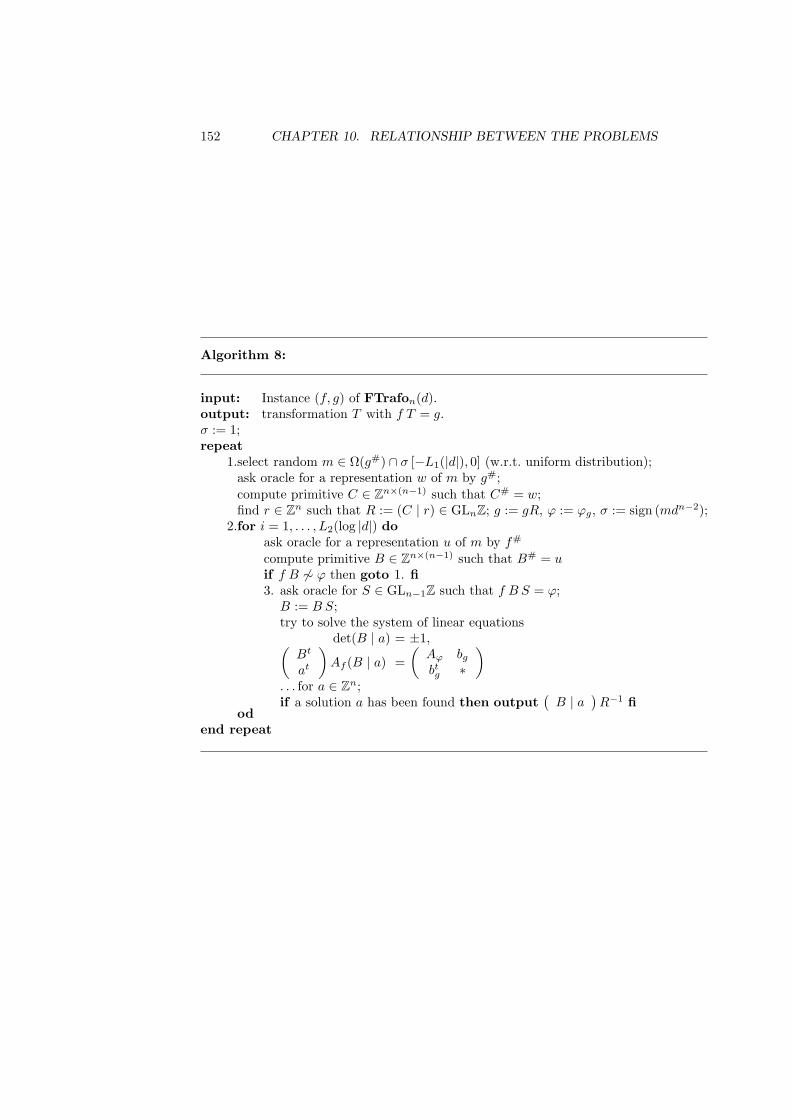
152 CHAPTER 10. RELATIONSHIP BETWEEN THE PROBLEMS
Algorithm 8:
input: Instance (f, g) of FTrafon(d).output: transformation T with f T = g.σ := 1;repeat
1.select random m ∈ Ω(g#) ∩ σ [−L1(|d|), 0] (w.r.t. uniform distribution);ask oracle for a representation w of m by g#;compute primitive C ∈ Zn×(n−1) such that C# = w;find r ∈ Zn such that R := (C | r) ∈ GLnZ; g := gR, ϕ := ϕg, σ := sign (mdn−2);
2.for i = 1, . . . , L2(log |d|) doask oracle for a representation u of m by f#
compute primitive B ∈ Zn×(n−1) such that B# = uif f B 6∼ ϕ then goto 1. fi3. ask oracle for S ∈ GLn−1Z such that f B S = ϕ;
B := B S;try to solve the system of linear equations
det(B | a) = ±1,(Bt
at
)Af (B | a) =
(Aϕ bg
btg ∗
). . . for a ∈ Zn;if a solution a has been found then output
(B | a
)R−1 fi
odend repeat
10.4. REDUCTION TO REPRESENTATIONS 153
Lemma 10.4.2 Let ϕ be as at label 3 in Algorithm 8. Then there are at most2ω(m) orbits of representations of ϕ by f under the automorphism group Q ∈GLnZ | f Q = f.
Proof : By [AS87], these orbits are at most as numerous as square roots of−dn−1ϕ# in (Z/mZ)[x1, . . . , xn−1], of which there are 2ω(m).
Since every representation from at least one of these orbits can be extendedto form a transformation, each iteration of the for loop has a probability ofsolving the problem of at least 2−ω(m). So if ω(m) ≤ 3
2 (log log m) say, then thealgorithm terminates successfully during the current iteration of the repeat loopwith significant, i. e. reciprocally polynomial probability. Finally, (1− o(1))x ofall integers 1 ≤ m ≤ x satisfy this bound [HW60, thm.431]. Now in step 1, thealgorithm scans several arithmetic progressions, hence a positive fraction of theintegers up (or down) to ±L1(|d|). Therefore it hits such m with probabilityat least `−1 where ` = P (L1(|d|)) for some positive polynomial P . Henceeach single iteration of the repeat loop brings the algorithm to a successfultermination with probability π ≥ 1
` . Since random bits used in step 1 areselected independently we obtain a geometric distribution:
Prob[success after ` iterations] = π∑i=0
(1− π)i
= 1− (1− π)`+1 ≥ 1− (1− `−1)`+1 ≥ 1− e−1. (10.11)
where e is Euler’s constant. Hence running the repeat loop d`e times andreturning fail in case of failure establishes the desired reduction.
This concludes the proof of Theorem 10.1.1.
We can now as well prove the corollary for dimension three.
Proof of Corollary 10.1.2: The second statement of Corollary 10.1.2 is adirect application of Theorem 10.1.1 for n = 3, so let us turn to the first one.
Let (f, g) be an instance of FTrafo3(d). Then Theorem 10.1.1 transforms itinto an instance (f ′,m) of ∗FRepr3(d2) and an instance (g, h) of FTrafo2. By[Die03], there is a solution T ∈ GL3Z to the original transformation problem ofpolynomial size. By the proof of Theorem 10.1.1 b), every such transformationarises from a construction as in Algorithm 8; in particular, with the notationfrom there, BS consist of the first two columns of RT , where S is the binaryequivalence transform. This implies that S depends linearly on B, R, and T ,and thus is of polynomial size. Hence the oracle query for S can be replaced byan application of Theorem 7.2.1, which finds S in polynomial time. Since wecannot be sure that such an S can be found for the particular m chosen in thefirst step of Algorithm 8, we have to modify Algorithm 8 as follows: Interruptthe attempt to compute S after a polynomial time bound, reselect m, repeat the
154 CHAPTER 10. RELATIONSHIP BETWEEN THE PROBLEMS
calculations up to the computation of S, increase the time bound polynomially,and retry. This proves the reduction without the Trafo2-oracle.
Bibliography
[AD97] Ajtai, Miklos and Dwork, Cynthia, A public-key cryptosystem withworst-case/average-case equivalence, Proceedings of the 29th an-nual ACM symposium on theory of computing, El Paso, TX,USA, May 4-6, 1997, Association for Computing Machinery, 1997,pp. 284–293.
[AEM87] Adleman, Leonard M., Estes, Dennis R., and McCurley, Kevin S.,Solving bivariate quadratic congruences in random polynomialtime, Mathematics of Computation 48 (1987), no. 177, 17–28.
[AKS04] Agrawal, Manindra, Kayal, Neeraj, and Saxena, Nitin, PRIMESis in P, Annals of Mathematics 160 (2004), no. 2, 781–793.
[AS87] Arenas-Sola, Angela, On integral representations by quadraticforms, Linear and Multilinear Algebra 22 (1987), 149–160.
[Bae78] Baeza, Ricardo, Quadratic forms over semilocal rings, LectureNotes in Mathematics, no. 655, Springer, 1978.
[BB97] Buchmann, Johannes and Biehl, Ingrid, An analysis of the reduc-tion algorithms for binary quadratic forms, Tech. Report No. TI-26/97, TU Darmstadt, 1997.
[BBBV97] Bennett, Charles H., Bernstein, Ethan, Brassard, Gilles, and Vazi-rani, Umesh, Strengths and weaknesses of quantum computing,SIAM Journal of Computing 26 (1997), no. 5, 1510–1523.
[BBS86] Blum, Lenore, Blum, Manuel, and Shub, Michael, A simple unpre-dictable pseudo-random number generator, SIAM Journal of Com-puting 15 (1986), 364–383.
[BBT94] Biehl, Ingrid, Buchmann, Johannes, and Thiel, Christoph, Cryp-tographic protocols based on discrete logarithms in real-quadraticorders, Advances in cryptology - CRYPTO ’94. 14th annual inter-national cryptology conference, Santa Barbara, CA, USA, August21-25, 1994. Proceedings (Desmedt, Yvo G., ed.), Lecture Notes inComputer Science, no. 839, Springer, 1994, pp. 56–60.
[BDG88] Balcazar, Jose Luis, Dıaz, Josep, and Gabarro, Joaquim, Struc-tural complexity. I, EATCS Monographs on Theoretical ComputerScience, no. 11, Springer, 1988.
155
156 BIBLIOGRAPHY
[BMM00] Buchmann, Johannes, Maurer, Markus, and Moran, Shlomo, Cryp-tography based on number fields with large regulator, Journal deTheorie des Nombres de Bordeaux 12 (2000), no. 2, 293–307.
[BR93] Bellare, Mihir and Rogaway, Phillip, Random oracles are practi-cal: a paradigm for designing efficient protocols, Proceedings of theFirst ACM Conference on Computer and Communications Secu-rity, Association for Computing Machinery, 1993, pp. 62–73.
[Bro06] Bromwich, Thomas John I’Anson, Quadratic forms and theirclassification by means of invariant-factors, Cambridge Tracts inMathematics and Mathematical Physics, no. 3, Cambridge Univer-sity Press, 1906.
[BTW95] Buchmann, Johannes, Thiel, Christoph, and Williams, Hugh,Short representation of quadratic integers, Computational algebraand number theory. Based on a meeting on computational algebraand number theory, held at Sydney University, Sydney, Australia,November of 1992. (Bosma, Wieb (ed.) et al., ed.), Math. Appl.,no. 325, Kluwer Academic Publishers, 1995, pp. 159–185.
[BV07] Buchmann, Johannes and Vollmer, Ulrich, Binary quadratic forms.An algorithmic approach, Algorithms and Computation in Mathe-matics, no. 20, Springer, 2007.
[BW90] Buchmann, Johannes and Williams, Hugh, A key exchange sys-tem based on real quadratic fields: Extended abstract, Advancesin Cryptology - CRYPTO ’89, Proc. Conf., Santa Barbara/CA(USA), Lecture Notes in Computer Science, no. 435, Springer,1990, pp. 335–343.
[Cas78] Cassels, John W. S., Rational quadratic forms, London Mathemat-ical Society Monographs, no. 13, Academic Press, 1978.
[CGH98] Canetti, Ran, Goldreich, Oded, and Halevi, Shai, The random or-acle model methodology revisited, STOC ’98. Proceedings of the30th annual ACM symposium on theory of computing, Dallas, TX,USA, May 23-26, 1998. New York, NY, Association for ComputingMachinery, 1998, pp. 209–218.
[CL84] Cohen, Henri and Lenstra jun., Hendrik W., Heuristics on classgroups of number fields, Number Theory, Proc. Journ. arith., No-ordwijkerhout 1983, Lecture Notes in Computer Science, no. 1068,Springer, 1984, pp. 33–62.
[CM87] Cohen, Henri and Martinet, Jacques, Class groups of number fields:Numerical heuristics, Mathematics of Computation 48 (1987),no. 177, 123–137.
[CM94] , Heuristics on class groups: Some good primes are no toogood, Mathematics of Computation 63 (1994), no. 207, 329–334.
[CM98] Cochrane, Todd and Mitchell, Patrick, Small solutions of the Leg-endre equation, Journal of Number Theory 70 (1998), no. 1, 62–66.
BIBLIOGRAPHY 157
[Coh93] Cohen, Henri, A course in computational algebraic number theory,Graduate Texts in Mathematics, vol. 138, Springer, 1993.
[Coh00] , Advanced topics in computational number theory, Gradu-ate Texts in Mathematics, vol. 193, Springer, 2000.
[CP01] Crandall, Richard and Pomerance, Carl, Prime numbers: A com-putational perspective, Springer, 2001.
[CR03] Cremona, J. E. and Rusin, D., Efficient solutions of rational conics,Mathematics of Computation 72 (2003), no. 243, 1417–1441.
[CS93] Conway, J. H. and Sloane, N. J. A. (eds.), Sphere packings, lat-tices and groups, 2nd ed., Grundlehren der mathematischen Wis-senschaften in Einzeldarstellungen, vol. 290, Springer, 1993.
[Dic34a] Dickson, Leonard Eugene, History of the theory of numbers: I.divisibility and primality, Chelsea, New York, 1934, (reprint of the1919 edition, Carnegie Inst., Washington DC).
[Dic34b] , History of the theory of numbers: II. diophantine analysis,Chelsea, New York, 1934, (reprint of the 1919 edition, CarnegieInst., Washington DC).
[Dic34c] , History of the theory of numbers: III. quadratic and higherforms, Chelsea, New York, 1934, (reprint of the 1919 edition,Carnegie Inst., Washington DC. Reprinted again in 1966).
[Die03] Dietmann, Rainer, Small solutions of quadratic Diophantine equa-tions, Proceedings of the London Mathematical Society, III. Ser.86 (2003), no. 3, 545–582.
[Dix81] Dixon, John D., Aymptotically fast factorization of integers, Math-ematics of Computation 36 (1981), 255–260.
[Eic52] Eichler, Martin, Quadratische Formen und Orthogonale Gruppen,Grundlehren der mathematischen Wissenschaften in Einzeldarstel-lungen, no. 63, Springer, 1952.
[Eis95] Eisenbud, David, Commutative algebra: With a view toward alge-braic geometry, Graduate Texts in Mathematics, no. 150, Springer,1995.
[EN81] Erdos, Pal and Nicolas, Jean-Louis, Sur la fonction: Nombre defacteurs premiers de n, L’Enseignement Mathematique, II. Ser. 27(1981), 3–27.
[Erd49] Erdos, Pal, On some applications of Brun’s method, Acta Mathe-matica 13 (1949), 57–63.
[FK06] Fouvry, Etienne and Kluners, Jurgen, On the 4-rank of class groupsof quadratic number fields, preprint, 2006.
158 BIBLIOGRAPHY
[FS87] Fiat, Amos and Shamir, Adi, How to prove yourself: Practical so-lutions of identification and signature problems, Advances in Cryp-tology – Proceedings of CRYPTO ’86 (Odlyzko, Andrew M., ed.),Lecture Notes in Computer Science, vol. 263, Association for Com-puting Machinery, 1987, pp. 186–194.
[Gau89] Gauß, Carl Friedrich, Untersuchungen uber hohere Arithmetik(Disquisitiones Arithmeticae), Springer, 1889, German translationby H. Maser.
[Ger84] Gerth III, F., The 4-class ranks of quadratic fields, InventionesMathematicae 77 (1984), no. 3, 489–515.
[Ger87] , Extension of conjectures of Cohen and Lenstra, Exposi-tiones Mathematicae 5 (1987), no. 2, 181–184.
[GGH97] Goldreich, Oded, Goldwasser, Shafi, and Halevi, Shai, Public-keycryptosystems from lattice reduction problems, Advances in Cryp-tology - CRYPTO ’97, 17th annual international cryptology confer-ence. Santa Barbara, CA, USA. (jun. Kaliski, Burton S., ed.), Lec-ture Notes in Computer Science, vol. 1294, Springer, 1997, pp. 112–131.
[GJ79] Garey, Michael R. and Johnson, David S., Computers and in-tractibility – a guide to the theory of np-completeness, Freeman,San Francisco, 1979.
[Gol01] Goldreich, Oded, Foundations of cryptography. I: Basic tools, Cam-bridge University Press, 2001.
[Gre69] Greenberg, Marvin J., Lectures on forms in many variables, Ben-jamin, New York, 1969.
[GS04] Grunewald, Fritz J. and Segal, Daniel, On the integer solutions ofquadratic equations, Journal fur die reine und angewandte Mathe-matik 569 (2004), 13–45.
[Hah94] Hahn, Alexander J., Quadratic algebras, Clifford algebras, andarithmetic Witt groups, Universitext, Springer, 1994.
[Har07] Hartung, Rupert Josef, Cryptography based on quadratic forms:Complexity considerations, Proceedings of WEWoRC 07, Bochum,to appear in: Lecture Notes in Computer Science, Springer, 2007.
[Has24] Hasse, Helmut, aquivalenz quadratischer Formen in einem beliebi-gen algebraischen Zahlkorper, Journal fur Mathematik 153 (1924),158–162.
[HHGP+03] Hoffstein, Jeffrey, Howgrave-Graham, Nick, Pipher, Jill, Silver-man, Joseph H., and Whyte, William, NTRUSign: Digital sig-natures using the NTRU lattice, Topics in cryptology – CT-RSA2003. The cryptographers’ track at the RSA conference 2003, SanFrancisco, CA, USA, April 13–17, 2003 (Joye, Marc, ed.), LectureNotes in Computer Science, vol. 2612, Springer, 2003, pp. 122–140.
BIBLIOGRAPHY 159
[HPS98] Hoffstein, Jeffrey, Pipher, Jill, and Silverman, Joseph H., NTRU:A ring-based public key cryptosystem, Algorithmic number theory.3rd international symposium, ANTS-III, Portland, OR, USA, June21–25, 1998 (Buhler, J. P., ed.), Lecture Notes in Computer Sci-ence, vol. 1423, Springer, 1998, pp. 267–288.
[HPS01] , NSS: an NTRU lattice-based signature scheme, Advancesin cryptology - EUROCRYPT 2001. 20th international conferenceon theory and application of cryptographic techniques, Innsbruck,Austria, May 6-10, 2001 (Pfitzmann, Birgit, ed.), Lecture Notes inComputer Science, vol. 2045, Springer, 2001, pp. 211–228.
[HS07a] Hartung, Rupert Josef and Schnorr, Claus-Peter, Identificationand signatures based on NP-hard problems of indefinite quadraticforms, preprint, 2007.
[HS07b] , Public key identification based on the equivalence ofquadratic forms, Mathematical Foundations of Computer Sci-ence 2007, 32nd International Symposium, MFCS 2007, CeskyKrumlov, Czech Republic, August 26–31, 2007, Proceedings(Kucera, Ludek and Kucera, Antonın, eds.), Lecture Notes in Com-puter Science, Springer, 2007, pp. 333–345.
[HW60] Hardy, G. H. and Wright, E. M., An introduction to the theory ofnumbers, fourth ed., Oxford: At the Clarendon Press, 1960.
[IAS96] Ivanyos, Gabor and Agnes Szanto, Lattice basis reduction for indef-inite forms and an application, Journal on Discrete Mathematics153 (1996), no. 1–3, 177–188.
[IM88] Imai, Hideki and Matsumoto, Tsutomu, Public quadraticpolynomial-tuples for efficient signature-verification and message-encryption, Advances in cryptology. Theory and application ofcryptographic techniques, Proc. Workshop, EUROCRYPT ’88,Lecture Notes in Computer Science, vol. 330, 1988, pp. 419–453.
[IW97] Impagliazzo, R. and Wigderson, A., P= BPP, unless E has subex-ponential circuits: Derandomizing the XOR-lemma, Proceedingsof the 29th Annual ACM Symposium on Theory of Computing,1997, pp. 220–229.
[Jon44] Jones, Burton Wadsworth, A canonical quadratic form for the ringof 2-adic integers, Duke Mathematical Journal 11 (1944), 715–727.
[Jon50] , The arithmetic theory of quadratic forms, Carus Mathe-matical Monographs, no. 10, John Wiley & Sons, 1950.
[Kan87] Kannan, Ravi, Minkowski’s convex body theorem and integer pro-gramming, Mathematics of Operations Research 12 (1987), no. 3,415–440.
[Kho05] Khot, Subash, Hardness of approximating the shortest vector prob-lem in lattices, Journal of the ACM 52 (2005), no. 5, 789–808.
160 BIBLIOGRAPHY
[Kit93] Kitaoka, Yoshiyuki, Arithmetic of quadratic forms, CambridgeTracts in Mathematics and Mathematical Physics, no. 106, Cam-bridge University Press, 1993.
[KM07] Koblitz, Neal and Menezes, Alfred J., Another look at “provablesecurity”, Journal of Cryptology 20 (2007), no. 1, 3–37.
[Kne02] Kneser, Martin, Quadratische Formen, Springer, 2002.
[Lag80] Lagarias, J. C., Worst-case complexity bounds for algorithms in thetheory of integral quadratic forms, Journal of Algorithms 1 (1980),142–186.
[Lam05] Lam, Tsit-Yuen, Introdction to quadratic forms over fields, Grad-uate Studies in Mathematics, no. 67, American Mathematical So-ciety, 2005.
[Leg85] Legendre, Adrien-Marie, Recherche d’analyse indeterminee, His-toire de l’Academie Royale des Sciences 1788 (1785), 465–559.
[Leg98] , Essai sur la theorie des nombres, Duprat, Paris, 1798.
[Lem95] Lemmermeyer, Franz, The Euclidean algorithm in algebraic num-ber fields, Expositiones Mathematicae 13 (1995), no. 5, 385–416.
[Len82] Lenstra jun., Hendrik W., On the calculation of regulators andclass numbers of quadratic fields, Journees arithmetiques, Exeter1980 (Armitage, J. V., ed.), Lecture Note Series, vol. 56, LondonMathematical Society, 1982, pp. 123–150.
[Len87] , Factoring integers with elliptic curves, Mathematische An-nalen (2) 126 (1987), 649–673.
[LL83] Lenstra, Arjen K. and Lenstra jun., Hendrik W. (eds.), The de-velopment of the number field sieve, Lecture Notes in ComputerScience, no. 1554, Springer, 1983.
[LLL82] Lenstra jun., Hendrik W., Lenstra, Arjen K., and Lovasz, Laszlo,Factoring polynomials with rational coefficients, MathematischeAnnalen 261 (1982), 515–534.
[LLMP90] Lenstra, Arjen K., Lenstra jun., Hendrik W., Manasse, Mark S.,and Pollard, John M., The number field sieve, Proceedings of the22nd Annual ACM Symposium on Theory of Computing (STOC),Baltimore, May 14–16, 1990, 1990, pp. 564–572.
[LO85] Lagarias, J. C. and Odlyzko, Andrew M., Solving low-density sub-set sum problems, Journal of the ACM 32 (1985), 229–246.
[LP92] Lenstra jun., Hendrik W. and Pomerance, Carl, A rigorous timebound for factoring integers, Journal of the American Mathemati-cal Society 5 (1992), 483–516.
[MA78] Manders, Kenneth L. and Adleman, Leonard M., NP -completedecision problems for binary quadratics, Journal of Computer andSystem Sciences 16 (1978), 168–184.
BIBLIOGRAPHY 161
[Man74] Manin, Yuri Ivanovitch, Cubic forms: Algebra, geometry, arith-metic, North-Holland Mathematical Library, vol. 4, North-Holland, 1974, Translated by M. Hazewinkel.
[Mat93] Matiyasevich, Yuri V., Hilbert’s tenth problem: With a foreword byMartin Davis, MIT Press, Cambridge MA, 1993.
[Mey91] Meyer, Arnold, Zur Theorie der indefiniten ternaren quadratischenFormen, Journal fur Mathematik CVIII (1891), 125–139.
[MG02] Micciancio, Daniele and Goldwasser, Shafi, Complexity of latticeproblems: a cryptographic perspective, The Kluwer InternationalSeries in Engineering and Computer Science, vol. 671, Kluwer Aca-demic Publishers, March 2002.
[Mih94] Mihailescu, P., Fast generation of provable primes using search inarithmetic progressions, Advances in cryptology - CRYPTO ’94.14th annual international cryptology conference, Santa Barbara,CA, USA, August 21-25, 1994. Proceedings (Desmedt, Yvo G.,ed.), Lecture Notes in Computer Science, no. 839, Springer, 1994,pp. 282–293.
[Min11] Minkowski, Hermann, Grundlagen einer Theorie der ganzzahligenquadratischen Formen, H. Minkowski: Gesammelte Werke (Hil-bert, David, ed.), Teubner, Wiesbaden, 1911, pp. 3–144.
[MSC96] Mitrinovic, D. S., Sandor, J., and Crstici, B. (eds.), Handbook ofnumber theory, Mathematics and Its Applications, vol. 351, KluwerAcademic Publishers, 1996.
[Neu92] Neukirch, Jurgen, Algebraische Zahlentheorie, Springer, 1992.
[O’M63] O’Meara, O. T., Introduction to quadratic forms, Grundlehren dermathematischen Wissenschaften in Einzeldarstellungen, vol. 117,Springer, 1963, (reprinted in 2000).
[Pap94] Papadimitriou, Christos H., Computational complexity, Addison-Wesley, 1994.
[Per54] Perron, Oskar, Die Lehre von den Kettenbruchen, 3rd ed., vol. I,Teubner, Stuttgart, 1954.
[Pom80] Pomerance, Carl, A note on the least prime in an arithmetic pro-gression, Journal of Number Theory 12 (1980), 218–223.
[Pom82] , Analysis and comparison of some integer factoring al-gorithms, Computational Methods in Number Theory, Part I(Lenstra jun., Hendrik W. and Tijdeman, R., eds.), Math. Cen-tre Tracts, vol. 154, Math. Centrum, 1982, pp. 89–139.
[Pom87] , Fast rigorous factorization and discrete logarithm al-gorithms, Discrete algorithms and complexity, Proc. Jap.-USJoint Semin., Kyoto/Jap. 1986, Perspect. Comput., no. 15, 1987,pp. 119–143.
162 BIBLIOGRAPHY
[PP85] Plesken, Wilhelm and Pohst, Michael E., Constructing integral lat-tices with prescribed minimum. I, Mathematics of Computation 45(1985), 209–221.
[Pra61] Prachar, Karl, Uber die kleinste Primzahl einer arithmetischenReihe, Journal fur die reine und angewandte Mathematik 206(1961), 3–4.
[PS85] Plesken, Wilhelm and Souvignier, B., Computing isometries of lat-tices, Mathematics of Computation 45 (1985), 209–221.
[PS87] Pollard, John M. and Schnorr, Claus-Peter, An efficient solutionof the congruence x2 + ky2 = m (mod n), IEEE Transactions onInformation Theory 33 (1987), 702–709.
[PZ89] Pohst, Michael E. and Zassenhaus, H., Algorithmic algebraic num-ber theory, Encyclopedia of Mathematics and its Applications,no. 30, Cambridge University Press, 1989.
[Sch04a] Schnorr, Claus-Peter, Indefinite ternary quadratic form signatures,preprint, 2004.
[Sch04b] , Reduction of quadratic forms reconsidered, preprint, 2004.
[Sch07] , Progress on LLL and lattice reduction, ProceedingsLLL+25, Caen, France, June 29–July 1, 2007, 2007, to appear.
[Ser73] Serre, Jean-Pierre, A course in arithmetic, Graduate Texts inMathematics, no. 7, Springer, 1973.
[SH07] Stehle, Damien and Hanrot, Guillaume, Improved analysis of Kan-nan’s shortest lattice vector algorithm, Advances in Cryptology- CRYPTO 2007, 27th Annual International Cryptology Confer-ence, Santa Barbara, CA, USA, August 19-23, 2007, Proceedings(Menezes, Alfred J., ed.), Lecture Notes in Computer Science, vol.4622, 2007, pp. 170–186.
[Sha72] Shanks, Daniel, The infrastructure of a real quadratic field and itsapplications, Proc. 1972 Number Theory Conf., Univ. Colorado,Boulder, 1972, pp. 217–224.
[Sha74] Shafarevich, I. R., Basic algebraic geometry, Grundlehren dermathematischen Wissenschaften in Einzeldarstellungen, no. 213,Springer, 1974.
[Sie35] Siegel, Carl Ludwig, Uber die analytische Theorie der quadratis-chen Formen, Annals of Mathematics (2) 36 (1935), 527–606.
[Sie36] , Uber die analytische Theorie der quadratischen Formen.II, Annals of Mathematics (2) 37 (1936), 230–263.
[Sie37] , Uber die analytische Theorie der quadratischen Formen.III, Annals of Mathematics (2) 38 (1937), 212–291.
BIBLIOGRAPHY 163
[Sie63] , Lectures on quadratic forms, Tata Institute of Fundamen-tal Research, Bombay, 1957 (reissued 1963), notes by K. G. Ra-manathan.
[Sie72] , Zur Theorie der quadratischen Formen, Nachrichten vonder Gesellschaft der Wissenschaften zu Gottingen, Mathematisch-Physikalische Klasse 1972 (1972), 21–46.
[Sim05a] Simon, Denis, Quadratic equations in dimensions 4, 5 and more,preprint, 2005.
[Sim05b] , Solving quadratic equations using reduced unimodular qua-dratic forms, Mathematics of Computation 74 (2005), no. 251,1531–1543.
[Sma98] Smart, Nigel P., The algorithmic resolution of diophantine equa-tions, Student Texts, vol. 41, London Mathematical Society, 1998.
[SO80] Scharlau, Winfried and Opolka, Hans, Von Fermat bis Minkowski:Eine Vorlesung uber Zahlentheorie und ihre Entwicklung, Springer,1980.
[TW86] Tennenhouse, M. and Williams, H.C., A note on the class-numberone in certain real quadratic and pure cubic fields, Mathematics ofComputation 46 (1986), no. 173, 333–336.
[Val91] Vallee, Brigitte, Generation of elements with small modular squaresand provably fast integer factoring algorithms, Mathematics ofComputation 56 (1991), no. 194, 823–849.
[VV07] Vallee, Brigitte and Vera, Antonio, Lattice reduction in two di-mensions: Analyses under realistic probabilistic models, preprint,2007.
[Wag79] Wagstaff, Jr., Samuel S., Greastest of the least primes in arithmeticprogressions having a given modulus, Mathematics of Computation33 (1979), no. 147, 1073–1080.
[Wat76] Watson, G.L., The 2-adic density of a quadratic form, Mathe-matika 23 (1976), 94–106.
[Wei84] Weil, Andre, Number theory: An approach through history; FromHammurapi to Legendre, Birkhauser, 1984.
[Zhu97] Zhuravlev, V. G., Representation of a form by the genus of qua-dratic forms, St. Petersburg Mathematical Journal 8 (1997), no. 1,15–84.
Index
k-power free, 19
adjoint form, 7, 146anisotropic, 9associated (ring elements), 27associated bilinear form, 7associated matrix (of a form), 6automorphism, 110, 121, 131, 132
proper, 132
Boolean formulae, ∈-notation122
classproper class, 19
class (of a form), 9, 19class structure
local fields, 13–16local rings, 17–18rational integers, 19rational numbers, 16–17real numbers, 15–16
classically integral, 6completion of the square, 10–12computational problem, 4counter-Blum integer, 87
decision problemrepresentation, 39
interval-constraint, 115transformation, 44
interval-constraint, 119decisional problem, 4, 5definite, 9determinant (of a form), 7diagonal form, 7, 10dimension (of a form), 6discriminant
of a number field, 128
encoding, 21equivalence (of forms), 9
factoring, 127algorithms, 127
factorization, 83–84, 87–88, 109–110,114, 127
field with encoding, 22form, see quadratic form
genus, 19one-class genera, 19
global, 13
Hasse Principle, 17Hasse-Minkowksi invariant, 13–15Hilbert norm residue symbol, 13–15hyperbolic plane, 61, 89, 102, 103
improperly primitive, 7indefinite, 9integral, 6integral domain with encoding, 22isotropic, 9, 83–85, 117, 120isotropic vector problem, 84
key generation, 30knowledge error, 32knowledge extractor, 32
length (encoding), 4local, 13
Meyer’s Theorem, 17modular square problem, 121
narrow, 121
negligible, 30norm residue symbol, 13–15
orthogonal sum, 7
precision, 23primitive
form, 7, 26–27
164
INDEX 165
representation, 8of forms, 146
problem union, 5, 145proof of knowledge, 32–33, 36proper equivalence, 9properly primitive, 7Properties of forms, 9
encoding, 23
quadratic form, 6
random oracle model (ROM), 36reducible, 9reduction (complexity theory), 5–6
Karp, 5non-adaptive, 5probabilistic, 6Turing, 5
regular, 7representation, 8
coprime, 24–26, 118, 145of forms, 146primitive, 8
of forms, 146problem, 24–26
interval-constraint, 115simultaneous, 96
ring with encoding, 22
signature, 16simulator, 34singular, 7special Cohen-Lenstra heuristic, 127–
130, 141, 142spinor norm, 110–114, 131–132square class, 12, 13square root problem, 84statistical distance, 30statistically close, 30symmetry, 110
transformation problem, 26interval-constraint, 119with factorization given, 101, 114
UFDwith encoding, 22
unique factorization domain (UFD),7
universal, 45, 130
Witt’s Lemma, 13
zero-knowledge, 34, 36–37statistical, 34