Data Mining

229

Datenaufbereitung für Analytik – Erstellen eines „One-Row-Per-Subject“ Data Marts

für Data Mining

Gerhard Svolba SAS-Österreich Mariahilfer Straße 116 A-1070 Wien Gerhard.svolba@aut.sas.com

Zusammenfassung

Das Erzeugen eines „one-row-per-subject“ data marts ist eine fundamentale Tätigkeit für Data Mining Analysen. Um die zugrunde liegende fachliche Frage zu beantworten, muss der Analytiker oder der Data-Mart Programmierer die relevanten Informationen aus unter-schiedlichen Datenquellen extrahieren. Das Erzeugen eines Data Marts geht über die simple Tätigkeit des Kopierens der Quelldaten in die Zieltabelle hinaus. Es beinhaltet auch die Aggregation oder Transposition von transaktionellen Daten oder Zeithistorien und das Erstellen von abgeleiteten Variablen. Dieser Prozess ist ein kritischer Erfolgsfaktor, um die fachliche Frage beantworten zu können und um gute Prädiktoren für ein Zielereignis oder einen Zielwert zu haben. Dieses Paper zeigt die Input-Datenstrukturen für einen „one-row-per-subject“ Data Mart und diskutiert das one-row-per-subject“ Paradigma aus einer tech-nischen und fachlichen Perspektive. Es wird gezeigt, wie hierarchische Abhängigkeiten auf eine Zeile pro Kunden aggregiert werden können. Ein umfassendes Beispiel zeigt wie ein one-row-per-subject“ data mart auf Basis unterschiedlicher Datenquellen erstellt werden kann.

Schlüsselwörter: Statistik, Data Mining, Datenaufbereitung, Data Mart, Aggregation, Transposing, Vorhersagemodelle, Data Set, Base SAS

1 Einleitung Neben der Auswahl und der Parametrisierung des entsprechenden Modells, sind die Datenverfügbarkeit und die Datenaufbereitung eine wichtige Voraussetzung für die Per-formance von analytischen Modellen. Abhängig von der fachlichen Fragestellung und den entsprechenden statistischen Methoden, werden unterschiedliche Datenstrukturen benötigt. Die beiden wichtigsten Vertreter sind der „one-row-per-subject“ data mart und der „multipe-row-per-subject“ data mart. Die Beantwortung einer fachlichen Fragestellung beinhaltet üblicherweise die folgenden Schritte:

1. Definition des Business-Problems. Hier ist intensive Zusammenarbeit zwischen Fachexperten, Statistikern und EDV-Experten nötig, um zu evaluieren, was tat-sächlich benötigt wird.

G. Svolba

230

2. Auf Basis der Definition der fachlichen Fragestellung wird bestimmt, welche bestehenden Daten in den IT-Systemen benötigt werden, um die Fragen zu be-antworten.

3. Festlegung, wie die Daten für die Modellierung und den analytischen Data Mart aufbereitet werden sollen.

4. Bereitstellung des analytischen Data Marts für die Analytischen Prozeduren, wie z.B.: Analysen von Zusammenhängen, Vorhersage von Werten oder Ereignissen, Segmentierung.

Es gibt 2 Hauptfaktoren, die die Qualität des analytischen Modells beeinflussen:

• Die Selektion und das Tuning des geeigneten analytischen Modells • Die Verfügbarkeit und die Aufbereitung der Daten, die für die Beantwortung der

fachlichen Fragestellung geeignet sind.

1.1 Erfolgsfaktoren für Analytik In der statistischen Theorie und Literatur gibt es einen starken Fokus auf die Selektion und das Trainieren von analytischen Modellen. Es gibt viele Bücher und Kurse, die sich auf das predictive modeling fokussieren – trainieren von Neuronalen Netzwerken, erstellen von Entscheidungsbäumen, Bau von Regressionsmodellen. Für diese Aufga-ben wird viel Wissen benötigt und diese Aufgaben haben sich als kritischer Erfolgsfak-tor für gute analytische Ergebnisse erwiesen. Neben der Bedeutung der analytischen Fähigkeiten ist jedoch die Verfügbarkeit von guten und relevanten Daten zur Beantwortung der fachlichen Fragen sehr wichtig.

1.2 Erfolgsfaktoren für Daten Die Verfügbarkeit der Daten für die Erstellung des analytischen Data Marts ist ein wichtiger Faktor, der sehr früh in einem Projekt sichergestellt werden sollte. Die Sicher-stellung, dass historische Sichtweisen auf Datenbestände („Historic Snapshot“) verfüg-bar sind, bedarf einer langfristigen Planung und Speicherung, da diese nicht kurzfristig erstellt werden können. Die adäquate Aufbereitung der Daten ist ein wichtiger Erfolgsfaktor für die Analyse. Auch wenn die richtigen Datenquellen verfügbar sind und auf sie zugegriffen werden kann, ist es nicht möglich die Analyse sofort zu starten. Die entsprechende Aufbereitung der Daten ist dabei ein wichtiger Zwischenschritt. Entsprechend der Erfahrung des Au-tors können fehlende oder nicht gut aufbereitete Informationen nicht durch noch so gute Modellierung ausgeglichen werden. Dieses Paper behandelt die Thematik der Datenaufbereitung. Es werden Inhalte aus dem Buch „Data Preparation for Analytics Using SAS“ von Gerhard Svolba, erschienen in SAS Press, verwendet (siehe auch http://www.sascommunity.org/wiki/Data_Preparation_for_Analytics).

Data Mining

231

Das Paper diskutiert und illustriert konzeptionelle Überlegung bei der Gestaltung eines „one-row-per-subject-datamarts“ und zeigt anhand einer Case Study, wie Daten für Data Mining aufbereitet werden können. Mit Ausnahme der Zusammenfassung und der Einleitung sind die folgenden Kapitel in englischer Sprache gehalten.

2 THE ONE-ROW-PER-SUBJECT PARADIGM

2.1 ANALYSIS SUBJECT Analysis subjects are entities that are being analyzed and the analysis results are inter-preted in their context. Analysis subjects are therefore also the basis for the structure of analysis tables. Examples of analysis subjects are:

• Persons: Depending on the area of the analysis the analysis subjects have more specific names like patients in medical statistics, customers in marketing ana-lytics, or applicants in credit scoring.

• Animals: Piglets, for example, are analyzed in feeding experiments; rats are ana-lyzed in pharmaceutical experiments.

• Parts of the body system: In medical research analysis subjects can also be parts of the body system like arms (left arm compared to the right arm), shoulders or hips. Note that from a statistical point of view the validity of the assumptions of the respective analysis methods have to be checked, if dependent observations per person are used in the analysis.

• Objects: Things like cash machines in cash demand prediction, cars in quality control in the automotive industry, or products in product analysis can be sub-jects.

• Legal entities: Examples are companies, contracts, accounts, and applications. • Geography: Regions or plots in agricultural studies or reservoirs in the maturity

prediction of fields in the oil and gas industries are examples.

Analysis subjects are therefore the heart of each analysis. The features of analysis sub-jects are measured, processed, and analyzed. In deductive statistics the features of the analysis subjects in the sample are used to infer the properties of the similar subjects in the larger population.

2.2 IMPORTANCE AND FREQUENT OCCURRENCE OF THIS TYPE OF DATA MART

The one-row-per-subject data mart is important for statistical and data mining analyses. Many business questions are answered based on a data mart of this type. The following list presents business examples:

G. Svolba

232

• Prediction of events such as

• Campaign response • Contract renewal • Contract cancellation (attrition or churn) • Insurance claim • Default on credit or loan payback • Identification of risk factors for a certain disease

• Prediction of values such as • Amount of loan that can be paid back • Customer turnover and profit for the next period • Time intervals like the remaining lifetime of a customer or patient • SUGI 31 Data Mining and Predictive Modeling • Time until next purchase • Value of next insurance claim

• Segmentation of customers The following analytical methods require a one-row-per-subject data mart: • Regression analysis • Analysis-of-variance analysis • Neural networks • Decision trees • Survival analysis • Cluster analysis • Principle components analysis and factor analysis

2.3 PUTTING ALL INFORMATION INTO ONE The above application examples coupled with the underlying algorithm requires that all the data source information be aggregated into one row. Central to this type is the fact that we have to put all information per analysis subject into one row. We will therefore call this the one-row-per-subject data mart paradigm in that all information has to be put into a single row. Multiple observations per analysis subject must not appear in addi-tional rows, but have to be converted over into additional columns. Obviously, putting all information into one row is very simple if we have no multiple observations per analysis subject. The values are then simply read into the analysis data mart and derived variables are being added. If we have multiple observations per analysis subject it is more effort to put all infor-mation into one row. Here we have to cover two aspects:

• The technical aspect--how multiple-row-per-subject data can be converted into one-row-per-subject data.

• The business aspect--which aggregations, derived variables, and so on can best be condensed from the multiple rows into columns.

Data Mining

233

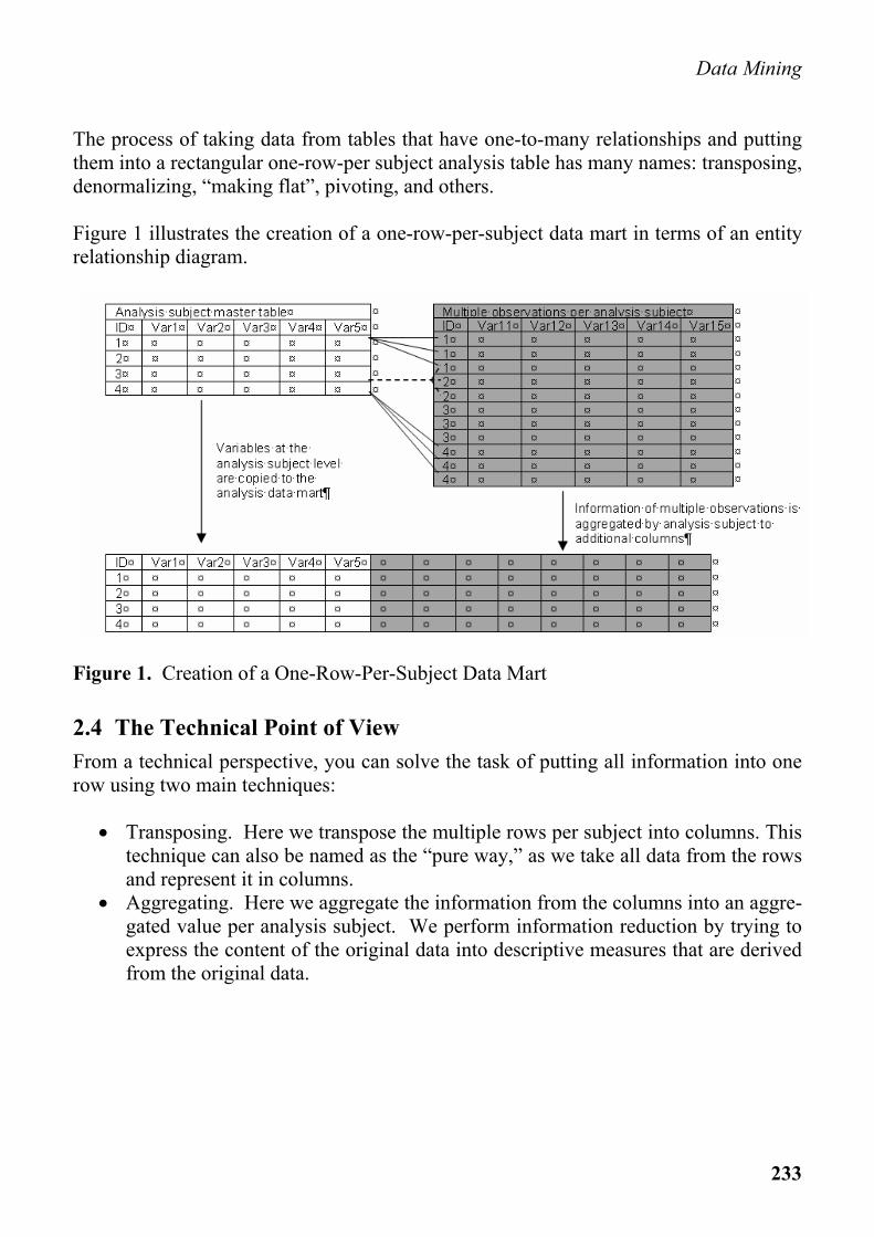
The process of taking data from tables that have one-to-many relationships and putting them into a rectangular one-row-per subject analysis table has many names: transposing, denormalizing, “making flat”, pivoting, and others. Figure 1 illustrates the creation of a one-row-per-subject data mart in terms of an entity relationship diagram.

Figure 1. Creation of a One-Row-Per-Subject Data Mart

2.4 The Technical Point of View From a technical perspective, you can solve the task of putting all information into one row using two main techniques:

• Transposing. Here we transpose the multiple rows per subject into columns. This technique can also be named as the “pure way,” as we take all data from the rows and represent it in columns.

• Aggregating. Here we aggregate the information from the columns into an aggre-gated value per analysis subject. We perform information reduction by trying to express the content of the original data into descriptive measures that are derived from the original data.

G. Svolba

234

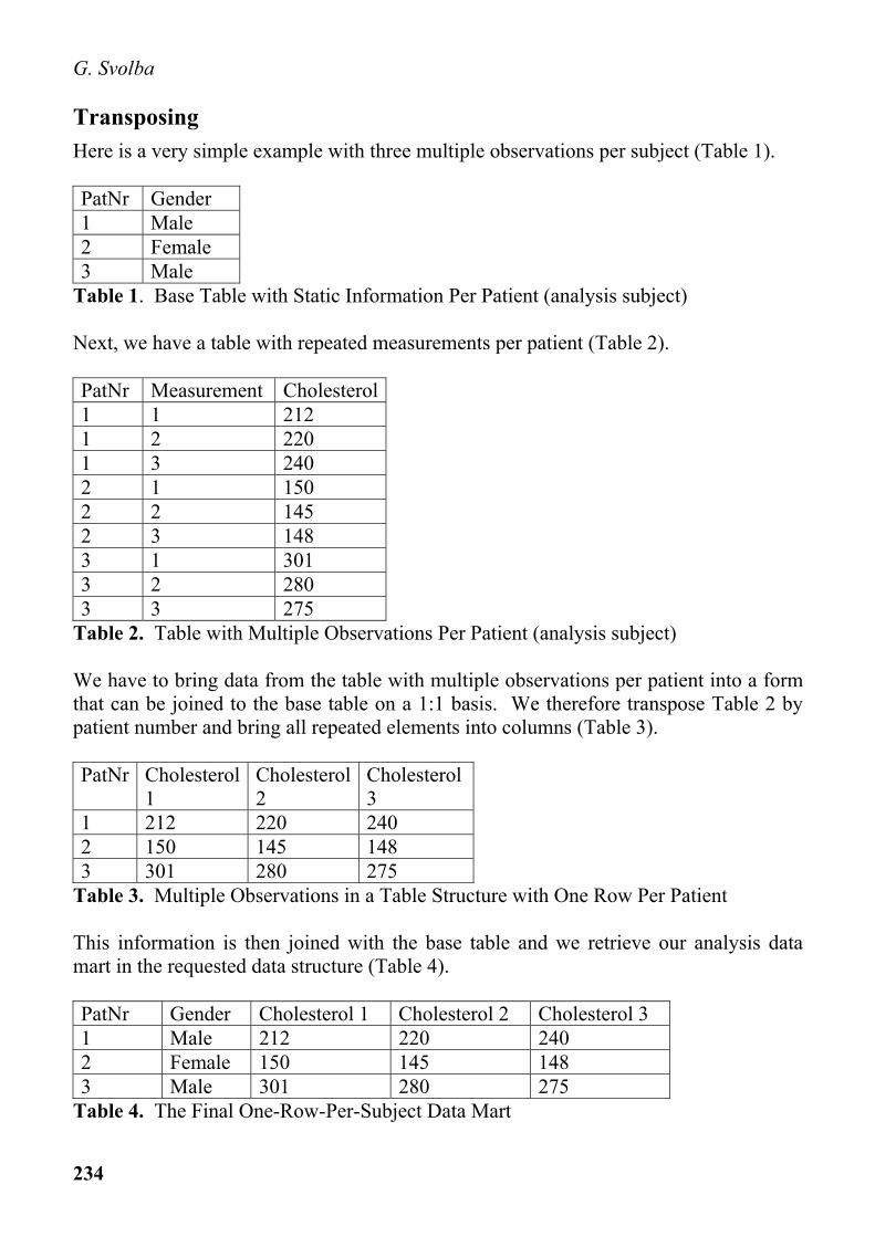
Transposing Here is a very simple example with three multiple observations per subject (Table 1). PatNr Gender 1 Male 2 Female 3 Male

Table 1. Base Table with Static Information Per Patient (analysis subject) Next, we have a table with repeated measurements per patient (Table 2). PatNr Measurement Cholesterol1 1 212 1 2 220 1 3 240 2 1 150 2 2 145 2 3 148 3 1 301 3 2 280 3 3 275

Table 2. Table with Multiple Observations Per Patient (analysis subject) We have to bring data from the table with multiple observations per patient into a form that can be joined to the base table on a 1:1 basis. We therefore transpose Table 2 by patient number and bring all repeated elements into columns (Table 3). PatNr Cholesterol

1 Cholesterol 2

Cholesterol 3

1 212 220 240 2 150 145 148 3 301 280 275

Table 3. Multiple Observations in a Table Structure with One Row Per Patient This information is then joined with the base table and we retrieve our analysis data mart in the requested data structure (Table 4). PatNr Gender Cholesterol 1 Cholesterol 2 Cholesterol 3 1 Male 212 220 240 2 Female 150 145 148 3 Male 301 280 275

Table 4. The Final One-Row-Per-Subject Data Mart

Data Mining

235

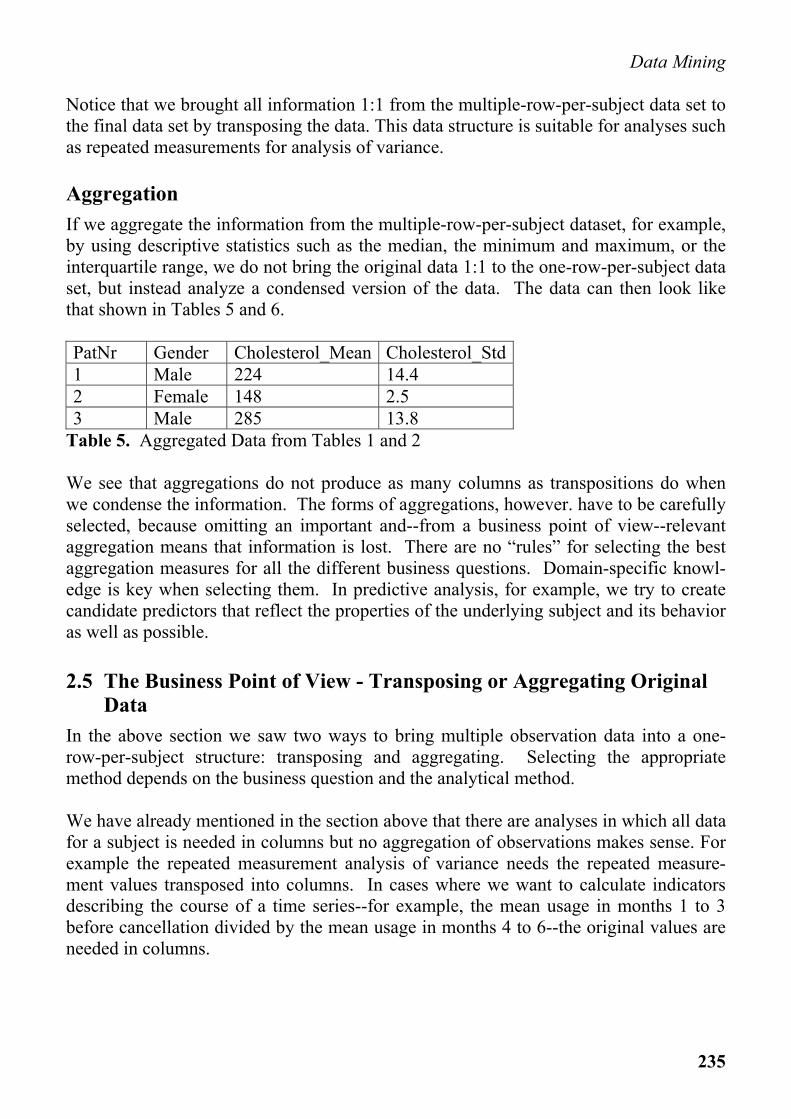
Notice that we brought all information 1:1 from the multiple-row-per-subject data set to the final data set by transposing the data. This data structure is suitable for analyses such as repeated measurements for analysis of variance.

Aggregation If we aggregate the information from the multiple-row-per-subject dataset, for example, by using descriptive statistics such as the median, the minimum and maximum, or the interquartile range, we do not bring the original data 1:1 to the one-row-per-subject data set, but instead analyze a condensed version of the data. The data can then look like that shown in Tables 5 and 6. PatNr Gender Cholesterol_Mean Cholesterol_Std1 Male 224 14.4 2 Female 148 2.5 3 Male 285 13.8

Table 5. Aggregated Data from Tables 1 and 2 We see that aggregations do not produce as many columns as transpositions do when we condense the information. The forms of aggregations, however. have to be carefully selected, because omitting an important and--from a business point of view--relevant aggregation means that information is lost. There are no “rules” for selecting the best aggregation measures for all the different business questions. Domain-specific knowl-edge is key when selecting them. In predictive analysis, for example, we try to create candidate predictors that reflect the properties of the underlying subject and its behavior as well as possible.

2.5 The Business Point of View - Transposing or Aggregating Original Data

In the above section we saw two ways to bring multiple observation data into a one-row-per-subject structure: transposing and aggregating. Selecting the appropriate method depends on the business question and the analytical method. We have already mentioned in the section above that there are analyses in which all data for a subject is needed in columns but no aggregation of observations makes sense. For example the repeated measurement analysis of variance needs the repeated measure-ment values transposed into columns. In cases where we want to calculate indicators describing the course of a time series--for example, the mean usage in months 1 to 3 before cancellation divided by the mean usage in months 4 to 6--the original values are needed in columns.

G. Svolba

236

There are, however, a lot of situations in which a 1:1 transfer of data is technically not possible nor practical. In these situations aggregations make much more sense. Let’s have a look at the following questions:

• If we have the cholesterol values expressed in columns, is this the information we need for further analysis?

• What shall we do if we have not only three observations for one measurement variable per subject, but 100 repetitions for 50 variables? Transposing all these data would lead to 5000 variables.

• Do we in the analysis data mart really need the data 1:1 from the original table, or do we more precisely need the information in concise aggregations?

• In predictive analysis, do we need data that has good predictive power for the modeling target and suitably describes the relationship between target and input variables instead of the original data?

The answers to these questions depend on the business questions, the modeling tech-nique, the data itself, and so on. However there are many cases, especially in data min-ing analysis, where clever aggregations of the data make much more sense than a 1:1 transposition. Determining how to best aggregate the data requires business and domain knowledge and a good understanding of the data. Having said that, putting all information into one row is not just data management; we show in this paper ways to cleverly prepare data from multiple observations. Following is an overview of methods that enable the information to be extracted and represented from the multiple observations per subject. When aggregating measurement data for a one-row-per-subject data mart we can use the following:

• simple descriptive statistics like sum, minimum, or maximum • frequency counts and number of distinct values • measures of location or dispersion like mean, median, standard deviation, the

quartiles, or special quantiles • concentration measures on the basis of cumulative sums • statistical measures describing trends and relationships like regression coeffi-

cients or correlations coefficients When analyzing multiple observations with categorical data that is aggregated per sub-ject we can use the following:

• total Counts • frequency counts per category and percentages per category • distinct counts • concentration measures on the basis of cumulative frequencies

Data Mining

237

2.6 Hierarchies: “Aggregating Up” and “Copying Down”

General In the case of repeated measurements over time we are usually aggregating this infor-mation by using the summary measurements described above. The aggregated values, such as means or sums, are then used at the subject level as a property of the corre-sponding subject. In the case of multiple observations because of hierarchical relationships, we are also aggregating information from a lower hierarchical level to a higher one. However, we can also have information at a higher hierarchical level that has to be available or ex-pressed to lower hierarchical levels. Also, information has to be shared between mem-bers of the same hierarchy, like the number of members at this hierarchy level.

Example Consider an example in which we have the following relationships:

• In one HOUSHOLD lives one or more CUSTOMER(s). • One CUSTOMER can have one or more CREDIT CARD(s). • On each CREDIT CARD a number of TRANSACTION(s) are associated.

For marketing purposes we do a segmentation of customers; therefore, CUSTOMER is chosen as the appropriate subject analysis level. When looking at the hierarchies, we aggregate information from the entity of CREDIT CARD and TRANSACTION to the CUSTOMER level and make information that is stored on the HOUSEHOLD level available to the entity CUSTOMER. We next show how data from different hierarchical levels is made available to the analysis data mart. Note that for didactical purposes, we reduce the number of variables to a few.

Information from the Same Level At the customer level we have the following variables directly available to our analysis data mart:

• customer birthday (on that basis the derived variable AGE is calculated) • gender • customer since (on that basis the duration of customer relationship is calculated)

Aggregating Up In our example, we create the following variables on customer level that are aggrega-tions from the lower levels CREDIT CARD and TRANSACTION.

G. Svolba

238

• number of cards per customer • number of transactions over all cards for the last 3 months • sum of transaction values over all cards for the last 3 months • average transaction value for the last 3 months (calculated on the basis of the val-

ues over all cards)

Dividing Down • At the HOUSEHOLD level the following information is available, that is copied

down to the customer level. • number of persons in the household • geographic region type of the household with the values RURAL, HIGHLY RU-

RAL, URBAN, HIGHLY URBAN.

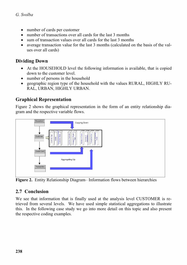
Graphical Representation Figure 2 shows the graphical representation in the form of an entity relationship dia-gram and the respective variable flows.

Figure 2. Entity Relationship Diagram– Information flows between hierarchies

2.7 Conclusion We see that information that is finally used at the analysis level CUSTOMER is re-trieved from several levels. We have used simple statistical aggregations to illustrate this. In the following case study we go into more detail on this topic and also present the respective coding examples.

Data Mining

239

3 Case Study – Building a Customer Data mart

3.1 Introduction This section provides an example of how a one-row-per-subject table can be built using a number of data sources. In these data sources we only have in the CUSTOMER table one row per subject; in the other tables we have multiple rows per subject. The task in this example is to combine these data sources to create a table that holds one row per customer. Therefore we have to aggregate the multiple observations per subject to one observation per subject Tables like this are frequently needed in data mining analyses such as prediction or segmentation. In our example, we assume that we can create data to predict the cancel-lation event of a customer.

3.2 The Business Context

General We want to create a data mart that reflects the properties and behaviors of customers. This table shall be used to predict which customer has a high probability to leave the company.

Data Sources In this example we will build a customer data mart for marketing purposes. Our basis is data from the following data sources:

• Customer data: demographic and customer baseline data • Account data: information customer accounts • Leasing data: data on leasing information • Call Center data: data on Call center contacts • Score data: data of value segment scores

From these data sources we want to build one table with one row per customer. We therefore have the classic one-row-per-subject paradigm in which we need to bring the repeated information from, for example, the account data to several columns.

Considerations for Predictive Modeling Determining whether a customer has left the company can be derived from its value segment. Table SCORE, (see Table 10) holds for each customer the valuesegment for the previous month. If VALUESEGMENT has the value ‘8. LOST’ then the customer

G. Svolba

240

cancelled his contract in the previous month. Otherwise VALUESEGMENT has values such as ‘1. GOLD’, ‘2. SILVER’ which represent the customer value grading. We define our snapshot date as June 1, 2003. This means that in our analysis we are allowed to use all information that is known on or before this date. We use the month June 2003 as the offset window and the month July 2003 as the target window. This means we want to predict which data cancellation events took place in July 2003. Therefore we have to consider the VALUESEGMENT in table SCOREDATA per Au-gust 1, 2003. The offset window is used to train the model to predict an event that does not take place immediately after the snapshot date but after some time. This makes sense, because retention actions can not start immediately after the snapshot data. They start after data is loaded into the data warehouse and scored. Then the retention actions are defined.

Reasons for Multiple Observations per Customer We have different reasons for multiple observations per customer in the different tables:

• In the score data, for example, we have multiple observations because of scores for different points in time.

• In account data we have already aggregated data over time, but we have multiple observations per customer because of different contract types.

• The call center table is a classic form of a transactional data structure. We have on row per call center contact.

The Data We have five tables available:

1. CUSTOMER 2. ACCOUNTS 3. LEASING 4. CALLCENTER 5. SCORES

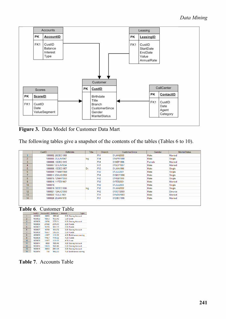
These tables can be merged by the unique CUSTID variable. Notice that, for example, the account table already holds data that are aggregated from a transactional account table. We already have one row per account type that holds aggregated data over time. The data model and the list of available variables can be seen in Figure 3.

Data Mining

241

Figure 3. Data Model for Customer Data Mart The following tables give a snapshot of the contents of the tables (Tables 6 to 10).

Table 6. Customer Table

Table 7. Accounts Table

G. Svolba

242

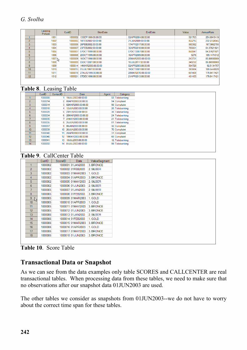
Table 8. Leasing Table

Table 9. CallCenter Table

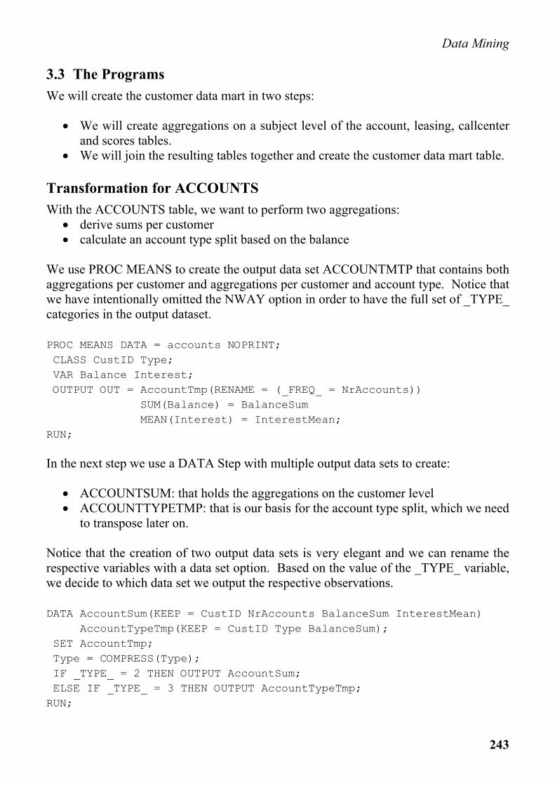
Table 10. Score Table

Transactional Data or Snapshot As we can see from the data examples only table SCORES and CALLCENTER are real transactional tables. When processing data from these tables, we need to make sure that no observations after our snapshot data 01JUN2003 are used. The other tables we consider as snapshots from 01JUN2003--we do not have to worry about the correct time span for these tables.

Data Mining

243

3.3 The Programs We will create the customer data mart in two steps:

• We will create aggregations on a subject level of the account, leasing, callcenter and scores tables.

• We will join the resulting tables together and create the customer data mart table.

Transformation for ACCOUNTS With the ACCOUNTS table, we want to perform two aggregations:

• derive sums per customer • calculate an account type split based on the balance

We use PROC MEANS to create the output data set ACCOUNTMTP that contains both aggregations per customer and aggregations per customer and account type. Notice that we have intentionally omitted the NWAY option in order to have the full set of _TYPE_ categories in the output dataset. PROC MEANS DATA = accounts NOPRINT; CLASS CustID Type; VAR Balance Interest; OUTPUT OUT = AccountTmp(RENAME = (_FREQ_ = NrAccounts)) SUM(Balance) = BalanceSum MEAN(Interest) = InterestMean; RUN; In the next step we use a DATA Step with multiple output data sets to create:

• ACCOUNTSUM: that holds the aggregations on the customer level • ACCOUNTTYPETMP: that is our basis for the account type split, which we need

to transpose later on. Notice that the creation of two output data sets is very elegant and we can rename the respective variables with a data set option. Based on the value of the _TYPE_ variable, we decide to which data set we output the respective observations. DATA AccountSum(KEEP = CustID NrAccounts BalanceSum InterestMean) AccountTypeTmp(KEEP = CustID Type BalanceSum); SET AccountTmp; Type = COMPRESS(Type); IF _TYPE_ = 2 THEN OUTPUT AccountSum; ELSE IF _TYPE_ = 3 THEN OUTPUT AccountTypeTmp; RUN;

G. Svolba

244

Finally we need to transpose the data set with the accounttypes to have a one-row-per-customer structure: PROC TRANSPOSE DATA = AccountTypeTmp OUT = AccountTypes(DROP = _NAME_ _LABEL_); BY CustID; VAR BalanceSum; ID Type; RUN;

Transformation for LEASING For the leasing data we simply summarize the value and the annual rate per customer with the following statement: PROC MEANS DATA = leasing NWAY NOPRINT; CLASS CustID; VAR Value AnnualRate; OUTPUT OUT = LeasingSum(DROP = _TYPE_ RENAME = (_FREQ_ = NrLeasing)) SUM(Value) = LeasingValue SUM(AnnualRate) = LeasingAnnualRate; RUN;

Transformation for CallCenter We first define the snapshot date for the data in a macro variable. %let snapdate = "01JUN2003"d; Then we aggregate the CALLCENTER data over all customers using the PROC FREQ. PROC FREQ DATA = callcenter NOPRINT; TABLE CustID / OUT = CallCenterContacts(DROP = Percent RENAME = (Count = Calls)); WHERE datepart(date) < &snapdate; RUN; Next we calculate the frequencies for the category COMPLAINT. PROC FREQ DATA = callcenter NOPRINT; TABLE CustID / OUT = CallCenterComplaints(DROP = Percent RENAME = (Count = Complaints)); WHERE Category = 'Complaint' and datepart(date) < &snapdate; RUN;

Data Mining

245

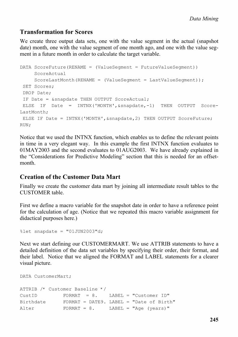
Transformation for Scores We create three output data sets, one with the value segment in the actual (snapshot date) month, one with the value segment of one month ago, and one with the value seg-ment in a future month in order to calculate the target variable. DATA ScoreFuture(RENAME = (ValueSegment = FutureValueSegment)) ScoreActual ScoreLastMonth(RENAME = (ValueSegment = LastValueSegment)); SET Scores; DROP Date; IF Date = &snapdate THEN OUTPUT ScoreActual; ELSE IF Date = INTNX('MONTH',&snapdate,-1) THEN OUTPUT Score-LastMonth; ELSE IF Date = INTNX('MONTH',&snapdate,2) THEN OUTPUT ScoreFuture; RUN; Notice that we used the INTNX function, which enables us to define the relevant points in time in a very elegant way. In this example the first INTNX function evaluates to 01MAY2003 and the second evaluates to 01AUG2003. We have already explained in the “Considerations for Predictive Modeling” section that this is needed for an offset-month.

Creation of the Customer Data Mart Finally we create the customer data mart by joining all intermediate result tables to the CUSTOMER table. First we define a macro variable for the snapshot date in order to have a reference point for the calculation of age. (Notice that we repeated this macro variable assignment for didactical purposes here.) %let snapdate = "01JUN2003"d; Next we start defining our CUSTOMERMART. We use ATTRIB statements to have a detailed definition of the data set variables by specifying their order, their format, and their label. Notice that we aligned the FORMAT and LABEL statements for a clearer visual picture. DATA CustomerMart; ATTRIB /* Customer Baseline */ CustID FORMAT = 8. LABEL = "Customer ID" Birthdate FORMAT = DATE9. LABEL = "Date of Birth" Alter FORMAT = 8. LABEL = "Age (years)"

G. Svolba

246

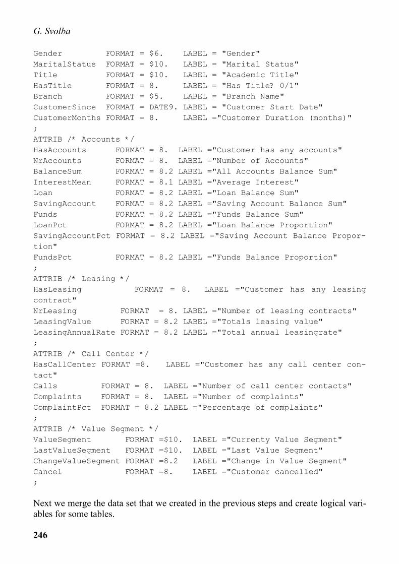
Gender FORMAT = $6. LABEL = "Gender" MaritalStatus FORMAT = $10. LABEL = "Marital Status" Title FORMAT = $10. LABEL = "Academic Title" HasTitle FORMAT = 8. LABEL = "Has Title? 0/1" Branch FORMAT = $5. LABEL = "Branch Name" CustomerSince FORMAT = DATE9. LABEL = "Customer Start Date" CustomerMonths FORMAT = 8. LABEL ="Customer Duration (months)" ; ATTRIB /* Accounts */ HasAccounts FORMAT = 8. LABEL ="Customer has any accounts" NrAccounts FORMAT = 8. LABEL ="Number of Accounts" BalanceSum FORMAT = 8.2 LABEL ="All Accounts Balance Sum" InterestMean FORMAT = 8.1 LABEL ="Average Interest" Loan FORMAT = 8.2 LABEL ="Loan Balance Sum" SavingAccount FORMAT = 8.2 LABEL ="Saving Account Balance Sum" Funds FORMAT = 8.2 LABEL ="Funds Balance Sum" LoanPct FORMAT = 8.2 LABEL ="Loan Balance Proportion" SavingAccountPct FORMAT = 8.2 LABEL ="Saving Account Balance Propor-tion" FundsPct FORMAT = 8.2 LABEL ="Funds Balance Proportion" ; ATTRIB /* Leasing */ HasLeasing FORMAT = 8. LABEL ="Customer has any leasing contract" NrLeasing FORMAT = 8. LABEL ="Number of leasing contracts" LeasingValue FORMAT = 8.2 LABEL ="Totals leasing value" LeasingAnnualRate FORMAT = 8.2 LABEL ="Total annual leasingrate" ; ATTRIB /* Call Center */ HasCallCenter FORMAT =8. LABEL ="Customer has any call center con-tact" Calls FORMAT = 8. LABEL ="Number of call center contacts" Complaints FORMAT = 8. LABEL ="Number of complaints" ComplaintPct FORMAT = 8.2 LABEL ="Percentage of complaints" ; ATTRIB /* Value Segment */ ValueSegment FORMAT =$10. LABEL ="Currenty Value Segment" LastValueSegment FORMAT =$10. LABEL ="Last Value Segment" ChangeValueSegment FORMAT =8.2 LABEL ="Change in Value Segment" Cancel FORMAT =8. LABEL ="Customer cancelled" ; Next we merge the data set that we created in the previous steps and create logical vari-ables for some tables.

Data Mining

247

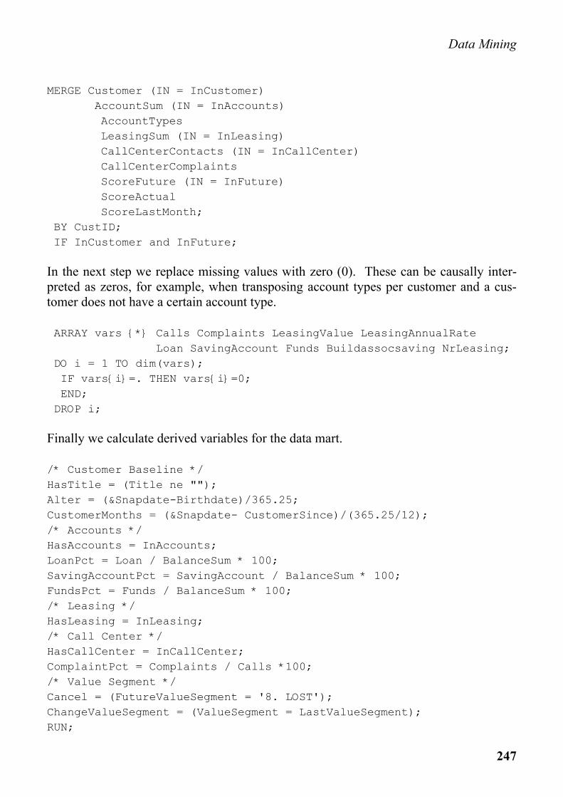
MERGE Customer (IN = InCustomer) AccountSum (IN = InAccounts) AccountTypes LeasingSum (IN = InLeasing) CallCenterContacts (IN = InCallCenter) CallCenterComplaints ScoreFuture (IN = InFuture) ScoreActual ScoreLastMonth; BY CustID; IF InCustomer and InFuture; In the next step we replace missing values with zero (0). These can be causally inter-preted as zeros, for example, when transposing account types per customer and a cus-tomer does not have a certain account type. ARRAY vars {*} Calls Complaints LeasingValue LeasingAnnualRate Loan SavingAccount Funds Buildassocsaving NrLeasing; DO i = 1 TO dim(vars); IF vars{i}=. THEN vars{i}=0; END; DROP i; Finally we calculate derived variables for the data mart. /* Customer Baseline */ HasTitle = (Title ne ""); Alter = (&Snapdate-Birthdate)/365.25; CustomerMonths = (&Snapdate- CustomerSince)/(365.25/12); /* Accounts */ HasAccounts = InAccounts; LoanPct = Loan / BalanceSum * 100; SavingAccountPct = SavingAccount / BalanceSum * 100; FundsPct = Funds / BalanceSum * 100; /* Leasing */ HasLeasing = InLeasing; /* Call Center */ HasCallCenter = InCallCenter; ComplaintPct = Complaints / Calls *100; /* Value Segment */ Cancel = (FutureValueSegment = '8. LOST'); ChangeValueSegment = (ValueSegment = LastValueSegment); RUN;

G. Svolba

248

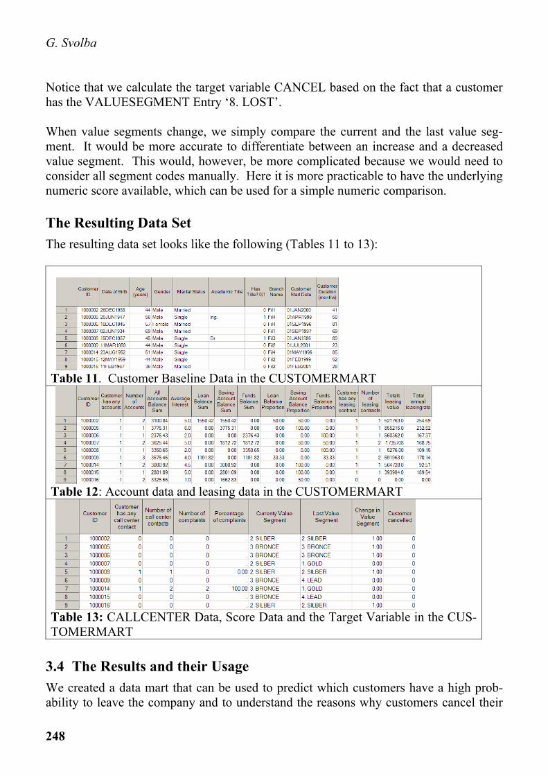
Notice that we calculate the target variable CANCEL based on the fact that a customer has the VALUESEGMENT Entry ‘8. LOST’. When value segments change, we simply compare the current and the last value seg-ment. It would be more accurate to differentiate between an increase and a decreased value segment. This would, however, be more complicated because we would need to consider all segment codes manually. Here it is more practicable to have the underlying numeric score available, which can be used for a simple numeric comparison.

The Resulting Data Set The resulting data set looks like the following (Tables 11 to 13):

Table 11. Customer Baseline Data in the CUSTOMERMART

Table 12: Account data and leasing data in the CUSTOMERMART

Table 13: CALLCENTER Data, Score Data and the Target Variable in the CUS-TOMERMART

3.4 The Results and their Usage We created a data mart that can be used to predict which customers have a high prob-ability to leave the company and to understand the reasons why customers cancel their

Data Mining

249

service. We can perform univariate and multivariate descriptive analysis on the cus-tomer attributes. We can develop predictive modeling to determine the likelihood that future customers will cancel. Notice that we only used data that we found in our five tables. We aggregated and transposed some of the data to a one-row-per-subject structure and joined these tables together. The derived variables that we defined give a good picture of the customer at-tributes and provide the best possible inference of customer behavior.

4 CONCLUSION This paper shows that data preparation is a key success factor for analytical projects. Besides multiple-row-per-subject data marts or longitudinal data marts, the one-row-per-subject data mart is frequently used and is central for statistical and data mining analyses. In many cases the available source data have a one-to-many relationship to the subject itself. Therefore data needs to be transposed or aggregated. The selection of the trans-position and aggregation methods is primarily driven by business considerations of what will be meaningful derived variables. This paper shows you ways to create a one-row-per-subject data mart from a conceptual and a coding point of view. Anyone who is interested in more details on Data Preparation for Analytics is referred to my book with the same name, which will be published by SAS Press (Book# 60502) in September 2006 (see the “Recommended Reading” section). In this book the busi-ness point of view, the concepts, and coding examples for data preparation in analytics is extensively discussed.

5 Recommended Reading The author of this paper has written a SAS Press publication titled Data Preparation for Analytics. See http://www.sascommunity.org/wiki/Data_Preparation_for_Analytics for more details on the book, the download of free macros, example code and example datasets, as well as sample chapters or a table of contents. The book provides a more detailed discussion on the topic of this paper. This book is written for SAS users and anyone involved in the data preparation process for analytics. The focus of the book is to give practical advice in the form of SAS coding tips and tricks, as well as conceptual background on data structures and considerations from the business point of view.

G. Svolba

250

This book will enable the reader to do the following:

• view analytic data preparation in light of its business environment and consider the underlying business question in data preparation

• learn about data models and relevant analytic data structures like the one-row-per-subject data mart, the multiple-row-per-subject data mart, and the longitudi-nal data mart

• use powerful SAS macros for the change between the various data mart structures • consider the specifics of predictive modeling for data mart creation • learn how to create meaningful derived variables for all data mart types • illustrate how to create a one-row-per-subject data mart from various data sources

and data structures • learn the concepts and considerations when preparing data for time series analysis • illustrate how scoring can be done with various SAS procedures themselves and

with SAS® Enterprise Miner™ • learn about the power of SAS for analytic data preparation and the data mart re-

quirements of various SAS procedures • benefit from many do’s and don’ts and practical examples for data mart building