DETERMINATION OF RESERVOIR DRAINAGE AREA FOR CONSTANT ... · DETERMINATION OF RESERVOIR DRAINAGE AREA FOR CONSTANT-PRESSURE SYSTEMS CT&F - Ciencia, Tecnología y Futuro - Vol. 4 Núm

51CT&F - Ciencia, Tecnología y Futuro - Vol. 4 Núm. 1 Jun. 2010

DETERMINATION OF RESERVOIR DRAINAGE AREA FOR CONSTANT-PRESSURE SYSTEMS USING WELL

TEST DATA

Freddy-Humberto Escobar1*, Yuly-Andrea Hernández2 and Djebbar Tiab3

1 Universidad Surcolombiana, Av. Pastrana – Cra. 1, Neiva, Huila, Colombia2 Columbus Energy Sucursal Colombia, Cra 7 # 71-21 Ofic. 1402B, Bogotá, Colombia

3 The University of Oklahoma, 100 E. Boyd St., Norman, OK, 73019, USA

e-mail: [email protected] [email protected] [email protected]

(Received, Jan. 29, 2010; Accepted May 26, 2010)

In this work, the conventional cartesian straight-line pseudosteady-state solution and the Total Dissolved Solids (TDS) solution to estimate reservoir drainage area is applied to constant-pressure reservoirs to observe its accuracy. It was found that it performs very poorly in such systems, especially in those having

rectangular shape. On the other hand, the pseudosteady-state solution of the TDS technique performs better in constant-pressure systems and may be applied only to regular square- or circular-shaped reservoirs with a resulting small deviation error. Therefore, new solutions for steady-state systems in circular, square and rect-angular reservoir geometries having one or two constant-pressure boundaries are developed, compared and successfully verified with synthetic and real field cases. Automatic matching performed by commercial software sometimes are so time consuming and tedious which leads to another reason to use the proposed equations.

* To whom correspondence may be addressed

Keywords: reservoir, pressure, well testing, reservoir drainage area, pseudosteady state, TDS Technique.

* To whom correspondence may be addressed

52 CT&F - Ciencia, Tecnología y Futuro - Vol. 4 Núm. 1 Jun. 2010

En este trabajo se aplica la solución convencional de análisis cartesiano para estimar el área de drenaje en yacimientos con fronteras a presión constante para verificar su exactitud. Se encontró que esta produce resultados muy pobres, especialmente en yacimientos con geometría rectangular.

Por otro lado, la solución de estado pseudoestable de la técnica TDS trabaja mejor en sistemas a presión constante y se podría aplicar con un pequeño margen de error en sistemas regulares con geometría circular o cuadrada. Por tanto, se desarrollaron nuevas soluciones para sistemas en estado estable con geometría circular, cuadrada y rectangular que tienen una o más fronteras de presión constante. Estas se compararon y se probaron exitosamente en casos simulados y de campo. El ajuste automático efectuado por los paquetes comerciales algunas veces consumen mucho tiempo y son tediosos. Esto proporciona otra razón para usar las ecuaciones aquí propuestas.

Palabras clave: yacimientos, presión, pruebas de presión, área de drenaje del yacimiento, estado pseudoestable, técnica TDS.

53

DETERMINATION OF RESERVOIR DRAINAGE AREA FOR CONSTANT-PRESSURE SYSTEMS

CT&F - Ciencia, Tecnología y Futuro - Vol. 4 Núm. 1 Jun. 2010

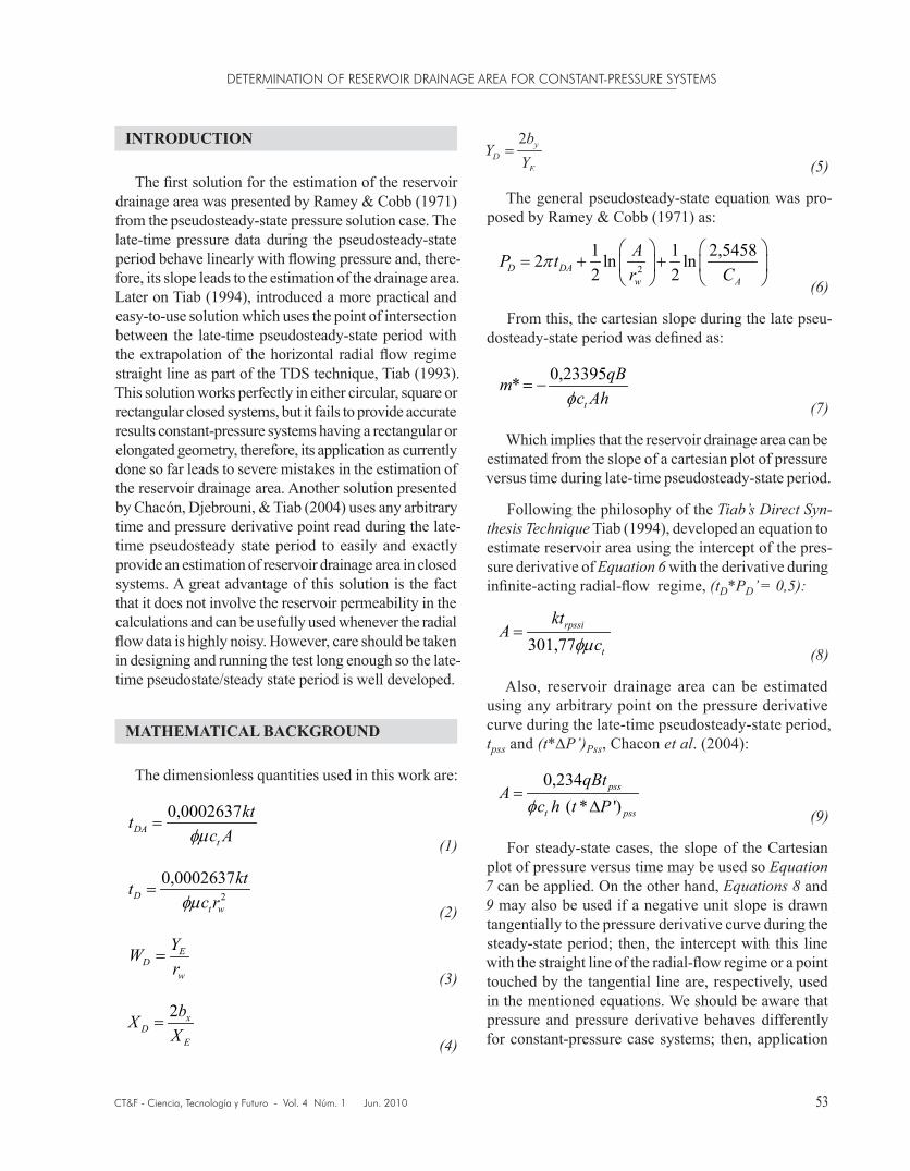
INTRODUCTION

The first solution for the estimation of the reservoir drainage area was presented by Ramey & Cobb (1971) from the pseudosteady-state pressure solution case. The late-time pressure data during the pseudosteady-state period behave linearly with flowing pressure and, there-fore, its slope leads to the estimation of the drainage area. Later on Tiab (1994), introduced a more practical and easy-to-use solution which uses the point of intersection between the late-time pseudosteady-state period with the extrapolation of the horizontal radial flow regime straight line as part of the TDS technique, Tiab (1993). This solution works perfectly in either circular, square or rectangular closed systems, but it fails to provide accurate results constant-pressure systems having a rectangular or elongated geometry, therefore, its application as currently done so far leads to severe mistakes in the estimation of the reservoir drainage area. Another solution presented by Chacón, Djebrouni, & Tiab (2004) uses any arbitrary time and pressure derivative point read during the late-time pseudosteady state period to easily and exactly provide an estimation of reservoir drainage area in closed systems. A great advantage of this solution is the fact that it does not involve the reservoir permeability in the calculations and can be usefully used whenever the radial flow data is highly noisy. However, care should be taken in designing and running the test long enough so the late-time pseudostate/steady state period is well developed.

MATHEMATICAL BACKGROUND

The dimensionless quantities used in this work are:

0,0002637DA

t

kttc Aφµ

(1)

2

0,0002637D

t w

kttc rφµ

(2)

ED

w

YWr

(3)

2 xD

E

bXX

(4)

(5)

The general pseudosteady-state equation was pro-posed by Ramey & Cobb (1971) as:

2

1 1 2,54582 ln ln2 2D DA

w A

AP tr C

π

(6)

From this, the cartesian slope during the late pseu-dosteady-state period was defined as:

0,23395*t

qBmc Ahφ

− (7)

Which implies that the reservoir drainage area can be estimated from the slope of a cartesian plot of pressure versus time during late-time pseudosteady-state period.

Following the philosophy of the Tiab’sDirectSyn-thesisTechnique Tiab (1994), developed an equation to estimate reservoir area using the intercept of the pres-sure derivative of Equation6 with the derivative during infinite-acting radial-flow regime, (tD*PD’=0,5):

301,77

rpssi

t

ktA

cφµ

(8)

Also, reservoir drainage area can be estimated using any arbitrary point on the pressure derivative curve during the late-time pseudosteady-state period, tpss and (t*∆P’)Pss, Chacon etal. (2004):

0,234 ( * ')

pss

t pss

qBtA

c h t Pφ

∆ (9)

For steady-state cases, the slope of the Cartesian plot of pressure versus time may be used so Equation 7 can be applied. On the other hand, Equations 8 and 9 may also be used if a negative unit slope is drawn tangentially to the pressure derivative curve during the steady-state period; then, the intercept with this line with the straight line of the radial-flow regime or a point touched by the tangential line are, respectively, used in the mentioned equations. We should be aware that pressure and pressure derivative behaves differently for constant-pressure case systems; then, application

FREDDY-HUMBERTO ESCOBAR et al


Suffix ssri stands for the intersection between the negative unit-slope line drawn tangentially to the pressure derivative curve with the radial line. It should be clarified that Equation 8 applies to any closed reservoir geometry, but Equation 12 only ap-plies to either circular or square shape drainage area as indicated in Table 1.

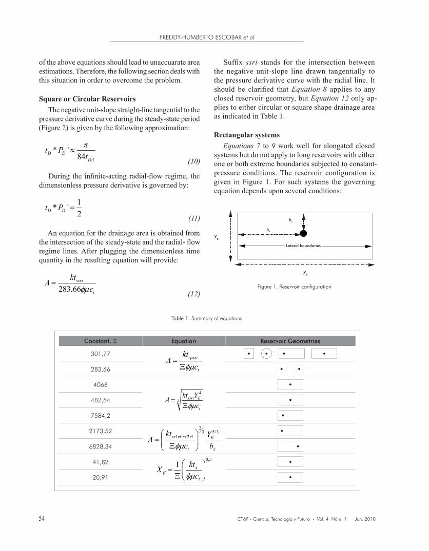
Rectangular systemsEquations7 to 9 work well for alongated closed

systems but do not apply to long reservoirs with either one or both extreme boundaries subjected to constant-pressure conditions. The reservoir configuration is given in Figure 1. For such systems the governing equation depends upon several conditions:

of the above equations should lead to unaccuarate area estimations. Therefore, the following section deals with this situation in order to overcome the problem.

Square or Circular Reservoirs The negative unit-slope straight-line tangential to the

pressure derivative curve during the steady-state period (Figure 2) is given by the following approximation:

* '

84D DDA

t Ptπ

≈ (10)

During the infinite-acting radial-flow regime, the dimensionless pressure derivative is governed by:

1* '2D Dt P

(11)

An equation for the drainage area is obtained from the intersection of the steady-state and the radial- flow regime lines. After plugging the dimensionless time quantity in the resulting equation will provide:

283,66

ssri

t

ktAcφµ

(12)

Figure 1. Reservoir configuration

YE

Lateral boundaries

bx

by

XE

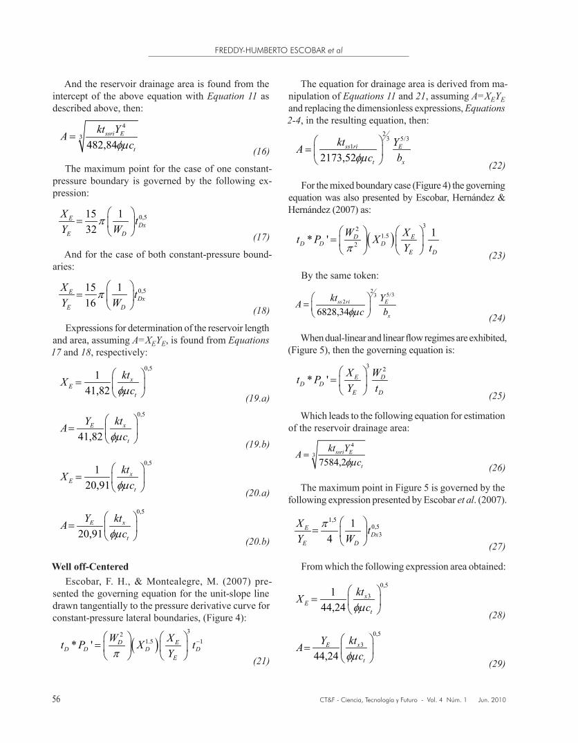
Table 1. Summary of equations

Constant, Ξ Equation Reservoir Geometries

301,77

283,66

4066

482,84

7584,2

2173,52

6828,34

41,82

20,91

55



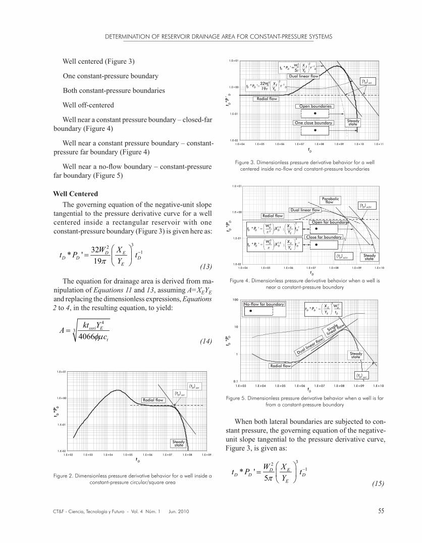
Figure 5. Dimensionless pressure derivative behavior when a well is far from a constant-pressure boundary

Figure 2. Dimensionless pressure derivative behavior for a well inside a constant-pressure circular/square area

Figure 3. Dimensionless pressure derivative behavior for a well centered inside no-flow and constant-pressure boundaries

Figure 4. Dimensionless pressure derivative behavior when a well is near a constant-pressure boundary

1.E+081.E-02

1.E-01

1.E+00

1.E+01

1.E+02 1.E+03 1.E+04 1.E+05 1.E+06 1.E+07 1.E+09

( )D ssrit

Radial flow

Steady state

( )D ssrit

t *

P'

D

D

t D

t D*P´ D

tD

1.E-02

1.E-01

1.E+00

1.E+01

1.E+04 1.E+05 1.E+06 1.E+07 1.E+08 1.E+09 1.E+10 1.E+11

Open boundaries

One close boundary

Dual linear flow

Radial flow

Steady state

( )D ssrit32132* '

19D E

D D DE

W Xt P t

Yπ−

321* '

5D E

D D DE

W XYπ

− = t P t

1.E-02

1.E-01

1.E+00

1.E+01

1.E+04 1.E+05 1.E+06 1.E+07 1.E+08 1.E+09 1.E+10

t *P

' D

D

tD

Open far boundary

Close far boundary

Dual linear flowRadial flow

Parabolic flow

Steady state

321.5 1

2* ' D E

D D D DE

W Xt P X t

Yπ−

321.5 1* ' D E

D D D DE

W Xt P X t

Yπ−

1( )D ss rit

2( )D ss rit

0.1

1

10

100

1.E+03 1.E+04 1.E+05 1.E+06 1.E+07 1.E+08 1.E+09 1.E+10

t *P

' D

D

tD

Dual linear fl

ow

Radial flow

Single

linear flow

Steady state

( )D ssrit

3 2

* ' E DD D

E D

X Wt P

Y t

No-flow far boundary

Well centered (Figure 3)

One constant-pressure boundary

Both constant-pressure boundaries

Well off-centered

Well near a constant pressure boundary – closed-far boundary (Figure 4)

Well near a constant pressure boundary – constant-pressure far boundary (Figure 4)

Well near a no-flow boundary – constant-pressure far boundary (Figure 5)

Well CenteredThe governing equation of the negative-unit slope

tangential to the pressure derivative curve for a well centered inside a rectangular reservoir with one constant-pressure boundary (Figure 3) is given here as:

32132* '

19D E

D D DE

W Xt P tYπ

−

(13)

The equation for drainage area is derived from ma-nipulation of Equations11 and 13, assuming A=XEYE and replacing the dimensionless expressions, Equations2 to 4, in the resulting equation, to yield:

4

34066

ssri E

t

kt YAcφµ

(14)

When both lateral boundaries are subjected to con-stant pressure, the governing equation of the negative-unit slope tangential to the pressure derivative curve, Figure 3, is given as:

321* '

5D E

D D DE

W Xt P tYπ

−

(15)



And the reservoir drainage area is found from the intercept of the above equation with Equation11 as described above, then:

4

3482,84

ssri E

t

kt YAcφµ

(16)

The maximum point for the case of one constant-pressure boundary is governed by the following ex-pression:

0,515 1

32E

DxE D

X tY W

π

(17)

And for the case of both constant-pressure bound-aries:

0,515 1

16E

DxE D

X tY W

π

(18)

Expressions for determination of the reservoir length and area, assuming A=XEYE, is found from Equations17 and 18, respectively:

0,51

41,82x

Et

ktXcφµ

(19.a)

0,5

41,82xE

t

ktYAcφµ

(19.b)

0,51

20,91x

Et

ktXcφµ

(20.a)

0,5

20,91xE

t

ktYAcφµ

(20.b)

Well off-CenteredEscobar, F. H., & Montealegre, M. (2007) pre-

sented the governing equation for the unit-slope line drawn tangentially to the pressure derivative curve for constant-pressure lateral boundaries, (Figure 4):

321.5 1* ' D E

D D D DE

W Xt P X tYπ

− (21)

The equation for drainage area is derived from ma-nipulation of Equations11 and 21, assuming A=XEYEand replacing the dimensionless expressions, Equations2-4, in the resulting equation, then:

23 5/3

1

2173,52ss ri E

t x

kt YAc bφµ

(22)

For the mixed boundary case (Figure 4) the governing equation was also presented by Escobar, Hernández & Hernández (2007) as:

321.5

2

1* ' D ED D D

E D

W Xt P XY tπ

(23)

By the same token:

25/33

2

6828,34ss ri E

x

kt YAc bφµ

(24)

When dual-linear and linear flow regimes are exhibited, (Figure 5), then the governing equation is:

3 2

* ' E DD D

E D

X Wt PY t

(25)

Which leads to the following equation for estimation of the reservoir drainage area:

4

37584,2

ssri E

t

kt YAcφµ

(26)

The maximum point in Figure 5 is governed by the following expression presented by Escobar etal. (2007).

1,50,5

31

4E

DxE D

X tY W

π

(27)

From which the following expression area obtained:

0,5

3144,24

xE

t

ktXcφµ

(28)

0,5

3

44,24xE

t

ktYAcφµ

(29)

57



bx and YE in Equations22 and 24 can be obtained from the equation presented by Escobar etal. (2007) using the TDS technique:

246,32RPBiE

xt

ktYbcφµ

(30)

0,05756 RDLi

Et

ktYcφµ

(31)

Or from the conventional straight-line method, Es-cobar & Montealegre (2007):

1,5

34780,8PB E

xt

m hY kbqB c µφ

−

(32)

0,5

8,1282EDLF t

qBYm h k c

µφ

(33)

The just mentioned references contain some other expression to estimate well position and reservoir width along with the estimation of the geometric skin factors.

A practical summary of the drainage area equations is provided in Table 1.

EXAMPLES

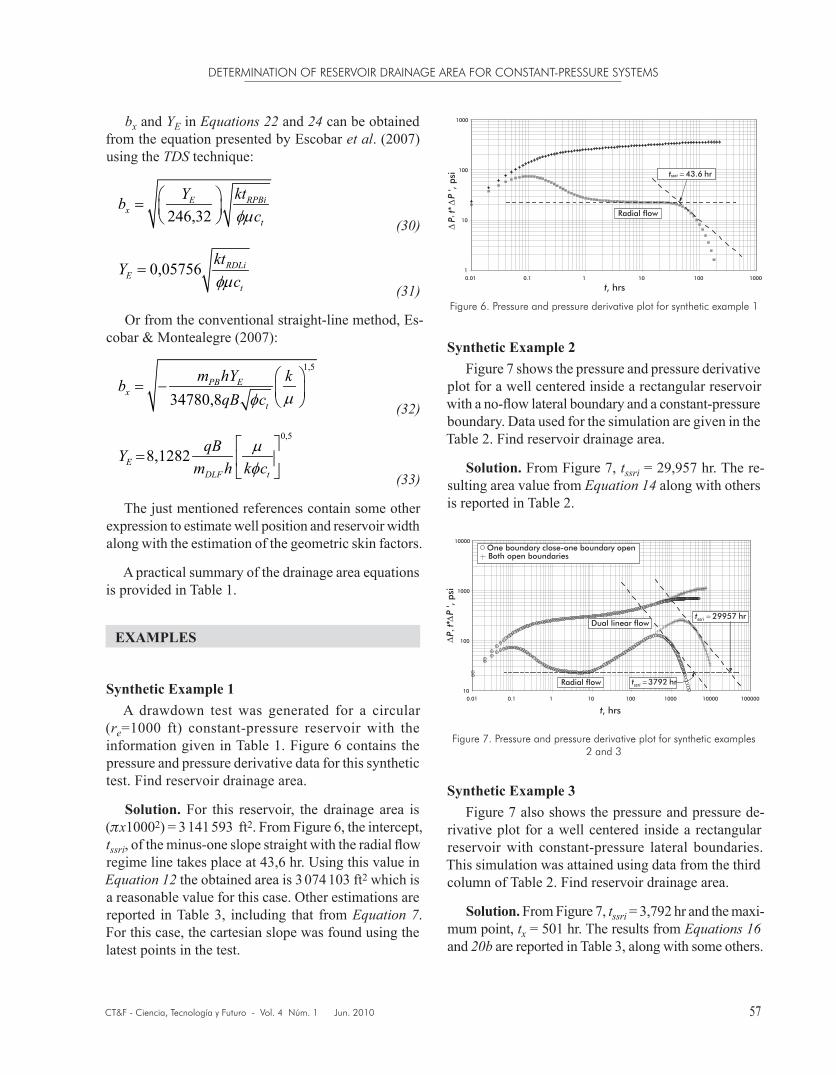
Synthetic Example 1A drawdown test was generated for a circular

(re=1000 ft) constant-pressure reservoir with the information given in Table 1. Figure 6 contains the pressure and pressure derivative data for this synthetic test. Find reservoir drainage area.

Solution. For this reservoir, the drainage area is (x10002) = 3 141 593 ft2. From Figure 6, the intercept, tssri, of the minus-one slope straight with the radial flow regime line takes place at 43,6 hr. Using this value in Equation12 the obtained area is 3 074 103 ft2 which is a reasonable value for this case. Other estimations are reported in Table 3, including that from Equation7. For this case, the cartesian slope was found using the latest points in the test.

Synthetic Example 2Figure 7 shows the pressure and pressure derivative

plot for a well centered inside a rectangular reservoir with a no-flow lateral boundary and a constant-pressure boundary. Data used for the simulation are given in the Table 2. Find reservoir drainage area.

Solution. From Figure 7, tssri = 29,957 hr. The re-sulting area value from Equation14 along with others is reported in Table 2.

Figure 6. Pressure and pressure derivative plot for synthetic example 1

1

10

100

1000

0.01 0.1 1 10 100 1000

∆ ∆

P t*

P ' ,

psi

t, hrs

43.6 hrssrit

Radial flow

Figure 7. Pressure and pressure derivative plot for synthetic examples 2 and 3

10

100

1000

10000

0.01 0.1 1 10 100 1000 10000 100000

∆P

t*∆

P ' ,

psi

t, hrs

3792 hrssrit

29957 hrssrit

One boundary close-one boundary openBoth open boundaries

Radial flow

Dual linear flow

Synthetic Example 3Figure 7 also shows the pressure and pressure de-

rivative plot for a well centered inside a rectangular reservoir with constant-pressure lateral boundaries. This simulation was attained using data from the third column of Table 2. Find reservoir drainage area.

Solution. From Figure 7, tssri = 3,792 hr and the maxi-mum point, tx = 501 hr. The results from Equations16 and 20b are reported in Table 3, along with some others.



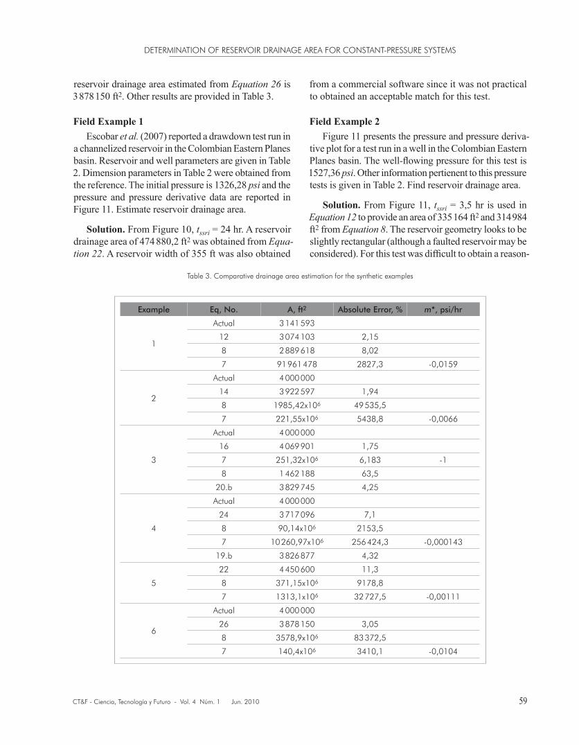
Synthetic Example 4A drawdown test was generated for a well centered

inside a rectangular-shaped reservoir with one constant-pressure boundary and one no-flow boundary, using the information given in Table 1. Figure 8 contains the pressure and pressure derivative data for this synthetic test. Find reservoir drainage area.

Solution. From Figure 8, tss2ri = 5,600 hr and tx = 2001 hr. The results from Equations24,19b,7 and 8 are also reported in Table 3.

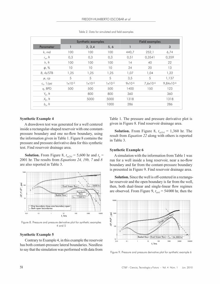
Table 2. Data for simulated and field examples

Synthetic examples Field examples

Parameter 1 2, 3,4 5, 6 1 2 3

k, md 100 100 100 440,7 252,1 6,74

rw, ft 0,3 0,3 0,3 0,51 0,3541 0,359

h, ft 100 100 100 14 40 22

, % 10 10 10 24 20 13

B, rb/STB 1,25 1,25 1,25 1,07 1,04 1,22

, cp 5 5 5 3,5 5 1,137

ct, 1/psi 1x10-5 1x10-5 1x10-5 9x10-6 7,6x10-6 9,84x10-6

q, BPD 500 500 500 1400 150 123

YE, ft 800 800 360 360

XE, ft 5000 5000 1318 1318

bx, ft 1000 286 286

Table 1. The pressure and pressure derivative plot is given in Figure 8. Find reservoir drainage area.

Solution. From Figure 8, tss1ri = 1,360 hr. The result from Equation22 along with others is reported in Table 3.

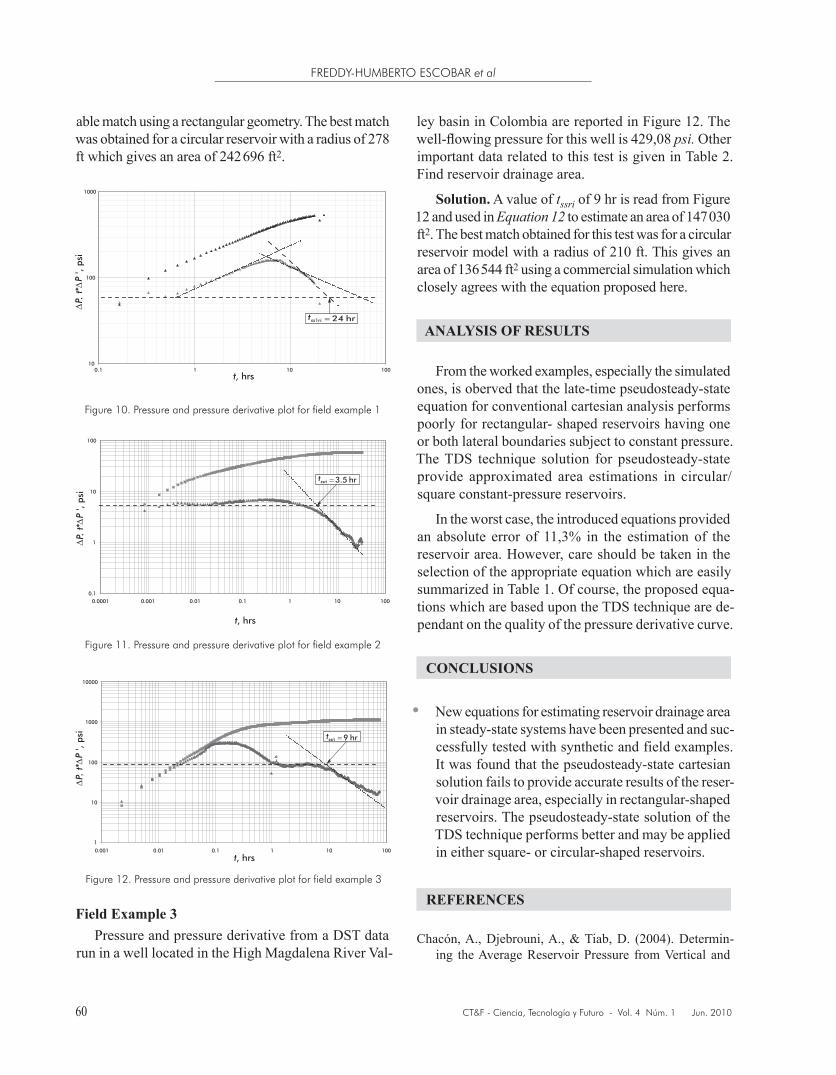
Synthetic Example 6A simulation with the information from Table 1 was

run for a well inside a long reservoir, near a no-flow boundary and far from the contant-pressure boundary is presented in Figure 9. Find reservoir drainage area.

Solution. Since the well is off-centered in a rectangu-lar reservoir and the open boundary is far from the well, then, both dual-linear and single-linear flow regimes are observed. From Figure 9, tssri= 54 000 hr, then the

Figure 9. Pressure and pressure derivative plot for synthetic example 6

Figure 8. Pressure and pressure derivative plot for synthetic examples 4 and 5

1

10

100

1000

0.01 0.1 1 10 100 1000 10000

∆P

t*∆

P ' ,

psi

t, hrs

1 1360 hrss rit

One boundary close-one boundary openBoth open boundaries

2 5600 hrss rit Dual linear flow

Radial flowParabolic

flow

10

100

1000

10000

0.01 0.1 1 10 100 1000 10000 100000

∆P

t*∆

P ' ,

psi

t, hrs

54,000 hrssrit Dual linear flowRadial flow

Single linear fl

ow

Synthetic Example 5Contrary to Example 4, in this example the reservoir

has both contant-pressure lateral boundaries. Needless to say that the simulation was performed with data from

59



from a commercial software since it was not practical to obtained an acceptable match for this test.

Field Example 2Figure 11 presents the pressure and pressure deriva-

tive plot for a test run in a well in the Colombian Eastern Planes basin. The well-flowing pressure for this test is 1527,36psi. Other information pertienent to this pressure tests is given in Table 2. Find reservoir drainage area.

Solution. From Figure 11, tssri = 3,5 hr is used in Equation12 to provide an area of 335 164 ft2 and 314 984 ft2 from Equation8. The reservoir geometry looks to be slightly rectangular (although a faulted reservoir may be considered). For this test was difficult to obtain a reason-

reservoir drainage area estimated from Equation26 is 3 878 150 ft2. Other results are provided in Table 3.

Field Example 1Escobar etal. (2007) reported a drawdown test run in

a channelized reservoir in the Colombian Eastern Planes basin. Reservoir and well parameters are given in Table 2. Dimension parameters in Table 2 were obtained from the reference. The initial pressure is 1326,28 psi and the pressure and pressure derivative data are reported in Figure 11. Estimate reservoir drainage area.

Solution. From Figure 10, tssri = 24 hr. A reservoir drainage area of 474 880,2 ft2 was obtained from Equa-tion22. A reservoir width of 355 ft was also obtained

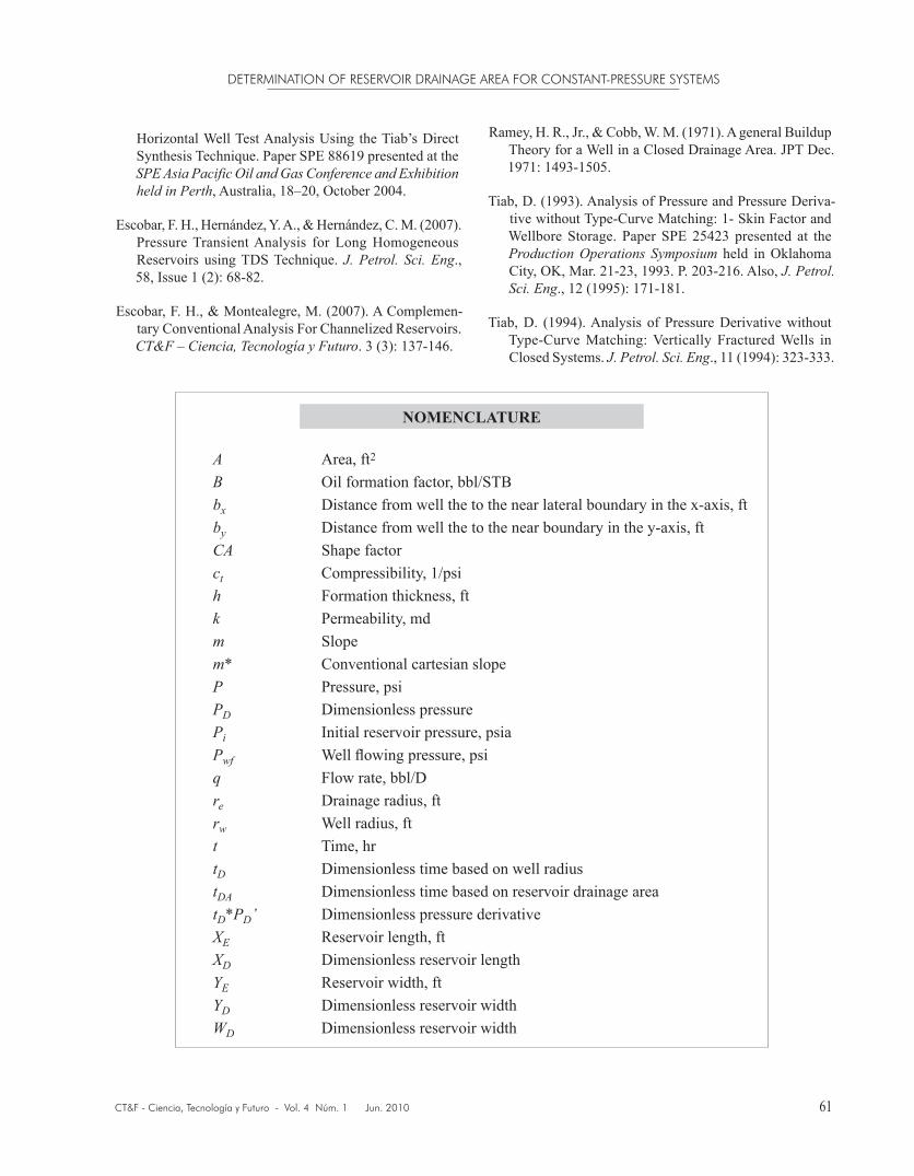
Table 3. Comparative drainage area estimation for the synthetic examples

Example Eq, No. A, ft2 Absolute Error, % m*, psi/hr

1

Actual 3 141 593

12 3 074 103 2,15

8 2 889 618 8,02

7 91 961 478 2827,3 -0,0159

2

Actual 4 000 000

14 3 922 597 1,94

8 1985,42x106 49 535,5

7 221,55x106 5438,8 -0,0066

3

Actual 4 000 000

16 4 069 901 1,75

7 251,32x106 6,183 -1

8 1 462 188 63,5

20.b 3 829 745 4,25

4

Actual 4 000 000

24 3 717 096 7,1

8 90,14x106 2153,5

7 10 260,97x106 256 424,3 -0,000143

19.b 3 826 877 4,32

5

22 4 450 600 11,3

8 371,15x106 9178,8

7 1313,1x106 32 727,5 -0,00111

6

Actual 4 000 000

26 3 878 150 3,05

8 3578,9x106 83 372,5

7 140,4x106 3410,1 -0,0104



Figure 11. Pressure and pressure derivative plot for field example 2

0.1

1

10

100

0.0001 0.001 0.01 0.1 1 10 100

∆P

t*∆

P ' ,

psi

t, hrs

3.5 hrssrit

ley basin in Colombia are reported in Figure 12. The well-flowing pressure for this well is 429,08 psi. Other important data related to this test is given in Table 2. Find reservoir drainage area.

Solution. A value of tssri of 9 hr is read from Figure 12 and used in Equation12 to estimate an area of 147 030 ft2. The best match obtained for this test was for a circular reservoir model with a radius of 210 ft. This gives an area of 136 544 ft2 using a commercial simulation which closely agrees with the equation proposed here.

ANALYSIS OF RESULTS

From the worked examples, especially the simulated ones, is oberved that the late-time pseudosteady-state equation for conventional cartesian analysis performs poorly for rectangular- shaped reservoirs having one or both lateral boundaries subject to constant pressure. The TDS technique solution for pseudosteady-state provide approximated area estimations in circular/square constant-pressure reservoirs.

In the worst case, the introduced equations provided an absolute error of 11,3% in the estimation of the reservoir area. However, care should be taken in the selection of the appropriate equation which are easily summarized in Table 1. Of course, the proposed equa-tions which are based upon the TDS technique are de-pendant on the quality of the pressure derivative curve.

CONCLUSIONS

• New equations for estimating reservoir drainage area in steady-state systems have been presented and suc-cessfully tested with synthetic and field examples. It was found that the pseudosteady-state cartesian solution fails to provide accurate results of the reser-voir drainage area, especially in rectangular-shaped reservoirs. The pseudosteady-state solution of the TDS technique performs better and may be applied in either square- or circular-shaped reservoirs.

REFERENCES

Chacón, A., Djebrouni, A., & Tiab, D. (2004). Determin-ing the Average Reservoir Pressure from Vertical and


1

10

100

1000

10000

0.001 0.01 0.1 1 10 100

∆P

t*∆

P ' ,

psi

t, hrs

9 hrssrit


10

100

1000

0.1 1 10 100

∆P

t*∆

P ' ,

psi

t, hrs

1 24 hrss rit

able match using a rectangular geometry. The best match was obtained for a circular reservoir with a radius of 278 ft which gives an area of 242 696 ft2.

Field Example 3Pressure and pressure derivative from a DST data

run in a well located in the High Magdalena River Val-

61



Horizontal Well Test Analysis Using the Tiab’s Direct Synthesis Technique. Paper SPE 88619 presented at the SPEAsiaPacificOilandGasConferenceandExhibitionheldinPerth, Australia, 18–20, October 2004.

Escobar, F. H., Hernández, Y. A., & Hernández, C. M. (2007). Pressure Transient Analysis for Long Homogeneous Reservoirs using TDS Technique. J.Petrol. Sci.Eng., 58, Issue 1 (2): 68-82.

Escobar, F. H., & Montealegre, M. (2007). A Complemen-tary Conventional Analysis For Channelized Reservoirs. CT&F–Ciencia,TecnologíayFuturo. 3 (3): 137-146.

NOMENCLATURE

A Area, ft2

B Oil formation factor, bbl/STBbx Distance from well the to the near lateral boundary in the x-axis, ftby Distance from well the to the near boundary in the y-axis, ftCA Shape factorct Compressibility, 1/psih Formation thickness, ftk Permeability, mdm Slopem* Conventional cartesian slopeP Pressure, psiPD Dimensionless pressurePi Initial reservoir pressure, psiaPwf Well flowing pressure, psiq Flow rate, bbl/Dre Drainage radius, ftrw Well radius, ftt Time, hrtD Dimensionless time based on well radiustDA Dimensionless time based on reservoir drainage areatD*PD’ Dimensionless pressure derivativeXE Reservoir length, ftXD Dimensionless reservoir lengthYE Reservoir width, ftYD Dimensionless reservoir widthWD Dimensionless reservoir width

Ramey, H. R., Jr., & Cobb, W. M. (1971). A general Buildup Theory for a Well in a Closed Drainage Area. JPT Dec. 1971: 1493-1505.

Tiab, D. (1993). Analysis of Pressure and Pressure Deriva-tive without Type-Curve Matching: 1- Skin Factor and Wellbore Storage. Paper SPE 25423 presented at the ProductionOperations Symposium held in Oklahoma City, OK, Mar. 21-23, 1993. P. 203-216. Also, J.Petrol.Sci.Eng., 12 (1995): 171-181.

Tiab, D. (1994). Analysis of Pressure Derivative without Type-Curve Matching: Vertically Fractured Wells in Closed Systems. J.Petrol.Sci.Eng., 11 (1994): 323-333.



Change, dropt Flow time, hrø Porosity, fraction Viscosity, cp

D DimensionlessDLF Dual-linear flowi Intersection or initial conditions L LinearPB Parabolicpss Pseudosteadypsi Pounds per Square InchSS SteadyDLPSSi Intersection of pseudosteady-state line with dual- linear lineLPSSi Intersection of pseudosteady-state line with lineal linerpssi Intersection of pseudosteady-state line with radial lineRDLi Intersection of radial line with dual lineal lineRLi Intersection of radial line with lineal lineRPBi Intersection of radial line with with the parabolic flow liness1ri Intersection between the radial line and the -1-slope line ss2ri Intersection of radial line with -1-slope line (SS2)ssri Intersection of radial line with -1-slope line (SS2)r radial floww Wellx Maximum point (peak) after dual linear flow is vanished and steady

state begins

SUFFICES

GREEK

Documents

DETERMINATION OF RESERVOIR DRAINAGE AREA FOR CONSTANT ... · DETERMINATION OF RESERVOIR DRAINAGE AREA FOR CONSTANT-PRESSURE SYSTEMS CT&F - Ciencia, Tecnología y Futuro - Vol. 4 Núm