Embed Size (px)
Citation preview
Veröffentlichungen der DGK
Ausschuss Geodäsie der Bayerischen Akademie der Wissenschaften
Reihe C Dissertationen Heft Nr. 779
David Becker
Advanced Calibration Methods
for Strapdown Airborne Gravimetry
München 2016
Verlag der Bayerischen Akademie der Wissenschaften
ISSN 0065-5325 ISBN 978-3-7696-5191-1
Diese Arbeit ist gleichzeitig veröffentlicht in:
Schriftenreihe Fachrichtung Geodäsie der Technischen Universität Darmstadt
ISBN 978-3-935631-40-2, Nr. 51, Darmstadt 2016

Veröffentlichungen der DGK
Ausschuss Geodäsie der Bayerischen Akademie der Wissenschaften
Reihe C Dissertationen Heft Nr. 779
Advanced Calibration Methods
for Strapdown Airborne Gravimetry
Vom Fachbereich Bau- und Umweltingenieurwissenschaften
der Technischen Universität Darmstadt
zur Erlangung des akademischen Grades eines
Doktor-Ingenieurs (Dr.-Ing.)
genehmigte Dissertation
vorgelegt von
Dipl.-Inform. David Becker, M.Sc.
aus Usingen
München 2016
Verlag der Bayerischen Akademie der Wissenschaften
ISSN 0065-5325 ISBN 978-3-7696-5191-1
Diese Arbeit ist gleichzeitig veröffentlicht in:
Schriftenreihe der Fachrichtung Geodäsie der Technischen Universität Darmstadt
ISBN 978-3-935631-40-2, Nr. 51, Darmstadt 2016

Adresse der DGK:
Ausschuss Geodäsie der Bayerischen Akademie der Wissenschaften (DGK)Alfons-Goppel-Straße 11 ! D – 80 539 München
Telefon +49 – 89 – 23 031 1113 ! Telefax +49 – 89 – 23 031 - 1283 / - 1100e-mail [email protected] ! http://www.dgk.badw.de
Referent: Prof. Dr.-Ing. Matthias BeckerProf. Dr. René Forsberg
Tag der Einreichung: 15.06.2016
Tag der mündlichen Prüfung: 01.09.2016
Diese Dissertation ist auf dem Server der DGK unter <http://dgk.badw.de/>sowie auf dem Server der TU Darmstadt unter <http://tuprints.ulb.tu-darmstadt.de/5691/>
elektronisch publiziert
© 2016 Bayerische Akademie der Wissenschaften, München
Alle Rechte vorbehalten. Ohne Genehmigung der Herausgeber ist es auch nicht gestattet,die Veröffentlichung oder Teile daraus auf photomechanischem Wege (Photokopie, Mikrokopie) zu vervielfältigen
ISSN 0065-5325 ISBN 978-3-7696-5191-1
Acknowledgements
I sincerely want to thank my supervisor, Prof. Dr.-Ing. Matthias Becker, for his continuousand profound support and guidance over the past five years. I also want to thank my colleagueDr.-Ing. Stefan Leinen, for his constant support and many fruitful discussions, and also forproviding valuable suggestions for this thesis.
I want to thank the colleagues at DTU Space for a successful cooperation over the pastthree years. The investigations presented in this thesis heavily rely on the availability ofairborne gravity data sets, which were acquired in the scope of this cooperation. In particular,thanks to Prof. Dr. Rene Forsberg, Dr. Arne Vestergaard Olesen, Dr. J. Emil Nielsen, andTim Jensen, for many helpful ideas, suggestions, and fruitful discussions.
Also, I want to express my gratitude to iMAR Navigation, for the outstanding supportover the last years. In particular, I want to thank Dr.-Ing. Edgar v. Hinuber for granting meaccess to the professional calibration facilities at iMAR. Also, thanks to Markus Petry for hisvaluable suggestions and assistance regarding the sensor calibrations.
I want to thank my colleagues at the chair of Physical and Satellite Geodesy (PSG) for aconstructive and friendly work environment.
The Chile aerogravity campaign was carried out in cooperation with the Instituto Ge-ografico Militar, Chile, and the US National Geospatial-Intelligence Agency (NGA). TheMalaysia aerogravity campaigns were financed by the Department of Survey and MappingMalaysia (JUPEM). The Mozambique/Malawi aerogravity campaign was financed by NGA.The PolarGap aerogravity campaign was financed by the European Space Agency (ESA),and carried out in cooperation with the British Antarctic Survey (BAS), and the NorwegianPolar Institue (NPI). All campaigns were carried out in cooperation with the Danish NationalSpace Institute at the Technical University of Denmark (DTU Space).

Zusammenfassung
Als Fluggravimetrie wird die Vermessung des Schwerefeldes der Erde bezeichnet, wobeials mobile Messplattform ein Flugzeug zum Einsatz kommt. Fur solche Messungen existierenin der Praxis zwei verschiedene Typen von Messinstrumenten: 1. Mechanische Federgravime-ter, welche wahrend des Fluges mit Hilfe einer geregelten kardanischen Aufhangung in einerkonstanten Orientierung gehalten werden, welche entlang der vertikalen Lotlinie des Schw-erefeldes ausgerichtet ist; 2. Fest mit dem Flugzeugkorper verbundene Inertiale Messsysteme(IMU), welche je eine Triade von Akzelerometern und Messkreiseln beinhalten. Letztere Sys-teme sind ublicherweise fur Navigationsanwendungen konzipiert, sie bieten aber auch furgravimetrische Messungen viele praktische Vorteile gegenuber den etablierteren, kardanischaufgehangten Federgravimetern. Insbesondere sind hier der erheblich geringere Platz- und En-ergiebedarf zu nennen, der autonome Betrieb des Instruments im Flug, die geringere Empfind-lichkeit gegenuber Turbulenzen, sowie die erheblich geringeren Anschaffungskosten.
Die vorliegende Arbeit stellt einen Beitrag zur IMU-basierten Fluggravimetrie dar. Diein der Praxis großte Fehlerquelle bei solchen Messungen sind nicht-kompensierte Driftender Akzelerometer. Es wird zunachst theoretisch, sowie anhand von Simulationen gezeigt,dass solche Sensordriften in der Praxis nicht von der zu bestimmenden Schwere trennbarsind. Hierauf aufbauend werden verschiedene Kalibriermethoden entwickelt, welche die imFlug auftretenden Driften reduzieren sollen. Vorrangig sind hier temperaturabhangige Ef-fekte zu nennen. Die untersuchten Kalibriermethoden werden anhand von Realdaten vonfunf Fluggravimetrie-Kampagnen evaluiert. Hierfur werden zunachst die gangigen Evalua-tionsmethoden zusammengefasst und diskutiert. Fur die IMU-basierten Schweremessungenwird schließlich eine Genauigkeit von etwa 1 · 10−5m/s2 nachgewiesen, welche gleichwertigoder sogar hoher ist als die unter vergleichbaren Bedingungen erzielbare Genauigkeit vonmechanischen Federgravimetern, welche in der Praxis nach wie vor die Standardinstrumen-tierung darstellen.
Abstract
Airborne gravimetry is the determination of the Earth’s gravity field, using aircraft asmobile measurement platforms. For such measurements, there exist two predominant typesof instrumentation: 1. Mechanical spring gravimeters, which are mounted on a gimballedplatform in order to maintain a constant sensor orientation during the flight, aligned withthe local vertical of the gravity field; 2. aircraft body-fixed ’strap-down’ Inertial MeasurementUnits (IMU), containing each one sensor triad of accelerometers and gyroscopes. While IMUsare commonly designed for navigation applications, they also turn out to have several practicaladvantages also for gravimetric applications, compared to the more established platform-stabilised spring-gravimeters. In particular advantageous are the lower space and energyconsumption, the autonomous operation during the flights, the lower sensitivity to turbulence,and the considerably lower acquisition costs.
This thesis is a contribution to the improvement of kinematic, IMU-based gravimetry(denoted as strapdown gravimetry). In practice, the predominant source of errors of suchsystems arises from uncompensated accelerometer drifts. It is shown theoretically, and basedon simulations as well, that such drifts are in practice inseparable from the gravity signalwhich is to be determined. Based on this finding, several accelerometer calibration methodsare developed, aiming at the reduction of in-flight accelerometer drifts. In particular, thermaleffects are shown to be the predominant error source. The proposed calibration methods areevaluated on real data, taken from five different airborne gravity campaigns. The common air-borne gravimetry evaluation methods are summarised and discussed. An IMU-based gravitymeasurement accuracy of approximately 1 · 10−5m/s2 is verified, being equal or even supe-rior compared to the achievable accuracy of mechanical spring-gravimeters under comparableconditions, which are still the predominant instrumentation for airborne gravimetry.
Contents
Notation v
List of Symbols vii
1 Introduction 11.1 The Earth’s gravity field . . . . . . . . . . . . . . . . . . . . . . . . . . . . . . 11.2 Gravimetry . . . . . . . . . . . . . . . . . . . . . . . . . . . . . . . . . . . . . 2
1.2.1 Terrestrial gravimetry . . . . . . . . . . . . . . . . . . . . . . . . . . . 31.2.2 Satellite gravimetry . . . . . . . . . . . . . . . . . . . . . . . . . . . . 31.2.3 Shipborne and airborne gravimetry . . . . . . . . . . . . . . . . . . . . 41.2.4 Strapdown and stable-platform gravimetry . . . . . . . . . . . . . . . 5
1.3 Applications . . . . . . . . . . . . . . . . . . . . . . . . . . . . . . . . . . . . . 71.3.1 Geoid determination . . . . . . . . . . . . . . . . . . . . . . . . . . . . 71.3.2 Geophysical applications . . . . . . . . . . . . . . . . . . . . . . . . . . 9
1.4 Thesis outline . . . . . . . . . . . . . . . . . . . . . . . . . . . . . . . . . . . . 9
2 State of the art 112.1 Stable-platform airborne gravimetry . . . . . . . . . . . . . . . . . . . . . . . 112.2 Strapdown gravimetry . . . . . . . . . . . . . . . . . . . . . . . . . . . . . . . 122.3 IMU calibration methods . . . . . . . . . . . . . . . . . . . . . . . . . . . . . 152.4 GNSS processing . . . . . . . . . . . . . . . . . . . . . . . . . . . . . . . . . . 17
3 An Integrated IMU/GNSS Strapdown Gravimetry System 193.1 Extended Kalman filter . . . . . . . . . . . . . . . . . . . . . . . . . . . . . . 20
3.1.1 Modelling IMU measurements as control . . . . . . . . . . . . . . . . . 213.1.2 Error state space formulation . . . . . . . . . . . . . . . . . . . . . . . 22
3.2 Strapdown Gravimetry System Design . . . . . . . . . . . . . . . . . . . . . . 223.2.1 Coordinate frames . . . . . . . . . . . . . . . . . . . . . . . . . . . . . 223.2.2 Normal gravity and gravity disturbance . . . . . . . . . . . . . . . . . 233.2.3 System state . . . . . . . . . . . . . . . . . . . . . . . . . . . . . . . . 233.2.4 Navigation equations . . . . . . . . . . . . . . . . . . . . . . . . . . . . 243.2.5 Sensor biases . . . . . . . . . . . . . . . . . . . . . . . . . . . . . . . . 263.2.6 Modelling the along-track gravity disturbance as a stochastic process . 273.2.7 Summary . . . . . . . . . . . . . . . . . . . . . . . . . . . . . . . . . . 28
3.3 Measurement updates . . . . . . . . . . . . . . . . . . . . . . . . . . . . . . . 283.4 Navigation update . . . . . . . . . . . . . . . . . . . . . . . . . . . . . . . . . 303.5 Gravity reductions . . . . . . . . . . . . . . . . . . . . . . . . . . . . . . . . . 31
3.5.1 Global gravity model reductions . . . . . . . . . . . . . . . . . . . . . 313.5.2 Topographic reductions . . . . . . . . . . . . . . . . . . . . . . . . . . 323.5.3 Modified system state . . . . . . . . . . . . . . . . . . . . . . . . . . . 32
3.6 Optimal smoothing . . . . . . . . . . . . . . . . . . . . . . . . . . . . . . . . . 34
i
CONTENTS
4 System analysis 354.1 Observability . . . . . . . . . . . . . . . . . . . . . . . . . . . . . . . . . . . . 35
4.1.1 Structure graph analysis . . . . . . . . . . . . . . . . . . . . . . . . . . 354.1.2 Algebraic analysis . . . . . . . . . . . . . . . . . . . . . . . . . . . . . 404.1.3 Scenarios and examples . . . . . . . . . . . . . . . . . . . . . . . . . . 41
4.2 Estimability . . . . . . . . . . . . . . . . . . . . . . . . . . . . . . . . . . . . . 444.2.1 Definition . . . . . . . . . . . . . . . . . . . . . . . . . . . . . . . . . . 444.2.2 Simulated flight trajectories . . . . . . . . . . . . . . . . . . . . . . . . 454.2.3 Real data example . . . . . . . . . . . . . . . . . . . . . . . . . . . . . 48
4.3 Implications for SAG . . . . . . . . . . . . . . . . . . . . . . . . . . . . . . . . 50
5 Error propagation analysis 555.1 Methodology . . . . . . . . . . . . . . . . . . . . . . . . . . . . . . . . . . . . 555.2 Systematic errors . . . . . . . . . . . . . . . . . . . . . . . . . . . . . . . . . . 59
5.2.1 Discretisation error . . . . . . . . . . . . . . . . . . . . . . . . . . . . . 595.2.2 IMU timestamp error . . . . . . . . . . . . . . . . . . . . . . . . . . . 605.2.3 Lever arm error . . . . . . . . . . . . . . . . . . . . . . . . . . . . . . . 615.2.4 Sensor misalignments . . . . . . . . . . . . . . . . . . . . . . . . . . . 625.2.5 Initial alignment error . . . . . . . . . . . . . . . . . . . . . . . . . . . 655.2.6 Accelerometer errors . . . . . . . . . . . . . . . . . . . . . . . . . . . . 665.2.7 Gyroscope errors . . . . . . . . . . . . . . . . . . . . . . . . . . . . . . 66
5.3 Stochastic sensor errors . . . . . . . . . . . . . . . . . . . . . . . . . . . . . . 695.3.1 IMU sensor noise . . . . . . . . . . . . . . . . . . . . . . . . . . . . . . 695.3.2 GNSS coordinate observation noise . . . . . . . . . . . . . . . . . . . . 69
5.4 Summary . . . . . . . . . . . . . . . . . . . . . . . . . . . . . . . . . . . . . . 72
6 Calibration methods for strapdown gravimetry 756.1 iMAR RQH-1003 functional system design . . . . . . . . . . . . . . . . . . . . 766.2 Honeywell QA-2000 sensor characteristics . . . . . . . . . . . . . . . . . . . . 776.3 Manufacturer calibrations . . . . . . . . . . . . . . . . . . . . . . . . . . . . . 806.4 Thermal calibration of the vertical accelerometer . . . . . . . . . . . . . . . . 80
6.4.1 Warm-up calibration . . . . . . . . . . . . . . . . . . . . . . . . . . . . 816.4.2 Temperature oven calibration . . . . . . . . . . . . . . . . . . . . . . . 83
6.5 Parametric error models . . . . . . . . . . . . . . . . . . . . . . . . . . . . . . 856.5.1 Bias, scale factor, cross-coupling (BSC) . . . . . . . . . . . . . . . . . 856.5.2 Bias, two scale factors, cross-coupling (BSSC) . . . . . . . . . . . . . . 916.5.3 Discussion . . . . . . . . . . . . . . . . . . . . . . . . . . . . . . . . . . 94
6.6 Extended sample-based error models . . . . . . . . . . . . . . . . . . . . . . . 956.6.1 A sample-based TRP calibration for strapdown airborne gravimetry . 96
6.7 Comparisons of the calibration results . . . . . . . . . . . . . . . . . . . . . . 104
7 Quality assessment 1077.1 Internal quality assessment . . . . . . . . . . . . . . . . . . . . . . . . . . . . 107
7.1.1 Cross-over residuals . . . . . . . . . . . . . . . . . . . . . . . . . . . . 1077.1.2 Repeated lines or line segments . . . . . . . . . . . . . . . . . . . . . . 1137.1.3 Error of closure . . . . . . . . . . . . . . . . . . . . . . . . . . . . . . . 113
7.2 Comparisons against external reference data . . . . . . . . . . . . . . . . . . . 1147.2.1 Inter-system comparison . . . . . . . . . . . . . . . . . . . . . . . . . . 1147.2.2 Global Earth gravity models . . . . . . . . . . . . . . . . . . . . . . . 1147.2.3 Topographic gravity effect . . . . . . . . . . . . . . . . . . . . . . . . . 1167.2.4 Ground control points . . . . . . . . . . . . . . . . . . . . . . . . . . . 116
7.3 A Turbulence Metric . . . . . . . . . . . . . . . . . . . . . . . . . . . . . . . . 117
ii
CONTENTS
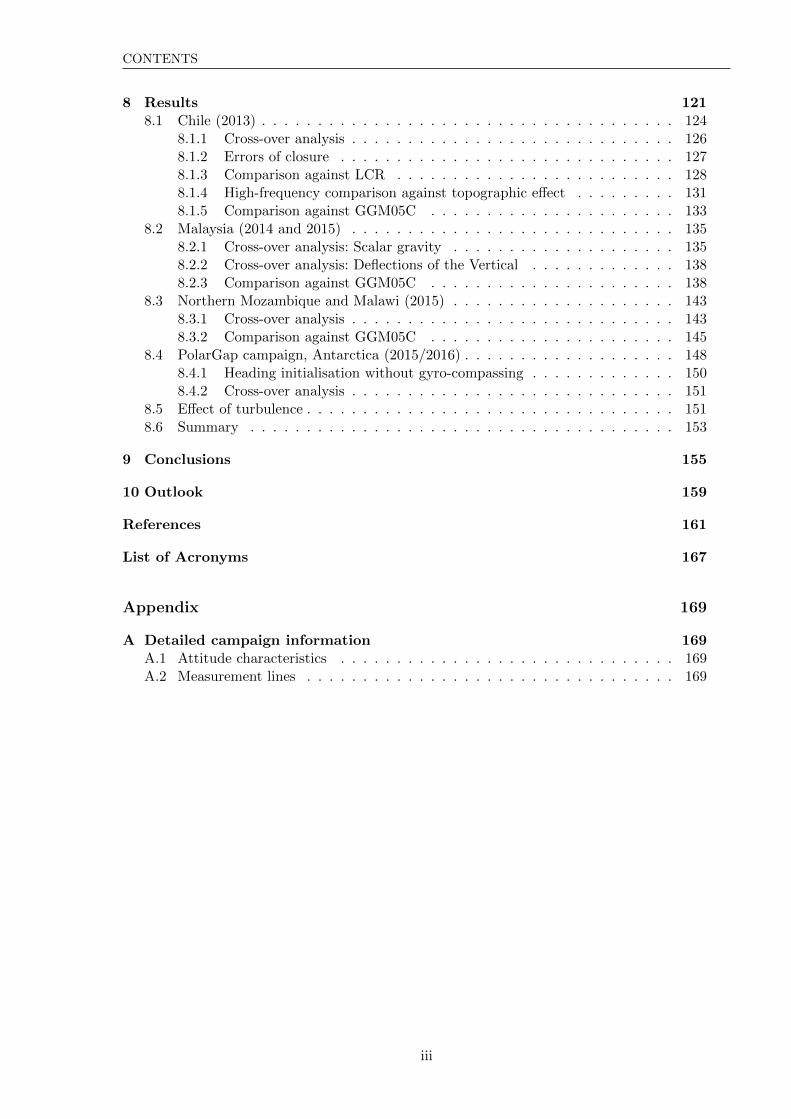
8 Results 1218.1 Chile (2013) . . . . . . . . . . . . . . . . . . . . . . . . . . . . . . . . . . . . . 124
8.1.1 Cross-over analysis . . . . . . . . . . . . . . . . . . . . . . . . . . . . . 1268.1.2 Errors of closure . . . . . . . . . . . . . . . . . . . . . . . . . . . . . . 1278.1.3 Comparison against LCR . . . . . . . . . . . . . . . . . . . . . . . . . 1288.1.4 High-frequency comparison against topographic effect . . . . . . . . . 1318.1.5 Comparison against GGM05C . . . . . . . . . . . . . . . . . . . . . . 133
8.2 Malaysia (2014 and 2015) . . . . . . . . . . . . . . . . . . . . . . . . . . . . . 1358.2.1 Cross-over analysis: Scalar gravity . . . . . . . . . . . . . . . . . . . . 1358.2.2 Cross-over analysis: Deflections of the Vertical . . . . . . . . . . . . . 1388.2.3 Comparison against GGM05C . . . . . . . . . . . . . . . . . . . . . . 138
8.3 Northern Mozambique and Malawi (2015) . . . . . . . . . . . . . . . . . . . . 1438.3.1 Cross-over analysis . . . . . . . . . . . . . . . . . . . . . . . . . . . . . 1438.3.2 Comparison against GGM05C . . . . . . . . . . . . . . . . . . . . . . 145
8.4 PolarGap campaign, Antarctica (2015/2016) . . . . . . . . . . . . . . . . . . . 1488.4.1 Heading initialisation without gyro-compassing . . . . . . . . . . . . . 1508.4.2 Cross-over analysis . . . . . . . . . . . . . . . . . . . . . . . . . . . . . 151
8.5 Effect of turbulence . . . . . . . . . . . . . . . . . . . . . . . . . . . . . . . . . 1518.6 Summary . . . . . . . . . . . . . . . . . . . . . . . . . . . . . . . . . . . . . . 153
9 Conclusions 155
10 Outlook 159
References 161
List of Acronyms 167
Appendix 169
A Detailed campaign information 169A.1 Attitude characteristics . . . . . . . . . . . . . . . . . . . . . . . . . . . . . . 169A.2 Measurement lines . . . . . . . . . . . . . . . . . . . . . . . . . . . . . . . . . 169
iii

CONTENTS
iv
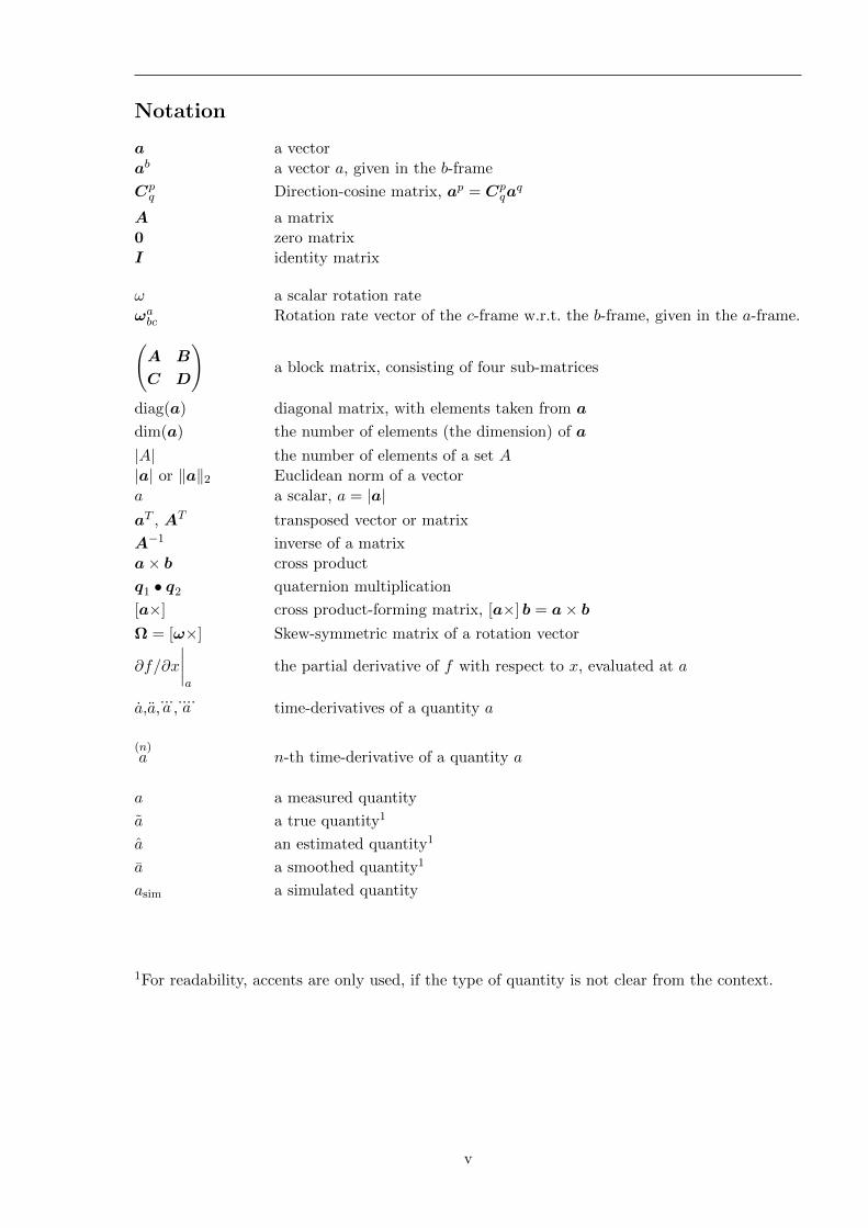
Notation
a a vector
ab a vector a, given in the b-frame
Cpq Direction-cosine matrix, ap = Cp
qaq
A a matrix
0 zero matrix
I identity matrix
ω a scalar rotation rate
ωabc Rotation rate vector of the c-frame w.r.t. the b-frame, given in the a-frame.(A B
C D
)a block matrix, consisting of four sub-matrices
diag(a) diagonal matrix, with elements taken from a
dim(a) the number of elements (the dimension) of a
|A| the number of elements of a set A
|a| or ‖a‖2 Euclidean norm of a vector
a a scalar, a = |a|aT , AT transposed vector or matrix
A−1 inverse of a matrix
a× b cross product
q1 • q2 quaternion multiplication
[a×] cross product-forming matrix, [a×] b = a× bΩ = [ω×] Skew-symmetric matrix of a rotation vector
∂f/∂x
∣∣∣∣a
the partial derivative of f with respect to x, evaluated at a
a,a,...a ,....a time-derivatives of a quantity a
(n)a n-th time-derivative of a quantity a
a a measured quantity
a a true quantity1
a an estimated quantity1
a a smoothed quantity1
asim a simulated quantity
1For readability, accents are only used, if the type of quantity is not clear from the context.
v

vi
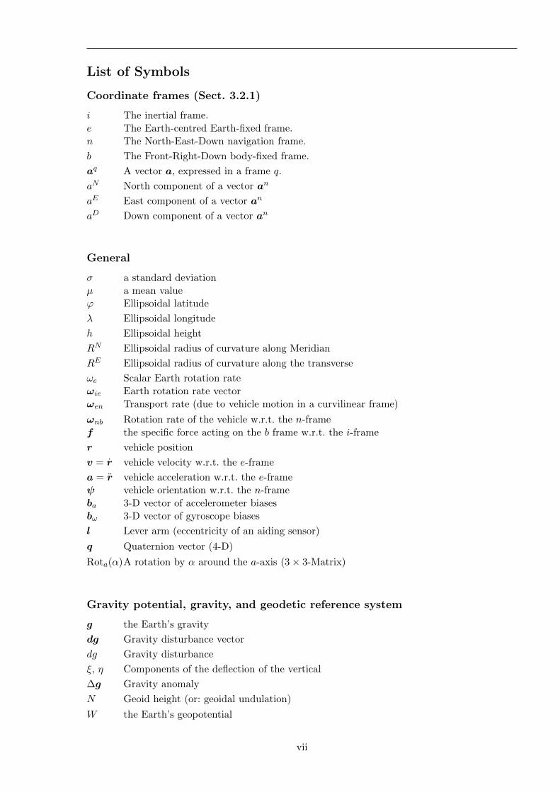
List of Symbols
Coordinate frames (Sect. 3.2.1)
i The inertial frame.
e The Earth-centred Earth-fixed frame.
n The North-East-Down navigation frame.
b The Front-Right-Down body-fixed frame.
aq A vector a, expressed in a frame q.
aN North component of a vector an
aE East component of a vector an
aD Down component of a vector an
General
σ a standard deviation
µ a mean value
ϕ Ellipsoidal latitude
λ Ellipsoidal longitude
h Ellipsoidal height
RN Ellipsoidal radius of curvature along Meridian
RE Ellipsoidal radius of curvature along the transverse
ωe Scalar Earth rotation rate
ωie Earth rotation rate vector
ωen Transport rate (due to vehicle motion in a curvilinear frame)
ωnb Rotation rate of the vehicle w.r.t. the n-frame
f the specific force acting on the b frame w.r.t. the i-frame
r vehicle position
v = r vehicle velocity w.r.t. the e-frame
a = r vehicle acceleration w.r.t. the e-frame
ψ vehicle orientation w.r.t. the n-frame
ba 3-D vector of accelerometer biases
bω 3-D vector of gyroscope biases
l Lever arm (eccentricity of an aiding sensor)
q Quaternion vector (4-D)
Rota(α)A rotation by α around the a-axis (3× 3-Matrix)
Gravity potential, gravity, and geodetic reference system
g the Earth’s gravity
dg Gravity disturbance vector
dg Gravity disturbance
ξ, η Components of the deflection of the vertical
∆g Gravity anomaly
N Geoid height (or: geoidal undulation)
W the Earth’s geopotential
vii
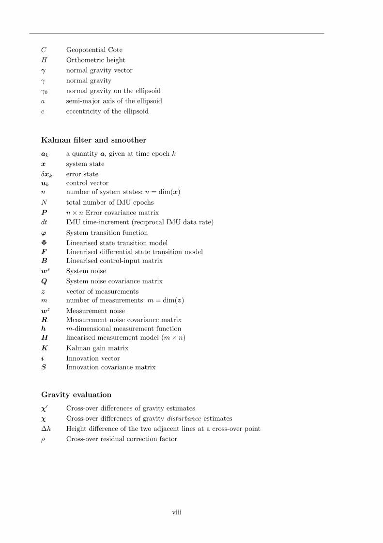
C Geopotential Cote
H Orthometric height
γ normal gravity vector
γ normal gravity
γ0 normal gravity on the ellipsoid
a semi-major axis of the ellipsoid
e eccentricity of the ellipsoid
Kalman filter and smoother
ak a quantity a, given at time epoch k
x system state
δxk error state
uk control vector
n number of system states: n = dim(x)
N total number of IMU epochs
P n× n Error covariance matrix
dt IMU time-increment (reciprocal IMU data rate)
ϕ System transition function
Φ Linearised state transition model
F Linearised differential state transition model
B Linearised control-input matrix
ws System noise
Q System noise covariance matrix
z vector of measurements
m number of measurements: m = dim(z)
wz Measurement noise
R Measurement noise covariance matrix
h m-dimensional measurement function
H linearised measurement model (m× n)
K Kalman gain matrix
i Innovation vector
S Innovation covariance matrix
Gravity evaluation
χ′ Cross-over differences of gravity estimates
χ Cross-over differences of gravity disturbance estimates
∆h Height difference of the two adjacent lines at a cross-over point
ρ Cross-over residual correction factor
viii
Chapter 1
Introduction
One of the major tasks of physical geodesy is the determination of the Earth’s gravityfield, and its potential W (Hofmann-Wellenhof and Moritz , 2006; Torge and Muller , 2012).The most important reference surface for geodetic height systems is the geoid, being theequipotential surfaceW =W0 = const for a predefined reference potentialW0. This referencepotential is commonly associated with the mean sea level.
The definition of this surface is intuitive in the absence of topography above sea level,however the equipotential surface continues below the landmasses. Therefore, the geoid canbe thought of as the mean sea level of an imaginative global ocean, continuing below thecontinents. The value of the geopotential on the geoid (Moritz , 1980)
W0 ≈ 62.636 · 106m2/s2 = 62.636MJ/kg (1.1)
may be interpreted as the energy which is required to move a unit mass located on the geoidto infinity, or equally, the energy performed by the Earth’s gravity field to move a unit massfrom infinity to the geoid. The geopotential W (x, y, z) is a scalar field, assigning a scalarvalue to each coordinate triple (x, y, z) of a Cartesian earth-fixed coordinate frame.
1.1 The Earth’s gravity field
The vector of gravity g is defined as the gradient of the geopotential,
g = gradW =(∂W∂x
∂W∂y
∂W∂z
)T. (1.2)
Thus, the gravity field g = g(x, y, z) is a vector field, assigning a vector to each coordinatetriple. The magnitude g = |g| is called scalar gravity.
The common unit for gravity used in the geodetic literature is Gal, which is not containedin the SI standard. It is defined as 1Gal = 1 · 10−2m/s2. The units 1mGal = 1 · 10−5m/s2
and 1µGal = 1 · 10−8m/s2 will be used throughout the text as well.
Several concepts exist on how to derive the geometrical shape of the geoid based on gravitymeasurements. For this, a geodetic reference system is used, commonly defining an oblate,rotating spheroid (also denoted as rotating ellipsoid of revolution), approximating the shapeof the geoid, and rotating at the Earth’s rotation rate ωe (Moritz , 1980). The surface of theellipsoid is at the same time an equipotential surface of its gravity potential, called the normalgravity potential U . On the ellipsoid, it is defined as U = U0 =W0. The normal potential Ucan easily be computed for any point on or above the ellipsoid (Torge and Muller , 2012). Asfor the actual gravity potential, the normal gravity vector γ is defined as the gradient of thenormal potential: γ = grad(U).
1
Introduction
The actual geodetic quantities are then reduced to differences with respect to this refer-ence system: The shape of the geoid can be defined by the vertical distance N between thegeoid and the ellipsoid surface. N is called geoid height, or geoidal undulation. The gravitydisturbance is defined as the difference between the actual gravity at a point P , and thenormal gravity at the same point: dg = gP − γP . Further, the gravity anomaly is defined asthe difference between the gravity at a point P , and the normal gravity at a point Q aboveor below P , with WP = UQ: ∆g = gP − γQ. A fundamental functional relationship betweenthese quantities was formulated by Stokes using a surface integral:
NP =R
4πγ0
∫∫σ∆gS(ψ)dσ , (1.3)
with Earth radius R, the spherical distance ψ between the point P and the running integrationpoint, and Stokes’ function (Hofmann-Wellenhof and Moritz , 2006)
S(ψ) =1
sin(ψ/2)− 6 sin
ψ
2+ 1− 5 cosψ − 3 cosψ ln(sin
ψ
2+ sin2
ψ
2) . (1.4)
Eq. 1.3 shows, that the knowledge of the gravity field (∆g) also allows the determination ofthe shape of the geoid, N . The practical use of knowing N will be discussed later in thischapter. For details on the derivation of Eq. 1.3, the reader is referred to standard literatureon physical geodesy, as Hofmann-Wellenhof and Moritz (2006); Torge and Muller (2012).
Similar as for the scalar gravity, the direction of the local gravity vector at any pointP can be expressed with respect to the direction of the normal gravity vector at the samepoint. Expressing the vectors in a local North-East-Down coordinate frame, and with theassumptions, that gNorth gDown and gEast gDown, the angular deflection of the vertical(DoV) can be defined by its two components
ξ = −dgNorth
g= −g
North − γNorth
g, and (1.5)
η = −dgEast
g= −g
East
g, (1.6)
because γEast = 0 due to the radial symmetry of the ellipsoid of revolution (spheroid). Note,that ξ increases when (hypothetically) introducing attracting masses in the South, and ηincreases when adding masses in the West. With these definitions, the angular componentsof the deflection of the vertical can be transformed into horizontal gravity components, andvice versa.
1.2 Gravimetry
While today there is no practical way of directly measuring the geopotential W withreasonable accuracy, the gravity g can be determined either
• by measuring the force that is acting on a proof mass, or
• by measuring accelerations (second derivative of observed positions) of a test bodybeing in free fall in a vacuum.
These are the main concepts of gravimeters.Depending on the instrument design and the type of the measured effect, gravimeters
may be limited to scalar gravimetry, i.e. the determination of g = |g|. In contrast, vectorgravimetry allows the determination of the full 3-D gravity vector g (or equivalently, g, ξ,and η).
Another distinction is commonly made with respect to the requirement of a referencegravity value:
2
1.2 Gravimetry
• Relative gravimetry is the determination of gravity with respect to a known referencegravity value. In other words, relative gravimetry can only determine gravity differencesbetween two points.
• Absolute gravimetry is the direct determination of gravity, without any external infor-mation.
This thesis is primarily concerned with relative vector gravimetry.There are three principal modi operandi for the gravity determination using a gravimeter,
given by the type of the measurement platform. These different modes of gravimetry arebriefly introduced in the following sections.
1.2.1 Terrestrial gravimetry
Terrestrial gravimetry is the determination of gravity on the Earth’s surface: The terres-trial gravimeter is statically standing on the ground without any movement during the mea-surement. Terrestrial gravimetry enables the gravity determination at high accuracy (typicallytens of µGal or better), and high spatial resolution, as there is no lower bound on the spacingbetween the measurement points. However, measurements can be difficult or even impossiblein areas of rugged terrain or water. In addition, performing terrestrial gravimetry for largerareas can be very costly, because the static measurements are time- and labour-consuming.The points have to be accessed on ground, e.g. using land vehicles or helicopters.
Historically, terrestrial gravimetry was the only modus operandi. Until today, many coun-tries maintain or extend dense terrestrial gravity point networks, serving as the main datasource for the determination of national height reference surfaces, also referred to as localgeoids.
Especially for large countries and remote areas, the use of terrestrial gravimetry for theestablishment of a national height system is too costly and time-consuming. Instead, a rel-atively sparse network of terrestrial gravity points is combined with airborne, shipborne, orsatellite gravity data.
1.2.2 Satellite gravimetry
With the launch of the Challenging Minisatellite Payload (CHAMP) mission (2000-2010),gravity observations from space became available by observing the orbital deviations of thissatellite. Until today, two more satellite missions were established, the Gravity RecoveryAnd Climate Experiment (GRACE, 2002), and the Gravity field and steady-state OceanCirculation Explorer (GOCE, 2009).
The GRACE mission consists of two low-Earth-orbiting satellites on the same orbits,which can determine their mutual distance with very high precision, also denoted as satellite-to-satellite tracking (SST). Variations of this mutual distance arise from local variations of thegravitational attraction of the Earth. Therefore, the distance variations allow the deductionof gravity.
3
Introduction
In addition to gravity, GOCE also provides measurements of the gravity gradient tensorgrad g = grad (gradW ), consisting of five independent gradients (Torge and Muller , 2012):
Wxx =∂2W
∂x2, (1.7)
Wyy =∂2W
∂y2, (1.8)
Wxy = Wyx =∂2W
∂x ∂y, (1.9)
Wxz = Wzx =∂2W
∂x ∂z, and (1.10)
Wyz = Wzy =∂2W
∂y ∂z. (1.11)
With higher altitudes, the attenuation of the Earth’s gravity field limits the spatial res-olution of the gravity determination (Torge, 1989). Satellite gravimetry orbits are chosen aslow as possible to limit this effect, e.g. GOCE was operated at an altitude of only 283.5 km,yielding a spatial resolution on the geoid of the order of 100 km (GRACE: 450 km to 500 kmaltitude, yielding a resolution of ≈ 150 km). More details will be provided in Sect. 7.2.2.
Satellite missions have greatly contributed to global gravity models (GGM), and alsoenabled new methods of global Earth system research in the fields of oceanography, glaciol-ogy, and geophysics. However, the limited spatial resolution does not allow a satellite-onlydetermination of local geoids at a sufficient resolution.
1.2.3 Shipborne and airborne gravimetry
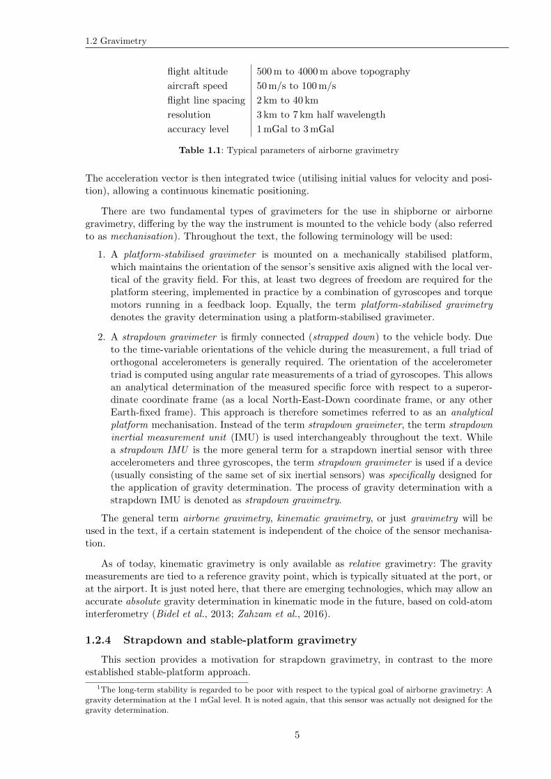
Shipborne and airborne gravimetry is today’s most important link between terrestrialand satellite gravimetry in terms of resolution and coverage. In the most common set-up, aship, or a fixed-wing aircraft, is equipped with a sea or air gravimeter, which is designed forkinematic measurements, in combination with a geodetic GNSS receiver. Table 1.1 shows thetypical parameters of airborne gravimetry and its products.
In the kinematic set-up, a gravimeter can not directly measure gravity, but only thesuperposition of gravity and vehicle accelerations r, which cannot be avoided in practice.This superposition is called specific force f . In an inertial coordinate frame i, it is defined as(Jekeli , 2001)
f i = ri − gi . (1.12)
This definition is intuitive, as gravity can not be distinguished from an acceleration in theopposite direction. In particular, f i = 0 during a free fall in a vacuum.
For the application of kinematic gravimetry, Eq. 1.12 is transformed into
gi = ri − f i . (1.13)
While f is measured by the gravimeter, the vehicle accelerations ri have to be determinedby an aiding sensor, as e.g. GNSS. When expressing Eq. 1.12 in an Earth-fixed, i.e. rotatedcoordinate system, centrifugal, Coriolis, and Euler forces have to be accounted for (Britting ,1971). The Euler term can be neglected under the assumption of a constant Earth’s rotationrate vector.
It is just briefly mentioned here, that the third possible transformation of Eq. 1.12 iscommonly used for inertial positioning (or: inertial navigation). Assuming the gravity isknown, the vehicle accelerations can be computed using:
ri = f i + gi . (1.14)
4
1.2 Gravimetry
flight altitude 500m to 4000m above topography
aircraft speed 50m/s to 100m/s
flight line spacing 2 km to 40 km
resolution 3 km to 7 km half wavelength
accuracy level 1mGal to 3mGal
Table 1.1: Typical parameters of airborne gravimetry
The acceleration vector is then integrated twice (utilising initial values for velocity and posi-tion), allowing a continuous kinematic positioning.
There are two fundamental types of gravimeters for the use in shipborne or airbornegravimetry, differing by the way the instrument is mounted to the vehicle body (also referredto as mechanisation). Throughout the text, the following terminology will be used:
1. A platform-stabilised gravimeter is mounted on a mechanically stabilised platform,which maintains the orientation of the sensor’s sensitive axis aligned with the local ver-tical of the gravity field. For this, at least two degrees of freedom are required for theplatform steering, implemented in practice by a combination of gyroscopes and torquemotors running in a feedback loop. Equally, the term platform-stabilised gravimetrydenotes the gravity determination using a platform-stabilised gravimeter.
2. A strapdown gravimeter is firmly connected (strapped down) to the vehicle body. Dueto the time-variable orientations of the vehicle during the measurement, a full triad oforthogonal accelerometers is generally required. The orientation of the accelerometertriad is computed using angular rate measurements of a triad of gyroscopes. This allowsan analytical determination of the measured specific force with respect to a superor-dinate coordinate frame (as a local North-East-Down coordinate frame, or any otherEarth-fixed frame). This approach is therefore sometimes referred to as an analyticalplatform mechanisation. Instead of the term strapdown gravimeter, the term strapdowninertial measurement unit (IMU) is used interchangeably throughout the text. Whilea strapdown IMU is the more general term for a strapdown inertial sensor with threeaccelerometers and three gyroscopes, the term strapdown gravimeter is used if a device(usually consisting of the same set of six inertial sensors) was specifically designed forthe application of gravity determination. The process of gravity determination with astrapdown IMU is denoted as strapdown gravimetry.
The general term airborne gravimetry, kinematic gravimetry, or just gravimetry will beused in the text, if a certain statement is independent of the choice of the sensor mechanisa-tion.
As of today, kinematic gravimetry is only available as relative gravimetry: The gravitymeasurements are tied to a reference gravity point, which is typically situated at the port, orat the airport. It is just noted here, that there are emerging technologies, which may allow anaccurate absolute gravity determination in kinematic mode in the future, based on cold-atominterferometry (Bidel et al., 2013; Zahzam et al., 2016).
1.2.4 Strapdown and stable-platform gravimetry
This section provides a motivation for strapdown gravimetry, in contrast to the moreestablished stable-platform approach.
1The long-term stability is regarded to be poor with respect to the typical goal of airborne gravimetry: Agravity determination at the 1 mGal level. It is noted again, that this sensor was actually not designed for thegravity determination.
5
Introduction
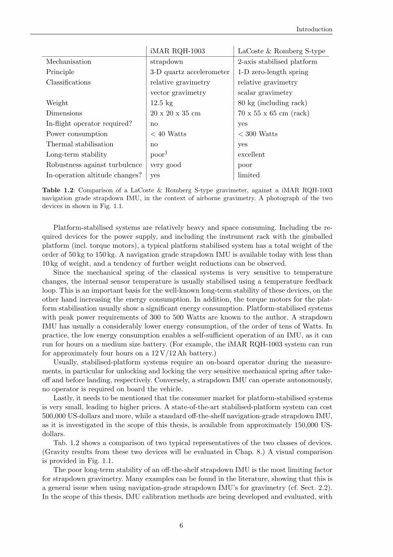
iMAR RQH-1003 LaCoste & Romberg S-type
Mechanisation strapdown 2-axis stabilised platform
Principle 3-D quartz accelerometer 1-D zero-length spring
Classifications relative gravimetry relative gravimetry
vector gravimetry scalar gravimetry
Weight 12.5 kg 80 kg (including rack)
Dimensions 20 x 20 x 35 cm 70 x 55 x 65 cm (rack)
In-flight operator required? no yes
Power consumption < 40 Watts < 300 Watts
Thermal stabilisation no yes
Long-term stability poor1 excellent
Robustness against turbulence very good poor
In-operation altitude changes? yes limited
Table 1.2: Comparison of a LaCoste & Romberg S-type gravimeter, against a iMAR RQH-1003navigation grade strapdown IMU, in the context of airborne gravimetry. A photograph of the twodevices in shown in Fig. 1.1.
Platform-stabilised systems are relatively heavy and space consuming. Including the re-quired devices for the power supply, and including the instrument rack with the gimballedplatform (incl. torque motors), a typical platform stabilised system has a total weight of theorder of 50 kg to 150 kg. A navigation grade strapdown IMU is available today with less than10 kg of weight, and a tendency of further weight reductions can be observed.
Since the mechanical spring of the classical systems is very sensitive to temperaturechanges, the internal sensor temperature is usually stabilised using a temperature feedbackloop. This is an important basis for the well-known long-term stability of these devices, on theother hand increasing the energy consumption. In addition, the torque motors for the plat-form stabilisation usually show a significant energy consumption. Platform-stabilised systemswith peak power requirements of 300 to 500 Watts are known to the author. A strapdownIMU has usually a considerably lower energy consumption, of the order of tens of Watts. Inpractice, the low energy consumption enables a self-sufficient operation of an IMU, as it canrun for hours on a medium size battery. (For example, the iMAR RQH-1003 system can runfor approximately four hours on a 12V/12Ah battery.)
Usually, stabilised-platform systems require an on-board operator during the measure-ments, in particular for unlocking and locking the very sensitive mechanical spring after take-off and before landing, respectively. Conversely, a strapdown IMU can operate autonomously,no operator is required on board the vehicle.
Lastly, it needs to be mentioned that the consumer market for platform-stabilised systemsis very small, leading to higher prices. A state-of-the-art stabilised-platform system can cost500,000 US-dollars and more, while a standard off-the-shelf navigation-grade strapdown IMU,as it is investigated in the scope of this thesis, is available from approximately 150,000 US-dollars.
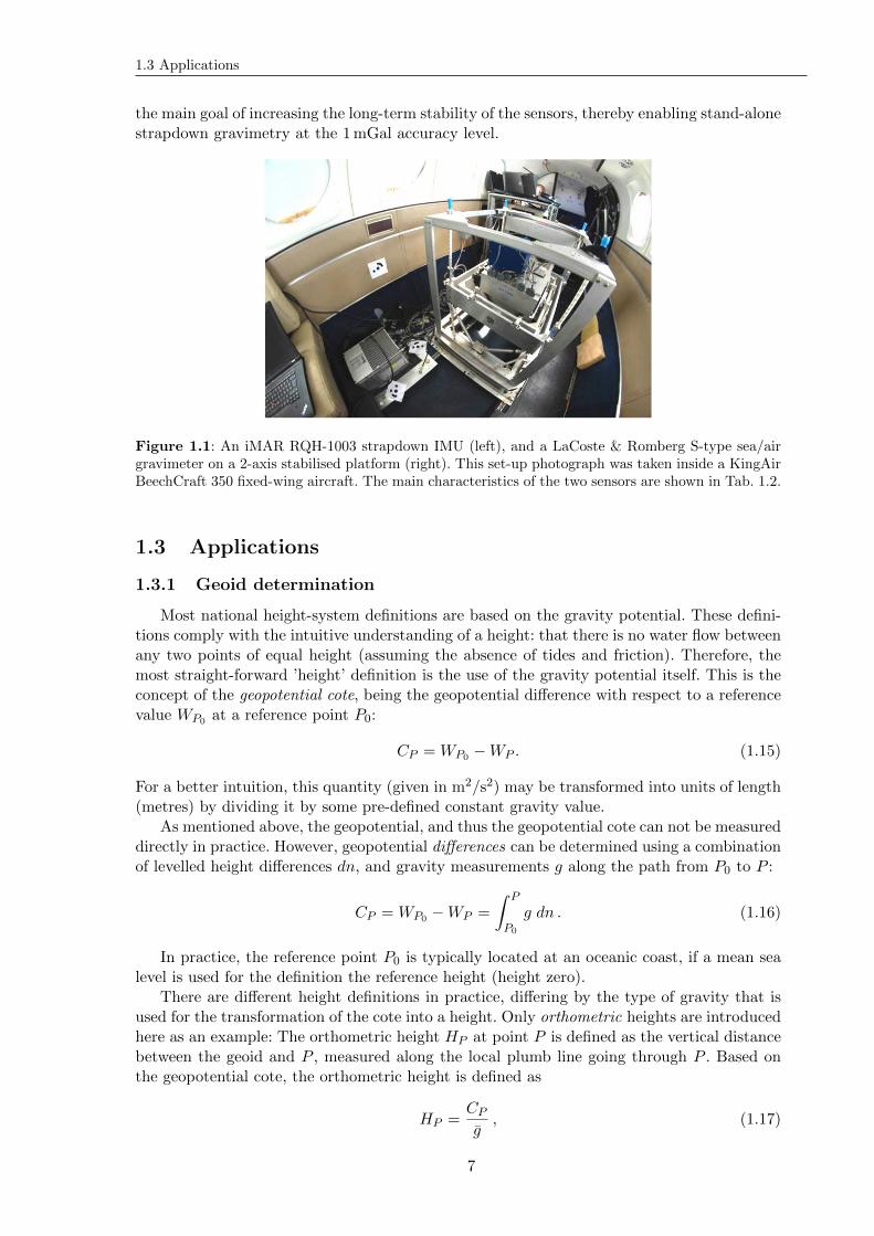
Tab. 1.2 shows a comparison of two typical representatives of the two classes of devices.(Gravity results from these two devices will be evaluated in Chap. 8.) A visual comparisonis provided in Fig. 1.1.
The poor long-term stability of an off-the-shelf strapdown IMU is the most limiting factorfor strapdown gravimetry. Many examples can be found in the literature, showing that this isa general issue when using navigation-grade strapdown IMU’s for gravimetry (cf. Sect. 2.2).In the scope of this thesis, IMU calibration methods are being developed and evaluated, with
6
1.3 Applications
the main goal of increasing the long-term stability of the sensors, thereby enabling stand-alonestrapdown gravimetry at the 1mGal accuracy level.
Figure 1.1: An iMAR RQH-1003 strapdown IMU (left), and a LaCoste & Romberg S-type sea/airgravimeter on a 2-axis stabilised platform (right). This set-up photograph was taken inside a KingAirBeechCraft 350 fixed-wing aircraft. The main characteristics of the two sensors are shown in Tab. 1.2.
1.3 Applications
1.3.1 Geoid determination
Most national height-system definitions are based on the gravity potential. These defini-tions comply with the intuitive understanding of a height: that there is no water flow betweenany two points of equal height (assuming the absence of tides and friction). Therefore, themost straight-forward ’height’ definition is the use of the gravity potential itself. This is theconcept of the geopotential cote, being the geopotential difference with respect to a referencevalue WP0 at a reference point P0:
CP =WP0 −WP . (1.15)
For a better intuition, this quantity (given in m2/s2) may be transformed into units of length(metres) by dividing it by some pre-defined constant gravity value.
As mentioned above, the geopotential, and thus the geopotential cote can not be measureddirectly in practice. However, geopotential differences can be determined using a combinationof levelled height differences dn, and gravity measurements g along the path from P0 to P :
CP =WP0 −WP =
∫ P
P0
g dn . (1.16)
In practice, the reference point P0 is typically located at an oceanic coast, if a mean sealevel is used for the definition the reference height (height zero).
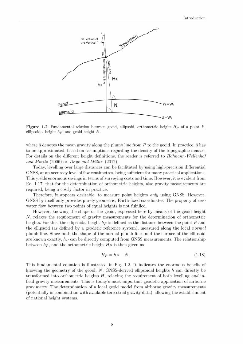
There are different height definitions in practice, differing by the type of gravity that isused for the transformation of the cote into a height. Only orthometric heights are introducedhere as an example: The orthometric height HP at point P is defined as the vertical distancebetween the geoid and P , measured along the local plumb line going through P . Based onthe geopotential cote, the orthometric height is defined as
HP =CPg, (1.17)
7
Introduction
P
Ellipsoid
Geoid
Topogra
phy
plu
mb lin
e
norm
al p
lum
b lin
e
W=W0
U=W0
.
.
Deection of
the Vertical
N
HP
hP
Figure 1.2: Fundamental relation between geoid, ellipsoid, orthometric height HP of a point P ,ellipsoidal height hP , and geoid height N .
where g denotes the mean gravity along the plumb line from P to the geoid. In practice, g hasto be approximated, based on assumptions regarding the density of the topographic masses.For details on the different height definitions, the reader is referred to Hofmann-Wellenhofand Moritz (2006) or Torge and Muller (2012).
Today, levelling over large distances can be facilitated by using high-precision differentialGNSS, at an accuracy level of few centimetres, being sufficient for many practical applications.This yields enormous savings in terms of surveying costs and time. However, it is evident fromEq. 1.17, that for the determination of orthometric heights, also gravity measurements arerequired, being a costly factor in practice.
Therefore, it appears desirable, to measure point heights only using GNSS. However,GNSS by itself only provides purely geometric, Earth-fixed coordinates. The property of zerowater flow between two points of equal heights is not fulfilled.
However, knowing the shape of the geoid, expressed here by means of the geoid heightN , relaxes the requirement of gravity measurements for the determination of orthometricheights. For this, the ellipsoidal height hP is defined as the distance between the point P andthe ellipsoid (as defined by a geodetic reference system), measured along the local normalplumb line. Since both the shape of the normal plumb lines and the surface of the ellipsoidare known exactly, hP can be directly computed from GNSS measurements. The relationshipbetween hP , and the orthometric height HP is then given as
HP ≈ hP −N . (1.18)
This fundamental equation is illustrated in Fig. 1.2. It indicates the enormous benefit ofknowing the geometry of the geoid, N : GNSS-derived ellipsoidal heights h can directly betransformed into orthometric heights H, relaxing the requirement of both levelling and in-field gravity measurements. This is today’s most important geodetic application of airbornegravimetry: The determination of a local geoid model from airborne gravity measurements(potentially in combination with available terrestrial gravity data), allowing the establishmentof national height systems.
8
1.4 Thesis outline
1.3.2 Geophysical applications
The knowledge of sub-surface density distributions is an important information for geo-physical investigations. However, in particular the determination of the sub-surface materialsand densities can be very costly in practice, requiring boreholes of considerable depth.
The most important geophysical application of gravity data is the determination of thesub-surface density distribution (gravity inversion). While the knowledge of the density dis-tribution would allow the unambiguous computation of gravity anomalies, the inverse trans-formation is ambiguous, requiring additional geophysical models and constraints (Oldenburg ,1974; Boulanger and Chouteau, 2001). Other data sources, as magnetic, seismic, or electricdata, are commonly used in combination with gravity data for the inversion, helping to resolveambiguities based on assumptions on the material properties (Li and Oldenburg , 1998).
Some examples which are relevant in practice are:
• The determination of ice cap thicknesses. Based on assumptions on the density of thebedrock density in combination with the known density of ice, the gravity data canprovide estimates for the height of the bedrock surface. A practical example can befound in Fretwell et al. (2013).
• The determination of the geometry of fault lines / tectonics, and its changes over time.
• The determination of other time-variable sub-surface mass movements.
• The gravity inversion can be used for mineral exploration. In particular, oil has arelatively small density compared to rock, allowing the gravimetric discovery of oilresources (Lelievre et al., 2012).
1.4 Thesis outline
This thesis is a contribution towards improving the accuracy of strapdown airbornegravimetry systems. The focus is set on strapdown gravimetry for geodetic applications.
Chap. 2 provides an overview of the state of the art of airborne gravimetry, and strapdowngravimetry in particular. Other authors consistently report a poor long-term stability forstrapdown gravimetry, when using an off-the-shelf navigation-grade strapdown IMU. Suchlong-term instabilities prevent a stand-alone use of such devices for geodetic applications.Further, several publications on IMU calibration methods are introduced, serving as a basisfor the parametric calibration methods investigated in this thesis.
The one-step error-state space Extended Kalman filter algorithm for the strapdowngravimetry system is introduced in Chap. 3. The non-linear navigation equations are shown,and the linearised system model and observation models are being deduced. The chapter in-troduces the modelling of gravity as a Gauss-Markov process. A Kalman smoother is appliedto the outputs of the Extended Kalman Filter (EKF).
Chap. 4 provides an analysis of the strapdown gravimetry system. Based on an observ-ability analysis, it is shown, 1. why the determination of the horizontal gravity components isdifficult, and 2. why non-linear accelerometer drifts can not be removed from the estimatedgravity in practice. A quantitative insight into the system is given by an estimability analy-sis. In particular, it is investigated how much observations of certain type and accuracy cancontribute to the gravity determination. It is also shown, how aircraft manoeuvres compris-ing accelerations can positively affect the strapdown gravity determination in theory. Somepractical conclusions are drawn from the analyses.
A comprehensive error propagation analysis is presented in Chap. 5. The analysis is basedon realistic simulations of aerogravity flights. A variety of systematic errors are investigated,
9
Introduction
as time-stamping errors, discretisation errors, GNSS-antenna lever arm errors, and also sys-tematic inertial sensor errors, as biases, scale factors, cross-couplings and misalignments.The findings are complemented by a brief analysis of stochastic inertial sensor errors, asaccelerometer and gyroscope noise, gradual stochastic accelerometer drifts, and GNSS coor-dinate noise. These error propagation simulations can be shown to support the qualitativeconclusions drawn in Chap. 4.
Chap. 6 discusses a variety of IMU calibration methods, with an emphasis on long-termaccelerometer errors. Among the discussed calibration methods are
1. sample-based models: look-up tables of sensor errors in a predefined state-space, and
2. the more established parametric approaches, calibrating biases, scale factors, and sensormisalignments based on sensor observations in different orientations.
The feasibility of an in-field calibration is briefly discussed for the individual methods. Thediscussed calibration methods are implemented for an iMAR RQH-1003 navigation-gradestrapdown IMU.
As a preparation for the real-data evaluations presented in Chap. 8, a summary of estab-lished airborne gravimetry evaluation methods is provided in Chap. 7. Some of the methods,as cross-over residuals and repeated line residuals, are discussed in more depth. Practicalrecommendations on how to apply these methods are being deduced.
Chap. 8 presents real-data examples of strapdown airborne gravimetry. Measurementsfrom five different airborne gravity campaigns are evaluated, in particular analysing thebenefits of the individual calibration methods shown in Chap. 6. The evaluation includescross-over analyses, an inter-system comparison against stable-platform gravity data, andcomparisons against a global gravity model (GGM). The invariance of the strapdown gravityquality against turbulence is shown.
The thesis is concluded with a summary of the central findings, and an outlook.
10
Chapter 2
State of the art
The first section of this chapter provides an overview of stable-platform airborne gravime-try, which as of today is the predominant method of airborne gravity determination forgeodetic applications. The second section gives an overview of publications on strapdowngravimetry, identifying the long-term instability of the sensor as the main limitation of thisapproach. The third section deals with IMU calibration methods in general, followed by abrief section on GNSS processing in view of airborne gravimetry.
2.1 Stable-platform airborne gravimetry
After kinematic gravimetry systems for the use in underwater gravimetry had already beeninvestigated since the early 1950s, the first test of airborne gravimetry was published in 1960using a stabilised-platform spring gravimeter (Nettleton et al., 1960). The measuring principlecan be explained as follows: A mechanical spring is attached to a horizontal beam, both beingin a high-viscosity fluid to dampen mechanical vibration and shocks. A so-called zero-lengthspring is being used (LaCoste, 1988). The tension of the spring is automatically adjustedin a feedback control circuit, such that the beam approximately maintains its horizontalalignment. The output of the sensor is given as a combination of the beam velocity (it is anunderdamped system), and the applied spring tension. These quantities are then transformedinto units of a specific force by using pre-calibrated look-up tables. In a kinematic set-up,this type of gravimeter requires a convergence time of typically 100 s to 200 s in order toprovide results at the level of few mGal. This implies, that the maximum spatial resolutionof the gravity measurements is limited mainly by the aircraft speed, where lower speeds yielda higher spatial resolution.
In practice, the platform stabilisation is subject to inaccuracies coming from latencies ofthe feedback-circuit, and drifts of the gyroscopes. Auxiliary, horizontally aligned accelerome-ters are used for computationally reducing such errors. In fact, a proper design of platform tiltcorrections could be shown to be crucial for accurate stable-platform gravimetry (LaCoste,1967; Olesen, 2002).
Aircraft accelerations r have to be removed from the measured specific force (cf.Sec. 1.2.3). Before global navigation satellite systems (GNSS) became available in the 1990s,the aircraft accelerations had to be measured using radar altimetry in combination withhigh-resolution terrain models.
Airborne gravimetry experienced a significant rise when the Global Positioning System(GPS) became available in the 1990s. The second derivatives of aircraft GPS positions couldbe used to determine the aircraft accelerations r more accurately and more easily compared toradar altimetry. Since then, the combination of a platform-stabilised spring gravimeter andGPS has been the predominant method for airborne gravity determination, with reportedaccuracies of 1mGal to 4mGal at a spatial resolution of several kilometres (typically 3 km
11
State of the art
to 10 km half-wavelength, depending on the aircraft speed). An overview of the platform-stabilised gravity data acquisition, and its use for the local geoid determination, can be foundin Forsberg and Olesen (2010). More results from stabilised-platform airborne gravimetrycampaigns can be found in Brozena (1992); Brozena et al. (1997); Bastos et al. (1998);Forsberg et al. (2001); Studinger et al. (2008).
2.2 Strapdown gravimetry
In parallel to the development and rise of platform-stabilised gravimeters, Schwarz (1983)already formulated the potential of using inertial measurement units (IMU) for geodeticpositioning and gravity field determination. In particular, an IMU with three orthogonalaccelerometers enables the determination of the full 3-D gravity vector (vector gravimetry).Forsberg et al. (1986) was able to show, that accuracies of 1-2 arc seconds are possible for thedeflections of the vertical (DoV), and 2.5mGal to 4mGal for the (vertical) gravity anomalies.Mainly due to the difficulties of determining the vehicle accelerations r, these measurementswere done in a semi-kinematic set-up: The vehicle (truck and helicopter) was parked inregular intervals to enable the gravity determination, by ensuring r = 0, i.e. the specific forcemeasurements could directly be used as gravity measurements, using f = −g. Exploiting suchknowledge of static phases of the vehicle motion (zero-velocity observations) is still relevantfor state-of-the-art navigation systems. Further, Forsberg et al. (1986) show the importanceof using optimal smoothers for such a gravimetry system. The quality of the original (non-smoothed) real-time gravity estimates was shown to be worse by a factor of 3 and more.
As for stabilised-platform gravimetry, the availability of accurate GPS signals enabledstrapdown gravimetry in a relatively simple and efficient set-up. (However, compared to to-day’s technology, it should be noted that the kinematic GPS data acquisition from an aircraftwas still a challenging task at that time.) The work of Schwarz et al. (1992) investigates therequirements to strapdown airborne vector gravimetry, also in view of the GNSS signal qual-ity. Based on accuracy requirements defined by the respective applications of vector gravitydata, e.g. for geophysical and geodetic applications, technical requirements for the IMU andthe GPS systems are deduced. A more comprehensive discussion of practical problems, asGPS errors, and IMU errors coming from aircraft vibration, is provided in Schwarz and Wei(1995). Also, the ultimate accuracy goal of scalar airborne gravimetry was defined to be1mGal in this publication.
Based on simulations, Jekeli (1994) investigates which kind of a stochastic process bestmodels the along-track gravity signal over time. Different Gauss-Markov processes are com-pared, showing that third- and fourth-order Gauss-Markov processes may serve as suitablemodels.
Also based on simulations, Jekeli (1994) analyses in more detail the particular challengesof vector gravimetry. It is stated, that the strong correlation between attitude instabilities andthe errors of the estimated deflections makes the gyroscope sensor stability the main limitingfactor for the determination of the DoV. For example, an attitude error of 1 arc secondsfully propagates into the DoV estimates (equivalent to ≈ 5mGal), while the same attitudeerror is negligible for the vertical component (1µGal). Based on simulated data, Jekeli(1994) expects that the DoVs can be determined at the level of 3mGal (0.63 arc seconds) forwavelengths shorter than 250 km, when using centimetre-level GPS updates in combinationwith high-precision ring-laser gyroscopes (assuming a gyroscope bias of 0.0006/h and anangular random walk of 0.00037/
√h). A similar conclusion was already drawn in Jekeli
(1992) for kinematic IMU/GPS gravimetry using a balloon as platform.The operability of a strapdown gravimetry system could be shown by Wei and Schwarz
(1998). The system consisted of a Honeywell LASEREV III strapdown IMU, with Honey-well GG1342 ring-laser gyroscopes, and Honeywell QA-2000 accelerometers. Differential GPS
12
2.2 Strapdown gravimetry
(DGPS) coordinates are used for the determination of the aircraft accelerations. Using arepeated-line agreement as quality metric, an estimated overall standard deviation of approx-imately 2mGal, and 3mGal, could be shown for along-track low-pass filters using thresholdfrequencies of 1/120Hz, and 1/90Hz, respectively.
Two different gravity processing methods are compared in Wei and Schwarz (1998):1. Using the gyroscope measurements for a full strapdown navigation solution, taking intoaccount the orientation of the sensor, and 2. only using the absolute specific force f = |f s|measured by the accelerometer triad in the sensor coordinate frame s. The latter approachappears desirable for its simplicity, as no attitude information is required (it is therefore calleda rotation-invariant system). However, the results presented in Wei and Schwarz (1998)show, that the full strapdown approach systematically yields better results. In the scope ofthis thesis, only the full strapdown approach is investigated. Compared to the repeated-lineagreement, the residuals of upward-continued ground points were clearly larger (4mGal to5mGal vs. 2mGal to 3mGal). The authors formulated the expectation, that the uncertaintiesinvolved with the spatial interpolation of the terrestrial gravity points, and their upwardcontinuation to flight altitude can reach the level of several mGal, thereby questioning theusability of such ground points as a reliable reference.
Shortly after this first successful test of strapdown gravimetry, the same group was ableto confirm the results of their LASEREV III based strapdown gravimetry system (Glennieand Schwarz , 1999). After removing a linear drift from the gravity estimates, a cross-overanalysis showed overall residuals as low as 1.6mGal. This emphasises the high potential ofstrapdown gravimetry. However, it needs to be mentioned here, that these precision valuesheavily depend on the removal of biases and linear drifts, which were computed individuallyfor each of the lines. Drifts of 4mGal to 5mGal per 15 minutes flight line are reported(≈18mGal/h). Also, the presented residual cross-over differences may be rather optimistic,coming from a relatively weak over-determination for the estimation of linear drift parameters.This will be discussed in more detail in Sect. 7.1.1. Since the assumption of linear drifts isnot true in practice, long-term drifts may still reside in the gravity estimates after applyingsuch a linear drift interpolation method, cf. Becker et al. (2015b).
It is just noted here, that Glennie and Schwarz (1999) report an optimal low-pass filtercut-off frequency for their test flights between 1/90Hz and 1/120Hz. The iMAR RQH-1003strapdown IMU, used for gravimetry tests in this thesis, shows a similar optimum low-passfrequency of approximately 1/90Hz. Lower cut-off frequencies may allow better estimationresults, if the actual along-track gravity does not contain such high-frequency component(promoted by lower flight speeds, and higher flight altitudes). Using higher low-pass thresholdfrequencies apparently introduces more noise than signal to the estimates, independent of thegravity field characteristics.
In Kwon and Jekeli (2001), a so-called wavenumber correlation filter was introduced,extracting correlating parts of the individual gravity measurements of repeated flight tracks.Vertical gravity estimates at a precision level of 3mGal to 4mGal could be achieved on realdata using a Honeywell LASEREV III IMU. The horizontal gravity components could beestimated at a precision of 6mGal. For production-oriented campaigns, it should be notedthough, that the repetition of all flight lines may be too costly in practice.
Kwon and Jekeli (2001) also analyse two different methods for modelling gravity: 1. Notmodelling gravity at all, but using the Kalman-filtered accelerometer bias estimates as gravityestimates instead, and 2. adding gravity states to an IMU/GNSS navigation Kalman filter,explicitly modelling gravity as a third-order Gauss-Markov process. It is stated, that such anextension of the filter state yielded worse results compared to not modelling gravity at all. Inthis thesis, the extended state approach is still being used, because it conversely yielded bestresults after applying an optimal filter to the Kalman filter estimates, commonly referred toas Kalman smoother, or RTS smoother (Rauch et al., 1965).
13
State of the art
Comparison results of the same LASEREV III strapdown IMU gravimetry system, anda platform-stabilised LaCoste & Romberg S-type sea/air gravimeter (LCR) are presented inGlennie et al. (2000). The two sensors were flown side by side for a set of three test flights outof Greenland. For the first time, a direct comparison between stable-platform and strapdowngravimetry was published. Such a side-by-side comparison can be expected to be the onlyway of getting resilient comparison results, because each aerogravity flight shows differentoperation conditions, making the comparison among different flights or campaigns difficult.Such conditions are for example
• the weather conditions / turbulence,
• the flight altitude and flight speed,
• aircraft-specific effects (as the so-called phugoid motion or other vibrations, cf. McRueret al. (2014)),
• the tropospheric and ionospheric activity hampering the GNSS signals,
• the GNSS satellite constellation,
• the characteristics of the true gravity signal, mainly depending on flight altitude andterrain type, or
• the type of filtering, and the type of the applied bias or drift removal, which itself mayyield different results depending on the line lengths and/or the number of cross-overpoints per line (some details are discussed in Becker et al. (2015b), and also in Chap. 7of this thesis).
In addition to the inter-system comparison, Glennie et al. (2000) were able to verify theresults based on shipborne gravity data, which was available along the flight tracks. Thelow flight altitude of only 300m allowed the use of this data without the requirement of anupward continuation. For the LCR data processing, a low-pass filter with a cut-off frequencyof 1/200Hz was used. To ensure comparability, the LASEREV III system was filtered withthe same parameters. Again, a linear drift had to be removed from the strapdown gravityestimates, documented to be as much as 0.01mGal/s (equalling 36mGal per hour). After low-pass filtering and drift removal for the strapdown data, both systems showed an agreementbetween 1.1mGal and 4.4mGal among the different flight lines. It is concluded in Glennieet al. (2000), that strapdown gravimetry has a comparable potential for the gravity fielddetermination with respect to the more established stable-platform systems (as LCR), exceptthat the long wavelength stability of the strapdown sensors is relatively poor, preventing itsstand-alone use for full-spectrum gravimetry. Instead, the authors expect that a combinationof both types of sensors may be beneficial, augmenting the long-wavelength stability of theLCR system with the higher spatial resolution of a strapdown device.
Summing up, while a strapdown gravimetry system could be shown to have a similaror even superior quality in the short-wavelength spectrum compared to mechanical stable-platform spring gravimeters (Glennie et al., 2000; Bruton, 2002), its long-term instabilityprevents stand-alone strapdown gravimetry at the accuracy level of 1mGal. It is expectedby several authors, that such long-term drifts of the gravity estimates come from uncompen-sated drifts of the accelerometers. For an almost horizontal and non-accelerated flight, suchaccelerometer drifts are inseparable from along-track changes of the gravity signal, becauseall observations show an equal response to either an accelerometer bias change, or an along-track change of the gravity signal of the same direction and intensity (Glennie and Schwarz ,1999; Kwon and Jekeli , 2001; Deurloo, 2011). This inseparability will be discussed in moredetail in Chap. 4, based on an observability analysis.
14
2.3 IMU calibration methods
Most authors suggest the removal of constant biases or linear drifts for each of the indi-vidual flight lines, using a least-squares regression based on redundant or external measure-ments, as cross-over residuals (Hwang et al. (2006); Glennie and Schwarz (1999), and others),or global gravity models (Bos et al., 2011; Deurloo, 2011; Ayres-Sampaio et al., 2015), seealso Becker et al. (2015b). This thesis aims to show, that by using appropriate IMU calibra-tion methods, accuracies at the 1mGal-level can be reached using very similar off-the-shelfinertial sensors without applying any bias or drift removal to the gravity estimates.
In particular, Bruton et al. (2001) and Bruton (2002), who faced similar drift rates usingthe same Honeywell LASEREV III system, expressed the expectation, that a relevant por-tion of these drifts may come from thermal effects. A side by side comparison is presented inBruton et al. (2001) between the LASEREV III strapdown system, and an AIRGrav airbornegravimetry system. The latter is a thermally stabilised IMU, mounted on a three-axis sta-bilised platform. While the LASEREV III system showed drift rates between 0.013mGal/kmand 0.065mGal/km (equivalent with 2.1mGal/h to 10.5mGal/h for the average flight speedof 45m/s), the AIRGrav system showed rates between 0.0005mGal/km and 0.003mGal/km(0.1mGal/h to 0.5mGal/h). The findings presented in this thesis support this expectationof a thermal dependency, showing that similar drift rates of the iMAR RQH-1003 system of3mGal/h to 4mGal/h can be reduced to only ≈0.3mGal/h by applying a suitable thermalcorrection to the QA-2000 accelerometer measurements.
2.3 IMU calibration methods
There exists plenty of literature on the calibration of IMU’s, and accelerometers andtriads of accelerometers in particular. The main principles for the calibration of lower-grade,so-called microelectromechanical systems (MEMS) are mostly identical to those carried outon tactical-grade or navigation-grade devices.
A standard error model for a single accelerometer is the combination of bias and scalefactor. Most of the sensor errors of a single accelerometer can typically be described usingsuch a model. The reason for this can be found in the working principle of an accelerometer:A proof mass is maintained in some defined zero-position using a feedback loop. The force,that needs to be applied to maintain this zero position (e.g. by using an electromagneticfield, controlled by an electric current) is then proportional to the specific force that is actingon the proof mass (following Newtons Second Law of motion). Thus, there is a proportion-ality factor between the controlled quantity (as the electric current) and the specific force.An accelerometer bias can be interpreted as the force that needs to be applied to keep theproof-mass in its defined zero-position, if actually no specific force is acting on the proofmass (i.e., the accelerometer is in free fall). An accelerometer scale factor arises from errorsof the proportionality factor, usually coming from inaccuracies of the electronic components(the quantisation and analogue-to-digital conversion of the applied quantity, or the actuatorsystem maintaining the zero-position). Such errors can change over time, and also over dif-ferent temperatures. While the long-term changes over months or years can usually not bepredicted adequately, the temperature dependency shows a relatively good repeatability ingeneral.
A thermal calibration of an accelerometer is the determination of any reproducible tem-perature dependencies of the sensor. The calibration principle is simple: The sensor is exposedto different temperatures, and the outputs are compared to a ground-truth reference value.Typical implementations are (Bhatt et al., 2012):
• The soak method: The sensor is given time to stabilise thermally, having a constantambient temperature (the core temperature of the sensor is typically higher, due toits electrical energy consumption). The outputs are then recorded for several ambienttemperatures, together with core temperature readings, if available.
15
State of the art
• The ramp method: The sensor is exposed to a variable ambient temperature (e.g. alinear temperature increase over time). The sensor outputs, and the ambient or coretemperature are recorded continuously.
The ramp method is not only a temperature calibration, but in fact also a temperaturegradient calibration: It typically takes a significant amount of time for the sensor to thermallystabilise. For example, for a QA-2000 accelerometer mounted inside the iMAR RQH-1003housing, it takes up to two hours for the internal sensor temperature to converge with lessthan 1K difference w.r.t. the asymptotic temperature (after infinite time). Thus, changesof the ambient temperature yield changes in the accelerometer readings with considerablelatency, depending on the physical characteristics of the involved materials, the temperaturegradients, and the absolute temperature level.
The ramp method is still a useful method for the calibration of a warming-up phase of thesensor. For such specific changes of temperature (and potentially changes of the temperaturegradient), it can be expected to yield better results than the soak method. Both methods areinvestigated in this thesis.
With respect to some external reference orientation of the accelerometer, two more pa-rameters have to be taken into consideration: the two angular misalignments of the sensor’ssensitive axis with respect to the predefined external orientation. These angular misalign-ments are sometimes denoted as hinge (-axis) and pendulum (-axis). Thermal dependenciesof these parameters can also be observed in practice, potentially coming from thermal defor-mations of the IMU housing, or bends of the accelerometer suspension.
A strapdown IMU usually comprises three nominally orthogonal accelerometers. Thisyields a total of 12 parameters for a triad of accelerometers (three biases and scale factors,and a total of six misalignment angles).
Calibrations of this set of parameters (or a subset of these) are commonly based on themeasurement of the local gravity in different IMU orientations (also referred to as multi-position methods). A good overview of such methods is shown in El-Diasty and Pagiatakis(2008). The accelerometer readings for six static orientations (each of the three axes pointingup and down) is sufficient for the determination of the three biases, scale factors, and thethree non-orthogonality angles (cross-couplings) of the triad. For high-precision calibrations,the exact 3-D gravity vector is required as an input. This requirement is seldom met inpractice, because the deflections of the vertical are relatively difficult to determine in thefield, compared to terrestrial scalar gravity measurements.
A novel method was introduced by Shin and El-Sheimy (2002), relaxing the requirementof knowing the 3-D gravity vector. It is shown, that only using the absolute gravity mea-surements of the accelerometer triad f = |f s|, and comparing it to the scalar ground truthgravity value, is sufficient for the determination of the nine aforementioned parameters. Forthis, however, each orientation of the IMU will only contribute a single condition equation tothe non-linear system. Therefore, a set of nine orientations is required for a direct computationof the nine parameters without over-determination. Using a larger set of IMU orientations issuggested by several authors in order to enable a least-squares adjustment with a reasonableover-determination (Shin and El-Sheimy , 2002; Skog and Handel , 2006; Batista et al., 2011).A major advantage of this method is, that the actual orientation of the IMU does not need tobe known. Therefore, such a calibration can be done in-field even for high-precision sensors,without using any professional calibration equipment (as a calibration turn table). This willbe illustrated in more detail in Sect. 6.4.
It is just briefly noted here, that such a multi-position (or multi-orientation) calibrationcan be equally used for the determination of gyroscope errors. However, scale factors andcross-couplings can not be determined reasonably, when using the relatively weak Earthrotation rate as stimulus signal. This issue is addressed by Syed et al. (2007), who propose amodified implementation based on a stronger stimulus signal, using a three-axis turn table.
16
2.4 GNSS processing
Several authors (Aggarwal et al., 2008b,a; Yang et al., 2013) investigate thermal multi-position calibrations: For a set of different nominal ambient temperatures, the IMU is giventime to thermally stabilise (’soak’ approach). Then, the multi-position calibration as intro-duced above is repeated for each of these nominal temperatures. The individual parameterestimates, computed for the discrete, nominal temperatures, are then interpolated using aregression polynomial or a smoothing spline, yielding nine continuous parameter functions oftemperature (for each of the nine parameters: biases, scale factors, and cross-couplings). Thisapproach will be investigated in Sect. 6.5.1 for the iMAR RQH-1003 unit. Also, an extendedparametric error model is investigated, using additional scale factors.
An important assumption for multi-position approaches in general is the constancy ofthe estimated parameters for the whole set of observations (among the different IMU orienta-tions). Thus, the ramp-method introduced above is not applicable to a thermal multi-positioncalibration (or only with respective modifications), as thermal drifts occurring within a setof multi-position observations can not be avoided.
Chap. 6 will also investigate non-parametric, sample-based approaches, which are lessestablished in the literature. After applying a standard calibration (bias, scale factor, cross-coupling), the residual sensor errors are collected in a look-up table. This look-up table isconstructed for a larger set of samples in a predefined state space, for example accountingfor temperature and IMU orientation.
2.4 GNSS processing
The focus of this thesis is set on the design and evaluation of strapdown IMU calibrationmethods for the use in strapdown gravimetry. Several authors state, that such IMU errors arethe main limiting factor when aiming at more accurate strapdown airborne gravity estimates(and this expectation is supported by the findings presented in this thesis). It is just brieflynoted here, that several authors also investigated methods for the accurate determination ofaircraft accelerations from GNSS, for the application of strapdown gravimetry (Jekeli andGarcia, 1997; Bruton et al., 2002; Kreye and Hein, 2003). In particular, Jekeli and Garcia(1997) show on real data, that an averaging of the GNSS-derived accelerations over 40 sis sufficient to gain estimates at the 1-mGal-level. By comparing this period to the typicalstrapdown gravimetry low-pass frequencies documented in the literature (typically 1/90Hz orlower, cf. Sect. 2.2), it can be seen, that a state-of-the-art GNSS processing is presumably notthe limiting factor for an IMU/GNSS strapdown gravimetry system. More details, includinga spectral comparison of GNSS accelerations and accelerometer measurements, can be foundin Jekeli (2001).
It is an open question, if, or how much airborne gravimetry in general can benefit fromthe new global navigation satellite systems becoming available (Beidou, Galileo). An analysisbased on simulated observation data is presented in Skaloud et al. (2015). In the scope ofthis thesis, an integrated IMU/GNSS Kalman filter approach is being used. GNSS coordinateobservations are introduced to the filter, which are computed in a pre-processing step usingthe commercial software Waypoint GrafNav 8.60 (Novatel Inc., 2014). Introducing readilyprocessed coordinates and velocities to an integrated IMU/GNSS filter is commonly referredto as a loosely-coupled IMU/GNSS integration. This thesis will use GNSS coordinates gainedfrom GNSS precise point positioning (PPP) (Kouba and Heroux , 2001), as well as from two-frequency carrier phase-differential GNSS (PD-GNSS) (Hunzinger , 1997; Hofmann-Wellenhofet al., 2012).
17

State of the art
18
Chapter 3
An Integrated IMU/GNSSStrapdown Gravimetry System
In this chapter, a Kalman Filter is designed for the integration of IMU and GNSS ob-servations. The Kalman Filter is a well-known best linear unbiased estimator (BLUE) fortime-discrete linear systems. For non-linear systems, the Extended Kalman Filter (EKF, cf.Gelb (1974)) can be used, which is based on a first-order Taylor approximation of the systemand measurement models. The EKF does not have the BLUE property in general, becauseof the errors resulting from the linearisation.
For strapdown gravimetry, there exist two common approaches for the processing of theIMU measurements in the literature:
• The cascaded approach, as used by Glennie and Schwarz (1999); Glennie et al. (2000);Bruton (2002) and others:
1. A standard IMU/GNSS navigation algorithm, typically based on a Kalman Filter,is executed in order to determine the rotation matrix Cn
b , transforming quantitiesbetween the local-level coordinate frame n, and the body-fixed IMU sensor frames for each epoch. For details on such navigation filters, the reader is referred toGroves (2013); Jekeli (2001). The unmodelled along-track gravity changes maypropagate into the attitude and accelerometer bias estimates. GNSS coordinatesare introduced as measurements to the EKF, and sometimes velocity measure-ments as well. A Kalman smoother may be applied (cf. Sect. 3.6).
2. Using an aiding sensor, aircraft accelerations rn are computed separately, e.g. bycomputing the second derivatives of GNSS coordinates.
3. The IMU specific force measurements f b are transformed into the navigation frameusing fn = Cn
b fb, where the rotation matrix Cn
b is taken from the integratedIMU/GNSS navigation solution.
4. The gravity g is then essentially determined by applying a low-pass filter to thedifference rn − fn (cf. Eq. 1.13).
• The one-step approach uses a single Kalman filter, integrating all relevant measure-ments and quantities, in particular including system states for gravity. Commonly, aKalman smoother or RTS smoother (Rauch et al., 1965) is applied to the outputs of theEKF. This smoother is directly applied to the EKF outputs, not requiring any addi-tional parameters. The one-step approach was introduced by Schwarz and Wei (1990),and used in similar form by Kwon and Jekeli (2001); Tome (2002); Deurloo (2011);Deurloo et al. (2015); Becker et al. (2015b); Ayres-Sampaio et al. (2015). The one-stepapproach is also called indirect approach, because gravity estimates are actually derivedfrom the comparison of coordinates, as will be shown later in this section (Jekeli , 2001).
19
An Integrated IMU/GNSS Strapdown Gravimetry System
In the scope of this thesis, only the one-step approach will be taken into consideration forthe following reasons:
• No additional low-pass filter needs to be applied to the outputs of the EKF, simpli-fying the overall process. The smoothed EKF estimates automatically include higherfrequency components of the gravity signal to the extent to which they are estimable(cf. Chap. 4).
• The one-step approach is regarded as the more rigorous one: Combining any availableinformation in a single system model may enable an optimal estimation. Conversely,separating parts of the system, which are actually inseparable (as gravity and accelerom-eter biases, or the deflections of the vertical and attitude, cf. Sect. 4.1), may introduceunwanted smearing effects.
• Standard system analysis methods, as an observability analysis or an estimability anal-ysis of the gravity states, can directly be applied to the system model of the one-stepapproach (cf. Chap. 4). Conversely, such methods are not directly applicable to thecascaded approach.
The well-known EKF equations are repeated in the following section for the sake ofcompleteness, and also for the clarification of the used symbols in this thesis. For details onKalman Filtering in general, the reader is referred to Gelb (1974).
3.1 Extended Kalman filter
For an n-dimensional system state vector xk−1 at time tk−1, the state transition to thenext epoch tk is given as
xk = ϕ(xk−1,uk−1, dtk−1) +wsk−1 , (3.1)
with control u, time increment dtk = tk− tk−1, the n-dimensional, non-linear state transitionfunction ϕ, and a vector of Gaussian white noise ws ∼ N (0,Qk), also called system noise.The linearised version of Eq. 3.1 can be defined using Jacobian matrices of partial derivativesas
xk = Φk−1xk−1 +Bk−1uk−1 +wsk−1 , with (3.2)
Φk−1 =∂ϕ
∂x
∣∣∣∣xk−1
(3.3)
Bk−1 =∂ϕ
∂u
∣∣∣∣xk−1
. (3.4)
For many applications, the system state change xk − xk−1 is proportional to the time incre-ment dtk, allowing a differential definition of the state transition function ϕ, using
ϕ(xk−1,uk−1, dtk−1) = xk−1 + f(xk−1,uk−1) dtk−1 , and (3.5)
Φk−1 = I + F k−1 dtk−1 , with (3.6)
F k−1 =∂f
∂x
∣∣∣∣xk−1
, (3.7)
where I denotes the n× n identity matrix.External information is introduced to the EKF using the concept of measurements. The
measurement model contains the functional, and the stochastic model of the measurements.
20
3.1 Extended Kalman filter
As for the system model, the measurement model can be defined in its general (non-linear)form, and its linearised equivalent as
zk = h(xk) +wzk, and (3.8)
zk = Hk xk +wzk, respectively, (3.9)
with measurements z, measurement noise wz ∼ N (0,Rk), and the Jacobian matrix of thepartial derivatives
Hk =∂h
∂x
∣∣∣∣xk
. (3.10)
Assumingmmeasurements at time epoch k (dim(zk) = m), the matrixHk is of the dimensionm× n.
The system is initialized with x0 and its covariance matrix P 0. The KF (or EKF) isthen based on two steps, carried out in each epoch: the prediction step (computing the statetransition from tk−1 to tk), and the measurement update, filtering the system state by meansof a measurement zk (if a measurement is available). Predicted and filtered quantities aremarked with superscripts −, and +, respectively.
The prediction step from tk−1 to tk is based on the filtered state and covariance estimatesof the previous epoch:
x−k = ϕ(x+
k−1,uk−1, dtk−1) (3.11)
P−k = Φk−1P
+k−1Φ
Tk−1 +Qk−1. (3.12)
Note, that the linearisation of ϕ is only used for the prediction of the covariance matrix P ,while the actual prediction of the system state can be evaluated exactly, using the non-lineartransition function ϕ.
The measurement update is given as
x+k = x−
k +Kkik (3.13)
P+k = P
−k −KkSkK
Tk , with (3.14)
ik = zk − h(x−k ) (3.15)
Sk = HkP−kH
Tk +Rk (3.16)
Kk = P−kH
TkS
−1k , (3.17)
with innovation i, innovation covariance matrix S and Kalman gain matrix K. The inno-vation i can be regarded as the driving force of the Kalman Filter: It compares the actualmeasurement zk with a hypothetical measurement h(x−
k ), that would have been sensed byan error-free sensor, if the predicted system state was error-free.
Note: The quantities i, S and K are estimated quantities, and even Φ, Q, and R maydepend on the estimated system state x itself for some applications. The respective accent( ) was omitted here for clarity.
3.1.1 Modelling IMU measurements as control
For efficiency reasons, the high-rate IMU measurements, accelerations and turn rates at100Hz or more, are not introduced to the EKF as measurements in the sense of the KalmanFilter definition, but as control u instead. This can reduce the computational load drasticallyin practice, because the time-consuming matrix inversion S−1 is not required at the highIMU data rate. Another advantage is, that the accelerations and turn rates do not have tobe included in the system state, as it would be required in order to model the functionalrelationship expressed by the h function (Eq. 3.8). The noise of the inertial sensors is then
21
An Integrated IMU/GNSS Strapdown Gravimetry System
accounted for in the system noise vector ws: the accelerometer noise maps into the velocitysystem noise, and the gyroscope noise maps into the attitude system noise (Groves, 2013).
Aiding information, as pre-processed GNSS coordinate and velocity observations, will beintroduced to the EKF as measurements z as introduced above, yielding innovations i withrespect to the predicted quantities (loosely-coupled integration).
The prediction of the system state covariance matrix P (Eq. 3.12) can be done at a lowerrate, e.g. only at 10Hz or 1Hz, without any significant impact on the state estimates (thesystem can be assumed to be linear for very short time periods), cf. Groves (2013).
3.1.2 Error state space formulation
For reasons of numerical stability, it is a common approach for integrated IMU/GNSSsystems to use an error state space formulation of the Kalman filter. Here, the actual sys-tem states, position, velocity, attitude, and sensor error estimates, are maintained outside ofthe filter, while the filter’s error state vector δx is modelled as the difference between theestimated and the true quantities, i.e.
δx = x− x . (3.18)
An immediate consequence of the bias-free estimation is, that the predicted error statevanishes at all times, i.e. δx− = 0. After each measurement update, the estimated error statevector δx+ is applied externally to the system states, and has to be reset to zero afterwards.Therefore, in the error-state formulation, Eq. 3.11 has to be replaced by letting
δx−k = 0 . (3.19)
3.2 Strapdown Gravimetry System Design
The system design for the strapdown gravimetry system is based on an error state spaceEKF. First, the used coordinate frames need to be introduced. Then the system state x isdefined, followed by a brief deduction of the system and observation models.
3.2.1 Coordinate frames
First, the relevant coordinate frames are introduced. All coordinate frames used are right-handed and Cartesian, thus the definition of two of the three mutually perpendicular axessuffices to define the frame:
• The Earth-centred inertial frame, denoted with superscript i: Located in the Geocentre,with xi pointing towards the vernal equinox, and zi pointing towards the Earth’s NorthPole, as given by the ITRF 2008 frame (Altamimi et al., 2011).
• The Earth-centred and Earth-fixed frame, denoted with superscript e: Located in theGeocentre, with xe pointing towards the intersection of the Greenwich meridian andthe Earth’s equatorial plane, and ze = zi.
• The navigation frame (sometimes called local level frame), denoted with superscriptn: Located in the common intersection of the three sensitive accelerometer axes of theIMU, with xn pointing towards North (as given by the ITRF 2008 frame), and zn
pointing downwards along the local tangent of the normal plumb line, and yn pointingEast. This frame is sometimes referred to as North-East-Down frame (NED). In thefollowing, the components of any vector an are therefore denoted as aN , aE , and aD.
22
3.2 Strapdown Gravimetry System Design
• The body-fixed frame, denoted with superscript b: Located at the same position as then frame (see above), with xb pointing to the front of the vehicle (based on any reason-able definition; aircraft: parallel to the fuselage axis), and zb pointing downwards (e.g.perpendicular to the vehicle floor). Thus, yb is pointing to the vehicle’s right (aircraft:parallel to the wing-axis), completing the right-handed frame. Note in particular, thatthe body-fixed ’down’ is not collinear with the navigation-frame ’down’ in general, i.e.zn 6= zb. For better readability, the three axes will also be denoted by their intuitivedirection with respect to the vehicle motion (Front-, Right-, and Down-Axis). Whenreferring to the IMU sensors, which are aligned in these directions, also the notationX-, Y-, and Z-axis (or X-accelerometer etc.) is used.
Other authors add additional frames, e.g. an IMU sensor frame s, in addition to thebody-fixed vehicle frame. In this thesis, only systems comprising a single IMU are analysed,therefore the body-fixed frame of the vehicle was defined here to be identical to the s framewithout the loss of generality. Therefore, the s frame is omitted entirely in the scope of thisthesis.
Note, that the position of the IMU, r, is by definition zero in the navigation and body-
fixed frames, rn = rb = 0. The IMU’s position is given in the e frame as re =(rex rey rez
)T,
which can be also transformed into the more intuitive coordinate triple of ellipsoidal latitudeϕ, ellipsoidal longitude λ, and ellipsoidal height h. For all ellipsoidal quantities used in thisthesis: normal gravity, the normal gravity gradient, and the definitions of North, East, andDown, the GRS80 ellipsoid definition is used (Moritz , 1980).
3.2.2 Normal gravity and gravity disturbance
For the definition of the system state, the gravity disturbance needs to be introduced first.The gravity disturbance is defined as the 3-D vector of differences of the actual (true or
observed) gravity g, and the normal gravity vector γ at the same point (cf. Sect. 1.1). In then-frame, this yields
dgn = gn − γn =
gNgEgD
−
0
0
γ
. (3.20)
Note, that the horizontal components of γ are zero due to the ellipsoidal definition of the n-frame. The reference ellipsoid used in this thesis is the Geodetic Reference System 80 ellipsoid(GRS) (Moritz , 1980), yielding the following approximation for γ0 on the ellipsoid, dependingon the ellipsoidal latitude ϕ (Torge and Muller , 2012):
γ0 =γa(1 + 0.0052790414 sin2 ϕ+ 2.327 18 · 10−5 sin4 ϕ
+ 1.262 · 10−7 sin6 ϕ+ 7 · 10−10 sin8 ϕ)(3.21)
where γa = 978 032.677 15mGal is the normal gravity on the equator. For a point atellipsoidal height h ≥ 0, the definition of normal gravity in the scope of this thesis is basedon the following approximation:
γ = γ0 − (0.30877− 4.3 · 10−4 sin2 ϕ)h+ 7.2 · 10−8h2 [mGal], (3.22)
where h is given in metres (Torge and Muller , 2012).
3.2.3 System state
The design of the strapdown gravimetry system is very similar to that of integratedIMU/GNSS navigation systems, but with additional error states for the gravity disturbance
23
An Integrated IMU/GNSS Strapdown Gravimetry System
dg. The basic 18-dimensional error state is given as
δx =(δrn δvn δψn δbba δbbω δdgn
)T, (3.23)
being the 3-D errors of position δrn, velocity δvn, attitude δψn, accelerometer biases δbba,gyroscope biases δbbω, and the gravity disturbance δdgn. Note, that this state definitionincludes the three-dimensional gravity disturbance, with North, East, and Down components,thereby enabling vector gravimetry. The horizontal components, dgNorth and dgEast, can beeasily transformed into the angular deflections of the vertical (DoV), which are more commonin geodesy:
ξ = −dgN/g , and (3.24)
η = −dgE/g , (3.25)
given here in units of radians, with g = |g| ≈ gD (for a horizontal gravity disturbance of upto 100mGal, the error of this approximation is less than 5µGal, yielding a relative error forξ and η of less than 10−8).
3.2.4 Navigation equations
The navigation equations of the strapdown gravimetry system are presented here briefly.More detailed derivations of these equations can be found in the standard literature onIMU/GNSS integration, cf. Groves (2013); Wendel (2011); Titterton and Weston (2004);Britting (1971).
Position
For the differential equation of the position error, the curvilinearity of the coordinate
frame definition needs to be taken into account. With δrn =(δrN δrE δrD
)Tand vn =(
vN vE vD)T
, the first-order Taylor approximation yields
δrN =vN
RNδrD + δvN (3.26)
δrE =vE tanϕ
RNδrN +
vE
REδrD + δvE (3.27)
δrD = δvD , (3.28)
where RN and RE denote the ellipsoidal radii of curvature, of the local meridian, and thetransverse, respectively:
RN = RN0 + h =a(1− e2)
(1− e2 sin2 ϕ)32
+ h (3.29)
RE = RE0 + h =a√
1− e2 sin2 ϕ+ h (3.30)
with semi-major axis a, and eccentricity e (according to the GRS80 ellipsoid definition), cf.Torge and Muller (2012).
The partial derivatives of the position error with respect to the relevant error states(position and velocity) are therefore given as
F 11 =∂rn
∂rn=
0 0 vN/RN
vE tanϕ/RN 0 vE/RE
0 0 0
, and (3.31)
∂rn
∂vn= I (3.32)
24
3.2 Strapdown Gravimetry System Design
Velocity
The fundamental relationship between gravity, specific force and aircraft acceleration(velocity change) was already introduced in Eq. 1.14. When transforming this equation fromthe inertial frame into the navigation frame (or any other frame which is fixed with respectto the rotating Earth), the Coriolis and centrifugal accelerations have to be accounted for(Britting , 1971; Groves, 2013). The Euler term is neglected here, because the assumption ofa constant Earth rotation rate vector can be done for gravimetry at the 1mGal level withoutthe loss of precision. Note, that the centrifugal acceleration is already included in the normalgravity γ. With Eq. 3.20 this yields
rn = vn = Cnb f
b + γn + dgn − (2ωnie + ωnen)× vn , (3.33)
with rotation matrix from the b-frame to the n-frame, Cnb , specific force f b (as measured by
the three accelerometers of a strapdown IMU), the Earth rotation rate vector ωnie, and theturn rate vector arising from the movement of the n-frame (fixed to the vehicle) along itscurvilinear axes, ωnen (also called transport rate), with
ωnie = ωe
cosϕ
0
− sinϕ
, and (3.34)
ωnen =
vE/RE
−vN/RN
−vE tanϕ/RE
, (3.35)
with the scalar Earth rotation rate ωe = |ωie|. Introducing the error states (cf. Eq.3.18),Eq. 3.33 can be transformed with [a×] b = − [b×]a into
δvn =Cnb δf
b −[Cnb f
b×]δψn + δγn + δdgn
− [(2ωnie + ωnen)×] δvn + [vn×] (2δωnie + δωnen) ,
(3.36)
where the error quantities are again denoted with a preceding δ. The normal gravity errorδγn obviously only depends on the position error. The Jacobian matrix of partial derivativesof γn can be approximated as
∂γn
∂rn≈
0 0 0
0 0 0
0 0 0.3086mGal/m
, (3.37)
where the change of normal gravity due to small horizontal position errors was neglected,being of the order of only 1µGal/m. Having state-of-the-art two-frequency differential GNSScoordinates or PPP coordinates available, position errors of less than 10 cm can be expected.
Note, that for a practical implementation of Eq. 3.36, and also for the determination of
the matrix F k at time tk, of course only the estimated or measured quantities, Cnb , f
b, vn,
ωnie, and ωnen are available. Again, the accents were omitted for readability.
The partial derivatives of Eq. 3.36 with respect to position, velocity and attitude errorsare given as
F 21 =∂vn
∂rn=
∂γn
∂rn+ [vn×] (2
∂ωnie∂rn
+∂ωnen∂rn
) (3.38)
F 22 =∂vn
∂vn= − [(2ωnie + ω
nen)×] + [vn×]
∂ωnen∂vn
(3.39)
F 23 =∂vn
∂ψn= −
[Cnb f
b×]. (3.40)
25
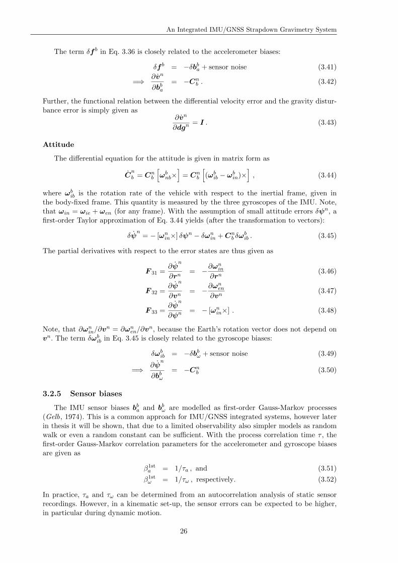
An Integrated IMU/GNSS Strapdown Gravimetry System
The term δf b in Eq. 3.36 is closely related to the accelerometer biases:
δf b = −δbba + sensor noise (3.41)
=⇒ ∂vn
∂bba= −Cn
b . (3.42)
Further, the functional relation between the differential velocity error and the gravity distur-bance error is simply given as
∂vn
∂dgn= I . (3.43)
Attitude
The differential equation for the attitude is given in matrix form as
Cnb = Cn
b
[ωbnb×
]= Cn
b
[(ωbib − ωbin)×
], (3.44)
where ωbib is the rotation rate of the vehicle with respect to the inertial frame, given inthe body-fixed frame. This quantity is measured by the three gyroscopes of the IMU. Note,that ωin = ωie + ωen (for any frame). With the assumption of small attitude errors δψn, afirst-order Taylor approximation of Eq. 3.44 yields (after the transformation to vectors):
δψn= − [ωnin×] δψn − δωnin +C
nb δω
bib . (3.45)
The partial derivatives with respect to the error states are thus given as
F 31 =∂ψ
n
∂rn= −∂ω
nin
∂rn(3.46)
F 32 =∂ψ
n
∂vn= −∂ω
nen
∂vn(3.47)
F 33 =∂ψ
n
∂ψn= − [ωnin×] . (3.48)
Note, that ∂ωnin/∂vn = ∂ωnen/∂v
n, because the Earth’s rotation vector does not depend onvn. The term δωbib in Eq. 3.45 is closely related to the gyroscope biases:
δωbib = −δbbω + sensor noise (3.49)
=⇒ ∂ψn
∂bbω= −Cn
b (3.50)
3.2.5 Sensor biases
The IMU sensor biases bba and bbω are modelled as first-order Gauss-Markov processes(Gelb, 1974). This is a common approach for IMU/GNSS integrated systems, however laterin thesis it will be shown, that due to a limited observability also simpler models as randomwalk or even a random constant can be sufficient. With the process correlation time τ , thefirst-order Gauss-Markov correlation parameters for the accelerometer and gyroscope biasesare given as
β1sta = 1/τa , and (3.51)
β1stω = 1/τω , respectively. (3.52)
In practice, τa and τω can be determined from an autocorrelation analysis of static sensorrecordings. However, in a kinematic set-up, the sensor errors can be expected to be higher,in particular during dynamic motion.
26
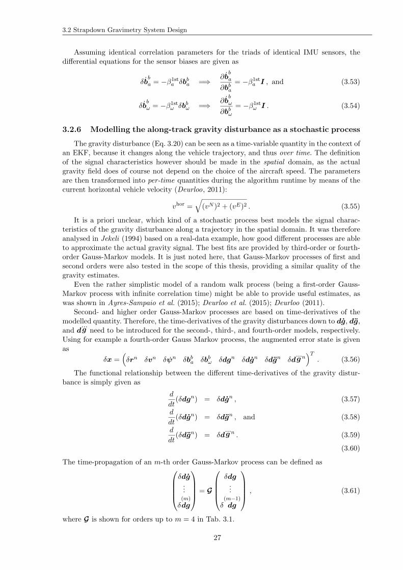
3.2 Strapdown Gravimetry System Design
Assuming identical correlation parameters for the triads of identical IMU sensors, thedifferential equations for the sensor biases are given as
δbba = −β1sta δbba =⇒ ∂b
ba
∂bba= −β1sta I , and (3.53)
δbbω = −β1stω δbbω =⇒ ∂b
bω
∂bbω= −β1stω I . (3.54)
3.2.6 Modelling the along-track gravity disturbance as a stochastic process
The gravity disturbance (Eq. 3.20) can be seen as a time-variable quantity in the context ofan EKF, because it changes along the vehicle trajectory, and thus over time. The definitionof the signal characteristics however should be made in the spatial domain, as the actualgravity field does of course not depend on the choice of the aircraft speed. The parametersare then transformed into per-time quantities during the algorithm runtime by means of thecurrent horizontal vehicle velocity (Deurloo, 2011):
vhor =√(vN )2 + (vE)2 . (3.55)
It is a priori unclear, which kind of a stochastic process best models the signal charac-teristics of the gravity disturbance along a trajectory in the spatial domain. It was thereforeanalysed in Jekeli (1994) based on a real-data example, how good different processes are ableto approximate the actual gravity signal. The best fits are provided by third-order or fourth-order Gauss-Markov models. It is just noted here, that Gauss-Markov processes of first andsecond orders were also tested in the scope of this thesis, providing a similar quality of thegravity estimates.
Even the rather simplistic model of a random walk process (being a first-order Gauss-Markov process with infinite correlation time) might be able to provide useful estimates, aswas shown in Ayres-Sampaio et al. (2015); Deurloo et al. (2015); Deurloo (2011).
Second- and higher order Gauss-Markov processes are based on time-derivatives of themodelled quantity. Therefore, the time-derivatives of the gravity disturbances down to dg, dg,and d
...g need to be introduced for the second-, third-, and fourth-order models, respectively.
Using for example a fourth-order Gauss Markov process, the augmented error state is givenas
δx =(δrn δvn δψn δbba δbbω δdgn δdgn δdgn δd
...g n)T
. (3.56)
The functional relationship between the different time-derivatives of the gravity distur-bance is simply given as
d
dt(δdgn) = δdgn , (3.57)
d
dt(δdgn) = δdgn , and (3.58)
d
dt(δdgn) = δd
...g n . (3.59)
(3.60)
The time-propagation of an m-th order Gauss-Markov process can be defined asδdg...
δ(m)
dg
= G
δdg...
δ(m−1)
dg
, (3.61)
where G is shown for orders up to m = 4 in Tab. 3.1.
27
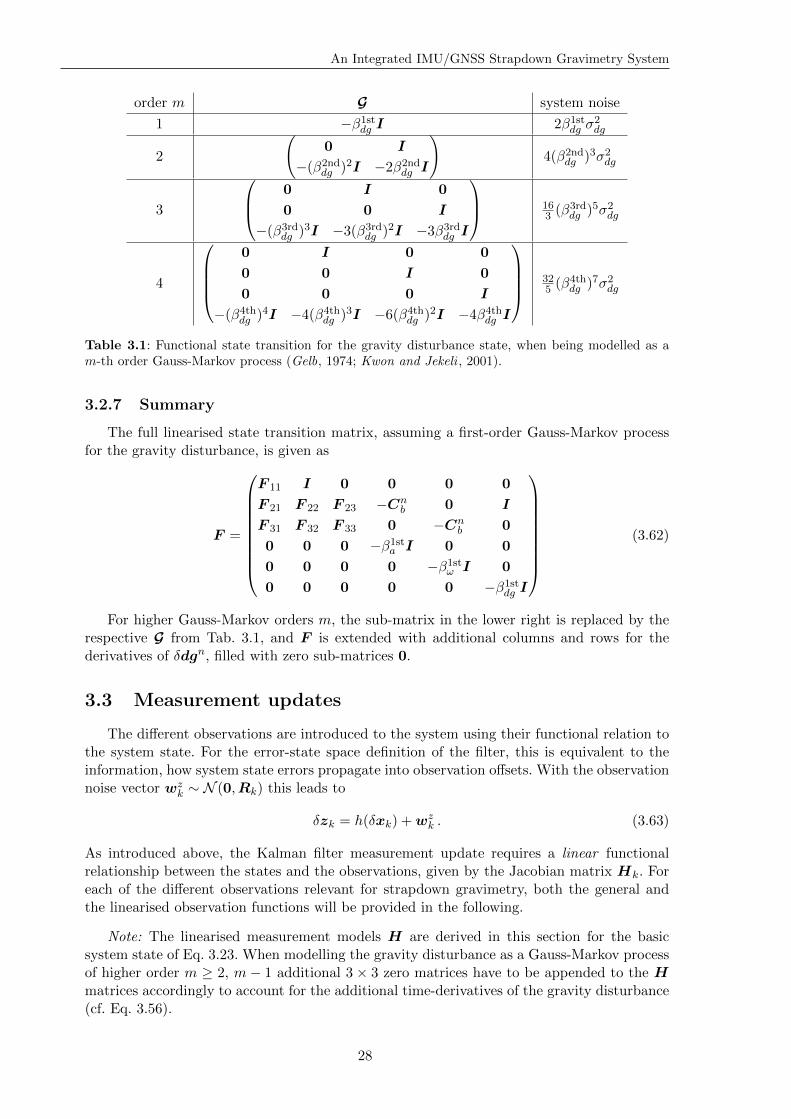
An Integrated IMU/GNSS Strapdown Gravimetry System
order m G system noise
1 −β1stdg I 2β1stdg σ2dg
2
(0 I
−(β2nddg )2I −2β2nddg I
)4(β2nddg )3σ2dg
3
0 I 0
0 0 I
−(β3rddg )3I −3(β3rddg )2I −3β3rddg I
163 (β
3rddg )5σ2dg
4
0 I 0 0
0 0 I 0
0 0 0 I
−(β4thdg )4I −4(β4thdg )3I −6(β4thdg )2I −4β4thdg I
325 (β
4thdg )7σ2dg
Table 3.1: Functional state transition for the gravity disturbance state, when being modelled as am-th order Gauss-Markov process (Gelb, 1974; Kwon and Jekeli , 2001).
3.2.7 Summary
The full linearised state transition matrix, assuming a first-order Gauss-Markov processfor the gravity disturbance, is given as
F =
F 11 I 0 0 0 0
F 21 F 22 F 23 −Cnb 0 I
F 31 F 32 F 33 0 −Cnb 0
0 0 0 −β1sta I 0 0
0 0 0 0 −β1stω I 0
0 0 0 0 0 −β1stdg I
(3.62)
For higher Gauss-Markov orders m, the sub-matrix in the lower right is replaced by therespective G from Tab. 3.1, and F is extended with additional columns and rows for thederivatives of δdgn, filled with zero sub-matrices 0.
3.3 Measurement updates
The different observations are introduced to the system using their functional relation tothe system state. For the error-state space definition of the filter, this is equivalent to theinformation, how system state errors propagate into observation offsets. With the observationnoise vector wz
k ∼ N (0,Rk) this leads to
δzk = h(δxk) +wzk . (3.63)
As introduced above, the Kalman filter measurement update requires a linear functionalrelationship between the states and the observations, given by the Jacobian matrix Hk. Foreach of the different observations relevant for strapdown gravimetry, both the general andthe linearised observation functions will be provided in the following.
Note: The linearised measurement models H are derived in this section for the basicsystem state of Eq. 3.23. When modelling the gravity disturbance as a Gauss-Markov processof higher order m ≥ 2, m − 1 additional 3 × 3 zero matrices have to be appended to the Hmatrices accordingly to account for the additional time-derivatives of the gravity disturbance(cf. Eq. 3.56).
28
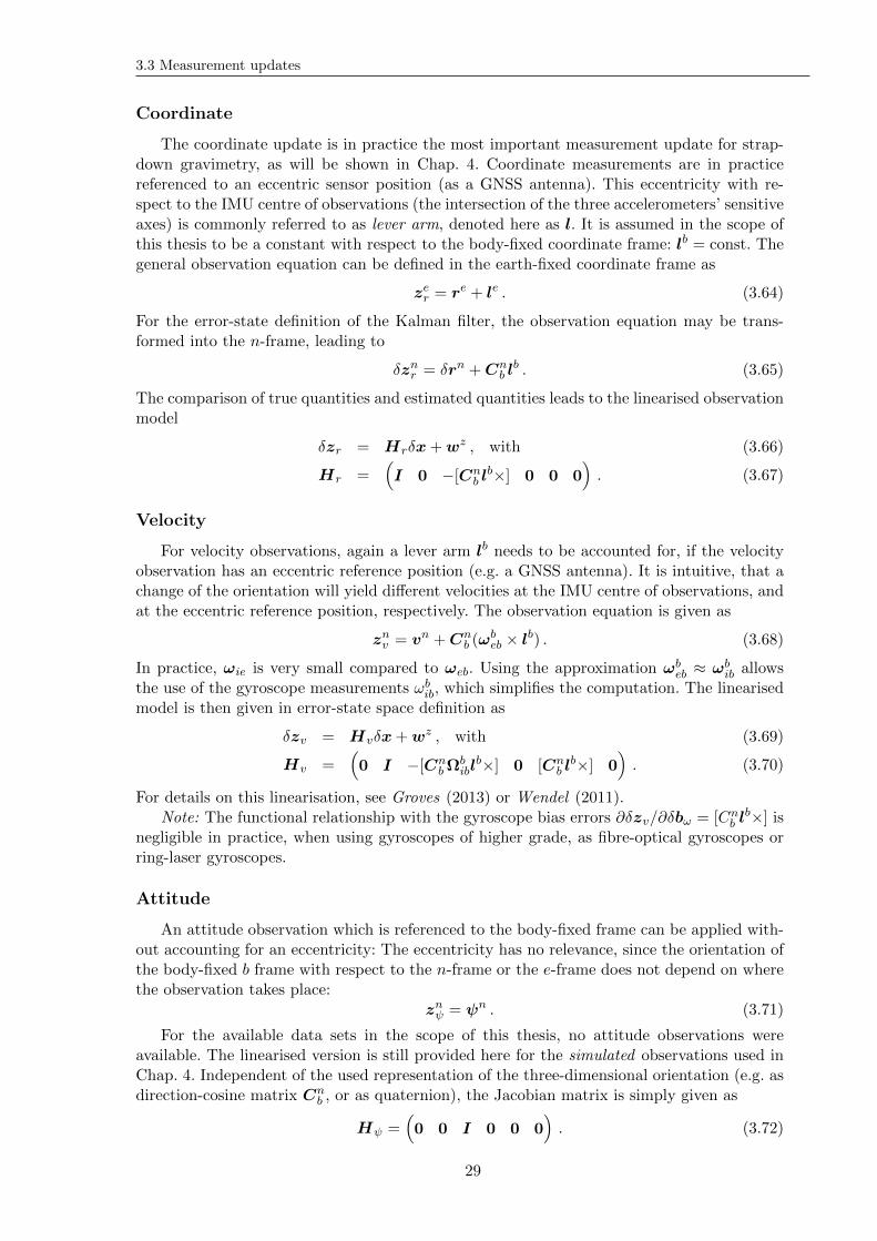
3.3 Measurement updates
Coordinate
The coordinate update is in practice the most important measurement update for strap-down gravimetry, as will be shown in Chap. 4. Coordinate measurements are in practicereferenced to an eccentric sensor position (as a GNSS antenna). This eccentricity with re-spect to the IMU centre of observations (the intersection of the three accelerometers’ sensitiveaxes) is commonly referred to as lever arm, denoted here as l. It is assumed in the scope ofthis thesis to be a constant with respect to the body-fixed coordinate frame: lb = const. Thegeneral observation equation can be defined in the earth-fixed coordinate frame as
zer = re + le . (3.64)
For the error-state definition of the Kalman filter, the observation equation may be trans-formed into the n-frame, leading to
δznr = δrn +Cnb lb . (3.65)
The comparison of true quantities and estimated quantities leads to the linearised observationmodel
δzr = Hrδx+wz , with (3.66)
Hr =(I 0 −[Cn
b lb×] 0 0 0
). (3.67)
Velocity
For velocity observations, again a lever arm lb needs to be accounted for, if the velocityobservation has an eccentric reference position (e.g. a GNSS antenna). It is intuitive, that achange of the orientation will yield different velocities at the IMU centre of observations, andat the eccentric reference position, respectively. The observation equation is given as
znv = vn +Cnb (ω
beb × lb) . (3.68)
In practice, ωie is very small compared to ωeb. Using the approximation ωbeb ≈ ωbib allowsthe use of the gyroscope measurements ωbib, which simplifies the computation. The linearisedmodel is then given in error-state space definition as
δzv = Hvδx+wz , with (3.69)
Hv =(0 I −[Cn
bΩbiblb×] 0 [Cn
b lb×] 0
). (3.70)
For details on this linearisation, see Groves (2013) or Wendel (2011).Note: The functional relationship with the gyroscope bias errors ∂δzv/∂δbω = [Cnb l
b×] isnegligible in practice, when using gyroscopes of higher grade, as fibre-optical gyroscopes orring-laser gyroscopes.
Attitude
An attitude observation which is referenced to the body-fixed frame can be applied with-out accounting for an eccentricity: The eccentricity has no relevance, since the orientation ofthe body-fixed b frame with respect to the n-frame or the e-frame does not depend on wherethe observation takes place:
znψ = ψn . (3.71)
For the available data sets in the scope of this thesis, no attitude observations wereavailable. The linearised version is still provided here for the simulated observations used inChap. 4. Independent of the used representation of the three-dimensional orientation (e.g. asdirection-cosine matrix Cn
b , or as quaternion), the Jacobian matrix is simply given as
Hψ =(0 0 I 0 0 0
). (3.72)
29
An Integrated IMU/GNSS Strapdown Gravimetry System
Gravity Disturbance
Introducing a gravity disturbance measurement may appear somewhat contradictory, be-cause it is actually the gravity disturbance that shall be determined by the filter. Still, thistype of observation has practical relevance: If the trajectory contains points of known gravity,this knowledge can be introduced to the filter as a measurement. For airborne gravimetry thisis typically the case after returning to the initial parking position on the apron of an airport,where a terrestrial gravity measurement of relatively high accuracy (better than 100µGal) istypically available (airborne gravimetry is usually relative gravimetry). It is assumed here,that the gravity disturbance observation is given in the n-frame and referenced to the IMUcentre of observations. The observation model is then given as
zndg = dgn , (3.73)
leading to the linearised functional relationship
Hdg =(0 0 0 0 0 I
). (3.74)
Note: Each of the measurement updates discussed in this section may be applied equiv-alently, if only a subset of components of the 3-D measurement vectors are available (forexample, if only the vertical component of the gravity disturbance is known).
3.4 Navigation update
In the navigation update, the time-discrete accelerations f b and turn rates ωbib measuredby the IMU are used to update the current estimates of position, velocity, and attitude, fromepoch k − 1 to epoch k. The equations are given here in an algorithmic fashion, showing therelevant inputs for each of the quantities being computed. The attitude update is based onquaternions qnb , being an equivalent representation of the direction-cosine matrix Cn
b (detailscan be found in Groves (2013)). The quaternion of the last epoch qnb,k−1 is assumed to beavailable.
gnk−1 = γn(ϕk−1, hk−1) + dgnk−1 (3.75)
ωbnb,k = (ωbib,k − bbω,k−1)− (ωnie(ϕk−1) + ωnen(ϕk−1, hk−1,v
nk−1)) (3.76)
∆ψ = ωbnb,k · dtk (3.77)
∆q =
(cos(0.5 · |∆ψ|)
sin(0.5 · |∆ψ|) ∆ψ|∆ψ|
)(3.78)
qnb,k = qnb,k−1 •∆q (3.79)
fnk = Cnb,k(f
bib,k − bba,k−1) (3.80)
anCoriolis,k = −(2ωnie + ωnen)× vnk−1 (3.81)
vnk = vnk−1 + (fnk + gnk−1 + a
nCoriolis,k) · dtk (3.82)
ϕk = ϕk−1 + 0.5 · (vNk−1 + vNk ) · dtk/RN (3.83)
λk = λk−1 + 0.5 · (vEk−1 + vEk ) · dtk/(RE cosϕk) (3.84)
hk = hk−1 − 0.5 · (vDk−1 + vDk ) · dtk (3.85)
Note, that these equations contain some approximations, e.g. the Coriolis force for epoch k iscomputed based on vk−1. Iterations can be implemented to circumvent the approximations,
30
3.5 Gravity reductions
however in practice no significant changes of the results could be observed. The change ofthe quantities (as normal gravity, Coriolis acceleration, velocity) between two time-epochs isusually very small due to the very short time increments of a strapdown IMU (10ms or less).
The update of the attitude is shown here using quaternions. It is just noted here, that forhigh-dynamic motion, a more exact computation may be preferable. A more exact method,based on matrix exponentials of the matrix [∆ψ×], can be found in Groves (2013). However,for the data sets introduced in Chap. 8, no significant effect on the state estimates could beobserved.
The update of latitude ϕ, longitude λ, and ellipsoidal height h is done based on theaverage velocity in the time interval [tk−1, tk] to account for accelerations, which are assumedto be constant during this time interval.
The estimates of the sensor biases bba and bbω, and the gravity disturbance dgn, remainunchanged in the scope of the navigation update: The last estimate is also the best predictionfor the next epoch. These states can only be updated, if measurements are introduced to thefilter. Therefore, bba,k−1, b
bω,k−1, and g
nk−1 are used in the above equations for epoch k, and
gnk = gnk−1, and so forth.
3.5 Gravity reductions
The estimation process can in general be supported, if additional (external) informationon the stochastic process can be introduced to the filter. In addition to the basic concept ofmeasurements in the sense of a Kalman filter, such external information may be introducedusing reductions of the estimated signal.
One example of such a reduction has already been introduced by using the concept ofgravity disturbances, being the residual gravity with respect to normal gravity. Thus, thegravity vector g was split into the two components
g = γ + dg . (3.86)
The estimation of the gravity disturbance is easier compared to the estimation of gravity,because the majority of the signal dynamics due to altitude changes of the aircraft is removedfrom the signal, thereby allowing a more trajectory-independent modelling of the stochasticprocess. (Residual effects of altitude changes can be observed in the gravity disturbance tothe extent, to which the normal gravity gradient deviates from the actual gravity gradient.)Also, the use of the much smaller gravity disturbances as system states may yield a highernumerical stability: Gravity disturbances are usually <100mGal (<400mGal) in regions withflat (high-mountain) topography, contributing only <0.01% (<0.04%) to the actual gravity.
In the following, the concept of gravity reductions shall be pursued in more depth, usingglobal gravity models (GGM) and topographic reductions.
3.5.1 Global gravity model reductions
Satellite-based global gravity models (GGM) may be applied as a long-wavelength gravityreduction for airborne gravimetry. The resolution of the satellite gravity models is typicallylimited to wavelengths of ≈ 100 km and more. The gravity reduction dgnGGM can be computedfor the aircraft positions along a flight trajectory based on the GNSS positions. In practice,this computation can be done as a preprocessing step, before the execution of the EKFalgorithm.
By applying a long-wavelength gravity reduction, the characteristics of the (residual)gravity disturbance can change significantly, yielding different correlation parameters βdg forthe Gauss-Markov processes. Fig. 3.1 shows a real-data example, taken from an aerogravityflight over the Chilean Andes. It can be seen, that the statistical properties of the data
31
An Integrated IMU/GNSS Strapdown Gravimetry System
signal change significantly after applying the GGM reduction (Fig. 3.1, bottom left). Thecorrelation time τ , being the leftmost intersection of the autocorrelation function with the1/e-line (Fig. 3.1), reduces from 30min to 12min, equivalent to a spatial correlation distanceof approximately 180 km, and 70 km, respectively.
3.5.2 Topographic reductions
When doing airborne gravimetry above mountainous terrain, the biggest part of the ob-served gravity disturbances may arise from the effect of the topographic masses below. Thespectral contribution very much depends on the characteristics of the terrain. In general, bothshort (>1 km) and long wavelengths (>100 km) can be found in the topographic effect.
With global digital terrain models (DTM) and bathymetry models being available(Amante and Eakins, 2009; Becker et al., 2009), the topographic effect dgntop can be com-puted along the vehicle trajectory. Note, that the topographic effect has to be computed atflight altitude. Details on the computation of dgntop can be found in Forsberg and Tscherning(1981) and Heck and Seitz (2007). For the topographic reductions shown in this thesis, thesoftware GRAVSOFT TC was used (Tscherning et al., 1992).
In general, it appears reasonable to combine both reductions, GGM and topography,because the long-wavelength Bouguer disturbances (after removing the topographic effect)will only be covered by the GGM, while short-wavelength effects can only be reduced based onthe topographic effect. However, it is important in this case to artificially limit the topographicreduction to shorter wavelengths (e.g. < 100 km) by computing the topographic effect onlyfor a DTM which is limited to such higher frequencies. In practice, a low resolution DTMmay be subtracted from the original full-resolution DTM. The topographic effect is thencomputed based on this residual terrain model (RTM), see Forsberg (1984). Fig. 3.1 showsthe topographic reduction for wavelengths shorter than 110 km, being consistent with onedegree in latitudinal direction, which is the resolution of the applied global gravity modelreduction.
After applying both reductions, the residual gravity disturbance signal is smoother, andhas lower amplitudes. The original absolute range of 230mGal reduces to 65mGal, and, asexpected, the reduced gravity disturbance has almost zero mean (Fig. 3.1).
3.5.3 Modified system state
Instead of using the standard definition of the gravity disturbance (Eqs. 3.20 and 3.86),the reduced gravity disturbance dgnr is defined as
dgnr = gn − γn − dgntop − dgnGGM = dgn − dgntop − dgnGGM . (3.87)
Thus, in the system state (Eq. 3.23, or its augmented version, Eq. 3.56), dgn will be replacedby dgnr . The navigation update (Eq. 3.75) needs to be changed accordingly:
gn = γn + dgntop + dgnGGM + dgnr (3.88)
The same equation may be applied to the final estimates of the reduced gravity, dgnr , in order
to restore the full gravity vector.The overall process of applying gravity reductions in order to support the gravity estima-
tion can be summarized as
1. Remove portions of the gravity gn by applying the gravity reductions.
2. Compute the residual gravity disturbances dgnr (done here using an EKF and a Kalmansmoother).
32
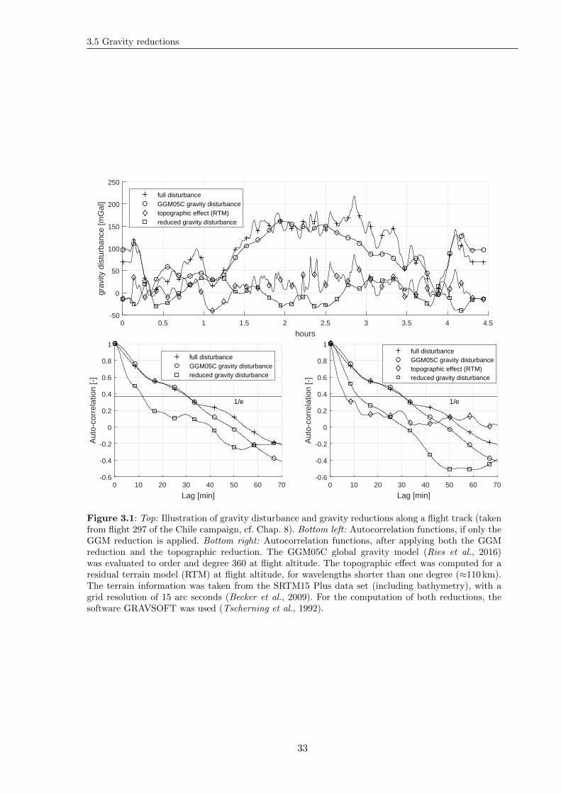
3.5 Gravity reductions
0 0.5 1 1.5 2 2.5 3 3.5 4 4.5
hours
-50
0
50
100
150
200
250
grav
ity d
istu
rban
ce [m
Gal
]
full disturbanceGGM05C gravity disturbancetopographic effect (RTM)reduced gravity disturbance
0 10 20 30 40 50 60 70
Lag [min]
-0.6
-0.4
-0.2
0
0.2
0.4
0.6
0.8
1
Aut
o-co
rrel
atio
n [-
]
1/e
full disturbanceGGM05C gravity disturbancereduced gravity disturbance
0 10 20 30 40 50 60 70
Lag [min]
-0.6
-0.4
-0.2
0
0.2
0.4
0.6
0.8
1
Aut
o-co
rrel
atio
n [-
]
1/e
full disturbanceGGM05C gravity disturbancetopographic effect (RTM)reduced gravity disturbance
Figure 3.1: Top: Illustration of gravity disturbance and gravity reductions along a flight track (takenfrom flight 297 of the Chile campaign, cf. Chap. 8). Bottom left: Autocorrelation functions, if only theGGM reduction is applied. Bottom right: Autocorrelation functions, after applying both the GGMreduction and the topographic reduction. The GGM05C global gravity model (Ries et al., 2016)was evaluated to order and degree 360 at flight altitude. The topographic effect was computed for aresidual terrain model (RTM) at flight altitude, for wavelengths shorter than one degree (≈110 km).The terrain information was taken from the SRTM15 Plus data set (including bathymetry), with agrid resolution of 15 arc seconds (Becker et al., 2009). For the computation of both reductions, thesoftware GRAVSOFT was used (Tscherning et al., 1992).
33
An Integrated IMU/GNSS Strapdown Gravimetry System
3. Restore the gravity gn by inversely applying the gravity reductions to dgnr (if required).
Thus, this method can be seen as a variant of the well-established remove-compute-restoretechnique, a tool which is commonly used for the geoid determination (Forsberg and Tsch-erning , 1981), to stabilise the downward continuation of surface gravity data to the geoid.
For the practical implementation of such gravity reductions, the actual reductions maybe pre-computed in the n-frame, using pre-processed GNSS coordinates.
3.6 Optimal smoothing
An EKF can only use the information of the past epochs up to the current epoch tk forthe estimation of the current system state xk. (The information is actually stored inside xk−1
and P k−1 only, which however depend on xk−2 and P k−2, and so forth.) Only the estimateof the final epoch tN is based on the entire set of available information. This limitation isobvious for real-time applications. However, in airborne gravimetry, a real-time output of theestimates is usually not required. The state estimation at epoch tk could be done by alsolooking at observations of future epochs.
An optimal smoother uses all available information for the estimation of the system stateat any epoch. The Rauch-Tung-Striebel (RTS) smoother, also called Kalman smoother, isa very efficient algorithm, going backwards over the EKF estimates. In practice, results canbe shown to improve significantly after applying the smoother. In particular, the gravitydisturbance estimates, which require a considerable period of IMU and GNSS observationsin order to converge to the mGal level (90 s or more), show immense accuracy improvementsby applying a smoother (Forsberg et al., 1986).
The RTS smoother is initialised using the EKF estimates of the last epoch: xN ≡ x+N and
PN ≡ P+N . The core RTS loop, going backward through the epochs, is then given as
xk = x+k +Ck(xk+1 − x−
k+1) (3.89)
P k = P+k +Ck(P k+1 − P−
k+1)CTk (3.90)
Ck = P+kΦ
Tk (P
−k+1)
−1 . (3.91)
It can be seen, that the smoothed states xk are the combination of the a-posteriori stateestimates, and an additional term introduced by the smoother.
When using an EKF in error state space formulation, Eq. 3.89 is given as
δxk = δx+k +Ck(δxk+1 − δx−
k+1) . (3.92)
The estimated a-posteriori errors δx+k were already applied to the (externally maintained)
system state during the EKF runtime, which is crucial for limiting the linearisation errors.After the execution of the RTS-smoother, this portion of the smoothed δxk must not beapplied again to the system state, but only the additional term introduced by the smootherin Eq. 3.92. The residual corrections, that need to be applied to the state estimates (position,velocity, a.s.f.), are therefore given as
∆δxk = δxk − δx+k . (3.93)
(The smoothed covariance estimates P k are valid without further modification.)
34
Chapter 4
System analysis
4.1 Observability
An observability analysis is carried out here for the IMU/GNSS integrated strapdowngravimetry system. In general, a system is called observable, if the observations (or measure-ments) introduced to the system enable the estimation of all system states.
An unobservable system can always be made observable by introducing additional obser-vations. In particular, a system is always observable, if each of the states is being observed.
The original definition of observability is a binary measure. It is already noted here, thatthe 18-state strapdown gravimetry system, as introduced in Chap. 3 is not observable. Still,a deeper insight into this system can be obtained by a closer analysis of so-called structuregraphs, and additionally by an algebraic analysis of the so-called observation matrix. Bothconcepts will be pursued in this section.
4.1.1 Structure graph analysis
Structure graphs enable an intuitive and visual observability analysis. Such a structuregraph is generated using the following construction rules (Dion et al., 2003):
1. For each system state, create a node in the graph.
2. For each observation (measurement), create an output node in the graph.
3. For each combination of two system states a and b (incl. a = b), add a directed edgefrom the a-node to the b-node, if ∂b/∂a 6= 0.
4. For each combination of system state a and observation z, add a directed edge fromthe a-node to the z-node, if ∂z/∂a 6= 0.
Thus, the edges in the graph indicate non-zero elements in the F matrix, and in the H-matrices, respectively. Such a graph can only fully reflect the observability of a system, if thesenon-zero elements are linearly independent. Such a system is then called a structured system(Dion et al., 2003). As will be shown later, the strapdown gravimetry system is not strictlya structured system. Still, the structure graph analysis will provide a deeper understandingof this system.
For the strapdown gravimetry system as introduced in Chapter 3, the structure graph isshown in Fig. 4.1. The nodes correspond to the 3-D system states as introduced in Chapter 3.The output nodes are included for the two typical observations in strapdown gravimetry:Coordinate observations zr, and velocity observations zv (both commonly taken from GNSSmeasurements). The edges reflect the non-zero entries of F , Hr, and Hv (cf. Eq. 3.62 andSect. 3.3).
35
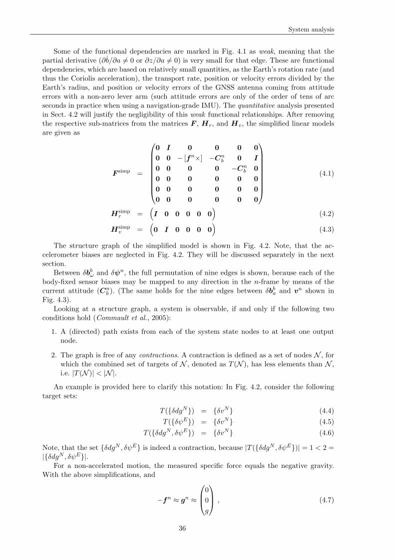
System analysis
Some of the functional dependencies are marked in Fig. 4.1 as weak, meaning that thepartial derivative (∂b/∂a 6= 0 or ∂z/∂a 6= 0) is very small for that edge. These are functionaldependencies, which are based on relatively small quantities, as the Earth’s rotation rate (andthus the Coriolis acceleration), the transport rate, position or velocity errors divided by theEarth’s radius, and position or velocity errors of the GNSS antenna coming from attitudeerrors with a non-zero lever arm (such attitude errors are only of the order of tens of arcseconds in practice when using a navigation-grade IMU). The quantitative analysis presentedin Sect. 4.2 will justify the negligibility of this weak functional relationships. After removingthe respective sub-matrices from the matrices F , Hr, and Hv, the simplified linear modelsare given as
F simp =
0 I 0 0 0 0
0 0 − [fn×] −Cnb 0 I
0 0 0 0 −Cnb 0
0 0 0 0 0 0
0 0 0 0 0 0
0 0 0 0 0 0
(4.1)
Hsimpr =
(I 0 0 0 0 0
)(4.2)
Hsimpv =
(0 I 0 0 0 0
)(4.3)
The structure graph of the simplified model is shown in Fig. 4.2. Note, that the ac-celerometer biases are neglected in Fig. 4.2. They will be discussed separately in the nextsection.
Between δbbω and δψn, the full permutation of nine edges is shown, because each of thebody-fixed sensor biases may be mapped to any direction in the n-frame by means of thecurrent attitude (Cn
b ). (The same holds for the nine edges between δbba and vn shown inFig. 4.3).
Looking at a structure graph, a system is observable, if and only if the following twoconditions hold (Commault et al., 2005):
1. A (directed) path exists from each of the system state nodes to at least one outputnode.
2. The graph is free of any contractions. A contraction is defined as a set of nodes N , forwhich the combined set of targets of N , denoted as T (N ), has less elements than N ,i.e. |T (N )| < |N |.
An example is provided here to clarify this notation: In Fig. 4.2, consider the followingtarget sets:
T (δdgN) = δvN (4.4)
T (δψE) = δvN (4.5)
T (δdgN , δψE) = δvN (4.6)
Note, that the set δdgN , δψE is indeed a contraction, because |T (δdgN , δψE)| = 1 < 2 =|δdgN , δψE|.
For a non-accelerated motion, the measured specific force equals the negative gravity.With the above simplifications, and
−fn ≈ gn ≈
0
0
g
, (4.7)
36
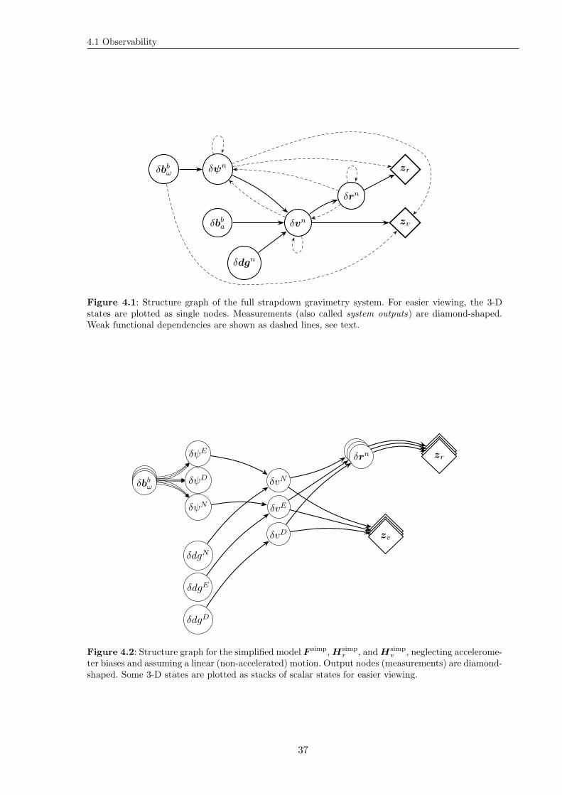
4.1 Observability
δbbω δψn
δbba
δdgn
δvn
δrn
zv
zr
Figure 4.1: Structure graph of the full strapdown gravimetry system. For easier viewing, the 3-Dstates are plotted as single nodes. Measurements (also called system outputs) are diamond-shaped.Weak functional dependencies are shown as dashed lines, see text.
δψN
δψE
δψD
δdgN
δdgE
δdgD
δvN
δvE
δvD
δrn
δbbω
zr
zv
Figure 4.2: Structure graph for the simplified model F simp,Hsimpr , andHsimp
v , neglecting accelerome-ter biases and assuming a linear (non-accelerated) motion. Output nodes (measurements) are diamond-shaped. Some 3-D states are plotted as stacks of scalar states for easier viewing.
37
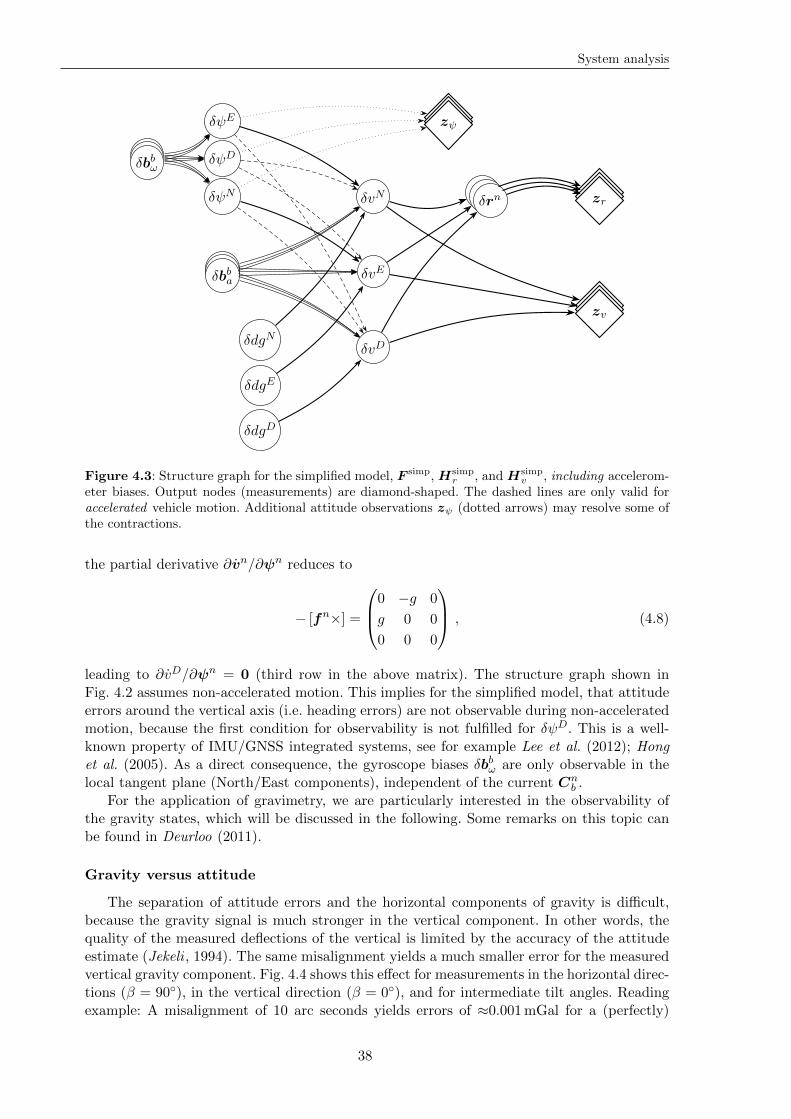
System analysis
δψN
δψE
δψD
δdgN
δdgE
δdgD
δvN
δvE
δvD
δrn
δbbω
δbba
zr
zv
zψ
Figure 4.3: Structure graph for the simplified model, F simp,Hsimpr , andHsimp
v , including accelerom-eter biases. Output nodes (measurements) are diamond-shaped. The dashed lines are only valid foraccelerated vehicle motion. Additional attitude observations zψ (dotted arrows) may resolve some ofthe contractions.
the partial derivative ∂vn/∂ψn reduces to
− [fn×] =
0 −g 0
g 0 0
0 0 0
, (4.8)
leading to ∂vD/∂ψn = 0 (third row in the above matrix). The structure graph shown inFig. 4.2 assumes non-accelerated motion. This implies for the simplified model, that attitudeerrors around the vertical axis (i.e. heading errors) are not observable during non-acceleratedmotion, because the first condition for observability is not fulfilled for δψD. This is a well-known property of IMU/GNSS integrated systems, see for example Lee et al. (2012); Honget al. (2005). As a direct consequence, the gyroscope biases δbbω are only observable in thelocal tangent plane (North/East components), independent of the current Cn
b .For the application of gravimetry, we are particularly interested in the observability of
the gravity states, which will be discussed in the following. Some remarks on this topic canbe found in Deurloo (2011).
Gravity versus attitude
The separation of attitude errors and the horizontal components of gravity is difficult,because the gravity signal is much stronger in the vertical component. In other words, thequality of the measured deflections of the vertical is limited by the accuracy of the attitudeestimate (Jekeli , 1994). The same misalignment yields a much smaller error for the measuredvertical gravity component. Fig. 4.4 shows this effect for measurements in the horizontal direc-tions (β = 90), in the vertical direction (β = 0), and for intermediate tilt angles. Readingexample: A misalignment of 10 arc seconds yields errors of ≈0.001mGal for a (perfectly)
38
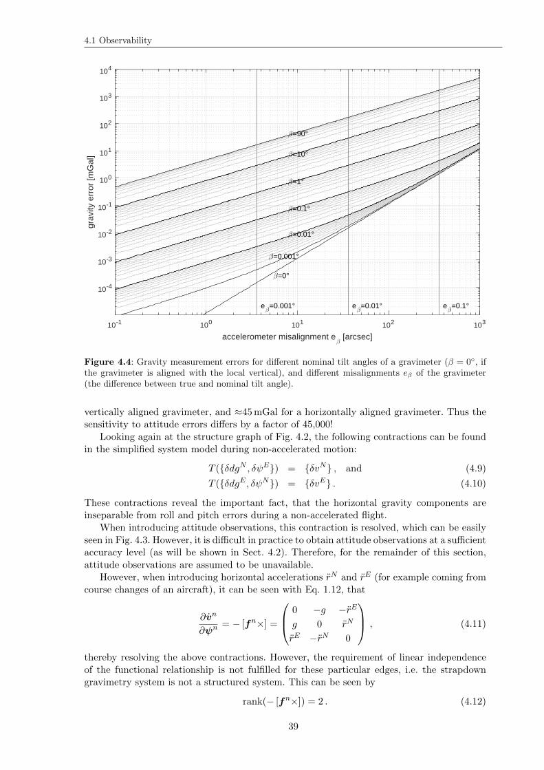
4.1 Observability
10-1 100 101 102 103
accelerometer misalignment eβ [arcsec]
10-4
10-3
10-2
10-1
100
101
102
103
104
grav
ity e
rror
[mG
al]
β=0°
β=0.001°
β=0.01°
β=0.1°
β=1°
β=10°
β=90°
eβ=0.001° e
β=0.01° e
β=0.1°
Figure 4.4: Gravity measurement errors for different nominal tilt angles of a gravimeter (β = 0, ifthe gravimeter is aligned with the local vertical), and different misalignments eβ of the gravimeter(the difference between true and nominal tilt angle).
vertically aligned gravimeter, and ≈45mGal for a horizontally aligned gravimeter. Thus thesensitivity to attitude errors differs by a factor of 45,000!
Looking again at the structure graph of Fig. 4.2, the following contractions can be foundin the simplified system model during non-accelerated motion:
T (δdgN , δψE) = δvN , and (4.9)
T (δdgE , δψN) = δvE . (4.10)
These contractions reveal the important fact, that the horizontal gravity components areinseparable from roll and pitch errors during a non-accelerated flight.
When introducing attitude observations, this contraction is resolved, which can be easilyseen in Fig. 4.3. However, it is difficult in practice to obtain attitude observations at a sufficientaccuracy level (as will be shown in Sect. 4.2). Therefore, for the remainder of this section,attitude observations are assumed to be unavailable.
However, when introducing horizontal accelerations rN and rE (for example coming fromcourse changes of an aircraft), it can be seen with Eq. 1.12, that
∂vn
∂ψn= − [fn×] =
0 −g −rE
g 0 rN
rE −rN 0
, (4.11)
thereby resolving the above contractions. However, the requirement of linear independenceof the functional relationship is not fulfilled for these particular edges, i.e. the strapdowngravimetry system is not a structured system. This can be seen by
rank(− [fn×]) = 2 . (4.12)
39
System analysis
(However, all other non-zero 3× 3 sub-matrices in F simp, Hsimpr , and Hsimp
v have full rank.)Also, the overall system is not observable due to the contraction
|T (δdgN , δdgE , δdgD, δψN , δψE , δψD)| = 3 . (4.13)
Still neglecting accelerometer biases, this implies however observability for the verticalgravity component during a non-accelerated flight: The states δdgD, δvD, δrD, and the mea-surements zDr and zDv are not connected to any of the other states in this case, yielding acompletely independent sub-system for the vertical components. There is obviously no con-traction in this sub-system, and all states are clearly connected to output states: along thepaths δdgD → δvD → δrD → zDr , and δdg
D → δvD → zDv .On the other hand, the vertical gravity is not observable (i.e. fully separable from attitude
errors) in the case of horizontal accelerations (i.e. when including the dashed edges in Fig. 4.3).
Gravity versus accelerometer biases
Now looking at the accelerometer biases δbba (Fig. 4.3), it can be seen, that even whenneglecting attitude errors,
|T (δdgN , δdgE , δdgD, δbXa , δbYa , δbZa )| = 3 , (4.14)
showing another important property of the strapdown gravimetry system: that gravity andaccelerometer biases are inseparable. Note, that this property also holds during acceleratedflight manoeuvres, and independent of the (constant) IMU orientation Cn
b .When accounting also for the attitude errors, the discrepancy between the number of
states |N | = 9 and the number of states in the target set |T (N )| = 3 is even stronger.
Velocity observations
For the simplified system model (Figs. 4.2 and 4.3), note that velocity observations zvdo not at all affect the observability of the system: the path from vn via rn to zr is clearlyconnected and free of contractions, also if the velocity observations are omitted.
It will be shown in Sect. 4.2, that velocity observations have also a lower relevance forstrapdown gravimetry from a quantitative perspective.
4.1.2 Algebraic analysis
The structure graphs introduced in the previous section allowed an intuitive understandingof the strapdown gravimetry system, pointing out particular inseparabilities between systemstates. This section presents a more thorough analysis, based on the well-established algebraicdefinition of observability, using the observability matrix. Different scenarios, including time-variable vehicle accelerations, and a time-variable attitude, can be analysed in view of theobservability of the system.
For a number of N epochs, the observability matrix Ξ is given with the definitions ofChap. 3 as
Ξ =
Hk
Hk+1Φk
Hk+2Φk+1Φk
...
Hk+N−1Φk+N−2Φk+N−3 . . .Φk
(4.15)
As introduced in Chap. 3, each matrix Hk maps the n-dimensional system state to themeasurement(s) zk of a given epoch: zk =Hkδxk, where zk can be a combination of multiple
40
4.1 Observability
observations, of different types. Further, the type and number of observations may changefrom epoch to epoch. A necessary condition for the system’s observability is, that the numberof observations d is equal or greater than the number of system states n, i.e.
d =k+N−1∑i=k
dim(zi) ≥ n . (4.16)
Thus, Ξ is a d × n matrix, with d ≥ n. Example: A series of N = 6 3-D measurements (asGNSS coordinates) is sufficient to fulfil this condition for the 18-state strapdown gravimetrysystem.
The rank deficiency r is then defined for the square symmetric matrix Ξ∗ = ΞTΞ as
r = n− rank(Ξ∗) . (4.17)
Note, that the rank is only defined for square matrices. Assuming d = n, also rank(Ξ) couldbe used, because rank(Ξ) = rank(Ξ∗) in this case.
A system is called observable, if and only if r = 0, i.e. the n×n matrix Ξ∗ has a full rankof n. If r > 0, only a n− r dimensional subspace of the state space is observable.
In particular, if a system is not observable, a principal component analysis of Ξ∗ can beperformed based on an Eigen decomposition of Ξ∗ in order to further investigate the systemproperties. An Eigen value of zero indicates an unobservable direction in the state space,which is given by the corresponding Eigen vector.
A more thorough, analytical observability analysis of an integrated IMU/GNSS navi-gation system is provided in Rothman et al. (2014). A method is shown for the analyticaldetermination of the unobservable subspace of a system. In this thesis, the analysis is lim-ited to the computation of rank deficiencies of the observability matrix for different systemconfigurations and scenarios. The next section shows, that such an analysis can provide avaluable insight into the system characteristics.
4.1.3 Scenarios and examples
The rank deficiency r, as introduced in the previous section, is computed for differentsystem state configurations (with particular system states being enabled or disabled). Asystem state is disabled by removing the respective rows and columns from F , and from Hr
and Hv.Further, four different vehicle motion scenarios are evaluated for each of the system con-
figurations:
• S1: Non-accelerated motion, and no attitude changes,
• S2: non-accelerated motion, with roll and pitch angle changes,
• S3: accelerated motion, no attitude changes, and
• S4: accelerated motion, with roll and pitch angle changes.
The motion is always horizontal (i.e. vD = 0). For S1 and S2, the track is a straight linepointing North. For S1 and S3, the body-fixed coordinate frame is aligned with the navigationframe without losing generality, i.e. Cn
b = I = const. A series of N = 6 observations is beingused.
The rank deficiency is evaluated for both the full system model of Eqs. 3.62ff, and thesimplified system model of Eqs. 4.1ff. The results are summarized in Tab. 4.1. It is expected,that the rank deficiencies for the simplified model (first value in each cell of the table) aremore realistic in a quantitative sense, because the very small quantities (the weak edges in
41
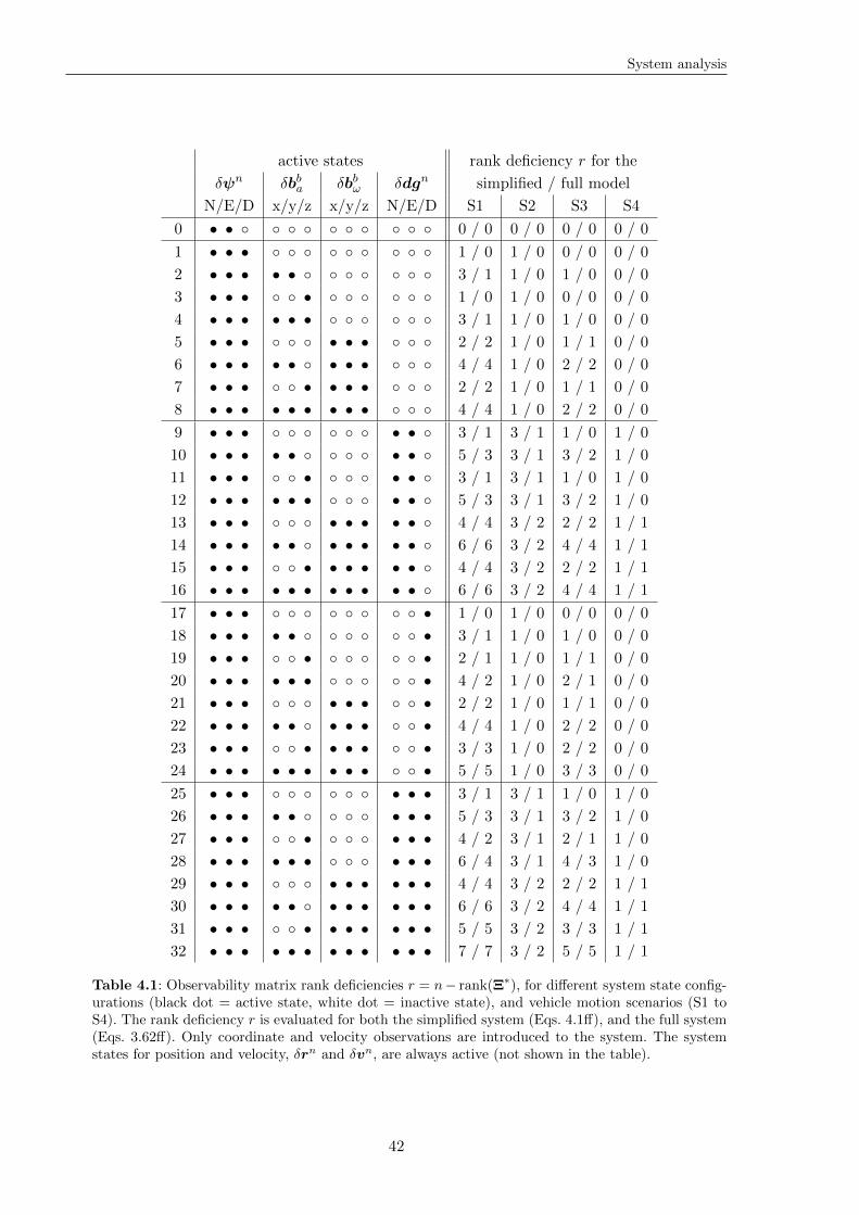
System analysis
active states rank deficiency r for the
δψn δbba δbbω δdgn simplified / full model
N/E/D x/y/z x/y/z N/E/D S1 S2 S3 S4
0 • • 0 / 0 0 / 0 0 / 0 0 / 0
1 • • • 1 / 0 1 / 0 0 / 0 0 / 0
2 • • • • • 3 / 1 1 / 0 1 / 0 0 / 0
3 • • • • 1 / 0 1 / 0 0 / 0 0 / 0
4 • • • • • • 3 / 1 1 / 0 1 / 0 0 / 0
5 • • • • • • 2 / 2 1 / 0 1 / 1 0 / 0
6 • • • • • • • • 4 / 4 1 / 0 2 / 2 0 / 0
7 • • • • • • • 2 / 2 1 / 0 1 / 1 0 / 0
8 • • • • • • • • • 4 / 4 1 / 0 2 / 2 0 / 0
9 • • • • • 3 / 1 3 / 1 1 / 0 1 / 0
10 • • • • • • • 5 / 3 3 / 1 3 / 2 1 / 0
11 • • • • • • 3 / 1 3 / 1 1 / 0 1 / 0
12 • • • • • • • • 5 / 3 3 / 1 3 / 2 1 / 0
13 • • • • • • • • 4 / 4 3 / 2 2 / 2 1 / 1
14 • • • • • • • • • • 6 / 6 3 / 2 4 / 4 1 / 1
15 • • • • • • • • • 4 / 4 3 / 2 2 / 2 1 / 1
16 • • • • • • • • • • • 6 / 6 3 / 2 4 / 4 1 / 1
17 • • • • 1 / 0 1 / 0 0 / 0 0 / 0
18 • • • • • • 3 / 1 1 / 0 1 / 0 0 / 0
19 • • • • • 2 / 1 1 / 0 1 / 1 0 / 0
20 • • • • • • • 4 / 2 1 / 0 2 / 1 0 / 0
21 • • • • • • • 2 / 2 1 / 0 1 / 1 0 / 0
22 • • • • • • • • • 4 / 4 1 / 0 2 / 2 0 / 0
23 • • • • • • • • 3 / 3 1 / 0 2 / 2 0 / 0
24 • • • • • • • • • • 5 / 5 1 / 0 3 / 3 0 / 0
25 • • • • • • 3 / 1 3 / 1 1 / 0 1 / 0
26 • • • • • • • • 5 / 3 3 / 1 3 / 2 1 / 0
27 • • • • • • • 4 / 2 3 / 1 2 / 1 1 / 0
28 • • • • • • • • • 6 / 4 3 / 1 4 / 3 1 / 0
29 • • • • • • • • • 4 / 4 3 / 2 2 / 2 1 / 1
30 • • • • • • • • • • • 6 / 6 3 / 2 4 / 4 1 / 1
31 • • • • • • • • • • 5 / 5 3 / 2 3 / 3 1 / 1
32 • • • • • • • • • • • • 7 / 7 3 / 2 5 / 5 1 / 1
Table 4.1: Observability matrix rank deficiencies r = n− rank(Ξ∗), for different system state config-urations (black dot = active state, white dot = inactive state), and vehicle motion scenarios (S1 toS4). The rank deficiency r is evaluated for both the simplified system (Eqs. 4.1ff), and the full system(Eqs. 3.62ff). Only coordinate and velocity observations are introduced to the system. The systemstates for position and velocity, δrn and δvn, are always active (not shown in the table).
42
4.1 Observability
Fig. 4.3) show barely any effect on the state estimation in practice (as will be confirmed inSect. 4.2). In other words, the rank deficiencies of the full system can be regarded as toooptimistic (too low) in practice. For each of the configurations, the full system model yieldsan equal or lower rank deficiency compared to the simplified model.
While it may be difficult to understand the reasons causing the rank deficiencies whenlooking at a particular rank deficiency, the comparison of different table entries can providea good understanding of the system, confirming the properties that were found using thestructure graphs in the previous section.
A turn was chosen for S3 and S4, because it is more common during real gravity flights,compared to constant accelerations. Note, that the scenario S3 still comprises a constantattitude during this right turn, facing North). Such a manoeuvre is in practice not possiblewhen using a fixed-wing aircraft. It is still useful here as an illustrative example.
For a right turn along a circular track, there is a constant acceleration to the right withrespect to the direction of travel arctan(vE/vN ), with the consequence, that fn 6= constamong the N epochs. This resolves the linear dependency of the edges between attitudeand velocity: Comparing row 1, S1 versus S3, apparently the heading error δψD becomesobservable for accelerated motion, cf. Hong et al. (2005). This also yields the separability ofattitude and the horizontal gravity components (row 9, S1 vs. S3).
During a typical aerogravity flight, small changes of the roll- and pitch angles can not beavoided on a nominally straight measurement line, and clearly such changes happen duringturns, and during the take-off and landing phases. The change of Cn
b among the N epochscan resolve linear dependencies in the system, reducing the rank deficiencies for those systemconfigurations including δbba and δbbω, e.g. rows 4, 5, or 8, comparing S1 against S2, or S3against S4.
Such reductions of the rank deficiencies have led to statements in the literature, thatmanoeuvres, as e.g. turns, can be useful for an in-flight calibration of the IMU, i.e. the in-flight determination of the sensor biases (Deurloo, 2011; Skaloud et al., 2015).
More findings can be drawn from the results of Tab. 4.1, in particular supporting thefindings of Sect. 4.1.1:
• Compare rows 1 and 17, S1: r is equal for both rows, indicating that the vertical gravitycomponent is observable during non-accelerated motion (as was shown using the sub-system of vertical components in Sect. 4.1.1).
• Compare rows 1 and 9, S1: When adding the two horizontal gravity components, rincreases by 2, reflecting that these states are inseparable from attitude (all gravitystates are connected to output nodes in Fig. 4.3, thus this deficiency must come froma contraction, i.e. an inseparability of system states).
• Compare rows 17 and 19, S1 or S3: The vertical gravity component, and an accelerom-eter bias in the same direction are inseparable (r increases by 1). This does not hold,if Cn
b 6= const: no increase for S2 and S4. The same can be seen for the horizontalcomponents (compare rows 9 and 10), and for the full 3-D gravity vector (rows 25 and28).
• Row 32: Note, that the full 18-state strapdown gravimetry system is unobservable forall vehicle motion scenarios.
• Row 8 represents the integrated, 15-state IMU/GNSS navigation system, for which theobservability has been analysed by several authors (Rothman et al., 2014; Lee et al.,2012; Hong et al., 2005).
43
System analysis
4.2 Estimability
Note: Parts of the work presented in this section have been published by the author beforethe publication of this thesis (Becker et al., 2015a).
The question, to what extent the system (or particular system states) is observable, isaddressed by the concept of estimability (Baram and Kailath, 1987). The estimability analysisdone in this section will address two major questions:
• How much is the gravity estimation affected by vehicle manoeuvres (i.e., accelerations)?
• How much is the gravity estimation affected by the observation accuracy (for coordinate,velocity, and attitude observations)?
4.2.1 Definition
For a series of N upcoming observations zi = H ixi (with i = k . . . (k + N − 1)), theestimability ν is a measure of how much these observations can reduce the a-priori systemstate covariances P−
k at epoch k.Note, that estimability does not account for the system noise ws ∼ N (0,Q). The a-priori
and a-posteriori system state covariance matrices, P− and P+, are used in this sense in thescope of this section.
The information matrix of such a series of observations is given as (Moon et al., 2008)
Lk,k+N−1 =N−1∑i=0
ΦTk+i,kH
Tk+iR
−1k+iHk+iΦk+i,k , (4.18)
where Φk+i,k = Φk+i−1Φk+i−2 . . .Φk is the system state transition matrix from epoch kto epoch k + i. As for the algebraic definition of observability, the matrix H may combinemultiple observations for each epoch, and the number and the types of observations maychange among the N epochs.
The estimability ν may then be calculated with respect to P−k and a direction in the state
space, u, as
ν(Lk,k+N−1,P−k ,u) =
uT (P−k − P+
k+N−1)u
uTP−k u
, with (4.19)
P+k+N−1 =
[(P−
k )−1 +Lk,k+N−1
]−1. (4.20)
This relation of a-priori covariances P−k and a-posteriori covariances P+
k+N−1 yields anestimability ν in the range between
• ν = 0: The observations do not reduce the system state uncertainty in the state spacedirection u, i.e. the system is not observable in the direction u; and
• ν = 1: The a-posteriori covariances become zero (this is impossible in practice, if theobservations have a non-zero uncertainty). ν ≈ 1 indicates a high estimability, i.e. thevariances reduce significantly.
Negative values for ν are not possible, since observations will never increase a system’s un-certainty estimates.
For the analysis, u is taken from the standard basis ej of the state space. Thus, estimabilityvalues for distinct system states are computed, in particular for the vertical and horizontalgravity components. Eq. 4.19 can then be rewritten for the j-th system state as
νj =(σ−j,k)
2 − (σ+j,k+N−1)2
(σ−j,k)2
= 1−(σ+j,k+N−1)
2
(σ−j,k)2
, (4.21)
44
4.2 Estimability
where σ−j,i and σ+j,i denote the a-priori and a-posteriori standard deviations for the j-th system
state at epoch i. Since the comparison of standard deviations is usually more intuitive than acomparison of variances, a modified estimability measure is introduced here based on Eq. 4.21:
ν∗j =σ−j,k − σ+j,k+N−1
σ−j,k= 1−
σ+j,k+N−1
σ−j,k= 1−
√1− νj , (4.22)
or in general: ν∗ = 1−√1− ν.
Alternative computation
In Moon et al. (2008), an equivalent formulation of ν can be found, based on a singularvalue decomposition (SVD) of the information matrix:
SVD : USV T =√P−k Lk,k+N−1
√P−k , (4.23)
where S is a diagonal matrix with elements si. Then,
D = diag(si
1 + si), z =
√P−k u
‖√P−k u‖2
, (4.24)
ν(Lk,k+N−1,P−k ,u) = z
TUDUTz . (4.25)
This formulation will be used for the following evaluation of test scenarios, due to its highernumerical stability.
4.2.2 Simulated flight trajectories
For a first analysis, basic flight trajectories are simulated:
1. A non-accelerated, northbound, horizontal flight with |vn| = 100m/s. In addition tothe coordinate observation accuracy, the impacts of velocity and attitude observations(as e.g. available from GNSS) are analysed for this case.
2. A horizontal circle, yielding cross-track accelerations (here: to the right in the directionof travel), again at 100m/s.
For the analysis, the full system model F , Hr, Hv, and Hψ is being used (cf. Eqs. 3.62and Sect. 3.3). The modified estimability ν∗ is computed for N = 100 epochs, at a rate of 1Hz.An interval of 100 s is typical for the (temporal) along-track gravity resolution of a strapdowngravimetry system (Glennie and Schwarz , 1999; Bruton et al., 2001; Ayres-Sampaio et al.,2015). At 100m/s, it is consistent with a spatial half-wavelength resolution of 5 km.
A crucial parameter for the analysis is the initial system covariance matrix P−k . Obviously,
when assuming lower initial standard deviations, the estimability ν (or ν∗) will reduce, andvice versa. Thus, the absolute estimability value is always given with respect to P−
k . It isdefined here with zero covariances between the states, and with the following initial standarddeviations: σr = 1 cm, σv = 1mm/s, σNψ = σEψ = 5”, σDψ = 20”, σbω = 1 · 10−3 ”/s, andσdg = σbacc = 5mGal.
Example: The estimability of ν∗ = 0.8 for the vertical gravity component reflects aobservation-driven reduction of the a-priori accuracy of 5mGal, down to 1mGal, as canbe seen from Eq. 4.22.
45
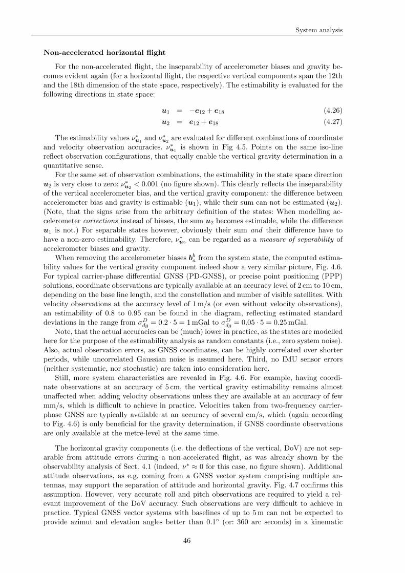
System analysis
Non-accelerated horizontal flight
For the non-accelerated flight, the inseparability of accelerometer biases and gravity be-comes evident again (for a horizontal flight, the respective vertical components span the 12thand the 18th dimension of the state space, respectively). The estimability is evaluated for thefollowing directions in state space:
u1 = −e12 + e18 (4.26)
u2 = e12 + e18 (4.27)
The estimability values ν∗u1and ν∗u2
are evaluated for different combinations of coordinateand velocity observation accuracies. ν∗u1
is shown in Fig 4.5. Points on the same iso-linereflect observation configurations, that equally enable the vertical gravity determination in aquantitative sense.
For the same set of observation combinations, the estimability in the state space directionu2 is very close to zero: ν∗u2
< 0.001 (no figure shown). This clearly reflects the inseparabilityof the vertical accelerometer bias, and the vertical gravity component: the difference betweenaccelerometer bias and gravity is estimable (u1), while their sum can not be estimated (u2).(Note, that the signs arise from the arbitrary definition of the states: When modelling ac-celerometer corrections instead of biases, the sum u2 becomes estimable, while the differenceu1 is not.) For separable states however, obviously their sum and their difference have tohave a non-zero estimability. Therefore, ν∗u2
can be regarded as a measure of separability ofaccelerometer biases and gravity.
When removing the accelerometer biases bba from the system state, the computed estima-bility values for the vertical gravity component indeed show a very similar picture, Fig. 4.6.For typical carrier-phase differential GNSS (PD-GNSS), or precise point positioning (PPP)solutions, coordinate observations are typically available at an accuracy level of 2 cm to 10 cm,depending on the base line length, and the constellation and number of visible satellites. Withvelocity observations at the accuracy level of 1m/s (or even without velocity observations),an estimability of 0.8 to 0.95 can be found in the diagram, reflecting estimated standarddeviations in the range from σDdg = 0.2 · 5 = 1mGal to σDdg = 0.05 · 5 = 0.25mGal.
Note, that the actual accuracies can be (much) lower in practice, as the states are modelledhere for the purpose of the estimability analysis as random constants (i.e., zero system noise).Also, actual observation errors, as GNSS coordinates, can be highly correlated over shorterperiods, while uncorrelated Gaussian noise is assumed here. Third, no IMU sensor errors(neither systematic, nor stochastic) are taken into consideration here.
Still, more system characteristics are revealed in Fig. 4.6. For example, having coordi-nate observations at an accuracy of 5 cm, the vertical gravity estimability remains almostunaffected when adding velocity observations unless they are available at an accuracy of fewmm/s, which is difficult to achieve in practice. Velocities taken from two-frequency carrier-phase GNSS are typically available at an accuracy of several cm/s, which (again accordingto Fig. 4.6) is only beneficial for the gravity determination, if GNSS coordinate observationsare only available at the metre-level at the same time.
The horizontal gravity components (i.e. the deflections of the vertical, DoV) are not sep-arable from attitude errors during a non-accelerated flight, as was already shown by theobservability analysis of Sect. 4.1 (indeed, ν∗ ≈ 0 for this case, no figure shown). Additionalattitude observations, as e.g. coming from a GNSS vector system comprising multiple an-tennas, may support the separation of attitude and horizontal gravity. Fig. 4.7 confirms thisassumption. However, very accurate roll and pitch observations are required to yield a rel-evant improvement of the DoV accuracy. Such observations are very difficult to achieve inpractice. Typical GNSS vector systems with baselines of up to 5m can not be expected toprovide azimut and elevation angles better than 0.1 (or: 360 arc seconds) in a kinematic
46
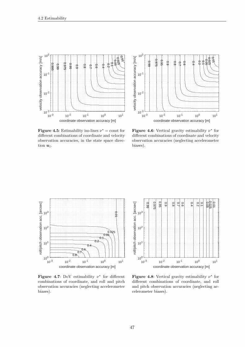
4.2 Estimability
0.01
0.0250.050.10.2
0.4
0.6
0.7
0.8
0.9
0.95
0.975
0.99
0.995
10-3 10-2 10-1 100 101
coordinate observation accuracy [m]
10-3
10-2
10-1
100
velo
city
obs
erva
tion
accu
racy
[m/s
]
Figure 4.5: Estimability iso-lines ν∗ = const fordifferent combinations of coordinate and velocityobservation accuracies, in the state space direc-tion u1.
0.010.025
0.050.10.2
0.4
0.6
0.7
0.8
0.9
0.95
0.975
0.99
10-3 10-2 10-1 100 101
coordinate observation accuracy [m]
10-3
10-2
10-1
100
velo
city
obs
erva
tion
accu
racy
[m/s
]Figure 4.6: Vertical gravity estimability ν∗ fordifferent combinations of coordinate and velocityobservation accuracies (neglecting accelerometerbiases).
0.80.7
0.60.4
0.20.1
0.050.025
0.01
10-3 10-2 10-1 100 101
coordinate observation accuracy [m]
100
101
102
103
roll/
pitc
h ob
serv
atio
n ac
c. [a
rcse
c]
Figure 4.7: DoV estimability ν∗ for differentcombinations of coordinate, and roll and pitchobservation accuracies (neglecting accelerometerbiases).
0.010.0250.05
0.10.2
0.4
0.60.7
0.8
0.9
0.95
0.99
0.975
10-3 10-2 10-1 100 101
coordinate observation accuracy [m]
100
101
102
103
roll/
pitc
h ob
serv
atio
n ac
c. [a
rcse
c]
Figure 4.8: Vertical gravity estimability ν∗ fordifferent combinations of coordinate, and rolland pitch observation accuracies (neglecting ac-celerometer biases).
47
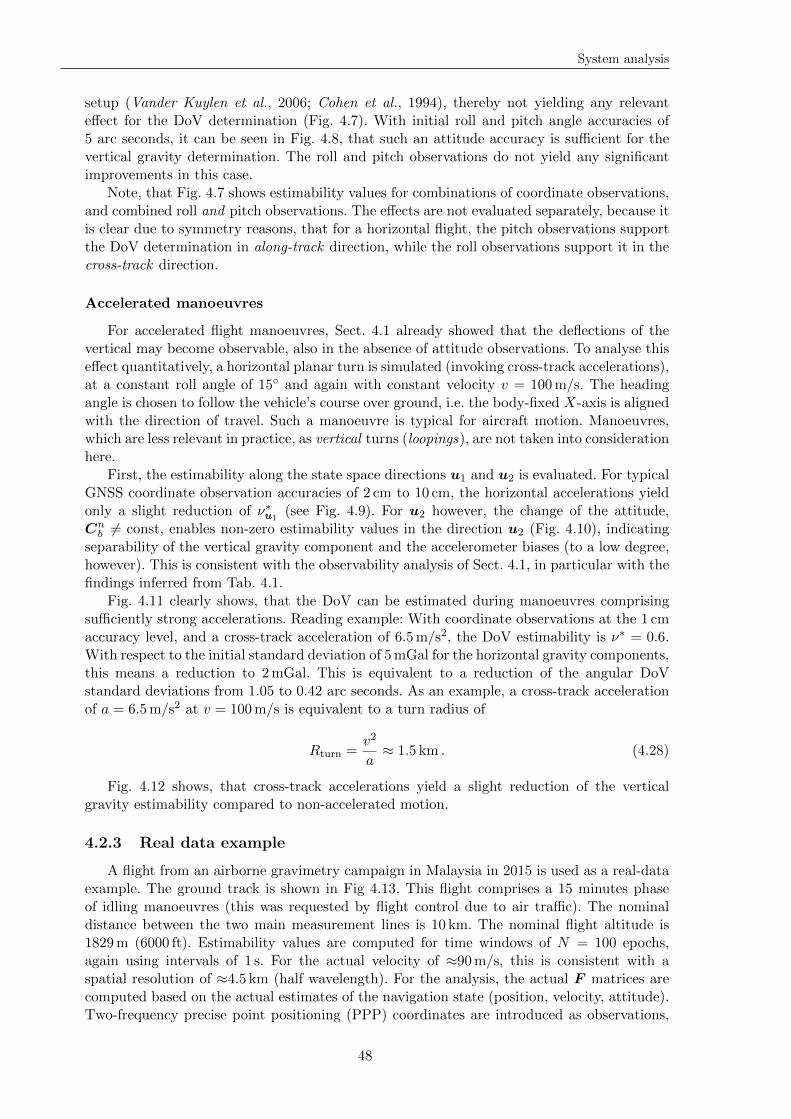
System analysis
setup (Vander Kuylen et al., 2006; Cohen et al., 1994), thereby not yielding any relevanteffect for the DoV determination (Fig. 4.7). With initial roll and pitch angle accuracies of5 arc seconds, it can be seen in Fig. 4.8, that such an attitude accuracy is sufficient for thevertical gravity determination. The roll and pitch observations do not yield any significantimprovements in this case.
Note, that Fig. 4.7 shows estimability values for combinations of coordinate observations,and combined roll and pitch observations. The effects are not evaluated separately, because itis clear due to symmetry reasons, that for a horizontal flight, the pitch observations supportthe DoV determination in along-track direction, while the roll observations support it in thecross-track direction.
Accelerated manoeuvres
For accelerated flight manoeuvres, Sect. 4.1 already showed that the deflections of thevertical may become observable, also in the absence of attitude observations. To analyse thiseffect quantitatively, a horizontal planar turn is simulated (invoking cross-track accelerations),at a constant roll angle of 15 and again with constant velocity v = 100m/s. The headingangle is chosen to follow the vehicle’s course over ground, i.e. the body-fixed X-axis is alignedwith the direction of travel. Such a manoeuvre is typical for aircraft motion. Manoeuvres,which are less relevant in practice, as vertical turns (loopings), are not taken into considerationhere.
First, the estimability along the state space directions u1 and u2 is evaluated. For typicalGNSS coordinate observation accuracies of 2 cm to 10 cm, the horizontal accelerations yieldonly a slight reduction of ν∗u1
(see Fig. 4.9). For u2 however, the change of the attitude,Cnb 6= const, enables non-zero estimability values in the direction u2 (Fig. 4.10), indicating
separability of the vertical gravity component and the accelerometer biases (to a low degree,however). This is consistent with the observability analysis of Sect. 4.1, in particular with thefindings inferred from Tab. 4.1.
Fig. 4.11 clearly shows, that the DoV can be estimated during manoeuvres comprisingsufficiently strong accelerations. Reading example: With coordinate observations at the 1 cmaccuracy level, and a cross-track acceleration of 6.5m/s2, the DoV estimability is ν∗ = 0.6.With respect to the initial standard deviation of 5mGal for the horizontal gravity components,this means a reduction to 2mGal. This is equivalent to a reduction of the angular DoVstandard deviations from 1.05 to 0.42 arc seconds. As an example, a cross-track accelerationof a = 6.5m/s2 at v = 100m/s is equivalent to a turn radius of
Rturn =v2
a≈ 1.5 km . (4.28)
Fig. 4.12 shows, that cross-track accelerations yield a slight reduction of the verticalgravity estimability compared to non-accelerated motion.
4.2.3 Real data example
A flight from an airborne gravimetry campaign in Malaysia in 2015 is used as a real-dataexample. The ground track is shown in Fig 4.13. This flight comprises a 15 minutes phaseof idling manoeuvres (this was requested by flight control due to air traffic). The nominaldistance between the two main measurement lines is 10 km. The nominal flight altitude is1829m (6000 ft). Estimability values are computed for time windows of N = 100 epochs,again using intervals of 1 s. For the actual velocity of ≈90m/s, this is consistent with aspatial resolution of ≈4.5 km (half wavelength). For the analysis, the actual F matrices arecomputed based on the actual estimates of the navigation state (position, velocity, attitude).Two-frequency precise point positioning (PPP) coordinates are introduced as observations,
48
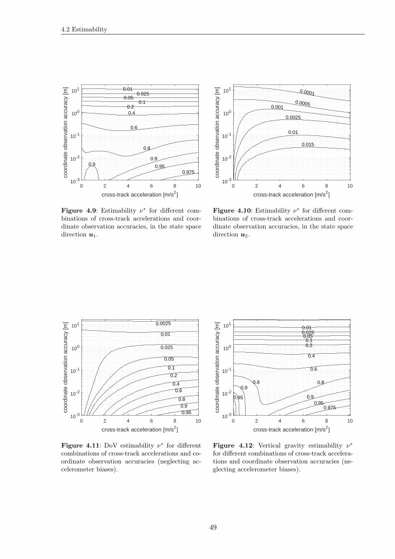
4.2 Estimability
0.9750.95
0.9
0.8
0.6
0.40.2
0.10.05
0.0250.01
0.9
0 2 4 6 8 10
cross-track acceleration [m/s2]
10-3
10-2
10-1
100
101
coor
dina
te o
bser
vatio
n ac
cura
cy [m
]
Figure 4.9: Estimability ν∗ for different com-binations of cross-track accelerations and coor-dinate observation accuracies, in the state spacedirection u1.
0.015
0.01
0.0025
0.0010.0005
0.0001
0 2 4 6 8 10
cross-track acceleration [m/s2]
10-3
10-2
10-1
100
101
coor
dina
te o
bser
vatio
n ac
cura
cy [m
]Figure 4.10: Estimability ν∗ for different com-binations of cross-track accelerations and coor-dinate observation accuracies, in the state spacedirection u2.
0.90.95
0.8
0.60.4
0.2
0.1
0.05
0.025
0.01
0.0025
0 2 4 6 8 10
cross-track acceleration [m/s2]
10-3
10-2
10-1
100
101
coor
dina
te o
bser
vatio
n ac
cura
cy [m
]
Figure 4.11: DoV estimability ν∗ for differentcombinations of cross-track accelerations and co-ordinate observation accuracies (neglecting ac-celerometer biases).
0.9750.95
0.9
0.8
0.6
0.4
0.20.1
0.050.0250.01
0.80.9
0.95
0 2 4 6 8 10
cross-track acceleration [m/s2]
10-3
10-2
10-1
100
101
coor
dina
te o
bser
vatio
n ac
cura
cy [m
]
Figure 4.12: Vertical gravity estimability ν∗
for different combinations of cross-track accelera-tions and coordinate observation accuracies (ne-glecting accelerometer biases).
49
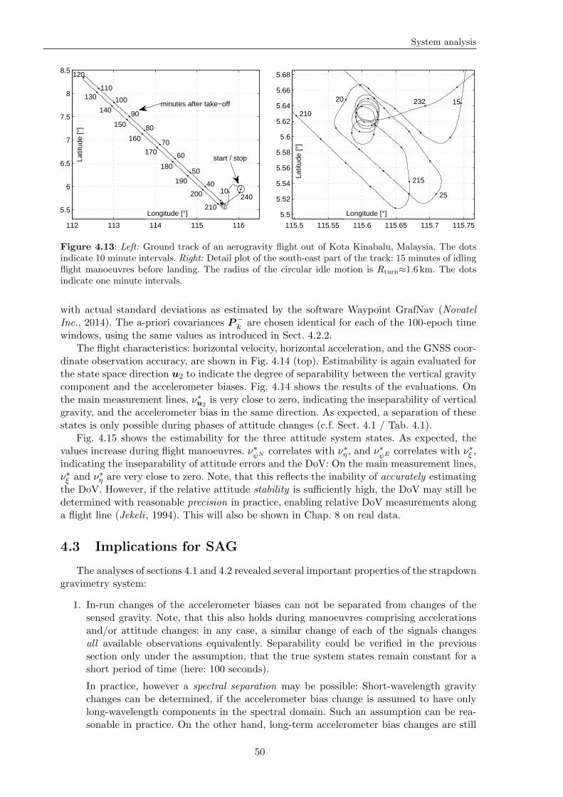
System analysis
112 113 114 115 116
5.5
6
6.5
7
7.5
8
8.5
1040
50
60
70
80
90
100
110
120
130
140
150
160
170
180
190
200 240
Longitude [°]
Latit
ude
[°]
210
minutes after take−off
start / stop
115.5 115.55 115.6 115.65 115.7 115.75
5.5
5.52
5.54
5.56
5.58
5.6
5.62
5.64
5.66
5.68
1520
25
30
210
215
Longitude [°]
Latit
ude
[°]
232
Figure 4.13: Left: Ground track of an aerogravity flight out of Kota Kinabalu, Malaysia. The dotsindicate 10 minute intervals. Right: Detail plot of the south-east part of the track: 15 minutes of idlingflight manoeuvres before landing. The radius of the circular idle motion is Rturn≈1.6 km. The dotsindicate one minute intervals.
with actual standard deviations as estimated by the software Waypoint GrafNav (NovatelInc., 2014). The a-priori covariances P−
k are chosen identical for each of the 100-epoch timewindows, using the same values as introduced in Sect. 4.2.2.
The flight characteristics: horizontal velocity, horizontal acceleration, and the GNSS coor-dinate observation accuracy, are shown in Fig. 4.14 (top). Estimability is again evaluated forthe state space direction u2 to indicate the degree of separability between the vertical gravitycomponent and the accelerometer biases. Fig. 4.14 shows the results of the evaluations. Onthe main measurement lines, ν∗u2
is very close to zero, indicating the inseparability of verticalgravity, and the accelerometer bias in the same direction. As expected, a separation of thesestates is only possible during phases of attitude changes (c.f. Sect. 4.1 / Tab. 4.1).
Fig. 4.15 shows the estimability for the three attitude system states. As expected, thevalues increase during flight manoeuvres. ν∗
ψN correlates with ν∗η , and ν∗ψE correlates with ν∗ξ ,
indicating the inseparability of attitude errors and the DoV: On the main measurement lines,ν∗ξ and ν∗η are very close to zero. Note, that this reflects the inability of accurately estimatingthe DoV. However, if the relative attitude stability is sufficiently high, the DoV may still bedetermined with reasonable precision in practice, enabling relative DoV measurements alonga flight line (Jekeli , 1994). This will also be shown in Chap. 8 on real data.
4.3 Implications for SAG
The analyses of sections 4.1 and 4.2 revealed several important properties of the strapdowngravimetry system:
1. In-run changes of the accelerometer biases can not be separated from changes of thesensed gravity. Note, that this also holds during manoeuvres comprising accelerationsand/or attitude changes: in any case, a similar change of each of the signals changesall available observations equivalently. Separability could be verified in the previoussection only under the assumption, that the true system states remain constant for ashort period of time (here: 100 seconds).
In practice, however a spectral separation may be possible: Short-wavelength gravitychanges can be determined, if the accelerometer bias change is assumed to have onlylong-wavelength components in the spectral domain. Such an assumption can be rea-sonable in practice. On the other hand, long-term accelerometer bias changes are still
50

4.3 Implications for SAG
problematic, as they prevent the accurate gravity determination in the respective fre-quency range.
2. On a straight flight line, the attitude changes are in practice too small to enable theseparation of accelerometer biases and gravity.
3. The determination of the DoV requires accurate attitude estimates. Therefore, in addi-tion to the accelerometer biases, the gyroscope stability is a limiting factor in practice(Jekeli , 1994). It is noted here again, that an uncompensated accelerometer bias changeof 4.75mGal has the same effect on the DoV determination, as an uncompensated at-titude error of only 1 arc second.
4. Heading angles are only estimable during manoeuvres comprising vehicle accelerations.
51
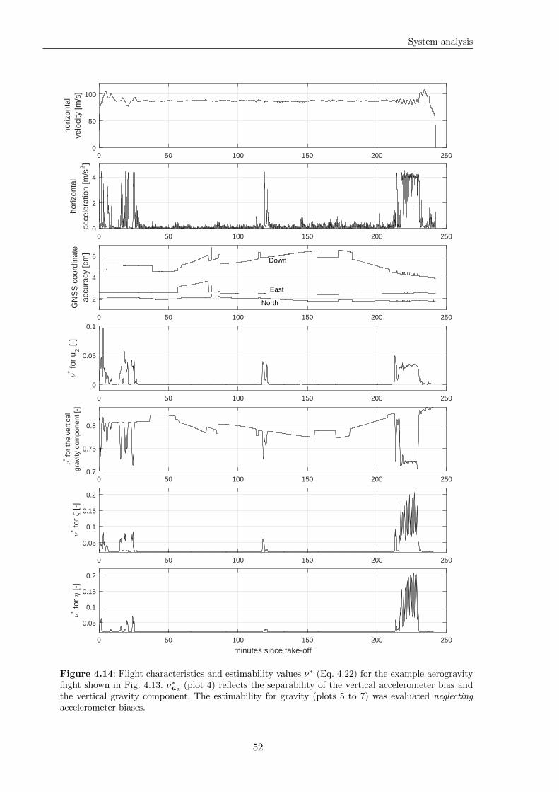
System analysis
0 50 100 150 200 2500
50
100
horiz
onta
lve
loci
ty [m
/s]
0 50 100 150 200 2500
2
4
horiz
onta
l
acce
lera
tion
[m/s
2]
0 50 100 150 200 250
2
4
6
GN
SS
coo
rdin
ate
accu
racy
[cm
]
Down
North
East
0 50 100 150 200 250
0
0.05
0.1
ν* fo
r u
2 [-
]
0 50 100 150 200 2500.7
0.75
0.8
ν* fo
r th
e ve
rtic
algr
avity
com
pone
nt [-
]
0 50 100 150 200 250
0.05
0.1
0.15
0.2
ν* fo
r ξ [-
]
0 50 100 150 200 250
minutes since take-off
0.05
0.1
0.15
0.2
ν* fo
r η [-
]
Figure 4.14: Flight characteristics and estimability values ν∗ (Eq. 4.22) for the example aerogravityflight shown in Fig. 4.13. ν∗u2
(plot 4) reflects the separability of the vertical accelerometer bias andthe vertical gravity component. The estimability for gravity (plots 5 to 7) was evaluated neglectingaccelerometer biases.
52
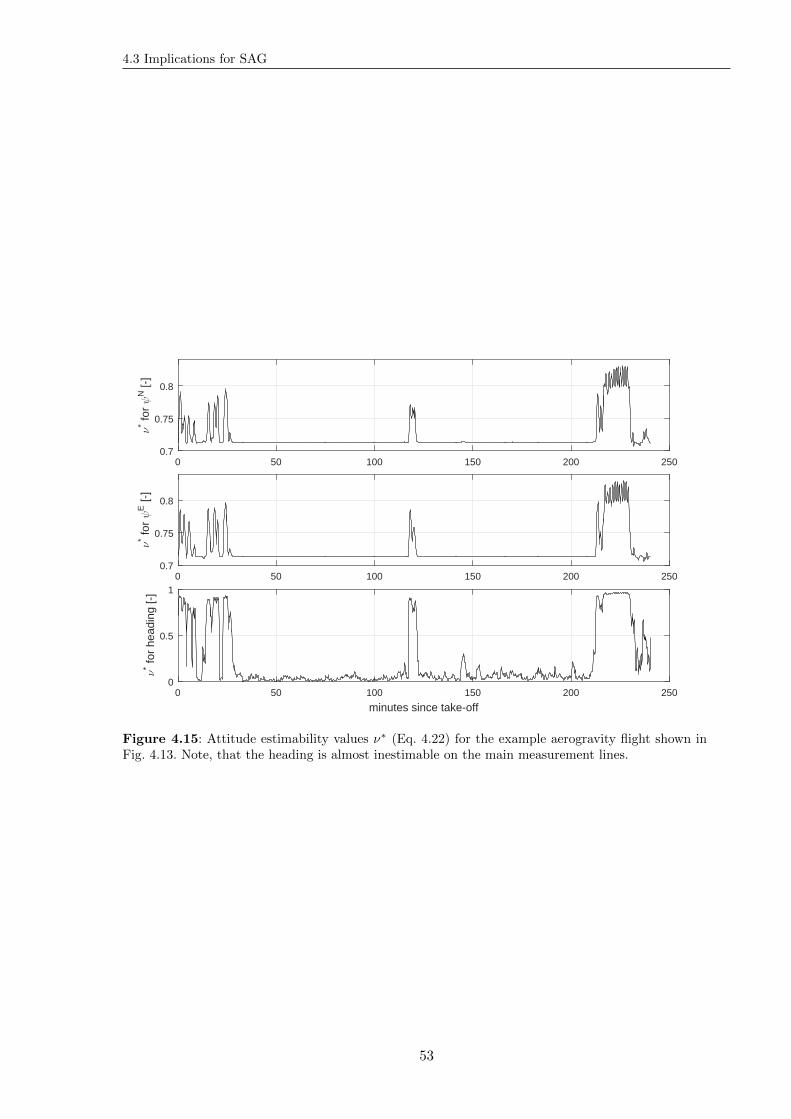
4.3 Implications for SAG
0 50 100 150 200 2500.7
0.75
0.8
ν* fo
r ψ
N [-
]
0 50 100 150 200 2500.7
0.75
0.8
ν* fo
r ψ
E [-
]
0 50 100 150 200 250
minutes since take-off
0
0.5
1
ν* fo
r he
adin
g [-
]
Figure 4.15: Attitude estimability values ν∗ (Eq. 4.22) for the example aerogravity flight shown inFig. 4.13. Note, that the heading is almost inestimable on the main measurement lines.
53

System analysis
54
Chapter 5
Error propagation analysis
Note: Parts of the analysis presented in this chapter have already been published by theauthor (Becker and Becker , 2015).
This chapter addresses the question, to what degree different types of IMU errors prop-agate into the gravity estimates of the strapdown gravity system introduced in Chap. 3.Such knowledge is important to assess the quality, and the relevance of the IMU calibrationmethods shown in Chap. 6.
Additionally, an error-free simulation is used in order to confirm the correctness of theintegrated IMU/GNSS strapdown gravimetry algorithm, used for the real-data evaluationsin Chap. 8.
The error types are separated into two groups:
1. systematic (non-stochastic) errors: constant sensor biases, scale factors, cross-couplings,misalignments, lever arm errors, timestamp errors, and discretisation errors; and
2. stochastic errors: sensor noise of the inertial sensors, and the GNSS coordinate obser-vations.
For each of the investigated error types, a threshold value is derived from simulations,indicating the magnitude of the particular error type, causing an error of the gravity estimatesof 1mGal (vertical component), or 1 arc second (DoV). This allows an easy comparabilityamong the different error types. The results of this chapter can be regarded as a guide forsetting up a strapdown gravimetry system: The results indicate, which error types of thesystem are relevant for the gravity determination in practice, and which are not.
The question how much an error propagates into the gravity estimates, is highly de-pendent on the characteristics of the vehicle motion. For example, it was already shown inChapter 4, that the gravity estimate quality is different during manoeuvres compared to linear(non-accelerated) motion. In order to gain realistic simulation results, the error propagationanalysis presented in this chapter is based on simulations of imitated aerogravity flights. Thereal trajectory is approximated using analytical functions. This enables a simulation of arealistic flight trajectory, with a perfect (error-free) reference trajectory.
5.1 Methodology
A set of twelve gravity flights flown out of Kota Kinabalu (North Borneo, Malaysia)in 2014 is used as the basis for the simulations (Fig. 5.1). Tab. 5.1 summarises the maincharacteristics of this campaign. Details for each of the twelve flights are provided in theAppendix, Sect. A.2. This set of flights is regarded as a typical representative for a production-oriented aerogravity campaign, including different levels of turbulence, auto-pilot course and
55
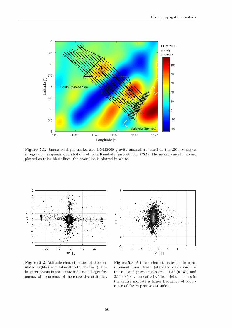
Error propagation analysis
EGM 2008gravityanomaly
Malaysia (Borneo)
BKI
South Chinese Sea
112° 113° 114° 115° 116° 117°
Longitude [°]
5°
5.5°
6°
6.5°
7°
7.5°
8°
8.5°
9°La
titud
e [°
]
-40
-20
0
20
40
60
80
100
Figure 5.1: Simulated flight tracks, and EGM2008 gravity anomalies, based on the 2014 Malaysiaaerogravity campaign, operated out of Kota Kinabalu (airport code BKI ). The measurement lines areplotted as thick black lines, the coast line is plotted in white.
Figure 5.2: Attitude characteristics of the sim-ulated flights (from take-off to touch-down). Thebrighter points in the centre indicate a larger fre-quency of occurrence of the respective attitudes.
Figure 5.3: Attitude characteristics on the mea-surement lines. Mean (standard deviation) forthe roll and pitch angles are −1.3 (0.75) and2.1 (0.60), respectively. The brighter points inthe centre indicate a larger frequency of occur-rence of the respective attitudes.
56
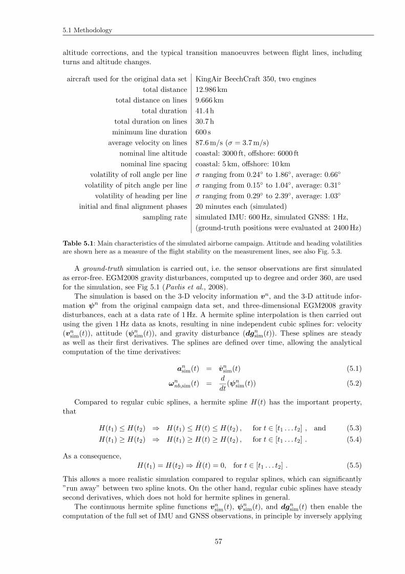
5.1 Methodology
altitude corrections, and the typical transition manoeuvres between flight lines, includingturns and altitude changes.
aircraft used for the original data set KingAir BeechCraft 350, two engines
total distance 12.986 km
total distance on lines 9.666 km
total duration 41.4 h
total duration on lines 30.7 h
minimum line duration 600 s
average velocity on lines 87.6m/s (σ = 3.7m/s)
nominal line altitude coastal: 3000 ft, offshore: 6000 ft
nominal line spacing coastal: 5 km, offshore: 10 km
volatility of roll angle per line σ ranging from 0.24 to 1.86, average: 0.66
volatility of pitch angle per line σ ranging from 0.15 to 1.04, average: 0.31
volatility of heading per line σ ranging from 0.29 to 2.39, average: 1.03
initial and final alignment phases 20 minutes each (simulated)
sampling rate simulated IMU: 600Hz, simulated GNSS: 1Hz,
(ground-truth positions were evaluated at 2400Hz)
Table 5.1: Main characteristics of the simulated airborne campaign. Attitude and heading volatilitiesare shown here as a measure of the flight stability on the measurement lines, see also Fig. 5.3.
A ground-truth simulation is carried out, i.e. the sensor observations are first simulatedas error-free. EGM2008 gravity disturbances, computed up to degree and order 360, are usedfor the simulation, see Fig 5.1 (Pavlis et al., 2008).
The simulation is based on the 3-D velocity information vn, and the 3-D attitude infor-mation ψn from the original campaign data set, and three-dimensional EGM2008 gravitydisturbances, each at a data rate of 1Hz. A hermite spline interpolation is then carried outusing the given 1Hz data as knots, resulting in nine independent cubic splines for: velocity(vnsim(t)), attitude (ψnsim(t)), and gravity disturbance (dgnsim(t)). These splines are steadyas well as their first derivatives. The splines are defined over time, allowing the analyticalcomputation of the time derivatives:
ansim(t) = vnsim(t) (5.1)
ωnnb,sim(t) =d
dt(ψnsim(t)) (5.2)
Compared to regular cubic splines, a hermite spline H(t) has the important property,that
H(t1) ≤ H(t2) ⇒ H(t1) ≤ H(t) ≤ H(t2) , for t ∈ [t1 . . . t2] , and (5.3)
H(t1) ≥ H(t2) ⇒ H(t1) ≥ H(t) ≥ H(t2) , for t ∈ [t1 . . . t2] . (5.4)
As a consequence,H(t1) = H(t2) ⇒ H(t) = 0, for t ∈ [t1 . . . t2] . (5.5)
This allows a more realistic simulation compared to regular splines, which can significantly”run away” between two spline knots. On the other hand, regular cubic splines have steadysecond derivatives, which does not hold for hermite splines in general.
The continuous hermite spline functions vnsim(t), ψnsim(t), and dg
nsim(t) then enable the
computation of the full set of IMU and GNSS observations, in principle by inversely applying
57
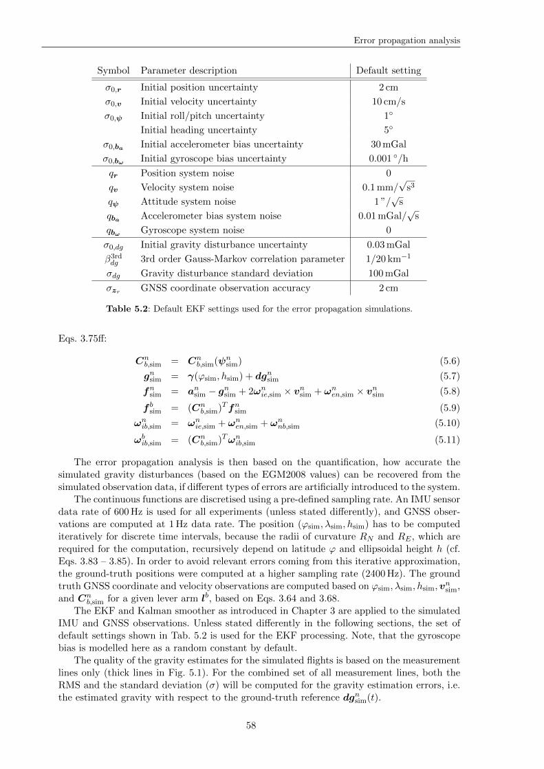
Error propagation analysis
Symbol Parameter description Default setting
σ0,r Initial position uncertainty 2 cm
σ0,v Initial velocity uncertainty 10 cm/s
σ0,ψ Initial roll/pitch uncertainty 1
Initial heading uncertainty 5
σ0,ba Initial accelerometer bias uncertainty 30mGal
σ0,bω Initial gyroscope bias uncertainty 0.001 /h
qr Position system noise 0
qv Velocity system noise 0.1mm/√s3
qψ Attitude system noise 1 ”/√s
qba Accelerometer bias system noise 0.01mGal/√s
qbω Gyroscope system noise 0
σ0,dg Initial gravity disturbance uncertainty 0.03mGal
β3rddg 3rd order Gauss-Markov correlation parameter 1/20 km−1
σdg Gravity disturbance standard deviation 100mGal
σzr GNSS coordinate observation accuracy 2 cm
Table 5.2: Default EKF settings used for the error propagation simulations.
Eqs. 3.75ff:
Cnb,sim = Cn
b,sim(ψnsim) (5.6)
gnsim = γ(ϕsim, hsim) + dgnsim (5.7)
fnsim = ansim − gnsim + 2ωnie,sim × vnsim + ωnen,sim × vnsim (5.8)
f bsim = (Cnb,sim)
Tfnsim (5.9)
ωnib,sim = ωnie,sim + ωnen,sim + ωnnb,sim (5.10)
ωbib,sim = (Cnb,sim)
Tωnib,sim (5.11)
The error propagation analysis is then based on the quantification, how accurate thesimulated gravity disturbances (based on the EGM2008 values) can be recovered from thesimulated observation data, if different types of errors are artificially introduced to the system.
The continuous functions are discretised using a pre-defined sampling rate. An IMU sensordata rate of 600Hz is used for all experiments (unless stated differently), and GNSS obser-vations are computed at 1Hz data rate. The position (ϕsim, λsim, hsim) has to be computediteratively for discrete time intervals, because the radii of curvature RN and RE , which arerequired for the computation, recursively depend on latitude ϕ and ellipsoidal height h (cf.Eqs. 3.83 – 3.85). In order to avoid relevant errors coming from this iterative approximation,the ground-truth positions were computed at a higher sampling rate (2400Hz). The groundtruth GNSS coordinate and velocity observations are computed based on ϕsim, λsim, hsim,v
nsim,
and Cnb,sim for a given lever arm lb, based on Eqs. 3.64 and 3.68.
The EKF and Kalman smoother as introduced in Chapter 3 are applied to the simulatedIMU and GNSS observations. Unless stated differently in the following sections, the set ofdefault settings shown in Tab. 5.2 is used for the EKF processing. Note, that the gyroscopebias is modelled here as a random constant by default.
The quality of the gravity estimates for the simulated flights is based on the measurementlines only (thick lines in Fig. 5.1). For the combined set of all measurement lines, both theRMS and the standard deviation (σ) will be computed for the gravity estimation errors, i.e.the estimated gravity with respect to the ground-truth reference dgnsim(t).
58
5.2 Systematic errors
It is just noted here, that the propagated errors tend to be higher during manoeuvres, astake-off, landing, and turns, which is of lower relevance in practice. At least for the simulation,these larger errors arise from stronger discretisation effects.
The full set of combinations of roll and pitch angles for the data set is shown in Fig. 5.2.Apparently, the roll angle was limited to ≈ 25 during the turns. On the straight measurementlines, the auto-pilot performed small correction manoeuvres to keep the requested course, inparticular during phases of turbulence. Note, that the roll angle on the lines reaches valuesof ±8. While the non-zero average of the pitch angle (here: 2.1, nose up) is typical fora relatively low aircraft speed, the roll angle bias of −1.3 is probably due to an eccentriccentre of mass, or due to non-symmetric power of the two engines (such an issue was indeedreported by the pilots).
5.2 Systematic errors
This section analyses the error propagation of systematic IMU errors, as well as otherrelevant error sources in a IMU/GNSS strapdown gravimetry system, as small time-stampingoffsets, discretisation errors, lever arm errors, or initial alignment errors.
The lever arm is given in body-fixed (front-right-down) coordinates as lb =(0 0 −1.5m
)T, thus the GNSS antenna is positioned 1.5m above the IMUs centre of
observations, which is a typical value using small aircraft or land vehicles.It is just noted here, that all of the subsequent simulations were also carried out using
an alternative lever arm, including a horizontal eccentricity: lb2 =(2m 0.5m −1.5m
)T.
However, no significant effect could be observed when using lb2 instead of lb (the deviationwas less than 5% for each of the subsequent simulation experiments). This indicates, thatthe choice of the lever arm is of lower relevance in practice.
5.2.1 Discretisation error
An IMU always provides measurements f b and ωbib for discrete epochs. For the processingof such data, usually the average between two measurements is being used for the respectivetime interval. The numerical integration then yields velocity and angle increments, which areimplicitly based on the assumption, that the measured specific forces and turn rates changelinearly over time.
However in practice, in particular during dynamic vehicle motion, this assumption iswrong: If both the specific force and the turn rate change non-linearly over time, the nu-merical integration generates systematic errors. This is illustrated here by a simple example:Assume two manoeuvres, taking place between two IMU epochs: the first is a short accel-eration to towards the sensor’s X-axis, the second is a slight turn around the Y-axis. TheIMU measurements were the same, if these two manoeuvres were carried out in reverse or-der, however the two navigation outcomes are clearly different. Such errors, coming fromsimultaneous non-linear changes of acceleration and turn rate, are called coning and scullingmotion (Groves, 2013; Wendel , 2011). Appropriate corrections may reduce the error whendown-sampling the available IMU data to a lower data rate, typical for time-critical appli-cations with limited computation resources. There is however no possibility of applying suchcorrections, if the highest available IMU data rate is already used.
It is analysed here, how much the discretisation of the simulated IMU measurementscan affect the gravity determination. The IMU and GNSS measurements are error-free. Theresults are shown in Fig 5.4. The combined RMS of the gravity errors of all measurementlines of the simulated campaign are shown. According to these results,
59
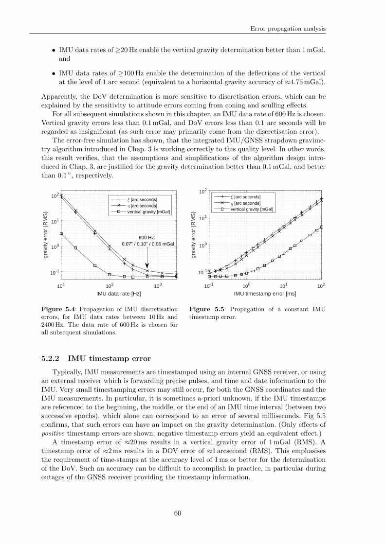
Error propagation analysis
• IMU data rates of ≥20Hz enable the vertical gravity determination better than 1mGal,and
• IMU data rates of ≥100Hz enable the determination of the deflections of the verticalat the level of 1 arc second (equivalent to a horizontal gravity accuracy of ≈4.75mGal).
Apparently, the DoV determination is more sensitive to discretisation errors, which can beexplained by the sensitivity to attitude errors coming from coning and sculling effects.
For all subsequent simulations shown in this chapter, an IMU data rate of 600Hz is chosen.Vertical gravity errors less than 0.1mGal, and DoV errors less than 0.1 arc seconds will beregarded as insignificant (as such error may primarily come from the discretisation error).
The error-free simulation has shown, that the integrated IMU/GNSS strapdown gravime-try algorithm introduced in Chap. 3 is working correctly to this quality level. In other words,this result verifies, that the assumptions and simplifications of the algorithm design intro-duced in Chap. 3, are justified for the gravity determination better than 0.1mGal, and betterthan 0.1 ”, respectively.
101 102 103
IMU data rate [Hz]
10-1
100
101
102
grav
ity e
rror
(R
MS
)
ξ [arc seconds]η [arc seconds]vertical gravity [mGal]
600 Hz: 0.07" / 0.10" / 0.06 mGal
Figure 5.4: Propagation of IMU discretisationerrors, for IMU data rates between 10Hz and2400Hz. The data rate of 600Hz is chosen forall subsequent simulations.
10-1 100 101 102
IMU timestamp error [ms]
10-1
100
101
102gr
avity
err
or (
RM
S)
ξ [arc seconds]η [arc seconds]vertical gravity [mGal]
Figure 5.5: Propagation of a constant IMUtimestamp error.
5.2.2 IMU timestamp error
Typically, IMU measurements are timestamped using an internal GNSS receiver, or usingan external receiver which is forwarding precise pulses, and time and date information to theIMU. Very small timestamping errors may still occur, for both the GNSS coordinates and theIMU measurements. In particular, it is sometimes a-priori unknown, if the IMU timestampsare referenced to the beginning, the middle, or the end of an IMU time interval (between twosuccessive epochs), which alone can correspond to an error of several milliseconds. Fig 5.5confirms, that such errors can have an impact on the gravity determination. (Only effects ofpositive timestamp errors are shown; negative timestamp errors yield an equivalent effect.)
A timestamp error of ≈20ms results in a vertical gravity error of 1mGal (RMS). Atimestamp error of ≈2ms results in a DOV error of ≈1 arcsecond (RMS). This emphasisesthe requirement of time-stamps at the accuracy level of 1ms or better for the determinationof the DoV. Such an accuracy can be difficult to accomplish in practice, in particular duringoutages of the GNSS receiver providing the timestamp information.
60
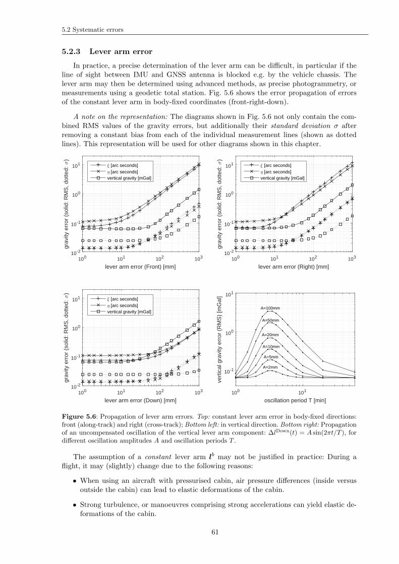
5.2 Systematic errors
5.2.3 Lever arm error
In practice, a precise determination of the lever arm can be difficult, in particular if theline of sight between IMU and GNSS antenna is blocked e.g. by the vehicle chassis. Thelever arm may then be determined using advanced methods, as precise photogrammetry, ormeasurements using a geodetic total station. Fig. 5.6 shows the error propagation of errorsof the constant lever arm in body-fixed coordinates (front-right-down).
A note on the representation: The diagrams shown in Fig. 5.6 not only contain the com-bined RMS values of the gravity errors, but additionally their standard deviation σ afterremoving a constant bias from each of the individual measurement lines (shown as dottedlines). This representation will be used for other diagrams shown in this chapter.
100 101 102 103
lever arm error (Front) [mm]
10-2
10-1
100
101
grav
ity e
rror
(so
lid: R
MS
, dot
ted:
σ)
ξ [arc seconds]η [arc seconds]vertical gravity [mGal]
100 101 102 103
lever arm error (Right) [mm]
10-2
10-1
100
101
grav
ity e
rror
(so
lid: R
MS
, dot
ted:
σ)
ξ [arc seconds]η [arc seconds]vertical gravity [mGal]
100 101 102 103
lever arm error (Down) [mm]
10-2
10-1
100
101
grav
ity e
rror
(so
lid: R
MS
, dot
ted:
σ)
ξ [arc seconds]η [arc seconds]vertical gravity [mGal]
100 101
oscillation period T [min]
10-1
100
101
vert
ical
gra
vity
err
or (
RM
S)
[mG
al]
A=2mm
A=5mm
A=10mm
A=20mm
A=50mm
A=100mm
Figure 5.6: Propagation of lever arm errors. Top: constant lever arm error in body-fixed directions:front (along-track) and right (cross-track); Bottom left: in vertical direction. Bottom right: Propagationof an uncompensated oscillation of the vertical lever arm component: ∆lDown(t) = A sin(2πt/T ), fordifferent oscillation amplitudes A and oscillation periods T .
The assumption of a constant lever arm lb may not be justified in practice: During aflight, it may (slightly) change due to the following reasons:
• When using an aircraft with pressurised cabin, air pressure differences (inside versusoutside the cabin) can lead to elastic deformations of the cabin.
• Strong turbulence, or manoeuvres comprising strong accelerations can yield elastic de-formations of the cabin.
61
Error propagation analysis
For the simulation of a lever arm instability ∆l(t), a simple sinus oscillation is used.The analysis is limited here to lever arm changes along the body-fixed vertical (Down-)axis,because lateral displacements are expected to be smaller in practice. Fig. 5.6 shows verticalgravity errors for different combinations of amplitude A and period T of the oscillation.
The lever arm oscillation creates an oscillation of the gravity error with the same fre-quency. The amplitude of the gravity error oscillation can be approximated as the RMSvalue times
√2. Reading example: A lever arm oscillation along the vertical component with
amplitude 20mm and period T = 1/f = 3min yields a gravity error of 0.7mGal (RMS),arising from a gravity error oscillation with an amplitude of ≈1mGal (with the same period).
The amplitude of the gravity error increases with longer periods until its maximum atapproximately T = 3min. The smaller effect of higher frequency oscillations can be explainedby the Gauss-Markov process that is used to model gravity in the EKF: The parameters aretuned for typical dynamics of along-track gravity changes. For higher frequencies, the EKFacts like a low-pass filter.
For periods longer than three minutes, the gravity error decreases, because the averageposition change of the GNSS antenna per time is becoming smaller, and thus the accelerationof the GNSS antenna relative to the body-fixed frame. It can be summarised, that for leverarm oscillations happening in the same frequency band as gravity changes, both signals cannot be separated. Similar results are obtained for an instability of the vertical accelerome-ter bias, and also for gradual error drifts of the GNSS height observations (Sections 5.3.1and 5.3.2).
Note, that the positions of the maxima arise from the specific choice of the simulatedaircraft speed, and the modelled gravity field characteristics. Still, the results qualitativelyshow, that there is a relevant error propagation in this case, that may have to be addressedin practice.
5.2.4 Sensor misalignments
An IMU consists of six inertial sensors: three accelerometers and three gyroscopes. Eachof the six sensors’ sensitive axes may be imperfectly oriented with respect to their nominaldirection (misalignment).
In the following, results of simulated IMU sensor misalignments are shown. For eachexperiment, the sensitive axis of one of the sensors is altered, while the other five sensorsremain unchanged (error-free). For each of the sensors, misalignments may appear in twodirections, yielding a total of 12 possible types of misalignments for an IMU. The followingsix angular misalignments are defined for both the accelerometer and the gyroscope triad:
1. εXY : bending the X-axis towards the Y-axis
2. εXZ : bending the X-axis towards the Z-axis
3. εY X : bending the Y-axis towards the X-axis
4. εY Z : bending the Y-axis towards the Z-axis
5. εZX : bending the Z-axis towards the X-axis
6. εZY : bending the Z-axis towards the Y-axis
A note on the nomenclature: If a sensor triad is analysed without any external referencedirection of the sensitive axes, only the relative, mutual misalignments can be modelled. Suchmutual misalignments are called cross-couplings, because two sensors mutually share a portionof their measured signals (the measurements are then coupled). A cross-coupling is non-zero, ifthe sensitive sensor axes are not mutually perpendicular. In this thesis, the term misalignment
62
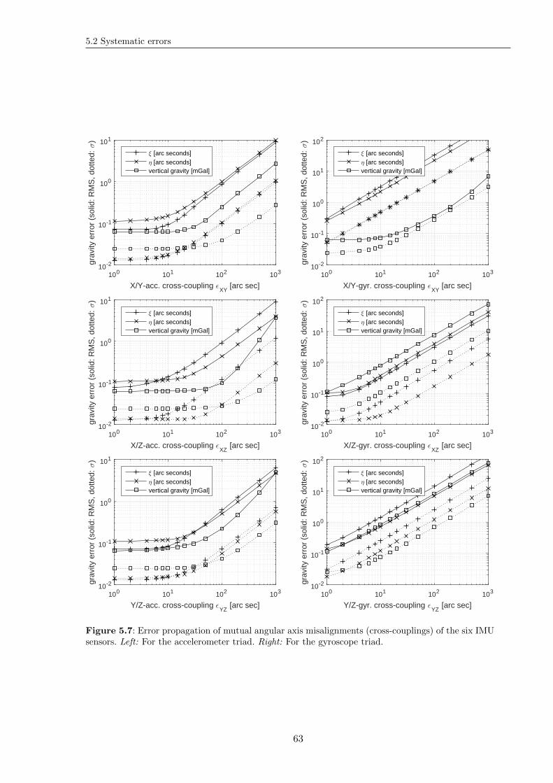
5.2 Systematic errors
100 101 102 103
X/Y-acc. cross-coupling ǫXY
[arc sec]
10-2
10-1
100
101
grav
ity e
rror
(so
lid: R
MS
, dot
ted:
σ)
ξ [arc seconds]η [arc seconds]vertical gravity [mGal]
100 101 102 103
X/Y-gyr. cross-coupling ǫXY
[arc sec]
10-2
10-1
100
101
102
grav
ity e
rror
(so
lid: R
MS
, dot
ted:
σ)
ξ [arc seconds]η [arc seconds]vertical gravity [mGal]
100 101 102 103
X/Z-acc. cross-coupling ǫXZ
[arc sec]
10-2
10-1
100
101
grav
ity e
rror
(so
lid: R
MS
, dot
ted:
σ)
ξ [arc seconds]η [arc seconds]vertical gravity [mGal]
100 101 102 103
X/Z-gyr. cross-coupling ǫXZ
[arc sec]
10-2
10-1
100
101
102gr
avity
err
or (
solid
: RM
S, d
otte
d: σ
)ξ [arc seconds]η [arc seconds]vertical gravity [mGal]
100 101 102 103
Y/Z-acc. cross-coupling ǫYZ
[arc sec]
10-2
10-1
100
101
grav
ity e
rror
(so
lid: R
MS
, dot
ted:
σ)
ξ [arc seconds]η [arc seconds]vertical gravity [mGal]
100 101 102 103
Y/Z-gyr. cross-coupling ǫYZ
[arc sec]
10-2
10-1
100
101
102
grav
ity e
rror
(so
lid: R
MS
, dot
ted:
σ)
ξ [arc seconds]η [arc seconds]vertical gravity [mGal]
Figure 5.7: Error propagation of mutual angular axis misalignments (cross-couplings) of the six IMUsensors. Left: For the accelerometer triad. Right: For the gyroscope triad.
63
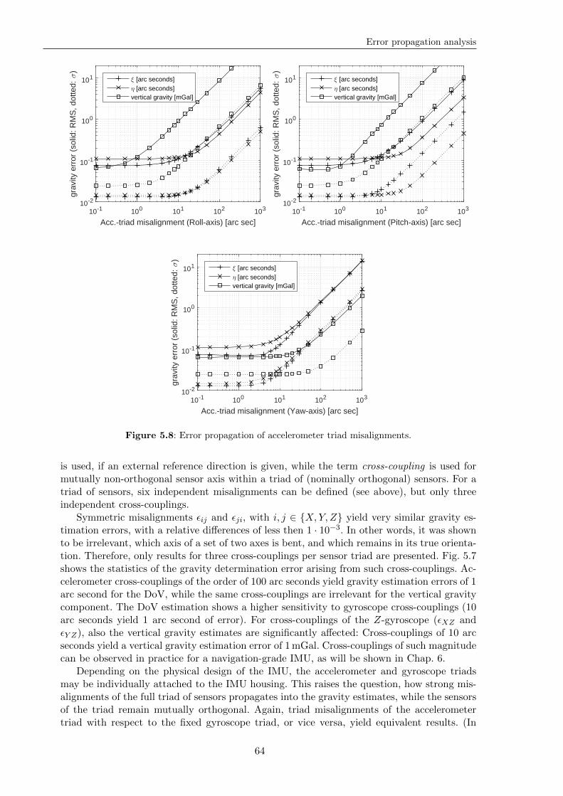
Error propagation analysis
10-1 100 101 102 103
Acc.-triad misalignment (Roll-axis) [arc sec]
10-2
10-1
100
101gr
avity
err
or (
solid
: RM
S, d
otte
d: σ
)ξ [arc seconds]η [arc seconds]vertical gravity [mGal]
10-1 100 101 102 103
Acc.-triad misalignment (Pitch-axis) [arc sec]
10-2
10-1
100
101
grav
ity e
rror
(so
lid: R
MS
, dot
ted:
σ)
ξ [arc seconds]η [arc seconds]vertical gravity [mGal]
10-1 100 101 102 103
Acc.-triad misalignment (Yaw-axis) [arc sec]
10-2
10-1
100
101
grav
ity e
rror
(so
lid: R
MS
, dot
ted:
σ)
ξ [arc seconds]η [arc seconds]vertical gravity [mGal]
Figure 5.8: Error propagation of accelerometer triad misalignments.
is used, if an external reference direction is given, while the term cross-coupling is used formutually non-orthogonal sensor axis within a triad of (nominally orthogonal) sensors. For atriad of sensors, six independent misalignments can be defined (see above), but only threeindependent cross-couplings.
Symmetric misalignments εij and εji, with i, j ∈ X,Y, Z yield very similar gravity es-timation errors, with a relative differences of less then 1 · 10−3. In other words, it was shownto be irrelevant, which axis of a set of two axes is bent, and which remains in its true orienta-tion. Therefore, only results for three cross-couplings per sensor triad are presented. Fig. 5.7shows the statistics of the gravity determination error arising from such cross-couplings. Ac-celerometer cross-couplings of the order of 100 arc seconds yield gravity estimation errors of 1arc second for the DoV, while the same cross-couplings are irrelevant for the vertical gravitycomponent. The DoV estimation shows a higher sensitivity to gyroscope cross-couplings (10arc seconds yield 1 arc second of error). For cross-couplings of the Z-gyroscope (εXZ andεY Z), also the vertical gravity estimates are significantly affected: Cross-couplings of 10 arcseconds yield a vertical gravity estimation error of 1mGal. Cross-couplings of such magnitudecan be observed in practice for a navigation-grade IMU, as will be shown in Chap. 6.
Depending on the physical design of the IMU, the accelerometer and gyroscope triadsmay be individually attached to the IMU housing. This raises the question, how strong mis-alignments of the full triad of sensors propagates into the gravity estimates, while the sensorsof the triad remain mutually orthogonal. Again, triad misalignments of the accelerometertriad with respect to the fixed gyroscope triad, or vice versa, yield equivalent results. (In
64
5.2 Systematic errors
fact, the only difference is the GNSS antenna lever arm error with respect to the one or theother triad, which is irrelevant for misalignments of the order of tens of arc seconds).
Fig. 5.8 shows the gravity determination error statistics for misalignments of the ac-celerometer triad, with angular misalignments about the roll-, pitch- and yaw-axis (corre-sponding to the nominal X/Y/Z IMU sensor axes). Triad misalignments about the roll- andthe pitch-axes are the most relevant ones for the vertical gravity determination: triad mis-alignments of 10 arc seconds propagate into the vertical gravity estimates at the level of1mGal.
5.2.5 Initial alignment error
The alignment is the initial determination of attitude and heading of an IMU-basednavigation or surveying system. A static alignment, having the IMU at rest over a sufficientlylong period, commonly consists of two parts (Groves, 2013; Jekeli , 2001):
1. The levelling is based on the approximation, that there is no gravity in the horizontaldirections of the local navigation frame. In other words, a transformation matrix Cn
b isbeing derived, such that with the assumption of r = 0,
Cnb f
b = fn =
0
0
g
(5.12)
with a measured gravity value of g (potentially containing accelerometer biases). Thelarge signal to noise ratio, with g ≈ 9.8ms−2 versus the accelerometer noise, allows aquick convergence of the levelling process. For example, an observation of the horizontalgravity components at ≈ 5mGal accuracy allows the determination of the initial rolland pitch angles at an accuracy of one arc second (cf. Fig. 4.4).
2. The gyroscope-compassing phase (or gyro-compassing) is the determination of the ini-tial heading angle, based on the assumption, that independently of the actual latitudeϕ, no Earth rotation can be observed around the East-axis, while non-zero Earth ro-tation components can only be sensed around the North and Down axes, cf. Eq. 3.34.This process converges much slower in practice, because the signal to noise ratio is muchsmaller, with ωe ≈ 7.292 · 10−5 s−1 versus the gyroscope noise. In fact, consumer-gradeand tactical-grade devices based on MEMS-gyroscopes or fibre-optic gyroscopes typi-cally do not allow a gyro-compassing at all, having gyroscope biases (much) larger thanωe.
If the vehicle is at rest, as for the static alignment, the system suffers from several in-separabilities of system states, as shown in Tab. 4.1 for the non-accelerated motion withoutattitude changes (scenario S1). As a consequence, sensor biases can not be fully determinedduring the alignment, thereby prohibiting the exact determination of the initial attitude andheading (Groves, 2013). As soon as the vehicle starts moving (accelerated manoeuvres), thesensor biases may be determined, thereby improving the attitude and heading estimates.Still, the alignment is important for an approximate determination of the initial angles: Aninitialisation with large attitude and heading errors may cause strong linearisation errors inthe EKF, potentially leading to a divergence of the filter.
The simulations however show, that initial attitude and heading errors of up to 90 did notyield any significant error for the gravity determination (no figure shown). Apparently, thefilter was still able to converge. Only for initial attitude or heading errors of 135 and 180, adivergence of the filter could be observed (resulting in very large gravity errors, of the orderof 1ms−2. It is however difficult to derive a general statement from this observation, as the
65
Error propagation analysis
processing of real data, including other sensor errors, may be more sensitive to initial attitudeerrors. If no static alignment data is available, or if the gyro-compassing is not possible dueto the sensor quality or an initial position close to the Earth’s poles, a kinematic alignmentmay be possible from GNSS coordinate and velocity observations, typically starting with theapproximation that heading and course over ground are identical.
5.2.6 Accelerometer errors
Simulation results of constant accelerometer biases are shown in Fig. 5.9 (left). For thissimulation, the initial accelerometer bias uncertainty σ0,ba was set to the respective simu-lated biases. Apparently, accelerometer biases of less than 1000mGal are irrelevant for thegravity determination. This can be explained by the initial alignment: The gravity distur-bance is initialised with a ground-truth value, with an accuracy of 0.03mGal. This allows thedetermination of the accelerometer bias at high accuracy. A significant error propagation canonly be observed for very large biases (the levelling procedure fails, and bad accelerometerbias estimates reside in the state estimates). Accelerometer biases of this magnitude are inpractice not observed for navigation-grade inertial sensors.
While constant accelerometer biases can be estimated accurately by the strapdown al-gorithm, constant accelerometer scale factors are not modelled as system states. Instead,the scale factors can be shown to propagate mainly into the bias estimates. This maskingof scale factors as biases is unproblematic for a constant IMU orientation. Attitude changeshowever necessarily lead to errors of the estimated gravity and attitude. For the simulationof accelerometer scale factors, the initial accelerometer bias uncertainty σ0,ba was set to theapproximate effect of the scale factor on the vertical gravity component, e.g. for a simulatedscale factor of 100 ppm, σ0,ba = 100mGal. Fig. 5.9 (right) shows the simulation results.
It can be summarised, that the vertical gravity component is not relevantly affectedfor scale factors <1000 ppm. The horizontal components are more sensitive to scale factors,however the error propagation is still not relevant for typical scale factors of <100 ppm fornavigation-grade inertial sensors (Honeywell International , 2016b).
Accelerometer drifts are commonly regarded as more relevant in the literature (cf.Sect. 2.2). Linear drifts can however be successfully removed from the gravity estimates,if a ground truth gravity observation is known before and after the flight. In the context ofthe strapdown gravimetry algorithm (EKF and Kalman smoother), this can be achieved bya gravity disturbance observation, cf. Sect. 3.3. The simulation of linear accelerometer driftssupports this expectation: No significant gravity errors can be observed (gravity errors arebelow 1mGal for linear drifts of hundreds of mGal per hour; no figure shown).
Conversely, if a ground-truth gravity can not be introduced at the end of the flight, the Z-accelerometer drifts significantly propagate into the vertical gravity estimates (see Fig. 5.10,left). The horizontal gravity components remain almost unaffected by linear accelerometerdrifts of <100mGal/h, which can be explained by the higher estimability of the horizontalaccelerometer biases during manoeuvres comprising horizontal accelerations.
5.2.7 Gyroscope errors
The simulation results of introducing constant gyroscope biases are shown in Fig. 5.11. Forthe simulation, the initial gyroscope noise uncertainty σ0,bω was set to the actual, simulatedmagnitude. As already discussed in Jekeli (1994), the horizontal gravity components are verysensitive to roll and pitch errors, which are arising from uncompensated X- and Y-gyroscopebiases in this case. Apparently, constant gyroscope biases can not be estimated reliably by thefilter, even though these errors are explicitly modelled in the EKF system state. Obviously,changes of the gyroscope biases can not be detected by the filter as well (no figure shown).
66
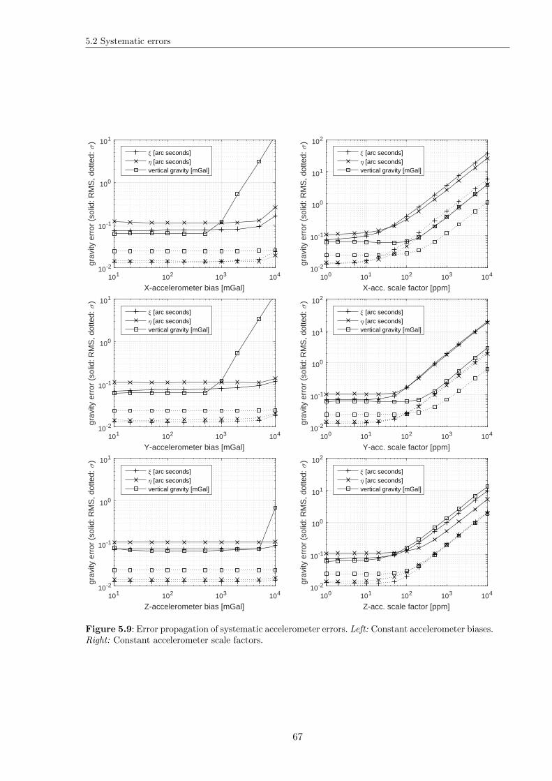
5.2 Systematic errors
101 102 103 104
X-accelerometer bias [mGal]
10-2
10-1
100
101
grav
ity e
rror
(so
lid: R
MS
, dot
ted:
σ)
ξ [arc seconds]η [arc seconds]vertical gravity [mGal]
100 101 102 103 104
X-acc. scale factor [ppm]
10-2
10-1
100
101
102
grav
ity e
rror
(so
lid: R
MS
, dot
ted:
σ)
ξ [arc seconds]η [arc seconds]vertical gravity [mGal]
101 102 103 104
Y-accelerometer bias [mGal]
10-2
10-1
100
101
grav
ity e
rror
(so
lid: R
MS
, dot
ted:
σ)
ξ [arc seconds]η [arc seconds]vertical gravity [mGal]
100 101 102 103 104
Y-acc. scale factor [ppm]
10-2
10-1
100
101
102gr
avity
err
or (
solid
: RM
S, d
otte
d: σ
)ξ [arc seconds]η [arc seconds]vertical gravity [mGal]
101 102 103 104
Z-accelerometer bias [mGal]
10-2
10-1
100
101
grav
ity e
rror
(so
lid: R
MS
, dot
ted:
σ)
ξ [arc seconds]η [arc seconds]vertical gravity [mGal]
100 101 102 103 104
Z-acc. scale factor [ppm]
10-2
10-1
100
101
102
grav
ity e
rror
(so
lid: R
MS
, dot
ted:
σ)
ξ [arc seconds]η [arc seconds]vertical gravity [mGal]
Figure 5.9: Error propagation of systematic accelerometer errors. Left: Constant accelerometer biases.Right: Constant accelerometer scale factors.
67
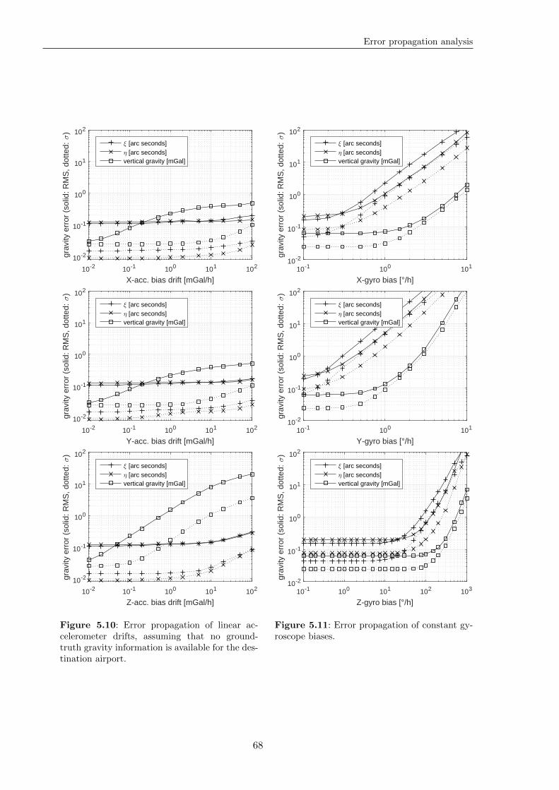
Error propagation analysis
10-2 10-1 100 101 102
X-acc. bias drift [mGal/h]
10-2
10-1
100
101
102
grav
ity e
rror
(so
lid: R
MS
, dot
ted:
σ)
ξ [arc seconds]η [arc seconds]vertical gravity [mGal]
10-2 10-1 100 101 102
Y-acc. bias drift [mGal/h]
10-2
10-1
100
101
102
grav
ity e
rror
(so
lid: R
MS
, dot
ted:
σ)
ξ [arc seconds]η [arc seconds]vertical gravity [mGal]
10-2 10-1 100 101 102
Z-acc. bias drift [mGal/h]
10-2
10-1
100
101
102
grav
ity e
rror
(so
lid: R
MS
, dot
ted:
σ)
ξ [arc seconds]η [arc seconds]vertical gravity [mGal]
Figure 5.10: Error propagation of linear ac-celerometer drifts, assuming that no ground-truth gravity information is available for the des-tination airport.
10-1 100 101
X-gyro bias [°/h]
10-2
10-1
100
101
102
grav
ity e
rror
(so
lid: R
MS
, dot
ted:
σ)
ξ [arc seconds]η [arc seconds]vertical gravity [mGal]
10-1 100 101
Y-gyro bias [°/h]
10-2
10-1
100
101
102
grav
ity e
rror
(so
lid: R
MS
, dot
ted:
σ)
ξ [arc seconds]η [arc seconds]vertical gravity [mGal]
10-1 100 101 102 103
Z-gyro bias [°/h]
10-2
10-1
100
101
102
grav
ity e
rror
(so
lid: R
MS
, dot
ted:
σ)
ξ [arc seconds]η [arc seconds]vertical gravity [mGal]
Figure 5.11: Error propagation of constant gy-roscope biases.
68
5.3 Stochastic sensor errors
The vertical gravity component is not significantly affected by gyroscope biases of lessthan 1 per hour. Such a gyroscope stability (or better) is commonly available for tactical-and navigation-grade strapdown IMUs.
5.3 Stochastic sensor errors
5.3.1 IMU sensor noise
First, Gaussian accelerometer and gyroscope noise N (0, σ) is simulated at the full rate off = 600Hz. The gravity estimation errors are shown in Figs. 5.12 and 5.13. The velocity andattitude system noise parameters qv and qψ, which reflect such inertial sensor noise, were setto the respective quantities.
In order to simulate gradual accelerometer drifts, e.g. coming from thermal effects inpractice, the simulation is repeated with Gaussian noise at much smaller frequencies f . Thenoise is transformed to the base IMU frequency of 600Hz by interpolation. In order to obtaina more realistic, gradual shape, a spline interpolation is used. As an example, Gaussian noisewith σ = 10mGal and 1/f = 10min is depicted in Fig. 5.14 (left). The error propagationof different combinations of frequency f , and standard deviation σ are shown in Fig. 5.14(right).
Noise of higher frequencies, in particular for f = 600Hz, is significantly reduced by theKalman filter, which is acting as a low-pass filter. The important conclusion from thesesimulations is, that random accelerometer bias variations, appearing in the same spectralinterval as gravity changes, are almost inseparable from gravity. In particular, Gaussian noiseat wavelengths of several minutes almost entirely propagates into the gravity estimates. Itis pointed out, that this strong propagation is observed here for error-free GNSS coordinateobservations, introduced to the filter as Gaussian distributed measurements with σ = 2 cm,which is a rather optimistic assumption in practice.
The calibration methods investigated in the scope of this thesis aim at the reduction ofsuch gradual, long-term accelerometer drifts. It will be shown, that the majority of such driftsmay be successfully corrected in practice using thermal calibration methods.
5.3.2 GNSS coordinate observation noise
For the previous sections, error-free GNSS coordinate observations were introduced to thefilter, with a modelled uncertainty of σzr = 2 cm. In this section, actual Gaussian noise willbe simulated for the GNSS coordinate observations. The filter parameter σzr is set to theaccording value, cf. Tab. 5.2.
First, Gaussian noise is simulated at the full GNSS coordinate observation rate of 1Hz, foreach of the individual components (North, East, Down). The results are shown in Fig. 5.15.In practice, noise of the order of several centimetres can be observed for phase-differentialtwo-frequency GNSS, among other factors mainly depending on the base line length.
As a second experiment, more gradual drifts in the vertical GNSS coordinate observationsare simulated. Long-wavelength Gaussian noise is generated for lower frequencies f , interpo-lated to the base data rate of 1Hz using a spline-interpolation (cf. Sect. 5.3.1). The resultsare shown in Fig. 5.15 (lower right). Such gradual, long-wavelength drifts can be observed inpractice arising from gradual variations of the tropospheric and ionospheric error terms, andalso from changes of the GNSS satellite constellation. The estimated accuracy of PD-GNSSin a kinematic, airborne set-up can typically be expected to be better than 20 cm for base-line lengths of up to several hundreds of kilometres. The accuracy of PPP solutions can beexpected to be on a similar level (Kouba and Heroux , 2001).
69
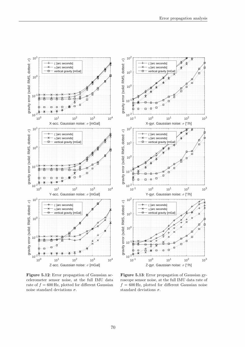
Error propagation analysis
100 101 102 103 104
X-acc. Gaussian noise: σ [mGal]
10-2
10-1
100
101
grav
ity e
rror
(so
lid: R
MS
, dot
ted:
σ)
ξ [arc seconds]η [arc seconds]vertical gravity [mGal]
100 101 102 103 104
Y-acc. Gaussian noise: σ [mGal]
10-2
10-1
100
101
grav
ity e
rror
(so
lid: R
MS
, dot
ted:
σ)
ξ [arc seconds]η [arc seconds]vertical gravity [mGal]
100 101 102 103 104
Z-acc. Gaussian noise: σ [mGal]
10-2
10-1
100
101
grav
ity e
rror
(so
lid: R
MS
, dot
ted:
σ)
ξ [arc seconds]η [arc seconds]vertical gravity [mGal]
Figure 5.12: Error propagation of Gaussian ac-celerometer sensor noise, at the full IMU datarate of f = 600Hz, plotted for different Gaussiannoise standard deviations σ.
10-1 100 101 102 103
X-gyr. Gaussian noise: σ [°/h]
10-2
10-1
100
101
102
grav
ity e
rror
(so
lid: R
MS
, dot
ted:
σ)
ξ [arc seconds]η [arc seconds]vertical gravity [mGal]
10-1 100 101 102 103
Y-gyr. Gaussian noise: σ [°/h]
10-2
10-1
100
101
102
grav
ity e
rror
(so
lid: R
MS
, dot
ted:
σ)
ξ [arc seconds]η [arc seconds]vertical gravity [mGal]
10-1 100 101 102 103
Z-gyr. Gaussian noise: σ [°/h]
10-2
10-1
100
101
102
grav
ity e
rror
(so
lid: R
MS
, dot
ted:
σ)
ξ [arc seconds]η [arc seconds]vertical gravity [mGal]
Figure 5.13: Error propagation of Gaussian gy-roscope sensor noise, at the full IMU data rate off = 600Hz, plotted for different Gaussian noisestandard deviations σ.
70

5.3 Stochastic sensor errors
0 20 40 60 80 100 120 140 160 180
time [min]
-25
-20
-15
-10
-5
0
5
10
15
20S
imul
ated
Acc
. noi
se [m
Gal
]
10-1 100 101
1/f [min]
10-1
100
101
vert
ical
gra
vity
err
or (
RM
S)
σ = 0.2 mGal
σ = 0.5 mGal
σ = 1 mGal
σ = 2 mGal
σ = 5 mGal
σ = 10 mGal
Figure 5.14: Left: Example of simulated, spline-interpolated Gaussian accelerometer noise with 1/f =10min and σ = 10mGal. Right: Error propagation of Gaussian Z-accelerometer noise, for differentcombinations of frequency f , and standard deviation σ.
10-2 10-1 100
GNSS coordinates: σNorth [m]
10-2
10-1
100
101
grav
ity e
rror
(so
lid: R
MS
, dot
ted:
σ)
ξ [arc seconds]η [arc seconds]vertical gravity [mGal]
10-2 10-1 100
GNSS coordinates: σEast [m]
10-2
10-1
100
101
grav
ity e
rror
(so
lid: R
MS
, dot
ted:
σ)
ξ [arc seconds]η [arc seconds]vertical gravity [mGal]
10-2 10-1 100
GNSS coordinates: σDown [m]
10-2
10-1
100
101
grav
ity e
rror
(so
lid: R
MS
, dot
ted:
σ)
ξ [arc seconds]η [arc seconds]vertical gravity [mGal]
10-2 10-1 100 101
1/f [min]
10-1
100
101
vert
ical
gra
vity
err
or (
RM
S)
σ=0.2cm
σ=0.5cm
σ=1cm
σ=2cm
σ=5cm
σ=10cm
σ=20cm
σ=50cmσ=100cm
Figure 5.15: Propagation of Gaussian noise in the GNSS coordinate observations. Top: 1Hz noisein the horizontal components, bottom left: 1Hz noise in the vertical component. Bottom right: Propa-gation of gradual GNSS height errors, shown for different combinations of frequency f , and standarddeviation σ (see text).
71
Error propagation analysis
5.4 Summary
The simulation results presented in this chapter are summarised in Tab. 5.3. For each ofthe error types, the error magnitude is shown, which propagates into the gravity estimates
• at the accuracy level of 1mGal (RMS) for the vertical gravity component, and
• at the accuracy level of 1 arc second (RMS) for the deflections of the vertical.
For the deflections of the vertical, only a single, combined value is shown for ξ and η for eacherror type, because it is expected, that primarily the (arbitrary) heading and course overground of the aircraft yield differences among the two DoV components. (Indeed, the effectson ξ and η are almost equal for each of the simulated errors.)
Error magnitudes are highlighted, if they can be expected to have a practical relevance forstrapdown gravimetry, when using a navigation-grade IMU in combination with PPP or PD-GNSS coordinate observations. This selection is done here based on the practical experienceswith the navigation-grade iMAR RQH-1003 IMU. This particular sensor will be analysed inmore detail in the scope of this thesis (cf. Chaps. 6 and 8).
The results from this chapter can be regarded as a guide, indicating which orders of mag-nitude for the different error types may require a special handling in practice, as a dedicatederror modelling in the filter, or accurate calibrations. Conversely, the non-highlighted errortypes can be expected to be less relevant in practice.
72
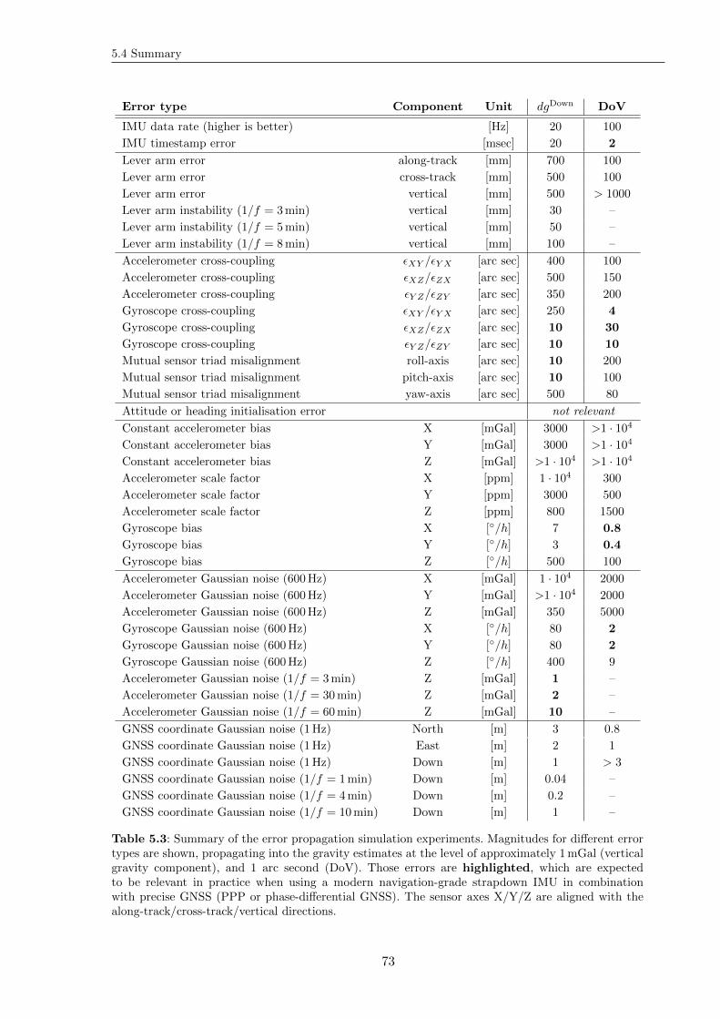
5.4 Summary
Error type Component Unit dgDown DoV
IMU data rate (higher is better) [Hz] 20 100
IMU timestamp error [msec] 20 2
Lever arm error along-track [mm] 700 100
Lever arm error cross-track [mm] 500 100
Lever arm error vertical [mm] 500 > 1000
Lever arm instability (1/f = 3min) vertical [mm] 30 –
Lever arm instability (1/f = 5min) vertical [mm] 50 –
Lever arm instability (1/f = 8min) vertical [mm] 100 –
Accelerometer cross-coupling εXY /εY X [arc sec] 400 100
Accelerometer cross-coupling εXZ/εZX [arc sec] 500 150
Accelerometer cross-coupling εY Z/εZY [arc sec] 350 200
Gyroscope cross-coupling εXY /εY X [arc sec] 250 4
Gyroscope cross-coupling εXZ/εZX [arc sec] 10 30
Gyroscope cross-coupling εY Z/εZY [arc sec] 10 10
Mutual sensor triad misalignment roll-axis [arc sec] 10 200
Mutual sensor triad misalignment pitch-axis [arc sec] 10 100
Mutual sensor triad misalignment yaw-axis [arc sec] 500 80
Attitude or heading initialisation error not relevant
Constant accelerometer bias X [mGal] 3000 >1 · 104
Constant accelerometer bias Y [mGal] 3000 >1 · 104
Constant accelerometer bias Z [mGal] >1 · 104 >1 · 104
Accelerometer scale factor X [ppm] 1 · 104 300
Accelerometer scale factor Y [ppm] 3000 500
Accelerometer scale factor Z [ppm] 800 1500
Gyroscope bias X [/h] 7 0.8
Gyroscope bias Y [/h] 3 0.4
Gyroscope bias Z [/h] 500 100
Accelerometer Gaussian noise (600Hz) X [mGal] 1 · 104 2000
Accelerometer Gaussian noise (600Hz) Y [mGal] >1 · 104 2000
Accelerometer Gaussian noise (600Hz) Z [mGal] 350 5000
Gyroscope Gaussian noise (600Hz) X [/h] 80 2
Gyroscope Gaussian noise (600Hz) Y [/h] 80 2
Gyroscope Gaussian noise (600Hz) Z [/h] 400 9
Accelerometer Gaussian noise (1/f = 3min) Z [mGal] 1 –
Accelerometer Gaussian noise (1/f = 30min) Z [mGal] 2 –
Accelerometer Gaussian noise (1/f = 60min) Z [mGal] 10 –
GNSS coordinate Gaussian noise (1Hz) North [m] 3 0.8
GNSS coordinate Gaussian noise (1Hz) East [m] 2 1
GNSS coordinate Gaussian noise (1Hz) Down [m] 1 > 3
GNSS coordinate Gaussian noise (1/f = 1min) Down [m] 0.04 –
GNSS coordinate Gaussian noise (1/f = 4min) Down [m] 0.2 –
GNSS coordinate Gaussian noise (1/f = 10min) Down [m] 1 –
Table 5.3: Summary of the error propagation simulation experiments. Magnitudes for different errortypes are shown, propagating into the gravity estimates at the level of approximately 1mGal (verticalgravity component), and 1 arc second (DoV). Those errors are highlighted, which are expectedto be relevant in practice when using a modern navigation-grade strapdown IMU in combinationwith precise GNSS (PPP or phase-differential GNSS). The sensor axes X/Y/Z are aligned with thealong-track/cross-track/vertical directions.
73

Error propagation analysis
74
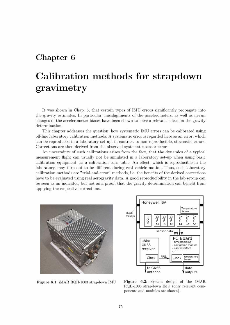
Chapter 6
Calibration methods for strapdowngravimetry
It was shown in Chap. 5, that certain types of IMU errors significantly propagate intothe gravity estimates. In particular, misalignments of the accelerometers, as well as in-runchanges of the accelerometer biases have been shown to have a relevant effect on the gravitydetermination.
This chapter addresses the question, how systematic IMU errors can be calibrated usingoff-line laboratory calibration methods. A systematic error is regarded here as an error, whichcan be reproduced in a laboratory set-up, in contrast to non-reproducible, stochastic errors.Corrections are then derived from the observed systematic sensor errors.
An uncertainty of such calibrations arises from the fact, that the dynamics of a typicalmeasurement flight can usually not be simulated in a laboratory set-up when using basiccalibration equipment, as a calibration turn table. An effect, which is reproducible in thelaboratory, may turn out to be different during real vehicle motion. Thus, such laboratorycalibration methods are ”trial-and-error” methods, i.e. the benefits of the derived correctionshave to be evaluated using real aerogravity data. A good reproducibility in the lab set-up canbe seen as an indicator, but not as a proof, that the gravity determination can benefit fromapplying the respective corrections.
Figure 6.1: iMAR RQH-1003 strapdown IMU
Honeywell ISA
Acc. X
Acc. Y
Acc. Z
Gyr. X
Gyr. Y
Gyr. Z
Clo
ck
PC Board
Clock
uBlox
GNSS
receiver
Clock
Temperature
Sensor
PPS
sensor data
Temperature
Sensor
to GNSS
antennadata
outputs
- timestamping
- navigation module
- user interface
- ...
shock
mounts
Figure 6.2: System design of the iMARRQH-1003 strapdown IMU (only relevant com-ponents and modules are shown).
75

Calibration methods for strapdown gravimetry
Accelerometers Gyroscopes
Model Honeywell Q-Flex R© QA-2000 Honeywell GG1320A
Technology etched-quartz-flexure seismic system Ring-laser
Sensor range ±20 g ±400/s
Resolution <1µg (depending on data rate) 1.13 arc seconds
Linearity error <100 ppm <5 ppm
Sensor bias <25µg < 0.003/h
Random walk <8µg/√Hz < 0.002/
√h
Table 6.1: Manufacturer specifications of the inertial sensors of the iMAR RQH-1003 strapdown IMU(Honeywell International , 2016a,b)
internal / output data rate 1800Hz / ≤300Hz
data latency <3ms (cf. Sect. 5.2.2)
outer dimensions ≈ 310∗ × 213× 180mm (∗no cables attached)
weight ≈12.5 kg
operating temperatures −40 C to 60 C
Table 6.2: Manufacturer specifications (relevant excerpt) of the iMAR RQH-1003 strapdown IMU.
The methods presented in this chapter are carried out for an iMAR RQH-1003 strapdownIMU (Fig. 6.1). This particular IMU was flown during several aerogravity campaigns in theyears 2013 to 2016. The evaluation of the proposed calibration methods will be presented inChap. 8, applying the different corrections to the available aerogravity data sets.
Because of the limited access to a professional calibration turn table, 3 out of the 4proposed calibration approaches could only be carried out once. Thus, a second uncertaintycomes from the fact, that some of the calibrations were carried out years after the acquisitionof the aerogravity data, on which the calibrations are to be evaluated in Chap. 8. The IMUerror characteristics may have changed in the meantime. In practice, it is advisable to repeatthe proposed calibrations on a regular basis.
6.1 iMAR RQH-1003 functional system design
The most important functional components of the iMAR RQH-1003 strapdown IMU aredepicted in Fig. 6.2. The six inertial sensors are bundled in a physical sensor box, calledinertial sensor assembly (ISA). The ISA also contains (at least) one temperature sensor, anda clock. Details about the internal design of the ISA, in particular the position of the inertialsensors and the temperature sensor(s), are classified and unknown to the author. The ISA isphysically attached to the main IMU chassis using shock mounts, which allow a dampeningof mechanical shocks and also higher frequency vibrations.
It is important to note, that misalignments of the ISA module with respect to the nominalIMU axes do not yield a mutual misalignment of the sensors’ axes with respect to eachother. For the IMU/GNSS integrated system, such an ISA-misalignment only affects thebody-fixed lever arm lb. According to the manufacturer, for typical flight dynamics includingturbulence, the ISA-misalignments can reach magnitudes of ±0.1. For example, for a leverarm component of 2m, such a misalignment is consistent with a lever arm error of 3.5mm,which is not relevant in practice (cf. Sect. 5.2.3).
Independent of the ISA misalignments, individual inertial sensor misalignments may beobserved. Later in this chapter it will be shown, that both the ISA misalignments, and the
76
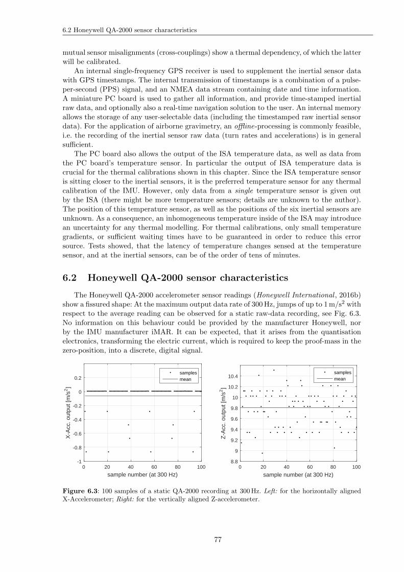
6.2 Honeywell QA-2000 sensor characteristics
mutual sensor misalignments (cross-couplings) show a thermal dependency, of which the latterwill be calibrated.
An internal single-frequency GPS receiver is used to supplement the inertial sensor datawith GPS timestamps. The internal transmission of timestamps is a combination of a pulse-per-second (PPS) signal, and an NMEA data stream containing date and time information.A miniature PC board is used to gather all information, and provide time-stamped inertialraw data, and optionally also a real-time navigation solution to the user. An internal memoryallows the storage of any user-selectable data (including the timestamped raw inertial sensordata). For the application of airborne gravimetry, an offline-processing is commonly feasible,i.e. the recording of the inertial sensor raw data (turn rates and accelerations) is in generalsufficient.
The PC board also allows the output of the ISA temperature data, as well as data fromthe PC board’s temperature sensor. In particular the output of ISA temperature data iscrucial for the thermal calibrations shown in this chapter. Since the ISA temperature sensoris sitting closer to the inertial sensors, it is the preferred temperature sensor for any thermalcalibration of the IMU. However, only data from a single temperature sensor is given outby the ISA (there might be more temperature sensors; details are unknown to the author).The position of this temperature sensor, as well as the positions of the six inertial sensors areunknown. As a consequence, an inhomogeneous temperature inside of the ISA may introducean uncertainty for any thermal modelling. For thermal calibrations, only small temperaturegradients, or sufficient waiting times have to be guaranteed in order to reduce this errorsource. Tests showed, that the latency of temperature changes sensed at the temperaturesensor, and at the inertial sensors, can be of the order of tens of minutes.
6.2 Honeywell QA-2000 sensor characteristics
The Honeywell QA-2000 accelerometer sensor readings (Honeywell International , 2016b)show a fissured shape: At the maximum output data rate of 300Hz, jumps of up to 1m/s2 withrespect to the average reading can be observed for a static raw-data recording, see Fig. 6.3.No information on this behaviour could be provided by the manufacturer Honeywell, norby the IMU manufacturer iMAR. It can be expected, that it arises from the quantisationelectronics, transforming the electric current, which is required to keep the proof-mass in thezero-position, into a discrete, digital signal.
0 20 40 60 80 100
sample number (at 300 Hz)
-1
-0.8
-0.6
-0.4
-0.2
0
0.2
X-A
cc. o
utpu
t [m
/s2]
samplesmean
0 20 40 60 80 100
sample number (at 300 Hz)
8.8
9
9.2
9.4
9.6
9.8
10
10.2
10.4
Z-A
cc. o
utpu
t [m
/s2]
samplesmean
Figure 6.3: 100 samples of a static QA-2000 recording at 300Hz. Left: for the horizontally alignedX-Accelerometer; Right: for the vertically aligned Z-accelerometer.
77
Calibration methods for strapdown gravimetry
Such jumps of 100.000mGal are apparently very large compared to the goal of strapdowngravimetry at the 1mGal level. When averaging the QA-2000 outputs over longer time-windows, the standard deviation of the sliding mean of static data reduces quickly.
In general, when averaging accelerometer outputs over very long periods (tens of minutesor hours), the respective long-term sensor instabilities, for example coming from thermaleffects or other purely stochastic effects, can be expected to eventually dominate the standarddeviation of the data window, while quantisation effects become negligible for such longaveraging periods (El-Sheimy et al., 2008).
The Allan variance (Allan, 1966) is a tool for quantifying such effects. While originallybeing intended for the analysis of long data sets of atomic clock frequencies, the conceptcan be equivalently applied to other sensors, and in particular to inertial sensors (El-Sheimyet al., 2008).
In the typical double-logarithmic plots showing the Allan standard deviations, the char-acteristics of the sensor errors can be interpreted based on the slope of the curves in thatdiagram (El-Sheimy et al., 2008). The relevant categories are repeated here:
• a slope of -1 indicates quantisation noise;
• a slope of -0.5 indicates a random walk (angular random walk for gyroscopes, or velocityrandom walk for accelerometers);
• a slope of 0 indicates a bias instability;
• a slope of 0.5 indicates a rate random walk;
• a slope of 1.0 indicates a drift rate ramp.
Fig. 6.4 shows the Allan standard deviation (being the square root of the Allan variance)for static 60-hour recordings of the iMAR RQH-1003 unit (Sect. 6.1). The three recordingswere done using different IMU orientations, see Fig. 6.5. It can be seen, that the horizontallyaligned accelerometers show larger standard deviations compared to the vertically alignedaccelerometer. Note, that this is consistent among the three different IMU orientations, i.e.the three accelerometers are apparently of similar quality. However, the individual sensorprecisions depend on the relative sensor orientation with respect to the stimulus signal (here:gravity).
For a time window size of 15 minutes (τ = 900 s), the horizontally aligned accelerometersshow a minimum standard deviation of >0.3mGal. For the same accelerometers being invertical orientation, standard deviations as low as 70µGal can be observed for τ ≈ 2500 s.For shorter window lengths, the quantisation errors are the predominant error source. Randomwalks, bias instabilities, rate random walks, and drift rate ramps are difficult to separate inthe plots. For large time window sizes τ , slopes of up to 1.0 can be observed.
For larger time window sizes (tens of minutes or more), the dissimilarity of the curvesamong the different IMU orientations potentially comes from small bends of the sensors’sensitive axes, arising e.g. from an attitude instability of the shock mounts. Such bendsmainly affect the readings of the horizontally aligned accelerometers (cf. Fig. 4.4).
The important conclusion from this analysis is the fact, that the vertically alignedQA-2000 accelerometer consistently shows a higher precision compared to the horizontallyaligned accelerometers. For typical averaging periods used for the calibrations in this chapter(90 s to 180 s), the Allan standard deviations differ by a factor of approximately 2.5–3. Forexample, for τ = 100 s, the standard deviations are 0.65mGal and 2mGal, respectively.
In the default orientation of the iMAR RQH-1003 unit, as it was used for the dataacquisition for the aerogravity data sets shown in Chap. 6, the Z-axis is (approximately)in vertical orientation (third row in Fig. 6.4).
78
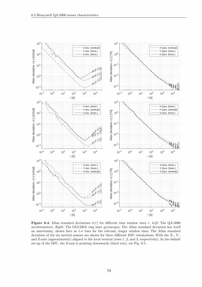
6.2 Honeywell QA-2000 sensor characteristics
10-1 100 101 102 103 104
τ [s]
10-1
100
101
102
103
Alla
n de
viat
ion σ
(τ)
[mG
al]
X-Acc. (vertical)Y-Acc. (horiz.)Z-Acc. (horiz.)
10-1 100 101 102 103 104
τ [s]
10-3
10-2
10-1
100
101
Alla
n de
viat
ion σ
(τ)
[°/h
]
X-Gyro. (vertical)Y-Gyro. (horiz.)Z-Gyro. (horiz.)
10-1 100 101 102 103 104
τ [s]
10-1
100
101
102
103
Alla
n de
viat
ion σ
(τ)
[mG
al]
X-Acc. (horiz.)Y-Acc. (vertical)Z-Acc. (horiz.)
10-1 100 101 102 103 104
τ [s]
10-3
10-2
10-1
100
101
Alla
n de
viat
ion σ
(τ)
[°/h
]
X-Gyro. (horiz.)Y-Gyro. (vertical)Z-Gyro. (horiz.)
10-1 100 101 102 103 104
τ [s]
10-1
100
101
102
103
Alla
n de
viat
ion σ
(τ)
[mG
al]
X-Acc. (horiz.)Y-Acc. (horiz.)Z-Acc. (vertical)
10-1 100 101 102 103 104
τ [s]
10-3
10-2
10-1
100
101
Alla
n de
viat
ion σ
(τ)
[°/h
]
X-Gyro. (horiz.)Y-Gyro. (horiz.)Z-Gyro. (vertical)
Figure 6.4: Allan standard deviations σ(τ) for different time window sizes τ . Left: The QA-2000accelerometers. Right: The GG1320A ring laser gyroscopes. The Allan standard deviation has itselfan uncertainty, shown here as 1-σ bars for the relevant, longer window sizes. The Allan standarddeviation of the six inertial sensors are shown for three different IMU orientations: With the X-, Y-,and Z-axis (approximately) aligned to the local vertical (rows 1, 2, and 3, respectively). In the defaultset-up of the IMU, the Z-axis is pointing downwards (third row), see Fig. 6.5.
79
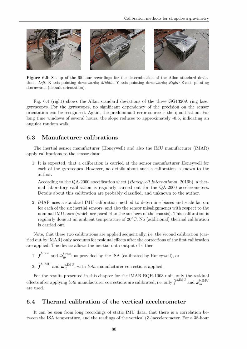
Calibration methods for strapdown gravimetry
Figure 6.5: Set-up of the 60-hour recordings for the determination of the Allan standard devia-tions. Left: X-axis pointing downwards; Middle: Y-axis pointing downwards; Right: Z-axis pointingdownwards (default orientation).
Fig. 6.4 (right) shows the Allan standard deviations of the three GG1320A ring lasergyroscopes. For the gyroscopes, no significant dependency of the precision on the sensororientation can be recognised. Again, the predominant error source is the quantisation. Forlong time windows of several hours, the slope reduces to approximately -0.5, indicating anangular random walk.
6.3 Manufacturer calibrations
The inertial sensor manufacturer (Honeywell) and also the IMU manufacturer (iMAR)apply calibrations to the sensor data:
1. It is expected, that a calibration is carried at the sensor manufacturer Honeywell foreach of the gyroscopes. However, no details about such a calibration is known to theauthor.
According to the QA-2000 specification sheet (Honeywell International , 2016b), a ther-mal laboratory calibration is regularly carried out for the QA-2000 accelerometers.Details about this calibration are probably classified, and unknown to the author.
2. iMAR uses a standard IMU calibration method to determine biases and scale factorsfor each of the six inertial sensors, and also the sensor misalignments with respect to thenominal IMU axes (which are parallel to the surfaces of the chassis). This calibration isregularly done at an ambient temperature of 20C. No (additional) thermal calibrationis carried out.
Note, that these two calibrations are applied sequentially, i.e. the second calibration (car-ried out by iMAR) only accounts for residual effects after the corrections of the first calibrationare applied. The device allows the inertial data output of either
1. fb,raw
and ωb,rawib : as provided by the ISA (calibrated by Honeywell), or
2. fb,IMU
and ωb,IMUib : with both manufacturer corrections applied.
For the results presented in this chapter for the iMAR RQH-1003 unit, only the residual
effects after applying both manufacturer corrections are calibrated, i.e. only fb,IMU
and ωb,IMUib
are used.
6.4 Thermal calibration of the vertical accelerometer
It can be seen from long recordings of static IMU data, that there is a correlation be-tween the ISA temperature, and the readings of the vertical (Z-)accelerometer. For a 38-hour
80
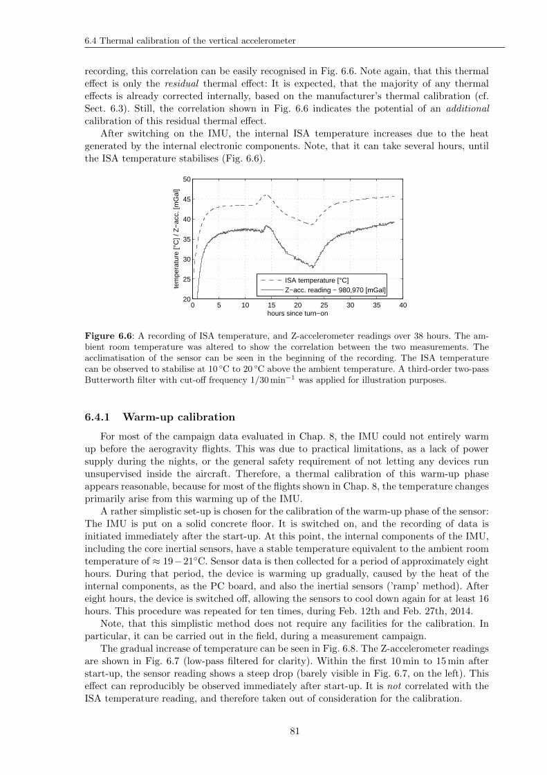
6.4 Thermal calibration of the vertical accelerometer
recording, this correlation can be easily recognised in Fig. 6.6. Note again, that this thermaleffect is only the residual thermal effect: It is expected, that the majority of any thermaleffects is already corrected internally, based on the manufacturer’s thermal calibration (cf.Sect. 6.3). Still, the correlation shown in Fig. 6.6 indicates the potential of an additionalcalibration of this residual thermal effect.
After switching on the IMU, the internal ISA temperature increases due to the heatgenerated by the internal electronic components. Note, that it can take several hours, untilthe ISA temperature stabilises (Fig. 6.6).
0 5 10 15 20 25 30 35 4020
25
30
35
40
45
50
hours since turn−on
tem
pera
ture
[°C
] / Z
−ac
c. [m
Gal
]
ISA temperature [°C]Z−acc. reading − 980,970 [mGal]
Figure 6.6: A recording of ISA temperature, and Z-accelerometer readings over 38 hours. The am-bient room temperature was altered to show the correlation between the two measurements. Theacclimatisation of the sensor can be seen in the beginning of the recording. The ISA temperaturecan be observed to stabilise at 10 C to 20 C above the ambient temperature. A third-order two-passButterworth filter with cut-off frequency 1/30min−1 was applied for illustration purposes.
6.4.1 Warm-up calibration
For most of the campaign data evaluated in Chap. 8, the IMU could not entirely warmup before the aerogravity flights. This was due to practical limitations, as a lack of powersupply during the nights, or the general safety requirement of not letting any devices rununsupervised inside the aircraft. Therefore, a thermal calibration of this warm-up phaseappears reasonable, because for most of the flights shown in Chap. 8, the temperature changesprimarily arise from this warming up of the IMU.
A rather simplistic set-up is chosen for the calibration of the warm-up phase of the sensor:The IMU is put on a solid concrete floor. It is switched on, and the recording of data isinitiated immediately after the start-up. At this point, the internal components of the IMU,including the core inertial sensors, have a stable temperature equivalent to the ambient roomtemperature of ≈ 19−21C. Sensor data is then collected for a period of approximately eighthours. During that period, the device is warming up gradually, caused by the heat of theinternal components, as the PC board, and also the inertial sensors (’ramp’ method). Aftereight hours, the device is switched off, allowing the sensors to cool down again for at least 16hours. This procedure was repeated for ten times, during Feb. 12th and Feb. 27th, 2014.
Note, that this simplistic method does not require any facilities for the calibration. Inparticular, it can be carried out in the field, during a measurement campaign.
The gradual increase of temperature can be seen in Fig. 6.8. The Z-accelerometer readingsare shown in Fig. 6.7 (low-pass filtered for clarity). Within the first 10min to 15min afterstart-up, the sensor reading shows a steep drop (barely visible in Fig. 6.7, on the left). Thiseffect can reproducibly be observed immediately after start-up. It is not correlated with theISA temperature reading, and therefore taken out of consideration for the calibration.
81
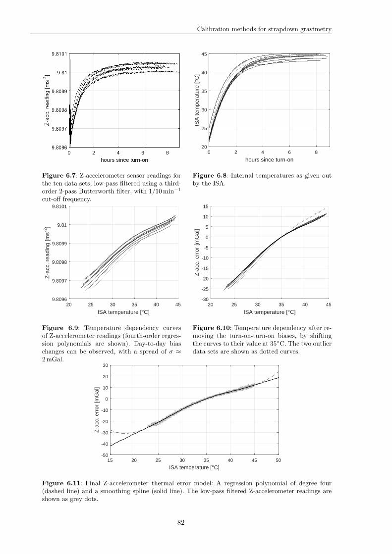
Calibration methods for strapdown gravimetry
Figure 6.7: Z-accelerometer sensor readings forthe ten data sets, low-pass filtered using a third-order 2-pass Butterworth filter, with 1/10min−1
cut-off frequency.
0 2 4 6 8
hours since turn-on
20
25
30
35
40
45
ISA
tem
pera
ture
[°C
]
Figure 6.8: Internal temperatures as given outby the ISA.
20 25 30 35 40 45
ISA temperature [°C]
9.8096
9.8097
9.8098
9.8099
9.81
9.8101
Z-a
cc. r
eadi
ng [m
s-2]
Figure 6.9: Temperature dependency curvesof Z-accelerometer readings (fourth-order regres-sion polynomials are shown). Day-to-day biaschanges can be observed, with a spread of σ ≈2mGal.
20 25 30 35 40 45
ISA temperature [°C]
-30
-25
-20
-15
-10
-5
0
5
10
15
Z-a
cc. e
rror
[mG
al]
Figure 6.10: Temperature dependency after re-moving the turn-on-turn-on biases, by shiftingthe curves to their value at 35C. The two outlierdata sets are shown as dotted curves.
15 20 25 30 35 40 45 50
ISA temperature [°C]
-50
-40
-30
-20
-10
0
10
20
30
Z-a
cc. e
rror
[mG
al]
Figure 6.11: Final Z-accelerometer thermal error model: A regression polynomial of degree four(dashed line) and a smoothing spline (solid line). The low-pass filtered Z-accelerometer readings areshown as grey dots.
82
6.4 Thermal calibration of the vertical accelerometer
Fig. 6.9 shows the dependency between ISA temperature reading, and the Z-accelerometerreading. The figure shows fourth-order regression polynomials. The slopes are in the rangebetween 1.2mGal/h and 2.3mGal/h. The curves of the ten runs have vertical offsets witha standard deviation of ≈ 2mGal, apparently being random day-to-day bias changes. Thesevertical offsets are removed, by shifting the curves such that they mutually intersect at thepoint 35C / 0mGal (Fig. 6.10). It can be seen, that two of the ten curves have a slightlydifferent shape (dotted curves in Fig. 6.10), compared to the other eight curves. The reasonfor this is unknown. A possible explanation could be the relatively large temperature gradientat these two days (see dotted curves in Fig. 6.8), perhaps coming from larger gradients of theambient room temperature. For the following derivation of a thermal correction, these twocurves are regarded as outliers. The remaining eight (shifted) curves show a good agreement:The bias differences between 25 C and 42 C have a variation of σ = 0.7mGal.
A final approximation function is derived based on the joint original data from the eightremaining data sets (grey dots in Fig. 6.11). Two different functions are derived:
1. a regression polynomial of degree four as used for the individual daily curves in Figs. 6.9and 6.10 (shown as dashed line in Fig. 6.11),
2. a smoothing spline (shown as solid line in Fig. 6.11).
One disadvantage of this calibration method is the limited temperature range covered,with ISA temperatures between 23C and 45C. An extrapolation to lower and higher tem-peratures is in general not advisable. Still, an attempt is done here, in order to enable thecorrection of aerogravity data sets being up to 5C outside of the given range. The smooth-ing spline yields a more reasonable extrapolation compared to the fourth-order polynomial(Fig 6.11). The smoothing spline is therefore selected. It is applied as correction (with negativesign) to the Z-accelerometer readings.
Using such a simple set-up, it is not possible to separate different contributions of theoverall error, as sensor biases, scale factors, and also sensor misalignments coming from ther-mal deformations. In fact, all these effects are masked here by a single temperature-dependentscalar quantity. However, the calibration is still useful for the application of strapdowngravimetry, since the sensor is almost in horizontal position during the main measurementlines (cf. Fig. 5.3). For airborne gravimetry, the aircraft accelerations on the measurementlines are typically small compared to the magnitude of the Earth’s gravity.
The following section shows a similar calibration, this time using a temperature oven.For this calibration, however, the IMU is given time to acclimatise first (’soak’ method).The thermal effects then arise only from the internal temperature following the ambienttemperature changes.
Later in this chapter, more sophisticated calibration methods will be introduced. Some ofthe discussed methods are based on parametric models, trying to accurately separate biases,scale factors and sensor cross-couplings, and thereby refining the simplistic model shown inthis section.
6.4.2 Temperature oven calibration
For a more controlled set-up, the iMAR RQH-1003 IMU is installed in a temperature oven.The sensor is then exposed to 22 different nominal oven temperatures, ranging from −20 Cto 48 C, see Fig. 6.13. The larger temperature interval will enable a thermal correction foroperations in very cold or hot environments (see for example the Antarctica data set shownin Chap. 8, with ISA temperatures starting at −5 C). Due to the limited availability of thetemperature oven, the experiment was limited to a single run.
Before the experiment, the IMU was running for approximately 3 hours at an oven tem-perature of −20 C, to let the sensors acclimatise. Note however, that until one hour after
83
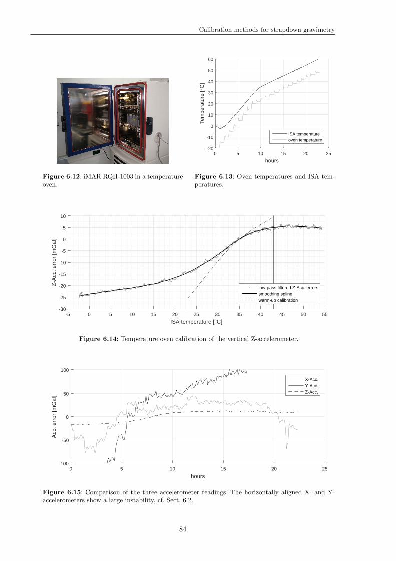
Calibration methods for strapdown gravimetry
Figure 6.12: iMAR RQH-1003 in a temperatureoven.
0 5 10 15 20 25
hours
-20
-10
0
10
20
30
40
50
60
Tem
pera
ture
[°C
]
ISA temperatureoven temperature
Figure 6.13: Oven temperatures and ISA tem-peratures.
-5 0 5 10 15 20 25 30 35 40 45 50 55
ISA temperature [°C]
-30
-25
-20
-15
-10
-5
0
5
10
Z-A
cc. e
rror
[mG
al]
low-pass filtered Z-Acc. errorssmoothing splinewarm-up calibration
Figure 6.14: Temperature oven calibration of the vertical Z-accelerometer.
0 5 10 15 20 25
hours
-100
-50
0
50
100
Acc
. err
or [m
Gal
]
X-Acc.Y-Acc.Z-Acc,
Figure 6.15: Comparison of the three accelerometer readings. The horizontally aligned X- and Y-accelerometers show a large instability, cf. Sect. 6.2.
84
6.5 Parametric error models
the start of the experiment, the internal ISA temperature was still reducing, indicating thatthe sensor was not yet fully acclimatised. This part of the data recording was not used forthe calibration.
In contrast to the warm-up calibration presented in the previous section, the observed sen-sor drifts only come from the oven temperature variations. The ISA temperature is graduallyfollowing the oven temperature changes, as can be seen in Fig. 6.13.
For oven temperatures up to 22 C, the ISA temperature gradient is ≈6 C/h. For thehigher temperatures, a finer spacing of the oven temperature setting was chosen, leading toan ISA temperature gradient of ≈2 C/h. Note, that these gradients differ significantly fromthose of the warm-up calibration (Fig. 6.8), for which the gradients decrease from 10 C/h inthe beginning (lower temperatures), down to zero (stabilised ISA temperature) in the end.
As in the previous section, a smoothing spline is fitted to the Z-accelerometer readings.Fig. 6.14 shows the results of the calibration. (The Z-accelerometer readings are shown afterapplying a third-order 2-pass Butterworth low-pass filter with 1/600 s−1 threshold frequencyfor clarity.)
The result of the warm-up calibration (cf. Fig. 6.11) is also included in Fig. 6.14 in theinterval between 23 C to 43 C, to allow a direct comparison of the two results. The significantdifferences are expected to come from the different temperature gradients in combination witha thermal latency.
The horizontally aligned X- and Y-accelerometers show a large instability compared to thevertical Z-accelerometer (Fig. 6.15). This instability is expected to come from small bends ofthe accelerometers’ sensitive axes, cf. Sect. 6.2. It is not expected, that a reasonable thermalcorrection can be derived from this data. Again, the calibration is therefore limited to thevertically aligned Z-accelerometer.
6.5 Parametric error models
Parametric error models are based on a predefined set of parameters. The most commonparameters are bias and scale factor, and additionally cross-couplings for triads of sensors,and sensor misalignments, if an external reference orientation is given.
It is commonly expected, that this set of standard parameters is suited to model the ma-jority of inertial sensor errors. For the iMAR RQH-1003 strapdown IMU, this expectation istrue: The majority of sensor errors is accounted for by such parametric models, used for themanufacturer calibrations. However, when aiming at a 1mGal precision for the accelerome-ters, extended models are required.
6.5.1 Bias, scale factor, cross-coupling (BSC)
The calibrations presented in this section are mainly based on the work of Shin andEl-Sheimy (2002), who published a particular calibration method for bias, scale factor, andcross-couplings (BSC-calibration) of a sensor triad, only using a known scalar value of astimulus signal (e.g. gravity for accelerometer calibrations, and the Earth rotation rate forgyroscope calibrations). The sensor triad is turned to different, arbitrary orientations, andthe 1-D measurements of scalar gravity |f |, or scalar turn rate ωib, are compared to theexternal reference value. An important assumption for this calibration method is, that theestimated parameters (bias, scale factor, cross-coupling) are constant for the set of differentIMU orientations. This section provides a brief overview of the method. A more detailedmathematical derivation, including the Jacobian matrix of the observation equation, can befound in Shin and El-Sheimy (2002). The calibration is repeated for different nominal oventemperatures, following the approach presented in Yang et al. (2013). Thereby, a set of nine
85
Calibration methods for strapdown gravimetry
thermal correction functions is deduced for the QA-2000 accelerometer triad (three biases,three scale factors, and three cross-couplings).
Note: This approach is in theory suited for the calibration of accelerometer and gyroscopetriads. The latter however can only be calibrated using the Earth rotation rate as stimulussignal (unless a 3-axis turn table is available). Such a weak stimulus signal does not allowa reasonable determination of gyroscope cross-couplings, or scale factors. For example, forthe application of navigation, the scale factors would have to be extrapolated from 0.004
per second (Earth rotation rate) to turn rates of the order of tens of degrees per second (ormore).
The approach is however well suited for an accelerometer triad, for navigation applicationswith low or medium dynamics, because the actual specific forces during the vehicle motionare of the same order as the stimulus signal during the calibration (the Earth’s gravity). Inthe following, the BSC calibration will be introduced for accelerometer triads only, as theauthor did not have access to a three-axis turn table with combined temperature oven.
Basic equations
Only based on the known scalar gravity gref , the following nine parameters are determinedby a least-squares estimation:
1. three biases: bX , bY , bZ ,
2. three scale factors: sX , sY , sZ , and
3. three cross-couplings: εY X , εZX , εZY (as defined in Sect. 5.2.4).
It is assumed, that the IMU axes (X/Y/Z) form a right-handed Cartesian coordinate frame.The approach is based on observations of the scalar gravity value only. As a consequence, aminimum of nine poses is required to fully determine the set of the nine parameters shownabove. In order to stabilize the estimation process (and also to enable a statistical evaluation),an over-determination is commonly suggested. For example, the following set of 26 poses areproposed by Shin and El-Sheimy (2002):
1. ”face down”: with the IMU at rest on each of the six surfaces (6 poses),
2. ”edge down”: with the IMU at rest on each of the 12 edges (12 poses), and
3. ”corner down”: with the IMU at rest on each of the 8 corner points (8 poses).
Since the approach does not involve any restriction or knowledge on the actual, absoluteorientation of the sensor triad with respect to the gravity vector, only mutual cross-couplingsof the sensors can be calibrated (εY X , εZX , εZY ). Conversely, the calibration of misalignmentswith respect to an externally defined reference orientation is not possible with this approach.The cross-couplings of a sensor triad are fully determined by the given set of three indepen-dent parameters. Therefore, only three out of the six possible misalignments introduced inSect. 5.2.4 are chosen, by selecting one out of each pair of symmetric misalignments (εij , εji).
The measured specific forces f for the X-, Y-, and Z-accelerometers of a sensor triad arethen given as
fX = bX + (1 + sX)fX (6.1)
fY = bY + (1 + sY )(fY cos(εY X)− fX sin(εY X)) (6.2)
fZ = bZ + (1 + sZ)(fZ cos(εZX) cos(εZY )− fX sin(εZX)− fY sin(εZY ) cos(εZX))(6.3)
86
6.5 Parametric error models
where fa is the true specific force along the given axis a. For small misalignments of the orderof tens of arc seconds, these equations can be approximated by
fX ≈ bX + (1 + sX)fX (6.4)
fY ≈ bY + (1 + sY )(fY − fXεY X) (6.5)
fZ ≈ bZ + (1 + sZ)(fZ − fXεZX − fY εZY ) . (6.6)
(The error of the approximation sin(ε) · g ≈ ε · g is smaller than 0.02µGal, if ε < 100 arcseconds.) These equations can be rearranged to
fX ≈ fX (6.7)
fY ≈ fY + fXεY X (6.8)
fZ ≈ fZ + fXεZX + (fY + fXεY X)εZY , with (6.9)
fa :=fa − ba
1 + sa, for a ∈ X,Y, Z . (6.10)
Note: Since the calibration is done with the sensor triad at rest (without accelerations, r = 0),the specific forces are equal to the respective components of the negative gravity vector, i.e.fa =: −ga and fa =: −ga for a given axis a.
The main condition equations for the mixed model (also called Gauss-Helmert model)are given by the equality of the scalar gravity as measured by the accelerometer, and thereference value. For the error-free observations of the specific force fa, this condition is givenas
g2 − g2ref = (fX)2 + (fY )2 + (fZ)2 − g2ref = 0 . (6.11)
Now accounting for sensor errors, each of the condition equations yields a contradiction w:
g2 − g2ref = (fX)2 + (fY )2 + (fZ)2 − g2ref = w . (6.12)
The set of all of these condition equations (one condition per IMU orientation) can be writtenin short form as F (L,X) = w, where L denotes the vector of observations, and X denotesthe 9-D vector of parameters (biases, scale factors, cross-couplings).
The Gauss-Helmert adjustment provides the vectors of adjusted observations, L, andadjusted parameters, X. The adjustment is based on the minimisation of vTv, where vdenotes the vector of residuals of the observations, with L = L+v. For the adjusted quantities,F (L, X) = 0 in general, i.e. the adjusted observations L in combination with the adjustedparameters X do not yield any contradiction in general. Note, that this is a non-linear system.For the required Jacobian matrices for the least-squares adjustment, the reader is referred toShin and El-Sheimy (2002). Starting with the approximation X0, with
bX0 = bY0 = bZ0 = sX0 = sY0 = sZ0 = εY X,0 = εZX,0 = εZY,0 = 0 , (6.13)
the adjustment is executed in an iterative manner, as suggested by the non-linearity of thefunctional relationship. The iteration loop was stopped as soon as the maximum absoluteparameter change was less then 10−15 (which is approximately the resolution of a matrixinversion, when using a 64 bit floating point representation). For the actual calibration mea-surements, this was the case after a maximum of 6 iteration steps.
Based on the set of adjusted error model parameters, X, the original observations L stillyield non-zero contradictions in general, i.e. F (L, X) = w 6= 0. These contradictions w canbe regarded as the residuals of the adjustment. Assuming, that the adjustment was doneusing a sufficient number of iterations, w can therefore be seen as a measure, of how good theestimated error model fits the original measurements, and thus, how good it fits the actualsensor error characteristics. Contradictions, which are large compared to the expected effectsof the sensor noise may lead to the conclusion, that the error model could not adequatelymodel the actual sensor error characteristics.
87
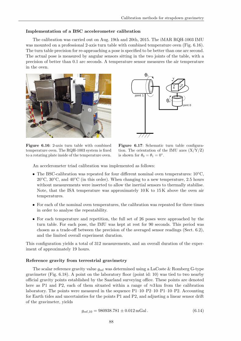
Calibration methods for strapdown gravimetry
Implementation of a BSC accelerometer calibration
The calibration was carried out on Aug. 19th and 20th, 2015. The iMAR RQH-1003 IMUwas mounted on a professional 2-axis turn table with combined temperature oven (Fig. 6.16).The turn table precision for re-approaching a pose is specified to be better than one arc second.The actual pose is measured by angular sensors sitting in the two joints of the table, with aprecision of better than 0.1 arc seconds. A temperature sensor measures the air temperaturein the oven.
Figure 6.16: 2-axis turn table with combinedtemperature oven. The RQH-1003 system is fixedto a rotating plate inside of the temperature oven.
X
Y
Z
0
1
joint 1
joint 0
Figure 6.17: Schematic turn table configura-tion. The orientation of the IMU axes (X/Y/Z)is shown for θ0 = θ1 = 0.
An accelerometer triad calibration was implemented as follows:
• The BSC-calibration was repeated for four different nominal oven temperatures: 10C,20C, 30C, and 40C (in this order). When changing to a new temperature, 2.5 hourswithout measurements were inserted to allow the inertial sensors to thermally stabilise.Note, that the ISA temperature was approximately 10K to 15K above the oven airtemperatures.
• For each of the nominal oven temperatures, the calibration was repeated for three timesin order to analyse the repeatability.
• For each temperature and repetition, the full set of 26 poses were approached by theturn table. For each pose, the IMU was kept at rest for 90 seconds. This period waschosen as a trade-off between the precision of the averaged sensor readings (Sect. 6.2),and the limited overall experiment duration.
This configuration yields a total of 312 measurements, and an overall duration of the exper-iment of approximately 19 hours.
Reference gravity from terrestrial gravimetry
The scalar reference gravity value gref was determined using a LaCoste & Romberg G-typegravimeter (Fig. 6.18). A point on the laboratory floor (point id: 10) was tied to two nearbyofficial gravity points established by the Saarland surveying office. These points are denotedhere as P1 and P2, each of them situated within a range of ≈3 km from the calibrationlaboratory. The points were measured in the sequence P1–10–P2–10–P1–10–P2. Accountingfor Earth tides and uncertainties for the points P1 and P2, and adjusting a linear sensor driftof the gravimeter, yields
gref,10 = 980938.781± 0.012mGal . (6.14)
88
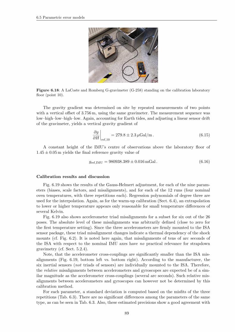
6.5 Parametric error models
Figure 6.18: A LaCoste and Romberg G-gravimeter (G-258) standing on the calibration laboratoryfloor (point 10).
The gravity gradient was determined on site by repeated measurements of two pointswith a vertical offset of 3.756m, using the same gravimeter. The measurement sequence waslow–high–low–high–low. Again, accounting for Earth tides, and adjusting a linear sensor driftof the gravimeter, yields a vertical gravity gradient of
∂g
∂H
∣∣∣∣ref,10
= 279.8± 2.3µGal/m . (6.15)
A constant height of the IMU’s centre of observations above the laboratory floor of1.45± 0.05m yields the final reference gravity value of
gref,IMU = 980938.389± 0.016mGal . (6.16)
Calibration results and discussion
Fig. 6.19 shows the results of the Gauss-Helmert adjustment, for each of the nine param-eters (biases, scale factors, and misalignments), and for each of the 12 runs (four nominaloven temperatures, with three repetitions each). Regression polynomials of degree three areused for the interpolation. Again, as for the warm-up calibration (Sect. 6.4), an extrapolationto lower or higher temperature appears only reasonable for small temperature differences ofseveral Kelvin.
Fig. 6.19 also shows accelerometer triad misalignments for a subset for six out of the 26poses. The absolute level of these misalignments was arbitrarily defined (close to zero forthe first temperature setting). Since the three accelerometers are firmly mounted to the ISAsensor package, these triad misalignment changes indicate a thermal dependency of the shockmounts (cf. Fig. 6.2). It is noted here again, that misalignments of tens of arc seconds ofthe ISA with respect to the nominal IMU axes have no practical relevance for strapdowngravimetry (cf. Sect. 5.2.4).
Note, that the accelerometer cross-couplings are significantly smaller than the ISA mis-alignments (Fig. 6.19, bottom left vs. bottom right). According to the manufacturer, thesix inertial sensors (not triads of sensors) are individually mounted to the ISA. Therefore,the relative misalignments between accelerometers and gyroscopes are expected be of a sim-ilar magnitude as the accelerometer cross-couplings (several arc seconds). Such relative mis-alignments between accelerometers and gyroscopes can however not be determined by thiscalibration method.
For each parameter, a standard deviation is computed based on the misfits of the threerepetitions (Tab. 6.3). There are no significant differences among the parameters of the sametype, as can be seen in Tab. 6.3. Also, these estimated precisions show a good agreement with
89
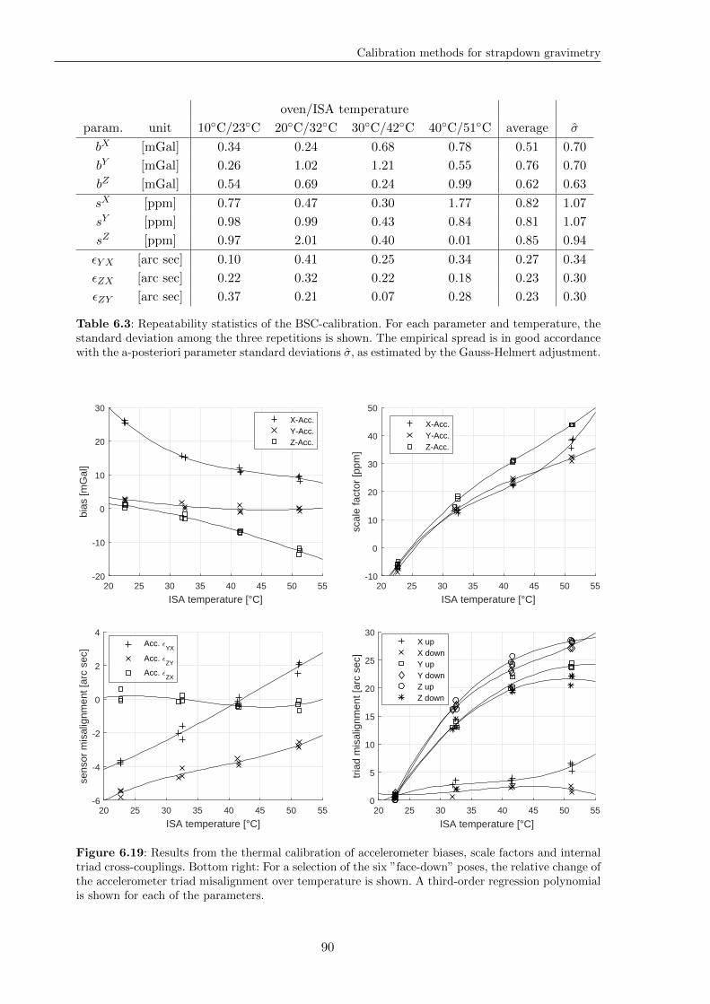
Calibration methods for strapdown gravimetry
oven/ISA temperature
param. unit 10C/23C 20C/32C 30C/42C 40C/51C average σ
bX [mGal] 0.34 0.24 0.68 0.78 0.51 0.70
bY [mGal] 0.26 1.02 1.21 0.55 0.76 0.70
bZ [mGal] 0.54 0.69 0.24 0.99 0.62 0.63
sX [ppm] 0.77 0.47 0.30 1.77 0.82 1.07
sY [ppm] 0.98 0.99 0.43 0.84 0.81 1.07
sZ [ppm] 0.97 2.01 0.40 0.01 0.85 0.94
εY X [arc sec] 0.10 0.41 0.25 0.34 0.27 0.34
εZX [arc sec] 0.22 0.32 0.22 0.18 0.23 0.30
εZY [arc sec] 0.37 0.21 0.07 0.28 0.23 0.30
Table 6.3: Repeatability statistics of the BSC-calibration. For each parameter and temperature, thestandard deviation among the three repetitions is shown. The empirical spread is in good accordancewith the a-posteriori parameter standard deviations σ, as estimated by the Gauss-Helmert adjustment.
20 25 30 35 40 45 50 55
ISA temperature [°C]
-20
-10
0
10
20
30
bias
[mG
al]
X-Acc.Y-Acc.Z-Acc.
20 25 30 35 40 45 50 55
ISA temperature [°C]
-10
0
10
20
30
40
50
scal
e fa
ctor
[ppm
]
X-Acc.Y-Acc.Z-Acc.
20 25 30 35 40 45 50 55
ISA temperature [°C]
-6
-4
-2
0
2
4
sens
or m
isal
ignm
ent [
arc
sec]
Acc. ǫYX
Acc. ǫZY
Acc. ǫZX
20 25 30 35 40 45 50 55
ISA temperature [°C]
0
5
10
15
20
25
30
tria
d m
isal
ignm
ent [
arc
sec]
X upX downY upY downZ upZ down
Figure 6.19: Results from the thermal calibration of accelerometer biases, scale factors and internaltriad cross-couplings. Bottom right: For a selection of the six ”face-down” poses, the relative change ofthe accelerometer triad misalignment over temperature is shown. A third-order regression polynomialis shown for each of the parameters.
90
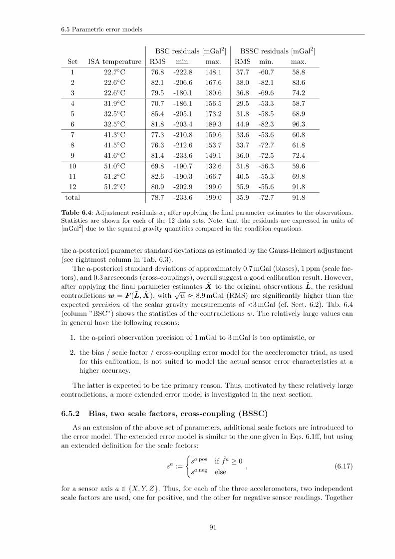
6.5 Parametric error models
BSC residuals [mGal2] BSSC residuals [mGal2]
Set ISA temperature RMS min. max. RMS min. max.
1 22.7C 76.8 -222.8 148.1 37.7 -60.7 58.8
2 22.6C 82.1 -206.6 167.6 38.0 -82.1 83.6
3 22.6C 79.5 -180.1 180.6 36.8 -69.6 74.2
4 31.9C 70.7 -186.1 156.5 29.5 -53.3 58.7
5 32.5C 85.4 -205.1 173.2 31.8 -58.5 68.9
6 32.5C 81.8 -203.4 189.3 44.9 -82.3 96.3
7 41.3C 77.3 -210.8 159.6 33.6 -53.6 60.8
8 41.5C 76.3 -212.6 153.7 33.7 -72.7 61.8
9 41.6C 81.4 -233.6 149.1 36.0 -72.5 72.4
10 51.0C 69.8 -190.7 132.6 31.8 -56.3 59.6
11 51.2C 82.6 -190.3 166.7 40.5 -55.3 69.8
12 51.2C 80.9 -202.9 199.0 35.9 -55.6 91.8
total 78.7 -233.6 199.0 35.9 -72.7 91.8
Table 6.4: Adjustment residuals w, after applying the final parameter estimates to the observations.Statistics are shown for each of the 12 data sets. Note, that the residuals are expressed in units of[mGal2] due to the squared gravity quantities compared in the condition equations.
the a-posteriori parameter standard deviations as estimated by the Gauss-Helmert adjustment(see rightmost column in Tab. 6.3).
The a-posteriori standard deviations of approximately 0.7mGal (biases), 1 ppm (scale fac-tors), and 0.3 arcseconds (cross-couplings), overall suggest a good calibration result. However,after applying the final parameter estimates X to the original observations L, the residualcontradictions w = F (L, X), with
√w ≈ 8.9mGal (RMS) are significantly higher than the
expected precision of the scalar gravity measurements of <3mGal (cf. Sect. 6.2). Tab. 6.4(column ”BSC”) shows the statistics of the contradictions w. The relatively large values canin general have the following reasons:
1. the a-priori observation precision of 1mGal to 3mGal is too optimistic, or
2. the bias / scale factor / cross-coupling error model for the accelerometer triad, as usedfor this calibration, is not suited to model the actual sensor error characteristics at ahigher accuracy.
The latter is expected to be the primary reason. Thus, motivated by these relatively largecontradictions, a more extended error model is investigated in the next section.
6.5.2 Bias, two scale factors, cross-coupling (BSSC)
As an extension of the above set of parameters, additional scale factors are introduced tothe error model. The extended error model is similar to the one given in Eqs. 6.1ff, but usingan extended definition for the scale factors:
sa :=
sa,pos if fa ≥ 0
sa,neg else, (6.17)
for a sensor axis a ∈ X,Y, Z. Thus, for each of the three accelerometers, two independentscale factors are used, one for positive, and the other for negative sensor readings. Together
91
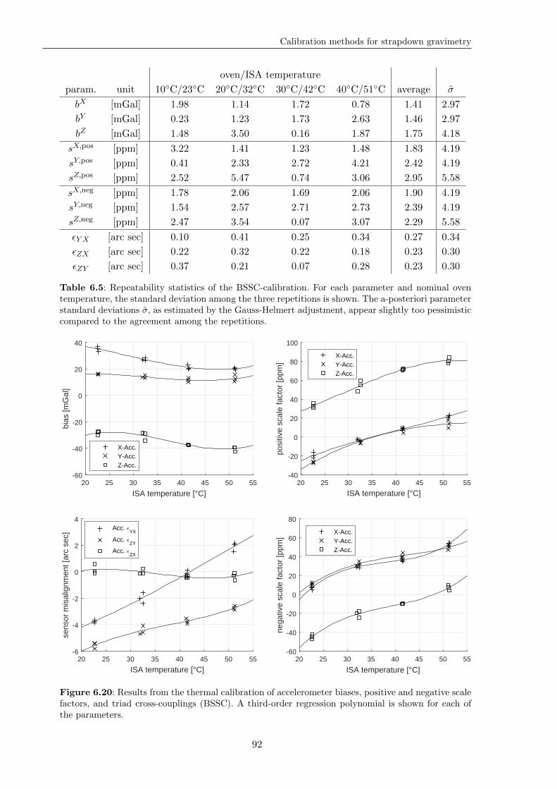
Calibration methods for strapdown gravimetry
oven/ISA temperature
param. unit 10C/23C 20C/32C 30C/42C 40C/51C average σ
bX [mGal] 1.98 1.14 1.72 0.78 1.41 2.97
bY [mGal] 0.23 1.23 1.73 2.63 1.46 2.97
bZ [mGal] 1.48 3.50 0.16 1.87 1.75 4.18
sX,pos [ppm] 3.22 1.41 1.23 1.48 1.83 4.19
sY,pos [ppm] 0.41 2.33 2.72 4.21 2.42 4.19
sZ,pos [ppm] 2.52 5.47 0.74 3.06 2.95 5.58
sX,neg [ppm] 1.78 2.06 1.69 2.06 1.90 4.19
sY,neg [ppm] 1.54 2.57 2.71 2.73 2.39 4.19
sZ,neg [ppm] 2.47 3.54 0.07 3.07 2.29 5.58
εY X [arc sec] 0.10 0.41 0.25 0.34 0.27 0.34
εZX [arc sec] 0.22 0.32 0.22 0.18 0.23 0.30
εZY [arc sec] 0.37 0.21 0.07 0.28 0.23 0.30
Table 6.5: Repeatability statistics of the BSSC-calibration. For each parameter and nominal oventemperature, the standard deviation among the three repetitions is shown. The a-posteriori parameterstandard deviations σ, as estimated by the Gauss-Helmert adjustment, appear slightly too pessimisticcompared to the agreement among the repetitions.
20 25 30 35 40 45 50 55
ISA temperature [°C]
-60
-40
-20
0
20
40
bias
[mG
al]
X-Acc.Y-Acc.Z-Acc.
20 25 30 35 40 45 50 55
ISA temperature [°C]
-40
-20
0
20
40
60
80
100
posi
tive
scal
e fa
ctor
[ppm
]
X-Acc.Y-Acc.Z-Acc.
20 25 30 35 40 45 50 55
ISA temperature [°C]
-6
-4
-2
0
2
4
sens
or m
isal
ignm
ent [
arc
sec]
Acc. ǫYX
Acc. ǫZY
Acc. ǫZX
20 25 30 35 40 45 50 55
ISA temperature [°C]
-60
-40
-20
0
20
40
60
80
nega
tive
scal
e fa
ctor
[ppm
]
X-Acc.Y-Acc.Z-Acc.
Figure 6.20: Results from the thermal calibration of accelerometer biases, positive and negative scalefactors, and triad cross-couplings (BSSC). A third-order regression polynomial is shown for each ofthe parameters.
92
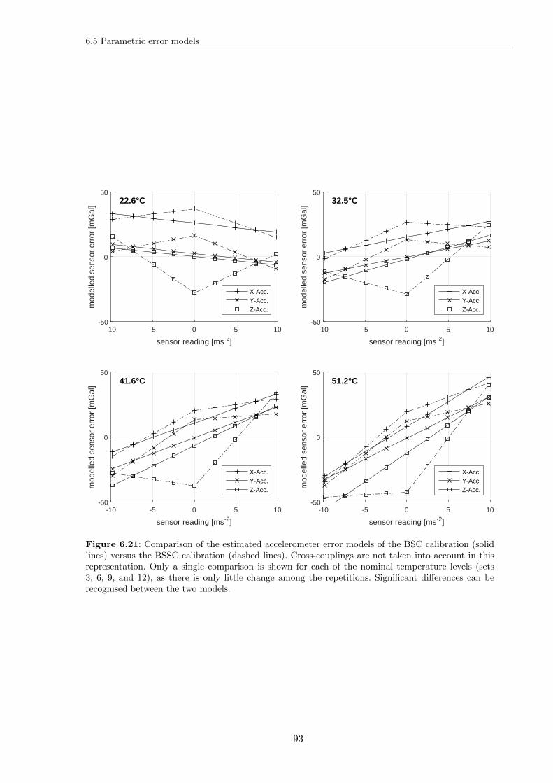
6.5 Parametric error models
-10 -5 0 5 10
sensor reading [ms-2]
-50
0
50
mod
elle
d se
nsor
err
or [m
Gal
] 22.6°C
X-Acc.Y-Acc.Z-Acc.
-10 -5 0 5 10
sensor reading [ms-2]
-50
0
50
mod
elle
d se
nsor
err
or [m
Gal
] 32.5°C
X-Acc.Y-Acc.Z-Acc.
-10 -5 0 5 10
sensor reading [ms-2]
-50
0
50
mod
elle
d se
nsor
err
or [m
Gal
] 41.6°C
X-Acc.Y-Acc.Z-Acc.
-10 -5 0 5 10
sensor reading [ms-2]
-50
0
50
mod
elle
d se
nsor
err
or [m
Gal
] 51.2°C
X-Acc.Y-Acc.Z-Acc.
Figure 6.21: Comparison of the estimated accelerometer error models of the BSC calibration (solidlines) versus the BSSC calibration (dashed lines). Cross-couplings are not taken into account in thisrepresentation. Only a single comparison is shown for each of the nominal temperature levels (sets3, 6, 9, and 12), as there is only little change among the repetitions. Significant differences can berecognised between the two models.
93
Calibration methods for strapdown gravimetry
with the sensor biases and cross-couplings as introduced in the previous section, this forms avector of twelve (instead of nine) parameters:
X ′ = (bX , bY , bZ , sX,pos, sY,pos, sZ,pos, sX,neg, sY,neg, sZ,neg, εY X , εZX , εZY )T . (6.18)
This extended model will be referred to as BSSC model, indicating the double scale factorsfor each of the sensors. Besides this extended scale factor definition, the calibration is carriedout with the same data set introduced in the previous section.
The results of the BSSC calibration are shown in Fig. 6.20. The statistics are shownin Tab. 6.5. Apparently, the lower over-determination leads to higher a-posteriori standarddeviations of the biases and scale factors. By comparison with Fig. 6.19, it can be seen, thatthe cross-coupling estimates are not affected by the extended error model. The same holdsfor the triad misalignments (no figure shown is for the BSSC calibration).
As an important result of the BSSC calibration, it can be seen that the positive andnegative scale factors differ significantly (Fig. 6.20). Apparently, the true sensor errors cannot be adequately represented by a single scale factor. A direct comparison of the error modelsas estimated by the BSC and the BSSC calibrations is shown in Fig. 6.21. The BSSC sensorerror models are ”V”- or ”Λ”-shaped, and differ significantly from the linear error models(straight lines in the plots) estimated in the scope of the BSC-calibration.
Statistics of the adjustment residuals w = F (L, X′), i.e. after applying the final BSSC
parameter estimates X′to the original observations L, are shown in Tab. 6.4. The residuals
are significantly smaller compared to the BSC calibration, indicating a better fit of the er-ror model with the actual sensor error characteristics. Still, the RMS of the contradictionsof 35.9mGal2, consistent with a scalar gravity residual of ≈ 6.0mGal, is relatively largecompared to the expected measurement precision.
6.5.3 Discussion
It was shown in the previous sections, that a BSSC error model is better suited for theerror modelling of the accelerometers compared to a BSC error model. However, the largemisfits of the corrected observations versus the reference gravity value of 6.0mGal (1-σ) forthe BSSC calibration shows, that the error model may still not be the optimal choice. Thehigher repeatability of the parameters of 3mGal and 4 ppm supports the expectation, thatthis misfit is not a purely stochastic effect. Thus, a different, probably finer error model mayimprove the fit, which can be accomplished by the introduction of additional parameters, asfor example
• coefficients of second-, third- or higher-degree polynomials, approximating the individ-ual sensor errors (instead of bias and scale factors),
• coefficients for smoothing splines approximating the error functions (linear functionswere used for the BSC and BSSC models), or
• parameters taking into account the different orientations of the IMU. In other words,the core assumption, that the parameters only depend on the sensor temperature, mayhave to be relaxed.
Fig. 6.22 illustrates the different error models. Instead of adding more parameters tothe model, the illustration shows, that a sensor error look-up table might be a reasonablealternative. In fact, the thermal correction of the vertical accelerometer shown in Sect. 6.4 isalready a simple example of a one-dimensional look-up table. This approach will be pursuedin more detail in the following section.
94
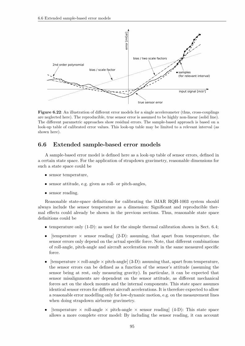
6.6 Extended sample-based error models
input signal [m/s²]
err
or
[mG
al]
samples
(for relevant interval)
true sensor error
bias / scale factor
bias / two scale factors
2nd order polynomial
Figure 6.22: An illustration of different error models for a single accelerometer (thus, cross-couplingsare neglected here). The reproducible, true sensor error is assumed to be highly non-linear (solid line).The different parametric approaches show residual errors. The sample-based approach is based on alook-up table of calibrated error values. This look-up table may be limited to a relevant interval (asshown here).
6.6 Extended sample-based error models
A sample-based error model is defined here as a look-up table of sensor errors, defined ina certain state space. For the application of strapdown gravimetry, reasonable dimensions forsuch a state space could be
• sensor temperature,
• sensor attitude, e.g. given as roll- or pitch-angles,
• sensor reading.
Reasonable state-space definitions for calibrating the iMAR RQH-1003 system shouldalways include the sensor temperature as a dimension: Significant and reproducible ther-mal effects could already be shown in the previous sections. Thus, reasonable state spacedefinitions could be
• temperature only (1-D): as used for the simple thermal calibration shown in Sect. 6.4;
• [temperature × sensor reading] (2-D): assuming, that apart from temperature, thesensor errors only depend on the actual specific force. Note, that different combinationsof roll-angle, pitch-angle and aircraft acceleration result in the same measured specificforce.
• [temperature × roll-angle × pitch-angle] (3-D): assuming that, apart from temperature,the sensor errors can be defined as a function of the sensor’s attitude (assuming thesensor being at rest, only measuring gravity). In particular, it can be expected thatsensor misalignments are dependent on the sensor attitude, as different mechanicalforces act on the shock mounts and the internal components. This state space assumesidentical sensor errors for different aircraft accelerations. It is therefore expected to allowa reasonable error modelling only for low-dynamic motion, e.g. on the measurement lineswhen doing strapdown airborne gravimetry.
• [temperature × roll-angle × pitch-angle × sensor reading] (4-D): This state spaceallows a more complete error model: By including the sensor reading, it can account
95
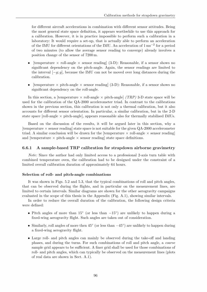
Calibration methods for strapdown gravimetry
for different aircraft accelerations in combination with different sensor attitudes. Beingthe most general state space definition, it appears worthwhile to use this approach fora calibration. However, it is in practice impossible to perform such a calibration in alaboratory: It would require a set-up, that is actually able to perform an accelerationof the IMU for different orientations of the IMU. An acceleration of 1ms−2 for a periodof two minutes (to allow the average sensor reading to converge) already involves aposition change of the sensor of 7200m.
• [temperature × roll-angle × sensor reading] (3-D): Reasonable, if a sensor shows nosignificant dependency on the pitch-angle. Again, the sensor readings are limited tothe interval [−g; g], because the IMU can not be moved over long distances during thecalibration.
• [temperature × pitch-angle × sensor reading] (3-D): Reasonable, if a sensor shows nosignificant dependency on the roll-angle.
In this section, a [temperature × roll-angle × pitch-angle] (TRP) 3-D state space will beused for the calibration of the QA-2000 accelerometer triad. In contrast to the calibrationsshown in the previous section, this calibration is not only a thermal calibration, but it alsoaccounts for different sensor orientation. In particular, a similar calibration, but in the 2-Dstate space [roll-angle × pitch-angle], appears reasonable also for thermally stabilised IMUs.
Based on the discussion of the results, it will be argued later in this section, why a[temperature × sensor reading] state space is not suitable for the given QA-2000 accelerometertriad. A similar conclusion will be drawn for the [temperature × roll-angle × sensor reading]and [temperature × pitch-angle × sensor reading] state space definitions.
6.6.1 A sample-based TRP calibration for strapdown airborne gravimetry
Note: Since the author had only limited access to a professional 2-axis turn table withcombined temperature oven, the calibration had to be designed under the constraint of alimited overall calibration duration of approximately 64 hours.
Selection of roll- and pitch-angle combinations
It was shown in Figs. 5.2 and 5.3, that the typical combinations of roll and pitch angles,that can be observed during the flights, and in particular on the measurement lines, arelimited to certain intervals. Similar diagrams are shown for the other aerogravity campaignsevaluated in the scope of this thesis in the Appendix (Fig. A.1), showing similar intervals.
In order to reduce the overall duration of the calibration, the following design criteriawere defined:
• Pitch angles of more than 15 (or less than −15) are unlikely to happen during afixed-wing aerogravity flight. Such angles are taken out of consideration.
• Similarly, roll angles of more then 45 (or less than −45) are unlikely to happen duringa fixed-wing aerogravity flight.
• Large roll- and pitch angles can mainly be observed during the take-off and landingphases, and during the turns. For such combinations of roll and pitch angle, a coarsesample grid appears to be sufficient. A finer grid shall be used for those combinations ofroll- and pitch angles, which can typically be observed on the measurement lines (plotsof real data are shown in Sect. A.1).
96
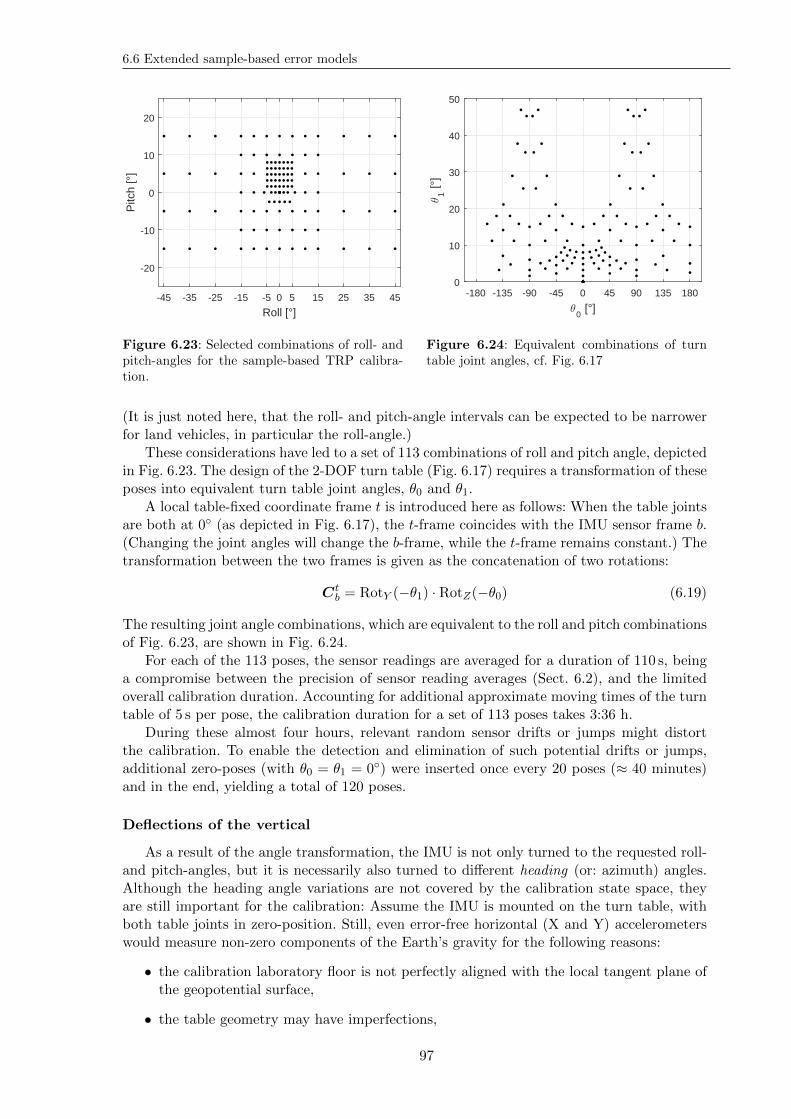
6.6 Extended sample-based error models
-45 -35 -25 -15 -5 0 5 15 25 35 45
Roll [°]
-20
-10
0
10
20P
itch
[°]
Figure 6.23: Selected combinations of roll- andpitch-angles for the sample-based TRP calibra-tion.
-180 -135 -90 -45 0 45 90 135 180
θ0 [°]
0
10
20
30
40
50
θ1 [°
]
Figure 6.24: Equivalent combinations of turntable joint angles, cf. Fig. 6.17
(It is just noted here, that the roll- and pitch-angle intervals can be expected to be narrowerfor land vehicles, in particular the roll-angle.)
These considerations have led to a set of 113 combinations of roll and pitch angle, depictedin Fig. 6.23. The design of the 2-DOF turn table (Fig. 6.17) requires a transformation of theseposes into equivalent turn table joint angles, θ0 and θ1.
A local table-fixed coordinate frame t is introduced here as follows: When the table jointsare both at 0 (as depicted in Fig. 6.17), the t-frame coincides with the IMU sensor frame b.(Changing the joint angles will change the b-frame, while the t-frame remains constant.) Thetransformation between the two frames is given as the concatenation of two rotations:
Ctb = RotY (−θ1) · RotZ(−θ0) (6.19)
The resulting joint angle combinations, which are equivalent to the roll and pitch combinationsof Fig. 6.23, are shown in Fig. 6.24.
For each of the 113 poses, the sensor readings are averaged for a duration of 110 s, beinga compromise between the precision of sensor reading averages (Sect. 6.2), and the limitedoverall calibration duration. Accounting for additional approximate moving times of the turntable of 5 s per pose, the calibration duration for a set of 113 poses takes 3:36 h.
During these almost four hours, relevant random sensor drifts or jumps might distortthe calibration. To enable the detection and elimination of such potential drifts or jumps,additional zero-poses (with θ0 = θ1 = 0) were inserted once every 20 poses (≈ 40 minutes)and in the end, yielding a total of 120 poses.
Deflections of the vertical
As a result of the angle transformation, the IMU is not only turned to the requested roll-and pitch-angles, but it is necessarily also turned to different heading (or: azimuth) angles.Although the heading angle variations are not covered by the calibration state space, theyare still important for the calibration: Assume the IMU is mounted on the turn table, withboth table joints in zero-position. Still, even error-free horizontal (X and Y) accelerometerswould measure non-zero components of the Earth’s gravity for the following reasons:
• the calibration laboratory floor is not perfectly aligned with the local tangent plane ofthe geopotential surface,
• the table geometry may have imperfections,
97
Calibration methods for strapdown gravimetry
• the mounting of the IMU may involve small angular errors, and
• the ISA sensor package may have a constant offset with respect to the nominal axes ofthe IMU, which are defined by the surfaces of the housing.
While the n-frame was defined based on the normal plumb line direction, another auxiliaryframe n′ is introduced here: the zn
′axis is pointing downward along the true local plumb line
of the gravity field. The xn′-axis is the projection of the xt axis onto the local tangent plane
of the actual plumb line. Equivalently, the yn′-axis is the projection of the yt axis onto the
local tangent plane. Note, that the n′-frame is not aligned with the local North- and East-directions. Instead, the xn
′and yn
′axes are basically aligned with the (arbitrary) directions
of the turn table, xt and yt.Thus, the t-frame and the n′-frame only differ by small deflections ξ′ and η′, which are
superpositions of the different inseparable effects listed above. The coordinate transformationbetween both frames can be accomplished with a small angle approximation using
Cn′t = RotX(η
′) · RotY (ξ′) ≈
1 0 −ξ′
0 1 η′
ξ′ −η′ 1
. (6.20)
The reference gravity is then given with Eq. 6.16 as
gn′
ref =
0
0
gref,IMU
, and (6.21)
gtref = (Cn′t )Tgn
′ref . (6.22)
Finally, for each of the different poses, the accelerometer readings fbwill be compared
against the reference gravity, which needs to be transformed into the b-frame:
δfb= f
b+ (Ct
b)T (Cn′
t )Tgn′
ref (6.23)
The result of the calibration is then a set of three look-up tables (one per accelerometer),containing the residuals δfa for different combinations of temperature, roll and pitch angles(with a ∈ X,Y, Z).
For the determination of the deflections ξ′ and η′, three additional poses are added to thecalibration program, basically rotating the IMU at θ1 = 0 around its vertical axis by stepsof ∆θ0 = 90. The last four poses of the program then are
1. θ0 = θ1 = 0
2. θ0 = 90, θ1 = 0
3. θ0 = 180, θ1 = 0
4. θ0 = 270, θ1 = 0,
each of them averaged over a slightly longer period of 180 s.A least-squares adjustment is then carried out based on the observations of the horizontal
accelerometers, gXi and gXi , in order to estimate ξ′ and η′. For this adjustment, random sensoroffsets oX and oY , which are assumed to be constant among the four observations, have tobe accounted for. This yields a four-element vector of parameters:
x =(ξ′ η′ oX oY
)T. (6.24)
98
6.6 Extended sample-based error models
Using the common notation, the observation equation is then given with the design matrixA and the vector of residuals v as
L = Ax− v =
1 0 1 0
0 −1 0 1
0 1 1 0
1 0 0 1
−1 0 1 0
0 1 0 1
0 −1 1 0
−1 0 0 1
ξ′
η′
oX
oY
− v =
gX1gY1gX2gY2gX3gY3gX4gY4
(6.25)
Temperature setting
The set of 123 poses as introduced above is repeated for a set of oven temperatures.It could be seen in Sect. 6.5.1, that a temperature spacing of 10K may be too coarse fora reasonable interpolation. Given the limited overall calibration time, the following oventemperature settings were selected:
• A spacing of 5K is used for lower temperatures, which are in practice mainly requiredfor the warming-up phases of the IMU: −15C, −10C, −5C, 0C, 5C, 10C, 15C,and 20C;
• A finer spacing of 3K is used for the predominant ambient temperatures that can beobserved during actual gravity surveys: (20C,) 23C, 26C, 29C, 32C, 35C, 38C,and 41C.
Note, that the internal ISA temperature is typically 10K to 15K higher compared to theambient air temperature.
The three-dimensional look-up table will allow arbitrary combinations of temperature,roll-, and pitch-angle. Thus, the requirement of an identical temperature for all poses of a set(as for the parametric calibrations) can be relaxed. For each of the sensor readings (averagedover 110 s), also the average ISA temperature will be used. Still, strong temperatures gradientsare to be avoided, to reduce thermal latency effects (as discussed in Sect. 6.4).
For the initial oven temperature setting (−15C), three hours were given to let the ISAtemperature stabilize. Then, for each of the 5K steps, a temperature stabilisation periodof 25 minutes was added, and 15 minutes for each of the 3K steps. This yields an overallcalibration duration of approximately 64 hours.
Note: The actual calibration took 76 hours, because the maximum angular speed forthe table joint motors were by mistake set to low numbers, resulting in an additional timerequirement of almost 12 hours.
Implementation
The calibration was carried out between March 11th and March 14th, 2016. The nomi-nal oven temperature settings and the actual ISA temperature measurements are shown inFig. 6.25. After the thermal stabilisation period (25 or 15 minutes), the measured oven tem-peratures differed by less than 0.2K from the nominal temperature. These differences are notrelevant for the calibration, which is anyway based on the ISA temperature measurement. Itcan be seen, that it takes several hours for the ISA temperature to stabilise. Thus, for the setsof 123 poses each, the ISA temperature is slightly increasing among the poses (decreasing forthe first set, cf. Fig. 6.25). For the last four poses of each set, the temperature was nearly
99
Calibration methods for strapdown gravimetry
0 20 40 60 80
hours since first measurement
-10
0
10
20
30
40
50
tem
pera
ture
[°C
]
ISA temperaturenominal oven temperature
Figure 6.25: Nominal oven temperatures, andmeasured ISA sensor temperatures.
-10 0 10 20 30 40
nominal oven temperature [°C]
-1
0
1
2
3
4
5
6
defle
ctio
ns ["
] / σ
v [mG
al]
ξ 'η'
σv
Figure 6.26: Deflections between the n′ and thet coordinate frames, as determined from the lastfour poses of each set. The empirical standarddeviations of the residuals σv are shown in unitsof mGal.
constant (σ < 0.1C), allowing the assumption of constant sensor offsets oX and oY for thedetermination of the deflections ξ′ and η′.
The estimated deflections are shown in Fig. 6.26. In order to keep the deflections low, thezero-levels of the joint angle sensors were re-calibrated based on the accelerometer outputs,shortly before the first measurements. Indeed, the initial deflections are close to zero. Whileξ′ shows a temperature dependency, η′ remains rather stable. The residuals v are slightlyhigher for the lower temperatures. The empirical standard deviations of the residuals, σv, arealso shown in Fig. 6.26, being in accordance with the expected noise level of the accelerometermeasurements (cf. Sect. 6.2).
With Fig. 4.4, it can be seen, that these deflections are indeed relevant for the calibration.For example, a deflection of ξ′ = 5 arc seconds shows up in the horizontal accelerometermeasurements at a magnitude of ≈20mGal.
Look-up table generation
The resulting look-up tables (one per accelerometer) contain 1695 entries each (113 mea-surements of δf b for each of the 15 nominal temperatures). A special interpolation methodfor scattered three-dimensional sample data, based on a Delaunay triangulation, is used tointerpolate these entries to any state space coordinate (temperature, roll, pitch).
The entries of the look-up table still contain significant noise (cf. Sect. 6.2). In order toenable a two-dimensional low-pass filtering, the scattered table data is transformed into aregular 3-D grid, with a finer sample spacing (1K, and 0.25 for roll and pitch). Based onthe Allan standard deviations shown in Sect. 6.2, a two-dimensional Gaussian low-pass filteris applied for each temperature level.
The low-pass filtered regular 3-D grids are shown in Figs. 6.27, 6.28, and 6.29, for aselection of ISA temperatures.
Results and Discussion
The figures indicate strong effects for different attitudes, up to ±100mGal for larger rolland pitch angles. The shown errors are the superposition of all error types: biases, scalefactors, any non-linear sensor errors, cross-couplings, and triad-misalignments. For almost
100
6.6 Extended sample-based error models
Front-axis, 0°CσG=5°
-40 -20 0 20 40
Roll angle [°]
-10
-5
0
5
10
Pitc
h an
gle
[°]
-150 mGal
-125 mGal
-100 mGal
-75 mGal
-50 mGal
-25 mGal
0 mGalFront-axis, 10°CσG=5°
-40 -20 0 20 40
Roll angle [°]
-10
-5
0
5
10
Pitc
h an
gle
[°]
-150 mGal
-125 mGal
-100 mGal
-75 mGal
-50 mGal
-25 mGal
0 mGal
Front-axis, 20°CσG=5°
-40 -20 0 20 40
Roll angle [°]
-10
-5
0
5
10
Pitc
h an
gle
[°]
-150 mGal
-125 mGal
-100 mGal
-75 mGal
-50 mGal
-25 mGal
0 mGalFront-axis, 30°CσG=5°
-40 -20 0 20 40
Roll angle [°]
-10
-5
0
5
10
Pitc
h an
gle
[°]
-150 mGal
-125 mGal
-100 mGal
-75 mGal
-50 mGal
-25 mGal
0 mGal
Front-axis, 40°CσG=5°
-40 -20 0 20 40
Roll angle [°]
-10
-5
0
5
10
Pitc
h an
gle
[°]
-150 mGal
-125 mGal
-100 mGal
-75 mGal
-50 mGal
-25 mGal
0 mGalFront-axis, 50°CσG=5°
-40 -20 0 20 40
Roll angle [°]
-10
-5
0
5
10
Pitc
h an
gle
[°]
-150 mGal
-125 mGal
-100 mGal
-75 mGal
-50 mGal
-25 mGal
0 mGal
Figure 6.27: Look-up table of sensor errors for the X-accelerometer (pointing to the front for thestandard mounting in a vehicle). A two-dimensional Gaussian low pass filter with σG = 5 was applied.
101
Calibration methods for strapdown gravimetry
Left-axis, 0°CσG=5°
-40 -20 0 20 40
Roll angle [°]
-10
-5
0
5
10
Pitc
h an
gle
[°]
0 mGal
25 mGal
50 mGal
75 mGal
100 mGalLeft-axis, 10°CσG=5°
-40 -20 0 20 40
Roll angle [°]
-10
-5
0
5
10
Pitc
h an
gle
[°]
0 mGal
25 mGal
50 mGal
75 mGal
100 mGal
Left-axis, 20°CσG=5°
-40 -20 0 20 40
Roll angle [°]
-10
-5
0
5
10
Pitc
h an
gle
[°]
0 mGal
25 mGal
50 mGal
75 mGal
100 mGalLeft-axis, 30°CσG=5°
-40 -20 0 20 40
Roll angle [°]
-10
-5
0
5
10
Pitc
h an
gle
[°]
0 mGal
25 mGal
50 mGal
75 mGal
100 mGal
Left-axis, 40°CσG=5°
-40 -20 0 20 40
Roll angle [°]
-10
-5
0
5
10
Pitc
h an
gle
[°]
0 mGal
25 mGal
50 mGal
75 mGal
100 mGalLeft-axis, 50°CσG=5°
-40 -20 0 20 40
Roll angle [°]
-10
-5
0
5
10
Pitc
h an
gle
[°]
0 mGal
25 mGal
50 mGal
75 mGal
100 mGal
Figure 6.28: Look-up table of sensor errors for the Y-accelerometer (pointing to the left for thestandard mounting in a vehicle). A two-dimensional Gaussian low pass filter with σG = 5 wasapplied.
102
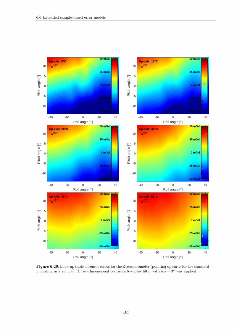
6.6 Extended sample-based error models
Up-axis, 0°CσG=3°
-40 -20 0 20 40
Roll angle [°]
-10
-5
0
5
10
Pitc
h an
gle
[°]
-50 mGal
-25 mGal
0 mGal
25 mGal
50 mGalUp-axis, 10°CσG=3°
-40 -20 0 20 40
Roll angle [°]
-10
-5
0
5
10
Pitc
h an
gle
[°]
-50 mGal
-25 mGal
0 mGal
25 mGal
50 mGal
Up-axis, 20°CσG=3°
-40 -20 0 20 40
Roll angle [°]
-10
-5
0
5
10
Pitc
h an
gle
[°]
-50 mGal
-25 mGal
0 mGal
25 mGal
50 mGalUp-axis, 30°CσG=3°
-40 -20 0 20 40
Roll angle [°]
-10
-5
0
5
10
Pitc
h an
gle
[°]
-50 mGal
-25 mGal
0 mGal
25 mGal
50 mGal
Up-axis, 40°CσG=3°
-40 -20 0 20 40
Roll angle [°]
-10
-5
0
5
10
Pitc
h an
gle
[°]
-50 mGal
-25 mGal
0 mGal
25 mGal
50 mGalUp-axis, 50°CσG=3°
-40 -20 0 20 40
Roll angle [°]
-10
-5
0
5
10
Pitc
h an
gle
[°]
-50 mGal
-25 mGal
0 mGal
25 mGal
50 mGal
Figure 6.29: Look-up table of sensor errors for the Z-accelerometer (pointing upwards for the standardmounting in a vehicle). A two-dimensional Gaussian low pass filter with σG = 3 was applied.
103
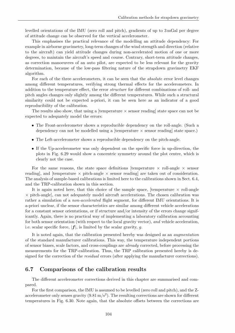
Calibration methods for strapdown gravimetry
levelled orientations of the IMU (zero roll and pitch), gradients of up to 3mGal per degreeof attitude change can be observed for the vertical accelerometer.
This emphasises the practical relevance of the modelling an attitude dependency: Forexample in airborne gravimetry, long-term changes of the wind strength and direction (relativeto the aircraft) can yield attitude changes during non-accelerated motion of one or moredegrees, to maintain the aircraft’s speed and course. Contrary, short-term attitude changes,as correction manoeuvres of an auto pilot, are expected to be less relevant for the gravitydetermination, because of the low-pass filtering nature of the strapdown gravimetry EKFalgorithm.
For each of the three accelerometers, it can be seen that the absolute error level changesamong different temperatures, verifying strong thermal effects for the accelerometers. Inaddition to the temperature effect, the error structure for different combinations of roll- andpitch angles changes only slightly among the different temperatures. While such a structuralsimilarity could not be expected a-priori, it can be seen here as an indicator of a goodreproducibility of the calibration.
The results also show, that using a [temperature × sensor reading] state space can not beexpected to adequately model the errors:
• The Front-accelerometer shows a reproducible dependency on the roll-angle. (Such adependency can not be modelled using a [temperature × sensor reading] state space.)
• The Left-accelerometer shows a reproducible dependency on the pitch-angle.
• If the Up-accelerometer was only dependent on the specific force in up-direction, theplots in Fig. 6.29 would show a concentric symmetry around the plot centre, which isclearly not the case.
For the same reasons, the state space definitions [temperature × roll-angle × sensorreading], and [temperature × pitch-angle × sensor reading] are taken out of consideration.The analysis of sample-based calibrations is limited here to the calibrations shown in Sect. 6.4,and the TRP-calibration shown in this section.
It is again noted here, that this choice of the sample space, [temperature × roll-angle× pitch-angle], can not adequately model aircraft accelerations. The chosen calibration wasrather a simulation of a non-accelerated flight segment, for different IMU orientations. It isa-priori unclear, if the sensor characteristics are similar among different vehicle accelerationsfor a constant sensor orientations, or if structure and/or intensity of the errors change signif-icantly. Again, there is no practical way of implementing a laboratory calibration accountingfor both sensor orientation (with respect to the local gravity vector), and vehicle acceleration,i.e. scalar specific force, |f |, is limited by the scalar gravity, g.
It is noted again, that the calibration presented hereby was designed as an augmentationof the standard manufacturer calibrations. This way, the temperature independent portionsof sensor biases, scale factors, and cross-couplings are already corrected, before processing themeasurements for the TRP-calibration. Thus, the TRP calibration presented hereby is de-signed for the correction of the residual errors (after applying the manufacturer corrections).
6.7 Comparisons of the calibration results
The different accelerometer corrections derived in this chapter are summarised and com-pared.
For the first comparison, the IMU is assumed to be levelled (zero roll and pitch), and the Z-accelerometer only senses gravity (9.81m/s2). The resulting corrections are shown for differenttemperatures in Fig. 6.30. Note again, that the absolute offsets between the corrections are
104
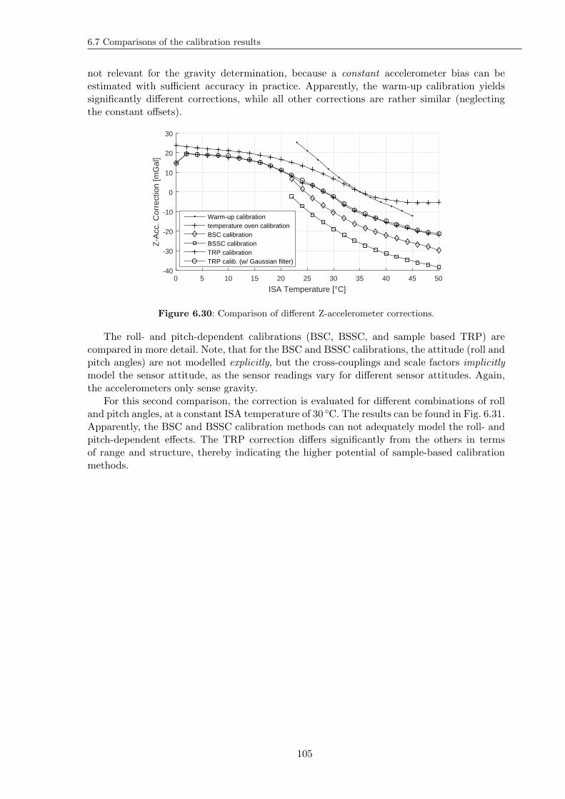
6.7 Comparisons of the calibration results
not relevant for the gravity determination, because a constant accelerometer bias can beestimated with sufficient accuracy in practice. Apparently, the warm-up calibration yieldssignificantly different corrections, while all other corrections are rather similar (neglectingthe constant offsets).
0 5 10 15 20 25 30 35 40 45 50
ISA Temperature [°C]
-40
-30
-20
-10
0
10
20
30
Z-A
cc. C
orre
ctio
n [m
Gal
]
Warm-up calibrationtemperature oven calibrationBSC calibrationBSSC calibrationTRP calibrationTRP calib. (w/ Gaussian filter)
Figure 6.30: Comparison of different Z-accelerometer corrections.
The roll- and pitch-dependent calibrations (BSC, BSSC, and sample based TRP) arecompared in more detail. Note, that for the BSC and BSSC calibrations, the attitude (roll andpitch angles) are not modelled explicitly, but the cross-couplings and scale factors implicitlymodel the sensor attitude, as the sensor readings vary for different sensor attitudes. Again,the accelerometers only sense gravity.
For this second comparison, the correction is evaluated for different combinations of rolland pitch angles, at a constant ISA temperature of 30 C. The results can be found in Fig. 6.31.Apparently, the BSC and BSSC calibration methods can not adequately model the roll- andpitch-dependent effects. The TRP correction differs significantly from the others in termsof range and structure, thereby indicating the higher potential of sample-based calibrationmethods.
105
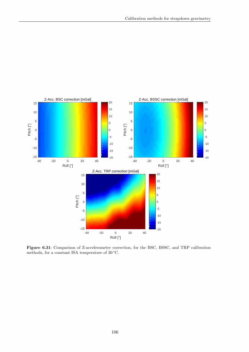
Calibration methods for strapdown gravimetry
Z-Acc. BSC correction [mGal]
-40 -20 0 20 40
Roll [°]
-15
-10
-5
0
5
10
15
Pitc
h [°
]
-20
-15
-10
-5
0
5
10
15
20Z-Acc. BSSC correction [mGal]
-40 -20 0 20 40
Roll [°]
-15
-10
-5
0
5
10
15
Pitc
h [°
]
-20
-15
-10
-5
0
5
10
15
20
Z-Acc. TRP correction [mGal]
-40 -20 0 20 40
Roll [°]
-15
-10
-5
0
5
10
15
Pitc
h [°
]
-20
-15
-10
-5
0
5
10
15
20
Figure 6.31: Comparison of Z-accelerometer correction, for the BSC, BSSC, and TRP calibrationmethods, for a constant ISA temperature of 30 C.
106
Chapter 7
Quality assessment
As a preparation for Chap. 8, different existing evaluation methods of airborne gravimetrywill be briefly introduced and discussed.
The chapter is split into two parts: the internal quality assessment for the determinationof the precision of the gravity data, and the comparison against external reference data forthe accuracy determination.
7.1 Internal quality assessment
7.1.1 Cross-over residuals
The cross-over point residual analysis is one of the most common quality assessmentprocedures in airborne gravimetry. It is based on the assumption, that gravity is constantover time for any given earth-fixed point. The vector difference of the individual gravityestimates at an intersection of two flight tracks A and B (a cross-over point) are the basisfor this quality measure:
χ′A,B = gA − gB = −χ′
B,A . (7.1)
Typically, the North- and East-components of these vector residuals are transformed fromunits of mGal into arc seconds (Eq. 1.5). The scalar equivalent of Eq. 7.1 is given as
χ′A,B = gA − gB = −χ′
B,A . (7.2)
The gravity at a given point is in fact time-varying:
1. Tides depend mainly on the positions of the Moon and the sun with respect to a localcoordinate frame. This effect reaches a level of ±150µGal (Torge, 1989), and is thereforeusually neglected for airborne gravity at accuracy levels of >1mGal.
2. Seasonal effects, mainly coming from hydrological effects, as different ground-waterlevels and ocean loading effects, constitute an overall effect of less than ±30µGal (Torge,1989), and are therefore also neglected. The same holds for deformations of the Earth’scrust (Earth tides).
3. The nutation, precession, and drift of the Earth’s axis of revolution yields small changesin the centrifugal acceleration (which is by definition included in the gravity). Sucheffects are even smaller (less than ±10µGal), and are also neglected (Torge, 1989).
4. The Earth’s atmospheric masses also contribute to the measured gravity. The air pres-sure, reflecting the local density of the Earth’s atmosphere, is also a time-varying quan-tity. The gravitational effect of such density variations is also smaller than ±10µGal(Torge, 1989).
107
Quality assessment
These time-varying effects are therefore negligible, and the assumption of constant gravityat a given point is valid for the expected accuracy level of airborne gravimetry of 1mGal ormore.
Full bandwidth comparison
An important property of the cross-over point residual analysis is, that the full spectrumof the estimated gravity signal is taken into account. In particular, an along-track low-passfiltering of the estimated gravity will yield an increase of the cross-over residuals, if moresignal than noise is filtered out, and if the two along-track signals are uncorrelated (or onlyweakly correlated). This effect is for example evident in the results presented in Glennie andSchwarz (1999). The requirement of uncorrelated signals is true for orthogonal measurementline intersections, and the correlation can still be assumed to be sufficiently small for thetypical intersection angles of 60−120. This invariance against the parameters of the along-track low-pass filtering of the gravity data allows the use of a single value as a meaningfulmetric.
Note: An along-track low-pass filtering is generally applied to airborne gravity data. Thisis either done explicitly, or implicitly by applying a Kalman Filter (which in fact acts asa low-pass filter). The nature of the used sensors does not allow the gravity determinationwithout applying a low-pass filter. This emphasises, that the invariance against the low-passfilter parameters is a desirable property for a quality metric.
Vertical offset and gravity gradient
Three-dimensional flight trajectories never intersect exactly at the same point: In practice,relevant differences in altitude can be observed. Even for identical nominal flight altitudes,vertical offsets of up to ∆h = 100m can be observed, coming from air-pressure based altitudedefinitions used for the aircraft navigation system, as it is common for aviation.
Obviously, the free-air gravity gradient of ∂g/∂h ≈ 309µGal/m then yields differentgravity values for the two individual flights. However, when comparing gravity disturbances,being gravity residuals with respect to the normal gravity field (as introduced in Chap. 3),the majority of this effect will be accounted for by the normal gravity gradient ∂γ/∂h. Thecross-over residual for the true gravity disturbances dgA and dgB is still non-zero, if the truegravity gradient differs from the normal gravity gradient:
χA,B = dgA − dgB= gA − γA − gB + γB
≈ gA − γA − gA +∂g
∂h
∣∣∣∣A,B
∆hA,B + γB
= gA − γA − gA +∂(γ + dg)
∂h
∣∣∣∣A,B
∆hA,B + γB
= −γA + γB +
(∂γ
∂h
∣∣∣∣A,B
+∂dg
∂h
∣∣∣∣A,B
)∆hA,B
≈ −γA + γA − ∂γ
∂h
∣∣∣∣A,B
∆hA,B +
(∂γ
∂h
∣∣∣∣A,B
+∂dg
∂h
∣∣∣∣A,B
)∆hA,B
=∂dg
∂h
∣∣∣∣A,B
∆hA,B ,
(7.3)
where∣∣A,B
denotes mean quantities along the local normal plumb line, between the points Aand B.
108
7.1 Internal quality assessment
In practice, the vertical free air gravity gradient disturbance ∂dgDown/∂h can reach±100µGal/m and more on the topography, while the horizontal gradients ∂dgNorth/∂h and∂dgEast/∂h are significantly smaller (Torge, 1989).
For the aerogravity data sets evaluated in Chap. 8, the impact of the topography on thethree diagonal components of the gravity gradient tensor at flight altitude were computedusing the software GRAVSOFT TC (Tscherning et al., 1992). The Chile campaign data setis used here to provide a exemplary magnitudes: The topography-induced horizontal gravitygradients are in the range of ±30µGal/m. The respective vertical gradient disturbance rangesfrom −80µGal/m to 130µGal/m. (These examples are shown here just to provide an orderof magnitude.)
The vertical cross-over offset ∆h can reach hundreds of metres or more in practice. Thus,the gravity gradient disturbance indeed yields relevant errors for the cross-over analysis. Thisproblem may be coped by two different strategies:
1. By limiting the vertical offsets ∆h to a certain limit ∆hmax, as e.g. 100m. Cross-over points with larger vertical offsets will not be used for the quality assessment. Inpractice, this can significantly reduce the number of available cross-over points, therebyincreasing the statistical uncertainty of the method.
2. By estimating the vertical gravity gradient based on a geoid model. Note, that this mayintroduce uncertainties, depending on the quality of the available geoid model.
In the scope of this thesis, the first strategy will be pursued, due to the lack of sufficientlyaccurate geoid models for the investigated regions.
Cross-over adjustment
It is a rather common procedure in airborne gravimetry to apply a so-called cross-overadjustment (or sometimes cross-over levelling, network adjustment, or just adjustment) toa set of measurement lines. Based on the cross-over points of the whole set, a constant,three-dimensional shift κ is computed for each measurement line, such that
• either the sum of squares of the cross-over residuals along a measurement line is min-imised (second moments), or
• the mean residual of all cross-over-points along a measurement line becomes zero (firstmoments).
The results are similar in practice, unless strong outliers are in the data. (Note, that theshifts κ are scalar (1-D) when doing scalar gravimetry.)
The adjusted cross-over residuals χ are given for an intersection of the i-th cross overpoint on line A and the j-th cross-over point on line B as
χA,B = (dgAi+ κA)− (dgBj
+ κB) . (7.4)
The statistics for an adjusted line, or for an adjusted campaign data set, is then commonlycomputed as the root-mean-square (RMS) of the adjusted cross-over residuals: RMS(χi).
The computation of the line-shifts κ can be performed using a least-squares adjustmentof the cross-over residuals. The adjusted cross-over residuals χ may then be regarded as aper-line-precision of the gravity data. Comparing χ against χ (where necessarily χ ≤ χ)may provide insight in the characteristics of the gravity estimation errors. Such a comparisoncan be done separately for each component of the gravity vector estimates, therefore a scalardefinition is sufficient here:
τ =χ
χ, where 0 ≤ τ ≤ 1 . (7.5)
109
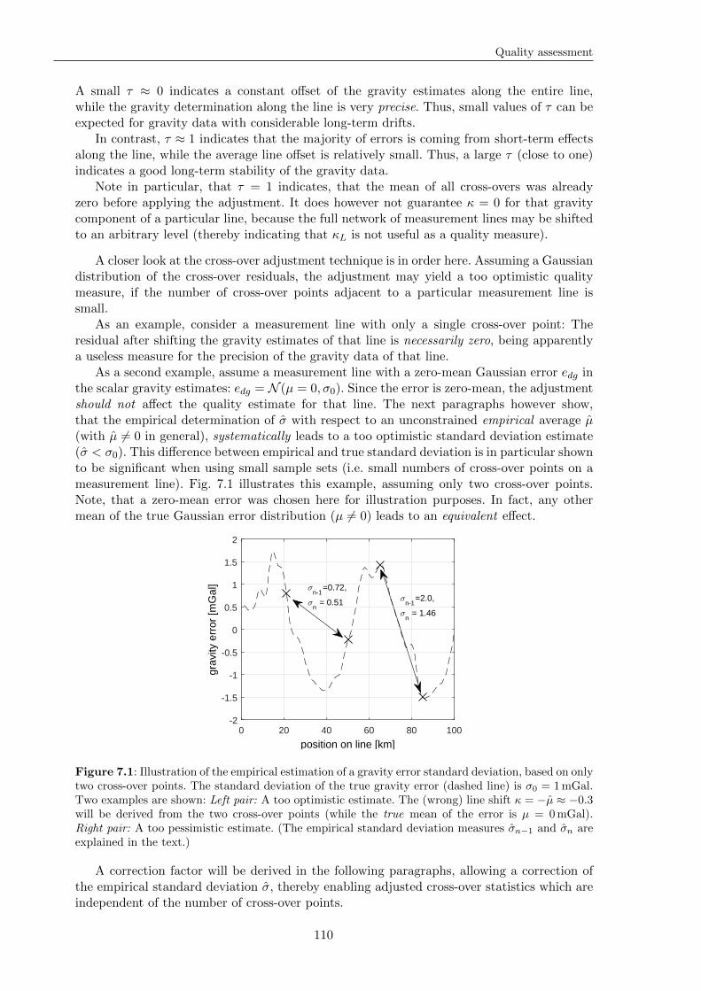
Quality assessment
A small τ ≈ 0 indicates a constant offset of the gravity estimates along the entire line,while the gravity determination along the line is very precise. Thus, small values of τ can beexpected for gravity data with considerable long-term drifts.
In contrast, τ ≈ 1 indicates that the majority of errors is coming from short-term effectsalong the line, while the average line offset is relatively small. Thus, a large τ (close to one)indicates a good long-term stability of the gravity data.
Note in particular, that τ = 1 indicates, that the mean of all cross-overs was alreadyzero before applying the adjustment. It does however not guarantee κ = 0 for that gravitycomponent of a particular line, because the full network of measurement lines may be shiftedto an arbitrary level (thereby indicating that κL is not useful as a quality measure).
A closer look at the cross-over adjustment technique is in order here. Assuming a Gaussiandistribution of the cross-over residuals, the adjustment may yield a too optimistic qualitymeasure, if the number of cross-over points adjacent to a particular measurement line issmall.
As an example, consider a measurement line with only a single cross-over point: Theresidual after shifting the gravity estimates of that line is necessarily zero, being apparentlya useless measure for the precision of the gravity data of that line.
As a second example, assume a measurement line with a zero-mean Gaussian error edg inthe scalar gravity estimates: edg = N (µ = 0, σ0). Since the error is zero-mean, the adjustmentshould not affect the quality estimate for that line. The next paragraphs however show,that the empirical determination of σ with respect to an unconstrained empirical average µ(with µ 6= 0 in general), systematically leads to a too optimistic standard deviation estimate(σ < σ0). This difference between empirical and true standard deviation is in particular shownto be significant when using small sample sets (i.e. small numbers of cross-over points on ameasurement line). Fig. 7.1 illustrates this example, assuming only two cross-over points.Note, that a zero-mean error was chosen here for illustration purposes. In fact, any othermean of the true Gaussian error distribution (µ 6= 0) leads to an equivalent effect.
0 20 40 60 80 100
position on line [km]
-2
-1.5
-1
-0.5
0
0.5
1
1.5
2
grav
ity e
rror
[mG
al] σ
n-1=0.72,
σn = 0.51 σ
n-1=2.0,
σn = 1.46
Figure 7.1: Illustration of the empirical estimation of a gravity error standard deviation, based on onlytwo cross-over points. The standard deviation of the true gravity error (dashed line) is σ0 = 1mGal.Two examples are shown: Left pair: A too optimistic estimate. The (wrong) line shift κ = −µ ≈ −0.3will be derived from the two cross-over points (while the true mean of the error is µ = 0mGal).Right pair: A too pessimistic estimate. (The empirical standard deviation measures σn−1 and σn areexplained in the text.)
A correction factor will be derived in the following paragraphs, allowing a correction ofthe empirical standard deviation σ, thereby enabling adjusted cross-over statistics which areindependent of the number of cross-over points.
110
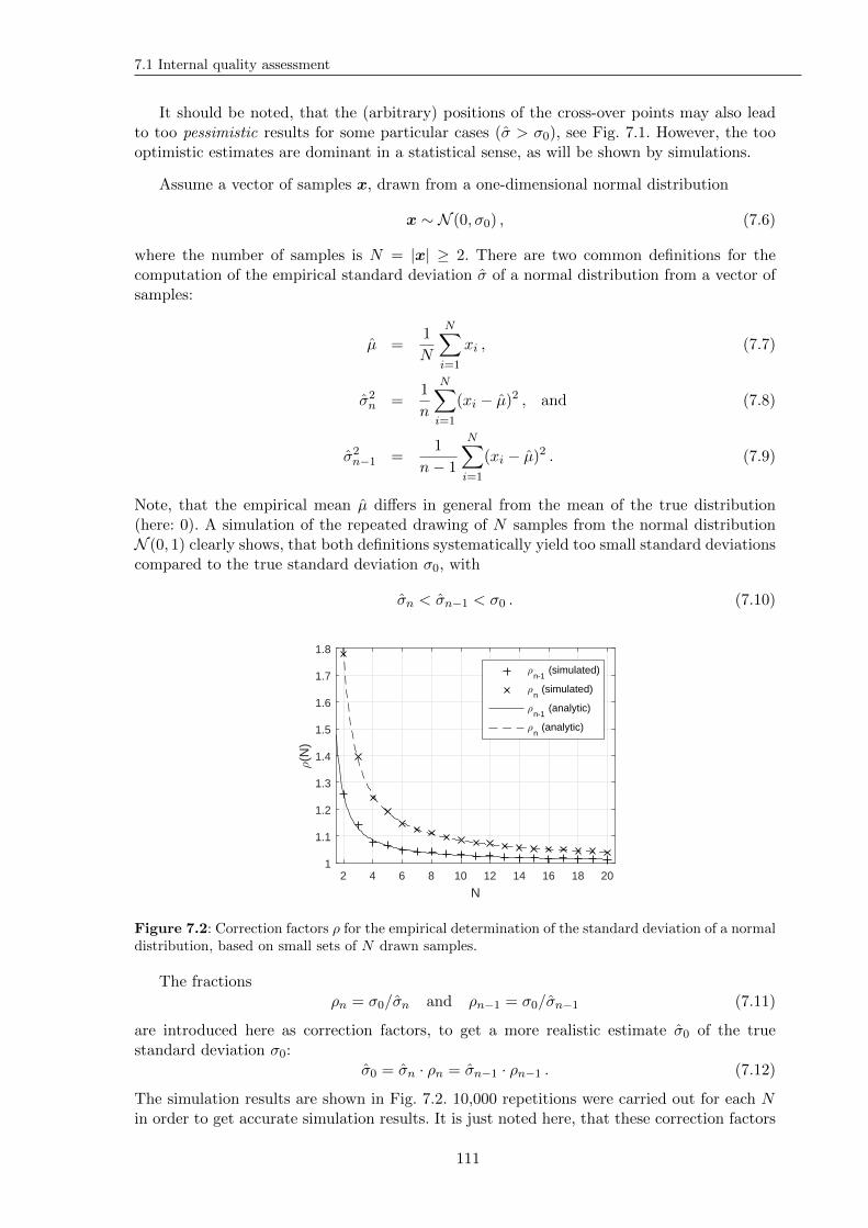
7.1 Internal quality assessment
It should be noted, that the (arbitrary) positions of the cross-over points may also leadto too pessimistic results for some particular cases (σ > σ0), see Fig. 7.1. However, the toooptimistic estimates are dominant in a statistical sense, as will be shown by simulations.
Assume a vector of samples x, drawn from a one-dimensional normal distribution
x ∼ N (0, σ0) , (7.6)
where the number of samples is N = |x| ≥ 2. There are two common definitions for thecomputation of the empirical standard deviation σ of a normal distribution from a vector ofsamples:
µ =1
N
N∑i=1
xi , (7.7)
σ2n =1
n
N∑i=1
(xi − µ)2 , and (7.8)
σ2n−1 =1
n− 1
N∑i=1
(xi − µ)2 . (7.9)
Note, that the empirical mean µ differs in general from the mean of the true distribution(here: 0). A simulation of the repeated drawing of N samples from the normal distributionN (0, 1) clearly shows, that both definitions systematically yield too small standard deviationscompared to the true standard deviation σ0, with
σn < σn−1 < σ0 . (7.10)
2 4 6 8 10 12 14 16 18 20
N
1
1.1
1.2
1.3
1.4
1.5
1.6
1.7
1.8
ρ(N
)
ρn-1
(simulated)
ρn (simulated)
ρn-1
(analytic)
ρn (analytic)
Figure 7.2: Correction factors ρ for the empirical determination of the standard deviation of a normaldistribution, based on small sets of N drawn samples.
The fractionsρn = σ0/σn and ρn−1 = σ0/σn−1 (7.11)
are introduced here as correction factors, to get a more realistic estimate σ0 of the truestandard deviation σ0:
σ0 = σn · ρn = σn−1 · ρn−1 . (7.12)
The simulation results are shown in Fig. 7.2. 10,000 repetitions were carried out for each Nin order to get accurate simulation results. It is just noted here, that these correction factors
111
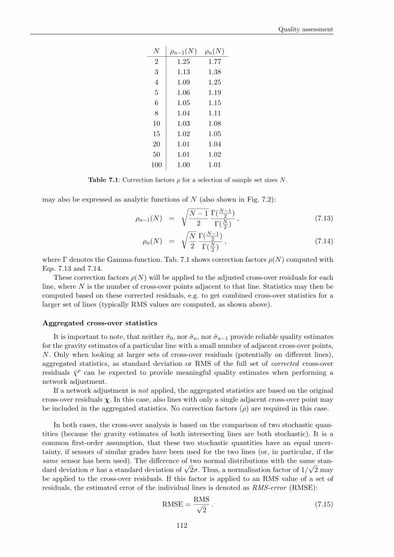
Quality assessment
N ρn−1(N) ρn(N)
2 1.25 1.77
3 1.13 1.38
4 1.09 1.25
5 1.06 1.19
6 1.05 1.15
8 1.04 1.11
10 1.03 1.08
15 1.02 1.05
20 1.01 1.04
50 1.01 1.02
100 1.00 1.01
Table 7.1: Correction factors ρ for a selection of sample set sizes N .
may also be expressed as analytic functions of N (also shown in Fig. 7.2):
ρn−1(N) =
√N − 1
2
Γ(N−12 )
Γ(N2 ), (7.13)
ρn(N) =
√N
2
Γ(N−12 )
Γ(N2 ), (7.14)
where Γ denotes the Gamma-function. Tab. 7.1 shows correction factors ρ(N) computed withEqs. 7.13 and 7.14.
These correction factors ρ(N) will be applied to the adjusted cross-over residuals for eachline, where N is the number of cross-over points adjacent to that line. Statistics may then becomputed based on these corrected residuals, e.g. to get combined cross-over statistics for alarger set of lines (typically RMS values are computed, as shown above).
Aggregated cross-over statistics
It is important to note, that neither σ0, nor σn, nor σn−1 provide reliable quality estimatesfor the gravity estimates of a particular line with a small number of adjacent cross-over points,N . Only when looking at larger sets of cross-over residuals (potentially on different lines),aggregated statistics, as standard deviation or RMS of the full set of corrected cross-overresiduals χρ can be expected to provide meaningful quality estimates when performing anetwork adjustment.
If a network adjustment is not applied, the aggregated statistics are based on the originalcross-over residuals χ. In this case, also lines with only a single adjacent cross-over point maybe included in the aggregated statistics. No correction factors (ρ) are required in this case.
In both cases, the cross-over analysis is based on the comparison of two stochastic quan-tities (because the gravity estimates of both intersecting lines are both stochastic). It is acommon first-order assumption, that these two stochastic quantities have an equal uncer-tainty, if sensors of similar grades have been used for the two lines (or, in particular, if thesame sensor has been used). The difference of two normal distributions with the same stan-dard deviation σ has a standard deviation of
√2σ. Thus, a normalisation factor of 1/
√2 may
be applied to the cross-over residuals. If this factor is applied to an RMS value of a set ofresiduals, the estimated error of the individual lines is denoted as RMS-error (RMSE):
RMSE =RMS√
2. (7.15)
112
7.1 Internal quality assessment
The RMSE measure is commonly used in the literature (Becker et al., 2015b; Bruton, 2002;Glennie et al., 2000; Glennie and Schwarz , 1999).
7.1.2 Repeated lines or line segments
The concept of repeated lines is very similar to that of cross-over point residuals. Twomeasurement lines or line segments have the same (nominal) ground track. For a differenceof flight altitudes ∆h, the findings of the previous section hold equivalently. For repeatedline segments at different heights, the gravity signal of the higher segment shows in general asmoother gravity signal, because of the attenuation of the true gravity signal with increasingheight (Torge, 1989).
In addition to altitude differences, horizontal offsets between the two lines may affectthe comparison. In practice it advisable to limit the maximum horizontal distance for thisanalysis. As mentioned above, the horizontal gravity gradient can be as high as ±40µGal/mat flight altitude (for high-mountain topography).
Obviously, the two gravity signals are highly correlated (for identical flight trajectories,the correlation is maximal, i.e. 100%). This implies, that a lower cut-off frequency for thealong-track low-pass filtering yields in general a better agreement between the two signals.This property can again be recognised in the results shown in Glennie and Schwarz (1999).In the extreme case, only the average of the two data sets is being compared. If in additionan adjustment is performed, the residual is necessarily zero.
The important conclusion is, that repeated line residuals are only a valid metric forcomparisons among different campaigns, sensors, or algorithms, if exactly the same filteringwas applied to the different data sets. Thus, a single-value comparison as for the cross-overresidual analysis is not sufficient in this case; The characteristics of the low-pass filteringalways have to be taken into account.
In practice, repeated lines have a lower relevance compared to cross-over lines forproduction-oriented campaigns. A repeated line only allows the quality assessment for asingle line, while a set of several cross-over lines can allow quality estimates for a whole net-work of lines, and thereby also enable the discovery of outliers. A regular repetition of all ofthe measurement lines is too costly in practice for production-oriented airborne gravimetry.
The aerogravity data sets of Chap. 8 contain several shorter repeated line segments. Therepetition of these segments was mainly motivated by an unsatisfying initial measurement,which needed to be redone (e.g. if strong turbulence disturbed the measurements).
Again, a factor of 1/√2 may be applied to the RMS of the two lines to get an individual
accuracy estimate (RMSE), if the assumption of equal individual gravity accuracies for bothlines is justified.
7.1.3 Error of closure
For an aerogravity flight, usually a tied gravity value determined by terrestrial gravimetryis known for the aircraft parking positions of both the origin and the destination airports. Inmany cases, both airports (and the parking positions) are identical, hence the term error ofclosure.
During the initial alignment phase, standing on the initial parking position rO, the filteris initialised using a terrestrial gravity value:
dgrO = dgrO = grO − γrO . (7.16)
After the flight, the estimated gravity value dgrF at the final parking position rF is comparedagainst the known ground-truth gravity value dgrF , yielding the error of closure e:
eOF = dgrF − dgrF . (7.17)
113
Quality assessment
If only scalar ground truth gravity values are known, the above equation can only be evaluatedfor the scalar gravity estimates (or the vertical component).
The gravity error of closure is a useful measure for determining the average long-termdrift of the estimated gravity values. For the analysis, the ground-truth reference is commonlyassumed to be error-free, typically having an accuracy of 100µGal or better for the verticalchannel (scalar gravity).
As for the cross-over points, the redundant knowledge of the gravity value at the finalparking position (ground-truth versus IMU estimate) may not only be used for deriving aquality measure. It can also be exploited for improving the gravity estimates, by assuming alinear drift of the gravity estimates. Such a linear drift interpolation is a common method interrestrial gravimetry. Although the drift may be highly non-linear, the linear interpolation isusually the best justified guess. It will be shown in Chap. 8, that this linear drift interpolationsignificantly helps to increase the overall accuracy of the gravity estimates. As shown inChap. 3, the known ground-truth gravity values can be introduced as measurements to theEKF.
7.2 Comparisons against external reference data
For a production-oriented aerogravity campaign, dense terrestrial reference gravity data isusually not available, as the campaigns naturally take place in areas with sparse gravity datacoverage. Still, several methods are introduced here, utilising global Earth gravity models ortopography data, which are available today at an almost global coverage.
7.2.1 Inter-system comparison
For the data sets shown in Chap. 8, the navigation-grade iMAR RQH-1003 IMU wasflown side-by-side with the two-axis stabilised-platform LaCoste & Romberg S-type springgravimeter. Comparisons will be shown for some of the flights. From cross-over analyses itis known, that the individual sensor results are of similar quality, thus data sets can not beused as a mutual reference. Still, the degree of agreement between both sensors can be usedas a quality measure, assuming that both sensors’ gravity estimate errors are uncorrelated(which is in general a justified assumption). If the assumption of equivalent sensor accuraciesis justified, the gravity differences may again be divided by
√2 in order to obtain an estimate
for the individual sensor accuracy.
7.2.2 Global Earth gravity models
Since the implementation of satellite-based gravimetry, gravity models with almost globalcoverage are available to the public. The used satellites are low-Earth-orbit (LEO) satellites,with altitudes of several hundreds of kilometres. Tab. 7.2 summarises the characteristics ofthe three satellite gravimetry missions that were implemented so far: CHAMP, GRACE, andGOCE. For details on these satellite gravity missions, the reader is referred to Torge andMuller (2012). Due to the attenuation of the gravity field at high altitudes, these satellitemissions are limited to a relatively low spatial resolution.
Several combined global gravity models (GGM) are published in the literature, augment-ing satellite gravity data with local gravity data, as terrestrial, airborne, or shipborne data.Such models contain coefficients up to degree and order 2190 (λ/2 ≈ 9 km). One of the mostfamous combined models is the Earth Gravity Model (EGM) 2008, see Pavlis et al. (2008).It is however important to note, that the use of the higher order coefficients is only justifiedin regions with an equivalently dense data basis.
1based on the availability of gravity models published in the ICGEM data base (Barthelmes and Forste,2011)
114
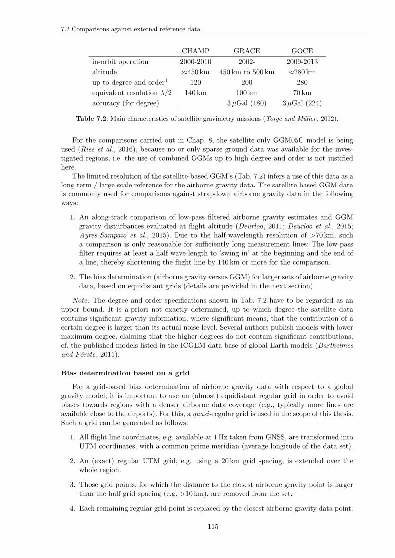
7.2 Comparisons against external reference data
CHAMP GRACE GOCE
in-orbit operation 2000-2010 2002- 2009-2013
altitude ≈450 km 450 km to 500 km ≈280 km
up to degree and order1 120 200 280
equivalent resolution λ/2 140 km 100 km 70 km
accuracy (for degree) 3µGal (180) 3µGal (224)
Table 7.2: Main characteristics of satellite gravimetry missions (Torge and Muller , 2012).
For the comparisons carried out in Chap. 8, the satellite-only GGM05C model is beingused (Ries et al., 2016), because no or only sparse ground data was available for the inves-tigated regions, i.e. the use of combined GGMs up to high degree and order is not justifiedhere.
The limited resolution of the satellite-based GGM’s (Tab. 7.2) infers a use of this data as along-term / large-scale reference for the airborne gravity data. The satellite-based GGM datais commonly used for comparisons against strapdown airborne gravity data in the followingways:
1. An along-track comparison of low-pass filtered airborne gravity estimates and GGMgravity disturbances evaluated at flight altitude (Deurloo, 2011; Deurloo et al., 2015;Ayres-Sampaio et al., 2015). Due to the half-wavelength resolution of >70 km, sucha comparison is only reasonable for sufficiently long measurement lines: The low-passfilter requires at least a half wave-length to ’swing in’ at the beginning and the end ofa line, thereby shortening the flight line by 140 km or more for the comparison.
2. The bias determination (airborne gravity versus GGM) for larger sets of airborne gravitydata, based on equidistant grids (details are provided in the next section).
Note: The degree and order specifications shown in Tab. 7.2 have to be regarded as anupper bound. It is a-priori not exactly determined, up to which degree the satellite datacontains significant gravity information, where significant means, that the contribution of acertain degree is larger than its actual noise level. Several authors publish models with lowermaximum degree, claiming that the higher degrees do not contain significant contributions,cf. the published models listed in the ICGEM data base of global Earth models (Barthelmesand Forste, 2011).
Bias determination based on a grid
For a grid-based bias determination of airborne gravity data with respect to a globalgravity model, it is important to use an (almost) equidistant regular grid in order to avoidbiases towards regions with a denser airborne data coverage (e.g., typically more lines areavailable close to the airports). For this, a quasi -regular grid is used in the scope of this thesis.Such a grid can be generated as follows:
1. All flight line coordinates, e.g. available at 1Hz taken from GNSS, are transformed intoUTM coordinates, with a common prime meridian (average longitude of the data set).
2. An (exact) regular UTM grid, e.g. using a 20 km grid spacing, is extended over thewhole region.
3. Those grid points, for which the distance to the closest airborne gravity point is largerthan the half grid spacing (e.g. >10 km), are removed from the set.
4. Each remaining regular grid point is replaced by the closest airborne gravity data point.
115
Quality assessment
The term quasi-regular is used here to indicate, that the resulting grid is of course notperfectly equidistant (examples are depicted in Chap. 8). The advantage of this methodis, that the comparison against the global model can be done without performing a up- ordownward continuation, and without the requirement of a spatial interpolation of the airbornegravity data.
Since high-resolution airborne gravity (half-wavelength resolution of 3 km to 5 km) is beingcompared to satellite-based gravity (resolutions of 100 km and more), the comparison onlyyields useful results in general, if a larger region is used for the comparison. For smallerregions, effects arising from the low resolution of the reference GGM data can significantlypropagate into the comparison. The reference data points are then biased with respect to thetrue gravity signal, and a reasonable comparison is not possible. In contrast, for a large area ofcoverage (multiple wavelengths of the reference data set in both latitudinal and longitudinaldirections), such effects are expected to level out on average.
For the real-data examples analysed in Chap. 8, the GGM data is only used for the grid-based bias determination. The overall accuracy of the gravity estimates of a data set can thenbe estimated by the combination of the absolute bias of a data set (from comparison againstGGM), and the relative precision of the system (determined e.g. from cross-over residuals).
7.2.3 Topographic gravity effect
While global gravity models can be used as a reference for the longer wavelength com-ponents of the estimated airborne gravity data, the topographic effect can be used as aquasi-reference for the short wavelength components. Such a comparison is based on the as-sumption, that the majority of the short-wavelength contributions to the gravity field comesfrom the topography. Therefore, such comparisons are only viable for mountainous regions, orregions with rugged terrain; In flat terrain regions, sub-surface density changes may equally,or even stronger contribute to the gravity signal over the whole frequency spectrum, comparedto the topographic effect.
For the comparisons shown in Chap. 8, the topographic effect is computed using thesoftware GRAVSOFT TC (Tscherning et al., 1992). The computation is based on griddedterrain data, taken from the SRTMPlus 15 data set (Becker et al., 2009), assuming a standardtopography density of 2.67 g/cm3. The SRTMPlus 15 data set includes bathymetry data. Themass of the ocean water is accounted for assuming a density of 1.025 kg/dm3.
For each discrete point r on the flight trajectory, the topographic effect is computed asa sum of gravity contributions of rectangular prisms within a radius of 100 km around r.For reasons of computational efficiency, the surrounding area is split into two zones: withina radius of 40 km, high resolution terrain information is processed, while in the outer zone(between 40 km and 100 km), a coarse terrain grid appears sufficient for the computationof the individual prism contributions (the contributions to the total gravity reduce with thesquare of the distance). Also, approximations are introduced for distant prisms (e.g. assuminga point mass) to save computation time. More details on such prism-based computations ofthe topographic effect can be found in Forsberg (1984); Heck and Seitz (2007).
7.2.4 Ground control points
Ground control points may serve as a reference for airborne gravity data. For a suffi-ciently dense set of terrestrial gravity points, a combination of grid-interpolation and upwardcontinuation may be performed to get reference data at flight altitude.
In the scope of this thesis, such a reference could not be computed due to the lack of denseterrestrial gravity date in the relevant regions (see Chap. 8). The approach is mentioned herefor the sake of completeness.
116
7.3 A Turbulence Metric
7.3 A Turbulence Metric
Turbulence is a limiting factor for production-oriented airborne gravimetry in general. Inparticular the classical spring-gravimeters tend to have larger sensor errors during dynamicmotion of the aircraft, which can be caused by turbulence and also the corresponding ma-noeuvres of the pilot or auto pilot to maintain a certain altitude, velocity, and course overground. The predominant causes for turbulence are abrupt changes of the vector of windspeeds, and air pressure.
In order to analyse the impact of turbulence, a measure of turbulence needs to be defined.It is desirable to quantify turbulence apart from subjective categories, as ’weak’ or ’strong’,in order to unify the findings and deductions among different airborne gravity campaigns andauthors.
Two common metrics are being in use for both commercial and military aviation:
1. The Eddy Dissipation Rate (EDR) is an aircraft-independent measure for the atmo-spheric turbulence state. It is based on ’the steady-state rate at which energy is beingput into the system in much larger eddies and removed by viscous effects related tosmall eddies’ (MacCready , 1962). It is therefore a solely weather-dependent measure.
2. Larger aircraft have a tendency to show less reaction to the same weather situation(having a given EDR) compared to smaller aircraft. The so-called RMS-g value isdefined as the standard deviation of the vertical aircraft accelerations. It is therefore ameasure of the actual reactions of an aircraft to atmospheric turbulence.
Aircraft accelerations coming from steered flight manoeuvres are also included in thisvalue. The term RMS-g appears misleading, since actually the standard deviation (notthe RMS) is computed. The difference is however small, if the average vertical accelera-tion is close to zero, as it is typically the case if the aircraft moves at constant (nominal)altitude.
There exist aircraft-dependent models, which allow the computation of expected RMS-gvalues for a given EDR. In aviation, such models are of practical relevance for the riskassessment: For a given EDR value, a large commercial jet may face relatively smallRMS-g values compared to a small aircraft, for which the same atmospheric state cancause severe aerodynamic instabilities.
For airborne gravimetry, the actual RMS-g value can easily be computed based on GNSSvelocities, or based on the high-rate strapdown IMU navigation solution (if available).For both approaches, the acceleration can be approximated by numerical differentiationof the vertical velocity components. It is known from experience, that relevant turbu-lence reactions can have periods of less than one second, thus a GNSS velocity data rateof at least 10Hz is suggested. The standard deviations are computed using a slidingwindow of a predefined width.
As an example, RMS-g values are computed for an aerogravity flight (flight id 298) carriedout in Chile in October 2013 (Fig. 7.3, cf. Sect. 8.1). The following RMS-g values are beingcompared:
1. using velocity values from two-frequency PPP at 10Hz data rate, and
2. using velocity estimates from the strapdown navigation solution, at 300Hz data rate.The strapdown inertial data was acquired with the iMAR RQH-1003 system introducedin Sect. 6.1.
Fig. 7.4 shows the computed RMS-g values. Both curves look similar, indicating that bothdata bases (PPP only at 10Hz and IMU/PPP integrated data at 300Hz) are suitable for thedetermination of the RMS-g value.
117
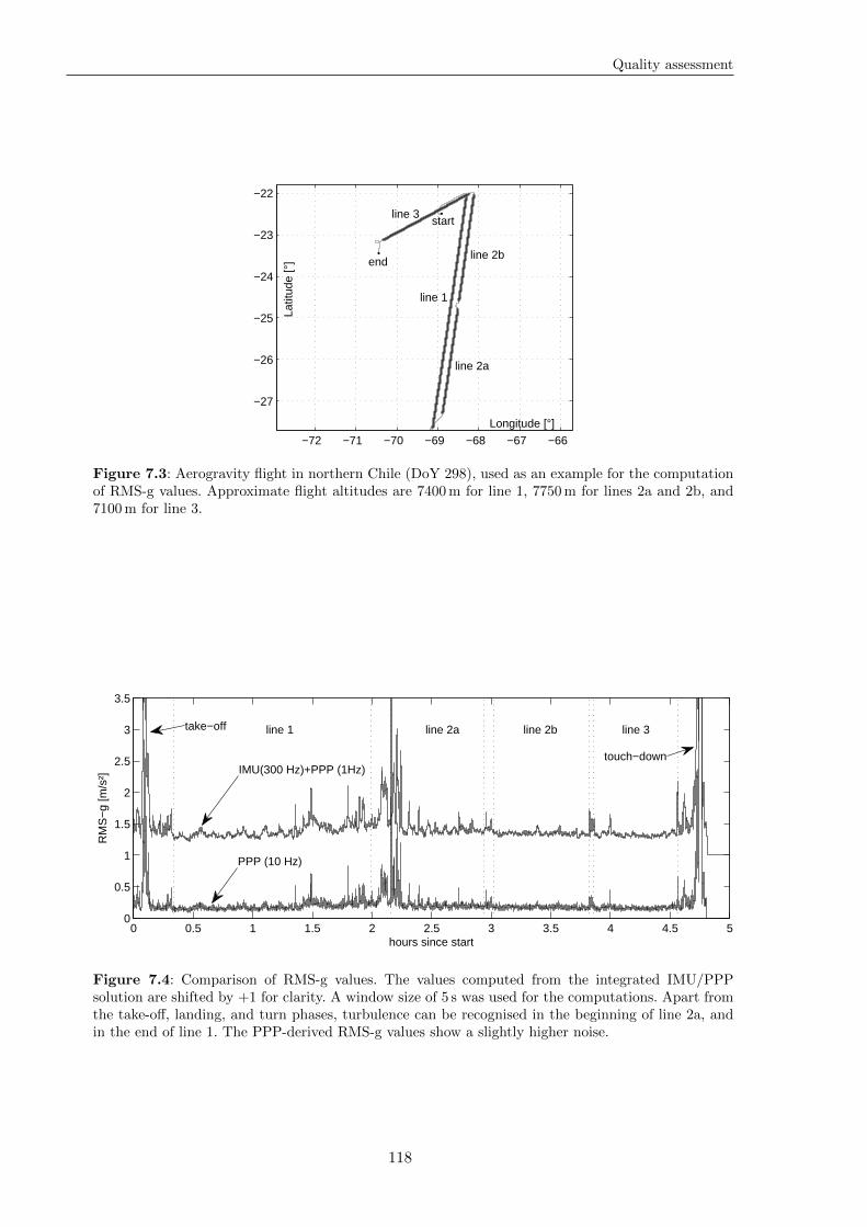
Quality assessment
−72 −71 −70 −69 −68 −67 −66
−27
−26
−25
−24
−23
−22
line 1
line 2a
line 2b
line 3
Latit
ude
[°]
Longitude [°]
start
end
Figure 7.3: Aerogravity flight in northern Chile (DoY 298), used as an example for the computationof RMS-g values. Approximate flight altitudes are 7400m for line 1, 7750m for lines 2a and 2b, and7100m for line 3.
0 0.5 1 1.5 2 2.5 3 3.5 4 4.5 50
0.5
1
1.5
2
2.5
3
3.5
hours since start
RM
S−
g [m
/s²]
line 3line 2bline 2aline 1
take−off
touch−downIMU(300 Hz)+PPP (1Hz)
PPP (10 Hz)
Figure 7.4: Comparison of RMS-g values. The values computed from the integrated IMU/PPPsolution are shifted by +1 for clarity. A window size of 5 s was used for the computations. Apart fromthe take-off, landing, and turn phases, turbulence can be recognised in the beginning of line 2a, andin the end of line 1. The PPP-derived RMS-g values show a slightly higher noise.
118

7.3 A Turbulence Metric
For the aerogravity data sets presented in Chap. 8, only high-rate accelerations from theIMU/PPP integration are being used, because only 1Hz or 2Hz GNSS data is available formost of the flights.
119

Quality assessment
120
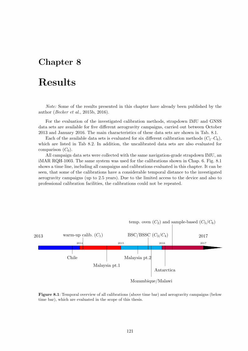
Chapter 8
Results
Note: Some of the results presented in this chapter have already been published by theauthor (Becker et al., 2015b, 2016).
For the evaluation of the investigated calibration methods, strapdown IMU and GNSSdata sets are available for five different aerogravity campaigns, carried out between October2013 and January 2016. The main characteristics of these data sets are shown in Tab. 8.1.
Each of the available data sets is evaluated for six different calibration methods (C1–C6),which are listed in Tab 8.2. In addition, the uncalibrated data sets are also evaluated forcomparison (C0).
All campaign data sets were collected with the same navigation-grade strapdown IMU, aniMAR RQH-1003. The same system was used for the calibrations shown in Chap. 6. Fig. 8.1shows a time line, including all campaigns and calibrations evaluated in this chapter. It can beseen, that some of the calibrations have a considerable temporal distance to the investigatedaerogravity campaigns (up to 2.5 years). Due to the limited access to the device and also toprofessional calibration facilities, the calibrations could not be repeated.
2013 2017
2014 2015 2016 2017
Chile
Malaysia pt.1
Malaysia pt.2
Mozambique/Malawi
Antarctica
warm-up calib. (C1) BSC/BSSC (C3/C4)
temp. oven (C2) and sample-based (C5/C6)
Figure 8.1: Temporal overview of all calibrations (above time bar) and aerogravity campaigns (belowtime bar), which are evaluated in the scope of this thesis.
121
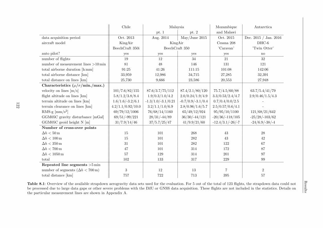
Resu
lts
Chile Malaysia Mozambique Antarctica
pt. 1 pt. 2 and Malawi
data acquisition period Oct. 2013 Aug. 2014 May/June 2015 Oct. 2015 Dec. 2015 / Jan. 2016
aircraft model KingAir KingAir Cessna 208 DHC-6
BeechCraft 350i BeechCraft 350 ’Caravan’ ’Twin Otter’
auto pilot? yes yes yes yes no
number of flights 19 12 34 21 32
number of measurement lines >10min 81 48 146 131 121
total airborne duration [h:mm] 91:25 41:26 111:15 101:08 142:06
total airborne distance [km] 33,959 12,986 34,715 27,285 32,391
total distance on lines [km] 25,730 9,666 23,586 20,553 27,948
Characteristics (µ/σ/min./max.)
velocity on lines [m/s] 101/7.6/82/155 87.6/3.7/75/112 87.4/2.1/80/120 75.7/4.5/60/88 63.7/5.4/41/79
flight altitude on lines [km] 5.8/1.2/3.8/8.4 1.9/0.3/1.0/4.2 2.0/0.24/1.9/4.9 3.3/0.53/2.4/4.7 2.9/0.46/1.5/4.3
terrain altitude on lines [km] 1.6/1.6/-3.2/6.1 -1.3/1.0/-3.1/0.21 -0.7/0.9/-3.1/0.4 0.7/0.4/0.0/2.5 -
terrain clearance on lines [km] 4.2/1.1/0.92/10.0 3.2/1.1/1.0/6.9 2.8/0.96/1.6/5.7 2.5/0.57/0.6/4.1 -
RMS-g [mm/s2] 69/79/12/1006 76/68/14/1160 65/49/12/924 95/95/10/1100 121/68/21/642
GGM05C gravity disturbance [mGal] 69/51/-99/221 28/31/-44/89 36/30/-44/121 -20/36/-118/105 -25/28/-103/62
GGM05C geoid height N [m] 31/7.9/14/46 37/5.7/25/47 41/9.9/21/60 -12.4/3.1/-26/-7 -24/6.9/-38/-4
Number of cross-over points
∆h < 50m 15 101 268 43 28
∆h < 100m 15 101 282 43 42
∆h < 350m 31 101 282 122 67
∆h < 700m 47 101 314 172 87
∆h < 1050m 57 129 314 201 97
total 102 133 317 229 99
Repeated line segments >5min
number of segments (∆h < 700m) 3 12 13 7 2
total distance [km] 757 722 713 395 57
Table 8.1: Overview of the available strapdown aerogravity data sets used for the evaluation. For 5 out of the total of 123 flights, the strapdown data could notbe processed due to large data gaps or other severe problems with the IMU or GNSS data acquisition. These flights are not included in the statistics. Details onthe particular measurement lines are shown in Appendix A.
122
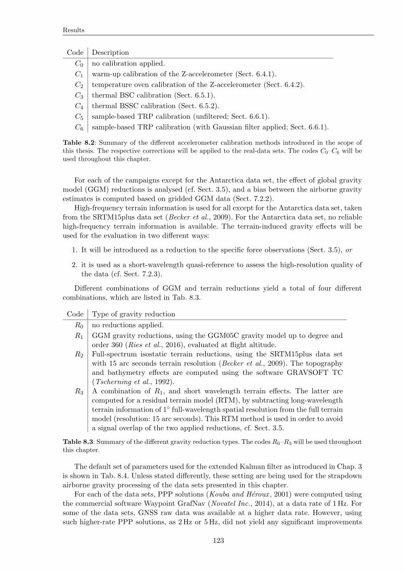
Results
Code Description
C0 no calibration applied.
C1 warm-up calibration of the Z-accelerometer (Sect. 6.4.1).
C2 temperature oven calibration of the Z-accelerometer (Sect. 6.4.2).
C3 thermal BSC calibration (Sect. 6.5.1).
C4 thermal BSSC calibration (Sect. 6.5.2).
C5 sample-based TRP calibration (unfiltered; Sect. 6.6.1).
C6 sample-based TRP calibration (with Gaussian filter applied; Sect. 6.6.1).
Table 8.2: Summary of the different accelerometer calibration methods introduced in the scope ofthis thesis. The respective corrections will be applied to the real-data sets. The codes C0–C6 will beused throughout this chapter.
For each of the campaigns except for the Antarctica data set, the effect of global gravitymodel (GGM) reductions is analysed (cf. Sect. 3.5), and a bias between the airborne gravityestimates is computed based on gridded GGM data (Sect. 7.2.2).
High-frequency terrain information is used for all except for the Antarctica data set, takenfrom the SRTM15plus data set (Becker et al., 2009). For the Antarctica data set, no reliablehigh-frequency terrain information is available. The terrain-induced gravity effects will beused for the evaluation in two different ways:
1. It will be introduced as a reduction to the specific force observations (Sect. 3.5), or
2. it is used as a short-wavelength quasi-reference to assess the high-resolution quality ofthe data (cf. Sect. 7.2.3).
Different combinations of GGM and terrain reductions yield a total of four differentcombinations, which are listed in Tab. 8.3.
Code Type of gravity reduction
R0 no reductions applied.
R1 GGM gravity reductions, using the GGM05C gravity model up to degree andorder 360 (Ries et al., 2016), evaluated at flight altitude.
R2 Full-spectrum isostatic terrain reductions, using the SRTM15plus data setwith 15 arc seconds terrain resolution (Becker et al., 2009). The topographyand bathymetry effects are computed using the software GRAVSOFT TC(Tscherning et al., 1992).
R3 A combination of R1, and short wavelength terrain effects. The latter arecomputed for a residual terrain model (RTM), by subtracting long-wavelengthterrain information of 1 full-wavelength spatial resolution from the full terrainmodel (resolution: 15 arc seconds). This RTM method is used in order to avoida signal overlap of the two applied reductions, cf. Sect. 3.5.
Table 8.3: Summary of the different gravity reduction types. The codesR0–R3 will be used throughoutthis chapter.
The default set of parameters used for the extended Kalman filter as introduced in Chap. 3is shown in Tab. 8.4. Unless stated differently, these setting are being used for the strapdownairborne gravity processing of the data sets presented in this chapter.
For each of the data sets, PPP solutions (Kouba and Heroux , 2001) were computed usingthe commercial software Waypoint GrafNav (Novatel Inc., 2014), at a data rate of 1Hz. Forsome of the data sets, GNSS raw data was available at a higher data rate. However, usingsuch higher-rate PPP solutions, as 2Hz or 5Hz, did not yield any significant improvements
123
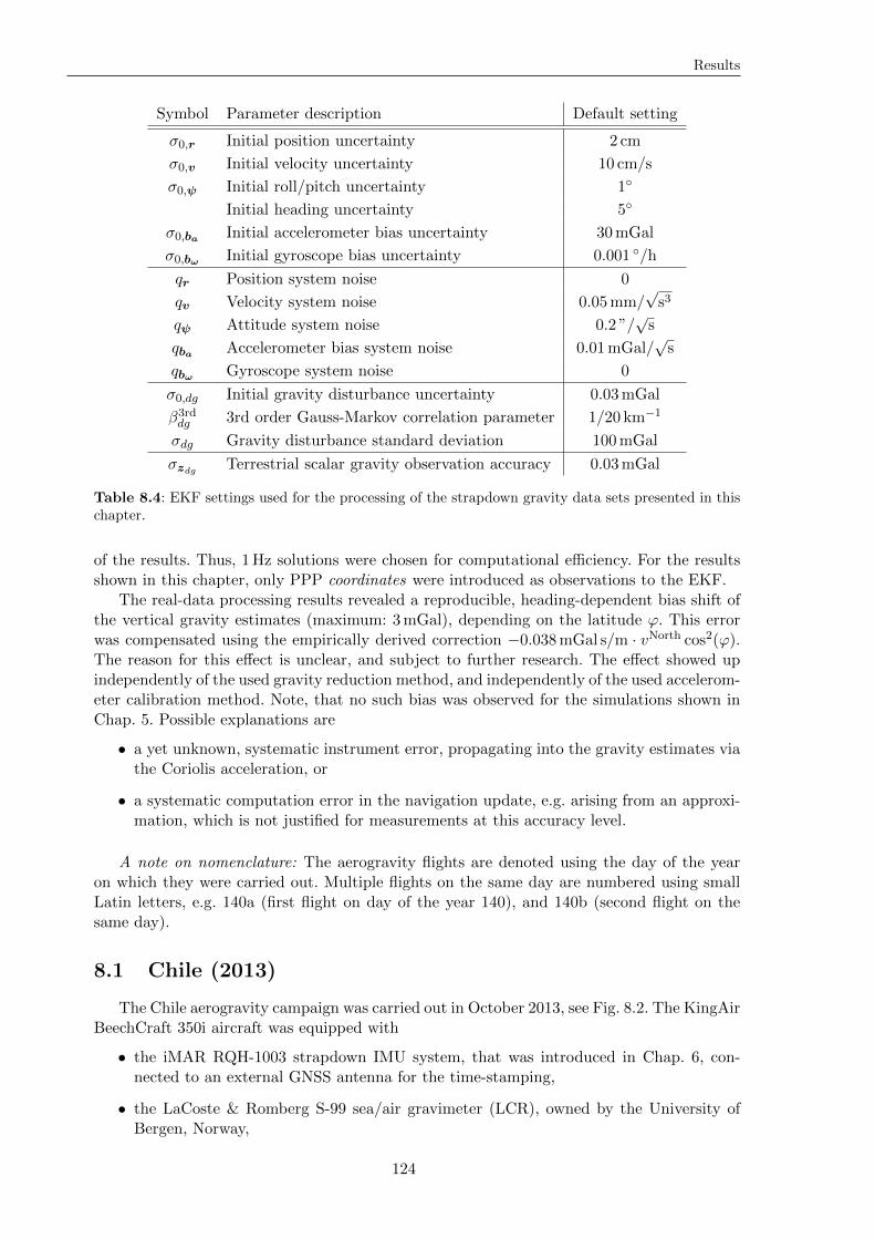
Results
Symbol Parameter description Default setting
σ0,r Initial position uncertainty 2 cm
σ0,v Initial velocity uncertainty 10 cm/s
σ0,ψ Initial roll/pitch uncertainty 1
Initial heading uncertainty 5
σ0,ba Initial accelerometer bias uncertainty 30mGal
σ0,bω Initial gyroscope bias uncertainty 0.001 /h
qr Position system noise 0
qv Velocity system noise 0.05mm/√s3
qψ Attitude system noise 0.2 ”/√s
qba Accelerometer bias system noise 0.01mGal/√s
qbω Gyroscope system noise 0
σ0,dg Initial gravity disturbance uncertainty 0.03mGal
β3rddg 3rd order Gauss-Markov correlation parameter 1/20 km−1
σdg Gravity disturbance standard deviation 100mGal
σzdg Terrestrial scalar gravity observation accuracy 0.03mGal
Table 8.4: EKF settings used for the processing of the strapdown gravity data sets presented in thischapter.
of the results. Thus, 1Hz solutions were chosen for computational efficiency. For the resultsshown in this chapter, only PPP coordinates were introduced as observations to the EKF.
The real-data processing results revealed a reproducible, heading-dependent bias shift ofthe vertical gravity estimates (maximum: 3mGal), depending on the latitude ϕ. This errorwas compensated using the empirically derived correction −0.038mGal s/m · vNorth cos2(ϕ).The reason for this effect is unclear, and subject to further research. The effect showed upindependently of the used gravity reduction method, and independently of the used accelerom-eter calibration method. Note, that no such bias was observed for the simulations shown inChap. 5. Possible explanations are
• a yet unknown, systematic instrument error, propagating into the gravity estimates viathe Coriolis acceleration, or
• a systematic computation error in the navigation update, e.g. arising from an approxi-mation, which is not justified for measurements at this accuracy level.
A note on nomenclature: The aerogravity flights are denoted using the day of the yearon which they were carried out. Multiple flights on the same day are numbered using smallLatin letters, e.g. 140a (first flight on day of the year 140), and 140b (second flight on thesame day).
8.1 Chile (2013)
The Chile aerogravity campaign was carried out in October 2013, see Fig. 8.2. The KingAirBeechCraft 350i aircraft was equipped with
• the iMAR RQH-1003 strapdown IMU system, that was introduced in Chap. 6, con-nected to an external GNSS antenna for the time-stamping,
• the LaCoste & Romberg S-99 sea/air gravimeter (LCR), owned by the University ofBergen, Norway,
124
8.1 Chile (2013)
−74˚
−74˚
−72˚
−72˚
−70˚
−70˚
−68˚
−68˚
−38˚ −38˚
−36˚ −36˚
−34˚ −34˚
−32˚ −32˚
−30˚ −30˚
−28˚ −28˚
−26˚ −26˚
−24˚ −24˚
−22˚ −22˚
−20˚ −20˚
−18˚ −18˚
0 100 200
km
−5000
0
5000
m
−74˚
−74˚
−72˚
−72˚
−70˚
−70˚
−68˚
−68˚
−38˚ −38˚
−36˚ −36˚
−34˚ −34˚
−32˚ −32˚
−30˚ −30˚
−28˚ −28˚
−26˚ −26˚
−24˚ −24˚
−22˚ −22˚
−20˚ −20˚
−18˚ −18˚
0 100 200
km
−100
0
100
200mGal
Figure 8.2: Overview of the Chile aerogravity campaign. The measurement lines are highlighted(bold lines), all other parts of the flights are shown as thin lines. Left: Topography / bathymetry.Right: Gravity anomalies of the GGM05C global gravity model (Ries et al., 2016), computed up toits maximum degree of 360.
125
Results
0 2 4 6 8 10 12
hours since start
15
20
25
30
35
40
ISA
tem
pera
ture
[°C
]
285
288
289
290a
291
292
294
295
296
297
0 2 4 6 8 10 12
hours since start
15
20
25
30
35
40
ISA
tem
pera
ture
[°C
]
298
299
301a
301b
302
303
304
305a
305b
Figure 8.3: Sensor temperatures for the Chile campaign. Left: Flights 285 to 297; Right: Flights 298to 305b.
• two Javad Delta-3 GNSS receivers (for redundancy reasons), collecting two-frequencyphases and pseudo-ranges from GPS and GLONASS at a rate of 1Hz. Both receiversshare a single Novatel GNSS Antenna, type ANT-A72GA-TW-N, using an active GNSSsignal splitter.
The campaign was production-oriented, leading to the practical requirement of an aircraftvelocity of ≈100m/s. This velocity is relatively high compared to similar airborne gravimetrycampaigns documented in the literature. It has an immediate impact on the maximum resolu-tion: For the typical low-pass filter frequency of 100 s to 150 s, the half wavelength resolutionwould be 5 km to 7.5 km, which is relatively large compared to the flight altitudes abovetopography in this campaign. Most flight segments were done above rugged high-mountainterrain, up to 6100m above sea level.
The Chile 2013 data set consists of 19 flights. Some of these flights contain an intermediatestop for fuelling the aircraft. Those flights, for which no terrestrial gravity tie was availablefor the intermediate stop, are processed as single flights, in order to enable the determinationof the error of closure, and in order to enable the removal of a linear drift of the gravityestimates (cf. Sect. 7.1.3). These flights are 291, 298, 299, 302, and 303. In contrast, theflights 301 and 305 both had a fuelling stop on an airport with available terrestrial gravitytie. Therefore these flights were split into two flights each (301a, 301b, 305a, 305b). Detailedinformation on the individual flights and measurement lines is provided in Appendix A.2.
8.1.1 Cross-over analysis
As shown in Tab. 8.1, the Chile data set contains only relatively few cross-over points.Some of the measurement lines do not contain a single cross-over point with a height differenceof ∆h < 100m (cf. App. A.2). Therefore, no cross-over adjustment is applied to the residualsfor this data set. Only cross-over points with ∆h < 100m are used for the aggregated cross-over statistics. The results are shown in Tab. 8.5. The gravity is modelled as a third-orderGauss-Markov process, with β3rddg = 1/10 km−1 for R0 and R1, and β
3rddg = 1/20 km−1 for R2
and R3, accounting for the smoother signal characteristics. These correlation parameters weredetermined empirically, based on the estimated gravity data itself, using a single iteration.The correlation parameters are equally used for all 19 flights.
The most relevant conclusion from the cross-over evaluation is, that a precision of 1mGalappears to be possible using an off-the-shelf navigation-grade IMU, when applying an appro-priate calibration to the accelerometers. In more detail, the conclusions are:
126
8.1 Chile (2013)
Cross-over residuals: RMS [mGal] (RMSE [mGal])
C0 C1 C2 C3 C4 C5 C6
R0 4.8 (3.4) 1.6 (1.2) 2.9 (2.1) 2.0 (1.4) 2.0 (1.4) 2.2 (1.5) 2.2 (1.6)
R1 4.8 (3.4) 1.6 (1.1) 2.9 (2.1) 2.0 (1.4) 1.9 (1.4) 2.2 (1.5) 2.3 (1.6)
R2 4.7 (3.3) 1.3 (0.9) 2.9 (2.0) 1.8 (1.3) 1.8 (1.2) 1.8 (1.3) 1.9 (1.4)
R3 4.6 (3.3) 1.4 (1.0) 2.8 (2.0) 1.8 (1.3) 1.8 (1.3) 1.7 (1.2) 1.8 (1.3)
Table 8.5: Cross-over residual statistics for the Chile 2013 campaign, for different combinations ofapplied gravity reductions (R0–R3, see Tab. 8.3), and accelerometer calibration methods (C0–C6, seeTab. 8.2). No cross-over adjustment was applied. The analysis is limited to cross-over points with aheight difference of ∆h < 100m (15 points). RMSE = RMS/
√2, cf. Sect. 7.1.1. The best result is
highlighted.
1. The reduction of topographic effects yields considerably lower cross-over residuals. Ap-parently, the topography-induced high-frequency portion of the gravity signal is diffi-cult to estimate for the given terrain characteristics, flight altitude, and aircraft speed.While such high-resolution signal components can be crucial for small-scale geophysicalmeasurements, they are typically of lower relevance for the local geoid determinationon a medium scale (hundreds of kilometres), because the topographic effect is anywayremoved from the full-range gravity signal for the downward-continuation.
2. Neither a long-wavelength GGM gravity reduction, nor the long wavelengths of thetopographic reduction do significantly affect the results (R0 results are similar to R1;R2 results are similar to R3).
3. The warm-up calibration introduced in Sect. 6.4.1 yields the best results among allevaluated accelerometer calibration methods. This emphasises the importance of tem-perature gradients: For most of the flights, a long warm-up phase of the IMU happensduring the flights (cf. Fig. 8.3), while sensor temperature changes due to changes of theambient temperature are less significant. Apparently, the warm-up calibration is themost appropriate method to model such in-flight warm-up effects.
8.1.2 Errors of closure
Cross-over residuals: RMS [mGal] (RMSE [mGal])
C0 C1 C2 C3 C4 C5 C6
R0 5.8 (4.1) 2.5 (1.8) 2.7 (1.9) 2.4 (1.7) 2.5 (1.7) 3.1 (2.2) 3.0 (2.1)
R1 5.8 (4.1) 2.5 (1.8) 2.6 (1.9) 2.3 (1.7) 2.4 (1.7) 3.1 (2.2) 3.0 (2.1)
R2 5.7 (4.0) 2.3 (1.6) 2.7 (1.9) 2.4 (1.7) 2.4 (1.7) 2.5 (1.8) 2.5 (1.8)
R3 5.6 (4.0) 2.5 (1.8) 2.6 (1.8) 2.2 (1.6) 2.4 (1.7) 2.6 (1.8) 2.5 (1.8)
Table 8.6: Cross-over residual statistics for the Chile 2013 campaign, not using the terrestrial gravitytie at the destination airport. No cross-over adjustment was applied. The analysis is limited to cross-over points with a height difference of ∆h < 100m (15 points). RMSE = RMS/
√2, cf. Sect. 7.1.1.
For all flights except 290a, a terrestrial gravity tie is available at both the origin and thedestination airports. For the cross-over residuals shown in Tab. 8.5, the destination airportterrestrial gravity tie was introduced to the EKF as an observation. This enables the Kalmansmoother to eliminate a linear drift in the gravity estimates (cf. Sect. 7.1.3). To illustratethe importance of using this observation, the data set was reprocessed, without using thisinformation. The cross-over statistics for this case are shown in Tab. 8.6, showing considerablelarger residuals compared to the results shown in Tab. 8.5.
127
Results
The error of closure can be regarded as an indicator for the long-term stability of theestimated gravity disturbance. It is defined here as the difference between the gravity estimateat the destination airport, and the terrestrial gravity tie (not introducing it as an observationto the EKF). The errors of closure are only evaluated for the vertical gravity component, asno ground-truth information was available for the deflections of the vertical at the differentairports. The observed errors of closure can be found in Tab. 8.7 for different calibrationmethods. The type of gravity reduction (R0–R3) did not show any significant effect (<5%),therefore results are only shown for R3. If no calibration is applied (C0), the errors of closurereach up to 6.5mGal/h. Again, the warm-up calibration of the Z-accelerometer (C1) yieldsthe best results, reducing the drifts from 3.4mGal/h to 0.3mGal/h.
flight Errors of closure [mGal] (average drift per hour [mGal/h])
ID C0 C1 C2 C3 C4 C5 C6
285 11.5 (2.2) 0.9 (0.2) 4.8 (0.9) 3.8 (0.7) 3.5 (0.7) 2.4 (0.5) 2.5 (0.5)
288 14.2 (2.3) -2.0 (-0.3) 3.6 (0.6) 2.4 (0.4) 1.7 (0.3) 0.4 (0.1) 0.7 (0.1)
289 7.4 (1.6) -1.6 (-0.3) 1.4 (0.3) 0.9 (0.2) 1.0 (0.2) -0.6 (-0.1) -0.4 (-0.1)
290a - - - - - - -
291 19.0 (1.7) -3.5 (-0.3) 6.3 (0.6) 0.4 (0.0) 0.9 (0.1) 0.3 (0.0) 0.5 (0.0)
292 12.8 (2.0) 0.2 (0.0) 7.1 (1.1) 0.5 (0.1) 1.0 (0.2) 3.9 (0.6) 3.9 (0.6)
294 21.4 (3.5) 2.0 (0.3) 8.8 (1.4) 7.1 (1.2) 6.5 (1.1) 4.5 (0.7) 4.9 (0.8)
295 25.6 (3.6) -3.3 (-0.5) 9.8 (1.4) -0.2 (-0.0) 0.2 (0.0) 5.0 (0.7) 5.1 (0.7)
296 30.5 (4.4) 2.6 (0.4) 14.6 (2.1) 7.0 (1.0) 7.2 (1.0) 8.3 (1.2) 8.4 (1.2)
297 34.6 (6.5) 2.1 (0.4) 16.3 (3.1) 7.0 (1.3) 6.9 (1.3) 8.5 (1.6) 8.9 (1.7)
298 23.5 (2.3) -1.8 (-0.2) 8.4 (0.8) 3.6 (0.4) 3.4 (0.3) 2.3 (0.2) 2.8 (0.3)
299 23.5 (2.2) -0.1 (-0.0) 9.2 (0.9) 5.0 (0.5) 4.7 (0.4) 3.9 (0.4) 4.3 (0.4)
301a 27.1 (5.1) 3.0 (0.6) 13.4 (2.5) 7.1 (1.3) 7.1 (1.3) 7.9 (1.5) 8.0 (1.5)
301b 2.1 (0.5) 2.1 (0.5) 2.1 (0.5) 2.4 (0.6) 2.5 (0.6) 1.4 (0.4) 1.3 (0.3)
302 25.2 (2.3) 0.2 (0.0) 12.1 (1.1) 2.6 (0.2) 3.5 (0.3) 4.5 (0.4) 4.4 (0.4)
303 25.6 (2.6) 1.9 (0.2) 12.1 (1.2) 5.8 (0.6) 6.4 (0.7) 4.1 (0.4) 4.0 (0.4)
304 30.6 (5.0) 1.0 (0.2) 14.3 (2.3) 4.2 (0.7) 4.6 (0.8) 7.4 (1.2) 7.3 (1.2)
305a 26.5 (4.9) -1.6 (-0.3) 10.4 (1.9) 2.7 (0.5) 2.6 (0.5) 5.6 (1.0) 5.6 (1.0)
305b 5.3 (0.9) 1.0 (0.2) 2.9 (0.5) 2.1 (0.4) 1.9 (0.3) 1.1 (0.2) 1.3 (0.2)
RMS 22.3 (3.4) 2.0 (0.3) 9.8 (1.5) 4.3 (0.7) 4.3 (0.7) 4.8 (0.8) 4.9 (0.8)
µ 20.3 (3.0) 0.2 (0.1) 8.7 (1.3) 3.6 (0.6) 3.6 (0.6) 3.9 (0.6) 4.1 (0.6)
σ 9.4 (1.6) 2.0 (0.3) 4.6 (0.8) 2.5 (0.4) 2.4 (0.4) 2.9 (0.5) 2.8 (0.5)
min 2.1 (0.5) -3.5 (-0.5) 1.4 (0.3) -0.2 (-0.0) 0.2 (0.0) -0.6 (-0.1) -0.4 (-0.1)
max 34.6 (6.5) 3.0 (0.6) 16.3 (3.1) 7.1 (1.3) 7.2 (1.3) 8.5 (1.6) 8.9 (1.7)
Table 8.7: Errors of closure for 18 out of 19 flights of the Chile 2013 campaign. No terrestrial gravitytie was available at the destination airport for flight 290a.
8.1.3 Comparison against LCR
For the whole data set, the LaCoste & Romberg S-99 sea/air gravimeter (LCR) was flownside-by-side with the strapdown system. For an inter-system comparison of the longer wave-lengths, both gravity data sets are preprocessed using a third-order, two-pass Butterworthlow-pass filter at cut-off frequency 1/500Hz (consistent with a spatial half-wavelength of
128
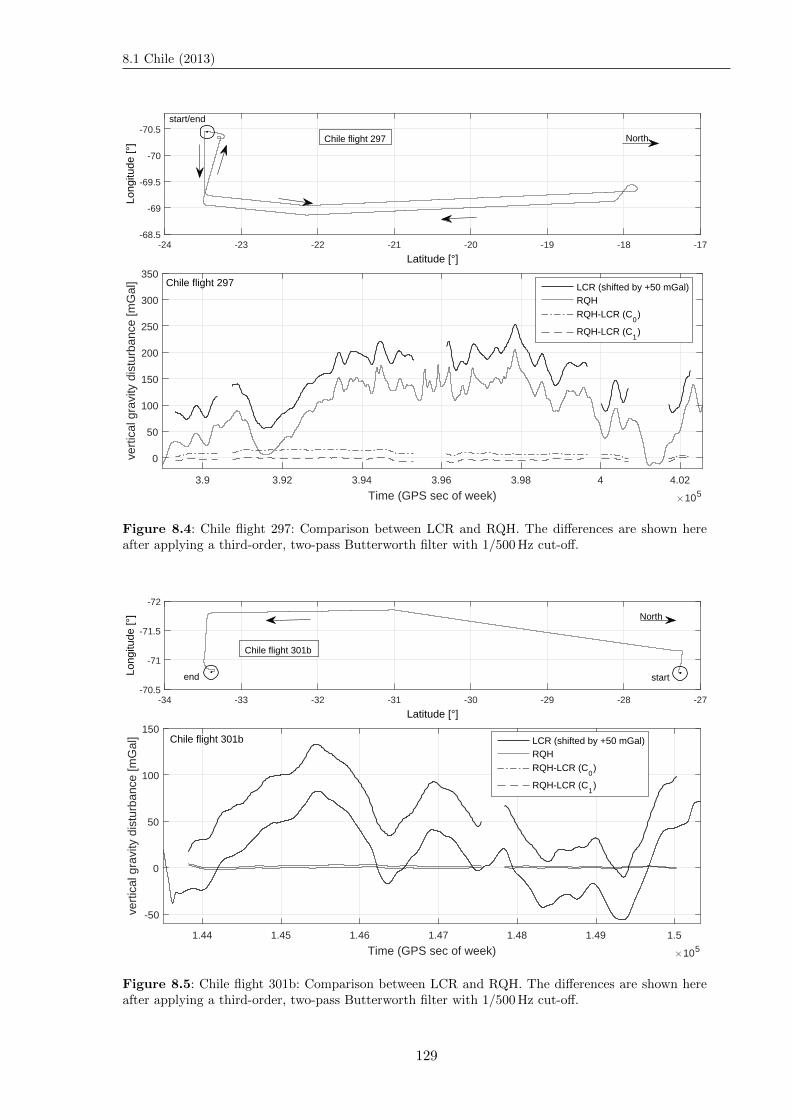
8.1 Chile (2013)
-24 -23 -22 -21 -20 -19 -18 -17
Latitude [°]
-70.5
-70
-69.5
-69
-68.5
Long
itude
[°] North
start/end
Chile flight 297
3.9 3.92 3.94 3.96 3.98 4 4.02
Time (GPS sec of week) ×105
0
50
100
150
200
250
300
350
vert
ical
gra
vity
dis
turb
ance
[mG
al] Chile flight 297 LCR (shifted by +50 mGal)
RQH
RQH-LCR (C0)
RQH-LCR (C1)
Figure 8.4: Chile flight 297: Comparison between LCR and RQH. The differences are shown hereafter applying a third-order, two-pass Butterworth filter with 1/500Hz cut-off.
-34 -33 -32 -31 -30 -29 -28 -27
Latitude [°]
-72
-71.5
-71
-70.5
Long
itude
[°]
startend
North
Chile flight 301b
1.44 1.45 1.46 1.47 1.48 1.49 1.5
Time (GPS sec of week) ×105
-50
0
50
100
150
vert
ical
gra
vity
dis
turb
ance
[mG
al] Chile flight 301b LCR (shifted by +50 mGal)
RQH
RQH-LCR (C0)
RQH-LCR (C1)
Figure 8.5: Chile flight 301b: Comparison between LCR and RQH. The differences are shown hereafter applying a third-order, two-pass Butterworth filter with 1/500Hz cut-off.
129
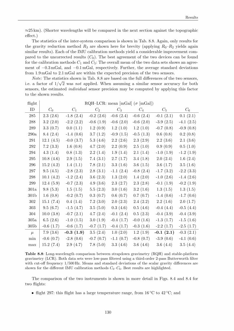
Results
≈25 km). (Shorter wavelengths will be compared in the next section against the topographiceffect.)
The statistics of the inter-system comparison is shown in Tab. 8.8. Again, only results forthe gravity reduction method R3 are shown here for brevity (applying R0–R2 yields againsimilar results). Each of the IMU calibration methods yield a considerable improvement com-pared to the uncorrected results (C0). The best agreement of the two devices can be foundfor the calibration methods C1 and C5: The overall mean of the two data sets shows an agree-ment of −0.3mGal, and −0.1mGal, respectively. Further, the average standard deviationsfrom 1.9mGal to 2.1mGal are within the expected precision of the two sensors.
Note: The statistics shown in Tab. 8.8 are based on the full differences of the two sensors,i.e. a factor of 1/
√2 was not applied. When assuming a similar sensor accuracy for both
sensors, the estimated individual sensor precision may be computed by applying this factorto the shown results.
flight RQH–LCR: mean [mGal] (σ [mGal])
ID C0 C1 C2 C3 C4 C5 C6
285 2.3 (2.6) -1.8 (2.4) -0.2 (2.6) -0.6 (2.4) -0.6 (2.4) -0.1 (2.1) 0.1 (2.1)
288 3.2 (2.0) -2.2 (2.2) -0.6 (1.9) -0.6 (2.0) -0.6 (2.0) -3.9 (2.5) -4.1 (2.5)
289 3.3 (0.7) 0.0 (1.1) 1.2 (0.9) 1.2 (1.0) 1.2 (1.0) -0.7 (0.8) -0.9 (0.8)
290a 8.4 (2.4) -1.4 (0.6) 3.7 (1.2) -0.9 (1.5) -0.5 (1.3) 0.6 (0.8) 0.2 (0.8)
291 12.1 (4.5) -0.0 (3.7) 5.3 (4.6) 2.2 (2.6) 2.3 (2.9) 2.2 (3.6) 2.1 (3.6)
292 7.2 (3.3) 1.6 (0.8) 4.7 (2.0) 2.2 (0.9) 2.5 (1.0) 0.9 (0.9) 0.5 (1.0)
294 4.3 (1.4) 0.8 (1.3) 2.2 (1.4) 1.9 (1.4) 2.1 (1.4) -1.0 (1.9) -1.2 (1.9)
295 10.8 (4.6) 2.9 (1.5) 7.4 (3.1) 2.7 (1.7) 3.4 (1.8) 2.0 (2.4) 1.6 (2.4)
296 15.2 (4.2) 1.4 (1.1) 7.8 (2.1) 3.3 (1.6) 3.6 (1.5) 3.6 (1.7) 3.5 (1.6)
297 9.5 (4.5) -2.8 (2.3) 2.8 (3.1) -1.1 (2.4) -0.8 (2.4) -1.7 (3.2) -2.2 (3.3)
298 10.1 (4.2) -1.2 (2.4) 3.6 (2.3) 1.3 (2.0) 1.4 (2.0) -1.0 (2.6) -1.4 (2.6)
299 12.4 (5.9) -0.7 (2.3) 4.9 (3.6) 2.3 (2.7) 2.3 (2.8) -0.1 (1.9) -0.2 (1.9)
301a 9.8 (5.3) 1.5 (1.5) 5.5 (2.3) 3.0 (1.6) 3.2 (1.6) 1.3 (1.5) 1.3 (1.5)
301b 1.6 (0.8) -0.2 (0.7) 0.3 (0.7) 0.6 (0.7) 0.7 (0.7) -1.4 (0.6) -1.7 (0.6)
302 15.1 (7.4) 0.4 (1.4) 7.2 (3.0) 2.0 (2.3) 2.4 (2.2) 2.2 (1.6) 2.0 (1.7)
303 9.5 (6.7) -1.5 (4.7) 3.5 (5.0) 0.3 (4.6) 0.5 (4.6) -0.4 (4.4) -0.5 (4.4)
304 10.0 (3.8) -0.7 (2.1) 4.7 (2.4) -0.1 (2.4) 0.5 (2.3) -0.4 (3.9) -0.4 (3.9)
305a 6.5 (2.6) -1.0 (1.5) 3.0 (1.9) -0.4 (1.7) -0.0 (1.6) -1.3 (1.7) -1.5 (1.6)
305b -0.6 (1.7) -0.6 (1.7) -0.7 (1.7) -0.4 (1.7) -0.3 (1.6) -2.2 (1.7) -2.5 (1.7)
µ 7.9 (3.6) -0.3 (1.9) 3.5 (2.4) 1.0 (2.0) 1.2 (1.9) -0.1 (2.1) -0.3 (2.1)
min -0.6 (0.7) -2.8 (0.6) -0.7 (0.7) -1.1 (0.7) -0.8 (0.7) -3.9 (0.6) -4.1 (0.6)
max 15.2 (7.4) 2.9 (4.7) 7.8 (5.0) 3.3 (4.6) 3.6 (4.6) 3.6 (4.4) 3.5 (4.4)
Table 8.8: Long-wavelength comparison between strapdown gravimetry (RQH) and stable-platformgravimetry (LCR). Both data sets were low-pass filtered using a third-order 2-pass Butterworth filterwith cut-off frequency 1/500Hz. Means and standard deviations of the scalar gravity differences areshown for the different IMU calibration methods C0–C6. Best results are highlighted.
The comparison of the two instruments is shown in more detail in Figs. 8.4 and 8.4 fortwo flights:
• flight 297: this flight has a large temperature range, from 16 C to 42 C; and
130
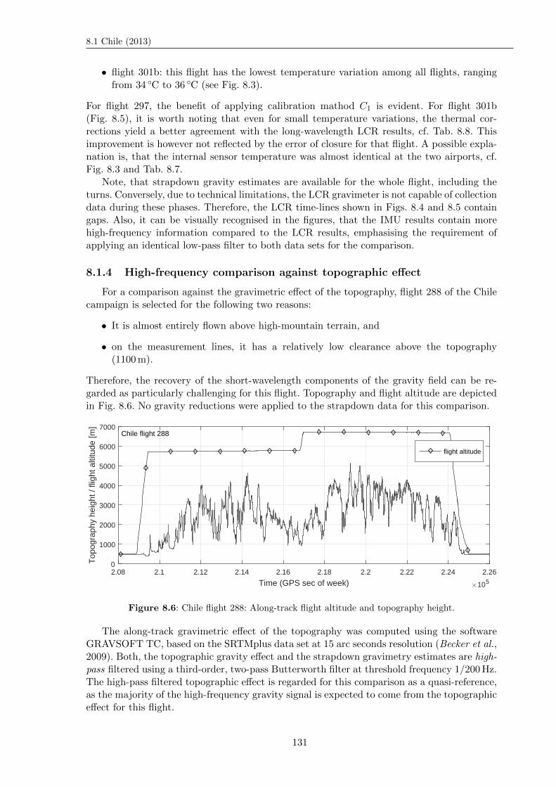
8.1 Chile (2013)
• flight 301b: this flight has the lowest temperature variation among all flights, rangingfrom 34 C to 36 C (see Fig. 8.3).
For flight 297, the benefit of applying calibration mathod C1 is evident. For flight 301b(Fig. 8.5), it is worth noting that even for small temperature variations, the thermal cor-rections yield a better agreement with the long-wavelength LCR results, cf. Tab. 8.8. Thisimprovement is however not reflected by the error of closure for that flight. A possible expla-nation is, that the internal sensor temperature was almost identical at the two airports, cf.Fig. 8.3 and Tab. 8.7.
Note, that strapdown gravity estimates are available for the whole flight, including theturns. Conversely, due to technical limitations, the LCR gravimeter is not capable of collectiondata during these phases. Therefore, the LCR time-lines shown in Figs. 8.4 and 8.5 containgaps. Also, it can be visually recognised in the figures, that the IMU results contain morehigh-frequency information compared to the LCR results, emphasising the requirement ofapplying an identical low-pass filter to both data sets for the comparison.
8.1.4 High-frequency comparison against topographic effect
For a comparison against the gravimetric effect of the topography, flight 288 of the Chilecampaign is selected for the following two reasons:
• It is almost entirely flown above high-mountain terrain, and
• on the measurement lines, it has a relatively low clearance above the topography(1100m).
Therefore, the recovery of the short-wavelength components of the gravity field can be re-garded as particularly challenging for this flight. Topography and flight altitude are depictedin Fig. 8.6. No gravity reductions were applied to the strapdown data for this comparison.
2.08 2.1 2.12 2.14 2.16 2.18 2.2 2.22 2.24 2.26
Time (GPS sec of week) ×105
0
1000
2000
3000
4000
5000
6000
7000
Top
ogra
phy
heig
ht /
fligh
t alti
tude
[m]
Chile flight 288
flight altitude
Figure 8.6: Chile flight 288: Along-track flight altitude and topography height.
The along-track gravimetric effect of the topography was computed using the softwareGRAVSOFT TC, based on the SRTMplus data set at 15 arc seconds resolution (Becker et al.,2009). Both, the topographic gravity effect and the strapdown gravimetry estimates are high-pass filtered using a third-order, two-pass Butterworth filter at threshold frequency 1/200Hz.The high-pass filtered topographic effect is regarded for this comparison as a quasi-reference,as the majority of the high-frequency gravity signal is expected to come from the topographiceffect for this flight.
131
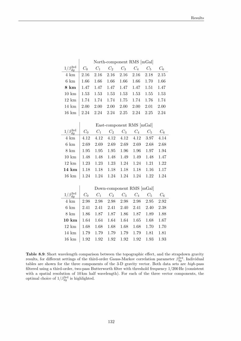
Results
North-component RMS [mGal]
1/β3rddg C0 C1 C2 C3 C4 C5 C6
4 km 2.16 2.16 2.16 2.16 2.16 2.18 2.15
6 km 1.66 1.66 1.66 1.66 1.66 1.70 1.66
8 km 1.47 1.47 1.47 1.47 1.47 1.51 1.47
10 km 1.53 1.53 1.53 1.53 1.53 1.55 1.53
12 km 1.74 1.74 1.74 1.75 1.74 1.76 1.74
14 km 2.00 2.00 2.00 2.00 2.00 2.01 2.00
16 km 2.24 2.24 2.24 2.25 2.24 2.25 2.24
East-component RMS [mGal]
1/β3rddg C0 C1 C2 C3 C4 C5 C6
4 km 4.12 4.12 4.12 4.12 4.12 3.97 4.14
6 km 2.69 2.69 2.69 2.69 2.69 2.68 2.68
8 km 1.95 1.95 1.95 1.96 1.96 1.97 1.94
10 km 1.48 1.48 1.48 1.49 1.49 1.48 1.47
12 km 1.23 1.23 1.23 1.24 1.24 1.21 1.22
14 km 1.18 1.18 1.18 1.18 1.18 1.16 1.17
16 km 1.24 1.24 1.24 1.24 1.24 1.22 1.24
Down-component RMS [mGal]
1/β3rddg C0 C1 C2 C3 C4 C5 C6
4 km 2.98 2.98 2.98 2.98 2.98 2.95 2.92
6 km 2.41 2.41 2.41 2.40 2.41 2.40 2.38
8 km 1.86 1.87 1.87 1.86 1.87 1.89 1.88
10 km 1.64 1.64 1.64 1.64 1.65 1.68 1.67
12 km 1.68 1.68 1.68 1.68 1.68 1.70 1.70
14 km 1.79 1.79 1.79 1.79 1.79 1.81 1.81
16 km 1.92 1.92 1.92 1.92 1.92 1.93 1.93
Table 8.9: Short wavelength comparison between the topographic effect, and the strapdown gravityresults, for different settings of the third-order Gauss-Markov correlation parameter β3rd
dg . Individualtables are shown for the three components of the 3-D gravity vector. Both data sets are high-passfiltered using a third-order, two-pass Butterworth filter with threshold frequency 1/200Hz (consistentwith a spatial resolution of 10 km half wavelength). For each of the three vector components, theoptimal choice of 1/β3rd
dg is highlighted.
132
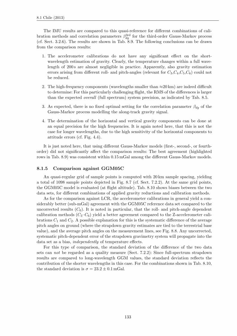
8.1 Chile (2013)
The IMU results are compared to this quasi-reference for different combinations of cali-bration methods and correlation parameters β3rddg for the third-order Gauss-Markov process(cf. Sect. 3.2.6). The results are shown in Tab. 8.9. The following conclusions can be drawnfrom the comparison results:
1. The accelerometer calibrations do not have any significant effect on the short-wavelength estimation of gravity. Clearly, the temperature changes within a full wave-length of 200 s are almost negligible in practice. Apparently, also gravity estimationerrors arising from different roll- and pitch-angles (relevant for C3,C4,C5,C6) could notbe reduced.
2. The high-frequency components (wavelengths smaller than ≈20 km) are indeed difficultto determine: For this particularly challenging flight, the RMS of the differences is largerthan the expected overall (full spectrum) system precision, as indicated by Tab. 8.5.
3. As expected, there is no fixed optimal setting for the correlation parameter βdg of theGauss-Markov process modelling the along-track gravity signal.
4. The determination of the horizontal and vertical gravity components can be done atan equal precision for the high frequencies. It is again noted here, that this is not thecase for longer wavelengths, due to the high sensitivity of the horizontal components toattitude errors (cf. Fig. 4.4).
It is just noted here, that using different Gauss-Markov models (first-, second-, or fourth-order) did not significantly affect the comparison results: The best agreement (highlightedrows in Tab. 8.9) was consistent within 0.15mGal among the different Gauss-Markov models.
8.1.5 Comparison against GGM05C
An quasi-regular grid of sample points is computed with 20 km sample spacing, yieldinga total of 1098 sample points depicted in Fig. 8.7 (cf. Sect. 7.2.2). At the same grid points,the GGM05C model is evaluated (at flight altitude). Tab. 8.10 shows biases between the twodata sets, for different combinations of applied gravity reductions and calibration methods.
As for the comparison against LCR, the accelerometer calibrations in general yield a con-siderably better (sub-mGal) agreement with the GGM05C reference data set compared to theuncorrected results (C0). It is noted in particular, that the roll- and pitch-angle dependentcalibration methods (C3–C6) yield a better agreement compared to the Z-accelerometer cali-brations C1 and C2. A possible explanation for this is the systematic difference of the averagepitch angles on ground (where the strapdown gravity estimates are tied to the terrestrial basevalue), and the average pitch angles on the measurement lines, see Fig. 8.8. Any uncorrected,systematic pitch-dependent error of the strapdown gravimetry system will propagate into thedata set as a bias, independently of temperature effects.
For this type of comparison, the standard deviation of the difference of the two datasets can not be regarded as a quality measure (Sect. 7.2.2): Since full-spectrum strapdownresults are compared to long-wavelength GGM values, the standard deviation reflects thecontribution of the shorter wavelengths in this case. For the combinations shown in Tab. 8.10,the standard deviation is σ = 23.2± 0.1mGal.
133
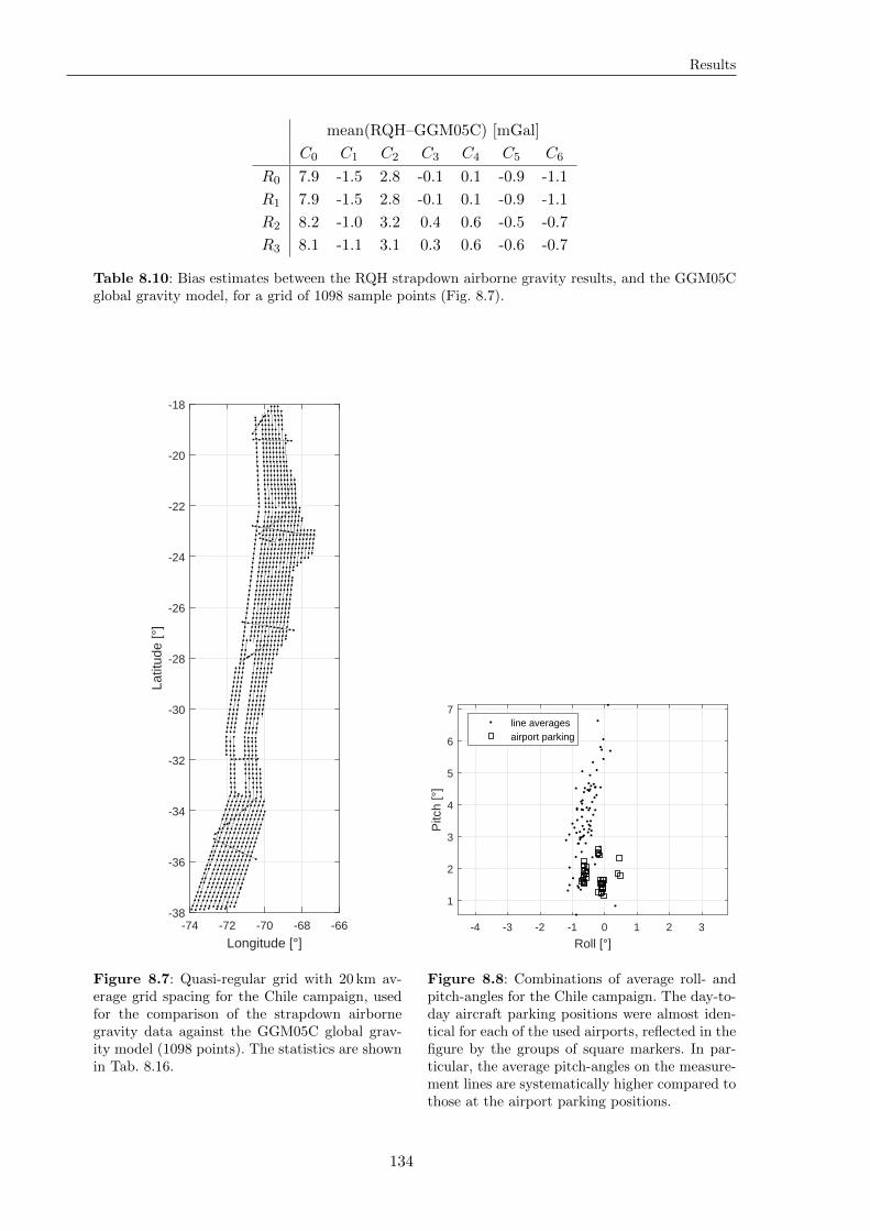
Results
mean(RQH–GGM05C) [mGal]
C0 C1 C2 C3 C4 C5 C6
R0 7.9 -1.5 2.8 -0.1 0.1 -0.9 -1.1
R1 7.9 -1.5 2.8 -0.1 0.1 -0.9 -1.1
R2 8.2 -1.0 3.2 0.4 0.6 -0.5 -0.7
R3 8.1 -1.1 3.1 0.3 0.6 -0.6 -0.7
Table 8.10: Bias estimates between the RQH strapdown airborne gravity results, and the GGM05Cglobal gravity model, for a grid of 1098 sample points (Fig. 8.7).
-74 -72 -70 -68 -66
Longitude [°]
-38
-36
-34
-32
-30
-28
-26
-24
-22
-20
-18
Latit
ude
[°]
Figure 8.7: Quasi-regular grid with 20 km av-erage grid spacing for the Chile campaign, usedfor the comparison of the strapdown airbornegravity data against the GGM05C global grav-ity model (1098 points). The statistics are shownin Tab. 8.16.
-4 -3 -2 -1 0 1 2 3
Roll [°]
1
2
3
4
5
6
7
Pitc
h [°
]
line averagesairport parking
Figure 8.8: Combinations of average roll- andpitch-angles for the Chile campaign. The day-to-day aircraft parking positions were almost iden-tical for each of the used airports, reflected in thefigure by the groups of square markers. In par-ticular, the average pitch-angles on the measure-ment lines are systematically higher compared tothose at the airport parking positions.
134
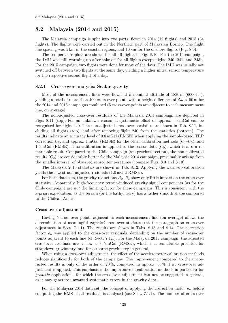
8.2 Malaysia (2014 and 2015)
8.2 Malaysia (2014 and 2015)
The Malaysia campaign is split into two parts, flown in 2014 (12 flights) and 2015 (34flights). The flights were carried out in the Northern part of Malaysian Borneo. The flightline spacing was 5 km in the coastal regions, and 10 km for the offshore flights (Fig. 8.9).
The temperature plots are shown for all 46 flights in Fig. 8.10. For the 2014 campaign,the IMU was still warming up after take-off for all flights except flights 240, 241, and 243b.For the 2015 campaign, two flights were done for most of the days. The IMU was usually notswitched off between two flights at the same day, yielding a higher initial sensor temperaturefor the respective second flight of a day.
8.2.1 Cross-over analysis: Scalar gravity
Most of the measurement lines were flown at a nominal altitude of 1830m (6000 ft ),yielding a total of more than 400 cross-over points with a height difference of ∆h < 50m forthe 2014 and 2015 campaigns combined (5 cross-over points are adjacent to each measurementline, on average).
The non-adjusted cross-over residuals of the Malaysia 2014 campaign are depicted inFigs. 8.11 (top). For an unknown reason, a systematic offset of approx. −3mGal can berecognised for flight 240. The non-adjusted cross-over statistics are shown in Tab. 8.11, in-cluding all flights (top), and after removing flight 240 from the statistics (bottom). Theresults indicate an accuracy level of 0.8mGal (RMSE) when applying the sample-based TRPcorrection C6, and approx. 1mGal (RMSE) for the other calibration methods (C1–C5), and1.6mGal (RMSE), if no calibration is applied to the sensor data (C0), which is also a re-markable result. Compared to the Chile campaign (see previous section), the non-calibratedresults (C0) are considerably better for the Malaysia 2014 campaign, presumably arising fromthe smaller interval of observed sensor temperatures (compare Figs. 8.3 and 8.10).
The Malaysia 2015 statistics are shown in Tab. 8.12. Applying the warm-up calibrationyields the lowest non-adjusted residuals (1.0mGal RMSE).
For both data sets, the gravity reductions R0–R3 show only little impact on the cross-overstatistics. Apparently, high-frequency terrain-induced gravity signal components (as for theChile campaign) are not the limiting factor for these campaigns. This is consistent with thea-priori expectation, as the terrain (or the bathymetry) has a rather smooth shape comparedto the Chilean Andes.
Cross-over adjustment
Having 5 cross-over points adjacent to each measurement line (on average) allows thedetermination of meaningful adjusted cross-over statistics (cf. the paragraph on cross-overadjustment in Sect. 7.1.1). The results are shown in Tabs. 8.13 and 8.14. The correctionfactor ρn was applied to the cross-over residuals, depending on the number of cross-overpoints adjacent to each line (cf. Sect. 7.1.1). For the Malaysia 2015 campaign, the adjustedcross-over residuals are as low as 0.5mGal (RMSE), which is a remarkable precision forstrapdown gravimetry, and for airborne gravimetry in general.
When using a cross-over adjustment, the effect of the accelerometer calibration methodsreduces significantly for both of the campaigns: The improvement compared to the uncor-rected results is only of the order of 20%, compared to approx. 55% if no cross-over ad-justment is applied. This emphasises the importance of calibration methods in particular forgeodetic applications, for which the cross-over adjustment can not be suggested in general,as it may generate unwanted systematic errors in the gravity data.
For the Malaysia 2014 data set, the concept of applying the correction factor ρn beforecomputing the RMS of all residuals is analysed (see Sect. 7.1.1). The number of cross-over
135
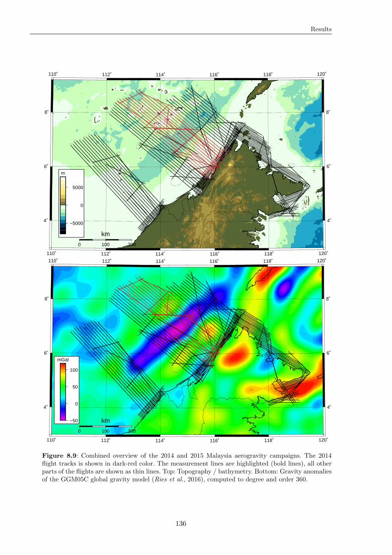
Results
110˚
110˚
112˚
112˚
114˚
114˚
116˚
116˚
118˚
118˚
120˚
120˚
4˚ 4˚
6˚ 6˚
8˚ 8˚
0 100 200
km
−5000
0
5000
m
110˚
110˚
112˚
112˚
114˚
114˚
116˚
116˚
118˚
118˚
120˚
120˚
4˚ 4˚
6˚ 6˚
8˚ 8˚
0 100 200
km−50
0
50
100
mGal
Figure 8.9: Combined overview of the 2014 and 2015 Malaysia aerogravity campaigns. The 2014flight tracks is shown in dark-red color. The measurement lines are highlighted (bold lines), all otherparts of the flights are shown as thin lines. Top: Topography / bathymetry. Bottom: Gravity anomaliesof the GGM05C global gravity model (Ries et al., 2016), computed to degree and order 360.
136
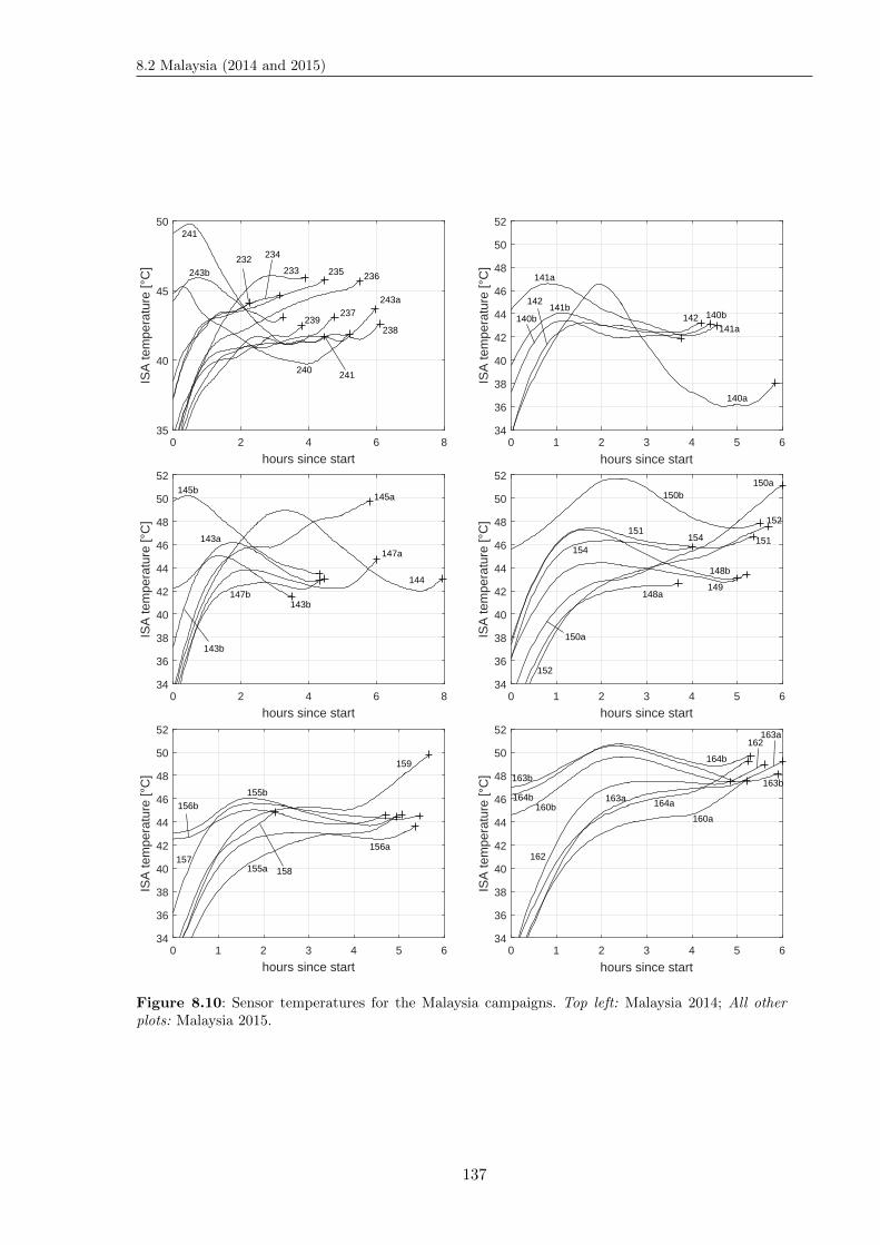
8.2 Malaysia (2014 and 2015)
0 2 4 6 8
hours since start
35
40
45
50
ISA
tem
pera
ture
[°C
]
232233
234
235 236
237
238239
240 241
243a
243b
241
0 1 2 3 4 5 6
hours since start
34
36
38
40
42
44
46
48
50
52
ISA
tem
pera
ture
[°C
]
140a
140b
141a
141b142
141a140b
142
0 2 4 6 8
hours since start
34
36
38
40
42
44
46
48
50
52
ISA
tem
pera
ture
[°C
]
143a
143b
144
145a145b
147a
147b
143b
0 1 2 3 4 5 6
hours since start
34
36
38
40
42
44
46
48
50
52IS
A te
mpe
ratu
re [°
C]
148a
148b
149
150a150b
151
152
154151
152
150a
154
0 1 2 3 4 5 6
hours since start
34
36
38
40
42
44
46
48
50
52
ISA
tem
pera
ture
[°C
]
155a
155b
156a
156b
157158
159
0 1 2 3 4 5 6
hours since start
34
36
38
40
42
44
46
48
50
52
ISA
tem
pera
ture
[°C
]
160a160b
162
163a
163b
164a
164b
163b
164b 163a
162
Figure 8.10: Sensor temperatures for the Malaysia campaigns. Top left: Malaysia 2014; All otherplots: Malaysia 2015.
137
Results
points is artificially reduced by removing randomly selected points from the full set. The RMSof the adjusted cross-over residuals is then computed for the reduced set of cross-over points.The experiment is repeated for more than 1500 times. The results are shown in Fig. 8.12,including linear regression polynomials, confirming the concept of these correction factors:The statistics of the uncorrected residuals clearly show a dependency on the number of cross-over points (the average RMS reduces by 25%). Thus, lower numbers of cross-over points yieldtoo optimistic estimates. Conversely, the corrected residuals show barely any dependency onthe number of cross-over points (the average RMS reduces by only 4%).
For the full set of 99 cross-over points, the RMS of the uncorrected residuals of 0.82mGalcan be expected to be too optimistic by 15% (0.14mGal).
8.2.2 Cross-over analysis: Deflections of the Vertical
The determination of the deflection of the vertical (DoV) heavily depends on the atti-tude stability of the system, as was shown by the observability and estimability analyses inChap. 4, and also by the error propagation simulations of Chap. 5. Therefore, the accelerom-eter calibrations are expected to have only a small effect on the DoV determination. This isindeed reflected by the results shown in Tab. 8.15.
For a navigation-grade strapdown IMU, the absolute attitude errors can be expected tobe of the order of 5–15 arc seconds, directly propagating into the DoV estimates (again,5–15 arc seconds). DoV estimates at this accuracy level usually do not have any practicaluse. Conversely, when applying a cross-over adjustment, the residual cross-over differencesindicate the relative stability of the DoV estimates along the flight lines.
The adjusted cross-over residuals for the deflections of the vertical are shown in Tab. 8.15,again corrected using the factor ρn. The Malaysia 2015 DoV estimates show significantly lowerresiduals. The reason for this is unknown, possible explanations are:
• The same aircraft was used for the two campaigns. However, between the two surveys,one of the engines underwent a major servicing due to some technical issue leadingto a lower power for that engine (i.e. an asymmetric power balance between the twoaircraft engines). Perhaps this malfunction had negatively influenced the aircraft motioncharacteristics for the 2014 campaign.
• A manufacturer firmware update was applied to the iMAR RQH-1003 IMU betweenthe two campaigns.
The shown DoV precision of approx. 0.8 to 1.2 arc seconds (RMSE) may be usable inpractice, e.g. for geophysical inversion, or as constraints for the local geoid determination, atthe borders of the region of available gravity data.
8.2.3 Comparison against GGM05C
The comparison against GGM05C is based on a quasi-regular grid of comparison points,with a grid-spacing of ≈20 km, cf. Sect. 7.2.2. The grid is depicted in Fig. 8.13. The coastalflight lines in the Eastern part of Borneo (see Fig. 8.13) are not used for the comparison,because the covered area is narrower than a single wavelength of the GGM05C data.
The statistics of the comparison are shown in Tab. 8.16. The biases can be shown to bewell below 1mGal for the sample-based calibration approaches. The uncorrected results (C0)show a significantly higher bias compared to the calibrated data sets. The applied gravityreductions show barely any effect for this comparison.
138
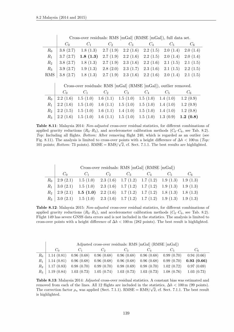
8.2 Malaysia (2014 and 2015)
Cross-over residuals: RMS [mGal] (RMSE [mGal]), full data set.
C0 C1 C2 C3 C4 C5 C6
R0 3.8 (2.7) 1.8 (1.3) 2.7 (1.9) 2.2 (1.6) 2.2 (1.5) 2.0 (1.4) 2.0 (1.4)
R1 3.7 (2.7) 1.8 (1.3) 2.7 (1.9) 2.2 (1.6) 2.2 (1.5) 2.0 (1.4) 2.0 (1.4)
R2 3.8 (2.7) 1.8 (1.3) 2.7 (1.9) 2.3 (1.6) 2.2 (1.6) 2.1 (1.5) 2.1 (1.5)
R3 3.9 (2.7) 1.9 (1.3) 2.8 (2.0) 2.3 (1.7) 2.3 (1.6) 2.1 (1.5) 2.2 (1.5)
RMS 3.8 (2.7) 1.8 (1.3) 2.7 (1.9) 2.3 (1.6) 2.2 (1.6) 2.0 (1.4) 2.1 (1.5)
Cross-over residuals: RMS [mGal] (RMSE [mGal]), outlier removed.
C0 C1 C2 C3 C4 C5 C6
R0 2.2 (1.6) 1.5 (1.0) 1.6 (1.1) 1.5 (1.0) 1.5 (1.0) 1.4 (1.0) 1.2 (0.9)
R1 2.2 (1.6) 1.5 (1.0) 1.6 (1.1) 1.5 (1.0) 1.5 (1.0) 1.4 (1.0) 1.2 (0.9)
R2 2.2 (1.5) 1.5 (1.0) 1.6 (1.1) 1.4 (1.0) 1.5 (1.0) 1.4 (1.0) 1.2 (0.8)
R3 2.2 (1.6) 1.5 (1.0) 1.6 (1.1) 1.5 (1.0) 1.5 (1.0) 1.3 (0.9) 1.2 (0.8)
Table 8.11: Malaysia 2014: Non-adjusted cross-over residual statistics, for different combinations ofapplied gravity reductions (R0–R3), and accelerometer calibration methods (C0–C6, see Tab. 8.2).Top: Including all flights. Bottom: After removing flight 240, which is regarded as an outlier (seeFig. 8.11). The analysis is limited to cross-over points with a height difference of ∆h < 100m (Top:101 points; Bottom: 73 points). RMSE = RMS/
√2, cf. Sect. 7.1.1. The best results are highlighted.
Cross-over residuals: RMS [mGal] (RMSE [mGal])
C0 C1 C2 C3 C4 C5 C6
R0 2.9 (2.1) 1.5 (1.0) 2.3 (1.6) 1.7 (1.2) 1.7 (1.2) 1.9 (1.3) 1.9 (1.3)
R1 3.0 (2.1) 1.5 (1.0) 2.3 (1.6) 1.7 (1.2) 1.7 (1.2) 1.9 (1.3) 1.9 (1.3)
R2 2.9 (2.1) 1.5 (1.0) 2.2 (1.6) 1.7 (1.2) 1.7 (1.2) 1.8 (1.3) 1.8 (1.3)
R3 3.0 (2.1) 1.5 (1.0) 2.3 (1.6) 1.7 (1.2) 1.7 (1.2) 1.9 (1.3) 1.9 (1.3)
Table 8.12: Malaysia 2015: Non-adjusted cross-over residual statistics, for different combinations ofapplied gravity reductions (R0–R3), and accelerometer calibration methods (C0–C6, see Tab. 8.2).Flight 149 has severe GNSS data errors and is not included in the statistics. The analysis is limited tocross-over points with a height difference of ∆h < 100m (282 points). The best result is highlighted.
Adjusted cross-over residuals: RMS [mGal] (RMSE [mGal])
C0 C1 C2 C3 C4 C5 C6
R0 1.14 (0.81) 0.96 (0.68) 0.96 (0.68) 0.96 (0.68) 0.96 (0.68) 0.99 (0.70) 0.94 (0.66)
R1 1.14 (0.81) 0.96 (0.68) 0.96 (0.68) 0.96 (0.68) 0.96 (0.68) 0.99 (0.70) 0.93 (0.66)
R2 1.17 (0.83) 0.98 (0.70) 0.99 (0.70) 0.98 (0.69) 0.98 (0.70) 1.02 (0.72) 0.97 (0.69)
R3 1.19 (0.84) 1.03 (0.73) 1.05 (0.74) 1.03 (0.73) 1.03 (0.73) 1.08 (0.76) 1.03 (0.73)
Table 8.13: Malaysia 2014: Adjusted cross-over residual statistics. A constant bias was estimated andremoved from each of the lines. All 12 flights are included in the statistics, ∆h < 100m (99 points).The correction factor ρn was applied (Sect. 7.1.1). RMSE = RMS/
√2, cf. Sect. 7.1.1. The best result
is highlighted.
139
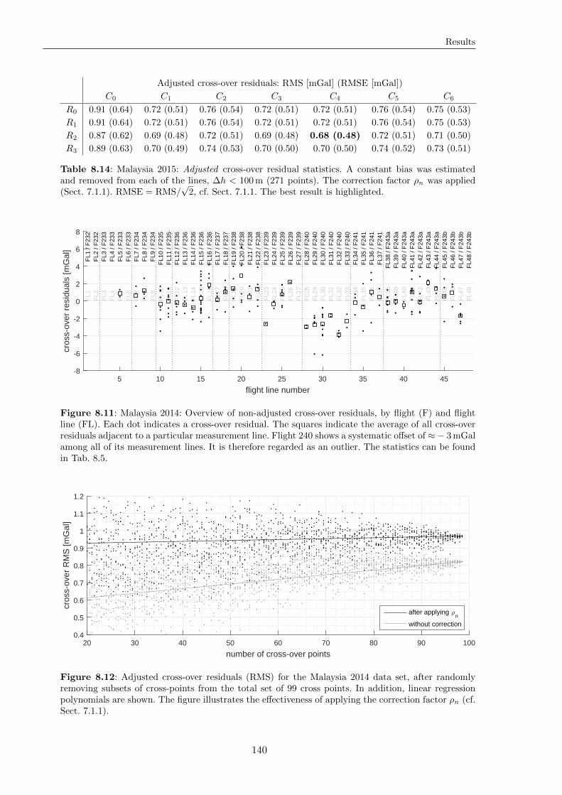
Results
Adjusted cross-over residuals: RMS [mGal] (RMSE [mGal])
C0 C1 C2 C3 C4 C5 C6
R0 0.91 (0.64) 0.72 (0.51) 0.76 (0.54) 0.72 (0.51) 0.72 (0.51) 0.76 (0.54) 0.75 (0.53)
R1 0.91 (0.64) 0.72 (0.51) 0.76 (0.54) 0.72 (0.51) 0.72 (0.51) 0.76 (0.54) 0.75 (0.53)
R2 0.87 (0.62) 0.69 (0.48) 0.72 (0.51) 0.69 (0.48) 0.68 (0.48) 0.72 (0.51) 0.71 (0.50)
R3 0.89 (0.63) 0.70 (0.49) 0.74 (0.53) 0.70 (0.50) 0.70 (0.50) 0.74 (0.52) 0.73 (0.51)
Table 8.14: Malaysia 2015: Adjusted cross-over residual statistics. A constant bias was estimatedand removed from each of the lines, ∆h < 100m (271 points). The correction factor ρn was applied(Sect. 7.1.1). RMSE = RMS/
√2, cf. Sect. 7.1.1. The best result is highlighted.
5 10 15 20 25 30 35 40 45
flight line number
-8
-6
-4
-2
0
2
4
6
8
cros
s-ov
er r
esid
uals
[mG
al]
FL1
/ F
232
FL1
FL2
/ F
232
FL2
FL3
/ F
233
FL3
FL4
/ F
233
FL4
FL5
/ F
233
FL5
FL6
/ F
233
FL6
FL7
/ F
234
FL7
FL8
/ F
234
FL8
FL9
/ F
234
FL9
FL1
0 / F
235
FL1
0F
L11
/ F23
5F
L11
FL1
2 / F
236
FL1
2F
L13
/ F23
6F
L13
FL1
4 / F
236
FL1
4F
L15
/ F23
6F
L15
FL1
6 / F
236
FL1
6F
L17
/ F23
7F
L17
FL1
8 / F
237
FL1
8F
L19
/ F23
8F
L19
FL2
0 / F
238
FL2
0F
L21
/ F23
8F
L21
FL2
2 / F
238
FL2
2F
L23
/ F23
9F
L23
FL2
4 / F
239
FL2
4F
L25
/ F23
9F
L25
FL2
6 / F
239
FL2
6F
L27
/ F23
9F
L27
FL2
8 / F
240
FL2
8F
L29
/ F24
0F
L29
FL3
0 / F
240
FL3
0F
L31
/ F24
0F
L31
FL3
2 / F
240
FL3
2F
L33
/ F24
0F
L33
FL3
4 / F
241
FL3
4F
L35
/ F24
1F
L35
FL3
6 / F
241
FL3
6F
L37
/ F24
1F
L37
FL3
8 / F
243a
FL3
8F
L39
/ F24
3aF
L39
FL4
0 / F
243a
FL4
0F
L41
/ F24
3aF
L41
FL4
2 / F
243a
FL4
2F
L43
/ F24
3aF
L43
FL4
4 / F
243a
FL4
4F
L45
/ F24
3bF
L45
FL4
6 / F
243b
FL4
6F
L47
/ F24
3bF
L47
FL4
8 / F
243b
FL4
8
Figure 8.11: Malaysia 2014: Overview of non-adjusted cross-over residuals, by flight (F) and flightline (FL). Each dot indicates a cross-over residual. The squares indicate the average of all cross-overresiduals adjacent to a particular measurement line. Flight 240 shows a systematic offset of ≈− 3mGalamong all of its measurement lines. It is therefore regarded as an outlier. The statistics can be foundin Tab. 8.5.
20 30 40 50 60 70 80 90 100
number of cross-over points
0.4
0.5
0.6
0.7
0.8
0.9
1
1.1
1.2
cros
s-ov
er R
MS
[mG
al]
after applying ρn
without correction
Figure 8.12: Adjusted cross-over residuals (RMS) for the Malaysia 2014 data set, after randomlyremoving subsets of cross-points from the total set of 99 cross points. In addition, linear regressionpolynomials are shown. The figure illustrates the effectiveness of applying the correction factor ρn (cf.Sect. 7.1.1).
140
8.2 Malaysia (2014 and 2015)
Malaysia 2014 DoV cross-over residuals: RMS [”] (RMSE [”])
C0 C1 C2 C3 C4 C5 C6
ξ 1.60 (1.13) 1.60 (1.13) 1.60 (1.13) 1.60 (1.13) 1.60 (1.13) 1.64 (1.16) 1.65 (1.16)
η 1.66 (1.17) 1.66 (1.17) 1.66 (1.17) 1.65 (1.17) 1.65 (1.16) 1.67 (1.18) 1.65 (1.17)
Malaysia 2015 DoV cross-over residuals: RMS [”] (RMSE [”])
C0 C1 C2 C3 C4 C5 C6
ξ 1.07 (0.76) 1.07 (0.76) 1.07 (0.76) 1.07 (0.76) 1.06 (0.75) 1.09 (0.77) 1.08 (0.77)
η 1.10 (0.78) 1.10 (0.78) 1.10 (0.78) 1.10 (0.78) 1.11 (0.78) 1.08 (0.77) 1.06 (0.75)
Table 8.15: DoV cross-over residual statistics. A constant bias was estimated and removed from eachof the lines. The analysis is limited to cross-over points with a height difference of ∆h < 100m (2014:99 points, 2015: 271 points).
111 112 113 114 115 116 117 118 119
Longitude [°]
3.5
4
4.5
5
5.5
6
6.5
7
7.5
8
8.5
9
Latit
ude
[°]
Figure 8.13: Quasi-regular grid with 20 km average grid spacing for the Malaysia campaigns, usedfor the comparison of the strapdown airborne gravity data against the GGM05C global gravity model(cf. Tab. 8.16).
Malaysia: mean(RQH–GGM05C) [mGal]
C0 C1 C2 C3 C4 C5 C6
R0 2.93 1.15 2.02 1.81 1.79 0.32 0.03
R1 3.00 1.22 2.10 1.88 1.87 0.39 0.10
R2 2.89 1.12 1.99 1.78 1.77 0.29 0.02
R3 2.91 1.14 2.01 1.81 1.79 0.32 0.04
Table 8.16: Mean difference of the strapdown gravity data minus GGM05C, evaluated at flightaltitude for the quasi-regular grid depicted in Fig. 8.13 (488 points).
141
Results
-2 -1 0 1 2
Roll [°]
0
1
2
3
Pitc
h [°
]
line averagesairport parking
Figure 8.14: Combinations of average roll- and pitch-angles for the Malaysia campaigns. The 2014campaign measurement lines have a systematically lower roll angle (around −1.3). The same aircraftand hardware set-up was used for the 2015 campaign, however one of the aircraft engines underwenta major maintenance, presumably explaining the shift of the average roll-angle to approximately 0.5.See also App. A.1.
142
8.3 Northern Mozambique and Malawi (2015)
8.3 Northern Mozambique and Malawi (2015)
An overview of the Northern Mozambique and Malawi campaign is shown in Fig. 8.15.The air-conditioning system of the Cessna 208 aircraft apparently yielded a very stable cabintemperature, which is evident from the sensor temperature curves shown in Fig. 8.16. Initially,all of the curves indicate a considerable warm-up of the sensor. At the final parking positionon the destination airport, the sensor temperature increases, because the air conditioningsystem was turned off.
8.3.1 Cross-over analysis
The non-adjusted cross-over statistics are shown in Tab. 8.17, again for different com-binations of gravity reduction (R0–R3) and accelerometer calibrations (C0–C6). The samecorrelation parameters were used as for the Chile campaign: β3rddg = 1/10 km−1 for R0 and R1
(no terrain reduction), and β3rddg = 1/20 km−1 for R2 and R3 (with terrain reduction). Thesesettings were determined empirically, on the data.
Flights 285, 287, and 299 are not included in the cross-over statistics, because they couldnot be processed from start to end due to IMU data acquisition problems: Short poweroutages resulted in gaps in the data recordings. These flights could still be processed, butthe linear drift removal based on the terrestrial gravity ties (cf. Sect. 7.1.3) was impossiblefor these flights. It is just noted here, that including these flights in the statistics leads tohigher cross-over residuals of approximately 1.9mGal (RMS) instead of 1.3mGal. Again,this emphasises the importance of a gap-free data recording from the original airport to thedestination airport.
Again, the accelerometer calibrations lead to considerable improvements, with cross-overresiduals decreasing from 3mGal to approximately 1mGal (RMSE). The terrain reductions(R2 and R3) yield equal or slightly better results among the different calibration methods.Best results are again provided by the sample-based TRP calibration methods, C5 and C6
(Sect. 6.6.1).Due to the lack of sufficient cross-over points at equal altitude, no meaningful adjusted
cross-over statistics are available for this data set. Consequently, no cross-over statistics arepresented for the deflections of the vertical.
Cross-over residuals: RMS [mGal] (RMSE [mGal])
C0 C1 C2 C3 C4 C5 C6
R0 4.10 (2.90) 1.69 (1.20) 1.58 (1.12) 1.61 (1.14) 1.52 (1.07) 1.28 (0.91) 1.29 (0.91)
R1 4.11 (2.91) 1.69 (1.19) 1.58 (1.12) 1.60 (1.13) 1.51 (1.07) 1.28 (0.90) 1.29 (0.91)
R2 4.20 (2.97) 1.47 (1.04) 1.62 (1.14) 1.42 (1.00) 1.34 (0.95) 1.44 (1.02) 1.44 (1.02)
R3 4.22 (2.98) 1.41 (1.00) 1.66 (1.17) 1.37 (0.97) 1.30 (0.92) 1.44 (1.01) 1.43 (1.01)
Table 8.17: Mozambique/Malawi: Cross-over residual statistics, excluding flights 285, 287, and 299(see text). No cross-over adjustment was applied. The analysis is limited to cross-over points with aheight difference of ∆h < 100m (33 points). The best result is highlighted.
143
Resu
lts
30˚
30˚
32˚
32˚
34˚
34˚
36˚
36˚
−18˚ −18˚
−16˚ −16˚
−14˚ −14˚
−12˚ −12˚
−10˚ −10˚
0 100 200
km
−5000
0
5000
m
30˚
30˚
32˚
32˚
34˚
34˚
36˚
36˚
−18˚ −18˚
−16˚ −16˚
−14˚ −14˚
−12˚ −12˚
−10˚ −10˚
0 100 200
km
−100
−50
0
50
100mGal
Figure 8.15: Overview of the Northern Mozambique and Malawi aerogravity campaigns. The measurement lines are highlighted (bold lines). Left: Topography.Right: Gravity anomalies of the GGM05C global gravity model (Ries et al., 2016), computed to degree and order 360.
144
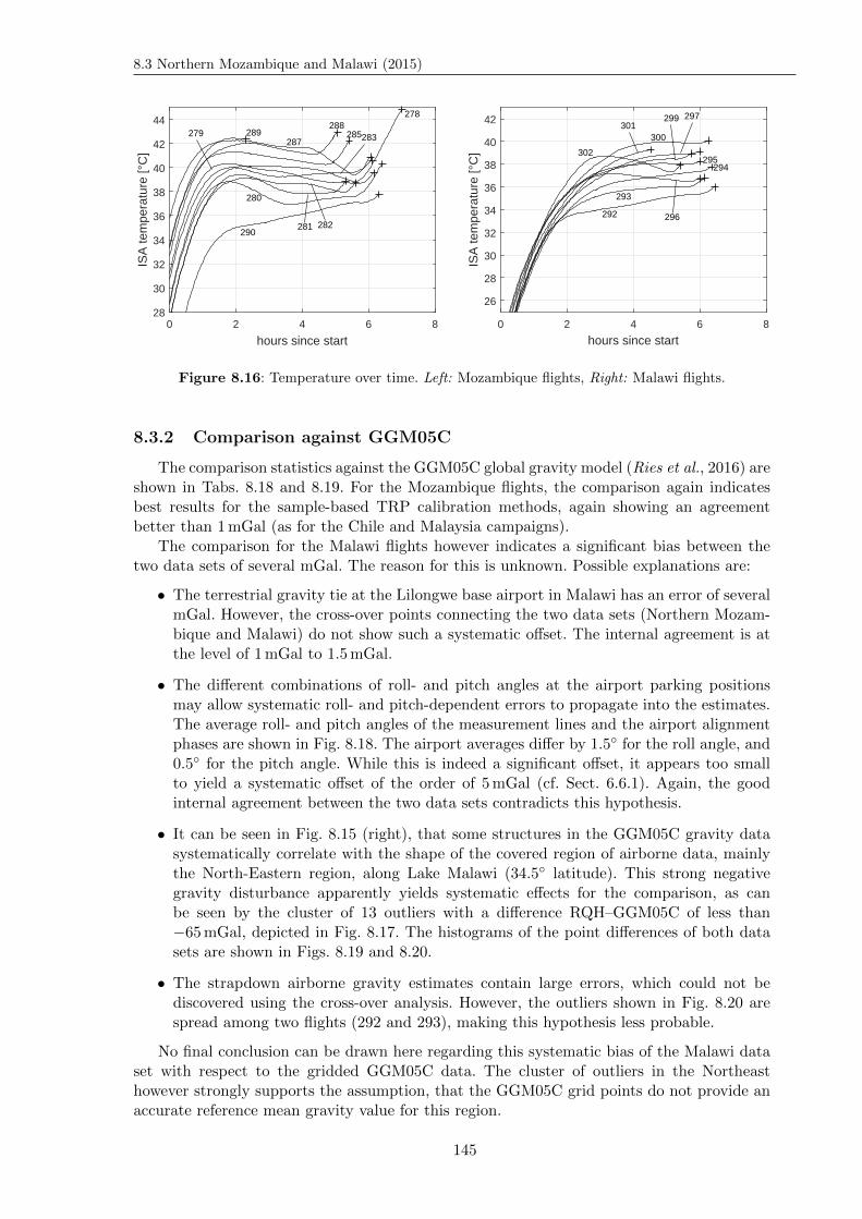
8.3 Northern Mozambique and Malawi (2015)
0 2 4 6 8
hours since start
28
30
32
34
36
38
40
42
44
ISA
tem
pera
ture
[°C
]
278
279
280
281 282
283285287
288289
290
0 2 4 6 8
hours since start
26
28
30
32
34
36
38
40
42
ISA
tem
pera
ture
[°C
]
292
293
294295
296
297299
300301
302
Figure 8.16: Temperature over time. Left: Mozambique flights, Right: Malawi flights.
8.3.2 Comparison against GGM05C
The comparison statistics against the GGM05C global gravity model (Ries et al., 2016) areshown in Tabs. 8.18 and 8.19. For the Mozambique flights, the comparison again indicatesbest results for the sample-based TRP calibration methods, again showing an agreementbetter than 1mGal (as for the Chile and Malaysia campaigns).
The comparison for the Malawi flights however indicates a significant bias between thetwo data sets of several mGal. The reason for this is unknown. Possible explanations are:
• The terrestrial gravity tie at the Lilongwe base airport in Malawi has an error of severalmGal. However, the cross-over points connecting the two data sets (Northern Mozam-bique and Malawi) do not show such a systematic offset. The internal agreement is atthe level of 1mGal to 1.5mGal.
• The different combinations of roll- and pitch angles at the airport parking positionsmay allow systematic roll- and pitch-dependent errors to propagate into the estimates.The average roll- and pitch angles of the measurement lines and the airport alignmentphases are shown in Fig. 8.18. The airport averages differ by 1.5 for the roll angle, and0.5 for the pitch angle. While this is indeed a significant offset, it appears too smallto yield a systematic offset of the order of 5mGal (cf. Sect. 6.6.1). Again, the goodinternal agreement between the two data sets contradicts this hypothesis.
• It can be seen in Fig. 8.15 (right), that some structures in the GGM05C gravity datasystematically correlate with the shape of the covered region of airborne data, mainlythe North-Eastern region, along Lake Malawi (34.5 latitude). This strong negativegravity disturbance apparently yields systematic effects for the comparison, as canbe seen by the cluster of 13 outliers with a difference RQH–GGM05C of less than−65mGal, depicted in Fig. 8.17. The histograms of the point differences of both datasets are shown in Figs. 8.19 and 8.20.
• The strapdown airborne gravity estimates contain large errors, which could not bediscovered using the cross-over analysis. However, the outliers shown in Fig. 8.20 arespread among two flights (292 and 293), making this hypothesis less probable.
No final conclusion can be drawn here regarding this systematic bias of the Malawi dataset with respect to the gridded GGM05C data. The cluster of outliers in the Northeasthowever strongly supports the assumption, that the GGM05C grid points do not provide anaccurate reference mean gravity value for this region.
145
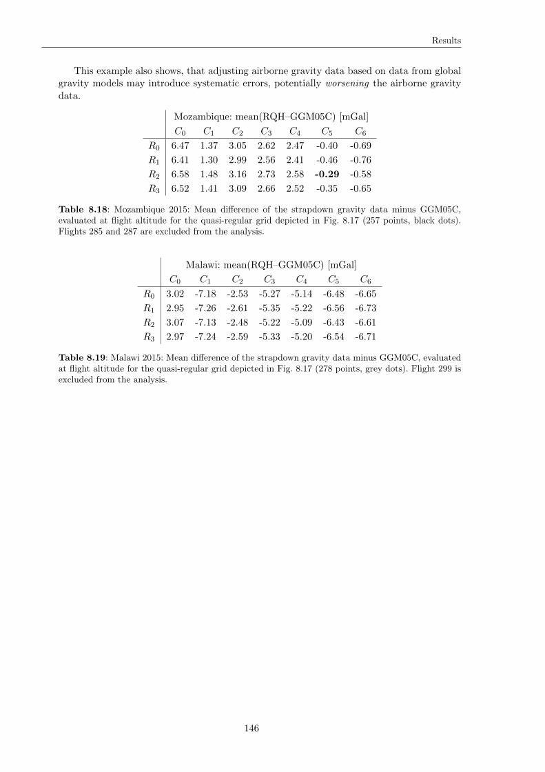
Results
This example also shows, that adjusting airborne gravity data based on data from globalgravity models may introduce systematic errors, potentially worsening the airborne gravitydata.
Mozambique: mean(RQH–GGM05C) [mGal]
C0 C1 C2 C3 C4 C5 C6
R0 6.47 1.37 3.05 2.62 2.47 -0.40 -0.69
R1 6.41 1.30 2.99 2.56 2.41 -0.46 -0.76
R2 6.58 1.48 3.16 2.73 2.58 -0.29 -0.58
R3 6.52 1.41 3.09 2.66 2.52 -0.35 -0.65
Table 8.18: Mozambique 2015: Mean difference of the strapdown gravity data minus GGM05C,evaluated at flight altitude for the quasi-regular grid depicted in Fig. 8.17 (257 points, black dots).Flights 285 and 287 are excluded from the analysis.
Malawi: mean(RQH–GGM05C) [mGal]
C0 C1 C2 C3 C4 C5 C6
R0 3.02 -7.18 -2.53 -5.27 -5.14 -6.48 -6.65
R1 2.95 -7.26 -2.61 -5.35 -5.22 -6.56 -6.73
R2 3.07 -7.13 -2.48 -5.22 -5.09 -6.43 -6.61
R3 2.97 -7.24 -2.59 -5.33 -5.20 -6.54 -6.71
Table 8.19: Malawi 2015: Mean difference of the strapdown gravity data minus GGM05C, evaluatedat flight altitude for the quasi-regular grid depicted in Fig. 8.17 (278 points, grey dots). Flight 299 isexcluded from the analysis.
146
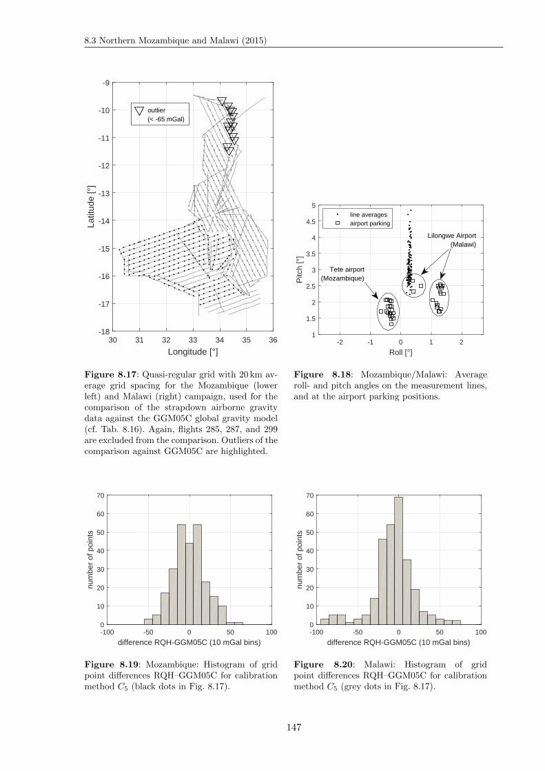
8.3 Northern Mozambique and Malawi (2015)
30 31 32 33 34 35 36
Longitude [°]
-18
-17
-16
-15
-14
-13
-12
-11
-10
-9La
titud
e [°
]
outlier (< -65 mGal)
Figure 8.17: Quasi-regular grid with 20 km av-erage grid spacing for the Mozambique (lowerleft) and Malawi (right) campaign, used for thecomparison of the strapdown airborne gravitydata against the GGM05C global gravity model(cf. Tab. 8.16). Again, flights 285, 287, and 299are excluded from the comparison. Outliers of thecomparison against GGM05C are highlighted.
-2 -1 0 1 2
Roll [°]
1
1.5
2
2.5
3
3.5
4
4.5
5
Pitc
h [°
]
line averagesairport parking
Tete airport(Mozambique)
Lilongwe Airport(Malawi)
Figure 8.18: Mozambique/Malawi: Averageroll- and pitch angles on the measurement lines,and at the airport parking positions.
-100 -50 0 50 100
difference RQH-GGM05C (10 mGal bins)
0
10
20
30
40
50
60
70
num
ber
of p
oint
s
Figure 8.19: Mozambique: Histogram of gridpoint differences RQH–GGM05C for calibrationmethod C5 (black dots in Fig. 8.17).
-100 -50 0 50 100
difference RQH-GGM05C (10 mGal bins)
0
10
20
30
40
50
60
70
num
ber
of p
oint
s
Figure 8.20: Malawi: Histogram of gridpoint differences RQH–GGM05C for calibrationmethod C5 (grey dots in Fig. 8.17).
147
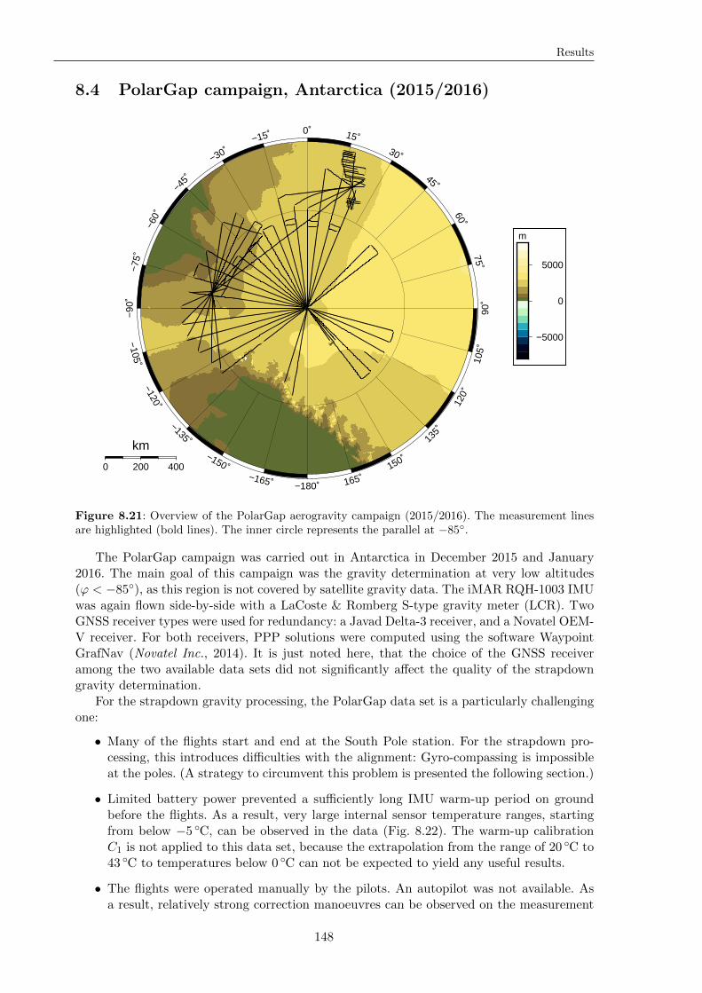
Results
8.4 PolarGap campaign, Antarctica (2015/2016)
−180˚−165˚
−150˚
−135˚
−120˚
−105˚
−90
˚−7
5˚−6
0˚
−45˚
−30˚−15˚ 0˚ 15˚
30˚
45˚
60˚75˚
90˚
105˚
120˚
135˚
150˚
165˚0 200 400
km
−5000
0
5000
m
Figure 8.21: Overview of the PolarGap aerogravity campaign (2015/2016). The measurement linesare highlighted (bold lines). The inner circle represents the parallel at −85.
The PolarGap campaign was carried out in Antarctica in December 2015 and January2016. The main goal of this campaign was the gravity determination at very low altitudes(ϕ < −85), as this region is not covered by satellite gravity data. The iMAR RQH-1003 IMUwas again flown side-by-side with a LaCoste & Romberg S-type gravity meter (LCR). TwoGNSS receiver types were used for redundancy: a Javad Delta-3 receiver, and a Novatel OEM-V receiver. For both receivers, PPP solutions were computed using the software WaypointGrafNav (Novatel Inc., 2014). It is just noted here, that the choice of the GNSS receiveramong the two available data sets did not significantly affect the quality of the strapdowngravity determination.
For the strapdown gravity processing, the PolarGap data set is a particularly challengingone:
• Many of the flights start and end at the South Pole station. For the strapdown pro-cessing, this introduces difficulties with the alignment: Gyro-compassing is impossibleat the poles. (A strategy to circumvent this problem is presented the following section.)
• Limited battery power prevented a sufficiently long IMU warm-up period on groundbefore the flights. As a result, very large internal sensor temperature ranges, startingfrom below −5 C, can be observed in the data (Fig. 8.22). The warm-up calibrationC1 is not applied to this data set, because the extrapolation from the range of 20 C to43 C to temperatures below 0 C can not be expected to yield any useful results.
• The flights were operated manually by the pilots. An autopilot was not available. Asa result, relatively strong correction manoeuvres can be observed on the measurement
148
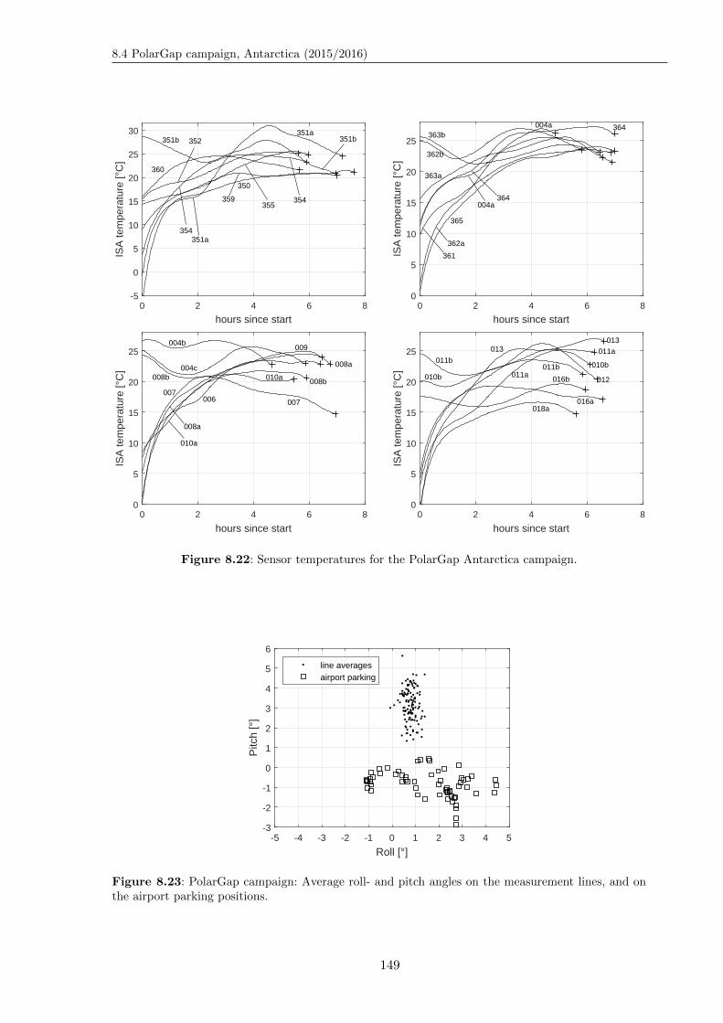
8.4 PolarGap campaign, Antarctica (2015/2016)
0 2 4 6 8
hours since start
-5
0
5
10
15
20
25
30IS
A te
mpe
ratu
re [°
C]
350
351a
351b 352
354355
359
360
354
351b351a
0 2 4 6 8
hours since start
0
5
10
15
20
25
ISA
tem
pera
ture
[°C
]
361
362a
362b
363a
363b364
365
004a
364004a
0 2 4 6 8
hours since start
0
5
10
15
20
25
ISA
tem
pera
ture
[°C
]
004b
004c
006 007
008a
008b
009
010a
010a
008b
007
008a
0 2 4 6 8
hours since start
0
5
10
15
20
25
ISA
tem
pera
ture
[°C
]
010b
011a011b
012
013
016a
016b
018a
010b011b
013
011a
Figure 8.22: Sensor temperatures for the PolarGap Antarctica campaign.
-5 -4 -3 -2 -1 0 1 2 3 4 5
Roll [°]
-3
-2
-1
0
1
2
3
4
5
6
Pitc
h [°
]
line averagesairport parking
Figure 8.23: PolarGap campaign: Average roll- and pitch angles on the measurement lines, and onthe airport parking positions.
149
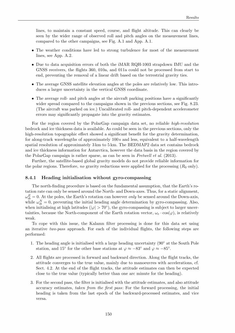
Results
lines, to maintain a constant speed, course, and flight altitude. This can clearly beseen by the wider range of observed roll and pitch angles on the measurement lines,compared to the other campaigns, see Fig. A.1 and App. A.1.
• The weather conditions have led to strong turbulence for most of the measurementlines, see App. A.2.
• Due to data acquisition errors of both the iMAR RQH-1003 strapdown IMU and theGNSS receivers, the flights 360, 010a, and 011a could not be processed from start toend, preventing the removal of a linear drift based on the terrestrial gravity ties.
• The average GNSS satellite elevation angles at the poles are relatively low. This intro-duces a larger uncertainty in the vertical GNSS coordinate.
• The average roll- and pitch angles at the aircraft parking positions have a significantlywider spread compared to the campaigns shown in the previous sections, see Fig. 8.23.(The aircraft was parked on ice.) Uncalibrated roll- and pitch-dependent accelerometererrors may significantly propagate into the gravity estimates.
For the region covered by the PolarGap campaign data set, no reliable high-resolutionbedrock and ice thickness data is available. As could be seen in the previous sections, only thehigh-resolution topographic effect showed a significant benefit for the gravity determination,for along-track wavelengths of approximately 100 s and less, equivalent to a half-wavelengthspatial resolution of approximately 3 km to 5 km. The BEDMAP2 data set contains bedrockand ice thickness information for Antarctica, however the data basis in the region covered bythe PolarGap campaign is rather sparse, as can be seen in Fretwell et al. (2013).
Further, the satellite-based global gravity models do not provide reliable information forthe polar regions. Therefore, no gravity reductions were applied for the processing (R0 only).
8.4.1 Heading initialisation without gyro-compassing
The north-finding procedure is based on the fundamental assumption, that the Earth’s ro-tation rate can only be sensed around the North- and Down-axes. Thus, for a static alignment,ωEib = 0. At the poles, the Earth’s rotation can however only be sensed around the Down-axis,while ωNib = 0, preventing the initial heading angle determination by gyro-compassing. Also,when initialising at high latitudes (|ϕ| > 70), the gyro-compassing is subject to larger uncer-tainties, because the North-component of the Earth rotation vector, ωe · cos(ϕ), is relativelyweak.
To cope with this issue, the Kalamn filter processing is done for this data set usingan iterative two-pass approach. For each of the individual flights, the following steps areperformed:
1. The heading angle is initialised with a large heading uncertainty (90 at the South Polestation, and 15 for the other base stations at ϕ ≈ −83 and ϕ ≈ −85.
2. All flights are processed in forward and backward direction. Along the flight tracks, theattitude converges to the true value, mainly due to manoeuvres with accelerations, cf.Sect. 4.2. At the end of the flight tracks, the attitude estimates can then be expectedclose to the true value (typically better than one arc minute for the heading).
3. For the second pass, the filter is initialised with the attitude estimates, and also attitudeaccuracy estimates, taken from the first pass: For the forward processing, the initialheading is taken from the last epoch of the backward-processed estimates, and viceversa.
150
8.5 Effect of turbulence
4. Reliable gravity estimates are then provided by the second pass. (For the first pass, inparticular for the South Pole flights, the attitude errors significantly propagate into thegravity estimates.)
8.4.2 Cross-over analysis
The non-adjusted cross-over residual statistics are shown in Tab. 8.20. All flights areincluded in the statistics, however there is a significant number of measurement lines whichare not adjacent to any cross-over point (cf. App. A.2). The shown statistics are still expectedto provide meaningful quality estimates, however it should be noted, that the shown RMSvalues only represent ≈50% of the flight lines (cf. Fig. 8.21). The warm-up calibration C1
was not applied, as mentioned above. The BSC and BSSC calibrations (C3 and C4) wereimplemented for ambient temperatures in the range from 10 C to 40 C (with internal sensortemperatures starting at 22 C. Thus, relevant extrapolation errors have to be expected alsowhen applying these calibrations, evident in Tab. 8.20 from the very poor cross-over precision.
The estimated precision of 1.9mGal is significantly worse compared to all other campaignsevaluated in the scope of this thesis (a factor of ≈ 2), presumably coming from the particulardifficulties for this data set as discussed in the previous section. The best results are providedby the temperature-chamber calibration C2, and the sample-based approaches C5 and C6.
A deeper analysis, e.g. comparisons against terrain effects and global gravity models,can not be carried out due to the lack of reliable reference data sets. It is just noted here,that a combined solution with the LCR gravity data may yield an optimised gravity data set,circumventing the strapdown long-term instability, which is presumably coming from thermaleffects.
Cross-over residuals: RMS [mGal] (RMSE [mGal])
C0 C1 C2 C3 C4 C5 C6
R0 4.0 (2.8) – 2.6 (1.9) (5.9 (4.2)) (5.4 (3.8)) 2.8 (2.0) 2.8 (2.0)
Table 8.20: PolarGap campaign: Cross-over residual statistics. No cross-over adjustment was applied.The analysis is limited to cross-over points with a height difference of ∆h < 100m (42 points). Theresults for C3 and C4 presumably suffer from strong extrapolation errors. The best result is highlighted.
8.5 Effect of turbulence
The effect of turbulence shall be quantified here using the results from the cross-overanalyses. The Malaysia and Mozambique/Malawi data sets are chosen, because they containa sufficient amount of cross-over points to allow the deduction of a general statement for thestrapdown gravimetry system.
RMS-g values are computed for all measurement lines of both data sets, using a time-window of 10 s, cf. Sect. 7.3. The results are shown in Fig. 8.24. Apparently, there is norecognisable relation between turbulence, and the quality of the strapdown airborne grav-ity data. This is an important result in practice. It indicates, that strapdown gravimetryis capable of providing reliable gravity estimates during flight segments containing strongturbulence.
Conversely, mechanical spring-gravimeters (as the LaCoste & Romberg S-type gravimeter)are known to be rather sensitive to strong turbulence.
151
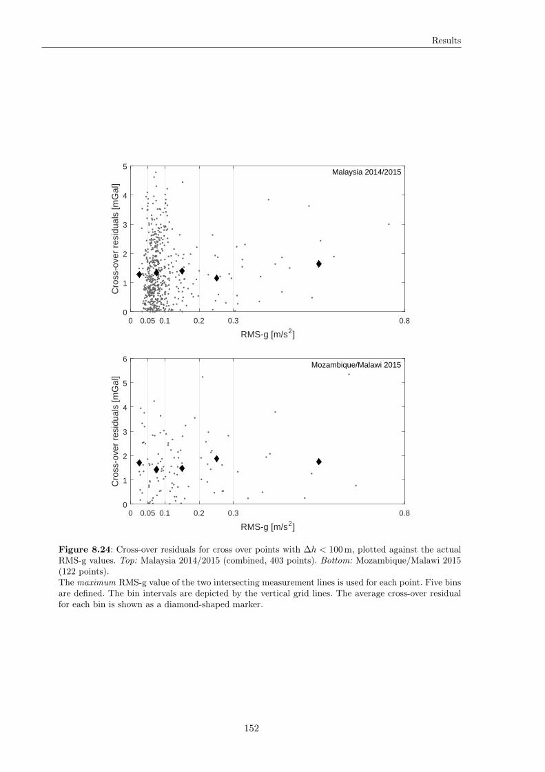
Results
0 0.05 0.1 0.2 0.3 0.8
RMS-g [m/s2]
0
1
2
3
4
5
Cro
ss-o
ver
resi
dual
s [m
Gal
]
Malaysia 2014/2015
0 0.05 0.1 0.2 0.3 0.8
RMS-g [m/s2]
0
1
2
3
4
5
6
Cro
ss-o
ver
resi
dual
s [m
Gal
]
Mozambique/Malawi 2015
Figure 8.24: Cross-over residuals for cross over points with ∆h < 100m, plotted against the actualRMS-g values. Top: Malaysia 2014/2015 (combined, 403 points). Bottom: Mozambique/Malawi 2015(122 points).The maximum RMS-g value of the two intersecting measurement lines is used for each point. Five binsare defined. The bin intervals are depicted by the vertical grid lines. The average cross-over residualfor each bin is shown as a diamond-shaped marker.
152
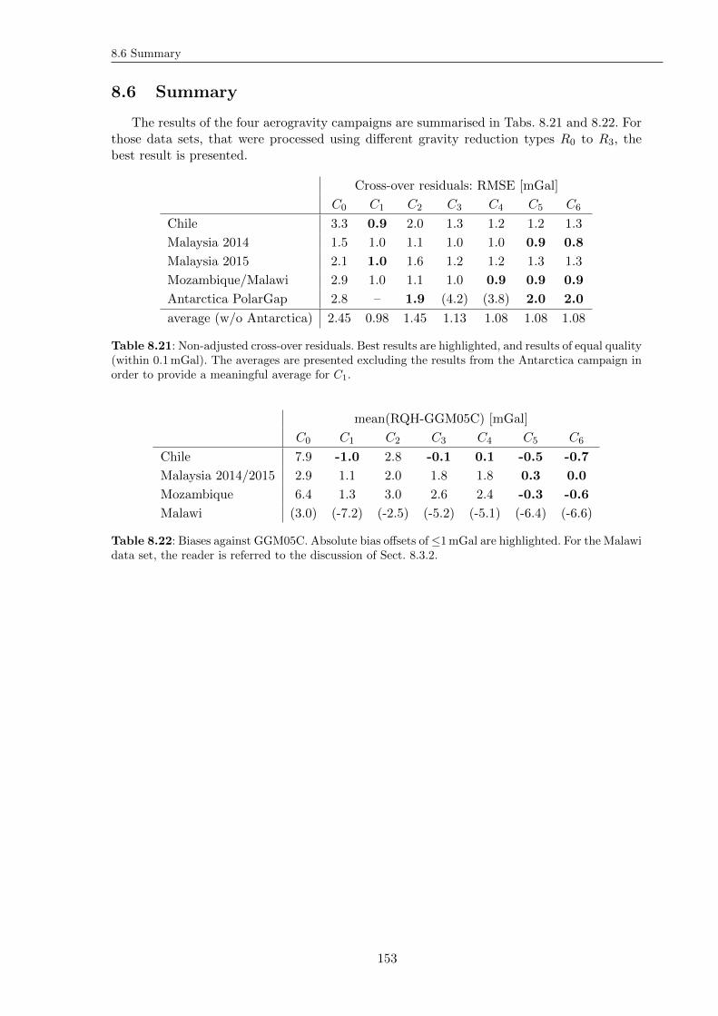
8.6 Summary
8.6 Summary
The results of the four aerogravity campaigns are summarised in Tabs. 8.21 and 8.22. Forthose data sets, that were processed using different gravity reduction types R0 to R3, thebest result is presented.
Cross-over residuals: RMSE [mGal]
C0 C1 C2 C3 C4 C5 C6
Chile 3.3 0.9 2.0 1.3 1.2 1.2 1.3
Malaysia 2014 1.5 1.0 1.1 1.0 1.0 0.9 0.8
Malaysia 2015 2.1 1.0 1.6 1.2 1.2 1.3 1.3
Mozambique/Malawi 2.9 1.0 1.1 1.0 0.9 0.9 0.9
Antarctica PolarGap 2.8 – 1.9 (4.2) (3.8) 2.0 2.0
average (w/o Antarctica) 2.45 0.98 1.45 1.13 1.08 1.08 1.08
Table 8.21: Non-adjusted cross-over residuals. Best results are highlighted, and results of equal quality(within 0.1mGal). The averages are presented excluding the results from the Antarctica campaign inorder to provide a meaningful average for C1.
mean(RQH-GGM05C) [mGal]
C0 C1 C2 C3 C4 C5 C6
Chile 7.9 -1.0 2.8 -0.1 0.1 -0.5 -0.7
Malaysia 2014/2015 2.9 1.1 2.0 1.8 1.8 0.3 0.0
Mozambique 6.4 1.3 3.0 2.6 2.4 -0.3 -0.6
Malawi (3.0) (-7.2) (-2.5) (-5.2) (-5.1) (-6.4) (-6.6)
Table 8.22: Biases against GGM05C. Absolute bias offsets of≤1mGal are highlighted. For the Malawidata set, the reader is referred to the discussion of Sect. 8.3.2.
153

Results
154
Chapter 9
Conclusions
The main conclusion of the methods and results presented in this thesis is, that strapdownairborne gravimetry using an off-the-shelf navigation-grade IMU can reliably provide non-adjusted gravity estimates at an accuracy level of 1mGal to 1.5mGal, if suitable accelerometercorrections are applied. It is pointed out again, that the evaluated aerogravity campaigns wereproduction-oriented. Except for the Antarctica campaign, the accuracy of 1mGal could beconsistently verified
• for aircraft velocities of up to 100m/s,
• for different types of terrain (ocean, flat/coastal, high-mountain),
• for different types of aircraft,
• for different temperature ranges, and
• for flight segments with strong turbulence.
It was shown in theory, and confirmed by real data examples, that the estimation of ac-celerometer errors only using the recorded flight data itself can not provide gravity estimatesat such quality, because the in-flight accelerometer drifts can not (or only weakly) be sep-arated from changes of the gravity signal, which is to be determined. This is in particularrelevant for flight segments of almost non-accelerated motion, as it is typically the case alongthe measurement lines. In theory, when using an error-free system, the introduction of cal-ibration manoeuvres, including significant accelerations and attitude changes, may improvethe gravity estimates, because such manoeuvres may enable the separation of attitude errors,accelerometer biases, and gravity (cf. Chap. 4). However in practice, the drawbacks of suchmanoeuvres, as the stronger error propagation of inertial sensor cross-couplings, lever-arm er-rors, or gyroscope biases, can be expected to compensate or even overcompensate the benefitsof such manoeuvres for the gravity determination (cf. Chap. 5).
As a consequence, the requirement of using off-line calibration methods, for examplein a laboratory set-up, is evident. This contradicts the well-established approach of onlyestimating accelerometer bias changes on-line, i.e. on the recorded data itself, by modellingthe biases as random walk or Gauss-Markov process in the Kalman filter.
In general, it can be expected that the inertial sensors of a navigation-grade IMU regu-larly undergo a manufacturer laboratory calibration. In particular, a thermal calibration iscarried out by the manufacturer for the QA-2000 accelerometers (Honeywell International ,2016b). It is further expected, that these manufacturer calibration methods can compensatethe majority of the sensor errors. However, this thesis could clearly show, that the residualerrors are still relevant for gravimetry applications. In particular, the observed residual ther-mal accelerometer drifts of 1mGal/C to 2mGal/C emphasise the importance of additional
155
Conclusions
calibrations. As an alternative to thermal calibrations, a thermal stabilisation system can beexpected significantly improve the accelerometer stability.
The main emphasis of this thesis is put on the use of strapdown gravimetry for geodeticapplications, as the determination of local geoid models. For this application, an adjustmentof the gravity data is commonly not suggested, because systematic errors may propagate intothe gravity estimates, and eventually into the estimated geoid model. For example, removinglinear drifts from the strapdown gravity data set based on cross-over residuals may introducea vertical offset, and potentially also a tilt of the gravity data set.
Similarly, it was shown for the Malawi data set, that satellite-based global gravity modelshave to be used with caution for the adjustment of gravity data. It could be seen in this dataset, that the average GGM value along a measurement line can be off by several mGal. Thisis in particular the case, if local structures in the true gravity field, spatially correlate withthe ground tracks of the measurement lines. The lower resolution of the GGM can then yielda systematic offset of the GGM along the measurement line with respect to the true gravityfield. Such systematic, local effects may then prevent the use of satellite-based gravity dataas a suitable reference, even if only the mean GGM gravity value along a measurement lineis being used for the adjustment.
The calibration methods introduced in Chap. 6 are mainly designed for geodetic applica-tions, aiming to correct long-term accelerometer drifts:
• Thermal effects of the accelerometers, which were shown to yield drifts of the order oftens of mGal within several hours, propagate into the relevant long-wavelength compo-nents of the gravity estimates, and
• long-term variations of the average attitude, e.g. coming from weather-dependentchanges of the roll and pitch angles on the flight lines, can also generate long-termdrifts in the gravity estimates. It was shown for the iMAR RQH-1003 unit, that theaccelerometer errors indeed show a roll- and pitch-angle dependency (Sect. 6.6.1).
Each of the six accelerometer calibration methods evaluated in the scope of this thesis(C1–C6) could be shown to significantly improve the non-adjusted gravity results,
• for the internal precision of the data set, as indicated by the cross-over residuals, and
• for the absolute level of the data set as well, indicated by the agreement with satellitegravity data for gridded data points, and by the inter-system agreement with LCR.
Combining these two quality measures, an accuracy of approximately 1mGal to 1.5mGalcan be derived for the Chile, Malaysia, and Mozambique/Malawi data sets, while the gravityaccuracy of the uncorrected data sets (C0) is only of the order of 3mGal to 6mGal. (Forthe Antarctica data set, a comparison against satellite-data was not possible. The overallaccuracy can be expected to be worse by a factor of 2 compared to the other data sets,presumably due to the particular challenges of this data set as discussed in Sect. 8.4).
No particular accelerometer calibration method could be found to be clearly superior withrespect to the other methods, which is evident from the summary tables shown in Sect. 8.6.However, the sample-based TRP calibration methods (C5 and C6) show the best combinedresults in terms of precision (cross over residuals) and absolute gravity level (comparisonagainst GGM05C). The simple Z-accelerometer warm-up calibration (C1) also yields veryprecise results at the 1mGal level, while the absolute gravity level was off by approximately1mGal for the different campaigns. Presumably, this comes from the fact, that the systematicdifferences between the average roll and pitch angles at the airport parking positions, andon the measurement lines, are not taken into account for this kind of calibration. Note, thatthe strapdown gravity data is tied to the terrestrial measurements at the airport parking
156
Conclusions
positions. Indeed, the sample-based TRP calibration, which explicitly models such a roll andpitch angle dependency, shows consistently better results, with biases well below 1mGal (cf.Sect. 8.6).
Geophysical applications are mainly concerned with local structures of the gravity field,enabling the discovery of geological sub-surface features by using inversion techniques. Thisincludes the application of mineral exploration. For such applications, an adjustment of thegravity data appears reasonable, because the local structure of the gravity field is the maininterest, while an absolute stability of the gravity data over longer distances (several hundredsof km) at 1mGal accuracy is commonly not a primary requirement. It was shown for theMalaysia data sets, that the cross-over adjusted precision of strapdown airborne gravimetrycan reach a precision level of 0.5mGal (RMSE), which is a remarkable result for an off-the-shelf navigation-grade IMU, that was actually not designed for this kind of application.When applying a cross-over adjustment, the accelerometer corrections could be shown to beless important, compared to the non-adjusted case.
The low sensitivity to turbulence underlines the practical benefits of strapdown gravime-try. In fact, being able to determine gravity during even strong turbulence can be cost-savingin practice, because less measurement lines may have to be re-flown due to perturbed gravitydata. This is a particularly notable result, because the more established, platform-stabilisedspring gravimeters are known to be rather sensitive to strong turbulence.
157

Conclusions
158
Chapter 10
Outlook
The real-data evaluation results do not clearly indicate a particular accelerometer cali-bration method, which outperforms the other methods for all combinations of data sets andquality measures. The significant difference between the C1 and C2 corrections already in-dicate, that the accelerometer errors are not only dependent on the internal temperaturereading (as provided by the ISA), but also on the temperature gradient (warming-up pe-riods versus periods of almost constant temperature). This indicates a potential of furtherextensions of the presented methods:
• The thermal correction might be repeated not only for different ambient temperatures,but also for different temperature gradients (yielding a two-dimensional state space).Still, a significant uncertainty may be introduced by the fact, that the provided ISAtemperature does not exactly reflect the core sensor temperatures. The inhomogeneoustemperature distribution inside of the ISA clearly indicates the limitations of suchmethods.
• The different calibration results may be combined to new, hybrid error models. Forexample, a combination of the warm-up calibration and the TRP calibration appearsreasonable: The absolute level of the correction is taken from the warm-up calibration,while only the roll and pitch angle dependent error components are taken from the TRPcalibration results.
• Another hybrid model could be a temporal concatenation of the warm-up correction,only used for the actual warm-up phase of the sensor, and one of the other calibrationmethods afterwards (assuming smaller temperature gradients). For such a hybrid model,it is important to implement the concatenation in a way, that the applied corrections donot contain jumps, as such jumps would directly propagate into the gravity estimates.
For the future development of strapdown gravimetry systems, the findings of this thesissupport two general strategies:
1. When doing fixed-wing airborne gravimetry, there is typically sufficient space and poweravailable in order to complement the IMU by a thermal stabilisation system. Dependingon the technical specifications of a system, upgrading an existing strapdown IMU withan internal thermal stabilisation system may be feasible. If this is not possible, dueto technical properties, or due to policy issues (manufacturer warranty), a thermallyinsulated housing for the IMU may be designed, with a temperature feedback loopcontrolling the inside air temperature of the housing.
It was shown in Sect. 6.2, that a sufficiently stable ambient temperature can yield a re-markable stability of the QA-2000 accelerometer, better than 0.1mGal when averaging
159
Outlook
over one hour. This emphasises the immense potential of using a thermally stabilisedquartz accelerometer (as the QA-2000) for gravimetry.
It is noted, that also a thermally stabilised system should be complemented by extendedlaboratory calibrations, e.g. modelling attitude dependent errors.
2. The main advantages of a strapdown IMU are the low space and power consumptioncompared to platform-stabilised gravimeters. This enables the use of much smaller plat-forms, as miniature unmanned aerial vehicles (UAV). A UAV-based strapdown gravime-try system has an enormous potential in terms of operational flexibility, and cost sav-ings. Modern miniature drones with combustion engines already provide a sufficientflight altitude and reach. For example, the Penguin-B drone (wingspan 3.3m) enables
• a maximum payload of 10 kg,
• a maximum flight altitude of 4500m,
• a maximum endurance of up to 20 hours,
• at a cruise speed of approximately 20m/s, and thereby
• a maximum reach of more than 1400 km.
The flight conditions of such a UAV-based strapdown gravimetry system can be ex-pected to comprise
• strong temperature variations, as there is no heating or air-conditioning systemavailable,
• considerable turbulence (because the aircraft is relatively small), and
• significant roll and pitch angle variations along the measurement lines due tochanges of the wind speed and direction.
These characteristics emphasise the importance of off-line calibration methods as dis-cussed in the scope of this thesis.
160
References
Aggarwal, P., Z. Syed, and N. El-Sheimy, Thermal calibration of low cost mems sensors forland vehicle navigation system, in Vehicular Technology Conference, 2008. VTC Spring2008. IEEE, pp. 2859–2863, IEEE, 2008a.
Aggarwal, P., Z. Syed, X. Niu, and N. El-Sheimy, A standard testing and calibration procedurefor low cost mems inertial sensors and units, Journal of navigation, 61 (02), 323–336, 2008b.
Allan, D. W., Statistics of atomic frequency standards, Proceedings of the IEEE, 54 (2),221–230, 1966.
Altamimi, Z., X. Collilieux, and L. Metivier, Itrf2008: an improved solution of the interna-tional terrestrial reference frame, Journal of Geodesy, 85 (8), 457–473, 2011.
Amante, C., and B. W. Eakins, ETOPO1 Global Relief Model converted to PanMap layerformat, doi:10.1594/PANGAEA.769615, 2009.
Ayres-Sampaio, D., R. Deurloo, M. Bos, A. Magalhaes, and L. Bastos, A comparison betweenthree imus for strapdown airborne gravimetry, Surveys in Geophysics, 36 (4), 571–586, 2015.
Baram, Y., and T. Kailath, Estimability and regulability of linear systems, in Decision andControl, 1987. 26th IEEE Conference on, vol. 26, pp. 1706–1713, IEEE, 1987.
Barthelmes, F., and C. Forste, The icgem-format, Potsdam: GFZ German Research Centrefor Geosciences, Department, 1, 2011.
Bastos, L., S. Cunha, R. Forsberg, A. Olesen, A. Gidskehaug, U. Meyer, T. Boebel, L. Tim-men, G. Xu, M. Nesemann, et al., An airborne geoid mapping system for regional sea-surface topography: application to the skagerrak and azores areas, in Geodesy on the Move,pp. 30–36, Springer, 1998.
Batista, P., C. Silvestre, P. Oliveira, and B. Cardeira, Accelerometer calibration and dynamicbias and gravity estimation: Analysis, design, and experimental evaluation, Control SystemsTechnology, IEEE Transactions on, 19 (5), 1128–1137, 2011.
Becker, D., and M. Becker, A study of non-stochastic imu errors in strapdown airbornegravimetry, in Inertial Sensors and Systems Symposium (ISS), 2015 DGON, pp. 1–18,IEEE, 2015.
Becker, D., M. Becker, S. Leinen, and Y. Zhao, Estimability in Strapdown Airborne VectorGravimetry, pp. 1–5, Springer Berlin Heidelberg, Berlin, Heidelberg, doi:10.1007/13452015 209, 2015a.
Becker, D., J. E. Nielsen, D. Ayres-Sampaio, R. Forsberg, M. Becker, and L. Bastos, Driftreduction in strapdown airborne gravimetry using a simple thermal correction, Journal ofGeodesy, 89 (11), 1133–1144, 2015b.
161
REFERENCES
Becker, D., M. Becker, A. V. Olesen, J. E. Nielsen, and R. Forsberg, Latest results in strap-down airborne gravimetry using an iMAR RQH unit, in Terrestrial Gravimetry: Staticand Mobile Measurements (TG-SMM), 2016, International Association of Geodesy (IAG),2016.
Becker, J. J., D. T. Sandwell, W. H. F. Smith, J. Braud, B. Binder, J. Depner, D. Fabre,J. Factor, S. Ingalls, S. H. Kim, R. Ladner, K. Marks, S. Nelson, A. Pharaoh, R. Trimmer,J. Von Rosenberg, G. Wallace, and P. Weatherall, Global Bathymetry and Elevation Dataat 30 Arc Seconds Resolution: SRTM30 PLUS, Marine Geodesy, 32, 2009.
Bhatt, D., P. Aggarwal, P. Bhattacharya, and V. Devabhaktuni, An enhanced mems errormodeling approach based on nu-support vector regression, Sensors, 12 (7), 9448–9466, 2012.
Bidel, Y., O. Carraz, R. Charriere, M. Cadoret, N. Zahzam, and A. Bresson, Compact coldatom gravimeter for field applications, Applied Physics Letters, 102 (14), 144,107, 2013.
Bos, M., R. Deurloo, M. Bastos, and A. Magalhaes, A new local geoid for madeira usingairborne gravimetry, in AGU fall meeting abstracts, vol. 1, p. 0880, 2011.
Boulanger, O., and M. Chouteau, Constraints in 3d gravity inversion, Geophysical Prospect-ing, 49 (2), 265–280, 2001.
Britting, K. R., Inertial navigation systems analysis, 1971.
Brozena, J., The greenland aerogeophysics project: Airborne gravity, topographic and mag-netic mapping of an entire continent, in From Mars to Greenland: Charting Gravity WithSpace and Airborne Instruments, pp. 203–214, Springer, 1992.
Brozena, J., M. Peters, and R. Salman, Arctic airborne gravity measurement program, inGravity, Geoid and Marine Geodesy, pp. 131–138, Springer, 1997.
Bruton, A., Y. Hammada, S. Ferguson, K. Schwarz, M. Wei, and J. Halpenny, A comparisonof inertial platform, damped 2-axis platform and strapdown airborne gravimetry, in Pro-ceedings of the international symposium on kinematic systems in geodesy, geomatics andnavigation, Banff, Canada, pp. 542–550, 2001.
Bruton, A., K. Schwarz, S. Ferguson, M. Kern, and M. Wei, Deriving acceleration from dgps:toward higher resolution applications of airborne gravimetry, GPS Solutions, 5 (3), 1–14,2002.
Bruton, A. M., Improving the accuracy and resolution of SINS/DGPS airborne gravimetry,National Library of Canada= Bibliotheque nationale du Canada, 2002.
Cohen, C. E., B. W. Parkinson, and B. D. McNally, Flight tests of attitude determinationusing gps compared against an inertial navigation unit, Navigation, 41 (1), 83–97, 1994.
Commault, C., J.-M. Dion, and D. H. Trinh, Observability recovering by additional sensorimplementation in linear structured systems, in Decision and Control, 2005 and 2005 Euro-pean Control Conference. CDC-ECC’05. 44th IEEE Conference on, pp. 7193–7197, IEEE,2005.
Deurloo, R., W. Yan, M. Bos, D. Ayres-Sampaio, A. Magalhaes, M. Becker, D. Becker, andL. Bastos, A comparison of the performance of medium-and high-quality inertial systemsgrades for strapdown airborne gravimetry, 2015.
Deurloo, R. A., Development of a kalman filter integrating system and measurement modelsfor a low-cost strapdown airborne gravimetry system, Ph.D. thesis, Faculty of Sciences,University of Porto, Porto, Portugal, 2011.
162
REFERENCES
Dion, J.-M., C. Commault, and J. Van Der Woude, Generic properties and control of linearstructured systems: a survey, Automatica, 39 (7), 1125–1144, 2003.
El-Diasty, M., and S. Pagiatakis, Calibration and stochastic modelling of inertial navigationsensor errors, Journal of Global Positioning Systems, 7 (2), 170–182, 2008.
El-Sheimy, N., H. Hou, and X. Niu, Analysis and modeling of inertial sensors using allanvariance, Instrumentation and Measurement, IEEE Transactions on, 57 (1), 140–149, 2008.
Forsberg, R., A study of terrain reductions, density anomalies and geophysical inversionmethods in gravity field modelling, Tech. rep., DTIC Document, 1984.
Forsberg, R., and A. V. Olesen, Airborne gravity field determination, in Sciences of Geodesy-I,pp. 83–104, Springer, 2010.
Forsberg, R., and C. Tscherning, The use of height data in gravity field approximation bycollocation, J. geophys. Res, 86 (B9), 7843–7854, 1981.
Forsberg, R., A. Vassiliou, K. Schwarz, and R. Wong, Inertial gravimetrya comparison ofkalman filtering-smoothing and post-mission adjustment techniques, Bulletin geodesique,60 (2), 129–142, 1986.
Forsberg, R., A. Olesen, K. Keller, M. Møller, A. Gidskehaug, and D. Solheim, Airbornegravity and geoid surveys in the arctic and baltic seas, in Proceedings of internationalsymposium on kinematic systems in geodesy, geomatics and navigation (KIS-2001), Banff,pp. 586–593, 2001.
Fretwell, P., H. D. Pritchard, D. G. Vaughan, J. Bamber, N. Barrand, R. Bell, C. Bianchi,R. Bingham, D. Blankenship, G. Casassa, et al., Bedmap2: improved ice bed, surface andthickness datasets for antarctica, The Cryosphere, 7 (1), 2013.
Gelb, A., Applied optimal estimation, MIT press, 1974.
Glennie, C., and K. Schwarz, A comparison and analysis of airborne gravimetry results fromtwo strapdown inertial/dgps systems, Journal of Geodesy, 73 (6), 311–321, 1999.
Glennie, C., K. Schwarz, A. Bruton, R. Forsberg, A. V. Olesen, and K. Keller, A comparisonof stable platform and strapdown airborne gravity, Journal of Geodesy, 74 (5), 383–389,2000.
Groves, P. D., Principles of GNSS, inertial, and multisensor integrated navigation systems,Artech house, 2013.
Heck, B., and K. Seitz, A comparison of the tesseroid, prism and point-mass approaches formass reductions in gravity field modelling, Journal of Geodesy, 81 (2), 121–136, 2007.
Hofmann-Wellenhof, B., and H. Moritz, Physical geodesy, Springer Science & Business Media,2006.
Hofmann-Wellenhof, B., H. Lichtenegger, and J. Collins, Global positioning system: theoryand practice, Springer Science & Business Media, 2012.
Honeywell International, I., GG1320AN Digital Laser Gyro specification sheet, https://aerospace.honeywell.com/∼/media/aerospace/files/brochures/gg1320andigitallasergyro-bro.pdf, accessed: 2016-05-09, 2016a.
163
REFERENCES
Honeywell International, I., Q-Flex QA-2000 Accelerometer specification sheet,https://aerospace.honeywell.com/∼/media/aerospace/files/brochures/accelerometers/q-flexqa-2000accelerometer bro.pdf, accessed: 2016-05-09, 2016b.
Hong, S., M. H. Lee, H.-H. Chun, S.-H. Kwon, and J. L. Speyer, Observability of error statesin gps/ins integration, Vehicular Technology, IEEE Transactions on, 54 (2), 731–743, 2005.
Hunzinger, J. F., carrier-phase differential gps, Ph.D. thesis, Department of Electrical Engi-neering, McGill University, Montreal, 1997.
Hwang, C., Y.-S. Hsiao, and H.-C. Shih, Data reduction in scalar airborne gravimetry: Theory,software and case study in taiwan, Computers & geosciences, 32 (10), 1573–1584, 2006.
Jekeli, C., Balloon gravimetry using gps and ins, in Position Location and Navigation Sympo-sium, 1992. Record. 500 Years After Columbus-Navigation Challenges of Tomorrow. IEEEPLANS’92., IEEE, pp. 481–487, IEEE, 1992.
Jekeli, C., Airborne vector gravimetry using precise, position-aided inertial measurementunits, Bulletin Geodesique, 69 (1), 1–11, 1994.
Jekeli, C., Inertial navigation systems with geodetic applications, Walter de Gruyter, 2001.
Jekeli, C., and R. Garcia, Gps phase accelerations for moving-base vector gravimetry, Journalof Geodesy, 71 (10), 630–639, 1997.
Kouba, J., and P. Heroux, Precise point positioning using igs orbit and clock products, GPSsolutions, 5 (2), 12–28, 2001.
Kreye, C., and G. W. Hein, Gnss based kinematic acceleration determination for airborne vec-tor gravimetry-methods and results, in Proceedings of the ION GPS/GNSS 2003 Meeting,Portland, Oregon, 2003.
Kwon, J. H., and C. Jekeli, A new approach for airborne vector gravimetry using gps/ins,Journal of Geodesy, 74 (10), 690–700, 2001.
LaCoste, L., The zero-length spring gravity meter, The Leading Edge, 7 (7), 20–21, 1988.
LaCoste, L. J., Measurement of gravity at sea and in the air, Reviews of Geophysics, 5 (4),477–526, 1967.
Lee, M. H., W. C. Park, K. S. Lee, S. Hong, H. G. Park, H. H. Chun, and F. Harashima,Observability analysis techniques on inertial navigation systems, Journal of System Designand Dynamics, 6 (1), 28–44, 2012.
Lelievre, P. G., C. G. Farquharson, and C. A. Hurich, Joint inversion of seismic traveltimesand gravity data on unstructured grids with application to mineral exploration, Geophysics,77 (1), K1–K15, 2012.
Li, Y., and D. W. Oldenburg, 3-d inversion of gravity data, Geophysics, 63 (1), 109–119, 1998.
MacCready, P. B., The inertial subrange of atmospheric turbulence, Journal of GeophysicalResearch, 67 (3), 1051–1059, 1962.
McRuer, D. T., D. Graham, and I. Ashkenas, Aircraft dynamics and automatic control,Princeton University Press, 2014.
Moon, J. H., S. Hong, H.-H. Chun, and M. H. Lee, Estimability measures and their applicationto gps/ins, Journal of Mechanical Science and Technology, 22 (5), 905–913, 2008.
164
REFERENCES
Moritz, H., Geodetic reference system 1980, Journal of Geodesy, 54 (3), 395–405, 1980.
Nettleton, L. L., L. LaCoste, and J. C. Harrison, Tests of an airborne gravity meter, Geo-physics, 25 (1), 181–202, 1960.
Novatel Inc., Waypoint grafnav, 2014.
Oldenburg, D. W., The inversion and interpretation of gravity anomalies, Geophysics, 39 (4),526–536, 1974.
Olesen, A. V., Improved airborne scalar gravimetry for regional gravity field mapping andgeoid determination, Ph.D. thesis, Faculty of Science, University of Copenhagen, 2002.
Pavlis, N. K., S. A. Holmes, S. C. Kenyon, and J. K. Factor, An earth gravitational modelto degree 2160: Egm2008, EGU General Assembly, pp. 13–18, 2008.
Rauch, H. E., C. Striebel, and F. Tung, Maximum likelihood estimates of linear dynamicsystems, AIAA journal, 3 (8), 1445–1450, 1965.
Ries, J., S. Bettadpur, R. Eanes, Z. Kang, U. Ko, C. McCullough, P. Nagel, N. Pie, S. Poole,T. Richter, H. Save, and B. Tapley, The Combined Gravity Model GGM05C, 2016.
Rothman, Y., I. Klein, and S. Filin, Analytical observability analysis of ins with vehicleconstraints, Navigation, 61 (3), 227–236, 2014.
Schwarz, K., Inertial surveying and geodesy, Reviews of Geophysics, 21 (4), 878–890, 1983.
Schwarz, K., and M. Wei, A framework for modelling kinematic measurements in gravity fieldapplications, Bulletin geodesique, 64 (4), 331–346, 1990.
Schwarz, K., and M. Wei, Some unsolved problems in airborne gravimetry, in Gravity andGeoid, pp. 131–150, Springer, 1995.
Schwarz, K., O. Colombo, G. Hein, and E. Knickmeyer, Requirements for airborne vectorgravimetry, in From Mars to Greenland: Charting Gravity With Space and Airborne In-struments, pp. 273–283, Springer, 1992.
Shin, E.-H., and N. El-Sheimy, A new calibration method for strapdown inertial navigationsystems, Zeitschrift fur Vermessungswesen.–2002.–Zfv, 127 (1), 41–50, 2002.
Skaloud, J., I. Colomina, M. Pares, M. Blazquez, J. Silva, and M. Cherisch, Progress inairborne gravimetry by combining strapdown inertial and new satellite observations viadynamic networks, in 26th IUGG General Assembly, IAG Symposia, EPFL-TALK-217065,2015.
Skog, I., and P. Handel, Calibration of a mems inertial measurement unit, in XVII IMEKOWorld Congress, pp. 1–6, Citeseer, 2006.
Studinger, M., R. Bell, and N. Frearson, Comparison of AIRGrav and GT-1A airbornegravimeters for research applications, Geophysics, 73 (6), I51–I61, 2008.
Syed, Z., P. Aggarwal, C. Goodall, X. Niu, and N. El-Sheimy, A new multi-position calibrationmethod for mems inertial navigation systems, Measurement Science and Technology, 18 (7),1897, 2007.
Titterton, D., and J. L. Weston, Strapdown inertial navigation technology, vol. 17, The Insti-tution of Engineering and Technology, 2004.
165
REFERENCES
Tome, P., Integration of inertial and satellite navigation systems for aircraft attitude deter-mination, Ph.D. thesis, Faculty of Sciences, University of Porto, Porto, Portugal, 2002.
Torge, W., Gravimetry walter de gruyter, Berlin–New York, 1989.
Torge, W., and J. Muller, Geodesy, Walter de Gruyter, 2012.
Tscherning, C., R. Forsberg, P. Knudsen, and K. og Matrikelstyrelsen, Gravsoft-a system forgeodetic gravity field modelling, in Proc. 1. Continental Workshop on the Geoid in Europe,Research Institute of Geodesy, Topography and Cartography, Prague, pp. 327–334, 1992.
Vander Kuylen, L., P. Nemry, F. Boon, and A. Simsky, Comparison of attitude performancefor multi-antenna receivers, European Journal of Navigation, 4 (2), 1–9, 2006.
Wei, M., and K. Schwarz, Flight test results from a strapdown airborne gravity system,Journal of Geodesy, 72 (6), 323–332, 1998.
Wendel, J., Integrierte Navigationssysteme: Sensordatenfusion, GPS und Inertiale Naviga-tion, Walter de Gruyter, 2011.
Yang, J., W. Wu, Y. Wu, and J. Lian, Thermal calibration for the accelerometer triad based onthe sequential multiposition observation, Instrumentation and Measurement, IEEE Trans-actions on, 62 (2), 467–482, 2013.
Zahzam, N., A. Bonnin, F. Theron, M. Cadoret, Y. Bidel, and A. Bresson, New advances inthe field of cold atom interferometers for onboard gravimetry, in Terrestrial Gravimetry:Static and Mobile Measurements (TG-SMM), 2016, International Association of Geodesy(IAG), 2016.
166
List of Acronyms
BSC Bias – Scale factor – Cross coupling calibration (Sect. 6.5.1)
BSSC Bias – double Scale factor – Cross coupling calibration (Sect. 6.5.2)
DCM Direction-Cosine-Matrix
DoV Deflection of the vertical (of the gravity vector)
DTM Digital Terrain Model
EKF Extended Kalman Filter
GNSS Global Navigation Satellite System
GGM Global Gravity Model
GPS The Global Positioning System
IMU Inertial Measurement Unit
ISA Inertial Sensor Assembly (cf. Sect. 6.1)
KF Kalman Filter
LCR LaCoste & Romberg S-type spring gravimeter
NMEA National Marine Electronics Association (navigation data streaming format)
PD-GNSS Carrier Phase-Differential GNSS
PPP Precise Point Positioning
PPS Pulse Per Second
RMS Root-Mean-Square
RMS-g RMS of vertical accelerations (used as turbulence metric, cf. Sect. 7.3)
RMSE Root-Mean-Square Error (= RMS/√2)
SAG Strapdown Airborne Gravimetry
TRP Temperature-Roll-Pitch (cf. Sect. 6.6)
UAV Unmanned Aerial Vehicle
UTM Universal Transverse Mercator (a map projection)
167

168
Appendix A
Detailed campaign information
A.1 Attitude characteristics
For each of the campaigns, the attitude characteristics on the lines differ significantly, com-ing from different aircraft speed, weather conditions, auto pilot characteristics, and aircraftmodel. 2-D histograms of the combinations of roll and pitch angle are depicted in Fig. A.1.
A.2 Measurement lines
For each of the aerogravity campaigns evaluated in the scope of this thesis, detailedinformation is provided for each of the measurement lines. For each campaign, a line overviewmap is provided, followed by a table with numerical properties. For the tables, the followingabbreviations are being used:
• F : Flight ID
• FL: Measurement Line ID
• topo: topography (or bathymetry) height
• Nχ: Number of adjacent cross-over points.
Again, µ and σ denote the average, and the standard deviation, respectively.
169
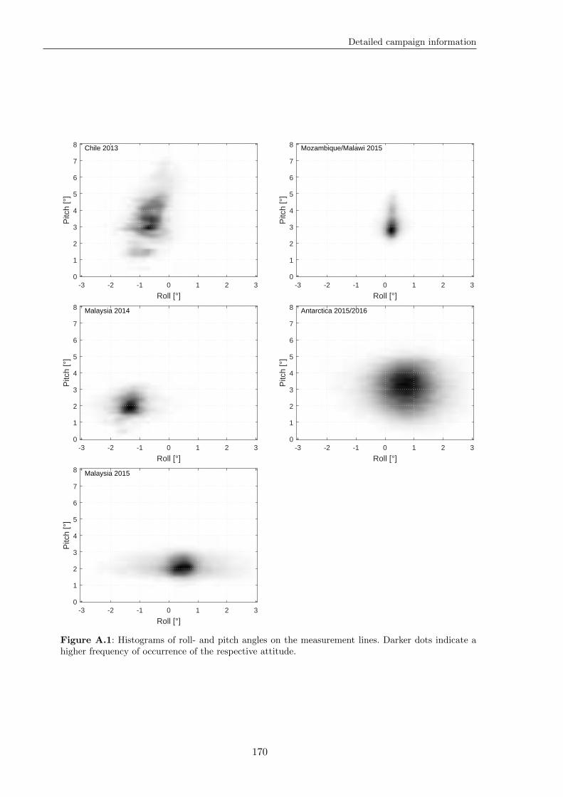
Detailed campaign information
Chile 2013
-3 -2 -1 0 1 2 3
Roll [°]
0
1
2
3
4
5
6
7
8
Pitc
h [°
]
Malaysia 2014
-3 -2 -1 0 1 2 3
Roll [°]
0
1
2
3
4
5
6
7
8
Pitc
h [°
]
Malaysia 2015
-3 -2 -1 0 1 2 3
Roll [°]
0
1
2
3
4
5
6
7
8
Pitc
h [°
]
Mozambique/Malawi 2015
-3 -2 -1 0 1 2 3
Roll [°]
0
1
2
3
4
5
6
7
8
Pitc
h [°
]
Antarctica 2015/2016
-3 -2 -1 0 1 2 3
Roll [°]
0
1
2
3
4
5
6
7
8
Pitc
h [°
]
Figure A.1: Histograms of roll- and pitch angles on the measurement lines. Darker dots indicate ahigher frequency of occurrence of the respective attitude.
170
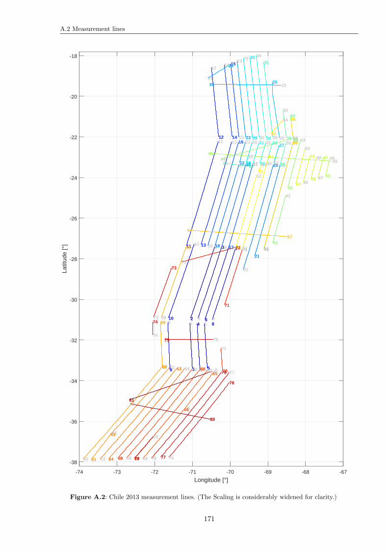
A.2 Measurement lines
-74 -73 -72 -71 -70 -69 -68 -67
Longitude [°]
-38
-36
-34
-32
-30
-28
-26
-24
-22
-20
-18
Latit
ude
[°]
1
12
2 3
34
4 5
56
6 7
78
89
910
1011
1112
12
13
1314
14 15
1516
16 17
1718
1819
19 20
20
21
2122
2223
2324
2425 25
26
26
27
2728
2829
29 30
3031
3132
32
33
3334
34
35
3536
3637
37 38
3839
3940
4041
41
42
42
43
4344
4445
45
46
4647
4748
4849
4950
50
51
5152
5253
53
54
54 55
5556
56
5757
58
5859
5960
60 61
6162
62 63
63 64
6465
6566
6667
6768
6869
69 70
70
71
7172
7273
7374
7475 75
76
7677
7778
7879
79
80
8081
81
Figure A.2: Chile 2013 measurement lines. (The Scaling is considerably widened for clarity.)
171
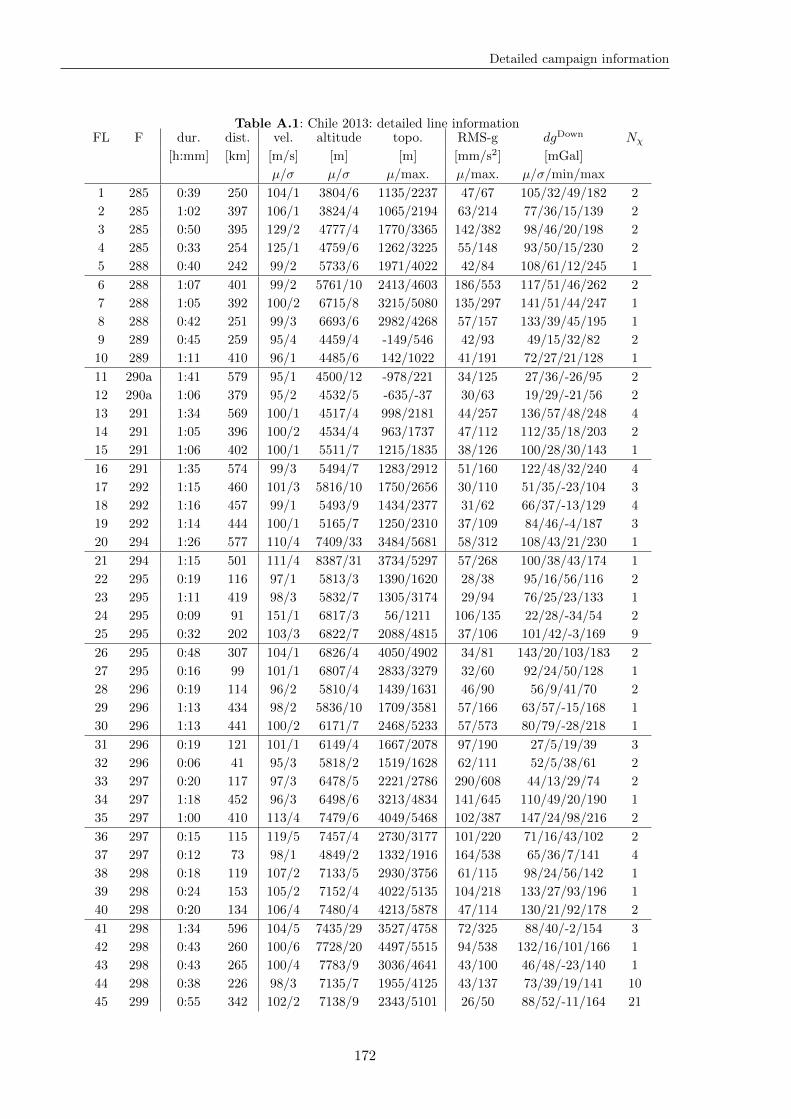
Detailed campaign information
Table A.1: Chile 2013: detailed line informationFL F dur. dist. vel. altitude topo. RMS-g dgDown Nχ
[h:mm] [km] [m/s] [m] [m] [mm/s2] [mGal]
µ/σ µ/σ µ/max. µ/max. µ/σ/min/max
1 285 0:39 250 104/1 3804/6 1135/2237 47/67 105/32/49/182 2
2 285 1:02 397 106/1 3824/4 1065/2194 63/214 77/36/15/139 2
3 285 0:50 395 129/2 4777/4 1770/3365 142/382 98/46/20/198 2
4 285 0:33 254 125/1 4759/6 1262/3225 55/148 93/50/15/230 2
5 288 0:40 242 99/2 5733/6 1971/4022 42/84 108/61/12/245 1
6 288 1:07 401 99/2 5761/10 2413/4603 186/553 117/51/46/262 2
7 288 1:05 392 100/2 6715/8 3215/5080 135/297 141/51/44/247 1
8 288 0:42 251 99/3 6693/6 2982/4268 57/157 133/39/45/195 1
9 289 0:45 259 95/4 4459/4 -149/546 42/93 49/15/32/82 2
10 289 1:11 410 96/1 4485/6 142/1022 41/191 72/27/21/128 1
11 290a 1:41 579 95/1 4500/12 -978/221 34/125 27/36/-26/95 2
12 290a 1:06 379 95/2 4532/5 -635/-37 30/63 19/29/-21/56 2
13 291 1:34 569 100/1 4517/4 998/2181 44/257 136/57/48/248 4
14 291 1:05 396 100/2 4534/4 963/1737 47/112 112/35/18/203 2
15 291 1:06 402 100/1 5511/7 1215/1835 38/126 100/28/30/143 1
16 291 1:35 574 99/3 5494/7 1283/2912 51/160 122/48/32/240 4
17 292 1:15 460 101/3 5816/10 1750/2656 30/110 51/35/-23/104 3
18 292 1:16 457 99/1 5493/9 1434/2377 31/62 66/37/-13/129 4
19 292 1:14 444 100/1 5165/7 1250/2310 37/109 84/46/-4/187 3
20 294 1:26 577 110/4 7409/33 3484/5681 58/312 108/43/21/230 1
21 294 1:15 501 111/4 8387/31 3734/5297 57/268 100/38/43/174 1
22 295 0:19 116 97/1 5813/3 1390/1620 28/38 95/16/56/116 2
23 295 1:11 419 98/3 5832/7 1305/3174 29/94 76/25/23/133 1
24 295 0:09 91 151/1 6817/3 56/1211 106/135 22/28/-34/54 2
25 295 0:32 202 103/3 6822/7 2088/4815 37/106 101/42/-3/169 9
26 295 0:48 307 104/1 6826/4 4050/4902 34/81 143/20/103/183 2
27 295 0:16 99 101/1 6807/4 2833/3279 32/60 92/24/50/128 1
28 296 0:19 114 96/2 5810/4 1439/1631 46/90 56/9/41/70 2
29 296 1:13 434 98/2 5836/10 1709/3581 57/166 63/57/-15/168 1
30 296 1:13 441 100/2 6171/7 2468/5233 57/573 80/79/-28/218 1
31 296 0:19 121 101/1 6149/4 1667/2078 97/190 27/5/19/39 3
32 296 0:06 41 95/3 5818/2 1519/1628 62/111 52/5/38/61 2
33 297 0:20 117 97/3 6478/5 2221/2786 290/608 44/13/29/74 2
34 297 1:18 452 96/3 6498/6 3213/4834 141/645 110/49/20/190 1
35 297 1:00 410 113/4 7479/6 4049/5468 102/387 147/24/98/216 2
36 297 0:15 115 119/5 7457/4 2730/3177 101/220 71/16/43/102 2
37 297 0:12 73 98/1 4849/2 1332/1916 164/538 65/36/7/141 4
38 298 0:18 119 107/2 7133/5 2930/3756 61/115 98/24/56/142 1
39 298 0:24 153 105/2 7152/4 4022/5135 104/218 133/27/93/196 1
40 298 0:20 134 106/4 7480/4 4213/5878 47/114 130/21/92/178 2
41 298 1:34 596 104/5 7435/29 3527/4758 72/325 88/40/-2/154 3
42 298 0:43 260 100/6 7728/20 4497/5515 94/538 132/16/101/166 1
43 298 0:43 265 100/4 7783/9 3036/4641 43/100 46/48/-23/140 1
44 298 0:38 226 98/3 7135/7 1955/4125 43/137 73/39/19/141 10
45 299 0:55 342 102/2 7138/9 2343/5101 26/50 88/52/-11/164 21
172
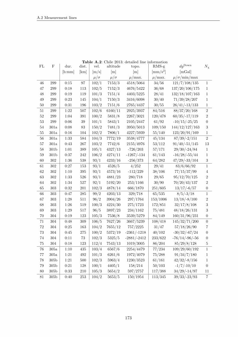
A.2 Measurement lines
Table A.2: Chile 2013: detailed line informationFL F dur. dist. vel. altitude topo. RMS-g dgDown Nχ
[h:mm] [km] [m/s] [m] [m] [mm/s2] [mGal]
µ/σ µ/σ µ/max. µ/max. µ/σ/min/max
46 299 0:15 97 102/1 7153/3 4518/5064 34/56 121/7/108/135 1
47 299 0:18 113 102/5 7152/3 4676/5422 36/68 137/20/106/175 1
48 299 0:19 119 101/3 7151/4 4403/5225 28/41 132/18/107/163 1
49 299 0:23 145 104/1 7150/3 3416/6098 30/40 71/39/28/207 1
50 299 0:31 196 103/2 7151/6 2765/4437 30/55 26/41/-13/133 1
51 299 1:22 507 102/6 6160/11 2925/3937 84/516 88/37/20/168 2
52 299 1:04 391 100/2 5831/8 2267/3021 120/478 60/35/-17/119 2
53 299 0:06 39 101/1 5843/1 2105/2447 61/92 -10/15/-25/25 0
54 301a 0:08 83 150/2 7481/3 3950/5013 109/150 144/12/127/163 3
55 301a 0:16 104 102/2 7806/1 4227/5939 55/140 123/20/91/169 1
56 301a 1:33 584 104/3 7772/19 3538/4777 45/134 87/39/-2/151 2
57 301a 0:43 267 103/2 7742/6 2155/4976 53/112 91/40/-51/145 13
58 301b 1:01 389 105/1 4327/13 -726/203 57/171 29/30/-24/84 1
59 301b 0:37 242 106/2 4274/11 -1267/-134 61/143 -16/28/-55/44 1
60 302 1:36 538 93/1 4233/16 -256/373 64/282 47/29/-33/104 3
61 302 0:27 153 93/1 4526/5 4/252 29/41 83/6/66/92 1
62 302 1:10 395 93/1 4573/16 -112/229 38/106 77/15/37/99 4
63 302 1:33 526 93/1 4881/23 280/718 29/65 95/12/70/125 2
64 302 1:34 527 92/1 5192/20 253/1166 30/90 70/20/43/137 2
65 303 0:32 201 102/3 4878/14 666/1870 251/605 13/17/-6/57 0
66 303 0:47 285 99/2 4203/13 329/718 65/535 8/5/-3/18 1
67 303 1:28 511 96/2 3904/26 297/1764 153/1006 13/18/-8/100 2
68 303 1:26 519 100/3 4224/30 275/1723 172/851 32/17/8/108 3
69 303 1:29 517 96/5 3897/23 234/1162 75/481 48/18/26/131 3
70 304 0:19 123 105/3 7536/8 3539/5279 84/149 160/31/96/231 0
71 304 0:48 309 106/5 7627/26 3667/5239 108/418 145/32/71/200 0
72 304 0:25 163 104/2 7655/12 757/2225 31/47 57/18/26/90 7
73 304 0:45 275 100/2 5372/19 -2361/-1218 40/102 -30/32/-67/24 0
74 304 0:11 73 102/3 5325/5 -2881/-2412 233/622 -76/14/-96/-56 0
75 304 0:18 123 112/4 7543/13 1019/3005 86/204 85/29/8/128 5
76 305a 1:10 435 103/4 6567/6 2254/4479 77/234 109/29/60/192 1
77 305a 1:21 492 101/3 6261/6 1972/4079 75/288 91/34/7/180 1
78 305b 1:21 500 102/3 5963/4 1230/3523 61/161 42/32/-8/156 1
79 305b 0:21 128 100/1 4405/1 158/214 50/103 -1/7/-10/10 0
80 305b 0:33 210 105/3 5654/2 597/2757 117/388 34/29/-14/97 11
81 305b 0:40 253 104/2 5653/5 150/1954 113/345 39/33/-23/93 7
173
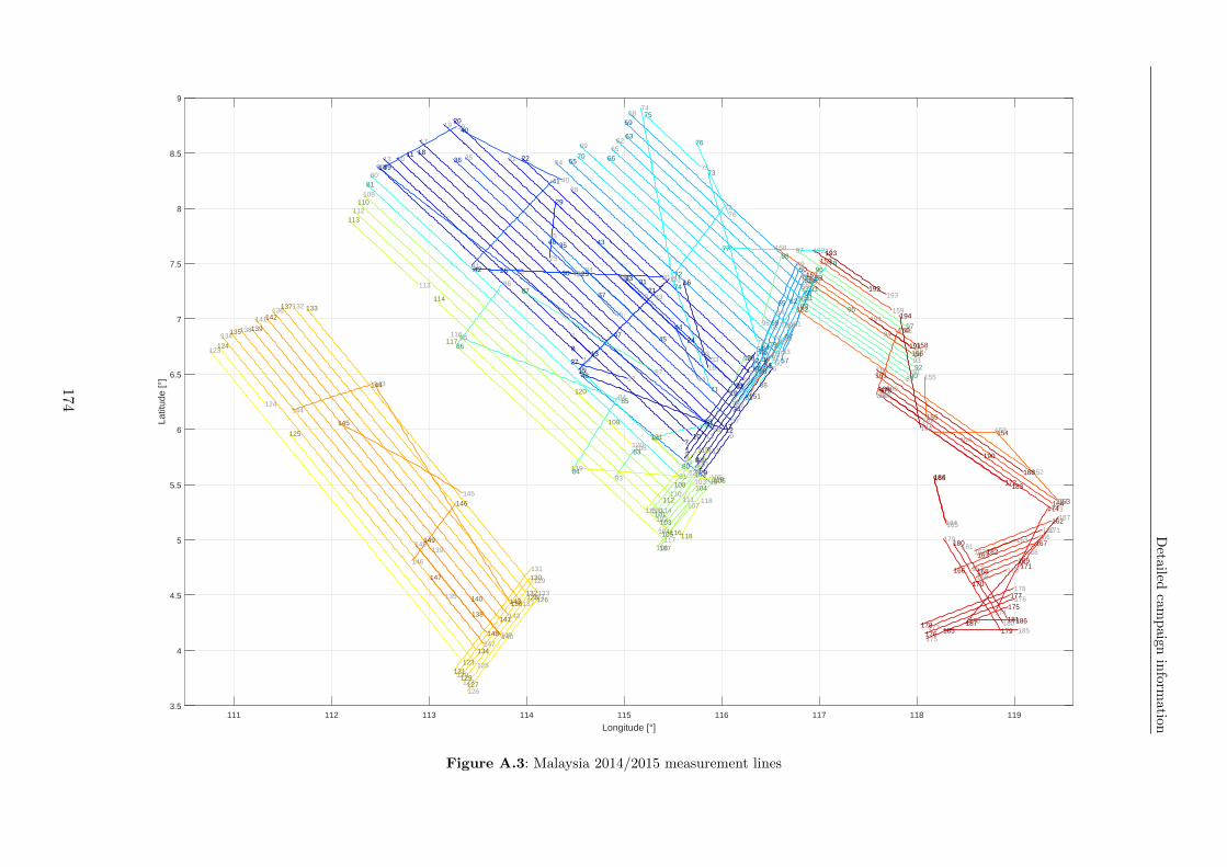
Detailed
campaign
inform
ation
111 112 113 114 115 116 117 118 119
Longitude [°]
3.5
4
4.5
5
5.5
6
6.5
7
7.5
8
8.5
9
Latit
ude
[°]
1
12
2
3
3 4
4
5
56
6
7
7
8
8
9
910
1011
1112
12
13
1314
14
15
15 16
16
17
17
18
18
19
1920
2021
21 22
22
23
23
24
2425252626
27
27
28
28
29
29
3030
31
3132
3233
33
34
34
35
3536
36
37
3738
3839
3940
4041
4142 42
43
43
44
44
45
4546
46
47
4748
48
49
4950
5051
5152
52
53
5354
54 55
55
56
56
57
5758
5859
5960
60
61
61
62
6263
63
64
6465
6566
66
67
67
68
6869
69
70
70
71
7172
72
73
73
74
7475
75
76
76
77 77
78
78
79
79
80
8081
81
82
82
83
8384
8485
8586
8687
87
88
88
89
8990
9091
9192
92 93
9394
94
95
95
96
9697
9798
98
99
99
100
100101
101
102
102103
103104
104105
105106
106107
107
108
108
109
109110
110
111
111112
112113
113
114
114
115
115
116
116117
117 118
118
119
119
120
120121
121
123
123124
124
125
125
126
126127
127128
128129
129130
130131
131
132
132 133
133
134
134135
135136
136137
137
138
138139
139
140
140
141
141142
142
143
143144
144
145
145146
146
147
147
148
148149
149
151
151
152
152
153
153154154
155
155
156
156157
157158
158
159
159
160
160
161
161
162
162163
163
164
164
165
165
166
166167
167168
168169
169170
170171
171
172
172
173
173174
174175
175176
176177
177178
178
179
179180
180181
181182
182
183
183
184
184
185 185186186187
187
188
188
189
189
190
190
191
191
192
192193
193
194
194
Figure A.3: Malaysia 2014/2015 measurement lines
174
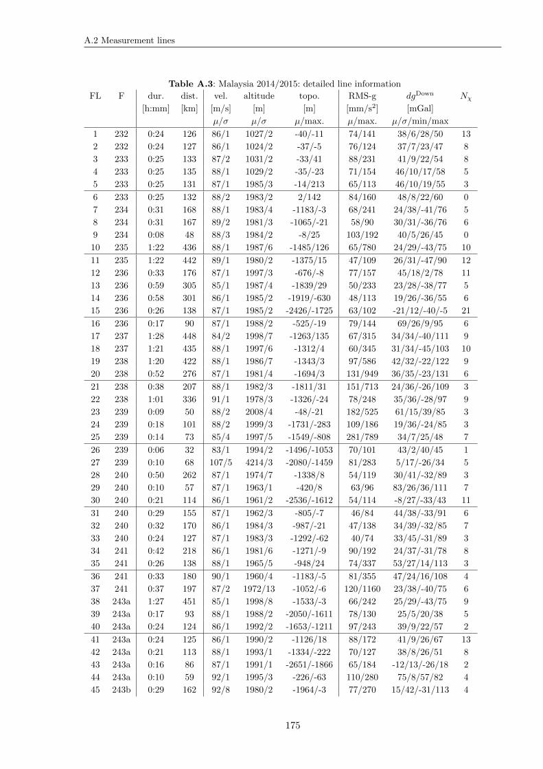
A.2 Measurement lines
Table A.3: Malaysia 2014/2015: detailed line information
FL F dur. dist. vel. altitude topo. RMS-g dgDown Nχ[h:mm] [km] [m/s] [m] [m] [mm/s2] [mGal]
µ/σ µ/σ µ/max. µ/max. µ/σ/min/max
1 232 0:24 126 86/1 1027/2 -40/-11 74/141 38/6/28/50 13
2 232 0:24 127 86/1 1024/2 -37/-5 76/124 37/7/23/47 8
3 233 0:25 133 87/2 1031/2 -33/41 88/231 41/9/22/54 8
4 233 0:25 135 88/1 1029/2 -35/-23 71/154 46/10/17/58 5
5 233 0:25 131 87/1 1985/3 -14/213 65/113 46/10/19/55 3
6 233 0:25 132 88/2 1983/2 2/142 84/160 48/8/22/60 0
7 234 0:31 168 88/1 1983/4 -1183/-3 68/241 24/38/-41/76 5
8 234 0:31 167 89/2 1981/3 -1065/-21 58/90 30/31/-36/76 6
9 234 0:08 48 88/3 1984/2 -8/25 103/192 40/5/26/45 0
10 235 1:22 436 88/1 1987/6 -1485/126 65/780 24/29/-43/75 10
11 235 1:22 442 89/1 1980/2 -1375/15 47/109 26/31/-47/90 12
12 236 0:33 176 87/1 1997/3 -676/-8 77/157 45/18/2/78 11
13 236 0:59 305 85/1 1987/4 -1839/29 50/233 23/28/-38/77 5
14 236 0:58 301 86/1 1985/2 -1919/-630 48/113 19/26/-36/55 6
15 236 0:26 138 87/1 1985/2 -2426/-1725 63/102 -21/12/-40/-5 21
16 236 0:17 90 87/1 1988/2 -525/-19 79/144 69/26/9/95 6
17 237 1:28 448 84/2 1998/7 -1263/135 67/315 34/34/-40/111 9
18 237 1:21 435 88/1 1997/6 -1312/4 60/345 31/34/-45/103 10
19 238 1:20 422 88/1 1986/7 -1343/3 97/586 42/32/-22/122 9
20 238 0:52 276 87/1 1981/4 -1694/3 131/949 36/35/-23/131 6
21 238 0:38 207 88/1 1982/3 -1811/31 151/713 24/36/-26/109 3
22 238 1:01 336 91/1 1978/3 -1326/-24 78/248 35/36/-28/97 9
23 239 0:09 50 88/2 2008/4 -48/-21 182/525 61/15/39/85 3
24 239 0:18 101 88/2 1999/3 -1731/-283 109/186 19/36/-24/85 3
25 239 0:14 73 85/4 1997/5 -1549/-808 281/789 34/7/25/48 7
26 239 0:06 32 83/1 1994/2 -1496/-1053 70/101 43/2/40/45 1
27 239 0:10 68 107/5 4214/3 -2080/-1459 81/283 5/17/-26/34 5
28 240 0:50 262 87/1 1974/7 -1338/8 54/119 30/41/-32/89 3
29 240 0:10 57 87/1 1963/1 -420/8 63/96 83/26/36/111 7
30 240 0:21 114 86/1 1961/2 -2536/-1612 54/114 -8/27/-33/43 11
31 240 0:29 155 87/1 1962/3 -805/-7 46/84 44/38/-33/91 6
32 240 0:32 170 86/1 1984/3 -987/-21 47/138 34/39/-32/85 7
33 240 0:24 127 87/1 1983/3 -1292/-62 40/74 33/45/-31/89 3
34 241 0:42 218 86/1 1981/6 -1271/-9 90/192 24/37/-31/78 8
35 241 0:26 138 88/1 1965/5 -948/24 74/337 53/27/14/113 3
36 241 0:33 180 90/1 1960/4 -1183/-5 81/355 47/24/16/108 4
37 241 0:37 197 87/2 1972/13 -1052/-6 120/1160 23/38/-40/75 6
38 243a 1:27 451 85/1 1998/8 -1533/-3 66/242 25/29/-43/75 9
39 243a 0:17 93 88/1 1988/2 -2050/-1611 78/130 25/5/20/38 5
40 243a 0:24 124 86/1 1992/2 -1653/-1211 97/243 39/9/22/57 2
41 243a 0:24 125 86/1 1990/2 -1126/18 88/172 41/9/26/67 13
42 243a 0:21 113 88/1 1993/1 -1334/-222 70/127 38/8/26/51 8
43 243a 0:16 86 87/1 1991/1 -2651/-1866 65/184 -12/13/-26/18 2
44 243a 0:10 59 92/1 1995/3 -226/-63 110/280 75/8/57/82 4
45 243b 0:29 162 92/8 1980/2 -1964/-3 77/270 15/42/-31/113 4
175
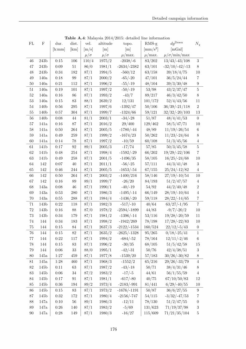
Detailed campaign information
Table A.4: Malaysia 2014/2015: detailed line information
FL F dur. dist. vel. altitude topo. RMS-g dgDown Nχ[h:mm] [km] [m/s] [m] [m] [mm/s2] [mGal]
µ/σ µ/σ µ/max. µ/max. µ/σ/min/max
46 243b 0:15 106 110/4 1975/2 -2038/-6 83/202 13/43/-43/108 3
47 243b 0:09 51 86/0 1981/1 -2634/-2382 63/101 -32/10/-42/-13 8
48 243b 0:34 182 87/1 1994/5 -560/12 63/158 39/18/4/75 10
49 140a 0:18 99 87/1 2000/2 -65/-20 47/101 36/5/24/44 7
50 140a 0:21 112 87/1 1996/2 -55/-19 48/104 39/3/30/48 9
51 140a 0:19 101 87/1 1997/2 -50/-19 53/98 43/2/37/47 5
52 140a 0:16 86 87/1 1993/2 -43/7 89/217 46/3/42/50 8
53 140a 0:15 83 88/1 2639/2 12/131 101/172 52/4/43/56 11
54 140b 0:56 295 87/1 1997/6 -1392/47 50/106 36/39/-21/118 2
55 140b 0:57 304 87/1 1999/7 -1324/66 59/121 32/32/-20/103 13
56 140b 0:08 44 81/1 2003/1 -34/-28 51/87 48/4/41/53 0
57 141a 0:16 87 87/1 2016/2 29/400 129/462 58/5/47/71 10
58 141a 0:50 264 87/1 2005/5 -1780/-44 48/89 11/19/-26/54 6
59 141a 0:49 259 87/1 1999/2 -1674/23 50/262 11/23/-24/64 8
60 141a 0:14 78 87/1 1997/2 -10/59 60/108 51/3/45/56 4
61 141b 0:17 92 89/1 2005/3 -17/74 57/85 50/3/45/58 5
62 141b 0:48 254 87/1 1998/4 -1592/-29 66/202 19/29/-22/106 7
63 141b 0:49 258 87/1 2001/5 -1496/35 58/105 16/25/-24/68 10
64 142 0:07 40 87/1 2011/1 -56/-25 57/111 44/3/41/48 3
65 142 0:46 244 87/1 2005/5 -1653/-54 67/155 25/24/-12/82 4
66 142 0:50 264 87/1 2003/2 -1400/216 58/146 27/19/-10/54 10
67 142 0:16 89 89/1 1999/7 -26/20 84/193 51/2/47/57 4
68 143a 0:08 46 87/1 1990/1 -40/-19 54/92 44/2/40/48 2
69 143a 0:53 280 87/1 1986/3 -1495/-14 66/149 28/19/-10/64 4
70 143a 0:55 288 87/1 1984/4 -1436/-20 59/118 28/22/-14/65 7
71 143b 0:22 118 87/1 1982/3 -517/-10 40/64 63/27/-1/95 7
72 143b 0:16 88 87/0 1978/2 -2594/-1899 44/83 -9/7/-20/2 10
73 143b 0:34 179 87/1 1981/2 -1396/-14 53/116 19/28/-20/59 11
74 144 0:34 183 87/1 1998/2 -1942/269 78/198 17/28/-22/83 10
75 144 0:15 84 87/1 2637/3 -2122/-1534 160/524 22/12/-5/43 0
76 144 0:15 82 87/1 2635/2 -2625/-1328 95/265 0/18/-25/41 1
77 144 0:22 117 87/1 1994/2 -684/-52 78/164 12/11/-2/46 6
78 144 0:15 83 87/1 1996/2 -30/35 68/105 51/5/42/58 15
79 144 0:06 33 88/0 1995/1 -42/-31 50/76 42/4/38/51 3
80 145a 1:27 459 87/1 1977/8 -1539/20 57/183 30/26/-30/82 8
81 145a 1:28 460 87/1 1968/3 -1552/2 65/216 29/26/-33/79 4
82 145b 0:11 63 87/1 1987/2 -43/-18 50/71 38/4/31/46 8
83 145b 0:06 34 87/2 1983/2 -17/-5 44/61 56/1/55/59 4
84 145b 0:17 91 87/1 1981/1 -617/-80 40/75 67/10/50/83 12
85 145b 0:36 194 89/2 1973/4 -2183/-991 81/441 6/29/-40/55 10
86 145b 0:15 83 87/1 1973/2 -1676/-1191 50/87 36/6/27/55 9
87 145b 0:32 172 87/1 1980/4 -2156/-747 54/115 -3/32/-47/53 7
88 147a 0:10 56 89/1 1986/3 -12/11 78/130 51/2/47/55 0
89 147a 0:26 140 87/1 1983/2 -5/69 131/623 71/19/37/98 3
90 147a 0:28 149 87/1 1980/3 -16/27 115/609 71/21/35/104 5
176
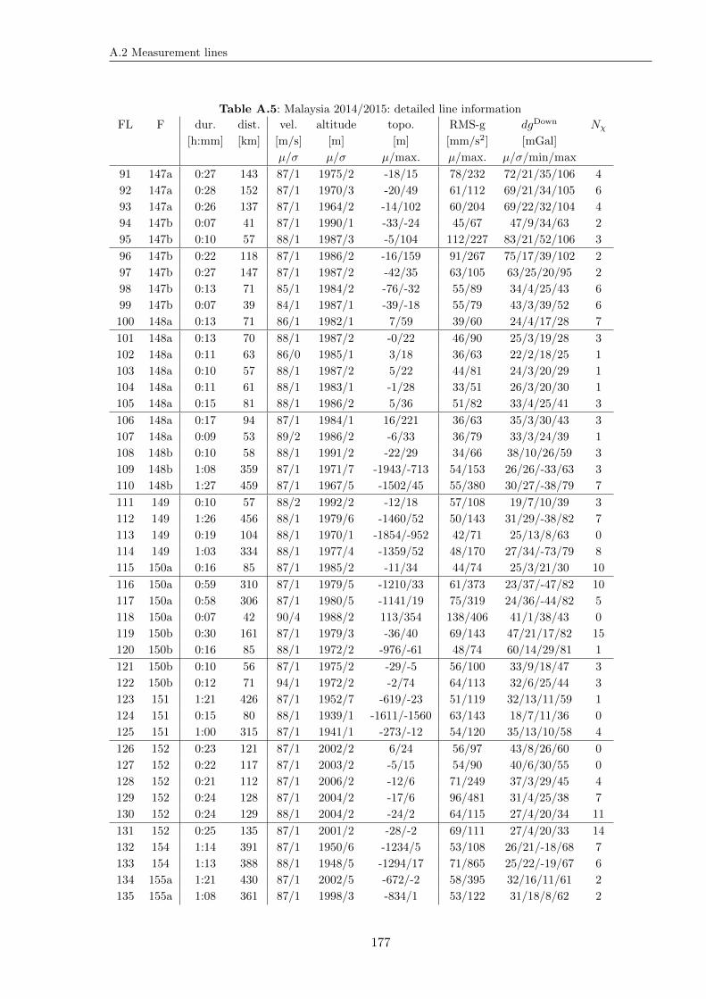
A.2 Measurement lines
Table A.5: Malaysia 2014/2015: detailed line information
FL F dur. dist. vel. altitude topo. RMS-g dgDown Nχ[h:mm] [km] [m/s] [m] [m] [mm/s2] [mGal]
µ/σ µ/σ µ/max. µ/max. µ/σ/min/max
91 147a 0:27 143 87/1 1975/2 -18/15 78/232 72/21/35/106 4
92 147a 0:28 152 87/1 1970/3 -20/49 61/112 69/21/34/105 6
93 147a 0:26 137 87/1 1964/2 -14/102 60/204 69/22/32/104 4
94 147b 0:07 41 87/1 1990/1 -33/-24 45/67 47/9/34/63 2
95 147b 0:10 57 88/1 1987/3 -5/104 112/227 83/21/52/106 3
96 147b 0:22 118 87/1 1986/2 -16/159 91/267 75/17/39/102 2
97 147b 0:27 147 87/1 1987/2 -42/35 63/105 63/25/20/95 2
98 147b 0:13 71 85/1 1984/2 -76/-32 55/89 34/4/25/43 6
99 147b 0:07 39 84/1 1987/1 -39/-18 55/79 43/3/39/52 6
100 148a 0:13 71 86/1 1982/1 7/59 39/60 24/4/17/28 7
101 148a 0:13 70 88/1 1987/2 -0/22 46/90 25/3/19/28 3
102 148a 0:11 63 86/0 1985/1 3/18 36/63 22/2/18/25 1
103 148a 0:10 57 88/1 1987/2 5/22 44/81 24/3/20/29 1
104 148a 0:11 61 88/1 1983/1 -1/28 33/51 26/3/20/30 1
105 148a 0:15 81 88/1 1986/2 5/36 51/82 33/4/25/41 3
106 148a 0:17 94 87/1 1984/1 16/221 36/63 35/3/30/43 3
107 148a 0:09 53 89/2 1986/2 -6/33 36/79 33/3/24/39 1
108 148b 0:10 58 88/1 1991/2 -22/29 34/66 38/10/26/59 3
109 148b 1:08 359 87/1 1971/7 -1943/-713 54/153 26/26/-33/63 3
110 148b 1:27 459 87/1 1967/5 -1502/45 55/380 30/27/-38/79 7
111 149 0:10 57 88/2 1992/2 -12/18 57/108 19/7/10/39 3
112 149 1:26 456 88/1 1979/6 -1460/52 50/143 31/29/-38/82 7
113 149 0:19 104 88/1 1970/1 -1854/-952 42/71 25/13/8/63 0
114 149 1:03 334 88/1 1977/4 -1359/52 48/170 27/34/-73/79 8
115 150a 0:16 85 87/1 1985/2 -11/34 44/74 25/3/21/30 10
116 150a 0:59 310 87/1 1979/5 -1210/33 61/373 23/37/-47/82 10
117 150a 0:58 306 87/1 1980/5 -1141/19 75/319 24/36/-44/82 5
118 150a 0:07 42 90/4 1988/2 113/354 138/406 41/1/38/43 0
119 150b 0:30 161 87/1 1979/3 -36/40 69/143 47/21/17/82 15
120 150b 0:16 85 88/1 1972/2 -976/-61 48/74 60/14/29/81 1
121 150b 0:10 56 87/1 1975/2 -29/-5 56/100 33/9/18/47 3
122 150b 0:12 71 94/1 1972/2 -2/74 64/113 32/6/25/44 3
123 151 1:21 426 87/1 1952/7 -619/-23 51/119 32/13/11/59 1
124 151 0:15 80 88/1 1939/1 -1611/-1560 63/143 18/7/11/36 0
125 151 1:00 315 87/1 1941/1 -273/-12 54/120 35/13/10/58 4
126 152 0:23 121 87/1 2002/2 6/24 56/97 43/8/26/60 0
127 152 0:22 117 87/1 2003/2 -5/15 54/90 40/6/30/55 0
128 152 0:21 112 87/1 2006/2 -12/6 71/249 37/3/29/45 4
129 152 0:24 128 87/1 2004/2 -17/6 96/481 31/4/25/38 7
130 152 0:24 129 88/1 2004/2 -24/2 64/115 27/4/20/34 11
131 152 0:25 135 87/1 2001/2 -28/-2 69/111 27/4/20/33 14
132 154 1:14 391 87/1 1950/6 -1234/5 53/108 26/21/-18/68 7
133 154 1:13 388 88/1 1948/5 -1294/17 71/865 25/22/-19/67 6
134 155a 1:21 430 87/1 2002/5 -672/-2 58/395 32/16/11/61 2
135 155a 1:08 361 87/1 1998/3 -834/1 53/122 31/18/8/62 2
177
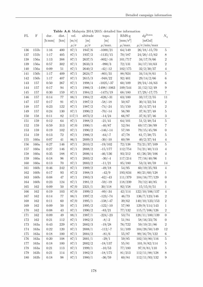
Detailed campaign information
Table A.6: Malaysia 2014/2015: detailed line information
FL F dur. dist. vel. altitude topo. RMS-g dgDown Nχ[h:mm] [km] [m/s] [m] [m] [mm/s2] [mGal]
µ/σ µ/σ µ/max. µ/max. µ/σ/min/max
136 155b 1:16 400 87/1 1947/6 -1088/21 64/149 26/18/-15/70 5
137 155b 1:17 405 87/1 1937/2 -1135/15 70/187 24/20/-15/62 8
138 156a 1:13 388 87/1 2637/5 -802/-16 101/717 34/17/9/66 2
139 156a 0:57 302 87/1 2633/3 -990/3 72/131 34/17/10/63 2
140 156a 0:09 51 87/1 2640/2 -42/-12 102/175 32/2/30/37 4
141 156b 1:17 409 87/1 2624/7 -801/31 88/924 34/14/8/61 5
142 156b 1:17 407 87/1 2615/3 -948/22 92/401 29/14/2/66 6
143 157 0:50 267 87/1 1998/4 -1025/-37 60/109 29/24/-16/63 6
144 157 0:17 94 87/1 1986/3 -1498/-1063 109/544 31/12/12/49 9
145 157 0:30 159 87/1 1984/2 -1475/19 68/180 17/29/-17/75 7
146 157 0:14 77 88/1 1984/2 -626/-31 63/100 33/17/2/55 11
147 157 0:17 91 87/1 1987/2 -58/-18 50/67 30/4/22/34 2
148 157 0:23 122 87/1 1987/2 -74/-24 55/150 35/4/27/44 2
149 157 0:24 130 87/1 1990/2 -70/-14 56/90 37/6/27/48 5
150 158 0:11 82 117/1 4873/2 -14/24 66/97 37/6/27/46 3
151 159 0:12 64 87/1 1988/2 -21/41 64/101 51/2/48/54 5
152 159 0:59 313 87/0 1990/1 -40/87 52/94 69/17/38/99 7
153 159 0:19 102 87/1 1990/2 -146/-14 57/88 79/15/45/98 0
154 159 0:13 72 87/1 1986/2 -64/-7 47/78 61/7/38/75 5
155 160a 0:07 41 86/1 2009/3 -30/-10 60/98 40/2/37/44 4
156 160a 0:27 146 87/1 2010/2 -19/102 72/138 73/21/37/109 5
157 160a 0:27 146 87/1 2008/2 -15/177 112/754 74/21/40/113 4
158 160a 0:35 188 87/1 2006/4 -46/136 93/212 61/26/20/106 4
159 160a 0:18 96 87/1 2003/2 -30/-4 117/214 77/16/40/96 1
160 160a 0:13 70 87/1 2003/2 -11/21 85/180 53/3/48/59 14
161 160b 0:46 242 87/1 1989/2 -49/18 54/95 60/19/25/93 4
162 160b 0:17 93 87/2 1988/3 -42/9 193/634 80/21/60/128 1
163 160b 0:08 47 87/1 1983/3 -62/-43 111/379 104/16/77/129 0
164 160b 0:23 124 87/1 1981/2 -59/-19 118/239 70/12/40/85 0
165 162 0:09 50 87/0 2321/1 30/118 92/158 15/15/0/51 1
166 162 0:19 103 87/0 1999/2 -89/-34 42/114 122/10/106/137 4
167 162 0:14 77 88/1 1997/2 -123/-74 46/73 136/7/123/146 2
168 162 0:11 60 87/0 1995/1 -138/-47 39/62 140/10/123/153 2
169 162 0:09 50 87/1 1995/2 -122/-10 57/80 129/9/114/143 1
170 162 0:08 43 87/1 1990/2 -83/21 77/132 115/7/106/126 2
171 162 0:09 49 88/1 1987/1 -224/-23 53/74 128/11/100/139 0
172 162 0:21 112 87/1 1982/2 -8/-2 51/84 58/16/23/76 0
173 163a 0:43 229 87/1 2002/3 -19/28 76/722 59/19/21/86 2
174 163a 0:22 120 87/1 2008/1 -112/-7 51/109 104/28/50/149 12
175 163a 0:18 100 87/1 2004/2 -81/6 55/87 99/16/78/122 6
176 163a 0:20 108 87/1 2001/1 -29/1 59/85 102/10/80/116 5
177 163a 0:18 100 87/1 2002/2 -18/137 55/81 101/8/82/114 5
178 163a 0:21 113 87/1 1999/1 -10/53 77/180 97/8/81/110 5
179 163b 0:21 114 87/1 1982/2 -18/175 81/213 112/11/88/128 8
180 163b 0:18 98 87/1 1980/1 -36/59 60/84 112/11/93/132 9
178
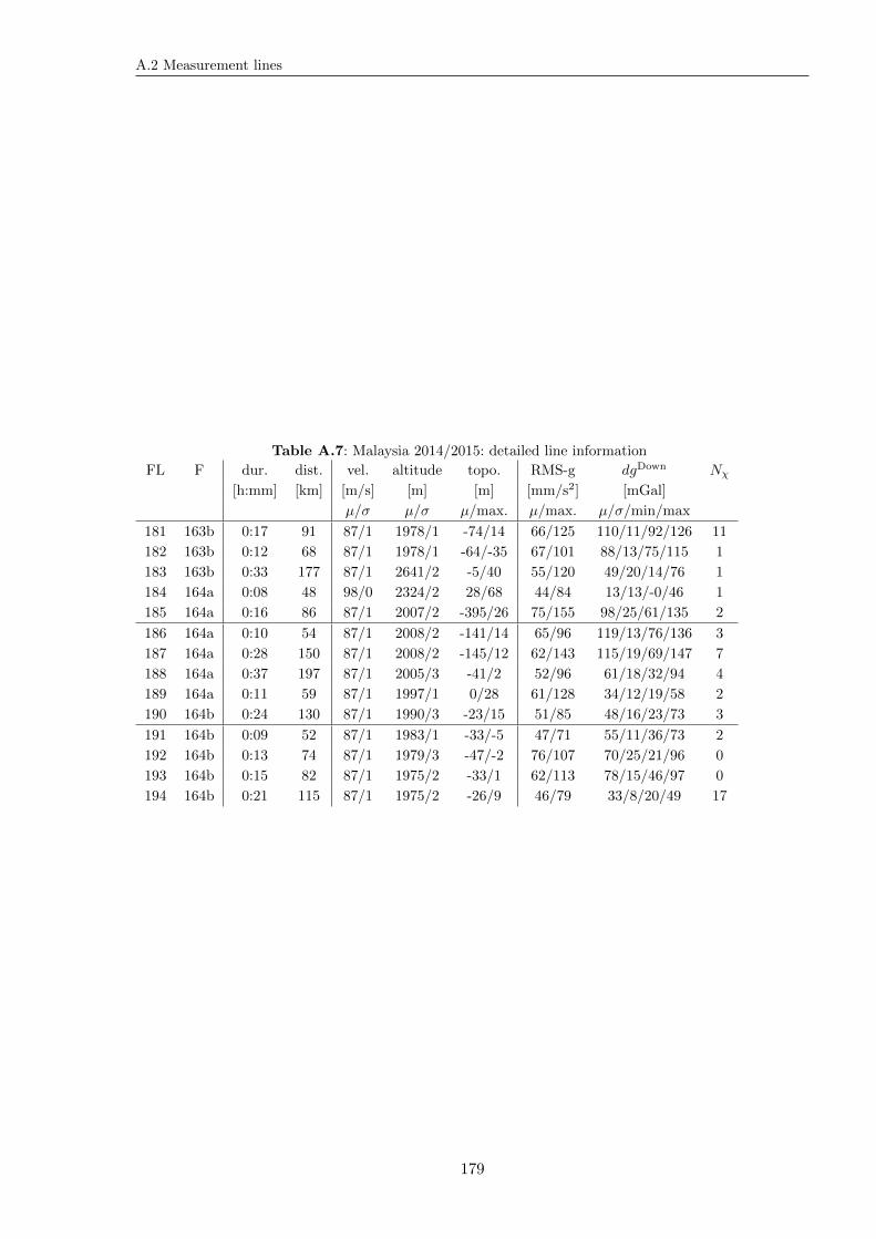
A.2 Measurement lines
Table A.7: Malaysia 2014/2015: detailed line information
FL F dur. dist. vel. altitude topo. RMS-g dgDown Nχ[h:mm] [km] [m/s] [m] [m] [mm/s2] [mGal]
µ/σ µ/σ µ/max. µ/max. µ/σ/min/max
181 163b 0:17 91 87/1 1978/1 -74/14 66/125 110/11/92/126 11
182 163b 0:12 68 87/1 1978/1 -64/-35 67/101 88/13/75/115 1
183 163b 0:33 177 87/1 2641/2 -5/40 55/120 49/20/14/76 1
184 164a 0:08 48 98/0 2324/2 28/68 44/84 13/13/-0/46 1
185 164a 0:16 86 87/1 2007/2 -395/26 75/155 98/25/61/135 2
186 164a 0:10 54 87/1 2008/2 -141/14 65/96 119/13/76/136 3
187 164a 0:28 150 87/1 2008/2 -145/12 62/143 115/19/69/147 7
188 164a 0:37 197 87/1 2005/3 -41/2 52/96 61/18/32/94 4
189 164a 0:11 59 87/1 1997/1 0/28 61/128 34/12/19/58 2
190 164b 0:24 130 87/1 1990/3 -23/15 51/85 48/16/23/73 3
191 164b 0:09 52 87/1 1983/1 -33/-5 47/71 55/11/36/73 2
192 164b 0:13 74 87/1 1979/3 -47/-2 76/107 70/25/21/96 0
193 164b 0:15 82 87/1 1975/2 -33/1 62/113 78/15/46/97 0
194 164b 0:21 115 87/1 1975/2 -26/9 46/79 33/8/20/49 17
179
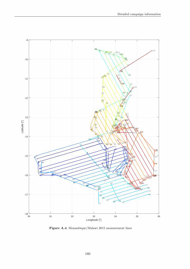
Detailed campaign information
30 31 32 33 34 35 36
Longitude [°]
-18
-17
-16
-15
-14
-13
-12
-11
-10
-9
Latit
ude
[°]
1
1
2
23
3
4
45
5
6
67
78
89
910 1011
1112
1213
1314
1415
15
16
1617
17
18
1819
19
20
20 21
21
22
22
23
2324
24
25
25
26
2627
27
28
28
29
2930
3031
31
32
3233 3334
34
35
35
36
36
37
37
38
3839
39
40
40
41
41
42
4243
43
44
4445
45
46
46
47
4748
4849
49
50
5051
5152
52
53
53
54
54
55
55
56
5657
57
58
5859
59
60
60
61
61
62
62
63
6364
6465
6566
6667
67
68
68
69
69
70
70
71
71
72
72
73
7374 74
75
75
76
7677
7778
78
79
79
80
8081
81
82
82
83
8384
84
85
85
86
8687
8788
88
89
8990
90
91
9192
92
93
9394
9495
9596
9697
9798
98
99
99
100
100
101
101
102
102103
103
104
104105
105 106
106107
107108
108109
109110
110111
111112
112113
113114
114115
115116
116117
117118
118119
119120
120
121
121
122
122
123
123124
124
125
125
126 126127
127
128
128
129
129
130
130
Figure A.4: Mozambique/Malawi 2015 measurement lines
180
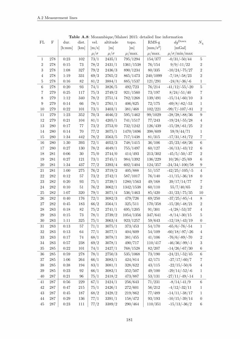
A.2 Measurement lines
Table A.8: Mozambique/Malawi 2015: detailed line information
FL F dur. dist. vel. altitude topo. RMS-g dgDown Nχ[h:mm] [km] [m/s] [m] [m] [mm/s2] [mGal]
µ/σ µ/σ µ/max. µ/max. µ/σ/min/max
1 278 0:23 102 73/1 2435/1 795/1294 154/377 -0/31/-50/44 5
2 278 0:15 73 78/2 2431/1 1361/1538 76/154 9/9/-11/22 2
3 278 1:08 327 79/2 2436/3 890/1234 80/335 -10/24/-75/27 2
4 278 1:19 331 69/3 2765/2 865/1473 240/1099 -7/18/-58/23 2
5 278 0:16 82 81/2 3884/1 885/1537 121/291 -24/8/-36/-6 1
6 278 0:20 93 74/1 3826/5 492/723 76/214 -41/12/-55/-20 5
7 279 0:25 117 75/3 2749/2 921/1560 73/197 8/24/-51/40 7
8 279 1:12 340 78/2 2751/4 782/1268 139/491 -15/14/-60/10 3
9 279 0:14 66 78/1 2761/1 406/625 72/175 -69/8/-82/-53 1
10 279 0:22 101 73/1 3403/1 381/468 102/221 -99/7/-107/-81 2
11 279 1:23 352 70/3 4046/2 595/1462 99/1029 -28/28/-88/36 9
12 279 0:21 104 81/1 4205/1 741/1517 77/243 -19/24/-55/28 4
13 280 0:17 77 73/2 2753/0 732/1242 126/439 -15/28/-61/25 2
14 280 0:14 70 77/2 3075/1 1470/1696 398/609 59/9/44/71 1
15 280 1:34 442 78/2 3563/5 717/1438 81/315 -17/31/-81/72 7
16 280 1:30 393 72/1 4052/3 748/1415 36/106 -25/23/-68/26 6
17 280 0:27 130 78/2 4049/1 755/1497 60/127 -16/13/-43/12 6
18 281 0:06 30 75/0 2744/0 414/493 213/302 -45/5/-50/-37 2
19 281 0:27 121 73/1 2745/1 984/1392 136/229 10/26/-25/69 6
20 281 1:34 437 77/2 3393/4 602/1404 124/357 -24/34/-100/58 9
21 281 1:00 275 76/2 3719/2 405/888 51/157 -42/25/-105/-5 4
22 282 0:12 57 73/2 2742/1 587/1017 76/140 -11/15/-36/18 0
23 282 0:20 93 75/1 2739/1 1280/1563 49/168 39/17/14/77 7
24 282 0:10 51 76/2 3062/1 1342/1538 60/110 55/7/40/65 2
25 282 1:07 320 79/1 3071/4 536/1463 85/420 -31/23/-75/35 10
26 282 0:40 176 72/1 3082/3 479/726 69/250 -37/25/-85/-4 8
27 282 0:45 183 66/2 3564/1 325/511 170/358 -15/20/-48/21 2
28 283 0:18 82 75/2 2741/1 695/1205 91/301 -4/28/-53/37 4
29 283 0:15 73 78/1 2739/2 1054/1356 347/641 -8/14/-30/15 5
30 283 1:11 325 75/1 3063/4 923/1257 59/643 -12/18/-43/19 0
31 283 0:13 57 71/1 3075/1 373/453 54/170 -65/6/-76/-54 1
32 283 0:13 64 77/1 3077/1 404/609 54/109 -60/18/-97/-26 4
33 283 0:17 74 68/1 3078/1 381/455 41/106 -76/6/-89/-70 2
34 283 0:57 238 69/2 3078/1 490/717 110/417 -46/36/-99/-1 3
35 285 0:22 101 74/1 2427/1 768/1528 82/207 -14/26/-67/30 6
36 285 0:59 278 78/1 2750/3 535/1068 73/190 -24/21/-52/45 6
37 285 1:06 264 66/1 3083/1 424/814 42/171 -27/17/-60/7 7
38 285 0:38 194 83/1 3081/1 328/622 43/115 -22/15/-50/6 4
39 285 0:23 92 66/1 3083/1 352/507 49/100 -29/14/-52/-6 1
40 287 0:21 96 75/1 2418/2 473/887 53/131 -27/11/-49/-14 1
41 287 0:56 229 67/1 2424/1 256/643 71/231 -8/14/-41/9 6
42 287 0:47 215 75/1 2426/1 272/601 56/212 -4/12/-32/11 1
43 287 0:45 187 68/2 2428/2 219/862 77/489 -14/11/-38/17 1
44 287 0:29 136 77/1 3391/1 158/472 93/193 -10/15/-39/14 0
45 287 0:23 111 77/2 3389/2 290/464 110/351 -15/13/-36/2 6
181
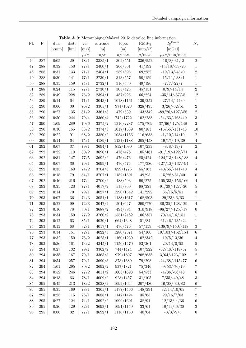
Detailed campaign information
Table A.9: Mozambique/Malawi 2015: detailed line information
FL F dur. dist. vel. altitude topo. RMS-g dgDown Nχ[h:mm] [km] [m/s] [m] [m] [mm/s2] [mGal]
µ/σ µ/σ µ/max. µ/max. µ/σ/min/max
46 287 0:05 29 78/1 3385/1 302/551 336/552 -10/8/-31/-3 2
47 288 0:32 150 77/1 2400/1 266/561 41/192 -14/18/-39/20 1
48 288 0:31 133 71/1 2404/1 259/395 69/252 -19/13/-45/0 2
49 288 0:30 141 77/1 2730/1 313/557 50/159 -15/11/-38/1 1
50 288 0:35 159 74/1 2732/1 316/530 49/196 -7/7/-22/7 1
51 288 0:24 115 77/1 2730/1 305/425 45/151 0/9/-14/14 2
52 289 0:49 228 76/2 2394/1 487/925 66/224 -35/14/-57/-5 12
53 289 0:14 64 71/1 3043/1 1018/1161 139/252 -27/14/-44/9 1
54 290 0:06 30 76/2 3365/1 971/1628 328/495 3/26/-32/51 2
55 290 0:27 135 81/2 3361/3 479/539 143/342 -89/26/-127/-56 2
56 290 0:50 244 79/4 3360/4 742/1722 102/288 -54/63/-168/40 3
57 290 1:09 289 70/6 3375/2 1310/2287 175/709 37/66/-125/148 2
58 290 0:30 155 83/2 3374/3 1017/1539 80/183 -15/55/-131/48 10
59 290 0:22 91 68/2 3380/2 1084/1156 116/638 -1/10/-14/19 2
60 290 0:14 64 75/1 4189/1 1137/1188 205/458 19/17/-19/39 4
61 292 0:07 37 79/1 3694/1 852/1090 107/233 -8/8/-19/7 2
62 292 0:22 110 80/2 3690/1 476/476 105/461 -91/19/-122/-71 4
63 292 0:31 147 77/5 3692/2 476/476 85/424 -124/13/-148/-88 4
64 292 0:07 36 79/1 3699/1 476/476 177/386 -127/12/-137/-94 1
65 292 0:35 160 74/2 3704/3 899/1775 55/163 -40/65/-141/40 4
66 292 0:15 79 84/1 3707/1 1152/1591 49/95 15/28/-51/40 0
67 292 0:46 216 77/4 3700/2 483/593 90/275 -105/33/-156/-66 4
68 292 0:25 120 77/1 4017/2 513/860 98/223 -91/29/-127/-20 5
69 292 0:14 70 79/1 4027/1 1290/1542 141/292 35/15/5/51 3
70 293 0:07 36 74/3 3051/1 1188/1617 168/503 29/23/-6/63 1
71 293 0:22 99 72/3 3047/2 501/647 290/770 -86/35/-128/-29 4
72 293 0:16 78 80/1 3688/2 494/994 310/918 -98/27/-125/-17 0
73 293 0:34 159 77/2 3760/2 1551/2482 106/357 70/44/16/151 1
74 293 0:12 63 85/1 4020/1 664/1348 51/84 -61/46/-135/24 1
75 293 0:13 68 82/1 4017/1 476/476 57/159 -138/9/-150/-118 3
76 293 0:34 151 72/1 4022/3 1280/2371 54/160 19/103/-152/154 6
77 293 0:32 150 76/2 4025/1 1160/1239 102/342 19/5/13/36 4
78 293 0:36 161 73/2 4345/1 1150/1470 83/261 20/14/0/55 5
79 294 0:27 132 79/1 3362/2 744/1474 107/222 -32/48/-118/57 5
80 294 0:35 167 79/1 3365/3 979/1807 208/635 3/64/-123/102 2
81 294 0:54 257 79/1 3690/3 878/1689 79/298 -24/68/-115/77 6
82 294 1:01 295 80/2 3692/2 937/1821 75/346 -9/53/-76/79 7
83 294 0:52 246 77/2 4011/2 1003/1693 54/533 -4/36/-56/48 6
84 294 0:13 63 78/1 4009/2 928/1457 31/105 7/35/-49/48 3
85 295 0:45 213 78/2 3038/2 1092/1644 207/480 16/28/-30/82 6
86 295 0:35 169 78/1 3365/1 1177/1466 148/294 32/14/10/65 7
87 295 0:25 115 76/1 3688/1 1147/1424 35/65 29/16/7/63 2
88 295 0:27 124 74/1 3692/2 1099/1601 38/91 12/13/-4/36 6
89 295 0:26 129 82/1 3693/1 1091/1159 33/61 10/11/-6/30 3
90 295 0:06 32 77/1 3692/1 1116/1150 40/64 -3/3/-9/5 0
182
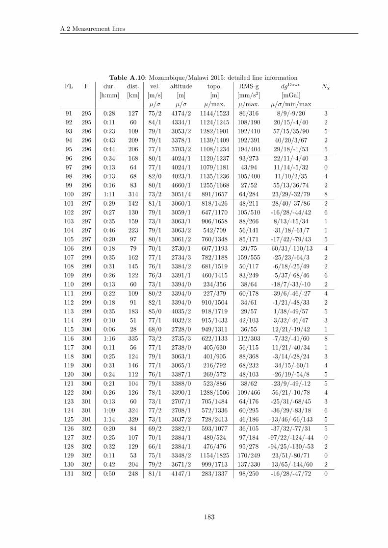
A.2 Measurement lines
Table A.10: Mozambique/Malawi 2015: detailed line information
FL F dur. dist. vel. altitude topo. RMS-g dgDown Nχ[h:mm] [km] [m/s] [m] [m] [mm/s2] [mGal]
µ/σ µ/σ µ/max. µ/max. µ/σ/min/max
91 295 0:28 127 75/2 4174/2 1144/1523 86/316 8/9/-9/20 3
92 295 0:11 60 84/1 4334/1 1124/1245 108/190 20/15/-4/40 2
93 296 0:23 109 79/1 3053/2 1282/1901 192/410 57/15/35/90 5
94 296 0:43 209 79/1 3378/1 1139/1409 192/391 40/20/3/67 2
95 296 0:44 206 77/1 3703/2 1108/1234 194/404 29/18/-1/53 5
96 296 0:34 168 80/1 4024/1 1120/1237 93/273 22/11/-4/40 3
97 296 0:13 64 77/1 4024/1 1079/1181 43/94 11/14/-5/32 0
98 296 0:13 68 82/0 4023/1 1135/1236 105/400 11/10/2/35 4
99 296 0:16 83 80/1 4660/1 1255/1668 27/52 55/13/36/74 2
100 297 1:11 314 73/2 3051/4 891/1657 64/284 23/29/-32/79 8
101 297 0:29 142 81/1 3060/1 818/1426 48/211 28/40/-37/86 2
102 297 0:27 130 79/1 3059/1 647/1170 105/510 -16/28/-44/42 6
103 297 0:35 159 73/1 3063/1 906/1658 88/266 8/13/-15/34 1
104 297 0:46 223 79/1 3063/2 542/709 56/141 -31/18/-61/7 1
105 297 0:20 97 80/1 3061/2 760/1348 85/171 -17/42/-79/43 5
106 299 0:18 79 70/1 2730/1 607/1193 39/75 -60/31/-110/13 4
107 299 0:35 162 77/1 2734/3 782/1188 159/555 -25/23/-64/3 2
108 299 0:31 145 76/1 3384/2 681/1519 50/117 -6/18/-25/49 2
109 299 0:26 122 76/3 3391/1 460/1415 83/249 -5/37/-68/46 6
110 299 0:13 60 73/1 3394/0 234/356 38/64 -18/7/-33/-10 2
111 299 0:22 109 80/2 3394/0 227/379 60/178 -39/6/-46/-27 4
112 299 0:18 91 82/1 3394/0 910/1504 34/61 -1/21/-48/33 2
113 299 0:35 183 85/0 4035/2 918/1719 29/57 1/38/-49/57 5
114 299 0:10 51 77/1 4032/2 915/1433 42/103 3/32/-46/47 3
115 300 0:06 28 68/0 2728/0 949/1311 36/55 12/21/-19/42 1
116 300 1:16 335 73/2 2735/3 622/1133 112/303 -7/32/-41/60 8
117 300 0:11 56 77/1 2738/0 405/630 56/115 11/21/-40/34 1
118 300 0:25 124 79/1 3063/1 401/905 88/368 -3/14/-28/24 3
119 300 0:31 146 77/1 3065/1 216/792 68/232 -34/15/-60/1 4
120 300 0:24 112 76/1 3387/1 269/572 48/103 -26/19/-54/8 5
121 300 0:21 104 79/1 3388/0 523/886 38/62 -23/9/-49/-12 5
122 300 0:26 126 78/1 3390/1 1288/1506 109/466 56/21/-10/78 4
123 301 0:13 60 73/1 2707/1 705/1484 64/176 -25/31/-68/45 3
124 301 1:09 324 77/2 2708/1 572/1336 60/295 -36/29/-83/18 6
125 301 1:14 329 73/1 3037/2 728/2413 46/186 -13/46/-66/143 5
126 302 0:20 84 69/2 2382/1 593/1077 36/105 -37/32/-77/31 5
127 302 0:25 107 70/1 2384/1 480/524 97/184 -97/22/-124/-44 0
128 302 0:32 129 66/1 2384/1 476/476 95/278 -94/25/-130/-53 2
129 302 0:11 53 75/1 3348/2 1154/1825 170/249 23/51/-80/71 0
130 302 0:42 204 79/2 3671/2 999/1713 137/330 -13/65/-144/60 2
131 302 0:50 248 81/1 4147/1 283/1337 98/250 -16/28/-47/72 0
183
Detailed
campaign
inform
ation
-150 -100 -50 0 50 100 150
Longitude [°]
-90
-89
-88
-87
-86
-85
-84
-83
-82
-81
Latit
ude
[°]
1
12
233
4
45 56
67
788
9
910101111
12
1213
1314
1415 15
16
1617
1718
1819
1920
20212122222323
2424
25 2526
26
272728
2829
293030
3131
3232
3333
3434
353536
3637
3738
3839
39
40
404141
424243
434444
45
4546
4647
4748
4849
4950
50515152
52
53
53545455
5556
5657
5758
5859
5960
6061
6162
6263
6364
6465
6566
6667
676868
69
697070
71
7172
7273
7374
74
757576
7677
77
78
7879
7980
8081
8182
82
83
8384 84
85
8586
868787
88
88
89
8990 90
91
9192
9293
9394
9495 95
96
96 97
9798 98
99
99100
100101101
102
102
103
103 104
104
105
105106106
107
107108
108109
109
110
110111
111112112
113
113114
114115115
116
116117
117118118
119
119
120
120121
121122
122123
123124
124
detail plot
Figure A.5: Antarctica 2015/2016 measurement lines
184
A.2 Measurement lines
5 10 15 20 25
Longitude [°]
-84.5
-84
-83.5
-83
-82.5
-82
Latit
ude
[°]
1 6
7
9
10 1011 11
12
12
13
13
1617
17
18
18
19
19
20
20
21 212222
2323
2424
2525
2626
27
27
28
2829
2930
30
3131
3232
33
33
34
34
35
35
36
36
37
37
38
3839
39
40
40
414142
4243
4344
44
45
45
46
Figure A.6: Antarctica 2015/2016 measurement lines (detail)
185
Detailed campaign information
Table A.11: Antarctica 2015/2016: detailed line information
FL F dur. dist. vel. altitude topo. RMS-g dgDown Nχ[h:mm] [km] [m/s] [m] [m] [mm/s2] [mGal]
µ/σ µ/σ µ/max. µ/max. µ/σ/min/max
1 350 1:26 326 63/1 2798/5 – / – 66/144 -18/22/-64/9 3
2 350 0:22 80 59/1 2732/4 – / – 81/145 -3/5/-11/7 0
3 350 0:09 35 63/1 2721/3 – / – 69/107 13/2/6/17 0
4 350 0:35 134 64/1 2636/2 – / – 54/109 -5/11/-23/14 0
5 350 0:09 34 62/0 2785/4 – / – 69/111 1/6/-6/12 0
6 350 1:39 368 61/1 2794/15 – / – 79/151 -20/23/-64/13 3
7 351a 0:54 231 71/2 2932/4 – / – 107/209 -50/18/-80/-9 7
8 351a 0:08 31 63/1 2928/4 – / – 110/140 -37/15/-54/-7 0
9 351a 1:15 267 59/4 2905/6 – / – 115/239 -26/29/-64/19 5
10 351a 0:07 32 66/1 2892/3 – / – 94/145 -51/3/-56/-45 0
11 351a 0:12 49 67/1 2902/5 – / – 117/169 -36/8/-43/-10 2
12 351a 0:12 58 76/1 2905/5 – / – 126/181 -39/23/-75/3 0
13 351b 1:00 258 71/1 2803/9 – / – 99/270 -29/25/-64/7 2
14 351b 0:18 76 70/1 2826/3 – / – 63/121 4/4/-3/11 2
15 351b 0:08 33 62/1 2860/4 – / – 89/140 12/3/6/18 0
16 351b 1:29 310 58/1 2858/8 – / – 83/174 -15/21/-71/15 4
17 351b 0:42 162 64/1 2826/7 – / – 104/189 -25/15/-62/6 0
18 352 0:08 32 65/1 2869/4 – / – 109/145 -67/2/-71/-64 0
19 352 0:21 84 64/0 2868/5 – / – 93/158 -36/11/-56/-18 1
20 352 0:08 31 62/0 2872/3 – / – 85/127 -25/2/-30/-23 0
21 352 0:08 35 69/0 2875/3 – / – 92/139 -19/8/-31/-5 0
22 352 0:09 40 66/1 2876/4 – / – 102/145 -31/6/-38/-20 0
23 352 0:12 53 68/1 2882/3 – / – 98/160 -48/6/-56/-31 0
24 352 0:12 53 68/1 2877/3 – / – 94/136 -47/6/-57/-32 0
25 352 0:16 67 66/1 2876/4 – / – 111/159 -56/11/-70/-38 1
26 352 0:15 65 72/1 2875/4 – / – 117/156 -69/10/-79/-38 1
27 352 0:26 104 65/1 2878/6 – / – 112/174 -63/9/-79/-46 1
28 352 0:11 54 77/1 2876/4 – / – 118/149 -49/7/-64/-38 1
29 354 0:53 183 56/1 2882/4 – / – 63/131 -53/22/-72/28 6
30 354 0:13 49 61/1 2886/3 – / – 72/109 -9/7/-22/6 0
31 354 0:15 56 61/1 2888/6 – / – 85/175 -42/7/-53/-26 0
32 354 0:15 59 61/0 2889/3 – / – 78/108 -36/11/-51/-19 0
33 354 0:33 122 61/1 2889/4 – / – 79/137 -40/13/-56/-13 2
34 354 0:26 101 63/1 2889/5 – / – 87/157 -60/9/-76/-45 1
35 354 0:25 96 62/1 2890/5 – / – 94/162 -57/10/-74/-43 1
36 354 0:14 60 67/1 2895/6 – / – 79/126 -44/14/-71/-17 1
37 355 0:08 38 71/0 2892/4 – / – 82/129 -71/6/-80/-58 0
38 355 0:13 54 69/0 2893/3 – / – 67/93 -68/3/-74/-61 4
39 355 0:13 48 59/1 2895/2 – / – 73/105 -36/6/-48/-20 2
40 355 0:06 28 69/0 2895/2 – / – 63/82 -71/4/-76/-62 0
41 355 0:06 24 65/0 2899/3 – / – 84/141 -69/7/-75/-48 2
42 355 0:15 61 65/1 2905/4 – / – 80/122 -31/35/-70/26 3
43 355 0:15 61 66/1 2901/5 – / – 100/165 -36/30/-74/13 3
44 355 0:07 31 65/0 2904/3 – / – 73/104 -53/10/-63/-22 1
45 355 0:17 61 59/1 2906/4 – / – 93/141 -50/31/-81/-2 1
186
A.2 Measurement lines
Table A.12: Antarctica 2015/2016: detailed line information
FL F dur. dist. vel. altitude topo. RMS-g dgDown Nχ[h:mm] [km] [m/s] [m] [m] [mm/s2] [mGal]
µ/σ µ/σ µ/max. µ/max. µ/σ/min/max
46 359 4:11 983 65/3 2927/11 – / – 179/494 -27/41/-99/63 14
47 360 0:06 27 64/2 2220/6 – / – 90/134 -99/11/-111/-74 0
48 360 2:00 447 62/3 2241/5 – / – 123/363 -18/49/-122/71 8
49 360 0:06 26 62/1 2265/3 – / – 103/154 56/5/44/62 0
50 360 0:16 64 64/1 2180/4 – / – 100/146 45/16/6/67 1
51 360 1:43 388 63/2 2178/4 – / – 134/451 -31/39/-124/36 5
52 361 2:23 446 52/3 2191/11 – / – 130/282 -17/47/-96/79 4
53 361 1:09 295 70/2 1954/15 – / – 141/273 -16/40/-95/58 2
54 361 0:34 154 74/1 1951/7 – / – 126/219 -43/41/-94/63 4
55 362a 1:01 265 71/3 2468/4 – / – 101/266 -9/27/-93/39 3
56 362a 2:51 673 65/3 2899/5 – / – 140/323 -7/32/-85/86 3
57 362b 2:28 612 69/3 3137/10 – / – 136/459 -9/34/-64/80 2
58 362b 1:18 329 70/1 2466/11 – / – 174/353 -10/41/-89/135 4
59 363a 1:03 227 60/2 2286/9 – / – 68/174 -8/36/-102/65 2
60 363a 2:57 684 64/2 2875/12 – / – 183/451 -5/35/-66/128 4
61 363b 2:38 591 62/4 3191/5 – / – 129/429 -16/26/-73/39 1
62 363b 1:37 395 68/2 3194/4 – / – 113/281 -10/38/-79/122 7
63 364 1:48 418 64/2 2144/5 – / – 75/239 -34/49/-130/66 7
64 364 0:56 212 63/1 2153/4 – / – 66/111 36/16/11/61 4
65 364 1:45 387 61/2 2198/5 – / – 109/264 -30/46/-88/151 3
66 365 1:02 225 60/1 1631/4 – / – 87/162 -45/30/-149/-3 2
67 365 0:41 170 68/2 1960/5 – / – 84/164 -37/55/-129/59 4
68 365 0:07 32 69/1 1960/3 – / – 145/189 63/11/45/81 0
69 365 0:52 183 58/2 1991/7 – / – 118/238 -21/61/-165/74 7
70 365 0:18 58 53/1 1564/6 – / – 153/233 17/9/6/33 0
71 365 0:51 178 58/2 1567/10 – / – 118/280 -57/40/-129/37 7
72 365 0:20 76 63/1 1582/6 – / – 95/138 -75/22/-106/-42 1
73 004a 0:40 175 72/2 1959/10 – / – 123/203 -16/33/-74/70 1
74 004a 1:10 212 50/3 2857/12 – / – 153/544 10/38/-85/72 5
75 004b 0:06 19 50/1 2825/25 – / – 84/129 -54/6/-61/-40 0
76 004b 2:23 496 57/4 2857/10 – / – 123/287 -21/30/-68/68 0
77 004c 1:02 270 72/1 3320/8 – / – 94/219 -19/23/-47/24 0
78 004c 1:04 260 67/1 4310/7 – / – 83/179 -27/60/-98/184 0
79 004c 1:34 418 73/2 2595/9 – / – 159/502 2/45/-67/98 6
80 006 0:26 114 71/3 1684/11 – / – 100/173 -32/22/-69/13 0
81 006 2:16 460 56/6 2680/9 – / – 108/261 -33/22/-100/13 6
82 006 0:40 160 66/1 2921/9 – / – 119/218 -34/9/-49/-12 0
83 007 2:02 456 62/1 3389/4 – / – 92/301 -32/14/-69/-7 0
84 007 0:09 36 63/1 3306/6 – / – 80/116 -28/3/-34/-23 0
85 007 1:55 475 68/3 3298/6 – / – 129/361 -36/10/-56/-14 0
86 008a 2:00 466 64/2 3299/4 – / – 108/380 -43/9/-66/-27 0
87 008a 0:11 43 65/1 3443/2 – / – 85/123 -26/7/-36/-16 0
88 008a 2:05 492 65/2 3436/5 – / – 93/171 -40/8/-58/-21 0
89 008b 2:10 466 60/2 3070/8 – / – 126/399 -46/29/-102/42 1
90 008b 0:10 40 64/1 2871/4 – / – 73/123 41/19/10/70 0
187
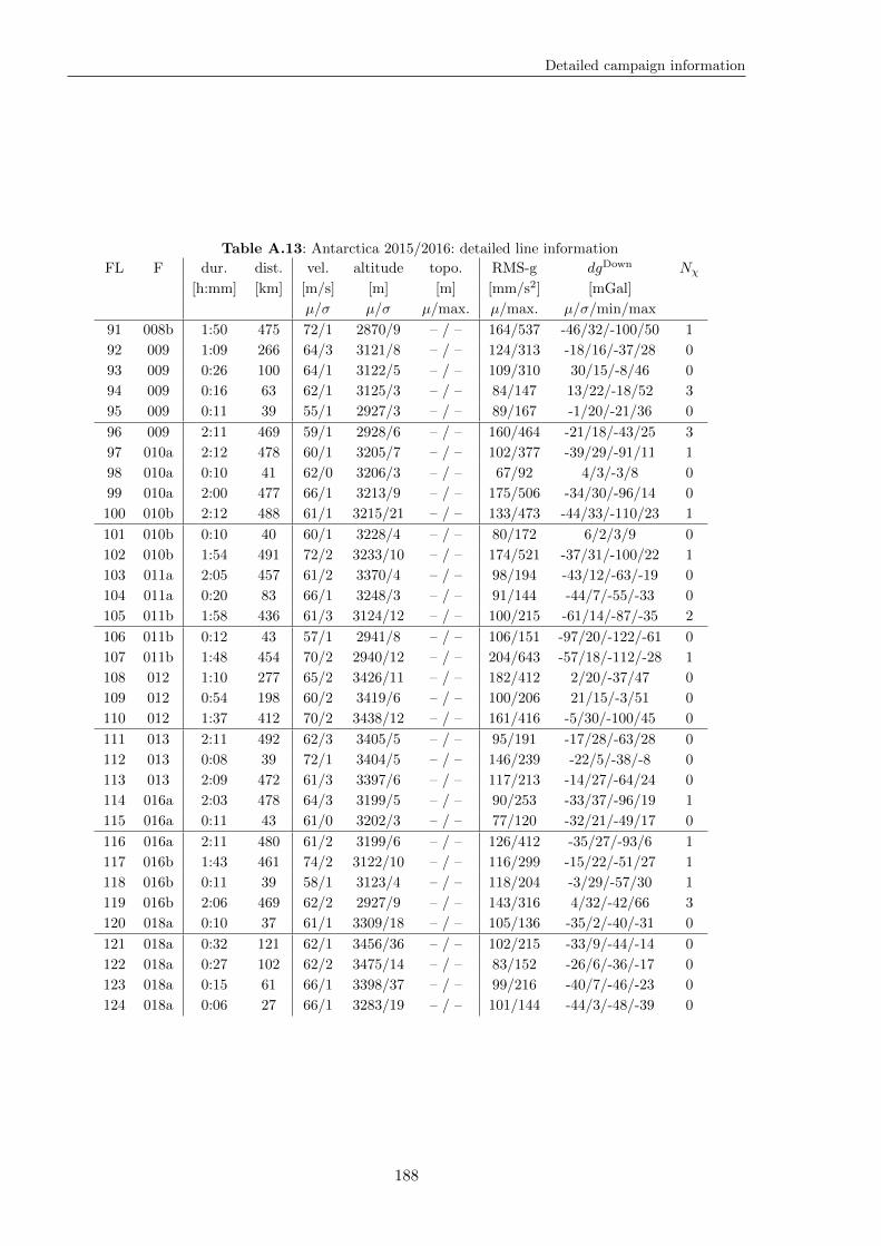
Detailed campaign information
Table A.13: Antarctica 2015/2016: detailed line information
FL F dur. dist. vel. altitude topo. RMS-g dgDown Nχ[h:mm] [km] [m/s] [m] [m] [mm/s2] [mGal]
µ/σ µ/σ µ/max. µ/max. µ/σ/min/max
91 008b 1:50 475 72/1 2870/9 – / – 164/537 -46/32/-100/50 1
92 009 1:09 266 64/3 3121/8 – / – 124/313 -18/16/-37/28 0
93 009 0:26 100 64/1 3122/5 – / – 109/310 30/15/-8/46 0
94 009 0:16 63 62/1 3125/3 – / – 84/147 13/22/-18/52 3
95 009 0:11 39 55/1 2927/3 – / – 89/167 -1/20/-21/36 0
96 009 2:11 469 59/1 2928/6 – / – 160/464 -21/18/-43/25 3
97 010a 2:12 478 60/1 3205/7 – / – 102/377 -39/29/-91/11 1
98 010a 0:10 41 62/0 3206/3 – / – 67/92 4/3/-3/8 0
99 010a 2:00 477 66/1 3213/9 – / – 175/506 -34/30/-96/14 0
100 010b 2:12 488 61/1 3215/21 – / – 133/473 -44/33/-110/23 1
101 010b 0:10 40 60/1 3228/4 – / – 80/172 6/2/3/9 0
102 010b 1:54 491 72/2 3233/10 – / – 174/521 -37/31/-100/22 1
103 011a 2:05 457 61/2 3370/4 – / – 98/194 -43/12/-63/-19 0
104 011a 0:20 83 66/1 3248/3 – / – 91/144 -44/7/-55/-33 0
105 011b 1:58 436 61/3 3124/12 – / – 100/215 -61/14/-87/-35 2
106 011b 0:12 43 57/1 2941/8 – / – 106/151 -97/20/-122/-61 0
107 011b 1:48 454 70/2 2940/12 – / – 204/643 -57/18/-112/-28 1
108 012 1:10 277 65/2 3426/11 – / – 182/412 2/20/-37/47 0
109 012 0:54 198 60/2 3419/6 – / – 100/206 21/15/-3/51 0
110 012 1:37 412 70/2 3438/12 – / – 161/416 -5/30/-100/45 0
111 013 2:11 492 62/3 3405/5 – / – 95/191 -17/28/-63/28 0
112 013 0:08 39 72/1 3404/5 – / – 146/239 -22/5/-38/-8 0
113 013 2:09 472 61/3 3397/6 – / – 117/213 -14/27/-64/24 0
114 016a 2:03 478 64/3 3199/5 – / – 90/253 -33/37/-96/19 1
115 016a 0:11 43 61/0 3202/3 – / – 77/120 -32/21/-49/17 0
116 016a 2:11 480 61/2 3199/6 – / – 126/412 -35/27/-93/6 1
117 016b 1:43 461 74/2 3122/10 – / – 116/299 -15/22/-51/27 1
118 016b 0:11 39 58/1 3123/4 – / – 118/204 -3/29/-57/30 1
119 016b 2:06 469 62/2 2927/9 – / – 143/316 4/32/-42/66 3
120 018a 0:10 37 61/1 3309/18 – / – 105/136 -35/2/-40/-31 0
121 018a 0:32 121 62/1 3456/36 – / – 102/215 -33/9/-44/-14 0
122 018a 0:27 102 62/2 3475/14 – / – 83/152 -26/6/-36/-17 0
123 018a 0:15 61 66/1 3398/37 – / – 99/216 -40/7/-46/-23 0
124 018a 0:06 27 66/1 3283/19 – / – 101/144 -44/3/-48/-39 0
188


![SPRINT-Studie: Update pharmakologische Therapie der ... · Den europäischen Leitlinien [European Heart Journal 2013], der Deutschen Gesellschaft für Kardiologie (DGK) und der Deutschen](https://img.pdfslide.org/doc/110x75/5d612afe88c993d14a8b856c/sprint-studie-update-pharmakologische-therapie-der-den-europaeischen-leitlinien.jpg)