Embed Size (px)
Citation preview

Diffusion processesin
white dwarf stellar atmospheres
Dissertationzur Erlangung des Grades eines
Doktors der Naturwissenschaftender Fakultat fur Mathematik und Physikder Eberhard-Karls-Universitat Tubingen
vorgelegt von
Sonja Landenberger-Schuh
aus Stuttgart2005

Tag der mundlichen Prufung: 22. 02. 2005Dekan: Prof. Dr. P. Schmid1. Berichterstatter: Prof. Dr. K. Werner2. Berichterstatter: Prof. Dr. M. A. Barstow
i
Deutsche Zusammenfassung
Landenberger-Schuh, Sonja
Diffusionsprozesse in Sternatmospharen
Die Atmospharen Weißer Zwerge zeigen eine praktisch mono-elementare Zusam-mensetzung. Aufgrund hoher Oberflachenschwerebeschleunigungen spielt die Ele-menttrennung durch gravitatives Absinken eine große Rolle, so dass in diesen Ster-nen der uberwiegende Anteil aller schwereren Elemente ausden außeren Schichtenverschwunden ist. Diese gravitationsbedingte Sedimentation geschieht auf sehr vielkurzeren Zeitskalen als die Entwicklung Weißer Zwerge entlang der Abkuhlsequenz.
Beobachtungen junger Weißer Zwerge im Rontgen- und extremultravioletten Spek-tralbereich haben gezeigt, dass das Absinken dort nicht ungestort vor sich gehen kann,da zusatzliche Opazitat beobachtet wird, die in den Atmospharen ubriggebliebenenMetallen zugeschrieben werden muss. Es war ein interessantes Ergebnis der von RO-SAT durchgefuhrten Himmelsdurchmusterung, dass praktisch keine Weißen Zwergeoberhalb einer Effektivtemperatur von etwa 65 000 K gefunden wurden. Das wirddurch den Strahlungsauftrieb in heißen Weißen Zwergen erklart, der der nach untengerichteten Diffusion schwerer Elemente effizient entgegenwirken kann. Das Zusam-menspiel dieser Krafte bestimmt die chemische Zusammensetzung der Atmosphare.Spuren von Metallen konnen dann durch radiativen Auftriebgehalten werden, wenndas Strahlungsfeld intensiv genug ist, um der nach unten gerichteten Schwerkraft aus-reichenden Impulsubertrag entgegenzusetzen. Dies ist inden meisten Objekten, dieheißer als
� � � �40 000 K sind, der Fall.
Eine Umsetzung dieser konkurrierenden Prozesse in Sternatmospharen-Modell-rechnungen liefert Vorhersagen fur die vertikale Schichtung und absolute Haufigkeitvon Metallen. Da die Strahlungsbeschleunigung durch ein NLTE-Strahlungsfeld aufin Spuren vorhandene Elemente uber deren lokale Opazitatubertragen wird, kann siestark mit der Tiefe variieren und somit zu einer chemisch geschichteten Atmospharen-struktur fuhren. Es wird insbesondere im Hinblick auf Weiße Zwerge einUberblickuber Modellierungsarbeiten auf dem Gebiet solcher Diffusionsrechnungen gegeben,mit den einschlagigen Referenzen sowohl zu ersten Erwahnungen dieser Ideen alsauch solchen zu neuen Arbeiten, die die aktuellen Implementierungen und deren An-wendungen beschreiben. Innerhalb dieser neueren Ansatzespielt die Gleichgewichts-formulierung eine besondere Rolle, da sie eine relativ einfache Beschreibung der Ba-lance zwischen gravitativem Absinken und Strahlungsauftrieb erlaubt.
Solche Modelle werden in dieser Arbeit vorgestellt. Sie berucksichtigen das Zu-sammenspiel zwischen Schwere- und Strahlungsbeschleunigung, um die chemischeSchichtung aus einer Gleichgewichtsbedingung fur die beiden Krafte herzuleiten, und
ii
losen selbstkonsistent gleichzeitig die zugehorige Atmospharenstruktur. Im Gegen-satz zu Atmospharenmodellen mit der Annahme chemischer Homogenitat wird dieAnzahl der freien Parameter auf allein die Effektivtemperatur und die Oberflachen-schwerebeschleunigung reduziert. Ihre Starke im Vergleich zu anderen Diffusionsmo-dellen liegt in der Selbstkonsistenz, die zudem unter NLTE-Bedingungen errechnetwird. Die Modelle berucksichtigen außerdem voll die Effekte des Line-Blanketingund verwenden detaillierte Atomdaten bis hin zu den Eisengruppenelementen.
Es werden die Ergebnisse verschiedener theoretischer Diffusionsrechnungen mit-einander verglichen. Ein Gitter fruherer, nicht-selbstkonsistenter Modelle sowie Vari-anten der neuen Modelle, die sich in der nummerischen Behandlung des Strahlungs-transports und des Temperaturkorrekturschemas sowie in der Komplexitat der ver-wendeten Atomdaten unterscheiden, werden untersucht und liefern bei naherer Be-trachtung unterschiedliche Ergebnisse.
Mit einem großen Diffusions-Modellgitter aus Atmospharenmodellendiesen neuenTyps wird ein EUV-selektiertes Sample heißer Weißer Zwergeanalysiert. Die insge-samt guteUbereinstimmung mit beobachteten EUVE-Spektren macht deutlich, dassdiese Modelle die physikalischen Bedingungen in den Atmospharen heißer WeißerZwerge im Großen und Ganzen gut beschreiben.
Die EUVE-Spektren werden durch die Eisenopazitat dominiert, so dass die tatsachli-chen Eisenhaufigkeiten offensichtlich durch die Vorhersagen der Theorie gut getrof-fen werden. In einem Vergleich von Haufigkeitsmessungen aneinzelnen Linien in ei-nem umfassenden Datensatz von IUE- und HST-STIS-Beobachtungen mit Vorhersa-gen fur Gleichgewichtshaufigkeiten gelangt man zu einer ¨ahnlichen Schlussfolgerungfur Eisen, und zu einem gewissen Grad auch fur Sauerstoff und Silizium, wahrend dieHaufigkeitsniveaus fur die Elemente Kohlenstoff, Stickstoff und Nickel nicht im ge-samten Parameterbereich genauso gut wiedergegeben werden. Um den Einfluss even-tuell bekannter Variabilitatserscheinungen oder Akkretionsprozesse mit zu beruck-sichtigen, werden alle Objekte des Samples einzeln diskutiert. Der Fall des ObjektsRE J1032� 535 wird besonders hervorgehoben, um die moglichen Schwierigkeiten,die sich bei der Analyse geschichteter Haufigkeitsprofile ergeben konnen, exempla-risch aufzuzeigen.
Eine wesentliche Grenze der Modelle scheint zu sein, dass der unbegrenzte Vorratfur alle beliebigen Elemente, den der Gleichgewichtsansatz voraussetzt, in Wirklich-keit nicht zur Verfugung steht. Das sollte dann kein Problem darstellen, wenn dieMetallhaufigkeiten, die aus diesem Vorrat bezogen werden,tatsachlich sehr geringenVerunreinigungen entsprechen, aber diese Annahme ist nicht mehr gultig, wenn dieGleichgewichtshaufigkeiten eines Elements nahe der seiner kosmischen Haufigkeitliegen. Da diese Einschrankung auf versteckte Art und Weise auch andere Elementebetreffen konnte, waren als eine zukunftige Entwicklung zeitabhangige Diffusions-rechnungen ohne die Einschrankung auf den Gleichgewichtsfall wunschenswert.
iii
Abstract
The atmospheres of white dwarfs exhibit a quasi-mono-elemental composition. Dueto high surface gravities, element segregation by gravitational settling is of great im-portance so that a large fraction of all heavy elements in these stars has disappearedfrom the outer layers. This gravitational sedimentation happens on much smaller timescales than the evolution along the white dwarf cooling sequence.
Observations of young white dwarfs in the X-ray and extreme ultra-violet spec-tral ranges have revealed that the settling cannot act undisturbed there because ad-ditional opacity is observed which must be attributed to metals remaining in theiratmospheres: It was one interesting result of the all-sky survey performed by ROSATthat essentially no hydrogen-rich white dwarfs above effective temperatures of about65 000 K were found. This is being explained by radiative levitation in hot whitedwarfs that can efficiently counteract the downward diffusion of heavy elements. Theinterplay between these forces governs the atmospheric chemical composition. Tracesof metals may be sustained by radiative levitation providedthe radiation field is in-tense enough to supply substantial momentum transfer against gravity’s downwardpull. This is the case in most objects hotter than
� � � �40 000 K.
Incorporating the competition of these processes into stellar atmosphere model cal-culations provides predictions for the vertical stratification and absolute abundancesof metals. The radiative acceleration is exerted on trace elements by a NLTE radi-ation field through the element’s local opacity and therefore can vary strongly withdepth, which results in a chemically stratified atmosphericstructure. An overviewof the modelling work done in the field of such diffusion calculations, with a focuson white dwarfs, is given, with the relevant references where these ideas were firstmentioned as well as recent papers which describe current implementations and theirapplications. Within these latest approaches, the equilibrium formulation is of spe-cial interest since it permits a relatively simple description of the balance betweengravitational settling and radiative levitation.
Such models are presented in this work. They take into account the interplay be-tween gravitational settling and radiative acceleration to predict the chemical stratifi-cation from an equilibrium between the two forces while self-consistently solving forthe atmospheric structure. In contrast to atmospheric models with the assumption ofchemical homogeneity, the number of free parameters in the new models is reducedto the effective temperature and surface gravity alone. Their superiority over otherdiffusion calculations is the full self-consistency, calculated under NLTE conditions.The models are also fully line-blanketed and incorporate detailed atomic data up tothe iron group elements.
The results from various theoretical diffusion calculations are compared. A grid ofearlier, not self-consistent models as well as variations of the new models that differ
iv
in the numerical treatment of the radiative transfer and thetemperature correctionscheme as well as in the complexity of atomic input data are considered and found toyield different solutions when examined in detail.
Based on a large diffusion model grid, a EUV selected sample of hot DA whitedwarfs is analysed using this new type of atmospheric models. The overall goodagreement with observed EUVE spectra reveals that these models are on the wholeable to describe the physical conditions in hot DA white dwarf atmospheres.
The EUVE spectra are dominated by the opacity due to iron, so the real iron abun-dances appear to be relatively well matched by the predictions of radiative levitationtheory. In a comparison of abundance measurements from individual lines in a com-prehensive set of IUE and HST-STIS UV spectra with equilibrium abundance pre-dictions, a similar conclusion is reached for iron, and to some extent also for oxygenand silicon, while the abundance levels for the elements carbon, nitrogen and nickelare not equally well reproduced over the full photospheric parameter range. To takeinto account effects such as known variability or accretion, all sample objects arediscussed individually. The case of RE J1032� 535 is given special consideration todemonstrate the potential difficulties in the analysis of stratified abundance profiles inan exemplary way.
One of the main constraints for the models seems to be that thetheoretically un-limited reservoir of any element implied by the equilibriumapproach is not availablein reality. This should not be a problem when the metal abundances drawn from thatreservoir correspond to almost negligible pollutants, butthe assumption breaks downin those cases where the equilibrium abundance of an elementstarts to be of the sameorder of magnitude as its cosmic abundance. Since this restriction may, in a moresubtle way, also affect the other element species, time-dependent non-equilibriumdiffusion calculations would be a desirable future development.
Contents
1 Introduction 11.1 Stellar evolution and white dwarfs . . . . . . . . . . . . . . . . . 11.2 White dwarf atmospheres and diffusion . . . . . . . . . . . . . . 51.3 Line formation and spectral analysis . . . . . . . . . . . . . . . . 9
2 Computational method 152.1 Radiative transfer . . . . . . . . . . . . . . . . . . . . . . . . . . 15
2.1.1 Basic equations . . . . . . . . . . . . . . . . . . . . . . . 152.1.2 Line formation in the case of inhomogeneous abundances . 182.1.3 Radiative transfer under realistic conditions . . . . .. . . 21
2.2 Atmospheric structure . . . . . . . . . . . . . . . . . . . . . . . . 212.3 Diffusion . . . . . . . . . . . . . . . . . . . . . . . . . . . . . . 242.4 Peculiarities of subsequent numerical implementations used . . . 292.5 Model atoms . . . . . . . . . . . . . . . . . . . . . . . . . . . . 30
3 Model grids and high resolution spectra 333.1 Overview . . . . . . . . . . . . . . . . . . . . . . . . . . . . . . 333.2 The model grid used for the EUV analysis . . . . . . . . . . . . . 33
3.2.1 Parameter range, atomic data and computational details . . 333.2.2 Spectra . . . . . . . . . . . . . . . . . . . . . . . . . . . 34
3.3 Extended model grid . . . . . . . . . . . . . . . . . . . . . . . . 353.3.1 Parameter range and computational details . . . . . . . . .353.3.2 Example results: spectral features . . . . . . . . . . . . . 363.3.3 Spectra fromSYNSPEC . . . . . . . . . . . . . . . . . . 37
3.4 New models: Test calculations . . . . . . . . . . . . . . . . . . . 38
4 Abundance tables 394.1 Characteristics of the models . . . . . . . . . . . . . . . . . . . . 394.2 Comparison to earlier models . . . . . . . . . . . . . . . . . . . . 464.3 Discussion of test calculations with more opacities . . .. . . . . 48
v
vi Contents
5 Analysis of spectroscopic EUVE data 535.1 Introduction . . . . . . . . . . . . . . . . . . . . . . . . . . . . . 535.2 EUVE observations of hot DA white dwarfs . . . . . . . . . . . . 54
5.2.1 The EUV selected DA sample . . . . . . . . . . . . . . . 545.2.2 Treatment of the ISM . . . . . . . . . . . . . . . . . . . . 55
5.3 Equilibrium abundances from stratified model atmospheres . . . . 555.3.1 Diffusion models . . . . . . . . . . . . . . . . . . . . . . 555.3.2 Scope of application . . . . . . . . . . . . . . . . . . . . 56
5.4 Testing the diffusion models and re-analysing the DA sample . . . 575.4.1 Comparison of theoretical and observed spectra . . . . .. 575.4.2 Revised atmospheric parameters . . . . . . . . . . . . . . 585.4.3 Metal index . . . . . . . . . . . . . . . . . . . . . . . . . 58
5.5 Discussion . . . . . . . . . . . . . . . . . . . . . . . . . . . . . . 635.5.1 Summary . . . . . . . . . . . . . . . . . . . . . . . . . . 635.5.2 Remarks on� and� � � � . . . . . . . . . . . . . . . . . . . 635.5.3 Outlook . . . . . . . . . . . . . . . . . . . . . . . . . . . 67
6 Abundance analysis in the UV 696.1 Graphical representation of the results . . . . . . . . . . . . .. . 696.2 Object-by-object discussion . . . . . . . . . . . . . . . . . . . . . 83
6.2.1 Objects contained in the EUVE sample . . . . . . . . . . 836.2.2 Other objects without EUVE spectra . . . . . . . . . . . . 946.2.3 A closer look at the nitrogen lines in RE J1032� 535 . . . 97
6.3 Element species in the full grid . . . . . . . . . . . . . . . . . . . 103
7 Conclusions 1197.1 Status of modelling . . . . . . . . . . . . . . . . . . . . . . . . . 1197.2 Recapitulation of results from EUV and UV observations .. . . . 1207.3 Perspective . . . . . . . . . . . . . . . . . . . . . . . . . . . . . 124
Bibliography 127
A Equilibrium abundances 135
Acknowledgements 157
Lebenslauf 159
List of Tables
2.1 Summary of ”old” model atoms . . . . . . . . . . . . . . . . . . 302.2 Summary of ”new” model atoms . . . . . . . . . . . . . . . . . 315.1 Results of the EUV analysis . . . . . . . . . . . . . . . . . . . . 606.1 The NV doublet in RE J1032� 535 from HST-STIS spectra . . . 1016.2 The NV doublet in RE J1032� 535 - comparison of two models . 1036.3 Location of� ross �
�� on the mass scale for Chayer et al. models 118
vii

viii List of Tables
List of Figures
1.1 Line profiles for a stratified absorber . . . . . . . . . . . . . . . 132.1 Radiative transfer quantities for a stratified absorber. . . . . . . 183.1 The extended model grid . . . . . . . . . . . . . . . . . . . . . 353.2 Emergent fluxes for selected parameters . . . . . . . . . . . . . 363.3 EUV spectra fromPRO2andSYNSPEC. . . . . . . . . . . . . 374.1 Iron abundances for different effective temperatures .. . . . . . 404.2 Iron abundances for different surface gravities . . . . . .. . . . 414.3 Silicon abundances for different effective temperatures . . . . . 424.4 Silicon abundances for different surface gravities . . .. . . . . 434.5 Nitrogen abundances for different effective temperatures . . . . 444.6 Nitrogen abundances for different surface gravities . .. . . . . 454.7 � ross �
�� on the mass scale as a function of
� � �and
� � �� . . . . 46
4.8 Comparison to Chayer’s elemental abundances . . . . . . . . .. 474.9 Temperature stratifications with the ”old” and ”new” codes . . . 494.10 Abundance stratifications with the ”old” and ”new” codes . . . . 505.1 EUVE spectrum of MCT 2331� 4731 . . . . . . . . . . . . . . . 575.2 Revised parameters of the program stars . . . . . . . . . . . . . 595.3 EUVE spectra of the program stars with theoretical spectra . . . 625.4 Comparison of old and new� � �
and� � �
� . . . . . . . . . . . . 645.5 Comparison of different measures of the metal content . .. . . 655.6 Parameters for G 191–B2B from different studies . . . . . . .. 666.1 UV elemental abundances of PG 0948� 534 . . . . . . . . . . . 716.2 UV elemental abundances of Ton 21 . . . . . . . . . . . . . . . 716.3 UV elemental abundances of RE J1738� 665 . . . . . . . . . . . 726.4 UV elemental abundances of PG 1342� 444 . . . . . . . . . . . 726.5 UV elemental abundances of RE J2214� 492 . . . . . . . . . . . 736.6 UV elemental abundances of Feige 24 . . . . . . . . . . . . . . 736.7 UV elemental abundances of RE J0558� 373 . . . . . . . . . . . 746.8 UV elemental abundances of WD 2218� 706 . . . . . . . . . . . 746.9 UV elemental abundances of RE J0623� 371 . . . . . . . . . . . 756.10 UV elemental abundances of PG 1123� 189 . . . . . . . . . . . 75
ix
x List of Figures
6.11 UV elemental abundances of RE J2334� 471 . . . . . . . . . . . 766.12 UV elemental abundances of G 191-B2B . . . . . . . . . . . . . 766.13 UV elemental abundances of HS 1234� 482 . . . . . . . . . . . 776.14 UV elemental abundances of GD 246 . . . . . . . . . . . . . . . 776.15 UV elemental abundances of RE J0457� 281 . . . . . . . . . . . 786.16 UV elemental abundances of HZ 43 . . . . . . . . . . . . . . . 786.17 UV elemental abundances of RE J2156� 546 . . . . . . . . . . . 796.18 UV elemental abundances of RE J1032� 532 . . . . . . . . . . . 796.19 UV elemental abundances of PG 1057� 719 . . . . . . . . . . . 806.20 UV elemental abundances of GD 394 . . . . . . . . . . . . . . . 806.21 UV elemental abundances of GD 153 . . . . . . . . . . . . . . . 816.22 UV elemental abundances of RE J1614� 085 . . . . . . . . . . . 816.23 UV elemental abundances of GD 659 . . . . . . . . . . . . . . . 826.24 UV elemental abundances of EG 102 . . . . . . . . . . . . . . . 826.25 Complete spectral energy distribution of GD 394 . . . . . .. . . 936.26 Nitrogen stratification profiles for RE J1032� 535 . . . . . . . . 996.27 The NV doublet in RE J1032� 535 from HST-STIS spectra . . . 1006.28 The NV doublet in RE J1032� 535 - comparison of two models . 1026.29 UV CIII abundances as a function of� � �
and� � �
� . . . . . . . 1046.30 UV CIII abundances as a function of� �
. . . . . . . . . . . . . 1056.31 UV CIV abundances as a function of� � �
and� � �
� . . . . . . . 1066.32 UV CIV abundances as a function of� �
. . . . . . . . . . . . . 1076.33 UV � abundances as a function of� � �
and� � �
� . . . . . . . . 1086.34 UV � abundances as a function of� �
. . . . . . . . . . . . . . 1096.35 UV � abundances as a function of� � �
and� � �
� . . . . . . . . 1106.36 UV � abundances as a function of� �
. . . . . . . . . . . . . . 1116.37 UV � � abundances as a function of� � �
and� � �
� . . . . . . . . 1126.38 UV � � abundances as a function of� �
. . . . . . . . . . . . . . 1136.39 UV � � abundances as a function of� � �
and� � �
� . . . . . . . . 1146.40 UV � � abundances as a function of� �
. . . . . . . . . . . . . . 1156.41 UV � � abundances as a function of� � �
and� � �
� . . . . . . . . 1166.42 UV � � abundances as a function of� �
. . . . . . . . . . . . . . 1176.43 Location of� ross �
�� on the mass scale for different models . . . 118
7.1 Summary of predicted and measured UV abundances . . . . . . 1227.2 Summary of abundance deviations . . . . . . . . . . . . . . . . 123A.1 Helium abundances as a function of� � �
. . . . . . . . . . . . . 136A.2 Helium abundances as a function of
� � �� . . . . . . . . . . . . 137
A.3 Carbon abundances as a function of� � �. . . . . . . . . . . . . 138
A.4 Carbon abundances as a function of� � �
� . . . . . . . . . . . . . 139A.5 Nitrogen abundances as a function of� � �
. . . . . . . . . . . . 140
List of Figures xi
A.6 Nitrogen abundances as a function of� � �
� . . . . . . . . . . . . 141A.7 Oxygen abundances as a function of� � �
. . . . . . . . . . . . . 142A.8 Oxygen abundances as a function of
� � �� . . . . . . . . . . . . 143
A.9 Silicon abundances as a function of� � �. . . . . . . . . . . . . 144
A.10 Silicon abundances as a function of� � �
� . . . . . . . . . . . . . 145A.11 Iron abundances as a function of� � �
. . . . . . . . . . . . . . . 146A.12 Iron abundances as a function of
� � �� . . . . . . . . . . . . . . 147
A.13 Nickel abundances as a function of� � �. . . . . . . . . . . . . 148
A.14 Nickel abundances as a function of� � �
� . . . . . . . . . . . . . 149A.15 Helium abundances as a function of� �
. . . . . . . . . . . . . 150A.16 Carbon abundances as a function of� �
. . . . . . . . . . . . . . 151A.17 Nitrogen abundances as a function of� �
. . . . . . . . . . . . . 152A.18 Oxygen abundances as a function of� �
. . . . . . . . . . . . . 153A.19 Silicon abundances as a function of� �
. . . . . . . . . . . . . . 154A.20 Iron abundances as a function of� �
. . . . . . . . . . . . . . . 155A.21 Nickel abundances as a function of� �
. . . . . . . . . . . . . . 156
xii List of Figures
”The fault, dear Brutus, is not in our stars,But in ourselves, that we are underlings.”
Cassius to Brutus in act I, scene II of ”Julius Caesar” (1598–1600) byW. Shakespeare.
CHAPTER 1
Introduction
1.1 Stellar evolution and white dwarfs
The visible matter in the universe is organised in galaxies,the building blocks oflarger structures, where – under the influence of their own gravity – gas and dustclouds contract to form clumps that can give rise to star birth. Stars are self-gravitatinggas balls which are hot and dense enough to maintain stable thermonuclear fusion intheir cores. As such, they are essentially factories that reprocess the material they aremade of, and return most of it to interstellar space during the last stages of their lives,leaving only a compact remnant of stellar ashes behind (or insome cases nothing atall). For an overwhelming majority of stars, this stellar remnant will simply be theleft-over, burnt-out core of the former star and is commonlyknown as a white dwarf(WD). The following introduction aims at retracing only themost important stepsleading to this common variant of stellar remnant.
Tracks in the Hertzsprung-Russell diagram (HRD1) are a very suitable way to de-scribe the evolutionary paths of stellar objects. Stars spend most of their lifetime onthe so-called main sequence, where they produce helium fromhydrogen via nuclearfusion processes in their cores. If, at this main sequence stage, the mass of an isolatedstar exceeds about 8-10 M� 2, it can subsequently evolve into an object as enigmaticas a neutron star or black hole. Most stars however are not massive enough to evolveinto either of these objects, but will eventually turn into white dwarf stars instead.
A typical white dwarf has a radius of� 10 000 km (i.e. roughly the same size as theearth). The mass distribution of white dwarfs peaks near 0.6M� . This implies a highmean density for these objects, as well as a large surface gravity of � 10
�cm s�
�(or
10�
times the earth’s gravitational acceleration), which is equivalent to a steep pres-sure gradient in the stellar remnant envelope. Since – by definition – at this stage all
1Spectral type or colour plotted against the absolute magnitude or luminosity, allowing a graphicalrepresentation of correlations for stellar parameters (developed by Hertzsprung 1911 and Russell 1913).
21 M� , i.e. one solar mass, corresponds to 1.989�10� �
g.
1
2 Chapter 1: Introduction
nuclear fusion processes inside the former star have ceased, the immense hydrostaticpressure built up by the weight of matter in above layers needs to be balanced byFermi degeneracy of the electron gas. The equilibrium allowed for by this equationof state prevents the degenerate, nearly isothermal white dwarf core from collaps-ing. The gravitational energy released through slow contraction provides some addi-tional luminosity, but essentially the overall luminosity, which is high at first – about10
�L� 3 – rapidly decreases as the dead star cools. Likewise, from roughly 100 000 K
at the exhaustion of the last fusion processes, the effective temperature (�
eff) subse-quently drops to 50 000 K in only 0.003 Gyr (Koester & Chanmugam 1990), whilethe lowest observed temperatures are not reached until roughly 10 Gyrs have passed(Koester 2002). Despite the high uncertainties for this last number (of the order of20%), the determination of cooling times is quite relevant to questions beyond stellarphysics issues, as outlined for example in a nice review by Fontaine et al. (2001).
Since the majority of all stars end their lives as a white dwarf, studying them helpsto understand the evolution processes that average stars undergo. How do these rela-tively extreme, compact objects evolve from stars such as our sun? Stellar evolutiontheory describes the process of star formation up to the mainsequence stage, the slowevolution away from thezero agemain sequence, and the various evolutionary pathsthat stars then can follow depending on their initial chemical composition, massesand mass-loss rates at different lifetimes. To end up as a 0.6M� white dwarf, a10 M� main sequence star obviously loses a very substantial fraction of its initialmass, which emphasises the important role of late stages of stellar evolution (includ-ing the initial-final mass relations it predicts) for the galactic circuit of matter. At anage of� 6 Gyr, the sun is about half-way on its long journey from the zero age mainsequence to the turn-off point, where it will have exhaustedthe hydrogen supply in itscore, forcing the hydrogen burning zone to move outwards. Shifting the fusion zonetowards higher layers results in an expansion of the stellarouter envelope, therebyturning the star into a red giant, while the burnt-out core grows in mass and contractsuntil helium fusion is ignited.
For sun-like stars, this happens in a violent event referredto as the helium flash,which brings the star onto the horizontal branch. Here helium core and hydrogenshell burning proceed calmly for a longer period of time (of the order of 0.1 Gyrfor a solar-mass star) before fuel exhaustion occurs once again, this time forcing thehelium burning zone into a shell, and triggering the next, agitated phases. On its wayalong the asymptotic giant branch (AGB) towards regions of high luminosities, thestar undergoes strong mass-loss through radiatively-driven winds. The subsequentstages are referred to as post-AGB evolution.
These late stages of stellar evolution comprise the processes up to the point where31 L� , i.e. the solar luminosity, corresponds to 3.90�10
� �erg s�
�
.
Chapter 1.1: Stellar evolution and white dwarfs 3
the star eventually pivots onto the white dwarf cooling sequence. At the top of theAGB, a formerly sun-like star undergoes alternating phasesof helium and hydrogenshell burning, and these thermal pulses lead to further mass-loss. The luminosityreaches a high value of� 10
�L� , then remains constant while the surface temperature
quickly rises within only� 10 000 yr, since the rapidly contracting hot core starts toshine through the expanding and dissipating envelope. Due to this contraction andthe gradual loss of its envelope, corresponding to a sharp decline in the stellar radius,the remaining object is much more compact. The stellar wind accelerates due to theincreased escape velocity, sweeping into and compressing the previously expelledmaterial in the process.
The expelled material is ionised by the ultraviolet photonsemitted from the increas-ingly hot object at its centre and starts to re-radiate at visible wavelengths, renderingit detectable as a planetary nebula. The nuclear fusion processes in the shell of thecentral star of the planetary nebula (CSPN) eventually cease, marking the now ”dead”star’s entry onto the white dwarf cooling sequence. According to the sequence of pro-cesses outlined here, standard stellar evolution theory hence predicts a white dwarfconsisting of a carbon-oxygen core4, surrounded by a helium layer, surrounded by anunprocessed hydrogen envelope. The thickness of this hydrogen envelope had beenthe subject of two competing theories for a while (known as the thick/thin layer dis-cussion): The discussion seems to have converged to the statement that a whole (moreor less continuous) range of envelope masses is required to explain the observations.
In addition to this, a non-negligible fraction of white dwarfs does not show sucha hydrogen envelope at all. A late thermal pulse in a young white dwarf can bringit back onto the AGB, so that it is re-born as a star, hence the name ”born-again”scenario for such an event. In this case, mixing processes draw the envelope materialdeep into the nuclear burning layers, where the remaining hydrogen supplies are beingused up, leaving the star hydrogen-deficient when it approaches the top of the coolingsequence a second time.
Another peculiar variant in this listing of white dwarf feeder channels are starsthat somehow already lose all but a tiny fraction of their hydrogen envelope as theyreach the horizontal branch state. While they go through helium core burning just asnormal horizontal branch stars do, their thin hydrogen envelopes are completely inertand make them appear as relatively hot, so-called extreme horizontal branch (EHB,spectral classification sdB, short for subdwarf B) stars. These objects do not have themeans to spectacularly shed off large amounts of envelope material for simple lack ofit, and instead follow a short-cut directly to the white dwarf graveyard.
Regardless of “details” in the surface composition, the final result of the evolutionof low- and medium mass stars is usually a white dwarf with a carbon-oxygen core.
4More precisely, the outer part of the carbon-oxygen core is expected to be depleted in oxygen due tothe temperature – and hence depth – dependency of the
� � � � � �� � � � reaction rate during helium burning.
4 Chapter 1: Introduction
For a small range of initial masses around 10 M� (the exact numbers are still underdiscussion), theory predicts the possibility of oxygen-neon-magnesium cores instead,provided that the core mass growth during carbon burning is halted through envelopeloss to prevent a subsequent core collapse. This should thenresult in massive whitedwarfs of� 1 M� , with little envelope material left that is possibly strongly enhancedin neon. In contrast to this, very low mass stars should instead evolve into helium corewhite dwarfs, since they never attain the central densitiesrequired for helium burning.However, as the long evolutionary time scales for very low mass stars exceed the ageof today’s universe, this evolutionary channel has not had achance yet to produce thehelium core objects observed along the white dwarf cooling sequence. They insteadexist because in binary systems, a close companion can draw off material from anageing star when it starts to expand – up to the point where thecore mass is reducedto below what is needed for the ignition of helium burning. Insuch a scenario thestellar ashes from only one instead of two main nuclear burning cycles make up thestellar remnant.
Just as the universe is too young to have produced helium corewhite dwarfs fromisolated stellar evolution yet, it is also not old enough to allow for a cooling and hencefading in luminosity of nearby white dwarfs beyond the detection limit of large tele-scopes. The current low-temperature record stands at� 2 200 K (Bergeron & Leggett2002). Interpreted as an evolutionary effect, the observedcut-off in the cooling se-quence of white dwarfs in our neighbourhood therefore provides a constraint for thegalactic disk’s age. Similarly, age and distance determinations from white dwarf cool-ing sequences can be attempted for open and globular clusters. Using a method thatinvolves white dwarfs indirectly as progenitors in type Ia supernovae, they even servein distance determinations on a cosmological scale. Understanding the underlyingprocesses – all the way from the white dwarf(s) involved to the exact temporal andspectral dependency of the energy output during such an explosion – is an objectivethat, if fully achieved, would greatly improve the confidence in the reliability of thismethod.
More generally speaking, this implies that – in order to makeuse of white dwarf ob-servations as tools in the quest for answers to other fundamental questions – one firsthas to understand the physical processes that link different evolutionary stages. Suchcontinuous evolutionary sequences cannot be observed directly, they rather must beconstructed from snapshots of individual stars at different ages. Stellar ages are gen-erally only accessible through a detailed modelling of the star as a system that evolvesthrough time according to given laws of physics. Other physical parameters such asthe effective temperature, surface gravity or mass, radiusand luminosity may be morereadily accessible, but their precise determination also requires very detailed numeri-cal simulations. An indispensable tool for such parameter determinations via spectralanalysis methods are model atmosphere calculations: All processes deemed relevant
Chapter 1.2: White dwarf atmospheres and diffusion 5
to the formation of the emergent spectral energy distribution of a star are mapped intoa simulated model of the light-emitting atmosphere. A comparison of simulated withobserved spectra then allows to draw conclusions about the exact physical conditionsnecessary to produce the observed spectrum. Besides a variety of fundamental stellarparameters that can be obtained from spectral analysis, theevaluation of if and howthe integrated (or sometimes even dispersed) light from a star varies with time canyield further independent measurements, e.g. in binary systems or for pulsating stars.
A good understanding of the complete structure and outside appearance of a starstill does not equal an understanding of its full history andfuture. To aquire insightinto these, time-dependent stellar evolution models are needed. Here, in additionto being an indispensable tool in spectral analysis work, stellar atmosphere modelsplay a crucial role by providing outer boundary conditions for these structural andevolutionary models. In particular, differences in the opaqueness of white dwarfs’atmospheres (due to the layer thickness) cause different cooling rates, just as thetransition from radiative to convective energy transport leads to changes in the coolingrates which are otherwise determined by structural evolution in the core (diffusion,gas/liquid and liquid/solid transitions).
In many current applications, the evolutionary models usedare those by Wood(1995).
The following Sect. 1.2 presents an inventory of the observed spectral propertiesof white dwarfs, which the entirety of both atmospheric and structural/evolutionarymodels will eventually have to reproduce and explain. Thereafter Sect. 1.3 detailssome demands to be made on stellar atmosphere models, and shows where this presentwork may be able to contribute an improvement.5
1.2 White dwarf atmospheres and diffusion
There are now more than two thousand white dwarfs compiled inthe Villanova Cata-logue of Spectroscopically Identified White Dwarfs by McCook & Sion (1999). Theobservational and physical information on white dwarfs it contains has been madeavailable in an online version, which is also the primary source for the data main-tained (and presented with some enhancements over the McCook & Sion 1999 onlineversion) in the regularly updated electronic white dwarf database6. A large fractionof the objects currently appearing in the catalogues were discovered in large blue andultraviolet (UV) excess surveys such as the Palomar-Green (PG, Green et al. 1986),Montreal-Cambridge-Tololo (MCT, Demers et al. 1986; Lamontagne et al. 2000) and
5The contents of this section partly rely on ideas collected in the Koester (2002) white dwarf reviewpaper.
6http://procyon.lpl.arizona.edu/WD/
6 Chapter 1: Introduction
the Edinburgh-Cape (EC, Stobie et al. 1997; Kilkenny et al. 1997) surveys, as wellas in the Hamburg Quasar and the Hamburg/ESO objective prismsurveys (HQS,Hagen et al. 1995 and HES, Wisotzki et al. 1996; Reimers & Wisotzki 1997; Wisotzkiet al. 2000).
With the Sloan Digital Sky Survey (SDSS), the number of photometrically detectedwhite dwarfs is expected to rise by an order of magnitude (Fan1999). On its way toachieving these additions through colour identification (and possibly follow-up spec-troscopy), the SDSS First Data Release (Abazajian et al. 2003, following the EarlyData Release, Stoughton et al. 2002) has already nearly doubled the number of spec-troscopically identified white dwarfs (Kleinman et al. 2004). As a primer to what canbe expected from the full SDSS once completed, Harris et al. (2003) have publishedWD numbers for a small area of sky.
Their compilation of exemplary observed spectra also constitutes a nice reviewof the different WD spectral types, from the very common to the rather unusualones. Based on classification in the optical, the spectral types (all denoted startingwith a D for degenerate) fall into two major categories: the hydrogen-rich DA andthe helium-rich DB white dwarfs. The DA sequence is characterised by stronglypressure-broadened Balmer lines, while the non-DA sequence shows HeI lines incase of DBs, and additional HeII lines in case of the much rarer DOs, which ex-tend the helium-rich sequence to high temperatures. Both the DA and the non-DAwhite dwarfs exhibit a quasi-mono-elemental chemical composition. Given that, inthe scenario sketched earlier, white dwarfs should either end up with an unprocessedhydrogen envelope (making them DAs) or an exposed helium layer (generally mak-ing them DOs or DBs), the strongly sub-solar metallicity in their practically purehydrogen or helium atmospheres would seem to contradict thegeneral expectation ofmetal-enrichment with increasing stellar age.
The basic mechanism for this purification of white dwarf envelopes was first ex-plained by Schatzman (1945, 1958): the strong gravitational field (typically,
� � �� � 8
in cgs units) on the surface of WDs yields a steep pressure gradient, and hencepressure-driven diffusion separates the elements according to their atomic weight.This process is generally referred to asgravitational settlingor sedimentation. Be-sides white dwarfs, where the sinking time scales are shortest in comparison, ele-ment segregation also affects the atmospheres of horizontal branch B stars, causingtheir helium and metal deficiency (Greenstein et al. 1967; Michaud et al. 1983), andis responsible for the chemical peculiarities observed in some A main sequence stars(Michaud 1970).
These diffusion processes cause perhaps the most obvious spectral evolutionary ef-fects seen in WDs. They alter the atmospheric composition from complex patternsstill observed beyond the AGB to just two mono-elemental variants. The strict separa-tion of both sequences is due to diffusion. The initial effectiveness of diffusion is not
Chapter 1.2: White dwarf atmospheres and diffusion 7
completely independent of temperature (as will be shown later) and hence also under-goes evolutionary change. Several other changes in appearance such as the evolutionof the overall flux level, colours, or ionisation equilibriacan also be directly linked tothe continuing cooling. The ranges of effective temperatures assumed by DA WDs aresimply parametrised by a spectral index from 1 to 7, calculated as 50 400 K / T
� �[K],
and are reflected by the increasing strength of the Balmer lines with decreasing ef-fective temperature. Just as the gradual recombination of ionised hydrogen to atomichydrogen characterises the DA sequence, the recombinationof He II to HeI marksthe transition from the hotter DOs to the cooler DBs, defined by the spectral linesobserved from the predominant ionisation stage.
In addition to this easily explained break in the helium-rich sequence (due to thepresence of more than one ionisation state, clearly reflected by a change in name), thehelium sequence is also interrupted by the so-called ”DB gap” (Liebert et al. 1986).A common explanation for the lack of any helium-rich objectsin the temperaturerange between 45 000 K (coolest DOs) and 28 500 K (hottest DB) goes as follows:The upwards diffusion of any remaining traces of hydrogen iseventually enough tocover the helium layer – corresponding to the high-temperature end of the gap wherehelium-rich objects (DOs) therefore are effectively turned into DAs. Once convectiondue to helium ionisation becomes efficient it dilutes any thin diffusive hydrogen layer;mixing occurs and turns a fraction of the DAs back into DBs (presumably mostly the“hidden” former helium-rich ones, but the fraction of non-DAs versus DAs does notrecover the ratio above the gap). However, there is as yet neither theoretical nor ob-servational evidence which unambiguously confirms this scenario (or any alternativeones brought forward until now).
Towards cooler temperatures, first the helium and then the hydrogen lines substan-tially weaken and finally vanish when the energy necessary toexcite the transitionsceases to be available. When no features can be discerned in such a WD, it is calleda DC type. In some cooler WDs, however, photospheric carbon can be detected,believed to be brought to the surface from the (stratified) C/O core by dredge-up pro-cesses. Such WDs with carbon features are classified as DQs. Metal lines observed ina cool WD, on the other hand, make it a DZ. The tendency to purification is in this casenot disturbed by convective mixing or dredge-up processes,but possibly by accretionfrom interstellar matter. Both DQ and DZ white dwarfs usually have helium-richatmospheres, which are more transparent in the optical and therefore allow for thedetection of smaller amounts of metals (including carbon) than hydrogen-rich ones.Aside from the white dwarf spectral classifications DA, DO, DB, DC, DQ and DZ,hybrid types are known. Though rare, they are often key objects to investigate pos-sible evolutionary links between the classes. Finally, whenever polarisation due tomagnetic fields has been measured, the classification is annexed by the letter P, andthe corresponding spectra can appear heavily distorted.
8 Chapter 1: Introduction
In the relatively pure, opacity-poor hydrogen or helium atmospheres, additionalabsorbers can have a substantial impact on the atmospheric structure and the spectraldistribution of the emergent flux. In the case of the types discussed above, the effectsare remarkable enough to result in different classifications for the objects. But thevery common DA white dwarfs (followed in number by DBs, with DA : DB
�7:1),
with the high degree of purification in their atmospheres brought about by diffusion,also continue to hold their surprises in this respect. In hotWDs with
� � � �40 000 K
upwards, the diffusion process is disturbed by the radiation pressure that elementsexperience, depending on the overlap of their wavelength-dependent opacities withthe maximum spectral flux. The overlap of the maximal spectral intensity with theregion of maximal opacity yields a considerable radiative acceleration on heavier el-ements in WD atmospheres, provided the luminosity is high enough (theoretical cal-culations by Vauclair et al. 1979; Fontaine & Michaud 1979, and later Morvan et al.1986; Vauclair 1987, 1989 as well as Chayer et al. 1989, 1991,1994, 1995a,b). Lumi-nosities L/L� � � are sufficient to sustain photospheric elements other than hydrogenwith abundances no higher than� � �
�relative to hydrogen.
In optical spectra of hot white dwarfs, these trace pollutants become directly vis-ible only when great effort is put in the detection of individual lines (Dupuis et al.2000a), but can influence the accurate determination of effective temperatures andsurface gravities. Through resonance lines in the UV and even more through thesheer number of lines in the extreme ultraviolet (EUV), these spectral ranges can bestrongly affected.
The flux deficit caused by the additional opacity in the EUV as compared to purehydrogen atmospheres, hinted at already by earlier data (Mewe et al. 1975; Hearn et al.1976; Lampton et al. 1976; Margon et al. 1976; Shipman 1976),became more andmore evident as the quality of observations improved with the HEAO 2 (Einstein),EXOSAT and ROSAT satellites (Kahn et al. 1984; Petre et al. 1986; Jordan et al. 1987;Paerels & Heise 1989; Barstow et al. 1993a; Jordan et al. 1994; Wolff et al. 1996). Inparticular, after ROSAT had found many fewer hot WDs than expected from predic-tions based on pure hydrogen atmospheres, both the levitation mechanism as well asthe identification of the elements involved were turned intofoci of research interest.
While EXOSAT (Vennes et al. 1989) and various ROSAT observations revealedthat the opacity must be mainly due to absorbers other than helium, only observationswith EUVE made a more detailed investigation of the nature ofabsorbers possible.Since then, first IUE and then subsequently HST have continued to place tight andsometimes contradictory constraints on the picture that starts to emerge. The appli-cation of radiative levitation theory to determine and explain the photospheric metalabundances in hot DA white dwarfs is the topic of this thesis.The remaining part ofthis introduction therefore compiles the most important results from previous workrelevant to this field.
Chapter 1.3: Line formation and spectral analysis 9
1.3 Line formation and spectral analysis
The atmospheres of WDs exhibit a quasi-mono-elemental composition because alarge fraction of all heavy elements has disappeared from the outer layers due togravitational sedimentation. Traces of metals may howeverbe sustained by radiativelevitation provided the radiation field is intense enough tosupply substantial mo-mentum transfer. Analysis of larger samples of hot white dwarf EUVE spectra byBarstow et al. (1997) and Wolff et al. (1998) have shown that this is the case in mostDAs hotter than T
� � �40 000 K – 50 000 K.
Photospheric abundances can only be obtained through comparisons with detailedsynthetic spectra, requiring a realistic modelling of stellar atmospheres. Using state-of-the-art non-LTE (NLTE) and LTE atmosphere models (see also the following chap-ter on modelling), both Barstow et al. and Wolff et al. derived a metal mix scalingfactor for each object in their respective DA sample. Barstow et al. use this sin-gle scaling factor per object to adjust metal abundances predicted for its combina-tion of effective temperature and surface gravity by Chayeret al. (1995a,b), whereasWolff et al. use relative metal abundances which they derived for the well-studiedstandard star G 191–B2B as a typical metal mix and give the appropriate scaling fac-tor that they callmetallicityfor each of their sample objects. The theoretical work byChayer et al. (1995a,b) assumes an equilibrium condition for the interplay betweengravitational settling and radiative levitation to obtainphotospheric abundance valuesfor various metals from a pre-computed atmospheric structure and its correspondingradiation field. The current state of similar calculations using equilibrium radiativelevitation theory to attempt to explain observed surface abundance patterns in DOand DA white dwarfs has been summarised by Dreizler & Schuh (2003). Recent re-lated work for different types of stars includes studies concerning the photospheresof horizontal branch stars (Hui-Bon-Hoa et al. 2000) and Ap/HgMn main sequencestars (Hui-Bon-Hoa et al. 2002; Budaj & Dworetsky 2002). Studies that additionallyincorporate the effects of mass-loss in the modelling of both white dwarf and sdB starenvelopes were last presented by Unglaub & Bues (1998, 2000,2001).
Since the radiative acceleration is exerted on the trace element by a non-local radia-tion field through the element’s local opacity, it can vary strongly with depth, leadingto a chemically stratified atmospheric structure. In the model atmospheres used inthe analyses by both Barstow et al. (1997) and Wolff et al. (1998), the distribution ofthe metals was assumed to be homogeneous, i.e. abundances were treated as beingthe same in all atmospheric depths (a standard assumption instellar atmosphere mod-elling). As the effects of sedimentation and radiative levitation lead to a chemicalgradient, fitting the emergent flux with homogeneous atmosphere model spectra hasits limits, and true consistency cannot be achieved if the real WD atmosphere is strat-ified. Barstow et al. (1999) first succeeded in providing observational evidence for
10 Chapter 1: Introduction
such an abundance gradient when their attempt to include theimpact of a chemicalgradient via an ad hoc stratification of iron could better reproduce the EUVE spec-trum of G 191–B2B. An improved model by Dreizler & Wolff (1999) with a muchmore sophisticated stratification pattern convincingly confirmed these findings forthis single object. Using the same type of advanced stratified models, Schuh (2000)then obtained first results for a larger sample, again comprising the available EUVEobservations of hot DAs.
The EUV spectral range is of particular importance here because the presence oftrace metals strongly affects the emergent flux in the short wavelength regimes wherehydrogen has become mostly transparent. Line blanketing effects redistribute the flux,sometimes up to a complete blocking of light in the short EUV/X-ray range. Since dif-ferent spectral energy bands emerge from different atmospheric depths, metal abun-dances varying with depth have the strongest impact on the flux distribution in theEUV. Hence the pseudo-continuum is distorted in the spectral regions of maximumenergy output, although observationally these are always subjected to interstellar ab-sorption of varying degree due to hydrogen and helium.
In addition to these effects, a chemical gradient also has the potential to affectthe line profiles of the element in question. Heavy line blending in combinationwith the limited spectral resolution makes it hard to identify individual metal linesin EUVE spectra, and impossible to examine their profiles in detail. The UV andfar-UV (FUV) spectral ranges, currently covered by the HST and FUSE observa-tories, are not as severely affected by line blending and usually only suffer frommore subtle interstellar absorption effects. Due to the possibility of extracting de-tailed information from individual lines, photospheric abundance studies have startedto shift primarily towards these windows. Evidence for chemical stratification ofnitrogen in the atmosphere of RE J1032� 535 was found from unusual line profilesobserved with HST by Holberg et al. (1999a). Chayer et al. (2003) also claim to re-quire oxygen stratification in order to simultaneously fit HST, FUSE and EUVE dataof Lan 23, GD 984, RE J1032� 535 and RE J2156� 543. To reach their conclusions,Holberg et al. (1999a) again used an ad hoc stratification, while Chayer et al. (2003)made use of the profiles provided by Schuh (2000).
Despite this growing evidence for important stratificationeffects, abundance anal-yses of larger samples of stars (Barstow et al. 2003c; Dupuiset al. 2003) still resort tohomogeneous atmosphere models: Beyond the few special cases just discussed, moreappropriate models have not been available. The derived abundances are then oftencompared to the numerical results by Chayer et al. (1995a,b).
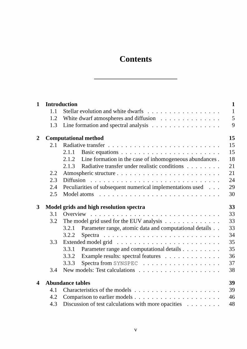
It is questionable, however, whether such comparisons can be meaningful at all:The potential consequences of fitting spectral features resulting from highly stratifiedabsorber patterns with such from homogeneously distributed absorber patterns areschematically illustrated in Fig. 1.1. A fixed amount of absorbing line forming mate-
Chapter 1.3: Line formation and spectral analysis 11
rial is placed at different optical depths in a surrounding gas slab in high concentra-tions (grey areas in right-hand panels). The correspondinghomogeneous abundance,obtained by evenly spreading the total absorber content over the given optical depthrange, would be the same and equal to 1 in all cases (not shown). Comparing theline profiles calculated for the concentrated material withthose calculated for vari-ous homogeneous distributions (i.e. abundance values smaller or greater than 1, notshown) gives a different result. The line profiles from the unevenly distributed pat-terns (grey lines in left-hand panels) can generally not be matched with profiles fromabundance patterns without gradients. Upper and lower limits to the homogeneousabundances required to approximately fit the line profiles can be derived by matchingthe line cores and the line wings separately (black lines in both panels: line profilesleft, abundance limits right). It can clearly be seen that these limits for the effectivehomogeneous abundances are not only systematically shifted towards lower or highervalues in comparison to the corresponding mean homogeneousabundance, but alsothat they are not correlated with the peak value of the stratified abundances either.
These complications, potentially only made worse when going from the above aca-demic example to a more realistic situation, suggest that direct comparison of abun-dance measurements obtained with homogeneous atmospheresto radiative levitationtheory predictions should be interpreted with caution. Although the disagreement of-ten seen in such comparisons has regularly been attributed either to shortcomings inthe models by Chayer et al. (1995a,b) – such as the missing feedback of the additionalabsorbers’ opacity on the atmospheric structure, or to the non-applicability of pure ra-diative levitation theory without the inclusion of further, so far unidentified physicalprocesses – this fundamental difficulty must also be appropriately considered.
The incapability of even the current complex NLTE, fully line-blanketed atmo-sphere models, incorporating virtually any desired element, to reproduce the finerdetails of hot DA spectra is hard to overcome with models using an externally im-posed depth-dependent stratification. Dreizler (1999) avoided the addition of numer-ous further adjustable parameters associated with such approaches, replacing themwith physically meaningful profiles instead, by introducing self-consistent diffusionmodels. The depth-dependent abundances for any metals in these full-grown WDatmosphere models are calculated assuming equilibrium between radiative elevationand gravitational settling, with the coupling between the chemical stratification andthe radiation field taken into account self-consistently through an iterative scheme. Aninherent property of the equilibrium condition used is thatthe metal abundances arenot free parameters as they would be in an homogeneous model,but determined at ev-ery single depth point for each of the metal species included, effectively reducing thefree parameters for the model atmosphere calculation to theeffective temperature andsurface gravity only. By significantly reducing the dimension of parameter space inthe fitting process, this approach also formally reduces thechances of finding the best
12 Chapter 1: Introduction
fit otherwise accessible through careful fine-tuning of (preferably depth-dependent!)abundance parameters. The requirement to describe the physics forming the chemi-cal stratification as realistically as possible is therefore extremely stringent. Failureto avoid important systematic errors in the modelling, or torecognise and include allrelevant physical processes, is likely to result in synthetic spectra that cannot repro-duce observations at all (as opposed to reproducing observations at distorted stellarparameter combinations). For the new diffusion models, Dreizler & Wolff (1999)and Schuh (2000) have shown that they are capable of correctly predicting the gen-eral trends in the metal content and stratification in hot DA white dwarf atmospheres.Based on a preliminary analysis of EUVE spectra with a rudimentary set of models,these successful demonstrations of overall agreement proved the remarkable potentialof the underlying principle, but still left many questions unanswered. Therefore, theobjectives of this thesis are:
� to provide a full grid of diffusion models complete with abundance tables andhigh-resolution spectra;
� to repeat the analysis of EUVE spectra based on this larger grid and usingimproved visual magnitudes;
� to quantify possible systematic errors in the models by comparing the resultsto earlier diffusion calculations, as well as to new models with more extensiveatomic input data (resulting in an improved treatment of theradiative accelera-tions);
� to quantify the contribution of systematic effects to the inconsistencies aris-ing when comparing predicted equilibrium abundances to abundance measure-ments obtained with homogeneous models from extensive UV/FUV data;
� to explore the magnitude and possible correlation with stellar parameters ofremaining discrepancies (after consideration of the issues above) which mustbe due to physical processes such as mass-loss, mixing, or accretion, all ignoredso far in the models;
� based on the lessons learned from the investigations above,to provide guide-lines on how the models can be productively used in systematic multi-wave-length analyses to understand the spectral evolution of WDsin a broader con-text.
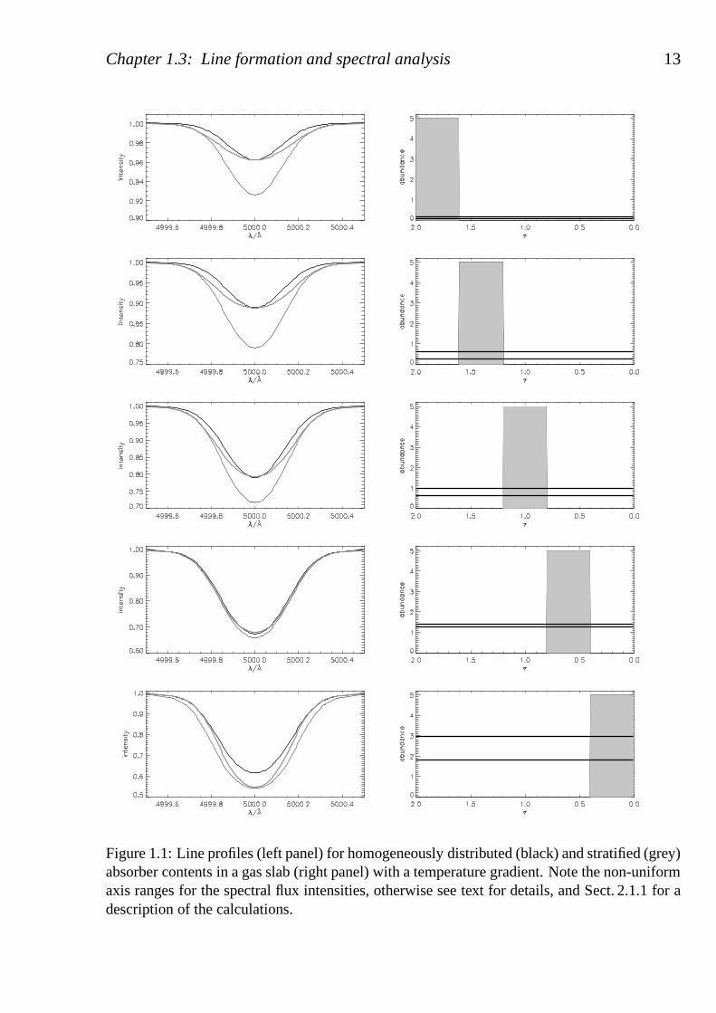
Chapter 1.3: Line formation and spectral analysis 13
Figure 1.1: Line profiles (left panel) for homogeneously distributed (black) and stratified (grey)absorber contents in a gas slab (right panel) with a temperature gradient. Note the non-uniformaxis ranges for the spectral flux intensities, otherwise seetext for details, and Sect. 2.1.1 for adescription of the calculations.

14 Chapter 1: Introduction
CHAPTER 2
Computational method
2.1 Radiative transfer
2.1.1 Basic equations
A star is not in thermodynamical equilibrium with its surroundings: The energy itproduces is eventually radiated away into space through itsatmosphere. For hot stars,the most efficient way to transfer energy through their atmospheres are radiative pro-cesses. The solution of the radiative transfer problem is hence one important ingredi-ent in the construction of any stellar atmosphere model, extensively treated elsewhere,which is why only a few basic principles (from Dreizler 2002,partly based on Rutten1997) are reiterated here.
In a simple one-dimensional configuration, the change of intensity� �
along a seg-ment
� �at a given frequency� is given by the attenuation of
�due to the opacity�
and the added contribution through the emissivity� :� � �� � � � � � � �
� � �� � � � � � � � � �
(2.1)
where the source function� has been introduced using the definition� � � � � . Anoptical depth scale� can be defined as
���
� � � � � (2.2)
allowing the expression of geometrical dependencies in units of the mean free pathfor photons. In the case of local thermodynamic equilibrium(LTE), where the elec-tron temperature and the radiation temperature of the plasma are so strongly coupledthrough frequent collisions that they can both be describedby one single value
�, the
source function may be approximated by the Planck function� , yielding� � ���
� � � �� � � � � � �
� � � (2.3)
15
16 Chapter 2: Computational method
For a given incident intensity� �
at the location� �
, the solution to this radiative trans-fer equation along a segment
� ��
� � � �can then be written as
� � �� �
� � �� � �� � � � � � �
� � � � �
� � � � � �� � �� �
� � �� � � � � � � � �
� � (2.4)
The optical depth is frequency-dependent since the opacity� generally is a complex,frequency-dependent function of atomic properties. For some problems however, itis desirable to define a frequency-independent mean opticaldepth scale, such as theone based on the Rosseland mean opacity:
� ross� �
�
�
� �� ross
� � �
�
� �
���
��� � �� �� �
��� �� � � �� �� �
���� � � (2.5)
For such a hypothetical “grey” opacity� ross, the optical depth scale becomes inde-pendent of frequency and can be thought of as if it described geometrical distances.
Generally speaking, opacity can result from photon absorption or stimulated emis-sion in atomic (or molecular) level transitions (bound-bound transitions), photoionisa-tion (bound-free transitions), free-free, or scattering processes. One basic and impor-tant contribution to� is the line opacity in the case of an exemplary two-level system(the opacities are additive when more levels are included).For an atom featuring alower and anupperstate, its opacity would be determined by the cross section� forthe transition and the level population� according to
� � � � � � � � � � � � low
(2.6)
The cross section� can be described by the classical cross section value for an elec-tron in an electromagnetic field corrected by a quantum mechanical correction term(oscillator strength� ), and the frequency-dependentcontribution separated into a pro-file function� , so that with
� � � � � � �
� �
� � � � � � low � � � (2.7)
� essentially becomes a function of the level population and the profile function fora given atomic line. The profile function will be a convolution of all broadeningmechanisms at work, and as such potentially depend on temperature, pressure, mag-netic field strength, micro turbulence, and large-scale movements such as convection,currents on the stellar surface, or rotation. The dominant effects of temperature and
Chapter 2.1: Radiative transfer 17
pressure1 in environments relevant to non-magnetic classical stellar atmosphere mod-elling can be described through the damping parameter� and a parametrisation inthe dimensionless frequency variable� of the Voigt function
� � � � . If this Voigt
function is used as a typical profile function, the frequencydependency of an opticaldepth scale may be written as
���
� �� � � � �
(2.8)
where
� � � � � �
� �� �
���
� �k� � �
(2.9)
and where��
shall be chosen so as to represent an arbitrary line opacity at the restfrequency of the line centre.
Given the two exemplary representations for� in Eqs. 2.5 and 2.8, the correspond-ing effects on
� �according to Eq. 2.4 can be illustrated using a simple two-temperature
model. In what is known as the Schuster-Schwarzschild model, a plane parallel,isothermal gas slab is irradiated by a Planck function of anyother temperature. Theincident intensity is exponentially attenuated for increasing optical depths, and for� � � drops to �� of its initial value. The fractional contribution of the sourcefunction in the emergent intensity increases with increasing optical depths; for anyfrequency-independent optical depth, the effects of the source function quickly be-come completely dominant. The emergent intensity is then solely determined by thetemperature of the gas slab, independent of what incident intensity it is being irradi-ated with, as long as this irradiation is not allowed to change the temperature of thegas itself. The situation is different for a transparent continuum modified only locally(in frequency) by an optically thick line. For this other extreme, the continuum contri-bution will be the unchanged incident radiation, since it can neither be attenuated norcan a gas slab with zero optical depth contribute to the intensity at those frequencies.The line centre, on the other hand, will again be dominated bythe source function ofthe gas slab alone, so that the maximum possible line depth isgiven by the ratio ofthe source functions of the irradiating and the irradiated material. When the sourcefunctions are Planck functions as in the above example, it isimmediately clear thatan irradiation of a gas slab with a temperature below the radiation temperature of theincident field will lead to absorption, while a gas slab hotter than the irradiating fieldwill cause emission. For equal temperatures, the attenuation is exactly balanced bythe contributions of the source function in the material crossed.
In real situations, the optical depth will be a complex function of both continuumand line opacities. Furthermore, neither the temperature nor the opacity and emis-sivity will usually be constant throughout a macroscopic gas slab, but also vary with
1They obviously also can have a strong influence on the level population at the same time.
18 Chapter 2: Computational method
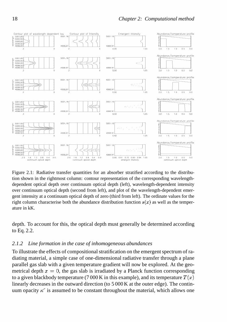
Figure 2.1: Radiative transfer quantities for an absorber stratified according to the distribu-tion shown in the rightmost column: contour representationof the corresponding wavelength-dependent optical depth over continuum optical depth (left), wavelength-dependent intensityover continuum optical depth (second from left), and plot ofthe wavelength-dependent emer-gent intensity at a continuum optical depth of zero (third from left). The ordinate values for theright column characterise both the abundance distributionfunction �
� � �as well as the temper-
ature in kK.
depth. To account for this, the optical depth must generallybe determined accordingto Eq. 2.2.
2.1.2 Line formation in the case of inhomogeneous abundances
To illustrate the effects of compositional stratification on the emergent spectrum of ra-diating material, a simple case of one-dimensional radiative transfer through a planeparallel gas slab with a given temperature gradient will nowbe explored. At the geo-metrical depth
�� � , the gas slab is irradiated by a Planck function corresponding
to a given blackbody temperature (7 000 K in this example), and its temperature� � �
linearly decreases in the outward direction (to 5 000 K at theouter edge). The contin-uum opacity� � is assumed to be constant throughout the material, which allows one
Chapter 2.1: Radiative transfer 19
to define a mean optical depth scale� �� �
=� � �� (from � � =0 at� �
to � � =2 at� � � � )
that is regular in geometrical depth. Additionally, the frequency-dependent opacityof a single line (centred at 5 000A) is introduced as� � �� � � � � � �
. The purpose ofthis line opacity is to simulate an absorbing element2, which can be distributed in anydesired depth intervals within the gas slab by means of the depth-dependent function� � �
. The full frequency-dependent optical depth scale is then of the form
�� � �
�
�
� �� � � � � � �
�
� �
� � � � � � � � �� � � � � � � � � � � � � (2.10)
which for � � =� �=1 (arbitrarily chosen for simplicity) transforms into
�� �
� � �
� �� ��
�� �
� �� � � �� � � � � �
� � � �� �
(2.11)
While the damping parameter for the Voigt function�
can be assigned a typical valueof � =�
� everywhere, the dimensionless frequency parameter� is re-evaluated at each
depth to take into account the non-zero temperature gradient.Given the above optical depth scale, the intensity of the radiation transferred through
the gaseous material can again, as in Eq. 2.4, be calculated as
� � �� �
�
� � �� �� �
� � � � � � � � � �� ��
� � �� �� �
� � � � � � � � ��
(2.12)
Rewritten for a discrete depth grid, this can equivalently be formulated as
� � �� �
�� � �
� �� �� � � � �
� ��� ��
� � � �� � � � � � � � � � �
�
(2.13)
This approach allows one to solve for the intensity at any desired � immediately,in principle without having to calculate intensities at intermediate depth values� .Known as ”long characteristics” treatment, it tends to suffer from numerical integra-tion inaccuracies, unless special attention is given to a good choice of integration
2Due to its very small extent in frequency, this additional opacity source would not significantly in-fluence the mean optical depth scale even if one of the more rigorous common definitions such as theRosseland scale were used here.
20 Chapter 2: Computational method
weights. While there exist absolutely adequate solutions to this, the ”short character-istics” method offers an alternative where the intensity obtained for a depth� uses theintensity obtained previously at� � � as the boundary condition for the subsequentintegration. Hence, in the respective variation of Eq. 2.13, the integral only spans onestep on the depth grid, so that� �� is to be replaced by� �
� � and� � �
� �� by
� � �� �
� �.
The focus is on an appropriate choice of the integration weights for this contribution(as first given by Kunasz & Olson 1988). Using the definitions
� � � � � �
� � � � �
� �� � �
(2.14.a)
� �� � � � � �
� � � � � � � � � �
� � � � (2.14.b)
� �� � � � � � � � � �
� � � � � � � � � �
� � � � (2.14.c)
and provided that� � �
� �� �
is given, Eq. 2.13 may then be rewritten as
� � �� �
�� � �
� �� �
� � �� � � � � �� � � � � � ��
� � �� � � � � � �� � �
(2.15)
Both of the radiative transfer solutions have been used in the construction of modelscalculated for this work (see later, Sects. 2.2, 3.3, and 2.5). They are mathematicallyidentical in a one-dimensional formulation, and may only differ numerically, so thatobviously either approach is equally well suited to obtain the results displayed inFig. 2.1. The rightmost column is similar to the one in Fig. 1.1, except in that it addi-tionally contains the temperature profile, and has one extrarow for a homogeneouslydistributed absorber profile. The first column from the left illustrates how the ab-sorber profile modifies the wavelength-dependent optical depth in the vicinity of theline centre as a function of the continuum optical depth, thesecond how the radiationfield intensity changes according to its effects. In these first two column panels, theline height contour decreases from left to right. Together,they demonstrate to whatextent the line centre in particular samples different areas in depth depending on theabsorber distribution. The resulting equivalent line widths implied by the emergentintensities (at a continuum optical depth of zero) in the third column’s plots naturallyunderline the strong influence of the depth where an absorberis placed rather than justits total amount among a line of sight. Moreover, a comparison of the detailed lineprofiles (as presented more clearly in Fig. 1.1) reveals the non-equivalence of a homo-geneous and a concentrated slab of line-forming material, and the highly non-trivialrelations between ”representative” and ”true” absolute abundances.
Chapter 2.2: Atmospheric structure 21
2.1.3 Radiative transfer under realistic conditions
In a plane parallel approximation, the change of intensity of the radiation field alonga line of sight
�at an angle� to the radial direction is
� � � � �� � � � � � � � � �
. With thestandard abbreviation� � � � � � , the radiative transfer equation then takes the generalform given in Eq. 2.16. To solve for the radiation field, the ”long characteristics”method of a Feautrier solution scheme was implemented to construct the model gridpresented in Sect. 3.3, while the ”short characteristics” were used in the version forthe newer (”improved”, see Sect. 2.5) models. In contrast tothe simplified examplejust discussed, where a very straightforward integration is possible, realistic situationsimply a much more complex� and � . In particular, when Thomson scattering isincluded (then� is usually renamed� ) in addition to bound-bound, bound-free, andfree-free processes, the solution requires either a Feautrier scheme (Feautrier 1964, inthe long characteristics approach) or an iteration scheme (for the short characteristicsapproach, Olson & Kunasz 1987).
2.2 Atmospheric structure
In the classical stellar atmosphere problem, the radiativetransfer needs to be solvedself-consistently with the energy balance and hydrostaticequilibrium conditions, andthe equations describing atomic level population (under NLTE conditions, the rateequations, which enforce statistical equilibrium). Further constraints are the massand charge conservation within the atmospheric structure.
The Tubingen model atmosphere programPRO2in its standard form approximatesstellar atmospheres as plane parallel, chemically homogeneous atmospheres in radia-tive, hydrostatic and statistical equilibrium. The solution of rate equations in fullNLTE for sophisticated atomic data makesPRO2especially suitable for applicationto hot compact stars. Restriction to the one-dimensional, plane parallel geometry isjustified whenever the extent of the atmospheric layer is small compared to the stellarradius, which is indeed particularly well fulfilled in compact objects. Atmospheresare in radiative equilibrium when alternative methods of energy transport, notablyconvection, are considerably less efficient than radiativetransfer, and when energyproduction does not occur in these layers. Hot stars do have such radiative atmo-spheres. Hydrostatic equilibrium, on the other hand, only holds as long as a star doesnot suffer significant mass-loss, which implies potential limitations since radiativelydriven winds are more important the hotter an object is.
A recent comprehensive description of the physics and numerical solution schemesimplemented inPRO2has been given by Werner et al. (2003), superseding an earlieroverview by Werner & Dreizler 1999. The review articles are complemented by auser’s guide (Werner et al. 1998), the work by Nagel (2003) which records aspects
22 Chapter 2: Computational method
concerning some of the latest updates that are also partly relevant to the modellingpresented here, and a series of several earlier publications often concentrating onselected topics within the overall problem as referred to inWerner et al. (2003).
Several extensions to this general concept have been recently or are currently beingimplemented (in addition to the references above, see Dreizler 2003; Rauch & Deetjen2003; Deetjen et al. 2003; Schuh & Dreizler 2003; Nagel et al.2003). To correctlydescribe the chemically stratified atmospheres of hot whitedwarfs and possibly sdBstars, modifications which allow the self-consistent prediction of depth-dependentabundance profiles have been implemented (Dreizler 1999 andlater; see the followingSect. 2.3). For an up-to-date overview of the status of NLTE atmosphere modelling aswell as related, current topics of more general interest to this field, two proceedingspublications on Stellar Atmosphere Modelling from recent conferences in Tubingenand Uppsala (Hubeny et al. 2003; Piskunov et al. 2004) each provide an excellent ref-erence.
Since this literature collection describes the various aspects of the techniques neces-sary for the construction of metal-line-blanketed model atmospheres under the above-mentioned set of assumptions in a much more comprehensive and detailed way thanwould be appropriate here, only a few central points are repeated here. The one-dimensional radiative transfer equation reads
� �� � �� � �
� � � � � � � � � � � � � �� � � (2.16)
The condition of hydrostatic equilibrium, meaning that gravitational pull is balancedby the total (gas, radiation and turbulent) pressure gradient, takes the form
� � � � � � � � � � � �
where � �
� �� �
(2.17)
The energy balance, or radiative equilibrium, requires that the overall flux is con-served from one depth to another, or else that the total energy absorbed per unitvolume and time is the same as that emitted, which in an integral formulation isequivalent to
���
�� � � � � � � � � � �
� �
��
� � � � � � � � � ���
(2.18)
� �is the quantity obtained by angle integrating
� ��. Statistical equilibrium can be
expressed through a set of rate equations where the ratesinto each level� from allother levels andawayfrom level � into any other level will on average cancel out
Chapter 2.2: Atmospheric structure 23
to yield time-independent population numbers� � :�
��
� � �� � � � � �� �� �� � � �
�� �� � � � � � � (2.19)
For an index� which runs through all levels of all ions of all elements, particle con-servation may be written as
� � ��� � � � � (2.20)
and charge conservation (with� � referring to the charge of the current ionisationstage� ) as
� � � � � � � � � � � (2.21.a)
� � � �� � � � �
� � (2.21.b)
respectively. Since� � is the same for all levels of one ionisation stage� , and thepopulation of this stage� is composed of the individual NLTE and LTE levels thatmodel it3, the right-hand side expression (corresponding to a summation over thepopulation numbers of all ionisation stages of all elementsonly) is also sufficient.Furthermore, for electron and ion gas temperatures that areindistinguishable, particledensities may be replaced with partial pressures using the ideal gas law, yielding anequivalent variant of the charge conservation as given by 2.21.b (this will be neededin Eq. 2.34).
A complete linearisation (CL) of this highly coupled, non-linear set of equationsyields a system whose numerical solution is still beyond current possibilities for rea-sonably large numbers of atomic levels. An iterative approach is therefore necessaryto partly remove the strong depth and frequency coupling. The Lambda iteration pro-cedure achieves this by basically separating the radiativetransfer from the rate andconstraint equations solution. For a given source function� (essentially determinedby the level populations� , approximately known from a previous iteration step� � � ),an updated radiation field� can then formally be determined by applying a Lambdaoperator on� :
� � � � � � � (2.22)
3This can be expressed through� � � NLTE�� � �� � � LTE�� � �
� �� .
24 Chapter 2: Computational method
A re-determination of the remaining solution vector in the next step then relies on thatfixed � from the formal solution, resulting in an extremely slow overall convergencebehaviour. It is more effective to insert the yet-to-be determined population numbersentering the radiative transfer equation into the structure solution part via a moresophisticated expression for� . This is feasible through the following split, at theheart of the so-called Accelerated Lambda Iteration (ALI):
� � � � � � �� � �
� � � � � � � � �� � � � (2.23)
If the Approximate Lambda Operator � (ALO) is chosen such that it avoids the re-introduction of excessive depth coupling, the first part of Eq. 2.23 can be substitutedinto the full Eq. 2.22 for an up-to-date� , while the second part corrects for the de-viations caused by this approximation, which can be calculated from quantities ofiteration� � � before introducing Eq. 2.23 into
�� � � � � � � � � � (2.24)
In the case of convergence, quantities� approach quantities� � � so that from a math-ematical point of view the exact form of � , although it actually differs from the true , becomes irrelevant. The problem of constructing a numerically stable ALO hasfor example been solved by Olson & Kunasz (1987).
2.3 Diffusion
Diffusion is a transport phenomenon based on stochastic thermodynamic processes.Random microscopic movements may result in a macroscopic change of state vari-ables if concentration (� ), temperature (
�) or pressure (
�) gradients are present. In a
generalisation of Fick’s first law, the mean diffusion velocity is proportional to thesegradients in the form given by
� � � � ��
� �� � � � �� � � �
� � � � � � (2.25)
(Kippenhahn & Weigert 1990) for a diffusion coefficient�
, and coefficients� for�
and�
, respectively (see also Chapman & Cowling 1970). Diffusionthen occurs oncharacteristic time scales of
� � � ��
�
� (2.26)
where
represents the typical scale height for the respective gradient, and� � theapproximate time to reach a stationary state where the mean diffusion velocity tends
Chapter 2.3: Diffusion 25
to zero. The transport phenomenon hence tends to cause the gradient that drives it tovanish, but in a situation where a gradient or a set of gradients is kept up by externalforces, these instead rather dictate the constraints underwhich diffusion proceeds.In other words, a pressure gradient - acting as an external force - can impose theformation (not the disappearance) of a concentration gradient in order for the overallsystem to reach a stationary state.
This is what is happening in white dwarf atmospheres. Koester & Chanmugam(1990) recapitulate the theoretical background for this situation, where the large pres-sure gradient (implying a short pressure scale height) completely dominates the dif-fusion velocity, leading to short diffusion time scales of the order of months4. Anycontributions from the temperature gradient, for which time scales are longer andscale heights larger (i.e. the resulting effects less pronounced), will be neglected inthe following.
For a given element species�
of atomic weight� � , the related pressure scale height is given by
� � �� �
� � � � � � � � �� �� � � � � ��
� �� � � � � ��
� �
� � �
(2.27)
if the conditions of hydrostatic equilibrium� �
and the ideal gas equation� � are
used. Under the assumption of an isothermal ideal gas (�
� const., unrealistic instellar atmospheres), the solution to the differential equation for
� � implied by 2.27� � �� � � � � �
� � (2.28)
is of the form
� � �� � � � �
��
� �� (2.29)
and equivalent to
� � � � � � � � ��
� �� (2.30)
since� � � in the isothermal case. Qualitatively, a roughly exponential decline of the
density� � for a species�on scale heights that decrease with increasing atomic weight
� � means that the density of heavier elements will fall off quicker along the directionof a negative pressure gradient than that of lighter ones. Heavier elements therefore”sink” into denser regions, while the lightest one ”floats” on top. The scale heightsin white dwarfs on which the decline happens are small compared to the geometrical
4”Short” in this context means in comparison to the respective stellar evolutionary time scale.
26 Chapter 2: Computational method
extension of the atmosphere, and the drop-off regions are located at different depthsfor different species, so that the resulting elemental distribution may be considered asrelatively well-defined, separated layers.
A more exact description of partial pressure and density distributions can be ob-tained from a balance of forces acting on each element species solved simultaneouslywith the full set of stellar atmosphere equations. A substantial simplification in thecase of white dwarf atmospheres results from the fact that a detailed description canmake use of the general results obtained from both observational evidence as well asthe qualitative discussion above: The lightest element floats on top of all others, andsince this is at the same time also the most abundant one in theatmosphere, its partialpressure mostly dominates the hydrostatic structure whileall other species are onlypresent in traces and can be treated as perturbations.
This remains true if, in addition to the gravitational settling, radiative accelerationis considered in the overall balance of forces. The levitation effect of momentumtransfer by radiative acceleration hence pollutes the white dwarf atmosphere withheavier elements, but cannot substantially alter the abundance of the main constituent.Under the assumptions that no processes competing with diffusion and levitation arepresentand that diffusion time scales are short, the distribution of trace elements in astellar atmosphere can then be expected to take on an equilibrium state, as proposedby Chayer et al. (1995a,b) and implemented for NLTE situations by Dreizler (1999).The solution of an equilibrium condition for each atomic species yields equilibriumabundances. For a plane parallel model atmosphere in hydrostatic equilibrium, thoseare solely determined by the photospheric parameters
� � �and
� � �� , in other words,
the photospheric abundances are no longer free parameters.In such a stationary situation, mean diffusion velocities of all elements
� � with
respect to the main constituent��
would be zero everywhere in the atmosphere, dueto an exact balance of the sum of gravitational, radiative, and electrical forces. Ne-glecting thermal and concentration diffusion, a detailed formulation of this condition
� � � � � � � � ��� � (2.31)
for polluting elements� �
in a hydrogen (or helium) plasma��
yields (followingDreizler 1999)
� � � � � � �� � � � � � �
� �(2.32.a)
� � � � � � � � � � � � � � � � �� � � � � � � �
� � (2.32.b)
The � � � � are the forces acting on element� �
,� � are the atomic weights,� � are
the mean electrical charges, E is the electrical field causedby the separation of elec-trons and ions,� � is the proton mass, and� � � �
� � is the radiative acceleration actingon element
� � . The following modified hydrostatic equilibrium conditions for the
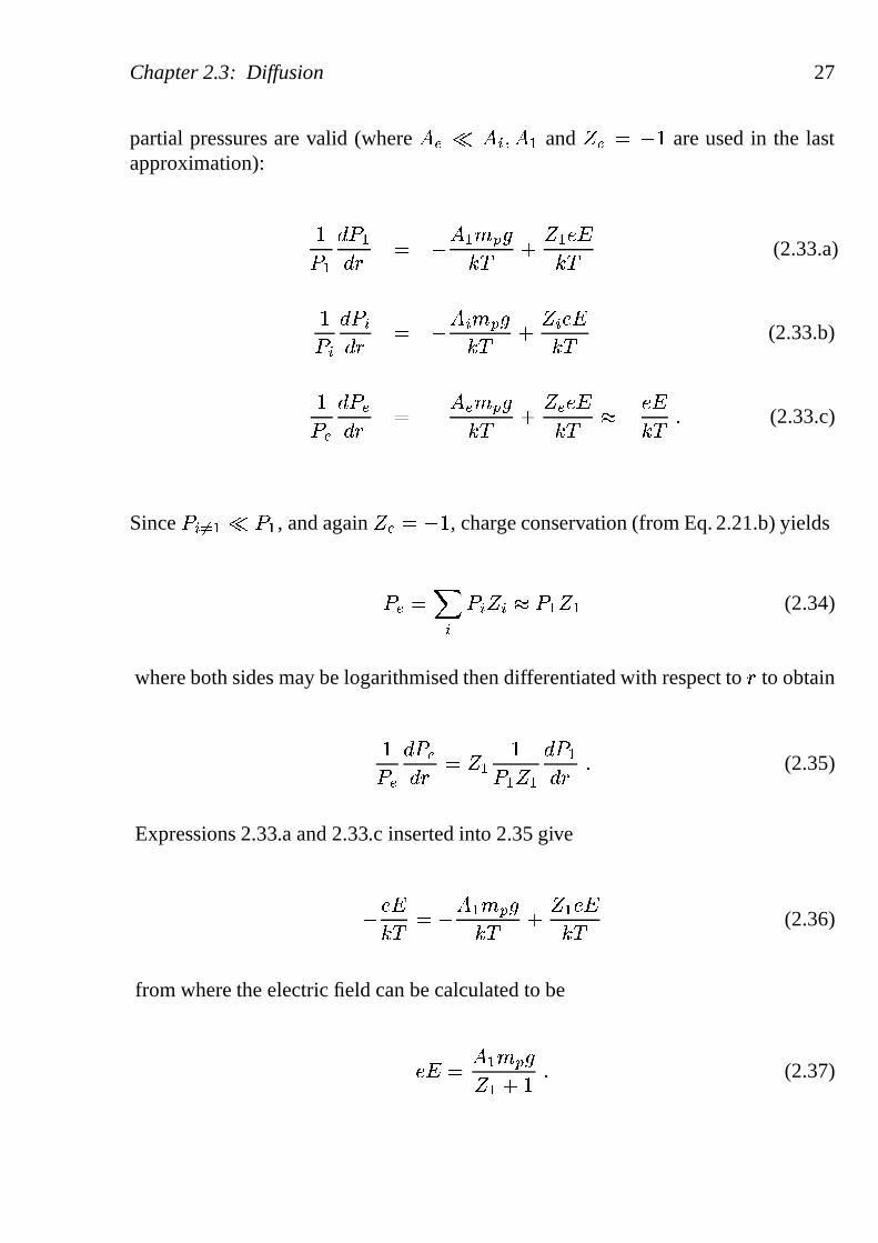
Chapter 2.3: Diffusion 27
partial pressures are valid (where� � �
� � � � and � � � � � are used in the lastapproximation):
���
� ��� � � �
�� � � �� � �
� �� �
� � (2.33.a)
�� �� � �� � � �
� � � � �� � �
� � � �� � (2.33.b)
�� �
� � �� � � �� � � � �
� � �� � � �� �
� �� �� �
(2.33.c)
Since� � �� � �
�� , and again� � � � � , charge conservation (from Eq. 2.21.b) yields
� � ���
� � � � � �� � � (2.34)
where both sides may be logarithmised then differentiated with respect to�
to obtain
�� �
� � �� � � � ���� � �
� ��� �
(2.35)
Expressions 2.33.a and 2.33.c inserted into 2.35 give
�� �� � � �
�� � � �� � �
� �� �
� � (2.36)
from where the electric field can be calculated to be
� ��
�� � � �
� � � �
(2.37)
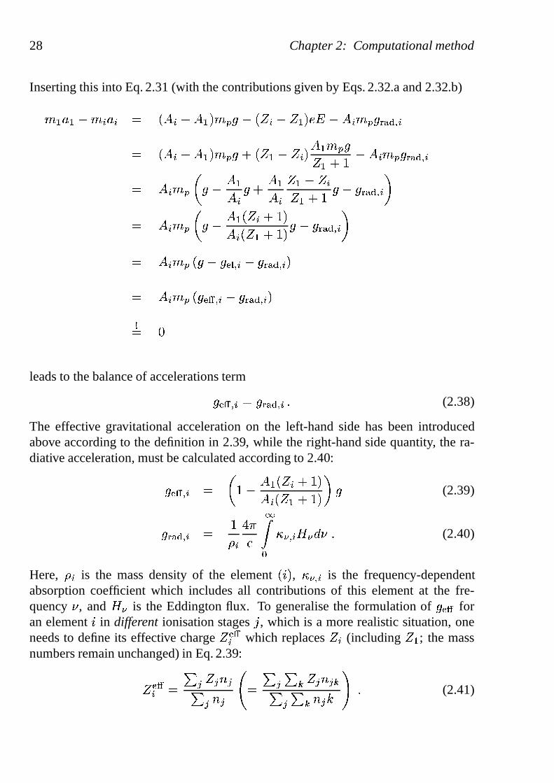
28 Chapter 2: Computational method
Inserting this into Eq. 2.31 (with the contributions given by Eqs. 2.32.a and 2.32.b)
� � � � � � � � � ��� � � �
�� � � � �� � � � �
� � � � � � � � � � �� �
��� � � �
�� � � �
�� � � � � �
� � � �� � � � � � �� � � � � �
� ��
� � � � � ��
�� � � ��
�� �� � � � �� � � �
� � � � � �� �
�� � � � � �
���� � � �
� � �� � � �
� � � � � �� �
�� � � �
�� � �
� � � � � � � � �� �
�� � � �
��� � � � � � � � �
� � �� �
leads to the balance of accelerations term
�� � � � � � � � �
� � (2.38)
The effective gravitational acceleration on the left-handside has been introducedabove according to the definition in 2.39, while the right-hand side quantity, the ra-diative acceleration, must be calculated according to 2.40:
�� � � � � � �
���� � � �
� � �� � � �
� (2.39)
� � � �� � �
�� �
�
���� � � � � � � �
(2.40)
Here, � � is the mass density of the element� �
, � � � � is the frequency-dependentabsorption coefficient which includes all contributions ofthis element at the fre-quency� , and
�is the Eddington flux. To generalise the formulation of�
� �for
an element�
in different ionisation stages� , which is a more realistic situation, oneneeds to define its effective charge�
� �� which replaces� � (including � � ; the mass
numbers remain unchanged) in Eq. 2.39:
�� �� �
� � � �
� � � � � � �
(2.41)
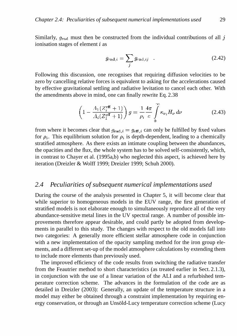
Chapter 2.4: Peculiarities of subsequent numerical implementations used 29
Similarly, � � � � must then be constructed from the individual contributionsof all �ionisation stages of element
�as
� � � �� � �
� � � � �
� � (2.42)
Following this discussion, one recognises that requiring diffusion velocities to bezero by cancelling relative forces is equivalent to asking for the accelerations causedby effective gravitational settling and radiative levitation to cancel each other. Withthe amendments above in mind, one can finally rewrite Eq. 2.38
� ��
���
� �� � �
� � ��
� �
� � � � �
�� �
�
���� � �
� � � � (2.43)
from where it becomes clear that� � � �� � � �
� � � � can only be fulfilled by fixed valuesfor � � . This equilibrium solution for� � is depth-dependent, leading to a chemicallystratified atmosphere. As there exists an intimate couplingbetween the abundances,the opacities and the flux, the whole system has to be solved self-consistently, which,in contrast to Chayer et al. (1995a,b) who neglected this aspect, is achieved here byiteration (Dreizler & Wolff 1999; Dreizler 1999; Schuh 2000).
2.4 Peculiarities of subsequent numerical implementations used
During the course of the analysis presented in Chapter 5, it will become clear thatwhile superior to homogeneous models in the EUV range, the first generation ofstratified models is not elaborate enough to simultaneouslyreproduce all of the veryabundance-sensitive metal lines in the UV spectral range. Anumber of possible im-provements therefore appear desirable, and could partly beadopted from develop-ments in parallel to this study. The changes with respect to the old models fall intotwo categories: A generally more efficient stellar atmosphere code in conjunctionwith a new implementation of the opacity sampling method forthe iron group ele-ments, and a different set-up of the model atmosphere calculations by extending themto include more elements than previously used.
The improved efficiency of the code results from switching the radiative transferfrom the Feautrier method to short characteristics (as treated earlier in Sect. 2.1.3),in conjunction with the use of a linear variation of the ALI and a refurbished tem-perature correction scheme. The advances in the formulation of the code are asdetailed in Dreizler (2003): Generally, an update of the temperature structure in amodel may either be obtained through a constraint implementation by requiring en-ergy conservation, or through an Unsold-Lucy temperaturecorrection scheme (Lucy
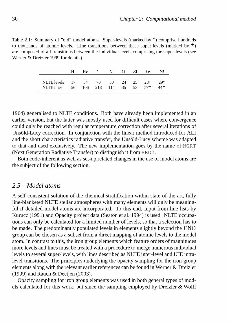
30 Chapter 2: Computational method
Table 2.1: Summary of ”old” model atoms. Super-levels (marked by � ) comprise hundredsto thousands of atomic levels. Line transitions between these super-levels (marked by� )are composed of all transitions between the individual levels comprising the super-levels (seeWerner & Dreizler 1999 for details).
� � � � � � � � � � �
NLTE levels 17 54 70 50 24 25 28� 29�NLTE lines 56 106 218 114 35 53 77� 44�
1964) generalised to NLTE conditions. Both have already been implemented in anearlier version, but the latter was mostly used for difficultcases where convergencecould only be reached with regular temperature correction after several iterations ofUnsold-Lucy correction. In conjunction with the linear method introduced for ALIand the short characteristics radiative transfer, the Uns¨old-Lucy scheme was adaptedto that and used exclusively. The new implementation goes bythe name ofNGRT(Next Generation Radiative Transfer) to distinguish it from PRO2.
Both code-inherent as well as set-up related changes in the use of model atoms arethe subject of the following section.
2.5 Model atoms
A self-consistent solution of the chemical stratification within state-of-the-art, fullyline-blanketed NLTE stellar atmospheres with many elements will only be meaning-ful if detailed model atoms are incorporated. To this end, input from line lists byKurucz (1991) and Opacity project data (Seaton et al. 1994) is used. NLTE occupa-tions can only be calculated for a limited number of levels, so that a selection has tobe made. The predominantly populated levels in elements slightly beyond the� � �group can be chosen as a subset from a direct mapping of atomiclevels to the modelatom. In contrast to this, the iron group elements which feature orders of magnitudesmore levels and lines must be treated with a procedure to merge numerous individuallevels to several super-levels, with lines described as NLTE inter-level and LTE intra-level transitions. The principles underlying the opacity sampling for the iron groupelements along with the relevant earlier references can be found in Werner & Dreizler(1999) and Rauch & Deetjen (2003).
Opacity sampling for iron group elements was used in both general types of mod-els calculated for this work, but since the sampling employed by Dreizler & Wolff
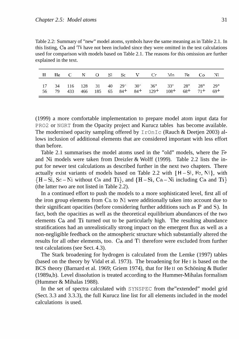
Chapter 2.5: Model atoms 31
Table 2.2: Summary of ”new” model atoms, symbols have the same meaning as in Table 2.1. Inthis listing, � � and � � have not been included since they were omitted in the test calculationsused for comparison with models based on Table 2.1. The reasons for this omission are furtherexplained in the text.
� � � � � � � � � � � � � � � � � � �
17 34 116 128 31 40 29� 30� 36� 33� 28� 28� 29�56 79 433 466 185 65 84� 84� 129� 108� 68� 71� 69�
(1999) a more comfortable implementation to prepare model atom input data forPRO2or NGRTfrom the Opacity project and Kurucz tables has become available.The modernised opacity sampling offered byIrOnIc (Rauch & Deetjen 2003) al-lows inclusion of additional elements that are considered important with less effortthan before.
Table 2.1 summarises the model atoms used in the ”old” models, where the� �and � � models were taken from Dreizler & Wolff (1999). Table 2.2 lists the in-put for newer test calculations as described further in the next two chapters. Thereactually exist variants of models based on Table 2.2 with � – � � , � � , � � � , with � – � � , � � – � � without � and � � � , and � – � � , � – � � including � and � � �(the latter two are not listed in Table 2.2).
In a continued effort to push the models to a more sophisticated level, first all ofthe iron group elements from� to � � were additionally taken into account due totheir significant opacities (before considering further additions such as� and � ). Infact, both the opacities as well as the theoretical equilibrium abundances of the twoelements� and � � turned out to be particularly high. The resulting abundancestratifications had an unrealistically strong impact on theemergent flux as well as anon-negligible feedback on the atmospheric structure which substantially altered theresults for all other elements, too.� and � � therefore were excluded from furthertest calculations (see Sect. 4.3).
The Stark broadening for hydrogen is calculated from the Lemke (1997) tables(based on the theory by Vidal et al. 1973). The broadening forHe I is based on theBCS theory (Barnard et al. 1969; Griem 1974), that for HeII on Schoning & Butler(1989a,b). Level dissolution is treated according to the Hummer-Mihalas formalism(Hummer & Mihalas 1988).
In the set of spectra calculated withSYNSPECfrom the”extended” model grid(Sect. 3.3 and 3.3.3), the full Kurucz line list for all elements included in the modelcalculations is used.

32 Chapter 2: Computational method
CHAPTER 3
Model grids and high resolution spectra
3.1 Overview
Applications to hot DA white dwarfs in Chapter 5 show that synthetic spectra derivedfrom chemically stratified models can quantitatively describe the EUV spectra ob-served from these objects. The model calculations (Sect. 3.2) used for the analysis ofEUVE spectra by Schuh et al. (2002) have since been extended to a larger model grid(Sect. 3.3). To investigate whether remaining discrepancies are due to limitations inthe way the models have been set up, or arise mainly from additional physical pro-cesses in the stellar atmosphere not so far incorporated in the modelling process, testsfor improvements of the models in Sect. 3.3 have been carriedout and are presentedin Sect. 3.4.
3.2 The model grid used for the EUV analysis
3.2.1 Parameter range, atomic data and computational details
The model grid used for the analysis in Chapter 5 spans the� � �
and� � �
� planeas suggested by the results from Wolff (1999): The effectivetemperatures cover arange from 38 000 – 70 000 K in 2 000 – 3 000 K steps, and the logarithmic surfacegravity a range from 7.2 – 8.3 in 0.1 – 0.2 dex steps. The grid used in the analysiswas an incomplete subset of the models shown in Fig. 3.1 and predominantly con-centrated around the previously found parameter combinations for the objects listedin Table 5.1. It must be emphasised once more that the total absorber content, i.e.the entire depth-dependent distribution of each individual trace element, is solely de-fined by the [
� � � � � �� ] – combination of the models, which makes
� � �and
� � ��
the only free parameters. The elements included in the model calculations are thesame as those used by Wolff et al. (1998) for the definition of their metal mix, whichin turn are those that they were able to identify in HST-GHRS data of the standard
33
34 Chapter 3: Model grids and high resolution spectra
star G 191–B2B. Other elements were assumed to be present in abundances too lowto significantly contribute to the EUV opacity, although stratification may possiblyinvalidate this assumption. While other elements than those used in Wolff’s and thisanalysis have been identified in UV spectra of some of the sample stars, includingG 191–B2B itself, the low abundances of 2.5�10�
�for phosphorus and 3.2�10� � for
sulfur, for example, as reported from the analysis of ORFEUSspectra by Vennes et al.(1996a), confirm that the opacities of these elements will presumably not contributesignificantly to the total EUV opacity. To investigate the possible effects of severaladditional elements, further analyses have been conducted(Sect. 3.4). For this analy-sis, the aim was to compare the results to a previous analysisin the EUV, as mentionedbefore. Consequently, the list of elements considered besides� reads� � , � , � , � ,� � , � � and � � . Differences remain with regard to the number of atomic levels andwith regard to the LTE/NLTE population of these levels. Details of the model calcula-tions presented here are summarised in Table 2.1. Note that the model atoms used forthe solution of the atmospheric structure and for the solution of the equilibrium con-dition are identical, which implies that the relatively high accuracy required for thecorrect evaluation of the radiative acceleration slows down the atmospheric structurecalculation.
The time it takes a model with the specified atomic data to converge depends pri-marily on the stratification of the input model. For homogeneous input models withabundances derived from the published metallicities as a first guess, roughly 5x� �
�
CRAY-CPU seconds are required, while for converged stratified models with photo-spheric parameters that are somewhat off the desired ones, convergence requires some5� � � �
CPU seconds. Due to this particularly large CPU time demand per model, theconvergence criterion for the models was set to be a less than5% change in the modelflux, which means that the maximal relative correction atany frequency point is nolarger than that limit, compared to the result from the previousdiffusion iterationstep. Only individual lines (usually two or three� � lines) are actually affected bythese larger variations, the continuum flux itself is much more exactly determinedand easily complies to the usual “� � � �
�” criterion.
As to the uniqueness of a particular solution, tests indicate that the results agreeto within the error limits regardless of the extremely different stratification of diversestart models, making a strong case at least for the stabilityof the result. One cantherefore trust that, no matter what the initial conditionsin the start model are, thefinal abundances in the converged model will always be the same.
3.2.2 Spectra
The emergent fluxes used for comparison with the observations have been calculated(with PRO2) from the model atmospheres on a frequency grid optimised for the EUVspectral range. This grid covers� � 50–700A in detail and contains more than 30 000
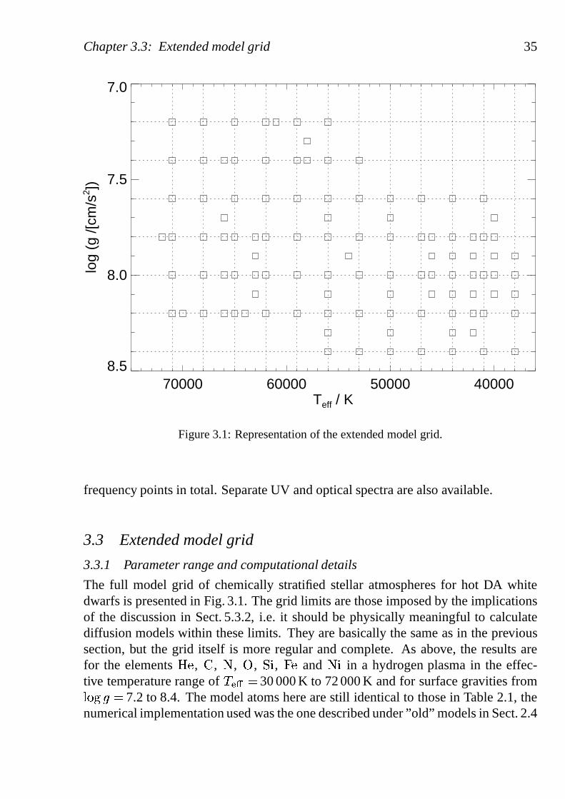
Chapter 3.3: Extended model grid 35
70000 60000 50000 40000Teff / K
8.5
8.0
7.5
7.0lo
g (g
/[cm
/s2 ])
Figure 3.1: Representation of the extended model grid.
frequency points in total. Separate UV and optical spectra are also available.
3.3 Extended model grid
3.3.1 Parameter range and computational details
The full model grid of chemically stratified stellar atmospheres for hot DA whitedwarfs is presented in Fig. 3.1. The grid limits are those imposed by the implicationsof the discussion in Sect. 5.3.2, i.e. it should be physically meaningful to calculatediffusion models within these limits. They are basically the same as in the previoussection, but the grid itself is more regular and complete. Asabove, the results arefor the elements� � , � , � , � , � � , � � and � � in a hydrogen plasma in the effec-tive temperature range of
� � �� 30 000 K to 72 000 K and for surface gravities from� � �
� � 7.2 to 8.4. The model atoms here are still identical to those in Table 2.1, thenumerical implementation used was the one described under ”old” models in Sect. 2.4
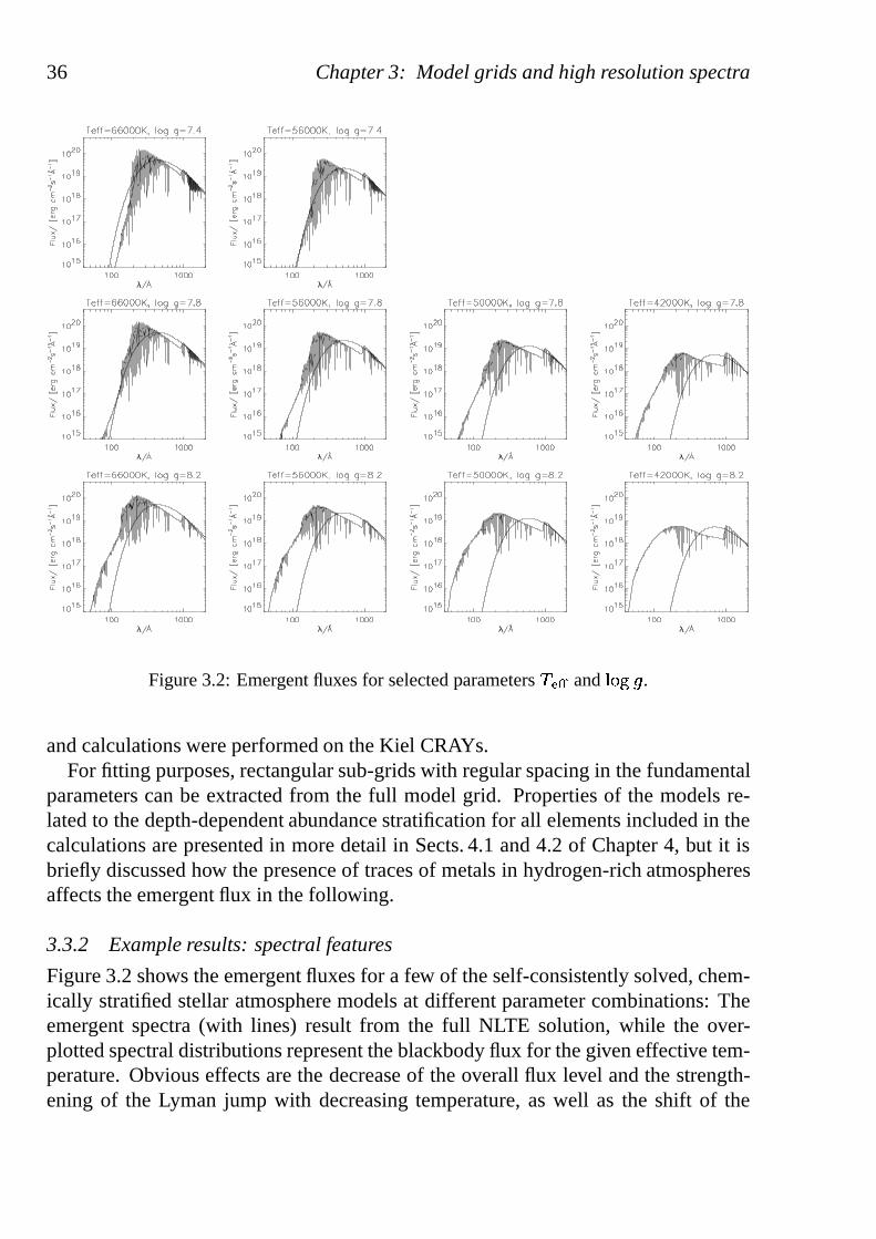
36 Chapter 3: Model grids and high resolution spectra
Figure 3.2: Emergent fluxes for selected parameters� � � and � � � � .
and calculations were performed on the Kiel CRAYs.For fitting purposes, rectangular sub-grids with regular spacing in the fundamental
parameters can be extracted from the full model grid. Properties of the models re-lated to the depth-dependent abundance stratification for all elements included in thecalculations are presented in more detail in Sects. 4.1 and 4.2 of Chapter 4, but it isbriefly discussed how the presence of traces of metals in hydrogen-rich atmospheresaffects the emergent flux in the following.
3.3.2 Example results: spectral features
Figure 3.2 shows the emergent fluxes for a few of the self-consistently solved, chem-ically stratified stellar atmosphere models at different parameter combinations: Theemergent spectra (with lines) result from the full NLTE solution, while the over-plotted spectral distributions represent the blackbody flux for the given effective tem-perature. Obvious effects are the decrease of the overall flux level and the strength-ening of the Lyman jump with decreasing temperature, as wellas the shift of the
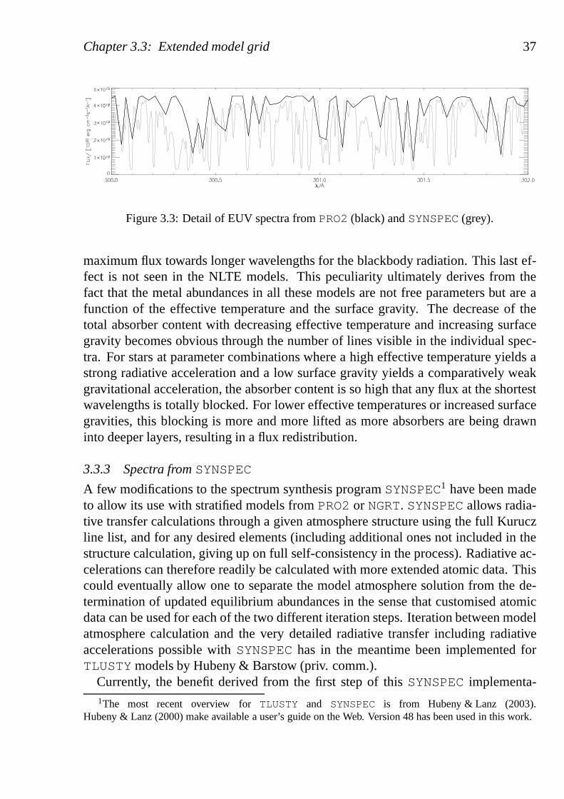
Chapter 3.3: Extended model grid 37
Figure 3.3: Detail of EUV spectra fromPRO2(black) andSYNSPEC(grey).
maximum flux towards longer wavelengths for the blackbody radiation. This last ef-fect is not seen in the NLTE models. This peculiarity ultimately derives from thefact that the metal abundances in all these models are not free parameters but are afunction of the effective temperature and the surface gravity. The decrease of thetotal absorber content with decreasing effective temperature and increasing surfacegravity becomes obvious through the number of lines visiblein the individual spec-tra. For stars at parameter combinations where a high effective temperature yields astrong radiative acceleration and a low surface gravity yields a comparatively weakgravitational acceleration, the absorber content is so high that any flux at the shortestwavelengths is totally blocked. For lower effective temperatures or increased surfacegravities, this blocking is more and more lifted as more absorbers are being drawninto deeper layers, resulting in a flux redistribution.
3.3.3 Spectra fromSYNSPEC
A few modifications to the spectrum synthesis programSYNSPEC1 have been madeto allow its use with stratified models fromPRO2or NGRT. SYNSPECallows radia-tive transfer calculations through a given atmosphere structure using the full Kuruczline list, and for any desired elements (including additional ones not included in thestructure calculation, giving up on full self-consistencyin the process). Radiative ac-celerations can therefore readily be calculated with more extended atomic data. Thiscould eventually allow one to separate the model atmospheresolution from the de-termination of updated equilibrium abundances in the sensethat customised atomicdata can be used for each of the two different iteration steps. Iteration between modelatmosphere calculation and the very detailed radiative transfer including radiativeaccelerations possible withSYNSPEChas in the meantime been implemented forTLUSTYmodels by Hubeny & Barstow (priv. comm.).
Currently, the benefit derived from the first step of thisSYNSPECimplementa-1The most recent overview forTLUSTY and SYNSPEC is from Hubeny & Lanz (2003).
Hubeny & Lanz (2000) make available a user’s guide on the Web.Version 48 has been used in this work.
38 Chapter 3: Model grids and high resolution spectra
tion for the extended model grid discussed here is a series ofhigh-resolution spectralgrids. For these, atomic input data has been prepared inSYNSPEC-readable format,identical in content to the data used for the calculation of the stratified model grid.The Lemke (1997) broadening tables for hydrogen Lyman and Balmer lines wereused. There are three grids, for the EUV (25 – 900A), UV (900 – 3 000A) and optical(3 000 – 10 000A) ranges, all at a minimum of 0.005A resolution. Figure 3.3 com-pares the emergent fluxes in a small section of the EUV wavelength range for spectracalculated according to Sect. 3.2.2 with those synthesisedhere.
3.4 New models: Test calculations
The next generation of models benefits from major improvements of the model atmo-sphere code that reduce the CPU time drastically. Test models have been calculatedwith the new code with atomic data prepared as similarly as possible as in the oldmodels, in particular including only the elements that werealso used there.
Further tests have included different atomic data for a model at� � �
� 56 000 Kand
� � �� � 7.6: First all elements from� to � � were added to the existing list. The
atomic data were prepared withIrOnIc , for details refer back to Table 2.2. However,this immediately resulted in hefty absorption edges in the EUV, incompatible withobservations. The equilibrium abundances of both� and � � were at levels wellabove those of� � and� � , which does not appear reasonable. A model with only thelighter elements plus� showed that the strong absorption edge was mainly due to� , but nevertheless both� and � � were removed in the final model to obtain theresults in Sect. 4.3. Along with these results, the procedure of removing� and � �is also further discussed and justified in Sect. 4.3.
All of these models were calculated on PCs in Tubingen.
CHAPTER 4
Abundance tables
4.1 Characteristics of the models
Based on the model grid presented in Sect. 3.3, abundance predictions are tabulatedfor optical depths ranging from 0.01� � ross � 10 for models covering the range of38 000 K� � � � � 71 000 K and 7.2� � � �
� � 8.4. For each [� � � � � �
� ] – combina-tion, a separate table exists with, in the first column, the Rosseland optical depth, andin the following columns, the relative abundances with respect to hydrogen for allelements contained in the model. Appendix A displays an essential part of the infor-mation from these tables compiled in graphical representations. The most noticeabletrends are illustrated in this section.
The models show the general properties as expected from diffusion theory, i.e. theoverall trace element abundances usually decrease with lower
� � �and higher
� � ��
values. Accordingly, the emergent spectra approach the fluxdistributions of those ofpure hydrogen model atmospheres at sufficiently evolved parameters on the coolingsequence. Iron and nickel dominate the opacity in the EUV, where the flux of hotwhite dwarfs peaks. Though their dominant effect on the EUV opacity is partly dueto the many lines these elements exhibit, it is equally important that their abundancesare, over a wide parameter range, simply larger than those ofthe � � � elements. Ofcourse these two effects are tightly correlated, since morelines directly translate intoa stronger radiative acceleration, which in this case easily compensates for the higheratomic weights and thus a stronger response to gravity.
As in previous calculations (Dreizler 1999; Dreizler & Wolff 1999), the iron groupelement abundance can reach solar values or more, with nickel being at virtually thesame level as the iron abundances. While the behaviour of iron is by and large con-sistent with results obtained from EUV analyses (see Chapter 5), the incompatibilitywith observation in the UV of an iron to nickel ratio close to unity must be addressedagain in Sect. 6.3.
Using the example of iron, Figs. 4.1 and 4.2 show that the ironabundance varies
39
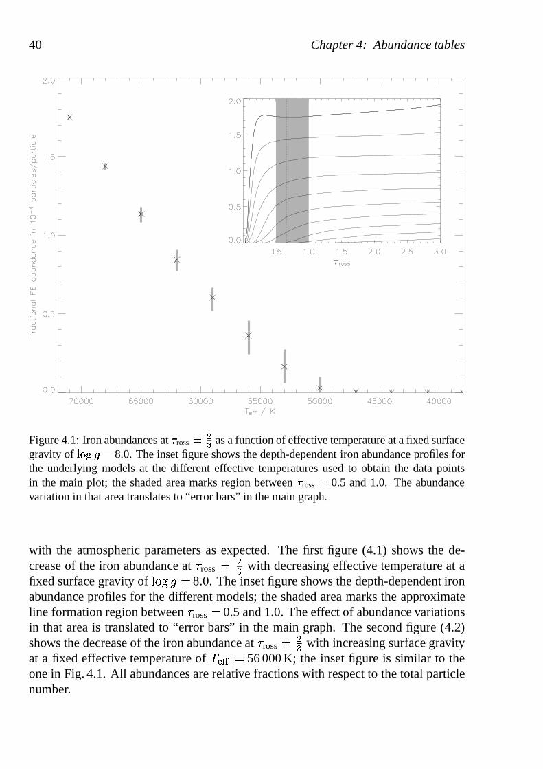
40 Chapter 4: Abundance tables
Figure 4.1: Iron abundances at� ross ��� as a function of effective temperature at a fixed surface
gravity of � � � � � 8.0. The inset figure shows the depth-dependent iron abundance profiles forthe underlying models at the different effective temperatures used to obtain the data pointsin the main plot; the shaded area marks region between� ross � 0.5 and 1.0. The abundancevariation in that area translates to “error bars” in the maingraph.
with the atmospheric parameters as expected. The first figure(4.1) shows the de-crease of the iron abundance at� ross �
�� with decreasing effective temperature at a
fixed surface gravity of� � �
� � 8.0. The inset figure shows the depth-dependent ironabundance profiles for the different models; the shaded areamarks the approximateline formation region between� ross � 0.5 and 1.0. The effect of abundance variationsin that area is translated to “error bars” in the main graph. The second figure (4.2)shows the decrease of the iron abundance at� ross �
�� with increasing surface gravity
at a fixed effective temperature of� � �
� 56 000 K; the inset figure is similar to theone in Fig. 4.1. All abundances are relative fractions with respect to the total particlenumber.
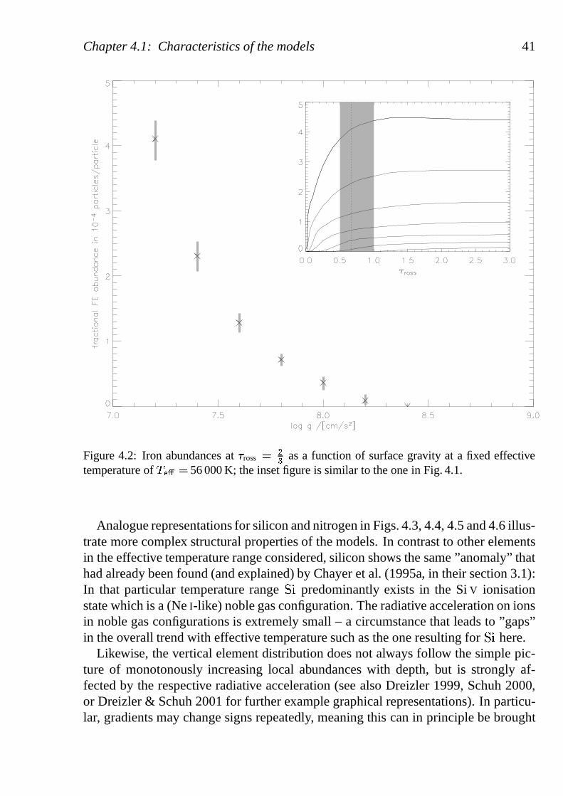
Chapter 4.1: Characteristics of the models 41
Figure 4.2: Iron abundances at� ross ��� as a function of surface gravity at a fixed effective
temperature of� � � � 56 000 K; the inset figure is similar to the one in Fig. 4.1.
Analogue representations for silicon and nitrogen in Figs.4.3, 4.4, 4.5 and 4.6 illus-trate more complex structural properties of the models. In contrast to other elementsin the effective temperature range considered, silicon shows the same ”anomaly” thathad already been found (and explained) by Chayer et al. (1995a, in their section 3.1):In that particular temperature range� � predominantly exists in the SiV ionisationstate which is a (NeI-like) noble gas configuration. The radiative accelerationon ionsin noble gas configurations is extremely small – a circumstance that leads to ”gaps”in the overall trend with effective temperature such as the one resulting for� � here.
Likewise, the vertical element distribution does not always follow the simple pic-ture of monotonously increasing local abundances with depth, but is strongly af-fected by the respective radiative acceleration (see also Dreizler 1999, Schuh 2000,or Dreizler & Schuh 2001 for further example graphical representations). In particu-lar, gradients may change signs repeatedly, meaning this can in principle be brought
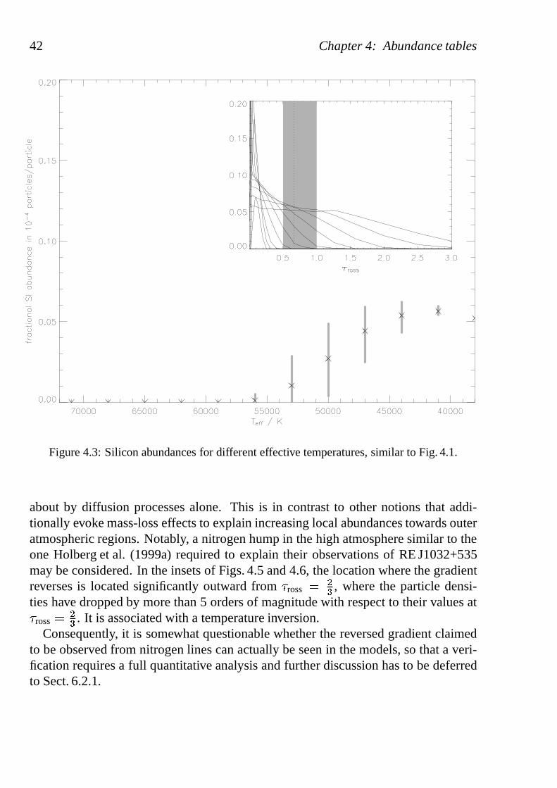
42 Chapter 4: Abundance tables
Figure 4.3: Silicon abundances for different effective temperatures, similar to Fig. 4.1.
about by diffusion processes alone. This is in contrast to other notions that addi-tionally evoke mass-loss effects to explain increasing local abundances towards outeratmospheric regions. Notably, a nitrogen hump in the high atmosphere similar to theone Holberg et al. (1999a) required to explain their observations of RE J1032+535may be considered. In the insets of Figs. 4.5 and 4.6, the location where the gradientreverses is located significantly outward from� ross �
�� , where the particle densi-
ties have dropped by more than 5 orders of magnitude with respect to their values at� ross �
�� . It is associated with a temperature inversion.
Consequently, it is somewhat questionable whether the reversed gradient claimedto be observed from nitrogen lines can actually be seen in themodels, so that a veri-fication requires a full quantitative analysis and further discussion has to be deferredto Sect. 6.2.1.
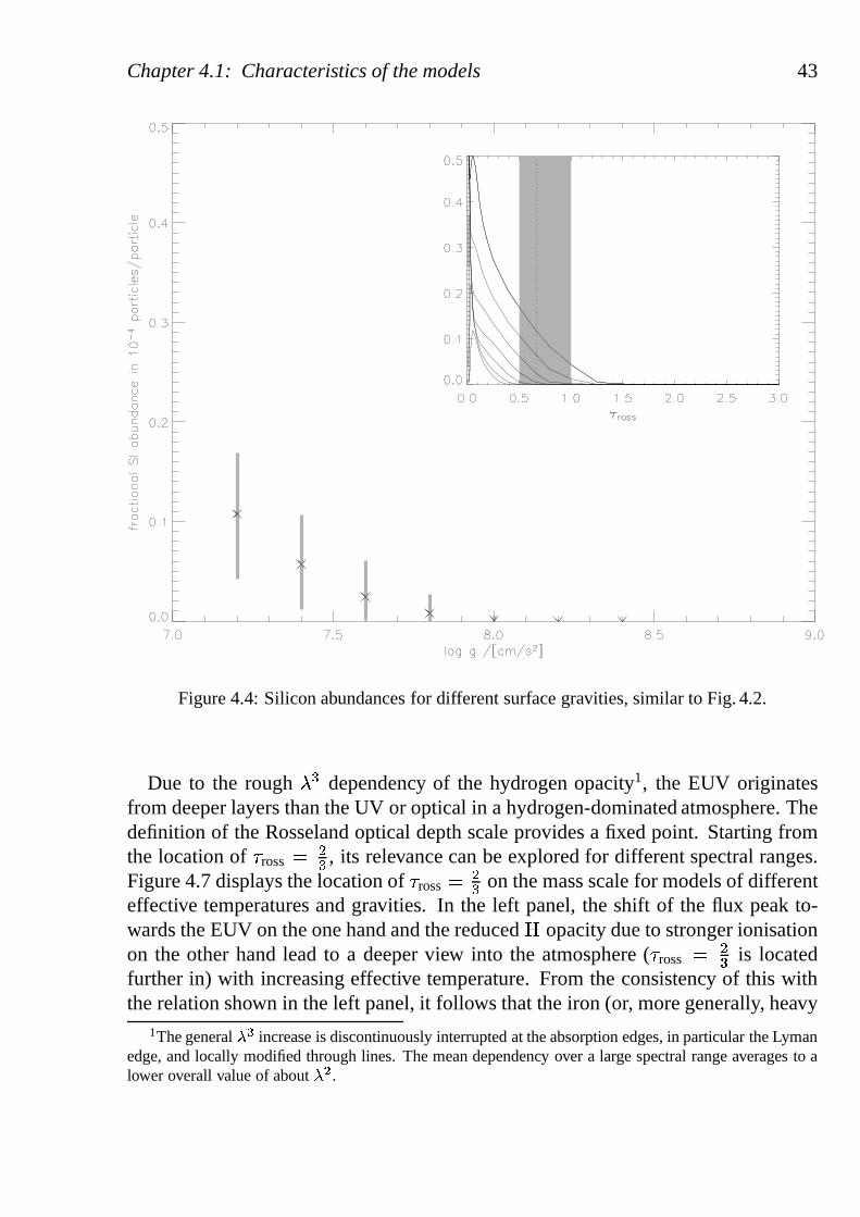
Chapter 4.1: Characteristics of the models 43
Figure 4.4: Silicon abundances for different surface gravities, similar to Fig. 4.2.
Due to the rough��
dependency of the hydrogen opacity1, the EUV originatesfrom deeper layers than the UV or optical in a hydrogen-dominated atmosphere. Thedefinition of the Rosseland optical depth scale provides a fixed point. Starting fromthe location of� ross �
�� , its relevance can be explored for different spectral ranges.
Figure 4.7 displays the location of� ross ��� on the mass scale for models of different
effective temperatures and gravities. In the left panel, the shift of the flux peak to-wards the EUV on the one hand and the reduced� opacity due to stronger ionisationon the other hand lead to a deeper view into the atmosphere (� ross �
�� is located
further in) with increasing effective temperature. From the consistency of this withthe relation shown in the left panel, it follows that the iron(or, more generally, heavy
1The general� �
increase is discontinuously interrupted at the absorptionedges, in particular the Lymanedge, and locally modified through lines. The mean dependency over a large spectral range averages to alower overall value of about
� �.
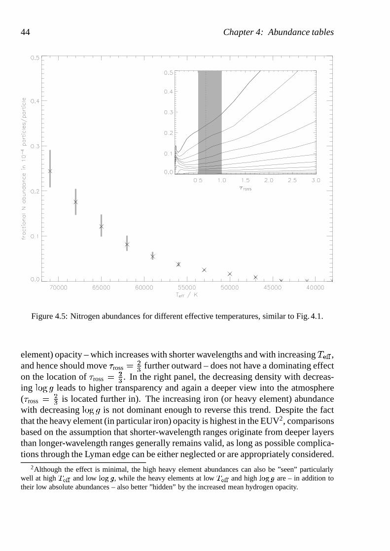
44 Chapter 4: Abundance tables
Figure 4.5: Nitrogen abundances for different effective temperatures, similar to Fig. 4.1.
element) opacity – which increases with shorter wavelengths and with increasing� � �
,and hence should move� ross �
�� further outward – does not have a dominating effect
on the location of� ross ��� . In the right panel, the decreasing density with decreas-
ing� � �
� leads to higher transparency and again a deeper view into theatmosphere(� ross �
�� is located further in). The increasing iron (or heavy element) abundance
with decreasing� � �
� is not dominant enough to reverse this trend. Despite the factthat the heavy element (in particular iron) opacity is highest in the EUV2, comparisonsbased on the assumption that shorter-wavelength ranges originate from deeper layersthan longer-wavelength ranges generally remains valid, aslong as possible complica-tions through the Lyman edge can be either neglected or are appropriately considered.
2Although the effect is minimal, the high heavy element abundances can also be ”seen” particularlywell at high� � � and low � � �
, while the heavy elements at low� � � and high� � �are – in addition to
their low absolute abundances – also better ”hidden” by the increased mean hydrogen opacity.
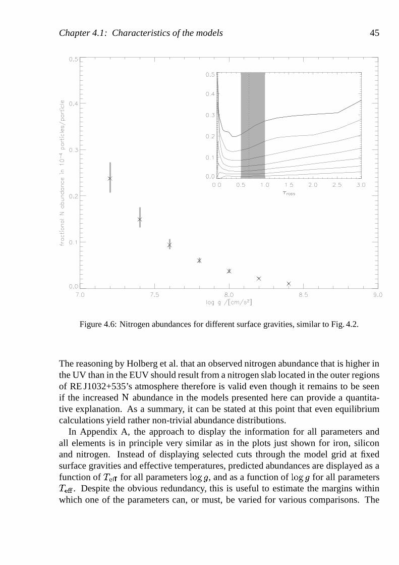
Chapter 4.1: Characteristics of the models 45
Figure 4.6: Nitrogen abundances for different surface gravities, similar to Fig. 4.2.
The reasoning by Holberg et al. that an observed nitrogen abundance that is higher inthe UV than in the EUV should result from a nitrogen slab located in the outer regionsof RE J1032+535’s atmosphere therefore is valid even thoughit remains to be seenif the increased� abundance in the models presented here can provide a quantita-tive explanation. As a summary, it can be stated at this pointthat even equilibriumcalculations yield rather non-trivial abundance distributions.
In Appendix A, the approach to display the information for all parameters andall elements is in principle very similar as in the plots justshown for iron, siliconand nitrogen. Instead of displaying selected cuts through the model grid at fixedsurface gravities and effective temperatures, predicted abundances are displayed as afunction of
� � �for all parameters
� � �� , and as a function of
� � �� for all parameters� � �
. Despite the obvious redundancy, this is useful to estimatethe margins withinwhich one of the parameters can, or must, be varied for various comparisons. The
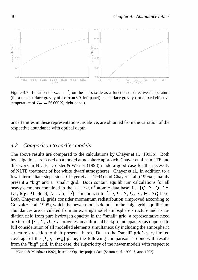
46 Chapter 4: Abundance tables
Figure 4.7: Location of� ross ��� on the mass scale as a function of effective temperature
(for a fixed surface gravity of� � � � � 8.0, left panel) and surface gravity (for a fixed effectivetemperature of� � � � 56 000 K, right panel).
uncertainties in these representations, as above, are obtained from the variation of therespective abundance with optical depth.
4.2 Comparison to earlier models
The above results are compared to the calculations by Chayeret al. (1995b). Bothinvestigations are based on a model atmosphere approach, Chayer et al.’s in LTE andthis work in NLTE. Dreizler & Werner (1993) made a good case for the necessityof NLTE treatment of hot white dwarf atmospheres. Chayer et al., in addition to afew intermediate steps since Chayer et al. (1994) and Chayeret al. (1995a), mainlypresent a ”big” and a ”small” grid. Both contain equilibriumcalculations for allheavy elements contained in theTOPBASE3 atomic data base, i.e. � , � , � , � � ,� , � �
, � �, � � , � , � � , � , � � � – in contrast to � � , � , � , � , � � , � � , � � � here.
Both Chayer et al. grids consider momentum redistribution (improved according toGonzalez et al. 1995), which the newer models do not. In the ”big” grid, equilibriumabundances are calculated from an existing model atmosphere structure and its ra-diation field from pure hydrogen opacity; in the ”small” grid, a representative fixedmixture of � , � , � , � � � provides an additional background opacity (as opposed tofull consideration of all modelled elements simultaneously including the atmosphericstructure’s reaction to their presence here). Due to the ”small” grid’s very limitedcoverage of the [
� � �,
� � �� ] plane, the following comparison is done with results
from the ”big” grid. In that case, the superiority of the newer models with respect to3Cunto & Mendoza (1992), based on Opacity project data (Seaton et al. 1992; Seaton 1992).
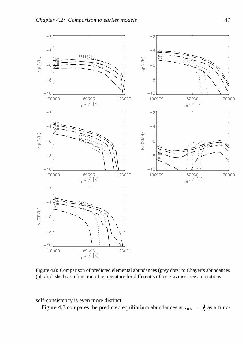
Chapter 4.2: Comparison to earlier models 47
Figure 4.8: Comparison of predicted elemental abundances (grey dots) to Chayer’s abundances(black dashed) as a function of temperature for different surface gravities: see annotations.
self-consistency is even more distinct.Figure 4.8 compares the predicted equilibrium abundances at � ross �
�� as a func-
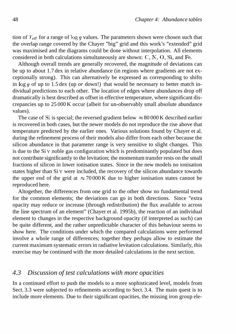
48 Chapter 4: Abundance tables
tion of� � �
for a range of� � �
� values. The parameters shown were chosen such thatthe overlap range covered by the Chayer ”big” grid and this work’s ”extended” gridwas maximised and the diagrams could be done without interpolation. All elementsconsidered in both calculations simultaneously are shown:� , � , � , � � , and� � .
Although overall trends are generally recovered, the magnitude of deviations canbe up to about 1.7 dex in relative abundance (in regions wheregradients are not ex-ceptionally strong). This can alternatively be expressed as corresponding to shiftsin
� � �� of up to 1.5 dex (upor down!) that would be necessary to better match in-
dividual predictions to each other. The location of edges where abundances drop offdramatically is best described as offset in effective temperature, where significant dis-crepancies up to 25 000 K occur (albeit for un-observably small absolute abundancevalues).
The case of� � is special; the reversed gradient below�
80 000 K described earlieris recovered in both cases, but the newer models do not reproduce the rise above thattemperature predicted by the earlier ones. Various solutions found by Chayer et al.during the refinement process of their models also differ from each other because thesilicon abundance in that parameter range is very sensitiveto slight changes. Thisis due to the SiV noble gas configuration which is predominantly populated but doesnot contribute significantly to the levitation; the momentum transfer rests on the smallfractions of silicon in lower ionisation states. Since in the new models no ionisationstates higher than SiV were included, the recovery of the silicon abundance towardsthe upper end of the grid at
�70 000 K due to higher ionisation states cannot be
reproduced here.Altogether, the differences from one grid to the other show no fundamental trend
for the common elements; the deviations can go in both directions. Since ”extraopacity may reduce or increase (through redistribution) the flux available to acrossthe line spectrum of an element” (Chayer et al. 1995b), the reaction of an individualelement to changes in the respective background opacity (ifinterpreted as such) canbe quite different, and the rather unpredictable characterof this behaviour seems toshow here. The conditions under which the compared calculations were performedinvolve a whole range of differences; together they perhapsallow to estimate thecurrent maximum systematic errors in radiative levitationcalculations. Similarly, thisexercise may be continued with the more detailed calculations in the next section.
4.3 Discussion of test calculations with more opacities
In a continued effort to push the models to a more sophisticated level, models fromSect. 3.3 were subjected to refinements according to Sect. 3.4. The main quest is toinclude more elements. Due to their significant opacities, the missing iron group ele-
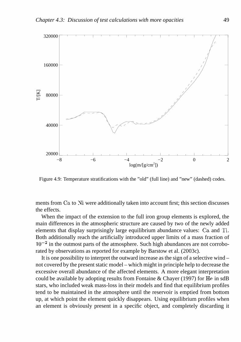
Chapter 4.3: Discussion of test calculations with more opacities 49
−8 −6 −4 −2 0 2log(m/[g/cm2])
20000
40000
80000
160000
320000T
/[K]
Figure 4.9: Temperature stratifications with the ”old” (full line) and ”new” (dashed) codes.
ments from� to � � were additionally taken into account first; this section discussesthe effects.
When the impact of the extension to the full iron group elements is explored, themain differences in the atmospheric structure are caused bytwo of the newly addedelements that display surprisingly large equilibrium abundance values:� and � � .Both additionally reach the artificially introduced upper limits of a mass fraction of� � �
�in the outmost parts of the atmosphere. Such high abundancesare not corrobo-
rated by observations as reported for example by Barstow et al. (2003c).It is one possibility to interpret the outward increase as the sign of a selective wind –
not covered by the present static model – which might in principle help to decrease theexcessive overall abundance of the affected elements. A more elegant interpretationcould be available by adopting results from Fontaine & Chayer (1997) for� � in sdBstars, who included weak mass-loss in their models and find that equilibrium profilestend to be maintained in the atmosphere until the reservoir is emptied from bottomup, at which point the element quickly disappears. Using equilibrium profiles whenan element is obviously present in a specific object, and completely discarding it
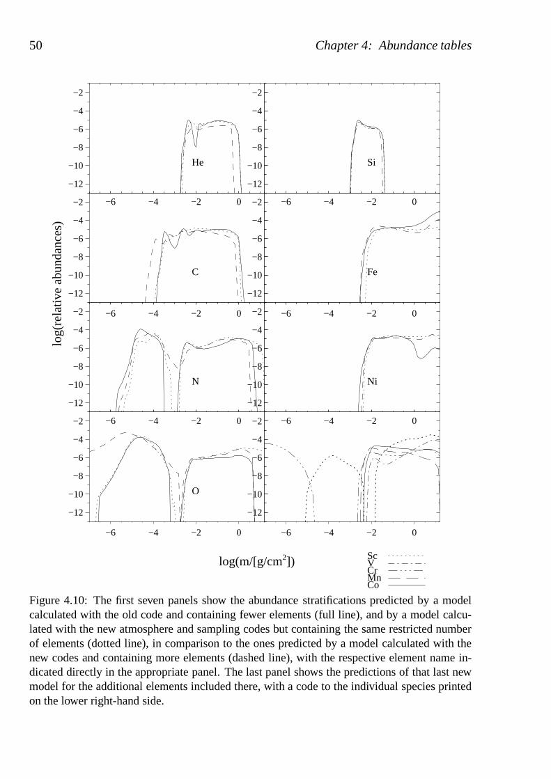
50 Chapter 4: Abundance tables
log(m/[g/cm2])
log(
rela
tive
abun
danc
es) −6 −4 −2 0
−12
−10
−8
−6
−4
−2
He
−6 −4 −2 0
−12
−10
−8
−6
−4
−2
Si
−6 −4 −2 0
−12
−10
−8
−6
−4
−2
C
−6 −4 −2 0
−12
−10
−8
−6
−4
−2
Fe
−6 −4 −2 0
−12
−10
−8
−6
−4
−2
N
−6 −4 −2 0
−12
−10
−8
−6
−4
−2
Ni
−6 −4 −2 0
−12
−10
−8
−6
−4
−2
O
−6 −4 −2 0
−12
−10
−8
−6
−4
−2
ScVCrMnCo
Figure 4.10: The first seven panels show the abundance stratifications predicted by a modelcalculated with the old code and containing fewer elements (full line), and by a model calcu-lated with the new atmosphere and sampling codes but containing the same restricted numberof elements (dotted line), in comparison to the ones predicted by a model calculated with thenew codes and containing more elements (dashed line), with the respective element name in-dicated directly in the appropriate panel. The last panel shows the predictions of that last newmodel for the additional elements included there, with a code to the individual species printedon the lower right-hand side.
Chapter 4.3: Discussion of test calculations with more opacities 51
otherwise, may therefore be an acceptable choice.Based on such considerations the addition of more elements was restricted to the
iron group elements without� and� � for the time being. This modification leads tochanges in the structure of the test model such as the slight alteration of the temper-ature structure shown in Fig. 4.9 and results in new abundance profiles as illustratedby Fig. 4.10. All results are for models with
� � �� 56 000 K and
� � �� � 7.6: one
taken directly from Sect. 3.3 for comparison (old code, old model atoms; ”old” modelrepresented by a full line), one calculated with the new codeand partially modifiedatomic data (but with no further elements included; dotted line), and one with addi-tional elements as discussed above (”new” model represented by a dashed line). Thiskey is valid for the elements common to all three models, while the abundance pre-dictions for the add-on elements as shown in the last panel ofFig. 4.10 are labelledindividually.
Since the new code has been thoroughly tested to give identical results for un-changed input data, the impact of the first step (compare the full and the dotted lines)must be attributed to the different methods of preparation of atomic input data (forthe same list of elements; details were given in Sect. 2.5).
The effect of adding more elements in the second step leads tothe differences inpredicted equilibrium abundances as shown using dashed lines. While for all ele-ments that are common to the three models the shapes of the equilibrium profiles arefairly similar in all cases, the absolute abundances in numbers at a given depth pointcan differ substantially, mainly due to the steep gradientsinvolved. It will thereforedepend heavily on the formation region of any given line how much its shape will beaffected.
The inclusion of further heavy elements does not affect the stratification profiles ofthose previously considered in a straightforward manner. In particular, the notion thatadditional elements with important opacity over a large wavelength range might leadto considerable flux blocking, reducing the relative abundance of similar species sothat only the total of heavy elements supported remains at a given level, proves to bewrong. The effects of flux redistribution do not lead to a ”saturation”, instead everynew element reaches approximately the same level as those already present (see lastpanel) and basically adds to the total opacity.
By comparing all results and evaluating the scale of the deviation, ”systematic”errors can be derived that amount to up to 2 dex uncertainty (plus a much larger de-viation for � in the outmost regions). This value is of the same order of magnitudeas in the last section, where Chayer et al. models were compared to current results. Itreflects the degree to which the predictions can perhaps be considered trustworthy, byestimating the influence from various modelling-dependenteffects.
52 Chapter 4: Abundance tables
CHAPTER 5
Analysis of spectroscopic EUVE data
The following is largely based on Schuh, Dreizler & Wolff (2002), with a few en-hancements in the contents, and with some subsections omitted or moved to otherparts in this thesis where they fit better. The contributionsof the co-authors to thiswork were the data reduction of the EUVE spectra performed byB. Wolff, whileS. Dreizler provided the diffusion code used to calculate the model grid. In compari-son to the analysis by Schuh (2000), this full reanalysis is based on a more completemodel grid (although not identical to the ”extended” model grid) and improved visualmagnitudes for the objects (taken from the literature).
5.1 Introduction
The basic physical mechanisms leading to the element stratification have long beenknown, so their actual modelling appears preferable to an adhoc approach. Chayeret al. (1995a,b) were the first to calculate an extensive model grid for white dwarfspredicting the chemical stratification assuming equilibrium between gravitational set-tling and radiative levitation. An improvement has now beenachieved through theintroduction of self-consistent NLTE model atmospheres which account for the cou-pling between chemical stratification and the radiation field (Dreizler 1999). Thesuccessful application of these models to the EUVE spectrumof G 191–B2B (Drei-zler & Wolff 1999) has motivated a more systematic analysis of a larger sample ofhot DA white dwarfs which we present here.
The investigation in this chapter exploits EUVE spectra anddiscusses the resultswith respect to parameter determinations in the optical. The following Chapter 6will deal with the UV wavelength ranges and give detailed metal abundance patternpredictions. The availability of EUVE spectra defines, as inWolff et al. (1998), theoverall sample, which is more thoroughly introduced in Sect. 5.2. The observationsand particular considerations concerning the interstellar medium are shortly describedthere as well. Sect. 5.3 recapitulates the principle of the model calculations as dis-cussed at some length in Chapter 2; for characteristics of the model grid computed
53
54 Chapter 5: Analysis of spectroscopic EUVE data
for comparison with the sample on hand we refer back to Chapters 3 and 4. The meth-ods and results from fitting the new class of theoretical spectra to the observations arepresented in Sect. 5.4. The implications of these results are discussed in Sect. 5.5.
5.2 EUVE observations of hot DA white dwarfs
5.2.1 The EUV selected DA sample
Generally speaking, the maximum spectral flux of hot WDs liesin the extreme ultra-violet (EUV). The fact that the main opacity of heavy elements at these temperaturestends to lie in the same range means that radiative acceleration can sustain traces ofthem in the atmosphere, but it also implies that the EUV is thebest suited spectralrange for the detection of these elements. Consequently, westart by surveying EUVEspectra, even though the spectral resolutions of its instruments are not high enoughto identify individual lines. The element-by-element identification is best deferredto high-resolution UV or FUV studies. The new models do not a priori require lineidentification, although it would in principle be desirableto be able to do that evenin the EUV. They impose no need for the use of a pre-defined metal mix (as usedby Wolff et al. 1998), nor do they require the adjustment of a scaling factor as inBarstow et al. (1997), as the abundances are not free parameters but are derived froman equilibrium condition (see Sect. 5.3). As the EUV flux is very sensitive to thechemical composition of the photosphere, a comparison in this regime is extremelyuseful to test the predictions of the diffusion models. Interpreting the repeated anal-ysis as a test case for the models, it is reasonable to start out by following previousinvestigations as closely as possible. For this reason, we chose to use the 26 DAspreviously analysed by Wolff (1999).
This sample comprises all hot (� � � � 40 000 K) DA white dwarfs with EUVE
observations, which were mostly taken from the EUVE public archive (now availableat the multi-mission data archive at STScI). The data sets and the reduction proceduresare described elsewhere (Wolff et al. 1998; Wolff 1999); those publications also showthe reduced spectra in the form used here, i.e. flux calibrated SW, MW and LW1 dataconcatenated to yield a single spectrum.
The effective temperatures of the sample stars lie above� � �
� 40 000 K, wherephotospheric metal abundances are still large enough to be detectable. Above� � �
� 70 000 K, mass-loss effects might start to disturb the expected equilibrium be-tween gravitational and radiative acceleration (Unglaub &Bues 1998), but the samplecontains no stars hotter than that. Wolff et al. (1998) have grouped the objects into
1SW (short-wavelength spectrometer, 70A – 190A, 0.5A resolution), MW (medium-wavelength spec-trometer, 140A – 380A, 1.0A resolution), and LW (long-wavelength spectrometer, 280A – 760A, 2.0Aresolution) refer to data from three different instrumentson-board the EUVE satellite.
Chapter 5.3: Equilibrium abundances from stratified model atmospheres 55
four different categories. The first set consists of G 191–B2B like objects, where thehigh metallicity yields a steep flux drop towards short wavelengths, beyond the inter-stellar HeII absorption edge. The second group includes GD 246 and similar objectswhich contain fewer photospheric metals, but still more than those in the third groupwhose spectra Wolff et al. could fit with pure hydrogen atmospheres. A fourth ratherinhomogeneous set compiles the remaining objects. For details, especially on the ef-fective temperature, surface gravity and metallicity region in parameter space coveredby the different groups, we refer once more to Wolff (1999).
5.2.2 Treatment of the ISM
The interstellar medium (ISM) considerably attenuates thestellar flux in the EUV.The most important features are the HI, HeI and HeII bound-free ground state ab-sorptions with edges at 911.7A, 504.3A and 227.8A, respectively. This is beingaccounted for in the same way as in Wolff et al. (1998): The effect of given inter-stellar column densities on the theoretical fluxes is modelled and applied followingRumph et al. (1994). The derivation of HI column density depends on the effectivetemperature of the model used, and the HeI and HeII column densities on its ab-sorber content. Due to the interrelation of
� � �and N(HI) and the fact that the Lyman
edge lies outside the range observed by EUVE, Wolff et al. (1998) have started fromoptically determined effective temperatures (by Finley etal. 1997), and additionallyhave retained surface gravities from that analysis unchanged. In the present approach,we start from the effective temperatures from Wolff (1999) and adopt his HI columndensities unalteredly whenever possible.
Even though the HeI and HeII column densities have to be constantly modifiedduring the fitting procedure depending on the assumed photospheric parameters, allinterstellar contributions will in the following be treated as a secondary effect on thestellar light that can be dealt with independently of the analysis of the source itself,disregarding the fact that an appropriate correction can only be madeafter a set ofphotospheric parameters has been adopted. As the interstellar absorption is more im-portant at longer wavelengths while the absorption by photospheric metals increasestowards shorter wavelengths, the different contributionscan partly be separated.
5.3 Equilibrium abundances from stratified model atmospheres
5.3.1 Diffusion models
Our self-consistent diffusion models have been introducedin the previous chapters.Chayer et al. (1995a,b) have presented extensive results ofsimilar calculations forwhite dwarfs. Their predicted equilibrium abundances werenot quantitatively con-sistent with observations. This might be partly due to the fact that the observations
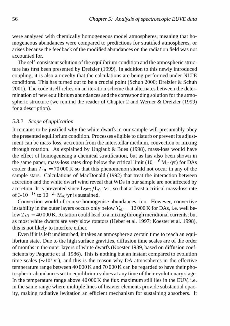
56 Chapter 5: Analysis of spectroscopic EUVE data
were analysed with chemically homogeneous model atmospheres, meaning that ho-mogeneous abundances were compared to predictions for stratified atmospheres, orarises because the feedback of the modified abundances on theradiation field was notaccounted for.
The self-consistent solution of the equilibrium conditionand the atmospheric struc-ture has first been presented by Dreizler (1999). In additionto this newly introducedcoupling, it is also a novelty that the calculations are being performed under NLTEconditions. This has turned out to be a crucial point (Schuh 2000; Dreizler & Schuh2001). The code itself relies on an iteration scheme that alternates between the deter-mination of new equilibrium abundances and the corresponding solution for the atmo-spheric structure (we remind the reader of Chapter 2 and Werner & Dreizler (1999)for a description).
5.3.2 Scope of application
It remains to be justified why the white dwarfs in our sample will presumably obeythe presented equilibrium condition. Processes eligible to disturb or prevent its adjust-ment can be mass-loss, accretion from the interstellar medium, convection or mixingthrough rotation. As explained by Unglaub & Bues (1998), mass-loss would havethe effect of homogenising a chemical stratification, but ashas also been shown inthe same paper, mass-loss rates drop below the critical limit (10� � � M� /yr) for DAscooler than
� � �� 70 000 K so that this phenomenon should not occur in any of the
sample stars. Calculations of MacDonald (1992) that treat the interaction betweenaccretion and the white dwarf wind reveal that WDs in our sample are not affected byaccretion. It is prevented since L� � � L� � 1, so that at least a critical mass-loss rateof 3�10� � � to 10�
� � M� /yr is sustained.Convection would of course homogenise abundances, too. However, convective
instability in the outer layers occurs only below� � �
� 12 000 K for DAs, i.e. well be-low
� � �� 40 000 K. Rotation could lead to a mixing through meridional currents; but
as most white dwarfs are very slow rotators (Heber et al. 1997; Koester et al. 1998),this is not likely to interfere either.
Even if it is left undisturbed, it takes an atmosphere a certain time to reach an equi-librium state. Due to the high surface gravities, diffusiontime scales are of the orderof months in the outer layers of white dwarfs (Koester 1989, based on diffusion coef-ficients by Paquette et al. 1986). This is nothing but an instant compared to evolutiontime scales (� 10� yr), and this is the reason why DA atmospheres in the effectivetemperature range between 40 000 K and 70 000 K can be regardedto have their pho-tospheric abundances set to equilibrium values at any time of their evolutionary stage.In the temperature range above 40 000 K the flux maximum still lies in the EUV, i.e.in the same range where multiple lines of heavier elements provide substantial opac-ity, making radiative levitation an efficient mechanism forsustaining absorbers. It
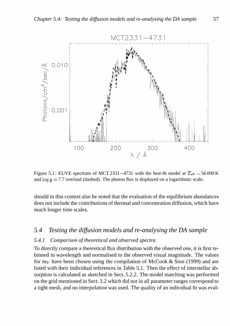
Chapter 5.4: Testing the diffusion models and re-analysingthe DA sample 57
Figure 5.1: EUVE spectrum of MCT 2331� 4731 with the best-fit model at� � � � 56 000 Kand � � � � � 7.7 overlaid (dashed). The photon flux is displayed on a logarithmic scale.
should in this context also be noted that the evaluation of the equilibrium abundancesdoes not include the contributions of thermal and concentration diffusion, which havemuch longer time scales.
5.4 Testing the diffusion models and re-analysing the DA sample
5.4.1 Comparison of theoretical and observed spectra
To directly compare a theoretical flux distribution with theobserved one, it is first re-binned in wavelength and normalised to the observed visual magnitude. The valuesfor m� have been chosen using the compilation of McCook & Sion (1999) and arelisted with their individual references in Table 5.1. Then the effect of interstellar ab-sorption is calculated as sketched in Sect. 5.2.2. The modelmatching was performedon the grid mentioned in Sect. 3.2 which did not in all parameter ranges correspond toa tight mesh, and no interpolation was used. The quality of anindividual fit was eval-
58 Chapter 5: Analysis of spectroscopic EUVE data
uated by eye. Of course, changing the interstellar� � column densities seemingly hasa big impact on the overall shape of the spectrum. However, the region most sensitiveto metal abundances lies at least partly beyond the HeII absorption edge, so once thisand the lower energy edges are fitted all remaining deviations have to be due to eithera different flux level as caused by the effective temperatureor a different amount ofabsorber content as regulated by the surface gravity in the equilibrium models.
5.4.2 Revised atmospheric parameters
The present model matching led to new atmospheric parameters where mainly thesurface gravities differ from former specifications. The improvement of many ofthe individual fits (see Fig. 5.3) as compared to fits with homogeneous models (inWolff et al. 1998; Wolff 1999; Dreizler & Wolff 1999) vindicates these adjustments.
With homogeneous models, discrepancies were encountered especially for highermetallicity stars in the shorter wavelength regimes, whichcould not be adjusted bya different metallicity value as this would have deteriorated the quality of the fit atother wavelengths. This difficulty is resolved with the new models, as they offer dif-ferent abundances at different formation depths. Consequently they can often betterreproduce especially these formerly delicate regions. Figure 5.1 shows an example.
Figure 5.3 displays all observations with the best-fit modelspectra over-plotted,both shown at 1A resolution. Table 5.1 lists the parameters of the best-fit model foreach object, along with the interstellar column densities used to produce the plots. Thelatter are to be regarded as very preliminary as fitting improved models to the spectramay yet again yield different values. High HeII column densities, found throughoutthe sample, may be an indication that in particular short-wavelength opacities arestill missing. The table additionally lists a quantity denoted� �
, which stands for themetal indexthat is introduced next.
5.4.3 Metal index
With depth-dependent abundances, it is difficult to quote one representative value foreach element (although problematic, we mostly retreat to using values at� ross �
��
in Chapter 4 and for the UV analysis in Chapter 6). To evade this problem here,we have introduced aphotospheric parameter-dependent quantity that relies entirelyon the predictions by diffusion theory. As explained above,the absorber content ofthe models is determined from the equilibrium between the radiative and the gravi-tational forces. The radiative acceleration scales with
� �� � due to the occurrence ofthe Eddington flux in Eq. 2.40, the effective gravitational acceleration scales with�as is evident from the upper expression in the same equation.The absorber contentshould thus be comparable along lines of constant
� �� � � � . To map this ratio onto a
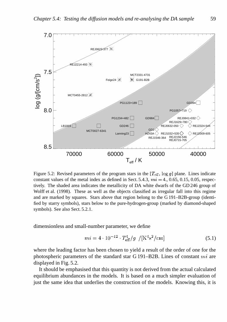
Chapter 5.4: Testing the diffusion models and re-analysingthe DA sample 59
70000 60000 50000 40000Teff / K
8.5
8.0
7.5
7.0lo
g (g
/[cm
/s2 ])
REJ2214-493
Feige24 G191-B2B
REJ0623-377
MCT2331-4731
MCT0455-2812
LB1919
MCT0027-6341
GD246
PG1234+482
PG1123+189
GD984
GD394
Lanning23GD2
REJ1032+535
REJ2324-544
REJ2156-546REJ2009-605
REJ0715-705
PG1057+719
HZ43A
REJ1546-364
REJ1629+780REJ0632-050
REJ0841+032
Figure 5.2: Revised parameters of the program stars in the [� � � , � � � � ] plane. Lines indicateconstant values of the metal index as defined in Sect. 5.4.3,�
�� 4., 0.65, 0.15, 0.05, respec-
tively. The shaded area indicates the metallicity of DA white dwarfs of the GD 246 group ofWolff et al. (1998). These as well as the objects classified asirregular fall into this regimeand are marked by squares. Stars above that region belong to the G 191–B2B-group (identi-fied by starry symbols), stars below to the pure-hydrogen-group (marked by diamond-shapedsymbols). See also Sect. 5.2.1.
dimensionless and small-number parameter, we define
� ��
� � � � � � � � � �� � � � � �� � � � � � � � (5.1)
where the leading factor has been chosen to yield a result of the order of one for thephotospheric parameters of the standard star G 191–B2B. Lines of constant� �
aredisplayed in Fig. 5.2.
It should be emphasised that this quantity is not derived from the actual calculatedequilibrium abundances in the models. It is based on a much simpler evaluation ofjust the same idea that underlies the construction of the models. Knowing this, it is
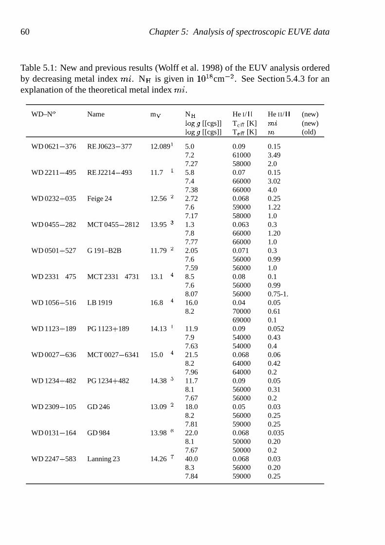
60 Chapter 5: Analysis of spectroscopic EUVE data
Table 5.1: New and previous results (Wolff et al. 1998) of theEUV analysis orderedby decreasing metal index� �
. N� is given in � � � � cm��. See Section 5.4.3 for an
explanation of the theoretical metal index� �.
WD–N� Name m� N� He I/�
He II /�
(new)� � �
[[cgs]] T� � [K] � � (new)� � �
[[cgs]] T� � [K] � (old)
WD 0621� 376 RE J0623� 377 12.089�
5.0 0.09 0.157.2 61000 3.497.27 58000 2.0
WD 2211� 495 RE J2214� 493 11.7�
5.8 0.07 0.157.4 66000 3.027.38 66000 4.0
WD 0232� 035 Feige 24 12.56�
2.72 0.068 0.257.6 59000 1.227.17 58000 1.0
WD 0455� 282 MCT 0455� 2812 13.95�
1.3 0.063 0.37.8 66000 1.207.77 66000 1.0
WD 0501� 527 G 191–B2B 11.79�
2.05 0.071 0.37.6 56000 0.997.59 56000 1.0
WD 2331� 475 MCT 2331� 4731 13.1 � 8.5 0.08 0.17.6 56000 0.998.07 56000 0.75-1.
WD 1056� 516 LB 1919 16.8 � 16.0 0.04 0.058.2 70000 0.61
69000 0.1WD 1123� 189 PG 1123� 189 14.13
�
11.9 0.09 0.0527.9 54000 0.437.63 54000 0.4
WD 0027� 636 MCT 0027� 6341 15.0 � 21.5 0.068 0.068.2 64000 0.427.96 64000 0.2
WD 1234� 482 PG 1234� 482 14.38 � 11.7 0.09 0.058.1 56000 0.317.67 56000 0.2
WD 2309� 105 GD 246 13.09�
18.0 0.05 0.038.2 56000 0.257.81 59000 0.25
WD 0131� 164 GD 984 13.98�
22.0 0.068 0.0358.1 50000 0.207.67 50000 0.2
WD 2247� 583 Lanning 23 14.26
40.0 0.068 0.038.3 56000 0.207.84 59000 0.25
Chapter 5.4: Testing the diffusion models and re-analysingthe DA sample 61
WD 0004� 330 GD 2 13.85�
82.4 0.068 0.018.25 50000 0.147.63 49000 � � � �
WD 2111� 498 GD 394 13.09�
6.5 0.07 0.157.9 40000 0.137.94 39600 0.25
WD 1314� 293 HZ 43A 12.914�
0.9 0.06 0.08.3 50000 0.137.99 50800 0.0
WD 1543� 366 RE J1546� 364 15.81� �
50.4 0.068 0.038.3 50000 0.138.88 45200 0.0
WD 1057� 719 PG 1057� 719 14.68�
20.7 0.068 0.0528.0 42000 0.127.90 41500 0.1
WD 0630� 050 RE J0632� 050 15.537�
30.1 0.01 0.0558.2 44000 0.098.39 44100 0.0
WD 1631� 781 RE J1629� 780 13.03� �
35.0 0.068 0.08.15 42000 0.097.79 44600 0.05
WD 0838� 035 RE J0841� 032 14.48�
16.0 0.068 0.0528.1 40000 0.087.78 38400 0.0
WD 2321� 549 RE J2324� 544 15.2�
9.5 0.05 0.068.2 42000 0.087.94 45000 0.05
WD 1029� 537 RE J1032� 535 14.455�
7.5 0.005 0.048.3 44000 0.087.77 44000 0.0
WD 2152� 548 RE J2156� 546 14.44�
7.0 0.04 0.048.3 44000 0.087.91 44000 0.0
WD 0715� 703 RE J0715� 705 14.178�
21.9 0.068 0.0158.3 44000 0.088.05 44000 0.0
WD 2004� 605 RE J2009� 605 13.6�
17.5 0.06 0.0158.3 42000 0.068.16 41900 0.0
�
Marsh et al. (1997a)�
Kidder et al. (1991)�
Barstow et al. (1994d)� Pounds et al. (1993)� Green
(1980)�
Wesemael & et al. (1995)
Vennes et al. (1997)�
Bergeron et al. (1992)�
Bohlin et al. (1995)� �
Vennes et al. (1996b)� �
Schwartz et al. (1995)
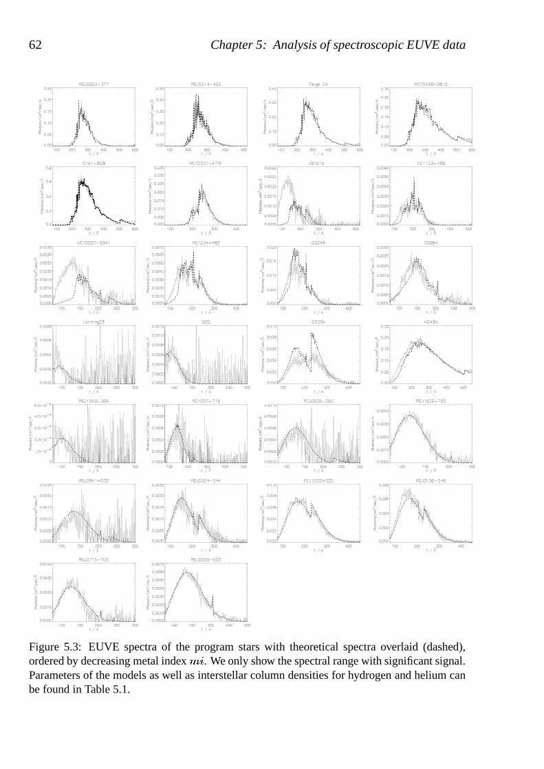
62 Chapter 5: Analysis of spectroscopic EUVE data
Figure 5.3: EUVE spectra of the program stars with theoretical spectra overlaid (dashed),ordered by decreasing metal index�
�. We only show the spectral range with significant signal.
Parameters of the models as well as interstellar column densities for hydrogen and helium canbe found in Table 5.1.
Chapter 5.5: Discussion 63
all the more surprising how well the metal indices� �at the newly determined pa-
rameters match the metallicities� that Wolff (1999) has derived for the objects.
5.5 Discussion
5.5.1 Summary
The new diffusion models can reproduce the observed EUV spectra of the majority ofthe hot DA white dwarfs in the sample. Since the models predict the chemical com-position from the equilibrium between sedimentation and radiative acceleration, thenumber of free stellar parameters is drastically reduced tothe effective temperatureand surface gravity only. The good agreement is a strong evidence that the interplayof these two processes defines the chemical composition and stratification. The agree-ment is, however, not in all cases better than with chemically homogeneous models,which requires a more detailed discussion.
Stars similar to G 191–B2B (the group one from Wolff et al. 1998) can be repro-duced significantly better with our self-consistent stratified models. This result is notsurprising since the first and successful application of these models to G 191–B2B(Dreizler & Wolff 1999) motivated this work in the first place. Our new models canalso reproduce the stars classified as pure hydrogen (group three from Wolff et al.1998), demonstrating that the vanishing of trace amounts ofmetals is correctly re-produced. Within this group, however, the surface gravity had to be increased by upto 0.5 dex in order to achieve a good fit (see also Table 5.1, andthe discussion inSect. 5.5.2).
The fits of PG 1123� 189, GD 246 and GD 984 are not completely satisfying butdeviations are of the same order as compared to fits with homogeneous models. Thefits for HZ 43A, RE J1032� 535, RE J2156� 546 and RE J2009� 605 are not quiteas good as the ones which could be achieved with spectra derived from the grid ofhomogeneous models. In four cases (LB 1919, MCT 0027� 6341, PG 1234� 482, andGD 394), using the new models results in a worse fit than before. These significantindividual deviations between models and observation could have physical reasons.As discussed in Sect. 5.3.2, competing processes can disturb the equilibrium betweenradiative acceleration and gravitational settling. As is evident from the overall good fitof our models, these are unimportant in general but individual exceptions are possible.In the case of LB 1919 for example, an unusually high rotationrate has been suspected(Finley et al. 1997).
5.5.2 Remarks on� and � � � �
As mentioned above, our surface gravities are in several cases higher than in earlieranalyses. Those analyses had evaluated the Balmer line profiles for a determination
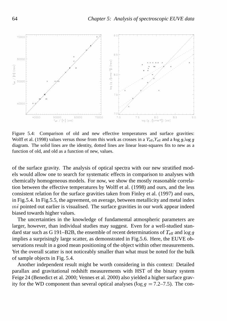
64 Chapter 5: Analysis of spectroscopic EUVE data
Figure 5.4: Comparison of old and new effective temperatures and surface gravities:Wolff et al. (1998) values versus those from this work as crosses in a� eff,� eff and a� � � � ,� � � �diagram. The solid lines are the identity, dotted lines are linear least-squares fits to new as afunction of old, and old as a function of new, values.
of the surface gravity. The analysis of optical spectra withour new stratified mod-els would allow one to search for systematic effects in comparison to analyses withchemically homogeneous models. For now, we show the mostly reasonable correla-tion between the effective temperatures by Wolff et al. (1998) and ours, and the lessconsistent relation for the surface gravities taken from Finley et al. (1997) and ours,in Fig.5.4. In Fig.5.5, the agreement, on average, between metallicity and metal index� �
pointed out earlier is visualised. The surface gravities inour work appear indeedbiased towards higher values.
The uncertainties in the knowledge of fundamental atmospheric parameters arelarger, however, than individual studies may suggest. Evenfor a well-studied stan-dard star such as G 191–B2B, the ensemble of recent determinations of
�eff and
� � ��
implies a surprisingly large scatter, as demonstrated in Fig.5.6. Here, the EUVE ob-servations result in a good mean positioning of the object within other measurements.Yet the overall scatter is not noticeably smaller than what must be noted for the bulkof sample objects in Fig. 5.4.
Another independent result might be worth considering in this context: Detailedparallax and gravitational redshift measurements with HSTof the binary systemFeige 24 (Benedict et al. 2000; Vennes et al. 2000) also yielded a higher surface grav-ity for the WD component than several optical analyses (
� � �� � 7.2–7.5). The con-
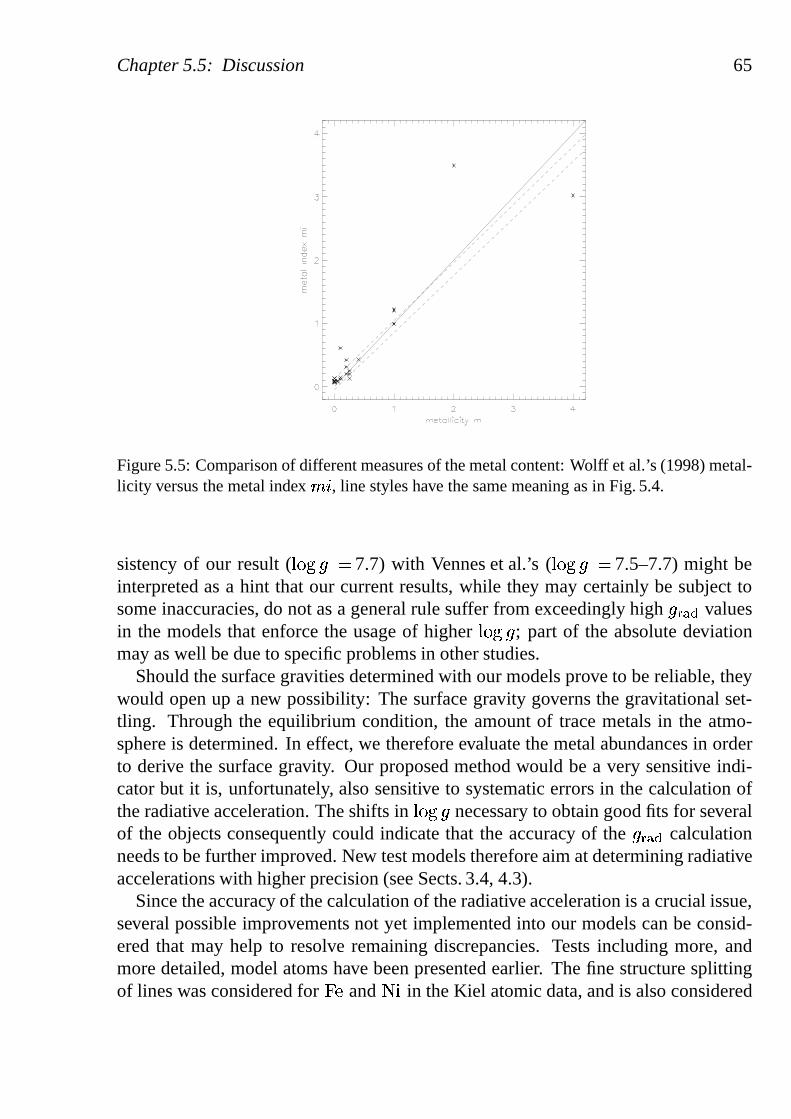
Chapter 5.5: Discussion 65
Figure 5.5: Comparison of different measures of the metal content: Wolff et al.’s (1998) metal-licity versus the metal index�
�, line styles have the same meaning as in Fig. 5.4.
sistency of our result (� � �
� � 7.7) with Vennes et al.’s (� � �
� � 7.5–7.7) might beinterpreted as a hint that our current results, while they may certainly be subject tosome inaccuracies, do not as a general rule suffer from exceedingly high � � � � valuesin the models that enforce the usage of higher
� � �� ; part of the absolute deviation
may as well be due to specific problems in other studies.Should the surface gravities determined with our models prove to be reliable, they
would open up a new possibility: The surface gravity governsthe gravitational set-tling. Through the equilibrium condition, the amount of trace metals in the atmo-sphere is determined. In effect, we therefore evaluate the metal abundances in orderto derive the surface gravity. Our proposed method would be avery sensitive indi-cator but it is, unfortunately, also sensitive to systematic errors in the calculation ofthe radiative acceleration. The shifts in
� � �� necessary to obtain good fits for several
of the objects consequently could indicate that the accuracy of the � � � � calculationneeds to be further improved. New test models therefore aim at determining radiativeaccelerations with higher precision (see Sects. 3.4, 4.3).
Since the accuracy of the calculation of the radiative acceleration is a crucial issue,several possible improvements not yet implemented into ourmodels can be consid-ered that may help to resolve remaining discrepancies. Tests including more, andmore detailed, model atoms have been presented earlier. Thefine structure splittingof lines was considered for� � and� � in the Kiel atomic data, and is also considered
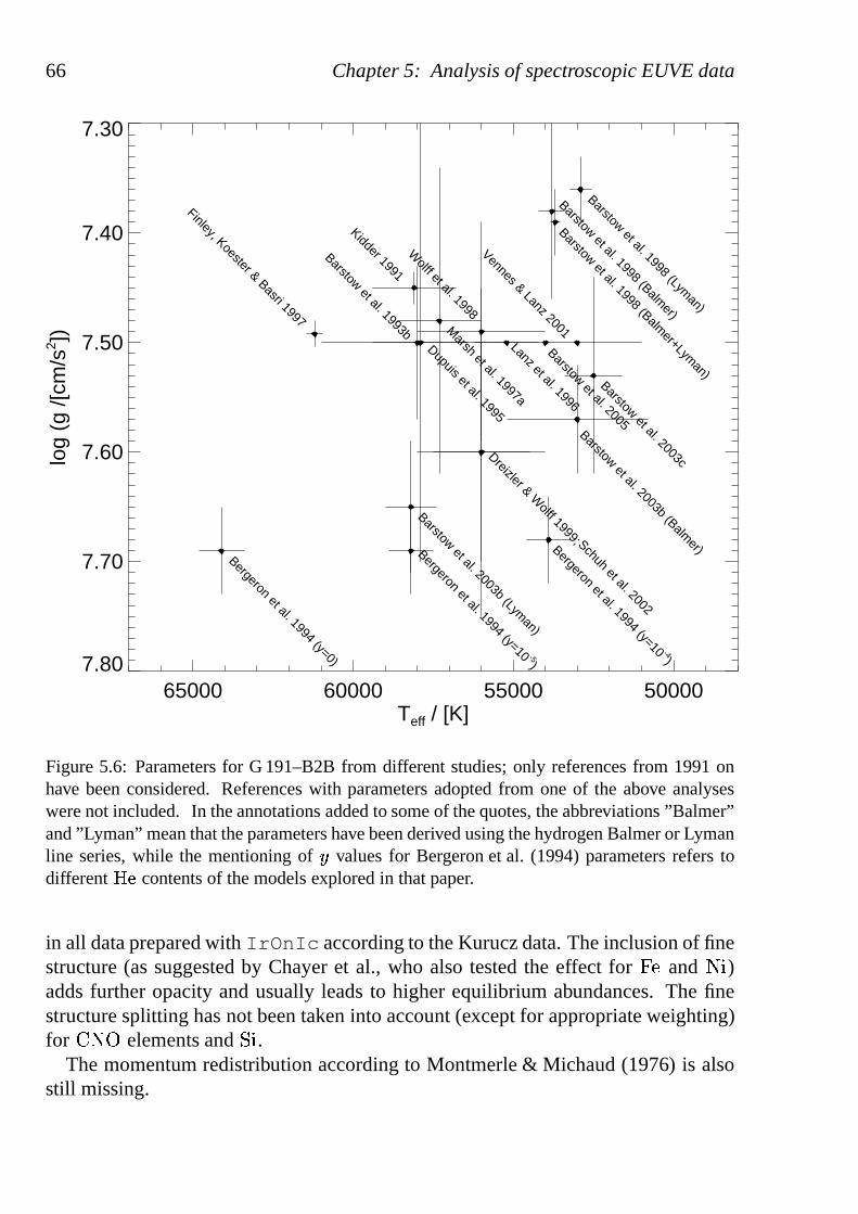
66 Chapter 5: Analysis of spectroscopic EUVE data
65000 60000 55000 50000Teff / [K]
7.80
7.70
7.60
7.50
7.40
7.30
log
(g /[
cm/s
2 ])
Kidder 1991
Barstow et al. 1993b
Bergeron et al. 1994 (y=0)
Bergeron et al. 1994 (y=10 -5)
Bergeron et al. 1994 (y=10 -4)
Dupuis et al. 1995
Lanz et al. 1996
Finley, Koester & Basri 1997
Barstow et al. 1998 (Balmer+Lym
an)
Barstow et al. 1998 (Balmer)
Barstow et al. 1998 (Lyman)
Wolff et al. 1998
Dreizler & Wolff 1999;
Vennes & Lanz 2001
Schuh et al. 2002
Barstow et al. 2003b (Balmer)
Barstow et al. 2003b (Lyman)
Barstow et al. 2003c
Barstow et al. 2005
Marsh et al. 1997a
Figure 5.6: Parameters for G 191–B2B from different studies; only references from 1991 onhave been considered. References with parameters adopted from one of the above analyseswere not included. In the annotations added to some of the quotes, the abbreviations ”Balmer”and ”Lyman” mean that the parameters have been derived usingthe hydrogen Balmer or Lymanline series, while the mentioning of� values for Bergeron et al. (1994) parameters refers todifferent � � contents of the models explored in that paper.
in all data prepared withIrOnIc according to the Kurucz data. The inclusion of finestructure (as suggested by Chayer et al., who also tested theeffect for � � and � � )adds further opacity and usually leads to higher equilibrium abundances. The finestructure splitting has not been taken into account (exceptfor appropriate weighting)for � � � elements and� � .
The momentum redistribution according to Montmerle & Michaud (1976) is alsostill missing.
Chapter 5.5: Discussion 67
5.5.3 Outlook
We have presented our chemically stratified model atmospheres describing the chem-ical composition through the equilibrium between gravitational settling and radiativeacceleration self-consistently. The application to 26 EUVE spectra of hot DA whitedwarfs has revealed an overall good agreement, demonstrating the potential of thesenew models.
In Chapter 6, we will discuss the derived parameters for individual objects in thecontext of an analysis of the metal lines observable in UV spectra. This will also be animportant test for the consistency of atmospheric parameters derived from differentparts of the spectrum, which often poses a problem. While analyses with chemicallyhomogeneous models may be biased due to systematic errors introduced through theneglect of stratification, the parameters presented here may be subject to systematicerrors due to the fixed photospheric abundances and might also not stand on excep-tionally firm ground yet.
Likewise, the determination of the interstellar column densities has to be regardedas preliminary, since these cannot be determined independently from the theoreticalspectra.
68 Chapter 5: Analysis of spectroscopic EUVE data
CHAPTER 6
Abundance analysis in the UV
6.1 Graphical representation of the results
In this chapter, the abundance values predicted by the diffusion models in a givenphotospheric layer are compared to results from analyses using established modelmatching techniques applied to abundance determinations from UV observations.This comparison uses photospheric parameters for a 25-object sample analysed andpublished by Barstow et al. (2003c) that, with 14 common stars, partly overlaps theEUVE sample in Chapter 5. Effective temperatures, surface gravities, and metal abun-dances were derived from IUE, HST, and FUSE spectra using a� �
fitting technique.For 7 objects only IUE spectra, for 3 objects only HST-GHRS spectra were available,while for the bulk of 14 objects HST-STIS spectra could be used. Both types of HSTspectra were in five cases supplemented by IUE data for betterspectral coverage.For one object a FUSE spectrum was used (PG 1342� 444, based on Barstow et al.2002). A comprehensive determination of metal abundances from all FUSE spectraobtained for hot DA white dwarfs is work in progress (Barstowet al. 2001b, 2003a;Dupuis et al. 2003).
Barstow et al. (2003c) calculated both pure hydrogen and heavy element blanketedNLTE models, with homogeneous abundances of � � , � , � , � , � � , � � , � � � fixedat the values measured for G 191–B2B for the blanketed models, to determine
� � �
and� � �
� from Balmer line fitting to optical spectra. Theoretical spectra with variableabundances for the purpose of model fitting of the UV spectra were obtained by cal-culating formal solutions with the modified abundances based on the existing modelstructures for one element at a time (using the element list above). The [
� � �,� � �
� ]parameters from Balmer line fitting were restricted to thesevalues within narrowbounds during the abundance determination from the UV spectra.
In the following, the equilibrium abundances predicted by diffusion models at the� � �and
� � �� parameters given by Barstow et al. (2003c) are compared to their abun-
dances measured by model matching. The first set of figures (6.1 – 6.24, starting on
69
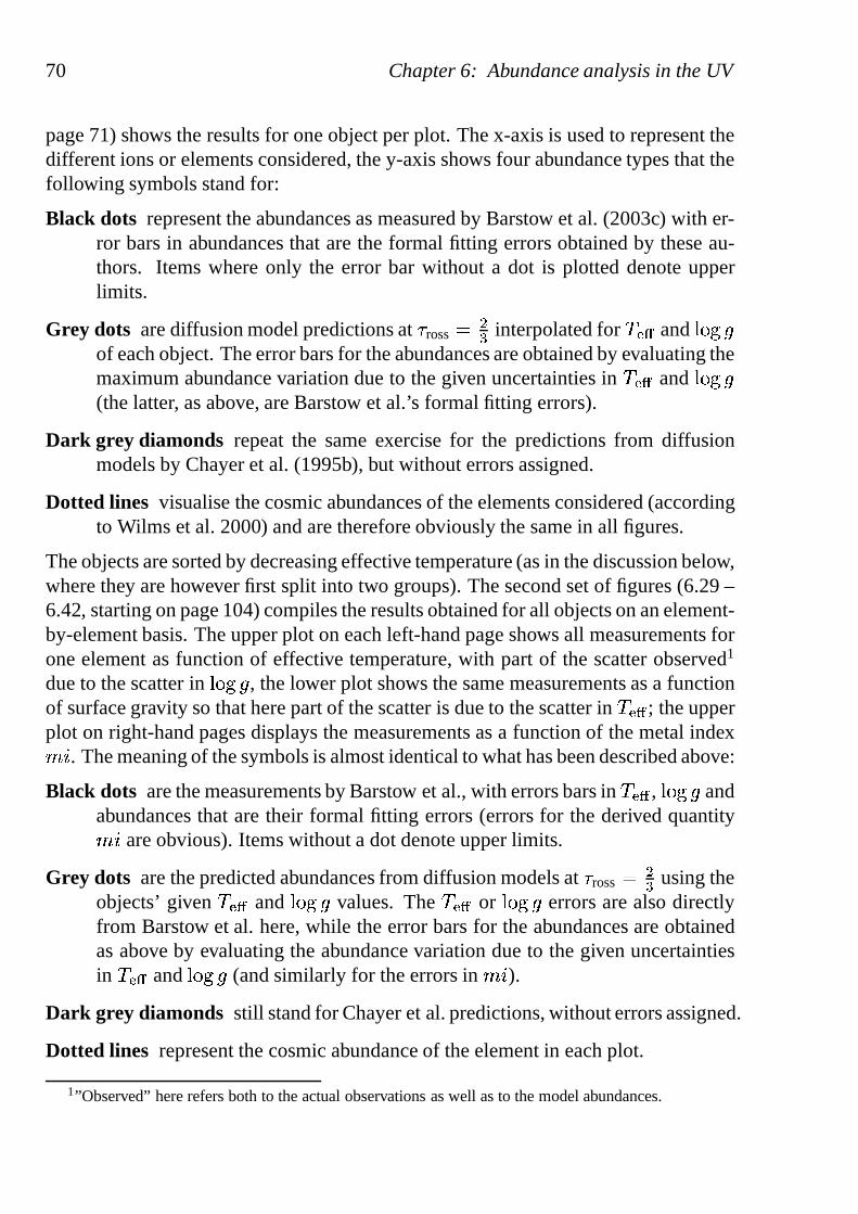
70 Chapter 6: Abundance analysis in the UV
page 71) shows the results for one object per plot. The x-axisis used to represent thedifferent ions or elements considered, the y-axis shows four abundance types that thefollowing symbols stand for:
Black dots represent the abundances as measured by Barstow et al. (2003c) with er-ror bars in abundances that are the formal fitting errors obtained by these au-thors. Items where only the error bar without a dot is plotteddenote upperlimits.
Grey dots are diffusion model predictions at� ross ��� interpolated for
� � �and
� � ��
of each object. The error bars for the abundances are obtained by evaluating themaximum abundance variation due to the given uncertaintiesin
� � �and
� � ��
(the latter, as above, are Barstow et al.’s formal fitting errors).
Dark grey diamonds repeat the same exercise for the predictions from diffusionmodels by Chayer et al. (1995b), but without errors assigned.
Dotted lines visualise the cosmic abundances of the elements considered(accordingto Wilms et al. 2000) and are therefore obviously the same in all figures.
The objects are sorted by decreasing effective temperature(as in the discussion below,where they are however first split into two groups). The second set of figures (6.29 –6.42, starting on page 104) compiles the results obtained for all objects on an element-by-element basis. The upper plot on each left-hand page shows all measurements forone element as function of effective temperature, with partof the scatter observed1
due to the scatter in� � �
� , the lower plot shows the same measurements as a functionof surface gravity so that here part of the scatter is due to the scatter in
� � �; the upper
plot on right-hand pages displays the measurements as a function of the metal index� �
. The meaning of the symbols is almost identical to what has been described above:
Black dots are the measurements by Barstow et al., with errors bars in� � �
,� � �
� andabundances that are their formal fitting errors (errors for the derived quantity� �
are obvious). Items without a dot denote upper limits.
Grey dots are the predicted abundances from diffusion models at� ross ��� using the
objects’ given� � �
and� � �
� values. The� � �
or� � �
� errors are also directlyfrom Barstow et al. here, while the error bars for the abundances are obtainedas above by evaluating the abundance variation due to the given uncertaintiesin
� � �and
� � �� (and similarly for the errors in� �
).
Dark grey diamonds still stand for Chayer et al. predictions, without errors assigned.
Dotted lines represent the cosmic abundance of the element in each plot.
1”Observed” here refers both to the actual observations as well as to the model abundances.
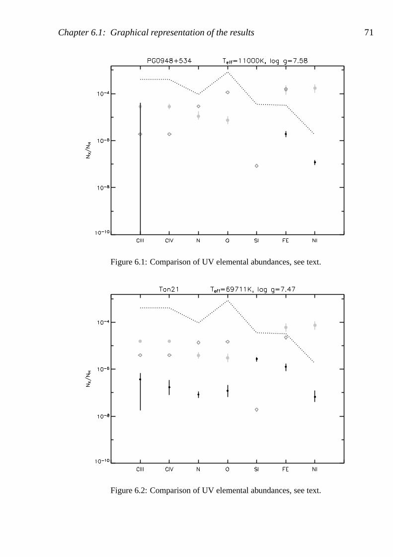
Chapter 6.1: Graphical representation of the results 71
Figure 6.1: Comparison of UV elemental abundances, see text.
Figure 6.2: Comparison of UV elemental abundances, see text.
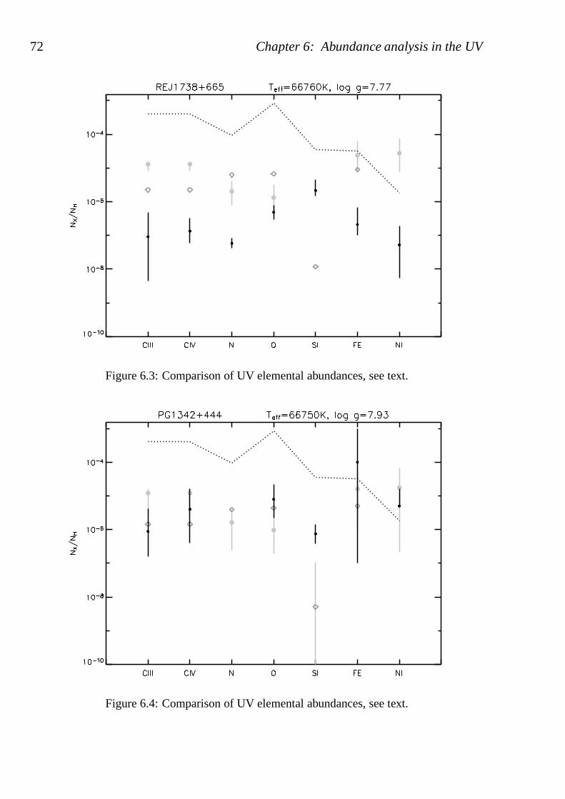
72 Chapter 6: Abundance analysis in the UV
Figure 6.3: Comparison of UV elemental abundances, see text.
Figure 6.4: Comparison of UV elemental abundances, see text.

Chapter 6.1: Graphical representation of the results 73
Figure 6.5: Comparison of UV elemental abundances, see text.
Figure 6.6: Comparison of UV elemental abundances, see text.
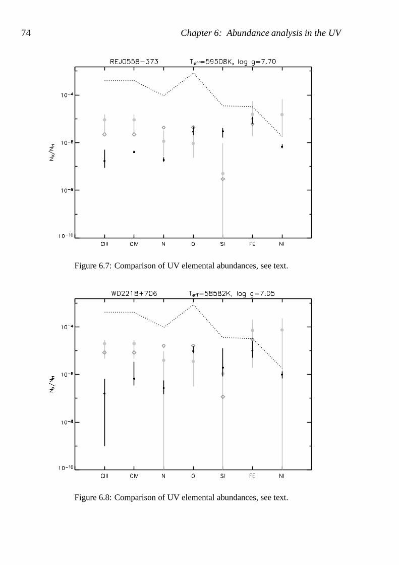
74 Chapter 6: Abundance analysis in the UV
Figure 6.7: Comparison of UV elemental abundances, see text.
Figure 6.8: Comparison of UV elemental abundances, see text.
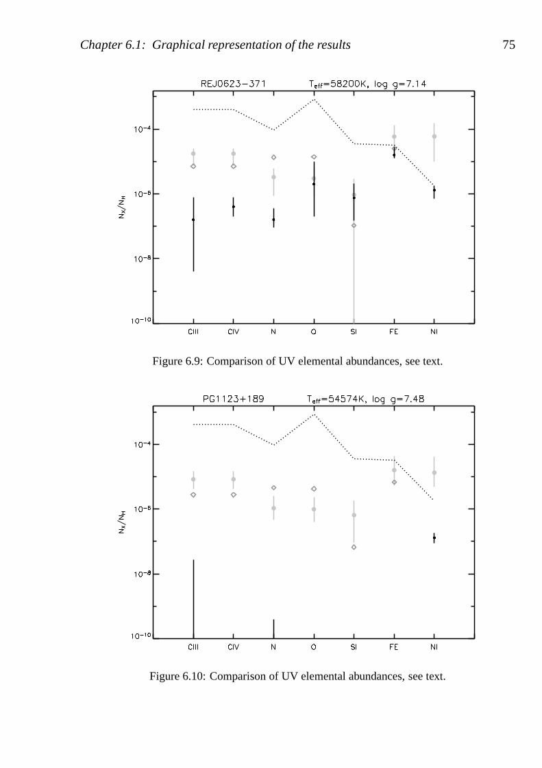
Chapter 6.1: Graphical representation of the results 75
Figure 6.9: Comparison of UV elemental abundances, see text.
Figure 6.10: Comparison of UV elemental abundances, see text.

76 Chapter 6: Abundance analysis in the UV
Figure 6.11: Comparison of UV elemental abundances, see text.
Figure 6.12: Comparison of UV elemental abundances, see text.
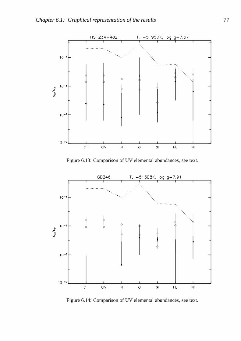
Chapter 6.1: Graphical representation of the results 77
Figure 6.13: Comparison of UV elemental abundances, see text.
Figure 6.14: Comparison of UV elemental abundances, see text.
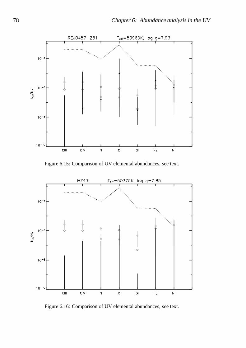
78 Chapter 6: Abundance analysis in the UV
Figure 6.15: Comparison of UV elemental abundances, see text.
Figure 6.16: Comparison of UV elemental abundances, see text.
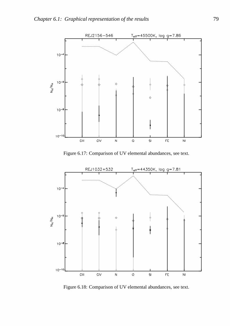
Chapter 6.1: Graphical representation of the results 79
Figure 6.17: Comparison of UV elemental abundances, see text.
Figure 6.18: Comparison of UV elemental abundances, see text.
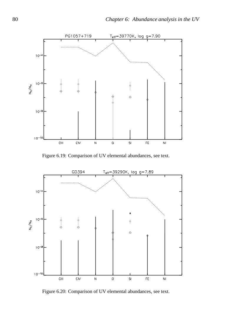
80 Chapter 6: Abundance analysis in the UV
Figure 6.19: Comparison of UV elemental abundances, see text.
Figure 6.20: Comparison of UV elemental abundances, see text.
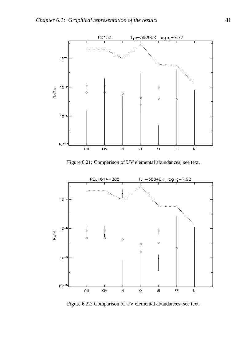
Chapter 6.1: Graphical representation of the results 81
Figure 6.21: Comparison of UV elemental abundances, see text.
Figure 6.22: Comparison of UV elemental abundances, see text.
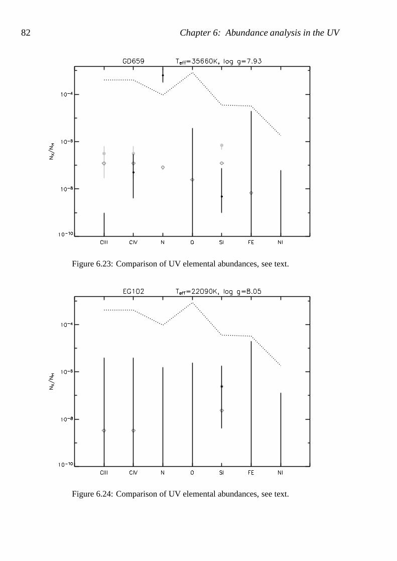
82 Chapter 6: Abundance analysis in the UV
Figure 6.23: Comparison of UV elemental abundances, see text.
Figure 6.24: Comparison of UV elemental abundances, see text.
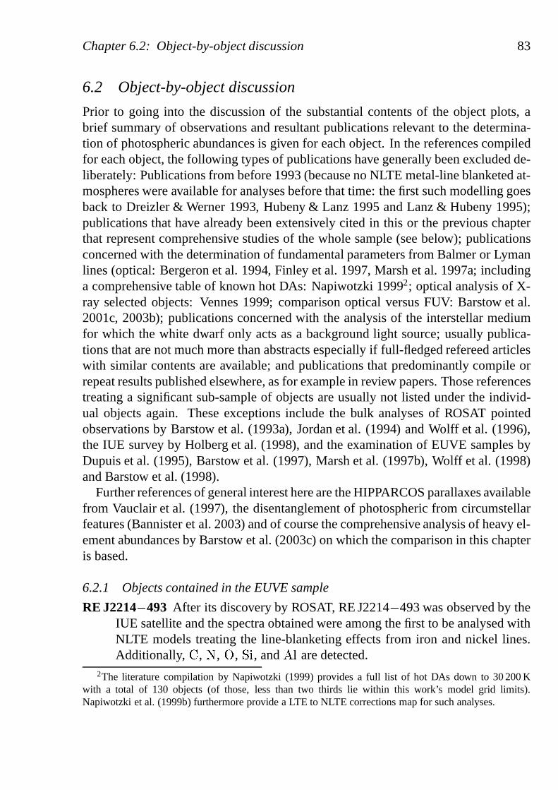
Chapter 6.2: Object-by-object discussion 83
6.2 Object-by-object discussion
Prior to going into the discussion of the substantial contents of the object plots, abrief summary of observations and resultant publications relevant to the determina-tion of photospheric abundances is given for each object. Inthe references compiledfor each object, the following types of publications have generally been excluded de-liberately: Publications from before 1993 (because no NLTEmetal-line blanketed at-mospheres were available for analyses before that time: thefirst such modelling goesback to Dreizler & Werner 1993, Hubeny & Lanz 1995 and Lanz & Hubeny 1995);publications that have already been extensively cited in this or the previous chapterthat represent comprehensive studies of the whole sample (see below); publicationsconcerned with the determination of fundamental parameters from Balmer or Lymanlines (optical: Bergeron et al. 1994, Finley et al. 1997, Marsh et al. 1997a; includinga comprehensive table of known hot DAs: Napiwotzki 19992; optical analysis of X-ray selected objects: Vennes 1999; comparison optical versus FUV: Barstow et al.2001c, 2003b); publications concerned with the analysis ofthe interstellar mediumfor which the white dwarf only acts as a background light source; usually publica-tions that are not much more than abstracts especially if full-fledged refereed articleswith similar contents are available; and publications thatpredominantly compile orrepeat results published elsewhere, as for example in review papers. Those referencestreating a significant sub-sample of objects are usually notlisted under the individ-ual objects again. These exceptions include the bulk analyses of ROSAT pointedobservations by Barstow et al. (1993a), Jordan et al. (1994)and Wolff et al. (1996),the IUE survey by Holberg et al. (1998), and the examination of EUVE samples byDupuis et al. (1995), Barstow et al. (1997), Marsh et al. (1997b), Wolff et al. (1998)and Barstow et al. (1998).
Further references of general interest here are the HIPPARCOS parallaxes availablefrom Vauclair et al. (1997), the disentanglement of photospheric from circumstellarfeatures (Bannister et al. 2003) and of course the comprehensive analysis of heavy el-ement abundances by Barstow et al. (2003c) on which the comparison in this chapteris based.
6.2.1 Objects contained in the EUVE sample
RE J2214� 493 After its discovery by ROSAT, RE J2214� 493 was observed by theIUE satellite and the spectra obtained were among the first tobe analysed withNLTE models treating the line-blanketing effects from ironand nickel lines.Additionally, � , � , � , � � , and� �
are detected.2The literature compilation by Napiwotzki (1999) provides afull list of hot DAs down to 30 200 K
with a total of 130 objects (of those, less than two thirds liewithin this work’s model grid limits).Napiwotzki et al. (1999b) furthermore provide a LTE to NLTE corrections map for such analyses.
84 Chapter 6: Abundance analysis in the UV
The� � abundances determined by Holberg et al. (1993) and Werner & Dreizler(1994) were based on the same model grid and compared well with each other(� � �
(� � /� ) � � 4.25� 0.25). The� � abundances published by Holberg et al.(1994, TLUSTY models:
� � �(� � /� ) � � 5.5) and Werner & Dreizler (1994,
PRO2models:� � �
(� � /� ) � � 4.4� 0.3), on the other hand, differ by 1 dex. Ata value of 0.4 – 5 of the� � /� � abundance ratio in the latter case, a clear enrich-ment compared to the solar value of
�20 is implied that the authors attribute to
radiative levitation. Both the value of� � /� � � 20� 10 by Holberg et al. (1994)as well as the current results represented in Fig. 6.5 (� � /� � � 14� 3 in numbers,differing from the older results by a re-determination of effective temperatureand surface gravity from new optical data, and new abundances found on thebasis of the IUE final data set – Barstow et al. 1998; Holberg etal. 1998) dis-agree with this. The issue remains to be settled and is perhaps symptomaticfor the remaining uncertainties due to modelling issues, inparticular concernedwith the accuracy and completeness of atomic data.
Taking the results in Fig. 6.5 at face value, the measured abundances of� inparticular, but also, to a lesser extent, of� � and, just within the error bars,� � , are matched by the predictions.� , � and� � are over-predicted by variousdegrees. It is remarkable that the iron and nickel abundancevalues appear closeto what looks like a limit set by the cosmic abundances.
The fit to the EUV spectrum in Chapter 5 is reasonably good and does notrequire to twist the fundamental parameters found in earlier studies. How-ever, since those earlier parameters imply an effective temperature almost 10%higher than that used in the above comparison, the sole fact that predicted andmeasured (UV) iron abundances are not too different in this comparison doesnot immediately signify consistency with the EUV results.
A FUSE spectrum exists, but has so far only been explored for studies of theISM (e.g. Hebrard et al. 2002).
Feige 24 Besides being a secondary photometric standard star, the Feige 24 systemis the prototype of a close binary that has just emerged from acommon enve-lope phase and is likely to evolve into a cataclysmic variable3. Fundamentalstellar and binary system parameters derived by Vennes & Thorstensen (1994)from optical and IUE data favour a low mass and a helium core for the hotwhite dwarf, a scenario further refined through modelling and interpretation in
3From Vennes & Thorstensen (1994): ”Feige 24 is the prototypeof a class of young, EUV-emitting,binary systems comprising a late main sequence secondary and a hot
�-rich white dwarf; the class is
characterized by optical and ultraviolet photospheric HeII absorption, circumstellar CIV (� � 1550A)
absorption, and by the presence of EUV-induced, phase-dependent Balmer fluorescence. These youngsystems present the best opportunity to constrain theory ofcommon-envelope evolution.”
Chapter 6.2: Object-by-object discussion 85
Vennes et al. (1995), only to be disputed by Benedict et al. (2000) who suggesta carbon core based on HST Fine Guidance Sensor 3 data. This conclusion wasalso adapted by Vennes et al. (2000) after they obtained revised atmosphericparameters from HST-STIS observations.
The HST-STIS data complement or partly supersede observations, among other,by ROSAT, IUE, EUVE (e.g. Barstow et al. 1994b), and earlier HST instru-ments. The IUE spectrum was used by Werner & Dreizler (1994) to measurephotospheric abundances, the EUVE spectrum was analysed byDupuis et al.(1995). EUV model spectra were also presented by Lanz & Hubeny (1995).Based on the HST-STIS spectrum first published by Vennes et al. (2000),Vennes & Lanz (2001) give photospheric abundances for� , � , � , � � , � , � � ,and � � . After removing part of an apparent ionisation imbalance for oxygenby applying NLTE models, Vennes et al. (2000) note a residualionisation im-balance that they attribute to either faulty atomic data foroxygen or chem-ical stratification. These considerations, also maintained in Vennes & Lanz(2001), could however not be solved in favour of the stratification hypothesisfor Feige 24 so far.
Similar as for RE J2214� 493, the abundances now determined tend to lie belowthe predictions, again with the exception of� � .A good EUVE fit could be obtained for a surface gravity value higher than pre-viously determined ones, but in return consistent with the results byVennes & Lanz (2001).
RE J0623� 377 Variously known as RE J0623� 374, RE J0623� 377, or simplyRE J0623� 37, and systematically called RE J0623� 371 in publications byBarstow et al., the object unambiguously identified by its white dwarf num-ber as WD 0621� 376 was first discovered by ROSAT (Holberg et al. 1993).The IUE spectrum was analysed by Werner & Dreizler (1994), and is of courseincluded in the studies by Holberg et al. (1998) and Barstow et al. (2003c).
In comparison to results from the latter, the predicted� and � abundancesare too high, while� and � � are very well,� � reasonably well matched. For� � , the same discrepancy as for RE J2214� 493 and Feige 24 is observed: Theprediction is at the same level as� � , the measurement is more than one or-der of magnitude smaller. This is just barely within the limits suggested byWerner & Dreizler (1994) who found� � /� � � 0.5 – 10 for this object.
The EUVE spectrum is very well reproduced at parameters consistent withthose that different studies generally seem to agree on.
A FUSE spectrum exists, but has so far only been explored for studies of theISM (e.g. Lehner et al. 2002).
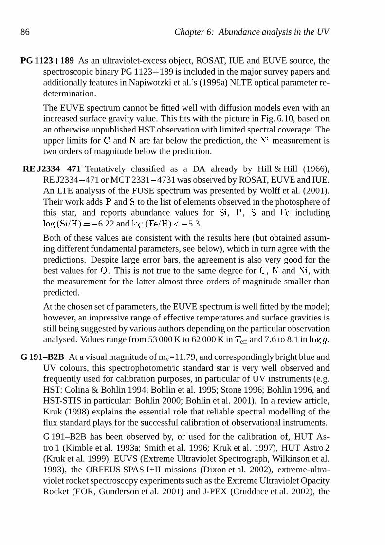
86 Chapter 6: Abundance analysis in the UV
PG 1123� 189 As an ultraviolet-excess object, ROSAT, IUE and EUVE source, thespectroscopic binary PG 1123� 189 is included in the major survey papers andadditionally features in Napiwotzki et al.’s (1999a) NLTE optical parameter re-determination.
The EUVE spectrum cannot be fitted well with diffusion modelseven with anincreased surface gravity value. This fits with the picture in Fig. 6.10, based onan otherwise unpublished HST observation with limited spectral coverage: Theupper limits for� and� are far below the prediction, the� � measurement istwo orders of magnitude below the prediction.
RE J2334� 471 Tentatively classified as a DA already by Hill & Hill (1966),RE J2334� 471 or MCT 2331� 4731 was observed by ROSAT, EUVE and IUE.An LTE analysis of the FUSE spectrum was presented by Wolff etal. (2001).Their work adds� and � to the list of elements observed in the photosphere ofthis star, and reports abundance values for� � , � , � and � � including� � �
(� � /� ) � � 6.22 and� � �
(� � /� ) � � 5.3.
Both of these values are consistent with the results here (but obtained assum-ing different fundamental parameters, see below), which inturn agree with thepredictions. Despite large error bars, the agreement is also very good for thebest values for� . This is not true to the same degree for� , � and � � , withthe measurement for the latter almost three orders of magnitude smaller thanpredicted.
At the chosen set of parameters, the EUVE spectrum is well fitted by the model;however, an impressive range of effective temperatures andsurface gravities isstill being suggested by various authors depending on the particular observationanalysed. Values range from 53 000 K to 62 000 K in
�eff and 7.6 to 8.1 in
� � �� .
G 191–B2B At a visual magnitude of mv=11.79, and correspondingly bright blue andUV colours, this spectrophotometric standard star is very well observed andfrequently used for calibration purposes, in particular ofUV instruments (e.g.HST: Colina & Bohlin 1994; Bohlin et al. 1995; Stone 1996; Bohlin 1996, andHST-STIS in particular: Bohlin 2000; Bohlin et al. 2001). Ina review article,Kruk (1998) explains the essential role that reliable spectral modelling of theflux standard plays for the successful calibration of observational instruments.
G 191–B2B has been observed by, or used for the calibration of, HUT As-tro 1 (Kimble et al. 1993a; Smith et al. 1996; Kruk et al. 1997), HUT Astro 2(Kruk et al. 1999), EUVS (Extreme Ultraviolet Spectrograph, Wilkinson et al.1993), the ORFEUS SPAS I+II missions (Dixon et al. 2002), extreme-ultra-violet rocket spectroscopy experiments such as the ExtremeUltraviolet OpacityRocket (EOR, Gunderson et al. 2001) and J-PEX (Cruddace et al. 2002), the
Chapter 6.2: Object-by-object discussion 87
X-ray observatory XMM (Chen et al. 2004 suggested G 191–B2B for XMM’swavelength calibration), and large optical telescopes such as Keck or VLT.
The extensive data allow a detailed modelling and parameterdetermination ofthis ”prototype” hot DA, resulting in knowledge about the object which is inturn required to fulfil the calibration needs. The remaininguncertainties in themodelling as documented in Fig. 5.6 might appear surprisingin this context:The host of values for
� � �and
� � �� found from optical (Balmer line series) and
Lyman line analyses (see the short compilation at the beginning of this sectionand Fig. 5.6 for the corresponding references) frame the various values used inor derived from UV and FUV studies. Besides systematic effects attributableto poorly understood effects from one wavelength range to another, and un-controllable random scatter from one observation to another, the discrepanciesamount to a large extent from different approximations in the models. The us-age of NLTE versus LTE models, the inclusion of� � and/or metals and theirexact composition, and the degree to which the imperative ofself-consistencyis observed all play a role. The efforts to explain the spectral energy distri-bution of G 191–B2B in particular reflect the overall increasing complexity ofthe atmosphere models utilised to understand the composition and physics inany hot DA atmosphere. New concepts were often first tested onthis star, dueto stronger constraints from new observations, numerouslyobtained for thistarget:
Barstow et al. (1993a,b) were unable to obtain an acceptablefit to ROSAT datawith H models. The first NLTE line-blanketed models with� � were presentedby Dreizler & Werner (1993) for comparison with EUV and IUE data, andsubsequently used in studies by Holberg et al. (1994) and Werner & Dreizler(1994) who determined� � and� � abundances from the IUE spectrum. Simi-larly sophisticated model atmospheres were then computed by Lanz & Hubeny(1995), and used in Lanz et al. (1996) to create a model specifically for G 191–B2B that resulted in the determination of a lower effective temperature, andheavy element abundance measurements (still based on the IUE and additionalEUV data). Vidal-Madjar et al. (1994) detected� , � � , and� � lines in an HST-GHRS spectrum, Vennes et al. (1996a)� and � in an ORFEUS spectrum.Barstow et al. (1994b) presented the first EUVE spectrum thatDupuis et al.(1995) then used to determine a suitable
�eff and analyse the ISM along the line
of sight towards G 191–B2B. However, the EUVE observation continued toelude successful modelling (Barstow & Hubeny 1998:� +� � stratified modelincluding heavy elements) until Barstow et al. (1999) suggested a stratified� �slab model. The diffusion model by Dreizler & Wolff (1999) delivered the jus-tification for such an approach and correctly predicted the� � opacity required
88 Chapter 6: Abundance analysis in the UV
to match HST-STIS and EUVE spectra simultaneously.
Recently, Vennes & Lanz (2001) have published a comparison of Feige 24 andG 191–B2B based on HST-STIS spectra, of which Holberg et al. (2002) of-fer a co-added, high signal-to-noise version. There have been efforts to sepa-rate photospheric from circumstellar metal line contributions (Bruhweiler et al.1999 mention such a component for� ; the major works on this topic have beenlisted in the introduction). FUSE observations (e.g. Lemoine et al. 2002, ISManalysis) await a detailed investigation as announced in Barstow et al. (2003a).A flight of the J-PEX instrument has targeted G 191–B2B, resulting in a newhigh-resolution spectral observation in the extreme-ultraviolet (Cruddace et al.2002; Barstow et al. 2005).
As for several other objects assigned to the so-called G 191–B2B-group, theagreement between predicted and measured value for� � is relatively good;it is excellent for� � and of only slightly lesser quality for� . A decreasingcoincidence must be noted for� , � , and� � in this order, with a large deviationfor � � . Owing to the well-matched� � profile, the fit to the EUVE spectrum,at an accepted pair of fundamental parameters, is good, as has been previouslyproven in Dreizler & Wolff (1999).
PG 1234� 482 Wolff et al. (1994) and Jordan et al. (1996) reported the detection of� � in the EUVE spectrum, and Homeier et al. (1998) have providedan inde-pendent optical parameter determination. Apart from a measurement of� � ,the new attempt only cites upper limits for other elements, all with large errorbars due to the noisy IUE spectrum. The non-detection of mostheavy elementsroughly fits with the notion that absorbers are missing in theshort-wavelengthpart of the EUVE spectrum that would bring down the observed spectrum tothe lower flux level of the diffusion model, which has alreadybeen boostedconsiderably by increasing the surface gravity.
GD 246 Napiwotzki et al. (1999a) give a NLTE optical parameter determination forthis faint spectrophotometric standard (Bessell 1999, UV normalisation;Hawarden et al. 2001, large optical telescopes; Smith et al.2002, SDSS stan-dard-star network).
The star has IUE and EUVE spectra that Vennes et al. (1993) used to provethe existence of interstellar HeII for the first time; one of the more recent ISMstudies based on a FUSE spectrum is, for example, Oliveira etal. (2003).
FUSE observations are also reported by Wolff et al. (2001) and Chayer et al.(2001). Wolff et al. (2001) identify� , � , � , � � , � , � � and � � and measurephotospheric abundances of� � , � and� � . The� � abundance is actually an up-per limit of
� � �(� � /� ) � � 4.7, but Dupuis et al. (2000b) and Vennes & Dupuis
Chapter 6.2: Object-by-object discussion 89
(2002) write about the presence of� � in a CHANDRA spectrum that they relateto the missing opacity in the EUV.
The diffusion models fail in fact to reproduce the EUVE spectrum; this is one ofonly two cases where the predicted flux is too high at intermediate EUV wave-lengths despite a lowered effective temperature. At short EUV wavelengths, thesituation is reversed, and cannot be reconciled by the increased surface gravityemployed.
The latter is in accord with the finding for� � in the comparison shown (basedon IUE and HST-STIS spectra, Holberg et al. 2000): The upper limit measuredlies far below the prediction. The same is true for most otherelements except� and � � , where some agreement can be noted.
MCT 0455� 2812 Identified with simultaneous discoveries by Barstow et al. (1992),MCT 0455� 2812 was ultimately published as a new ROSAT white dwarfRE J0457� 281 by Barstow et al. (1994d).
NLTE analyses of optical spectra are available from Napiwotzki et al. (1999a)and Koester et al. (2001, SPY); the latter cites a larger T
� �than used here.
Apart from IUE and EUVE spectra, MCT 0455� 2812 also has an ORFEUS Ispectrum (1993 flight) that reveals the presence of� and � (Vennes et al.1996a; Barstow et al. 1998). An analysis of the FUSE spectrumwas presentedby Wolff et al. (2001); similar to GD 246,� , � , � , � � , � , � and� � are found.An upper limit of
� � �(� � /� ) � � 5 is cited.
The EUVE can be reproduced fairly well, at a significantly higher temperaturethan even found in Koester et al. (2001), so that a direct comparison of resultsin the EUVE versus those in the UV makes little sense. Nevertheless, both� � and� � are well matched, although the iron measurement is higher than theprediction, in contrast to the systematics emerging so far.At the higher temper-ature suggested by the EUVE fit, this would probably appear reversed again.The remaining elements show a gaudy scatter in the directionof deviations, inconjunction with large error bars.
HZ 43 A Despite its red companion, HZ 43 A is a very popular spectrophotometricstandard. The wide common proper motion pair are separated by about 3”, sothat depending on the seeing and the spatial resolution of the telescope the� � �component will or will not contaminate an optical spectrum.It can be easilyseparated with HST, and its contribution to shorter wavelength observations isnegligible.
Napiwotzki et al. (1993) and Heber et al. (1997, determination of an upper limitfor the rotational velocity) have presented good optical spectra in addition to the
90 Chapter 6: Abundance analysis in the UV
familiar standard works. The binary nature of the system canbe exploited tostudy, within a larger sample, evolutionary channels in non-interacting binarysystems (Barstow et al. 1994a), population membership via the radial velocityand metallicity of the un-evolved companion (Silvestri et al. 2002), and gravi-tational redshifts (Reid 1996, allowing an independent determination of
� � �� ).
HZ 43 A is one of four primary white dwarf standards used as a spectropho-tometric reference for various HST instruments (Bohlin et al. 1995, Bohlin1996, Bohlin 2000, Bohlin et al. 2001). It is treated in Kruk’s 1998 reviewabout UV calibration, prominently features in the Hopkins Ultraviolet Tele-scope Astro-1 and Astro-2 calibration (Kruk et al. 1997, 1999), and suppliedthe in-flight calibration of ORFEUS-SPAS II (Hurwitz et al. 1998; Dixon et al.2002). Further, it is used in Massa & Fitzpatrick’s (2000) re-calibration ofIUE NEWSIPS, in the FUSE calibration (Sahnow et al. 2000), XMM-Newton’s(Jansen et al. 2001) and also CHANDRA’s low-energy calibration (see alsoVennes & Dupuis 2002).
After having established a set of fundamental photosphericparameters in 1993,Napiwotzki et al. exclude HZ 43 A from their 1999a analysis but state that sys-tematic errors of 0.3 dex in
� � �� , as found between Napiwotzki et al. (1993)
and Finley et al. (1997), are not so serious in the light of their new results.4
Although the smaller shifts in effective temperature warrant correspondinglyfewer discussions, it is noteworthy that the work by Bessell(1999) on spec-trophotometric standards uses
�BB � 35 000 K, a blackbody temperature, that
obviously deviates strongly from the accepted effective temperature of about50 000 K. Generally, of course, the discussion is not betweenblackbody versusLTE � models, but between LTE� models (as used in virtually all of the cali-bration works) versus NLTE models, and with various traces of � � or metals.
Undisputedly, HZ 43 A exhibits an unusually pure� atmosphere. Regularly,spectra from new instruments only place upper limits on heavy element abun-dances. Modelling efforts have therefore concentrated, among other things, onNLTE models (also for spherical symmetry) for various� � /� compositions, orLTE model atmospheres with comptonisation (Madej 1998) which contributessome additional opacity that however only has an effect on the emergent X-rayspectra when the atmosphere contains no� � .
The series of observations that have failed to detect photospheric metals in4From Napiwotzki et al. (1999a): ”Therefore, we conclude that the accuracy is not limited by the noise
for good spectra, and we suggest that other effects, such as details of the extraction or fluxing and nor-malisation procedures, contribute more. Considering these systematic uncertainties, the 0.3 dex differencebetween the gravity determinations of Finley et al. (1997) and Napiwotzki et al. (1993) for HZ 43 A is onlya 1.5� deviation and therefore not as serious as considered by Finley et al. (1997).”
Chapter 6.2: Object-by-object discussion 91
HZ 43 A includes Kimble et al. (1993b, HUT); Barstow et al. (1995, includinga constraint of
� � �(� � /� ) � � 6.5, from EUVE spectra); Dupuis et al. (1998,
ORFEUS-SPAS II); and Kruk et al. (2002) who, within an ISM analysis withFUSE data, amended by HST-GHRS and EUVE, once more report that noheavy elements are detected in the photosphere.
Likewise, Fig. 6.16 shows only upper limits from IUE and HST-STIS measure-ments; although those for� , � , � � and� � remain marginally consistent withthe predictions. The ORFEUS spectrum actually places tighter limits on the�and � abundances, definitely destroying any consistency for� . The limitingabundances for� � and � � remain high however and are instead further con-strained by the EUVE spectrum: Irrespective of the above Napiwotzki et al.(1993) / Finley et al. (1997) discussion, the
� � �� required to purify the atmo-
sphere to the observed degree is higher by yet another 0.3 dexat least thanthose values, reminiscent only of the historical value by Holberg et al. (1986)from a Lyman line analysis (not confirmed in the newer work by Barstow et al.2003b).
Fuhrmeister & Schmitt (2003) set the flare flag in the tabulated results of theirROSAT variability study, although they mention in the papertext that they haveused HZ 43 A as a stable reference to test their methods.
RE J2156� 546 First observed in the Einstein IPC slew survey (Elvis et al. 1992),this object is also a ROSAT (e.g. Chu et al. 2004), EUVE (ISM paper:Wolff et al. 1999), HST and FUSE (ISM paper: Lehner et al. 2003) target.In their SPY survey, Koester et al. (2001) find a slightly higher
�eff and lower� � �
� (46 700 K, 7.65) than cited in Chapter 5 (44 000 K, 7.91), whileboth the�eff and
� � �� used for the comparison here (45 500 K, 7.86) lie in between those
values.
Although generally classified as another pure hydrogen-object, RE J2156� 546surprisingly shows oxygen lines in the FUSE range; from a combination ofthis finding with STIS and EUVE data, Chayer et al. (2003) conclude that�must be stratified in this (and three further) stars. Their modelling is based ona stratification profile taken from this work for a model with
�eff � 46 00 K and� � �
� � 7.8.
While for their � +� NLTE models the EUVE spectrum can apparently bereproduced, the fit here is not completely satisfactory for the full models in-cluding other elements, and even this can only be achieved if
� � �� is increased
by 0.4 or 0.5 dex.
For most elements, the STIS spectrum only allows to derive upper limits; al-though those for� , � and� � are consistent with the predicted values, at least
92 Chapter 6: Abundance analysis in the UV
� � is probably quite a bit lower than predicted.� and � � are detected, but atmuch lower levels than expected.
RE J1032� 535 Holberg et al. (1999a,b) discuss the STIS spectrum of RE J1032� 535in conjunction with the EUVE spectrum. One of their conclusions is that�must be stratified in this star; this issue is disputed by Chayer et al. (2005, inpress), and further discussed in some detail in Sect. 6.2.3.From the FUSE data(Welsh et al. 2002, ISM), on the other hand, Chayer et al. (2003) deduce anoxygen stratification. Barstow et al. (2003c), finally, suspect a stratification ofcarbon based on the line profiles observed in the STIS spectrum.
The EUVE fit, similarly to RE J2156� 546, requires a� � �
� increased by about0.5 dex, while other parameter determinations exhibit lessscatter in
�eff and� � �
� .
The problems with the EUVE fit probably result from too high values for � �and� � in the equilibrium model. Although their predicted values are consistentwith the upper limits shown in Fig. 6.18, the actual values could be significantlylower. � , � and � � are also predicted somewhat too high, in stark contrastto � : The use of the stratified profile from Holberg et al. (1999a) results in aparticularly high value. This apparent� superabundance leads to the definitionof a group that also encompasses RE J1614� 085 and GD 659.
For the ROSAT data, Fuhrmeister & Schmitt (2003) set the ”flare” flag (as for5 more out of the 13 white dwarfs they detect).
PG 1057� 719 ROSAT and EUVE data for this object suggest it has a pure hydrogenatmosphere. Holberg et al. (1997b) also find no evidence of heavy elementsin this object’s HST-GHRS spectrum; consequently, Fig. 6.19 displays upperlimits for � , � , � � , � � , � � based on the wavelengths covered by the GHRSobservations. In particular, PG 1057� 719 does not show nitrogen lines.
The EUVE spectrum appears strongly absorbed; it can be fittedat generallyaccepted parameters.
Fuhrmeister & Schmitt (2003) find everything from flare activity to periodicityand a trend in the ROSAT data.
GD 394 Given how complex the object GD 394 has turned out to be, it must havebeen a challenge for some applications to use it for calibration purposes, ascarried out for example in Finley et al. (1984, IUE), Kruk et al. (1999, HUT),and again Smith (2001, test of IUE wavelength calibration).The star appearsconfusing enough to merit to be featured in Trimble & Aschwanden’s ”Astro-physics in 2000” review (2001).
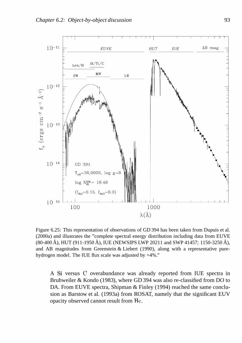
Chapter 6.2: Object-by-object discussion 93
Figure 6.25: This representation of observations of GD 394 has been taken from Dupuis et al.(2000a) and illustrates the ”complete spectral energy distribution including data from EUVE(80-400A), HUT (911-1950A), IUE (NEWSIPS LWP 20211 and SWP 41457; 1150-3250A),and AB magnitudes from Greenstein & Liebert (1990), along with a representative pure-hydrogen model. The IUE flux scale was adjusted by +4%.”
A � � versus � overabundance was already reported from IUE spectra inBruhweiler & Kondo (1983), where GD 394 was also re-classified from DO toDA. From EUVE spectra, Shipman & Finley (1994) reached the same conclu-sion as Barstow et al. (1993a) from ROSAT, namely that the significant EUVopacity observed cannot result from� � .
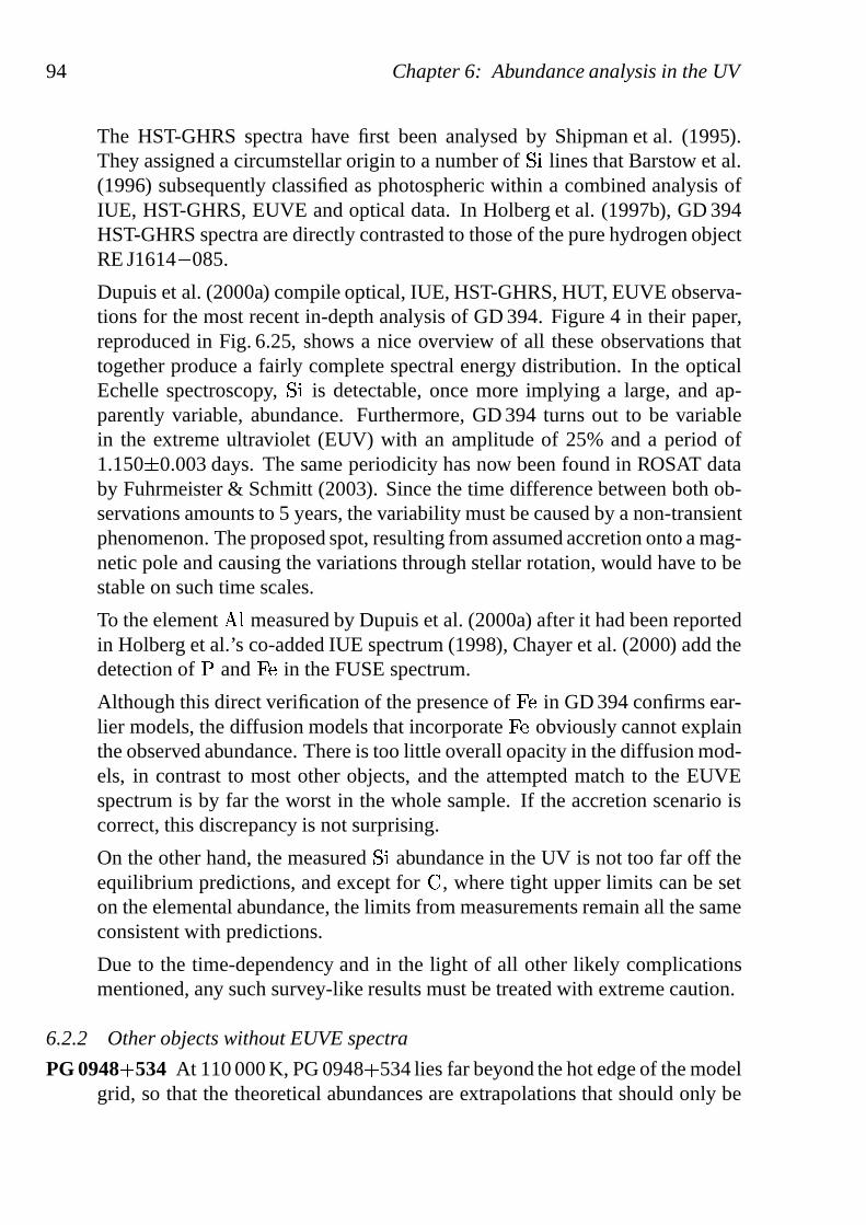
94 Chapter 6: Abundance analysis in the UV
The HST-GHRS spectra have first been analysed by Shipman et al. (1995).They assigned a circumstellar origin to a number of� � lines that Barstow et al.(1996) subsequently classified as photospheric within a combined analysis ofIUE, HST-GHRS, EUVE and optical data. In Holberg et al. (1997b), GD 394HST-GHRS spectra are directly contrasted to those of the pure hydrogen objectRE J1614� 085.
Dupuis et al. (2000a) compile optical, IUE, HST-GHRS, HUT, EUVE observa-tions for the most recent in-depth analysis of GD 394. Figure4 in their paper,reproduced in Fig. 6.25, shows a nice overview of all these observations thattogether produce a fairly complete spectral energy distribution. In the opticalEchelle spectroscopy,� � is detectable, once more implying a large, and ap-parently variable, abundance. Furthermore, GD 394 turns out to be variablein the extreme ultraviolet (EUV) with an amplitude of 25% anda period of1.150� 0.003 days. The same periodicity has now been found in ROSAT databy Fuhrmeister & Schmitt (2003). Since the time difference between both ob-servations amounts to 5 years, the variability must be caused by a non-transientphenomenon. The proposed spot, resulting from assumed accretion onto a mag-netic pole and causing the variations through stellar rotation, would have to bestable on such time scales.
To the element� �measured by Dupuis et al. (2000a) after it had been reported
in Holberg et al.’s co-added IUE spectrum (1998), Chayer et al. (2000) add thedetection of� and� � in the FUSE spectrum.
Although this direct verification of the presence of� � in GD 394 confirms ear-lier models, the diffusion models that incorporate� � obviously cannot explainthe observed abundance. There is too little overall opacityin the diffusion mod-els, in contrast to most other objects, and the attempted match to the EUVEspectrum is by far the worst in the whole sample. If the accretion scenario iscorrect, this discrepancy is not surprising.
On the other hand, the measured� � abundance in the UV is not too far off theequilibrium predictions, and except for� , where tight upper limits can be seton the elemental abundance, the limits from measurements remain all the sameconsistent with predictions.
Due to the time-dependency and in the light of all other likely complicationsmentioned, any such survey-like results must be treated with extreme caution.
6.2.2 Other objects without EUVE spectra
PG 0948� 534 At 110 000 K, PG 0948� 534 lies far beyond the hot edge of the modelgrid, so that the theoretical abundances are extrapolations that should only be
Chapter 6.2: Object-by-object discussion 95
read with extreme caution. Additionally, Barstow et al. (2003c) could not findsatisfactory fits to the CIV , N V, OV and SiIV lines that are detected in theHST-STIS spectrum although they note values larger than about 10�
� ��.
The extrapolated� � and� � abundances (both well beyond solar here) are toohigh by 2 and 3 dex, respectively, compared to the measurements.
Ton 21 Although Ton 21 is a spectrophotometric standard star (Massey et al. 1988),no FUSE spectra are available. The HST spectra are discussedin recent surveysmentioned in the introduction.
All predicted elemental abundances are too high, including� � and � � wherethe discrepancy becomes similarly large as for PG 0948� 534. Crudely speak-ing, the offset scatters around a value of about 2 dex. It is higher for� � whichrather seems to be loosely constrained by the cosmic ratio. It is extremely largefor � � , the most abundant element in the observation. This is probably due tomissing higher ionisation stages that were not included in the model calcula-tions.
RE J1738� 665 This object was the hottest WD detected by ROSAT (Barstow et al.1994c), a discovery even followed up by a discussion in Nature (Shipman 1994;Tweedy 1995). It might also still be surrounded by an old planetary nebula(Tweedy & Kwitter 1994). In contrast to the notion shortly after its discoverythat it must have unusually low metal abundances to show the detected softX-ray flux, its abundance patterns do not appear too peculiarin the light ofnewer parameter determinations (RE J1738� 665 is included in the recent sur-veys analysing HST and FUSE spectra).
The abundance pattern and how it relates to the predictions is very similar tothat of Ton 21.
PG 1342� 444 As do Ton 21 and RE J1738� 665, PG 1342� 444 also lies near the hotedge of the model grid. A FUSE spectrum is the only available high-resolutionobservation in the UV (Barstow et al. 2002). It is one of the spectra that enteredinto the study comparing effective temperatures as derivedfrom Balmer andLyman lines by Barstow et al. (2001c, 2003b). The results displayed in Fig. 6.4were also obtained based on that data.
The overall abundance pattern as obtained from the FUSE spectrum is (roughly)matched by the predictions better than for most other objects. But while the er-ror bars continue to overlap, in detail the mean values actually do differ byone order of magnitude. In particular, the� � discrepancy mentioned for otherobjects above remains.
96 Chapter 6: Abundance analysis in the UV
RE J0558� 373 The EUVE spectrum of this object was not included in Wolff et al.’s(1998) sample.
In the element abundance determination, although the first impression again isnot too bad, very small error bars on the measurements destroy compatibilityin all but two cases. So the predictions only meet the values for � and � � –this quite well.
WD 2218� 706 WD 2218� 706 is surrounded by an ancient planetary nebula (e.g.Acker et al. 1992); HST-STIS spectra of the central star havepreviously beenanalysed by Barstow et al. (2001a).
In the abundance pattern, the matches are not so good for� and � , and theapparent limit imposed on� � by the cosmic abundance is also particularlystriking and results in a mismatch. The measurement for� lies slightly abovethe prediction but very close to it.
GD 153 GD 153 is frequently used for calibrations. For this reason,a variety of ob-servations exist, including, for example, observations from FAUST(Bowyer et al. 1993), HST-FOS (Bohlin et al. 1995), Astro-1 and Astro-2 ofHUT (Kruk et al. 1997, 1999), IUE (Massa & Fitzpatrick 2000),HST-STIS andHST-NICMOS (Bohlin 2000; Bohlin et al. 2001), and XMM-Newton(Jansen et al. 2001).
ROSAT observations exist and were, in addition to the standard publications,also reported on by Thomas et al. (1998).
GD 153 is furthermore useful for ISM studies, as conducted using EUVE(Vennes et al. 1994), FUSE (Lehner et al. 2003) and HST-STIS observations(Redfield & Linsky 2004a,b).
Due to their global non-detection, the abundances from metal lines are all upperlimits. Those are tight enough for� and � � only in order to disagree with thediffusion models.
RE J1614� 085 Following up on Holberg et al. (1997b), Fig 6.22 presents revisedabundance measurements from HST-GHRS spectra.
With respect to the equilibrium predictions,� is well matched, while the ob-served� � is lower and� is higher at an extreme value of more than 6 ordersof magnitude. This causes it to be grouped together with RE J1032� 535 andGD 659 by Barstow et al. (2003c).
The exceedingly large abundance of� in that group is disputed by results fromChayer et al. (2005, in press) that are shortly discussed again in the context ofRE J1032� 535 in Sect. 6.2.3.
Chapter 6.2: Object-by-object discussion 97
GD 659 Early EUVE and ROSAT observations, presented by Finley et al. (1993) andWolff et al. (1995), respectively, suggested a pure hydrogen atmosphere of thisobject. It is part of the MCT sample (Lamontagne et al. 2000) and of interestfor ISM studies so that a FUSE spectrum is available (Lehner et al. 2003).
In their initial analysis of EUVE and IUE spectra, Holberg etal. (1995) foundmetals but favoured a circumstellar origin of the observed� , � and � � lines,that are now interpreted as photospheric in the IUE and HST-STIS observa-tions. In comparison to the radiative levitation calculations, the observed irreg-ular abundance pattern shows occasional consistencies butis generally lowerthan the predictions. The exception to this is again� , for which the highestabundance in the whole sample is reported.
For this member of the nitrogen-rich group, Chayer et al. (2005, in press) alsoobtain different results.
EG 102 This is another spectrophotometric standard star (Colina &Bohlin 1994, op-tical; Kaiser et al. 1998 and Bohlin et al. 2001, HST-STIS andHST-NICMOS;Smith 2001, IUE). A FUSE spectrum also exists (Hebrard et al. 2003).
The star has been reported to show lines of� � , � �and � �
(see for exampleHolberg et al. 1997a). Due to its low effective temperature,the presence of met-als is attributed to accretion, which Debes & Sigurdsson (2002) speculate mightcome from a perishing planet. Zuckerman & Reid (1998) and Zuckerman et al.(2003) analyse the metal lines observations within a largersample of cool ob-jects.
The comparison shown for the� � measurement implies a risky extrapolation tolow effective temperatures far beyond the actual model grid; funnily enough,the match is so perfect that the data points shown become indistinguishable.While no accretion would then be necessary to explain the presence of� � , � �and� �
remain unexplained. The upper limits given for all other elements areconsistent with their absence in diffusion calculations due to complete settling.
Wolf 1346 Since this object has an even lower effective temperature than EG 102,and only� � – whose presence is also generally being attributed to accretion –could be measured (Holberg et al. 1996), this work refrains from displaying aplot with abundance comparisons.
6.2.3 A closer look at the nitrogen lines in RE J1032� 535
The following analyses rely on the NV resonance line doublet at rest wavelengths of1238.82 and 1242.80A observed in the HST-STIS spectrum. Holberg et al. (1999a)have used it in conjunction with EUVE data to derive a chemical stratification in
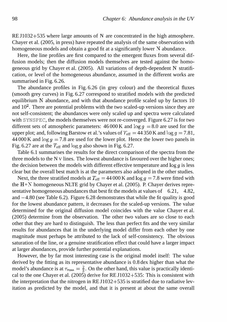
98 Chapter 6: Abundance analysis in the UV
RE J1032� 535 where large amounts of� are concentrated in the high atmosphere.Chayer et al. (2005, in press) have repeated the analysis of the same observation withhomogeneous models and obtain a good fit at a significantly lower � abundance.
Here, the line profiles are first compared to the emergent fluxes from several dif-fusion models; then the diffusion models themselves are tested against the homo-geneous grid by Chayer et al. (2005). All variations of depth-dependent� stratifi-cation, or level of the homogeneous abundance, assumed in the different works aresummarised in Fig. 6.26.
The abundance profiles in Fig. 6.26 (in grey colour) and the theoretical fluxes(smooth grey curves) in Fig. 6.27 correspond to stratified models with the predictedequilibrium � abundance, and with that abundance profile scaled up by factors 10and 10
�. There are potential problems with the two scaled-up versions since they are
not self-consistent; the abundances were only scaled up andspectra were calculatedwith SYNSPEC, the models themselves were not re-converged. Figure 6.27 is for twodifferent sets of atmospheric parameters: 46 000 K and
� � �� � 8.0 are used for the
upper plot; and, following Barstow et al.’s values of�
eff � 44 350 K and� � �
� � 7.81,44 000 K and
� � �� � 7.8 are used for the lower plot. Hence the lower two panels in
Fig. 6.27 are at the�
eff and� � �
� also shown in Fig. 6.27.Table 6.1 summarises the results for the direct comparison of the spectra from the
three models to the NV lines. The lowest abundance is favoured over the higher ones;the decision between the models with different effective temperature and
� � �� is less
clear but the overall best match is at the parameters also adopted in the other studies.Next, the three stratified models at
�eff � 44 000 K and
� � �� � 7.8 were fitted with
the � +� homogeneous NLTE grid by Chayer et al. (2005). P. Chayer derives repre-sentative homogeneous abundances that best fit the models atvalues of� 6.21,� 4.82,and� 4.80 (see Table 6.2). Figure 6.28 demonstrates that while the fit quality is goodfor the lowest abundance pattern, it decreases for the scaled-up versions. The valuedetermined for the original diffusion model coincides withthe value Chayer et al.(2005) determine from the observation. The other two valuesare so close to eachother that they are hard to distinguish. The less than perfect fits and the very similarresults for abundances that in the underlying model differ from each other by onemagnitude must perhaps be attributed to the lack of self-consistency. The obvioussaturation of the line, or a genuine stratification effect that could have a larger impactat larger abundances, provide further potential explanations.
However, the by far most interesting case is the original model itself: The valuederived by the fitting as its representative abundance is 0.8dex higher than what themodel’s abundance is at� � � � � �
�� . On the other hand, this value is practically identi-
cal to the one Chayer et al. (2005) derive for RE J1032� 535: This is consistent withthe interpretation that the nitrogen in RE J1032� 535 is stratified due to radiative lev-itation as predicted by the model, and that it is present at about the same overall
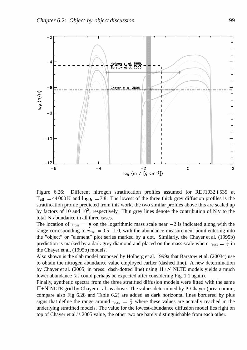
Chapter 6.2: Object-by-object discussion 99
Figure 6.26: Different nitrogen stratification profiles assumed for RE J1032�
535 atT� � � 44 000 K and� � � � � 7.8: The lowest of the three thick grey diffusion profiles is thestratification profile predicted from this work, the two similar profiles above this are scaled upby factors of 10 and 10
�, respectively. Thin grey lines denote the contribution of NV to the
total � abundance in all three cases.The location of� ross �
�� on the logarithmic mass scale near� 2 is indicated along with the
range corresponding to� ross � 0.5 – 1.0, with the abundance measurement point entering intothe ”object” or ”element” plot series marked by a dot. Similarly, the Chayer et al. (1995b)prediction is marked by a dark grey diamond and placed on the mass scale where� ross �
�� in
the Chayer et al. (1995b) models.Also shown is the slab model proposed by Holberg et al. 1999a that Barstow et al. (2003c) useto obtain the nitrogen abundance value employed earlier (dashed line). A new determinationby Chayer et al. (2005, in press: dash-dotted line) using� +� NLTE models yields a muchlower abundance (as could perhaps be expected after considering Fig. 1.1 again).Finally, synthetic spectra from the three stratified diffusion models were fitted with the same� +� NLTE grid by Chayer et al. as above. The values determined by P. Chayer (priv. comm.,compare also Fig. 6.28 and Table 6.2) are added as dark horizontal lines bordered by plussigns that define the range around� ross �
�� where these values are actually reached in the
underlying stratified models. The value for the lowest-abundance diffusion model lies right ontop of Chayer et al.’s 2005 value, the other two are barely distinguishable from each other.
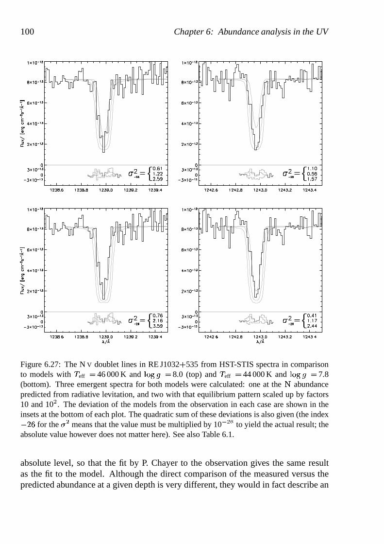
100 Chapter 6: Abundance analysis in the UV
Figure 6.27: The NV doublet lines in RE J1032�
535 from HST-STIS spectra in comparisonto models with� eff � 46 000 K and� � � � � 8.0 (top) and� eff � 44 000 K and� � � � � 7.8(bottom). Three emergent spectra for both models were calculated: one at the� abundancepredicted from radiative levitation, and two with that equilibrium pattern scaled up by factors10 and 10
�. The deviation of the models from the observation in each case are shown in the
insets at the bottom of each plot. The quadratic sum of these deviations is also given (the index� � � for the�
�means that the value must be multiplied by 10�
� �to yield the actual result; the
absolute value however does not matter here). See also Table6.1.
absolute level, so that the fit by P. Chayer to the observationgives the same resultas the fit to the model. Although the direct comparison of the measured versus thepredicted abundance at a given depth is very different, theywould in fact describe an
Chapter 6.2: Object-by-object discussion 101
Table 6.1: The NV doublet in RE J1032�
535 from HST-STIS spectra compared to emergentspectra from diffusion models: The fit results are sorted by decreasing� �
�� � � , which results
in an almost simultaneous sorting in� � � (� /� ) at � ross ��� except for the two best-fit models
where the one with the T� � , � � � � parameters closer to those published matches better.
T� � [K] � � � � �[cm s�
�]� � �
(�
/�
) N V � � � � : ��� � � N V � � � � : �
�� � � �
��� � �
44 000 7.8 � 7.0 0.76 0.41 1.1746 000 8.0 � 7.2 0.61 1.10 1.7146 000 8.0 � 6.2 1.22 0.56 1.7844 000 7.8 � 6.0 2.16 1.17 3.3346 000 8.0 � 5.2 2.59 1.57 4.1644 000 7.8 � 5.0 3.59 2.44 6.03
identical situation. It is also remarkable that the fit in that case is very good, indicat-ing that although the stratification is present in the model,there are no direct hints ofit in the line profile.
The predicted stratification profile cannot be validated from the argument alonethat it results in spectral lines that fit the observation, and that those spectral lines inturn behave the same as the observation when fitted with spectra from a homogeneousmodel. Nevertheless, the picture is consistent and the validity of the model is givenfurther credibility by the fact that the stratification profile is not simply an educatedguess, but relies on modelling the radiative levitation process. One important questionis what the offset in representative versus actual abundance at� ross �
�� in the model
is due to. It cannot be a NLTE effect; it could be related to the� +� only composition(the diffusion model also has – too much – iron as well as� , � � , � , � , � , � � and� � ). Or it could indeed be a stratification effect; then the bumpat
� � � � � � 4 wouldin fact play a role.
The lower � abundance around� � � � � � 2 should not result in a nitrogen ab-
sorption edge in the synthetic EUV spectrum that would become inconsistent withobservations, since it also does not pose this problem at a corresponding abundancelevel in Chayer et al. (2005). The bump further out cannot have any effect on theEUV range. That bump may however contribute some opacity in the core of the NV
lines even though the density is low in this region; this is infact more plausible thanto assume that the additional contribution needed for the model to look like it has anincreased average abundance mostly comes from the
� � � � �0 region.
Besides RE J1032� 535, Chayer et al. find similar results for the other cool objectsRE J1614� 085 and GD 659. This does not resolve the question why the so-called”twin” objects RE J2156� 546, PG 1057� 719, GD 394 and GD 153 that have simi-
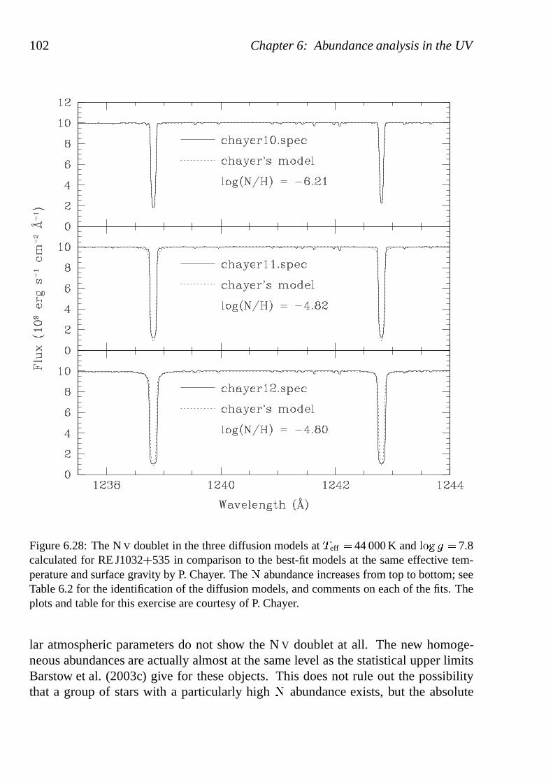
102 Chapter 6: Abundance analysis in the UV
Figure 6.28: The NV doublet in the three diffusion models at� eff � 44 000 K and� � � � � 7.8calculated for RE J1032
�535 in comparison to the best-fit models at the same effectivetem-
perature and surface gravity by P. Chayer. The� abundance increases from top to bottom; seeTable 6.2 for the identification of the diffusion models, andcomments on each of the fits. Theplots and table for this exercise are courtesy of P. Chayer.
lar atmospheric parameters do not show the NV doublet at all. The new homoge-neous abundances are actually almost at the same level as thestatistical upper limitsBarstow et al. (2003c) give for these objects. This does not rule out the possibilitythat a group of stars with a particularly high� abundance exists, but the absolute
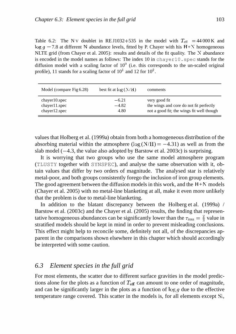
Chapter 6.3: Element species in the full grid 103
Table 6.2: The NV doublet in RE J1032�
535 in the model with� eff � 44 000 K and� � � � � 7.8 at different� abundance levels, fitted by P. Chayer with his� +� homogeneousNLTE grid (from Chayer et al. 2005): results and details of the fit quality. The� abundanceis encoded in the model names as follows: The index 10 inchayer10.spec stands for thediffusion model with a scaling factor of 10
�(i.e. this corresponds to the un-scaled original
profile), 11 stands for a scaling factor of 10�
and 12 for 10�.
Model (compare Fig 6.28) best fit at� �(�
/�
) comments
chayer10.spec � 6.21 very good fitchayer11.spec � 4.82 the wings and core do not fit perfectlychayer12.spec � 4.80 not a good fit; the wings fit well though
values that Holberg et al. (1999a) obtain from both a homogeneous distribution of theabsorbing material within the atmosphere (
� � �(� /� ) � � 4.31) as well as from the
slab model (� 4.3, the value also adopted by Barstow et al. 2003c) is surprising.It is worrying that two groups who use the same model atmosphere program
(TLUSTY together withSYNSPEC), and analyse the same observation with it, ob-tain values that differ by two orders of magnitude. The analysed star is relativelymetal-poor, and both groups consistently forego the inclusion of iron group elements.The good agreement between the diffusion models in this work, and the� +� models(Chayer et al. 2005) with no metal-line blanketing at all, make it even more unlikelythat the problem is due to metal-line blanketing.
In addition to the blatant discrepancy between the Holberg et al. (1999a) /Barstow et al. (2003c) and the Chayer et al. (2005) results, the finding that represen-tative homogeneous abundances can be significantly lower than the� ross �
�� value in
stratified models should be kept in mind in order to prevent misleading conclusions.This effect might help to reconcile some, definitely not all,of the discrepancies ap-parent in the comparisons shown elsewhere in this chapter which should accordinglybe interpreted with some caution.
6.3 Element species in the full grid
For most elements, the scatter due to different surface gravities in the model predic-tions alone for the plots as a function of
� � �can amount to one order of magnitude,
and can be significantly larger in the plots as a function of� � �
� due to the effectivetemperature range covered. This scatter in the models is, for all elements except� � ,
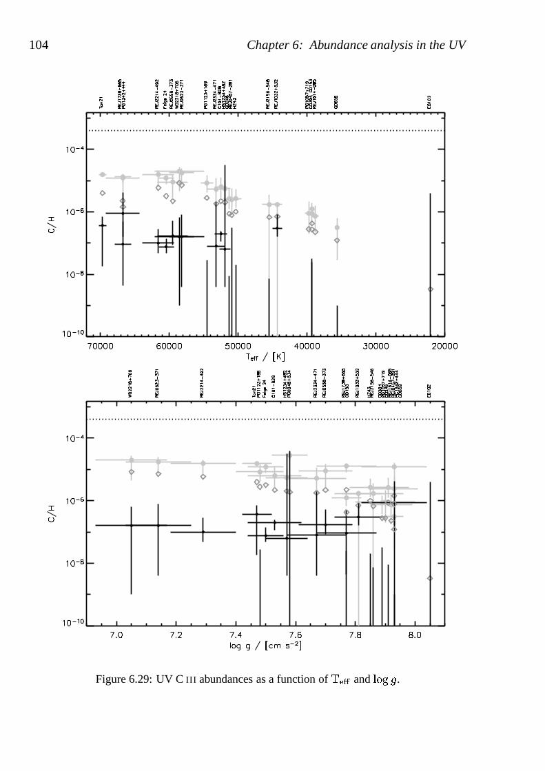
104 Chapter 6: Abundance analysis in the UV
Figure 6.29: UV CIII abundances as a function of� � � and� � � � .
Chapter 6.3: Element species in the full grid 105
Figure 6.30: UV CIII abundances as a function of the metal index��.
drastically reduced in those plots where the results are shown as a function of themetal index� �
.This is true for both Chayer et al.’s (1995b) as well as for thecurrent diffusion
models. In a duplication of the results from Sect. 4.2, Figs.6.29 to 6.42 show againthat Chayer et al.’s predictions for� , � � , and� � lie below, those for� and� abovethose of the new models. No overall systematic effect is evident.
The location of� ross ��� on the mass scale in Chayer et al.’s hydrogen models
with respect to the diffusion models with potentially largeamounts of heavy elementsdoes not result in significant offsets that could distort therepresentation of the results.According to the data in Table 6.3, and an interpolation fromthe models in this workto the representative surface gravity cited there, it is obvious that this difference resultsin an offset in the� ross scale no larger than 0.04 dex in
� � � � over a large effectivetemperature range (as shown in Fig. 6.43). It is therefore unlikely that this producesany noticeable systematic differences. The larger offset in Fig. 6.26 results from aslightly wrong surface gravity used in the determination ofthe location of� ross �
��
on the mass scale.Is is also worth noting that with very few exceptions (objects belonging to the upper
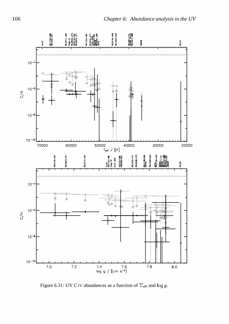
106 Chapter 6: Abundance analysis in the UV
Figure 6.31: UV CIV abundances as a function of� � � and � � � � .
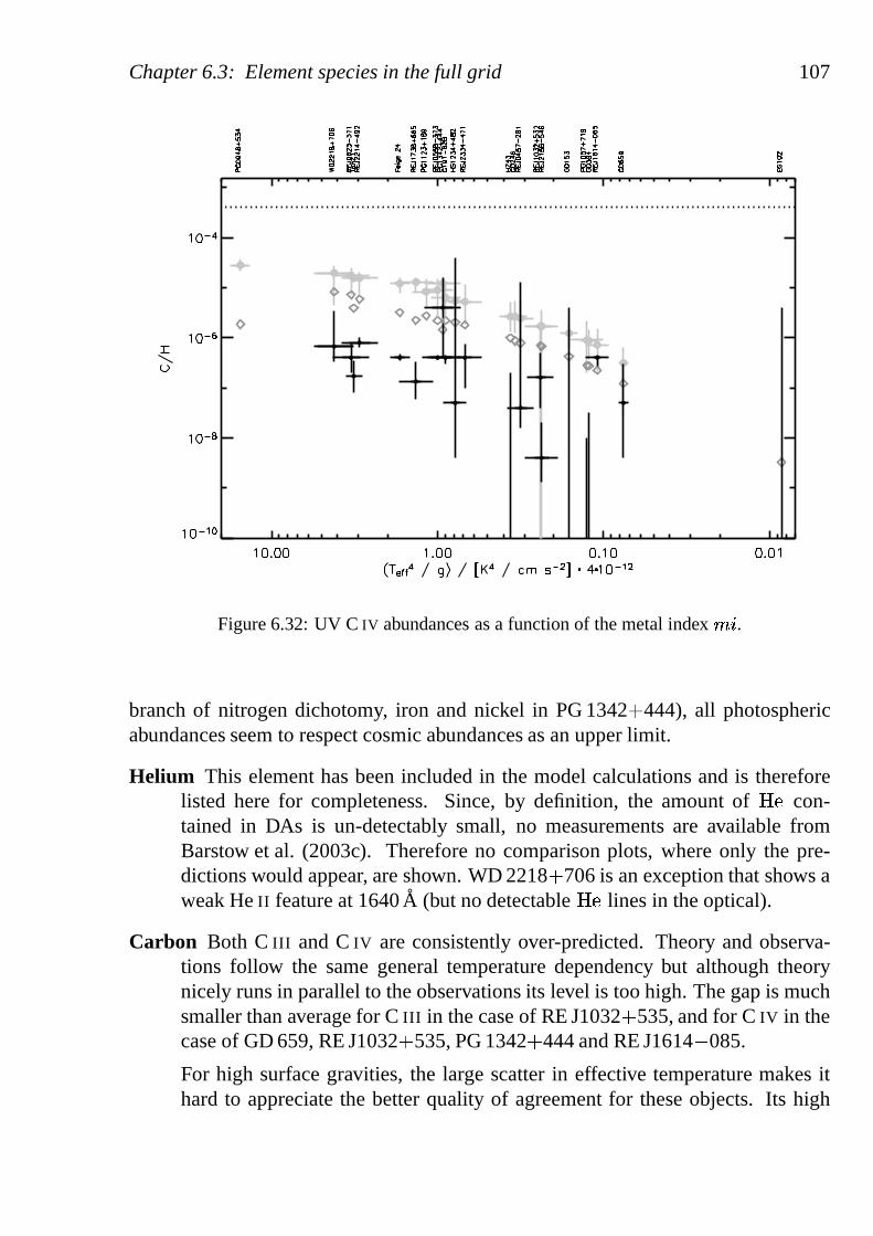
Chapter 6.3: Element species in the full grid 107
Figure 6.32: UV CIV abundances as a function of the metal index��.
branch of nitrogen dichotomy, iron and nickel in PG 1342� 444), all photosphericabundances seem to respect cosmic abundances as an upper limit.
Helium This element has been included in the model calculations andis thereforelisted here for completeness. Since, by definition, the amount of � � con-tained in DAs is un-detectably small, no measurements are available fromBarstow et al. (2003c). Therefore no comparison plots, where only the pre-dictions would appear, are shown. WD 2218� 706 is an exception that shows aweak HeII feature at 1640A (but no detectable� � lines in the optical).
Carbon Both CIII and CIV are consistently over-predicted. Theory and observa-tions follow the same general temperature dependency but although theorynicely runs in parallel to the observations its level is too high. The gap is muchsmaller than average for CIII in the case of RE J1032� 535, and for CIV in thecase of GD 659, RE J1032� 535, PG 1342� 444 and RE J1614� 085.
For high surface gravities, the large scatter in effective temperature makes ithard to appreciate the better quality of agreement for theseobjects. Its high
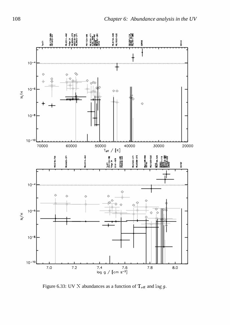
108 Chapter 6: Abundance analysis in the UV
Figure 6.33: UV� abundances as a function of� � � and � � � � .
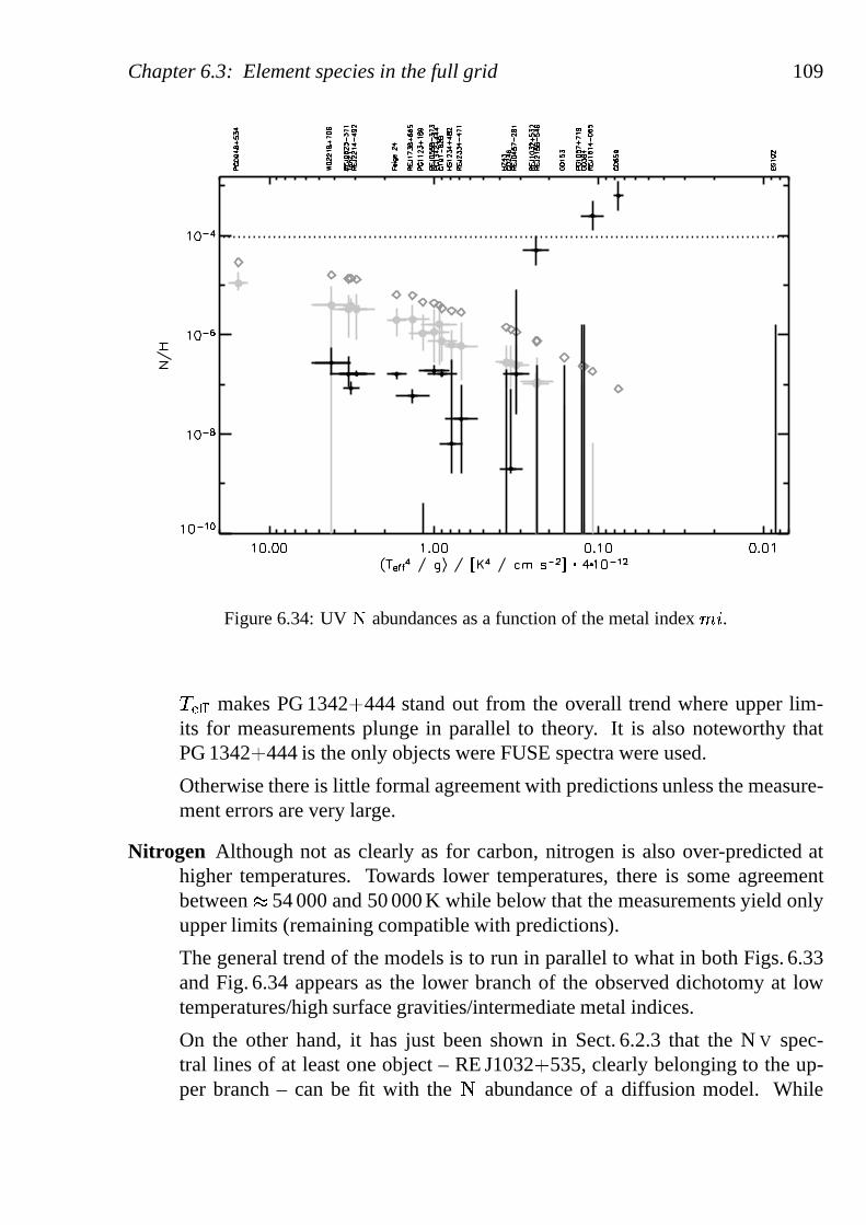
Chapter 6.3: Element species in the full grid 109
Figure 6.34: UV� abundances as a function of the metal index��.
� � �makes PG 1342� 444 stand out from the overall trend where upper lim-
its for measurements plunge in parallel to theory. It is alsonoteworthy thatPG 1342� 444 is the only objects were FUSE spectra were used.
Otherwise there is little formal agreement with predictions unless the measure-ment errors are very large.
Nitrogen Although not as clearly as for carbon, nitrogen is also over-predicted athigher temperatures. Towards lower temperatures, there issome agreementbetween
�54 000 and 50 000 K while below that the measurements yield only
upper limits (remaining compatible with predictions).
The general trend of the models is to run in parallel to what inboth Figs. 6.33and Fig. 6.34 appears as the lower branch of the observed dichotomy at lowtemperatures/high surface gravities/intermediate metalindices.
On the other hand, it has just been shown in Sect. 6.2.3 that the NV spec-tral lines of at least one object – RE J1032� 535, clearly belonging to the up-per branch – can be fit with the� abundance of a diffusion model. While
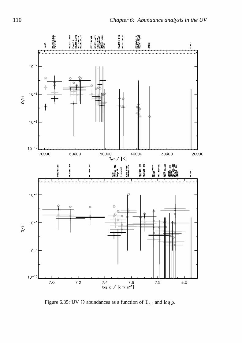
110 Chapter 6: Abundance analysis in the UV
Figure 6.35: UV� abundances as a function of� � � and � � � � .
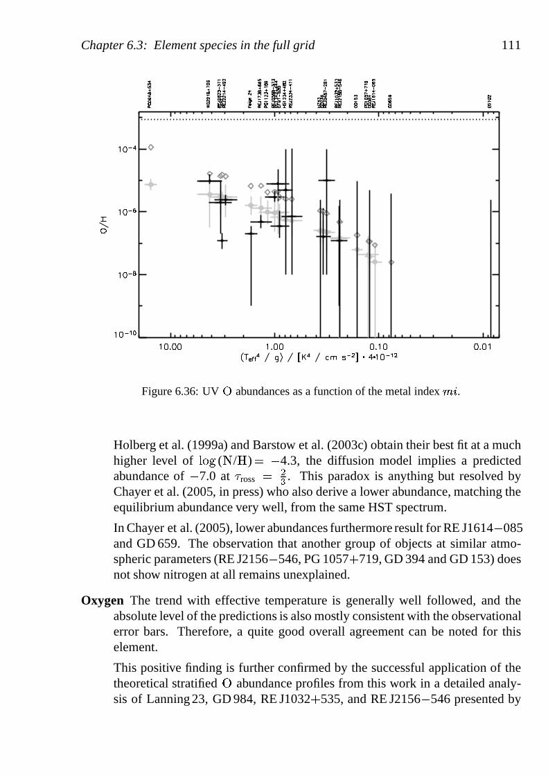
Chapter 6.3: Element species in the full grid 111
Figure 6.36: UV� abundances as a function of the metal index��.
Holberg et al. (1999a) and Barstow et al. (2003c) obtain their best fit at a muchhigher level of
� � �(� /� ) � � 4.3, the diffusion model implies a predicted
abundance of� 7.0 at � ross ��� . This paradox is anything but resolved by
Chayer et al. (2005, in press) who also derive a lower abundance, matching theequilibrium abundance very well, from the same HST spectrum.
In Chayer et al. (2005), lower abundances furthermore result for RE J1614� 085and GD 659. The observation that another group of objects at similar atmo-spheric parameters (RE J2156� 546, PG 1057� 719, GD 394 and GD 153) doesnot show nitrogen at all remains unexplained.
Oxygen The trend with effective temperature is generally well followed, and theabsolute level of the predictions is also mostly consistentwith the observationalerror bars. Therefore, a quite good overall agreement can benoted for thiselement.
This positive finding is further confirmed by the successful application of thetheoretical stratified� abundance profiles from this work in a detailed analy-sis of Lanning23, GD 984, RE J1032� 535, and RE J2156� 546 presented by
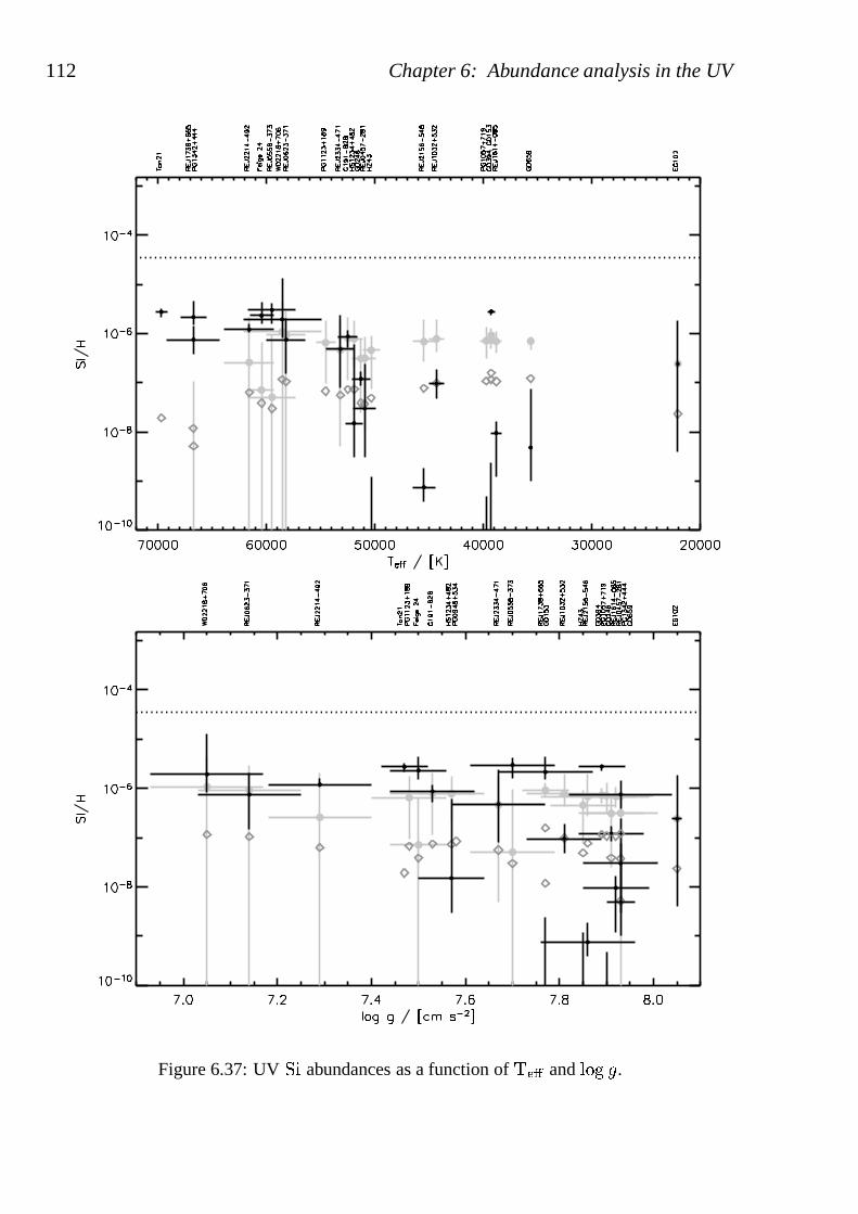
112 Chapter 6: Abundance analysis in the UV
Figure 6.37: UV� � abundances as a function of� � � and � � � � .
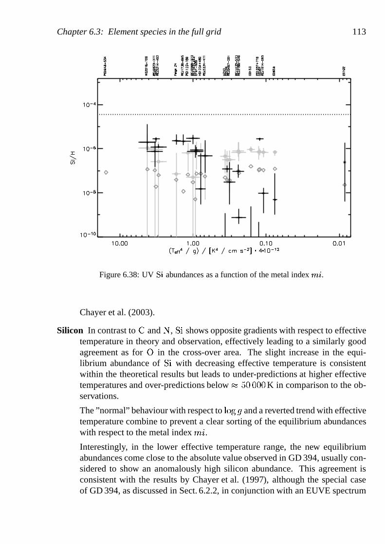
Chapter 6.3: Element species in the full grid 113
Figure 6.38: UV� � abundances as a function of the metal index��.
Chayer et al. (2003).
Silicon In contrast to� and� , � � shows opposite gradients with respect to effectivetemperature in theory and observation, effectively leading to a similarly goodagreement as for� in the cross-over area. The slight increase in the equi-librium abundance of� � with decreasing effective temperature is consistentwithin the theoretical results but leads to under-predictions at higher effectivetemperatures and over-predictions below
� � � � � � K in comparison to the ob-servations.
The ”normal” behaviour with respect to� � �
� and a reverted trend with effectivetemperature combine to prevent a clear sorting of the equilibrium abundanceswith respect to the metal index� �
.
Interestingly, in the lower effective temperature range, the new equilibriumabundances come close to the absolute value observed in GD 394, usually con-sidered to show an anomalously high silicon abundance. Thisagreement isconsistent with the results by Chayer et al. (1997), although the special caseof GD 394, as discussed in Sect. 6.2.2, in conjunction with anEUVE spectrum
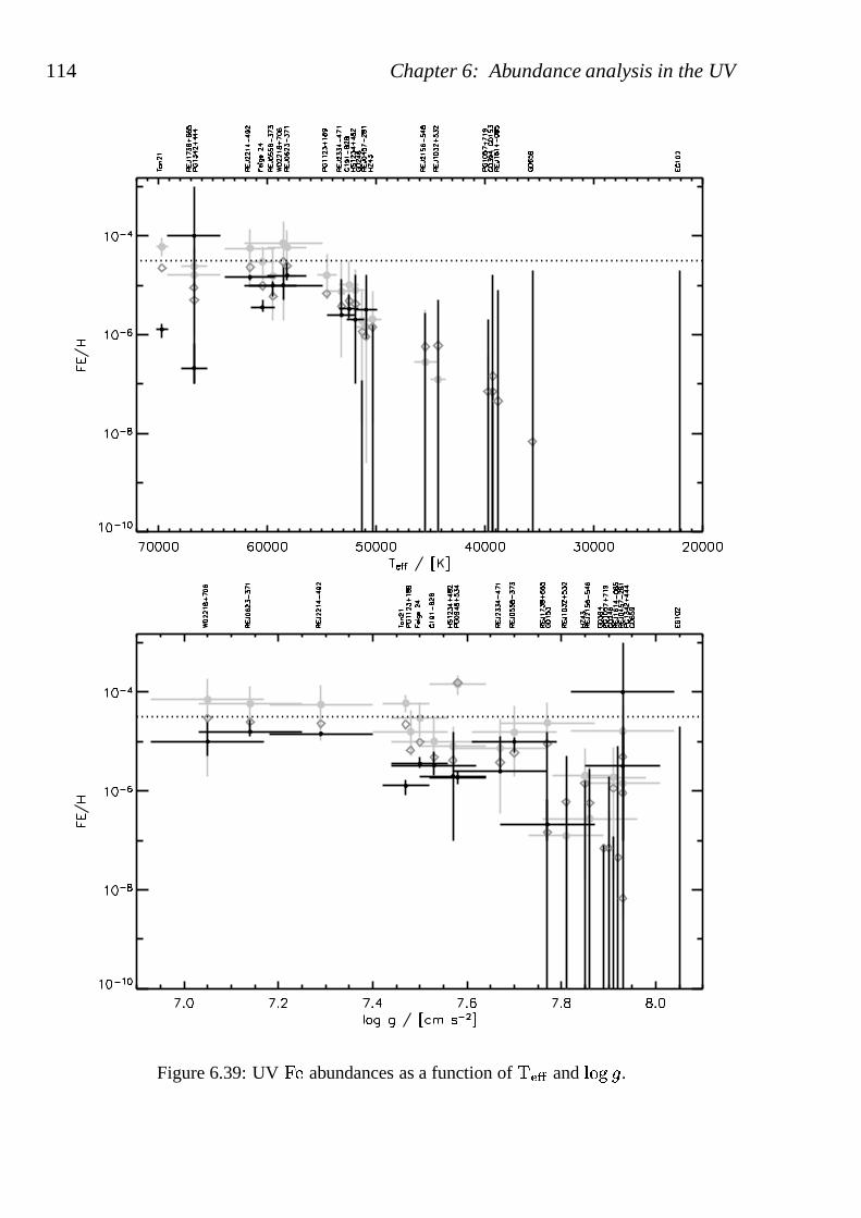
114 Chapter 6: Abundance analysis in the UV
Figure 6.39: UV� � abundances as a function of� � � and � � � � .
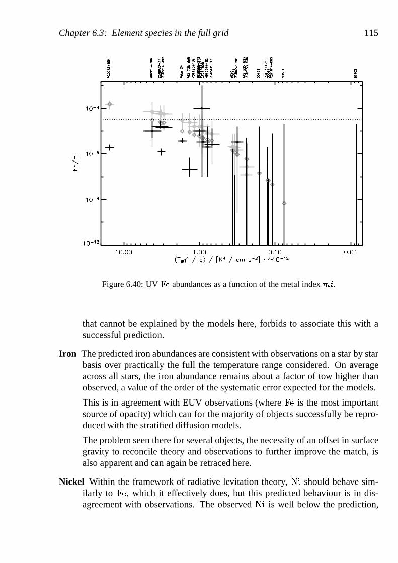
Chapter 6.3: Element species in the full grid 115
Figure 6.40: UV� � abundances as a function of the metal index��.
that cannot be explained by the models here, forbids to associate this with asuccessful prediction.
Iron The predicted iron abundances are consistent with observations on a star by starbasis over practically the full the temperature range considered. On averageacross all stars, the iron abundance remains about a factor of tow higher thanobserved, a value of the order of the systematic error expected for the models.
This is in agreement with EUV observations (where� � is the most importantsource of opacity) which can for the majority of objects successfully be repro-duced with the stratified diffusion models.
The problem seen there for several objects, the necessity ofan offset in surfacegravity to reconcile theory and observations to further improve the match, isalso apparent and can again be retraced here.
Nickel Within the framework of radiative levitation theory,� � should behave sim-ilarly to � � , which it effectively does, but this predicted behaviour isin dis-agreement with observations. The observed� � is well below the prediction,
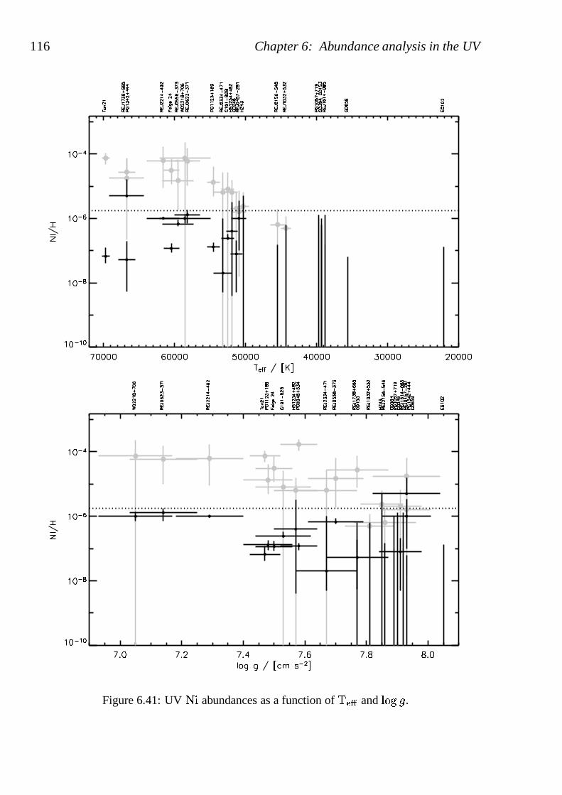
116 Chapter 6: Abundance analysis in the UV
Figure 6.41: UV� � abundances as a function of� � � and� � � � .
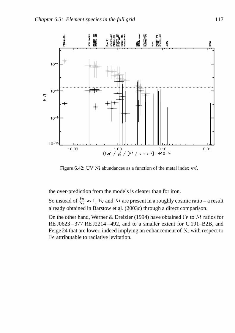
Chapter 6.3: Element species in the full grid 117
Figure 6.42: UV� � abundances as a function of the metal index��.
the over-prediction from the models is clearer than for iron.
So instead of��
� ��
� , � � and� � are present in a roughly cosmic ratio – a resultalready obtained in Barstow et al. (2003c) through a direct comparison.
On the other hand, Werner & Dreizler (1994) have obtained� � to � � ratios forRE J0623� 377 RE J2214� 492, and to a smaller extent for G 191–B2B, andFeige 24 that are lower, indeed implying an enhancement of� � with respect to� � attributable to radiative levitation.
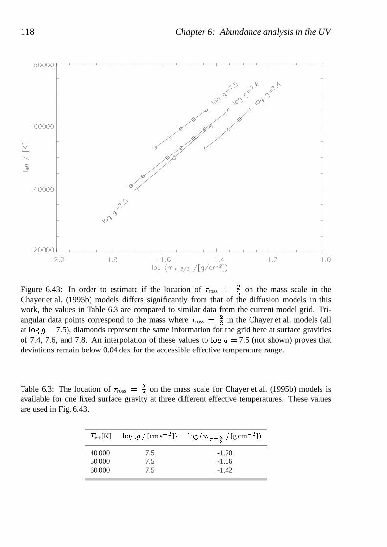
118 Chapter 6: Abundance analysis in the UV
Figure 6.43: In order to estimate if the location of� ross ��� on the mass scale in the
Chayer et al. (1995b) models differs significantly from thatof the diffusion models in thiswork, the values in Table 6.3 are compared to similar data from the current model grid. Tri-angular data points correspond to the mass where� ross �
�� in the Chayer et al. models (all
at � � � � � 7.5), diamonds represent the same information for the grid here at surface gravitiesof 7.4, 7.6, and 7.8. An interpolation of these values to� � � � � 7.5 (not shown) proves thatdeviations remain below 0.04 dex for the accessible effective temperature range.
Table 6.3: The location of� ross ��� on the mass scale for Chayer et al. (1995b) models is
available for one fixed surface gravity at three different effective temperatures. These valuesare used in Fig. 6.43.
� eff[K] � � � � �[cm s�
�]� � � �
� � � ���
[g cm�
�]�
40 000 7.5 -1.7050 000 7.5 -1.5660 000 7.5 -1.42
CHAPTER 7
Conclusions
7.1 Status of modelling
Stellar atmosphere models have been calculated for the analysis of a sample of hot DA(= hydrogen-rich) white dwarfs. By coupling radiative levitation theory with state-of-the-art metal-line blanketed NLTE stellar atmosphere models and self-consistentlysolving the full system of equations, photospheric chemical abundance profiles can bepredicted by this novel method for a given combination of effective temperature andsurface gravity as the only input parameters. The evaluation of radiative accelerationsrequires a detailed modelling of atomic data. NLTE conditions, fully self-consistentdiffusion, and an exhaustive treatment of iron group element atomic data have for thefirst time been combined to construct models detailed enoughfor a direct comparisonof theoretical emergent fluxes with the high-resolution UV and EUV observationsnow available.
The main grid of diffusion models consists of atmospheric structures where theabundances of the elements� � � � � � � � � � � as trace absorbers in a backgroundplasma dominated by� are self-consistently predicted from an equilibrium conditionbetween radiative levitation and gravitational settling.Abundance tables and high-resolution spectra for the optical, UV to FUV and EUV spectral ranges are availablefor the full grid. In comparison to Schuh (2000), this implies both a significant en-largement of the model grid as well as more extensive data products.
The main motivation for further developments is the desire for an improved treat-ment of the radiative accelerations. This can primarily be achieved with more exten-sive atomic input data, as explored in a few test models. By comparing the results toearlier diffusion calculations (LTE, not self-consistent), and by exploring the effectsof improvements in the modelling, a quantitative estimate of the systematic errorsinherent in the models is possible. While the internal errorwithin one type of calcula-tion is only about a factor of two, the variations from Chayeret al. (1995b) models tomodels in this work’s major grid, and from those to test models with more elements
119
120 Chapter 7: Conclusions
included, can amount to 2 dex in the respective equilibrium abundances, mainly dueto the strong depth-dependency of the resulting profiles. While these discrepanciesare understood to arise from the different conditions imposed on the modelling, it isnot immediately clear which of them resemble reality most closely.
7.2 Recapitulation of results from EUV and UV observations
Based on this larger and more complete model grid, and using improved visual mag-nitudes, a re-analysis of EUVE spectra has been presented. When comparing the the-oretical spectra to spectroscopic EUVE observations, the fits turn out to be of goodquality for most of the sample stars, and in those cases oftenbetter than with chemi-cally homogeneous stellar model atmospheres. The fractionof objects with good fitscould be increased thanks to the improvements in the repeated analysis in compari-son to Schuh (2000). From these results (published in Schuh et al. 2002), the currentimplementation of diffusion theory therefore seems to be able to quantitatively de-scribe the processes taking place in moderately hot white dwarf atmospheres and cansuccessfully reproduce observed EUV spectra. Exceptions to this, most prominentlyperhaps GD 394, have been discussed in the previous chapters.
The picture is more complex for the analysis of UV observations. In that case, in-stead of matching the spectra directly, abundances derivedfrom individual lines in UV(IUE, HST-GHRS and HST-STIS) spectra with homogeneous models (Barstow et al.2003c) have been compared to the equilibrium abundance predictions of the diffusionmodels. Overall the best agreement across the board for individual stars is obtained inthe effective temperature range
�50 000 – 55 000 K. However, in strictly absolute val-
ues, the offset between observed and predicted abundance levels is often such that noformal agreement of the exact numbers is achievable anywhere on the full parameterrange of the model grid. This suggests that an attempt of formally fitting UV spectrawith diffusion models would only result in parameters at theedges of the model grid,because it would only be possible to compensate discrepancies in abundance by shiftsin effective temperature and surface gravity. The usefulness of such a procedure at thepresent state is questionable and can currently not be recommended for large samplesof stars. Instead, it is advisable to closely examine every object individually, and testvarious scenarios, to track down the particular reason for potential mismatches be-tween predicted absorption lines and their observed counterparts. The description ofthe physics in white dwarf atmospheres through diffusion models is most likely stillbetter than with homogeneous models, although those may, due to the significantlylarger number of free parameters, currently yield better fits in a direct matching ofspectral lines. Exceptions where the diffusion models do better straightaway exist.
One such example of an in-depth examination is the analysis of RE J1032� 532.
Chapter 7.2: Recapitulation of results from EUV and UV observations 121
Also, using the predicted stratification profiles, Chayer etal. (2003) succeeded in si-multaneously reproducing the observed oxygen lines of different ionisation stages inFUSE and HST-STIS spectra of GD 984, RE J1032� 532 and WD 2152� 548.
Generally, the manageable amount of individual lines for most elements, and theirgood resolution in many UV observations, allows – and requires – one to differentiatemore than in EUVE observations. In the element-by-element comparison betweentheory and measurements, there are cases where both gradients have the same signas well as cases where they are opposite to each other, so thatthe required offset infundamental parameters would even point in different directions, respectively.
Overall, measured photospheric abundances seem to respectcosmic abundances asan upper limit – which the equilibrium abundances do not where the radiative accel-eration is large enough –, with very few exceptions: iron andnickel in PG 1342� 444,and nitrogen in RE J1614� 085 and GD 659 (nitrogen is also close to solar inRE J1032� 535). Given that equilibrium radiative levitation theory ignores any evo-lutionary constraints, the subsolar photospheric abundances may be indicative of a”reservoir problem” (meaning there is no unlimited supply of all elements available)in the real stars.
A summary of all results of the comparison between predictedequilibrium abun-dances to abundance measurements obtained with homogeneous models from the UVdata is shown in Figs. 7.1 and 7.2. Figure 7.1 combines the total of all measurementsfor all elements and for all stars (sorted by metal index� �
; upper plot) and all cor-responding predictions (lower plot). This representationdoes not take into accountthe errors assigned to these mean values, it just recapitulates the latter from the moredetailed graphs in Chapter 6. Figure 7.2 condenses this information further by sub-tracting the numbers in the upper left from those in the lowerleft plot. In the upperpanel of Fig. 7.2, this is done for the actual mean values. In the lower panel, the errorsare now taken into account and the minimal residual differences allowed are shownfor all values. Consistency of measurement and prediction within the error bars yieldsa deviation of zero in this case.
There are three possible sources for the remaining discrepancies still seen in themerged final results. The errors cited above are statisticalerrors, but from the compar-ison of different homogeneous analyses alone, the various results from several worksimply that the hidden systematic errors must be at least of the order of� 1 dex (seethe examples of the nitrogen abundance for RE J1032� 535, the nickel abundances forRE J0623� 377 and RE J2214� 492, or the fundamental parameters for G 191–B2B).
Besides these uncertainties in methods regarded as well established for the deter-mination of abundances from the analysis of observations, successive generations ofdiffusion models that try to predict these results still disagree with each other by upto 2 dex. In the same spirit as above, this must be interpretedas the systematic errors
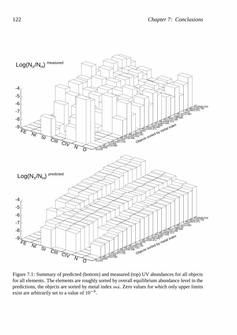
122 Chapter 7: Conclusions
EG102 GD659
REJ1614-085 GD394
PG1057+719 GD153
REJ2156-546 REJ1032+532
REJ0457-281 GD246
HZ43 REJ2334-471
HS1234+482 G191-B2B
PG1342+444 REJ0558-373
PG1123+189 REJ1738+665
Feige 24 REJ2214-492
Ton21 REJ0623-371
WD2218+706 PG0948+534
-9
-8
-7
-6
-5
-4
Log(NX/NH) measured
Objects sorted by metal index
FE NI SI CIII CIV N O
EG102 GD659
REJ1614-085 GD394
PG1057+719 GD153
REJ2156-546 REJ1032+532
REJ0457-281 GD246
HZ43 REJ2334-471
HS1234+482 G191-B2B
PG1342+444 REJ0558-373
PG1123+189 REJ1738+665
Feige 24 REJ2214-492
Ton21 REJ0623-371
WD2218+706 PG0948+534
-9
-8
-7
-6
-5
-4
Log(NX/NH) predicted
Objects sorted by metal index
FE NI SI CIII CIV N O
Figure 7.1: Summary of predicted (bottom) and measured (top) UV abundances for all objectsfor all elements. The elements are roughly sorted by overallequilibrium abundance level in thepredictions, the objects are sorted by metal index�
�. Zero values for which only upper limits
exist are arbitrarily set to a value of 10�
�.
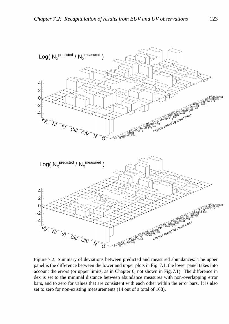
Chapter 7.2: Recapitulation of results from EUV and UV observations 123
EG102 GD659
REJ1614-085 GD394
PG1057+719 GD153
REJ2156-546 REJ1032+532
REJ0457-281 GD246
HZ43 REJ2334-471
HS1234+482 G191-B2B
PG1342+444 REJ0558-373
PG1123+189 REJ1738+665
Feige 24 REJ2214-492
Ton21 REJ0623-371
WD2218+706 PG0948+534
-4
-2
0
2
4
Log( NXpredicted / NX
measured )
Objects sorted by metal index
FE NI SI CIII CIV N O
Figure 7.2: Summary of deviations between predicted and measured abundances: The upperpanel is the difference between the lower and upper plots in Fig. 7.1, the lower panel takes intoaccount the errors (or upper limits, as in Chapter 6, not shown in Fig. 7.1). The difference index is set to the minimal distance between abundance measures with non-overlapping errorbars, and to zero for values that are consistent with each other within the error bars. It is alsoset to zero for non-existing measurements (14 out of a total of 168).
124 Chapter 7: Conclusions
currently inherent in the models. Taking together these twocontributions, it seemspossible to reconcile a good number of the residuals in Fig. 7.2 with a value nearzero.
The third possibility is to attribute the deviations to physical processes ignoredso far in the models such as mass-loss, mixing, or accretion.There is, however,no evidence of any clear pattern in the residuals that would help to explore a possiblecorrelation with stellar parameters. While mass-loss effects would disturb equilibriumconditions predominantly in the high metal index range, accretion would be expectedto have an effect only at lower metal indices.
In summary, the impression remains that the equilibrium abundances are generallytoo high. Any suspicion that measurements with homogeneousmodels may result insystematically lower values is partly invalidated by the results from the EUVE fits.Apart from perhaps a factor of two, the level of iron is well matched by predictionswith respect to the UV measurements, and the same agreement,also with a slighttrend towards too high equilibrium values, is seen in the EUVE analysis where thespectra are dominated by the iron content of the atmosphere.The few mismatches inthe EUV analysis have a tendency to cluster in the intermediate metal index regime.The abundance levels of other elements are relatively unimportant and therefore donot spoil the overall encouraging results from the EUVE analysis. The UV analysisresults imply that equilibrium radiative levitation theory still has some problems toreproduce in detail the multi-wavelength spectral evolution of white dwarfs.
There are two results that suggest that a limited supply of elements from the outsetmay be the key to the problem: The observed nickel abundancesappear to be limitedby the cosmic nickel abundance. Despite similar reactions to radiative momentumtransfer that would result in roughly equal equilibrium abundances for iron and nickel,these cannot be reached in the case of nickel since its cosmicabundance is lower thanthe predicted abundance level, and lower than that of iron where this restriction doesnot apply. The same circumstances seem to prevent a realistic description of the lessabundant iron group elements that have tentatively been included in test calculationsin the equilibrium approach and reach unrealistically highlevels. In a less obviousway, this restricting mechanism could also influence the abundances of other elementsthat in the calculations formally remain below the cosmic abundance limit.
7.3 Perspective
On the observational side, the legacy of HST-STIS was irrevocably completed withthe failure of this instrument in August 2004. The set of UV white dwarf spectraavailable may now only be amended by FUSE, which covers shorter wavelengths,provided it comes back into normal operations from its current safe mode status due
Chapter 7.3: Perspective 125
to the failure of another reaction wheel. It can be hoped thata fairly homogeneous anddecently calibrated data set will be available from FUSE in afew years’ time. Furtherprogress would also be possible with the planned WSO (World Space Observatory)which will take some time to come into existence, if at all.
Another approach is pursued in rocket-based experiments such as J-PEX: In a col-laboration with the group who flew with this mission, the high-resolution EUV dataof G 191–B2B have been analysed, among other models with the diffusion modelsfrom this work. Results will be published in Barstow et al. (2005).
The present successes on a global scale as seen in the EUVE analysis justify a fur-ther pursuit of the radiative equilibrium theory approach.Due to remaining puzzlesin detailed comparisons, further efforts to improve the existing models are necessary.Those include a strategy for the consideration ofall elements, the inclusion of finestructure in the atomic data of non-iron-group elements, the implementation of mo-mentum redistribution, and of a more efficient coupling between the computation ofthe model structure and the chemical stratification.
Ultimately, this method will probably be found to be the correct approach to de-termine depth-dependent photospheric abundances. What remains to be done is themajor step of replacing the present equilibrium approach with the treatment of fullytime-dependent diffusion in the non-equilibrium case together with mass-loss for self-consistent NLTE models, where the accumulation and successive removal of reser-voirs can be tracked over time. These improvements, necessary in a longer perspec-tive, are beyond the scope of the present thesis.

126 Chapter 7: Conclusions
Bibliography
Abazajian, K., Adelman-McCarthy, J. K.,Agueros, M. A., et al. 2003, AJ, 126, 2081
Acker, A., Marcout, J., Ochsenbein, F., Sten-holm, B., & Tylenda, R. 1992, Strasbourg- ESO catalogue of galactic planetary neb-ulae. Part 1; Part 2 (Garching: EuropeanSouthern Observatory, 1992)
Bannister, N. P., Barstow, M. A., Holberg,J. B., & Bruhweiler, F. C. 2003, MNRAS,341, 477
Barnard, A. J., Cooper, J., & Shamey, L. J.1969, A&A, 1, 28
Barstow, M., Cruddace, R., Kowalski, M.,et al. 2005, MNRAS, submitted
Barstow, M. A., Bannister, N. P., Holberg,J. B., et al. 2001a, MNRAS, 325, 1149
Barstow, M. A., Burleigh, M. R., Bannister,N. P., Holberg, J. B., & Hubeny, I. 2001b,in ASP Conf. Ser. 226: 12
� �
EuropeanWorkshop on White Dwarfs, 94
Barstow, M. A., Dobbie, P. D., Holberg, J. B.,Hubeny, I., & Lanz, T. 1997, MNRAS,286, 58
Barstow, M. A., Fleming, T. A., Diamond,C. J., et al. 1993a, MNRAS, 264, 16
Barstow, M. A., Fleming, T. A., Finley, D. S.,Koester, D., & Diamond, C. J. 1993b, MN-RAS, 260, 631
Barstow, M. A., Good, S. A., Bannister, N. P.,et al. 2003a, in NATO ASIB Proc. 105:White Dwarfs, 121
Barstow, M. A., Good, S. A., Burleigh, M. R.,et al. 2003b, MNRAS, 344, 562
Barstow, M. A., Good, S. A., Holberg, J. B.,et al. 2002, MNRAS, 330, 425
Barstow, M. A., Good, S. A., Holberg, J. B.,et al. 2003c, MNRAS, 341, 870
Barstow, M. A., Holberg, J. B., Fleming,T. A., et al. 1994a, MNRAS, 270, 499
Barstow, M. A., Holberg, J. B., Hubeny, I.,et al. 2001c, MNRAS, 328, 211
Barstow, M. A., Holberg, J. B., Hubeny, I.,et al. 1996, MNRAS, 279, 1120
Barstow, M. A., Holberg, J. B., & Koester, D.1994b, MNRAS, 268, L35
Barstow, M. A., Holberg, J. B., & Koester, D.1995, MNRAS, 274, L31
Barstow, M. A., Holberg, J. B., Marsh, M. C.,et al. 1994c, MNRAS, 271, 175
Barstow, M. A. & Hubeny, I. 1998, MNRAS,299, 379
Barstow, M. A., Hubeny, I., & Holberg, J. B.1998, MNRAS, 299, 520
Barstow, M. A., Hubeny, I., & Holberg, J. B.1999, MNRAS, 307, 884
Barstow, M. A., Wesemael, F., Fontaine, G.,et al. 1992, IAU Circ., 5518, 1
Barstow, M. A., Wesemael, F., Holberg, J. B.,et al. 1994d, MNRAS, 267, 647
Benedict, G. F., McArthur, B. E., Franz,O. G., et al. 2000, AJ, 119, 2382
Bergeron, P. & Leggett, S. K. 2002, ApJ, 580,1070
Bergeron, P., Saffer, R. A., & Liebert, J. 1992,ApJ, 394, 228
Bergeron, P., Wesemael, F., Beauchamp, A.,
127
128 Bibliography
et al. 1994, ApJ, 432, 305Bessell, M. S. 1999, PASP, 111, 1426Bohlin, R. C. 1996, AJ, 111, 1743Bohlin, R. C. 2000, AJ, 120, 437Bohlin, R. C., Colina, L., & Finley, D. S.
1995, AJ, 110, 1316Bohlin, R. C., Dickinson, M. E., & Calzetti,
D. 2001, AJ, 122, 2118Bowyer, S., Sasseen, T. P., Lampton, M., &
Wu, X. 1993, ApJ, 415, 875Bruhweiler, F., Barstow, M., Holberg, J., &
Sahu, M. 1999, Bulletin of the AmericanAstronomical Society, 31, 1419
Bruhweiler, F. C. & Kondo, Y. 1983, ApJ,269, 657
Budaj, J. & Dworetsky, M. M. 2002, MN-RAS, 337, 1340
Chapman, S. & Cowling, T. G. 1970, Themathematical theory of non-uniform gases.An account of the kinetic theory of vis-cosity, thermal conduction and diffusion ingases (Cambridge: University Press, 1970,3rd ed.)
Chayer, P., Fontaine, G., & Pelletier, C. 1997,in ASSL Vol. 214: White dwarfs, 253
Chayer, P., Fontaine, G., & Wesemael, F.1989, in IAU Colloq. 114: White Dwarfs,253
Chayer, P., Fontaine, G., & Wesemael, F.1991, in NATO ASIC Proc. 336: WhiteDwarfs, 249
Chayer, P., Fontaine, G., & Wesemael, F.1995a, ApJS, 99, 189
Chayer, P., Kruk, J. W., Ake, T. B., et al. 2000,ApJ, 538, L91
Chayer, P., Kruk, J. W., Vennes, S., & Dupuis,J. 2001, in ASP Conf. Ser. 226: 12
� �
Euro-pean Workshop on White Dwarfs, 90
Chayer, P., LeBlanc, F., Fontaine, G., et al.1994, ApJ, 436, L161
Chayer, P., Oliveira, C., Dupuis, J., Moos,H. W., & Welsh, B. 2003, in Kluwer Aca-demics NATO Science Series II., Vol. 105,
The 13� �
European Workshop on WhiteDwarfs, ed. D. de Martino, R. Silvotti, J.-E. Solheim, & R. Kalytis, 127
Chayer, P., Vennes, S., & Dupuis, J. 2005, inASP Conf. Series: 14
� �
European Work-shop on White Dwarfs, ed. D. Koester &S. Mohler, in press
Chayer, P., Vennes, S., Pradhan, A. K., et al.1995b, ApJ, 454, 429
Chen, B., Schartel, N., Kirsch, M. G. F., et al.2004, Memorie della Societa AstronomicaItaliana, 75, 561
Chu, Y., Guerrero, M. A., Gruendl, R. A., &Webbink, R. F. 2004, AJ, 127, 477
Colina, L. & Bohlin, R. C. 1994, AJ, 108,1931
Cruddace, R. G., Kowalski, M. P., Yentis, D.,et al. 2002, ApJ, 565, L47
Cunto, W. & Mendoza, C. 1992, Revista Mex-icana de Astronomia y Astrofisica, vol. 23,23, 107
Debes, J. H. & Sigurdsson, S. 2002, ApJ, 572,556
Deetjen, J. L., Dreizler, S., Jordan, S., &Werner, K. 2003, in ASP Conf. Ser. 288:Stellar Atmosphere Modeling, 617
Demers, S., Beland, S., Kibblewhite, E. J., Ir-win, M. J., & Nithakorn, D. S. 1986, AJ,92, 878
Dixon, W. V. D., Dupuis, J., & Hurwitz, M.2002, PASP, 114, 112
Dreizler, S. 1999, A&A, 352, 632Dreizler, S. 2002, Sternatmospharen I+II,
lecture notes (University of Tubingen),available at http://astro.uni-tuebingen.de/˜ dreizler/teaching/Sternatmosphaeren.html
Dreizler, S. 2003, in ASP Conf. Ser. 288: Stel-lar Atmosphere Modeling, 69
Dreizler, S. & Schuh, S. 2001, in ASP Con-ference Series, Vol. 226, The 12
� �
Euro-pean Workshop on White Dwarfs, ed. J. L.Provencal, H. L. Shipman, J. MacDonald,& S. Goodchild, 69
Bibliography 129
Dreizler, S. & Schuh, S. L. 2003, in IAU Sym-posium 210: Modelling of Stellar Atmo-spheres, ed. N. E. Piskunov, W. W. Weiss,& D. F. Gray, 33
Dreizler, S. & Werner, K. 1993, A&A, 278,199
Dreizler, S. & Wolff, B. 1999, A&A, 348, 189Dupuis, J., Chayer, P., Kruk, J. W., & Vennes,
S. 2003, in Kluwer Academics NATO Sci-ence Series II., Vol. 105, The 13
� �
Eu-ropean Workshop on White Dwarfs, ed.D. de Martino, R. Silvotti, J.-E. Solheim,& R. Kalytis, 157
Dupuis, J., Chayer, P., Vennes, S., Christian,D. J., & Kruk, J. W. 2000a, ApJ, 537, 977
Dupuis, J., Vennes, S., Bowyer, S., Pradhan,A. K., & Thejll, P. 1995, ApJ, 455, 574
Dupuis, J., Vennes, S., & Chayer, P. 2000b,Bulletin of the American Astronomical So-ciety, 32, 1543
Dupuis, J., Vennes, S., Chayer, P., Hurwitz,M., & Bowyer, S. 1998, ApJ, 500, L45+
Elvis, M., Plummer, D., Schachter, J., & Fab-biano, G. 1992, ApJS, 80, 257
Fan, X. 1999, AJ, 117, 2528Feautrier, P. 1964, C. R. Acad. Sc. Paris, 258,
3189Finley, D. S., Basri, G., & Bowyer, S. 1984,
Self-consistent recalibration of IUE deter-mination of hot DA white dwarf effectivetemperatures, Tech. rep.
Finley, D. S., Jelinsky, P., Dupuis, J., &Koester, D. 1993, ApJ, 417, 259
Finley, D. S., Koester, D., & Basri, G. 1997,ApJ, 488, 375
Fontaine, G., Brassard, P., & Bergeron, P.2001, PASP, 113, 409
Fontaine, G. & Chayer, P. 1997, in The ThirdConference on Faint Blue Stars, 169
Fontaine, G. & Michaud, G. 1979, ApJ, 231,826
Fuhrmeister, B. & Schmitt, J. H. M. M. 2003,A&A, 403, 247
Gonzalez, J.-F., Leblanc, F., Artru, M.-C., &Michaud, G. 1995, A&A, 297, 223
Green, R. F. 1980, ApJ, 238, 685Green, R. F., Schmidt, M., & Liebert, J. 1986,
ApJS, 61, 305Greenstein, J. L. & Liebert, J. W. 1990, ApJ,
360, 662Greenstein, J. S., Truran, J. W., & Cameron,
A. G. W. 1967, Nat, 213, 871Griem, H. R. 1974, Spectral line broaden-
ing by plasmas (Pure and Applied Physics,New York: Academic Press, 1974)
Gunderson, K., Wilkinson, E., Green, J. C., &Barstow, M. A. 2001, ApJ, 562, 992
Hebrard, G., Allard, N. F., Kielkopf, J. F.,et al. 2003, A&A, 405, 1153
Hebrard, G., Lemoine, M., Vidal-Madjar, A.,et al. 2002, ApJS, 140, 103
Hagen, H.-J., Groote, D., Engels, D., &Reimers, D. 1995, A&AS, 111, 195
Harris, H. C., Liebert, J., Kleinman, S. J., et al.2003, AJ, 126, 1023
Hawarden, T. G., Leggett, S. K., Letawsky,M. B., Ballantyne, D. R., & Casali, M. M.2001, MNRAS, 325, 563
Hearn, D. R., Richardson, J. A., Bradt, H.V. D., et al. 1976, ApJL, 203, L21
Heber, U., Napiwotzki, R., & Reid, I. N.1997, A&A, 323, 819
Hertzsprung, E. 1911, Publikationen des As-trophysikalischen Observatoriums zu Pots-dam, 63
Hill, P. W. & Hill, S. R. 1966, MNRAS, 133,205
Holberg, J. B., Barstow, M. A., Bruhweiler,F. C., & Collins, J. 1996, AJ, 111, 2361
Holberg, J. B., Barstow, M. A., Bruhweiler,F. C., & Hubeny, I. 2000, Bulletin of theAmerican Astronomical Society, 32, 1543
Holberg, J. B., Barstow, M. A., Bruhweiler,F. C., Hubeny, I., & Green, E. M. 1999a,ApJ, 517, 850
Holberg, J. B., Barstow, M. A., Bruhweiler,
130 Bibliography
F. C., & Sion, E. M. 1995, ApJ, 453, 313Holberg, J. B., Barstow, M. A., Buckley,
D. A. H., et al. 1993, ApJ, 416, 806Holberg, J. B., Barstow, M. A., & Green,
E. M. 1997a, ApJ, 474, L127+Holberg, J. B., Barstow, M. A., Hubeny, I.,
et al. 2002, Bulletin of the American As-tronomical Society, 34, 765
Holberg, J. B., Barstow, M. A., Lanz, T., &Hubeny, I. 1997b, ApJ, 484, 871
Holberg, J. B., Barstow, M. A., & Sion, E. M.1998, ApJS, 119, 207
Holberg, J. B., Basile, J., & Wesemael, F.1986, ApJ, 306, 629
Holberg, J. B., Bruhweiler, F. C., Barstow,M. A., & Dobbie, P. D. 1999b, ApJ, 517,841
Holberg, J. B., Hubeny, I., Barstow, M. A.,et al. 1994, ApJ, 425, L105
Homeier, D., Koester, D., Hagen, H.-J., et al.1998, A&A, 338, 563
Hubeny, I. & Lanz, T. 1995, ApJ, 439, 875Hubeny, I. & Lanz, T. 2000, SYNSPEC
- A User’s Guide, version 43 edn.,NASA/GSFC, Code 681, Greenbelt, MD20771, (current version is 48)
Hubeny, I. & Lanz, T. 2003, in ASP Confer-ence Series, Vol. 288, Stellar AtmosphereModeling, ed. I. Hubeny, D. Mihalas, &K. Werner, 51
Hubeny, I., Mihalas, D., & Werner, K., eds.2003, Stellar Atmosphere Modeling
Hui-Bon-Hoa, A., LeBlanc, F., & Hauschildt,P. H. 2000, ApJL, 535, L43
Hui-Bon-Hoa, A., LeBlanc, F., Hauschildt,P. H., & Baron, E. 2002, A&A, 381, 197
Hummer, D. G. & Mihalas, D. 1988, ApJ,331, 794
Hurwitz, M., Bowyer, S., Bristol, R., et al.1998, ApJ, 500, L1+
Jansen, F., Lumb, D., Altieri, B., et al. 2001,A&A, 365, L1
Jordan, S., Koester, D., & Finley, D. 1996, in
IAU Colloq. 152: Astrophysics in the Ex-treme Ultraviolet, 235
Jordan, S., Koester, D., Wulf-Mathies, C., &Brunner, H. 1987, A&A, 185, 253
Jordan, S., Wolff, B., Koester, D., & Napi-wotzki, R. 1994, A&A, 290, 834
Kahn, S. M., Wesemael, F., Liebert, J., et al.1984, ApJ, 278, 255
Kaiser, M. E., Bohlin, R. C., Lindler, D. J.,et al. 1998, PASP, 110, 978
Kidder, K. M., Holberg, J. B., & Mason, P. A.1991, AJ, 101, 579
Kilkenny, D., O’Donoghue, D., Koen, C.,Stobie, R. S., & Chen, A. 1997, MNRAS,287, 867
Kimble, R. A., Davidsen, A. F., Blair, W. P.,et al. 1993a, ApJ, 404, 663
Kimble, R. A., Davidsen, A. F., Long, K. S.,& Feldman, P. D. 1993b, ApJ, 408, L41
Kippenhahn, R. & Weigert, A. 1990, Stel-lar Structure and Evolution, 1st edn., ed.I. Appenzeller, M. Harwit, R. Kippenhahn,P. Strittmatter, & V. Trimble, Astronomyand Astrophysics Library (Berlin, Heidel-berg, New York: Springer Verlag)
Kleinman, S. J., Harris, H. C., Eisenstein,D. J., et al. 2004, ApJ, 607, 426
Koester, D. 1989, in Lecture Notes in Physics,Vol. 328, IAU Colloq. 114: White Dwarfs,ed. G. Wegner, 206
Koester, D. 2002, A&ARv, 11, 33Koester, D. & Chanmugam, G. 1990, Reports
of Progress in Physics, 53, 837Koester, D., Dreizler, S., Weidemann, V., &
Allard, N. F. 1998, A&A, 338, 612Koester, D., Napiwotzki, R., Christlieb, N.,
et al. 2001, A&A, 378, 556Kruk, J. W. 1998, in IAU Symp. 189: Funda-
mental Stellar Properties, 67Kruk, J. W., Brown, T. M., Davidsen, A. F.,
et al. 1999, ApJS, 122, 299Kruk, J. W., Howk, J. C., Andre, M., et al.
2002, ApJS, 140, 19
Bibliography 131
Kruk, J. W., Kimble, R. A., Buss, R. H., et al.1997, ApJ, 482, 546
Kunasz, P. B. & Olson, G. L. 1988, Journalof Quantitative Spectroscopy and RadiativeTransfer, 39, 1
Kurucz, R. L. 1991, in NATO ASIC Proc.341: Stellar Atmospheres - Beyond Clas-sical Models, 441
Lamontagne, R., Demers, S., Wesemael, F.,Fontaine, G., & Irwin, M. J. 2000, AJ, 119,241
Lampton, M., Margon, B., Paresce, F., Stern,R., & Bowyer, S. 1976, ApJL, 203, L71
Lanz, T., Barstow, M. A., Hubeny, I., & Hol-berg, J. B. 1996, ApJ, 473, 1089
Lanz, T. & Hubeny, I. 1995, ApJ, 439, 905Lehner, N., Gry, C., Sembach, K. R., et al.
2002, ApJS, 140, 81Lehner, N., Jenkins, E. B., Gry, C., et al. 2003,
ApJ, 595, 858Lemke, M. 1997, A&AS, 122, 285Lemoine, M., Vidal-Madjar, A., Hebrard, G.,
et al. 2002, ApJS, 140, 67Liebert, J., Wesemael, F., Fontaine, G.,
Hansen, C. J., & Shipman, H. L. 1986, inASSL Vol. 128: IAU Colloq. 87: HydrogenDeficient Stars and Related Objects, 387
Lucy, L. B. 1964, in First Havard Smithsonianconference on stellar atmospheres, 93
MacDonald, J. 1992, ApJ, 394, 619Madej, J. 1998, A&A, 340, 617Margon, B., Malina, R., Bowyer, S., Crud-
dace, R., & Lampton, M. 1976, ApJL, 203,L25
Marsh, M. C., Barstow, M. A., Buckley,D. A., et al. 1997a, MNRAS, 286, 369
Marsh, M. C., Barstow, M. A., Buckley,D. A., et al. 1997b, MNRAS, 287, 705
Massa, D. & Fitzpatrick, E. L. 2000, ApJS,126, 517
Massey, P., Strobel, K., Barnes, J. V., & An-derson, E. 1988, ApJ, 328, 315
McCook, G. P. & Sion, E. M. 1999, ApJS,
121, 1Mewe, R., Heise, J., Gronenschild, E. H.
B. M., et al. 1975, ApJL, 202, L67Michaud, G. 1970, ApJ, 160, 641Michaud, G., Vauclair, G., & Vauclair, S.
1983, ApJ, 267, 256Montmerle, T. & Michaud, G. 1976, ApJS,
31, 489Morvan, E., Vauclair, G., & Vauclair, S. 1986,
A&A, 163, 145Nagel, T. 2003, Dissertation, Eberhard-Karls-
Universitat TubingenNagel, T., Dreizler, S., & Werner, K. 2003,
in ASP Conf. Ser. 288: Stellar AtmosphereModeling, 641
Napiwotzki, R. 1999, A&A, 350, 101Napiwotzki, R., Barstow, M. A., Fleming, T.,
et al. 1993, A&A, 278, 478Napiwotzki, R., Green, P. J., & Saffer, R. A.
1999a, ApJ, 517, 399Napiwotzki, R., Green, P. J., & Saffer, R. A.
1999b, in ASP Conf. Ser. 169: 11th Euro-pean Workshop on White Dwarfs, 492
Oliveira, C. M., Hebrard, G., Howk, J. C.,et al. 2003, ApJ, 587, 235
Olson, G. L. & Kunasz, P. B. 1987, Journalof Quantitative Spectroscopy and RadiativeTransfer, 38, 325
Paerels, F. B. S. & Heise, J. 1989, ApJ, 339,1000
Paquette, C., Pelletier, C., Fontaine, G., &Michaud, G. 1986, ApJS, 61, 177
Petre, R., Shipman, H. L., & Canizares, C. R.1986, ApJ, 304, 356
Piskunov, N., Weiss, W. W., & Gray, D. F.,eds. 2004, Modeling of Stellar Atmo-spheres
Pounds, K. A., Allan, D. J., Barber, C., et al.1993, MNRAS, 260, 77
Rauch, T. & Deetjen, J. L. 2003, in ASP Conf.Ser. 288: Stellar Atmosphere Modeling,103
Redfield, S. & Linsky, J. L. 2004a, ApJ, 602,
132 Bibliography
776Redfield, S. & Linsky, J. L. 2004b, ApJ, 613,
1004Reid, I. N. 1996, AJ, 111, 2000Reimers, D. & Wisotzki, L. 1997, The Mes-
senger, 88, 14Rumph, T., Bowyer, S., & Vennes, S. 1994,
AJ, 107, 2108Russell, H. N. 1913, The Observatory, 36, 324Rutten, R. J. 1997, Radiative Transfer in
Stellar Atmospheres,� th WWW edn., lec-
ture notes (Utrecht University), available athttp://www.fys.ruu.nl/ rutten
Sahnow, D. J., Moos, H. W., Ake, T. B., et al.2000, ApJ, 538, L7
Schatzman, E. 1945, Annalesd’Astrophysique, 8, 143
Schatzman, E. 1958, White Dwarfs (NorthHolland Publishing Company, Amsterdam)
Schoning, T. & Butler, K. 1989a, A&AS, 78,51
Schoning, T. & Butler, K. 1989b, A&A, 219,326
Schuh, S. 2000, Diploma thesis, Eberhard-Karls-Universitat Tubingen
Schuh, S., Barstow, M. A., & Dreizler, S.2005, in ASP Conf. Series: 14
� �
EuropeanWorkshop on White Dwarfs, ed. D. Koester& S. Mohler, in press
Schuh, S., Dreizler, S., & Wolff, B. 2001, inASP Conference Series, Vol. 226, The 12
� �
European Workshop on White Dwarfs, ed.J. L. Provencal, H. L. Shipman, J. Mac-Donald, & S. Goodchild, 79
Schuh, S. L. & Dreizler, S. 2003, in ASPConf. Ser. 288: Stellar Atmosphere Mod-eling, 633
Schuh, S. L., Dreizler, S., & Deetjen, J. L.2003, in Kluwer Academics NATO ScienceSeries II., Vol. 105, The 13
� �
EuropeanWorkshop on White Dwarfs, ed. D. de Mar-tino, R. Silvotti, J.-E. Solheim, & R. Ka-lytis, 147
Schuh, S. L., Dreizler, S., & Wolff, B. 2002,A&A, 382, 164
Schwartz, R. D., Dawkins, D., Findley, D., &Chen, D. 1995, PASP, 107, 667
Seaton, M. J. 1992, Revista Mexicana de As-tronomia y Astrofisica, vol. 23, 23, 180
Seaton, M. J., Yan, Y., Mihalas, D., & Prad-han, A. K. 1994, MNRAS, 266, 805
Seaton, M. J., Zeippen, C. J., Tully, J. A., et al.1992, Revista Mexicana de Astronomia yAstrofisica, vol. 23, 23, 19
Shipman, H. J. 1994, Nature, 372, 317Shipman, H. L. 1976, ApJL, 206, L67Shipman, H. L. & Finley, D. S. 1994, Bulletin
of the American Astronomical Society, 26,870
Shipman, H. L., Provencal, J., Roby, S. W.,et al. 1995, AJ, 109, 1220
Silvestri, N. M., Oswalt, T. D., & Hawley,S. L. 2002, AJ, 124, 1118
Smith, E. P., Pica, A. J., Bohlin, R. C., et al.1996, ApJS, 104, 287
Smith, J. A., Tucker, D. L., Kent, S., et al.2002, AJ, 123, 2121
Smith, M. A. 2001, PASP, 113, 882Stobie, R. S., Kilkenny, D., O’Donoghue, D.,
et al. 1997, MNRAS, 287, 848Stone, R. P. S. 1996, ApJS, 107, 423Stoughton, C., Lupton, R. H., Bernardi, M.,
et al. 2002, AJ, 123, 485Thomas, H.-C., Beuermann, K., Reinsch, K.,
et al. 1998, A&A, 335, 467Trimble, V. & Aschwanden, M. J. 2001,
PASP, 113, 1025Tweedy, R. W. 1995, Nature, 373, 666Tweedy, R. W. & Kwitter, K. B. 1994, ApJ,
433, L93Unglaub, K. & Bues, I. 1998, A&A, 338, 75Unglaub, K. & Bues, I. 2000, A&A, 359,
1042Unglaub, K. & Bues, I. 2001, A&A, 374, 570Vauclair, G. 1987, in IAU Colloq. 95: Second
Conference on Faint Blue Stars, 341
Bibliography 133
Vauclair, G. 1989, in IAU Colloq. 114: WhiteDwarfs, 176
Vauclair, G., Schmidt, H., Koester, D., & Al-lard, N. 1997, A&A, 325, 1055
Vauclair, G., Vauclair, S., & Greenstein, J. L.1979, A&A, 80, 79
Vennes, S. 1999, ApJ, 525, 995Vennes, S., Chayer, P., Fontaine, G., & Wese-
mael, F. 1989, ApJL, 336, L25Vennes, S., Chayer, P., Hurwitz, M., &
Bowyer, S. 1996a, ApJ, 468, 898Vennes, S. & Dupuis, J. 2002, in ASP Conf.
Ser. 262: The High Energy Universe atSharp Focus: Chandra Science, 57
Vennes, S., Dupuis, J., Bowyer, S., et al. 1994,ApJ, 421, L35
Vennes, S., Dupuis, J., Rumph, T., et al. 1993,ApJ, 410, L119
Vennes, S., Fontaine, G., & Brassard, P. 1995,A&A, 296, 117
Vennes, S. & Lanz, T. 2001, ApJ, 553, 399Vennes, S., Polomski, E. F., Lanz, T., et al.
2000, ApJ, 544, 423Vennes, S., Thejll, P. A., Galvan, R. G., &
Dupuis, J. 1997, ApJ, 480, 714Vennes, S., Thejll, P. A., Wickramasinghe,
D. T., & Bessell, M. S. 1996b, ApJ, 467,782
Vennes, S. & Thorstensen, J. R. 1994, AJ,108, 1881
Vidal, C. R., Cooper, J., & Smith, E. W. 1973,ApJS, 25, 37
Vidal-Madjar, A., Allard, N. F., Koester, D.,et al. 1994, A&A, 287, 175
Welsh, B. Y., Sallmen, S., Sfeir, D., Shelton,R. L., & Lallement, R. 2002, A&A, 394,691
Werner, K., Deetjen, J. L., Dreizler, S., et al.2003, in ASP Conf. Ser. 288: Stellar Atmo-sphere Modeling, 31
Werner, K. & Dreizler, S. 1994, A&A, 286,L31
Werner, K. & Dreizler, S. 1999, in Journal of
Computational and Applied Mathematics,Vol. 109, Computational Astrophysics, ed.H. Riffert & K. Werner (Amsterdam: Else-vier Press), 65
Werner, K., Rauch, T., & Dreizler, S. 1998,A Users’s Guide to the Tubingen NLTEModel Atmosphere Package, Institut furAstronomie und Astrophysik, Astronomie,Tubingen, available at http://astro.uni-tuebingen.de/˜ rauch/
Wesemael, F. & et al. 1995, , in preparationWilkinson, E., Green, J. C., & Cash, W. 1993,
ApJS, 89, 211Wilms, J., Allen, A., & McCray, R. 2000,
ApJ, 542, 914Wisotzki, L., Christlieb, N., Bade, N., et al.
2000, A&A, 358, 77Wisotzki, L., Koehler, T., Groote, D., &
Reimers, D. 1996, A&AS, 115, 227Wolff, B. 1999, PhD thesis, Christian-
Albrechts-Universitat KielWolff, B., Jordan, S., Bade, N., & Reimers, D.
1995, A&A, 294, 183Wolff, B., Jordan, S., & Koester, D. 1994, in
Astronomische Gesellschaft Abstract Se-ries, 134–134
Wolff, B., Jordan, S., & Koester, D. 1996,A&A, 307, 149
Wolff, B., Koester, D., Dreizler, S., & Haas,S. 1998, A&A, 329, 1045
Wolff, B., Koester, D., & Lallement, R. 1999,A&A, 346, 969
Wolff, B., Kruk, J. W., Koester, D., et al. 2001,A&A, 373, 674
Wood, M. A. 1995, in White Dwarfs, ed.D. Koester & K. Werner, Lecture Notes inPhysics 443 (Berlin, Heidelberg: SpringerVerlag), 41
Zuckerman, B., Koester, D., Reid, I. N., &Hunsch, M. 2003, ApJ, 596, 477
Zuckerman, B. & Reid, I. N. 1998, ApJ, 505,L143

134 Bibliography
APPENDIX A
Equilibrium abundances
135
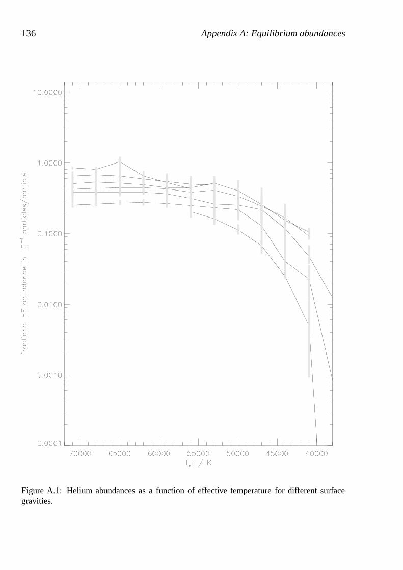
136 Appendix A: Equilibrium abundances
Figure A.1: Helium abundances as a function of effective temperature for different surfacegravities.
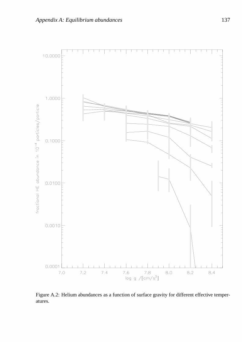
Appendix A: Equilibrium abundances 137
Figure A.2: Helium abundances as a function of surface gravity for different effective temper-atures.
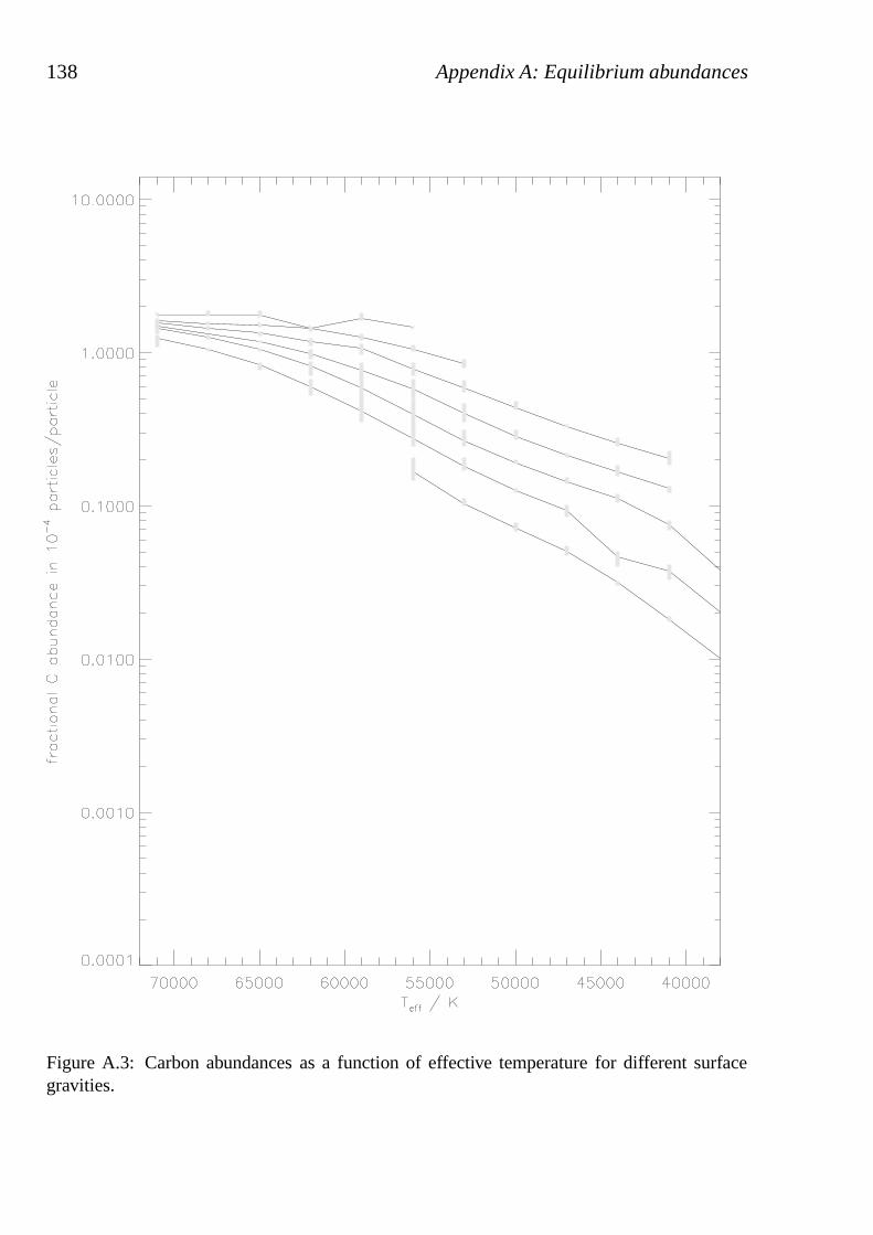
138 Appendix A: Equilibrium abundances
Figure A.3: Carbon abundances as a function of effective temperature for different surfacegravities.
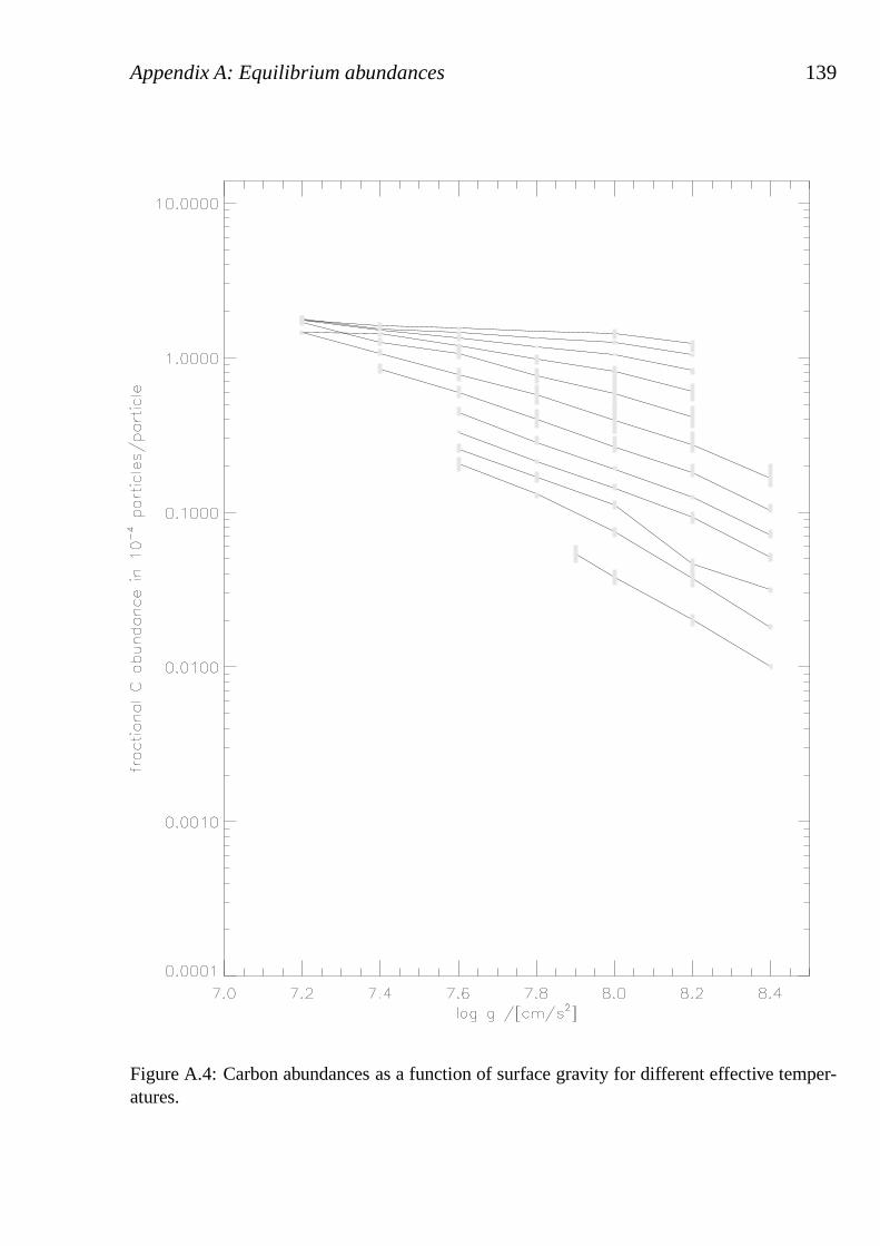
Appendix A: Equilibrium abundances 139
Figure A.4: Carbon abundances as a function of surface gravity for different effective temper-atures.
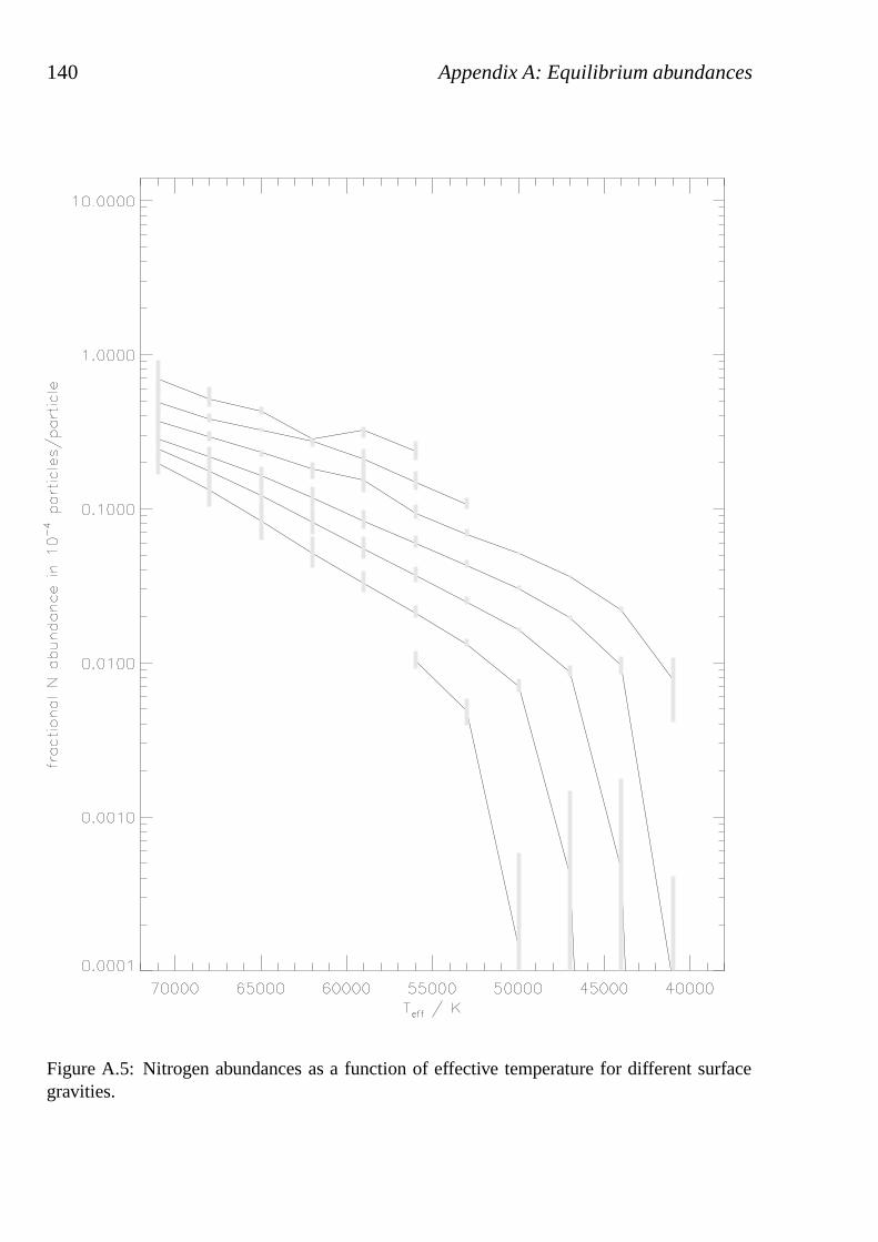
140 Appendix A: Equilibrium abundances
Figure A.5: Nitrogen abundances as a function of effective temperature for different surfacegravities.
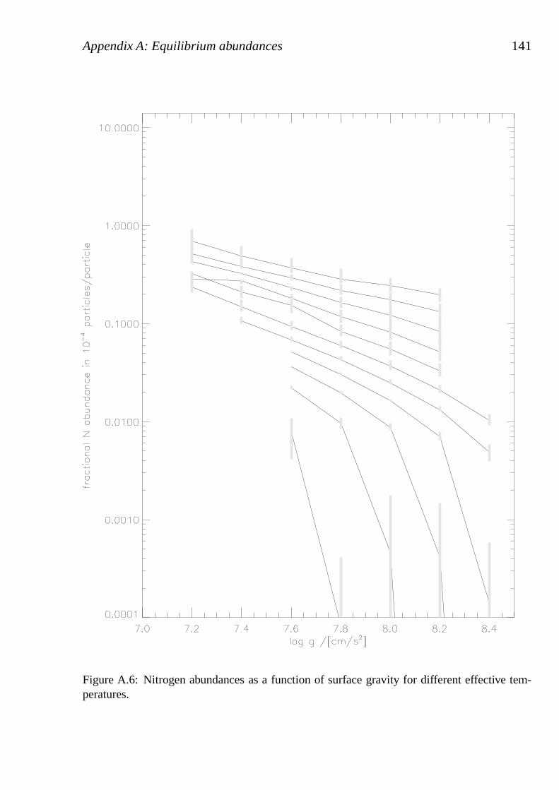
Appendix A: Equilibrium abundances 141
Figure A.6: Nitrogen abundances as a function of surface gravity for different effective tem-peratures.
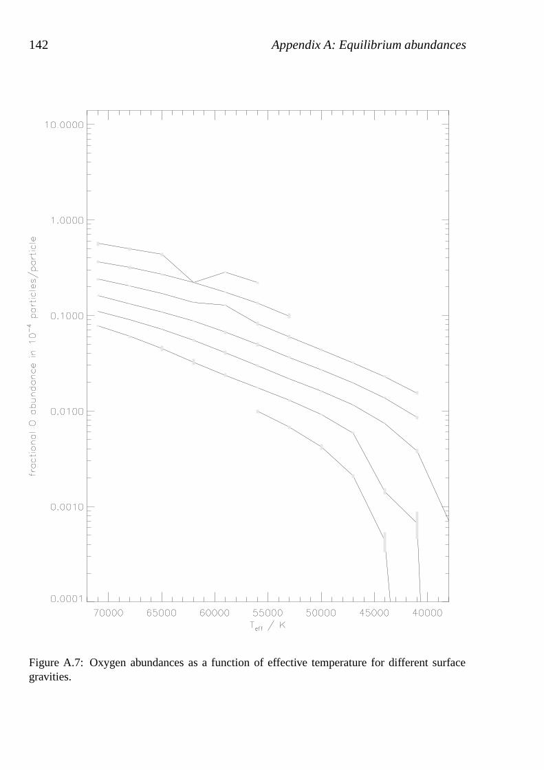
142 Appendix A: Equilibrium abundances
Figure A.7: Oxygen abundances as a function of effective temperature for different surfacegravities.
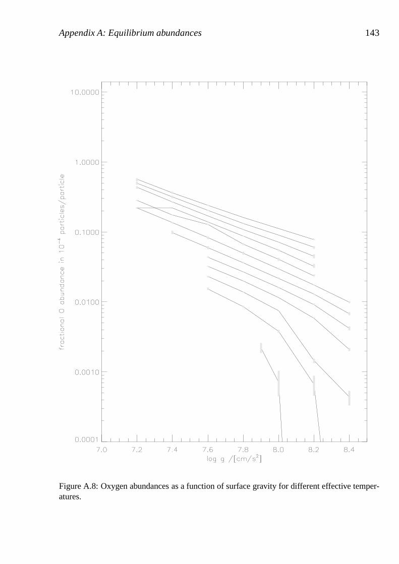
Appendix A: Equilibrium abundances 143
Figure A.8: Oxygen abundances as a function of surface gravity for different effective temper-atures.
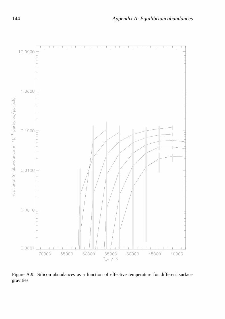
144 Appendix A: Equilibrium abundances
Figure A.9: Silicon abundances as a function of effective temperature for different surfacegravities.
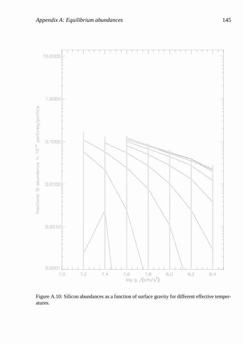
Appendix A: Equilibrium abundances 145
Figure A.10: Silicon abundances as a function of surface gravity for different effective temper-atures.
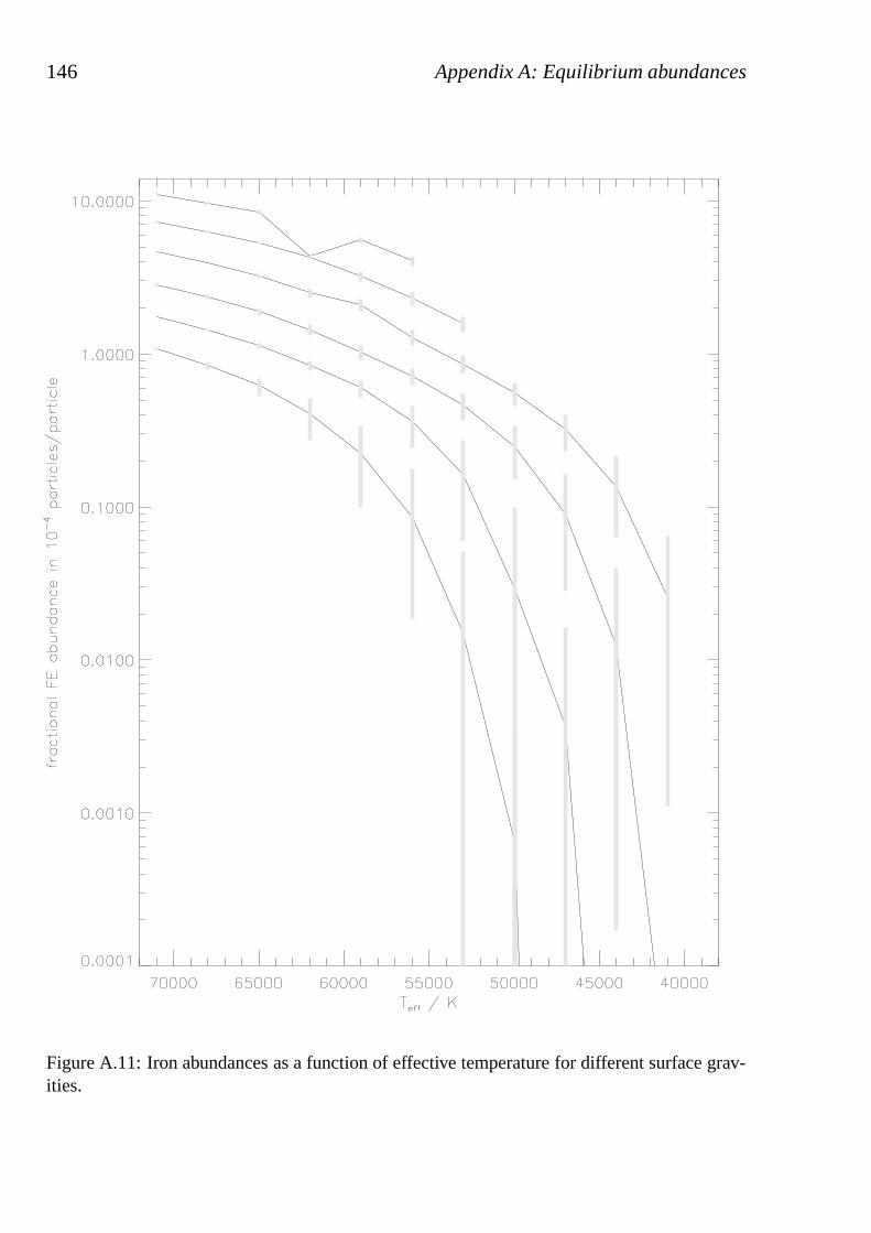
146 Appendix A: Equilibrium abundances
Figure A.11: Iron abundances as a function of effective temperature for different surface grav-ities.
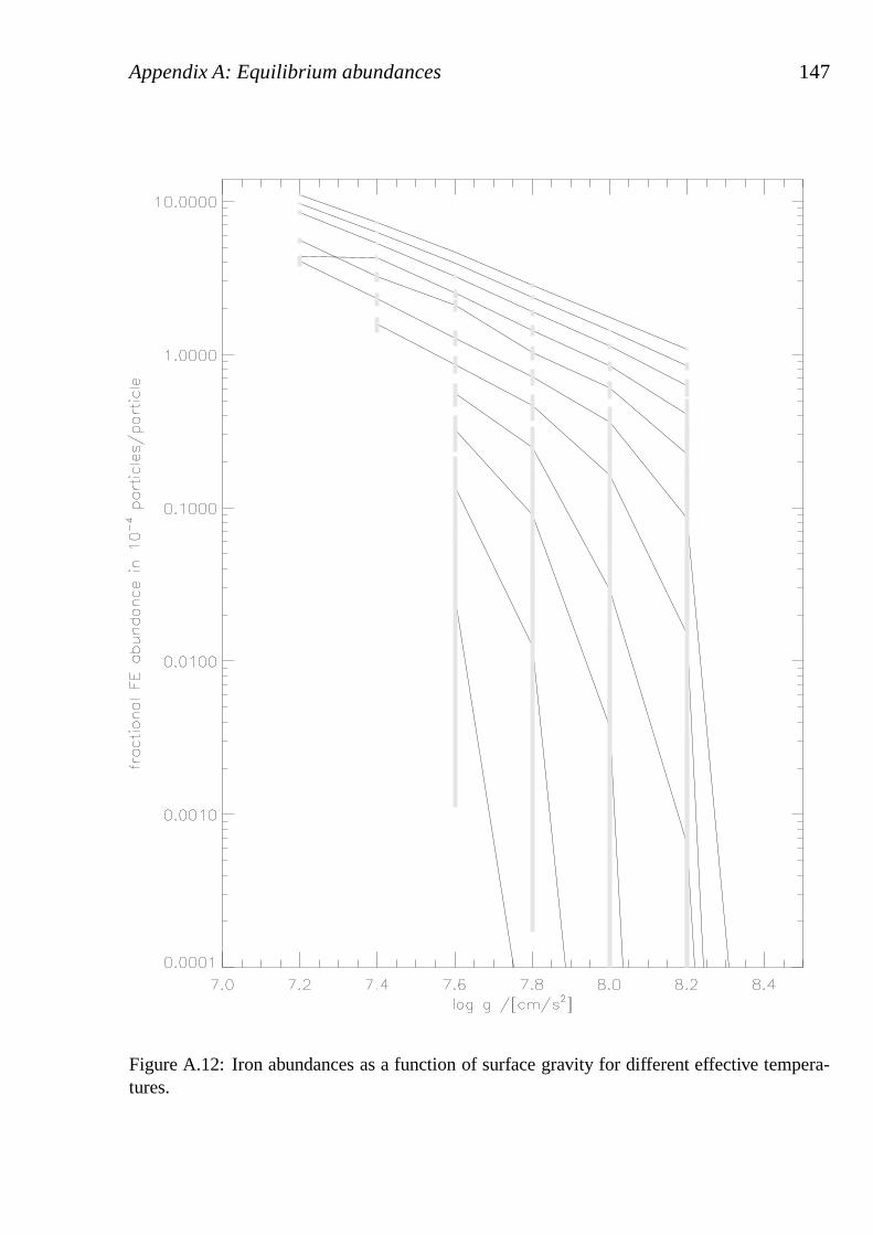
Appendix A: Equilibrium abundances 147
Figure A.12: Iron abundances as a function of surface gravity for different effective tempera-tures.
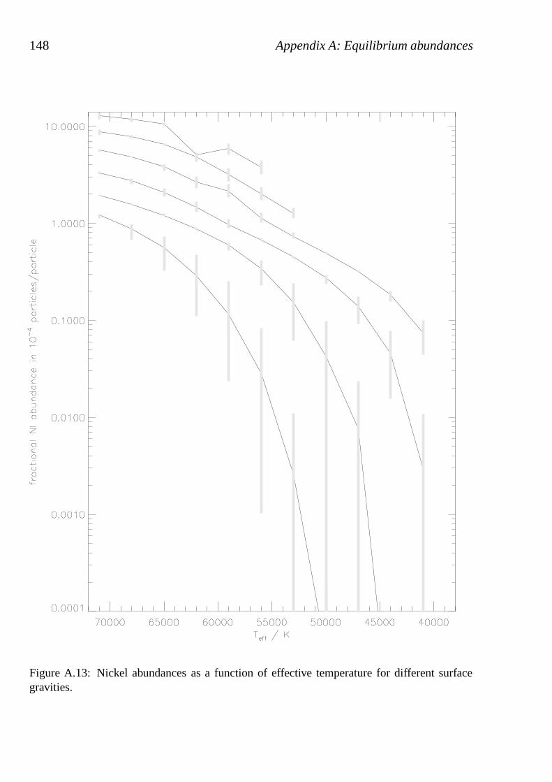
148 Appendix A: Equilibrium abundances
Figure A.13: Nickel abundances as a function of effective temperature for different surfacegravities.
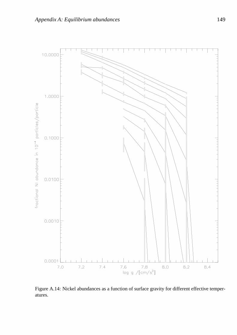
Appendix A: Equilibrium abundances 149
Figure A.14: Nickel abundances as a function of surface gravity for different effective temper-atures.
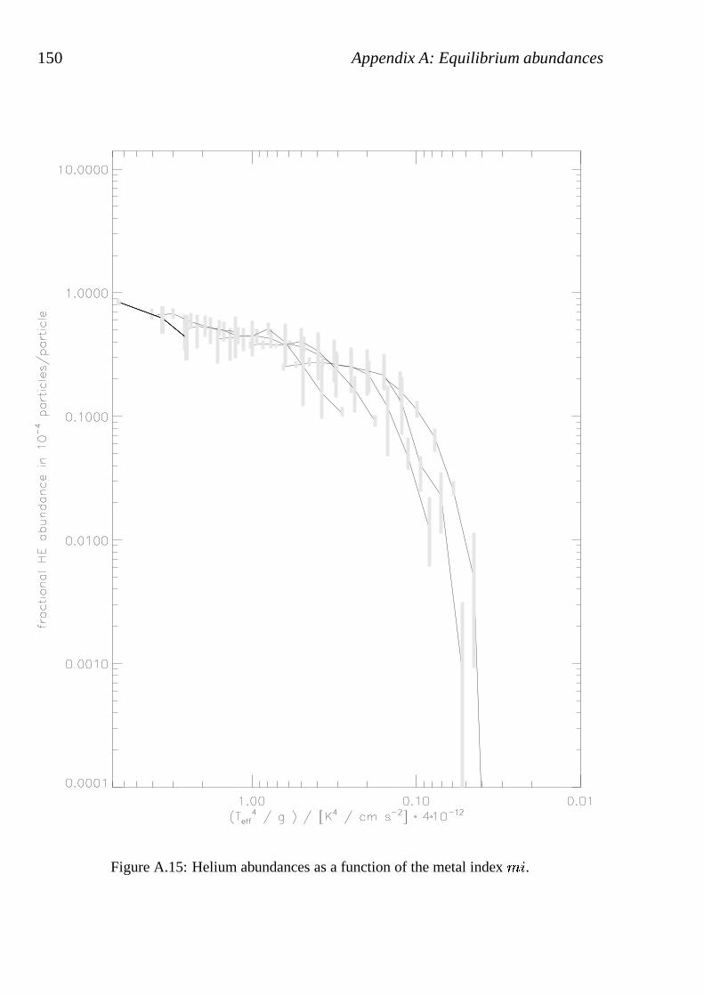
150 Appendix A: Equilibrium abundances
Figure A.15: Helium abundances as a function of the metal index��.
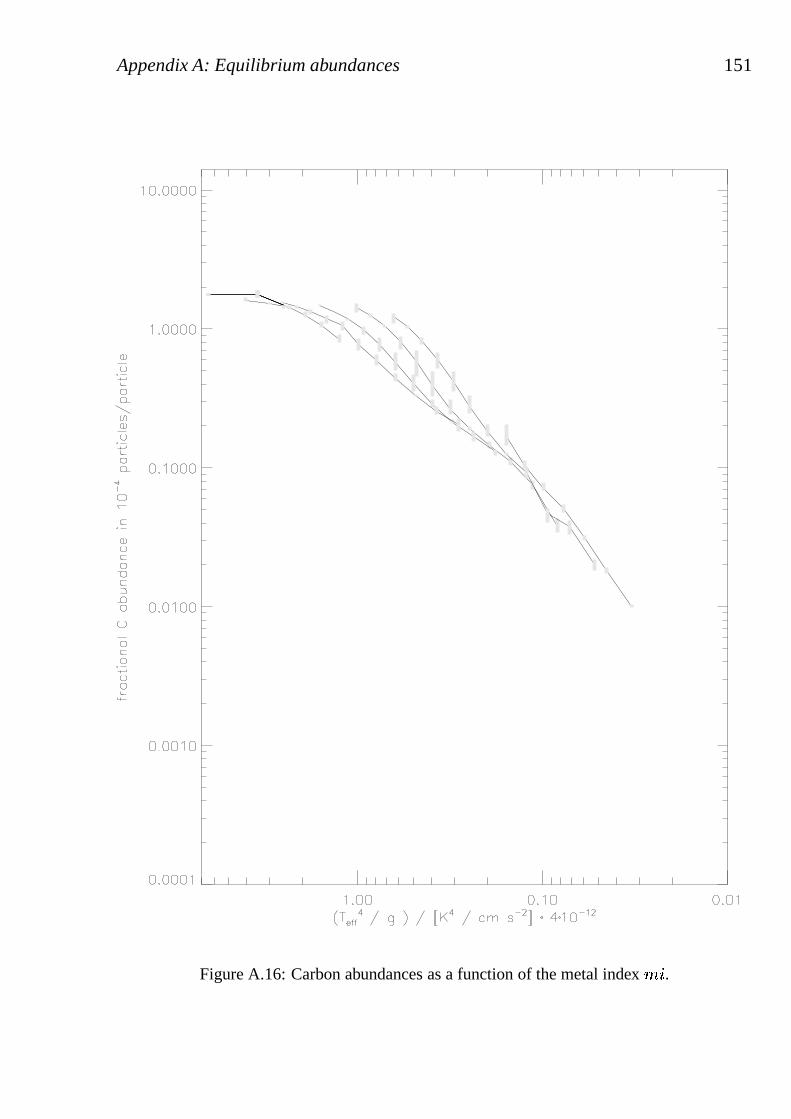
Appendix A: Equilibrium abundances 151
Figure A.16: Carbon abundances as a function of the metal index ��.
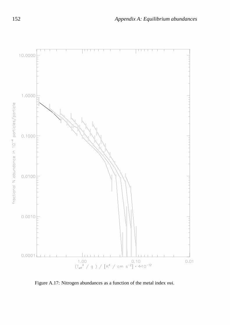
152 Appendix A: Equilibrium abundances
Figure A.17: Nitrogen abundances as a function of the metal index��.
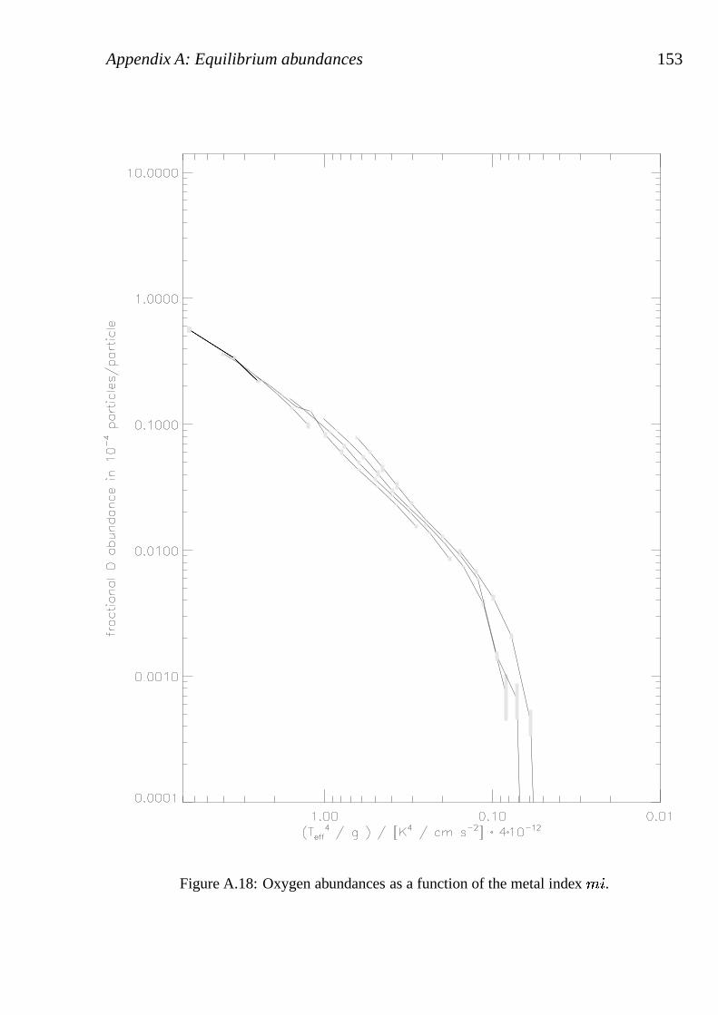
Appendix A: Equilibrium abundances 153
Figure A.18: Oxygen abundances as a function of the metal index��.
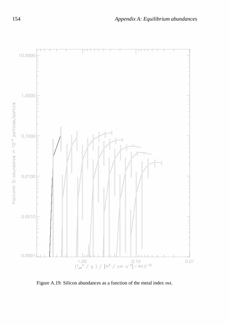
154 Appendix A: Equilibrium abundances
Figure A.19: Silicon abundances as a function of the metal index��.
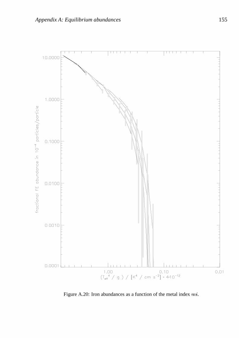
Appendix A: Equilibrium abundances 155
Figure A.20: Iron abundances as a function of the metal index��.
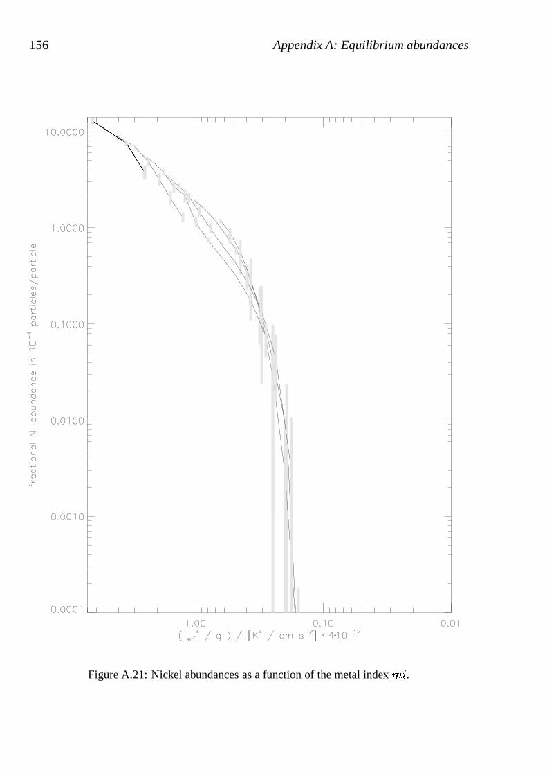
156 Appendix A: Equilibrium abundances
Figure A.21: Nickel abundances as a function of the metal index ��.
Acknowledgements 157
Acknowledgements
Klaus Werner’s and Stefan Dreizler’s advice during the course of this work has beeninvaluable. It is a great privilege to have such excellent teachers. Without their contin-ued support and steady yet un-intrusive encouragement thisthesis might never havebeen finished. I am particularly grateful for the motivationthat radiates from theirpersons, and for making sure that the funding situation allowed to translate this intowhat I hope will for some be useful research results. Stefan’s trust in me when hedecided to continue to foster my career through a position inGottingen honours mebeyond merit.
Burkhard Wolff has laid the grounds for a vital part of this work by providing hisreduced EUVE spectra; he and Detlev Koester have additionally provided part of thesource code for the handling of the ISM absorption. I also thank Ivan Hubeny andMartin Barstow for fruitful collaborations as well as Pierre Chayer for a stimulatingexchange with respect to this work. It is also a pleasure to thank the members of thewhite dwarf community who have expressed a vivid interest inmy subject.
Thorsten Nagel, Klaus Beuermann, and many others have supplied useful com-ments and discussions. I thank Thorsten, my personal onlinemanual#tuebingen ,the Tubingen Espressorunde including Jorn Wilms and Katja Pottschmidt, the USWGottingen ”Gang”, and many more for technical and moral support.
There are no words to express what role family and friends have played in partic-ular during the last year of finishing this thesis. I deeply thank all those who haveexpressed their love, friendship and support.
This work was supported by the Deutsche Forschungsgemeinschaft under grantsDR 281/13-1 and DR 281/13-2. Travel cost for a research trip to NOAO to visitIvan Hubeny was funded by the Schuler Stiftung. PPARC, through a University ofLeicester travel grant, funded a research visit to work withMartin Barstow and topresent this work during a talk. Further presentations weresupported through finan-cial contributions by the Astronomische Gesellschaft (Herbsttagungen Munchen 2001and Berlin 2002), conference fee waivers from the organisers of the European WhiteDwarf workshop at Kiel (2004) and from the organisers of the Stellar AtmosphereModelling conference at Tubingen (2002).
Model atmospheres have been calculated on CRAY machines of the Rechenzen-trum der Universitat Kiel and the IAAT workstation cluster. This research is in partsbased on observations made with the EUVE Satellite, has madeuse of NASA’s Astro-physics Data System Bibliographic Services and of the SIMBAD database, operatedat CDS, Strasbourg, France.

158
Lebenslauf 159
Lebenslauf
29.01.1975 geboren in Stuttgart, Baden-Wurttemberg08.1981–08.1985 Grundschule Bisingen, Baden-Wurttemberg08.1985–06.1994 Gymnasium Hechingen, Baden-Wurttemberg08.1991–12.1991 Lycee Marguerite de Navarre, Bourges, Frankreich11.1993 Bundessiegerin im “The Future Astronomers of Europe” Essay
Contest des European Southern Observatory19.06.1994 Abitur08.1994–07.1996 Eberhard-Karls-Universitat Tubingen, Studium der Physik19.08.1996 Vordiplom08.1996–08.1997 Queen’s University, Kingston, Ontario, Kanada09.1997–06.2000 Eberhard-Karls-Universitat Tubingen10.1997–12.1997 Wissenschaftliche Hilfskraft, Fakultat fur Physik04.1998–05.1998 Wissenschaftliche Hilfskraft, Physikalisches Institut01.1998–07.2003 Dozentin fur Physik am Leibniz-Kolleg T¨ubingen03.1999–06.2000 Wissenschaftliche Hilfskraft, Institutfur Astronomie und Astro-
physik (IAA) Tubingen06.1999–06.2000 Diplomarbeit uber “Gleichgewichtshaufigkeiten in heißen Wei-
ßen Zwergen” am IAA Tubingen unter der Anleitung von HerrnProf. Dr. K. Werner
09.06.2000 Diplom07.2000–06.2003 Wissenschaftliche Angestellte, IAA Tubingen07.2003–09.2003 Wissenschaftliche Hilfskraft, Universitatssternwarte Gottingen10.2003– Wissenschaftliche Angestellte, Universitatssternwarte Gottingen07.2000– Anfertigung der Dissertation mit dem Titel “Diffusion proces-
ses in stellar atmospheres” an der Eberhard-Karls-UniversitatTubingen, Institut fur Astronomie und Astrophysik, AbteilungAstronomie, unter Anleitung von Herrn Prof. Dr. K. Werner
Meine akademischen Lehrer waren die Professorinnen, Professoren, Dozentinnen undDozenten Dres.:Angewandte Physik:E. Plies; R. Fletcher, A. McLean;Astronomie und Astrophysik:H. Mauder, H. Ruder, R. Staubert, K. Werner, S. Dreizler; M.J. Duncan, D.A. Hanes,J. Irwin; Chemie:J. Strahle, H. Ebert;Experimentalphysik:M. Baumann, H. Cle-ment, F. Gonnenwein, P. Grabmayr, W. Hartmann, R. Hubener, O. Lutz, W. Nakel,G. Staudt, G. Wagner;Mathematik:H. Kaul, M. Wolff, H. Fischer, F. Loose;Theore-tische Physik:A. Faßler, P. Kramer, H. Muther, N. Schopohl; E. Zaremba, B. Castel.