Univ.-Prof. Dr. Friedrich Aumayr

DIPLOMARBEIT

Experimental and Simulated Sputtering ofGold, Iron and Wollastonite with a

Catcher-QCM Setup

Ausgefuhrt am Institut fur

Angewandte Physik der

Technischen Universitat Wien

Wiedner Hauptstraße 8-10 / 134

1040 Wien

unter der Anleitung von

Univ.-Prof. Dr. Friedrich Aumayr

und

Dr. Bernhard M. Berger

durch

Paul Stefan Szabo

Matrikelnummer: 01225017

Breitenseer Straße 58/9

1140 Wien

Wien, am 4. September 2017 Paul Szabo

Die approbierte Originalversion dieser Diplom-/ Masterarbeit ist in der Hauptbibliothek der Tech-nischen Universität Wien aufgestellt und zugänglich.

http://www.ub.tuwien.ac.at

The approved original version of this diploma or master thesis is available at the main library of the Vienna University of Technology.

http://www.ub.tuwien.ac.at/eng

Abstract

When ions of the solar wind hit rocky bodies such as the Moon or Mercury they have

a major effect on the surface of these bodies in a process called space weathering.

Furthermore, sputtered material forms a thin exosphere that can be investigated in

order to gain information about the body’s surface. A detailed understanding of the

underlying physical processes can give important insights into planets, moons and

asteroids.

Establishing experimental data for these effects is a very important improvement

for research on space weathering and exosphere formation. This thesis describes both

experimental and theoretical investigations of sputtering measurements of various

targets with a setup where a quartz crystal microbalance (QCM) is used as a catcher

to collect sputtered material. These targets include Au for testing purposes, Fe for

investigating surface roughness effects and Wollastonite (CaSiO3), which represents

a moon analogue material for investigating sputtering by solar-wind ions.

In Section 1, the motivation will be presented along with a background on the

sputtering effects relevant for this thesis. Section 2 then describes the QCM tech-

nique for measuring sputtering yields as well as the catcher-QCM setup, which allows

indirect sputtering measurements. Furthermore, an overview of the sample prepara-

tions and analysis techniques that were performed is given. The theoretical approach

for simulating catcher-QCM measurements and the software used are presented in

Section 3, along with a description of simulating rough surfaces with SDTrimSP-

2D. Finally, Section 4 presents experimental results along with a comparison to

simulation results and discusses how the differences in them can be explained. The

conclusion in Section 5 gives a summary of the knowledge gained through this thesis

and describes how the catcher-QCM setup might be improved in the future.

Both experiments and simulations show a very good agreement over a wide vari-

ety of parameters for all investigated samples. Showing the feasibility of the catcher

setup opens up several possibilities for more realistic measurements of the solar-wind

sputtering using rock or powder targets. The coinciding results of the experiments

also indicate that the particle distributions of the sputtered materials provided by

SDTrimSP can very confidently be used for simulating exosphere formations.

i

Kurzfassung

Sonnenwind-Ionen, die auf die Oberflache von Gesteinskorpern wie Mond oder Mer-

kur treffen, verursachen eine starke Veranderung dieser Oberflachen durch einen

Prozess, der als Weltraumverwitterung bezeichnet wird. Außerdem bildet sich ei-

ne dunne Exosphare aus zerstaubtem Material, welches untersucht werden kann,

um Ruckschlusse auf die Oberflachenzusammensetzung des betrachteten Planeten,

Mondes oder Asteroiden zu ziehen. Ein genaues Verstandnis der zugrunde liegen-

den physikalischen Prozesse kann dabei einen wichtigen Beitrag zur Erforschung

dieser Objekte leisten und die Ermittlung experimenteller Daten, die diese Effekte

beschreiben, stellt eine bedeutende Verbesserung fur die Forschung im Bereich der

Weltraumverwitterung und der Exospharen-Bildung dar.

Die vorliegende Arbeit beschaftigt sich sowohl experimentell als auch theoretisch

mit der Untersuchung des Zerstaubungsverhaltens verschiedener Materialien. Da-

bei kommt ein experimenteller Aufbau zum Einsatz, beim dem eine Quarzkristall-

Mikrowaage (QCM) als Auffanger fur zerstaubtes Material verwendet wird. Die

untersuchten Proben sind Au, um den Aufbau zu testen, Fe, um den Einfluss

verschiedener Oberflachenrauigkeiten zu untersuchen, und Wollastonit, ein Mond-

Analogmaterial, das sich fur erste realistische Untersuchungen des Zerstaubens durch

Sonnenwind-Ionen eignet.

In Kapitel 1 werden die Motivation fur diese Arbeit und eine Zusammenfassung

der fur die durchgefuhrten Experimente relevanten Zerstaubungseffekte prasentiert

und in Kapitel 2 werden die QCM-Methode zur Messung von Zerstaubungsausbeuten

und der Auffangeraufbau, der eine indirekte Untersuchung der Zerstaubung ermog-

licht, beschrieben. Außerdem wird ein Uberblick uber die verwendeten Techniken

zur Probenpraparation und -analyse gegeben. Die Simulation der Auffanger-QCM-

Messungen und die dafur verwendeten Computer-Programme werden in Kapitel 3

behandelt, das auch eine Beschreibung der Simulationen rauer Oberflachen mit dem

Programm SDTrimSP-2D beinhaltet. Die Resultate der Messungen werden schließ-

lich in Kapitel 4 prasentiert und mit den Ergebnissen der Berechnungen verglichen.

Das Fazit in Kapitel 5 fasst die in der vorliegenden Arbeit gewonnenen Erkenntnis-

se zusammen und erlautert, wie der Auffangeraufbau in Zukunft verbessert werden

kann.

Die experimentellen und die theoretischen Resultate stimmen bei allen verwen-

deten Proben und einem Großteil der untersuchten Parameter sehr gut uberein.

ii

Diese vielversprechenden Ergebnisse mit dem neuen Aufbau eroffnen damit neue

Moglichkeiten fur realistischere Untersuchungen der Zerstaubung durch Sonnenwind-

Ionen, zum Beispiel mit Stein- oder Pulverproben. Die mit SDTrimSP berechneten

Teilchen-Verteilungen des zerstaubten Materials, mit denen sich die experimentellen

Resultate verlasslich reproduzieren lassen, sind daher auch geeignet, die Bildung von

Exospharen zu simulieren.

iii

List of Publications

Publications in Scientific Journals

• B. M. Berger, P. S. Szabo, R. Stadlmayr, F. Aumayr: Sputtering measure-

ments using a quartz crystal microbalance as a catcher, Nucl. Instrum. Meth.

Phys. Res. B 406 (2017), 533-537.

Contributions to International Conferences

Short Oral Presentation

• P. S. Szabo, R. Chiba, B. M. Berger, R. Stadlmayr, H. Biber, M. Doppler, J.

Appenroth, A. Galli, M. Sauer, H. Hutter, J. Fleig, P. Wurz, F. Aumayr: Sput-

tering of Wollastonite, 22nd International Workshop on Inelastic Ion-Surface

Collisions (IISC 22), September 17th-22nd, 2017.

Posters

• P. S. Szabo, B. M. Berger, R. Stadlmayr, F. Aumayr: Sputtering Mea-

surements with a New Catcher QCM Setup, 27th International Conference on

Atomic Collisions in Solids (ICACS-27), July 24th-29th, 2016.

• P. S. Szabo, B. M. Berger, R. Stadlmayr, A. Galli, H. Lammer, P. Wurz, F.

Aumayr: A new setup for sputtering experiments with Mercury and Moon ana-

logues, 12th European Conference on Atoms, Molecules and Photons (ECAMP

12), September 5th-9th, 2016.

• P. S. Szabo, B. M. Berger, R. Chiba, R. Stadlmayr, F. Aumayr: A new setup

for experimental investigations of solar wind sputtering, European Geosciences

Union General Assembly 2017 (EGU 2017), April 23rd-28th, 2017.

iv

Contents

Abstract i

Kurzfassung ii

List of Publications iv

Contents v

1 Introduction 1

1.1 Motivation . . . . . . . . . . . . . . . . . . . . . . . . . . . . . . . . . 1

1.2 Sputtering by Ion Bombardment . . . . . . . . . . . . . . . . . . . . . 6

1.2.1 Different Sputtering Effects . . . . . . . . . . . . . . . . . . . 6

1.2.2 Sputtering Yield Y . . . . . . . . . . . . . . . . . . . . . . . . 8

1.2.3 Particle Distributions . . . . . . . . . . . . . . . . . . . . . . . 10

1.2.4 Sputtering of Rough Surfaces . . . . . . . . . . . . . . . . . . 14

1.3 Outline . . . . . . . . . . . . . . . . . . . . . . . . . . . . . . . . . . . 16

2 Experimental Methods 17

2.1 Augustin Ion-Beam Facility . . . . . . . . . . . . . . . . . . . . . . 17

2.2 Quartz Crystal Microbalance (QCM) . . . . . . . . . . . . . . . . . . 19

2.2.1 Measuring Sputter Yields with a QCM . . . . . . . . . . . . . 19

2.3 Catcher-QCM Setup . . . . . . . . . . . . . . . . . . . . . . . . . . . 24

2.3.1 Design . . . . . . . . . . . . . . . . . . . . . . . . . . . . . . . 24

2.3.2 Evaluation Methods . . . . . . . . . . . . . . . . . . . . . . . 26

2.3.3 The parameter g . . . . . . . . . . . . . . . . . . . . . . . . . 28

2.4 Sample Preparation and Analysis . . . . . . . . . . . . . . . . . . . . 29

2.4.1 Au QCM-Films . . . . . . . . . . . . . . . . . . . . . . . . . . 29

2.4.2 Fe QCM-Films . . . . . . . . . . . . . . . . . . . . . . . . . . 30

2.4.3 Wollastonite (CaSiO3) . . . . . . . . . . . . . . . . . . . . . . 34

3 Theoretical Description of Catcher Measurements 42

3.1 Calculating yC . . . . . . . . . . . . . . . . . . . . . . . . . . . . . . . 42

3.1.1 Contribution of Sputtered Atoms . . . . . . . . . . . . . . . . 42

3.1.2 Contribution of Reflected Ions . . . . . . . . . . . . . . . . . . 45

3.1.3 Conclusion . . . . . . . . . . . . . . . . . . . . . . . . . . . . . 46

v

3.2 SDTrimSP Simulations . . . . . . . . . . . . . . . . . . . . . . . . . . 47

3.2.1 Detailed calculation of yjC,r and yiC,sp . . . . . . . . . . . . . . 48

3.2.2 Summary . . . . . . . . . . . . . . . . . . . . . . . . . . . . . 52

3.3 Simulation of Rough Surfaces with SDTrimSP-2D . . . . . . . . . . . 54

3.3.1 SDTrimSP-2D . . . . . . . . . . . . . . . . . . . . . . . . . . . 54

3.3.2 Approach for Fe Simulations . . . . . . . . . . . . . . . . . . . 55

4 Results and Discussion 57

4.1 2 keV Ar+ on Au . . . . . . . . . . . . . . . . . . . . . . . . . . . . . 57

4.2 1 keV Ar+ on Fe . . . . . . . . . . . . . . . . . . . . . . . . . . . . . 61

4.2.1 Target Sputtering Yield . . . . . . . . . . . . . . . . . . . . . 62

4.2.2 Catcher Measurements . . . . . . . . . . . . . . . . . . . . . . 64

4.3 2 keV Ar+ on Wollastonite (CaSiO3) . . . . . . . . . . . . . . . . . . 68

4.3.1 Target Mass Removal Rate . . . . . . . . . . . . . . . . . . . . 68

4.3.2 Catcher Measurements . . . . . . . . . . . . . . . . . . . . . . 70

5 Conclusion and Outlook 74

References 77

List of Figures 85

List of Tables 85

List of Abbreviations 86

Danksagung 87

vi

1 Introduction

1.1 Motivation

Space weathering is a very important aspect for planetary science. It describes the

erosion and transformation of the surfaces of rocky bodies in the solar system as

a result of different influences from space [1]. Generally, these asteroids, moons or

planets are exposed to the impact of meteroites, electromagnetic radiation and ions

([2], [3]). With regard to the lunar surface, the consequences of meteorite impacts

are apparent, as its surface is covered by craters. However, observed darkening

processes of these craters’ surroundings lead to the assumption that there are also

interactions taking place that change the optical properties of the lunar soil [4].

This was experimentally verified after the first NASA Apollo missions, where lunar

material turned out to be darker than comparable pulverized stones [5]. What was

first thought to be caused by vitrification processes [6], where glass particles are

created as a result of meteorite impacts, was then attributed to ion sputtering and

impact vaporization ([7], [8]). It was found that a darkening of powder samples

is created from “submicroscopic metallic iron” that forms coherent crusts on the

powder [1].

Besides an optical change of the surface, particles are evaporated and a tenuous

atmosphere, an exosphere, is created. This exosphere is interesting for planetary

science as its composition allows conclusions on the composition of the planetary

surface [9]. It thus enables another method of remotely investigating objects in the

solar system besides spectroscopically examining characteristic absorption lines [10].

During flyby missions, this exosphere can be analyzed and as a result, information on

the surface can be gained without having the complex task of landing a spacecraft.

Several such missions have been performed in the past, for example the Messenger

mission to Mercury [11], and in the Bepi Colombo mission another spacecraft is

planned which has the goal of analyzing the Mercury exosphere [12].

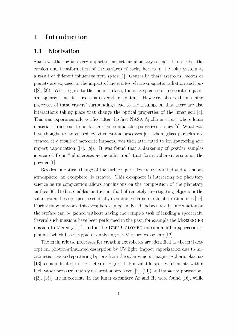
The main release processes for creating exospheres are identified as thermal des-

orption, photon-stimulated desorption by UV light, impact vaporization due to mi-

crometeorites and sputtering by ions from the solar wind or magnetospheric plasmas

[13], as is indicated in the sketch in Figure 1. For volatile species (elements with a

high vapor pressure) mainly desorption processes ([2], [14]) and impact vaporizations

([3], [15]) are important. In the lunar exosphere Ar and He were found [16], while

1

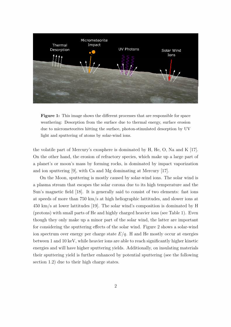
Figure 1: This image shows the different processes that are responsible for space

weathering: Desorption from the surface due to thermal energy, surface erosion

due to micrometeorites hitting the surface, photon-stimulated desorption by UV

light and sputtering of atoms by solar-wind ions.

the volatile part of Mercury’s exosphere is dominated by H, He, O, Na and K [17].

On the other hand, the erosion of refractory species, which make up a large part of

a planet’s or moon’s mass by forming rocks, is dominated by impact vaporization

and ion sputtering [9], with Ca and Mg dominating at Mercury [17].

On the Moon, sputtering is mostly caused by solar-wind ions. The solar wind is

a plasma stream that escapes the solar corona due to its high temperature and the

Sun’s magnetic field [18]. It is generally said to consist of two elements: fast ions

at speeds of more than 750 km/s at high heliographic lattitudes, and slower ions at

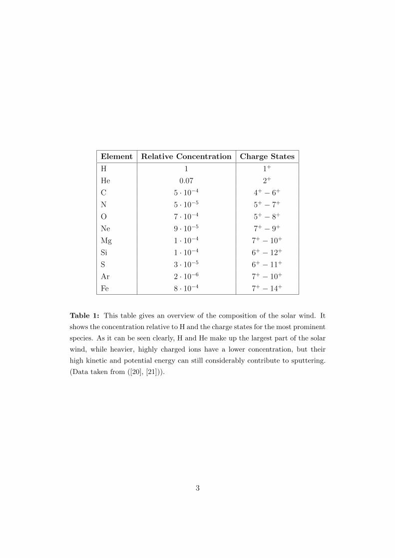
450 km/s at lower lattitudes [19]. The solar wind’s composition is dominated by H

(protons) with small parts of He and highly charged heavier ions (see Table 1). Even

though they only make up a minor part of the solar wind, the latter are important

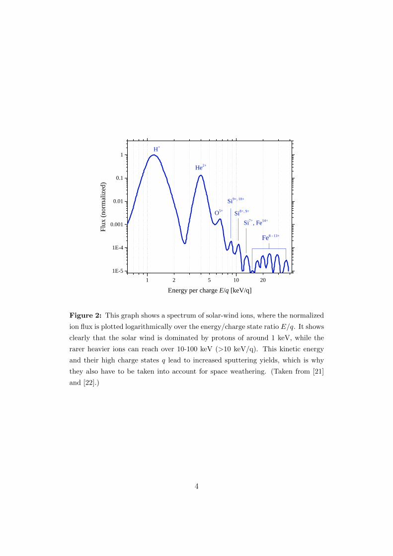
for considering the sputtering effects of the solar wind. Figure 2 shows a solar-wind

ion spectrum over energy per charge state E/q. H and He mostly occur at energies

between 1 and 10 keV, while heavier ions are able to reach significantly higher kinetic

energies and will have higher sputtering yields. Additionally, on insulating materials

their sputtering yield is further enhanced by potential sputtering (see the following

section 1.2) due to their high charge states.

2

Element Relative Concentration Charge States

H 1 1+

He 0.07 2+

C 5 · 10−4 4+ − 6+

N 5 · 10−5 5+ − 7+

O 7 · 10−4 5+ − 8+

Ne 9 · 10−5 7+ − 9+

Mg 1 · 10−4 7+ − 10+

Si 1 · 10−4 6+ − 12+

S 3 · 10−5 6+ − 11+

Ar 2 · 10−6 7+ − 10+

Fe 8 · 10−4 7+ − 14+

Table 1: This table gives an overview of the composition of the solar wind. It

shows the concentration relative to H and the charge states for the most prominent

species. As it can be seen clearly, H and He make up the largest part of the solar

wind, while heavier, highly charged ions have a lower concentration, but their

high kinetic and potential energy can still considerably contribute to sputtering.

(Data taken from ([20], [21])).

3

2 5 2 01 1 01 E - 5

1 E - 4

0 . 0 0 1

0 . 0 1

0 . 1

1

F e 8 - 1 3 +

S i 7 + , F e 1 4 +S i 8 + , 9 +

S i 9 + , 1 0 +

O 5 +

H e 2 +

Flux (

norma

lized)

E n e r g y p e r c h a r g e E / q [ k e V / q ]

H +

Figure 2: This graph shows a spectrum of solar-wind ions, where the normalized

ion flux is plotted logarithmically over the energy/charge state ratio E/q. It shows

clearly that the solar wind is dominated by protons of around 1 keV, while the

rarer heavier ions can reach over 10-100 keV (>10 keV/q). This kinetic energy

and their high charge states q lead to increased sputtering yields, which is why

they also have to be taken into account for space weathering. (Taken from [21]

and [22].)

4

On a planet like Mercury, a different situation is found. Mercury has not been

able to retain an atmosphere that would sufficiently shield it against ion bombard-

ment [23], but solar-wind ions predominantly hit the polar regions, where they are

not deflected by the planet’s magnetic field [24]. However, there is a contribution

by a plasma precipitation from Mercury’s magnetosphere on its nightside [25].

Taking all the effects that can cause space weathering into account, simulations

can be performed to calculate exosphere densities, as it is done for the Moon [26]

and Mercury [27]. The input for the sputtering contribution is taken from SRIM

simulations [28], as there have not yet been many experimental investigations of

the sputtering of relevant analogue materials (see [20] for an example). As a result,

performing such experiments and examining how well the sputtering behavior of

lunar or planetary rocks can be described with existing simulations such as TRIM

or SDTrimSP could bring a substantial improvement for modelling space weathering

effects. Furthermore, a more precise investigation of the potential sputtering effects

by highly charged solar-wind ions will provide important insights, as they are often

overlooked in simulations.

The main goal of this thesis is to take a first step into using the existing knowl-

edge of the Institute of Applied Physics (IAP) about ion-surface interactions and

sputtering in particular to investigate the sputtering contribution to space weather-

ing. Sputtering experiments at IAP have been performed for several decades using a

Quartz Crystal Microbalance (QCM) technique for measuring sputtering yields [29],

which will be presented in Section 2.2. By measuring the frequency change of an

oscillating quartz it allows precise in-situ measurements of a thin film’s mass change

due to sputtering. Using a QCM, effects like potential sputtering ([30], [31]) or the

erosion of potential wall materials for a nuclear fusion reactor have been investigated

([32], [33], [34]). Recently, a new experimental setup was developed that allows using

a QCM as a catcher for sputtered atoms and thus enables measurements on a wide

range of targets [35]. First experimental work using this catcher setup is presented

in this thesis, including measurements with Au and Fe targets as well as the first

astrophysically relevant investigations of the sputtering of Wollastonite (CaSiO3),

which can be found in lunar regolith [36].

5

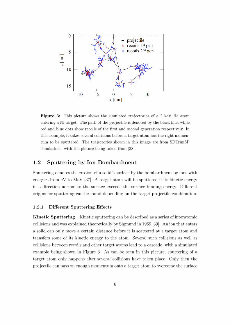
Figure 3: This picture shows the simulated trajectories of a 2 keV He atom

entering a Ni target. The path of the projectile is denoted by the black line, while

red and blue dots show recoils of the first and second generation respectively. In

this example, it takes several collisions before a target atom has the right momen-

tum to be sputtered. The trajectories shown in this image are from SDTrimSP

simulations, with the picture being taken from [38].

1.2 Sputtering by Ion Bombardment

Sputtering denotes the erosion of a solid’s surface by the bombardment by ions with

energies from eV to MeV [37]. A target atom will be sputtered if its kinetic energy

in a direction normal to the surface exceeds the surface binding energy. Different

origins for sputtering can be found depending on the target-projectile combination.

1.2.1 Different Sputtering Effects

Kinetic Sputtering Kinetic sputtering can be described as a series of interatomic

collisions and was explained theoretically by Sigmund in 1969 [39]. An ion that enters

a solid can only move a certain distance before it is scattered at a target atom and

transfers some of its kinetic energy to the atom. Several such collisions as well as

collisions between recoils and other target atoms lead to a cascade, with a simulated

example being shown in Figure 3. As can be seen in this picture, sputtering of a

target atom only happens after several collisions have taken place. Only then the

projectile can pass on enough momentum onto a target atom to overcome the surface

6

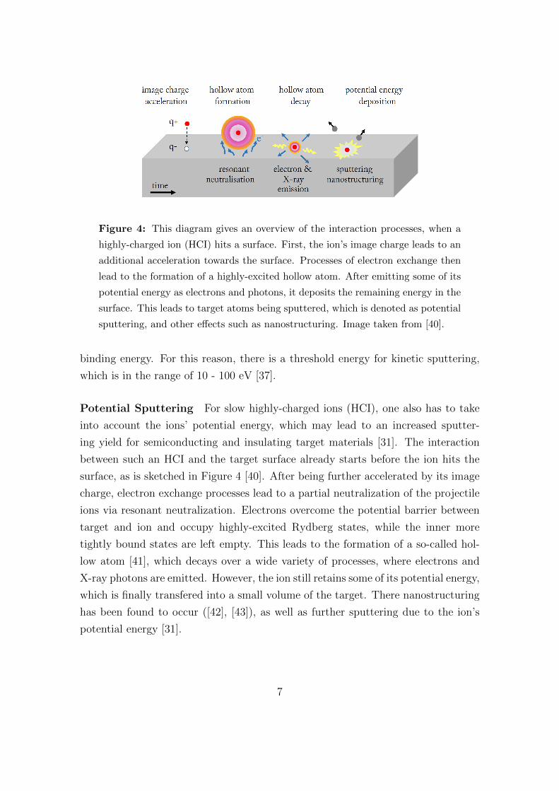
Figure 4: This diagram gives an overview of the interaction processes, when a

highly-charged ion (HCI) hits a surface. First, the ion’s image charge leads to an

additional acceleration towards the surface. Processes of electron exchange then

lead to the formation of a highly-excited hollow atom. After emitting some of its

potential energy as electrons and photons, it deposits the remaining energy in the

surface. This leads to target atoms being sputtered, which is denoted as potential

sputtering, and other effects such as nanostructuring. Image taken from [40].

binding energy. For this reason, there is a threshold energy for kinetic sputtering,

which is in the range of 10 - 100 eV [37].

Potential Sputtering For slow highly-charged ions (HCI), one also has to take

into account the ions’ potential energy, which may lead to an increased sputter-

ing yield for semiconducting and insulating target materials [31]. The interaction

between such an HCI and the target surface already starts before the ion hits the

surface, as is sketched in Figure 4 [40]. After being further accelerated by its image

charge, electron exchange processes lead to a partial neutralization of the projectile

ions via resonant neutralization. Electrons overcome the potential barrier between

target and ion and occupy highly-excited Rydberg states, while the inner more

tightly bound states are left empty. This leads to the formation of a so-called hol-

low atom [41], which decays over a wide variety of processes, where electrons and

X-ray photons are emitted. However, the ion still retains some of its potential energy,

which is finally transfered into a small volume of the target. There nanostructuring

has been found to occur ([42], [43]), as well as further sputtering due to the ion’s

potential energy [31].

7

Preferential Sputtering Sputtering yields are strongly dependent on the target-

projectile combination, and for this reason different species in compound materials

are sputtered at varying rates. This preferential sputtering causes an alteration

of the surface composition, thus fluence dependence finally leads to a steady state

behavior. There differences in sputtering yields and concentration cancel each other

and the mass removal rate by ion sputtering becomes stable.

Chemical Sputtering, Channeling Further effects that influence the sputtering

behavior have been found: chemical sputtering can occur when reactions between

target and projectile material can change the surface binding energy and thus influ-

ence the sputtering behavior [44]. This can lead to an increase as well as a decrease

in the sputtering yield. Ion bombardment of a crystalline target is influenced by the

crystal orientation, with channeling effects causing lower sputtering yields [45].

1.2.2 Sputtering Yield Y

The key quantity to describe sputtering effects is the sputtering yield Y , which is

defined as

Y =number of sputtered target atoms

number of incident ions

For the experiments in this thesis, it is mostly kinetic sputtering that has to

be taken into account. Then Y is dependent on the projectile’s mass, the target’s

mass, the projectile’s kinetic energy and the angle of incidence. Variations in these

parameters have been investigated experimentally and theoretically in recent decades

with a large database being already available. The following pictures (Figure 5 and

6) give examples of the general behaviors that have been found.

First, Figure 5 depicts experimentally determined sputtering yields under varia-

tion of impact energy and angle. The graph on the left (taken from [37], data from

the references therein) shows experimental and calculated sputtering yields for Ar

ions hitting a Fe sample under normal incidence for different energies. The logarith-

mic plot shows a threshold energy of 10-20 eV with a strong increase for low energies

as more energy is available to be passed on to target atoms. For keV energy ranges,

under which most experiments at IAP are performed, the sputtering yield here is in

the order of 1, its maximum of ≈ 3 can be found at energies of about 10 keV. Ions

8

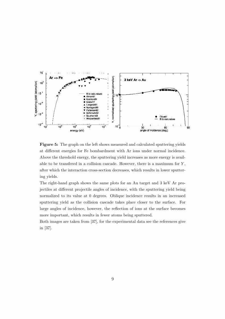
Figure 5: The graph on the left shows measured and calculated sputtering yields

at different energies for Fe bombardment with Ar ions under normal incidence.

Above the threshold energy, the sputtering yield increases as more energy is avail-

able to be transfered in a collision cascade. However, there is a maximum for Y ,

after which the interaction cross-section decreases, which results in lower sputter-

ing yields.

The right-hand graph shows the same plots for an Au target and 3 keV Ar pro-

jectiles at different projectile angles of incidence, with the sputtering yield being

normalized to its value at 0 degrees. Oblique incidence results in an increased

sputtering yield as the collision cascade takes place closer to the surface. For

large angles of incidence, however, the reflection of ions at the surface becomes

more important, which results in fewer atoms being sputtered.

Both images are taken from [37], for the experimental data see the references give

in [37].

9

faster than that experience a decrease in the nuclear interaction cross-section and

thus a lower stopping power, which results in a decreasing sputtering yield [39].

The right-hand graph in Figure 5 shows the dependency of the normalized sput-

tering yield Y (α)/Y (0) on the angle of incidence α with 0 degrees being denoted

as normal incidence. It shows an increased sputtering yield for oblique incidence

with a maximum that is usually found at about 60 degrees. The increase can be

explained by two aspects: Firstly, as Figure 3 shows, several collisions are necessary

to result in a sputtered atom, as the momentum perpendicular to the surface has

to be transversed. This becomes easier for larger angles of incidence because in this

case the ions have less initial momentum in the direction normal to the surface.

Furthermore, the collision cascade created by the projectile ion is moved closer to

the surface due to the skew incidence and thus more atoms can be sputtered. Under

grazing incidence more and more ions are reflected from the surface and as a result,

the sputter yield decreases again.

1.2.3 Particle Distributions

For more detailed experimental research of sputtering effects, as intended with the

catcher-QCM setup at IAP, the sputtering yield Y does not represent the only

quantity of interest. Knowledge about energy and angular distributions both for

sputtered target atoms and reflected projectile ions are also required.

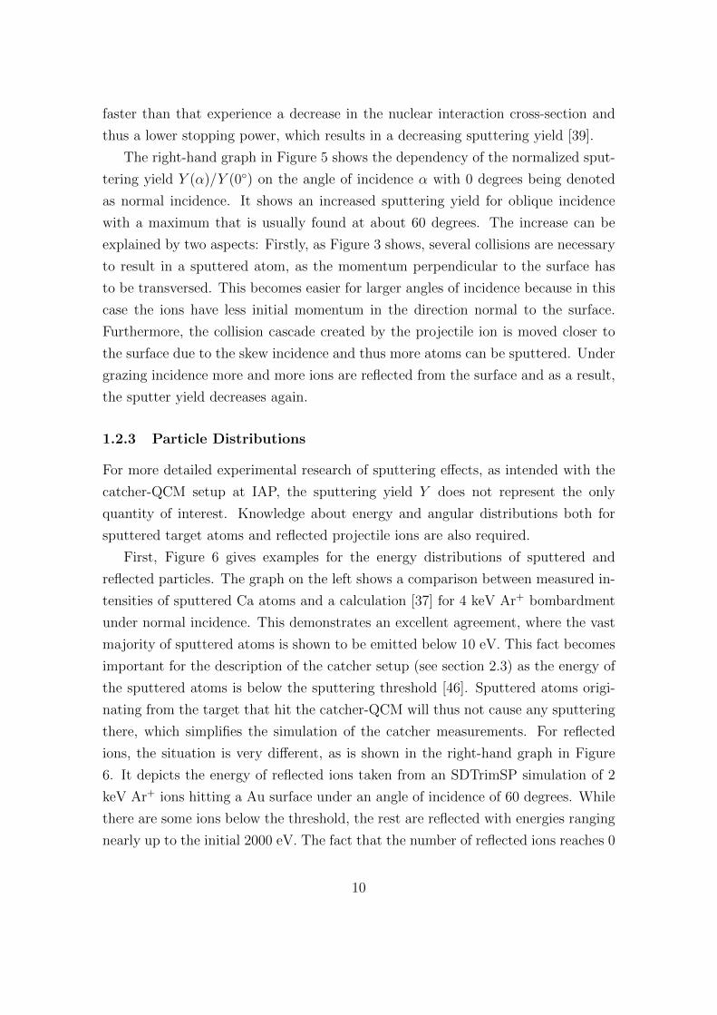
First, Figure 6 gives examples for the energy distributions of sputtered and

reflected particles. The graph on the left shows a comparison between measured in-

tensities of sputtered Ca atoms and a calculation [37] for 4 keV Ar+ bombardment

under normal incidence. This demonstrates an excellent agreement, where the vast

majority of sputtered atoms is shown to be emitted below 10 eV. This fact becomes

important for the description of the catcher setup (see section 2.3) as the energy of

the sputtered atoms is below the sputtering threshold [46]. Sputtered atoms origi-

nating from the target that hit the catcher-QCM will thus not cause any sputtering

there, which simplifies the simulation of the catcher measurements. For reflected

ions, the situation is very different, as is shown in the right-hand graph in Figure

6. It depicts the energy of reflected ions taken from an SDTrimSP simulation of 2

keV Ar+ ions hitting a Au surface under an angle of incidence of 60 degrees. While

there are some ions below the threshold, the rest are reflected with energies ranging

nearly up to the initial 2000 eV. The fact that the number of reflected ions reaches 0

10

0 5 0 0 1 0 0 0 1 5 0 0 2 0 0 00 . 0

0 . 2

0 . 4

0 . 6

0 . 8

1 . 0

1 . 2

Ar Int

ensity

(norm

alized

)

E n e r g y [ e V ]

2 k e V A r + A uα = 6 0 °

Figure 6: The graph on the left shows the energy distribution for sputtered

target atoms after the bombardment of a Ca target with 4 keV Ar+ ions under

normal incidence, normalized to the maximum intensity. Most sputtered particles

have energies below 10 eV, which is below the sputtering threshold [46]. (Picture

taken from [37].)

The right-hand graph shows the simulated energy distribution of reflected projec-

tiles for 2 keV Ar+ bombardment of a Au target under an angle of incidence of 60

degrees, normalized to the maximum intensity. In contrast to before, it shows a

distribution over a wide range of energy nearly up to the initial energy of 2 keV.

The maximum energy of about 1800 eV can be explained by the fact that each

reflected ion undergoes at least one collision where it loses some of its energy to

a target atom.

11

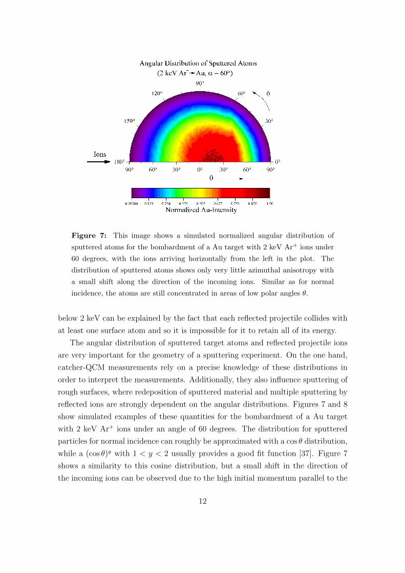
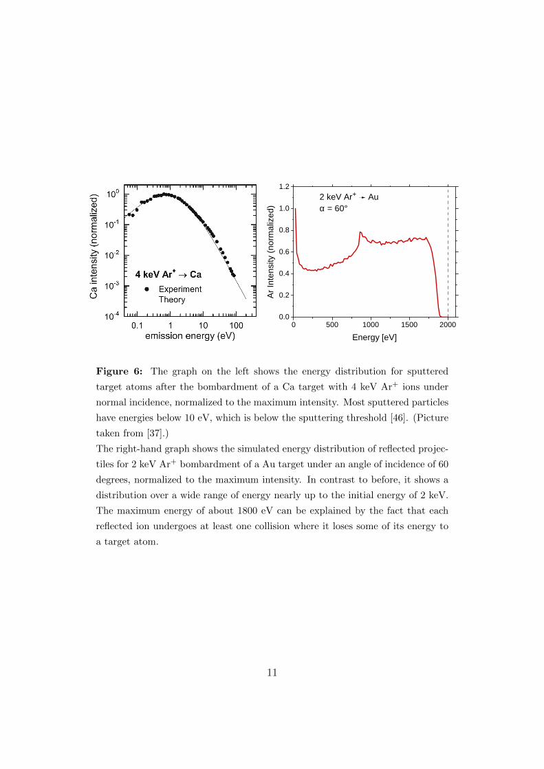
Figure 7: This image shows a simulated normalized angular distribution of

sputtered atoms for the bombardment of a Au target with 2 keV Ar+ ions under

60 degrees, with the ions arriving horizontally from the left in the plot. The

distribution of sputtered atoms shows only very little azimuthal anisotropy with

a small shift along the direction of the incoming ions. Similar as for normal

incidence, the atoms are still concentrated in areas of low polar angles θ.

below 2 keV can be explained by the fact that each reflected projectile collides with

at least one surface atom and so it is impossible for it to retain all of its energy.

The angular distribution of sputtered target atoms and reflected projectile ions

are very important for the geometry of a sputtering experiment. On the one hand,

catcher-QCM measurements rely on a precise knowledge of these distributions in

order to interpret the measurements. Additionally, they also influence sputtering of

rough surfaces, where redeposition of sputtered material and multiple sputtering by

reflected ions are strongly dependent on the angular distributions. Figures 7 and 8

show simulated examples of these quantities for the bombardment of a Au target

with 2 keV Ar+ ions under an angle of 60 degrees. The distribution for sputtered

particles for normal incidence can roughly be approximated with a cos θ distribution,

while a (cos θ)y with 1 < y < 2 usually provides a good fit function [37]. Figure 7

shows a similarity to this cosine distribution, but a small shift in the direction of

the incoming ions can be observed due to the high initial momentum parallel to the

12

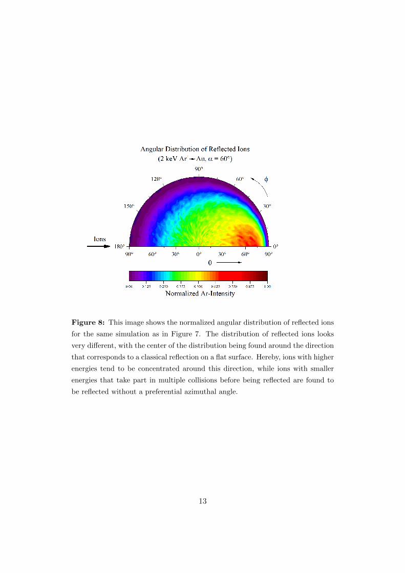
Figure 8: This image shows the normalized angular distribution of reflected ions

for the same simulation as in Figure 7. The distribution of reflected ions looks

very different, with the center of the distribution being found around the direction

that corresponds to a classical reflection on a flat surface. Hereby, ions with higher

energies tend to be concentrated around this direction, while ions with smaller

energies that take part in multiple collisions before being reflected are found to

be reflected without a preferential azimuthal angle.

13

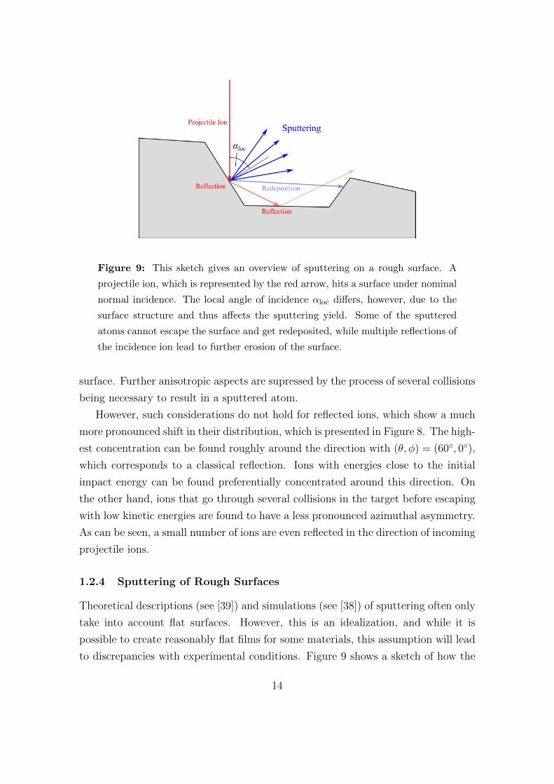
Figure 9: This sketch gives an overview of sputtering on a rough surface. A

projectile ion, which is represented by the red arrow, hits a surface under nominal

normal incidence. The local angle of incidence αloc differs, however, due to the

surface structure and thus affects the sputtering yield. Some of the sputtered

atoms cannot escape the surface and get redeposited, while multiple reflections of

the incidence ion lead to further erosion of the surface.

surface. Further anisotropic aspects are supressed by the process of several collisions

being necessary to result in a sputtered atom.

However, such considerations do not hold for reflected ions, which show a much

more pronounced shift in their distribution, which is presented in Figure 8. The high-

est concentration can be found roughly around the direction with (θ, φ) = (60, 0),

which corresponds to a classical reflection. Ions with energies close to the initial

impact energy can be found preferentially concentrated around this direction. On

the other hand, ions that go through several collisions in the target before escaping

with low kinetic energies are found to have a less pronounced azimuthal asymmetry.

As can be seen, a small number of ions are even reflected in the direction of incoming

projectile ions.

1.2.4 Sputtering of Rough Surfaces

Theoretical descriptions (see [39]) and simulations (see [38]) of sputtering often only

take into account flat surfaces. However, this is an idealization, and while it is

possible to create reasonably flat films for some materials, this assumption will lead

to discrepancies with experimental conditions. Figure 9 shows a sketch of how the

14

roughness of a surface affects the sputtering. It shows a projectile ion (red arrow)

hitting the surface under a nominal angle of 0 degrees, which would mean normal

incidence for a perfectly flat surface. However, due to the surface structure the local

angle of incidence αloc is different, with its value being strongly dependent on the

exact point of incidence. There the two already discussed events of surface sputtering

and ion reflection occur. On average Y (αloc) atoms are sputtered preferentially in

the direction of the local surface normal. As is indicated in Figure 9, not all of the

sputtered atoms are able to escape the surface. Some of them hit the right flank and

are deposited there, which can be described by a redeposition factor R. Additionally,

the ion is reflected with a probability of Pr(αloc) and may hit the surface a second

time. As it was discussed in Figure 6, the reflected ion’s energy is lower than the

incident energy, but still high enough to lead to further sputtering. These sputtered

particles are then again partly redeposited and with a given probability further

reflection may occur, whose depiction is omitted in Figure 9 for comprehensibility

purposes.

Ultimately, the sputtering yield Y for a rough surface is given as a sum of all

these effects:

Y =∑n

P nr · Y (E(n), α

(n)loc ) · (1−R(n)) (1)

with P nr signifying the probability of the nth reflection, E(n) describing the ion’s

energy after n reflections, α(n)loc describing its local angle of incidence and R(n) the

respective redeposition factor.

Evidently, a theoretical description of the sputtering of rough surfaces becomes

quite complex. Kustner et al. achieved remarkable results using STM images as

an input and a simple model to describe redeposition effects ([47], [48]). However,

more detailed modeling of this situation is necessary to take into account effects

such as shadowing (especially for flat ion incidence, some parts of the surface will

not be hit by ions) and the change in angular and energy distributions, where Figure

9 already indicates large changes compared to a flat surface. For this reason, the

investigations of rough Fe surfaces which are included in this thesis are simulated

with the newly developed SDTrimSP-2D code ([49], [50]), which makes it possible

to take surface structures into account in the sputtering calculations (see Section

3.3 for more information on the simulation and Section 4.2 for the presentation of

the results).

15

1.3 Outline

In this section, the motivation and the physical effects that are relevant for this thesis

were introduced. Following up, Section 2 will present the experimental methods

that were used with an emphasis on the QCM technique, which allows precise in-

situ sputtering measurements, and the catcher-QCM setup, which enables unique

possibilities for using a wide variety of targets. Using this catcher-QCM setup to

collect sputtered material requires a theoretical model for calculating sputtering

yields of the initial target. It takes into account the geometry of the setup and

the distributions of sputtered atoms and reflected ions to reproduce the measured

signal, which is described in detail in Section 3. Section 4 then shows the results of

both experiments and simulations for different targets discussing both concurrence

and disparities between these results. Solving these problems and performing further

experiments remain challenges for future work in this field, which will be highlighted

in Section 5.

16

2 Experimental Methods

The experiments shown in this thesis are performed at the Augustin ion-beam

facility at the IAP at TU Wien. An overview of this experimental setup is given

at the beginning of this section followed by an explanation of the Quartz Crystal

Microbalance (QCM) technique, which allows high-precision in-situ measurements

of the sputtering yield. The QCM is used as part of a catcher setup for measuring the

sputtering yield of a wide variety of targets, which will be presented thereafter. At

the end of this section, the different samples investigated and the necessary methods

of sample preparation and analysis are shown.

2.1 Augustin Ion-Beam Facility

An overview of the Augustin ion-beam facility is given in Figure 10. It is built

around a 14.5 GHz Electron Cyclotron Resonance Ion Source (ECRIS) which was

developed to optimize experiments with slow multiply-charged ions ([51], [52]). In

such an ECRIS, a plasma is confined magnetically and heated with microwave radi-

ation. Gas atoms are then ionized due to electron cyclotron resonance and can be

extracted by a voltage of up to several kV to form the ion beam. This beam is then

focused by a lens system consisting of two sets of quadrupole magnets and deflected

into one of the experiment’s three beamlines by a sector magnet (indicated by the

red arrows in Figure 10). Its magnetic field is also used as a selector for the desired

mass over charge state ratio of the beam’s ions.

The experimental setup described in this thesis is connected to the beamline

that is represented by the full red arrow in Figure 10. There the ion beam can be

guided and formed by two sets of electrostatic deflection plates and an einzel lens.

Using this setup the ion beam is focused into the sample chamber, where a pair of

scanning plates is used to create a uniform current profile across the sample. This

is achieved by applying alternating voltages to these plates with a frequency of 1.6

kHz and 52 Hz respectively so that the focused ion beam is scanned over a specified

area. Inside the sample chamber, a target holder and a catcher-QCM are mounted

on manipulators, which will be presented in detail in Section 2.3.

The Augustin ion-beam facility operates under Ultra-High Vacuum (UHV) con-

ditions, which is maintained by membrane, turbomolecular and ion pumps. Pres-

sures as low as 10−10 mbar enable ion-beam and surface experiments with minimal

17

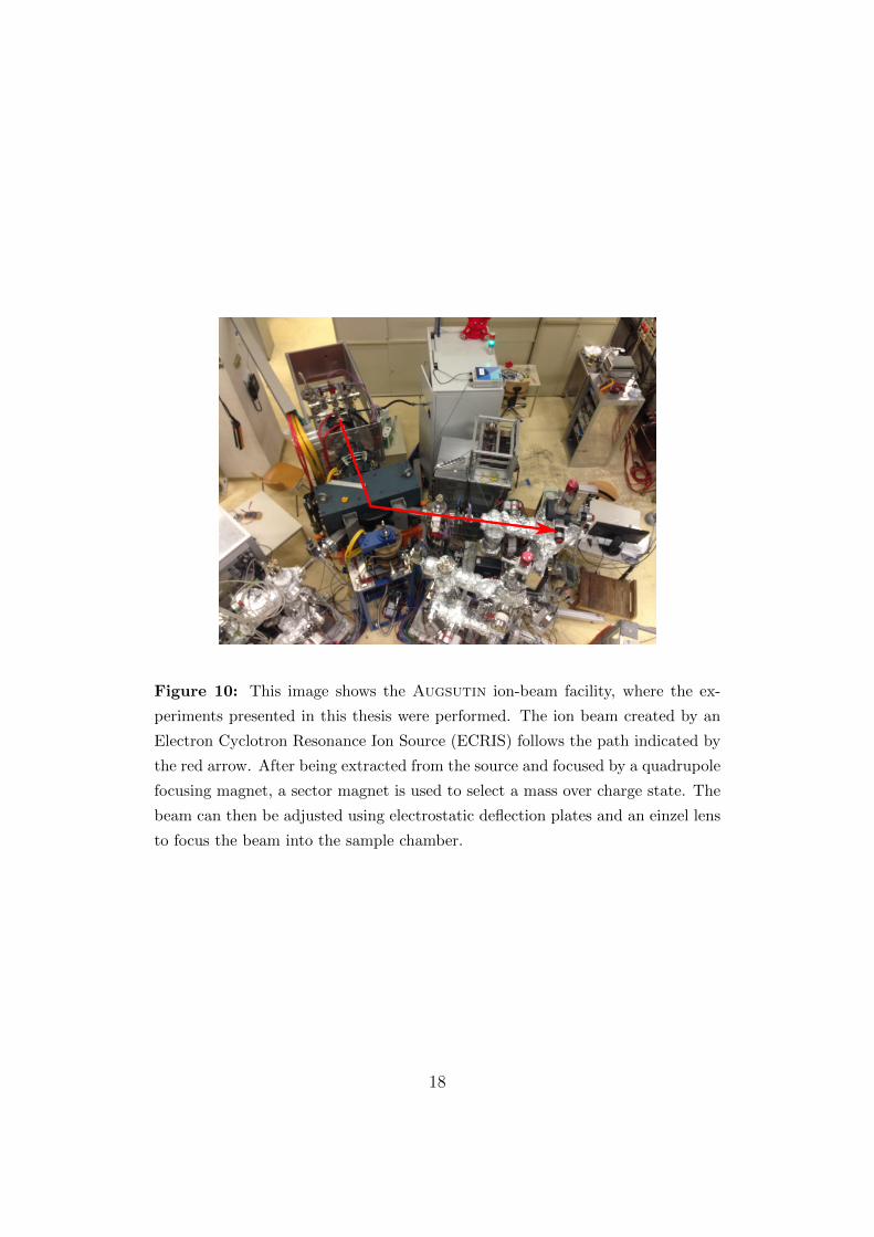
Figure 10: This image shows the Augsutin ion-beam facility, where the ex-

periments presented in this thesis were performed. The ion beam created by an

Electron Cyclotron Resonance Ion Source (ECRIS) follows the path indicated by

the red arrow. After being extracted from the source and focused by a quadrupole

focusing magnet, a sector magnet is used to select a mass over charge state. The

beam can then be adjusted using electrostatic deflection plates and an einzel lens

to focus the beam into the sample chamber.

18

disturbance. The mean free path of an ion moving through rest-gas molecules in

such a vacuum is in the order of several kilometers, which is why any interactions

with residual gas molecules can be neglected. Additionally, QCM experiments are

very sensitive to the mass change at the surface of the quartz, which is why they re-

quire UHV conditions. Only then the impingment rate of residual gas is low enough

to substain clean surfaces over the time of a measurement.

More detailed information on the experimental setup of the ion-beam facility can

be found in [33] and [53].

2.2 Quartz Crystal Microbalance (QCM)

The QCM is a method that has been used regularly at the IAP for measuring

ion-induced sputtering and implantation effects [29]. It is used to detect small mass

changes with sufficient sensitivity to calculate an atomic sputtering yield. In order to

investigate the material’s properties under ion bombardment, it has to be deposited

on the QCM in the form of thin target films. Realizing such targets is possible for a

great variety of materials, but this also imposes a restriction on the target sample,

which is why the catcher-QCM setup (see Section 2.3) was designed [35].

2.2.1 Measuring Sputter Yields with a QCM

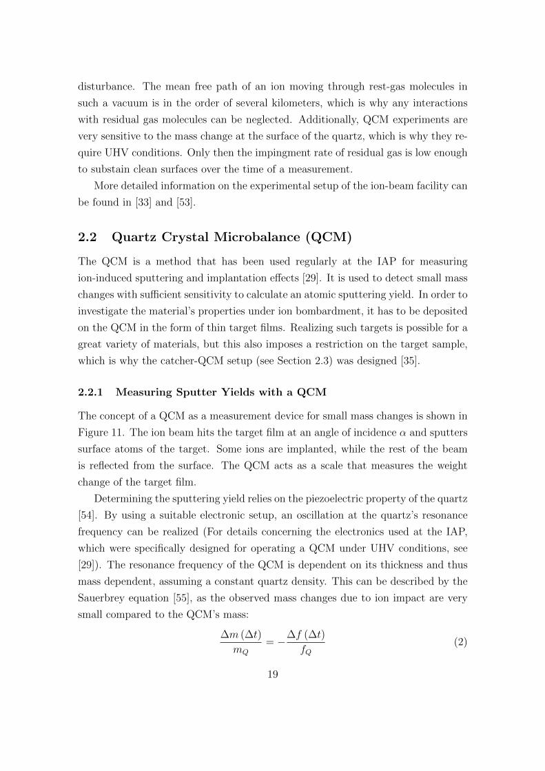
The concept of a QCM as a measurement device for small mass changes is shown in

Figure 11. The ion beam hits the target film at an angle of incidence α and sputters

surface atoms of the target. Some ions are implanted, while the rest of the beam

is reflected from the surface. The QCM acts as a scale that measures the weight

change of the target film.

Determining the sputtering yield relies on the piezoelectric property of the quartz

[54]. By using a suitable electronic setup, an oscillation at the quartz’s resonance

frequency can be realized (For details concerning the electronics used at the IAP,

which were specifically designed for operating a QCM under UHV conditions, see

[29]). The resonance frequency of the QCM is dependent on its thickness and thus

mass dependent, assuming a constant quartz density. This can be described by the

Sauerbrey equation [55], as the observed mass changes due to ion impact are very

small compared to the QCM’s mass:

∆m (∆t)

mQ

= −∆f (∆t)

fQ(2)

19

ion beam

QCMelectronics

sputteredparticles

αtarget film

quartz crystal(thickness shear mode)

Au electrodes

reflectedions

Figure 11: This sketch shows how a QCM is used for sputtering yield measure-

ments. The piezoelectric quartz is part of an oscillating circuit, whose resonance

frequency is dependent on the quartz mass. Changes in the target film’s mass

due to sputtering or implantation then result in frequency changes, which can be

measured very precisely.

In this equation, mQ describes the mass of the oscillating quartz and fQ its resonance

frequency, while ∆m and ∆f represent the respective changes during a given time

period ∆t. As frequency variations can easily be measured, this method is used to

determine mass changes ∆m of the QCM.

However, this quantity alone is not sufficient to calculate the sputter yield, which

describes the number of sputtered atoms per incident ion. It is thus necessary to

determine how many ions hit the quartz, which is realized by measuring the beam

current density j. The number of ions Nions hitting the quartz per unit area during

∆t is then given as

Nions (∆t)[ion/cm2

]=

∫jdt

q · e0

=j∆t

q · e0

(3)

In this equation, q describes the ions’ charge state, e0 represents the elementary

charge and the current density j is assumed to be constant over time. These ions

cause a mass change of ∆mA in atomic mass units per unit area:

∆mA (∆t)[amu/cm2

]=

∆m (∆t)

AQm0

= −∆f (∆t) ·mQ

fQAQm0

= −∆f (∆t) · ρQlQfQm0

(4)

20

- 5 - 4 - 3 - 2 - 1 0 1 2 3 4 50 . 0

0 . 2

0 . 4

0 . 6

0 . 8

1 . 0 E x p e r i m e n t a l T h e o r e t i c a l

Sens

itivity

[arb.

units]

x [ m m ]

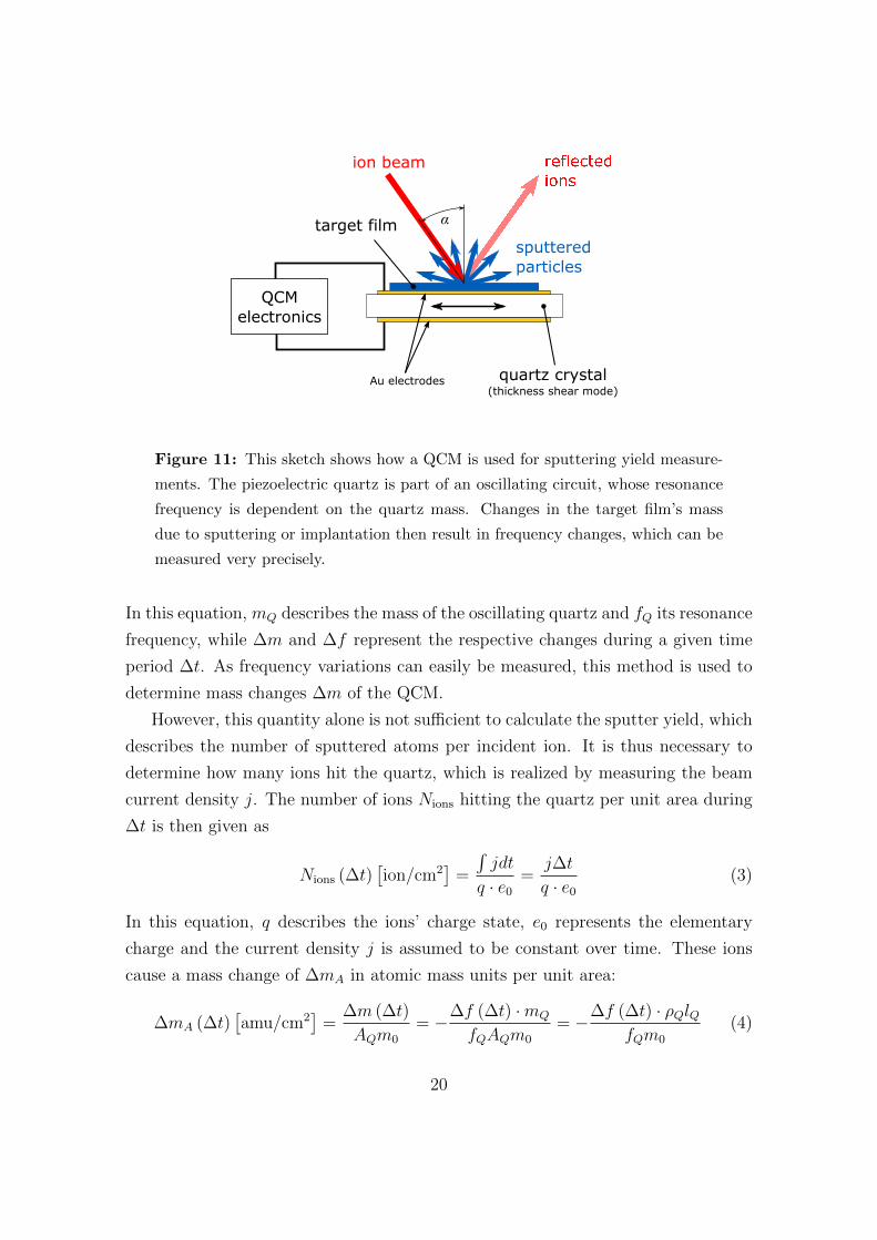
Figure 12: The result of measurements for the radial sensitivity of a QCM. The

experimental values for a focused ion beam (red) coincide excellently with the

theoretical calculation (blue) based on [56] (see also [53]).

Here the quartz mass is written as mQ = ρQlQAQ using the quartz’s density ρQ, its

thickness lQ and its surface area AQ. Including m0 leads to ∆mA being described

in atomic mass units. The mass removal per ion y is then given as

y [amu/ion] = −∆mA (∆t)

Nions (∆t)= qe0 ·

∆f (∆t)

∆t· ρQlQfQm0

· 1

j(5)

where a mass decrease leads to positive y. Mass changes of a QCM are not only

caused by sputtering, but the implantation of ions also has to be taken into account.

However, this can be neglected if the projectile ion’s mass is significantly smaller

than the mass of the sputtered atoms or if steady-state conditions are reached [29].

For composite targets, the sputtering behavior is best described by using the mass

removal y. Measuring the frequency change can only give information about the

total mass change, but not how the different target elements contribute to it.

For a uniform target, its atoms’ standard atomic mass number mi can then be

used to describe the sputter yield as

Y [atoms/ion] =y

mi

=qe0

mi

· ∆f (∆t)

∆t· ρQlQfQm0

· 1

j(6)

A summary of the quantites used to calculate the sputter yield with a QCM is given

in Table 2.

21

Y . . . sputter yield (number of sputtered atoms per incoming ion)

y . . . mass removal per incoming ion

∆m (∆t) . . . mass change of the quartz during ∆t

∆mA (∆t) . . . mass change of the quartz in amu per unit area during ∆t

∆f (∆t) . . . frequency change of the quartz during ∆t

Nions (∆t) . . . number of incoming ions per unit area during ∆t

Nsp (∆t) . . . number of sputtered particles during ∆t

j . . . current density of the ion beam

q . . . charge state of projectile ions

e0 . . . elementary charge

mi . . . atomic mass number of the target material

m0 . . . atomic mass unit

mQ . . . quartz mass

ρQ . . . quartz density

lQ . . . quartz thickness

fQ . . . quartz resonance frequency

AQ . . . active area of the quartz

Table 2: An overview of the different quantities used for sputter yield calculation

with a QCM.

22

For practical purposes, equations (5) and (6) can be simplified to

y = q · Cj· ∆f (∆t)

∆t(7)

and

Y =q

mi

· Cj· ∆f (∆t)

∆t(8)

where C =e0ρQlQfQm0

summarizes all remaining constant quantities in the previous

equations. The slope of the QCM’s output signal ∆f(∆t)∆t

is recorded during the

measurement process. The ion current density j is determined before and after each

measurement with a Faraday Cup (FC) [57] with the additional option of using a

beam monitor [58] for taking current variations during the measurement process

into account.

With regard to frequency changes due to mass change, the sensitivity of an

oscillating quartz decreases radially outwards from its center [55]. It is proportional

to the squared shear amplitude of the quartz, which corresponds to a Gaussian

function [56]. This property was also investigated experimentally for the QCMs

used at the IAP and the result is presented in Figure 12. It shows a normalized

comparison of the QCM’s frequency change for a focused ion beam hitting the

QCM at varying distances to the quartz’s center point. For this reason, the curve

represents the convolution of the quartz’s sensitivity and the beam profile. However,

due to the small ion-beam diameter of less than 1 mm, this curve can be used to

describe the QCM’s sensitivity. This is supported by the theoretical calculation

based on the work by Stevens and Tiersten [56] that is included in Figure 12 and

fits the experimental data excellently (for details on how to calculate the sensitivity,

see [53]).

Measurement of sputtering is thus restricted to the so-called active area where

the sensitivity is non-vanishing, while mass changes outside of the active area can-

not be registered. However, non-uniform mass removal across the quartz surface can

lead to deviations from the Sauerbrey equation (2) [59]. Accordingly, past measure-

ments with a QCM have shown that this method is best suited for determining area

sputter yields under uniform ion bombardment [29]. This is realized by scanning

the incoming ion beam over the QCM so that the whole active area is exposed to

a uniform current density. The beam can be further shaped by using one of sev-

eral apertures that are included in the sample chamber and can be moved into the

beam’s path to ensure that the ion beam only hits the target sample.

23

ion beam

target-QCM

catcher - QCM

α

d

Δx x

y

z

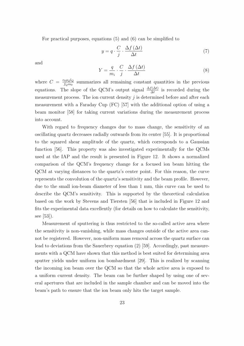
Figure 13: This diagram shows the catcher-QCM setup, where a second QCM is

placed beside the target. It is used to measure the amount of sputtered atoms that

stick to its surface, and the target sputtering yield Ytar can then be reproduced

using a theoretical model. The setup has three variable parameters: The angle of

incidence α, the target-catcher distance d and the target shift ∆x. (Image taken

from [53].)

2.3 Catcher-QCM Setup

2.3.1 Design

The catcher-QCM setup was designed in order to enable sputtering experiments with

a larger variety of targets [35]. For direct ion bombardment of a target-QCM a thin

film is deposited on the quartz, which poses a restriction on the target material and

different effects on the sputtering yield. Especially for complex materials creating

thin films with the same composition can be a challenge. Furthermore, properties

of the thin film, such as the surface roughness, will be different from that of the

original material.

For this reason, a catcher-QCM was placed beside the target holder, as can be

seen in the sketch in Figure 13 [35]. The sputtered target atoms are emitted in

a cone at energies mostly below 50 eV (see Figure 6 and [37]) and can stick to

the catcher surface. The catcher yield YC is then measured as the amount of target

24

atoms sticking to the catcher surface per incident ion, which leads to a mass increase

of the quartz. However, part of the ion beam is reflected at the target surface and

may sputter the catcher-QCM’s surface, resulting in a mass decrease. Taking these

effects into account, the sputtering yield of the target Ytar can be reproduced using

a theoretical model based on SDTrimSP simulations (see Section 3). It should be

noted that the target-QCM is included in this setup for proof-of-concept purposes

that make it possible to check the feasibility of the catcher setup and the simulations.

For future experiments, the target-QCM will be replaced by a rock or a powder target

to fully take advantage of the possibilities provided by the new catcher setup.

The catcher setup allows three variable parameters for positioning as indicated

in Figure 13. With regard to the coordinate system used in this image, the catcher-

QCM itself can only be moved in y-direction, which changes the distance d between

target and catcher. Additionally, the orientation of the target and, thus, the angle

of incidence α can be changed, as well as the target’s position in x-direction, which

leads to a target-shift ∆x.

Both the target-QCM and the catcher-QCM are mounted in the same mechanical

way, which is indicated in Figure 13. There they are fixed in stainless steel holders

with springs, where Au electrodes provide the contacts for the electrical signals that

drive the quartz oscillations. At each holder heating connectors are included in order

to operate the QCM in different temperature ranges that can provide a more stable

oscillation [29]. The target sample holder includes a shielded FC that allows beam

current density and beam profile measurements before and after an experiment.

The target can be rotated around the z-axis so that different angles of incidence up

to 75 can be achieved and it is also connected to three stepper motors that allow

position changes in x-, y- and z-direction. Due to the fixed direction of the incoming

ion beam, however, the latter two variations are only used for measurements of the

beam profile.

Measurements with a catcher-QCM require precise control of the ion beam, which

must not hit anything outside of the target. For example, atoms sputtered from the

steel target holder would also be able to reach the catcher-QCM and thus lead to

measurement errors. For this reason a set of circular apertures (Ø2, 3, 4 and 7 mm)

mounted on a manipulator was installed in the sample chamber between the scanning

plates and the target. By using these apertures the beam size can be controlled very

precisely, which is important for evaluating the catcher-QCM’s signal. However, the

25

divergence of the scanned ion beam has to be taken into account for determining

which aperture to use and for calculating the total beam current hitting the target,

which is described in the following section.

More information on this experimental setup can be found in [53].

2.3.2 Evaluation Methods

During sputtering experiments, the frequency changes of the QCMs are recorded

and together with the ion-beam current and the quartz’s properties, the yields on

the target and the catcher can be calculated. In section 2.2.1 the mass removal rate

y was derived under the assumption that the Sauerbrey equation (2) is fulfilled (see

equation (7)). Following this method, the mass change rate is calculated for both

the target- and the catcher-QCM as follows, however, both cases have to be treated

separately.

Target-QCM Scanning of the incoming ion beam is performed in order to ensure

a homogeneous beam current across the active area of the quartz and, thus, homo-

geneous sputtering of the surface, which is required for using the Sauerbrey equation

in sputter yield calculations. However, ions that do not hit the active area of the

quartz do not result in a frequency change. For this reason, the ion-beam current

has to be written as the current on the QCM’s active area

I = j (α) · AQ (9)

The mean of the current densitiy j is calculated from FC measurements of the

ion-beam profile of the scanned beam

j =IFC

AFC

· cosα (10)

where IFC is the current measured with the FC and AFC is its area. j is dependent on

the angle of incidence α because less of the scanned ion beam can hit the active area

under non-normal incidence. Additionally, the current at the target is affected by

the divergence of the scanned ion beam: Larger ∆x mean a greater distance to the

scanning plates and thus a wider ion beam. Regarding the active area, this results

in a lower current density, which has to be taken into account for mass change rate

determination.

26

The formula for calculating the mass removal rate at the target-QCM ytar can

then be simplified as was shown in section 2.2.1, which leads to equation (5):

ytar = q · C

j (α)· ∆f

∆t(11)

For a single-element target, a sputtering yield per atom can then be derived as shown

in equation (8):

Ytar =ytar

mi

=q

mi

· C

j (α)· ∆f

∆t(12)

Catcher-QCM The quantity that can be measured with the catcher-QCM is the

catcher mass change rate yC, which equals the mass change of the catcher quartz in

amu per incoming ion. For single-element targets, the catcher yield YC is defined as

the number of target atoms that stick to the catcher surface, a mass increase of the

catcher-QCM thus leads to a positive catcher yield. It should be emphasized that

this is contrary to the evaluation of the target-QCM, where a mass removal leads to

a positive sputtering yield Ytar.

To calculate the catcher mass change rate, the whole current that hits the target

has to be considered. With a QCM target, this also includes the contribution of ions

that hit outside of the active area, as their sputtering behavior is the same as for

other ions. As long as it can be guaranteed that the whole ion beam hits the target,

the current is not dependent on the angle of incidence. However, scanning the ion

beam larger than the target should be avoided at all costs, because sputtering of

the surrounding target holder would then also occur and influence the catcher yield.

For this reason, the scanned ion beam can be controlled with a set of apertures with

known diameters as described in the previous section in order to ensure sputtering

only of the film deposited on the target-QCM.

As a result, the number of ions hitting the QCM per unit area during ∆t

Nions (∆t) [ion/cm2] in equation (3) has to be replaced by the total number of ions

hitting the target-QCM in the same time span

N totalions (∆t) [ion] =

I∆t

q · e0

(13)

The mass change per unit area ∆mA (∆t) [amu/cm2] during ∆t in equation (4) has

to be similarly adapted, which instead becomes the total mass change during ∆t

∆m (∆t) [amu] =∆m (∆t)

m0

= −∆f (∆t) · ρQlQAQfQm0

(14)

27

The catcher mass change rate yC is then defined as

yC [amu/ion] =∆m (∆t)

N totalions (∆t)

= q · C∗

I· ∆f (∆t)

∆t(15)

with C∗ = C ·AQ =e0ρQlQAQ

fQm0including the QCM’s active area. The total ion beam

current I can be derived from the measured FC current IFC by taking into account

the area of the aperture and the divergence of the scanned ion beam:

I =IFC

AFC

· (rap + sx · tan β)2 · π (16)

Here Aap = r2ap · π describes the aperture area used, sx is the distance between the

aperture and FC in x-direction and β represents the divergence angle of the ion-beam

scanning. The expression in brackets in equation (16) thus describes the radius of

the area where the scanned ion beam hits the target. This has to be included as the

ion beam broadens after passing the aperture and irradiates an area on the QCM

larger than Aap.

2.3.3 The parameter g

Using the catcher-QCM setup with a target-QCM is a feasible way of investigat-

ing sputtering behavior in regard to angular dependencies of sputtered material or

reflected ions. However, when using targets that do not allow direct sputtering mea-

surements in the same way as with a QCM, the interpretation of the catcher signal

is very important. The goal for solar-wind-effect measurements is, for example, di-

rectly bombarding a piece of stone and measuring only the catcher mass change rate

yC . In order to calculate the target mass removal rate ytar, exact knowledge of the

expected angular distributions, the sputtering at the catcher-QCM by reflected ions

and the sticking of sputtered material is required.

In order to describe the relation of target and catcher, the parameter g = yC/ytar

is defined, which describes the ratio between the mass change of the catcher and the

target. g can be determined experimentally with a target- and a catcher-QCM, but

can also be calculated theoretically. The latter is necessary for the reconstruction of

the target mass change ytar, rec = yC, exp/gsim with the measured catcher mass change

yC, exp and a simulated parameter gsim. The simulation is based on the geometric

analysis of SDTrimSP calculations, which is the topic of Section 3.

First proof-of-principle measurements with two QCMs (see Section 4.1 and [35])

were performed with the goal of comparing experimental and calculated g values to

28

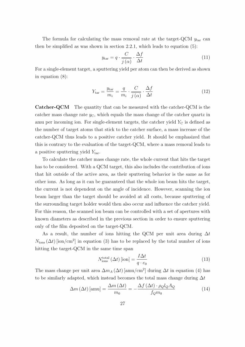
Figure 14: The Atomic Force Microscopy (AFM) image of the Au-coated QCM

shows a regular island pattern. The RMS value of the surface roughness has been

found to be rather low, at 2.9 nm, and thus the sample can be considered as flat.

(Image taken from [53].)

show the feasibility of the setup. This was continued with Fe targets of different

roughness - an aspect that is not included in conventional SDTrimSP simulations,

instead a simulation approach using the expansion SDTrimSP-2D was used (see

Section 4.2). Finally, Wollastonite-coated QCMs were investigated to look at catcher

measurements for composite targets and to compare the catcher mass change rate

to values observed by directly bombarding a stone (Section 4.3).

2.4 Sample Preparation and Analysis

2.4.1 Au QCM-Films

A substantial amount of literature data exists for the projectile target combination

Ar and Au, and Au-targets are comparably easy to handle considering contamina-

tions. For this reason, Au was chosen for performing first proof-of-concept measure-

ments with the catcher setup. Mutliple QCMs with a thin Au film created with

sputter deposition were provided by Prof. Eisenmenger-Sittner from the Institute

of Solid State Physics at TU Wien.

AFM In order to analyze the structure of the surface, one Au QCM was investi-

gated with an Atomic Force Microscope (AFM). Using a nm-scale tip mounted on a

cantilever, surfaces can be investigated with an AFM by measuring the cantilever’s

distortion due to interatomic forces between sample and tip [60]. This makes it

29

possible to record images at nm resolution, as seen in Figure 14 for the Au-coated

QCM. Small island structures can be seen there that result in a root mean square

(RMS) value of the surface roughness of 2.9 nm [53]. Compared to the Fe samples

that were also used in this thesis (see the following section 2.4.2), this value is rather

low and for this reason the Au targets were considered as flat in the simulations.

2.4.2 Fe QCM-Films

For the investigation of Fe targets with different surface roughness, multiple sputter

deposited quartzes were supplied by the Max-Planck-Institute of Plasma Physics

(IPP) Garching. It was decided to use such samples with different surface rough-

nesses for experiments with the catcher setup in order to investigate the influence

of this surface structure on the catcher signal. The target’s surface roughness repre-

sents a very important aspect of future experiments with stone or powder samples.

For this reason, the influence of this quantity is first investigated with the thin film

QCMs, which are much easier to interpret due to the possibility of direct sput-

tering yield measurements. The sputtering behavior of these QCMs for different

angles of incidence and under long-term irradiation had also been investigated at

IAP beforehand [61].

AFM As a part of the above-mentioned experiments, AFM images of the Fe-

coated QCMs were taken before and after irradiation. Initially, grain-like features

are visible that change during the ion bombardment (under an incident angle of 60

degrees) due to the sputtering to a ripple structure that is strongly aligned with the

direction of incoming ions.

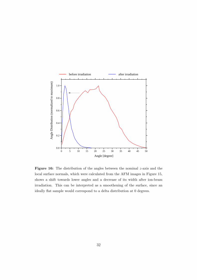
During the irradiation a surface smoothening also occurs, which can be quantified

by the distribution of local angles, which denote the angle between the local surface

normal and the z-axis. This distribution can be calculated from the AFM data and a

comparison between this distribution of angles before and after irradiation is shown

in Figure 16. The distribution of the initial rough surface (red) has a peak at around

20 degrees and is very broad compared to the distribution after the irradiation (blue).

As a perfectly flat surface would be represented by a delta distribution centered at

0 degrees, the surface can be interpreted as much smoother after the irradiation.

Furthermore, a decrease of the root mean square (RMS) roughness from about 5.2

to 3.5 nm was found [61].

30

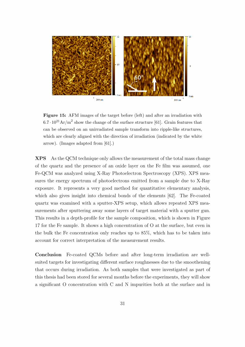
Figure 15: AFM images of the target before (left) and after an irradiation with

6.7 · 1021Ar/m2 show the change of the surface structure [61]. Grain features that

can be observed on an unirradiated sample transform into ripple-like structures,

which are clearly aligned with the direction of irradiation (indicated by the white

arrow). (Images adapted from [61].)

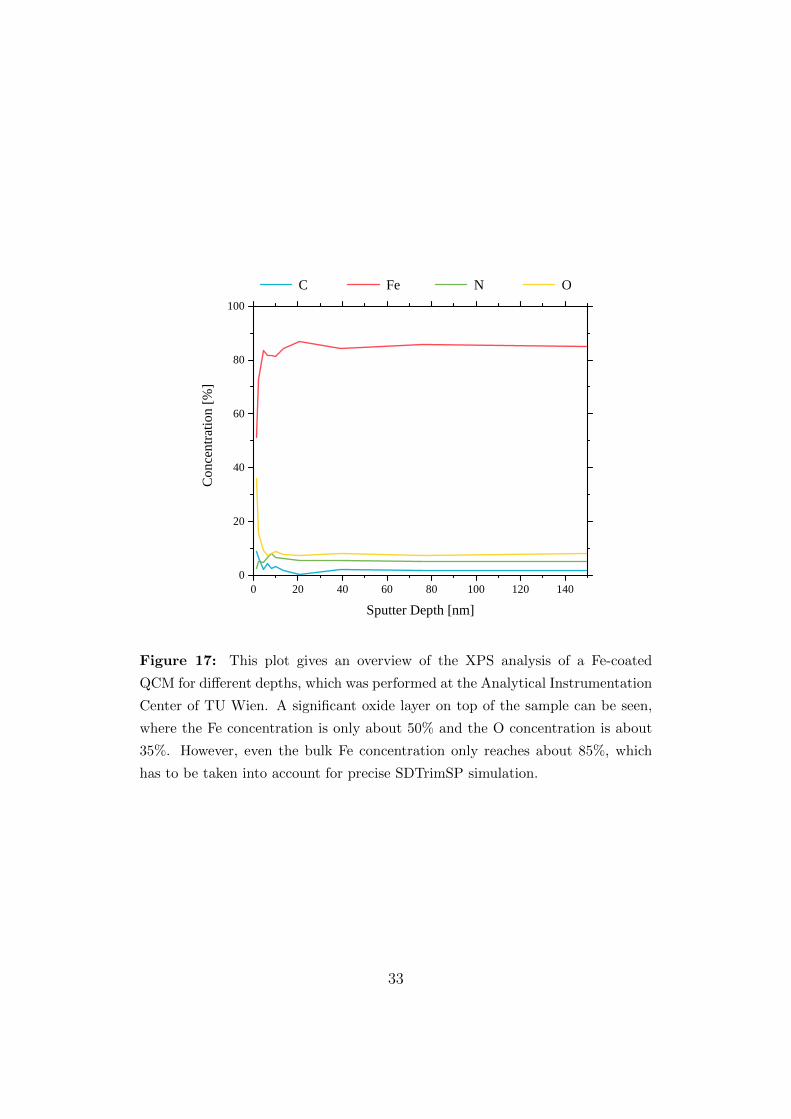
XPS As the QCM technique only allows the measurement of the total mass change

of the quartz and the presence of an oxide layer on the Fe film was assumed, one

Fe-QCM was analyzed using X-Ray Photoelectron Spectroscopy (XPS). XPS mea-

sures the energy spectrum of photoelectrons emitted from a sample due to X-Ray

exposure. It represents a very good method for quantitative elementary analysis,

which also gives insight into chemical bonds of the elements [62]. The Fe-coated

quartz was examined with a sputter-XPS setup, which allows repeated XPS mea-

surements after sputtering away some layers of target material with a sputter gun.

This results in a depth-profile for the sample composition, which is shown in Figure

17 for the Fe sample. It shows a high concentration of O at the surface, but even in

the bulk the Fe concentration only reaches up to 85%, which has to be taken into

account for correct interpretation of the measurement results.

Conclusion Fe-coated QCMs before and after long-term irradiation are well-

suited targets for investigating different surface roughnesses due to the smoothening

that occurs during irradiation. As both samples that were investigated as part of

this thesis had been stored for several months before the experiments, they will show

a significant O concentration with C and N impurities both at the surface and in

31

0 5 1 0 1 5 2 0 2 5 3 0 3 5 4 0 4 5 5 00 . 0

0 . 2

0 . 4

0 . 6

0 . 8

1 . 0

b e f o r e i r r a d i a t i o n a f t e r i r r a d i a t i o n

Angle

Distri

bution

(norm

alized

to ma

ximum

)

A n g l e [ d e g r e e ]

A n g l e D i s t r i b u t i o n s ( 6 0 ° i r r a d i a t i o n )

Figure 16: The distribution of the angles between the nominal z-axis and the

local surface normals, which were calculated from the AFM images in Figure 15,

shows a shift towards lower angles and a decrease of its width after ion-beam

irradiation. This can be interpreted as a smoothening of the surface, since an

ideally flat sample would correspond to a delta distribution at 0 degrees.

32

0 2 0 4 0 6 0 8 0 1 0 0 1 2 0 1 4 00

2 0

4 0

6 0

8 0

1 0 0

Conce

ntratio

n [%]

S p u t t e r D e p t h [ n m ]

C F e N O

Figure 17: This plot gives an overview of the XPS analysis of a Fe-coated

QCM for different depths, which was performed at the Analytical Instrumentation

Center of TU Wien. A significant oxide layer on top of the sample can be seen,

where the Fe concentration is only about 50% and the O concentration is about

35%. However, even the bulk Fe concentration only reaches about 85%, which

has to be taken into account for precise SDTrimSP simulation.

33

the bulk. For correct simulation of these experiments, both the composition and the

surface roughness have to be taken into account.

2.4.3 Wollastonite (CaSiO3)

The mineral Wollastonite (CaSiO3) has a similar chemical composition to the py-

roxene group (for example, Enstatite (MgSiO3) and Ferrosilite (FeSiO3)), but it is

regarded seperately due to differences in crystal structure ([36], [63]). On Earth

it occurs regularly in limestone and can be found across most continents [63]. Its

applications are found in different material manufacturing processes, but most im-

portantly Wollastonite has been used as a bioactive ceramic [64]. For the purpose

of planetary research it is relevant as rock samples from the Moon provided by

the Apollo missions showed an abundance of pyroxene minerals [36]. Experiments

with a Wollastonite sample thus provide an interesting opportunity to investigate

solar-wind effects on the lunar surface.

While measuring the sputtering of the stone due to ion bombardment represents

the most relevant experiment for investigating solar-wind effects, there are many

uncertainties connected to these measurements. Compared to a thin film, angu-

lar distributions of the particles hitting the catcher may be different and sticking

coefficients, especially from O, may be less than 1 [65]. Furthermore, due to Wol-

lastonite’s insulating nature, potential sputtering is expected to occur [31]. The

different chemical potentials and the crystal structure of bound CaSiO3 that are not

included in SDTrimSP correctly can also lead to inaccuracies in the simulation.

For this reason, it was decided to first investigate a thin Wollastonite film de-

posited on a QCM. Due to direct information on the sputtering it becomes easier

to explain possible deviations from the simulated behavior. Furthermore, using a

catcher-QCM with target material should maximize the sticking coefficient of the

sputtered material. Thus, establishing the sample preparation and analysis tech-

niques presented in this section is also helpful for future experiments with other

composite materials.

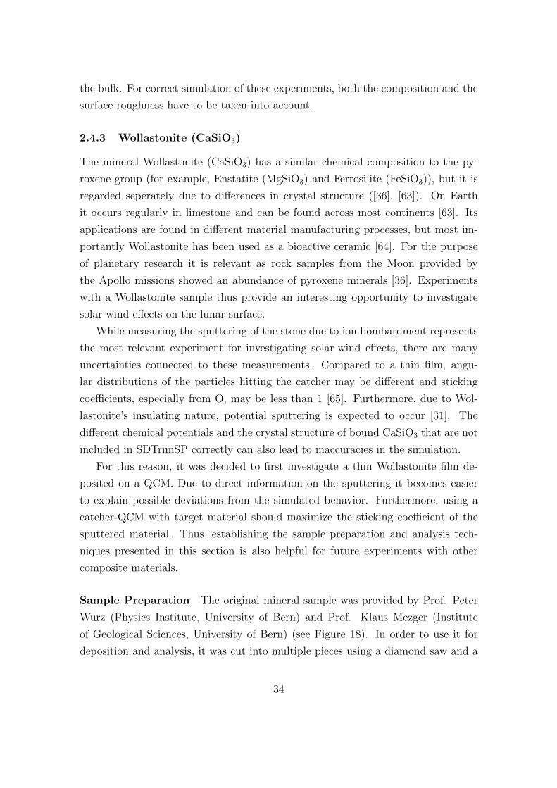
Sample Preparation The original mineral sample was provided by Prof. Peter

Wurz (Physics Institute, University of Bern) and Prof. Klaus Mezger (Institute

of Geological Sciences, University of Bern) (see Figure 18). In order to use it for

deposition and analysis, it was cut into multiple pieces using a diamond saw and a

34

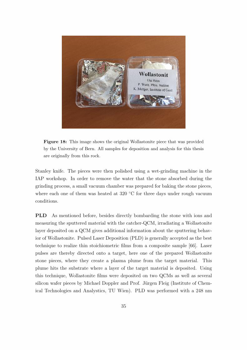
Figure 18: This image shows the original Wollastonite piece that was provided

by the University of Bern. All samples for deposition and analysis for this thesis

are originally from this rock.

Stanley knife. The pieces were then polished using a wet-grinding machine in the

IAP workshop. In order to remove the water that the stone absorbed during the

grinding process, a small vacuum chamber was prepared for baking the stone pieces,

where each one of them was heated at 320 C for three days under rough vacuum

conditions.

PLD As mentioned before, besides directly bombarding the stone with ions and

measuring the sputtered material with the catcher-QCM, irradiating a Wollastonite

layer deposited on a QCM gives additional information about the sputtering behav-

ior of Wollastonite. Pulsed Laser Deposition (PLD) is generally accepted as the best

technique to realize thin stoichiometric films from a composite sample [66]. Laser

pulses are thereby directed onto a target, here one of the prepared Wollastonite

stone pieces, where they create a plasma plume from the target material. This

plume hits the substrate where a layer of the target material is deposited. Using

this technique, Wollastonite films were deposited on two QCMs as well as several

silicon wafer pieces by Michael Doppler and Prof. Jurgen Fleig (Institute of Chem-

ical Technologies and Analystics, TU Wien). PLD was performed with a 248 nm

35

KrF excimer laser at a pulse frequency of 5 Hz and a pulse energy of 5 mJ while the

sample was kept at about 250 C. The deposition times of the QCMs were 30 and

60 minutes with the latter being used as the target so that more material would be

available for sputtering.

XRD Directly after the laser deposition, Michael Doppler investigated the film

growth using X-Ray diffractometry (XRD). XRD is a very important tool in crystal-

lography, which uses the photons scattering at atom’s electron clouds to determine

its crystallic structure. X-Ray photons are diffracted at the lattice and interfere

constructively following Bragg’s law n · λ = 2d · sin θ [67]. The visible peaks of the

XRD-measurements show only the Au layer of the QCM, while no diffraction from

any Wollastonite was observed. However, this method only registers X-Ray photons

diffracted from a regular crystal structure, while no signal from an amorphous solid

can be measured. As a result, the XRD analysis cannot tell whether an amorphous

layer of Wollastonite has formed or if there is no dense film at all. This information

would be important for judging the feasibility of using these QCMs for experiments

where a thorough layer of Wollastonite is necessary. Otherwise, sputtering of the

QCM’s Au electrode would also occur and lead to false results as only the absolute

mass change rate can be measured with a QCM.

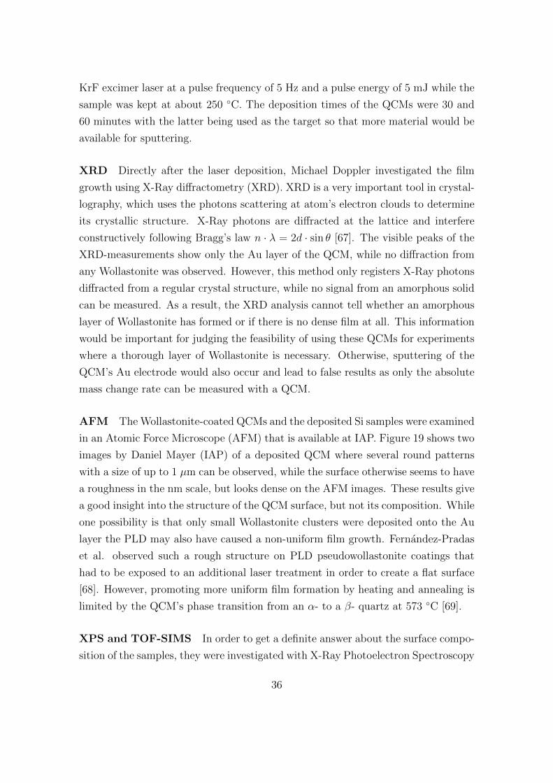
AFM The Wollastonite-coated QCMs and the deposited Si samples were examined

in an Atomic Force Microscope (AFM) that is available at IAP. Figure 19 shows two

images by Daniel Mayer (IAP) of a deposited QCM where several round patterns

with a size of up to 1 µm can be observed, while the surface otherwise seems to have

a roughness in the nm scale, but looks dense on the AFM images. These results give

a good insight into the structure of the QCM surface, but not its composition. While

one possibility is that only small Wollastonite clusters were deposited onto the Au

layer the PLD may also have caused a non-uniform film growth. Fernandez-Pradas

et al. observed such a rough structure on PLD pseudowollastonite coatings that

had to be exposed to an additional laser treatment in order to create a flat surface

[68]. However, promoting more uniform film formation by heating and annealing is

limited by the QCM’s phase transition from an α- to a β- quartz at 573 C [69].

XPS and TOF-SIMS In order to get a definite answer about the surface compo-

sition of the samples, they were investigated with X-Ray Photoelectron Spectroscopy

36

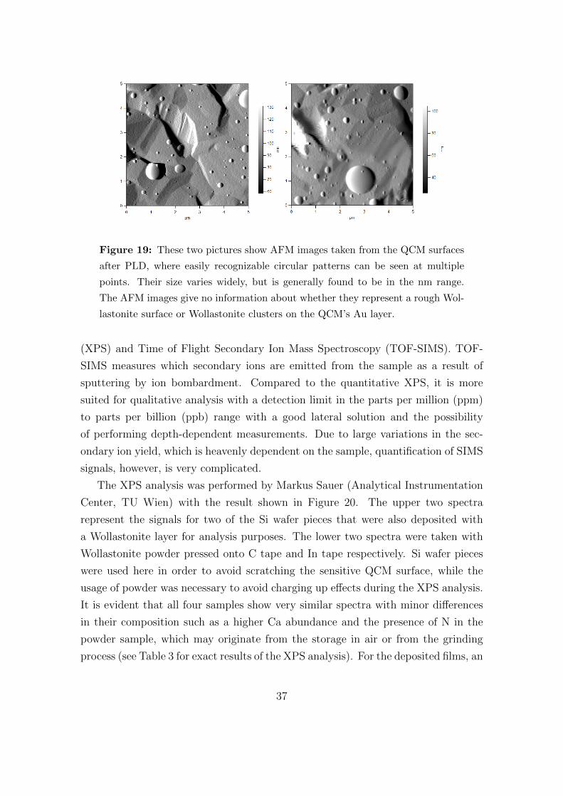
Figure 19: These two pictures show AFM images taken from the QCM surfaces

after PLD, where easily recognizable circular patterns can be seen at multiple

points. Their size varies widely, but is generally found to be in the nm range.

The AFM images give no information about whether they represent a rough Wol-

lastonite surface or Wollastonite clusters on the QCM’s Au layer.

(XPS) and Time of Flight Secondary Ion Mass Spectroscopy (TOF-SIMS). TOF-

SIMS measures which secondary ions are emitted from the sample as a result of

sputtering by ion bombardment. Compared to the quantitative XPS, it is more

suited for qualitative analysis with a detection limit in the parts per million (ppm)

to parts per billion (ppb) range with a good lateral solution and the possibility

of performing depth-dependent measurements. Due to large variations in the sec-

ondary ion yield, which is heavenly dependent on the sample, quantification of SIMS

signals, however, is very complicated.

The XPS analysis was performed by Markus Sauer (Analytical Instrumentation

Center, TU Wien) with the result shown in Figure 20. The upper two spectra

represent the signals for two of the Si wafer pieces that were also deposited with

a Wollastonite layer for analysis purposes. The lower two spectra were taken with

Wollastonite powder pressed onto C tape and In tape respectively. Si wafer pieces

were used here in order to avoid scratching the sensitive QCM surface, while the

usage of powder was necessary to avoid charging up effects during the XPS analysis.

It is evident that all four samples show very similar spectra with minor differences

in their composition such as a higher Ca abundance and the presence of N in the

powder sample, which may originate from the storage in air or from the grinding

process (see Table 3 for exact results of the XPS analysis). For the deposited films, an

37

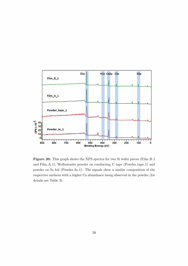
Figure 20: This graph shows the XPS spectra for two Si wafer pieces (Film B 1

and Film A 1), Wollastonite powder on conducting C tape (Powder tape 1) and

powder on In foil (Powder In 1). The signals show a similar composition of the

respective surfaces with a higher Ca abundance being observed in the powder (for

details see Table 3).

38

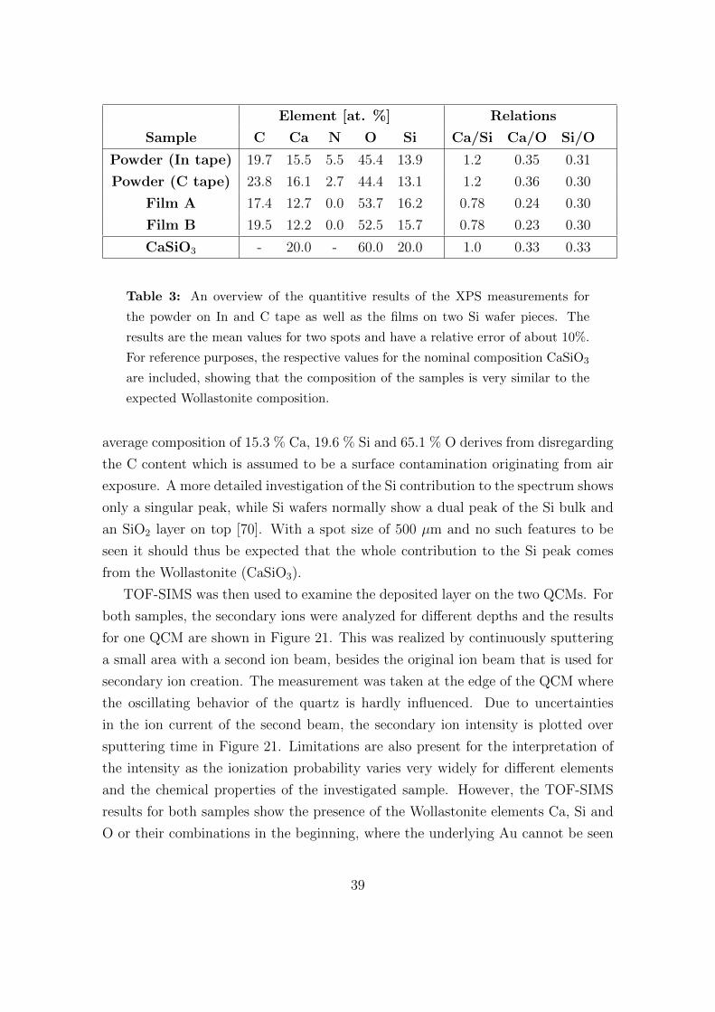
Element [at. %] Relations

Sample C Ca N O Si Ca/Si Ca/O Si/O

Powder (In tape) 19.7 15.5 5.5 45.4 13.9 1.2 0.35 0.31

Powder (C tape) 23.8 16.1 2.7 44.4 13.1 1.2 0.36 0.30

Film A 17.4 12.7 0.0 53.7 16.2 0.78 0.24 0.30

Film B 19.5 12.2 0.0 52.5 15.7 0.78 0.23 0.30

CaSiO3 - 20.0 - 60.0 20.0 1.0 0.33 0.33

Table 3: An overview of the quantitive results of the XPS measurements for

the powder on In and C tape as well as the films on two Si wafer pieces. The

results are the mean values for two spots and have a relative error of about 10%.

For reference purposes, the respective values for the nominal composition CaSiO3

are included, showing that the composition of the samples is very similar to the

expected Wollastonite composition.

average composition of 15.3 % Ca, 19.6 % Si and 65.1 % O derives from disregarding

the C content which is assumed to be a surface contamination originating from air

exposure. A more detailed investigation of the Si contribution to the spectrum shows

only a singular peak, while Si wafers normally show a dual peak of the Si bulk and

an SiO2 layer on top [70]. With a spot size of 500 µm and no such features to be

seen it should thus be expected that the whole contribution to the Si peak comes

from the Wollastonite (CaSiO3).

TOF-SIMS was then used to examine the deposited layer on the two QCMs. For

both samples, the secondary ions were analyzed for different depths and the results

for one QCM are shown in Figure 21. This was realized by continuously sputtering

a small area with a second ion beam, besides the original ion beam that is used for

secondary ion creation. The measurement was taken at the edge of the QCM where

the oscillating behavior of the quartz is hardly influenced. Due to uncertainties

in the ion current of the second beam, the secondary ion intensity is plotted over

sputtering time in Figure 21. Limitations are also present for the interpretation of

the intensity as the ionization probability varies very widely for different elements

and the chemical properties of the investigated sample. However, the TOF-SIMS

results for both samples show the presence of the Wollastonite elements Ca, Si and

O or their combinations in the beginning, where the underlying Au cannot be seen

39

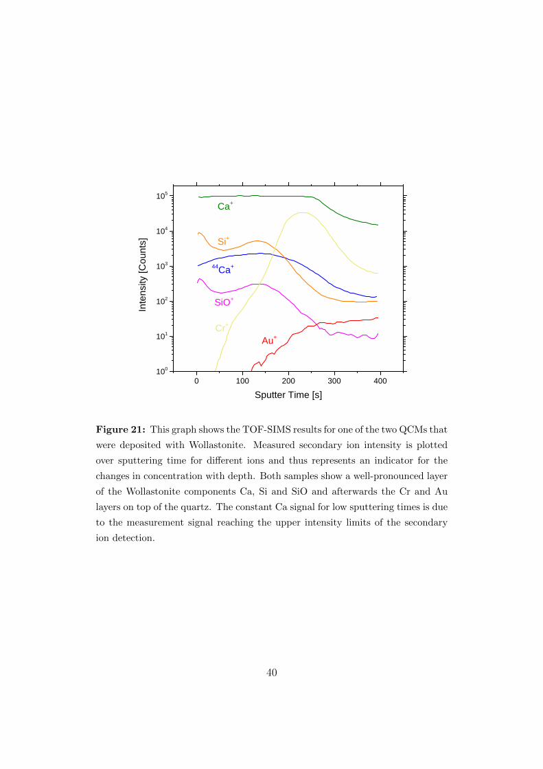
0 1 0 0 2 0 0 3 0 0 4 0 01 0 0

1 0 1

1 0 2

1 0 3

1 0 4

1 0 5

A u +C r +

S i O +

4 4 C a +

S i +

Inten

sity [C

ounts

]

S p u t t e r T i m e [ s ]

C a +

Figure 21: This graph shows the TOF-SIMS results for one of the two QCMs that

were deposited with Wollastonite. Measured secondary ion intensity is plotted

over sputtering time for different ions and thus represents an indicator for the

changes in concentration with depth. Both samples show a well-pronounced layer

of the Wollastonite components Ca, Si and SiO and afterwards the Cr and Au

layers on top of the quartz. The constant Ca signal for low sputtering times is due

to the measurement signal reaching the upper intensity limits of the secondary

ion detection.

40

at all. Only after sputtering away the top layers of the material the Au signal and a

Cr layer covering the electrod can be seen, which is connected to a decrease in the

intensity for the ions of the elements of Wollastonite.

Conclusion Despite originally being indicated otherwise, XPS and TOF-SIMS

conclusively lead to the result that a dense layer of Wollastonite material has formed

on top of the QCMs during PLD. They are thus suited for usage during sputtering

experiments to investigate the effects of ions hitting Wollastonite and comparing the

results to sputtering of the original rock sample. It should however be noted that

differences in behavior are to be expected due to the amorphous structure of the

thin film, the differences in composition (Ca abundance) and the surface features

observed with the AFM.

41

3 Theoretical Description of Catcher

Measurements

The goal of the catcher setup is the investigation of sputtering behavior without

direct measurements at the target. This is realized by calculating the mass change

of the catcher-QCM and using this information to determine the mass removal at

the target.

In order to theoretically describe the measured catcher signal, two contributions

have to be taken into account:

• sticking of atoms that were sputtered from the target to the catcher surface

• sputtering of the catcher surface by projectiles that were reflected by the target

and hit the catcher

Further surface erosion at the catcher by sputtered atoms from the target is

ignored because of their low kinetic energy (see section 1.2.3). It should be noted

that implantation of projectile ions was ignored during the simulations described

in this section. The mass change of the catcher per projectile ion represents the

increase due to the sticking of sputtered atoms (yC,sp) minus the contribution of

sputtered atoms caused by reflected ions (yC,r). The measured mass change rate at

the catcher yC can therefore be described as the difference between these quantities:

yC = yC,sp − yC,r (17)

3.1 Calculating yC

3.1.1 Contribution of Sputtered Atoms

The mass increase at the catcher caused by the sticking of sputtered atoms yC,sp

is dependent on the sputtering at the target, the angular distribution of the sput-

tered atoms and the position of the catcher, which can be described by the angle

of incidence α, a displacement ∆x of the target in the ion beam’s direction and

the distance d between the target and the catcher (see Figure 13). Furthermore,

sticking coefficients Si for each target element i have to be taken into account to

describe the only partial surface adsorption of atoms reaching the catcher. These

dependencies can be combined in factors yiC,sp describing the catcher mass change

42

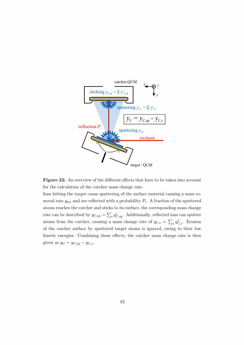
target / QCM

catcher-QCM x

ion beam

sputtering ytar

sticking yC,sp = Σ yiC,sp

i

reflection Pr

sputtering yC,r = Σ yjC,r

j

yC = yC,sp - yC,r

z

y

Figure 22: An overview of the different effects that have to be taken into account

for the calculation of the catcher mass change rate.

Ions hitting the target cause sputtering of the surface material causing a mass re-

moval rate ytar and are reflected with a probability Pr. A fraction of the sputtered

atoms reaches the catcher and sticks to its surface, the corresponding mass change

rate can be described by yC,sp =∑

i yiC,sp. Additionally, reflected ions can sputter

atoms from the catcher, causing a mass change rate of yC,r =∑

j yjC,r. Erosion

of the catcher surface by sputtered target atoms is ignored, owing to their low

kinetic energies. Combining these effects, the catcher mass change rate is then

given as yC = yC,sp − yC,r.

43

rate caused by the sticking atoms of the element i. yC,sp can be derived by summing

the contributions of all target elements i:

yC,sp =∑i

yiC,sp (18)

In order to specifiy yiC,sp, the number of sputtered atoms that can be measured

with the catcher has to be calculated. The target is therefore assumed to be on the

xy-plane with its center being the origin of the coordinate system. Ions hitting the

target at the point (x, y) cause target atoms of element i to be sputtered in the solid

angle Ω with a angular distribution f isp (Ω, x, y) with∫2π

f isp (Ω, x, y) dΩ = 1 (19)

Sputtered atoms do not originate at the same point, but across the area of the

beam cross section represented by the current density j (x, y) with∫Atar

j (x, y) dA = I (20)

Here j is integrated over the target surface Atar and I represents the total current

of the ion beam.

Sputtered atoms originating from points with high current density will add a

greater contribution to the total resulting angular distribution f isp of sputtered atoms

of element i. For this reason, the product of j and f isp has to be integrated over the

beam cross section in order to calculate f isp:

f isp(Ω) =1

I

∫Atar

[j (x, y) · f isp (Ω, x, y)

]dA (21)

The division by I is necessary for the normalization of the integral.

For the description of the measured signal at the catcher, this distribution has to

be weighted with the QCM’s sensitivity s (rC). The value of s is dependent on where

a sticking atom hits the catcher surface, which is only dependent on the distance

rC from its center point (see Figure 12). The position and direction of the catcher

surface are dependent on the parameters α, d and ∆x. For the calculation of yiC,sp,

however, the only relevant dependence of s is the solid angle Ω. The limited size

of the quartz’s active area is considered in the sensitivity s(Ω), and for this reason

the integration can be performed over all angles. How rC(Ω) and thus s(Ω) can be

44

calculated exactly is described in detail later in section 3.2.1. In order to obtain the

final result for the mass change rate yiC,sp, the integral over the spatial distribution

has to be multiplied with the target mass removal rate ytar as the sputtering of the

target determines how many sputtered atoms can reach the catcher. Assuming a

constant sticking coefficient Si leads to the following expression:

yiC,sp = ytar · Si∫

2π

[f isp(Ω) · s(Ω)

]dΩ =

= ytar ·Si

I

∫Atar

∫2π

[j (x, y) · f isp (Ω, x, y) · s (Ω)

]dΩdA (22)

3.1.2 Contribution of Reflected Ions

Looking at the reflected ions, the results are similar to the sputtered atoms’ contri-

bution. The catcher mass removal rate yC,r, which describes sputtering of catcher

material by reflected ions, is dependent on the reflection probability Pr. The mass

removal rates yjC, r of the catcher elements j are used to describe the relation

yC,r =∑j

yjC,r (23)

Equivalent to f isp, fr is used to describe the distribution of the reflected ions

originating from (x, y). In contrast to before, the number of reflected ions that hit

the catcher alone is not of importance, but the sputtered atoms of element j caused

by these ions are. One ion hitting the catcher causes a mass removal of yj (αr, E),

which is dependent on the ions’ angle of incidence αr on the catcher surface and

the ions’ energy E. For this reason, the energy distribution has to be included in

fr (Ω, x, y, E) with ∫ ∞0

∫2π

fr (Ω, x, y, E) dΩdE = 1 (24)

With regard to the beam-current profile, the same arguments that were used to de-

rive equation (22) apply here. Again, a resulting spatial distribution of the reflected

ions fr(Ω, E) can be defined as follows:

fr(Ω, E) =1

I

∫Atar

[j (x, y) · fr (Ω, x, y, E)

]dA (25)

Similar to rC, the angle of incidence on the catcher surface αr is only dependent on

the solid angle Ω. Its detailed calculation can also be found in section 3.2.1. Finally,

45

the calculation of yjC,r requires the multiplication of the integral by the reflection

probability Pr. Taking these aspects into account, yjC,r can be written as

yjC,r = Pr ·∫ ∞

0

∫2π

[fr(Ω, E) · yj(Ω, E) · s(Ω)

]dΩdE =

= Pr ·1

I

∫Atar

∫ ∞0

∫2π

[j (x, y) · fr (Ω, E, x, y) · yj (Ω, E) · s (Ω)

]dΩdEdA (26)

3.1.3 Conclusion

By calculating the respective mass change rates yiC,sp and yjC,r, the combined factor

g with ytar = yC/g can be theoretically described:

yC = yC,sp − yC,r =∑i

yiC,sp −∑j

yjC,r = g · ytar

⇒ g =

∑i y

iC,sp −

∑j y

jC,r

ytar

(27)

This combined factor g is well-suited for a comparison between experimental and

theoretical results. On the one hand, both yC and ytar can be measured simulta-

neously by using a target-QCM. On the other hand, both quantities and thus the

factor g can be calculated in a simulation, which is described in the following section.

In case of targets consisting of only one chemical element, the theoretical de-

scription of the parameter g can be simplified, as is described in [35]. As both the

target and the catcher are made up of the same element, the sums over i and j can

be omitted. It is also more convenient to characterize the sputtering behavior using

the sputtering yield Y = y/mi with mi being the mass of the investigated element

in amu. The mass removal rates y in equation (26) and ytar in equation (27) can

therefore be replaced by the respective sputtering yields Y and Ytar. Instead of yC,sp

and yC,r the yields YC,sp = gsp ·Ytar and YC,r can be used. By defining the parameter

gsp that only describes the contribution to g by the sputtered atoms sticking on the

catcher, the target yield Ytar can be cancelled. This leads to the following expression

for g:

g =YC,sp − YC,r

Ytar

= gsp −YC,r

Ytar

(28)

46

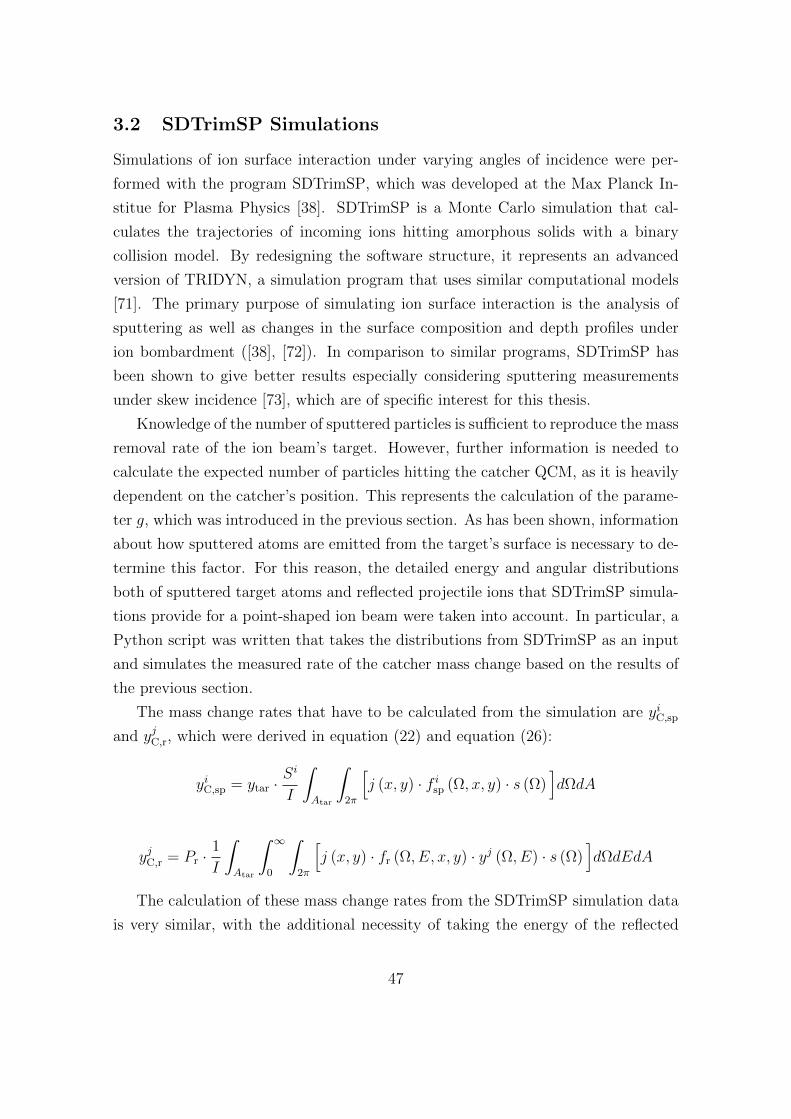
3.2 SDTrimSP Simulations

Simulations of ion surface interaction under varying angles of incidence were per-

formed with the program SDTrimSP, which was developed at the Max Planck In-

stitue for Plasma Physics [38]. SDTrimSP is a Monte Carlo simulation that cal-

culates the trajectories of incoming ions hitting amorphous solids with a binary

collision model. By redesigning the software structure, it represents an advanced

version of TRIDYN, a simulation program that uses similar computational models

[71]. The primary purpose of simulating ion surface interaction is the analysis of

sputtering as well as changes in the surface composition and depth profiles under

ion bombardment ([38], [72]). In comparison to similar programs, SDTrimSP has

been shown to give better results especially considering sputtering measurements

under skew incidence [73], which are of specific interest for this thesis.

Knowledge of the number of sputtered particles is sufficient to reproduce the mass

removal rate of the ion beam’s target. However, further information is needed to

calculate the expected number of particles hitting the catcher QCM, as it is heavily

dependent on the catcher’s position. This represents the calculation of the parame-

ter g, which was introduced in the previous section. As has been shown, information

about how sputtered atoms are emitted from the target’s surface is necessary to de-

termine this factor. For this reason, the detailed energy and angular distributions

both of sputtered target atoms and reflected projectile ions that SDTrimSP simula-

tions provide for a point-shaped ion beam were taken into account. In particular, a

Python script was written that takes the distributions from SDTrimSP as an input

and simulates the measured rate of the catcher mass change based on the results of

the previous section.

The mass change rates that have to be calculated from the simulation are yiC,sp

and yjC,r, which were derived in equation (22) and equation (26):

yiC,sp = ytar ·Si

I

∫Atar

∫2π

[j (x, y) · f isp (Ω, x, y) · s (Ω)

]dΩdA

yjC,r = Pr ·1

I

∫Atar

∫ ∞0

∫2π

[j (x, y) · fr (Ω, E, x, y) · yj (Ω, E) · s (Ω)

]dΩdEdA

The calculation of these mass change rates from the SDTrimSP simulation data

is very similar, with the additional necessity of taking the energy of the reflected

47

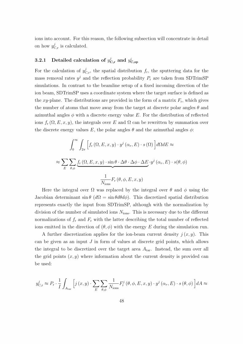
ions into account. For this reason, the following subsection will concentrate in detail

on how yjC,r is calculated.

3.2.1 Detailed calculation of yjC,r and yiC,sp

For the calculation of yjC,r, the spatial distribution fr, the sputtering data for the

mass removal rates yj and the reflection probability Pr are taken from SDTrimSP

simulations. In contrast to the beamline setup of a fixed incoming direction of the

ion beam, SDTrimSP uses a coordinate system where the target surface is defined as

the xy-plane. The distributions are provided in the form of a matrix Fr, which gives

the number of atoms that move away from the target at discrete polar angles θ and

azimuthal angles φ with a discrete energy value E. For the distribution of reflected

ions fr (Ω, E, x, y), the integrals over E and Ω can be rewritten by summation over

the discrete energy values E, the polar angles θ and the azimuthal angles φ:∫ ∞0

∫2π

[fr (Ω, E, x, y) · yj (αr, E) · s (Ω)

]dΩdE ≈

≈∑E

∑θ,φ

fr (Ω, E, x, y) · sin θ ·∆θ ·∆φ ·∆E︸ ︷︷ ︸ ·yj (αr, E) · s(θ, φ)

1

Nions

Fr (θ, φ, E, x, y)

Here the integral over Ω was replaced by the integral over θ and φ using the

Jacobian determinant sin θ (dΩ = sin θdθdφ). This discretized spatial distribution

represents exactly the input from SDTrimSP, although with the normalization by

division of the number of simulated ions Nions. This is necessary due to the different

normalizations of fr and Fr with the latter describing the total number of reflected

ions emitted in the direction of (θ, φ) with the energy E during the simulation run.

A further discretization applies for the ion-beam current density j (x, y). This

can be given as an input J in form of values at discrete grid points, which allows

the integral to be discretized over the target area Atar. Instead, the sum over all

the grid points (x, y) where information about the current density is provided can

be used:

yjC,r ≈ Pr ·1

I

∫Atar

[j (x, y) ·

∑E

∑θ,φ

1

Nions

F jr (θ, φ, E, x, y) · yj (αr, E) · s (θ, φ)

]dA ≈

48

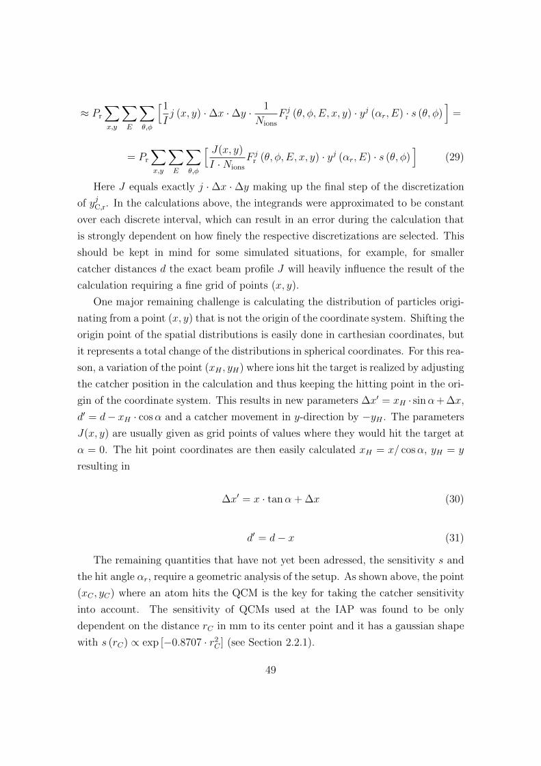
≈ Pr

∑x,y

∑E

∑θ,φ

[1

Ij (x, y) ·∆x ·∆y · 1

Nions

F jr (θ, φ, E, x, y) · yj (αr, E) · s (θ, φ)

]=

= Pr

∑x,y

∑E

∑θ,φ

[ J(x, y)

I ·Nions

F jr (θ, φ, E, x, y) · yj (αr, E) · s (θ, φ)

](29)

Here J equals exactly j ·∆x ·∆y making up the final step of the discretization

of yjC,r. In the calculations above, the integrands were approximated to be constant

over each discrete interval, which can result in an error during the calculation that

is strongly dependent on how finely the respective discretizations are selected. This

should be kept in mind for some simulated situations, for example, for smaller

catcher distances d the exact beam profile J will heavily influence the result of the

calculation requiring a fine grid of points (x, y).

One major remaining challenge is calculating the distribution of particles origi-

nating from a point (x, y) that is not the origin of the coordinate system. Shifting the

origin point of the spatial distributions is easily done in carthesian coordinates, but

it represents a total change of the distributions in spherical coordinates. For this rea-

son, a variation of the point (xH , yH) where ions hit the target is realized by adjusting

the catcher position in the calculation and thus keeping the hitting point in the ori-

gin of the coordinate system. This results in new parameters ∆x′ = xH · sinα+ ∆x,

d′ = d− xH · cosα and a catcher movement in y-direction by −yH . The parameters

J(x, y) are usually given as grid points of values where they would hit the target at

α = 0. The hit point coordinates are then easily calculated xH = x/ cosα, yH = y

resulting in

∆x′ = x · tanα + ∆x (30)

d′ = d− x (31)

The remaining quantities that have not yet been adressed, the sensitivity s and

the hit angle αr, require a geometric analysis of the setup. As shown above, the point

(xC , yC) where an atom hits the QCM is the key for taking the catcher sensitivity

into account. The sensitivity of QCMs used at the IAP was found to be only

dependent on the distance rC in mm to its center point and it has a gaussian shape

with s (rC) ∝ exp [−0.8707 · r2C ] (see Section 2.2.1).

49

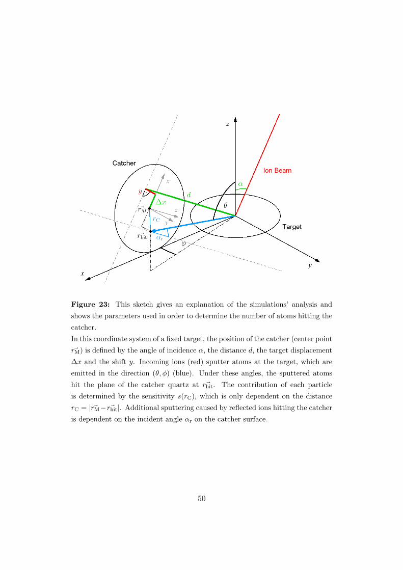
Figure 23: This sketch gives an explanation of the simulations’ analysis and

shows the parameters used in order to determine the number of atoms hitting the

catcher.

In this coordinate system of a fixed target, the position of the catcher (center point

~rM) is defined by the angle of incidence α, the distance d, the target displacement

∆x and the shift y. Incoming ions (red) sputter atoms at the target, which are

emitted in the direction (θ, φ) (blue). Under these angles, the sputtered atoms

hit the plane of the catcher quartz at ~rhit. The contribution of each particle

is determined by the sensitivity s(rC), which is only dependent on the distance

rC = | ~rM− ~rhit|. Additional sputtering caused by reflected ions hitting the catcher

is dependent on the incident angle αr on the catcher surface.

50

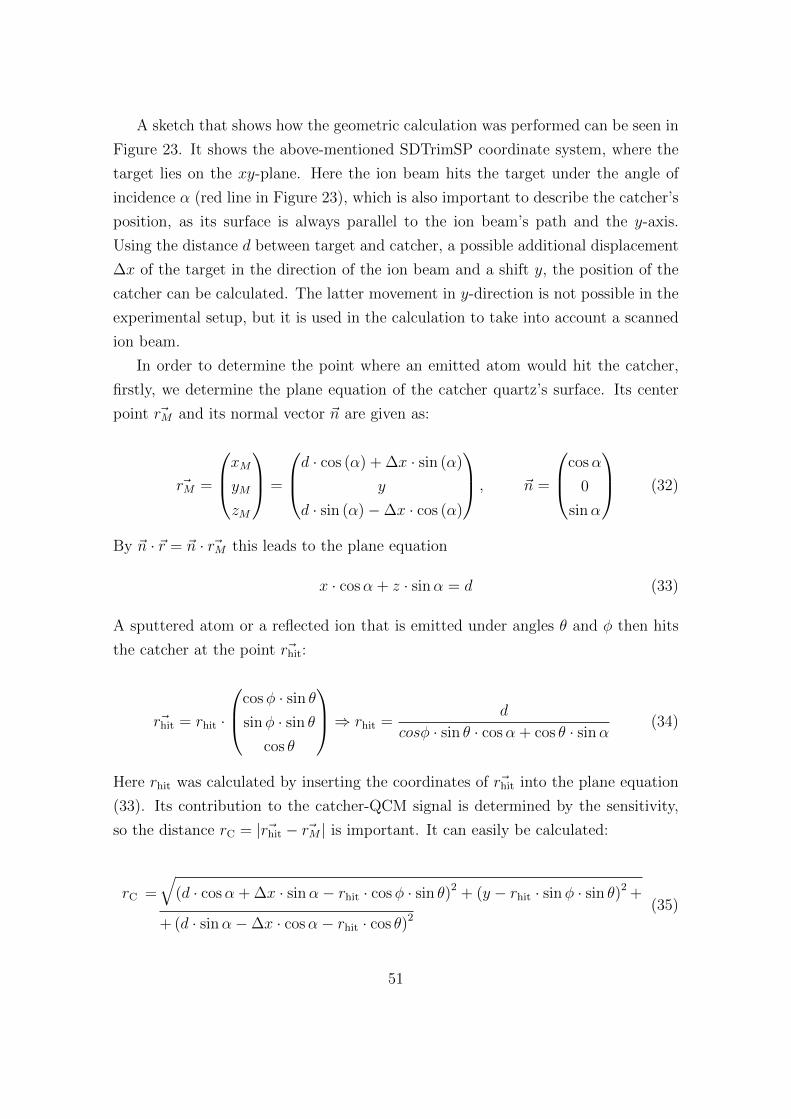
A sketch that shows how the geometric calculation was performed can be seen in

Figure 23. It shows the above-mentioned SDTrimSP coordinate system, where the

target lies on the xy-plane. Here the ion beam hits the target under the angle of

incidence α (red line in Figure 23), which is also important to describe the catcher’s

position, as its surface is always parallel to the ion beam’s path and the y-axis.

Using the distance d between target and catcher, a possible additional displacement

∆x of the target in the direction of the ion beam and a shift y, the position of the

catcher can be calculated. The latter movement in y-direction is not possible in the

experimental setup, but it is used in the calculation to take into account a scanned

ion beam.

In order to determine the point where an emitted atom would hit the catcher,

firstly, we determine the plane equation of the catcher quartz’s surface. Its center

point ~rM and its normal vector ~n are given as:

~rM =

xMyMzM

=

d · cos (α) + ∆x · sin (α)

y

d · sin (α)−∆x · cos (α)

, ~n =

cosα

0

sinα

(32)

By ~n · ~r = ~n · ~rM this leads to the plane equation

x · cosα + z · sinα = d (33)

A sputtered atom or a reflected ion that is emitted under angles θ and φ then hits

the catcher at the point ~rhit:

~rhit = rhit ·

cosφ · sin θsinφ · sin θ

cos θ

⇒ rhit =d

cosφ · sin θ · cosα + cos θ · sinα(34)

Here rhit was calculated by inserting the coordinates of ~rhit into the plane equation

(33). Its contribution to the catcher-QCM signal is determined by the sensitivity,

so the distance rC = | ~rhit − ~rM | is important. It can easily be calculated:

rC =

√(d · cosα + ∆x · sinα− rhit · cosφ · sin θ)2 + (y − rhit · sinφ · sin θ)2 +

+ (d · sinα−∆x · cosα− rhit · cos θ)2(35)

51

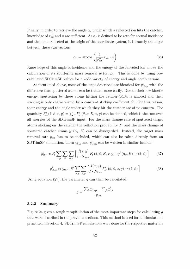
Finally, in order to retrieve the angle αr under which a reflected ion hits the catcher,

knowledge of ~rhit and ~n are sufficient. As αr is defined to be zero for normal incidence

and the ion is reflected at the origin of the coordinate system, it is exactly the angle

between these two vectors:

αr = arccos

(1

| ~rhit|~rhit · ~n

)(36)

Knowledge of this angle of incidence and the energy of the reflected ion allows the

calculation of its sputtering mass removal yj (αr, E). This is done by using pre-

calculated SDTrimSP values for a wide variety of energy and angle combinations.

As mentioned above, most of the steps described are identical for yiC,sp with the

difference that sputtered atoms can be treated more easily. Due to their low kinetic

energy, sputtering by these atoms hitting the catcher-QCM is ignored and their

sticking is only characterized by a constant sticking coefficient Si. For this reason,

their energy and the angle under which they hit the catcher are of no concern. The

quanitity F isp(θ, φ, x, y) =

∑E F

isp(θ, φ, E, x, y) can be defined, which is the sum over

all energies of the SDTrimSP input. For the mass change rate of sputtered target

atoms sticking on the catcher the reflection probability Pr and the mass change of

sputtered catcher atoms yj (αr, E) can be disregarded. Instead, the target mass

removal rate ytar has to be included, which can also be taken directly from an

SDTrimSP simulation. Then yjC,r and yiC,sp can be written in similar fashion:

yjC,r ≈ Pr

∑x,y

∑E

∑θ,φ

[ J(x, y)

I ·Nions

Fr (θ, φ, E, x, y) · yj (αr, E) · s (θ, φ)]

(37)

yiC,sp ≈ ytar · Si∑x,y

∑θ,φ

[ J(x, y)

I ·Nions

F isp (θ, φ, x, y) · s (θ, φ)

](38)

Using equation (27), the parameter g can then be calculated:

g =

∑i y

iC,sp −

∑j y

jC,r

ytar

3.2.2 Summary

Figure 24 gives a rough recapitulation of the most important steps for calculating g

that were described in the previous sections. This method is used for all simulations

presented in Section 4. SDTrimSP calculations were done for the respective materials

52

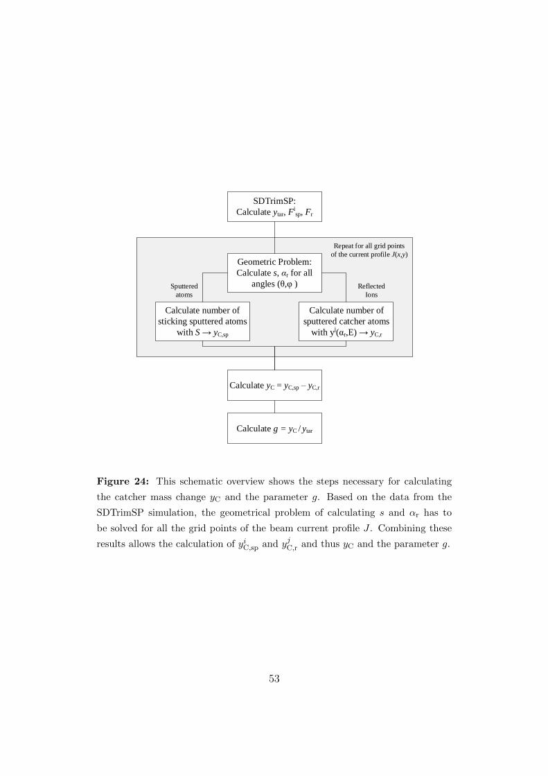
Repeat for all grid points

of the current profile J(x,y)

SDTrimSP:

Calculate ytar, Fisp, Fr

Geometric Problem:

Calculate s, αr for all

angles (θ,φ )

Calculate number of

sputtered catcher atoms

with yj(αr,E) yC,r

Calculate number of

sticking sputtered atoms

with S yC,sp

Calculate g = yC / ytar

Sputtered

atoms

Reflected

Ions

Calculate yC = yC,sp – yC,r

Figure 24: This schematic overview shows the steps necessary for calculating

the catcher mass change yC and the parameter g. Based on the data from the

SDTrimSP simulation, the geometrical problem of calculating s and αr has to

be solved for all the grid points of the beam current profile J . Combining these

results allows the calculation of yiC,sp and yjC,r and thus yC and the parameter g.

53

and with their input the procedure for calculating the catcher signal is identical. The

results of these calculations is included in the plots of the experimental results in

Section 4.

As was shown in this section, several approximations were done in order to

calculate g. As the experience showed, these approximations lead to errors for small

catcher distances, where the results are heavily dependent on the exact beam profile.

Ignoring inprecisions of SDTrimSP itself, a more sophisticated usage of numerical

methods for calculating g would be an improvement at this point. However, this

exceeds the scope of this thesis and will be a possible issue for future work with the

catcher-QCM setup.

3.3 Simulation of Rough Surfaces with SDTrimSP-2D

3.3.1 SDTrimSP-2D

As already mentioned, the applicability of 1D simulations is limited in some cases

(see section 1.2.4). For this reason, the two-dimensional expansion SDTrimSP-2D

was developed at IPP, which allows the implementation of a surface structure into

an SDTrimSP simulation [49]. This is achieved by expanding the geometrical de-

scription from layers to a grid, where again the cell modification is calculated from

the material transport following the collision cascades. Surface cells can grow and

shrink based on the transport of target atoms and thus a change in the surface

morphology can be simulated. First results are very promising and can reproduce

experimental observations precisely (see for an example [74]).

The surface structure can be given as a new input to SDTrimSP-2D, which can

be defined with a set of (x,z)-coordinates. The initial surface of the simulated

target is then created by linearly interpolating between these given points. The

composition of the target can be defined with different layers that can be defined

either as horizontal or as following the initial surface structure, which allows more

realistic modeling, for example, of an oxide layer.

Apart from the geometrical aspects, the functionality of SDTrimSP-2D remains

the same. As a result, both static and dynamic sputtering simulations are possible

and the energy and angular distributions for the sputtered atoms and the reflected

ions can also be calculated. The resulting output of SDTrimSP-2D can thus be used

as an input for the catcher simulation in the same way as before.

54

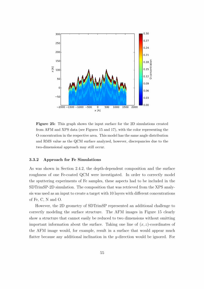
Figure 25: This graph shows the input surface for the 2D simulations created

from AFM and XPS data (see Figures 15 and 17), with the color representing the

O concentration in the respective area. This model has the same angle distribution

and RMS value as the QCM surface analyzed, however, discrepancies due to the

two-dimensional approach may still occur.

3.3.2 Approach for Fe Simulations

As was shown in Section 2.4.2, the depth-dependent composition and the surface

roughness of one Fe-coated QCM were investigated. In order to correctly model

the sputtering experiments of Fe samples, these aspects had to be included in the

SDTrimSP-2D simulation. The composition that was retrieved from the XPS analy-

sis was used as an input to create a target with 10 layers with different concentrations

of Fe, C, N and O.

However, the 2D geometry of SDTrimSP represented an additional challenge to

correctly modeling the surface structure. The AFM images in Figure 15 clearly

show a structure that cannot easily be reduced to two dimensions without omitting

important information about the surface. Taking one line of (x, z)-coordinates of

the AFM image would, for example, result in a surface that would appear much

flatter because any additional inclination in the y-direction would be ignored. For

55

this reason, another approach was chosen by evaluating the importance of different

surface aspects for sputtering. Due to the big angular dependence of the sputtering

yield, the distribution of local angles plays a very important role. The initial surface

structure for the 2D target was thus created in a way that it has the same angle

distribution and the same RMS roughness value as the real sample. The final target

surface that was used as a starting point for the Fe simulations in this thesis is

shown in Figure 25, where the color denotes the O concentration.

The approach sketched in this section was used as yet unpublished work to

simulate the dependence of the sputtering yield of a Fe-coated QCM on the angle

of incidence and the fluence applied. The results showed a good agreement between

experiment and the SDTrimSP-2D simulation, which is why this method was also

chosen for simulating the catcher measurements with rough Fe targets.

56

4 Results and Discussion

Sputtering experiments and simulations were performed with Au, Fe and Wollas-

tonite targets. The quantities investigated are the parameter g and the target mass

removal rate ytar or the target sputtering yield Ytar respectively. g can be deter-

mined experimentally by measuring the mass removal rates of the target-QCM and

the catcher-QCM simultaneously and dividing the two results:

g =yC

ytar

This is compared to the theoreticaled prediction of g based on the calculation de-

scribed in the previous section.

For future experiments without a target-QCM, the reconstructed target mass re-

moval rate ytar is the most interesting quantity. It represents the estimated value for

ytar calculated from the experimental catcher mass change rate yC and the simulated

parameter g:

ytar =yC

g

It is determined for all the catcher measurements in the following sections and

compared to the measured target mass removal rate ytar.

4.1 2 keV Ar+ on Au

Measurements of the sputtering yield of Au under 2 keV Ar+ bombardment were per-

formed as proof-of-principle measurements for showing the feasiblity of the catcher

setup. It is a well known projectile-target combination with a wide range of compara-

ble literature data [37]. For this reason, it is very well-suited to comparing simulated

and experimental catcher yields and to investigating how well energy and angular

distributions of sputtered and reflected particles can be reproduced by SDTrimSP.

In order to have as few uncertainties as possible, a Au-coated catcher-QCM was

used, so that the sticking factor S for sputtered Au atoms on a Au surface can be

assumed to be close to one ([75], [76]).

The results of these experiments are shown in Figures 26 - 28, which were mea-

sured within the scope of this thesis and have been published already [35]. The

figures show a comparison between the experimental and simulated parameter g in

the left-hand plot as well as the reconstructed and measured target sputtering yield

Ytar on the right-hand plot respectively. Here the three defining parameters of the

57

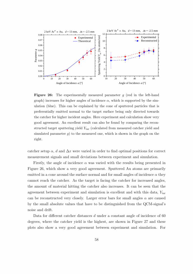
0 1 0 2 0 3 0 4 0 5 0 6 00 . 0 00 . 0 10 . 0 20 . 0 30 . 0 40 . 0 50 . 0 60 . 0 70 . 0 8

2 k e V A r + A u , d = 1 3 m m , x = - 2 . 5 m m E x p e r i m e n t a l T h e o r e t i c a l

Param

eter g

A n g l e o f I n c i d e n c e [ ° ]1 0 2 0 3 0 4 0 5 0 6 0

0

2

4

6

8

1 0

1 22 k e V A r + A u , d = 1 3 m m , x = - 2 . 5 m m

E x p e r i m e n t a l R e c o n s t r u c t e d

Sputt

ering

Yield

Y tar [A

u atom

s/ion]

A n g l e o f I n c i d e n c e [ ° ]

Figure 26: The experimentally measured parameter g (red in the left-hand

graph) increases for higher angles of incidence α, which is supported by the sim-

ulation (blue). This can be explained by the cone of sputtered particles that is

preferentially emitted normal to the target surface being only directed towards

the catcher for higher incident angles. Here experiment and calculation show very

good agreement. An excellent result can also be found by comparing the recon-

structed target sputtering yield Ytar (calculated from measured catcher yield and

simulated parameter g) to the measured one, which is shown in the graph on the

right.

catcher setup α, d and ∆x were varied in order to find optimal positions for correct

measurement signals and small deviations between experiment and simulation.

Firstly, the angle of incidence α was varied with the results being presented in

Figure 26, which show a very good agreement. Sputtered Au atoms are primarily

emitted in a cone around the surface normal and for small angles of incidence α they

cannot reach the catcher. As the target is facing the catcher for increased angles,

the amount of material hitting the catcher also increases. It can be seen that the

agreement between experiment and simulation is excellent and with this data, Ytar

can be reconstructed very closely. Larger error bars for small angles α are caused

by the small absolute values that have to be distinguished from the QCM-signal’s

noise and drift.

Data for different catcher distances d under a constant angle of incidence of 60

degrees, where the catcher yield is the highest, are shown in Figure 27 and these

plots also show a very good agreement between experiment and simulation. For

58

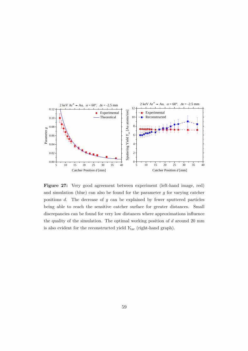
5 1 0 1 5 2 0 2 5 3 0 3 5 4 00 . 0 0

0 . 0 2

0 . 0 4

0 . 0 6

0 . 0 8

0 . 1 0

0 . 1 22 k e V A r + A u , = 6 0 ° , x = - 2 . 5 m m

E x p e r i m e n t a l T h e o r e t i c a l

Param

eter g

C a t c h e r P o s i t i o n d [ m m ]5 1 0 1 5 2 0 2 5 3 0 3 5 4 0

0

2

4

6

8

1 0

1 22 k e V A r + A u , = 6 0 ° , x = - 2 . 5 m m

E x p e r i m e n t a l R e c o n s t r u c t e d

Sputt

ering

Yield

Y tar [A

u atom

s/ion]

C a t c h e r P o s i t i o n d [ m m ]

Figure 27: Very good agreement between experiment (left-hand image, red)

and simulation (blue) can also be found for the parameter g for varying catcher

positions d. The decrease of g can be explained by fewer sputtered particles

being able to reach the sensitive catcher surface for greater distances. Small

discrepancies can be found for very low distances where approximations influence

the quality of the simulation. The optimal working position of d around 20 mm

is also evident for the reconstructed yield Ytar (right-hand graph).

59

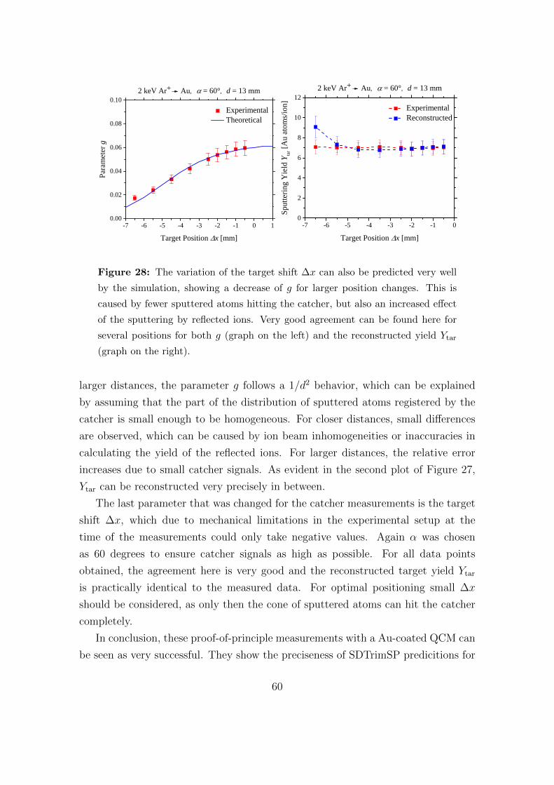
- 7 - 6 - 5 - 4 - 3 - 2 - 1 0 10 . 0 0

0 . 0 2

0 . 0 4

0 . 0 6

0 . 0 8

0 . 1 02 k e V A r + A u , = 6 0 ° , d = 1 3 m m

E x p e r i m e n t a l T h e o r e t i c a l

Param

eter g

T a r g e t P o s i t i o n x [ m m ]- 7 - 6 - 5 - 4 - 3 - 2 - 1 0

0

2

4

6

8

1 0

1 22 k e V A r + A u , = 6 0 ° , d = 1 3 m m

E x p e r i m e n t a l R e c o n s t r u c t e d

Sputt

ering

Yield

Y tar [A

u atom

s/ion]

T a r g e t P o s i t i o n x [ m m ]

Figure 28: The variation of the target shift ∆x can also be predicted very well

by the simulation, showing a decrease of g for larger position changes. This is

caused by fewer sputtered atoms hitting the catcher, but also an increased effect

of the sputtering by reflected ions. Very good agreement can be found here for

several positions for both g (graph on the left) and the reconstructed yield Ytar

(graph on the right).

larger distances, the parameter g follows a 1/d2 behavior, which can be explained

by assuming that the part of the distribution of sputtered atoms registered by the

catcher is small enough to be homogeneous. For closer distances, small differences

are observed, which can be caused by ion beam inhomogeneities or inaccuracies in

calculating the yield of the reflected ions. For larger distances, the relative error

increases due to small catcher signals. As evident in the second plot of Figure 27,

Ytar can be reconstructed very precisely in between.

The last parameter that was changed for the catcher measurements is the target

shift ∆x, which due to mechanical limitations in the experimental setup at the

time of the measurements could only take negative values. Again α was chosen

as 60 degrees to ensure catcher signals as high as possible. For all data points

obtained, the agreement here is very good and the reconstructed target yield Ytar

is practically identical to the measured data. For optimal positioning small ∆x

should be considered, as only then the cone of sputtered atoms can hit the catcher

completely.

In conclusion, these proof-of-principle measurements with a Au-coated QCM can

be seen as very successful. They show the preciseness of SDTrimSP predicitions for

60

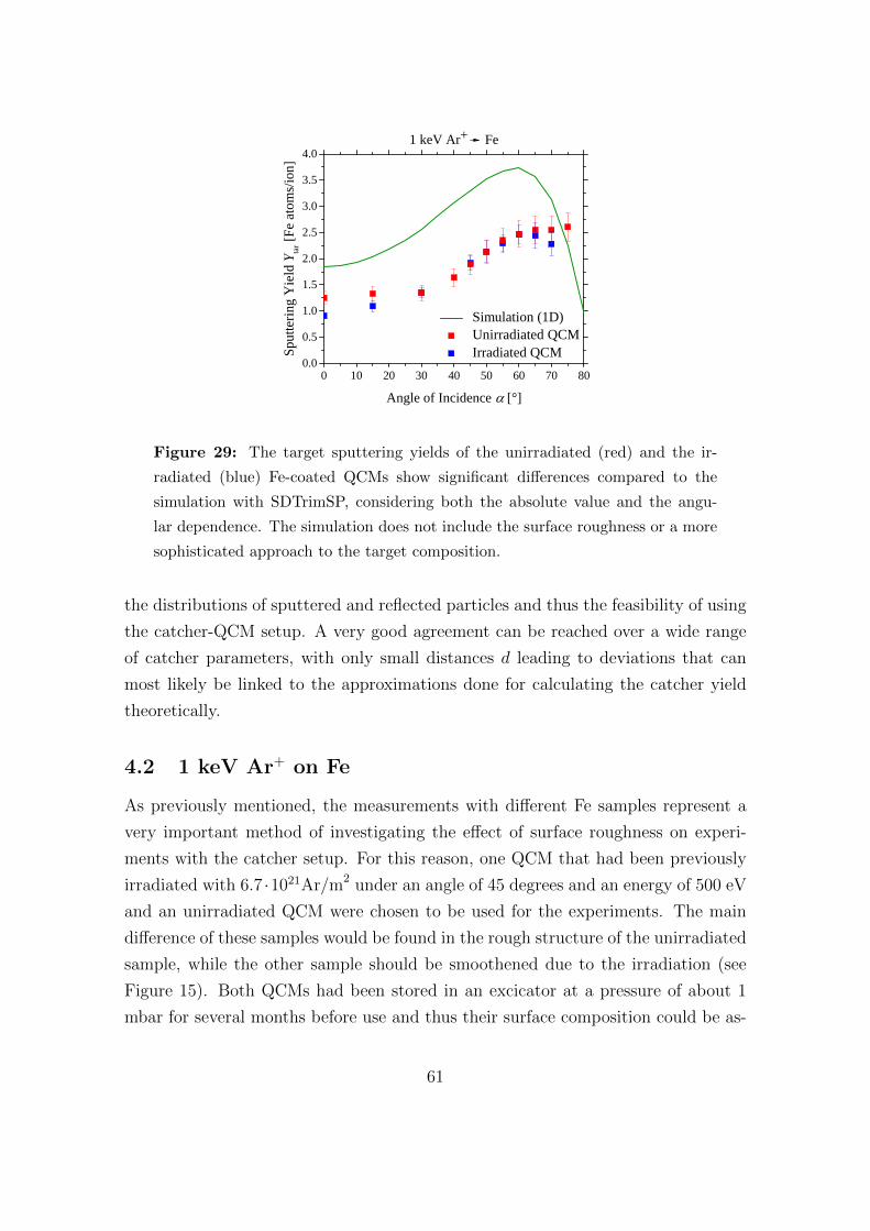
0 1 0 2 0 3 0 4 0 5 0 6 0 7 0 8 00 . 00 . 51 . 01 . 52 . 02 . 53 . 03 . 54 . 0

S i m u l a t i o n ( 1 D ) U n i r r a d i a t e d Q C M I r r a d i a t e d Q C MSp

utteri

ng Yie

ld Y tar

[Fe a

toms/io

n]

A n g l e o f I n c i d e n c e [ ° ]

1 k e V A r + F e

Figure 29: The target sputtering yields of the unirradiated (red) and the ir-

radiated (blue) Fe-coated QCMs show significant differences compared to the

simulation with SDTrimSP, considering both the absolute value and the angu-

lar dependence. The simulation does not include the surface roughness or a more

sophisticated approach to the target composition.

the distributions of sputtered and reflected particles and thus the feasibility of using

the catcher-QCM setup. A very good agreement can be reached over a wide range

of catcher parameters, with only small distances d leading to deviations that can

most likely be linked to the approximations done for calculating the catcher yield

theoretically.

4.2 1 keV Ar+ on Fe

As previously mentioned, the measurements with different Fe samples represent a

very important method of investigating the effect of surface roughness on experi-

ments with the catcher setup. For this reason, one QCM that had been previously

irradiated with 6.7 ·1021Ar/m2 under an angle of 45 degrees and an energy of 500 eV

and an unirradiated QCM were chosen to be used for the experiments. The main

difference of these samples would be found in the rough structure of the unirradiated

sample, while the other sample should be smoothened due to the irradiation (see

Figure 15). Both QCMs had been stored in an excicator at a pressure of about 1

mbar for several months before use and thus their surface composition could be as-

61

sumed to be similar to the XPS composition (see Figure 17) due to oxidation during

the storage.

4.2.1 Target Sputtering Yield

Both samples were irradiated with 1 keV Ar+ under different angles of incidence

in order to measure the angular dependence of the sputtering yield both on the

target-QCM and on the catcher-QCM. The results for the respective targets are

shown in Figure 29 along with a 1D SDTrimSP simulation with a pure Fe target.

While the differences between the two experimental curves are not very significant,

they are evidently not very well described by the simulation. Neither the absolute

value nor the qualitative characteristic of the angular dependence can be reproduced

correctly with this simulation. The similarity of the experimental yields suggests

that the main reason for the discrepancy compared to the simulation can be found

in the C, N and O concentrations of the sample. For this reason, the more thorough

simulation approach presented in Section 3.3.2 was chosen, which takes into account

both the composition and the surface roughness of the target.

The sputtering yields of the unirradiated target were simulated with the initial

target surface shown in Figure 25, but with a small applied fluence 5 · 1019Ar/m2

in order to simulate the cleaning of the sample before the sputtering yield mea-

surements. Then the angular dependence was simulated using the static mode of

SDTrimSP-2D assuming that the small fluence during one measurement would only

lead to a negligible change of the target. The result is shown in the graph on the

left in Figure 30 where a very good agreement with the experimental values can be

seen. From the simulation’s results, the effective Fe sputtering yield was calculated,

which represents the mass loss per ion due to sputtering of Fe, C, N and O divided by

the mass of one Fe atom. Therefore, the low absolute value of the yields compared

to a pure Fe simulation can be explained as mainly O is preferentially sputtered

leading to a smaller mass loss. Only after longer irradiation the impurities would

be depleted, leading to a steady state where mostly Fe would be sputtered. By in-

cluding the surface structure and components in the calculation, the exact angular

dependence can be quite well calculated with only small discrepancies around inci-

dent angles of 30 degrees. However, especially compared to the initial SDTrimSP

simulations included in Figure 30 (green), a significant improvement can be found.

62

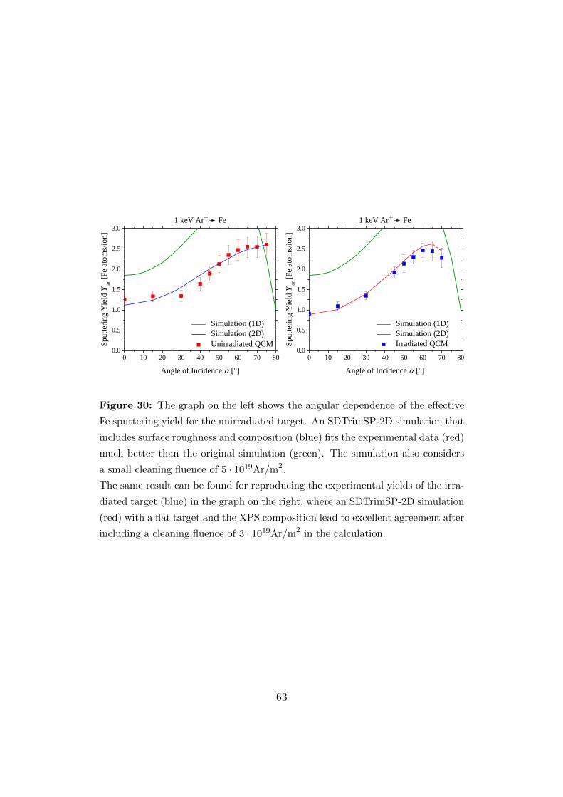
0 1 0 2 0 3 0 4 0 5 0 6 0 7 0 8 00 . 0

0 . 5

1 . 0

1 . 5

2 . 0

2 . 5

3 . 0

S i m u l a t i o n ( 1 D ) S i m u l a t i o n ( 2 D ) U n i r r a d i a t e d Q C MSp

utteri

ng Yie

ld Y tar

[Fe a

toms/io

n]

A n g l e o f I n c i d e n c e [ ° ]

1 k e V A r + F e

0 1 0 2 0 3 0 4 0 5 0 6 0 7 0 8 00 . 0

0 . 5

1 . 0

1 . 5

2 . 0

2 . 5

3 . 0

S i m u l a t i o n ( 1 D ) S i m u l a t i o n ( 2 D ) I r r a d i a t e d Q C MSp

utteri

ng Yie

ld Y tar

[Fe a

toms/io

n]

A n g l e o f I n c i d e n c e [ ° ]

1 k e V A r + F e

Figure 30: The graph on the left shows the angular dependence of the effective

Fe sputtering yield for the unirradiated target. An SDTrimSP-2D simulation that

includes surface roughness and composition (blue) fits the experimental data (red)

much better than the original simulation (green). The simulation also considers

a small cleaning fluence of 5 · 1019Ar/m2.

The same result can be found for reproducing the experimental yields of the irra-

diated target (blue) in the graph on the right, where an SDTrimSP-2D simulation

(red) with a flat target and the XPS composition lead to excellent agreement after

including a cleaning fluence of 3 · 1019Ar/m2 in the calculation.

63

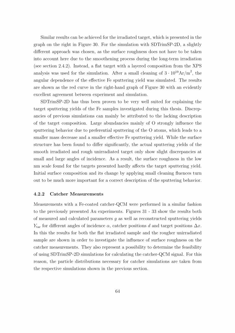
Similar results can be achieved for the irradiated target, which is presented in the

graph on the right in Figure 30. For the simulation with SDTrimSP-2D, a slightly

different approach was chosen, as the surface roughness does not have to be taken

into account here due to the smoothening process during the long-term irradiation

(see section 2.4.2). Instead, a flat target with a layered composition from the XPS

analysis was used for the simulation. After a small cleaning of 3 · 1019Ar/m2, the

angular dependence of the effective Fe sputtering yield was simulated. The results

are shown as the red curve in the right-hand graph of Figure 30 with an evidently

excellent agreement between experiment and simulation.

SDTrimSP-2D has thus been proven to be very well suited for explaining the

target sputtering yields of the Fe samples investigated during this thesis. Discrep-

ancies of previous simulations can mainly be attributed to the lacking description

of the target composition. Large abundancies mainly of O strongly influence the

sputtering behavior due to preferential sputtering of the O atoms, which leads to a

smaller mass decrease and a smaller effective Fe sputtering yield. While the surface

structure has been found to differ significantly, the actual sputtering yields of the

smooth irradiated and rough unirradiated target only show slight discrepancies at

small and large angles of incidence. As a result, the surface roughness in the low

nm scale found for the targets presented hardly affects the target sputtering yield.

Initial surface composition and its change by applying small cleaning fluences turn

out to be much more important for a correct description of the sputtering behavior.

4.2.2 Catcher Measurements

Measurements with a Fe-coated catcher-QCM were performed in a similar fashion

to the previously presented Au experiments. Figures 31 - 33 show the results both

of measured and calculated parameters g as well as reconstructed sputtering yields

Ytar for different angles of incidence α, catcher positions d and target positions ∆x.

In this the results for both the flat irradiated sample and the rougher unirradiated

sample are shown in order to investigate the influence of surface roughness on the

catcher measurements. They also represent a possibility to determine the feasibility

of using SDTrimSP-2D simulations for calculating the catcher-QCM signal. For this

reason, the particle distributions necessary for catcher simulations are taken from

the respective simulations shown in the previous section.

64

2 0 3 0 4 0 5 0 6 0 7 00 . 0 0

0 . 0 2

0 . 0 4

0 . 0 6

0 . 0 8

0 . 1 0

1 k e V A r + F e , d = 1 2 . 2 m m , x = 1 m m

E x p e r i m e n t a l ( u n i r r a d i a t e d ) T h e o r e t i c a l ( u n i r r a d i a t e d ) E x p e r i m e n t a l ( i r r a d i a t e d ) T h e o r e t i c a l ( i r r a d i a t e d )

Param

eter g

A n g l e o f I n c i d e n c e [ ° ]2 0 3 0 4 0 5 0 6 0 7 0

0 . 0

0 . 5

1 . 0

1 . 5

2 . 0

2 . 5

3 . 0 1 k e V A r + F e , d = 1 2 . 2 m m , x = 1 m m

E x p e r i m e n t a l ( i r r a d i a t e d ) R e c o n s t r u c t e d ( i r r a d i a t e d )Sp

utteri

ng Yie

ld Y tar

[Fe a

toms/io

n]

A n g l e o f I n c i d e n c e [ ° ]

Figure 31: The angular dependence of the parameter g can be seen in the graph

on the left for the unirradiated (red) and the irradiated (blue) target. The respec-

tive simulations fit the experimental results quite well, with small discrepancies

at high angles α for the rough (unirradiated) target. This could be improved by

using a 3D simulation that takes into account the geometry of the target in more

detail.

The right-hand graph shows a comparison of the experimental (blue) and the

reconstructed target sputtering yield Ytar (black) for the irradiated target. The

latter is too low for higher angles of incidence, but in general both curves show

good agreement.

65

The angular dependence of the parameter g at d = 12.2mm and ∆x = 1mm in

Figure 31 on the one hand shows good agreement between experiment (squares) and

simulation (lines) and on the other hand very similar values of g (α) for the rough

(red) and the flat (blue) sample. The SDTrimSP-2D simulation correctly predicts

the absolute value of g and its maximum at about 50 degrees. The experimental

results of the irradiated target especially are very well reproduced. This can also

be seen in the graph on the right, where the measured (blue) and the reconstructed

target sputtering yield Ytar (black) of the irradiated target are compared. For the

parameter g, small discrepancies arise at higher angles for the unirradiated target,

which could be explained by the simulation’s limited 2D-approach for the surface

roughness. It correctly takes into account the surface’s distribution of angles deter-

mined by the AFM images (see section 3.3.2), but the inclinations of the simulated

rough surface are always in the same plane. However, atoms are sputtered primar-

ily around the local surface normal, which is determined by the direction of these

inclinations. As a result, a more detailed calculation of the distributions for rough

targets would require a 3D version of SDTrimSP that correctly takes into account

the surface’s geometry. Nevertheless, the 2D version also gives good results here as

the small roughness in the low nm scale does not affect the sputtering behavior sig-

nificantly. The experimental results show even fewer differences for rough and flat

samples, which supports the previously stated conclusions that detailed informa-

tion about the surface composition is much more important for a correct theoretical

description of these experiments.

The variation in the catcher position d at α = 60 and ∆x = 1mm presented in

Figure 32 shows the expected 1/d2 behavior that is hardly affected by the different

surface roughnesses. As the left-hand graph shows, the simulation very precisely

reproduces the measured values of g(d) as well as correctly predicting a slightly

smaller value for the unirradiated sample. As a result, the reproduced target sput-

tering yield Ytar coincides with the measured values over the whole range covered in

the experiments, which is shown for the irradiated target in the graph on the right

in Figure 32.

More interesting information is provided by the variation of ∆x shown in Figure

33. Here larger differences for the two targets and discrepancies between experiments

and simulations are observed for negative values of ∆x, where the simulated values

of g(∆x) are too high. However, the differences between rough and flat sample in

66

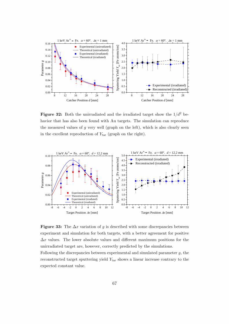
8 1 2 1 6 2 0 2 4 2 80 . 0 00 . 0 20 . 0 40 . 0 60 . 0 80 . 1 00 . 1 20 . 1 40 . 1 6

1 k e V A r + F e , = 6 0 ° , x = 1 m m E x p e r i m e n t a l ( u n i r r a d i a t e d ) T h e o r e t i c a l ( u n i r r a d i a t e d ) E x p e r i m e n t a l ( i r r a d i a t e d ) T h e o r e t i c a l ( i r r a d i a t e d )

Param

eter g

C a t c h e r P o s i t i o n d [ m m ]8 1 2 1 6 2 0 2 4 2 8

0 . 00 . 51 . 01 . 52 . 02 . 53 . 03 . 54 . 0 1 k e V A r + F e , = 6 0 ° , x = 1 m m

E x p e r i m e n t a l ( i r r a d i a t e d ) R e c o n s t r u c t e d ( i r r a d i a t e d )Sp

utteri

ng Yie

ld Y tar

[Fe a

toms/io

n]

C a t c h e r P o s i t i o n d [ m m ]

Figure 32: Both the unirradiated and the irradiated target show the 1/d2 be-

havior that has also been found with Au targets. The simulation can reproduce

the measured values of g very well (graph on the left), which is also clearly seen

in the excellent reproduction of Ytar (graph on the right).

- 8 - 6 - 4 - 2 0 2 4 6 8 1 0 1 20 . 0 0

0 . 0 2

0 . 0 4

0 . 0 6

0 . 0 8

0 . 1 0 1 k e V A r + F e , = 6 0 ° , d = 1 2 . 2 m m

E x p e r i m e n t a l ( u n i r r a d i a t e d ) T h e o r e t i c a l ( u n i r r a d i a t e d ) E x p e r i m e n t a l ( i r r a d i a t e d ) T h e o r e t i c a l ( i r r a d i a t e d )

Param

eter g

T a r g e t P o s i t i o n x [ m m ]- 8 - 6 - 4 - 2 0 2 4 6 8 1 0 1 2

0 . 00 . 51 . 01 . 52 . 02 . 53 . 03 . 54 . 04 . 55 . 0 1 k e V A r + F e , = 6 0 ° , d = 1 2 . 2 m m

E x p e r i m e n t a l ( i r r a d i a t e d ) R e c o n s t r u c t e d ( i r r a d i a t e d )

Sputt

ering

Yield

Y tar [F

e atom

s/ion]

T a r g e t P o s i t i o n x [ m m ]

Figure 33: The ∆x variation of g is described with some discrepancies between

experiment and simulation for both targets, with a better agreement for positive

∆x values. The lower absolute values and different maximum positions for the

unirradiated target are, however, correctly predicted by the simulations.

Following the discrepancies between experimental and simulated parameter g, the

reconstructed target sputtering yield Ytar shows a linear increase contrary to the

expected constant value.

67

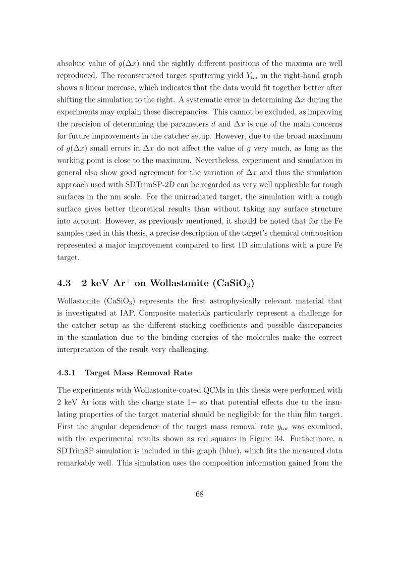
absolute value of g(∆x) and the sightly different positions of the maxima are well

reproduced. The reconstructed target sputtering yield Ytar in the right-hand graph

shows a linear increase, which indicates that the data would fit together better after

shifting the simulation to the right. A systematic error in determining ∆x during the

experiments may explain these discrepancies. This cannot be excluded, as improving

the precision of determining the parameters d and ∆x is one of the main concerns

for future improvements in the catcher setup. However, due to the broad maximum

of g(∆x) small errors in ∆x do not affect the value of g very much, as long as the

working point is close to the maximum. Nevertheless, experiment and simulation in

general also show good agreement for the variation of ∆x and thus the simulation

approach used with SDTrimSP-2D can be regarded as very well applicable for rough

surfaces in the nm scale. For the unirradiated target, the simulation with a rough

surface gives better theoretical results than without taking any surface structure

into account. However, as previously mentioned, it should be noted that for the Fe

samples used in this thesis, a precise description of the target’s chemical composition

represented a major improvement compared to first 1D simulations with a pure Fe

target.

4.3 2 keV Ar+ on Wollastonite (CaSiO3)

Wollastonite (CaSiO3) represents the first astrophysically relevant material that

is investigated at IAP. Composite materials particularly represent a challenge for

the catcher setup as the different sticking coefficients and possible discrepancies

in the simulation due to the binding energies of the molecules make the correct

interpretation of the result very challenging.

4.3.1 Target Mass Removal Rate

The experiments with Wollastonite-coated QCMs in this thesis were performed with

2 keV Ar ions with the charge state 1+ so that potential effects due to the insu-

lating properties of the target material should be negligible for the thin film target.

First the angular dependence of the target mass removal rate ytar was examined,

with the experimental results shown as red squares in Figure 34. Furthermore, a

SDTrimSP simulation is included in this graph (blue), which fits the measured data

remarkably well. This simulation uses the composition information gained from the

68

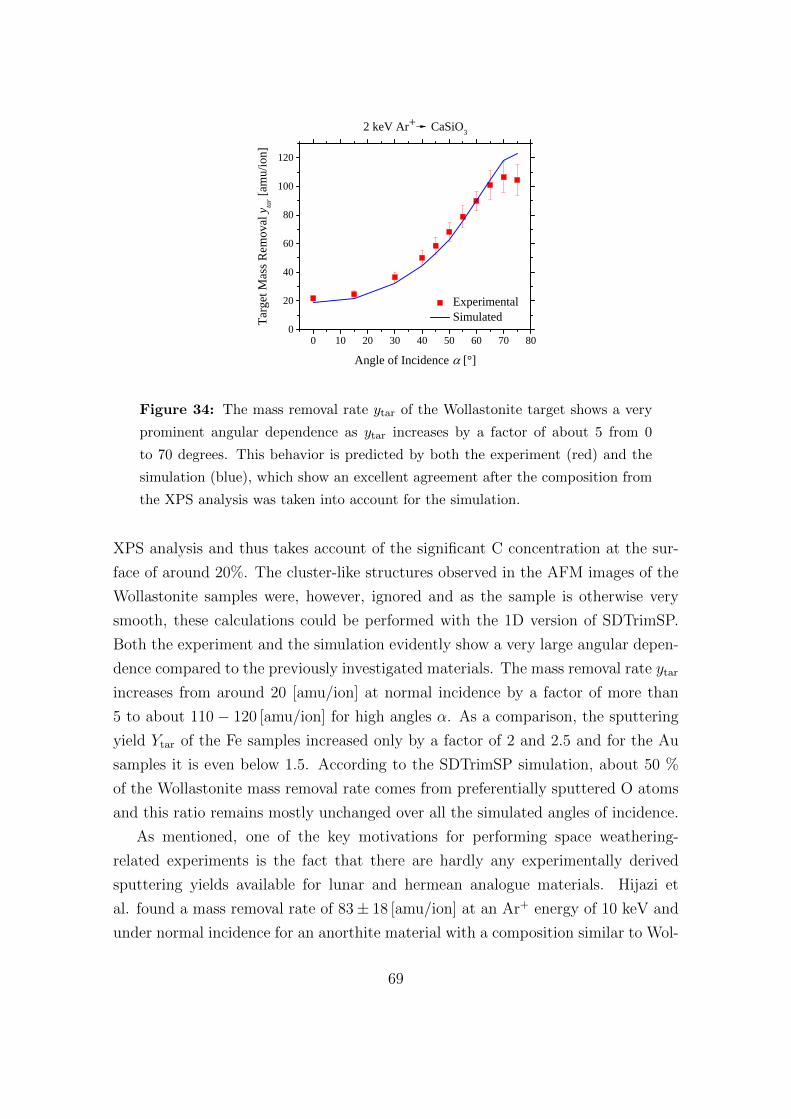
0 1 0 2 0 3 0 4 0 5 0 6 0 7 0 8 00

2 0

4 0

6 0

8 0

1 0 0

1 2 0

2 k e V A r + C a S i O 3

E x p e r i m e n t a l S i m u l a t e dTa

rget M

ass Re

moval

y tar [a

mu/io

n]

A n g l e o f I n c i d e n c e [ ° ]

Figure 34: The mass removal rate ytar of the Wollastonite target shows a very

prominent angular dependence as ytar increases by a factor of about 5 from 0

to 70 degrees. This behavior is predicted by both the experiment (red) and the

simulation (blue), which show an excellent agreement after the composition from

the XPS analysis was taken into account for the simulation.

XPS analysis and thus takes account of the significant C concentration at the sur-

face of around 20%. The cluster-like structures observed in the AFM images of the

Wollastonite samples were, however, ignored and as the sample is otherwise very

smooth, these calculations could be performed with the 1D version of SDTrimSP.

Both the experiment and the simulation evidently show a very large angular depen-

dence compared to the previously investigated materials. The mass removal rate ytar

increases from around 20 [amu/ion] at normal incidence by a factor of more than

5 to about 110− 120 [amu/ion] for high angles α. As a comparison, the sputtering

yield Ytar of the Fe samples increased only by a factor of 2 and 2.5 and for the Au

samples it is even below 1.5. According to the SDTrimSP simulation, about 50 %

of the Wollastonite mass removal rate comes from preferentially sputtered O atoms

and this ratio remains mostly unchanged over all the simulated angles of incidence.

As mentioned, one of the key motivations for performing space weathering-

related experiments is the fact that there are hardly any experimentally derived

sputtering yields available for lunar and hermean analogue materials. Hijazi et

al. found a mass removal rate of 83± 18 [amu/ion] at an Ar+ energy of 10 keV and

under normal incidence for an anorthite material with a composition similar to Wol-

69

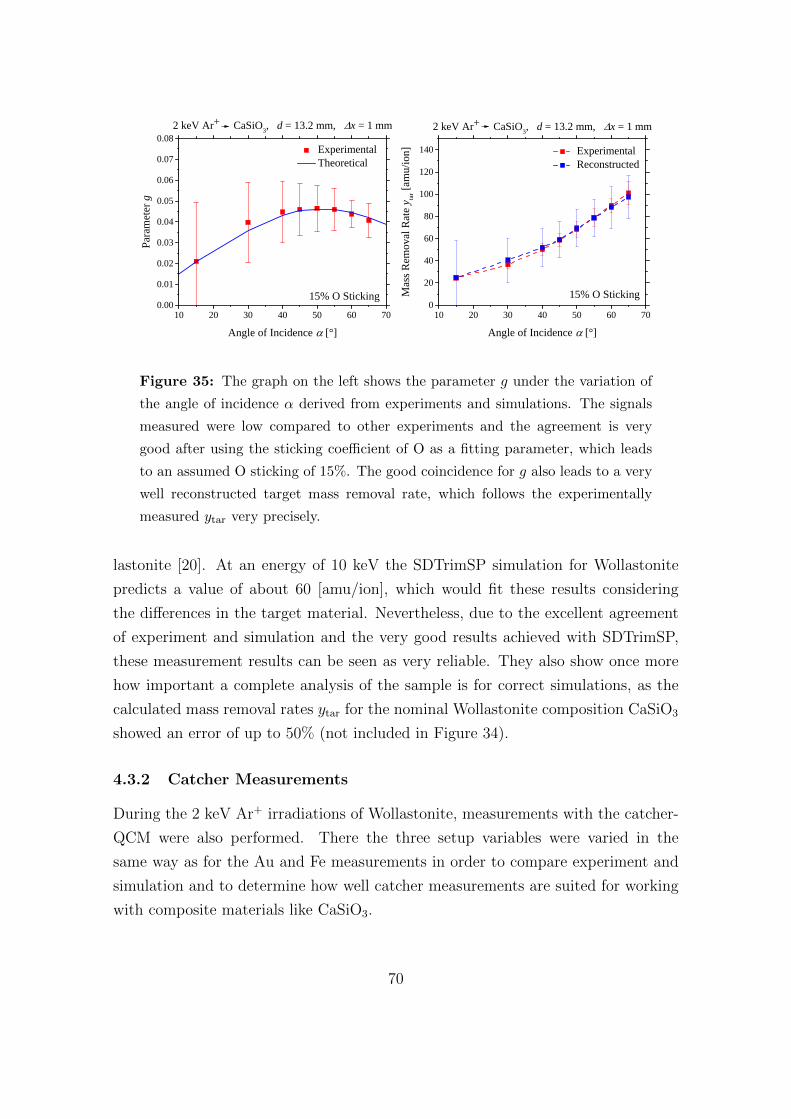
1 0 2 0 3 0 4 0 5 0 6 0 7 00 . 0 00 . 0 10 . 0 20 . 0 30 . 0 40 . 0 50 . 0 60 . 0 70 . 0 8

2 k e V A r + C a S i O 3 , d = 1 3 . 2 m m , x = 1 m m E x p e r i m e n t a l T h e o r e t i c a l

Param

eter g

A n g l e o f I n c i d e n c e [ ° ]

1 5 % O S t i c k i n g1 0 2 0 3 0 4 0 5 0 6 0 7 0

02 04 06 08 0

1 0 01 2 01 4 0

1 5 % O S t i c k i n g

2 k e V A r + C a S i O 3 , d = 1 3 . 2 m m , x = 1 m m E x p e r i m e n t a l R e c o n s t r u c t e d

Mass

Remo

val Ra

te ytar

[amu

/ion]

A n g l e o f I n c i d e n c e [ ° ]

Figure 35: The graph on the left shows the parameter g under the variation of

the angle of incidence α derived from experiments and simulations. The signals

measured were low compared to other experiments and the agreement is very

good after using the sticking coefficient of O as a fitting parameter, which leads

to an assumed O sticking of 15%. The good coincidence for g also leads to a very

well reconstructed target mass removal rate, which follows the experimentally

measured ytar very precisely.

lastonite [20]. At an energy of 10 keV the SDTrimSP simulation for Wollastonite

predicts a value of about 60 [amu/ion], which would fit these results considering

the differences in the target material. Nevertheless, due to the excellent agreement

of experiment and simulation and the very good results achieved with SDTrimSP,

these measurement results can be seen as very reliable. They also show once more

how important a complete analysis of the sample is for correct simulations, as the

calculated mass removal rates ytar for the nominal Wollastonite composition CaSiO3

showed an error of up to 50% (not included in Figure 34).

4.3.2 Catcher Measurements

During the 2 keV Ar+ irradiations of Wollastonite, measurements with the catcher-

QCM were also performed. There the three setup variables were varied in the

same way as for the Au and Fe measurements in order to compare experiment and

simulation and to determine how well catcher measurements are suited for working

with composite materials like CaSiO3.

70

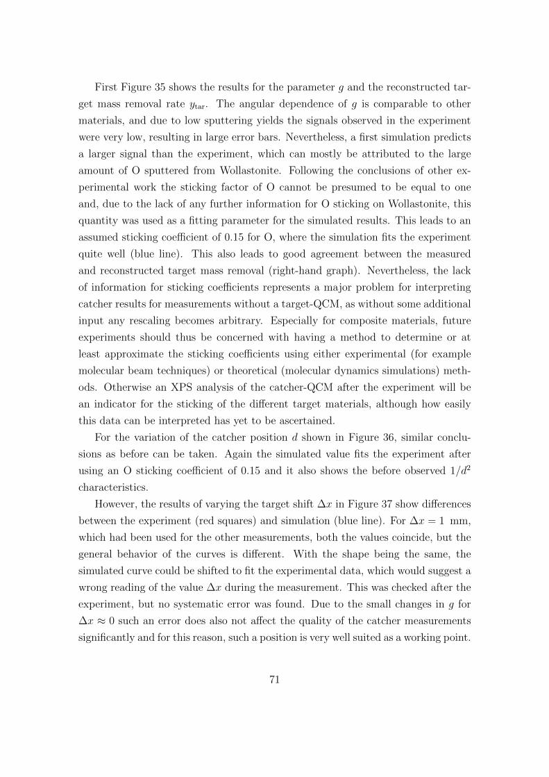
First Figure 35 shows the results for the parameter g and the reconstructed tar-

get mass removal rate ytar. The angular dependence of g is comparable to other

materials, and due to low sputtering yields the signals observed in the experiment

were very low, resulting in large error bars. Nevertheless, a first simulation predicts

a larger signal than the experiment, which can mostly be attributed to the large

amount of O sputtered from Wollastonite. Following the conclusions of other ex-

perimental work the sticking factor of O cannot be presumed to be equal to one

and, due to the lack of any further information for O sticking on Wollastonite, this

quantity was used as a fitting parameter for the simulated results. This leads to an

assumed sticking coefficient of 0.15 for O, where the simulation fits the experiment

quite well (blue line). This also leads to good agreement between the measured

and reconstructed target mass removal (right-hand graph). Nevertheless, the lack

of information for sticking coefficients represents a major problem for interpreting

catcher results for measurements without a target-QCM, as without some additional

input any rescaling becomes arbitrary. Especially for composite materials, future

experiments should thus be concerned with having a method to determine or at

least approximate the sticking coefficients using either experimental (for example

molecular beam techniques) or theoretical (molecular dynamics simulations) meth-

ods. Otherwise an XPS analysis of the catcher-QCM after the experiment will be

an indicator for the sticking of the different target materials, although how easily

this data can be interpreted has yet to be ascertained.

For the variation of the catcher position d shown in Figure 36, similar conclu-

sions as before can be taken. Again the simulated value fits the experiment after

using an O sticking coefficient of 0.15 and it also shows the before observed 1/d2

characteristics.

However, the results of varying the target shift ∆x in Figure 37 show differences

between the experiment (red squares) and simulation (blue line). For ∆x = 1 mm,

which had been used for the other measurements, both the values coincide, but the

general behavior of the curves is different. With the shape being the same, the

simulated curve could be shifted to fit the experimental data, which would suggest a

wrong reading of the value ∆x during the measurement. This was checked after the

experiment, but no systematic error was found. Due to the small changes in g for

∆x ≈ 0 such an error does also not affect the quality of the catcher measurements

significantly and for this reason, such a position is very well suited as a working point.

71

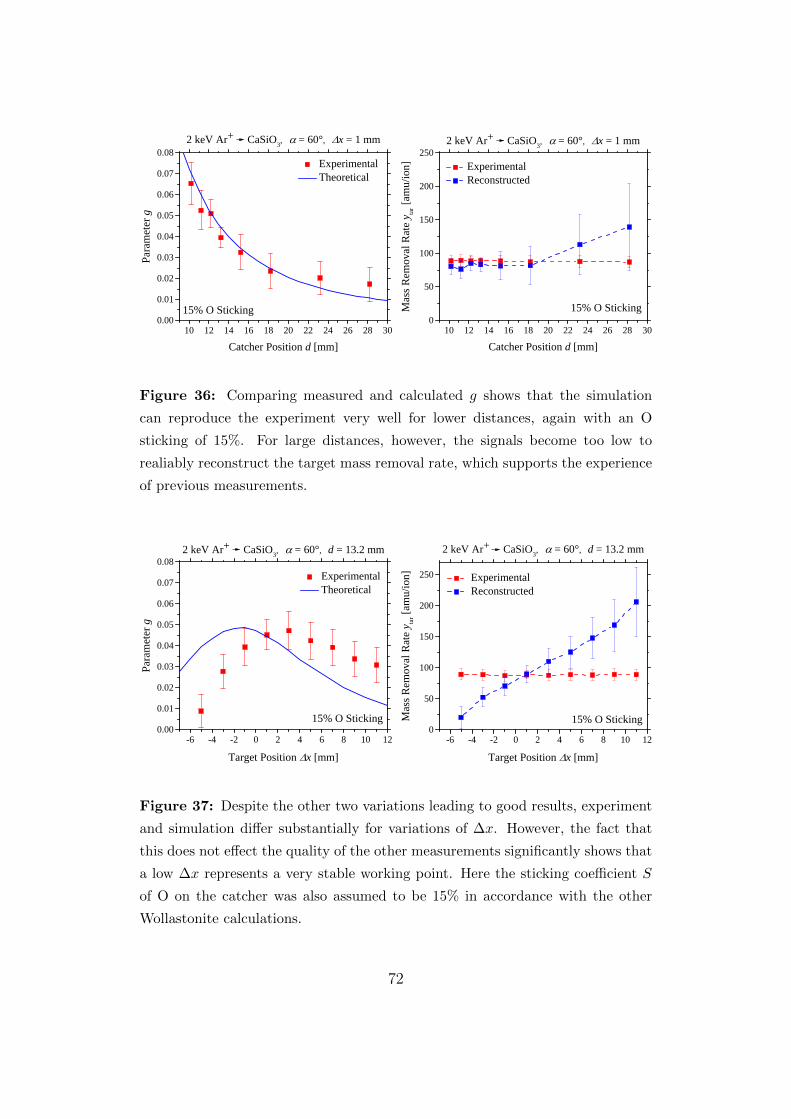
1 0 1 2 1 4 1 6 1 8 2 0 2 2 2 4 2 6 2 8 3 00 . 0 00 . 0 10 . 0 20 . 0 30 . 0 40 . 0 50 . 0 60 . 0 70 . 0 8

1 5 % O S t i c k i n g

2 k e V A r + C a S i O 3 , = 6 0 ° , x = 1 m m E x p e r i m e n t a l T h e o r e t i c a l

Param

eter g

C a t c h e r P o s i t i o n d [ m m ]1 0 1 2 1 4 1 6 1 8 2 0 2 2 2 4 2 6 2 8 3 0

0

5 0

1 0 0

1 5 0

2 0 0

2 5 0

1 5 % O S t i c k i n g

2 k e V A r + C a S i O 3 , = 6 0 ° , x = 1 m m E x p e r i m e n t a l R e c o n s t r u c t e d

Mass

Remo

val Ra

te ytar

[amu

/ion]

C a t c h e r P o s i t i o n d [ m m ]

Figure 36: Comparing measured and calculated g shows that the simulation

can reproduce the experiment very well for lower distances, again with an O

sticking of 15%. For large distances, however, the signals become too low to

realiably reconstruct the target mass removal rate, which supports the experience

of previous measurements.

- 6 - 4 - 2 0 2 4 6 8 1 0 1 20 . 0 00 . 0 10 . 0 20 . 0 30 . 0 40 . 0 50 . 0 60 . 0 70 . 0 8

1 5 % O S t i c k i n g

2 k e V A r + C a S i O 3 , = 6 0 ° , d = 1 3 . 2 m m E x p e r i m e n t a l T h e o r e t i c a l

Param

eter g

T a r g e t P o s i t i o n x [ m m ]- 6 - 4 - 2 0 2 4 6 8 1 0 1 2

0

5 0

1 0 0

1 5 0

2 0 0

2 5 0

1 5 % O S t i c k i n g

2 k e V A r + C a S i O 3 , = 6 0 ° , d = 1 3 . 2 m m

E x p e r i m e n t a l R e c o n s t r u c t e d

Mass

Remo

val Ra

te ytar

[amu

/ion]

T a r g e t P o s i t i o n x [ m m ]

Figure 37: Despite the other two variations leading to good results, experiment

and simulation differ substantially for variations of ∆x. However, the fact that

this does not effect the quality of the other measurements significantly shows that

a low ∆x represents a very stable working point. Here the sticking coefficient S

of O on the catcher was also assumed to be 15% in accordance with the other

Wollastonite calculations.

72

Nevertheless, it can not be completely disregarded, which suggests that including an

additional reference for checking the correct positioning should be included in the

experimental setup for future measurements. In view of the excellently fitting proof-

of-principle measurements with Au targets, such an Au reference material might be

feasible.

Despite these inaccuracies and the fitting of the oxygen sticking factor, experi-

ments and simulations already show very promising results. Especially the target

mass removal rate ytar and the angular dependence of the parameter g were repro-

duced very well. As long as the target composition is known, where XPS analysis

has been proven to be very useful, factors like the small cluster features observed in

the AFM images and the exact chemical properties of the mineral did not have to

be taken into account in the SDTrimSP simulation. This represents a very promis-

ing result as it makes measurements with composite targets like Wollastonite much

easier to simulate.

73

5 Conclusion and Outlook

The catcher-QCM setup and its theoretical description represent a very important

development for sputtering experiments at IAP. Losing the restrictions of thin film

materials will open up a wide variety of possibilities for new sputtering investigations,

especially for space weathering and exosphere formations. The use of stone and

powder targets will allow even more realistic experiments, while still retaining the

advantages of the very precise in-situ QCM technique.

The first measurements that were performed with the catcher setup as a part of

this thesis showed very good results, with the simulation being able to reproduce

most of the measurements very precisely. The characteristics of the parameter g

are very similar for the three different sample materials investigated in the scope of

this thesis. The parameter g(α) increases for higher angles of incidence α reaching a

maximum between around 50 and 60 degrees. For the Fe and Wollastonite samples,

where only elements occur with atomic masses much lower (mi ≤ 56) than the

atomic mass of Au (mi = 197), the maxima can be found at the lower end of this

interval, which is connected to a much more pronounced angular dependence of the

sputtering yield of lighter target materials. Variations in the catcher distance d

showed a nearly identical 1/d2 behavior for all samples for d & 10 mm. There the

part of the distribution of sputtered particles that hits the catcher can be interpreted

as homogeneous across the whole catcher surface, making the simulation much easier.

The variation in the target shift ∆x was very well reproduced for the proof-of-

concept Au measurements, but proved to show some discrepancies for the Fe and

Wollastonite samples. Either inaccuracies in the SDTrim simulation or systematic

errors in determining ∆x may be the cause, which is why additional references for

checking a correct ∆x are planned improvements for the future. Nevertheless, this

hardly affected the quality of the other measurements, due to the broad maximum

of g(∆x) at ∆x ≈ 0 mm representing a very stable working point. Other parameters

for determining such a working point should be the angle of incidence α where the

parameter g has its maximum around 50 - 60 degrees and a catcher distance d

around 10 mm. There a high catcher signal can be achieved that is still not affected

by the inaccuracies of the simulation at low d values. Smaller distances still lead to

discrepancies between experiment and simulation, which are most likely connected

to the approximations of the calculation and possible inhomogeneities of the ion

beam profile during the experiments. However, a solution for this problem will

74

be necessary in the future, especially considering solar-wind-related experiments.

Currently, for the chosen catcher distances d between 10 and 15 mm, the maximum

of g reached between 0.05 and 0.1, meaning that the catcher signals measured are

only 5 - 10 % of the signals at the target-QCM using Ar ions as the projectile. The

solar wind is mostly made up of protons, which will cause a much lower sputtering

yield than the heavier Ar ions. In order to obtain a catcher signal that is high

enough to be significantly distinguished from the catcher signal’s drift and noise,

lower catcher distances d may be necessary.

In general, SDTrimSP and SDTrimSP-2D proved to be very valuable tools in the

simulation of the sputtering process. After taking into account the precise target

composition and the surface roughness, experimental target sputtering yields could

be reproduced excellently. The calculated distributions of sputtered atoms and re-

flected ions also allowed a very precise simulation of the catcher signal measured,

even for rougher surfaces. Here the surface roughness in the low nm order only had

a small effect on the sputtering behavior. Future measurements, which will be done

with much rougher samples (for example, powder targets), will probably require the

currently developed 3D version of SDTrimSP, which allows a complete description

of the sample’s geometry. Judging from the very good experiences with the previous

program version so far, one can be very optimistic that the 3D version will also lead

to excellent results. Another very interesting possibility for using SDTrimSP simu-

lations is the calculation of the exosphere formation. As the calculated distributions

of sputtered atoms turned out to be very reliable, these emission characteristics

should be suitable for use in exosphere models. Currently these calculations are

mostly based on TRIM and SRIM (see for example [26] and [27]) and the enhanced

SDTrimSP program and its expansions that make it possible to simulate rough

surfaces will definitely be an improvement for calculating exosphere formation.

A remaining issue for composite targets such as Wollastonite is the determina-

tion of the sticking coefficients S, especially for materials containing a large amount

of O. Depositing thin target films on the catcher-QCM should lead to maximal and

mostly stable sticking coefficients. On the other hand, using a Au-coated catcher-

QCM would have caused a highly variable sticking coefficient as a Wollastonite layer

would build up over time and change the sticking properties. Nevertheless, some

reference for these coefficients should be provided either experimentally or theo-

retically. Molecular dynamics simulations, which exist in well-developed form for

75

Wollastonite, may be an easily available way to calculate the sticking. Otherwise, in-

vestigating a sample under molecular-beam evaporation represents an experimental

possibility to determine sticking coefficients. An XPS analysis of the catcher-QCM

after measurements have finished will also provide some information on how the

sputtered atoms stick to its surface. However, there is no experience with either

of these methods for determining the sticking coefficients, so the solution of this

problem will be one of the major challenges for future work with the catcher setup.

Considering the successful experiments with Ar bombardment of a Wollastonite-

coated QCM, the next step in astrophysically-relevant sputtering measurements will

on one hand involve projectiles such as H+ or D+ and on the other hand replacing

the target-QCM with a Wollastonite stone target. This will be the first experiment

using only the catcher-QCM, which will give interesting insights into the differences

from the thin film target, especially considering potential sputtering effects, and the

feasibility of the catcher setup without a target-QCM. However, this will require

some adaptions to the current experimental setup: the insulating properties of Wol-

lastonite did not affect the Ar+ measurements on the thin film with a thickness of a

few 100 nm. On the other hand, a stone would charge up during ion bombardment

making stable measurements impossible. For this reason, an electron flood gun that

emits low energy electrons to neutralize positively charged up samples will be added

to the current sample chamber setup. This will allow experiments with insulating

targets, which are very important for space weathering-related research. Consider-

ing the already excellent experiences with the setup, this will lead to very exciting

insights into the sputtering of lunar and hermean materials.

76

References

[1] Hapke B., “Space weathering from Mercury to the asteroid belt”, Journal of

Geophysical Research: Planets, 106, 10039 (2001)

[2] Yakshinskiy B. and Madey T., “Photon-stimulated desorption as a substantial

source of sodium in the lunar atmosphere”, Nature, 400, 642 (1999)

[3] Grun E., Horanyi M. and Sternovsky Z., “The lunar dust environment”, Plan-

etary and Space Science, 59, 1672 (2011)

[4] Gold T., “The lunar surface”, Monthly Notices of the Royal Astronomical So-

ciety, 115, 585 (1955)

[5] Hapke B., Cohen A., Cassidy W. and Wells E., “Solar radiation effects on the

optical properties of Apollo 11 samples”, Geochimica et Cosmochimica Acta

Supplement, 1, 2199 (1970)

[6] Conel J. and Nash D., “Spectral reflectance and albedo of Apollo 11 lunar

samples: Effects of irradiation and vitrification and comparison with telescopic

observations”, Geochimica et Cosmochimica Acta Supplement, 1, 2013 (1970)

[7] Hapke B., Cassidy W. and Wells E., “Effects of vapor-phase deposition pro-

cesses on the optical, chemical, and magnetic properties OE the lunar regolith”,

The moon, 13, 339 (1975)

[8] Pieters C.M., Taylor L.A., Noble S.K., Keller L.P., Hapke B., Morris R.V., Allen

C.C., McKAY D.S. and Wentworth S., “Space weathering on airless bodies:

Resolving a mystery with lunar samples”, Meteoritics & Planetary Science, 35,

1101 (2000)

[9] Wurz P., Whitby J., Rohner U., Martın-Fernandez J., Lammer H. and Kolb

C., “Self-consistent modelling of Mercury’s exosphere by sputtering, micro-

meteorite impact and photon-stimulated desorption”, Planetary and Space Sci-

ence, 58, 1599 (2010)

[10] Potter A. and Morgan T., “Discovery of sodium and potassium vapor in the

atmosphere of the Moon”, Science, 241, 675 (1988)

77

[11] Vervack R.J., McClintock W.E., Killen R.M., Sprague A.L., Anderson B.J.,

Burger M.H., Bradley E.T., Mouawad N., Solomon S.C. and Izenberg N.R.,

“Mercury’s complex exosphere: Results from MESSENGER’s third flyby”, Sci-

ence, 329, 672 (2010)

[12] Orsini S., Livi S., Torkar K., Barabash S., Milillo A., Wurz P., Di Lellis A.,

Kallio E. and the SERENA team, “SERENA: A suite of four instruments

(ELENA, STROFIO, PICAM and MIPA) on board BepiColombo-MPO for

particle detection in the Hermean environment”, Planetary and Space Science,

58, 166 (2010)

[13] Wurz P. and Lammer H., “Monte-Carlo simulation of Mercury’s exosphere”,

Icarus, 164, 1 (2003)

[14] Madey T.E., Yakshinskiy B., Ageev V. and Johnson R., “Desorption of alkali

atoms and ions from oxide surfaces: Relevance to origins of Na and K in atmo-

spheres of Mercury and the Moon”, Journal of Geophysical Research: Planets,

103, 5873 (1998)

[15] Borin P., Cremonese G., Marzari F., Bruno M. and Marchi S., “Statistical

analysis of micrometeoroids flux on Mercury”, Astronomy & Astrophysics, 503,

259 (2009)

[16] Stern S.A., “The lunar atmosphere: History, status, current problems, and con-

text”, Reviews of Geophysics, 37, 453 (1999)

[17] Killen R.M. and Hahn J.M., “Impact vaporization as a possible source of Mer-

cury’s calcium exosphere”, Icarus, 250, 230 (2015)

[18] Brueckner G. and Bartoe J.D., “Observations of high-energy jets in the corona

above the quiet sun, the heating of the corona, and the acceleration of the solar

wind”, The Astrophysical Journal, 272, 329 (1983)

[19] Feldman U., Landi E. and Schwadron N., “On the sources of fast and slow solar

wind”, Journal of Geophysical Research: Space Physics, 110 (2005)

[20] Hijazi H., Bannister M.E., Meyer H., Rouleau C.M., Barghouty A., Rickman

D. and Meyer F.W., “Anorthite sputtering by H+ and Arq+ (q= 1-9) at solar

78

wind velocities”, Journal of Geophysical Research: Space Physics, 119, 8006

(2014)

[21] Bame S., Asbridge J., Feldman W., Montgomery M. and Kearney P., “Solar

wind heavy ion abundances”, Solar Physics, 43, 463 (1975)

[22] Russell C., Luhmann J.G. and Strangeway R.J., Space Physics: An Introduc-

tion, Cambridge University Press (2016)

[23] Hunten D., Morgan T. and Shemansky D., The Mercury atmosphere, Univ. of

Arizona Press Tucson (1988)

[24] Bida T.A., Killen R.M. and Morgan T.H., “Discovery of calcium in Mercury’s

atmosphere”, Nature, 404, 159 (2000)

[25] Burger M.H., Killen R.M., Vervack R.J., Bradley E.T., McClintock W.E.,

Sarantos M., Benna M. and Mouawad N., “Monte Carlo modeling of sodium in

Mercury’s exosphere during the first two MESSENGER flybys”, Icarus, 209,

63 (2010)

[26] Wurz P., Rohner U., Whitby J.A., Kolb C., Lammer H., Dobnikar P. and

Martın-Fernandez J., “The lunar exosphere: The sputtering contribution”,

Icarus, 191, 486 (2007)

[27] Pfleger M., Lichtenegger H., Wurz P., Lammer H., Kallio E., Alho M., Mura A.,

McKenna-Lawlor S. and Martın-Fernandez J., “3D-modeling of Mercury’s solar

wind sputtered surface-exosphere environment”, Planetary and space science,

115, 90 (2015)

[28] Ziegler J.F., Ziegler M.D. and Biersack J.P., “SRIM: The stopping and range of

ions in matter (2010)”, Nuclear Instruments and Methods in Physics Research

Section B: Beam Interactions with Materials and Atoms, 268, 1818 (2010)

[29] Hayderer G., Schmid M., Varga P., Winter H. and Aumayr F., “A highly

sensitive quartz-crystal microbalance for sputtering investigations in slow ion–

surface collisions”, Review of Scientific Instruments, 70, 3696 (1999)

[30] Hayderer G., Cernusca S., Schmid M., Varga P., Winter H., Aumayr F., Nie-

mann D., Hoffmann V., Stolterfoht N. and Lemell C., “Kinetically assisted

79

potential sputtering of insulators by highly charged ions”, Physical Review Let-

ters, 86, 3530 (2001)

[31] Aumayr F. and Winter H., “Potential sputtering”, Philosophical Transactions

of the Royal Society of London. Series A: Mathematical, Physical and Engi-

neering Sciences, 362, 77 (2004)

[32] Golczewski A., Dobes K., Wachter G., Schmid M. and Aumayr F., “A quartz-

crystal-microbalance technique to investigate ion-induced erosion of fusion rel-

evant surfaces”, Nuclear Instruments and Methods in Physics Research Section

B: Beam Interactions with Materials and Atoms, 267, 695 (2009)

[33] Dobes K., “Erosion of Fusion Relevant Surfaces under Ion Impact”, Ph.D.

thesis, TU Wien (2014)

[34] Berger B.M., Stadlmayr R., Bloch D., Gruber E., Sugiyama K., Schwarz-

Selinger T. and Aumayr F., “Erosion of Fe-W model system under normal

and oblige D ion irradiation”, Nuclear Materials and Energy (2017)

[35] Berger B.M., Szabo P.S., Stadlmayr R. and Aumayr F., “Sputtering measure-

ments using a quartz crystal microbalance as a catcher”, Nuclear Instruments

and Methods in Physics Research Section B: Beam Interactions with Materials

and Atoms, 406, 533 (2017)

[36] Levinson A.A. and Taylor S.R., Moon rocks and minerals: scientific results of

the study of the Apollo 11 lunar samples with preliminary data on Apollo 12

samples, Elsevier (2015)

[37] Behrisch R. and Eckstein W., Sputtering by Particle Bombardment: Experi-

ments and Computer Calculations from Threshold to MeV Energies, Springer

Science & Business Media (2007)

[38] Mutzke A., A. E., Schneider R. and Dohmen R., “SDTrimSP: Version 5.00”,

IPP Report 12/8 (2011)

[39] Sigmund P., “Theory of sputtering. I. Sputtering yield of amorphous and poly-

crystalline targets”, Physical Review, 184, 383 (1969)

[40] Gruber E., “Interaction of Ions with 3D and 2D Materials”, Ph.D. thesis, TU

Wien (2017)

80

[41] Winter H. and Aumayr F., “Hollow atoms”, Journal of Physics B: Atomic,

Molecular and Optical Physics, 32, R39 (1999)

[42] Aumayr F., Facsko S., El-Said A.S., Trautmann C. and Schleberger M., “Single

ion induced surface nanostructures: a comparison between slow highly charged

and swift heavy ions”, Journal of Physics: Condensed Matter, 23, 393001

(2011)

[43] Wilhelm R.A., El-Said A.S., Krok F., Heller R., Gruber E., Aumayr F. and

Facsko S., “Highly charged ion induced nanostructures at surfaces by strong

electronic excitations”, Progress in Surface Science, 90, 377 (2015)

[44] Jacob W. and Roth J., “Chemical sputtering”, in Sputtering by particle bom-

bardment, 329–400, Springer (2007)

[45] Roosendaal H.E., “Sputtering yields of single crystalline targets”, in Sputtering

by particle bombardment I, 219–256, Springer (1981)

[46] Hotston E., “Threshold energies for sputtering”, Nuclear Fusion, 15, 544 (1975)

[47] Kustner M., Eckstein W., Dose V. and Roth J., “The influence of surface rough-

ness on the angular dependence of the sputter yield”, Nuclear Instruments and

Methods in Physics Research Section B: Beam Interactions with Materials and

Atoms, 145, 320 (1998)

[48] Kustner M., Eckstein W., Hechtl E. and Roth J., “Angular dependence of the

sputtering yield of rough beryllium surfaces”, Journal of Nuclear Materials,

265, 22 (1999)

[49] Mutzke A., Schneider R. and Bandelow G., “SDTrimSP-2D: Simulation of

Particles Bombarding on a Two Dimensional Target-Version 2.0”, IPP Report

12/11 (2013)

[50] Mutzke A., Bizyukov I., Schneider R. and Davis J., “Nano-scale modification

of 2D surface structures exposed to 6keV carbon ions: Experiment and model-

ing”, Nuclear Instruments and Methods in Physics Research Section B: Beam

Interactions with Materials and Atoms, 269, 582 (2011)

[51] Galutschek E., “Development of a 14.5 GHz All-Permanent Magnet Multi-

charged ECR Ion Source for Remote Operation”, Ph.D. thesis, TU Wien (2005)

81

[52] Galutschek E., Trassl R., Salzborn E., Aumayr F. and Winter H., “Compact

14.5 GHz all-permanent magnet ECRIS for experiments with slow multicharged

ions”, 58, 395 (2007)

[53] Berger B., “Laboratory work on plasma-wall-interaction processes relevant for

fusion experiments”, Ph.D. thesis, TU Wien ((2017)), unpublished

[54] Lu C. and Czanderna A.W., Applications of piezoelectric quartz crystal mi-

crobalances, Elsevier (2012)

[55] Sauerbrey G., “Verwendung von Schwingquarzen zur Wagung dunner Schichten

und zur Mikrowagung”, Zeitschrift fur Physik, 155, 206 (1959)

[56] Stevens D. and Tiersten H., “An analysis of doubly rotated quartz resonators

utilizing essentially thickness modes with transverse variation”, The Journal of

the Acoustical Society of America, 79, 1811 (1986)

[57] Gerdin G., Stygar W. and Venneri F., “Faraday cup analysis of ion beams

produced by a dense plasma focus”, Journal of Applied Physics, 52, 3269 (1981)

[58] Szabo P., “Development of a Beam Current Monitor”, Bachelor thesis, Vienna

University of Technology (2015)

[59] Vig J.R. and Ballato A., “Comments on the effects of nonuniform mass loading

on a quartz crystal microbalance”, Ultrasonics, Ferroelectrics, and Frequency

Control, IEEE Transactions on, 45, 1123 (1998)

[60] Binnig G., Quate C.F. and Gerber C., “Atomic force microscope”, Physical

review letters, 56, 930 (1986)

[61] Bloch D., “Influence of Ion Sputtering on Iron-Tungsten Alloy Surfaces and

Iron Surfaces”, Diploma Thesis, TU Wien (2017), unpublished

[62] Watts J.F. and Wolstenholme J., An Introduction to Surface Analysis by XPS

and AES, Wiley (2003)

[63] Deer W.A., Howie R.A. and Zussman J., Rock-forming minerals: single-chain

silicates, Volume 2A (1997)

[64] De Aza P., Guitian F. and De Aza S., “Bioactivity of wollastonite ceramics: in

vitro evaluation”, Scripta metallurgica et materialia, 31, 1001 (1994)

82

[65] Sjovall P. and Uvdal P., “Oxygen sticking on Pd (111): double precursors,

corrugation and substrate temperature effects”, Chemical physics letters, 282,

355 (1998)

[66] Eason R., Pulsed laser deposition of thin films: applications-led growth of func-

tional materials, John Wiley & Sons (2007)

[67] Blake A.J. and Clegg W., Crystal structure analysis: principles and practice,

volume 13, Oxford University Press (2009)

[68] Fernandez-Pradas J., Serra P., Morenza J. and De Aza P., “Pulsed laser depo-

sition of pseudowollastonite coatings”, Biomaterials, 23, 2057 (2002)

[69] Shapiro S.M., O’Shea D.C. and Cummins H.Z., “Raman Scattering Study of

the Alpha-Beta Phase Transition in Quartz”, Phys. Rev. Lett., 19, 361 (1967)

[70] Morita M., Ohmi T., Hasegawa E., Kawakami M. and Ohwada M., “Growth of

native oxide on a silicon surface”, Journal of Applied Physics, 68, 1272 (1990)

[71] Moller W., Eckstein W. and Biersack J., “Tridyn-binary collision simulation

of atomic collisions and dynamic composition changes in solids”, Computer

Physics Communications, 51, 355 (1988)

[72] Eckstein W., Computer Simulation of Ion-Solid Interactions, Springer Science

& Business Media (2013)

[73] Hofsass H., Zhang K. and Mutzke A., “Simulation of ion beam sputtering with

SDTrimSP, TRIDYN and SRIM”, Applied Surface Science, 310, 134 (2014)

[74] Bizyukov I., Mutzke A., Schneider R. and Davis J., “Evolution of the 2D surface

structure of a silicon pitch grating under argon ion bombardment: Experiment

and modeling”, Nuclear Instruments and Methods in Physics Research Section

B: Beam Interactions with Materials and Atoms, 268, 2631 (2010)

[75] Ikuse K., Yoshimura S., Kiuchi M., Hine K. and Hamaguchi S., “Measurement

of sticking probability and sputtering yield of Au by low-energy mass selected

ion beams with a quartz crystal microbalance”, 106, 012016 (2008)

[76] Bachmann L. and Shin J., “Measurement of the sticking coefficients of silver

and gold in an ultrahigh vacuum”, Journal of Applied Physics, 37, 242 (1966)

83

List of Figures

1 An overview of the release processes in space weathering. . . . . . . . 2

2 An overview of the solar-wind ions’ energy spectrum. . . . . . . . . . 4

3 A simulated example of a collision cascade following an ion entering

a solid. . . . . . . . . . . . . . . . . . . . . . . . . . . . . . . . . . . . 6

4 An overview of the ion-surface interaction. . . . . . . . . . . . . . . . 7

5 Examples for sputtering yields at different energies and angles of in-

cidence. . . . . . . . . . . . . . . . . . . . . . . . . . . . . . . . . . . 9

6 Energy distributions of sputtered atoms and reflected ions. . . . . . . 11

7 Simulated angular distribution of sputtered atoms. . . . . . . . . . . 12

8 Simulated angular distribution of reflected ions. . . . . . . . . . . . . 13

9 The processes that have to be taken into account for rough surfaces. . 14

10 An overview of the Augsutin ion-beam facility. . . . . . . . . . . . . 18

11 An overview of the QCM technique for sputtering measurements. . . 20

12 Experimental results of the QCM’s sensitivity. . . . . . . . . . . . . . 21

13 A sketch of the catcher-QCM setup. . . . . . . . . . . . . . . . . . . . 24

14 An AFM image of the Au sample. . . . . . . . . . . . . . . . . . . . . 29

15 AFM images before and after irradiation. . . . . . . . . . . . . . . . . 31

16 Angle Distributions before and after irradiation. . . . . . . . . . . . . 32

17 Element concentrations from XPS at different sputter depths. . . . . 33

18 The original Wollastonite rock sample. . . . . . . . . . . . . . . . . . 35

19 AFM images of the QCM surface after PLD. . . . . . . . . . . . . . . 37

20 The XPS spectra for Wollastonite powder and the deposited Si wafer

pieces. . . . . . . . . . . . . . . . . . . . . . . . . . . . . . . . . . . . 38

21 TOF-SIMS results for the Wollastonite deposited QCMs. . . . . . . . 40

22 Overview of the different effects that have to be taken into account

for the calculation of the catcher yield . . . . . . . . . . . . . . . . . 43

23 Explanation of the simulations’ analysis . . . . . . . . . . . . . . . . . 50

24 A schematic overview of the calculation of the parameter g. . . . . . . 53

25 The randomly created surface for SDTrimSP-2D simulations of rough

targets. . . . . . . . . . . . . . . . . . . . . . . . . . . . . . . . . . . . 55

26 Au measurements for variation of the angle of incidence α. . . . . . . 58

27 Au measurements for variation of the catcher distance d. . . . . . . . 59

28 Au measurements for variation of the target shift ∆x. . . . . . . . . . 60

84

29 Comparison of the experimental and simulated Fe target sputtering

yields. . . . . . . . . . . . . . . . . . . . . . . . . . . . . . . . . . . . 61

30 Experimental sputtering yields for unirradiated and irradiated Fe tar-

gets compared to SDTrimSP-2D simulations. . . . . . . . . . . . . . . 63

31 The parameter g and the reconstructed Fe sputtering yield for differ-

ent α. . . . . . . . . . . . . . . . . . . . . . . . . . . . . . . . . . . . 65

32 The parameter g and the reconstructed Fe sputtering yield for differ-

ent d. . . . . . . . . . . . . . . . . . . . . . . . . . . . . . . . . . . . . 67

33 The parameter g and the reconstructed Fe sputtering yield for differ-

ent ∆x. . . . . . . . . . . . . . . . . . . . . . . . . . . . . . . . . . . 67

34 The angular dependence of the mass removal rate for Wollastonite. . 69

35 The parameter g and the reconstructed mass removal rate for different

α. . . . . . . . . . . . . . . . . . . . . . . . . . . . . . . . . . . . . . . 70

36 The parameter g and the reconstructed mass removal rate for different

d. . . . . . . . . . . . . . . . . . . . . . . . . . . . . . . . . . . . . . . 72

37 The parameter g and the reconstructed mass removal rate for different

∆x. . . . . . . . . . . . . . . . . . . . . . . . . . . . . . . . . . . . . . 72

List of Tables

1 Composition of the solar wind. . . . . . . . . . . . . . . . . . . . . . . 3

2 Overview of the different quantities used for sputter yield calculation. 22

3 Quantitative XPS analysis for Wollastonite. . . . . . . . . . . . . . . 39

85

List of Abbreviations

amu atomic mass unit

ECRIS Electron Cyclotron Resonance Ion Source

eV electronvolts

FC Faraday Cup

GHz gigahertz

HCI Highly-Charged Ion

IAP Institute of Applied Physics

IPP Max-Planck-Institute of Plasma Physics

keV kilo-electronvolt

MeV mega-electronvolt

QCM Quartz Crystal Microbalance

SDTrimSP Static-Dynamic TRIM Sequential-Parallel

SRIM Stopping and Range of Ions in Matter

TRIDYN Dynamic TRIM

TRIM Transport of Ions in Matter

UHV ultra-high vacuum

86

Danksagung

Das Fertigstellen dieser Diplomarbeit ist fur mich der Anlass, mich bei den Personen

zu bedanken, die das alles moglich gemacht haben.

Mein großter Dank gilt meinem Betreuer Prof. Dr. Friedrich Aumayr, der mich

schon 2014 als Bachelorstudenten aufgenommen und mich in die wissenschaftliche

Arbeit eingefuhrt hat. Ich mochte dir sehr herzlich dafur danken, dass du mich

in den letzten Jahren so intensiv gefordert hast und mir auch mehrere Konferenz-

teilnahmen, einen Studienaufenthalt in Greifswald und das Mitwirken an einer wis-

senschaftlichen Veroffentlichung ermoglicht hast. Dass du auf jede Frage einen

wertvollen Ratschlag parat hast und dass du fur deine Studenten immer eine of-

fene Tur und ein offenes Ohr hast, ist eine wirklich große Unterstutzung. Das ist

fur mich alles andere als selbstverstandlich.

Besonders mochte ich mich auch bei Dr. Bernhard Berger bedanken, der mich

seit dem Beginn meiner Bachelorarbeit unter seine Fittiche genommen hat. Deine

Fahigkeit, Probleme mit einer Selbstverstandlichkeit zu losen, die mir vorher noch

unbekannt war, war uberaus hilfreich und ich habe gerade bei der Laborarbeit sehr

viel von dir gelernt. Deine Begeisterungsfahigkeit fur die verschiedensten Dinge hat

es im Labor auch nie langweilig werden lassen, was ich dir hoch anrechne. Unsere

beruflichen Wege haben sich mittlerweile leider getrennt, aber ich wunsche dir und

deiner Familie alles Gute und viel Erfolg bei eurem nachsten Lebensabschnitt in

Freistadt.

Eine wichtige Rolle spielen auch meine Kolleginnen und Kollegen der Arbeits-

gruppe: Janine Schwestka, Reinhard Stadlmayr, Elisabeth Gruber, Georg Harrer,

Florian Laggner, Rimpei Chiba und alle anderen, mit denen ich zusammenarbeiten

durfte. Ihr habt den Alltag am Institut gepragt und es mir nicht sehr schwer

gemacht, auch einmal langere Abende dort zu verbringen. Gleichzeitig konnte ich

mich immer auf eure Hilfsbereitschaft verlassen und ich freue mich sehr darauf, auch

in Zukunft ein Teil dieser Arbeitsgruppe sein zu durfen.

Ein herzliches Dankeschon mochte ich auch meinen Eltern aussprechen. Es gibt

mir eine große Sicherheit zu wissen, dass ihr mir in jeder Lebenslage zur Seite steht,

und das bedeutet mir sehr viel.

87