Embed Size (px)
Citation preview
Dynamic Task Management in MPSoC Platforms
Von der Fakultät für Elektrotechnik und Informationstechnik
der Rheinisch–Westfälischen Technischen Hochschule Aachen
zur Erlangung des akademischen Grades
eines Doktors der Ingenieurwissenschaften
genehmigte Dissertation
vorgelegt von
Diplom–Ingenieur Diandian Zhang
aus Jiangsu, VR China
Berichter: Universitätsprofessor Dr.-Ing. Gerd Ascheid
Universitätsprofessor Dr. rer. nat. Rainer Leupers
Tag der mündlichen Prüfung: 11.04.2017
Diese Dissertation ist auf den Internetseiten
der Hochschulbibliothek online verfügbar.

Acknowledgements
This thesis is the result of my work as research assistant at the Institute for Integrated
Signal Processing Systems (ISS) at the RWTH Aachen University. I am sure that the
time at ISS will be one of the most important periods in my life. When I look back at
the time, I can still feel the enthusiasm for research, the inspiring discussions and the
shining lights in late evenings at the institute. During the time, I met many brilliant
people, who are so different in their own way, but all are kind. I had the fortune to
work with them and want to take this opportunity to thank them for the wonderful
time and their kind help and support.
First, I would like to sincerely thank my advisor Professor Gerd Ascheid for giving
me the opportunity to join his team. I deeply appreciate his constant guidance and
support in finishing this work, especially his patience and allowing mistakes, which
were strong encouragement to me. I would also like to thank Professor Rainer Leupers
who gave me many valuable suggestions to my work. In the cooperative projects with
his team, I learned many things from him, especially how to concentrate on the key
problems and solve them, and he made me become much more confident.
Furthermore, I would like to thank Jeronimo Castrillon. We worked seamlessly
together on the OSIP project, which built the base of this work, and I could always
get his opinions on the my further work on OSIP. I was always impressed by his fast
understanding of problems and his ability of finding good solutions. No wonder that
he has become a professor of the department of computer science of the TU Dresden.
I am also very grateful to Han Zhang and Li Lu for their valuable experimentations
and analysis made for this work. I would also like to thank Stefan Schürmans for
the pleasant teamwork in the project of high-level power estimation for NoCs, which
provided me an initial NoC architecture to address the OSIP integration problem into
NoC-based systems.
It was my fortune to work with a group of people having different areas of ex-
pertise. I could always get my questions answered. Many of them have helped me,
even though many of them probably do not remember their help any more. Some of
them have become good friends of mine, and some of them will probably only be able
to be met occasionally. But here I want to say a sincere thank you to them all, espe-
cially to Anupam Chattopadhyay, David Kammler, Martin Witte, Torsten Kempf and
Filippo Borlenghi from the architectures group, Jeronimo Castrillon, Stefan Schür-
mans, Christoph Schumacher, Hanno Scharwächter, Weihua Sheng, Jianjiang Ceng
and Felix Engel from the tools group, Dan Zhang, Xitao Gong and I-Wei Lai from the

4
algorithms group. I also owe my special thanks to Elisabeth Böttcher, Christoph Vogt,
Ute Müller, Michael Rieb, Gabi Reimann, Christoph Zörkler and Tanja Palmen for the
years of kind help on the non-technical part of my time at ISS.
Finally, I want to express my deepest thanks to my parents and my wife Yong.
They are always there for me. Without their patience and consistent support, it would
not have been possible to complete this work.
Diandian Zhang, June 2017
Contents
1 Introduction 1
1.1 Multi-Processor System-on-Chip (MPSoC) . . . . . . . . . . . . . . . . . 2
1.2 Task Management in MPSoCs . . . . . . . . . . . . . . . . . . . . . . . . . 4
1.3 Contributions of this Thesis . . . . . . . . . . . . . . . . . . . . . . . . . . 5
1.4 Outline . . . . . . . . . . . . . . . . . . . . . . . . . . . . . . . . . . . . . . 5
2 Related Work 7
2.1 Static and Dynamic Task Management . . . . . . . . . . . . . . . . . . . . 7
2.1.1 Static Task Management . . . . . . . . . . . . . . . . . . . . . . . . 7
2.1.2 Semi-static Task Management . . . . . . . . . . . . . . . . . . . . . 9
2.1.3 Dynamic Task Management . . . . . . . . . . . . . . . . . . . . . . 10
2.2 Centralized and Distributed Task Management . . . . . . . . . . . . . . . 14
2.2.1 Centralized Task Management . . . . . . . . . . . . . . . . . . . . 14
2.2.2 Distributed Task Management . . . . . . . . . . . . . . . . . . . . 15
2.3 Task Management Implementations . . . . . . . . . . . . . . . . . . . . . 16
2.3.1 RISC-based Implementations . . . . . . . . . . . . . . . . . . . . . 17
2.3.2 ASIC-based Implementations . . . . . . . . . . . . . . . . . . . . . 18
2.3.3 ASIP-based Implementations . . . . . . . . . . . . . . . . . . . . . 19
2.4 Communication Architectures . . . . . . . . . . . . . . . . . . . . . . . . . 20
2.4.1 On-Chip Bus . . . . . . . . . . . . . . . . . . . . . . . . . . . . . . . 21
2.4.2 Network-on-Chip (NoC) . . . . . . . . . . . . . . . . . . . . . . . . 22
2.5 System-Level Exploration . . . . . . . . . . . . . . . . . . . . . . . . . . . 26
2.5.1 Virtual Platform . . . . . . . . . . . . . . . . . . . . . . . . . . . . . 27
2.5.2 Platform Architect . . . . . . . . . . . . . . . . . . . . . . . . . . . 28
i
ii CONTENTS
2.6 Summary . . . . . . . . . . . . . . . . . . . . . . . . . . . . . . . . . . . . . 30
3 OSIP-based Systems 31
3.1 System Overview . . . . . . . . . . . . . . . . . . . . . . . . . . . . . . . . 31
3.1.1 Basic Concept . . . . . . . . . . . . . . . . . . . . . . . . . . . . . . 31
3.1.2 Programming Model and Software Integration . . . . . . . . . . . 32
3.1.3 Hardware Integration . . . . . . . . . . . . . . . . . . . . . . . . . 35
3.2 OSIP Architecture Development . . . . . . . . . . . . . . . . . . . . . . . 38
3.2.1 Design Flow . . . . . . . . . . . . . . . . . . . . . . . . . . . . . . . 38
3.2.2 Application Analysis . . . . . . . . . . . . . . . . . . . . . . . . . . 40
3.2.3 Processor Architecture . . . . . . . . . . . . . . . . . . . . . . . . . 43
3.2.4 OSIP Code Example . . . . . . . . . . . . . . . . . . . . . . . . . . 55
3.3 Results . . . . . . . . . . . . . . . . . . . . . . . . . . . . . . . . . . . . . . 56
3.3.1 Area, Timing and Area-Time Product (AT) . . . . . . . . . . . . . 56
3.3.2 Power, Energy and Area-Time-Energy Product (ATE) . . . . . . . 59
3.4 Summary . . . . . . . . . . . . . . . . . . . . . . . . . . . . . . . . . . . . . 61
3.5 Discussion . . . . . . . . . . . . . . . . . . . . . . . . . . . . . . . . . . . . 61
3.5.1 OSIP Address Generation Unit (OSIP-AGU) . . . . . . . . . . . . 61
3.5.2 Node Comparator . . . . . . . . . . . . . . . . . . . . . . . . . . . 62
4 System-Level Analysis of OSIP Efficiency 63
4.1 System Setup . . . . . . . . . . . . . . . . . . . . . . . . . . . . . . . . . . 63
4.2 Benchmark Applications . . . . . . . . . . . . . . . . . . . . . . . . . . . . 64
4.2.1 Synthetic Application . . . . . . . . . . . . . . . . . . . . . . . . . 65
4.2.2 H.264 Video Decoding . . . . . . . . . . . . . . . . . . . . . . . . . 67
4.3 Efficiency Analysis with an Ideal Communication Architecture . . . . . 68
4.3.1 Synthetic Application . . . . . . . . . . . . . . . . . . . . . . . . . 68
4.3.2 H.264 . . . . . . . . . . . . . . . . . . . . . . . . . . . . . . . . . . . 70
4.4 Impact of Communication Architecture . . . . . . . . . . . . . . . . . . . 73
4.4.1 Detailed Analysis of Communication Overhead . . . . . . . . . . 74
4.5 Optimized Communication Architecture . . . . . . . . . . . . . . . . . . 76
4.5.1 Multi-layer AHB . . . . . . . . . . . . . . . . . . . . . . . . . . . . 76
4.5.2 Cache System . . . . . . . . . . . . . . . . . . . . . . . . . . . . . . 77
CONTENTS iii
4.5.3 Write Buffer . . . . . . . . . . . . . . . . . . . . . . . . . . . . . . . 79
4.5.4 Results . . . . . . . . . . . . . . . . . . . . . . . . . . . . . . . . . . 80
4.6 Joint Consideration of OSIP Efficiency and Communication Architecture 83
4.6.1 H.264 . . . . . . . . . . . . . . . . . . . . . . . . . . . . . . . . . . . 84
4.6.2 Synthetic Application . . . . . . . . . . . . . . . . . . . . . . . . . 84
4.7 Summary . . . . . . . . . . . . . . . . . . . . . . . . . . . . . . . . . . . . . 89
5 OSIP Support for Efficient Spinlock Control 91
5.1 Research on Spinlocks . . . . . . . . . . . . . . . . . . . . . . . . . . . . . 92
5.2 Basic Spinlock Control in OSIP-based Systems . . . . . . . . . . . . . . . 94
5.3 Application-Aware Spinlock Control . . . . . . . . . . . . . . . . . . . . . 95
5.3.1 Key Concept . . . . . . . . . . . . . . . . . . . . . . . . . . . . . . . 95
5.3.2 APIs for Spinlock Reservation . . . . . . . . . . . . . . . . . . . . . 95
5.3.3 Enhanced Spinlock Control . . . . . . . . . . . . . . . . . . . . . . 96
5.3.4 Hardware Overhead . . . . . . . . . . . . . . . . . . . . . . . . . . 100
5.4 Case Studies . . . . . . . . . . . . . . . . . . . . . . . . . . . . . . . . . . . 100
5.4.1 Synthetic Application . . . . . . . . . . . . . . . . . . . . . . . . . 100
5.4.2 H.264 . . . . . . . . . . . . . . . . . . . . . . . . . . . . . . . . . . . 104
5.5 Joint Impact of OSIP Efficiency and Flexibility . . . . . . . . . . . . . . . 105
5.5.1 Synthetic Application . . . . . . . . . . . . . . . . . . . . . . . . . 106
5.5.2 H.264 . . . . . . . . . . . . . . . . . . . . . . . . . . . . . . . . . . . 108
5.6 Summary . . . . . . . . . . . . . . . . . . . . . . . . . . . . . . . . . . . . . 110
5.7 Discussion . . . . . . . . . . . . . . . . . . . . . . . . . . . . . . . . . . . . 110
5.7.1 Tool Support for Spinlock Reservation . . . . . . . . . . . . . . . . 111
5.7.2 Scalability Problem . . . . . . . . . . . . . . . . . . . . . . . . . . . 111
5.7.3 Nested Spinlocks . . . . . . . . . . . . . . . . . . . . . . . . . . . . 112
6 OSIP Integration in NoC-based Systems 113
6.1 OSIP Integration Problems in NoC-based Systems . . . . . . . . . . . . . 114
6.2 Basic Concept of OSIP Integration in NoC-based Systems . . . . . . . . . 114
6.3 Case Study . . . . . . . . . . . . . . . . . . . . . . . . . . . . . . . . . . . . 116
6.3.1 NoC Structure . . . . . . . . . . . . . . . . . . . . . . . . . . . . . . 116
6.3.2 Application – MIMO-OFDM Iterative Receiver . . . . . . . . . . . 124
iv CONTENTS
6.4 System Implementation . . . . . . . . . . . . . . . . . . . . . . . . . . . . 128
6.4.1 Data Flow Graph . . . . . . . . . . . . . . . . . . . . . . . . . . . . 129
6.4.2 VPU Assignment . . . . . . . . . . . . . . . . . . . . . . . . . . . . 129
6.4.3 Node Mapping . . . . . . . . . . . . . . . . . . . . . . . . . . . . . 130
6.4.4 VPU Subsystem . . . . . . . . . . . . . . . . . . . . . . . . . . . . . 131
6.4.5 OSIP Subsystem . . . . . . . . . . . . . . . . . . . . . . . . . . . . . 132
6.4.6 Preliminary System Analysis . . . . . . . . . . . . . . . . . . . . . 135
6.5 Enhancements for NoC-based Communication Architecture . . . . . . . 136
6.5.1 Increasing link data width . . . . . . . . . . . . . . . . . . . . . . . 136
6.5.2 DMA Support . . . . . . . . . . . . . . . . . . . . . . . . . . . . . . 136
6.5.3 Pipelined Execution . . . . . . . . . . . . . . . . . . . . . . . . . . 136
6.5.4 Performance Analysis with Enhanced Communication Architec-
ture . . . . . . . . . . . . . . . . . . . . . . . . . . . . . . . . . . . . 139
6.6 Analysis of OSIP Efficiency in NoC-based Systems . . . . . . . . . . . . . 140
6.7 Summary . . . . . . . . . . . . . . . . . . . . . . . . . . . . . . . . . . . . . 142
6.8 Discussion . . . . . . . . . . . . . . . . . . . . . . . . . . . . . . . . . . . . 143
6.8.1 Proxy Complexity . . . . . . . . . . . . . . . . . . . . . . . . . . . . 143
6.8.2 Multi-OSIP-System . . . . . . . . . . . . . . . . . . . . . . . . . . . 145
7 Conclusion and Outlook 147
Appendix 151
A Packet Types and Communication Protocol of NoC 151
A.1 Packet Types . . . . . . . . . . . . . . . . . . . . . . . . . . . . . . . . . . . 151
A.2 Communication between IP components . . . . . . . . . . . . . . . . . . 151
A.2.1 Transmission of Read Request Packet (PCK_R) . . . . . . . . . . . 152
A.2.2 Transmission of Read Response Packet (PCK_RR) . . . . . . . . . 153
A.2.3 Transmission of Write Request Packet (PCK_W) . . . . . . . . . . 153
A.2.4 Transmission of Write Response Packet (PCK_WR) . . . . . . . . 153
A.2.5 Transmission of Synchronization Packet (PCK_S) . . . . . . . . . 153
A.2.6 Constraint . . . . . . . . . . . . . . . . . . . . . . . . . . . . . . . . 153
Glossary 157

CONTENTS v
List of Figures 161
List of Tables 165
Bibliography 167

vi CONTENTS
Chapter 1
Introduction
The fast development of the submicron silicon technology enables integrating a huge
number of transistors on a single chip. Billion-transistor chips are common today.
Well-known examples are Intel Xeon® server processor (4.3B transistors) [158], IBM’s
Power8 processor (4.2B transistors) [90] and Nvidia’s Kepler GK110 Graphical Pro-
cessing Unit (GPU) (7.1B transistors) [147]. According to the International Technol-
ogy Roadmap for Semiconductors (ITRS), chips with around 50 billion transistors will
emerge in the market in 2026 [93].
However, the consistently shrinking silicon technology is reaching its physical
limit caused by the size of the silicon atom. The ITRS already predicts a gate length
of 5.9 nm in 2026, which is only 25 times as large as the silicon atom diameter of
0.234 nm. Therefore, increasing the computing performance of future chips will be
faced with large limitations, if only considering using small silicon technologies for
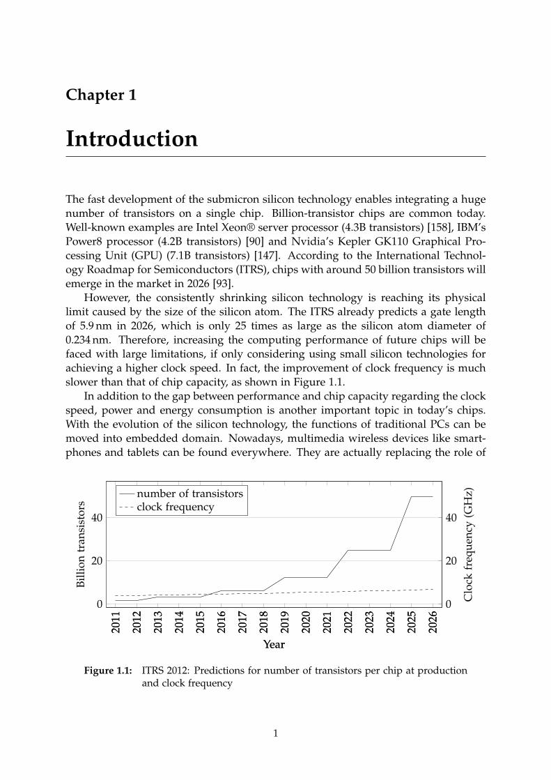
achieving a higher clock speed. In fact, the improvement of clock frequency is much
slower than that of chip capacity, as shown in Figure 1.1.
In addition to the gap between performance and chip capacity regarding the clock
speed, power and energy consumption is another important topic in today’s chips.
With the evolution of the silicon technology, the functions of traditional PCs can be
moved into embedded domain. Nowadays, multimedia wireless devices like smart-
phones and tablets can be found everywhere. They are actually replacing the role of
2011
2012
2013
2014
2015
2016
2017
2018
2019
2020
2021
2022
2023
2024
2025
2026
0
20
40
Year
Bil
lio
ntr
ansi
sto
rs
2011
2012
2013
2014
2015
2016
2017
2018
2019
2020
2021
2022
2023
2024
2025
2026
0
20
40
Year
Clo
ckfr
equ
ency
(GH
z)number of transistorsclock frequency
Figure 1.1: ITRS 2012: Predictions for number of transistors per chip at productionand clock frequency
1
2 Chapter 1. Introduction
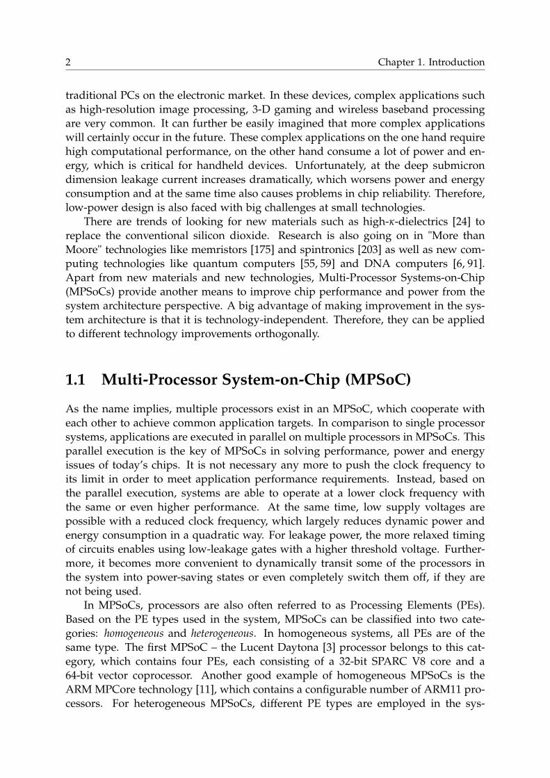
traditional PCs on the electronic market. In these devices, complex applications such
as high-resolution image processing, 3-D gaming and wireless baseband processing
are very common. It can further be easily imagined that more complex applications
will certainly occur in the future. These complex applications on the one hand require
high computational performance, on the other hand consume a lot of power and en-
ergy, which is critical for handheld devices. Unfortunately, at the deep submicron
dimension leakage current increases dramatically, which worsens power and energy
consumption and at the same time also causes problems in chip reliability. Therefore,
low-power design is also faced with big challenges at small technologies.
There are trends of looking for new materials such as high-κ-dielectrics [24] to
replace the conventional silicon dioxide. Research is also going on in "More than
Moore" technologies like memristors [175] and spintronics [203] as well as new com-
puting technologies like quantum computers [55, 59] and DNA computers [6, 91].
Apart from new materials and new technologies, Multi-Processor Systems-on-Chip
(MPSoCs) provide another means to improve chip performance and power from the
system architecture perspective. A big advantage of making improvement in the sys-
tem architecture is that it is technology-independent. Therefore, they can be applied
to different technology improvements orthogonally.
1.1 Multi-Processor System-on-Chip (MPSoC)
As the name implies, multiple processors exist in an MPSoC, which cooperate with
each other to achieve common application targets. In comparison to single processor
systems, applications are executed in parallel on multiple processors in MPSoCs. This
parallel execution is the key of MPSoCs in solving performance, power and energy
issues of today’s chips. It is not necessary any more to push the clock frequency to
its limit in order to meet application performance requirements. Instead, based on
the parallel execution, systems are able to operate at a lower clock frequency with
the same or even higher performance. At the same time, low supply voltages are
possible with a reduced clock frequency, which largely reduces dynamic power and
energy consumption in a quadratic way. For leakage power, the more relaxed timing
of circuits enables using low-leakage gates with a higher threshold voltage. Further-
more, it becomes more convenient to dynamically transit some of the processors in
the system into power-saving states or even completely switch them off, if they are
not being used.
In MPSoCs, processors are also often referred to as Processing Elements (PEs).
Based on the PE types used in the system, MPSoCs can be classified into two cate-
gories: homogeneous and heterogeneous. In homogeneous systems, all PEs are of the
same type. The first MPSoC – the Lucent Daytona [3] processor belongs to this cat-
egory, which contains four PEs, each consisting of a 32-bit SPARC V8 core and a
64-bit vector coprocessor. Another good example of homogeneous MPSoCs is the
ARM MPCore technology [11], which contains a configurable number of ARM11 pro-
cessors. For heterogeneous MPSoCs, different PE types are employed in the sys-
1.1. Multi-Processor System-on-Chip (MPSoC) 3
tem, such as Reduced Instruction Set Computers (RISCs), Digital Signal Processors
(DSPs), Application-Specific Instructions-set Processors (ASIPs), Field-Programmable
Gate Arrays (FPGAs) or Application-Specific Integrated Circuits (ASICs). Represen-
tative examples for this category are the Open Multimedia Application Platform
(OMAP) family [191] from Texas Instruments (TI) and the Cell Broadband Engine
from IBM [103]. The latest OMAP processor contains an ARM Cortex-A15, two ARM
Cortex-M4 microcontrollers, a mini-C64x DSP, a PowerVR GPU and several other
accelerators for image, video and audio processing. The Cell processor consists of
a PowerPC and eight specialized coprocessors known as Synergistic Processing Ele-
ments (SPEs) for performing floating-point operations.
Both homogeneous and heterogeneous MPSoCs have their advantages and dis-
advantages. For homogeneous MPSoCs, the homogeneity of PEs makes the system
architecture easily scalable, from both the hardware and the software perspective. Es-
pecially, programming such a system is relatively simple, which becomes very impor-
tant for today’s large systems. Other advantages include convenient system debug-
ging due to the same software tool set, higher fault-tolerance with multiple instances
of the same PE type and low system development costs. The biggest disadvantage
of homogeneous systems is their low efficiency in area, energy and power consump-
tion. The PEs are mostly RISC-based for the programmability reason. Therefore, they
cannot easily meet high performance requirement of complex applications without
applying a large number of them, which reduces efficiency.
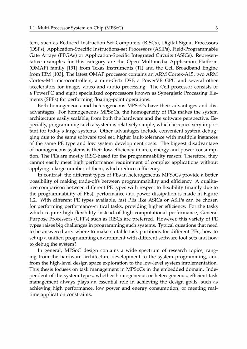
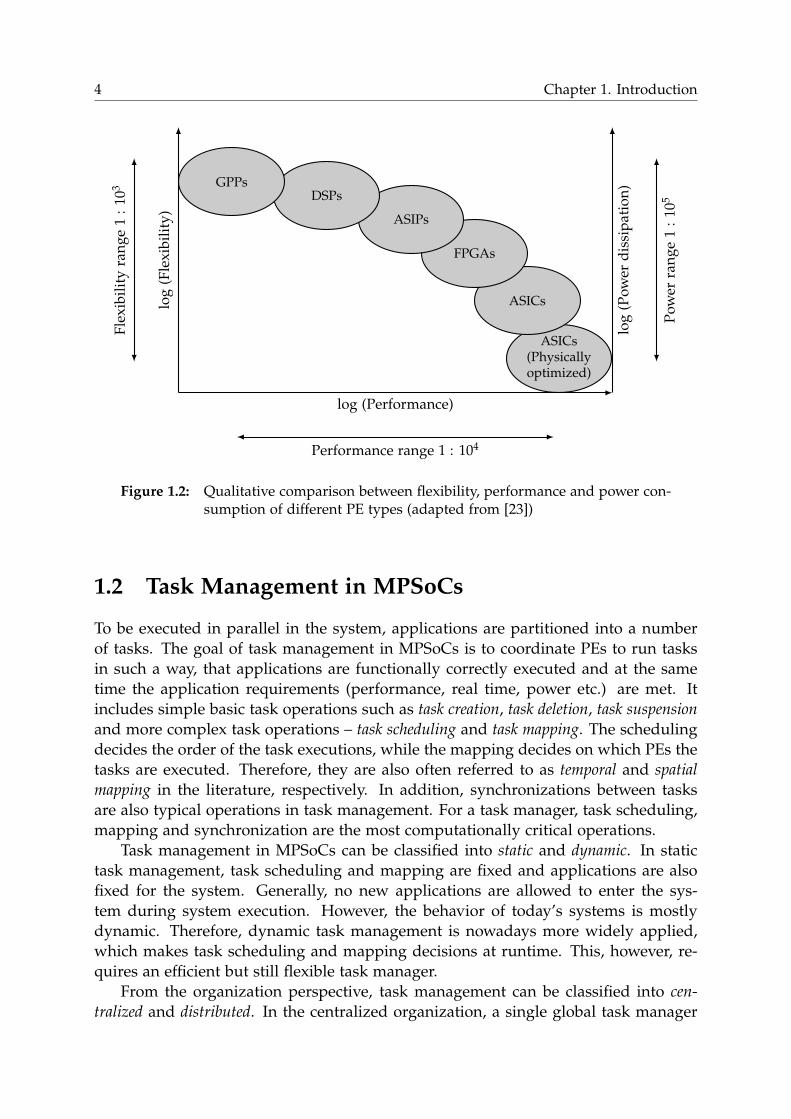
In contrast, the different types of PEs in heterogeneous MPSoCs provide a better
possibility of making trade-offs between programmability and efficiency. A qualita-
tive comparison between different PE types with respect to flexibility (mainly due to
the programmability of PEs), performance and power dissipation is made in Figure
1.2. With different PE types available, fast PEs like ASICs or ASIPs can be chosen
for performing performance-critical tasks, providing higher efficiency. For the tasks
which require high flexibility instead of high computational performance, General
Purpose Processors (GPPs) such as RISCs are preferred. However, this variety of PE
types raises big challenges in programming such systems. Typical questions that need
to be answered are: where to make suitable task partitions for different PEs, how to
set up a unified programming environment with different software tool-sets and how
to debug the system?
In general, MPSoC design contains a wide spectrum of research topics, rang-
ing from the hardware architecture development to the system programming, and
from the high-level design space exploration to the low-level system implementation.
This thesis focuses on task management in MPSoCs in the embedded domain. Inde-
pendent of the system types, whether homogeneous or heterogeneous, efficient task
management always plays an essential role in achieving the design goals, such as
achieving high performance, low power and energy consumption, or meeting real-
time application constraints.
4 Chapter 1. Introduction
ASICs(Physicallyoptimized)
ASICs
FPGAs
ASIPs
DSPsGPPs
log (Performance)
Performance range 1 : 104
log
(Fle
xib
ilit
y)
Fle
xib
ilit
yra
ng
e1
:10
3
log
(Po
wer
dis
sip
atio
n)
Po
wer
ran
ge
1:
105
Figure 1.2: Qualitative comparison between flexibility, performance and power con-sumption of different PE types (adapted from [23])
1.2 Task Management in MPSoCs
To be executed in parallel in the system, applications are partitioned into a number
of tasks. The goal of task management in MPSoCs is to coordinate PEs to run tasks
in such a way, that applications are functionally correctly executed and at the same
time the application requirements (performance, real time, power etc.) are met. It
includes simple basic task operations such as task creation, task deletion, task suspension
and more complex task operations – task scheduling and task mapping. The scheduling
decides the order of the task executions, while the mapping decides on which PEs the
tasks are executed. Therefore, they are also often referred to as temporal and spatial
mapping in the literature, respectively. In addition, synchronizations between tasks
are also typical operations in task management. For a task manager, task scheduling,
mapping and synchronization are the most computationally critical operations.
Task management in MPSoCs can be classified into static and dynamic. In static
task management, task scheduling and mapping are fixed and applications are also
fixed for the system. Generally, no new applications are allowed to enter the sys-
tem during system execution. However, the behavior of today’s systems is mostly
dynamic. Therefore, dynamic task management is nowadays more widely applied,
which makes task scheduling and mapping decisions at runtime. This, however, re-
quires an efficient but still flexible task manager.
From the organization perspective, task management can be classified into cen-
tralized and distributed. In the centralized organization, a single global task manager
1.3. Contributions of this Thesis 5
is responsible for the whole system. In contrast, in the distributed task management
multiple local task managers exist in the system. Nevertheless, efficient task managers
are always needed, regardless of the task management organization.
In the literature, the implementation of dynamic task management in the embed-
ded domain mostly either follows software approaches using RISCs or applies dedi-
cated hardwired solutions based on ASICs. In the former approaches, task manage-
ment is traditionally a part of an Operating System (OS). Typical examples are Linux
mobile OSes with Symmetric Multiprocessing (SMP) support. These approaches often
suffers from low efficiency in managing tasks for large MPSoCs and task management
can easily become the system bottleneck. In contrast, in the latter approaches, task
management is often separated from the OS, so that it can be accelerated by native
hardware. Therefore, these approaches can provide high efficiency. However, they
lack in flexibility, which makes them difficult to adapt to different system scenarios.
In this thesis, a centralized ASIP-based approach is presented, which combines the
pros of both implementation types, namely the flexibility of RISCs and the efficiency
of ASICs, and shows its unique advantages in the task management.
1.3 Contributions of this Thesis
The contributions of this thesis are summarized as follows:
• An ASIP has been developed, which is specialized for dynamic task manage-
ment in MPSoCs. The ASIP is called OSIP, standing for Operating System
application-specific Instruction-set Processor.
• The advantages of using an ASIP as the task manager of MPSoCs have been pre-
sented from both the efficiency and the flexibility perspective. New applications
in system control have been identified for ASIPs in addition to their traditional
usages in improving data processing.
• An extensive analysis has been provided for the joint impact between the effi-
ciency of the task manager and communication architectures on system perfor-
mance.
• An advanced spinlock control mechanism for MPSoCs has been proposed, which
is based on the so-called spinlock reservation.
• A proof-of-concept of integrating OSIP into large-scale MPSoCs has been pro-
vided, in which distributed communication architectures based on the Networks-
on-Chip (NoCs) communication paradigm are used.
1.4 Outline
In this chapter, the background and importance of MPSoCs are introduced. For large
MPSoCs, efficient dynamic task management is highly demanded in order to utilize
6 Chapter 1. Introduction
the PEs of the system in an effective way, whether considering performance or power
and energy consumption. At the same time, task management should still be flexible
enough to make the system adaptable. The requirement of both efficiency and flexi-
bility calls for an ASIP-based implementation of the task management, which is the
main objective of this work. The remainder of this thesis is organized as follows.
Chapter 2 introduces related works on task management in MPSoCs. In addi-
tion, two state-of-the-art communication paradigms in MPSoCs — buses and NoCs
— are introduced. Furthermore, a virtual platform, which is used as the evaluation
environment in this work is described.
In Chapter 3, OSIP-based systems are introduced. The basic concept of these sys-
tems is explained from the perspective of the software and hardware integration. The
main part of this chapter shows the development flow of the OSIP architecture and
special hardware features to efficiently support dynamic task management. Hardware
results of the area, maximum clock frequency and power of the OSIP architecture are
reported.
In Chapter 4, the efficiency of OSIP is evaluated based on the comparisons with
a RISC-based architecture and a hypothetical extremely fast ASIC implementation in
a multi-ARM-processor system. This chapter also analyzes the joint effect of the task
manager and the communication architecture on the system performance. The latter
has a big impact on the utilization of the efficiency of the former.
Chapter 5 analyzes OSIP from the flexibility point of view. An advanced spinlock
control mechanism is enabled by using the programmability of OSIP, which effectively
reduces high randomness of spinlocks by introducing user-defined control algorithms
in OSIP. The analysis results also show that the efficiency of a task manager is impor-
tant for utilizing its flexibility.
Chapter 6 discusses the integration of OSIP into NoC-based systems to support
large MPSoCs. OSIP is a central task manager, while NoCs are a distributed com-
munication paradigm, which have big advantages in future large MPSoCs due to its
scalability. This contradiction makes the integration difficult. In this chapter, a proxy-
based solution is proposed and a proof-of-concept is made, demonstrating how to
easily integrate OSIP in such NoC-based systems.
Chapter 7 summarizes this thesis and gives an outlook to possible extensions to
OSIP-based systems.
Chapter 2
Related Work
Efficient task management plays an essential role in MPSoCs in maximizing system
performance, meeting real-time constraints and minimizing power and energy con-
sumption. In the literature, numerous works about task management in MPSoCs
have been presented from various aspects. In this chapter, a short survey of the major
related works is made, mainly considering the aspects from the dynamism, the orga-
nization and the implementation of the task management. As will be shown in later
chapters of this thesis, communication architectures also have big impact on the effi-
ciency of task management. So two mainstream communication architectures based
on on-chip buses and NoCs are also briefly introduced in the chapter. Throughout this
work, the MPSoCs are modeled using a virtual platform environment called Platform
Architect to assess the proposed ASIP-based approach for the implementation of the
task manager. Using a virtual platform has big advantages in fast system architecture
exploration and convenient in-depth system-level performance analysis. Therefore,
an introduction to the system-level exploration as well as to the Platform Architect is
also made.
The organization of this chapter is as follows. First, related works on static and
dynamic task management are introduced. Then, centralized and distributed task
management are discussed. Afterwards, different types of implementations of the
task manager are shown, which are either hardware-based or software-based. Then,
the mainstream communication architectures and system-level exploration using vir-
tual platforms are introduced. Finally, a short summary is given.
2.1 Static and Dynamic Task Management
Static and dynamic task management differ in the decision time of scheduling and
mapping. While the former makes scheduling and mapping decisions at design time
of a system, the latter makes the decisions at runtime.
2.1.1 Static Task Management
In static task management, both the applications and the underlying hardware plat-
form are known to the designer at design time. The application information is often
represented using Data Flow Graphs (DFGs) [125]. Depending on the optimization
goals of the task management, specific models are typically created for the platform.
Both the applications and the platform models are then taken as the inputs to an
7
8 Chapter 2. Related Work
optimization algorithm, the outputs of which are scheduled tasks and their spatial
mapping to the PEs.
The accuracy of a platform model plays an important role in achieving good qual-
ity of task management. It can be a performance model, a power model, a thermal
model or a system lifetime model. A performance model presents the execution time
of tasks on different PEs of a system, in which the communication overhead is also
often considered. A power model and a thermal model reflect the power consumption
and thermal characteristics of system components during task execution, respectively.
A system lifetime model describes the possibility of component failures caused by
hardware wear-out. It is often applied for the optimization of system reliability. If
multiple optimization goals are targeted in the task management, multiple platform
models can be combined during the optimization.
Optimization algorithms of the task management are another important factor in-
fluencing its quality. Finding an optimal solution for task scheduling and mapping is
NP-Complete [198]. However, as the optimization is performed at design time, com-
plex algorithms such as Integer Linear Programming (ILP) [166], Genetic Algorithms
(GA) [67], Tabu Search (TS) [65, 66] and Simulated Annealing (SA) [102, 200] can be
applied to find optimal or close to optimal solutions. For example, in [155] and [96],
ILP is used to optimize the energy consumption of the system and the execution
time of the application, respectively. The authors of [70] use ILP for improving the
power consumption while considering real-time constraints. Generic algorithms can
be found in [112] and [206], which target the optimization of the application execution
time and energy consumption in NoCs, respectively. Tabu search is used in [119] for
task mapping in NoCs to guarantee the packet latency. Examples of using simulated
annealing can be found in [148] and [121]. While the former targets improving the
execution time, the latter also considers the energy consumption in addition. Other
heuristics like Ant Colony Optimization (ACO) [56] and Constraints Programming
(CP) [124] can be found in [26, 75] and [157], respectively.
There are also customized optimization algorithms for task management pre-
sented in the literature. For example, in [207] two scheduling algorithms Scheduling1D
and Scheduling2D are proposed for linear and general task graphs of streaming appli-
cations, respectively, optimizing the throughput, response time and energy consump-
tion. In [36], the optimization algorithm is partitioned into four steps (task scheduling,
processor mapping, data mapping and packet routing) to reduce the algorithm com-
plexity. In [35], a heuristic called URSEM is applied to maximize the throughput of
streaming applications by iteratively performing unrolling and re-timing the stream
formats, targeting systems with scratchpad memories.
In Table 2.1 some research works in the literature on static task management are
listed, showing a wide optimization spectrum. As the applications and the hard-
ware platform are known at design time, static task management has a global view
of the system. Enhanced by complex optimization algorithms in addition, static task
management is able to achieve highly optimized task scheduling and mapping re-
sults. On the other hand, the pre-condition of having system information at design
time makes static task management unsuitable for systems with dynamic behavior,
2.1. Static and Dynamic Task Management 9
which is its major disadvantage. In fact, nowadays systems are becoming more and
more dynamic, especially in the embedded domain. Simple examples are dynamic
power management in MPSoCs for saving power and energy or downloading new
applications in smartphones.
2.1.2 Semi-static Task Management
Semi-static task management is an enhancement to static task management to provide
certain support for dynamic system behavior. In the literature, it is sometimes also
called quasi-static or pseudo-dynamic task management. In this task management strat-
egy, the target applications and the hardware platform are also known at design time.
But, in contrast to a single fixed task scheduling and mapping configuration in static
management, a set of task scheduling and mapping configurations are determined for
multiple scenarios at design time in this management. Then at runtime, depending
on the actual scenario the system is in, one proper configuration is selected out of the
configuration set.
The scenarios can be distinguished between use-case scenarios and system scenarios.
In use-case scenarios, task management focuses on different use cases of the system.
Considering smartphones as an example, the use cases of a smartphone can be the
place where it is used (e.g., urban or rural), or the different applications and their
combinations running on it (e.g., making a call, playing MP3 or games). System
scenarios are a complementary to use-case scenarios, which in addition consider the
dynamic behavior of the applications and system resource requirements to reduce
the system cost. For example, a video decoding normally requires different compu-
tational resources for different video frames. In this case, decoding the frames that
require similar computational resources is considered as the same system scenario
and those requiring different computational resources result in different system sce-
narios. Examples of using use-case scenarios for semi-static management are given
in [211] and [174], and [63] and [210] are examples of using system scenarios.
In semi-static management big challenges are raised by a large number of scenar-
ios, which grows exponentially with the number of the applications, different system
environments as well as the internal application modes. Apart from the large ex-
ploration effort at design time for calculating an optimal solution for every scenario,
the large number of scenarios would require a huge memory space to store the so-
lutions. Furthermore, it would take a long time to select the optimal solution out of
the large solution space for a given scenario at runtime. Therefore, various proposals
are made in the literature to reduce the optimum solution space (Pareto configura-
tions). In [211], a step-wise filtering is applied to reduce the Pareto configuration set
according to the number of resources for each application. To reduce the selection
overhead at runtime, the configurations are further sorted. In [176], a heuristic is
used to determine the Pareto configurations in an iterative way for Synchronous Data
Flow Graph (SDFG) based applications. It has a complexity of O(
hn3)
, n being the
number of actors in the application graph and h being the maximum hop distances
between the actors, which makes the approach well scalable. In [152], simulations
10 Chapter 2. Related Work
and an analytical model are combined to prune the design space and accelerate the
exploration time at the design phase. A framework called NASA is provided in [97]
to allow the designer to configure and tailor different search algorithms for various
design space exploration dimensions.
More related work on semi-static task management can be found in Table 2.1.
In general, semi-static task management is much more flexible than the pure static
management. It enables the system to effectively cooperate with changing scenarios
for achieving optimal design goals. However, additional memory spaces are needed to
store the pre-defined task scheduling and mapping configurations, which can often
be large, depending on the system and application dimensions. Furthermore, the
prerequisite that the applications and scenarios must be well known at the design
time for the exploration largely limits the flexibility of this strategy by nature. It will
be difficult to handle unknown system situations, e.g., adding new applications at
runtime.
2.1.3 Dynamic Task Management
In dynamic task management, task scheduling and mapping configurations are calcu-
lated completely at runtime. It takes the actual system information as input, e.g., the
PE status, the task information, the utilization of system resources like communication
bandwidth and decides at what time which task should be executed on which PE. The
strategy of runtime calculation of scheduling and mapping configurations is the key
difference of the dynamic management from the semi-static management. The latter
performs a runtime selection of pre-calculated configurations. With this strategy, dy-
namic task management well overcomes the limitations of static and semi-static task
management that the applications and scenarios must be well known at design time.
Unpredictable or unexpected changes at system runtime caused by e.g. new applica-
tions or defect PEs can be effectively tackled by re-scheduling and re-mapping of the
application tasks. For today’s systems, which often present highly dynamic behavior,
dynamic task management is especially important.
A list of researches in the literature on dynamic task management is also given
in Table 2.1. Similar to static and semi-static task management, dynamic manage-
ment can be applied for different optimization goals like performance, power, energy,
etc., or combinations of them. For example, in [82], the application execution time
is reduced by re-mapping the tasks based on the online detected task load of the
PEs. In [107], guarantee of performance requirement is targeted by applying ad-
mission control to new applications and regulating (suspending and recovering) the
running applications based on monitoring their progress. The work in [42] optimizes
the communication energy in a NoC-based system. The task management of this
system takes both the application characteristic and the user behavior into considera-
tion. A Global-scheduling-based Reliability-Aware Power Management (G-RAPM) is
applied in [153], which addresses possible transient faults during Dynamic Voltage-
Frequency Scaling (DVFS). The task scheduling at runtime takes in addition the task
recovery time caused by possible failures into account and improves both the en-
2.1. Static and Dynamic Task Management 11
ergy consumption and the system reliability. The system reliability problem is also
addressed in [74] and [46] (further extended in [47]). In the former, the wear informa-
tion of the system components is included in the dynamic mapping to increase the
system lifetime, while in the latter, temperature hotspots and gradients are reduced
by migrating tasks onto cool cores.
Since the scheduling and mapping decisions are made at runtime, complex heuris-
tics such as simulated annealing or genetic algorithms are not suitable for dynamic
management due to their large latency. Rather, relative simpler heuristics are pre-
ferred to enable the system to react to changing scenarios in time. Typical scheduling
algorithms are, e.g., first-come first-served (FCFS), priority-based and fair queuing. These
algorithms define the policies, which task should be executed as the next. For map-
ping, round-robin (RR) and priority-based are widely used algorithms. They decide
which PE should execute the next task. Different PEs can be assigned with different
priorities depending on the PE types and design optimization goals. A fast PE like
ASIP will most probably be assigned with a higher priority than a slow PE based on
RISC if the design targets performance optimization. Due to the limitations in apply-
ing highly complex heuristic optimization algorithms, dynamic task management is
unlikely able to achieve the same optimization level as static/semi-static management,
if the applications are known at design time. Also, compared to static management,
dynamic management introduces additional runtime computational overhead. But it
can efficiently meet the inherent challenges faced by static/semi-static management
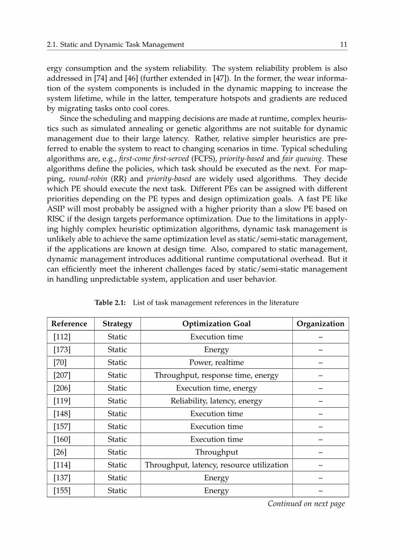
in handling unpredictable system, application and user behavior.
Table 2.1: List of task management references in the literature
Reference Strategy Optimization Goal Organization
[112] Static Execution time –
[173] Static Energy –
[70] Static Power, realtime –
[207] Static Throughput, response time, energy –
[206] Static Execution time, energy –
[119] Static Reliability, latency, energy –
[148] Static Execution time –
[157] Static Execution time –
[160] Static Execution time –
[26] Static Throughput –
[114] Static Throughput, latency, resource utilization –
[137] Static Energy –
[155] Static Energy –
Continued on next page
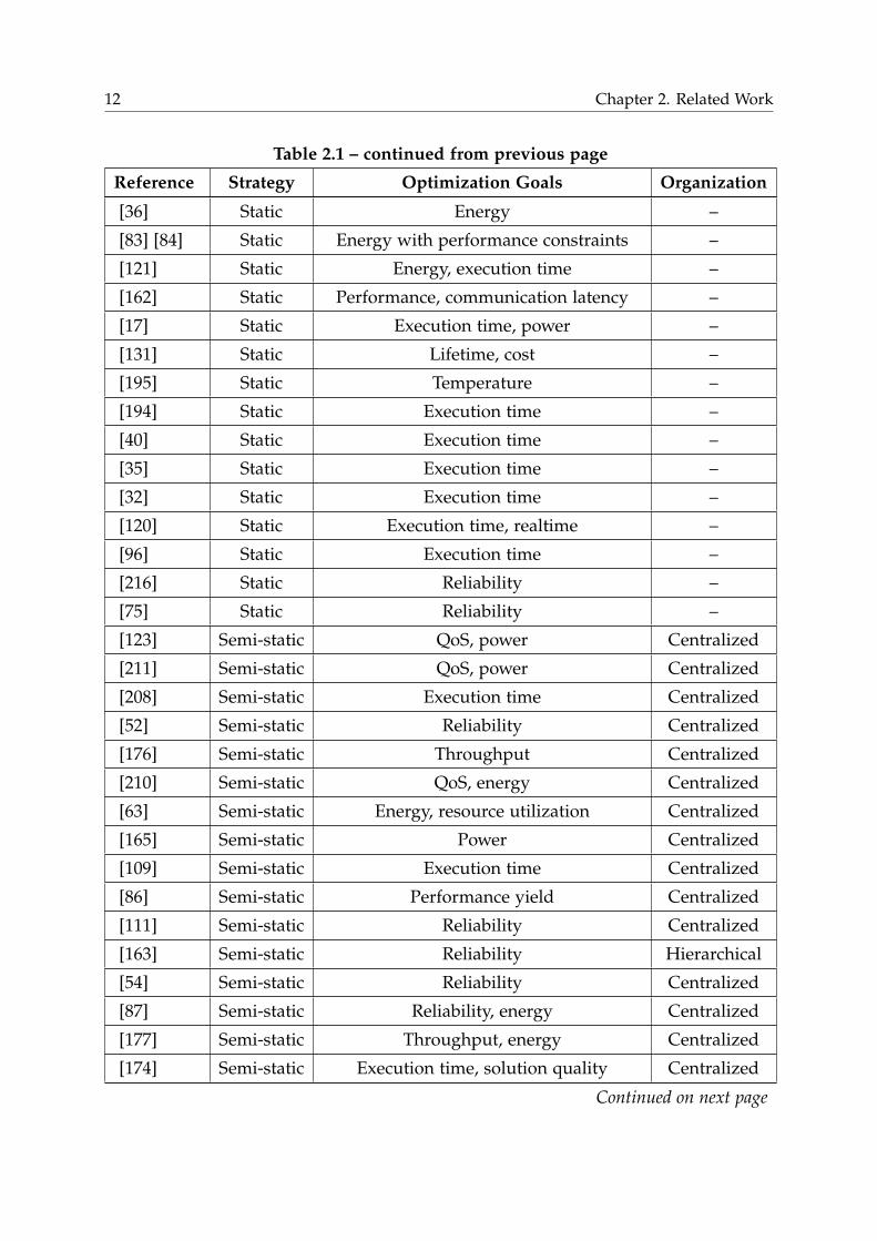
12 Chapter 2. Related Work
Table 2.1 – continued from previous page
Reference Strategy Optimization Goals Organization
[36] Static Energy –
[83] [84] Static Energy with performance constraints –
[121] Static Energy, execution time –
[162] Static Performance, communication latency –
[17] Static Execution time, power –
[131] Static Lifetime, cost –
[195] Static Temperature –
[194] Static Execution time –
[40] Static Execution time –
[35] Static Execution time –
[32] Static Execution time –
[120] Static Execution time, realtime –
[96] Static Execution time –
[216] Static Reliability –
[75] Static Reliability –
[123] Semi-static QoS, power Centralized
[211] Semi-static QoS, power Centralized
[208] Semi-static Execution time Centralized
[52] Semi-static Reliability Centralized
[176] Semi-static Throughput Centralized
[210] Semi-static QoS, energy Centralized
[63] Semi-static Energy, resource utilization Centralized
[165] Semi-static Power Centralized
[109] Semi-static Execution time Centralized
[86] Semi-static Performance yield Centralized
[111] Semi-static Reliability Centralized
[163] Semi-static Reliability Hierarchical
[54] Semi-static Reliability Centralized
[87] Semi-static Reliability, energy Centralized
[177] Semi-static Throughput, energy Centralized
[174] Semi-static Execution time, solution quality Centralized
Continued on next page
2.1. Static and Dynamic Task Management 13
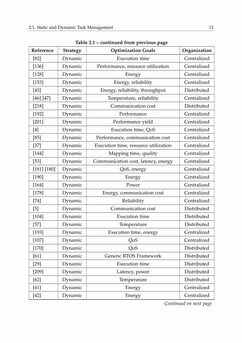
Table 2.1 – continued from previous page
Reference Strategy Optimization Goals Organization
[82] Dynamic Execution time Centralized
[136] Dynamic Performance, resource utilization Centralized
[128] Dynamic Energy Centralized
[153] Dynamic Energy, reliability Centralized
[43] Dynamic Energy, reliability, throughput Distributed
[46] [47] Dynamic Temperature, reliability Centralized
[218] Dynamic Communication cost Distributed
[192] Dynamic Performance Centralized
[201] Dynamic Performance yield Centralized
[4] Dynamic Execution time, QoS Centralized
[85] Dynamic Performance, communication cost Centralized
[37] Dynamic Execution time, resource utilization Centralized
[144] Dynamic Mapping time, quality Centralized
[53] Dynamic Communication cost, latency, energy Centralized
[181] [180] Dynamic QoS, energy Centralized
[190] Dynamic Energy Centralized
[164] Dynamic Power Centralized
[178] Dynamic Energy, communication cost Centralized
[74] Dynamic Reliability Centralized
[5] Dynamic Communication cost Distributed
[104] Dynamic Execution time Distributed
[57] Dynamic Temperature Distributed
[193] Dynamic Execution time, energy Centralized
[107] Dynamic QoS Centralized
[170] Dynamic QoS Distributed
[61] Dynamic Generic RTOS Framework Distributed
[29] Dynamic Execution time Distributed
[209] Dynamic Latency, power Distributed
[62] Dynamic Temperature Distributed
[41] Dynamic Energy Centralized
[42] Dynamic Energy Centralized
Continued on next page
14 Chapter 2. Related Work
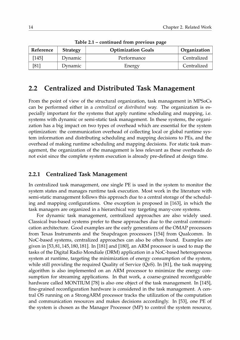
Table 2.1 – continued from previous page
Reference Strategy Optimization Goals Organization
[145] Dynamic Performance Centralized
[81] Dynamic Energy Centralized
2.2 Centralized and Distributed Task Management
From the point of view of the structural organization, task management in MPSoCs
can be performed either in a centralized or distributed way. The organization is es-
pecially important for the systems that apply runtime scheduling and mapping, i.e.
systems with dynamic or semi-static task management. In these systems, the organi-
zation has a big impact on two types of overhead which are essential for the system
optimization: the communication overhead of collecting local or global runtime sys-
tem information and distributing scheduling and mapping decisions to PEs, and the
overhead of making runtime scheduling and mapping decisions. For static task man-
agement, the organization of the management is less relevant as these overheads do
not exist since the complete system execution is already pre-defined at design time.
2.2.1 Centralized Task Management
In centralized task management, one single PE is used in the system to monitor the
system states and manages runtime task execution. Most work in the literature with
semi-static management follows this approach due to a central storage of the schedul-
ing and mapping configurations. One exception is proposed in [163], in which the
task managers are organized in a hierarchical way targeting many-core systems.
For dynamic task management, centralized approaches are also widely used.
Classical bus-based systems prefer to these approaches due to the central communi-
cation architecture. Good examples are the early generations of the OMAP processors
from Texas Instruments and the Snapdragon processors [154] from Qualcomm. In
NoC-based systems, centralized approaches can also be often found. Examples are
given in [53,81,145,180,181]. In [181] and [180], an ARM processor is used to map the
tasks of the Digital Radio Mondiale (DRM) application in a NoC-based heterogeneous
system at runtime, targeting the minimization of energy consumption of the system,
while still providing the required Quality of Service (QoS). In [81], the task mapping
algorithm is also implemented on an ARM processor to minimize the energy con-
sumption for streaming applications. In that work, a coarse-grained reconfigurable
hardware called MONTIUM [78] is also one object of the task management. In [145],
fine-grained reconfiguration hardware is considered in the task management. A cen-
tral OS running on a StrongARM processor tracks the utilization of the computation
and communication resources and makes decisions accordingly. In [53], one PE of
the system is chosen as the Manager Processor (MP) to control the system resource,
2.2. Centralized and Distributed Task Management 15
configuration and task manipulations (scheduling, binding, mapping and migration)
with the goal of optimizing the network channel congestion.
A big advantage of managing tasks in a centralized way is that the task manager
has a global view of the whole running system, such as task execution states, resource
utilization and communication congestion. This enables the task manager to make
efficient decisions with respect to a global optimization and largely reduces the risks
of falling into locally optimal solutions. Furthermore, the implementation of such
systems with a central task manager is rather intuitive and has a relatively low design
complexity, both from the hardware and the software architecture perspective. For the
user, programming such systems is also relatively straightforward, mainly focusing
on the communication between the central manager and the rest of the system.
The major drawback of centralized approaches is their limited scalability, which
can be critical, if applied to large systems such as many-core systems. In these large
systems, a central task manager has to control the task execution over a large number
of PEs, which can introduce extremely high workload to the manager. If the man-
ager cannot provide a high scheduling and mapping efficiency to cope with the high
workload, it can easily become the bottleneck of the system and consequently degrade
the system performance. In addition, to make global optimal decisions on the task
management, the amount of the system information collected by the central manager
is high in large systems. This generates a lot of communication traffic to the man-
ager, which can also make the communication near the manager become the system
bottleneck.
2.2.2 Distributed Task Management
The scalability problem of centralized approaches can be well overcome by distributed
task management, in which multiple PEs instead of one single PE are used to perform
task management. These PEs are typically distributively located over the system from
the topology view. Distributed task management can be further classified into fully
distributed, hierarchical and cluster-based.
In the fully distributed case, each PE performs local task management. An ex-
ample is presented in [62], in which a local core only communicates and exchanges
tasks with its nearest neighbors with respect to reducing thermal hot spots and large
temperature gradients on the chip.
An alternative to the fully distributed case are the hierarchical approaches, as pro-
posed in [218] and [209], in which the task management is realized in two steps. The
first step is performed in a global way, which is meant to find a good initial solution
for the task mapping or migration by utilizing global system information statistics.
In the second step, distributed algorithms are executed on local PEs to further im-
prove the task mapping or migration results. A similar approach is proposed in [170],
which mainly focuses on the task admission control. A central admission controller
is used to calculate the credits or rates of different actors (tasks) for each individual
PE and distributes this information to them. After receiving the credits or the task
rate information, each individual PE determines the task execution locally. In com-
16 Chapter 2. Related Work
parison to the work presented in [218] and [209], this one exhibits more centralized
characteristics.
Very often, task management in large systems is also organized using clusters
[5, 29, 61, 104]. The clusters do not necessarily have a fixed size. Instead, they can
be resized and organized virtually at runtime. Within each local cluster, one PE is
chosen as the manager. As the clusters are built at runtime, the managers can, but
not necessarily have to be bound to certain fixed PEs. In addition to local managers,
global managers might also exist in the systems. In [5], global managers are applied,
which have global information of all clusters. Therefore, when a task mapping request
arrives at a global manager, it is able to choose the most suitable cluster to execute
the task (probably with task migration), or even resizes the clusters, if the task can
not be mapped to any of the existing clusters. Similarly, a global manager is applied
in the system of [29], in which the position of each local manager is fixed and the
clusters are initially equally sized. During runtime, the cluster sizes can vary. In case
that more computational power is needed, a local manager can borrow processing
resources from other clusters over the global manager. In contrast to the two systems
above, the system presented in [104] does not have a global manager. Each local
cluster manager negotiates processing resources with its neighboring managers and
identifies its local domain for an application. During the time of building the local
domain, the role of the task manager can be transferred from one PE to another within
the cluster. Generally, due to the virtual clusters and variable local resource managers,
these cluster-based approaches are more suitable for homogeneous systems.
Distributed task management has a unique advantage over centralized task man-
agement in the scalability, which makes it more suitable in supporting large systems
with many cores. At the same time, its nature also implies that it mostly only uses
local system information for making decisions. Because of the lack of global infor-
mation, there is a high possibility that only sub-optimal solutions are found. For this
reason, in many distributed approaches, as shown above, a global manager is still
used to guide the task management in local domains. Furthermore, in local domains,
mostly one PE is selected to manage each domain in a kind of centralized way. There-
fore, despite the difference of the centralized and distributed approaches, an efficient
implementation of the task manager is usually highly desired, no matter whether it is
used globally or locally.
2.3 Task Management Implementations
The efficiency of a task management implementation largely influences the efficiency
of the system. It is especially important for dynamic task management, for which
scheduling and mapping have to be calculated at runtime. A slow task manager in
such systems would on the one hand result in a long decision time, which can be criti-
cal for the systems with high performance requirements such as real-time constraints.
On the other hand, the task manager would not be able to react to changing system
states in time, thus leading to sub-optimal scheduling and mapping decisions. In con-
2.3. Task Management Implementations 17
trast to dynamic task management, the efficiency requirement of the task manager in
static and semi-static task management is relatively low because of the pre-calculated
scheduling and mapping configurations at design time. In this section, a discussion
about different implementations of the task manager is made, which range from RISC
implementations to ASIC implementations, and the focus is laid on dynamic task
management.
2.3.1 RISC-based Implementations
Most of the task managers in the literature have a RISC-based implementation. They
apply RISC processors like ARM processors (e.g., in [81,136,144,180,181]), MicroBlaze
processors (e.g., in [41,42,42,193]) or SPARC processors (e.g., in [46,47,82]) to execute
scheduling and mapping algorithms. There are also researches, in which the task
manager is not really implemented, but given as an abstract generic processor model
[53, 164] or based on SystemC threads [178], or uses a formal model [107, 170]. These
implementations can most probably also be considered as RISC-based.
In the mainstream commercial devices, RISC architectures are also the most popu-
lar choice for the implementation of the task manager. For example, the master of the
OMAP processors is based on the ARM architectures. While on the OMAP 1 platform,
only one ARM926EJ-S processor controls one C55x DSP, in the latest OMAP systems, a
MPCore technology based master (ARM Cortex-A15 with four parallel cores) is used
to control a bunch of slave components including two ARM Cortex-M4 microcon-
trollers, a mini-C64x DSP, a PowerVR GPU and several other hardware accelerators
for image, video and audio processing. Similar to the OMAP processors, the Qual-
comm Snapdragon processors apply a single ARM11 processor as the master in its
first generation, and later on a quad-core Krait processor (ARM instruction-set based)
in the latest generation. The Samsung Exynos application processor family [159] also
follows the same strategy. In its early generation, only one ARM processor is used
to control the system. In the later generations multi-core processors based on the
MPCore technology or even eight cores (a quad-core A15 and a quad-core A7), con-
figured as the ARM big.LITTLE architecture [72], are used. In the big.LITTLE archi-
tecture, the quad-core A15 is larger and has higher performance, while the quad-core
A7 is smaller but more power-efficient. Depending on the system load, the task man-
agement can be internally switched between both quad-cores. Another commercial
example is made by the Cell Broadband Engine, which was jointly developed by IBM,
Sony and Toshiba. In this system, one PowerPC is used as the master of the sys-
tem, which runs the operating system and coordinates eight specialized coprocessors
known as Synergistic Processing Elements (SPEs).
RISC-based implementations of a task manager have very high flexibility in han-
dling tasks. Different algorithms can be executed by the manager and easily extended
and upgraded. As there is no hardware support for the task management algorithms,
this sort of implementations are considered as pure software implementations. Con-
ceptually, they are well suited to dynamic task management, in which flexibility is
needed due to the system dynamism. Furthermore, the convention of running an OS
18 Chapter 2. Related Work
on RISC processors for managing tasks makes the system able to be used and con-
trolled in a convenient way for the user. However, the main disadvantage of using
RISC processors as the task manager is their low efficiency, which can raise serious
performance issues for the systems with high performance requirements. In the liter-
ature, several to several tens of milliseconds are often reported for the task scheduling
and mapping [81, 164, 180, 181, 190]. As a comparison, the round-trip of processing a
slot of one radio frame according to the LTE standard is allowed to only have a latency
of 4ms at maximum. For such systems, RISC-based implementations can become in-
applicable without further optimizations in the algorithms.
2.3.2 ASIC-based Implementations
Due to the inefficiency of pure software implementations for the task manager based
on RISC processors, especially for large MPSoCs, researches are made to consider
shifting the implementation from software to hardware in order to improve the effi-
ciency. Several ASIC-based implementations are proposed in the literature, which
provide native hardware support for the OS functionality either in uni-core plat-
forms [105, 140, 142, 146] or in MPSoCs [113, 115, 141, 150, 169]. In the following, the
ASIC support for the MPSoC task management is further introduced.
HOSK The Hardware Operating System Kernel (HOSK) [150] is a hardware copro-
cessor, which performs task scheduling, inter-processor communication and context
switching in multiprocessor systems. It consists of three components: a main con-
troller, a thread manager and a context manager. The main controller receives the
service requests from the PEs of the system and controls the other two components.
The thread manager schedules the threads and provides inter-processor communica-
tion services based on hardware semaphores. A single thread queue is implemented
in the thread manager, which supports up to 128 threads. In the context manager, the
context of the scheduled and suspended threads is maintained. However, to make the
context manager to work properly, a dedicated context controller needs to be imple-
mented at the side of each PE to cooperate with the context manager. This makes the
integration of HOSK difficult into the systems using off-the-shelf processors. HOSK
has low context switch overhead. Less than 1% overhead is reported for 1 kcycle
threads, if using a wide 544-bit context bus.
CoreManager The CoreManager [113,169] is a hardware scheduler designed to sup-
port task management in systems targeting wireless communication applications such
as LTE and WiMAX. It detects and solves task dependency at runtime and sched-
ules ready tasks to the PEs. The PEs can be instruction-set processors or ASICs. A
programming model is provided along with CoreManager, supporting a Model of
Computation (MoC) similar to SDFGs. High scheduling efficiency is reported for
CoreManager (60 cycles to schedule a task in average), which however is at the cost
of high area overhead.
2.3. Task Management Implementations 19
SystemWeaver The approach of SystemWeaver [115] focuses on the issue of task
scheduling and mapping on heterogeneous MPSoCs, supported by a programming
model. It has a slightly higher flexibility than HOSK and CoreManager by allow-
ing the user to compose different basic scheduling and mapping primitives so as to
construct complex algorithms. The construction of the algorithms is built upon task
and PE queues, over which a hardware state machine is executed to make scheduling
and mapping decisions. However, its flexibility is still rather limited and the usage is
rather difficult due to its design complexity.
HW-RTOS The HardWare Real Time Operating System (HW-RTOS) [34] is a dedi-
cated hardware implementation of the standard OS layer. In [141], it is integrated into
Symmetric Multiprocessing (SMP) architectures to support task synchronization and
scheduling in multiprocessor systems. In the system, a HW-RTOS instance is created
for each PE, and the multiple HW-RTOS instances are synchronized using a common
Lock Unit to protect critical shared memory accesses. A task queue is implemented
in HW-RTOS, and the task scheduling is based on the round-robin policy. As a case
study, a dual-ARM system is analyzed. A major problem of this architecture is its
scalability. To support a large number of PEs, the area increases significantly due to
multiple HW-RTOS instances.
The ASIC-based implementations for dynamic task management largely increases the
scheduling and mapping efficiency in comparison to the RISC-based implementa-
tions. On the other hand, the flexibility of these implementations is low. They can only
support limited scheduling and mapping algorithms or narrow application domains,
or have difficulties in integration into common systems due to the hardware specialty.
Furthermore, the additional hardware logic introduces area overhead, which is often
not negligible.
2.3.3 ASIP-based Implementations
While dynamic task management requires both flexibility and efficiency in schedul-
ing and mapping, and both RISC-based and ASIC-based implementations only partly
fulfill the requirements (RISCs for flexibility and ASICs for efficiency), new implemen-
tations need to be found that can fill the gap between RISCs and ASICs. As shown in
Figure 1.2 of Chapter 1, the uniqueness of ASIP in combining programmability and
native hardware support for performance-critical operations provides a promising so-
lution for solving this problem. This motivates an ASIP-implementation for dynamic
task management.
In the literature, ASIP designs are widely used for intensive data processing, such
as baseband signal processing [171], multimedia signal processing [77], or crypto-
graphic operations [99], etc. For supporting control-centric applications, in this con-
text, managing tasks as a system controller, using ASIPs is still not very popular. Two
architectures have been found so far in the literature, which follow the ASIP concept
20 Chapter 2. Related Work
for this purpose. The one is the ASIP-CoreManager presented in [15] and the other
one is the OSIP architecture presented in [31].
ASIP-CoreManager The ASIP-CoreManager presented in [15] is an ASIP-like ver-
sion of the hardwired CoreManager in [113, 169]. Its development was motivated by
the analysis on the performance and scalability of an RISC-based (ARM926) imple-
mentation for the same functionality of the hardwired CoreManager (see [14]). This
ASIP architecture is an extension of a basic Tensilica Xtensa LX4 core [28], featuring
Very Large Instruction Words (VLIW) and Single Instruction Multiple Data operations
(SIMD). A set of customized instructions are introduced, under which many are used
for solving task dependencies or enhancing normal arithmetic and logic instructions.
In comparison to the original Xtensa LX4 core, the ASIP-CoreManager doubles the
area, but can reduce the execution time by up to 97% when checking task dependen-
cies.
OSIP In comparison to CoreManager and ASIP-CoreManager, which support a lim-
ited set of applications based on SDF, another ASIP-based implementation called OSIP
is presented in [31], which provides more generic support for task management. OSIP
stands for Operating System application-specific Instruction-set Processor. It has a
Harvard architecture with 6 pipeline stages, containing special instructions to handle
the operations related to lists, which are a common data structure used in operating
systems. A programming model and hardware interfaces are provided along with
OSIP, which enable an easy integration of OSIP into different MPSoCs. During run-
time, OSIP communicates with all PEs of the system, which can be homogeneous
or heterogeneous, and schedules and distributes tasks based on user-defined algo-
rithms. In summary, the OSIP-based task management is ASIP-based and centralized
dynamic task management.
In [31], a preliminary analysis of OSIP efficiency in task management is made.
This thesis provides a much more extensive analysis of OSIP efficiency as well as
its flexibility from the system perspective in order to highlight the applicability and
advantages of using ASIPs as the task manager in general. Furthermore, a proof-
of-concept of integrating OSIP, which is a central task manager, into large MPSoCs
connected by NoCs, which are distributed architectures, is provided. The results
presented in this thesis have been published in part by the author in [31, 213–215].
2.4 Communication Architectures
Using an ASIP for managing tasks combines the advantages of RISCs and ASICs.
However, evaluating the performance of an ASIP for this kind of control-centric ap-
plications is not a simple task. It largely differs from the evaluation for the ASIPs
used for data processing. For the latter, the performance evaluation can be reasonably
done in a standalone way, i.e., isolated from the other components of the system. This
is because data-centric processing normally has a relatively small performance vari-
2.4. Communication Architectures 21
ance, which enables the designer easily to judge whether an ASIP implementation is
suitable for given applications or not. For example, in the domain of signal process-
ing, measuring the latency and throughput of executing certain algorithm kernels is
a typical way of evaluating the ASIP performance.
In contrast, the performance of a control-centric ASIP has to be evaluated from
the system-level, since the ASIP in principle controls the complete system. So, the
evaluation has to be jointly investigated with other system aspects, such as the sys-
tem size, task sizes (execution time of tasks), etc. Among them, the communication
architecture plays a specially important role in evaluating the efficiency of an ASIP as
the task manager. As both the communication architecture and the task manager are
shared resources, they compete with each other when determining the overall system
performance.
The two mainstream communication architecture paradigms of today’s MPSoCs
are bus-based and NoC-based. In the following, some basics of both communication
paradigms are introduced.
2.4.1 On-Chip Bus
Buses are a traditional on-chip communication architecture, which is nowadays still
widely used in modern system designs. Representative bus examples are the ARM
Advanced Microcontroller Bus Architecture (AMBA) series [10], IBM CoreConnect
[89], STBus of STMicroelectronics [184] and Sonics SMART Interconnect [182].
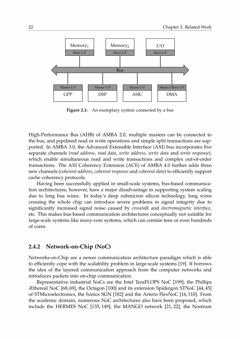
On-chip buses are a centralized communication architecture, connecting all sys-
tem components, as shown in Figure 2.1. It typically has two types of sockets: master
sockets and slave sockets. The master sockets are used to connect the system com-
ponents that initiate requests to the bus, e.g., PEs. These components are considered
as the masters of the bus. Analogously, the slave sockets are connected to the slaves
of the bus, e.g., memories and peripherals. The slaves react to the bus requests sent
from the master sockets. There are also system components such as Direct Memory
Access (DMA) controllers, which are both the masters and the slaves of the bus at the
same time.
The basic bus signals can be divided into three groups: data signals, address
signals and control signals. The data signals transfer the real data payload exchanged
between the masters and slaves. The address signals are used to identify which slave
component is accessed. The identification of the accessed slave component is made by
a decoder inside the bus. The control signals defines bus access types, e.g., write/read
signals, burst accesses, data masking, etc. Being a shared resource, it is very likely
that multiple masters access the bus at the same time. In order to ensure that only
one master gains the access to a slave at a time, arbiters are used in the bus. Different
arbitration schemes can be implemented in the bus, ranging from simple schemes
like static priority-based and round-robin to complexes ones like dynamic priority-based
or fair-among-equal.
To cope with the increasingly complex systems of today, the bus complexity in-
creases steadily as well. Taking the AMBA series as an example. In the Advanced
22 Chapter 2. Related Work
Bus
DSP
Master I/F
GPP
Master I/F
ASIC
Master I/F
DMA
Master/Slave I/F
Memory2
Slave I/F
Memory1
Slave I/F
I/O
Slave I/F
Figure 2.1: An exemplary system connected by a bus
High-Performance Bus (AHB) of AMBA 2.0, multiple masters can be connected to
the bus, and pipelined read or write operations and simple split transactions are sup-
ported. In AMBA 3.0, the Advanced Extensible Interface (AXI) bus incorporates five
separate channels (read address, read data, write address, write data and write response),
which enable simultaneous read and write transactions and complex out-of-order
transactions. The AXI Coherency Extension (ACE) of AMBA 4.0 further adds three
new channels (coherent address, coherent response and coherent data) to efficiently support
cache coherency protocols.
Having been successfully applied in small-scale systems, bus-based communica-
tion architectures, however, have a major disadvantage in supporting system scaling
due to long bus wires. In today’s deep submicron silicon technology, long wires
crossing the whole chip can introduce severe problems in signal integrity due to
significantly increased signal noise caused by crosstalk and electromagnetic interface,
etc. This makes bus-based communication architectures conceptually not suitable for
large-scale systems like many-core systems, which can contain tens or even hundreds
of cores.
2.4.2 Network-on-Chip (NoC)
Networks-on-Chip are a newer communication architecture paradigm which is able
to efficiently cope with the scalability problem in large-scale systems [19]. It borrows
the idea of the layered communication approach from the computer networks and
introduces packets into on-chip communication.
Representative industrial NoCs are the Intel TeraFLOPS NoC [199], the Phillips
Æthereal NoC [68, 69], the Octagon [100] and its extension Spidergon STNoC [44, 45]
of STMicroelectronics, the Sonics SGN [182] and the Arteris FlexNoC [16, 110]. From
the academic domain, numerous NoC architectures also have been proposed, which
include the HERMES NoC [135, 149], the MANGO network [21, 22], the Nostrum
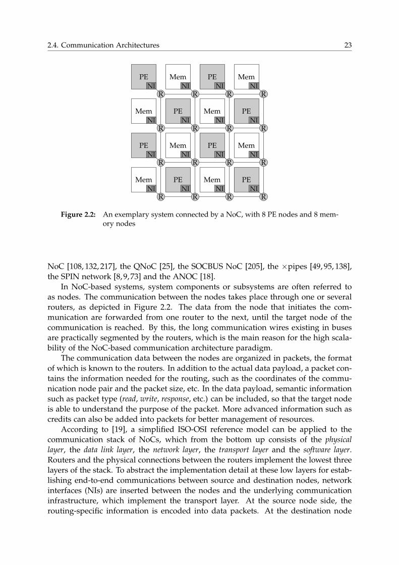
2.4. Communication Architectures 23
Mem
R
NI
PE
R
NI
Mem
R
NI
PE
R
NI
PE
R
NI
Mem
R
NI
PE
R
NI
Mem
R
NI
Mem
R
NI
PE
R
NI
Mem
R
NI
PE
R
NI
PE
R
NI
Mem
R
NI
PE
R
NI
Mem
R
NI
Figure 2.2: An exemplary system connected by a NoC, with 8 PE nodes and 8 mem-ory nodes
NoC [108, 132, 217], the QNoC [25], the SOCBUS NoC [205], the ×pipes [49, 95, 138],
the SPIN network [8, 9, 73] and the ANOC [18].
In NoC-based systems, system components or subsystems are often referred to
as nodes. The communication between the nodes takes place through one or several
routers, as depicted in Figure 2.2. The data from the node that initiates the com-
munication are forwarded from one router to the next, until the target node of the
communication is reached. By this, the long communication wires existing in buses
are practically segmented by the routers, which is the main reason for the high scala-
bility of the NoC-based communication architecture paradigm.
The communication data between the nodes are organized in packets, the format
of which is known to the routers. In addition to the actual data payload, a packet con-
tains the information needed for the routing, such as the coordinates of the commu-
nication node pair and the packet size, etc. In the data payload, semantic information
such as packet type (read, write, response, etc.) can be included, so that the target node
is able to understand the purpose of the packet. More advanced information such as
credits can also be added into packets for better management of resources.
According to [19], a simplified ISO-OSI reference model can be applied to the
communication stack of NoCs, which from the bottom up consists of the physical
layer, the data link layer, the network layer, the transport layer and the software layer.
Routers and the physical connections between the routers implement the lowest three
layers of the stack. To abstract the implementation detail at these low layers for estab-
lishing end-to-end communications between source and destination nodes, network
interfaces (NIs) are inserted between the nodes and the underlying communication
infrastructure, which implement the transport layer. At the source node side, the
routing-specific information is encoded into data packets. At the destination node
24 Chapter 2. Related Work
side, the NI extracts the payload data including the semantics from the packet for the
destination node for further processing. At the software layer of the NoC commu-
nication stack, the operating system, being either centralized or distributed, and the
applications are located. Especially, a programming model is often needed to simplify
the accesses to the network and to enable an efficient control of the network resources.
Designing a NoC is a complex task. Many design aspects have to be considered
at the different layers, among which NoC topologies, routing schemes and algorithms
and the flow control are especially important.
2.4.2.1 Topology
The topology of a NoC defines the way how the nodes of the NoC are connected with
each other. Depending on the performance and cost requirements of the application
and the system, different topologies can be considered. The most common topology
is mesh, in which the connection of the NoC nodes is constructed as a grid. The topol-
ogy of the NoC presented in Figure 2.2 is an example of the mesh topology. A slight
extension to the mesh topology is torus, in which connections are added between the
nodes at the opposite edges of the network to reduce the communication latencies
between these nodes. Other well-known topologies are, e.g., ring (a special case of
torus), octagon, spidergon, fat tree and butterfly. There are also irregular topologies,
which are mostly dedicated designed for specific applications. For example, unneces-
sary nodes of a regular topology are removed from the network to reduce the cost, or
a combination between different NoC topologies or even between a NoC and a shared
bus can be considered.
2.4.2.2 Routing Scheme
Routing schemes determine the paths, following which the packets travel from the
source nodes to the destination nodes. In general, routing paths of the packets can
either be pre-calculated before the source nodes send them, or be calculated at the
time when the packets arrive at different routers. The former is referred to as source
routing, in which routing paths are completely encoded into the packets and routers
only need to follow the paths. Source routing simplifies the router architecture, but
the data payload is reduced due to the additional path information in the packets.
In the latter case, each router itself determines the routing direction. The routing
algorithm in the routers is implemented using either dedicated hardware logic or the
so-called routing tables which can be configured.
When packets are transferred between the routers, different switching mecha-
nisms can be applied, such as store and forward, virtual cut through and wormhole switch-
ing. In the modern NoC design, the wormhole switching is the most commonly used
one due to its low buffer requirement in the router architecture. However, it can
introduce cyclic data graphs into the network, hence potentially create deadlocks.
There are different ways to cope with deadlocks during routing. One way is
adding virtual channels (VCs) into the routers and multiplexing the VCs to access
the physical channels of the network. By ordering the assignment to the VCs, cyclic
2.4. Communication Architectures 25
graphs can be prevented, which is mathematically proven in [51]. In addition, VCs
generally help improve the performance of networks, shown in [50]. Other widely
used schemes for avoiding deadlocks in the network are the XY routing scheme and
the turn model [64]. In the XY routing, packets are first routed along the x direction of
a 2-D network, then along the y dimension till the destination node is reached. In the
turn model such as west-first routing, north-last routing and negative-first routing, some
special turns of the packets are forbidden during the routing in order to avoid cycles.
For example, in the west-first routing, the turns from south to west and from north to
west are not allowed.
2.4.2.3 Flow Control
In NoCs, the flow control decides how data are transferred over the network, which
needs to take several aspects into consideration. These aspects include e.g., deadlocks,
network congestion, virtual channel and buffer utilization. The units, on which the
network control operates, are the so-called flow control units (flits). Flits are the basic
elements to build up a packet, containing the necessary information for the flow
control, such as routing-related information, priorities and semantics information.
Commonly, a packet uses three types of flits, which starts with a head flit, followed
by multiple data flits, and ends with a tail flit. A flit can be further divided into one
or multiple physical units (phits), which are the basic data units transferred through
the physical links between the routers. So, the sizes of phits always correspond to
the data link width of the routers, while the flit size can be larger than the data link
width.
The flow control can operate at different network layers. At the data-link layer,
synchronization mechanisms like using hand-shake signals can be applied to ensure
the correctness of the flit transmission. At the network layer, routing schemes and
algorithms are important for establishing efficient and reliable routing paths through
the network, e.g., avoiding deadlocks as discussed above, and/or providing QoS, etc.
At the transport layer, end-to-end flow control and congestion control services can
be implemented at the NIs to prevent message-dependent deadlocks [79, 139] and to
reduce network contention.
Compared to shared buses, NoCs have a unique advantage in the scalability, which
makes NoCs be a more promising solution to address the communication issues in
large-scale systems. At the same time, challenges also exist for NoCs. Some of the
main challenges are presented in the following. More comprehensive surveys of open
research problems in designing NoCs can be found in [122] and [151].
• Complexity: NoCs are generally more complex than shared buses. In large
systems, a large number of routers and NIs are required to connect the system
components. A router is usually implemented as a crossbar, enhanced with VCs
for improving performance and helping solve deadlock issues. Sophisticated
arbiters are often applied for the arbitration between the VCs and between the
router ports. For achieving a better clock frequency, pipelining a router is a
26 Chapter 2. Related Work
standard way. All of these make a router architecture quite complex. Upon
that, the architecture of NIs can also be very complex if specific flow control
mechanisms are needed. In total, NoCs have much larger area than buses for
the same system dimension, which at the same time also implies higher power
consumption, both in the static power (especially in the small technologies below
65nm) and in the dynamic power due to the high circuit switching distributed
along the routing paths.
• Latency: Due to the parallel point-to-point data communications between the
routers, NoCs provide higher bandwidth than traditional buses, hence improve
the throughput. However, latency becomes a critical issue in NoCs. First, when
a packet is routed from a source node to a destination node, it has to travel along
the routing path over multiple intermediate routers. Second, the pipeline stages
and the arbitration inside the routers also contribute to the latency. Third, pack-
etizing and de-packetizing the data at the source and destination NI introduce
again additional latency. Therefore, for the real-time applications, the latency
problem should be carefully handled.
• Design: In today’s design for bus-based systems, buses are mostly well stan-
dardized and can be used as an off-the-shelf component. The most effort that
the designer needs to spend on the integration of a bus into the system is the bus
configuration. In case that the bus interfaces do not match the interfaces of the
system components, adding adapters between them is sufficient. In comparison
to the standardized buses, using a NoC to connect a system often requires many
customizations or a new design from scratch. Considering the many design as-
pects and parameters of NoCs, the design effort which covers from high-level
design space exploration and specification down to low-level verification and
physical implementation is significantly larger than for buses.
In this section, two mainstream communication architecture paradigms – buses and
NoCs, are shortly introduced. Both have their advantages and disadvantages. Choos-
ing which one to use in the system largely depends on the system size and the target
applications. Generally for small systems, buses would be more suitable due to their
simplicity, and NoCs are preferred in large systems due to the scalability.
2.5 System-Level Exploration
Today’s embedded systems are highly complex, from both the hardware and the soft-
ware perspective, which results in a large design space. To meet design requirements
and optimization goals, system-level explorations are an inevitable design step to find
the most optimized design points. During the system-level exploration, the following
questions usually need to be addressed:
• Where is the hardware/software partitioning of the system made?
2.5. System-Level Exploration 27
• How many PEs and what kinds of PEs are required in the system?
• How is the memory hierarchy organized?
• How does the communication architecture look like?
• What are the task scheduling and mapping strategy and policies?
To answer these questions, experiments and evaluations for different system de-
sign points considering both the hardware and software architecture are desired. For
large systems, it can be very beneficial if the experiments and evaluations can be per-
formed fast due to the large design space. However, at the early design stage of a
system, the hardware prototypes of the system are mostly still not available, which
prevents the designer from developing the software, hence delays the exploration
process. A widely used way to deal with this problem is using high-level simulation
environments, which are also known as virtual platforms.
2.5.1 Virtual Platform
A virtual platform is a software simulation platform, which mimics the hardware
behavior of a system in software. As the platform is software-based, it makes the ex-
periments for the system exploration more convenient and enables an efficient hard-
ware/software co-design. In the virtual platform, once the initial simulation models
of the hardware components are available, the software development can already take
place. At the time the software is being developed, the hardware components can be
further modified, optimized and refined in parallel. This parallel development of the
hardware and software significantly reduces the development time of the system. Fur-
thermore, the designer is provided with better opportunities to analyze, profile and
debug the system, thanks to the software modeling of the system. The internal states
of the system can be much more easily traced in the software that in a hardware proto-
type. Furthermore, a virtual platform typically also provides a user-friendly graphical
interface to assist these purposes.
In a virtual platform, both PEs and communication architectures as well as mem-
ory hierarchies can be modeled and simulated at different abstraction levels, depend-
ing on the required simulation accuracy. For example, a programmable processor
can be modeled with a synthesizable Register-Transfer Level (RTL) description, sen-
sitive to every signal event. Or a cycle-accurate Instruction-Set Simulator (ISS) can
be applied to the processor, guaranteeing the correct behavior of the processor for
each clock cycle. An ISS can also be modeled at the instruction-accurate level, in
which the simulator only needs to make sure that correct results are produced after
the execution of each instruction. Source-level simulation [183] is an even higher ab-
straction model, in which the software is executed as the native machine code, but
instrumented with timing annotations. In [60] and [106], a hybrid-simulation technol-
ogy is proposed, which combines ISS with native C simulation. The authors of [33]
developed a generic High-level Virtual Platform (HVP) for supporting software de-
velopment at early design stage, which also allows mixed use of ISS and native C
28 Chapter 2. Related Work
simulation. Similar to the modeling of PEs, communication architectures and mem-
ory hierarchies can also be modeled at different abstraction levels, from RTL over
cycle-accurate level to Transaction-Level (TL).
In general, the higher an abstraction level is, the faster the simulation becomes and
the lower accuracy the simulation has. In order to increase the simulation speed and
at the same time still provide sufficient accuracy, co-simulations are often applied in
the system, in which the components of a system are modeled at different simulation
abstraction levels. While the high-level simulations are more used for the functional
modeling of non-performance-critical components, the simulations at a low abstrac-
tion level are typically used for the components that are performance-critical and need
in-depth analyses. It is the designer’s responsibility to decide for which system parts,
at which design stages and at which granularity to apply the co-simulation during
the system development.
Virtual platforms exist both in the industry and from the academic domain. Rep-
resentative examples are Synopsys Platform Architect [189], Intel CoFluent Technol-
ogy [92], ARM SoC Designer [12] and Open Virtual Platforms (OVP) [1]. For this
work, the Synopsys Platform Architect is used for creating, simulating and evaluating
the systems.
2.5.2 Platform Architect
The Synopsys Platform Architect is a SystemC-based virtual platform, aiming at an
efficient hardware/software co-design for SoCs. It provides an IP library containing a
rich number of widely used IP blocks such as processors (e.g., ARM processors), buses
(e.g., AHB and AXI buses) and bridges, memories and many others likes Ethernet,
USB, HDMI, etc. For supporting easy exploration with co-simulation, different types
of transactors for the interface translation between the models at different abstraction
levels are also provided. With simple drag and drop operations, the designer can
easily set up a basic working system. The designer also has the flexibility to develop
his own system components at different abstraction levels and integrate them into
the system. A number of system evaluation and debugging tools further support the
designer to make fast as well as detailed analyses.
To accelerate the exploration of hardware/software partitioning for MPSoCs and
enable an early start of the software development, Platform Architect introduces
the so-called MultiCore Optimization (MCO) technology based on Virtual Process-
ing Units (VPUs) [101].
Virtual Processing Unit (VPU) To exploit the parallel execution of multiple PEs in
MPSoCs, an application is commonly divided into a set of tasks, which are connected
with each other using communication channels. The tasks are mapped onto the PEs,
while the communication channels are mapped onto the communication architecture.
At the early design stage of the system, it is often desired that the analysis and ex-
ploration of different mapping strategies are fast but still accurate enough. However,
at this stage many hardware components such as PEs are mostly still not available,
2.5. System-Level Exploration 29
which makes the mapping impossible. Even if some PE models exist, e.g., by means
of simulators, running tasks on the simulators can take a long time. This slows down
the process of early design space exploration.
Virtual Processing Units (VPUs) provide a means to address this problem. As
indicated by the name, a VPU is not a real PE, but it can virtually represent different
PE types like processors or ASICs using SystemC threads. In other words, VPUs are
able to execute tasks like normal PEs and enable the mapping of tasks onto them at
a high abstraction level. In order to be mapped onto VPUs, tasks are also modeled
using SystemC threads. By annotating timing information into tasks, which can be
obtained, e.g., by educated guess or reasonable estimates based on the underlying PE
types, different mapping strategies can be tried and evaluated in a relatively accurate
way. As both VPUs and the tasks in the VPUs are SystemC-based, the simulation of
the system is in principle based on the native machine code, therefore very fast. This
enables fast system exploration. Even further, when searching for proper mappings
to meet the target constraints, it is sometimes less relevant, how the tasks are really
implemented, if the timing estimates for the tasks are good enough. So, even dummy
tasks can be employed in the system, running on the VPUs, as long as the data traffic
with respect to the input and output data of the tasks is precise, which is important for
the communication architecture exploration. In this way, the software development
can take place in parallel to the system design space exploration, which accelerates
the design process even more.
To schedule multiple tasks running on the same VPU, which is a typical case if
a PE is a programmable processor, a generic OS is provided in VPUs as the task
manager. Several basic scheduling algorithms like round-robin and priority-based are
already pre-implemented in the generic OS to handle the task queues in the VPUs,
and the tasks can be present in different states (ready, running, suspended, etc.) as in
a conventional OS. If needed, the designer can also implement his own scheduling al-
gorithms. In addition, interrupts are supported by the generic OS for easy integration
of VPUs.
In this work, system-level exploration is used for modeling different systems to ana-
lyze the efficiency and flexibility of using OSIP as the task manager from the system
perspective. The systems are varied in the number of PEs and different communica-
tion architectures in order to show what kind of impact these system configurations
have on the OSIP performance. In some systems, VPUs with dummy tasks are used
to hide the simulations of complex algorithm kernels, while accurate timing annota-
tions and task communication patterns are provided. This is intended to speed up
the system simulation by omitting less relevant information for the OSIP performance
analysis.

30 Chapter 2. Related Work
2.6 Summary
This chapter gives a short survey about related work on task management in MPSoCs,
which can be categorized into static, semi-static and dynamic task management. As
the system behavior nowadays exhibits high dynamism, dynamic task management
is especially important. To provide efficient but still flexible management, using an
ASIP as the task manager is motivated in this chapter. In addition, this chapter also
makes a short introduction to the today’s mainstream communication architectures,
which are also important for task management. Finally, the system-level exploration
environment used by this work is introduced.
Chapter 3
OSIP-based Systems
As shown in the previous chapter, efficient dynamic task management is important in
today’s MPSoCs. It is at the same time also challenging, if flexibility of the implemen-
tation for task management is desired. From the user perspective, programming large
MPSoCs, especially heterogeneous systems, is another big challenge. A program-
ming model is typically needed, with which the user can conveniently define tasks
and configure task scheduling and mapping as well as task synchronizations. A good
programming model should on the one hand simplify the programming by hiding
the underlying hardware details from the user. On the other hand, it should also be
able to provide the user with the flexibility of constructing different task scheduling
and mapping algorithms for different applications and design goals. In this chap-
ter, an approach based on an ASIP task manager called OSIP is introduced, which
comes along with a well-defined programming model and efficiently addresses the
above-mentioned challenges.
The chapter first starts with an overview of OSIP-based systems, introducing their
basic concept and the system construction from both the software and the hardware
perspective. Then, the core component of these systems – OSIP, is described in detail
together with its architectural development flow. Hardware analyses in terms of area,
timing, power and energy as well as a preliminary performance analysis are presented
afterwards. Finally, a summary is given and discussions on possible architectural
extensions are made.
3.1 System Overview
In this section, an overview of OSIP-based systems is given. After a short explana-
tion of the basic concept of the systems, the details of the software and hardware
integration are introduced.
3.1.1 Basic Concept
The OSIP-based systems address the efficiency and flexibility problem in the task
management by using an ASIP called OSIP as the task manager. OSIP is an abbrevia-
tion for OS ASIP. It is a special programmable processor customized for OS operations
and can be used as an off-the-shelf IP block for integration into MPSoCs.
In order to functionally involve OSIP into operation, a set of light-weight software
APIs are provided. Through the APIs, the information specified by the user during
programming can be translated into the low-level information, which is interpretable
31
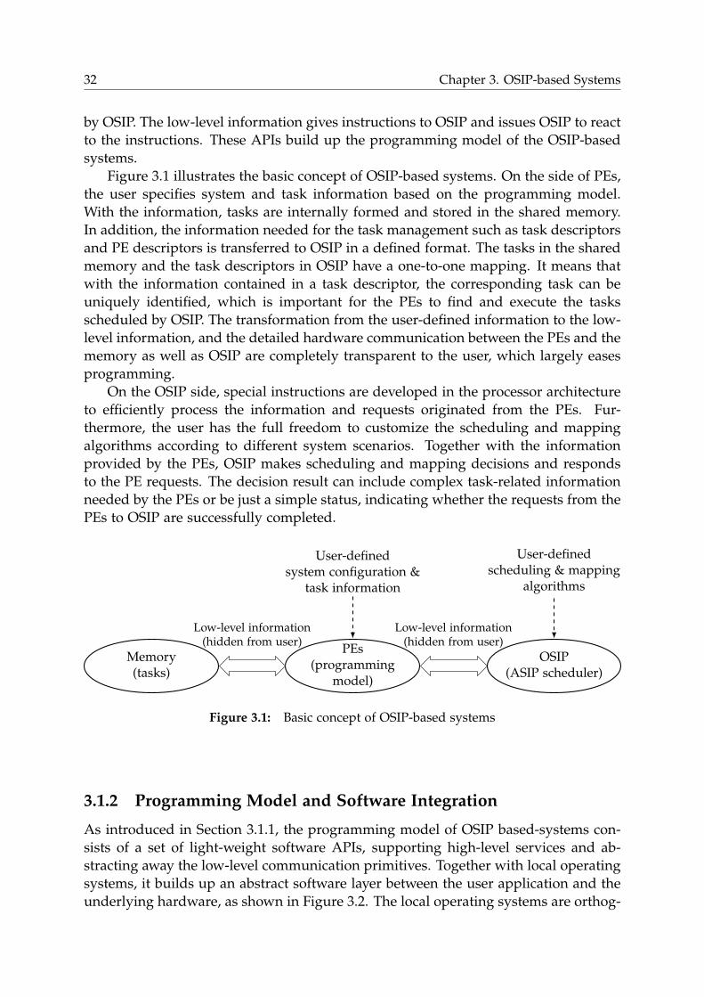
32 Chapter 3. OSIP-based Systems
by OSIP. The low-level information gives instructions to OSIP and issues OSIP to react
to the instructions. These APIs build up the programming model of the OSIP-based
systems.
Figure 3.1 illustrates the basic concept of OSIP-based systems. On the side of PEs,
the user specifies system and task information based on the programming model.
With the information, tasks are internally formed and stored in the shared memory.
In addition, the information needed for the task management such as task descriptors
and PE descriptors is transferred to OSIP in a defined format. The tasks in the shared
memory and the task descriptors in OSIP have a one-to-one mapping. It means that
with the information contained in a task descriptor, the corresponding task can be
uniquely identified, which is important for the PEs to find and execute the tasks
scheduled by OSIP. The transformation from the user-defined information to the low-
level information, and the detailed hardware communication between the PEs and the
memory as well as OSIP are completely transparent to the user, which largely eases
programming.
On the OSIP side, special instructions are developed in the processor architecture
to efficiently process the information and requests originated from the PEs. Fur-
thermore, the user has the full freedom to customize the scheduling and mapping
algorithms according to different system scenarios. Together with the information
provided by the PEs, OSIP makes scheduling and mapping decisions and responds
to the PE requests. The decision result can include complex task-related information
needed by the PEs or be just a simple status, indicating whether the requests from the
PEs to OSIP are successfully completed.
PEs(programming
model)
OSIP(ASIP scheduler)
Memory(tasks)
Low-level information(hidden from user)
Low-level information(hidden from user)
User-definedsystem configuration &
task information
User-definedscheduling & mapping
algorithms
Figure 3.1: Basic concept of OSIP-based systems
3.1.2 Programming Model and Software Integration
As introduced in Section 3.1.1, the programming model of OSIP based-systems con-
sists of a set of light-weight software APIs, supporting high-level services and ab-
stracting away the low-level communication primitives. Together with local operating
systems, it builds up an abstract software layer between the user application and the
underlying hardware, as shown in Figure 3.2. The local operating systems are orthog-
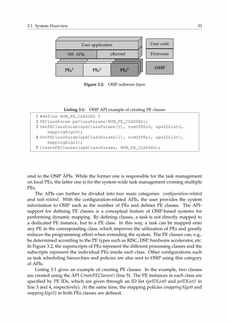
3.1. System Overview 33
PE01
PE02
PE03
SW APIs µKernel
User application
OSIP
Firmware
User code
Figure 3.2: OSIP software layer
Listing 3.1: OSIP API example of creating PE classes
1 #define NUM_PE_CLASSES 2
2 PEClassParam peClassParams[NUM_PE_CLASSES];
3 SetPEClassParam(&peClassParams[0], numOfPEs0, &peIDList0,
mappingAlgo0);
4 SetPEClassParam(&peClassParams[1], numOfPEs1, &peIDList1,
mappingAlgo1);
5 CreatePEClasses(&peClassParams, NUM_PE_CLASSES);
onal to the OSIP APIs. While the former one is responsible for the task management
on local PEs, the latter one is for the system-wide task management crossing multiple
PEs.
The APIs can further be divided into two main categories: configuration-related
and task-related. With the configuration-related APIs, the user provides the system
information to OSIP such as the number of PEs and defines PE classes. The API-
support for defining PE classes is a conceptual feature of OSIP-based systems for
performing dynamic mapping. By defining classes, a task is not directly mapped to
a dedicated PE instance, but to a PE class. In this way, a task can be mapped onto
any PE in the corresponding class, which improves the utilization of PEs and greatly
reduces the programming effort when extending the system. The PE classes can, e.g.,
be determined according to the PE types such as RISC, DSP, hardware accelerator, etc.
In Figure 3.2, the superscripts of PEs represent the different processing classes and the
subscripts represent the individual PEs inside each class. Other configurations such
as task scheduling hierarchies and policies are also sent to OSIP using this category
of APIs.
Listing 3.1 gives an example of creating PE classes. In the example, two classes
are created using the API CreatePEClasses() (line 5). The PE instances in each class are
specified by PE IDs, which are given through an ID list (peIDList0 and peIDList1 in
line 3 and 4, respectively). At the same time, the mapping policies (mappingAlgo0 and
mappingAlgo1) in both PEs classes are defined.
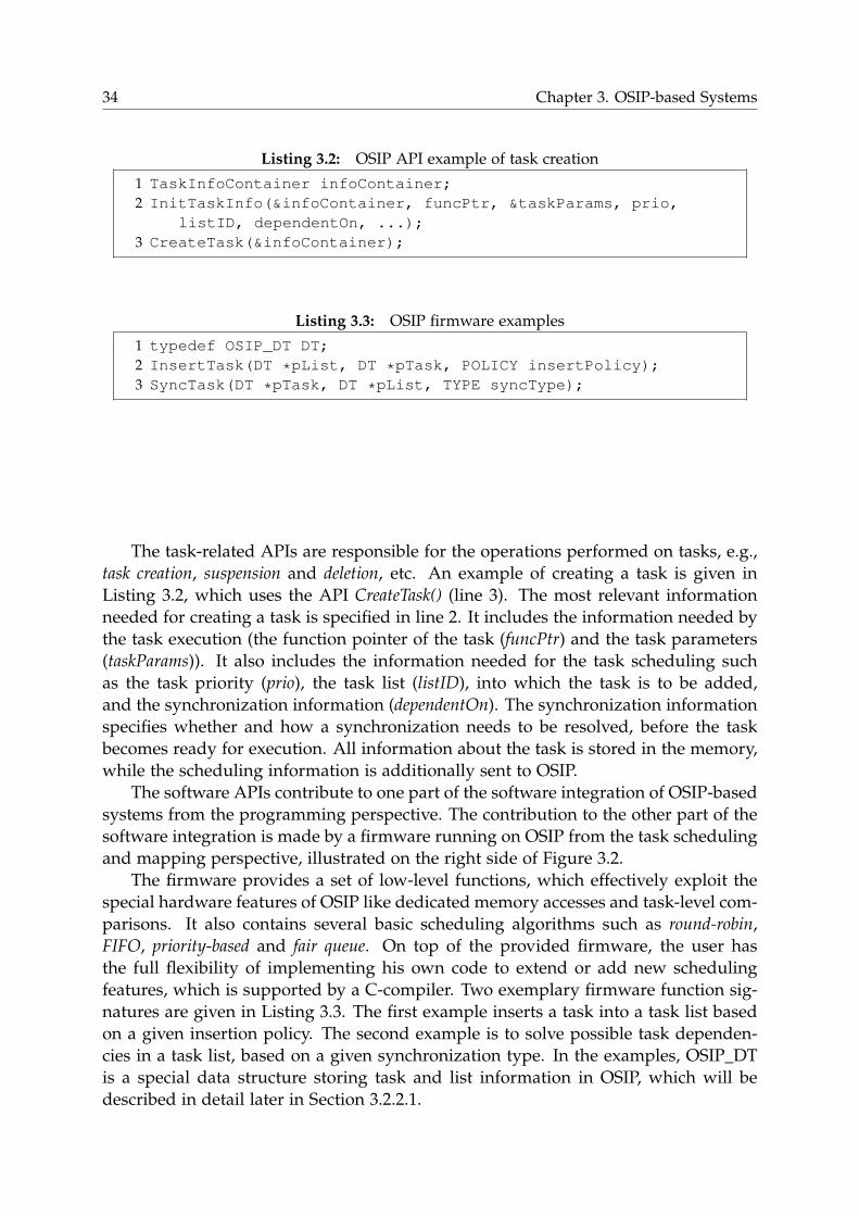
34 Chapter 3. OSIP-based Systems
Listing 3.2: OSIP API example of task creation
1 TaskInfoContainer infoContainer;
2 InitTaskInfo(&infoContainer, funcPtr, &taskParams, prio,
listID, dependentOn, ...);
3 CreateTask(&infoContainer);
Listing 3.3: OSIP firmware examples
1 typedef OSIP_DT DT;
2 InsertTask(DT *pList, DT *pTask, POLICY insertPolicy);
3 SyncTask(DT *pTask, DT *pList, TYPE syncType);
The task-related APIs are responsible for the operations performed on tasks, e.g.,
task creation, suspension and deletion, etc. An example of creating a task is given in
Listing 3.2, which uses the API CreateTask() (line 3). The most relevant information
needed for creating a task is specified in line 2. It includes the information needed by
the task execution (the function pointer of the task (funcPtr) and the task parameters
(taskParams)). It also includes the information needed for the task scheduling such
as the task priority (prio), the task list (listID), into which the task is to be added,
and the synchronization information (dependentOn). The synchronization information
specifies whether and how a synchronization needs to be resolved, before the task
becomes ready for execution. All information about the task is stored in the memory,
while the scheduling information is additionally sent to OSIP.
The software APIs contribute to one part of the software integration of OSIP-based
systems from the programming perspective. The contribution to the other part of the
software integration is made by a firmware running on OSIP from the task scheduling
and mapping perspective, illustrated on the right side of Figure 3.2.
The firmware provides a set of low-level functions, which effectively exploit the
special hardware features of OSIP like dedicated memory accesses and task-level com-
parisons. It also contains several basic scheduling algorithms such as round-robin,
FIFO, priority-based and fair queue. On top of the provided firmware, the user has
the full flexibility of implementing his own code to extend or add new scheduling
features, which is supported by a C-compiler. Two exemplary firmware function sig-
natures are given in Listing 3.3. The first example inserts a task into a task list based
on a given insertion policy. The second example is to solve possible task dependen-
cies in a task list, based on a given synchronization type. In the examples, OSIP_DT
is a special data structure storing task and list information in OSIP, which will be
described in detail later in Section 3.2.2.1.
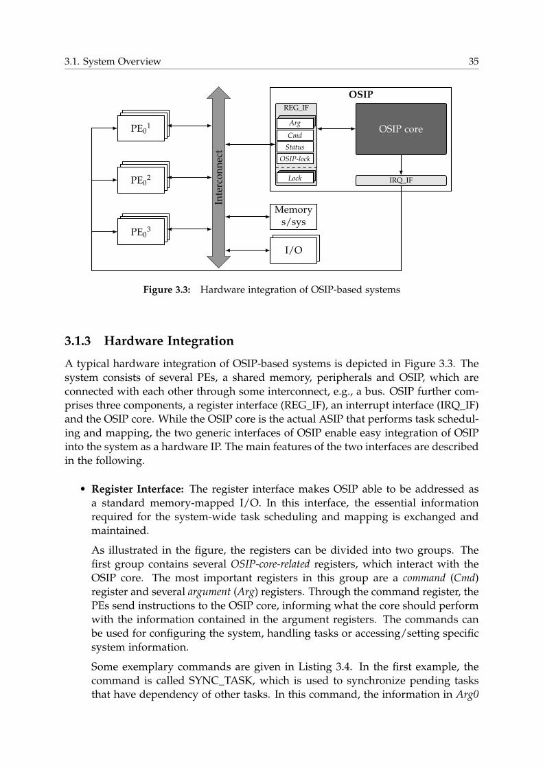
3.1. System Overview 35
PE01
PE02
PE03
Inte
rco
nn
ect
OSIP
REG_IF
Arg
Cmd
Status
OSIP-lock
Lock
OSIP core
IRQ_IF
Memorys/sys
I/O
Figure 3.3: Hardware integration of OSIP-based systems
3.1.3 Hardware Integration
A typical hardware integration of OSIP-based systems is depicted in Figure 3.3. The
system consists of several PEs, a shared memory, peripherals and OSIP, which are
connected with each other through some interconnect, e.g., a bus. OSIP further com-
prises three components, a register interface (REG_IF), an interrupt interface (IRQ_IF)
and the OSIP core. While the OSIP core is the actual ASIP that performs task schedul-
ing and mapping, the two generic interfaces of OSIP enable easy integration of OSIP
into the system as a hardware IP. The main features of the two interfaces are described
in the following.
• Register Interface: The register interface makes OSIP able to be addressed as
a standard memory-mapped I/O. In this interface, the essential information
required for the system-wide task scheduling and mapping is exchanged and
maintained.
As illustrated in the figure, the registers can be divided into two groups. The
first group contains several OSIP-core-related registers, which interact with the
OSIP core. The most important registers in this group are a command (Cmd)
register and several argument (Arg) registers. Through the command register, the
PEs send instructions to the OSIP core, informing what the core should perform
with the information contained in the argument registers. The commands can
be used for configuring the system, handling tasks or accessing/setting specific
system information.
Some exemplary commands are given in Listing 3.4. In the first example, the
command is called SYNC_TASK, which is used to synchronize pending tasks
that have dependency of other tasks. In this command, the information in Arg0
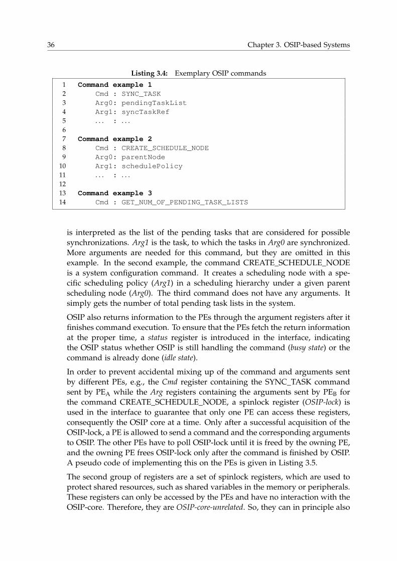
36 Chapter 3. OSIP-based Systems
Listing 3.4: Exemplary OSIP commands
1 Command example 1
2 Cmd : SYNC_TASK
3 Arg0: pendingTaskList
4 Arg1: syncTaskRef
5 . . . : . . .6
7 Command example 2
8 Cmd : CREATE_SCHEDULE_NODE
9 Arg0: parentNode
10 Arg1: schedulePolicy
11 . . . : . . .12
13 Command example 3
14 Cmd : GET_NUM_OF_PENDING_TASK_LISTS
is interpreted as the list of the pending tasks that are considered for possible
synchronizations. Arg1 is the task, to which the tasks in Arg0 are synchronized.
More arguments are needed for this command, but they are omitted in this
example. In the second example, the command CREATE_SCHEDULE_NODE
is a system configuration command. It creates a scheduling node with a spe-
cific scheduling policy (Arg1) in a scheduling hierarchy under a given parent
scheduling node (Arg0). The third command does not have any arguments. It
simply gets the number of total pending task lists in the system.
OSIP also returns information to the PEs through the argument registers after it
finishes command execution. To ensure that the PEs fetch the return information
at the proper time, a status register is introduced in the interface, indicating
the OSIP status whether OSIP is still handling the command (busy state) or the
command is already done (idle state).
In order to prevent accidental mixing up of the command and arguments sent
by different PEs, e.g., the Cmd register containing the SYNC_TASK command
sent by PEA while the Arg registers containing the arguments sent by PEB for
the command CREATE_SCHEDULE_NODE, a spinlock register (OSIP-lock) is
used in the interface to guarantee that only one PE can access these registers,
consequently the OSIP core at a time. Only after a successful acquisition of the
OSIP-lock, a PE is allowed to send a command and the corresponding arguments
to OSIP. The other PEs have to poll OSIP-lock until it is freed by the owning PE,
and the owning PE frees OSIP-lock only after the command is finished by OSIP.
A pseudo code of implementing this on the PEs is given in Listing 3.5.
The second group of registers are a set of spinlock registers, which are used to
protect shared resources, such as shared variables in the memory or peripherals.
These registers can only be accessed by the PEs and have no interaction with the
OSIP-core. Therefore, they are OSIP-core-unrelated. So, they can in principle also
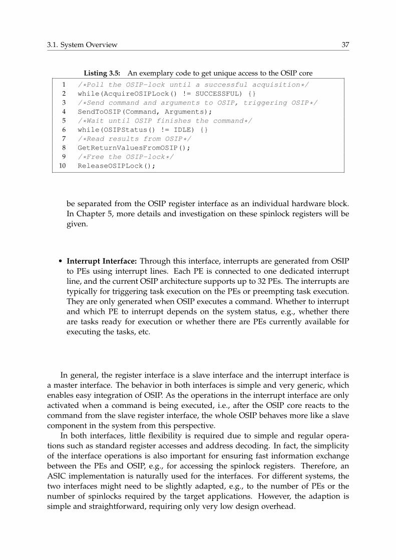
3.1. System Overview 37
Listing 3.5: An exemplary code to get unique access to the OSIP core
1 /*Poll the OSIP-lock until a successful acquisition*/
2 while(AcquireOSIPLock() != SUCCESSFUL) {}
3 /*Send command and arguments to OSIP, triggering OSIP*/
4 SendToOSIP(Command, Arguments);
5 /*Wait until OSIP finishes the command*/
6 while(OSIPStatus() != IDLE) {}
7 /*Read results from OSIP*/
8 GetReturnValuesFromOSIP();
9 /*Free the OSIP-lock*/
10 ReleaseOSIPLock();
be separated from the OSIP register interface as an individual hardware block.
In Chapter 5, more details and investigation on these spinlock registers will be
given.
• Interrupt Interface: Through this interface, interrupts are generated from OSIP
to PEs using interrupt lines. Each PE is connected to one dedicated interrupt
line, and the current OSIP architecture supports up to 32 PEs. The interrupts are
typically for triggering task execution on the PEs or preempting task execution.
They are only generated when OSIP executes a command. Whether to interrupt
and which PE to interrupt depends on the system status, e.g., whether there
are tasks ready for execution or whether there are PEs currently available for
executing the tasks, etc.
In general, the register interface is a slave interface and the interrupt interface is
a master interface. The behavior in both interfaces is simple and very generic, which
enables easy integration of OSIP. As the operations in the interrupt interface are only
activated when a command is being executed, i.e., after the OSIP core reacts to the
command from the slave register interface, the whole OSIP behaves more like a slave
component in the system from this perspective.
In both interfaces, little flexibility is required due to simple and regular opera-
tions such as standard register accesses and address decoding. In fact, the simplicity
of the interface operations is also important for ensuring fast information exchange
between the PEs and OSIP, e.g., for accessing the spinlock registers. Therefore, an
ASIC implementation is naturally used for the interfaces. For different systems, the
two interfaces might need to be slightly adapted, e.g., to the number of PEs or the
number of spinlocks required by the target applications. However, the adaption is
simple and straightforward, requiring only very low design overhead.
38 Chapter 3. OSIP-based Systems
3.2 OSIP Architecture Development
In the previous section, an overview of OSIP-based systems is given, especially from
the system integration point of view. In this section, the main component of the
OSIP-based systems — the OSIP core — and its development are introduced.
The section starts with an introduction to the general design flow of the OSIP core.
Then, the application running on the OSIP core, namely the task scheduling, mapping
and synchronization, is analyzed and characterized in order to provide hints for the
development of the OSIP core architecture. Following the analysis, the OSIP core
architecture is proposed and the main architectural features to support task manage-
ment are presented. As introduced in the previous section, OSIP behaves mainly as
a slave component in the system, which becomes active, only when there is a new
command received at the register interface. The details about this synchronization
between the register interface and the OSIP core are also described. Finally, an exem-
plary program is given, showing how to start and control the OSIP core to react to the
commands or how to enter the idle state.
In the remaining part of this thesis, OSIP is implicitly referred to as the OSIP core
for simplifying the text description, if not explicitly stated otherwise.
3.2.1 Design Flow
OSIP is developed with the Synopsys Processor Designer [143]. In the Processor De-
signer, a processor architecture is described in an Architecture Description Language
(ADL) called LISA [80, 161]. From the LISA description, both the software tools such
as assembler, linker, compiler and simulator and the hardware descriptions in VHDL
or Verilog HDL at RTL can be automatically generated by the tool suite provided by
the Processor Designer. The automatic process of this design environment signifi-
cantly reduces the processor development cycles.
The OSIP design flow is depicted in Figure 3.4, in which three main steps are fol-
lowed. Along with the three steps, the processor architecture is explored and refined.
In the first step, a complete system containing multiple ARM926EJ-S proces-
sors [13], a shared memory, several peripherals, an AHB bus and a SystemC model
of OSIP is created. In the SystemC model, the functional behavior of OSIP is imple-
mented in the plain C language and further enhanced by a SystemC wrapper for the
integration into the system. This functional behavior covers a wide range of schedul-
ing and mapping algorithms such as FIFO, round-robin, priority-based and fair queuing,
etc. It interprets the low-level information originated from the PEs and processes the
information correspondingly with the scheduling and mapping algorithms.
The goal of creating this SystemC model is to provide a functionally correct C-
implementation of the OSIP behavior, which serves as the base for the further ar-
chitecture development. Therefore, no timing information is included in the model.
When simulating the system for different applications, the inputs to the OSIP model
(commands and arguments from the register interface) and the outputs generated
from the OSIP model (return values to the register interface and interrupt signals to
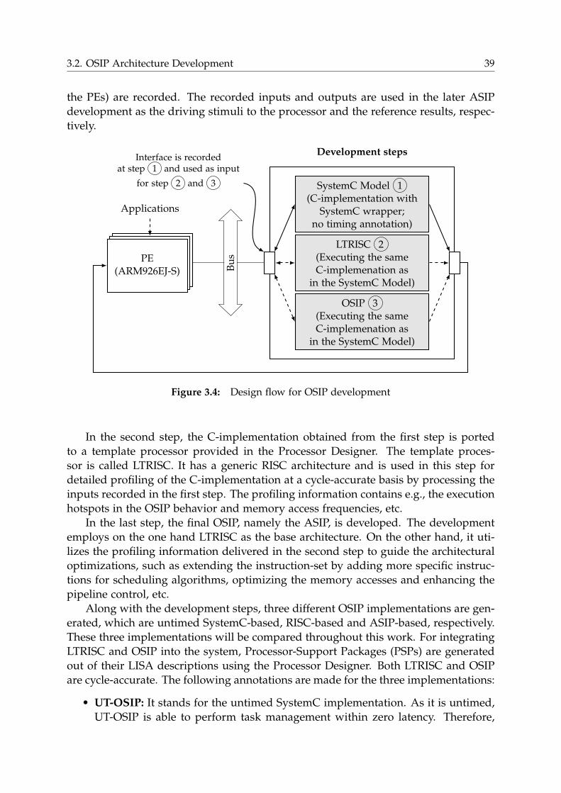
3.2. OSIP Architecture Development 39
the PEs) are recorded. The recorded inputs and outputs are used in the later ASIP
development as the driving stimuli to the processor and the reference results, respec-
tively.
PE(ARM926EJ-S)
Applications
Bu
s
LTRISC 2(Executing the sameC-implemenation as
in the SystemC Model)
SystemC Model 1(C-implementation with
SystemC wrapper;no timing annotation)
OSIP 3(Executing the sameC-implemenation as
in the SystemC Model)
Development stepsInterface is recorded
at step 1 and used as input
for step 2 and 3
Figure 3.4: Design flow for OSIP development
In the second step, the C-implementation obtained from the first step is ported
to a template processor provided in the Processor Designer. The template proces-
sor is called LTRISC. It has a generic RISC architecture and is used in this step for
detailed profiling of the C-implementation at a cycle-accurate basis by processing the
inputs recorded in the first step. The profiling information contains e.g., the execution
hotspots in the OSIP behavior and memory access frequencies, etc.
In the last step, the final OSIP, namely the ASIP, is developed. The development
employs on the one hand LTRISC as the base architecture. On the other hand, it uti-
lizes the profiling information delivered in the second step to guide the architectural
optimizations, such as extending the instruction-set by adding more specific instruc-
tions for scheduling algorithms, optimizing the memory accesses and enhancing the
pipeline control, etc.
Along with the development steps, three different OSIP implementations are gen-
erated, which are untimed SystemC-based, RISC-based and ASIP-based, respectively.
These three implementations will be compared throughout this work. For integrating
LTRISC and OSIP into the system, Processor-Support Packages (PSPs) are generated
out of their LISA descriptions using the Processor Designer. Both LTRISC and OSIP
are cycle-accurate. The following annotations are made for the three implementations:
• UT-OSIP: It stands for the untimed SystemC implementation. As it is untimed,
UT-OSIP is able to perform task management within zero latency. Therefore,
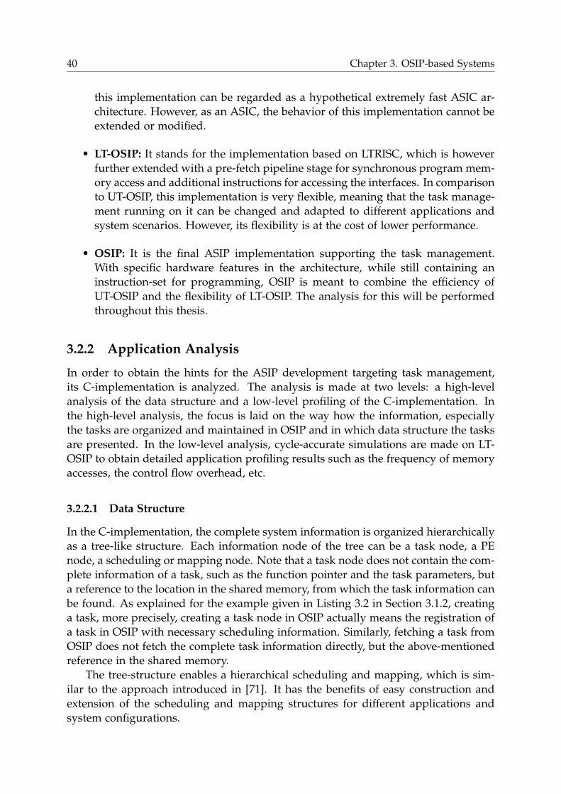
40 Chapter 3. OSIP-based Systems
this implementation can be regarded as a hypothetical extremely fast ASIC ar-
chitecture. However, as an ASIC, the behavior of this implementation cannot be
extended or modified.
• LT-OSIP: It stands for the implementation based on LTRISC, which is however
further extended with a pre-fetch pipeline stage for synchronous program mem-
ory access and additional instructions for accessing the interfaces. In comparison
to UT-OSIP, this implementation is very flexible, meaning that the task manage-
ment running on it can be changed and adapted to different applications and
system scenarios. However, its flexibility is at the cost of lower performance.
• OSIP: It is the final ASIP implementation supporting the task management.
With specific hardware features in the architecture, while still containing an
instruction-set for programming, OSIP is meant to combine the efficiency of
UT-OSIP and the flexibility of LT-OSIP. The analysis for this will be performed
throughout this thesis.
3.2.2 Application Analysis
In order to obtain the hints for the ASIP development targeting task management,
its C-implementation is analyzed. The analysis is made at two levels: a high-level
analysis of the data structure and a low-level profiling of the C-implementation. In
the high-level analysis, the focus is laid on the way how the information, especially
the tasks are organized and maintained in OSIP and in which data structure the tasks
are presented. In the low-level analysis, cycle-accurate simulations are made on LT-
OSIP to obtain detailed application profiling results such as the frequency of memory
accesses, the control flow overhead, etc.
3.2.2.1 Data Structure
In the C-implementation, the complete system information is organized hierarchically
as a tree-like structure. Each information node of the tree can be a task node, a PE
node, a scheduling or mapping node. Note that a task node does not contain the com-
plete information of a task, such as the function pointer and the task parameters, but
a reference to the location in the shared memory, from which the task information can
be found. As explained for the example given in Listing 3.2 in Section 3.1.2, creating
a task, more precisely, creating a task node in OSIP actually means the registration of
a task in OSIP with necessary scheduling information. Similarly, fetching a task from
OSIP does not fetch the complete task information directly, but the above-mentioned
reference in the shared memory.
The tree-structure enables a hierarchical scheduling and mapping, which is sim-
ilar to the approach introduced in [71]. It has the benefits of easy construction and
extension of the scheduling and mapping structures for different applications and
system configurations.
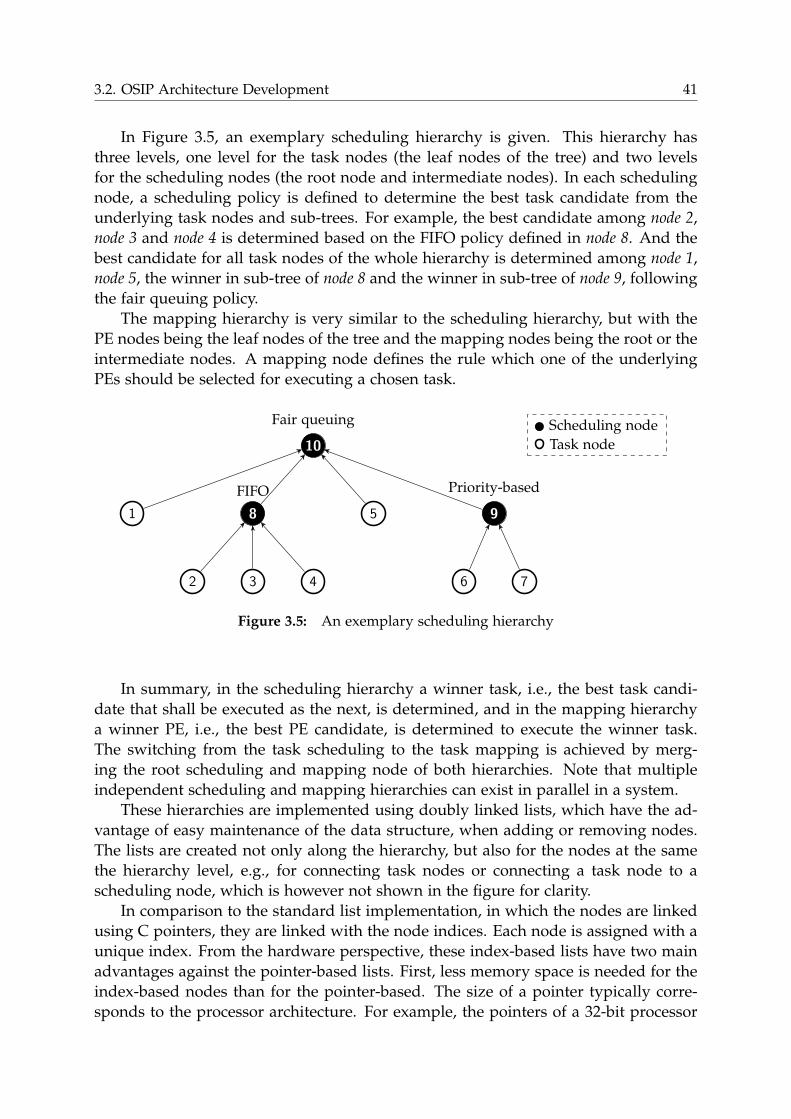
3.2. OSIP Architecture Development 41
In Figure 3.5, an exemplary scheduling hierarchy is given. This hierarchy has
three levels, one level for the task nodes (the leaf nodes of the tree) and two levels
for the scheduling nodes (the root node and intermediate nodes). In each scheduling
node, a scheduling policy is defined to determine the best task candidate from the
underlying task nodes and sub-trees. For example, the best candidate among node 2,
node 3 and node 4 is determined based on the FIFO policy defined in node 8. And the
best candidate for all task nodes of the whole hierarchy is determined among node 1,
node 5, the winner in sub-tree of node 8 and the winner in sub-tree of node 9, following
the fair queuing policy.
The mapping hierarchy is very similar to the scheduling hierarchy, but with the
PE nodes being the leaf nodes of the tree and the mapping nodes being the root or the
intermediate nodes. A mapping node defines the rule which one of the underlying
PEs should be selected for executing a chosen task.
10
1 8
2 3 4
5 9
6 7
Fair queuing
FIFO Priority-based
Scheduling node
Task node
Figure 3.5: An exemplary scheduling hierarchy
In summary, in the scheduling hierarchy a winner task, i.e., the best task candi-
date that shall be executed as the next, is determined, and in the mapping hierarchy
a winner PE, i.e., the best PE candidate, is determined to execute the winner task.
The switching from the task scheduling to the task mapping is achieved by merg-
ing the root scheduling and mapping node of both hierarchies. Note that multiple
independent scheduling and mapping hierarchies can exist in parallel in a system.
These hierarchies are implemented using doubly linked lists, which have the ad-
vantage of easy maintenance of the data structure, when adding or removing nodes.
The lists are created not only along the hierarchy, but also for the nodes at the same
the hierarchy level, e.g., for connecting task nodes or connecting a task node to a
scheduling node, which is however not shown in the figure for clarity.
In comparison to the standard list implementation, in which the nodes are linked
using C pointers, they are linked with the node indices. Each node is assigned with a
unique index. From the hardware perspective, these index-based lists have two main
advantages against the pointer-based lists. First, less memory space is needed for the
index-based nodes than for the pointer-based. The size of a pointer typically corre-
sponds to the processor architecture. For example, the pointers of a 32-bit processor
42 Chapter 3. OSIP-based Systems
usually have a size of 32 bits. In contrast, the bits needed for an index depend on the
maximum number of the supported nodes. To support 65536 nodes in the system,
which are already large enough for most of the today’s applications, only 16 bits are
needed for the index. Second, the indexing of the nodes enables efficient hardware
support for the operations performed in the lists, which will be shown later.
The linked lists through indices are made possible by: a) fixing the same size for
all node types (task node, PE node, scheduling node and mapping node); b) allocating
consecutively a static array for the nodes. In the actual C-implementation, each node
has a size of eight 32-bit words, serving as the basic data type that is considered
during the scheduling and mapping by OSIP. This basic data type is further referred
to as OSIP_DT. But internally, for different node types, the construction of OSIP_DT
is different, largely depending on which information should be included in the nodes.
3.2.2.2 Profiling
In addition to the high-level analysis for the data structure of the C-implementation,
cycle-accurate simulations are run on LT-OSIP to profile the C-implementation from
the instruction-level. A set of applications, ranging from synthetic programs to real-
life applications like H.264 video decoding are simulated. The profiling results are
given in Figure 3.6.
arithmetic;logic;
compare;misc
(41.2%) memoryaccess
(32.5%)
control(26.3%)
1-2 3-4 5-6 6+
0
20
40
Number of consecutivearithmetic/logic/compare
instructions
Per
cen
tag
e(%
)
branch nop,stall,flush
0
20
40
60
80
Per
cen
tag
e(%
)
load store nop,stall
0
20
40
Per
cen
tag
e(%
)
Figure 3.6: Instruction-level profiling of C-implementation
The following observations can be made from the profiling results. First, arith-
metic operations, memory accesses and control flows (branch/jump operations) can
be roughly considered as evenly distributed, shown by the pie-diagram in the figure.
Even the largest group of the operations — the arithmetic operations — does not
dominate the execution time.
Second, there are only few cases, in which a large number of arithmetic instruc-
tions are executed consecutively (see the left bar diagram of the figure). 46% of the
3.2. OSIP Architecture Development 43
consecutive executions contain only one or two arithmetic instructions. This results
from the fact that the arithmetic instructions are frequently separated by the con-
trol and/or memory access instructions. This is determined by the characteristic of
this kind of OS-like applications. During task scheduling and mapping, no highly
complex data processing exists, unlike the signal processing from the multimedia or
wireless communication domain. Instead, examination of the system information like
checking the status of a task or a PE, and simple arithmetic instructions like compar-
ing task priorities are the most common operations needed for making scheduling
and mapping decisions. This application characteristic on the one hand requires fre-
quent memory accesses, on the other hand involves high control overhead for making
decisions based on the information obtained from the memory accesses. Therefore,
the ASIP development for OSIP largely differs from the typical data-centric ASIP de-
velopment. Instead, it is control-centric. This makes the development challenging, for
which efficient handling of the control and memory accesses is extremely important.
Third, a further profiling of the control and memory accesses in the two bar di-
agrams on the right side of the figure shows that large execution overhead of these
operations is caused by the pipeline hazards, including both the data and the control
hazards. A large number of pipeline stall and flush operations, and additional nop
instructions are presented. This again highlights the necessity of efficient handling of
the control and memory accesses, or even reducing them generally by using native
hardware support.
3.2.3 Processor Architecture
This section introduces the main architectural features of OSIP. First, an overview of
the pipeline architecture of OSIP is given. Then, special instructions are introduced,
considering the profiling results presented in the previous section. In addition, in-
structions for accessing the interfaces are introduced. Finally, the synchronization
mechanism between the OSIP core and the register interface is described.
3.2.3.1 Pipeline Structure
OSIP is a 32-bit load-store architecture, which is extended from LT-OSIP. It has 6
pipeline stages: pre-fetch (PFE)1, fetch (FE), decode (DC), execution (EX), memory (MEM)
and writeback (WB). A program memory and a data memory are connected to the
pipeline. Both are single-port Synchronous Static RandomAccess Memories (SSRAMs).
A register file with 16 32-bit registers is implemented.
An overview of the pipeline structure is given in Figure 3.7. In the PFE-stage, it is
first decided whether the complete pipeline is suspended or activated by checking the
OSIP internal state and the request from the register interface. In case that the pipeline
is activated, the Program Counter (PC) is generated, and the instruction is fetched
in the FE-stage. In the DC-stage, the instructions are decoded and the execution
1 The original LT-OSIP processor does not have a pre-fetch stage. It has an asynchronous programmemory.

44 Chapter 3. OSIP-based Systems
of unconditional branch instructions (jump, call) also takes place here. Also, the
command and arguments are read from the register interface at this stage. In the EX-
stage, arithmetic and logic operations as well as conditional branches are executed,
and the register interface and the interrupt interface are written. Furthermore, the
memory access address is prepared, for which two different ways are distinguished.
The one is for accessing the data of the OSIP_DT nodes of the scheduling and mapping
hierarchies. The other one is for accessing the normal data. Memory accesses take
place either in the MEM-stage or in the WB-stage. In addition, OSIP_DT nodes are
compared in the WB-stage and the register file is written there.
3.2.3.2 Customized Instructions
To efficiently support the control and memory operations performed for the list-based
scheduling and mapping hierarchy, special instructions are implemented.
Enhancing control: The OSIP application is highly control-centric. In many cases,
the control is needed to check the information of the nodes for making further de-
cisions. It checks e.g., the type of a node, the state of a task node, or whether the
task list of a scheduler node is empty, etc. This kind of node information is typically
not long, can be enumerated with maximum 4 bits. If following a typical branch im-
plementation, three instructions would normally be needed. First, the status or the
type, with which the information of a node is going to be compared, is loaded into
a general purpose register. Then, this register is compared with another one, which
contains the fetched node status or type, and the result can be stored in an internal
status register of the processor or again in a general purpose register. In the third
instruction, a branch is executed based on the comparison result.
In the OSIP architecture, these three instructions are merged into one single in-
struction.
• Compare & Branch
enh_b cond R[idx1], imm4, BRANCH_ADDR
enh_b cond R[idx1],R[idx2], BRANCH_ADDR
These two instructions compare a register value R[idx1] against a 4-bit immedi-
ate imm4, more generally, against another register value R[idx2] and make the
branch decision right after the comparison. cond specifies typical comparison
conditions such as equal, not equal, larger than, etc.
In the pipeline, the comparison and branch decision are both made in the EX-
stage. If the branch is taken, the instructions in the PFE- and FE-stage are
flushed, while the DC-stage is still further executed. Therefore, this instruction
has one delay slot.
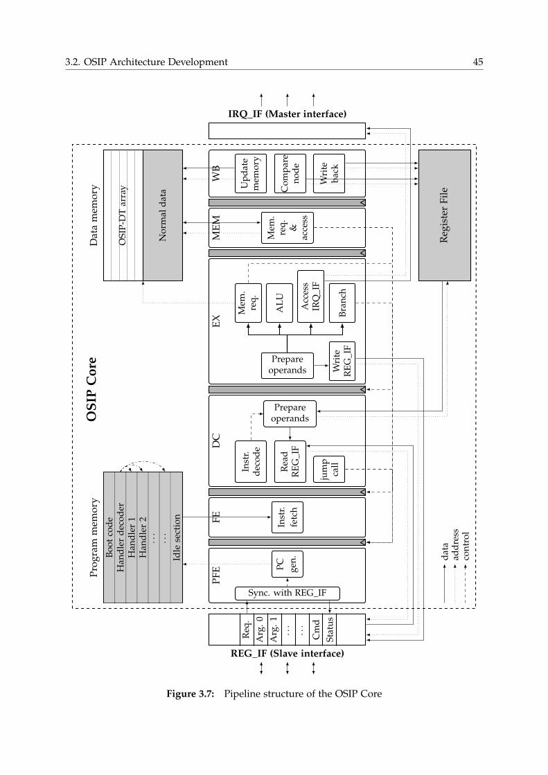
3.2. OSIP Architecture Development 45
PF
EF
ED
CE
XM
EM
WB
REG_IF (Slave interface)
Req
.
Arg
.0
Arg
.1
...
...
Cm
d
Sta
tus
IRQ_IF (Master interface)
Pro
gra
mm
emo
ry
Bo
ot
cod
eH
and
ler
dec
od
erH
and
ler
1H
and
ler
2..
...
.
Idle
sect
ion
Dat
am
emo
ry
OS
IP-D
Tar
ray
No
rmal
dat
a
Reg
iste
rF
ile
OS
IPC
ore
Sync. with REG_IF
PC
gen
.In
str.
fetc
h
Inst
r.d
eco
de
Rea
dR
EG
_IF
jum
pca
ll
Prepareoperands
Mem
.re
q.
AL
U
Acc
ess
IRQ
_IF
Bra
nch
Wri
teR
EG
_IF
Prepareoperands
Mem
.re
q.
&ac
cess
Up
dat
em
emo
ry
Co
mp
are
no
de
Wri
teb
ack
dat
aad
dre
ssco
ntr
ol
Figure 3.7: Pipeline structure of the OSIP Core
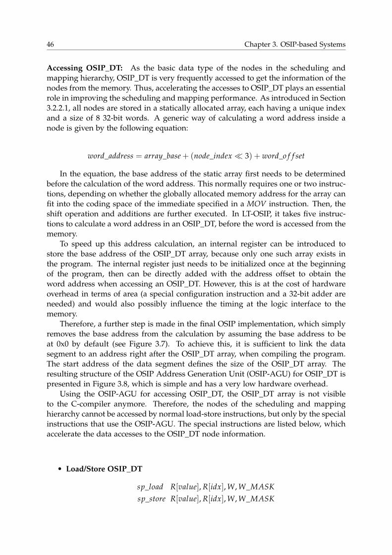
46 Chapter 3. OSIP-based Systems
Accessing OSIP_DT: As the basic data type of the nodes in the scheduling and
mapping hierarchy, OSIP_DT is very frequently accessed to get the information of the
nodes from the memory. Thus, accelerating the accesses to OSIP_DT plays an essential
role in improving the scheduling and mapping performance. As introduced in Section
3.2.2.1, all nodes are stored in a statically allocated array, each having a unique index
and a size of 8 32-bit words. A generic way of calculating a word address inside a
node is given by the following equation:
word_address = array_base+ (node_index≪ 3) + word_o f f set
In the equation, the base address of the static array first needs to be determined
before the calculation of the word address. This normally requires one or two instruc-
tions, depending on whether the globally allocated memory address for the array can
fit into the coding space of the immediate specified in a MOV instruction. Then, the
shift operation and additions are further executed. In LT-OSIP, it takes five instruc-
tions to calculate a word address in an OSIP_DT, before the word is accessed from the
memory.
To speed up this address calculation, an internal register can be introduced to
store the base address of the OSIP_DT array, because only one such array exists in
the program. The internal register just needs to be initialized once at the beginning
of the program, then can be directly added with the address offset to obtain the
word address when accessing an OSIP_DT. However, this is at the cost of hardware
overhead in terms of area (a special configuration instruction and a 32-bit adder are
needed) and would also possibly influence the timing at the logic interface to the
memory.
Therefore, a further step is made in the final OSIP implementation, which simply
removes the base address from the calculation by assuming the base address to be
at 0x0 by default (see Figure 3.7). To achieve this, it is sufficient to link the data
segment to an address right after the OSIP_DT array, when compiling the program.
The start address of the data segment defines the size of the OSIP_DT array. The
resulting structure of the OSIP Address Generation Unit (OSIP-AGU) for OSIP_DT is
presented in Figure 3.8, which is simple and has a very low hardware overhead.
Using the OSIP-AGU for accessing OSIP_DT, the OSIP_DT array is not visible
to the C-compiler anymore. Therefore, the nodes of the scheduling and mapping
hierarchy cannot be accessed by normal load-store instructions, but only by the special
instructions that use the OSIP-AGU. The special instructions are listed below, which
accelerate the data accesses to the OSIP_DT node information.
• Load/Store OSIP_DT
sp_load R[value],R[idx],W,W_MASK
sp_store R[value],R[idx],W,W_MASK
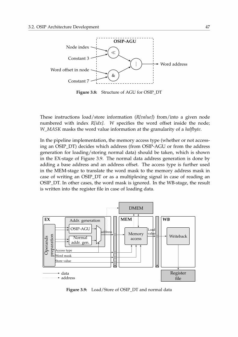
3.2. OSIP Architecture Development 47
Node index
Constant 3
Word offset in node
Constant 7
≪
&
| Word address
OSIP-AGU
Figure 3.8: Structure of AGU for OSIP_DT
These instructions load/store information (R[value]) from/into a given node
numbered with index R[idx]. W specifies the word offset inside the node;
W_MASK masks the word value information at the granularity of a halfbyte.
In the pipeline implementation, the memory access type (whether or not access-
ing an OSIP_DT) decides which address (from OSIP-AGU or from the address
generation for loading/storing normal data) should be taken, which is shown
in the EX-stage of Figure 3.9. The normal data address generation is done by
adding a base address and an address offset. The access type is further used
in the MEM-stage to translate the word mask to the memory address mask in
case of writing an OSIP_DT or as a multiplexing signal in case of reading an
OSIP_DT. In other cases, the word mask is ignored. In the WB-stage, the result
is written into the register file in case of loading data.
EX MEM WB
Registerfile
DMEM
Addr. generation
OSIP-AGU
Normaladdr. gen.
Op
eran
ds
pre
par
atio
n
Access type
address
Word mask
Store value
Memoryaccess
Loadvalue
Writeback
dataaddress
Figure 3.9: Load/Store of OSIP_DT and normal data
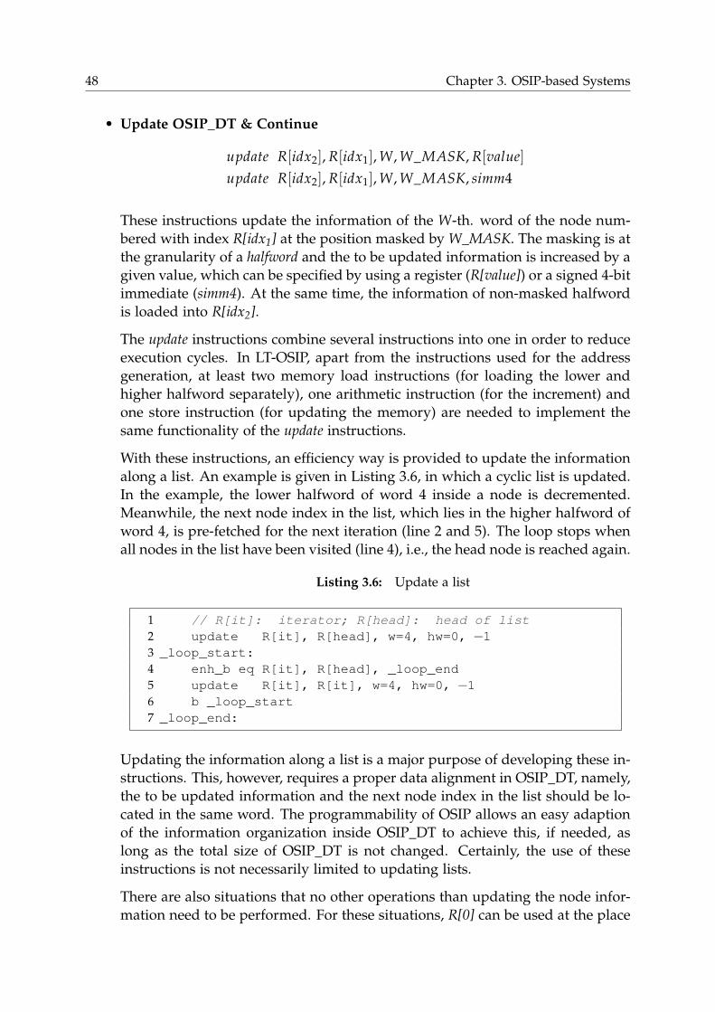
48 Chapter 3. OSIP-based Systems
• Update OSIP_DT & Continue
update R[idx2],R[idx1],W,W_MASK,R[value]
update R[idx2],R[idx1],W,W_MASK, simm4
These instructions update the information of the W-th. word of the node num-
bered with index R[idx1] at the position masked by W_MASK. The masking is at
the granularity of a halfword and the to be updated information is increased by a
given value, which can be specified by using a register (R[value]) or a signed 4-bit
immediate (simm4). At the same time, the information of non-masked halfword
is loaded into R[idx2].
The update instructions combine several instructions into one in order to reduce
execution cycles. In LT-OSIP, apart from the instructions used for the address
generation, at least two memory load instructions (for loading the lower and
higher halfword separately), one arithmetic instruction (for the increment) and
one store instruction (for updating the memory) are needed to implement the
same functionality of the update instructions.
With these instructions, an efficiency way is provided to update the information
along a list. An example is given in Listing 3.6, in which a cyclic list is updated.
In the example, the lower halfword of word 4 inside a node is decremented.
Meanwhile, the next node index in the list, which lies in the higher halfword of
word 4, is pre-fetched for the next iteration (line 2 and 5). The loop stops when
all nodes in the list have been visited (line 4), i.e., the head node is reached again.
Listing 3.6: Update a list
1 // R[it]: iterator; R[head]: head of list
2 update R[it], R[head], w=4, hw=0, −13 _loop_start:
4 enh_b eq R[it], R[head], _loop_end
5 update R[it], R[it], w=4, hw=0, −16 b _loop_start
7 _loop_end:
Updating the information along a list is a major purpose of developing these in-
structions. This, however, requires a proper data alignment in OSIP_DT, namely,
the to be updated information and the next node index in the list should be lo-
cated in the same word. The programmability of OSIP allows an easy adaption
of the information organization inside OSIP_DT to achieve this, if needed, as
long as the total size of OSIP_DT is not changed. Certainly, the use of these
instructions is not necessarily limited to updating lists.
There are also situations that no other operations than updating the node infor-
mation need to be performed. For these situations, R[0] can be used at the place
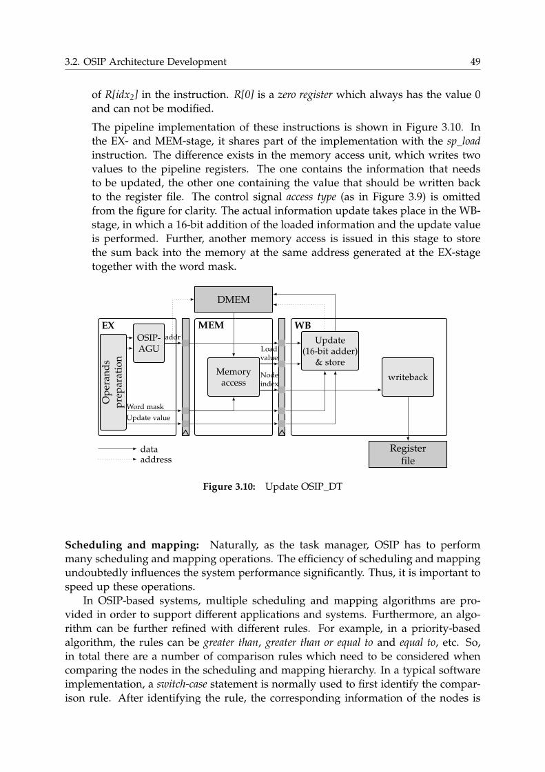
3.2. OSIP Architecture Development 49
of R[idx2] in the instruction. R[0] is a zero register which always has the value 0
and can not be modified.
The pipeline implementation of these instructions is shown in Figure 3.10. In
the EX- and MEM-stage, it shares part of the implementation with the sp_load
instruction. The difference exists in the memory access unit, which writes two
values to the pipeline registers. The one contains the information that needs
to be updated, the other one containing the value that should be written back
to the register file. The control signal access type (as in Figure 3.9) is omitted
from the figure for clarity. The actual information update takes place in the WB-
stage, in which a 16-bit addition of the loaded information and the update value
is performed. Further, another memory access is issued in this stage to store
the sum back into the memory at the same address generated at the EX-stage
together with the word mask.
EX MEM WB
Registerfile
DMEM
OSIP-AGU
Op
eran
ds
pre
par
atio
n
addr
Word mask
Update value
Memoryaccess
Loadvalue
Nodeindex
Update(16-bit adder)
& store
writeback
dataaddress
Figure 3.10: Update OSIP_DT
Scheduling and mapping: Naturally, as the task manager, OSIP has to perform
many scheduling and mapping operations. The efficiency of scheduling and mapping
undoubtedly influences the system performance significantly. Thus, it is important to
speed up these operations.
In OSIP-based systems, multiple scheduling and mapping algorithms are pro-
vided in order to support different applications and systems. Furthermore, an algo-
rithm can be further refined with different rules. For example, in a priority-based
algorithm, the rules can be greater than, greater than or equal to and equal to, etc. So,
in total there are a number of comparison rules which need to be considered when
comparing the nodes in the scheduling and mapping hierarchy. In a typical software
implementation, a switch-case statement is normally used to first identify the compar-
ison rule. After identifying the rule, the corresponding information of the nodes is
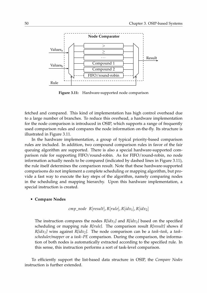
50 Chapter 3. OSIP-based Systems
>
≥
. . .
Compound 1
Compound 2
FIFO/round-robin
Valuesa
Valuesb
Result
Rule
Node Comparator
Figure 3.11: Hardware-supported node comparison
fetched and compared. This kind of implementation has high control overhead due
to a large number of branches. To reduce this overhead, a hardware implementation
for the node comparison is introduced in OSIP, which supports a range of frequently
used comparison rules and compares the node information on-the-fly. Its structure is
illustrated in Figure 3.11.
In the hardware implementation, a group of typical priority-based comparison
rules are included. In addition, two compound comparison rules in favor of the fair
queuing algorithm are supported. There is also a special hardware-supported com-
parison rule for supporting FIFO/round-robin. As for FIFO/round-robin, no node
information actually needs to be compared (indicated by dashed lines in Figure 3.11),
the rule itself determines the comparison result. Note that these hardware-supported
comparisons do not implement a complete scheduling or mapping algorithm, but pro-
vide a fast way to execute the key steps of the algorithm, namely comparing nodes
in the scheduling and mapping hierarchy. Upon this hardware implementation, a
special instruction is created.
• Compare Nodes
cmp_node R[result],R[rule],R[idx1],R[idx2]
The instruction compares the nodes R[idx1] and R[idx2] based on the specified
scheduling or mapping rule R[rule]. The comparison result R[result] shows if
R[idx1] wins against R[idx2]. The node comparison can be a task–task, a task–
scheduler/mapper or a task–PE comparison. During the comparison, the informa-
tion of both nodes is automatically extracted according to the specified rule. In
this sense, this instruction performs a sort of task-level comparison.
To efficiently support the list-based data structure in OSIP, the Compare Nodes
instruction is further extended.
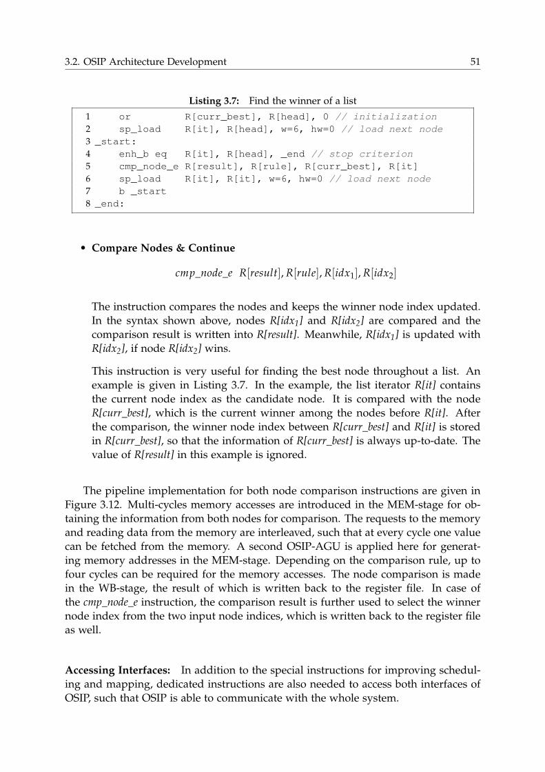
3.2. OSIP Architecture Development 51
Listing 3.7: Find the winner of a list
1 or R[curr_best], R[head], 0 // initialization
2 sp_load R[it], R[head], w=6, hw=0 // load next node
3 _start:
4 enh_b eq R[it], R[head], _end // stop criterion
5 cmp_node_e R[result], R[rule], R[curr_best], R[it]
6 sp_load R[it], R[it], w=6, hw=0 // load next node
7 b _start
8 _end:
• Compare Nodes & Continue
cmp_node_e R[result],R[rule],R[idx1],R[idx2]
The instruction compares the nodes and keeps the winner node index updated.
In the syntax shown above, nodes R[idx1] and R[idx2] are compared and the
comparison result is written into R[result]. Meanwhile, R[idx1] is updated with
R[idx2], if node R[idx2] wins.
This instruction is very useful for finding the best node throughout a list. An
example is given in Listing 3.7. In the example, the list iterator R[it] contains
the current node index as the candidate node. It is compared with the node
R[curr_best], which is the current winner among the nodes before R[it]. After
the comparison, the winner node index between R[curr_best] and R[it] is stored
in R[curr_best], so that the information of R[curr_best] is always up-to-date. The
value of R[result] in this example is ignored.
The pipeline implementation for both node comparison instructions are given in
Figure 3.12. Multi-cycles memory accesses are introduced in the MEM-stage for ob-
taining the information from both nodes for comparison. The requests to the memory
and reading data from the memory are interleaved, such that at every cycle one value
can be fetched from the memory. A second OSIP-AGU is applied here for generat-
ing memory addresses in the MEM-stage. Depending on the comparison rule, up to
four cycles can be required for the memory accesses. The node comparison is made
in the WB-stage, the result of which is written back to the register file. In case of
the cmp_node_e instruction, the comparison result is further used to select the winner
node index from the two input node indices, which is written back to the register file
as well.
Accessing Interfaces: In addition to the special instructions for improving schedul-
ing and mapping, dedicated instructions are also needed to access both interfaces of
OSIP, such that OSIP is able to communicate with the whole system.
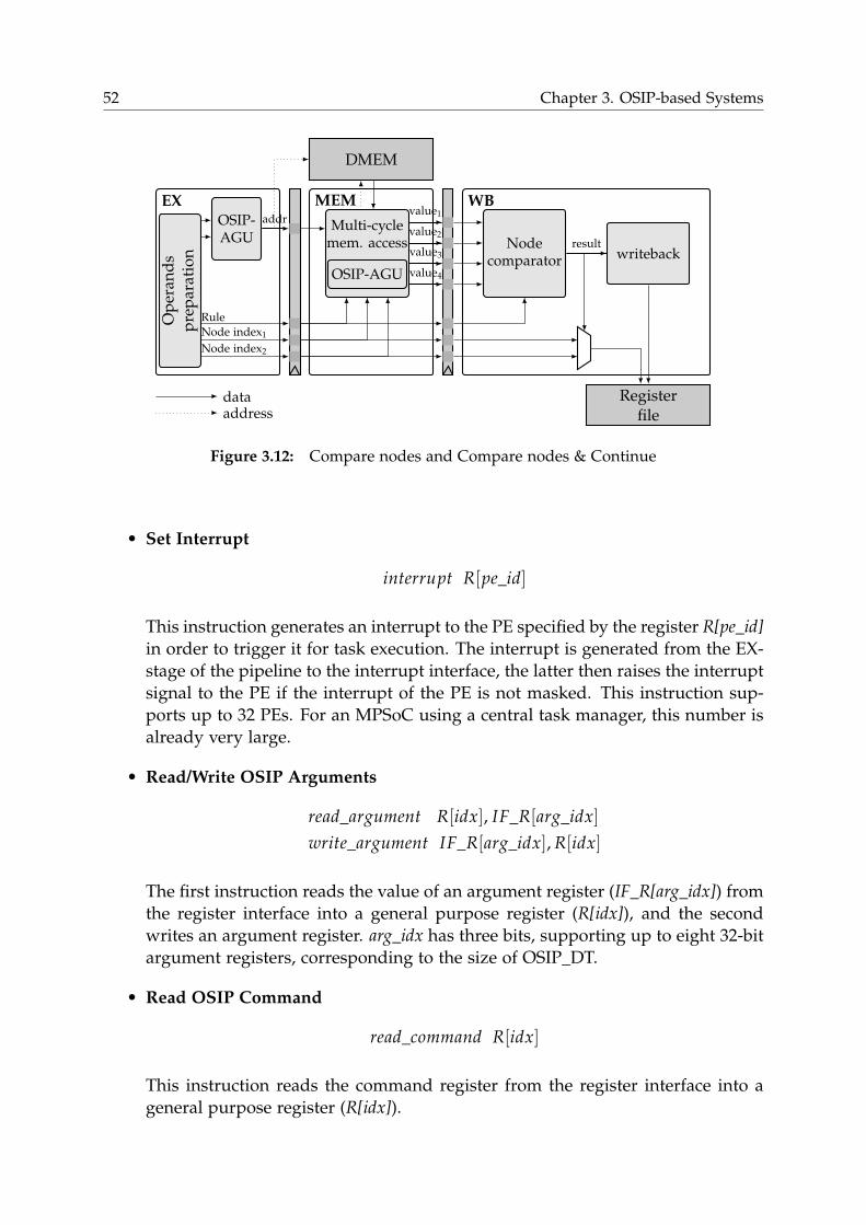
52 Chapter 3. OSIP-based Systems
EX MEM WB
Registerfile
DMEM
OSIP-AGU
Op
eran
ds
pre
par
atio
n
addr
Rule
Node index1
Node index2
Multi-cyclemem. access
OSIP-AGU
value1
value2
value3
value4
Nodecomparator writeback
result
dataaddress
Figure 3.12: Compare nodes and Compare nodes & Continue
• Set Interrupt
interrupt R[pe_id]
This instruction generates an interrupt to the PE specified by the register R[pe_id]
in order to trigger it for task execution. The interrupt is generated from the EX-
stage of the pipeline to the interrupt interface, the latter then raises the interrupt
signal to the PE if the interrupt of the PE is not masked. This instruction sup-
ports up to 32 PEs. For an MPSoC using a central task manager, this number is
already very large.
• Read/Write OSIP Arguments
read_argument R[idx], IF_R[arg_idx]
write_argument IF_R[arg_idx],R[idx]
The first instruction reads the value of an argument register (IF_R[arg_idx]) from
the register interface into a general purpose register (R[idx]), and the second
writes an argument register. arg_idx has three bits, supporting up to eight 32-bit
argument registers, corresponding to the size of OSIP_DT.
• Read OSIP Command
read_command R[idx]
This instruction reads the command register from the register interface into a
general purpose register (R[idx]).
3.2. OSIP Architecture Development 53
• Set Idle Status:
set_idle
This instruction sets the status register at the register interface to idle, indicating
that OSIP has finished the current command and is ready for executing the next
one. This instruction has no argument. The setting of the status takes place at
the DC-stage, and flushes the following instructions at the PFE- and FE-stage
from the pipeline.
Note that there is no explicit instruction to set the status register to busy. Instead,
the busy state is internally generated in the PFE-stage, which depends on the
current processor state and the input from the register interface to the OSIP
core. Details about this are given later in Section 3.2.3.3.
Accessing Command Handler Decoder: OSIP is a component which only reacts
to the requests from the PEs. When a new command arrives, OSIP first needs to
identify the corresponding command handler through a command handler decoder
(see the program memory structure in Figure 3.7), which follows a similar principle
as an interrupt vector table. So the entry address of the handler decoder must be
available at the arrival of the command. In OSIP, this entry address is stored in an
internal register, which enables a hardware-assisted PC determination. A dedicated
instruction is implemented for this purpose, which is shown below.
• Get Decoder Address:
get_decoder_address
The instruction determines the entry point to the command handler decoder. It
does not have an explicit argument, but uses its instruction address as an inter-
nal argument. By incrementing this address, it automatically calculates the ad-
dress of the following instruction. The calculated address is then stored into an
internal register called Decoder_PC (DPC). From the DPC, the command handler
decoder can be reached, which however should be ensured by the programmer.
In this work, this instruction is placed before a CALL instruction, which calls the
handler decoder. When OSIP switches from idle to busy at the arrival of a new
command, the PC is updated with DPC. More details about this are given in
Section 3.2.3.3.
In addition to getting the entry point to the handler decoder, this instruction
also sets the processor state to idle for the initialization purpose.
3.2.3.3 Interaction with Register Interface
When the OSIP core is at the busy state, i.e., executing a command, the processor
behaves in a standard way. At every cycle, a new PC is generated and a request is
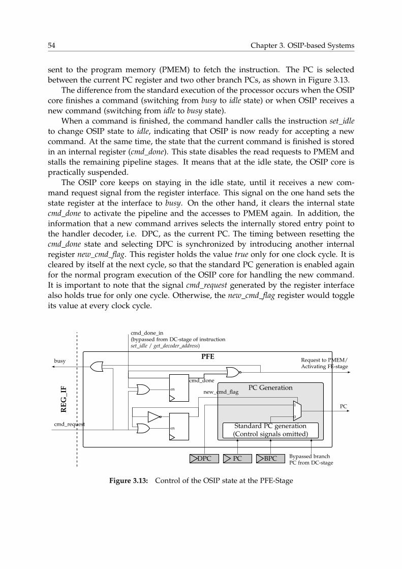
54 Chapter 3. OSIP-based Systems
sent to the program memory (PMEM) to fetch the instruction. The PC is selected
between the current PC register and two other branch PCs, as shown in Figure 3.13.
The difference from the standard execution of the processor occurs when the OSIP
core finishes a command (switching from busy to idle state) or when OSIP receives a
new command (switching from idle to busy state).
When a command is finished, the command handler calls the instruction set_idle
to change OSIP state to idle, indicating that OSIP is now ready for accepting a new
command. At the same time, the state that the current command is finished is stored
in an internal register (cmd_done). This state disables the read requests to PMEM and
stalls the remaining pipeline stages. It means that at the idle state, the OSIP core is
practically suspended.
The OSIP core keeps on staying in the idle state, until it receives a new com-
mand request signal from the register interface. This signal on the one hand sets the
state register at the interface to busy. On the other hand, it clears the internal state
cmd_done to activate the pipeline and the accesses to PMEM again. In addition, the
information that a new command arrives selects the internally stored entry point to
the handler decoder, i.e. DPC, as the current PC. The timing between resetting the
cmd_done state and selecting DPC is synchronized by introducing another internal
register new_cmd_flag. This register holds the value true only for one clock cycle. It is
cleared by itself at the next cycle, so that the standard PC generation is enabled again
for the normal program execution of the OSIP core for handling the new command.
It is important to note that the signal cmd_request generated by the register interface
also holds true for only one cycle. Otherwise, the new_cmd_flag register would toggle
its value at every clock cycle.
PFE
RE
G_IF en
en
PC Generation
Standard PC generation(Control signals omitted)
BPCPCDPC Bypassed branchPC from DC-stage
0
1
cmd_done
cmd_done_in(bypassed from DC-stage of instructionset_idle / get_decoder_address)
cmd_request
busy
new_cmd_flag
PC
Request to PMEM/Activating FE-stage
Figure 3.13: Control of the OSIP state at the PFE-Stage
3.2. OSIP Architecture Development 55
3.2.4 OSIP Code Example
In this section, an exemplary code of programming the OSIP core is shown, explaining
in detail how the processor is controlled by the software to handle the commands and
especially to synchronize with the register interface, consequently with the PEs of the
system.
The code is given in Listing 3.8. It starts with a typical booting process of a proces-
sor such as the initialization of the stack and frame pointer and other initializations
(line 3–4). By now the processor is at the busy state, because the internal register
cmd_done is set to false when the processor is reset.
Then, the instruction get_decoder_address is executed to get the entry point to the
handler decoder, in this case the main() function, and to set the processor status to
idle. The register DPC now gets the address of the instruction which calls the main()
function (line 6). At this point, the processor has been booted, but does not execute
further instructions, until a new command request is sent from the register interface.
At the arrival of a command request, the processor is awaken to take the DPC
as the next to be executed PC and continues with the program at line 6. Then the
command and arguments are read from the register interface (line 16–17). Afterwards,
the command is decoded and the corresponding handler of the command is called
(line 18–22). After handling the command, results are written back to the argument
registers at the interface (line 26), and the program execution jumps directly to the
idle section (line 27).
In the idle section (line 8–10), the instruction set_idle (line 10) is executed, which
again sets the processor state to idle for receiving the next command. For the next
command, the program execution starts from line 6 again.
Note that at the end of the command execution in the handler, it does not nec-
essarily need to directly jump to the idle section. A conventional way can also be
followed, in which the program is executed to the end of the main() function, then en-
ters the idle section. However, this can introduce a lot of runtime overhead caused by
the calling stacks. In fact, between two consecutive commands no context information
(registers and memory content) needs to be maintained, except the static array allo-
cated for the OSIP_DTs. As introduced in Section 3.2.3.2, this array is not reachable
by the C-compiler. Therefore, the information inside the array is untouched and safe
if skipping the recovery process of the calling stacks, as done in this exemplary code.
But there is one step that must be done before entering the idle state, namely resetting
the stack pointer and the frame pointer (line 9)2. This step is important for preventing
stack overflow. Otherwise, the stack and frame pointer would continuously increase
from one command to the next.
2 Theoretically, the same thing should also be done for the heap. However, the use of malloc() is avoidedand also not needed in the OSIP application.
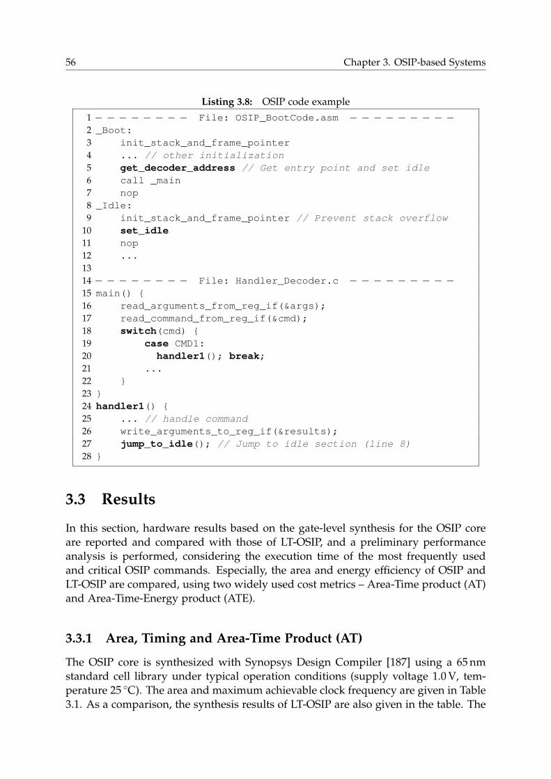
56 Chapter 3. OSIP-based Systems
Listing 3.8: OSIP code example
1 − − − − − − − − File: OSIP_BootCode.asm − − − − − − − − −2 _Boot:
3 init_stack_and_frame_pointer
4 ... // other initialization
5 get_decoder_address // Get entry point and set idle
6 call _main
7 nop
8 _Idle:
9 init_stack_and_frame_pointer // Prevent stack overflow
10 set_idle
11 nop
12 ...
13
14 − − − − − − − − File: Handler_Decoder.c − − − − − − − − −15 main() {
16 read_arguments_from_reg_if(&args);
17 read_command_from_reg_if(&cmd);
18 switch(cmd) {
19 case CMD1:
20 handler1(); break;
21 ...
22 }
23 }
24 handler1() {
25 ... // handle command
26 write_arguments_to_reg_if(&results);
27 jump_to_idle(); // Jump to idle section (line 8)
28 }
3.3 Results
In this section, hardware results based on the gate-level synthesis for the OSIP core
are reported and compared with those of LT-OSIP, and a preliminary performance
analysis is performed, considering the execution time of the most frequently used
and critical OSIP commands. Especially, the area and energy efficiency of OSIP and
LT-OSIP are compared, using two widely used cost metrics – Area-Time product (AT)
and Area-Time-Energy product (ATE).
3.3.1 Area, Timing and Area-Time Product (AT)
The OSIP core is synthesized with Synopsys Design Compiler [187] using a 65 nm
standard cell library under typical operation conditions (supply voltage 1.0V, tem-
perature 25 ◦C). The area and maximum achievable clock frequency are given in Table
3.1. As a comparison, the synthesis results of LT-OSIP are also given in the table. The
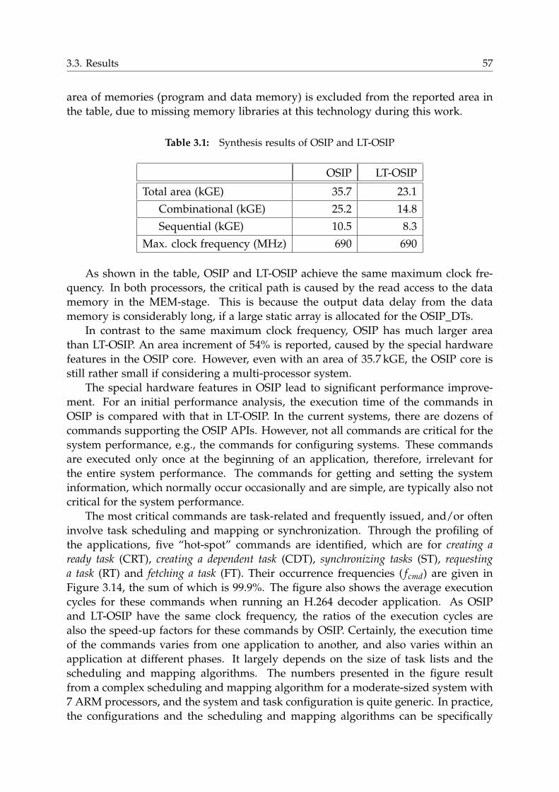
3.3. Results 57
area of memories (program and data memory) is excluded from the reported area in
the table, due to missing memory libraries at this technology during this work.
Table 3.1: Synthesis results of OSIP and LT-OSIP
OSIP LT-OSIP
Total area (kGE) 35.7 23.1
Combinational (kGE) 25.2 14.8
Sequential (kGE) 10.5 8.3
Max. clock frequency (MHz) 690 690
As shown in the table, OSIP and LT-OSIP achieve the same maximum clock fre-
quency. In both processors, the critical path is caused by the read access to the data
memory in the MEM-stage. This is because the output data delay from the data
memory is considerably long, if a large static array is allocated for the OSIP_DTs.
In contrast to the same maximum clock frequency, OSIP has much larger area
than LT-OSIP. An area increment of 54% is reported, caused by the special hardware
features in the OSIP core. However, even with an area of 35.7 kGE, the OSIP core is
still rather small if considering a multi-processor system.
The special hardware features in OSIP lead to significant performance improve-
ment. For an initial performance analysis, the execution time of the commands in
OSIP is compared with that in LT-OSIP. In the current systems, there are dozens of
commands supporting the OSIP APIs. However, not all commands are critical for the
system performance, e.g., the commands for configuring systems. These commands
are executed only once at the beginning of an application, therefore, irrelevant for
the entire system performance. The commands for getting and setting the system
information, which normally occur occasionally and are simple, are typically also not
critical for the system performance.
The most critical commands are task-related and frequently issued, and/or often
involve task scheduling and mapping or synchronization. Through the profiling of
the applications, five “hot-spot” commands are identified, which are for creating a
ready task (CRT), creating a dependent task (CDT), synchronizing tasks (ST), requesting
a task (RT) and fetching a task (FT). Their occurrence frequencies ( fcmd) are given in
Figure 3.14, the sum of which is 99.9%. The figure also shows the average execution
cycles for these commands when running an H.264 decoder application. As OSIP
and LT-OSIP have the same clock frequency, the ratios of the execution cycles are
also the speed-up factors for these commands by OSIP. Certainly, the execution time
of the commands varies from one application to another, and also varies within an
application at different phases. It largely depends on the size of task lists and the
scheduling and mapping algorithms. The numbers presented in the figure result
from a complex scheduling and mapping algorithm for a moderate-sized system with
7 ARM processors, and the system and task configuration is quite generic. In practice,
the configurations and the scheduling and mapping algorithms can be specifically
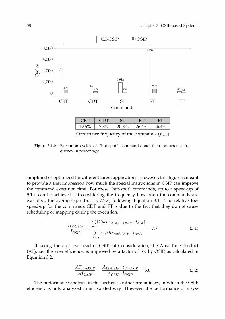
58 Chapter 3. OSIP-based Systems
CRT CDT ST RT FT
0
2,000
4,000
6,000
8,000
3,791
869
1,912
7,197
337498 305 252792
135
Commands
Cy
cles
LT-OSIP OSIP
CRT CDT ST RT FT
19.5% 7.3% 20.3% 26.4% 26.4%
Occurrence frequency of the commands ( fcmd)
Figure 3.14: Execution cycles of “hot-spot” commands and their occurrence fre-quency in percentage
simplified or optimized for different target applications. However, this figure is meant
to provide a first impression how much the special instructions in OSIP can improve
the command execution time. For these “hot-spot” commands, up to a speed-up of
9.1× can be achieved. If considering the frequency how often the commands are
executed, the average speed-up is 7.7×, following Equation 3.1. The relative low
speed-up for the commands CDT and FT is due to the fact that they do not cause
scheduling or mapping during the execution.
tLT-OSIP
tOSIP=
∑
cmd
(Cyclescmd,LT-OSIP · fcmd)
∑
cmd
(Cyclescmd,OSIP · fcmd)= 7.7 (3.1)
If taking the area overhead of OSIP into consideration, the Area-Time-Product
(AT), i.e. the area efficiency, is improved by a factor of 5× by OSIP, as calculated in
Equation 3.2.
ATLT-OSIP
ATOSIP=
ALT-OSIP · tLT-OSIP
AOSIP · tOSIP= 5.0 (3.2)
The performance analysis in this section is rather preliminary, in which the OSIP
efficiency is only analyzed in an isolated way. However, the performance of a sys-

3.3. Results 59
tem does not only depend on the efficiency of the task manager, even though it is
certainly an important factor, but also on many others, such as task sizes, the commu-
nication architecture, etc. The bottleneck component of the system finally determines
the system performance. The bottleneck could be the manager, or the communication
architecture as well as the PEs. A systematic system-level analysis needs to be made
for a more comprehensive evaluation of the OSIP performance, which will be shown
in the next chapter.
3.3.2 Power, Energy and Area-Time-Energy Product (ATE)
The power consumption of the OSIP core is estimated using post-synthesis gate-level
power simulation with Synopsys PrimeTime [188], running a H.264 video decoding
at a clock frequency of 690MHz with a supply voltage of 1.0V. The power of the
memories is not considered.
As described in Section 3.2.3.3, the OSIP core has two states: busy and idle. In Table
3.2, the average power consumption of OSIP at both states is listed. At the idle state,
the OSIP core consumes about 7.2% of the power at the busy state. While the static
power stays almost unchanged, since it is only influenced by the area, the dynamic
power is reduced by a factor of 17.3× from the busy state to the idle state.
Table 3.2: Power consumption of OSIP and LT-OSIP
OSIP LT-OSIP
Busy (mW) 17.20 8.54
Dynamic Power (mW) 16.92 8.38
Static Power (mW) 0.28 0.16
Idle (mW) 1.25 0.95
Dynamic Power (mW) 0.98 0.80
Static Power (mW) 0.27 0.15
A detailed analysis of the power consumption of the OSIP core is depicted in
Figure 3.15. For both OSIP states, the main contributor to the power consumption
is the clock tree, including the clock gating elements and the clock pins driving the
registers.3 In the busy state, the contribution by the registers and the combinational
logic is also considerably large in comparison to the idle state. For the latter, the
contribution by the registers and the combination logic is only due to the static power,
as the complete pipeline is deactivated, i.e., no data switching in the pipeline.
Table 3.2 also presents the average power consumption of LT-OSIP. Compared to
OSIP, LT-OSIP consumes less power than OSIP, both in the busy and idle state, which
3 In a gate-level synthesis, the clock tree buffers are typically not generated. Therefore, Figure 3.15 doesnot present the power consumed by the clock tree buffers.
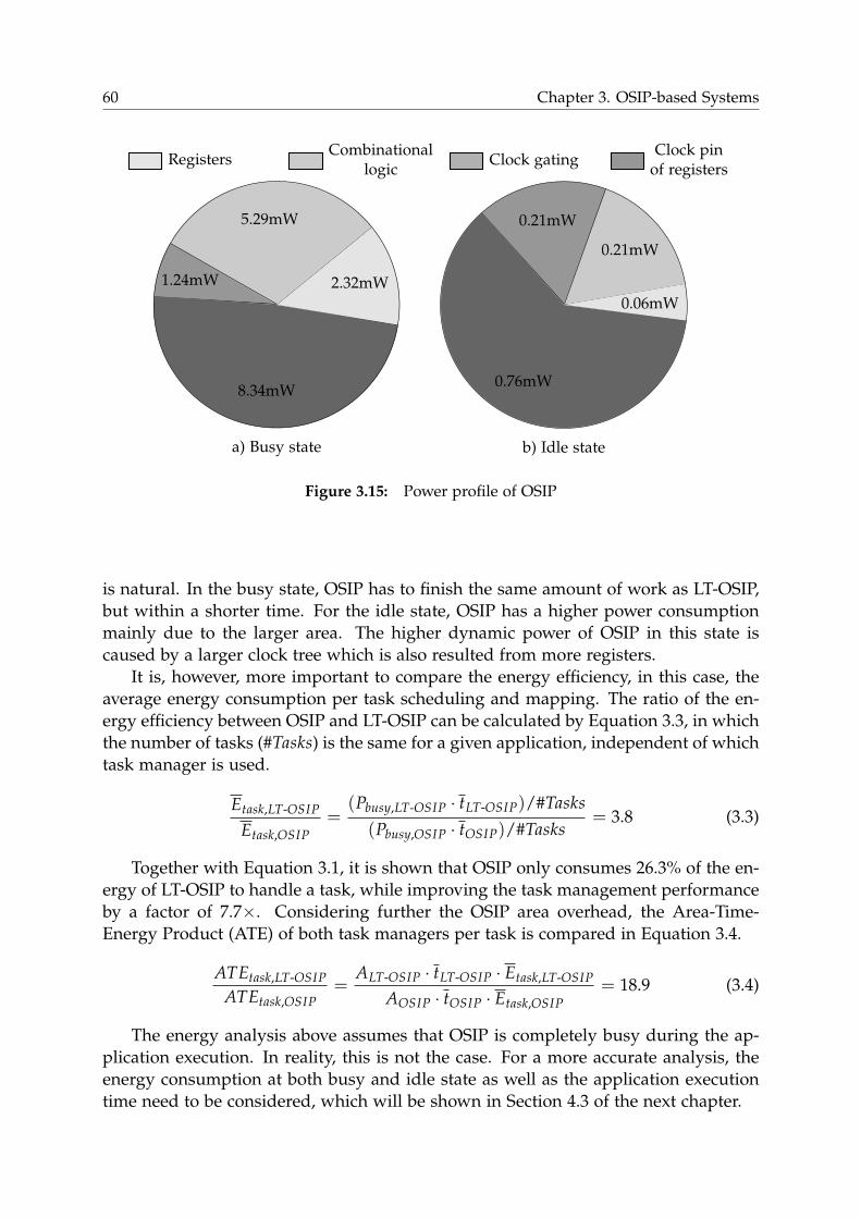
60 Chapter 3. OSIP-based Systems
1.24mW
8.34mW
2.32mW
5.29mW
a) Busy state
0.21mW
0.76mW
0.06mW
0.21mW
b) Idle state
RegistersCombinational
logicClock gating
Clock pinof registers
Figure 3.15: Power profile of OSIP
is natural. In the busy state, OSIP has to finish the same amount of work as LT-OSIP,
but within a shorter time. For the idle state, OSIP has a higher power consumption
mainly due to the larger area. The higher dynamic power of OSIP in this state is
caused by a larger clock tree which is also resulted from more registers.
It is, however, more important to compare the energy efficiency, in this case, the
average energy consumption per task scheduling and mapping. The ratio of the en-
ergy efficiency between OSIP and LT-OSIP can be calculated by Equation 3.3, in which
the number of tasks (#Tasks) is the same for a given application, independent of which
task manager is used.
Etask,LT-OSIP
Etask,OSIP
=(Pbusy,LT-OSIP · tLT-OSIP)/#Tasks
(Pbusy,OSIP · tOSIP)/#Tasks= 3.8 (3.3)
Together with Equation 3.1, it is shown that OSIP only consumes 26.3% of the en-
ergy of LT-OSIP to handle a task, while improving the task management performance
by a factor of 7.7×. Considering further the OSIP area overhead, the Area-Time-
Energy Product (ATE) of both task managers per task is compared in Equation 3.4.
ATEtask,LT-OSIP
ATEtask,OSIP=
ALT-OSIP · tLT-OSIP · Etask,LT-OSIP
AOSIP · tOSIP · Etask,OSIP
= 18.9 (3.4)
The energy analysis above assumes that OSIP is completely busy during the ap-
plication execution. In reality, this is not the case. For a more accurate analysis, the
energy consumption at both busy and idle state as well as the application execution
time need to be considered, which will be shown in Section 4.3 of the next chapter.
3.4. Summary 61
3.4 Summary
In this chapter, an overview of OSIP-based systems is given, and the major advantages
of such systems are highlighted from the efficiency and flexibility perspective.
As the key component of the system, the architecture of OSIP – an application-
specific processor for OS, is described in detail. A preliminary performance analysis
already shows the efficiency of OSIP in the task management by comparing it with
a generic RISC processor. The control-centric OSIP architecture development is chal-
lenging. But it is effectively overcome with the special hardware features for handling
list-based operations, fast memory accesses and comparing list nodes as well as com-
pact branch instructions. The hardware results including the area, timing and the
power are presented, and the area and energy efficiency of OSIP is highlighted.
3.5 Discussion
The special hardware features in OSIP improve the OSIP efficiency, but at the cost of
the reduced flexibility. Among these hardware features, the OSIP-AGU and the node
comparator are the most prominent ones, which are discussed in this section.
3.5.1 OSIP Address Generation Unit (OSIP-AGU)
The OSIP-AGU, which introduces little hardware overhead, greatly speeds up the
memory accesses to the OSIP_DTs. This is thanks to the regular structure of the
OSIP_DTs with eight words and their arrangement in a static array, for which a simple
address generation using a shift operation by a constant and basic logic operations
instead of arithmetic operations becomes possible. However, this can be a limitation
in the programming, if over eight words are needed for a node.
Normally, eight words are already large enough for storing the necessary informa-
tion in a node, whether for a task node, a scheduling/mapping node or for a PE node.
In fact, there are still fields in the nodes, which are not used, but reserved for future
extensions. In case that more words are really needed for storing the information, a
workaround has to be done. For example, the node information can be distributed
in two consecutive OSIP_DTs, so that the OSIP-AGU is still applicable. Of course,
necessary information conversions between the node and the OSIP_DT structure for
the index and word offset must be made in the OSIP software. If the number of the
needed words for the node is not a multiple of eight, some words get wasted.
On the other hand, if the designer wants to reduce the memory usage by reducing
the node size, in case that less information is needed for a node, it is not possible with
the OSIP-AGU. This also means wasting memory words.
A more generic way of implementing the OSIP-AGU would be using a hardware
multiplier, which multiplies the node index by the node size (i.e., the number of
words per node) to calculate the base address of a node. Then, the word offset is
added with the base address to obtain the final word address. In comparison with the
current OSIP-AGU, this implementation would result in a larger area in the pipeline
62 Chapter 3. OSIP-based Systems
and possibly worsen the timing. However, for certain applications, it could enable
better memory utilization and also has higher flexibility. Hence, a trade-off can be
considered.
3.5.2 Node Comparator
The node comparator is another hardware feature, which can have flexibility limita-
tions when using the cmp_node and cmp_node_e instructions. Naturally, it is impossible
for a hardware node comparator to cover all possible comparison rules and different
combinations, and the current comparator already supports a quite wide range of
rules. However, if new rules should be applied, software implementation is needed
in the OSIP scheduling algorithms to support them. To still be able to use these two
special instructions for node comparison, an additional flag can be introduced in the
software to distinguish the currently supported rules and the new ones.
Another approach of implementing a flexible comparator, which at the same time
can cover an even larger range of rules in hardware, is using a Coarse-Grained Re-
configurable Architecture (CGRA) [39, 76, 129, 172], in which different rules can be
configured statically or dynamically.
Chapter 4
System-Level Analysis of OSIPEfficiency
As a central task manager, the efficiency of OSIP undoubtedly has a big impact on the
system performance. The previous chapter has made a preliminary analysis of the
OSIP efficiency by analyzing the execution time of the most critical OSIP commands
for scheduling and mapping tasks. In comparison to a RISC-based task manager,
OSIP is able to execute these commands within much less time. However, from the
system perspective, this analysis is only isolated and rather one-sided, as it does not
show how the OSIP efficiency influences the overall system performance.
For a complete system, its performance depends on many factors, among which
the performance of PEs, the task sizes and the communication architecture are es-
pecially important in addition to the task manager. These factors need to be jointly
investigated in order to analyze the OSIP efficiency in a system context. In this chap-
ter, a thorough characterization of the performance of OSIP is provided from the
system point of view. A special focus is laid on the joint impact of the communication
architecture and the OSIP efficiency, as the communication architecture has become
one of the dominant factors for the performance of modern MPSoCs.
This chapter is organized as follows. First, the system setup for the analysis and
the benchmarking applications — a synthetic application and a real-life H.264 video
decoding application — are introduced. Then, the OSIP-efficiency is analyzed in
systems without considering the communication overhead by idealizing the commu-
nication architecture. Afterwards, the impact of the communication architecture on
the OSIP-based system performance is highlighted. Following this, optimized realis-
tic communication architectures are presented. Based on the resulted different com-
munication architectures, the impact of the OSIP efficiency and the communication
architecture on the system performance is jointly investigated. Finally, a summary is
made for the OSIP efficiency from the system perspective.1
4.1 System Setup
For evaluating the OSIP efficiency at the system-level, a virtual platform is built using
Synopsys Platform Architect. The platform consists of several instruction-accurate
ARM926EJ-S processor models, an OSIP model, a shared memory and some periph-
1 Portions of this chapter have been published by the author in [214] in the International Journal ofEmbedded and Real-Time Communication Systems, edited by Seppo Virtanen. Copyright 2011, IGI Global,www.igi-global.com. Posted by permission of the publisher.
63
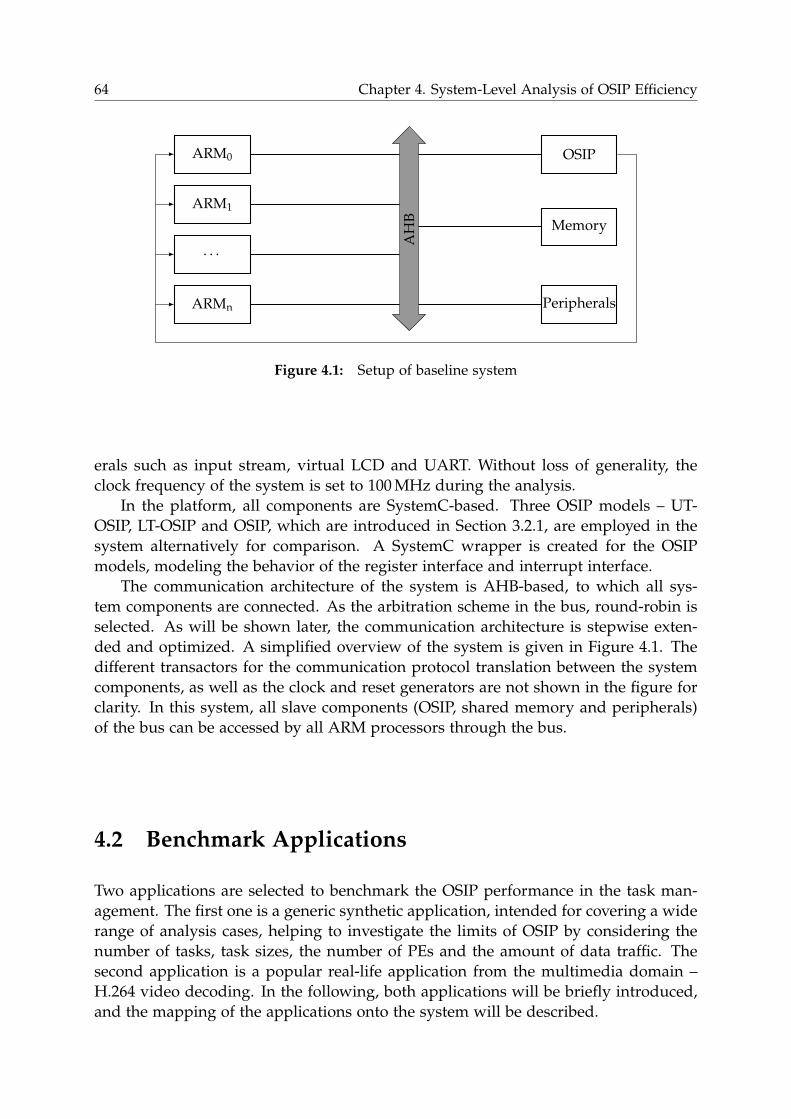
64 Chapter 4. System-Level Analysis of OSIP Efficiency
ARM0
ARM1
. . .
ARMn
AH
B
OSIP
Memory
Peripherals
Figure 4.1: Setup of baseline system
erals such as input stream, virtual LCD and UART. Without loss of generality, the
clock frequency of the system is set to 100MHz during the analysis.
In the platform, all components are SystemC-based. Three OSIP models – UT-
OSIP, LT-OSIP and OSIP, which are introduced in Section 3.2.1, are employed in the
system alternatively for comparison. A SystemC wrapper is created for the OSIP
models, modeling the behavior of the register interface and interrupt interface.
The communication architecture of the system is AHB-based, to which all sys-
tem components are connected. As the arbitration scheme in the bus, round-robin is
selected. As will be shown later, the communication architecture is stepwise exten-
ded and optimized. A simplified overview of the system is given in Figure 4.1. The
different transactors for the communication protocol translation between the system
components, as well as the clock and reset generators are not shown in the figure for
clarity. In this system, all slave components (OSIP, shared memory and peripherals)
of the bus can be accessed by all ARM processors through the bus.
4.2 Benchmark Applications
Two applications are selected to benchmark the OSIP performance in the task man-
agement. The first one is a generic synthetic application, intended for covering a wide
range of analysis cases, helping to investigate the limits of OSIP by considering the
number of tasks, task sizes, the number of PEs and the amount of data traffic. The
second application is a popular real-life application from the multimedia domain –
H.264 video decoding. In the following, both applications will be briefly introduced,
and the mapping of the applications onto the system will be described.
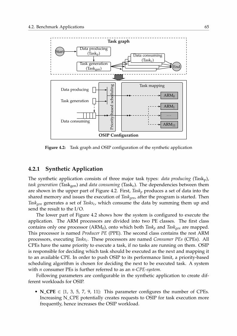
4.2. Benchmark Applications 65
OSIP Configuration
Task graph
Task mapping
Pri
ori
ty-b
ased
sch
edu
lin
g
Data producing
Task generation
Data consuming
ARM0
. . .
ARM1
ARM11
StartData producing
(Taskp)
Task generation(Taskgen)
Data consuming(Taskc)
End
Figure 4.2: Task graph and OSIP configuration of the synthetic application
4.2.1 Synthetic Application
The synthetic application consists of three major task types: data producing (Taskp),
task generation (Taskgen) and data consuming (Taskc). The dependencies between them
are shown in the upper part of Figure 4.2. First, Taskp produces a set of data into the
shared memory and issues the execution of Taskgen, after the program is started. Then
Taskgen generates a set of Tasksc, which consume the data by summing them up and
send the result to the I/O.
The lower part of Figure 4.2 shows how the system is configured to execute the
application. The ARM processors are divided into two PE classes. The first class
contains only one processor (ARM0), onto which both Taskp and Taskgen are mapped.
This processor is named Producer PE (PPE). The second class contains the rest ARM
processors, executing Tasksc. These processors are named Consumer PEs (CPEs). All
CPEs have the same priority to execute a task, if no tasks are running on them. OSIP
is responsible for deciding which task should be executed as the next and mapping it
to an available CPE. In order to push OSIP to its performance limit, a priority-based
scheduling algorithm is chosen for deciding the next to be executed task. A system
with n consumer PEs is further referred to as an n-CPE-system.
Following parameters are configurable in the synthetic application to create dif-
ferent workloads for OSIP.
• N_CPE ∈ {1, 3, 5, 7, 9, 11}: This parameter configures the number of CPEs.
Increasing N_CPE potentially creates requests to OSIP for task execution more
frequently, hence increases the OSIP workload.
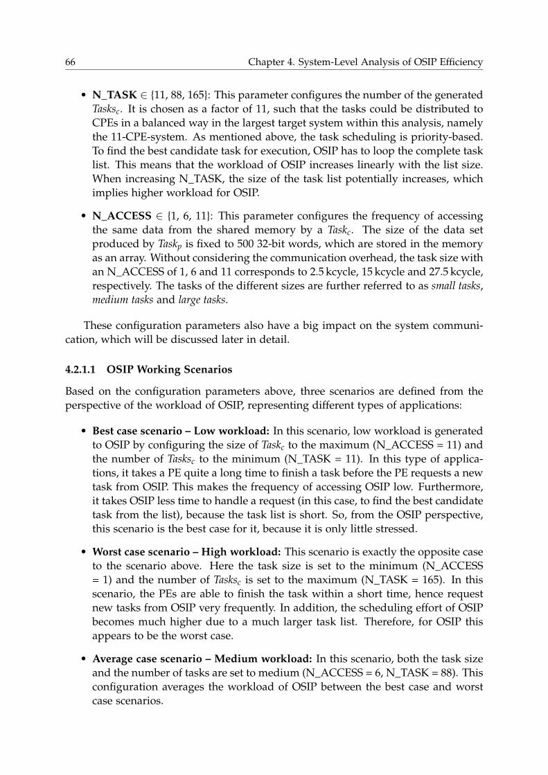
66 Chapter 4. System-Level Analysis of OSIP Efficiency
• N_TASK ∈ {11, 88, 165}: This parameter configures the number of the generated
Tasksc. It is chosen as a factor of 11, such that the tasks could be distributed to
CPEs in a balanced way in the largest target system within this analysis, namely
the 11-CPE-system. As mentioned above, the task scheduling is priority-based.
To find the best candidate task for execution, OSIP has to loop the complete task
list. This means that the workload of OSIP increases linearly with the list size.
When increasing N_TASK, the size of the task list potentially increases, which
implies higher workload for OSIP.
• N_ACCESS ∈ {1, 6, 11}: This parameter configures the frequency of accessing
the same data from the shared memory by a Taskc. The size of the data set
produced by Taskp is fixed to 500 32-bit words, which are stored in the memory
as an array. Without considering the communication overhead, the task size with
an N_ACCESS of 1, 6 and 11 corresponds to 2.5 kcycle, 15 kcycle and 27.5 kcycle,
respectively. The tasks of the different sizes are further referred to as small tasks,
medium tasks and large tasks.
These configuration parameters also have a big impact on the system communi-
cation, which will be discussed later in detail.
4.2.1.1 OSIP Working Scenarios
Based on the configuration parameters above, three scenarios are defined from the
perspective of the workload of OSIP, representing different types of applications:
• Best case scenario – Low workload: In this scenario, low workload is generated
to OSIP by configuring the size of Taskc to the maximum (N_ACCESS = 11) and
the number of Tasksc to the minimum (N_TASK = 11). In this type of applica-
tions, it takes a PE quite a long time to finish a task before the PE requests a new
task from OSIP. This makes the frequency of accessing OSIP low. Furthermore,
it takes OSIP less time to handle a request (in this case, to find the best candidate
task from the list), because the task list is short. So, from the OSIP perspective,
this scenario is the best case for it, because it is only little stressed.
• Worst case scenario – High workload: This scenario is exactly the opposite case
to the scenario above. Here the task size is set to the minimum (N_ACCESS
= 1) and the number of Tasksc is set to the maximum (N_TASK = 165). In this
scenario, the PEs are able to finish the task within a short time, hence request
new tasks from OSIP very frequently. In addition, the scheduling effort of OSIP
becomes much higher due to a much larger task list. Therefore, for OSIP this
appears to be the worst case.
• Average case scenario – Medium workload: In this scenario, both the task size
and the number of tasks are set to medium (N_ACCESS = 6, N_TASK = 88). This
configuration averages the workload of OSIP between the best case and worst
case scenarios.
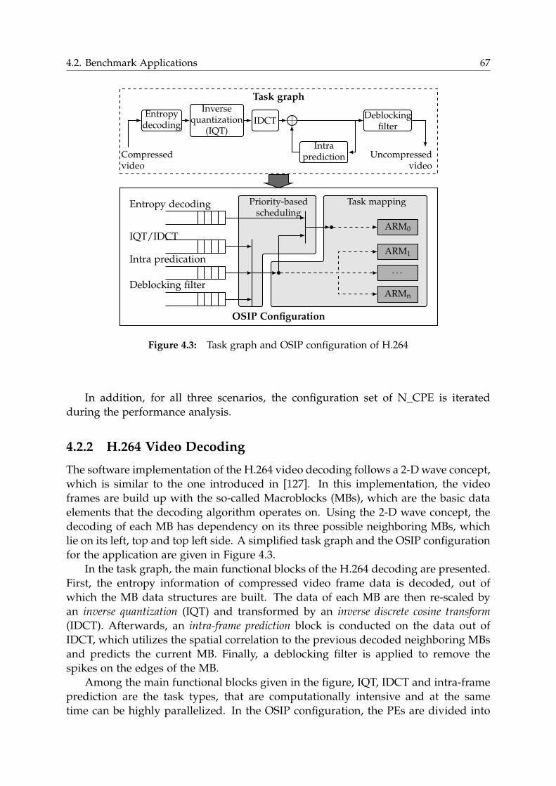
4.2. Benchmark Applications 67
OSIP Configuration
Task graph
Task mappingPriority-basedscheduling
ARM0
. . .
ARM1
ARMn
Entropy decoding
IQT/IDCT
Intra predication
Deblocking filter
Entropydecoding
Inversequantization
(IQT)IDCT
Deblockingfilter
IntrapredictionCompressed
videoUncompressed
video
Figure 4.3: Task graph and OSIP configuration of H.264
In addition, for all three scenarios, the configuration set of N_CPE is iterated
during the performance analysis.
4.2.2 H.264 Video Decoding
The software implementation of the H.264 video decoding follows a 2-D wave concept,
which is similar to the one introduced in [127]. In this implementation, the video
frames are build up with the so-called Macroblocks (MBs), which are the basic data
elements that the decoding algorithm operates on. Using the 2-D wave concept, the
decoding of each MB has dependency on its three possible neighboring MBs, which
lie on its left, top and top left side. A simplified task graph and the OSIP configuration
for the application are given in Figure 4.3.
In the task graph, the main functional blocks of the H.264 decoding are presented.
First, the entropy information of compressed video frame data is decoded, out of
which the MB data structures are built. The data of each MB are then re-scaled by
an inverse quantization (IQT) and transformed by an inverse discrete cosine transform
(IDCT). Afterwards, an intra-frame prediction block is conducted on the data out of
IDCT, which utilizes the spatial correlation to the previous decoded neighboring MBs
and predicts the current MB. Finally, a deblocking filter is applied to remove the
spikes on the edges of the MB.
Among the main functional blocks given in the figure, IQT, IDCT and intra-frame
prediction are the task types, that are computationally intensive and at the same
time can be highly parallelized. In the OSIP configuration, the PEs are divided into
68 Chapter 4. System-Level Analysis of OSIP Efficiency
two classes. The first class contains a single PE (ARM0), on which the task type
entropy decoding is mapped. After the entropy decoding is finished, parallel operations
on the MBs are possible. The second PE class then includes all PEs, and all task
types except the entropy decoding are mapped onto this class. In the actual software
implementation, IQT and IDCT are merged.
For the system performance analysis purpose, the number of PEs is set to be
configurable in the software implementation. The different PE number results in
different frame rates, which are given in Frame per Second (fps). This frame rate is
used as the criterion for evaluating the OSIP efficiency.
4.3 Efficiency Analysis with an Ideal Communication
Architecture
The performance of a system depends on many factors, among which the commu-
nication architecture has a large impact. In this section, to isolate the effect of the
scheduling and mapping efficiency of OSIP, the communication architecture is first
bypassed in the simulation platform. With this, an idealized communication architec-
ture is obtained, i.e., the data communication through the bus introduces no latency
in the system. In other words, the communication architecture of the system has an
infinitive bandwidth.
4.3.1 Synthetic Application
In the synthetic application, the execution times of the application using the three
different OSIP implementations, namely OSIP, LT-OSIP and UT-OSIP, are compared.
In the upper part of Figure 4.4, an overview of the application execution time in
different scenarios is presented. The following observations can be made.
First, the OSIP-based systems and the UT-OSIP-based systems have a close system
performance. In general, with more workload generated onto OSIP, the difference of
the execution times between these two systems increases. However, even in the worst
case scenario, the difference is rather small. In the best case scenario, the difference is
only marginal. In contrast, the system performance based on LT-OSIP is much worse
than that of the other two for all scenarios.
Second, the system behaviors of the OSIP-based and UT-OSIP-based systems are
very similar. With the increasing number of the PEs, the execution time decreases. In
the average case and worst case scenarios, the performance becomes saturated in large
systems in terms of a large number of PEs. In the former case, the saturation starts
with a 7-CPE-system and in the latter case it already starts with a 3-CPE-system. In
these systems, the system performance is limited by the degree of the task parallelism,
which is obviously not able to match the computational power provided by the given
PEs.
In the LT-OSIP-based systems, the curves of the execution time present a very dif-
ferent performance behavior. In all three scenarios, the execution time first decreases
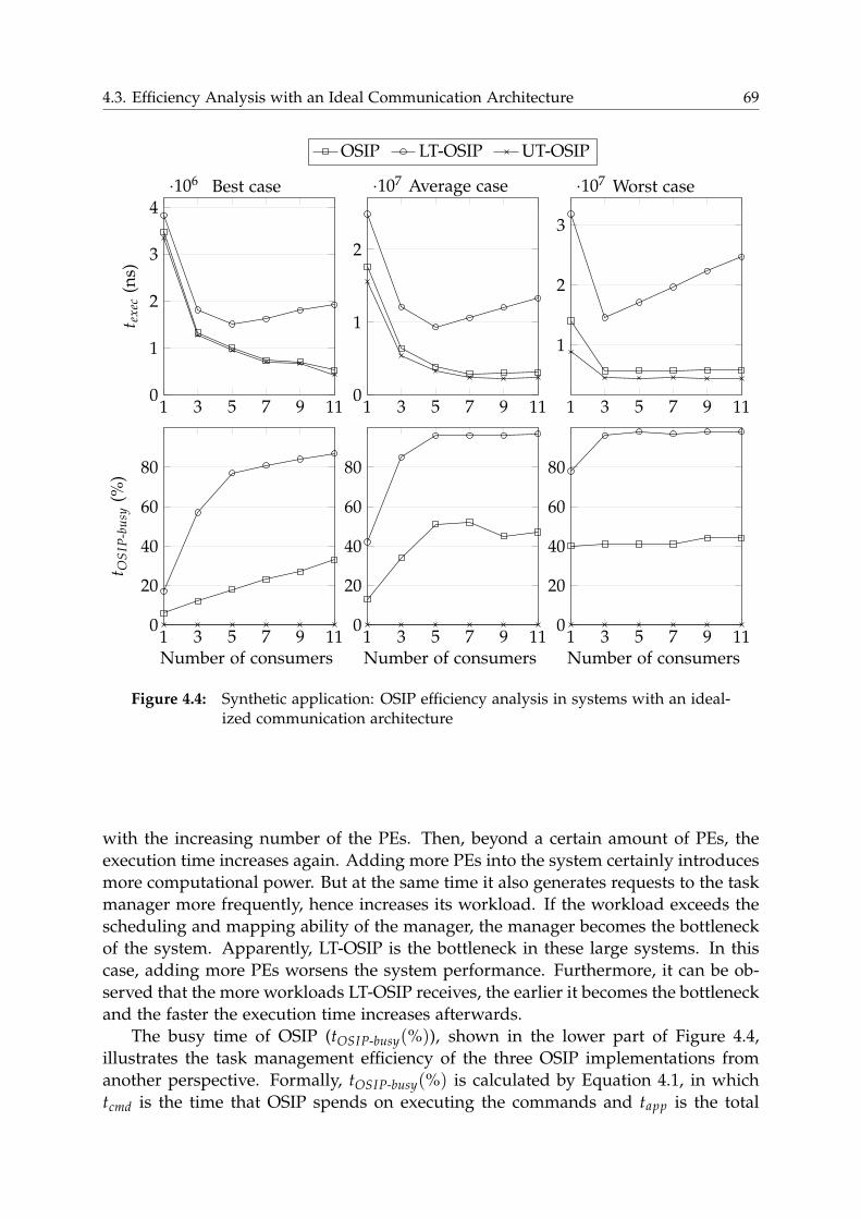
4.3. Efficiency Analysis with an Ideal Communication Architecture 69
1 3 5 7 9 110
1
2
3
4·106
t ex
ec(n
s)
Best case
1 3 5 7 9 110
1
2
·107
OSIP LT-OSIP UT-OSIP
Average case
1 3 5 7 9 11
1
2
3
·107 Worst case
1 3 5 7 9 110
20
40
60
80
t OS
IP-b
usy
(%)
Number of consumers1 3 5 7 9 11
0
20
40
60
80
Number of consumers1 3 5 7 9 11
0
20
40
60
80
Number of consumers
Figure 4.4: Synthetic application: OSIP efficiency analysis in systems with an ideal-ized communication architecture
with the increasing number of the PEs. Then, beyond a certain amount of PEs, the
execution time increases again. Adding more PEs into the system certainly introduces
more computational power. But at the same time it also generates requests to the task
manager more frequently, hence increases its workload. If the workload exceeds the
scheduling and mapping ability of the manager, the manager becomes the bottleneck
of the system. Apparently, LT-OSIP is the bottleneck in these large systems. In this
case, adding more PEs worsens the system performance. Furthermore, it can be ob-
served that the more workloads LT-OSIP receives, the earlier it becomes the bottleneck
and the faster the execution time increases afterwards.
The busy time of OSIP (tOSIP-busy(%)), shown in the lower part of Figure 4.4,
illustrates the task management efficiency of the three OSIP implementations from
another perspective. Formally, tOSIP-busy(%) is calculated by Equation 4.1, in which
tcmd is the time that OSIP spends on executing the commands and tapp is the total
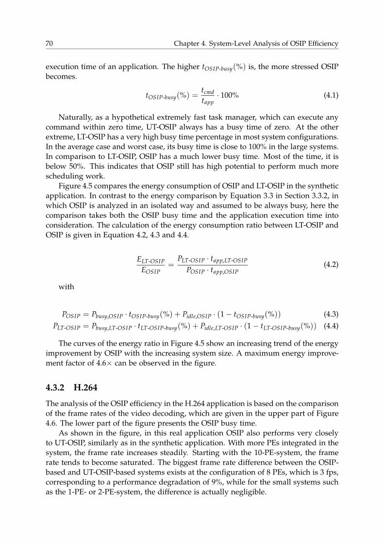
70 Chapter 4. System-Level Analysis of OSIP Efficiency
execution time of an application. The higher tOSIP-busy(%) is, the more stressed OSIP
becomes.
tOSIP-busy(%) =tcmd
tapp· 100% (4.1)
Naturally, as a hypothetical extremely fast task manager, which can execute any
command within zero time, UT-OSIP always has a busy time of zero. At the other
extreme, LT-OSIP has a very high busy time percentage in most system configurations.
In the average case and worst case, its busy time is close to 100% in the large systems.
In comparison to LT-OSIP, OSIP has a much lower busy time. Most of the time, it is
below 50%. This indicates that OSIP still has high potential to perform much more
scheduling work.
Figure 4.5 compares the energy consumption of OSIP and LT-OSIP in the synthetic
application. In contrast to the energy comparison by Equation 3.3 in Section 3.3.2, in
which OSIP is analyzed in an isolated way and assumed to be always busy, here the
comparison takes both the OSIP busy time and the application execution time into
consideration. The calculation of the energy consumption ratio between LT-OSIP and
OSIP is given in Equation 4.2, 4.3 and 4.4.
ELT-OSIP
EOSIP=
PLT-OSIP · tapp,LT-OSIP
POSIP · tapp,OSIP(4.2)
with
POSIP = Pbusy,OSIP · tOSIP-busy(%) + Pidle,OSIP · (1− tOSIP-busy(%)) (4.3)
PLT-OSIP = Pbusy,LT-OSIP · tLT-OSIP-busy(%) + Pidle,LT-OSIP · (1− tLT-OSIP-busy(%)) (4.4)
The curves of the energy ratio in Figure 4.5 show an increasing trend of the energy
improvement by OSIP with the increasing system size. A maximum energy improve-
ment factor of 4.6× can be observed in the figure.
4.3.2 H.264
The analysis of the OSIP efficiency in the H.264 application is based on the comparison
of the frame rates of the video decoding, which are given in the upper part of Figure
4.6. The lower part of the figure presents the OSIP busy time.
As shown in the figure, in this real application OSIP also performs very closely
to UT-OSIP, similarly as in the synthetic application. With more PEs integrated in the
system, the frame rate increases steadily. Starting with the 10-PE-system, the frame
rate tends to become saturated. The biggest frame rate difference between the OSIP-
based and UT-OSIP-based systems exists at the configuration of 8 PEs, which is 3 fps,
corresponding to a performance degradation of 9%, while for the small systems such
as the 1-PE- or 2-PE-system, the difference is actually negligible.
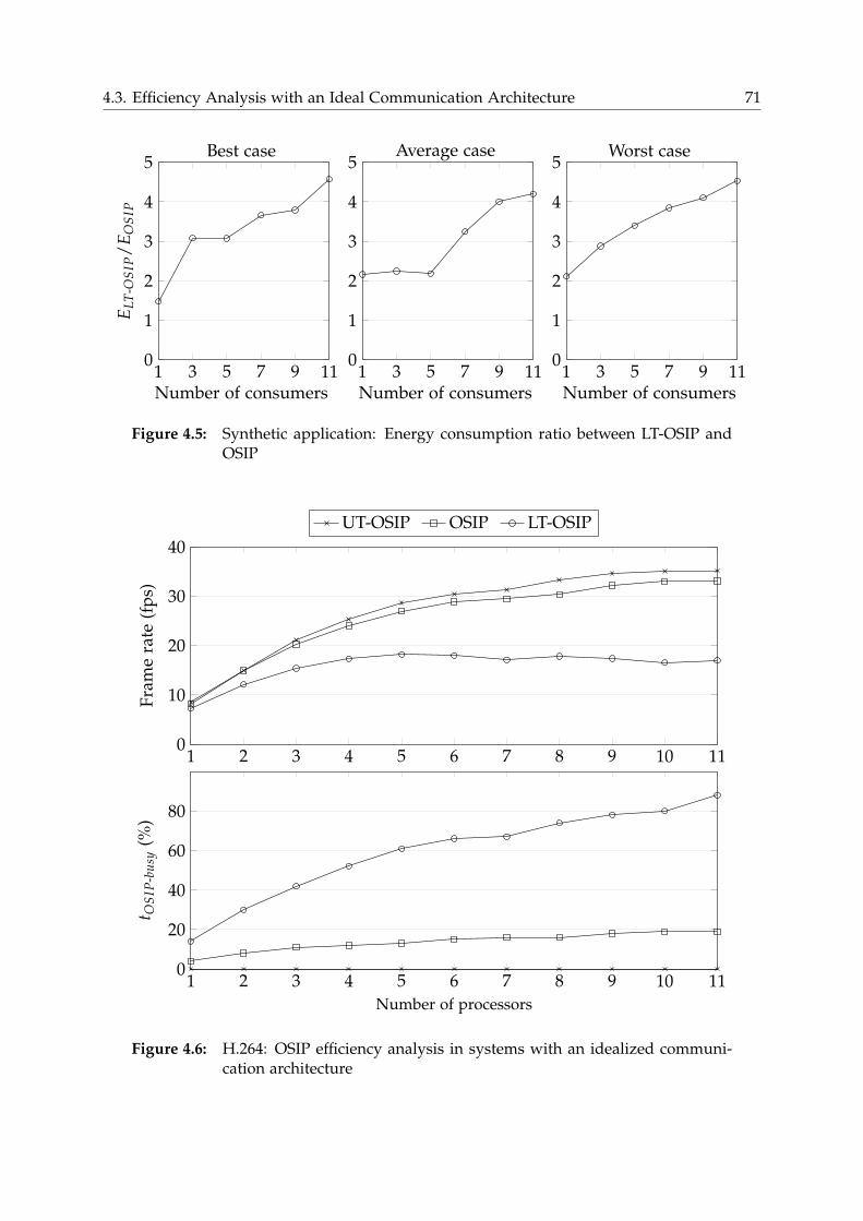
4.3. Efficiency Analysis with an Ideal Communication Architecture 71
1 3 5 7 9 110
1
2
3
4
5
EL
T-O
SIP
/E
OS
IP
Best case
Number of consumers1 3 5 7 9 11
0
1
2
3
4
5Average case
Number of consumers1 3 5 7 9 11
0
1
2
3
4
5Worst case
Number of consumers
Figure 4.5: Synthetic application: Energy consumption ratio between LT-OSIP andOSIP
1 2 3 4 5 6 7 8 9 10 110
10
20
30
40
Fra
me
rate
(fp
s)
UT-OSIP OSIP LT-OSIP
1 2 3 4 5 6 7 8 9 10 110
20
40
60
80
t OS
IP-b
usy
(%)
Number of processors
Figure 4.6: H.264: OSIP efficiency analysis in systems with an idealized communi-cation architecture
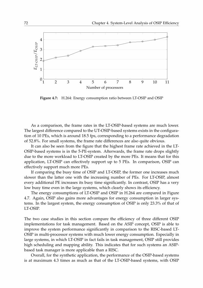
72 Chapter 4. System-Level Analysis of OSIP Efficiency
1 2 3 4 5 6 7 8 9 10 110
1
2
3
4E
LT
-OS
IP
/E
OS
IP
Number of processors
Figure 4.7: H.264: Energy consumption ratio between LT-OSIP and OSIP
As a comparison, the frame rates in the LT-OSIP-based systems are much lower.
The largest difference compared to the UT-OSIP-based systems exists in the configura-
tion of 10 PEs, which is around 18.5 fps, corresponding to a performance degradation
of 52.8%. For small systems, the frame rate differences are also quite obvious.
It can also be seen from the figure that the highest frame rate achieved in the LT-
OSIP-based systems is in the 5-PE-system. Afterwards, the frame rate drops slightly
due to the more workload to LT-OSIP created by the more PEs. It means that for this
application, LT-OSIP can effectively support up to 5 PEs. In comparison, OSIP can
effectively support much more PEs.
If comparing the busy time of OSIP and LT-OSIP, the former one increases much
slower than the latter one with the increasing number of PEs. For LT-OSIP, almost
every additional PE increases its busy time significantly. In contrast, OSIP has a very
low busy time even in the large systems, which clearly shows its efficiency.
The energy consumptions of LT-OSIP and OSIP in H.264 are compared in Figure
4.7. Again, OSIP also gains more advantages for energy consumption in larger sys-
tems. In the largest system, the energy consumption of OSIP is only 23.3% of that of
LT-OSIP.
The two case studies in this section compare the efficiency of three different OSIP
implementations for task management. Based on the ASIP concept, OSIP is able to
improve the system performance significantly in comparison to the RISC-based LT-
OSIP in multi-processor systems with much lower energy consumption. Especially in
large systems, in which LT-OSIP in fact fails in task management, OSIP still provides
high scheduling and mapping ability. This indicates that for such systems an ASIP-
based task manager is more applicable than a RISC.
Overall, for the synthetic application, the performance of the OSIP-based systems
is at maximum 4.3 times as much as that of the LT-OSIP-based systems, with OSIP
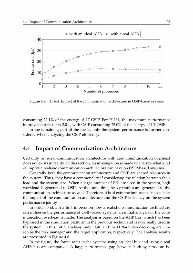
4.4. Impact of Communication Architecture 73
1 2 3 4 5 6 7 8 9 10 110
10
20
30
40
Fra
me
rate
(fp
s)with an ideal AHB with a real AHB
Number of processors
Figure 4.8: H.264: Impact of the communication architecture in OSIP-based systems
consuming 22.1% of the energy of LT-OSIP. For H.264, the maximum performance
improvement factor is 2.0×, with OSIP consuming 25.0% of the energy of LT-OSIP.
In the remaining part of the thesis, only the system performance is further con-
sidered when analyzing the OSIP efficiency.
4.4 Impact of Communication Architecture
Certainly, an ideal communication architecture with zero communication overhead
does not exists in reality. In this section, an investigation is made to analyze what kind
of impact a realistic communication architecture can have on OSIP-based systems.
Generally, both the communication architecture and OSIP are shared resources in
the system. Thus, they have a commonality if considering the relation between their
load and the system size. When a large number of PEs are used in the system, high
workload is generated to OSIP. At the same time, heavy traffics are generated to the
communication architecture as well. Therefore, it is of extreme importance to consider
the impact of the communication architecture and the OSIP efficiency on the system
performance jointly.
In order to obtain a first impression how a realistic communication architecture
can influence the performance of OSIP-based systems, an initial analysis of the com-
munication overhead is made. The analysis is based on the AHB bus, which has been
bypassed in the simulation platform in the previous section and is now really used in
the system. In this initial analysis, only OSIP and the H.264 video decoding are cho-
sen as the task manager and the target application, respectively. The analysis results
are presented in Figure 4.8.
In the figure, the frame rates in the systems using an ideal bus and using a real
AHB bus are compared. A large performance gap between both systems can be
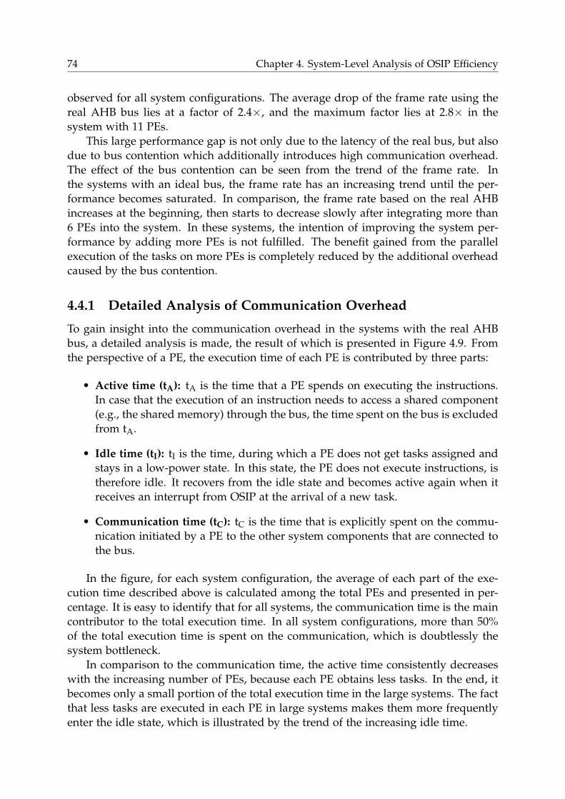
74 Chapter 4. System-Level Analysis of OSIP Efficiency
observed for all system configurations. The average drop of the frame rate using the
real AHB bus lies at a factor of 2.4×, and the maximum factor lies at 2.8× in the
system with 11 PEs.
This large performance gap is not only due to the latency of the real bus, but also
due to bus contention which additionally introduces high communication overhead.
The effect of the bus contention can be seen from the trend of the frame rate. In
the systems with an ideal bus, the frame rate has an increasing trend until the per-
formance becomes saturated. In comparison, the frame rate based on the real AHB
increases at the beginning, then starts to decrease slowly after integrating more than
6 PEs into the system. In these systems, the intention of improving the system per-
formance by adding more PEs is not fulfilled. The benefit gained from the parallel
execution of the tasks on more PEs is completely reduced by the additional overhead
caused by the bus contention.
4.4.1 Detailed Analysis of Communication Overhead
To gain insight into the communication overhead in the systems with the real AHB
bus, a detailed analysis is made, the result of which is presented in Figure 4.9. From
the perspective of a PE, the execution time of each PE is contributed by three parts:
• Active time (tA): tA is the time that a PE spends on executing the instructions.
In case that the execution of an instruction needs to access a shared component
(e.g., the shared memory) through the bus, the time spent on the bus is excluded
from tA.
• Idle time (tI): tI is the time, during which a PE does not get tasks assigned and
stays in a low-power state. In this state, the PE does not execute instructions, is
therefore idle. It recovers from the idle state and becomes active again when it
receives an interrupt from OSIP at the arrival of a new task.
• Communication time (tC): tC is the time that is explicitly spent on the commu-
nication initiated by a PE to the other system components that are connected to
the bus.
In the figure, for each system configuration, the average of each part of the exe-
cution time described above is calculated among the total PEs and presented in per-
centage. It is easy to identify that for all systems, the communication time is the main
contributor to the total execution time. In all system configurations, more than 50%
of the total execution time is spent on the communication, which is doubtlessly the
system bottleneck.
In comparison to the communication time, the active time consistently decreases
with the increasing number of PEs, because each PE obtains less tasks. In the end, it
becomes only a small portion of the total execution time in the large systems. The fact
that less tasks are executed in each PE in large systems makes them more frequently
enter the idle state, which is illustrated by the trend of the increasing idle time.
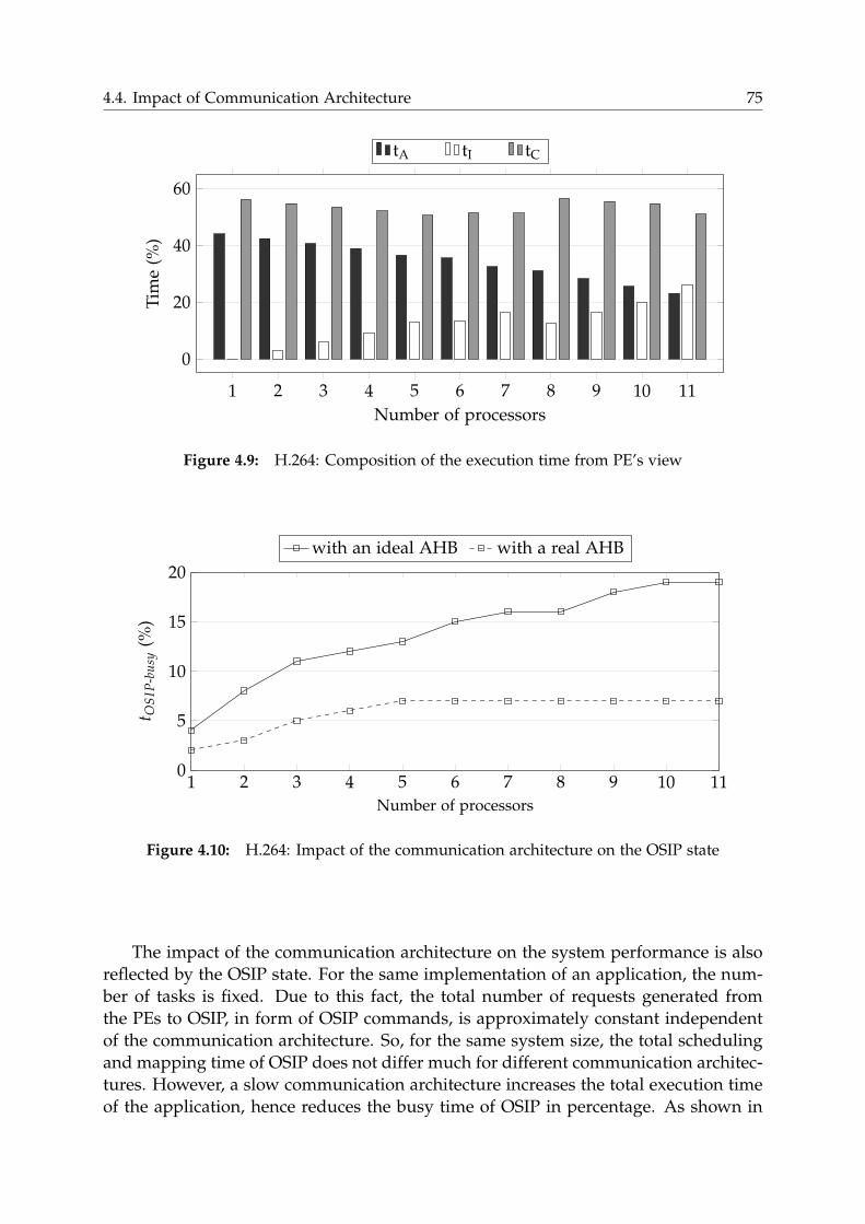
4.4. Impact of Communication Architecture 75
1 2 3 4 5 6 7 8 9 10 11
0
20
40
60
Number of processors
Tim
e(%
)tA tI tC
Figure 4.9: H.264: Composition of the execution time from PE’s view
1 2 3 4 5 6 7 8 9 10 110
5
10
15
20
t OS
IP-b
usy
(%)
with an ideal AHB with a real AHB
Number of processors
Figure 4.10: H.264: Impact of the communication architecture on the OSIP state
The impact of the communication architecture on the system performance is also
reflected by the OSIP state. For the same implementation of an application, the num-
ber of tasks is fixed. Due to this fact, the total number of requests generated from
the PEs to OSIP, in form of OSIP commands, is approximately constant independent
of the communication architecture. So, for the same system size, the total scheduling
and mapping time of OSIP does not differ much for different communication architec-
tures. However, a slow communication architecture increases the total execution time
of the application, hence reduces the busy time of OSIP in percentage. As shown in
76 Chapter 4. System-Level Analysis of OSIP Efficiency
Figure 4.10, the busy time of OSIP in the systems with a real AHB is much lower than
that with an ideal bus. In the former, OSIP mostly stays at an idle state (tOSIP-busy(%)
below 8%).
On the other hand, with the same communication architecture, logically requests
would be generated to OSIP more frequently, if there are more PEs integrated in
the system. So in a large system OSIP would be kept in the busy state more often.
However, in Figure 4.10, this statement only holds true for the systems with the ideal
bus, in which the busy time of OSIP increases steadily with more PEs. For the systems
with the real AHB, the busy time of OSIP first increases with the increasing number
of PEs, then becomes nearly unchanged. The traffic contention in these large systems
prolongs the actual task execution time, hence slows down the request generations to
OSIP.
Based on the analysis above, it can be concluded that an unoptimized communi-
cation architecture can have a disastrous effect on the system performance. It easily
makes OSIP largely underutilized, delaying the task scheduling and mapping. There-
fore, in order to improve the utilization of OSIP, the communication architecture has
to be optimized. This is addressed in the next section.
4.5 Optimized Communication Architecture
Three optimization steps for the communication architecture of the OSIP-based sys-
tems studied in this chapter are proposed, which include employing a multi-layer
AHB, a cache system with coherence control and write buffers. These optimizations
are quite common in general, but the goal is to evaluate the impact of different com-
munication architectures in OSIP-based systems.
4.5.1 Multi-layer AHB
The advantages of a multi-layer AHB [10] against an AHB bus is that parallel accesses
from bus masters to bus slaves are possible, as long as the masters do not address
the same slave at the same time. This type of parallel communication fits well into
the communication characteristics in the OSIP-based systems, in which three types of
independent data communications can be differentiated:
• Communication between PEs and OSIP: This communication is specific for
OSIP-based systems. Based on it, the information is exchanged between the
PEs and OSIP, which is needed for the system-wide scheduling, mapping and
synchronization. Therefore, this communication type is very control-centric. Typ-
ically, the number of the tasks and PEs influences this communication.
• Communication between PEs and shared memory: In this communication,
data are exchanged between different tasks, which may run on the same PE
or on different PEs. The data payload of the tasks determines the required com-
munication bandwidth of the system. So, this communication is data-centric.
4.5. Optimized Communication Architecture 77
• Communication between PEs and peripherals: This communication serves for
reading the input data stream and sending the results to the peripherals. It
however only contributes to a minor part of the total communication.
By applying the multi-layer AHB, the communication overhead caused by bus
contention in the AHB bus can be effectively reduced, especially if the control-centric
communication and the data-centric communication are well balanced. In the cur-
rent simulation platform, all PEs are treated equally. Therefore, each processor is
connected to a dedicated bus layer, which means that the multi-layer AHB is fully
connected. However, the area of a full multi-layer AHB for a large number of proces-
sors can be very big, which should be carefully considered during the system design.
Tradeoffs need to be made by e.g., sharing a bus layer between several PEs.
4.5.2 Cache System
Compared to a multi-layer AHB, which mainly focuses on improving bus contention,
a cache focuses on reducing bus accesses by exploiting data locality. The low latency
of accessing data locally can result in a significant reduction of the total communi-
cation time, if the cache works properly. Moreover, the reduced accesses to the bus
potentially also reduce the communication overhead caused by bus contention.
However, in multi-processor systems cache coherence is of vital importance. Data
inconsistency occurs if a PE is updating the data in the shared memory, while another
PE is still reading the old data from its local cache. This leads to system malfunction.
So, the cache system must ensure that the data fetched from the PE must be the latest
updated data, and the local copy of the data in the cache must be consistent with
the data in the shared memory. In the literature [58, 116, 196, 197], this problem has
been thoroughly studied. In this work, a cache coherence system based on the write-
broadcast approach has been implemented at the system-level, which is illustrated in
Figure 4.11.
The cache system contains two basic functional modules: a local cache module for
each individual PE and a global Cache Coherence Management Unit (CCMU), which
manages the data consistency crossing the local cache modules.
Each local cache module consists of a local cache controller and a cache memory,
following the principle of a four-way set associative cache. The data replacement
policy in case of cache miss is Least Recently Used (LRU). The cache controller has
two functions. On the one hand, it manages the data in the cache memory, such as
accessing the local or shared memory and updating the cache data. On the other hand,
it acts as a bridge to the CCMU using an additional interface. Through this interface,
information is exchanged from one cache over the CCMU to the other caches.
When reading data, this multi-cache system behaves exactly in the same way as
a normal single-cache system. The local cache controller checks whether there is a
valid data copy in the cache. If so, the controller reads the data from the cache and
sends the value to the PE. Otherwise, the controller fetches the data from the shared
memory and updates the cache correspondingly.
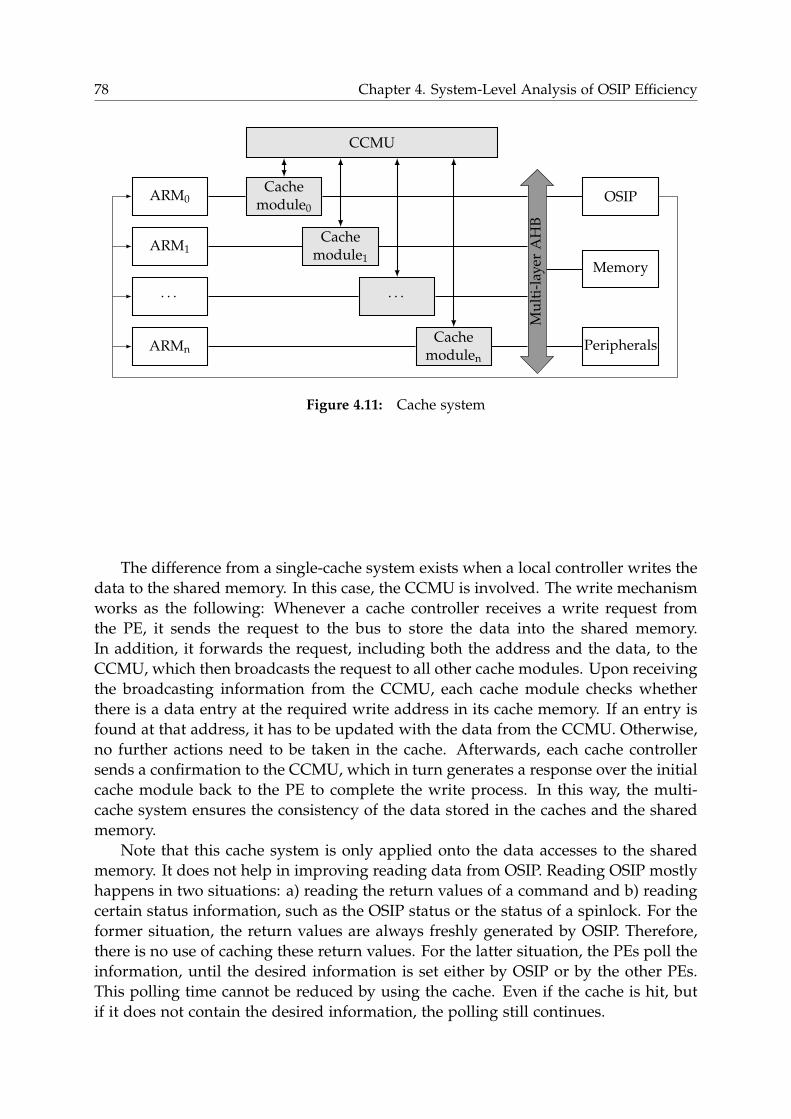
78 Chapter 4. System-Level Analysis of OSIP Efficiency
ARM0
ARM1
. . .
ARMn
Cachemodule0
Cachemodule1
. . .
Cachemodulen
CCMU
Mu
lti-
lay
erA
HB
OSIP
Memory
Peripherals
Figure 4.11: Cache system
The difference from a single-cache system exists when a local controller writes the
data to the shared memory. In this case, the CCMU is involved. The write mechanism
works as the following: Whenever a cache controller receives a write request from
the PE, it sends the request to the bus to store the data into the shared memory.
In addition, it forwards the request, including both the address and the data, to the
CCMU, which then broadcasts the request to all other cache modules. Upon receiving
the broadcasting information from the CCMU, each cache module checks whether
there is a data entry at the required write address in its cache memory. If an entry is
found at that address, it has to be updated with the data from the CCMU. Otherwise,
no further actions need to be taken in the cache. Afterwards, each cache controller
sends a confirmation to the CCMU, which in turn generates a response over the initial
cache module back to the PE to complete the write process. In this way, the multi-
cache system ensures the consistency of the data stored in the caches and the shared
memory.
Note that this cache system is only applied onto the data accesses to the shared
memory. It does not help in improving reading data from OSIP. Reading OSIP mostly
happens in two situations: a) reading the return values of a command and b) reading
certain status information, such as the OSIP status or the status of a spinlock. For the
former situation, the return values are always freshly generated by OSIP. Therefore,
there is no use of caching these return values. For the latter situation, the PEs poll the
information, until the desired information is set either by OSIP or by the other PEs.
This polling time cannot be reduced by using the cache. Even if the cache is hit, but
if it does not contain the desired information, the polling still continues.
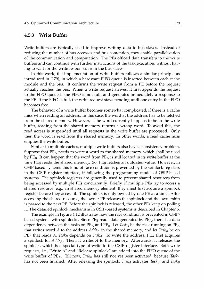
4.5. Optimized Communication Architecture 79
4.5.3 Write Buffer
Write buffers are typically used to improve writing data to bus slaves. Instead of
reducing the number of bus accesses and bus contention, they enable parallelization
of the communication and computation. The PEs offload data transfers to the write
buffers and can continue with further instructions of the task execution, without hav-
ing to wait for the write responses from the bus slaves.
In this work, the implementation of write buffers follows a similar principle as
introduced in [179], in which a hardware FIFO queue is inserted between each cache
module and the bus. It confirms the write request from a PE before the request
actually reaches the bus. When a write request arrives, it first appends the request
to the FIFO queue if the FIFO is not full, and generates immediately a response to
the PE. If the FIFO is full, the write request stays pending until one entry in the FIFO
becomes free.
The behavior of a write buffer becomes somewhat complicated, if there is a cache
miss when reading an address. In this case, the word at the address has to be fetched
from the shared memory. However, if the word currently happens to be in the write
buffer, reading from the shared memory returns a wrong word. To avoid this, the
read access is suspended until all requests in the write buffer are processed. Only
then the word is read from the shared memory. In other words, a read cache miss
empties the write buffer.
Similar to multiple caches, multiple write buffers also have a consistency problem.
Suppose that PEA needs to write a word to the shared memory, which shall be used
by PEB. It can happen that the word from PEA is still located in its write buffer at the
time PEB reads the shared memory. So, PEB fetches an outdated value. However, in
OSIP-based systems this kind of race condition is prevented by the spinlock registers
in the OSIP register interface, if following the programming model of OSIP-based
systems. The spinlock registers are generally used to prevent shared resources from
being accessed by multiple PEs concurrently. Briefly, if multiple PEs try to access a
shared resource, e.g., an shared memory element, they must first acquire a spinlock
register before they access it. The spinlock is only owned by one PE at a time. After
accessing the shared resource, the owner PE releases the spinlock and the ownership
is passed to the next PE. Before the spinlock is released, the other PEs keep on polling
it. The detailed spinlock mechanism in OSIP-based systems is described in Chapter 5.
The example in Figure 4.12 illustrates how the race condition is prevented in OSIP-
based systems with spinlocks. Since PEB reads data generated by PEA, there is a data
dependency between the tasks on PEA and PEB. Let TaskA be the task running on PEA
that writes word A to the address AddrA in the shared memory, and let TaskB be on
PEB that reads A. TaskB depends on TaskA. To write the address, PEA first acquires
a spinlock for AddrA. Then, it writes A to the memory. Afterwards, it releases the
spinlock, which is a special type of write to the OSIP register interface. Both write
requests, i.e., “Write A” and “Release spinlock” are added into the FIFO queue of the
write buffer of PEA. Till now, TaskB has still not yet been activated, because TaskAhas not been finished. After releasing the spinlock, TaskA activates TaskB, and TaskB
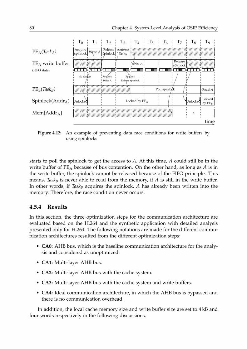
80 Chapter 4. System-Level Analysis of OSIP Efficiency
T0 T1 T2 T3 T4 T5 T6 T7 T8 T9
Acquirespinlock Write A
Releasespinlock
ActivateTaskB
PEA(TaskA)
Write AReleasespinlockPEA write buffer
(FIFO state)
No request Request:
Write A
Request:
Release spinlock
Poll spinlock Read APEB(TaskB)
Unlocked Locked by PEA UnlockedLockedby PEB
Spinlock(AddrA)
AMem[AddrA]
time
Figure 4.12: An example of preventing data race conditions for write buffers byusing spinlocks
starts to poll the spinlock to get the access to A. At this time, A could still be in the
write buffer of PEA because of bus contention. On the other hand, as long as A is in
the write buffer, the spinlock cannot be released because of the FIFO principle. This
means, TaskB is never able to read from the memory, if A is still in the write buffer.
In other words, if TaskB acquires the spinlock, A has already been written into the
memory. Therefore, the race condition never occurs.
4.5.4 Results
In this section, the three optimization steps for the communication architecture are
evaluated based on the H.264 and the synthetic application with detailed analysis
presented only for H.264. The following notations are made for the different commu-
nication architectures resulted from the different optimization steps:
• CA0: AHB bus, which is the baseline communication architecture for the analy-
sis and considered as unoptimized.
• CA1: Multi-layer AHB bus.
• CA2: Multi-layer AHB bus with the cache system.
• CA3: Multi-layer AHB bus with the cache system and write buffers.
• CA4: Ideal communication architecture, in which the AHB bus is bypassed and
there is no communication overhead.
In addition, the local cache memory size and write buffer size are set to 4 kB and
four words respectively in the following discussions.
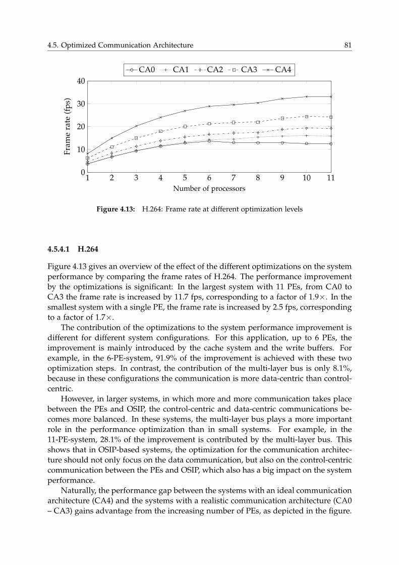
4.5. Optimized Communication Architecture 81
1 2 3 4 5 6 7 8 9 10 110
10
20
30
40
Fra
me
rate
(fp
s)CA0 CA1 CA2 CA3 CA4
Number of processors
Figure 4.13: H.264: Frame rate at different optimization levels
4.5.4.1 H.264
Figure 4.13 gives an overview of the effect of the different optimizations on the system
performance by comparing the frame rates of H.264. The performance improvement
by the optimizations is significant: In the largest system with 11 PEs, from CA0 to
CA3 the frame rate is increased by 11.7 fps, corresponding to a factor of 1.9×. In the
smallest system with a single PE, the frame rate is increased by 2.5 fps, corresponding
to a factor of 1.7×.The contribution of the optimizations to the system performance improvement is
different for different system configurations. For this application, up to 6 PEs, the
improvement is mainly introduced by the cache system and the write buffers. For
example, in the 6-PE-system, 91.9% of the improvement is achieved with these two
optimization steps. In contrast, the contribution of the multi-layer bus is only 8.1%,
because in these configurations the communication is more data-centric than control-
centric.
However, in larger systems, in which more and more communication takes place
between the PEs and OSIP, the control-centric and data-centric communications be-
comes more balanced. In these systems, the multi-layer bus plays a more important
role in the performance optimization than in small systems. For example, in the
11-PE-system, 28.1% of the improvement is contributed by the multi-layer bus. This
shows that in OSIP-based systems, the optimization for the communication architec-
ture should not only focus on the data communication, but also on the control-centric
communication between the PEs and OSIP, which also has a big impact on the system
performance.
Naturally, the performance gap between the systems with an ideal communication
architecture (CA4) and the systems with a realistic communication architecture (CA0
– CA3) gains advantage from the increasing number of PEs, as depicted in the figure.
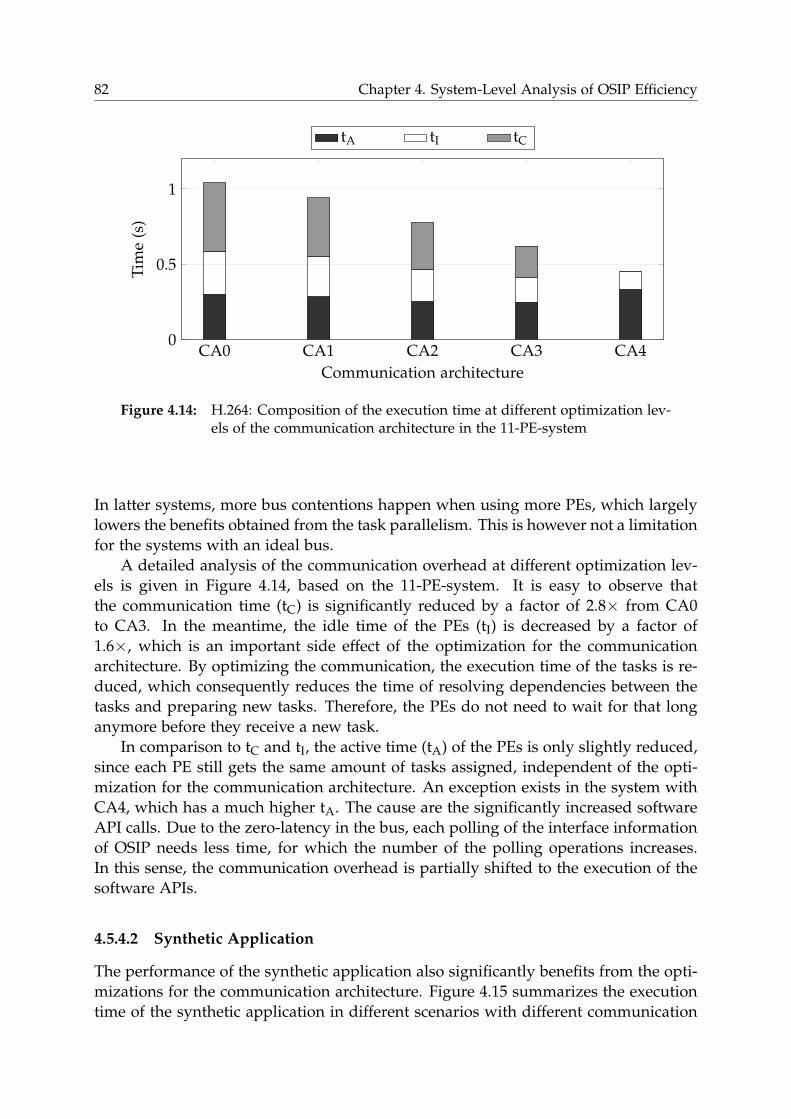
82 Chapter 4. System-Level Analysis of OSIP Efficiency
CA0 CA1 CA2 CA3 CA40
0.5
1
Communication architecture
Tim
e(s
)tA tI tC
Figure 4.14: H.264: Composition of the execution time at different optimization lev-els of the communication architecture in the 11-PE-system
In latter systems, more bus contentions happen when using more PEs, which largely
lowers the benefits obtained from the task parallelism. This is however not a limitation
for the systems with an ideal bus.
A detailed analysis of the communication overhead at different optimization lev-
els is given in Figure 4.14, based on the 11-PE-system. It is easy to observe that
the communication time (tC) is significantly reduced by a factor of 2.8× from CA0
to CA3. In the meantime, the idle time of the PEs (tI) is decreased by a factor of
1.6×, which is an important side effect of the optimization for the communication
architecture. By optimizing the communication, the execution time of the tasks is re-
duced, which consequently reduces the time of resolving dependencies between the
tasks and preparing new tasks. Therefore, the PEs do not need to wait for that long
anymore before they receive a new task.
In comparison to tC and tI, the active time (tA) of the PEs is only slightly reduced,
since each PE still gets the same amount of tasks assigned, independent of the opti-
mization for the communication architecture. An exception exists in the system with
CA4, which has a much higher tA. The cause are the significantly increased software
API calls. Due to the zero-latency in the bus, each polling of the interface information
of OSIP needs less time, for which the number of the polling operations increases.
In this sense, the communication overhead is partially shifted to the execution of the
software APIs.
4.5.4.2 Synthetic Application
The performance of the synthetic application also significantly benefits from the opti-
mizations for the communication architecture. Figure 4.15 summarizes the execution
time of the synthetic application in different scenarios with different communication
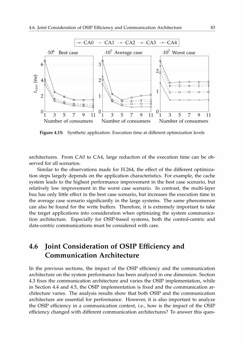
4.6. Joint Consideration of OSIP Efficiency and Communication Architecture 83
1 3 5 7 9 110
2
4
6
·106
tex
ec
(ns)
Best case
Number of consumers1 3 5 7 9 11
0
1
2
3
·107
CA0 CA1 CA2 CA3 CA4
Average case
Number of consumers1 3 5 7 9 11
0
1
2
·107 Worst case
Number of consumers
Figure 4.15: Synthetic application: Execution time at different optimization levels
architectures. From CA0 to CA4, large reduction of the execution time can be ob-
served for all scenarios.
Similar to the observations made for H.264, the effect of the different optimiza-
tion steps largely depends on the application characteristics. For example, the cache
system leads to the highest performance improvement in the best case scenario, but
relatively low improvement in the worst case scenario. In contrast, the multi-layer
bus has only little effect in the best case scenario, but increases the execution time in
the average case scenario significantly in the large systems. The same phenomenon
can also be found for the write buffers. Therefore, it is extremely important to take
the target applications into consideration when optimizing the system communica-
tion architecture. Especially for OSIP-based systems, both the control-centric and
data-centric communications must be considered with care.
4.6 Joint Consideration of OSIP Efficiency and
Communication Architecture
In the previous sections, the impact of the OSIP efficiency and the communication
architecture on the system performance has been analyzed in one dimension. Section
4.3 fixes the communication architecture and varies the OSIP implementation, while
in Section 4.4 and 4.5, the OSIP implementation is fixed and the communication ar-
chitecture varies. The analysis results show that both OSIP and the communication
architecture are essential for performance. However, it is also important to analyze
the OSIP efficiency in a communication context, i.e., how is the impact of the OSIP
efficiency changed with different communication architectures? To answer this ques-
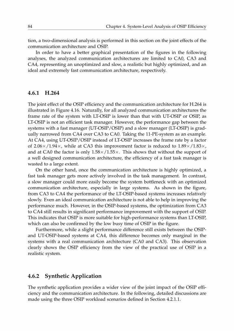
84 Chapter 4. System-Level Analysis of OSIP Efficiency
tion, a two-dimensional analysis is performed in this section on the joint effects of the
communication architecture and OSIP.
In order to have a better graphical presentation of the figures in the following
analyses, the analyzed communication architectures are limited to CA0, CA3 and
CA4, representing an unoptimized and slow, a realistic but highly optimized, and an
ideal and extremely fast communication architecture, respectively.
4.6.1 H.264
The joint effect of the OSIP efficiency and the communication architecture for H.264 is
illustrated in Figure 4.16. Naturally, for all analyzed communication architectures the
frame rate of the system with LT-OSIP is lower than that with UT-OSIP or OSIP, as
LT-OSIP is not an efficient task manager. However, the performance gap between the
systems with a fast manager (UT-OSIP/OSIP) and a slow manager (LT-OSIP) is grad-
ually narrowed from CA4 over CA3 to CA0. Taking the 11-PE-system as an example.
At CA4, using UT-OSIP/OSIP instead of LT-OSIP increases the frame rate by a factor
of 2.06×/1.94×, while at CA3 this improvement factor is reduced to 1.89×/1.83×,and at CA0 the factor is only 1.58×/1.55×. This shows that without the support of
a well designed communication architecture, the efficiency of a fast task manager is
wasted to a large extent.
On the other hand, once the communication architecture is highly optimized, a
fast task manager gets more actively involved in the task management. In contrast,
a slow manager could more easily become the system bottleneck with an optimized
communication architecture, especially in large systems. As shown in the figure,
from CA3 to CA4 the performance of the LT-OSIP-based systems increases relatively
slowly. Even an ideal communication architecture is not able to help in improving the
performance much. However, in the OSIP-based systems, the optimization from CA3
to CA4 still results in significant performance improvement with the support of OSIP.
This indicates that OSIP is more suitable for high-performance systems than LT-OSIP,
which can also be confirmed by the low busy time of OSIP in the figure.
Furthermore, while a slight performance difference still exists between the OSIP-
and UT-OSIP-based systems at CA4, this difference becomes only marginal in the
systems with a real communication architecture (CA0 and CA3). This observation
clearly shows the OSIP efficiency from the view of the practical use of OSIP in a
realistic system.
4.6.2 Synthetic Application
The synthetic application provides a wider view of the joint impact of the OSIP effi-
ciency and the communication architecture. In the following, detailed discussions are
made using the three OSIP workload scenarios defined in Section 4.2.1.1.
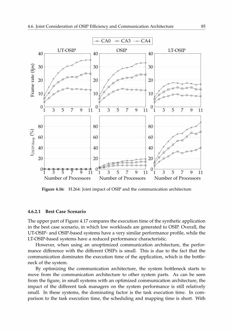
4.6. Joint Consideration of OSIP Efficiency and Communication Architecture 85
1 3 5 7 9 110
10
20
30
40
Fra
me
rate
(fp
s)
UT-OSIP
1 3 5 7 9 110
10
20
30
40
CA0 CA3 CA4
OSIP
1 3 5 7 9 110
10
20
30
40LT-OSIP
1 3 5 7 9 110
20
40
60
80
t OS
IP-b
usy
(%)
Number of Processors1 3 5 7 9 11
0
20
40
60
80
Number of Processors1 3 5 7 9 11
0
20
40
60
80
Number of Processors
Figure 4.16: H.264: Joint impact of OSIP and the communication architecture
4.6.2.1 Best Case Scenario
The upper part of Figure 4.17 compares the execution time of the synthetic application
in the best case scenario, in which low workloads are generated to OSIP. Overall, the
UT-OSIP- and OSIP-based systems have a very similar performance profile, while the
LT-OSIP-based systems have a reduced performance characteristic.
However, when using an unoptimized communication architecture, the perfor-
mance difference with the different OSIPs is small. This is due to the fact that the
communication dominates the execution time of the application, which is the bottle-
neck of the system.
By optimizing the communication architecture, the system bottleneck starts to
move from the communication architecture to other system parts. As can be seen
from the figure, in small systems with an optimized communication architecture, the
impact of the different task managers on the system performance is still relatively
small. In these systems, the dominating factor is the task execution time. In com-
parison to the task execution time, the scheduling and mapping time is short. With
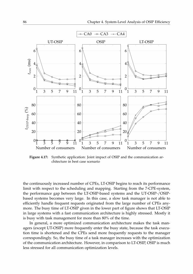
86 Chapter 4. System-Level Analysis of OSIP Efficiency
1 3 5 7 9 110
2
4
6
t ex
ec(m
s)
UT-OSIP
1 3 5 7 9 110
2
4
6
CA0 CA3 CA4
OSIP
1 3 5 7 9 110
2
4
6
LT-OSIP
1 3 5 7 9 110
20
40
60
80
t OS
IP-b
usy
(%)
Number of consumers
1 3 5 7 9 110
20
40
60
80
Number of consumers
1 3 5 7 9 110
20
40
60
80
Number of consumers
Figure 4.17: Synthetic application: Joint impact of OSIP and the communication ar-chitecture in best case scenario
the continuously increased number of CPEs, LT-OSIP begins to reach its performance
limit with respect to the scheduling and mapping. Starting from the 7-CPE-system,
the performance gap between the LT-OSIP-based systems and the UT-OSIP-/OSIP-
based systems becomes very large. In this case, a slow task manager is not able to
efficiently handle frequent requests originated from the large number of CPEs any-
more. The busy time of LT-OSIP given in the lower part of figure shows that LT-OSIP
in large systems with a fast communication architecture is highly stressed. Mostly it
is busy with task management for more than 80% of the time.
In general, a more optimized communication architecture makes the task man-
agers (except UT-OSIP) more frequently enter the busy state, because the task execu-
tion time is shortened and the CPEs send more frequently requests to the manager
correspondingly. So, the busy time of a task manager increases with the optimization
of the communication architecture. However, in comparison to LT-OSIP, OSIP is much
less stressed for all communication optimization levels.
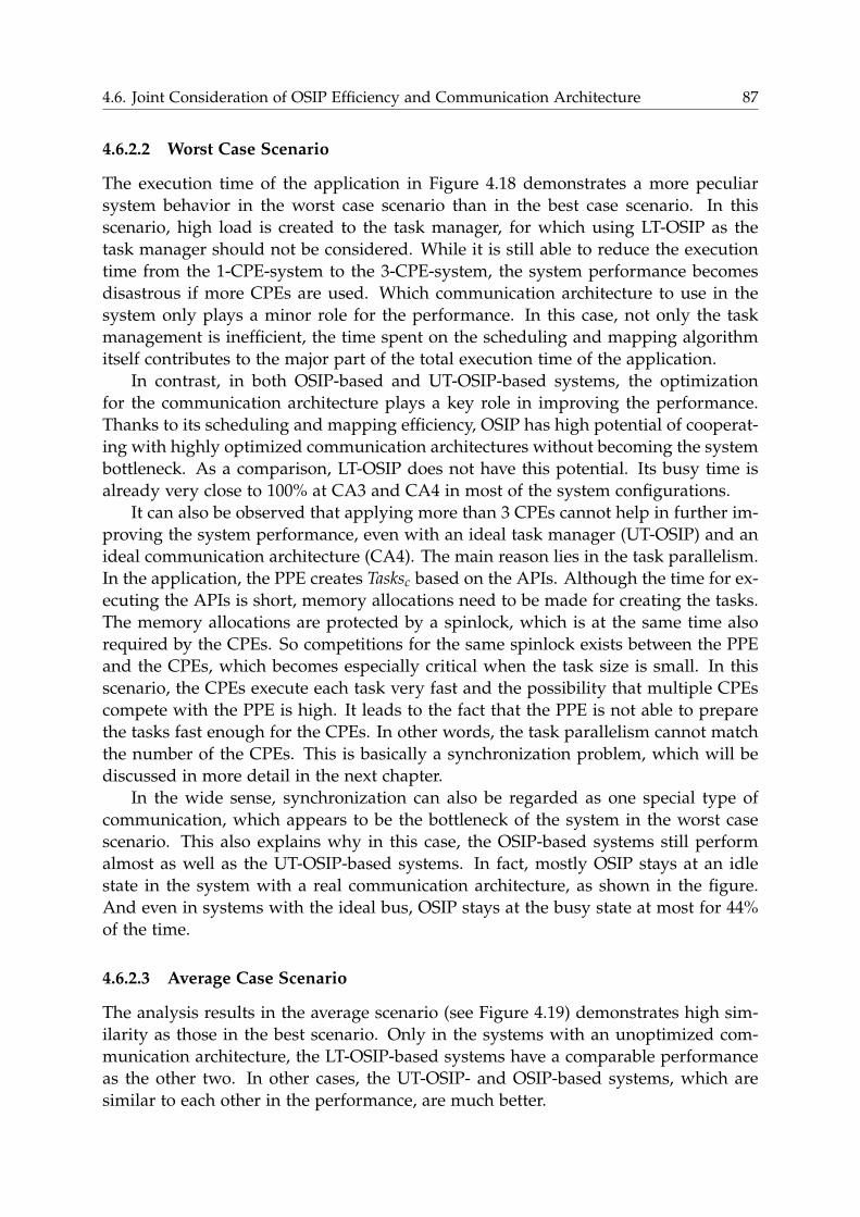
4.6. Joint Consideration of OSIP Efficiency and Communication Architecture 87
4.6.2.2 Worst Case Scenario
The execution time of the application in Figure 4.18 demonstrates a more peculiar
system behavior in the worst case scenario than in the best case scenario. In this
scenario, high load is created to the task manager, for which using LT-OSIP as the
task manager should not be considered. While it is still able to reduce the execution
time from the 1-CPE-system to the 3-CPE-system, the system performance becomes
disastrous if more CPEs are used. Which communication architecture to use in the
system only plays a minor role for the performance. In this case, not only the task
management is inefficient, the time spent on the scheduling and mapping algorithm
itself contributes to the major part of the total execution time of the application.
In contrast, in both OSIP-based and UT-OSIP-based systems, the optimization
for the communication architecture plays a key role in improving the performance.
Thanks to its scheduling and mapping efficiency, OSIP has high potential of cooperat-
ing with highly optimized communication architectures without becoming the system
bottleneck. As a comparison, LT-OSIP does not have this potential. Its busy time is
already very close to 100% at CA3 and CA4 in most of the system configurations.
It can also be observed that applying more than 3 CPEs cannot help in further im-
proving the system performance, even with an ideal task manager (UT-OSIP) and an
ideal communication architecture (CA4). The main reason lies in the task parallelism.
In the application, the PPE creates Tasksc based on the APIs. Although the time for ex-
ecuting the APIs is short, memory allocations need to be made for creating the tasks.
The memory allocations are protected by a spinlock, which is at the same time also
required by the CPEs. So competitions for the same spinlock exists between the PPE
and the CPEs, which becomes especially critical when the task size is small. In this
scenario, the CPEs execute each task very fast and the possibility that multiple CPEs
compete with the PPE is high. It leads to the fact that the PPE is not able to prepare
the tasks fast enough for the CPEs. In other words, the task parallelism cannot match
the number of the CPEs. This is basically a synchronization problem, which will be
discussed in more detail in the next chapter.
In the wide sense, synchronization can also be regarded as one special type of
communication, which appears to be the bottleneck of the system in the worst case
scenario. This also explains why in this case, the OSIP-based systems still perform
almost as well as the UT-OSIP-based systems. In fact, mostly OSIP stays at an idle
state in the system with a real communication architecture, as shown in the figure.
And even in systems with the ideal bus, OSIP stays at the busy state at most for 44%
of the time.
4.6.2.3 Average Case Scenario
The analysis results in the average scenario (see Figure 4.19) demonstrates high sim-
ilarity as those in the best scenario. Only in the systems with an unoptimized com-
munication architecture, the LT-OSIP-based systems have a comparable performance
as the other two. In other cases, the UT-OSIP- and OSIP-based systems, which are
similar to each other in the performance, are much better.
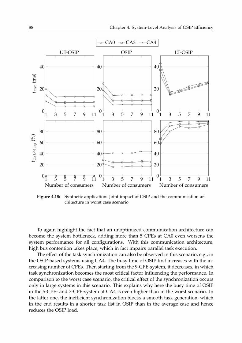
88 Chapter 4. System-Level Analysis of OSIP Efficiency
1 3 5 7 9 110
20
40
t ex
ec(m
s)
UT-OSIP
1 3 5 7 9 110
20
40
CA0 CA3 CA4
OSIP
1 3 5 7 9 110
20
40
LT-OSIP
1 3 5 7 9 110
20
40
60
80
t OS
IP-b
usy
(%)
Number of consumers
1 3 5 7 9 110
20
40
60
80
Number of consumers
1 3 5 7 9 110
20
40
60
80
Number of consumers
Figure 4.18: Synthetic application: Joint impact of OSIP and the communication ar-chitecture in worst case scenario
To again highlight the fact that an unoptimized communication architecture can
become the system bottleneck, adding more than 5 CPEs at CA0 even worsens the
system performance for all configurations. With this communication architecture,
high bus contention takes place, which in fact impairs parallel task execution.
The effect of the task synchronization can also be observed in this scenario, e.g., in
the OSIP-based systems using CA4. The busy time of OSIP first increases with the in-
creasing number of CPEs. Then starting from the 9-CPE-system, it decreases, in which
task synchronization becomes the most critical factor influencing the performance. In
comparison to the worst case scenario, the critical effect of the synchronization occurs
only in large systems in this scenario. This explains why here the busy time of OSIP
in the 5-CPE- and 7-CPE-system at CA4 is even higher than in the worst scenario. In
the latter one, the inefficient synchronization blocks a smooth task generation, which
in the end results in a shorter task list in OSIP than in the average case and hence
reduces the OSIP load.
4.7. Summary 89
1 3 5 7 9 110
20
40
t ex
ec(m
s)
UT-OSIP
1 3 5 7 9 110
20
40
CA0 CA3 CA4
OSIP
1 3 5 7 9 110
20
40
LT-OSIP
1 3 5 7 9 110
20
40
60
80
t OS
IP-b
usy
(%)
Number of consumers
1 3 5 7 9 110
20
40
60
80
Number of consumers
1 3 5 7 9 110
20
40
60
80
Number of consumers
Figure 4.19: Synthetic application: Joint impact of OSIP and the communication ar-chitecture in average case scenario
4.7 Summary
In this chapter, the efficiency of OSIP is analyzed from the system level, based on
a synthetic application and a real-life application. Especially the joint impact of the
OSIP efficiency and the communication architecture is thoroughly investigated by
comparing the systems with an unoptimized AHB bus, an ideal bus and a realistic but
highly optimized bus. The analysis results show that from the system point of view,
OSIP has very high efficiency in task scheduling and mapping, which is comparable
to a hypothetical extremely fast task manager.
In addition, the communication architecture plays an important role in the OSIP-
based systems. In order to fully utilize the OSIP efficiency, an optimized communi-
cation architecture is required. Otherwise, the OSIP efficiency would be wasted to
a large extent. More generally, designing MPSoCs based on a central task manager
90 Chapter 4. System-Level Analysis of OSIP Efficiency
must take special care of the balance between the efficiency of the task manager and
the communication architecture.
As shown in the synthetic application, the synchronization is another important
factor, which can limit the utilization of OSIP. In the next chapter, how to effectively
handle the synchronization problem is addressed by using the flexibility of OSIP.
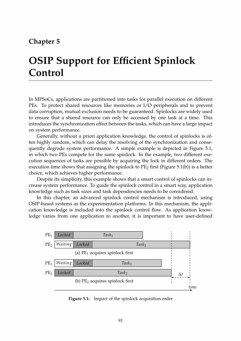
Chapter 5
OSIP Support for Efficient SpinlockControl
In MPSoCs, applications are partitioned into tasks for parallel execution on different
PEs. To protect shared resources like memories or I/O peripherals and to prevent
data corruption, mutual exclusion needs to be guaranteed. Spinlocks are widely used
to ensure that a shared resource can only be accessed by one task at a time. This
introduces the synchronization effect between the tasks, which can have a large impact
on system performance.
Generally, without a priori application knowledge, the control of spinlocks is of-
ten highly random, which can delay the resolving of the synchronization and conse-
quently degrade system performance. A simple example is depicted in Figure 5.1,
in which two PEs compete for the same spinlock. In the example, two different exe-
cution sequences of tasks are possible by acquiring the lock in different orders. The
execution time shows that assigning the spinlock to PE2 first (Figure 5.1(b)) is a better
choice, which achieves higher performance.
Despite its simplicity, this example shows that a smart control of spinlocks can in-
crease system performance. To guide the spinlock control in a smart way, application
knowledge such as task sizes and task dependencies needs to be considered.
In this chapter, an advanced spinlock control mechanism is introduced, using
OSIP-based systems as the experimentation platforms. In this mechanism, the appli-
cation knowledge is included into the spinlock control flow. As application know-
ledge varies from one application to another, it is important to have user-defined
PE1 Locked Task1
PE2 Waiting Locked Task2
(a) PE1 acquires spinlock first
PE1 Waiting Locked Task1
PE2 Locked Task2
(b) PE2 acquires spinlock first
∆t
time
Figure 5.1: Impact of the spinlock acquisition order
91
92 Chapter 5. OSIP Support for Efficient Spinlock Control
spinlock control algorithms, which are able to be adapted to applications. This calls
for a programmable processor, either a RISC or an ASIP, to execute the control al-
gorithm. Instead of developing yet another controller, which would introduce high
area cost, in OSIP-based systems, the existing task manager – OSIP, is re-used for this
purpose in addition to its original design purpose for task scheduling and mapping.
This chapter is organized as follows. First, some related work on the spinlock con-
trol is discussed. Then, the basic spinlock control flow in OSIP-based systems is intro-
duced. This basic flow is then extended to an application-aware control flow, which
starts from an high-level integration of application knowledge down to a low-level
realization. The two case studies in the previous chapter — the synthetic application
and the H.264 video decoding — are further analyzed and discussed based on the
extended spinlock control mechanism. Finally a summary is given and some further
discussions are made.1
5.1 Research on Spinlocks
Spinlocks are a very commonly used technique to address mutual exclusion in multi-
processor systems. Many implementations have been proposed for spinlocks in the
literature.
The simplest approach is the test-and-set lock, which repeatedly tries to replace the
flag of a lock with true in order to acquire the lock. Although the implementation is
rather simple, it introduces heavy traffic load due to continuous updates of the flag,
especially in cache coherent systems. One improvement is suggested by using the test
and test-and-set lock [156], in which updates are only made when the lock is assumed
to be available. Another important improvement is made in [7] by adding a certain
delay (backoff) between two unsuccessful trials.
Having the test-and-set lock, the grants to the requests can be very unevenly dis-
tributed. In contrast, a queuing lock provides better fairness, in which the PEs acquire
a lock in turns (FIFO fairness). In [7], an array-based queuing lock is introduced, in
which the requests of PEs are maintained using an array per lock in the shared mem-
ory. When a PE releases a lock, the control of the lock is passed to the next requesting
PE in the array. To support array-based locks, large memory space is required, given
as O (pn) for p processes and n locks. This space is reduced to 2p+n words by the
Mellor-Crummey and Scott (MCS) queuing lock in [130]. It employs a linked list for
the requests, constructed by pointing each request to its successor. A similar approach
to the MCS lock is the Craig, Landin and Hagersten (CLH) lock presented in [48,118],
in which each process points to its predecessor in the linked list.
Recent research also applies hardware support for queuing locks to improve the
efficiency. A dedicated hardware controller is presented in [212], which is provided
to each PE and uses a set of register pairs to locally maintain the queue information
1 Portions of this chapter have been published by the author in [213] in the International Journal ofEmbedded and Real-Time Communication Systems, edited by Seppo Virtanen. Copyright 2013, IGI Global,www.igi-global.com. Posted by permission of the publisher.
5.1. Research on Spinlocks 93
and grant the locks. Each pair contains a TOTAL register and an AHEAD register,
showing how many PEs are requesting a lock in total and how many PEs have re-
quested the lock before its own PE, respectively. The controller updates the registers
by observing the lock requests on the bus, and can furthermore decide whether to
switch the PE to a low-power state, when waiting for a lock. In the work of [38], the
synchronization problems in NoCs are addressed. A hardware module called Syn-
chronization Handler (SH) is used at each node of the network for the queue manage-
ment. Different from these two distributed approaches, a central hardware module
called Synchronization-Operation Buffer (SB) is introduced in [134]. It is located in
the memory controller to manage the lock queue and notifies a PE automatically if
it decides that the PE should be the next one to acquire the lock. By this, the traffic
overhead due to the polling can be significantly reduced. Another central approach,
not directly related to the queuing lock, but to reduce the memory contention caused
by polling is presented in [94]. They suggest a hardware lock unit separated from the
memory to support spinlocks.
However, in all above-mentioned approaches, the acquisition of locks features
high randomness, since the grant decision solely depends on the time stamp when
the locks are required, regardless of the fairness. As mentioned at the beginning of
this chapter, a proper control of spinlocks would most likely have a positive impact
on system performance. Priority-based spinlocks are a way of implementing this, in
which locks are granted by comparing the priorities of the requests in the queues. In
the work presented in [48], which process receives the grant to a lock as the next, is
determined by looping over the queue at the time the lock is released. In contrast, the
work in [98] suggests sorting the queue by the priority during the time that the lock
is being held by others. However, while the former approach potentially increases the
workload of the PEs, the latter one needs to extend the process to support the insertion
of spinlock requests into the queue at proper positions. And in general, priority-
based approaches can suffer from the starvation problem. In [185], a central hardware
memory controller is proposed to arbitrate the competitions for protected memory
regions based on the dynamic priority scheme [204]. However, no architectural detail
has been given by the authors, and the presented results based on a dual-core system
are not representative for typical multi-processor systems.
The spinlock control mechanism presented in the chapter is based on a centralized
way, which has some similarities to the approach introduced in [94]. However, the
main distinctions of this approach are made by:
• Enabling the programmer to introduce application-specific spinlock control in-
formation into the control flow to guide spinlock decisions. The control infor-
mation can be, but is not limited to priorities.
• Utilizing the flexibility of an existing task manager, the OSIP, to execute user-
defined, application-aware spinlock control algorithms. If needed, runtime sys-
tem information can be included into the algorithms to make the most suitable
decisions. Furthermore, with the user-defined control algorithms, the starvation
problem can be efficiently handled.
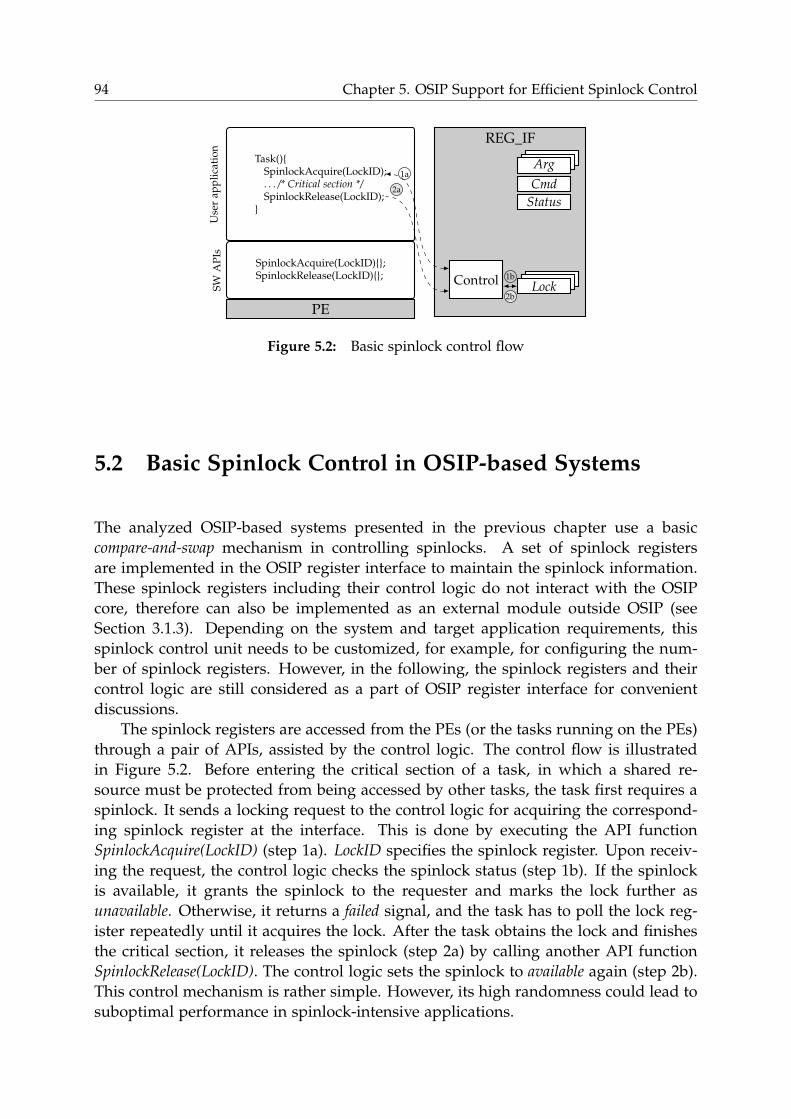
94 Chapter 5. OSIP Support for Efficient Spinlock Control
REG_IF
PE
Use
rap
pli
cati
on
Task(){SpinlockAcquire(LockID);. . . /* Critical section */SpinlockRelease(LockID);
}S
WA
PIs
SpinlockAcquire(LockID){};SpinlockRelease(LockID){};
Arg
Cmd
Status
LockControl
1a
1b
2b
2a
Figure 5.2: Basic spinlock control flow
5.2 Basic Spinlock Control in OSIP-based Systems
The analyzed OSIP-based systems presented in the previous chapter use a basic
compare-and-swap mechanism in controlling spinlocks. A set of spinlock registers
are implemented in the OSIP register interface to maintain the spinlock information.
These spinlock registers including their control logic do not interact with the OSIP
core, therefore can also be implemented as an external module outside OSIP (see
Section 3.1.3). Depending on the system and target application requirements, this
spinlock control unit needs to be customized, for example, for configuring the num-
ber of spinlock registers. However, in the following, the spinlock registers and their
control logic are still considered as a part of OSIP register interface for convenient
discussions.
The spinlock registers are accessed from the PEs (or the tasks running on the PEs)
through a pair of APIs, assisted by the control logic. The control flow is illustrated
in Figure 5.2. Before entering the critical section of a task, in which a shared re-
source must be protected from being accessed by other tasks, the task first requires a
spinlock. It sends a locking request to the control logic for acquiring the correspond-
ing spinlock register at the interface. This is done by executing the API function
SpinlockAcquire(LockID) (step 1a). LockID specifies the spinlock register. Upon receiv-
ing the request, the control logic checks the spinlock status (step 1b). If the spinlock
is available, it grants the spinlock to the requester and marks the lock further as
unavailable. Otherwise, it returns a failed signal, and the task has to poll the lock reg-
ister repeatedly until it acquires the lock. After the task obtains the lock and finishes
the critical section, it releases the spinlock (step 2a) by calling another API function
SpinlockRelease(LockID). The control logic sets the spinlock to available again (step 2b).
This control mechanism is rather simple. However, its high randomness could lead to
suboptimal performance in spinlock-intensive applications.
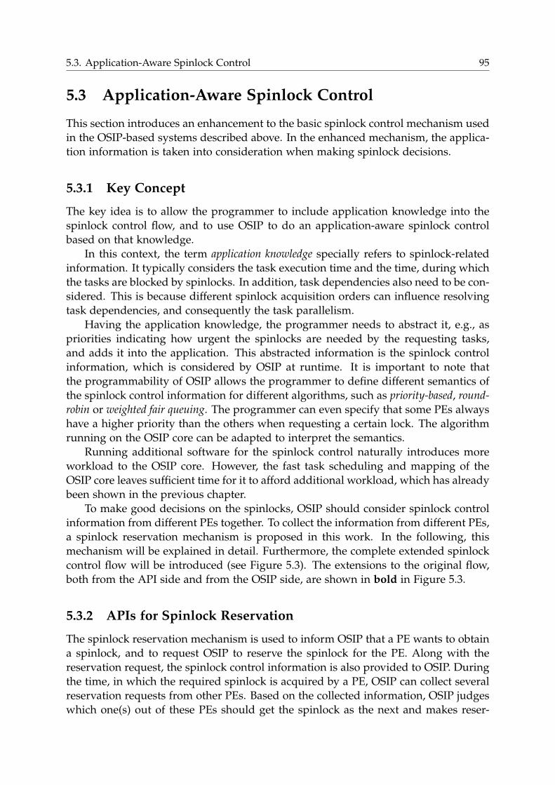
5.3. Application-Aware Spinlock Control 95
5.3 Application-Aware Spinlock Control
This section introduces an enhancement to the basic spinlock control mechanism used
in the OSIP-based systems described above. In the enhanced mechanism, the applica-
tion information is taken into consideration when making spinlock decisions.
5.3.1 Key Concept
The key idea is to allow the programmer to include application knowledge into the
spinlock control flow, and to use OSIP to do an application-aware spinlock control
based on that knowledge.
In this context, the term application knowledge specially refers to spinlock-related
information. It typically considers the task execution time and the time, during which
the tasks are blocked by spinlocks. In addition, task dependencies also need to be con-
sidered. This is because different spinlock acquisition orders can influence resolving
task dependencies, and consequently the task parallelism.
Having the application knowledge, the programmer needs to abstract it, e.g., as
priorities indicating how urgent the spinlocks are needed by the requesting tasks,
and adds it into the application. This abstracted information is the spinlock control
information, which is considered by OSIP at runtime. It is important to note that
the programmability of OSIP allows the programmer to define different semantics of
the spinlock control information for different algorithms, such as priority-based, round-
robin or weighted fair queuing. The programmer can even specify that some PEs always
have a higher priority than the others when requesting a certain lock. The algorithm
running on the OSIP core can be adapted to interpret the semantics.
Running additional software for the spinlock control naturally introduces more
workload to the OSIP core. However, the fast task scheduling and mapping of the
OSIP core leaves sufficient time for it to afford additional workload, which has already
been shown in the previous chapter.
To make good decisions on the spinlocks, OSIP should consider spinlock control
information from different PEs together. To collect the information from different PEs,
a spinlock reservation mechanism is proposed in this work. In the following, this
mechanism will be explained in detail. Furthermore, the complete extended spinlock
control flow will be introduced (see Figure 5.3). The extensions to the original flow,
both from the API side and from the OSIP side, are shown in bold in Figure 5.3.
5.3.2 APIs for Spinlock Reservation
The spinlock reservation mechanism is used to inform OSIP that a PE wants to obtain
a spinlock, and to request OSIP to reserve the spinlock for the PE. Along with the
reservation request, the spinlock control information is also provided to OSIP. During
the time, in which the required spinlock is acquired by a PE, OSIP can collect several
reservation requests from other PEs. Based on the collected information, OSIP judges
which one(s) out of these PEs should get the spinlock as the next and makes reser-
96 Chapter 5. OSIP Support for Efficient Spinlock Control
REG_IF
PE
OSIP coreUse
rap
pli
cati
on Task(){
SpinlockReserve(LockID,LockInfo);SpinlockAcquire(LockID);. . . /* Critical section */SpinlockRelease(LockID);SpinlockClearReservation();
}
SW
AP
Is SpinlockReserve(LockID,LockInfo){};SpinlockAcquire(LockID){};SpinlockRelease(LockID){};SpinlockClearReservation(){};
SRR
Arg
Cmd
Status
LockControl
ReservingSpinlock(){
/* User-defined */. . .
}
1
2a
2b
3b
2c
4b
3a 4a
4c
4d
Figure 5.3: Enhanced spinlock control flow
vation for it/them. Once the spinlock is reserved, the PE(s) that has/have got the
reservation has/have advantages over the other PEs when requesting the spinlock. In
this way, the randomness of granting spinlock requests is largely reduced.
To help the programmer add the control information into the application in a
simple way, an API called SpinlockReserve() is introduced. It contains two parameters:
LockID and LockInfo, specifying the required spinlock register and the control infor-
mation, respectively. For minimizing the communication overhead, both parameters
are combined into a 32-bit word before they are transferred to OSIP. Note that the
reservation request does not try to acquire the spinlock immediately, but makes a
preparation for the spinlock acquisition. Therefore, it must be sent to OSIP before the
actual acquisition request starts. Complementarily, another API SpinlockClearReserva-
tion() is defined to clear the reservation after the spinlock is released.
These two APIs should be always used in pair to enclose spinlock acquisition and
release. A simple example is given in function Task() in Figure 5.3. In practice, this
API pair can also be used to enclose multiple spinlock acquisition/release pairs, if
desired, as long as they require the same lock. And it is not always necessary to
do the reservation for all spinlocks. Instead, identifying the most critical ones and
making reservations of these ones with proper reservation information is essential for
better system performance.
5.3.3 Enhanced Spinlock Control
The APIs for reserving spinlocks require an extension to the original spinlock con-
trol logic to store the reservation information and to interact with the OSIP core for
the enhanced control of spinlocks. Four stages are defined for the extended spin-
lock control in OSIP: spinlock information collection stage, decision stage, release stage and
reservation stage. The first three stages are purely controlled by the hardware in the
interface, while the last stage needs a collaboration between the hardware interface
and the software control of the OSIP core.
5.3. Application-Aware Spinlock Control 97
5.3.3.1 Information Collection Stage
Upon receiving a spinlock reservation request from a PE, the reservation information
is stored in an internal register at the interface, which is named Spinlock Reservation
Register (SRR) (Figure 5.3, step 1). Each PE has a dedicated SRR with the following
four fields:
• LockID (8 bits): This is the spinlock ID, indicating which spinlock should be
considered for reservation. The current system has 256 spinlock registers in the
interface.
• LockInfo (4 bits): It is the information needed by the OSIP core to make reser-
vation decisions on the corresponding spinlock.
• ReservationFlag (1 bit): This flag indicates whether the corresponding PE of the
SRR wants to reserve the spinlock.
• ReservedFlag (1 bit): This flag shows whether the spinlock has been reserved
for the PE.
The information bits for the spinlock ID and spinlock control information are
adjusted to the current system, which can be easily extended.
To avoid confusion, this stage only collects control information, but does not make
reservations. The spinlock reservation for a requesting PE is only triggered by other
PEs, which is explained in detail later in the reservation stage (Section 5.3.3.4).
5.3.3.2 Decision Stage
When the interface receives a spinlock acquisition request (step 2a), the decision stage
starts. In this stage, the interface decides whether the requesting PE acquires the
spinlock. The control flow is depicted in Figure 5.4.
First, the interface checks the status of the spinlock (step 2b). If the spinlock
is currently already locked, the PE fails to acquire the spinlock and has to poll it
again, which is the same as in the original approach. The difference from the original
approach exists when the spinlock is currently available. In this state, the interface
needs to further check the reservation status of the spinlock (step 2c). If the spinlock
has not been reserved for the requesting PE, but reserved for other PEs, the current
request still fails. In other words, the request can only become successful, when the
requesting PE has got the reservation (no matter whether other PEs also have got the
reservation of the same spinlock), or the spinlock currently has not been reserved for
any PEs.
From this control mechanism, it can be seen that the PEs that have got the spinlock
reserved have a better opportunity to acquire it than the other PEs. By introducing
additional control information to the spinlocks, the programmer is now able to in-
fluence the reservation decisions made by the OSIP core, consequently the spinlock
acquisition order.
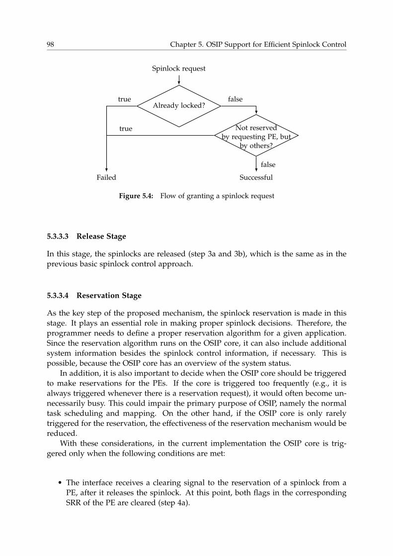
98 Chapter 5. OSIP Support for Efficient Spinlock Control
Already locked?
Not reservedby requesting PE, but
by others?
Spinlock request
SuccessfulFailed
false
true
falsetrue
Figure 5.4: Flow of granting a spinlock request
5.3.3.3 Release Stage
In this stage, the spinlocks are released (step 3a and 3b), which is the same as in the
previous basic spinlock control approach.
5.3.3.4 Reservation Stage
As the key step of the proposed mechanism, the spinlock reservation is made in this
stage. It plays an essential role in making proper spinlock decisions. Therefore, the
programmer needs to define a proper reservation algorithm for a given application.
Since the reservation algorithm runs on the OSIP core, it can also include additional
system information besides the spinlock control information, if necessary. This is
possible, because the OSIP core has an overview of the system status.
In addition, it is also important to decide when the OSIP core should be triggered
to make reservations for the PEs. If the core is triggered too frequently (e.g., it is
always triggered whenever there is a reservation request), it would often become un-
necessarily busy. This could impair the primary purpose of OSIP, namely the normal
task scheduling and mapping. On the other hand, if the OSIP core is only rarely
triggered for the reservation, the effectiveness of the reservation mechanism would be
reduced.
With these considerations, in the current implementation the OSIP core is trig-
gered only when the following conditions are met:
• The interface receives a clearing signal to the reservation of a spinlock from a
PE, after it releases the spinlock. At this point, both flags in the corresponding
SRR of the PE are cleared (step 4a).
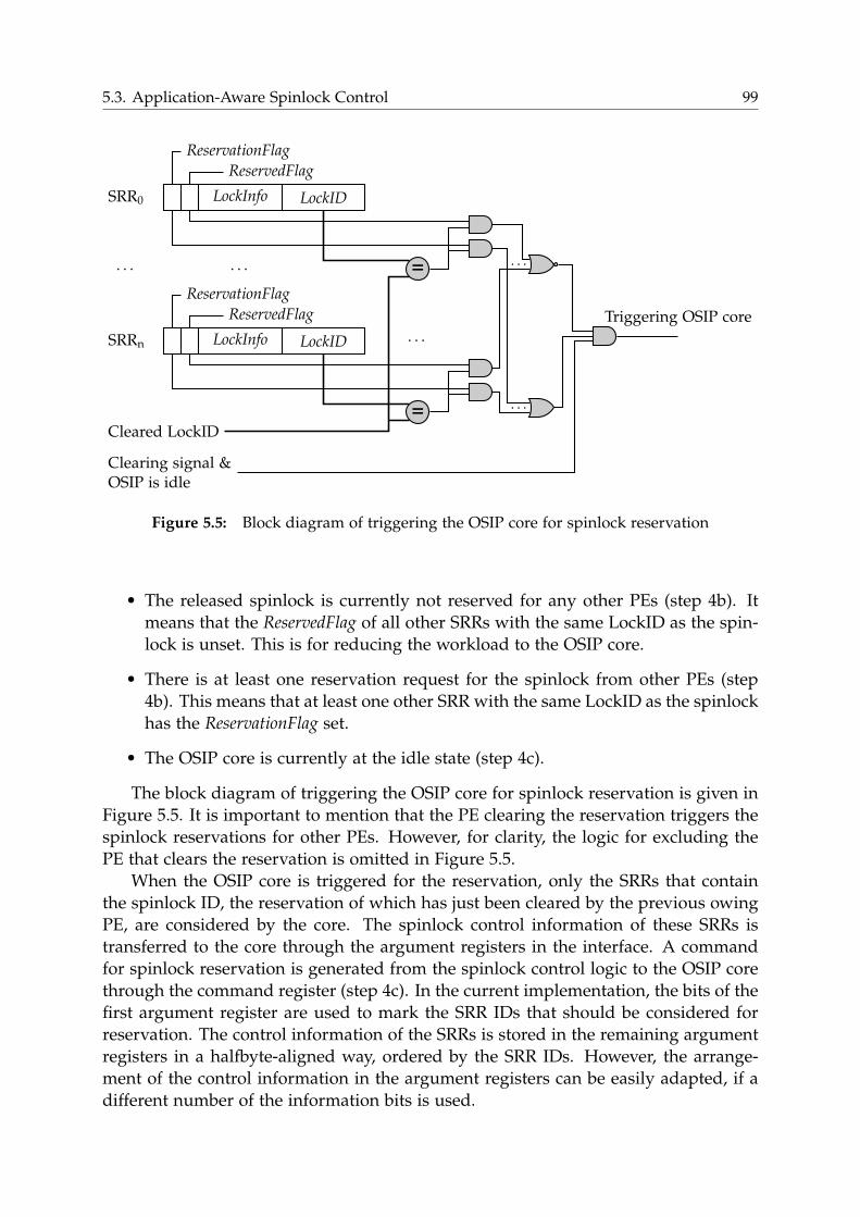
5.3. Application-Aware Spinlock Control 99
LockInfo LockID
=. . .
ReservationFlag
ReservedFlag
SRR0
LockInfo LockID
=. . .
ReservationFlag
ReservedFlag
SRRn
Cleared LockID
Clearing signal &OSIP is idle
Triggering OSIP core
. . . . . .
. . .
Figure 5.5: Block diagram of triggering the OSIP core for spinlock reservation
• The released spinlock is currently not reserved for any other PEs (step 4b). It
means that the ReservedFlag of all other SRRs with the same LockID as the spin-
lock is unset. This is for reducing the workload to the OSIP core.
• There is at least one reservation request for the spinlock from other PEs (step
4b). This means that at least one other SRR with the same LockID as the spinlock
has the ReservationFlag set.
• The OSIP core is currently at the idle state (step 4c).
The block diagram of triggering the OSIP core for spinlock reservation is given in
Figure 5.5. It is important to mention that the PE clearing the reservation triggers the
spinlock reservations for other PEs. However, for clarity, the logic for excluding the
PE that clears the reservation is omitted in Figure 5.5.
When the OSIP core is triggered for the reservation, only the SRRs that contain
the spinlock ID, the reservation of which has just been cleared by the previous owing
PE, are considered by the core. The spinlock control information of these SRRs is
transferred to the core through the argument registers in the interface. A command
for spinlock reservation is generated from the spinlock control logic to the OSIP core
through the command register (step 4c). In the current implementation, the bits of the
first argument register are used to mark the SRR IDs that should be considered for
reservation. The control information of the SRRs is stored in the remaining argument
registers in a halfbyte-aligned way, ordered by the SRR IDs. However, the arrange-
ment of the control information in the argument registers can be easily adapted, if a
different number of the information bits is used.
100 Chapter 5. OSIP Support for Efficient Spinlock Control
After the OSIP core is triggered, the spinlock reservation is executed as a normal
OSIP command (step 4d). The OSIP status is set to busy to prevent further commands
from being issued to the OSIP core. The reservation algorithm is user-defined and de-
cides which PE(s) should get the reservation, based on the provided spinlock control
information. As mentioned before, the algorithm can also take internal system status
into consideration when making the decision. Afterwards, the spinlock control logic
gets informed of the decision result by the OSIP core and update the ReservedFlag of
the corresponding SRR(s). Note that the reservation of a spinlock is not necessarily
limited to one PE. In fact, making a reservation for multiple PEs at the same time
helps reducing the workload of the OSIP core and accelerating the response to the
spinlock request.
5.3.4 Hardware Overhead
As shown above, the previous basic spinlock control unit is enhanced with additional
hardware to support the spinlock reservation mechanism. A number of 14-bit SRRs
are needed, as many as PEs. Besides, the spinlock control logic is extended. However,
since the computationally most intensive part for making reservation decisions is
performed in software, the additional control logic (mainly for storing/extracting
information into/from the SRRs and equivalence comparison of spinlock IDs) only
results in low hardware overhead, both from the area and timing perspective. For
a 12-PE-system, the largest system considered in this thesis, the additional hardware
has an area of 3.3 kGE, achieving a maximum clock frequency of 2.0GHz (synthesized
with Synopsys Design Compiler for a 65 nm standard cell library, supply voltage
1.0V, temperature 25°C). As a comparison, the OSIP core has an area of 35.7 kGE and
achieves 690MHz under the same synthesis conditions (see Section 3.3.1).
The hardware logic for the extended spinlock control in the interface can theoret-
ically be completely implemented in software running on the OSIP core. However,
this would on the one hand introduce too much workload to the core. On the other
hand, this control logic only requires very low flexibility for a given system, which
naturally calls for a native hardware implementation.
5.4 Case Studies
In this section, the two applications introduced in the previous chapter — the syn-
thetic application and H.264 — are further used as the case study applications for
analyzing the proposed enhanced spinlock control mechanism. The communication
architecture of the systems in the case studies is based on a multi-layer AHB bus with
the cache coherence system and write buffers (CA3 defined in Section 4.5.4).
5.4.1 Synthetic Application
As shown in Section 4.6.2.2, in the worst case scenarios, the execution time of the
application in UT-OSIP-/OSIP-based systems cannot be improved by applying more
5.4. Case Studies 101
than three CPEs, even if the system uses an ideal bus. A major cause is inefficient task
synchronization. If looking deeper into the application, it can be found that Taskscand Taskgen have to compete for the same spinlock for protecting the used standard C
library functions. Taskgen needs a malloc() process for creating tasks while Taskc calls
printf() to send the results to the I/O. Since the GNU C compiler for the ARM pro-
cessor, which is currently used in the simulation platforms, internally issues malloc()
when calling printf(), the same spinlock has to be used in Taskgen and Taskc to avoid
executing multiple malloc functions at the same time. Note that it is not always the
case if using other compilers. However, this does not influence the generality of the
analysis performed below. For example, it can be imagined that Taskgen could also
print information to the I/O or Taskc could do memory allocations as well.
In general, the execution time of creating a task in Taskgen is much shorter than
that of Taskc. However, since Tasksc are executed by multiple processors, it can happen
that the task generation speed of Taskgen cannot catch up with the speed of executing
Tasksc to consume data. As a consequence, some CPEs in the system might often or
even always stay at an idle state, waiting for Tasksc and wasting cycles. This becomes
especially critical if Taskgen is frequently blocked by Tasksc because of the competition
for the spinlock. On the other hand, if currently enough Tasksc have been generated
in the system, waiting for being executed, Taskgen should not block the execution of
Tasksc when competing for the spinlock. This can allow Tasksc to be more smoothly
completed. Therefore, a balance between Taskgen and Tasksc is desired when they are
executed.
The traditional way of assigning different priorities to the tasks does not help
much in this situation. Task priorities only determine the task execution order, but
not the spinlock acquisition order. If the spinlock control is done randomly, a high-
priority task can still be blocked by a low-priority task, simply because the high-
priority task loses the competition for the spinlock. Therefore, the spinlock reservation
approach is applied here to handle the spinlock competition between Taskgen and
Tasksc in a better way.
As explained above, in this application a balance between Taskgen and Tasksc is
desired to maximize the system performance. To achieve this, the execution of the
reservation algorithm should be dynamically adapted to the system status. In the
implementation, spinlock reservations are used in both Taskgen and Tasksc, but with
different spinlock control information. Assume without loss of generality that two
values A and B are assigned to the control information of Taskgen and Tasksc, respec-
tively, and A is unequal to B. In addition, a threshold is set in the reservation algo-
rithm executed on the OSIP core, which is meant to help judging whether enough
Tasksc have been prepared in the system. A prepared task is a Taskc which has been
generated but not yet been executed. Since OSIP is aware of the system status, it com-
pares the number of the prepared tasks with the threshold value, when it executes
the reservation algorithm. If the number is lower than the threshold, more tasks need
to be generated in the system to meet the requirement of data consumption. In this
situation, the reservation algorithm reserves the spinlock for the task with the control
value A, namely for Taskgen. If the system has a higher number of prepared tasks than
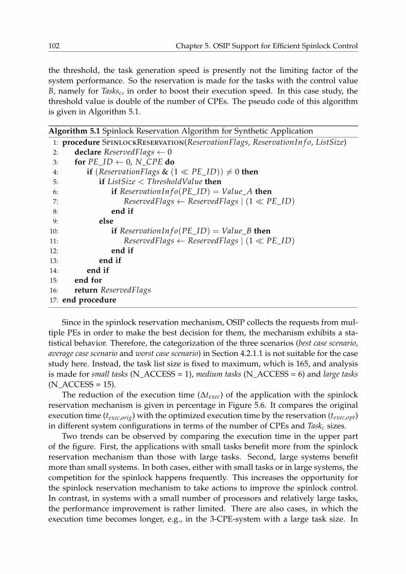
102 Chapter 5. OSIP Support for Efficient Spinlock Control
the threshold, the task generation speed is presently not the limiting factor of the
system performance. So the reservation is made for the tasks with the control value
B, namely for Tasksc, in order to boost their execution speed. In this case study, the
threshold value is double of the number of CPEs. The pseudo code of this algorithm
is given in Algorithm 5.1.
Algorithm 5.1 Spinlock Reservation Algorithm for Synthetic Application
1: procedure SpinlockReservation(ReservationFlags, ReservationIn f o, ListSize)2: declare ReservedFlags← 03: for PE_ID← 0, N_CPE do4: if (ReservationFlags & (1≪ PE_ID)) 6= 0 then5: if ListSize < ThresholdValue then6: if ReservationIn f o(PE_ID) = Value_A then7: ReservedFlags← ReservedFlags | (1≪ PE_ID)8: end if9: else
10: if ReservationIn f o(PE_ID) = Value_B then11: ReservedFlags← ReservedFlags | (1≪ PE_ID)12: end if13: end if14: end if15: end for16: return ReservedFlags17: end procedure
Since in the spinlock reservation mechanism, OSIP collects the requests from mul-
tiple PEs in order to make the best decision for them, the mechanism exhibits a sta-
tistical behavior. Therefore, the categorization of the three scenarios (best case scenario,
average case scenario and worst case scenario) in Section 4.2.1.1 is not suitable for the case
study here. Instead, the task list size is fixed to maximum, which is 165, and analysis
is made for small tasks (N_ACCESS = 1), medium tasks (N_ACCESS = 6) and large tasks
(N_ACCESS = 15).
The reduction of the execution time (∆texec) of the application with the spinlock
reservation mechanism is given in percentage in Figure 5.6. It compares the original
execution time (texec,orig) with the optimized execution time by the reservation (texec,opt)
in different system configurations in terms of the number of CPEs and Taskc sizes.
Two trends can be observed by comparing the execution time in the upper part
of the figure. First, the applications with small tasks benefit more from the spinlock
reservation mechanism than those with large tasks. Second, large systems benefit
more than small systems. In both cases, either with small tasks or in large systems, the
competition for the spinlock happens frequently. This increases the opportunity for
the spinlock reservation mechanism to take actions to improve the spinlock control.
In contrast, in systems with a small number of processors and relatively large tasks,
the performance improvement is rather limited. There are also cases, in which the
execution time becomes longer, e.g., in the 3-CPE-system with a large task size. In
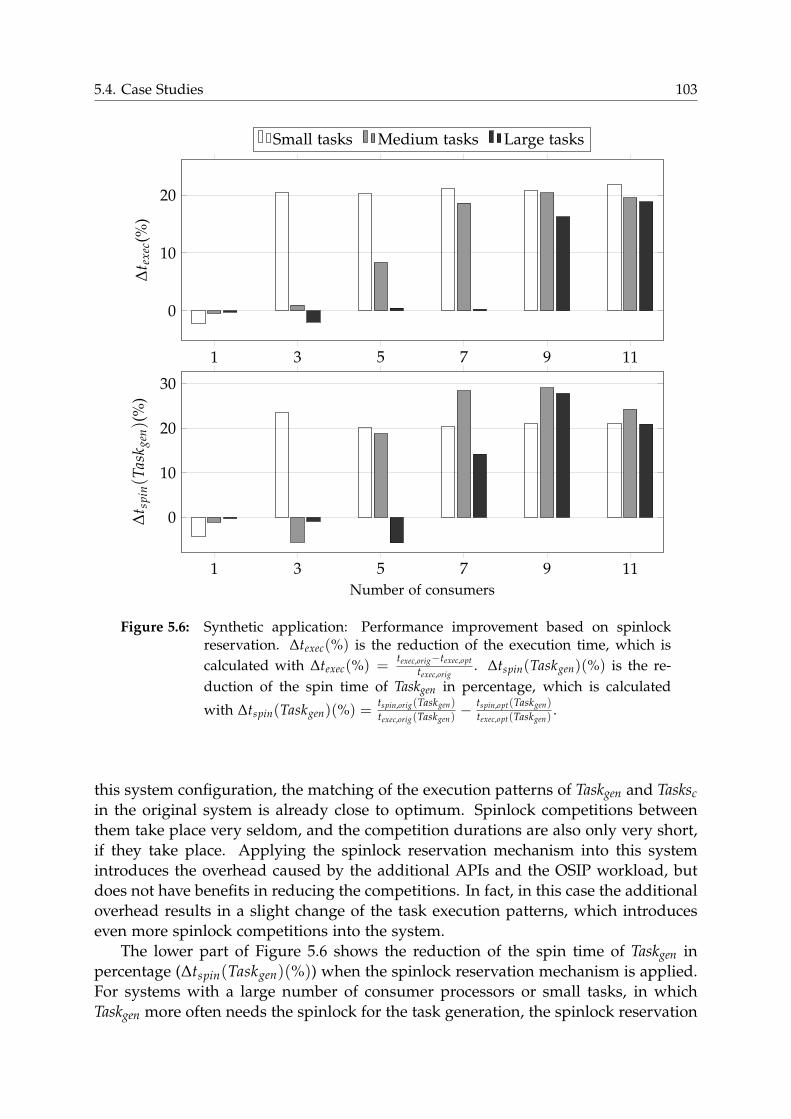
5.4. Case Studies 103
1 3 5 7 9 11
0
10
20
∆t e
xec
(%)
Small tasks Medium tasks Large tasks
1 3 5 7 9 11
0
10
20
30
∆t s
pin(T
ask g
en)(
%)
Number of consumers
Figure 5.6: Synthetic application: Performance improvement based on spinlockreservation. ∆texec(%) is the reduction of the execution time, which is
calculated with ∆texec(%) =texec,orig−texec,opt
texec,orig. ∆tspin(Taskgen)(%) is the re-
duction of the spin time of Taskgen in percentage, which is calculated
with ∆tspin(Taskgen)(%) =tspin,orig(Taskgen)
texec,orig(Taskgen)−
tspin,opt(Taskgen)
texec,opt(Taskgen).
this system configuration, the matching of the execution patterns of Taskgen and Taskscin the original system is already close to optimum. Spinlock competitions between
them take place very seldom, and the competition durations are also only very short,
if they take place. Applying the spinlock reservation mechanism into this system
introduces the overhead caused by the additional APIs and the OSIP workload, but
does not have benefits in reducing the competitions. In fact, in this case the additional
overhead results in a slight change of the task execution patterns, which introduces
even more spinlock competitions into the system.
The lower part of Figure 5.6 shows the reduction of the spin time of Taskgen in
percentage (∆tspin(Taskgen)(%)) when the spinlock reservation mechanism is applied.
For systems with a large number of consumer processors or small tasks, in which
Taskgen more often needs the spinlock for the task generation, the spinlock reservation
104 Chapter 5. OSIP Support for Efficient Spinlock Control
mechanism can greatly reduce the spin time of Taskgen. In contrast, for small systems
with relatively large tasks, in which Taskgen does not need the spinlock frequently, the
adaptive reservation algorithm tends to increase the spin time of Taskgen for the benefit
of executing Tasksc.
5.4.2 H.264
The spinlock reservation mechanism also applies to H.264. As introduced in Section
4.3.2, the IQT, IDCT and intra-frame prediction tasks can be highly parallelized in this
application. The IQT and IDCT can be processed for each MB independently, while
the prediction for an MB has dependency both on the IQT/IDCT for the same MB
and on the predictions for the neighboring MBs on the left, top and top left of the
current one. The task synchronization between the IQT/IDCT and prediction for an
MB, and especially between the predictions for the neighboring MBs, has a big impact
on the frame rate of the video decoding. If the task synchronization is not efficiently
resolved, the frame rate could be largely reduced.
However, in the original implementation the task synchronization is often delayed
by spinlock competitions. Similar to the synthetic application, the memory allocation
for creating new IQT/IDCT and prediction tasks is often blocked by the I/O accesses
for outputting MBs. To change this situation, spinlock reservations are made for the
creation of these tasks. Furthermore, the reservation for creating a prediction task is
assigned with a higher priority than for creating an IQT/IDCT task, because resolving
the synchronization between the predictions is more critical for improving the system
performance.
The reservation algorithm is given in Algorithm 5.2. First, the number of the PEs
which require a spinlock reservation is counted and the IDs of these PEs are recorded
(line 4 – 9). Then, a search is made among these PEs to find the ones with the highest
reservation priorities (line 11 – 20), which have been given as the spinlock control
information when reservations are requested by the PEs. Finally, the reservation result
is returned.
The performance improvement with the spinlock reservation mechanism is high-
lighted in the upper part of Figure 5.7 by comparing the video frame rates. A signifi-
cant increment of the frame rate can be observed starting from a 6-processor-system,
which clearly shows the efficiency of the proposed approach. For large systems, a
speedup of up to 1.2× is achieved. The low improvement for small systems with less
processors results from the low competition for the spinlock, in which the improve-
ment opportunities are rather limited.
Similarly as done for the synthetic application, the spin time for the lock is an-
alyzed in order to have a closer look at the reason for the speedup. Shown in the
lower part of Figure 5.7, the average spin time of trying to acquire the lock in the
application is largely reduced by reserving the spinlock, which effectively improves
the utilization of the processors. As a side effect, the communication traffic is also
reduced.
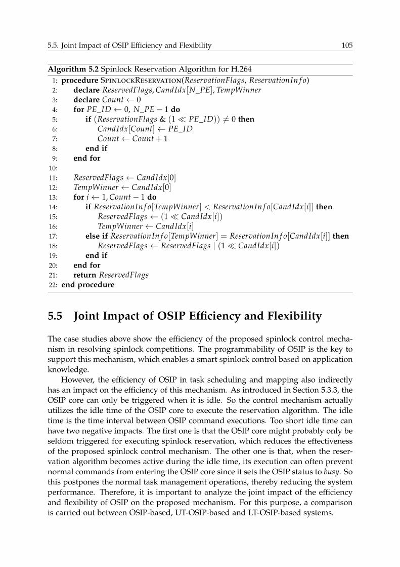
5.5. Joint Impact of OSIP Efficiency and Flexibility 105
Algorithm 5.2 Spinlock Reservation Algorithm for H.264
1: procedure SpinlockReservation(ReservationFlags, ReservationIn f o)2: declare ReservedFlags,CandIdx[N_PE], TempWinner3: declare Count← 04: for PE_ID← 0, N_PE− 1 do5: if (ReservationFlags & (1≪ PE_ID)) 6= 0 then6: CandIdx[Count]← PE_ID7: Count← Count+ 18: end if9: end for
10:
11: ReservedFlags← CandIdx[0]12: TempWinner← CandIdx[0]13: for i← 1,Count− 1 do14: if ReservationIn f o[TempWinner] < ReservationIn f o[CandIdx[i]] then15: ReservedFlags← (1≪ CandIdx[i])16: TempWinner← CandIdx[i]17: else if ReservationIn f o[TempWinner] = ReservationIn f o[CandIdx[i]] then18: ReservedFlags← ReservedFlags | (1≪ CandIdx[i])19: end if20: end for21: return ReservedFlags22: end procedure
5.5 Joint Impact of OSIP Efficiency and Flexibility
The case studies above show the efficiency of the proposed spinlock control mecha-
nism in resolving spinlock competitions. The programmability of OSIP is the key to
support this mechanism, which enables a smart spinlock control based on application
knowledge.
However, the efficiency of OSIP in task scheduling and mapping also indirectly
has an impact on the efficiency of this mechanism. As introduced in Section 5.3.3, the
OSIP core can only be triggered when it is idle. So the control mechanism actually
utilizes the idle time of the OSIP core to execute the reservation algorithm. The idle
time is the time interval between OSIP command executions. Too short idle time can
have two negative impacts. The first one is that the OSIP core might probably only be
seldom triggered for executing spinlock reservation, which reduces the effectiveness
of the proposed spinlock control mechanism. The other one is that, when the reser-
vation algorithm becomes active during the idle time, its execution can often prevent
normal commands from entering the OSIP core since it sets the OSIP status to busy. So
this postpones the normal task management operations, thereby reducing the system
performance. Therefore, it is important to analyze the joint impact of the efficiency
and flexibility of OSIP on the proposed mechanism. For this purpose, a comparison
is carried out between OSIP-based, UT-OSIP-based and LT-OSIP-based systems.
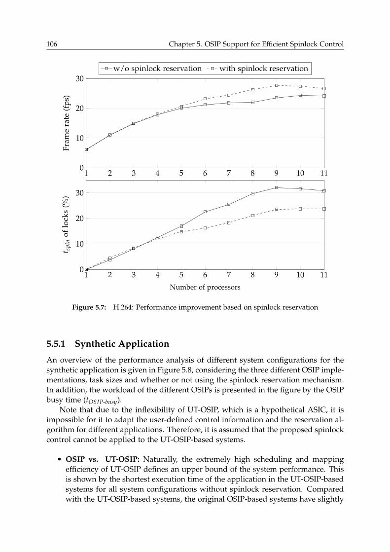
106 Chapter 5. OSIP Support for Efficient Spinlock Control
1 2 3 4 5 6 7 8 9 10 110
10
20
30
Fra
me
rate
(fp
s)w/o spinlock reservation with spinlock reservation
1 2 3 4 5 6 7 8 9 10 110
10
20
30
t sp
ino
flo
cks
(%)
Number of processors
Figure 5.7: H.264: Performance improvement based on spinlock reservation
5.5.1 Synthetic Application
An overview of the performance analysis of different system configurations for the
synthetic application is given in Figure 5.8, considering the three different OSIP imple-
mentations, task sizes and whether or not using the spinlock reservation mechanism.
In addition, the workload of the different OSIPs is presented in the figure by the OSIP
busy time (tOSIP-busy).
Note that due to the inflexibility of UT-OSIP, which is a hypothetical ASIC, it is
impossible for it to adapt the user-defined control information and the reservation al-
gorithm for different applications. Therefore, it is assumed that the proposed spinlock
control cannot be applied to the UT-OSIP-based systems.
• OSIP vs. UT-OSIP: Naturally, the extremely high scheduling and mapping
efficiency of UT-OSIP defines an upper bound of the system performance. This
is shown by the shortest execution time of the application in the UT-OSIP-based
systems for all system configurations without spinlock reservation. Compared
with the UT-OSIP-based systems, the original OSIP-based systems have slightly
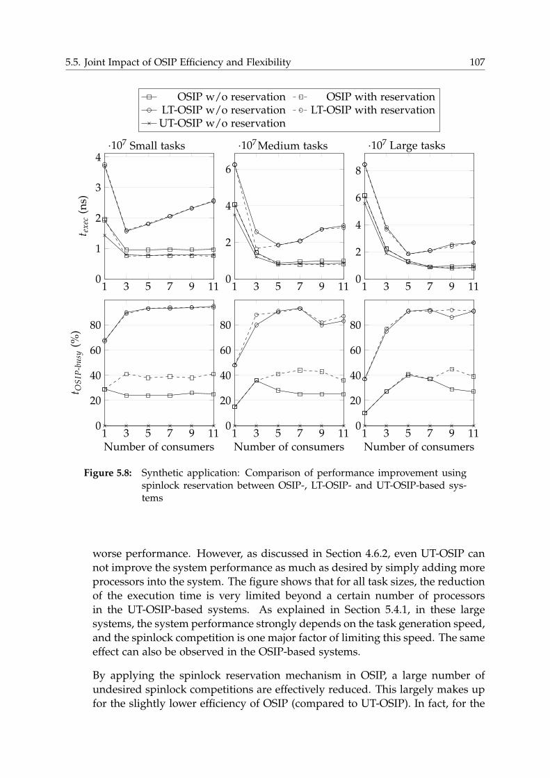
5.5. Joint Impact of OSIP Efficiency and Flexibility 107
1 3 5 7 9 110
1
2
3
4·107
t ex
ec(n
s)
Small tasks
1 3 5 7 9 110
2
4
6
·107
OSIP w/o reservation OSIP with reservationLT-OSIP w/o reservation LT-OSIP with reservationUT-OSIP w/o reservation
Medium tasks
1 3 5 7 9 110
2
4
6
8
·107 Large tasks
1 3 5 7 9 110
20
40
60
80
t OS
IP-b
usy
(%)
Number of consumers1 3 5 7 9 11
0
20
40
60
80
Number of consumers1 3 5 7 9 11
0
20
40
60
80
Number of consumers
Figure 5.8: Synthetic application: Comparison of performance improvement usingspinlock reservation between OSIP-, LT-OSIP- and UT-OSIP-based sys-tems
worse performance. However, as discussed in Section 4.6.2, even UT-OSIP can
not improve the system performance as much as desired by simply adding more
processors into the system. The figure shows that for all task sizes, the reduction
of the execution time is very limited beyond a certain number of processors
in the UT-OSIP-based systems. As explained in Section 5.4.1, in these large
systems, the system performance strongly depends on the task generation speed,
and the spinlock competition is one major factor of limiting this speed. The same
effect can also be observed in the OSIP-based systems.
By applying the spinlock reservation mechanism in OSIP, a large number of
undesired spinlock competitions are effectively reduced. This largely makes up
for the slightly lower efficiency of OSIP (compared to UT-OSIP). In fact, for the
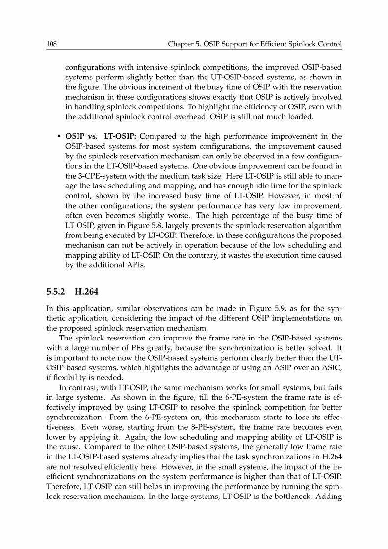
108 Chapter 5. OSIP Support for Efficient Spinlock Control
configurations with intensive spinlock competitions, the improved OSIP-based
systems perform slightly better than the UT-OSIP-based systems, as shown in
the figure. The obvious increment of the busy time of OSIP with the reservation
mechanism in these configurations shows exactly that OSIP is actively involved
in handling spinlock competitions. To highlight the efficiency of OSIP, even with
the additional spinlock control overhead, OSIP is still not much loaded.
• OSIP vs. LT-OSIP: Compared to the high performance improvement in the
OSIP-based systems for most system configurations, the improvement caused
by the spinlock reservation mechanism can only be observed in a few configura-
tions in the LT-OSIP-based systems. One obvious improvement can be found in
the 3-CPE-system with the medium task size. Here LT-OSIP is still able to man-
age the task scheduling and mapping, and has enough idle time for the spinlock
control, shown by the increased busy time of LT-OSIP. However, in most of
the other configurations, the system performance has very low improvement,
often even becomes slightly worse. The high percentage of the busy time of
LT-OSIP, given in Figure 5.8, largely prevents the spinlock reservation algorithm
from being executed by LT-OSIP. Therefore, in these configurations the proposed
mechanism can not be actively in operation because of the low scheduling and
mapping ability of LT-OSIP. On the contrary, it wastes the execution time caused
by the additional APIs.
5.5.2 H.264
In this application, similar observations can be made in Figure 5.9, as for the syn-
thetic application, considering the impact of the different OSIP implementations on
the proposed spinlock reservation mechanism.
The spinlock reservation can improve the frame rate in the OSIP-based systems
with a large number of PEs greatly, because the synchronization is better solved. It
is important to note now the OSIP-based systems perform clearly better than the UT-
OSIP-based systems, which highlights the advantage of using an ASIP over an ASIC,
if flexibility is needed.
In contrast, with LT-OSIP, the same mechanism works for small systems, but fails
in large systems. As shown in the figure, till the 6-PE-system the frame rate is ef-
fectively improved by using LT-OSIP to resolve the spinlock competition for better
synchronization. From the 6-PE-system on, this mechanism starts to lose its effec-
tiveness. Even worse, starting from the 8-PE-system, the frame rate becomes even
lower by applying it. Again, the low scheduling and mapping ability of LT-OSIP is
the cause. Compared to the other OSIP-based systems, the generally low frame rate
in the LT-OSIP-based systems already implies that the task synchronizations in H.264
are not resolved efficiently here. However, in the small systems, the impact of the in-
efficient synchronizations on the system performance is higher than that of LT-OSIP.
Therefore, LT-OSIP can still helps in improving the performance by running the spin-
lock reservation mechanism. In the large systems, LT-OSIP is the bottleneck. Adding
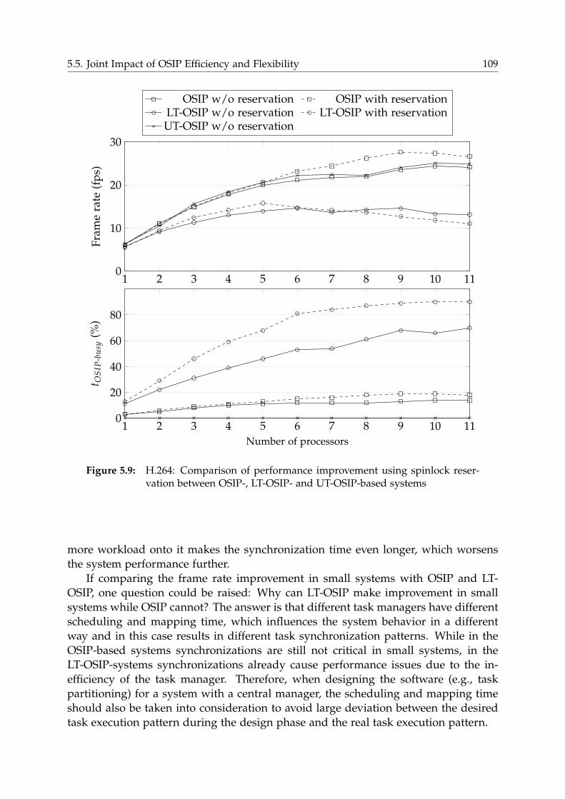
5.5. Joint Impact of OSIP Efficiency and Flexibility 109
1 2 3 4 5 6 7 8 9 10 110
10
20
30
Fra
me
rate
(fp
s)OSIP w/o reservation OSIP with reservation
LT-OSIP w/o reservation LT-OSIP with reservationUT-OSIP w/o reservation
1 2 3 4 5 6 7 8 9 10 110
20
40
60
80
t OS
IP-b
usy
(%)
Number of processors
Figure 5.9: H.264: Comparison of performance improvement using spinlock reser-vation between OSIP-, LT-OSIP- and UT-OSIP-based systems
more workload onto it makes the synchronization time even longer, which worsens
the system performance further.
If comparing the frame rate improvement in small systems with OSIP and LT-
OSIP, one question could be raised: Why can LT-OSIP make improvement in small
systems while OSIP cannot? The answer is that different task managers have different
scheduling and mapping time, which influences the system behavior in a different
way and in this case results in different task synchronization patterns. While in the
OSIP-based systems synchronizations are still not critical in small systems, in the
LT-OSIP-systems synchronizations already cause performance issues due to the in-
efficiency of the task manager. Therefore, when designing the software (e.g., task
partitioning) for a system with a central manager, the scheduling and mapping time
should also be taken into consideration to avoid large deviation between the desired
task execution pattern during the design phase and the real task execution pattern.
110 Chapter 5. OSIP Support for Efficient Spinlock Control
Based on the comparison between the systems using different OSIP implementations,
it can be concluded that the flexibility of a system can help increasing the system
performance significantly by using application knowledge. In this work, the applica-
tion knowledge is applied to spinlock control. Large improvements can be observed
in both OSIP-based and LT-OSIP-based systems. Especially the OSIP-based systems,
supported by the application knowledge, perform even better than the systems using
an extremely fast ASIC task manager in many cases.
On the other hand, considering additional application knowledge in the system
introduces additional workload, which can also lead to worse system performance.
This can be confirmed by the reduced performance of the LT-OSIP-based systems
in most of the analyzed cases. Compared to LT-OSIP-based systems, OSIP-based
systems, however, can achieve much more stable performance improvement. This
shows that the efficiency of OSIP enables more advanced system control techniques.
More in general, the efficiency is essential for guaranteeing an effective utilization of
the system flexibility.
5.6 Summary
In this chapter, a centralized spinlock control mechanism is introduced, in which
spinlocks can be reserved for the tasks to prevent random spinlock acquisitions. The
reservation information is user-defined, based on application knowledge. A sim-
ple spinlock reservation API pair enables easy integration of the application know-
ledge into the spinlock control flow. The OSIP processor, originally designed for task
scheduling and mapping, is used additionally to support this mechanism for making
application-aware spinlock decisions. The performance improvement in the presented
case studies shows the efficiency of this mechanism in spinlock-intensive applications.
Furthermore, an extensive analysis of this mechanism considering different OSIP im-
plementations is made. The analysis results highlight the efficiency and the flexibility
of OSIP, thanks to the ASIP concept, which enables successful employment of this
mechanism in practice.
Although the experiments in this chapter are done in the OSIP-based systems, the
basic concept of spinlock reservation can be generalized to systems using a central
programmable controller. Certainly, the efficiency of the controller should be consid-
ered when applying this mechanism.
5.7 Discussion
The spinlock reservation mechanism shows its efficiency in improving the spinlock
control in general. However, there are still several potential improvement possibilities,
which are discussed in the following.
5.7. Discussion 111
5.7.1 Tool Support for Spinlock Reservation
The reservation information, also including whether and where to make reservations,
plays a key role in this approach. In the two case studies given in this chapter, the
information is derived by analyzing the applications manually. This requires much te-
dious work, even though both applications have relatively regular task execution and
spinlock competition patterns. And in these two case studies, both spinlock control
algorithms are simple, but still demonstrate high efficiency in improving the system
performance. This is possible because they focus on solving the most critical spinlock
competitions that have a large impact on the task parallelism degree. However, there
are certainly applications, in which more complicated and optimized spinlock acqui-
sition orders are needed to maximize task parallelism. This requires complex control
algorithms. However, too complex algorithms could introduce high additional work-
load to OSIP, which can potentially impair the normal task scheduling and mapping
operations of OSIP. Therefore, a balance needs to be found between the possible gain
in task parallelism achieved by the complex algorithms and the additional workload
caused by them. All these naturally call for tool support such as MAPS compiler [30],
which on the one hand can provide a more systematic analysis, on the other hand can
considerately accelerate the complete design flow of the proposed approach.
5.7.2 Scalability Problem
As a central mechanism, the proposed spinlock control approach can inherently be
faced with the scalability problem. If the system size becomes very large, the central
controller would likely become the system bottleneck. This is, however, not the case
in the presented case studies if OSIP is used as the controller, which is indicated
by its low busy time shown in Figure 5.8 and Figure 5.9. In fact, in systems based
on a central bus, the scalability problem at the central controller is not necessarily
critical. If an efficient enough central controller like OSIP is employed, the system
bottleneck would most likely be shifted to the bus communication due to heavy traffic
in large systems, as shown in Chapter 4, in which a detailed joint analysis of the
communication architecture and the OSIP efficiency is made.
However, in systems with high communication bandwidths, e.g., using NoCs, the
scalability problem of the proposed central mechanism can become serious. In these
systems, a combination of this mechanism and other distributed mechanisms like the
ones presented in [212] and [38] can be considered, which are complementary to each
other. OSIP, being the system task manager, can be used to perform global task-level
spinlock control, focusing on maximizing task parallelism. In contrast, the control
jobs at more fine-grained granularity levels, such as word-level read/write locks, can
be done in a distributed way, thereby reducing traffic and the OSIP workload. The
simple system integration of OSIP makes it possible to combine both mechanisms,
and the user only needs to define separate address-mappings for the spinlocks to
distinguish the requests to the central controller and local control units.
112 Chapter 5. OSIP Support for Efficient Spinlock Control
5.7.3 Nested Spinlocks
In the current experiments, nested spinlock reservations are not supported. This
means, a later reservation of a PE always overwrites its previous reservation. To
support nested reservations, buffers need to be introduced in the spinlock control
unit to allocate multiple reservation requests from the same PE.
Chapter 6
OSIP Integration in NoC-basedSystems
In Chapter 4 and Chapter 5, the advantages of using OSIP for handling task schedul-
ing and mapping have been presented from the efficiency and flexibility perspective.
In these two chapters, the systems are built on a shared bus with a shared memory.
As this kind of system architectures is centralized, a central task manager such as
OSIP fits well into such systems. Its integration into the system can be easily done as
a standard memory-mapped peripheral.
However, in systems with a large number of PEs towards many-core systems,
the shared bus based communication architectures are not suitable anymore. As in-
troduced in Section 2.4, they inherently suffer from the scalability problem caused
by long bus wires in large systems. For these systems, NoCs are a preferred com-
munication architecture paradigm, in which the long wires are segmented by using
packet-based communications through routers. In comparison to bus-based systems,
NoC-based systems have a distributed architecture. As OSIP is a central manager,
some general questions would be: Is it still possible to integrate the central OSIP into
distributed NoC-based systems? How to integrate OSIP, if it is possible? Is OSIP still
efficient in such systems? In this chapter, answers to these questions are given.
This chapter is organized as follows. First, two main problems of integrating OSIP
into NoC-based systems are presented. Following this, the basic idea of addressing
the integration problems is illustrated. Afterwards, a complex case study is pro-
vided. In this case study, both the NoC architecture used in this work and the target
application are introduced. The application is taken from the wireless communica-
tion domain, which is a 2×2 Multiple-Input Multiple-Output (MIMO) Orthogonal
Frequency-Division Multiplexing (OFDM) digital receiver. Then, the system imple-
mentation at a high abstraction level using VPUs is introduced and the concrete inte-
gration of OSIP into the system with the NoC is described in detail. Also, preliminary
results about the impact of the NoC on the system performance are reported. Based
on the preliminary results, optimizations are proposed for the communication and
in-depth analyses are performed. Finally, a summary is made and further possible
extensions for OSIP integration into NoC-based systems are discussed.1
1 Portions of this chapter have been published by the author in [215] in Advancing Embedded Systemsand Real-Time Communications with Emerging Technologies, edited by Seppo Virtanen. Copyright 2014,IGI Global, www.igi-global.com. Posted by permission of the publisher.
113
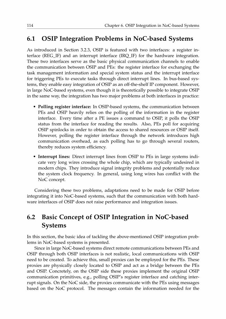
114 Chapter 6. OSIP Integration in NoC-based Systems
6.1 OSIP Integration Problems in NoC-based Systems
As introduced in Section 3.2.3, OSIP is featured with two interfaces: a register in-
terface (REG_IF) and an interrupt interface (IRQ_IF) for the hardware integration.
These two interfaces serve as the basic physical communication channels to enable
the communication between OSIP and PEs: the register interface for exchanging the
task management information and special system status and the interrupt interface
for triggering PEs to execute tasks through direct interrupt lines. In bus-based sys-
tems, they enable easy integration of OSIP as an off-the-shelf IP component. However,
in large NoC-based systems, even though it is theoretically possible to integrate OSIP
in the same way, the integration has two major problems at both interfaces in practice:
• Polling register interface: In OSIP-based systems, the communication between
PEs and OSIP heavily relies on the polling of the information in the register
interface. Every time after a PE issues a command to OSIP, it polls the OSIP
status from the interface for reading the results. Also, PEs poll for acquiring
OSIP spinlocks in order to obtain the access to shared resources or OSIP itself.
However, polling the register interface through the network introduces high
communication overhead, as each polling has to go through several routers,
thereby reduces system efficiency.
• Interrupt lines: Direct interrupt lines from OSIP to PEs in large systems indi-
cate very long wires crossing the whole chip, which are typically undesired in
modern chips. They introduce signal integrity problems and potentially reduce
the system clock frequency. In general, using long wires has conflict with the
NoC concept.
Considering these two problems, adaptations need to be made for OSIP before
integrating it into NoC-based systems, such that the communication with both hard-
ware interfaces of OSIP does not raise performance and integration issues.
6.2 Basic Concept of OSIP Integration in NoC-based
Systems
In this section, the basic idea of tackling the above-mentioned OSIP integration prob-
lems in NoC-based systems is presented.
Since in large NoC-based systems direct remote communications between PEs and
OSIP through both OSIP interfaces is not realistic, local communications with OSIP
need to be created. To achieve this, small proxies can be employed for the PEs. These
proxies are physically closely located to OSIP and act as a bridge between the PEs
and OSIP. Concretely, on the OSIP side these proxies implement the original OSIP
communication primitives, e.g., polling OSIP’s register interface and catching inter-
rupt signals. On the NoC side, the proxies communicate with the PEs using messages
based on the NoC protocol. The messages contain the information needed for the
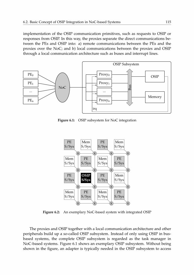
6.2. Basic Concept of OSIP Integration in NoC-based Systems 115
implementation of the OSIP communication primitives, such as requests to OSIP or
responses from OSIP. In this way, the proxies separate the direct communications be-
tween the PEs and OSIP into: a) remote communications between the PEs and the
proxies over the NoC; and b) local communications between the proxies and OSIP
through a local communication architecture such as buses and interrupt lines.
PE0
PE1
...
PEn
NoC
OSIP Subsystem
Proxy0
Proxy1
...
Proxyn
Bu
s
OSIP
Memory
irq
Figure 6.1: OSIP subsystem for NoC integration
MemS/Sys
R
PES/Sys
R
MemS/Sys
R
PES/Sys
R
PES/Sys
R R
PES/Sys
R
MemS/Sys
R
MemS/Sys
R
PES/Sys
R
MemS/Sys
R
PES/Sys
R
PES/Sys
R
MemS/Sys
R
PES/Sys
R
MemS/Sys
R
OSIP
S/Sys
Figure 6.2: An exemplary NoC-based system with integrated OSIP
The proxies and OSIP together with a local communication architecture and other
peripherals build up a so-called OSIP subsystem. Instead of only using OSIP in bus-
based systems, the complete OSIP subsystem is regarded as the task manager in
NoC-based systems. Figure 6.1 shows an exemplary OSIP subsystem. Without being
shown in the figure, an adapter is typically needed in the OSIP subsystem to access
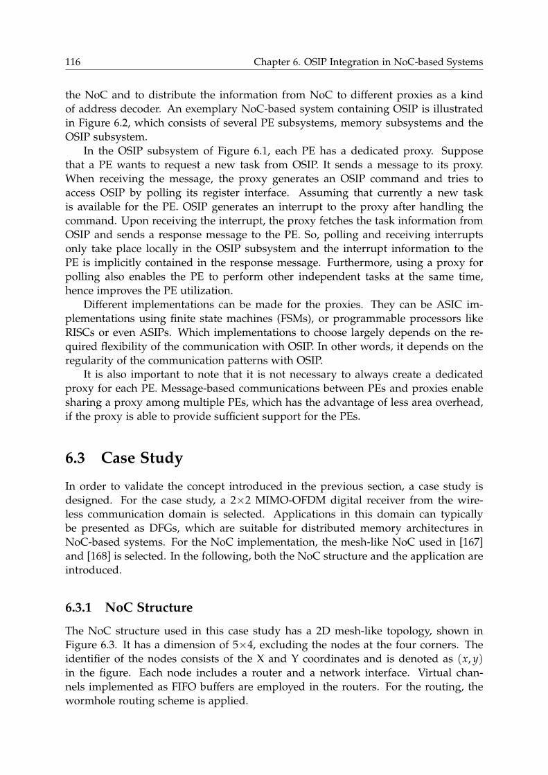
116 Chapter 6. OSIP Integration in NoC-based Systems
the NoC and to distribute the information from NoC to different proxies as a kind
of address decoder. An exemplary NoC-based system containing OSIP is illustrated
in Figure 6.2, which consists of several PE subsystems, memory subsystems and the
OSIP subsystem.
In the OSIP subsystem of Figure 6.1, each PE has a dedicated proxy. Suppose
that a PE wants to request a new task from OSIP. It sends a message to its proxy.
When receiving the message, the proxy generates an OSIP command and tries to
access OSIP by polling its register interface. Assuming that currently a new task
is available for the PE. OSIP generates an interrupt to the proxy after handling the
command. Upon receiving the interrupt, the proxy fetches the task information from
OSIP and sends a response message to the PE. So, polling and receiving interrupts
only take place locally in the OSIP subsystem and the interrupt information to the
PE is implicitly contained in the response message. Furthermore, using a proxy for
polling also enables the PE to perform other independent tasks at the same time,
hence improves the PE utilization.
Different implementations can be made for the proxies. They can be ASIC im-
plementations using finite state machines (FSMs), or programmable processors like
RISCs or even ASIPs. Which implementations to choose largely depends on the re-
quired flexibility of the communication with OSIP. In other words, it depends on the
regularity of the communication patterns with OSIP.
It is also important to note that it is not necessary to always create a dedicated
proxy for each PE. Message-based communications between PEs and proxies enable
sharing a proxy among multiple PEs, which has the advantage of less area overhead,
if the proxy is able to provide sufficient support for the PEs.
6.3 Case Study
In order to validate the concept introduced in the previous section, a case study is
designed. For the case study, a 2×2 MIMO-OFDM digital receiver from the wire-
less communication domain is selected. Applications in this domain can typically
be presented as DFGs, which are suitable for distributed memory architectures in
NoC-based systems. For the NoC implementation, the mesh-like NoC used in [167]
and [168] is selected. In the following, both the NoC structure and the application are
introduced.
6.3.1 NoC Structure
The NoC structure used in this case study has a 2D mesh-like topology, shown in
Figure 6.3. It has a dimension of 5×4, excluding the nodes at the four corners. The
identifier of the nodes consists of the X and Y coordinates and is denoted as (x, y)in the figure. Each node includes a router and a network interface. Virtual chan-
nels implemented as FIFO buffers are employed in the routers. For the routing, the
wormhole routing scheme is applied.
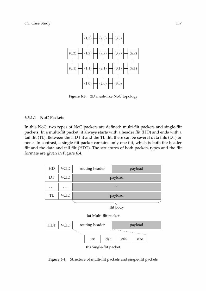
6.3. Case Study 117
(1,0) (2,0) (3,0)
(0,1) (1,1) (2,1) (3,1) (4,1)
(0,2) (1,2) (2,2) (3,2) (4,2)
(1,3) (2,3) (3,3)
Figure 6.3: 2D mesh-like NoC topology
6.3.1.1 NoC Packets
In this NoC, two types of NoC packets are defined: multi-flit packets and single-flit
packets. In a multi-flit packet, it always starts with a header flit (HD) and ends with a
tail flit (TL). Between the HD flit and the TL flit, there can be several data flits (DT) or
none. In contrast, a single-flit packet contains only one flit, which is both the header
flit and the data and tail flit (HDT). The structures of both packets types and the flit
formats are given in Figure 6.4.
HD VCID routing header payload
DT VCID payload
. . . . . . . . .
TL VCID payload
flit body
(a) Multi-flit packet
HDT VCID routing header payload
src dst prio size
(b) Single-flit packet
Figure 6.4: Structure of multi-flit packets and single-flit packets
118 Chapter 6. OSIP Integration in NoC-based Systems
Each flit consists of three fields: flit type (HD/DT/TL/HDT), virtual channel ID
(VCID) and flit body. VCID specifies which virtual channel of the next router is
required to buffer the flit. The flit body contains the payload data of the packet. In
the HD/HDT flit, it also contains the routing header, which provides the necessary
information needed for routing. The information includes:
• src: Coordinates of the source node, from which the packet is sent.
• dst: Coordinates of the destination node, to which the packet is sent.
• prio: Priority of the packet, which is used for the arbitration when competing
with other packets for virtual channels and router output ports.
• size: Payload size of the packet, which is given in bytes.
6.3.1.2 Router
The router architecture of this NoC is scalable regarding the following parameters:
the number of router input and output ports, the number of virtual channels, the size
of virtual channels and the data link width between routers. The block diagram of the
router architecture is shown in Figure 6.5, in which the following five main functional
blocks can be identified:
• Receiving (RCV): In this functional block, the flits from the neighboring routers
are received. The VCID information of the flits is extracted and used for selecting
the corresponding virtual channels for the flits. There are as many RCV blocks
as the router ports, and within one clock cycle, one flit can be received by one
port at most.
• Routing (RUT): In this block, the routing direction of the flits to the next router
is determined. A routing table is defined in each router, following a modified
XY routing algorithm, because the normal XY routing algorithm cannot be di-
rectly applied to this NoC due to the missing nodes at the four corners. In
this modified algorithm, the routers first forward the packet in X-direction, un-
til the X-coordinate of the destination node is reached or the packet cannot be
forwarded any further if the boundary of the NoC in X-direction is reached.
Then the packet is forwarded in Y-direction until the Y-coordinate of the node
is reached. If the node is exactly the destination node, the routing is finished,
which is the same as in the normal XY routing. Otherwise, the routing continues
in X-direction again until the destination node is reached. One example for the
latter case is the routing from node (1, 3) to node (4, 2), which has the routing
path (1, 3) → (2, 3) → (3, 3) → (3, 2) → (4, 2). Note this modified XY routing
is also deadlock-free as the normal XY routing, because no cycles can be created
during the routing.
The routing table is hard-wired and configurable at the design time. When the
RUT block receives a flit from the RCV block, it first examines the flit type. In
6.3. Case Study 119
case of an HD/HDT flit, the coordinates of the destination nodes are extracted
from the dst field of the flit and used as the input to the routing table. The
outcome is the output port of the router, to which the flit should be sent. If the
flit is a DT/TL flit, it simply takes the previous routing result for the HD flit of
the same packet.
• Virtual Channel Allocation (VCA): After the routing direction (i.e., the output
port of the router) for a flit is determined, a virtual channel at the corresponding
input port of the next router needs to be allocated for the flit. A virtual channel
at the current router and at the next router are further referred to as an input
and output virtual channel, respectively. As introduced in Section 2.4.2, virtual
channels are common means to improve the NoC throughput.
For the allocation of an output virtual channel, competitions can happen be-
tween the flits in the current router, which are not only from different input
ports, but also from different input virtual channels at each port. To reduce
the hardware complexity, the arbitrations are performed in a hierarchical way
consisting of two levels.
At the first level, local arbitrations are performed to find an available output vir-
tual channel for each input virtual channel individually. The availability of an
output virtual channel is indicated by a so-called credit signal, showing whether
the buffer of the virtual channel is full. This level of arbitrations is static. The
output virtual channels with smaller IDs, if they are available, have higher pri-
orities than the ones with higher IDs.
At the second level, a global arbitration across all input virtual channels is per-
formed. This arbitration is dynamic, based on the Fair-Among-Equal scheme.
Here the priorities in the prio field of the HD/HDT flits from different input
virtual channels are compared if they compete for the same output virtual chan-
nel. The input virtual channel with the highest flit priority wins. In case that
multiple input virtual channels have the same highest priority, a round-robin
arbitration is further performed for fairness.
To support the wormhole routing scheme, all flits of a packet always use the
same virtual channel of a router, and the flits of other packets are not allowed to
be inserted in between. This means that if an output virtual channel is currently
allocated for a packet, it is in general not available for the flits of other packets,
until the complete packet has been received by the virtual channel.
As the outcome of this functional block, at most one output virtual channel per
output port can be allocated. However, it is possible that multiple input virtual
channels at one input port can allocate an output channel each, while the input
channels of some other input ports allocate none.
• Switch Allocation (SWA): With an allocated output virtual channel, a flit is
ready for being transferred to the next router. As there are more virtual chan-
nels than physical channels between neighboring routers, competitions can also
120 Chapter 6. OSIP Integration in NoC-based Systems
happen among the flits from different input virtual channels for allocating the
physical channels. For fairness of transferring packets from different input ports,
at most one flit from each input port can obtain the access to a physical channel
within one clock cycle. Therefore, another two-level arbitration is applied, using
the same dynamic Fair-Among-Equal scheme described above for both levels. At
the first level, arbitrations are performed among the input virtual channels at
each input port to find a winner input channel (i.e., a winner flit) of the port.
Then, at the second level, the winner flits from all input ports are compared to
determine which ones can finally obtain the access to the physical channels.
Note that different from the allocation of a virtual channel, which must be con-
tinuously allocated for a complete packet, the allocation of a physical channel
does not have this limitation. The flits of different packets can be transferred to
the next router in an interleaved way. This effectively improves the utilization
of the physical channels and prevents the situation that a packet with a higher
priority is blocked by a packet with a lower priority for a long time.
• Crossbar Transfer (XT): This is the last functional block of the router. The flits
which have obtained the access to the physical channels are finally transferred
to the next routers through a crossbar.
In the current implementation, pipeline registers are inserted between the RUT
and VCA block to improve the maximum clock frequency. The pipeline can be stalled
for each input virtual channel independently. This means that, if a flit in the pipeline
register cannot be forwarded to the next router, only the output of the corresponding
input virtual channel is stalled while the other input virtual channels are not affected.
Certainly, more pipeline registers can be inserted between other functional blocks, but
at the cost of more area overhead and higher latency.
6.3.1.3 Network Interface
The Network Interface (NI) provides an interface for the system IP components such
as processors and memories to access the network. At the source side of a packet
communication, it creates the flits of the packet. Depending on the payload size
specified by the source node, NI might need to do zero-padding to complete the tail
flit of the packet. At the destination side, it extracts the data payload out of the flits
to the node.
The block diagram of the NI is shown in Figure 6.6. It has a register interface
connected to the IP component and a router interface connected to the network. The
register interface is accessed by the IP component in the memory-mapped way. Data
are transferred to/from the NI_IN/NI_OUT register, which are bound to an input and
output FIFO, respectively. And the NI can be configured through the NI_CFG register,
specifying how to generate interrupt and suspend signals to the IP component. For
example, an interrupt can be generated to the IP for receiving new data, if a new
packet arrives from the network. Similarly, a suspend signal can be generated to
suspend the data transfer from the IP, if the input FIFO is full . In addition, the NI
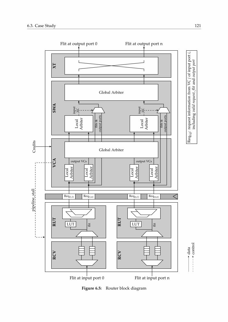
6.3. Case Study 121
RC
V
Flit at input port 0
RC
V
Flit at input port n
RU
T
LUT flit
RU
T
LUT flit
Req(1,1) Req(1,n) Req(n,1) Req(n,n)
VC
A
Lo
cal
Arb
iter
Lo
cal
Arb
iter
Lo
cal
Arb
iter
Lo
cal
Arb
iter
SW
A
Lo
cal
Arb
iter
Lo
cal
Arb
iter
output VCs output VCs
flit
s&
ou
tpu
tp
ort
s
flit
s&
ou
tpu
tp
ort
s
Global Arbiter
XT
inp
ut
VC
inp
ut
VC
Flit at output port 0 Flit at output port n
pip
elin
e_st
all
Cre
dit
s
dat
aco
ntr
ol
Req
(i,j)
:re
qu
est
info
rmat
ion
fro
mV
Cj
of
inp
ut
po
rti,
incl
ud
ing
vali
dre
ques
t,fl
itan
dou
tpu
tpo
rt
Global Arbiter
Figure 6.5: Router block diagram
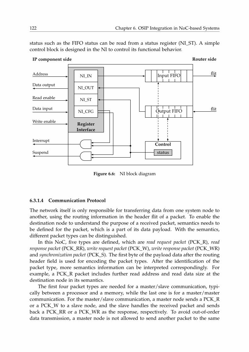
122 Chapter 6. OSIP Integration in NoC-based Systems
status such as the FIFO status can be read from a status register (NI_ST). A simple
control block is designed in the NI to control its functional behavior.
NI_IN
NI_OUT
NI_ST
NI_CFG
Register
Interface
Input FIFO
Output FIFO
Control
status
flit
flit
Address
Data output
Read enable
Data input
Write enable
Interrupt
Suspend
IP component side Router side
Figure 6.6: NI block diagram
6.3.1.4 Communication Protocol
The network itself is only responsible for transferring data from one system node to
another, using the routing information in the header flit of a packet. To enable the
destination node to understand the purpose of a received packet, semantics needs to
be defined for the packet, which is a part of its data payload. With the semantics,
different packet types can be distinguished.
In this NoC, five types are defined, which are read request packet (PCK_R), read
response packet (PCK_RR), write request packet (PCK_W), write response packet (PCK_WR)
and synchronization packet (PCK_S). The first byte of the payload data after the routing
header field is used for encoding the packet types. After the identification of the
packet type, more semantics information can be interpreted correspondingly. For
example, a PCK_R packet includes further read address and read data size at the
destination node in its semantics.
The first four packet types are needed for a master/slave communication, typi-
cally between a processor and a memory, while the last one is for a master/master
communication. For the master/slave communication, a master node sends a PCK_R
or a PCK_W to a slave node, and the slave handles the received packet and sends
back a PCK_RR or a PCK_WR as the response, respectively. To avoid out-of-order
data transmission, a master node is not allowed to send another packet to the same
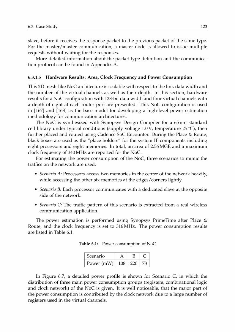
6.3. Case Study 123
slave, before it receives the response packet to the previous packet of the same type.
For the master/master communication, a master node is allowed to issue multiple
requests without waiting for the responses.
More detailed information about the packet type definition and the communica-
tion protocol can be found in Appendix A.
6.3.1.5 Hardware Results: Area, Clock Frequency and Power Consumption
This 2D mesh-like NoC architecture is scalable with respect to the link data width and
the number of the virtual channels as well as their depth. In this section, hardware
results for a NoC configuration with 128-bit data width and four virtual channels with
a depth of eight at each router port are presented. This NoC configuration is used
in [167] and [168] as the base model for developing a high-level power estimation
methodology for communication architectures.
The NoC is synthesized with Synopsys Design Compiler for a 65 nm standard
cell library under typical conditions (supply voltage 1.0V, temperature 25 ◦C), then
further placed and routed using Cadence SoC Encounter. During the Place & Route,
black boxes are used as the “place holders” for the system IP components including
eight processors and eight memories. In total, an area of 2.56MGE and a maximum
clock frequency of 340MHz are reported for the NoC.
For estimating the power consumption of the NoC, three scenarios to mimic the
traffics on the network are used:
• Scenario A: Processors access two memories in the center of the network heavily,
while accessing the other six memories at the edges/corners lightly.
• Scenario B: Each processor communicates with a dedicated slave at the opposite
side of the network.
• Scenario C: The traffic pattern of this scenario is extracted from a real wireless
communication application.
The power estimation is performed using Synopsys PrimeTime after Place &
Route, and the clock frequency is set to 316MHz. The power consumption results
are listed in Table 6.1.
Table 6.1: Power consumption of NoC
Scenario A B C
Power (mW) 108 220 73
In Figure 6.7, a detailed power profile is shown for Scenario C, in which the
distribution of three main power consumption groups (registers, combinational logic
and clock network) of the NoC is given. It is well noticeable, that the major part of
the power consumption is contributed by the clock network due to a large number of
registers used in the virtual channels.
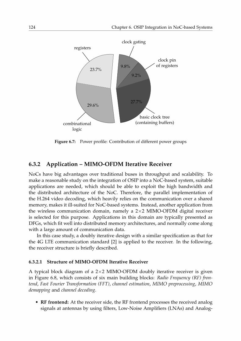
124 Chapter 6. OSIP Integration in NoC-based Systems
23.7%
registers
29.6%
combinationallogic
27.7%
basic clock tree(containing buffers)
9.2%
clock pinof registers9.8%
clock gating
Figure 6.7: Power profile: Contribution of different power groups
6.3.2 Application – MIMO-OFDM Iterative Receiver
NoCs have big advantages over traditional buses in throughput and scalability. To
make a reasonable study on the integration of OSIP into a NoC-based system, suitable
applications are needed, which should be able to exploit the high bandwidth and
the distributed architecture of the NoC. Therefore, the parallel implementation of
the H.264 video decoding, which heavily relies on the communication over a shared
memory, makes it ill-suited for NoC-based systems. Instead, another application from
the wireless communication domain, namely a 2×2 MIMO-OFDM digital receiver
is selected for this purpose. Applications in this domain are typically presented as
DFGs, which fit well into distributed memory architectures, and normally come along
with a large amount of communication data.
In this case study, a doubly iterative design with a similar specification as that for
the 4G LTE communication standard [2] is applied to the receiver. In the following,
the receiver structure is briefly described.
6.3.2.1 Structure of MIMO-OFDM Iterative Receiver
A typical block diagram of a 2×2 MIMO-OFDM doubly iterative receiver is given
in Figure 6.8, which consists of six main building blocks: Radio Frequency (RF) fron-
tend, Fast Fourier Transformation (FFT), channel estimation, MIMO preprocessing, MIMO
demapping and channel decoding.
• RF frontend: At the receiver side, the RF frontend processes the received analog
signals at antennas by using filters, Low-Noise Amplifiers (LNAs) and Analog-
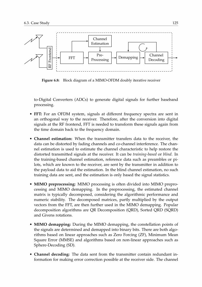
6.3. Case Study 125
RF
Fro
nte
nd
FFTPre-
ProcessingDemapping
ChannelEstimation
ChannelDecoding
Figure 6.8: Block diagram of a MIMO-OFDM doubly iterative receiver
to-Digital Converters (ADCs) to generate digital signals for further baseband
processing.
• FFT: For an OFDM system, signals at different frequency spectra are sent in
an orthogonal way to the receiver. Therefore, after the conversion into digital
signals at the RF frontend, FFT is needed to transform these signals again from
the time domain back to the frequency domain.
• Channel estimation: When the transmitter transfers data to the receiver, the
data can be distorted by fading channels and co-channel interference. The chan-
nel estimation is used to estimate the channel characteristic to help restore the
distorted transmitted signals at the receiver. It can be training-based or blind. In
the training-based channel estimation, reference data such as preambles or pi-
lots, which are known to the receiver, are sent by the transmitter in addition to
the payload data to aid the estimation. In the blind channel estimation, no such
training data are sent, and the estimation is only based the signal statistics.
• MIMO preprocessing: MIMO processing is often divided into MIMO prepro-
cessing and MIMO demapping. In the preprocessing, the estimated channel
matrix is typically decomposed, considering the algorithmic performance and
numeric stability. The decomposed matrices, partly multiplied by the output
vectors from the FFT, are then further used in the MIMO demapping. Popular
decomposition algorithms are QR Decomposition (QRD), Sorted QRD (SQRD)
and Givens rotations.
• MIMO demapping: During the MIMO demapping, the constellation points of
the signals are determined and demapped into binary bits. There are both algo-
rithms based on linear approaches such as Zero Forcing (ZF), Minimum Mean
Square Error (MMSE) and algorithms based on non-linear approaches such as
Sphere-Decoding (SD).
• Channel decoding: The data sent from the transmitter contain redundant in-
formation for making error correction possible at the receiver side. The channel
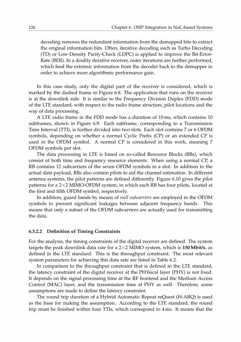
126 Chapter 6. OSIP Integration in NoC-based Systems
decoding removes the redundant information from the demapped bits to extract
the original information bits. Often, iterative decoding such as Turbo Decoding
(TD) or Low-Density Parity-Check (LDPC) is applied to improve the Bit-Error-
Rate (BER). In a doubly iterative receiver, outer iterations are further performed,
which feed the extrinsic information from the decoder back to the demapper in
order to achieve more algorithmic performance gain.
In this case study, only the digital part of the receiver is considered, which is
marked by the dashed frame in Figure 6.8. The application that runs on the receiver
is at the downlink side. It is similar to the Frequency Division Duplex (FDD) mode
of the LTE standard, with respect to the radio frame structure, pilot locations and the
way of data processing.
A LTE radio frame in the FDD mode has a duration of 10ms, which contains 10
subframes, shown in Figure 6.9. Each subframe, corresponding to a Transmission
Time Interval (TTI), is further divided into two slots. Each slot contains 7 or 6 OFDM
symbols, depending on whether a normal Cyclic Prefix (CP) or an extended CP is
used in the OFDM symbol. A normal CP is considered in this work, meaning 7
OFDM symbols per slot.
The data processing in LTE is based on so-called Resource Blocks (RBs), which
consist of both time and frequency resource elements. When using a normal CP, a
RB contains 12 subcarriers of the seven OFDM symbols in a slot. In addition to the
actual data payload, RBs also contain pilots to aid the channel estimation. In different
antenna systems, the pilot patterns are defined differently. Figure 6.10 gives the pilot
patterns for a 2×2 MIMO-OFDM system, in which each RB has four pilots, located at
the first and fifth OFDM symbol, respectively.
In addition, guard bands by means of null subcarriers are employed in the OFDM
symbols to prevent significant leakages between adjacent frequency bands. This
means that only a subset of the OFDM subcarriers are actually used for transmitting
the data.
6.3.2.2 Definition of Timing Constraints
For the analysis, the timing constraints of the digital receiver are defined. The system
targets the peak downlink data rate for a 2×2 MIMO system, which is 150Mbit/s, as
defined in the LTE standard. This is the throughput constraint. The most relevant
system parameters for achieving this data rate are listed in Table 6.2.
In comparison to the throughput constraint that is defined in the LTE standard,
the latency constraint of the digital receiver at the PHYsical layer (PHY) is not fixed.
It depends on the signal processing time at the RF frontend and the Medium Access
Control (MAC) layer, and the transmission time at PHY as well. Therefore, some
assumptions are made to define the latency constraint.
The round trip duration of a Hybrid Automatic Repeat reQuest (H-ARQ) is used
as the base for making the assumption. According to the LTE standard, the round
trip must be finished within four TTIs, which correspond to 4ms. It means that the
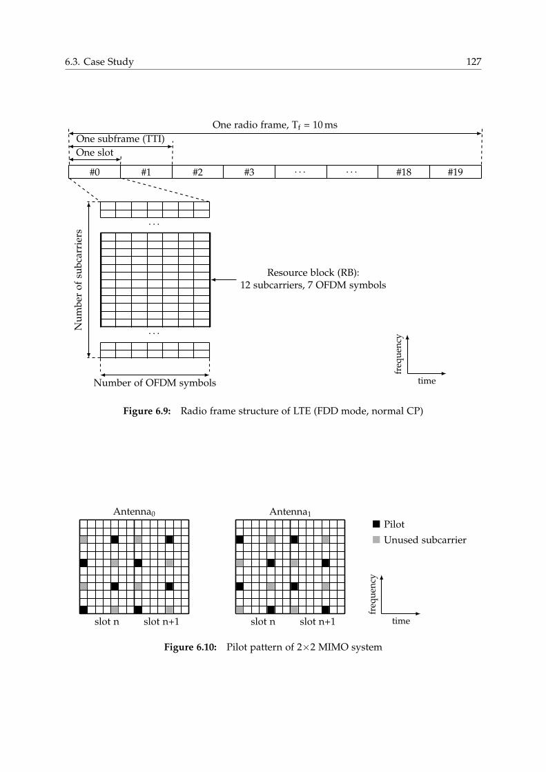
6.3. Case Study 127
#0 #1 #2 #3 . . . . . . #18 #19
One radio frame, Tf = 10 ms
One subframe (TTI)
One slot
. . .
. . .Nu
mb
ero
fsu
bca
rrie
rs
Number of OFDM symbols
Resource block (RB):12 subcarriers, 7 OFDM symbols
time
freq
uen
cy
Figure 6.9: Radio frame structure of LTE (FDD mode, normal CP)
Antenna0
slot n slot n+1
Antenna1
slot n slot n+1
Pilot
Unused subcarrier
time
freq
uen
cy
Figure 6.10: Pilot pattern of 2×2 MIMO system
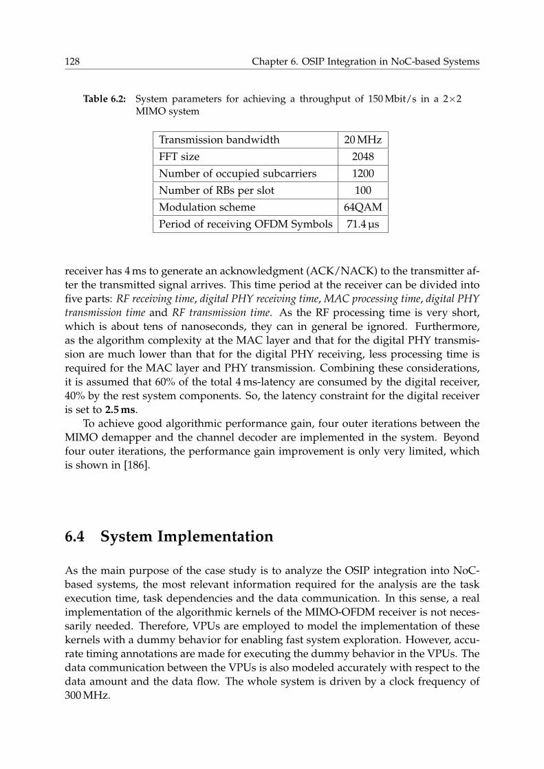
128 Chapter 6. OSIP Integration in NoC-based Systems
Table 6.2: System parameters for achieving a throughput of 150Mbit/s in a 2×2MIMO system
Transmission bandwidth 20MHz
FFT size 2048
Number of occupied subcarriers 1200
Number of RBs per slot 100
Modulation scheme 64QAM
Period of receiving OFDM Symbols 71.4 µs
receiver has 4ms to generate an acknowledgment (ACK/NACK) to the transmitter af-
ter the transmitted signal arrives. This time period at the receiver can be divided into
five parts: RF receiving time, digital PHY receiving time, MAC processing time, digital PHY
transmission time and RF transmission time. As the RF processing time is very short,
which is about tens of nanoseconds, they can in general be ignored. Furthermore,
as the algorithm complexity at the MAC layer and that for the digital PHY transmis-
sion are much lower than that for the digital PHY receiving, less processing time is
required for the MAC layer and PHY transmission. Combining these considerations,
it is assumed that 60% of the total 4ms-latency are consumed by the digital receiver,
40% by the rest system components. So, the latency constraint for the digital receiver
is set to 2.5ms.
To achieve good algorithmic performance gain, four outer iterations between the
MIMO demapper and the channel decoder are implemented in the system. Beyond
four outer iterations, the performance gain improvement is only very limited, which
is shown in [186].
6.4 System Implementation
As the main purpose of the case study is to analyze the OSIP integration into NoC-
based systems, the most relevant information required for the analysis are the task
execution time, task dependencies and the data communication. In this sense, a real
implementation of the algorithmic kernels of the MIMO-OFDM receiver is not neces-
sarily needed. Therefore, VPUs are employed to model the implementation of these
kernels with a dummy behavior for enabling fast system exploration. However, accu-
rate timing annotations are made for executing the dummy behavior in the VPUs. The
data communication between the VPUs is also modeled accurately with respect to the
data amount and the data flow. The whole system is driven by a clock frequency of
300MHz.
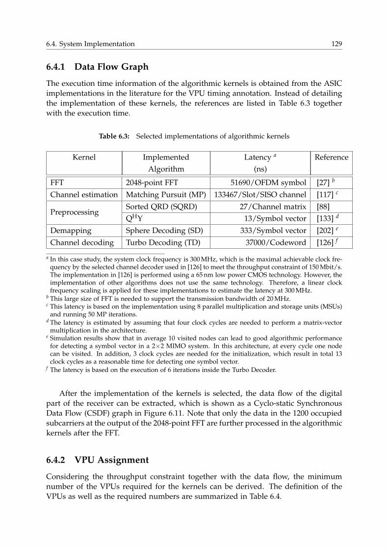
6.4. System Implementation 129
6.4.1 Data Flow Graph
The execution time information of the algorithmic kernels is obtained from the ASIC
implementations in the literature for the VPU timing annotation. Instead of detailing
the implementation of these kernels, the references are listed in Table 6.3 together
with the execution time.
Table 6.3: Selected implementations of algorithmic kernels
Kernel Implemented
Algorithm
Latency a
(ns)
Reference
FFT 2048-point FFT 51690/OFDM symbol [27] b
Channel estimation Matching Pursuit (MP) 133467/Slot/SISO channel [117] c
PreprocessingSorted QRD (SQRD) 27/Channel matrix [88]
QHY 13/Symbol vector [133] d
Demapping Sphere Decoding (SD) 333/Symbol vector [202] e
Channel decoding Turbo Decoding (TD) 37000/Codeword [126] f
a In this case study, the system clock frequency is 300MHz, which is the maximal achievable clock fre-quency by the selected channel decoder used in [126] to meet the throughput constraint of 150Mbit/s.The implementation in [126] is performed using a 65 nm low power CMOS technology. However, theimplementation of other algorithms does not use the same technology. Therefore, a linear clockfrequency scaling is applied for these implementations to estimate the latency at 300MHz.
b This large size of FFT is needed to support the transmission bandwidth of 20MHz.c This latency is based on the implementation using 8 parallel multiplication and storage units (MSUs)and running 50 MP iterations.
d The latency is estimated by assuming that four clock cycles are needed to perform a matrix-vectormultiplication in the architecture.
e Simulation results show that in average 10 visited nodes can lead to good algorithmic performancefor detecting a symbol vector in a 2×2 MIMO system. In this architecture, at every cycle one nodecan be visited. In addition, 3 clock cycles are needed for the initialization, which result in total 13clock cycles as a reasonable time for detecting one symbol vector.
f The latency is based on the execution of 6 iterations inside the Turbo Decoder.
After the implementation of the kernels is selected, the data flow of the digital
part of the receiver can be extracted, which is shown as a Cyclo-static Synchronous
Data Flow (CSDF) graph in Figure 6.11. Note that only the data in the 1200 occupied
subcarriers at the output of the 2048-point FFT are further processed in the algorithmic
kernels after the FFT.
6.4.2 VPU Assignment
Considering the throughput constraint together with the data flow, the minimum
number of the VPUs required for the kernels can be derived. The definition of the
VPUs as well as the required numbers are summarized in Table 6.4.
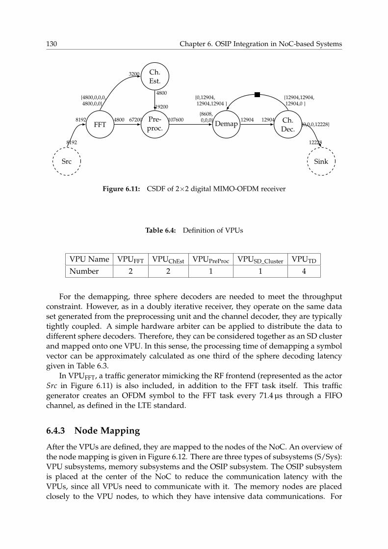
130 Chapter 6. OSIP Integration in NoC-based Systems
Src
FFT
Ch.Est.
Pre-proc.
Demap Ch.Dec.
Sink
8192
8192
{4800,0,0,0,4800,0,0}
3200
4800 67200
4800
19200
107600{8608,0,0,0} 12904 12904
{12904,12904,12904,0 }
{0,12904,12904,12904 }
{0,0,0,12228}
12228
Figure 6.11: CSDF of 2×2 digital MIMO-OFDM receiver
Table 6.4: Definition of VPUs
VPU Name VPUFFT VPUChEst VPUPreProc VPUSD_Cluster VPUTD
Number 2 2 1 1 4
For the demapping, three sphere decoders are needed to meet the throughput
constraint. However, as in a doubly iterative receiver, they operate on the same data
set generated from the preprocessing unit and the channel decoder, they are typically
tightly coupled. A simple hardware arbiter can be applied to distribute the data to
different sphere decoders. Therefore, they can be considered together as an SD cluster
and mapped onto one VPU. In this sense, the processing time of demapping a symbol
vector can be approximately calculated as one third of the sphere decoding latency
given in Table 6.3.
In VPUFFT, a traffic generator mimicking the RF frontend (represented as the actor
Src in Figure 6.11) is also included, in addition to the FFT task itself. This traffic
generator creates an OFDM symbol to the FFT task every 71.4 µs through a FIFO
channel, as defined in the LTE standard.
6.4.3 Node Mapping
After the VPUs are defined, they are mapped to the nodes of the NoC. An overview of
the node mapping is given in Figure 6.12. There are three types of subsystems (S/Sys):
VPU subsystems, memory subsystems and the OSIP subsystem. The OSIP subsystem
is placed at the center of the NoC to reduce the communication latency with the
VPUs, since all VPUs need to communicate with it. The memory nodes are placed
closely to the VPU nodes, to which they have intensive data communications. For
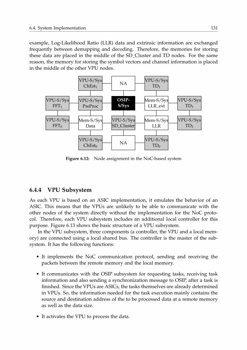
6.4. System Implementation 131
example, Log-Likelihood Ratio (LLR) data and extrinsic information are exchanged
frequently between demapping and decoding. Therefore, the memories for storing
these data are placed in the middle of the SD_Cluster and TD nodes. For the same
reason, the memory for storing the symbol vectors and channel information is placed
in the middle of the other VPU nodes.
VPU-S/SysFFT0
VPU-S/SysFFT1
VPU-S/SysChEst0
Mem-S/SysData
VPU-S/SysPreProc
VPU-S/SysChEst1
NA
VPU-S/SysSD_Cluster
OSIP-
S/Sys
NA
VPU-S/SysTD0
Mem-S/SysLLR
Mem-S/SysLLR_ext
VPU-S/SysTD1
VPU-S/SysTD2
VPU-S/SysTD3
Figure 6.12: Node assignment in the NoC-based system
6.4.4 VPU Subsystem
As each VPU is based on an ASIC implementation, it emulates the behavior of an
ASIC. This means that the VPUs are unlikely to be able to communicate with the
other nodes of the system directly without the implementation for the NoC proto-
col. Therefore, each VPU subsystem includes an additional local controller for this
purpose. Figure 6.13 shows the basic structure of a VPU subsystem.
In the VPU subsystem, three components (a controller, the VPU and a local mem-
ory) are connected using a local shared bus. The controller is the master of the sub-
system. It has the following functions:
• It implements the NoC communication protocol, sending and receiving the
packets between the remote memory and the local memory.
• It communicates with the OSIP subsystem for requesting tasks, receiving task
information and also sending a synchronization message to OSIP, after a task is
finished. Since the VPUs are ASICs, the tasks themselves are already determined
in VPUs. So, the information needed for the task execution mainly contains the
source and destination address of the to be processed data at a remote memory
as well as the data size.
• It activates the VPU to process the data.
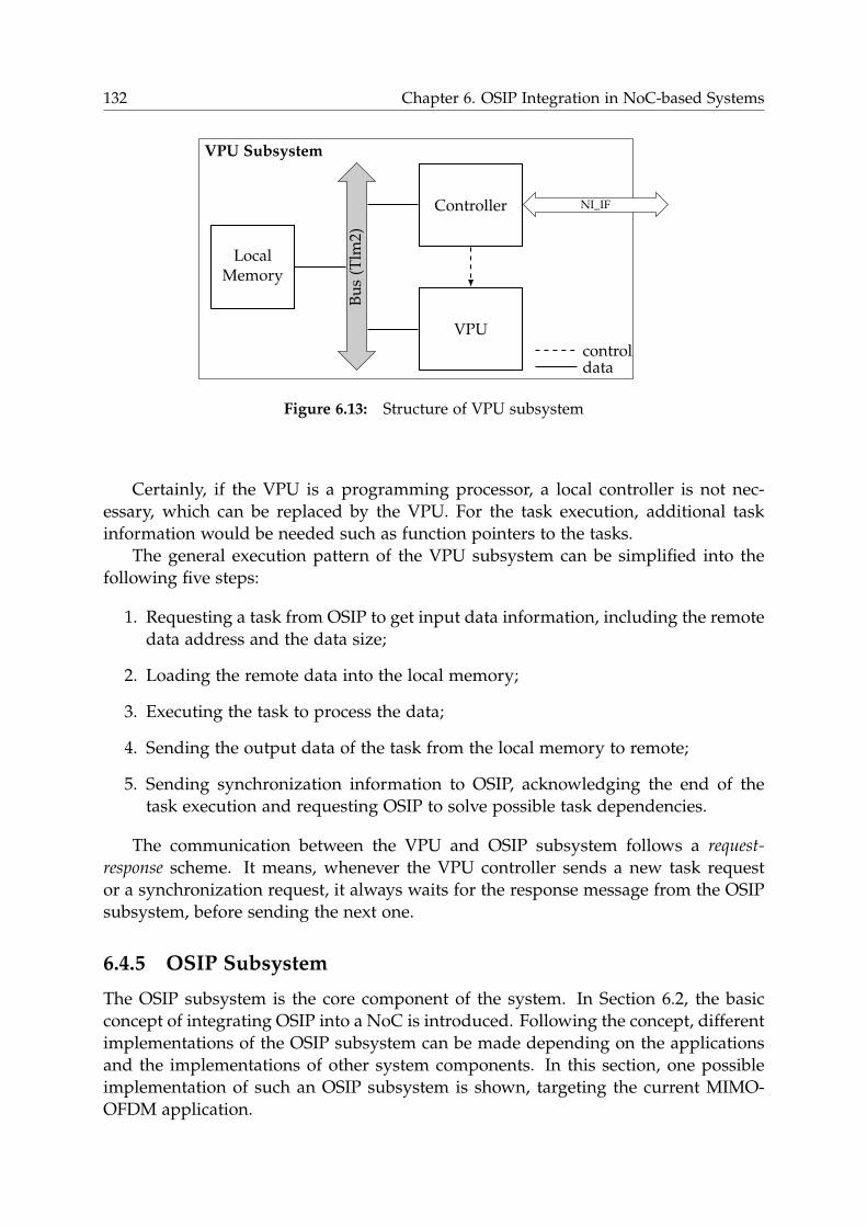
132 Chapter 6. OSIP Integration in NoC-based Systems
VPU Subsystem
LocalMemory
Bu
s(T
lm2)
Controller
VPU
NI_IF
datacontrol
Figure 6.13: Structure of VPU subsystem
Certainly, if the VPU is a programming processor, a local controller is not nec-
essary, which can be replaced by the VPU. For the task execution, additional task
information would be needed such as function pointers to the tasks.
The general execution pattern of the VPU subsystem can be simplified into the
following five steps:
1. Requesting a task from OSIP to get input data information, including the remote
data address and the data size;
2. Loading the remote data into the local memory;
3. Executing the task to process the data;
4. Sending the output data of the task from the local memory to remote;
5. Sending synchronization information to OSIP, acknowledging the end of the
task execution and requesting OSIP to solve possible task dependencies.
The communication between the VPU and OSIP subsystem follows a request-
response scheme. It means, whenever the VPU controller sends a new task request
or a synchronization request, it always waits for the response message from the OSIP
subsystem, before sending the next one.
6.4.5 OSIP Subsystem
The OSIP subsystem is the core component of the system. In Section 6.2, the basic
concept of integrating OSIP into a NoC is introduced. Following the concept, different
implementations of the OSIP subsystem can be made depending on the applications
and the implementations of other system components. In this section, one possible
implementation of such an OSIP subsystem is shown, targeting the current MIMO-
OFDM application.
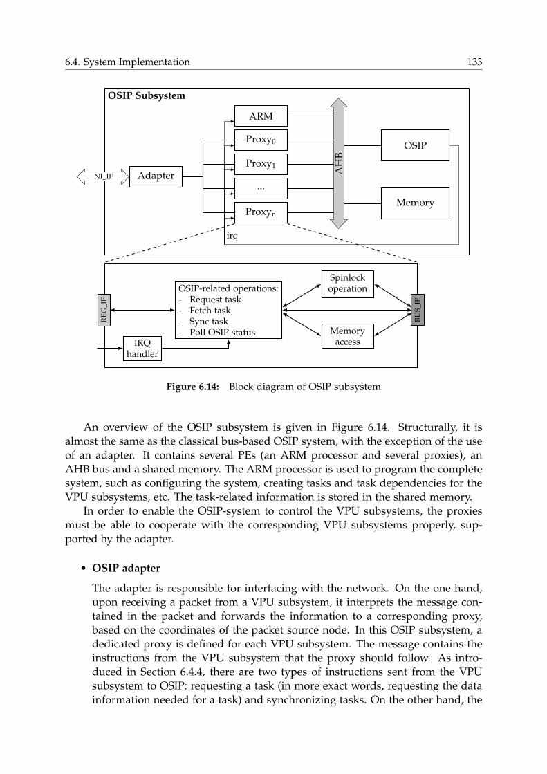
6.4. System Implementation 133
OSIP Subsystem
Proxy0
Proxy1
...
Proxyn
AdapterNI_IF
ARM
AH
B
OSIP
Memory
irq
RE
G_I
F
BU
S_I
F
OSIP-related operations:- Request task- Fetch task- Sync task- Poll OSIP status
IRQhandler
Spinlockoperation
Memoryaccess
Figure 6.14: Block diagram of OSIP subsystem
An overview of the OSIP subsystem is given in Figure 6.14. Structurally, it is
almost the same as the classical bus-based OSIP system, with the exception of the use
of an adapter. It contains several PEs (an ARM processor and several proxies), an
AHB bus and a shared memory. The ARM processor is used to program the complete
system, such as configuring the system, creating tasks and task dependencies for the
VPU subsystems, etc. The task-related information is stored in the shared memory.
In order to enable the OSIP-system to control the VPU subsystems, the proxies
must be able to cooperate with the corresponding VPU subsystems properly, sup-
ported by the adapter.
• OSIP adapter
The adapter is responsible for interfacing with the network. On the one hand,
upon receiving a packet from a VPU subsystem, it interprets the message con-
tained in the packet and forwards the information to a corresponding proxy,
based on the coordinates of the packet source node. In this OSIP subsystem, a
dedicated proxy is defined for each VPU subsystem. The message contains the
instructions from the VPU subsystem that the proxy should follow. As intro-
duced in Section 6.4.4, there are two types of instructions sent from the VPU
subsystem to OSIP: requesting a task (in more exact words, requesting the data
information needed for a task) and synchronizing tasks. On the other hand, the
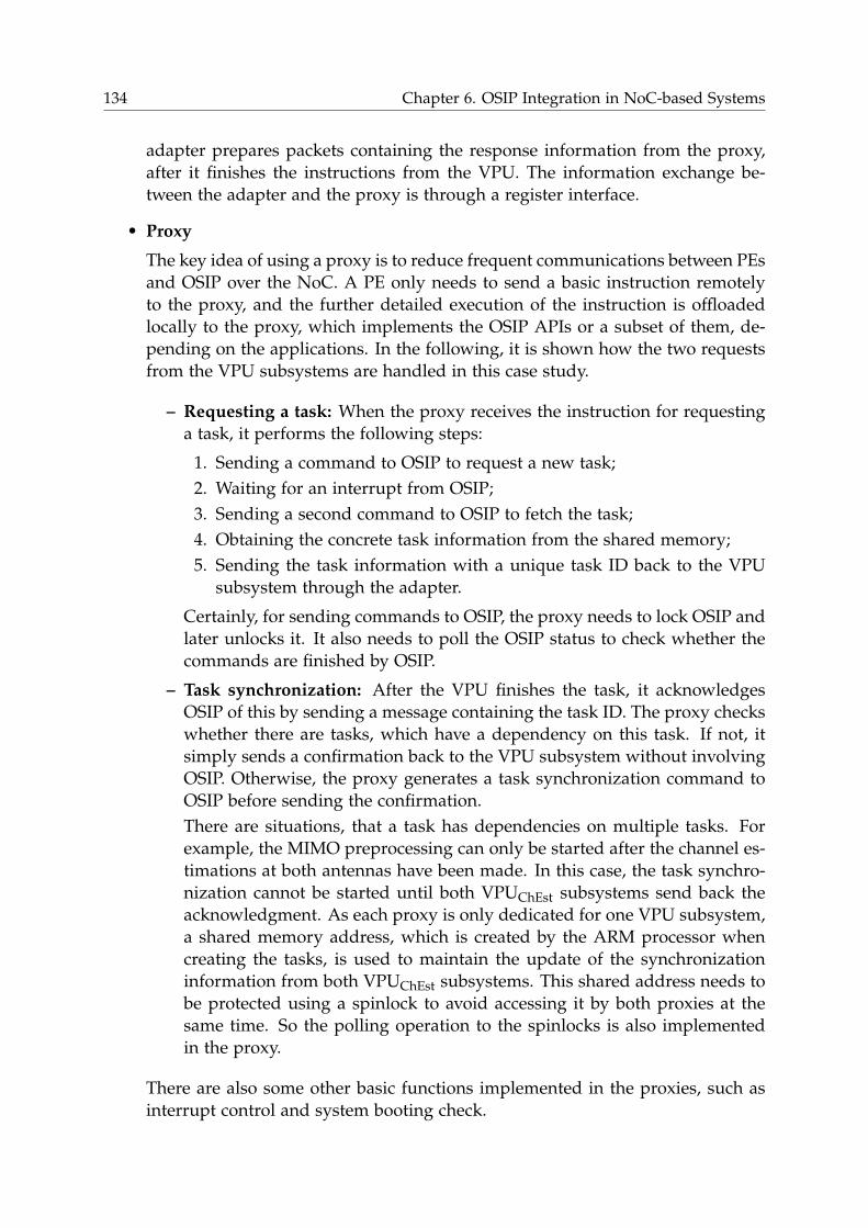
134 Chapter 6. OSIP Integration in NoC-based Systems
adapter prepares packets containing the response information from the proxy,
after it finishes the instructions from the VPU. The information exchange be-
tween the adapter and the proxy is through a register interface.
• Proxy
The key idea of using a proxy is to reduce frequent communications between PEs
and OSIP over the NoC. A PE only needs to send a basic instruction remotely
to the proxy, and the further detailed execution of the instruction is offloaded
locally to the proxy, which implements the OSIP APIs or a subset of them, de-
pending on the applications. In the following, it is shown how the two requests
from the VPU subsystems are handled in this case study.
– Requesting a task: When the proxy receives the instruction for requesting
a task, it performs the following steps:
1. Sending a command to OSIP to request a new task;
2. Waiting for an interrupt from OSIP;
3. Sending a second command to OSIP to fetch the task;
4. Obtaining the concrete task information from the shared memory;
5. Sending the task information with a unique task ID back to the VPU
subsystem through the adapter.
Certainly, for sending commands to OSIP, the proxy needs to lock OSIP and
later unlocks it. It also needs to poll the OSIP status to check whether the
commands are finished by OSIP.
– Task synchronization: After the VPU finishes the task, it acknowledges
OSIP of this by sending a message containing the task ID. The proxy checks
whether there are tasks, which have a dependency on this task. If not, it
simply sends a confirmation back to the VPU subsystem without involving
OSIP. Otherwise, the proxy generates a task synchronization command to
OSIP before sending the confirmation.
There are situations, that a task has dependencies on multiple tasks. For
example, the MIMO preprocessing can only be started after the channel es-
timations at both antennas have been made. In this case, the task synchro-
nization cannot be started until both VPUChEst subsystems send back the
acknowledgment. As each proxy is only dedicated for one VPU subsystem,
a shared memory address, which is created by the ARM processor when
creating the tasks, is used to maintain the update of the synchronization
information from both VPUChEst subsystems. This shared address needs to
be protected using a spinlock to avoid accessing it by both proxies at the
same time. So the polling operation to the spinlocks is also implemented
in the proxy.
There are also some other basic functions implemented in the proxies, such as
interrupt control and system booting check.
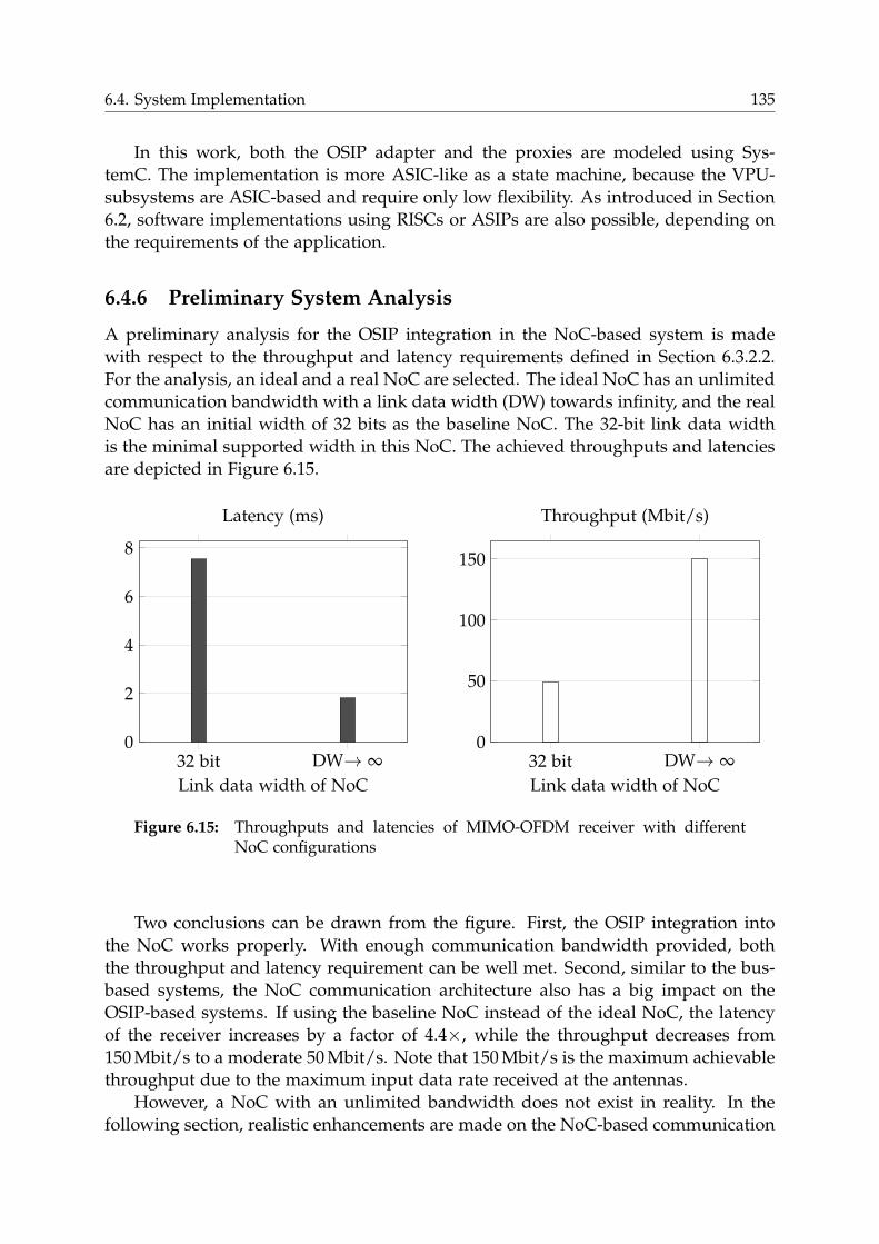
6.4. System Implementation 135
In this work, both the OSIP adapter and the proxies are modeled using Sys-
temC. The implementation is more ASIC-like as a state machine, because the VPU-
subsystems are ASIC-based and require only low flexibility. As introduced in Section
6.2, software implementations using RISCs or ASIPs are also possible, depending on
the requirements of the application.
6.4.6 Preliminary System Analysis
A preliminary analysis for the OSIP integration in the NoC-based system is made
with respect to the throughput and latency requirements defined in Section 6.3.2.2.
For the analysis, an ideal and a real NoC are selected. The ideal NoC has an unlimited
communication bandwidth with a link data width (DW) towards infinity, and the real
NoC has an initial width of 32 bits as the baseline NoC. The 32-bit link data width
is the minimal supported width in this NoC. The achieved throughputs and latencies
are depicted in Figure 6.15.
32 bit DW→ ∞
0
2
4
6
8
Link data width of NoC
Latency (ms)
32 bit DW→ ∞
0
50
100
150
Link data width of NoC
Throughput (Mbit/s)
Figure 6.15: Throughputs and latencies of MIMO-OFDM receiver with differentNoC configurations
Two conclusions can be drawn from the figure. First, the OSIP integration into
the NoC works properly. With enough communication bandwidth provided, both
the throughput and latency requirement can be well met. Second, similar to the bus-
based systems, the NoC communication architecture also has a big impact on the
OSIP-based systems. If using the baseline NoC instead of the ideal NoC, the latency
of the receiver increases by a factor of 4.4×, while the throughput decreases from
150Mbit/s to a moderate 50Mbit/s. Note that 150Mbit/s is the maximum achievable
throughput due to the maximum input data rate received at the antennas.
However, a NoC with an unlimited bandwidth does not exist in reality. In the
following section, realistic enhancements are made on the NoC-based communication
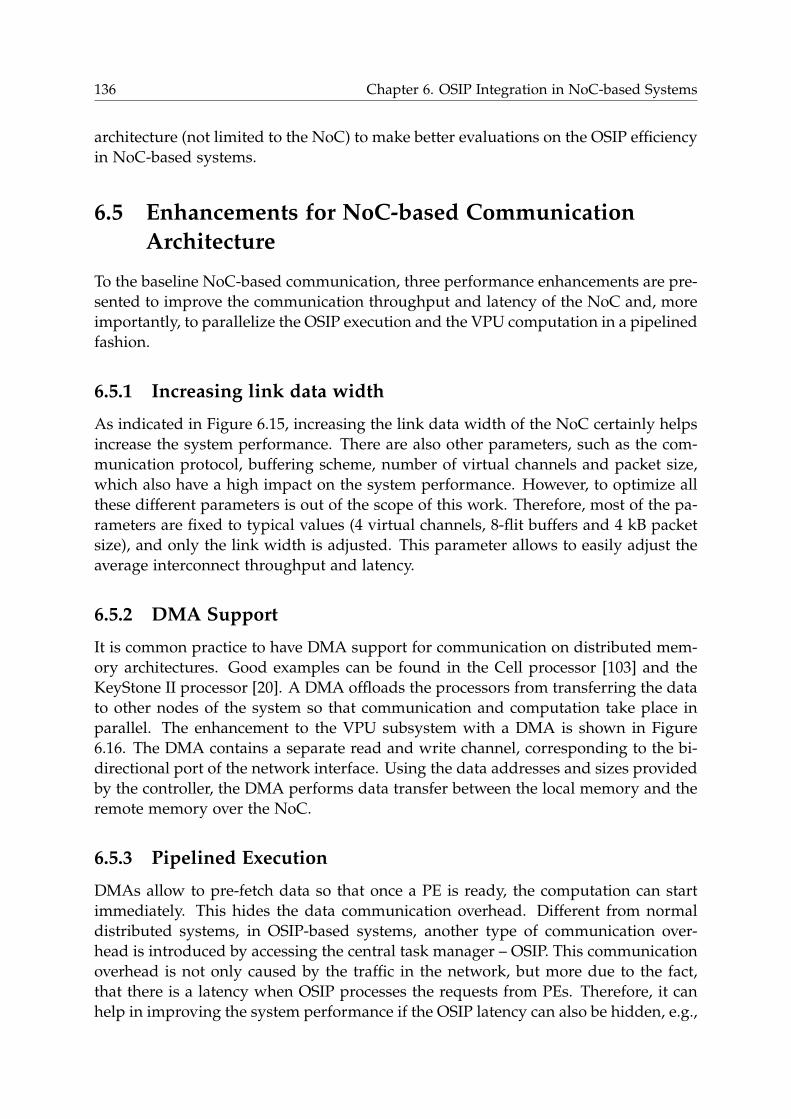
136 Chapter 6. OSIP Integration in NoC-based Systems
architecture (not limited to the NoC) to make better evaluations on the OSIP efficiency
in NoC-based systems.
6.5 Enhancements for NoC-based Communication
Architecture
To the baseline NoC-based communication, three performance enhancements are pre-
sented to improve the communication throughput and latency of the NoC and, more
importantly, to parallelize the OSIP execution and the VPU computation in a pipelined
fashion.
6.5.1 Increasing link data width
As indicated in Figure 6.15, increasing the link data width of the NoC certainly helps
increase the system performance. There are also other parameters, such as the com-
munication protocol, buffering scheme, number of virtual channels and packet size,
which also have a high impact on the system performance. However, to optimize all
these different parameters is out of the scope of this work. Therefore, most of the pa-
rameters are fixed to typical values (4 virtual channels, 8-flit buffers and 4 kB packet
size), and only the link width is adjusted. This parameter allows to easily adjust the
average interconnect throughput and latency.
6.5.2 DMA Support
It is common practice to have DMA support for communication on distributed mem-
ory architectures. Good examples can be found in the Cell processor [103] and the
KeyStone II processor [20]. A DMA offloads the processors from transferring the data
to other nodes of the system so that communication and computation take place in
parallel. The enhancement to the VPU subsystem with a DMA is shown in Figure
6.16. The DMA contains a separate read and write channel, corresponding to the bi-
directional port of the network interface. Using the data addresses and sizes provided
by the controller, the DMA performs data transfer between the local memory and the
remote memory over the NoC.
6.5.3 Pipelined Execution
DMAs allow to pre-fetch data so that once a PE is ready, the computation can start
immediately. This hides the data communication overhead. Different from normal
distributed systems, in OSIP-based systems, another type of communication over-
head is introduced by accessing the central task manager – OSIP. This communication
overhead is not only caused by the traffic in the network, but more due to the fact,
that there is a latency when OSIP processes the requests from PEs. Therefore, it can
help in improving the system performance if the OSIP latency can also be hidden, e.g.,

6.5. Enhancements for NoC-based Communication Architecture 137
VPU Subsystem (with DMA)
LocalMemory
Bu
s(T
lm2)
DMA Controller
VPU
NI_IF
datacontrol
Figure 6.16: Structure of VPU subsystem with DMA
by means of pre-fetching the next tasks during the execution of PEs. In fact, in this
system, pre-fetching tasks is obligatory for the pre-fetch of data. Without a task, the
data information including the addresses and the data size is unknown to the DMA.
To hide the communication overhead of both data transfer and the accessing to
OSIP, the pipelining concept is applied. Referring to the execution steps listed in
Section 6.4.4, three pipeline stages are built: step 1) and 2) are grouped into the first
pipeline stage, step 3) is in the second stage, and step 4) and 5) are grouped into
the third stage. The pipelining is only applied to the demapping (SD_cluster) and
the channel decoding (TD) subsystems due to frequent data and task information
exchange between them, which is caused by the outer iterations. Deeper pipelining
would be also possible by assigning each step to a separate stage. Note that in the
non-pipelined execution of the system, in which DMAs are not used, the controller of
the VPU subsystems has to transfer the data in step 2) and 4) between the local and
remote memory.
An exemplary execution pattern of the non-pipelined and pipelined control flow
of the master subsystem is illustrated in Figure 6.17. As shown in the non-pipelined
pattern, the executions of TaskA, TaskB and TaskC (including requesting task, reading
input data and sending output data) take place in a sequential order in the VPU
subsystem. In contrast, in the pipelined pattern, their execution are interleaved. As
shown in the figure, while executing TaskB, TaskC is pre-fetched from OSIP and the
input data are prepared. In parallel, the output data of TaskA are sent and a task
synchronization is issued to OSIP.
In the pipelined execution flow, there is a situation that deadlocks would happen
between task executions, if no additional actions are taken on the OSIP side. Suppose
that TaskC has a dependency on TaskB. If the controller is currently sending a request
to OSIP for TaskC, it is not able to receive the task, because TaskB is not finished
yet. On the other hand, when TaskB is finished, the controller is not able to send the
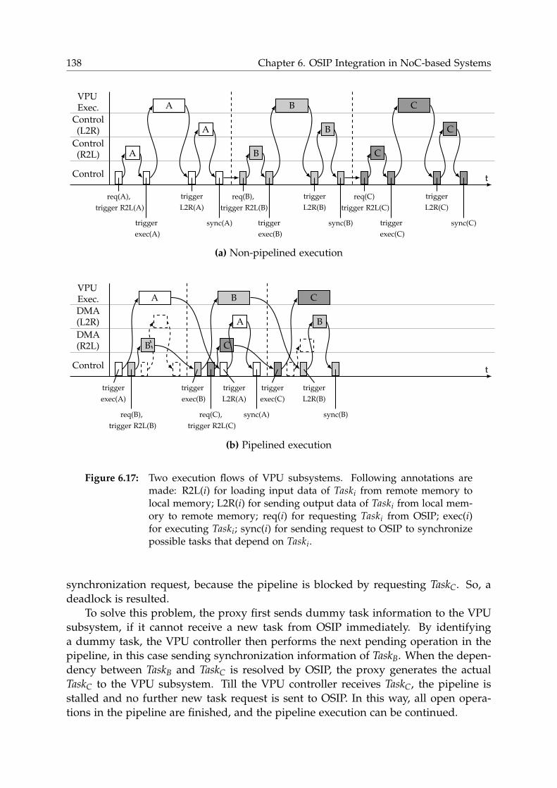
138 Chapter 6. OSIP Integration in NoC-based Systems
tControl
Control(R2L)
Control(L2R)
VPUExec.
A
A
A
B
B
B
C
C
C
req(A),
trigger R2L(A)
trigger
exec(A)
trigger
L2R(A)
sync(A)
req(B),
trigger R2L(B)
trigger
exec(B)
trigger
L2R(B)
sync(B)
req(C)
trigger R2L(C)
trigger
exec(C)
trigger
L2R(C)
sync(C)
(a) Non-pipelined execution
tControl
DMA(R2L)
DMA(L2R)
VPUExec. A
B
B
C
A
C
B
trigger
exec(A)
req(B),
trigger R2L(B)
trigger
exec(B)
req(C),
trigger R2L(C)
trigger
L2R(A)
sync(A)
trigger
exec(C)
trigger
L2R(B)
sync(B)
(b) Pipelined execution
Figure 6.17: Two execution flows of VPU subsystems. Following annotations aremade: R2L(i) for loading input data of Taski from remote memory tolocal memory; L2R(i) for sending output data of Taski from local mem-ory to remote memory; req(i) for requesting Taski from OSIP; exec(i)for executing Taski; sync(i) for sending request to OSIP to synchronizepossible tasks that depend on Taski.
synchronization request, because the pipeline is blocked by requesting TaskC. So, a
deadlock is resulted.
To solve this problem, the proxy first sends dummy task information to the VPU
subsystem, if it cannot receive a new task from OSIP immediately. By identifying
a dummy task, the VPU controller then performs the next pending operation in the
pipeline, in this case sending synchronization information of TaskB. When the depen-
dency between TaskB and TaskC is resolved by OSIP, the proxy generates the actual
TaskC to the VPU subsystem. Till the VPU controller receives TaskC, the pipeline is
stalled and no further new task request is sent to OSIP. In this way, all open opera-
tions in the pipeline are finished, and the pipeline execution can be continued.
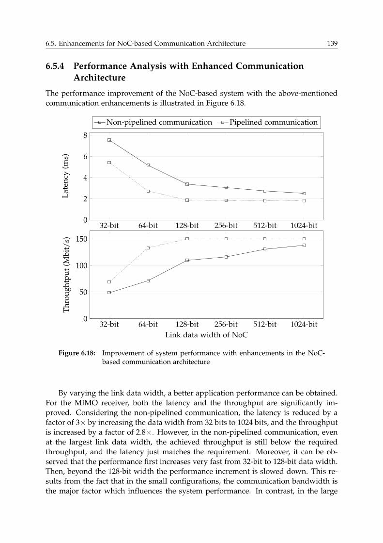
6.5. Enhancements for NoC-based Communication Architecture 139
6.5.4 Performance Analysis with Enhanced Communication
Architecture
The performance improvement of the NoC-based system with the above-mentioned
communication enhancements is illustrated in Figure 6.18.
32-bit 64-bit 128-bit 256-bit 512-bit 1024-bit0
2
4
6
8
Lat
ency
(ms)
Non-pipelined communication Pipelined communication
32-bit 64-bit 128-bit 256-bit 512-bit 1024-bit0
50
100
150
Link data width of NoC
Th
rou
gh
tpu
t(M
bit
/s)
Figure 6.18: Improvement of system performance with enhancements in the NoC-based communication architecture
By varying the link data width, a better application performance can be obtained.
For the MIMO receiver, both the latency and the throughput are significantly im-
proved. Considering the non-pipelined communication, the latency is reduced by a
factor of 3× by increasing the data width from 32 bits to 1024 bits, and the throughput
is increased by a factor of 2.8×. However, in the non-pipelined communication, even
at the largest link data width, the achieved throughput is still below the required
throughput, and the latency just matches the requirement. Moreover, it can be ob-
served that the performance first increases very fast from 32-bit to 128-bit data width.
Then, beyond the 128-bit width the performance increment is slowed down. This re-
sults from the fact that in the small configurations, the communication bandwidth is
the major factor which influences the system performance. In contrast, in the large
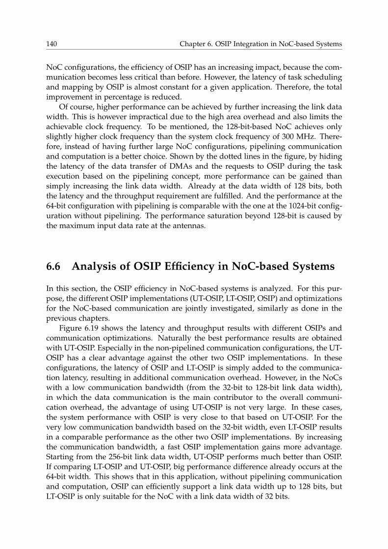
140 Chapter 6. OSIP Integration in NoC-based Systems
NoC configurations, the efficiency of OSIP has an increasing impact, because the com-
munication becomes less critical than before. However, the latency of task scheduling
and mapping by OSIP is almost constant for a given application. Therefore, the total
improvement in percentage is reduced.
Of course, higher performance can be achieved by further increasing the link data
width. This is however impractical due to the high area overhead and also limits the
achievable clock frequency. To be mentioned, the 128-bit-based NoC achieves only
slightly higher clock frequency than the system clock frequency of 300 MHz. There-
fore, instead of having further large NoC configurations, pipelining communication
and computation is a better choice. Shown by the dotted lines in the figure, by hiding
the latency of the data transfer of DMAs and the requests to OSIP during the task
execution based on the pipelining concept, more performance can be gained than
simply increasing the link data width. Already at the data width of 128 bits, both
the latency and the throughput requirement are fulfilled. And the performance at the
64-bit configuration with pipelining is comparable with the one at the 1024-bit config-
uration without pipelining. The performance saturation beyond 128-bit is caused by
the maximum input data rate at the antennas.
6.6 Analysis of OSIP Efficiency in NoC-based Systems
In this section, the OSIP efficiency in NoC-based systems is analyzed. For this pur-
pose, the different OSIP implementations (UT-OSIP, LT-OSIP, OSIP) and optimizations
for the NoC-based communication are jointly investigated, similarly as done in the
previous chapters.
Figure 6.19 shows the latency and throughput results with different OSIPs and
communication optimizations. Naturally the best performance results are obtained
with UT-OSIP. Especially in the non-pipelined communication configurations, the UT-
OSIP has a clear advantage against the other two OSIP implementations. In these
configurations, the latency of OSIP and LT-OSIP is simply added to the communica-
tion latency, resulting in additional communication overhead. However, in the NoCs
with a low communication bandwidth (from the 32-bit to 128-bit link data width),
in which the data communication is the main contributor to the overall communi-
cation overhead, the advantage of using UT-OSIP is not very large. In these cases,
the system performance with OSIP is very close to that based on UT-OSIP. For the
very low communication bandwidth based on the 32-bit width, even LT-OSIP results
in a comparable performance as the other two OSIP implementations. By increasing
the communication bandwidth, a fast OSIP implementation gains more advantage.
Starting from the 256-bit link data width, UT-OSIP performs much better than OSIP.
If comparing LT-OSIP and UT-OSIP, big performance difference already occurs at the
64-bit width. This shows that in this application, without pipelining communication
and computation, OSIP can efficiently support a link data width up to 128 bits, but
LT-OSIP is only suitable for the NoC with a link data width of 32 bits.
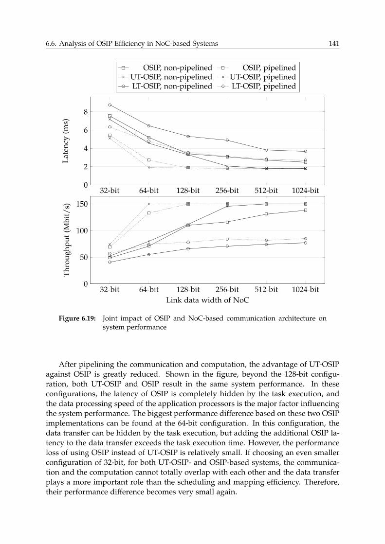
6.6. Analysis of OSIP Efficiency in NoC-based Systems 141
32-bit 64-bit 128-bit 256-bit 512-bit 1024-bit0
2
4
6
8
Lat
ency
(ms)
OSIP, non-pipelined OSIP, pipelinedUT-OSIP, non-pipelined UT-OSIP, pipelinedLT-OSIP, non-pipelined LT-OSIP, pipelined
32-bit 64-bit 128-bit 256-bit 512-bit 1024-bit0
50
100
150
Link data width of NoC
Th
rou
gh
pu
t(M
bit
/s)
Figure 6.19: Joint impact of OSIP and NoC-based communication architecture onsystem performance
After pipelining the communication and computation, the advantage of UT-OSIP
against OSIP is greatly reduced. Shown in the figure, beyond the 128-bit configu-
ration, both UT-OSIP and OSIP result in the same system performance. In these
configurations, the latency of OSIP is completely hidden by the task execution, and
the data processing speed of the application processors is the major factor influencing
the system performance. The biggest performance difference based on these two OSIP
implementations can be found at the 64-bit configuration. In this configuration, the
data transfer can be hidden by the task execution, but adding the additional OSIP la-
tency to the data transfer exceeds the task execution time. However, the performance
loss of using OSIP instead of UT-OSIP is relatively small. If choosing an even smaller
configuration of 32-bit, for both UT-OSIP- and OSIP-based systems, the communica-
tion and the computation cannot totally overlap with each other and the data transfer
plays a more important role than the scheduling and mapping efficiency. Therefore,
their performance difference becomes very small again.
142 Chapter 6. OSIP Integration in NoC-based Systems
Pipelining the LT-OSIP-based systems also increases the system performance.
However, in comparison to the other two fast OSIP implementations, the high latency
of LT-OSIP largely prevents the total communication overhead from being hidden
by the task execution. This results in much lower system performance improvement
even with the pipelining support, especially in the systems with a high communi-
cation bandwidth for the data transfer. As shown in the figure, starting from the
link data width of 128 bits, the performance increment becomes very small. In these
systems, the overhead caused by the data transfer is not critical, but the latency of
LT-OSIP dominates the communication time, which cannot catch up with the task
execution speed.
A more direct indication of the OSIP efficiency – the OSIP busy state is compared
in Figure 6.20. Compared to LT-OSIP, OSIP has much less busy time, which clearly
highlights its efficiency in task management. The pipelined execution in the system
involves OSIP more frequently into operation, but in total its busy time is not more
than 50%, showing that OSIP still has enough capability for handling more tasks. The
almost unchanged OSIP busy time starting from the 128-bit configuration with the
pipelined execution confirms that the latency of OSIP is completely hidden by the
task execution.
32-bit 64-bit 128-bit 256-bit 512-bit 1024-bit0
20
40
60
80
t OS
IP-b
usy
(%)
OSIP, non-pipelined OSIP, pipelinedUT-OSIP, non-pipelined UT-OSIP, pipelinedLT-OSIP, non-pipelined LT-OSIP, pipelined
Figure 6.20: OSIP busy state at different NoC-based communication architectures
6.7 Summary
In this chapter, the potential problems of integrating OSIP into NoC-based systems
are presented, which are caused by frequent polling to OSIP and long interrupt lines.
A proxy-based approach is proposed, which acts as a bridge between the remote PEs
and OSIP. It handles the polling and the interrupts and implements the OSIP APIs
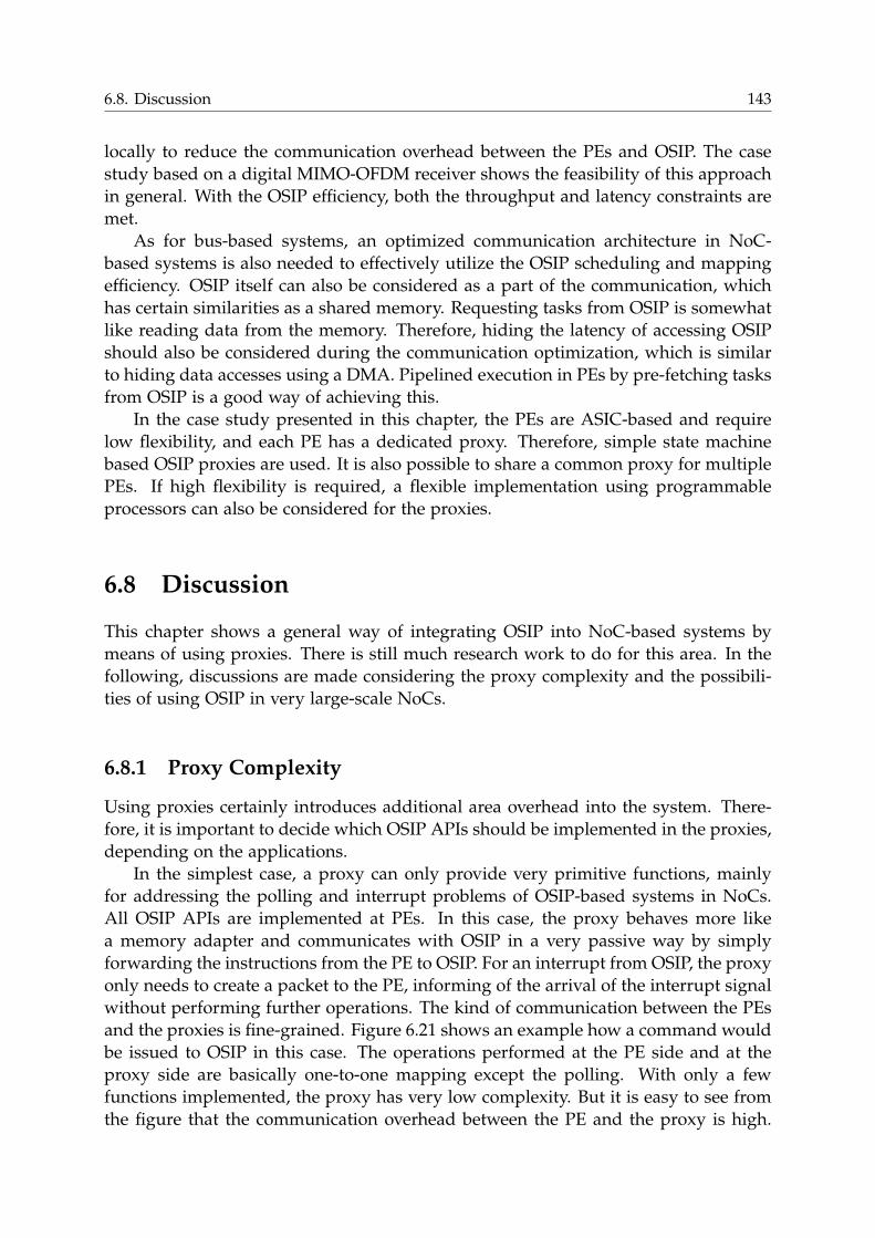
6.8. Discussion 143
locally to reduce the communication overhead between the PEs and OSIP. The case
study based on a digital MIMO-OFDM receiver shows the feasibility of this approach
in general. With the OSIP efficiency, both the throughput and latency constraints are
met.
As for bus-based systems, an optimized communication architecture in NoC-
based systems is also needed to effectively utilize the OSIP scheduling and mapping
efficiency. OSIP itself can also be considered as a part of the communication, which
has certain similarities as a shared memory. Requesting tasks from OSIP is somewhat
like reading data from the memory. Therefore, hiding the latency of accessing OSIP
should also be considered during the communication optimization, which is similar
to hiding data accesses using a DMA. Pipelined execution in PEs by pre-fetching tasks
from OSIP is a good way of achieving this.
In the case study presented in this chapter, the PEs are ASIC-based and require
low flexibility, and each PE has a dedicated proxy. Therefore, simple state machine
based OSIP proxies are used. It is also possible to share a common proxy for multiple
PEs. If high flexibility is required, a flexible implementation using programmable
processors can also be considered for the proxies.
6.8 Discussion
This chapter shows a general way of integrating OSIP into NoC-based systems by
means of using proxies. There is still much research work to do for this area. In the
following, discussions are made considering the proxy complexity and the possibili-
ties of using OSIP in very large-scale NoCs.
6.8.1 Proxy Complexity
Using proxies certainly introduces additional area overhead into the system. There-
fore, it is important to decide which OSIP APIs should be implemented in the proxies,
depending on the applications.
In the simplest case, a proxy can only provide very primitive functions, mainly
for addressing the polling and interrupt problems of OSIP-based systems in NoCs.
All OSIP APIs are implemented at PEs. In this case, the proxy behaves more like
a memory adapter and communicates with OSIP in a very passive way by simply
forwarding the instructions from the PE to OSIP. For an interrupt from OSIP, the proxy
only needs to create a packet to the PE, informing of the arrival of the interrupt signal
without performing further operations. The kind of communication between the PEs
and the proxies is fine-grained. Figure 6.21 shows an example how a command would
be issued to OSIP in this case. The operations performed at the PE side and at the
proxy side are basically one-to-one mapping except the polling. With only a few
functions implemented, the proxy has very low complexity. But it is easy to see from
the figure that the communication overhead between the PE and the proxy is high.
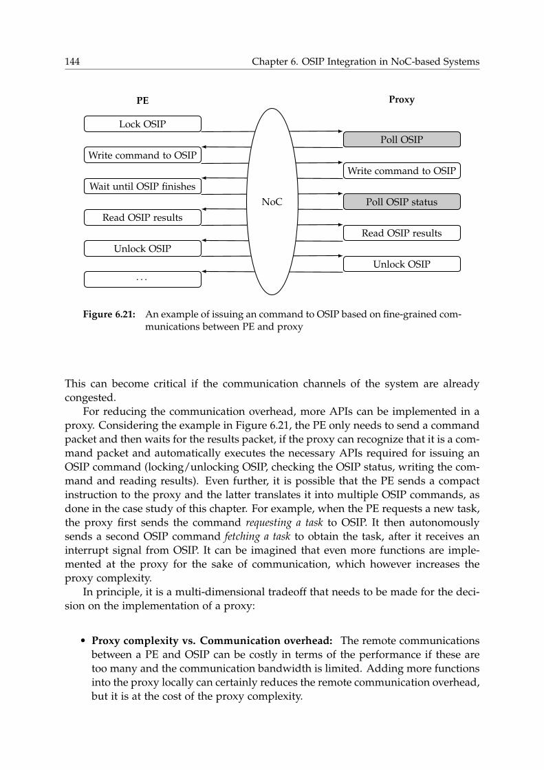
144 Chapter 6. OSIP Integration in NoC-based Systems
PE Proxy
Lock OSIP
Poll OSIP
Write command to OSIP
Write command to OSIP
Wait until OSIP finishes
Poll OSIP status
Read OSIP results
Read OSIP results
Unlock OSIP
Unlock OSIP
. . .
NoC
Figure 6.21: An example of issuing an command to OSIP based on fine-grained com-munications between PE and proxy
This can become critical if the communication channels of the system are already
congested.
For reducing the communication overhead, more APIs can be implemented in a
proxy. Considering the example in Figure 6.21, the PE only needs to send a command
packet and then waits for the results packet, if the proxy can recognize that it is a com-
mand packet and automatically executes the necessary APIs required for issuing an
OSIP command (locking/unlocking OSIP, checking the OSIP status, writing the com-
mand and reading results). Even further, it is possible that the PE sends a compact
instruction to the proxy and the latter translates it into multiple OSIP commands, as
done in the case study of this chapter. For example, when the PE requests a new task,
the proxy first sends the command requesting a task to OSIP. It then autonomously
sends a second OSIP command fetching a task to obtain the task, after it receives an
interrupt signal from OSIP. It can be imagined that even more functions are imple-
mented at the proxy for the sake of communication, which however increases the
proxy complexity.
In principle, it is a multi-dimensional tradeoff that needs to be made for the deci-
sion on the implementation of a proxy:
• Proxy complexity vs. Communication overhead: The remote communications
between a PE and OSIP can be costly in terms of the performance if these are
too many and the communication bandwidth is limited. Adding more functions
into the proxy locally can certainly reduces the remote communication overhead,
but it is at the cost of the proxy complexity.
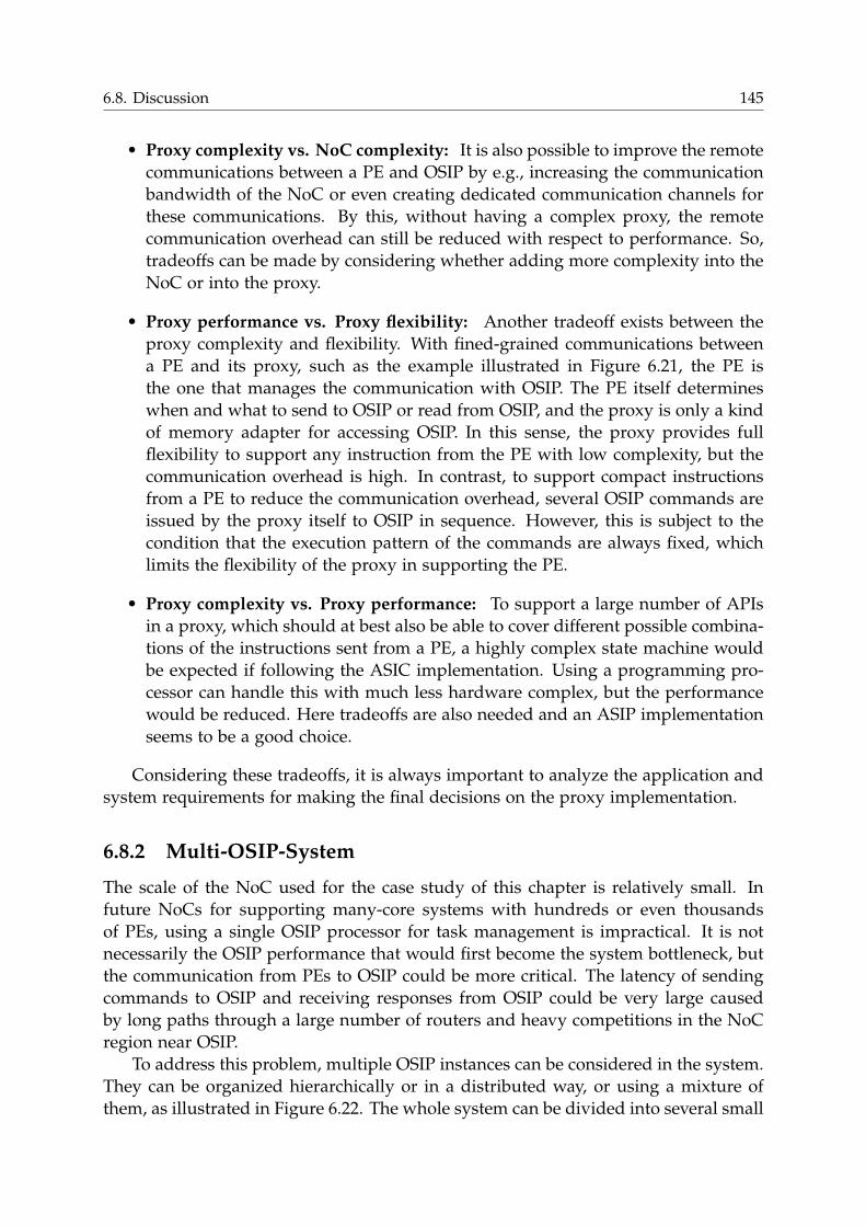
6.8. Discussion 145
• Proxy complexity vs. NoC complexity: It is also possible to improve the remote
communications between a PE and OSIP by e.g., increasing the communication
bandwidth of the NoC or even creating dedicated communication channels for
these communications. By this, without having a complex proxy, the remote
communication overhead can still be reduced with respect to performance. So,
tradeoffs can be made by considering whether adding more complexity into the
NoC or into the proxy.
• Proxy performance vs. Proxy flexibility: Another tradeoff exists between the
proxy complexity and flexibility. With fined-grained communications between
a PE and its proxy, such as the example illustrated in Figure 6.21, the PE is
the one that manages the communication with OSIP. The PE itself determines
when and what to send to OSIP or read from OSIP, and the proxy is only a kind
of memory adapter for accessing OSIP. In this sense, the proxy provides full
flexibility to support any instruction from the PE with low complexity, but the
communication overhead is high. In contrast, to support compact instructions
from a PE to reduce the communication overhead, several OSIP commands are
issued by the proxy itself to OSIP in sequence. However, this is subject to the
condition that the execution pattern of the commands are always fixed, which
limits the flexibility of the proxy in supporting the PE.
• Proxy complexity vs. Proxy performance: To support a large number of APIs
in a proxy, which should at best also be able to cover different possible combina-
tions of the instructions sent from a PE, a highly complex state machine would
be expected if following the ASIC implementation. Using a programming pro-
cessor can handle this with much less hardware complex, but the performance
would be reduced. Here tradeoffs are also needed and an ASIP implementation
seems to be a good choice.
Considering these tradeoffs, it is always important to analyze the application and
system requirements for making the final decisions on the proxy implementation.
6.8.2 Multi-OSIP-System
The scale of the NoC used for the case study of this chapter is relatively small. In
future NoCs for supporting many-core systems with hundreds or even thousands
of PEs, using a single OSIP processor for task management is impractical. It is not
necessarily the OSIP performance that would first become the system bottleneck, but
the communication from PEs to OSIP could be more critical. The latency of sending
commands to OSIP and receiving responses from OSIP could be very large caused
by long paths through a large number of routers and heavy competitions in the NoC
region near OSIP.
To address this problem, multiple OSIP instances can be considered in the system.
They can be organized hierarchically or in a distributed way, or using a mixture of
them, as illustrated in Figure 6.22. The whole system can be divided into several small
146 Chapter 6. OSIP Integration in NoC-based Systems
(a) Hierarchical structure (b) Distributed structure (c) Mixed structure
OSIP subsystemPE subsystem
Figure 6.22: Examples of multi-OSIP-systems in different organizations
MPSoCs and each one is controlled by one OSIP subsystem. If these MPSoCs are only
loosely coupled with each other in executing tasks, a distributed organization is well
suitable. On the contrary, if the task management needs to cross multiple MPSoCs,
a hierarchical organization is preferred. In this case, an OSIP subsystem at a lower
hierarchy level becomes a PE subsystem of an upper-level OSIP subsystem. However,
despite of the different structural organizations, they are all possible thanks to the
flexibility of OSIP.
Chapter 7
Conclusion and Outlook
The development of today’s submicron silicon technology brings both benefits and
challenges. On the one hand, much more functionalities can be integrated onto the
chip of the same size than before, which has driven the evolution of embedded sys-
tems since the past decade. On the other hand, power and energy issues are becoming
extremely critical, and the gap between chip performance and capacity is becoming
larger and larger. To address these challenges, the MPSoC technology provides a
convincing solution. The key is its task-level parallelism.
To efficiently exploit the parallelism of MPSoCs, task management plays an es-
sential role. As introduced in Chapter 2, task management in MPSoCs can be static,
semi-static or dynamic, among which dynamic task management is especially im-
portant for coping with high dynamism of today’s embedded systems. However,
the increasing system complexity, from both the hardware architecture and the ap-
plication software perspective, makes the design of good dynamic task management
highly challenging. It should be fast and have high quality, and at the same time be
flexible due to its dynamic nature.
In the literature, most task manager implementations are either based on RISC
processors or dedicated hardwired solutions. Both have their limitations, the former
lacking efficiency while the latter the flexibility. This work argues that ASIPs are a
more promising way for implementing task managers, which combine the advantages
of the other two implementation types.
In this work, an ASIP task manager called OSIP is proposed and analyzed in
depth with respect to its efficiency and flexibility. The design of the OSIP architec-
ture focuses on accelerating the typical and the most critical kernel operations in task
management, such as list operations, various task comparison metrics, fast extraction
of task information and frequent branches. For these operations, a set of customized
instructions are developed, which largely speed up the major components of task
management – scheduling, mapping and synchronization. Meanwhile, OSIP contains
a normal RISC instruction-set, which provides enough flexibility for its possible func-
tional extensions.
The efficiency of OSIP is assessed by comparing it with two other task manager
implementations – a hypothetical extremely fast ASIC annotated as UT-OSIP and a
RISC processor annotated as LT-OSIP. It is important to mention that a meaningful
comparison must be performed within a system context, considering e.g., the system
size in terms of the number of PEs and task sizes, etc. They influence the load to
the task manager. It is also important to include the impact of the communication
architecture into the assessment. Both being a shared resource, the task manager and
147
148 Chapter 7. Conclusion and Outlook
the communication architecture in fact compete with each other during the system
execution: which one is finally the system bottleneck? The analysis results in Chapter
4 show that the high efficiency of OSIP in task management makes it unlikely become
the system bottleneck. The system performance is mostly limited by the communi-
cation bandwidth or the task parallelism. In this case, adding more efficiency to the
task manager, e.g., by using UT-OSIP, is rather a waste of the efficiency. On the other
hand, the RISC-based LT-OSIP can easily become the system bottleneck due to its low
efficiency, especially for large systems.
The evaluation for the flexibility of OSIP is performed when it is applied for im-
proving the spinlock control mechanism in OSIP-based systems by using a-priori ap-
plication knowledge, which is presented in Chapter 5. The programmability of OSIP
enables the designer to extend the OSIP functionality by software to support more
advanced spinlock control mechanism based on the so-called spinlock reservation,
which results in significant performance improvement. By this, the OSIP-based sys-
tems have an even better performance than the UT-OSIP-based systems in many cases
in the presented case study. For the latter, the extension is not applicable due to the
flexibility limitation of ASIC. The successful application of the OSIP flexibility onto
the spinlock improvement is supported by its efficiency, which supplies OSIP with
enough performance margin for much more additional workload. In contrast, LT-
OSIP also has flexibility, but it often fails in improving the spinlock control with the
extended mechanism. Its low efficiency does not allow it to afford the additional
work. In this sense, its flexibility is largely wasted.
The efficiency and flexibility are usually considered to be contradictory when de-
signing a system. However, in this thesis it is shown that they actually enhance each
other in dynamic task management, which requires both. With efficiency, the utiliza-
tion of the flexibility can largely increase. And with flexibility, more efficiency can be
achieved. Being able to make good trade-offs between the efficiency and flexibility,
an ASIP provides a very promising solution to implement a dynamic task manager
in complex MPSoCs. It can be more generally concluded that ASIPs are not only
suitable for intensive data processing, but also able to be well applied in supporting
control-centric applications such as system control.
The task management in OSIP-based systems is organized in a centralized way,
i.e., OSIP manages tasks for several PEs and each of these PEs communicates with
OSIP. This centralized organization would most likely be the preferred organization,
if an ASIP is used as the task manager. A fully distributed task management using
an ASIP manager at each PE would be an overdesign, which would cost too much
hardware. However, in the systems with a NoC, which has a distributive characteris-
tic, the centralized management might introduce too much communication overhead
between the task manager and the PEs, which can impair the management efficiency
of the ASIP. In OSIP-based systems, this problem is solved by introducing proxies
for the PEs. An OSIP subsystem is created based on the proxies and OSIP, which is
considered as the task manager as a whole towards the outside. The PEs do not com-
municate with OSIP directly, but with the OSIP subsystem by only sending a small
number of instructions in form of packets. Inside the OSIP subsystem, the proxies in-
149
terpret the instructions and perform detailed communications with OSIP, complying
with the OSIP programming model. In this way, the remote communication overhead
through the NoC is effectively reduced to a large extent. Although the solution is
rather specific for OSIP-based systems, the idea of converting remote communications
into local communications can be generalized for the centralized task management.
Using an ASIP as the task manager, or more generally as the system controller in
MPSoCs is still not popular in the research in spite of its advantages over RISC- or
ASIC-based approaches. Among others, a major reason could lie in its design com-
plexity. In comparison to the ASIC design, a complete software development tool
chain needs to be developed for an ASIP, which largely increases the design complex-
ity. In comparison to the RISC design, identifying efficient customized instructions
for an ASIP is also not a trivial task. An ADL-based ASIP design environment, such
as the Processor Designer used in this work, eases the ASIP design flow. But there
are still many challenges to overcome. For example, developing a highly optimized
compiler for an ASIP, which can effectively exploit the customized instructions, is still
highly challenging. In this work, most of the customized instructions of OSIP are
used based on the Compiler-Known Functions (CKFs), which certainly decreases its
usability.
Concretely for OSIP-based systems, there are also several things which can be
further optimized:
• Current systems always use a RISC processor as the master of the complete
system. It boots up the system and creates an initial configuration of scheduling
and mapping hierarchy. As OSIP is programmable, these tasks can in principle
also be performed directly by OSIP. As a consequence, the RISCmaster processor
can be removed from the system, which not only reduces the area cost, but also
creates a clearer system control flow structure.
• OSIP takes actions upon the requests from PEs through its register interface. The
information, on which OSIP makes task management decisions, is also com-
pletely provided by PEs through the register interface using commands. This
makes the behavior of OSIP passive. As the task manager, it should be able to
take the responsibility in controlling systems more actively, which is however
limited by its current two interfaces. OSIP does have a good overview of the
system tasks and load. But if it should take more active decisions, it sometimes
needs to know the context of tasks. However, a direct access from OSIP to the
task context is currently not available. A workaround through the PEs over the
register interface has to be made, if needed. This is certainly not an efficient way.
Therefore, a bus interface, e.g., compliant to the AHB protocol, is desired, which
enables a direct access of OSIP to the shared memory over the bus for fetching
required information.
• The task management of OSIP-based systems follows the centralized approach,
which has to be faced with the scalability problem. At the end of Chapter 6,
several possibilities have been shown to support very large-scale systems by
150 Chapter 7. Conclusion and Outlook
introducing multiple OSIPs. However, concrete case studies are still needed to
evaluate the different multi-OSIP structures and many researches can further be
carried on in this area.
Dynamic task management in MPSoCs is highly complex and challenging. This
thesis has proposed an ASIP-based approach to overcome the challenges. The results
show significant performance gain by applying this approach. Although there are still
many things to work on in ASIP-based task management, using ASIPs turns out to
the best way to meet both the efficiency and the flexibility requirements in dynamic
task management of MPSoCs.
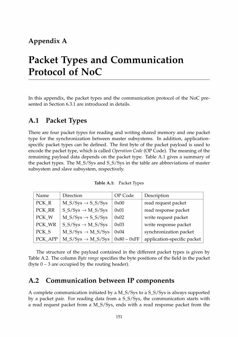
Appendix A
Packet Types and CommunicationProtocol of NoC
In this appendix, the packet types and the communication protocol of the NoC pre-
sented in Section 6.3.1 are introduced in details.
A.1 Packet Types
There are four packet types for reading and writing shared memory and one packet
type for the synchronization between master subsystems. In addition, application-
specific packet types can be defined. The first byte of the packet payload is used to
encode the packet type, which is called Operation Code (OP Code). The meaning of the
remaining payload data depends on the packet type. Table A.1 gives a summary of
the packet types. The M_S/Sys and S_S/Sys in the table are abbreviations of master
subsystem and slave subsystem, respectively.
Table A.1: Packet Types
Name Direction OP Code Description
PCK_R M_S/Sys→ S_S/Sys 0x00 read request packet
PCK_RR S_S/Sys→ M_S/Sys 0x01 read response packet
PCK_W M_S/Sys→ S_S/Sys 0x02 write request packet
PCK_WR S_S/Sys→ M_S/Sys 0x03 write response packet
PCK_S M_S/Sys→ M_S/Sys 0x04 synchronization packet
PCK_APP M_S/Sys→ M_S/Sys 0x80 – 0xFF application-specific packet
The structure of the payload contained in the different packet types is given by
Table A.2. The column Byte range specifies the byte positions of the field in the packet
(byte 0 – 3 are occupied by the routing header).
A.2 Communication between IP components
A complete communication initiated by a M_S/Sys to a S_S/Sys is always supported
by a packet pair. For reading data from a S_S/Sys, the communication starts with
a read request packet from a M_S/Sys, ends with a read response packet from the
151
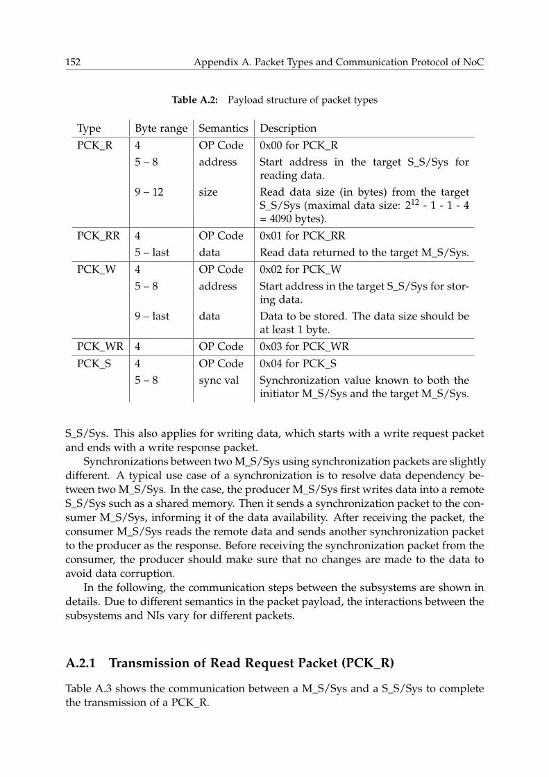
152 Appendix A. Packet Types and Communication Protocol of NoC
Table A.2: Payload structure of packet types
Type Byte range Semantics Description
PCK_R 4 OP Code 0x00 for PCK_R
5 – 8 address Start address in the target S_S/Sys forreading data.
9 – 12 size Read data size (in bytes) from the targetS_S/Sys (maximal data size: 212 - 1 - 1 - 4= 4090 bytes).
PCK_RR 4 OP Code 0x01 for PCK_RR
5 – last data Read data returned to the target M_S/Sys.
PCK_W 4 OP Code 0x02 for PCK_W
5 – 8 address Start address in the target S_S/Sys for stor-ing data.
9 – last data Data to be stored. The data size should beat least 1 byte.
PCK_WR 4 OP Code 0x03 for PCK_WR
PCK_S 4 OP Code 0x04 for PCK_S
5 – 8 sync val Synchronization value known to both theinitiator M_S/Sys and the target M_S/Sys.
S_S/Sys. This also applies for writing data, which starts with a write request packet
and ends with a write response packet.
Synchronizations between twoM_S/Sys using synchronization packets are slightly
different. A typical use case of a synchronization is to resolve data dependency be-
tween two M_S/Sys. In the case, the producer M_S/Sys first writes data into a remote
S_S/Sys such as a shared memory. Then it sends a synchronization packet to the con-
sumer M_S/Sys, informing it of the data availability. After receiving the packet, the
consumer M_S/Sys reads the remote data and sends another synchronization packet
to the producer as the response. Before receiving the synchronization packet from the
consumer, the producer should make sure that no changes are made to the data to
avoid data corruption.
In the following, the communication steps between the subsystems are shown in
details. Due to different semantics in the packet payload, the interactions between the
subsystems and NIs vary for different packets.
A.2.1 Transmission of Read Request Packet (PCK_R)
Table A.3 shows the communication between a M_S/Sys and a S_S/Sys to complete
the transmission of a PCK_R.
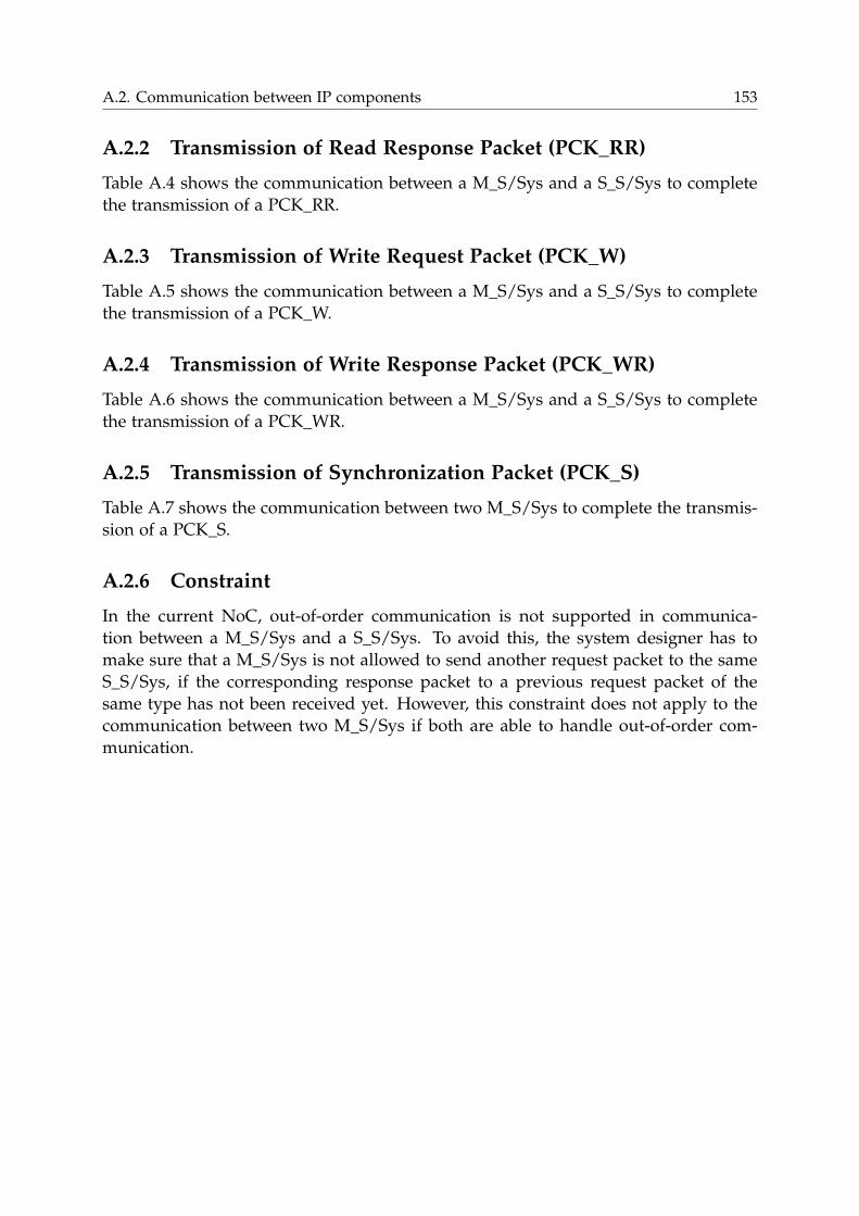
A.2. Communication between IP components 153
A.2.2 Transmission of Read Response Packet (PCK_RR)
Table A.4 shows the communication between a M_S/Sys and a S_S/Sys to complete
the transmission of a PCK_RR.
A.2.3 Transmission of Write Request Packet (PCK_W)
Table A.5 shows the communication between a M_S/Sys and a S_S/Sys to complete
the transmission of a PCK_W.
A.2.4 Transmission of Write Response Packet (PCK_WR)
Table A.6 shows the communication between a M_S/Sys and a S_S/Sys to complete
the transmission of a PCK_WR.
A.2.5 Transmission of Synchronization Packet (PCK_S)
Table A.7 shows the communication between two M_S/Sys to complete the transmis-
sion of a PCK_S.
A.2.6 Constraint
In the current NoC, out-of-order communication is not supported in communica-
tion between a M_S/Sys and a S_S/Sys. To avoid this, the system designer has to
make sure that a M_S/Sys is not allowed to send another request packet to the same
S_S/Sys, if the corresponding response packet to a previous request packet of the
same type has not been received yet. However, this constraint does not apply to the
communication between two M_S/Sys if both are able to handle out-of-order com-
munication.
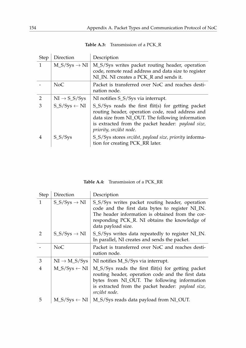
154 Appendix A. Packet Types and Communication Protocol of NoC
Table A.3: Transmission of a PCK_R
Step Direction Description
1 M_S/Sys→ NI M_S/Sys writes packet routing header, operationcode, remote read address and data size to registerNI_IN. NI creates a PCK_R and sends it.
- NoC Packet is transferred over NoC and reaches desti-nation node.
2 NI→ S_S/Sys NI notifies S_S/Sys via interrupt.
3 S_S/Sys← NI S_S/Sys reads the first flit(s) for getting packetrouting header, operation code, read address anddata size from NI_OUT. The following informationis extracted from the packet header: payload size,priority, src/dst node.
4 S_S/Sys S_S/Sys stores src/dst, payload size, priority informa-tion for creating PCK_RR later.
Table A.4: Transmission of a PCK_RR
Step Direction Description
1 S_S/Sys→ NI S_S/Sys writes packet routing header, operationcode and the first data bytes to register NI_IN.The header information is obtained from the cor-responding PCK_R. NI obtains the knowledge ofdata payload size.
2 S_S/Sys→ NI S_S/Sys writes data repeatedly to register NI_IN.In parallel, NI creates and sends the packet.
- NoC Packet is transferred over NoC and reaches desti-nation node.
3 NI→ M_S/Sys NI notifies M_S/Sys via interrupt.
4 M_S/Sys← NI M_S/Sys reads the first flit(s) for getting packetrouting header, operation code and the first databytes from NI_OUT. The following informationis extracted from the packet header: payload size,src/dst node.
5 M_S/Sys← NI M_S/Sys reads data payload from NI_OUT.
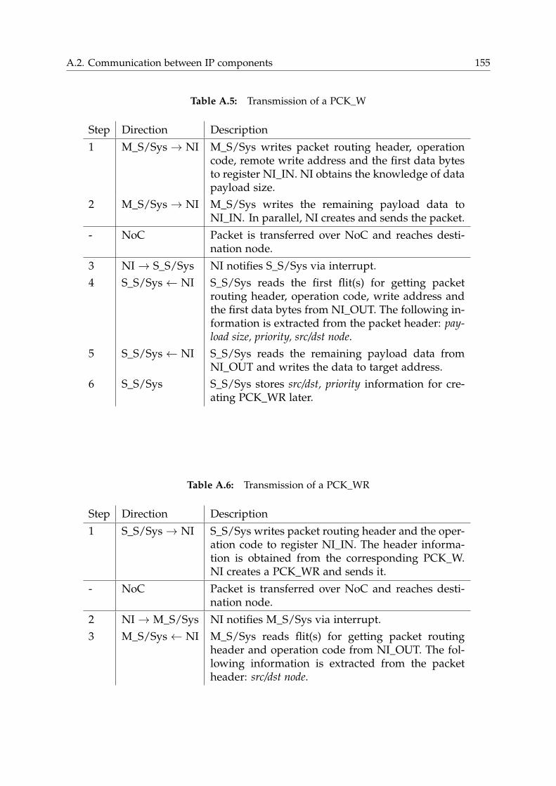
A.2. Communication between IP components 155
Table A.5: Transmission of a PCK_W
Step Direction Description
1 M_S/Sys→ NI M_S/Sys writes packet routing header, operationcode, remote write address and the first data bytesto register NI_IN. NI obtains the knowledge of datapayload size.
2 M_S/Sys→ NI M_S/Sys writes the remaining payload data toNI_IN. In parallel, NI creates and sends the packet.
- NoC Packet is transferred over NoC and reaches desti-nation node.
3 NI→ S_S/Sys NI notifies S_S/Sys via interrupt.
4 S_S/Sys← NI S_S/Sys reads the first flit(s) for getting packetrouting header, operation code, write address andthe first data bytes from NI_OUT. The following in-formation is extracted from the packet header: pay-load size, priority, src/dst node.
5 S_S/Sys← NI S_S/Sys reads the remaining payload data fromNI_OUT and writes the data to target address.
6 S_S/Sys S_S/Sys stores src/dst, priority information for cre-ating PCK_WR later.
Table A.6: Transmission of a PCK_WR
Step Direction Description
1 S_S/Sys→ NI S_S/Sys writes packet routing header and the oper-ation code to register NI_IN. The header informa-tion is obtained from the corresponding PCK_W.NI creates a PCK_WR and sends it.
- NoC Packet is transferred over NoC and reaches desti-nation node.
2 NI→ M_S/Sys NI notifies M_S/Sys via interrupt.
3 M_S/Sys← NI M_S/Sys reads flit(s) for getting packet routingheader and operation code from NI_OUT. The fol-lowing information is extracted from the packetheader: src/dst node.
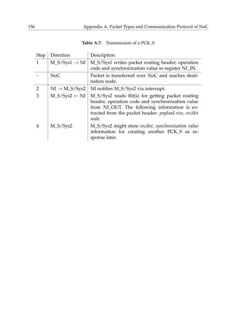
156 Appendix A. Packet Types and Communication Protocol of NoC
Table A.7: Transmission of a PCK_S
Step Direction Description
1 M_S/Sys1→ NI M_S/Sys1 writes packet routing header, operationcode and synchronization value to register NI_IN.
- NoC Packet is transferred over NoC and reaches desti-nation node.
2 NI→ M_S/Sys2 NI notifies M_S/Sys2 via interrupt.
3 M_S/Sys2← NI M_S/Sys2 reads flit(s) for getting packet routingheader, operation code and synchronization valuefrom NI_OUT. The following information is ex-tracted from the packet header: payload size, src/dstnode.
4 M_S/Sys2 M_S/Sys2 might store src/dst, synchronization valueinformation for creating another PCK_S as re-sponse later.
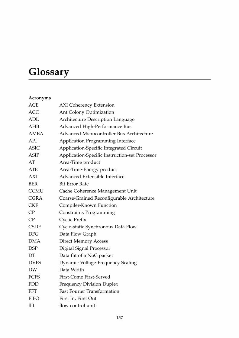
Glossary
Acronyms
ACE AXI Coherency Extension
ACO Ant Colony Optimization
ADL Architecture Description Language
AHB Advanced High-Performance Bus
AMBA Advanced Microcontroller Bus Architecture
API Application Programming Interface
ASIC Application-Specific Integrated Circuit
ASIP Application-Specific Instruction-set Processor
AT Area-Time product
ATE Area-Time-Energy product
AXI Advanced Extensible Interface
BER Bit Error Rate
CCMU Cache Coherence Management Unit
CGRA Coarse-Grained Reconfigurable Architecture
CKF Compiler-Known Function
CP Constraints Programming
CP Cyclic Prefix
CSDF Cyclo-static Synchronous Data Flow
DFG Data Flow Graph
DMA Direct Memory Access
DSP Digital Signal Processor
DT Data flit of a NoC packet
DVFS Dynamic Voltage-Frequency Scaling
DW Data Width
FCFS First-Come First-Served
FDD Frequency Division Duplex
FFT Fast Fourier Transformation
FIFO First In, First Out
flit flow control unit
157
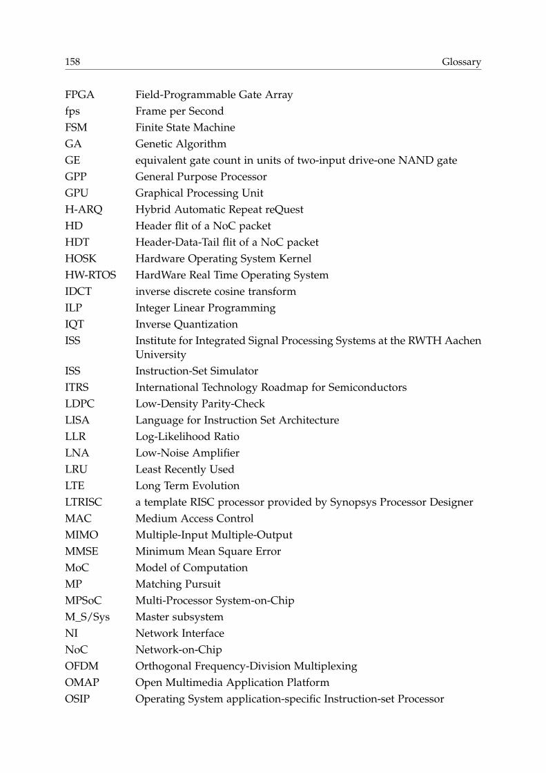
158 Glossary
FPGA Field-Programmable Gate Array
fps Frame per Second
FSM Finite State Machine
GA Genetic Algorithm
GE equivalent gate count in units of two-input drive-one NAND gate
GPP General Purpose Processor
GPU Graphical Processing Unit
H-ARQ Hybrid Automatic Repeat reQuest
HD Header flit of a NoC packet
HDT Header-Data-Tail flit of a NoC packet
HOSK Hardware Operating System Kernel
HW-RTOS HardWare Real Time Operating System
IDCT inverse discrete cosine transform
ILP Integer Linear Programming
IQT Inverse Quantization
ISS Institute for Integrated Signal Processing Systems at the RWTH Aachen
University
ISS Instruction-Set Simulator
ITRS International Technology Roadmap for Semiconductors
LDPC Low-Density Parity-Check
LISA Language for Instruction Set Architecture
LLR Log-Likelihood Ratio
LNA Low-Noise Amplifier
LRU Least Recently Used
LTE Long Term Evolution
LTRISC a template RISC processor provided by Synopsys Processor Designer
MAC Medium Access Control
MIMO Multiple-Input Multiple-Output
MMSE Minimum Mean Square Error
MoC Model of Computation
MP Matching Pursuit
MPSoC Multi-Processor System-on-Chip
M_S/Sys Master subsystem
NI Network Interface
NoC Network-on-Chip
OFDM Orthogonal Frequency-Division Multiplexing
OMAP Open Multimedia Application Platform
OSIP Operating System application-specific Instruction-set Processor
Glossary 159
OS Operating System
PC Personal Computer
PC Program Counter
PE Processing Element
PHY PHYsical layer
PSP Processor-Support Package
QAM Quadrature Amplitude Modulation
QoS Quality of Service
QRD QR Decomposition
RB Resource Block
RF Radio Frequency
RISC Reduced Instruction Set Computer
RR Round-Robin
RTL Register-Transfer Level
S/Sys subsystem
SA Simulated Annealing
SDFG Synchronous Data Flow Graph
SDF Synchronous Data Flow
SD Sphere-Decoding
SIMD Single Instruction Multiple Data
SMP Symmetric Multiprocessing
SPE Synergistic Processing Element
SQRD Sorted QR Decomposition
S_S/Sys Slave subsystem
SSRAM Synchronous Static Random Access Memory
TD Turbo Decoding
TI Texas Instruments
TL Tail flit of a NoC packet
TL Transaction-Level
TS Tabu Search
TTI Transmission Time Interval
VC Virtual Channel
VLIW Very Large Instruction Word
VPU Virtual Processing Unit
ZF Zero Forcing

160 Glossary
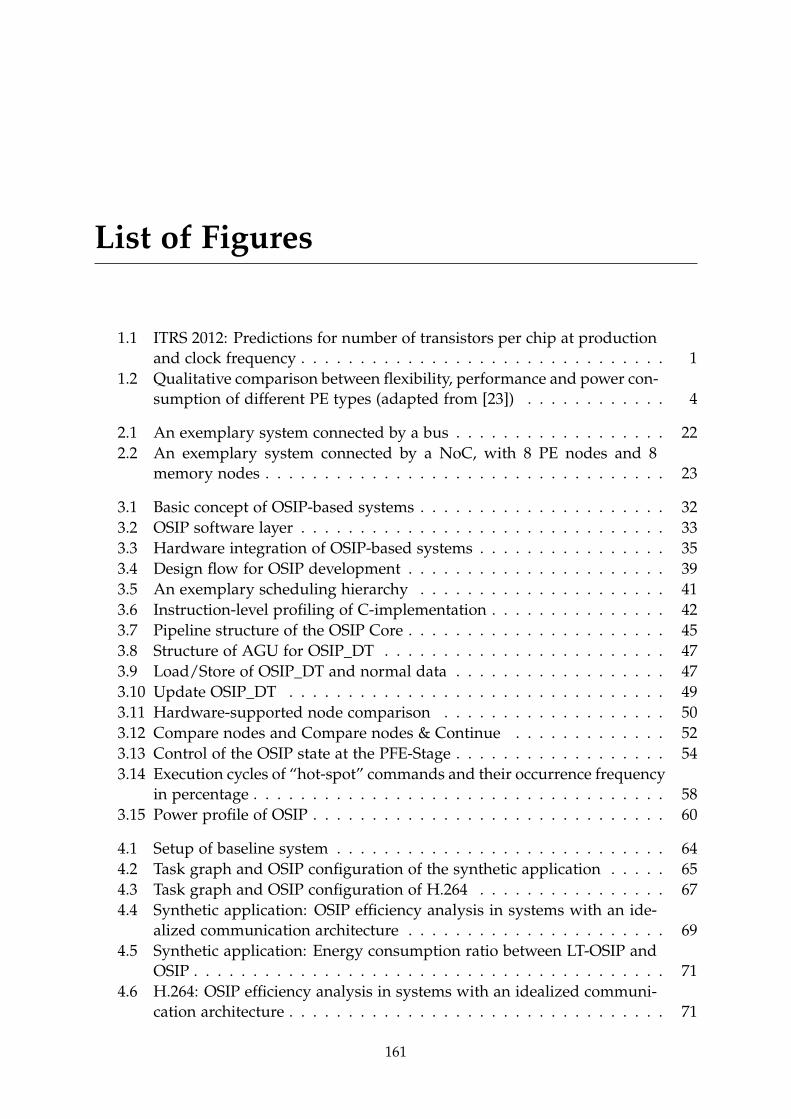
List of Figures
1.1 ITRS 2012: Predictions for number of transistors per chip at production
and clock frequency . . . . . . . . . . . . . . . . . . . . . . . . . . . . . . . 1
1.2 Qualitative comparison between flexibility, performance and power con-
sumption of different PE types (adapted from [23]) . . . . . . . . . . . . 4
2.1 An exemplary system connected by a bus . . . . . . . . . . . . . . . . . . 22
2.2 An exemplary system connected by a NoC, with 8 PE nodes and 8
memory nodes . . . . . . . . . . . . . . . . . . . . . . . . . . . . . . . . . . 23
3.1 Basic concept of OSIP-based systems . . . . . . . . . . . . . . . . . . . . . 32
3.2 OSIP software layer . . . . . . . . . . . . . . . . . . . . . . . . . . . . . . . 33
3.3 Hardware integration of OSIP-based systems . . . . . . . . . . . . . . . . 35
3.4 Design flow for OSIP development . . . . . . . . . . . . . . . . . . . . . . 39
3.5 An exemplary scheduling hierarchy . . . . . . . . . . . . . . . . . . . . . 41
3.6 Instruction-level profiling of C-implementation . . . . . . . . . . . . . . . 42
3.7 Pipeline structure of the OSIP Core . . . . . . . . . . . . . . . . . . . . . . 45
3.8 Structure of AGU for OSIP_DT . . . . . . . . . . . . . . . . . . . . . . . . 47
3.9 Load/Store of OSIP_DT and normal data . . . . . . . . . . . . . . . . . . 47
3.10 Update OSIP_DT . . . . . . . . . . . . . . . . . . . . . . . . . . . . . . . . 49
3.11 Hardware-supported node comparison . . . . . . . . . . . . . . . . . . . 50
3.12 Compare nodes and Compare nodes & Continue . . . . . . . . . . . . . 52
3.13 Control of the OSIP state at the PFE-Stage . . . . . . . . . . . . . . . . . . 54
3.14 Execution cycles of “hot-spot” commands and their occurrence frequency
in percentage . . . . . . . . . . . . . . . . . . . . . . . . . . . . . . . . . . . 58
3.15 Power profile of OSIP . . . . . . . . . . . . . . . . . . . . . . . . . . . . . . 60
4.1 Setup of baseline system . . . . . . . . . . . . . . . . . . . . . . . . . . . . 64
4.2 Task graph and OSIP configuration of the synthetic application . . . . . 65
4.3 Task graph and OSIP configuration of H.264 . . . . . . . . . . . . . . . . 67
4.4 Synthetic application: OSIP efficiency analysis in systems with an ide-
alized communication architecture . . . . . . . . . . . . . . . . . . . . . . 69
4.5 Synthetic application: Energy consumption ratio between LT-OSIP and
OSIP . . . . . . . . . . . . . . . . . . . . . . . . . . . . . . . . . . . . . . . . 71
4.6 H.264: OSIP efficiency analysis in systems with an idealized communi-
cation architecture . . . . . . . . . . . . . . . . . . . . . . . . . . . . . . . . 71
161
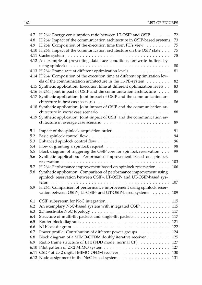
162 LIST OF FIGURES
4.7 H.264: Energy consumption ratio between LT-OSIP and OSIP . . . . . . 72
4.8 H.264: Impact of the communication architecture in OSIP-based systems 73
4.9 H.264: Composition of the execution time from PE’s view . . . . . . . . 75
4.10 H.264: Impact of the communication architecture on the OSIP state . . . 75
4.11 Cache system . . . . . . . . . . . . . . . . . . . . . . . . . . . . . . . . . . 78
4.12 An example of preventing data race conditions for write buffers by
using spinlocks . . . . . . . . . . . . . . . . . . . . . . . . . . . . . . . . . 80
4.13 H.264: Frame rate at different optimization levels . . . . . . . . . . . . . 81
4.14 H.264: Composition of the execution time at different optimization lev-
els of the communication architecture in the 11-PE-system . . . . . . . . 82
4.15 Synthetic application: Execution time at different optimization levels . . 83
4.16 H.264: Joint impact of OSIP and the communication architecture . . . . 85
4.17 Synthetic application: Joint impact of OSIP and the communication ar-
chitecture in best case scenario . . . . . . . . . . . . . . . . . . . . . . . . 86
4.18 Synthetic application: Joint impact of OSIP and the communication ar-
chitecture in worst case scenario . . . . . . . . . . . . . . . . . . . . . . . 88
4.19 Synthetic application: Joint impact of OSIP and the communication ar-
chitecture in average case scenario . . . . . . . . . . . . . . . . . . . . . . 89
5.1 Impact of the spinlock acquisition order . . . . . . . . . . . . . . . . . . . 91
5.2 Basic spinlock control flow . . . . . . . . . . . . . . . . . . . . . . . . . . . 94
5.3 Enhanced spinlock control flow . . . . . . . . . . . . . . . . . . . . . . . . 96
5.4 Flow of granting a spinlock request . . . . . . . . . . . . . . . . . . . . . 98
5.5 Block diagram of triggering the OSIP core for spinlock reservation . . . 99
5.6 Synthetic application: Performance improvement based on spinlock
reservation . . . . . . . . . . . . . . . . . . . . . . . . . . . . . . . . . . . . 103
5.7 H.264: Performance improvement based on spinlock reservation . . . . 106
5.8 Synthetic application: Comparison of performance improvement using
spinlock reservation between OSIP-, LT-OSIP- and UT-OSIP-based sys-
tems . . . . . . . . . . . . . . . . . . . . . . . . . . . . . . . . . . . . . . . 107
5.9 H.264: Comparison of performance improvement using spinlock reser-
vation between OSIP-, LT-OSIP- and UT-OSIP-based systems . . . . . . 109
6.1 OSIP subsystem for NoC integration . . . . . . . . . . . . . . . . . . . . . 115
6.2 An exemplary NoC-based system with integrated OSIP . . . . . . . . . . 115
6.3 2D mesh-like NoC topology . . . . . . . . . . . . . . . . . . . . . . . . . . 117
6.4 Structure of multi-flit packets and single-flit packets . . . . . . . . . . . . 117
6.5 Router block diagram . . . . . . . . . . . . . . . . . . . . . . . . . . . . . . 121
6.6 NI block diagram . . . . . . . . . . . . . . . . . . . . . . . . . . . . . . . . 122
6.7 Power profile: Contribution of different power groups . . . . . . . . . . 124
6.8 Block diagram of a MIMO-OFDM doubly iterative receiver . . . . . . . . 125
6.9 Radio frame structure of LTE (FDD mode, normal CP) . . . . . . . . . . 127
6.10 Pilot pattern of 2×2 MIMO system . . . . . . . . . . . . . . . . . . . . . . 127
6.11 CSDF of 2×2 digital MIMO-OFDM receiver . . . . . . . . . . . . . . . . . 130
6.12 Node assignment in the NoC-based system . . . . . . . . . . . . . . . . . 131
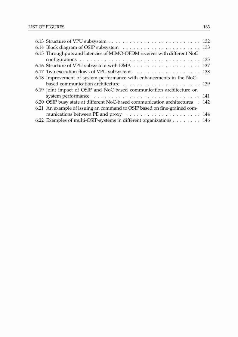
LIST OF FIGURES 163
6.13 Structure of VPU subsystem . . . . . . . . . . . . . . . . . . . . . . . . . . 132
6.14 Block diagram of OSIP subsystem . . . . . . . . . . . . . . . . . . . . . . 133
6.15 Throughputs and latencies of MIMO-OFDM receiver with different NoC
configurations . . . . . . . . . . . . . . . . . . . . . . . . . . . . . . . . . . 135
6.16 Structure of VPU subsystem with DMA . . . . . . . . . . . . . . . . . . . 137
6.17 Two execution flows of VPU subsystems . . . . . . . . . . . . . . . . . . 138
6.18 Improvement of system performance with enhancements in the NoC-
based communication architecture . . . . . . . . . . . . . . . . . . . . . . 139
6.19 Joint impact of OSIP and NoC-based communication architecture on
system performance . . . . . . . . . . . . . . . . . . . . . . . . . . . . . . 141
6.20 OSIP busy state at different NoC-based communication architectures . 142
6.21 An example of issuing an command to OSIP based on fine-grained com-
munications between PE and proxy . . . . . . . . . . . . . . . . . . . . . 144
6.22 Examples of multi-OSIP-systems in different organizations . . . . . . . . 146

164 LIST OF FIGURES
List of Tables
2.1 List of task management references in the literature . . . . . . . . . . . . 11
3.1 Synthesis results of OSIP and LT-OSIP . . . . . . . . . . . . . . . . . . . . 57
3.2 Power consumption of OSIP and LT-OSIP . . . . . . . . . . . . . . . . . . 59
6.1 Power consumption of NoC . . . . . . . . . . . . . . . . . . . . . . . . . . 123
6.2 System parameters for achieving a throughput of 150Mbit/s in a 2×2MIMO system . . . . . . . . . . . . . . . . . . . . . . . . . . . . . . . . . . 128
6.3 Selected implementations of algorithmic kernels . . . . . . . . . . . . . . 129
6.4 Definition of VPUs . . . . . . . . . . . . . . . . . . . . . . . . . . . . . . . 130
A.1 Packet Types . . . . . . . . . . . . . . . . . . . . . . . . . . . . . . . . . . . 151
A.2 Payload structure of packet types . . . . . . . . . . . . . . . . . . . . . . . 152
A.3 Transmission of a PCK_R . . . . . . . . . . . . . . . . . . . . . . . . . . . 154
A.4 Transmission of a PCK_RR . . . . . . . . . . . . . . . . . . . . . . . . . . . 154
A.5 Transmission of a PCK_W . . . . . . . . . . . . . . . . . . . . . . . . . . . 155
A.6 Transmission of a PCK_WR . . . . . . . . . . . . . . . . . . . . . . . . . . 155
A.7 Transmission of a PCK_S . . . . . . . . . . . . . . . . . . . . . . . . . . . . 156
165

166 LIST OF TABLES
Bibliography
[1] “Open Virtual Platforms.” [Online]. Available: http://www.ovpworld.org
[2] 3GPP, “3GPP Release 8.” [Online]. Available: http://www.3gpp.org/specifications/releases/72-release-8
[3] B. Ackland, A. Anesko, D. Brinthaupt, S. Daubert, A. Kalavade, J. Knobloch, E. Micca,M. Moturi, C. Nicol, J. O’Neill, J. Othmer, E. Sackinger, K. Singh, J. Sweet, C. Terman,and J. Williams, “A Single-Chip, 1.6-Billion, 16-b MAC/s Multiprocessor DSP,” IEEEJournal of Solid-State Circuits, vol. 35, no. 3, pp. 412–424, March 2000.
[4] W. Ahmed, M. Shafique, L. Bauer, and J. Henkel, “Adaptive Resource Management forSimultaneous Multitasking in Mixed-Grained Reconfigurable Multi-Core Processors,”in Proceedings of International Conference on Hardware/Software Codesign and System Synthe-sis (CODES+ISSS), Taipei, Taiwan, Oct 2011, pp. 365–374.
[5] M. Al Faruque, R. Krist, and J. Henkel, “ADAM: Run-Time Agent-Based DistributedApplication Mapping for on-chip Communication,” in Proceedings of Design AutomationConference (DAC), Anaheim, CA, USA, 2008, pp. 760–765.
[6] M. Amos, Theoretical and Experimental DNA Computation, ser. Natural Computing Series.Springer, June 2005, vol. XIII, ISBN 978-3-540-28131-3.
[7] T. E. Anderson, “The Performance of Spin Lock Alternatives for Shared-Memory Multi-processors,” IEEE Transactions on Parallel and Distributed Systems, vol. 1, no. 1, pp. 6–16,Jan. 1990.
[8] A. Andriahantenaina, H. Charlery, A. Greiner, L. Mortiez, and C. Zeferino, “SPIN: AScalable, Packet Switched, On-Chip Micro-Network,” in Proceedings of Design, Automa-tion and Test in Europe Conference and Exhibition (DATE), Munich, Germany, 2003, pp.70–73.
[9] A. Andriahantenaina and A. Greiner, “Micro-network for SoC: Implementation of a 32-port SPIN network,” in Proceedings of Design, Automation and Test in Europe Conferenceand Exhibition (DATE), Munich, Germany, 2003, pp. 1128–1129.
[10] ARM, “AMBA System Architecture.” Online: http://www.arm.com/products/system-ip/amba-specifications
[11] ARM, “ARM MPCore Technology.” Online: http://www.arm.com/products/processors/cortex-a/index.php
[12] ARM, “ARM SoC Designer.” Online: https://developer.arm.com/products/system-design/cycle-models/arm-soc-designer
167
168 BIBLIOGRAPHY
[13] ARM, “ARM926EJ-S Processor.” Online: http://www.arm.com/products/processors/classic/arm9/arm926.php
[14] O. Arnold and G. Fettweis, “On the Impact of Dynamic Task Scheduling in Heteroge-neous MPSoCs,” in Proceedings of International Conference on Embedded Computer Systems:Architectures, Modeling, and Simulation (SAMOS), Samos, Greece, 2011, pp. 17–24.
[15] O. Arnold, B. Noethen, and G. Fettweis, “Instruction Set Architecture Extensions for aDynamic Task Scheduling Unit,” in Proceedings of IEEE Computer Society Annual Sympo-sium on VLSI (ISVLSI), Amherst, USA, 2012, pp. 249–254.
[16] Arteris, “FlexNoC Interconnect IP.” Online: http://www.arteris.com/flexnoc
[17] G. Ascia, V. Catania, and M. Palesi, “Multi-objective Mapping for Mesh-based NoCArchitectures,” in Proceedings of International Conference on Hardware/Software Codesignand System Synthesis (CODES+ISSS), Stockholm, Sweden, Sept 2004, pp. 182–187.
[18] E. Beigné, F. Clermidy, P. Vivet, A. Clouard, and M. Renaudin, “An Asynchronous NOCArchitecture Providing Low Latency Service and Its Multi-Level Design Framework(ASYNC),” in Proceedings of IEEE International Symposium on Asynchronous Circuits andSystems, New York City, USA, 2005, pp. 54–63.
[19] L. Benini and G. De Micheli, “Networks on Chips: a New SoC Paradigm,” Computer,vol. 35, no. 1, pp. 70–78, 2002.
[20] E. Biscondi, T. Flanagan, F. Fruth, Z. Lin, and F. Moerman, “Maximizing MulticoreEfficiency with Navigator Runtime,” White Paper, 2012. Online: www.ti.com/lit/wp/spry190/spry190.pdf
[21] T. Bjerregaard, “The MANGO Clockless Network-on-Chip: Concepts and Imple-mentation,” Ph.D. dissertation, Informatics and Mathematical Modelling, TechnicalUniversity of Denmark (DTU), 2005. Online: http://www2.imm.dtu.dk/pubdb/p.php?4025
[22] T. Bjerregaard and J. Sparso, “A Router Architecture for Connection-Oriented ServiceGuarantees in the MANGO Clockless Network-on-Chip,” in Proceedings of Design, Au-tomation and Test in Europe Conference and Exhibition (DATE), Munich, Germany, 2005, pp.1226–1231.
[23] H. Blume, H. Hubert, H. Feldkamper, and T. Noll, “Model-based Exploration of theDesign Space for Heterogeneous Systems on Chip,” in Proceedings of IEEE InternationalConference on Application-Specific Systems, Architectures and Processors (ASAP), San Jose,CA, USA, 2002, pp. 29–40.
[24] M. Bohr, R. Chau, T. Ghani, and K. Mistry, “The High-k Solution,” IEEE Spectrum,vol. 44, no. 10, pp. 29–35, Oct 2007.
[25] E. Bolotin, I. Cidon, R. Ginosar, and A. Kolodny, “QNoC: QoS Architecture and DesignProcess for Network on Chip,” Journal of Systems Architecture, vol. 50, pp. 105–128, 2004.
[26] A. Bonfietti, L. Benini, M. Lombardi, and M. Milano, “An Efficient and Complete Ap-proach for Throughput-maximal SDF Allocation and Scheduling on Multi-Core Plat-forms,” in Proceedings of Design, Automation and Test in Europe Conference and Exhibition(DATE), Dresden, Germany, March 2010, pp. 897–902.
BIBLIOGRAPHY 169
[27] H. Boyapati and R. V. R. Kumar, “A Comparison of DSP, ASIC, and RISC DSP BasedImplementations of Multiple Access in LTE,” in Proceedings of International Symposiumon Communications, Control and Signal Processing (ISCCSP), Limassol, Cyprus, 2010, pp.1–5.
[28] Cadence Design Systems, Inc., “Tensilica Customizable Processors.” Online: https://ip.cadence.com/ipportfolio/tensilica-ip
[29] G. Castilhos, M. Mandelli, G. Madalozzo, and F. Moraes, “Distributed Resource Man-agement in NoC-based MPSoCs with Dynamic Cluster Sizes,” in Proceedings of IEEEComputer Society Annual Symposium on VLSI (ISVLSI), Natal, Brazil, 2013, pp. 153–158.
[30] J. Castrillon, R. Leupers, and G. Ascheid, “MAPS: Mapping Concurrent Dataflow Ap-plications to Heterogeneous MPSoCs,” IEEE Transactions on Industrial Informatics, vol. 9,no. 1, pp. 527–545, 2013.
[31] J. Castrillon, D. Zhang, T. Kempf, B. Vanthournout, R. Leupers, and G. Ascheid, “TaskManagement in MPSoCs: An ASIP Approach,” in Proceedings of IEEE/ACM InternationalConference on Computer-Aided Design (ICCAD), San Jose, CA, USA, 2009, pp. 587–594.
[32] J. Castrillon, A. Tretter, R. Leupers, and G. Ascheid, “Communication-aware Mappingof KPN Applications Onto Heterogeneous MPSoCs,” in Proceedings of Design AutomationConference (DAC), San Francisco, CA, USA, 2012, pp. 1266–1271.
[33] J. Ceng, W. Sheng, J. Castrillon, A. Stulova, R. Leupers, G. Ascheid, and H. Meyr,“A High-level Virtual Platform for Early MPSoC Software Development,” in Pro-ceedings of International Conference on Hardware/Software Codesign and System Synthesis(CODES+ISSS), Grenoble, France, 2009, pp. 11–20.
[34] S. Chandra, F. Regazzoni, and M. Lajolo, “Hardware/Software Partitioning of Operat-ing Systems: A Behavioral Synthesis Approach,” in Proceedings of the ACM Great LakesSymposium on VLSI (GLSVLSI), Philadelphia, PA, USA, 2006, pp. 324–329.
[35] W. Che and K. S. Chatha, “Unrolling and Retiming of Stream Applications Onto Em-bedded Multicore Processors,” in Proceedings of Design Automation Conference (DAC), SanFrancisco, CA, USA, 2012, pp. 1272–1277.
[36] G. Chen, F. Li, S. Son, and M. Kandemir, “Application Mapping for Chip Multiproces-sors,” in Proceedings of Design Automation Conference (DAC), Anaheim, CA, USA, June2008, pp. 620–625.
[37] L. Chen, T. Marconi, and T. Mitra, “Online Scheduling for Multi-Core Shared Recon-figurable Fabric,” in Proceedings of Design, Automation and Test in Europe Conference andExhibition (DATE), Dresden, Germany, March 2012, pp. 582–585.
[38] X. Chen, Z. Lu, A. Jantsch, and S. Chen, “Handling Shared Variable Synchronizationin Multi-Core Network-on-Chips with Distributed Memory,” in Proceedings of the IEEEInternational SOC Conference (SOCC), Indianapolis, Indiana, USA, 2010, pp. 467–472.
[39] X. Chen, A. Minwegen, Y. Hassan, D. Kammler, S. Li, T. Kempf, A. Chattopadhyay,and G. Ascheid, “FLEXDET: Flexible, Efficient Multi-Mode MIMO Detection UsingReconfigurable ASIP,” in IEEE Annual International Symposium on Proceedings of Field-Programmable Custom Computing Machines (FCCM), Toronto, Ontario, Canada, April2012, pp. 69–76.
170 BIBLIOGRAPHY
[40] J. Choi, H. Oh, S. Kim, and S. Ha, “Executing Synchronous Dataflow Graphs on a SPM-based Multicore Architecture,” in Proceedings of Design Automation Conference (DAC), SanFrancisco, CA, USA, 2012, pp. 664–671.
[41] C.-L. Chou and R. Marculescu, “Incremental Run-time Application Mapping for Homo-geneous NoCs with Multiple Voltage Levels,” in Proceedings of International Conference onHardware/Software Codesign and System Synthesis (CODES+ISSS), Salzburg, Austria, 2007,pp. 161–166.
[42] C.-L. Chou and R. Marculescu, “User-Aware Dynamic Task Allocation in Networks-on-Chip,” in Proceedings of Design, Automation and Test in Europe Conference and Exhibition(DATE), Munich, Germany, 2008, pp. 1232–1237.
[43] C.-L. Chou and R. Marculescu, “FARM: Fault-Aware Resource Management in NoC-based Multiprocessor Platforms,” in Proceedings of Design, Automation and Test in EuropeConference and Exhibition (DATE), Grenoble, France, March 2011, pp. 1–6.
[44] M. Coppola, R. Locatelli, G. Maruccia, L. Pieralisi, and A. Scandurra, “Spidergon: Anovel on-chip communication network,” in Proceedings of International Symposium onSystem-on-Chip (SoC), Tampere, Finland, 2004, p. 15.
[45] M. Coppola, M. D. Grammatikakis, R. Locatelli, G. Maruccia, and L. Pieralisi, Design ofCost-Efficient Interconnect Processing Units: Spidergon STNoC (System-on-Chip Design andTechnologies), F. Mafie, Ed. CRC Press, 2009.
[46] A. Coskun, T. Rosing, and K. Gross, “Temperature Management in Multiprocessor SoCsUsing Online Learning,” in Proceedings of Design Automation Conference (DAC), Anaheim,CA, USA, June 2008, pp. 890–893.
[47] A. Coskun, T. Rosing, and K. Gross, “Utilizing Predictors for Efficient Thermal Manage-ment in Multiprocessor SoCs,” IEEE Transactions on Computer-Aided Design of IntegratedCircuits and Systems, vol. 28, no. 10, pp. 1503–1516, Oct 2009.
[48] T. Craig, “Building FIFO and Priority-Queuing Spin Locks from Atomic Swap,”University of Washington, Department of Computer Science, Tech. Rep. TR 93-02-02,1993. Online: ftp://ftp.cs.washington.edu/tr/1993/02/UW-CSE-93-02-02.pdf
[49] M. Dall’Osso, G. Biccari, L. Giovannini, D. Bertozzi, and L. Benini, “×pipes: A LatencyInsensitive Parameterized Network-on-chip Architecture For Multi-Processor SoCs,” inProceedings of International Conference on Computer Design (ICCD), San Jose, CA, USA,2003, pp. 536–539.
[50] W. J. Dally, “Virtual-Channel Flow Control,” IEEE Transactions on Parallel and DistributedSystems, vol. 3, no. 2, pp. 194–205, 1992.
[51] W. J. Dally and C. L. Seitz, “Deadlock-Free Message Routing in Multiprocessor Inter-connection Networks,” IEEE Transactions on Computers, vol. C-36, no. 5, pp. 547–553,1987.
[52] A. Das, A. Kumar, and B. Veeravalli, “Reliability-Driven Task Mapping for LifetimeExtension of Networks-on-Chip Based Multiprocessor Systems,” in Proceedings of Design,Automation and Test in Europe Conference and Exhibition (DATE), Grenoble, France, March2013, pp. 689–694.
BIBLIOGRAPHY 171
[53] E. de Souza Carvalho, N. Calazans, and F. Moraes, “Dynamic Task Mapping for MP-SoCs,” IEEE Design Test of Computers, vol. 27, no. 5, pp. 26–35, 2010.
[54] O. Derin, D. Kabakci, and L. Fiorin, “Online Task Remapping Strategies for Fault-Tolerant Network-on-Chip Multiprocessors,” in Proceedings of IEEE/ACM InternationalSymposium on Networks on Chip (NoCS), Pittsburgh, Pennsylvania, USA, May 2011, pp.129–136.
[55] D. Deutsch, “Quantum Computation,” Physics World, pp. 57–61, June 1992.
[56] M. Dorigo, V. Maniezzo, and A. Colorni, “The Ant System: An AutocatalyticOptimizing Process,” Milano, Italy, Tech. Rep. 91-016, 1991. Online: http://citeseerx.ist.psu.edu/viewdoc/summary?doi=10.1.1.51.4214
[57] T. Ebi, D. Kramer, W. Karl, and J. Henkel, “Economic Learning for Thermal-aware PowerBudgeting in Many-core Architectures,” in Proceedings of International Conference on Hard-ware/Software Codesign and System Synthesis (CODES+ISSS), Taipei, Taiwan, 2011, pp.189–196.
[58] S. J. Eggers and R. H. Katz, “Evaluating the Performance of Four Snooping CacheCoherency Protocols,” Berkeley, University of California., Tech. Rep. UCB/CSD-88-478,1998. Online: http://www2.eecs.berkeley.edu/Pubs/TechRpts/1988/6054.html
[59] R. P. Feynman, “Simulating Physics with Computers,” International Journal of TheoreticalPhysics, vol. 21, no. 6–7, pp. 467–488, June 1982.
[60] L. Gao, S. Krämer, R. Leupers, G. Ascheid, and H. Meyr, “A Fast and Generic HybridSimulation Approach Using C Virtual Machine,” in Proceedings of International Conferenceon Compilers, Architecture and Synthesis for Embedded Systems (CASES), Salzburg, Austria,2007, pp. 3–12.
[61] R. Garibotti, L. Ost, R. Busseuil, M. Kourouma, C. Adeniyi-Jones, G. Sassatelli, andM. Robert, “Simultaneous Multithreading Support in Embedded Distributed MemoryMPSoCs,” in Proceedings of Design Automation Conference (DAC), Austin, TX, USA, 2013,pp. 1–7.
[62] Y. Ge, P. Malani, and Q. Qiu, “Distributed Task Migration for Thermal Managementin Many-core Systems,” in Proceedings of Design Automation Conference (DAC), Anaheim,California, USA, 2010, pp. 579–584.
[63] S. V. Gheorghita, M. Palkovic, J. Hamers, A. Vandecappelle, S. Mamagkakis, T. Basten,L. Eeckhout, H. Corporaal, F. Catthoor, F. Vandeputte, and K. D. Bosschere, “System-scenario-based Design of Dynamic Embedded Systems,” ACM Transactions on DesignAutomation of Electronic Systems, vol. 14, no. 1, pp. 3:1–3:45, Jan. 2009.
[64] C. J. Glass and L. M. Ni, “The Turn Model for Adaptive Routing,” in Proceedings of Inter-national Symposium on Computer Architecture (ISCA), Gold Coast, Queensland, Australia,1992, pp. 278–287.
[65] F. Glover, “Tabu Search – Part I,” ORSA Journal on Computing, vol. 1, no. 3, pp. 190–206,1989.
[66] F. Glover, “Tabu Search – Part II,” ORSA Journal on Computing, vol. 2, no. 1, pp. 4–32,1990.
172 BIBLIOGRAPHY
[67] D. E. Goldberg, Genetic Algorithms in Search, Optimization and Machine Learning, 1st ed.Boston, MA, USA: Addison-Wesley Longman Publishing Co., Inc., 1989.
[68] K. Goossens, J. Dielissen, and A. Radulescu, “Æthereal Network on Chip: Concepts,Architectures, and Implementations,” IEEE Design Test of Computers, vol. 22, no. 5, pp.414–421, 2005.
[69] K. Goossens, J. van Meerbergen, A. Peeters, and P. Wielage, “Networks on Silicon: Com-bining Best-Effort and Guaranteed Services,” in Proceedings of Design, Automation and Testin Europe Conference and Exhibition (DATE), Paris, France, 2002, pp. 423–425.
[70] M. Goraczko, J. Liu, D. Lymberopoulos, S. Matic, B. Priyantha, and F. Zhao, “Energy-Optimal Software Partitioning in Heterogeneous Multiprocessor Embedded Systems,”in Proceedings of Design Automation Conference (DAC), Anaheim, CA, USA, 2008, pp. 191–196.
[71] P. Goyal, X. Guo, and H. M. Vin, “A Hierarchical CPU Scheduler for Multimedia Oper-ating Systems,” in Proceedings of Symposium on Operating Systems Design and Implementa-tions (OSDI), Seattle, Washington, USA, 1996, pp. 107–121.
[72] P. Greenhalgh, “big.LITTLE Processing with ARM Cortex-A15 & Cortex-A7,” ARM,Tech. Rep., September 2011, white paper. Online: https://www.arm.com/files/pdf/big_LITTLE_Technology_the_Futue_of_Mobile.pdf
[73] P. Guerrier and A. Greiner, “A Generic Architecture for On-Chip Packet-Switched In-terconnections,” in Proceedings of Design, Automation and Test in Europe Conference andExhibition (DATE), Paris, France, 2000, pp. 250–256.
[74] A. S. Hartman and D. E. Thomas, “Lifetime Improvement Through Runtime Wear-basedTask Mapping,” in Proceedings of International Conference on Hardware/Software Codesignand System Synthesis (CODES+ISSS), Tampere, Finland, 2012, pp. 13–22.
[75] A. Hartman, D. Thomas, and B. Meyer, “A Case for Lifetime-Aware Task Mappingin Embedded Chip Multiprocessors,” in Proceedings of International Conference on Hard-ware/Software Codesign and System Synthesis (CODES+ISSS), Scottsdale, AZ, USA, Oct2010, pp. 145–154.
[76] S. Hauck, T. Fry, M. Hosler, and J. Kao, “The Chimaera Reconfigurable Functional Unit,”IEEE Transactions on Very Large Scale Integration (VLSI) Systems, vol. 12, no. 2, pp. 206–217,Feb 2004.
[77] I. Hautala, J. Boutellier, J. Hannuksela, and O. Silven, “Programmable Low-Power Mul-ticore Coprocessor Architecture for HEVC/H.265 In-Loop Filtering,” IEEE Transactionson Circuits and Systems for Video Technology, vol. 25, no. 7, pp. 1217–1230, 2015.
[78] P. M. Heysters, “Coarse-Grained Reconfigurable Processors – Flexibility meets Effi-ciency,” Ph.D. dissertation, University of Twente, Enschede, The Netherlands, 2004.
[79] Y. Ho Song and T. M. Pinkston, “A Progressive Approach to Handling Message-Dependent Deadlock in Parallel Computer Systems,” IEEE Transactions on Parallel andDistributed Systems, vol. 14, no. 3, pp. 259–275, Mar. 2003.
[80] A. Hoffmann, H. Meyr, and R. Leupers, Architecture Exploration for Embedded Processorswith LISA. Kluwer Academic Publishers, 2002.
BIBLIOGRAPHY 173
[81] P. Hölzenspies, J. Hurink, J. Kuper, and G. J. M. Smit, “Run-time Spatial Mappingof Streaming Applications to a Heterogeneous Multi-Processor System-on-Chip (MP-SOC),” in Proceedings of Design, Automation and Test in Europe Conference and Exhibition(DATE), Munich, Germany, 2008, pp. 212–217.
[82] S. Hong, S. Narayanan, M. Kandemir, and O. Ozturk, “Process Variation Aware ThreadMapping for Chip Multiprocessors,” in Proceedings of Design, Automation and Test inEurope Conference and Exhibition (DATE), Nice, France, April 2009, pp. 821–826.
[83] J. Hu and R. Marculescu, “Energy-Aware Mapping for Tile-based NoC ArchitecturesUnder Performance Constraints,” in Proceedings of Asia and South Pacific Design Automa-tion Conference (ASP-DAC), Kitakyushu, Japan, Jan 2003, pp. 233–239.
[84] J. Hu and R. Marculescu, “Energy- and Performance-Aware Mapping for Regular NoCArchitectures,” IEEE Transactions on Computer-Aided Design of Integrated Circuits and Sys-tems, vol. 24, no. 4, pp. 551–562, April 2005.
[85] J. Huang, A. Raabe, C. Buckl, and A. Knoll, “A Workflow for Runtime Adaptive TaskAllocation on Heterogeneous MPSoCs,” in Proceedings of Design, Automation and Test inEurope Conference and Exhibition (DATE), Grenoble, France, March 2011, pp. 1–6.
[86] L. Huang and Q. Xu, “Performance Yield-Driven Task Allocation and Scheduling forMPSoCs under Process Variation,” in Proceedings of Design Automation Conference (DAC),Anaheim, California, USA, June 2010, pp. 326–331.
[87] L. Huang, R. Ye, and Q. Xu, “Customer-aware Task Allocation and Scheduling for Multi-mode MPSoCs,” in Proceedings of Design Automation Conference (DAC), San Diego, Cali-fornia, USA, 2011, pp. 387–392.
[88] Y.-T. Hwang and W.-D. Chen, “A Low Complexity Complex QR Factorization Designfor Signal Detection in MIMO OFDM Systems,” in Proceedings of IEEE International Sym-posium on Circuits and Systems (ISCAS), Seattle, Washington, USA, 2008, pp. 932–935.
[89] IBM, “CoreConnect Bus Architecture.” Online: https://www-01.ibm.com/chips/techlib/techlib.nsf/products/CoreConnect_Bus_Architecture
[90] IBM, “Power8 Processor.” Online: http://www-03.ibm.com/systems/power
[91] Z. Ignatova, I. Martinez-Perez, and K.-H. Zimmermann, DNA Computing Models.Springer, January 2008, ISBN 978-0-387-73635-8.
[92] Intel, “CoFluent Technology.” Online: http://www.intel.com/content/www/us/en/cofluent/cofluent-difference.html
[93] International Technology Roadmap for Semiconductors (ITRS), “Overall RoadmapTechnology Characteristics (ORTC),” 2012. Online: http://www.itrs2.net/2012-itrs.html
[94] P. Jääskeläinen, E. Salminen, O. Esko, and J. Takala, “Customizable Datapath IntegratedLock Unit,” in 2011 International Symposium on System on Chip (SoC), Tampere, Finland,2011, pp. 29–33.
[95] A. Jalabert, S. Murali, L. Benini, and G. De Micheli, “×pipesCompiler: A tool for Instan-tiating application specific Networks on Chip,” in Proceedings of Design, Automation andTest in Europe Conference and Exhibition (DATE), vol. 2, Paris, France, 2004, pp. 884–889.
174 BIBLIOGRAPHY
[96] H. Javaid and S. Parameswaran, “A Design Flow for Application Specific Heteroge-neous Pipelined Multiprocessor Systems,” in Proceedings of Design Automation Conference(DAC), San Francisco, CA, USA, July 2009, pp. 250–253.
[97] Z. Jia, A. D. Pimentel, M. Thompson, T. Bautista, and A. Nuenz, “NASA: A GenericInfrastructure for System-level MPSoC Design Space Exploration,” in Proceedings ofthe IEEE/ACM/IFIP Workshop on Embedded Systems for Real-Time Multimedia (ESTIMedia),Scottsdale, AZ, USA, October 2010.
[98] T. Johnson and K. Harathi, “A Prioritized Multiprocessor Spinlock,” IEEE Transactionson Parallel and Distributed Systems, vol. 8, no. 9, pp. 926–933, 1997.
[99] D. Kammler, D. Zhang, P. Schwabe, H. Scharwaechter, M. Langenberg, D. Auras, G. As-cheid, and R. Mathar, “Designing an ASIP for Cryptographic Pairings over Barreto-Naehrig Curves,” in Cryptographic Hardware and Embedded Systems - CHES 2009, ser.Lecture Notes in Computer Science, C. Clavier and K. Gaj, Eds. Springer Berlin Hei-delberg, 2009, vol. 5747, pp. 254–271.
[100] F. Karim, A. Nguyen, and S. Dey, “An Interconnect Architecture for Networking Systemson Chips,” IEEE Micro, vol. 22, no. 5, pp. 36–45, 2002.
[101] T. Kempf, G. Ascheid, and R. Leupers, Multiprocessor Systems on Chip: Design SpaceExploration. Springer, 2011.
[102] S. Kirkpatrick, C. D. Gelatt., and M. P. Vecchi, “Optimization by Simulated Annealing,”Science, vol. 220, no. 4598, pp. 671–680, May 1983.
[103] M. Kistler, M. Perrone, and F. Petrini, “Cell Multiprocessor Communication Network:Built for Speed,” IEEE Micro, vol. 26, no. 3, pp. 10–23, 2006.
[104] S. Kobbe, L. Bauer, D. Lohmann, W. Schröder-Preikschat, and J. Henkel, “DistRM: Dis-tributed Resource Management for On-Chip Many-Core Systems,” in Proceedings of In-ternational Conference on Hardware/Software Codesign and System Synthesis (CODES+ISSS),Taipei, Taiwan, 2011, pp. 119–128.
[105] P. Kohout, B. Ganesh, and B. Jacob, “Hardware Support for Real-Time Operating Sys-tems,” in Proceedings of International Conference on Hardware/Software Codesign and SystemSynthesis (CODES+ISSS), Newport Beach, CA, USA, 2003, pp. 45–51.
[106] S. Krämer, L. Gao, J. Weinstock, R. Leupers, G. Ascheid, and H. Meyr, “HySim: A FastSimulation Framework for Embedded Software Development,” in Proceedings of Inter-national Conference on Hardware/Software Codesign and System Synthesis (CODES+ISSS),Salzburg, Austria, Sept 2007, pp. 75–80.
[107] A. Kumar, B. Mesman, B. Theelen, H. Corporaal, and Y. Ha, “Analyzing Composabilityof Applications on MPSoC Platforms,” Journal of Systems Architecture, vol. 54, no. 3-4,pp. 369–383, Mar. 2008.
[108] S. Kumar, A. Jantsch, J.-P. Soininen, M. Forsell, M. Millberg, J. Oberg, K. Tiensyrja, andA. Hemani, “A Network on Chip Architecture and Design Methodology,” in Proceedingsof IEEE Computer Society Annual Symposium on VLSI (ISVLSI), Pittsburgh, PA, USA, 2002,pp. 105–112.
BIBLIOGRAPHY 175
[109] Y.-K. Kwok, A. A. Maciejewski, H. J. Siegel, I. Ahmad, and A. Ghafoor, “A Semi-staticApproach to Mapping Dynamic Iterative Tasks Onto Heterogeneous Computing Sys-tems,” Journal of Parallel and Distributed Computing, vol. 66, no. 1, pp. 77–98, Jan. 2006.
[110] J.-J. Lecler and G. Baillieu, “Application Driven Network-on-Chip Architecture Explo-ration & Refinement for a Complex SoC,” Design Automation for Embedded Systems,vol. 15, pp. 133–158, 2011.
[111] C. Lee, H. Kim, H. woo Park, S. Kim, H. Oh, and S. Ha, “A Task Remapping Techniquefor Reliable Multi-core Embedded Systems,” in Proceedings of International Conference onHardware/Software Codesign and System Synthesis (CODES+ISSS), Scottsdale, AZ, USA,Oct 2010, pp. 307–316.
[112] T. Lei and S. Kumar, “A Two-step Genetic Algorithm for Mapping Task Graphs to aNetwork on Chip Architecture,” in Proceedings of Euromicro Symposium on Digital SystemDesign, Belek-Antalya, Turkey, 2003, pp. 180–187.
[113] T. Limberg, M. Winter, M. Bimberg, R. Klemm, and G. Fettweis, “A HeterogeneousMPSoC with Hardware Supported Dynamic Task Scheduling for Software Defined Ra-dio,” San Francisco, CA, USA, 2009, paper presented at the DAC/ISSCC Student DesignContest.
[114] L.-Y. Lin, C.-Y. Wang, P.-J. Huang, C.-C. Chou, and J.-Y. Jou, “Communication-drivenTask Binding for Multiprocessor with Latency Insensitive Network-on-Chip,” in Proceed-ings of Asia and South Pacific Design Automation Conference (ASP-DAC), vol. 1, Shanghai,China, Jan 2005, pp. 39–44.
[115] M. Lippett, “An IP core based approach to the on-chip management of heterogeneousSoCs.” IP Based SoC Design Forum & Exhibition, 2004.
[116] M. Loghi, M. Poncino, and L. Benini, “Cache Coherence Tradeoffs in Shared-MemoryMPSoCs,” ACM Transactions on Embedded Computing Systems, vol. 5, no. 2, pp. 383–407,2006.
[117] P. Maechler, P. Greisen, N. Felber, and A. Burg, “Matching Pursuit: Evaluation andImplementation for LTE Channel Estimation,” in Proceedings of IEEE International Sym-posium on Circuits and Systems (ISCAS), Paris, France, 2010, pp. 589–592.
[118] P. S. Magnusson, A. Landin, and E. Hagersten, “Queue Locks on Cache Coherent Mul-tiprocessors,” in Proceedings of International Symposium on Parallel Processing (IPPS), Can-cún, Mexico, 1994, pp. 165–171.
[119] S. Manolache, P. Eles, and Z. Peng, “Fault and Energy-Aware Communication Map-ping with Guaranteed Latency for Applications Implemented on NoC,” in Proceedingsof Design Automation Conference (DAC), San Diego, CA, USA, 2005, pp. 266–269.
[120] S. Manolache, P. Eles, and Z. Peng, “Task Mapping and Priority Assignment for SoftReal-time Applications Under Deadline Miss Ratio Constraints,” ACM Transactions onEmbedded Computing Systems, vol. 7, no. 2, pp. 19:1–19:35, Jan. 2008.
[121] C. Marcon, A. Borin, A. Susin, L. Carro, and F. Wagner, “Time and Energy EfficientMapping of Embedded Applications onto NoCs,” in Proceedings of Asia and South PacificDesign Automation Conference (ASP-DAC), vol. 1, Shanghai, China, Jan 2005, pp. 33–38.
176 BIBLIOGRAPHY
[122] R. Marculescu, U. Ogras, L.-S. Peh, N. Jerger, and Y. Hoskote, “Outstanding ResearchProblems in NoC Design: System, Microarchitecture, and Circuit Perspectives,” IEEETransactions on Computer-Aided Design of Integrated Circuits and Systems, vol. 28, no. 1, pp.3–21, Jan 2009.
[123] G. Mariani, P. Avasare, G. Vanmeerbeeck, C. Ykman-Couvreur, G. Palermo, C. Silvano,and V. Zaccaria, “An industrial design space exploration framework for supporting run-time resource management on multi-core systems,” in Proceedings of Design, Automationand Test in Europe Conference and Exhibition (DATE), Dresden, Germany, March 2010, pp.196–201.
[124] K. Marriott and P. Stuckey, Programming with Constraints: An Introduction. Cambridge,MA, USA: The MIT Press, 1998.
[125] D. E. Martin and G. Estrin, “Models of Computational Systems-Cyclic to Acyclic GraphTransformations,” IEEE Transactions on Electronic Computers, vol. EC-16, no. 1, pp. 70–79,Feb 1967.
[126] M. May, T. Ilnseher, N. Wehn, and W. Raab, “A 150Mbit/s 3GPP LTE Turbo Code De-coder,” in Proceedings of Design, Automation and Test in Europe Conference and Exhibition(DATE), Dresden, Germany, 2010, pp. 1420–1425.
[127] C. Meenderinck, A. Azevedo, M. Alvarez, B. Juurlink, and A. Ramirez, “Parallel Scal-ability of H.264,” in Workshop on Programmability Issues for Multi-Core Computers, Gote-borg, Sweden, January 2008, pp. 1–12.
[128] A. Mehran, A. Khademzadeh, and S. Saeidi, “DSM: A Heuristic Dynamic Spiral Map-ping algorithm for network on chip,” IEICE Electronics Express, vol. 5, no. 13, pp. 464–471, 2008.
[129] B. Mei, A. Lambrechts, J.-Y. Mignolet, D. Verkest, and R. Lauwereins, “ArchitectureExploration for a Reconfigurable Architecture Template,” IEEE Design Test of Computers,vol. 22, no. 2, pp. 90–101, March 2005.
[130] J. M. Mellor-Crummey and M. L. Scott, “Algorithms for Scalable Synchronization onShared-Memory Multiprocessors,” ACM Transactions on Computer Systems, vol. 9, no. 1,pp. 21–65, Feb. 1991.
[131] B. H. Meyer, A. S. Hartman, and D. E. Thomas, “Cost-effective Slack Allocation forLifetime Improvement in NoC-based MPSoCs,” in Proceedings of Design, Automation andTest in Europe Conference and Exhibition (DATE), Dresden, Germany, 2010, pp. 1596–1601.
[132] M. Millberg, E. Nilsson, R. Thid, and A. Jantsch, “Guaranteed Bandwidth using LoopedContainers in Temporally Disjoint Networks within the Nostrum Network on Chip,”in Proceedings of Design, Automation and Test in Europe Conference and Exhibition (DATE),vol. 2, Paris, France, 2004, pp. 890–895.
[133] A. Minwegen, D. Auras, U. Deidersen, and G. Ascheid, “Architectures for MIMO-OFDM Simplified Decision Directed Channel Estimation,” in Proceedings of IEEE Interna-tional Symposium on Circuits and Systems (ISCAS), Seoul, Korea, May 2012, pp. 2861–2864.
[134] M. Monchiero, G. Palermo, C. Silvano, and O. Villa, “Efficient Synchronization forEmbedded On-Chip Multiprocessors,” IEEE Transactions on Very Large Scale Integration(VLSI) Systems, vol. 14, no. 10, pp. 1049–1062, 2006.
BIBLIOGRAPHY 177
[135] F. Moraes, N. Calazans, A. Mello, L. Möller, and L. Ost, “HERMES: an infrastructurefor low area overhead packet-switching networks on chip,” Integration, the VLSI Journal,vol. 38, no. 1, pp. 69–93, 2004.
[136] O. Moreira, J. J.-D. Mol, and M. Bekooij, “Online Resource Management in a Multipro-cessor with a Network-on-chip,” in Proceedings of ACM Symposium on Applied Computing(SAC), Seoul, Korea, 2007, pp. 1557–1564.
[137] S. Murali, M. Coenen, A. Radulescu, K. Goossens, and G. De Micheli, “A Methodologyfor Mapping Multiple Use-Cases onto Networks on Chips,” in Proceedings of Design,Automation and Test in Europe Conference and Exhibition (DATE), vol. 1, Munich, Germany,March 2006, pp. 1–6.
[138] S. Murali and G. De Micheli, “SUNMAP: A Tool for Automatic Topology Selection andGeneration for NoCs,” in Proceedings of Design Automation Conference (DAC), San Diego,CA, USA, 2004, pp. 914–919.
[139] S. Murali, P. Meloni, F. Angiolini, D. Atienza, S. Carta, L. Benini, G. De Micheli,and L. Raffo, “Designing Message-Dependent Deadlock Free Networks on Chips forApplication-Specific Systems on Chips,” in Proceedings of IFIP International Conference onVery Large Scale Integration (VLSI-SOC), Nice, France, Oct 2006, pp. 158–163.
[140] Z. Murtaza, S. Khan, A. Rafique, K. Bajwa, and U. Zaman, “Silicon Real Time Operat-ing System for Embedded DSPs,” in Proceedings of International Conference on EmergingTechnologies (ICET), Peshawar, Pakistan, 2006, pp. 188–191.
[141] A. Nacul, F. Regazzoni, and M. Laiolo, “Hardware Scheduling Support in SMP Archi-tectures,” in Proceedings of Design, Automation and Test in Europe Conference and Exhibition(DATE), Nice, France, 2007, pp. 1–6.
[142] T. Nakano, A. Utama, M. Itabashi, A. Shiomi, and M. Imai, “Hardware Implementationof a Real-time Operating System,” in Proceedings of TRON Project International Sympo-sium, Tokyo, Japan, 1995, pp. 34–42.
[143] A. Nohl, F. Schirrmeister, and D. Taussig, “Application Specific Processor Design: Archi-tectures, Design Methods and Tools,” in Proceedings of IEEE/ACM International Conferenceon Computer-Aided Design (ICCAD), San Jose, CA, USA, Nov 2010, pp. 349–352.
[144] V. Nollet, P. Avasare, H. Eeckhaut, D. Verkest, and H. Corporaal, “Run-Time Manage-ment of a MPSoC Containing FPGA Fabric Tiles,” IEEE Transactions on Very Large ScaleIntegration (VLSI) Systems, vol. 16, no. 1, pp. 24–33, Jan 2008.
[145] V. Nollet, T. Marescaux, P. Avasare, D. Verkest, and J.-Y. Mignolet, “Centralized Run-Time Resource Management in a Network-on-Chip Containing Reconfigurable Hard-ware Tiles,” in Proceedings of Design, Automation and Test in Europe Conference and Exhibi-tion (DATE), Munich, Germany, 2005, pp. 234–239.
[146] S. Nordstrom and L. Asplund, “Configurable Hardware/Software Support for SingleProcessor Real-Time Kernels,” in Proceedings of International Symposium on System-on-Chip (SoC), Tampere, Finland, 2007, pp. 1–4.
[147] Nvidia, “Kepler GK110 – Extreme Performance, Extreme Effi-ciency,” White paper. Online: http://www.nvidia.com/content/PDF/kepler/NVIDIA-Kepler-GK110-Architecture-Whitepaper.pdf
178 BIBLIOGRAPHY
[148] H. Orsila, T. Kangas, E. Salminen, T. D. Hämäläinen, and M. Hännikäinen, “Automatedmemory-aware application distribution for Multi-processor System-on-Chips,” Journalof Systems Architecture, vol. 53, no. 11, pp. 795–815, Nov. 2007.
[149] L. Ost, A. Mello, J. Palma, F. Moraes, and N. Calazans, “MAIA - A Framework forNetworks on Chip Generation and Verification,” in Proceedings of Asia and South PacificDesign Automation Conference (ASP-DAC), vol. 1, Shanghai, China, 2005, pp. 49–52.
[150] S. Park, D. sun Hong, and S.-I. Chae, “A hardware operating system kernel for multi-processor systems,” IEICE Electronics Express, vol. 5, no. 9, pp. 296–302, 2008.
[151] S. Pasricha and N. Dutt, On-Chip Communication Architectures: System on Chip Intercon-nect, ser. Systems on Silicon. Morgan Kaufmann, 2008.
[152] R. Piscitelli and A. Pimentel, “Design Space Pruning through Hybrid Analysis inSystem-level Design Space Exploration,” in Proceedings of Design, Automation and Testin Europe Conference and Exhibition (DATE), Dresden, Germany, March 2012, pp. 781–786.
[153] X. Qi, D. Zhu, and H. Aydin, “Global Reliability-Aware Power Management for Multi-processor Real-Time Systems,” in Proceedings of International Conference on Embedded andReal-Time Computing Systems and Applications (RTCSA), Macau, SAR, China, Aug 2010,pp. 183–192.
[154] Qualcomm Ltd., “Snapdragon Processor.” Online: https://www.qualcomm.com/products/snapdragon
[155] C.-E. Rhee, H.-Y. Jeong, and S. Ha, “Many-to-Many Core-Switch Mapping in 2-D MeshNoC Architectures,” in Proceedings of International Conference on Computer Design (ICCD),San Jose, CA, USA, Oct 2004, pp. 438–443.
[156] L. Rudolph and Z. Segall, “Dynamic Decentralized Cache Schemes for MIMD ParallelProcessors,” ACM SIGARCH Computer Architecture News, vol. 12, no. 3, pp. 340–347, Jan.1984.
[157] M. Ruggiero, A. Guerri, D. Bertozzi, F. Poletti, and M. Milano, “Communication-AwareAllocation and Scheduling Framework for Stream-Oriented Multi-Processor Systems-on-Chip,” in Proceedings of Design, Automation and Test in Europe Conference and Exhibition(DATE), vol. 1, Munich, Germany, March 2006, pp. 3–8.
[158] S. Rusu, H. Muljono, D. Ayers, S. Tam, W. Chen, A. Martin, S. Li, S. Vora, R. Varada, andE. Wang, “Ivytown: A 22nm 15-Core Enterprise Xeon® Processor Family,” in Proceedingsof IEEE International Solid-State Circuits Conference (ISSCC), San Francisco, CA, USA, Feb2014, pp. 102–103.
[159] Samsung, “Exynosapplication Processors.” Online: http://www.samsung.com/global/business/semiconductor/product/application-processor
[160] N. Satish, K. Ravindran, and K. Keutzer, “A Decomposition-based Constraint Opti-mization Approach for Statically Scheduling Task Graphs with Communication Delaysto Multiprocessors,” in Proceedings of Design, Automation and Test in Europe Conference andExhibition (DATE), Nice, France, April 2007, pp. 1–6.
[161] O. Schliebusch, H. Meyr, and R. Leupers, Optimized ASIP Synthesis from ArchitectureDescription Language Models. Springer, 2007.
BIBLIOGRAPHY 179
[162] T. Schönwald, A. Viehl, O. Bringmann, and W. Rosenstiel, “Shared Memory AwareMPSoC Software Deployment,” in Proceedings of Design, Automation and Test in EuropeConference and Exhibition (DATE), Grenoble, France, March 2013, pp. 1771–1776.
[163] L. Schor, I. Bacivarov, D. Rai, H. Yang, S.-H. Kang, and L. Thiele, “Scenario-based De-sign Flow for Mapping Streaming Applications Onto On-chip Many-core Systems,” inProceedings of International Conference on Compilers, Architecture and Synthesis for EmbeddedSystems (CASES), Tampere, Finland, 2012, pp. 71–80.
[164] A. Schranzhofer, J.-J. Chen, and L. Thiele, “Power-Aware Mapping of Probabilistic Ap-plications onto Heterogeneous MPSoC Platforms,” in Proceedings of IEEE Real-Time andEmbedded Technology and Applications Symposium (RTAS), San Francisco, CA, USA, April2009, pp. 151–160.
[165] A. Schranzhofer, J.-J. Chen, and L. Thiele, “Dynamic Power-Aware Mapping of Applica-tions onto Heterogeneous MPSoC Platforms,” IEEE Transactions on Industrial Informatics,vol. 6, no. 4, pp. 692–707, Nov 2010.
[166] A. Schrijver, Theory of Linear and Integer Programming. New York, USA: John Wiley &Sons, Inc., 1986.
[167] S. Schürmans, D. Zhang, D. Auras, R. Leupers, G. Ascheid, X. Chen, and L. Wang, “Cre-ation of ESL Power Models for Communication Architectures using Automatic Calibra-tion,” in Proceedings of Design Automation Conference (DAC), Austin, TX, USA, June 2013,pp. 1–6.
[168] S. Schürmans, D. Zhang, R. Leupers, G. Ascheid, and X. Chen, “Improving ESL PowerModels using Switching Activity Information from Timed Functional Models,” in Pro-ceedings of the 17th International Workshop on Software and Compilers for Embedded Systems,St. Goar, Germany, June 2014, pp. 89–97.
[169] H. Seidel, A Task-Level Programmable Processor. WiKu-Verlag, 2006.
[170] A. Shabbir, A. Kumar, B. Mesman, and H. Corporaal, “Distributed Resource Manage-ment for Concurrent Execution of Multimedia Applications on MPSoC Platforms,” inProceedings of International Conference on Embedded Computer Systems: Architectures, Mod-eling, and Simulation (SAMOS), Samos, Greece, 2011, pp. 132–139.
[171] S. Shahabuddin, J. Janhunen, M. Juntti, A. Ghazi, and O. Silvén, “Design of a TransportTriggered Vector Processor for Turbo Decoding,” Analog Integrated Circuits and SignalProcessing, vol. 78, no. 3, pp. 611–622, 2014.
[172] K. Shahzad, A. Khalid, Z. E. Rákossy, G. Paul, and A. Chattopadhyay, “CoARX: ACoprocessor for ARX-based Cryptographic Algorithms,” in Proceedings of Design Au-tomation Conference (DAC), Austin, TX, USA, 2013, pp. 1–10.
[173] D. Shin and J. Kim, “Power-Aware Communication Optimization for Networks-On-Chips With Voltage Scalable Links,” in Proceedings of International Conference on Hard-ware/Software Codesign and System Synthesis (CODES+ISSS), Stockholm, Sweden, 2004,pp. 170–175.
[174] H. Shojaei, A.-H. Ghamarian, T. Basten, M. Geilen, S. Stuijk, and R. Hoes, “A Parame-terized Compositional Multi-dimensional Multiple-choice Knapsack Heuristic for CMPRun-time Management,” in Proceedings of Design Automation Conference (DAC), San Fran-cisco, CA, USA, July 2009, pp. 917–922.
180 BIBLIOGRAPHY
[175] A. Siemon, S. Menzel, A. Chattopadhyay, R. Waser, and E. Linn, “In-Memory AdderFunctionality in 1S1R Arrays,” in Proceedings of IEEE International Symposium on Circuitsand Systems (ISCAS), Lisbon, Portugal, May 2015, pp. 1338–1341.
[176] A. K. Singh, A. Kumar, and T. Srikanthan, “A Hybrid Strategy for Mapping Multi-ple Throughput-constrained Applications on MPSoCs,” in Proceedings of InternationalConference on Compilers, Architecture and Synthesis for Embedded Systems (CASES), Taipei,Taiwan, 2011, pp. 175–184.
[177] A. K. Singh, A. Kumar, and T. Srikanthan, “Accelerating Throughput-aware RuntimeMapping for Heterogeneous MPSoCs,” ACM Transactions on Design Automation of Elec-tronic Systems, vol. 18, no. 1, pp. 9:1–9:29, Jan. 2013.
[178] A. K. Singh, T. Srikanthan, A. Kumar, and W. Jigang, “Communication-aware Heuris-tics for Run-time Task Mapping on NoC-based MPSoC Platforms,” Journal of SystemsArchitecture, vol. 56, no. 7, pp. 242–255, Jul. 2010.
[179] A. Sloss, D. Symes, and C. Wright, ARM System Developer’s Guide: Designing and Opti-mizing System Software, D. Penrose, Ed. San Francisco, CA, USA: Morgan Kaufmann,2004.
[180] L. T. Smit, J. L. Hurink, and G. J. M. Smit, “Run-time Mapping of Applications to aHeterogeneous SoC,” in Proceedings of International Symposium on System-on-Chip (SoC),Tampere, Finland, 2005, pp. 78–81.
[181] L. T. Smit, G. J. M. Smit, J. L. Hurink, H. Broersma, D. Paulusma, and P. T. Wolkotte,“Run-time Assignment of Tasks to Multiple Heterogeneous Processors,” in Proceedingsof PROGRESS Symposium on Embedded Systems, Nieuwegein, The Netherlands, 2004, pp.185–192.
[182] Sonics Inc., “Sonics SMART Interconnect.” Online: https://sonicsinc.com/on-chip-networks
[183] S. Stattelmann, O. Bringmann, and W. Rosenstiel, “Fast and Accurate Source-level Sim-ulation of Software Timing Considering Complex Code Optimizations,” in Proceedings ofDesign Automation Conference (DAC), San Diego, California, USA, June 2011, pp. 486–491.
[184] STMicroelectronics, “STBus Communication System: Concepts and Definitions,” Tech.Rep., May 2003, Reference Guide.
[185] C. Stoif, M. Schoeberl, B. Liccardi, and J. Haase, “Hardware Synchronization for Em-beddedMulti-Core Processors,” in Proceedings of IEEE International Symposium on Circuitsand Systems (ISCAS), Rio de Janeiro, Brazil, 2011, pp. 2557–2560.
[186] C. Studer and H. Bolcskei, “Soft-Input Soft-Output Single Tree-Search Sphere Decod-ing,” IEEE Transactions on Information Theory, vol. 56, no. 10, pp. 4827–4842, 2010.
[187] Synopsys, “Design Compiler.” Online: http://www.synopsys.com/Tools/Implementation/RTLSynthesis/Pages/default.aspx
[188] Synopsys, “PrimeTime.” Online: http://www.synopsys.com/Tools/Implementation/SignOff/Pages/PrimeTime.aspx
[189] Synopsys, “Synopsys Platform Architect.” Online: http://www.synopsys.com/Systems/ArchitectureDesign/Pages/PlatformArchitect.aspx
BIBLIOGRAPHY 181
[190] T. D. ter Braak, P. K. Hölzenspies, J. Kuper, J. L. Hurink, and G. J. Smit, “Run-timeSpatial Resource Management for Real-Time Applications on Heterogeneous MPSoCs,”in Proceedings of Design, Automation and Test in Europe Conference and Exhibition (DATE),Dresden, Germany, March 2010, pp. 357–362.
[191] Texas Instrument, “OMAP Processors.” Online: http://www.ti.com/lsds/ti/omap-applications-processors/products.page?paramCriteria=no
[192] T. Theocharides, M. K. Michael, M. Polycarpou, and A. Dingankar, “Towards EmbeddedRuntime System Level Optimization for MPSoCs: On-chip Task Allocation,” in Proceed-ings of the ACM Great Lakes Symposium on VLSI (GLSVLSI), Boston Area, MA, USA, 2009,pp. 121–124.
[193] D. Theodoropoulos, P. Pratikakis, and D. Pnevmatikatos, “Efficient Runtime Supportfor Embedded MPSoCs,” in Proceedings of International Conference on Embedded ComputerSystems: Architectures, Modeling, and Simulation (SAMOS), Samos, Greece, July 2013, pp.164–171.
[194] L. Thiele, I. Bacivarov, W. Haid, and K. Huang, “Mapping Applications to Tiled Multi-processor Embedded Systems,” in International Conference on Application of Concurrencyto System Design (ACSD), Bratislava, Slovak Republic, July 2007, pp. 29–40.
[195] L. Thiele, L. Schor, H. Yang, and I. Bacivarov, “Thermal-Aware System Analysis andSoftware Synthesis for Embedded Multi-Processors,” in Proceedings of Design AutomationConference (DAC), San Diego, California, USA, June 2011, pp. 268–273.
[196] M. Tomasevic and V. Milutinovic, “Hardware Approaches to Cache Coherence inShared-Memory Multiprocessors, Part 1,” IEEE Micro, vol. 14, no. 5, pp. 52–59, De-cember 1994.
[197] M. Tomasevic and V. Milutinovic, “Hardware Approaches to Cache Coherence inShared-Memory Multiprocessors, Part 2,” IEEE Micro, vol. 14, no. 6, pp. 61–66, De-cember 1994.
[198] J. D. Ullman, “NP-Complete Scheduling Problems,” Journal of Computer and System Sci-ences, vol. 10, no. 3, pp. 384–393, June 1975.
[199] S. R. Vangal, J. Howard, G. Ruhl, S. Dighe, H. Wilson, J. Tschanz, D. Finan, A. Singh,T. Jacob, S. Jain, V. Erraguntla, C. Roberts, Y. Hoskote, N. Borkar, and S. Borkar, “An80-Tile Sub-100-W TeraFLOPS Processor in 65-nm CMOS,” IEEE Journal of Solid-StateCircuits, vol. 43, no. 1, pp. 29–41, Jan 2008.
[200] V. Oerný, “Thermodynamical Approach to the Traveling Salesman Problem: An efficientSimulation Algorithm,” Journal of Optimization Theory and Applications, vol. 45, pp. 41–51,1985.
[201] F. Wang, Y. Chen, C. Nicopoulos, X. Wu, Y. Xie, and N. Vijaykrishnan, “Variation-Aware Task and Communication Mapping for MPSoC Architecture,” IEEE Transactionson Computer-Aided Design of Integrated Circuits and Systems, vol. 30, no. 2, pp. 295–307,Feb 2011.
[202] E. Witte, F. Borlenghi, G. Ascheid, R. Leupers, and H. Meyr, “A Scalable VLSI Architec-ture for Soft-Input Soft-Output Single Tree-Search Sphere Decoding,” IEEE Transactionson Circuits and Systems II: Express Briefs, vol. 57, no. 9, pp. 706–710, 2010.
182 BIBLIOGRAPHY
[203] S. A. Wolf, J. Lu, M. Stan, E. Chen, and D. Treger, “The Promise of Nanomagnetics andSpintronics for Future Logic and Universal Memory,” Proceedings of the IEEE, vol. 98,no. 12, pp. 2155–2168, Dec 2010.
[204] W. Wolf, Computers as components: Principles of embedded computing system design. SanFrancisco, CA, USA: Morgan Kaufmann Publishers, 2001.
[205] P. Wolkotte, G. J. M. Smit, G. Rauwerda, and L. Smit, “An Energy-Efficient Reconfig-urable Circuit-Switched Network-on-Chip,” in Proceedings of IEEE International Paralleland Distributed Processing Symposium (IPDPS), Denver, Colorado, USA, 2005, pp. 155–161.
[206] D. Wu, B. Al-Hashimi, and P. Eles, “Scheduling andMapping of Conditional Task Graphfor the Synthesis of Low Power Embedded Systems,” IET Computers & Digital Techniques,vol. 150, no. 5, pp. 262–273, 2003.
[207] R. Xu, R. Melhem, and D. Mosse, “Energy-Aware Scheduling for Streaming Applica-tions on Chip Multiprocessors,” in Proceedings of IEEE International Real-Time SystemsSymposium (RTSS), Tucson, Arizona, USA, 2007, pp. 25–38.
[208] L. Xue, O. Ozturk, F. Li, M. Kandemir, and I. Kolcu, “Dynamic Partitioning of Processingand Memory Resources in Embedded MPSoC Architectures,” in Proceedings of Design,Automation and Test in Europe Conference and Exhibition (DATE), vol. 1, Munich, Germany,March 2006, pp. 690–695.
[209] H. Yaghoubi, M. Modarresi, and H. Sarbazi-Azad, “A Distributed Task MigrationScheme for Mesh-Based Chip-Multiprocessors,” in Proceedings of International Conferenceon Parallel and Distributed Computing, Applications and Technologies (PDCAT), Gwangju,Korea, 2011, pp. 24–29.
[210] P. Yang, P. Marchal, C. Wong, S. Himpe, F. Catthoor, P. David, J. Vounckx, and R. Lauw-ereins, “Managing Dynamic Concurrent Tasks in Embedded Real-Time Multimedia Sys-tems,” in Proceedings of International Symposium on System Synthesis (ISSS), Kyoto, Japan,Oct 2002, pp. 112–119.
[211] C. Ykman-Couvreur, P. Avasare, G. Mariani, G. Palermo, C. Silvano, and V. Zaccaria,“Linking run-time resource management of embedded multi-core platforms with auto-mated design-time exploration,” IET Computers & Digital Techniques, vol. 5, no. 2, pp.123–135, March 2011.
[212] C. Yu and P. Petrov, “Distributed and Low-Power Synchronization Architecture for Em-bedded Multiprocessors,” in Proceedings of International Conference on Hardware/SoftwareCodesign and System Synthesis (CODES+ISSS), Atlanta, GA, USA, 2008, pp. 73–78.
[213] D. Zhang, L. Lu, J. Castrillon, T. Kempf, G. Ascheid, R. Leupers, and B. Vanthournout,“Efficient Implementation of Application-Aware Spinlock Control in MPSoCs,” Interna-tional Journal of Embedded and Real-Time Communication Systems, vol. 4, no. 1, pp. 64–84,2013.
[214] D. Zhang, H. Zhang, J. Castrillon, T. Kempf, B. Vanthournout, G. Ascheid, and R. Leu-pers, “Optimized Communication Architecture of MPSoCs with a Hardware Scheduler:A System-Level Analysis,” International Journal of Embedded and Real-Time CommunicationSystems, vol. 2, no. 3, pp. 1–20, 2011.
BIBLIOGRAPHY 183
[215] D. Zhang, J. Castrillon, S. Schürmans, G. Ascheid, R. Leupers, and B. Vanthournout,“System-Level Analysis of MPSoCs with a Hardware Scheduler,” in Advancing EmbeddedSystems and Real-Time Communications with Emerging Technologies, 1st ed., S. Virtanen, Ed.Hershey, PA, USA: IGI Global, 2014, ch. 14, pp. 335–367.
[216] C. Zhu, Z. Gu, R. Dick, and L. Shang, “Reliable Multiprocessor System-on-Chip Synthe-sis,” in Proceedings of International Conference on Hardware/Software Codesign and SystemSynthesis (CODES+ISSS), Salzburg, Austria, Sept 2007, pp. 239–244.
[217] H. Zimmer and A. Jantsch, “A Fault Model Notation and Error-control Scheme forSwitch-to-switch Buses in a Network-on-chip,” in Proceedings of International Conferenceon Hardware/Software Codesign and System Synthesis (CODES+ISSS), Newport Beach, CA,USA, 2003, pp. 188–193.
[218] P. Zipf, G. Sassatelli, N. Utlu, N. Saint-Jean, P. Benoit, and M. Glesner, “A DecentralisedTask Mapping Approach for Homogeneous Multiprocessor Network-On-Chips,” Inter-national Journal of Reconfigurable Computing, vol. 2009, pp. 3:1–3:14, 2009.

Curriculum Vitae
Name Diandian Zhang
Date of birth May 17th, 1977, Jiangsu, China
since Jun. 2017 Continental Teves AG & Co. oHG, Frankfurt am Main,Germany
Apr. 2015 – May. 2017 Cypress Semiconductor Corp., Langen, Germany
Apr. 2014 – Mar. 2015 Spansion Inc., Langen, Germany
Jun. 2006 – Dec. 2013 Research assistant at the Institute for Integrated SignalProcessing Systems, Prof. Dr.-Ing. Gerd Ascheid, RWTHAachen University, Germany
Feb. 2006 Graduation as Dipl.-Ing.
Diploma thesis at the Institute for Integrated SignalProcessing Systems, RWTH Aachen University, Germany:“Analysis and Automatic Determination of Power-efficientInstruction Encoding for Application-Specific Instruction-Set Processors (ASIPs)”
Oct. 2000 – Feb. 2006 Study of Electrical Engineering and Information Technologywith focus on Information and Communication Engineer-ing, RWTH Aachen University, Germany
Sep. 1998 – Jul. 2000 German teacher at Deutschkolleg of Tongji University,Shanghai, China
Sep. 1994 – Jul. 1998 Bachelor study in German studies
Bachelor thesis at Tongji University, Shanghai, China: “AThematic Comparison between Chinese and German PopMusic”
Bad Homburg, June 2017 Diandian Zhang


![Symmetric Multiprocessing mit einer FPGA basierten MPSoC ...ubicomp/projekte/master10-11... · Multiple MicroBlazes in Real-Time Automotive System [2] 9 ... Scheduling durch adäquates](https://img.pdfslide.org/doc/110x75/5d565dc488c99339638b922b/symmetric-multiprocessing-mit-einer-fpga-basierten-mpsoc-ubicompprojektemaster10-11.jpg)


![Task Force Lehre PJ [Schreibgeschützt]](https://img.pdfslide.org/doc/110x75/6195f893478ffb70f7159382/task-force-lehre-pj-schreibgeschtzt.jpg)