Dis cus si on Paper No. 09-052

Econometric Evaluation of EU Cohesion Policy –

A Survey

Tobias Hagen and Philipp Mohl

Dis cus si on Paper No. 09-052

Econometric Evaluation of EU Cohesion Policy –

A Survey

Tobias Hagen and Philipp Mohl

Die Dis cus si on Pape rs die nen einer mög lichst schnel len Ver brei tung von neue ren For schungs arbei ten des ZEW. Die Bei trä ge lie gen in allei ni ger Ver ant wor tung

der Auto ren und stel len nicht not wen di ger wei se die Mei nung des ZEW dar.

Dis cus si on Papers are inten ded to make results of ZEW research prompt ly avai la ble to other eco no mists in order to encou ra ge dis cus si on and sug gesti ons for revi si ons. The aut hors are sole ly

respon si ble for the con tents which do not neces sa ri ly repre sent the opi ni on of the ZEW.

Download this ZEW Discussion Paper from our ftp server:

ftp://ftp.zew.de/pub/zew-docs/dp/dp09052.pdf

Non-technical summary

More than one third of the total EU budget is spent on so-called Cohe-

sion Policy via the structural funds. Its main purpose is to reduce dispar-

ities among EU regions and to promote economic growth and convergence.

Therefore, the convergence process of EU regions is a question of high politi-

cal importance. The overall empirical evidence points to a small convergence

effect of all or at least some European regions. However, whether or not this

potential success results from EU Cohesion Policy remains an open question.

The existing empirical evidence has provided mixed, if not contradictory, re-

sults. While some authors do find evidence of a positive impact of structural

funds on economic growth, others find little to no impact at all.

Against this background, this paper provides a fundamental review of the

econometric evaluation of EU Cohesion Policy in order to shed light on the

reasons for the diverging results. It has been shown that the econometric

evaluation of EU Cohesion Policy is hampered by several econometric issues.

Based on these issues we discuss potential solutions on how to cope with

these problems and discuss the related literature.

The most that can be concluded from empirical studies using country-level

data is that Cohesion Policy seems to be only conditionally effective. Given

a good quality institutional setup or decentralised governmental structures,

Cohesion Policy has a positive impact on growth. However, using regional

level data might be the preferable alternative because, first, EU Cohesion

Policy focuses on the development and convergence of regions and, second,

the robustness of the results is increased by the higher number of cross sec-

tions. The majority of the studies based on EU regions find at least a weak

positive effect.

One explanation for the weak results might be the fact that almost all

studies are derived from a neoclassical growth model assuming that EU Cohe-

sion Policy increases investments, and ultimately raising the economic growth

rate. However, there is some empirical evidence that Cohesion Policy may

only have a modest impact on investments. Moreover, we know very little

about the labour market impact of EU Cohesion Policy. Hence, one task for

future studies will be to investigate more thoroughly the channels through

i

which EU Cohesion Policy works.

Another reason for the inconclusive empirical results might be that the

allocation of funds is at least partly determined by political-economic factors.

In this context, the allocation of Cohesion Policy is not solely based on

clear-cut criteria, rather there is room for political bargaining and/or side

payments. This might result in the funding of politically feasible, and less

economically efficient, projects.

Zusammenfassung

Mehr als ein Drittel des EU-Haushalts wird fur die Kohasionspolitik ver-

wendet, deren Mittel uber die so genannten Strukturfonds verausgabt wer-

den. Das zentrale Ziel dieser Politik besteht in der Verringerung von Dis-

paritaten zwischen den europaischen Regionen und der Forderung von Wirt-

schaftswachstum und Konvergenz. Somit ist der Konvergenz-Prozess der Re-

gionen von hohem politischem Interesse. Die verfugbaren empirischen Stu-

dien deuten auf einen geringen Konvergenzeffekt aller (zum Teil nur einiger)

europaischer Regionen hin. Welche Rolle dabei allerdings die Kohasionspoli-

tik spielt, ist unklar, da entsprechende okonometrische Evaluationsstudien

keine eindeutige Evidenz liefern. Abgesehen von Studien, die positive Ef-

fekte auf das regionale Wachstum herausfinden, existieren auch solche, die

zu keinen oder sogar negativen Effekten gelangen.

Vor diesem Hintergrund ist es das Ziel dieser Studie, einen grundlichen

Uberblick uber die okonometrischen Studien zu geben und mogliche Grunde

fur die divergierenden Ergebnisse zu durchleuchten. Es wird aufgezeigt, dass

die okonometrische Evaluation der Wachstums- und Konvergenzeffekte der

Kohasionspolitik mit einer Reihe von methodischen Schwierigkeiten verbun-

den ist. Hierauf aufbauend werden potentielle Losungen aufgezeigt und die

existierende Literatur diskutiert.

Es wird deutlich, dass aus okonometrischen Studien, die auf EU-Lander-

Daten basieren, hochstens auf einen bedingt positiven Effekt der EU Koha-

sionspolitik geschlossen werden kann. Es zeigen sich nur dann positive Ef-

fekte, wenn bestimmte institutionelle Gegebenheiten vorliegen, wie beispiels-

weise eine dezentralisierte Regierungsstruktur oder eine hohe Qualitat offen-

ii

tlicher Institutionen. Okonometrische Studien basierend auf Regionaldaten

sind aus zwei Grunden vorzuziehen. Zum einen zielt die Kohasionspolitik ge-

rade auf Regionen ab. Zum anderen werden die Ergebnisse durch die großere

Anzahl an Untersuchungseinheiten stabiler. Die Mehrzahl der Studien findet

leicht positive Wachstumseffekte der Kohasionspolitik auf regionaler Ebene.

Abschließend werden weitere mogliche Grunde fur die insgesamt geringe

Wirksamkeit der Kohasionspolitik genannt. Eine mogliche Erklarung be-

steht darin, dass die empirischen Studien meist auf Annahmen der neo-

klassischen Wachstumstheorie basieren und (implizit) unterstellen, dass die

Kohasionspolitik die Investitionen erhoht und somit zu einer hoheren Wachs-

tumsrate beitragt. Allerdings ist dieser investitionserhohende Effekt der

Kohasionspolitik nicht eindeutig nachgewiesen. Daruber hinaus ist wenig

uber die Arbeitsmarkteffekte der Kohasionspolitik bekannt. Dies zeigt, dass

die Untersuchung der Wirkungskanale der Kohasionspolitik von besonderem

Interesse ist.

Ein weiterer moglicher Erklarungsansatz fur eine ineffektive Kohasions-

politik besteht darin, dass sich die regionale Verteilung der Mittel der Koha-

sionspolitik teilweise durch politokonomische Faktoren erklaren lasst, wohin-

gegen die okonomische Notwendigkeit in diesen Fallen nur eine untergeord-

nete Rolle spielt. Da Kohasionspolitik zu einem gewissen Grad als das Ergeb-

nis von Ausgleichszahlungen im Rahmen politischer Verhandlungsprozesse

zwischen den Mitgliedstaten zu interpretieren ist, erscheint es denkbar, dass

die Mittel nicht immer effizient verwendet werden.

iii

Econometric Evaluation of EU Cohesion

Policy – A Survey∗

Tobias Hagen? and Philipp Mohl??

September 13, 2009

Abstract

More than one third of the European Union’s total budget is spent on so-called Cohesion Policy via the structural funds. Its main purpose is to pro-mote the development of the EU and to support convergence between thelevels of development of the various European regions. Investigating theimpact of European Cohesion Policy on economic growth and convergenceis a wide research topic in applied econometric research. Nevertheless, theempirical evidence has provided mixed, if not contradictory, results. Againstthis background, the aim of this chapter is to provide a fundamental reviewon this topic. Taking fundamental methodological issues into account, wereview the existing econometric evaluation studies, draw several conclusionsand provide some remarks for future research.

Keywords: economic integration, regional growth, EU Cohesion Policy,panel data, spatial econometricsJEL classification: R10; R11; C21; C23

? University of Applied Labour Studies (HdBA), P.O. Box 250217, 68163 Mannheim, Ger-many, E-mail: tobiashagen@email.de?? Centre for European Economic Research (ZEW) and University of Heidelberg, P.O.Box 103443, 68034 Mannheim, Germany, E-mail: philipp.mohl@gmail.com

∗This paper will be published in the International Handbook of Economic Integrationedited by M. Jovanovic, Edward Elgar, 2010, forthcoming.

1 Introduction

More than one third of the total budget of the European Union (EU) is

spent on so-called Cohesion Policy1 via the structural funds (SF). Its main

purpose is to promote the “overall harmonious development” of the EU, to

reduce disparities between the levels of development of the various regions,

and to strengthen its “economic, social and territorial cohesion” (Article 158

of the Treaty establishing the European Community). By making explicit

the goal of reducing disparities in economic development, the Treaty implic-

itly requires that EU Cohesion Policy should affect resource allocation and

factor endowment to promote growth. Hence, “cohesion policies are aimed

at increasing investment to achieve higher growth and are not specifically

concerned either with expanding consumption directly or with redistribution

of income‘” (European Commission, 2001, p. 117).

European Cohesion Policy is successful if disparities between regions are

decreased. Therefore, the convergence-process of EU-regions is a question

of high political importance. Generally, the empirical evidence points to a

small convergence effect of all or some European regions at least (Barro and

Sala-i-Martin (1991); Sala-i-Martin (1996), see, for a survey, Eckey and Turk

(2006)). However, whether the potential success with regard to convergence

results from EU Cohesion Policy is an open question. Investigating the im-

pact of European Cohesion Policy on economic growth and convergence is a

wide research topic in applied econometric research. Nevertheless, the empir-

ical evidence has provided mixed, if not contradictory, results. While some

authors do find evidence of a positive impact of structural funds on economic

growth (e.g., Ramajo, Marquez, Hewings and Salinas, 2008), others find little

(e.g., Esposti and Bussoletti, 2008) to no impact at all (e.g., Dall’erba and

Le Gallo, 2008).

Against this background, the aim of this chapter is to provide a funda-

mental review of the econometric evaluation of EU Cohesion Policy in order

to shed light on the reasons for the diverging results. To be more precise,

1In the following, the terms “EU Cohesion Policy” and “EU Regional Policy” are usedsynonymously. Both refer to the policy of the EU to co-finance national projects mostlycarried out at the regional level by payments from the so-called “structural funds”.

1

this chapter forms an introduction to the institutional background, presents

the theoretical framework used to evaluate EU Cohesion Policy, discusses

the main econometric issues and surveys the existing literature. Note that

this chapter does not include a discussion on the question of whether or not

and to what extent Cohesion Policy may be effective from a theoretical point

of view. A more general discussion on Regional Policy can be found in Jo-

vanovic (2009) or Baldwin and Wyplosz (2009). Furthermore, the spatial

effects of economic integration – also from the EU – are treated by Camagni

and Capello (2010).

The remainder of this chapter is structured as follows. Section 2 starts

with a brief introduction to the institutional background, before section 3

explains how the effectiveness of EU Cohesion Policy can be evaluated. This

is followed by a review of the main econometric issues and an outline of

potential solutions in section 4, while section 5 discusses the related literature

against the background of sections 3 and 4. Finally, section 6 concludes and

provides some remarks for future research.

2 Institutional set-up of EU Cohesion Policy

The EU Cohesion Policy started in 1975 with the introduction of the Euro-

pean Regional Funds (ERDF). The ERDF focused on expenditure for devel-

opment projects in the poorer regions. Since that time, the Cohesion Policy

has gained importance; several additional funds have been created and it has

become the most important budget item comprising almost 36 percent of the

total EU budget in the period 2007-2013 (the second most important item is

the Common Agricultural Policy).

The Cohesion Policy can be divided into at least two policy regimes: be-

fore and after 1989. Before 1989, the EU budget was implemented annually

and the Regional Policy focused on the ERDF, where the main beneficiaries

were Italy, the UK, France, and Greece. After the passage of the Single Eu-

ropean Act in 1987, the regional policy was allocated within multi-annual

‘programme periods’, the first of which ran from 1989 to 1993.2 Most impor-

2The subsequent multi-annual frameworks comprise the following time periods: 1994-1999,2000-2006 and 2007-2013.

2

tantly, the explicit purpose of the Cohesion Policy was established, namely

to enhance cohesion and to reduce welfare disparities among the EU re-

gions. The EU also introduced a number of further financial instruments

to implement the structural policies. The most important of these are the

European Social Fund (ESF), the Guidance Section of the European Agri-

cultural Guidance and Guarantee Fund (EAGGF) and the Cohesion Fund.

In addition, several allocation rules and guiding principles were introduced.

In our context, the main principle of Cohesion Policy is that the payments

by the EU have to be co-funded by the member states and must not crowd

out national/regional policy expenditures.

Since 1989, European Cohesion Policy addresses regional problems under

various so-called “objectives”. These objectives reflect the key priorities for

EU expenditures. They are listed for the last two financial periods in Table

1. The current Cohesion Policy (for the period 2007-2013) is not described

here since it has not been taken into account in econometric studies yet.3

The most important objective by far is to support lagging regions (the so-

called Objective 1 regions), comprising approximately 75 percent of the total

SF. The other objectives are targeted at areas affected by industrial decline

(Objective 2), fighting long-term unemployment (Objective 3), adaptation

to industrial change (Objective 4), reform of agricultural sectors (Objective

5a), rural areas (Objective 5b) and sparsely populated areas (Objective 6).

Note that there is a clear-cut definition on what qualifies a region as an

Objective 1 receiver (regional GDP has to be lower than 75 percent of the

EU average), while a clear allocation scheme is missing in the case of the

latter two objectives. Table 1 shows that both the number and the definition

of the objectives are not fixed over time, but rather that they vary over

the programme periods. For example, the number of objectives was reduced

3Since 2007, the EU Cohesion policy has revolved around three new (rearranged) objec-tives: (1.) Convergence (formerly Objective 1) (81.7% of total Cohesion Policy pay-ments): support for growth and job creation in the least developed member states andregions (GDP per capita less than 75% of the EU average). (2.) Competitiveness andemployment (formerly Objective 2) (15.8%): designed to help the richer member states todeal with economic and social change, globalisation and the transition to the knowledgebased society. (3.) Territorial cooperation: to stimulate cross-border co-operation, thedevelopment of economic relations and the networking of member states.

3

from six to three in the financial framework 2000-2006 in order to strengthen

the concentration of EU support.4 However, this rearrangement was purely

cosmetic, as the same eligibility criteria continued under different labels.

This corresponds precisely to one conclusion which can be drawn from the

history of Cohesion Policy: Once introduced, a particular objective is rarely

(completely) phased out in future.

Table 1 approximately here

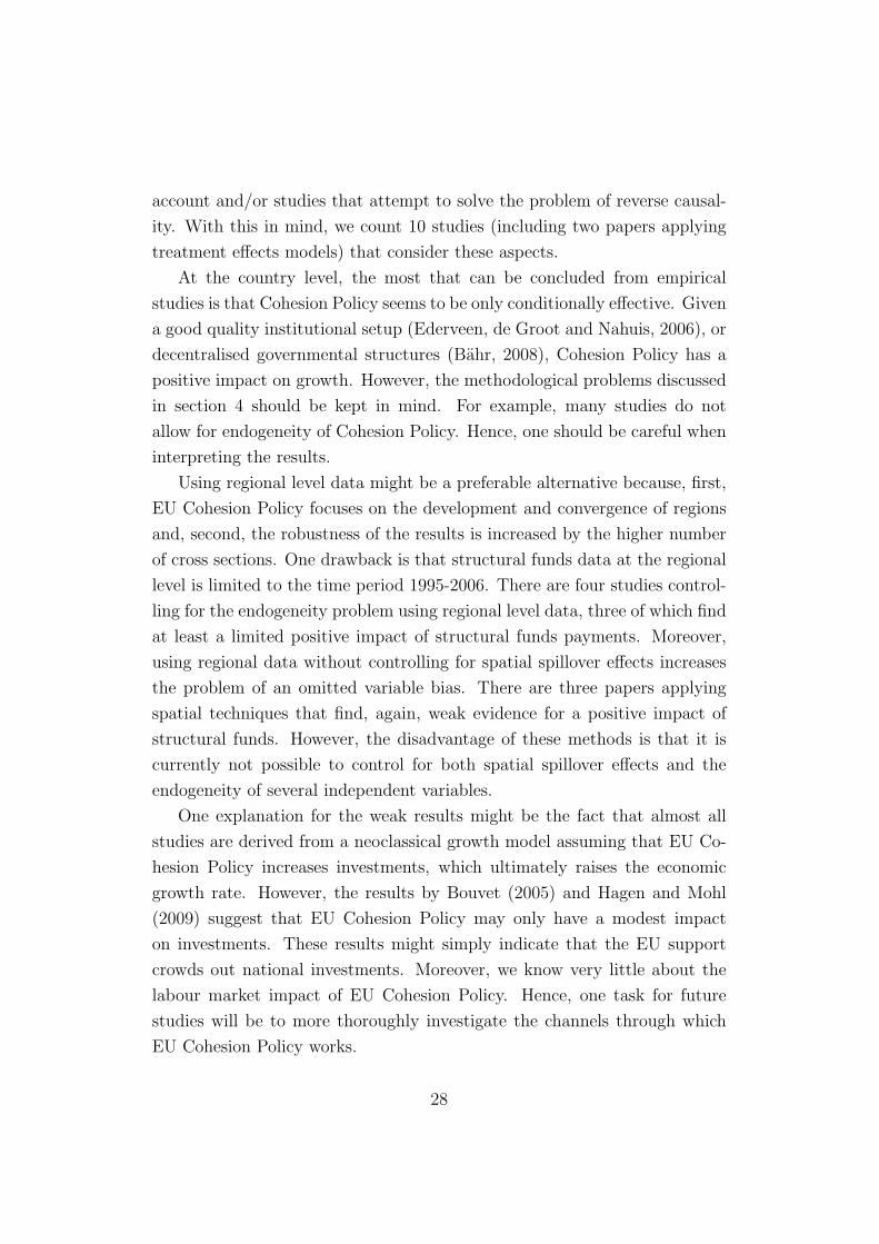
Figure 1 shows the historical development, including the total (nominal)

EU Cohesion Policy payments5(vertical bars) and their shares relative to

the EU-GNI (solid line) and to the public national spending (dotted line).

It becomes clear that there is a long-term upward trend in payments when

measured in absolute terms, which can be explained, inter alia, by the en-

largement steps of the EU (1973: EU-9, 1981: EU-10, 1986: EU-12, 1995:

EU-15, 2004: EU-25, 2007: EU-27). By contrast, payments measured as per-

cent of EU-GNI or public national spending have almost remained constant

since 1993. Furthermore, Figure 1 shows that – on average – SF payments

do not seem to be particularly large compared to total public spending with

an EU-27 average of below 0.7 percent in 2007.

Figure 1 approximately here

However, focusing on the relatively small EU-average share might obscure

the fact that the EU regional policy is quite important for some countries.

Figure 2 compares the Cohesion Policy payments with the public invest-

ment in the member states. It becomes clear that EU spending is quite

important for the poorest countries, that is, those countries receiving money

from the Cohesion Fund, namely the so-called “old” (Spain, Greece, Ireland,

and Portugal) and “new” (Eastern European countries) cohesion countries.

In addition, focusing on the regional level, EU spending has a particularly

4There has been a recent discussion on whether further objectives should be introduced.Proposals focused on aid for regions/countries with climate change, environmental prob-lems or strong demographic changes (European Commission, 2007).

5These are the ERDF, the ESF, the EAGGF, and the Financial Instrument for FisheriesGuidance (FIFG), as well as the Cohesion Fund and the Instrument for Structural Policiesfor Pre-accession (ISPA) for the accession countries.

4

high importance for some regions (e.g., Extremadura received more than 2.7

percent of EU support (as percent of GDP) in 2002). Thus, these figures

illustrate two aspects: First, EU policy matters at least in some regions

and/or member states. Second, given the volume of the spending, it may in-

deed be difficult for some countries to absorb the transfers and to co-finance

European projects without cutting expenses elsewhere.

Figure 2 approximately here

Furthermore, it should be noted that ever since the introduction of the

multi-annual financial framework, the European Commission determines so-

called “commitments”, which do not have to be equal to the final flows of

EU support, the so-called SF “payments”. For example, due to missing

absorption capability, the commitments may not be entirely depleted or may

be called up with a delay of one or two years. In this context, the so-called

N+2 rule states that SF payments have to be called up with a delay of two

years at the latest. This introduces big time lags between the determination

of the eligibility for EU funding and the final flows of EU money. Figure 3

clarifies this issue by using the current financial framework 2007-2013 as an

example. The statistical data basis to determine which regions receive EU

support is based on the annual averages of the years 2000-2002, whereas the

list of supported regions is published in 2006. As the financial framework

runs from 2007-2013 the latest possibility to call up EU support is in 2015

due to the N+2 rule. Hence, there is a gap of up to 15 years between the

underlying statistical data and the calling up of EU support.

Figure 3 approximately here

Finally, some studies try to explain the entire development of the EU

expenditure (and revenue) side in the light of political negotiation processes.

Due to the veto power, Cohesion Policy is affected by side payments and

the bargaining power of the EU member states (e.g., Blankart and Kirchner,

2003; Feld, 2005; Feld and Schnellenbach, 2007). A prominent example is

the establishment of the Cohesion Fund in 1994, which can be explained by

the fact that the poor countries had to be compensated against losses of the

single currency of the European Monetary Union (van der Beek and Neal,

2004).

5

3 Measuring the effectiveness of Cohesion

Policy

There are several approaches to the evaluation of Cohesion Policy. One may

distinguish between ex ante and ex post studies on the one hand, and qual-

itative, as well as quantitative, methods on the other hand. Qualitative

studies are, for example, case studies. Since this type of study is beyond

the scope of this chapter, a discussion is omitted here (for example, Davies,

Bachtler, Gross, Michie, Vironen and Yuill, 2007; Milio, 2007). With regard

to quantitative studies, one may distinguish between macroeconomic simu-

lation studies (which can be used for ex ante, as well as ex post, evaluations;

e.g. Bradley and Untiedt, 2007) on the one hand and (ex post) econometric

studies on the other hand. The results of the simulation studies strongly

depend on the – more or less – plausible assumptions. For example, in this

respect it is often assumed that EU Cohesion Policy leads to an increase in

investments and that these are profitable. However, this assumption typi-

cally leads to the result that all models indicate a positive effect of Cohesion

Policy. Hence, the results of simulation models can be interpreted as an esti-

mate of the potential of Cohesion Policy and should not be taken as empirical

evidence in favour of its effectiveness.

As a consequence, we focus on (quantitative ex post) econometric studies

here. In these studies the sample consists of EU countries or regions. Be-

yond this, there are microeconometric studies using individual level or firm

level data evaluating the effects of single programmes (co-)financed by SF

on various outcome variables at the micro-level. For example, Bondonio and

Greenbaum (2006) analyse the effects of (Objective 2) business investment

incentives on employment using firm-level data.

So far, theoretically founded econometric evaluations of the Cohesion

Policy have mostly been based on the neoclassical growth theory.6 In the

6Roughly speaking, the theoretical approaches can be classified as growth theories andtrade theories and one can distinguish between “new” and “traditional” approaches.These have diametric political implications (Heinemann, Hagen, Mohl, Osterloh and Sel-lenthin, 2009). For example, while traditional neoclassical growth theory (Solow, 1956;Swan, 1956) implies that regional policy have no long-term effects, the new economic

6

following, it is shown how this theory is applied to panel data, although it

was originally applied to cross-sectional data.7

The literature on the convergence of income levels (e.g., GDP per capita)

distinguishes between the so-called β– and σ–convergence. The former pre-

dicts that if countries have the same steady-state determinants converging

to a common balanced growth path, then those countries with relatively low

initial income levels grow faster than richer countries (Durlauf, Johnson and

Temple, 2005, p. 585). Moreover, β–convergence can be easily evaluated in

a linear regression context, e.g. of the neoclassical growth model. Assuming

that β–convergence holds for i = 1, ..., N regions, the natural logarithm of

income y of region i at time t (e.g., measured as GDP per capita) can be

approximated by:

ln(yit) = α + (1 − β) ln(yit−1) + uit, (1)

where and is an i.i.d. error term (Sala-i-Martin, 1996; Young, Higgins and

Daniel, 2008). Since is assumed to be constant across regions, the balanced

growth paths are identical. Rearranging (1) yields to the more common

version of the neoclassical growth model (Young, Higgins and Daniel, 2008):

ln(yit) − ln(yit−1) = α + β ln(yit−1) + uit. (2)

Hence, β < 0 implies a negative correlation between growth and initial

log income.8

The neoclassical growth model assumes that economies (countries or re-

gions) with similar economic conditions converge with respect to their income

level. Absolute / unconditional convergence refers to an inverse relationship

between the growth of income and the initial level if control variables are

geography (Krugman, 1991; Krugman and Venables, 1995) indicates positive effects onregional convergence under certain circumstances. Nevertheless, the latter also predictsa trade-off between growth and convergence. From the perspective of the new (endoge-nous) growth theory (Romer, 1986, 1990), regional policy may have long-term effects ifit promotes R&D or human capital.

7A more general survey which includes cross section as well as time series data can befound in Magrini (2004).

8yit may also indicate the GDP per capita of the region i relative to the aggregate GDPper capita of all regions at time t. In doing so, common time effects are cancelled out

7

absent, i.e., a significantly negative β in the regression framework described

above. Conditional convergence prevails if this relationship still holds af-

ter conditioning on further variables. Hence, the neoclassical growth model

predicts a negative β. Empirical studies provide evidence in favour of both

hypotheses (Islam, 1995, 2003; Cuaresma, Ritzberger-Grunwald and Silgoner,

2008). The estimated convergence rates are typically a little lower in cross-

section studies (approximately 2 percent per year Barro and Sala-i Martin,

2004) than in panel studies (Lee, Pesaran and Smith, 1998).9

To make the distinction between conditional and unconditional conver-

gence clear, we plug fixed regional or country effects into equation (2) and

distinguish two simple regression equations for regional-level data (Ederveen,

Gorter, de Mooij and Nahuis, 2002):

ln(yit) − ln(yit−1) = α + β ln(yit−1) + ci + uit, (3)

ln(yit) − ln(yit−1) = α + β ln(yit−1) + µi + uit, (4)

with ci denoting country-specific fixed effects (a set of country dummies)

and µi region-specific fixed effects (a set of region dummies).

While β in equation (2) is a measure of absolute convergence, (3) and

(4) provide estimates of conditional convergence. To be precise, equation

(3) analyses convergence conditional on whether a region lies in a particu-

lar country. Thus, it allows for differences in steady states of income be-

tween country 1 and country 2 (country-specific steady states). It assumes,

however, that within countries, different regions receive equal income levels.

Equation (4) assumes region-specific steady-states, that is, there may be in-

come gaps between regions which are never bridged even within countries

(for a more detailed discussion on this topic see Islam, 2003).

The concept of σ–convergence is a measure of statistical dispersion of

income at period T (Barro and Sala-i-Martin, 1991, 1992). σ-convergence

holds if the dispersion of income levels declines between t and t+T (Durlauf,

Johnson and Temple, 2005), i.e., if:

σ2ln yt

− σ2ln yt+T

> 0. (5)

9For a critical review on the 2 percent finding see Quah (1996).

8

The concepts of β– and σ–convergence are linked: β–convergence provides

the necessary, but not the sufficient, condition for σ–convergence. As a con-

sequence, σ–convergence can only be achieved with β–convergence, whereas

this does not hold the other way round. Hence, even if β–convergence can

be observed (poorer regions grow faster than richer ones), the dispersion be-

tween the income levels of regions may increase, so that there would be no

σ–convergence.

Almost all econometric studies analyzing the growth effects of EU re-

gional policy are based on a neoclassical growth model of the type Solow

(1956) and Swan (1956), that is, equation (2) is augmented by further theory-

driven variables. In this context, SF payments are assumed to correspond to

investments (Ederveen, de Groot and Nahuis, 2006; Bahr, 2008; Mohl and

Hagen, 2008). A regression equation for regional data may be specified as:

ln(yit) − ln(yit−1) =α + β1 ln(yit−1) + β2 ln(sfit−1) + β3 ln(savit−1)+

β4 (nit−1 + g + δ) + β5 ln(educit−1) + µi + λt + uit,(6)

where savit−1 is the saving rate, nit−1 is the population growth rate, g

and δ stand for the technological progress and the time discount factor. Most

authors follow the seminal paper by Mankiw, Romer and Weill (1992) and

assume that g and δ are constant over time and region and jointly amount

to 5%. Furthermore, educit−1 measures the education level of the population

(e.g., percentage share of population with higher education). Finally, equa-

tion (6) includes fixed-region effects (µi) as well as fixed time effects (λt).

The reasons for their inclusion will be discussed in section 4.

The main variable of interest in this kind of literature is the SF variable

(sfit−1), which is expressed as payments as a share of nominal GDP (among

others, Bahr, 2008) or as percent of persons employed (e.g., Esposti and

Bussoletti, 2008). If the estimate of is positive and significantly different

from zero, the SF payments positively affect the regions’ steady-state growth

rate, hence, they enhance the transitional growth rate of each region towards

its own steady state (Dall’erba and Le Gallo, 2008).

Most papers only focus on the evaluation of the sign of the coefficient

of SF and neglect the size of its impact. However, the latter should be of

relevance since an expensive EU regional policy with a tiny size effect might

9

be effective but not “cost-efficient”. Those authors who discuss the size

effect usually interpret the short-term elasticity of the impact. Given that

the variables of equation (6) are specified in logarithmic terms, a one percent

increase of the SF variable increases the growth rate by β2 percent. However,

note that equation (6) equals the dynamic approach shown in equation (1),

so that it is more convincing to interpret the long-term impact of variables,

which can simply be calculated as φ = (β2/− β1) in the case of SF payments.

The long-term elasticity can be interpreted as showing that a one percent

increase of SF payments (as percent of GDP) raises the real GDP per capita

by φ percent. Unfortunately, most studies do not discuss the quantitative

long-term impact.

Note that regressions of the type of equation (6) only allow for an esti-

mation of the effect of SF payments on growth, and hence we cannot learn

directly from β2 whether or not a poor region A catches up with a rich region

B. However, this is precisely one important aim of Cohesion Policy. What

we learn from β2 is “only” whether and to what extent SF promotes growth.

Nevertheless, since the allocation criteria of the SF (in the case of Objective

1 payments, as well as total SF payments) imply a negative correlation be-

tween the level of GDP per capita and SF payments, a significantly positive

β2 can be interpreted as an indication for convergence at least.

In order to directly measure the effects of Cohesion Policy on conver-

gence, Eggert, von Ehrlich, Fenge and Konig (2007) propose the following

specification using regional data:

ln(yit) − ln(yit−1) =α + β1 ln(yit−1) + β2 ln(sfit−1)+

c ln(yit−1) ln(sfit−1) + ...+ uit.(7)

This equation states that the estimated effect of SF payments depends

on the initial income level. In this case β2 indicates the impact of SF pay-

ments given an initial income level (yit−1) equalling zero, which is obviously

of no use as there are no regions with a GDP of zero. Given a positive

β2, a negative c implies that this positive effect declines with an increasing

initial income level, which, in turn, may be interpreted as a sign of conver-

gence. One possibility of deriving meaningful quantitative conclusions from

equation (7) is to calculate the marginal effects of SF payments across the ob-

10

served range of initial income level (yit−1) by: β2 + c ln(yit−1). Subsequently,

these marginal effects might be illustrated graphically including confidence

intervals around the slope to show the statistical significance level (Brambor,

Clark and Golder, 2006).

Several studies, especially those using country-level data (e.g., Ederveen,

de Groot and Nahuis, 2006; Bahr, 2008), investigate whether the effectiveness

of SF payments depends on institutional and economic aspects of the country,

such as the quality of institutions,10 the member states’ federal structure

(decentralisation) or the openness to trade. They use specifications similar

to the following:

ln(yit) − ln(yit−1) =α + β1 ln(yit−1) + β2 ln(sfit−1) + c1 condit+

c2 condit ln(sfit−1) + ...+ uit,(8)

where condit denotes a variable including the aspects of the country i in

year t and condit ln(sfit−1) is an interaction term. Solid results should again

be derived by calculating and illustrating the marginal effects as indicated

above.

A further issue is the question through which channel SF payments af-

fect growth. The assumption underlying virtually all empirical studies is

that the Cohesion Policy increases regional investments leading to a higher

steady-state capital stock per capita and, ultimately, to a higher GDP. This

may be justified by the nature of SF spending which consists predominantly

of investments. However, as pointed out by Esposti and Bussoletti (2008)

or Bouvet (2005), SF payments may influence long-run growth in two more

ways within the neoclassical growth model. First, it may increase the initial

level or the growth of the regional total factor productivity (TFP). Sec-

ond, it may affect the labour market, that is, the growth rate of the initial

workforce. One problem here concerns the many neoclassical growth specifi-

cations, which (implicitly) assume full employment or constant employment

rates over time, as well as across regions. Since the employment rates dif-

fer between European states and evolve differently over time, and since SF

payments are likely to affect employment, Esposti and Bussoletti (2008) pro-

10Ederveen, de Groot and Nahuis (2006) use, for example, the World Bank governanceindicators “political stability”, “government effectiveness” and “rule of law”.

11

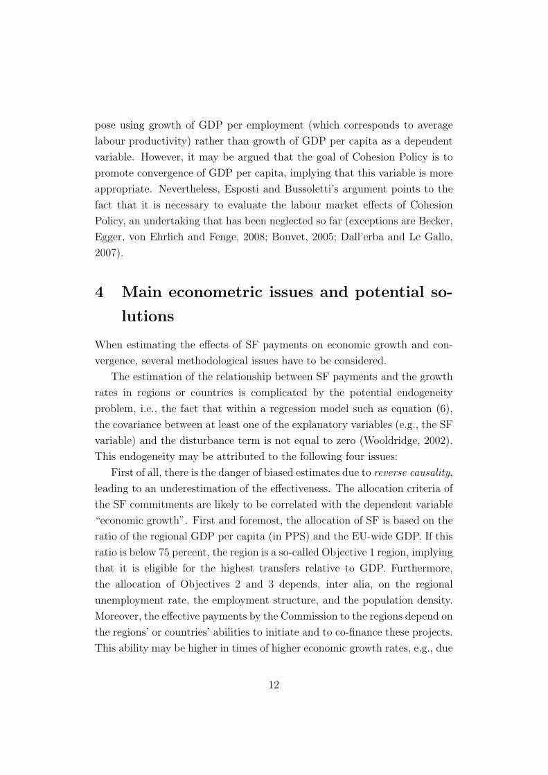
pose using growth of GDP per employment (which corresponds to average

labour productivity) rather than growth of GDP per capita as a dependent

variable. However, it may be argued that the goal of Cohesion Policy is to

promote convergence of GDP per capita, implying that this variable is more

appropriate. Nevertheless, Esposti and Bussoletti’s argument points to the

fact that it is necessary to evaluate the labour market effects of Cohesion

Policy, an undertaking that has been neglected so far (exceptions are Becker,

Egger, von Ehrlich and Fenge, 2008; Bouvet, 2005; Dall’erba and Le Gallo,

2007).

4 Main econometric issues and potential so-

lutions

When estimating the effects of SF payments on economic growth and con-

vergence, several methodological issues have to be considered.

The estimation of the relationship between SF payments and the growth

rates in regions or countries is complicated by the potential endogeneity

problem, i.e., the fact that within a regression model such as equation (6),

the covariance between at least one of the explanatory variables (e.g., the SF

variable) and the disturbance term is not equal to zero (Wooldridge, 2002).

This endogeneity may be attributed to the following four issues:

First of all, there is the danger of biased estimates due to reverse causality,

leading to an underestimation of the effectiveness. The allocation criteria of

the SF commitments are likely to be correlated with the dependent variable

“economic growth”. First and foremost, the allocation of SF is based on the

ratio of the regional GDP per capita (in PPS) and the EU-wide GDP. If this

ratio is below 75 percent, the region is a so-called Objective 1 region, implying

that it is eligible for the highest transfers relative to GDP. Furthermore,

the allocation of Objectives 2 and 3 depends, inter alia, on the regional

unemployment rate, the employment structure, and the population density.

Moreover, the effective payments by the Commission to the regions depend on

the regions’ or countries’ abilities to initiate and to co-finance these projects.

This ability may be higher in times of higher economic growth rates, e.g., due

12

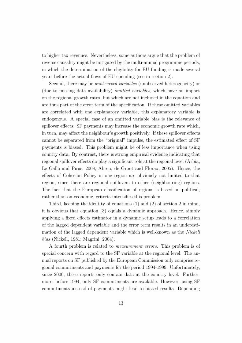
to higher tax revenues. Nevertheless, some authors argue that the problem of

reverse causality might be mitigated by the multi-annual programme periods,

in which the determination of the eligibility for EU funding is made several

years before the actual flows of EU spending (see in section 2).

Second, there may be unobserved variables (unobserved heterogeneity) or

(due to missing data availability) omitted variables, which have an impact

on the regional growth rates, but which are not included in the equation and

are thus part of the error term of the specification. If these omitted variables

are correlated with one explanatory variable, this explanatory variable is

endogenous. A special case of an omitted variable bias is the relevance of

spillover effects: SF payments may increase the economic growth rate which,

in turn, may affect the neighbour’s growth positively. If these spillover effects

cannot be separated from the “original” impulse, the estimated effect of SF

payments is biased. This problem might be of less importance when using

country data. By contrast, there is strong empirical evidence indicating that

regional spillover effects do play a significant role at the regional level (Arbia,

Le Gallo and Piras, 2008; Abreu, de Groot and Florax, 2005). Hence, the

effects of Cohesion Policy in one region are obviously not limited to that

region, since there are regional spillovers to other (neighbouring) regions.

The fact that the European classification of regions is based on political,

rather than on economic, criteria intensifies this problem.

Third, keeping the identity of equations (1) and (2) of section 2 in mind,

it is obvious that equation (3) equals a dynamic approach. Hence, simply

applying a fixed effects estimator in a dynamic setup leads to a correlation

of the lagged dependent variable and the error term results in an underesti-

mation of the lagged dependent variable which is well-known as the Nickell

bias (Nickell, 1981; Magrini, 2004).

A fourth problem is related to measurement errors. This problem is of

special concern with regard to the SF variable at the regional level. The an-

nual reports on SF published by the European Commission only comprise re-

gional commitments and payments for the period 1994-1999. Unfortunately,

since 2000, these reports only contain data at the country level. Further-

more, before 1994, only SF commitments are available. However, using SF

commitments instead of payments might lead to biased results. Depending

13

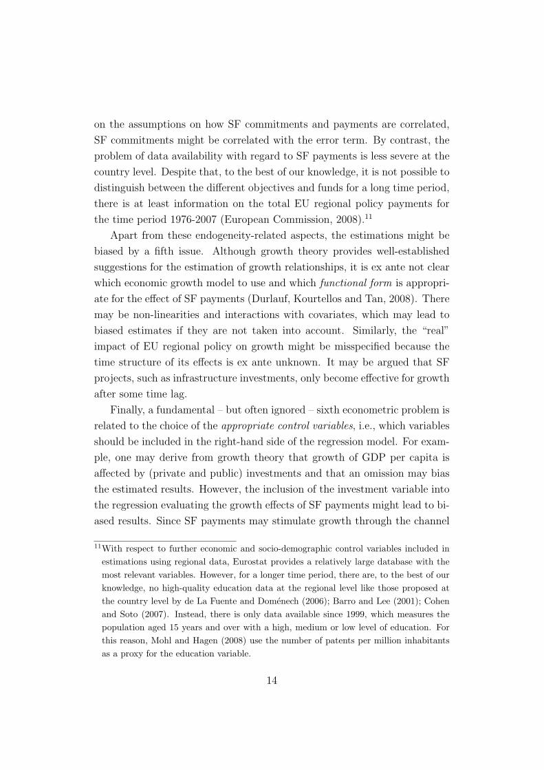
on the assumptions on how SF commitments and payments are correlated,

SF commitments might be correlated with the error term. By contrast, the

problem of data availability with regard to SF payments is less severe at the

country level. Despite that, to the best of our knowledge, it is not possible to

distinguish between the different objectives and funds for a long time period,

there is at least information on the total EU regional policy payments for

the time period 1976-2007 (European Commission, 2008).11

Apart from these endogeneity-related aspects, the estimations might be

biased by a fifth issue. Although growth theory provides well-established

suggestions for the estimation of growth relationships, it is ex ante not clear

which economic growth model to use and which functional form is appropri-

ate for the effect of SF payments (Durlauf, Kourtellos and Tan, 2008). There

may be non-linearities and interactions with covariates, which may lead to

biased estimates if they are not taken into account. Similarly, the “real”

impact of EU regional policy on growth might be misspecified because the

time structure of its effects is ex ante unknown. It may be argued that SF

projects, such as infrastructure investments, only become effective for growth

after some time lag.

Finally, a fundamental – but often ignored – sixth econometric problem is

related to the choice of the appropriate control variables, i.e., which variables

should be included in the right-hand side of the regression model. For exam-

ple, one may derive from growth theory that growth of GDP per capita is

affected by (private and public) investments and that an omission may bias

the estimated results. However, the inclusion of the investment variable into

the regression evaluating the growth effects of SF payments might lead to bi-

ased results. Since SF payments may stimulate growth through the channel

11With respect to further economic and socio-demographic control variables included inestimations using regional data, Eurostat provides a relatively large database with themost relevant variables. However, for a longer time period, there are, to the best of ourknowledge, no high-quality education data at the regional level like those proposed atthe country level by de La Fuente and Domenech (2006); Barro and Lee (2001); Cohenand Soto (2007). Instead, there is only data available since 1999, which measures thepopulation aged 15 years and over with a high, medium or low level of education. Forthis reason, Mohl and Hagen (2008) use the number of patents per million inhabitantsas a proxy for the education variable.

14

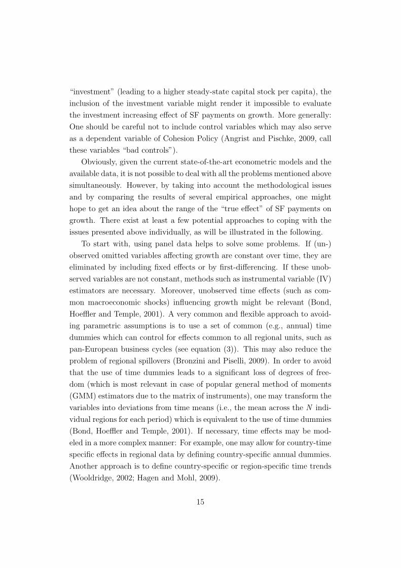
“investment” (leading to a higher steady-state capital stock per capita), the

inclusion of the investment variable might render it impossible to evaluate

the investment increasing effect of SF payments on growth. More generally:

One should be careful not to include control variables which may also serve

as a dependent variable of Cohesion Policy (Angrist and Pischke, 2009, call

these variables “bad controls”).

Obviously, given the current state-of-the-art econometric models and the

available data, it is not possible to deal with all the problems mentioned above

simultaneously. However, by taking into account the methodological issues

and by comparing the results of several empirical approaches, one might

hope to get an idea about the range of the “true effect” of SF payments on

growth. There exist at least a few potential approaches to coping with the

issues presented above individually, as will be illustrated in the following.

To start with, using panel data helps to solve some problems. If (un-)

observed omitted variables affecting growth are constant over time, they are

eliminated by including fixed effects or by first-differencing. If these unob-

served variables are not constant, methods such as instrumental variable (IV)

estimators are necessary. Moreover, unobserved time effects (such as com-

mon macroeconomic shocks) influencing growth might be relevant (Bond,

Hoeffler and Temple, 2001). A very common and flexible approach to avoid-

ing parametric assumptions is to use a set of common (e.g., annual) time

dummies which can control for effects common to all regional units, such as

pan-European business cycles (see equation (3)). This may also reduce the

problem of regional spillovers (Bronzini and Piselli, 2009). In order to avoid

that the use of time dummies leads to a significant loss of degrees of free-

dom (which is most relevant in case of popular general method of moments

(GMM) estimators due to the matrix of instruments), one may transform the

variables into deviations from time means (i.e., the mean across the N indi-

vidual regions for each period) which is equivalent to the use of time dummies

(Bond, Hoeffler and Temple, 2001). If necessary, time effects may be mod-

eled in a more complex manner: For example, one may allow for country-time

specific effects in regional data by defining country-specific annual dummies.

Another approach is to define country-specific or region-specific time trends

(Wooldridge, 2002; Hagen and Mohl, 2009).

15

In order to deal with the first and second problem, an IV estimator

combined with fixed effects or first differences seems to be the right choice.

However, to the best of our knowledge, no convincing external IV has been

proposed in the literature (exceptions may be the studies by Dall’erba and

Le Gallo, 2008; Bouvet, 2005, summarised in section 5). Hence, identification

has to be based on internal instruments via the GMM estimators (Arellano

and Bond, 1991; Roodman, 2009b). In addition, GMM estimators are also

suitable for dealing with the third issue introduced above, by instrumenting

the initial income level (as well as further variables) by lagged values. On

the one hand, there is evidence that the first-differenced GMM (FD-GMM)

estimator by Arellano and Bond (1991) has a large finite sample bias and

poor precisions when the time series are persistent, so that the system GMM

(SYS-GMM) estimator by Blundell and Bond (1998) should be preferred. On

the other hand, some applications question the superiority of the SYS-GMM

estimator because the additional instruments might not be valid (Lucchetti,

Papi and Zazzaro, 2001). Hence, one might apply different estimators to

draw well-founded conclusions. Note that the consistency of both GMM es-

timators is based on large N, which might not be given in the analyses using

country-level data. However, there is preliminary evidence of Monte Carlo

simulations showing that, given pre-determined explanatory variables, the

SYS-GMM estimator has a lower bias and higher efficiency than the FD-

GMM or the fixed effects estimator (Soto, 2006). Nevertheless, country-level

data (such as EU-15 data) may still be too small for GMM estimations.

One should be careful as regards the use of instruments when apply-

ing GMM estimators: Using too many instruments can overfit instrumented

variables (Roodman, 2009a), reduce the power properties of the Hansen test

(Bowsher, 2002) and lead to a downward bias in two-step standard errors

(Windmeijer, 2005).12 One solution might be to include lag limits or to col-

lapse the set of instruments.13 Since an increasing number of studies on the

effects of Cohesion Policy apply GMM estimators, these aspects are highly

12Roodman (2009a, p. 156): “Perhaps, the lesson to be drawn is that internal instruments,though attractive as a response to endogeneity, have serious limitations”.

13However, the choice of the number of lags used as instruments or the possibility ofcollapsing the number of instruments might seem arbitrary.

16

relevant and should be taken into account in order to avoid misleading esti-

mation results.

Applying spatial panel econometric techniques helps to control for spatial

spillover effects, which is of special concern when using region-level data (for

a survey see LeSage and Pace, 2009). The usual approach is to specify a

weight matrix containing information on the number of or distance of neigh-

bours (Anselin, Florax and Rey, 2004). This is done by focusing on the (i)

contiguity of each region, (ii) its k-nearest neighbours, or (iii) the geographi-

cal distance (e.g., expressed in kilometers) to its neighbours. Sometimes the

weight matrices are weighted by some economic variables (e.g., using trade

data between regions). However, often geographical distance based weight

matrices are preferred because they are strictly exogenous. Nevertheless, the

right choice of the weight matrix is of fundamental concern as incorrectly

specified weight matrices might lead to wrong conclusions (LeSage and Fis-

cher, 2008).

Generally speaking, including a weight matrix does affect the efficiency

and/or the consistency of the OLS estimator leading to biased results. Hence,

the spatial econometric estimations are usually estimated by Maximum Like-

lihood (Anselin, 1988; Anselin and Hudak, 1992; Elhorst, 2010) or by GMM

(Kelejian and Prucha, 1998, 1999; Bell and Bockstael, 2000). There are

two predominant approaches to specifying the spatial model: One can ei-

ther include a spatially weighted dependent variable (the so-called “spatial

lag model”) or a spatially autocorrelated error (“spatial error model”) into

the regression model. These approaches were originally focused on cross-

sectional (Anselin, 1988; Anselin and Bera, 1998; Anselin, 2006) and static

panel datasets (Elhorst, 2003) and they have been extended to the case of

dynamic panel estimators (Badinger, Muller and Tondl, 2004; Yu, de Jong

and Lee, 2008). Recently, further approaches have been introduced, such

as including both spatial lag and spatial error simultaneously (Kelejian and

Prucha, 1998; Lee, 2003) or including spatially weighted independent vari-

ables (the so-called spatial Durban model, see, e.g., Elhorst, Piras and Arbia,

2006; Ertur and Koch, 2007). Unfortunately, there is as yet no estimator

which controls for both spatial spillover and endogeneity of further indepen-

dent variables (besides the lagged dependent variable) within a panel data

17

framework.

The fourth problem should be addressed by using SF payments instead of

commitments. As mentioned in section 2, the differences between payments

and commitments can be sizable.

As regards the fifth problem, almost all studies are based on a neoclas-

sical growth model. Despite some criticism due to its strict assumptions

(Dall’erba and Le Gallo, 2008), the use of the neoclassical growth model

might be explained by the limited data availability at the regional level.14

Possible approaches to this problem have been proposed by Becker, Egger,

von Ehrlich and Fenge (2008) as well as by Hagen and Mohl (2008), who

avoid strict functional form assumptions by using treatment effect methods

(for a recent survey for applied researchers see Austin, 2007). These studies

will be summarised in section 5 in greater detail.

In order to take into account that SF payments might be effective after

some time lag, Rodrıguez-Pose and Fratesi (2004) as well as Mohl and Ha-

gen (2008) include past values of the SF variable besides contemporaneous

values. For example, Mohl and Hagen (2008) start their empirical analyses

by excluding any SF variable, and then gradually add the lagged SF pay-

ments, beginning with a lag of one year and ending up with a specification

comprising SF with a lag of one to five years (∑5

j=1 ln SFi,t−j).15

5 Empirical evidence

The main aspects of the previous literature on the impact of Cohesion Pol-

icy on economic growth are summarised in the following. We distinguish

between studies using country-level data (Table 2), regional-level data in a

multi-country framework (Table 3), and regional-level data within one county

14For a recent empirical comparison of different theoretical convergence models at theEuropean regional level, see Arbia, Le Gallo and Piras (2008).

15Due to multicollinearity, the coefficients and standard errors of the SF variable cannotbe interpreted if the variable is included into the regression with several lags. As aconsequence, Mohl and Hagen (2008) calculate the joint sum of SF coefficients corre-sponding to the short-term elasticity and use a simple Wald test to determine whetherthis short-term elasticity is statistically different from zero. Based on this, it is possibleto calculate the long-term elasticity as described above.

18

(Table 4).

Generally, EU regions are classified into three different groups by the Eu-

ropean Commission according to the “Nomenclature des unites territoriales

statistiques” (NUTS). These units refer to the country level (NUTS-0) and

to three lower subdivisions (NUTS-1, NUTS-2 and NUTS-3) which are clas-

sified according to the size of population (Eurostat, 2007). The advantage

of regional data for econometric analyses is the resulting large sample size

which allows the application of methods based on a large number of cross

sections (N ). Furthermore, regions (as opposed to countries) are usually the

unit of interest for Cohesion Policy. By contrast, using country-level data

comes with the advantage of larger data availability but with the drawback

of small sample sizes (EU-12, EU-15 etc.). Moreover, region-specific effects

cannot be analysed by definition.

Apart from the choice of the appropriate sample, the studies differ in the

time period covered, the econometric methods applied, the type of dataset

used (cross-section versus panel) and the operationalisation of SF payments.

With respect to the latter, theory does not provide an unambiguous indica-

tion. While most studies operationalize SF as a continuous variable, some

studies use a dummy variable to indicate whether a region is an Objective 1

region or not. The latter case has the advantage that data on payments are

not necessary, but it comes with the disadvantage that it is not possible to

measure the real size effect of regional policy. If SF are operationalised as

continuous variable, the studies differ with regard to the question of whether

to express the SF as percent of GDP, in purchasing power parities (PPP)

and/or in per capita terms. Moreover, not all studies use SF payments –

some use data on SF commitments. From our point of view, using (nominal)

SF payments as percent of (nominal) GDP is the most convincing approach

since differences in purchasing powers are cancelled out in a very simple

manner.16

With respect to the econometric methods used, there are various ap-

proaches to dealing with the issues described in the last section. Simple

cross-sectional or pooled OLS estimators are based on the assumption that,

16Incidentally, this is the exact approach chosen in the empirical literature on the growtheffects of foreign aid (Easterly, 2003).

19

after conditioning on further explanatory variables, many of the problems

discussed in section 4 (reversed causality, omitted/unobserved variables) are

not relevant. Thus, it seems to be more convincing to rely on panel data

methods which, in fact, most studies do. As mentioned in the last section,

using panel data enables the researcher to eliminate unobserved fixed effects

affecting SF and growth simultaneously.

We start the survey with the studies based on country-level data (Table

2). Ederveen, Gorter, de Mooij and Nahuis (2002) analyse the effects at the

national (EU-12) as well as at the regional (NUTS 2) level. The study only

investigates the effects of the ERDF and applies a pooled OLS estimator:

only conditionally positive growth effects for an EU-12 sample for the time

period 1960-1995 are found (implemented via an interaction term, see equa-

tion (6)). In particular, cohesion support is more likely to be effective for

member states with open economies (such as Ireland) and less likely to be

effective in closed ones (such as Spain). According to the explanation of the

authors, openness disciplines governments, which stimulates more productive

investment of cohesion support.

Beugelsdijk and Eijffinger (2005) restrict their analysis to the programme

period 1995-2001. They focus on the dependency of the effectiveness from

moral hazard behaviour and substitution effects by interacting the SF vari-

able with a corruption index. According to the authors, the moral hazard

effect matters because countries might be inclined not to raise the welfare

level of those regions which are close to the critical value of getting EU sup-

port, as this would possibly imply a reduction in future financial EU support.

Hence, it is possible that the resources are not used for projects that would

have the largest direct and indirect impact, so that the moral hazard effect

might lead to an inappropriate use of SF. The substitution effect means that

SF payments lead to a crowding out of national spending. Using EU-15 data

and different dynamic panel data estimators (including an FD-GMM in or-

der to take endogeneity into account) they find that the hypothesis that SF

contribute to fewer interregional disparities within the current 15 European

countries cannot be rejected. Furthermore, the results do not indicate that

the more corrupt countries use their SF in a less efficient way.

Ederveen, de Groot and Nahuis (2006) analyse the effectiveness of the

20

ERDF for the period 1960-1995 using dynamic panel approaches for an EU-

13 sample. Among other econometric techniques, they apply FD-GMM and

SYS-GMM estimators, assuming, however, that the SF payments are strictly

exogenous. They find that SF as such do not improve the countries’ growth

performance. However, they find evidence that they only enhance growth

in those countries with the “right” institutions, that is, countries with a

high economic openness and high direct measures of institutional quality

(such as low inflation and low public debt). From these findings, Ederveen,

de Groot and Nahuis (2006, p. 25) derive consequences for a redesign of the

EU regional policy: In the light of the EU enlargement process, the funds

should be allocated first and foremost toward institution building. Given

institutions of a satisfactory quality, the EU regional policy may be effective

in stimulating growth.

Recently, Bahr (2008) complemented these results by analyzing whether

the degree of decentralisation within countries mattered in the EU-15 dur-

ing the period of 1975-1995. The hypothesis is that, given the sensitiv-

ity of EU Cohesion Policy to specific regional needs, member states with a

higher degree of decentralisation should be able to implement more effective

programmes. An interaction variable comprising SF and a decentralisation

measure is introduced to the model, which is estimated by various panel

estimators. Robustness checks are performed, inter alia, by instrumenting

the SF variable with its own lagged values. While SF cannot be said to be

unambiguously growth promoting in itself, Bahr finds a significantly positive

effect of SF on growth in more decentralised countries. This is explained by

the fact that regional authorities have better information on specific growth

inducing projects, so that there is a more effective regional implementation

of the programs in traditionally decentralised countries.

Bradley and Untiedt (2008) criticise the approaches by Ederveen, Gorter,

de Mooij and Nahuis (2002) as well as those by Ederveen, de Groot and

Nahuis (2006), inter alia, for the following reasons: First, the time period

used includes the time before the fundamental reform of Cohesion Policy in

1989, a period in which payments were relatively low. Second, they point

to misspecifications in the regression (especially with regard to the interac-

tion of SF payments and institutional variables). Third, they criticise the

21

assumption of exogeneity of Cohesion Policy and show that the econometric

results are far from being robust (for the expression of fundamental concerns

on the evaluation of growth effects of public policies see Rodrik, 2005).

Table 2 approximately here

Apart from these country analyses, some studies use more detailed data

and focus on the regional level (Table 3).

The conclusions of the analysis of Ederveen, Gorter, de Mooij and Nahuis

(2002) for 183 NUTS-2 regions from 1981 to 1996 using pooled OLS depend

on the convergence model used. Assuming that all regions finally catch up to

the same income level (absolute convergence, i.e., neither further explanatory

variables nor country or regional dummies are included), they find a negative

effect of SF on growth. By contrast, assuming that the convergence process is

limited to convergence within countries (including country dummies and no

further explanatory variables), they do not find a significant effect. Finally,

when assuming region-specific steady-states, that is, including regional fixed

effects, a significantly positive effect is found. The authors conclude from

these results (p. 55) “...the more optimistic one is about convergence in the

long run, the more pessimistic one should be about the impact of Cohesion

Policy, and vice versa [...]. The somewhat grim conclusion must be: either

Cohesion Policy is counterproductive, or regional differences will persist.”

However, one should keep in mind that there are good reasons to assume

that omitting fixed effects (regional dummies) and further control variables

results in biased estimates (see section 4).

Cappelen, Castellacci, Fagerberg and Verspagen (2003) focus on the ques-

tion of whether the SF reform in 1989 has increased the effectiveness of Cohe-

sion Policy by dividing their sample period into two time periods (1980-1988

and 1989-1997). Using these two cross-sections and applying OLS, they find

a positive impact on regional growth. The authors find evidence that SF

are most effective in more developed regions (measured in terms of the un-

employment rate, R&D spending etc), whereas the effectiveness is limited

in “poorer” regions. Furthermore, it turns out that the reform of 1989 has

increased the effectiveness.

22

Esposti and Bussoletti (2008) analyse the impact of Objective 1 spending

on regional growth using a data set with 206 NUTS-2 regions covering the

time period 1989-2000. They apply different estimation techniques (such as

DIFF-GMM, SYS-GMM). However, it seems that SF payments are treated

as strictly exogenous and only the lagged dependent variable is instrumented.

They find a positive impact of SF on Objective 1 regions over the whole EU

area, even though its size and statistical significance vary across alternative

estimators. Generally, the impact is quite limited and becomes negligible

or even negative in some regional cases. For instance, when regions are

grouped by country, a negative effect may be observed for German, Greek,

and Spanish Objective 1 regions. By contrast, the French Objective 1 regions

show the highest policy treatment effect.

The study by Puigcerver-Penalver (2007) is based on 41 NUTS-2 regions

in the EU-12. It analyses whether Objective 1 payments to these regions

promoted growth in the period 1989-2000, with SF payments modeled as

being affected by the total factor productivity. Using a fixed effects model it

is shown that the effectiveness depends on the time period. While Cohesion

Policy (Objective 1) had a positive impact in the funding period 1989-1993,

no significantly positive impact can be detected during 1994-1999.

Using a cross-sectional approach, de Freitas, Pereira and Torres (2003)

analyse whether Objective 1 regions grow faster than non-Objective 1 regions

between 1990 and 2001, assuming strict exogeneity of the Objective 1 status.

They find evidence of conditional convergence among EU regions. Moreover,

the quality of national institutions has a positive impact, while there is no

evidence of a correlation between the eligibility for Objective 1 payments and

faster convergence.

Rodrıguez-Pose and Fratesi (2004) also focus on Objective 1 regions. The

study not only analyses the time lags of SF effects but also differentiates be-

tween categories of Cohesion Policy, such as (a) support to agriculture and

rural promotion, (b) business and tourism support, (c) investment in human

capital, (d) investment in infrastructure and environment. However, the

analysis is based on SF commitments instead of on SF payments. Applying

fixed effects as well as pooled GLS estimators, they cannot find significant ef-

fects of SF on infrastructure and, to a lesser extent, on business support. By

23

contrast, support for agriculture has positive short-term effects on growth,

but these wane quickly; and only investments in education and human cap-

ital – representing only about one-eighth of the total commitments – show

positive and significant returns.

The study by Bouvet (2005) goes one step further by not only investi-

gating the impact of the ERDF spendings on economic growth but also by

analyzing through which channels Cohesion Policy might work, i.e., invest-

ment, total factor productivity or employment (see section (3)). The data

base consists of 118 NUTS-2 regions in the EU-8 from 1975 to 1999. The SF

payments (ERDF) are instrumented with political variables.17 It turns out

that Cohesion Policy has a positive but modest effect on growth. The study

does not find significant evidence that this positive effect works through an

increase in regional investment. By contrast, it is found that Cohesion Pol-

icy increases TFP and employment growth and that these are the channels

through which the policy affects GDP growth.18

As mentioned in section 4, a major econometric problem when using

regional-level data results from omitting regional spillover effects, which may

lead to biased results. Dall’erba and Le Gallo (2008)19 is one of the few

studies that try to cope with this problem. This, however, comes with the

drawback that other econometric issues (regional fixed effects, among others)

are not taken into account. The authors use spatial econometric techniques

for cross-sectional data for 145 regions in 1989-1999. The SF payments are

instrumented, inter alia, with the regions’ distances to Brussels using two-

stage least squares. The results from Dall’erba and Le Gallo (2008) indicate

that significant convergence takes place, but that the SF have no impact on

17The following instrumental variables are used: the interaction term of the coincidencebetween local central governments and the coincidence between the central governmentand the president of the Commission, the interaction term of the local incumbent dummyand the coincidence between the central government and the president of the Commis-sion, the coincidence between local central governments, the local-incumbent dummyand the national incumbent dummy.

18Bouvet (2005) also examines the determinants of fund allocation. While more fundsare allotted to regions with lower per capita incomes and structural deficiencies, someevidence of political interference in the allocation process is found.

19In a preceding study, Dall’erba (2005) applies an exploratory spatial analysis and findsa positive relationship between SF payments and regional growth.

24

it.

Ramajo, Marquez, Hewings and Salinas (2008) apply cross-sectional spa-

tial econometric techniques to estimate the speed of convergence for a sample

of 163 regions in the EU-12 over the period 1981-1996. First of all, they find

evidence in favour of the existence of two spatial convergence clubs among

European regions, namely, the presence of two significantly different spatial

clusters formed by regions belonging to Cohesion (Ireland, Greece, Portu-

gal and Spain) and non-Cohesion countries. The estimations indicate that

throughout the period analysed, there is a faster conditional convergence

in relative income levels of the regions belonging to Cohesion countries (5.3

percent) than in the rest of the regions of the EU (3.3 percent). Hence, the

results provide support for policies that are explicitly designed to promote

regional growth in the less-developed regions located in Cohesion countries.

Based on a sample of 1084 NUTS-3 regions (EU-15) over the period of

1995-2004, Falk and Sinabell (2008) investigate the determinants of Objec-

tive 1 payments on the regional growth of GDP per capita in a cross-sectional

analysis. As the Lagrange Multiplier test statistic does not hint at spatial

spillover effects, they focus on robust OLS and weighted-least-squares pro-

cedures. The latter is used in order to control for outliers. In addition, Falk

and Sinabell decompose the growth following the Blinder-Oaxaca decompo-

sition (Oaxaca and Ransom, 1994) in order to check how much of the growth

differential can be explained by observable differences between Objective 1

and non-Objective 1 regions. Their results indicate that there is a significant

growth differential, which is, however, almost entirely due to the difference in

characteristics such as initial GDP per capita, economic structure and pop-

ulation density. As a consequence, these results point to a low effectiveness

of the EU funds.

Mohl and Hagen (2008) use a panel dataset of 124 NUTS-2 regions over

the time period 1995-2005, extending the literature with regard to the follow-

ing aspects: First of all, they use more precise measures of SF by distinguish-

ing between Objective 1, 2, 3 and 1+2+3 payments and by a more thorough

investigation of the impact of time lags. Second, the time period of the in-

vestigation is extended, using SF payments of the last financial framework

2000-2006 that have not been analysed before. Third, the paper examines

25

the robustness of the results by comparing various econometric approaches.

Apart from SYS-GMM (which allows for endogeneity of SF payments as well

as of further variables), spatial panel econometric techniques are applied.

The results show that Objective 1 payments in particular promote regional

economic growth, whereas Objectives 2 and 3 do not have a positive and

significant impact on the EU regions’ growth rates. Furthermore, Mohl and

Hagen find that time lags substantially affect the results, i.e., the growth

impact does not occur immediately, but rather with a time lag of up to five

years.

Finally, there are two papers that use treatment effect methods in order

to deal with the problem of unknown functional form and parameter hetero-

geneity (Wooldridge, 2002, Ch. 18). Becker, Egger, von Ehrlich and Fenge

(2008) use up to 3301 NUTS-3 regions and apply “regression discontinuity

design” techniques.20 They make use of the relatively clear-cut rule that

defines an Objective 1 region: NUTS-2 regions with a GDP per capita level

below 75 percent of the EU average. This enables the authors to use regres-

sion discontinuity design techniques, which basically means estimating the

effect by comparing “treated” and “non-treated” regions near the 75 percent

threshold. On average, the Objective 1 status raises per-capita income by

about 1.8 percent relative to similar “non-treated” regions. Since the authors

do not find a positive employment effect, they conclude that the growth effect

may work through an investment increasing effect. Furthermore, they pro-

vide a simple cost-benefit analysis: one euro spent on Objective 1 transfers

leads to 1.21 euros of additional GDP in the eligible regions.

Hagen and Mohl (2008) interpret total SF payments (Objective 1+2+3)

as a “continuous treatment” and apply the method of generalised propensity

score which leads to the estimation of a dose-response function as proposed by

Hirano and Imbens (2004). They use a sample of 122 NUTS-1 and NUTS-

2 (EU-15) regions for the time period 1995-2005 and find a positive, but

not statistically significant, impact on the regions’ average three-year growth

rates. This would imply that it does not matter which “dose” of SF payments

a region receives.

20An introduction to regression discontinuity design can be found in the Journal of Econo-metrics 142 (2008); see especially Imbens and Lemieux (2008).

26

Table 3 approximately here

Besides the studies presented above, there are further studies focusing on

regions within single countries (see Table 4). Since their focus may be too

narrow to draw a conclusion with regard to European integration, we do not

discuss them here.

Table 4 approximately here

6 Conclusions and remarks for future research

The Cohesion Policy of the European Union has gained importance over the

recent decades, becoming the most important budget item and totaling 36

percent of the total EU budget in the period 2007-2013. With its rising

relevance, the attempts to evaluate this policy field have increased. Despite

its primary goal to “reduce disparities among the regions”, surprisingly, the

focus of these studies is not so much on the question if EU Cohesion Policy

has decreased divergence, but rather on the question if EU support is growth

enhancing. One reason for this might be that the question of convergence

refers to a long-run concept, which is difficult to evaluate given the available

empirical data.

This chapter shows that the econometric evaluation of EU Cohesion Pol-

icy is hampered by several econometric issues, namely reverse causality, mea-

surement error, omitted variables (including spatial spillovers), Nickell bias,

strict functional form assumptions and the potential inclusion of inappro-

priate control variables. Based on these issues we present potential solu-

tions on how to cope with these problems individually. Unfortunately, given

the econometric methods and the available data base, there is currently no

method to control for all problems mentioned above simultaneously. As a

consequence, by comparing the results of several approaches, one has to de-

rive conclusions on the robustness of the results.

As the data availability for EU Cohesion Policy payments has improved

significantly over the last years, we would argue that meaningful results

should be based on panel data, which reduces some of the main econometric

problems. Moreover, it is advisable to use studies taking fixed effects into

27

account and/or studies that attempt to solve the problem of reverse causal-

ity. With this in mind, we count 10 studies (including two papers applying

treatment effects models) that consider these aspects.

At the country level, the most that can be concluded from empirical

studies is that Cohesion Policy seems to be only conditionally effective. Given

a good quality institutional setup (Ederveen, de Groot and Nahuis, 2006), or

decentralised governmental structures (Bahr, 2008), Cohesion Policy has a

positive impact on growth. However, the methodological problems discussed

in section 4 should be kept in mind. For example, many studies do not

allow for endogeneity of Cohesion Policy. Hence, one should be careful when

interpreting the results.

Using regional level data might be a preferable alternative because, first,

EU Cohesion Policy focuses on the development and convergence of regions

and, second, the robustness of the results is increased by the higher number

of cross sections. One drawback is that structural funds data at the regional

level is limited to the time period 1995-2006. There are four studies control-

ling for the endogeneity problem using regional level data, three of which find

at least a limited positive impact of structural funds payments. Moreover,

using regional data without controlling for spatial spillover effects increases

the problem of an omitted variable bias. There are three papers applying

spatial techniques that find, again, weak evidence for a positive impact of

structural funds. However, the disadvantage of these methods is that it is

currently not possible to control for both spatial spillover effects and the

endogeneity of several independent variables.

One explanation for the weak results might be the fact that almost all

studies are derived from a neoclassical growth model assuming that EU Co-

hesion Policy increases investments, which ultimately raises the economic

growth rate. However, the results by Bouvet (2005) and Hagen and Mohl

(2009) suggest that EU Cohesion Policy may only have a modest impact

on investments. These results might simply indicate that the EU support

crowds out national investments. Moreover, we know very little about the

labour market impact of EU Cohesion Policy. Hence, one task for future

studies will be to more thoroughly investigate the channels through which

EU Cohesion Policy works.

28

Another reason for the inconclusive empirical results might be that the

allocation of funds is at least partly determined by political-economic factors.

In this context, Cohesion Policy is not solely based on clear criteria. Hence,

there is room for political bargaining and/or side payments which might

result in the funding of politically feasible, and less economically efficient,

projects.

29

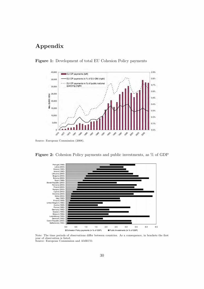
Appendix

Figure 1: Development of total EU Cohesion Policy payments

Source: European Commission (2008).

Figure 2: Cohesion Policy payments and public investments, as % of GDP

Note: The time periods of observations differ between countries. As a consequence, in brackets the firstyear of observation is listed.Source: European Commission and AMECO.

30

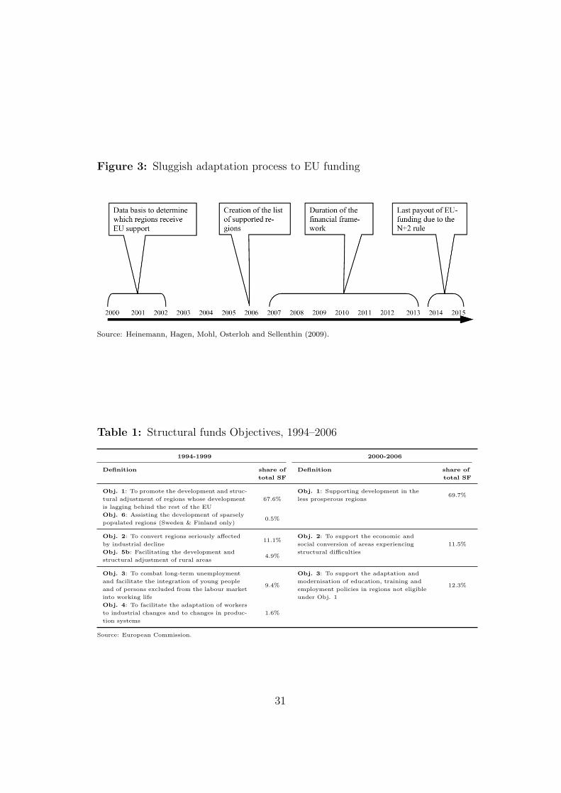
Figure 3: Sluggish adaptation process to EU funding

Source: Heinemann, Hagen, Mohl, Osterloh and Sellenthin (2009).

Table 1: Structural funds Objectives, 1994–2006

1994-1999 2000-2006

Definition share of Definition share of

total SF total SF

Obj. 1: To promote the development and struc-

67.6%

Obj. 1: Supporting development in the69.7%

tural adjustment of regions whose development less prosperous regions

is lagging behind the rest of the EU

Obj. 6: Assisting the development of sparsely0.5%

populated regions (Sweden & Finland only)

Obj. 2: To convert regions seriously affected11.1%

Obj. 2: To support the economic and

11.5%by industrial decline social conversion of areas experiencing

Obj. 5b: Facilitating the development and4.9%

structural difficulties

structural adjustment of rural areas

Obj. 3: To combat long-term unemployment

9.4%

Obj. 3: To support the adaptation and

12.3%and facilitate the integration of young people modernisation of education, training and

and of persons excluded from the labour market employment policies in regions not eligible

into working life under Obj. 1

Obj. 4: To facilitate the adaptation of workers

1.6%to industrial changes and to changes in produc-

tion systems

Source: European Commission.

31

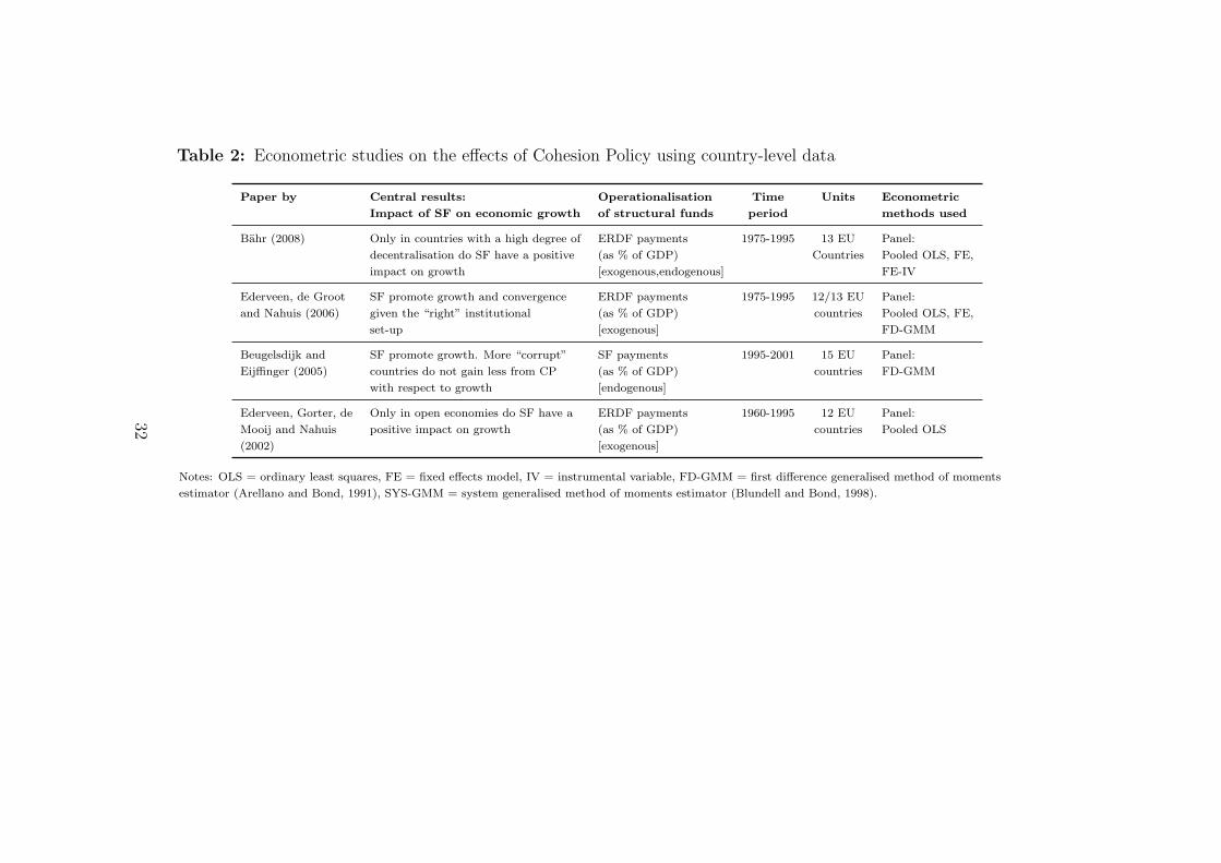
Table 2: Econometric studies on the effects of Cohesion Policy using country-level data

Paper by Central results: Operationalisation Time Units Econometric

Impact of SF on economic growth of structural funds period methods used

Bahr (2008) Only in countries with a high degree of ERDF payments 1975-1995 13 EU Panel:

decentralisation do SF have a positive (as % of GDP) Countries Pooled OLS, FE,

impact on growth [exogenous,endogenous] FE-IV

Ederveen, de Groot SF promote growth and convergence ERDF payments 1975-1995 12/13 EU Panel:

and Nahuis (2006) given the “right” institutional (as % of GDP) countries Pooled OLS, FE,

set-up [exogenous] FD-GMM

Beugelsdijk and SF promote growth. More “corrupt” SF payments 1995-2001 15 EU Panel:

Eijffinger (2005) countries do not gain less from CP (as % of GDP) countries FD-GMM

with respect to growth [endogenous]

Ederveen, Gorter, de Only in open economies do SF have a ERDF payments 1960-1995 12 EU Panel:

Mooij and Nahuis positive impact on growth (as % of GDP) countries Pooled OLS

(2002) [exogenous]

Notes: OLS = ordinary least squares, FE = fixed effects model, IV = instrumental variable, FD-GMM = first difference generalised method of moments

estimator (Arellano and Bond, 1991), SYS-GMM = system generalised method of moments estimator (Blundell and Bond, 1998).

32

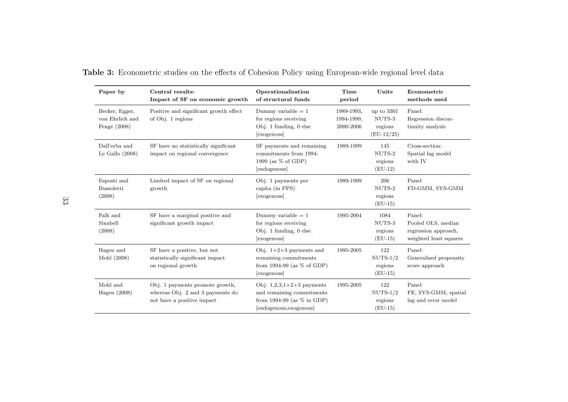
Table 3: Econometric studies on the effects of Cohesion Policy using European-wide regional level data

Paper by Central results: Operationalisation Time Units Econometric

Impact of SF on economic growth of structural funds period methods used

Becker, Egger, Positive and significant growth effect Dummy variable = 1 1989-1993, up to 3301 Panel:

von Ehrlich and of Obj. 1 regions for regions receiving 1994-1999, NUTS-3 Regression discon-

Fenge (2008) Obj. 1 funding, 0 else 2000-2006 regions tinuity analysis

[exogenous] (EU-12/25)

Dall’erba and SF have no statistically significant SF payments and remaining 1989-1999 145 Cross-section:

Le Gallo (2008) impact on regional convergence commitments from 1994- NUTS-2 Spatial lag model

1999 (as % of GDP) regions with IV

[endogenous] (EU-12)

Esposti and Limited impact of SF on regional Obj. 1 payments per 1989-1999 206 Panel:

Bussoletti growth capita (in PPS) NUTS-2 FD-GMM, SYS-GMM

(2008) [exogenous] regions

(EU-15)

Falk and SF have a marginal positive and Dummy variable = 1 1995-2004 1084 Panel:

Sinabell significant growth impact for regions receiving NUTS-3 Pooled OLS, median

(2008) Obj. 1 funding, 0 else regions regression approach,

[exogenous] (EU-15) weighted least squares

Hagen and SF have a positive, but not Obj. 1+2+3 payments and 1995-2005 122 Panel:

Mohl (2008) statistically significant impact remaining commitments NUTS-1/2 Generalised propensity

on regional growth from 1994-99 (as % of GDP) regions score approach

[exogenous] (EU-15)

Mohl and Obj. 1 payments promote growth, Obj. 1,2,3,1+2+3 payments 1995-2005 122 Panel:

Hagen (2008) whereas Obj. 2 and 3 payments do and remaining commitments NUTS-1/2 FE, SYS-GMM, spatial

not have a positive impact from 1994-99 (as % in GDP) regions lag and error model

[endogenous,exogenous] (EU-15)

33

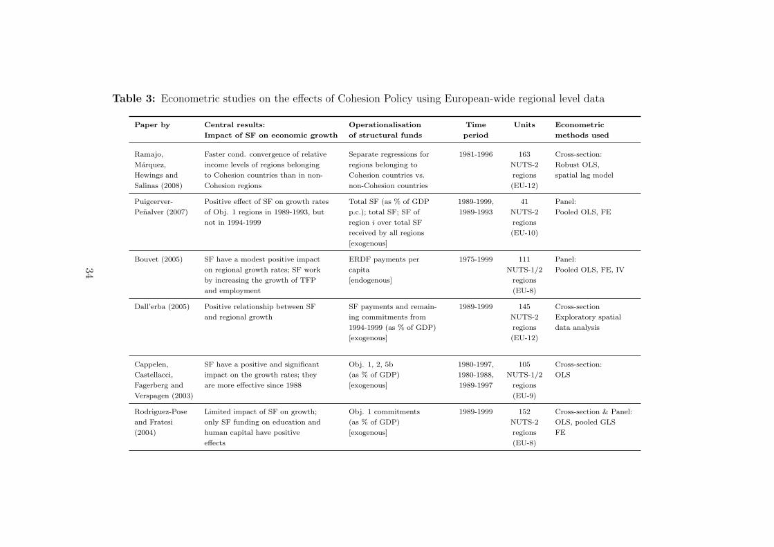
Table 3: Econometric studies on the effects of Cohesion Policy using European-wide regional level data

Paper by Central results: Operationalisation Time Units Econometric

Impact of SF on economic growth of structural funds period methods used

Ramajo, Faster cond. convergence of relative Separate regressions for 1981-1996 163 Cross-section:

Marquez, income levels of regions belonging regions belonging to NUTS-2 Robust OLS,

Hewings and to Cohesion countries than in non- Cohesion countries vs. regions spatial lag model

Salinas (2008) Cohesion regions non-Cohesion countries (EU-12)

Puigcerver- Positive effect of SF on growth rates Total SF (as % of GDP 1989-1999, 41 Panel:

Penalver (2007) of Obj. 1 regions in 1989-1993, but p.c.); total SF; SF of 1989-1993 NUTS-2 Pooled OLS, FE

not in 1994-1999 region i over total SF regions

received by all regions (EU-10)

[exogenous]

Bouvet (2005) SF have a modest positive impact ERDF payments per 1975-1999 111 Panel:

on regional growth rates; SF work capita NUTS-1/2 Pooled OLS, FE, IV

by increasing the growth of TFP [endogenous] regions

and employment (EU-8)

Dall’erba (2005) Positive relationship between SF SF payments and remain- 1989-1999 145 Cross-section

and regional growth ing commitments from NUTS-2 Exploratory spatial

1994-1999 (as % of GDP) regions data analysis

[exogenous] (EU-12)

Cappelen, SF have a positive and significant Obj. 1, 2, 5b 1980-1997, 105 Cross-section:

Castellacci, impact on the growth rates; they (as % of GDP) 1980-1988, NUTS-1/2 OLS

Fagerberg and are more effective since 1988 [exogenous] 1989-1997 regions

Verspagen (2003) (EU-9)

Rodriguez-Pose Limited impact of SF on growth; Obj. 1 commitments 1989-1999 152 Cross-section & Panel:

and Fratesi only SF funding on education and (as % of GDP) NUTS-2 OLS, pooled GLS

(2004) human capital have positive [exogenous] regions FE

effects (EU-8)

34

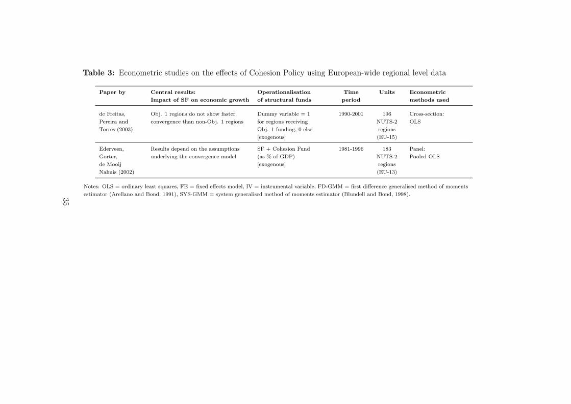
Table 3: Econometric studies on the effects of Cohesion Policy using European-wide regional level data

Paper by Central results: Operationalisation Time Units Econometric

Impact of SF on economic growth of structural funds period methods used

de Freitas, Obj. 1 regions do not show faster Dummy variable = 1 1990-2001 196 Cross-section:

Pereira and convergence than non-Obj. 1 regions for regions receiving NUTS-2 OLS

Torres (2003) Obj. 1 funding, 0 else regions

[exogenous] (EU-15)

Ederveen, Results depend on the assumptions SF + Cohesion Fund 1981-1996 183 Panel:

Gorter, underlying the convergence model (as % of GDP) NUTS-2 Pooled OLS

de Mooij [exogenous] regions

Nahuis (2002) (EU-13)

Notes: OLS = ordinary least squares, FE = fixed effects model, IV = instrumental variable, FD-GMM = first difference generalised method of moments

estimator (Arellano and Bond, 1991), SYS-GMM = system generalised method of moments estimator (Blundell and Bond, 1998).35

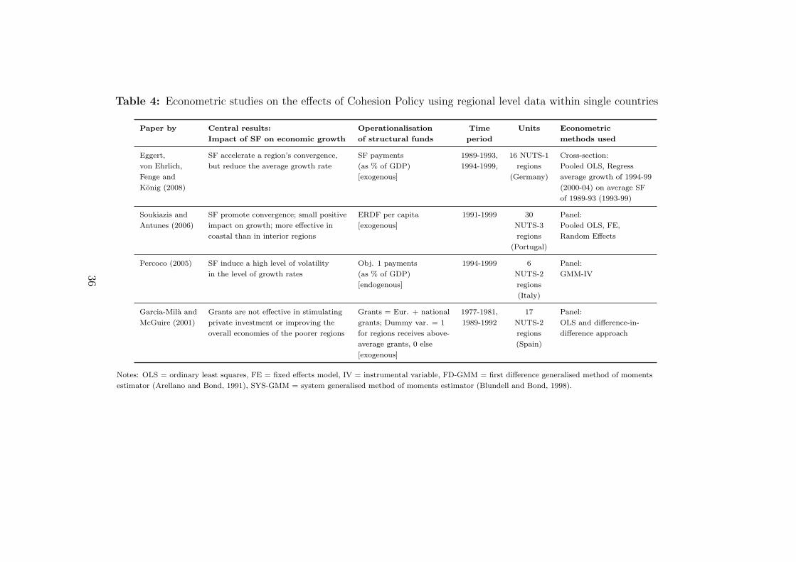
Table 4: Econometric studies on the effects of Cohesion Policy using regional level data within single countries

Paper by Central results: Operationalisation Time Units Econometric

Impact of SF on economic growth of structural funds period methods used

Eggert, SF accelerate a region’s convergence, SF payments 1989-1993, 16 NUTS-1 Cross-section:

von Ehrlich, but reduce the average growth rate (as % of GDP) 1994-1999, regions Pooled OLS, Regress

Fenge and [exogenous] (Germany) average growth of 1994-99

Konig (2008) (2000-04) on average SF

of 1989-93 (1993-99)

Soukiazis and SF promote convergence; small positive ERDF per capita 1991-1999 30 Panel:

Antunes (2006) impact on growth; more effective in [exogenous] NUTS-3 Pooled OLS, FE,

coastal than in interior regions regions Random Effects

(Portugal)

Percoco (2005) SF induce a high level of volatility Obj. 1 payments 1994-1999 6 Panel:

in the level of growth rates (as % of GDP) NUTS-2 GMM-IV

[endogenous] regions

(Italy)

Garcia-Mila and Grants are not effective in stimulating Grants = Eur. + national 1977-1981, 17 Panel:

McGuire (2001) private investment or improving the grants; Dummy var. = 1 1989-1992 NUTS-2 OLS and difference-in-

overall economies of the poorer regions for regions receives above- regions difference approach

average grants, 0 else (Spain)

[exogenous]

Notes: OLS = ordinary least squares, FE = fixed effects model, IV = instrumental variable, FD-GMM = first difference generalised method of moments

estimator (Arellano and Bond, 1991), SYS-GMM = system generalised method of moments estimator (Blundell and Bond, 1998).

36

ReferencesAbreu, M., H. de Groot and R. Florax (2005): “Space and growth: A

survey of empirical evidence and methods,” Region et Developpement, 2005-21,12–43.

Angrist, J. and J. Pischke (2009): Mostly harmless econometrics: An empiri-cist’s companion. Princeton University Press, Princeton.

Anselin, L. (1988): Spatial econometrics: Methods and models. Kluwer, Dor-drecht.

(2006): “Spatial econometrics,” in Palgrave handbook of econometrics,ed. by T. Mills and K. Patterson, vol. 1, pp. 901–969. Palgrave Macmillan,Basingstoke.

Anselin, L. and A. Bera (1998): “Spatial dependence in linear regression mod-els with an introduction to spatial econometrics,” in Handbook of applied eco-nomic statistic, ed. by A. Ullah and D. Giles, pp. 237–289. Marce Dekker, NewYork.

Anselin, L., R. Florax and S. Rey (2004): Advances in spatial econometrics.Springer, Berlin, Heidelberg, New York.

Anselin, L. and S. Hudak (1992): “Spatial econometrics in practice: A reviewof software options,” Regional Science and Urban Economics, 22, 509–536.

Arbia, G., J. Le Gallo and G. Piras (2008): “Does evidence on regional eco-nomic convergence depend on the estimation strategy? Outcomes from analysisof a set of NUTS2 EU regions,” Spatial Economic Analysis, 3(2), 209–224.

Arellano, M. and S. Bond (1991): “Some tests of specification for panel data:Monte Carlo evidence and an application to employment equations,” The Reviewof Economic Studies, 58, 277–297.

Austin, N. (2007): “Causal inference with observational data,” The Stata Jour-nal, 7(4), 507–541.

Badinger, H., W. Muller and G. Tondl (2004): “Regional convergence inthe European Union 1985-1999: A spatial dynamic panel analysis,” RegionalStudies, 38(3), 241–253.

Bahr, C. (2008): “How does sub-national autonomy affect the effectiveness ofstructural funds?,” Kyklos, 61(1), 3–18.

Baldwin, R. and C. Wyplosz (2009): The economics of European integration.Mcgraw-Hill Higher Education, London.

Barro, R. and J.-W. Lee (2001): “International comparisons of educationalattainment,” Journal of Monetary Economics, 32(3), 363–394.

Barro, R. and X. Sala-i-Martin (1991): “Convergence across states and re-gions,” Brookings Papers on Economic Activity, 1, 107–182.

(1992): “Convergence,” Journal of Political Economy, 100(2), 223–251.

37

Barro, R. and X. Sala-i Martin (2004): Economic growth. The MIT Press,Cambridge, Massachusetts.

Becker, S., P. Egger, M. von Ehrlich and R. Fenge (2008): “Going NUTS:The effect of EU structural funds on regional performance,” CESifo WorkingPaper, 2495.

Bell, K. and N. Bockstael (2000): “Applying the generalized moments-estimation approach to spatial problems involving microlevel data,” Review ofEconomics and Statistics, 82, 72–82.

Beugelsdijk, M. and S. Eijffinger (2005): “The effectiveness of structuralpolicy in the European Union: An empirical analysis for the EU-15 in 1995-2001,” Journal of Common Market Studies, 40, 37–51.

Blankart, C. B. and C. Kirchner (2003): “The deadlock of the EU budget:An economic analysis of ways in and ways out,” CESifo Working Paper, 989.

Blundell, R. and S. Bond (1998): “Initial conditions and moment restrictionsin dynamic panel data models,” Journal of Econometrics, 87, 115–143.

Bond, S., A. Hoeffler and J. Temple (2001): “GMM estimation of empiricalgrowth models,” Nuffield College Economics Working Paper, 2001-W21.

Bondonio, D. and R. Greenbaum (2006): “Do business investment incen-tives promote employment in declining areas? Evidence from EU Objective-2regions,” European Urban and Regional Studies, 13, 225–244.

Bouvet, F. (2005): “European Union regional policy: Allocation determinantsand effects on regional economic growth,” mimeo.

Bowsher, C. (2002): “On testing overidentifying restrictions in dynamic paneldata models,” Economic Letters, 77, 211–220.

Bradley, J. and G. Untiedt (2007): “Do economic models tell us anythinguseful about Cohesion Policy impacts? A comparison of HERMIN, QUEST andECOMOD,” GEFRA Working Paper, July.

(2008): “EU Cohesion Policy and “conditional” effectiveness: What docross-section regression tell us?,” GEFRA Working Paper, May 2008(4).

Brambor, T., W. Clark and M. Golder (2006): “Understanding interactionmodels: Improving empirical analyses,” Political Analysis, 14, 63–82.

Bronzini, R. and P. Piselli (2009): “Determinants of long-run regional pro-ductivity with geographical spillovers: The role of R&D, human capital andpublic infrastructure,” Regional Science and Urban Economics, 39, 187–199.

Camagni, R. and R. Capello (2010): “Spatial effects of economic integration:A conceptualization from regional growth and location theories’,” in Interna-tional Handbook of Economic Integration, ed. by M. Jovanovic. Edward Elgar.

Cappelen, A., F. Castellacci, J. Fagerberg and B. Verspagen (2003):“The impact of EU regional support on growth and convergence in the EuropeanUnion,” Journal of Common Market Studies, 41(4), 621–644.

38

Cohen, D. and M. Soto (2007): “Growth and human capital: good data, goodresults,” Journal of Economic Growth, 12, 51–76.

Cuaresma, J., D. Ritzberger-Grunwald and M. Silgoner (2008):“Growth, convergence and EU membership,” Applied Economics, 40(5), 643–656.

Dall’erba, S. (2005): “Distribution of regional income and regional funds in Eu-rope 1989-1999: An exploratory spatial data analysis,” The Annals of RegionalScience, 39, 121–148.

Dall’erba, S. and J. Le Gallo (2007): “The impact of EU regional supporton growth and employment,” Czech Journal of Economics and Finance, 57(7),325–340.

(2008): “Regional convergence and the impact of European structuralfunds 1989-1999: A spatial econometric analysis,” Papers in Regional Science,82(2), 219–244.

Davies, S., J. Bachtler, F. Gross, R. Michie, H. Vironen and D. Yuill(2007): “The impact of structural funds programmes in Scotland 1994-2006,”European Policy Research Paper, 60.

de Freitas, M., F. Pereira and F. Torres (2003): “Convergence among EUregions, 1990-2001. Quality of national institutions and “Objective 1” status,”Intereconomics, September/October(2003), 270–275.

de La Fuente, A. and R. Domenech (2006): “Human capital in growth regres-sions: How much difference does data quality make?,” Journal of the EuropeanEconomic Association, 4(1), 1–36.

Durlauf, S., P. Johnson and J. Temple (2005): “Growth econometrics,” inHandbook of economic growth, ed. by P. Aghion and S. Durlauf, vol. 1 A, pp.555–677. Elsevier.

Durlauf, S., A. Kourtellos and C. Tan (2008): “Are any growth theoriesrobust?,” The Economic Journal, 118(March), 329–346.

Easterly, W. (2003): “Can foreign aid buy growth,” Journal of Economic Per-spectives, 17(3), 23–48.

Eckey, H. and M. Turk (2006): “Convergence of EU-regions. A literaturereport,” University of Kassel, Discussion Papers in Economics, 80/06.

Ederveen, S., H. de Groot and R. Nahuis (2006): “Fertile soil for struc-tural funds? A panel data analysis of the conditional effectiveness of Europeancohesion policy,” Kyklos, 59, 17–42.

Ederveen, S., J. Gorter, R. de Mooij and R. Nahuis (2002): Funds andgames. The economics of European Cohesion Policy. The Hague.

Eggert, W., M. von Ehrlich, R. Fenge and G. Konig (2007): “Konvergenz-und Wachstumseffekte der europaischen Regionalpolitik in Deutschland,” Per-spektiven der Wirtschaftspolitik, 8(2), 130–146.

39

Elhorst, P., G. Piras and G. Arbia (2006): “Growth and convergence in amulti-regional model with space-time dynamics,” Paper presented at the SpatialEconometric Workshop, May 25-27, 2006, Rome.

Elhorst, P. J. (2003): “Specification and estimation of spatial panel data mod-els,” International Regional Science Review, 26, 244–268.

(2010): “Spatial panel data models,” in Handbook of applied spatial anal-ysis, ed. by M. Fischer and A. Getis. Springer, Berlin, forthcoming.

Ertur, C. and W. Koch (2007): “Growth, technological interdependence andspatial externalities: Theory and evidence,” Journal of Applied Econometrics,22(6), 1033–1062.

Esposti, R. and S. Bussoletti (2008): “Impact of Objective 1 funds on regionalgrowth convergence in the European Union: A panel-data approach,” RegionalStudies, 42(2), 159–173.

European Commission (2001): Unity, solidarity, diversity for Europe, its peopleand its territory. Second report on economic and social cohesion. Brussels.

(2007): Growing regions, growing Europe: Fourth report on economic andsocial cohesion. Brussels.

(2008): EU budget 2007 – Financial report. Office for Official Publicationsof the European Communities, Luxembourg.

Eurostat (2007): Geographic information system of the European Commission(GISCO): NUTS 2003. Luxembourg.

Falk, M. and F. Sinabell (2008): “The effectiveness of Objective 1 structuralfunds in the EU15: New empirical evidence from NUTS 3 regions,” WIFOWorking Papers, 310(February).

Feld, L. (2005): “European public finances: Much ado about nothing?,” inHandbook of public administration and policy in the European Union, ed. byM. van der Hoek, vol. 13, pp. 257–310. CRC Press, Taylor and Francis Group,Boca Raton.

Feld, L. and J. Schnellenbach (2007): “Das Finanzierungssystem der EUund die Nettozahlerdebatte,” Wirtschaftsdienst, 87(2), 114–120.

Garcia-Mila, T. and T. McGuire (2001): “Do interregional transfers improvethe economic performance of poor regions? The case of Spain,” InternationalTax and Public Finance, 8, 281–295.

Hagen, T. and P. Mohl (2008): “Which is the right dose of EU Cohesion Policyfor economic growth?,” ZEW Discussion Paper, 08-104.

(2009): “How does EU Cohesion Policy work? Evaluating its effects onfiscal outcome variables,” ZEW Discussion Paper.

Heinemann, F., T. Hagen, P. Mohl, S. Osterloh and M. Sellenthin(2009): Die Zukunft der EU-Strukturpolitik, ZEW Wirtschaftsanalysen. NomosVerl.-Ges., Baden-Baden.

40

Hirano, K. and G. W. Imbens (2004): “The propensity score with continuoustreatments,” in Applied bayesian modeling and causal inference from incomplete-data perspectives, ed. by A. Gelman and X.-L. Meng, pp. 73–84. John Wiley andSons, West Sussex.

Imbens, G. and T. Lemieux (2008): “Regression dicontinuity design: A guideto practice,” Journal of Econometrics, 142, 615–635.

Islam, N. (1995): “Growth empirics: A panel data approach,” Quarterly Journalof Economics, 110, 1127–1170.

(2003): “What have we learnt from the convergence debate?,” Journal ofEconomic Surveys, 17, 309–362.

Jovanovic, M. (2009): Evolutionary economic geography: Location of productionand the European Union. Routledge, London and New York.

Kelejian, H. and I. Prucha (1998): “A generalized spatial two-stage leastsquares procedure for estimating a spatial autoregressive models with autore-gressive disturbance,” Journal of Real Estate Finance and Economics, 17(1),99–121.

(1999): “A generalized moments estimator for the autoregressive param-eter in a spatial model,” International Economic Review, 40, 509–533.

Krugman, P. (1991): “Increasing returns and economic geography,” Journal ofPolitical Economy, 99(3), 483–499.

Krugman, P. and A. Venables (1995): “Globalization and the inequality ofnations,” Quarterly Journal of Economics, 110, 857–880.

Lee, K., M. Pesaran and R. Smith (1998): “Growth and convergence in amulti-country empirical stochastic Solow model,” Journal of Applied Econo-metrics, 12(4), 357–392.

Lee, L.-F. (2003): “Best spatial two-stage least squares estimators for a spatialautoregressive model with autoregressive disturbances,” Econometric Reviews,22(4), 307–335.

LeSage, J. and M. Fischer (2008): “Spatial growth regressions: Model speci-fication, estimation and interpretation,” Spatial Economic Analysis, 3(3), 275–304.

LeSage, J. P. and K. R. Pace (2009): Introduction to spatial econometrics.CRC Press/Taylor and Francis Group, London.

Lucchetti, R., L. Papi and A. Zazzaro (2001): “Banks’ inefficiency and eco-nomic growth: a micro-macro approach,” Scottish Journal of Political Economy,48, 400–424.

Magrini, S. (2004): “Regional (di)convergence,” in Handbook of regional andurban economics, ed. by V. Henderson and J.-F. Thisse, vol. 4.

Mankiw, N., P. Romer and D. Weill (1992): “A contribution to the empiricsof economic growth,” Quarterly Journal of Economics, 107, 407–437.

41

Milio, S. (2007): “Can administrative capacity explain differences in regional per-formances? Evidence from structural funds implementation in southern Italy,”Regional Studies, 41(4), 429–442.

Mohl, P. and T. Hagen (2008): “Does EU Cohesion Policy promote growth?Evidence from regional data and alternative econometric approaches,” ZEWDiscussion Paper, 08-086.

Nickell, S. (1981): “Biases in dynamic models with fixed effects,” Econometrica,49, 1417–1426.

Oaxaca, R. and M. Ransom (1994): “On discrimination and the decompositionof wage differentials,” Journal of Econometrics, 61, 5–21.

Percoco, M. (2005): “The impact of structural funds on the Italian Mezzogiorno,1994-1999,” Region et Developpement, 21, 141–152.

Puigcerver-Penalver, M. (2007): “The impact of structural funds policy onEuropean regions’ growth. A theoretical and empirical approach,” The EuropeanJournal of Comparative Economics, 4(2), 179–208.

Quah, D. (1996): “Empirics for economic growth and convergence,” EuropeanEconomic Review, 40, 1353–1375.

Ramajo, J., M. Marquez, G. Hewings and M. Salinas (2008): “Spatialheterogeneity and interregional spillovers in the European Union: Do cohesionpolicies encourage convergence across regions?,” European Economic Review,52, 551–567.

Rodrıguez-Pose, A. and U. Fratesi (2004): “Between development and so-cial policies: The impact of European structural funds in Objective 1 regions,”Regional Studies, 38(1), 97–113.

Rodrik, D. (2005): “Why we learn nothing from regressing economic growth onpolicies,” Harvard University Working Paper, March.

Romer, P. (1986): “Increasing returns and long run growth,” Journal of PoliticalEconomy, 95(5), 1002–1037.

(1990): “Endogenous technological change,” Journal of Political Econ-omy, 98(5), 71–102.

Roodman, D. (2009a): “How to do xtabond2: An introduction to difference andsystem GMM in Stata,” The Stata Journal, 9(1), 86–136.

(2009b): “A note on the theme of too many instruments,” Oxford Bulletinof Economics and Statistics, 71(1), 135–158.

Sala-i-Martin, X. (1996): “Region cohesion: Evidence and theories of regionalgrowth and convergence,” European Economic Review, 40, 1325–1352.

Solow, R. (1956): “A contribution to the theory of economic growth,” QuarterlyJournal of Economics, 70(1), 65–94.

42

Soto, M. (2006): “System GMM estimation with a small number of individuals,”Mimeo.

Soukiazis, E. and M. Antunes (2006): “Two speed regional convergence inPortugal and the importance of structural funds on growth,” Ekonomia, 9(2),222–241.

Swan, T. (1956): “Economic growth and capital accumulation,” EconomicRecord, 32(334-361).

van der Beek, G. and L. Neal (2004): “The dilemma of enlargement for theEuropean Union’s regional policy,” The World Economy, April, 587–607.

Windmeijer, F. (2005): “A finite sample correction for the variance of linearefficient two-step GMM estimators,” Journal of Econometrics, 126(1), 25–51.

Wooldridge, J. M. (2002): Econometric analysis of cross section and paneldata. The MIT Press, Cambridge, MA.

Young, A., M. Higgins and L. Daniel (2008): “Sigma convergence versusbeta convergence: Evidence from U.S. county-level data,” Journal of Money,Credit and Banking, 50(5), 1083–1093.

Yu, J., R. de Jong and L.-f. Lee (2008): “Quasi-maximum likelihood estima-tors for spatial dynamic panel data with fixed effects when both n and T arelarge,” Journal of Econometrics, 146, 118–134.

43