Embed Size (px)
Citation preview
econstor www.econstor.eu
Der Open-Access-Publikationsserver der ZBW – Leibniz-Informationszentrum WirtschaftThe Open Access Publication Server of the ZBW – Leibniz Information Centre for Economics
Standard-Nutzungsbedingungen:
Die Dokumente auf EconStor dürfen zu eigenen wissenschaftlichenZwecken und zum Privatgebrauch gespeichert und kopiert werden.
Sie dürfen die Dokumente nicht für öffentliche oder kommerzielleZwecke vervielfältigen, öffentlich ausstellen, öffentlich zugänglichmachen, vertreiben oder anderweitig nutzen.
Sofern die Verfasser die Dokumente unter Open-Content-Lizenzen(insbesondere CC-Lizenzen) zur Verfügung gestellt haben sollten,gelten abweichend von diesen Nutzungsbedingungen die in der dortgenannten Lizenz gewährten Nutzungsrechte.
Terms of use:
Documents in EconStor may be saved and copied for yourpersonal and scholarly purposes.
You are not to copy documents for public or commercialpurposes, to exhibit the documents publicly, to make thempublicly available on the internet, or to distribute or otherwiseuse the documents in public.
If the documents have been made available under an OpenContent Licence (especially Creative Commons Licences), youmay exercise further usage rights as specified in the indicatedlicence.
zbw Leibniz-Informationszentrum WirtschaftLeibniz Information Centre for Economics
Hospido, Laura; Villanueva, Ernesto; Zamarro, Gema
Working Paper
Finance for All: The Impact of Financial LiteracyTraining in Compulsory Secondary Education inSpain
IZA Discussion Papers, No. 8902
Provided in Cooperation with:Institute for the Study of Labor (IZA)
Suggested Citation: Hospido, Laura; Villanueva, Ernesto; Zamarro, Gema (2015) : Finance forAll: The Impact of Financial Literacy Training in Compulsory Secondary Education in Spain, IZADiscussion Papers, No. 8902
This Version is available at:http://hdl.handle.net/10419/110143
DI
SC
US
SI
ON
P
AP
ER
S
ER
IE
S
Forschungsinstitut zur Zukunft der ArbeitInstitute for the Study of Labor
Finance for All:The Impact of Financial Literacy Training inCompulsory Secondary Education in Spain
IZA DP No. 8902
March 2015
Laura HospidoErnesto VillanuevaGema Zamarro
Finance for All: The Impact of Financial Literacy Training in Compulsory Secondary Education in Spain
Laura Hospido Banco de España
and IZA
Ernesto Villanueva Banco de España
Gema Zamarro University of Arkansas
and CESR at USC
Discussion Paper No. 8902 March 2015
IZA
P.O. Box 7240 53072 Bonn
Germany
Phone: +49-228-3894-0 Fax: +49-228-3894-180
E-mail: [email protected]
Any opinions expressed here are those of the author(s) and not those of IZA. Research published in this series may include views on policy, but the institute itself takes no institutional policy positions. The IZA research network is committed to the IZA Guiding Principles of Research Integrity. The Institute for the Study of Labor (IZA) in Bonn is a local and virtual international research center and a place of communication between science, politics and business. IZA is an independent nonprofit organization supported by Deutsche Post Foundation. The center is associated with the University of Bonn and offers a stimulating research environment through its international network, workshops and conferences, data service, project support, research visits and doctoral program. IZA engages in (i) original and internationally competitive research in all fields of labor economics, (ii) development of policy concepts, and (iii) dissemination of research results and concepts to the interested public. IZA Discussion Papers often represent preliminary work and are circulated to encourage discussion. Citation of such a paper should account for its provisional character. A revised version may be available directly from the author.
IZA Discussion Paper No. 8902 March 2015
ABSTRACT
Finance for All: The Impact of Financial Literacy Training in Compulsory Secondary Education in Spain*
We estimate the impact on objective measures of financial literacy of a 10-hours financial education program among 15-year old students in compulsory secondary schooling. We use a matched sample of students and teachers in Madrid and two different estimation strategies. Firstly, we use reweighting estimators to compare the performance in a test of financial knowledge of students in treatment and control schools. In another specification, we use school fixed-effect estimates of the effect of the course on change in the score in tests of financial knowledge. The program increased treated students’ financial knowledge by between one fourth and one third of a standard deviation. We uncover heterogeneous effects, as students in private schools did not increase their knowledge much, possibly due to a less intensive implementation of the program. Secondly, we analyze the bias that arises because the set of schools that participate in financial literacy programs is not random. Such selection bias is estimated as the pre-program performance in financial PISA of students in applicant schools relative to a nationally representative sample of schools. We then study if estimators that condition on school and parental characteristics mitigate selection bias. JEL Classification: D14, I22 Keywords: financial education, impact evaluation, selection bias Corresponding author: Laura Hospido Bank of Spain Research Division DG Economics, Statistics, and Research Alcalá 48 28014 Madrid Spain E-mail: [email protected]
* We thank Olympia Bover, Annamaria Lusardi, Núria Rodriguez-Planas, Justin McCrary, an anonymous referee and seminar participants at Banco de España for comments and suggestions. We also thank Lucía Sánchez, Ismael Sanz and Francisco Javier García Crespo for their invaluable help with the data used in this article. The opinions and analyses are the responsibility of the authors and, therefore, do not necessarily coincide with those of the Banco de España or the Eurosystem.
1 Introduction
Today we live in a world of growing sophistication of financial products where the onus of a
good financial situation and a good plan for the future is increasingly on citizens and less on
governments. Given this trend, a growing concern exists regarding the level of preparedness of
the general population to make sound financial decisions. This concern is motivated by research
that has demonstrated that many families lack basic financial literacy. For example, Lusardi
and Michell (2011), using data on adults 50 years and older from the United States survey
“Health and Retirement Study” (HRS), find that only half of the sample group knew how to
answer simple questions about interest rates and inflation correctly, and only one third was able
to answer these questions and a question related to investment in the stock market correctly.
Similar results were obtained using other samples for Americans of different ages and from
different datasets, including young adults between 23 and 28 years of age using the 2007-2008
survey National Longitudinal Survey of Youth (NLSY) (Lusardi et al., 2010), adults 18 years or
older from the Internet panel RAND American Life Panel (ALP) (Lusardi and Mitchell, 2009),
high school students using data from JumpStart Coalition for Personal Financial Literacy and
the National Council on Economic Education (Mandell 2008) and university students (Chen
and Volpe, 1998 and Shim et al., 2010), among others.1 Similar results were also obtained in
other countries such as Italy (Fornero and Monticone, 2011), Germany (Bucher-Koenen and
Lusardi, 2011), the Netherlands (Van Rooij et. al, 2012 or Alessie et al., 2011), and France
(Arrondel et. al., 2013).
As early as 2005, the OECD Recommendation specifically advised that “financial education
should start at school. People should be educated about financial matters as early as possible in
their lives”(OECD, 2005).2 Two main reasons support this recommendation. On the one hand,
younger generations are likely to face ever-increasing complexity in financial products, services
and markets; on the other, schools are well positioned to advance financial literacy among all
demographic groups and reduce financial literacy gaps and inequalities.
In order to equip the general population with the necessary tools for making wise financial
decisions, many educational systems have incorporated Financial Education (FE) as part of
their curriculum in secondary education. For example, since 1957, various US states have been
adopting mandates to include FE in the curriculum of high school students. As a result of
these mandates, some states require FE as a mandatory subject in their schools.3 Another
example is the FE program in the third year of Mandatory Secondary Education in Spain (the
1See Lusardi and Mitchell (2014) for a recent review of this literature.2 In its Recommendation on Principles and Good Practices for Financial Education and Awareness, the OECD
defined financial education as “the process by which financial consumers/investors improve their understanding
of financial products, concepts and risks and, through information, instruction and/or objective advice, develop
the skills and confidence to become more aware of financial risks and opportunities, to make informed choices, to
know where to go for help, and to take other effective actions to improve their financial well-being” .3This is the case in 19 states, including Florida, Texas, Arizona, North Carolina and New Jersey, among
others.
1
Spanish equivalent of ninth grade in the US), jointly promoted by the Banco de España and the
Spanish Stock Exchange Commission (BdE-CNMV Program), which has been offered for two
academic years (2013 and 2014). The program is part of the broad "Finance for All" initiative,
aimed at improving financial knowledge among the population. The general objective of the
FE program was that students become suffi ciently financially literate to take financial decisions
and to ensure their financial well-being. In particular, it consists of a 10-hours course in FE
with support from a website with guides and training materials.4
In this paper, we evaluate this intervention using data on twenty-two schools in the region
of Madrid, using matched data on the teachers who gave the course and the family background
and financial literacy scores of students. Our first estimation strategy compares the scores in a
final exam on financial knowledge of those students that receive the FE course (the treatment)
with the hypothetical outcome that these same students would have obtained if they had not
received classes - who could have acquired financial knowledge through informal channels such
as the family. The counterfactual performance in the final exam is inferred using a control
group, composed of students in three schools in Madrid who did not receive classes but did
conduct tests of financial knowledge. To ensure that the treatment and control groups are
strictly comparable in observables, observations in the control group are re-weighted by assigning
relatively more weight to those students whose characteristics are similar to those of the mean of
the treated group. As the intervention was not randomized, we conduct two alternative tests of
unconfoundedness by examining pre-program differential scores in financial knowledge between
samples of treated students and an alternative control group. This second specification uses
school-fixed effect estimates to obtain the impact of the program on the change in scores in
financial literacy tests of students who took the course relative to those who did not.
We document three main findings. The first is that the program increased treated students’
performance in overall financial literacy between one fourth and one third of a standard devia-
tion, a surprisingly large result given the number of hours of the intervention. By examining the
responses to particular questions of the exam we find that the impact of the program was not
specially high among numerical questions, suggesting that the training provided in the course
goes beyond applying basic numerical skills. Our evidence suggests an improvement in the score
related to Banking relationships, while we can not find much evidence of learning about sustain-
able consumption. Finally, our tentative results suggest that there is substantial heterogeneity
in the effect of the program across types of school. In particular, the impact of the program in
private schools is at best negligible, another surprising finding given that those schools typically
have students with a better background and more experienced teachers. Using survey data of
the teachers of the course, we document that private schools made a much lighter use of the
web-based facilities than non-private schools and took a lighter approach to teaching the course
- for example, treated private schools did not evaluate students at the end of the course. The
latter result highlights the relevance of obtaining information on program implementation.
4Section 2 contains more information about this program.
2
In addition, we study the role of unobservable variables that prompt certain schools to
decide to provide financial literacy courses (or selection in unobservable variables), an issue
that is typically overlooked in studies on the impact of school-based financial literacy courses.
Such selection is important in our setting because the control schools were not chosen randomly.
However, even random assignment of treatment does not solve the problem that the existence
of unobservable variables poses. In an experiment, each school that volunteers can be assigned
to the treated group (schools that offer the course) or to the control group (schools that do not
offer it), but a non-volunteer school cannot be forced to offer the course. If the treated schools
differ from the rest of the population along unobservable variables, it is diffi cult to know if the
estimated effect in an experiment can be extrapolated to other groups of the population.
Then, as a second contribution of this paper, we estimate the role of selection both in
observable and in unobservable variables, by combining, on the one hand, the information
available in the PISA 2012 financial literacy test for Spain with, on the other, the existence
of the FE program offered one and two years later (2013 and 2014). We identify in PISA the
schools that volunteered for both editions of the program (and that had not offered the subject
before). In this sample, any difference in performance on PISA financial tests among students
of the schools that volunteered for the program and the rest of the schools can be attributed
solely to a selection bias. The wealth of PISA information allows us to (i) characterize the
selection bias associated with volunteering to participate in a FE program and (ii) to study to
what extent our estimation procedures can mitigate the role of unobservable variables.
We find a significant amount of selection bias, positive for boys and negative for girls.
Comparing the characteristics of the schools that volunteer to participate in the program and
those that do not, we see that both groups differ significantly in observable characteristics of
the students such as the fact of having been held back a year, parents’ employment status
and the region where the school is located. In addition, the admissions criteria and the level
of competition of schools providing financial literacy courses differ from those of the average
school. Once we reweight the sample of students in schools that did not volunteer to take part
in the program so that they have a similar rate of repetition, parents’employment status and
regional distribution than schools that volunteered for the program, we can eliminate between
33% and 50% of the bias. When, in addition, students in schools with similar admissions criteria
are compared, we are able to correct 65% of the bias. That evidence suggests that reweighting
estimators like those we use in the first part of the paper deliver unbiased estimates of the
impact of financial literacy courses on objective measures of financial knowledge.
Our results contribute to the growing literature assessing the relevance of financial literacy
below 18 in two dimensions. Some experiments suggest that short financial literacy courses
do increase financial knowledge. Walstad et al. (2010) show that a video on financial literacy
to high school students increased scores in financial knowledge exams substantially. Bruhn et
al. (2013) conduct a randomized experiment that randomly assigns a 78-hours course across
Brazilian states. The course increase financial (and economic) knowledge in an objective test
3
by a third of a standard deviation. On the other hand, Lührmann et al. (2012) show that a 90
minutes financial literacy course increased self-assessed financial knowledge as well as the ability
to assess risks correctly of a sample of German teenagers between 14 and 16. However, those
students did not perform well in other topics related to the role of advertisement. Bechetti et
al. (2011) do not find any impact of financial literacy courses on financial knowledge in Italian
high schools. Our results on the Madrid sample suggest that even in a relatively homogenous
urban sample in the same city, results vary by type of school, possibly because implementation
varies in dimensions that are hard to control. In addition, the existence of selection bias may
provide an explanation for the diversity of results across studies, as different financial programs
are directed to different groups of students.5
The rest of the paper is organized as follows. In Section 2 we describe the most important
features of the FE program offered in Spanish schools. Section 3 presents our methodological
approach, and Section 4 summarizes the main results of the evaluation. Section 5 provides the
estimates of the selection bias. Finally, Section 6 concludes.
2 The 2013 BdE-CNMV Program
Between February and May of 2013, students of 275 Secondary Schools in Spain received classes
of Financial Education under the National Financial Education Plan. The target population
were students of the third year of high school, that would be completed between the ages of 15
and 16 -assuming normal progression through the educational system. The choice of the third
year of high school (9th grade) is a balance between the objective of the program of reaching as
many students as possible and the fact that the material was deemed appropriate for students
in the later stages of compulsory schooling. The third year of high school is the last course in
compulsory schooling with few, if any, elective courses.6
2.1 The contents of the course
The intervention consists on a set of teaching materials and resources which have been developed
for a recommended 10 hours of lessons that were taught in those schools that voluntarily choose
to participate. Such materials include the Student’s Guide, which provides a set of contents on
financial education tailored to the cognitive characteristics of students in the third year of high
school. The Level I of the Guide focuses on contents related to financial security, the intelligent
5For example, the sample used by Lürhmann et al. (2012) is composed of students of low stream high schools
in Germany, leaving out other tracks. The samples in Bruhn et al. (2013) or Walstad et al. (2010) contain public
high schools that volunteered for the program.6Fourth year of high school is the last year of compulsory schooling, but it contains already many electives,
and it was considered that many schools would give the material in one of those electives, thus restricting the
outreach of the program. Students in Spain must complete 6 grades of primary schooling, starting at 6 and
finishing at 12. After that age, students must compulsorily attend lower secondary education for four extra years.
At the time of the program, all those degrees were common and compulsory for all students.
4
consumption, saving, personal budgeting, cash, accounts and banking relationships, cards and
personal data protection (see Appendix A for a brief description of each of those topics). The
Level II contains advanced materials on different means of payment and savings products and
financing. The implementation of the program in 2013 focused on Level I only. The Teacher’s
Guide contains the same materials worked in the Student Guide, together with the solutions to
the proposed activities. In addition, this Guide includes a Financial Trivial and a Game of the
Goose with general questions about the contents. Finally, both teachers and students have an
online support through the website Gepeese (http://www.finanzasparatodos.es/gepeese/ ) offer-
ing practical exercises, activities, games, and additional resources to enhance the development
of the program.
The program aimed at increasing financial knowledge among the population of students and
facilitating taking better financial decisions later in life. There are at least three ways through
which financial education can facilitate this aim. The first is by raising awareness about the
future and avoiding present bias. Consumers may have hyperbolic preferences so that they
discount consumption choices between today and the near future (say, three months from now)
at a rate that exceeds the rate they apply to future choices (say, between three and six months
from now). Financial education makes individuals aware about the future consequences of
current actions, leading students to apply similar discount rates to present and future choices
-see Lührmann et al. (2014) or Alan and Ertac (2014). That channel emphasizes that education
shapes individual’s preferences. A second channel takes preferences as primitives and stresses
framing problems in financial choices. Ambuehl et al. (2014) find that individuals choices
between two allocations vary depending on how the choices are presented. The same individual
chooses one allocation if the choices are presented as given amount of dollars in two moments in
time but a different one if the same choices are presented in terms of the take up of a financial
product that achieves those same amounts. Financial education helps individuals in making
choices consistent when presented in alternative forms. Finally, some scholars have argued that
a lack of financial knowledge simply reflects a lack of numeracy skills. Financial education may
then help individuals by putting numerical skills into practice.
It is likely that all channels operate in the case of the BdE-CNMV program. The contents
of some chapters provide basic information about basic financial products while stressing the
consequences of current saving behavior. Special attention is given to the way of managing a
stream of revenues and expenses to meet a future target (for example, purchasing a bicycle).
Arguably, those topics try to accomplish that students are able to reconcile consumption choices
and saving vehicles -similar to the financial competence concept that Ambuehl et al. (2014)
suggest. The program also emphasizes the importance of saving or the advantages of sustainable
consumption. The latter topic arguably tries to shape preferences. We look at the responses to
different questions to get some insights on which channels may have been most relevant.
5
2.1.1 Implementation
After an advertising campaign during the academic course 2011-2012, teachers from 275 schools
requested access to the materials in 2012. Access to the materials was granted to all solicitants
by sending them a login and a password. Despite the recommendation of teaching the material
among 15-16 years of age, teachers could choose the specific grade and course where those
materials be taught.7 According to a survey passed to all teachers giving the course, the
material was taught during regular school hours. Given the interdisciplinary nature of the
course, the material was given in different classes. 25% of teachers reported having given the
material as part of the Mathematics class, while 20% gave it as part of the regular Social Sciences
and Geography class. In other cases, the material was taught in courses without standardized
content, such as the weekly tutorial time (17%) or in courses tailored to students who choose
not to attend the Religion class (6%). The median number of hours taught per teacher was 10.
Furthermore, 46% of teachers declaring having complemented the classes with home assignments
(mostly applications of the materials taught in real-life examples). Those teachers estimate that
the average time required to complete those assignments was about 1 hour and a half.
Teachers who were granted access to the materials received a diploma that could be used to
obtain future promotions. Schools also received the certification of participation in the program.
There was no specific training for teachers (on top of the material provided). Survey information
suggests that 40% of teachers had a specialization in Social Sciences or Economics, and that
another 33% were specialized in Maths or Physics.8
2.2 Evaluation in 2012-2013
The impact of the financial literacy program was assessed by conducting two tests in all par-
ticipant schools in the region of Madrid and six schools in Andalusia. One test was conducted
in February 2013 - prior to the initial start of the program, called pre-test- and the second one
was conducted after the full development of Level I in May 2013 -the post-test.9 Schools in the
evaluation sample gave the material in the third year of high school only. In addition, students
in the fourth year of high school went through the same set of financial literacy tests but were
not taught the financial literacy material.
The results of the pre- and the post- test had not curricular consequences. Hence, students
7 In the particular case of the evaluation sample, treated students were all in third grade.8Overall, about 70% of participants had background on Social Science (including Economics) or Mathematics:
17% of teachers were economists, 33% were specialized in Mathematics or Physics and 22% had an specialization
in Geography and Social Sciences.9To ensure comparability of results between the pre-test and post-test, two parallel forms (A and B) were
constructed. In the pre-test each form consists of 30 items: 20 are common, and 10 items are specific to each
form. These specific items will be applied in the cross post-test; that is, those students who made the A form
in the pre-test make the specific items in the post-test B (and vice versa). The two tests A and B post-test also
have 20 common items, different from the pre-test. All examinations were carried out by computer, supervised
by the staff of the company that made the fieldwork (FESE foundation).
6

had the same incentive to perform well as they would have in a PISA test. There was however
an incentive to learn the material because 60% of teachers in the evaluation sample included
financial literacy contents as a part of the compulsory curriculum (Social Science or Maths).
2.2.1 The control sample
Prior to the implementation of the program, two control schools in the region of Madrid were
approached and convinced to implement a pre-test and post-test to students in the third year of
high school at the same time than the treatment group -however, those schools did not offer any
training on financial literacy. Both schools was chosen because they had collaborated with the
fieldwork company in the past and had shown some interest in the financial literacy program.
A third school contained both a treated and a control group in the third year of high school.
The choice of the control group is not random.
The main evaluation is made by comparing the group in third year of high school that
received the class (or “treatment” group) and the group of students in control schools that
also did the exams but did not participate in the program (called the “control” sample). We
make limited use of the group of students in fourth year of high school in treated schools as an
additional control group. It is not clear to what extent not participating in the program made
students less motivated to perform well in the test than participant students. We can only get
indirect information about their motivation by examining how achievement in the pre-test varies
with participation in the program. Our estimates in Table 3 (discussed below) do not suggest
a lower performance among control students, after controlling for parental characteristics and
school type.
2.2.2 The evaluation sample
The main evaluation sample uses students in Madrid. The estimation sample that we use
includes 1,223 students of 3rd grade in 22 schools of Madrid (981 treated and 242 controls). Table
1, columns 1 and 2, shows descriptive statistics for the treated and control groups, respectively.
The proportion of girls is higher among the treated students, whereas the incidence of grade
repetition and the proportion of private schools is higher among the controls. Parents are more
educated and skilled in the control group than in the treated group, while the proportion of
those who work is higher for the treated. We discuss those differences below.
2.2.3 Evaluation tools
We use four evaluation tools. The first tool is the score in each of the aforementioned exams
made by students in the evaluation and the control samples. The second tool were on-line
surveys that the families of the students in Madrid had to fill. The third tool were on-line
questionnaires filled by the principals of the treated and control schools. Finally, the fourth
tool is a survey made to the teachers who taught the program, both in Madrid and elsewhere.
7
That information provides details on how the program was implemented. The four tools permit
us to build a matched teacher-student sample.
Standardized tests Each test contained 30 different questions on three main topics:
saving and financial planning (9 questions in one of the two post-tests), money and banking
(18 questions in that post-test) and sustainable consumption (3 questions). The questions were
designed by an interdisciplinary team of Educational Science experts, and a pilot study on their
reliability was conducted in a limited number of schools prior to the test. All questions were
multiple choice, giving four different possibilities of which only one was correct. Importantly,
each student faced different questions in the pre- and the post- test.10
The test was designed to determine if students had acquired certain competences in the
three domains mentioned above. Questions on “Savings and Financial Planning” presented
students with a fictional budget (including expected incomes and expenses) and asked about
the soundness of the financial situation of that family or about the feasibility of reaching certain
saving targets in a given period. Questions on “Banking relationships”asked about identifying
the characteristics of saving and checking accounts, or about the meaning of key components
of a bank statement. Alternatively, students were asked to compute the remaining balance in
an account at a future date given an expected flow of revenues and expenses and an initial
balance. Finally, questions on “Sustainable Consumption”posed a fictional situation where a
given need could be satisfied in alternative ways. The students were to identify which form was
more environmentally friendly or healthier than the rest (see Appendix B for a brief description
of the questions in the test).
Parental questionnaire In March 2013 parents were sent an on-line questionnaire, asking
20 questions about their education, occupation as well as indicators of their socio-economic
background (number of cars, televisions, availability of room and table to study, etc.). We use
that information to elaborate a weighting scheme of the sample of non-participant students
so that their average characteristics are comparable to those of treated students. The overall
response rate of parents was high (83%) and we only use students for whom we have information
about parental background.
School-level information In June 2013, the principals of the treated and control schools
filled an on-line questionnaire about basic characteristics of the school. We use the information
about school type as a control variable in the analysis (namely, whether the school is private or
not).
Teacher-level information In addition, in June 2013, once the course had been delivered,
all teachers involved were asked to fill an on-line survey about their own background and about
10See Bruhn et al. (2013) on the potential problems associated to posing twice the same questions.
8
the details about the implementation. Among other items, the questionnaire enquired about
the course where the material was given, the exact number of hours taught, the parts of the
material covered and their assessment about the usefulness of the program. We make use of
this material in Table 2. 80% of students took the course from a teacher that used the webpage.
The degree of completion of the syllabus was very high, as 90% of the students were lectured on
at least 7 of the nine topics. In the evaluation sample, 67% of students took financial literacy as
part of a math course, 24% in a social science course and the rest in other courses. However, and
possibly due to constraints in increasing the teaching load, the course was typically taught by 2
or more teachers, so 50% of students in the evaluation sample had a teacher with a social science
background. Finally, the teachers reported a high degree of satisfaction with the program.11
3 Estimating the Impact of the Program
We compare the score in the final exam on financial knowledge of students in the treatment
group to a predicted value of the score that those students would have obtained if they had
not received classes - assuming that in that case they would have acquired financial knowledge
through other subjects or other informal channels such as family.
3.1 Reweighting estimates
The counterfactual performance in the test in the absence of the treatment is inferred using
the grades in the post-test of the control group, that is composed of students who did not
receive a financial literacy course but completed both the pre- and the post-test. Generating
a counterfactual grade in the post-test for a student who had received the course on the basis
of the performance in the post-test of similar students requires that the characteristics of the
treatment and control groups are similar in their initial financial knowledge as well as their
family environment.
As mentioned above, students in the treatment and control groups belonged to different
schools, and had different background characteristics. Hence, we use the rich contextual ob-
servable information at our disposal about students, their parents and schools to reweight the
sample of controls in a manner that can provide a counterfactual to the grades of the treatment
group.
Formally, we can define an indicator of belonging to the treated group as Di = 1, and Di = 0
if student i belongs to the control group. We denote as Yi the score on the final exam, and Xi a
vector K×1 of regressors (including a constant term). The score in terms of potential outcomes
can be expressed: Yi = DiY1i + (1 −Di)Y
0i , where Y
1i is the result that student i would have
obtained if she had received the course, and Y 0i if had not taken financial education classes.
The average effect we are interested in estimating to assess the impact of the program is:
E[Y 1i |Di = 1
]−E
[Y 0i |Di = 1
], where the second term is unobservable and it must be estimated.
11Table 2 gives details on implementation of the program for the evaluation sample.
9
Under the standard assumptions of conditional independence:(Y 1i , Y
0i
)⊥ Di|Xi, (1)
and common support,
0 < e(Xi) < 1, (2)
where e(Xi) = Pr(Di = 1|Xi), we have that:
E[Y 0i |Di = 1
]= E [ω(Xi)Yi|Di = 0] ,
with ω(Xi) = 1−ππ ×
e(Xi)1−e(Xi) , and π = Pr(Di = 1). That is, we can impute the counterfac-
tual distribution of the scores of the treated group if they had experienced no treatment by
reweighting the sample of controls. The weights ω(Xi) increase the relevance in the control
sample of the observations that are very similar to treated students, where similarity is defined
by the predicted probability of “participation”in a logit that explains participation with some
covariates Xi.12 For our analysis we use the inverse probability weighting estimator.13 This
procedure aims to obtain estimates of the average treatment effect for the treated (ATT), that
is, the average effect for those in schools that teach the course.14
Given a set of covariates X, assumption (2) is testable, by comparing the distributions of
the probability of participation in the program between the treatment group and the controls.15
Moreover, the existence of biases in the estimated impact of the program depends critically
on assumption (1). In principle, those schools that voluntarily chose to participate in the
financial education program may have done this for reasons such as a special interest of parents
or teachers, or a special concern for financial performance of students in the center. If these
variables are correlated with the distribution of potential outcomes, our estimate of the impact
of the intervention on test scores would be biased. Section 5 uses the PISA exam on financial
knowledge to detect selection bias among schools that volunteered for the program.
3.2 School fixed-effects estimates
The second parameter we estimate is the difference between the (observed) change in grades
between the pre- and the post test among students who received the course and the (unobserved)
12Given the variety of available characteristics, and the limited size of the sample, we compare “treated”
students with “control” students using a continuous variable of susceptibility to treatment (propensity score).
An alternative, feasible only on the basis of more data, would be to compare each “treated”student with students
of the control group with exactly the same observed characteristics. However, we do not expect this second option
to produce very different results given that Rosenbaum and Rubin (1983) demonstrated that the two methods
are equivalent under the assumption that selection is only due to observables.13We implement the estimator by running GLS regressions of grades on treatment, where each observation is
weighted by ω(Xi). As a robustness check, we include the covariates Xi also in the regression.14See Hirano et al. (2003) or Busso et al. (2013) for methodological details.15 In Section 4, we provide evidence-based graphics on the existence of common support in the data.
10
change in grades that these students would have experienced if they had not received the course.
That is,
∆ = E[Y 1i (1)− Y 1i (0)|Di = 1
]− E[Y 0i (1)− Y 0i (0)|Di = 1].
Y 1i (1) (Y 1i (0)) is the observed performance in the post-test (pre-test) of students who received
the material. Y 0i (1) is the unobserved performance in the post-test of those students had they
not taken the course. We estimate E[Y 0i (1)−Y 0i (0)|Di = 1] using students in the treated schools
who were also tested but who did not receive the course. Those students were all in fourth year
of high school (tenth grade). Hence, we assume
E[Y 0i (1)− Y 0i (0)|Di = 1, X
]= E
[Y 0i (1)− Y 0i (0)|Di = 0, X
]. (3)
Assumption (3) implies that the evolution of scores in financial knowledge among fourth-
grade students represents an unbiased estimate of what the evolution of financial knowledge
among third grade students would have been in the absence of the course. In other terms,
assumption (3) implies that financial literacy is acquired through informal means at the same
pace at age 15 or at age 16.16 Secondly, assumption (3) rules out spillover effects within the
school. For example, it would fail if teachers who gave the financial literacy course in the third
year of high school used parts of the material in their fourth-year classes. On the other hand,
as the parameter ∆ is estimated within the set of schools that volunteered for the program,
assumption (3) holds even if there are time invariant characteristics that lead centers to teach
financial literacy.
The impact of the program is identified in this case by the coeffi cient d in a model with
school-level fixed effects
∆Ys,i = Ys,i(1)− Ys,i(0) = αs + d× 1(Di,s = 1) + ∆εs,i
∆Ys,i is the observed change in grades between the pre- and the post-test of student i in
school s, and 1(Di,s = 1) is an indicator of having received the financial literacy course. Finally,
αs is a school-level fixed effect. d is the estimate of ∆.
4 Results
Before discussing the results, we describe the outcome of interest Yi. We use various measures
of performance in the test. The first is a PISA-like normalized score in a scale from 0 to 10.
That strategy gives a different weight to each question in the pre- and post- test according to
the fraction of students who guessed the answer correctly. Our second measure is, simply, the
sum of correct answers in the 30-question test, divided by 3. We term that outcome the average
of correct answers.
16We provide below some supportive evidence in favor of that assumption by comparing the grade growth
of control students in treated schools (who are all in 4th year of high school) and the grade growth of control
students in control schools (3rd year of high school).
11
4.1 Are students who received financial literacy courses similar to those in
the control group?
Students who received the financial literacy course are different in important respects from
those who serve as a control. As shown in Table 1, relative to students who took the course in
financial literacy, controls came disproportionally from private schools, were less likely to be girls
- mostly due to the presence of three classes from a single-sex school - were 8 points more likely
to have mothers with a college degree and 8 points more likely to have mothers working in a high
skill occupation. On the other hand, even though average differences in pre-test scores were not
substantial between treatment and controls, there were statistically significant differences in the
pre-test within students in private schools. An important difference is that 73% students come
from schools publicly funded but privately owned (concerted schools). Conversely, students
in the control sample are either from a school publicly funded and run by the state or from a
private school. In the analysis below we pool all publicly funded schools into a single category.17
Propensity score We estimate the predicted probability of program participation as a
function of contextual information on students, parents, and type of school -the propensity
score e(X). The set of determinants included in X was chosen according to the differences in
mean covariates documented in Table 1. We include indicators of female student, of whether
the student had repeated a grade and the initial grade in the pre-test as well as the type of
school. Regarding parental variables, we included only those of the mother, leaving out those
of the father. Such omission leads to a more parsimonious specification.18 We then augment
the basic Logit model by including additional variables or interactions that were statistically
different from zero according to a two-sided t-test, finally reaching the specification in Table 3.
The estimates of the propensity score confirm the results of Table 1. Treatment and control
students in non-private schools performed similarly in the pre-tests (the main term "Score in
the pre-test" does not predict participation). However the interaction of "score in the pre-test"
and private school is negative, suggesting that treated students in private schools performed
worse than their counterparts in the control school. That evidence is not consistent with the
hypothesis that students in control schools were less motivated to do the test. As for the rest
of covariates, and compared to control students, the mothers of treated ones were more likely
to be currently working and to report having a mid-skill occupation.
17We have explored if students in concerted schools had a different performance in financial literacy tests
by regressing the treated students’grades in the pre-test on parental background and type of school dummies.
Controlling for parental background, the dummy "concerted school" was not statistically significant. That finding
supports our assumption that, conditional on parental background, students in public and concerted schools
performed similarly.18 In addition, variables excluded from the propensity score allow an assessment of whether the reweighting of
the sample on the basis of the information on the mother achieves a balanced sample in terms of characteristics
we do not explicit condition upon.
12
Differences in observables and comparability across samples The third column of
Table 1 presents the means of the control sample, once that sample is reweighted by ω(X) =
1−ππ
e(X)1−e(X) . The differences in the characteristics listed in the first panel of Table 1 shown
in Columns 1 (treated group) and 3 (reweighted controls) are not statistically different from
each other. An exception is the share of mothers with a college degree, slightly higher in the
control sample than in the reweighted sample. More importantly, the sample is also similar
along dimensions that we do not explicitly include in the propensity score - variables such as
the education or occupation of the father. Again, the only exception is the share of parents in
middle-skilled occupations, higher in the treatment than in the control sample.
Figure 1 presents a visual comparison of how similar the control sample and the treatment
samples are. Firstly, the support of the values of the propensity score of treated students
(the triangles at the top) and that of the control (the circles at the bottom) both range from
about 0.29 to 0.97. Secondly, there is accumulation of the value of the propensity score of
controls (density in dotted line) and treatments (density in solid line) above 50 percentage
points. Overall, the assumption of common support seems to hold in our sample. We do not
trim the sample of treatments or controls.
4.2 Are students who received financial literacy different along unobserved
dimensions? Assessing unconfoundedness
In the absence of a randomized experiment, a possible concern is that students in treated and
control schools differ along unobserved variables. We follow Imbens (2014) and examine if
students in the third year of high school in schools that volunteered for the program differed
from those in control schools in variables that are related to the outcome of interest but cannot
have been affected by the treatment. In particular, Imbens (2014) proposes examining lagged
values of the outcome evaluated before treatment, a variable that in our case would correspond
to the grades of the pre-test. The results are shown in Table 4. In none of the cases the
performance in the pre-test varies with treatment.
4.3 Differences in outcomes
4.3.1 Changes in the mean and in the distribution of financial literacy scores
The estimated effect of the program is reported in the Panel A of Table 5 (also in the first
row of Panel B in Table 1). The treated group attained an overall score of 5.24, while that of
the (reweighted) control attained 4.88. The 0.36 difference is the impact of the program, that
amounts to 0.28 of one standard deviation(= 0.36
1.27
). The standard error accounts for arbitrary
correlation at the school level and is 0.21, so the estimate is only statistically significant at the
10 percent confidence level. The effect is remarkably similar -but much more precise- when we
hold constant all the variables included in the logit model used to obtain the weights (column 2).
The point estimate is similar when we use a nearest neighbor PS matching estimator (column
13
3).19
Figures 2 and 3 investigate how financial literacy changes the whole distribution of scores
in the post-test. For each possible value of the score x in the X axis, the Y axis shows the
proportion of the sample that obtaining a grade below x (i.e., the conditional distribution
function of grades). We present three cdf’s: the cdf of scores among the treated group of students
(solid line), the actual distribution of scores among controls (dashed line) and the reweighted
distribution of controls (dotted line). Figure 2 reports the corresponding distributions of pre-test
scores with no noticeable difference among the three lines.
Figure 3 shows the distributions of post-test scores. Now we obtain that, for each possible
value of the score in the x-axis, there is a lower fraction of students below that score among
the treated sample (solid line) than among the reweighted control sample (dotted line). As
the reweighted sample is, under our assumptions, the distribution of the scores that treated
students would have achieved in the absence of the program, the patterns in Figure 3 suggest
an overall increase in the distribution of financial knowledge.
4.3.2 Financial literacy vs numeracy
The materials of the course presented the student with the fictional balance of a household or,
alternatively, with alternative bank accounts with different fees and commissions. Contents also
included qualitative answers teaching which consumption strategies were more appropriate for
maintaining a sustainable level of consumption. Hence, a valid question is: did the program
increased financial literacy or it just provide further training in applied math? We cast some
light on the issue by examining the impact of the program on the score in questions with
differential arithmetic content.
Namely, we classified the 30 questions in the final exam on financial knowledge into “arith-
metic”and “non-arithmetic”ones (see Appendix B for details). The first set is composed by
questions that require either a numerical computation or, alternatively, assessing a situation
based on a numerical score. Approximately, one third of the questions were numeric according
to that definition. Finally, we construct separate grades on a 0 to 10 scale for the arithmetic
and the non-arithmetic parts.
Table 6 shows the average grade in the numerical and non-numerical parts among treated
and (reweighted) controls. The average of overall correct answers in the treated sample is
0.40 points higher than in the (reweighted) control. On the other hand, the average of correct
answers in the numerical part of the exam is 0.24 points higher among the treated group, and
the result does not vary much when we include the covariates in the propensity score in the
regression. However, both estimates are not statistically different from each other. In any case,
the results in Table 6 do not support the hypothesis that the whole impact of the program is
working through a differential performance in the numerical part.
19We do not present OLS estimates. The magnitude is qualitatively similar to that of the reweighting estimator,
but it varies substantially depending on whether or not we control for further covatiates.
14
4.3.3 Differences by topic
We also examine to what extent the program increased different aspects of financial knowledge.
The exam covered topics on three main areas: saving and planning, banking relationships
and responsible consumption (see Appendix B). Hence, we classified each question in those
three areas and computed the average of correct answers for each part. Using that measure
as the dependent variable, we computed differences in the average grade for each part between
treatment and the (weighted) control sample -with and without controlling for further covariates.
The results are shown in Table 6. We find that knowledge of topics related to banking rela-
tionships and of saving and financial planning increased on average after the course. However,
the point estimate in the sustainable consumption part is negative, small and not statistically
different from zero. One possible explanation is that, unlike the contents of banking relations
or saving and financial planning, identifying sustainable consumption in particular situations
lacks a solid theoretical basis.
4.3.4 Heterogeneity in implementation? Differences by school type
Next, we examine students’performance in the post-test by type of school -private or not. The
rationale of such distinction lies in the markedly different set of characteristics of the parents
whose children attend private schools, as they are more educated and work in jobs with a higher
skill content than the rest. The comparison is made by means of the following linear regression:
E [Yi|Di = 1, privatei = 1] = γ0 + γ1Di + γ2privatei + γ3privatei ∗Di
where each observation of controls is weighted by ω(Xi) = 1−ππ × e(Xi)
1−e(Xi) while treated
students has a weight of 1. Xi contains the set of controls displayed in Table 3. In a specification
without covariates, γ3 measures the the difference in scores in the final exam between treated
and controls within the set of private school students. The comparison is appropriate if the
covariates of private school students in the control and treated schools are comparable to each
other. We compare those characteristics using the propensity score. The top panel of Figure
4 provides some evidence by plotting the distributions of the propensity score of treated and
control students in private schools. Both distributions overlap and share a common support
-although the overlap in particular covariates cannot be complete, because the control private
school contains no females. Similarly, the overlap of the distribution of covariates in non-private
schools among treated and controls is similar as well. The visual evidence in Figure 4 supports
the use of a regression model with interactions.
Table 7 compares the average performance in the post test of treated students in private
schools to students in control private schools. The results point at negligible effects of the
program on those private schools. In a scale from 0 to 10, the average score in the post-test in
treated private schools was -0.13 points lower than in the control private school. On the other
hand, the average of correct answers in post-score grades was 0.54 points higher in the treated
15

non-private schools than in the control non-private schools. Importantly, within each type of
school, once we reweight the sample by the propensity score, there were little differences in the
mean pre-test scores among those groups.
Those results are surprising at face value, because the characteristics of private school stu-
dents lead one to expect a substantial impact of the program. Parents of private school students
have higher schooling levels and work in more skilled jobs. Furthermore, the proportion of stu-
dents who fail to pass a grade and must take it twice is also lower in private schools. One
possible explanation for the lack of an impact is that the effect of financial training on objective
measures of knowledge can be specially large among students with weaker parental background.
Schools could be very effective in providing financial knowledge within the set of students whose
parents have lower schooling, for example. However, using a sample of students in non-private
schools, we could not find a differential impact of the course by the schooling or occupation of
the mother.20
The information on implementation of the program by school type provides some insights
on the sources of the differences by school type. Without attaching any causal interpretation,
we compare details on program implementation in private and non-private schools in Table 2.
Firstly, we do not find large differences in the degree of completion of the syllabus as teachers
in the treated private schools were equally likely to have covered all the material than their
counterparts in non-private ones. Furthermore, teachers in private schools have more years of
overall experience.
However, the implementation of the program differed between private and non-private
schools. Teachers in private institutions reported having used the Web facilities less than their
colleagues in non-private institutions. Only 63% of students in private schools took the course
with a teacher who used the program’s web page, compared to 85% in non-private schools.
Secondly, none of the teachers in the private schools that participated in the program reported
having made an independent evaluation of the financial literacy of the students after the course.
Conversely, teachers report that 55% of students in non-private schools took an evaluation on
the contents of the course that was independent of the pre- and post- test. A possible ex-
planation is that, according to the teacher’s survey, while 18% of non-private school students
were given the material in classes with no standardized curriculum (tutorials or alternative to
Religion), the corresponding number in private schools was 45%.
20We used the sample of non-private schools to estimate models where treatment is interacted with dummies
for whether or not the mother had college (either 4- or 2-year). The estimation uses OLS and we weight control
students by 1−ππ
e(Xi)1−e(Xi)
. In a different specification, we interacted treatment with dummies for whether or not
the mother works or has worked in a high skill occupation (managers, scientists or professionals). The sign and
magnitude of the interactions do not give strong evidence of differential impacts by the characteristics of the
mother. The results are not shown, but available upon request.
16

4.4 Robustness: student fixed effects estimates in treated schools
This section experiments using an alternative estimation strategy. In six treated schools, one
class in 10th grade in the schools that participated in the program did not take the course, but
students were nonetheless tested on their knowledge about financial literacy in February and
May 2013. The tests were the same for students in their fourth year of high school (10th grade)
and in the third year (9th grade). Under the identifying assumption that, in the absence of the
program, the change in the financial score would be the same among students in the third year
and in the fourth year, we can obtain an alternative estimate of the impact of the program.
We start by running fixed effect models of grade progression in financial literacy, defined as
the difference between grades in the pre- and the post-test. All models use the subset of students
in treated schools in Madrid, but, unlike previous tables, the sample also includes students of
treated schools in 10th grade (who did not take the course). The dependent variable is the
student-level change in the performance in the financial literacy test between the pre- and the
post- test. The key independent variable takes value 1 if the student belongs to a class that
received the financial literacy course and 0 otherwise. Finally, the model includes school-specific
fixed effects.
The results are shown in Panel A of Table 8. Relative to their fourth-grade peers, third
graders increased their financial score by 23% of one standard deviation between the pre- and
the post- test. The estimate is rather similar when we include indicators of parental educational
attainment or labor market status to account for within-school variation in parental background.
Next, we provide some support in favor of the identifying assumption (3) by comparing the
evolution of grades in financial literacy among 10th graders in treated schools to 9th graders in
control schools. The idea is that neither group has received a course in financial literacy so, if
the acquisition of financial knowledge differed between younger and older students, one should
expect differences in the rate of growth of performance in financial literacy tests to differ. The
panel B of Table 8 regresses the change in the financial score on a dummy of fourth year of
high school using the full sample of control students in Madrid. The coeffi cient of fourth grade
is 8% of one standard deviation, small and statistically not different from zero. In sum, the
evidence from fixed-effect models supports the notion that training in financial literacy increases
performance in financial competences. Hence, the evolution of financial knowledge, as measured
by tests, does not seem to depend on the students’age.
Finally, columns 2-4 in Table 8 present separate impacts by topic of the exam. Again,
the largest impacts are observed in banking relationships. However, in this sample we do not
observe a gain in the savings and financial planning questions. The differences across topics
may be due to the specific sample of six schools, though.
In sum, the change in mean scores in financial knowledge exams is about 23% of one standard
deviation larger among treated students than among control students in the same school. The
student-school fixed effects estimates are hence similar to those presented previously.
17

5 Selection Bias
The estimates in the previous section can be challenged on the grounds that treated schools
volunteer for the program, while control schools did not. Hence, students in treated schools may
have unobserved characteristics that correlate with the decision of the principals to participate
in financial literacy programs and with financial competence. This Section uses PISA data on
financial literacy to characterize possible selection biases in a context in which we know that
the true effect of a non-existent program is zero.
We start by defining selection bias in our context, following Heckman et al. (1998). Let’s
consider the following linear model:
Yt = X ′tβ + Z ′tγ + εt,
which through a regression analysis compares the average results of PISA students in moment t
(Yt) according to such observables as characteristics of the school (Xt) and family environment
(Zt). Let us now consider that one of the characteristics of the school is the availability of FE
in the academic curriculum, indicating as E(Yt|·) the conditioned average of the Y variable at
a concrete value of the regressors. We would then have:
E(Yt|Xt = x, Zt = z, EFt = ef) = x′β + z′γ + δef. (4)
This regression provides us with descriptive information about the statistical association be-
tween receiving financial literacy courses and the performance in a standardized test. However,
it is hard to attach a causal interpretation to the estimated coeffi cients due to possible selection
biases that arise because of the influence of unobservable variables on both the decision to offer
the FE courses and the financial performance of the students. It is diffi cult to establish a priori
the sign or magnitude of such bias.
Suppose we replicate the analysis in (4) by substituting EF for an indicator Dt+1 if the
school volunteered for the BdE-CNMV Program without having any FE course available in the
school before, then21:
E(Yt|Xt = x, Zt = z,Dt+1 = 1) = x′β + z′γ + αD.
In the absence of selection bias, the estimated α should be zero. Otherwise, the size of
the coeffi cient will provide us with a measure of how important the selection bias is and for
which population groups it is most relevant.22 Given the previous analysis, we use the inverse
21Dt+1 is measured in moment t+1 and scores Yt in moment t because the treatment will happen in one after
financial knowledge is measured in PISA.22The PISA test on financial capabilities took place in the second semester of 2012, before the students were
able to participate in the BdE-CNMV program. It is, therefore, possible that the performance on PISA financial
tests could cause schools to be more sensitive to the need to offer FE in their schools. However, among the
reasons that the schools indicated for their enrollment in the program, none mentioned the results PISA financial
literacy test.
18
probability weighting estimator described in Section 3 to assess if estimators that control for
differences in observable variables eliminate biases due to unobservable variables.
Thus, the first step consists in estimating the adjusted probability of volunteering for the
program depending on a series of characteristics, V = {X,Z}, in which “treated”and “control”students differ. The second step involves weighting the students in the control group in such
a way that their observable weighted characteristics coincide with those of the treated group.
In the third step, the (nonexistent) effect of participating in the BdE-CNMV program for
the “treated” students — or selection bias (B) — is constructed as the difference between the
average outcomes of “treated”students and weighted average outcomes of the “control”group
—weighted with the ω̂(V ) ≡ ω̂ weights:
B(V ) = E(Yt|Dt+1 = 1)− E(ω̂Yt|Dt+1 = 0)
B(V ) can be estimated via a linear regression model where the treated observations receive a
weight of 1 and the controlled ones the weight ω̂. If the model is well specified, the estimate of
B(ω̂) should not vary if the regression also includes the characteristics vector V as additional
regressors. Selection bias B(V ) will disappear, therefore, if, for a given V , the average perfor-
mance of the “treated”group does not differ significantly from that of the reweighted average
of the “controls”.23
5.1 The data
Throughout the exercise, we make use of two different samples (see Table 9):
(1) Students who took the PISA financial literacy test in schools that do not
offer Financial Education (Sample 1) Our main sample is made up of 919 students from
151 schools in Spain that do not offer nor have offered financial education. In each of these
schools around 8 students took the PISA financial literacy test. In turn, the sample is made up
of 119 “treated”students —students in schools that volunteered for the BdE-CNMV program in
2013 and/or 2014 —and 800 “control”students —students from schools that did not volunteer for
this program.24 This first sample, therefore, allows for characterizing the differences in financial
literacy among students from schools that volunteered for the program and those in schools that
did not. The difference in financial literacy scores cannot be due to literacy acquired in a course
offered at least one year later, but rather to the influence of other factors (unobserved) that
explain the decision to participate in a program of this kind. In a second instance, the analysis
23PISA gives five possible values of literacy outcomes to each student that responds to that part of the ques-
tionnaire. For the purpose of this study, the first out of the 5 possible values allocated for the test is used.
Furthermore, the standard errors presented do not use replication weights. Future versions of the study will
examine the robustness of the results to the consideration of these two issues.24We are not aware of the existence of any other FE program in which these schools could have participated
after 2012.
19

of this sample also permits identifying which variables account for the selection bias. Although
the sample size is limited, we still consider that it is large enough to deliver informative results.
For example, Heckman et al. (1998) use samples of about 200 treated subjects to investigate
the properties of selection biases in employment programs.
(2) Students who took the PISA financial literacy test and students who took
other PISA tests in the schools from sample 1 (Sample 2) The relatively small sample
size per school in sample 1 complicates inferences about the characteristics of the student body
of the school on the basis of the group of students that take the PISA financial exam. For this
reason, we have created an additional sample that links total PISA information (with 4 times
more students per school) with sample 1. While this sample lacks information about perfor-
mance on financial knowledge for all students, it enables examining other student outcomes, in
a more reliable way, such as rate of repetition or the results in math and reading tests.
5.2 Are the schools that volunteered for the BdE-CNMV program different
from the rest?
Differences in sample 1 Table 10 compares the characteristics of the students in sample
1. In comparing schools that volunteered and not, we focus on three types of factors. First,
we examine the geographical location as well as the institutional form of the school -public
or private. Secondly, and given the possible differences in admissions criteria, we examine the
student body selection practices, according to the school administration. Finally, we look at
both the family environment and some performance measures - for example, if the student has
been held back a year. The schools that later showed an interest in participating in the BdE-
CNMV program in 2013 or 2014 differ from the rest of the institutions that did not teach the
subject in all the mentioned factors. The most striking difference corresponds to geographic
distribution: 62% of students in schools that applied to offer the program in 2013 or 2014 are
located in Andalusia, Ceuta, Melilla, Murcia and the Canary Islands (we refer to this group of
regions as “South” ). Conversely, among the schools that did not volunteer for the program,
the percentage of students in the South is only 24%. Secondly, around 43% of the students
in the schools that asked to offer the program were private or state subsidized, while among
the institutions that did not request to participate in the program, the proportion of private or
state-subsidized institutions was 32%. Finally, for the schools that participated in the program
in 2013 or 2014, the proportion of students held back is 7 percentage points lower than among the
rest of schools. The information that the school administration provides illustrates two possible
reasons for the lower repetition rate in participating schools in the BdE-CNMV program. The
applicant schools are exposed to greater competition with other schools in the district and use
different admissions criteria: 41% never select their students based on the student’s residence
20

criterion, while in the rest of the schools this percentage is only 19%.25 Secondly, 33% of the
treated students attend schools that can transfer students with behavior problems to other
schools, while the percentage in the rest of the institutions is 25%. Regarding the average
grade on the financial test, students from the volunteer schools and in the rest obtained rather
similar scores (around 480 points in both cases). The lack of differences suggests that there is
no selection bias among the schools that would later participate in the BdE-CNMV program.
Despite of the large differences in school type, location and school admission procedures, the
degree of financial literacy of the student body was, at first glance, similar to that of the other
schools.
Differences by gender The absence of differences in performance on PISA financial
among schools that volunteered and schools that didn’t obscures substantial differences in the
performance between boys and girls: treated girls perform substantially worse than girls in
the control group; in particular, their financial literacy grades are one quarter of one standard
deviation below girls in non-participant schools (see Table 11). The negative difference in PISA
performance between treated girls and girls from the control group is compensated by a positive
difference for the treated boys, whose performance on the exam improves that of the boys from
the control group by, again, one quarter of one standard deviation.
To study to what extent these gender differences persist in larger samples of students of
those schools, we briefly examine three alternative measures of the performance of the students
in a bigger sample.
Differences in sample 2 Table 12 shows the characteristics of the student body in the
linked sample with the total PISA sample —with a size 4 times greater than our main sample.
Obviously, the linked sample does not allow for comparing the performance of the students on
financial PISA, but it does provide other indications of the students’performance, such as the
proportion of students being held back and the scores on PISA math and reading tests.
The results shown in Table 12 suggest that part of the differences in student performance
observed on PISA financial can be attributed to a small sample size. For example, the rate of
treated males repeating a grade is 25% in sample 1, an abnormally low percentage compared with
that observed for these same schools in sample 2 (where it is 32%). The average performance
of boys on the math test is 473 in the treated schools, a slightly inferior figure than that of the
rest of the schools, where it is 485.26
For its part, the rate of grade repetition among “treated” girls is substantially lower in
25Public schools and state-subsidized schools have an assigned area of influence in which residents are given
preference for entering the school, while private schools do not have this preference. Still, some public or state-
subsidized schools indicate having the capability of selecting their students regardless of their place of residence.26While differences exist among the schools in PISA results on reading and math exams, we found that these
play less of a role when it comes to understanding selection bias on financial scores and are not considered in the
remainder of the analysis.
21

treated schools than in control schools. As for scores on PISA — math and reading — the
performance of “treated” girls is very similar to that of the control schools, the substantially
lower rate of repetition notwithstanding.
Summary: differences in treated and control schools The student body of the
schools that volunteered for the BdE-CNMV program differ from the rest of schools along the
following dimensions:
• In treated schools, prior to the implementation of the program, boys received substantiallybetter scores on PISA financial literacy than those of the rest of the schools - their scores
were one fourth of one standard deviation higher than among other schools. On the
contrary, girls obtained substantially worse scores, the magnitude of the difference being
again one fourth of one standard deviation.
• These discrepancies in financial literacy are partly explained by the small number ofstudents who, in each school, took the PISA financial test. Among the boys who, in the
treated schools, took the exam, an unusually low number had been held back a grade.
However, that cannot be the whole story. The percentage of students that repeated a
grade among treated girls was only slightly higher than the percentage that would be
obtained in bigger samples.
• Finally, additional information suggests that the student body of the applicant schoolsdiffers systematically from the rest of the schools on account of factors beyond a possible
limited size of the PISA financial sample. The administration of the treated schools claims
to use selection criteria for their entire student body that differ from those applied by the
other schools.
The existence of differences prior to the implementation of the BdE-CNMV program illus-
trates the diffi culty of assessing the impact of FE courses on the students’ level of financial
literacy. The differences in performance in financial literacy between both groups of schools
could reflect the influence of FE courses, but also, as Tables 11 and 12 reveal, that of other
variables.
In this case, we know that PISA financial took place in 2012, before the BdE-CNMV program
was implemented. Thus, the difference in financial literacy can only be due to the influence
of unobserved characteristics or selection bias. The remainder of the paper examines which
estimation procedures might eliminate the influence of selection bias in the relation between FE
courses and financial literacy.
5.3 Estimates of the selection bias
The estimation of the selection bias involves three steps. The first consists of predicting the
variable “request to teach Financial Education in the third year of secondary education”, de-
22

pending on the characteristics observed for students within each type of school. Secondly, that
prediction is used to construct a weighted average for students in the control group. Finally,
the average financial literacy of “treated” students is compared with the weighted average of
students from the “control group”.
5.3.1 First step: probability of participation in the program
Two sets of information are used. First, a limited set of observed variables is used, which
is usually available in other studies: geographical location of the school, student’s gender,
parents’ employment status and whether the student has been held back (model 1). Given
the evidence in Table 11, interactions of each of these variables with the student’s gender are
included. The second information set uses to a greater extent the information provided by
school administrators by adding, among other factors, the selection criteria reported by the
principal of the school (model 2).
The analysis of participation determinants confirms that the group of treated students con-
tains fewer girls and more schools in regions of the South (see Table 13). Similarly, the sample
of treated students contains an unusually high proportion of boys that have not repeated a
grade and, to a lesser extent, of girls whose parents were employed at the time of the interview.
The analysis based on the limited information set (model 1) suggests that the students in
the control group that study in regions of the South and, in the case of boys, those who have
not repeated any grade are the ones most comparable to the treated students. Column 3 of
Table 10 shows the average characteristics of the sample of control students once it is weighted
according to the adjusted probability of participation with the smaller information set. It can
be seen that the control sample, once weighted, is similar to that of the treated group in terms
of rate of grade repetition and geographical composition.
5.3.2 Second step: distribution of the predicted probability of participation
Figure 5 shows the distributions of the predicted probability of participation —or propensity
score- in the BdE-CNMV program for the treated groups (solid line) and control groups (dotted
line). Results for model 1 suggest that both distributions, while very different in form, have
values in a restricted set of values between 0 and 0.4, with scarce concentration in zero. These
properties suggest that the samples are comparable once weighted.27 For model 2, on the
contrary, the support - although also common - is more sparse.
5.3.3 Third step: selection bias
Model 1: selection bias due to family environment, geographical location and
repetition We now turn to a comparison between the average financial performance of the27A concentration of predicted values of participation probability at around zero or one would indicate that for
certain treated students, there are no comparable control students. It does not appear to be a relevant problem
in this basic specification.
23
“treated”group and that of the “control”sample —once reweighted to match the grade repetition
rate, geographic location and family environment of treated students (see Table 14). The
difference in the average score between the treated and control groups is substantially reduced
when the control sample is reweighted. In particular, the difference between performance on
PISA of students from schools that volunteered for the program and those that did not is
reduced by approximately one third (the selection bias is reduced from 23% of one standard
deviation to 16%). Intuitively, the reason for the lower selection bias is that, when the results
on PISA financial of non-repeater boys in the control group —whose performance is foreseeably
better than that of the average —are more weighted, the positive difference between the result
of treated and control students is reduced.
On the other hand, the difference between the performance of girls in participating schools
in the BdE-CNMV program and the rest of the institutions is also reduced by half once we
reweight the control sample by the fraction of repeaters, location or labor status of the family:
the bias diminishes from 27% of one standard deviation to 13%.28
Nevertheless, the selection bias, while significantly smaller, does not disappear.29 One reason
is that, after the control sample is re-weighted so that the average rate of repetition, geographic
location and family environment are similar to those of the treatment group, control students
continue differing from the treated in the capacity of their schools to select students (see the
third column in Table 10). Indeed, the proportion of students in schools that select according to
criteria other than residence is 20 points higher among treated than among weighted controls.
Not only that, the difference in student selection capacity between treated and weighted control
groups is very similar to the one relative to the unweighted control sample.
Next, the “control”sample is weighted to also coincide with the sample of “treated”students
in the selection criteria of the school.
Model 2: selection bias due to family environment, geographic location, repeti-
tion and admissions criteria in the school The differences in admission criteria among
the schools suggest an extension of the set of determinants of the variable “participation in
the BdE-CNMV program” . In this second specification we include variables that reflect the
type of school: if it is a religious school, two variables that indicate the selection criteria of the
student body, and a variable that normally is not observable such as “teacher morale”according
to the schools’principals. The variable “religious school” is included because the BdE-CNMV
28 It should be noted that the coeffi cient of the variable “the school volunteers for the BdE-CNMV program”
is similar in Column 2 of Table 14 (a regression of the performance on PISA regarding this single variable,
weighted according to ω̂ weights) and in Column 3 of the same Table (a regression of the performance on PISA
financial regarding the participation indicator and, in addition, all the regressors shown in Table 13, also weighted
according to ω̂ weights). The robustness of the results suggest that the specification of the model that predicts
participation is appropriate.29For example, the confidence interval of 95% for the estimated bias for boys in Table 14, column 2, row 1 is
[-0.14, 0.46], interval that contains the point estimate of the “true effect”of the program in Section 4.
24

program was publicized widely among Catholic schools. The other variables are included for
the purpose of comparing schools with similar admissions criteria. The fourth column in Table
10 shows that the samples of treated and control students, once weighted, are similar in all
the aspects considered. Now, hovewer, the distribution of the probability of treatment for the
control group has more variance and shows a certain accumulation in values close to zero (see
the lower left panel in Figure 5).
In any case, after reweighting the sample according to model 2, the estimate of the selection
bias drops to 9.8% of one standard deviation for girls and 7% for boys (see Table 14). In both
cases, the magnitude of the selection bias is reduced by 65%, dropping to an about a tenth of
one standard deviation.
5.3.4 Summary: selection bias in Secondary Education
The results on PISA financial literacy of the schools that asked to participate in the BdE-CNMV
program were very different from those of the rest of the schools one year before the program
was implemented, suggesting that a significant selection bias exists. Between 33% and 50%
of the size of this selection bias can be explained by differences in the geographic location of
the schools, the employment status of students’ father or a different rate of repetition of the
students.
Moreover, the schools that asked to participate in Financial Education in the third year of
Secondary Education also have student body admission criteria that differ from those of the rest
of the schools. Accounting for these latter differences reduce the selection bias up to 65%. The
above results thus suggest that it is feasible to obtain estimates of the impact on PISA financial
scores of receiving a course on FE with significantly reduced selection bias by re-weighting the
sample according to basic observable variables.
6 Conclusions
A number of studies have analyzed if financial literacy training in high school has long lasting
effects on financial decisions over the life cycle. Bernheim et al. (2001) documented that individ-
uals who studied in US states that had in the curriculum financial education had accumulated
higher wealth levels than the rest. Brown et al. (2013) find that individuals who underwent
financial education are less likely to hold debt or hold lower debt-income ratios. Both studies
suggest that the financial content of high school curriculum shapes portfolio decisions, pre-
sumably by increasing financial knowledge of the students. However, empirical studies on how
specific financial literacy programs increase students’financial knowledge delivers mixed results
(see Becchetti et al. 2011, or Lührmann et al. 2012). Those studies measure the evolution
of financial knowledge by delivering the same questions before and after the course. Evidence
from a large program in Brazil in Bruhn et al. (2013) yield stronger evidence, as the financial
literacy course studied there increased financial literacy scores by 20% of one standard devia-
25
tion, measured by different sets of questions delivered before and after the course. However,
that course was unusually intensive: 78 hours spread over one year and a half. The change in
the curriculum following such intervention is by no means trivial.
Our study examines the impact on financial knowledge of a financial literacy course given to
15 year olds in Spanish high schools in Madrid, the most densely populated region of Spain. The
course consists of 10 modules of one hour each, which is relatively easy to integrate in Math,
Social Sciences or other courses. We measure financial literacy by using tests similar to those
implemented in PISA, the result of an interdisciplinary effort of pedagogues and economists.
There are outcomes of interest other than performance in test scores. However, we consider
that performance in tests is a key mediating outcome: it is hard to think that financial training
may have long-run impacts on economic decisions if it does not even increase performance in
general tests of financial knowledge.
We assess the impact of the program of Financial Literacy on tests by implementing re-
weighting estimators that construct counterfactuals for students in twenty schools that imple-
mented the course using students from three schools that did not, but did conduct tests on
financial knowledge. We document three results: (1) students of the course performed one third
of one standard deviation better in a test of financial competences, being the impact positive
over the whole distribution of financial knowledge; (2) students performed better in the sub-
set of non-arithmetic questions, suggesting that the gain is not only due to practicing math;
and, (3) gains in performance were mainly associated to questions on banking relationships and
budgeting, as opposed to questions on sustainable consumption
Finally, our study provides an assessment of the extent of (and possible solutions to) the
problem of selection bias. We do this using the 2012 PISA test on financial competence. We
identify there the set of schools that take part of the BdE-CNMV program in 2013-2014 and
investigate if their performance differs from that of the rest of the schools. As the financial
literacy course only took place one year after the PISA exam, any difference in performance
must be due to a selection bias. We document that there is indeed a selection bias, and that the
re-weighting estimators that we use in the first part of the study go a long way in addressing
that bias. Those results reassure us in using re-weighting estimators to study the impact of the
program.
Our results are drawn from an urban sample in Madrid, and effects are likely different in
other settings. In addition, the ultimate object of interest are financial decisions in adulthood.
In further research, we expect to investigate those issues.
26
References
[1] Alan, S. and S. Ertac. 2014. Good Things Come to Those Who (Are Taught How to) Wait:Results from a Randomized Educational Intervention on Time Preference. Unpublishedmanuscript, University of Essex.
[2] Ambuehl, S., D. Bernheim and A. Lusardi. 2014. Financial Literacy, Financial Competence,and Consumer Welfare. NBER Working Paper 20618.
[3] Alessie, R., M. Van Rooij, and A. Lusardi. 2011. Financial Literay, Retirement Preparationand Pension Expectations in the Netherlands. Journal of Pension Economics and Finance,10 (4): 527-45.
[4] Arrondel, L., M. Debbich, and F. Sauvignac. 2013. Financial Literacy and Financial Plan-ning in France. Numeracy, 6 (2): article 8.
[5] Becchetti, L., S. Caiazza, and D. Coviello. 2011. Financial education and investment atti-tudes in high schools: evidence from a randomized experiment.CEIS Working Paper No.210.
[6] Bernheim, D., D. Garrett, and D. Maki. 2001. Education and Saving: The Long-termEffects of High School Financial Curriculum Mandates. Journal of Public Economics 80:435-565.
[7] Brown, M, W. van der Klaauw, J. Wen, and B. Zafar. 2013. Financial Education and theDebt Behavior of the Young. Federal Reserve Bank of New York, Staff report, Number 634.
[8] Bruhn, M., L. de Souza Leao, A. Legovini, R. Marchetti, and B. Zia. 2013. The Impactof High School Financial Education Experimental Evidence from Brazil. The World BankDevelopment Research Group & Latin America and Caribbean Region. Policy ResearchWorking Paper 6723.
[9] Bucher-Koenen, T., and A. Lusardi. 2011. Financial Literacy and Retirement Planning inGermany. Journal of Pension Economics and Finance, 10 (4): 565-84.
[10] Busso, M., J. DiNardo, and J. McCrary. 2013. New Evidence on the Finite Sample Proper-ties of Propensity Score Matching and Reweighting Estimators. Review of Economics andStatistics, forthcoming.
[11] Chen, H., and R. P. Volpe. 1998. An Analysis of Personal Literacy among College Students.Financial Services Review, 7 (2): 253-266.
[12] Fornero, E. and C. Monticone. 2011. Financial Literacy and Pension Plan Participation inItaly. Journal of Pension Economics and Finance, 10 (4): 547-564.
[13] Heckman, J., H. Ichimura, J. Smith and P. Todd. 1998. Characterizing Selection Bias UsingExperimental Data. Econometrica, 66(5): 1017-1098.
[14] Hirano, K., G. Imbens, and G. Ridder. 2003. Effi cient Estimation of Average TreatmentEffects Using the Estimated Propensity Score. Econometrica, 71(4): 1161-1189.
[15] Imbens, G. W. 2014. Matching Methods in Practice: Three Examples. IZA DP No. 8049.
27
[16] Lührmann, M., M. Serra-Garcia, and J. Winter. 2012. The effects of financial literacytraining: Evidence from a field experiment with German high-school children. DiscussionPapers in Economics 14101, University of Munich, Department of Economics.
[17] Lührmann, M., M. Serra-Garcia, and J. Winter. 2014. The Impact of Financial Educationon Adolescents’Intertemporal Choices. CESifo Working Paper Series 4925, CESifo GroupMunich.
[18] Lusardi, A., and O. S. Mitchell. 2009. How Ordinary Consumers Make Complex EconomicDecisions: Financial Literacy and Retirement Readiness. NBER Working Paper 15350.
[19] Lusardi, A. and O. S. Mitchell. 2011. Financial Literacy and Retirement Planning in theUnited States. Journal of Pension Economics and Finance 10(4): 509-525.
[20] Lusardi, A. and O. S. Mitchell. 2014. The Economic Importance of Financial Literacy:Theory and Evidence. Journal of Economic Literature, 52 (1): 5-44.
[21] Lusardi, A., O. S. Mitchell, and V. Curto. 2010. Financial Literacy Among the Young.Journal of Consumer Affairs, 44 (2): 358-380.
[22] Mandell, L. 2008. Financial Education in High School. In Overcoming the Saving Slump:How to Increase the Effectiveness of Financial Education and Saving Programs, AnnamariaLusardi Editor, Chicago and London: University of Chicago Press, 257-279.
[23] Organization for Economic Co-Operation and Development (OECD). 2005. Improving Fi-nancial Literacy: Analysis of Issues and Policies. Paris, France: OECD.
[24] Rosenbaum, P. and D. B. Rubin. 1983. The Central Role of the Propensity Score in Ob-servational Studies for Causal Effects. Biometrika, 70 (1): 4155.
[25] Shim, S., B. L. Barber, N. A. Card, J. J. Xiao, and J. Serido. 2010. Financial Socializationof First-Year College Students: The Roles of Parents, Work, and Education. Journal ofYouth and Adolescence, 33 (12): 1457-1470.
[26] Van Rooij, M., A. Lusardi, and R. Alessie. 2011. Financial Literacy and Stock MarketParticipation. Journal of Financial Economics 101(2): 449-472.
[27] Walstad, W., K. Rebeck, and R. MacDonald. 2010. The Effects of Financial Educationon the Financial Knowledge of High School Students. Journal of Consumer Affairs 44(2):336-357.
Tables and figures
28
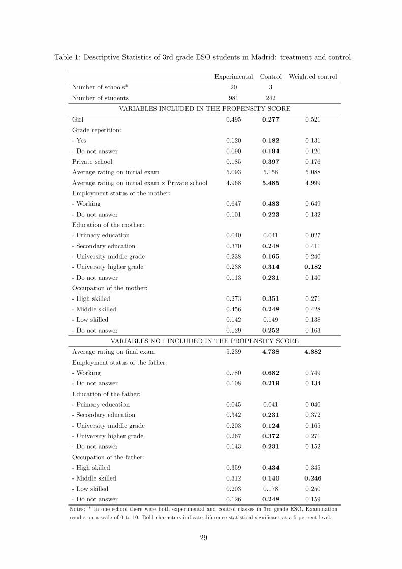
Table 1: Descriptive Statistics of 3rd grade ESO students in Madrid: treatment and control.
Experimental Control Weighted control
Number of schools* 20 3
Number of students 981 242
VARIABLES INCLUDED IN THE PROPENSITY SCORE
Girl 0.495 0.277 0.521
Grade repetition:
- Yes 0.120 0.182 0.131
- Do not answer 0.090 0.194 0.120
Private school 0.185 0.397 0.176
Average rating on initial exam 5.093 5.158 5.088
Average rating on initial exam x Private school 4.968 5.485 4.999
Employment status of the mother:
- Working 0.647 0.483 0.649
- Do not answer 0.101 0.223 0.132
Education of the mother:
- Primary education 0.040 0.041 0.027
- Secondary education 0.370 0.248 0.411
- University middle grade 0.238 0.165 0.240
- University higher grade 0.238 0.314 0.182
- Do not answer 0.113 0.231 0.140
Occupation of the mother:
- High skilled 0.273 0.351 0.271
- Middle skilled 0.456 0.248 0.428
- Low skilled 0.142 0.149 0.138
- Do not answer 0.129 0.252 0.163
VARIABLES NOT INCLUDED IN THE PROPENSITY SCORE
Average rating on final exam 5.239 4.738 4.882
Employment status of the father:
- Working 0.780 0.682 0.749
- Do not answer 0.108 0.219 0.134
Education of the father:
- Primary education 0.045 0.041 0.040
- Secondary education 0.342 0.231 0.372
- University middle grade 0.203 0.124 0.165
- University higher grade 0.267 0.372 0.271
- Do not answer 0.143 0.231 0.152
Occupation of the father:
- High skilled 0.359 0.434 0.345
- Middle skilled 0.312 0.140 0.246
- Low skilled 0.203 0.178 0.250
- Do not answer 0.126 0.248 0.159Notes: * In one school there were both experimental and control classes in 3rd grade ESO. Examination
results on a scale of 0 to 10. Bold characters indicate diference statistical significant at a 5 percent level.
29
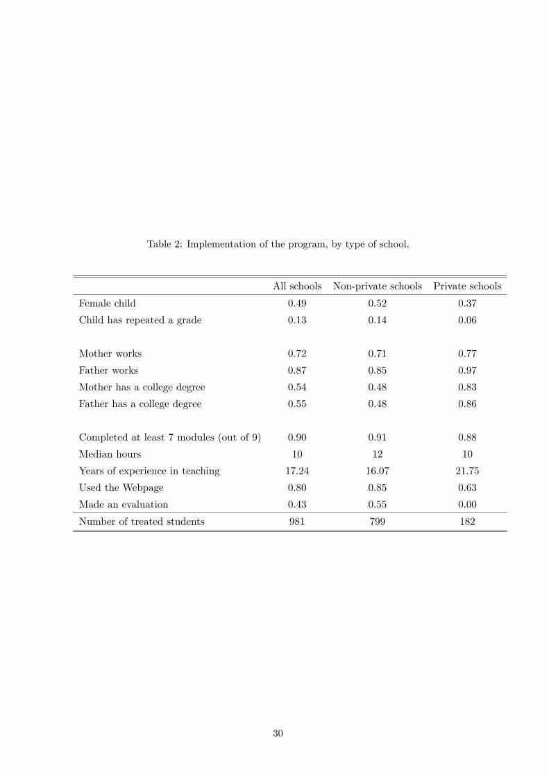
Table 2: Implementation of the program, by type of school.
All schools Non-private schools Private schools
Female child 0.49 0.52 0.37
Child has repeated a grade 0.13 0.14 0.06
Mother works 0.72 0.71 0.77
Father works 0.87 0.85 0.97
Mother has a college degree 0.54 0.48 0.83
Father has a college degree 0.55 0.48 0.86
Completed at least 7 modules (out of 9) 0.90 0.91 0.88
Median hours 10 12 10
Years of experience in teaching 17.24 16.07 21.75
Used the Webpage 0.80 0.85 0.63
Made an evaluation 0.43 0.55 0.00
Number of treated students 981 799 182
30
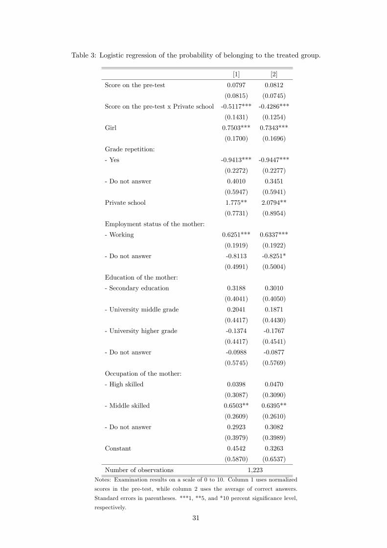
Table 3: Logistic regression of the probability of belonging to the treated group.
[1] [2]
Score on the pre-test 0.0797 0.0812
(0.0815) (0.0745)
Score on the pre-test x Private school -0.5117*** -0.4286***
(0.1431) (0.1254)
Girl 0.7503*** 0.7343***
(0.1700) (0.1696)
Grade repetition:
- Yes -0.9413*** -0.9447***
(0.2272) (0.2277)
- Do not answer 0.4010 0.3451
(0.5947) (0.5941)
Private school 1.775** 2.0794**
(0.7731) (0.8954)
Employment status of the mother:
- Working 0.6251*** 0.6337***
(0.1919) (0.1922)
- Do not answer -0.8113 -0.8251*
(0.4991) (0.5004)
Education of the mother:
- Secondary education 0.3188 0.3010
(0.4041) (0.4050)
- University middle grade 0.2041 0.1871
(0.4417) (0.4430)
- University higher grade -0.1374 -0.1767
(0.4417) (0.4541)
- Do not answer -0.0988 -0.0877
(0.5745) (0.5769)
Occupation of the mother:
- High skilled 0.0398 0.0470
(0.3087) (0.3090)
- Middle skilled 0.6503** 0.6395**
(0.2609) (0.2610)
- Do not answer 0.2923 0.3082
(0.3979) (0.3989)
Constant 0.4542 0.3263
(0.5870) (0.6537)
Number of observations 1,223Notes: Examination results on a scale of 0 to 10. Column 1 uses normalized
scores in the pre-test, while column 2 uses the average of correct answers.
Standard errors in parentheses. ***1, **5, and *10 percent significance level,
respectively.
31
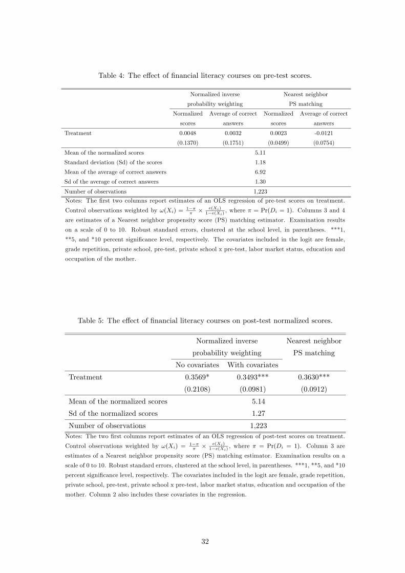
Table 4: The effect of financial literacy courses on pre-test scores.
Normalized inverse Nearest neighbor
probability weighting PS matching
Normalized Average of correct Normalized Average of correct
scores answers scores answers
Treatment 0.0048 0.0032 0.0023 -0.0121
(0.1370) (0.1751) (0.0499) (0.0754)
Mean of the normalized scores 5.11
Standard deviation (Sd) of the scores 1.18
Mean of the average of correct answers 6.92
Sd of the average of correct answers 1.30
Number of observations 1,223
Notes: The first two columns report estimates of an OLS regression of pre-test scores on treatment.
Control observations weighted by ω(Xi) = 1−ππ× e(Xi)
1−e(Xi), where π = Pr(Di = 1). Columns 3 and 4
are estimates of a Nearest neighbor propensity score (PS) matching estimator. Examination results
on a scale of 0 to 10. Robust standard errors, clustered at the school level, in parentheses. ***1,
**5, and *10 percent significance level, respectively. The covariates included in the logit are female,
grade repetition, private school, pre-test, private school x pre-test, labor market status, education and
occupation of the mother.
Table 5: The effect of financial literacy courses on post-test normalized scores.
Normalized inverse Nearest neighbor
probability weighting PS matching
No covariates With covariates
Treatment 0.3569* 0.3493*** 0.3630***
(0.2108) (0.0981) (0.0912)
Mean of the normalized scores 5.14
Sd of the normalized scores 1.27
Number of observations 1,223Notes: The two first columns report estimates of an OLS regression of post-test scores on treatment.
Control observations weighted by ω(Xi) = 1−ππ× e(Xi)
1−e(Xi), where π = Pr(Di = 1). Column 3 are
estimates of a Nearest neighbor propensity score (PS) matching estimator. Examination results on a
scale of 0 to 10. Robust standard errors, clustered at the school level, in parentheses. ***1, **5, and *10
percent significance level, respectively. The covariates included in the logit are female, grade repetition,
private school, pre-test, private school x pre-test, labor market status, education and occupation of the
mother. Column 2 also includes these covariates in the regression.
32
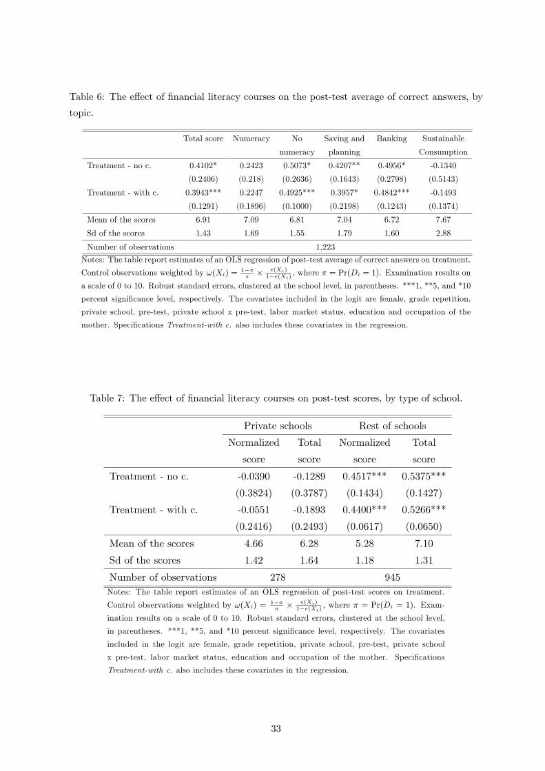
Table 6: The effect of financial literacy courses on the post-test average of correct answers, by
topic.
Total score Numeracy No Saving and Banking Sustainable
numeracy planning Consumption
Treatment - no c. 0.4102* 0.2423 0.5073* 0.4207** 0.4956* -0.1340
(0.2406) (0.218) (0.2636) (0.1643) (0.2798) (0.5143)
Treatment - with c. 0.3943*** 0.2247 0.4925*** 0.3957* 0.4842*** -0.1493
(0.1291) (0.1896) (0.1000) (0.2198) (0.1243) (0.1374)
Mean of the scores 6.91 7.09 6.81 7.04 6.72 7.67
Sd of the scores 1.43 1.69 1.55 1.79 1.60 2.88
Number of observations 1,223
Notes: The table report estimates of an OLS regression of post-test average of correct answers on treatment.
Control observations weighted by ω(Xi) = 1−ππ× e(Xi)
1−e(Xi), where π = Pr(Di = 1). Examination results on
a scale of 0 to 10. Robust standard errors, clustered at the school level, in parentheses. ***1, **5, and *10
percent significance level, respectively. The covariates included in the logit are female, grade repetition,
private school, pre-test, private school x pre-test, labor market status, education and occupation of the
mother. Specifications Treatment-with c. also includes these covariates in the regression.
Table 7: The effect of financial literacy courses on post-test scores, by type of school.
Private schools Rest of schools
Normalized Total Normalized Total
score score score score
Treatment - no c. -0.0390 -0.1289 0.4517*** 0.5375***
(0.3824) (0.3787) (0.1434) (0.1427)
Treatment - with c. -0.0551 -0.1893 0.4400*** 0.5266***
(0.2416) (0.2493) (0.0617) (0.0650)
Mean of the scores 4.66 6.28 5.28 7.10
Sd of the scores 1.42 1.64 1.18 1.31
Number of observations 278 945Notes: The table report estimates of an OLS regression of post-test scores on treatment.
Control observations weighted by ω(Xi) = 1−ππ× e(Xi)
1−e(Xi), where π = Pr(Di = 1). Exam-
ination results on a scale of 0 to 10. Robust standard errors, clustered at the school level,
in parentheses. ***1, **5, and *10 percent significance level, respectively. The covariates
included in the logit are female, grade repetition, private school, pre-test, private school
x pre-test, labor market status, education and occupation of the mother. Specifications
Treatment-with c. also includes these covariates in the regression.
33
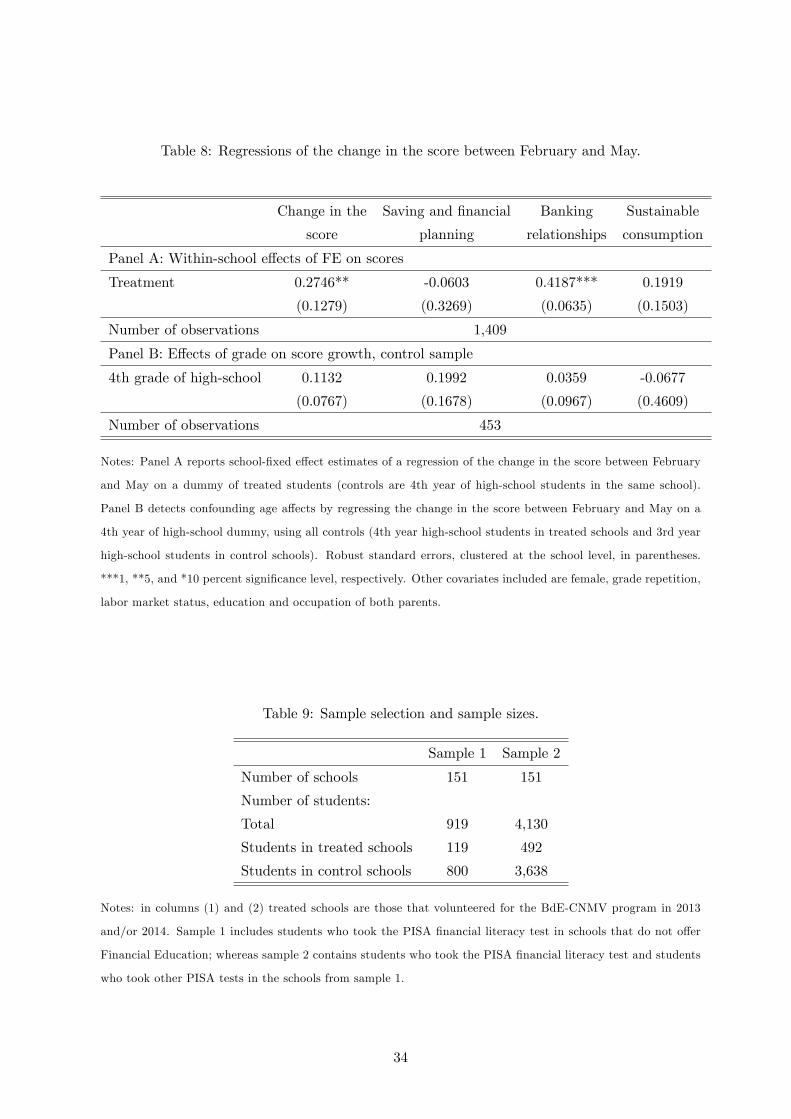
Table 8: Regressions of the change in the score between February and May.
Change in the Saving and financial Banking Sustainable
score planning relationships consumption
Panel A: Within-school effects of FE on scores
Treatment 0.2746** -0.0603 0.4187*** 0.1919
(0.1279) (0.3269) (0.0635) (0.1503)
Number of observations 1,409
Panel B: Effects of grade on score growth, control sample
4th grade of high-school 0.1132 0.1992 0.0359 -0.0677
(0.0767) (0.1678) (0.0967) (0.4609)
Number of observations 453
Notes: Panel A reports school-fixed effect estimates of a regression of the change in the score between February
and May on a dummy of treated students (controls are 4th year of high-school students in the same school).
Panel B detects confounding age affects by regressing the change in the score between February and May on a
4th year of high-school dummy, using all controls (4th year high-school students in treated schools and 3rd year
high-school students in control schools). Robust standard errors, clustered at the school level, in parentheses.
***1, **5, and *10 percent significance level, respectively. Other covariates included are female, grade repetition,
labor market status, education and occupation of both parents.
Table 9: Sample selection and sample sizes.
Sample 1 Sample 2
Number of schools 151 151
Number of students:
Total 919 4,130
Students in treated schools 119 492
Students in control schools 800 3,638
Notes: in columns (1) and (2) treated schools are those that volunteered for the BdE-CNMV program in 2013
and/or 2014. Sample 1 includes students who took the PISA financial literacy test in schools that do not offer
Financial Education; whereas sample 2 contains students who took the PISA financial literacy test and students
who took other PISA tests in the schools from sample 1.
34
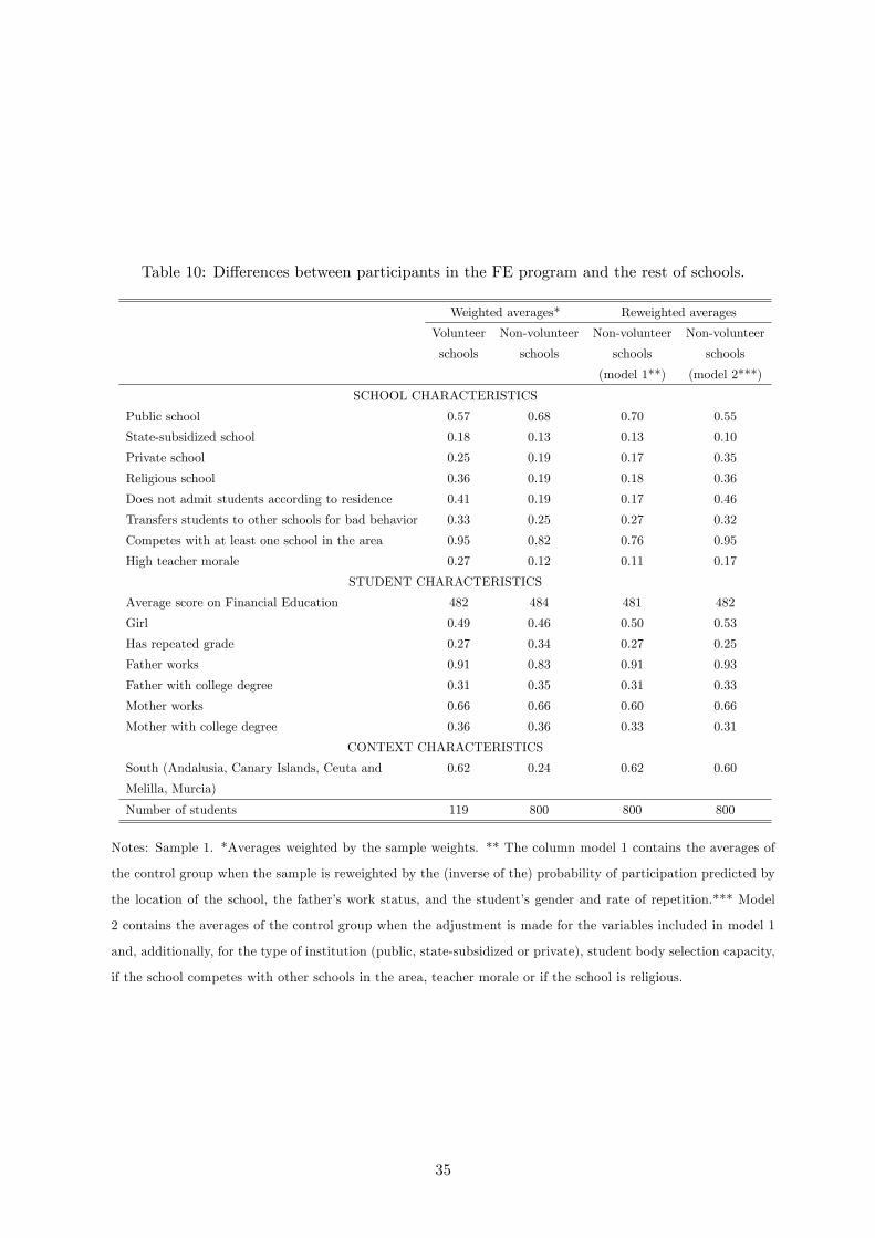
Table 10: Differences between participants in the FE program and the rest of schools.
Weighted averages* Reweighted averages
Volunteer Non-volunteer Non-volunteer Non-volunteer
schools schools schools schools
(model 1**) (model 2***)
SCHOOL CHARACTERISTICS
Public school 0.57 0.68 0.70 0.55
State-subsidized school 0.18 0.13 0.13 0.10
Private school 0.25 0.19 0.17 0.35
Religious school 0.36 0.19 0.18 0.36
Does not admit students according to residence 0.41 0.19 0.17 0.46
Transfers students to other schools for bad behavior 0.33 0.25 0.27 0.32
Competes with at least one school in the area 0.95 0.82 0.76 0.95
High teacher morale 0.27 0.12 0.11 0.17
STUDENT CHARACTERISTICS
Average score on Financial Education 482 484 481 482
Girl 0.49 0.46 0.50 0.53
Has repeated grade 0.27 0.34 0.27 0.25
Father works 0.91 0.83 0.91 0.93
Father with college degree 0.31 0.35 0.31 0.33
Mother works 0.66 0.66 0.60 0.66
Mother with college degree 0.36 0.36 0.33 0.31
CONTEXT CHARACTERISTICS
South (Andalusia, Canary Islands, Ceuta and 0.62 0.24 0.62 0.60
Melilla, Murcia)
Number of students 119 800 800 800
Notes: Sample 1. *Averages weighted by the sample weights. ** The column model 1 contains the averages of
the control group when the sample is reweighted by the (inverse of the) probability of participation predicted by
the location of the school, the father’s work status, and the student’s gender and rate of repetition.*** Model
2 contains the averages of the control group when the adjustment is made for the variables included in model 1
and, additionally, for the type of institution (public, state-subsidized or private), student body selection capacity,
if the school competes with other schools in the area, teacher morale or if the school is religious.
35
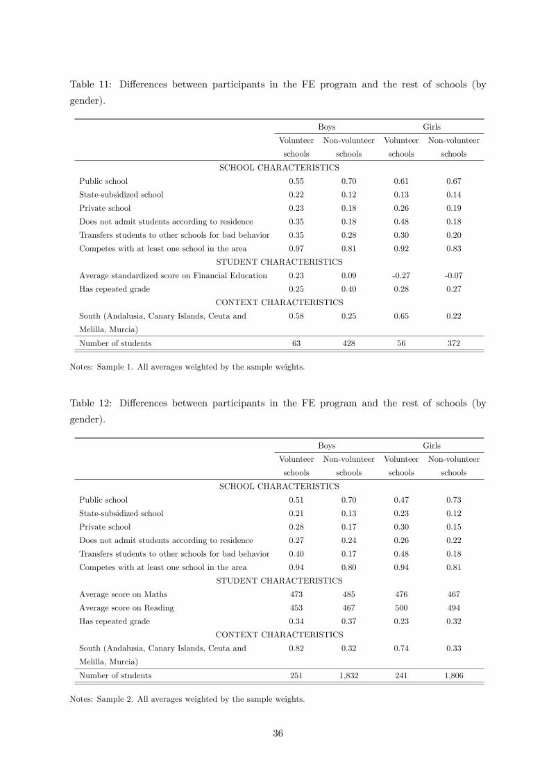
Table 11: Differences between participants in the FE program and the rest of schools (by
gender).
Boys Girls
Volunteer Non-volunteer Volunteer Non-volunteer
schools schools schools schools
SCHOOL CHARACTERISTICS
Public school 0.55 0.70 0.61 0.67
State-subsidized school 0.22 0.12 0.13 0.14
Private school 0.23 0.18 0.26 0.19
Does not admit students according to residence 0.35 0.18 0.48 0.18
Transfers students to other schools for bad behavior 0.35 0.28 0.30 0.20
Competes with at least one school in the area 0.97 0.81 0.92 0.83
STUDENT CHARACTERISTICS
Average standardized score on Financial Education 0.23 0.09 -0.27 -0.07
Has repeated grade 0.25 0.40 0.28 0.27
CONTEXT CHARACTERISTICS
South (Andalusia, Canary Islands, Ceuta and 0.58 0.25 0.65 0.22
Melilla, Murcia)
Number of students 63 428 56 372
Notes: Sample 1. All averages weighted by the sample weights.
Table 12: Differences between participants in the FE program and the rest of schools (by
gender).
Boys Girls
Volunteer Non-volunteer Volunteer Non-volunteer
schools schools schools schools
SCHOOL CHARACTERISTICS
Public school 0.51 0.70 0.47 0.73
State-subsidized school 0.21 0.13 0.23 0.12
Private school 0.28 0.17 0.30 0.15
Does not admit students according to residence 0.27 0.24 0.26 0.22
Transfers students to other schools for bad behavior 0.40 0.17 0.48 0.18
Competes with at least one school in the area 0.94 0.80 0.94 0.81
STUDENT CHARACTERISTICS
Average score on Maths 473 485 476 467
Average score on Reading 453 467 500 494
Has repeated grade 0.34 0.37 0.23 0.32
CONTEXT CHARACTERISTICS
South (Andalusia, Canary Islands, Ceuta and 0.82 0.32 0.74 0.33
Melilla, Murcia)
Number of students 251 1,832 241 1,806
Notes: Sample 2. All averages weighted by the sample weights.
36
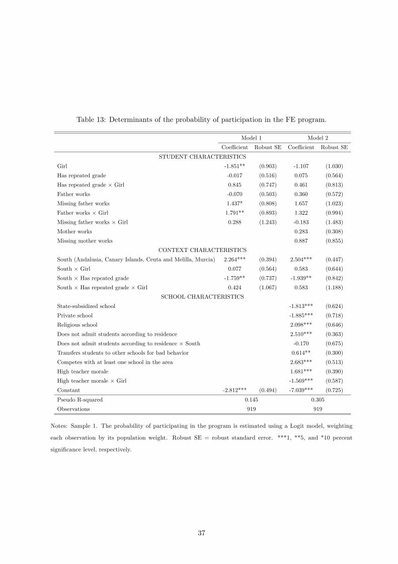
Table 13: Determinants of the probability of participation in the FE program.
Model 1 Model 2
Coeffi cient Robust SE Coeffi cient Robust SE
STUDENT CHARACTERISTICS
Girl -1.851** (0.903) -1.107 (1.030)
Has repeated grade -0.017 (0.516) 0.075 (0.564)
Has repeated grade × Girl 0.845 (0.747) 0.461 (0.813)
Father works -0.070 (0.503) 0.360 (0.572)
Missing father works 1.437* (0.808) 1.657 (1.023)
Father works × Girl 1.791** (0.893) 1.322 (0.994)
Missing father works × Girl 0.288 (1.243) -0.183 (1.483)
Mother works 0.283 (0.308)
Missing mother works 0.887 (0.855)
CONTEXT CHARACTERISTICS
South (Andalusia, Canary Islands, Ceuta and Melilla, Murcia) 2.264*** (0.394) 2.504*** (0.447)
South × Girl 0.077 (0.564) 0.583 (0.644)
South × Has repeated grade -1.759** (0.737) -1.939** (0.842)
South × Has repeated grade × Girl 0.424 (1.067) 0.583 (1.188)
SCHOOL CHARACTERISTICS
State-subsidized school -1.813*** (0.624)
Private school -1.885*** (0.718)
Religious school 2.098*** (0.646)
Does not admit students according to residence 2.510*** (0.363)
Does not admit students according to residence × South -0.170 (0.675)
Transfers students to other schools for bad behavior 0.614** (0.300)
Competes with at least one school in the area 2.683*** (0.513)
High teacher morale 1.681*** (0.390)
High teacher morale × Girl -1.569*** (0.587)
Constant -2.812*** (0.494) -7.039*** (0.725)
Pseudo R-squared 0.145 0.305
Observations 919 919
Notes: Sample 1. The probability of participating in the program is estimated using a Logit model, weighting
each observation by its population weight. Robust SE = robust standard error. ***1, **5, and *10 percent
significance level, respectively.
37
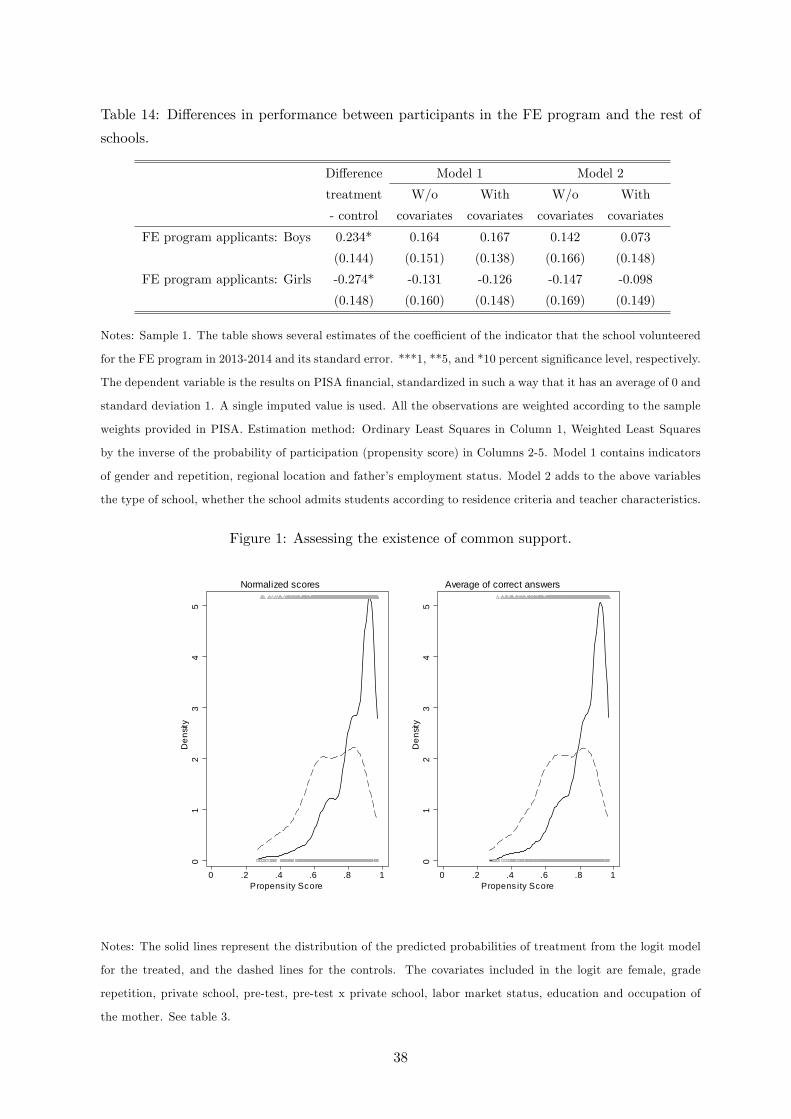
Table 14: Differences in performance between participants in the FE program and the rest of
schools.
Difference Model 1 Model 2
treatment W/o With W/o With
- control covariates covariates covariates covariates
FE program applicants: Boys 0.234* 0.164 0.167 0.142 0.073
(0.144) (0.151) (0.138) (0.166) (0.148)
FE program applicants: Girls -0.274* -0.131 -0.126 -0.147 -0.098
(0.148) (0.160) (0.148) (0.169) (0.149)
Notes: Sample 1. The table shows several estimates of the coeffi cient of the indicator that the school volunteered
for the FE program in 2013-2014 and its standard error. ***1, **5, and *10 percent significance level, respectively.
The dependent variable is the results on PISA financial, standardized in such a way that it has an average of 0 and
standard deviation 1. A single imputed value is used. All the observations are weighted according to the sample
weights provided in PISA. Estimation method: Ordinary Least Squares in Column 1, Weighted Least Squares
by the inverse of the probability of participation (propensity score) in Columns 2-5. Model 1 contains indicators
of gender and repetition, regional location and father’s employment status. Model 2 adds to the above variables
the type of school, whether the school admits students according to residence criteria and teacher characteristics.
Figure 1: Assessing the existence of common support.
01
23
45
Den
sity
0 .2 .4 .6 .8 1Propens ity Score
Normalized scores
01
23
45
Den
sity
0 .2 .4 .6 .8 1Propens ity Score
Average of correct answers
Notes: The solid lines represent the distribution of the predicted probabilities of treatment from the logit model
for the treated, and the dashed lines for the controls. The covariates included in the logit are female, grade
repetition, private school, pre-test, pre-test x private school, labor market status, education and occupation of
the mother. See table 3.
38
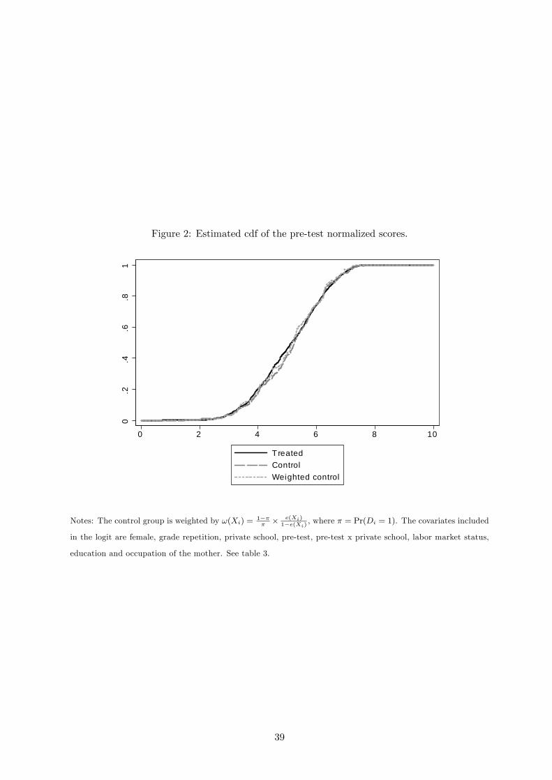
Figure 2: Estimated cdf of the pre-test normalized scores.
0.2
.4.6
.81
0 2 4 6 8 10
TreatedControlWeighted control
Notes: The control group is weighted by ω(Xi) = 1−ππ× e(Xi)
1−e(Xi), where π = Pr(Di = 1). The covariates included
in the logit are female, grade repetition, private school, pre-test, pre-test x private school, labor market status,
education and occupation of the mother. See table 3.
39
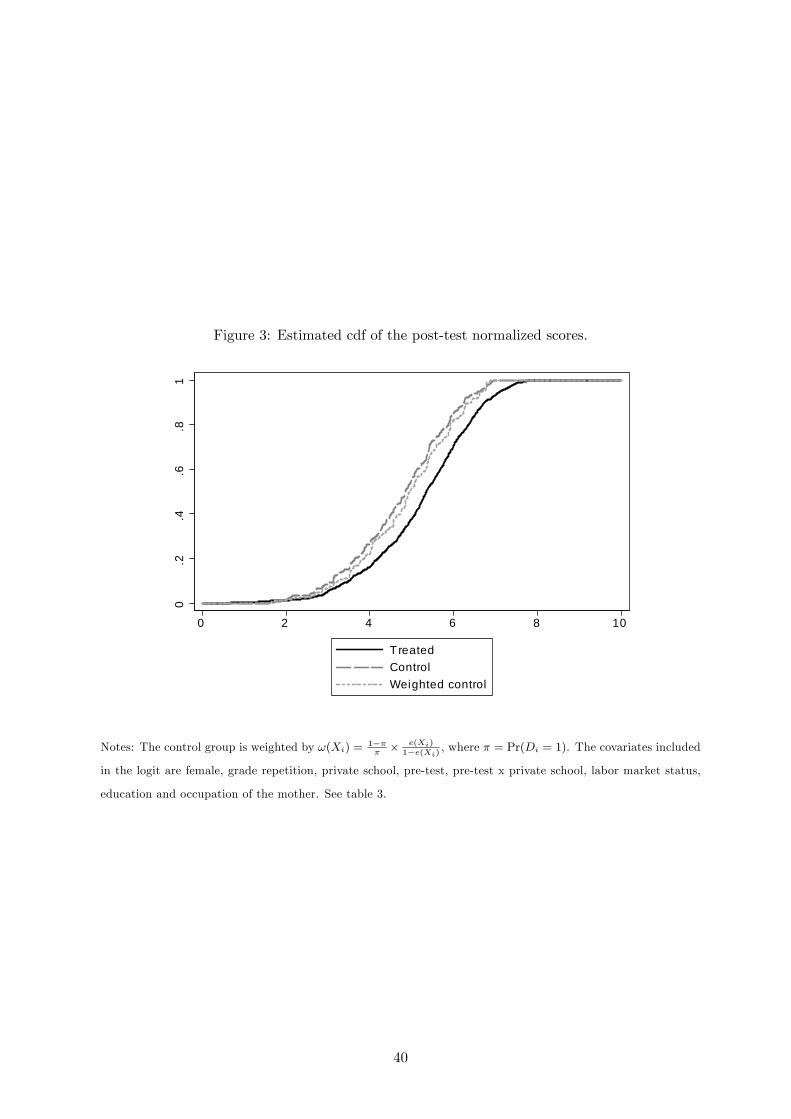
Figure 3: Estimated cdf of the post-test normalized scores.
0.2
.4.6
.81
0 2 4 6 8 10
TreatedControlWeighted control
Notes: The control group is weighted by ω(Xi) = 1−ππ× e(Xi)
1−e(Xi), where π = Pr(Di = 1). The covariates included
in the logit are female, grade repetition, private school, pre-test, pre-test x private school, labor market status,
education and occupation of the mother. See table 3.
40
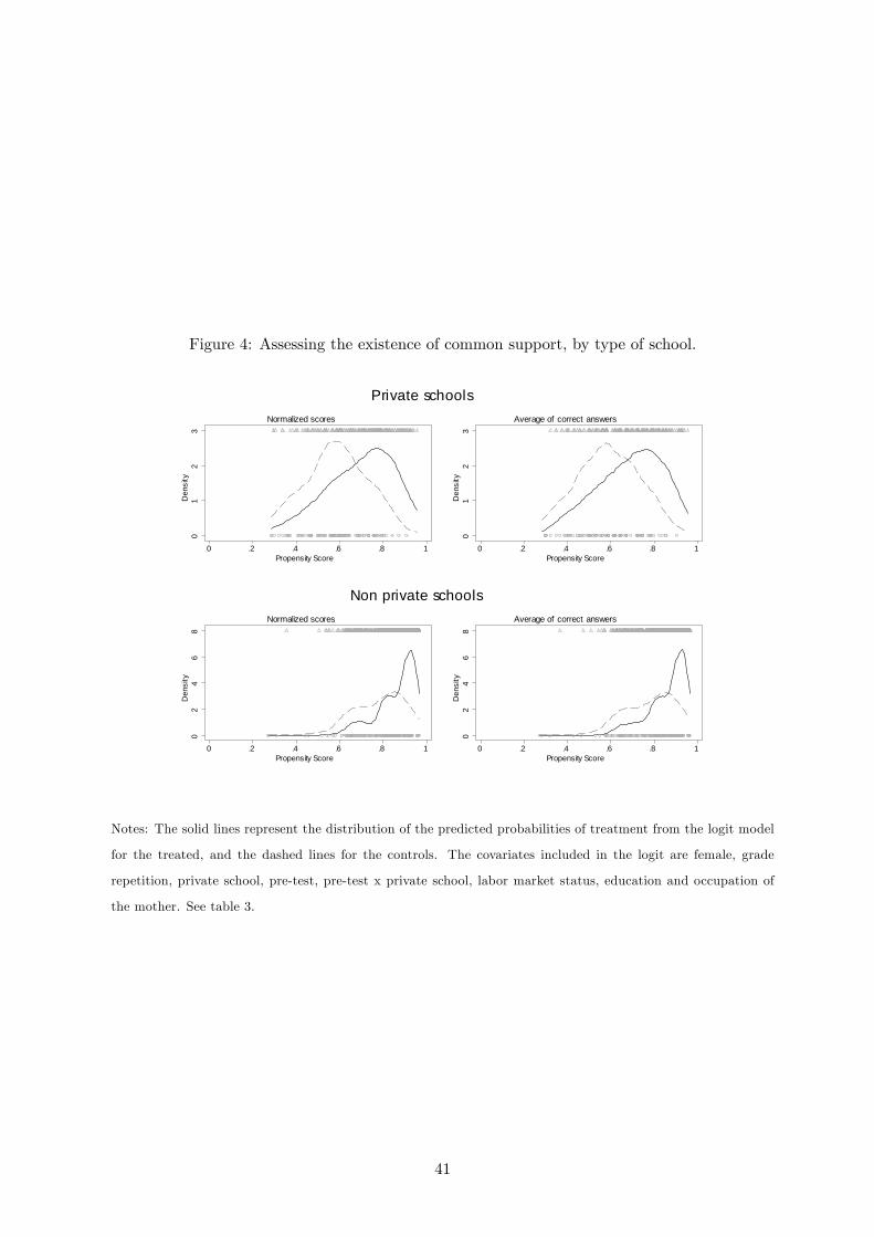
Figure 4: Assessing the existence of common support, by type of school.
01
23
Den
sity
0 .2 .4 .6 .8 1Propensity Score
Normalized scores
01
23
Den
sity
0 .2 .4 .6 .8 1Propensity Score
Average of correct answers
Private schools
02
46
8D
ensi
ty
0 .2 .4 .6 .8 1Propensity Score
Normalized scores
02
46
8D
ensi
ty
0 .2 .4 .6 .8 1Propensity Score
Average of correct answers
Non private schools
Notes: The solid lines represent the distribution of the predicted probabilities of treatment from the logit model
for the treated, and the dashed lines for the controls. The covariates included in the logit are female, grade
repetition, private school, pre-test, pre-test x private school, labor market status, education and occupation of
the mother. See table 3.
41
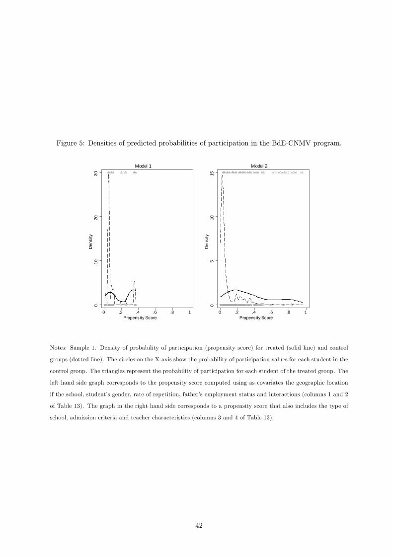
Figure 5: Densities of predicted probabilities of participation in the BdE-CNMV program.
010
2030
Den
sity
0 .2 .4 .6 .8 1Propensity Score
Model 1
05
1015
Den
sity
0 .2 .4 .6 .8 1Propensity Score
Model 2
Notes: Sample 1. Density of probability of participation (propensity score) for treated (solid line) and control
groups (dotted line). The circles on the X-axis show the probability of participation values for each student in the
control group. The triangles represent the probability of participation for each student of the treated group. The
left hand side graph corresponds to the propensity score computed using as covariates the geographic location
if the school, student’s gender, rate of repetition, father’s employment status and interactions (columns 1 and 2
of Table 13). The graph in the right hand side corresponds to a propensity score that also includes the type of
school, admission criteria and teacher characteristics (columns 3 and 4 of Table 13).
42

APPENDIX
A Topics covered in the program
The financial literacy course taught in 2012-2013 was structured in nine chapters. There was atenth one that reviewed the previous material.
Financial security Learning to manage money. Establishing savings goals and how toreach them.
Intelligent consumption How to improve quality of life by expenditure choices. Thedefinition of healthy, responsible and sustainable consumption. The role of advertising.
Saving Definition of saving. Reasons for saving and the role of uncertainty. Differencesbetween saving and investing.
Personal budgeting Elaboration of a personal budget. Identifying fixed and variableexpenses. Identifying adjustable expenses.
Money and monetary transactions Advantages and disadvantages of using cash. Iden-tification of fake currency.
Bank accounts Differences between checking and savings accounts. Opening a bankaccount. Consequences of an overdraft. Understanding checking account statements. Managingbank accounts. Internet and phone banking.
Credit and Debit Cards The use of credit and debit cards: advantages and disadvan-tages. The use of tellers and cash stations.
Data protection Problems using Internet banking.
Banking relationships Opening and closing bank accounts. Different forms of bank fees.
B Contents of the tests
Two different tests were passed in May 2013. Each student made only one, but to avoid leakingof information across classes and schools, not all students made the same test. We describe nowthe contents of the second one. The questions on the test spanned three main topics:
• Saving and Financial Planning (9 questions, 6 of them require an arithmetic computation)
• Money and Bank Accounts (18 questions, 5 of them require an arithmetic computation)
• Sustainable Consumption (3 questions, none of them requires an arithmetic computation)
43
The questions on Saving and Financial planning presented students with data on hypotheti-cal financial situations and asked about which concepts should be included in a budget or abouthow to reach specific targets given a flow of expected expenses and incomes. Questions onMoneyand Bank Accounts tried to establish if students understood the functioning of checking andsavings account by means of specific examples. Those questions also presented situations wherestudents had to identify the best payment methods for different outlays. Finally, students weretested about basic notions of security when using bank accounts. Questions about Sustainableconsumption presented hypothetical situations where the students should to identify the mostresponsible expenditure pattern (i.e., the healthiest or the environmentally friendliest).
44


![Coração que sente [Valsa] · Title: Coração que sente [Valsa] Author: Nazareth, Ernesto - Editeur: Rio de Janeiro: Ernesto Augusto de Mattos, n.d. Plate 3-E.A.M. Subject](https://img.pdfslide.org/doc/110x75/60748496383b205153158cf9/corao-que-sente-valsa-title-corao-que-sente-valsa-author-nazareth.jpg)