Zeitschrift für

Gletscherkundeund Glazialgeologie

Herausgegeben vonMICHAEL KUHN

BAND 40 (2005/2006)

ISSN 0044-2836

UNIVERSITÄTSVERLAG WAGNER · INNSBRUCK

1907 wurde von Eduard Brückner in Wien der erste Band der Zeitschrift für Gletscherkunde, für Eiszeitforschung und Geschichte des Klimas fertig gestellt. Mit dem 16. Band über-nahm 1928 Raimund von Klebelsberg in Innsbruck die Herausgabe der Zeitschrift, deren 28. Band 1942 erschien. Nach dem Zweiten Weltkrieg gab Klebelsberg die neue Zeitschrift für Gletscherkunde und Glazialgeologie im Universitätsverlag Wagner in Innsbruck heraus. Der erste Band erschien 1950. 1970 übernahmen Herfried Hoinkes und Hans Kinzl die Herausgeberschaft, von 1979 bis 2001 Gernot Patzelt und Michael Kuhn.

In 1907 this Journal was founded by Eduard Brückner as Zeitschrift für Gletscherkunde, für Eiszeitforschung und Geschichte des Klimas. Raimund von Klebelsberg followed as editor in 1928, he started Zeitschrift für Gletscherkunde und Glazialgeologie anew with Vol.1 in 1950, followed by Hans Kinzl and Herfried Hoinkes in 1970 and by Gernot Patzelt and Michael Kuhn from 1979 to 2001.

Herausgeber Michael Kuhn EditorSchriftleitung Angelika Neuner & Mercedes Blaas Executive editors

Wissenschaftlicher Beirat Editorial advisory boardJon Ove Hagen, Oslo

Ole Humlum, LongyearbyenPeter Jansson, StockholmGeorg Kaser, Innsbruck

Vladimir Kotlyakov, MoskvaHeinz Miller, Bremerhaven

Koni Steffen, Boulder

ISSN 0044-2836

Figure on front page: “Vue prise de la Voute nommée le Chapeau, du Glacier des Bois, et des Aiguilles. du Charmoz.”; signed down in the middle “fait par Jn. Ante. Linck.”; coloured contour etching; 36.2 x 48.7 cm; Bibliothèque publique et universitaire de Genève, 37 M Nr. 1964/181; Photograph by H. J. Zumbühl.

Copyright © 2007 by Universitätsverlag Wagner, A–6020 Innsbruck

Das Werk ist urheberrechtlich geschützt. Die dadurch begründeten Rechte, insbesondere die der Übersetzung, des Nachdruckes, der Entnahme von Abbildungen, der Funksendung, der Wiedergabe auf photomechanischem oder ähnlichem Wege und der Speicherung in Datenverarbeitungsanlagen

bleiben, auch bei nur auszugsweiser Verwertung, vorbehalten.

Herstellung: Grasl Druck & Neue Medien, A–2540 Bad Vöslau

Fluctuations of the “Mer de Glace”(Mont Blanc area, France) AD 1500–2050:

an interdisciplinary approachusing new historical data and neural network

simulations

Gletscherschwankungen des “Mer de Glace”(Mont Blanc-Gebiet, Frankreich) AD 1500–2050:

ein interdisziplinärer Ansatz,basierend auf neuen historischen Daten und neuronalen

Netzen

S. U. NUSSBAUMER / H. J. ZUMBÜHL / D. STEINER

“Il n’y a dans les Alpes rien de constant que leur variété.”Horace-Bénédict de Saussure (1740–1799)

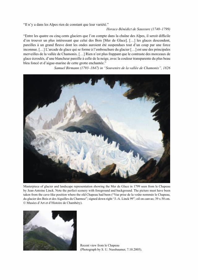
“Entre les quatre ou cinq cents glaciers que l’on compte dans la chaîne des Alpes, il seroit difficile d’en trouver un plus intéressant que celui des Bois [Mer de Glace]. […] les glaces descendent, pareilles à un grand fleuve dont les ondes auroient été suspendues tout d’un coup par une force inconnue. […] L’arcade de glace qui se forme à l’embouchure du glacier […] est une des principales merveilles de la vallée de Chamonix. […] Rien n’est plus frappant que le contraste des morceaux de glace écroulés, d’une blancheur pareille à celle de la neige, avec la couleur transparente du plus beau bleu foncé et d’aigue-marine de cette grotte enchantée.”

Samuel Birmann (1793–1847) in “Souvenirs de la vallée de Chamonix”, 1826

Masterpiece of glacier and landscape representation showing the Mer de Glace in 1799 seen from le Chapeau by Jean-Antoine Linck. Note the perfect scenery with foreground and background. The picture must have been taken from the cave-like position where the old Chapeau had been (“Vue prise de la voûte nommée le Chapeau, du glacier des Bois et des Aiguilles du Charmoz”; signed down right “J.-A. Linck 99”; oil on canvas; 39 x 50 cm. © Musées d’Art et d’Histoire de Chambéry).

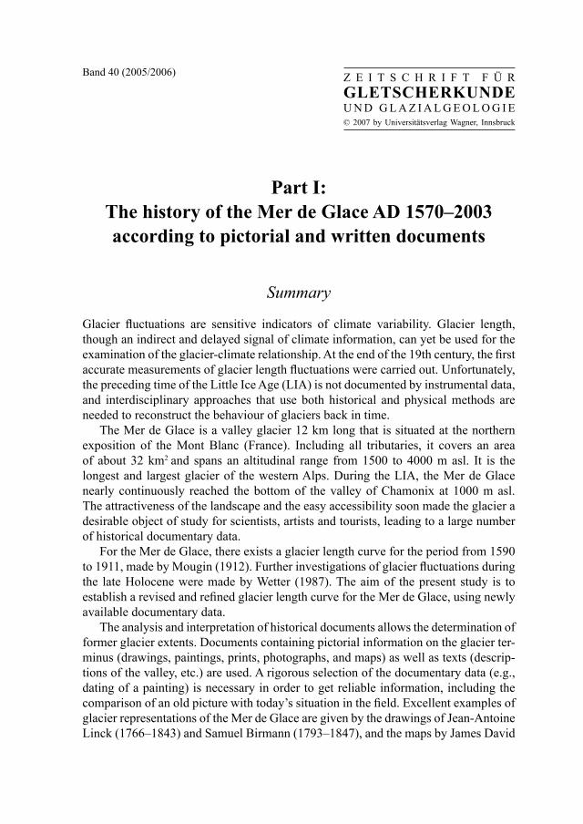
Recent view from le Chapeau (Photograph by S. U. Nussbaumer, 7.10.2005).

Part I: The history of the Mer de Glace AD 1570–2003according to pictorial and written documents

Summary

Glacier fluctuations are sensitive indicators of climate variability. Glacier length, though an indirect and delayed signal of climate information, can yet be used for the examination of the glacier-climate relationship. At the end of the 19th century, the first accurate measurements of glacier length fluctuations were carried out. Unfortunately, the preceding time of the Little Ice Age (LIA) is not documented by instrumental data, and interdisciplinary approaches that use both historical and physical methods are needed to reconstruct the behaviour of glaciers back in time.

The Mer de Glace is a valley glacier 12 km long that is situated at the northern exposition of the Mont Blanc (France). Including all tributaries, it covers an area of about 32 km2 and spans an altitudinal range from 1500 to 4000 m asl. It is the longest and largest glacier of the western Alps. During the LIA, the Mer de Glace nearly continuously reached the bottom of the valley of Chamonix at 1000 m asl. The attractiveness of the landscape and the easy accessibility soon made the glacier a desirable object of study for scientists, artists and tourists, leading to a large number of historical documentary data.

For the Mer de Glace, there exists a glacier length curve for the period from 1590 to 1911, made by Mougin (1912). Further investigations of glacier fluctuations during the late Holocene were made by Wetter (1987). The aim of the present study is to establish a revised and refined glacier length curve for the Mer de Glace, using newly available documentary data.

The analysis and interpretation of historical documents allows the determination of former glacier extents. Documents containing pictorial information on the glacier ter-minus (drawings, paintings, prints, photographs, and maps) as well as texts (descrip-tions of the valley, etc.) are used. A rigorous selection of the documentary data (e.g., dating of a painting) is necessary in order to get reliable information, including the comparison of an old picture with today’s situation in the field. Excellent examples of glacier representations of the Mer de Glace are given by the drawings of Jean-Antoine Linck (1766–1843) and Samuel Birmann (1793–1847), and the maps by James David

Band 40 (2005/2006) Z E I T S C H R I F T F Ü RGLETSCHERKUNDEU N D G L A Z I A L G E O L O G I E© 2007 by Universitätsverlag Wagner, Innsbruck

6

Forbes (1809–1868) and Eugène Viollet-le-Duc (1814–1879). Additionally, moraines have been mapped for the determination of former glacier extents.

The analysis of old topographical maps (from 1906, 1939, 1958, and 1967) and a photogrammetric evaluation of recent aerial photographs (from 2001) yield a detailed description of the present state of the glacier. The calculation of digital elevation models (DEMs) allows the quantification of volume changes for the Mer de Glace for the 20th century.

The revised and refined glacier length curve for the Mer de Glace goes as far back as 1570. Not surprisingly, the glacier shows a generally large extent during the LIA. The largest glacier extension, documented by several archive texts and moraines, occurred around 1644. The largest glacier advance in the 19th century culminated in 1821 and is roughly 40 m smaller than the 1644 advance. A second advance in the 19th century occurred in 1852, with the glacier still lying roughly 70 m behind the well-formed 1821 moraines. Other major glacier advances are documented around 1600, 1720, and 1778. Since the 1850s, the glacier has retreated more or less con-tinuously (except for some minor advances, e.g. until 1995) by more than 2 km until the present-day. During the 20th century, the Mer de Glace shows a remarkable ice volume loss which mainly took place in the lower part of the glacier.

The new glacier length curve is in good agreement with the curve made by Mougin (1912). However, significant differences occur around 1850, when the glacier extent seems to have been much more extensive than assumed by Mougin. Furthermore, the new documentary data allows a more detailed description of glacier fluctuations for the 1750–1820 period. The glacier extension around 1644 is roughly 100 m smaller than shown by the Mougin curve.

A comparison of the Mer de Glace length curve with the one of the Unterer Grindelwaldgletscher (Zumbühl, 1980; Zumbühl et al., 1983) yields an astonishing simultaneity between the glaciers, despite the different settings in the western and central Alps. Small differences occur around 1855 (19th century maximum of the Unterer Grindelwaldgletscher) as well as between 1650 and 1750 (generally greater extension of the Mer de Glace with more variability). In order to further confirm the knowledge gained, it would be interesting to consider more Alpine glaciers, and also to extend the comparison by studying LIA glacier fluctuations in other parts of the world.

Summary Part I

7

Zusammenfassung Teil I: Das Mer de Glace AD 1570–2003

in den historischen Bild- und Schriftquellen

Klimaänderungen widerspiegeln sich deutlich in Gletscherschwankungen. Obwohl die Veränderung der Gletscherlänge ein indirektes und verspätetes Signal einer Klima-information darstellt, ist sie ein geeignetes Mittel, um Gletscher-Klima-Beziehungen zu untersuchen. Ende des 19. Jahrhunderts wurden erstmals genaue Messungen von Gletscherlängenänderungen durchgeführt. Leider ist die vorhergehende Zeit der Klei-nen Eiszeit nicht durch instrumentelle Daten dokumentiert. Dieser Umstand erfordert interdisziplinäre Ansätze, welche sowohl historische als auch physikalische Metho-den einschliessen, um das Verhalten von Gletschern in jener Zeit zu rekonstruieren.

Das Mer de Glace, ein 12 km langer Talgletscher, liegt nördlich des Mont Blanc (Frankreich). Einschliesslich aller Nebenzuflüsse ist es ein ca. 32 km2 grosser Eis-strom, der heute einen Höhenbereich von 1500 bis 4000 m ü. M. umspannt und damit der längste und grösste Gletscher der Westalpen ist. Während der Kleinen Eiszeit reichte das Mer de Glace praktisch ununterbrochen bis in den Talboden bei Chamonix auf 1000 m ü. M. hinunter. Die Attraktivität der Landschaft und die leichte Zugäng-lichkeit machten den Gletscher schon früh zu einem begehrten Studienobjekt für Wis-senschaftler, Künstler und Touristen, was zu einer grossen Anzahl von historischem Dokumentationsmaterial über den Gletscher führte.

Es existiert eine Gletscherlängenänderungskurve für das Mer de Glace für die Zeitspanne 1590–1911 von Mougin (1912). Weitere Untersuchungen über Schwan-kungen des Mer de Glace im späten Holozän wurden von Wetter (1987) gemacht. Das Ziel der vorliegenden Studie ist es, eine revidierte und verfeinerte Gletscherlängen-änderungskurve für das Mer de Glace zu erstellen, indem neu zugängliches Doku-mentationsmaterial ausgewertet wird.

Die Analyse und Interpretation von historischen Dokumenten ermöglichen die Rekonstruktion früherer Gletscherstände. Dokumente, die historische Bildinformatio-nen über das Gletscherende enthalten (Zeichnungen, Ölgemälde, Drucke, Fotografien, Karten), als auch Texte (Talbeschreibungen etc.), werden ausgewertet. Eine kritische Auswahl des Dokumentationsmaterials ist wichtig, um verlässliche Informationen zu erhalten. Der Vergleich von alten Bildern mit der heutigen Situation vor Ort im Feld sowie Moränenkartierungen ermöglichen die Bestimmung von früheren Glet-scherständen. Exzellente Beispiele für Gletscherabbildungen des Mer de Glace sind die Zeichnungen von Jean-Antoine Linck (1766–1843) und Samuel Birmann (1793–1847), sowie die Karten von James David Forbes (1809–1868) und Eugène Viollet-le-Duc (1814–1879).

Als Ergänzung gibt die Analyse von alten topographischen Karten (von 1906, 1939, 1958 und 1967) und die photogrammetrische Auswertung von aktuellen Luft-

Zusammenfassung Teil I

8

bildern (von 2001) eine detaillierte Beschreibung des Ist-Zustandes des Gletschers. Die Berechnung eines digitalen Höhenmodells (DEM) für die verschiedenen Jahre erlaubt die Quantifizierung von Gletschervolumenänderungen für das 20. Jahrhun-dert.

Die revidierte und verfeinerte Längenänderungskurve für das Mer de Glace reicht bis ins Jahr 1570 zurück und zeigt, nicht überraschend, eine generell grosse Gletscher-ausdehnung während der Kleinen Eiszeit. Die grösste Gletscherausdehnung, doku-mentiert durch verschiedene Archivtexte und Moränen, gab es um 1644. Der grösste Gletschervorstoss im 19. Jahrhundert kulminierte um 1821 und ist ca. 40 m geringer als der Vorstoss im 17. Jahrhundert. Ein zweiter Vorstoss im 19. Jahrhundert fand 1852 statt, wobei der Gletscher jedoch ca. 70 m hinter die gut ausgebildete 1821er Moräne zu liegen kam. Weitere grosse Gletschervorstösse sind um 1600, 1720 und 1778 belegt. Mit Ausnahme von einigen kleinen Vorstössen (letztmals bis 1995) zog sich der Gletscher seit den 1850er Jahren bis heute kontinuierlich um mehr als 2 km zurück. Im 20. Jahrhundert weist das Mer de Glace einen beträchtlichen Volumen-verlust auf, welcher hauptsächlich im unteren Teil des Gletschers stattfand.

Die neue Gletscherlängenänderungskurve stimmt gut mit der Kurve von Mougin (1912) überein. Signifikante Unterschiede gibt es jedoch um 1850, als der Gletscher offensichtlich eine weitaus grössere Ausdehnung hatte, als dies von Mougin ange-nommen wurde. Ausserdem erlaubt das zusätzliche Datenmaterial eine detailliertere Beschreibung der Gletscherschwankungen für die Zeitperiode von 1750–1820. Die Gletscherausdehnung um 1644 ist ungefähr 100 m geringer als in der Mouginkurve gezeigt.

Ein Vergleich der Längenkurve des Mer de Glace mit derjenigen des Unteren Grindelwaldgletschers (Zumbühl, 1980; Zumbühl et al., 1983) zeigt, dass die beiden Gletscher in den letzten 500 Jahren fast synchron reagierten, trotz den unterschied-lichen Lagen der Gletscher in den West- resp. Zentralalpen. Kleine Differenzen gibt es um 1855, als der Untere Grindelwaldgletscher sein Maximum im 19. Jahrhundert erreichte (Mer de Glace um 1821), wie auch zwischen 1650–1750 (generell grössere Ausdehnung des Mer de Glace mit mehr Variabilität). Diese Resultate könnten mit weiteren Gletschern in den Alpen oder in anderen Teilen der Erde verglichen werden, um Gletscherschwankungen während der Kleinen Eiszeit weiter untersuchen und bes-ser verstehen zu können.

Zusammenfassung Teil I

9

Résumé de la première partie: L’histoire de la Mer de Glace AD 1570–2003

documentée par images et sources écrites

Les changements de climat se reflètent nettement dans les fluctuations des glaciers. Bien que les changements de longueur des glaciers représentent un signal indirect et tardif d’une information de climat, ils sont un moyen adapté pour examiner la relation glaciers-climat. C’est à la fin du 19ème siècle qu’on a mesuré pour la première fois les changements de longueur des glaciers. Malheureusement l’époque précédente, le Petit âge glaciaire, n’est pas documentée par des données expérimentales. De ce fait il est indispensable d’avoir recours à un procédé interdisciplinaire comprenant aussi bien des méthodes historiques que physiques pour reconstituer les fluctuations des glaciers pour cette époque.

La Mer de Glace est un glacier de vallée de 12 km qui se trouve au versant nord du Mont Blanc et recouvre un territoire d’environ 32 km2, allant de 4000 à 1500 m d’altitude. Elle est ainsi le glacier le plus grand et le plus long des Alpes occidentales. Lors du Petit âge glaciaire la Mer de Glace croissait plus ou moins de manière con-tinue en s’étendant jusqu’en bas, près de Chamonix à 1000 m. Le caractère intéressant du paysage et son accessibilité facile ont toujours fait du glacier un objet de recherche par excellence, attirant savants, artistes et touristes. Cela a mené à une grande quantité de matériel historique qui permet un bon témoignage de la Mer de Glace.

Il y a une courbe de changement de longueur de la Mer de Glace pour la période 1590–1911, établie par Mougin (1912). D’autres investigations concernant les fluctuations de la Mer de Glace dans le Holocène tardif ont été faites par Wetter (1987). Le but de ce travail est donc d’établir une courbe de longueur révisée et plus détaillée pour la Mer de Glace, en exploitant le matériel de documentation accessible depuis peu.

L’analyse et l’interprétation de documents historiques rendent possible la recon-struction des positions d’autrefois du front du glacier. L’iconographie ancienne (des-sins, peintures à l’huile, tirages, photos et cartes) ainsi que des écrits historiques (descriptions de vallée etc.) sont analysés. Un choix critique du matériel de docu-mentation est indispensable pour obtenir des informations sûres. La comparaison de tableaux anciens avec la situation d’aujourd’hui examinée sur place, ainsi que le relevé des moraines permettent de déterminer les positions d’autrefois du front du glacier. D’excellents exemples qui donnent une représentation remarquable de la Mer de Glace sont les dessins de Jean-Antoine Linck (1766–1843) et de Samuel Birmann (1793–1847) ainsi que les cartes de James David Forbes (1809–1868) et d’Eugène Viollet-le-Duc (1814–1879).

Comme complément, l’analyse d’anciennes cartes topographiques (de 1906, 1939, 1958 et 1967) et l’exploitation photogrammétrique de photos aériennes actuelles (de 2001) donnent une description détaillée de l’état de la Mer de Glace. L’évaluation

Résumé de la première partie

10

d’un modèle d’altitude (DEM) pour les années mentionnées permet la quantification des changements de volume du glacier pour le 20ème siècle.

La courbe de longueur révisée et plus détaillée de la Mer de Glace remonte jusqu’à 1570 et indique – ce qui n’est pas surprenant – une extension singulière du glacier durant le Petit âge glaciaire. La plus grande extension du glacier, attestée par divers textes d’archives et prouvée également par les moraines, eut lieu vers 1644. L’avancée la plus remarquable du glacier au 19ème siècle avait atteint son point culminant en 1821 et avait environ 40 m de moins qu’en 1644. La deuxième avancée au 19ème siècle eut lieu en 1852 et le front s’était arrêté à peu près 70 m derrière la moraine de 1821, aujourd’hui toujours visible. D’autres grandes avancées du glacier sont docu-mentées vers 1600, 1720 et 1778. A l’exception de certaines ré-avancées mineures (pour la dernière fois jusqu’à 1995), le glacier s’est retiré continuellement depuis les années 1850 jusqu’à aujourd’hui de plus de 2 km. Au 20ème siècle la Mer de Glace montre une perte de volume considérable qui a eu lieu principalement dans la partie inférieure du glacier.

La nouvelle courbe de longueur correspond assez bien à la courbe de Mougin (1912). Il y a toutefois des différences significatives en ce qui concerne les années 1850, quand le glacier avait manifestement une extension beaucoup plus grande que celle supposée par Mougin. En outre, le matériel documentaire supplémentaire permet une description plus détaillée des fluctuations du glacier pour la période de 1750 à 1820. Enfin, l’extension du glacier autour de 1644 est environ de 100 m moindre que montrée par la courbe de Mougin.

Une comparaison de la courbe de longueur de la Mer de Glace et de l’Unterer Grin-delwaldgletscher (Zumbühl, 1980; Zumbühl et al., 1983) montre que les deux glaciers réagissaient d’une façon presque synchrone au cours des derniers 500 ans, malgré les positions très différentes des deux glaciers dans les Alpes occidentales ou centrales. Il y a de petites différences vers les années 1855, quand l’Unterer Grindelwaldgletscher atteignait son maximum d’extension au 19ème siècle (Mer de Glace vers 1821), ainsi qu’entre 1650–1750 (en général une plus grande extension de la Mer de Glace avec plus de variabilité). Les résultats sus-mentionnés pourraient être comparés avec ceux d’autres glaciers dans les Alpes ou dans d’autres parties du monde pour mieux com-prendre les fluctuations de glaciers pendant le Petit âge glaciaire.

Résumé de la première partie

1 Introduction

1.1 Glacier fluctuations as a climate indicator

Glaciers are objects sensitive to climate variability, and glacier mass balance and fluctuations are largely controlled by climate (IPCC, 2001). Mass balance observa-tions and glacier geometry parameters (incl. glacier length) represent two types of data reflected by glacier variations (e.g., Hoinkes, 1970; Oerlemans, 2001). Climate condi-tions determine at a certain place the amount of precipitation as well as its phase (i.e., snow or rain), and the energy that is available for melting, too. Due to the surrounding topography of the glacier, the regional climatic conditions are modified, and a local cli-mate prevails. The local climate dominates the mass and energy exchange of a glacier, resulting in the net mass balance. Hence, climatic conditions cause a glacier response, which leads to changes in the glacier’s size and front position, observably as glacier advance or retreat. If the glacier is under balanced conditions (net mass balance = 0), the glacier reflects the prevailing general climate conditions (Paterson, 1994: 54).

Glacier mass balance is therefore a direct function of temperature and precipitation, and determines, among other factors, the dynamical behaviour and fluctuations of a glacier. Glacier length on the other hand is an indirect and delayed signal of climate information, but much easier to determine than mass balance. It is therefore a use-ful and pragmatic tool for the examination of the glacier-climate relationship, and the application of glacier length data is not only intuitive but important and an evident fact for studying climate variability (e.g., Oerlemans, 2001, 2005). However, it has to be noted that changes in glacier form may not exclusively be controlled by mass balance changes, but also by ice dynamics (i.e., subglacial hydrological conditions, and temperature conditions in and under the glacier). Moreover, the reaction of glaciers to long-term climate changes is delayed. This delay depends on the area, length, exposi-tion, debris cover, and gradient of the glacier (e.g., Lliboutry, 1965; Paterson, 1994).

Mass balance observations are labour-intensive, expensive to maintain and thus few in number. Moreover, most of these data cover only the last decades (Dyurgerov, 2002; Steiner, 2005). In contrast, glacier length data are much easier to obtain and available in large numbers. These data go back to the 16th century for a few single glaciers, e.g. the unique length record of the Unterer Grindelwaldgletscher back to the year 1535 (Zumbühl, 1980; Zumbühl et al., 1983). Attempts to reconstruct glacier mass balance from glacier length data exist (Hoelzle et al., 2003), although the data quality does not attain the quality of direct glacier mass balance measurements. How-ever, it has recently been shown by Oerlemans (2005) that glacier length data from all over the world reflect a distinct global temperature signal. According to this study, moderate global warming started in the middle of the 19th century, and has been increasing in the recent decades. Glacier length can thus be used as a climate proxy independent of instrumental data and other proxies.

12

At the end of the 19th century, the first accurate measurements of glacier length fluctuations were performed. Unfortunately, the preceding time of the “Little Ice Age” (LIA; see next section) is not documented by instrumental glacier length data. In view of the current global warming, which is no longer only a natural swinging back of the pendulum after the colder LIA (IPCC, 2001), it is very important to get more detailed knowledge about glacier fluctuations during the past. Only then is it possible to judge whether glacier variations lie within natural variability or not. Knowledge about glacier change in the past is also indispensable in order to make predictions of future glacier fluctuations, and climate changes, respectively. The importance of past glacier fluctuations, and the absence of widespread instrumental data on glacier fluctuations during the LIA at the same time, call for interdisciplinary approaches that combine historical and physical methods to reconstruct the behaviour of glaciers back in time.

1.2 The “Little Ice Age” concept

This study deals with glacier fluctuations back to the 16th century. Historical docu-mentary data used for the reconstruction of past glacier fluctuations mostly date back to before 1900 and therefore fall into the time of the “Little Ice Age” (LIA). The understanding of the LIA as the time preceding the warmer 20th century is needed for the comprehension of 20th century and future climate fluctuations and variabilities. Hence, it is necessary to briefly define this time period.

The LIA is marked by a wealth of documentary data (concerning climate). The course of the LIA in central Europe is comprehensively discussed by Pfister (1999, 2005) in a climate historic context. A precise discussion of the term “LIA” mainly in a glacier historic context can also be found in Zumbühl and Holzhauser (1988).

The term “Little Ice Age” is literally rather unfavourable, but widely used to describe the period lasting a few centuries between the Middle Ages and the warm-ing of the first half of the 20th century (Grove, 2004: 3). The term has been widely used by geographers, geologists, glaciologists and, most significantly, climatologists, to describe the period of glacial advance of the last few centuries, or “the cold Little Ice Age climate of about 1550 to 1800” as mentioned by Lamb (1977: 140). How-ever, the term is still discussed controversially today, also concerning the time period (Matthews and Briffa, 2005).

Authors nowadays use the term “LIA” in several different ways, depending on regional research results or the type, amount, and accuracy of the availability of tra-ditions (Pfister, 1999: 52). The dates assigned to it are not always identical as they are influenced by the local experience of individual researchers and the volume and accuracy of the evidence available to them (Grove, 2004: 4). Moreover, it is evident that there was significant regional temperature variation during the LIA (Nesje and Dahl, 2003).

Introduction

13

In the Alps, the LIA stands for a generally cooler period between the natural warm period of the High Middle Ages (around 900–1300; “Medieval Warm Period”) and the warm 20th century (Pfister, 1999: 52; Osborn and Briffa, 2006). The LIA is a period during which glaciers in many parts of the world expanded and fluctuated about more advanced positions than those they occupied in the centuries before or after this generally cooler interval (Grove, 2004: 3). Depending on author and study, the term LIA is used back to 1300. For some Swiss glaciers (e.g., Grosser Aletsch-gletscher, Gornergletscher), a major glacier advance is known in the second half of the 14th century (Holzhauser and Zumbühl, 2003), which legitimates extending the time of the LIA back to 1300. However, the availability of data is weak at that time (Holz-hauser and Zumbühl, 1999). The LIA is thus often meant as the time from the Late Middle Ages (1300–1500) until 1860 in the European central Alps (e.g., Zumbühl et al., 1983: 8). In this study, the term “LIA” is used in a narrower sense and restricted to the time period from the end of the 16th century up to the 1850s.

Pfister (1999) made a detailed compilation of the climate during the LIA for Switzerland and mentions a time span from 1566–1895 for the LIA. In long-term con-siderations, Pfister (1999) defines the LIA as a period with glacier areas being more extended than today and glacier fronts reaching deep into the valleys, extremely cold summers from time to time (single or grouped) likely due to volcanic eruptions, and with cold months (November–March) that were colder and drier than today (Pfister, 1999: 52). Especially regarding glacier contexts, the last mentioned fact implies a long-lasting snow cover which is very favourable for positive glacier mass balance (e.g., Hock, 1998; Jonsell et al., 2003).

Historical evidence of LIA events (i.e., glacier advances, weather anomalies, etc.) is much more plentiful in Europe than elsewhere, but the documentation from other continents, though sparser, is supported by a great volume of field evidence (e.g., Grove, 2004). It emerges that the LIA was a global phenomenon that began in or around the 14th century. Note that this period was not unique in the Holocene since glacier advances are also reported to have occurred in the first millennium (e.g., Röth-lisberger, 1986; Reyes et al., 2006).

The synchronization of glacier advances in different parts of the world is complex and differs widely, especially on a more detailed scale. In Europe, there seems to be a large discrepancy between the LIA glacier maxima (e.g., anti-phasing between Scandinavian and Alpine glacier’s fluctuations; e.g., Nesje and Dahl, 2003). Even in the same regions, some glaciers may be advancing while others are retreating. This is mainly caused by differences in local climates, aspect, size, steepness, and speed of individual glaciers (Nesje and Dahl, 2000: 93).

Although the LIA is marked by generally lower temperatures, they were not sus-tained throughout the whole period. The LIA itself consisted of a series of frequent fluctuations with individual years and clusters of years in which weather conditions depart strongly from longer-term means, with extreme positive and negative anoma-lies (Grove, 2004). According to Wanner et al. (2000: 77), so called “Little Ice Age-

Introduction

14

type Events” (LIATES) occurred at certain times and led to glacier advances due to favourable temperature and precipitation patterns. However, there were also phases without any anomalies with astonishingly low variability (Pfister, 1999: 202). It is thus more appropriate to use the term “climate during the LIA” instead of “LIA cli-mate” (Pfister, 2005).

Summarizing, it can be said that average conditions throughout the LIA were “glacier-friendly”. Mountain glaciers therefore advanced to more forward positions than those they had occupied for several centuries, or in some areas even millennia, and fluctuated about those positions until the warming phase in the decades around 1900 brought them back to where they had been in earlier Holocene warm periods. Improved understanding of long-term, natural climate variability on different spatial and temporal scales is crucial in order to place the recent climate change in a longer-term context (e.g., Jones and Mann, 2004; Osborn and Briffa, 2006).

In this regard, the understanding of the LIA is needed for the comprehension of 20th century and future climate fluctuations and variabilities. The current greenhouse climate attracts attention since the last decades, and also affects the fluctuations of glaciers. In the last years, Alpine glaciers retreated in an unprecedented way. In 2003, the year of a strong heatwave in middle Europe, Alpine glaciers lost 5–10% of their ice volume with reference to 2002 (Neu and Thalmann, 2005: 11).

1.3 Glacier change in the Mont Blanc area

The first investigations of glacier fluctuations date back to the 18th and 19th century, when Alpine glaciers were much more extensive than nowadays. Glacier observations were sporadic and limited to glacier fronts easily accessible and reaching far down into the valleys. Examples are the glaciers near Grindelwald, the Rhônegletscher because of the nearby Alpine pass, and of course the Mont Blanc glaciers. A simul-taneity of advances and retreats of glaciers was recognized quite early. For all those glaciers, moraine ridges formed by the glaciers lie close together, limiting the glacier extent to a certain amount.

From medieval times, very few written documents exist about glacier fluctuations in the valleys far away from towns and main pathways, and people did not care about happenings there. At the beginning, people noticed those dangerous regions just from a distance. Journeys in these regions just followed the main tracks and easily accessible paths (e.g., Holzhauser, 1984). However, tithe registers for some Alpine regions yet proved the existence of glaciers (e.g., for Grindelwald; Zumbühl, 1980).

In the present study, glacier fluctuations during the LIA will be studied in detail on the Mer de Glace in the Mont Blanc area as a well-known glacier and representative for the western Alps. The western Alps comprise the regions between Lake Geneva and the Mediterranean Sea and contain around 1/5 of the glacierized area of the Alps

Introduction

15

(Vivian, 1975). In this paper, we present fluctuations of the Mer de Glace for the last more than 400 years.

The Mont Blanc region in general and the valley of Chamonix in particular are quite well documented by early records. First, the valley is easily accessible, and only a few other places show such a vicinity of glaciers to civilization and settlements. Moreover, the attractiveness of the Mont Blanc itself was a centre of attraction par excellence. Hence, there is a rich variety of different kinds of documentary data on the most famous glaciers of the Mont Blanc region. The fluctuations of the big gla-ciers in the valley of Chamonix are documented by several written sources in a very impressive way, as it was often the case that people and their property were seriously threatened by the advancing glaciers during the LIA. The Mer de Glace is the most prominent and the longest ice stream of the region.

The Alpine regions have always been settled by people, and we thus indeed have early observations of glacier variations, though most of this information has not been written down. Some naturalists later wrote down those legends, which are unfortu-nately often very inaccurate and unreliable. On the other hand and complementing those vague observations, physical evidence like moraines, fossil woods and soils, and lichenographical measurements help us to improve the understanding of glacier fluctuations in e.g. the Middle Ages. Later on up to the present, the availability of written and pictorial documents about glaciers highly increases, and starting at the end of the 19th century, many Alpine glacier fronts have been measured accurately with instruments. This measuring program is ongoing until the present and represents a very important source for the study of glacier fluctuations in the context of climate change.

1.3.1 Previous glacier studies in the Mont Blanc area

Due to its important role in the history of alpinism, the discovery of the Mont Blanc massif led to several early studies, which makes the region one of the best-documented areas of the Alps. Beside the very first attempts to describe the area by the English travellers Windham and Pococke, the works and descriptions by the French Martel and by Bourrit from Geneva (Bourrit, 1787) have to be mentioned. De Saussure set a milestone with his work “Voyages dans les Alpes” (1779–1796). These volumes contain first descriptions of moraine ridges, length fluctuations of the Mont Blanc glaciers, and statements by local people on this matter. Due to their importance in the historical context of the discovery of the Mont Blanc area and for following studies, a more detailed description of these early works can be found in section 3.2.1.

Pioneering general research with special focus on glaciology was then carried out by Forbes (1843), and Agassiz (1845, 1847), respectively. With the help of a triangu-lation net, Forbes (1843) made a very good map for that time of the Mer de Glace (at the scale of 1:25’000), completed by numerous descriptions. The work has been partly

Introduction

16

translated into German in Forbes (1855), including a map of the Mer de Glace at the scale of 1:50’000.

Later on, Favre (1867) made geological studies in the Mont Blanc area, including a consideration of the development of the glaciers, whereas Tyndall (1873) fully con-centrated on the glaciers. The architect and universal scientist Viollet-le-Duc finally continued this research (Viollet-le-Duc, 1876), which influenced the scientific value of the Mont Blanc area to a significant degree.

Systematic observations and measurements of the large Mont Blanc glaciers were performed by Favre (1867), Forel (1881), and Payot (1884). Those works contain the first accurate length measurements of the Mer de Glace and the other prominent Mont Blanc glaciers, which have been continued more or less constantly until the present (see below).

At the turn from the 19th to the 20th century, Joseph Vallot started the first modern glaciological investigations (among other research topics) in the Mont Blanc area (e.g., Vallot, 1900). Alpinist and scientist, Vallot became last but not least famous in 1890 by the construction of an observatory below the summit of Mont Blanc at 4350 m asl. in order to perform long-term experiments in high altitudes. From 1891 to 1899, he investigated variations of the Mer de Glace. Later, he became popular for his main contribution to the famous map “Carte du Massif du Mont Blanc” (see section 3.2.2).

In Vallot (1900), we find detailed glaciological investigations on the Mer de Glace. It constitutes the beginning of early modern glaciological studies on this glacier, which are later on continued by the French glaciologist Paul Mougin. Mougin pre-sented a comprehensive and for that time simply excellent six volume opus on glacier fluctuations, published from 1909–1934, also containing a treatment of the glacier history in the Mont Blanc area. Volume 3 deals among others with the fluctuations of the famous Mont Blanc glaciers like Glacier du Tour, Glacier d’Argentière, Mer de Glace, and Glacier des Bossons (Mougin, 1912). This work by Mougin can be seen as fundamental work for glacio-morphological studies in this region. Using old maps and views as well as texts about the glaciers and field evidence of his own and ground surveys, Mougin was able to reconstruct the behaviour of these glaciers back in time. For the Mer de Glace, Mougin reconstructed a glacier length curve that goes back to 1590. However, this curve is not very detailed (see section 5.1.1) and has to be con-sidered as uncertain before c. 1820 (Wetter, 1987: 217).

Other work on the Mont Blanc glaciers in general and the Mer de Glace in par-ticular was carried out by Blanchard (1913) and Rabot (1914/15). Blanchard (1913) searched the archives concerning texts relevant for glacier history. Those texts are very important for the reconstruction of the glacier extent in the 17th century and have been used extensively by Le Roy Ladurie (1967) in his general overview of Alpine and Mont Blanc glaciers during the LIA.

Kinzl (1932) also treated the Mer de Glace when visiting all big Alpine gla-ciers. He checked the conclusions by Mougin (1912) concerning glacier history and

Introduction

17

was the first to clearly show that in the valley of Chamonix, the glacier advances in the 17th century were more extensive than in the 19th century. These interpreta-tions are partially based on new field evidence. Moreover, Kinzl (1932) was able to show some misinterpretations made by Mougin (mainly concerning the glacier extent before and around the 1850s). Zienert (1965) finally studied the pre-historical and historical glacier position on the southern side of the Mont Blanc and in the Gran Paradiso area.

As already mentioned above, Le Roy Ladurie (1967) gives a general overview of the climate during the LIA and its impacts, with special focus also on the Mont Blanc area. He publishes und interprets available documents and compares them to field evidence and written sources on crop yield, grape gathering data and popula-tion development. This work is by far the most complete account of the behaviour of the Mont Blanc glaciers as they are portrayed in original archival sources, including newly available documents and facts and providing also new interpretations, and thus revising the previous works in many aspects.

Glaciological studies on the Mer de Glace were then performed by Lliboutry (1958) and Vallon (1967). Vivian (1975) gives a broad summary and systematic inventory of the state of the glaciers in the French sector of the Mont Blanc massif and includes a detailed discussion of change of volume, area, and length. This focus on glaciological methods also shortly treats the history of glaciers in the Mont Blanc area. In another more recent and well-illustrated book, the glaciers of the whole Mont Blanc area are described in a general overview (Vivian, 2001).

In an extensive work on glacier fluctuations in the lower valley of Chamonix and the Val Montjoie (including the Mer de Glace and Glacier des Bossons), Wetter (1987) studies the glacier history since the last glaciation. The late-glacial, post-glacial, and LIA history of the glaciers in the investigated area is treated. This study contains a detailed mapping of the moraines formed by the main LIA glacier advances of the Mer de Glace (and also Glacier des Bossons). In contrast to the field surveys by Mougin (1912) which are not always complete, the surveys by Wetter (1987) are the most comprehensive. In a similar way, Aeschlimann (1983) treats the Italian side of the Mont Blanc massif, whereas Bless (1984) treats the northeastern part (including Gla-cier d’Argentière, Glacier du Tour, and the Swiss areas, e.g. Glacier du Trient), so that the whole massif is covered.

Recent studies concern mass balance investigations of the Mont Blanc glaciers and the Mer de Glace (Vincent, 2002; Vincent et al., 2005), and a re-taking up of the fluctuations of the Mont Blanc glaciers during the 20th century and the LIA (Rey- naud and Vincent, 2000, 2002). Additionally, the tongue of the Mer de Glace has been investigated by satellite imagery methods, showing a rapid thinning in the last years (Berthier et al., 2004, 2005). A recent work by Deline (2005) finally deals with the debris cover on glaciers in the Mont Blanc massif. Deline (2005) reconstructs the expansion in the debris cover of three main glaciers in the Mont Blanc massif (includ-ing the Mer de Glace) since the LIA, using historical (pictorial) documents.

Introduction

18

1.3.2 Motivation of the present study

Several pieces of written and pictorial historical information document the fluctuations of the Mer de Glace. Paul Mougin deduced from this information a glacier length curve for the 1590–1911 period as mentioned in the previous section (Mougin, 1912). This curve, published in 1912, has to be seen as uncertain before 1818 (e.g., Wet-ter, 1987: 217). The aim of the presented study is therefore to establish a revised and refined glacier length change curve for the Mer de Glace, using newly available documentary data. In addition, the analysis of old maps and current aerial photographs allows drawing some conclusions concerning volume changes of the Mer de Glace during the 20th century.

The main part of interest is the time period before the 1870s, since when instru-mental measurements of the front of the Mer de Glace have been performed with some regularity. The data for deducing the new curve is mainly based on historical pictorial, but also on written documents. The method follows the earlier studies of reconstruc-tions of glacier length curves for the prime central Swiss Alpine glaciers, i.e. the two glaciers near Grindelwald (of which the curve of the Unterer Grindelwaldgletscher (Zumbühl, 1980; Zumbühl et al., 1983) is the longest record of this type; Oerlemans, 2005), Grosser Aletschgletscher (Holzhauser, 1984), Gornergletscher (Holzhauser et al., 2005), and Rhônegletscher, Unteraargletscher, and Rosenlauigletscher (Zumbühl and Holzhauser, 1988, 1990).

Beside Mougin (1912), further investigations of glacier fluctuations during the late Holocene for the Mer de Glace were made by Wetter (1987), and correspond-ing results are incorporated in this study. However, the historical pictorial documents have never been caught up on as has been done by Zumbühl (1980) for the first time for the Unterer Grindelwaldgletscher. In the case of the Mer de Glace, the existing curve by Mougin is just rough and partly inconsistent (see section 5.1.1). The work by Le Roy Ladurie (1967) goes further, but following the more general character of his study, just a few pictures of the Mer de Glace are used, and the stress lies on written sources. Wetter (1987) on the other hand just points out the big glacier advances in his more general overview.

In the sense of the methodology by Zumbühl (1980) and Zumbühl and Holzhauser (1988), the available historical (mainly pictorial) documentary materials about the Mer de Glace are analysed and interpreted with a view to former glacier length fluctuations. This is part of the glacier history, covering the time period from 1570 to 2003. As a complement, the actual state of the glacier is described by an accurate analysis and photogrammetric evaluation of aerial photographs in order to get reliable information about the current glacier parameters. In combination with the evaluation of old topographic maps, this allows the quantification of ice volume changes for the 20th century, too (Bauder, 2001; Steiner et al., in press).

The overriding aim is to get insight into the glacier-climate relationship, illustrated by the example of a specific glacier, but to be seen in context with other glaciers. As

Introduction

19

there are no widespread instrumental climate data for the time before around 1850, we have to rely upon indirect indicators, so called climate proxies. Glacier length data can be seen as a valuable temperature proxy (Oerlemans, 2005).

Finally, glacier fluctuations are not only to be seen in a climate context, but also regarding perception (Haeberli and Zumbühl, 2003; Zumbühl et al., in press). People’s view of glaciers changes, from monstrosities threatening people and cultivated land, to study object and climate indicator number one nowadays. The discovery of the Mont Blanc area with its glaciers is a very prominent example in this connection.

The focus of the study is of relevance to glacier (and climate) history, but morpho-logical mappings and datings (moraines, fossil woods, etc.) were also considered. Section 2 contains a description of the features of the Mont Blanc area relevant for the present investigation. This includes the geographical, geological, and climatical setting of the greater Mer de Glace area.

A detailed description of the data and methods used follows in section 3. A general description of the methods for investigations of glacier change is presented. Historical methods have been applied for reconstructing former glacier extents, considering all available types of documentary data. A special focus hereby lies on cartography and the evaluation of pictorial documents.

In section 4, the new revised glacier length curve for the Mer de Glace going back to 1570 is presented. In addition, the analysis of different digital elevation models generated is presented and quantifies the glacier change.

Section 5 places the new length curve into a greater context and compares it with existing glacier length curves, such as the curve by Mougin (1912), and the length curve of the Unterer Grindelwaldgletscher. An overall synthesis of glacier change in the Mer de Glace for roughly 500 years is drawn, and the most important conclusions are finally summarized in section 6.

Introduction

2 Study site: the Mer de Glace area

2.1 Geographical setting of the Mer de Glace

The Mer de Glace is a valley glacier 12 km long that drains the northwestern flank of the Mont Blanc chain, situated in the French part of the massif. The glacier is formed from the snow fields that cover the heights directly north of Mont Blanc, several of which, as the Grandes Jorasses, the Aiguille Verte with les Drus, the Aiguille du Géant, Aiguille du Midi, and the Mont Blanc du Tacul reach about 4000 m asl. The nearby village of Chamonix and the prominent touristic utilization make the area well-known. Due to its dimensions, the Mer de Glace has always been a fascinating and well- studied object to scientists, artists, and travellers since the beginning of alpinism.

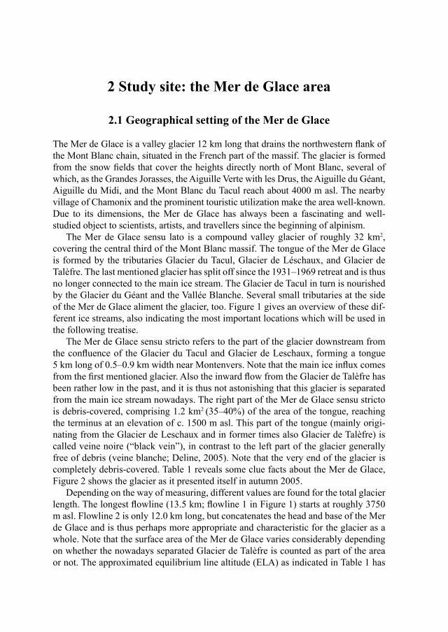
The Mer de Glace sensu lato is a compound valley glacier of roughly 32 km2, covering the central third of the Mont Blanc massif. The tongue of the Mer de Glace is formed by the tributaries Glacier du Tacul, Glacier de Léschaux, and Glacier de Talèfre. The last mentioned glacier has split off since the 1931–1969 retreat and is thus no longer connected to the main ice stream. The Glacier de Tacul in turn is nourished by the Glacier du Géant and the Vallée Blanche. Several small tributaries at the side of the Mer de Glace aliment the glacier, too. Figure 1 gives an overview of these dif-ferent ice streams, also indicating the most important locations which will be used in the following treatise.

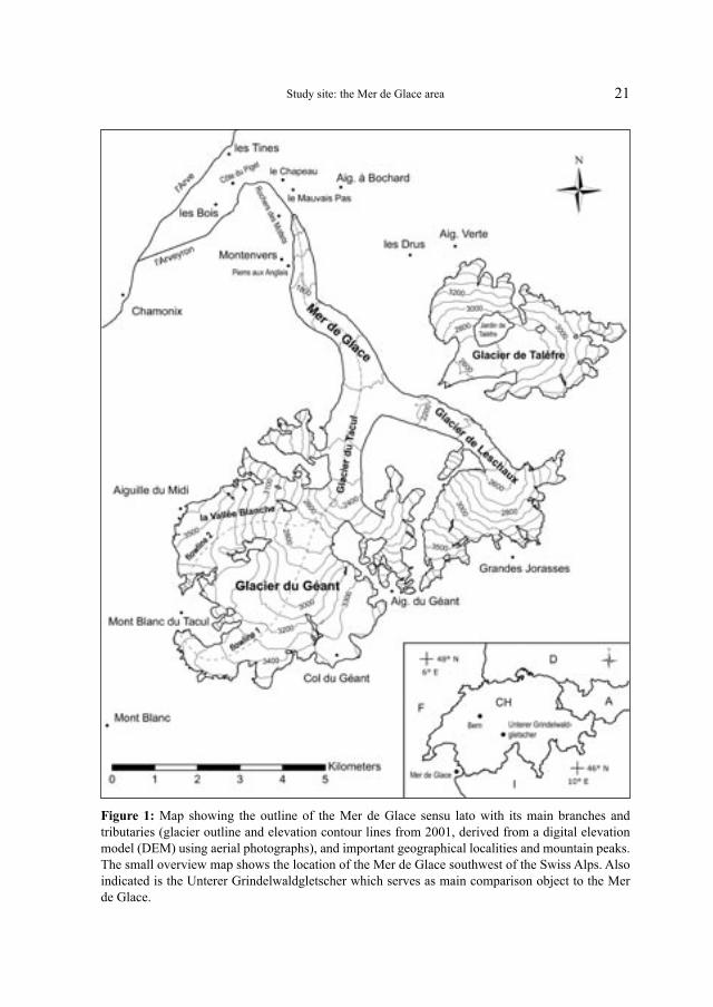
The Mer de Glace sensu stricto refers to the part of the glacier downstream from the confluence of the Glacier du Tacul and Glacier de Leschaux, forming a tongue 5 km long of 0.5–0.9 km width near Montenvers. Note that the main ice influx comes from the first mentioned glacier. Also the inward flow from the Glacier de Talèfre has been rather low in the past, and it is thus not astonishing that this glacier is separated from the main ice stream nowadays. The right part of the Mer de Glace sensu stricto is debris-covered, comprising 1.2 km2 (35–40%) of the area of the tongue, reaching the terminus at an elevation of c. 1500 m asl. This part of the tongue (mainly origi-nating from the Glacier de Leschaux and in former times also Glacier de Talèfre) is called veine noire (“black vein”), in contrast to the left part of the glacier generally free of debris (veine blanche; Deline, 2005). Note that the very end of the glacier is completely debris-covered. Table 1 reveals some clue facts about the Mer de Glace, Figure 2 shows the glacier as it presented itself in autumn 2005.

Depending on the way of measuring, different values are found for the total glacier length. The longest flowline (13.5 km; flowline 1 in Figure 1) starts at roughly 3750 m asl. Flowline 2 is only 12.0 km long, but concatenates the head and base of the Mer de Glace and is thus perhaps more appropriate and characteristic for the glacier as a whole. Note that the surface area of the Mer de Glace varies considerably depending on whether the nowadays separated Glacier de Talèfre is counted as part of the area or not. The approximated equilibrium line altitude (ELA) as indicated in Table 1 has

21Study site: the Mer de Glace area

Figure 1: Map showing the outline of the Mer de Glace sensu lato with its main branches and tributaries (glacier outline and elevation contour lines from 2001, derived from a digital elevation model (DEM) using aerial photographs), and important geographical localities and mountain peaks. The small overview map shows the location of the Mer de Glace southwest of the Swiss Alps. Also indicated is the Unterer Grindelwaldgletscher which serves as main comparison object to the Mer de Glace.

22

been determined by using an accumulation area ratio (AAR) of 0.67 and is situated at 2775 m asl. An AAR of 0.6 ± 0.05 is usually considered to characterize steady-state conditions of valley and cirque glaciers (Nesje and Dahl, 2000: 61). Note that this is a general formula for the approximate estimation of the equilibrium line. Direct mass balance measurements on the Mer de Glace exist just for a few points (Vincent, 2002). The ELA is situated in an area where the glacier passes an escarpment. If the ELA is situated in rather steep areas as in this case (less area that is close to the ELA), the sensitivity of a glacier is lower (Sugden and John, 1976: 105). The ice flow velocity of the glacier amounts to 100–150 m per year (above Montenvers), total ice volume is estimated as being 4 km3, and maximal ice thickness is 400 m (at Glacier du Tacul; Vivian, 2001: 131).

In 2001, the Mer de Glace terminated at 1467 m asl. into a small pond which formed on the morainic debris. Since 2000, the pond is divided into two water reser-voirs as a consequence of the collapse of a part of the right lateral moraine. Further down in the valley, the glacier overflowed a bedrock step (formed by the Rochers des Mottets on the left side and the Mauvais Pas rock wall to the right) at times when it had a larger extent than today. Into this bedrock, a gorge has been cut in the course

Figure 2: (a) Recent view of the Mer de Glace seen from la Flégère on the opposite side of the valley of Chamonix, France (Photograph by S. U. Nussbaumer, 8.10.2005). (b) The snout of the Mer de Glace beneath Mauvais Pas. Note the morainic foreland with the well-formed 1995 frontal moraine and the highly debris-covered glacier tongue ending near a pond (Photograph by S. U. Nussbaumer, 7.10.2005).

Study site: the Mer de Glace area

23

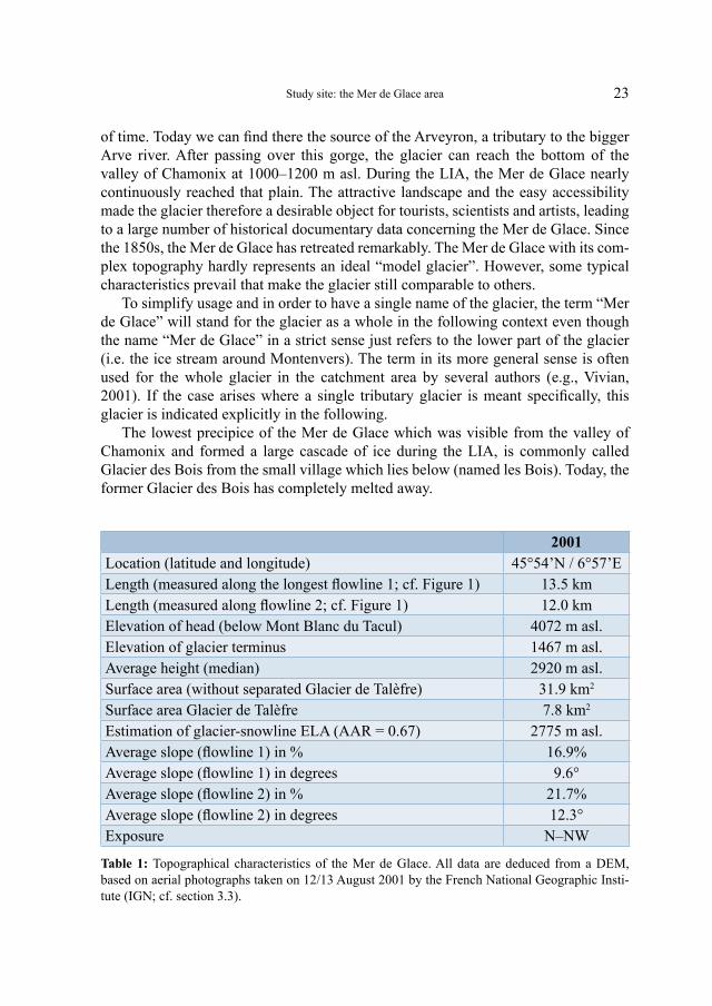
of time. Today we can find there the source of the Arveyron, a tributary to the bigger Arve river. After passing over this gorge, the glacier can reach the bottom of the valley of Chamonix at 1000–1200 m asl. During the LIA, the Mer de Glace nearly continuously reached that plain. The attractive landscape and the easy accessibility made the glacier therefore a desirable object for tourists, scientists and artists, leading to a large number of historical documentary data concerning the Mer de Glace. Since the 1850s, the Mer de Glace has retreated remarkably. The Mer de Glace with its com-plex topography hardly represents an ideal “model glacier”. However, some typical characteristics prevail that make the glacier still comparable to others.

To simplify usage and in order to have a single name of the glacier, the term “Mer de Glace” will stand for the glacier as a whole in the following context even though the name “Mer de Glace” in a strict sense just refers to the lower part of the glacier (i.e. the ice stream around Montenvers). The term in its more general sense is often used for the whole glacier in the catchment area by several authors (e.g., Vivian, 2001). If the case arises where a single tributary glacier is meant specifically, this glacier is indicated explicitly in the following.

The lowest precipice of the Mer de Glace which was visible from the valley of Chamonix and formed a large cascade of ice during the LIA, is commonly called Glacier des Bois from the small village which lies below (named les Bois). Today, the former Glacier des Bois has completely melted away.

2001 Location (latitude and longitude) 45°54’N / 6°57’E Length (measured along the longest flowline 1; cf. Figure 1) 13.5 km Length (measured along flowline 2; cf. Figure 1) 12.0 km Elevation of head (below Mont Blanc du Tacul) 4072 m asl. Elevation of glacier terminus 1467 m asl. Average height (median) 2920 m asl. Surface area (without separated Glacier de Talèfre) 31.9 km2 Surface area Glacier de Talèfre 7.8 km2 Estimation of glacier-snowline ELA (AAR = 0.67) 2775 m asl. Average slope (flowline 1) in % 16.9% Average slope (flowline 1) in degrees 9.6° Average slope (flowline 2) in % 21.7% Average slope (flowline 2) in degrees 12.3° Exposure N–NW

Table 1: Topographical characteristics of the Mer de Glace. All data are deduced from a DEM, based on aerial photographs taken on 12/13 August 2001 by the French National Geographic Insti-tute (IGN; cf. section 3.3).

Study site: the Mer de Glace area

24

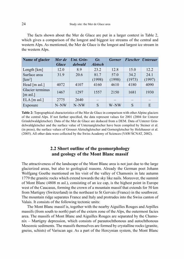
The facts shown about the Mer de Glace are put in a larger context in Table 2, which gives a comparison of the longest and biggest ice streams of the central and western Alps. As mentioned, the Mer de Glace is the longest and largest ice stream in the western Alps.

Name of glacier Mer de Glace

Unt. Grin-delwald

Gr. Aletsch

Gorner Fiescher Unteraar

Length [km] 12.0 8.9 23.2 12.8 15.0 12.2 Surface area [km2]

31.9 20.6 81.7 (1998)

57.0 (1998)

34.2 (1973)

24.1 (1997)

Head [m asl.] 4072 4107 4160 4610 4180 4090 Glacier terminus [m asl.]

1467 1297 1557 2150 1681 1930

ELA [m asl.] 2775 2640 – – – – Exposure N–NW N–NW S W–NW S E

Table 2: Topographical characteristics of the Mer de Glace in comparison with other Alpine glaciers of the central Alps. If not further specified, the data represent values for 2001 (2004 for Unterer Grindelwaldgletscher). Data of the Mer de Glace are deduced from a DEM. Data of Unterer Grin-delwaldgletscher and the surface value of Unteraargletscher have been compiled by Steiner et al. (in press), the surface values of Grosser Aletschgletscher and Gornergletscher by Holzhauser et al. (2005). All other data were collected by the Swiss Academy of Sciences (VAW/SCNAT, 2002).

2.2 Short outline of the geomorphology and geology of the Mont Blanc massif

The attractiveness of the landscape of the Mont Blanc area is not just due to the large glacierized areas, but also to geological reasons. Already the German poet Johann Wolfgang Goethe mentioned on his visit of the valley of Chamonix in late autumn 1779 the granitic rocks which extend towards the sky like nails. Moreover, the summit of Mont Blanc (4808 m asl.), consisting of an ice cap, is the highest point in Europe west of the Caucasus, forming the crown of a mountain massif that extends for 50 km from Martigny (Switzerland) in the northeast to St Gervais (France) in the southwest. The mountain ridge separates France and Italy and protrudes into the Swiss canton of Valais. It consists of the following tectonic units:

The Mont Blanc massif is, together with the nearby Aiguilles Rouges and Arpilles massifs (from south to north) part of the extern zone of the Alps, the outermost facies area. The massifs of Mont Blanc and Aiguilles Rouges are separated by the Chamo-nix – Martigny depression, which consists of parautochthonous and autochthonous Mesozoic sediments. The massifs themselves are formed by crystalline rocks (granite, gneiss, schists) of Variscan age. As a part of the Hercynian system, the Mont Blanc

Study site: the Mer de Glace area

25

massif consists of sedimentary rocks metamorphosed by granitic magmas. The central granites form the near vertical slopes of les Drus, Grandes Jorasses and Aiguille du Géant and are capped at the highest levels by crystalline schists which outcrop in the Grands Mulets and near the summit of Mont Blanc itself. Deep-valley cirques are overlooked by granite needles, heavily dissected by erosion. The Mont Blanc granite, also called protogine by the local people, contains less biotite but more quartz, which sets it apart from the Aiguilles Rouges granite (Trümpy, 1980).

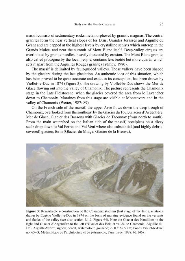
The massif is delimited by fault-guided valleys. Those valleys have been shaped by the glaciers during the last glaciation. An authentic idea of this situation, which has been proved to be quite accurate and exact in its conception, has been drawn by Viollet-le-Duc in 1874 (Figure 3). The drawing by Viollet-le-Duc shows the Mer de Glace flowing out into the valley of Chamonix. The picture represents the Chamonix stage in the Late Pleistocene, when the glacier covered the area from le Lavancher down to Chamonix. Moraines from this stage are visible at Montenvers and in the valley of Chamonix (Wetter, 1987: 89).

On the French side of the massif, the upper Arve flows down the deep trough of Chamonix, overlooked from the southeast by the Glacier du Tour, Glacier d’Argentière, Mer de Glace, Glacier des Bossons with Glacier de Taconnaz (from north to south). From the main watershed on the Italian side of the massif, precipices on a dizzy scale drop down to Val Ferret and Val Veni where also substantial (and highly debris- covered) glaciers form (Glacier du Miage, Glacier de la Brenva).

Figure 3: Remarkable reconstruction of the Chamonix stadium (last stage of the last glaciation), drawn by Eugène Viollet-le-Duc in 1874 on the basis of moraine evidence found on the versants and flanks of the valley (see also section 4.1.9, Figure 64). Note the Glacier des Nantillons to the right and Glacier d’Argentière to the left (“Glacier des Bois et vallée de Chamonix, Aiguille-du-Dru, Aiguille-Verte”; signed; pencil, watercolour, gouache; 29.0 x 69.5 cm; Fonds Viollet-le-Duc, no. 65–G; Médiathèque de l’architecture et du patrimoine, Paris; Frey, 1988: 63/146).

Study site: the Mer de Glace area

26

The Mont Blanc massif comprises large changes in elevation with a high relief. The Glacier des Bossons is a very impressive example, flowing (in contrast to the Mer de Glace) directly from the summit of Mont Blanc down to the Arve river valley. The massif shows a very high mean altitude which is the main cause for the occurrence of extensive glacier areas comparable to those of the central Alps. This stands in contrast to the other glacierized areas of France with a rather low mean altitude (despite high summits) where glaciers are small or very small in size (Reynaud, 1993).

2.3 Climate of the Mont Blanc area

The general climate in central Europe prevailing during the LIA has already been dis-cussed in section 1.2. At this point, those explanations may be completed by a short description of the actual climatic situation of the valley of Chamonix.

Not only forming the watershed separating the catchment areas of Rhône and Po, the chain of Mont Blanc also marks the border between two completely different cli-mate regions, separating the northern/western from the southern Alps. Weather condi-tions in the Mer de Glace area are therefore comparable to the north side of the Swiss Alps, although there might be some differences in particular weather situations (e.g., if southwest currents are prevailing).

The precipitation is evenly distributed in the French Alps over all months of the year. However, it strongly varies with elevation and exposure, also in the Mont Blanc area. The valley of Chamonix, situated at the bottom of the northwestern face of the Mont Blanc, receives, due to frequent westerly wind situations, much more precipita-tion than the valleys on the lee side. The precipitation in the French Alps is mostly due to a flow of maritime air from the west (Atlantic Ocean), whereas circulation from the southeast (Mediterranean Sea) is less common. Depending on changes in the tracks of low-pressure disturbances, north-south differences may be accentuated (Reynaud, 1993).

The annual precipitation sum for Chamonix (1054 m asl.) was 1262 mm for the 1934–1962 period, the mean annual temperature was 6.6°C during the 1935–1960 period (Vivian, 1969). Note that there is a high vertical precipitation gradient. At the Col du Midi at 3500 m asl., the annual precipitation amounts to 3100 mm, but near the summit of Mont Blanc at around 4250 m asl., the annual precipitation is lower and reaches only 1100 mm (1969–1979 period; Reynaud, 1993). Nevertheless, the climatic situation is comparable to the conditions in the Bernese Alps (especially the Grindelwald region; Steiner, 2005), apart from the fact that the valley of Chamonix is a little drier.

According to Corbel (1963), the climate in the valley of Chamonix is of continen-tal type with more than 10°C difference between the two temperature extremes (Janu-ary–July), a remarkable precipitation peak in summer (July–August) and a dry winter. However, Corbel (1963) was referring to Bénévent (1926) for those interpretations.

Study site: the Mer de Glace area

27

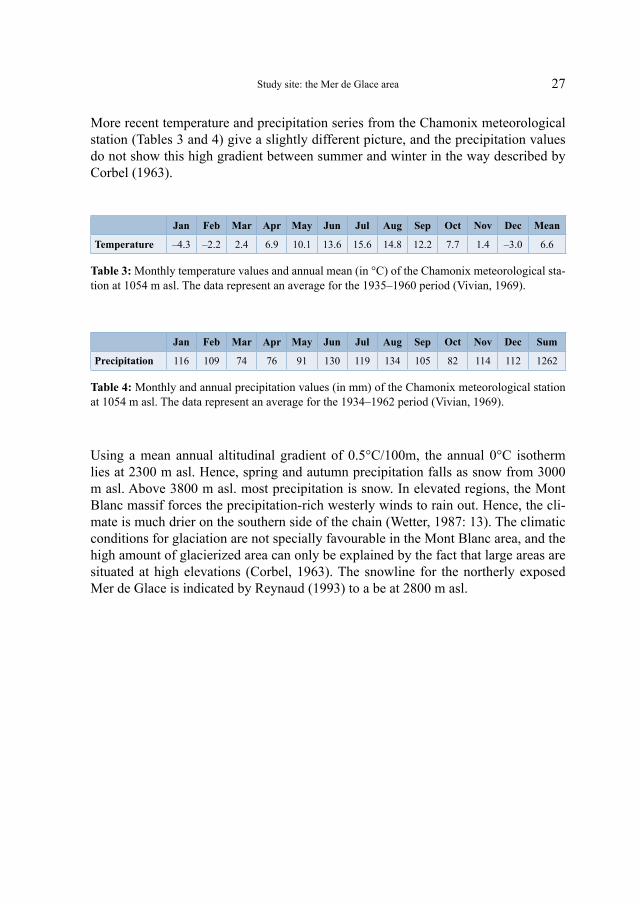
More recent temperature and precipitation series from the Chamonix meteorological station (Tables 3 and 4) give a slightly different picture, and the precipitation values do not show this high gradient between summer and winter in the way described by Corbel (1963).

Jan Feb Mar Apr May Jun Jul Aug Sep Oct Nov Dec Mean

Temperature –4.3 –2.2 2.4 6.9 10.1 13.6 15.6 14.8 12.2 7.7 1.4 –3.0 6.6

Table 3: Monthly temperature values and annual mean (in °C) of the Chamonix meteorological sta-tion at 1054 m asl. The data represent an average for the 1935–1960 period (Vivian, 1969).

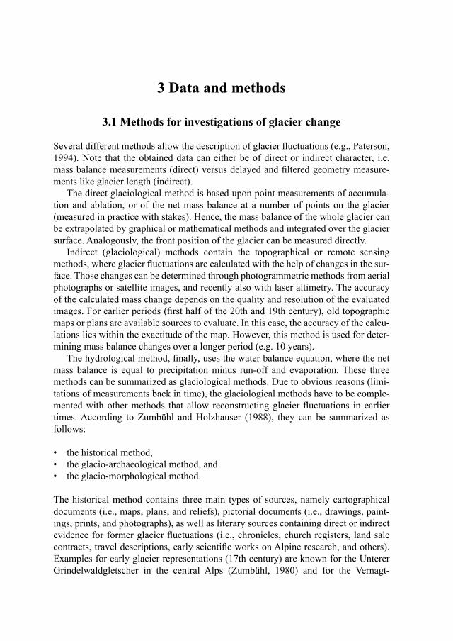
Jan Feb Mar Apr May Jun Jul Aug Sep Oct Nov Dec Sum

Precipitation 116 109 74 76 91 130 119 134 105 82 114 112 1262

Table 4: Monthly and annual precipitation values (in mm) of the Chamonix meteorological station at 1054 m asl. The data represent an average for the 1934–1962 period (Vivian, 1969).

Using a mean annual altitudinal gradient of 0.5°C/100m, the annual 0°C isotherm lies at 2300 m asl. Hence, spring and autumn precipitation falls as snow from 3000 m asl. Above 3800 m asl. most precipitation is snow. In elevated regions, the Mont Blanc massif forces the precipitation-rich westerly winds to rain out. Hence, the cli-mate is much drier on the southern side of the chain (Wetter, 1987: 13). The climatic conditions for glaciation are not specially favourable in the Mont Blanc area, and the high amount of glacierized area can only be explained by the fact that large areas are situated at high elevations (Corbel, 1963). The snowline for the northerly exposed Mer de Glace is indicated by Reynaud (1993) to a be at 2800 m asl.

Study site: the Mer de Glace area

3 Data and methods

3.1 Methods for investigations of glacier change

Several different methods allow the description of glacier fluctuations (e.g., Paterson, 1994). Note that the obtained data can either be of direct or indirect character, i.e. mass balance measurements (direct) versus delayed and filtered geometry measure-ments like glacier length (indirect).

The direct glaciological method is based upon point measurements of accumula-tion and ablation, or of the net mass balance at a number of points on the glacier (measured in practice with stakes). Hence, the mass balance of the whole glacier can be extrapolated by graphical or mathematical methods and integrated over the glacier surface. Analogously, the front position of the glacier can be measured directly.

Indirect (glaciological) methods contain the topographical or remote sensing methods, where glacier fluctuations are calculated with the help of changes in the sur-face. Those changes can be determined through photogrammetric methods from aerial photographs or satellite images, and recently also with laser altimetry. The accuracy of the calculated mass change depends on the quality and resolution of the evaluated images. For earlier periods (first half of the 20th and 19th century), old topographic maps or plans are available sources to evaluate. In this case, the accuracy of the calcu-lations lies within the exactitude of the map. However, this method is used for deter-mining mass balance changes over a longer period (e.g. 10 years).

The hydrological method, finally, uses the water balance equation, where the net mass balance is equal to precipitation minus run-off and evaporation. These three methods can be summarized as glaciological methods. Due to obvious reasons (limi-tations of measurements back in time), the glaciological methods have to be comple-mented with other methods that allow reconstructing glacier fluctuations in earlier times. According to Zumbühl and Holzhauser (1988), they can be summarized as follows:

• the historical method, • the glacio-archaeological method, and • the glacio-morphological method.

The historical method contains three main types of sources, namely cartographical documents (i.e., maps, plans, and reliefs), pictorial documents (i.e., drawings, paint-ings, prints, and photographs), as well as literary sources containing direct or indirect evidence for former glacier fluctuations (i.e., chronicles, church registers, land sale contracts, travel descriptions, early scientific works on Alpine research, and others). Examples for early glacier representations (17th century) are known for the Unterer Grindelwaldgletscher in the central Alps (Zumbühl, 1980) and for the Vernagt-

29

ferner in the eastern Alps (oldest pictorial documents known for a glacier; Nicolussi, 1990).

The density of historical material prior to 1800 highly depends on the elevation of the glacier tongue and the threatening of settlements and cultivated land due to glacier advances. Hints are also descriptions of pass routes that were easily or hardly accessible depending on the glacier extension, or the snow coverage, respectively. However, those pieces of information have to be considered carefully and local circumstances have to be taken into account. Information from travel descriptions started in the mid 18th century and went on until the mid 19th century when they were replaced by the much more accurate systematic measurements of glacier length changes. Since the mid 19th century, the historical material can also be complemented with the first photographs of glaciers. A rigorous selection of the available documentary data is necessary in order to get reliable information; additional information obtained by labour-intensive archive work is often needed, e.g. for dating a photograph of the glacier terminus.

Those sources of information are reliable (drawings, paintings, sketches and litho-graphs as well as written documents) and can yield valuable evidence of glacial extent and character if their dates are known and if the author intended an accurate repre-sentation of nature (e.g., Grove, 2004; Oerlemans, 2005). Especially in Europe, the historical sources are more plentiful than elsewhere, and have also more been worked on than in other parts of the world.

The glacio-archaeological method aims at finding evidence of former glacier extents by finding archaeological remains such as old trails, passes, foundations of destroyed buildings, relics of water conduits. Dating is often possible with the help of literary sources or by means of radiocarbon dating or dendrochronology.

The glacio-morphological method, finally, comprises the mapping of the glacier foreland and the moraines found therein. Major glacier advances are reflected in moraines that are often still visible nowadays. In the present study, the foreland of the Mer de Glace has been mapped by fieldwork and by the interpretation of aerial photo-graphs from 1980 and 2001 by the French National Geographic Institute (IGN).

Other relics that can be found in the glacier foreland are fossil soils, i.e. over-whelmed vegetation surfaces, which can be dated with the radiocarbon dating method. Fossil wood (trunks, rootstocks, roots, bushes) can either be dated by radiocarbon dating or dendrochronology. The latter utilizes the fact that different climatic condi-tions lead to narrow or wide tree rings. A complementary method is the analysis of the density of the tree rings (dendrodensitometry). The dendrochronological method has been applied e.g. by Holzhauser (2002) for the Grosser Aletschgletscher (central Alps) or by Nicolussi (1994) for Hintereisferner (eastern Alps). For the Mer de Glace, several wood probings from the right lateral moraine have been examined by Wetter (1987). In some cases, also the lichenometric method can be applied for the dating of moraines back to 1500 (Wetter, 1987).

All these methods allow the determination of glacier fluctuations of the Mer de Glace for the period of the LIA. Note that because of the formation of moraines and

Data and methods

30

the often existing threat to local inhabitants by glaciers, advancing periods are often much better documented than glacier retreats. Since 1878, the front variations of the Mer de Glace have been measured more or less continuously and are nowadays col-lected by the Laboratoire de Glaciologie et Géophysique de l’Environnement (LGGE) at Grenoble, France.

3.2 Historical data and methods

3.2.1 History of alpinism and important personalities regarding the Mont Blanc area

The Mont Blanc area and so the Mer de Glace were easily accessible from Geneva following the Arve river. This led several important personalities to visit the region. They represent the base for the following studies of the region and glaciers, not only on a local scale, but for the exploration of the entire Alpine chain in general.

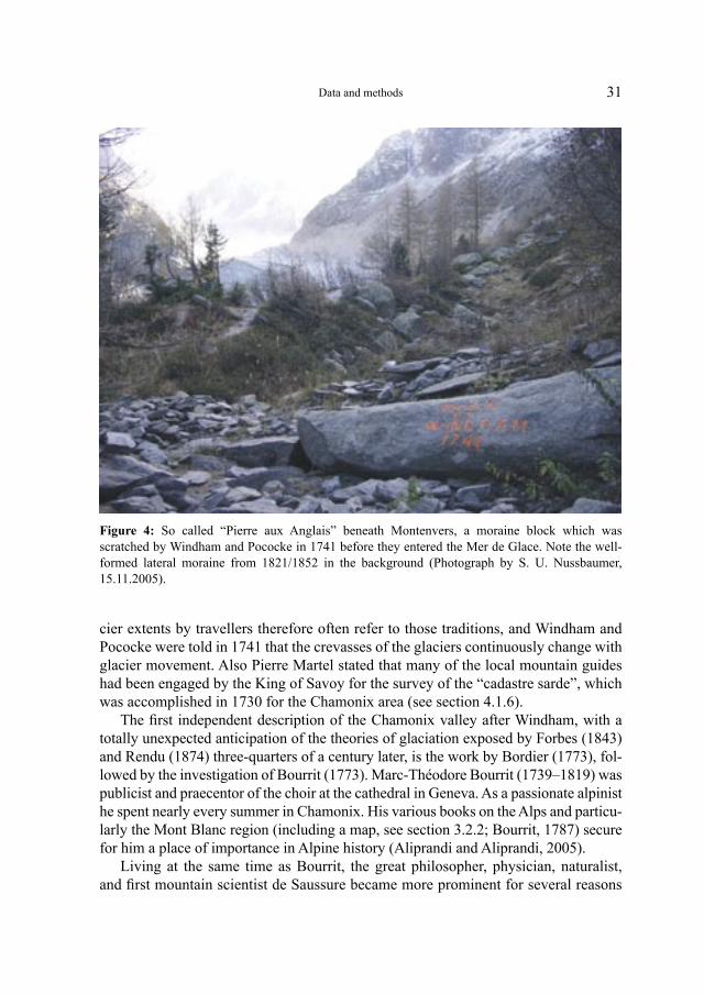
The Alpine and tourist history of the valley of Chamonix starts with the visit of the two English travellers William Windham (1717–1761) and Dr Richard Pococke (1704–1765) in 1741. They were probably the first foreigners to visit the Mer de Glace, and certainly the first to publish a record of their visit and to attract people’s attention to the Mont Blanc area. Windham’s letters on the visit became widely spread and are seen as the beginning of modern tourism in the Mont Blanc area, and the journey of Windham und Pococke to the Montenvers, where they entered the Mer de Glace, became legendary (Cunningham, 1990: 10). The two men engraved their names in a moraine block situated nowadays behind the 1821/1852 moraine beneath Montenvers (Figure 4) before they stepped onto the glacier (Wetter, 1987: 160).

In 1742, Pierre Martel, a Genevese engineer, repeated the Windham-Pococke expedition, which by then has also been published. Both accounts (by Windham, and Martel, respectively) were first published in French, but in 1744 the two were com-bined in one volume for an English translation, containing both Windham’s letters to his friend Arlaud and Pierre Martel’s letters to Windham, and also the first specific map of the Mont Blanc area, drawn by Martel (Martel, 1744; see section 3.2.2).

In the early days, the discovery of the valley of Chamonix was commonly attri-buted to those gentlemen. Though this was clearly incorrect, they were the first to provide any significant degree of publicity to Chamonix through the said publica-tions. Following the publication of Windham’s account, a visit to Chamonix became a “must” for the experienced British traveller. At the same time, it was recognized that Mont Blanc was the highest mountain, and this was assumed to mean that it was also the highest summit in the Old World, for at this time it was believed that only the Andes exceeded the Alps in altitude (Cunningham, 1990: 10).

The mountain guides that served the travellers were mostly chamois chasers or crystal seekers, knowing the glaciers very well. First descriptions of former gla-

Data and methods

31

cier extents by travellers therefore often refer to those traditions, and Windham and Pococke were told in 1741 that the crevasses of the glaciers continuously change with glacier movement. Also Pierre Martel stated that many of the local mountain guides had been engaged by the King of Savoy for the survey of the “cadastre sarde”, which was accomplished in 1730 for the Chamonix area (see section 4.1.6).

The first independent description of the Chamonix valley after Windham, with a totally unexpected anticipation of the theories of glaciation exposed by Forbes (1843) and Rendu (1874) three-quarters of a century later, is the work by Bordier (1773), fol-lowed by the investigation of Bourrit (1773). Marc-Théodore Bourrit (1739–1819) was publicist and praecentor of the choir at the cathedral in Geneva. As a passionate alpinist he spent nearly every summer in Chamonix. His various books on the Alps and particu-larly the Mont Blanc region (including a map, see section 3.2.2; Bourrit, 1787) secure for him a place of importance in Alpine history (Aliprandi and Aliprandi, 2005).

Living at the same time as Bourrit, the great philosopher, physician, naturalist, and first mountain scientist de Saussure became more prominent for several reasons

Data and methods

Figure 4: So called “Pierre aux Anglais” beneath Montenvers, a moraine block which was scratched by Windham and Pococke in 1741 before they entered the Mer de Glace. Note the well-formed lateral moraine from 1821/1852 in the background (Photograph by S. U. Nussbaumer, 15.11.2005).

32

(Sigrist, 2001). Horace Bénédict de Saussure (1740–1799) was the most famous member of a distinguished Huguenot family living in Geneva. He can be seen as the first and in some ways the greatest mountain scientist, and was the leading figure in a group of Genevese scholars which included Bourrit and the elder de Luc. Like his colleagues, de Saussure had a positive passion for the mountains, but at the same time there is no doubt that it was the pursuit of science which justified his excursions. He cultivated also a long friendship with the Bernese Albrecht von Haller.

Travelling through many parts of the Alps, de Saussure’s example has had a last-ing influence on mountain exploration and helped to form our present view and idea of the Alps, and his work revealed Mont Blanc to the European public. His “Voyages dans les Alpes” (de Saussure, 1779–1796), the first volume appeared in 1779, soon became a classic. It provided a hitherto unequalled store of information and acute observations about the topography, geology, glaciers, and meteorology of the Alps. Its chief shortcoming was the lack of an over-riding hypothesis by which its information and observations might be harmonized (Cunningham, 1990: 39). Volume 1 deals with the Chamonix area; Volume 2 is entirely about Mont Blanc itself; Volume 4 contains among others the 1788 expedition (see below). The first two volumes contain maps of the area (see section 3.2.2).

The work “Voyages dans les Alpes” contains several illustrations drawn and engraved by Marc-Théodore Bourrit, Adam-Wolfgang Töpffer and two amateurs, Jalabert and Bartoluzzi. Those illustrations are not only of value in the glacier history context, but are remarkably due to the novelty of their composition and their realism, revealing a world unpublished, in a time when the alarming legends were still remain-ing and circulating among the people and thus restrict the access to the high mountains to a small circle of well-informed aristocrats, dynamic and rich, because the scientific alibi was then indispensable: it was the only thing which authorized undaunted expe-ditions that common sense disapproved (Bourrit, 1773: 149). Moreover, these illustra-tions introduced the realistic representation of the high mountains into the iconogra-phy of Genevese painting and thus led to a new kind of landscape painting. Following Caspar Wolf (1735–1783), several Genevese artists including Jean-Antoine Linck (see below and sections 4.1.7 and 4.1.8) took over those new definitions to create a new genre of Alpine painting (Bouchardy, 1986: 5).

In 1760, de Saussure offered a prize to the first person to reach the summit of Mont Blanc. The route thus opened would have enabled the Genevese scientist to attempt the ascent to perform scientific observations on the summit. However, it was to take 26 years until the first successful ascent to the summit became reality on 8 August 1786 by the two Chamoniards Jacques Balmat (1762–1834), a crystal seeker and mountain guide, and Dr Michel Gabriel Paccard (1757–1827), doctor in Chamonix and enthusiastic alpinist. De Saussure was the third who lucked to climb the mountain on 3 August 1787 in company of his servant and with Jacques Balmat (Figure 5) and many other guides and with lot of equipment, performing the first scientific observa-tions and measurements on the summit.

Data and methods

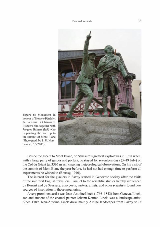
33

Beside the ascent to Mont Blanc, de Saussure’s greatest exploit was in 1788 when, with a large party of guides and porters, he stayed for seventeen days (3–19 July) on the Col du Géant (at 3365 m asl.) making meteorological observations. On his visit of the summit of Mont Blanc the year before, he had not had enough time to perform all experiments he wished to (Roussy, 1940).

The interest for the glaciers in Savoy started in Genevese society after the visits of the said first English travellers. Parallel to the scientific studies hereby influenced by Bourrit and de Saussure, also poets, writers, artists, and other scientists found new sources of inspiration in those mountains.

A very prominent artist was Jean-Antoine Linck (1766–1843) from Geneva. Linck, son and student of the enamel painter Johann Konrad Linck, was a landscape artist. Since 1789, Jean-Antoine Linck drew mainly Alpine landscapes from Savoy to St

Data and methods

Figure 5: Monument in honour of Horace-Bénédict de Saussure in Chamonix. It shows him together with Jacques Balmat (left) who is pointing the trail up to the summit of Mont Blanc (Photograph by S. U. Nuss-baumer, 5.5.2005).

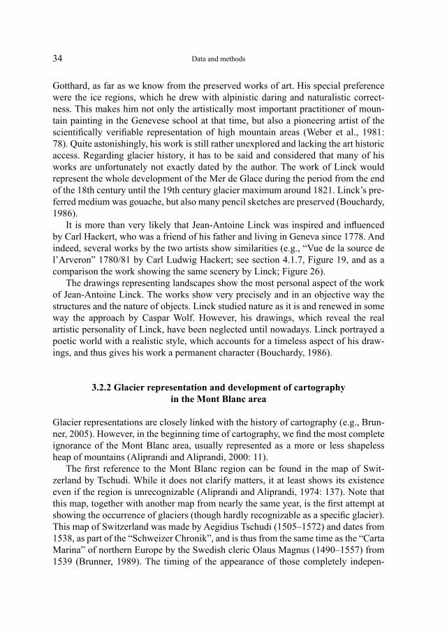
34

Gotthard, as far as we know from the preserved works of art. His special preference were the ice regions, which he drew with alpinistic daring and naturalistic correct-ness. This makes him not only the artistically most important practitioner of moun-tain painting in the Genevese school at that time, but also a pioneering artist of the scientifically verifiable representation of high mountain areas (Weber et al., 1981: 78). Quite astonishingly, his work is still rather unexplored and lacking the art historic access. Regarding glacier history, it has to be said and considered that many of his works are unfortunately not exactly dated by the author. The work of Linck would represent the whole development of the Mer de Glace during the period from the end of the 18th century until the 19th century glacier maximum around 1821. Linck’s pre-ferred medium was gouache, but also many pencil sketches are preserved (Bouchardy, 1986).

It is more than very likely that Jean-Antoine Linck was inspired and influenced by Carl Hackert, who was a friend of his father and living in Geneva since 1778. And indeed, several works by the two artists show similarities (e.g., “Vue de la source de l’Arveron” 1780/81 by Carl Ludwig Hackert; see section 4.1.7, Figure 19, and as a comparison the work showing the same scenery by Linck; Figure 26).

The drawings representing landscapes show the most personal aspect of the work of Jean-Antoine Linck. The works show very precisely and in an objective way the structures and the nature of objects. Linck studied nature as it is and renewed in some way the approach by Caspar Wolf. However, his drawings, which reveal the real artistic personality of Linck, have been neglected until nowadays. Linck portrayed a poetic world with a realistic style, which accounts for a timeless aspect of his draw-ings, and thus gives his work a permanent character (Bouchardy, 1986).

3.2.2 Glacier representation and development of cartography in the Mont Blanc area

Glacier representations are closely linked with the history of cartography (e.g., Brun-ner, 2005). However, in the beginning time of cartography, we find the most complete ignorance of the Mont Blanc area, usually represented as a more or less shapeless heap of mountains (Aliprandi and Aliprandi, 2000: 11).

The first reference to the Mont Blanc region can be found in the map of Swit-zerland by Tschudi. While it does not clarify matters, it at least shows its existence even if the region is unrecognizable (Aliprandi and Aliprandi, 1974: 137). Note that this map, together with another map from nearly the same year, is the first attempt at showing the occurrence of glaciers (though hardly recognizable as a specific glacier). This map of Switzerland was made by Aegidius Tschudi (1505–1572) and dates from 1538, as part of the “Schweizer Chronik”, and is thus from the same time as the “Carta Marina” of northern Europe by the Swedish cleric Olaus Magnus (1490–1557) from 1539 (Brunner, 1989). The timing of the appearance of those completely indepen-

Data and methods

35

dent maps may not be coincidental, as this is the time of first glacier advances of the beginning LIA period, e.g. in the European Alps (Zumbühl et al., 1983; Pfister, 1999). Interesting is the fact that also later heavy glacier advances were reflected by several independent cartographers (Brunner, 1989).

The first specific map showing the Mont Blanc massif is the map of Savoy by Tomaso Borgonio (born around 1620), made between 1672 and 1677 and containing 15 sheets at the scale of 1:150’000. It just shows the inscription “Les Glacières” where the Mont Blanc area is situated. The Lombardia map by Nicolas Sanson d’Abbéville (1600–1667) from 1648 also gives the toponym “Les Glacières” and is the first map to indicate the “Col Major”, a legendary passage between Courmayeur and Chamonix. It is about a pass which will be mentioned again in later maps up to the end of the 18th century. Sanson’s map is the first cartographical document where the toponym “Les Glacières” can be referred to the Mont Blanc area (Aliprandi and Aliprandi, 2000: 39).

Note that the mid 17th century was a time of high glacier activity (see section 1.2). Nearly a century later, the 1768 map of the canton of Valais (Switzerland) by Gabriel Walser (1695–1776) contains the notes “SAVOYEN abscheuliche Eisberge Gletscher Glaciers Montes Glaciales genannt” (Brunner, 1989).

The first specific though very simple glacier map was made by Martel. Martel made a sketch of the Arve area in 1742 on which the glaciers of Chamonix are repre-sented, and which was published in 1744. The map is rudimentary as Martel, after being in Montenvers, did not have more than three hours for making a plan of the glaciers (Grove, 2004: 103), and it is thus more appropriate to call it a sketch. How-ever, the great novelty of this sketch is the representation and denomination of peaks and glaciers many of which had been nameless up to that time. The map represents the idea that the glaciers were simply cascades of ice coming from a great central reservoir where snow and ice had accumulated. Such an idea must have been very common in the 18th century, also in other parts of the Alps (Aliprandi and Aliprandi, 1974: 153). This map could usefully have integrated the information available to the cartographers at that time and completed the knowledge of the area avoiding the repetition of mistakes and the omissions of the previous centuries. But the map had in reality a very limited distribution, because only a small number of copies of the book-let “An account of the glacieres or ice Alps in Savoy” which included the map had been printed by Martel (1744). Nevertheless, the booklet had considerable influence on the British public and certainly roused curiosity about Alpine valleys (Aliprandi and Aliprandi, 1974: 153).

Two other maps that follow were made by Pictet; they are still very coarse, but for the first time they comprise the Mont Blanc glaciers as a whole. Marc-Auguste Pictet (1752–1825) was a topographer on de Saussure’s expeditions, and it is due to him that we have the important surveys of the great map illustrating the second volume of de Saussure’s “Voyages dans les Alpes” (Figure 6; de Saussure, 1786). Note that depend-ing on the edition, some details on the map may differ from other copies. The map has

Data and methods

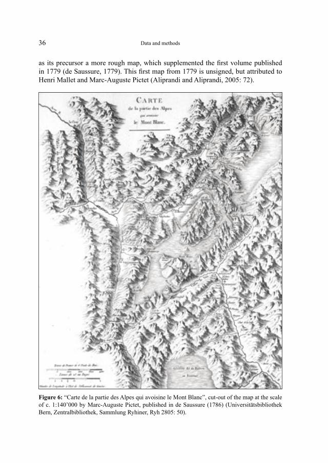
36 Data and methods

Figure 6: “Carte de la partie des Alpes qui avoisine le Mont Blanc”, cut-out of the map at the scale of c. 1:140’000 by Marc-Auguste Pictet, published in de Saussure (1786) (Universitätsbibliothek Bern, Zentralbibliothek, Sammlung Ryhiner, Ryh 2805: 50).

as its precursor a more rough map, which supplemented the first volume published in 1779 (de Saussure, 1779). This first map from 1779 is unsigned, but attributed to Henri Mallet and Marc-Auguste Pictet (Aliprandi and Aliprandi, 2005: 72).

37

From the viewpoint of cartography, the map inserted in de Saussure’s work marks a remarkable step forward. Originally, the plan had been to adopt an existing map for the book and to complete it with observations of his own, which failed, though. Hence, the Pictet map is unrelated to traditional representations and gives a picture of the area based on data derived from direct observations. The prestige of de Saussure and the wide distribution of his work were such that the results reached could no lon-ger be ignored, and were brought to the attention of the European public (Aliprandi and Aliprandi, 2005: 73).

It is worth mentioning that the maps by de Saussure were judged as being very poor by Forbes in an article of the North British Review in 1865: “… it is hardly pos-sible to speak too disparagingly [of de Saussure’s maps]. They are in one sense worse than the map of Martel because they are filled up with material absolutely fictitious.” (Forbes, 1900: 537).

This shows that Forbes made great demands on a map. The statement is justified by Forbes by an examination of the maps and a comparison with reality. Even conced-ing that all of Forbes’ remarks are right, the fact remains that the map by de Saussure was the first one to represent the area with any detail, and the map is therefore anyway an unquestionable advance.

In 1785, a sketch map including the Mont Blanc area on one hand appeared inserted in Bourrit’s descriptions of the Alps of Savoy, but without new elements compared to the previous maps (Bourrit, 1785). In contrast, the 1790 map by Charles-François Exchaquet (“Carte en perspéctive de la Vallée de Chamouni et des montagnes avoi-sinantes dans le Haut Faucigni”; a reprint of this map was published in 1818) contains a lot of new toponyms; and although the map is not very detailed in the valleys, it is a step forward in the cartographic exploration of the Mont Blanc (Aliprandi and Aliprandi, 2000: 89). The map is not to be confused with several maps which were drawn after the relief by Exchaquet (see section 4.1.7).

The French cartography work “Carte de Cassini” was made between 1756 and 1789 and contains also areas with glaciers, but does not cover the Mont Blanc area. In the 19th century, the “Carte de l’Etat Major” at the scale of 1:80’000 followed that early cartographical document, then including the Mont Blanc area. The map sheets covering the Alps were made between 1860 and 1880. Hence, this map represents the retreating glaciers (Brunner, 1989). The map sheet “Vallorcine” with the Mer de Glace was published in 1867 (see section 4.1.9).

Although published not earlier than 1815 for editorial reasons, the map “Carte phy-sique et minéralogique du Mont Blanc et des montagnes et vallées qui l’avoisinent” by Jean-Baptiste Raymond (1766–1830) has ground surveys performed in 1797–1799 as its base. The map at the scale of c. 1:86’400 aimed at complementing the work by de Saussure’s “Voyages dans les Alpes” for the use of travellers to the valley of Chamonix. The representation of nature given by the map is very realistic, and as a consequence, the map is judged by Forbes as much better than the map by de Saussure (Aliprandi and Aliprandi, 2000: 87).

Data and methods

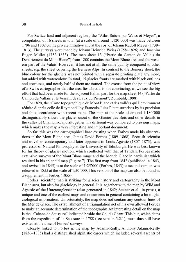
38

For Switzerland and adjacent regions, the “Atlas Suisse par Weiss et Meyer”, a compilation of 16 sheets in total (at a scale of around 1:120’000) was made between 1796 and 1802 on the private initiative and at the cost of Johann Rudolf Meyer (1739–1813). The surveys were made by Johann Heinrich Weiss (1758–1826) and Joachim Eugen Müller (1752–1833). The map sheet 13 (“Partie du Canton du Vallais du Departement du Mont Blanc”) from 1800 contains the Mont Blanc area and the west-ern part of the Valais. However, it has not at all the same quality compared to other sheets, e.g. the sheet covering the Bernese Alps. In contrast to the Bernese sheet, the blue colour for the glaciers was not printed with a separate printing plate any more, but added with watercolour. In total, 15 glacier fronts are marked with black outlines and crevasses, and nearly half of them are named. The excuse from the point of view of a Swiss cartographer that the area lies abroad is not convincing, as we see the big effort that had been made for the adjacent Italian part for the map sheet 14 (“Partie du Canton du Vallais et le Versant des Eaux du Piemont”; Zumbühl, 1998).

For 1829, the “Carte topographique du Mont Blanc et des vallées qui l’environnent réduite d’après celle de Raymond” by François-Jules Pictet surprises by its precision and thus accordance with recent maps. The map at the scale of around 1:180’000 distinguishably shows the glacier snout of the Glacier des Bois and other details in the valley of Chamonix, and altogether in a different way compared to previous maps, which makes the map a very interesting and important document.

So far, this was the cartographical base existing when Forbes made his observa-tions in the Mont Blanc area. James David Forbes (1809–1868), Scottish scientist and traveller, contemporary and later opponent to Louis Agassiz (1807–1873), was professor of Natural Philosophy at the University of Edinburgh. He was best known for his theory of glacier motion, which conflicted with that of Tyndall. Forbes made extensive surveys of the Mont Blanc range and the Mer de Glace in particular which resulted in his splendid map (Figure 7). The first map from 1842 (published in 1843, and revised in 1845) is at the scale of 1:25’000 (Forbes, 1843); a second version was released in 1855 at the scale of 1:50’000. This version of the map can also be found as a supplement in Forbes (1855).

Forbes’ scientific map is striking for glacier history and cartography in the Mont Blanc area, but also for glaciology in general. It is, together with the map by Wild and Agassiz of the Unteraargletscher (also generated in 1842; Steiner et al., in press), a unique and one of the earliest maps and documents in general containing a lot of gla-ciological information. Unfortunately, the map does not contain any contour lines of the Mer de Glace. The establishment of a triangulation net of his own allowed Forbes to make an accurate determination of the topography. An interesting detail on the map is the “Cabane de Saussure” indicated beside the Col du Géant. This hut, which dates from the expedition of de Saussure in 1788 (see section 3.2.1), must thus still have existed at the time of Forbes’ surveys.

Closely linked to Forbes is the map by Adams-Reilly. Anthony Adams-Reilly (1836–1885) had a distinguished alpinistic career which included several ascents of

Data and methods

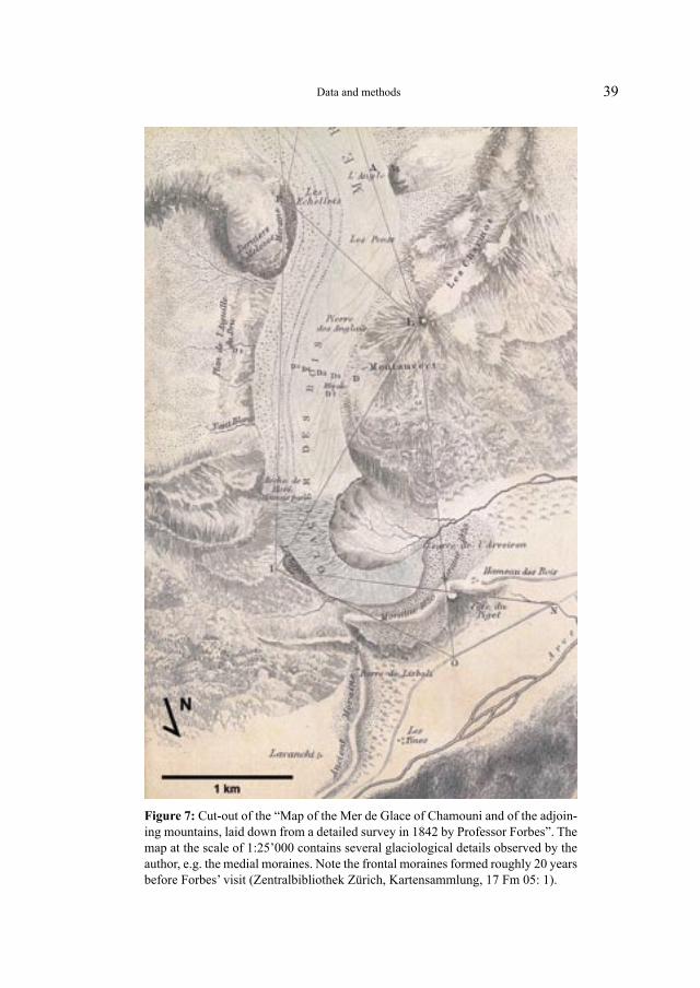
39Data and methods

Figure 7: Cut-out of the “Map of the Mer de Glace of Chamouni and of the adjoin-ing mountains, laid down from a detailed survey in 1842 by Professor Forbes”. The map at the scale of 1:25’000 contains several glaciological details observed by the author, e.g. the medial moraines. Note the frontal moraines formed roughly 20 years before Forbes’ visit (Zentralbibliothek Zürich, Kartensammlung, 17 Fm 05: 1).

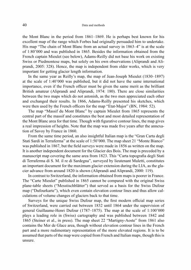
40

the Mont Blanc in the period from 1861–1869. He is perhaps best known for his excellent map of the range which Forbes had originally persuaded him to undertake. His map “The chain of Mont Blanc from an actual survey in 1863–4” is at the scale of 1:80’000 and was published in 1865. Besides the information obtained from the French captain Mieulet (see below), Adams-Reilly did not base his work on existing Swiss or Piedmontese maps, but solely on his own observations (Aliprandi and Ali-prandi, 2005: 328). Hence, the map is independent from older works, which is very important for getting glacier length information.

In the same year as Reilly’s map, the map of Jean-Joseph Mieulet (1830–1897) at the scale of 1:40’000 was published, but it did not have the same international importance, even if the French officer must be given the same merit as the brilliant British amateur (Aliprandi and Aliprandi, 1974: 180). There are close similarities between the two maps which do not astonish, as the two men appreciated each other and exchanged their results. In 1866, Adams-Reilly presented his sketches, which were then used by the French officers for the map “Etat-Major” (BN, 1984: 52).

The map “Massif du Mont Blanc” by captain Mieulet from 1865 represents the central part of the massif and constitutes the best and most detailed representation of the Mont Blanc area for that time. Though with figurative contour lines, the map gives a real impression of heights. Note that the map was made five years after the annexa-tion of Savoy by France in 1860.

From the same time period, an also insightful Italian map is the “Gran Carta degli Stati Sardi in Terraferma” at the scale of 1:50’000. The map sheet 21 “Monte Bianco” was published in 1867, but the field surveys were made in 1856 as written on the map. It is another independent document for the Glacier des Bois. The map is preceded by a manuscript map covering the same area from 1823. This “Carta topografia degli Stati di Terraferma di S. M. il re di Sardegna”, surveyed by lieutenant Muletti, constitutes an important document for the maximum glacier extension during the LIA, as the gla-cier advance from around 1820 is shown (Aliprandi and Aliprandi, 2000: 119).

In contrast to Switzerland, the information obtained from maps is poorer in France. The “Carte Mieulet” published in 1865 cannot be compared with the original Swiss plane-table sheets (“Messtischblätter”) that served as a basis for the Swiss Dufour map (“Dufourkarte”), which even contain elevation contour lines and thus allow cal-culations of volume changes of glaciers back to that time.

Surveys for the unique Swiss Dufour map, the first modern official map series of Switzerland, were carried out between 1832 until 1864 under the supervision of general Guillaume-Henri Dufour (1787–1875). The map at the scale of 1:100’000 plays a leading role in (Swiss) cartography and was published between 1842 and 1865 (Steiner et al., in press). The map sheet 22 “Martigny-Aoste” from 1861 also contains the Mer de Glace area, though without elevation contour lines in the French part and a more rudimentary representation of the more elevated regions. It is to be assumed that parts of the map were copied from French and Italian maps, though this is unsure.

Data and methods

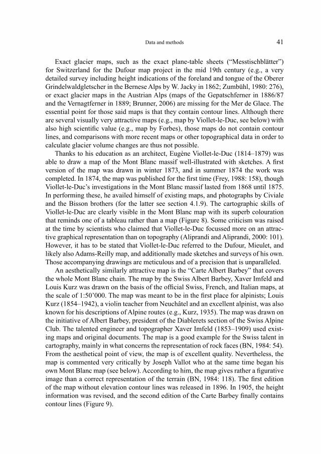
41

Exact glacier maps, such as the exact plane-table sheets (“Messtischblätter”) for Switzerland for the Dufour map project in the mid 19th century (e.g., a very detailed survey including height indications of the foreland and tongue of the Oberer Grindelwaldgletscher in the Bernese Alps by W. Jacky in 1862; Zumbühl, 1980: 276), or exact glacier maps in the Austrian Alps (maps of the Gepatschferner in 1886/87 and the Vernagtferner in 1889; Brunner, 2006) are missing for the Mer de Glace. The essential point for those said maps is that they contain contour lines. Although there are several visually very attractive maps (e.g., map by Viollet-le-Duc, see below) with also high scientific value (e.g., map by Forbes), those maps do not contain contour lines, and comparisons with more recent maps or other topographical data in order to calculate glacier volume changes are thus not possible.

Thanks to his education as an architect, Eugène Viollet-le-Duc (1814–1879) was able to draw a map of the Mont Blanc massif well-illustrated with sketches. A first version of the map was drawn in winter 1873, and in summer 1874 the work was completed. In 1874, the map was published for the first time (Frey, 1988: 158), though Viollet-le-Duc’s investigations in the Mont Blanc massif lasted from 1868 until 1875. In performing these, he availed himself of existing maps, and photographs by Civiale and the Bisson brothers (for the latter see section 4.1.9). The cartographic skills of Viollet-le-Duc are clearly visible in the Mont Blanc map with its superb colouration that reminds one of a tableau rather than a map (Figure 8). Some criticism was raised at the time by scientists who claimed that Viollet-le-Duc focussed more on an attrac-tive graphical representation than on topography (Aliprandi and Aliprandi, 2000: 101). However, it has to be stated that Viollet-le-Duc referred to the Dufour, Mieulet, and likely also Adams-Reilly map, and additionally made sketches and surveys of his own. Those accompanying drawings are meticulous and of a precision that is unparalleled.

An aesthetically similarly attractive map is the “Carte Albert Barbey” that covers the whole Mont Blanc chain. The map by the Swiss Albert Barbey, Xaver Imfeld and Louis Kurz was drawn on the basis of the official Swiss, French, and Italian maps, at the scale of 1:50’000. The map was meant to be in the first place for alpinists; Louis Kurz (1854–1942), a violin teacher from Neuchâtel and an excellent alpinist, was also known for his descriptions of Alpine routes (e.g., Kurz, 1935). The map was drawn on the initiative of Albert Barbey, president of the Diablerets section of the Swiss Alpine Club. The talented engineer and topographer Xaver Imfeld (1853–1909) used exist-ing maps and original documents. The map is a good example for the Swiss talent in cartography, mainly in what concerns the representation of rock faces (BN, 1984: 54). From the aesthetical point of view, the map is of excellent quality. Nevertheless, the map is commented very critically by Joseph Vallot who at the same time began his own Mont Blanc map (see below). According to him, the map gives rather a figurative image than a correct representation of the terrain (BN, 1984: 118). The first edition of the map without elevation contour lines was released in 1896. In 1905, the height information was revised, and the second edition of the Carte Barbey finally contains contour lines (Figure 9).

Data and methods

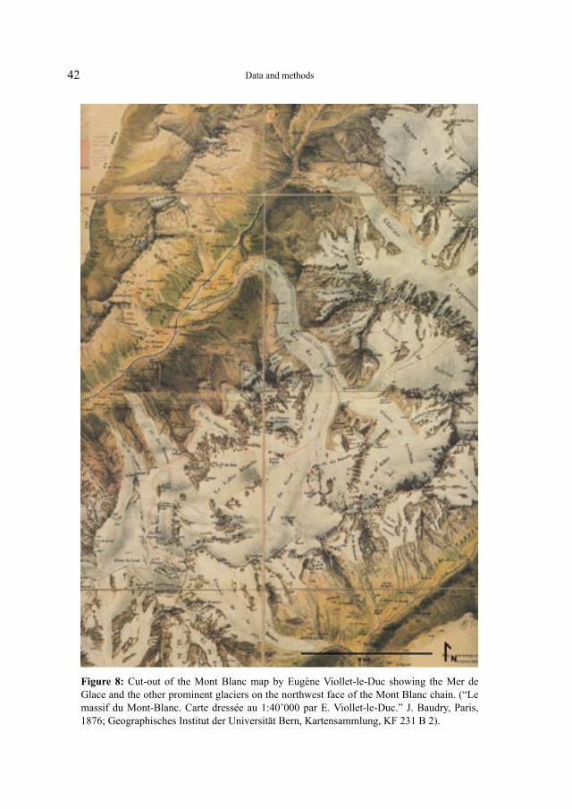
42

Figure 8: Cut-out of the Mont Blanc map by Eugène Viollet-le-Duc showing the Mer de Glace and the other prominent glaciers on the northwest face of the Mont Blanc chain. (“Le massif du Mont-Blanc. Carte dressée au 1:40’000 par E. Viollet-le-Duc.” J. Baudry, Paris, 1876; Geographisches Institut der Universität Bern, Kartensammlung, KF 231 B 2).

Data and methods

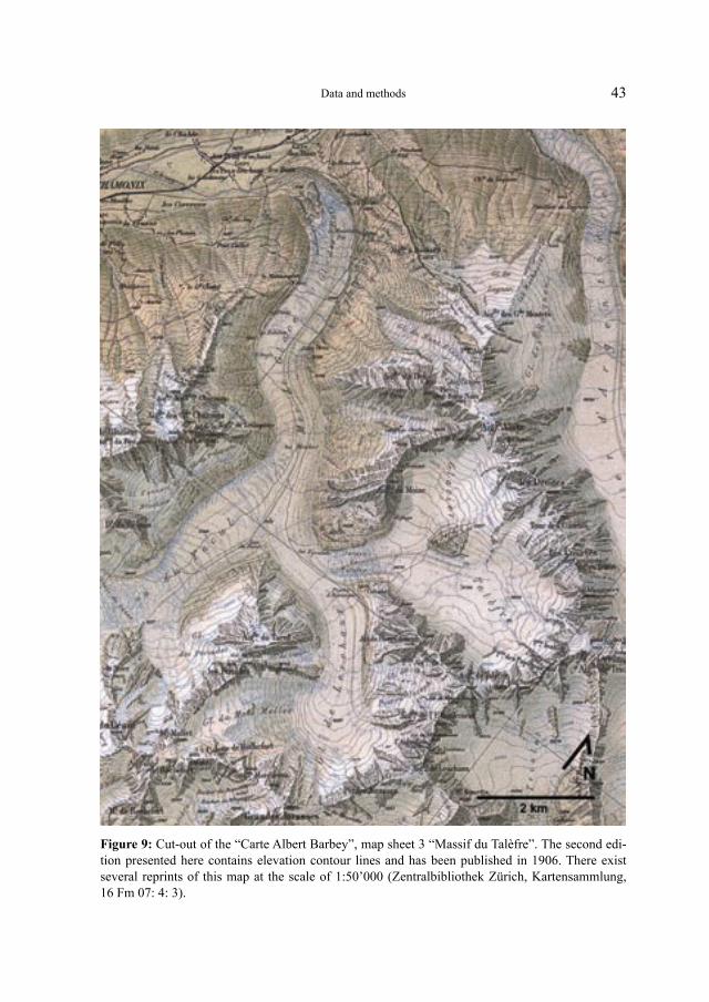
43

Figure 9: Cut-out of the “Carte Albert Barbey”, map sheet 3 “Massif du Talèfre”. The second edi-tion presented here contains elevation contour lines and has been published in 1906. There exist several reprints of this map at the scale of 1:50’000 (Zentralbibliothek Zürich, Kartensammlung, 16 Fm 07: 4: 3).

Data and methods

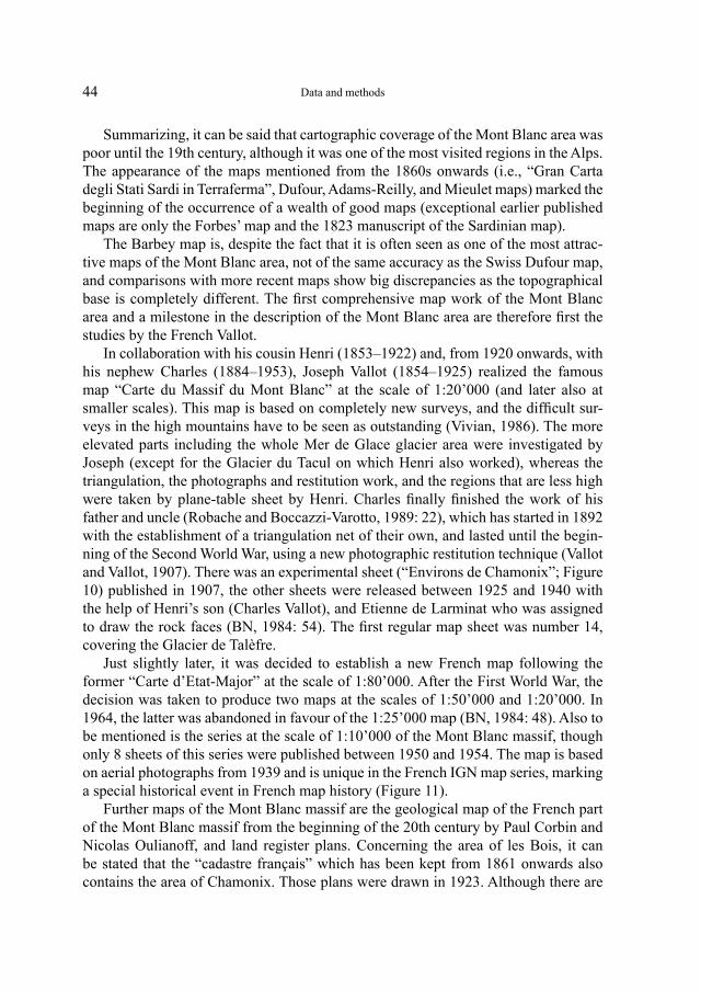
44

Summarizing, it can be said that cartographic coverage of the Mont Blanc area was poor until the 19th century, although it was one of the most visited regions in the Alps. The appearance of the maps mentioned from the 1860s onwards (i.e., “Gran Carta degli Stati Sardi in Terraferma”, Dufour, Adams-Reilly, and Mieulet maps) marked the beginning of the occurrence of a wealth of good maps (exceptional earlier published maps are only the Forbes’ map and the 1823 manuscript of the Sardinian map).

The Barbey map is, despite the fact that it is often seen as one of the most attrac-tive maps of the Mont Blanc area, not of the same accuracy as the Swiss Dufour map, and comparisons with more recent maps show big discrepancies as the topographical base is completely different. The first comprehensive map work of the Mont Blanc area and a milestone in the description of the Mont Blanc area are therefore first the studies by the French Vallot.

In collaboration with his cousin Henri (1853–1922) and, from 1920 onwards, with his nephew Charles (1884–1953), Joseph Vallot (1854–1925) realized the famous map “Carte du Massif du Mont Blanc” at the scale of 1:20’000 (and later also at smaller scales). This map is based on completely new surveys, and the difficult sur-veys in the high mountains have to be seen as outstanding (Vivian, 1986). The more elevated parts including the whole Mer de Glace glacier area were investigated by Joseph (except for the Glacier du Tacul on which Henri also worked), whereas the triangulation, the photographs and restitution work, and the regions that are less high were taken by plane-table sheet by Henri. Charles finally finished the work of his father and uncle (Robache and Boccazzi-Varotto, 1989: 22), which has started in 1892 with the establishment of a triangulation net of their own, and lasted until the begin-ning of the Second World War, using a new photographic restitution technique (Vallot and Vallot, 1907). There was an experimental sheet (“Environs de Chamonix”; Figure 10) published in 1907, the other sheets were released between 1925 and 1940 with the help of Henri’s son (Charles Vallot), and Etienne de Larminat who was assigned to draw the rock faces (BN, 1984: 54). The first regular map sheet was number 14, covering the Glacier de Talèfre.

Just slightly later, it was decided to establish a new French map following the former “Carte d’Etat-Major” at the scale of 1:80’000. After the First World War, the decision was taken to produce two maps at the scales of 1:50’000 and 1:20’000. In 1964, the latter was abandoned in favour of the 1:25’000 map (BN, 1984: 48). Also to be mentioned is the series at the scale of 1:10’000 of the Mont Blanc massif, though only 8 sheets of this series were published between 1950 and 1954. The map is based on aerial photographs from 1939 and is unique in the French IGN map series, marking a special historical event in French map history (Figure 11).

Further maps of the Mont Blanc massif are the geological map of the French part of the Mont Blanc massif from the beginning of the 20th century by Paul Corbin and Nicolas Oulianoff, and land register plans. Concerning the area of les Bois, it can be stated that the “cadastre français” which has been kept from 1861 onwards also contains the area of Chamonix. Those plans were drawn in 1923. Although there are

Data and methods

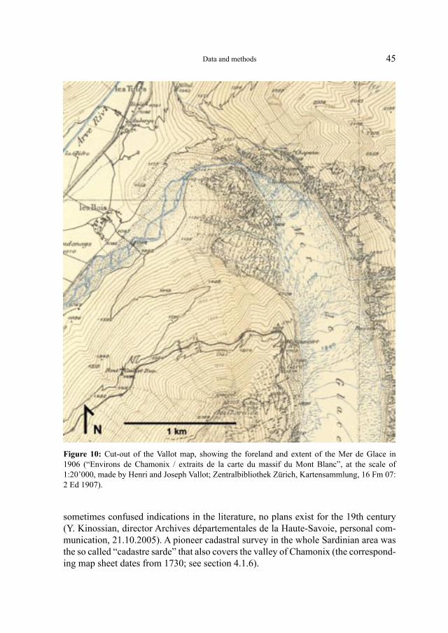
45

sometimes confused indications in the literature, no plans exist for the 19th century (Y. Kinossian, director Archives départementales de la Haute-Savoie, personal com-munication, 21.10.2005). A pioneer cadastral survey in the whole Sardinian area was the so called “cadastre sarde” that also covers the valley of Chamonix (the correspond- ing map sheet dates from 1730; see section 4.1.6).

Figure 10: Cut-out of the Vallot map, showing the foreland and extent of the Mer de Glace in 1906 (“Environs de Chamonix / extraits de la carte du massif du Mont Blanc”, at the scale of 1:20’000, made by Henri and Joseph Vallot; Zentralbibliothek Zürich, Kartensammlung, 16 Fm 07: 2 Ed 1907).

Data and methods

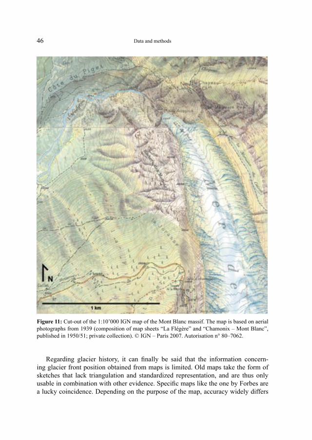
46

Regarding glacier history, it can finally be said that the information concern-ing glacier front position obtained from maps is limited. Old maps take the form of sketches that lack triangulation and standardized representation, and are thus only usable in combination with other evidence. Specific maps like the one by Forbes are a lucky coincidence. Depending on the purpose of the map, accuracy widely differs

Figure 11: Cut-out of the 1:10’000 IGN map of the Mont Blanc massif. The map is based on aerial photographs from 1939 (composition of map sheets “La Flégère” and “Chamonix – Mont Blanc”, published in 1950/51; private collection). © IGN – Paris 2007. Autorisation n° 80–7062.

Data and methods

47

between the various maps, and a major problem is often also the unknown exact date of the ground surveys which form the basis of the maps. Even the modern maps are susceptible to the interpretation of the user. Most accurate is the direct analysis of aerial photographs, also in order to skip possible mistakes that occur in the course of the production of the map (see section 3.3).

3.2.3 The evaluation of pictorial documents

The reconstruction of former glacier extents based on the evaluation of pictorial docu-ments and the corresponding method and its possibilities as well as problems is dis-cussed in the following. According to Zumbühl and Holzhauser (1988), three condi-tions have to be fulfilled in order to obtain reliable results concerning former glacier extents:

1. the dating of the pictorial document has to be known or reconstructed, 2. the glacier and its surroundings have to be represented realistically and topo-

graphically correctly (which implies certain qualities of the picture and skills of the corresponding author), and

3. the artist’s position in the field should be known.

Most useful documents are illustrated travel sketchbooks where the authors noted all details concerning time and circumstances when making the picture. A very important source in glacier history contexts are the drawings by the famous Swiss landscape artist Samuel Birmann (1793–1847) from Basel. Birmann made illustrated descrip-tions of his several journeys through the Alps, e.g. a sketchbook about the Mont Blanc area (Schneider, 2007; see section 4.1.8).

For oil paintings it is important to distinguish between the time of taking the draft in the field and the production of the painting itself later on. Although this is not always the case, the topographical accuracy usually increases with the artistic quality.

If some of the said requirements are not met, the glacier front position deduced from the document contains a certain error, and the uncertainty has to be specified. Some artists liked composing motifs of their own in the foreground or omitting un- aesthetic frontal moraines. The works have thus to pass a critical appraisal of the literature, and reliable documents have to be selected for interpretation. The bio- graphy of the artist or his notes of the journey are also additional sources of informa-tion helping to improve the reliability of the document. Under these conditions, it is obvious that a photograph representing the glacier front is very valuable.

Distinctive elements in the glacier’s surroundings such as rock steps or hills help to improve and simplify the evaluation of historical documentary data. Also, promi-nent mountain peaks in the background have to be studied and considered carefully. The geographical settings on the picture often limit the possible range where the gla-

Data and methods

48

cier front must have been situated at that time (e.g., a big glacier snout arcade at the Glacier des Bois was only possible when the glacier reached down to the plain). The comparison of the work of art with today’s situation in the field is often helpful and allows a quite accurate determination of the former glacier front, subject to the condi-tion that the work is accurate and reliable.

Concerning the Mer de Glace frontal area it has to be stated that the glacier is only visible from the valley of Chamonix if it exceeds a certain extent. The glacier flows over a gorge and thereafter reaches the valley bottom, but bounded by the Côte du Piget hill on the right-hand side. At very advanced frontal positions, the glacier overflowed this hill. With regard to the interpretation of pictorial documents, the back-ground of the works is very important. Points of reference at the Mer de Glace are the high mountain peaks of les Drus, the Aiguille à Bochard, the Rochers des Mottets, and of course the Côte du Piget. The pre-conditions in the field for the reconstruction of former glacier extents of the Mer de Glace are therefore convenient, although a very distinctive element like the rock band (“Schopffelsen”) at the Unterer Grindelwald-gletscher (Zumbühl, 1980) is missing.

Excellent examples of glacier representations of the Mer de Glace are given by the drawings of Jean-Antoine Linck, Samuel Birmann, and Eugène Viollet-le-Duc (see section 4.1). All three authors have a very reliable style and made representa-tions of the glacier from several points of view and in different years. Exceptionally well documented is the year 1823, when Birmann fixed the state of the glacier from different positions (e.g. Figure 12).

The historical (pictorial) material appears exceptionally rich for the Mont Blanc region and the Mer de Glace. This abundance is due to the fact that the glacier reached far down into the valley of Chamonix during the LIA. The glacier was an attractive object, either at the glacier snout, which was an often visited object (e.g., Bourrit, 1787), or around Montenvers, where plenty of tourists invaded the glacier since the beginning of alpinism.

Since the mid 19th century, photography and modern cartography have consti-tuted more accurate sources. Problems occurring at the Mer de Glace are the rapid re-forestation of the glacier foreland that makes comparisons with earlier glacier pictures sometimes very difficult. Moreover, construction activities in the valley of Chamonix changed the appearance completely, including the correction of the Arveyron river in the last years (in order to prevent floods downstream). At this point, old maps (or aerial photographs) are very helpful to reconstruct earlier situa- tions.

Nevertheless, it was possible to reconstruct former glacier fluctuations by inter-pretation of documentary sources and early scientific research. However, as archive material prior to the 19th century is not rare but often ambiguous and thus delicate for interpretation, the material has been selected very carefully according to the criteria mentioned above (known dating, realistic representation of the glacier, known loca-tion).

Data and methods

49

3.3 Generation of digital elevation models for the Mer de Glace

The reconstruction of the glacier front of the Mer de Glace only deals with glacier length and not glacier mass balance. To complement the length reconstructions as described in the sections before, a photogrammetric mass balance approach was used to quantify the long-term changes in ice volume for chosen time spans during the 20th century.

Essential for the calculation of ice volume changes over time is the availability of height information on the glacier topography, preferably by maps (or aerial photo-graphs or satellite imagery). Digitization of the elevation contour lines of old topo-graphic maps allows generating a digital elevation model (DEM). Comparisons of the surface topography by DEMs from different years allow an analysis of volume changes and glacier response to climate. For elevation differences between years, the older DEMs were subtracted from newer DEMs. As mentioned in section 3.2.2, the

Figure 12: Mer de Glace seen from la Flégère in 1823 by Samuel Birmann (Cut-out from “à la Flégère. 1823.”; pencil, watercolour, little opaque colour, two types of opaque white; beige paper, light-grey grounded; 20.4 cm (height) x 46.9 cm (width) (centrepiece of picture 20.4 x 28.7 cm); Kunstmuseum Basel, Kupferstichkabinett, Inv. Bi.334 fol. 16v; Photograph by H. J. Zumbühl, with kind permission of Kunstmuseum Basel).

Data and methods

50

cartographic coverage of the Mont Blanc area was poor prior to the mid 19th cen-tury compared to e.g. the Swiss Alps. Also for the time thereafter, maps of the Mer de Glace are not of the same quality as those we have for Swiss glaciers. Note that is was possible for Steiner et al. (in press) to calculate ice volume changes back to 1861 as the quality of the early Swiss cartography was unique and those early maps already contained elevation contour lines and a topographical base comparable to present maps.

The first map of the Mont Blanc area containing elevation contour lines is the “Carte Barbey” from 1896, i.e. the height information by contour lines is added in 1905. Unfortunately, this map has a different projection from subsequent maps, and the accuracy of the map in the complex mountain topography is unknown. It was thus not possible to use this map for direct comparison with more recent maps. The first map which it was possible to evaluate is the map of the Mont Blanc massif by the Vallot cousins. Ground surveys for that map were performed during several years (Vivian, 1986). The experimental sheet for the surroundings of Chamonix represents the glacier topography of 1906 (Mougin, 1912). However, the following sheets were not published before 1925. We can assume that the map was surveyed in the beginning of the 20th century (likely between 1900–1906; Vincent, 2002).

A second map that was evaluated is the map by the French National Geographic Institute (IGN) from 1939 (at the scale of 1:10’000, and 1:25’000, respectively). The accuracy of these maps is hard to determine. The maps are based on aerial photographs that were complemented by ground surveys in the field. Note that in the highly-ele-vated areas, the content of the map highly depends on the skills of the cartographer. In the present study, the bergschrund (as far as detectable) has been taken as upper limitation of the glacier.

For the lower part of the Mer de Glace, partly revised maps by IGN (at the scales of 1:20’000 and 1:25’000) from 1958 and 1967 are available. Those maps were also digitized and a DEM for only a part of the glacier was generated for these years.

Most accurate is the creation of a DEM based on aerial photographs. The current DEM that is available for the Mer de Glace area from IGN dates from 1981 and has a resolution of 40 x 40 m (P. Jublier, IGN, personal communication, 18.10.2005). Within the present study, a more recent DEM was generated by the evaluation of aerial photographs of the entire Mer de Glace area taken by IGN on 12/13 August 2001. A total of 12 digital pictures was evaluated by means of photogrammetry in order to calculate the DEM. The DEM obtained has a horizontal accuracy of about 5–10 m and a resolution of 25 x 25 m. The accuracy of the DEM generated exceeds that of the old maps.

Finally, it was possible to use the different DEMs to make volume calculations for the 20th century. Additionally, the evaluation of the aerial photographs allowed mapping different recent moraines (cf. section 4.1.2).

Data and methods

51

4 Results

4.1 Revised glacier length curve for the Mer de Glace

4.1.1 Preliminary remarks and new length curve

The uncertainty of the reconstructed glacier length curve for the Mer de Glace is aug-mented with increasing time backwards. Each determination of the glacier front posi-tion is tainted with a certain error that is indicated. This error highly depends on the quality of the data source; errors due to interpretation of the data have to be reduced to a minimum by selecting reliable sources. However, even in earlier times (e.g. in the 16th century) when the error exceeds ± 100 m, the result is still remarkable.

In order to allow a direct comparison of the new glacier length curve with the existing Mougin curve, certain requirements have to be met: For all length measure-ments, a centre line (longest flowline, see section 2.1, Figure 1) was drawn from the glacier terminus to a chosen reference point (in this case the glacier extent accord-ing to the 1906 Vallot map at 1:20’000 scale, as this map was also used by Mougin, 1912). Note that the Mougin curve ends in 1911. It is thus possible to make a direct comparison of the two curves. Moreover, the centre line in this study was chosen to be the same as in Mougin (1912); it just differs in cases where the glacier terminus is significantly beside the centre line (e.g. in the map of Forbes), and the centre line is in that case bent towards the glacier terminus.

All data points reflect a mean value and the most likely position of the glacier front. Corresponding errors are indicated separately and discussed in the following sections for each data point. Figure 13 shows the reconstructed glacier length curve of the Mer de Glace. For a more detailed curve with additional information concerning the used documentary data, see Appendix, Figure 76. To facilitate orientation, Figure 14 (section 4.1.2) shows the greater Mer de Glace frontal area with important locali-ties mentioned in the next sections.

4.1.2 Glacier foreland and LIA moraines

Moraines of the Mer de Glace have already been mapped by Wetter (1987). The fol-lowing map (Figure 14) completes this map by field surveys by the authors. Moreover, the analysis of aerial photographs from summer 2001 (cf. section 3.3) made it possible to add clearly visible moraines in the upper part of the glacier (e.g., Glacier de Talèfre; not shown). It is to be assumed that most of these very well preserved moraines cor-respond to the last major advances around 1821 or 1852, as also the well-formed moraine at Montenvers dates from that time (Wetter, 1987: 221). Figure 74 (Appen-dix) gives an overview of the former glacier extents.

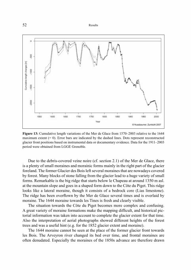
52

Due to the debris-covered veine noire (cf. section 2.1) of the Mer de Glace, there is a plenty of small moraines and morainic forms mainly in the right part of the glacier foreland. The former Glacier des Bois left several moraines that are nowadays covered by forest. Many blocks of stone falling from the glacier lead to a huge variety of small forms. Remarkable is the big ridge that starts below le Chapeau at around 1350 m asl. at the mountain slope and goes in a shaped form down to the Côte du Piget. This ridge looks like a lateral moraine, though it consists of a bedrock core (Lias limestone). The ridge has been overflown by the Mer de Glace several times and is overlaid by moraine. The 1644 moraine towards les Tines is fresh and clearly visible.

The situation towards the Côte du Piget becomes more complex and confusing. A great variety of moraine formations make the mapping difficult, and historical pic-torial information was taken into account to complete the glacier extent for that time. Also the interpretation of aerial photographs showed different heights of the forest trees and was a useful hint (e.g. for the 1852 glacier extent and moraine).

The 1644 moraine cannot be seen at the place of the former glacier front towards les Bois. The Arveyron river changed its bed over time, and frontal moraines are often denudated. Especially the moraines of the 1850s advance are therefore drawn

Figure 13: Cumulative length variations of the Mer de Glace from 1570–2003 relative to the 1644 maximum extent (= 0). Error bars are indicated by the dashed lines. Dots represent reconstructed glacier front positions based on instrumental data or documentary evidence. Data for the 1911–2003 period were obtained from LGGE Grenoble.

Results

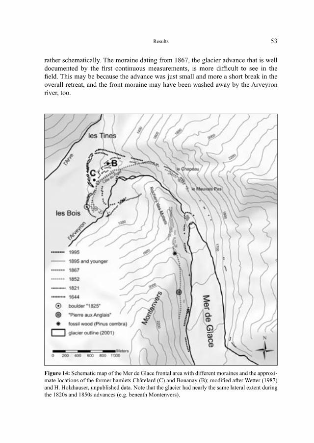
53

rather schematically. The moraine dating from 1867, the glacier advance that is well documented by the first continuous measurements, is more difficult to see in the field. This may be because the advance was just small and more a short break in the overall retreat, and the front moraine may have been washed away by the Arveyron river, too.

Figure 14: Schematic map of the Mer de Glace frontal area with different moraines and the approxi-mate locations of the former hamlets Châtelard (C) and Bonanay (B); modified after Wetter (1987) and H. Holzhauser, unpublished data. Note that the glacier had nearly the same lateral extent during the 1820s and 1850s advances (e.g. beneath Montenvers).

Results

54

Moraines near le Chapeau and Rochers des Mottets are difficult to date. The fact is that until the 1850s, the Mer de Glace flowed onto the Rochers des Mottets, where ice falls prevented the formation of moraines. The moraines near Rochers des Mottets thus have to be younger (they date from the 1890s or 1920s; Wetter, 1987: 222). The huge lateral moraines of the Mer de Glace above le Mauvais Pas contain several fossil soils and woods that reflect glacier fluctuations from the Middle Ages. A compilation of fossil organic material found is listed and interpreted in Wetter (1987). The right lateral moraine is eroding in a high degree and might reveal new material, which is however unfortunately very difficult to get.

A fossil tree was detected in between large boulders of the left lateral moraine (cf. Figure 14). This very clearly distinguishable moraine ridge ranges from above Montenvers towards the Rochers des Mottets. The tree (Pinus cembra) was felled anthropogenically before it was overridden by the advancing glacier. There were 215 tree rings counted (H. Holzhauser, unpublished data). This implies that the location of the growth of the tree was ice-free for at least 215 years. Taking into account the time needed for a tree to grow after a glacier retreat (about 20 years or more), the time during which the location was ice-free is at least 235 years. By comparing the tree ring curve with a reference curve from the Valais (Switzerland), the year of felling could be set to 1851 (H. Holzhauser, unpublished data). According to the findings stated, the previous extensive stage of the glacier must have occurred around 1610, which is in agreement with a glacier advance in the beginning of the 17th century proved by historical documents (cf. section 4.1.4).

The tree trunk was packed into morainic material during the mid 19th century maximum glacier extent (around 1852; see section 4.1.8), probably very soon after the felling. It was often the case that people tried to save wood threatened by advanc-ing glaciers. These findings imply that in the 1850s, the glacier had at that place the same magnitude as the previous 1820s advance and had overwhelmed its moraine (H. Holzhauser, personal communication, 30.5.2006). However, regarding the front, the glacier was more advanced in the 1820s than in the 1850s, as proved by several his-torical documents and geomorphological evidence (frontal moraine from the 1820s; cf. section 4.1.8)

4.1.3 Small glacier extension in the Middle Ages, and indication of a climate deterioration towards 1600

Little information is available on glacier or climate fluctuations in the Mont Blanc area for the Middle Ages. Some notion of the state of the glaciers during the Late Middle Ages may be gathered from local tradition and myth, yielding indirect evidence that the first LIA advances occurred in the Late Middle Ages (Grove, 2004: 124). Part of tradition in the valley of Chamonix is the description of Alpine passes used in former times (Aliprandi and Aliprandi, 1974: 144). Although there are no direct clues as to

Results

55

the glacier extent, it can be concluded that local people likely used those trails, indi-cating a general glacier extension in the Mont Blanc area that is much smaller than during the following main stage of the LIA.

Kinzl (1932) reveals other facts indicating a generally small glacier extension before 1500. He could not find any late Holocene moraines beside the 17th century and 1820s lateral moraines, respectively. Other evidence that the Mont Blanc glaciers, especially also the Mer de Glace, did not exceed the LIA lateral moraines, is provided, at least for the last millennium, through the existence of old settlements close to the glaciers (see below) near Chamonix (e.g., le Tour, Argentière, les Bossons, and others; Kinzl, 1932). Additionally, bigger glacier extensions than during the LIA would have caused glacier-dammed lakes, making especially the valley of Chamonix inhabitable.

Complaints by the Chamoniards document the existence of glaciers, but no devas-tating damages due to an advancing glacier front before 1500. Indications of increased glacier activity appear towards the mid 16th century. It is very probable that there was a slight glacier advance at this time, though it can not have been dangerous both for the inhabitants and the cultivated land. For the years 1559–1562, severe avalanches in combination with low temperatures are attested for the valley of Chamonix (Le Roy Ladurie, 1967: 108). Wetter (1987: 172) mentions a text which proves the vicinity of glacier ice to cornfields. Yet, this text is quite imprecise, but indicates a larger glacier extension than in the 1960s as concluded by Le Roy Ladurie (1967). All in all, Le Roy Ladurie (1967) concludes, in agreement with Kinzl (1932), that from 1557 to 1577 there were relatively advanced glacier front positions, proved by widespread poverty and unfavourable climatic conditions in the valley of Chamonix. Moreover, the plague is reported to have gone round in the valley of Chamonix from 1570 to 1632.

A very valuable and accurate description of the valley of Chamonix is given by an archive text from 1580 (see Appendix). Note that it is the first detailed text about the glaciers at Chamonix, and surely even one of the first descriptions at all which are of glaciological interest. The text is about a process of taxes. Bernard Combet, archdeacon of Tarentaise, had the task to see how serious the situation in the valley of Chamonix was, after a few complaints by inhabitants. The text clearly shows a glacier advance or at least a big glacier extension, which would imply a first glacier advance around 1570–1580. After describing the route, Combet gives a description of the valley with special focus on the glaciers. Combet depicts three glaciers that spread through rifts in the mountains and descend almost to the plain in at least three places. Remarkable is the fact that he already mentions the flowing ice during summertime, and thus shows a beginning understanding of glacier dynamics. Moreover, he also recognizes glacier lake outburst floods.

There has been some disagreement over the interpretation of this text, mainly between Rabot and Blanchard. Rabot (1914/15) identified the three glaciers men-tioned by Combet as Glacier des Bossons, Glacier d’Argentière and Glacier du Tour, and thus concluded that the glacier advances of the LIA had not yet begun in 1580, if these were the only glacier tongues which could be seen from the plain. On the other

Results

56

side, Blanchard (1913) concluded that Glacier du Tour is much too far away from the other two glaciers to have been intended, and also dismissed Glacier de Taconnaz (beside Glacier des Bossons) because its tongue has always been higher than that of the Glacier des Bossons (Grove, 2004: 107). As Combet specified his exact route, we know that nowhere on it he could have seen the Glacier du Tour. Le Roy Ladurie (1967) and Wetter (1987) follow this argumentation, which already was assumed by Mougin (1912).

The fact that Combet saw the Glacier des Bois reaching “almost to the plain” implies that the glacier was more extensive than at any time in the 20th century and that the advance was already well under way in 1580. Because of the known itiner-ary of Combet (from Chamonix up to Montroc), it can be concluded that the three mentioned glaciers are Glacier des Bossons, Mer de Glace, and Glacier d’Argentière, respectively. The itinerary mentioned above as well as the description of outburst floods from the valley in the middle which is probably the valley of the Mer de Glace refute this argument.

From the point of view of climate, this time is characterized by cold and inhospi-table years (Wetter, 1987: 174). An indication for cold and harsh climate in 1580 is in fact mentioned in the text by Combet, which says that people did not dare to sow in autumn, probably because of heavy snow conditions. Whether the said glacier out-burst floods prove a glacier advance or retreat cannot be said. However, it is a sign for glacial activity at that time. Glacier lake outburst floods always occurred at the Mer de Glace and other glaciers of the Mont Blanc area, leading to damages in villages of the valley (Mougin, 1912: 43; Wetter, 1987: 218).

Summarizing, the extent of the Mer de Glace was small prior to the mid 16th cen-tury, though the available data is sparse for the Middle Ages. A severe glacier advance is documented for the turn to the 17th century.

4.1.4 Destruction of Châtelard and Bonanay towards maximum glacier extension around 1644

Of special interest are two hamlets in very close vicinity to the Mer de Glace, Bonanay and Châtelard. At the time of the establishment of these small villages, the glacier can not have been menacing. Further on, however, the glacier may well have advanced close to the hamlets, without leaving any damages. Châtelard possibly existed since 1289; it is attested since 1384 (Le Roy Ladurie, 1967: 127). Le Roy Ladurie (1967) collected texts about the three hamlets Châtelard, les Bois, and les Praz for the time period from 1384 to 1640. The tithe yield from Châtelard has always been the most important, and in three texts from 1458, 1467, and 1521, the position of Châtelard below the Côte du Piget is confirmed. In 1570, people still bought land or properties in Châtelard. Purchasers did not seem to be afraid of the nearby glacier, which confirms the rather low glacier activity as described in the previous section.

Results

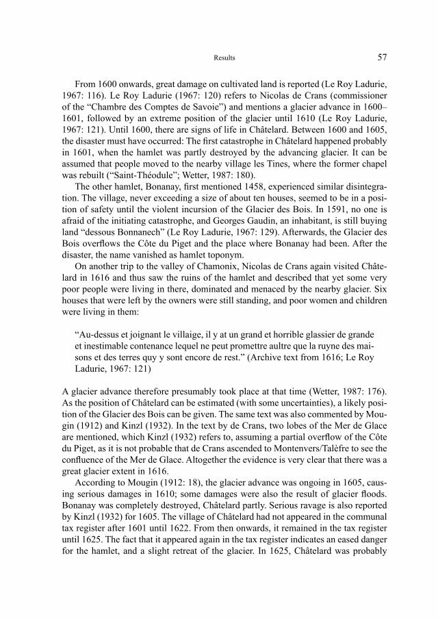
57

From 1600 onwards, great damage on cultivated land is reported (Le Roy Ladurie, 1967: 116). Le Roy Ladurie (1967: 120) refers to Nicolas de Crans (commissioner of the “Chambre des Comptes de Savoie”) and mentions a glacier advance in 1600–1601, followed by an extreme position of the glacier until 1610 (Le Roy Ladurie, 1967: 121). Until 1600, there are signs of life in Châtelard. Between 1600 and 1605, the disaster must have occurred: The first catastrophe in Châtelard happened probably in 1601, when the hamlet was partly destroyed by the advancing glacier. It can be assumed that people moved to the nearby village les Tines, where the former chapel was rebuilt (“Saint-Théodule”; Wetter, 1987: 180).

The other hamlet, Bonanay, first mentioned 1458, experienced similar disintegra-tion. The village, never exceeding a size of about ten houses, seemed to be in a posi-tion of safety until the violent incursion of the Glacier des Bois. In 1591, no one is afraid of the initiating catastrophe, and Georges Gaudin, an inhabitant, is still buying land “dessous Bonnanech” (Le Roy Ladurie, 1967: 129). Afterwards, the Glacier des Bois overflows the Côte du Piget and the place where Bonanay had been. After the disaster, the name vanished as hamlet toponym.

On another trip to the valley of Chamonix, Nicolas de Crans again visited Châte-lard in 1616 and thus saw the ruins of the hamlet and described that yet some very poor people were living in there, dominated and menaced by the nearby glacier. Six houses that were left by the owners were still standing, and poor women and children were living in them:

“Au-dessus et joignant le villaige, il y at un grand et horrible glassier de grande et inestimable contenance lequel ne peut promettre aultre que la ruyne des mai-sons et des terres quy y sont encore de rest.” (Archive text from 1616; Le Roy Ladurie, 1967: 121)

A glacier advance therefore presumably took place at that time (Wetter, 1987: 176). As the position of Châtelard can be estimated (with some uncertainties), a likely posi-tion of the Glacier des Bois can be given. The same text was also commented by Mou-gin (1912) and Kinzl (1932). In the text by de Crans, two lobes of the Mer de Glace are mentioned, which Kinzl (1932) refers to, assuming a partial overflow of the Côte du Piget, as it is not probable that de Crans ascended to Montenvers/Talèfre to see the confluence of the Mer de Glace. Altogether the evidence is very clear that there was a great glacier extent in 1616.

According to Mougin (1912: 18), the glacier advance was ongoing in 1605, caus-ing serious damages in 1610; some damages were also the result of glacier floods. Bonanay was completely destroyed, Châtelard partly. Serious ravage is also reported by Kinzl (1932) for 1605. The village of Châtelard had not appeared in the communal tax register after 1601 until 1622. From then onwards, it remained in the tax register until 1625. The fact that it appeared again in the tax register indicates an eased danger for the hamlet, and a slight retreat of the glacier. In 1625, Châtelard was probably

Results

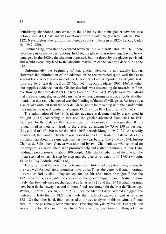
58

definitively abandoned, and erased in the 1640s by the main glacier advance (see below). In 1643, Châtelard was mentioned for the last time (Le Roy Ladurie, 1967: 122). Nevertheless, the ruins of this tragedy could still be seen in 1920 (Le Roy Ladu-rie, 1967: 120).

Summarizing, devastation occurred between 1600 and 1605, and until 1610 there were once more heavy destructions. In 1616, the glacier was retreating, leaving heavy damages. In the 1620s, the situation appeased, but the threat by the glacier persisted, and would eventually lead to the absolute maximum of the Mer de Glace during the LIA.

Unfortunately, the beginning of that glacier advance is not exactly known. However, the culmination of the advance an be reconstructed quite well thanks to several texts. A heavy advance of the Glacier des Bois is reported for August 1641 to spring 1642 (text dating from 28 May 1624; Le Roy Ladurie, 1967: 146). Another text supplies evidence that the Glacier des Bois was descending far towards les Praz, overflowing the Côte du Piget (Le Roy Ladurie, 1967: 147). People were even afraid that the advancing glacier could dam the Arve river, causing disastrous floods. Another inundation that really happened was the flooding of the small village les Rosières by a glacier lake outburst from the Mer de Glace (not to be mixed up with the hamlet with the same name near Argentière; Mougin, 1912: 29; Le Roy Ladurie, 1967: 145).

The culmination of the 1640s glacier advance is documented by a text cited in Mougin (1912). According to that text, the glacier advanced from 1641 to 1643 each year by the distance that is given by the measuring unit of a gunshot. If this is quantified in meters, it leads to the glacier advancing by 75 to 150 m per year (i.e., a total of 150–300 m for the 1641–1643 period; Mougin, 1912: 21). As already mentioned, the hamlet Châtelard was erased in 1643. In 1644, the Glacier des Bois probably had about the same extension as the year before. The 29 May 1644, bishop Charles de Sales from Geneva was alarmed by two Chamoniards who reported on the dangerous glacier. The bishop promised help and visited Chamonix in June 1644, holding a procession with about 300 people. After the benediction of the glacier, the threat seemed to vanish step by step and the glacier retreated until 1663 (Mougin, 1912; Le Roy Ladurie, 1967: 148).

The question of the exact glacier terminus in 1644 is not easy to answer, as despite the very well formed lateral moraines towards les Tines, there are no frontal moraines towards les Bois visible today (except for the fair 1821 moraine ridge). Either the 1821 advance is, as regards the very end of the glacier, bigger than in 1644, or, more likely, the 1644 advance reached about as far as in 1821 and the 1644 frontal moraines have been flushed away (several outburst floods are known for the Mer de Glace; e.g., Wetter, 1987: 218; Vivian, 2001: 153). Since the Mer de Glace covered a bigger area with ice in 1644 than in 1821, it is likely that the front reached at least as far as in 1821. On the other hand, findings based on fir tree analyses in this proximate frontal area limit the possible glacier extension. Tree ring analysis by Wetter (1987) yielded an age of up to 350 years for those trees. Moreover, the exact time of felling is known

Results

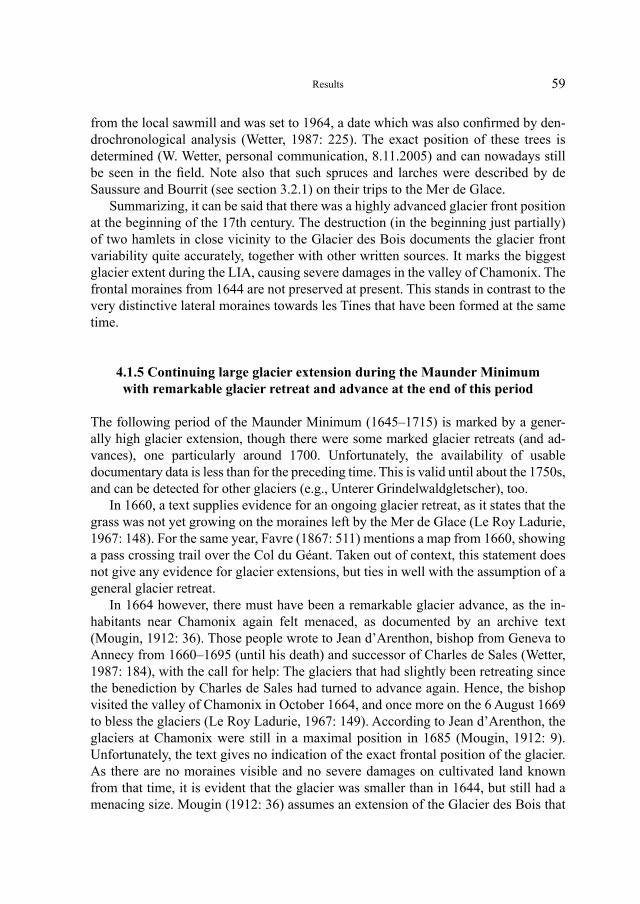
59

from the local sawmill and was set to 1964, a date which was also confirmed by den-drochronological analysis (Wetter, 1987: 225). The exact position of these trees is determined (W. Wetter, personal communication, 8.11.2005) and can nowadays still be seen in the field. Note also that such spruces and larches were described by de Saussure and Bourrit (see section 3.2.1) on their trips to the Mer de Glace.

Summarizing, it can be said that there was a highly advanced glacier front position at the beginning of the 17th century. The destruction (in the beginning just partially) of two hamlets in close vicinity to the Glacier des Bois documents the glacier front variability quite accurately, together with other written sources. It marks the biggest glacier extent during the LIA, causing severe damages in the valley of Chamonix. The frontal moraines from 1644 are not preserved at present. This stands in contrast to the very distinctive lateral moraines towards les Tines that have been formed at the same time.

4.1.5 Continuing large glacier extension during the Maunder Minimum with remarkable glacier retreat and advance at the end of this period

The following period of the Maunder Minimum (1645–1715) is marked by a gener-ally high glacier extension, though there were some marked glacier retreats (and ad- vances), one particularly around 1700. Unfortunately, the availability of usable documentary data is less than for the preceding time. This is valid until about the 1750s, and can be detected for other glaciers (e.g., Unterer Grindelwaldgletscher), too.

In 1660, a text supplies evidence for an ongoing glacier retreat, as it states that the grass was not yet growing on the moraines left by the Mer de Glace (Le Roy Ladurie, 1967: 148). For the same year, Favre (1867: 511) mentions a map from 1660, showing a pass crossing trail over the Col du Géant. Taken out of context, this statement does not give any evidence for glacier extensions, but ties in well with the assumption of a general glacier retreat.

In 1664 however, there must have been a remarkable glacier advance, as the in- habitants near Chamonix again felt menaced, as documented by an archive text (Mougin, 1912: 36). Those people wrote to Jean d’Arenthon, bishop from Geneva to Annecy from 1660–1695 (until his death) and successor of Charles de Sales (Wetter, 1987: 184), with the call for help: The glaciers that had slightly been retreating since the benediction by Charles de Sales had turned to advance again. Hence, the bishop visited the valley of Chamonix in October 1664, and once more on the 6 August 1669 to bless the glaciers (Le Roy Ladurie, 1967: 149). According to Jean d’Arenthon, the glaciers at Chamonix were still in a maximal position in 1685 (Mougin, 1912: 9). Unfortunately, the text gives no indication of the exact frontal position of the glacier. As there are no moraines visible and no severe damages on cultivated land known from that time, it is evident that the glacier was smaller than in 1644, but still had a menacing size. Mougin (1912: 36) assumes an extension of the Glacier des Bois that

Results

60

is 50 m shorter than in 1644. The same value has also been used in the present study. Despite the limited accuracy of this value, it is still reliable as the possible range of the extension of the Mer de Glace for this time is restricted due to information for the following years. In 1690, the same source reports a glacier retreat by roughly 60 m. For 1697, an exact value for the length fluctuation of the Mer de Glace is found, which gives an accurate value relative to 1690: according to an archive text, the glacier retreated “un demi quart de lieue”. Following the train of thought by Mougin (1912) and taking into consideration the value for this old French measuring unit (1 lieue de poste française = 3898 m), we get a glacier retreat of nearly 490 m for the 1690–1697 time period (Mougin, 1912: 9; Le Roy Ladurie, 1967: 156).

For the following time, a glacier minimum occurred at the turn from the 17th to the 18th century. This is documented by a statement of baron La Rochefoucauld in 1762 (Mougin, 1912: 22). In 1707 yet, a map indicates once more the pass crossing from Chamonix to Courmayeur (Favre, 1867: 511). Unfortunately, it is not specified which pass on which map it is about, though it is fair to assume that the pass crossing by the Col du Géant is meant. Still not knowing an exact glacier terminus position, a generally small glacier extension can be assumed for this time. Furthermore, this stands in agreement with the comment by the engineer Pierre Martel, who claimed that a glacier advance at the beginning of the 18th century made the pass crossing by the Col du Géant impossible from that time on (Favre, 1867: 512). And indeed, the Glacier des Bois was advancing heavily in 1716, as a call for help of the local people near Chamonix to the King of Sardinia proves (Mougin, 1912: 21).

Summarizing, the Mer de Glace continuously had a very advanced frontal position with some variability in the second half of the 17th century. This period is abruptly finished by a heavy and unprecedented retreat in the 1690s, and a re-advance of the same intensity towards 1720.

4.1.6 Glacier retreat during the first half of the 18th century until the 1760s

As the availability of documentary data concerning glacier extension increases, also the quality and accuracy of the presented glacier length curve improves considerably. In 1720, there may have been a relative maximum of the Mer de Glace (Le Roy Ladu-rie, 1967: 169; Wetter, 1987: 189). For 1725, John Moore describes a glacier advance, also mentioning the small glacier extension at the beginning of the 18th century, and last but not least alluding to the passage by the Col du Géant that became unusable at that time (Moore, 1779: 233).

For 1730 finally, there exists a cadastral plan of the area of les Bois. Although the general state of cartography still left much to be desired (see section 3.2.2), the cadastral survey that led to this cadastral plan was exceptional, and it is of great value as a primary source. The “cadastre sarde” was drawn up under the King of Sardinia,

Results

61

Victor-Amédée II (1675–1730), between 1728 and 1738. This early and very valuable plan contains a lot of valuable information for that time in geographic, economic, and social contexts (Guichonnet, 1955). The map sheet representing also the Glacier des Bois was made in 1730 and allows drawing conclusions on the position of the glacier front. The map shows the lower part of the glaciers of the valley of Chamonix and includes the glacier snouts with the glacier rivers and the position of moraine ridges. All tongues were still much enlarged but had retreated so far that they no longer immediately threatened the villages in the valley (Wetter, 1987: 189).

According to the “cadastre sarde”, the terminus of the Glacier des Bois was 150 m behind the last moraines. From which time those moraines date is not specified, which led to a difference of opinion between Mougin (1912) and Le Roy Ladurie (1967). Mougin believes that it is about the 1644 moraines, whereas Le Roy Ladurie thinks that the 1720 moraines are meant. An absolutely certain solution to this problem can-not be given. However, we do not know any reports about damages caused by the glacier in 1720 (Mougin, 1912: 10), and a glacier extent bigger than 1644 (or 1821) is quite unlikely. Hence, the opinion of Mougin was taken into account for the determi-nation of glacier length in the present study, as has also been done by Wetter (1987).

The indications for the 1741 and 1742 extent of the Mer de Glace are unfortu-nately quite contradictory. According to the report by Windham and Martel (see sec-tion 3.2.1), the glacier was retreating and had a terminal position distinctly behind the 1730 state (Mougin, 1912: 23). Moreover, it is stated by Pierre Martel that the ice thickness decreased by around 27 m (80 feet) from 1730–1742, which is another unequivocal piece of evidence for a glacier retreat. Yet in Pierre Martel’s account of his 1742 visit to Chamonix he told of large boulders then lying on the valley floor which villagers assured him had once been on the surface of an enlarged Glacier des Bois (Cunningham, 1990: 35).

On the other hand, Windham writes in a letter on his visit of Montenvers and the Mer de Glace that the glacier is advancing. Windham refers to reports by local moun-tain guides; at the time of their fathers, the glaciers apparently were much smaller than in 1741, when the ice was covering more and more land. Windham also describes his descent to the ice over a very steep morainic slope, covered with a lot of loose debris. It is thus very likely that the glacier was retreating (Martel, 1744). The report by the guides cited by Windham has therefore to be seen as a general state of the glaciers, which does not take into consideration that the relative glacier maximum had already occurred around 1720.

According to a letter by Pierre Martel, the terminus of the Mer de Glace was at a certain distance from the confluence of the Arveyron with the Arve river (“environ à une demi lieue de là”). Taking again the measure of 3898 m for one lieue (cf. section 4.1.5), the approximate state of the glacier can be reconstructed (Wetter, 1987: 190). Other evidence is given by a description cited in Gruner (1760). It is about a transla-tion of a text by Windham from 1744 (on his journey in 1741) and gives us the follow-ing additional information: A lot of snow and thus damages by avalanches occurred in

Results

62

the valley of Chamonix. The Arveyron river had its source in two wonderful glacier snouts of pure ice. Half an hour away from the source, the river flowed into the Arve river, and water was dripping from the icebergs (possibly also over the Rochers des Mottets; Gruner, 1760).

In Gruner (1760), we also find what may well be the first attempt to illustrate the Chamonix valley, glaciers and the chain of Mont Blanc as a whole. The work significantly influenced de Saussure and his later interest in mountains as they relate to the natural sciences. Moreover, it contains an etching, the first pictorial representa-tion (beside the Martel map) of the glaciers and mountains of Haut-Faucigny, naming glaciers and mountains. But the imaginative way in which the glaciers and mountain peaks are drawn led de Saussure to make the statement that the picture has nothing in common with reality. And indeed, the author of the engraving has never visited the place (Baud et al., 1986: 49)!

In 1760, Horace Bénédict de Saussure visited the Mer de Glace (as he would often do in the following years) for the first time (Roussy, 1940). According to his descrip-tions of the valley of Chamonix, the glacier must still have had a majestic shape despite the preceding glacier retreat (de Saussure, 1779; Le Roy Ladurie, 1967). In 1764, this state of the Glacier des Bois persisted, as documented by another (anonymous) text that says that the Arveyron had its source in an impressive glacier snout, which formed an arcade-shaped cavern like a cathedral’s front (Le Roy Ladurie, 1967: 307).

The glacier then reached a relative minimum front position. However, the avail-ability of data is sparse during the first half of the 18th century, and determinations of the glacier front are based on few, but reliable documents.

4.1.7 Well-documented period from 1770 onwards and distinct glacier advance in 1778 and retreat thereafter

The first pictorial document with usefulness for the determination of glacier extent is the watercolour drawing “Part of the Valley of Chamonix 1770” by William Pars (1742–1782). On his journey through the Alps in 1770, Pars made several topographi-cal studies of Alpine scenery. When some of them were exhibited in London in 1771, they were among the first studies of this kind and marked the beginning of a long asso-ciation between English landscape artists and the Alps (Wilton, 1979: 27). Although the watercolour showing the front of the Mer de Glace situated between the Aiguille Verte and the Aiguilles de Chamonix has some deficiencies, it shows a highly retreated glacier only just reaching the plain of the valley (Figure 15). The lack of quality can partially be explained by the fact that Pars had very little time for making his study of the Mer de Glace due to a rising thunderstorm (Wilton, 1979: 31). The exact frontal position cannot be ascertained. However, the position can be limited by the nearby Rochers des Mottets. Another work by William Pars showing the Mer de Glace near Montenvers represents a very mighty body of ice.

Results

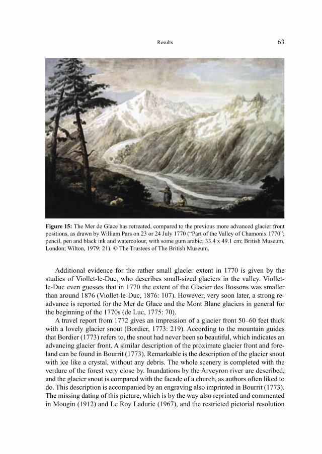
63

Additional evidence for the rather small glacier extent in 1770 is given by the studies of Viollet-le-Duc, who describes small-sized glaciers in the valley. Viollet-le-Duc even guesses that in 1770 the extent of the Glacier des Bossons was smaller than around 1876 (Viollet-le-Duc, 1876: 107). However, very soon later, a strong re-advance is reported for the Mer de Glace and the Mont Blanc glaciers in general for the beginning of the 1770s (de Luc, 1775: 70).

A travel report from 1772 gives an impression of a glacier front 50–60 feet thick with a lovely glacier snout (Bordier, 1773: 219). According to the mountain guides that Bordier (1773) refers to, the snout had never been so beautiful, which indicates an advancing glacier front. A similar description of the proximate glacier front and fore-land can be found in Bourrit (1773). Remarkable is the description of the glacier snout with ice like a crystal, without any debris. The whole scenery is completed with the verdure of the forest very close by. Inundations by the Arveyron river are described, and the glacier snout is compared with the facade of a church, as authors often liked to do. This description is accompanied by an engraving also imprinted in Bourrit (1773). The missing dating of this picture, which is by the way also reprinted and commented in Mougin (1912) and Le Roy Ladurie (1967), and the restricted pictorial resolution

Figure 15: The Mer de Glace has retreated, compared to the previous more advanced glacier front positions, as drawn by William Pars on 23 or 24 July 1770 (“Part of the Valley of Chamonix 1770”; pencil, pen and black ink and watercolour, with some gum arabic; 33.4 x 49.1 cm; British Museum, London; Wilton, 1979: 21). © The Trustees of The British Museum.

Results

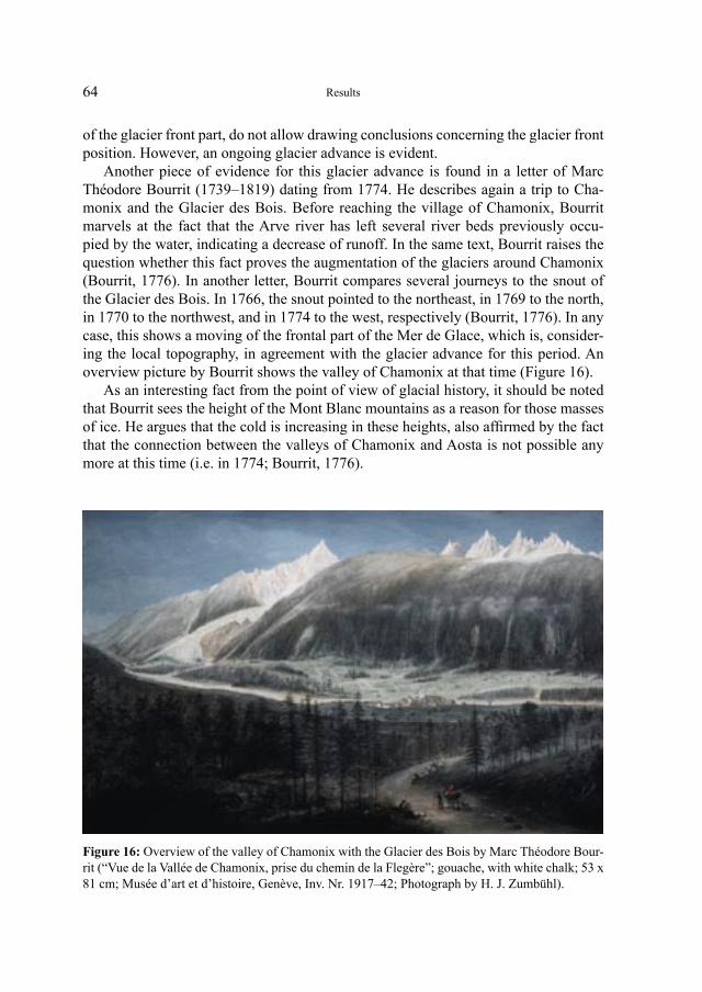
64

of the glacier front part, do not allow drawing conclusions concerning the glacier front position. However, an ongoing glacier advance is evident.

Another piece of evidence for this glacier advance is found in a letter of Marc Théodore Bourrit (1739–1819) dating from 1774. He describes again a trip to Cha- monix and the Glacier des Bois. Before reaching the village of Chamonix, Bourrit marvels at the fact that the Arve river has left several river beds previously occu-pied by the water, indicating a decrease of runoff. In the same text, Bourrit raises the question whether this fact proves the augmentation of the glaciers around Chamonix (Bourrit, 1776). In another letter, Bourrit compares several journeys to the snout of the Glacier des Bois. In 1766, the snout pointed to the northeast, in 1769 to the north, in 1770 to the northwest, and in 1774 to the west, respectively (Bourrit, 1776). In any case, this shows a moving of the frontal part of the Mer de Glace, which is, consider-ing the local topography, in agreement with the glacier advance for this period. An overview picture by Bourrit shows the valley of Chamonix at that time (Figure 16).

As an interesting fact from the point of view of glacial history, it should be noted that Bourrit sees the height of the Mont Blanc mountains as a reason for those masses of ice. He argues that the cold is increasing in these heights, also affirmed by the fact that the connection between the valleys of Chamonix and Aosta is not possible any more at this time (i.e. in 1774; Bourrit, 1776).

Figure 16: Overview of the valley of Chamonix with the Glacier des Bois by Marc Théodore Bour-rit (“Vue de la Vallée de Chamonix, prise du chemin de la Flegère”; gouache, with white chalk; 53 x 81 cm; Musée d’art et d’histoire, Genève, Inv. Nr. 1917–42; Photograph by H. J. Zumbühl).

Results

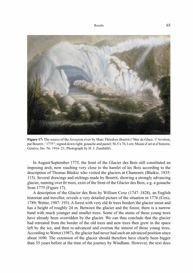
65

In August/September 1775, the front of the Glacier des Bois still constituted an imposing arch, now reaching very close to the hamlet of les Bois according to the description of Thomas Blaikie who visited the glaciers at Chamonix (Blaikie, 1935: 115). Several drawings and etchings made by Bourrit, showing a strongly advancing glacier, running over fir trees, exist of the front of the Glacier des Bois, e.g. a gouache from 1775 (Figure 17).

A description of the Glacier des Bois by William Coxe (1747–1828), an English historian and traveller, reveals a very detailed picture of the situation in 1776 (Coxe, 1789; Wetter, 1987: 193). A forest with very old fir trees borders the glacier snout and has a height of roughly 24 m. Between the glacier and the forest, there is a narrow band with much younger and smaller trees. Some of the stems of these young trees have already been overridden by the glacier. We can thus conclude that the glacier had retreated from the border of the old trees and new trees then grew in the space left by the ice, and then re-advanced and overran the inmost of those young trees. According to Wetter (1987), the glacier had never had such an advanced position since about 1690. The extension of the glacier should therefore have clearly been bigger than 35 years before at the time of the journey by Windham. However, the text does

Figure 17: The source of the Arveyron river by Marc Théodore Bourrit (“Mer de Glace / l’Arvéron, par Bourrit. / 1775”; signed down right; gouache and pastel; 56.5 x 76.3 cm; Musée d’art et d’histoire, Genève, Inv. Nr. 1916–21; Photograph by H. J. Zumbühl).

Results

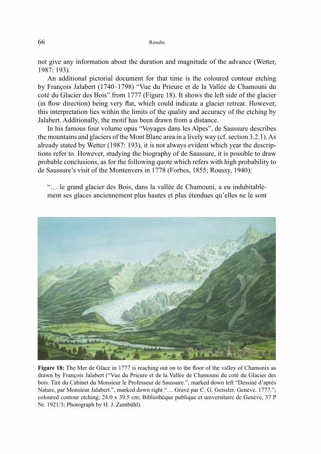
66

not give any information about the duration and magnitude of the advance (Wetter, 1987: 193).

An additional pictorial document for that time is the coloured contour etching by François Jalabert (1740–1798) “Vue du Prieure et de la Vallée de Chamouni du coté du Glacier des Bois” from 1777 (Figure 18). It shows the left side of the glacier (in flow direction) being very flat, which could indicate a glacier retreat. However, this interpretation lies within the limits of the quality and accuracy of the etching by Jalabert. Additionally, the motif has been drawn from a distance.

In his famous four volume opus “Voyages dans les Alpes”, de Saussure describes the mountains and glaciers of the Mont Blanc area in a lively way (cf. section 3.2.1). As already stated by Wetter (1987: 193), it is not always evident which year the descrip-tions refer to. However, studying the biography of de Saussure, it is possible to draw probable conclusions, as for the following quote which refers with high probability to de Saussure’s visit of the Montenvers in 1778 (Forbes, 1855; Roussy, 1940):

“… le grand glacier des Bois, dans la vallée de Chamouni, a eu indubitable-ment ses glaces anciennement plus hautes et plus étendues qu’elles ne le sont

Figure 18: The Mer de Glace in 1777 is reaching out on to the floor of the valley of Chamonix as drawn by François Jalabert (“Vue du Prieure et de la Vallée de Chamouni du coté du Glacier des bois. Tiré du Cabinet du Monsieur le Professeur de Saussure.”; marked down left “Dessiné d’après Nature, par Monsieur Jalabert.”, marked down right “… Gravé par C. G. Geissler. Genève. 1777.”; coloured contour etching; 24.0 x 39.5 cm; Bibliothèque publique et universitaire de Genève, 37 P Nr. 1921/3; Photograph by H. J. Zumbühl).

Results

67

aujourd’hui. Car au dessous de Montanvert, ces glaces sont de 40 ou 50 pieds plus basses que cet amas de débris qui borde le glacier, et que l’on nomme la moraine. Elles doivent pourtant avoir été de niveau avec ces débris, et même plus élevées, puisque ce sont elles qui les ont transportés et accumulés dans cette place; …” (de Saussure, 1779: 464)

Summarizing, we can say that the Mer de Glace was advancing to a great extent, reach-ing a maximum position in 1778 according to de Saussure who registered (probably for the time period 1760s–1778) the biggest advance ever (Le Roy Ladurie, 1967: 186). Nevertheless, this big advance has to be smaller than the advances in the 17th century, as well as probably around 1720, as the evident lateral moraines around Montenvers are not reached by the glacier. This advanced glacier position is also noted by the description of the valley of Chamonix by Johann Wolfgang Goethe (1749–1832) in his letters to Frau von Stein from 4/5 November 1779. Goethe describes the glaciers advancing far into the valley and a visit to the Mer de Glace at Montenvers, followed by a visit to and entering of the glacier snout:

“Vor ihm sahen wir eine Reihe von Schneegebirgen dämmernder auf den Rücken von schwarzen Fichtenbergen liegen und ungeheure Gletscher zwischen den schwarzen Wäldern herunter ins Tal steigen. […] Der Montblanc und die Gebirge, die von ihm herabsteigen, die Eismassen, die diese unge-heuren Klüfte ausfüllen, machen die östliche Wand aus, an der die ganze Länge des Tals hin sieben Gletscher, einer grösser als der andere, herunterkommen.” (Goethe, 1965: 23/24)

A much and often controversially discussed pictorial document is the front view of the Glacier des Bois “Vue de la Source de L’Arveron” by Carl Ludwig Hackert (1740–1796). It is a coloured contour etching, dating from 1780 or 1781 (Figure 19). The work is dated by the artist to 1781 (Bouchardy, 1986; Deline, 2005), though the date of survey in the field could be one year earlier since other works of art about the Mont Blanc area by Hackert date from 1780 (Forel, 1901; Mougin, 1912). The exact place of the artist’s position in front of the glacier seems to be quite easy to determine. However, this position does not fit at all with other data. It has to be noted on this occasion that the picture’s background on the left side of the work does not tally with the real topo-graphy. The etching clearly gives the impression of an advancing glacier (note the cross and firs twisted by the glacier on the left hand of the picture). Conversely, as already mentioned, the maximum frontal position of the Glacier des Bois has to have occurred earlier according to several pieces of evidence mentioned above. Still, the glacier fore-land allows drawing the conclusion of a glacier that has started retreating. Forel (1901) was the first to interpret the work of art by Hackert. According to him, the glacier was 1 km away from the 1901 position, which yields a distance of 330 m between the gla-cier front and the bridge over the Arveyron river, giving us a plausible result.

Results

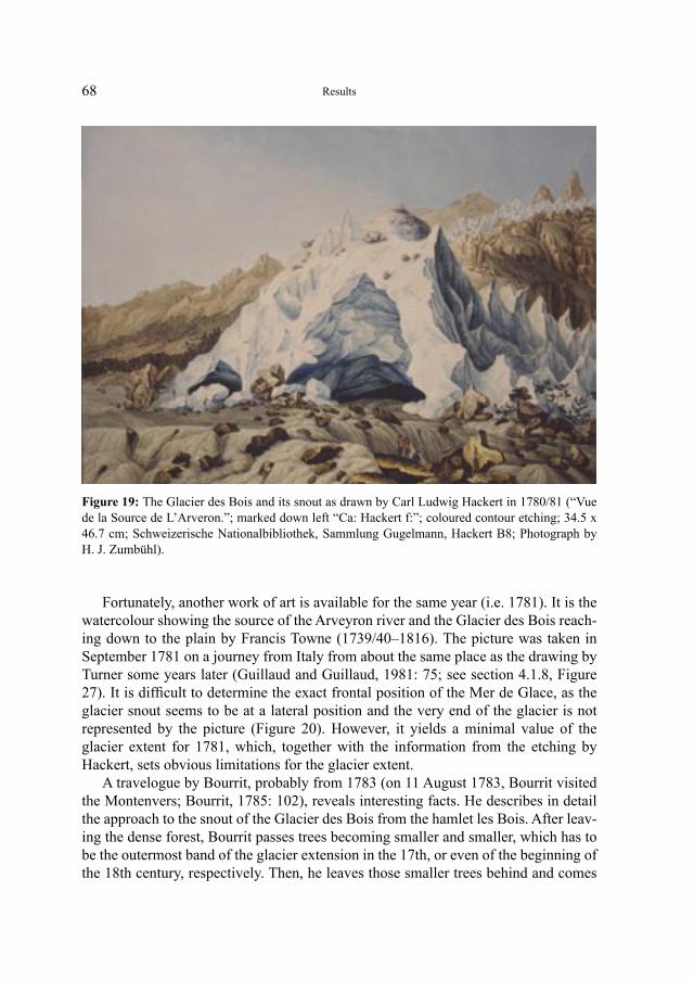
68

Fortunately, another work of art is available for the same year (i.e. 1781). It is the watercolour showing the source of the Arveyron river and the Glacier des Bois reach-ing down to the plain by Francis Towne (1739/40–1816). The picture was taken in September 1781 on a journey from Italy from about the same place as the drawing by Turner some years later (Guillaud and Guillaud, 1981: 75; see section 4.1.8, Figure 27). It is difficult to determine the exact frontal position of the Mer de Glace, as the glacier snout seems to be at a lateral position and the very end of the glacier is not represented by the picture (Figure 20). However, it yields a minimal value of the glacier extent for 1781, which, together with the information from the etching by Hackert, sets obvious limitations for the glacier extent.

A travelogue by Bourrit, probably from 1783 (on 11 August 1783, Bourrit visited the Montenvers; Bourrit, 1785: 102), reveals interesting facts. He describes in detail the approach to the snout of the Glacier des Bois from the hamlet les Bois. After leav-ing the dense forest, Bourrit passes trees becoming smaller and smaller, which has to be the outermost band of the glacier extension in the 17th, or even of the beginning of the 18th century, respectively. Then, he leaves those smaller trees behind and comes

Figure 19: The Glacier des Bois and its snout as drawn by Carl Ludwig Hackert in 1780/81 (“Vue de la Source de L’Arveron.”; marked down left “Ca: Hackert f:”; coloured contour etching; 34.5 x 46.7 cm; Schweizerische Nationalbibliothek, Sammlung Gugelmann, Hackert B8; Photograph by H. J. Zumbühl).

Results

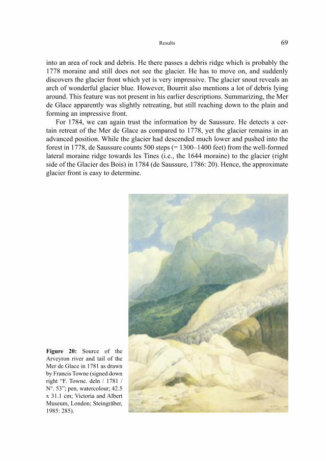
69

into an area of rock and debris. He there passes a debris ridge which is probably the 1778 moraine and still does not see the glacier. He has to move on, and suddenly discovers the glacier front which yet is very impressive. The glacier snout reveals an arch of wonderful glacier blue. However, Bourrit also mentions a lot of debris lying around. This feature was not present in his earlier descriptions. Summarizing, the Mer de Glace apparently was slightly retreating, but still reaching down to the plain and forming an impressive front.

For 1784, we can again trust the information by de Saussure. He detects a cer-tain retreat of the Mer de Glace as compared to 1778, yet the glacier remains in an advanced position. While the glacier had descended much lower and pushed into the forest in 1778, de Saussure counts 500 steps (= 1300–1400 feet) from the well-formed lateral moraine ridge towards les Tines (i.e., the 1644 moraine) to the glacier (right side of the Glacier des Bois) in 1784 (de Saussure, 1786: 20). Hence, the approximate glacier front is easy to determine.

Figure 20: Source of the Arveyron river and tail of the Mer de Glace in 1781 as drawn by Francis Towne (signed down right “F. Towne. deln / 1781 / N°. 53”; pen, watercolour; 42.5 x 31.1 cm; Victoria and Albert Museum, London; Steingräber, 1985: 285).

Results

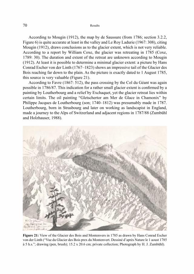
70

According to Mougin (1912), the map by de Saussure (from 1786; section 3.2.2, Figure 6) is quite accurate at least in the valley and Le Roy Ladurie (1967: 308), citing Mougin (1912), draws conclusions as to the glacier extent, which is not very reliable. According to a report by William Coxe, the glacier was retreating in 1785 (Coxe, 1789: 30). The duration and extent of the retreat are unknown according to Mougin (1912). At least it is possible to determine a minimal glacier extent: a picture by Hans Conrad Escher von der Linth (1767–1823) shows an impressive tail of the Glacier des Bois reaching far down to the plain. As the picture is exactly dated to 1 August 1785, this source is very valuable (Figure 21).

According to Favre (1867: 512), the pass crossing by the Col du Géant was again possible in 1786/87. This indication for a rather small glacier extent is confirmed by a painting by Loutherbourg and a relief by Exchaquet, yet the glacier retreat lies within certain limits. The oil painting “Gletschertor am Mer de Glace in Chamonix” by Philippe Jacques de Loutherbourg (son; 1740–1812) was presumably made in 1787. Loutherbourg, born in Strasbourg and later on working as landscapist in England, made a journey to the Alps of Switzerland and adjacent regions in 1787/88 (Zumbühl and Holzhauser, 1988).

Figure 21: View of the Glacier des Bois and Montenvers in 1785 as drawn by Hans Conrad Escher von der Linth (“Vue du Glacier des Bois prex du Montenvert. Dessiné d’après Nature le 1 aoust 1785 à 5 h.s.”; drawing (pen, brush); 15.2 x 20.6 cm; private collection; Photograph by H. J. Zumbühl).

Results

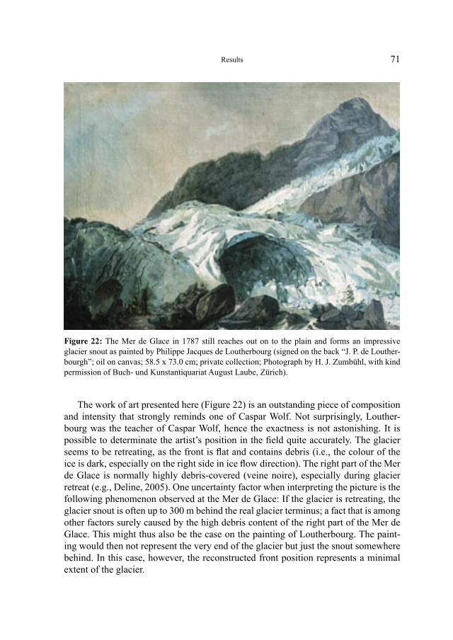
71

The work of art presented here (Figure 22) is an outstanding piece of composition and intensity that strongly reminds one of Caspar Wolf. Not surprisingly, Louther-bourg was the teacher of Caspar Wolf, hence the exactness is not astonishing. It is possible to determinate the artist’s position in the field quite accurately. The glacier seems to be retreating, as the front is flat and contains debris (i.e., the colour of the ice is dark, especially on the right side in ice flow direction). The right part of the Mer de Glace is normally highly debris-covered (veine noire), especially during glacier retreat (e.g., Deline, 2005). One uncertainty factor when interpreting the picture is the following phenomenon observed at the Mer de Glace: If the glacier is retreating, the glacier snout is often up to 300 m behind the real glacier terminus; a fact that is among other factors surely caused by the high debris content of the right part of the Mer de Glace. This might thus also be the case on the painting of Loutherbourg. The paint-ing would then not represent the very end of the glacier but just the snout somewhere behind. In this case, however, the reconstructed front position represents a minimal extent of the glacier.

Figure 22: The Mer de Glace in 1787 still reaches out on to the plain and forms an impressive glacier snout as painted by Philippe Jacques de Loutherbourg (signed on the back “J. P. de Louther-bourgh”; oil on canvas; 58.5 x 73.0 cm; private collection; Photograph by H. J. Zumbühl, with kind permission of Buch- und Kunstantiquariat August Laube, Zürich).

Results

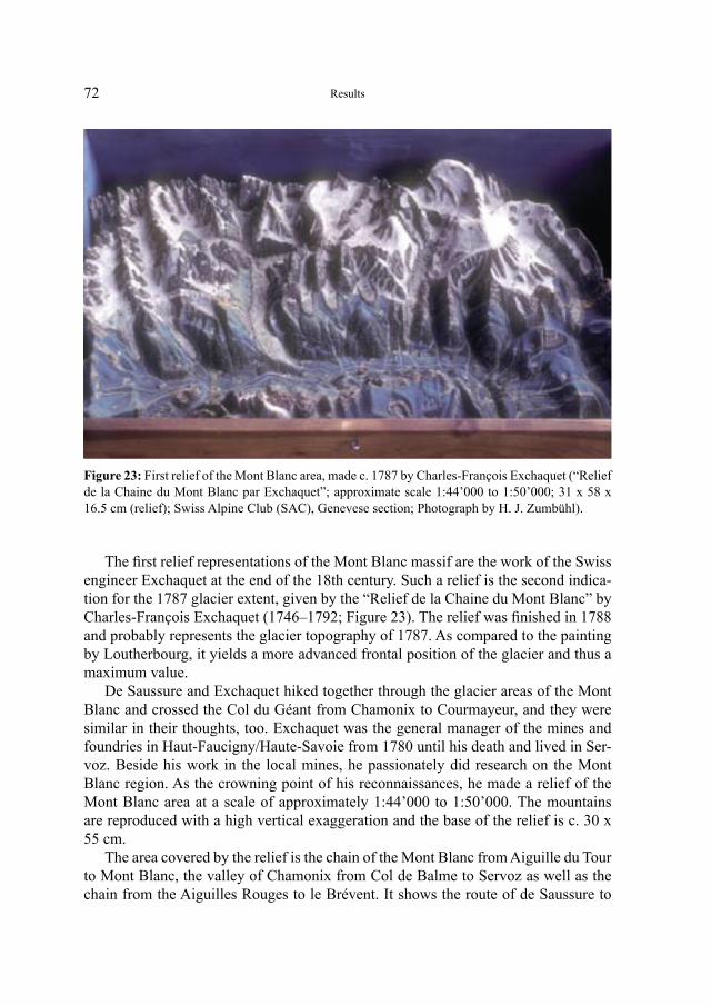
72

The first relief representations of the Mont Blanc massif are the work of the Swiss engineer Exchaquet at the end of the 18th century. Such a relief is the second indica-tion for the 1787 glacier extent, given by the “Relief de la Chaine du Mont Blanc” by Charles-François Exchaquet (1746–1792; Figure 23). The relief was finished in 1788 and probably represents the glacier topography of 1787. As compared to the painting by Loutherbourg, it yields a more advanced frontal position of the glacier and thus a maximum value.

De Saussure and Exchaquet hiked together through the glacier areas of the Mont Blanc and crossed the Col du Géant from Chamonix to Courmayeur, and they were similar in their thoughts, too. Exchaquet was the general manager of the mines and foundries in Haut-Faucigny/Haute-Savoie from 1780 until his death and lived in Ser-voz. Beside his work in the local mines, he passionately did research on the Mont Blanc region. As the crowning point of his reconnaissances, he made a relief of the Mont Blanc area at a scale of approximately 1:44’000 to 1:50’000. The mountains are reproduced with a high vertical exaggeration and the base of the relief is c. 30 x 55 cm.

The area covered by the relief is the chain of the Mont Blanc from Aiguille du Tour to Mont Blanc, the valley of Chamonix from Col de Balme to Servoz as well as the chain from the Aiguilles Rouges to le Brévent. It shows the route of de Saussure to

Figure 23: First relief of the Mont Blanc area, made c. 1787 by Charles-François Exchaquet (“Relief de la Chaine du Mont Blanc par Exchaquet”; approximate scale 1:44’000 to 1:50’000; 31 x 58 x 16.5 cm (relief); Swiss Alpine Club (SAC), Genevese section; Photograph by H. J. Zumbühl).

Results

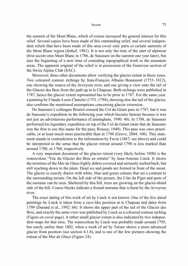
73

the summit of the Mont Blanc, which of course increased the general interest for this relief. Several copies have been made of this outstanding relief, and several indepen-dent reliefs that have been made of this area cover only parts or certain summits of the Mont Blanc region (Imhof, 1981). It is not only the time of the start of alpinism (first ascent onto Mont Blanc in 1786, de Saussure on the summit one year later), but also the beginning of a new time of extending topographical work to the mountain areas. The apparent original of the relief is in possession of the Genevese section of the Swiss Alpine Club (SAC).

Moreover, three other documents allow verifying the glacier extent in these years. Two coloured contour etchings by Jean-François Albanis Beaumont (1753–1812), one showing the source of the Arveyron river, and one giving a view onto the tail of the Glacier des Bois from the path up to le Chapeau. Both etchings were published in 1787, hence the glacier extent represented has to be prior to 1787. For the same year, a painting by Claude-Louis Chatelet (1753–1794), showing also the tail of the glacier, also confirms the mentioned assumptions concerning glacier extension.

De Saussure’s colleague Bourrit crossed the Col du Géant pass in 1787, but it was de Saussure’s expedition in the following year which became famous because it was not just an adventurous performance (Cunningham, 1990: 40). In 1788, de Saussure performed his legendary expedition on top of the Col du Géant (note that de Saussure was the first to use this name for the pass; Roussy, 1940). This pass was once practi-cable, or at least much more practicable than in 1788 (Grove, 2004: 106). This state-ment stands in contradiction to the information by Favre (1867; see above) and could be interpreted in the sense that the glacier retreat around 1790 is less marked than around 1700, or 1760, respectively.

A very important document of the glacier retreat (very likely before 1800) is the watercolour “Vue du Glacier des Bois en retraite” by Jean-Antoine Linck. It shows the terminus of the Mer de Glace highly debris-covered and seriously melted back, but still reaching down to the plain. Dead ice and ponds are formed in front of the snout. The glacier is exactly drawn with white, blue and green colours that set a contrast to the surrounding terrain. On the left side of the picture, the Côte du Piget and parts of the moraine can be seen. Sheltered by this hill, trees are growing on the glacier-distal side of the hill. Coarse blocks indicate a frontal moraine that is burst by the Arveyron river.

The exact dating of this work of art by Linck is not known. One of the few dated paintings by Linck is taken from a cave-like position at le Chapeau and dates from 1799 (Durand et al., 1992: 68). It shows the upper part of the tail of the Glacier des Bois, and exactly the same view was published by Linck as a coloured contour etching (Figure on cover page). A rather small glacier extent is also indicated by two indepen-dent maps for that time. The watercolour by Linck was probably made around 1795, but surely earlier than 1802, when a work of art by Turner shows a more advanced glacier front position (see section 4.1.8), and is one of the few pictures showing the retreat of the Mer de Glace (Figure 24).

Results

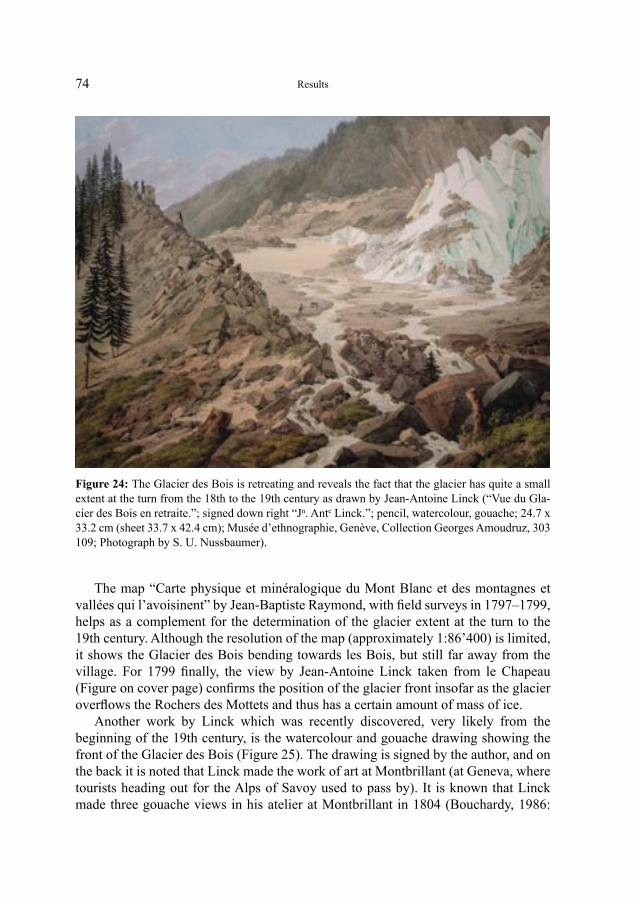
74

The map “Carte physique et minéralogique du Mont Blanc et des montagnes et vallées qui l’avoisinent” by Jean-Baptiste Raymond, with field surveys in 1797–1799, helps as a complement for the determination of the glacier extent at the turn to the 19th century. Although the resolution of the map (approximately 1:86’400) is limited, it shows the Glacier des Bois bending towards les Bois, but still far away from the village. For 1799 finally, the view by Jean-Antoine Linck taken from le Chapeau (Figure on cover page) confirms the position of the glacier front insofar as the glacier overflows the Rochers des Mottets and thus has a certain amount of mass of ice.

Another work by Linck which was recently discovered, very likely from the beginning of the 19th century, is the watercolour and gouache drawing showing the front of the Glacier des Bois (Figure 25). The drawing is signed by the author, and on the back it is noted that Linck made the work of art at Montbrillant (at Geneva, where tourists heading out for the Alps of Savoy used to pass by). It is known that Linck made three gouache views in his atelier at Montbrillant in 1804 (Bouchardy, 1986:

Figure 24: The Glacier des Bois is retreating and reveals the fact that the glacier has quite a small extent at the turn from the 18th to the 19th century as drawn by Jean-Antoine Linck (“Vue du Gla-cier des Bois en retraite.”; signed down right “Jn. Ante Linck.”; pencil, watercolour, gouache; 24.7 x 33.2 cm (sheet 33.7 x 42.4 cm); Musée d’ethnographie, Genève, Collection Georges Amoudruz, 303 109; Photograph by S. U. Nussbaumer).

Results

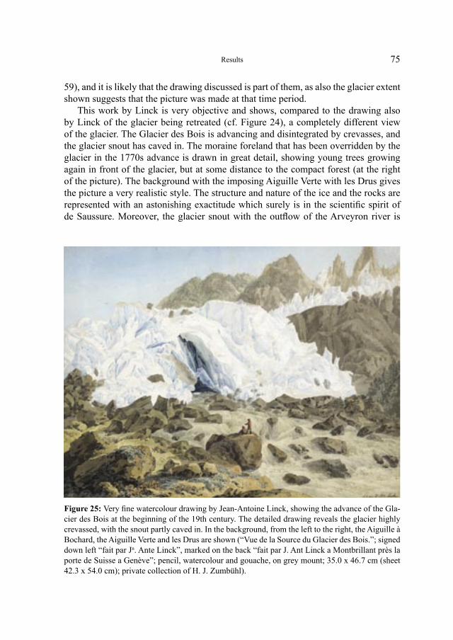
75

59), and it is likely that the drawing discussed is part of them, as also the glacier extent shown suggests that the picture was made at that time period.

This work by Linck is very objective and shows, compared to the drawing also by Linck of the glacier being retreated (cf. Figure 24), a completely different view of the glacier. The Glacier des Bois is advancing and disintegrated by crevasses, and the glacier snout has caved in. The moraine foreland that has been overridden by the glacier in the 1770s advance is drawn in great detail, showing young trees growing again in front of the glacier, but at some distance to the compact forest (at the right of the picture). The background with the imposing Aiguille Verte with les Drus gives the picture a very realistic style. The structure and nature of the ice and the rocks are represented with an astonishing exactitude which surely is in the scientific spirit of de Saussure. Moreover, the glacier snout with the outflow of the Arveyron river is

Figure 25: Very fine watercolour drawing by Jean-Antoine Linck, showing the advance of the Gla-cier des Bois at the beginning of the 19th century. The detailed drawing reveals the glacier highly crevassed, with the snout partly caved in. In the background, from the left to the right, the Aiguille à Bochard, the Aiguille Verte and les Drus are shown (“Vue de la Source du Glacier des Bois.”; signed down left “fait par Jn. Ante Linck”, marked on the back “fait par J. Ant Linck a Montbrillant près la porte de Suisse a Genève”; pencil, watercolour and gouache, on grey mount; 35.0 x 46.7 cm (sheet 42.3 x 54.0 cm); private collection of H. J. Zumbühl).

Results

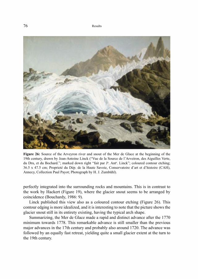
76

perfectly integrated into the surrounding rocks and mountains. This is in contrast to the work by Hackert (Figure 19), where the glacier snout seems to be arranged by coincidence (Bouchardy, 1986: 9).

Linck published this view also as a coloured contour etching (Figure 26). This contour edging is more idealized, and it is interesting to note that the picture shows the glacier snout still in its entirety existing, having the typical arch shape.

Summarizing, the Mer de Glace made a rapid and distinct advance after the 1770 minimum towards 1778. This remarkable advance is still smaller than the previous major advances in the 17th century and probably also around 1720. The advance was followed by an equally fast retreat, yielding quite a small glacier extent at the turn to the 19th century.

Figure 26: Source of the Arveyron river and snout of the Mer de Glace at the beginning of the 19th century, drawn by Jean-Antoine Linck (“Vue de la Source de l’Arveiron, des Aiguilles Verte, du Dru, et du Bochard.”; marked down right “fait par Jn. Ante. Linck”; coloured contour etching; 36.5 x 47.5 cm; Proprieté du Dép. de la Haute Savoie, Conservatoire d’art et d’histoire (CAH), Annecy, Collection Paul Payot; Photograph by H. J. Zumbühl).

Results

77

4.1.8 Beginning of the 19th century and major glacier advance in 1821, followed by a minor advance in 1852

Cartography was still of poor quality at the beginning of the 19th century in the Mont Blanc massif. The map sheet 13 of the “Atlas Suisse par Weiss et Meyer” from 1800 covering the Mont Blanc area is disappointing (see section 3.2.2). The Glacier des Bois has been drawn rather rudimentarily, but the glacier seems to have a com-paratively small extent at the glacier terminus.

Two years later, the important watercolour “Gletscher am Fuss des Mont Blanc 1802” by Joseph Mallord William Turner (1775–1851) shows again the attraction of the Mont Blanc area to English travellers and artists. The work, dated to 1802, is a unique composition of the tail of the Glacier des Bois and allows a quite accurate determination of the glacier front (Figure 27). It is one of the most powerful studies in the St Gotthard and Mont Blanc sketchbook by Turner and served as the basis for a painting that Turner made for Walter Fawkes probably c. 1806–9 (Guillaud and Guil-laud, 1981: 75). About the same viewpoint had been taken by one of Turner’s precur-sors, Francis Towne, who also made a watercolour of the source of the Arveyron river

Figure 27: Drawing by Joseph Mallord William Turner from 1802 showing the source of the Arvey-ron river which rises in a cavern at the base of the Mer de Glace (“Gletscher am Fuss des Mont Blanc 1802”; watercolour and body colour with scraping out, on white paper prepared with a grey wash; 31.2 x 46.8 cm; British Museum, London, T.B. LXXV-21). © The Trustees of The British Museum.

Results

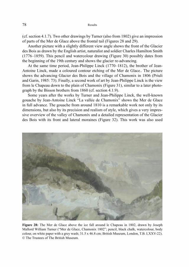
78

Figure 28: The Mer de Glace above the ice fall around le Chapeau in 1802, drawn by Joseph Mallord William Turner (“Mer de Glace, Chamonix 1802”; pencil, black chalk, watercolour, body colour, on white paper with a grey wash; 31.5 x 46.8 cm; British Museum, London, T.B. LXXV-22). © The Trustees of The British Museum.

(cf. section 4.1.7). Two other drawings by Turner (also from 1802) give an impression of parts of the Mer de Glace above the frontal tail (Figures 28 and 29).

Another picture with a slightly different view angle shows the front of the Glacier des Bois as drawn by the English artist, naturalist and soldier Charles Hamilton Smith (1776–1859). This pencil and watercolour drawing (Figure 30) possibly dates from the beginning of the 19th century and shows the glacier re-advancing.

At the same time period, Jean-Philippe Linck (1770–1812), the brother of Jean-Antoine Linck, made a coloured contour etching of the Mer de Glace.. The picture shows the advancing Glacier des Bois and the village of Chamonix in 1806 (Priuli and Garin, 1985: 73). Finally, a second work of art by Jean-Philippe Linck is the view from le Chapeau down to the plain of Chamonix (Figure 31), similar to a later photo-graph by the Bisson brothers from 1860 (cf. section 4.1.9).

Some years after the works by Turner and Jean-Philippe Linck, the well-known gouache by Jean-Antoine Linck “La vallée de Chamonix” shows the Mer de Glace in full advance. The gouache from around 1810 is a remarkable work not only by its dimensions, but also by its precision and realism of style, which gives a very impres-sive overview of the valley of Chamonix and a detailed representation of the Glacier des Bois with its front and lateral moraines (Figure 32). This work was also used

Results

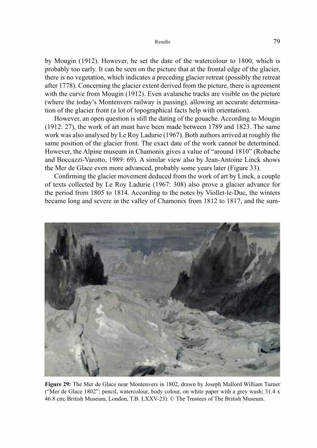
79

Figure 29: The Mer de Glace near Montenvers in 1802, drawn by Joseph Mallord William Turner (“Mer de Glace 1802”; pencil, watercolour, body colour, on white paper with a grey wash; 31.4 x 46.8 cm; British Museum, London, T.B. LXXV-23). © The Trustees of The British Museum.

by Mougin (1912). However, he set the date of the watercolour to 1800, which is probably too early. It can be seen on the picture that at the frontal edge of the glacier, there is no vegetation, which indicates a preceding glacier retreat (possibly the retreat after 1778). Concerning the glacier extent derived from the picture, there is agreement with the curve from Mougin (1912). Even avalanche tracks are visible on the picture (where the today’s Montenvers railway is passing), allowing an accurate determina-tion of the glacier front (a lot of topographical facts help with orientation).

However, an open question is still the dating of the gouache. According to Mougin (1912: 27), the work of art must have been made between 1789 and 1823. The same work was also analysed by Le Roy Ladurie (1967). Both authors arrived at roughly the same position of the glacier front. The exact date of the work cannot be determined. However, the Alpine museum in Chamonix gives a value of “around 1810” (Robache and Boccazzi-Varotto, 1989: 69). A similar view also by Jean-Antoine Linck shows the Mer de Glace even more advanced, probably some years later (Figure 33).

Confirming the glacier movement deduced from the work of art by Linck, a couple of texts collected by Le Roy Ladurie (1967: 308) also prove a glacier advance for the period from 1805 to 1814. According to the notes by Viollet-le-Duc, the winters became long and severe in the valley of Chamonix from 1812 to 1817, and the sum-

Results

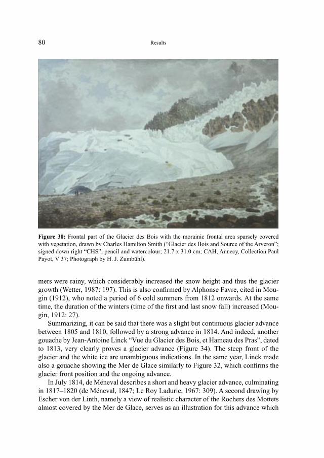
80

Figure 30: Frontal part of the Glacier des Bois with the morainic frontal area sparsely covered with vegetation, drawn by Charles Hamilton Smith (“Glacier des Bois and Source of the Arveron”; signed down right “CHS”; pencil and watercolour; 21.7 x 31.0 cm; CAH, Annecy, Collection Paul Payot, V 37; Photograph by H. J. Zumbühl).

mers were rainy, which considerably increased the snow height and thus the glacier growth (Wetter, 1987: 197). This is also confirmed by Alphonse Favre, cited in Mou-gin (1912), who noted a period of 6 cold summers from 1812 onwards. At the same time, the duration of the winters (time of the first and last snow fall) increased (Mou-gin, 1912: 27).

Summarizing, it can be said that there was a slight but continuous glacier advance between 1805 and 1810, followed by a strong advance in 1814. And indeed, another gouache by Jean-Antoine Linck “Vue du Glacier des Bois, et Hameau des Pras”, dated to 1813, very clearly proves a glacier advance (Figure 34). The steep front of the glacier and the white ice are unambiguous indications. In the same year, Linck made also a gouache showing the Mer de Glace similarly to Figure 32, which confirms the glacier front position and the ongoing advance.

In July 1814, de Méneval describes a short and heavy glacier advance, culminating in 1817–1820 (de Méneval, 1847; Le Roy Ladurie, 1967: 309). A second drawing by Escher von der Linth, namely a view of realistic character of the Rochers des Mottets almost covered by the Mer de Glace, serves as an illustration for this advance which

Results

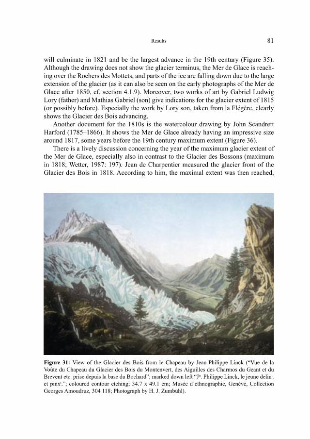
81

will culminate in 1821 and be the largest advance in the 19th century (Figure 35). Although the drawing does not show the glacier terminus, the Mer de Glace is reach-ing over the Rochers des Mottets, and parts of the ice are falling down due to the large extension of the glacier (as it can also be seen on the early photographs of the Mer de Glace after 1850, cf. section 4.1.9). Moreover, two works of art by Gabriel Ludwig Lory (father) and Mathias Gabriel (son) give indications for the glacier extent of 1815 (or possibly before). Especially the work by Lory son, taken from la Flégère, clearly shows the Glacier des Bois advancing.

Another document for the 1810s is the watercolour drawing by John Scandrett Harford (1785–1866). It shows the Mer de Glace already having an impressive size around 1817, some years before the 19th century maximum extent (Figure 36).

There is a lively discussion concerning the year of the maximum glacier extent of the Mer de Glace, especially also in contrast to the Glacier des Bossons (maximum in 1818; Wetter, 1987: 197). Jean de Charpentier measured the glacier front of the Glacier des Bois in 1818. According to him, the maximal extent was then reached,

Results

Figure 31: View of the Glacier des Bois from le Chapeau by Jean-Philippe Linck (“Vue de la Voûte du Chapeau du Glacier des Bois du Montenvert, des Aiguilles des Charmos du Geant et du Brevent etc. prise depuis la base du Bochard”; marked down left “Jn. Philippe Linck, le jeune delint. et pinxt.”; coloured contour etching; 34.7 x 49.1 cm; Musée d’ethnographie, Genève, Collection Georges Amoudruz, 304 118; Photograph by H. J. Zumbühl).

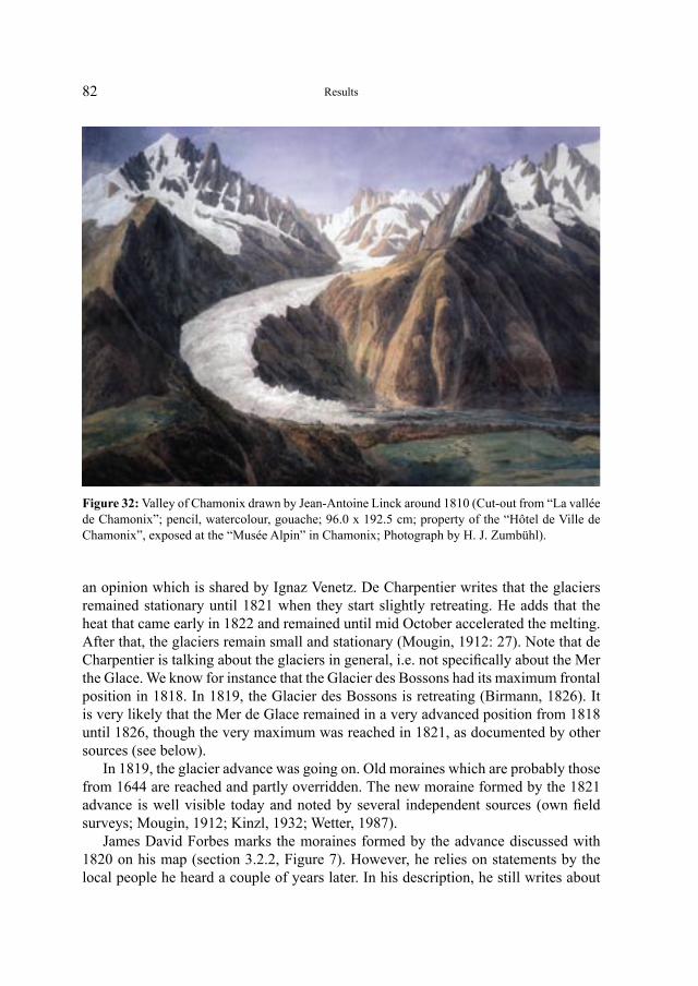
82

Figure 32: Valley of Chamonix drawn by Jean-Antoine Linck around 1810 (Cut-out from “La vallée de Chamonix”; pencil, watercolour, gouache; 96.0 x 192.5 cm; property of the “Hôtel de Ville de Chamonix”, exposed at the “Musée Alpin” in Chamonix; Photograph by H. J. Zumbühl).

an opinion which is shared by Ignaz Venetz. De Charpentier writes that the glaciers remained stationary until 1821 when they start slightly retreating. He adds that the heat that came early in 1822 and remained until mid October accelerated the melting. After that, the glaciers remain small and stationary (Mougin, 1912: 27). Note that de Charpentier is talking about the glaciers in general, i.e. not specifically about the Mer the Glace. We know for instance that the Glacier des Bossons had its maximum frontal position in 1818. In 1819, the Glacier des Bossons is retreating (Birmann, 1826). It is very likely that the Mer de Glace remained in a very advanced position from 1818 until 1826, though the very maximum was reached in 1821, as documented by other sources (see below).

In 1819, the glacier advance was going on. Old moraines which are probably those from 1644 are reached and partly overridden. The new moraine formed by the 1821 advance is well visible today and noted by several independent sources (own field surveys; Mougin, 1912; Kinzl, 1932; Wetter, 1987).

James David Forbes marks the moraines formed by the advance discussed with 1820 on his map (section 3.2.2, Figure 7). However, he relies on statements by the local people he heard a couple of years later. In his description, he still writes about

Results

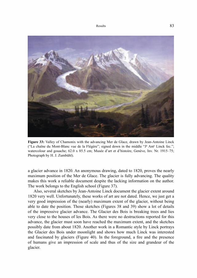
83

a glacier advance in 1820. An anonymous drawing, dated to 1820, proves the nearly maximum position of the Mer de Glace. The glacier is fully advancing. The quality makes this work a reliable document despite the lacking information on the author. The work belongs to the English school (Figure 37).

Also, several sketches by Jean-Antoine Linck document the glacier extent around 1820 very well. Unfortunately, these works of art are not dated. Hence, we just get a very good impression of the (nearly) maximum extent of the glacier, without being able to date the position. Those sketches (Figures 38 and 39) show a lot of details of the impressive glacier advance. The Glacier des Bois is breaking trees and lies very close to the houses of les Bois. As there were no destructions reported for this advance, the glacier must soon have reached the maximum extent, and the sketches possibly date from about 1820. Another work in a Romantic style by Linck portrays the Glacier des Bois under moonlight and shows how much Linck was interested and fascinated by glaciers (Figure 40). In the foreground, a fire and the presence of humans give an impression of scale and thus of the size and grandeur of the glacier.

Results

Figure 33: Valley of Chamonix with the advancing Mer de Glace, drawn by Jean-Antoine Linck (“La chaîne du Mont-Blanc vue de la Flégère”; signed down in the middle “Jn Ante Linck fec.”; watercolour and gouache; 62.0 x 85.5 cm; Musée d’art et d’histoire, Genève, Inv. Nr. 1915–75; Photograph by H. J. Zumbühl).

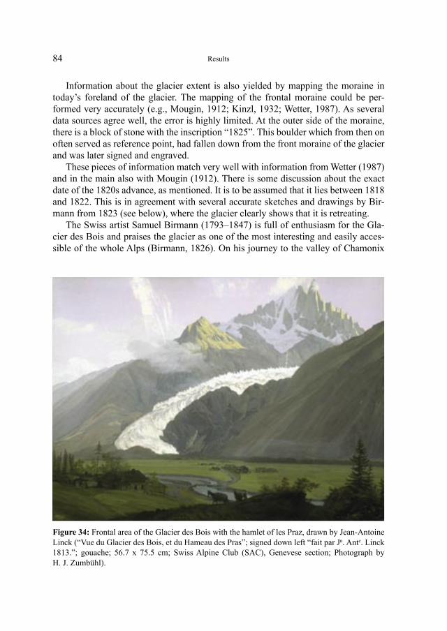
84

Information about the glacier extent is also yielded by mapping the moraine in today’s foreland of the glacier. The mapping of the frontal moraine could be per-formed very accurately (e.g., Mougin, 1912; Kinzl, 1932; Wetter, 1987). As several data sources agree well, the error is highly limited. At the outer side of the moraine, there is a block of stone with the inscription “1825”. This boulder which from then on often served as reference point, had fallen down from the front moraine of the glacier and was later signed and engraved.

These pieces of information match very well with information from Wetter (1987) and in the main also with Mougin (1912). There is some discussion about the exact date of the 1820s advance, as mentioned. It is to be assumed that it lies between 1818 and 1822. This is in agreement with several accurate sketches and drawings by Bir-mann from 1823 (see below), where the glacier clearly shows that it is retreating.

The Swiss artist Samuel Birmann (1793–1847) is full of enthusiasm for the Gla-cier des Bois and praises the glacier as one of the most interesting and easily acces-sible of the whole Alps (Birmann, 1826). On his journey to the valley of Chamonix

Figure 34: Frontal area of the Glacier des Bois with the hamlet of les Praz, drawn by Jean-Antoine Linck (“Vue du Glacier des Bois, et du Hameau des Pras”; signed down left “fait par Jn. Ante. Linck 1813.”; gouache; 56.7 x 75.5 cm; Swiss Alpine Club (SAC), Genevese section; Photograph by H. J. Zumbühl).

Results

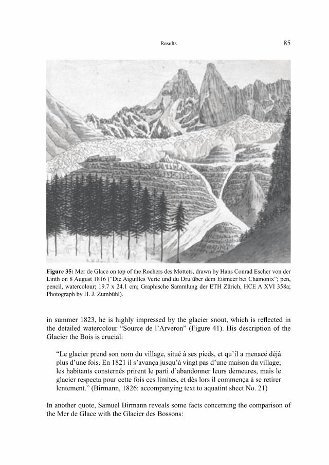
85

in summer 1823, he is highly impressed by the glacier snout, which is reflected in the detailed watercolour “Source de l’Arveron” (Figure 41). His description of the Glacier the Bois is crucial:

“Le glacier prend son nom du village, situé à ses pieds, et qu’il a menacé déjà plus d’une fois. En 1821 il s’avança jusqu’à vingt pas d’une maison du village; les habitants consternés prirent le parti d’abandonner leurs demeures, mais le glacier respecta pour cette fois ces limites, et dès lors il commença à se retirer lentement.” (Birmann, 1826: accompanying text to aquatint sheet No. 21)

In another quote, Samuel Birmann reveals some facts concerning the comparison of the Mer de Glace with the Glacier des Bossons:

Figure 35: Mer de Glace on top of the Rochers des Mottets, drawn by Hans Conrad Escher von der Linth on 8 August 1816 (“Die Aiguilles Verte und du Dru über dem Eismeer bei Chamonix”; pen, pencil, watercolour; 19.7 x 24.1 cm; Graphische Sammlung der ETH Zürich, HCE A XVI 358a; Photograph by H. J. Zumbühl).

Results

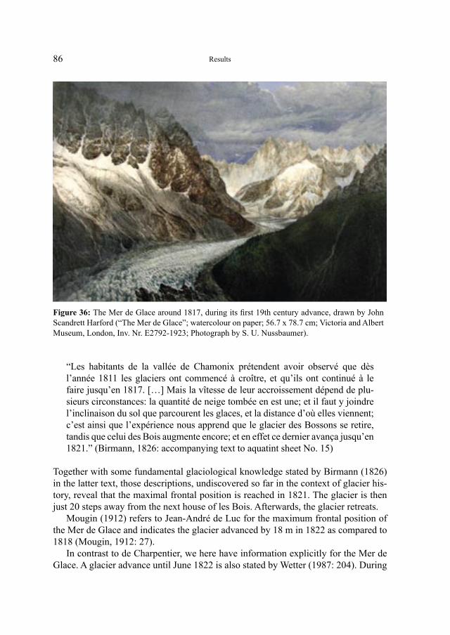
86

“Les habitants de la vallée de Chamonix prétendent avoir observé que dès l’année 1811 les glaciers ont commencé à croître, et qu’ils ont continué à le faire jusqu’en 1817. […] Mais la vîtesse de leur accroissement dépend de plu-sieurs circonstances: la quantité de neige tombée en est une; et il faut y joindre l’inclinaison du sol que parcourent les glaces, et la distance d’où elles viennent; c’est ainsi que l’expérience nous apprend que le glacier des Bossons se retire, tandis que celui des Bois augmente encore; et en effet ce dernier avança jusqu’en 1821.” (Birmann, 1826: accompanying text to aquatint sheet No. 15)

Together with some fundamental glaciological knowledge stated by Birmann (1826) in the latter text, those descriptions, undiscovered so far in the context of glacier his-tory, reveal that the maximal frontal position is reached in 1821. The glacier is then just 20 steps away from the next house of les Bois. Afterwards, the glacier retreats.

Mougin (1912) refers to Jean-André de Luc for the maximum frontal position of the Mer de Glace and indicates the glacier advanced by 18 m in 1822 as compared to 1818 (Mougin, 1912: 27).

In contrast to de Charpentier, we here have information explicitly for the Mer de Glace. A glacier advance until June 1822 is also stated by Wetter (1987: 204). During

Figure 36: The Mer de Glace around 1817, during its first 19th century advance, drawn by John Scandrett Harford (“The Mer de Glace”; watercolour on paper; 56.7 x 78.7 cm; Victoria and Albert Museum, London, Inv. Nr. E2792-1923; Photograph by S. U. Nussbaumer).

Results

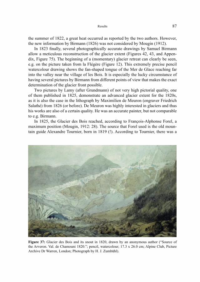
87

the summer of 1822, a great heat occurred as reported by the two authors. However, the new information by Birmann (1826) was not considered by Mougin (1912).

In 1823 finally, several photographically accurate drawings by Samuel Birmann allow a meticulous reconstruction of the glacier extent (Figures 42, 43, and Appen-dix, Figure 75). The beginning of a (momentary) glacier retreat can clearly be seen, e.g. on the picture taken from la Flégère (Figure 12). This extremely precise pencil watercolour drawing shows the fan-shaped tongue of the Mer de Glace reaching far into the valley near the village of les Bois. It is especially the lucky circumstance of having several pictures by Birmann from different points of view that makes the exact determination of the glacier front possible.

Two pictures by Lamy (after Grundmann) of not very high pictorial quality, one of them published in 1825, demonstrate an advanced glacier extent for the 1820s, as it is also the case in the lithograph by Maximilien de Meuron (engraver Friedrich Salathé) from 1826 (or before). De Meuron was highly interested in glaciers and thus his works are also of a certain quality. He was an accurate painter, but not comparable to e.g. Birmann.

In 1825, the Glacier des Bois reached, according to François-Alphonse Forel, a maximum position (Mougin, 1912: 28). The source that Forel used is the old moun-tain guide Alexandre Tournier, born in 1819 (!). According to Tournier, there was a

Figure 37: Glacier des Bois and its snout in 1820, drawn by an anonymous author (“Source of the Arveron. Val. de Chamouni 1820.”; pencil, watercolour; 17.3 x 26.0 cm; Alpine Club, Picture Archive Dr Warren, London; Photograph by H. J. Zumbühl).

Results

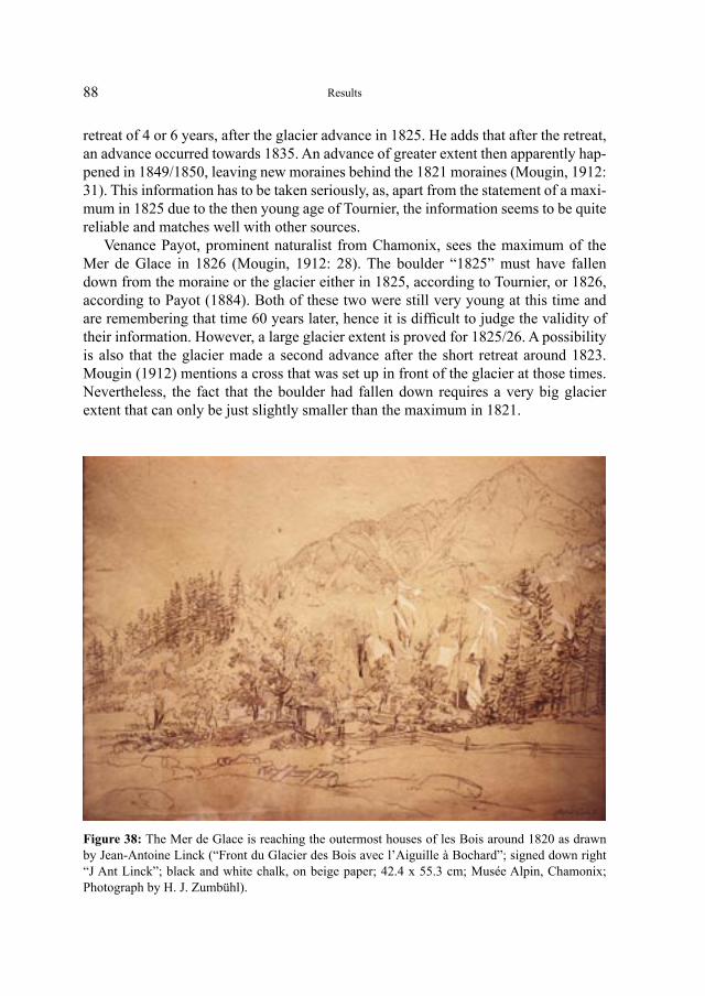
88

retreat of 4 or 6 years, after the glacier advance in 1825. He adds that after the retreat, an advance occurred towards 1835. An advance of greater extent then apparently hap-pened in 1849/1850, leaving new moraines behind the 1821 moraines (Mougin, 1912: 31). This information has to be taken seriously, as, apart from the statement of a maxi-mum in 1825 due to the then young age of Tournier, the information seems to be quite reliable and matches well with other sources.

Venance Payot, prominent naturalist from Chamonix, sees the maximum of the Mer de Glace in 1826 (Mougin, 1912: 28). The boulder “1825” must have fallen down from the moraine or the glacier either in 1825, according to Tournier, or 1826, according to Payot (1884). Both of these two were still very young at this time and are remembering that time 60 years later, hence it is difficult to judge the validity of their information. However, a large glacier extent is proved for 1825/26. A possibility is also that the glacier made a second advance after the short retreat around 1823. Mougin (1912) mentions a cross that was set up in front of the glacier at those times. Nevertheless, the fact that the boulder had fallen down requires a very big glacier extent that can only be just slightly smaller than the maximum in 1821.

Figure 38: The Mer de Glace is reaching the outermost houses of les Bois around 1820 as drawn by Jean-Antoine Linck (“Front du Glacier des Bois avec l’Aiguille à Bochard”; signed down right “J Ant Linck”; black and white chalk, on beige paper; 42.4 x 55.3 cm; Musée Alpin, Chamonix; Photograph by H. J. Zumbühl).

Results

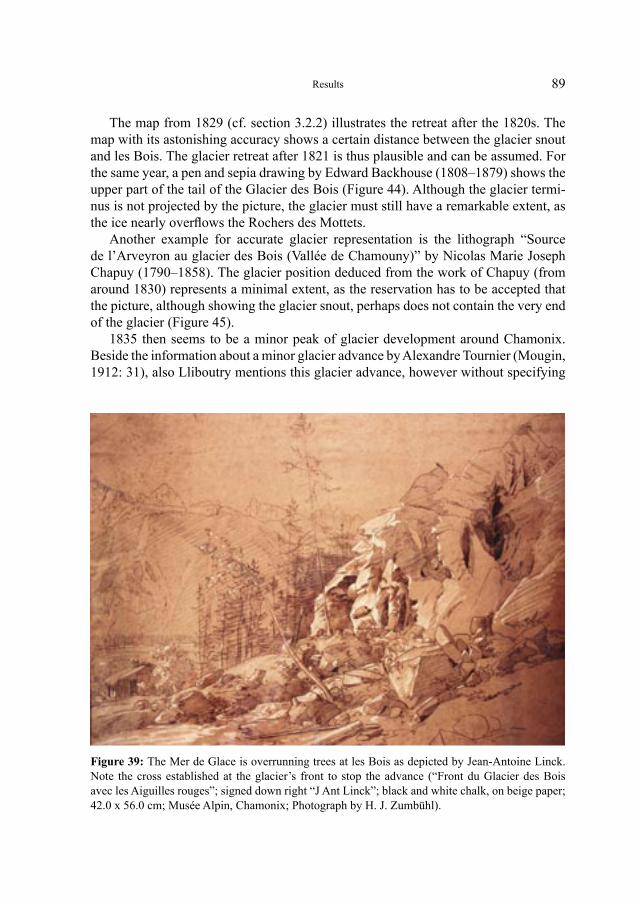
89

The map from 1829 (cf. section 3.2.2) illustrates the retreat after the 1820s. The map with its astonishing accuracy shows a certain distance between the glacier snout and les Bois. The glacier retreat after 1821 is thus plausible and can be assumed. For the same year, a pen and sepia drawing by Edward Backhouse (1808–1879) shows the upper part of the tail of the Glacier des Bois (Figure 44). Although the glacier termi-nus is not projected by the picture, the glacier must still have a remarkable extent, as the ice nearly overflows the Rochers des Mottets.

Another example for accurate glacier representation is the lithograph “Source de l’Arveyron au glacier des Bois (Vallée de Chamouny)” by Nicolas Marie Joseph Chapuy (1790–1858). The glacier position deduced from the work of Chapuy (from around 1830) represents a minimal extent, as the reservation has to be accepted that the picture, although showing the glacier snout, perhaps does not contain the very end of the glacier (Figure 45).

1835 then seems to be a minor peak of glacier development around Chamonix. Beside the information about a minor glacier advance by Alexandre Tournier (Mougin, 1912: 31), also Lliboutry mentions this glacier advance, however without specifying

Figure 39: The Mer de Glace is overrunning trees at les Bois as depicted by Jean-Antoine Linck. Note the cross established at the glacier’s front to stop the advance (“Front du Glacier des Bois avec les Aiguilles rouges”; signed down right “J Ant Linck”; black and white chalk, on beige paper; 42.0 x 56.0 cm; Musée Alpin, Chamonix; Photograph by H. J. Zumbühl).

Results

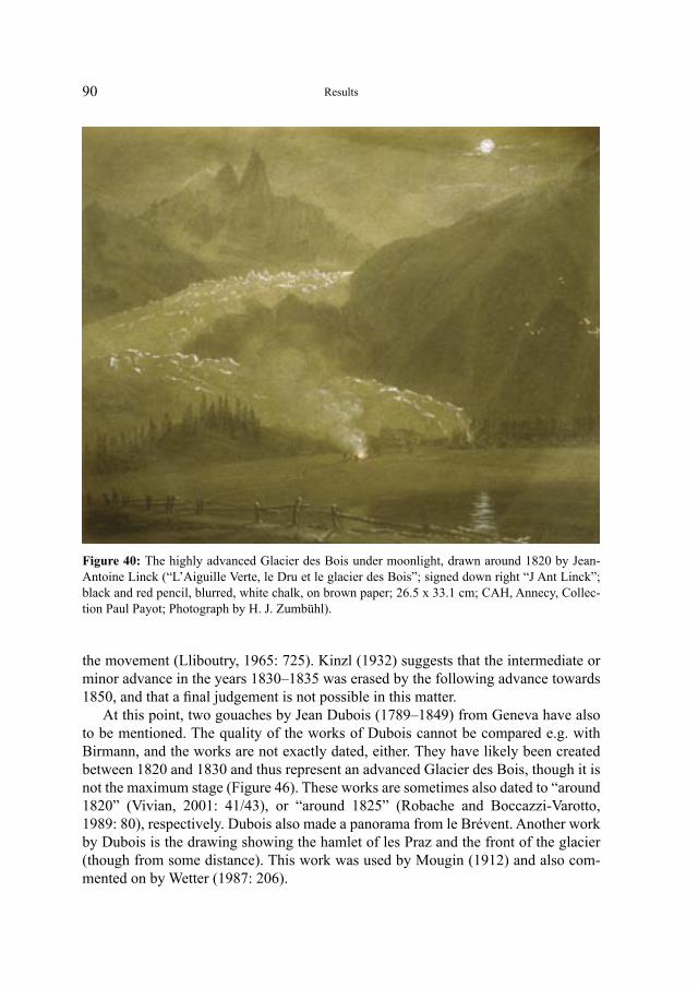
90

the movement (Lliboutry, 1965: 725). Kinzl (1932) suggests that the intermediate or minor advance in the years 1830–1835 was erased by the following advance towards 1850, and that a final judgement is not possible in this matter.

At this point, two gouaches by Jean Dubois (1789–1849) from Geneva have also to be mentioned. The quality of the works of Dubois cannot be compared e.g. with Birmann, and the works are not exactly dated, either. They have likely been created between 1820 and 1830 and thus represent an advanced Glacier des Bois, though it is not the maximum stage (Figure 46). These works are sometimes also dated to “around 1820” (Vivian, 2001: 41/43), or “around 1825” (Robache and Boccazzi-Varotto, 1989: 80), respectively. Dubois also made a panorama from le Brévent. Another work by Dubois is the drawing showing the hamlet of les Praz and the front of the glacier (though from some distance). This work was used by Mougin (1912) and also com-mented on by Wetter (1987: 206).

Figure 40: The highly advanced Glacier des Bois under moonlight, drawn around 1820 by Jean-Antoine Linck (“L’Aiguille Verte, le Dru et le glacier des Bois”; signed down right “J Ant Linck”; black and red pencil, blurred, white chalk, on brown paper; 26.5 x 33.1 cm; CAH, Annecy, Collec-tion Paul Payot; Photograph by H. J. Zumbühl).

Results

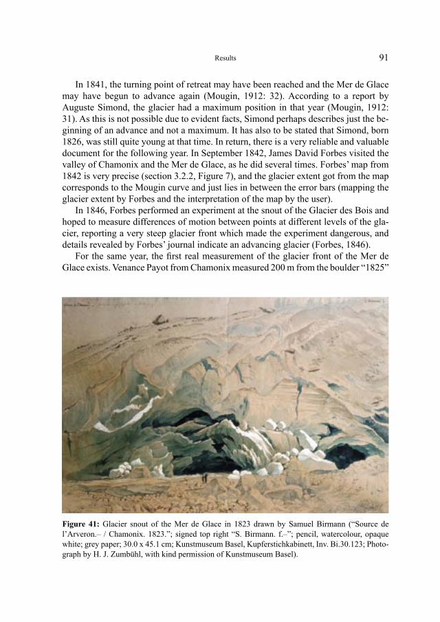
91

In 1841, the turning point of retreat may have been reached and the Mer de Glace may have begun to advance again (Mougin, 1912: 32). According to a report by Auguste Simond, the glacier had a maximum position in that year (Mougin, 1912: 31). As this is not possible due to evident facts, Simond perhaps describes just the be- ginning of an advance and not a maximum. It has also to be stated that Simond, born 1826, was still quite young at that time. In return, there is a very reliable and valuable document for the following year. In September 1842, James David Forbes visited the valley of Chamonix and the Mer de Glace, as he did several times. Forbes’ map from 1842 is very precise (section 3.2.2, Figure 7), and the glacier extent got from the map corresponds to the Mougin curve and just lies in between the error bars (mapping the glacier extent by Forbes and the interpretation of the map by the user).

In 1846, Forbes performed an experiment at the snout of the Glacier des Bois and hoped to measure differences of motion between points at different levels of the gla-cier, reporting a very steep glacier front which made the experiment dangerous, and details revealed by Forbes’ journal indicate an advancing glacier (Forbes, 1846).

For the same year, the first real measurement of the glacier front of the Mer de Glace exists. Venance Payot from Chamonix measured 200 m from the boulder “1825”

Figure 41: Glacier snout of the Mer de Glace in 1823 drawn by Samuel Birmann (“Source de l’Arveron.– / Chamonix. 1823.”; signed top right “S. Birmann. f.–”; pencil, watercolour, opaque white; grey paper; 30.0 x 45.1 cm; Kunstmuseum Basel, Kupferstichkabinett, Inv. Bi.30.123; Photo-graph by H. J. Zumbühl, with kind permission of Kunstmuseum Basel).

Results

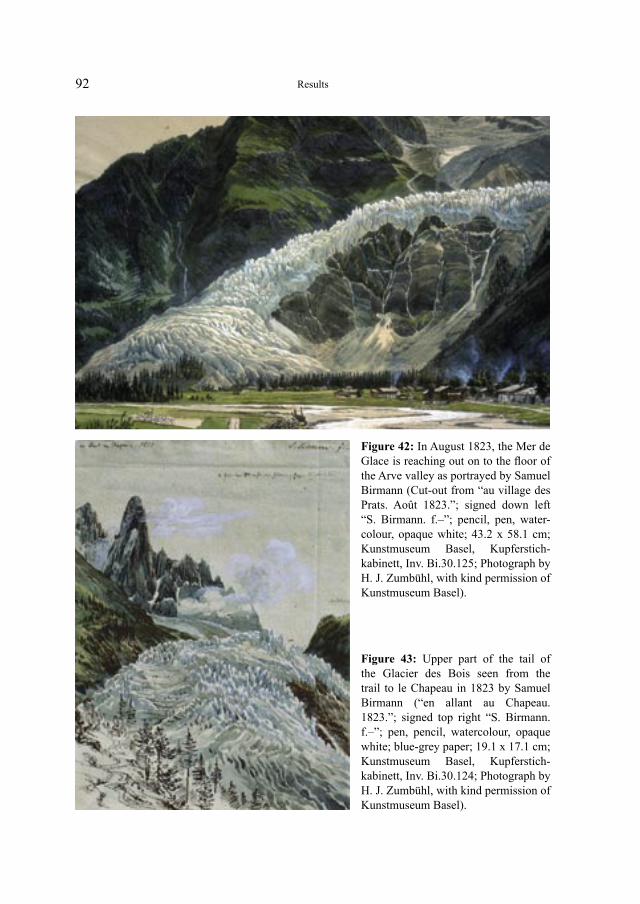
92

Figure 42: In August 1823, the Mer de Glace is reaching out on to the floor of the Arve valley as portrayed by Samuel Birmann (Cut-out from “au village des Prats. Août 1823.”; signed down left “S. Birmann. f.–”; pencil, pen, water-colour, opaque white; 43.2 x 58.1 cm; Kunstmuseum Basel, Kupferstich- kabinett, Inv. Bi.30.125; Photograph by H. J. Zumbühl, with kind permission of Kunstmuseum Basel).

Figure 43: Upper part of the tail of the Glacier des Bois seen from the trail to le Chapeau in 1823 by Samuel Birmann (“en allant au Chapeau. 1823.”; signed top right “S. Birmann. f.–”; pen, pencil, watercolour, opaque white; blue-grey paper; 19.1 x 17.1 cm; Kunstmuseum Basel, Kupferstich-kabinett, Inv. Bi.30.124; Photograph by H. J. Zumbühl, with kind permission of Kunstmuseum Basel).

Results

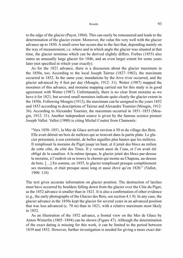
93

to the edge of the glacier (Payot, 1884). This can easily be remeasured and leads to the determination of the glacier extent. Moreover, the value fits very well with the glacier advance up to 1850. A small error bar occurs due to the fact that, depending mainly on the way of measurement, i.e. where and in which angle the glacier was situated at that time, the glacier terminus which can be derived slightly differs. Forbes (1855) also states an unusually large glacier for 1846, and an even larger extent for some years later (not specified in which year exactly).

As for the 1821 advance, there is a discussion about the glacier maximum in the 1850s, too. According to the local Joseph Tairraz (1827–1902), the maximum occurred in 1852. In the same year, inundations by the Arve river occurred, and the glacier advanced by 4 feet per day (Mougin, 1912: 31). Wetter (1987) mapped the moraines of this advance, and moraine mapping carried out for this study is in good agreement with Wetter (1987). Unfortunately, there is no clear front moraine as we have it for 1821, but several small moraines indicate quite clearly the glacier extent in the 1850s. Following Mougin (1912), the maximum can be assigned to the years 1852 and 1853 according to descriptions of Tairraz and Alexandre Tournier (Mougin, 1912: 36). According to Alexandre Tournier, the maximum occurred in 1851–1853 (Mou-gin, 1912: 31). Another independent source is given by the famous science pioneer Joseph Vallot. Vallot (1900) is citing Michel Couttet from Chamonix:

“Vers 1850–1851, la Mer de Glace arrivait environ à 50 m du village des Bois. Elle avait détruit un bois de mélèzes qui se trouvait dans la partie plate. Le gla-cier présentait, à son extrémité, de belles aiguilles plus hautes que les mélèzes. Il remplissait la moraine du Piget jusqu’en haut, et il jetait des blocs au milieu de cette côte, du côté des Tines. Il y versait aussi de l’eau, et l’on avait été obligé de la canaliser. A la même époque, le glacier jetait des blocs par-dessus la moraine, à l’endroit où se trouve le chemin qui monte au Chapeau, au-dessus du bois. […] En somme, en 1855, le glacier remplissait presque complètement ses moraines, et était presque aussi long et aussi élevé qu’en 1820.” (Vallot, 1900: 118)

The text gives accurate information on glacier position. The destruction of larches must have occurred by boulders falling down from the glacier over the Côte du Piget, as the 1852 advance is smaller than in 1821. It is also a confirmation of other evidence (e.g., the early photographs of the Glacier des Bois, see section 4.1.9). In any case, the glacier advance in the 1850s kept the glacier for several years in an advanced position that was less advanced (c. 70 m) than in 1821, with a relative maximum most likely in 1852.

As an illustration of the 1852 advance, a frontal view on the Mer de Glace by Anton Winterlin (1805–1894) can be shown (Figure 47). Although the determination of the exact dating is missing for this work, it can be limited to the period between 1839 and 1852. However, further investigation is needed for giving a more exact dat-

Results

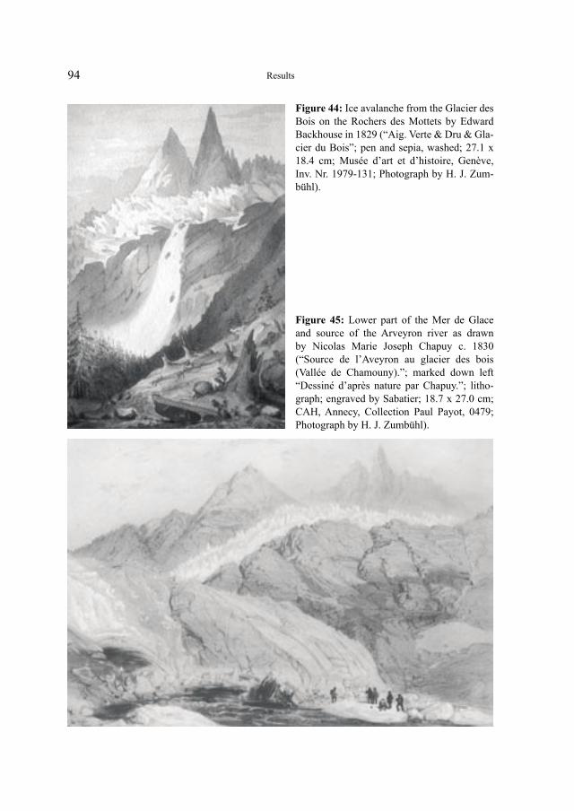
94

Figure 44: Ice avalanche from the Glacier des Bois on the Rochers des Mottets by Edward Backhouse in 1829 (“Aig. Verte & Dru & Gla-cier du Bois”; pen and sepia, washed; 27.1 x 18.4 cm; Musée d’art et d’histoire, Genève, Inv. Nr. 1979-131; Photograph by H. J. Zum-bühl).

Figure 45: Lower part of the Mer de Glace and source of the Arveyron river as drawn by Nicolas Marie Joseph Chapuy c. 1830 (“Source de l’Aveyron au glacier des bois (Vallée de Chamouny).”; marked down left “Dessiné d’après nature par Chapuy.”; litho-graph; engraved by Sabatier; 18.7 x 27.0 cm; CAH, Annecy, Collection Paul Payot, 0479; Photograph by H. J. Zumbühl).

Results

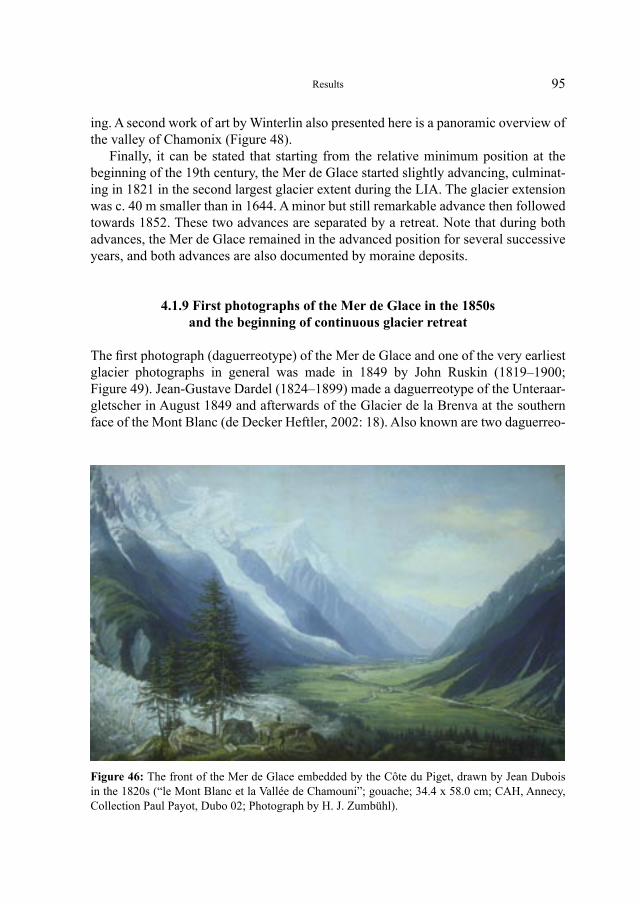
95

Figure 46: The front of the Mer de Glace embedded by the Côte du Piget, drawn by Jean Dubois in the 1820s (“le Mont Blanc et la Vallée de Chamouni”; gouache; 34.4 x 58.0 cm; CAH, Annecy, Collection Paul Payot, Dubo 02; Photograph by H. J. Zumbühl).

ing. A second work of art by Winterlin also presented here is a panoramic overview of the valley of Chamonix (Figure 48).

Finally, it can be stated that starting from the relative minimum position at the beginning of the 19th century, the Mer de Glace started slightly advancing, culminat-ing in 1821 in the second largest glacier extent during the LIA. The glacier extension was c. 40 m smaller than in 1644. A minor but still remarkable advance then followed towards 1852. These two advances are separated by a retreat. Note that during both advances, the Mer de Glace remained in the advanced position for several successive years, and both advances are also documented by moraine deposits.

4.1.9 First photographs of the Mer de Glace in the 1850s and the beginning of continuous glacier retreat

The first photograph (daguerreotype) of the Mer de Glace and one of the very earliest glacier photographs in general was made in 1849 by John Ruskin (1819–1900; Figure 49). Jean-Gustave Dardel (1824–1899) made a daguerreotype of the Unteraar- gletscher in August 1849 and afterwards of the Glacier de la Brenva at the southern face of the Mont Blanc (de Decker Heftler, 2002: 18). Also known are two daguerreo-

Results

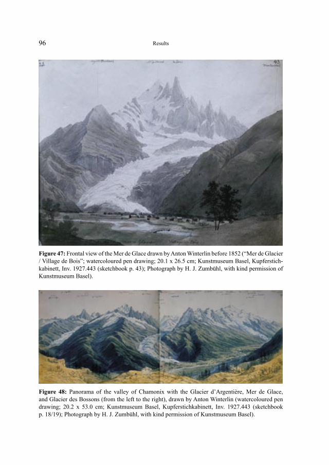
96

Figure 47: Frontal view of the Mer de Glace drawn by Anton Winterlin before 1852 (“Mer de Glacier / Village de Bois”; watercoloured pen drawing; 20.1 x 26.5 cm; Kunstmuseum Basel, Kupferstich-kabinett, Inv. 1927.443 (sketchbook p. 43); Photograph by H. J. Zumbühl, with kind permission of Kunstmuseum Basel).

Figure 48: Panorama of the valley of Chamonix with the Glacier d’Argentière, Mer de Glace, and Glacier des Bossons (from the left to the right), drawn by Anton Winterlin (watercoloured pen drawing; 20.2 x 53.0 cm; Kunstmuseum Basel, Kupferstichkabinett, Inv. 1927.443 (sketchbook p. 18/19); Photograph by H. J. Zumbühl, with kind permission of Kunstmuseum Basel).

Results

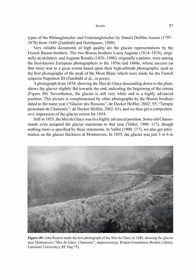
97

types of the Rhônegletscher and Unteraargletscher by Daniel Dollfus-Ausset (1797–1870) from 1849 (Zumbühl and Holzhauser, 1988).

Very reliable documents of high quality are the glacier representations by the French Bisson brothers. The two Bisson brothers Louis Auguste (1814–1876), origi-nally an architect, and Auguste Rosalie (1826–1900), originally a painter, were among the best-known European photographers in the 1850s and 1860s, whose success (at that time) was to a great extent based upon their high-altitude photographs, such as the first photographs of the peak of the Mont Blanc which were made for the French emperor Napoléon III (Zumbühl et al., in press).

A photograph from 1854, showing the Mer de Glace descending down to the plain, shows the glacier slightly flat towards the end, indicating the beginning of the retreat (Figure 50). Nevertheless, the glacier is still very white and in a highly advanced position. This picture is complemented by other photographs by the Bisson brothers dated to the same year (“Glacier des Bossons”, de Decker Heftler, 2002: 55; “Temple protestant de Chamonix”, de Decker Heftler, 2002: 63), and we thus get a comprehen-sive impression of the glacier extent for 1854.

Still in 1855, the Mer de Glace was in a highly advanced position. Some old Chamo-niards even assigned the glacier maximum to that year (Vallot, 1900: 117), though nothing more is specified by these statements. In Vallot (1900: 117), we also get infor-mation on the glacier thickness at Montenvers: In 1855, the glacier was just 5 or 6 m

Figure 49: John Ruskin made the first photograph of the Mer de Glace in 1849, showing the glacier near Montenvers (“Mer de Glace, Chamonix”; daguerreotype; Ruskin Foundation (Ruskin Library, Lancaster University), RF Dag 75).

Results

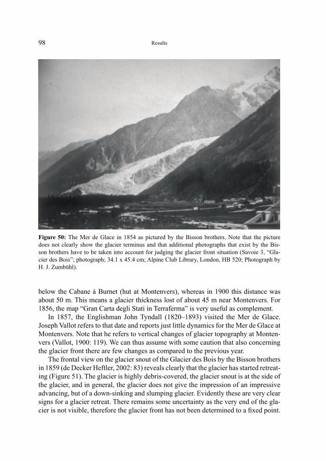
98

below the Cabane à Burnet (hut at Montenvers), whereas in 1900 this distance was about 50 m. This means a glacier thickness lost of about 45 m near Montenvers. For 1856, the map “Gran Carta degli Stati in Terraferma” is very useful as complement.

In 1857, the Englishman John Tyndall (1820–1893) visited the Mer de Glace. Joseph Vallot refers to that date and reports just little dynamics for the Mer de Glace at Montenvers. Note that he refers to vertical changes of glacier topography at Monten-vers (Vallot, 1900: 119). We can thus assume with some caution that also concerning the glacier front there are few changes as compared to the previous year.

The frontal view on the glacier snout of the Glacier des Bois by the Bisson brothers in 1859 (de Decker Heftler, 2002: 83) reveals clearly that the glacier has started retreat-ing (Figure 51). The glacier is highly debris-covered, the glacier snout is at the side of the glacier, and in general, the glacier does not give the impression of an impressive advancing, but of a down-sinking and slumping glacier. Evidently these are very clear signs for a glacier retreat. There remains some uncertainty as the very end of the gla-cier is not visible, therefore the glacier front has not been determined to a fixed point.

Figure 50: The Mer de Glace in 1854 as pictured by the Bisson brothers. Note that the picture does not clearly show the glacier terminus and that additional photographs that exist by the Bis-son brothers have to be taken into account for judging the glacier front situation (Savoie 3, “Gla-cier des Bois”; photograph; 34.1 x 45.4 cm; Alpine Club Library, London, HB 520; Photograph by H. J. Zumbühl).

Results

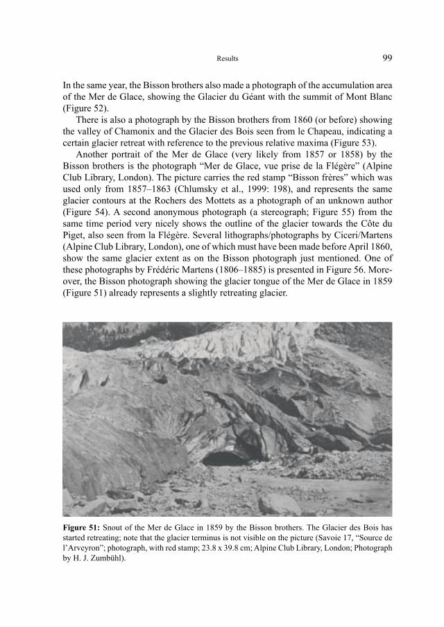
99

In the same year, the Bisson brothers also made a photograph of the accumulation area of the Mer de Glace, showing the Glacier du Géant with the summit of Mont Blanc (Figure 52).

There is also a photograph by the Bisson brothers from 1860 (or before) showing the valley of Chamonix and the Glacier des Bois seen from le Chapeau, indicating a certain glacier retreat with reference to the previous relative maxima (Figure 53).

Another portrait of the Mer de Glace (very likely from 1857 or 1858) by the Bisson brothers is the photograph “Mer de Glace, vue prise de la Flégère” (Alpine Club Library, London). The picture carries the red stamp “Bisson frères” which was used only from 1857–1863 (Chlumsky et al., 1999: 198), and represents the same glacier contours at the Rochers des Mottets as a photograph of an unknown author (Figure 54). A second anonymous photograph (a stereograph; Figure 55) from the same time period very nicely shows the outline of the glacier towards the Côte du Piget, also seen from la Flégère. Several lithographs/photographs by Ciceri/Martens (Alpine Club Library, London), one of which must have been made before April 1860, show the same glacier extent as on the Bisson photograph just mentioned. One of these photographs by Frédéric Martens (1806–1885) is presented in Figure 56. More-over, the Bisson photograph showing the glacier tongue of the Mer de Glace in 1859 (Figure 51) already represents a slightly retreating glacier.

Figure 51: Snout of the Mer de Glace in 1859 by the Bisson brothers. The Glacier des Bois has started retreating; note that the glacier terminus is not visible on the picture (Savoie 17, “Source de l’Arveyron”; photograph, with red stamp; 23.8 x 39.8 cm; Alpine Club Library, London; Photograph by H. J. Zumbühl).

Results

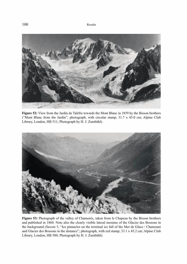
100

Figure 52: View from the Jardin de Talèfre towards the Mont Blanc in 1859 by the Bisson brothers (“Mont Blanc from the Jardin”; photograph, with circular stamp; 31.7 x 45.0 cm; Alpine Club Library, London, HB 511; Photograph by H. J. Zumbühl).

Figure 53: Photograph of the valley of Chamonix, taken from le Chapeau by the Bisson brothers and published in 1860. Note also the clearly visible lateral moraine of the Glacier des Bossons in the background (Savoie 5, “Ice pinnacles on the terminal ice fall of the Mer de Glace / Chamouni and Glacier des Bossons in the distance”; photograph, with red stamp; 33.1 x 45.2 cm; Alpine Club Library, London, HB 500; Photograph by H. J. Zumbühl).

Results

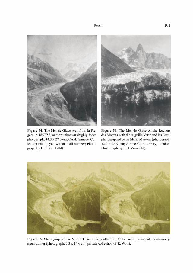
101

Figure 54: The Mer de Glace seen from la Flé-gère in 1857/58, author unknown (highly faded photograph; 34.3 x 27.0 cm; CAH, Annecy, Col-lection Paul Payot, without call number; Photo-graph by H. J. Zumbühl).

Figure 55: Stereograph of the Mer de Glace shortly after the 1850s maximum extent, by an anony-mous author (photograph; 7.3 x 14.6 cm; private collection of R. Wolf).

Figure 56: The Mer de Glace on the Rochers des Mottets with the Aiguille Verte and les Drus, photographed by Frédéric Martens (photograph; 32.0 x 25.9 cm; Alpine Club Library, London; Photograph by H. J. Zumbühl).

Results

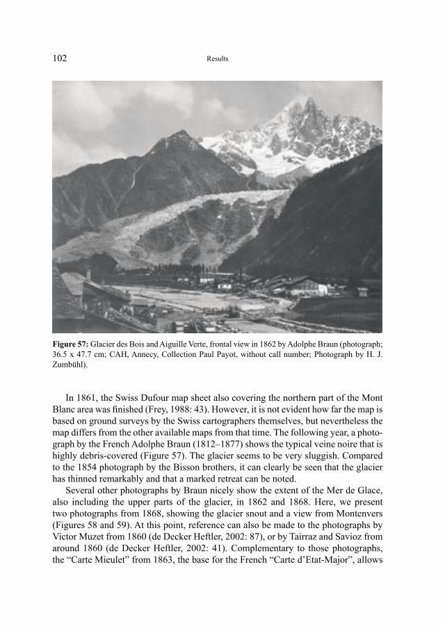
102

In 1861, the Swiss Dufour map sheet also covering the northern part of the Mont Blanc area was finished (Frey, 1988: 43). However, it is not evident how far the map is based on ground surveys by the Swiss cartographers themselves, but nevertheless the map differs from the other available maps from that time. The following year, a photo-graph by the French Adolphe Braun (1812–1877) shows the typical veine noire that is highly debris-covered (Figure 57). The glacier seems to be very sluggish. Compared to the 1854 photograph by the Bisson brothers, it can clearly be seen that the glacier has thinned remarkably and that a marked retreat can be noted.

Several other photographs by Braun nicely show the extent of the Mer de Glace, also including the upper parts of the glacier, in 1862 and 1868. Here, we present two photographs from 1868, showing the glacier snout and a view from Montenvers (Figures 58 and 59). At this point, reference can also be made to the photographs by Victor Muzet from 1860 (de Decker Heftler, 2002: 87), or by Tairraz and Savioz from around 1860 (de Decker Heftler, 2002: 41). Complementary to those photographs, the “Carte Mieulet” from 1863, the base for the French “Carte d’Etat-Major”, allows

Figure 57: Glacier des Bois and Aiguille Verte, frontal view in 1862 by Adolphe Braun (photograph; 36.5 x 47.7 cm; CAH, Annecy, Collection Paul Payot, without call number; Photograph by H. J. Zumbühl).

Results

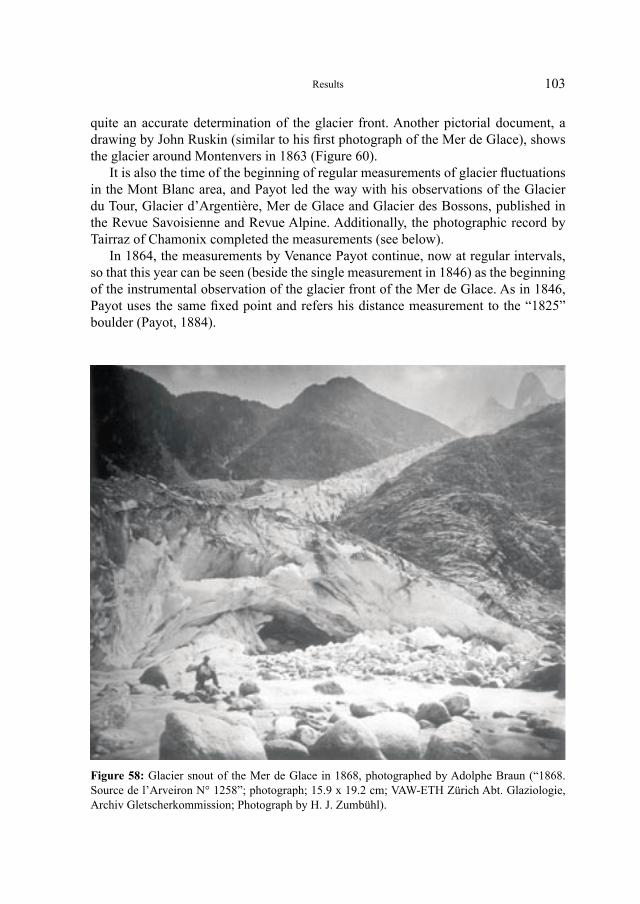
103

quite an accurate determination of the glacier front. Another pictorial document, a drawing by John Ruskin (similar to his first photograph of the Mer de Glace), shows the glacier around Montenvers in 1863 (Figure 60).

It is also the time of the beginning of regular measurements of glacier fluctuations in the Mont Blanc area, and Payot led the way with his observations of the Glacier du Tour, Glacier d’Argentière, Mer de Glace and Glacier des Bossons, published in the Revue Savoisienne and Revue Alpine. Additionally, the photographic record by Tairraz of Chamonix completed the measurements (see below).

In 1864, the measurements by Venance Payot continue, now at regular intervals, so that this year can be seen (beside the single measurement in 1846) as the beginning of the instrumental observation of the glacier front of the Mer de Glace. As in 1846, Payot uses the same fixed point and refers his distance measurement to the “1825” boulder (Payot, 1884).

Figure 58: Glacier snout of the Mer de Glace in 1868, photographed by Adolphe Braun (“1868. Source de l’Arveiron N° 1258”; photograph; 15.9 x 19.2 cm; VAW-ETH Zürich Abt. Glaziologie, Archiv Gletscherkommission; Photograph by H. J. Zumbühl).

Results

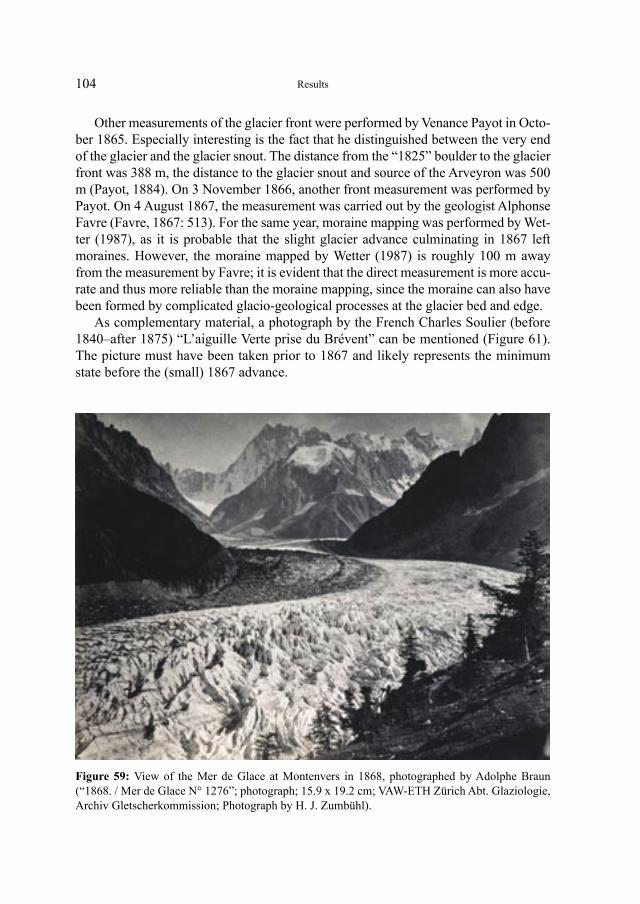
104

Other measurements of the glacier front were performed by Venance Payot in Octo-ber 1865. Especially interesting is the fact that he distinguished between the very end of the glacier and the glacier snout. The distance from the “1825” boulder to the glacier front was 388 m, the distance to the glacier snout and source of the Arveyron was 500 m (Payot, 1884). On 3 November 1866, another front measurement was performed by Payot. On 4 August 1867, the measurement was carried out by the geologist Alphonse Favre (Favre, 1867: 513). For the same year, moraine mapping was performed by Wet-ter (1987), as it is probable that the slight glacier advance culminating in 1867 left moraines. However, the moraine mapped by Wetter (1987) is roughly 100 m away from the measurement by Favre; it is evident that the direct measurement is more accu-rate and thus more reliable than the moraine mapping, since the moraine can also have been formed by complicated glacio-geological processes at the glacier bed and edge.

As complementary material, a photograph by the French Charles Soulier (before 1840–after 1875) “L’aiguille Verte prise du Brévent” can be mentioned (Figure 61). The picture must have been taken prior to 1867 and likely represents the minimum state before the (small) 1867 advance.

Figure 59: View of the Mer de Glace at Montenvers in 1868, photographed by Adolphe Braun (“1868. / Mer de Glace N° 1276”; photograph; 15.9 x 19.2 cm; VAW-ETH Zürich Abt. Glaziologie, Archiv Gletscherkommission; Photograph by H. J. Zumbühl).

Results

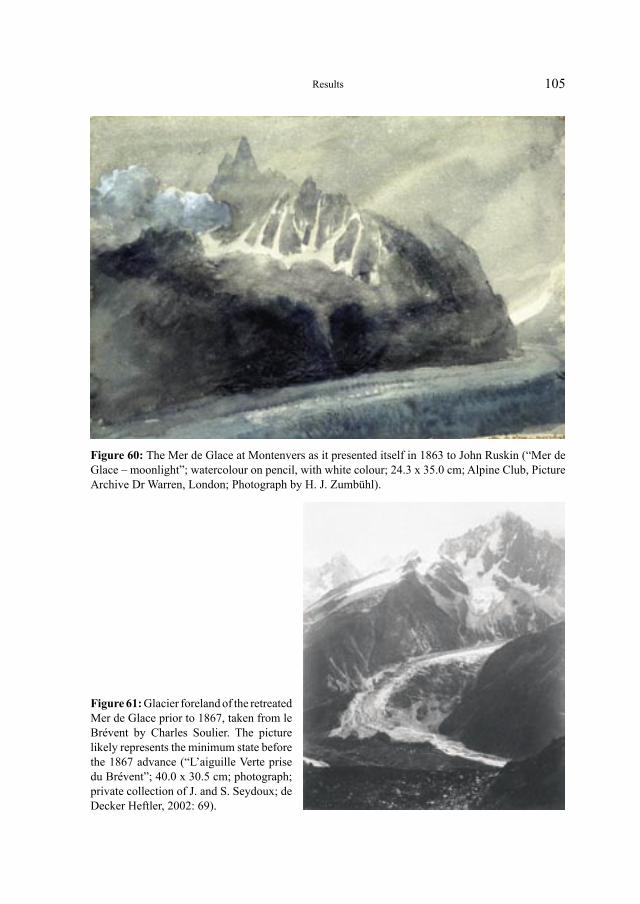
105

Figure 60: The Mer de Glace at Montenvers as it presented itself in 1863 to John Ruskin (“Mer de Glace – moonlight”; watercolour on pencil, with white colour; 24.3 x 35.0 cm; Alpine Club, Picture Archive Dr Warren, London; Photograph by H. J. Zumbühl).

Figure 61: Glacier foreland of the retreated Mer de Glace prior to 1867, taken from le Brévent by Charles Soulier. The picture likely represents the minimum state before the 1867 advance (“L’aiguille Verte prise du Brévent”; 40.0 x 30.5 cm; photograph; private collection of J. and S. Seydoux; de Decker Heftler, 2002: 69).

Results

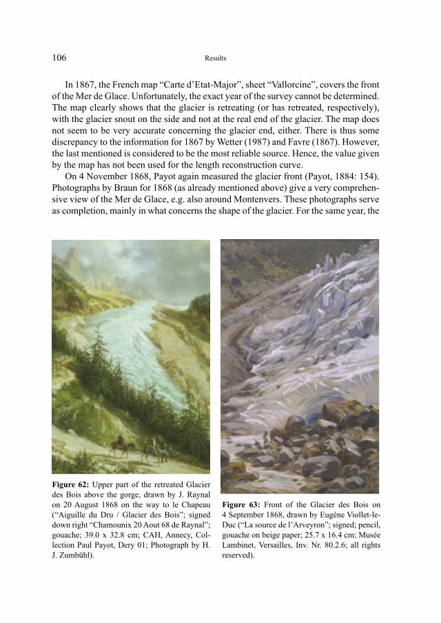
106

Figure 62: Upper part of the retreated Glacier des Bois above the gorge, drawn by J. Raynal on 20 August 1868 on the way to le Chapeau (“Aiguille du Dru / Glacier des Bois”; signed down right “Chamounix 20 Aout 68 de Raynal”; gouache; 39.0 x 32.8 cm; CAH, Annecy, Col-lection Paul Payot, Dery 01; Photograph by H. J. Zumbühl).

Figure 63: Front of the Glacier des Bois on 4 September 1868, drawn by Eugène Viollet-le-Duc (“La source de l’Arveyron”; signed; pencil, gouache on beige paper; 25.7 x 16.4 cm; Musée Lambinet, Versailles, Inv. Nr. 80.2.6; all rights reserved).

In 1867, the French map “Carte d’Etat-Major”, sheet “Vallorcine”, covers the front of the Mer de Glace. Unfortunately, the exact year of the survey cannot be determined. The map clearly shows that the glacier is retreating (or has retreated, respectively), with the glacier snout on the side and not at the real end of the glacier. The map does not seem to be very accurate concerning the glacier end, either. There is thus some discrepancy to the information for 1867 by Wetter (1987) and Favre (1867). However, the last mentioned is considered to be the most reliable source. Hence, the value given by the map has not been used for the length reconstruction curve.

On 4 November 1868, Payot again measured the glacier front (Payot, 1884: 154). Photographs by Braun for 1868 (as already mentioned above) give a very comprehen-sive view of the Mer de Glace, e.g. also around Montenvers. These photographs serve as completion, mainly in what concerns the shape of the glacier. For the same year, the

Results

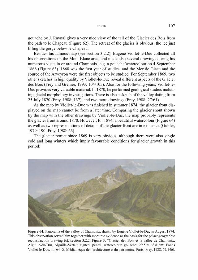
107

gouache by J. Raynal gives a very nice view of the tail of the Glacier des Bois from the path to le Chapeau (Figure 62). The retreat of the glacier is obvious, the ice just filling the gorge below le Chapeau.

Besides his famous map (see section 3.2.2), Eugène Viollet-le-Duc collected all his observations on the Mont Blanc area, and made also several drawings during his numerous visits in or around Chamonix, e.g. a gouache/watercolour on 4 September 1868 (Figure 63). 1868 was the first year of studies, and the Mer de Glace and the source of the Arveyron were the first objects to be studied. For September 1869, two other sketches in high quality by Viollet-le-Duc reveal different aspects of the Glacier des Bois (Frey and Grenier, 1993: 104/105). Also for the following years, Viollet-le-Duc provides very valuable material. In 1870, he performed geological studies includ-ing glacial morphology investigations. There is also a sketch of the valley dating from 25 July 1870 (Frey, 1988: 137), and two more drawings (Frey, 1988: 27/61).

As the map by Viollet-le-Duc was finished in summer 1874, the glacier front dis-played on the map cannot be from a later time. Comparing the glacier snout shown by the map with the other drawings by Viollet-le-Duc, the map probably represents the glacier front around 1870. However, for 1874, a beautiful watercolour (Figure 64) as well as two representations of details of the glacier front are in existence (Gubler, 1979: 190; Frey, 1988: 66).

The glacier retreat since 1869 is very obvious, although there were also single cold and long winters which imply favourable conditions for glacier growth in this period:

Figure 64: Panorama of the valley of Chamonix, drawn by Eugène Viollet-le-Duc in August 1874. This observation served him together with morainic evidence as the basis for the palaeogeographic reconstruction drawing (cf. section 3.2.2, Figure 3; “Glacier des Bois et la vallée de Chamonix, Aiguille-du-Dru, Aiguille-Verte”; signed; pencil, watercolour, gouache; 29.5 x 68.8 cm; Fonds Viollet-le-Duc, no. 64–G; Médiathèque de l’architecture et du patrimoine, Paris; Frey, 1988: 62/146).

Results

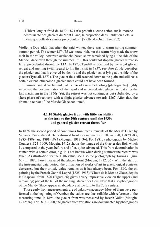
108

“L’hiver long et froid de 1870–1871 n’a produit aucune action sur la marche décroissante des glaciers du Mont Blanc, la proportion dans l’ablation a été la même que celle des années précédentes.” (Viollet-le-Duc, 1876: 202)

Viollet-le-Duc adds that after the said winter, there was a warm spring-summer-autumn period. The winter 1874/75 was snow-rich, but the warm May made the snow melt in the valley; however, avalanche-based snow remained lying at the side of the Mer de Glace even through the summer. Still, this could not stop the glacier retreat so far unprecedented during the LIA. In 1873, Tyndall is horrified by the rapid glacier retreat and melting (with regard to his first visit in 1857; see above). He describes the glacier end that is covered by debris and the glacier snout lying at the side of the glacier (Tyndall, 1873). The glacier thus still reached down to the plain and still has a certain extent, otherwise a glacier snout could not have been formed.

Summarizing, it can be said that the rise of a new technology (photography) highly improved the documentation of the rapid and unprecedented glacier retreat after the last maximum in the 1850s. Yet, the retreat was not continuous but subdivided by a short phase of recovery with a slight glacier advance towards 1867. After that, the dramatic retreat of the Mer de Glace continued.

4.1.10 Stable glacier front with little variability at the turn to the 20th century until the 1930s

and general glacier retreat thereafter

In 1878, the second period of continuous front measurements of the Mer de Glace by Venance Payot started. He performed front measurements in 1878–1880, 1882/1883, 1885–1889, and 1891–1893 (Mougin, 1912: 36). For 1881, a photograph by Michel Couttet (1824–1909; Mougin, 1912) shows the tongue of the Glacier des Bois which is, compared to the years before and after, quite advanced. This front determination is tainted with a certain error, e.g. it is not known when during summer the picture was taken. As illustration for the 1886 value, see also the photograph by Tairraz (Figure 65). In 1890, Forel measured the glacier front (Mougin, 1912: 36). With the start of the instrumental data period, the utilization of works of art in glaciological contexts decreases, but their artistic value remains as it has always been. For 1890, the oil painting by the French Gabriel Loppé (1825–1913) “Chute de la Mer de Glace, depuis le Chapeau” from 1890 (Figure 66) gives a very impressive view on the upper (and remaining) part of the tail of the melting Glacier des Bois. Note that also photographs of the Mer de Glace appear in abundance at the turn to the 20th century.

Those early front measurements are of unknown accuracy. Most of them were per-formed at the beginning of October, the values are thus reliable with reference to the measuring time. In 1894, the glacier front was measured by Joseph Vallot (Mougin, 1912: 36). For 1895–1900, the glacier front variations are documented by photographs

Results

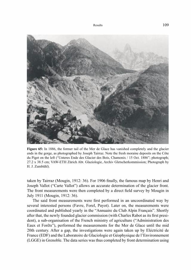
109

taken by Tairraz (Mougin, 1912: 36). For 1906 finally, the famous map by Henri and Joseph Vallot (“Carte Vallot”) allows an accurate determination of the glacier front. The front measurements were then completed by a direct field survey by Mougin in July 1911 (Mougin, 1912: 36).

The said front measurements were first performed in an uncoordinated way by several interested persons (Favre, Forel, Payot). Later on, the measurements were coordinated and published yearly in the “Annuaire du Club Alpin Français”. Shortly after that, the newly founded glacier commission (with Charles Rabot as its first presi-dent), a sub-organisation of the French ministry of agriculture (“Administration des Eaux et Forêts”), performed the measurements for the Mer de Glace until the mid 20th century. After a gap, the investigations were again taken up by Eléctricité de France (EDF) and the Laboratoire de Glaciologie et Géophysique de l’Environnement (LGGE) in Grenoble. The data series was thus completed by front determination using

Figure 65: In 1886, the former tail of the Mer de Glace has vanished completely and the glacier ends in the gorge, as photographed by Joseph Tairraz. Note the fresh moraine deposits on the Côte du Piget on the left (“Unteres Ende des Glacier des Bois, Chamonix / 15 Oct. 1886”; photograph; 27.2 x 38.5 cm; VAW-ETH Zürich Abt. Glaziologie, Archiv Gletscherkommission; Photograph by H. J. Zumbühl).

Results

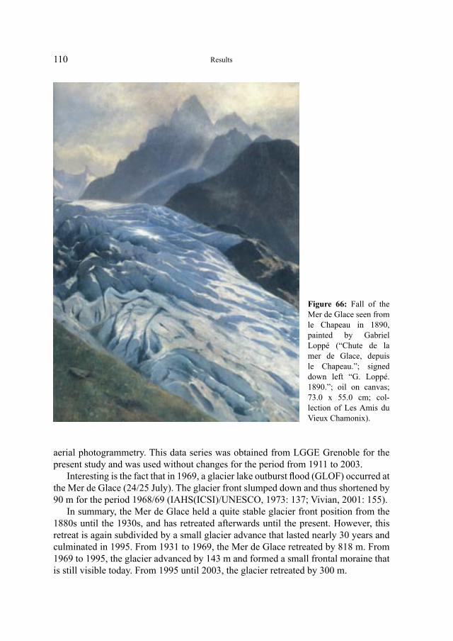
110

aerial photogrammetry. This data series was obtained from LGGE Grenoble for the present study and was used without changes for the period from 1911 to 2003.

Interesting is the fact that in 1969, a glacier lake outburst flood (GLOF) occurred at the Mer de Glace (24/25 July). The glacier front slumped down and thus shortened by 90 m for the period 1968/69 (IAHS(ICSI)/UNESCO, 1973: 137; Vivian, 2001: 155).

In summary, the Mer de Glace held a quite stable glacier front position from the 1880s until the 1930s, and has retreated afterwards until the present. However, this retreat is again subdivided by a small glacier advance that lasted nearly 30 years and culminated in 1995. From 1931 to 1969, the Mer de Glace retreated by 818 m. From 1969 to 1995, the glacier advanced by 143 m and formed a small frontal moraine that is still visible today. From 1995 until 2003, the glacier retreated by 300 m.

Figure 66: Fall of the Mer de Glace seen from le Chapeau in 1890, painted by Gabriel Loppé (“Chute de la mer de Glace, depuis le Chapeau.”; signed down left “G. Loppé. 1890.”; oil on canvas; 73.0 x 55.0 cm; col-lection of Les Amis du Vieux Chamonix).

Results

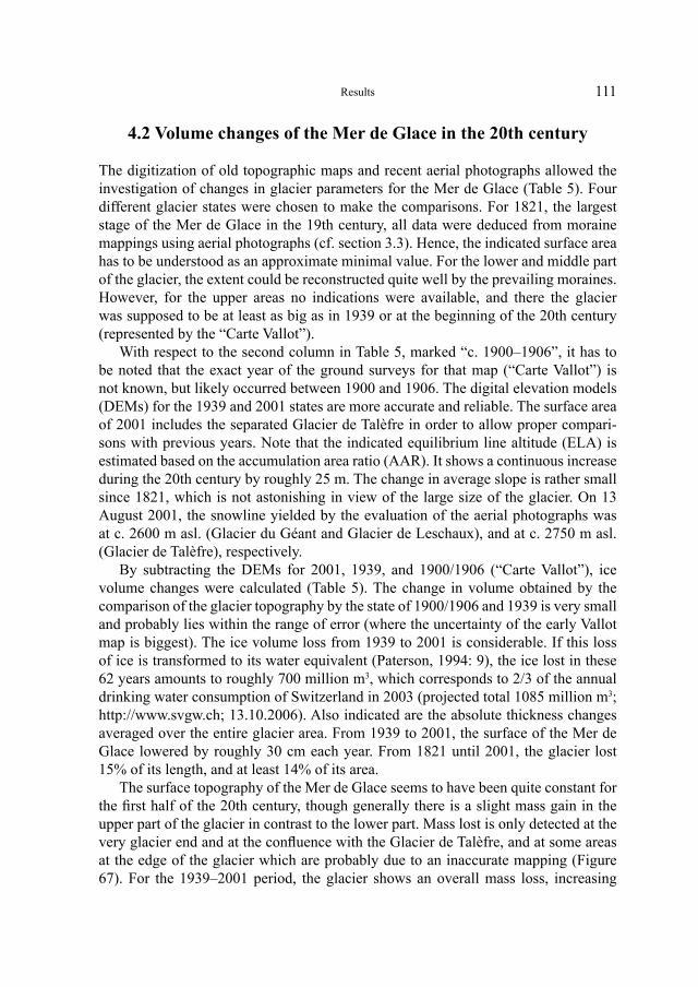
111

4.2 Volume changes of the Mer de Glace in the 20th century

The digitization of old topographic maps and recent aerial photographs allowed the investigation of changes in glacier parameters for the Mer de Glace (Table 5). Four different glacier states were chosen to make the comparisons. For 1821, the largest stage of the Mer de Glace in the 19th century, all data were deduced from moraine mappings using aerial photographs (cf. section 3.3). Hence, the indicated surface area has to be understood as an approximate minimal value. For the lower and middle part of the glacier, the extent could be reconstructed quite well by the prevailing moraines. However, for the upper areas no indications were available, and there the glacier was supposed to be at least as big as in 1939 or at the beginning of the 20th century (represented by the “Carte Vallot”).

With respect to the second column in Table 5, marked “c. 1900–1906”, it has to be noted that the exact year of the ground surveys for that map (“Carte Vallot”) is not known, but likely occurred between 1900 and 1906. The digital elevation models (DEMs) for the 1939 and 2001 states are more accurate and reliable. The surface area of 2001 includes the separated Glacier de Talèfre in order to allow proper compari-sons with previous years. Note that the indicated equilibrium line altitude (ELA) is estimated based on the accumulation area ratio (AAR). It shows a continuous increase during the 20th century by roughly 25 m. The change in average slope is rather small since 1821, which is not astonishing in view of the large size of the glacier. On 13 August 2001, the snowline yielded by the evaluation of the aerial photographs was at c. 2600 m asl. (Glacier du Géant and Glacier de Leschaux), and at c. 2750 m asl. (Glacier de Talèfre), respectively.

By subtracting the DEMs for 2001, 1939, and 1900/1906 (“Carte Vallot”), ice volume changes were calculated (Table 5). The change in volume obtained by the comparison of the glacier topography by the state of 1900/1906 and 1939 is very small and probably lies within the range of error (where the uncertainty of the early Vallot map is biggest). The ice volume loss from 1939 to 2001 is considerable. If this loss of ice is transformed to its water equivalent (Paterson, 1994: 9), the ice lost in these 62 years amounts to roughly 700 million m3, which corresponds to 2/3 of the annual drinking water consumption of Switzerland in 2003 (projected total 1085 million m3; http://www.svgw.ch; 13.10.2006). Also indicated are the absolute thickness changes averaged over the entire glacier area. From 1939 to 2001, the surface of the Mer de Glace lowered by roughly 30 cm each year. From 1821 until 2001, the glacier lost 15% of its length, and at least 14% of its area.

The surface topography of the Mer de Glace seems to have been quite constant for the first half of the 20th century, though generally there is a slight mass gain in the upper part of the glacier in contrast to the lower part. Mass lost is only detected at the very glacier end and at the confluence with the Glacier de Talèfre, and at some areas at the edge of the glacier which are probably due to an inaccurate mapping (Figure 67). For the 1939–2001 period, the glacier shows an overall mass loss, increasing

Results

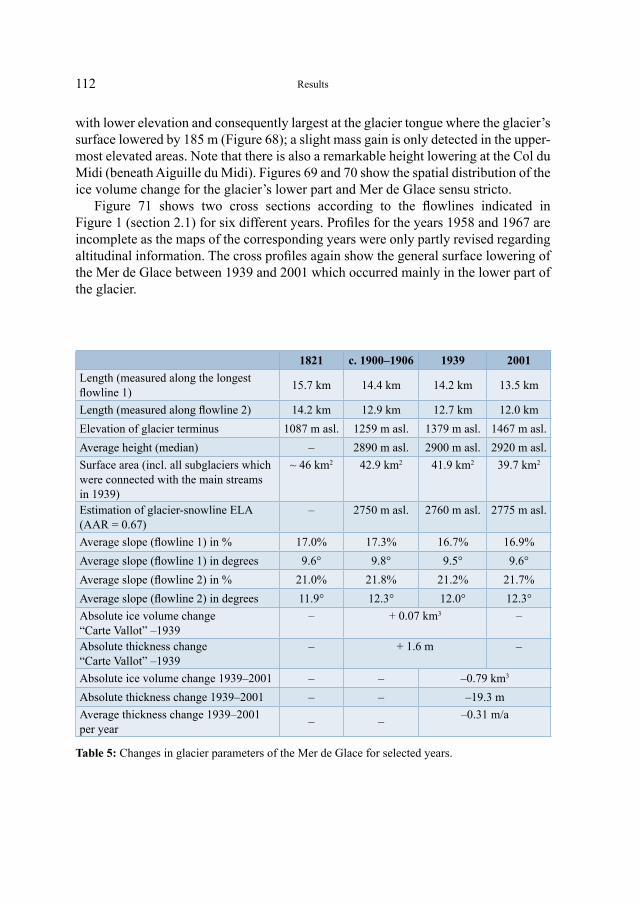
112

with lower elevation and consequently largest at the glacier tongue where the glacier’s surface lowered by 185 m (Figure 68); a slight mass gain is only detected in the upper-most elevated areas. Note that there is also a remarkable height lowering at the Col du Midi (beneath Aiguille du Midi). Figures 69 and 70 show the spatial distribution of the ice volume change for the glacier’s lower part and Mer de Glace sensu stricto.

Figure 71 shows two cross sections according to the flowlines indicated in Figure 1 (section 2.1) for six different years. Profiles for the years 1958 and 1967 are incomplete as the maps of the corresponding years were only partly revised regarding altitudinal information. The cross profiles again show the general surface lowering of the Mer de Glace between 1939 and 2001 which occurred mainly in the lower part of the glacier.

1821 c. 1900–1906 1939 2001

Length (measured along the longest flowline 1)

15.7 km 14.4 km 14.2 km 13.5 km

Length (measured along flowline 2) 14.2 km 12.9 km 12.7 km 12.0 km

Elevation of glacier terminus 1087 m asl. 1259 m asl. 1379 m asl. 1467 m asl.

Average height (median) – 2890 m asl. 2900 m asl. 2920 m asl.

Surface area (incl. all subglaciers which were connected with the main streams in 1939)

~ 46 km2 42.9 km2 41.9 km2 39.7 km2

Estimation of glacier-snowline ELA (AAR = 0.67)

– 2750 m asl. 2760 m asl. 2775 m asl.

Average slope (flowline 1) in % 17.0% 17.3% 16.7% 16.9%

Average slope (flowline 1) in degrees 9.6° 9.8° 9.5° 9.6°

Average slope (flowline 2) in % 21.0% 21.8% 21.2% 21.7%

Average slope (flowline 2) in degrees 11.9° 12.3° 12.0° 12.3°

Absolute ice volume change “Carte Vallot” –1939

– + 0.07 km3 –

Absolute thickness change “Carte Vallot” –1939

– + 1.6 m –

Absolute ice volume change 1939–2001 – – –0.79 km3

Absolute thickness change 1939–2001 – – –19.3 m

Average thickness change 1939–2001 per year

– ––0.31 m/a

Table 5: Changes in glacier parameters of the Mer de Glace for selected years.

Results

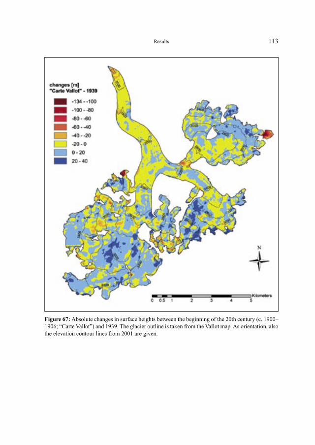
113

Figure 67: Absolute changes in surface heights between the beginning of the 20th century (c. 1900–1906; “Carte Vallot”) and 1939. The glacier outline is taken from the Vallot map. As orientation, also the elevation contour lines from 2001 are given.

Results

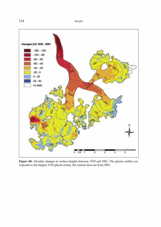
114

Figure 68: Absolute changes in surface heights between 1939 and 2001. The glacier outline cor-responds to the (larger) 1939 glacier extent, the contour lines are from 2001.

Results

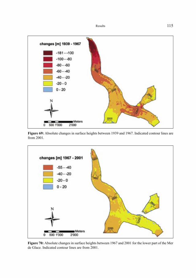
115

Figure 70: Absolute changes in surface heights between 1967 and 2001 for the lower part of the Mer de Glace. Indicated contour lines are from 2001.

Figure 69: Absolute changes in surface heights between 1939 and 1967. Indicated contour lines are from 2001.

Results

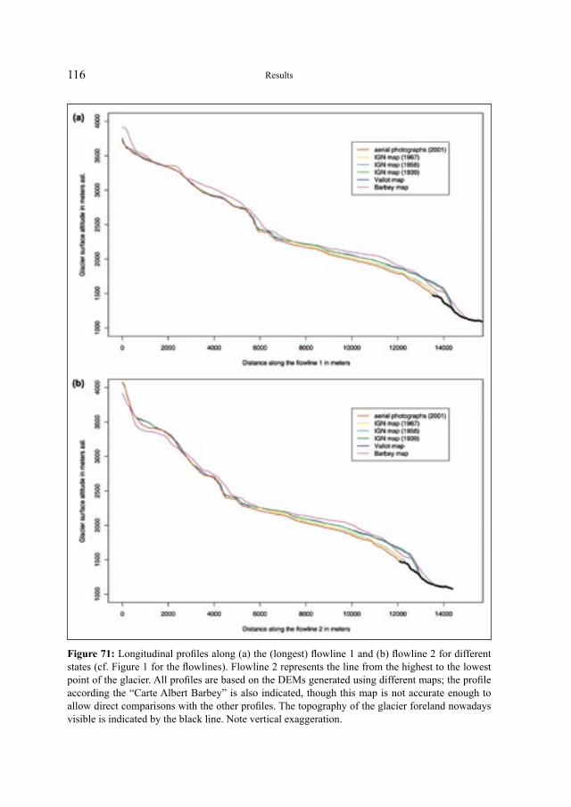
116

Figure 71: Longitudinal profiles along (a) the (longest) flowline 1 and (b) flowline 2 for different states (cf. Figure 1 for the flowlines). Flowline 2 represents the line from the highest to the lowest point of the glacier. All profiles are based on the DEMs generated using different maps; the profile according the “Carte Albert Barbey” is also indicated, though this map is not accurate enough to allow direct comparisons with the other profiles. The topography of the glacier foreland nowadays visible is indicated by the black line. Note vertical exaggeration.

Results

5 Discussion

5.1 The new Mer de Glace length curve viewed in the context of other existing glacier length curves

The new and revised glacier length curve of the Mer de Glace shows that there were large glacier fluctuations during the LIA. Compared to them, the intensity of glacier fluctuations during the 20th century is moderate. However, the glacier extent of 2003 was reached at no other time before since 1570. Not astonishingly, the glacier showed a generally large extension during the LIA. Moreover, rapid advances and retreats, trig-gered by favourable climatic conditions, were normal during that generally glacier-friendly time period. However, the retreat of the Mer de Glace at the end of the LIA after the 1850s (with a small break around 1867) is unprecedented in the past 500 years.

The new Mer de Glace length curve confirms what is generally known of the behaviour of glaciers during the LIA: During this period, the glaciers are generally speaking always in a more advanced position compared to the 20th century, and many short-term advances occur. Since the end of the LIA, the glaciers are more or less continuously retreating (Zumbühl et al., 1983).

Note that evidence for the very early times is rare and interpretations therefore difficult (large corresponding error in the length curve). The distribution of the docu-mentary data for the Mer de Glace (Appendix, Figure 76) reveals the concentration of the material between 1770 and 1900. Earlier times are documented nearly exclusively by written sources.

The maximal extent of the Mer de Glace in the 19th century was reached in 1821 (Birmann, 1826) and therefore differs from that of many other Alpine glaciers, which reached their maximum in the 1850s (e.g., Holzhauser and Zumbühl, 2003). However, also the Rosenlauigletscher in the Bernese Alps had its 19th century maximum in 1826 similarly to the Mer de Glace (Zumbühl and Holzhauser, 1988).

Concerning the glaciers of the greater Mont Blanc area, Zienert (1965) could show, mainly based on moraine mappings, that the glaciers on the southern face of Mont Blanc and in the nearby Gran Paradiso area reached maximum positions around 1600, 1680, 1770, 1820, 1860, and 1920, similarly to the Mer de Glace. An interesting result of his study is the fact that the lateral moraines are in general very clearly visible and contain coarse block material, whereas the end moraines are often just intimated. Zienert (1965) concludes that this has to be related to the forming of the respective moraines. In the 15th century the historical glacier advance started together with the formation of a lot of new small glaciers. Glaciers that already had a certain amount of ice were able to grow fastest. This could be the reason for the bigger Mont Blanc glaciers reaching their maximum already in the 17th century, whereas small glaciers followed with a delay. For a lot of middle-sized glaciers, the advance with a maximum in 1818–1820 seems to be the biggest since 1500 (Zienert, 1965).

118

For the northern part of the Mont Blanc mountain range, the Glacier du Trient seems to be interesting as a comparison glacier, as it has the best instrumental length record of all Mont Blanc glaciers (i.e., without gaps since 1879). LIA fluctuations of the Glacier du Trient are briefly treated by Bless (1984). The glacier reacts similarly to the Mer de Glace, having maximum positions around 1610, 1640, 1780, 1818/20, 1895, and 1920. Interesting is the fact that the glacier reached its maximum extent in 1780 (Bless, 1984: 22). The continuous front measurements of the Glacier du Trient, nowadays performed by the Swiss Academy of Sciences (SCNAT), started in 1879 and show, in contrast to the Mer de Glace, a complete annual record without any gaps. This excellent series of Swiss glacier front variation measurements was first compiled and started by Forel in 1880 (Forel, 1881).

A comparison of length fluctuations of Glacier des Bossons, Mer de Glace, Glacier d’Argentière, and Glacier du Trient since c. 1875 can be found in Reynaud and Vincent (2000). The fluctuations of these four Mont Blanc glaciers are nearly synchronous and just vary due to different time delay and response times of the glaciers (Glacier des Bossons reacts first, the Mer de Glace last). All four glaciers show advances around 1890, 1920, and 1970 that alternate with retreats. Due to the individual character of each glacier, the length variations of the four Mont Blanc glaciers cannot be considered to fully represent the fluctuations of the French Alpine glaciers (Reynaud, 1993).

5.1.1 Comparison with the existing Mougin curve

In the following, the new glacier length curve for the Mer de Glace shall be discussed and compared with the existing curve by Mougin (1912). As already mentioned in section 4.1.1, the same centre line has been chosen for determining the glacier lengths and a direct comparison with the results by Mougin (1912) is thus possible. The methodology for deriving the length curve in Mougin (1912) is the same as in this study. However, the availability of documentary data was sparse at the time when Mougin made his curve. Figure 72 shows the two curves in comparison for the time period up to 1911 (the Mougin curve ends there). Unfortunately, the Mougin curve does not show any error ranges. Table 6 compares the main glacier advances and sub-sequent retreats obtained by this study with the results by Mougin (1912). The main differences to the Mougin curve concern the LIA maximum glacier extent and the minor advance around 1850.

The glacier front in 1644 is indicated by Mougin (1912) by a position roughly 100 m more advanced than in the present study. Mougin (1912: 21) refers to a small ridge situated 150 m in front of the 1821 moraine that could be the 1644 frontal moraine. However, this moraine can hardly be seen today in the field, in contrast to the well-formed 1821 frontal moraine.

It is undisputed that the lateral glacier extent in 1644 was much larger than in 1821 towards les Tines, as there is evidence from the lateral moraines. The age of those

Discussion

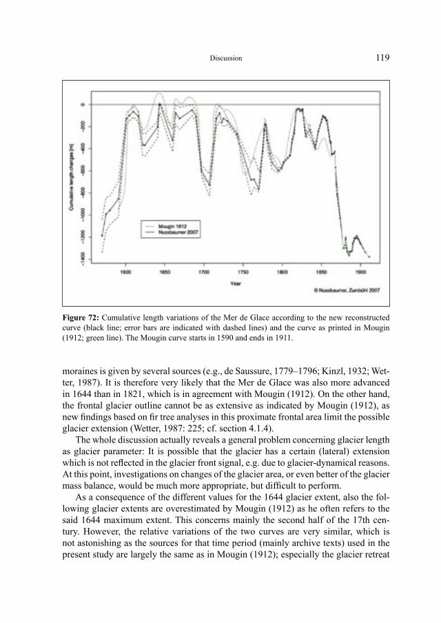
119

moraines is given by several sources (e.g., de Saussure, 1779–1796; Kinzl, 1932; Wet-ter, 1987). It is therefore very likely that the Mer de Glace was also more advanced in 1644 than in 1821, which is in agreement with Mougin (1912). On the other hand, the frontal glacier outline cannot be as extensive as indicated by Mougin (1912), as new findings based on fir tree analyses in this proximate frontal area limit the possible glacier extension (Wetter, 1987: 225; cf. section 4.1.4).

The whole discussion actually reveals a general problem concerning glacier length as glacier parameter: It is possible that the glacier has a certain (lateral) extension which is not reflected in the glacier front signal, e.g. due to glacier-dynamical reasons. At this point, investigations on changes of the glacier area, or even better of the glacier mass balance, would be much more appropriate, but difficult to perform.

As a consequence of the different values for the 1644 glacier extent, also the fol-lowing glacier extents are overestimated by Mougin (1912) as he often refers to the said 1644 maximum extent. This concerns mainly the second half of the 17th cen-tury. However, the relative variations of the two curves are very similar, which is not astonishing as the sources for that time period (mainly archive texts) used in the present study are largely the same as in Mougin (1912); especially the glacier retreat

Figure 72: Cumulative length variations of the Mer de Glace according to the new reconstructed curve (black line; error bars are indicated with dashed lines) and the curve as printed in Mougin (1912; green line). The Mougin curve starts in 1590 and ends in 1911.

Discussion

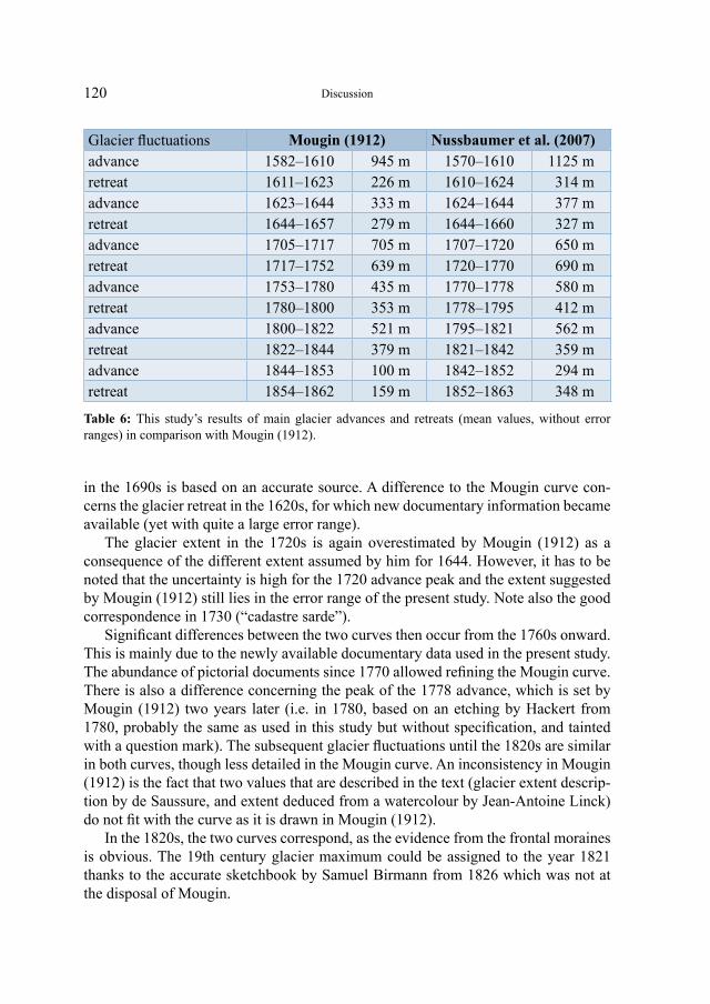
120

in the 1690s is based on an accurate source. A difference to the Mougin curve con-cerns the glacier retreat in the 1620s, for which new documentary information became available (yet with quite a large error range).

The glacier extent in the 1720s is again overestimated by Mougin (1912) as a consequence of the different extent assumed by him for 1644. However, it has to be noted that the uncertainty is high for the 1720 advance peak and the extent suggested by Mougin (1912) still lies in the error range of the present study. Note also the good correspondence in 1730 (“cadastre sarde”).

Significant differences between the two curves then occur from the 1760s onward. This is mainly due to the newly available documentary data used in the present study. The abundance of pictorial documents since 1770 allowed refining the Mougin curve. There is also a difference concerning the peak of the 1778 advance, which is set by Mougin (1912) two years later (i.e. in 1780, based on an etching by Hackert from 1780, probably the same as used in this study but without specification, and tainted with a question mark). The subsequent glacier fluctuations until the 1820s are similar in both curves, though less detailed in the Mougin curve. An inconsistency in Mougin (1912) is the fact that two values that are described in the text (glacier extent descrip-tion by de Saussure, and extent deduced from a watercolour by Jean-Antoine Linck) do not fit with the curve as it is drawn in Mougin (1912).

In the 1820s, the two curves correspond, as the evidence from the frontal moraines is obvious. The 19th century glacier maximum could be assigned to the year 1821 thanks to the accurate sketchbook by Samuel Birmann from 1826 which was not at the disposal of Mougin.

Glacier fluctuations Mougin (1912) Nussbaumer et al. (2007) advance 1582–1610 945 m 1570–1610 1125 m retreat 1611–1623 226 m 1610–1624 314 m advance 1623–1644 333 m 1624–1644 377 m retreat 1644–1657 279 m 1644–1660 327 m advance 1705–1717 705 m 1707–1720 650 m retreat 1717–1752 639 m 1720–1770 690 m advance 1753–1780 435 m 1770–1778 580 m retreat 1780–1800 353 m 1778–1795 412 m advance 1800–1822 521 m 1795–1821 562 m retreat 1822–1844 379 m 1821–1842 359 m advance 1844–1853 100 m 1842–1852 294 m retreat 1854–1862 159 m 1852–1863 348 m

Table 6: This study’s results of main glacier advances and retreats (mean values, without error ranges) in comparison with Mougin (1912).

Discussion

121

For the 1830 glacier extent, there is quite a large difference between the two curves. Mougin (1912) used a drawing by Dubois, showing the glacier from a distance, but he deduced the glacier extent from the glacier retreat 1820–1842, and not in first order from the picture by Dubois. Hence, the information cannot be seen as independent in this case. The lithograph by Chapuy used in the present study is therefore much more appropriate to determine the glacier front position.

Remarkable differences then occur around 1850. Mougin (1912) did not use any concrete reference point for drawing his curve, and the glacier extent highly deviates from the results of the present study. This is even more surprising as Mougin disposed of more (additional) information, e.g. the front measurement by Payot in 1846 (Mou-gin, 1912: 29), but does not seem to have used it for his curve.

For the following time periods, the accordance between the two curves is good (same source for both curves, based on direct front measurements). Additional (picto-rial) documents used in this study are the sketches by Viollet-le-Duc, which stand in very good agreement with the dramatic glacier retreat from 1867–1878. Small dis-crepancies between the two curves occur in the 1890s. Mougin (1912) counted a mea-surement for September sometimes to the next year and sometimes not, which leads to shifts of one year that are more a question of interpretation than different results.

On the whole, it can be said that the new glacier length curve for the Mer de Glace is in good agreement with the curve by Mougin (1912). However, significant dif-ferences occur around 1850, when the glacier seems to be much more extensive than assumed by Mougin. Furthermore, the new documentary data allowed a more detailed description of glacier fluctuations for the 1750–1820 period. The glacier extension around 1644 is roughly 100 m smaller than shown by the Mougin curve.

5.1.2 Comparison Mer de Glace – Unterer Grindelwaldgletscher

The Mer de Glace and the Unterer Grindelwaldgletscher are among the glaciers best-documented by different kinds of historical sources (Zumbühl et al., in press). The length curve of the Unterer Grindelwaldgletscher, starting in 1535, is the longest glacier record of this type (e.g., Oerlemans, 2005). The new Mer de Glace length curve starts in 1570 and is another very long glacier curve, and a comparison of the two curves therefore suggests itself. The availability of (pictorial) documentary data is similar for both glaciers, perhaps even more abundant for the Mer de Glace, but the quality of the documents for the Unterer Grindelwaldgletscher is distinctly bet-ter. Several artists portrayed both glaciers (e.g., Samuel Birmann, Bisson brothers), whereas others are specific to one glacier (e.g., Caspar Wolf for the Unterer Grindel-waldgletscher, Jean-Antoine Linck for the Mer de Glace).

The comparison of the Mer de Glace length curve with the one of the Unterer Grindelwaldgletscher (Zumbühl, 1980; Zumbühl et al., 1983; Holzhauser and Zum-bühl, 1996; Steiner et al., in press) yielded an astonishing simultaneity between the

Discussion

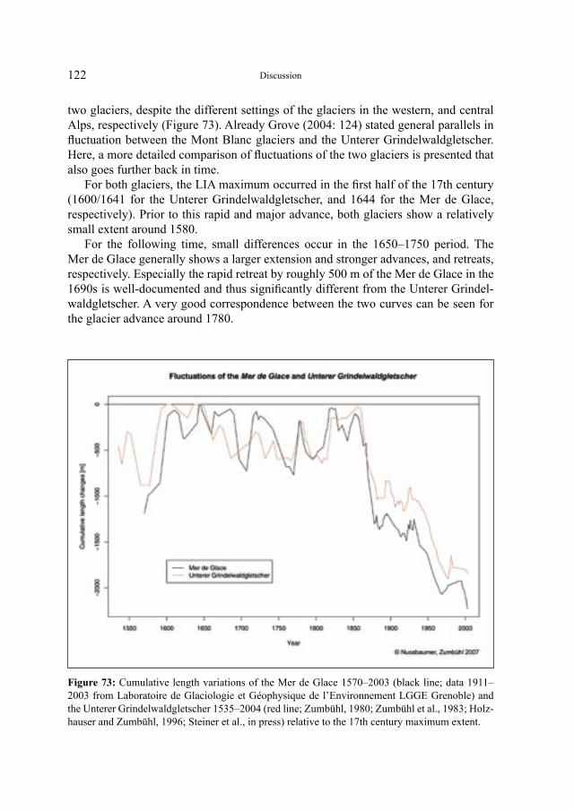
122

two glaciers, despite the different settings of the glaciers in the western, and central Alps, respectively (Figure 73). Already Grove (2004: 124) stated general parallels in fluctuation between the Mont Blanc glaciers and the Unterer Grindelwaldgletscher. Here, a more detailed comparison of fluctuations of the two glaciers is presented that also goes further back in time.

For both glaciers, the LIA maximum occurred in the first half of the 17th century (1600/1641 for the Unterer Grindelwaldgletscher, and 1644 for the Mer de Glace, respectively). Prior to this rapid and major advance, both glaciers show a relatively small extent around 1580.

For the following time, small differences occur in the 1650–1750 period. The Mer de Glace generally shows a larger extension and stronger advances, and retreats, respectively. Especially the rapid retreat by roughly 500 m of the Mer de Glace in the 1690s is well-documented and thus significantly different from the Unterer Grindel-waldgletscher. A very good correspondence between the two curves can be seen for the glacier advance around 1780.

Figure 73: Cumulative length variations of the Mer de Glace 1570–2003 (black line; data 1911–2003 from Laboratoire de Glaciologie et Géophysique de l’Environnement LGGE Grenoble) and the Unterer Grindelwaldgletscher 1535–2004 (red line; Zumbühl, 1980; Zumbühl et al., 1983; Holz-hauser and Zumbühl, 1996; Steiner et al., in press) relative to the 17th century maximum extent.

Discussion

123

A major difference between the two glaciers concerns the 19th century maximum. For the Mer de Glace, this occurred in 1821, whereas for the Unterer Grindelwald-gletscher, the maximum was reached not earlier than 1855/56. Note also that the gla-cier minimum of the Mer de Glace around 1842 is documented by the very reliable map of Forbes. However, both glaciers show a distinct advance in the 1820s, and 1850s, respectively.

The subsequent retreat is dramatic for both glaciers, showing an unprecedented retreat by more than 1 km between the 1850s and c. 1880. As compared to the shrink-age of the Mer de Glace (15% of length and at least 14% of area loss from 1821 to 2001; cf. section 4.2, Table 5), the Unterer Grindelwaldgletscher lost relatively more area compared to its length (18% of length and 21% of area from the 1860s to 2004; Steiner et al., in press).

For the time period covered by instrumental glacier front data, both glaciers react nearly simultaneously. Unfortunately, the glacier length data of the Unterer Grindel-waldgletscher ends in 1983 due to the hardly accessible glacier terminus in a gorge. Values later on were obtained by interpretation of aerial photographs (Steiner et al., in press).

Summarizing, the behaviour of the Mer de Glace and the Unterer Grindelwald-gletscher was very similar in the past. This is astonishing, as the characteristics of the two glaciers partly differ (e.g. length, size), but other parameters (e.g. ELA, height range) are similar (cf. section 2.1, Table 2). Moreover, the distance between the gla-ciers and the different settings in the western and central Alps lead to a difference in climate parameters. As shown now by the comparison of the two glaciers, this differ-ence does not seem to be very large, as e.g. compared to inner Alpine valleys (Valais) or the southern Alps. Both glaciers, the Mer de Glace and the Unterer Grindelwald-gletscher, are probably dominated by westerly wind circulation modes.

5.2 Glacier change at the Mer de Glace

Glacier length is a function of mass balance and ice dynamics, which in turn are determined by the topography and prevailing climate (including energy balance and albedo), and variations in front position can be delayed and may continue long after the climate has re-stabilized following a change. Glacier front changes thus need not necessarily to be coupled solely with climate, which complicates climatic interpreta-tions of glacier fluctuations.

In contrast to glacier length, mass balance reacts almost immediately to a change in climatic conditions. But as glacier mass balance data hardly reach back to the first half of the 20th century and only exist for few glaciers, glacier length data as a much more easily determinable parameter has to be considered as an alternative. Glacier length on the other hand is an indirect, delayed, filtered and strongly enhanced signal (Hae-berli, 1998), which necessarily leads to some restrictions when using this parameter

Discussion

124

in relation to current climate change. More appropriate are volume change investiga-tions, as has been done in part in the present study, allowing the quantification of mass changes for the 20th century.

However, insight into the behaviour of the Mer de Glace during the LIA is only possible with historical data, as shown with the new and revised glacier length curve. Note that the beginning of the advance of the Mer de Glace in the 1570s coincides with the crisis of 1570/71, caused by harsh climate leading to price rises, which sur-prised people in central Europe (Pfister, 2005).

Concerning the Late Middle Ages, little documentation is available for the Mer de Glace so far. Wetter (1987) found a fossil wood in the right lateral moraine near Mauvais Pas and was able to date it to the end of the 15th century. For the preceding time, glacier advances were detected around AD 800, 1100, and 1300, respectively (Wetter, 1987: 152). However, this information is rather sketchy, and the right lateral moraine of the Mer de Glace surely holds more information concerning these glacier fluctuations. Of considerable interest is also the comparison with the Grosser Aletsch-gletscher and Gornergletscher, which showed a major advance around 1350–1385 (Holzhauser et al., 2005).

The historical method, which allows reconstructing former glacier front positions was complemented with an analysis of old topographic maps and an evaluation of recent aerial photographs. The large Mer de Glace showed a high decrease in ice volume from 1939 to 2001 out of proportion to the observed change in glacier length. As the separation of the Glacier de Talèfre has shown, there is now a large glacierized area that does not contribute to the length fluctuations at the glacier tongue, but still loses ice volume. This part of the Mer de Glace sensu lato probably did not contribute much to the length variations of the Mer de Glace in the past, either. Still, the situation is much more marked at the Unterer Grindelwaldgletscher, which showed a remark-able loss in ice volume in the 1990s but hardly a retreat at the tongue since 1983 for dynamical reasons (debris-covered tongue ending in a gorge; Steiner et al., in press).

The results of DEM comparisons yielded reliable rates of thickness changes for the Mer de Glace. However, the quantification of volume changes by digitizing topo-graphic maps and evaluating aerial photographs is time-consuming and thus only pos-sible for certain chosen years. Most reliable (due to the data quality) is the information for the 1939–2001 period, which shows a mean lowering of the glacier by c. 30 cm per year. However, this loss is not at all equally distributed over the whole glacier area, but concentrated on the glacier’s lower parts. Unfortunately, comparisons with the 19th century maximum glacier extents are not possible due to lack of correspond-ing maps for the Mer de Glace. This stands in contrast to the Unterer Grindelwald-gletscher where a plane-table sheet from 1861 is available for volume change evalua-tions (Steiner et al., in press).

Despite the large amount of ice lost, the Mer de Glace did not heavily change its form, and the overall similarity in the shape of the longitudinal surface profiles (i.e., relatively steep in the accumulation area with several steps, flatter in the lower

Discussion

125

part (ablation area), and again steeper at the front; cf. section 4.2, Figure 71) during the last 100 years suggests that the bedrock topography plays a significant role in controlling the surface topography. The climate changes over the last century have not affected the glacier enough to alter the overall shape of the surface. It would be inter-esting to compare the results (mainly the accurate 2001 glacier state obtained by the aerial photographs) with other years. Also high resolution satellite imaginary would allow reconstructing glacier topographies (e.g., Berthier et al., 2004).

Another interesting fact about the Mer de Glace is the existing debris cover, mainly on the lower part of the glacier. Debris-covered glaciers have dynamics that are unusual in relation to uncovered glaciers, and can react extremely sluggishly (e.g., Nakawo et al., 2000). Possible effects are smaller amplitudes of frontal fluctuations, glacier fronts descending further down, less negative mass balance during retreat periods, and highly developed moraine complexes (Deline, 2005). As a consequence, debris covers on glaciers have to be taken into consideration when interpreting glacier fluctuations as a climate proxy. On the Mer de Glace, nearly the whole part from beneath Monten-vers to the tongue is debris-covered. This (in the beginning just partial) debris cover formed the present veine noire by coalescence of two of four medial moraines at the close of the LIA (until 1890; Deline, 2005).

According to Deline (2005), the Mer de Glace was partly or wholly debris-free during the LIA. At the close of the LIA, the changing state of the surface of the Mer de Glace appears to coincide with rapid climatic amelioration, and a more transport-dominant period during the LIA with sparse or discontinuous debris cover contrasts with the post LIA time. For the Mer de Glace (and also other glaciers), the close of the LIA therefore represents a threshold marked by a rapid change in state from “clean” to debris-covered glaciers (Deline, 2005). It has to be noted that this change can very clearly be seen in the glacier length curve. From the 1890s on, the Mer de Glace has had its position always much behind and not comparable to the state during the LIA.

Discussion

6 Conclusions

Historical methods allowed reconstructing a revised glacier length curve for the Mer de Glace back to 1570. This time coincides with the beginning of a strong glacier advance typically for the LIA. The new glacier length curve is more accurate and detailed than the existing curve by Paul Mougin. This was mainly achieved due to newly avail-able historical documentary data, including an abundance of pictorial documents for the 1770–1900 period. The two curves are generally in good agreement, but some significant differences occur for the LIA maximum extent in 1644, the 1760–1780 period, and the second largest extent in the 19th century in 1852. The glacier exten-sion around 1644 is roughly 100 m smaller than shown by the Mougin curve. The new documentary data allows a more detailed description of glacier fluctuations for the 1750–1820 period. Around 1850, the glacier extent seems to have been much more extensive than assumed by Mougin. Moreover, the 19th century maximum extent could be assigned to the year 1821 according to the descriptions of Samuel Birmann.

The comparison of the new Mer de Glace length curve with the length curve from the Unterer Grindelwaldgletscher yielded an astonishing simultaneity between the two glaciers, despite the different settings of the glaciers in the western, and central Alps, respectively. Both glaciers had their maximum LIA extent in the first half of the 17th century, and two minor peaks in the 19th century (in the 1820s, and 1850s, respectively). In contrast to the Unterer Grindelwaldgletscher, which culminated in 1855/56, the Mer de Glace had its relative maximum extent in 1821. Since the 1850s, both glaciers retreated in an unprecedented way by more than 1 km until c. 1880. From 1821 until 2001, the Mer de Glace lost 15% of its length, and nearly the same relative amount of its area (at least 14%).

A complementary analysis by evaluation of topographical maps and aerial photo-graphs allowed the quantification of ice volume changes for the Mer de Glace during the 20th century. From 1939 to 2001, the surface of the glacier lowered in the mean by roughly 30 cm each year, which corresponds to 700 million m3 water equivalent. This ice loss took mainly place in the lower part of the glacier. From the beginning of the 20th century up to 1939, the glacier hardly changed its surface topography.

As sensitive indicators to climate variability, glacier variations very clearly indicate a changing climate. Proxy data obtained by glacier front reconstructions are important for climate reconstructions before the instrumental area. Today, several glacier length curves from the Alps allow drawing an overall pattern of glacier fluctuations. Simi-larities between the different glaciers suggest that the western and central European Alps, exemplified in the present study by the similar behaviour shown of the Mer de Glace and Unterer Grindelwaldgletscher, were affected on the whole in a similar way by the climate during the LIA. In order to further confirm this behaviour, it would be interesting to consider more Alpine glaciers and also to extend the comparison by studying LIA glacier fluctuations in other parts of the world.

Acknowledgements

This paper would not have been possible in its present form without the help of many people who are hereby kindly acknowledged: We are indebted to R. Eggimann and D. Mihajlovic from Photogram-metrie Perrinjaquet AG, Gümligen, Switzerland, for their help in photogrammetric interpretation of aerial photographs and the generation of digital elevation models (DEMs). Thanks are also due to A. Amacher, M. Küttel and H. von Weissenfluh for proofreading the manuscript. T. Bader is very much acknowledged for English corrections, E. Andersson from the Department of Classical Lan-guages, Stockholm University, Sweden, for the translation of the archive text from 1580.

Thanks also go to C. Vincent and the Laboratoire de Glaciologie et Géophysique de l’Environnement (LGGE), Saint-Martin-d’Hères, France, for providing data from the Mer de Glace, and to H. Holzhauser, Zürich, for dating fossil woods in the foreland of the Mer de Glace.

In addition, we would particularly like to thank the following people for their invaluable help without which this study would have been much less complete: M. Oehrli from the Zentralbibliothek Zürich, Kartensammlung, T. Klöti from the Swiss Federal Office of Topography (swisstopo), Bern–Wabern, and the Universitätsbibliothek Bern, Zentralbibliothek, Sammlung Ryhiner, B. Laube, Buch- und Kunstantiquariat August Laube, Zürich, C. Ramseyer, Kunstmuseum Basel, R. Wolf, Fri-bourg, W. Wetter, Rheinau, Switzerland, C. Gros from the Musée d’ethnographie Genève, K. Létang from the local archive of Chamonix, B. Cottard and M. Gay from Les Amis du Vieux Chamonix, C. Poletti from the Musée Alpin, Chamonix, S. Paul from the Musée d’art et d’histoire, Chambéry, N. Huc from the Musée Lambinet, Versailles, R. Patterson and J. Shepherd from the Ruskin Library, Lancaster, V. Coueraud from the IGN, Paris, S. Owen from the British Museum, London, and P. Deline and S. Jaillet from the Laboratoire EDYTEM, Université de Savoie, Le Bourget-du-Lac, France.

We thank the following institutions for the authorization to publish the pictorial documents: Alpine Club, London; Bibliothèque publique et universitaire de Genève; British Museum, London; Conservatoire d’art et d’histoire, Annecy; Fonds Viollet-le-Duc; Geographisches Institut der Uni-versität Bern; Graphische Sammlung der ETH Zürich; Kunstmuseum Basel (Kupferstichkabinett); Institut Géographique National (IGN), Paris; Les Amis du Vieux Chamonix; Musée Alpin, Chamo-nix; Musée d’art et d’histoire, Chambéry; Musée d’art et d’histoire, Genève; Musée d’ethnographie, Genève; Musée Lambinet, Versailles; Ruskin Library, Lancaster; Schweizerische Nationalbiblio-thek, Bern; Universitätsbibliothek Bern; Swiss Alpine Club (Genevese section); VAW-ETH Zürich Abt. Glaziologie (Archiv Gletscherkommission); Victoria and Albert Museum, London; Zentral-bibliothek Zürich.

This publication was supported by the Foundation Marchese Francesco Medici del Vascello and Résidence Sebastiana, Pully/VD, Switzerland. S. U. Nussbaumer has been funded by the Swiss National Science Foundation, grant 200021–116354.

References

Aeschlimann, H. (1983). Zur Gletschergeschichte des italienischen Mont Blanc Gebietes: Val Veni – Val Ferret – Ruitor. Ph. D. thesis, Geographisches Institut der Universität Zürich, Zürich, 106 pp.

Agassiz, L. (1845). Les glaciers et le terrain erratique du revers méridional du Mont Blanc. In E. Desor (Ed.), Nouvelles excursions et séjours dans les glaciers et les hautes régions des Alpes de M. Agassiz et ses compagnons de voyage. Kissling, Neuchâtel.

Agassiz, L. (1847). Système glaciaire ou recherche sur les glaciers, leur mécanisme, leur ancienne extension et le rôle qu’ils ont joué dans l’histoire de la terre. Première partie: Nouvelles études et expériences sur les glaciers actuels: leur structure, leur progression et leur action physique sur le sol. V. Masson, Paris, L. Voss, Leipzig, 2 Vols.

Aliprandi, L. and G. Aliprandi (1974). Le Grandi Alpi nella cartografia dei secoli passati 1482–1865. Priuli e Verlucca, Ivrea, 471 pp.

Aliprandi, L. and G. Aliprandi (2000). La découverte du Mont Blanc par les cartographes 1515–1925. Priuli e Verlucca, Ivrea, 167 pp.

Aliprandi, L. and G. Aliprandi (2005). Les Grandes Alpes dans la cartographie 1482–1885. Histoire de la cartographie alpine. Vol. 1. Libris, Grenoble, 359 pp.

Baud, H., J. P. Couren, P. Guichonnet, E. Rabut, P. Soudan, M. C. Vellozzi, and M. T. Vercken (1986). Découverte et sentiment de la montagne 1740–1840. Collection Paul Payot. Catalogue. Exposi-tion Conservatoire d’art et d’histoire de la Haute-Savoie, 15.07–31.12.1986, Annecy, 171 pp.

Bauder, A. (2001). Bestimmung der Massenbilanz von Gletschern mit Fernerkundungsmethoden und Fliessmodellierungen. Eine Sensitivitätsstudie auf dem Unteraargletscher. Versuchsanstalt für Wasserbau, Hydrologie und Glaziologie (VAW) der Eidgenössischen Technischen Hoch-schule Zürich (ETHZ), Mitteilungen No. 169. 171 pp.

Bénévent, E. (1926). Le climat des Alpes françaises. Mémorial de l’Office National Météorologique de France, 14. Office National Météorologique, Paris, 435 pp.

Berthier, E., Y. Arnaud, D. Baratoux, C. Vincent, and F. Rémy (2004). Recent rapid thinning of the “Mer de Glace” glacier derived from satellite optical images. Geophysical Research Letters 31 (17), L17401, doi:10.1029/2004GL020706.

Berthier, E., H. Vadon, D. Baratoux, Y. Arnaud, C. Vincent, K. L. Feigl, F. Rémy, and B. Legrésy (2005). Surface motion of mountain glaciers derived from satellite optical imagery. Remote Sensing of Environment 95 (1), 14–28.

Birmann, S. (1826). Souvenirs de la vallée de Chamonix. Birmann et fils, Basel. Blaikie, T. (1935). Journal de Thomas Blaikie. Excursions d’un botaniste écossais dans les Alpes et

le Jura en 1775. Traduit de l’anglais avec introduction et notes par Louis Seylaz. Éditions de la Baconnière, Neuchâtel, 158 pp.

Blanchard, R. (1913). La crue glaciaire dans les Alpes de Savoie au XVIIe siècle. Recueil de travaux de l’Institut de Géographie Alpine 1, 443–454.

Bless, R. (1984). Beiträge zur spät- und postglazialen Geschichte der Gletscher im nordöstlichen Mont Blanc Gebiet. Physische Geographie, Vol. 15. Geographisches Institut der Universität Zürich, Zürich, 116 pp.

BN (Ed.) (1984). Images de la montagne. De l’artiste cartographe à l’ordinateur. Catalogue et essais. Bibliothèque Nationale, Paris, 132 pp.

Bordier, A. C. (1773). Voyage pitoresque aux glacières de Savoye. Fait en 1772. Caille, Genève, 303 pp.

129

Bouchardy, M. P. (1986). Jean-Antoine Linck (1766–1843) – paysagiste genevois. Mémoire de Licence (unpublished), Université de Genève, 101 pp.

Bourrit, M. T. (1773). Description des glacières, glaciers et amas de glace du Duché de Savoye. Bonnant, Genève, 136 pp.

Bourrit, M. T. (1776). Description des aspects du Mont Blanc présenté à sa majesté le roi de Sar-daigne. Société Thypographique, Lausanne, 160 pp.

Bourrit, M. T. (1785). Nouvelle description des glacières et glaciers de Savoye, particulièrement de la vallée de Chamonix et du Mont Blanc, et de la dernière découverte d’une route pour parvenir sur cette haute montagne. Ouvrage qui complète la description des Alpes Pennines et Rhétiennes du même auteur. Tome 1. Barde, Genève, 308 pp.

Bourrit, M. T. (1787). Nouvelle description des glacières, vallées de glace et glaciers qui forment la grande chaîne des Alpes, de Savoye, de Suisse et d’Italie. Barde, Genève, 3 Vols.

Brunner, K. (1989). Gletscherdarstellungen in topographischen Karten und Veduten. Internationales Jahrbuch für Kartographie 29, 55–79.

Brunner, K. (2005). Kartographie als Klimaarchiv? Meereis im Norden, vom Eis verschlossene Schiffspassagen und vorstossende Gletscher. Eiszeitalter und Gegenwart 55, 1–24.

Brunner, K. (2006). Karten dokumentieren den Rückzug der Gletscher seit 1850. Wiener Schriften zur Geographie und Kartographie 17, 191–200.

Chlumsky, M., U. Eskildsen, and B. Marbot (1999). Die Brüder Bisson. Aufstieg und Fall eines Fotografenunternehmens im 19. Jahrhundert. Katalog zur gleichnamigen Ausstellung: Museum Folkwang, Essen, 07.02.–28.03.1999; Fotomuseum im Münchner Stadtmuseum, 11.04.–30.05.1999; Bibliothèque nationale de France, Paris, 15.06.–15.08.1999. Verlag der Kunst, Amsterdam, 232 pp.

Corbel, J. (1963). Glaciers et climats dans le massif du Mont Blanc. Revue de Géographie Alpine 51 (2), 321–360.

Coxe, W. (1789). Travels in Switzerland in a series of letters to William Melmoth. Vol. 2. Cadell, London, 422 pp.

Cunningham, F. F. (1990). James David Forbes. Pioneer Scottish glaciologist. Scottish Academic Press, Edinburgh, 329 pp.

de Decker Heftler, S. (2002). Photographier le Mont Blanc. Les pionniers. (Collection Sophie et Jérôme Seydoux). Guérin, Chamonix, 174 pp.

de Luc, J.-A. (1775). Reise durch Savoyen und auf die dortigen Gletscher. Typographischer Verlag, Bern, 78 pp.

de Méneval, C.-F. (1847). Récit d’une excursion de l’impératrice Marie-Louise aux glaciers de Savoie en juillet 1814. Amyot, Paris.

de Saussure, H. B. (1779). Voyages dans les Alpes. Tome 1. S. Fauche, Neuchâtel, 540 pp. de Saussure, H. B. (1779–1796). Voyages dans les Alpes. S. Fauche, Neuchâtel, 4 Vols. de Saussure, H. B. (1786). Voyages dans les Alpes. Tome 2. Barde, Manget et Compagnie, Genève,

641 pp. Deline, P. (2005). Change in surface debris cover on Mont Blanc massif glaciers after the ‘Little Ice

Age’ termination. The Holocene 15 (2), 302–309. Durand, G., D. Ponnau, and G. Collot (1992). Couleurs de neige. Catalogue. Exposition Musée

Savoisien, 17.01.–29.03.1992, Chambéry, 112 pp. Dyurgerov, M. (2002). Glacier mass balance and regime: data of measurements and analysis. In

M. Meier and R. Armstrong (Eds.), INSTAAR Occasional Paper No. 55. Institute of Arctic and Alpine Research, University of Colorado, Boulder, CO.

Favre, A. (1867). Recherches géologiques dans les parties de la Savoie, du Piémont et de la Suisse voisines du Mont Blanc. Tome 3. Masson, Paris, 587 pp.

References

130

Forbes, J. D. (1843). Travels through the alps of Savoy and other parts of the Pennine chain with observations of the phenomena of glaciers. Adam and Charles Black, Edinburgh, 424 pp.

Forbes, J. D. (1846). Unpublished journal no. 26 (2 July–6 Sept). In: An index to the correspondence and papers of James David Forbes (1809–1868). University Library, St Andrews, 1968, 104.

Forbes, J. D. (1855). Über die Gletscher-Welt im allgemeinen und die Gletscher des Mont Blanc im besonderen. Petermann’s Geographische Mittheilungen, 173–199.

Forbes, J. D. (1900). Travels through the Alps of Savoy and other parts of the Pennine chain. In W. A. B. Coolidge (Ed.), Travels through the Alps. (New edition). Adam and Charles Black, London, 572 pp.

Forel, F.-A. (1881). Les variations périodiques des glaciers des Alpes. 1er rapport. Extrait de l’Echo des Alpes 17, 20–46.

Forel, F.-A. (1901). Les glacier du Mont Blanc en 1780. Annuaire du C. A. F. 28, 425–435. Frey, P. A. (Ed.) (1988). E. Viollet-le-Duc et le massif du Mont Blanc 1868–1879. Editions Payot,

Lausanne, 160 pp. Frey, P. A. and L. Grenier (Eds.) (1993). Viollet-le-Duc et la montagne. Glénat, Grenoble, 159 pp. Goethe, J. W. (1965). Vermischte Schriften. Goethe Werke, 6. Band. Insel-Verlag, Frankfurt am

Main. Grove, J. M. (2004). Little ice ages: ancient and modern. 2nd edition. Routledge, London and New

York, 2 Vols. Gruner, G. S. (1760). Die Eisgebirge des Schweizerlandes. A. Wagner, Sohn, Bern, 3 Vols. Gubler, J. (Ed.) (1979). Viollet-le-Duc. Centenaire de la mort à Lausanne. Catalogue. Exposition au

Musée historique de l’Ancien-Evêché, 22.06–30.09.1979, Lausanne, 293 pp. Guichonnet, P. (1955). Le cadastre savoyard de 1738 et son utilisation pour les recherches d’histoire

et de géographie sociales. Revue de Géographie Alpine 43, 255–298. Guillaud, J. and M. Guillaud (1981). Turner en France. Catalogue. Exposition Centre Culturel du

Marais CRES, 7.10.1968–10.01.1982, Paris, 637 pp. Haeberli, W. (1998). Historical evolution and operational aspects of worldwide glacier monitor-

ing. In W. Haeberli, M. Hoelzle, and S. Suter (Eds.), Into the second century of worldwide glacier monitoring: prospects and strategies, UNESCO Studies and Reports in Hydrology, 56, 35–51.

Haeberli, W. and H. J. Zumbühl (2003). Schwankungen der Alpengletscher im Wandel von Klima und Perzeption. In F. Jeanneret, D. Wastl-Walter, U. Wiesmann, and M. Schwyn (Eds.), Welt der Alpen – Gebirge der Welt. Ressourcen, Akteure, Perspektiven. Jahrbuch der Geographischen Gesellschaft Bern, Band 61. Haupt, Bern/Stuttgart/Wien, 77–92.

Hock, R. (1998). Modelling of glacier melt and discharge. Ph. D. thesis, Swiss Federal Institute of Technology (ETH), Zürich.

Hoelzle, M., W. Haeberli, M. Dischl, and W. Peschke (2003). Secular glacier mass balances derived from cumulative glacier length changes. Global and Planetary Change 36 (4), 295–306.

Hoinkes, H. (1970). Methoden und Möglichkeiten von Massenhaushaltsstudien auf Gletschern. Ergebnisse der Messreihe Hintereisferner (Ötztaler Alpen) 1953–1968. Zeitschrift für Gletscherkunde und Glazialgeologie 6 (1–2), 37–90.

Holzhauser, H. (1984). Zur Geschichte der Aletschgletscher und des Fieschergletschers. Physische Geographie, Vol. 13. Geographisches Institut der Universität Zürich, Zürich, 448 pp.

Holzhauser, H. (2002). Dendrochronologische Auswertung fossiler Hölzer zur Rekonstruktion der nacheiszeitlichen Gletschergeschichte. Schweizerische Zeitschrift für Forstwesen 153 (1), 17–28.

Holzhauser, H., M. Magny, and H. J. Zumbühl (2005). Glacier and lake-level variations in west-central Europe over the last 3500 years. The Holocene 15 (6), 789–801.

References

131

Holzhauser, H. and H. J. Zumbühl (1996). To the history of the Lower Grindelwald Glacier during the last 2800 years – palaeosols, fossil wood and historical pictorial records – new results. Zeitschrift für Geomorphologie, Neue Folge, Supplementband 104, 95–127.

Holzhauser, H. and H. J. Zumbühl (1999). Glacier fluctuations in the western Swiss and French Alps in the 16th century. Climatic Change 43 (1), 223–237.

Holzhauser, H. and H. J. Zumbühl (2003). Nacheiszeitliche Gletscherschwankungen. In R. Wein-gartner and M. Spreafico (Eds.), Hydrologischer Atlas der Schweiz. Special edition for the 54th “Deutscher Geographentag” in Berne. Bundesamt für Landestopographie, Bern–Wabern, Tafel 3.8.

IAHS(ICSI)/UNESCO (1973). Fluctuations of glaciers 1965–1970, Volume II (P. Kasser, Ed.). Per-manent Service on the Fluctuations of Glaciers (PSFG), Paris, 357 pp.

Imhof, E. (1981). Bildhauer der Berge: ein Bericht über alpine Gebirgsmodelle in der Schweiz. Die Alpen 57 (3), 103–166.

IPCC (2001). Climate change 2001: the scientific basis. Contribution of Working Group I to the Third Assessment Report of the Intergovernmental Panel on Climate Change. (Houghton, J. T., Ding, Y., Griggs, D. J., Noguer, M., van der Linden, P. J., Dai, X., Maskell, K. and Johnson, C. A., Eds.). Cambridge University Press, Cambridge, UK, and New York, NY, USA, 881 pp.

Jones, P. D. and M. E. Mann (2004). Climate over past millennia. Reviews of Geophysics 42 (2), RG2002, doi:10.1029/2003RG000143.

Jonsell, U., R. Hock, and B. Holmgren (2003). Spatial and temporal variations in albedo on Stor-glaciären, Sweden. Journal of Glaciology 49 (164), 59–68.

Kinzl, H. (1932). Die grössten nacheiszeitlichen Gletschervorstösse in den Schweizer Alpen und in der Mont Blanc-Gruppe. Zeitschrift für Gletscherkunde und Glazialgeologie 20 (4–5), 269–397.

Kurz, L. (1935). Guide de la chaîne du Mont Blanc. 4ième édition. (Revue et mise à jour par Marcel Kurz, ingénieur-topographe). Payot, Lausanne, 501 pp.

Lamb, H. H. (1977). Climate: present, past and future. Climatic history and the future. Vol. 2. Methuen, London, 835 pp.

Le Roy Ladurie, E. (1967). Histoire du climat depuis l’an mil. Flammarion, Paris, 379 pp. Lliboutry, L. (1958). La dynamique de la Mer de Glace et la vague de 1891–95 d’après les mesures de

Joseph Vallot. International Association of Hydrological Sciences (IAHS) Publ. 47, 125–138. Lliboutry, L. (1964/1965). Traité de glaciologie. Masson, Paris, 2 Vols. Martel, P. (1744). An account of the glacieres or ice Alps in Savoy. In two letters. As laid before the

Royal Society, London. Matthews, J. A. and K. R. Briffa (2005). The ‘Little Ice Age’: re-evaluation of an evolving concept.

Geografiska Annaler 87A (1), 17–36. Moore, J. (1779). A view of society and manners in France, Switzerland, and Germany: with anec-

dotes relating to some eminent characters. Vol. 1. Second edition. Cadell, London, 451 pp. Mougin, P. (1912). Etudes glaciologiques. Savoie – Pyrénées. Tome III. Imprimerie Nationale,

Paris, 166 pp. Nakawo, M., C. F. Raymond, and A. Fountain (Eds.) (2000). Debris-covered glaciers. Proceedings

of a workshop held at Seattle, Washington, USA, September 2000. International Association of Hydrological Sciences (IAHS) Publ. 264.

Nesje, A. and S. O. Dahl (2000). Glaciers and environmental change. Arnold, London, 203 pp. Nesje, A. and S. O. Dahl (2003). The ‘Little Ice Age’ – only temperature? The Holocene 13 (1),

139–145. Neu, U. and E. Thalmann (Eds.) (2005). Synthesebericht Hitzesommer 2003. ProClim-Forum for

Climate and Global Change, Platform of the Swiss Academy of Sciences, Bern, 28 pp.

References

132

Nicolussi, K. (1990). Bilddokumente zur Geschichte des Vernagtferners im 17. Jahrhundert. Zeitschrift für Gletscherkunde und Glazialgeologie 26 (2), 97–119.

Nicolussi, K. (1994). Jahrringe und Massenbilanz. Dendroklimatische Rekonstruktion der Massen-bilanzreihe des Hintereisferners bis zum Jahr 1400 mittels Pinus cembra-Reihen aus den Ötz-taler Alpen, Tirol. Zeitschrift für Gletscherkunde und Glazialgeologie 30 (1–2), 11–52.

Oerlemans, J. (2001). Glaciers and climate change. A. A. Balkema Publishers, Rotterdam, 148 pp. Oerlemans, J. (2005). Extracting a climate signal from 169 glacier records. Science 308, 675–677;

published online 3 March 2005 (10.1126/science.1107046). Osborn, T. J. and K. R. Briffa (2006). The spatial extent of 20th-century warmth in the context of the

past 1200 years. Science 311, 841–844. Paterson, W. S. B. (1994). The physics of glaciers. 3rd edition. Elsevier Science, Oxford, 481 pp. Payot, V. (1884). Oscillations des quatre grands glaciers de la vallée de Chamonix et énumération

des ascensionnistes au Mont Blanc. Sandoz, Genève. Pfister, C. (1999). Wetternachhersage. 500 Jahre Klimavariationen und Naturkatastrophen (1496–

1995). Haupt, Bern/Stuttgart/Wien, 304 pp. Pfister, C. (2005). Weeping in the snow – the second period of Little Ice Age-type impacts, 1570–

1630. In W. Behringer, H. Lehmann, and C. Pfister (Eds.), Kulturelle Konsequenzen der “Kleinen Eiszeit” – Cultural consequences of the “Little Ice Age”. Vandenhoeck & Ruprecht, Göttingen, 31–86.

Priuli, G. and P. Garin (1985). Le Mont Blanc dans la gravure ancienne. Glénat, Grenoble, 385 pp. Rabot, C. (1914–1915). Récent travaux glaciaires dans les Alpes françaises. La Géographie 30,

257–268. Rendu, L. (1874). Theory of the glaciers of Savoy. (Reprint with English translation. Translated by

Alfred Wills). Macmillan and Co., London, 216 pp. Reyes, A. V., G. C. Wiles, D. J. Smith, D. J. Barclay, S. Allen, S. Jackson, S. Larocque, S. Laxton,

D. Lewis, P. E. Calkin, and J. J. Clague (2006). Expansion of alpine glaciers in Pacific North America in the first millennium A.D. Geology 34 (1), 57–60.

Reynaud, L. (1993). The French Alps. In R. S. William and J. G. Ferrigno (Eds.), Satellite image atlas of glaciers of the world. Glaciers of Europe. U.S. Geological Survey Professional Paper 1386–E, E23–E36.

Reynaud, L. and C. Vincent (2000). Relevés de fluctuations sur quelques glaciers des Alpes Fran-çaises. La Houille Blanche 5, 79–86.

Reynaud, L. and C. Vincent (2002). Histoire des fluctuations des glaciers en remontant le Petit Age de Glace. La Houille Blanche 8, 16–19.

Robache, T. and A. Boccazzi-Varotto (1989). La mémoire des Alpes. Livre Total, Lausanne, 121 pp. Röthlisberger, F. (1986). 10’000 Jahre Gletschergeschichte der Erde. Sauerländer, Aarau, 416 pp. Roussy, A. (1940). Horace-Bénédict de Saussure, 1740–1799. Die Alpen 16 (1), 107–115. Schneider, H. (2007). Life and works of Samuel Birmann, available online at http://www.samuel-

birmann.ch/; last accessed 16.7.2007.Sigrist, R. (Ed.) (2001). H.-B. de Saussure (1740–1799): un regard sur la terre. Bibliothèque d’Histoire

des Sciences, 4. Georg Editeur, M&H Département livre, Chêne–Bourg/Genève, 540 pp. Steiner, D. (2005). Glacier variations in the Bernese Alps (Switzerland) – Reconstructions and simu-

lations. Ph. D. thesis, Philosophisch-naturwissenschaftliche Fakultät der Universität Bern, Bern, 109 pp.

Steiner, D., H. J. Zumbühl, and A. Bauder (in press). Two Alpine glaciers over the past two centu-ries: a scientific view based on pictorial sources. In B. Orlove, E. Wiegandt, and B. H. Luckman (Eds.), Darkening peaks: glacier retreat, science, and society. University of California Press, Berkeley, CA.

References

133

Steingräber, E. (1985). Zweitausend Jahre europäische Landschaftsmalerei. Hirmer, München, 436 pp.

Sugden, D. E. and B. S. John (1976). Glaciers and landscape. Edward Arnold, London, 376 pp. Trümpy, R. (1980). Geology of Switzerland. A guide-book, Part A: an outline of the geology of

Switzerland. Wepf, Basel, 104 pp. Tyndall, J. (1873). Les glaciers et les transformations de l’eau. Germer Baillière, Paris, 268 pp. Vallon, M. (1967). Contribution à l’étude de la Mer de Glace. Ph. D. thesis, Faculté des Sciences de

Grenoble, Grenoble, 133 pp. Vallot, H. and J. Vallot (1907). Applications de la photographie aux levés topographiques en haute

montagne. Gauthier-Villars, Paris, 237 pp. Vallot, J. (1900). Annales de l’observatoire météorologique, physique et glaciaire du Mont Blanc.

Tome 4. Steinheil, Paris, 189 pp. VAW/SCNAT (1881–2002). Die Gletscher der Schweizer Alpen. Jahrbücher der Glaziologischen

Kommission der Akademie der Naturwissenschaften Schweiz (SCNAT). Versuchsanstalt für Wasserbau, Hydrologie und Glaziologie (VAW) der ETH, Zürich, No. 1–122. (http://glaciology.ethz.ch/swiss-glaciers/).

Vincent, C. (2002). Influence of climate change over the 20th century on four French glacier mass balances. Journal of Geophysical Research 107 (D19), 4375, doi:10.1029/2001JD000832.

Vincent, C., E. Le Meur, D. Six, and M. Funk (2005). Solving the paradox of the end of the Little Ice Age in the Alps. Geophysical Research Letters 32 (9), L09706, doi:10.1029/2005GL022552.

Viollet-le-Duc, E. (1876). Le massif du Mont Blanc. Etude sur sa constitution géodésique et géologique, sur ses transformations et sur l’état ancien et moderne de ses glaciers. Baudry, Paris, 280 pp.

Vivian, R. (1969). Fiches des glaciers français: La Mer de Glace. Revue de Géographie Alpine 57 (3), 659–663.

Vivian, R. (1975). Les glaciers des Alpes Occidentales. Etude géographique. Imprimerie Allier, Grenoble, 513 pp.

Vivian, R. (1986). L’épopée Vallot au Mont Blanc. Denoël, Paris, 199 pp. Vivian, R. (2001). Des glacier du Faucigny aux glacier du Mont Blanc. La Fontaine de Siloé, Mont-

mélian, 296 pp. Wanner, H., D. Gyalistras, J. Luterbacher, R. Rickli, E. Salvisberg, C. Schmutz, and S. Brönnimann

(2000). Klimawandel im Schweizer Alpenraum. (Schlussbericht NFP 31). vdf Hochschulverlag an der ETH, Zürich, 285 pp.

Weber, B., N. Rasmo, M. Roethlisberger, E. Ruhmer, and A. Wied (1981). Die Alpen in der Malerei. Rosenheimer Verlagshaus A. Förg, Rosenheim, 336 pp.

Wetter, W. (1987). Spät- und postglaziale Gletscherschwankungen im Mont Blanc-Gebiet: Untere Vallée de Chamonix – Val Montjoie. Physische Geographie, Vol. 22. Geographisches Institut der Universität Zürich, Zürich, 267 pp.

Wilton, A. (1979). William Pars. Journey through the Alps – Reise durch die Alpen – Voyages dans les Alpes. De Clivio Press, Dübendorf (Zürich), 71 pp.

Zienert, A. (1965). Gran Paradiso – Mont Blanc: Prähistorische und historische Gletscherstände. Eiszeitalter und Gegenwart 16, 202–225.

Zumbühl, H. J. (1980). Die Schwankungen der Grindelwaldgletscher in den historischen Bild- und Schriftquellen des 12. bis 19. Jahrhunderts. Ein Beitrag zur Gletschergeschichte und Erfor-schung des Alpenraumes. Denkschriften der Schweizerischen Naturforschenden Gesellschaft (SNG), Band 92, Birkhäuser, Basel/Boston/Stuttgart, 279 pp.

Zumbühl, H. J. (1998). Von den “abscheulichen Eisbergen” zu den blauen Gletschern des “Atlas Suisse” – Gletscher und Karte am Ende des 18. Jahrhunderts. In Der Weltensammler. Eine

References

134

aktuelle Sicht auf die 16’000 Landkarten des Johann Friedrich von Ryhiner (1732–1803). Begleitheft zur Sonderausstellung vom 10.09.–06.12.1998 im Schweizerischen Alpinen Mu- seum, Bern, 30–35.

Zumbühl, H. J. and H. Holzhauser (1988). Alpengletscher in der Kleinen Eiszeit. Sonderheft zum 125jährigen Jubiläum des SAC. Die Alpen 64 (3), 129–322.

Zumbühl, H. J. and H. Holzhauser (1990). Alpengletscher in der Kleinen Eiszeit. Ergänzungsband zum Sonderheft “Die Alpen” 3. Quartal 1988. Geographica Bernensia, G 31. Geographisches Institut der Universität Bern, Bern, 36 pp.

Zumbühl, H. J., B. Messerli, and C. Pfister (1983). Die Kleine Eiszeit: Gletschergeschichte im Spie-gel der Kunst. Katalog zur Sonderausstellung des Schweizerischen Alpinen Museums Bern und des Gletschergarten-Museums Luzern vom 09.06.–14.08.1983 (Luzern), 24.08.–16.10.1983 (Bern), 60 pp.

Zumbühl, H. J., D. Steiner, and S. U. Nussbaumer (in press). 19th century glacier representations and fluctuations in the central and western European Alps: an interdisciplinary approach. Global and Planetary Change.

References

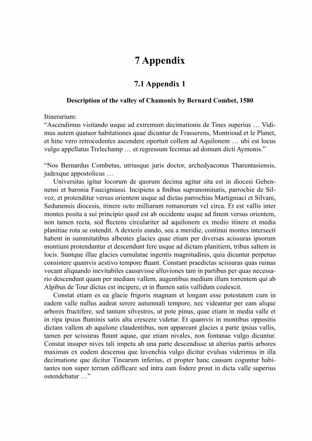
7 Appendix

7.1 Appendix 1

Description of the valley of Chamonix by Bernard Combet, 1580

Itinerarium:“Ascendimus visitando usque ad extremum decimationis de Tines superius … Vidi-mus autem quatuor habitationes quae dicuntur de Frasserens, Montrioud et le Planet, et hinc vero retrocedentes ascendere oportuit collem ad Aquilonem … ubi est locus vulgo appellatus Trelechamp … et regressum fecimus ad domum dicti Aymonis.”

“Nos Bernardus Combetus, utriusque juris doctor, archedyaconus Tharentasiensis, judexque appostolicus …

Universitas igitur locorum de quorum decima agitur sita est in diocesi Geben-nensi et baronia Faucigniassi. Incipiens a finibus supranominatis, parrochie de Sil-voz, et protenditur versus orientem usque ad dictas parrochias Martigniaci et Silvani, Sedunensis diocesis, itinere octo milliarum romanorum vel circa. Et est vallis inter montes posita a sui principio quod est ab occidente usque ad finem versus orientem, non tamen recta, sed flectens circulariter ad aquilonem ex medio itinere et media planitiae rota se ostendit. A dexteris eundo, seu a meridie, continui montes intersecti habent in summitatibus albentes glacies quae etiam per diversas scissuras ipsorum montium protenduntur et descendunt fere usque ad dictam planitiem, tribus saltem in locis. Suntque illae glacies cumulatae ingentis magnitudinis, quia dicuntur perpetuo consistere quamvis aestivo tempore fluant. Constant praedictas scissuras quas ruinas vocant aliquando inevitabiles causavisse alluviones tam in partibus per quas necessa-rio descendunt quam per mediam vallem, augentibus medium illum torrentem qui ab Alpibus de Tour dictus est incipere, et in flumen satis vallidum coalescit.

Constat etiam es ea glacie frigoris magnam et longam esse potestatem cum in eadem valle nullus audeat serere autumnali tempore, nec videantur per eam alique arbores fructifere, sed tantum silvestres, ut pote pinus, quae etiam in media valle et in ripa ipsius fluminis satis alta crescere videtur. Et quamvis in montibus oppositis dictam vallem ab aquilone claudentibus, non appareant glacies a parte ipsius vallis, tamen per scissuras fluunt aquae, que etiam nivales, non fontanae vulgo dicuntur. Constat insuper nives tali impetu ab una parte descendisse ut alterius partis arbores maximas ex eodem descensu que lavenchia vulgo dicitur evulsas viderimus in illa decimatione que dicitur Tinearum inferius, et propter hanc causam coguntur habi-tantes non super terram edifficare sed intra eam fodere prout in dicta valle superius ostendebatur …”

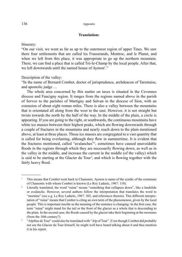
136

Translation:

Itinerary: “On our visit, we went as far as up to the outermost region of upper Tines. We saw there four settlements that are called les Frasserands, Montroc, and le Planet, and when we left from this place, it was appropriate to go up the northern mountain. There, we can find a place that is called Tré-le-Champ by the local people. After that, we left downwards until the named house of Aymon1.”

Description of the valley: “In the name of Bernard Combet, doctor of jurisprudence, archdeacon of Tarentaise, and apostolic judge …

The whole area concerned by this matter on taxes is situated in the Cevennes diocese and Faucigny region. It ranges from the regions named above in the parish of Servoz to the parishes of Martigny and Salvan in the diocese of Sion, with an extension of about eight roman miles. There is also a valley between the mountains that is orientated all along from the west to the east. However, it is not straight but twists towards the north by the half of the way. In the middle of the plain, a circle is appearing. If you are going to the right, or southwards, the continuous mountains have white ice masses between their highest peaks, which are flowing downwards through a couple of fractures in the mountains and nearly reach down to the plain mentioned above, at least at three places. Those ice masses are congregated to a vast quantity that is called for being everlasting, although they flow in summertime. It is evident that the fractures mentioned, called “avalanches”2, sometimes have caused unavoidable floods in the regions through which they are necessarily flowing down, as well as in the valley in the middle, and increase the current in the middle (of the valley) which is said to be starting at the Glacier du Tour3, and which is flowing together with the fairly heavy flood.

1 This means that Combet went back to Chamonix. Aymon is name of the syndic of the commune of Chamonix with whom Combet is known (Le Roy Ladurie, 1967: 110).

2 Literally translated, the word “ruina” means “something that collapses down”, like a landslide or avalanche. However, several authors follow the interpretation that translates the word to “moraine” (see e.g. Le Roy Ladurie, 1967: 302, and references therein). This different interpre-tation of “ruina” means that Combet is citing an own term of the phenomenon, given by the local people. This is important insofar as the meaning of the sentence is changing: In the first case, the term “ruina” might stand for the tail or the front of the glacier as a whole that is descending to the plain. In the second case, the floods caused by the glacier take their beginning at the moraines (from the 16th century?).

3 “Alpibus de Tour” could also be translated with “Alp of Tour”. Even though Combet did probably not see the Glacier du Tour himself, he might well have heard talking about it and thus mention it in his report.

Appendix

137

Furthermore, it is evident that there is a big and enduring force in the cold of that mass of ice, as nobody in this valley dares to sow in autumn. Neither are there any fruit trees, but only forest trees, more precisely pines, which even in the centre of the valley and at the riverside seem to grow quite high. And although there are no ice masses visible from the valley bottom on the opposite mountains which delimit the valley to the north, water is still running through fractures; that water is named “snow water” and not “sources”. Moreover, it is clear that the masses of snow have come down from one place with such a force that we could see the highest trees being frag-mented because of this mass movement that is called “avalanche” by the people in the region named lower Tines. Due to that, the inhabitants cannot build houses above the earth, but are forced to dig into it, which can be seen higher up in the valley mentioned above …”

Source: Archives départementales de la Haute-Savoie, No. 10 G 287 (1580)

Appendix

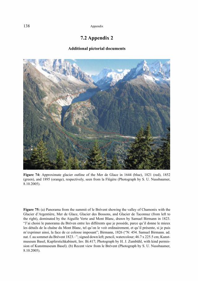
138

7.2 Appendix 2

Additional pictorial documents

Figure 74: Approximate glacier outline of the Mer de Glace in 1644 (blue), 1821 (red), 1852 (green), and 1895 (orange), respectively, seen from la Flégère (Photograph by S. U. Nussbaumer, 8.10.2005).

Figure 75: (a) Panorama from the summit of le Brévent showing the valley of Chamonix with the Glacier d’Argentière, Mer de Glace, Glacier des Bossons, and Glacier de Taconnaz (from left to the right), dominated by the Aiguille Verte and Mont Blanc, drawn by Samuel Birmann in 1823. “J’ai choisi le panorama du Bréven entre les différents que je possède, parce qu’il donne le mieux les détails de la chaîne du Mont Blanc, tel qu’on le voit ordinairement, et qu’il présente, si je puis m’exprimer ainsi, la face de ce colosse imposant”; Birmann, 1826 (“N: 454. Samuel Birmann. ad. nat. f. au sommet du Brévent 1823.–”; signed down left; pencil, watercolour; 46.7 x 225.5 cm; Kunst-museum Basel, Kupferstichkabinett, Inv. Bi.417; Photograph by H. J. Zumbühl, with kind permis-sion of Kunstmuseum Basel). (b) Recent view from le Brévent (Photograph by S. U. Nussbaumer, 8.10.2005).

Appendix

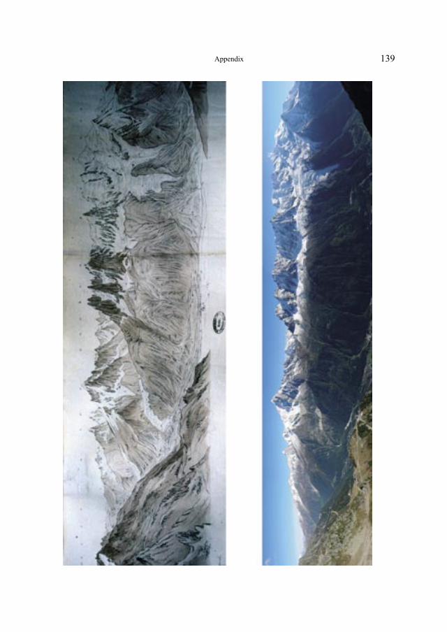
139Appendix

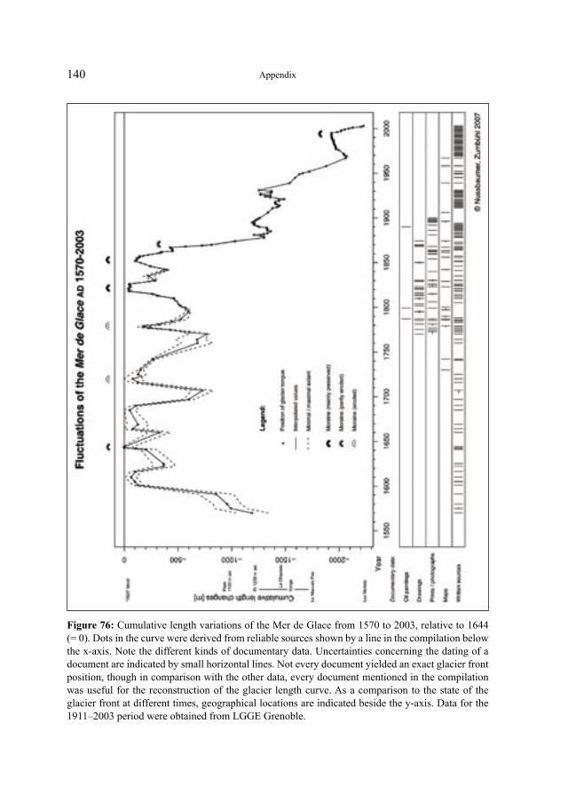
140

Figure 76: Cumulative length variations of the Mer de Glace from 1570 to 2003, relative to 1644 (= 0). Dots in the curve were derived from reliable sources shown by a line in the compilation below the x-axis. Note the different kinds of documentary data. Uncertainties concerning the dating of a document are indicated by small horizontal lines. Not every document yielded an exact glacier front position, though in comparison with the other data, every document mentioned in the compilation was useful for the reconstruction of the glacier length curve. As a comparison to the state of the glacier front at different times, geographical locations are indicated beside the y-axis. Data for the 1911–2003 period were obtained from LGGE Grenoble.

Appendix

Part II: The application of a neural network

to the length record of the Mer de Glace

Summary

A new suitable statistical approach to simulating glacier variations is the application of a neural network model, especially in combination with high-resolution climate data. In the present study, a non-linear back-propagation neural network model is suc-cessfully applied to simulate glacier variations of the Mer de Glace (Mont Blanc area, France), using multi-proxy reconstructions of seasonal temperature and precipitation back to 1500.

The neural network model is trained with high-resolution climate data (input data) and glacier length variations of the Mer de Glace (output data; cf. Part I of this issue). In the absence of glacier length data before 1570, the application of a neural network model yields plausible qualitative reconstructions of glacier fluctuations for the 16th century (glacier maximum around 1565, minima around 1552 and 1575).

In addition, future glacier length variations of the Mer de Glace are simulated using two climate scenarios. The first scenario assumes no changes in mean climate, the second scenario embodies higher temperature and changing precipitation values. Confronting current climate change, the more likely scenario 2 shows a continuous and remarkable retreat of the Mer de Glace until the end of the simulation period in 2042. The prediction for scenario 1 indicates a glacier front position in 2042 around that of the present-day. For both scenarios, the simulation period ranges from 1900 to 2042, showing a very good accordance between the simulated curve and the measured glacier front values for the 20th century. The glacier responses significantly distin-guish between the two scenarios, showing the key role of glaciers for the detection of climate changes.

Moreover, the utilization of the neural network model as a sensitivity analysis tool suggests that the Mer de Glace is more influenced by temperature than precipitation, in contrast to the Unterer Grindelwaldgletscher (Bernese Alps, Switzerland). Finally, this non-linear neural network approach is a new contribution to the various investi-gations of the complex glacier-climate system, which allows finding explanations for several glacier advances and retreats. Even though the relationship between glacier length and climate parameters is not easy to determine, clear statements concerning glacier reaction to climate variables are possible.

142

Zusammenfassung Teil II: Anwendung von neuronalen Netzen

auf die Längenänderungen des Mer de Glace

Ein neuer statistischer Ansatz für die Simulation von Gletscherschwankungen ist die Anwendung von neuronalen Netzen in Kombination mit hochaufgelösten Klima-daten. In der vorliegenden Studie wurde ein nichtlineares “back-propagation neural network”-Modell erfolgreich auf das Mer de Glace (Mont Blanc-Gebiet, Frankreich) angewandt unter Verwendung von multi-proxy Rekonstruktionen von saisonal aufge-lösten Temperatur- und Niederschlagsdaten bis ins Jahr 1500 zurück.

Das neuronale Netz wird mit hochaufgelösten Klimadaten (Inputdaten) und Glet-scherlängenänderungen des Mer de Glace (Outputdaten; vgl. Teil I) trainiert. Aufgrund des Fehlens von Gletscherlängendaten vor 1570 liefert das angewandte Gletschermo-dell basierend auf neuronalen Netzwerken plausible qualitative Rekonstruktionen für Gletscherschwankungen im 16. Jahrhundert (Gletschermaximum um 1565, -minima um 1552 und 1575).

Zusätzlich werden zwei Klimaszenarien verwendet, um zukünftige Gletscher-schwankungen des Mer de Glace zu simulieren. Gemäss Szenario 1, welches von gleichbleibendem Klima ausgeht, findet das Mer de Glace ein quasi Gleichgewicht mit einer Lage der Gletscherzunge um 2042 ähnlich wie heute. Szenario 2 berück-sichtigt die gegenwärtige Klimaänderung (höhere Temperaturen, veränderte Nieder-schlagswerte) und zeigt einen fortgesetzten und starken Gletscherrückgang an. Bei beiden Szenarien wird von 1900 bis 2042 simuliert, wobei die simulierten Gletscher-schwankungen für das 20. Jahrhundert sehr gut mit den gemessenen Längendaten übereinstimmen. Die Reaktionen des Gletschers gemäss den beiden Szenarien unter-scheiden sich signifikant, was die Schlüsselrolle der Gletscher für das Erkennen von Klimaänderungen bestätigt.

Das Modell ermöglicht schliesslich auch eine Sensitivitätsanalyse des Mer de Glace bezüglich Temperatur- und Niederschlagsparametern. Dabei wird gezeigt, dass das Mer de Glace im Vergleich zum Unteren Grindelwaldgletscher (Berner Alpen, Schweiz) stärker auf Temperatur statt Niederschlag reagiert. Dieser nichtlineare sta-tistische Ansatz stellt einen weiteren Beitrag zu den Untersuchungen des komplexen Gletscher-Klima-Systems dar und ermöglicht Erklärungen für einzelne Gletscher-schwankungen. Obwohl der Einfluss von Klimaparametern auf die Gletscherlänge kompliziert und schwierig zu bestimmen ist, sind klare Aussagen bezüglich der Reak-tion eines Gletschers auf sich ändernde Klimaparameter möglich.

Zusammenfassung Teil II

143

Résumé de la deuxième partie: Application d’un réseau neuronal

aux variations de longueur de la Mer de Glace

Un nouveau procédé statistique pour simuler des variations de glacier est l’applica-tion d’un réseau neuronal, surtout en combinaison avec des données de climat à haute résolution. Dans ce travail, un réseau neuronal “back-propagation” non-linéaire est appliqué avec succès à la Mer de Glace (région du Mont Blanc, France) en utilisant des reconstructions “multi-proxy” de données de température et de précipitations, dis-soutes selon la saison, reconstructions qui remontent jusqu’à l’année 1500.

Le modèle est “entraîné” avec des données de climat à haute résolution (input) et des changements de longueur de la Mer de Glace (output; cf. première partie). En raison du manque de données avant 1570, l’application du réseau neuronal nous donne des reconstructions plausibles pour les fluctuations du glacier au 16ème siècle (maximum de glacier vers 1565, minima vers 1552 et 1575).

En outre, deux scénarios de climat sont appliqués pour simuler les fluctuations du glacier dans le futur. Selon le scénario 1, qui présuppose un climat constant, la Mer de Glace finit par trouver une sorte d’équilibre avec une position de la langue du glacier vers 2042 qui est à peu près la même qu’aujourd’hui. Le scénario 2 prend en considé-ration le réchauffement actuel du climat et présage un recul continu et remarquable du glacier. Dans les deux scénarios, les simulations s’étendent de 1900 jusqu’à 2042, et on constate que les fluctuations de glacier simulées durant le 20ème siècle correspon-dent très bien aux données de longueur mesurées. Suivant l’un ou l’autre scénario, le glacier réagit différemment, et cela d’une façon significative. Cela confirme le rôle clé des glaciers en considération de la reconnaissance des changements de climat.

Enfin, en appliquant le réseau neuronal pour faire une analyse de sensitivité du gla-cier, il s’avère que la Mer de Glace, mise en comparaison avec l’Unterer Grindelwald-gletscher (Alpes bernoises, Suisse), réagit plus fortement à la température qu’aux pré-cipitations. Ce procédé se basant sur un réseau neuronal non-linéaire est une nouvelle contribution aux investigations concernant le système glaciers-climat, et il permet de trouver des explications quant aux fluctuations de glacier. Bien que l’influence de paramètres de climat sur la longueur de glacier soit compliquée et difficile à détermi-ner, des énonciations claires sont possibles quant à la façon dont un glacier réagit à des paramètres de climat changeant.

Résumé de la deuxième partie

1 Introduction

Mountains and their environments are highly sensitive indicators of climate vari-ability over the decadal to centennial time scales. In particular and corresponding to global trends in temperature, glaciers have retreated significantly since the mid 19th century (e.g., IPCC, 2001; Paul et al., 2004; Oerlemans, 2005). By the year 2000, Alpine glaciers had lost almost 50% of their total area since 1850, and continuation or even acceleration of ongoing trends in retreating glaciers will soon lead to conditions without historical or even Holocene comparability and could cause nearly complete deglaciation of many now still glaciated mountain ranges (Zemp et al., 2006).

Glacier length change as a reflector of climate change can easily be measured, and corresponding continuous records exist since the end of the 19th century (e.g., VAW/SCNAT, 2002). Although glacier length is an indirect, filtered and delayed response of climate change (Oerlemans, 2001), it can be used to reconstruct glacier mass balance (Haeberli and Hoelzle, 1995; Hoelzle et al., 2003) as well as large scale temperature changes over the last centuries (Oerlemans, 2005).

The evaluation of historical data gives insight into the change in glacier length over time (cf. Part I of this issue) without showing the climatic driving factors which pre-sumably affected these glacier changes. Many studies have been carried out in order to investigate the relationship between the meteorological conditions and variations of glaciers. For instance, regression techniques with different numbers and types of predictors have often been used (e.g., Oerlemans and Reichert, 2000, and references therein). Available glacier-climate models differ widely and can be applied in many different situations and settings. However, many of these classical methods use linear assumptions.

Because glacier length is a complex function dependent on climate, time, glacier geometry and other factors, it may be well-suited to non-linear model approaches. Since the late 1980s, neural network models have become popular for performing non-linear regression and classification (e.g., Hsieh, 2004, and references therein). A neural network is an information processing paradigm that is inspired by the way biological nervous systems, such as the brain, process information, and can be used to extract patterns and detect trends from complex data.

The methodology of neural network models was applied by Steiner et al. (2005) for the first time to these subjects of glaciology. The neural network approach differs from classical models (and also from linear statistical methods) in that it uses a non-linear approach. As the climate system (including the glacier system) can be seen as non-linear (IPCC, 2001), it has to be questioned whether traditional linear statistical models are able to describe the full complexity of the system’s behaviour. Steiner et al. (2005) show that for reconstructing the glacier mass balance of the Grosser Aletsch-gletscher, the neural network approach performs better than stepwise multiple linear regression. In another study, Zumbühl et al. (in press) apply a neural network model

145

to the Unterer Grindelwaldgletscher, in order to explain the glacier reaction (19th century advance and retreat) to climate parameters.

In this study, the neural network approach is used on the Mer de Glace in order to get more insight into the capabilities of neural network models in glaciological con-texts. Moreover, the aim is getting information on the behaviour of the glacier in the 16th century, and in the near future (2000–2050). Finally, the method allows validat-ing the new length curve of the Mer de Glace (cf. Part I of this issue) for certain time periods and can be used as a glacier sensitivity analysis tool.

The Mer de Glace is a valley glacier 12 km long that is situated at the northern exposition of the Mont Blanc (French Alps). It is the longest and largest glacier of the western Alps and, including all tributaries, it covers an area of about 32 km2 and spans an altitudinal range from 1500 to 4000 m asl. During the Little Ice Age (LIA), the Mer de Glace nearly continuously reached the bottom of the valley of Chamonix at 1000 m asl. The attractiveness of the landscape and its easy accessibility soon made the glacier a desirable object of study for scientists, artists and tourists, leading to a large number of historical documentary data. For a detailed description of the location and geographical settings of the Mer de Glace, see Part I of this issue.

This study complements the historical point of view (Part I of this issue) of the Mer de Glace and forms an interdisciplinary approach using historical and physical methods to reconstruct and simulate fluctuations of the Mer de Glace. The modelling results complement the historical analysis in order to give a better picture of how, and why the glacier has reacted.

Section 2 gives an overview of data and methods used in this study (climate data used as model input; concept of the neural network approach). As an example for a neural network, the back-propagation neural network is discussed. The results of the neural network simulations are presented in section 3, including a validation of the new length curve, simulations of length fluctuations for the 16th century and the near future, and a sensitivity analysis of the Mer de Glace. Finally, the results and the performance of the method used within this study are discussed in section 4, and final conclusions are drawn in section 5.

Introduction

146

2 Data and methods 2.1 Multi-proxy reconstructions of temperature

and precipitation back to 1500

Neural network models are especially appropriate and well-performing in combina-tion with high-resolution climate data (Steiner, 2005). In the present study, a non-linear back-propagation neural network model is applied to the Mer de Glace, using multi-proxy reconstructions of seasonal temperature and precipitation back to 1500, and climate scenarios for the period from 2000 to 2050 (cf. section 2.2).

New gridded high-resolution multi-proxy reconstructions of temperature and pre-cipitation patterns are available for the European land areas. These are reconstruc-tions of temperature (Luterbacher et al., 2004; Xoplaki et al., 2005) and precipitation (Pauling et al., 2006) back to the year 1500. Analogously, Casty et al. (2005) recon-structed both temperature and precipitation for the European Alps (43.25–48.25°N and 4.25–16.25°E; 0.5° × 0.5° resolution) back to 1500 (seasonal 1500–1658, monthly 1659–2000). These reconstructions are based on instrumental station data collected over a long time period combined with documentary and natural proxy evidence, applying principal component regression analysis. Temperature and precipitation are reconstructed independently, i.e. they share no common predictors (Casty et al., 2005). Note that the quality of the reconstructions decreases the further back in time we go, and varies over seasons and space, too. A means for estimating the quality of the reconstructions is the so called Reduction of Error (RE) statistics. A RE value of 1 stands for a perfect reconstruction, and RE values greater than zero indicate recon-structions that are better than climatology. A detailed description of the reconstruction methods, the predictor data used and the reliability of the reconstructions can be found in Casty et al. (2005).

As the data set has a high spatial and temporal resolution, it is appropriate for regional studies (e.g., climate-glacier relationship). Seasonal data over the whole time period from this data set will be used as input parameter for the neural network model for the simulations of the Mer de Glace glacier length fluctuations (cf. section 2.4). In order to do this, the data of the grid point that is closest to the glacier location has been chosen (45.75°N / 6.75°E). The data series for that location are presented in the Appendix. Figure 10 shows the average seasonal precipitation sum anomalies (mm) with regard to the 1901–2000 mean from 1500 to 2000 at the grid point 45.75°N/ 6.75°E. Figure 11 illustrates the corresponding time series for the temperature anoma-lies (°C) for the same period at the same grid point.

147

2.2 Climate scenarios 2000–2050

Climate scenarios show the possible future evolution of climate. As the main purpose of climate scenarios is to investigate the potential impacts of anthropogenic climate change, the scenarios should represent the plausible future climate based on vari-able pre-conditions. In IPCC (2001), different climate projections are mentioned that describe the modelled response of the climate system to various scenarios of green-house gas and aerosol concentrations. Climate scenarios by such model projections are still tainted with large uncertainties, which poses a problem. Moreover, uncer-tainty estimates are often based on expert judgement rather than objective quantitative methods.

The studies by Frei (2004) aim at reducing this problem by using a probabilistic approach by which the said uncertainties can at least be partially quantified. This is achieved by ensembles of climate change integrations that use different models start-ing from different initial conditions. The result allows making a probabilistic predic-tion of climate change for the 2000–2050 period on a regional scale (Frei, 2004). Analogous, probabilistic climate projections exist for the global temperature mean (Wigley and Raper, 2001; Knutti et al., 2002).

Regional climate model simulations for central and southern Europe indicate a remarkable increase in summer temperatures during the 21st century. Those results are based on the IPCC SRES A2 transient greenhouse-gas scenario (“business-as-usual”) and imply that about every second summer will be as hot or even hotter than 2003 (Neu and Thalmann, 2005) by the end of the 21st century (2071–2100; Schär et al., 2004; Stott et al., 2004).

The probabilistic projections of temperature and precipitation by Frei (2004) also use the IPCC SRES A2 emission scenario as model input. Additionally, the IPCC SRES B2 (“dynamics-as-usual”) emission scenario was used, too. It allowed perform-ing regional probabilistic projections of temperature and precipitation for the Swiss Alpine region based on simulations with 16 different climate model chains. In doing this, Frei (2004) distinguished between the northern and southern Alps, resulting in different predictions for each region.

For the present study, the results by Frei (2004) were used to force the neural network model (cf. section 2.4) with two regional climate scenarios of temperature and precipitation from 2000 until 2050 (Table 1). In doing this, the projections for the northern part of the Alps were chosen.

Data and methods

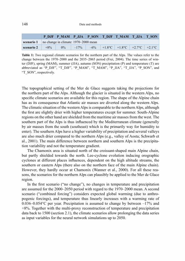
148

P_DJF P_MAM P_JJA P_SON T_DJF T_MAM T_JJA T_SON

scenario 1 no change in climate: 1970–2000 mean

scenario 2 +8% 0% –17% –6% +1.8°C +1.8°C +2.7°C +2.1°C

Table 1: Two regional climate scenarios for the northern part of the Alps. The values refer to the change between the 1970–2000 and the 2035–2065 period (Frei, 2004). The time series of win-ter (DJF), spring (MAM), summer (JJA), autumn (SON) precipitation (P) and temperature (T) are abbreviated as “P_DJF”, “T_DJF”, “P_MAM”, “T_MAM”, “P_JJA”, “T_JJA”, “P_SON”, and “T_SON”, respectively.

The topographical setting of the Mer de Glace suggests taking the projections for the northern part of the Alps. Although the glacier is situated in the western Alps, no specific climate scenarios are available for this region. The shape of the Alpine chain has as its consequence that Atlantic air masses are diverted along the western Alps. The climatic situation of the western Alps is comparable to the northern Alps, although the first are slightly drier with higher temperatures except for summer. South-Alpine regions on the other hand are shielded from the maritime air masses from the west. The southern part of the Alps is thus influenced by the Mediterranean climate (generally by air masses from the south (southeast) which is the primarily way for humidity to enter). The southern Alps have a higher variability of precipitation and several valleys are also much drier compared to the northern Alps (e.g., valley of Aosta; Schwarb et al., 2001). The main difference between northern and southern Alps is the precipita-tion variability and not the temperature gradient.

The Chamonix area is situated north of the croissant-shaped main Alpine chain, but partly shielded towards the north. Lee-cyclone evolution inducing orographic cyclones at different places influences, dependent on the high altitude streams, the southern or eastern Alps (there also on the northern face of the main Alpine chain). However, they hardly occur at Chamonix (Wanner et al., 2000). For all these rea-sons, the scenarios for the northern Alps can plausibly be applied to the Mer de Glace region.

In the first scenario (“no change”), no changes in temperature and precipitation are assumed for the 2000–2050 period with regard to the 1970–2000 mean. A second scenario (“combined forcing”) considers expected global warming (due to anthro-pogenic forcings), and temperature thus linearly increases with a warming rate of 0.036–0.054°C per year. Precipitation is assumed to change by between –17% and +8%. Together with the multi-proxy reconstruction of temperature and precipitation data back to 1500 (section 2.1), the climate scenarios allow prolonging the data series as input variables for the neural network simulations up to 2050.

Data and methods

149

2.3 The response time of glaciers

The response of the glacier tongue to changes in climate parameters is delayed. The response time is the time required for a glacier to adjust from one “steady-state” to another following a change in the mass balance (e.g., Nesje and Dahl, 2000: 93). This definition is problematic insofar as a glacier hardly remains in a distinct steady state, making the response time a complicated and difficult term being unknown for most glaciers.

Nye (1960) was the first to define the response time of a glacier as the time between two steady state conditions. He founded his definition on theoretical analyses based on the kinematic wave theory. Jóhannesson et al. (1989) on the other hand argued that there is a discrepancy between the theoretical model and the record of past glacier and climate fluctuations as all those theoretical models assume a small step in mass balance and a more or less unchanged glacier geometry. Jóhannesson et al. (1989) therefore proposed a simplified analytical model where the response time is proportional to the glacier thickness and inversely proportional to the net balance at the terminus. Bahr et al. (1998) and Pfeffer et al. (1998) finally refined the geometrical influence on the response time and showed that the response time depends on the mass balance index, defined as the slope of the balance curve as a function of horizontal distance. The mass balance index is typically larger for small glaciers, which will therefore respond faster than large glaciers. This quicker response is due to mass balance and glacier size considerations. Also maritime glaciers have a higher mass balance index than glaciers situated in areas with more continental climate.

It has to be taken into account that in fact there are two different response times depending on whether the glacier is advancing or retreating, as shown by Schmeits and Oerlemans (1997). Glacier advances are of a more dynamic character than retreats, which are dominated by ablation and thus more dependent on climate parameters. Retreat and advance are two completely different processes. Moreover, the reaction of a glacier to a change in climatic parameters depends on the prehistory of the glacier, e.g. a glacier advance is rather triggered by cool summers combined with high pre-cipitation during the accumulation season following a period of average climate than by an extraordinary warm and dry preceding period (Steiner, 2005).

It is necessary to have available an estimation of the response time (i.e., the time lag between the reaction of the glacier front to a change in climate parameters) of the Mer de Glace for the following simulations using neural networks (cf. section 2.4). Based on glacier length analysis since 1870, it could be seen that the Mer de Glace had its minimum frontal position between 11 and 15 years after the much shorter and steeper Glacier des Bossons, which has a short response time (Reynaud, 1993). However, it must be noted that the reaction to climate at the glacier snout can also be more immediate in some situations, e.g. after runs of cool summers (Matthews and Briffa, 2005).

Data and methods

150

A simple (optical) analysis of the time lag between a distinct temperature signal and the corresponding glacier front reaction of the Mer de Glace suggests a value of approximate 25–30 years, which is also confirmed by estimation formulae. Hence, a time lag of 30 years has been chosen for the neural network simulations. Note that those 30 years are not a fixed time lag but the upper limit of the lag which is set by the neural network model (i.e., the best fitting values, dependent on the time lag, get most weight), as will be described in the next section.

2.4 The back-propagation neural network model

The main idea of the neural network approach is to use the same processing para-digm as used by biological organisms, and by our brain. The main purpose that stands behind the application of neural networks is to derive meaning from complicated data where other methods fail, e.g. for extracting patterns or detecting trends that are too complex to be noticed by either other computer techniques or humans. A more detailed explanation of the technique can be found in Steiner et al. (2005).

The way our brain processes information can be described in a strongly simplified way as follows: The human brain consists of highly interconnected nerve cells that process input information signals to produce an output signal. However, there is only an output signal if the input information exceeds a certain threshold, in order to acti-vate the following neurological responses and to trigger an action. The unique learn-ing algorithm of the human brain makes it possible to steer the processing of informa-tion in order to get the wanted output/action.

A neural network aims at imitating this kind of processing. It consists of a set of highly interconnected units which process information as a response to external stimuli. Following a learning algorithm, the neural network model detects certain fea-tures of the data, which consist of input variables and desired output responses, using a training subset. After the training process, these features are tested on an unknown validation subset, on which the performance of the neural network model can be determined. Internal parameters of the network architecture are adjusted according to a specific learning rule so that the network ideally captures all intrinsic data features (Steiner et al., 2005). Note that a neural network is just a simplistic mathematical realization of the information processing in human brains that emulates the signal integration and threshold firing behaviour of biological neurons by means of mathe-matical equations.

A typical neural network model consists of three layers (input, processing, and output layers) and is shown exemplified in Figure 1. The input to a neural network model is a vector of elements xk, where the index k stands for the number of input units in the network (input layer in Figure 1). Input signals are weighted with weights wjk where j represents the number of processing units, to give the inputs to the pro-cessing units. Weighted input signals are processed if they exceed a certain threshold

Data and methods

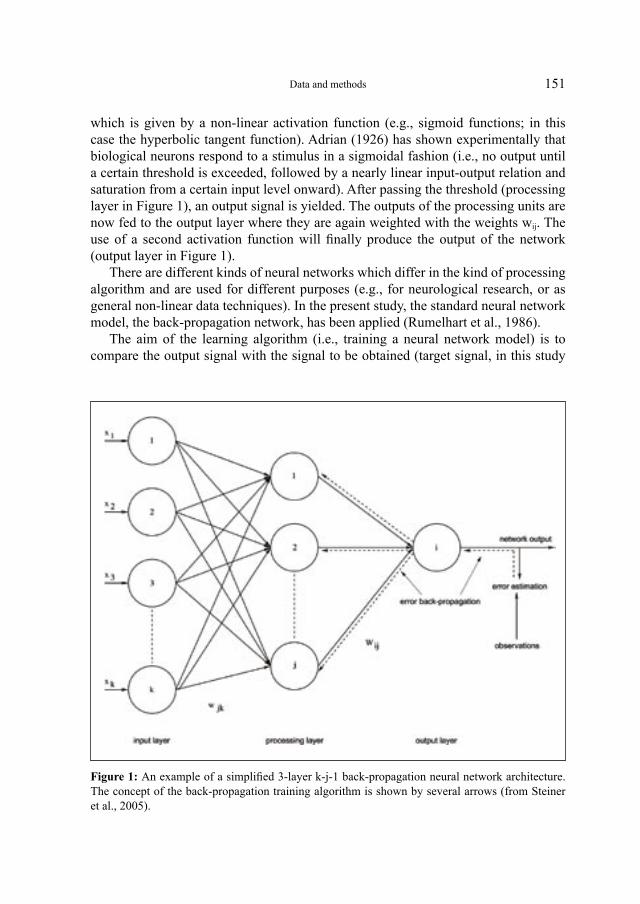
151

which is given by a non-linear activation function (e.g., sigmoid functions; in this case the hyperbolic tangent function). Adrian (1926) has shown experimentally that biological neurons respond to a stimulus in a sigmoidal fashion (i.e., no output until a certain threshold is exceeded, followed by a nearly linear input-output relation and saturation from a certain input level onward). After passing the threshold (processing layer in Figure 1), an output signal is yielded. The outputs of the processing units are now fed to the output layer where they are again weighted with the weights wij. The use of a second activation function will finally produce the output of the network (output layer in Figure 1).

There are different kinds of neural networks which differ in the kind of processing algorithm and are used for different purposes (e.g., for neurological research, or as general non-linear data techniques). In the present study, the standard neural network model, the back-propagation network, has been applied (Rumelhart et al., 1986).

The aim of the learning algorithm (i.e., training a neural network model) is to compare the output signal with the signal to be obtained (target signal, in this study

Figure 1: An example of a simplified 3-layer k-j-1 back-propagation neural network architecture. The concept of the back-propagation training algorithm is shown by several arrows (from Steiner et al., 2005).

Data and methods

152

the glacier length). The difference between the real value and the model output result makes the processing unit change the weights set at the previous processing step. As the weights are changed, also a new output signal is produced. The processing unit continues until a sufficient output result is reached, i.e. until a set of coefficients is found that reduces the error between the model outputs and the given test data y(xk). This is usually done by adjusting the weights wij and wjk to minimize the least square error. One way to adjust these weights is error back-propagation.

The architecture of the back-propagation neural network is based on a supervised learning algorithm to find a minimum cost function. In contrast to a simulated anneal-ing schedule (a modified Monte Carlo method for examining (minimum) energy states in thermodynamical systems, and by analogy also applied to various combinatorial optimization problems; Metropolis et al., 1953), the back-propagation neural network does not guarantee that the global minimum of this cost function will be reached, though it is very likely that a minimum good enough to produce responses in the data can be found. Because this approach bears a certain risk of overfitting, the data have to be separated into a training and a validation subset. Using the so called cross-valida-tion technique (Stone, 1974; Michaelsen, 1987), the actual “learning” process of the network is performed on the training subset only, whereas the validation subset serves as an independent reference for the simulation quality. When applying neural network models to a non-stationary time series, as in this approach, the training subset includes the full range of extremes in both predictors and predictands. Otherwise, the algorithm will fail during the validation process if confronted with an extreme value that was not part of the training subset. In this study, 75% of all data were used for training and the remaining 25% for validation (Walter and Schönwiese, 2003).

The back-propagation training consists of two passes of computation: a forward pass and a backward pass. In the forward pass, an input vector is applied to the units in the input layer. The signals from the input layer propagate to the units in the pro-cessing layer and each unit produces an output. The outputs of these units are propa-gated to units in subsequent layers. This process continues until the signals reach the output layer where the actual response of the network to the input vector is obtained. During the forward pass the weights of the network are fixed. During the backward pass (see dashed arrows in Figure 1), on the other hand, the weights are all adjusted in accordance with an error signal that is propagated backward through the network against the initial direction.

Using too few/many processing units can lead to underfitting/overfitting problems because the simulation results are highly sensitive to the number of processing units and learning parameters. Therefore a variety of back-propagation neural networks must be checked to obtain robust results. As mentioned above, this network architec-ture still carries the risk of being stuck in local minima on the error hypersurface. To reduce this risk, conjugate gradient descent was used in this study. This is an improved version of standard back-propagation with accelerated convergence. For a detailed description of this technique, see Steiner et al. (2005).

Data and methods

153

In general, glacier fluctuations are primarily influenced by air temperature, while precipitation is the second most important climatic factor (Kuhn, 1981; Oerlemans, 2001). For the present study, seasonal temperature and precipitation data series for the period from 1500 to 2000 (cf. section 2.1), as well as climate scenarios for the years 2000–2050 (cf. section 2.2) were used as input data. Glacier length data from the Mer de Glace served as target function. The back-propagation neural network has to find the connection between the input and target data, which is the core of the “learning” process.

All seasonal climate data were used as forcings (T_DJF, T_MAM, T_JJA, T_SON, P_DJF, P_MAM, P_JJA, P_SON). Note that the response of the glacier length to a climate forcing is not immediate but delayed. This is considered by the neural network model by the setting of a time lag of 30 years for all input data. The input data was shifted stepwise so that all lags between 0 and 30 years were considered to account for the uncertain and changing reaction time of the glacier. The neural network model chooses those input series which fit best to explain the behaviour of the target func-tion, i.e. the delay of the glacier length to climate stimuli should be recognized cor-rectly.

The architecture of the neural network model can be chosen, though the model processes well if the number of processing units is set to half the number of input units as shown by Steiner (2005). Using a time lag from 0 to 30 years for this study, we get 31 · 8 = 248 input units (climate variables), 124 processing units in 1 processing layer and the length fluctuations as output unit. This neural network architecture is abbre-viated as 248–124–1.

An uncertainty in the back-propagation neural network simulation is related to the fact that the identified minimum is dependent on the starting point on the error hypersurface. To reduce this kind of uncertainty, i.e. in order to ensure that the error reduction process does not always follow the exact same path, multiple model runs are needed. The simulations start from different initial conditions, using the training data in different orders. Hence, the back-propagation neural network was performed 30 times, starting from different locations on the error hypersurface. Finally, the aver-age of the 30 model results was analysed. In one case (weak input data quality), the model was driven 50 times to ensure the reliability of the result (cf. section 3.1.2).

The neural network model was used for several purposes in this study. First, it served as a validation tool for the new glacier length curve for the 1570–2003 period. Two time periods were chosen for validation: the best-documented 20th century, and the period of the Maunder Minimum (1645–1715), respectively. The latter was chosen since as a dry and cold period it is a special time in Europe during the LIA, and as the reconstructed Mer de Glace length variations show a significant retreat followed by a re-advance around 1700 (cf. Part I of this issue).

For the validation of the curve in the 20th century, input data until 1900 were used to train the neural network model. In doing this, the time lag of 30 years was taken into account, so that the simulated curve effectually started in 1900. After training, the

Data and methods

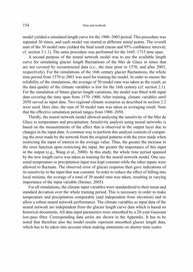
154

model yielded a simulated length curve for the 1900–2003 period. This procedure was repeated 30 times, and each model run started at different initial points. The overall sum of the 30 model runs yielded the final result (mean and 95% confidence interval; cf. section 3.1.1). The same procedure was performed for the 1645–1715 time span.

A second purpose of the neural network model was to use the available length curve for simulating glacier length fluctuations of the Mer de Glace in times that are not covered by reconstructed data (i.e., the time prior to 1570, and after 2003, respectively). For the simulations of the 16th century glacier fluctuations, the whole time period from 1570 to 2003 was used for training the model. In order to ensure the reliability of the simulations, the average of 50 model runs was taken as the result, as the data quality of the climate variables is low for the 16th century (cf. section 2.1). For the simulation of future glacier length variations, the model was fitted with input data covering the time span from 1570–1900. After training, climate variables until 2050 served as input data. Two regional climate scenarios as described in section 2.2 were used. Here also, the sum of 30 model runs was taken as averaging result. Note that the effective simulation period ranges from 1900–2050.

Thirdly, the neural network model allowed analysing the sensitivity of the Mer de Glace to temperature and precipitation. Sensitivity analysis using neural networks is based on the measurements of the effect that is observed in the output layer due to changes in the input data. A common way to perform this analysis consists of compar-ing the error made by the network from the original patterns with the error made when restricting the input of interest to the average value. Thus, the greater the increase in the error function upon restricting the input, the greater the importance of this input in the output (e.g., Wang et al., 2000). In this study, the whole time period spanned by the new length curve was taken as training for the neural network model. One sea-sonal temperature or precipitation input was kept constant while the other inputs were allowed to fluctuate. The observed error of glacier response then gave indications of its sensitivity to the input that was constant. In order to reduce the effect of falling into local minima, the average of a total of 30 model runs was taken, resulting in varying importance of the input variable (Steiner, 2005).

For all simulations, the climate input variables were standardized to their mean and standard deviation over the whole training period. This is necessary in order to make temperature and precipitation comparable (and independent from elevation) and to allow a robust neural network performance. The climate variables as input data of the neural network are independent from the glacier length curve data which is based on historical documents. All data input parameters were smoothed by a 20-year Gaussian low-pass filter. Corresponding data series are shown in the Appendix. It has to be noted that therefore also the model results represent smoothed glacier length data, which has to be taken into account when making statements on shorter time scales.

Data and methods

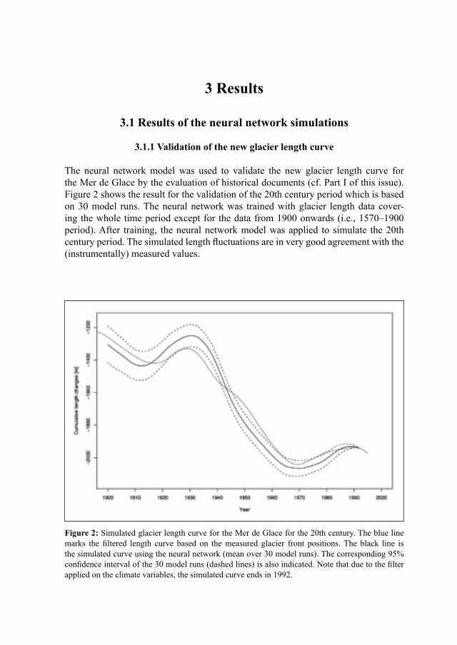
3 Results

3.1 Results of the neural network simulations

3.1.1 Validation of the new glacier length curve

The neural network model was used to validate the new glacier length curve for the Mer de Glace by the evaluation of historical documents (cf. Part I of this issue). Figure 2 shows the result for the validation of the 20th century period which is based on 30 model runs. The neural network was trained with glacier length data cover-ing the whole time period except for the data from 1900 onwards (i.e., 1570–1900 period). After training, the neural network model was applied to simulate the 20th century period. The simulated length fluctuations are in very good agreement with the (instrumentally) measured values.

Figure 2: Simulated glacier length curve for the Mer de Glace for the 20th century. The blue line marks the filtered length curve based on the measured glacier front positions. The black line is the simulated curve using the neural network (mean over 30 model runs). The corresponding 95% confidence interval of the 30 model runs (dashed lines) is also indicated. Note that due to the filter applied on the climate variables, the simulated curve ends in 1992.

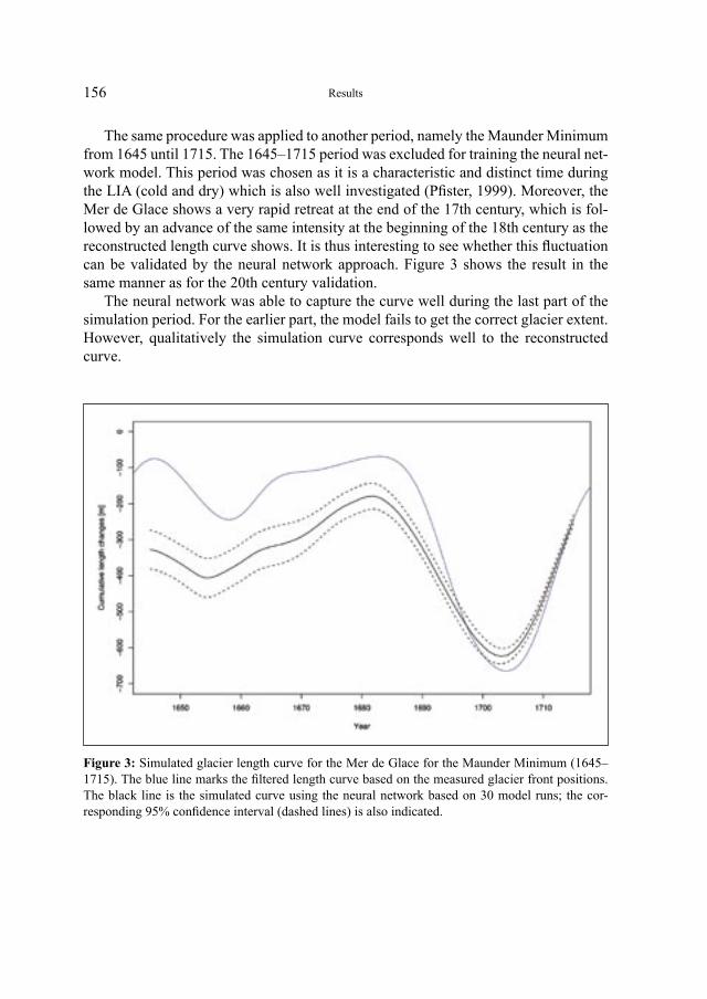
156

The same procedure was applied to another period, namely the Maunder Minimum from 1645 until 1715. The 1645–1715 period was excluded for training the neural net-work model. This period was chosen as it is a characteristic and distinct time during the LIA (cold and dry) which is also well investigated (Pfister, 1999). Moreover, the Mer de Glace shows a very rapid retreat at the end of the 17th century, which is fol-lowed by an advance of the same intensity at the beginning of the 18th century as the reconstructed length curve shows. It is thus interesting to see whether this fluctuation can be validated by the neural network approach. Figure 3 shows the result in the same manner as for the 20th century validation.

The neural network was able to capture the curve well during the last part of the simulation period. For the earlier part, the model fails to get the correct glacier extent. However, qualitatively the simulation curve corresponds well to the reconstructed curve.

Figure 3: Simulated glacier length curve for the Mer de Glace for the Maunder Minimum (1645–1715). The blue line marks the filtered length curve based on the measured glacier front positions. The black line is the simulated curve using the neural network based on 30 model runs; the cor-responding 95% confidence interval (dashed lines) is also indicated.

Results

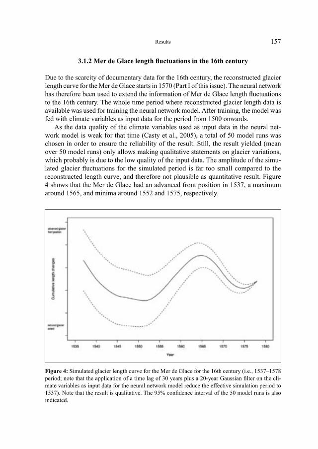
157

3.1.2 Mer de Glace length fluctuations in the 16th century

Due to the scarcity of documentary data for the 16th century, the reconstructed glacier length curve for the Mer de Glace starts in 1570 (Part I of this issue). The neural network has therefore been used to extend the information of Mer de Glace length fluctuations to the 16th century. The whole time period where reconstructed glacier length data is available was used for training the neural network model. After training, the model was fed with climate variables as input data for the period from 1500 onwards.

As the data quality of the climate variables used as input data in the neural net-work model is weak for that time (Casty et al., 2005), a total of 50 model runs was chosen in order to ensure the reliability of the result. Still, the result yielded (mean over 50 model runs) only allows making qualitative statements on glacier variations, which probably is due to the low quality of the input data. The amplitude of the simu-lated glacier fluctuations for the simulated period is far too small compared to the reconstructed length curve, and therefore not plausible as quantitative result. Figure 4 shows that the Mer de Glace had an advanced front position in 1537, a maximum around 1565, and minima around 1552 and 1575, respectively.

Figure 4: Simulated glacier length curve for the Mer de Glace for the 16th century (i.e., 1537–1578 period; note that the application of a time lag of 30 years plus a 20-year Gaussian filter on the cli-mate variables as input data for the neural network model reduce the effective simulation period to 1537). Note that the result is qualitative. The 95% confidence interval of the 50 model runs is also indicated.

Results

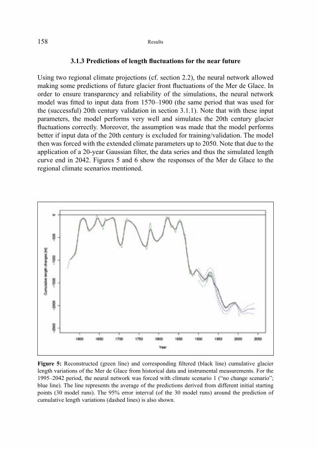
158

3.1.3 Predictions of length fluctuations for the near future

Using two regional climate projections (cf. section 2.2), the neural network allowed making some predictions of future glacier front fluctuations of the Mer de Glace. In order to ensure transparency and reliability of the simulations, the neural network model was fitted to input data from 1570–1900 (the same period that was used for the (successful) 20th century validation in section 3.1.1). Note that with these input parameters, the model performs very well and simulates the 20th century glacier fluctuations correctly. Moreover, the assumption was made that the model performs better if input data of the 20th century is excluded for training/validation. The model then was forced with the extended climate parameters up to 2050. Note that due to the application of a 20-year Gaussian filter, the data series and thus the simulated length curve end in 2042. Figures 5 and 6 show the responses of the Mer de Glace to the regional climate scenarios mentioned.

Figure 5: Reconstructed (green line) and corresponding filtered (black line) cumulative glacier length variations of the Mer de Glace from historical data and instrumental measurements. For the 1995–2042 period, the neural network was forced with climate scenario 1 (“no change scenario”; blue line). The line represents the average of the predictions derived from different initial starting points (30 model runs). The 95% error interval (of the 30 model runs) around the prediction of cumulative length variations (dashed lines) is also shown.

Results

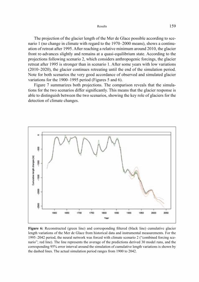
159

Figure 6: Reconstructed (green line) and corresponding filtered (black line) cumulative glacier length variations of the Mer de Glace from historical data and instrumental measurements. For the 1995–2042 period, the neural network was forced with climate scenario 2 (“combined forcing sce-nario”; red line). The line represents the average of the predictions derived 30 model runs, and the corresponding 95% error interval around the simulation of cumulative length variations is shown by the dashed lines. The actual simulation period ranges from 1900 to 2042.

The projection of the glacier length of the Mer de Glace possible according to sce-nario 1 (no change in climate with regard to the 1970–2000 means), shows a continu-ation of retreat after 1995. After reaching a relative minimum around 2010, the glacier front re-advances slightly and remains at a quasi-equilibrium state. According to the projections following scenario 2, which considers anthropogenic forcings, the glacier retreat after 1995 is stronger than in scenario 1. After some years with low variations (2010–2020), the glacier continues retreating until the end of the simulation period. Note for both scenarios the very good accordance of observed and simulated glacier variations for the 1900–1995 period (Figures 5 and 6).

Figure 7 summarizes both projections. The comparison reveals that the simula-tions for the two scenarios differ significantly. This means that the glacier response is able to distinguish between the two scenarios, showing the key role of glaciers for the detection of climate changes.

Results

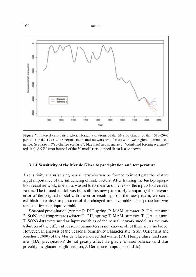
160

3.1.4 Sensitivity of the Mer de Glace to precipitation and temperature

A sensitivity analysis using neural networks was performed to investigate the relative input importance of the influencing climate factors. After training the back-propaga-tion neural network, one input was set to its mean and the rest of the inputs to their real values. The trained model was fed with this new pattern. By comparing the network error of the original model with the error resulting from the new pattern, we could establish a relative importance of the changed input variable. This procedure was repeated for each input variable.

Seasonal precipitation (winter: P_DJF, spring: P_MAM, summer: P_JJA, autumn: P_SON) and temperature (winter: T_DJF, spring: T_MAM, summer: T_JJA, autumn: T_SON) data were used as input variables of the neural network model. As the con-tribution of the different seasonal parameters is not known, all of them were included. However, an analysis of the Seasonal Sensitivity Characteristic (SSC; Oerlemans and Reichert, 2000) of the Mer de Glace showed that winter (DJF) temperature (and sum-mer (JJA) precipitation) do not greatly affect the glacier’s mass balance (and thus possibly the glacier length reaction; J. Oerlemans, unpublished data).

Figure 7: Filtered cumulative glacier length variations of the Mer de Glace for the 1578–2042 period. For the 1995–2042 period, the neural network was forced with two regional climate sce-narios: Scenario 1 (“no change scenario”; blue line) and scenario 2 (“combined forcing scenario”; red line). A 95% error interval of the 30 model runs (dashed lines) is also shown.

Results

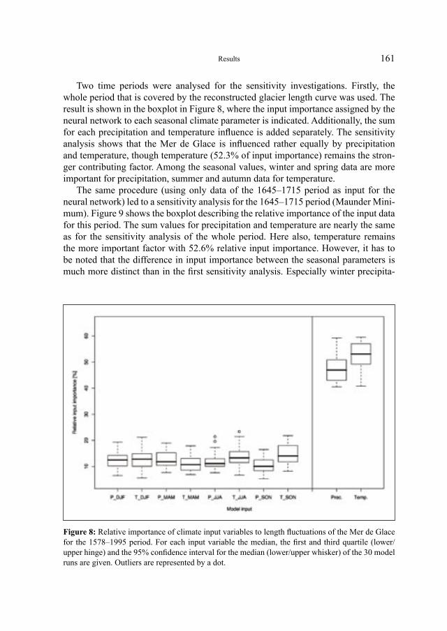
161

Two time periods were analysed for the sensitivity investigations. Firstly, the whole period that is covered by the reconstructed glacier length curve was used. The result is shown in the boxplot in Figure 8, where the input importance assigned by the neural network to each seasonal climate parameter is indicated. Additionally, the sum for each precipitation and temperature influence is added separately. The sensitivity analysis shows that the Mer de Glace is influenced rather equally by precipitation and temperature, though temperature (52.3% of input importance) remains the stron-ger contributing factor. Among the seasonal values, winter and spring data are more important for precipitation, summer and autumn data for temperature.

The same procedure (using only data of the 1645–1715 period as input for the neural network) led to a sensitivity analysis for the 1645–1715 period (Maunder Mini-mum). Figure 9 shows the boxplot describing the relative importance of the input data for this period. The sum values for precipitation and temperature are nearly the same as for the sensitivity analysis of the whole period. Here also, temperature remains the more important factor with 52.6% relative input importance. However, it has to be noted that the difference in input importance between the seasonal parameters is much more distinct than in the first sensitivity analysis. Especially winter precipita-

Figure 8: Relative importance of climate input variables to length fluctuations of the Mer de Glace for the 1578–1995 period. For each input variable the median, the first and third quartile (lower/upper hinge) and the 95% confidence interval for the median (lower/upper whisker) of the 30 model runs are given. Outliers are represented by a dot.

Results

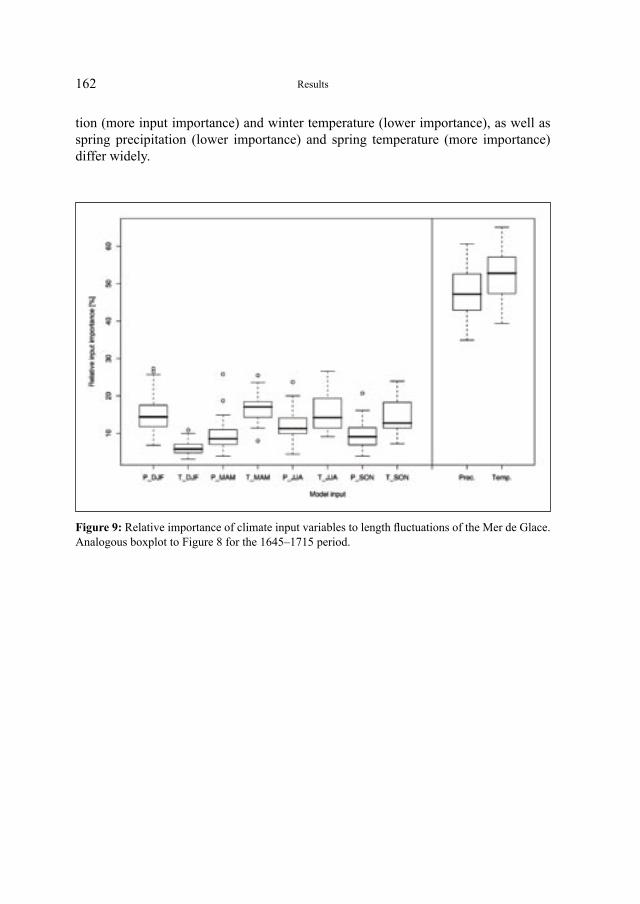
162

tion (more input importance) and winter temperature (lower importance), as well as spring precipitation (lower importance) and spring temperature (more importance) differ widely.

Figure 9: Relative importance of climate input variables to length fluctuations of the Mer de Glace. Analogous boxplot to Figure 8 for the 1645–1715 period.

Results

4 Discussion

4.1 Neural networks in glaciological contexts

4.1.1 Neural network models as a tool for simulating glacier length

For the first time, a neural network model has successfully been applied to the Mer de Glace. Essential for the application of the neural network model is the independent character of the input and target data, which is given in the present study. By training and validation of the model with glacier length and climate data from 1570–1900, it was possible to correctly simulate the 20th century length fluctuations of the Mer de Glace (cf. section 3.1.1).

The correct simulation of glacier length fluctuations is difficult, since glacier length as glacier parameter is complicated to handle. It depends on the glacier’s mass balance and ice dynamics, which again are controlled by climate and bedrock topo-graphy, among other factors. One of the most successful simulation of a long histori-cal glacier record was made by Schmeits and Oerlemans (1997). The study deals with a simulation of the length fluctuations of the Unterer Grindelwaldgletscher. The good quality of the data available for this glacier surely contributed to the success of the simulation.

The simulated length curve for the Mer de Glace for the 20th century as presented in this study shows a very good accordance. This is firstly a confirmation of the data quality being sufficient (climate parameters as input data, glacier length reconstruc-tions as target data, respectively), and secondly a proof for the usefulness of the new neural network approach. The neural network model also performed well for the 1645–1715 time period (Maunder Minimum), and the simulated curve shows the dis-tinct retreat and re-advance at the turn from the 17th to the 18th century. For the pre-ceding time, the simulated curve well matches the reconstructed curve qualitatively.

An explanation for this behaviour of the model result might be found in the input data parameters. From around 1675, the amount of predictors used for the reconstruc-tion of temperature and precipitation data instantly increases (Casty et al., 2005). These predictors that are available since 1675 are mostly located in southern Europe and complement the existing predictor set (which is rather dominated by central Euro-pean localities). The effect of additional predictors on the quality of the climate data is difficult to assess, but very likely the quality is improved, especially if the new predic-tors improve the spatial representation as in this case here. Nevertheless, it has to be noted that also the historical glacier length record is affected with a certain error (espe-cially at this early time), which makes it difficult to give a final answer in this respect.

However, it has to be noted that it was not possible to simulate glacier length variations over the whole time period. This is basically not possible with the neural network approach, as there is always a training/validation period needed for the neural

164

network simulations. These time periods are obviously not available for simulating. A good quality of the input/target data is then crucial for a good neural network perfor-mance, as is a representative distribution of the characteristic data (i.e., characteristic glacier length fluctuations have to be covered by the training/validation data, as well as “representative” input climate data, in order to model analogous glacier behaviour over the simulation time period). The neural network model is only able to simulate a certain glacier reaction if a similar behaviour has already occurred in the past and therefore is “learned” by the model. Enough information has to be available for the model to learn, and as many training/validation data as possible should therefore be considered for feeding the model.

A time period which the neural network model was not able to fully simulate is e.g. the 19th century. The model did not recognize the major 1821 glacier advance. One explanation for this mis-performance of the model is the fact that a glacier advance of the same intensity only occurred at the beginning of the 17th century for the Mer de Glace (in 1610, and 1644, respectively). For that time however, the quality of the climate input data is insufficient, and a correct recognition of the glacier-climate rela-tionship by the neural network model therefore well doubtful.

Despite the rather low quality of the climate input data, the application of the neu-ral network model yielded plausible qualitative reconstructions of glacier fluctuations for the 16th century in the absence of widespread glacier length data before 1570 for the Mer de Glace (cf. section 3.1.2). The glacier maximum around 1565 (and advanced position in 1537) and the minima around 1552 and 1575 yielded by the model correspond well (yet with a certain time delay) with the length data of the Unterer Grindelwaldgletscher (advanced position in 1535, maximum around 1550, and minima in 1540 and around 1570; Zumbühl et al., 1983). Note also that mass balance reconstructions for the Hintereisferner by Nicolussi (1994) show an increased mass growth around 1550 and a less positive mass balance around 1575.

Moreover, the neural network model allowed making some predictions of future (i.e., 2000–2050 period) fluctuations of the Mer de Glace (cf. section 3.1.3). Note that the two simulation scenarios are significantly different. The prediction for scenario 1 (no change in mean climate) which indicates a small re-advance of the Mer de Glace around 2025 is similar to the result obtained by Steiner (2005), who simulated the length fluctuations of the Unterer Grindelwaldgletscher also for the 2000–2050 period, using the same climate scenarios as in the present study. As scenario 1 represents no change in mean climate, the result of a re-advance is plausible since the glacier would find its way into a new equilibrium state.

Also for scenario 2 (considering climate change), the obtained result is similar to the simulated behaviour of the Unterer Grindelwaldgletscher by Steiner (2005) who prognosticated a continuous and rapid retreat. However, according to the model result, the retreat of the Mer de Glace is less pronounced, which could indicate a lower sensitivity to climate change of the Mer de Glace. Also the analysis of the SSC of both glaciers (J. Oerlemans, unpublished data) showed that the SSC of the Mer de

Discussion

165

Glace is less sensitive than that for the Unterer Grindelwaldgletscher, mainly due to lower precipitation. In contrast to the Unterer Grindelwaldgletscher, where the ELA is situated in relatively flat areas (Steiner et al., in press), the ELA for the Mer de Glace can be found in rather steep areas (at roughly 2775 m asl.; cf. Part I of this issue), and the glacier thus has a lower sensitivity (Sugden and John, 1976: 105). However, the simulated time period (1995–2042) is quite short regarding the possible long response times of the glacier, so it is difficult to draw final conclusions.

The expected behaviour (retreat) of the Mer de Glace in the next 50 years was never observed during the LIA and is therefore not considered by the training/valida-tion data of the neural network. Many tongues of Alpine glaciers rather collapse than continuously retreat due to very warm summers, as could be observed e.g. during the summer heatwave in 2003 (Neu and Thalmann, 2005). Note that such effects are not considered by the neural network model. On the other hand, the ice body of the Mer de Glace is still massive and well-connected, and thus supposed to show a (normal) dynamical behaviour. Note that the results show that it is possible to simulate the gla-cier’s front variations for the 20th century using training/validation data from the LIA period when much larger glacier extents prevailed. The observed model results show that the fundamental behaviour of the Mer de Glace during the 20th century might be controlled by the same mechanisms as during the LIA (i.e., up to 1900). An alternative method for simulating glacier length would be the application of a numerical ice-flow model (e.g., Huybrechts et al., 1989; Schmeits and Oerlemans, 1997).

4.1.2 Neural network models as a sensitivity analysis tool

Beside the utilization of the neural network for simulating glacier length, the model was used as a sensitivity analysis tool (cf. section 3.1.4). The main result obtained by the neural network model is the rather balanced input importance of the seasonal climate parameters. The Mer de Glace is more influenced by temperature than precipi-tation, though the difference in relative input importance is small.

Interesting is the fact that the sensitivity analysis for the 1645–1715 period (Maun-der Minimum) yielded more distinctive (and expected) differences between the sea-sonal climate variables, e.g. winter precipitation and summer temperature are domi-nant as usually expected for Alpine glaciers (e.g., Oerlemans and Reichert, 2000). As the 1645–1715 period contains a large retreat and re-advance of the Mer de Glace, it is plausible that winter precipitation and summer temperature were responsible to a large degree for this rapid change. However, the comparison with the sensitivity results obtained for the whole reference period (1570–2003) shows that other climate input parameters are important as well, and that the reaction of the glacier front to climate parameters is more complicated.

The sensitivity analysis for the Mer de Glace over the whole reference period showed the high influence of autumn temperature (biggest relative input importance).

Discussion

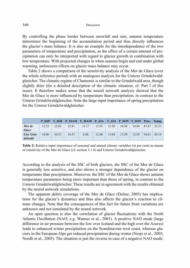
166

By controlling the phase border between snowfall and rain, autumn temperature determines the beginning of the accumulation period and thus directly influences the glacier’s mass balance. It is also an example for the interdependence of the two parameters of temperature and precipitation, as the effect of a certain amount of pre-cipitation can only be interpreted with regard to glacier growth in combination with low temperature. With projected changes in when seasons begin and end under global warming, unforeseen effects on glacier mass balance may occur.

Table 2 shows a comparison of the sensitivity analysis of the Mer de Glace (over the whole reference period) with an analogous analysis for the Unterer Grindelwald-gletscher. The climatic regime of Chamonix is similar to the Grindelwald area, though slightly drier (for a detailed description of the climatic situation, cf. Part I of this issue). It therefore makes sense that the neural network analysis showed that the Mer de Glace is more influenced by temperature than precipitation, in contrast to the Unterer Grindelwaldgletscher. Note the large input importance of spring precipitation for the Unterer Grindelwaldgletscher.

P_DJF T_DJF P_MAM T_MAM P_JJA T_JJA P_SON T_SON Prec. Temp.

Mer de Glace

12.53 12.82 12.81 11.17 11.95 13.50 10.38 14.84 47.67 52.33

Unt. Grin-delwald

14.06 10.33 14.57 8.86 12.60 13.04 13.58 12.95 54.81 45.19

Table 2: Relative input importance of seasonal and annual climate variables (in per cent) as means of sensitivity of the Mer de Glace (cf. section 3.1.4) and Unterer Grindelwaldgletscher.

According to the analysis of the SSC of both glaciers, the SSC of the Mer de Glace is generally less sensitive, and also shows a stronger dependence of the glacier on temperature than precipitation. Moreover, the SSC of the Mer de Glace shows autumn temperature parameters being more important than those of spring, in contrast to the Unterer Grindelwaldgletscher. These results are in agreement with the results obtained by the neural network simulations.

The apparent debris coverage of the Mer de Glace (Deline, 2005) has implica-tions for the glacier’s dynamics and thus also affects the glacier’s reaction to cli-mate changes. Note that the consequences of this fact for future front variations are unknown und not simulated by the neural network.

An open question is also the correlation of glacier fluctuations with the North Atlantic Oscillation (NAO; e.g. Wanner et al., 2001). A positive NAO mode (large difference in air pressure between the low over Iceland and the high over the Azores) leads to enhanced winter precipitation on the Scandinavian west coast, whereas gla-ciers in the European Alps get reduced precipitation during winter (Nesje et al., 2005; Nordli et al., 2005). The situation is just the reverse in case of a negative NAO mode:

Discussion

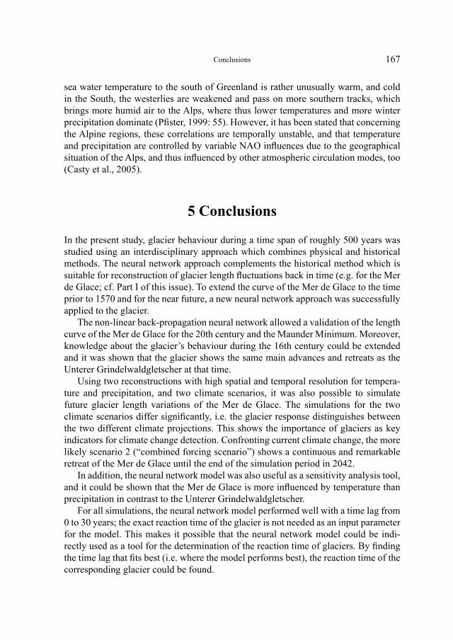
167

sea water temperature to the south of Greenland is rather unusually warm, and cold in the South, the westerlies are weakened and pass on more southern tracks, which brings more humid air to the Alps, where thus lower temperatures and more winter precipitation dominate (Pfister, 1999: 55). However, it has been stated that concerning the Alpine regions, these correlations are temporally unstable, and that temperature and precipitation are controlled by variable NAO influences due to the geographical situation of the Alps, and thus influenced by other atmospheric circulation modes, too (Casty et al., 2005).

5 Conclusions

In the present study, glacier behaviour during a time span of roughly 500 years was studied using an interdisciplinary approach which combines physical and historical methods. The neural network approach complements the historical method which is suitable for reconstruction of glacier length fluctuations back in time (e.g. for the Mer de Glace; cf. Part I of this issue). To extend the curve of the Mer de Glace to the time prior to 1570 and for the near future, a new neural network approach was successfully applied to the glacier.

The non-linear back-propagation neural network allowed a validation of the length curve of the Mer de Glace for the 20th century and the Maunder Minimum. Moreover, knowledge about the glacier’s behaviour during the 16th century could be extended and it was shown that the glacier shows the same main advances and retreats as the Unterer Grindelwaldgletscher at that time.

Using two reconstructions with high spatial and temporal resolution for tempera-ture and precipitation, and two climate scenarios, it was also possible to simulate future glacier length variations of the Mer de Glace. The simulations for the two climate scenarios differ significantly, i.e. the glacier response distinguishes between the two different climate projections. This shows the importance of glaciers as key indicators for climate change detection. Confronting current climate change, the more likely scenario 2 (“combined forcing scenario”) shows a continuous and remarkable retreat of the Mer de Glace until the end of the simulation period in 2042.

In addition, the neural network model was also useful as a sensitivity analysis tool, and it could be shown that the Mer de Glace is more influenced by temperature than precipitation in contrast to the Unterer Grindelwaldgletscher.

For all simulations, the neural network model performed well with a time lag from 0 to 30 years; the exact reaction time of the glacier is not needed as an input parameter for the model. This makes it possible that the neural network model could be indi-rectly used as a tool for the determination of the reaction time of glaciers. By finding the time lag that fits best (i.e. where the model performs best), the reaction time of the corresponding glacier could be found.

Conclusions

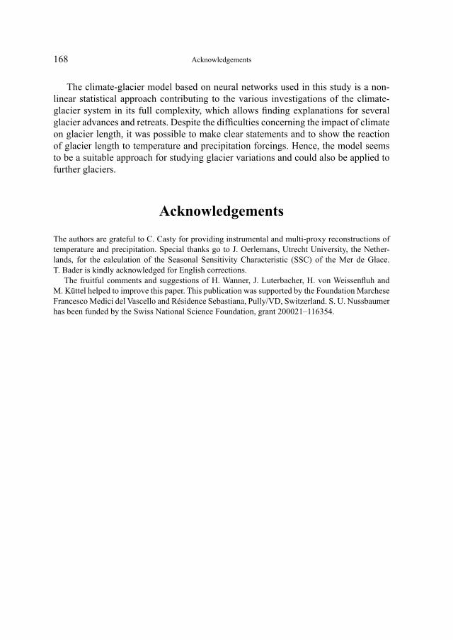
168

The climate-glacier model based on neural networks used in this study is a non-linear statistical approach contributing to the various investigations of the climate-glacier system in its full complexity, which allows finding explanations for several glacier advances and retreats. Despite the difficulties concerning the impact of climate on glacier length, it was possible to make clear statements and to show the reaction of glacier length to temperature and precipitation forcings. Hence, the model seems to be a suitable approach for studying glacier variations and could also be applied to further glaciers.

Acknowledgements

The authors are grateful to C. Casty for providing instrumental and multi-proxy reconstructions of temperature and precipitation. Special thanks go to J. Oerlemans, Utrecht University, the Nether-lands, for the calculation of the Seasonal Sensitivity Characteristic (SSC) of the Mer de Glace. T. Bader is kindly acknowledged for English corrections.

The fruitful comments and suggestions of H. Wanner, J. Luterbacher, H. von Weissenfluh and M. Küttel helped to improve this paper. This publication was supported by the Foundation Marchese Francesco Medici del Vascello and Résidence Sebastiana, Pully/VD, Switzerland. S. U. Nussbaumer has been funded by the Swiss National Science Foundation, grant 200021–116354.

Acknowledgements

169

References

Adrian, E. (1926). The impulses produced by sensory nerve endings. Part I. Journal of Physiology (London) 61, 49–72.

Bahr, D. B., W. T. Pfeffer, C. Sassolas, and M. F. Meier (1998). Response time of glaciers as a function of size and mass balance: 1. Theory. Journal of Geophysical Research 103 (B5), 9777–9782.

Casty, C., H. Wanner, J. Luterbacher, J. Esper, and R. Böhm (2005). Temperature and precipita-tion variability in the European Alps since 1500. International Journal of Climatology 25 (14), 1855–1880.

Deline, P. (2005). Change in surface debris cover on Mont Blanc massif glaciers after the ‘Little Ice Age’ termination. The Holocene 15 (2), 302–309.

Frei, C. (2004). Die Klimazukunft der Schweiz – Eine probabilistische Projektion (Working paper for the OcCC project “Switzerland in 2050”). Organe consultatif sur les changements clima-tiques (OcCC), Bern.

Haeberli, W. and M. Hoelzle (1995). Application of inventory data for estimating characteristics of and regional climatic–change effects on mountain glaciers: a pilot study with the European Alps. Annals of Glaciology 21, 206–212.

Hoelzle, M., W. Haeberli, M. Dischl, and W. Peschke (2003). Secular glacier mass balances derived from cumulative glacier length changes. Global and Planetary Change 36 (4), 295–306.

Hsieh, W. W. (2004). Nonlinear multivariate and time series analysis by neural network methods. Reviews of Geophysics 42 (1), RG1003, doi:10.1029/2002RG000112.

Huybrechts, P., P. de Nooze, and H. Decleir (1989). Numerical modelling of Glacier d’Argentière and its historic front variations. In J. Oerlemans (Ed.), Glacier fluctuations and climatic change. Proceedings of the Symposium on Glacier Fluctuations and Climatic Change. Amsterdam, 1–5 June 1987. Kluwer Academic Publishers, Dordrecht, 373–389.

IPCC (2001). Climate change 2001: the scientific basis. Contribution of Working Group I to the Third Assessment Report of the Intergovernmental Panel on Climate Change. (Houghton, J. T., Ding, Y., Griggs, D. J., Noguer, M., van der Linden, P. J., Dai, X., Maskell, K. and Johnson, C. A., Eds.). Cambridge University Press, Cambridge, UK, and New York, NY, USA, 881 pp.

Jóhannesson, T., C. F. Raymond, and E. Waddington (1989). A simple method for determining the response time of glaciers. In J. Oerlemans (Ed.), Glacier fluctuations and climatic change. Pro-ceedings of the Symposium on Glacier Fluctuations and Climatic Change. Amsterdam, 1–5 June 1987. Kluwer Academic Publishers, Dordrecht, 343–352.

Knutti, R., T. F. Stocker, F. Joos, and R. Plattner (2002). Constraints on radiative forcing and future climate change from observations and climate model ensembles. Nature 416, 719–723.

Kuhn, M. (1981). Climate and glaciers. International Association of Hydrological Sciences (IAHS) Publ. 131, 3–20.

Luterbacher, J., D. Dietrich, E. Xoplaki, M. Grosjean, and H. Wanner (2004). European seasonal and annual temperature variability, trends, and extremes since 1500. Science 303, 1499–1503.

Matthews, J. A. and K. R. Briffa (2005). The ‘Little Ice Age’: re-evaluation of an evolving concept. Geografiska Annaler 87A (1), 17–36.

Metropolis, N., A. W. Rosenbluth, M. N. Rosenbluth, A. H. Teller, and E. Teller (1953). Equa-tion of state calculations by fast computing machines. The Journal of Chemical Physics 21 (6), 1087–1092.

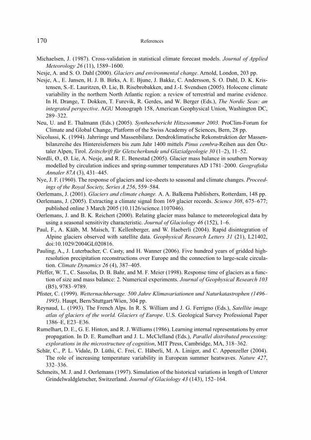
170

Michaelsen, J. (1987). Cross-validation in statistical climate forecast models. Journal of Applied Meteorology 26 (11), 1589–1600.

Nesje, A. and S. O. Dahl (2000). Glaciers and environmental change. Arnold, London, 203 pp. Nesje, A., E. Jansen, H. J. B. Birks, A. E. Bjune, J. Bakke, C. Andersson, S. O. Dahl, D. K. Kris-

tensen, S.-E. Lauritzen, Ø. Lie, B. Risebrobakken, and J.-I. Svendsen (2005). Holocene climate variability in the northern North Atlantic region: a review of terrestrial and marine evidence. In H. Drange, T. Dokken, T. Furevik, R. Gerdes, and W. Berger (Eds.), The Nordic Seas: an integrated perspective. AGU Monograph 158, American Geophysical Union, Washington DC, 289–322.

Neu, U. and E. Thalmann (Eds.) (2005). Synthesebericht Hitzesommer 2003. ProClim-Forum for Climate and Global Change, Platform of the Swiss Academy of Sciences, Bern, 28 pp.

Nicolussi, K. (1994). Jahrringe und Massenbilanz. Dendroklimatische Rekonstruktion der Massen-bilanzreihe des Hintereisferners bis zum Jahr 1400 mittels Pinus cembra-Reihen aus den Ötz-taler Alpen, Tirol. Zeitschrift für Gletscherkunde und Glazialgeologie 30 (1–2), 11–52.

Nordli, Ø., Ø. Lie, A. Nesje, and R. E. Benestad (2005). Glacier mass balance in southern Norway modelled by circulation indices and spring-summer temperatures AD 1781–2000. Geografiska Annaler 87A (3), 431–445.

Nye, J. F. (1960). The response of glaciers and ice-sheets to seasonal and climate changes. Proceed-ings of the Royal Society, Series A 256, 559–584.

Oerlemans, J. (2001). Glaciers and climate change. A. A. Balkema Publishers, Rotterdam, 148 pp. Oerlemans, J. (2005). Extracting a climate signal from 169 glacier records. Science 308, 675–677;

published online 3 March 2005 (10.1126/science.1107046). Oerlemans, J. and B. K. Reichert (2000). Relating glacier mass balance to meteorological data by

using a seasonal sensitivity characteristic. Journal of Glaciology 46 (152), 1–6. Paul, F., A. Kääb, M. Maisch, T. Kellenberger, and W. Haeberli (2004). Rapid disintegration of

Alpine glaciers observed with satellite data. Geophysical Research Letters 31 (21), L21402, doi:10.1029/2004GL020816.

Pauling, A., J. Luterbacher, C. Casty, and H. Wanner (2006). Five hundred years of gridded high-resolution precipitation reconstructions over Europe and the connection to large-scale circula-tion. Climate Dynamics 26 (4), 387–405.

Pfeffer, W. T., C. Sassolas, D. B. Bahr, and M. F. Meier (1998). Response time of glaciers as a func-tion of size and mass balance: 2. Numerical experiments. Journal of Geophysical Research 103 (B5), 9783–9789.

Pfister, C. (1999). Wetternachhersage. 500 Jahre Klimavariationen und Naturkatastrophen (1496–1995). Haupt, Bern/Stuttgart/Wien, 304 pp.

Reynaud, L. (1993). The French Alps. In R. S. William and J. G. Ferrigno (Eds.), Satellite image atlas of glaciers of the world. Glaciers of Europe. U.S. Geological Survey Professional Paper 1386–E, E23–E36.

Rumelhart, D. E., G. E. Hinton, and R. J. Williams (1986). Learning internal representations by error propagation. In D. E. Rumelhart and J. L. McClelland (Eds.), Parallel distributed processing: explorations in the microstructure of cognition, MIT Press, Cambridge, MA, 318–362.

Schär, C., P. L. Vidale, D. Lüthi, C. Frei, C. Häberli, M. A. Liniger, and C. Appenzeller (2004). The role of increasing temperature variability in European summer heatwaves. Nature 427, 332–336.

Schmeits, M. J. and J. Oerlemans (1997). Simulation of the historical variations in length of Unterer Grindelwaldgletscher, Switzerland. Journal of Glaciology 43 (143), 152–164.

References

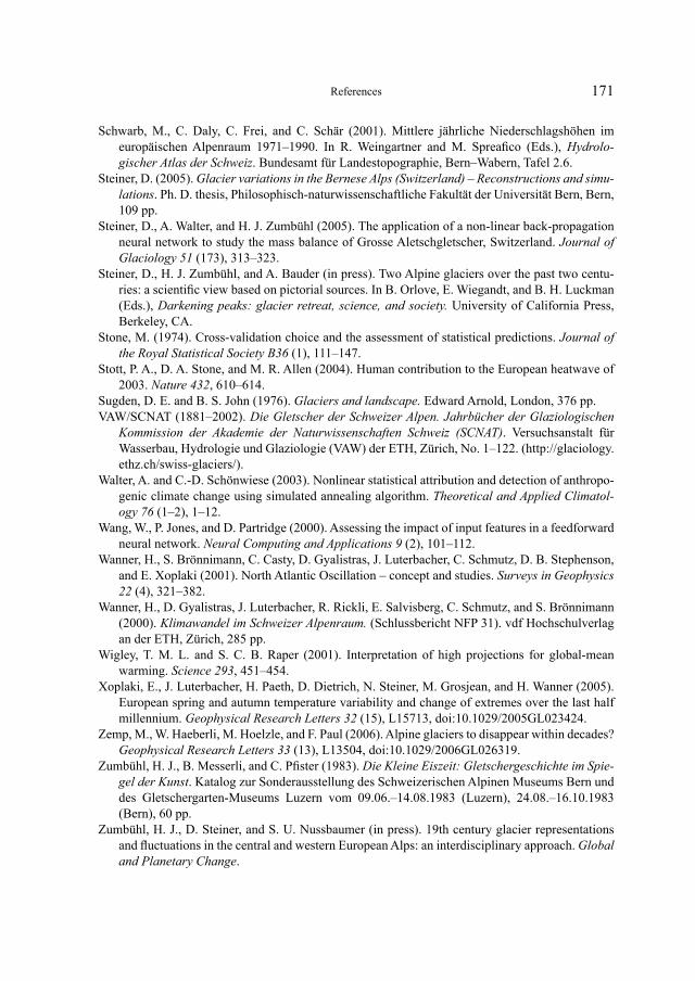
171

Schwarb, M., C. Daly, C. Frei, and C. Schär (2001). Mittlere jährliche Niederschlagshöhen im europäischen Alpenraum 1971–1990. In R. Weingartner and M. Spreafico (Eds.), Hydrolo-gischer Atlas der Schweiz. Bundesamt für Landestopographie, Bern–Wabern, Tafel 2.6.

Steiner, D. (2005). Glacier variations in the Bernese Alps (Switzerland) – Reconstructions and simu-lations. Ph. D. thesis, Philosophisch-naturwissenschaftliche Fakultät der Universität Bern, Bern, 109 pp.

Steiner, D., A. Walter, and H. J. Zumbühl (2005). The application of a non-linear back-propagation neural network to study the mass balance of Grosse Aletschgletscher, Switzerland. Journal of Glaciology 51 (173), 313–323.

Steiner, D., H. J. Zumbühl, and A. Bauder (in press). Two Alpine glaciers over the past two centu-ries: a scientific view based on pictorial sources. In B. Orlove, E. Wiegandt, and B. H. Luckman (Eds.), Darkening peaks: glacier retreat, science, and society. University of California Press, Berkeley, CA.

Stone, M. (1974). Cross-validation choice and the assessment of statistical predictions. Journal of the Royal Statistical Society B36 (1), 111–147.

Stott, P. A., D. A. Stone, and M. R. Allen (2004). Human contribution to the European heatwave of 2003. Nature 432, 610–614.

Sugden, D. E. and B. S. John (1976). Glaciers and landscape. Edward Arnold, London, 376 pp. VAW/SCNAT (1881–2002). Die Gletscher der Schweizer Alpen. Jahrbücher der Glaziologischen

Kommission der Akademie der Naturwissenschaften Schweiz (SCNAT). Versuchsanstalt für Wasserbau, Hydrologie und Glaziologie (VAW) der ETH, Zürich, No. 1–122. (http://glaciology.ethz.ch/swiss-glaciers/).

Walter, A. and C.-D. Schönwiese (2003). Nonlinear statistical attribution and detection of anthropo-genic climate change using simulated annealing algorithm. Theoretical and Applied Climatol-ogy 76 (1–2), 1–12.

Wang, W., P. Jones, and D. Partridge (2000). Assessing the impact of input features in a feedforward neural network. Neural Computing and Applications 9 (2), 101–112.

Wanner, H., S. Brönnimann, C. Casty, D. Gyalistras, J. Luterbacher, C. Schmutz, D. B. Stephenson, and E. Xoplaki (2001). North Atlantic Oscillation – concept and studies. Surveys in Geophysics 22 (4), 321–382.

Wanner, H., D. Gyalistras, J. Luterbacher, R. Rickli, E. Salvisberg, C. Schmutz, and S. Brönnimann (2000). Klimawandel im Schweizer Alpenraum. (Schlussbericht NFP 31). vdf Hochschulverlag an der ETH, Zürich, 285 pp.

Wigley, T. M. L. and S. C. B. Raper (2001). Interpretation of high projections for global-mean warming. Science 293, 451–454.

Xoplaki, E., J. Luterbacher, H. Paeth, D. Dietrich, N. Steiner, M. Grosjean, and H. Wanner (2005). European spring and autumn temperature variability and change of extremes over the last half millennium. Geophysical Research Letters 32 (15), L15713, doi:10.1029/2005GL023424.

Zemp, M., W. Haeberli, M. Hoelzle, and F. Paul (2006). Alpine glaciers to disappear within decades? Geophysical Research Letters 33 (13), L13504, doi:10.1029/2006GL026319.

Zumbühl, H. J., B. Messerli, and C. Pfister (1983). Die Kleine Eiszeit: Gletschergeschichte im Spie-gel der Kunst. Katalog zur Sonderausstellung des Schweizerischen Alpinen Museums Bern und des Gletschergarten-Museums Luzern vom 09.06.–14.08.1983 (Luzern), 24.08.–16.10.1983 (Bern), 60 pp.

Zumbühl, H. J., D. Steiner, and S. U. Nussbaumer (in press). 19th century glacier representations and fluctuations in the central and western European Alps: an interdisciplinary approach. Global and Planetary Change.

References

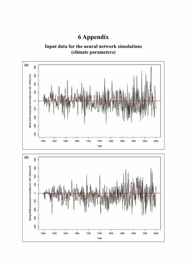
6 Appendix Input data for the neural network simulations

(climate parameters)

(a)

(b)

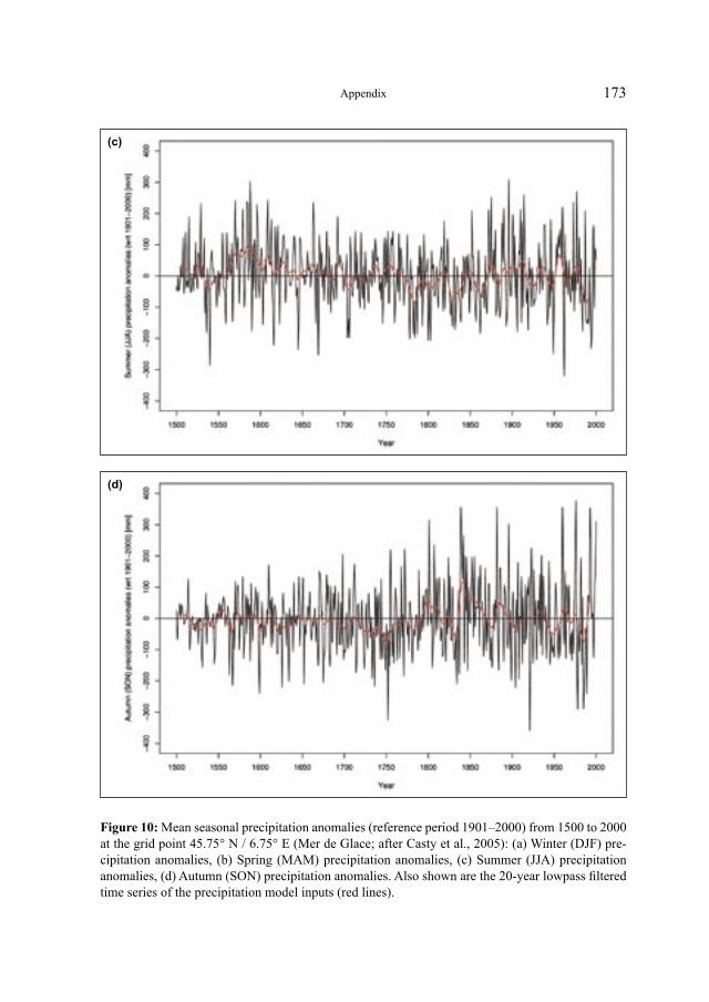
173

(c)

(d)

Figure 10: Mean seasonal precipitation anomalies (reference period 1901–2000) from 1500 to 2000 at the grid point 45.75° N / 6.75° E (Mer de Glace; after Casty et al., 2005): (a) Winter (DJF) pre-cipitation anomalies, (b) Spring (MAM) precipitation anomalies, (c) Summer (JJA) precipitation anomalies, (d) Autumn (SON) precipitation anomalies. Also shown are the 20-year lowpass filtered time series of the precipitation model inputs (red lines).

Appendix

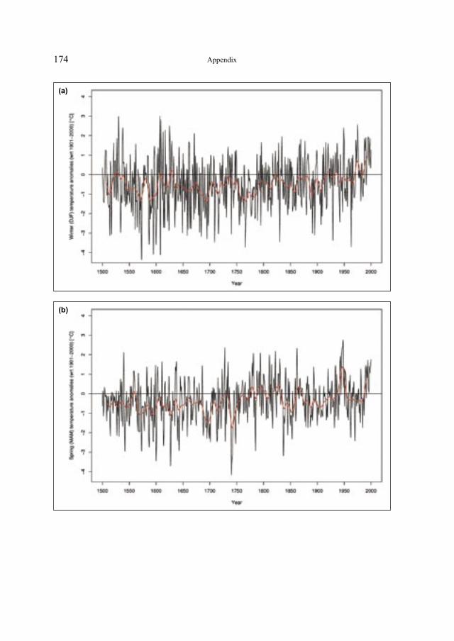
174

(a)

(b)

Appendix

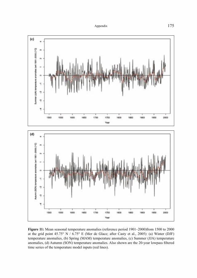
175

(c)

(d)

Figure 11: Mean seasonal temperature anomalies (reference period 1901–2000)from 1500 to 2000 at the grid point 45.75° N / 6.75° E (Mer de Glace; after Casty et al., 2005): (a) Winter (DJF) temperature anomalies, (b) Spring (MAM) temperature anomalies, (c) Summer (JJA) temperature anomalies, (d) Autumn (SON) temperature anomalies. Also shown are the 20-year lowpass filtered time series of the temperature model inputs (red lines).

Appendix

176

Manuscript submitted to Zeitschrift für Gletscherkunde und Glazialgeologie: 15/10/2006

Authors’ addresses: S. U. Nussbaumer* H. J. Zumbühl, D. Steiner Institute of Geography, University of Bern Hallerstrasse 12 CH–3012 Bern * also: National Centre of Competence in Research on Climate (NCCR Climate) University of Bern Phone: +41 31 631 85 51, fax: +41 31 631 85 11 E-Mail: samuel.nussbaumer@giub.unibe.ch zumbuehl@giub.unibe.ch daniel.steiner@phzh.ch

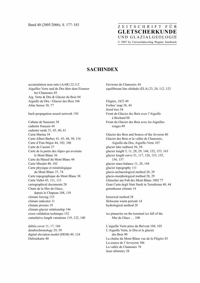
SACHINDEX

Band 40 (2005/2006), S. 177–183 Z E I T S C H R I F T F Ü RGLETSCHERKUNDEU N D G L A Z I A L G E O L O G I E© 2007 by Universitätsverlag Wagner, Innsbruck

accumulation area ratio (AAR) 22,112Aiguilles Verte und du Dru über dem Eismeer

bei Chamonix 85Aig. Verte & Dru & Glacier du Bois 94Aiguille du Dru / Glacier des Bois 106Atlas Suisse 38, 77

back-propagation neural network 150

Cabane de Saussure 38cadastre français 44cadastre sarde 31, 45, 60, 61Carta Marina 34Carte Albert Barbey 41, 43, 44, 50, 116Carte d’Etat-Major 44, 102, 106Carte de Cassini 37Carte de la partie des Alpes qui avoisine le Mont Blanc 36Carte du Massif du Mont Blanc 44Carte Mieulet 40, 102Carte physique et minéralogique du Mont Blanc 37, 74Carte topographique du Mont Blanc 38Carte Vallot 45, 111, 113cartographical documents 28Chute de la Mer de Glace, depuis le Chapeau 108, 110climate forcing 153climate indicator 11climate proxies 19climate-glacier relationship 146cross-validation technique 152cumulative length variations 119, 122, 140

debris cover 11, 17, 166dendrochronology 29, 59digital elevation model (DEM) 49, 124Dufourkarte 40

Environs de Chamonix 44equilibrium line altidude (ELA) 23, 24, 112, 123

Flégère, 1823 49Forbes’ map 38, 44fossil tree 54Front du Glacier des Bois avec l’Aiguille à Bochard 88Front du Glacier des Bois avec les Aiguilles rouges 89

Glacier des Bois and Source of the Arveron 80Glacier des Bois et la vallée de Chamonix, Aiguille-du-Dru, Aiguille-Verte 107glacier lake outburst 56, 58glacier length 5, 11, 28, 29, 144, 152, 153, 163glacier length curve 51, 117, 126, 153, 155, 156, 157glacier mass balance 11, 28, 144glacier topography 111glacio-archaeological method 28, 29glacio-morphological method 28, 29Gletscher am Fuß des Mont Blanc 1802 77Gran Carta degli Stati Sardi in Terraferma 40, 44greenhouse climate 14

historical method 28Holocene warm periods 14hydrological method 28

ice pinnacles on the terminal ice fall of the Mer de Glace … 100

L’aiguille Verte prise du Brévent 104, 105L’Aiguille Verte, le Dru et le glacier des Bois 90La chaîne du Mont-Blanc vue de la Flégère 83La source de l’Arveyron 106La vallée de Chamonix 78laser altimetry 28

178

le Mont Blanc et la Vallée de Chamouni 95length curve 51, 117, 126, 153, 155, 156, 157 length measurements 16length variations 52, 158Little Ice Age (LIA) 5, 12, 17, 23, 26, 35, 51, 55, 58, 59, 117, 124, 125, 126, 145, 156, 165literary sources 28Little Ice Age-type Events 13, 14longitudinal profiles 116

Map of the Mer de Glace of Chamouni 1842 39mass balance 11, 28, 144Maunder Minimum 59, 153, 156, 163, 165Medieval Warm Period 13Mer de Glace – moonlight 105Mer de Glace 1802 79Mer de Glace, Chamonix 1802 78Mer de Glace / l’Arvéron, par Bourrit 65Mer de Glacier / Village de Bois 96Messtischblätter 40Middle Ages 54, 124Mont Blanc from the Jardin 100moraines 19, 52, 54, 58, 59Mougin curve 51, 118, 119

neural network 141non-linear back-propagation 141North Atlantic Oscillation 166

Part of the Valley of Chamonix 1770 63Partie du Canton du Vallais 38perception 19pictorial documents 28precipitation 26, 27, 141, 154, 160, 163precipitation gradient 26predictions 158principal component regression analysis 146probabilistic projections 147proxy data 126

radiocarbon dating 29reduction of error 146relief representations 72remote sensing 28response time of glaciers 149

satellite imagery 17, 28Schweizer Chronik 34sensitivity analysis 165snowline 27Source de l’Arveron.-/Chamonix. 1823 91Source de l’Aveyron au glacier des bois (Vallée de Chamouny) 94Source of the Arveron. Val. de Chamouni 1820 87surface topography 111, 125

target signal 151temperature 27, 141, 154, 163, 160, 163topographical characteristics 23

Unteres Ende des Glacier des Bois, Chamonix 109

veine blanche 20veine noire 20, 52volume changes 111Vue de la Source de l’Arveiron, des Aiguilles Vertes … 76Vue de la source de l’Arveron 34Vue de la Source de L’Arveron 67, 68Vue de la Source du Glacier des Bois 75Vue de la Vallée de Chamonix 64Vue de la Voûte du Chapeau du Glacier des du Montenvert, … 82Vue du Glacier des Bois en retraite 73, 74Vue du Glacier des Bois prex du Montenvert 70Vue du Glacier des Bois, et du Hameau des Pras 84Vue du Prieure 66

Index

179

ORTSINDEX

Aiguille à Bochard 48Aiguille du Géant 20, 25Aiguille du Midi 20Aiguille Rouge 24, 25, 72Aiguille Verte 20, 75, 76, 90, 101Aiguilles du Charmoz 4

Chapeau 54, 73, 78, 92, 100–108Col de Balme 72Col du Géant 33, 38, 59, 60, 72, 73Col du Midi 26, 112Col Major 35Côte du Piget 48, 52–58, 73, 95

Drus 20, 25, 48, 75, 90, 101

Gepatschferner 41Glacier d’Argentière 16–56, 96, 103, 118, 138Glacier de la Brenva 25, 95Glacier de Leschaux 20, 111Glacier de Taconnaz 25, 56, 138Glacier de Talèfre 20, 23, 51, 111Glacier des Bois 3–176Glacier des Bossons 16–56, 82–97, 103, 118, 138, 149Glacier des Nantillons 25Glacier du Géant 99, 111Glacier du Miage 25

Glacier du Tour 16, 17, 25, 55, 103Glacier du Trient 17, 118Gornergletscher 18, 24, 124Gran Paradiso 17Grandes Jorasses 20, 25Grands Mulets 25Greenland 167Grosser Aletschgletscher 1–29, 124, 144

Massif du Talèfre 43Mer de Glace 3–176Mont Blanc area 3–176Mont Blanc du Tacul 20, 23

Oberer Grindelwaldgletscher 41

Rhônegletscher 14, 18, 97Rochers des Mottets 22, 48, 54, 62, 80–101Rosenlauigletscher 18

Unteraargletscher 18, 95, 97Unterer Grindelwaldgletscher 6–48, 121–126,

141–145, 163–167

Val Ferret 25Val Monjoie 17Val Veni 25Vallée Blanche 20Vernagtferner 28, 29, 41

Index

180

Adams-Reilly 38, 39, 41, 44Adrian 151, 169Aeschlimann 17, 128Agassiz 15, 38, 128Aliprandi 31–41, 54, 128Allen 132, 171Amacher 127Andersson 127, 170Appenzeller 170Arlaud 30, 128

Bader 127Bahr 149, 169, 170Bakke 170Balmat 32, 33Baratoux 128Barbey 41Barclay 132Bartoluzzi 32Baud 62, 128Bauder 18, 128, 133, 171Baudry 42Beaumont 73Benestad 170Bénévent 26, 128Berger 170Berthier 17, 125, 128Birks 170Birmann 5, 7, 47–49, 84–92, 117–138Bisson 41, 78, 97–100, 121Bjune 170Blaikie 65, 128Blanchard 16, 55, 56, 128Bless 17, 118, 128Boccazzi-Varotto 44, 79, 90, 132Böhm 169Bordier 31, 63, 128Borgonio 35Bouchardy 32–35, 63–76, 128, 129Bourrit 15, 31–48, 63–73, 129Braun 102–106Briffa 12–14, 131–149, 169Brönnimann 133, 171Brunner 34–41, 129

Calkin 132Casty 146–171Chapuy 89, 94, 121

Chatelet 73Chlumsky 99, 129Ciceri 99Civiale 41Clague 132Collot 129Combet 55, 135Corbel 26, 27, 129Corbin 44Cottard 127Couren 128Couttet 93, 108Coxe 65, 70, 129Cunningham 30, 32, 73, 129

Dahl 12, 13, 22, 131, 132, 149, 170Daly 171Dardel 95de Charpentier 81de Crans 57de Decker Heftler 95–98, 102, 105, 129de Luc 129de Méneval 80, 129de Saussure 4–75, 119, 129, 132Decleir 169Deline 17, 20, 67, 71, 125–129, 166, 169 Dietrich 169, 171Dischl 130, 169Dokken 170Dollfus-Ausset 97Drange 170Dubois 90, 95, 121Dufour 40, 44Durand 73, 129Dyurgerov 11, 129

Eggimann 127Escher von der Linth 70, 80, 85Eskildsen 129Esper 169Exchaquet 37, 72

Favre 16, 59, 60, 70, 73, 80, 104–109, 130Feigl 128Forbes 5–51, 82, 91, 93, 128–130Forel 16, 67, 87–130Fountain 131Frei 147, 169, 170, 171

Index

AUTORENINDEX

181

Frey 25, 41 102, 107, 130Funk 133Furevik 170

Gabriel 81Garin 78, 132Garnier 107Gaudin 57Gay 127Geissler 66Gerdes 170Goethe 67, 130Grenier 130Gros 127Grosjean 169, 171Grove 12, 13, 29–73, 122, 130Gruner 61, 62, 130Gubler 130Gugelmann 68Guichonnet 61, 128, 130Guillaud 68, 77, 130Gyalistras 133, 171

Hackert 34, 67, 68, 76, 120Haeberli 19, 123–170Harford 81, 86Hinton 170Hock 13, 130, 131 Hoelzle 11, 130, 144, 169, 171Hoinkes 11, 130Holmgren 131Holzhauser 12–54, 70, 97, 117–134Hsieh 144, 169Huybrechts 165, 169

Imfeld 41Imhof 73, 131

Jackson 132Jacky 41Jaillet 127Jalabert 32, 66Jansen 170Jóhannesson 149, 169John 22, 133, 165, 171Jones 14, 131, 171Jonsell 13, 131Joos 169Jublier 50

Kääb 170Kellenberger 170Kinossian 45Kinzl 16, 17, 55–90, 119, 131Knutti 147, 169Kristensen 170Kuhn 153, 169Kurz 41, 131Küttel 127, 168

Lamb 12, 131Lamy 87Larminat 44Larocque 132Laube 71, 127Lauritzen 170Laxton 132Le Meur 133Le Roy Ladurie 16–18, 55–80, 131, 136Legrésy 128Lewis 132Lie 170Linck 5–9, 33–48, 73–89, 120Liniger 170Lliboutry 11, 17, 98, 90, 131Loppé 108, 110Lory 81Loutherbourg 70, 71, 72Luterbacher 133, 146, 168–171Lüthi 170

Magnus 34Maisch 170Mallet 36Mann 14, 131Marbot 129Martel 30–35, 61, 131Martens 99, 101Matthews 12, 131, 149, 169Meier 169, 170Messerli 134, 171Metropolis 152, 169Meyer 38Michaelsen 152, 170Mieulet 40, 44Mihajlovic 127Moore 60, 131Mougin 5–131Muletti 40Müller 38Muzet 102

Index

182

Nakawo 125, 131Nesje 12, 13, 22, 131, 132, 149, 166, 170Neu 14, 132, 147, 165, 170Nicolussi 29, 132, 164, 170Nooze 169Nordli 166, 170Nussbaumer 3–176Nye 149, 170

Oehrli 127Oerlemans 11–29, 121–170Osborn 13, 14, 132Oulianoff 44

Paccard 32Paeth 171Pars 62Partridge 171Paterson 11, 28, 111, 132Paul 170, 171Pauling 146, 170Payot 16, 80–109, 121, 132Perrinjaquet 127Peschke 130, 169Pfeffer 149, 169, 170Pfister 12–14, 35, 124–171Pictet 35–38Plattner 169Pococke 30, 31Ponnau 129Priuli 78, 132

Rabot 16, 55, 109, 132Rabut 128Ramseyer 127Raper 147, 171Rasmo 133Raymond 37, 131, 169Raynal 107Reichert 144, 160, 170Rémy 128Rendu 31, 132Reyes 13, 132Reynaud 26, 27, 118, 132, 149, 170Rickli 133, 171Risebrobakken 170Robache 44, 79, 90, 132Rochefoucauld 60Rosenbluth 169Röthlisberger 13, 132, 133Roussy 33, 62, 66, 73, 132Ruhmer 133

Rumelhart 151, 170Ruskin 95–105

Salvisberg 133, 171Sanson 35Sassolas 169, 170Savioz 102Schär 147, 170, 171Schmeits 149, 163–170Schmutz 133, 171Schneider 47, 132Schönwiese 152, 171Schwarb 147, 171Seydoux 105Sigrist 32, 132Simond 91Six 133Smith 78, 80, 132Soudan 128Soulier 104, 105Spreafico 171Steiner 3–176Steingräber 69, 133Stephenson 171Stocker 152, 169, 171Stott 147, 171Sugden 22, 133, 165, 171Svendsen 170

Tairraz 93, 102, 108, 109Teller 169Thalmann 14, 132, 147, 165, 170Töpffer 32Tournier 87, 88, 89, 93Towne 68, 69Trümpy 25, 133Tschudi 34Turner 73–79Tyndall 16, 98, 108, 133

Vadon 128Vallon 17, 133Vallot 41–50, 93–109, 133Vellozzi 128Venetz 81Vercken 128Vidale 170Vincent 17, 22, 50, 127–133Viollet-le-Duc 5–25, 41–79, 106–133Vivian 15–27, 44–58, 90, 133von Weissenfluh 127, 168

Index

183

Waddington 169Walser 35Walter 152, 171Wang 154, 171Wanner 13, 133, 147, 166–171Weber 34, 133Weingartner 171Weiss 38Wetter 5–9, 53–93, 104–133Wied 133Wigley 147, 171Wild 38Wiles 132Williams 170Wilton 62, 63, 133Windham 30, 31, 61, 65Winterlin 93, 96Wolf, C. 32, 34, 71, 121, Wolf, R. 101, 127

Xoplaki 17, 146, 169

Zemp 144, 171Zienert 17, 117, 133Zumbühl 3–176

Index