Geant4 Simulation eines auf GEM basierten Detektors

Technische Universität MünchenFakultät für Physik

Abschlussarbeit im Bachelorstudiengang Physik

Geant4 Simulation eines auf GEMbasierten Detektors

Geant4 simulation of a GEM based detector

Gramos Qerimi

16. September 2015

Erstgutachter (Themensteller): Prof. L. FabbiettiZweitgutachter: Dr. A. Ulrich

Betreuer: Dr. P. Gasik

Contents

Introduction . . . . . . . . . . . . . . . . . . . . . . . . . . . . . . . . . . . . v

1 Principles of a GEM TPC . . . . . . . . . . . . . . . . . . . . . . . . . . . 11.1 Time Projection Chamber . . . . . . . . . . . . . . . . . . . . . . . . . 11.2 MWPC vs. GEM . . . . . . . . . . . . . . . . . . . . . . . . . . . . . . 31.3 GEM stability against electric discharges . . . . . . . . . . . . . . . . . 7

2 Simulation framework . . . . . . . . . . . . . . . . . . . . . . . . . . . . . 112.1 Detector description in GEANT4 . . . . . . . . . . . . . . . . . . . . . 112.2 Reference simulations with a point-like source . . . . . . . . . . . . . . 152.3 Simulations with a mixed source . . . . . . . . . . . . . . . . . . . . . 262.4 Simulations with additional el. field . . . . . . . . . . . . . . . . . . . 36

3 Comparison to the experimental data and outlook . . . . . . . . . . . . 41

A Principal difference between GEM TPC and wire TPC . . . . . . . . . . 43

B 2D simulated plots . . . . . . . . . . . . . . . . . . . . . . . . . . . . . . . 45

C Time results of the analysis with el. field . . . . . . . . . . . . . . . . . . 47

Bibliography . . . . . . . . . . . . . . . . . . . . . . . . . . . . . . . . . . . . 51

Acknowledgements . . . . . . . . . . . . . . . . . . . . . . . . . . . . . . . . 53

iii

Introduction

Gated multi-wire proportional chambers (MWPCs), which consist of a grid of wiresto amplify and measure signals, are commonly used in a time projection chamber(TPC), the main apparatus of the ALICE experiment located at CERN. This track-ing detector with a large gas volume measures the space-time-coordinates of chargedparticles in high-multiplicity events and is therefore able to reconstruct their traject-ories. The TPC operates in gated mode in order to collect the ions produced in theamplification process, that could drift back into the drift volume. Therefore it canprevent possible distortions in reconstructing the tracks (space charge effect). [1]At the moment in ALICE there are studies of Pb-Pb collisions at a center-of-massenergy of

√s = 2.76 TeV, and the gating grid is operating with a frequency of 1

kHz. In 2019 however, after the LHC upgrade during the second Long Shutdown,the luminosity and energy of the Pb-nucleons will be increased up to

√s = 5.5 TeV.

That means, that the particle velocities are much higher as before, which correspondsto a collision rate of 50 kHz over the beam time. To fulfill these requirements, theconventional MWPC will be replaced by Gas Electron Multipliers (GEMs). [2]This new type of the TPC has the capability to reach higher trigger rates so thatGEM based detectors would overcome the rate limitations of the gating grid. There-fore the use of Gas Electron Multiplier for gas amplification and intrinsic ion-backflowsuppression in the TPC allows a sufficient opportunity to satisfy the major ALICE-TPC upgrade. As a first version, a small detector with three GEM-foils has beenbuilt successfully at the Technische Universität München.During measurements on the stability of this prototype for different HV-settings ofthe GEMs, there is found a straight correlation between high charge-densities on thefoils and sparks. The aim of this bachelor thesis is to study the cause of dischargeprobabilities on the basis of a detailed GEANT4 simulation in order to explain thecondition of this effect, that is responsible for a break-down of the stability and evena harm of the GEM foil.After showing briefly the technical properties of GEM TPCs and defining the dis-charge probability, the full simulation framework is introduced in order to describethis relevant effect. The final chapters of the thesis are dedicated to the comparisonbetween the simulation and experimental data followed by a recapitulation betweenthe discharge probability and charge densities in gaseous detectors.

v

Chapter 1

Principles of a GEM TPC

During decades the development of advanced detector technologies for fast track-ing applications has been compelled due to the ever-growing scientific goals in ex-perimental particle physics. Especially the ALICE experiment, which is located inGeneva at CERN, whose main task is to produce and study the quark-gluon-plasma1,is planning an upgrade in its central barrel, the time projection chamber. [3]

1.1 Time Projection Chamber

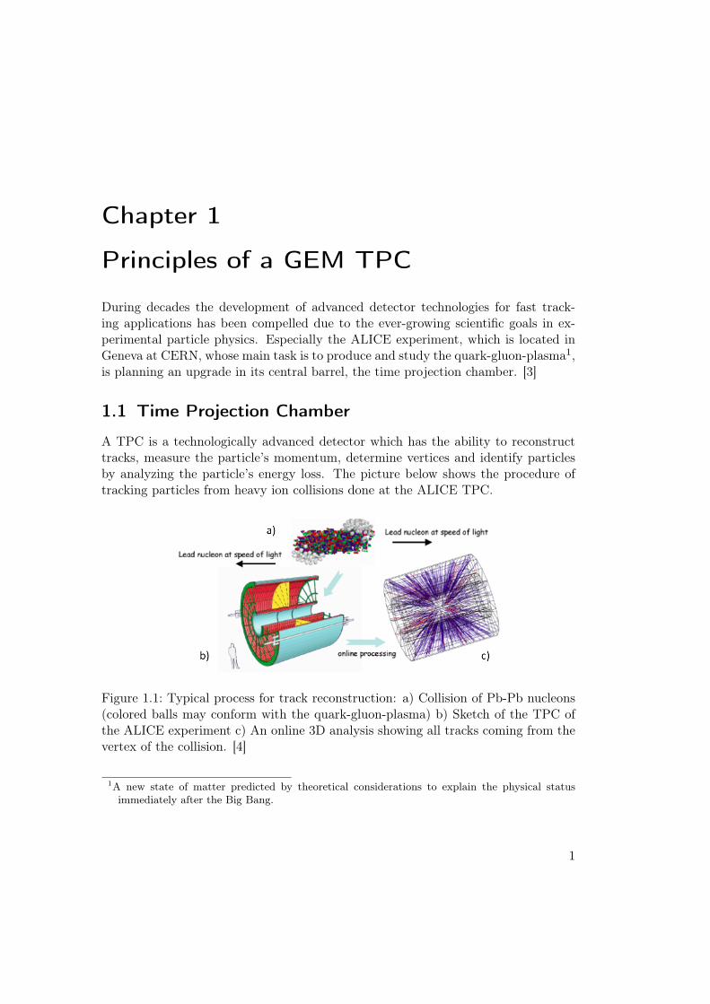
A TPC is a technologically advanced detector which has the ability to reconstructtracks, measure the particle’s momentum, determine vertices and identify particlesby analyzing the particle’s energy loss. The picture below shows the procedure oftracking particles from heavy ion collisions done at the ALICE TPC.

Figure 1.1: Typical process for track reconstruction: a) Collision of Pb-Pb nucleons(colored balls may conform with the quark-gluon-plasma) b) Sketch of the TPC ofthe ALICE experiment c) An online 3D analysis showing all tracks coming from thevertex of the collision. [4]

1A new state of matter predicted by theoretical considerations to explain the physical statusimmediately after the Big Bang.

1

Chapter 1 Principles of a GEM TPC

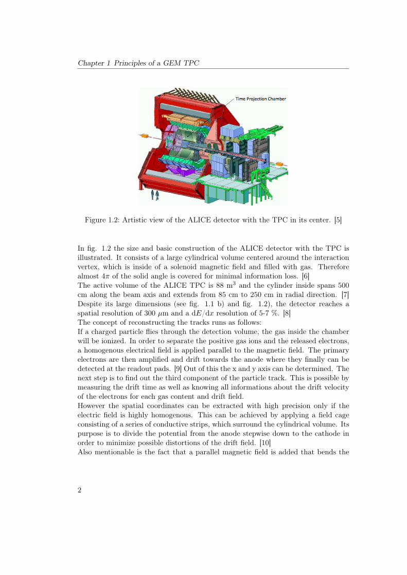
Figure 1.2: Artistic view of the ALICE detector with the TPC in its center. [5]

In fig. 1.2 the size and basic construction of the ALICE detector with the TPC isillustrated. It consists of a large cylindrical volume centered around the interactionvertex, which is inside of a solenoid magnetic field and filled with gas. Thereforealmost 4π of the solid angle is covered for minimal information loss. [6]The active volume of the ALICE TPC is 88 m3 and the cylinder inside spans 500cm along the beam axis and extends from 85 cm to 250 cm in radial direction. [7]Despite its large dimensions (see fig. 1.1 b) and fig. 1.2), the detector reaches aspatial resolution of 300 µm and a dE/dx resolution of 5-7 %. [8]The concept of reconstructing the tracks runs as follows:If a charged particle flies through the detection volume, the gas inside the chamberwill be ionized. In order to separate the positive gas ions and the released electrons,a homogenous electrical field is applied parallel to the magnetic field. The primaryelectrons are then amplified and drift towards the anode where they finally can bedetected at the readout pads. [9] Out of this the x and y axis can be determined. Thenext step is to find out the third component of the particle track. This is possible bymeasuring the drift time as well as knowing all informations about the drift velocityof the electrons for each gas content and drift field.However the spatial coordinates can be extracted with high precision only if theelectric field is highly homogenous. This can be achieved by applying a field cageconsisting of a series of conductive strips, which surround the cylindrical volume. Itspurpose is to divide the potential from the anode stepwise down to the cathode inorder to minimize possible distortions of the drift field. [10]Also mentionable is the fact that a parallel magnetic field is added that bends the

2

1.2 MWPC vs. GEM

particle tracks to enable measurements of their momenta. It leads to the additionaleffect of suppressing the transversal diffusion of the drifting electrons. To sum up,these requirements to the TPC allow not only a 3D reconstruction of the spatialinformation of the particles but also a good momentum determination. Togetherwith a dE/dx measurement the full particle identification can be reached in a TPC.

1.2 MWPC vs. GEM

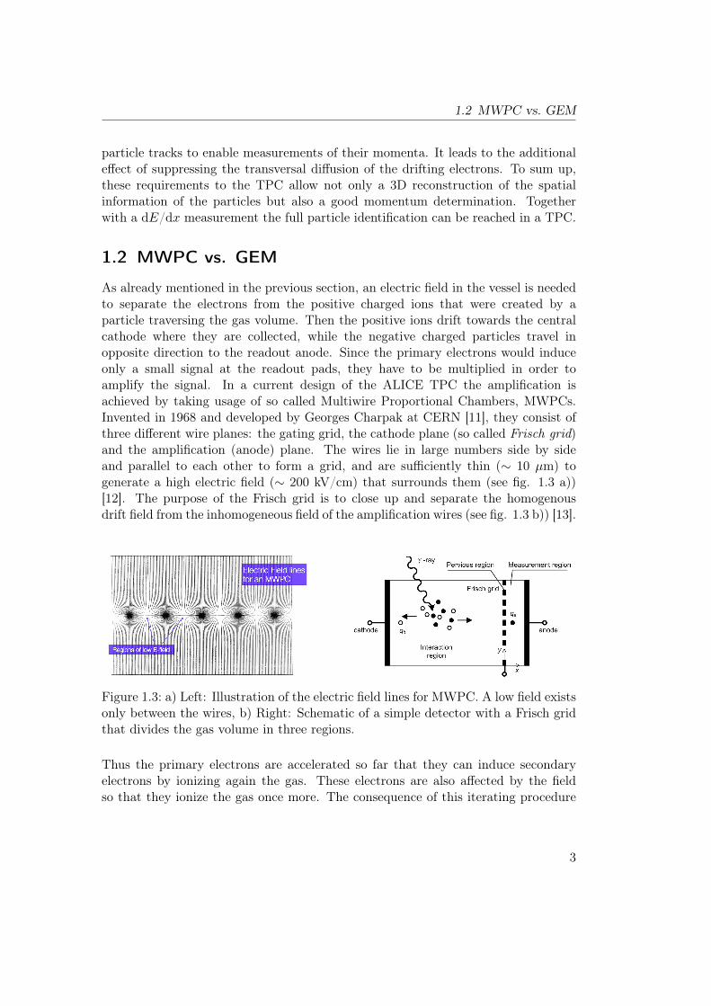
As already mentioned in the previous section, an electric field in the vessel is neededto separate the electrons from the positive charged ions that were created by aparticle traversing the gas volume. Then the positive ions drift towards the centralcathode where they are collected, while the negative charged particles travel inopposite direction to the readout anode. Since the primary electrons would induceonly a small signal at the readout pads, they have to be multiplied in order toamplify the signal. In a current design of the ALICE TPC the amplification isachieved by taking usage of so called Multiwire Proportional Chambers, MWPCs.Invented in 1968 and developed by Georges Charpak at CERN [11], they consist ofthree different wire planes: the gating grid, the cathode plane (so called Frisch grid)and the amplification (anode) plane. The wires lie in large numbers side by sideand parallel to each other to form a grid, and are sufficiently thin (∼ 10 µm) togenerate a high electric field (∼ 200 kV/cm) that surrounds them (see fig. 1.3 a))[12]. The purpose of the Frisch grid is to close up and separate the homogenousdrift field from the inhomogeneous field of the amplification wires (see fig. 1.3 b)) [13].

Figure 1.3: a) Left: Illustration of the electric field lines for MWPC. A low field existsonly between the wires, b) Right: Schematic of a simple detector with a Frisch gridthat divides the gas volume in three regions.

Thus the primary electrons are accelerated so far that they can induce secondaryelectrons by ionizing again the gas. These electrons are also affected by the fieldso that they ionize the gas once more. The consequence of this iterating procedure

3


is a chain reaction followed by an avalanche of electrons, all collected by the wires.Meanwhile the positive ions drift towards the Frisch grid and as a result theirinduced image charges are registered by the readout pads. [14]An “Ion Back Flow”, i.e. when the ions fly back to the drift volume, could destroy thehomogeneity of the electric field. To overcome this relevant problem, MWPC-basedTPCs normally use a gating mechanism, i.e. the gating grid placed in front ofthe amplification stage to collect the positive ions (that indeed could accumulateand induce a space charge effect in the drift volume). The time to switch it onand off is limited to the collection time of the ions, which corresponds to a max-imum rate of ca. 1 kHz. Thus using a gating grid causes a dead time in the TPC. [15]

The invention of MWPCs revolutionized the field of gaseous detectors. With amodest accuracy and rate capability, the Multi Wire Proportional Chamber allowedlarge areas to be instrumented with fast tracking detectors and gives the possibilityto localize particle trajectories with sub-mm precision. That’s why this kind of driftchamber is a benchmark for the ALICE TPC, designed to cope with extreme in-stantaneous particle densities produced in heavy ion collisions at the LHC. However,position-sensitive detectors based on wire structures have reached limitations in ratecapacity and detector granularity of about 100 µm due to diffusion processes andspace charge effects in the gas. [16]Despite various improvements of MWPCs, the previously mentioned problems to-gether with the practical difficulty to manufacture detectors with a large numberof closely lying wires, has motivated the evolution of a new generation of gaseousdetectors for high luminosity accelerator science, the Micro-Pattern Gas Detectors(MPGD).2, which can be classified in two large groups: micromesh-based detect-ors and hole-type structures. While Micromegas, “Bulk” Micromegas, “Microbulk”Micromegas and “InGrid” instruments belong to the micromesh-based structures,the GEMs, THGEM, RETGEM and MHSP elements take a huge part in the lattergroup. [16]In the following chapters GEMs (Gas Electron Multipliers) will be discussed morein detail since the ALICE TPC is going to remove the currently used MWPCs andinsert Gas Electron Multipliers during the second long shutdown (LS2) in 2018.3 [2]

The Gas Electrons Multiplier (GEM), invented by F. Sauli at CERN in 1996,

2Actually, before the MPGDs were invented, the Micro-Strip Gas Chamber (MSGC) was developedto solve the difficulties that MWPCs had. However, detailed studies of long-term behavior athigh rates have revealed the problem of aging, i.e. a slow degradation of the detector’s efficiencydue to sustained irradiation, and sensitivity regarding discharges in presence of highly ionizingparticles that could damage the whole chamber. [17]

3Worth to mention is the fact that GEM-based detectors have already been employed successfullyfor example at the COMPASS experiment at the SPS at CERN. [18]

4

1.2 MWPC vs. GEM

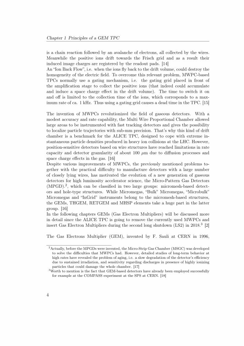
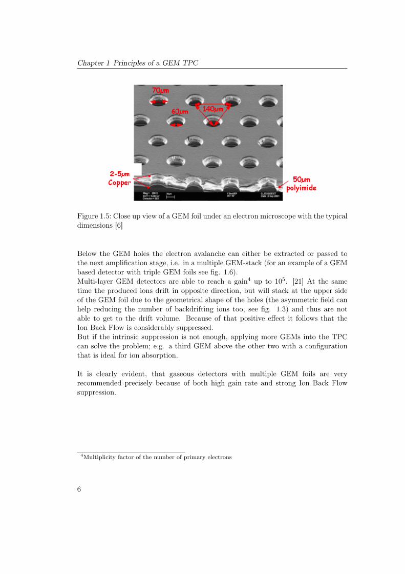
consists of a polyimide foil (∼ 50 µm thin) that is copper clad on both sides (each∼ 5 µm thin) and contains a large number of small holes extending through the foil.[19]The first time developed on the basis of modern photo-lithographic technology andetching mechanism at CERN, GEM holes have a remarkable double conical shapewith an inner diameter of only 50-60 µm and outer diameter of 70 µm so thatGEM foils form a dense, regular pattern of holes. In a standard configuration, twoneighboring holes have a distance of ∼ 140 µm from each other.The mechanism of the electron amplification in GEMs to induce a sufficient signalworks as follows: The metal layers play the role of electrodes, and when a highvoltage is applied across the copper-insulator-copper structure, a large electric fieldarises inside the holes. Once released by the primary ionization particle in the upperconversion region above the foil, the electrons pass through the GEM holes wherethe strong field acting on them induces the cascade. [20]Fig. 1.4 illustrates a rough draft of the electric field lines and the affected electronstogether with the ions, while the dimensions of the GEM structure are showed infig. 1.5.

Figure 1.4: Sketch of the cross section of a GEM foil with electric field lines due tothe strong potential difference of 300 - 400 V: a) Left: electrons drift into a holeand trigger an avalanche, b) Right: while the electrons drift to the anode, almost allproduced ions get collected. [6]

5


Figure 1.5: Close up view of a GEM foil under an electron microscope with the typicaldimensions [6]

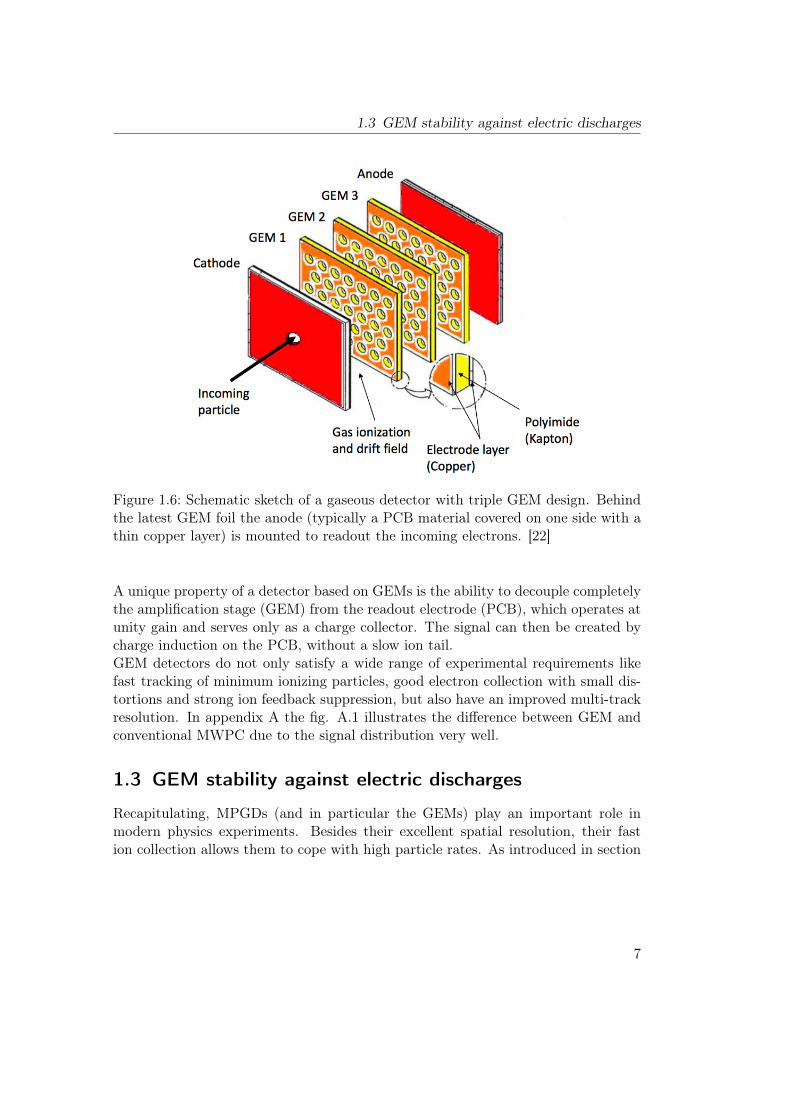
Below the GEM holes the electron avalanche can either be extracted or passed tothe next amplification stage, i.e. in a multiple GEM-stack (for an example of a GEMbased detector with triple GEM foils see fig. 1.6).Multi-layer GEM detectors are able to reach a gain4 up to 105. [21] At the sametime the produced ions drift in opposite direction, but will stack at the upper sideof the GEM foil due to the geometrical shape of the holes (the asymmetric field canhelp reducing the number of backdrifting ions too, see fig. 1.3) and thus are notable to get to the drift volume. Because of that positive effect it follows that theIon Back Flow is considerably suppressed.But if the intrinsic suppression is not enough, applying more GEMs into the TPCcan solve the problem; e.g. a third GEM above the other two with a configurationthat is ideal for ion absorption.

It is clearly evident, that gaseous detectors with multiple GEM foils are veryrecommended precisely because of both high gain rate and strong Ion Back Flowsuppression.

4Multiplicity factor of the number of primary electrons

6

1.3 GEM stability against electric discharges

Figure 1.6: Schematic sketch of a gaseous detector with triple GEM design. Behindthe latest GEM foil the anode (typically a PCB material covered on one side with athin copper layer) is mounted to readout the incoming electrons. [22]

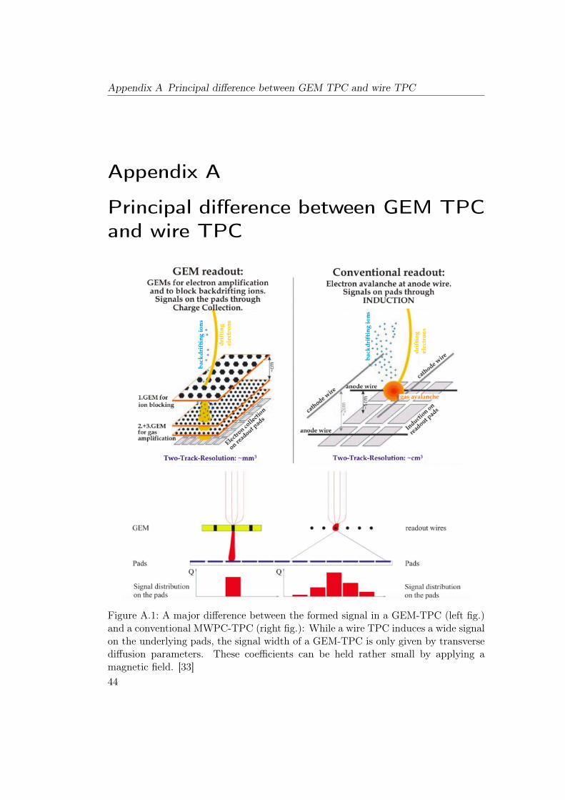
A unique property of a detector based on GEMs is the ability to decouple completelythe amplification stage (GEM) from the readout electrode (PCB), which operates atunity gain and serves only as a charge collector. The signal can then be created bycharge induction on the PCB, without a slow ion tail.GEM detectors do not only satisfy a wide range of experimental requirements likefast tracking of minimum ionizing particles, good electron collection with small dis-tortions and strong ion feedback suppression, but also have an improved multi-trackresolution. In appendix A the fig. A.1 illustrates the difference between GEM andconventional MWPC due to the signal distribution very well.


Recapitulating, MPGDs (and in particular the GEMs) play an important role inmodern physics experiments. Besides their excellent spatial resolution, their fastion collection allows them to cope with high particle rates. As introduced in section

7


1.2, the Ion Back Flow5 is a commonly used quantity to describe the suppression ofback drifting ions. Mounting a triple GEM-stack into the TPC can reduce it belowone percent. [23]At very high fluxes, however, the modern GEM detector suffers from a major prob-lem in terms of its stability: the so called electrical discharges (sparks).A high ionizing particle (e.g. α - particle), that traverses the drift volume, depositsa large amount of its energy by ionizing the gas and thus releasing a lot of electronsand positively charged ions. In other words, it creates a high charge density at acertain point. Then the density will be increased in order to reach a high gain. Nowassuming a spark is induced by a local, large charge density, the spark rate grows asa power law with the gain (or number of the electrons) of the detector.If the certain limit Qcrit

6 for electron amplification, the Raether Limit [25], is reachedor even exceeded, then discharges are very likely to occur. In that case a transitionto a streamer mode occurs, leading to a breakdown in the amplification region. Theresulting drop of the detector’s gain therefore yields detection inefficiency. It caneven damage the detector itself. [26]

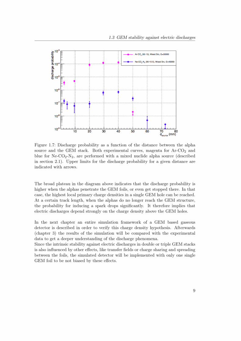
To quantify systematically the origin and the development of a discharge, ex-tensive experimental studies have been performed to measure the spark rate. Inthe following chapters discharge probability studies are referred to the experimentaldata7 (see fig. 1.7) taken from the Technical Design Report (TDR) of the ALICEcollaboration [27].For that experiment a small-size prototype detector with a triple GEM stack wasconstructed. The detector was filled with Ne-CO2-N2 as well as with Ar-CO2 (thereason for this gas choice is explained in section 2.1). A mixed nuclide alpha sourcewas placed on top of the cathode, so that during the measurement alphas were sendperpendicular to the GEM foils.In comparison to previous measurements with 220Rn, the resulting difference sug-gests that the primary charge density arriving at the GEM holes after drift may betoo low (due to the track inclination and the diffusion) to affect the stability of thedetector. Thus, the measurements were continued with the alpha source. [27]

5Generally defined as the ratio of the number of ions arriving at the cathode to the number ofelectrons arriving at the anode.

6The critical total charge in the avalanche is in the order of Qcrit ∼ 106 — 107 electrons [24]7The experimental data shown in this bachelor thesis represent the current results of recent R&D(“research and development”) efforts.

8


Figure 1.7: Discharge probability as a function of the distance between the alphasource and the GEM stack. Both experimental curves, magenta for Ar-CO2 andblue for Ne-CO2-N2, are performed with a mixed nuclide alpha source (describedin section 2.1). Upper limits for the discharge probability for a given distance areindicated with arrows.

The broad plateau in the diagram above indicates that the discharge probability ishigher when the alphas penetrate the GEM foils, or even get stopped there. In thatcase, the highest local primary charge densities in a single GEM hole can be reached.At a certain track length, when the alphas do no longer reach the GEM structure,the probability for inducing a spark drops significantly. It therefore implies thatelectric discharges depend strongly on the charge density above the GEM holes.

In the next chapter an entire simulation framework of a GEM based gaseousdetector is described in order to verify this charge density hypothesis. Afterwards(chapter 3) the results of the simulation will be compared with the experimentaldata to get a deeper understanding of the discharge phenomena.Since the intrinsic stability against electric discharges in double or triple GEM stacksis also influenced by other effects, like transfer fields or charge sharing and spreadingbetween the foils, the simulated detector will be implemented with only one singleGEM foil to be not biased by these effects.

9

Chapter 2

Simulation framework

The Gas Electron Multiplier was introduced as a suitable candidate for the upcom-ing ALICE TPC upgrade. Its physical principles and optical properties were expli-citly described in chapter 1. Also the advantages with reference to the conventionalMWPCs are discussed in detail, which are generally well understood nowadays. Butthere is still one hitch, which has a negative impact on the GEMs, namely the elec-trical discharges. Experimentally observed with a small detector prototype includingthree GEM foils (see fig. 1.7), the next step is to analyze it in such a way that itscause can physically be explained.The following sections are dedicated to a GEANT41 - based Monte Carlo simulation2

which describes the geometry and tracking of a virtual detector including the gas,source and the physical processes (e.g. electromagnetic interactions etc.).

2.1 Detector description in GEANT4

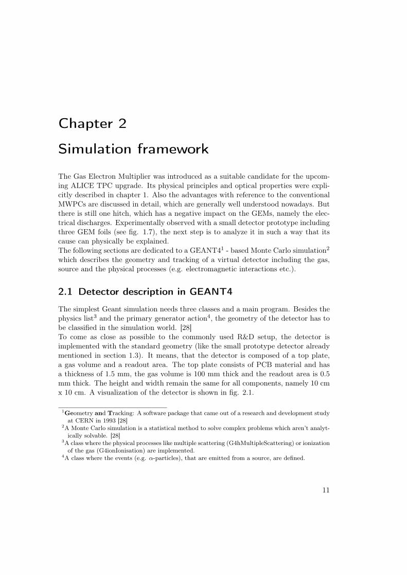
The simplest Geant simulation needs three classes and a main program. Besides thephysics list3 and the primary generator action4, the geometry of the detector has tobe classified in the simulation world. [28]To come as close as possible to the commonly used R&D setup, the detector isimplemented with the standard geometry (like the small prototype detector alreadymentioned in section 1.3). It means, that the detector is composed of a top plate,a gas volume and a readout area. The top plate consists of PCB material and hasa thickness of 1.5 mm, the gas volume is 100 mm thick and the readout area is 0.5mm thick. The height and width remain the same for all components, namely 10 cmx 10 cm. A visualization of the detector is shown in fig. 2.1.

1Geometry and Tracking: A software package that came out of a research and development studyat CERN in 1993 [28]

2A Monte Carlo simulation is a statistical method to solve complex problems which aren’t analyt-ically solvable. [28]

3A class where the physical processes like multiple scattering (G4hMultipleScattering) or ionizationof the gas (G4ionIonisation) are implemented.

4A class where the events (e.g. α-particles), that are emitted from a source, are defined.

11

Chapter 2 Simulation framework

Figure 2.1: Detector setup for the simulations: gas volume (orange) between thereadout area (yellow) and the PCB plate (green). The mixed source, placed in thetransfixion of the PCB plate, emits alpha particles (dark red), which in turn produceelectrons (blue) in the gas volume. The α-particles drift in the volume until theydeposit their whole energy in the gas (black point).

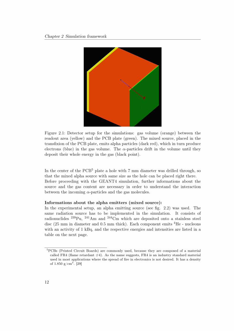
In the center of the PCB5 plate a hole with 7 mm diameter was drilled through, sothat the mixed alpha source with same size as the hole can be placed right there.Before proceeding with the GEANT4 simulation, further informations about thesource and the gas content are necessary in order to understand the interactionbetween the incoming α-particles and the gas molecules.

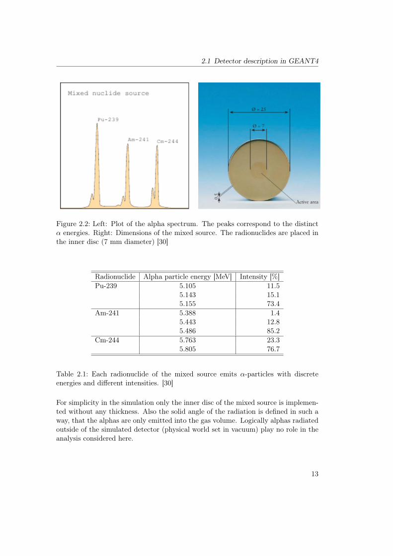
Informations about the alpha emitters (mixed source):In the experimental setup, an alpha emitting source (see fig. 2.2) was used. Thesame radiation source has to be implemented in the simulation. It consists ofradionuclides 239Pu, 241Am and 244Cm which are deposited onto a stainless steeldisc (25 mm in diameter and 0.5 mm thick). Each component emits 4He - nucleonswith an activity of 1 kBq, and the respective energies and intensities are listed in atable on the next page.

5PCBs (Printed Circuit Boards) are commonly used, because they are composed of a materialcalled FR4 (flame retardant #4). As the name suggests, FR4 is an industry standard materialused in most applications where the spread of fire in electronics is not desired. It has a densityof 1.850 g/cm3. [29]

12

2.1 Detector description in GEANT4

Figure 2.2: Left: Plot of the alpha spectrum. The peaks correspond to the distinctα energies. Right: Dimensions of the mixed source. The radionuclides are placed inthe inner disc (7 mm diameter) [30]

Radionuclide Alpha particle energy [MeV] Intensity [%]Pu-239 5.105 11.5

5.143 15.15.155 73.4

Am-241 5.388 1.45.443 12.85.486 85.2

Cm-244 5.763 23.35.805 76.7

Table 2.1: Each radionuclide of the mixed source emits α-particles with discreteenergies and different intensities. [30]

For simplicity in the simulation only the inner disc of the mixed source is implemen-ted without any thickness. Also the solid angle of the radiation is defined in such away, that the alphas are only emitted into the gas volume. Logically alphas radiatedoutside of the simulated detector (physical world set in vacuum) play no role in theanalysis considered here.

13


Informations about the gas mixture:Usually in a TPC the inserted gas consists of two gas components. The one gascomponent is a noble gas (in the R&D setup, see fig. 1,7, Argon and Neon areused), while the other constituent (so called quencher) is required for stability inthe amplification stage. A noble gas has the positive aspect that the atom shellsare completely filled with electrons so that it is chemically non-reactive to othergas molecules. Hence it is stable under the standard conditions (300 K, 1 baratmospheric pressure) the detector is experimentally used and simulated.During the amplification process some gas atoms can be excited. When they falldown to their ground states, they emit photons in the visible and UV range, whichcan in turn ionize the gas atoms or extract electrons from the surrounding electrodes(photoelectric effect), resulting in creation of even more charge.6 It could even leadto a formation of a new avalanche separated from the primary one. If the fieldsare strong enough, the process can be self-sustaining, thus resulting in a completeelectric breakdown. Suing pure noble gases is not sufficient to prevent this problem.Therefore the second constituent, called quenching gas, has to be added to the gascontent. Proper candidates are organic, polyatomic gases like CO2 or CH4 with alarge photon absorption cross section in the visible and UV range. Adding an extrafraction of quenching gas (like N2) can lead to even more stable conditions.Therefore the R&D prototype detector was operated with both Ar-CO2 and Ne-CO2-N2 gases. The ratios of the components in the gas mixture are indicated behindthe gas name. Typically for Ar-CO2 two different ratios are used (90 - 10 or 70- 30), while Neon is normally contained in the gas mixtures Ne-CO2 (90 - 10) orNe-CO2-N2 (90 - 10 - 5).7

Despite huge efforts to maintain 100% granularity, impurities in the gas are in-evitable. In mixtures containing electronegative molecules such as O2, H2O or CF4,electrons can be captured to form negative ions. These electronegative moleculesare not desired because they capture primary electrons and thus spoil the energyresolution. However, constantly flushing the detector suppresses the water or oxygencontent to few parts per million (ppm) in the detector volume.While in experiments this basic effect is ubiquitous, in the simulation framework itneeds not be taken into account.

6This effect is usually called photon feedback7in this case normalized to 105%

14

2.2 Reference simulations with a point-like source


This section is dedicated to a reference simulation with a point like source (i.e.without spatial extension) in order to understand firstly the behavior of the α-particles in the gas volume. Afterwards the ionization of the gas due to the energyloss of the incoming radiation is analyzed.

2.2.1 Energy deposition and Bragg curves

The process of detection in the simulated gaseous detector starts with the emissionof charged particles from a radiation source. Here an ideal, point like source isconsidered which emits alphas with a certain energy fixed by the simulation.The particles traversing the active volume of the detector interact with the gasmolecules. Due to inelastic collisions8 with the bound electrons of the atoms, thealphas loose their energy or finally can be stopped in the gas. Generally it is quitecomplicated to calculate the exact energy deposit of the incoming particles, sinceit depends on the magnitude of the alpha-atom (molecule) scattering cross section(and this in turn is only determinable if the quantum mechanical rotational andvibrational levels of the molecules as well as the drift velocity and diffusion of thealpha are known).Nevertheless it is possible to calculate the mean energy loss of a charged particle in acertain medium by using the quantum mechanical, relativistic Bethe - Bloch formula[31]:

−〈dEdx〉 = 2πNar

2emec

2ρZ

A

z2

β2[ln

2meγ2v2Wmax

I2− 2β2], (2.1)

where:

ρ = density of the absorbing material (here the gas mixture)z = charge of incident particle in units of eZ = atomic number of the absorbing materialA = atomic weight of the absorbing materialI = mean excitation potential

Wmax = maximum energy transfer in a single collision

The formula above is part of G4EmLivermore, the physics list for low-energy elec-tromagnetic interactions, which is used in the simulation.Now the following situation is simulated: The point like source is placed in the center

8Elastic scattering on the nuclei is possible too, but negligible compared to inelastic collisions.

15


of the PCB hole (see fig. 2.1) and emits α-particles perpendicular into the activevolume of the detector. Four simulations are done with four different gas mixturesArCO2 (70 - 30), ArCO2 (90 - 10), NeCO2 (90 - 10) and NeCO2N2 (90 - 10 - 5),that are successively set into the volume. In each gas the particle energy of the α’sis set to 5.2 MeV, 5.5 MeV and 5.8 MeV.9

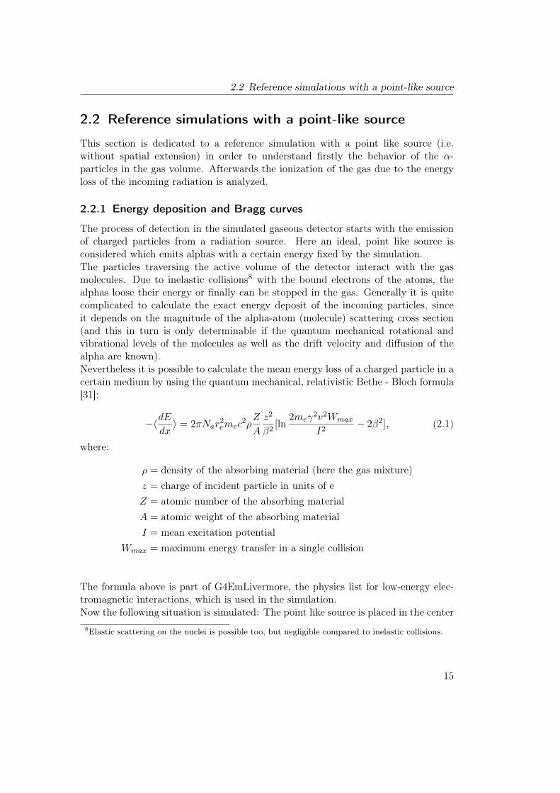
Then the range, i.e. how far the particles drift till they stop in the gas, and theenergy loss per mm are analyzed. The corresponding Bragg curves for each gas andparticle energy are illustrated in the diagrams below.

Figure 2.3: GEANT4 simulation of the ranges in different gas mixtures of alphaparticles: a) Bragg curves for Eα = 5.2 MeV, b) Eα = 5.5 MeV, c) Eα = 5.8 MeV

By comparing the plots in fig. 2.3 it can be seen, that the higher the energy ofthe incoming α-particles is the longer is the range in the volume. Also for argonmixtures all curves are, in contrary to the neon based gas, steeper and the track

9These energies are chosen because they come close to the radiation energies of 239Pu, 241Am and244Cm of the real mixed source.

16


length is almost 40% shorter due to the Z-dependency of the mean energy loss (seeeq. 2.1) .A similarity between the simulated plots and the experimental diagram on page 9can be noticed: The plots show that the particles with Eα = 5.8 MeV (equivalent tothe highest energy component of 244Cm and also for the mixed source) have a rangeof around 50 mm in Ar-CO2 (90 - 10) and almost 70 mm in Ne-CO2-N2 (90 - 10 - 5).At these values the discharge probability for both gas mixtures drops significantly.Furthermore the Bragg peaks simulated for argon mixtures are higher and narrower,which means that the alphas deposit more energy nearly the range maximum thanin the neon mixtures. As a result, locally higher charge densities are achieved, whichmatches well with the experimental plot in terms of the charge density hypothesis:the discharge probability in argon based gas mixture is higher than in neon based.

2.2.2 Ionisation of the gas and “Bragg cluster” definition

Still not mentioned is the fact, that the Bragg curves totally differ for NeCO2 (90 -10) and ArCO2 (90 - 10), although the amount of quencher is the same in both mix-tures. According to that the mass and atomic number of the noble gas componentshave to dominate over the range and the steepness of the curves. Since argon hasa higher ordinal number than neon, in a gas filled with ArCO2 the probability foran inelastic collision between incoming particle and electrons is increased. Thereforethe alpha-particles loose much faster their energy and thus the mean free path issmaller respectively to that of the lighter noble gas.In order to create an electron - ion pair, the energy deposit must be equal or higherthan the effective ionization potential10 of the gas molecule. The characteristic ion-ization potentials of the four gas mixtures considered in the simulation are listed intable 2.2.

gas mixture effective ionization potential Wi [eV]Ar-CO2 (70 - 30) 28.10Ar-CO2 (90 - 10) 28.77Ne-CO2 (90 - 10) 38.10Ne-CO2-N2 (90 - 10 - 5) 37.29

Table 2.2: The in the simulation considered gas mixtures together with each effectiveionization potential. [32]

10In an effective ionization potential both the excitation and ionization energy are considered.

17


For example, if an incident alpha-particle deposits 5 MeV in Ar-CO2 (90 - 10), thenthe total amount of produced free electrons in average is:

# electrons =∆EαWi

=5MeV

28.77eV= 173.8 · 103 (2.2)

In GEANT4 the track of the alpha-particles in the drift volume is divided in severalsteps, where at each step N electrons are created at rest (N is calculated from eq.2.2). Since these electrons are not equally distributed within a GEANT step butcreated in one place, they have the same spatial coordinates for each step.Now applying the same calculation with Ne-CO2-N2 as the gas content, the alphawould produce 134.1 · 103 electrons. So at a given gain the charge density in theargon based mixture would be 173.8

134.1 = 1.3 times larger.As a consequence, the simple calculation together with the experimental observation(see fig. 1.7) explain the strong dependence of the discharge probability on the usedgas mixture. But by normalizing the gain and assuming that the charge densityhypothesis can be accurate, the spark rate will be dependent of the created electrondensity, no matter which gas content is chosen (in general however many otherfactors need to be considered in addition to describe the origin of the electricaldischarges). [26]

In the next step a static (i.e. without electric field) simulation is performed inorder to get more informations about the amount of electrons that alphas produceat a certain position. The point like source still remains unchanged at the center ofthe cylindrical hole. But the PCB plate is removed, since no electric field is applied.The source emits 5 · 105 α-particles (from now on often called events) isotropicallytowards the drift volume.11 Each of the particles has the fixed energy Eα = 5.2 MeVand Ne-CO2-N2 is the chosen gas mixture in the further simulations.

As already mentioned in the lower section on page 9, in the simulation only onesingle-GEM layer is implemented into the detector to avoid large diffusion effects ofthe electrons, that generally occur in multiple GEM based detectors. Furthermorethe GEM foil doesn’t contain any holes, since no electrical field is set inside the gasbox, in order to simplify the simulations. In this chapter namely the charge densityof the electrons inside the GEM area to the number of alpha-particles that penetrateit is of interest.

11The amount of the events is arbitrary set to that value. The only requirement is, that the numberhas to be large to get high statistics.

18


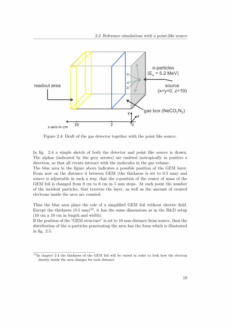
Figure 2.4: Draft of the gas detector together with the point like source.

In fig. 2.4 a simple sketch of both the detector and point like source is drawn.The alphas (indicated by the grey arrows) are emitted isotropically in positive zdirection, so that all events interact with the molecules in the gas volume.The blue area in the figure above indicates a possible position of the GEM layer.From now on the distance d between GEM (the thickness is set to 0.5 mm) andsource is adjustable in such a way, that the z-position of the center of mass of theGEM foil is changed from 0 cm to 6 cm in 5 mm steps. At each point the numberof the incident particles, that traverse the layer, as well as the amount of createdelectrons inside the area are counted.

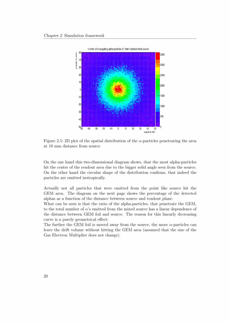
Thus the blue area plays the role of a simplified GEM foil without electric field.Except the thickness (0.5 mm)12, it has the same dimensions as in the R&D setup(10 cm x 10 cm in length and width).If the position of the “GEM structure” is set to 10 mm distance from source, then thedistribution of the α-particles penetrating the area has the form which is illustratedin fig. 2.5:

12In chapter 2.4 the thickness of the GEM foil will be varied in order to look how the electrondensity inside the area changes for each distance

19


Figure 2.5: 2D plot of the spatial distribution of the α-particles penetrating the areaat 10 mm distance from source

On the one hand this two-dimensional diagram shows, that the most alpha-particleshit the center of the readout area due to the bigger solid angle seen from the source.On the other hand the circular shape of the distribution confirms, that indeed theparticles are emitted isotropically.

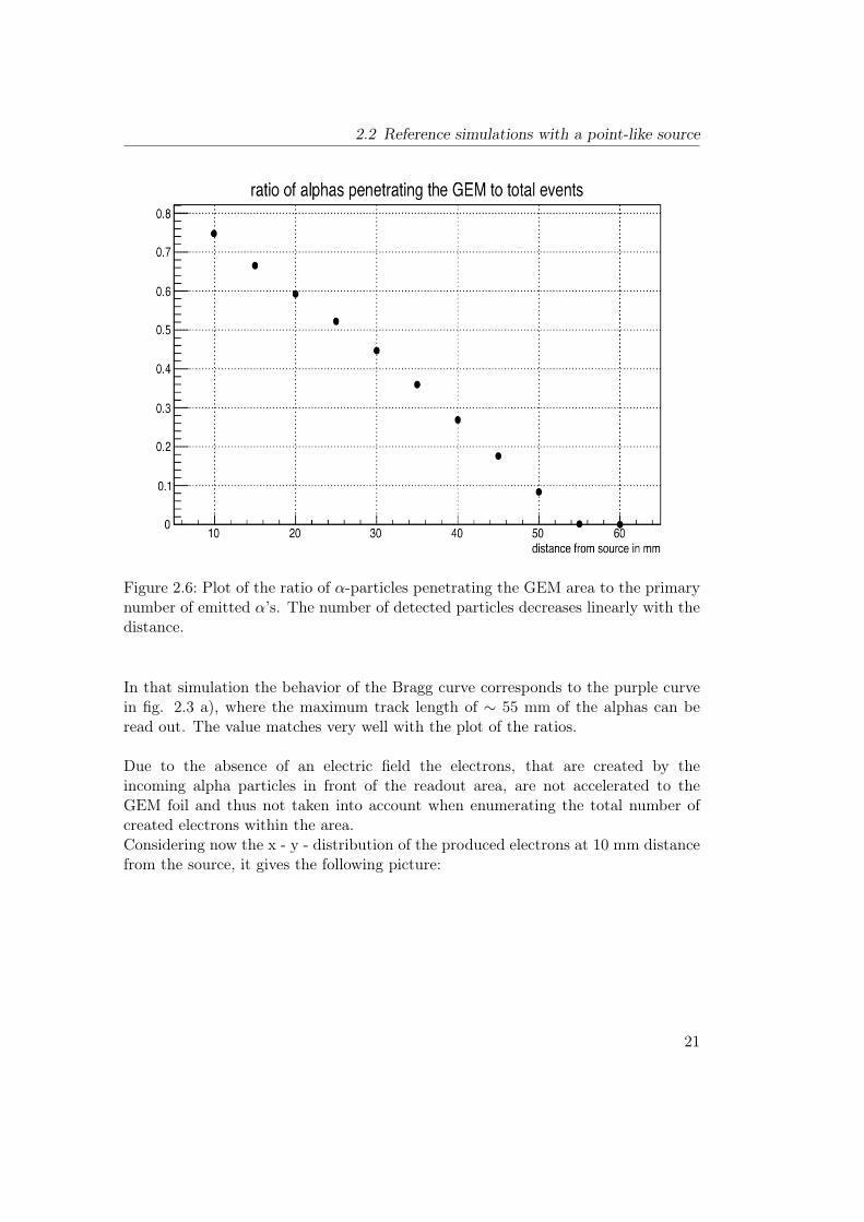
Actually not all particles that were emitted from the point like source hit theGEM area. The diagram on the next page shows the percentage of the detectedalphas as a function of the distance between source and readout plane.What can be seen is that the ratio of the alpha-particles, that penetrate the GEM,to the total number of α’s emitted from the mixed source has a linear dependence ofthe distance between GEM foil and source. The reason for this linearly decreasingcurve is a purely geometrical effect:The further the GEM foil is moved away from the source, the more α-particles canleave the drift volume without hitting the GEM area (assumed that the size of theGas Electron Multiplier does not change).

20


Figure 2.6: Plot of the ratio of α-particles penetrating the GEM area to the primarynumber of emitted α’s. The number of detected particles decreases linearly with thedistance.

In that simulation the behavior of the Bragg curve corresponds to the purple curvein fig. 2.3 a), where the maximum track length of ∼ 55 mm of the alphas can beread out. The value matches very well with the plot of the ratios.

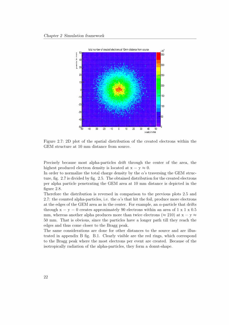
Due to the absence of an electric field the electrons, that are created by theincoming alpha particles in front of the readout area, are not accelerated to theGEM foil and thus not taken into account when enumerating the total number ofcreated electrons within the area.Considering now the x - y - distribution of the produced electrons at 10 mm distancefrom the source, it gives the following picture:

21


Figure 2.7: 2D plot of the spatial distribution of the created electrons within theGEM structure at 10 mm distance from source.

Precisely because most alpha-particles drift through the center of the area, thehighest produced electron density is located at x = y ≈ 0.In order to normalize the total charge density by the α’s traversing the GEM struc-ture, fig. 2.7 is divided by fig. 2.5. The obtained distribution for the created electronsper alpha particle penetrating the GEM area at 10 mm distance is depicted in thefigure 2.8.Therefore the distribution is reversed in comparison to the previous plots 2.5 and2.7: the counted alpha-particles, i.e. the α’s that hit the foil, produce more electronsat the edges of the GEM area as in the center. For example, an α-particle that driftsthrough x = y = 0 creates approximately 90 electrons within an area of 1 x 1 x 0.5mm, whereas another alpha produces more than twice electrons (≈ 210) at x = y ≈50 mm. That is obvious, since the particles have a longer path till they reach theedges and thus come closer to the Bragg peak.The same considerations are done for other distances to the source and are illus-trated in appendix B fig. B.1. Clearly visible are the red rings, which correspondto the Bragg peak where the most electrons per event are created. Because of theisotropically radiation of the alpha-particles, they form a donut-shape.

22


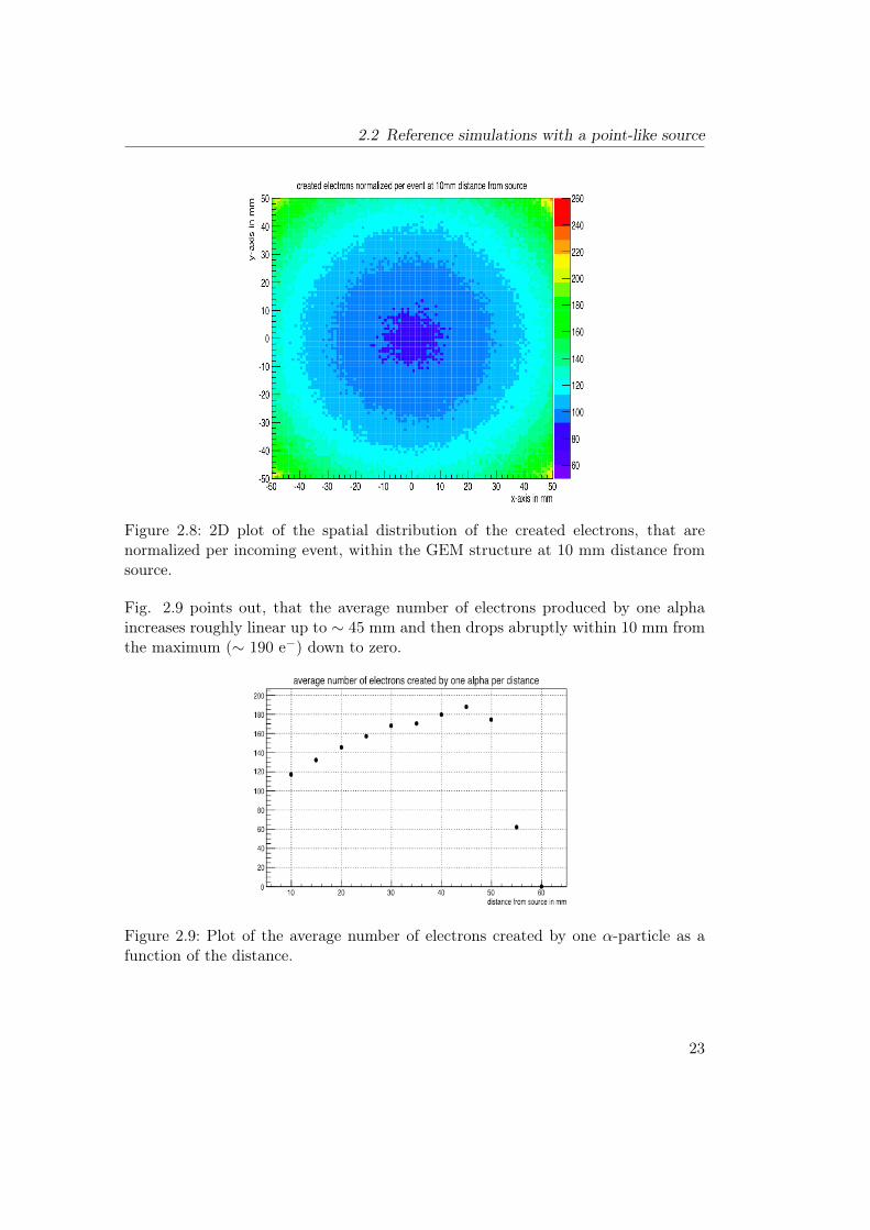
Figure 2.8: 2D plot of the spatial distribution of the created electrons, that arenormalized per incoming event, within the GEM structure at 10 mm distance fromsource.

Fig. 2.9 points out, that the average number of electrons produced by one alphaincreases roughly linear up to ∼ 45 mm and then drops abruptly within 10 mm fromthe maximum (∼ 190 e−) down to zero.

Figure 2.9: Plot of the average number of electrons created by one α-particle as afunction of the distance.

23


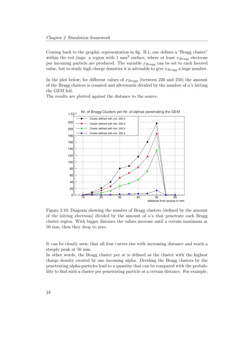
Coming back to the graphic representation in fig. B.1, one defines a “Bragg cluster”within the red rings: a region with 1 mm2 surface, where at least xBragg electronsper incoming particle are produced. The variable xBragg can be set to each favoredvalue, but to study high charge densities it is advisable to give xBragg a huge number.

In the plot below, for different values of xBragg (between 220 and 250) the amountof the Bragg clusters is counted and afterwards divided by the number of α’s hittingthe GEM foil.The results are plotted against the distance to the source.

Figure 2.10: Diagram showing the number of Bragg clusters (defined by the amountof the inlying electrons) divided by the amount of α’s that penetrate each Braggcluster region. With bigger distance the values increase until a certain maximum at50 mm, then they drop to zero.

It can be clearly seen, that all four curves rise with increasing distance and reach asteeply peak at 50 mm.In other words, the Bragg cluster per se is defined as the cluster with the highestcharge density created by one incoming alpha. Dividing the Bragg clusters by thepenetrating alpha-particles lead to a quantity that can be compared with the probab-ility to find such a cluster per penetrating particle at a certain distance. For example,

24


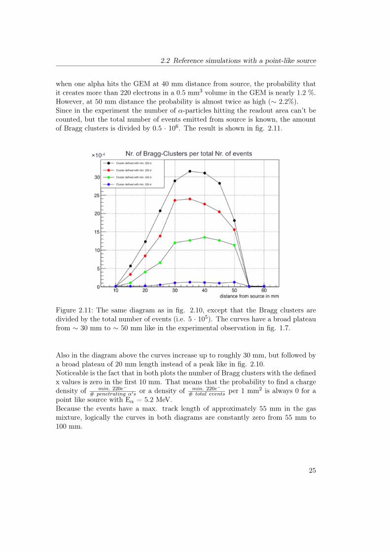
when one alpha hits the GEM at 40 mm distance from source, the probability thatit creates more than 220 electrons in a 0.5 mm3 volume in the GEM is nearly 1.2 %.However, at 50 mm distance the probability is almost twice as high (∼ 2.2%).Since in the experiment the number of α-particles hitting the readout area can’t becounted, but the total number of events emitted from source is known, the amountof Bragg clusters is divided by 0.5 · 106. The result is shown in fig. 2.11.

Figure 2.11: The same diagram as in fig. 2.10, except that the Bragg clusters aredivided by the total number of events (i.e. 5 · 105). The curves have a broad plateaufrom ∼ 30 mm to ∼ 50 mm like in the experimental observation in fig. 1.7.

Also in the diagram above the curves increase up to roughly 30 mm, but followed bya broad plateau of 20 mm length instead of a peak like in fig. 2.10.Noticeable is the fact that in both plots the number of Bragg clusters with the definedx values is zero in the first 10 mm. That means that the probability to find a chargedensity of min. 220e−

# penetrating α′s or a density of min. 220e−

# total events per 1 mm2 is always 0 for apoint like source with Eα = 5.2 MeV.Because the events have a max. track length of approximately 55 mm in the gasmixture, logically the curves in both diagrams are constantly zero from 55 mm to100 mm.

25


2.3 Simulations with a mixed source

All calculations in the section before are done with a point-like radiation source (nospatial extension) that emits alpha-particles with Eα = 5.2 MeV into a Ne-CO2-N2 (90 - 10 - 5) gas mixture. Since the experiment is performed with a mixedradionuclide source (see page 10 f.) and the aim is to reproduce the experimentaldata in fig. 1.6 with the simulation, from now on the point like source is replaced bythe mixed source.Basically the radionuclides 239Pu, 241Am and 244Cm in the source emit α’s with thesame rate but with different energies and intensities. Arithmetically averaging theenergies weighted with the intensities, the mean α-energy of each nuclide is:

Eα = 5.147 MeV for Pu-239Eα = 5.446 MeV for Am-241Eα = 5.795 MeV for Cm-244

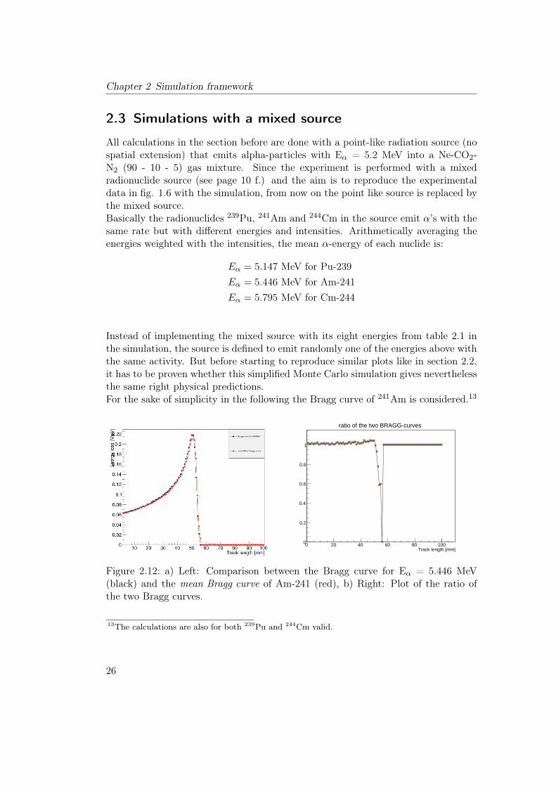
Instead of implementing the mixed source with its eight energies from table 2.1 inthe simulation, the source is defined to emit randomly one of the energies above withthe same activity. But before starting to reproduce similar plots like in section 2.2,it has to be proven whether this simplified Monte Carlo simulation gives neverthelessthe same right physical predictions.For the sake of simplicity in the following the Bragg curve of 241Am is considered.13

Track length [mm]0 20 40 60 80 1000

0.2

0.4

0.6

0.8

1

ratio of the two BRAGG-curves

Figure 2.12: a) Left: Comparison between the Bragg curve for Eα = 5.446 MeV(black) and the mean Bragg curve of Am-241 (red), b) Right: Plot of the ratio ofthe two Bragg curves.

13The calculations are also for both 239Pu and 244Cm valid.

26


Primarily the energy loss for each alpha-energy (5.388 MeV, 5.443 MeV and 5.486MeV) is calculated. The corresponding Bragg curves are then weighted with the in-tensity of each energy and afterwards added in order to obtain the mean Bragg curveof the americium nuclide. Analogously the Bragg curve of the average alpha-energyEα = 5.446 of Am-241 is calculated. In order to compare both curves they areplotted in one diagram which is illustrated in fig. 2.12 a). Furthermore both aredivided from each other and the corresponding ratio is depicted in fig. 2.12 b).Now if both Bragg curves were equal, they would describe the same physics of theemitted alpha-particles in the gas volume and the ratio would be constantly one.However, fig. 2.12 b) shows a deviation of the constant at ≈ 55 mm which has nearlythe form of a delta peak. This comes from the fact that both curves are shifted by≈ 1 mm from each other.Since the height and width are equal, the calculation shows that the deviation isnegligible if the charge density is studied only in 5 mm steps. Thus, the simulationsare valid when taking the mean alpha-energies of the radionuclides, as long as thesteps are not of the order of 1 mm or smaller.

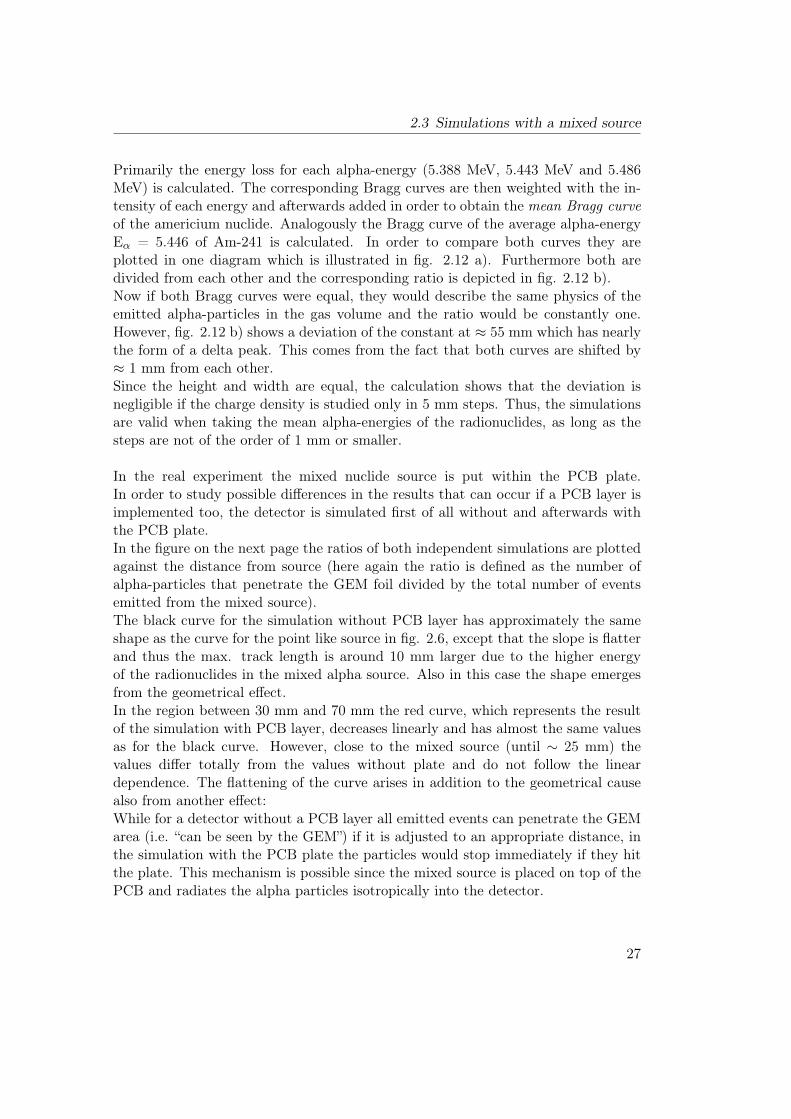
In the real experiment the mixed nuclide source is put within the PCB plate.In order to study possible differences in the results that can occur if a PCB layer isimplemented too, the detector is simulated first of all without and afterwards withthe PCB plate.In the figure on the next page the ratios of both independent simulations are plottedagainst the distance from source (here again the ratio is defined as the number ofalpha-particles that penetrate the GEM foil divided by the total number of eventsemitted from the mixed source).The black curve for the simulation without PCB layer has approximately the sameshape as the curve for the point like source in fig. 2.6, except that the slope is flatterand thus the max. track length is around 10 mm larger due to the higher energyof the radionuclides in the mixed alpha source. Also in this case the shape emergesfrom the geometrical effect.In the region between 30 mm and 70 mm the red curve, which represents the resultof the simulation with PCB layer, decreases linearly and has almost the same valuesas for the black curve. However, close to the mixed source (until ∼ 25 mm) thevalues differ totally from the values without plate and do not follow the lineardependence. The flattening of the curve arises in addition to the geometrical causealso from another effect:While for a detector without a PCB layer all emitted events can penetrate the GEMarea (i.e. “can be seen by the GEM”) if it is adjusted to an appropriate distance, inthe simulation with the PCB plate the particles would stop immediately if they hitthe plate. This mechanism is possible since the mixed source is placed on top of thePCB and radiates the alpha particles isotropically into the detector.

27


distance from source in mm10 20 30 40 50 60 70

0

0.1

0.2

0.3

0.4

0.5

0.6

0.7

0.8without PCB plate

with PCB plate

ratio of alphas penetrating the GEM to total events

Figure 2.13: Plot of the ratio of α-particles penetrating the GEM area to the primarynumber of emitted α’s. The number of detected particles decreases linearly with thedistance for the simulation without PCB (black curve), analogous to fig. 2.6 forthe point like source. The red curve is dedicated to the simulation with PCB plate,where a linear drop starts from ∼ 25 mm.

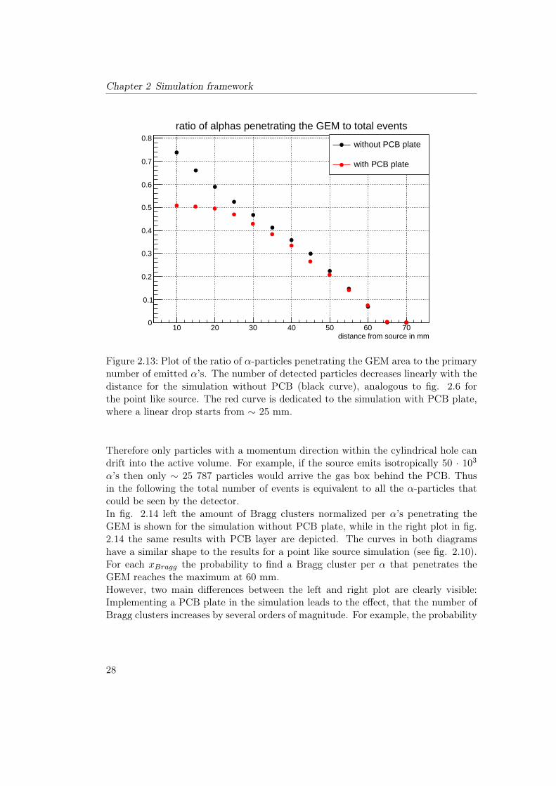
Therefore only particles with a momentum direction within the cylindrical hole candrift into the active volume. For example, if the source emits isotropically 50 · 103α’s then only ∼ 25 787 particles would arrive the gas box behind the PCB. Thusin the following the total number of events is equivalent to all the α-particles thatcould be seen by the detector.In fig. 2.14 left the amount of Bragg clusters normalized per α’s penetrating theGEM is shown for the simulation without PCB plate, while in the right plot in fig.2.14 the same results with PCB layer are depicted. The curves in both diagramshave a similar shape to the results for a point like source simulation (see fig. 2.10).For each xBragg the probability to find a Bragg cluster per α that penetrates theGEM reaches the maximum at 60 mm.However, two main differences between the left and right plot are clearly visible:Implementing a PCB plate in the simulation leads to the effect, that the number ofBragg clusters increases by several orders of magnitude. For example, the probability

28


Figure 2.14: Diagrams showing the number of Bragg clusters divided by the amountof α’s that penetrate each Bragg cluster region. Left: results without PCB plate,Right: results with PCB plate. With bigger distance the values in both plots increaseuntil a certain maximum at 60 mm, then they drop to zero.

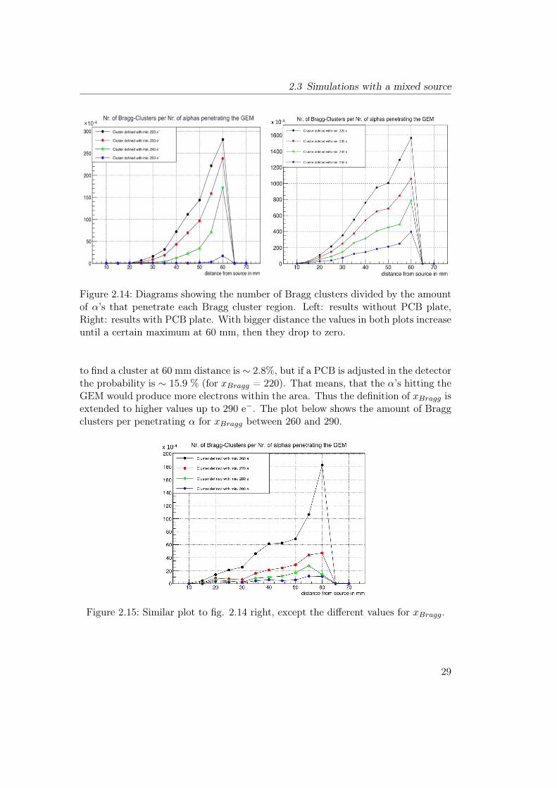
to find a cluster at 60 mm distance is ∼ 2.8%, but if a PCB is adjusted in the detectorthe probability is ∼ 15.9 % (for xBragg = 220). That means, that the α’s hitting theGEM would produce more electrons within the area. Thus the definition of xBragg isextended to higher values up to 290 e−. The plot below shows the amount of Braggclusters per penetrating α for xBragg between 260 and 290.

Figure 2.15: Similar plot to fig. 2.14 right, except the different values for xBragg.

29


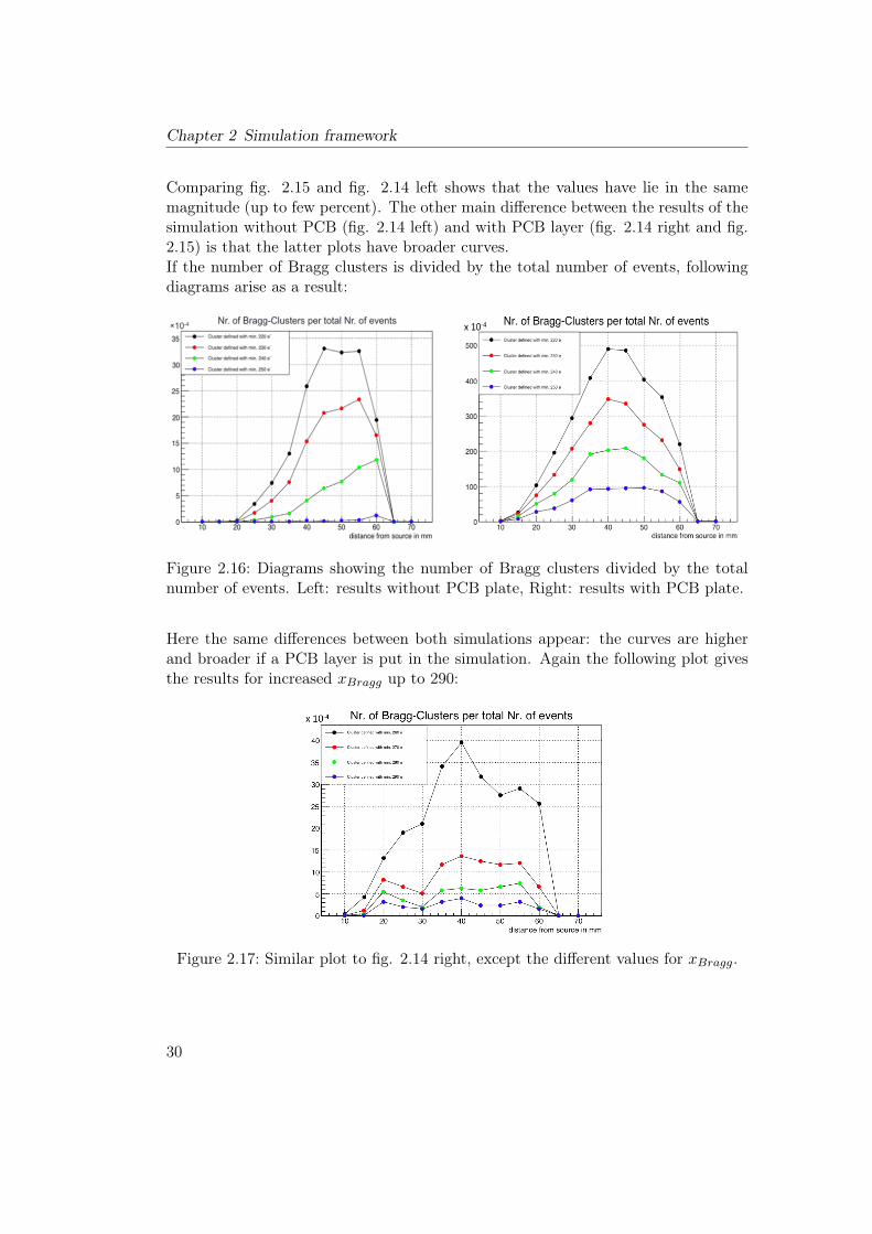
Comparing fig. 2.15 and fig. 2.14 left shows that the values have lie in the samemagnitude (up to few percent). The other main difference between the results of thesimulation without PCB (fig. 2.14 left) and with PCB layer (fig. 2.14 right and fig.2.15) is that the latter plots have broader curves.If the number of Bragg clusters is divided by the total number of events, followingdiagrams arise as a result:

Figure 2.16: Diagrams showing the number of Bragg clusters divided by the totalnumber of events. Left: results without PCB plate, Right: results with PCB plate.

Here the same differences between both simulations appear: the curves are higherand broader if a PCB layer is put in the simulation. Again the following plot givesthe results for increased xBragg up to 290:

Figure 2.17: Similar plot to fig. 2.14 right, except the different values for xBragg.

30



0

20

40

60

80

100

120

140

160

180

200 with PCB plate

without PCB plate

average number of electrons created by one alpha per distance

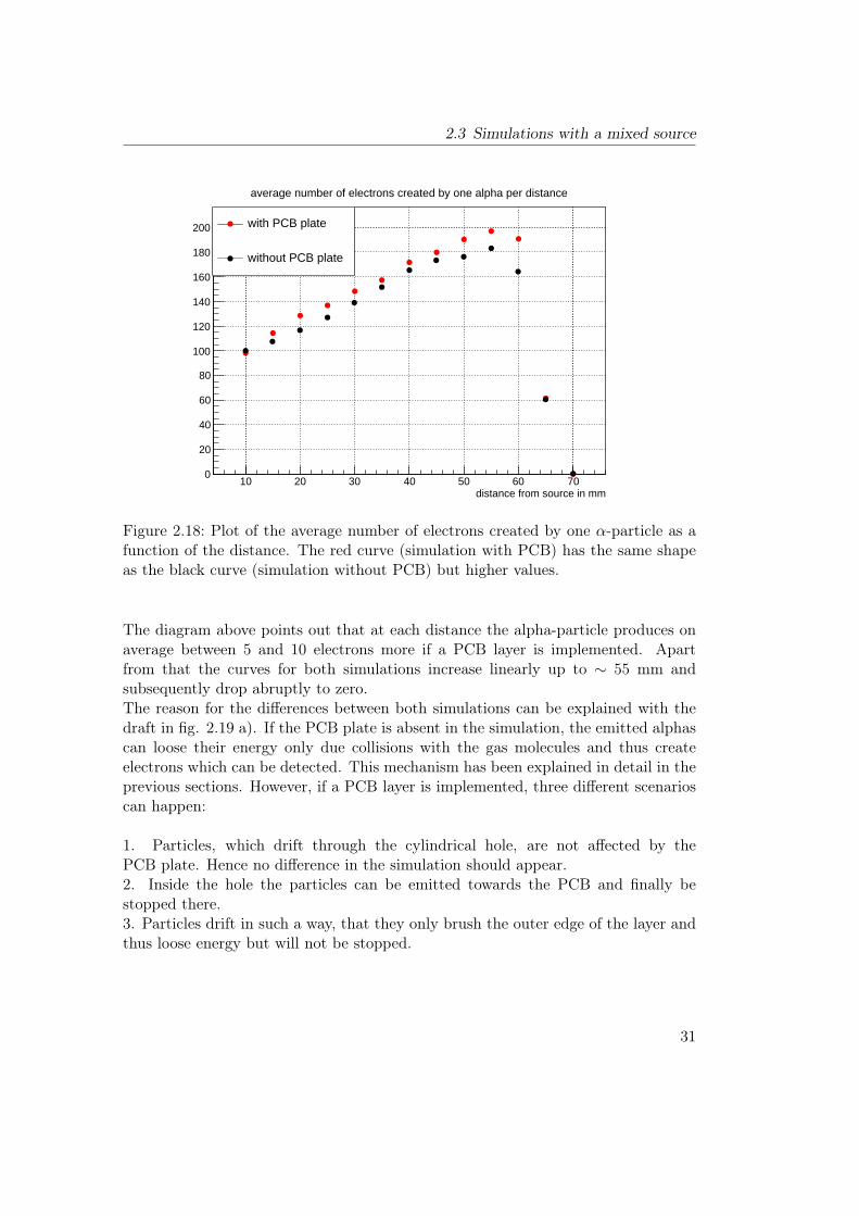
Figure 2.18: Plot of the average number of electrons created by one α-particle as afunction of the distance. The red curve (simulation with PCB) has the same shapeas the black curve (simulation without PCB) but higher values.

The diagram above points out that at each distance the alpha-particle produces onaverage between 5 and 10 electrons more if a PCB layer is implemented. Apartfrom that the curves for both simulations increase linearly up to ∼ 55 mm andsubsequently drop abruptly to zero.The reason for the differences between both simulations can be explained with thedraft in fig. 2.19 a). If the PCB plate is absent in the simulation, the emitted alphascan loose their energy only due collisions with the gas molecules and thus createelectrons which can be detected. This mechanism has been explained in detail in theprevious sections. However, if a PCB layer is implemented, three different scenarioscan happen:

1. Particles, which drift through the cylindrical hole, are not affected by thePCB plate. Hence no difference in the simulation should appear.2. Inside the hole the particles can be emitted towards the PCB and finally bestopped there.3. Particles drift in such a way, that they only brush the outer edge of the layer andthus loose energy but will not be stopped.

31


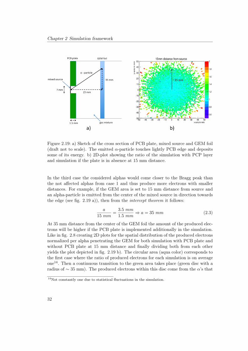
Figure 2.19: a) Sketch of the cross section of PCB plate, mixed source and GEM foil(draft not to scale). The emitted α-particle touches lightly PCB edge and depositssome of its energy. b) 2D-plot showing the ratio of the simulation with PCP layerand simulation if the plate is in absence at 15 mm distance.

In the third case the considered alphas would come closer to the Bragg peak thanthe not affected alphas from case 1 and thus produce more electrons with smallerdistances. For example, if the GEM area is set to 15 mm distance from source andan alpha-particle is emitted from the center of the mixed source in direction towardsthe edge (see fig. 2.19 a)), then from the intercept theorem it follows:

a

15 mm=

3.5 mm

1.5 mm⇒ a = 35 mm (2.3)

At 35 mm distance from the center of the GEM foil the amount of the produced elec-trons will be higher if the PCB plate is implemented additionally in the simulation.Like in fig. 2.8 creating 2D plots for the spatial distribution of the produced electronsnormalized per alpha penetrating the GEM for both simulation with PCB plate andwithout PCB plate at 15 mm distance and finally dividing both from each otheryields the plot depicted in fig. 2.19 b). The circular area (aqua color) corresponds tothe first case where the ratio of produced electrons for each simulation is on averageone14. Then a continuous transition to the green area takes place (green disc with aradius of ∼ 35 mm). The produced electrons within this disc come from the α’s that

14Not constantly one due to statistical fluctuations in the simulation.

32


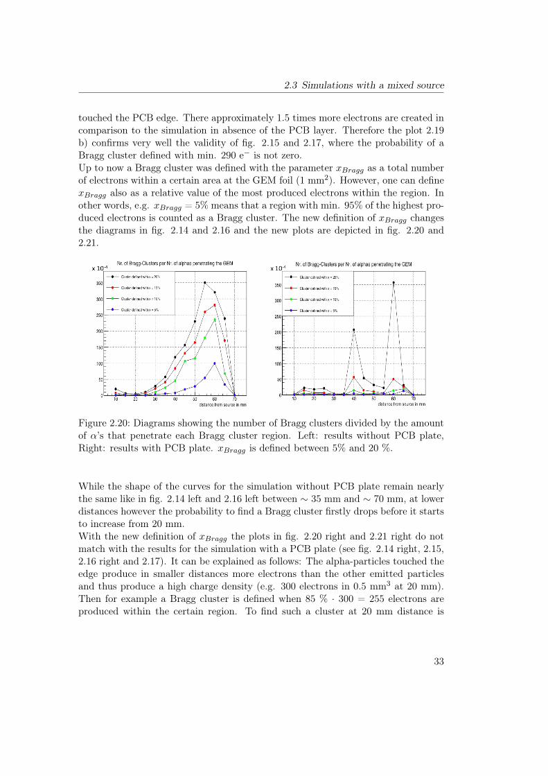
touched the PCB edge. There approximately 1.5 times more electrons are created incomparison to the simulation in absence of the PCB layer. Therefore the plot 2.19b) confirms very well the validity of fig. 2.15 and 2.17, where the probability of aBragg cluster defined with min. 290 e− is not zero.Up to now a Bragg cluster was defined with the parameter xBragg as a total numberof electrons within a certain area at the GEM foil (1 mm2). However, one can definexBragg also as a relative value of the most produced electrons within the region. Inother words, e.g. xBragg = 5% means that a region with min. 95% of the highest pro-duced electrons is counted as a Bragg cluster. The new definition of xBragg changesthe diagrams in fig. 2.14 and 2.16 and the new plots are depicted in fig. 2.20 and2.21.

Figure 2.20: Diagrams showing the number of Bragg clusters divided by the amountof α’s that penetrate each Bragg cluster region. Left: results without PCB plate,Right: results with PCB plate. xBragg is defined between 5% and 20 %.

While the shape of the curves for the simulation without PCB plate remain nearlythe same like in fig. 2.14 left and 2.16 left between ∼ 35 mm and ∼ 70 mm, at lowerdistances however the probability to find a Bragg cluster firstly drops before it startsto increase from 20 mm.With the new definition of xBragg the plots in fig. 2.20 right and 2.21 right do notmatch with the results for the simulation with a PCB plate (see fig. 2.14 right, 2.15,2.16 right and 2.17). It can be explained as follows: The alpha-particles touched theedge produce in smaller distances more electrons than the other emitted particlesand thus produce a high charge density (e.g. 300 electrons in 0.5 mm3 at 20 mm).Then for example a Bragg cluster is defined when 85 % · 300 = 255 electrons areproduced within the certain region. To find such a cluster at 20 mm distance is

33


extremely unlikely because most alpha-particles don’t reach the Bragg peak at 20mm to produce min. 250 electrons.

Figure 2.21: Diagrams showing the number of Bragg clusters divided by the totalnumber of events. Left: results without PCB plate, Right: results with PCB plate.xBragg is defined between 5% and 20 %.

Therefore the right plots in fig. 2.20 and 2.21 represent only the probability ofBragg clusters induced by alpha-particles touched the PCB edge. In order to get thefamiliar shape of the curves like in the other diagrams, the xBragg-parameter has tobe increased up to 30% or 40%.The large fluctuations and jumps in fig. 2.15, 2.17, 2.20 right and 2.21 right couldbe due to statistical nature. To avoid high statistical errors more amount of data isneeded, i.e. emitting more events into the active volume of the detector.

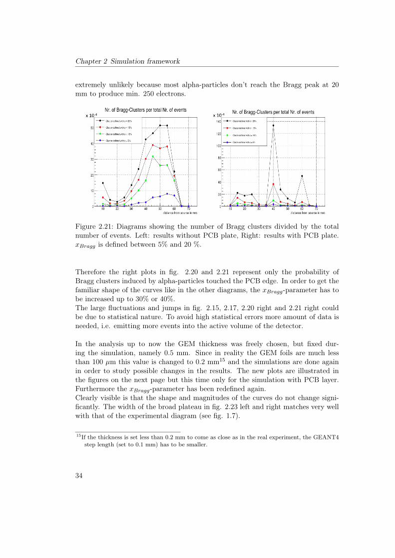
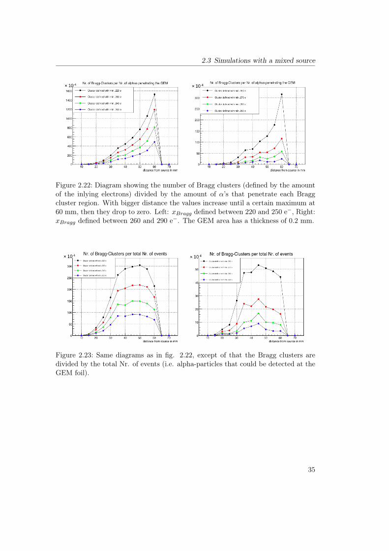
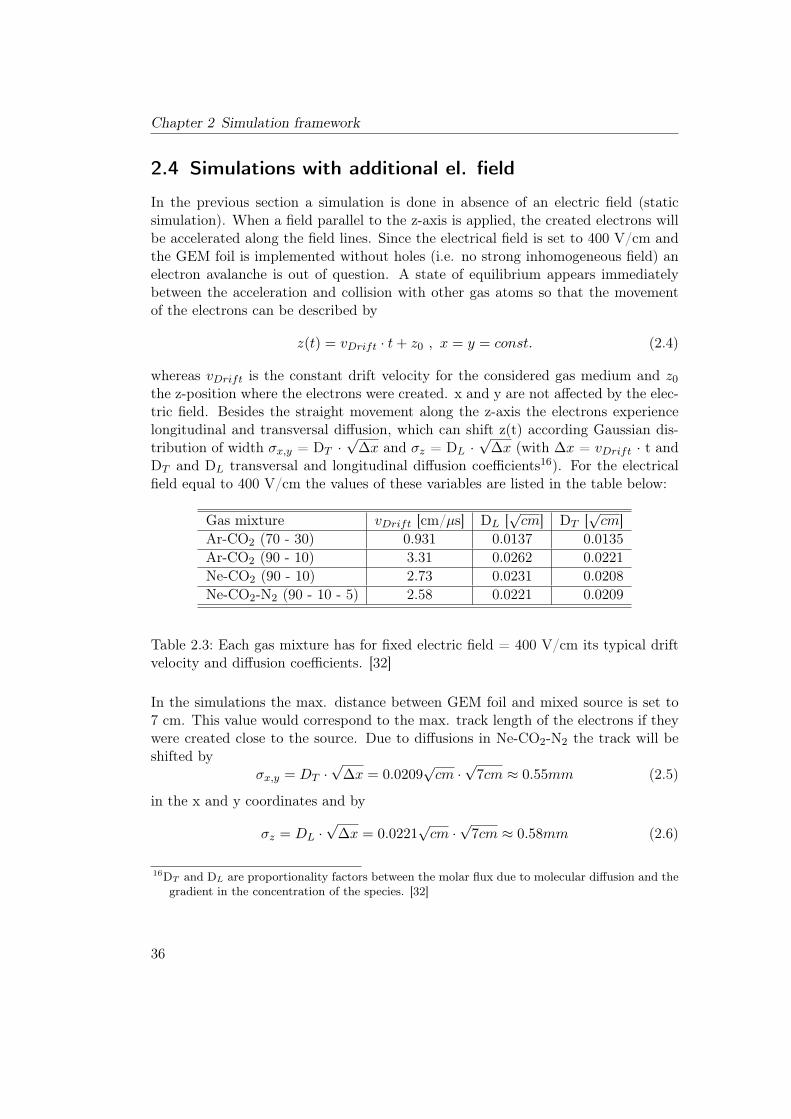
In the analysis up to now the GEM thickness was freely chosen, but fixed dur-ing the simulation, namely 0.5 mm. Since in reality the GEM foils are much lessthan 100 µm this value is changed to 0.2 mm15 and the simulations are done againin order to study possible changes in the results. The new plots are illustrated inthe figures on the next page but this time only for the simulation with PCB layer.Furthermore the xBragg-parameter has been redefined again.Clearly visible is that the shape and magnitudes of the curves do not change signi-ficantly. The width of the broad plateau in fig. 2.23 left and right matches very wellwith that of the experimental diagram (see fig. 1.7).

15If the thickness is set less than 0.2 mm to come as close as in the real experiment, the GEANT4step length (set to 0.1 mm) has to be smaller.

34


Figure 2.22: Diagram showing the number of Bragg clusters (defined by the amountof the inlying electrons) divided by the amount of α’s that penetrate each Braggcluster region. With bigger distance the values increase until a certain maximum at60 mm, then they drop to zero. Left: xBragg defined between 220 and 250 e−, Right:xBragg defined between 260 and 290 e−. The GEM area has a thickness of 0.2 mm.

Figure 2.23: Same diagrams as in fig. 2.22, except of that the Bragg clusters aredivided by the total Nr. of events (i.e. alpha-particles that could be detected at theGEM foil).

35


2.4 Simulations with additional el. field

In the previous section a simulation is done in absence of an electric field (staticsimulation). When a field parallel to the z-axis is applied, the created electrons willbe accelerated along the field lines. Since the electrical field is set to 400 V/cm andthe GEM foil is implemented without holes (i.e. no strong inhomogeneous field) anelectron avalanche is out of question. A state of equilibrium appears immediatelybetween the acceleration and collision with other gas atoms so that the movementof the electrons can be described by

z(t) = vDrift · t+ z0 , x = y = const. (2.4)

whereas vDrift is the constant drift velocity for the considered gas medium and z0the z-position where the electrons were created. x and y are not affected by the elec-tric field. Besides the straight movement along the z-axis the electrons experiencelongitudinal and transversal diffusion, which can shift z(t) according Gaussian dis-tribution of width σx,y = DT ·

√∆x and σz = DL ·

√∆x (with ∆x = vDrift · t and

DT and DL transversal and longitudinal diffusion coefficients16). For the electricalfield equal to 400 V/cm the values of these variables are listed in the table below:

Gas mixture vDrift [cm/µs] DL [√cm] DT [

√cm]

Ar-CO2 (70 - 30) 0.931 0.0137 0.0135Ar-CO2 (90 - 10) 3.31 0.0262 0.0221Ne-CO2 (90 - 10) 2.73 0.0231 0.0208Ne-CO2-N2 (90 - 10 - 5) 2.58 0.0221 0.0209

Table 2.3: Each gas mixture has for fixed electric field = 400 V/cm its typical driftvelocity and diffusion coefficients. [32]

In the simulations the max. distance between GEM foil and mixed source is set to7 cm. This value would correspond to the max. track length of the electrons if theywere created close to the source. Due to diffusions in Ne-CO2-N2 the track will beshifted by

σx,y = DT ·√

∆x = 0.0209√cm ·

√7cm ≈ 0.55mm (2.5)

in the x and y coordinates and by

σz = DL ·√

∆x = 0.0221√cm ·

√7cm ≈ 0.58mm (2.6)

16DT and DL are proportionality factors between the molar flux due to molecular diffusion and thegradient in the concentration of the species. [32]

36


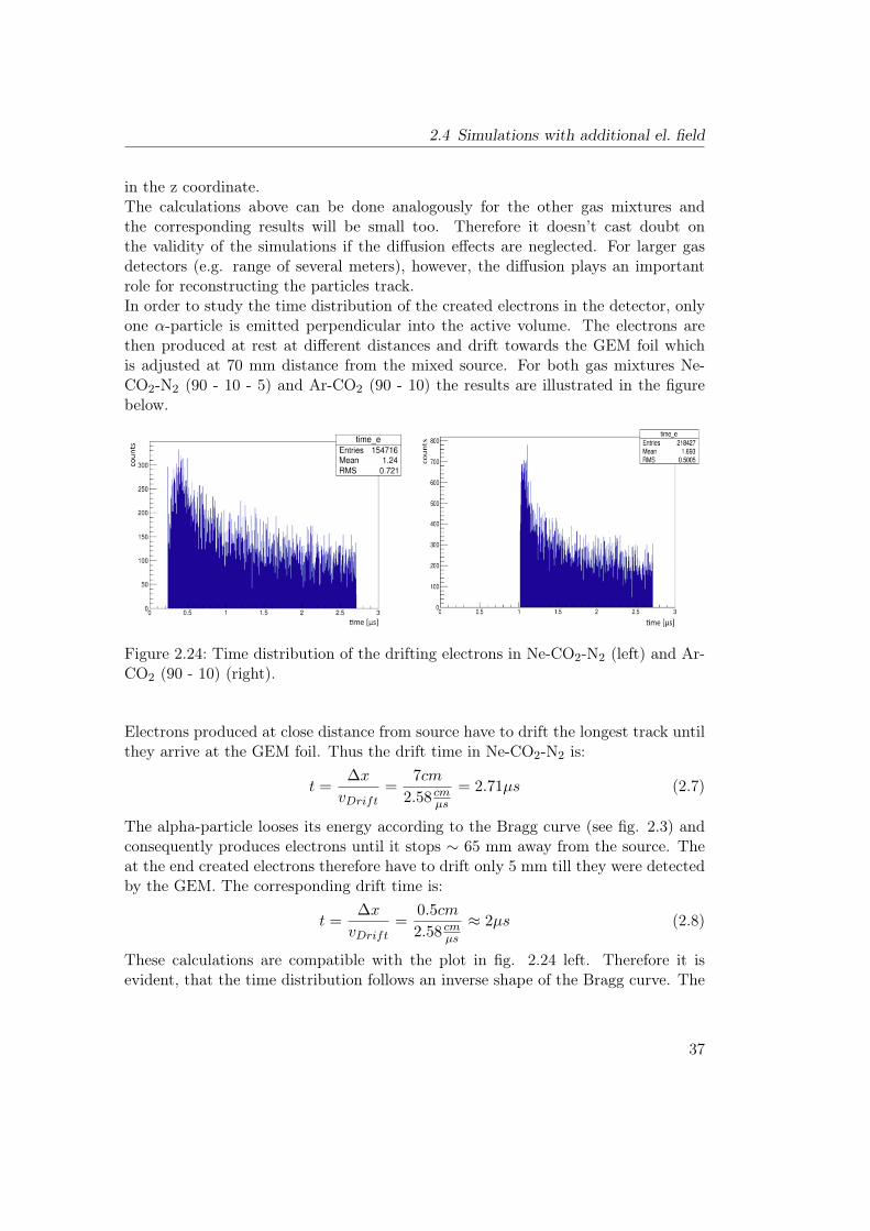
in the z coordinate.The calculations above can be done analogously for the other gas mixtures andthe corresponding results will be small too. Therefore it doesn’t cast doubt onthe validity of the simulations if the diffusion effects are neglected. For larger gasdetectors (e.g. range of several meters), however, the diffusion plays an importantrole for reconstructing the particles track.In order to study the time distribution of the created electrons in the detector, onlyone α-particle is emitted perpendicular into the active volume. The electrons arethen produced at rest at different distances and drift towards the GEM foil whichis adjusted at 70 mm distance from the mixed source. For both gas mixtures Ne-CO2-N2 (90 - 10 - 5) and Ar-CO2 (90 - 10) the results are illustrated in the figurebelow.

Figure 2.24: Time distribution of the drifting electrons in Ne-CO2-N2 (left) and Ar-CO2 (90 - 10) (right).

Electrons produced at close distance from source have to drift the longest track untilthey arrive at the GEM foil. Thus the drift time in Ne-CO2-N2 is:

t =∆x

vDrift=

7cm

2.58 cmµs= 2.71µs (2.7)

The alpha-particle looses its energy according to the Bragg curve (see fig. 2.3) andconsequently produces electrons until it stops ∼ 65 mm away from the source. Theat the end created electrons therefore have to drift only 5 mm till they were detectedby the GEM. The corresponding drift time is:

t =∆x

vDrift=

0.5cm

2.58 cmµs≈ 2µs (2.8)

These calculations are compatible with the plot in fig. 2.24 left. Therefore it isevident, that the time distribution follows an inverse shape of the Bragg curve. The

37


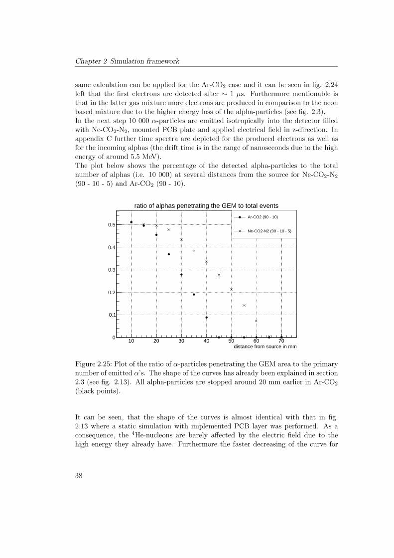
same calculation can be applied for the Ar-CO2 case and it can be seen in fig. 2.24left that the first electrons are detected after ∼ 1 µs. Furthermore mentionable isthat in the latter gas mixture more electrons are produced in comparison to the neonbased mixture due to the higher energy loss of the alpha-particles (see fig. 2.3).In the next step 10 000 α-particles are emitted isotropically into the detector filledwith Ne-CO2-N2, mounted PCB plate and applied electrical field in z-direction. Inappendix C further time spectra are depicted for the produced electrons as well asfor the incoming alphas (the drift time is in the range of nanoseconds due to the highenergy of around 5.5 MeV).The plot below shows the percentage of the detected alpha-particles to the totalnumber of alphas (i.e. 10 000) at several distances from the source for Ne-CO2-N2

(90 - 10 - 5) and Ar-CO2 (90 - 10).


0

0.1

0.2

0.3

0.4

0.5

Ar-CO2 (90 - 10)

Ne-CO2-N2 (90 - 10 - 5)

ratio of alphas penetrating the GEM to total events

Figure 2.25: Plot of the ratio of α-particles penetrating the GEM area to the primarynumber of emitted α’s. The shape of the curves has already been explained in section2.3 (see fig. 2.13). All alpha-particles are stopped around 20 mm earlier in Ar-CO2

(black points).

It can be seen, that the shape of the curves is almost identical with that in fig.2.13 where a static simulation with implemented PCB layer was performed. As aconsequence, the 4He-nucleons are barely affected by the electric field due to thehigh energy they already have. Furthermore the faster decreasing of the curve for

38


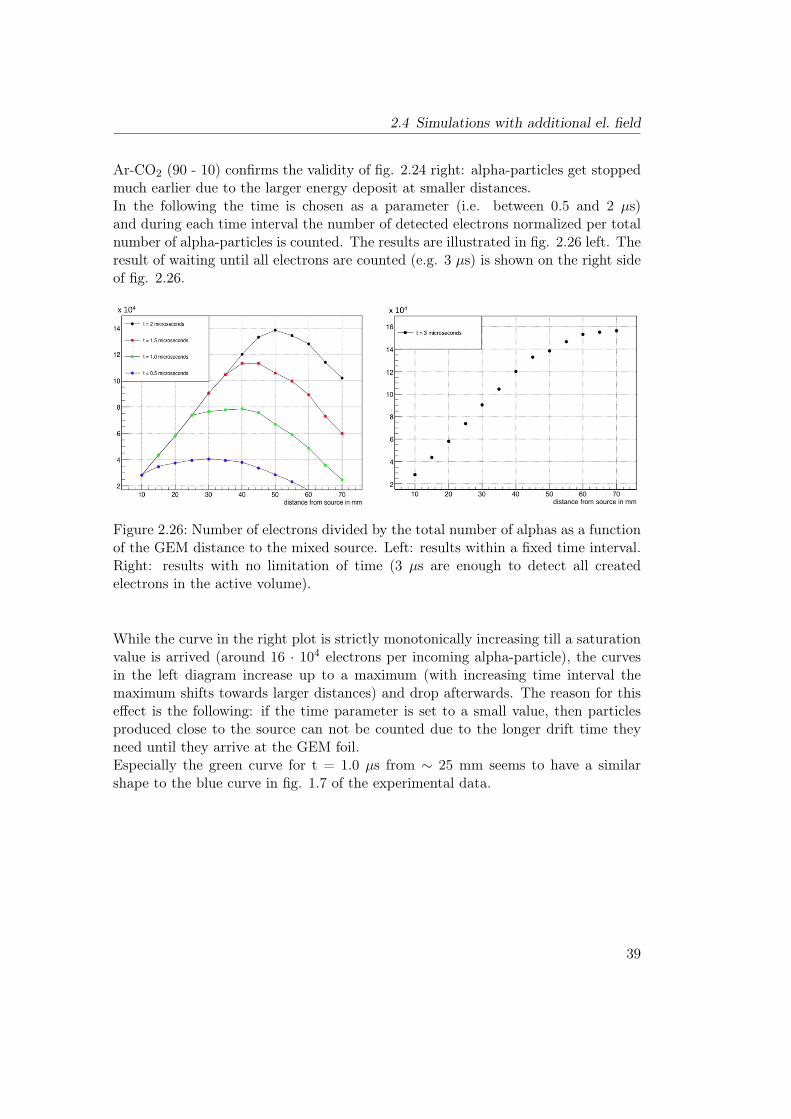
Ar-CO2 (90 - 10) confirms the validity of fig. 2.24 right: alpha-particles get stoppedmuch earlier due to the larger energy deposit at smaller distances.In the following the time is chosen as a parameter (i.e. between 0.5 and 2 µs)and during each time interval the number of detected electrons normalized per totalnumber of alpha-particles is counted. The results are illustrated in fig. 2.26 left. Theresult of waiting until all electrons are counted (e.g. 3 µs) is shown on the right sideof fig. 2.26.

Figure 2.26: Number of electrons divided by the total number of alphas as a functionof the GEM distance to the mixed source. Left: results within a fixed time interval.Right: results with no limitation of time (3 µs are enough to detect all createdelectrons in the active volume).

While the curve in the right plot is strictly monotonically increasing till a saturationvalue is arrived (around 16 · 104 electrons per incoming alpha-particle), the curvesin the left diagram increase up to a maximum (with increasing time interval themaximum shifts towards larger distances) and drop afterwards. The reason for thiseffect is the following: if the time parameter is set to a small value, then particlesproduced close to the source can not be counted due to the longer drift time theyneed until they arrive at the GEM foil.Especially the green curve for t = 1.0 µs from ∼ 25 mm seems to have a similarshape to the blue curve in fig. 1.7 of the experimental data.

39

Chapter 3

Comparison to the experimental dataand outlook

The aim of the bachelor thesis was to connect the discharge probability revealed inthe R&D experimental setup shown in fig. 1.7 with the charge density in a singleGEM based detector simulated with GEANT4.After the implementation of the detector with similar size to the experimentalprototype detector, the first simulations were done with a point like source withoutelectric field in order to have a reference to the further analysis and to study thebehavior of the alpha-particles in the gas volume together with the produced elec-trons.Since high electron densities created in a small region in the GEM area could causean electrical discharge (charge density hypothesis, see section 2.1), Bragg clusterswere defined and the probability to find such a cluster per incoming alpha-particlewas studied at different GEM distances. The corresponding diagram is illustrated infig. 2.11. The shape of the curves seem to have a similarity with the experimentallydetermined blue curve in fig. 1.7. However, at low distances from the source as wellas from 55 mm the values are completely different with the observed values fromthe experiment.To come closer to the experimental setup, the point like source was replaced bythe same mixed source used in the experiment. Simulations were performed inabsence of the PCB plate (see fig. 2.16) as well as with the plate implemented (seefig. 2.16). By comparing both plots one can see that the PCB layer increases theBragg cluster probability and thus the probability to find a high charge density ata certain distance. Furthermore the maxima are shifted around 15 mm towards themixed source and the plateaus are more broaden too. In contrary to the plot of thepoint like source, this simulation shows that Bragg clusters can occur at 55 or 60mm which are conform with the experiment (i.e. the discharge probability at thesedistances is not zero).Still the falling edge at around 10 mm can not be explained, but by redefining theBragg cluster (see section 2.3) the simulation yields the result shown in fig. 2.21left where a minimum at ∼ 20 mm can be seen. Since the PCB plate seems to shift

41

Chapter 3 Comparison to the experimental data and outlook

the Bragg cluster curves between 10 and 15 mm, it could move the minimum tothe appropriate position. To verify it, the same plot as in fig. 2.21 right has to beperformed but with lower values for xBragg.Changing the thickness of the GEM from 0.5 mm to 0.2 mm doesn’t change theshape of the other results significantly. Since the experimental data has been takenof a detector with applied electrical field of 400 V/cm, also a dynamic GEANT4simulation has been performed and the corresponding results were illustrated infig. 2.26. Setting limitations on the time interval, the curves are bend and form amaximum with a broad plateau as in the previous results with the additional effectthat electrons now are also been counted at 70 mm.

In the simulated plots a dependence between the discharge probability and thecharge density could be observed. In order to obtain the Bragg cluster shape closerto the curve from the experimental setup, the GEM foil has to be implemented withholes and additional inhomogeneous electric field to increase the gain. A next stepcould be to improve the plots for the Bragg cluster probability by inserting error barswhich give the opportunity to describe the behavior of the experimental results moreprecisely. Furthermore instead of a single GEM foil a triple GEM stack with samedimensions has to be implemented to come as close as possible to the experimentalsetup. Then the charge densities in the simulation have to be investigated again toobtain a proper insight into the phenomena of electrical discharges in GEM baseddetectors.

42

43

Appendix A Principal difference between GEM TPC and wire TPC

Appendix A

Principal difference between GEM TPCand wire TPC

Figure A.1: A major difference between the formed signal in a GEM-TPC (left fig.)and a conventional MWPC-TPC (right fig.): While a wire TPC induces a wide signalon the underlying pads, the signal width of a GEM-TPC is only given by transversediffusion parameters. These coefficients can be held rather small by applying amagnetic field. [33]44

Appendix B

2D simulated plots

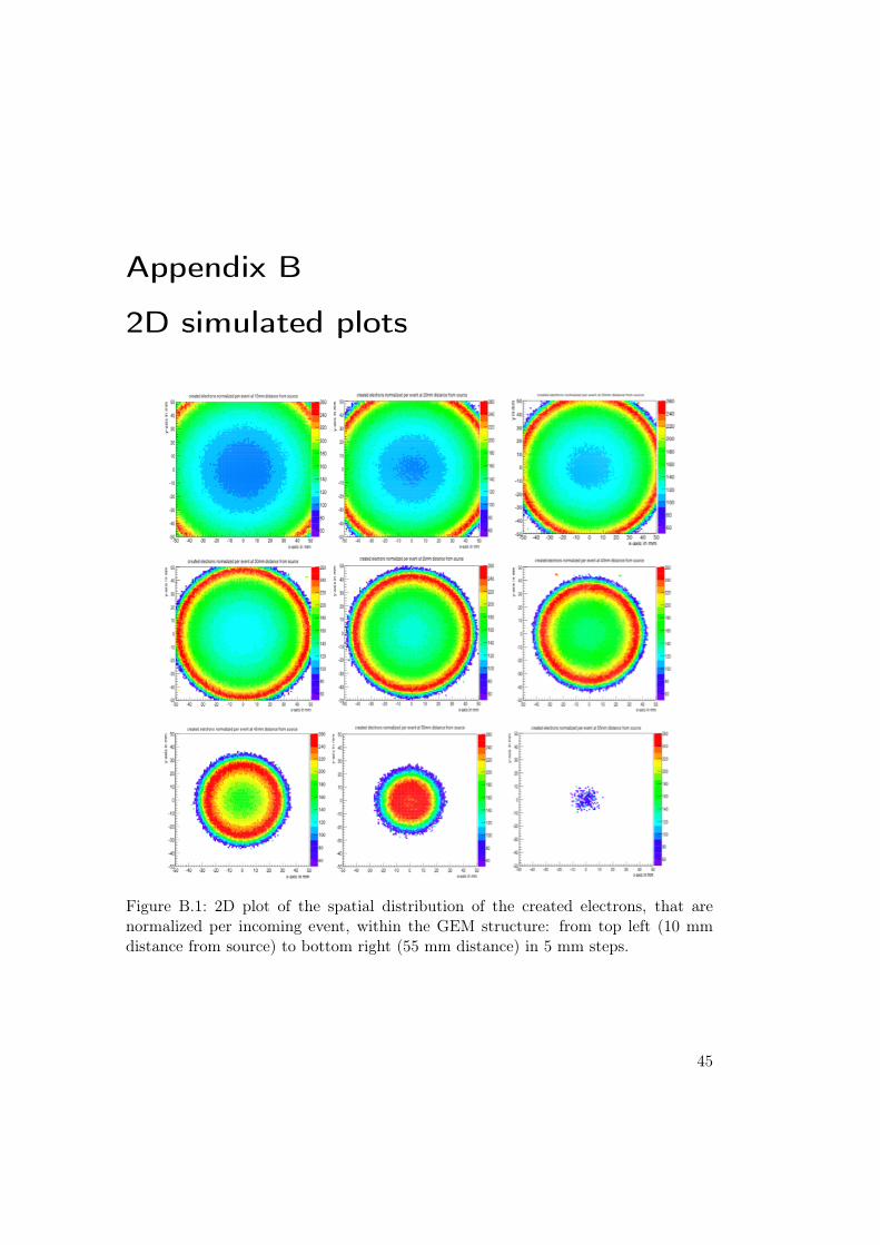
Figure B.1: 2D plot of the spatial distribution of the created electrons, that arenormalized per incoming event, within the GEM structure: from top left (10 mmdistance from source) to bottom right (55 mm distance) in 5 mm steps.

45

47

Appendix C Time results of the analysis with el. field

Appendix C

Time results of the analysis with el.field

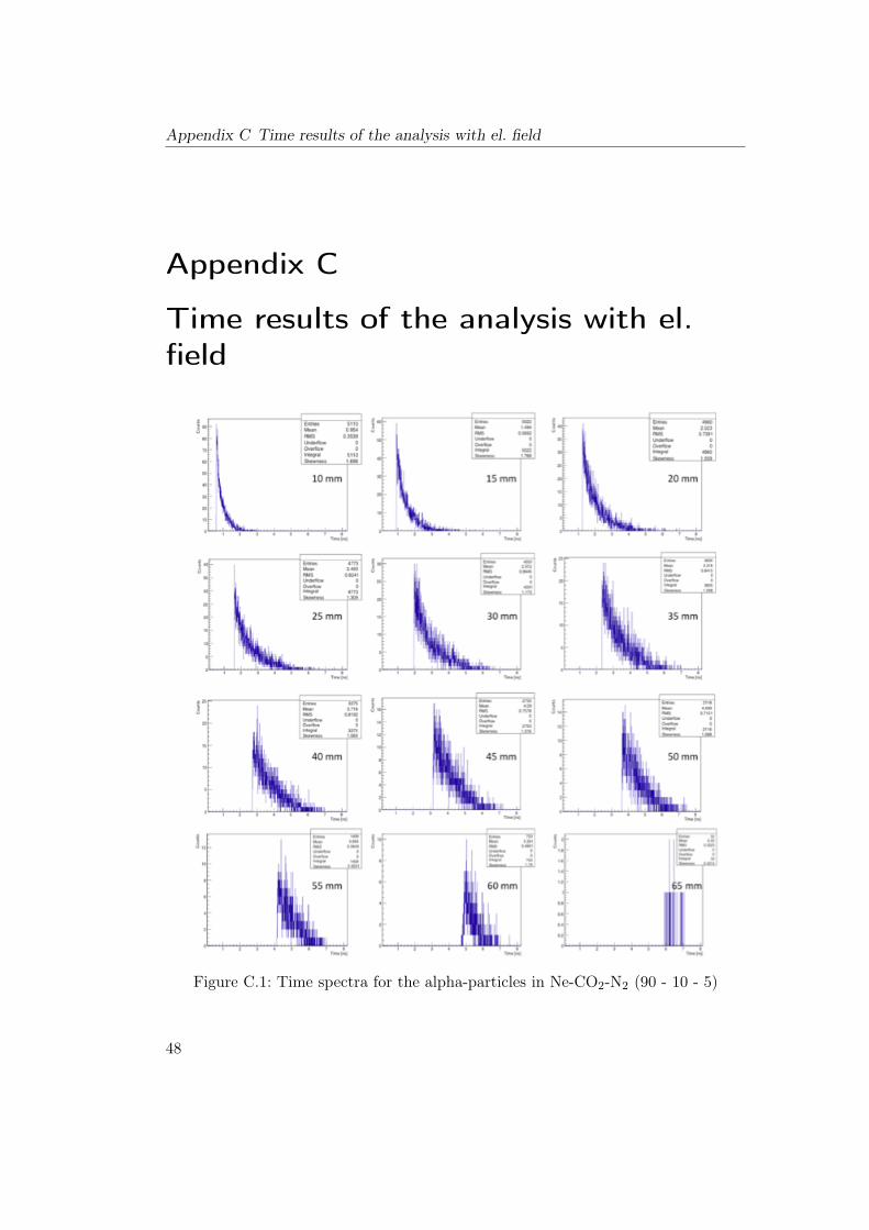
Figure C.1: Time spectra for the alpha-particles in Ne-CO2-N2 (90 - 10 - 5)

48

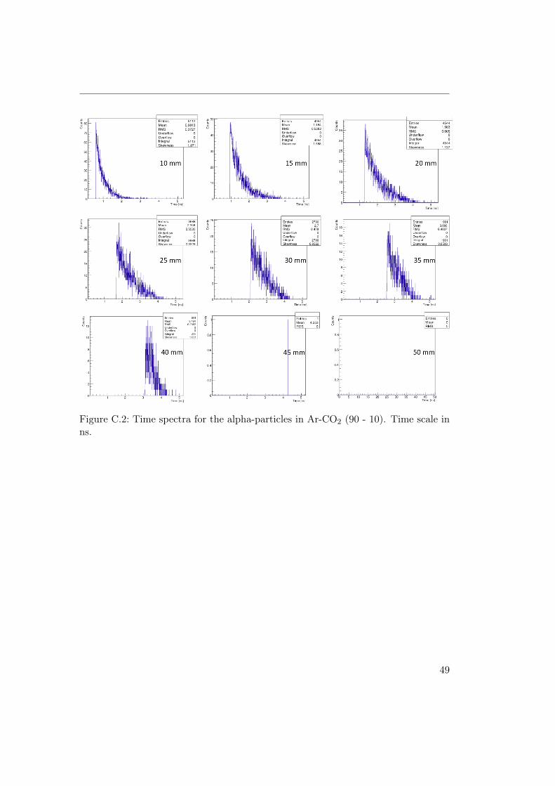
Figure C.2: Time spectra for the alpha-particles in Ar-CO2 (90 - 10). Time scale inns.

49

Appendix C Time results of the analysis with el. field

!

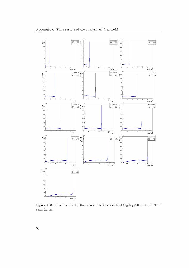
Figure C.3: Time spectra for the created electrons in Ne-CO2-N2 (90 - 10 - 5). Timescale in µs.

50

Bibliography

[1] P. N. Murgatroyd. Theory of space-charge-limited current enhanced by Frenkeleffect. Vol. Volume 3. 1970.

[2] ALICE Collaboration. Nucl. Instr. and Meth. 316 A 622. 2010.

[3] L. Cifarelli. The Quark-Gluon Plasma, a nearly perfect fluid. Europhys. News,2012.

[4] ALICE Collaboration. 5. September 2015. url: http://aliceinfo.cern.ch/Public/en/Chapter2/Chap2_HLT.html.

[5] ALICE Collaboration. Journal of Instrumentation 3. S08002, 2008.

[6] M. Ball; F.V. Bohmer; S. Dorheim; C. Hoppner; B. Ketzer. Technical DesignStudy for the PANDA Time Projection Chamber. 2012.

[7] K. Aamodt; A. Abrahantes Quintina; R. Achenbach. The ALICE experimentat the CERN LHC. Journal of Instrumentation 3, 2008.

[8] C. Garabatos. Nucl. Instr. and Meth. A 535, 197. 2004.

[9] W. Blum; W. Riegler; L. Rolandi. Particle Detection with Drift Chambers.Springer-Verlag, 2008.

[10] ALICE@CERN. 5. September 2015. url: http : / / aliceinfo . cern .ch/TPC/node/8.

[11] G. Knoll. Radiation Detection and Measurement. 2nd ed. New York: Wiley,1989.

[12] KIP Uni-Heidelberg. 6. September 2015. url: http : / / www . kip .uni - heidelberg . de/ ~coulon/ Lectures/ DetectorsSoSe10/ Free _PDFs/Lecture8.pdf.

[13] Z. Qiushi; Y. Kun; L. Yanye. Progress in the Development of CdZnTe UnipolarDetectors for Different Anode Geometries and Data Corrections. Sensors 2013,13(2), 2447-2474, 2013.

[14] N. Marx; R. Nygren. TheTimeProjectionChamber. Phys.Today 31N10, 1978.

[15] H.J. Hilke. Time projection chambers. Rep. Prog. Phys., 73:116201, 2010.

[16] M. Titov. Gaseous Detectors: recent developments and applications. arXiv:1008.3736 [physics.ins-det], 2010.

51

http://aliceinfo.cern.ch/Public/en/Chapter2/Chap2_HLT.html

http://aliceinfo.cern.ch/Public/en/Chapter2/Chap2_HLT.html

http://aliceinfo.cern.ch/TPC/node/8

http://aliceinfo.cern.ch/TPC/node/8

http://www.kip.uni-heidelberg.de/~coulon/Lectures/DetectorsSoSe10/Free_PDFs/Lecture8.pdf



[17] A. Oed. Nucl. Instrum. Methods A 490, 223, 2002.

[18] C. Altunbas. Nucl. Instr. and Meth. A 490. 2002.

[19] F. Sauli. Nucl. Instrum. Methods. A 386 . 531, 1997.

[20] B. Azmoun; W. Anderson; D. Crary; J. Durham; T. Hemmick; A Study of GainStability and Charging Effects in GEM Foils. IEEE Nuclear Science SymposiumConference Record, 2006.

[21] S. Bachmann. Nucl. Instrum. Methods A 479. 2002.

[22] C.H. Hahn; I. Kim; W. Kim; J. Yu. Apparatus for digital imaging photodetectorusing gas electron multiplier. 2010.

[23] S. Blatt. Nucl. Phys. B (Proc. Suppl.) 150. 2006.

[24] Yu. Ivanuouchenkov. Nucl. Instr. and Meth. A 422. 300, 1999.

[25] H. Raether. Electron avalanches and breakdown in gases. Butterworths, 1964.

[26] S. Procureur; J. Ball; P. Konczykowski; B. Moreno; H. Moutarde; F. Sabatie.A Geant4-based study on the origin of the sparks in a Micromegas detector andestimate of the spark probability with hadron beams. Nuclear Instruments andMethods in Physics Research A 621 177–183, 2010.

[27] ALICE Collaboration. Addendum to the Technical Design Report for the Up-grade of the ALICE Time Projection Chamber. ALICE-TDR-016-ADD-1, 2015.

[28] Geant4 Collaboration. Geant4 User’s Guide for Application Developers. 2009.

[29] UMI. Studies on Irradiation Effects of Silicon-on-sapphire Devices. ProQuestLLC, 2008.

[30] Eckert Ziegler. Calibration Standards and Instruments. RD1, 2009.

[31] H. Bethe. Annalen der Physik. 397, 325, 1930.

[32] ALICE Collaboration. Technical Design report for the Upgrade of the ALICETime Projection Chamber. ALICE-TDR-016. CERN-LHCC-2013-020, 2014.

[33] A Time Projection Chamber with Gas Electron Multipliers for the TESLADetector. 8. September 2015. url: http://www-ekp.physik.uni-karlsruhe.de/~ilctpc/GEM-TPC/triplegem.gif.

52

http://www-ekp.physik.uni-karlsruhe.de/~ilctpc/GEM-TPC/triplegem.gif

http://www-ekp.physik.uni-karlsruhe.de/~ilctpc/GEM-TPC/triplegem.gif

Acknowledgements

First of all I want to thank Prof. Laura Fabbietti to make this thesis possible. Iam deeply grateful for her guidance, encouragement and patience over the last fewmonths. Thank you so much for your outstanding knowledge in experimental physics,for looking at my work in different ways and for opening my mind.I would like to express the deepest appreciation to Dr. Piotr Gasik for helping mein any situation and taking time to talk with me on many occasions. I would like tothank him for providing indispensable advice, information and support on differentaspects of my project. It was a pleasure for me to take part in his lecture gaseousdetectors and to learn the physics behind my work.Also I would like to offer my special thank to Tobias Kunz for his incredible helpwith software problems of any kind, for his awesome support and the very fruitfuldiscussions we had. I appreciate the feedback and support offered by Dr. RobertMünzer and want to thank him also for teaching me a lot in the lecture gaseousdetectors.Of course I want to thank the people I love, my parents and my siblings for theiroutstanding motivating words and great support. At last I want to thank JenniferPadberg for her awesome support even though she was also busy with her ownbachelor thesis.

53

Documents

Geant4 Simulation eines auf GEM basierten Detektors