Embed Size (px)
Citation preview

Globalization, income distributionand voter preferences:
Transmission mechanisms andreform acceptance
Inauguraldissertation zur Erlangung des Doktorgrades im
Fachbereich Wirtschaftswissenschaften der Universitat Mannheim
Tanja Hennighausen

Abteilungssprecher: Prof. Dr. Eckhard Janeba
Referent: Prof. Dr. Roland Vaubel
Korreferent: PD. Dr. Friedrich Heinemann
Tag der mundlichen Prufung: 04. Marz 2014

Preface
First of all, I would like to thank Prof. Dr. Roland Vaubel for the opportunity
to start my dissertation at his chair. I appreciate that he gave me the necessary
freedom to work on my different research projects. I also wish to thank PD Dr.
Friedrich Heinemann for his immediate willingness to co-supervise my thesis.
This thesis has been completed during my work at the Centre for European
Economic Research (ZEW) and the Department of Economics at the University of
Mannheim. I had several colleagues who contributed much to the success of my
research. In particular, I would like to thank my co-authors Friedrich Heinemann,
Ivo Bischoff and Marc-Daniel Moessinger for the fruitful cooperation. I also thank
Katharina Finke for her continuous support during the whole dissertation process
and her helpful advice.
I am also indebted to many former and current colleagues at the ZEW and at the
University for the pleasant work environment, inspiring discussions, numerous lunch
and coffee breaks, evening activities and trips to the surroundings of Mannheim. I
very much enjoyed spending the time with you.
Special thanks go to my family and friends for providing distraction and for
keeping me in good humor. Moreover, I thank my sister-in-law Barbara for proof-
reading large parts of this thesis. Last but not least, I am deeply grateful to my
parents and my brother Axel for their unconditional support and their confidence
in me.
III

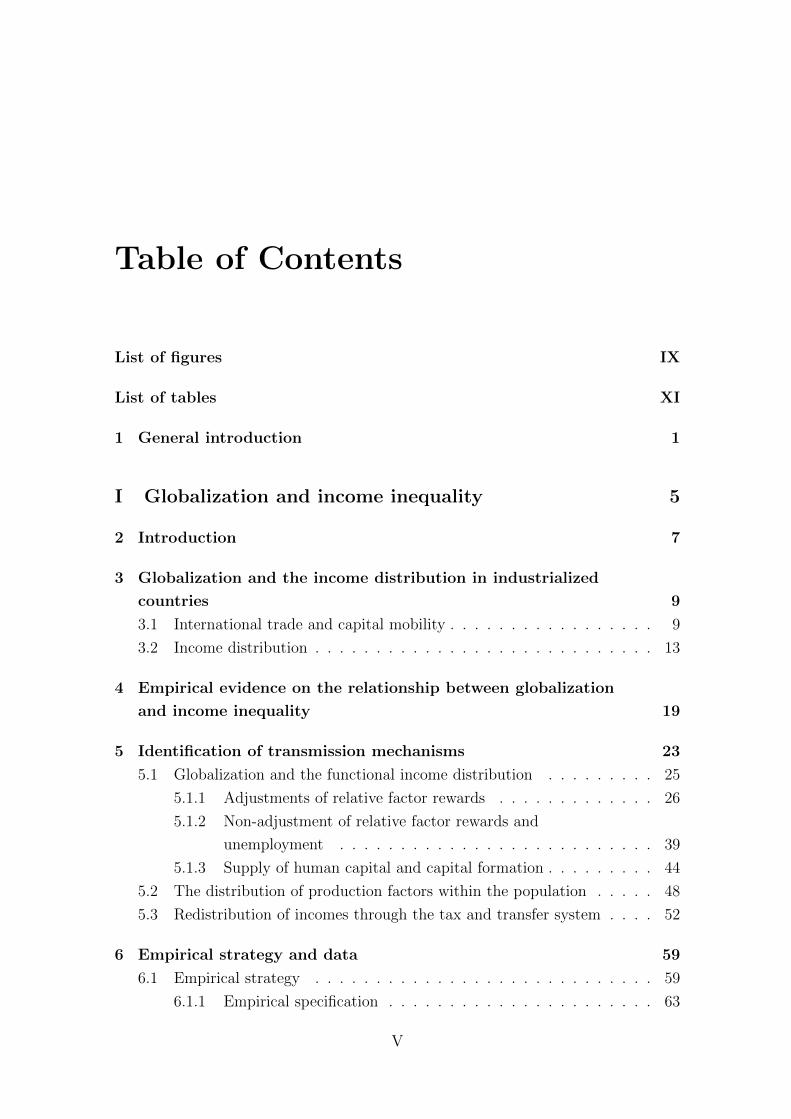
Table of Contents
List of figures IX
List of tables XI
1 General introduction 1
I Globalization and income inequality 5
2 Introduction 7
3 Globalization and the income distribution in industrialized
countries 9
3.1 International trade and capital mobility . . . . . . . . . . . . . . . . . 9
3.2 Income distribution . . . . . . . . . . . . . . . . . . . . . . . . . . . . 13
4 Empirical evidence on the relationship between globalization
and income inequality 19
5 Identification of transmission mechanisms 23
5.1 Globalization and the functional income distribution . . . . . . . . . 25
5.1.1 Adjustments of relative factor rewards . . . . . . . . . . . . . 26
5.1.2 Non-adjustment of relative factor rewards and
unemployment . . . . . . . . . . . . . . . . . . . . . . . . . . 39
5.1.3 Supply of human capital and capital formation . . . . . . . . . 44
5.2 The distribution of production factors within the population . . . . . 48
5.3 Redistribution of incomes through the tax and transfer system . . . . 52
6 Empirical strategy and data 59
6.1 Empirical strategy . . . . . . . . . . . . . . . . . . . . . . . . . . . . 59
6.1.1 Empirical specification . . . . . . . . . . . . . . . . . . . . . . 63
V
VI TABLE OF CONTENTS
6.1.2 Expected influence of globalization-induced changes of the
transmission mechanisms . . . . . . . . . . . . . . . . . . . . . 68
6.2 Data . . . . . . . . . . . . . . . . . . . . . . . . . . . . . . . . . . . . 69
6.2.1 Data on income distribution . . . . . . . . . . . . . . . . . . . 69
6.2.2 Data on transmission mechanisms . . . . . . . . . . . . . . . . 73
6.2.3 Globalization data . . . . . . . . . . . . . . . . . . . . . . . . 76
6.2.4 Control variables . . . . . . . . . . . . . . . . . . . . . . . . . 77
7 Results 81
7.1 Globalization and labor market outcomes . . . . . . . . . . . . . . . . 81
7.1.1 Main results . . . . . . . . . . . . . . . . . . . . . . . . . . . . 82
7.1.2 Interdependence between globalization and labor market
institutions . . . . . . . . . . . . . . . . . . . . . . . . . . . . 99
7.1.3 Robustness checks . . . . . . . . . . . . . . . . . . . . . . . . 107
7.2 Labor market outcomes and the distribution of incomes . . . . . . . . 128
8 Quantification of the relative effects of the transmission
mechanisms 137
9 Conclusion 143
II Policy preferences of German voters 147
10 Introduction 149
11 Preferences toward progressive taxation 153
11.1 Introduction . . . . . . . . . . . . . . . . . . . . . . . . . . . . . . . . 153
11.2 Attitudes toward progressive taxation within the German
population . . . . . . . . . . . . . . . . . . . . . . . . . . . . . . . . . 155
11.3 Potential determinants of individual attitudes toward progressive
taxation . . . . . . . . . . . . . . . . . . . . . . . . . . . . . . . . . . 158
11.4 Econometric analysis . . . . . . . . . . . . . . . . . . . . . . . . . . . 166
11.4.1 Main results . . . . . . . . . . . . . . . . . . . . . . . . . . . . 166
11.4.2 Robustness of the results . . . . . . . . . . . . . . . . . . . . . 170
11.5 Conclusion . . . . . . . . . . . . . . . . . . . . . . . . . . . . . . . . . 182
12 Labor market policy preferences 183
12.1 Introduction . . . . . . . . . . . . . . . . . . . . . . . . . . . . . . . . 183
12.2 Labor market preferences of German voters . . . . . . . . . . . . . . . 184
TABLE OF CONTENTS VII
12.3 Potential determinants of individual labor market policy preferences . 186
12.4 Econometric analysis . . . . . . . . . . . . . . . . . . . . . . . . . . . 192
12.4.1 Main results . . . . . . . . . . . . . . . . . . . . . . . . . . . . 195
12.4.2 Results for specific labor market policies . . . . . . . . . . . . 196
12.5 Conclusion . . . . . . . . . . . . . . . . . . . . . . . . . . . . . . . . . 207
13 Pension reform preferences 209
13.1 Introduction . . . . . . . . . . . . . . . . . . . . . . . . . . . . . . . . 209
13.2 Literature survey . . . . . . . . . . . . . . . . . . . . . . . . . . . . . 210
13.2.1 Pension reform preferences . . . . . . . . . . . . . . . . . . . . 210
13.2.2 Intrinsic motivation . . . . . . . . . . . . . . . . . . . . . . . . 212
13.3 Theoretical expectations . . . . . . . . . . . . . . . . . . . . . . . . . 213
13.4 Data . . . . . . . . . . . . . . . . . . . . . . . . . . . . . . . . . . . . 217
13.5 Econometric analysis . . . . . . . . . . . . . . . . . . . . . . . . . . . 219
13.6 Robustness of the results . . . . . . . . . . . . . . . . . . . . . . . . . 227
13.6.1 Physical job stress . . . . . . . . . . . . . . . . . . . . . . . . 227
13.6.2 Ideology, children, and age . . . . . . . . . . . . . . . . . . . . 228
13.6.3 Job match . . . . . . . . . . . . . . . . . . . . . . . . . . . . . 230
13.6.4 General reform inclination . . . . . . . . . . . . . . . . . . . . 230
13.7 Conclusion . . . . . . . . . . . . . . . . . . . . . . . . . . . . . . . . . 232
14 Television and individual belief formation 235
14.1 Introduction . . . . . . . . . . . . . . . . . . . . . . . . . . . . . . . . 235
14.2 Institutional background: television in the GDR . . . . . . . . . . . . 238
14.3 The role of Western television in belief formation . . . . . . . . . . . 240
14.4 Empirical strategy and data . . . . . . . . . . . . . . . . . . . . . . . 243
14.5 Econometric analysis . . . . . . . . . . . . . . . . . . . . . . . . . . . 250
14.6 Robustness and some further results . . . . . . . . . . . . . . . . . . . 256
14.6.1 Varying the control group . . . . . . . . . . . . . . . . . . . . 256
14.6.2 Alternative explanations . . . . . . . . . . . . . . . . . . . . . 258
14.6.3 Additional insights into the role of Western television . . . . . 263
14.7 Conclusion . . . . . . . . . . . . . . . . . . . . . . . . . . . . . . . . . 266
Bibliography 267
Appendices 289
A Globalization and income inequality 291
A.1 Data description and issues . . . . . . . . . . . . . . . . . . . . . . . 291

VIII TABLE OF CONTENTS
A.1.1 Measurement error . . . . . . . . . . . . . . . . . . . . . . . . 302
A.2 Robustness checks . . . . . . . . . . . . . . . . . . . . . . . . . . . . . 305
B Policy preferences of German voters 323
B.1 Data sources and definitions . . . . . . . . . . . . . . . . . . . . . . . 323
B.2 Additional information . . . . . . . . . . . . . . . . . . . . . . . . . . 333
List of Figures
3.1 Trade openness (1970-2009) . . . . . . . . . . . . . . . . . . . . . . . 10
3.2 Trade openness for goods and services (1970-2008) . . . . . . . . . . . 11
3.3 Imports from non-OECD countries (as a share of total imports,
1970-2012) . . . . . . . . . . . . . . . . . . . . . . . . . . . . . . . . . 11
3.4 Cross-border flows of private capital (as a share of GDP, 1975-2010) . 12
3.5 Net private capital imports (1975-2010) . . . . . . . . . . . . . . . . . 13
3.6 Distribution of disposable incomes (Gini coefficients, 1985-2005) . . . 15
3.7 Distribution of market and disposable incomes and redistribution
(Gini coefficients, mid-2000s) . . . . . . . . . . . . . . . . . . . . . . . 16
3.8 Development of income inequality (average annual changes in
Gini-coefficients, 1985-2010) . . . . . . . . . . . . . . . . . . . . . . . 18
5.1 Globalization and income distribution: identification of transmission
mechanisms . . . . . . . . . . . . . . . . . . . . . . . . . . . . . . . . 24
5.2 Consequences of capital mobility . . . . . . . . . . . . . . . . . . . . 35
5.3 Determination of relative wages based on a demand and supply
framework . . . . . . . . . . . . . . . . . . . . . . . . . . . . . . . . . 46
5.4 Share of different income sources in total income . . . . . . . . . . . . 49
6.1 Relationship between globalization and the transmission
mechanisms . . . . . . . . . . . . . . . . . . . . . . . . . . . . . . . . 61
6.2 Relationship between the transmission mechanisms and the personal
distribution of incomes . . . . . . . . . . . . . . . . . . . . . . . . . . 62
7.1 Labor income share: exclusion of countries and time periods . . . . . 125
7.2 Wage dispersion: exclusion of countries and time periods . . . . . . . 125
7.3 Unemployment rate: exclusion of countries and time periods . . . . . 126
7.4 Relative human capital supply: exclusion of countries and
time periods . . . . . . . . . . . . . . . . . . . . . . . . . . . . . . . . 126
IX

X LIST OF FIGURES
7.5 Relative income unemployed: exclusion of countries and
time periods . . . . . . . . . . . . . . . . . . . . . . . . . . . . . . . . 127
8.1 Globalization and its impact on the income distribution through the
transmission mechanisms . . . . . . . . . . . . . . . . . . . . . . . . . 138
11.1 Preferences on income tax share for high income people . . . . . . . . 156
12.1 Preferences for market oriented labor market policies . . . . . . . . . 186
14.1 West German television reception in the GDR . . . . . . . . . . . . . 239
List of Tables
6.1 Expected signs . . . . . . . . . . . . . . . . . . . . . . . . . . . . . . 68
6.2 Definition of income . . . . . . . . . . . . . . . . . . . . . . . . . . . 70
6.3 Summary statistics: main variables . . . . . . . . . . . . . . . . . . . 79
6.4 Correlations between main variables . . . . . . . . . . . . . . . . . . 80
7.1 Labor income share (pooled OLS) . . . . . . . . . . . . . . . . . . . . 84
7.2 Labor income share (FEM) . . . . . . . . . . . . . . . . . . . . . . . . 85
7.3 Wage dispersion (pooled OLS) . . . . . . . . . . . . . . . . . . . . . . 87
7.4 Wage dispersion (FEM) . . . . . . . . . . . . . . . . . . . . . . . . . 88
7.5 Unemployment rate (pooled OLS) . . . . . . . . . . . . . . . . . . . . 90
7.6 Unemployment rate (FEM) . . . . . . . . . . . . . . . . . . . . . . . 91
7.7 Relative supply of human capital (pooled OLS) . . . . . . . . . . . . 93
7.8 Relative supply of human capital (FEM) . . . . . . . . . . . . . . . . 94
7.9 Relative income of unemployed (pooled OLS) . . . . . . . . . . . . . 96
7.10 Relative income of unemployed (FEM) . . . . . . . . . . . . . . . . . 98
7.11 Labor income share: interaction globalization and labor market
regulation . . . . . . . . . . . . . . . . . . . . . . . . . . . . . . . . . 100
7.12 Wage dispersion: interaction globalization and labor market
regulation . . . . . . . . . . . . . . . . . . . . . . . . . . . . . . . . . 102
7.13 Unemployment rate: interaction globalization and labor market
regulation . . . . . . . . . . . . . . . . . . . . . . . . . . . . . . . . . 103
7.14 Relative supply of human capital: interaction globalization and labor
market regulation . . . . . . . . . . . . . . . . . . . . . . . . . . . . . 105
7.15 Relative income unemployed: interaction globalization and labor
market regulation . . . . . . . . . . . . . . . . . . . . . . . . . . . . . 106
7.16 Measurement of capital mobility: gross capital movements . . . . . . 109
7.17 Measurement of capital mobility: net exports of FDI capital . . . . . 110
7.18 Technological change versus globalization . . . . . . . . . . . . . . . . 112
XI
XII LIST OF TABLES
7.19 Relative supply of human capital: role of wage dispersion and
unemployment . . . . . . . . . . . . . . . . . . . . . . . . . . . . . . . 118
7.20 Seemingly unrelated regression: country and year fixed effects . . . . 120
7.21 Market income inequality (Gini coefficients) . . . . . . . . . . . . . . 130
7.22 Redistribution . . . . . . . . . . . . . . . . . . . . . . . . . . . . . . . 132
7.23 Disposable income inequality (Gini coefficient) . . . . . . . . . . . . . 134
8.1 Quantitative effect of globalization-induced changes in transmission
variables . . . . . . . . . . . . . . . . . . . . . . . . . . . . . . . . . . 142
11.1 International comparison of preferences for progressive taxation . . . 157
11.2 Sign expectations . . . . . . . . . . . . . . . . . . . . . . . . . . . . . 166
11.3 Descriptive statistics . . . . . . . . . . . . . . . . . . . . . . . . . . . 167
11.4 Determinants of German voters’ attitudes toward progressive
taxation . . . . . . . . . . . . . . . . . . . . . . . . . . . . . . . . . . 169
11.5 Robustness test: ordered Probit estimates . . . . . . . . . . . . . . . 172
11.6 Robustness test: different income groups and additional control
variables . . . . . . . . . . . . . . . . . . . . . . . . . . . . . . . . . . 174
11.7 Fairness considerations of low and high income individuals
(comparison of mean values) . . . . . . . . . . . . . . . . . . . . . . . 175
11.8 Robustness test: interaction between fairness considerations and
income . . . . . . . . . . . . . . . . . . . . . . . . . . . . . . . . . . . 178
11.9 Robustness test: equivalent household incomes . . . . . . . . . . . . . 180
11.10 Robustness test: sample split according to marital status . . . . . . . 181
12.1 Descriptive statistics . . . . . . . . . . . . . . . . . . . . . . . . . . . 194
12.2 Sign expectations . . . . . . . . . . . . . . . . . . . . . . . . . . . . . 195
12.3 Determinants of labor market policy preferences . . . . . . . . . . . . 198
12.4 Cutting social benefits . . . . . . . . . . . . . . . . . . . . . . . . . . 202
12.5 Cutting unemployment benefits . . . . . . . . . . . . . . . . . . . . . 203
12.6 Cutting subsidies to declining industries . . . . . . . . . . . . . . . . 204
12.7 Phasing out employment programs . . . . . . . . . . . . . . . . . . . 205
12.8 Liberalizing employment protection . . . . . . . . . . . . . . . . . . . 206
13.1 Descriptive statistics . . . . . . . . . . . . . . . . . . . . . . . . . . . 219
13.2 Preferences for a higher pension age . . . . . . . . . . . . . . . . . . . 221
13.3 Preferences for higher contributions . . . . . . . . . . . . . . . . . . . 222
13.4 Preferences for pension cuts . . . . . . . . . . . . . . . . . . . . . . . 223
13.5 Preferences for different pension reform options . . . . . . . . . . . . 225
LIST OF TABLES XIII
13.6 Predicted probabilities for intrinsic motivation and organizational
commitment . . . . . . . . . . . . . . . . . . . . . . . . . . . . . . . . 226
13.7 Robustness test: alternative explanations . . . . . . . . . . . . . . . . 229
13.8 Robustness test: placebo analysis . . . . . . . . . . . . . . . . . . . . 231
14.1 Self-reported frequency of watching West German television . . . . . 240
14.2 Descriptive statistics of the dependent variables . . . . . . . . . . . . 246
14.3 Electoral outcomes in the Reichstag election 1932 . . . . . . . . . . . 247
14.4 Comparison of GDR-districts . . . . . . . . . . . . . . . . . . . . . . 248
14.5 Internal and external migration in the GDR 1988/89 . . . . . . . . . 250
14.6 Effort pays off, GDR late 1980s . . . . . . . . . . . . . . . . . . . . . 251
14.7 Success in life is mainly a matter of luck, FRG 1994-99 . . . . . . . . 253
14.8 Luck matters for success (FRG 1994-99): interaction effects . . . . . . 255
14.9 Luck matters for success (FRG 1994-99): differential time trends
(balanced panel) . . . . . . . . . . . . . . . . . . . . . . . . . . . . . 256
14.10 Robustness test: different group of districts . . . . . . . . . . . . . . 258
14.11 Effort pays off (GDR, late 1980s): additional control variables . . . . 261
14.12 Luck matters for success (FRG 1994-99): additional control
variables . . . . . . . . . . . . . . . . . . . . . . . . . . . . . . . . . . 262
14.13 Attitudes toward the GDR and socialism, GDR, late 1980s . . . . . 264
14.14 Attitudes toward the GDR and happiness, FRG, 1990s . . . . . . . . 265
A.1 Variable description . . . . . . . . . . . . . . . . . . . . . . . . . . . . 292
A.2 Information about LIS data sets . . . . . . . . . . . . . . . . . . . . . 295
A.3 Information on income concepts . . . . . . . . . . . . . . . . . . . . . 297
A.4 Income inequality among prime age households (Gini coefficients,
1970 - 2010) . . . . . . . . . . . . . . . . . . . . . . . . . . . . . . . . 300
A.5 Labor income share: labor market institutions . . . . . . . . . . . . . 306
A.6 Wage dispersion: labor market institutions . . . . . . . . . . . . . . . 307
A.7 Unemployment rate: labor market institutions . . . . . . . . . . . . . 308
A.8 Relative human capital supply: labor market institutions . . . . . . . 309
A.9 Relative income unemployed: labor market institutions . . . . . . . . 310
A.10 Labor income share: different time lags . . . . . . . . . . . . . . . . . 311
A.11 Wage dispersion: different time lags . . . . . . . . . . . . . . . . . . . 312
A.12 Unemployment rate: different time lags . . . . . . . . . . . . . . . . . 313
A.13 Relative supply of human capital: different time lags . . . . . . . . . 314
A.14 Relative income of the unemployed: different time lags . . . . . . . . 315
A.15 Labor income share: 5-year averages . . . . . . . . . . . . . . . . . . 316
XIV LIST OF TABLES
A.16 Wage dispersion: 5-year averages . . . . . . . . . . . . . . . . . . . . 317
A.17 Unemployment rate: 5-year averages . . . . . . . . . . . . . . . . . . 318
A.18 Relative supply of human capital: 5-year averages . . . . . . . . . . . 319
A.19 Relative income of the unemployed: 5-year averages . . . . . . . . . . 320
A.20 Seemingly unrelated regression: without fixed effects . . . . . . . . . 321
A.21 Seemingly unrelated regression: country fixed effects . . . . . . . . . . 322
B.1 Description of variables used in the analysis of attitudes toward
progressive taxation (chapter 11) . . . . . . . . . . . . . . . . . . . . 324
B.2 Description of variables used in the analysis of labor market policy
preferences (chapter 12) . . . . . . . . . . . . . . . . . . . . . . . . . 327
B.3 Description of variables used in the analysis of pension reform
preferences (chapter 13) . . . . . . . . . . . . . . . . . . . . . . . . . 329
B.4 Description of variables used in the analysis of belief formation
(chapter 14) . . . . . . . . . . . . . . . . . . . . . . . . . . . . . . . . 331
B.5 Descriptive statistics additional variables (chapter 11) . . . . . . . . . 333
B.6 Descriptive statistics - GDR 1988/89 (chapter 14) . . . . . . . . . . . 334
B.7 Descriptive statistics - SOEP data (chapter 14) . . . . . . . . . . . . 335
Chapter 1
General introduction
This thesis consists of two self-contained parts, which examine the distributional
consequences of globalization (chapters 2 to 9) and the ability to conduct market-
friendly reforms from the perspective of industrialized countries (chapters 10 to 14).
In the first part of this thesis, I analyze how international trade and capital mobility
affect the income distribution in industrialized countries. The second part deals
with general attitudes of voters toward a range of policies in the fields of the labor
market, social security and tax system.
The opinion on the benefits of international trade and factor mobility is presum-
ably the issue in which the perception of economic experts deviates most sharply
from the public’s views. One reason for these different assessments may be that
both groups’ judgements refer to different aspects of global integration: whereas
economists usually assess the consequences of globalization based on the expected
positive effects on efficiency and therefore on overall welfare, the public debate fo-
cuses mostly on the distributional consequences. But usually economic experts are
also aware of a potential distributional impact of globalization. In particular, the
concern that certain domestic groups have to bear losses due to a stronger eco-
nomic integration while others benefit is firmly rooted in economic theory (such as
neoclassical trade models).
This issue has been addressed also by numerous empirical works that provide,
however, rather mixed results. A possible explanation for the inconclusive evidence
by earlier studies might be related to their conceptualization. In particular, the
focus on only one specific aspect of income distribution (such as the dispersion of
wages) may not provide an adequate description of the distributional consequences
of growing international integration. Similarly, an isolated analysis of the personal
distribution of market or even disposable incomes without a further inspection of
1
2 Chapter 1 General introduction
the different channels through which globalization influences income inequality is
not satisfactory. Even if the results point at an impact of globalization on income
inequality, the formulation of concrete policy recommendations would require a more
profound knowledge of the exact mechanisms.
Hence, the main focus of my study is on the role of different transmission mech-
anisms through which globalization affects the distribution of incomes. Based on
theoretical reasoning, the following transmission mechanisms are considered in the
empirical analysis: the labor income share and the earnings dispersion in order to
account for potential adjustments in the relative factor rewards, the unemployment
rate, the relative supply of human capital and the net income of unemployed persons
relative to workers.
Based on a panel of OECD countries covering the period between 1960 and 2010,
I analyze empirically how different aspects of globalization affect these transmission
mechanisms. In a second step, I test how these transmission mechanisms are re-
lated to the distribution of market and disposable incomes as well as the degree
of income redistribution. The results indicate that this comprehensive view on the
distributional consequences of globalization is justified since several transmission
mechanisms have been proven relevant. This also applies to factors, which have
so far been neglected such as adjustments in the relative supply of educated work-
ers. A further relevant empirical finding of my analysis is the relevance of domestic
institutions for the evolution of labor market outcomes and income inequality. In
particular, the institutional design of the labor markets plays a crucial role in de-
termining how a country is affected by a rising exposure to international trade of
goods and factors.
Motivated by this finding, the second part of this thesis is devoted to the study of
a country’s ability to create a potentially market-friendly institutional environment
in order to cope with the challenges of globalization. From the perspective of a
globalized country, reforms in the fields of labor market institutions, social security
and the tax system might be desirable. In a democracy, however, the ability to
conduct those reforms depends crucially on the support by voters. I therefore study
the individual determinants of German voters’ attitudes toward selected reforms.
This analysis of policy preferences by German voters covers a wide range of policy
proposals, which have been part of recent reform debates (e.g. in the context of the
so-called “Agenda 2010”). The empirical tests of the chapters 11 to 13 are based
on survey data from the German General Social Survey (ALLBUS) that is designed
to be representative for the German population. This data set offers valuable infor-
3
mation both on the respondents’ assessment of different policies and on a range of
attitudes as well as their individual characteristics.
In chapter 11 I start with an empirical analysis of the individual determinants
of tax rate preferences, which is based on joint work with Friedrich Heinemann.1
In this study we use survey information on German voters’ attitudes toward pro-
gressive, proportional, and regressive taxation. Based on theoretical considerations,
we explore the factors which, beyond individual financial gains, should drive prefer-
ences for progressive taxation. Our empirical results confirm that the heterogeneity
in individual attitudes is not solely driven by a person’s pecuniary interest. Rather,
the choice of the favored tax rate also depends on fairness considerations and beliefs
about the role of effort for economic success.
In chapter 12 (co-authored with Friedrich Heinemann and Ivo Bischoff)2 a sim-
ilar approach has been applied for studying the drivers of labor market reform ac-
ceptance. We use information about German voters’ opinion toward benefit cuts,
cutting subsidies to declining industries, phasing out of employment programs or a
liberalization of employment protection. Again, we expect that beyond the pecu-
niary interest, a person’s level of information, fairness judgements, economic beliefs
as well as other individual factors such as socialization under the communist regime
in the former German Democratic Republic matter for reform preferences. The
empirical results support this notion: although self-interest is important for the as-
sessment of labor market policies, a number of factors well beyond the narrow scope
of self-interest also shape individual reform preferences.
The readiness to support an increase of the statutory pension age is analyzed
in depth in chapter 13, which draws on a joint work with Friedrich Heinemann
and Marc-Daniel Moessinger.3 In the light of the demographic change, the German
pay-as-you-go pension system is highly unsustainable. Nevertheless, reforms, such
as a higher pension age, are highly unpopular. This contribution focuses on the
role of intrinsic motivation as a driver for pension reform preferences. Theoretical
reasoning suggests that this driver should be relevant as it decreases the subjective
costs of a higher pension age. The empirical results support this key hypothesis
unambiguously: in addition to factors such as age or education, the inclusion of
1 This chapter is based on the paper “Don’t Tax Me? Determinants of Individual AttitudesToward Progressive Taxation” published in German Economic Review (forthcoming).
2 The content of this chapter is based on the paper “Choosing from the Reform Menu Card -Individual Determinants of Labour Market Policy Preferences” published in the Jahrbucherfur Nationalokonomie and Statistik 229, 180-197.
3 This chapter is based on the essay “Intrinsic Work Motivation and Pension Reform Prefer-ences” published in Journal of Pension Economics and Finance 12, 190-217.

4 Chapter 1 General introduction
intrinsic work motivation helps to improve our prediction of an individual’s reform
orientation.
The analyses of the individual determinants of policy preferences point at the
relevance of economic beliefs as an explanation for the individual heterogeneity in
reform acceptance. Individuals who perceive that everyone is responsible for his own
economic situation and that effort pays off are also more likely to support market-
friendly reforms and lower degree of income redistribution. Despite the relevance of
individual beliefs, our understanding of the factors that explain these perceptions
is still incomplete. Against this background, I focus on the role of television and
analyze whether it has the power to persistently affect individual beliefs about the
drivers of success in life (see chapter 144). For that purpose, I exploit a natural exper-
iment on the reception of West German television in the former German Democratic
Republic. After identifying the impact of Western television on individual beliefs
and attitudes in the late 1980s, longitudinal data from the German Socio-Economic
Panel is used to test the persistence of the television effect on individual beliefs
during the 1990s. The empirical findings indicate that Western television exposure
has made East Germans more inclined to believe that effort rather than luck de-
termines success in life. Furthermore, this effect still persists several years after
German reunification.
4 The content of this chapter is based on “Exposure to Television and Individual Beliefs: Evi-dence from a Natural Experiment” (ZEW Discussion Paper No. 12-078).

Part I
Globalization and income
inequality: Identification of
transmission mechanisms
5


Chapter 2
Introduction
In the past decades, the distribution of incomes has become more unequal in several
developed countries. At the same time, the economic integration of these countries
into the world markets has increased substantially. This coincidence between the
growing exposure to international trade or capital mobility and the income dispersion
has raised the question of a possible causal link between these developments. Eco-
nomic theories such as neoclassical trade models have long established a framework
to assess the distributional consequences of globalization. These models primarily
suggest that certain domestic groups (e.g. unskilled workers in the industrialized
countries) have to bear losses, whereas others benefit from a stronger economic inte-
gration. Despite the straightforward theoretical predictions, the empirical evidence
provides rather mixed results concerning the impact of globalization on the income
distribution in developed countries.
This may be explained by the fact that most empirical works study only one
specific aspect of the possible impacts of globalization on the income distribution.
In particular, the link between international trade and wage inequality has been an-
alyzed extensively. These analyses do, however, not account for the possibility that
international trade and factor mobility affect the distribution of incomes through
different channels. A study focusing only on the consequences of globalization on
the distribution of wages, for example, neglects the potential impact on employment,
the rewards of capital or adjustments in the supply of educated workers. Moreover,
these channels might either mitigate or reinforce the impact of globalization-induced
changes in the wage dispersion on overall income inequality. Hence, it is not possible
to infer only from a significantly positive effect of international trade or capital mo-
bility on wage dispersion that globalization raises income inequality. Furthermore,
the joint existence of different transmission mechanisms through which globaliza-
7
8 Chapter 2 Introduction
tion affects income inequality could also explain the often insignificant results in
regressions of income inequality on indicators for global integration.
This study therefore aims at providing a more comprehensive analysis to enhance
our understanding of the distributional consequences of globalization. I identify sev-
eral channels through which globalization might influence the personal distribution
of market and disposable incomes and test their relevance based on an unbalanced
panel of 28 industrialized countries from 1960 to 2010. In particular, I elaborate
on the impact of the following transmission mechanisms: the labor income share,
the degree of wage dispersion, the unemployment rate, the relative supply of human
capital and the net income of unemployed persons relative to workers. In a fur-
ther step, I consider the possibility that both the impact of globalization on these
transmission mechanisms and the extent to which their changes affect the income
distribution depends on the design of domestic institutions. Finally, I discuss how
deviations from my standard estimation approach with respect to different specifi-
cations and estimators, variations in the sample of countries and additional controls
accounting for alternative explanations would affect the results.
The remainder of this study is organized as follows: chapter 3 illustrates some
stylized facts on the evolution of globalization and the distribution of incomes in
OECD countries since the 1970s. In chapter 4, I briefly review the empirical litera-
ture on the relationship between increasing global integration and the distribution
of wages or incomes. Chapter 5 discusses the theoretical literature on the distri-
butional consequences of globalization. Based on the theoretical predictions, I also
introduce the transmission mechanisms through which globalization should affect
the distribution of incomes. The empirical approach and the data are described in
chapter 6. Chapter 7 presents the results of the empirical analysis and includes ex-
tensive robustness checks. To provide an insight into the quantitative impact of the
transmission mechanisms, chapter 8 extents the analysis in this respect. For that
purpose, I estimate the standardized beta coefficients for the globalization variables
and the transmission mechanisms on the basis of a common sample. Finally, chapter
9 summarizes the results and concludes.

Chapter 3
Globalization and the income
distribution in industrialized
countries
3.1 International trade and capital mobility
The economic integration of OECD countries has increased substantially since the
middle of the 20th century. Although globalization is not a recent phenomenon, the
elimination of political barriers to trade and capital mobility as well as improvements
in transportation and communication technologies in the last decades have lowered
the trade costs considerably.
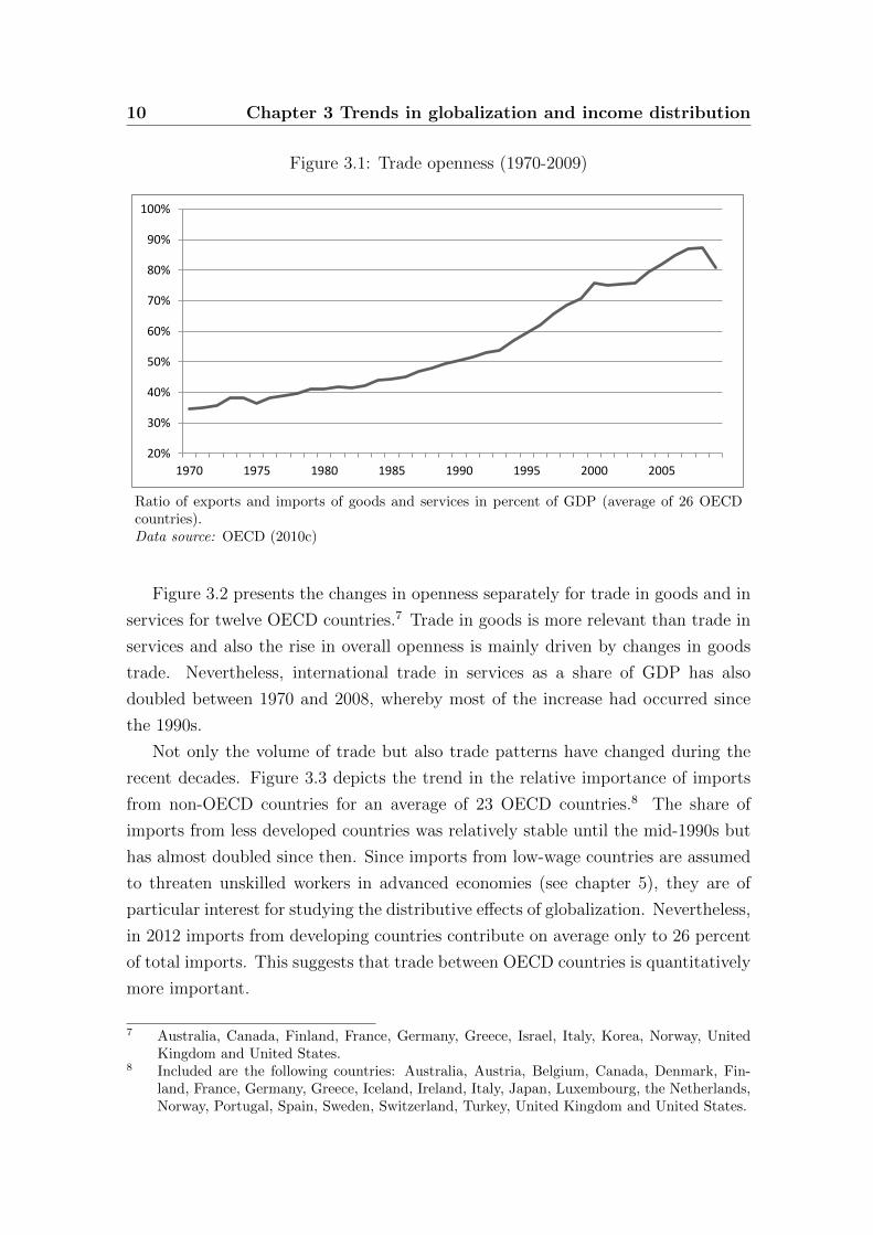
This is also reflected in the rising importance of international trade for OECD
countries. Figure 3.1 illustrates the evolution of trade openness, i.e. the sum of
exports and imports of goods and services as a percentage of GDP, for an average
of 26 OECD countries5 between 1970 and 2009. The share of trade in goods and
services in domestic output increased substantially from 35 percent in 1970 to 81
percent in 2009. Moreover, the rising exposure to international trade is common
to all countries. In 18 of the 26 countries the trade-to-GDP ratio has more than
doubled during that period.6
5 Included are the following countries (based on data availability): Australia, Austria, Belgium,Canada, Denmark, Finland, France, Germany, Greece, Iceland, Ireland, Israel, Italy, Japan,Korea, Mexico, the Netherlands, New Zealand, Norway, Portugal, Spain, Sweden, Switzerland,Turkey, United Kingdom and United States.
6 Despite the growing relevance of international trade for all countries, there is also a consid-erable variation as the overall increase in openness from 1970 to 2009 ranges from 15 percentin Iceland to about 480 percent in Korea.
9
10 Chapter 3 Trends in globalization and income distribution
Figure 3.1: Trade openness (1970-2009)
20%
30%
40%
50%
60%
70%
80%
90%
100%
1970 1975 1980 1985 1990 1995 2000 2005
Ratio of exports and imports of goods and services in percent of GDP (average of 26 OECDcountries).Data source: OECD (2010c)
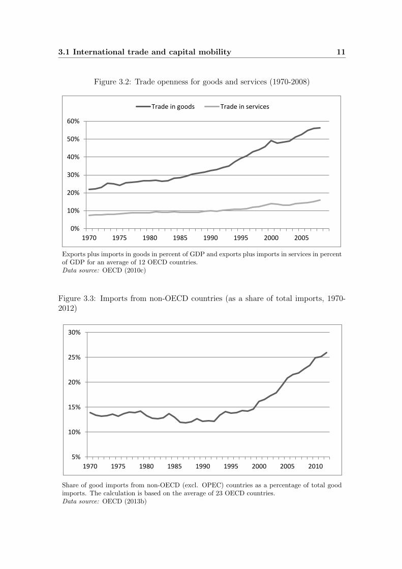
Figure 3.2 presents the changes in openness separately for trade in goods and in
services for twelve OECD countries.7 Trade in goods is more relevant than trade in
services and also the rise in overall openness is mainly driven by changes in goods
trade. Nevertheless, international trade in services as a share of GDP has also
doubled between 1970 and 2008, whereby most of the increase had occurred since
the 1990s.
Not only the volume of trade but also trade patterns have changed during the
recent decades. Figure 3.3 depicts the trend in the relative importance of imports
from non-OECD countries for an average of 23 OECD countries.8 The share of
imports from less developed countries was relatively stable until the mid-1990s but
has almost doubled since then. Since imports from low-wage countries are assumed
to threaten unskilled workers in advanced economies (see chapter 5), they are of
particular interest for studying the distributive effects of globalization. Nevertheless,
in 2012 imports from developing countries contribute on average only to 26 percent
of total imports. This suggests that trade between OECD countries is quantitatively
more important.
7 Australia, Canada, Finland, France, Germany, Greece, Israel, Italy, Korea, Norway, UnitedKingdom and United States.
8 Included are the following countries: Australia, Austria, Belgium, Canada, Denmark, Fin-land, France, Germany, Greece, Iceland, Ireland, Italy, Japan, Luxembourg, the Netherlands,Norway, Portugal, Spain, Sweden, Switzerland, Turkey, United Kingdom and United States.
3.1 International trade and capital mobility 11
Figure 3.2: Trade openness for goods and services (1970-2008)
0%
10%
20%
30%
40%
50%
60%
1970 1975 1980 1985 1990 1995 2000 2005
Trade in goods Trade in services
Exports plus imports in goods in percent of GDP and exports plus imports in services in percentof GDP for an average of 12 OECD countries.Data source: OECD (2010c)
Figure 3.3: Imports from non-OECD countries (as a share of total imports, 1970-2012)
5%
10%
15%
20%
25%
30%
1970 1975 1980 1985 1990 1995 2000 2005 2010
Share of good imports from non-OECD (excl. OPEC) countries as a percentage of total goodimports. The calculation is based on the average of 23 OECD countries.Data source: OECD (2013b)
12 Chapter 3 Trends in globalization and income distribution
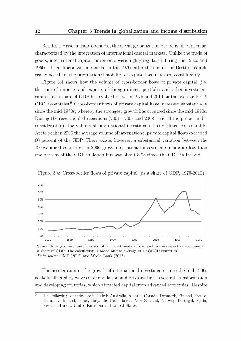
Besides the rise in trade openness, the recent globalization period is, in particular,
characterized by the integration of international capital markets. Unlike the trade of
goods, international capital movements were highly regulated during the 1950s and
1960s. Their liberalization started in the 1970s after the end of the Bretton Woods
era. Since then, the international mobility of capital has increased considerably.
Figure 3.4 shows how the volume of cross-border flows of private capital (i.e.
the sum of imports and exports of foreign direct, portfolio and other investment
capital) as a share of GDP has evolved between 1975 and 2010 on the average for 19
OECD countries.9 Cross-border flows of private capital have increased substantially
since the mid-1970s, whereby the strongest growth has occurred since the mid-1990s.
During the recent global recessions (2001 - 2003 and 2008 - end of the period under
consideration), the volume of international investments has declined considerably.
At its peak in 2006 the average volume of international private capital flows exceeded
60 percent of the GDP. There exists, however, a substantial variation between the
19 examined countries: in 2006 gross international investments made up less than
one percent of the GDP in Japan but was about 3.98 times the GDP in Ireland.
Figure 3.4: Cross-border flows of private capital (as a share of GDP, 1975-2010)
0%
10%
20%
30%
40%
50%
60%
70%
1975 1980 1985 1990 1995 2000 2005 2010
Sum of foreign direct, portfolio and other investments abroad and in the respective economy asa share of GDP. The calculation is based on the average of 19 OECD countries.Data source: IMF (2012) and World Bank (2012)
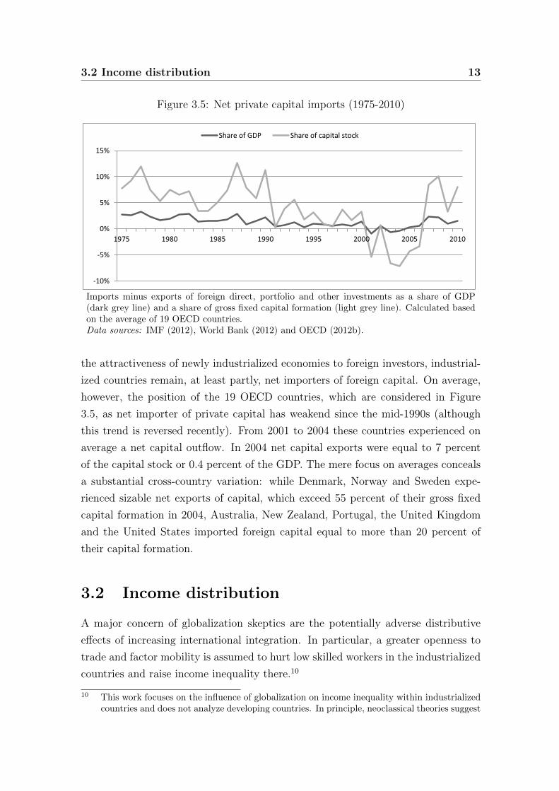
The acceleration in the growth of international investments since the mid-1990s
is likely affected by waves of deregulation and privatization in several transformation
and developing countries, which attracted capital from advanced economies. Despite
9 The following countries are included: Australia, Austria, Canada, Denmark, Finland, France,Germany, Ireland, Israel, Italy, the Netherlands, New Zealand, Norway, Portugal, Spain,Sweden, Turkey, United Kingdom and United States.
3.2 Income distribution 13
Figure 3.5: Net private capital imports (1975-2010)
-10%
-5%
0%
5%
10%
15%
1975 1980 1985 1990 1995 2000 2005 2010
Share of GDP Share of capital stock
Imports minus exports of foreign direct, portfolio and other investments as a share of GDP(dark grey line) and a share of gross fixed capital formation (light grey line). Calculated basedon the average of 19 OECD countries.Data sources: IMF (2012), World Bank (2012) and OECD (2012b).
the attractiveness of newly industrialized economies to foreign investors, industrial-
ized countries remain, at least partly, net importers of foreign capital. On average,
however, the position of the 19 OECD countries, which are considered in Figure
3.5, as net importer of private capital has weakend since the mid-1990s (although
this trend is reversed recently). From 2001 to 2004 these countries experienced on
average a net capital outflow. In 2004 net capital exports were equal to 7 percent
of the capital stock or 0.4 percent of the GDP. The mere focus on averages conceals
a substantial cross-country variation: while Denmark, Norway and Sweden expe-
rienced sizable net exports of capital, which exceed 55 percent of their gross fixed
capital formation in 2004, Australia, New Zealand, Portugal, the United Kingdom
and the United States imported foreign capital equal to more than 20 percent of
their capital formation.
3.2 Income distribution
A major concern of globalization skeptics are the potentially adverse distributive
effects of increasing international integration. In particular, a greater openness to
trade and factor mobility is assumed to hurt low skilled workers in the industrialized
countries and raise income inequality there.10
10 This work focuses on the influence of globalization on income inequality within industrializedcountries and does not analyze developing countries. In principle, neoclassical theories suggest
14 Chapter 3 Trends in globalization and income distribution
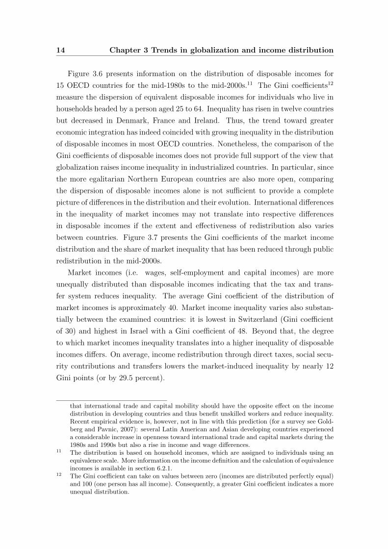
Figure 3.6 presents information on the distribution of disposable incomes for
15 OECD countries for the mid-1980s to the mid-2000s.11 The Gini coefficients12
measure the dispersion of equivalent disposable incomes for individuals who live in
households headed by a person aged 25 to 64. Inequality has risen in twelve countries
but decreased in Denmark, France and Ireland. Thus, the trend toward greater
economic integration has indeed coincided with growing inequality in the distribution
of disposable incomes in most OECD countries. Nonetheless, the comparison of the
Gini coefficients of disposable incomes does not provide full support of the view that
globalization raises income inequality in industrialized countries. In particular, since
the more egalitarian Northern European countries are also more open, comparing
the dispersion of disposable incomes alone is not sufficient to provide a complete
picture of differences in the distribution and their evolution. International differences
in the inequality of market incomes may not translate into respective differences
in disposable incomes if the extent and effectiveness of redistribution also varies
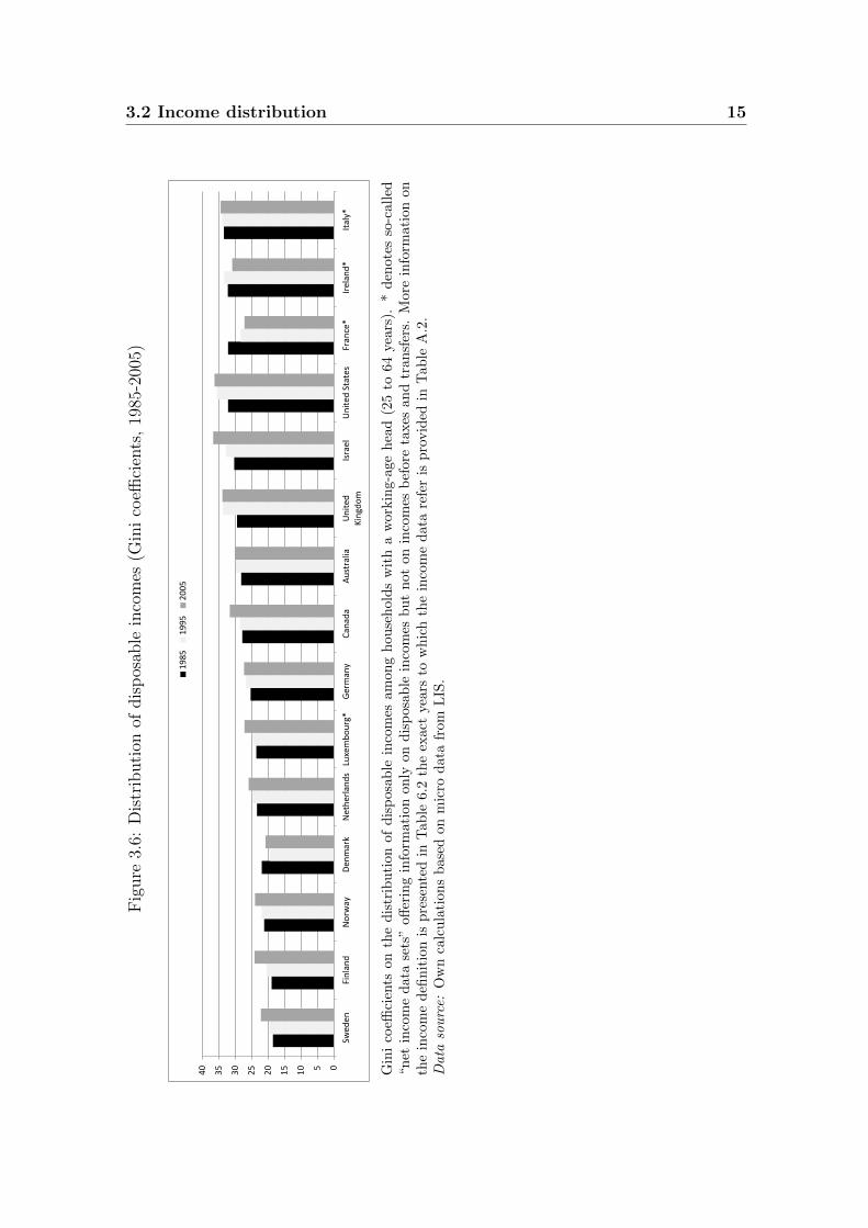
between countries. Figure 3.7 presents the Gini coefficients of the market income
distribution and the share of market inequality that has been reduced through public
redistribution in the mid-2000s.
Market incomes (i.e. wages, self-employment and capital incomes) are more
unequally distributed than disposable incomes indicating that the tax and trans-
fer system reduces inequality. The average Gini coefficient of the distribution of
market incomes is approximately 40. Market income inequality varies also substan-
tially between the examined countries: it is lowest in Switzerland (Gini coefficient
of 30) and highest in Israel with a Gini coefficient of 48. Beyond that, the degree
to which market incomes inequality translates into a higher inequality of disposable
incomes differs. On average, income redistribution through direct taxes, social secu-
rity contributions and transfers lowers the market-induced inequality by nearly 12
Gini points (or by 29.5 percent).
that international trade and capital mobility should have the opposite effect on the incomedistribution in developing countries and thus benefit unskilled workers and reduce inequality.Recent empirical evidence is, however, not in line with this prediction (for a survey see Gold-berg and Pavnic, 2007): several Latin American and Asian developing countries experienceda considerable increase in openness toward international trade and capital markets during the1980s and 1990s but also a rise in income and wage differences.
11 The distribution is based on household incomes, which are assigned to individuals using anequivalence scale. More information on the income definition and the calculation of equivalenceincomes is available in section 6.2.1.
12 The Gini coefficient can take on values between zero (incomes are distributed perfectly equal)and 100 (one person has all income). Consequently, a greater Gini coefficient indicates a moreunequal distribution.
3.2 Income distribution 15F
igure
3.6:
Dis
trib
uti
onof
dis
pos
able
inco
mes
(Gin
ico
effici
ents
,19
85-2
005)
0
5
10
15
20
25
30
35
40
Swed
en
Fin
lan
d
No
rway
D
enm
ark
Net
her
lan
ds
Luxe
mb
ou
rg*
Ger
man
y C
anad
a A
ust
ralia
U
nit
ed
Kin
gdo
m
Isra
el
Un
ited
Sta
tes
Fran
ce*
Irel
and
*
Ital
y*
19
85
1
99
5
20
05
Gin
ico
effici
ents
onth
ed
istr
ibu
tion
ofd
isp
osab
lein
com
esam
on
gh
ou
seh
old
sw
ith
aw
ork
ing-a
ge
hea
d(2
5to
64
years
).*
den
ote
sso
-call
ed“n
etin
com
ed
ata
sets
”off
erin
gin
form
atio
non
lyon
dis
posa
ble
inco
mes
bu
tn
ot
on
inco
mes
bef
ore
taxes
an
dtr
an
sfer
s.M
ore
info
rmati
on
on
the
inco
me
defi
nit
ion
isp
rese
nte
din
Tab
le6.
2th
eex
act
years
tow
hic
hth
ein
com
ed
ata
refe
ris
pro
vid
edin
Tab
leA
.2.
Data
sou
rce:
Ow
nca
lcu
lati
ons
bas
edon
mic
rod
ata
from
LIS
.
16 Chapter 3 Trends in globalization and income distribution
The reduction of market income dispersion is less in Switzerland (probably also
due to a comparably low level of inequality), the United States and Canada, while
redistribution is considerably higher in Scandinavian countries. In Denmark and
Sweden, for instance, the Gini coefficients of disposable incomes are over 40 percents
lower than the coefficients of the market income distribution.
Figure 3.7: Distribution of market and disposable incomes and redistribution (Ginicoefficients, mid-2000s)
0
10
20
30
40
50
60
disposable incomes redistribution market incomes
Gini coefficients on the distribution of disposable incomes (dark grey bar), market incomes(cross) and the share of the Gini coefficient of market incomes that is reduced by redistributionover taxes and transfers (light grey bar). Calculated for the distribution of incomes betweenhouseholds with a working-age head (25 to 64 years old). More information on the incomedefinition is presented in Table 6.2 and information on the exact years to which the income datarefer is available in Table A.2.Data source: Own calculations based on micro data from LIS.
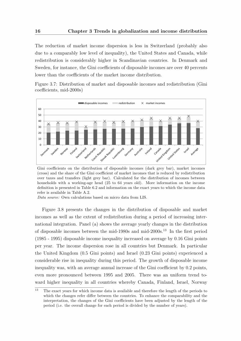
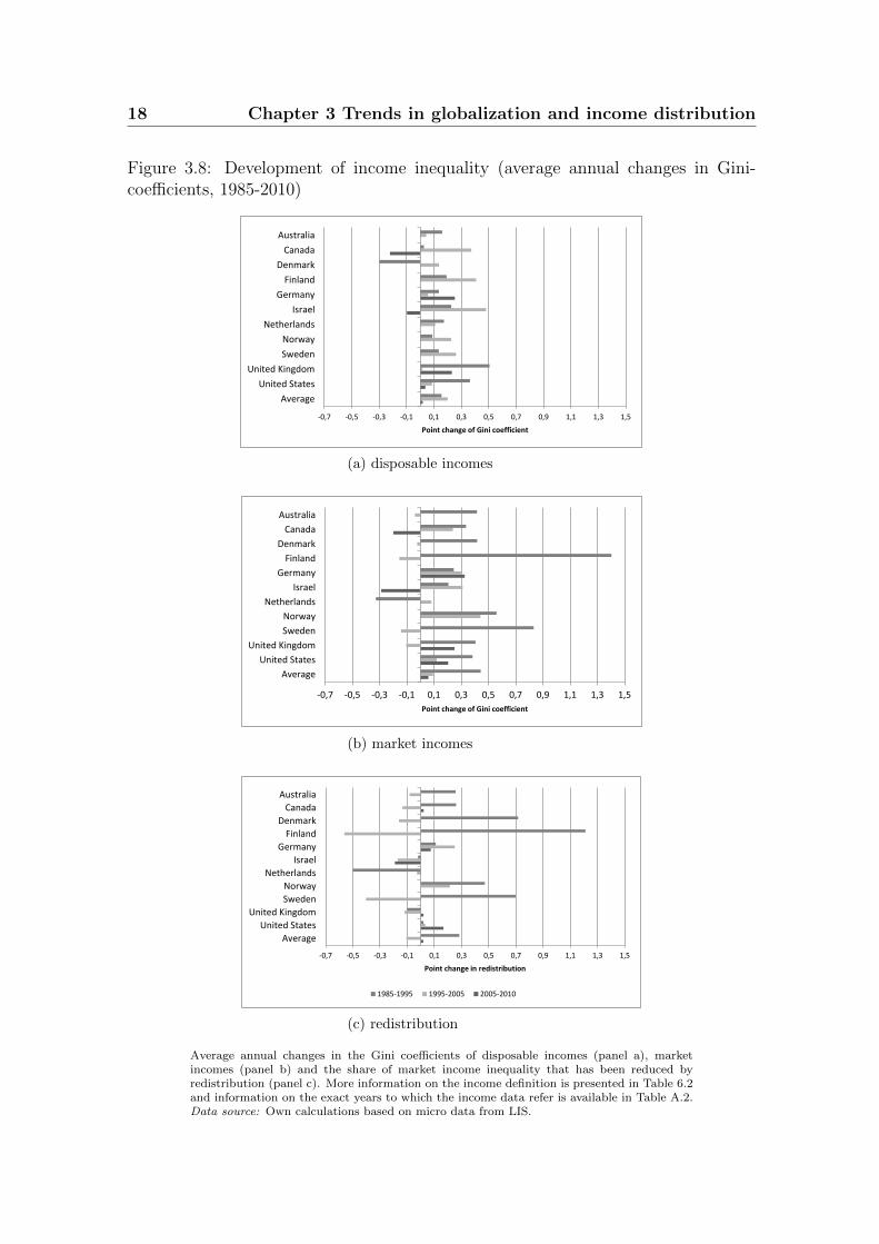
Figure 3.8 presents the changes in the distribution of disposable and market
incomes as well as the extent of redistribution during a period of increasing inter-
national integration. Panel (a) shows the average yearly changes in the distribution
of disposable incomes between the mid-1980s and mid-2000s.13 In the first period
(1985 - 1995) disposable income inequality increased on average by 0.16 Gini points
per year. The income dispersion rose in all countries but Denmark. In particular
the United Kingdom (0.5 Gini points) and Israel (0.23 Gini points) experienced a
considerable rise in inequality during this period. The growth of disposable income
inequality was, with an average annual increase of the Gini coefficient by 0.2 points,
even more pronounced between 1995 and 2005. There was an uniform trend to-
ward higher inequality in all countries whereby Canada, Finland, Israel, Norway
13 The exact years for which income data is available and therefore the length of the periods towhich the changes refer differ between the countries. To enhance the comparability and theinterpretation, the changes of the Gini coefficients have been adjusted by the length of theperiod (i.e. the overall change for each period is divided by the number of years).
3.2 Income distribution 17
and Sweden experienced above average increases. For the last period (2005 - 2010)
the pattern is less obvious. The average increase of the Gini coefficient for the
five countries for which data is available is rather modest (about 0.02 points per
year). Inequality remained stable in the United States, increased in Germany and
the United Kingdom and declined in Canada and Israel.
Consequently, the main increase in inequality occurred between 1985 and 2005,
in particular since the mid-1990s. Panel (b) of Figure 3.8 presents the average yearly
changes of market income inequality. The rise in market income dispersion was par-
ticularly strong between 1985 and 1995. During that period the Gini coefficient rose
on average by 0.44 points per year and all countries, except the Netherlands, ex-
perienced growing market income inequalities. The increase was highest in Finland
(1.4 Gini points per year) and lowest, though still sizable, in Israel (0.21 Gini points
per year). Between 1995 and 2005, the rise in market-induced income dispersion
has been less pronounced with average yearly increases of the Gini coefficient by
0.09 points. Overall, rising Gini coefficients are reported for six countries, while five
countries experienced a decline in market inequality. During the most recent period
(2005 - 2010) the Gini coefficient of the five reported countries rose on average by
0.06 points yearly. This modest increase conceals, however, sizable and significantly
different developments at the country level. In Germany, the United Kingdom and
the United States the Gini coefficient increased by more than 0.2 points per year,
whereby Israel and Canada experienced a likewise reduction of inequality.
Finally, panel (c) depicts the development of redistribution through taxes and
transfers. The picture is rather mixed: between 1985 and 1995 redistribution in-
creased in eight countries and the share of market income inequality, which had been
reduced via taxes and transfers, grew on average by 0.28 points per year. The period
from 1995 to 2005 is on average characterized by a decline in redistribution (0.11
points lower reduction of the Gini coefficient of the market income distribution).
The most recent period (2005-2010) does, on average, indicate no major changes in
redistribution. This conceals, in particular, the large increase in income redistribu-
tion in the United States and a comparable decline in market inequality reduction
in Israel.
In sum, the rising dispersion of disposable incomes between 1985 and 1995 mainly
reflects large increases in market income inequality, which were only partly reduced
by greater redistribution. From 1995 to 2005 the rising inequality was driven more
by a reduction in redistribution than by considerable increases in market inequality.
18 Chapter 3 Trends in globalization and income distribution
Figure 3.8: Development of income inequality (average annual changes in Gini-coefficients, 1985-2010)
-0,7 -0,5 -0,3 -0,1 0,1 0,3 0,5 0,7 0,9 1,1 1,3 1,5
Average
United States
United Kingdom
Sweden
Norway
Netherlands
Israel
Germany
Finland
Denmark
Canada
Australia
Point change of Gini coefficient
(a) disposable incomes
-0,7 -0,5 -0,3 -0,1 0,1 0,3 0,5 0,7 0,9 1,1 1,3 1,5
Average
United States
United Kingdom
Sweden
Norway
Netherlands
Israel
Germany
Finland
Denmark
Canada
Australia
Point change of Gini coefficient
(b) market incomes
-0,7 -0,5 -0,3 -0,1 0,1 0,3 0,5 0,7 0,9 1,1 1,3 1,5
Average
United States
United Kingdom
Sweden
Norway
Netherlands
Israel
Germany
Finland
Denmark
Canada
Australia
Point change in redistribution
1985-1995 1995-2005 2005-2010
(c) redistribution
Average annual changes in the Gini coefficients of disposable incomes (panel a), marketincomes (panel b) and the share of market income inequality that has been reduced byredistribution (panel c). More information on the income definition is presented in Table 6.2and information on the exact years to which the income data refer is available in Table A.2.Data source: Own calculations based on micro data from LIS.
Chapter 4
Empirical evidence on the
relationship between globalization
and income inequality
The descriptive analysis in chapter 3 suggests that OECD countries both experi-
enced a rise in income dispersion and in exposure to international trade and capital
mobility during the last decades. The question whether this common trend toward
greater economic integration and income inequality reflects a causal relationship or
is a simple coincidence has been the subject of several empirical studies. The empir-
ical evidence provides rather mixed results concerning the impact of globalization
on the income distribution in developed countries.
Some studies focus directly on the consequences of globalization on the income
distribution in advanced economies. The findings by Alderson and Nielsen (2002),
for instance, support the view that globalization contributed to the rising inequal-
ity in OECD countries. Based on data for 16 OECD countries from 1976 to 1992,
the authors find that the outflow of direct investment capital and manufacturing
imports from developing countries are related to a greater income inequality. A
related analysis by Mahler (2004) does, however, not confirm the finding that glob-
alization has a substantial effect on income inequality. Economic integration (i.e.
the relevance of imports from less developed countries, financial openness and for-
eign direct investments) has no significant impact on the distribution of disposable
incomes for a sample of 14 advanced economies between the early 1980s and 2000.
Mahler concludes that domestic factors such as the strength of trade unions or wage
coordination have been more relevant drivers of trends in income inequality.
Several authors argue that the focus on economic globalization may not be suf-
19
20 Chapter 4 Empirical evidence on globalization and inequality
ficient to explain changes in the distribution of incomes. Emphasizing the relevance
of different aspects of globalization, Dreher and Gaston (2008) use an index account-
ing for various dimensions of global integration (KOF Index). The basic reasoning
for this approach is that economic integration is usually accompanied by a greater
degree of social and political integration. Since these different dimensions of glob-
alization might have opposing effects on the distribution of income, the mixed and
often insignificant findings on the relationship between globalization and inequality
may be explained by the one-sided focus on economic factors. The empirical anal-
ysis of Dreher and Gaston indeed suggests that overall globalization has increased
income (and also partly wage) inequality in OECD countries between 1970 and
2000. Moreover, the disaggregation of the globalization index into its subcompo-
nents economic, social and political integration, does not point at a significant effect
of economic globalization on income inequality but rather suggests some influence
of social and political integration. A related work by Bergh and Nilsson (2010) also
employs the KOF Index to analyze the effect of globalization on the distribution
of net incomes among households. Their findings are in line with those of Dreher
and Gaston (2008): globalization has a positive and marginally significant impact
on inequality.14 Additionally, freedom to trade internationally (as measured by the
Economic Freedom Index) is associated with a higher dispersion in the distribution
of net incomes.
The considerable rise in wage dispersion and the decrease in employment of less
educated workers in many industrialized countries since the 1980s has attracted
the attention of economists who analyzed the determinants of these developments
empirically. Most empirical studies focused on the role of trade in explaining the
increase in wage inequality (surveys of this literature are provided by Richardson,
1995; Harrison et al., 2010; Kurokawa, 2010). The extensive literature on the impact
of trade on wages often provides results which are inconsistent with the predictions of
classical trade theories. Hence, many economists have concluded that not trade but
other factors such as technological change favoring educated workers are responsible
for the rise in wage inequality. The minor impact of international trade on the
14 The disaggregation of the index reveals that this effect is mainly driven by social globalization.This subindex includes information, for instance, about international telephone calls, internetuse and proxies for cultural proximity. This positive correlation between social integrationand inequality, which matters especially for low- and middle income countries, may reflectchanging social norms or interactions between the social dimension of globalization and acountry’s social policy. The latter has been emphasized by Dreher et al. (2008) who arguethat a higher cultural proximity and an easier exchange of information leads to higher effectsof capital mobility on fiscal policies.
4 Empirical evidence on globalization and inequality 21
distribution of wages might also be explained by the fact that alternative mechanisms
(e.g. adjustments in the relative supply of educated workers) are widely neglected.
Recently, several studies have analyzed new mechanisms through which trade can
affect workers and income inequality (e.g. the role of labor market frictions). These
studies indeed point at a larger role of international trade (e.g. the empirical studies
surveyed in Harrison et al., 2010).
The inconclusive empirical evidence on the relevance of international trade and
capital mobility for the income inequality may result from the conceptualization of
most studies. The common approach of regressing measures of income distribution
(e.g. Gini coefficients or earnings percentiles) on globalization indicators has several
shortcomings (for a brief discussion see Atkinson, 2002). Such an analysis does not
account for the possibility that international trade and capital mobility affect the
income distribution through several channels. If these channels work in opposite
directions and thus cancel each other (at least partly) out, then this may explain
the often insignificant results.
A first attempt to analyze different channels through which globalization affects
the wage distribution has been undertaken in a recent OECD study (OECD, 2011).
Instead of relating the international integration of a country directly with the dis-
tribution of wage income among its population, this study provides separate tests
for the impact of globalization on wage dispersion among full-time workers and on
employment. The findings do not suggest a robustly significant relationship between
international trade or capital mobility and the earnings dispersion or employment
in OECD countries. Although this study does account for two different channels
through which international integration can affect the personal wage distribution,
it still neglects a number of alternative mechanisms and does therefore not provide
comprehensive information on the distributional effects of globalization. In partic-
ular, possible supply responses are widely neglected.
Checci and Garcia-Penalosa (2010) stress the relevance of a broad analysis of the
personal distribution of incomes encompassing various channels for our understand-
ing of the determinants of inequality. Their study on the impact of labor market
institutions is based on the idea that overall inequality can be decomposed into
several components that serve as channels through which different labor market in-
stitutions influence income inequality. The authors propose an estimation approach
consisting of two different steps. First, they estimate the effect of different kinds
of labor market institutions on the wage differential, the labor income share and
the unemployment rate. Second, they test how these variables alter the personal
22 Chapter 4 Empirical evidence on globalization and inequality
distribution of incomes. Checci and Garcia-Penalosa find that labor market insti-
tutions have a significant impact on labor market outcomes and, thereby, also on
the income distribution. Since institutions influence several labor market outcomes
with potentially different implications for the personal income distribution (e.g. a
higher union density reduces the wage differential but also raises the unemployment
rate), the findings imply that a narrow focus on just one labor market outcome
might deliver misleading results.
My study develops the basic idea of OECD (2011) further and combines the rela-
tionship between globalization and several labor market outcomes with an analysis of
the impact of these factors on the personal distribution of market and disposable in-
comes (as suggested by Checci and Garcia-Penalosa, 2010). Beyond the combination
of globalization effects on a set of labor market outcomes15 and their transmission
into inequality, I also enhance the two mentioned analyses by focusing on a broader
range of transmission channels and providing information on the distribution of dif-
ferent types of incomes. In particular, I assume that the relative supply of human
capital is affected by factors such as globalization and labor market institutions and
is thus not taken as given.
The choice of transmission mechanisms is based on theoretical considerations
and is discussed in chapter 5.
15 Checci and Garcia-Penalosa (2010) find a negative (though not always significant) relation-ship between trade openness and income inequality. The authors do, however, include tradeopenness only in the analysis of the unemployment rate and, hence, ignore its impact throughother channels.

Chapter 5
Identification of transmission
mechanisms
This chapter provides an overview about theoretical explanations regarding the re-
lationship between globalization and economic inequality in advanced economies.
The main objective is the identification of transmission mechanisms through which
international trade and capital mobility may affect the income distribution. Figure
5.1 illustrates the relevant transmission channels and also serves as an outline of the
subsequent discussion.
I focus on the exposure to international trade and capital mobility, which is
expected to affect the functional distribution of incomes (i.e. the relative income of
different production factors).16 Trade affects the relative demand for capital, skilled
and unskilled labor, while international capital flows change the relative supply of
production factors.17 With perfect competition on factor markets these changes in
relative factor demand and supply should induce adjustments of the relative factor
rewards. The relationship between international trade and capital mobility and the
relative rewards of production factors is indicated by the arrow (a) in Figure 5.1.
16 From an economy-wide perspective, international trade in goods and services and internationalcapital flows are linked due to balance of payments restrictions. The international exchangeof goods is accompanied by international capital flows (i.e. each import (export) requiresa net capital inflow (outflow)) unless the goods exchange is reciprocal. While conceptuallyinternational trade and capital flows are two sides of a coin, the mechanisms through whichthey affect the income distribution differ. Thus, I discuss them separately.
17 Besides capital mobility also labor mobility affects the distribution of incomes. Internationallabor markets are less integrated than capital markets since cultural and language differenceshinder the free movement of people. In addition, an empirical analysis of the effects ofmigration flows of workers with different levels of education for a panel of countries is notpossible since the required data is not available for a sufficient number of countries and years.Hence, I focus on the impact of capital mobility though, in principle, the implications alsoapply to labor mobility.
23
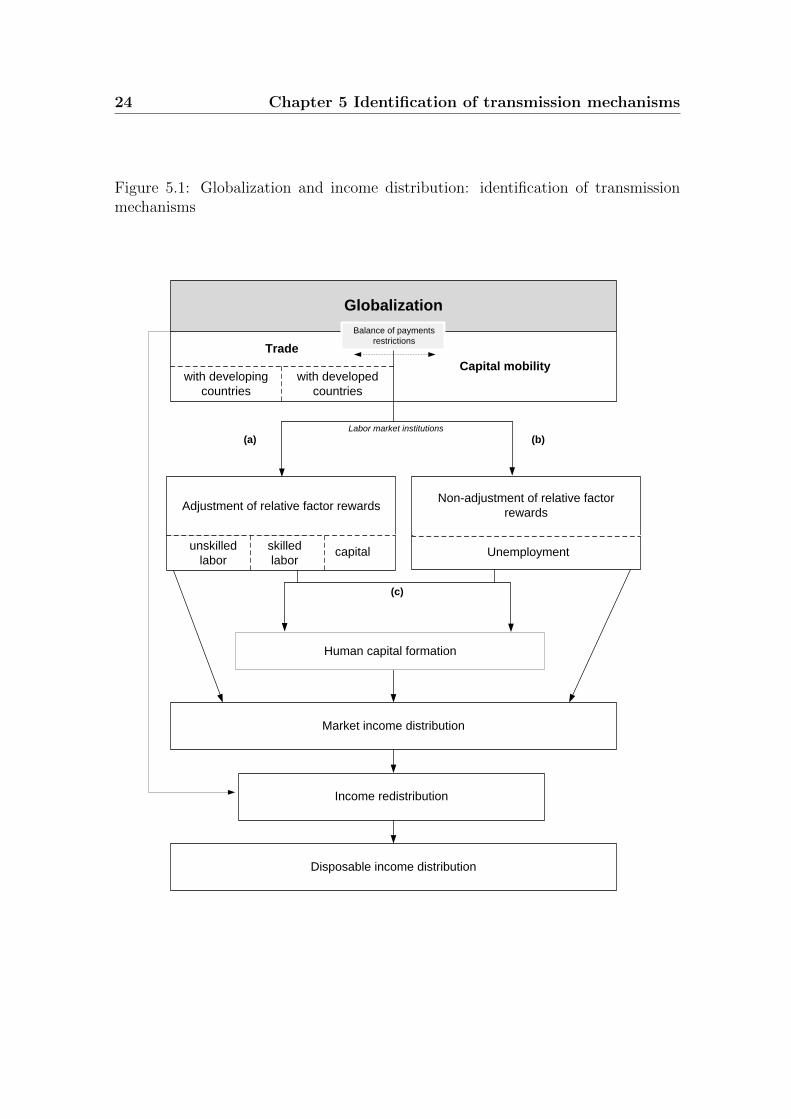
24 Chapter 5 Identification of transmission mechanisms
Figure 5.1: Globalization and income distribution: identification of transmissionmechanisms
Globalization
Trade
Capital mobilitywith developing
countries
with developed
countries
Adjustment of relative factor rewards
unskilled
laborcapital
skilled
labor
Market income distribution
Income redistribution
Disposable income distribution
Balance of payments
restrictions
Non-adjustment of relative factor
rewards
Unemployment
Human capital formation
Labor market institutions
(a) (b)
(c)
5.1 Globalization and the functional income distribution 25
Many advanced economies, however, face labor market frictions which impede the
adjustments of wages. If the relative wages of unskilled workers do not respond to
changes in relative labor demand, then the relative employment of unskilled workers
will adjust (see channel (b) in Figure 5.1).
So far, the supply of production factors has been assumed to be inelastic. While
this assumption is appropriate in the short-run, the relative supply of skilled workers
(human capital) and capital should respond to changes in relative factor demand in
the medium- to long-run (see channel (c) in Figure 5.1). Hence, changes in the skill
premium or employment opportunities for well educated workers affect the returns
to human capital investments and thus the supply of skills.
Globalization influences the functional income distribution via changes in the
relative rewards, employment and supply of production factors. Conclusions about
its impact on market income inequality (and thereby the distribution among indi-
viduals or households rather than production factors) require additional information
about the actual ownership of production factors among different income groups.
Individuals are mainly interested in disposable incomes, which determine their
consumption opportunities. The distribution of disposable incomes depends both on
market incomes and redistribution via taxes and transfers. Consequently, a rise in
market income inequality does not increase the inequality of disposable incomes by
the same extent. The scope and effectiveness of public redistribution itself depends
on a country’s exposure to international trade and capital markets. The theoretical
predictions regarding the effect of globalization on the welfare state are ambiguous.
On the one hand, foreign competition limits the scope for taxation for national
governments and the financing of the welfare state. On the other hand, the demand
for redistribution and social insurance may increase as countries become more open.
5.1 Globalization and the functional income dis-
tribution
The subsequent section discusses the relationship between globalization and the
functional income distribution. Based on a standard set of assumptions underly-
ing most theories about international trade and capital mobility (such as perfect
competition on goods and factor markets), the first part is devoted to changes in
the relative factor payments. Afterwards, the assumption of perfectly competitive
markets is relaxed by introducing labor market frictions. In this case, relative fac-
tor prices do not fully adjust but globalization changes the relative employment of
26 Chapter 5 Identification of transmission mechanisms
workers. Finally, the relative factor supply may respond to globalization induced
shifts in relative factor demand.
5.1.1 Adjustments of relative factor rewards
International trade
For the discussion of the distributional consequences of international trade for indus-
trialized countries, I distinguish between trade with other industrialized countries
(intra-industry trade) and with developing countries (inter-industry trade).18 In ad-
dition to the literature on trade in final goods also theories devoted to the effect of
trade in intermediate products are reviewed.
To analyze the consequences of inter-industry trade for the distribution of in-
comes, economists have long employed either the Heckscher-Ohlin or the Ricardo-
Viner (“specific-factors”) model.19 The Heckscher-Ohlin model explains patterns of
trade in final goods between countries based on different factor endowments. Each
country exports the good which uses the abundant factor of production intensively.
Industrialized economies, which are capital or human capital abundant compared
to developing countries, will thus specialize in the production of (human) capital-
intensive goods. The lowering of the barriers to trade raises the demand for skilled
relative to unskilled labor20 and the relative demand for capital vis-a-vis labor in the
industrialized countries. Hence, the owners of the abundant factor (i.e. skilled work-
ers and capital owners) benefit from trade liberalization and experience rising real
incomes while the real income of unskilled workers declines (Stolper and Samuelson,
1941).21
One basic assumption of the Heckscher-Ohlin model is that production factors are
fully mobile between industries in each country (though internationally immobile).
In contrast to this, the Ricardo-Viner (“specific factors”) model takes a short-term
perspective and presumes that at least one factor can be used for production only
18 Unless mentioned otherwise, the theories of international trade introduced in this sectionassume that the production factors are internationally immobile.
19 The impact of trade on the distribution of wages can be also analyzed based on a Ricardianapproach (i.e. incorporating technological differences as in Johnson and Stafford, 1999).
20 In accordance with the literature, the expressions human capital and skilled labor are usedinterchangeably.
21 This strong version of the Stolper-Samuelson theorem is based on the assumptions of thestandard Heckscher-Ohlin model focusing on two countries, two goods and two factors. Thebasic distributive implications usually hold also in more general settings such as the Heckscher-Ohlin-Vanek model covering many countries, goods and factors as long as the number of goodsdoes not exceed the number of factors (e.g. Feenstra, 2004).
5.1 Globalization and the functional income distribution 27
in one specific industry.
In a simple version, this model covers two sectors each using both labor and
capital for production. Capital is supposed to be fully mobile between both sectors
but the supply of labor is fixed in each industry, i.e. reflecting different skill re-
quirements for workers in each sector. In this framework, trade liberalization raises
the rate of return on capital,22 it increases the real wage of workers in the sector,
in which the country has a comparative advantage and it lowers the real wage of
workers employed in the sector where the country has a comparative disadvantage.
In industrialized countries, unskilled workers tend to be disproportionately more
often employed in import-competing industries, in which the country does not have
a comparative advantage. Thus, the skill premium will rise.
In sum, standard trade models suggest a positive effect of trade in final goods
on income inequality as long as production factors which are abundant or specific to
export industries received higher payments before trade liberalization. This is, how-
ever, often not confirmed by the data (a recent discussion is provided by Kurokawa,
2010 and Harrison et al., 2010). In contrast to the predictions of the theories dis-
cussed above, much of the change in the relative wage and employment of skilled
and unskilled workers is driven by within-industry shifts rather than of reallocations
between industries. Hence, rising wage inequality cannot be explained by changes
in the production structure (i.e. the weight of certain sectors in GDP) but are more
likely a consequence of within-industry shifts in the relative demand for unskilled la-
bor. Given this inconsistency, many economists focused on skill-biased technological
changes instead of international trade as an explanation for rising wage inequality
(Berman et al., 1994). A study by Bernand and Jensen (1997), however, indicates
that trade might also affect wages through within-industry changes of labor demand.
An attempt to explain these changes of relative labor demand within industries
is based on the role of trade in intermediate goods. Improvements in transporta-
tion and communication technology (especially since the 1980s) allowed a stronger
disintegration of the production process (or a “slicing-up the value chain” as stated
by Krugman, 1995). This has induced a boom in offshoring or outsourcing of pro-
duction activities with firms taking advantage of international differences in factor
prices.
Feenstra and Hanson (1996) introduce a model of trade in intermediate inputs
which indicates that the offshoring of production activities reduces the relative wages
22 The rewards to capital as the mobile factor of production will increase by less than the priceof the export good. Consequently, the effect on the real interest rate depends on the relativeconsumption regarding the import and export good.

28 Chapter 5 Identification of transmission mechanisms
of unskilled workers by lowering the relative demand for this group of workers within
each industry.23
The model incorporates an industrialized and a developing country, which pro-
duce each one final good assembled from intermediate inputs. The production of
each input requires unskilled and skilled labor as well as capital. The skill-intensities
(i.e. the amount of skilled relative to unskilled labor required for production) dif-
fer for the intermediate inputs. Moreover, the wage of skilled relative to unskilled
labor and the real interest rate are supposed to be lower in the industrialized than
in the developing country.24 Consequently, the unit costs of production of each in-
put will, depending on its skill-intensity, differ between the two countries. Based
on a cost minimization calculus, firms locate the production of inputs with high
skill-intensity in the industrialized country and inputs which require relatively more
unskilled workers are produced in the developing country. Hence, there exists a
unique level of skill-intensity below which the unit costs of production for the in-
termediate inputs are lower in the developing country and which are thus produced
in this country. The industrialized country will specialize on the production of all
intermediate inputs with a skill-intensity above this critical value since its unit costs
of production are lower than in the developing country.
If now the capital stock grows (e.g. due to capital mobility) or technology im-
proves (i.e. neutral technological progress) in the developing relative to the indus-
trialized country, then the costs of production will decline in the developing but rise
in the industrialized country (Feenstra and Hanson, 1996).25 Due to this relative
decline in general production costs in the developing country, the critical value of
skill-intensity above which the industrialized country has lower unit costs increases
(i.e. the developing country has now a relative cost advantage for intermediate
goods with a higher skill intensity than before). This induces a further relocation of
production activities and the skill-intensity in the production of inputs increases in
both countries. The relative demand for unskilled labor therefore declines in both
countries. This will, ceteris paribus, lower the relative wage of unskilled workers.26
23 Thus, trade in intermediates has the same impact on wages and employment as skill-biasedtechnological change (Feenstra, 1998).
24 This is a reasonable assumption if the industrialized country is skilled labor and capitalabundant. If capital is mobile between the two countries, then it will relocate to the developingcountry because of the higher rents.
25 Capital movements from the (capital-abundant) industrialized to the (capital-scarce) devel-oping country increase the interest rate in the former and lower it in the latter country. Thischange in the costs of capital leads to a general increase in the unit costs of production in theindustrialized country and a decline in the developing country.
26 This result is based on the assumption that capital movements only affect the general pro-
5.1 Globalization and the functional income distribution 29
A related approach focuses on tradable tasks performed by workers of different
skill levels. These “trade in tasks” models rely on the basic idea that the production
process of each good consists of several tasks which are performed by each factor of
production.27 The assignment of production factors to certain tasks (i.e. steps in
the production process) is however not fixed. Technological improvements make it
possible that tasks, which have previously been performed by labor are conducted by
machinery (usually routine tasks) or are produced abroad.28 Grossman and Rossi-
Hansberg (2008) analyze based on a Heckscher-Ohlin framework how a decline in
the costs of offshoring affects workers with different skill levels. In contrast to the
predictions by Feenstra and Hanson (1996), the offshoring of tasks performed by
unskilled labor does not necessarily lower the domestic wages of unskilled workers.
A decline in offshoring costs increases the effective supply of unskilled labor in the
industrialized country and lowers the relative price of the unskilled labor-intensive
good. Furthermore, it induces cost savings (of already offshored tasks) that are
greater in the unskilled labor intensive sector and leads to an expansion of this
sector. While the first two effects result in a fall of the relative wage of unskilled
workers, the third works in favor of this group.
The theories discussed above allow only statements about the distributional con-
sequences of trade between countries with different factor endowments (e.g. indus-
trialized and developing countries). For most industrialized countries, however, a
considerable part of trade relationships comprises the exchange of similar goods.
Attempts to explain this intra-industry trade are usually based on the existence of
increasing returns to scale in the production of differentiated goods (as in the model
developed by Krugman, 1980). The underlying idea of these models of monopolistic
competition is that consumers have a “taste for variety” (i.e. prefer to consume a
broad range of varieties of a differentiated good). Each firm produces one variety of
this good whereas the production technology is characterized by increasing returns
to scale. The preferences for the consumption of a broad range of varieties implies
that many firms should each produce a small quantity of a variety of the differen-
tiated good. In the presence of scale economies, however, it would be efficient that
few firms produce larger quantities and thereby serve the whole market at lower av-
duction costs but do not have a differential impact on the two types of labor (i.e. the degreeof complementarity to capital is the same for skilled and unskilled labor).
27 This tasks approach differs from the canonical production function which does not allow todifferentiate between the questions which factors are used in the production and what theirrole is (i.e. which services does each factor provide).
28 A detailed discussion of the task approach and its conceptualization is provided in Autor(2013) and Acemoglu and Autor (2010).
30 Chapter 5 Identification of transmission mechanisms
erage costs. Consequently, a trade-off exists between the supply of a greater number
of varieties and the utilization of scale effects. In this set-up, trade has the same
implications as an increase in market size. Firms can serve the foreign market and
are therefore able to produce and sell a larger quantity of their varieties to utilize
scale effects. At the same time, more varieties are available for domestic consumers
because they can also consume varieties produced by foreign firms. Krugman (1980)
presumes that firms are homogeneous. Recent works, however, relax that assump-
tion and allow firms to differ in their productivity and other characteristics. These
models are a good starting point to analyze the implications of intra-industry trade
for wage inequality.
The model by Melitz (2003) incorporates firm heterogeneity into Krugman’s
(1980) model of trade under monopolistic competition and increasing returns. The
firms differ in their productivity and thus have different marginal costs of production.
Depending on their level of productivity, firms decide whether to produce or not.29
In an open economy firms could also serve the foreign market but exporting requires
an additional fixed investment.30 Due to these costs only the most productive firms
will export. Compared to the autarky situation domestic firms incur a loss in market
shares after the economy opens to trade since foreign firms also serve the domestic
market. This induces the least productive firms to leave the market.31 Hence, the
exposure to trade raises the overall productivity in the industry and leads to a
reallocation of market and profit shares among firms. Only exporters as the most
productive firms can (more than) compensate the loss of domestic sales with their
exports. This standard approach assumes identical workers and competitive labor
markets in which all workers will receive the same wage. This model can therefore
not be employed to analyze the effect of trade on wage dispersion.
Recently, several modifications of heterogenous firm models have been introduced
which imply that trade leads to a wage differential between exporting and non-
exporting firms. In principle, these heterogenous firm models could also explain
changes in the rewards of labor relative to capital, the focus of these recent models
29 The firms are ex ante identical. After a payment of fixed entry costs, which are afterwardssunk, firms enter the market and learn about their (randomly assigned) level of productivity.Depending on their productivity, firms decide whether to exit or stay in the market.
30 To enter the export market, both a sunk fixed investment and per-unit shipping costs incur.31 The production of each variety and the sunk fixed investments to enter the market and export
require labor. Thus, all domestic firms compete on domestic labor markets. After the economyopens to trade the more productive firms will enter the export market and new firms enter themarket because of increasing profit opportunities. This raises the demand for labor, which isinelastically supplied, and increases the real wage. The least productive firms cannot affordthe higher wages and are forced to exit the market.
5.1 Globalization and the functional income distribution 31
is, however, on the relative wage of unskilled workers.
One way of incorporating wage differentials into heterogenous trade models is
based on the assumption that firms’ productivity is related to the skill-intensity of
their production. Yeaple (2005) extents the standard heterogenous-firms models by
combining the use of different technologies by firms and workers with heterogenous
skills.32 More productive exporting firms use a technology that favors highly skilled
workers.33 Falling trade costs34 make exporting and therefore investments into the
advanced technology more attractive. This raises the relative demand for skilled
workers in all industries and, hence, also their relative wage.35
In a related study, Vannoorenberghe (2011) also assumes that exporters produce
more skill-intensive goods than the less productive and purely domestic firms. A
reduction of trade costs induces a reallocation of resources between firms because
skill-intensive exporters expand and the least productive firms, which use relatively
more unskilled workers, leave the market. The relative demand for unskilled workers
and also their relative wages decrease.36 Harrigan and Reshef (2011) introduce a
32 In contrast to Melitz (2003) who incorporates firm heterogeneity into a trade model by ran-domly assigning different productivity levels to firms, Yeaple (2005) allows firms to chose bothfrom competing technologies and workers with different skills.
33 The more advanced technology has lower unit costs of production but requires the payment ofadditional fixed costs. This technology is profitable for large firms. Moreover, as skilled work-ers have a comparative advantage in that technology, they are intensively used by exportingfirms.
34 A reduction of trade costs could be due to trade liberalization (e.g. lower tariffs) or a declinein transaction and information costs.
35 Trade liberalization increases the nominal wages of the most skilled workers in the economy,does not affect the nominal wages of the least skilled workers who are employed in the non-tradable sector and lowers the nominal wages of moderately skilled workers. This is due tothe greater use of the high-skilled technology, which is required to produce the export good,instead of technologies in which moderately-skilled workers have a comparative advantagebut that cannot be used to produce the export good. Moderately skilled workers using thistechnology suffer wage losses after the contraction of their industry because many of themwork in the non-tradable sector where they are less productive and therefore earn lower wages.Due to a reduction in prices, the real incomes of both the most and least skilled workers willrise. The impact on the real income of moderately skilled workers is ambiguous since theyface a reduction in nominal wages but also benefit from lower prices of the tradable good.
36 The expansion of skill-intensive exporting firms and thus the higher demand for skilled workersand the release of unskilled labor by firms leaving the market both lower the relative wageof unskilled workers. A third channel through which falling trade costs can affect the skillpremium is the relative skill-intensity of new firms which enter the export market. Theirimpact on relative wages is however ambiguous and depends on the initial trade costs. If theinitial trade costs are high, then only productive firms with above average skill-intensity enterthe export market and the relative demand for unskilled labor further decreases. If however,the initial level of trade costs is low, then firms entering the export market are relativelyunskilled-intensive and therefore increase the relative demand for unskilled labor. But thiseffect cannot overcompensate the first two and, consequently, trade liberalization lowers therelative wage of unskilled workers.
32 Chapter 5 Identification of transmission mechanisms
skill-biased technology into a heterogenous-firms framework and show that falling
barriers to trade depress the wage of unskilled workers.
Instead of assuming that exporters and purely domestic firms differ in their rela-
tive demand for skilled versus unskilled labor, several studies combine heterogenous-
firm models with a comparative advantage framework (i.e. based on the combination
of differences in the relative factor endowments between countries and different fac-
tor intensities between industries).
Bernard et al. (2007) show that in this framework, falling trade costs lead to a
rise (fall) in the relative nominal wage of the abundant (scarce) factor.37 The effects
of a reduction in barriers to trade on real wages also depend on changes in goods
prices, which are affected through different channels. First, as in Melitz (2003)
trade increases the average productivity as the least productive firms are forced to
leave the market and more productive firms gain market shares. Second, domestic
consumers gain access to foreign varieties of the differentiated goods. This increases
the competition as the number of available varieties rises and thus lowers the prices
(as in Krugman, 1980). Third, the average firm size rises which again reduces the
number of domestic varieties and increases the prices. Overall, the impact of trade
on prices and therefore real wages is ambiguous. If the impact of rising productivity
and import-competition on prices is stronger than the effect of a reduced domestic
supply of varieties, then the price reduction may even overcompensate the nominal
wage loss of the scarce factor. Moreover, trade liberalization will result in substantial
job turnover. While more jobs are created than destroyed in comparative advantage
industries, the comparative disadvantage industries face a net job destruction.
A related study by Burstein and Vogel (2010) also incorporates firm heterogeneity
into a comparative advantage model. That approach allows an analysis of the effects
of trade liberalization on the reallocation of production factors both within and
between industries. A reduction of trade costs induces a shift of resources in favor
of the comparative advantage industry and increases the relative demand for the
factor used intensively in this sector. The relative wage of skilled workers will
rise in the skill-abundant (presumingly industrialized) country. In addition to the
change in relative factor demand driven by between-industry reallocations, within
each industry the more productive (and by assumption also more skill-intensive)
firms expand and the relative demand for skilled workers rises in every country (i.e.
regardless of the relative factor endowments).
37 This is a result of the comparative advantage and based on the mechanism proposed by Stolperand Samuelson (1941).
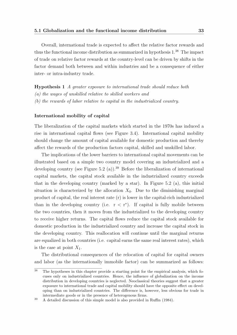
5.1 Globalization and the functional income distribution 33
Overall, international trade is expected to affect the relative factor rewards and
thus the functional income distribution as summarized in hypothesis 1.38 The impact
of trade on relative factor rewards at the country-level can be driven by shifts in the
factor demand both between and within industries and be a consequence of either
inter- or intra-industry trade.
Hypothesis 1 A greater exposure to international trade should reduce both
(a) the wages of unskilled relative to skilled workers and
(b) the rewards of labor relative to capital in the industrialized country.
International mobility of capital
The liberalization of the capital markets which started in the 1970s has induced a
rise in international capital flows (see Figure 3.4). International capital mobility
should change the amount of capital available for domestic production and thereby
affect the rewards of the production factors capital, skilled and unskilled labor.
The implications of the lower barriers to international capital movements can be
illustrated based on a simple two country model covering an industrialized and a
developing country (see Figure 5.2 (a)).39 Before the liberalization of international
capital markets, the capital stock available in the industrialized country exceeds
that in the developing country (marked by a star). In Figure 5.2 (a), this initial
situation is characterized by the allocation X0. Due to the diminishing marginal
product of capital, the real interest rate (r) is lower in the capital-rich industrialized
than in the developing country (i.e. r < r∗). If capital is fully mobile between
the two countries, then it moves from the industrialized to the developing country
to receive higher returns. The capital flows reduce the capital stock available for
domestic production in the industrialized country and increase the capital stock in
the developing country. This reallocation will continue until the marginal returns
are equalized in both countries (i.e. capital earns the same real interest rates), which
is the case at point X1.
The distributional consequences of the relocation of capital for capital owners
and labor (as the internationally immobile factor) can be summarized as follows:
38 The hypotheses in this chapter provide a starting point for the empirical analysis, which fo-cuses only on industrialized countries. Hence, the influence of globalization on the incomedistribution in developing countries is neglected. Neoclassical theories suggest that a greaterexposure to international trade and capital mobility should have the opposite effect on devel-oping than on industrialized countries. The difference is, however, less obvious for trade inintermediate goods or in the presence of heterogenous firms.
39 A detailed discussion of this simple model is also provided in Ruffin (1984).
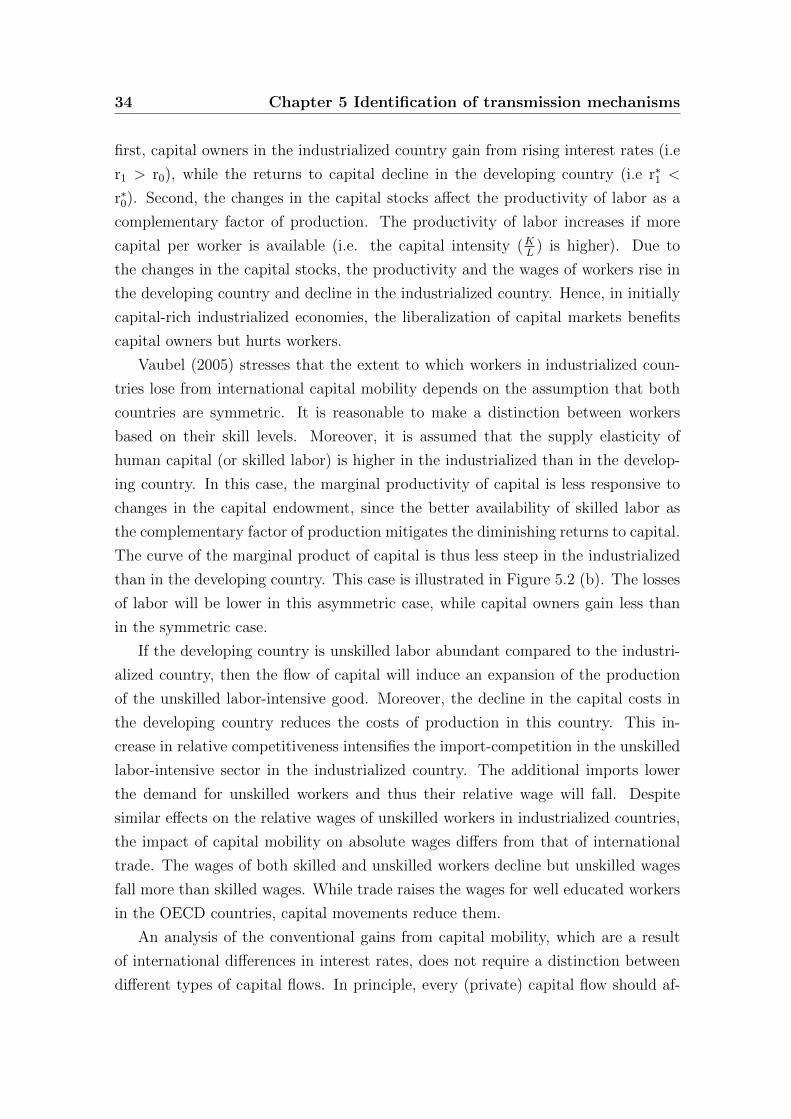
34 Chapter 5 Identification of transmission mechanisms
first, capital owners in the industrialized country gain from rising interest rates (i.e
r1 > r0), while the returns to capital decline in the developing country (i.e r∗1 <
r∗0). Second, the changes in the capital stocks affect the productivity of labor as a
complementary factor of production. The productivity of labor increases if more
capital per worker is available (i.e. the capital intensity (KL
) is higher). Due to
the changes in the capital stocks, the productivity and the wages of workers rise in
the developing country and decline in the industrialized country. Hence, in initially
capital-rich industrialized economies, the liberalization of capital markets benefits
capital owners but hurts workers.
Vaubel (2005) stresses that the extent to which workers in industrialized coun-
tries lose from international capital mobility depends on the assumption that both
countries are symmetric. It is reasonable to make a distinction between workers
based on their skill levels. Moreover, it is assumed that the supply elasticity of
human capital (or skilled labor) is higher in the industrialized than in the develop-
ing country. In this case, the marginal productivity of capital is less responsive to
changes in the capital endowment, since the better availability of skilled labor as
the complementary factor of production mitigates the diminishing returns to capital.
The curve of the marginal product of capital is thus less steep in the industrialized
than in the developing country. This case is illustrated in Figure 5.2 (b). The losses
of labor will be lower in this asymmetric case, while capital owners gain less than
in the symmetric case.
If the developing country is unskilled labor abundant compared to the industri-
alized country, then the flow of capital will induce an expansion of the production
of the unskilled labor-intensive good. Moreover, the decline in the capital costs in
the developing country reduces the costs of production in this country. This in-
crease in relative competitiveness intensifies the import-competition in the unskilled
labor-intensive sector in the industrialized country. The additional imports lower
the demand for unskilled workers and thus their relative wage will fall. Despite
similar effects on the relative wages of unskilled workers in industrialized countries,
the impact of capital mobility on absolute wages differs from that of international
trade. The wages of both skilled and unskilled workers decline but unskilled wages
fall more than skilled wages. While trade raises the wages for well educated workers
in the OECD countries, capital movements reduce them.
An analysis of the conventional gains from capital mobility, which are a result
of international differences in interest rates, does not require a distinction between
different types of capital flows. In principle, every (private) capital flow should af-
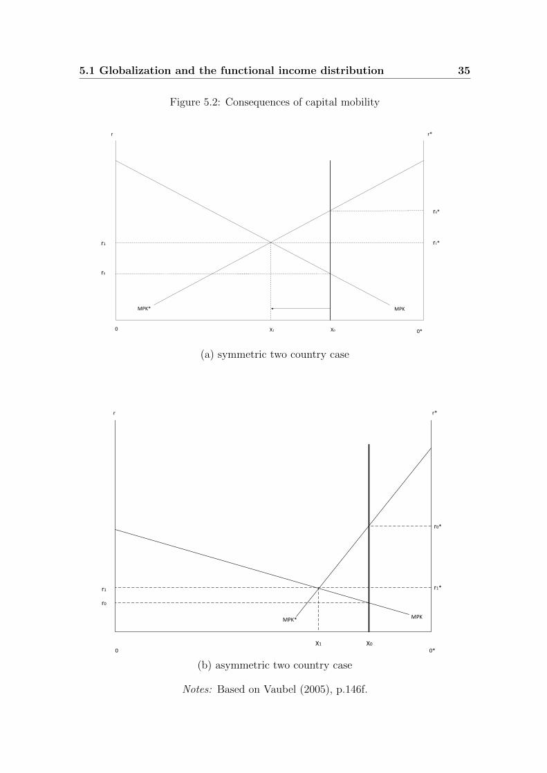
5.1 Globalization and the functional income distribution 35
Figure 5.2: Consequences of capital mobility
r*r
0 0*
MPK* MPK
X0X1
r1
r0
r0*
r1*
(a) symmetric two country case
r r*
0*0
MPK* MPK
X1 X0
r0
r1
r0*
r1*
(b) asymmetric two country case
Notes: Based on Vaubel (2005), p.146f.
36 Chapter 5 Identification of transmission mechanisms
fect a country’s capital stock and, hence, relative factor payments. Many studies
on capital mobility, however, focus solely on foreign direct investments (FDI) and
neglect other types of private capital flows. One reason for this has been the per-
ception that different kinds of international investments have different implications,
for instance, regarding the use of capital and its efficiency. Ownership is more dis-
persed among portfolio investors who hold smaller shares of foreign firms than FDI
investors. Thus, Razin (2003) argues that attempts to improve a firm’s management
under portfolio equity ownership will be hampered by a free-riding problem since
an investor who engages in improving management quality will not enjoy the full
benefits but any measure will be equally beneficial to all investors. Consequently,
the incentive to monitor and improve the management of the firm is lower for a
portfolio than for an FDI investor. Due to a probably superior management, FDI
firms might be more productive and this may also lead to higher wage payments (as
indicated by the findings of heterogenous-firms trade models).40 A higher produc-
tivity of multinational compared to purely domestic firms may be necessary since
activities in foreign markets by multinational firms are likely associated with addi-
tional costs, which local competitors do not bear. Insofar, multinational firms must
have a comparative advantage to survive in a foreign market (for a discussion of
this issue see Greenaway and Nelson, 2001). This effect may be reinforced through
the transfer of foreign technology and know-how to the firms located in the host
country. Besides these arguments, it may be reasonable to distinguish between the
international mobility of financial and real capital since the latter might be subject
to more political restrictions and controls (this point has been raised by Schulze and
Ursprung, 1999).
The theoretical expectations regarding the impact of international capital mo-
bility on the relative payments to different production factors are summarized in
hypothesis 2.
Hypothesis 2 The lowering of barriers to international capital movements
(a) increases the returns to capital relative to labor and
(b) lowers the wage of unskilled relative to skilled workers.
40 Helpman et al. (2004) propose a theoretical model of heterogenous-firms indicating that onlymore productive firms produce for foreign markets. Moreover, those firms with the highestproductivity serve foreign markets through foreign production facilities (FDI) while the othersexport their products. This model does, however, not allow to draw any conclusions aboutthe impact of different kinds of foreign investments (such as portfolio investments versus FDI)on firms’ productivity and wages but indicate that FDI might be related to firms’ economicsuccess and thus affect the wage distribution.
5.1 Globalization and the functional income distribution 37
Empirical evidence on globalization and relative factor prices
An extensive empirical literature exists, which - due to the coincidence of rising trade
and wage dispersion in many industrialized countries since the 1980s - elaborates
on the relationship between international trade and wage inequality. The empirical
evidence on this issue is, however, ambiguous (a literature review is provided by e.g.
Freeman, 1995; Greenaway and Nelson, 2001).
Several studies analyze the consequences of international trade based on estima-
tions of the relative factor content of imports and exports and, hence, approximate
the changes in relative labor demand due to trade. Whereas some authors (e.g.
Wood, 1995, 1998) find that international trade is a major cause of the reduced de-
mand for unskilled workers in the industrialized countries, others observe significant
but modest effects of trade on relative wages in advanced countries (e.g. Borjas et al.,
1992). A different approach41 has been chosen by several trade economists who an-
alyze whether the data supports the mechanisms suggested by the Heckscher-Ohlin
model. Several inconsistencies are detected in the data and, hence, the authors ar-
gue that trade cannot explain rising wage inequality. One basic issue is based on
the development of relative product prices. The chain of causation suggested by
the Stolper-Samuelson mechanism runs from trade-induced shifts in relative good
prices to changing relative factor rewards. Lawrence and Slaughter (1993) do not
find an increase in the relative prices of skill-intensive goods in the U.S. and there-
fore conclude that trade could not explain the rising wage differential. Sachs and
Shatz (1994), however, exclude computers, which distort the price calculations due
to massive price reductions, and come to a different conclusion that is in line with
the predictions by trade theory. A further objection raised against the relevance of
international trade is that the average skill-intensity has increased in all industries,
which is not suggested by the Stolper-Samuelson theorem.42
Therefore, many economists conclude that not international trade but techno-
logical change in favor of human capital must be the explanation for rising wage
differentials in many industrialized countries. This distinction between interna-
tional trade and technological change is, however, rather artificial as both are highly
41 The empirical studies conducted during the 1990s usually employ one of the following threeapproaches to elaborate on the relationship between international trade and labor marketoutcomes: factor-content, price or computable general equilibrium studies. Factor-contentstudies calculate (based on a set of very restrictive assumptions as e.g. critized by Wood,1995) the amount of labor incorporated in imported and exported goods. The differencebetween the relative amount of (skilled) labor embodied in traded goods, then, indicates howtrade affects relative labor demand and therefore wages.
42 This issue and its implications has already been discussed on page 27.
38 Chapter 5 Identification of transmission mechanisms
interrelated. On the one hand, improvements in transportation and communica-
tions technologies have fostered the international exchange of final and intermediate
goods. On the other hand, the greater competitive pressure resulting from trade
with low-wage countries such as China has induced defensive innovation in import-
competing industries (e.g. Van Reenen, 2011). Wood (1998) reports that both tech-
nological change and trade with developing countries matter for the rise in relative
demand for skilled labor.43 Koeninger et al. (2007) find a positive relationship be-
tween import penetration and wage dispersion in OECD countries between 1973
and 1998 after controlling for differences in domestic labor institutions. The effect
is more pronounced if the authors focus only on imports from non-OECD countries.
Moreover, R&D intensity (as a proxy for technological change in favor of skilled
workers) fails to have a significant impact.
Newer developments since the 1990s are the expansion of trade with low-wage
countries such as China and the vertical disintegration of the production process
through offshoring and outsourcing. This leads to a stronger specialization of low-
wage countries in the production of (unskilled) labor-intensive goods or components
in otherwise skill- or capital-intensive products (e.g. computers). Using data for the
U.S. from 1979 to 1990, Feenstra and Hanson (1999) analyze how outsourcing and
high-technology capital affect relative wages. The estimates indicate that investment
in high-technology capital (e.g. computers) account for 35 percent of the increase in
the wage differential, while outsourcing (i.e. imports of intermediate inputs) explains
15 percent of this rise. Geishecker and Gorg (2007) test empirically how international
outsourcing affected wages of German workers between 1991 and 2000. For that
purpose, the authors combine micro-level data for workers with information about
outsourcing activities of the industry in which they are employed. The regression
results suggest that imports of intermediate inputs increase the wages of high skilled
workers but reduce the wage of low skilled workers. This finding is remarkable since
outsourcing has widened the skill premium despite a highly regulated German labor
market and the absence of a considerable rise in the wage differential at the aggregate
level as experienced in the U.S..
Empirical evidence on the impact of international capital movements on the
distribution of wages is limited. Moreover, most empirical studies are concerned
with multinational firms and offshoring activities through FDI.44 A recent empirical
43 He concludes that technological changes explain most of the increase in the relative demand forskilled labor during the 20th century but international trade is responsible for the accelerationin its growth since the 1980s.
44 Offshoring activities, i.e. firms’ investment in foreign plants relate to international capital
5.1 Globalization and the functional income distribution 39
analysis based on a panel of OECD countries (OECD, 2011) indicates that fewer
restrictions toward FDI and a greater stock of outward FDI are associated with
greater wage inequality.
5.1.2 Non-adjustment of relative factor rewards and
unemployment
So far, the predictions regarding the impact of globalization on the functional income
distribution have focused only on changes of the relative rewards of production
factors. This would be sufficient if the relative factor prices were flexible and fully
adjusted to shifts in the relative factor demand or supply. This is the case if factor
markets are perfectly competitive. In many industrialized countries, however, several
market imperfections exist which prevent a full adjustment of the relative factor
prices and thereby market clearing.45
Globalization lowers the relative demand for unskilled workers and thus induces
a downward pressure on the relative wages of unskilled workers. The prevalence
of labor market rigidities may hinder the relative wages from responding to these
demand shifts. If the wages of unskilled relative to skilled workers are fixed at some
level exceeding the equilibrium wage (e.g. because of minimum wages), then this
leads to an increase in involuntary unemployment among unskilled workers. Conse-
quently, the change in the relative labor demand will affect the income distribution
either through a rising wage dispersion or a shift in the relative employment of
workers.46
Role of rigid labor market institutions
Several theoretical works shed light on the effects of international trade and capital
mobility on employment. A first group of studies focuses on inter-industry trade
movements. At the same time, the production of intermediate inputs abroad raises tradevolumes as these inputs are imported and used for domestic production. Hence, the rise inimports of intermediate goods and outflows of capital are two sides of a coin.
45 Although imperfections in any good or factor market may result in a situation in which factorprices are not fully flexible, labor market imperfections that are existent in many advancedeconomies are probably the most prominent and relevant source of market failure. Hence, themain focus of the subsequent discussion is on labor market rigidities.
46 A popular perception is that the different adjustments of either relative wages or employmentrefer to the American (flexible labor market) and the European (rigid labor markets) case(e.g. Johnson and Stafford, 1999). This is, however, an oversimplification as indicators ofwage flexibility (e.g. the overall responsiveness of wages to the level of unemployment) do notdiffer much between Europe and North America. Moreover, labor market institutions varyconsiderably between European countries (Nickell, 1997).
40 Chapter 5 Identification of transmission mechanisms
and compares the labor market outcomes for different institutional settings.
Krugman (1995) analyzes the wage and employment effects in advanced economies
that result from trade with less developed countries with a specific focus on the role
of labor market institutions. He performs his analysis of the consequences of trade
separately for economies with different degrees of labor market flexibility and com-
pares the impact of trade liberalization in these different setups. His calculations
suggest that the adverse labor market effects of inter-industry trade are rather small
with flexible labor markets but can be substantial in the presence of labor market
rigidities.47 In a related work, Davis (1998) chooses a theoretical framework in which
the world economy consists of a country with fully flexible wages and another with
a binding minimum wage. In a Heckscher-Ohlin approach, free trade tends to raise
unemployment in the economy with rigid labor markets and to increase wages in
the other. If both countries start trading with a third economy (e.g. a less devel-
oped country), then the import-competion will increase in the rigid economy (due
to differences in the relative good prices resulting from the minimum wage) but not
affect the flexible market.
A recent strand of literature uses heterogenous-firms models combined with im-
perfect labor markets. For instance, Davis and Harrigan (2007) introduce efficiency
wages which are paid at the firm-level into a standard Melitz-model. To increase
workers’ costs of a job loss and thus shirking, firms pay higher wages. Moreover,
firms pay different wages as they differ in their ability to monitor workers and to
detect shirking. In this framework, trade liberalization destroys jobs with high
marginal cost of production and those paying high efficiency wages. A related work
by Egger and Kreickemeier (2009) incorporates workers with a preference for fair
wages into a general equilibrium model with heterogenous-firms. The wage workers
consider to be fair depends on the firms’ productivity (i.e. is motivated by a rent-
sharing motive) and workers adjust their effort on the wage they are paid. Hence,
wages depend on the economic success and the productivity of the firm. The profit
maximizing firm pays a fair wage, which is above the equilibrium wage and induces
involuntary unemployment. As the most productive firms start to export and the
least productive firms leave the market after trade liberalization, average profits of
firms and therefore wages rise. In this framework, trade liberalization increases in-
voluntary unemployment. Egger et al. (2001) show that the international mobility
of capital further exacerbates the negative effects of international trade on earnings
47 The estimates indicate that trade with developing countries causes around 20% of the increasein European unemployment and approximately 10% of the rise in U.S. wage inequality.
5.1 Globalization and the functional income distribution 41
dispersion or unemployment (in the presence of rigid labor markets).
Globalization and the elasticity of labor demand
Besides its impact on the relative wages or employment of unskilled workers, glob-
alization may also increase the elasticity of the labor demand.48 This can be a
consequence of a greater ease at which domestic workers can be replaced by for-
eign labor due to imports or the relocation of the production.49 A higher labor
demand elasticity might adversely affect workers, for instance, by shifting the inci-
dence of labor taxes from employers to workers or reducing the bargaining power
of labor (Rodrik, 1997). Hence, international trade and capital mobility may also
influence the functioning of the labor markets via their impact on labor demand
elasticities. In particular, a greater integration into world markets tends to lower
the relative strength of trade unions in the wage bargaining process. In product
markets with imperfect competition, firms receive rents which are shared between
firms and unions. International trade increases the competition in product markets
and lowers firms’ rents as well as the union wages (e.g. Gaston and Trefler, 1995).
If unions do not realize this decline in rents and, hence, fail to adjust their wage
claims, then unemployment will rise in response to the greater economic integration.
Over time, unions adjust their bargaining behavior, which results in lower wages and
unemployment (Blanchard and Philippon, 2003).
Choi (2001) analyzed how the threat effects of capital mobility influence the
union wage premium. He argues that as the costs of foreign investment decline,
the likelihood of offshoring production activities rises. The better outside options
of the firms reduce the relative bargaining power of unions and therefore the union
wage premium. A lower union wage premium might reduce unemployment. At the
same time, the wage dispersion may increase if predominantly the wages of unskilled
workers are bargained by unions.
Frictional unemployment
While labor market imperfections prevent a long-term adjustment of relative wages
and therefore create unemployment, globalization may also increase job turnover and
frictional unemployment. Trade models usually compare different long-term equilib-
48 The analysis by Slaughter (2001) provides limited support for this hypothesis. Internationaltrade and capital mobility had the expected impact on labor demand elasticities in U.S.manufacturing between 1961 and 1991 but only if the empirical analysis does not include timeeffects.
49 Relevant are not actual transactions but the ease at which they can be undertaken.
42 Chapter 5 Identification of transmission mechanisms
ria (e.g. the autarky versus free trade equilibrium) to elaborate on the distributive
effects of exposure to international competition. The transition processes related to
shifts in the production structure of trading economies are largely neglected (e.g.
Richardson, 1995). Due to changes in the relative goods prices, the export sectors
expand while import-competing sectors contract. If, as it is assumed by long-run
trade models, workers are fully mobile between sectors, the relative wages adjust
to reabsorb the displaced workers. These reallocations are, however, highly com-
plex and relative prices will not adjust immediately. Consequently, workers who are
displaced from import-competing industries will experience some period of search
unemployment before finding a new job. The length of the transition period (and
the average unemployment spell of displaced workers) and the size of the short-
term adjustment costs depend on a country’s institutional framework and its labor
market flexibility. Davidson and Matusz (2000) emphasize the relevance of labor
market institutions for the net gains from trade (i.e. the difference between long-
term increases in income and short-term costs due to job loss). The authors propose
a model incorporating workers with different abilities who experience consecutive
periods of training, employment and unemployment. Trade liberalization leads to
a reallocation of jobs from the low-tech to the high-tech sector and increases unem-
ployment as workers in the high-tech sector require a specific training. Although
the long-term benefits always exceed the short-term adjustment costs, their relative
size depends on labor market institutions.50
The point discussed above is also raised by Ranjan (2012) who employs a short-
to medium-run framework where labor is not mobile between the export and the
import-competing sector. Trade liberalization increases both the creation and de-
struction of jobs in the import-competing industry, but has no immediate effect on
job turnover in the export sector. Since the speed of transition differs between both
sectors the unemployment rate adjusts gradually: while the jobs in the import-
competing sector are destroyed immediately, new jobs are created in the export
sector only in the medium run. Hence, trade liberalization will induce short-term
spikes in unemployment. More generous unemployment benefits (as a reservation
wage for workers) raise the job destruction and unemployment due to trade liberal-
ization.
Felbermayr et al. (2011a) focus on the existence of labor market frictions, which
prevent displaced workers from immediately finding a new employment because they
50 Simulations by Davidson and Matusz indicate that the net gains from trade are highest iflabor markets are either fully flexible or very rigid. Economies where the speed of adjustmentlies between these extremes, the benefits might be almost offset by the short-term costs.
5.1 Globalization and the functional income distribution 43
have to invest in a period of active search. Falling trade costs (or the emergence of
new trading partners) raise the average productivity of firms (through a reallocation
in market shares as in Melitz, 2003) and reduce search unemployment since the
recruitment of workers becomes more profitable. In particular, rising productivity
increases the value of the marginal product of labor relative to the recruitment costs
of firms.51 Thus, declining trade costs can both lower unemployment and raise real
wages as long as it improves average productivity.
Hypothesis 3 Globalization is expected to increase the unemployment of unskilled
workers if the relative wages of unskilled workers do not fully adjust to demand shifts
(e.g. in the presence of labor market rigidities). In particular in the short-run, inter-
national trade and capital mobility may lead to a rise in transitory unemployment. In
the medium- to long-run, globalization could also lower unemployment, for instance,
by raising labor productivity or reducing labor market frictions.
Empirical tests of the relationship between openness and unemployment in ad-
vanced economies are still scarce. Trefler (2004) studies the consequences of the
free-trade agreement between Canada and the U.S. (NAFTA) for Canadian indus-
tries. His findings suggest that tariff cuts induced considerable job losses especially
in import-competing industries. These negative consequences of trade liberalization,
however, seem to reflect the short-run adjustment costs as Canada did not expe-
rience a permanent increase in unemployment.52 Hence, while trade liberalization
tends to increase frictional unemployment due to the reallocation of resources be-
tween industries and firms, the long-run effects are less obvious. Felbermayr et al.
(2011b) find that trade openness tends to lower unemployment for a panel of 20
OECD countries.53 The analysis conducted by Checci and Garcia-Penalosa (2010)
also points at a negative relationship between openness and unemployment.
The long-run consequences of international trade and capital mobility for the
development of unemployment rates likely depend on the impact of globalization
51 The firms’ decision to post vacancies and hire workers is based on a comparison of the shadowvalue (i.e. the additional revenue generated) of an additional worker relative to the expectedmarginal recruitment costs. Once a firm and worker are matched, they bargain over thewage including the rents generated by the successful job match. Falling trade costs raises theaverage productivity of firms and thus also the rents. As long as firms receive some of the rentsresulting from a filled vacancy, they will hire more workers. Hence, search unemployment willdecline.
52 Trefler’s analysis points at the same time at considerable productivity gains and thereforelong-term benefits of NAFTA for the Canadian economy.
53 The regressions show either significant negative or insignificant effects of trade openness onunemployment.
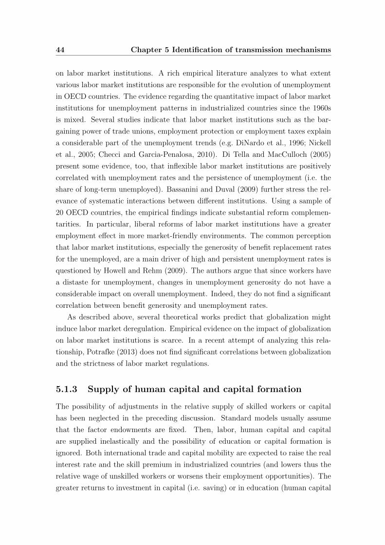
44 Chapter 5 Identification of transmission mechanisms
on labor market institutions. A rich empirical literature analyzes to what extent
various labor market institutions are responsible for the evolution of unemployment
in OECD countries. The evidence regarding the quantitative impact of labor market
institutions for unemployment patterns in industrialized countries since the 1960s
is mixed. Several studies indicate that labor market institutions such as the bar-
gaining power of trade unions, employment protection or employment taxes explain
a considerable part of the unemployment trends (e.g. DiNardo et al., 1996; Nickell
et al., 2005; Checci and Garcia-Penalosa, 2010). Di Tella and MacCulloch (2005)
present some evidence, too, that inflexible labor market institutions are positively
correlated with unemployment rates and the persistence of unemployment (i.e. the
share of long-term unemployed). Bassanini and Duval (2009) further stress the rel-
evance of systematic interactions between different institutions. Using a sample of
20 OECD countries, the empirical findings indicate substantial reform complemen-
tarities. In particular, liberal reforms of labor market institutions have a greater
employment effect in more market-friendly environments. The common perception
that labor market institutions, especially the generosity of benefit replacement rates
for the unemployed, are a main driver of high and persistent unemployment rates is
questioned by Howell and Rehm (2009). The authors argue that since workers have
a distaste for unemployment, changes in unemployment generosity do not have a
considerable impact on overall unemployment. Indeed, they do not find a significant
correlation between benefit generosity and unemployment rates.
As described above, several theoretical works predict that globalization might
induce labor market deregulation. Empirical evidence on the impact of globalization
on labor market institutions is scarce. In a recent attempt of analyzing this rela-
tionship, Potrafke (2013) does not find significant correlations between globalization
and the strictness of labor market regulations.
5.1.3 Supply of human capital and capital formation
The possibility of adjustments in the relative supply of skilled workers or capital
has been neglected in the preceding discussion. Standard models usually assume
that the factor endowments are fixed. Then, labor, human capital and capital
are supplied inelastically and the possibility of education or capital formation is
ignored. Both international trade and capital mobility are expected to raise the real
interest rate and the skill premium in industrialized countries (and lowers thus the
relative wage of unskilled workers or worsens their employment opportunities). The
greater returns to investment in capital (i.e. saving) or in education (human capital
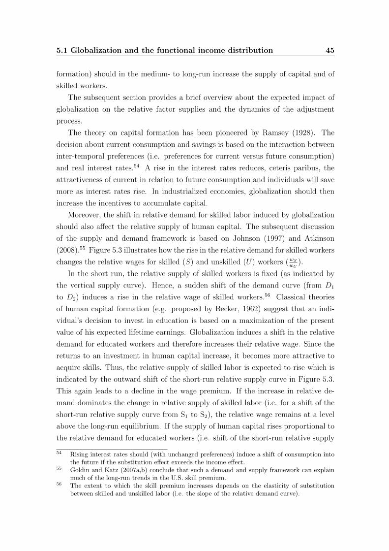
5.1 Globalization and the functional income distribution 45
formation) should in the medium- to long-run increase the supply of capital and of
skilled workers.
The subsequent section provides a brief overview about the expected impact of
globalization on the relative factor supplies and the dynamics of the adjustment
process.
The theory on capital formation has been pioneered by Ramsey (1928). The
decision about current consumption and savings is based on the interaction between
inter-temporal preferences (i.e. preferences for current versus future consumption)
and real interest rates.54 A rise in the interest rates reduces, ceteris paribus, the
attractiveness of current in relation to future consumption and individuals will save
more as interest rates rise. In industrialized economies, globalization should then
increase the incentives to accumulate capital.
Moreover, the shift in relative demand for skilled labor induced by globalization
should also affect the relative supply of human capital. The subsequent discussion
of the supply and demand framework is based on Johnson (1997) and Atkinson
(2008).55 Figure 5.3 illustrates how the rise in the relative demand for skilled workers
changes the relative wages for skilled (S) and unskilled (U) workers (wS
wU).
In the short run, the relative supply of skilled workers is fixed (as indicated by
the vertical supply curve). Hence, a sudden shift of the demand curve (from D1
to D2) induces a rise in the relative wage of skilled workers.56 Classical theories
of human capital formation (e.g. proposed by Becker, 1962) suggest that an indi-
vidual’s decision to invest in education is based on a maximization of the present
value of his expected lifetime earnings. Globalization induces a shift in the relative
demand for educated workers and therefore increases their relative wage. Since the
returns to an investment in human capital increase, it becomes more attractive to
acquire skills. Thus, the relative supply of skilled labor is expected to rise which is
indicated by the outward shift of the short-run relative supply curve in Figure 5.3.
This again leads to a decline in the wage premium. If the increase in relative de-
mand dominates the change in relative supply of skilled labor (i.e. for a shift of the
short-run relative supply curve from S1 to S2), the relative wage remains at a level
above the long-run equilibrium. If the supply of human capital rises proportional to
the relative demand for educated workers (i.e. shift of the short-run relative supply
54 Rising interest rates should (with unchanged preferences) induce a shift of consumption intothe future if the substitution effect exceeds the income effect.
55 Goldin and Katz (2007a,b) conclude that such a demand and supply framework can explainmuch of the long-run trends in the U.S. skill premium.
56 The extent to which the skill premium increases depends on the elasticity of substitutionbetween skilled and unskilled labor (i.e. the slope of the relative demand curve).
46 Chapter 5 Identification of transmission mechanisms
Figure 5.3: Determination of relative wages based on a demand and supply frame-work
ws / wu
S / U
D1
S1
Long-run supply
D2
S2 S3
Notes: Based on Atkinson (2008), page 8.
from S1 to S3), the relative wage will return to its long-run equilibrium level.
The long-run supply of educated workers and the relative wage (i.e. the horizon-
tal line in Figure 5.3) is based on human capital formation models assuming that all
individuals are identical in their capabilities and decide on investment in education
by comparing the present value of their earnings. In the absence of any schooling
costs, the opportunity costs of training are equal to the postponement of earnings.
In this framework, the wage differential equals the opportunity costs of education
and is just sufficient to compensate for the foregone discounted earnings.57
The dynamics of shifts in relative skill demand and supply which continue over
time have been described by Atkinson (2008). The basic idea that the increasing
exposure to globalization (or to skill-biased technological change) is responsible for
the rising skill premium in industrialized countries implies permanent shifts in the
relative demand for educated workers. If the relative demand curve steadily shifts
57 The size of the wage differential depends on the real interest rate since the foregone earningsduring the training period have to be discounted to calculate their present value. A higherreal interest rate then increases the present value of the foregone earnings and hence theopportunity costs of education. Thus, higher interest rates lead to a greater wage differential.Capital markets may also explain the rise of the skill premium (compare Atkinson, 2008).

5.1 Globalization and the functional income distribution 47
upward at a constant proportional rate, then the skill premium increases. This
leads to a rise in the relative skill supply. The steady increase of the relative demand
results in a semi-equilibrium where skilled labor persistently receives a skill premium
exceeding the long-run equilibrium. Even if this wage differential remains constant
(despite a steady increase in the relative demand for skilled workers), the share of
unskilled workers will fall.
Tinbergen (1974) named the persistent shifts in both the relative demand for
and supply of educated workers the “race between technology and education”.58
The evolution of the skill premium depends on the relative strength of demand and
supply adjustments.
Cross-country differences in the speed of supply changes may explain different
developments of the earnings distribution although all countries face comparable
changes in the relative demand for skilled labor induced by globalization or tech-
nological change. Furthermore, the ability to react to adjustments in the relative
returns to education depends on a country’s institutional framework (such as its
education system and labor market institutions).
The expectations regarding the effect of globalization on the human capital sup-
ply is summarized in hypothesis 4.
Hypothesis 4 Globalization, and the resulting increase in the relative demand for
skilled labor, should lower the relative supply of unskilled workers as it raises the
returns to education in the industrialized countries.
The determinants of human capital formation and the relative endowment of
skilled workers have been studied theoretically and also related to a country’s ex-
posure to globalization. Still, the relationship between international economic inte-
gration and investment in human capital has been widely neglected in the empirical
literature, which focuses mostly on other labor market outcomes such as the evolu-
tion of the wage differential.59
Machin and Van Reenen (1998) elaborate on the impact of technological change
on the supply of skills in seven OECD countries between 1973 to 1989. The authors
focus on technological change as an explanation for changes in the relative demand
58 The development of the skill premium ultimately depends on the relative pace of both changes.Goldin and Katz (2007a,b) further study this race focusing on the United States (see also thereview by Acemoglu and Autor (2012) and their extension using the task approach).
59 A notable exception is a recent study by Hickman and Olney (2011) who analyze how off-shoring and immigration affect the education decision of U.S. workers. The findings point atsome impact of globalization on investments in human capital as the enrollment rates in com-munity colleges are higher in states with a higher share of immigrants and workers employedin foreign-owned firms.
48 Chapter 5 Identification of transmission mechanisms
for skilled labor. The empirical analysis of industry-level data reveals a positive (and
mostly significant) association between the R&D intensity and the compensation of
non-production relative to production workers. Import penetration does, however,
not contribute significantly to the explanation of changes in the wage-bill shares of
non-production workers.
5.2 The distribution of production factors within
the population
The preceding section discussed the potential effects of globalization on the func-
tional income distribution. Statements about the impact of international trade and
capital mobility on the distribution of market incomes, however, require a profound
knowledge about how production factors are distributed within the population of a
country.
The question whether the inequality of market incomes increases in response to
a greater economic integration or not can only be answered empirically. Due to its
focus on the role of transmission mechanisms, the empirical analysis in section 7.2
shall provide information on how changes in the functional income distribution affect
market inequality. Nevertheless, this section already offers a first insight into the
distribution of production factors within the population of OECD countries based
on a descriptive analysis and the findings by some recent studies.
In general, individuals receive incomes from different sources (e.g. employment,
self-employment or capital) and might therefore at the same time be affected by
different developments of the functional income distribution. Beyond the distribu-
tion of production factors between individuals, also the household composition (e.g.
assortative mating and household size) matters if the relevant income unit is the
household.60
Figure 5.4 provides information about the relative importance of different income
sources for the population in eleven OECD countries around the year 2000. More-
over, differences in the relevance of these income sources for the disposable income
of low and high income individuals are compared across the respective countries.
Although this section focuses on the distribution of market incomes, non-market
60 Changes in living arrangements (e.g. rise in the importance of single-households) and demo-graphic structures (e.g. increasing share of the elderly) affect the income distribution. Sincethis study focuses on economic factors, I do not address these factors explicitly but havetested in the subsequent econometric analysis whether compositional effects matter for theexplanation of income differences. For a detailed discussion see OECD (2008, 2011).
5.2 Distribution of production factors within the population 49
Figure 5.4: Share of different income sources in total income
-60-40-20
020406080
100120140160180
wage income self-employment income capital income private transfers social transfers taxes
(a) all income groups
-60-40-20
020406080
100120140160180
wage income self-employment income capital income private transfers social transfers taxes
(b) low income recipients
-60-40-20
020406080
100120140160180
wage income self-employment income capital income private transfers social transfers taxes
(c) high income recipients
Notes: Own calculations based on equivalent incomes. Data comes from the wave V (around 2000)of the Luxembourg Income Study. More information about the data concept is offered in chapter6.2 and information about the exact years to which the data refers is available in Table A.2.
50 Chapter 5 Identification of transmission mechanisms
income components (e.g. private and public transfers, social security contributions
and direct taxes) should also be relevant since taxes and transfers affect individual
incentives to work or invest and thereby indirectly also the market incomes.
Figure 5.4 (a) depicts the shares of wage, self-employment and capital income,
private and social transfers as well as income tax payments and social security con-
tributions in the average disposable income for the population of eleven OECD
countries in 2000. It is evident that incomes from dependent work are the most
important income source in these countries. The average for the examined countries
suggests that wages account for 101 percent of the total income (i.e. before the
deduction of taxes and social security contributions).61 However, the contributions
of wage incomes differ between the countries: gross wage incomes make up only
64 percent of the disposable income of the average person in Poland but almost
119 percent in Denmark. These differences are related to both a higher tax burden
in Denmark and the relative importance of other income sources for individuals in
Poland. Incomes from self-employment activity contribute on average to 11 percent
of the disposable income in these industrialized countries. The data indicates a sub-
stantial variation in the importance of this income source between these countries:
the relative importance of self-employment for the average disposable income of the
population is lowest in Sweden (4 percent) and highest in Poland (18 percent). Cap-
ital income is a less relevant income source for the population average: The average
share of gross capital incomes in disposable incomes for the eleven OECD countries
is 4 percent and varies between 0.2 percent in Poland and 7.3 percent in Norway.
The relative weight of different income sources for the average income earners
already reveals that the overall importance of different income sources varies con-
siderably. Consequently, an equal increase in the dispersion of the wage or capital
income distribution might have very different implications for the development of
market inequality.62 Furthermore, one needs to examine differences in the relevance
of these income sources for different types of income recipients. The overall distribu-
tive consequences of an increase in the rewards to capital relative to labor for market
income inequality depends on the relative importance of these income sources for
61 The share of all single income sources may add to more than 100 percent of the disposableincome because the income sources are all gross of taxes. To normalize the contribution ofthe different incomes, one could deduct the average taxes (share of taxes and social securitypayments) from each income source. This might, however, not be useful here as the maininterest is on information about market incomes.
62 In general, contribution of a single type of income to overall income inequality depends bothon how unequal this income type is distributed within the population and on how much theparticular income type contributes to the overall income.
5.2 Distribution of production factors within the population 51
low and high income households. If high income earners receive a greater share of
their incomes from capital than low income recipients, then higher relative payments
to capital should raise the inequality of market incomes and vice versa.
Hence, Figure 5.4 (b) and (c) present the shares of different income sources
in disposable incomes both for low and high income individuals. A first overall
finding is that the different types of market-generated incomes contribute less to
the average disposable income of the 25 percent of the population with the lowest
equivalent incomes than of the 25 percent with the highest incomes. The average
of all examined countries suggest that nearly 42 percent of the disposable income of
individuals belonging to the lowest quartile consists of transfer income. In contrast
to that, the share of transfers in the disposable income of the upper quartile is on
average about 7 percent. The relative importance of each type of market income
also confirms this general finding: the share of wage and self-employment income
in disposable income of a high income individual is on average about 1.7 times
higher than for an individual in the lowest quartile of the income distribution. The
difference between high and low income individuals is even more pronounced for
capital incomes. In this case, the share of capital incomes in disposable income is on
average four times higher for high than for low income recipients. This suggests that
wealthy individuals earn disproportionately more capital income than low income
individuals and, hence, also benefit from a rise in rewards to capital relative to labor.
As a consequence, market income inequality is expected to rise.
To achieve a broader impression of the relationship between the functional and
personal income distribution, the descriptive analysis presented above is supple-
mented by two recent OECD studies (OECD, 2008, 2011) that describe the rela-
tionship between factor and market income inequality. The main findings suggest
that the more unequal distribution of wages (among full-time employed men)63 has
contributed to a more dispersed market income distribution in the OECD. Besides
changes in wage inequality, work intensity also matters for the evolution of market
income inequality. During the last decades, reductions of hours for workers (e.g.
the growing incidence of part-time and temporary work) have raised the dispersion
of market incomes as foremost low-wage recipients work fewer hours. The distribu-
tion of household wages, which is affected by partnership formation and household
size (i.e. via economies of scale in consumption), has remained rather stable since
the mid-1990s. This is mainly because increasing labor market participation has
63 The studies use data from the OECD earnings data set which offers information on weekly,monthly and annual wages of full-time employees (here: dependent male workers) at variouspercentiles.
52 Chapter 5 Identification of transmission mechanisms
offset the effect of growing wage dispersion on the distribution of wages between
households. In addition, the relevance of non-wage incomes for the market income
distribution is rather modest. Despite the more uneven distribution of incomes
from capital and self-employment compared to wage incomes and the fact that the
increase in their inequality was greater in most OECD countries, these non-wage
incomes account only for a small share of the overall income.
This general pattern is also supported by the findings of Kenworthy (2008),
which suggest a strong positive relationship between market income inequality and
the dispersion of earnings among employed workers, the share of households without
earners and - though less pronounced - the share of single-adult households and the
correlation between spouses’ earnings.64 His bivariate correlations based on twelve
advanced economies do, however, not support the findings of the OECD regarding
a strong impact of (part-time) employment on the distribution of market incomes.
5.3 Redistribution of incomes through the tax and
transfer system
The distribution of disposable incomes and therefore of consumption possibilities
depends not only on the distribution of market incomes among individuals but also
on the design and implementation of redistributive policies (e.g. taxes and transfers).
Beyond its impact on the distribution of market incomes, globalization might also
change the effectiveness and scope of redistributive policies.
The consequences of a greater integration of a country into world goods and
capital markets for its government size and structure are theoretically ambiguous.
In principle, two distinct impacts of globalization should be taken into account: on
the one hand, the competition for mobile factors might increase the costs of redis-
tribution for national governments. On the other hand, globalization likely raises
market income inequality (as discussed in the preceding sections) and potentially
also income volatility (via a greater exposure to external income risks), which leads
to a higher demand for redistribution among voters.
The first effect (the so-called “efficiency hypothesis”) relates to the supply of pub-
lic redistribution and suggests that the openness to international trade and capital
mobility limits the size of the welfare state. The second effect (the “compensation
64 From the perspective of social policy, differences between market and disposable incomes areof major interest. Nonetheless, a detailed knowledge of the sources of income differences maybe required to design policies targeted at a potentially desired reduction of inequality.
5.3 Redistribution of incomes through the tax and transfer system 53
hypothesis”) takes a demand-side view and expects rising redistribution and social
security spending as voters’ support for globalization policies might be conditional
to an adequate compensation.
The basic ideas behind these opposite effects of globalization are briefly summa-
rized below. For an extensive survey, which focuses also on supply and demand side
explanations compare, for instance, Schulze and Ursprung (1999).
The efficiency hypothesis rests on the basic reasoning that the competition of
national states for mobile production factors (mostly capital) constrains the scope
of taxation. The classical model of tax competition65 by Zodrow and Mieszkowski
(1986) predicts that the mobility of capital between different jurisdictions lowers
the provision of public goods due to the inefficiency of capital taxation in a small
open economy. From the perspective of a small open economy, the net returns to
capital (or other mobile factors) are determined on the world market. Hence, the
government’s scope to raise a capital tax is limited since fully mobile capital will leave
if the returns net of taxes fall below those available at the world market. Countries
that impose higher capital tax rates than other jurisdictions will experience capital
outflows and an erosion of the tax base, which impedes the provision of public
goods and transfers.66 Most of the early works on the consequences of capital tax
competition conclude that the competition for mobile capital leads to lower taxes
on capital and levels of public goods (an extensive survey is provided by Wilson and
Wildasin, 2004; Fuest et al., 2005).
There are though reasons to expect that tax competition does not fully abolish
a government’s possibility to tax mobile factors. In principle, taxation is but one
aspect in the location decision of firms and mobile capital. If taxes are used to
finance the provision of public input goods (e.g. infrastructure, education), which
increase the productivity of capital and thereby its gross returns, then taxation
should still be possible. Nevertheless, capital would then only pay for the use of
services and does not engage in redistribution.
The distributive effects of tax competition for mobile factors are also evident
65 Wilson and Wildasin (2004) propose to define tax competition “as [a] noncooperative taxsetting by independent governments, under which each government’s policy choices influencethe allocation of a mobile tax base [e.g. workers, firms, capital, or shoppers] among ‘regions’represented by these governments” (p. 1067).
66 The assessment of the decline of tax rates due to tax competition depends on the questionwhether the autarky tax level has been chosen to maximize welfare or not. In the first case,tax competition may lead to inefficiently low taxes and an underprovision of public goods. Ifthe size of the government is, however, excessively high and does not maximize voters utility(e.g. as suggested by Leviathan models described e.g. in Blankart, 2008, chapter 11.C), thenthe constraints due to capital mobility are welfare-enhancing.
54 Chapter 5 Identification of transmission mechanisms
if at least one production factor is not fully mobile between different countries. If
capital is fully mobile and labor cannot cross borders, then capital could escape
redistributive taxation and the reduction of the domestic capital stock would lower
the productivity and the income of labor as the complementary factor of production.
The tax burden is thus shifted to labor as the immobile and inelastically supplied
factor. Based on optimal taxation theory, capital, whose supply is infinitely elastic
from the perspective of a small open economy, should not be taxed.
In several cases, capital taxation is still possible (Wilson and Wildasin, 2004).
For instance, large countries that can influence the net returns to capital on the
world market will be able to tax capital (though presumingly less than under au-
tarky). Moreover, international mobility of production factors can also lead to lower
subsidies on mobile firms by limiting the opportunities of wasteful policies (such as
strategic trade policies, compare Janeba, 1998).
In addition, trade liberalization does also not necessarily impede the possibility
of income redistribution between different sectors. Vannoorenberghe and Janeba
(2013) propose a model with workers who differ in their sector-specific productivity
and are partly mobile between different sectors. The workers decide by majority
voting over redistribution toward the sector facing a low demand. If redistribution
is implemented its extent will be higher under free trade than under autarky (as
redistribution is more likely in an open economy though with lower amounts).67
Due to an apparent fear of a “race to the bottom” in taxation and welfare state
spending (as predicted, for instance, by Sinn, 2003), politicians regularly attempt
to limit the extent of international tax competition through political coordination.68
Boockmann and Vaubel (2009) stress that international coordination may not simply
prevent a (potentially harmful) decline in taxation but rather result in a minimum
level of taxation, which is even higher than the level originally chosen by high-
tax countries. Under majority voting, high-tax countries try to raise their rivals’
costs and increase taxes in other countries. Hence, the high-tax majority aims at
establishing its (or an even higher) level of taxation also in other countries which
prefer lower taxes. Moreover, the authors stress that even if governments compete
for mobile capital and are also interested in taxation (e.g. to win elections) this
would induce a “race to the Nash-point” (i.e. an uncooperative equilibrium with a
67 The basic idea behind this result is that in a small open economy, subsidization of a sectoris less distortive and more redistributive than in a closed economy because the subsidy doesnot affect goods prices and demand on the world market.
68 Such as the Code of Conduct for business taxation of the European Union (compare http:
//ec.europa.eu/taxation_customs/taxation/company_tax/harmful_tax_practices/).
5.3 Redistribution of incomes through the tax and transfer system 55
positive level of taxation and regulation) rather than a “race to the bottom”.
In the following, I review some theories that predict a positive relationship be-
tween a greater exposure to global markets and the size of the welfare state.
A political-economic explanation for rising redistribution is based on the median
voter theorem, which explains political outcomes with majority decisions. Given
that several assumptions regarding the preferences of voters and political parties
apply,69 the policy choice of the median voter will be implemented. Meltzer and
Richard (1981) employ the median voter approach to explain political decisions
about income redistribution. The redistributive policy consists of a lump-sum trans-
fer financed by a proportional income tax. The median voter chooses the tax rate,
which maximizes his utility considering that the tax distorts individual work incen-
tives and therefore reduces the overall income. The choice of the tax rate depends
on the difference between the median and mean income. If the median income is
below the mean income, then the median voter benefits financially from income
redistribution and vice versa.
Since the inequality of before tax-and-transfer incomes likely increases as an
industrialized country opens to international trade and capital mobility (see section
5.1), the difference between the median and mean income rises (and the distribution
will be more skewed to the right). The median voter, hence, is more likely to gain
more from redistribution and votes for higher tax rates. Consequently, a greater
international integration should raise the extent of redistribution through its effect
on market income inequality.
A further explanation for a positive effect of globalization on the size of the
welfare state is based on an insurance motive. Rodrik (1998) explains the observa-
tion that more open countries tend to have bigger governments based on the risk-
mitigating role of public spending notably unemployment insurance and transfers
to the unemployed. The basic argument is that globalization increases a country’s
exposure to external risk and thus income volatility.70 Wildasin (1995) objects that
with region-specific shocks interregional mobility of workers and a public insurance
against income shocks (at the national level) are substitutes.71 To the extent that
69 These assumptions are the single-peakedness of voters’ preferences regarding a one-dimensional policy decision, the competition between two political parties aiming to maximizevotes and everyone being fully informed.
70 From a theoretical perspective, globalization does not necessarily imply greater risks at na-tional level. A small open economy may experience lower price volatility on world marketsand also the opportunity of diversification might reduce risks (e.g. on capital markets).
71 Wildasin focuses on a jurisdiction where the regions might be hit by region-specific shocksthat reduce the income of workers. If workers are fully mobile between regions, then those whoexperience a negative income shock will move to a high income jurisdiction and thus wages
56 Chapter 5 Identification of transmission mechanisms
full arbitrage of factor returns is not possible (e.g. due to a home bias in investment)
or not all factors are fully mobile, voters may still demand public expenditures as an
insurance for income risks. Government spending e.g. on welfare and social insur-
ance programs reduces income risk.72 As a country’s exposure to external risks (e.g.
volatility of the terms-of-trade) rises with greater openness, its risk-averse voters
will demand more public expenditures. This reasoning is also supported empirically
by Rodrik who shows that the positive effect of trade openness on government ex-
penditures (and for industrialized countries also social spending) is mainly present
for countries facing a high terms-of-trade risk. This finding suggests that a coun-
try’s integration into world markets may be accompanied by higher social spending
and welfare state expenditures since voters demand a compensation for their greater
risks.
Another explanation for increasing social spending in OECD countries is pro-
vided by Vaubel (2005). Several empirical studies indicate that the rise in social
expenditures as a percentage of GDP is closely related with increasing unemploy-
ment rates. Vaubel argues that capital exports have contributed to rising unem-
ployment in OECD countries to the extent that wages did not adjust to lower labor
productivity. Higher unemployment has, then, induced a rise in social insurance
expenditures. The positive relationship between the exposure to globalization and
welfare state size is, hence, not driven by changes in the demand for redistribution
but reflect the inability of countries to adjust to changes in labor productivity.
For the effect of globalization on the scope of redistribution no clear hypothesis
exists.
Hypothesis 5 The overall impact of globalization on income redistribution is am-
biguous.
(a) A negative relationship between globalization and income redistribution is pre-
dicted by the efficiency hypothesis since governments face rising costs of financing
redistributive policies.
(b) A positive relationship between globalization and income redistribution is ex-
pected by the compensation hypothesis. In this case the demand for redistribution
will equalize between regions. Insofar, interregional labor mobility functions as an insuranceagainst income shocks.
72 Rodrik (1998) considers a more general case, which focuses on general government spending.His basic argument is that incomes and employment in the government sector are more stablethan those in the private sector and thus a larger government share reduces income risks. Therisk-mitigating effects are, however, supposed to be highest for social insurance and welfarestate spending. This does not fully apply for developing countries without a functioningwelfare system but for advanced economies.
5.3 Redistribution of incomes through the tax and transfer system 57
increases because
1. the median voter will demand more income redistribution because his in-
come will fall relative to the average income if globalization leads to greater
market income inequality.
2. voters demand higher welfare state spending and redistribution as an insur-
ance against greater external income and employment risks. In this case, in
particular the compensation for unemployed individuals should rise as a coun-
try’s economic integration increases.
3. the unemployment rate increases if the wages do not adjust to falling labor
productivity in countries that experience capital exports.
The empirical evidence on the relationship between globalization and government
expenditures, welfare state size or income redistribution delivers rather mixed results
(for a survey, see e.g. Schulze and Ursprung, 1999; Dreher et al., 2008). This might
reflect the opposing effects on the governments’ costs of financing the welfare state
and redistribution on the one hand and the increasing demand for those policies by
voters on the other hand. Several authors do not find any empirical support for
the argument that globalization reduces taxes on mobile factors and welfare state
spending. Vaubel (2000) provides empirical evidence indicating that rising imports
significantly increase social spending as a percentage of GDP.
To disentangle the effects of international trade and factor mobility on fiscal
policies, both its influence on a governments’ costs of raising revenue and on the
size and composition of expenditures matters. A comprehensive analysis including
both aspects has been conducted by Dreher (2006). His empirical analysis based
on a sample of OECD countries between 1970 and 2000 even points at a positive
relationship between globalization and revenues from capital taxation. In addition,
Dreher et al. (2008) do not find evidence that globalization affects the composition
of government expenditures. The absence of a significant impact of economic in-
tegration may also be interpreted as evidence against the compensation hypothesis
since especially public expenditures with an insurance character (e.g. unemployment
compensation) should be raised.73
A further channel through which globalization might influence income redistri-
bution is related to its consequences for the distribution of market incomes. A large
literature has been devoted to the study of the relationship between market income
inequality and redistributive spending (for a survey, see Mohl and Pamp, 2008).
73 Burgoon (2001) provides some evidence in favor of this hypothesis since trade with low-wagecountries is positively associated with expenditures on labor training and relocation policies.
58 Chapter 5 Identification of transmission mechanisms
A prominent theory of fiscal redistribution, the median voter theorem, indicates
a positive relationship between income inequality and redistribution (Meltzer and
Richard, 1981).74 The effect of greater income inequality and thus the difference be-
tween the median and mean income has been studied by several empirical studies.
Kenworthy and Pontusson (2005) find a positive correlation between market income
inequality and redistribution (measured as the extent to which market-induced in-
come differences are reduced by the tax and transfer system). The distribution of
market incomes has become more unequal in the 1980s and 1990s75 but due to re-
distribution the inequality of disposable incomes increased less (see chapter 3). A
further test of the median voter hypothesis is provided by Milanovic (2000). He
also finds that countries with greater market income inequality redistribute more
to the poor, at least if pension incomes are included.76 The validity of the median
voter theorem (e.g. a redistribution from rich to poor as inequality rises) vis-a-vis
alternative theories predicting less redistributive spending and thus benefit the rich
(e.g. Moene and Wallerstein, 2001, 2003, since the median voter’s demand for insur-
ance decreases with falling income) or redistribution from both ends to the middle
of the distribution (e.g. through the public provision of goods) has been analyzed
by Mohl and Pamp (2008). The authors find that redistribution is higher if market
incomes are more unequally distributed and these results seem to be driven mostly
by income differences between the middle and the top of the distribution. Hence,
the findings support the median voter hypothesis.77 But the middle class seems to
benefit not only from redistribution from the top but also from the bottom of the
distribution as the bottom quintile loses from redistribution.
74 Moene and Wallerstein (2001, 2003) argue that greater inequality could also be negativelyrelated with government spending, in particular, if they have a strong insurance character.
75 The authors argue that rising market inequality during this period has been mainly driven byemployment changes.
76 Milanovic (2000) also analyzes whether different income deciles gain from redistribution. Thefifth decile does not gain and thus the median voter hypothesis is not supported in a narrowsense.
77 As a straightforward test of the median voter theorem, the authors also relate the differ-ence between the mean and median income to redistribution but do not find a significantrelationship.

Chapter 6
Empirical strategy and data
This chapter explains the data and empirical strategy employed to estimate the
relative importance of the transmission mechanisms through which globalization
affects the personal income distribution.
6.1 Empirical strategy
The basic empirical approach is to decompose the analysis into two parts: the first
part of the analysis measures how globalization influences the various transmission
mechanisms related to the functional distribution of incomes and the scope of the
welfare state. In the second part, I relate these transmission mechanisms to the
distribution of market and disposable incomes as well as to the extent of income
redistribution. The aim of this approach is to provide a comprehensive test of the
effects of globalization on a set of labor market outcomes and how these translate
into a greater (or smaller) income inequality. Moreover, the estimated coefficients
are used to infer on the relative importance of each transmission mechanism.
Based on the theoretical considerations discussed in chapter 5 the analysis focuses
on five transmission mechanisms.78 The relative rewards of production factors are
measured based on the labor income share and the wage dispersion (as a proxy for the
relative wages of skilled versus unskilled workers). Furthermore, the unemployment
rate captures employment responses to globalization. To proxy the relative supply
of human capital, I use the ratio between individuals with tertiary and those with
primary education for the population aged 25 years and older. Finally, the generosity
of the welfare state is indicated by the disposable income of unemployed individuals
relative to that of employees.
78 Chapter 6.2 offers detailed information on the definition of the variables and the data sources.
59
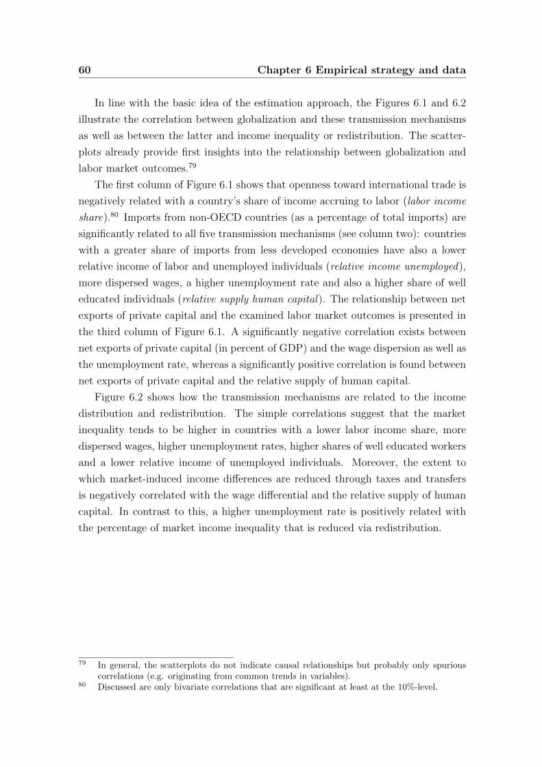
60 Chapter 6 Empirical strategy and data
In line with the basic idea of the estimation approach, the Figures 6.1 and 6.2
illustrate the correlation between globalization and these transmission mechanisms
as well as between the latter and income inequality or redistribution. The scatter-
plots already provide first insights into the relationship between globalization and
labor market outcomes.79
The first column of Figure 6.1 shows that openness toward international trade is
negatively related with a country’s share of income accruing to labor (labor income
share).80 Imports from non-OECD countries (as a percentage of total imports) are
significantly related to all five transmission mechanisms (see column two): countries
with a greater share of imports from less developed economies have also a lower
relative income of labor and unemployed individuals (relative income unemployed),
more dispersed wages, a higher unemployment rate and also a higher share of well
educated individuals (relative supply human capital). The relationship between net
exports of private capital and the examined labor market outcomes is presented in
the third column of Figure 6.1. A significantly negative correlation exists between
net exports of private capital (in percent of GDP) and the wage dispersion as well as
the unemployment rate, whereas a significantly positive correlation is found between
net exports of private capital and the relative supply of human capital.
Figure 6.2 shows how the transmission mechanisms are related to the income
distribution and redistribution. The simple correlations suggest that the market
inequality tends to be higher in countries with a lower labor income share, more
dispersed wages, higher unemployment rates, higher shares of well educated workers
and a lower relative income of unemployed individuals. Moreover, the extent to
which market-induced income differences are reduced through taxes and transfers
is negatively correlated with the wage differential and the relative supply of human
capital. In contrast to this, a higher unemployment rate is positively related with
the percentage of market income inequality that is reduced via redistribution.
79 In general, the scatterplots do not indicate causal relationships but probably only spuriouscorrelations (e.g. originating from common trends in variables).
80 Discussed are only bivariate correlations that are significant at least at the 10%-level.
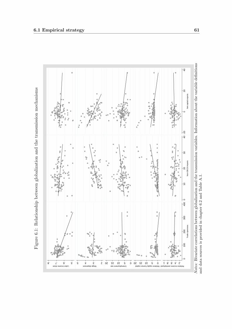
6.1 Empirical strategy 61F
igure
6.1:
Rel
atio
nsh
ipb
etw
een
glob
aliz
atio
nan
dth
etr
ansm
issi
onm
echan
ism
s
.5.6.7.8Labor income share
2345Wage dispersion
05101520Unemployment rate
05101520Relative supply human capital
.2.4.6.81Relative income unemployed
010
020
030
040
0T
rade
ope
nnes
s
010
2030
40N
on-O
EC
D im
port
s
-20
020
40N
et c
apita
l exp
orts
Note
s:B
ivar
iate
corr
elat
ion
sb
etw
een
glob
aliz
ati
on
an
dth
etr
an
smis
sion
vari
able
s.In
form
ati
on
ab
ou
tth
eva
riab
led
efin
itio
ns
and
dat
aso
urc
esis
pro
vid
edin
chap
ter
6.2
an
dT
ab
leA
.1.
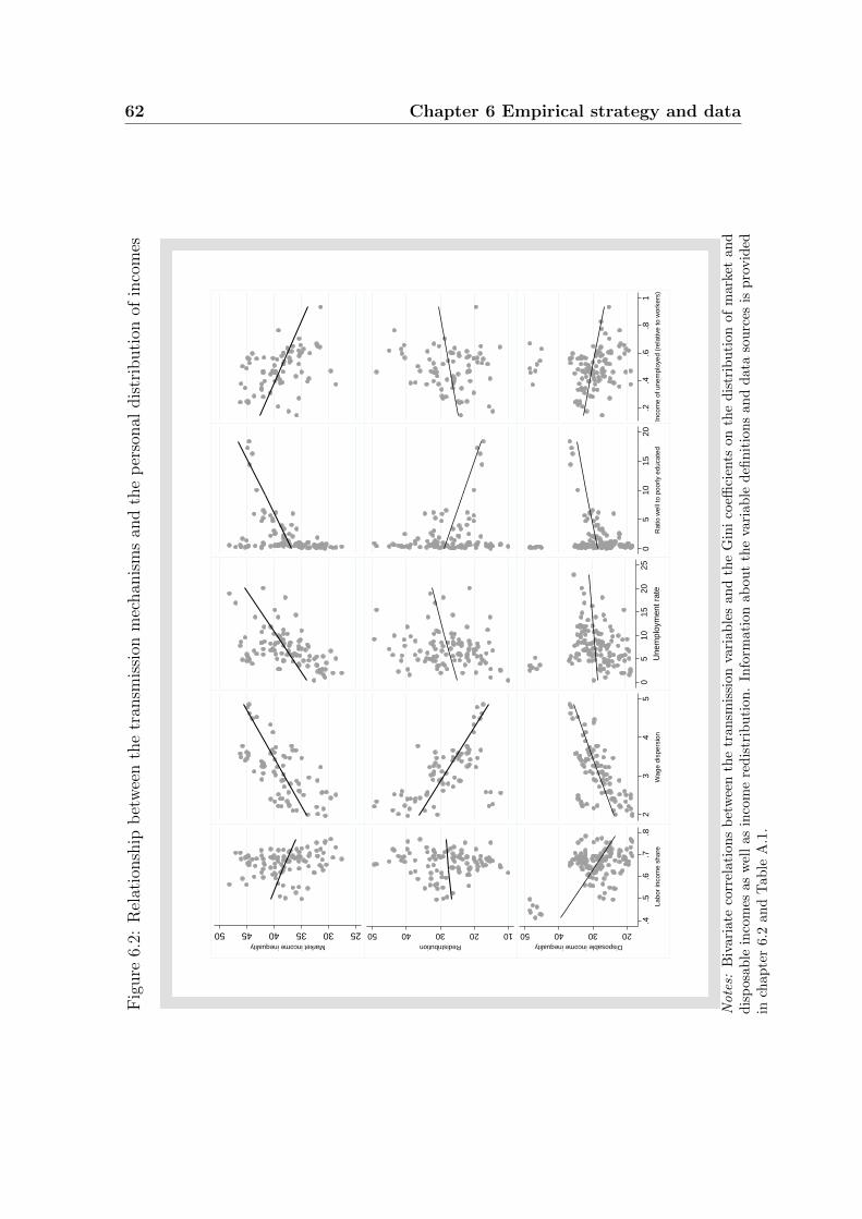
62 Chapter 6 Empirical strategy and dataF
igure
6.2:
Rel
atio
nsh
ipb
etw
een
the
tran
smis
sion
mec
han
ism
san
dth
ep
erso
nal
dis
trib
uti
onof
inco
mes
253035404550Market income inequality
1020304050Redistribution
20304050Disposable income inequality
.4.5
.6.7
.8La
bor
inco
me
shar
e
23
45
Wag
e di
sper
sion
05
1015
2025
Une
mpl
oym
ent r
ate
05
1015
20R
atio
wel
l to
poor
ly e
duca
ted
.2.4
.6.8
1In
com
e of
une
mpl
oyed
(re
lativ
e to
wor
kers
)
Note
s:B
ivar
iate
corr
elat
ion
sb
etw
een
the
tran
smis
sion
vari
ab
les
and
the
Gin
ico
effici
ents
on
the
dis
trib
uti
on
of
mark
etan
dd
isp
osab
lein
com
esas
wel
las
inco
me
red
istr
ibuti
on
.In
form
ati
on
ab
ou
tth
eva
riab
led
efin
itio
ns
an
dd
ata
sou
rces
isp
rovid
edin
chapte
r6.
2an
dT
able
A.1
.
6.1 Empirical strategy 63
The third row of Figure 6.2 illustrates the link between the transmission mech-
anisms and the distribution of disposable incomes. A higher labor income share as
well as a higher relative income of unemployed is related to a more equal distribution
of disposable incomes. Since higher wage differences increase the inequality in the
distribution of market incomes and are negatively related to income redistribution,
it is little surprising that the degree of inequality in the distribution of disposable
incomes is higher, too, if the distribution of wages is more dispersed.81 Finally, a
higher relative supply of human capital is associated with a greater inequality in
disposable incomes.82
The subsequent empirical analysis aims at providing information beyond such
simple bivariate correlations. In principle, I apply the same basic strategy. To draw
conclusions about the impact of trade openness, for instance, on market income
inequality, I test how openness affects the various transmission variables and, then,
how these impact on the distribution of incomes within the population. The line of
argumentation would then be as follows: a higher degree of openness is related to a
lower labor income share (compare Figure 6.1). A reduction in the relative rewards of
labor is further associated with greater inequality of market and disposable incomes
(Figure 6.2). Hence, trade openness is, ceteris paribus, related to a more dispersed
income distribution through its effect on the relative income of labor. After this has
been done for each transmission variable, the overall effect of globalization on the
income distribution in advanced economies can be assessed and, furthermore, the
relative effects of the transmission variables can be estimated.
6.1.1 Empirical specification
The following section offers a more formal description of the estimation approach.
As described above, I start by examining how globalization influences the trans-
mission mechanisms. For that purpose, I regress the labor income share (θ), wage
dispersion (ω), unemployment rate (u), the relative share of human capital (H)
and the relative income of unemployed (B) on globalization indicators and a set
of further explanatory variables. Hence, the following reduced-form equations are
estimated:
81 Surprisingly, the unemployment rate is not significantly correlated with the distribution ofdisposable incomes.
82 However, this seems to be a result of a few influential observations.
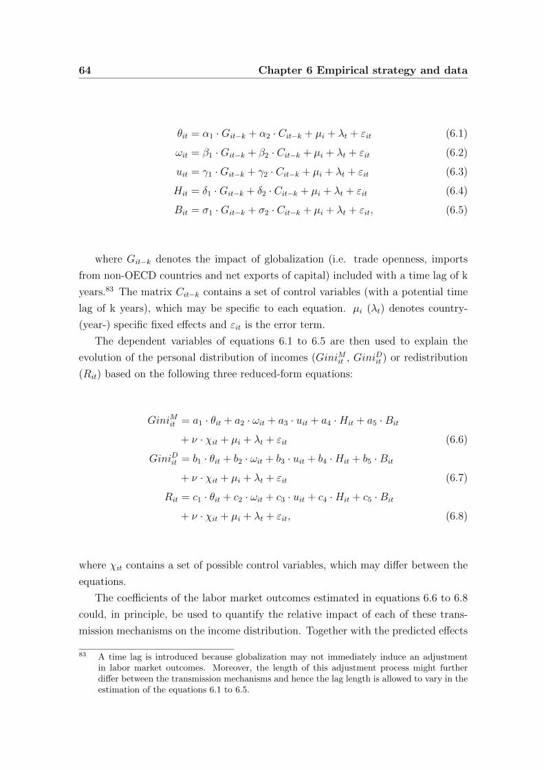
64 Chapter 6 Empirical strategy and data
θit = α1 ·Git−k + α2 · Cit−k + µi + λt + εit (6.1)
ωit = β1 ·Git−k + β2 · Cit−k + µi + λt + εit (6.2)
uit = γ1 ·Git−k + γ2 · Cit−k + µi + λt + εit (6.3)
Hit = δ1 ·Git−k + δ2 · Cit−k + µi + λt + εit (6.4)
Bit = σ1 ·Git−k + σ2 · Cit−k + µi + λt + εit, (6.5)
where Git−k denotes the impact of globalization (i.e. trade openness, imports
from non-OECD countries and net exports of capital) included with a time lag of k
years.83 The matrix Cit−k contains a set of control variables (with a potential time
lag of k years), which may be specific to each equation. µi (λt) denotes country-
(year-) specific fixed effects and εit is the error term.
The dependent variables of equations 6.1 to 6.5 are then used to explain the
evolution of the personal distribution of incomes (GiniMit , GiniDit ) or redistribution
(Rit) based on the following three reduced-form equations:
GiniMit = a1 · θit + a2 · ωit + a3 · uit + a4 ·Hit + a5 ·Bit
+ ν · χit + µi + λt + εit (6.6)
GiniDit = b1 · θit + b2 · ωit + b3 · uit + b4 ·Hit + b5 ·Bit
+ ν · χit + µi + λt + εit (6.7)
Rit = c1 · θit + c2 · ωit + c3 · uit + c4 ·Hit + c5 ·Bit
+ ν · χit + µi + λt + εit, (6.8)
where χit contains a set of possible control variables, which may differ between the
equations.
The coefficients of the labor market outcomes estimated in equations 6.6 to 6.8
could, in principle, be used to quantify the relative impact of each of these trans-
mission mechanisms on the income distribution. Together with the predicted effects
83 A time lag is introduced because globalization may not immediately induce an adjustmentin labor market outcomes. Moreover, the length of this adjustment process might furtherdiffer between the transmission mechanisms and hence the lag length is allowed to vary in theestimation of the equations 6.1 to 6.5.
6.1 Empirical strategy 65
of the globalization variables estimated based on the first set of equations, these co-
efficients allow a quantification of globalization-induced changes of the distribution
of incomes in industrialized countries.
The empirical analysis is based on a panel data set covering 28 current OECD
member countries over the period from 1960 to 2010. The panel is, however, highly
unbalanced due to a large number of missing observations and the limited avail-
ability of income data. This has several implications for the subsequent empirical
analysis. In particular, the number of observations differs considerably between the
regressions. To allow a comparison of the relative effects of the transmission mecha-
nisms, the prediction of the quantitative effects is based on a common sample. The
number of observations is, in that case, very low, which impedes the identification of
significant effects. The strategy of the empirical analysis is thus to use all available
observations for the main analysis and the robustness checks in chapter 7. I only
restrict the sample to common observations for the estimation of the relative effects
of the transmission mechanisms (chapter 8).
The identification of a causal effect of globalization on the transmission mech-
anisms and therewith the income distribution is characterized by difficulties. In
particular, the estimated coefficients might be biased by a possible reverse causa-
tion and potential confounding factors that influence both a country’s openness to
international trade or capital mobility and its labor market outcomes as well as
income distribution.
The theoretical approaches reviewed in chapter 5 suggest that globalization has
an impact on the labor market outcomes considered in this study. Nonetheless, it
is possible that the transmission variables themselves affect a country’s exposure to
globalization. This reverse causation issue is clearly present in the estimation of the
relative supply of human capital because the relative endowment with skilled workers
determines a country’s comparative advantage in international trade and, hence, its
structure of trade.84 A possible reverse relationship could further be driven by trade
policies. In particular, a declining labor income share or rising wage dispersion
and unemployment rates might increase voters’ demand for protectionist measures.
Another possible reverse causation exists for the relationship between international
84 Moreover, the relative supply of human capital may also affect the returns to capital if theelasticity of substitution between physical capital and labor (unskilled labor) differs from thatbetween physical capital and human capital (skilled labor). Several studies (e.g. Griliches(1969), Krusell et al. (2000) and Lindquist (2005)) indeed suggest that elasticity of substitutionbetween capital and skilled labor is greater than the elasticity of substitution between capitaland unskilled labor (i.e. that skilled labor is more complementary to capital than unskilledlabor).
66 Chapter 6 Empirical strategy and data
trade and the relative income of unemployed persons. Janeba (2007) shows that
the welfare state itself has an impact on trade volumes. If, in the presence of labor
market rigidities, firms’ entry into foreign markets require a risky investment, a
rise in unemployment benefits induces an increase in exports.85 Reverse causation
problems could also affect the estimates of the second step of the analysis. The
level of income redistribution, for instance, is not only affected by the labor market
outcomes but has itself an impact on labor market behavior through its effect on
the incentives to work or invest into education.
I can neither rule out the existence of a reverse causation problem nor fully
solve this problem.86 To mitigate the problem of reverse causation, I introduce a
time-lag for the variables of interest. Although the simple fact that current labor
market outcomes are explained by past globalization experience is not sufficient for
a causal relationship, it is more reasonable to assume that the labor markets adjust
to previous openness experience. Still, the estimated coefficients should rather be
interpreted as correlations than as causal effects.
Besides reverse causation issues, the existence of factors, which correlate both
with the globalization and the transmission variables or with the latter and the
measures of income distribution might further bias the results. If these potential
confounding factors are not considered in the regressions, then this would induce
an omitted variable bias. To avoid this, I apply the following estimation approach.
The empirical analysis starts with OLS regressions. The pooled OLS estimates
might, however, be biased due to unobserved country-specific effects, which are cor-
related both with a country’s openness to trade or capital mobility and its labor
market outcomes or income distribution. To account for a potential heterogene-
ity between countries (i.e. time-invariant and country-specific omitted variables),
I include dummy variables for each country.87 Moreover, I introduce year fixed ef-
fects to capture year-specific factors that are common to all countries (e.g. general
85 Some firms that enter the export market do not survive and their workers become unem-ployed. The wage in the export sector depends on the firm’s probability of surviving and therespective income workers receive when employed or unemployed (i.e. workers decide aboutworking in the export or non-tradable sector based on their expected income). Since higherunemployment benefits increase the expected wage in the export sector, it allows the firms tolower their wage payments. This reduces the overall production costs and prices of the exportgood and, hence, increases the export volume.
86 A possibility to solve these reverse causation problems would be to utilize an exogenousvariation in a country’s exposure to globalization (e.g. a natural experiment). This approachmight be feasible if one focuses only on a specific country and question but not in a complexstudy based on a panel of countries.
87 To avoid the “dummy-trap” and estimate a constant (which is not reported), one countrydummy is omitted from each regression.
6.1 Empirical strategy 67
macroeconomic conditions).88 In addition to the fixed effects, I also directly control
for various factors that might be correlated with the variables of interest and the
independent variables. The choice of the control variables is motivated by findings
of comparable studies and by theoretical considerations. In the first step of the
empirical analysis, which is described by the equations 6.1 to 6.5, the amount of
capital per worker, the labor productivity, the growth of multifactor productivity
and the output gap are considered as additional control variables. To capture the
institutional framework of a country, I also include a measure for the degree of labor
market regulation. The relative income of the unemployed is determined politically
and thus both the share of left wing parties in the government and the voter turnout
in parliamentary elections is included in the regressions.
The second part of the empirical analysis (see equations 6.6 to 6.8) includes
several control variables (denoted by χit). Considered are those factors that influence
how labor market outcomes or welfare state generosity translate into a more or less
unequal distribution of incomes among households or those that affect inequality
through some independent channels. The following variables have been included:
the GDP per capita and its square (controlling for a Kutznets curve effect) as well as
the deviation of the annual growth rate of the real GDP from its five-year average.89
Additionally, the estimations of the extent of income redistribution also take political
factors such as the share of left wing parties in the government and voter turnout
into account. Several variables have been tested but failed to be significant and are
thus not included in the empirical analysis in section 7.2.90
Finally, the estimation of the determinants of labor market outcomes (equations
6.1 to 6.5) using OLS might further introduce a simultaneity bias since the residuals
(εit) may be correlated between equations. I address this issue and estimate a system
of equations using the seemingly unrelated regressions (SUR) model.
88 F-tests of the joint significance of country or year fixed effects are reported in each regressiontable.
89 The consideration of business cycle effects is motivated by the possibility that changes in thedegree of the measured inequality between two years might simply reflect different economicconditions in these years but not actual developments of medium- or long-term inequalitytrends.
90 These variables are the share of manufacturing employment, age dependency ratio and femalelabor force participation.
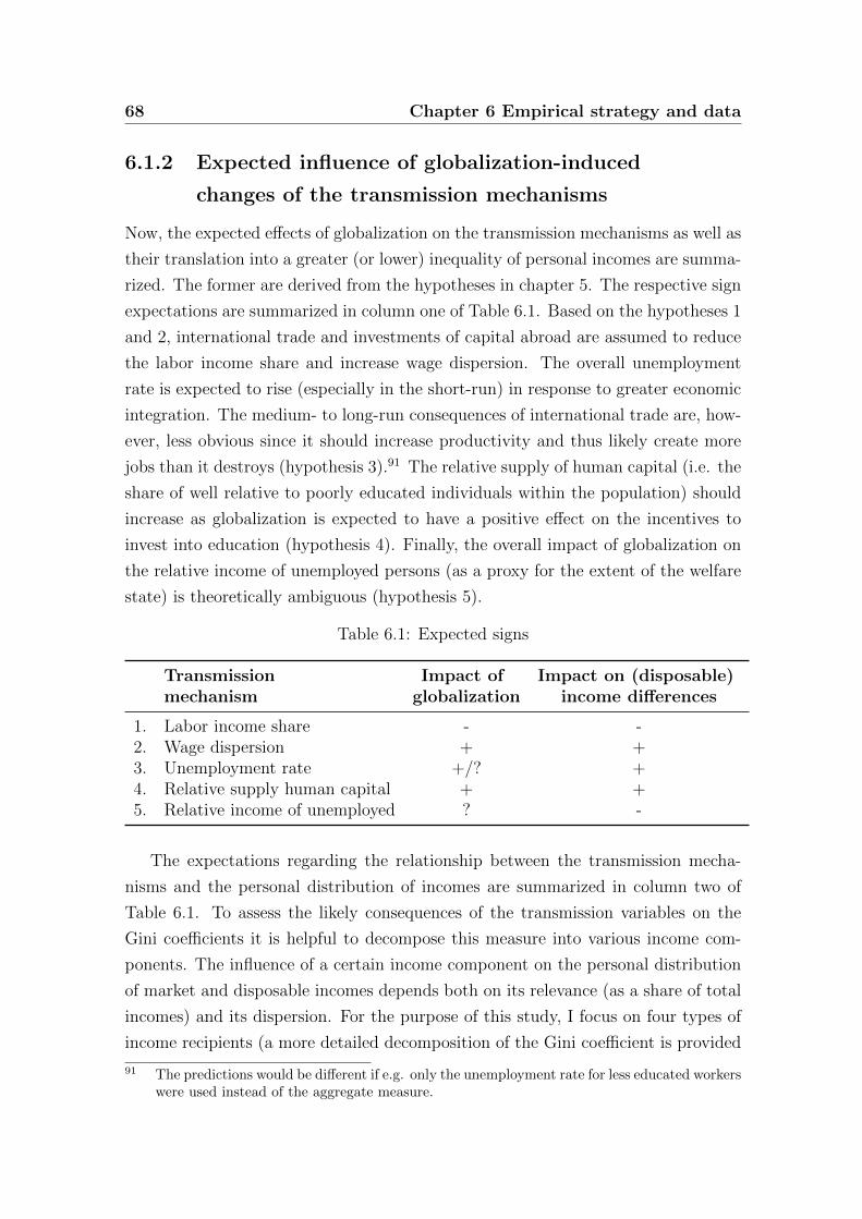
68 Chapter 6 Empirical strategy and data
6.1.2 Expected influence of globalization-induced
changes of the transmission mechanisms
Now, the expected effects of globalization on the transmission mechanisms as well as
their translation into a greater (or lower) inequality of personal incomes are summa-
rized. The former are derived from the hypotheses in chapter 5. The respective sign
expectations are summarized in column one of Table 6.1. Based on the hypotheses 1
and 2, international trade and investments of capital abroad are assumed to reduce
the labor income share and increase wage dispersion. The overall unemployment
rate is expected to rise (especially in the short-run) in response to greater economic
integration. The medium- to long-run consequences of international trade are, how-
ever, less obvious since it should increase productivity and thus likely create more
jobs than it destroys (hypothesis 3).91 The relative supply of human capital (i.e. the
share of well relative to poorly educated individuals within the population) should
increase as globalization is expected to have a positive effect on the incentives to
invest into education (hypothesis 4). Finally, the overall impact of globalization on
the relative income of unemployed persons (as a proxy for the extent of the welfare
state) is theoretically ambiguous (hypothesis 5).
Table 6.1: Expected signs
Transmission Impact of Impact on (disposable)mechanism globalization income differences
1. Labor income share - -2. Wage dispersion + +3. Unemployment rate +/? +4. Relative supply human capital + +5. Relative income of unemployed ? -
The expectations regarding the relationship between the transmission mecha-
nisms and the personal distribution of incomes are summarized in column two of
Table 6.1. To assess the likely consequences of the transmission variables on the
Gini coefficients it is helpful to decompose this measure into various income com-
ponents. The influence of a certain income component on the personal distribution
of market and disposable incomes depends both on its relevance (as a share of total
incomes) and its dispersion. For the purpose of this study, I focus on four types of
income recipients (a more detailed decomposition of the Gini coefficient is provided
91 The predictions would be different if e.g. only the unemployment rate for less educated workerswere used instead of the aggregate measure.
6.2 Data 69
by Checci and Garcia-Penalosa, 2010): the share of the unemployed persons (u)
who receive unemployment benefits (B, which is equal to the income of unemployed
relative to workers), unskilled and skilled workers earning the respective wages and
some individuals who also own capital and receive capital incomes.
A rising wage dispersion (i.e. difference between the wage of skilled and unskilled
workers) increases the inequality within the group of workers and therewith also the
overall income inequality. A higher educational attainment in the population and
thus a rise in the relative supply of skilled workers is, ceteris paribus, expected
to increase inequality (at least as there are more unskilled than skilled workers).92
A higher labor income share reduces the inequality between capital owners and
workers (between group inequality) but the effect on the Gini coefficient depends
on the inequality of wage incomes versus capital incomes (within group inequality).
Since capital incomes are usually less equally distributed than earnings, a higher
labor income share is expected to reduce inequality. A higher relative income of
unemployed persons reduces the inequality between workers and unemployed persons
and therefore also the overall income inequality. Moreover, the dispersion of personal
distribution of incomes should increase in response to a higher unemployment rate.93
6.2 Data
The following section describes the variables used in the empirical analysis. In
addition to the variable description in the text, Table A.1 entails further information
on the variable definitions and the data sources.
6.2.1 Data on income distribution
My primary source for income distribution data is the Luxembourg Income Study
(LIS). LIS collects national micro-datasets and harmonizes them for cross-national
income comparisons.94 Currently, income data is available for 46 high- and middle-
92 In addition, a higher relative supply of human capital should, other things equal, reduce theearnings dispersion and thereby income inequality. The effect of changes in the distributionof wages on the income distribution is, however, directly captured by the inclusion of thisvariable.
93 Theoretically, the impact of a higher share of unemployed persons might be ambiguous be-cause incomes are more equally distributed within the group of unemployed than amongworkers. This effect does, however, not dominate the rise in between-group inequality unlessthe majority of the population is unemployed.
94 More detailed information on LIS is provided at http://www.lisdatacenter.org. See alsoGornick et al. (2013); Atkinson et al. (1995).
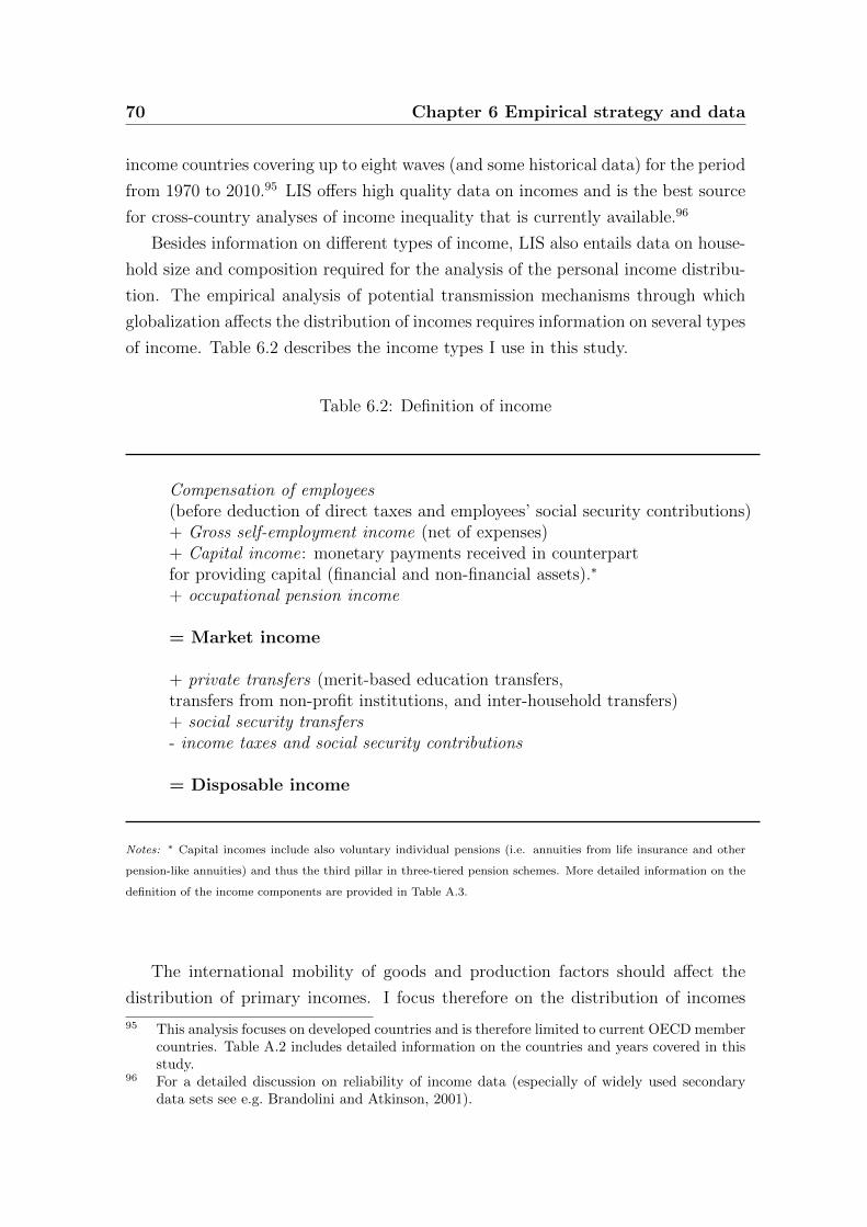
70 Chapter 6 Empirical strategy and data
income countries covering up to eight waves (and some historical data) for the period
from 1970 to 2010.95 LIS offers high quality data on incomes and is the best source
for cross-country analyses of income inequality that is currently available.96
Besides information on different types of income, LIS also entails data on house-
hold size and composition required for the analysis of the personal income distribu-
tion. The empirical analysis of potential transmission mechanisms through which
globalization affects the distribution of incomes requires information on several types
of income. Table 6.2 describes the income types I use in this study.
Table 6.2: Definition of income
Compensation of employees(before deduction of direct taxes and employees’ social security contributions)+ Gross self-employment income (net of expenses)+ Capital income: monetary payments received in counterpartfor providing capital (financial and non-financial assets).∗
+ occupational pension income
= Market income
+ private transfers (merit-based education transfers,transfers from non-profit institutions, and inter-household transfers)+ social security transfers- income taxes and social security contributions
= Disposable income
Notes: ∗ Capital incomes include also voluntary individual pensions (i.e. annuities from life insurance and other
pension-like annuities) and thus the third pillar in three-tiered pension schemes. More detailed information on the
definition of the income components are provided in Table A.3.
The international mobility of goods and production factors should affect the
distribution of primary incomes. I focus therefore on the distribution of incomes
95 This analysis focuses on developed countries and is therefore limited to current OECD membercountries. Table A.2 includes detailed information on the countries and years covered in thisstudy.
96 For a detailed discussion on reliability of income data (especially of widely used secondarydata sets see e.g. Brandolini and Atkinson, 2001).
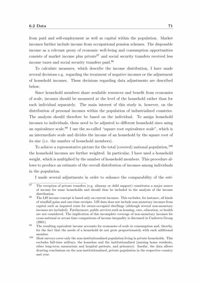
6.2 Data 71
from paid and self-employment as well as capital within the population. Market
incomes further include income from occupational pension schemes. The disposable
income as a relevant proxy of economic well-being and consumption opportunities
consists of market income plus private97 and social security transfers received less
income taxes and social security transfers paid.98
To calculate measures, which describe the income distribution, I have made
several decisions e.g. regarding the treatment of negative incomes or the adjustment
of household incomes. These decisions regarding data adjustments are described
below.
Since household members share available resources and benefit from economies
of scale, incomes should be measured at the level of the household rather than for
each individual separately. The main interest of this study is, however, on the
distribution of personal incomes within the population of industrialized countries.
The analysis should therefore be based on the individual. To assign household
incomes to individuals, these need to be adjusted to different household sizes using
an equivalence scale.99 I use the so-called “square root equivalence scale”, which is
an intermediate scale and divides the income of an household by the square root of
its size (i.e. the number of household members).
To achieve a representative picture for the total (covered) national population,100
the household incomes are further weighted. In particular, I have used a household
weight, which is multiplied by the number of household members. This procedure al-
lows to produce an estimate of the overall distribution of incomes among individuals
in the population.
I made several adjustments in order to enhance the comparability of the esti-
97 The reception of private transfers (e.g. alimony or child support) constitutes a major sourceof income for some households and should thus be included in the analysis of the incomedistribution.
98 The LIS income concept is based only on current incomes. This excludes, for instance, all kindsof windfall gains and one-time receipts. LIS data does not include non-monetary incomes fromcapital such as imputed rents for owner-occupied dwellings (although several non-monetaryincomes are included). Furthermore, public services such as housing, care, education, or healthare not considered. The implication of this incomplete coverage of non-monetary incomes forcross-national or across time comparisons of income inequality is discussed in Canberra Group(2001).
99 The resulting equivalent income accounts for economies of scale in consumption and, thereby,for the fact that the needs of a household do not grow proportionately with each additionalmember.
100 Most surveys cover only the non-institutionalized population living in private households. Thisexcludes full-time military, the homeless and the institutionalized (nursing home residents,other long-term sanatarium and hospital patients, and prisoners). Insofar, the data allowsdrawing conclusions on the non-institutionalized, private population in the respective countryand year.
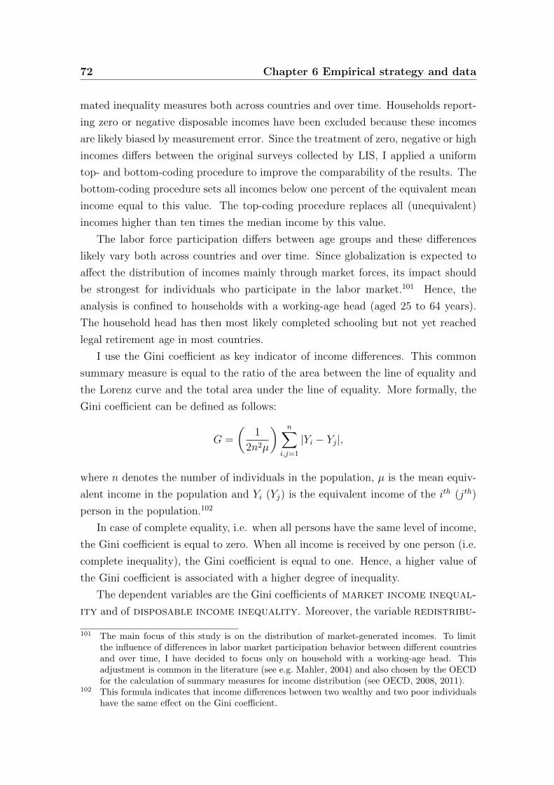
72 Chapter 6 Empirical strategy and data
mated inequality measures both across countries and over time. Households report-
ing zero or negative disposable incomes have been excluded because these incomes
are likely biased by measurement error. Since the treatment of zero, negative or high
incomes differs between the original surveys collected by LIS, I applied a uniform
top- and bottom-coding procedure to improve the comparability of the results. The
bottom-coding procedure sets all incomes below one percent of the equivalent mean
income equal to this value. The top-coding procedure replaces all (unequivalent)
incomes higher than ten times the median income by this value.
The labor force participation differs between age groups and these differences
likely vary both across countries and over time. Since globalization is expected to
affect the distribution of incomes mainly through market forces, its impact should
be strongest for individuals who participate in the labor market.101 Hence, the
analysis is confined to households with a working-age head (aged 25 to 64 years).
The household head has then most likely completed schooling but not yet reached
legal retirement age in most countries.
I use the Gini coefficient as key indicator of income differences. This common
summary measure is equal to the ratio of the area between the line of equality and
the Lorenz curve and the total area under the line of equality. More formally, the
Gini coefficient can be defined as follows:
G =
(1
2n2µ
) n∑i,j=1
|Yi − Yj|,
where n denotes the number of individuals in the population, µ is the mean equiv-
alent income in the population and Yi (Yj) is the equivalent income of the ith (jth)
person in the population.102
In case of complete equality, i.e. when all persons have the same level of income,
the Gini coefficient is equal to zero. When all income is received by one person (i.e.
complete inequality), the Gini coefficient is equal to one. Hence, a higher value of
the Gini coefficient is associated with a higher degree of inequality.
The dependent variables are the Gini coefficients of market income inequal-
ity and of disposable income inequality. Moreover, the variable redistribu-
101 The main focus of this study is on the distribution of market-generated incomes. To limitthe influence of differences in labor market participation behavior between different countriesand over time, I have decided to focus only on household with a working-age head. Thisadjustment is common in the literature (see e.g. Mahler, 2004) and also chosen by the OECDfor the calculation of summary measures for income distribution (see OECD, 2008, 2011).
102 This formula indicates that income differences between two wealthy and two poor individualshave the same effect on the Gini coefficient.
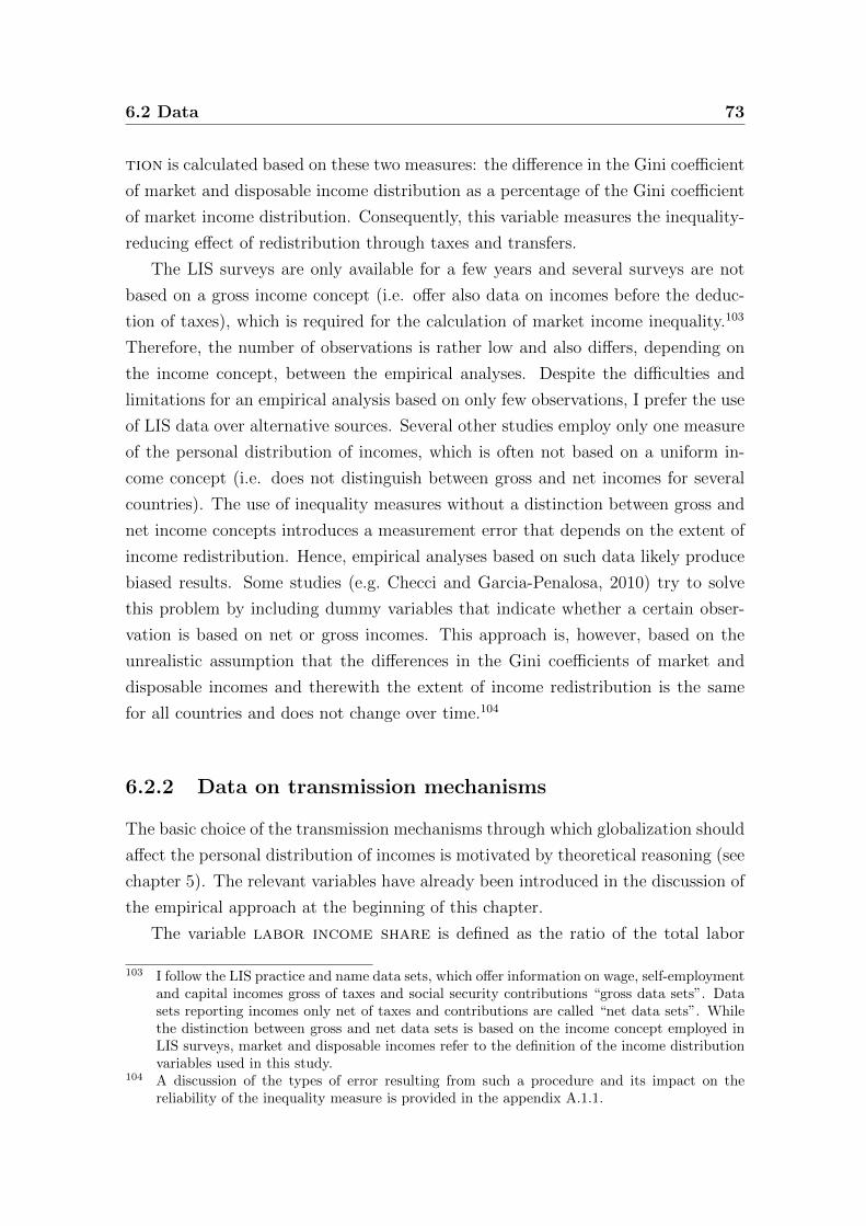
6.2 Data 73
tion is calculated based on these two measures: the difference in the Gini coefficient
of market and disposable income distribution as a percentage of the Gini coefficient
of market income distribution. Consequently, this variable measures the inequality-
reducing effect of redistribution through taxes and transfers.
The LIS surveys are only available for a few years and several surveys are not
based on a gross income concept (i.e. offer also data on incomes before the deduc-
tion of taxes), which is required for the calculation of market income inequality.103
Therefore, the number of observations is rather low and also differs, depending on
the income concept, between the empirical analyses. Despite the difficulties and
limitations for an empirical analysis based on only few observations, I prefer the use
of LIS data over alternative sources. Several other studies employ only one measure
of the personal distribution of incomes, which is often not based on a uniform in-
come concept (i.e. does not distinguish between gross and net incomes for several
countries). The use of inequality measures without a distinction between gross and
net income concepts introduces a measurement error that depends on the extent of
income redistribution. Hence, empirical analyses based on such data likely produce
biased results. Some studies (e.g. Checci and Garcia-Penalosa, 2010) try to solve
this problem by including dummy variables that indicate whether a certain obser-
vation is based on net or gross incomes. This approach is, however, based on the
unrealistic assumption that the differences in the Gini coefficients of market and
disposable incomes and therewith the extent of income redistribution is the same
for all countries and does not change over time.104
6.2.2 Data on transmission mechanisms
The basic choice of the transmission mechanisms through which globalization should
affect the personal distribution of incomes is motivated by theoretical reasoning (see
chapter 5). The relevant variables have already been introduced in the discussion of
the empirical approach at the beginning of this chapter.
The variable labor income share is defined as the ratio of the total labor
103 I follow the LIS practice and name data sets, which offer information on wage, self-employmentand capital incomes gross of taxes and social security contributions “gross data sets”. Datasets reporting incomes only net of taxes and contributions are called “net data sets”. Whilethe distinction between gross and net data sets is based on the income concept employed inLIS surveys, market and disposable incomes refer to the definition of the income distributionvariables used in this study.
104 A discussion of the types of error resulting from such a procedure and its impact on thereliability of the inequality measure is provided in the appendix A.1.1.
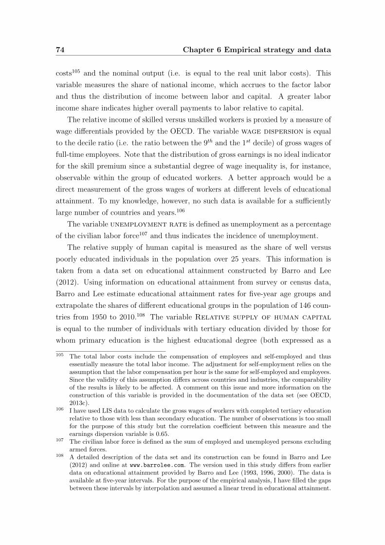
74 Chapter 6 Empirical strategy and data
costs105 and the nominal output (i.e. is equal to the real unit labor costs). This
variable measures the share of national income, which accrues to the factor labor
and thus the distribution of income between labor and capital. A greater labor
income share indicates higher overall payments to labor relative to capital.
The relative income of skilled versus unskilled workers is proxied by a measure of
wage differentials provided by the OECD. The variable wage dispersion is equal
to the decile ratio (i.e. the ratio between the 9th and the 1st decile) of gross wages of
full-time employees. Note that the distribution of gross earnings is no ideal indicator
for the skill premium since a substantial degree of wage inequality is, for instance,
observable within the group of educated workers. A better approach would be a
direct measurement of the gross wages of workers at different levels of educational
attainment. To my knowledge, however, no such data is available for a sufficiently
large number of countries and years.106
The variable unemployment rate is defined as unemployment as a percentage
of the civilian labor force107 and thus indicates the incidence of unemployment.
The relative supply of human capital is measured as the share of well versus
poorly educated individuals in the population over 25 years. This information is
taken from a data set on educational attainment constructed by Barro and Lee
(2012). Using information on educational attainment from survey or census data,
Barro and Lee estimate educational attainment rates for five-year age groups and
extrapolate the shares of different educational groups in the population of 146 coun-
tries from 1950 to 2010.108 The variable Relative supply of human capital
is equal to the number of individuals with tertiary education divided by those for
whom primary education is the highest educational degree (both expressed as a
105 The total labor costs include the compensation of employees and self-employed and thusessentially measure the total labor income. The adjustment for self-employment relies on theassumption that the labor compensation per hour is the same for self-employed and employees.Since the validity of this assumption differs across countries and industries, the comparabilityof the results is likely to be affected. A comment on this issue and more information on theconstruction of this variable is provided in the documentation of the data set (see OECD,2013c).
106 I have used LIS data to calculate the gross wages of workers with completed tertiary educationrelative to those with less than secondary education. The number of observations is too smallfor the purpose of this study but the correlation coefficient between this measure and theearnings dispersion variable is 0.65.
107 The civilian labor force is defined as the sum of employed and unemployed persons excludingarmed forces.
108 A detailed description of the data set and its construction can be found in Barro and Lee(2012) and online at www.barrolee.com. The version used in this study differs from earlierdata on educational attainment provided by Barro and Lee (1993, 1996, 2000). The data isavailable at five-year intervals. For the purpose of the empirical analysis, I have filled the gapsbetween these intervals by interpolation and assumed a linear trend in educational attainment.
6.2 Data 75
percentage of the population older than 25 years).
Finally, I consider the extent of government redistribution through the welfare
state and the social security system as a further transmission mechanism. To mea-
sure welfare state generosity, I focus on the relative net income of unemployed per-
sons compared to that of employees. The relative amount of incomes which indi-
viduals receive in case of unemployment is likely to depend on a country’s exposure
to international trade and capital mobility (see section 5.3). Transfer payments to
the unemployed are an adequate transmission mechanism since they are closely re-
lated to the insurance function of the welfare state. Consequently, this variable is
closely related to the demand-side effect of globalization on income redistribution as
suggested by Rodrik (1998) (see hypothesis 5 (b.2)). This variable should therefore
be particularly suitable for testing the competing hypotheses regarding the rela-
tionship between globalization and redistribution (i.e. hypothesis 5 (a) versus (b)).
Moreover, the income of unemployed relative to employed individuals should have a
substantial impact on the income distribution. If unemployment rises, then the in-
crease in disposable income inequality will, ceteris paribus, be stronger in countries
with a lower relative income of unemployed workers. To measure the relative in-
come of unemployed, I employ LIS data. The mean incomes are calculated based on
the total disposable income (i.e. sum of labor, capital and transfer income received
less the payment of direct taxes and social security contributions) at the individual
level. The variable relative income of the unemployed is equal to the ratio of
the average disposable income of unemployed individuals to the average disposable
income of employees. This approach differs somewhat from the OECD calculations
of the net replacement rates (OECD, 2007), which are based on simulations. The
replacement rates of unemployed persons are specified as the average of different
durations of unemployment, family situations and assumptions about spouse’s in-
come.109 The net replacement rates have only been available since 2001 and are thus
109 Further information is also provided at www.oecd.org/els/social/workincentives. In con-trast to the OECD simulations, my calculations do not distinguish between different types ofunemployment (e.g. short- and long-term) and family situations. The length of an unemploy-ment spell is, however, likely related to the type and amount of compensation an unemployedperson is eligible for. I further focus on the individual and not on the equivalent householdincome because the latter is also affected by the employment status and income reception ofother household members. This would be misleading since the main interest is on the ques-tion how unemployment affects the income of the person who becomes unemployed. It should,however, be mentioned that transfer payments might depend on, for instance, the number ofchildren or the income of the spouse. The variable relative income of the unemployedrefers to the relative income of all types of unemployed, independent of the duration andeligibility rules and, hence, may not only reflect the design of the transfer system but also thecomposition of the unemployed population.

76 Chapter 6 Empirical strategy and data
not suitable for the subsequent empirical analysis. Several studies have also focused
on gross replacement rates, which are, however, less appropriate for the generosity
of unemployment compensation (see e.g. Howell and Rehm, 2009).
6.2.3 Globalization data
The first indicator for a country’s economic integration is its openness to interna-
tional trade defined as the ratio between trade in goods and services (i.e. the sum
of exports and imports) and GDP. The variable trade openness serves as an in-
dicator for the overall exposure to international trade and thus is used to measure
the impact of trade on the distribution of incomes.
In particular neoclassical trade theories emphasize the relevance of trade with
less developed countries for the income distribution in advanced economies. Hence,
the relative importance of trade with non-OECD member countries is included as
a further trade measure. The variable non-OECD imports is equal to the share
of imports from non-OECD countries (excluding those from OPEC states110) in an
economy’s total imports. To reduce the influence of outliers, I express both variables
in logs.
The extent of capital mobility is measured as following: based on the consider-
ations in section 5.1, I use the net exports of private capital (i.e. outflows minus
inflows of foreign direct, portfolio and other investments) as a share of GDP.111 The
variable net capital export is based on the idea that the international mobility
of private capital, ceteris paribus, affects the domestic capital stock and thereby
the factor rewards. This effect should not depend on the specific type of capital
(as long as it is invested) and therefore a distinction between FDI, portfolio and
other investments is not necessary. To check the robustness of the impact of capital
mobility, I also use a measure of gross capital movements (i.e. the sum of inflows
and outflows of private capital) as a percentage of GDP and net exports of FDI. The
latter is motivated by the observation that most empirical studies which analyze the
effects of international capital flows focus only on FDI.112
110 Imports from OPEC countries should be dominated by petroleum, which is not expected tohave similar effects on the income distribution as manufacturing imports. To avoid an impre-cise measurement, the petroleum-exporting countries are not included in the construction ofthis variable.
111 This variable takes on negative values if a country is a net importer of capital. Hence, nologarithm is used because this would lead to a loss of these observations.
112 Possible explanations for this confined measure might be the relevance of FDI as a long-term investment, potential additional effects related to the managerial involvement of an FDIrelative to a portfolio investor or that foreign direct investments are compared to foreign loans
6.2 Data 77
6.2.4 Control variables
Several additional explanatory variables are included in the following empirical anal-
yses.113 Due to a limited number of observations, in particular, in the regressions
of market and disposable income inequality and redistribution on the transmission
variables, I mostly include those variables that have been proven significant at least
at the 10%-level in the baseline regressions.
Hence, the following control variables are included in the analysis of the trans-
mission mechanisms. The relative capital endowment is measured as the amount
of capital per worker (in logs) and is used as an explanatory variable in the
analysis of the labor income share, the wage dispersion, the unemployment rate and
the relative supply of human capital. Moreover, a measure for labor productiv-
ity is included in the regressions of the labor income share and the unemployment
rate, whereas the growth of multifactor productivity is employed as an indi-
cator for productivity shocks in the analysis of the relative supply of human capital.
Moreover, the output gap captures the impact of business cycle effects in the re-
gressions of the unemployment rate. The latter is used as a control for e.g. demand
shocks, which affect domestic production (and thus employment) but also imports,
and thus might introduce a omitted variable bias if not included in the regressions.
One aspect which should affect all examined labor outcomes is the institutional
framework of a country. In particular, globalization and its impact on labor demand
likely depends on the degree of labor market regulation. To measure the degree of
regulation of the labor market, I use the Economic Freedom of the World (EFW)
Index from the Fraser Institute (Gwartney et al., 2012). The subindex labor market
regulation assesses the freedom of employers and employees based on the follow-
ing types of regulations: minimum wages, hiring and firing regulation, centralized
collective bargaining, hours regulation, mandated costs of worker dismissals and
conscription. A higher value of this index and thus of the variable labor market
freedom is equal to more economic freedom and less regulated labor markets.114
The set of control variables employed in the empirical analysis of the relative
income of unemployed individuals differ from those included in the other regressions.
This is due to the fact that the amount of transfer incomes received by unemployed
or credits (i.e. other investments) subject to stronger controls at country level (see section5.1).
113 A detailed description of the variables and the data sources is provided in Table A.1.114 It might, however, be the case that not only the degree of labor market regulation affects the
examined labor market outcomes but the causation goes from these outcomes to the regulationof labor markets. A greater dispersion of wages, for instance, could raise voters’ demand forminimum wages and related regulations of the labor market.
78 Chapter 6 Empirical strategy and data
persons is determined politically. Hence, I consider both the share of left wing parties
in the government (left government) and the voter turnout in parliamentary
elections in the empirical analysis.
In the analyses of the Gini coefficients on market and disposable income inequal-
ity as well as redistribution the following control variables are included: the GDP
per capita and its square (controlling for a Kutznets curve effect) as well as the
deviation of the real GDP growth from its five-year average. The inclusion
of the latter is motivated by the possibility that the measured level of inequality
depends on the economic conditions in the year to which the survey data refers. A
change in the measured level of income inequality might solely reflect business cycle
effects but not actual trends in inequality (i.e. the Gini coefficient might change
simply because one compares observations from a boom phase and a recession). In-
sofar, the inclusion of the deviation from the real GDP growth rate is motivated by
a different reasoning than the inclusion of the output gap in the empirical analysis
of the unemployment rate. As in the empirical analysis of the relative income of
unemployed persons, the variables left government and voter turnout are
included in the analysis of income redistribution. Several variables have been tested
but failed to be significant and are thus not included in the empirical analyses in
section 7.2.115
The summary statistics for the variables employed in the main regressions are
reported in Table 6.3. Furthermore, the correlations between the variables are re-
ported in Table 6.4. The correlations between the explanatory variables are below
an absolute value of 0.70.116
115 These variables are the share of manufacturing employment, age dependency ratio and femalelabor force participation.
116 Only the correlation coefficient between growth in multifactor productivity and labor produc-tivity is 0.79.
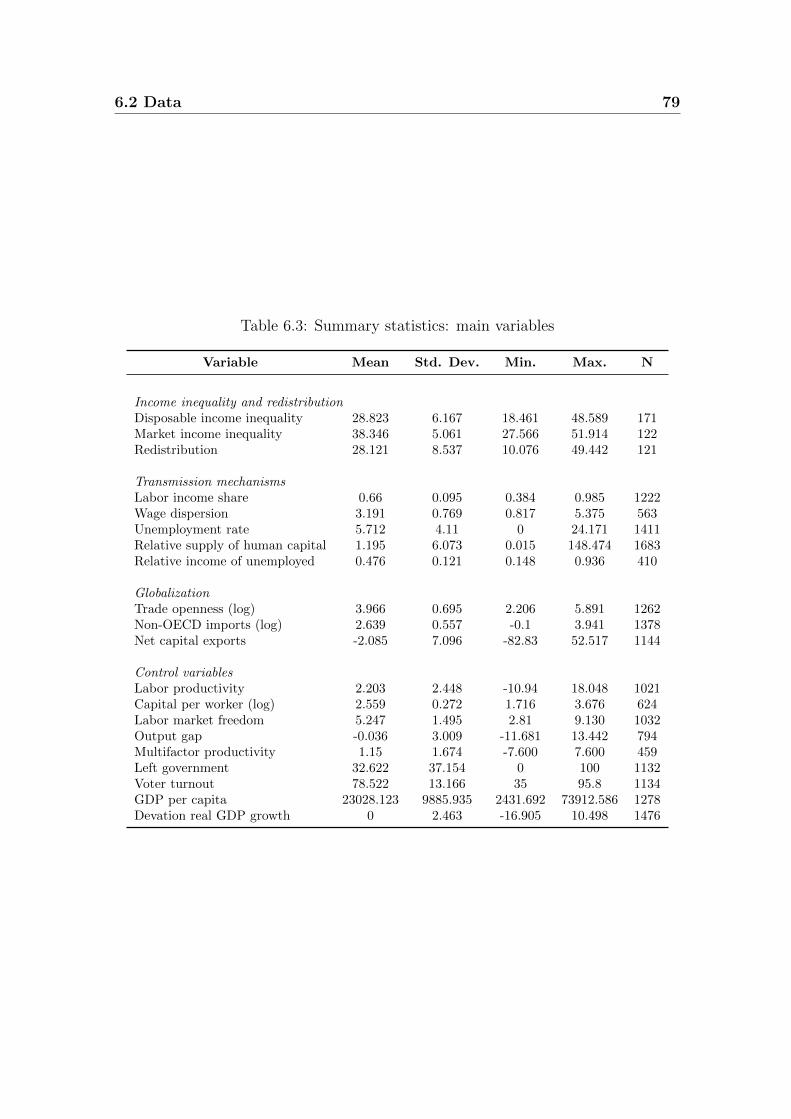
6.2 Data 79
Table 6.3: Summary statistics: main variables
Variable Mean Std. Dev. Min. Max. N
Income inequality and redistributionDisposable income inequality 28.823 6.167 18.461 48.589 171Market income inequality 38.346 5.061 27.566 51.914 122Redistribution 28.121 8.537 10.076 49.442 121
Transmission mechanismsLabor income share 0.66 0.095 0.384 0.985 1222Wage dispersion 3.191 0.769 0.817 5.375 563Unemployment rate 5.712 4.11 0 24.171 1411Relative supply of human capital 1.195 6.073 0.015 148.474 1683Relative income of unemployed 0.476 0.121 0.148 0.936 410
GlobalizationTrade openness (log) 3.966 0.695 2.206 5.891 1262Non-OECD imports (log) 2.639 0.557 -0.1 3.941 1378Net capital exports -2.085 7.096 -82.83 52.517 1144
Control variablesLabor productivity 2.203 2.448 -10.94 18.048 1021Capital per worker (log) 2.559 0.272 1.716 3.676 624Labor market freedom 5.247 1.495 2.81 9.130 1032Output gap -0.036 3.009 -11.681 13.442 794Multifactor productivity 1.15 1.674 -7.600 7.600 459Left government 32.622 37.154 0 100 1132Voter turnout 78.522 13.166 35 95.8 1134GDP per capita 23028.123 9885.935 2431.692 73912.586 1278Devation real GDP growth 0 2.463 -16.905 10.498 1476
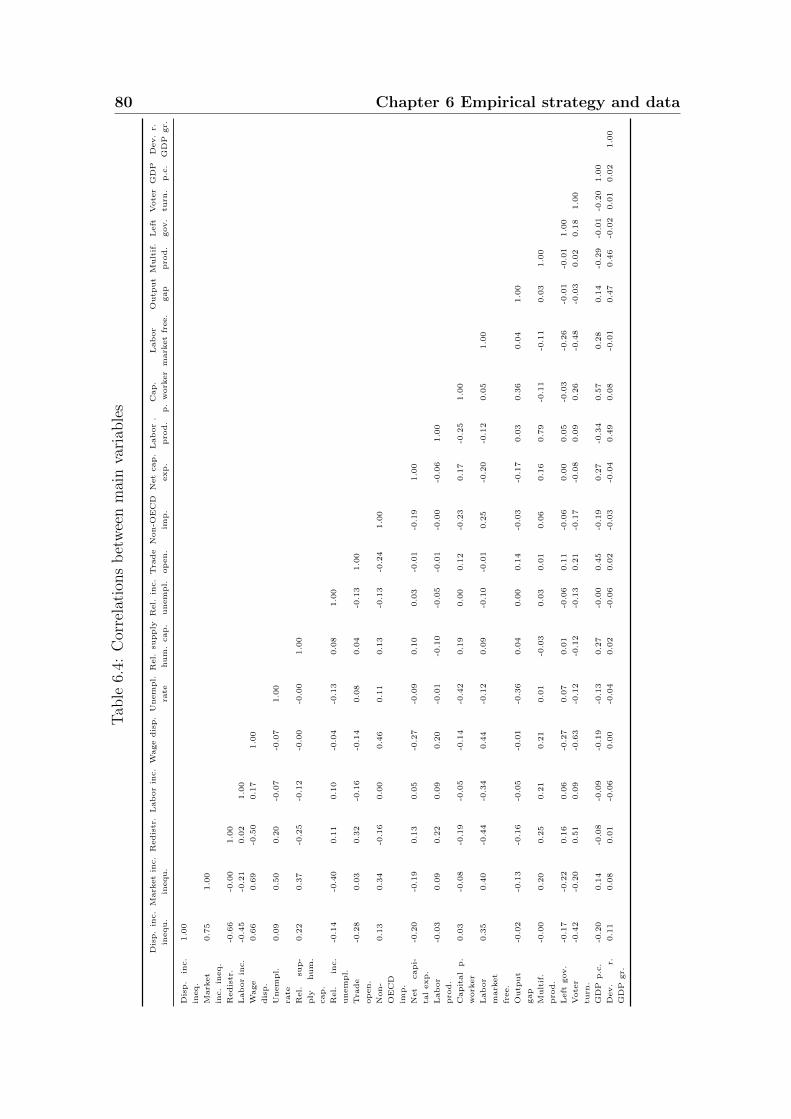
80 Chapter 6 Empirical strategy and dataT
able
6.4:
Cor
rela
tion
sb
etw
een
mai
nva
riab
les
Dis
p.
inc.
Mark
et
inc.
Redis
tr.
Lab
or
inc.
Wage
dis
p.
Unem
pl.
Rel.
supply
Rel.
inc.
Tra
de
Non-O
EC
DN
et
cap.
Lab
or
.C
ap.
Lab
or
Outp
ut
Mult
if.
Left
Vote
rG
DP
Dev.
r.
inequ.
inequ.
rate
hum
.cap.
unem
pl.
op
en.
imp.
exp.
pro
d.
p.
work
er
mark
et
free.
gap
pro
d.
gov.
turn
.p.c
.G
DP
gr.
Dis
p.
inc.
ineq.
1.0
0
Mark
et
inc.
ineq.
0.7
51.0
0
Redis
tr.
-0.6
6-0
.00
1.0
0
Lab
or
inc.
-0.4
5-0
.21
0.0
21.0
0
Wage
dis
p.
0.6
60.6
9-0
.50
0.1
71.0
0
Unem
pl.
rate
0.0
90.5
00.2
0-0
.07
-0.0
71.0
0
Rel.
sup-
ply
hum
.
cap.
0.2
20.3
7-0
.25
-0.1
2-0
.00
-0.0
01.0
0
Rel.
inc.
unem
pl.
-0.1
4-0
.40
0.1
10.1
0-0
.04
-0.1
30.0
81.0
0
Tra
de
op
en.
-0.2
80.0
30.3
2-0
.16
-0.1
40.0
80.0
4-0
.13
1.0
0
Non-
OE
CD
imp.
0.1
30.3
4-0
.16
0.0
00.4
60.1
10.1
3-0
.13
-0.2
41.0
0
Net
capi-
tal
exp.
-0.2
0-0
.19
0.1
30.0
5-0
.27
-0.0
90.1
00.0
3-0
.01
-0.1
91.0
0
Lab
or
pro
d.
-0.0
30.0
90.2
20.0
90.2
0-0
.01
-0.1
0-0
.05
-0.0
1-0
.00
-0.0
61.0
0
Capit
al
p.
work
er
0.0
3-0
.08
-0.1
9-0
.05
-0.1
4-0
.42
0.1
90.0
00.1
2-0
.23
0.1
7-0
.25
1.0
0
Lab
or
mark
et
free.
0.3
50.4
0-0
.44
-0.3
40.4
4-0
.12
0.0
9-0
.10
-0.0
10.2
5-0
.20
-0.1
20.0
51.0
0
Outp
ut
gap
-0.0
2-0
.13
-0.1
6-0
.05
-0.0
1-0
.36
0.0
40.0
00.1
4-0
.03
-0.1
70.0
30.3
60.0
41.0
0
Mult
if.
pro
d.
-0.0
00.2
00.2
50.2
10.2
10.0
1-0
.03
0.0
30.0
10.0
60.1
60.7
9-0
.11
-0.1
10.0
31.0
0
Left
gov.
-0.1
7-0
.22
0.1
60.0
6-0
.27
0.0
70.0
1-0
.06
0.1
1-0
.06
0.0
00.0
5-0
.03
-0.2
6-0
.01
-0.0
11.0
0
Vote
r
turn
.
-0.4
2-0
.20
0.5
10.0
9-0
.63
-0.1
2-0
.12
-0.1
30.2
1-0
.17
-0.0
80.0
90.2
6-0
.48
-0.0
30.0
20.1
81.0
0
GD
Pp.c
.-0
.20
0.1
4-0
.08
-0.0
9-0
.19
-0.1
30.2
7-0
.00
0.4
5-0
.19
0.2
7-0
.34
0.5
70.2
80.1
4-0
.29
-0.0
1-0
.20
1.0
0
Dev.
r.
GD
Pgr.
0.1
10.0
80.0
1-0
.06
0.0
0-0
.04
0.0
2-0
.06
0.0
2-0
.03
-0.0
40.4
90.0
8-0
.01
0.4
70.4
6-0
.02
0.0
10.0
21.0
0

Chapter 7
Results
The subsequent chapter presents the results of the empirical analysis. First, I focus
on the transmission mechanisms that should be affected by international trade and
capital mobility (section 7.1). Second, I analyze how these transmission mechanisms
affect the personal distribution of disposable and market incomes as well as income
redistribution in industrialized countries (section 7.2). The robustness of the main
results is tested using alternative explanations, different empirical specifications and
estimators.
7.1 Globalization and labor market outcomes
In the following, I test empirically how trade openness, imports from non-OECD
countries and net exports of private capital affect a country’s labor income share,
wage dispersion, unemployment rate, the relative supply of human capital and the
income of unemployed persons relative to workers.
To enhance the comparability of the results, the empirical approach for the base-
line estimations reported in this section is the same for each dependent variable. I
gradually introduce the explanatory variables: column (1) to (3) of each Table show
the bivariate correlations between the transmission variables and each globalization
indicator, whereas column (4) reports the results of the joint analysis of all global-
ization variables. Finally, specifications (5) to (7) include further control variables.
As described in section 6.1.1, the empirical analysis starts with pooled OLS
regressions and then introduces country and year fixed effects. The explanatory
variables (i.e. the globalization and control variables) are introduced with a time
lag of one year in the empirical analyses of the labor income share, wage dispersion,
unemployment rate and the relative income of unemployed persons. A lag of five
81
82 Chapter 7 Results
years is chosen for the analysis of the relative supply of human capital. Consequently,
the transmission variables are explained by the level of explanatory variables in the
preceding year or their level five years ago. I chose to lag the explanatory variables
because this approach should mitigate (though not fully solve) a bias introduced
by a potential reverse causation between the transmission variables and the right-
hand side variables. More importantly, trade theories suggest that the mechanisms
through which globalization affects labor market outcomes are highly complex. It
is therefore unlikely that a greater (or lower) openness to international trade and
capital mobility have immediate effects on domestic labor markets and change the
outcomes of interest in the same year. For some control variables such an immediate
impact is more likely (i.e. the introduction of a minimum wage should limit the wage
differential without a time lag). To distinguish between the impact of globalization
and the other explanatory variables, I chose the same lag length to avoid that
the estimated globalization effects are biased by the possibility that globalization
influences the transmission variables through the other covariates.117
7.1.1 Main results
Determinants of the labor income share
The first transmission mechanism is the share of national income that accrues to
labor. The results of the OLS regressions are presented in Table 7.1. The bivariate
regressions reported in the first three columns indicate that trade openness is sig-
nificantly negatively and net exports of private capital are significantly positively
correlated with the labor income share, whereas the share of imports from non-
OECD countries fails to be significant.
After the inclusion of further explanatory variables, the results suggest that the
labor income share is lower in countries, which are more open to international trade
or have a higher share of imports from developing countries. Net outflows of private
capital, however, do not seem to be significantly related to the relative rewards of
labor in industrialized countries.
Overall, the low value of the adjusted R2 of 0.0145 (see column (4)) points at
a limited explanatory power of globalization for the evolution of the labor income
share. The explanatory power increases substantially when the economy’s capital
endowment and labor productivity are included as additional controls. Only labor
117 The sensitivity of the results toward variations in the length of the time lag is tested in section7.1.3.
7.1 Globalization and labor market outcomes 83
productivity, however, reaches a conventional level of significance if the degree of
labor market freedom is also taken into account.118 The significant and negative
coefficient of the labor market freedom index indicates that countries with less regu-
lated labor markets also have a lower labor income share.119 Finally, the linear time
trend points at a decline in the relative rewards of labor over time.
Table 7.2 presents the results of the fixed effects regressions (FEM) including
country and partly also year fixed effects. The results of the fixed effects model
differ from those obtained by pooled OLS regressions and the F-tests of the joint
significance of the country and year fixed effects justify their inclusion.
The results are in line with hypotheses 1 and 2 as outlined in chapter 5: trade
openness and the share of imports from developing countries are still negatively re-
lated with the labor’s share of national income. Moreover, net exports of private
capital are now associated with falling relative labor incomes.120 The latter effect is
also robust to the inclusion of the other globalization indicators and further controls,
whereas trade openness and the share of imports from developing countries partly fail
to be significant. Trade openness is only significant if year fixed effects are included
and further the degree of labor market flexibility is not taken into account. Imports
from non-OECD countries are generally insignificant in regressions including year
fixed effects. This may indicate that the exposure to imports from less developed
countries is correlated with another trend variable (e.g. capital-augmenting tech-
nological change), which could explain industrialized countries’ reduction in labor
income share over the recent decades.121
118 The considerable rise of the overall explanatory power of the regressions after the inclusion offurther variables, which are, however, not significant (see column (5)) could be an indicatorfor the presence of multicollinearity. The pairwise correlations shown in Table 6.4 do notsupport this since they are well below a critical value of 0.7. Moreover, the mean varianceinflation factor (VIF) reported in Table 7.1 does not indicate multicollinearity as its value isbelow the rule-of-thumb of ten and this also applies to each variable’s VIF.
119 The negative correlation between the degree of labor market freedom and the labor incomeshare could also be caused by a third factor such as the government’s ideology. Left govern-ments may be more likely to introduce measures to both increase the labor income share andthe degree of labor market regulation. Hence, the significantly negative coefficient of labormarket freedom may simply reflect the impact of government ideology on both variables. Totest whether such a common cause interdependence is a likely explanation, I include the shareof left wing parties in the government as a further control variable (results are not reported).The influence of labor market regulation, however, remains robust and the presumption thatthis correlation merely reflects the impact of government ideology is thus not confirmed.
120 Net capital exports directly affect the labor income share because they reduce the amountof capital in the exporting country. Hence, the labor income share should, ceteris paribus,increase because the amount of capital decreases but not because labor receives higher incomes.This endowment effect should, however, at least partly be captured by the inclusion of thecapital stock per worker.
121 This issue is further analyzed in section 7.1.3.
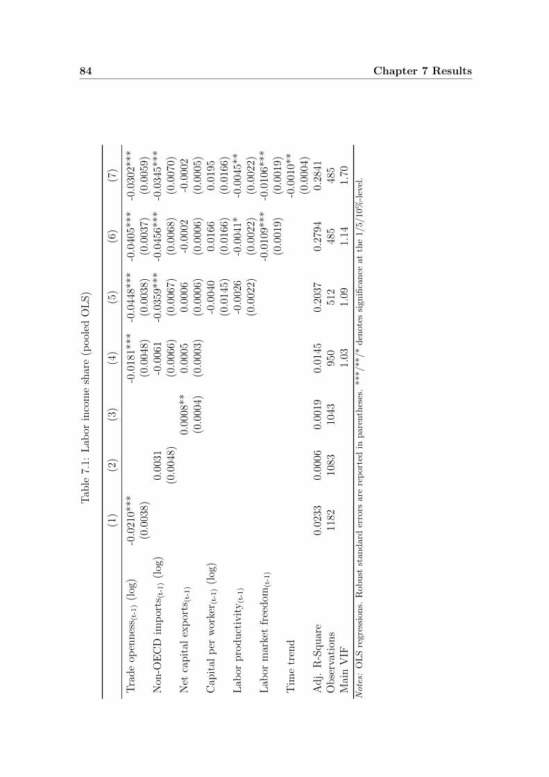
84 Chapter 7 ResultsT
able
7.1:
Lab
orin
com
esh
are
(pool
edO
LS)
(1)
(2)
(3)
(4)
(5)
(6)
(7)
Tra
de
open
nes
s (t-
1)
(log
)-0
.021
0***
-0.0
181*
**-0
.044
8***
-0.0
405*
**-0
.030
2***
(0.0
038)
(0.0
048)
(0.0
038)
(0.0
037)
(0.0
059)
Non
-OE
CD
imp
orts
(t-1
)(l
og)
0.00
31-0
.006
1-0
.035
9***
-0.0
456*
**-0
.034
5***
(0.0
048)
(0.0
066)
(0.0
067)
(0.0
068)
(0.0
070)
Net
capit
alex
por
ts(t
-1)
0.00
08**
0.00
050.
0006
-0.0
002
-0.0
002
(0.0
004)
(0.0
003)
(0.0
006)
(0.0
006)
(0.0
005)
Cap
ital
per
wor
ker (
t-1)
(log
)-0
.004
00.
0166
0.01
95(0
.014
5)(0
.016
6)(0
.016
6)L
abor
pro
duct
ivit
y(t
-1)
-0.0
026
-0.0
041*
-0.0
045*
*(0
.002
2)(0
.002
2)(0
.002
2)L
abor
mar
ket
free
dom
(t-1
)-0
.010
9***
-0.0
106*
**(0
.001
9)(0
.001
9)T
ime
tren
d-0
.001
0**
(0.0
004)
Adj.
R-S
quar
e0.
0233
0.00
060.
0019
0.01
450.
2037
0.27
940.
2841
Obse
rvat
ions
1182
1083
1043
950
512
485
485
Mai
nV
IF1.
031.
091.
141.
70
Note
s:O
LS
regr
essi
ons.
Rob
ust
stan
dar
der
rors
are
rep
ort
edin
pare
nth
eses
.***/**/*
den
ote
ssi
gn
ifica
nce
at
the
1/5/10%
-lev
el.
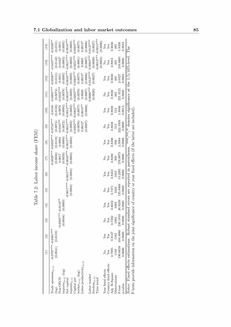
7.1 Globalization and labor market outcomes 85T
able
7.2:
Lab
orin
com
esh
are
(FE
M)
(1)
(2)
(3)
(4)
(5)
(6)
(7)
(8)
(9)
(10)
(11)
(12)
(13)
(14)
Tra
de
op
enn
ess (
t-1)
-0.0
797***
-0.0
381***
-0.0
828***
-0.0
350***
-0.0
733***
-0.0
168
-0.0
805***
-0.0
330**
-0.0
437***
-0.0
330**
(log)
(0.0
041)
(0.0
119)
(0.0
056)
(0.0
118)
(0.0
074)
(0.0
158)
(0.0
074)
(0.0
151)
(0.0
142)
(0.0
151)
Non
-OE
CD
-0.0
505***
-0.0
143**
0.0
017
-0.0
004
-0.0
167**
-0.0
079
-0.0
242***
-0.0
011
-0.0
162*
-0.0
011
imp
ort
s (t-
1)
(log)
(0.0
048)
(0.0
069)
(0.0
059)
(0.0
069)
(0.0
072)
(0.0
094)
(0.0
078)
(0.0
095)
(0.0
083)
(0.0
095)
Net
cap
ital
-0.0
017***
-0.0
015***
-0.0
016***
-0.0
015***
-0.0
015***
-0.0
012***
-0.0
019***
-0.0
016***
-0.0
017***
-0.0
016***
exp
ort
s (t-
1)
(0.0
004)
(0.0
004)
(0.0
004)
(0.0
004)
(0.0
002)
(0.0
002)
(0.0
003)
(0.0
003)
(0.0
003)
(0.0
003)
Cap
ital
per
0.0
382***
0.0
462***
0.0
282***
0.0
303***
0.0
251***
0.0
303***
work
er(t
-1)
(log)
(0.0
076)
(0.0
077)
(0.0
079)
(0.0
077)
(0.0
081)
(0.0
077)
Lab
or
pro
du
ctiv
ity
(t-1
)0.0
012*
0.0
018**
0.0
009
0.0
013*
0.0
005
0.0
013*
(0.0
007)
(0.0
008)
(0.0
007)
(0.0
008)
(0.0
007)
(0.0
008)
Lab
or
mark
et0.0
086***
0.0
137***
0.0
083***
0.0
137***
free
dom
(t-1
)(0
.0020)
(0.0
027)
(0.0
020)
(0.0
027)
Tim
etr
end
-0.0
013***
-0.0
015***
(0.0
004)
(0.0
006)
Yea
rfi
xed
effec
tsN
oY
esN
oY
esN
oY
esN
oY
esN
oY
esN
oY
esN
oY
esC
ou
ntr
yfi
xed
effec
tsY
esY
esY
esY
esY
esY
esY
esY
esY
esY
esY
esY
esY
esY
esA
dj.
R-S
qu
are
0.7
995
0.8
147
0.7
392
0.8
032
0.7
471
0.8
453
0.8
286
0.8
396
0.8
838
0.8
938
0.8
930
0.9
030
0.8
953
0.9
030
Ob
serv
ati
on
s1182
1182
1083
1083
1043
1043
950
950
512
512
485
485
485
485
F-t
est
190.6
659
104.4
880
230.1
810
26.9
249
135.8
468
13.2
205
276.0
075
2.5
084
222.1
958
1.8
946
221.3
121
2.0
327
216.6
681
1.8
356
p-v
alu
e0.0
000
0.0
000
0.0
000
0.0
000
0.0
000
0.0
000
0.0
000
0.0
000
0.0
000
0.0
013
0.0
000
0.0
004
0.0
000
0.0
024
Note
s:F
ixed
effec
tses
tim
atio
ns.
Rob
ust
stan
dar
der
rors
are
rep
ort
edin
pare
nth
eses
.***/**/*
den
ote
ssi
gnifi
can
ceat
the
1/5/10%
-lev
el.
Th
eF
-tes
tsp
rovid
ein
form
atio
non
the
join
tsi
gnifi
can
ceof
cou
ntr
yor
year
fixed
effec
ts(i
fth
ela
tter
are
incl
ud
ed).
86 Chapter 7 Results
Labor market freedom, the amount of capital per worker and partly also labor
productivity have now a significant positive effect on the labor income share. This
indicates that a country’s labor income share increases if the amount of capital per
worker increases or labor markets become more flexible.122 Moreover, the time trend
still indicates a general downward trend in the labor income share.
Determinants of the wage dispersion
The wage differential, as a second transmission variable, proxies the wages of skilled
(well educated) relative to unskilled (poorly educated) workers. The results of the
OLS regressions are shown in Table 7.3. The bivariate regressions indicate that wage
dispersion is negatively related with trade openness as well as net exports of private
capital and positively with the share of imports from non-OECD countries.
The effect of net export of capital remains robust but the significance of trade
openness and non-OECD imports is partly affected by the inclusion of further con-
trols.123 Among the further control variables only the degree of labor market freedom
is significantly and robustly related to earnings dispersion, which is greater in coun-
tries with less regulated labor markets. Finally, a positive and marginal significant
time trend points at an increase in wage dispersion that is common to all countries.
To account for a possible heterogeneity among different countries, Table 7.4
presents the fixed effects estimates. The signs of the coefficients are in line with
the theoretical expectations (see hypotheses 1 and 2). Both trade openness124 and
imports from developing countries are now positively related to the wage differential.
Net exports of capital fail to be significant. Again, the relative capital endowment
is mostly insignificant, whereas less regulated labor markets are associated with a
higher wage inequality. The time trend is significantly positive only if year fixed
effects are not included.
122 By controlling for time-invariant and country-specific effects, the fixed effects model focuseson changes within countries, whereas the pooled OLS regressions utilize both variation withinand between countries. The difference between the two estimated effects of labor marketregulation could be interpreted as follows: countries with highly regulated labor markets alsohave a higher labor income share but a further liberalization of labor markets in a certaincountry may be beneficial for labor.
123 In particular, the share of imports from developing countries is statistically significant only inspecifications that do not account for differences in labor market institutions.
124 The negative effect of trade openness in the OLS regressions is thus likely driven by unobservedand country-specific factors.
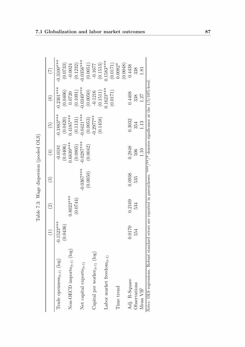
7.1 Globalization and labor market outcomes 87T
able
7.3:
Wag
edis
per
sion
(pool
edO
LS)
(1)
(2)
(3)
(4)
(5)
(6)
(7)
Tra
de
open
nes
s (t-
1)
(log
)-0
.152
3***
-0.0
181
-0.1
883*
**-0
.230
1***
-0.3
100*
**(0
.043
6)(0
.040
6)(0
.042
0)(0
.040
6)(0
.073
3)N
on-O
EC
Dim
por
ts(t
-1)
(log
)0.
8023
***
0.68
39**
*0.
4185
***
0.07
20-0
.002
4(0
.074
4)(0
.080
5)(0
.113
1)(0
.109
1)(0
.123
2)N
etca
pit
alex
por
ts(t
-1)
-0.0
367*
**-0
.028
7***
-0.0
421*
**-0
.034
9***
-0.0
356*
**(0
.005
0)(0
.004
2)(0
.005
3)(0
.005
0)(0
.005
1)C
apit
alp
erw
orke
r (t-
1)
(log
)-0
.297
7**
-0.1
216
-0.1
677
(0.1
458)
(0.1
511)
(0.1
513)
Lab
orm
arke
tfr
eedom
(t-1
)0.
1623
***
0.15
83**
*(0
.017
1)(0
.017
1)T
ime
tren
d0.
0082
*(0
.004
8)A
dj.
R-S
quar
e0.
0170
0.21
690.
0938
0.28
480.
3032
0.44
080.
4438
Obse
rvat
ions
554
534
535
506
354
338
338
Mea
nV
IF1.
101.
131.
271.
81
Note
s:O
LS
regr
essi
ons.
Rob
ust
stan
dar
der
rors
are
rep
ort
edin
pare
nth
eses
.***/**/*
den
ote
ssi
gn
ifica
nce
at
the
1/5/10%
-lev
el.

88 Chapter 7 ResultsT
able
7.4:
Wag
edis
per
sion
(FE
M)
(1)
(2)
(3)
(4)
(5)
(6)
(7)
(8)
(9)
(10)
(11)
(12)
(13)
(14)
Tra
de
op
enn
ess (
t-1)
(log)
0.2
310***
0.3
552***
0.4
478***
0.6
851***
0.4
222***
0.2
970***
0.3
794***
0.3
008**
0.1
169
0.3
008**
(0.0
559)
(0.1
051)
(0.0
457)
(0.1
065)
(0.0
679)
(0.1
123)
(0.0
721)
(0.1
184)
(0.0
949)
(0.1
184)
Non
-OE
CD
imp
ort
s (t-
1)
(log)
0.4
945***
0.1
173*
0.1
365***
0.2
626***
0.1
212**
0.2
002*
0.0
507
0.3
027**
-0.0
076
0.3
027**
(0.0
385)
(0.0
696)
(0.0
386)
(0.0
630)
(0.0
529)
(0.1
044)
(0.0
727)
(0.1
364)
(0.0
794)
(0.1
364)
Net
cap
ital
exp
ort
s (t-
1)
-0.0
012
-0.0
021
0.0
011
0.0
017
0.0
004
0.0
007
0.0
013
0.0
010
0.0
009
0.0
010
(0.0
024)
(0.0
020)
(0.0
018)
(0.0
021)
(0.0
026)
(0.0
023)
(0.0
026)
(0.0
024)
(0.0
022)
(0.0
024)
Cap
ital
per
work
er(t
-1)
(log)
0.1
182
0.3
133***
0.1
283
0.2
052
0.1
890
0.2
052
(0.1
014)
(0.1
153)
(0.1
106)
(0.1
258)
(0.1
149)
(0.1
258)
Lab
or
mark
etfr
eed
om
(t-1
)0.0
402**
0.0
400*
0.0
321*
0.0
400*
(0.0
194)
(0.0
231)
(0.0
185)
(0.0
231)
Tim
etr
end
0.0
100**
-0.0
000
(0.0
039)
(0.0
033)
Yea
rfi
xed
effec
tsN
oY
esN
oY
esN
oY
esN
oY
esN
oY
esN
oY
esN
oY
esC
ou
ntr
yfi
xed
effec
tsY
esY
esY
esY
esY
esY
esY
esY
esY
esY
esY
esY
esY
esY
esA
dj.
R-S
qu
are
0.9
086
0.9
330
0.9
110
0.9
296
0.9
037
0.9
271
0.9
420
0.9
425
0.9
355
0.9
385
0.9
358
0.9
389
0.9
373
0.9
389
Ob
serv
ati
on
s554
554
534
534
535
535
506
506
354
354
338
338
338
338
F-t
est
520.8
241
2.0
e+11
3.0
e+03
3.7
067
391.5
504
4.4
967
2.3
e+03
4.6
571
667.7
426
3.7
980
315.6
713
18.5
129
372.7
793
15.5
154
p-v
alu
e0.0
000
0.0
000
0.0
000
0.0
000
0.0
000
0.0
000
0.0
000
0.0
000
0.0
000
0.0
000
0.0
000
0.0
000
0.0
000
0.0
000
Note
s:F
ixed
effec
tses
tim
atio
ns.
Rob
ust
stan
dar
der
rors
are
rep
ort
edin
pare
nth
eses
.***/**/*
den
ote
ssi
gnifi
can
ceat
the
1/5/10%
-lev
el.
Th
eF
-tes
tsp
rovid
ein
form
atio
non
the
join
tsi
gnifi
can
ceof
cou
ntr
yor
year
fixed
effec
ts(i
fth
ela
tter
are
incl
ud
ed).
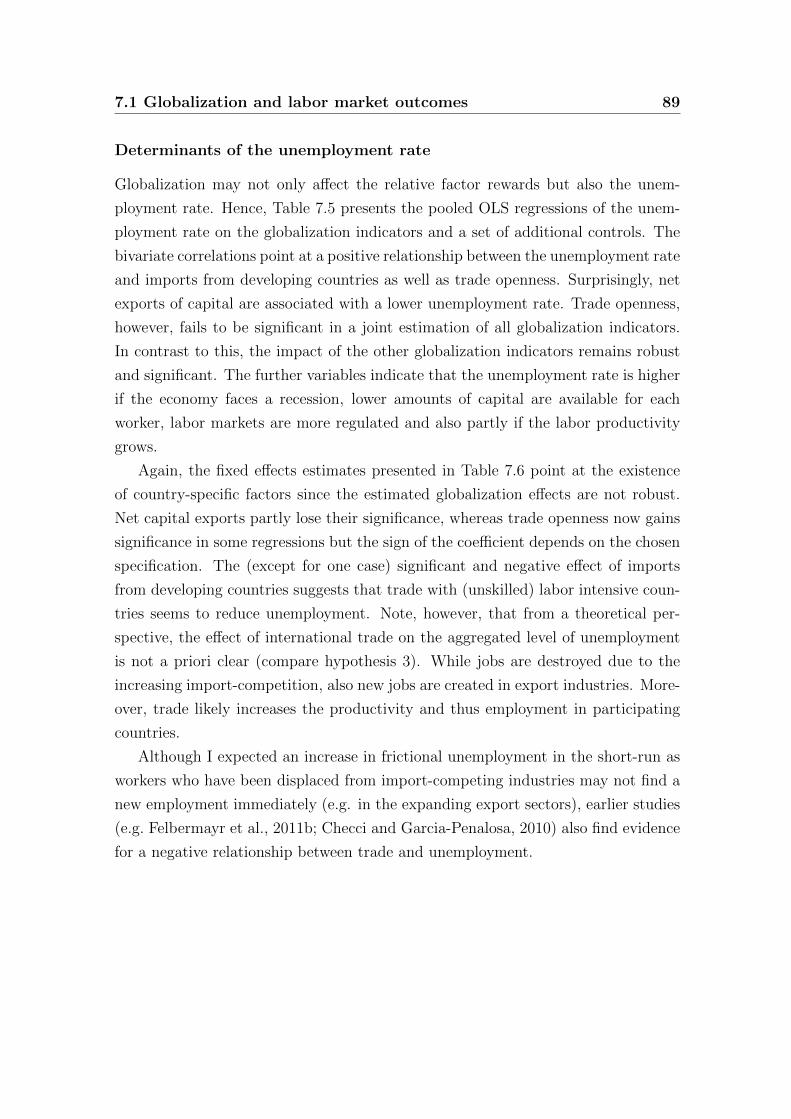
7.1 Globalization and labor market outcomes 89
Determinants of the unemployment rate
Globalization may not only affect the relative factor rewards but also the unem-
ployment rate. Hence, Table 7.5 presents the pooled OLS regressions of the unem-
ployment rate on the globalization indicators and a set of additional controls. The
bivariate correlations point at a positive relationship between the unemployment rate
and imports from developing countries as well as trade openness. Surprisingly, net
exports of capital are associated with a lower unemployment rate. Trade openness,
however, fails to be significant in a joint estimation of all globalization indicators.
In contrast to this, the impact of the other globalization indicators remains robust
and significant. The further variables indicate that the unemployment rate is higher
if the economy faces a recession, lower amounts of capital are available for each
worker, labor markets are more regulated and also partly if the labor productivity
grows.
Again, the fixed effects estimates presented in Table 7.6 point at the existence
of country-specific factors since the estimated globalization effects are not robust.
Net capital exports partly lose their significance, whereas trade openness now gains
significance in some regressions but the sign of the coefficient depends on the chosen
specification. The (except for one case) significant and negative effect of imports
from developing countries suggests that trade with (unskilled) labor intensive coun-
tries seems to reduce unemployment. Note, however, that from a theoretical per-
spective, the effect of international trade on the aggregated level of unemployment
is not a priori clear (compare hypothesis 3). While jobs are destroyed due to the
increasing import-competition, also new jobs are created in export industries. More-
over, trade likely increases the productivity and thus employment in participating
countries.
Although I expected an increase in frictional unemployment in the short-run as
workers who have been displaced from import-competing industries may not find a
new employment immediately (e.g. in the expanding export sectors), earlier studies
(e.g. Felbermayr et al., 2011b; Checci and Garcia-Penalosa, 2010) also find evidence
for a negative relationship between trade and unemployment.

90 Chapter 7 Results
Tab
le7.
5:U
nem
plo
ym
ent
rate
(pool
edO
LS)
(1)
(2)
(3)
(4)
(5)
(6)
(7)
Tra
de
open
nes
s (t-
1)
(log
)0.
3887
**0.
2986
0.21
700.
2354
-0.2
773
(0.1
682)
(0.1
872)
(0.2
413)
(0.2
559)
(0.3
592)
Non
-OE
CD
imp
orts
(t-1
)(l
og)
0.69
68**
*0.
5691
**1.
1113
***
1.78
00**
*0.
9748
**(0
.186
2)(0
.262
5)(0
.258
4)(0
.365
9)(0
.479
3)N
etca
pit
alex
por
ts(t
-1)
-0.0
674*
**-0
.070
9***
-0.0
558*
**-0
.104
0***
-0.1
112*
**(0
.016
8)(0
.019
3)(0
.019
1)(0
.028
4)(0
.028
2)O
utp
ut
gap
(t-1
)-0
.343
3***
-0.3
329*
**-0
.338
0***
(0.0
699)
(0.0
709)
(0.0
709)
Lab
orpro
duct
ivit
y(t
-1)
0.13
38**
0.08
640.
1220
*(0
.066
0)(0
.066
9)(0
.070
5)C
apit
alp
erw
orke
r (t-
1)
(log
)-3
.967
4***
-4.0
033*
**-4
.136
4***
(0.8
060)
(0.8
322)
(0.8
073)
Lab
orm
arke
tfr
eedom
(t-1
)-0
.528
6***
-0.5
653*
**(0
.094
6)(0
.097
0)T
ime
tren
d0.
0832
**(0
.034
9)A
dj.
R-S
quar
e0.
0034
0.00
790.
0125
0.01
970.
3162
0.34
100.
3491
Obse
rvat
ions
1164
1261
1018
951
430
417
417
Mea
nV
IF1.
041.
211.
231.
66
Note
s:O
LS
regr
essi
ons.
Rob
ust
stan
dar
der
rors
are
rep
ort
edin
pare
nth
eses
.***/**/*
den
ote
ssi
gn
ifica
nce
at
the
1/5/10%
-lev
el.
7.1 Globalization and labor market outcomes 91T
able
7.6:
Unem
plo
ym
ent
rate
(FE
M)
(1)
(2)
(3)
(4)
(5)
(6)
(7)
(8)
(9)
(10)
(11)
(12)
(13)
(14)
Tra
de
op
enn
ess (
t-1)
2.3
452***
-0.2
845
1.9
757***
-1.3
377**
0.1
182
-1.4
542
1.1
117*
-0.1
146
-1.3
049
-0.1
146
(log)
(0.2
434)
(0.5
470)
(0.3
722)
(0.6
487)
(0.5
623)
(1.1
319)
(0.5
743)
(1.1
248)
(1.0
433)
(1.1
248)
Non
-OE
CD
-1.1
189***
-1.9
065***
-2.0
638***
-2.3
933***
-0.9
275*
-3.7
495***
-0.2
408
-3.4
516***
-1.6
891**
-3.4
516***
imp
ort
s (t-
1)
(log)
(0.2
757)
(0.2
794)
(0.3
855)
(0.3
942)
(0.4
751)
(0.6
141)
(0.5
573)
(0.6
434)
(0.6
881)
(0.6
434)
Net
cap
ital
-0.0
042
-0.0
057
-0.0
017
0.0
078
-0.0
325**
-0.0
120
-0.0
627***
-0.0
434***
-0.0
701***
-0.0
434***
exp
ort
s (t-
1)
(0.0
148)
(0.0
129)
(0.0
189)
(0.0
157)
(0.0
154)
(0.0
142)
(0.0
180)
(0.0
150)
(0.0
184)
(0.0
150)
Ou
tpu
tgap
(t-1
)-0
.3805***
-0.4
205***
-0.4
188***
-0.4
524***
-0.3
834***
-0.4
524***
(0.0
496)
(0.0
558)
(0.0
503)
(0.0
517)
(0.0
504)
(0.0
517)
Lab
or
pro
du
ctiv
ity
(t-1
)0.0
285
0.1
312***
0.0
190
0.1
325***
0.0
438
0.1
325***
(0.0
435)
(0.0
493)
(0.0
433)
(0.0
468)
(0.0
438)
(0.0
468)
Cap
ital
per
-3.4
684***
-3.2
695***
-3.0
568***
-2.2
484*
-3.6
281***
-2.2
484*
work
er(t
-1)
(log)
(1.0
894)
(1.1
804)
(1.1
209)
(1.1
723)
(1.2
933)
(1.1
723)
Lab
or
mark
et-0
.5863***
-1.0
695***
-0.5
873***
-1.0
695***
free
dom
(t-1
)(0
.1665)
(0.1
896)
(0.1
637)
(0.1
896)
Tim
etr
end
0.1
360***
0.2
051***
(0.0
466)
(0.0
407)
Yea
rfi
xed
effec
tsN
oY
esN
oY
esN
oY
esN
oY
esN
oY
esN
oY
esN
oY
esC
ou
ntr
yfi
xed
effec
tsY
esY
esY
esY
esY
esY
esY
esY
esY
esY
esY
esY
esY
esY
esA
dj.
R-S
qu
are
0.5
746
0.7
010
0.4
535
0.6
937
0.5
787
0.6
871
0.6
036
0.7
006
0.7
767
0.8
038
0.7
803
0.8
166
0.7
853
0.8
166
Ob
serv
ati
on
s1164
1164
1261
1261
1018
1018
951
951
430
430
417
417
417
417
F-t
est
89.8
739
12.7
154
56.5
659
20.1
106
64.1
314
26.4
499
68.0
999
5.6
e+09
56.2
341
6.8
045
64.3
483
6.7
455
65.4
683
6.8
262
p-v
alu
e0.0
000
0.0
000
0.0
000
0.0
000
0.0
000
0.0
000
0.0
000
0.0
000
0.0
000
0.0
000
0.0
000
0.0
000
0.0
000
0.0
000
Note
s:F
ixed
effec
tses
tim
atio
ns.
Rob
ust
stan
dar
der
rors
are
rep
ort
edin
pare
nth
eses
.***/**/*
den
ote
ssi
gnifi
can
ceat
the
1/5/10%
-lev
el.
Th
eF
-tes
tsp
rovid
ein
form
atio
non
the
join
tsi
gnifi
can
ceof
cou
ntr
yor
year
fixed
effec
ts(i
fth
ela
tter
are
incl
ud
ed).
92 Chapter 7 Results
The influence of the other explanatory variables remains widely unaffected by
the choice of the estimators. Overall, a comparison of the pooled OLS and fixed
effects estimations points at an interesting pattern in the data. The pooled regres-
sions suggest that more open countries also have higher unemployment rates. One
should, however, not infer from this finding that trade increases unemployment.
The results of the fixed effects regressions even suggest the opposite. Rather the
findings indicate that country-specific factors explain why more open economies also
have higher unemployment rates. After controlling for these effects, the results do
not support the view that globalization itself is responsible for rising unemployment
in industrialized countries.125 Rather, an economy’s ability to cope with the chal-
lenges of globalization (e.g. allow declining) seems to matter for the evolution of
unemployment.
Determinants of the relative supply of human capital
So far, I have implicitly assumed that the relative factor endowments are not di-
rectly affected by globalization. To relax this assumption, the econometric anal-
ysis presented in the Tables 7.7 and 7.8 examines a possible relationship between
globalization and the relative supply of human capital in the population of OECD
countries.
For theoretical reasons, the specifications differ from those employed for the anal-
yses of the relative factor rewards and the unemployment rate. The globalization
indicators are now introduced with a lag of five instead of one year. This deviation
from my standard specification is reasonable because the relative supply of human
capital (measured as the ratio between individuals with tertiary and those with pri-
mary education) is a consequence of past education decisions. The global integration
of an economy should affect the individual decision to invest into education. Hence,
the relative supply of human capital is assumed to depend on past and not current
globalization experience.
Table 7.7 presents the findings of the pooled OLS regressions. The bivariate
correlations reported in columns (1) to (3) suggest that only imports from develop-
ing countries are significantly and positively related to the share of well educated
individuals five years later.
125 The estimated coefficients are equal to the effect of globalization on unemployment rates foran average OECD country but must not apply to a certain country considered in this study.Rather, the impact of international trade and globalization might vary considerably amongOECD countries. In particular, domestic institutions could explain different responses toglobalization (see section 7.1.2).
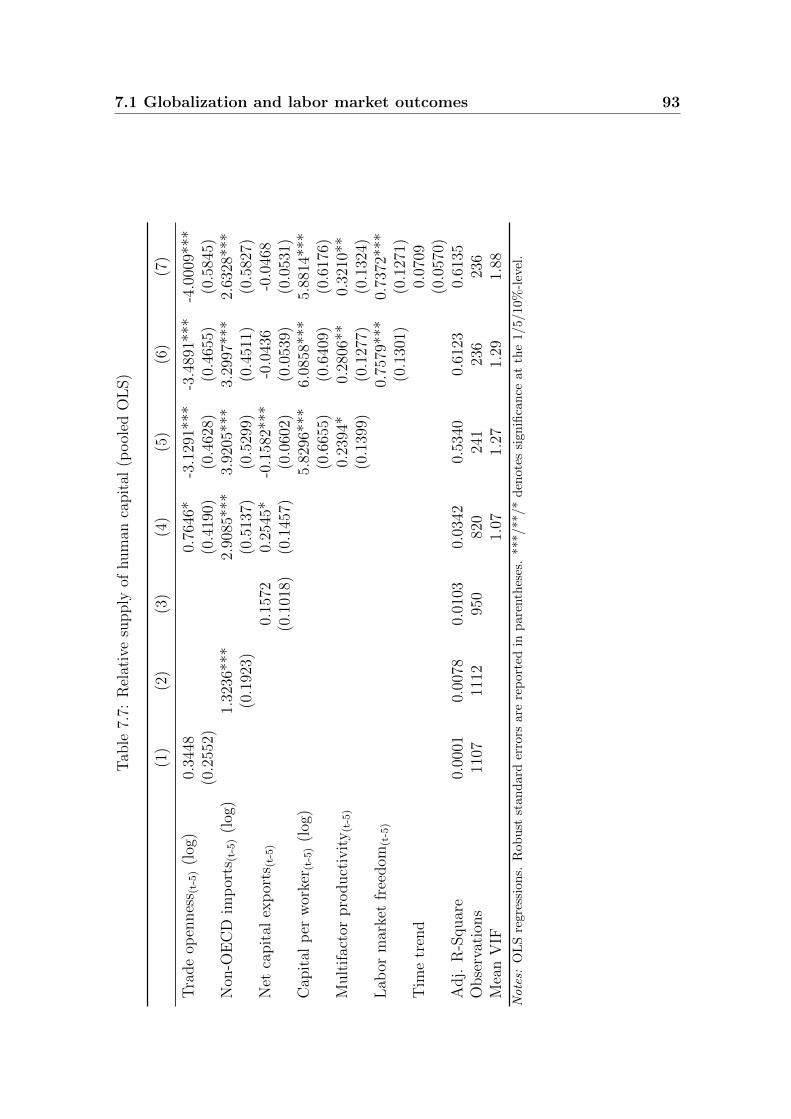
7.1 Globalization and labor market outcomes 93T
able
7.7:
Rel
ativ
esu
pply
ofhum
anca
pit
al(p
ool
edO
LS)
(1)
(2)
(3)
(4)
(5)
(6)
(7)
Tra
de
open
nes
s (t-
5)
(log
)0.
3448
0.76
46*
-3.1
291*
**-3
.489
1***
-4.0
009*
**(0
.255
2)(0
.419
0)(0
.462
8)(0
.465
5)(0
.584
5)N
on-O
EC
Dim
por
ts(t
-5)
(log
)1.
3236
***
2.90
85**
*3.
9205
***
3.29
97**
*2.
6328
***
(0.1
923)
(0.5
137)
(0.5
299)
(0.4
511)
(0.5
827)
Net
capit
alex
por
ts(t
-5)
0.15
720.
2545
*-0
.158
2***
-0.0
436
-0.0
468
(0.1
018)
(0.1
457)
(0.0
602)
(0.0
539)
(0.0
531)
Cap
ital
per
wor
ker (
t-5)
(log
)5.
8296
***
6.08
58**
*5.
8814
***
(0.6
655)
(0.6
409)
(0.6
176)
Mult
ifac
tor
pro
duct
ivit
y(t
-5)
0.23
94*
0.28
06**
0.32
10**
(0.1
399)
(0.1
277)
(0.1
324)
Lab
orm
arke
tfr
eedom
(t-5
)0.
7579
***
0.73
72**
*(0
.130
1)(0
.127
1)T
ime
tren
d0.
0709
(0.0
570)
Adj.
R-S
quar
e0.
0001
0.00
780.
0103
0.03
420.
5340
0.61
230.
6135
Obse
rvat
ions
1107
1112
950
820
241
236
236
Mea
nV
IF1.
071.
271.
291.
88
Note
s:O
LS
regr
essi
ons.
Rob
ust
stan
dar
der
rors
are
rep
ort
edin
pare
nth
eses
.***/**/*
den
ote
ssi
gn
ifica
nce
at
the
1/5/10%
-lev
el.

94 Chapter 7 ResultsT
able
7.8:
Rel
ativ
esu
pply
ofhum
anca
pit
al(F
EM
)
(1)
(2)
(3)
(4)
(5)
(6)
(7)
(8)
(9)
(10)
(11)
(12)
(13)
(14)
Tra
de
op
enn
ess (
t-5)
2.8
948***
-8.4
361***
1.3
693**
-14.0
627***
6.7
417***
7.4
140***
6.8
433***
7.6
690***
5.1
917**
7.6
690***
(log)
(0.3
364)
(3.1
045)
(0.5
772)
(4.7
580)
(1.4
372)
(2.4
002)
(1.5
372)
(2.4
621)
(2.0
224)
(2.4
621)
Non
-OE
CD
4.3
820***
3.0
181***
4.7
881***
4.0
405***
-0.3
979
-0.2
320
0.0
527
0.3
957
-0.4
501
0.3
957
imp
ort
s (t-
5)
(log)
(1.1
207)
(0.8
770)
(1.4
275)
(1.4
407)
(0.7
828)
(1.0
132)
(0.8
178)
(1.0
496)
(0.9
899)
(1.0
496)
Net
cap
ital
0.3
066**
0.2
632**
0.3
955**
0.3
832**
-0.1
139***
-0.1
070***
-0.1
179***
-0.1
184***
-0.1
182***
-0.1
184***
exp
ort
s (t-
5)
(0.1
271)
(0.1
197)
(0.1
776)
(0.1
604)
(0.0
420)
(0.0
377)
(0.0
446)
(0.0
398)
(0.0
442)
(0.0
398)
Cap
ital
per
-0.4
635
1.8
527
-0.4
884
1.7
296
-0.8
336
1.7
296
work
er(t
-5)
(log)
(1.0
282)
(1.1
958)
(1.1
509)
(1.2
477)
(1.2
121)
(1.2
477)
Mu
ltif
act
or
0.1
279*
0.2
149**
0.1
099
0.2
129**
0.1
216
0.2
129**
pro
du
ctiv
ity
(t-5
)(0
.0699)
(0.0
891)
(0.0
758)
(0.0
913)
(0.0
777)
(0.0
913)
Lab
or
mark
et-0
.1923
-0.4
630**
-0.2
380
-0.4
630**
free
dom
(t-5
)(0
.1668)
(0.1
884)
(0.1
613)
(0.1
884)
Tim
etr
end
0.0
834
0.0
041
(0.0
784)
(0.1
125)
Yea
rfi
xed
effec
tsN
oY
esN
oY
esN
oY
esN
oY
esN
oY
esN
oY
esN
oY
esC
ou
ntr
yfi
xed
effec
tsY
esY
esY
esY
esY
esY
esY
esY
esY
esY
esY
esY
esY
esY
esA
dj.
R-S
qu
are
0.1
730
0.2
102
0.1
436
0.1
695
0.1
967
0.2
163
0.2
294
0.2
601
0.9
074
0.9
058
0.9
072
0.9
071
0.9
072
0.9
071
Ob
serv
ati
on
s1107
1107
1112
1112
950
950
820
820
241
241
236
236
236
236
F-t
est
63.7
456
0.3
192
131.8
212
1.0
160
15.6
764
2.8
844
22.1
767
1.3
e+07
82.0
319
0.6
263
72.4
661
0.7
491
68.0
015
0.7
839
p-v
alu
e0.0
000
1.0
000
0.0
000
0.4
445
0.0
000
0.0
000
0.0
000
0.0
000
0.0
000
0.8
904
0.0
000
0.7
712
0.0
000
0.7
245
Note
s:F
ixed
effec
tses
tim
atio
ns.
Rob
ust
stan
dar
der
rors
are
rep
ort
edin
pare
nth
eses
.***/**/*
den
ote
ssi
gnifi
can
ceat
the
1/5/10%
-lev
el.
Th
eF
-tes
tsp
rovid
ein
form
atio
non
the
join
tsi
gnifi
can
ceof
cou
ntr
yor
year
fixed
effec
ts(i
fth
ela
tter
are
incl
ud
ed).
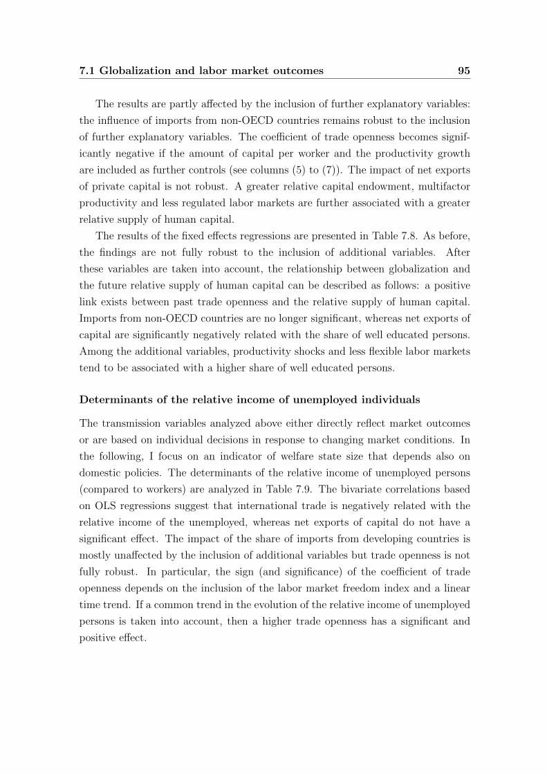
7.1 Globalization and labor market outcomes 95
The results are partly affected by the inclusion of further explanatory variables:
the influence of imports from non-OECD countries remains robust to the inclusion
of further explanatory variables. The coefficient of trade openness becomes signif-
icantly negative if the amount of capital per worker and the productivity growth
are included as further controls (see columns (5) to (7)). The impact of net exports
of private capital is not robust. A greater relative capital endowment, multifactor
productivity and less regulated labor markets are further associated with a greater
relative supply of human capital.
The results of the fixed effects regressions are presented in Table 7.8. As before,
the findings are not fully robust to the inclusion of additional variables. After
these variables are taken into account, the relationship between globalization and
the future relative supply of human capital can be described as follows: a positive
link exists between past trade openness and the relative supply of human capital.
Imports from non-OECD countries are no longer significant, whereas net exports of
capital are significantly negatively related with the share of well educated persons.
Among the additional variables, productivity shocks and less flexible labor markets
tend to be associated with a higher share of well educated persons.
Determinants of the relative income of unemployed individuals
The transmission variables analyzed above either directly reflect market outcomes
or are based on individual decisions in response to changing market conditions. In
the following, I focus on an indicator of welfare state size that depends also on
domestic policies. The determinants of the relative income of unemployed persons
(compared to workers) are analyzed in Table 7.9. The bivariate correlations based
on OLS regressions suggest that international trade is negatively related with the
relative income of the unemployed, whereas net exports of capital do not have a
significant effect. The impact of the share of imports from developing countries is
mostly unaffected by the inclusion of additional variables but trade openness is not
fully robust. In particular, the sign (and significance) of the coefficient of trade
openness depends on the inclusion of the labor market freedom index and a linear
time trend. If a common trend in the evolution of the relative income of unemployed
persons is taken into account, then a higher trade openness has a significant and
positive effect.
96 Chapter 7 Results
Tab
le7.
9:R
elat
ive
inco
me
ofunem
plo
yed
(pool
edO
LS)
(1)
(2)
(3)
(4)
(5)
(6)
(7)
(8)
Tra
de
open
nes
s (t-
1)
(log
)-0
.021
5***
-0.0
301*
**-0
.034
4***
-0.0
076
0.07
43**
*0.
0433
**(0
.006
0)(0
.007
9)(0
.010
7)(0
.011
1)(0
.021
7)(0
.020
2)N
on-O
EC
D-0
.026
1***
-0.0
713*
**-0
.093
6***
-0.1
727*
**-0
.096
1***
-0.1
265*
**im
por
ts(t
-1)
(log
)(0
.008
6)(0
.013
2)(0
.020
1)(0
.019
0)(0
.028
0)(0
.024
8)N
etca
pit
alex
por
ts(t
-1)
-0.0
001
-0.0
005
-0.0
015
-0.0
042*
**-0
.006
8***
-0.0
059*
**(0
.000
6)(0
.000
8)(0
.001
4)(0
.001
5)(0
.001
7)(0
.001
6)L
eft
gove
rnm
ent (
t-1)
-0.0
003*
-0.0
004*
*-0
.000
3*-0
.000
1(0
.000
2)(0
.000
2)(0
.000
2)(0
.000
2)V
oter
turn
out (
t-1)
-0.0
032*
**-0
.003
6***
-0.0
035*
**(0
.000
6)(0
.000
6)(0
.000
5)L
abor
mar
ket
-0.0
195*
**-0
.019
5***
-0.0
266*
**fr
eedom
(t-1
)(0
.005
4)(0
.005
1)(0
.005
1)U
nem
plo
ym
ent
rate
(t-1
)-0
.010
0***
(0.0
016)
Tim
etr
end
-0.0
068*
**-0
.005
5***
(0.0
018)
(0.0
016)
Adj.
R-S
quar
e0.
0135
0.01
550.
0026
0.07
080.
0765
0.22
920.
2951
0.36
80O
bse
rvat
ions
408
394
385
374
321
303
303
303
Mea
nV
IF1.
111.
221.
452.
072.
05
Note
s:O
LS
regr
essi
ons.
Rob
ust
stan
dar
der
rors
are
rep
ort
edin
pare
nth
eses
.***/**/*
den
ote
ssi
gn
ifica
nce
at
the
1/5/10%
-lev
el.
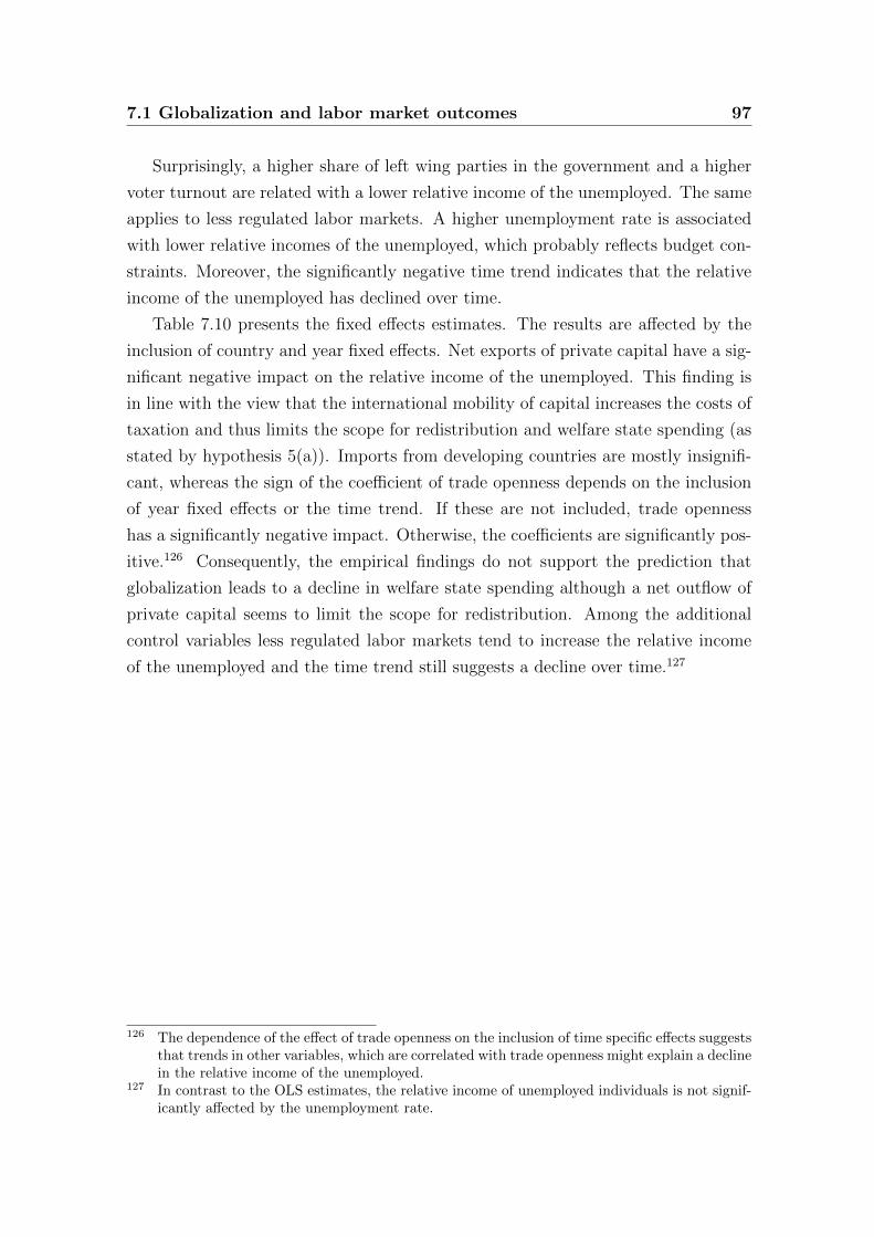
7.1 Globalization and labor market outcomes 97
Surprisingly, a higher share of left wing parties in the government and a higher
voter turnout are related with a lower relative income of the unemployed. The same
applies to less regulated labor markets. A higher unemployment rate is associated
with lower relative incomes of the unemployed, which probably reflects budget con-
straints. Moreover, the significantly negative time trend indicates that the relative
income of the unemployed has declined over time.
Table 7.10 presents the fixed effects estimates. The results are affected by the
inclusion of country and year fixed effects. Net exports of private capital have a sig-
nificant negative impact on the relative income of the unemployed. This finding is
in line with the view that the international mobility of capital increases the costs of
taxation and thus limits the scope for redistribution and welfare state spending (as
stated by hypothesis 5(a)). Imports from developing countries are mostly insignifi-
cant, whereas the sign of the coefficient of trade openness depends on the inclusion
of year fixed effects or the time trend. If these are not included, trade openness
has a significantly negative impact. Otherwise, the coefficients are significantly pos-
itive.126 Consequently, the empirical findings do not support the prediction that
globalization leads to a decline in welfare state spending although a net outflow of
private capital seems to limit the scope for redistribution. Among the additional
control variables less regulated labor markets tend to increase the relative income
of the unemployed and the time trend still suggests a decline over time.127
126 The dependence of the effect of trade openness on the inclusion of time specific effects suggeststhat trends in other variables, which are correlated with trade openness might explain a declinein the relative income of the unemployed.
127 In contrast to the OLS estimates, the relative income of unemployed individuals is not signif-icantly affected by the unemployment rate.
98 Chapter 7 Results
Tab
le7.
10:
Rel
ativ
ein
com
eof
unem
plo
yed
(FE
M)
(1)
(2)
(3)
(4)
(5)
(6)
(7)
(8)
(9)
(10)
(11)
(12)
(13)
(14)
(15)
(16)
Tra
de
-0.1
018***
0.1
431***
-0.1
173***
0.1
640***
-0.1
712***
0.2
232***
-0.1
577***
0.2
567***
0.2
861***
0.2
567***
0.2
922***
0.2
565***
op
enn
ess (
t-1)
(log)
(0.0
175)
(0.0
385)
(0.0
266)
(0.0
383)
(0.0
370)
(0.0
553)
(0.0
333)
(0.0
531)
(0.0
658)
(0.0
531)
(0.0
669)
(0.0
538)
Non
-OE
CD
-0.0
694***
0.0
401
0.0
133
0.0
379
0.0
313
0.0
423
0.0
685
0.0
493
0.1
074**
0.0
493
0.1
123**
0.0
486
imp
ort
s (t-
1)
(log)
(0.0
188)
(0.0
259)
(0.0
328)
(0.0
273)
(0.0
457)
(0.0
419)
(0.0
596)
(0.0
433)
(0.0
465)
(0.0
433)
(0.0
464)
(0.0
437)
Net
cap
ital
-0.0
016***
-0.0
023***
-0.0
012**
-0.0
024***
-0.0
022***
-0.0
030***
-0.0
034***
-0.0
074***
-0.0
060***
-0.0
074***
-0.0
062***
-0.0
074***
exp
ort
s (t-
1)
(0.0
005)
(0.0
006)
(0.0
005)
(0.0
007)
(0.0
006)
(0.0
010)
(0.0
011)
(0.0
014)
(0.0
012)
(0.0
014)
(0.0
013)
(0.0
016)
Lef
t0.0
003*
0.0
002
0.0
001
0.0
001
0.0
001
0.0
001
0.0
001
0.0
001
gover
nm
ent (
t-1)
(0.0
002)
(0.0
001)
(0.0
002)
(0.0
001)
(0.0
001)
(0.0
001)
(0.0
001)
(0.0
001)
Vote
r0.0
025**
0.0
009
0.0
011
0.0
009
0.0
010
0.0
009
turn
ou
t (t-
1)
(0.0
010)
(0.0
010)
(0.0
009)
(0.0
010)
(0.0
010)
(0.0
011)
Lab
or
-0.0
106
0.0
202*
0.0
215**
0.0
202*
0.0
221**
0.0
200
mark
etfr
eed
om
(t-1
)
(0.0
104)
(0.0
116)
(0.0
087)
(0.0
116)
(0.0
089)
(0.0
122)
Un
emp
loym
ent
0.0
008
-0.0
001
rate
(t-1
)(0
.0015)
(0.0
018)
Tim
etr
end
-0.0
184***
-0.0
196***
-0.0
187***
-0.0
195***
(0.0
033)
(0.0
046)
(0.0
033)
(0.0
047)
Yea
rfi
xed
effec
tsN
oY
esN
oY
esN
oY
esN
oY
esN
oY
esN
oY
esN
oY
esN
oY
es
Cou
ntr
yfi
xed
effec
tsY
esY
esY
esY
esY
esY
esY
esY
esY
esY
esY
esY
esY
esY
esY
esY
es
Ad
j.R
-S
qu
are
0.5
646
0.6
814
0.5
041
0.6
591
0.5
119
0.6
741
0.5
501
0.6
792
0.5
797
0.6
862
0.6
179
0.7
358
0.7
220
0.7
358
0.7
211
0.7
347
Ob
serv
ati
on
s408
408
394
394
385
385
374
374
321
321
303
303
303
303
303
303
F-t
est
426.2
032
2.5
525
914.9
078
3.1
925
3.2
e+12
3.7
417
541.9
283
2.9
534
108.6
777
2.5
997
61.6
399
3.1
428
74.8
101
0.9
213
60.4
669
0.8
997
p-v
alu
e0.0
000
0.0
000
0.0
000
0.0
000
0.0
000
0.0
000
0.0
000
0.0
000
0.0
000
0.0
000
0.0
000
0.0
000
0.0
000
0.5
997
0.0
000
0.6
342
Note
s:F
ixed
effec
tses
tim
atio
ns.
Rob
ust
stan
dar
der
rors
are
rep
ort
edin
pare
nth
eses
.***/**/*
den
ote
ssi
gnifi
can
ceat
the
1/5/10%
-lev
el.
Th
eF
-tes
tsp
rovid
ein
form
atio
non
the
join
tsi
gnifi
can
ceof
cou
ntr
yor
year
fixed
effec
ts(i
fth
ela
tter
are
incl
ud
ed).
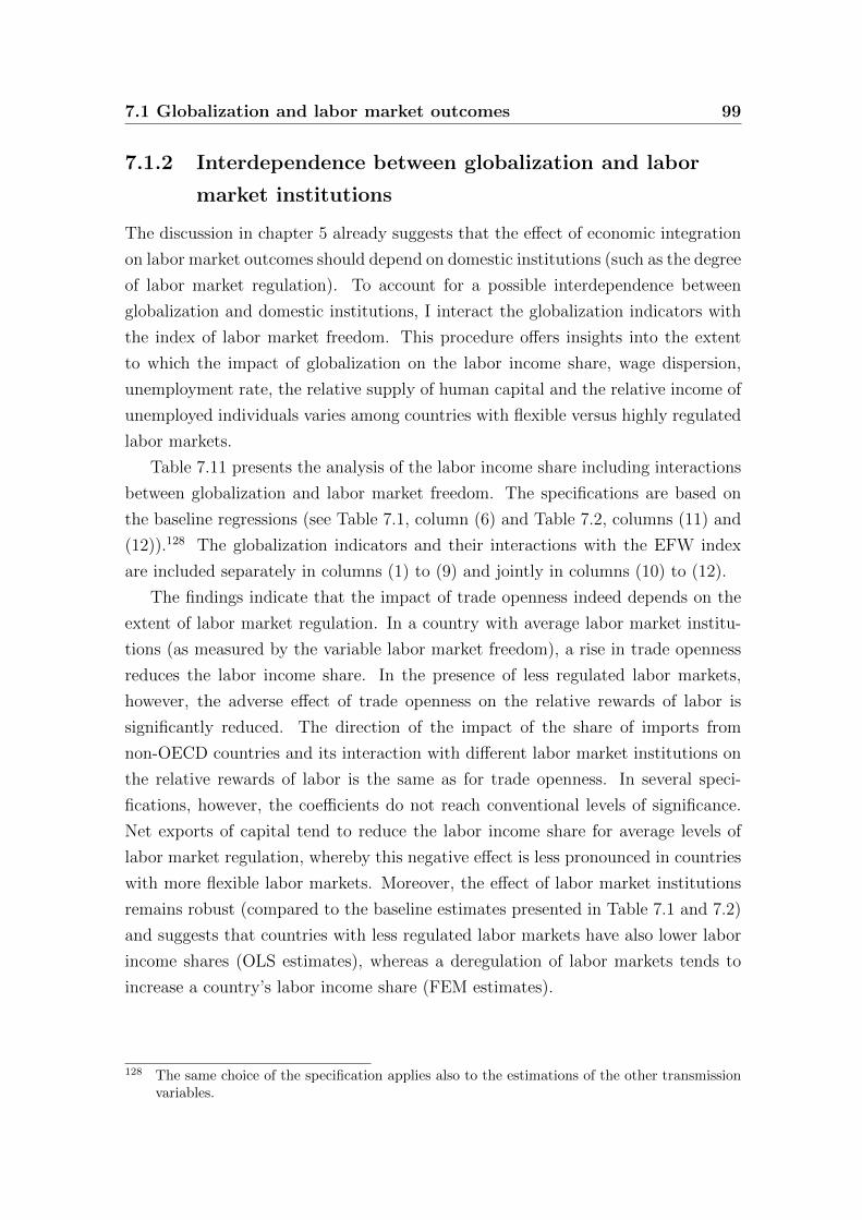
7.1 Globalization and labor market outcomes 99
7.1.2 Interdependence between globalization and labor
market institutions
The discussion in chapter 5 already suggests that the effect of economic integration
on labor market outcomes should depend on domestic institutions (such as the degree
of labor market regulation). To account for a possible interdependence between
globalization and domestic institutions, I interact the globalization indicators with
the index of labor market freedom. This procedure offers insights into the extent
to which the impact of globalization on the labor income share, wage dispersion,
unemployment rate, the relative supply of human capital and the relative income of
unemployed individuals varies among countries with flexible versus highly regulated
labor markets.
Table 7.11 presents the analysis of the labor income share including interactions
between globalization and labor market freedom. The specifications are based on
the baseline regressions (see Table 7.1, column (6) and Table 7.2, columns (11) and
(12)).128 The globalization indicators and their interactions with the EFW index
are included separately in columns (1) to (9) and jointly in columns (10) to (12).
The findings indicate that the impact of trade openness indeed depends on the
extent of labor market regulation. In a country with average labor market institu-
tions (as measured by the variable labor market freedom), a rise in trade openness
reduces the labor income share. In the presence of less regulated labor markets,
however, the adverse effect of trade openness on the relative rewards of labor is
significantly reduced. The direction of the impact of the share of imports from
non-OECD countries and its interaction with different labor market institutions on
the relative rewards of labor is the same as for trade openness. In several speci-
fications, however, the coefficients do not reach conventional levels of significance.
Net exports of capital tend to reduce the labor income share for average levels of
labor market regulation, whereby this negative effect is less pronounced in countries
with more flexible labor markets. Moreover, the effect of labor market institutions
remains robust (compared to the baseline estimates presented in Table 7.1 and 7.2)
and suggests that countries with less regulated labor markets have also lower labor
income shares (OLS estimates), whereas a deregulation of labor markets tends to
increase a country’s labor income share (FEM estimates).
128 The same choice of the specification applies also to the estimations of the other transmissionvariables.

100 Chapter 7 ResultsT
able
7.11
:L
abor
inco
me
shar
e:in
tera
ctio
ngl
obal
izat
ion
and
lab
orm
arke
tre
gula
tion
(1)
(2)
(3)
(4)
(5)
(6)
(7)
(8)
(9)
(10)
(11)
(12)
Tra
de
op
enness
(t-1
)(l
og)
-0.0
496***
-0.0
756***
-0.0
439***
-0.0
387***
-0.0
806***
-0.0
331**
-0.0
403***
-0.0
755***
-0.0
289*
-0.0
475***
-0.0
711***
-0.0
395***
(0.0
060)
(0.0
069)
(0.0
149)
(0.0
037)
(0.0
074)
(0.0
150)
(0.0
038)
(0.0
077)
(0.0
149)
(0.0
059)
(0.0
071)
(0.0
146)
Non-O
EC
Dim
port
s (t-1
)(l
og)
-0.0
449***
-0.0
303***
-0.0
096
-0.0
554***
-0.0
243***
-0.0
018
-0.0
422***
-0.0
231***
-0.0
023
-0.0
532***
-0.0
289***
-0.0
110
(0.0
069)
(0.0
076)
(0.0
090)
(0.0
091)
(0.0
077)
(0.0
095)
(0.0
073)
(0.0
073)
(0.0
090)
(0.0
094)
(0.0
070)
(0.0
086)
Net
capit
al
exp
ort
s (t-1
)-0
.0001
-0.0
016***
-0.0
014***
0.0
001
-0.0
018***
-0.0
015***
-0.0
007
-0.0
024***
-0.0
020***
-0.0
003
-0.0
020***
-0.0
018***
(0.0
006)
(0.0
003)
(0.0
003)
(0.0
006)
(0.0
003)
(0.0
003)
(0.0
007)
(0.0
003)
(0.0
003)
(0.0
007)
(0.0
003)
(0.0
003)
Lab
or
pro
ducti
vit
y(t-1
)-0
.0042*
0.0
008
0.0
013*
-0.0
042*
0.0
009
0.0
013*
-0.0
044**
0.0
007
0.0
011
-0.0
048**
0.0
005
0.0
010
(0.0
022)
(0.0
007)
(0.0
007)
(0.0
022)
(0.0
007)
(0.0
007)
(0.0
022)
(0.0
007)
(0.0
008)
(0.0
022)
(0.0
007)
(0.0
007)
Capit
al
per
work
er (
t-1
)(l
og)
0.0
212
0.0
384***
0.0
431***
0.0
102
0.0
267***
0.0
293***
0.0
184
0.0
280***
0.0
307***
0.0
152
0.0
362***
0.0
419***
(0.0
170)
(0.0
070)
(0.0
071)
(0.0
165)
(0.0
080)
(0.0
077)
(0.0
168)
(0.0
080)
(0.0
079)
(0.0
169)
(0.0
072)
(0.0
071)
Lab
or
mark
et
freedom
(t-1
)-0
.0109***
0.0
032
0.0
079***
-0.0
120***
0.0
074***
0.0
127***
-0.0
117***
0.0
081***
0.0
126***
-0.0
133***
0.0
017
0.0
060**
(0.0
019)
(0.0
026)
(0.0
027)
(0.0
018)
(0.0
020)
(0.0
027)
(0.0
020)
(0.0
019)
(0.0
027)
(0.0
018)
(0.0
024)
(0.0
028)
Lab
or
mark
et
freedom
(t-1
)×
0.0
081**
0.0
138***
0.0
141***
0.0
084**
0.0
131***
0.0
134***
Tra
de
op
enness
(t-1
)(0
.0033)
(0.0
028)
(0.0
019)
(0.0
033)
(0.0
028)
(0.0
020)
Lab
or
mark
et
freedom
(t-1
)×
0.0
123**
0.0
038
0.0
028
0.0
159***
0.0
039*
0.0
028
Non-O
EC
Dim
port
s (t-1
)(0
.0048)
(0.0
024)
(0.0
025)
(0.0
051)
(0.0
023)
(0.0
024)
Lab
or
mark
et
freedom
(t-1
)×
0.0
007
0.0
007***
0.0
006***
0.0
009**
0.0
006***
0.0
006***
Net
capit
al
exp
ort
s (t-1
)(0
.0004)
(0.0
002)
(0.0
002)
(0.0
004)
(0.0
002)
(0.0
002)
Year
fixed
eff
ects
No
No
Yes
No
No
Yes
No
No
Yes
No
No
Yes
Countr
yfi
xed
eff
ects
No
Yes
Yes
No
Yes
Yes
No
Yes
Yes
No
Yes
Yes
Adj.
R-S
quare
0.2
852
0.9
028
0.9
131
0.2
883
0.8
933
0.9
031
0.2
827
0.8
963
0.9
057
0.3
024
0.9
060
0.9
153
Obse
rvati
ons
485
485
485
485
485
485
485
485
485
485
485
485
Note
s:O
LS
and
fixed
effec
tsre
gres
sion
s.R
obu
stst
and
ard
erro
rsare
rep
ort
edin
pare
nth
eses
.***/**/*
den
ote
ssi
gn
ifica
nce
at
the
1/5/
10%
-lev
el.
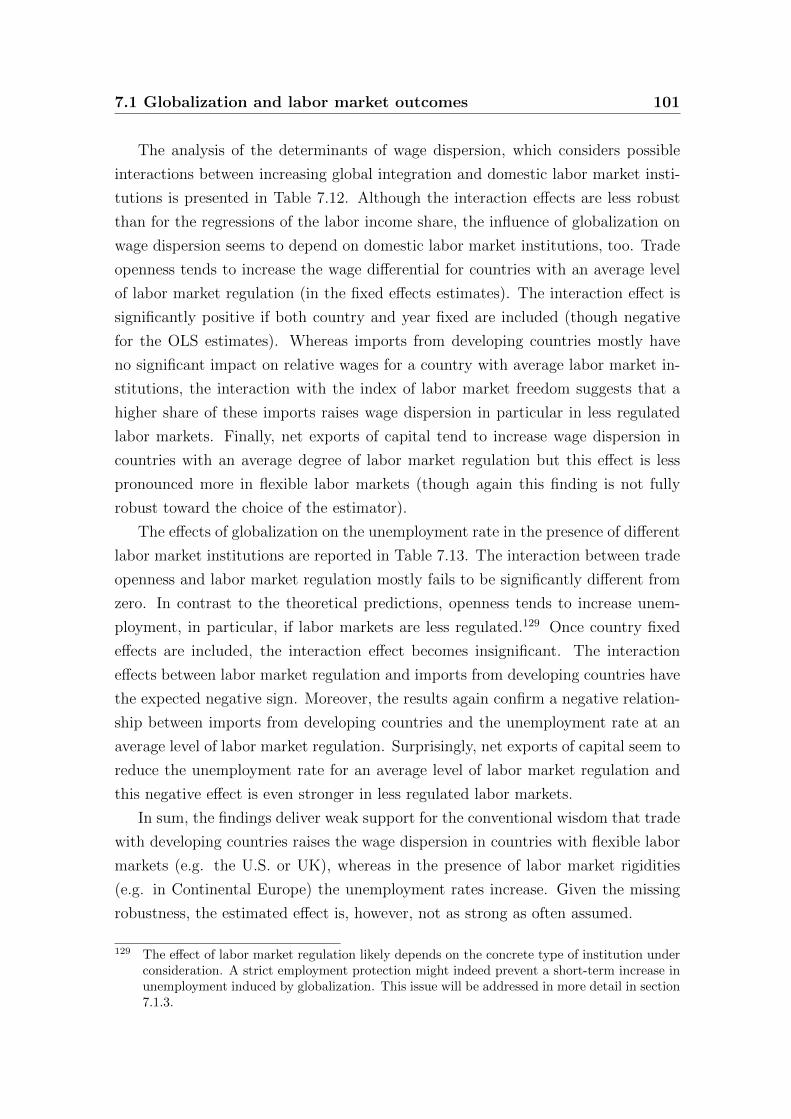
7.1 Globalization and labor market outcomes 101
The analysis of the determinants of wage dispersion, which considers possible
interactions between increasing global integration and domestic labor market insti-
tutions is presented in Table 7.12. Although the interaction effects are less robust
than for the regressions of the labor income share, the influence of globalization on
wage dispersion seems to depend on domestic labor market institutions, too. Trade
openness tends to increase the wage differential for countries with an average level
of labor market regulation (in the fixed effects estimates). The interaction effect is
significantly positive if both country and year fixed are included (though negative
for the OLS estimates). Whereas imports from developing countries mostly have
no significant impact on relative wages for a country with average labor market in-
stitutions, the interaction with the index of labor market freedom suggests that a
higher share of these imports raises wage dispersion in particular in less regulated
labor markets. Finally, net exports of capital tend to increase wage dispersion in
countries with an average degree of labor market regulation but this effect is less
pronounced more in flexible labor markets (though again this finding is not fully
robust toward the choice of the estimator).
The effects of globalization on the unemployment rate in the presence of different
labor market institutions are reported in Table 7.13. The interaction between trade
openness and labor market regulation mostly fails to be significantly different from
zero. In contrast to the theoretical predictions, openness tends to increase unem-
ployment, in particular, if labor markets are less regulated.129 Once country fixed
effects are included, the interaction effect becomes insignificant. The interaction
effects between labor market regulation and imports from developing countries have
the expected negative sign. Moreover, the results again confirm a negative relation-
ship between imports from developing countries and the unemployment rate at an
average level of labor market regulation. Surprisingly, net exports of capital seem to
reduce the unemployment rate for an average level of labor market regulation and
this negative effect is even stronger in less regulated labor markets.
In sum, the findings deliver weak support for the conventional wisdom that trade
with developing countries raises the wage dispersion in countries with flexible labor
markets (e.g. the U.S. or UK), whereas in the presence of labor market rigidities
(e.g. in Continental Europe) the unemployment rates increase. Given the missing
robustness, the estimated effect is, however, not as strong as often assumed.
129 The effect of labor market regulation likely depends on the concrete type of institution underconsideration. A strict employment protection might indeed prevent a short-term increase inunemployment induced by globalization. This issue will be addressed in more detail in section7.1.3.
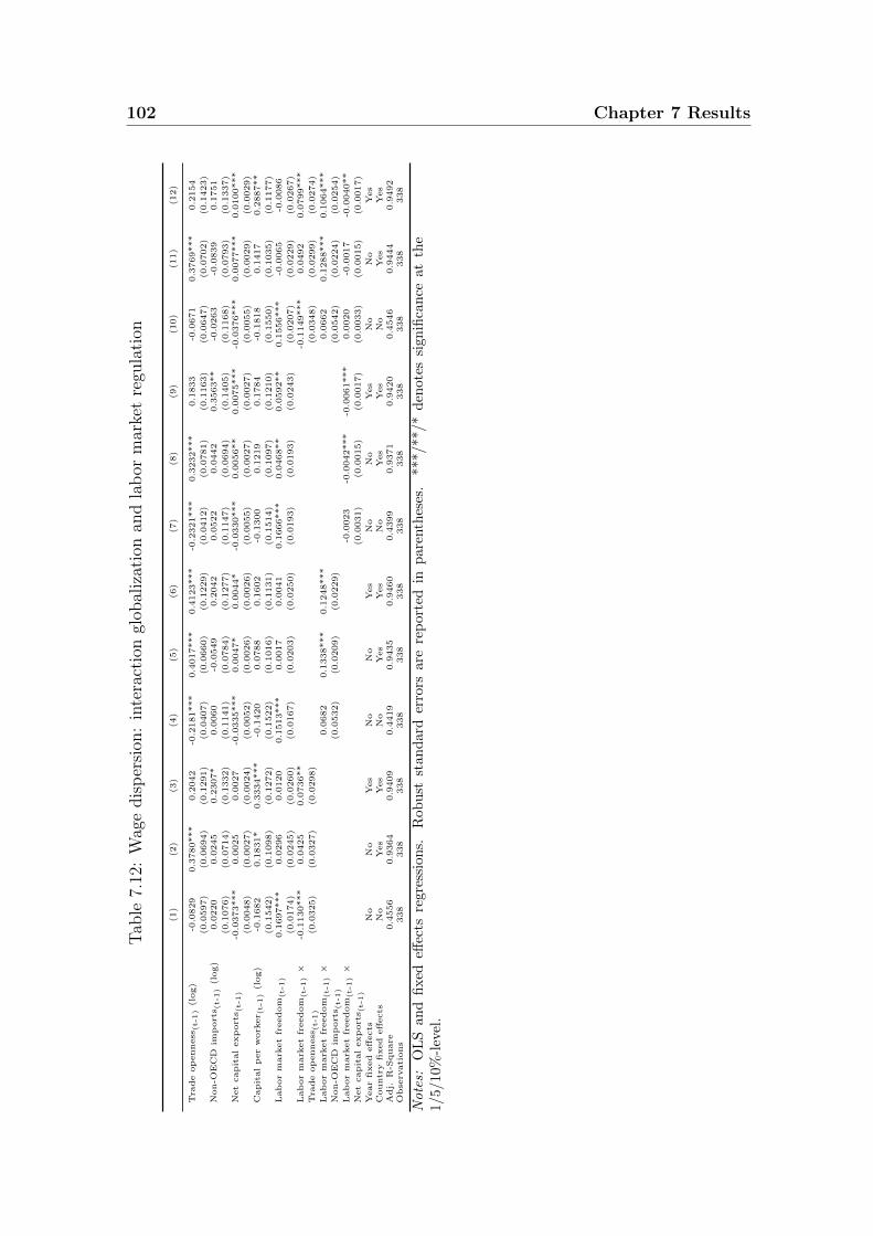
102 Chapter 7 ResultsT
able
7.12
:W
age
dis
per
sion
:in
tera
ctio
ngl
obal
izat
ion
and
lab
orm
arke
tre
gula
tion
(1)
(2)
(3)
(4)
(5)
(6)
(7)
(8)
(9)
(10)
(11)
(12)
Tra
de
op
enness
(t-1
)(l
og)
-0.0
829
0.3
780***
0.2
042
-0.2
181***
0.4
017***
0.4
123***
-0.2
321***
0.3
232***
0.1
833
-0.0
671
0.3
769***
0.2
154
(0.0
597)
(0.0
694)
(0.1
291)
(0.0
407)
(0.0
660)
(0.1
229)
(0.0
412)
(0.0
781)
(0.1
163)
(0.0
647)
(0.0
702)
(0.1
423)
Non-O
EC
Dim
port
s (t-1
)(l
og)
0.0
220
0.0
245
0.2
307*
0.0
060
-0.0
549
0.2
042
0.0
522
0.0
442
0.3
563**
-0.0
263
-0.0
839
0.1
751
(0.1
076)
(0.0
714)
(0.1
332)
(0.1
141)
(0.0
784)
(0.1
277)
(0.1
147)
(0.0
694)
(0.1
405)
(0.1
168)
(0.0
793)
(0.1
337)
Net
capit
al
exp
ort
s (t-1
)-0
.0373***
0.0
025
0.0
027
-0.0
335***
0.0
047*
0.0
044*
-0.0
330***
0.0
056**
0.0
075***
-0.0
376***
0.0
077***
0.0
100***
(0.0
048)
(0.0
027)
(0.0
024)
(0.0
052)
(0.0
026)
(0.0
026)
(0.0
055)
(0.0
027)
(0.0
027)
(0.0
055)
(0.0
029)
(0.0
029)
Capit
al
per
work
er (
t-1
)(l
og)
-0.1
682
0.1
831*
0.3
334***
-0.1
420
0.0
788
0.1
602
-0.1
300
0.1
219
0.1
784
-0.1
818
0.1
417
0.2
887**
(0.1
542)
(0.1
098)
(0.1
272)
(0.1
522)
(0.1
016)
(0.1
131)
(0.1
514)
(0.1
097)
(0.1
210)
(0.1
550)
(0.1
035)
(0.1
177)
Lab
or
mark
et
freedom
(t-1
)0.1
697***
0.0
296
0.0
120
0.1
513***
0.0
017
0.0
041
0.1
666***
0.0
468**
0.0
592**
0.1
556***
-0.0
065
-0.0
086
(0.0
174)
(0.0
245)
(0.0
260)
(0.0
167)
(0.0
203)
(0.0
250)
(0.0
193)
(0.0
193)
(0.0
243)
(0.0
207)
(0.0
229)
(0.0
267)
Lab
or
mark
et
freedom
(t-1
)×
-0.1
130***
0.0
425
0.0
736**
-0.1
149***
0.0
492
0.0
799***
Tra
de
op
enness
(t-1
)(0
.0325)
(0.0
327)
(0.0
298)
(0.0
348)
(0.0
299)
(0.0
274)
Lab
or
mark
et
freedom
(t-1
)×
0.0
682
0.1
338***
0.1
248***
0.0
662
0.1
288***
0.1
064***
Non-O
EC
Dim
port
s (t-1
)(0
.0532)
(0.0
209)
(0.0
229)
(0.0
542)
(0.0
224)
(0.0
254)
Lab
or
mark
et
freedom
(t-1
)×
-0.0
023
-0.0
042***
-0.0
061***
0.0
020
-0.0
017
-0.0
040**
Net
capit
al
exp
ort
s (t-1
)(0
.0031)
(0.0
015)
(0.0
017)
(0.0
033)
(0.0
015)
(0.0
017)
Year
fixed
eff
ects
No
No
Yes
No
No
Yes
No
No
Yes
No
No
Yes
Countr
yfi
xed
eff
ects
No
Yes
Yes
No
Yes
Yes
No
Yes
Yes
No
Yes
Yes
Adj.
R-S
quare
0.4
556
0.9
364
0.9
409
0.4
419
0.9
435
0.9
460
0.4
399
0.9
371
0.9
420
0.4
546
0.9
444
0.9
492
Obse
rvati
ons
338
338
338
338
338
338
338
338
338
338
338
338
Note
s:O
LS
and
fixed
effec
tsre
gres
sion
s.R
obu
stst
and
ard
erro
rsare
rep
ort
edin
pare
nth
eses
.***/**/*
den
ote
ssi
gn
ifica
nce
at
the
1/5/
10%
-lev
el.
7.1 Globalization and labor market outcomes 103T
able
7.13
:U
nem
plo
ym
ent
rate
:in
tera
ctio
ngl
obal
izat
ion
and
lab
orm
arke
tre
gula
tion
(1)
(2)
(3)
(4)
(5)
(6)
(7)
(8)
(9)
(10)
(11)
(12)
Tra
de
op
enness
(t-1
)(l
og)
-0.9
615**
1.1
144*
-0.1
556
-0.1
151
0.9
939*
-0.3
874
0.2
445
0.7
916
-0.2
484
-0.8
999**
0.5
650
-0.7
040
(0.4
035)
(0.5
751)
(1.1
432)
(0.2
618)
(0.5
869)
(1.1
685)
(0.2
520)
(0.6
092)
(1.1
213)
(0.4
090)
(0.6
451)
(1.1
987)
Non-O
EC
Dim
port
s (t-1
)(l
og)
1.8
644***
-0.2
424
-3.4
619***
2.5
836***
-0.2
074
-3.4
082***
2.1
318***
-0.2
491
-3.3
895***
2.6
661***
-0.2
063
-3.3
329***
(0.3
603)
(0.5
565)
(0.6
454)
(0.3
136)
(0.5
473)
(0.6
195)
(0.3
943)
(0.5
622)
(0.6
417)
(0.3
399)
(0.5
532)
(0.6
158)
Net
capit
al
exp
ort
s (t-1
)-0
.0955***
-0.0
629***
-0.0
432***
-0.1
484***
-0.0
723***
-0.0
522***
-0.1
532***
-0.0
442**
-0.0
332*
-0.1
543***
-0.0
506**
-0.0
385**
(0.0
286)
(0.0
182)
(0.0
150)
(0.0
308)
(0.0
188)
(0.0
161)
(0.0
321)
(0.0
196)
(0.0
181)
(0.0
341)
(0.0
200)
(0.0
187)
Outp
ut
gap(t-1
)-0
.3433***
-0.4
186***
-0.4
530***
-0.3
414***
-0.4
141***
-0.4
424***
-0.3
498***
-0.4
137***
-0.4
475***
-0.3
536***
-0.4
076***
-0.4
350***
(0.0
693)
(0.0
509)
(0.0
520)
(0.0
681)
(0.0
499)
(0.0
509)
(0.0
703)
(0.0
506)
(0.0
522)
(0.0
671)
(0.0
507)
(0.0
520)
Lab
or
pro
ducti
vit
y(t-1
)0.0
803
0.0
193
0.1
320***
0.1
058
0.0
198
0.1
358***
0.0
556
0.0
294
0.1
372***
0.0
882
0.0
320
0.1
420***
(0.0
663)
(0.0
432)
(0.0
469)
(0.0
689)
(0.0
425)
(0.0
467)
(0.0
647)
(0.0
439)
(0.0
475)
(0.0
666)
(0.0
432)
(0.0
476)
Capit
al
per
work
er (
t-1
)(l
og)
-3.6
175***
-3.0
636***
-2.2
380*
-2.9
543***
-2.9
450***
-2.2
409*
-3.6
972***
-3.0
595***
-2.2
774**
-2.7
093***
-2.9
054***
-2.2
603**
(0.8
209)
(1.1
508)
(1.1
776)
(0.8
152)
(1.1
018)
(1.1
687)
(0.8
250)
(1.1
025)
(1.1
548)
(0.8
025)
(1.0
980)
(1.1
450)
Lab
or
mark
et
freedom
(t-1
)-0
.6346***
-0.5
802***
-1.0
857***
-0.2
583***
-0.4
409**
-0.9
402***
-0.5
920***
-0.5
532***
-1.0
346***
-0.3
884***
-0.3
923**
-0.9
018***
(0.0
900)
(0.1
923)
(0.2
080)
(0.0
784)
(0.1
725)
(0.1
858)
(0.0
976)
(0.1
688)
(0.1
971)
(0.0
825)
(0.1
945)
(0.2
103)
Lab
or
mark
et
freedom
(t-1
)×
0.9
329***
-0.0
127
0.0
320
0.6
485***
0.0
408
0.0
636
Tra
de
op
enness
(t-1
)(0
.2078)
(0.1
753)
(0.1
563)
(0.2
306)
(0.1
801)
(0.1
602)
Lab
or
mark
et
freedom
(t-1
)×
-1.6
542***
-0.3
919**
-0.3
347**
-1.4
470***
-0.4
649***
-0.3
879***
Non-O
EC
Dim
port
s (t-1
)(0
.2074)
(0.1
601)
(0.1
315)
(0.2
145)
(0.1
753)
(0.1
396)
Lab
or
mark
et
freedom
(t-1
)×
0.0
689***
-0.0
236**
-0.0
126
0.0
244
-0.0
294***
-0.0
181*
Net
capit
al
exp
ort
s (t-1
)(0
.0157)
(0.0
100)
(0.0
093)
(0.0
188)
(0.0
111)
(0.0
101)
Year
fixed
eff
ects
No
No
Yes
No
No
Yes
No
No
Yes
No
No
Yes
Countr
yfi
xed
eff
ects
No
Yes
Yes
No
Yes
Yes
No
Yes
Yes
No
Yes
Yes
Adj.
R-S
quare
0.3
724
0.7
797
0.8
162
0.4
282
0.7
828
0.8
184
0.3
644
0.7
819
0.8
168
0.4
461
0.7
850
0.8
187
Obse
rvati
ons
417
417
417
417
417
417
417
417
417
417
417
417
Note
s:O
LS
and
fixed
effec
tsre
gres
sion
s.R
obu
stst
and
ard
erro
rsare
rep
ort
edin
pare
nth
eses
.***/**/*
den
ote
ssi
gn
ifica
nce
at
the
1/5/
10%
-lev
el.
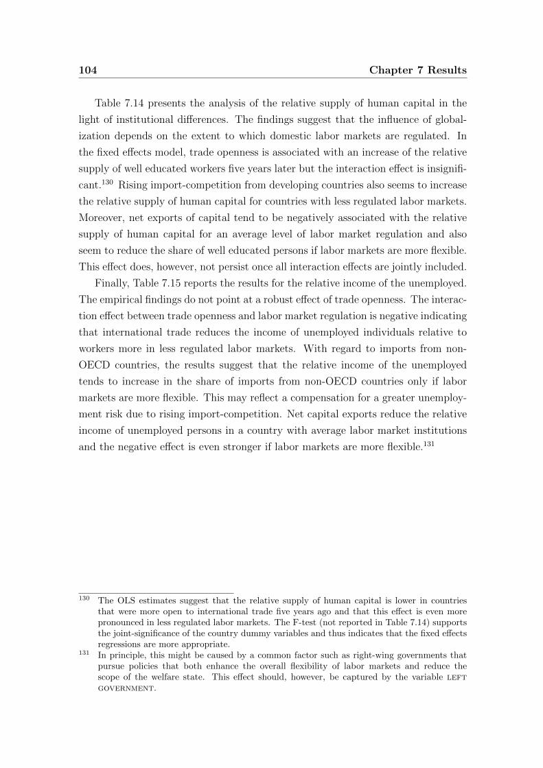
104 Chapter 7 Results
Table 7.14 presents the analysis of the relative supply of human capital in the
light of institutional differences. The findings suggest that the influence of global-
ization depends on the extent to which domestic labor markets are regulated. In
the fixed effects model, trade openness is associated with an increase of the relative
supply of well educated workers five years later but the interaction effect is insignifi-
cant.130 Rising import-competition from developing countries also seems to increase
the relative supply of human capital for countries with less regulated labor markets.
Moreover, net exports of capital tend to be negatively associated with the relative
supply of human capital for an average level of labor market regulation and also
seem to reduce the share of well educated persons if labor markets are more flexible.
This effect does, however, not persist once all interaction effects are jointly included.
Finally, Table 7.15 reports the results for the relative income of the unemployed.
The empirical findings do not point at a robust effect of trade openness. The interac-
tion effect between trade openness and labor market regulation is negative indicating
that international trade reduces the income of unemployed individuals relative to
workers more in less regulated labor markets. With regard to imports from non-
OECD countries, the results suggest that the relative income of the unemployed
tends to increase in the share of imports from non-OECD countries only if labor
markets are more flexible. This may reflect a compensation for a greater unemploy-
ment risk due to rising import-competition. Net capital exports reduce the relative
income of unemployed persons in a country with average labor market institutions
and the negative effect is even stronger if labor markets are more flexible.131
130 The OLS estimates suggest that the relative supply of human capital is lower in countriesthat were more open to international trade five years ago and that this effect is even morepronounced in less regulated labor markets. The F-test (not reported in Table 7.14) supportsthe joint-significance of the country dummy variables and thus indicates that the fixed effectsregressions are more appropriate.
131 In principle, this might be caused by a common factor such as right-wing governments thatpursue policies that both enhance the overall flexibility of labor markets and reduce thescope of the welfare state. This effect should, however, be captured by the variable leftgovernment.
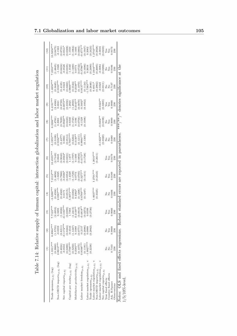
7.1 Globalization and labor market outcomes 105T
able
7.14
:R
elat
ive
supply
ofhum
anca
pit
al:
inte
ract
ion
glob
aliz
atio
nan
dla
bor
mar
ket
regu
lati
on
(1)
(2)
(3)
(4)
(5)
(6)
(7)
(8)
(9)
(10)
(11)
(12)
Tra
de
op
enness
(t-5
)(l
og)
-1.3
311***
6.8
964***
7.7
123***
-3.3
290***
7.2
112***
10.4
555***
-3.1
955***
6.3
206***
6.4
191***
-1.4
858***
7.2
355***
10.5
850***
(0.3
860)
(1.5
755)
(2.4
953)
(0.4
594)
(1.4
656)
(2.7
149)
(0.5
108)
(1.4
781)
(2.4
566)
(0.3
445)
(1.4
845)
(2.8
475)
Non-O
EC
Dim
port
s (t-5
)(l
og)
2.8
613***
-0.0
359
0.3
293
2.0
367***
-1.0
225
0.0
645
2.5
332***
0.3
061
0.6
841
2.3
183***
-1.1
826
-0.1
563
(0.4
024)
(0.8
311)
(1.0
026)
(0.4
569)
(0.7
966)
(0.9
040)
(0.4
377)
(0.7
829)
(0.9
739)
(0.4
185)
(0.8
424)
(0.8
721)
Net
capit
al
exp
ort
s (t-5
)-0
.0555
-0.1
172***
-0.1
183***
0.0
171
-0.0
586*
-0.0
563*
0.0
061
-0.0
920**
-0.0
873**
-0.0
223
-0.0
526
-0.0
541*
(0.0
490)
(0.0
444)
(0.0
399)
(0.0
515)
(0.0
354)
(0.0
331)
(0.0
514)
(0.0
423)
(0.0
356)
(0.0
460)
(0.0
335)
(0.0
308)
Capit
al
per
work
er (
t-5
)(l
og)
5.1
798***
-0.4
544
1.7
383
5.4
071***
-1.4
329
1.1
477
5.7
057***
-0.6
340
1.2
825
4.9
809***
-1.3
540
1.1
550
(0.5
250)
(1.1
247)
(1.2
413)
(0.6
382)
(1.1
729)
(1.1
797)
(0.6
264)
(1.1
725)
(1.2
850)
(0.5
544)
(1.1
490)
(1.1
964)
Mult
ifacto
rpro
ducti
vit
y(t-5
)0.2
585**
0.1
089
0.2
130**
0.2
362*
0.0
773
0.1
409
0.3
130**
0.1
186
0.2
145**
0.2
538**
0.0
771
0.1
405
(0.1
075)
(0.0
771)
(0.0
919)
(0.1
208)
(0.0
705)
(0.0
856)
(0.1
211)
(0.0
756)
(0.0
878)
(0.1
070)
(0.0
722)
(0.0
884)
Lab
or
mark
et
freedom
(t-5
)0.8
188***
-0.2
157
-0.4
818**
0.6
769***
-0.3
277**
-0.4
175**
0.8
884***
-0.1
529
-0.3
402*
0.8
137***
-0.3
786**
-0.4
771**
(0.1
181)
(0.2
086)
(0.2
273)
(0.1
247)
(0.1
411)
(0.1
728)
(0.1
305)
(0.1
598)
(0.1
952)
(0.1
124)
(0.1
696)
(0.1
947)
Lab
or
mark
et
regula
tion(t-5
)×
-1.9
927***
0.0
988
0.0
599
-1.7
383***
0.2
616
0.2
062
Tra
de
op
enness
(t-5
)(0
.2238)
(0.2
842)
(0.2
736)
(0.2
646)
(0.2
490)
(0.2
423)
Lab
or
mark
et
regula
tion(t-5
)×
1.4
637***
1.2
701***
1.2
616***
0.4
911*
1.2
444***
1.2
743***
Non-O
EC
Dim
port
s (t-5
)(0
.3325)
(0.2
543)
(0.2
611)
(0.2
962)
(0.2
685)
(0.2
928)
Lab
or
mark
et
regula
tion(t-5
)×
-0.1
422***
-0.0
402**
-0.0
424**
-0.0
325
-0.0
084
-0.0
016
Net
capit
al
exp
ort
s (t-5
)(0
.0320)
(0.0
198)
(0.0
205)
(0.0
311)
(0.0
206)
(0.0
223)
Year
fixed
eff
ects
No
No
Yes
No
No
Yes
No
No
Yes
No
No
Yes
Countr
yfi
xed
eff
ects
No
Yes
Yes
No
Yes
Yes
No
Yes
Yes
No
Yes
Yes
Adj.
R-S
quare
0.7
103
0.9
068
0.9
066
0.6
406
0.9
189
0.9
179
0.6
480
0.9
090
0.9
090
0.7
137
0.9
186
0.9
173
Obse
rvati
ons
236
236
236
236
236
236
236
236
236
236
236
236
Note
s:O
LS
and
fixed
effec
tsre
gres
sion
s.R
obu
stst
and
ard
erro
rsare
rep
ort
edin
pare
nth
eses
.***/**/*
den
ote
ssi
gn
ifica
nce
at
the
1/5/
10%
-lev
el.
106 Chapter 7 ResultsT
able
7.15
:R
elat
ive
inco
me
unem
plo
yed:
inte
ract
ion
glob
aliz
atio
nan
dla
bor
mar
ket
regu
lati
on
(1)
(2)
(3)
(4)
(5)
(6)
(7)
(8)
(9)
(10)
(11)
(12)
Tra
de
op
enness
(t-1
)(l
og)
0.0
280**
-0.1
818***
0.2
533***
-0.0
028
-0.1
583***
0.2
726***
-0.0
093
-0.1
712***
0.2
364***
0.0
261**
-0.1
963***
0.2
462***
(0.0
128)
(0.0
400)
(0.0
612)
(0.0
115)
(0.0
335)
(0.0
544)
(0.0
113)
(0.0
368)
(0.0
532)
(0.0
130)
(0.0
428)
(0.0
639)
Non-O
EC
Dim
port
s (t-1
)(l
og)
-0.1
932***
0.0
807
0.0
501
-0.2
022***
0.0
669
0.0
426
-0.1
832***
0.0
766
0.0
632
-0.2
093***
0.0
875
0.0
545
(0.0
177)
(0.0
609)
(0.0
451)
(0.0
182)
(0.0
589)
(0.0
413)
(0.0
197)
(0.0
614)
(0.0
434)
(0.0
172)
(0.0
612)
(0.0
433)
Net
capit
al
exp
ort
s (t-1
)-0
.0047***
-0.0
041***
-0.0
075***
-0.0
026*
-0.0
031***
-0.0
067***
-0.0
040***
-0.0
028***
-0.0
068***
-0.0
034**
-0.0
033***
-0.0
066***
(0.0
015)
(0.0
011)
(0.0
015)
(0.0
015)
(0.0
011)
(0.0
013)
(0.0
015)
(0.0
011)
(0.0
014)
(0.0
015)
(0.0
011)
(0.0
014)
Left
govern
ment (
t-1
)-0
.0003
0.0
001
0.0
001
-0.0
004**
0.0
001
0.0
000
-0.0
004**
0.0
001
0.0
000
-0.0
003**
0.0
001
0.0
000
(0.0
002)
(0.0
001)
(0.0
001)
(0.0
002)
(0.0
002)
(0.0
001)
(0.0
002)
(0.0
002)
(0.0
001)
(0.0
002)
(0.0
002)
(0.0
001)
Vote
rtu
rnout (
t-1
)-0
.0024***
0.0
021**
0.0
009
-0.0
022***
0.0
026**
0.0
012
-0.0
029***
0.0
024**
0.0
009
-0.0
019***
0.0
021**
0.0
011
(0.0
006)
(0.0
010)
(0.0
011)
(0.0
006)
(0.0
010)
(0.0
010)
(0.0
006)
(0.0
010)
(0.0
010)
(0.0
006)
(0.0
010)
(0.0
010)
Lab
or
mark
et
freedom
(t-1
)-0
.0189***
-0.0
044
0.0
205*
-0.0
227***
-0.0
134
0.0
126
-0.0
175***
-0.0
109
0.0
197*
-0.0
226***
-0.0
068
0.0
146
(0.0
052)
(0.0
102)
(0.0
123)
(0.0
054)
(0.0
114)
(0.0
117)
(0.0
054)
(0.0
104)
(0.0
115)
(0.0
053)
(0.0
111)
(0.0
122)
Lab
or
mark
et
freedom
(t-1
)×
-0.0
428***
-0.0
283**
-0.0
015
-0.0
348***
-0.0
308**
-0.0
054
Tra
de
op
enness
(t-1
)(0
.0066)
(0.0
143)
(0.0
126)
(0.0
072)
(0.0
153)
(0.0
126)
Lab
or
mark
et
freedom
(t-1
)×
0.0
585***
0.0
115
0.0
293***
0.0
488***
0.0
110
0.0
249**
Non-O
EC
Dim
port
s (t-1
)(0
.0084)
(0.0
105)
(0.0
095)
(0.0
096)
(0.0
112)
(0.0
103)
Lab
or
mark
et
regula
tion(t-1
)×
-0.0
019***
-0.0
013**
-0.0
015***
0.0
009
-0.0
012**
-0.0
009*
Net
capit
al
exp
ort
s (t-1
)(0
.0007)
(0.0
006)
(0.0
005)
(0.0
007)
(0.0
005)
(0.0
005)
Year
fixed
eff
ects
No
No
Yes
No
No
Yes
No
No
Yes
No
No
Yes
Countr
yfi
xed
eff
ects
No
Yes
Yes
No
Yes
Yes
No
Yes
Yes
No
Yes
Yes
Adj.
R-S
quare
0.2
999
0.6
254
0.7
347
0.2
926
0.6
178
0.7
437
0.2
388
0.6
206
0.7
401
0.3
313
0.6
283
0.7
435
Obse
rvati
ons
303
303
303
303
303
303
303
303
303
303
303
303
Note
s:O
LS
and
fixed
effec
tsre
gres
sion
s.R
obu
stst
and
ard
erro
rsare
rep
ort
edin
pare
nth
eses
.***/**/*
den
ote
ssi
gn
ifica
nce
at
the
1/5/
10%
-lev
el.
7.1 Globalization and labor market outcomes 107
7.1.3 Robustness checks
To check the robustness of my results, I run a battery of regressions using different
specifications, samples and estimators. In addition, I address several alternative ex-
planations for the observable changes in the transmission mechanisms. In particular,
I employ different measures of capital mobility, test the relevance of technological
change as a competing explanation for changes in labor market outcomes, focus on
the role of specific labor market institutions and provide a more detailed analysis
of the determinants of the relative supply of human capital. Moreover, I conduct
seemingly unrelated regressions to take a potential simultaneity bias into account
and vary the length of the time lags. Finally, the sensitivity of the results toward
the exclusion of certain countries and periods is tested. The additional variables
included in the regressions of this section are described in Table A.1.
Alternative measurement of capital mobility
The following analysis tests the robustness of the findings by using different measures
for the degree of financial openness. Instead of employing net exports of capital
(i.e. the difference between outflows and inflows of private capital as a percentage of
GDP) as an indicator of international capital mobility, I use gross capital movements
(i.e. the sum of in- and outflows of private capital as a percent of GDP) in Table
7.16 and net exports of FDI (in percent of GDP) in Table 7.17.
Gross capital movements indicate to what extent a country is open to interna-
tional capital flows irrespectively of their direction. The overall amount of capital
flows may also be a better proxy for the degree of capital mobility and thus the ease
at which capital can leave a country.132 Table 7.16 indicates that the effect of gross
capital movements on the transmission variables are partly different from that of
net exports of capital. The labor income share is significantly negatively related to
both gross capital movements and net exports of capital. Wage dispersion and the
unemployment rate are not significantly associated with gross capital movements.133
Both the relative supply of human capital and the relative income of unemployed
persons tend to decrease with increasing capital flows. The negative effect of gross
capital movements is, however, only significant if year fixed effects are not included.
Both transmission variables are also negatively related with net exports of private
132 Note that for the threat effect of capital exit no actual movements are necessary. To constrainthe bargaining power of labor, the mere possibility of a capital outflow would be sufficient.
133 In contrast to this, net exports of capital tend to have a significantly negative effect on theunemployment rate.
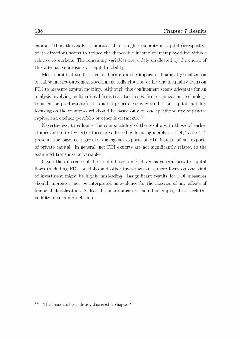
108 Chapter 7 Results
capital. Thus, the analysis indicates that a higher mobility of capital (irrespective
of its direction) seems to reduce the disposable income of unemployed individuals
relative to workers. The remaining variables are widely unaffected by the choice of
this alternative measure of capital mobility.
Most empirical studies that elaborate on the impact of financial globalization
on labor market outcomes, government redistribution or income inequality focus on
FDI to measure capital mobility. Although this confinement seems adequate for an
analysis involving multinational firms (e.g. tax issues, firm organization, technology
transfers or productivity), it is not a priori clear why studies on capital mobility
focusing on the country-level should be based only on one specific source of private
capital and exclude portfolio or other investments.134
Nevertheless, to enhance the comparability of the results with those of earlier
studies and to test whether these are affected by focusing merely on FDI, Table 7.17
presents the baseline regressions using net exports of FDI instead of net exports
of private capital. In general, net FDI exports are not significantly related to the
examined transmission variables.
Given the difference of the results based on FDI versus general private capital
flows (including FDI, portfolio and other investments), a mere focus on one kind
of investment might be highly misleading. Insignificant results for FDI measures
should, moreover, not be interpreted as evidence for the absence of any effects of
financial globalization. At least broader indicators should be employed to check the
validity of such a conclusion.
134 This issue has been already discussed in chapter 5.
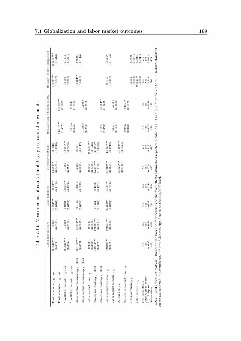
7.1 Globalization and labor market outcomes 109T
able
7.16
:M
easu
rem
ent
ofca
pit
alm
obilit
y:
gros
sca
pit
alm
ovem
ents
Lab
or
incom
esh
are
Wage
dis
pers
ion
Unem
plo
ym
ent
rate
Rela
tive
supply
hum
an
capit
al
Rela
tive
incom
eunem
plo
yed
Tra
de
op
enness
(t-1
)(l
og)
-0.0
510***
-0.0
162
0.4
033***
0.2
884**
1.5
551**
0.3
010
-0.0
896***
0.2
206***
(0.0
090)
(0.0
151)
(0.0
767)
(0.1
198)
(0.6
422)
(1.1
273)
(0.0
287)
(0.0
616)
Tra
de
op
enness
(t-5
)(l
og)
6.8
048***
7.5
099***
(1.5
878)
(2.6
685)
Non-O
EC
Dim
port
s (t-1
)(l
og)
-0.0
345***
-0.0
133
0.0
531
0.2
983**
-0.4
500
-3.6
111***
0.0
662
0.0
404
(0.0
084)
(0.0
100)
(0.0
722)
(0.1
360)
(0.5
553)
(0.6
505)
(0.0
568)
(0.0
441)
Non-O
EC
Dim
port
s (t-5
)(l
og)
-0.1
135
0.3
044
(0.8
256)
(1.0
900)
Gro
sscapit
al
movem
ents
(t-1
)(l
og)
-0.0
139***
-0.0
094***
-0.0
145
-0.0
110
-0.2
208
0.0
301
-0.0
294**
-0.0
099
(0.0
027)
(0.0
027)
(0.0
222)
(0.0
279)
(0.1
919)
(0.2
117)
(0.0
126)
(0.0
115)
Gro
sscapit
al
movem
ents
(t-5
)(l
og)
-0.4
506*
-0.2
767
(0.2
380)
(0.2
911)
Lab
or
pro
ducti
vit
y(t-1
)0.0
006
0.0
011
0.0
059
0.1
295***
(0.0
006)
(0.0
007)
(0.0
437)
(0.0
470)
Capit
al
per
work
er (
t-1
)(l
og)
0.0
341***
0.0
303***
0.1
261
0.1
998
-3.2
341***
-2.3
264**
(0.0
073)
(0.0
074)
(0.1
104)
(0.1
251)
(1.1
166)
(1.1
422)
Capit
al
per
work
er (
t-5
)(l
og)
1.1
570
3.1
554**
(1.0
506)
(1.3
281)
Lab
or
mark
et
freedom
(t-1
)0.0
101***
0.0
153***
0.0
390**
0.0
397*
-0.5
319***
-1.0
328***
-0.0
101
0.0
229*
(0.0
020)
(0.0
026)
(0.0
194)
(0.0
236)
(0.1
668)
(0.1
912)
(0.0
107)
(0.0
124)
Lab
or
mark
et
freedom
(t-5
)-0
.1531
-0.3
161
(0.1
743)
(0.2
157)
Outp
ut
gap(t-1
)-0
.3875***
-0.4
383***
(0.0
498)
(0.0
524)
Mult
ifacto
rpro
ducti
vit
y(t-5
)0.0
887
0.1
624*
(0.0
736)
(0.0
877)
Left
govern
ment (
t-1
)0.0
001
0.0
000
(0.0
002)
(0.0
001)
Vote
rtu
rnout (
t-1
)0.0
027**
0.0
015
(0.0
011)
(0.0
011)
Year
fixed
eff
ects
No
Yes
No
Yes
No
Yes
No
Yes
No
Yes
Countr
yfi
xed
eff
ects
Yes
Yes
Yes
Yes
Yes
Yes
Yes
Yes
Yes
Yes
Adj.
R-S
quare
0.8
889
0.8
978
0.9
358
0.9
388
0.7
746
0.8
137
0.9
040
0.9
028
0.6
214
0.7
073
Obse
rvati
ons
485
485
338
338
417
417
236
236
303
303
Notes:
Fix
edeff
ects
esti
mati
on
s.B
ase
don
the
base
lin
esp
ecifi
cati
on
sof
the
fixed
effec
tses
tim
ati
on
sre
port
edin
colu
mn
s(1
1)
an
d(1
2)
of
Tab
le7.2
to7.1
0.
Rob
ust
stan
dard
erro
rsare
rep
ort
edin
pare
nth
eses
.***/**/*
den
ote
ssi
gn
ifica
nce
at
the
1/5/10%
-lev
el.
110 Chapter 7 ResultsT
able
7.17
:M
easu
rem
ent
ofca
pit
alm
obilit
y:
net
exp
orts
ofF
DI
capit
al
Lab
or
incom
esh
are
Wage
dis
pers
ion
Unem
plo
ym
ent
rate
Rela
tive
supply
hum
an
capit
al
Rela
tive
incom
eunem
plo
yed
Tra
de
op
enness
(t-1
)(l
og)
-0.0
773***
-0.0
151
0.3
744***
0.2
888**
1.1
861**
0.3
015
-0.1
559***
0.2
115***
(0.0
079)
(0.0
153)
(0.0
729)
(0.1
206)
(0.5
892)
(1.1
390)
(0.0
334)
(0.0
580)
Tra
de
op
enness
(t-5
)(l
og)
6.0
449***
6.8
588***
(1.4
006)
(2.4
154)
Non-O
EC
Dim
port
s (t-1
)(l
og)
-0.0
353***
-0.0
070
0.0
568
0.3
121**
-0.5
325
-3.6
475***
0.0
679
0.0
454
(0.0
087)
(0.0
101)
(0.0
723)
(0.1
332)
(0.5
330)
(0.6
451)
(0.0
600)
(0.0
456)
Non-O
EC
Dim
port
s (t-5
)(l
og)
-0.0
750
0.3
098
(0.8
062)
(1.1
044)
Net
FD
Iexp
ort
s (t-1
)0.0
002
0.0
003
0.0
007
0.0
021
0.0
236
-0.0
101
0.0
005
0.0
001
(0.0
004)
(0.0
004)
(0.0
029)
(0.0
033)
(0.0
249)
(0.0
169)
(0.0
008)
(0.0
008)
Net
FD
Iexp
ort
s (t-5
)-0
.0143
-0.0
067
(0.0
198)
(0.0
208)
Lab
or
pro
ducti
vit
y(t-1
)0.0
009
0.0
012*
0.0
106
0.1
291***
(0.0
007)
(0.0
007)
(0.0
442)
(0.0
476)
Capit
al
per
work
er (
t-1
)(l
og)
0.0
293***
0.0
305***
0.1
230
0.2
017
-3.3
649***
-2.3
114**
(0.0
073)
(0.0
074)
(0.1
099)
(0.1
254)
(1.1
259)
(1.1
434)
Capit
al
per
work
er (
t-5
)(l
og)
0.7
295
3.0
382**
(1.0
439)
(1.3
174)
Lab
or
mark
et
freedom
(t-1
)0.0
113***
0.0
154***
0.0
384**
0.0
381
-0.5
123***
-1.0
287***
-0.0
078
0.0
239*
(0.0
021)
(0.0
027)
(0.0
193)
(0.0
231)
(0.1
605)
(0.1
874)
(0.0
106)
(0.0
123)
Lab
or
mark
et
freedom
(t-5
)-0
.1363
-0.3
642*
(0.1
735)
(0.2
031)
Outp
ut
gap(t-1
)-0
.3940***
-0.4
383***
(0.0
509)
(0.0
526)
Mult
ifacto
rpro
ducti
vit
y(t-5
)0.0
772
0.1
608*
(0.0
727)
(0.0
872)
Left
govern
ment (
t-1
)0.0
001
0.0
000
(0.0
002)
(0.0
001)
Vote
rtu
rnout (
t-1
)0.0
027**
0.0
014
(0.0
011)
(0.0
011)
Year
fixed
eff
ects
No
Yes
No
Yes
No
Yes
No
Yes
No
Yes
Countr
yfi
xed
eff
ects
Yes
Yes
Yes
Yes
Yes
Yes
Yes
Yes
Yes
Yes
Adj.
R-S
quare
0.8
817
0.8
955
0.9
357
0.9
389
0.7
744
0.8
138
0.9
026
0.9
024
0.6
109
0.7
063
Obse
rvati
ons
485
485
338
338
417
417
236
236
303
303
Notes:
Fix
edeff
ects
esti
mati
on
s.B
ase
don
the
base
lin
esp
ecifi
cati
on
sof
the
fixed
effec
tses
tim
ati
on
sre
port
edin
colu
mn
s(1
1)
an
d(1
2)
of
Tab
le7.2
to7.1
0.
Rob
ust
stan
dard
erro
rsare
rep
ort
edin
pare
nth
eses
.***/**/*
den
ote
ssi
gn
ifica
nce
at
the
1/5/10%
-lev
el.
7.1 Globalization and labor market outcomes 111
The role of technological change
There is a widespread agreement among economists that shifts in the relative de-
mand for skilled versus unskilled labor are responsible for growing wage inequality
or unemployment in many industrialized countries. No consensus exists, however,
on the underlying forces. In general, two explanations compete: international trade
and skill-biased technological change. Due to reasons discussed in chapter 5, many
economists have focused on the role of technological change. To check the robust-
ness of the baseline results concerning the role of globalization, I control for several
measures of technological change. The results are presented in Table 7.18.135 The
labor income share decreases if the share of information and communication tech-
nology (ICT) investments grows, whereas the wage dispersions is not significantly
and robustly related to any of the proxies of technological change. Only R&D ex-
penditures are significantly negatively associated with the wage differential if year
fixed effects are not included. The unemployment rate is affected by technological
improvements: whereas the growth of investments in ICT in relation to total capital
input is negatively correlated with the unemployment rate (if year fixed effects are
not included), both higher R&D expenditures and employment increase the unem-
ployment rate. Surprisingly, the relative supply of highly educated individuals is
significantly negatively related with ICT investments.
Despite the inclusion of proxies for technological change, globalization mostly re-
mains significantly related to the transmission mechanisms. Thus, the view of several
economists that not international trade but predominantly technological change is
responsible for developments such as rising wage dispersion cannot be confirmed.
135 Technological change is expected to affect the relative labor demand and the consequencesfor labor market outcomes are, hence, comparable to those of globalization. The effect on thewelfare state is, however, less clear since technological change should not affect its financinglike, for instance, international tax competition. Consequently, I do not analyze the relativeincome of the unemployed in this context.

112 Chapter 7 ResultsT
able
7.18
:T
echnol
ogic
alch
ange
vers
us
glob
aliz
atio
n
Lab
or
incom
esh
are
Wage
dis
pers
ion
(1)
(2)
(3)
(4)
(5)
(6)
(1)
(2)
(3)
(4)
(5)
(6)
Tra
de
op
enness
(t-1
)(l
og)
-0.0
764***
-0.0
158
-0.0
722***
-0.0
356*
-0.0
783***
-0.0
276
0.2
301**
0.6
271***
0.0
625
0.0
929
0.2
848***
0.3
383**
(0.0
116)
(0.0
217)
(0.0
116)
(0.0
188)
(0.0
098)
(0.0
170)
(0.1
051)
(0.1
559)
(0.0
812)
(0.1
673)
(0.0
813)
(0.1
510)
Non-O
EC
Dim
port
s (t-1
)(l
og)
-0.0
043
0.0
220
-0.0
193*
-0.0
034
-0.0
171
0.0
086
0.1
401*
0.3
326**
0.2
472***
0.4
625***
0.1
428**
0.2
861**
(0.0
099)
(0.0
134)
(0.0
114)
(0.0
134)
(0.0
104)
(0.0
119)
(0.0
774)
(0.1
369)
(0.0
700)
(0.1
701)
(0.0
644)
(0.1
417)
Net
capit
al
exp
ort
s (t-1
)-0
.0023***
-0.0
024***
-0.0
015***
-0.0
012***
-0.0
016***
-0.0
013***
-0.0
050*
-0.0
071**
0.0
043*
0.0
038
0.0
027
0.0
022
(0.0
004)
(0.0
004)
(0.0
003)
(0.0
003)
(0.0
003)
(0.0
003)
(0.0
029)
(0.0
036)
(0.0
024)
(0.0
027)
(0.0
022)
(0.0
024)
Lab
or
pro
ducti
vit
y(t-1
)0.0
002
0.0
006
0.0
005
0.0
010
0.0
009
0.0
014*
-0.0
006
0.0
023
-0.0
060
-0.0
102
-0.0
036
-0.0
019
(0.0
010)
(0.0
010)
(0.0
007)
(0.0
008)
(0.0
008)
(0.0
008)
(0.0
048)
(0.0
059)
(0.0
045)
(0.0
064)
(0.0
046)
(0.0
060)
Capit
al
per
work
er (
t-1
)(l
og)
0.0
149
0.0
388**
0.0
279***
0.0
349***
0.0
280***
0.0
377***
-0.0
563
-0.0
562
-0.1
200
-0.2
527
-0.0
077
0.0
199
(0.0
157)
(0.0
193)
(0.0
089)
(0.0
091)
(0.0
092)
(0.0
090)
(0.1
345)
(0.1
599)
(0.1
102)
(0.1
585)
(0.1
068)
(0.1
507)
Lab
or
mark
et
freedom
(t-1
)0.0
042*
0.0
106***
0.0
084***
0.0
121***
0.0
080***
0.0
131***
0.0
368**
0.0
508**
0.0
289
0.0
284
0.0
278
0.0
164
(0.0
023)
(0.0
028)
(0.0
024)
(0.0
030)
(0.0
023)
(0.0
031)
(0.0
150)
(0.0
200)
(0.0
208)
(0.0
251)
(0.0
180)
(0.0
221)
ICT
invest
ment (
t-1
)(l
og)
-0.0
077**
-0.0
140**
0.0
025
-0.0
534
(0.0
035)
(0.0
069)
(0.0
390)
(0.0
490)
R&
Dp
ers
onnel (t-1
)(l
og)
-0.0
121
-0.0
051
-0.1
204
-0.0
418
(0.0
109)
(0.0
114)
(0.1
324)
(0.1
443)
R&
Dexp
endit
ure
s (t-1
)(l
og)
-0.0
119
-0.0
096
-0.2
048*
-0.1
991
(0.0
087)
(0.0
090)
(0.1
067)
(0.1
320)
Year
fixed
eff
ects
No
Yes
No
Yes
No
Yes
No
Yes
No
Yes
No
Yes
Countr
yfi
xed
eff
ects
Yes
Yes
Yes
Yes
Yes
Yes
Yes
Yes
Yes
Yes
Yes
Yes
Adj.
R-S
quare
0.9
094
0.9
217
0.8
866
0.8
946
0.8
854
0.8
996
0.9
671
0.9
663
0.9
476
0.9
478
0.9
579
0.9
568
Obse
rvati
ons
297
297
358
358
407
407
229
229
253
253
287
287
Con
tin
ued
on
next
page
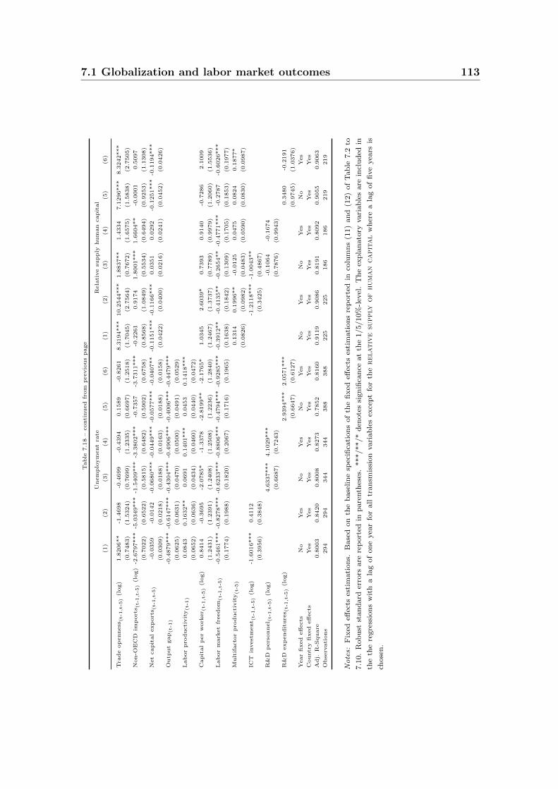
7.1 Globalization and labor market outcomes 113T
able
7.1
8–
conti
nued
from
pre
vio
us
page
Unem
plo
ym
ent
rate
Rela
tive
supply
hum
an
capit
al
(1)
(2)
(3)
(4)
(5)
(6)
(1)
(2)
(3)
(4)
(5)
(6)
Tra
de
op
enness
(t-1
,t-5
)(l
og)
1.8
206**
-1.4
698
-0.4
699
-0.4
394
0.1
589
-0.8
261
8.3
194***
10.2
544***
1.8
837**
1.4
334
7.1
296***
8.3
242***
(0.7
483)
(1.5
324)
(0.7
699)
(1.2
335)
(0.6
697)
(1.2
518)
(1.7
045)
(2.7
564)
(0.7
672)
(1.6
575)
(1.5
838)
(2.7
505)
Non-O
EC
Dim
port
s (t-1
,t-5
)(l
og)
-2.6
797***
-5.0
349***
-1.5
409***
-3.3
802***
-0.7
357
-3.7
311***
-0.2
261
0.9
174
1.8
001***
1.6
604**
-0.0
001
0.5
097
(0.7
022)
(0.6
522)
(0.5
815)
(0.6
482)
(0.5
902)
(0.6
758)
(0.8
568)
(1.0
849)
(0.5
534)
(0.6
494)
(0.9
253)
(1.1
308)
Net
capit
al
exp
ort
s (t-1
,t-5
)-0
.0359
-0.0
142
-0.0
680***
-0.0
449***
-0.0
577***
-0.0
407**
-0.1
151***
-0.1
166***
0.0
351
0.0
292
-0.1
251***
-0.1
194***
(0.0
309)
(0.0
218)
(0.0
188)
(0.0
163)
(0.0
188)
(0.0
158)
(0.0
422)
(0.0
400)
(0.0
216)
(0.0
241)
(0.0
452)
(0.0
426)
Outp
ut
gap(t-1
)-0
.4879***
-0.6
147***
-0.4
304***
-0.4
906***
-0.4
006***
-0.4
479***
(0.0
625)
(0.0
631)
(0.0
470)
(0.0
500)
(0.0
491)
(0.0
529)
Lab
or
pro
ducti
vit
y(t-1
)0.0
843
0.1
632**
0.0
691
0.1
401***
0.0
453
0.1
418***
(0.0
652)
(0.0
636)
(0.0
434)
(0.0
460)
(0.0
440)
(0.0
472)
Capit
al
per
work
er (
t-1
,t-5
)(l
og)
0.8
414
-0.3
695
-2.0
785*
-1.3
378
-2.8
199**
-2.1
765*
1.0
345
2.6
039*
0.7
393
0.9
140
-0.7
286
2.1
009
(1.2
431)
(1.2
391)
(1.2
408)
(1.2
508)
(1.2
236)
(1.2
840)
(1.2
467)
(1.3
737)
(0.7
789)
(0.9
979)
(1.2
060)
(1.5
536)
Lab
or
mark
et
freedom
(t-1
,t-5
)-0
.5461***
-0.8
278***
-0.6
233***
-0.8
806***
-0.4
794***
-0.9
285***
-0.3
912**
-0.4
135**
-0.2
654**
-0.4
771***
-0.2
787
-0.6
026***
(0.1
774)
(0.1
988)
(0.1
820)
(0.2
067)
(0.1
716)
(0.1
965)
(0.1
638)
(0.1
842)
(0.1
309)
(0.1
705)
(0.1
853)
(0.1
977)
Mult
ifacto
rpro
ducti
vit
y(t-5
)0.1
314
0.1
996**
-0.0
125
0.0
475
0.0
824
0.1
877*
(0.0
826)
(0.0
982)
(0.0
483)
(0.0
590)
(0.0
830)
(0.0
987)
ICT
invest
ment (
t-1
,t-5
)(l
og)
-1.6
016***
0.4
112
-1.2
118***
-1.0
043**
(0.3
956)
(0.3
848)
(0.3
425)
(0.4
867)
R&
Dp
ers
onnel (t-1
,t-5
)(l
og)
4.6
337***
4.1
029***
-0.1
064
-0.1
674
(0.6
687)
(0.7
243)
(0.7
876)
(0.9
943)
R&
Dexp
endit
ure
s (t-1
,t-5
)(l
og)
2.9
394***
2.0
571***
0.3
480
-0.2
191
(0.6
647)
(0.6
127)
(0.9
745)
(1.0
376)
Year
fixed
eff
ects
No
Yes
No
Yes
No
Yes
No
Yes
No
Yes
No
Yes
Countr
yfi
xed
eff
ects
Yes
Yes
Yes
Yes
Yes
Yes
Yes
Yes
Yes
Yes
Yes
Yes
Adj.
R-S
quare
0.8
003
0.8
420
0.8
008
0.8
273
0.7
852
0.8
160
0.9
119
0.9
086
0.8
191
0.8
092
0.9
055
0.9
063
Obse
rvati
ons
294
294
344
344
388
388
225
225
186
186
219
219
Notes:
Fix
edeff
ects
esti
mati
on
s.B
ase
don
the
base
lin
esp
ecifi
cati
on
sof
the
fixed
effec
tses
tim
ati
on
sre
port
edin
colu
mn
s(1
1)
an
d(1
2)
of
Tab
le7.2
to
7.1
0.
Rob
ust
stan
dard
erro
rsare
rep
ort
edin
pare
nth
eses
.***/**/*
den
ote
ssi
gn
ifica
nce
at
the
1/5/10%
-lev
el.
Th
eex
pla
nato
ryvari
ab
les
are
incl
ud
edin
the
the
regre
ssio
ns
wit
ha
lag
of
on
eyea
rfo
rall
tran
smis
sion
vari
ab
les
exce
pt
for
the
relativ
esu
pply
of
hum
an
capit
al
wh
ere
ala
gof
five
yea
rsis
chose
n.
114 Chapter 7 Results
Impact of specific labor market institutions
The empirical analysis points at a considerable impact of the overall level of labor
market regulation on labor market outcomes. The EFW index of labor market free-
dom, however, covers a set of different types of labor market institutions. In the
following, I conduct a more disaggregated analysis, which offers information on the
impact of specific labor market institutions and tests the robustness of the globaliza-
tion effects with respect to their inclusion. The following aspects of labor markets,
which have proven relevant in earlier studies are considered: employment protec-
tion legislation, union density and union coverage, coordination of wage bargaining,
gross benefit replacement rates, benefit duration, the ratio between legal minimum
wages and the median wage and the tax wedge.136 A joint inclusion of these vari-
ables could be problematic since the results are likely affected by multicollinearity
in that case. The EFW index as an indicator for the overall design of labor market
institutions (i.e. the degree to which labor markets are regulated) is thus preferable
to the inclusion of a battery of different indicators. Nonetheless, the substitution of
this index by single aspects of labor market policies may enhance the understanding
of the specific institutional features, which are important for the examined labor
market outcomes.137
The empirical analysis of the labor income share is presented in Table A.5.138
Among the different labor market institutions, a higher share of workers covered by
union wages, a higher degree of bargaining coordination and more generous unem-
ployment benefits (i.e. higher gross replacement rates and longer benefit durations)
and a greater tax wedge are associated with a significantly lower labor share. More-
over, higher minimum wages tend to reduce the share of income accruing to labor,
whereas a higher union density tends to be associated with a higher labor income
share. These variables are, however, only partly significant. The globalization in-
dicators remain mostly robust: net capital exports are unaffected by the separate
inclusion of different labor market institutions, whereas trade openness gains signifi-
cance and becomes positive in one case.139 The influence of imports from developing
136 The data is from Nickell (2006).137 For the assessment of the determinants of labor market outcomes and the relative importance
of globalization, the EFW index is a better proxy of the relevant institutional framework. Inparticular, since the labor market institutions are strongly interrelated. One should keep thisin mind, when assessing the results.
138 To facilitate the readability, this and the other Tables discussed in this section are includedin appendix A.2.
139 If the relative minimum wage is included in combination with year fixed effects, trade opennessis positively correlated with the labor income share.
7.1 Globalization and labor market outcomes 115
countries, however, is not robust.
Table A.6 illustrates how specific labor market institutions are associated with
the wage differential in industrialized countries. Union coverage, bargaining coor-
dination, gross replacement rates and benefit duration, minimum wages and the
tax wedge are related to a significantly lower wage dispersion across the different
specifications. Moreover, the level of employment protection also reduces the wage
differential in the analysis including year fixed effects. The impact of the global-
ization indicators indeed seems to depend on the inclusion of certain institutions.
Trade openness and imports from non-OECD countries become less significant in
most cases. Now, net exports of capital have negative coefficients and are significant
most specifications.
The results of the analysis concerning the relevance of certain labor market in-
stitutions for the unemployment rate are presented in Table A.7. Union coverage,
higher gross replacement rates and the tax wedge are significantly positively related
with the unemployment rate (even after controlling for year-specific effects). Union
density and a more coordinated bargaining process also tend to raise the unemploy-
ment rate if year fixed effects are not included. The minimum wage is associated
with higher unemployment if year fixed effects are included. Again, the influence
of the globalization indicators on the unemployment rate seems to depend on the
consideration of the overall degree of labor market regulation. Without this overall
indicator, trade openness loses its significance in several cases, whereas the share of
imports from developing countries gains significance and remains insignificant only
in three cases. The results suggest that especially the influence of trade openness on
the unemployment rate depends on the overall design of labor market institutions.
The strongest change is observed for net exports of capital, which become com-
pletely insignificant and, hence, suggest that the impact of capital outflows on the
unemployment rate in industrialized countries depends on the overall institutional
framework.
So far, the focus has been on rather immediate effects of labor market institu-
tions and globalization on equilibrium outcomes. Table A.8 offers further insights
into the relationship between specific features of labor markets and the supply of
well relative to poorly educated persons. The findings indicate that a more generous
compensation of the unemployed (both through longer benefit durations and partly
also higher gross replacement rates) and higher taxes on labor have a significant
negative effect on the relative supply of human capital five years later. A possible
explanation for this finding is that generous unemployment transfers improve the
116 Chapter 7 Results
outside option for poorly educated workers who are at risk of being displaced. Thus,
for these workers the incentive to invest in education in order to improve their em-
ployment perspectives will be reduced. Similarly, a greater tax wedge reduces the
wage income, which is available for consumption compared to the wage costs faced
by employers. Rising taxation of labor lowers the net income gains from educa-
tion and therefore also the individual incentives for further educational attainment.
Among the remaining labor market institutions, bargaining coordination tends to
be positively correlated with the future supply of human capital (though only partly
significant). A higher minimum wage is related to a lower relative supply of edu-
cated individuals as this increases the relative wages of workers with low educational
attainment and therewith reduces the rewards to investments in education. The im-
pact of globalization on the relative supply of human capital is not strongly affected
by the focus on specific aspects of labor market institutions instead of the overall
index.
Finally, the consequences of different labor market policies for the income of
unemployed persons relative to workers are analyzed in Table A.9. The results
indicate that employment protection and unemployment compensation tend to be
substitutes because a higher protection of existing jobs is associated with signifi-
cantly lower relative incomes for unemployed persons. More powerful trade unions
and the coordination of the bargaining process are positively correlated with the
generosity of unemployment compensation. Furthermore, a positive (and without
year fixed effects also marginally significant) correlation exists between the minimum
wage and the relative income of the unemployed. The impact of trade openness and
net exports of private capital is not much affected by the separate inclusion of labor
market institutions, whereas the share of non-OECD imports even becomes more
significant in most specifications.
Channels through which globalization affects the relative supply of human
capital
The theoretical predictions concerning the link between globalization and the rela-
tive supply of human capital rest on the assumption that international trade and
capital mobility reduce either the relative wage or the employment prospects of less
educated workers. Thus, both the dispersion of wages and the unemployment rate
(based on the implicit assumption that unemployment disproportionately affects
less educated workers) should be positively related with the future relative supply
of educated workers. To test this empirically, I have added the decile ratio of the
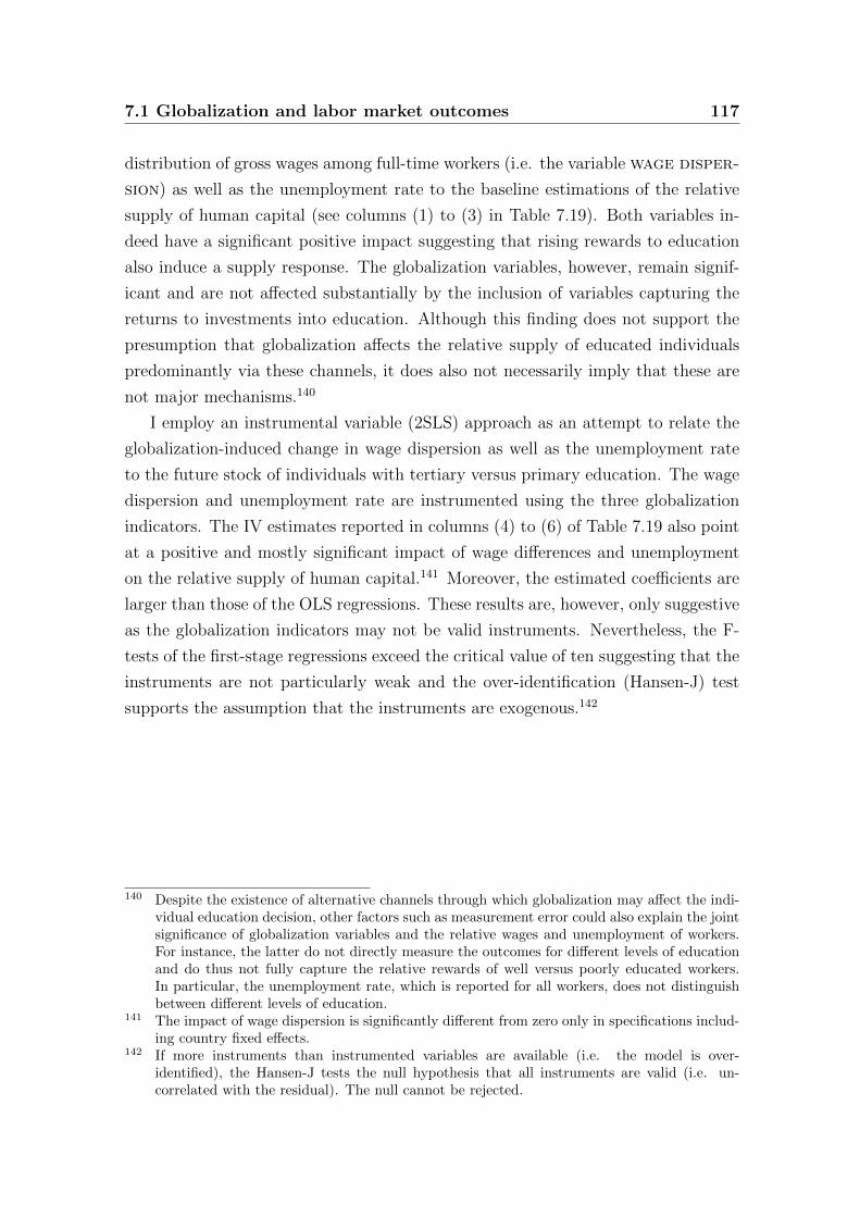
7.1 Globalization and labor market outcomes 117
distribution of gross wages among full-time workers (i.e. the variable wage disper-
sion) as well as the unemployment rate to the baseline estimations of the relative
supply of human capital (see columns (1) to (3) in Table 7.19). Both variables in-
deed have a significant positive impact suggesting that rising rewards to education
also induce a supply response. The globalization variables, however, remain signif-
icant and are not affected substantially by the inclusion of variables capturing the
returns to investments into education. Although this finding does not support the
presumption that globalization affects the relative supply of educated individuals
predominantly via these channels, it does also not necessarily imply that these are
not major mechanisms.140
I employ an instrumental variable (2SLS) approach as an attempt to relate the
globalization-induced change in wage dispersion as well as the unemployment rate
to the future stock of individuals with tertiary versus primary education. The wage
dispersion and unemployment rate are instrumented using the three globalization
indicators. The IV estimates reported in columns (4) to (6) of Table 7.19 also point
at a positive and mostly significant impact of wage differences and unemployment
on the relative supply of human capital.141 Moreover, the estimated coefficients are
larger than those of the OLS regressions. These results are, however, only suggestive
as the globalization indicators may not be valid instruments. Nevertheless, the F-
tests of the first-stage regressions exceed the critical value of ten suggesting that the
instruments are not particularly weak and the over-identification (Hansen-J) test
supports the assumption that the instruments are exogenous.142
140 Despite the existence of alternative channels through which globalization may affect the indi-vidual education decision, other factors such as measurement error could also explain the jointsignificance of globalization variables and the relative wages and unemployment of workers.For instance, the latter do not directly measure the outcomes for different levels of educationand do thus not fully capture the relative rewards of well versus poorly educated workers.In particular, the unemployment rate, which is reported for all workers, does not distinguishbetween different levels of education.
141 The impact of wage dispersion is significantly different from zero only in specifications includ-ing country fixed effects.
142 If more instruments than instrumented variables are available (i.e. the model is over-identified), the Hansen-J tests the null hypothesis that all instruments are valid (i.e. un-correlated with the residual). The null cannot be rejected.
118 Chapter 7 ResultsT
able
7.19
:R
elat
ive
supply
ofhum
anca
pit
al:
role
ofw
age
dis
per
sion
and
unem
plo
ym
ent
OL
SIV
Fir
st-s
tage
IVF
irst
-sta
ge
IVF
irst
-sta
ge
Wage
dis
p.
Un
emp
l.ra
teW
age
dis
p.
Un
emp
l.ra
teW
age
dis
p.
Un
emp
l.ra
te(1
)(2
)(3
)(4
)(5
)(6
)
Tra
de
op
enn
ess (
t-5)
-2.0
707***
7.1
653***
9.9
951***
-0.5
916***
-0.9
630**
0.1
916**
1.1
66
0.4
451**
0.5
397
(log)
(0.6
859)
(1.4
376)
(2.9
832)
(0.1
083)
(0.4
366)
(0.0
928)
(1.0
445)
(0.2
031)
(2.2
121)
Non
-OE
CD
4.0
599***
-0.4
661
1.6
828
-0.1
206
0.0
464
0.2
344***
-4.1
998***
0.3
664**
-6.8
279***
imp
ort
s (t-
5)
(log)
(0.6
420)
(1.0
224)
(1.7
973)
(0.1
583)
(0.6
494)
(0.0
717)
(0.7
519)
(0.1
429)
(1.3
725)
Net
cap
ital
-0.0
172
-0.1
344***
-0.1
391***
0.0
075
0.0
21
-0.0
105***
0.0
131
-0.0
111***
0.0
012
exp
ort
s (t-
5)
(0.0
651)
(0.0
407)
(0.0
394)
(0.0
130)
(0.0
571)
(0.0
030)
(0.0
489)
(0.0
035)
(0.0
445)
Cap
ital
per
5.4
739***
1.7
972
3.9
581**
108.7
372
0.7
217**
-4.8
612***
13.8
168**
0.0
171
-9.5
120***
8.9
600**
-0.0
002
-8.4
580***
work
er(t
-5)
(log)
(1.2
325)
(1.5
296)
(2.0
011)
(211.5
155)
(0.3
268)
(1.3
008)
(6.4
817)
(0.1
030)
(1.6
188)
(3.6
136)
(0.1
328)
(1.9
988)
Mu
ltif
act
or
0.1
507
-0.0
086
0.0
767
-1.7
848
0.0
417
0.1
64
-0.0
694
0.0
047
0.0
093
-0.0
372
0.0
068
0.0
531
pro
du
ctiv
ity
(t-5
)(0
.1672)
(0.0
871)
(0.0
934)
(4.6
921)
(0.0
304)
(0.1
459)
(0.1
883)
(0.0
073)
(0.0
864)
(0.1
504)
(0.0
085)
(0.0
978)
Lab
or
mark
et-0
.0715
-0.3
694**
-0.5
201**
17.4
125
0.1
995***
-0.7
141***
-0.9
308**
0.0
16
0.2
081
-0.5
476
0.0
166
-0.3
633*
free
dom
(t-5
)(0
.1707)
(0.1
836)
(0.2
051)
(37.8
908)
(0.0
181)
(0.1
030)
(0.4
115)
(0.0
161)
(0.1
456)
(0.4
525)
(0.0
201)
(0.2
051)
Wage
3.2
438***
5.9
364***
5.9
003***
-20.6
419
28.4
293***
21.1
289***
dis
per
sion
(t-4
)(0
.4913)
(1.3
217)
(1.2
304)
(61.3
241)
(5.9
943)
(4.5
209)
Un
emp
loym
ent
-0.0
912
0.4
057***
0.4
271***
17.4
549
1.6
668**
1.1
015***
rate
(t-4
)(0
.0995)
(0.0
844)
(0.1
044)
(36.1
642)
(0.6
849)
(0.4
080)
Yea
rfi
xed
effec
tsN
oN
oY
esN
oN
oN
oN
oN
oN
oY
esY
esY
esC
ou
ntr
yfi
xed
effec
tsN
oY
esY
esN
oN
oN
oY
esY
esY
esY
esY
esY
esF
-tes
t33.3
817
117.9
323
79.7
365
0.4
169
53.7
669
27.6
797
34.7
757
725.2
245
53.3
139
42.4
022
298.1
809
72.4
894
Ad
j.R
-Squ
are
0.7
185
0.9
357
0.9
363
-58.4
592
0.5
688
0.4
347
0.6
498
0.9
762
0.8
248
0.8
143
0.9
75
0.8
489
Ob
serv
ati
on
s184
184
184
184
184
184
184
184
184
184
184
184
Han
sen
J0.0
475
00
1.3
373
00
0.6
713
00
p-v
alu
eH
an
sen
J0.8
275
0.2
475
0.4
126
Notes:
OL
San
dIV
(2S
LS
)es
tim
ati
on
sin
clu
din
gth
efi
rst-
stage
regre
ssio
ns.
Th
evari
ab
les
earn
ings
dis
per
sion
an
du
nem
plo
ym
ent
rate
are
inst
rum
ente
du
sin
gtrade
openness
,non-O
EC
Dim
ports
an
dnet
capit
al
exports.
Rob
ust
stan
dard
erro
rsare
rep
ort
edin
pare
nth
eses
.***/**/*
den
ote
ssi
gn
ifica
nce
at
the
1/5/10%
-lev
el.
7.1 Globalization and labor market outcomes 119
Although the evidence is rather suggestive and should therefore be interpreted
with caution, globalization-induced changes in the income opportunities of workers
at different skill levels seem to be associated with an increase in the relative supply of
skills. Whereas a more rigorous analysis of the exact channels through which trade
and capital mobility affect the supply of skills is beyond the scope of this study,
it might be a fruitful field for future empirical work on the distributional effects of
globalization.
Seemingly unrelated regressions
A qualified concern regarding the reliability of the OLS estimates is that the ana-
lyzed transmission mechanisms are not the result of an independent optimization
but reflect equilibrium outcomes that are determined jointly. Relative wages and
unemployment rates, for instance, should not be studied in isolation as both are the
result of interactions between labor demand and supply.
Due to the simultaneous determination of these variables, the residuals of the
equations might be correlated and OLS may thus be not efficiently estimated. To
cope with this issue, I have estimated a system of equations using the seemingly
unrelated regressions (SUR) model proposed by Zellner (1962). Table 7.20 reports
the results for the baseline specification including country and year fixed effects.143
Since this estimation approach requires a balanced panel dataset, the number of
observations is considerably lower for the SUR regressions than in the baseline es-
timates. To enhance the comparability of the results, Table 7.20 also presents OLS
estimations based on the common sample.
The SUR-coefficients differ, at least partly, from the baseline estimates discussed
in section 7.1. This does, however, not necessarily imply that the OLS estimates are
biased but could also result from the different sample sizes. This is indeed what a
comparison of both estimators based on a common sample suggests. The variables
are widely unaffected by the choice of the estimator and the simultaneity bias seems
to be not very severe. The estimates based on the common sample indicate that
greater openness to international trade reduces the labor income share and the
unemployment rate but raises the wage dispersion and the relative income of the
unemployed in OECD countries. Moreover, the relative supply of well educated
individuals is significantly higher five years after an increase in trade openness.
143 Tables A.20 and A.21 in the appendix present the results of the pooled regressions and thoseincluding country fixed effects. The basic conclusions are the same and thus only Table 7.20will be discussed in the text.
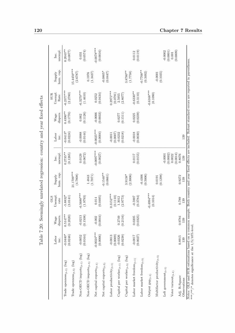
120 Chapter 7 Results
Tab
le7.
20:
See
min
gly
unre
late
dre
gres
sion
:co
untr
yan
dye
arfixed
effec
ts
OL
SS
UR
Lab
or
Wage
Un
emp
l.S
up
ply
Inc.
Lab
or
Wage
Un
emp
l.S
up
ply
Inc.
inc.
dis
per
s.ra
tehu
m.
cap
.u
nem
pl.
inc.
dis
per
s.R
ate
hu
m.
cap
.u
nem
pl.
Tra
de
op
enn
ess (
t-1)
(log)
-0.0
440*
0.5
147**
-5.8
832*
0.2
735**
-0.0
413*
0.4
390**
-6.2
377***
0.2
043**
(0.0
246)
(0.2
020)
(3.0
141)
(0.1
265)
(0.0
224)
(0.1
770)
(2.2
780)
(0.0
877)
Tra
de
op
enn
ess (
t-5)
(log)
21.1
709***
15.4
459***
(4.7
808)
(2.6
787)
Non
-OE
CD
imp
ort
s (t-
1)
(log)
-0.0
052
-0.0
213
-6.5
688***
0.0
129
-0.0
088
0.0
62
-6.3
270***
0.0
31
(0.0
164)
(0.1
508)
(1.9
793)
(0.0
672)
(0.0
144)
(0.1
126)
(1.4
610)
(0.0
574)
Non
-OE
CD
imp
ort
s (t-
5)
(log)
1.4
843
0.1
976
(1.7
071)
(1.3
437)
Net
cap
ital
exp
ort
s (t-
1)
-0.0
024***
-0.0
02
0.0
14
-0.0
097***
-0.0
025***
-0.0
006
0.0
252
-0.0
078***
(0.0
006)
(0.0
044)
(0.0
495)
(0.0
027)
(0.0
004)
(0.0
033)
(0.0
434)
(0.0
016)
Net
cap
ital
exp
ort
s (t-
5)
-0.1
540**
-0.0
805*
(0.0
661)
(0.0
447)
Lab
or
pro
du
ctiv
ity
(t-1
)-0
.0013
0.3
152***
-0.0
011
0.2
975***
(0.0
009)
(0.1
110)
(0.0
007)
(0.0
791)
Cap
ital
per
work
er(t
-1)
(log)
-0.0
326
0.2
749
1.3
012
-0.0
232
0.0
277
2.5
955
(0.0
238)
(0.2
116)
(2.9
773)
(0.0
218)
(0.1
511)
(2.8
077)
Cap
ital
per
work
er(t
-5)
(log)
3.9
138*
3.8
780**
(2.3
006)
(1.7
758)
Lab
or
mark
etfr
eed
om
(t-1
)-0
.0017
0.0
205
-0.5
907
0.0
117
-0.0
018
0.0
225
-0.6
330**
0.0
112
(0.0
027)
(0.0
325)
(0.3
784)
(0.0
155)
(0.0
030)
(0.0
239)
(0.3
110)
(0.0
119)
Lab
or
mark
etfr
eed
om
(t-5
)-0
.4306
-0.7
700**
(0.5
006)
(0.3
492)
Ou
tpu
tgap
(t-1
)-0
.4994***
-0.6
168***
(0.1
014)
(0.1
090)
Mu
ltif
act
or
pro
du
ctiv
ity
(t-5
)0.0
191
-0.0
001
(0.1
298)
(0.1
035)
Lef
tgover
nm
ent (
t-1)
-0.0
001
-0.0
002
(0.0
002)
(0.0
001)
Vote
rtu
rnou
t (t-
1)
0.0
022
0.0
01
(0.0
014)
(0.0
009)
Ad
j.R
-Squ
are
0.8
915
0.9
784
0.7
89
0.9
272
0.8
076
Ob
serv
ati
on
s139
139
139
139
139
139
Notes:
OL
San
dS
UR
esti
mati
on
sb
ase
don
aco
mm
on
sam
ple
.B
oth
cou
ntr
yan
dyea
rfi
xed
effec
tsare
incl
ud
ed.
Rob
ust
stan
dard
erro
rsare
rep
ort
edin
pare
nth
eses
.***/**/*
den
ote
ssi
gn
ifica
nce
at
the
1/5/10%
-lev
el.
7.1 Globalization and labor market outcomes 121
A higher share of imports from developing countries tends to reduce the un-
employment rate, whereas the relative rewards of labor, the relative income of the
unemployed and the relative supply of human capital are lower if net capital exports
increase.
Alternative specifications
A further concern may be related to the speed at which the examined labor market
outcomes respond to changes in exposure to globalization. Tables A.10 to A.19 in
appendix A.2 therefore present the results of further regressions, which experiment
with the length of time lags, measure the variables in first-differences instead of
levels and use five-year averages rather than yearly data. These procedures offer
additional information on the relationship between globalization and labor market
outcomes in the short- versus the medium- to long-run and additionally serve as a
robustness check for the main results.
The analysis of the labor income share is presented in Table A.10. The impact of
trade openness is widely unaffected by variations in the time lags in the specifications
without year fixed effects but loses significance if year fixed effects are included.
The significantly negative relationship between net exports of capital and the labor
income share seems to be limited to the short-run. In particular, this variable loses
its statistical significance if it is included with a lag of five or ten years. Imports
from non-OECD countries seem lower the labor income share in the short- and
medium-run (though only if year fixed effects are not included). The specifications
reported in columns (9) to (12) are based on first-differences in the labor income
and the explanatory variables instead of levels.144 These estimates deliver rather
mixed results: only trade openness has some immediately significant and negative
effect, whereas the share of imports from developing countries is associated with a
falling labor income share with a time lag of one period.
The results concerning the determinants of wage dispersion are shown in Table
A.11. Though the impact of globalization is mostly robust, the findings suggest
that the effects of trade openness and non-OECD imports tend to be stronger in
the short- to medium-run than in the long-run. Moreover, the findings presented in
Table A.11 do not point at a significant relationship between year-to-year differences
in the globalization measures and the wage differential.
144 The use of first differences (i.e. changes in a variable occurring between year t and t-1) alreadyremove time-invariant but country-specific effects. A further inclusion of country fixed effectsis therefore obsolete. Year fixed effects are still included in specification (14) and (16).
122 Chapter 7 Results
Table A.12 presents the estimates for the unemployment rates. Again, the in-
fluence of international trade seems to be of a rather short- or medium-term nature
as the significance of the globalization variables decreases with longer time lags.
The share of imports from developing countries tends to be associated with lower
unemployment rates (in particular if year fixed effects are included). The effect of
trade openness differs between the short- and medium-run. Without a time lag,
trade openness increases the unemployment rate. This short-term effect of rising
exposure to international trade is in line with the theoretical expectations (see hy-
pothesis 3). In the medium-run (i.e. with a lag of five years), greater trade openness
reduces ceteris paribus the unemployment rate. With a lag of ten years, the trade
variables are not significantly correlated with the unemployment rate. Net capital
exports are (if included with a time lag) significantly negatively associated with the
unemployment rate if measured in levels. The regressions based on first-differences
do not indicate that changes in exposure to international trade and capital mo-
bility contribute to the explanation of the evolution of the unemployment rate in
industrialized countries.
The relative supply of human capital is positively related to trade openness and
is negatively related to net exports of capital (see Table A.13), whereby the size of
the effect is stronger in the short- to medium-run than in the long-run. The share of
imports from non-OECD countries only has a significant effect on the relative supply
of human capital in specifications where it is included with a lag of ten years. The
globalization indicators are not significantly related to the supply of well relative to
poorly educated individuals if they are included in first differences.
Finally, Table A.14 shows the results for the regressions of the relative income
of the unemployed. The effect of trade openness does not depend much on the
length of the time lag. Whereas non-OECD imports become partly significant if
five- or ten-year lags are used, net capital exports are statistically significant only in
the short-run. Again, year-to-year differences seem not appropriate for explaining
changes in the relative income of unemployed individuals.
A further concern may be that the results could be driven by cyclical effects.
Hence, the Tables A.15 to A.19 report further robustness tests using five-year av-
erages instead of yearly data to eliminate short-term fluctuations. This comes,
however, at the cost of a substantial loss of observations.
Table A.15 reports the results for the labor income share. Columns (1) to (3) are
devoted to the findings of regressions of the labor income share on globalization and
other explanatory variables based on average values for the same five-year period.
7.1 Globalization and labor market outcomes 123
The significance of the globalization variables tends to be lower in specifications
based on five-year averages, the directions of the effects are, however, not affected.
To account for potential long-term effects of globalization, columns (4) to (6) report
the results of regressions, which explains the average values of the labor income share
over a five-year period with the averages of the globalization variables during the
preceding period. The effect of international trade remains robust but net exports
of capital do not longer contribute to the explanation of the labor income share.
The estimates for the wage dispersion are presented in Table A.16. The global-
ization variables are again less significant than in the baseline analysis using yearly
data. Furthermore, the findings do not point at a different long-term effect of glob-
alization.
The relationship between non-OECD imports and the unemployment rate is
not considerably affected by the use of five-year averages, whereas trade openness
gains significance and net exports of capital are not longer significant. The further
introduction of an one-period time lag reduces the impact of trade openness145 and
the share of non-OECD imports, whereas net exports of capital gain significance
(although with an unexpected sign).
Table A.18 shows the results of the estimates of the relative supply of human
capital. Compared to the baseline estimates, the estimated effects of globalization
(especially of trade openness and capital mobility) are weaker.
Finally, the additional estimates for the relative income of the unemployed are
reported in Table A.19. Despite a decreasing significance, the results do not change
much. The long-term effects of globalization do not differ considerably from those
in the medium-run.
The influence of the globalization indicators varies in some cases with the length
of the time lags suggesting that their short-run effects on labor market outcomes
may differ from those in the medium- to long-run. Nevertheless, the general findings
of section 7.1 remain valid.
Different samples
To test the sensitivity of the results regarding the inclusion of certain observations, I
have subsequently excluded single countries from the sample. Figure 7.1 to 7.5 show
how the exclusion of each country affects the predicted coefficients of the globaliza-
tion variables. This robustness test is based on the baseline specifications including
year-fixed effects since the F-tests usually support their inclusion. In general, the
145 Again, trade openness has a negative impact on the unemployment rate in the long-run.
124 Chapter 7 Results
results do not seem to be very sensitive to the exclusion of observations from single
countries.146 Nonetheless, in several cases excluding a country affects the predicted
coefficients so that the point-estimates are outside the 95% confidence interval of
the baseline regressions (indicated by the grey lines). The exclusion of Spain sig-
nificantly reduces the coefficient of trade openness and non-OECD imports in the
estimations of the labor income share. Moreover, excluding Hungary reduces the
coefficient of net exports of capital for the labor income share. The coefficients
of trade openness in the regressions of wage dispersion and the relative supply of
human capital are significantly smaller if observations from the U.S. are not in-
cluded, whereas the estimated effect of trade openness and imports of developing
countries on the relative income of unemployed persons is lower if the UK or the
U.S. are excluded.147 Moreover, the predicted effect of net capital exports on the
relative income of unemployed persons is higher if observations from the U.S. are
not included.
Most panel studies of the labor market effects of globalization in industrialized
countries are based on data for the 1980s and 1990s. Insofar, this study extends
the period of analyses by including also observations for the 2000s. To test whether
the inclusion of these observations affects the results and thus the comparability of
findings with earlier studies, I exclude observations for the years since 2001 (post-
2000) and 2006 (post-2005). The latter is reasonable because the severe financial
and economic crisis experienced by several countries since 2006 might blur the re-
sults. Indeed, the exclusion of more recent observations significantly increases the
estimated coefficients of international trade on the labor income share and lowers
the coefficients of net capital exports. Without observations for the 2000s, the esti-
mated impact of trade openness on wage dispersion and the relative supply of human
capital is significantly higher, too. For net exports of capital the predicted effect for
the unemployment rate and partly also for the relative income of the unemployed is
significantly higher, whereas the coefficient significantly decreases in the regressions
of wage dispersion.
In sum, this exercise suggests that panel studies on the consequences of global-
ization for a set of labor market outcomes can still provide new insights. Especially,
since the availability of more recent data allows to analyze whether the effects of
globalization have changed since the 1990s.
146 To avoid that the results are driven by a few influential observations, I have also calculatedthe Cook’s D to detect outliers. This measure does, however, not exceed a critical value ofone.
147 Although in these cases, the point estimates do not deviate much from the confidence interval.
7.1 Globalization and labor market outcomes 125
Figure 7.1: Labor income share: exclusion of countries and time periods
-0.09-0.08-0.07-0.06-0.05-0.04-0.03-0.02-0.010.000.010.02
allcountries
AU AT CA CZ DK FI FR DE HU IE IT NL NZ NO PL PT SK ES TU UK US EasternEurope
post-2005 post-2000
Trade openness
-0.03
-0.02
-0.01
0.00
0.01
0.02
0.03
allcountries
AU AT CA CZ DK FI FR DE HU IE IT NL NZ NO PL PT SK ES TU UK US EasternEurope
post-2005 post-2000
Non-OECD imports
-0.004
-0.003
-0.003
-0.002
-0.002
-0.001
-0.001
0.000
allcountries
AU AT CA CZ DK FI FR DE HU IE IT NL NZ NO PL PT SK ES TU UK US EasternEurope
post-2005 post-2000
Net capital exports
Notes: The coefficients of the globalization variables (denoted by the dots) excluding several countriesand years are estimated using specification (12) in Table 7.2. The upper and lower bounds of the 95%confidence interval of the baseline estimates (based on the full sample) is marked by the grey lines.
Figure 7.2: Wage dispersion: exclusion of countries and time periods
-0.40
-0.20
0.00
0.20
0.40
0.60
0.80
1.00
1.20
1.40
all countries AU AT BE CA CZ DK FI FR DE HU IE IT NL NZ NO PL PT SK ES UK US EasternEurope
post-2005 post-2000
Trade openness
0.00
0.10
0.20
0.30
0.40
0.50
0.60
all countries AU AT BE CA CZ DK FI FR DE HU IE IT NL NZ NO PL PT SK ES UK US EasternEurope
post-2005 post-2000
Non-OECD imports
-0.012
-0.010
-0.008
-0.006
-0.004
-0.002
0.000
0.002
0.004
0.006
0.008
all countries AU AT BE CA CZ DK FI FR DE HU IE IT NL NZ NO PL PT SK ES UK US EasternEurope
post-2005 post-2000
Net capital exports
Notes: The coefficients of the globalization variables (denoted by the dots) excluding several countriesand years are estimated using specification (12) in Table 7.4. The upper and lower bounds of the 95%confidence interval of the baseline estimates (based on the full sample) is marked by the grey lines.
126 Chapter 7 Results
Figure 7.3: Unemployment rate: exclusion of countries and time periods
-3.00
-2.50
-2.00
-1.50
-1.00
-0.50
0.00
0.50
1.00
1.50
2.00
2.50
allcountries
AU AT BE CA CZ DK FI FR DE HU IE IT NL NZ NO PL PT SK ES TU UK US EasternEurope
post-2005 post-2000
Trade openness
-5.00
-4.50
-4.00
-3.50
-3.00
-2.50
-2.00
-1.50
-1.00
-0.50
0.00
allcountries
AU AT BE CA CZ DK FI FR DE HU IE IT NL NZ NO PL PT SK ES TU UK US EasternEurope
post-2005 post-2000
Non-OECD imports
-0.08
-0.06
-0.04
-0.02
0.00
0.02
0.04
0.06
0.08
allcountries
AU AT BE CA CZ DK FI FR DE HU IE IT NL NZ NO PL PT SK ES TU UK US EasternEurope
post-2005 post-2000
Net capital exports
Notes: The coefficients of the globalization variables (denoted by the dots) excluding several countriesand years are estimated using specification (12) in Table 7.6. The upper and lower bounds of the 95%confidence interval of the baseline estimates (based on the full sample) is marked by the grey lines.
Figure 7.4: Relative human capital supply: exclusion of countries and time periods
0.00
5.00
10.00
15.00
20.00
25.00
all countries AU AT CA DK FI FR DE IE IT NL NZ PL ES UK US post-2005 post-2000
Trade openness
-2.00
-1.50
-1.00
-0.50
0.00
0.50
1.00
1.50
2.00
2.50
3.00
all countries AU AT CA DK FI FR DE IE IT NL NZ PL ES UK US post-2005 post-2000
Non-OECD imports
-0.25
-0.20
-0.15
-0.10
-0.05
0.00
0.05
0.10
all countries AU AT CA DK FI FR DE IE IT NL NZ PL ES UK US post-2005 post-2000
Net capital exports
Notes: The coefficients of the globalization variables (denoted by the dots) excluding several countriesand years are estimated using specification (12) in Table 7.8. The upper and lower bounds of the 95%confidence interval of the baseline estimates (based on the full sample) is marked by the grey lines.
7.1 Globalization and labor market outcomes 127
Figure 7.5: Relative income unemployed: exclusion of countries and time periods
0.00
0.05
0.10
0.15
0.20
0.25
0.30
0.35
0.40
all countries AU AT CA DK FI FR DE GR IE IT NL ES SE CH UK US post-2005 post-2000
Trade openness
-0.10
-0.05
0.00
0.05
0.10
0.15
all countries AU AT CA DK FI FR DE GR IE IT NL ES SE CH UK US post-2005 post-2000
Non-OECD imports
-0.012
-0.010
-0.008
-0.006
-0.004
-0.002
0.000
all countries AU AT CA DK FI FR DE GR IE IT NL ES SE CH UK US post-2005 post-2000
Net capital exports
Notes: The coefficients of the globalization variables (denoted by the dots) excluding several countriesand years are estimated using specification (12) in Table 7.10. The upper and lower bounds of the 95%confidence interval of the baseline estimates (based on the full sample) is marked by the grey lines.
128 Chapter 7 Results
7.2 Labor market outcomes and the distribution
of incomes
The following section is devoted to the analysis of the relationship between labor
market outcomes and the personal distribution of market and disposable incomes
as well as the redistribution of incomes via taxes and transfers. This empirical
analysis is supposed to answer the question to which extent (globalization-induced)
changes of the transmission variables affect income inequality. For that purpose,
the Gini coefficients of market and disposable income inequality and the extent of
income redistribution (i.e. the difference between the Gini coefficients of market
and disposable income inequality as a percentage of market income inequality) are
regressed on the five transmission variables both with and without the inclusion of
additional control variables.148
To test the robustness of the results and to consider the potential heterogeneity
between countries as well as time-specific effects, each specification is estimated both
using pooled OLS and fixed effects models (both with and without the inclusion of
period fixed effects). The income distribution data is available only infrequently and
thus several years include only observations for one country. Hence, the inclusion
year fixed effects would lead to a further loss of observations. Nevertheless, to
account for time-specific effects, I introduce period fixed effects capturing ten-year
periods from 1960 to 2010.149
Market income inequality
The estimated impact of the five transmission variables on the Gini coefficient of
the market income distribution is reported in Table 7.21. In columns (1) to (3),
the transmission variables are jointly considered as determinants of the level of in-
equality in the distribution of market incomes among working-age households. The
specifications (4) to (6) repeat the baseline estimations without including the rela-
tive income of the unemployed since this should not directly affect the distribution
of market incomes, which do not cover transfer incomes and therefore the main in-
come source for unemployed individuals.150 The GDP per capita and its square are
148 The choice of control variables and their definition is described in section 6.1.1 and 6.2.4.149 The years 2000 to 2010 are divided into two periods to capture a potential impact of the
financial, economic and debt crisis starting in 2007. Consequently, dummy variables areincluded for the following periods: 1960-69, 1970-79, 1980-89, 1990-99, 2000-06 and 2007-10.
150 The generosity of the replacement income might, however, indirectly affect market incomeinequality through work incentives and the duration of unemployment spells or higher reser-
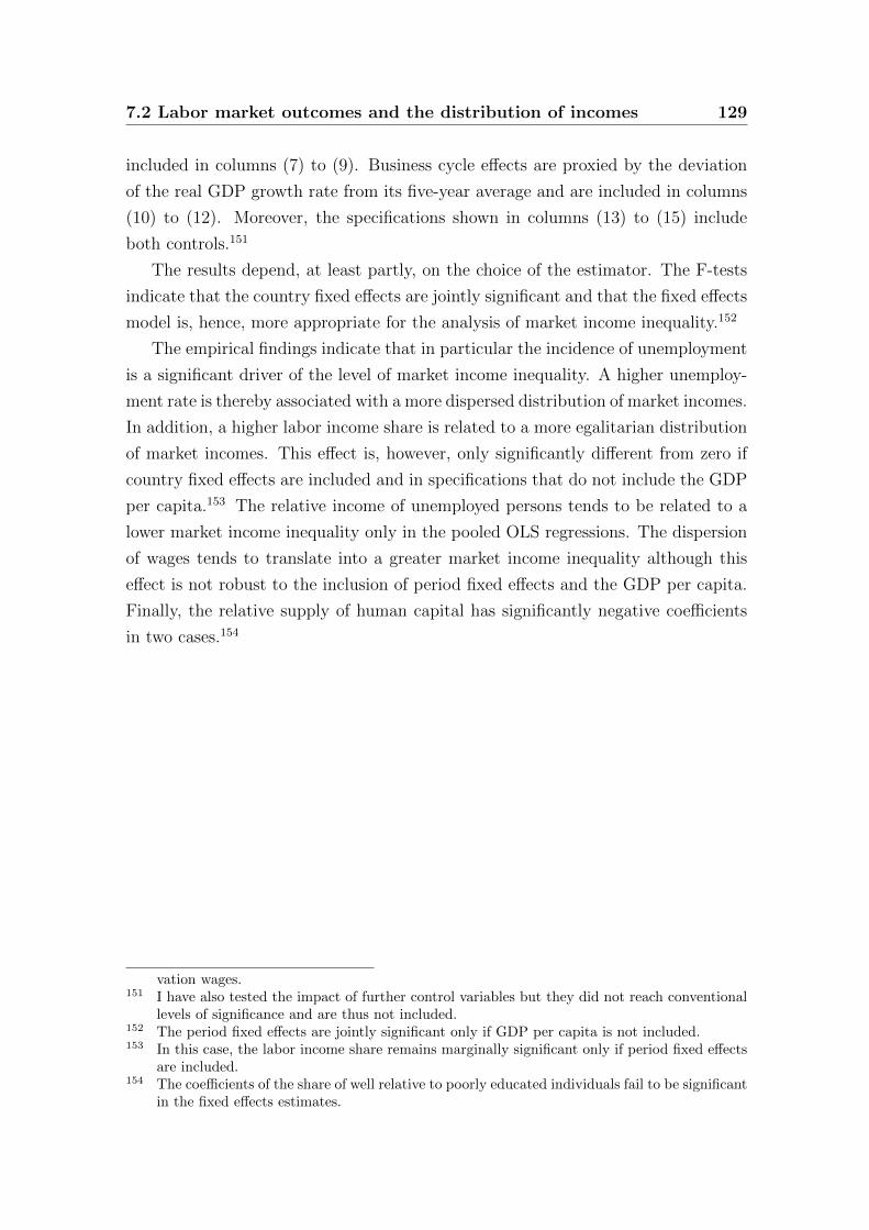
7.2 Labor market outcomes and the distribution of incomes 129
included in columns (7) to (9). Business cycle effects are proxied by the deviation
of the real GDP growth rate from its five-year average and are included in columns
(10) to (12). Moreover, the specifications shown in columns (13) to (15) include
both controls.151
The results depend, at least partly, on the choice of the estimator. The F-tests
indicate that the country fixed effects are jointly significant and that the fixed effects
model is, hence, more appropriate for the analysis of market income inequality.152
The empirical findings indicate that in particular the incidence of unemployment
is a significant driver of the level of market income inequality. A higher unemploy-
ment rate is thereby associated with a more dispersed distribution of market incomes.
In addition, a higher labor income share is related to a more egalitarian distribution
of market incomes. This effect is, however, only significantly different from zero if
country fixed effects are included and in specifications that do not include the GDP
per capita.153 The relative income of unemployed persons tends to be related to a
lower market income inequality only in the pooled OLS regressions. The dispersion
of wages tends to translate into a greater market income inequality although this
effect is not robust to the inclusion of period fixed effects and the GDP per capita.
Finally, the relative supply of human capital has significantly negative coefficients
in two cases.154
vation wages.151 I have also tested the impact of further control variables but they did not reach conventional
levels of significance and are thus not included.152 The period fixed effects are jointly significant only if GDP per capita is not included.153 In this case, the labor income share remains marginally significant only if period fixed effects
are included.154 The coefficients of the share of well relative to poorly educated individuals fail to be significant
in the fixed effects estimates.
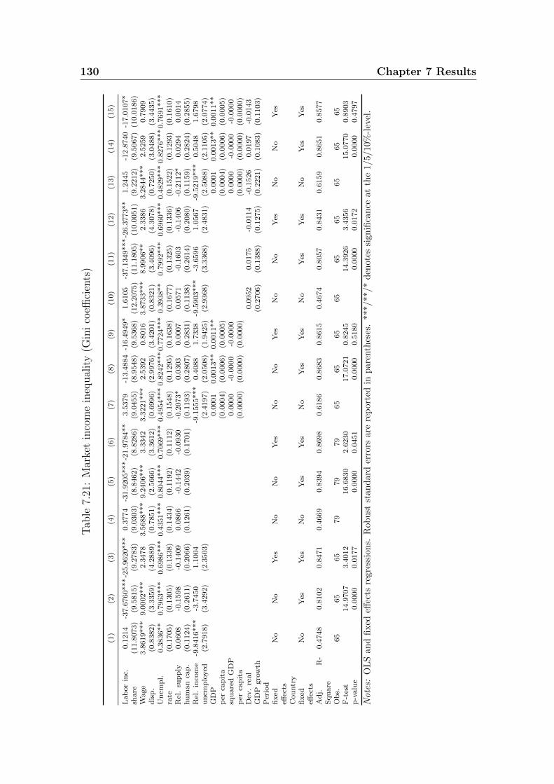
130 Chapter 7 ResultsT
able
7.21
:M
arke
tin
com
ein
equal
ity
(Gin
ico
effici
ents
)
(1)
(2)
(3)
(4)
(5)
(6)
(7)
(8)
(9)
(10)
(11)
(12)
(13)
(14)
(15)
Lab
or
inc.
0.1
214
-37.6
760***
-25.9
620***
0.3
774
-31.9
205***
-21.9
784**
3.5
379
-13.4
884
-16.4
949*
1.6
105
-37.1
349***
-26.3
773**
1.2
445
-12.8
740
-17.0
107*
share
(11.8
073)
(9.5
815)
(9.2
783)
(9.0
303)
(8.8
462)
(8.8
286)
(9.0
455)
(8.9
548)
(9.5
368)
(12.2
075)
(11.1
805)
(10.0
051)
(9.2
212)
(9.5
067)
(10.0
186)
Wage
3.8
619***
9.0
002***
2.3
478
3.5
688***
9.2
406***
3.3
342
3.3
221***
2.5
392
0.8
016
3.8
733***
8.9
906**
2.3
386
3.2
844***
2.5
259
0.7
909
dis
p.
(0.8
382)
(3.3
359)
(4.2
889)
(0.7
851)
(2.5
666)
(3.3
612)
(0.6
996)
(2.9
976)
(3.4
201)
(0.8
321)
(3.4
096)
(4.3
078)
(0.7
250)
(3.0
488)
(3.4
435)
Un
emp
l.0.3
836**
0.7
963***
0.6
986***
0.4
351***
0.8
044***
0.7
069***
0.4
954***
0.8
242***
0.7
724***
0.3
938**
0.7
992***
0.6
960***
0.4
829***
0.8
276***
0.7
691***
rate
(0.1
705)
(0.1
305)
(0.1
338)
(0.1
434)
(0.1
192)
(0.1
112)
(0.1
548)
(0.1
295)
(0.1
638)
(0.1
677)
(0.1
325)
(0.1
336)
(0.1
522)
(0.1
293)
(0.1
610)
Rel
.su
pp
ly0.0
608
-0.1
598
-0.1
409
0.0
866
-0.1
442
-0.0
930
-0.2
073*
0.0
303
0.0
007
0.0
571
-0.1
603
-0.1
406
-0.2
112*
0.0
294
0.0
014
hu
man
cap
.(0
.1124)
(0.2
611)
(0.2
066)
(0.1
261)
(0.2
039)
(0.1
701)
(0.1
193)
(0.2
807)
(0.2
831)
(0.1
138)
(0.2
614)
(0.2
080)
(0.1
159)
(0.2
824)
(0.2
855)
Rel
.in
com
e-9
.8416***
-3.7
450
1.1
004
-9.1
555***
0.4
088
1.7
338
-9.5
903***
-3.6
596
1.0
567
-9.5
219***
0.5
048
1.6
798
un
emp
loyed
(2.7
918)
(3.4
292)
(2.3
503)
(2.4
197)
(2.0
508)
(1.9
425)
(2.9
368)
(3.3
368)
(2.4
831)
(2.5
088)
(2.1
105)
(2.0
774)
GD
P0.0
001
0.0
013**
0.0
011**
0.0
001
0.0
013**
0.0
011**
per
cap
ita
(0.0
004)
(0.0
006)
(0.0
005)
(0.0
004)
(0.0
006)
(0.0
005)
squ
are
dG
DP
0.0
000
-0.0
000
-0.0
000
0.0
000
-0.0
000
-0.0
000
per
cap
ita
(0.0
000)
(0.0
000)
(0.0
000)
(0.0
000)
(0.0
000)
(0.0
000)
Dev
.re
al
0.0
952
0.0
175
-0.0
114
-0.1
526
0.0
197
-0.0
143
GD
Pgro
wth
(0.2
706)
(0.1
388)
(0.1
275)
(0.2
221)
(0.1
083)
(0.1
103)
Per
iod
fixed
No
No
Yes
No
No
Yes
No
No
Yes
No
No
Yes
No
No
Yes
effec
tsC
ou
ntr
yfi
xed
No
Yes
Yes
No
Yes
Yes
No
Yes
Yes
No
Yes
Yes
No
Yes
Yes
effec
tsA
dj.
R-
Squ
are
0.4
748
0.8
102
0.8
471
0.4
669
0.8
394
0.8
698
0.6
186
0.8
683
0.8
615
0.4
674
0.8
057
0.8
431
0.6
159
0.8
651
0.8
577
Ob
s.65
65
65
79
79
79
65
65
65
65
65
65
65
65
65
F-t
est
14.9
707
3.4
012
16.6
830
2.6
230
17.0
721
0.8
245
14.3
926
3.4
356
15.0
770
0.8
903
p-v
alu
e0.0
000
0.0
177
0.0
000
0.0
451
0.0
000
0.5
180
0.0
000
0.0
172
0.0
000
0.4
797
Note
s:O
LS
and
fixed
effec
tsre
gres
sion
s.R
obu
stst
and
ard
erro
rsare
rep
ort
edin
pare
nth
eses
.***/**/*
den
ote
ssi
gn
ifica
nce
at
the
1/5/10%
-lev
el.
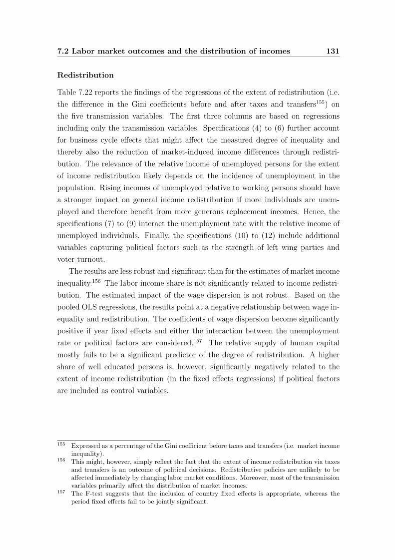
7.2 Labor market outcomes and the distribution of incomes 131
Redistribution
Table 7.22 reports the findings of the regressions of the extent of redistribution (i.e.
the difference in the Gini coefficients before and after taxes and transfers155) on
the five transmission variables. The first three columns are based on regressions
including only the transmission variables. Specifications (4) to (6) further account
for business cycle effects that might affect the measured degree of inequality and
thereby also the reduction of market-induced income differences through redistri-
bution. The relevance of the relative income of unemployed persons for the extent
of income redistribution likely depends on the incidence of unemployment in the
population. Rising incomes of unemployed relative to working persons should have
a stronger impact on general income redistribution if more individuals are unem-
ployed and therefore benefit from more generous replacement incomes. Hence, the
specifications (7) to (9) interact the unemployment rate with the relative income of
unemployed individuals. Finally, the specifications (10) to (12) include additional
variables capturing political factors such as the strength of left wing parties and
voter turnout.
The results are less robust and significant than for the estimates of market income
inequality.156 The labor income share is not significantly related to income redistri-
bution. The estimated impact of the wage dispersion is not robust. Based on the
pooled OLS regressions, the results point at a negative relationship between wage in-
equality and redistribution. The coefficients of wage dispersion become significantly
positive if year fixed effects and either the interaction between the unemployment
rate or political factors are considered.157 The relative supply of human capital
mostly fails to be a significant predictor of the degree of redistribution. A higher
share of well educated persons is, however, significantly negatively related to the
extent of income redistribution (in the fixed effects regressions) if political factors
are included as control variables.
155 Expressed as a percentage of the Gini coefficient before taxes and transfers (i.e. market incomeinequality).
156 This might, however, simply reflect the fact that the extent of income redistribution via taxesand transfers is an outcome of political decisions. Redistributive policies are unlikely to beaffected immediately by changing labor market conditions. Moreover, most of the transmissionvariables primarily affect the distribution of market incomes.
157 The F-test suggests that the inclusion of country fixed effects is appropriate, whereas theperiod fixed effects fail to be jointly significant.
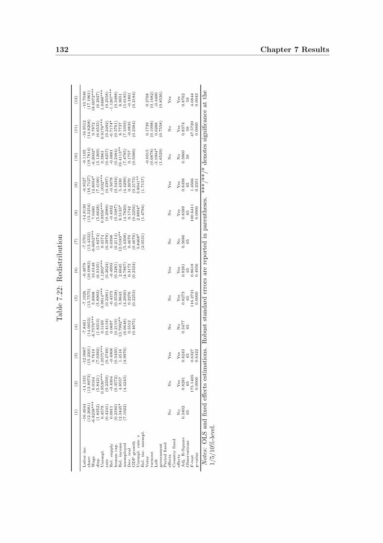
132 Chapter 7 ResultsT
able
7.22
:R
edis
trib
uti
on
(1)
(2)
(3)
(4)
(5)
(6)
(7)
(8)
(9)
(10)
(11)
(12)
Lab
or
inc.
-16.4
644
-14.1
331
-12.0
067
-7.8
461
-7.1
026
-0.4
879
-7.5
701
-14.8
130
-6.9
527
-9.1
105
-16.9
512
-10.7
046
share
(12.2
681)
(13.8
973)
(15.2
301)
(14.0
053)
(13.7
575)
(16.0
983)
(13.4
332)
(13.5
254)
(16.7
127)
(19.7
814)
(14.8
208)
(17.1
961)
Wage
-6.8
238***
6.0
164
9.7
619
-6.7
576***
5.8
908
10.0
148
-6.6
052***
7.0
480
12.8
054*
-6.2
002*
9.7
872
18.0
072***
dis
p.
(1.8
352)
(5.8
421)
(7.0
392)
(1.8
313)
(5.8
903)
(6.9
105)
(1.8
274)
(5.6
628)
(7.4
100)
(3.1
269)
(6.6
535)
(6.2
027)
Unem
pl.
0.4
579
0.9
530***
1.0
575***
0.5
169
0.9
914***
1.1
293***
0.4
574
0.9
356***
1.1
032***
0.3
861
0.9
176***
1.0
488***
rate
(0.4
241)
(0.2
359)
(0.2
749)
(0.4
118)
(0.2
281)
(0.2
624)
(0.3
978)
(0.2
089)
(0.2
397)
(0.4
257)
(0.2
492)
(0.2
558)
Rel.
supply
0.0
911
-0.4
304
-0.4
908
0.0
697
-0.4
375
-0.4
993
0.0
398
-0.4
932
-0.5
678
-0.0
881
-0.7
174*
-1.1
267***
hum
an
cap.
(0.2
160)
(0.3
572)
(0.3
430)
(0.2
119)
(0.3
538)
(0.3
281)
(0.2
114)
(0.3
487)
(0.3
434)
(0.2
484)
(0.3
761)
(0.3
488)
Rel.
incom
e12.3
445*
4.8
557
1.4
516
13.7
992**
5.9
643
2.6
645
12.5
183**
8.5
133*
5.4
330
19.4
113**
8.7
737
8.9
051
unem
plo
yed
(7.1
022)
(4.4
243)
(4.9
976)
(6.6
648)
(4.2
930)
(4.7
867)
(5.4
308)
(4.7
820)
(4.4
299)
(7.4
785)
(7.1
059)
(5.6
185)
Dev.
real
0.5
512
0.2
276
0.3
173
0.4
670
0.1
742
0.3
070
0.1
757
-0.0
835
-0.1
801
GD
Pgro
wth
(0.4
675)
(0.2
253)
(0.2
324)
(0.4
676)
(0.2
256)
(0.2
173)
(0.5
086)
(0.2
384)
(0.2
184)
Unem
pl.
rate×
3.8
468*
2.8
894*
3.8
941**
Rel.
inc.
unem
pl.
(2.0
531)
(1.4
794)
(1.7
157)
Vote
r-0
.0315
0.1
739
0.2
768
turn
out
(0.0
878)
(0.1
098)
(0.1
682)
Left
-3.1
904*
0.0
288
-0.4
400
govern
ment
(1.6
529)
(0.7
558)
(0.8
536)
Peri
od
fixed
eff
ects
No
No
Yes
No
No
Yes
No
No
Yes
No
No
Yes
Countr
yfi
xed
eff
ects
No
Yes
Yes
No
Yes
Yes
No
Yes
Yes
No
Yes
Yes
Adj.
R-S
quare
0.3
402
0.8
281
0.8
243
0.3
477
0.8
273
0.8
261
0.3
686
0.8
389
0.8
498
0.3
860
0.8
374
0.8
762
Obse
rvati
ons
65
65
65
65
65
65
65
65
65
59
59
59
F-t
est
175.1
405
0.6
327
116.2
721
0.8
618
100.6
411
1.4
566
47.5
720
4.6
844
p-v
alu
e0.0
000
0.6
422
0.0
000
0.4
956
0.0
000
0.2
351
0.0
000
0.0
043
Note
s:O
LS
and
fixed
effec
tses
tim
atio
ns.
Rob
ust
stan
dard
erro
rsare
rep
ort
edin
pare
nth
eses
.***/**/*
den
ote
ssi
gn
ifica
nce
at
the
1/5/
10%
-lev
el.
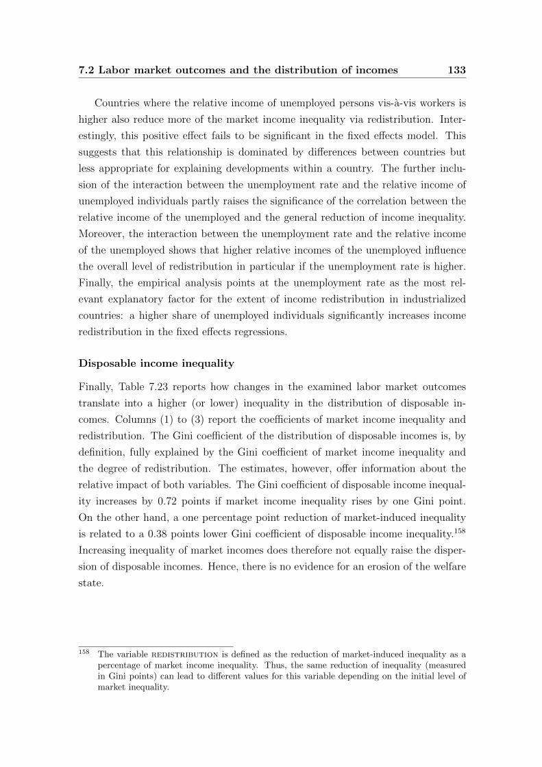
7.2 Labor market outcomes and the distribution of incomes 133
Countries where the relative income of unemployed persons vis-a-vis workers is
higher also reduce more of the market income inequality via redistribution. Inter-
estingly, this positive effect fails to be significant in the fixed effects model. This
suggests that this relationship is dominated by differences between countries but
less appropriate for explaining developments within a country. The further inclu-
sion of the interaction between the unemployment rate and the relative income of
unemployed individuals partly raises the significance of the correlation between the
relative income of the unemployed and the general reduction of income inequality.
Moreover, the interaction between the unemployment rate and the relative income
of the unemployed shows that higher relative incomes of the unemployed influence
the overall level of redistribution in particular if the unemployment rate is higher.
Finally, the empirical analysis points at the unemployment rate as the most rel-
evant explanatory factor for the extent of income redistribution in industrialized
countries: a higher share of unemployed individuals significantly increases income
redistribution in the fixed effects regressions.
Disposable income inequality
Finally, Table 7.23 reports how changes in the examined labor market outcomes
translate into a higher (or lower) inequality in the distribution of disposable in-
comes. Columns (1) to (3) report the coefficients of market income inequality and
redistribution. The Gini coefficient of the distribution of disposable incomes is, by
definition, fully explained by the Gini coefficient of market income inequality and
the degree of redistribution. The estimates, however, offer information about the
relative impact of both variables. The Gini coefficient of disposable income inequal-
ity increases by 0.72 points if market income inequality rises by one Gini point.
On the other hand, a one percentage point reduction of market-induced inequality
is related to a 0.38 points lower Gini coefficient of disposable income inequality.158
Increasing inequality of market incomes does therefore not equally raise the disper-
sion of disposable incomes. Hence, there is no evidence for an erosion of the welfare
state.
158 The variable redistribution is defined as the reduction of market-induced inequality as apercentage of market income inequality. Thus, the same reduction of inequality (measuredin Gini points) can lead to different values for this variable depending on the initial level ofmarket inequality.
134 Chapter 7 Results
Tab
le7.
23:
Dis
pos
able
inco
me
ineq
ual
ity
(Gin
ico
effici
ent)
(1)
(2)
(3)
(4)
(5)
(6)
(7)
(8)
(9)
Mar
ket
inco
me
0.71
99**
*0.
7244
***
0.7
064***
ineq
ual
ity
(0.0
137)
(0.0
131)
(0.0
197)
Red
istr
ibu
tion
-0.3
724*
**-0
.386
6***
-0.3
876***
(0.0
070)
(0.0
135)
(0.0
128)
Lab
orin
com
e17.4
300**
-14.1
557*
-8.6
938
16.9
941**
-13.1
131
-8.1
959
shar
e(7
.7875)
(7.9
194)
(9.4
318)
(7.4
342)
(8.5
569)
(10.0
782)
Wag
e3.4
819***
4.2
565**
1.6
448
3.4
932***
4.2
628**
1.6
674
dis
per
sion
(0.6
480)
(2.0
858)
(1.6
918)
(0.6
566)
(2.0
702)
(1.6
656)
Un
emp
loym
ent
0.2
932**
0.2
200**
0.1
621*
0.2
923**
0.2
235**
0.1
644*
rate
(0.1
315)
(0.0
858)
(0.0
815)
(0.1
325)
(0.0
859)
(0.0
823)
Rel
ativ
esu
pp
ly0.2
168***
0.0
951
0.0
379
0.2
160***
0.0
858
0.0
345
hu
man
capit
al(0
.0797)
(0.1
564)
(0.1
356)
(0.0
803)
(0.1
505)
(0.1
350)
Rel
ativ
ein
com
e-1
2.7
297***
-4.2
507**
0.0
691
-12.8
141***
-3.9
802**
0.1
665
un
emp
loye
d(2
.4562)
(1.9
377)
(1.7
563)
(2.4
742)
(1.7
741)
(1.8
697)
Dev
iati
onre
al-0
.0395
0.0
756
0.0
309
GD
Pgr
owth
(0.2
027)
(0.1
203)
(0.1
148)
Per
iod
fixed
effec
tsN
oN
oY
esN
oN
oY
esN
oN
oY
esC
ountr
yfi
xed
effec
tsN
oY
esY
esN
oY
esY
esN
oY
esY
esA
dj.
R-S
qu
are
0.99
250.
9956
0.9
959
0.4
970
0.8
660
0.8
919
0.4
907
0.8
648
0.8
900
Ob
serv
atio
ns
121
121
121
83
83
83
83
83
83
F-t
est
27.1
932
1.8
026
26.8
743
4.4
041
25.6
785
4.3
388
p-v
alu
e0.
0000
0.1
350
0.0
000
0.0
037
0.0
000
0.0
041
Note
s:O
LS
and
fixed
effec
tses
tim
atio
ns.
Rob
ust
stan
dard
erro
rsare
rep
ort
edin
pare
nth
eses
.***/**/*
den
ote
ssi
gn
ifica
nce
at
the
1/5/
10%
-lev
el.
7.2 Labor market outcomes and the distribution of incomes 135
Columns (4) to (6) of Table 7.23 present the results of the regression of the Gini
coefficient of disposable income inequality on the transmission variables without
further controls, whereas the specifications (7) to (9) also consider a possible bias
of the measured level of inequality due to different positions in the business cycle.
The labor income share is significantly positive in the pooled OLS regressions but
negative if country fixed effects are included. In the latter case, the coefficient is,
however, only significantly different from zero if business cycle effects are not con-
sidered. A more unequal distribution of wages translates into greater inequality of
the income after taxes and transfers (though the effect is not significant once period
fixed effects are taken into account). A higher relative income of the unemployed
has a significant negative impact on the Gini coefficient of disposable incomes (both
in the pooled OLS and country fixed effects regressions). The relative supply of hu-
man capital tends to be positively related with disposable income inequality (though
this effect is only significant in the pooled OLS regressions). As already indicated
by the analysis of market income inequality and the extent of redistribution, the
unemployment rate is a major driver of income inequality: higher unemployment
rates are related to a more unequal distribution of disposable incomes.

Chapter 8
Quantification of the relative
effects of the transmission
mechanisms
After the discussion of the main results and their robustness, the following chap-
ter aims at quantifying the relative impact of the transmission mechanisms on the
income distribution and the extent to which they are affected by globalization.
The main results of chapter 7 are summarized in Figure 8.1. International trade
and net exports of private capital reduce the labor income share. Whereas net
exports of capital remain statistically significant in all specifications, international
trade fails to be significant in some cases. Moreover, the degree of wage dispersion
tends to rise if a country engages in international trade. The effects of globaliza-
tion on the relative factor rewards are in line with the theoretical expectations but
its impact on the unemployment rate is less obvious. Trade openness is not sig-
nificantly related with unemployment and imports from non-OECD countries seem
to reduce the unemployment rate. Surprisingly, also net exports of private capital
are negatively correlated with the unemployment rate (though the effect is not al-
ways significant). The relative supply of human capital rises in response to past
trade openness and declines if the exports of capital increase. Finally, the income
of unemployed persons relative to workers is lower if net exports of capital rise but
increases with a greater exposure to international trade. Hence, a possible “race to
the bottom” in welfare state spending is not supported by the empirical analysis.
137
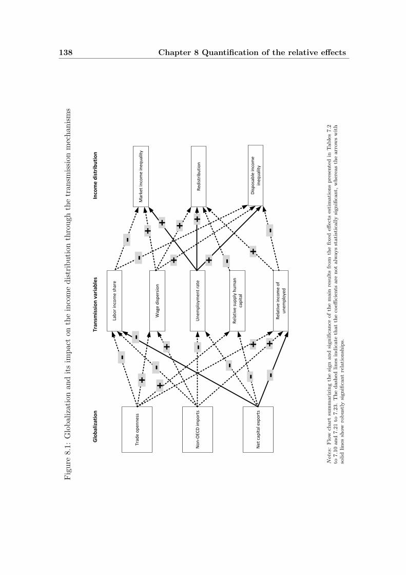
138 Chapter 8 Quantification of the relative effects
Fig
ure
8.1:
Glo
bal
izat
ion
and
its
impac
ton
the
inco
me
dis
trib
uti
onth
rough
the
tran
smis
sion
mec
han
ism
s
Trad
e o
pen
nes
s
No
n-O
ECD
imp
ort
s
Net
cap
ital
exp
ort
s
Lab
or
inco
me
shar
e
Wag
e d
isp
ersi
on
Un
emp
loym
ent
rate
Rel
ativ
e su
pp
ly h
um
an
cap
ital
Rel
ativ
e in
com
e o
f u
nem
plo
yed
-
-+
+ -
-
-
+
-+ +
-
Mar
ket
inco
me
ineq
ual
ity
Red
istr
ibu
tio
n
Dis
po
sab
le in
com
e in
equ
alit
y
-
-
-
+ +
+
+ +
++
Glo
bal
izat
ion
Tran
smis
sio
n v
aria
ble
sIn
com
e d
istr
ibu
tio
n
-
Notes:
Flo
wch
art
sum
mari
zin
gth
esi
gn
an
dsi
gn
ifica
nce
of
the
main
resu
lts
from
the
fixed
effec
tses
tim
ati
on
sp
rese
nte
din
Tab
les
7.2
to7.1
0an
d7.2
1to
7.2
3.
Th
ed
ash
edlin
esin
dic
ate
that
the
coeffi
cien
tsare
not
alw
ays
stati
stic
ally
sign
ifica
nt,
wh
erea
sth
earr
ow
sw
ith
solid
lin
essh
ow
rob
ust
lysi
gn
ifica
nt
rela
tion
ship
s.
8 Quantification of the relative effects 139
The influence of the transmission variables on the distribution of market and
disposable incomes as well as income redistribution is also illustrated in Figure 8.1.
A higher labor income share reduces market income inequality and has no signifi-
cant impact on the income distribution. Hence, the inequality in the distribution of
disposable incomes declines if labor receives a higher share of the national income.
Higher differences in the distribution of wages among full-time workers raise both
the Gini coefficient of market income inequality and the extent to which these in-
come differences are reduced through redistribution. The effect on market income
inequality seems to dominate the impact on redistribution since the wage dispersion
is also positively correlated with the Gini coefficient of disposable incomes. The
unemployment rate is also positively related with the market income inequality,
income redistribution and disposable income inequality. In contrast to the other
transmission variables, the unemployment rate is statistically significant in all spec-
ifications. The relative supply of human capital is negatively and partly significantly
related with income redistribution. Finally, the relative income of unemployed indi-
viduals tends to increase income redistribution and thus lower the inequality in the
distribution of disposable income inequality.
Although these results are not fully robust to variations in the specifications
and sample, the basic implications remain mostly valid. So far, however, the focus
was on the signs and the significance of the coefficients but the quantitative effects
of globalization and the transmission mechanisms have not been assessed. Hence,
Table 8.1 presents the standardized beta coefficients calculated for the baseline es-
timations.159 To assess the relative importance of specific transmission variables, I
use only those observations that are available for the analysis of the determinants of
all transmission variables (see the first five columns) or for all regressions including
the income distribution variables (see the remaining columns), respectively. De-
spite the considerable loss of observations and the associated difficulty to identify
significant effects, this procedure is still necessary because otherwise it would not
be clear whether differences in the relative influence of transmission variables are
simply driven by the sample composition.160
Keeping these limitations in mind, colums one to five in Table 8.1 suggest that
trade openness reduces the labor income share and the unemployment rate but raises
159 The significance of the effects reported in Table 8.1 is, in most cases, considerably lowerthan for the main results in chapter 7. This is likely a consequence of the lower number ofobservations that have been used for the regressions shown in Table 8.1.
160 For the interpretation of the quantitative effects reported in this chapter, one should be awarethat the observations underlying these estimates are restricted to the 1990s and 2000s.
140 Chapter 8 Quantification of the relative effects
the degree of wage dispersion, the relative supply of human capital and the relative
income of unemployed persons. An increase in trade openness by one standard
deviation (equal to 0.52 for this sample) reduces the labor income share by 0.64
standard deviations (or by approximately 2 percentage points).161 At the same time,
a rise in trade openness by one standard deviation increases the wage dispersion by
nearly 0.4 standard deviations or 27 percentage points. The relative supply of human
capital grows by 2.24 standard deviations after trade openness has risen by one
standard deviation five years ago. In that case, the ratio between individuals with
tertiary education and those with primary education increases by 11.7 percentage
points.
The share of imports from non-OECD countries is only significantly related to
the unemployment rate: if the share of these imports rises by one standard deviation,
the unemployment rate falls by 2.27 percentage points, which is equal to nearly 86
percent of the standard deviation. Moreover, the unemployment-reducing effect of
non-OECD imports is the only significant relationship between globalization and the
transmission mechanisms in the smaller sample. Net exports of capital are associated
with a significantly lower labor income share, relative supply of human capital and
relative income of unemployed individuals. If the net outflows of private capital (as
a percentage of GDP) increase by one standard deviation, the labor income share
will be 1.1 percentage points lower, whereas the relative supply of human capital and
the relative income of the unemployed decreases by 5.3 and 4.4 percentage points.
The remaining columns of Table 8.1 present the standardized beta coefficients,
which are estimated based on a common sample for the empirical analysis of both
the transmission variables and the income distribution measures. The empirical
analyses are thus based on only 41 observations.
In the first step of the analysis (i.e. the estimation of the transmission variables)
only three of the globalization variables remain statistically significant.162 The un-
employment rate is significantly negatively associated with the international trade
variables. An increase of trade openness by one standard deviation reduces the un-
employment rate by 2.9 standard deviations or 9 percentage points. Furthermore,
an increase of the share of non-OECD imports by one standard deviation lowers
the unemployment rate by 5 percentage points. The relative income of unemployed
individuals depends negatively on net capital exports. A rise of net exports of pri-
161 The changes in percentage points are calculated based on the standard deviation of the re-spective variables for the current sample.
162 The p-values (reported in parentheses) indicate the effect of net capital exports on the laborincome share and of non-OECD imports on wage dispersion are only marginally insignificant.
8 Quantification of the relative effects 141
vate capital by one standard deviation reduces the income of unemployed persons
relative to workers by 4.7 percentage points.
The analysis of the income distribution is presented in the last three columns
of Table 8.1. Only four of the beta coefficients are also significant.163 The results
indicate that a rise of the unemployment rate by one standard deviation increases
the Gini coefficient of market income inequality by 0.37 standard deviations. The
unemployment rate also affects the distribution of disposable incomes. The Gini
coefficient of disposable incomes increases by 0.27 standard deviations if the unem-
ployment rate rises by one standard deviation. Unemployment has thus a stronger
effect on the distribution of market incomes than on disposable incomes. This is
likely a consequence of income redistribution, which reduces market-induced income
differences resulting from unemployment and therefore prevent an equal increase in
disposable income inequality.
The globalization-induced changes of the distribution of market and disposable
incomes that are transmitted through the unemployment rate can be described as
follows: a rise in the trade openness (imports from non-OECD countries) reduce the
unemployment rate by 9 (5) percentage points164 and thereby lower market income
inequality by 4 (2.35) Gini points. The impact of international trade on the distri-
bution of disposable incomes that is transmitted through the unemployment rate
leads to the following changes. If trade openness rises by one standard deviation,
then the Gini coefficient of disposable incomes declines by 3.6 points. A one stan-
dard deviation higher share of non-OECD imports further reduce disposable income
inequality by 2.1 Gini points.
Moreover, the relative supply of human capital is significantly positively related
to a higher market inequality and, surprisingly, also income redistribution. A rise
in the relative supply of well versus poorly educated individuals by one standard
deviation increases market income inequality by 1.06 standard deviations or about
four Gini points and income redistribution by 0.50 standard deviations (or 4.1 per-
centage points). In this case, however, the changes in the relative supply of human
capital are not driven by developments in international trade and capital mobility.
163 The p-values shown in parenthesis further indicate that most coefficients are not close to beingsignificant, except for the impact of the labor income share on disposable income inequalityand the relative income of the unemployed on income redistribution.
164 This is equal to 287 (166) percent of the standard deviation in the Gini coefficient of marketincome inequality.
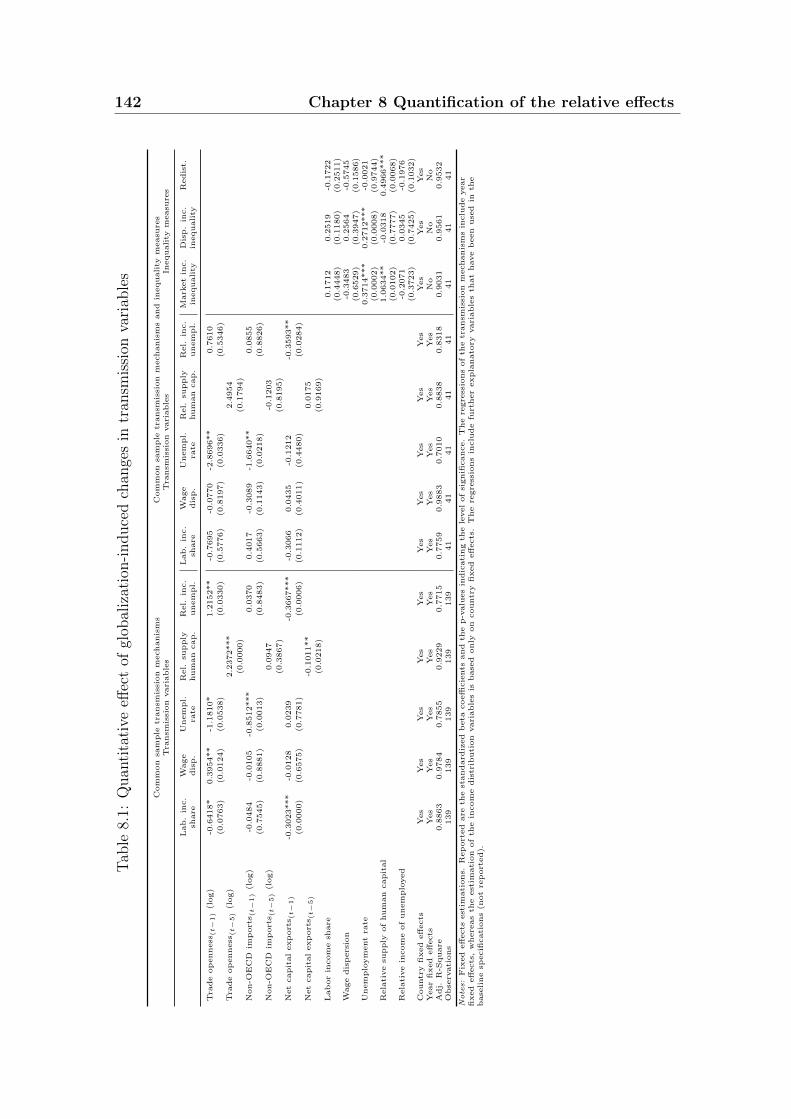
142 Chapter 8 Quantification of the relative effectsT
able
8.1:
Quan
tita
tive
effec
tof
glob
aliz
atio
n-i
nduce
dch
ange
sin
tran
smis
sion
vari
able
s
Com
mon
sam
ple
transm
issi
on
mechanis
ms
Com
mon
sam
ple
transm
issi
on
mechanis
ms
and
inequality
measu
res
Tra
nsm
issi
on
vari
able
sT
ransm
issi
on
vari
able
sIn
equality
measu
res
Lab.
inc.
Wage
Unem
pl.
Rel.
supply
Rel.
inc.
Lab.
inc.
Wage
Unem
pl.
Rel.
supply
Rel.
inc.
Mark
et
inc.
Dis
p.
inc.
Redis
t.sh
are
dis
p.
rate
hum
an
cap.
unem
pl.
share
dis
p.
rate
hum
an
cap.
unem
pl.
inequality
inequality
Tra
de
op
enness
(t−
1)
(log)
-0.6
418*
0.3
954**
-1.1
810*
1.2
152**
-0.7
695
-0.0
770
-2.8
696**
0.7
610
(0.0
763)
(0.0
124)
(0.0
538)
(0.0
330)
(0.5
776)
(0.8
197)
(0.0
336)
(0.5
346)
Tra
de
op
enness
(t−
5)
(log)
2.2
372***
2.4
954
(0.0
000)
(0.1
794)
Non-O
EC
Dim
port
s (t−
1)
(log)
-0.0
484
-0.0
105
-0.8
512***
0.0
370
0.4
017
-0.3
089
-1.6
640**
0.0
855
(0.7
545)
(0.8
881)
(0.0
013)
(0.8
483)
(0.5
663)
(0.1
143)
(0.0
218)
(0.8
826)
Non-O
EC
Dim
port
s (t−
5)
(log)
0.0
947
-0.1
203
(0.3
867)
(0.8
195)
Net
capit
al
exp
ort
s (t−
1)
-0.3
023***
-0.0
128
0.0
239
-0.3
667***
-0.3
066
0.0
435
-0.1
212
-0.3
593**
(0.0
000)
(0.6
575)
(0.7
781)
(0.0
006)
(0.1
112)
(0.4
011)
(0.4
480)
(0.0
284)
Net
capit
al
exp
ort
s (t−
5)
-0.1
011**
0.0
175
(0.0
218)
(0.9
169)
Lab
or
incom
esh
are
0.1
712
0.2
519
-0.1
722
(0.4
448)
(0.1
180)
(0.2
511)
Wage
dis
pers
ion
-0.3
483
0.2
564
-0.5
745
(0.6
529)
(0.3
947)
(0.1
586)
Unem
plo
ym
ent
rate
0.3
714***
0.2
712***
-0.0
021
(0.0
002)
(0.0
008)
(0.9
744)
Rela
tive
supply
of
hum
an
capit
al
1.0
634**
-0.0
318
0.4
966***
(0.0
102)
(0.7
777)
(0.0
068)
Rela
tive
incom
eof
unem
plo
yed
-0.2
071
0.0
345
-0.1
976
(0.3
723)
(0.7
425)
(0.1
032)
Countr
yfi
xed
eff
ects
Yes
Yes
Yes
Yes
Yes
Yes
Yes
Yes
Yes
Yes
Yes
Yes
Yes
Year
fixed
eff
ects
Yes
Yes
Yes
Yes
Yes
Yes
Yes
Yes
Yes
Yes
No
No
No
Adj.
R-S
quare
0.8
863
0.9
784
0.7
855
0.9
229
0.7
715
0.7
759
0.9
883
0.7
010
0.8
838
0.8
318
0.9
031
0.9
561
0.9
532
Obse
rvati
ons
139
139
139
139
139
41
41
41
41
41
41
41
41
Note
s:F
ixed
eff
ects
est
imati
ons.
Rep
ort
ed
are
the
standard
ized
beta
coeffi
cie
nts
and
the
p-v
alu
es
indic
ati
ng
the
level
of
signifi
cance.
The
regre
ssio
ns
of
the
transm
issi
on
mechanis
ms
inclu
de
year
fixed
eff
ects
,w
here
as
the
est
imati
on
of
the
incom
edis
trib
uti
on
vari
able
sis
base
donly
on
countr
yfi
xed
eff
ects
.T
he
regre
ssio
ns
inclu
de
furt
her
expla
nato
ryvari
able
sth
at
have
been
use
din
the
base
line
specifi
cati
ons
(not
rep
ort
ed).
Chapter 9
Conclusion
The coincidence between growing exposure to international trade as well as capital
mobility and the dispersion of incomes experienced by many industrialized countries
has raised the question of a possible causal relationship between these developments.
The existing empirical evidence on this issue is, however, inconclusive. I argue that
these mixed empirical findings may be explained by the focus of many studies on only
one specific aspect of the possible distributional consequences of globalization. These
studies, thereby, ignore alternative channels through which economic integration
likely affects the distribution of incomes.
I have reviewed the literature on the relationship between globalization and var-
ious labor market outcomes and identified a number of transmission mechanisms
through which globalization potentially influences the distribution of market and
disposable incomes in industrialized countries. In a comprehensive analysis based
on a panel of 28 OECD countries between 1960 and 2010, I test empirically how
globalization-induced changes in the labor income share, wage dispersion, unem-
ployment rate, relative supply of human capital and relative income of unemployed
affect the distribution of market and disposable incomes as well as redistribution.
The main results suggest that globalization indeed alters the relative rewards of
production factors. International trade tends to reduce the labor income share and
increases the dispersion of wages among full-time workers, whereas net exports of
private capital lower the relative rewards of labor but have no significant impact on
the degree of wage dispersion.
A robust finding is related to the link between globalization and the unemploy-
ment rate in OECD countries: imports from developing countries reduce unemploy-
ment, whereas trade openness mostly has no significant impact on unemployment.
In contrast to the theoretical expectations, net exports of capital are negatively
143
144 Chapter 9 Conclusion
related to the unemployment rate.
I further analyze how the relative supply of human capital responds to globalization-
induced shifts in the relative rewards to education. These supply adjustments have,
so far, been neglected in studies on the distributional consequences of international
trade and capital mobility. My results show that the relative supply of human capi-
tal increases in response to trade openness and declines if a country faces higher net
outflows of private capital.
Finally, international trade and capital mobility affect the relative income of
unemployed persons differently. Net exports of private capital reduce the income of
unemployed relative to employed individuals. International trade, however, increases
the relative income of unemployed individuals.
Despite the consequences of globalization for labor market outcomes, the rela-
tionship between these outcomes and the income distribution matters for the assess-
ment of the overall distributional effects as well. The combined findings for both
steps of the empirical analysis can be summarized as follows: a greater openness
to international trade increases market income inequality by lowering the labor in-
come share and raising the wage dispersion. Imports from non-OECD countries
raise market income differences through their impact on the relative factor rewards
(i.e. the labor income share and wage dispersion) but tend to reduce market income
inequality by lowering the unemployment rate. Moreover, net outflows of private
capital increase market income differences via the labor income share but lower the
corresponding Gini coefficient by decreasing the unemployment rate.
Beyond its impact on the distribution of market incomes, globalization also mat-
ters for the extent of income redistribution in industrialized countries. A greater
openness toward international trade increases redistribution both by increasing the
wage dispersion and the relative income of the unemployed. Moreover, a higher
supply of human capital in response to greater trade openness reduces income re-
distribution. On the one hand, imports from developing countries raise income
redistribution through a greater wage dispersion. On the other hand, imports from
non-OECD countries reduce redistribution because they lower the unemployment
rate and raise the relative income of unemployed individuals. Net exports of private
capital lower income redistribution through their impact on the unemployment rate
and the relative income of the unemployed but increase it via the relative supply of
human capital.
The transmission mechanisms through which international trade and capital mo-
bility alter the distribution of disposable incomes can be described as follows: trade
9 Conclusion 145
openness leads to higher (lower) differences in the distribution in disposable incomes
because it reduces the labor income share and increases the wage dispersion (raises
the relative income of the unemployed). Non-OECD imports have a similar impact
on the Gini coefficient of the disposable income distribution but reduce inequality
as well by lowering the unemployment rate. Net exports of capital also increase
disposable income inequality via their negative influence on the labor income share
and the relative income of the unemployed but reduce income dispersion through
reducing the unemployment rate.
To sum up, the concern that globalization is a main driver of rising inequality in
developed countries cannot generally be confirmed by the empirical analysis. On the
contrary, the overall impact of a growing exposure to international trade and capital
mobility is ambiguous. While globalization increases the differences in the factor
rewards, it also reduces the unemployment rate in industrialized countries. In par-
ticular the latter effect has proven relevant for the income distribution in advanced
economies. Hence, the positive employment effect of globalization tends to over-
compensate the effect of a greater dispersion in factor rewards. This indicates that,
probably due to productivity gains, more jobs are created by international trade and
capital mobility than destroyed. It is thus possible for advanced economies to bene-
fit from the overall welfare gains from globalization without facing a persistent and
undesirable rise in income differences. The question how globalization affects the
distribution of market and disposable incomes (through the identified transmission
mechanisms) varies between countries depending on the design of their domestic
labor market institutions. In particular, the extent of labor market regulation de-
termines how different labor market outcomes react to increasing international trade
and capital mobility. The adverse effects of international trade on the labor income
share, for instance, are less pronounced if labor markets are less regulated. At the
same time, a globalization-induced rise in wage dispersion is higher in less regulated
labor markets and imports from developing countries reduce the unemployment rate
especially in countries with less regulated labor markets. Since the unemployment
rate has a stronger overall effect on income inequality in industrialized countries than
the earnings distribution, deregulation of labor markets could be an appropriate way
to cope with the challenges of globalization.


Part II
Policy preferences of German
voters
147


Chapter 10
Introduction
The preceding chapters of this book focused on the impact of globalization on the
personal distribution of incomes in industrialized economies. The findings of this
analysis suggest that economic integration affects income inequality through dif-
ferent channels. The relative importance of these channels depends on domestic
institutions such as characteristics of the labor market. Hence, the institutional
framework may be decisive in governing the merits and risks of an increasing global
competition.
In order to cope with the challenges of globalization, policy makers in many
developed countries are confronted with a considerable need for reforms, for instance,
in the fields of the labor market, social security and taxation. These reforms are
supposed to enhance the competitiveness and efficiency of the economy and are, thus,
highly desirable. In democracies, however, their political feasibility is constrained by
the preferences of voters. A successful implementation of welfare-enhancing policies
requires therefore a profound knowledge about the determinants of policy preferences
among voters.
Against this background, the aim of the following chapters is to provide a com-
prehensive analysis of the determinants of voters’ attitudes toward several labor
market and welfare state policies. The empirical analyses are based on data on the
German electorate. The focus on Germany has several advantages for this analysis
due to the fundamental reforms which took place in the early 2000s. Prior to these
reforms, the existence of rigid institutions hampered economic growth and employ-
ment. The reforms undertaken within the scope of the ‘Agenda 2010’ enhanced the
institutional environment and, thereby, the competitiveness of the German economy
and contributed to a substantial reduction in unemployment. Despite their positive
economic consequences, these policies are not very popular within the German pop-
149
150 Chapter 10 Introduction
ulation. Especially the public opinion about the labor market (so called “Hartz”)
reforms suggests that reform resistance cannot fully be explained by conventional
political-economic theories. These theories usually assume that an individual’s sup-
port for or resistance against a certain policy can be explained by its pecuniary
self-interest. Consequently, a reform proposal should be supported by persons who
benefit financially (net recipients) and opposed by those who bear a financial loss.
The recent labor market reforms seem to be not only opposed by individuals who
experienced financial losses but are in general not very popular. The political and
public discussion about the reforms of the ‘Agenda 2010’ often emphasizes its neg-
ative aspects and, in particular, a growing injustice and inequality.165
Motivated by the public opinion on the recent reforms, the following chapters
analyze the determinants of German voters’ attitudes toward a range of labor mar-
ket, social security and redistributive policies accounting for different aspects of the
contentious reforms of the ‘Agenda 2010’. A comprehensive study of the factors
that explain individual preferences for progressive income taxation (with wealthy
individuals paying a larger share of their income in taxes than low income recipi-
ents) is provided in chapter 11. The attitudes toward market oriented labor market
policies (e.g. cutting unemployment benefits and reducing interventionist policies)
are further studied in chapter 12. Possible explanations for interpersonal differences
in tax and labor market policy preferences are the financial self-interest, the level of
information, the general assessment of the fairness of income differences and beliefs
about the relevance of effort for economic success.166 Moreover, several individual
characteristics are taken into account. Chapter 13 is devoted to the empirical ex-
amination of the support of pension reforms. The main focus is on the assessment
of an increase in the legal retirement age which has been part of the recent labor
market reforms and is very unpopular among German voters. This analysis proposes
a new possible source of pension reform resistance: an individual’s (dis-)utility from
work. It is argued that people with intrinsic work motivation will be less anxious
about longer working years compared to people for whom work is a burden. A
higher pension age should, thus, be a relatively attractive reform option for intrinsi-
165 Compare also the current annual report by the German council of economic experts(Sachverstadigenrat zur Begutachtung der gesamtwirtschaftlichen Entwicklung, 2013).
166 The focus on fairness issues such as fairness preferences, the assessment of the income orsocial differences and the role of beliefs about the drivers of inequality is motivated by thepublic debate on the reforms of the ‘Agenda 2010’ and the availability of survey data. Theindividual attitudes toward redistributive policies can, of course, also be explained by otherfactors. In particular, individuals might accept financial losses (e.g. being a net payer toincome redistribution) because of altruistic motives or simply compassion for the recipients.
10 Introduction 151
cally motivated workers compared to the reform alternatives of cutting pensions or
increasing contributions.
The empirical analyses of chapter 11 to 13 are based on data from the German
General Social Survey (“Allgemeine Bevolkerungsumfrage der Sozialwissenschaften”:
ALLBUS), which is designed to be representative for the German population.
ALLBUS has been conducted biannually since 1980167 and is promoted by DFG
(German Research Society) and GESIS (Institute for Social Science), which also
conduct the German part of the International Social Survey Programme (ISSP).
The latter program was firstly implemented in 1985 and collects data for various
themes of social science annually. ALLBUS and the integrated ISSP-surveys offer
plenty of valuable information on the respondents’ assessment of several policies, on
the individual labor market status and socioeconomic situation as well as on fairness
issues.
The findings of the chapters 11 to 13 provide information on various robust
correlations between policy preferences and their potential driving factors. Given
that a better understanding of reform support or resistance among voters is highly
relevant for a successful implementation of growth-enhancing reforms in a democ-
racy, learning about robust correlations and patterns related to individual policy
preferences is valuable. Regarding the interpretation of the results and their impli-
cations, however, one should be aware of the limitations of these empirical analyses.
In particular, the econometric approach does not allow the identification of causal
relationships. It is, for instance, not possible to exclude a reverse causality or that
omitted variables affect the results. Moreover, the different categories of impact
factors may not be fully independent of each other. Since the ALLBUS data set
is a repeated cross-section, different persons are surveyed in each wave. Hence, it
is not possible to control for interpersonal heterogeneity and ascribe changes in a
person’s policy preferences to changes in his socioeconomic situation or self-interest,
for example.
The findings indicate that the mere focusing on financial self-interest as an ex-
planation for policy preferences leaves out an important part of the story. Although
variables approximating self-interest play a crucial role, other dimensions contribute
substantially to our understanding of individual heterogeneity in labor market and
welfare reform acceptance. In particular, individual beliefs on the sources of eco-
nomic success are highly correlated with policy preferences: a person who believes
167 For details on ALLBUS see http://www.gesis.org/en/services/data/survey-data/
allbus
152 Chapter 10 Introduction
that everyone is responsible for his own economic situation tends to be less inclined
to support redistributive policies.
Motivated by the relevance of beliefs for individual policy preferences, chapter 14
analyzes how individuals form their beliefs about the drivers of success in life. For
that purpose, a specific feature of the German history, the separation of the country
and the existence of two distinct regimes after World War II is used. Several studies
point at persistent differences between individuals who have been socialized under
the communist regime in East Germany and their West German fellow citizens (e.g.
Alesina and Fuchs-Schundeln, 2007; Heineck and Sussmuth, 2010; Heinemann et al.,
2011). These differences in policy preferences, fairness considerations and beliefs
likely reflect the differential socialization and indoctrination by different regimes.
Hence, chapter 14 analyzes whether indoctrination has affected East Germans’ be-
liefs on the drivers of success by exploiting a natural experiment on the reception
of West German television in the former German Democratic Republic. While the
majority of GDR citizens had access to West German television already before the
reunification, approximately 15 percent of the population could not receive these
broadcasts due to geographical and topological reasons. Hence, the empirical analy-
sis in chapter 14 allows the identification of a causal television effect as it makes use
of an exogenous variation in access to Western television. Based on GDR survey data
collected in the late 1980s and longitudinal data from the German Socio-Economic
Panel for the 1990s the impact of differential access to Western television on East
Germans’ beliefs both before and after reunification is tested empirically.
The findings of the following chapters are of particular interest when it comes
to the actual implementation of potentially growth-enhancing reforms. To foster
voters’ support for labor market and welfare state policies, politicians could also
address issues beyond financial net gains from a certain measure. Notably, fairness
considerations are found to be highly relevant for one’s assessment of labor market
and tax reforms. Moreover, a person’s degree of intrinsic motivation can explain his
willingness to accept an increase in legal retirement age. The analysis in chapter 14
further indicates that mass media may have the power to affect individual attitudes
toward reforms not only by focusing on a concrete policy measure and addressing its
consequences but also by changing fairness considerations. Furthermore, the latter
effect may persist as it was the case with the political indoctrination of East German
citizens via both West and East German television broadcasts.
Chapter 11
Preferences toward progressive
taxation∗
11.1 Introduction
Highly progressive tax systems confront high income individuals with substantial
marginal tax rates. Thus, they entail disincentives for private economic activity
and may hamper potential growth. Although the introduction of alternative tax
systems might be a desirable part of a growth enhancing fiscal strategy, a transition
toward a less progressive tax schedule or even a flat tax is regularly confronted
with opposition. Flat tax regimes have only been possible in very few countries.
Obviously, tax progression seems to be a majority preference in many industrialized
countries.
While the economic effects of tax progression have received much attention (see
Fuest and Huber, 2001 for a brief survey) a full understanding of its political popular-
ity is still lacking. Basically, two alternative but not necessarily mutually exclusive
explanations compete: narrow redistributive self-interest and fairness concerns.
The view that an individual’s tax policy preferences are largely driven by the
impact of redistributive taxation on the individual’s own net income is firmly rooted
in political-economic theories. These approaches postulate that individuals choose
their preferred tax rate based on a narrow financial self-interest calculus (Hettich
and Winer, 1997). Thus, increasing income redistribution should be supported by
persons who benefit financially (net recipients), and opposed by those who are net
payers to the welfare state (Meltzer and Richard, 1981). From that perspective,
∗ This chapter is based on a joint work with Friedrich Heinemann (see Hennighausen andHeinemann, forthcoming).
153
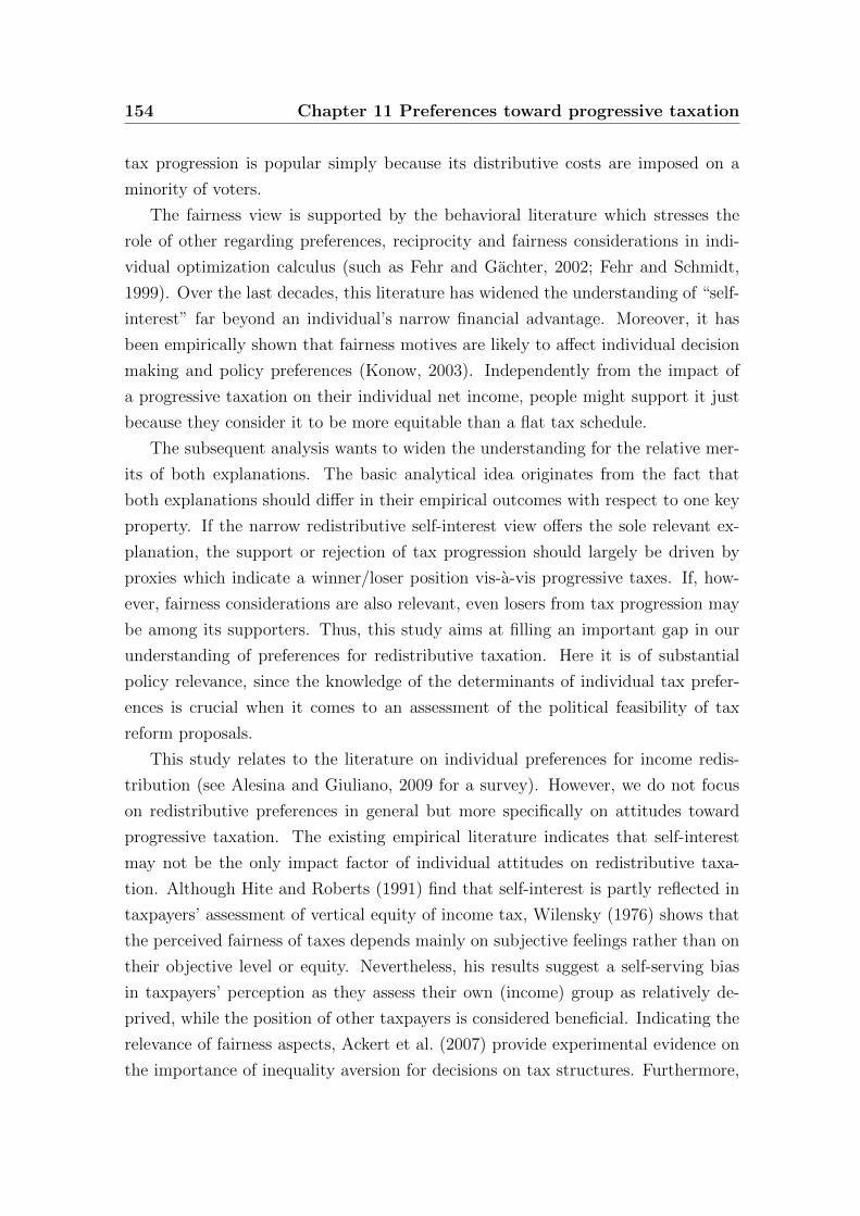
154 Chapter 11 Preferences toward progressive taxation
tax progression is popular simply because its distributive costs are imposed on a
minority of voters.
The fairness view is supported by the behavioral literature which stresses the
role of other regarding preferences, reciprocity and fairness considerations in indi-
vidual optimization calculus (such as Fehr and Gachter, 2002; Fehr and Schmidt,
1999). Over the last decades, this literature has widened the understanding of “self-
interest” far beyond an individual’s narrow financial advantage. Moreover, it has
been empirically shown that fairness motives are likely to affect individual decision
making and policy preferences (Konow, 2003). Independently from the impact of
a progressive taxation on their individual net income, people might support it just
because they consider it to be more equitable than a flat tax schedule.
The subsequent analysis wants to widen the understanding for the relative mer-
its of both explanations. The basic analytical idea originates from the fact that
both explanations should differ in their empirical outcomes with respect to one key
property. If the narrow redistributive self-interest view offers the sole relevant ex-
planation, the support or rejection of tax progression should largely be driven by
proxies which indicate a winner/loser position vis-a-vis progressive taxes. If, how-
ever, fairness considerations are also relevant, even losers from tax progression may
be among its supporters. Thus, this study aims at filling an important gap in our
understanding of preferences for redistributive taxation. Here it is of substantial
policy relevance, since the knowledge of the determinants of individual tax prefer-
ences is crucial when it comes to an assessment of the political feasibility of tax
reform proposals.
This study relates to the literature on individual preferences for income redis-
tribution (see Alesina and Giuliano, 2009 for a survey). However, we do not focus
on redistributive preferences in general but more specifically on attitudes toward
progressive taxation. The existing empirical literature indicates that self-interest
may not be the only impact factor of individual attitudes on redistributive taxa-
tion. Although Hite and Roberts (1991) find that self-interest is partly reflected in
taxpayers’ assessment of vertical equity of income tax, Wilensky (1976) shows that
the perceived fairness of taxes depends mainly on subjective feelings rather than on
their objective level or equity. Nevertheless, his results suggest a self-serving bias
in taxpayers’ perception as they assess their own (income) group as relatively de-
prived, while the position of other taxpayers is considered beneficial. Indicating the
relevance of fairness aspects, Ackert et al. (2007) provide experimental evidence on
the importance of inequality aversion for decisions on tax structures. Furthermore,
11.2 Attitudes toward progressive taxation 155
Slemrod (2006) shows that US-citizens are more likely to support a substantial tax
reform if they judge the current system to be unfair.
The remainder of this chapter is organized as follows: section 11.2 offers some
facts about the attitudes toward progressive taxation among German voters. The
subsequent section is devoted to the identification of potential factors that explain
why individuals differ in their preferences for progressive tax rates. The econometric
results and several robustness tests are presented in section 11.4 and some concluding
remarks are offered in section 11.5.
11.2 Attitudes toward progressive taxation within
the German population
To analyze the individual determinants of voters’ attitudes toward progressive tax-
ation, we employ survey data from the German General Social Survey (ALLBUS).
In the present study, we focus on data collected in the year 2000, which also in-
cludes questions designed for the International Social Survey Programme (ISSP). In
the context of the ISSP-survey Social Inequality III the respondents were asked to
answer the following question related to their tax preferences: “Do you think people
with high incomes should pay a larger share of their income in taxes than those with
low incomes, the same share or a smaller share?” The participants could choose
between the following answers: people with high incomes should pay “a larger” or
“much larger share”, “the same share” or “a smaller” respectively “a much smaller
share” of their incomes in taxes than people with lower incomes. While the first two
alternatives relate to progressive tax rates, the latter correspond to a proportional
and a regressive taxation respectively.168
Figure 1 depicts the response pattern. It is remarkable that a clear majority of
the German population (nearly 80 percent) seems to favor a progressive tax system.
The share of the respondents’ preferring a proportional tax rate is considerably
lower (19 percent), while the number of individuals choosing a regressive tax can
be neglected. The three bars on the right show the tax structure preferences for
different income groups.169
168 A progressive tax scheme (i.e. tax payments that increase disproportionately in income)implies rising average tax rates with income (e.g. due to tax exemptions) but not necessarilyincreasing marginal tax rates.
169 The allocation of the ALLBUS participants into these income groups is based on their self-reported monthly net income. The net income of the 25th percentile is below 750 Euro, whilethe individuals belonging to the 75th percentile earn at least 1500 Euro (on average the income
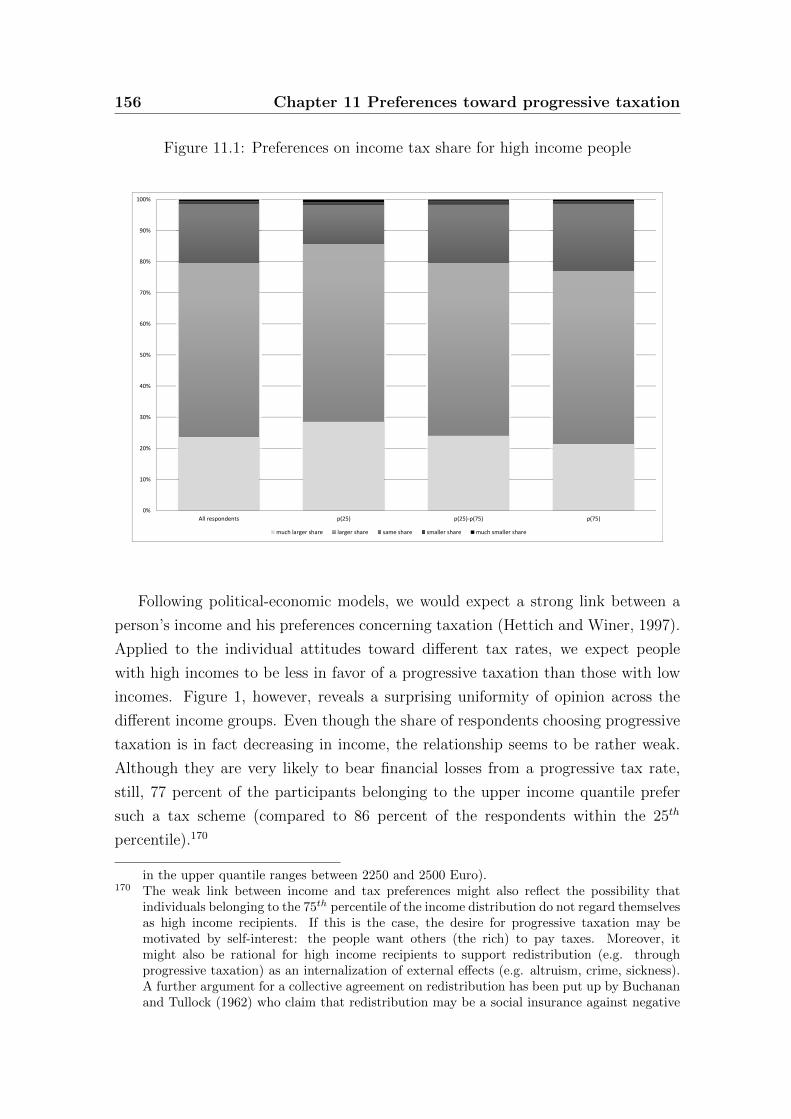
156 Chapter 11 Preferences toward progressive taxation
Figure 11.1: Preferences on income tax share for high income people
0%
10%
20%
30%
40%
50%
60%
70%
80%
90%
100%
All respondents p(25) p(25)‐p(75) p(75)
much larger share larger share same share smaller share much smaller share
Following political-economic models, we would expect a strong link between a
person’s income and his preferences concerning taxation (Hettich and Winer, 1997).
Applied to the individual attitudes toward different tax rates, we expect people
with high incomes to be less in favor of a progressive taxation than those with low
incomes. Figure 1, however, reveals a surprising uniformity of opinion across the
different income groups. Even though the share of respondents choosing progressive
taxation is in fact decreasing in income, the relationship seems to be rather weak.
Although they are very likely to bear financial losses from a progressive tax rate,
still, 77 percent of the participants belonging to the upper income quantile prefer
such a tax scheme (compared to 86 percent of the respondents within the 25th
percentile).170
in the upper quantile ranges between 2250 and 2500 Euro).170 The weak link between income and tax preferences might also reflect the possibility that
individuals belonging to the 75th percentile of the income distribution do not regard themselvesas high income recipients. If this is the case, the desire for progressive taxation may bemotivated by self-interest: the people want others (the rich) to pay taxes. Moreover, itmight also be rational for high income recipients to support redistribution (e.g. throughprogressive taxation) as an internalization of external effects (e.g. altruism, crime, sickness).A further argument for a collective agreement on redistribution has been put up by Buchananand Tullock (1962) who claim that redistribution may be a social insurance against negative
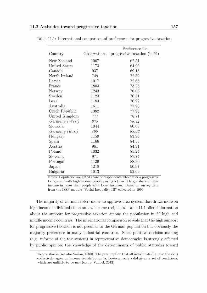
11.2 Attitudes toward progressive taxation 157
Table 11.1: International comparison of preferences for progressive taxation
Preference forCountry Observations progressive taxation (in %)
New Zealand 1067 62.51United States 1173 64.96Canada 937 69.18North Ireland 749 72.39Latvia 1017 72.66France 1803 73.26Norway 1243 76.03Sweden 1123 76.31Israel 1183 76.92Australia 1611 77.90Czech Republic 1382 77.95United Kingdom 777 78.71Germany (West) 875 78.74Slovakia 1044 80.65Germany (East) 489 83.03Hungary 1159 83.96Spain 1166 84.55Austria 961 84.91Poland 1032 85.24Slovenia 971 87.74Portugal 1129 88.30Japan 1218 90.97Bulgaria 1013 92.69
Notes: Population-weighted share of respondents who prefer a progressivetax system with high income people paying a (much) larger share of theirincome in taxes than people with lower incomes. Based on survey datafrom the ISSP module “Social Inequality III” collected in 1999.
The majority of German voters seems to approve a tax system that draws more on
high income individuals than on low income recipients. Table 11.1 offers information
about the support for progressive taxation among the population in 22 high and
middle income countries. The international comparison reveals that the high support
for progressive taxation is not peculiar to the German population but obviously the
majority preference in many industrial countries. Since political decision making
(e.g. reforms of the tax system) in representative democracies is strongly affected
by public opinion, the knowledge of the determinants of public attitudes toward
income shocks (see also Varian, 1980). The presumption that all individuals (i.e. also the rich)collectively agree on income redistribution is, however, only valid given a set of conditions,which are unlikely to be met (comp. Vaubel, 2012).
158 Chapter 11 Preferences toward progressive taxation
tax systems is crucial when it comes to an assessment of the political feasibility
of reform proposals. Although redistributive self-interest seems to correspond to
these attitudes, the link is far from being as close as suggested by conventional
political-economic theory. This raises the question of other relevant driving factors
of individual attitudes toward tax structures beyond individual gains or losses. Since
taxation is an instrument of the government to redistribute market incomes, it is
reasonable to expect that fairness aspects play a major role in the formation of the
corresponding attitudes.
11.3 Potential determinants of individual attitudes
toward progressive taxation
As individual views on the design of the tax structure are likely to depend on very
different factors, the aim of our empirical analysis is twofold. Apart from the identi-
fication171 of the factors related to individual attitudes toward progressive taxation,
we want to derive insights into the relative impact of different groups of driving
factors. First, self-interest is supposed to be important as individuals are affected
differently by a given tax design. Second, the level of information about taxa-
tion may differ. Furthermore, fairness considerations are likely to affect individual
attitudes toward progressive taxation in several respects. Besides differences in dis-
tributive preferences, people may entertain diverging beliefs on the role of incentives
and the causes of inequality. This can result in different conclusions about the effi-
ciency and necessity of progressive taxation. Finally, it is reasonable to assume that
individuals judge tax structures based on their views on the fairness of the existing
income distribution.
Thus, we express the probability that an individual i prefers a progressive tax
(PROGi) as a function of his narrow financial self-interest (FINSELFi), fairness
considerations (FAIRi), level of information (INFOi) as well as a set of socioeco-
nomic characteristics (INDi):
Prob(PROGi = 1) = Φ(β · INDi + δ1 · FINSELFi + δ2 · FAIRi + δ3 · INFOi)
171 The survey data used in this study does not allow a clear identification of a causal relationship.Rather, the objective of our empirical analysis is the identification of factors that are signifi-cantly correlated with tax policy preferences and, thus, have to be addressed in a successfulselling of tax reforms.
11.3 Determinants of individual attitudes toward tax progression 159
The preference for progressive taxation of individual i is captured by his answer
to the survey question introduced in section 11.2. The binary variable (PROGi) is
equal to one if the respondent states that high income recipients should pay a (much)
larger share of their income in taxes than those with low incomes, and equals zero
if he prefers a proportional or regressive income tax.172
Financial self-interest
Political-economic models assume that individual support for or resistance against
income redistribution is driven mainly by a narrow self-interest, which is preoccu-
pied with the individual’s own gains or losses. Meltzer and Richard (1981) show
that the median voter will choose a positive tax rate as long as he earns less than
the population average and, thus, benefits financially from income redistribution.173
Applied to the decision about the degree of tax progression, one would expect sup-
port from individuals who are net-recipients from such a tax scheme. Since the tax
liability is disproportionately higher for wealthy individuals than for those with low
incomes, it is reasonable to assume that the former will be less likely to support a
progressive tax scheme.174
Financial self-interest has been proven relevant for the assessment of tax policies.
Hite and Roberts (1991) find that individuals in higher income brackets are less
content with the fairness of steeply progressive tax rates. Furthermore, the financial
situation of individuals has been found to affect the perceived fairness of different
taxes or tax systems (Slemrod, 2006).
Simple political-economic models are, however, not able to explain why individu-
als support redistributive policies (e.g. via progressive taxation) although they have
to bear financial losses from it. One possible explanation still adhering to financial
self-interest is offered by Benabou and Ok (2001). Given the possibility of income
mobility, it might be rational for the currently rich (poor) to support (oppose) redis-
tribution if they expect to earn less (more) than the population average in the future.
172 To facilitate the interpretation of the subsequent empirical analysis, our main results are basedon a probit estimation. Since the structure of the dependent variable is ordered, Table 11.5contains information on the robustness of the results using an ordered probit approach.
173 In this model, voters also consider work disincentives due to redistribution and the resultingwelfare loss. It is, however, questionable to what extent the disincentive effects of progressivetaxation are considered in the formation of public opinion on this topic. Reed-Arthurs andSheffrin (2010) find that the public does not take them into account when making judgmentson progressive taxation and furthermore does not believe that this should be done.
174 Taxes do not only finance redistribution but also the provision of public goods. However,for the public good related part of government budgets low income individuals should alsosupport progression.
160 Chapter 11 Preferences toward progressive taxation
Another aspect of income mobility has been stressed by Piketty (1995). Experienced
social mobility is likely to alter the beliefs concerning the relative importance of in-
dividual effort for economic success. Individuals who experienced upward mobility
may stress the relevance of effort, while those facing a loss in social status may
ascribe this to bad luck (Alesina and La Ferrara, 2005).
To account both for static and dynamic (i.e. mobility related) redistributive
self-interest, we exploit information on the respondents’ position in the income dis-
tribution based on their individual net income175 and the evolution of their self-
reported social status over time. ALLBUS contains data about the respondents’
placement in the social stratum in the year the survey has been conducted as well
as ten years before. Based on this information we construct the variable social
mobility.176 This variable takes a negative value for individuals who experienced
downward mobility and a positive value for those who experienced upward mobil-
ity.177 The respondents’ placement in the income distribution is measured by three
dummy variables indicating whether the respondent has a low, intermediate or
high income (i.e. belongs to the bottom quantile, the middle range or the top
quantile of the income distribution). We expect that the support for progressive
taxation should be the highest among low income recipients and the lowest among
those with high incomes, while experienced upward mobility should further reduce
preferences for this tax structure.
Information
The level of information has been found to influence the individual assessment of
economic policy. Boeri et al. (2002) show that a better knowledge of the functioning
and costs of unfunded pension systems relates to a higher support for pension re-
forms. In the context of tax systems, the level of information is likely to be reflected
175 ALLBUS only offers information on monthly net incomes. Information about income beforetaxes and transfers would be more appropriate to assess the financial self-interest related totax structures. Since we are using the position in the income distribution (i.e. belonging to the25th, 25th to 75th, or 75th percentile), the bias due to a change of an individual’s income groupafter redistribution should be less severe compared to an analysis based on concrete amountsof income. In an earlier version of this paper, we have also used the respondents’ socialstatus to capture their self-interest and the results remain robust. Additional estimates usinginformation on both the income and structure of the respondents’ households are presentedin section 11.4.2.
176 ALLBUS only offers information on the respondents’ realized but not on their expected mobil-ity. Hence, the interpretation of the variable social mobility is limited to the consequencesof mobility which are suggested by Piketty (1995) but cannot be extended to mobility expec-tations.
177 More information on this and other included variables is provided in Table B.1 in the appendix.
11.3 Determinants of individual attitudes toward tax progression 161
in individual policy assessments. Slemrod (2006) argues that the observable prefer-
ence of US citizens for a flat or sales tax at least partly mirrors misconceptions about
the degree of tax progression of the current system. Furthermore, Sheffrin (1993)
points out that tax policy concepts are rather complex and receive little attention
in public debates. The general public’s lack of knowledge about taxation (especially
related to the concept of progression) is reflected in the fact that the framing of
survey questions is likely to affect the respondents’ answers (Roberts et al., 1994).
Confronted with abstract questions, the majority of the respondents seem to prefer
a progressive system, which is not the case if the respondents are offered a concrete
example (e.g. declaration of just tax payments for different income groups). Fur-
thermore, the evaluation of tax structures depends on whether the tax payments of
different income groups have been presented in rates or in absolute values.
Thus, we would expect that the individual level of information about the tax
system should be relevant for the corresponding answer behavior. ALLBUS offers
no direct information on the respondents’ knowledge about taxation and different
tax schemes. Nevertheless, an empirical analysis of individual attitudes toward
progressive taxation should take the respondents’ level of information into account
(at least to minimize possibly biased results due to minor knowledge). For this
purpose, we make use of two types of variables to proxy the respondents’ degree
of information about taxation: first, we control for the level of education since
Blinder and Krueger (2004) provide some evidence that higher educated individuals
have a better knowledge about major economic policy issues. Hence, we introduce
the dummy variables secondary and upper secondary education as well as
university, which are equal to one for respondents with the corresponding degree.
In addition, we employ the respondent’s opinion on the importance of politics
to his personal life. The perception that political decisions affect the own life and
well-being should increase the incentive to be informed about major political topics.
This relationship has also been stressed by Edlund (2003) who argues that the
high relevance of fiscal policy for the Swedish population due to the welfare state
generosity involves a stronger awareness of topics related to public finance. Although
we would expect that a better information level reduces, ceteris paribus, biases and
misunderstandings, we do not have any a priori knowledge about the direction of
this bias.
162 Chapter 11 Preferences toward progressive taxation
Beliefs
The relevance of beliefs (e.g. concerning the underlying reasons of inequality) for
welfare state preferences has been emphasized by Alesina and Angeletos (2005).178
It has been shown empirically that beliefs matter for tax preferences. For members
of parliament beliefs on company mobility affect the preferred levels of corporate
taxes (Heinemann and Janeba, 2011). For voters the impact of individual effort
relative to exogenous factors (like birth or luck) can explain differences in welfare
state preferences (Alesina et al., 2001; Fong, 2001). The implicit assumption that
everyone is responsible for his own economic situation and that inequality results
from differences in individual effort should lead to a less favorable assessment of
progressive taxation. The same is expected for individuals believing that incentives
affect individual effort. The disincentives of increasing tax rates for private economic
activity should be weighted more and, thus, lead to a more critical assessment of tax
progression. The respondents’ beliefs concerning the reasons for economic success
are captured by the dummy variable effort. This variable takes on the value one
for participants stating that differences in social status reflect individual variations
in effort. For the corresponding regression coefficient a negative sign is expected.
A further belief that may be relevant for tax preferences is related to the proce-
dural fairness of the political system. Following the concept of procedural fairness,
the perceived justice of a certain (policy) outcome depends on the underlying de-
cision making process. It has been shown that procedural fairness increases the
acceptance of decisions with unfavorable outcomes (Sondak and Tyler, 2007) as well
as the perceived fairness of social inequality (Bischoff et al., 2008). The respondents’
beliefs regarding the degree of procedural fairness of the German political system
is measured by their assessment of the functioning of the democracy. The impact
of the resulting dummy variable democracy (equal to one for those claiming to
be (fully) satisfied with the democracy as practiced in Germany; zero otherwise)
is theoretically ambiguous. It is reasonable to assume that the effectiveness of the
democratic system fosters the trust of voters in the usage of taxpayers’ money. The
belief in an appropriate use of public money might, however, increase the willingness
178 In accordance with the literature (e.g. Alesina and Angeletos, 2005; Alesina et al., 2001;Giuliano and Spilimbergo, 2009; Benabou and Tirole, 2006a), we define individual beliefs asa person’s view on the relative weight of discretionary (e.g. achievement, industriousness)versus exogenous factors (e.g. luck, social background) as a determinant for success andupward mobility. The survey questions used to capture beliefs thus provide information onthe respondents’ views about the determinants of inequality. It might, however, be the casethat these questions do not exactly ask about a belief (i.e. may not asked whether a respondentbelieves that income differences exist because of differences in effort).
11.3 Determinants of individual attitudes toward tax progression 163
to pay higher taxes for all voters and, thus, facilitates the acceptance of taxes in
general. Nevertheless, a comprehensive empirical analysis of attitudes toward taxa-
tion should also control for the belief in procedural fairness of the decision making
process since tax rates are determined politically.
Fairness preferences and the assessment of the status quo
distribution
The design of a tax system is a major part of redistributive policies in developed
countries. Consequently, fairness preferences are likely to shape attitudes toward
progressive taxation. The individually preferred income distribution is the bench-
mark to assess the existing distributive outcome. Thus, persons favoring a distribu-
tion that guarantees everyone the (financial) means necessary for a reasonable living
(need principle) should diverge in their attitudes toward redistribution from those
who prefer the equity principle, for example. For them, the optimizing calculus
on the preferred tax system would assign a positive value to a more need-related
redistribution independent from the financial consequences for themselves. The re-
spective respondents’ fairness preferences are indicated by their agreement with the
statement that people should have a decent income even without achievement. For
the dummy variable need a positive sign is expected: other things equal, individuals
who prefer a distribution according to the need principle should be more supportive
of a progressive taxation than those without that kind of preference.
It seems reasonable to expect that individuals who perceive the existing distri-
bution of incomes and wealth within their country as inadequate should be in favor
of redistributive policies. On the other hand, the judgment of the existing inequal-
ity as fair should decrease the demand for redistribution. Hence, we expect that
individuals assessing the existing social differences as (completely) just as well
as those who do not observe a worsening of the situation of ordinary people are
less likely to exhibit preferences for progressive taxes.179 Besides information on
the respondents’ assessment of the social justice, ALLBUS also includes a question
related to the perceived justice of the own income situation and, thus, allows to
introduce a more egocentric view on the fairness of the income distribution. The
participants were asked whether the income they receive is appropriate given their
179 The assessed fairness of existing income or social differences is captured by questions aboutdifferent aspects of the distributive situation and its justice. In contrast to economic beliefs,the corresponding variables refer to the assessed justice of the actual distributive situationbut not to its underlying reasons.
164 Chapter 11 Preferences toward progressive taxation
achievements. Based on this information, we construct the dummy variable ade-
quate wage, which equals one for respondents stating to be (at least) adequately
paid relative to their effort. It is hypothesized that the individuals’ satisfaction with
their own earnings is related to a lower demand for redistribution and, therefore,
progressive taxation.
Individual characteristics
A number of personal characteristics are likely to go along with preferences for pro-
gressive taxation. Some of these characteristics capture specific aspects of the above
discussed aspects of financial self-interest, information, beliefs or fairness assessments
that cannot be observed directly. In addition, however, personal characteristics ac-
count for new aspects.
Focusing on policy preferences of German citizens, it is necessary to account
for the historical feature of the existence of the two former German regimes. The
socialization under the communist regime of the former GDR has been found to
have left its marks in people’s minds and beliefs (see chapter 14). The analysis
in chapter 12 suggests that individuals from the former GDR are more skeptical
toward market-oriented reforms of the labor market than those socialized in the
Western part of Germany. Furthermore, Alesina and Fuchs-Schundeln (2007) find
that, compared to their Western German countrymen, East Germans have a stronger
preference for redistribution, which cannot fully be explained by their relatively low
income. Motivated by the previous findings, we expect that socialization under
Communism180 implies a stronger preference for progressive taxation.
There are several reasons why older people might differ in their welfare pref-
erences from younger individuals. First, the experience of different cohorts might
differ substantially. Giuliano and Spilimbergo (2009) find that the experience of
sharp recessions during early adulthood affects redistributive preferences. In line
with this, older individuals may remember the substantial social inequalities be-
fore the expansion of the welfare state since the 1970s (Lindbeck, 1995; Heinemann,
2008). This socialization may make them see today’s situation less critical and,
therefore, perceive less necessity to redistribute. Second, uncertainty about the own
economic and social status in life is larger for the young than for the old. Compared
to the old, the perspective of young people with respect to their country’s social
180 Since we are interested in the effect of being socialized in the GDR and not in the respondents’current state of residence, our east-dummy is equal to one for respondents born in the formerGDR.
11.3 Determinants of individual attitudes toward tax progression 165
situation is rather characterized by a thicker “veil of ignorance” (Rawls, 1971). As
a consequence, the lower insecurity of the old may let them pay less attention to
redistribution as an insurance for income risk. In addition, Sheffrin (1994) points to
a possible status quo bias in the individual attitudes toward progressive taxation.
Comparing British and US survey data, he finds a relatively higher preference for
progressive taxation among the population in the UK and traces this back to the fact
that the British taxes were more progressive than those in the US when the surveys
were conducted. It seems reasonable to expect that the views of older individuals
may be more biased in favor of the status quo than those of younger ones. Hence,
the progressivity of the German income tax system might be reflected in a higher
preference for increasing tax rates, especially among older people. The impact of a
person’s age on the tax rate preferences is, thus, a priori ambiguous.
The literature reports that women have a stronger preference for income redis-
tribution (e.g. Corneo and Gruner, 2002). Therefore, females should also be more
supportive of a highly redistributive taxation than males.
Furthermore, several variables related to the respondents’ employment status
are included in our empirical analysis. We would expect individuals who do not
participate in the labor market (i.e. being either unemployed or not employed)
and are, thus, dependent on public or private transfers to be more likely to support
redistribution than those who are employed. This should also be the case for pro-
gressive taxation as these respondents should be, ceteris paribus, net recipients of
this tax policy.181
Other things equal, self-employed individuals are more prone to take (financial)
risks and might also be more individualistic. Thus, we would expect that the self-
employed are less supportive toward progressive taxation than employees.
Public employees are less likely to receive a high income than individuals em-
ployed in private enterprises. When it comes to pecuniary self-interest, we expect
them to be in favor of a progressive tax system (relative to private economy employ-
ees). A further argument for diverging tax preferences between workers employed
in the public and private sector is related to bureaucracy theories (e.g. Tullock,
1965). In general, we would expect bureaucrats to have a distinct interest in taxes
as they increase their budget and, thus, power. It is, however, a priori unclear which
kind of tax structure public sector employees prefer. Given the German income tax
181 The household composition may, however, matter as respondents who are not active in thelabor market and, thus, dependent on intra-household transfers might be less likely to favorredistribution if this reduces the income of their household. This issue is also addressed inthe robustness tests in section 11.4.2.
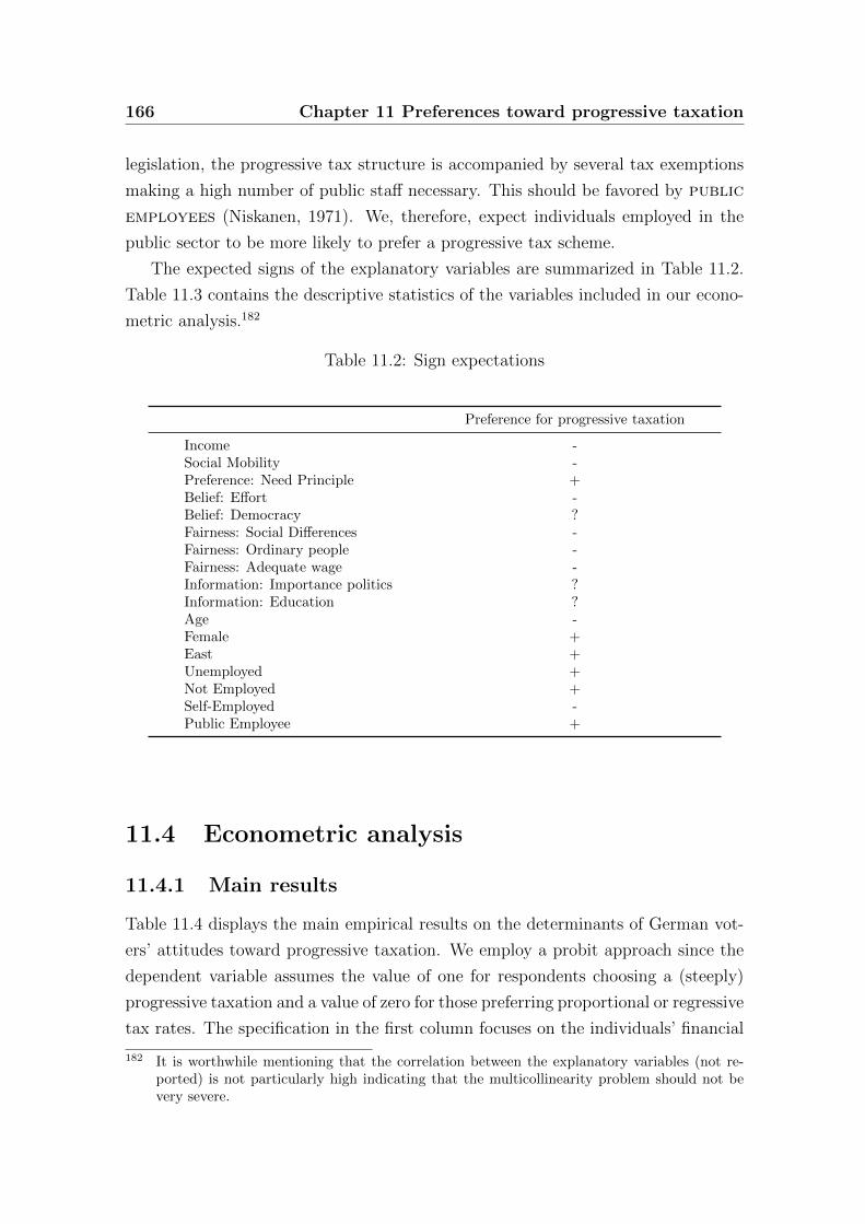
166 Chapter 11 Preferences toward progressive taxation
legislation, the progressive tax structure is accompanied by several tax exemptions
making a high number of public staff necessary. This should be favored by public
employees (Niskanen, 1971). We, therefore, expect individuals employed in the
public sector to be more likely to prefer a progressive tax scheme.
The expected signs of the explanatory variables are summarized in Table 11.2.
Table 11.3 contains the descriptive statistics of the variables included in our econo-
metric analysis.182
Table 11.2: Sign expectations
Preference for progressive taxation
Income -Social Mobility -Preference: Need Principle +Belief: Effort -Belief: Democracy ?Fairness: Social Differences -Fairness: Ordinary people -Fairness: Adequate wage -Information: Importance politics ?Information: Education ?Age -Female +East +Unemployed +Not Employed +Self-Employed -Public Employee +
11.4 Econometric analysis
11.4.1 Main results
Table 11.4 displays the main empirical results on the determinants of German vot-
ers’ attitudes toward progressive taxation. We employ a probit approach since the
dependent variable assumes the value of one for respondents choosing a (steeply)
progressive taxation and a value of zero for those preferring proportional or regressive
tax rates. The specification in the first column focuses on the individuals’ financial
182 It is worthwhile mentioning that the correlation between the explanatory variables (not re-ported) is not particularly high indicating that the multicollinearity problem should not bevery severe.
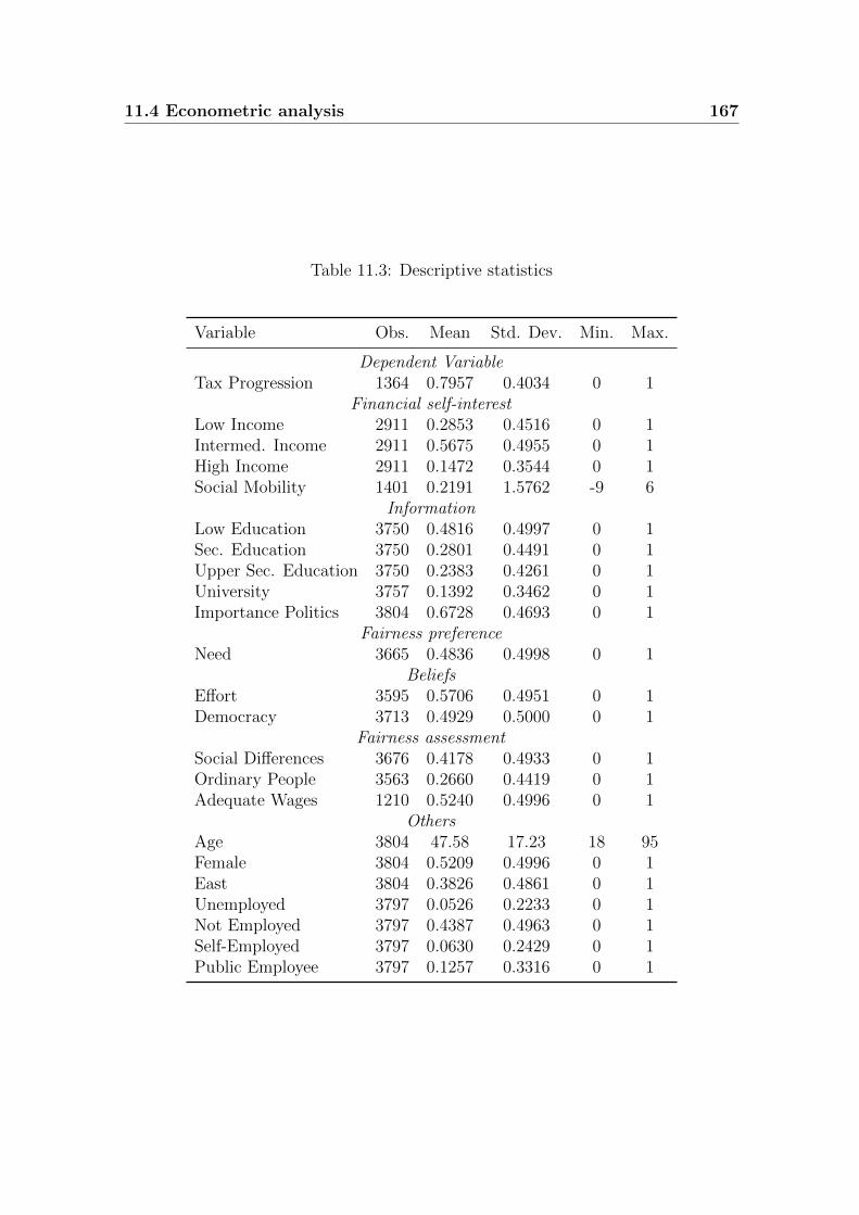
11.4 Econometric analysis 167
Table 11.3: Descriptive statistics
Variable Obs. Mean Std. Dev. Min. Max.
Dependent VariableTax Progression 1364 0.7957 0.4034 0 1
Financial self-interestLow Income 2911 0.2853 0.4516 0 1Intermed. Income 2911 0.5675 0.4955 0 1High Income 2911 0.1472 0.3544 0 1Social Mobility 1401 0.2191 1.5762 -9 6
InformationLow Education 3750 0.4816 0.4997 0 1Sec. Education 3750 0.2801 0.4491 0 1Upper Sec. Education 3750 0.2383 0.4261 0 1University 3757 0.1392 0.3462 0 1Importance Politics 3804 0.6728 0.4693 0 1
Fairness preferenceNeed 3665 0.4836 0.4998 0 1
BeliefsEffort 3595 0.5706 0.4951 0 1Democracy 3713 0.4929 0.5000 0 1
Fairness assessmentSocial Differences 3676 0.4178 0.4933 0 1Ordinary People 3563 0.2660 0.4419 0 1Adequate Wages 1210 0.5240 0.4996 0 1
OthersAge 3804 47.58 17.23 18 95Female 3804 0.5209 0.4996 0 1East 3804 0.3826 0.4861 0 1Unemployed 3797 0.0526 0.2233 0 1Not Employed 3797 0.4387 0.4963 0 1Self-Employed 3797 0.0630 0.2429 0 1Public Employee 3797 0.1257 0.3316 0 1
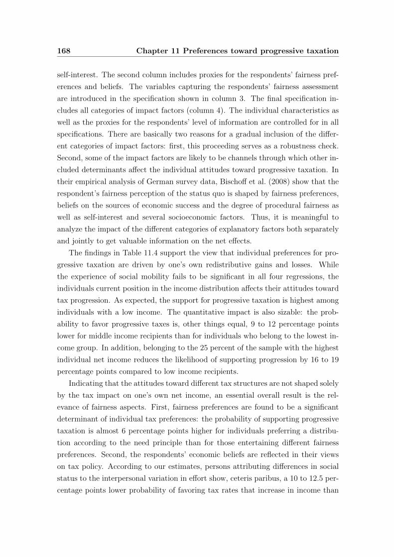
168 Chapter 11 Preferences toward progressive taxation
self-interest. The second column includes proxies for the respondents’ fairness pref-
erences and beliefs. The variables capturing the respondents’ fairness assessment
are introduced in the specification shown in column 3. The final specification in-
cludes all categories of impact factors (column 4). The individual characteristics as
well as the proxies for the respondents’ level of information are controlled for in all
specifications. There are basically two reasons for a gradual inclusion of the differ-
ent categories of impact factors: first, this proceeding serves as a robustness check.
Second, some of the impact factors are likely to be channels through which other in-
cluded determinants affect the individual attitudes toward progressive taxation. In
their empirical analysis of German survey data, Bischoff et al. (2008) show that the
respondent’s fairness perception of the status quo is shaped by fairness preferences,
beliefs on the sources of economic success and the degree of procedural fairness as
well as self-interest and several socioeconomic factors. Thus, it is meaningful to
analyze the impact of the different categories of explanatory factors both separately
and jointly to get valuable information on the net effects.
The findings in Table 11.4 support the view that individual preferences for pro-
gressive taxation are driven by one’s own redistributive gains and losses. While
the experience of social mobility fails to be significant in all four regressions, the
individuals current position in the income distribution affects their attitudes toward
tax progression. As expected, the support for progressive taxation is highest among
individuals with a low income. The quantitative impact is also sizable: the prob-
ability to favor progressive taxes is, other things equal, 9 to 12 percentage points
lower for middle income recipients than for individuals who belong to the lowest in-
come group. In addition, belonging to the 25 percent of the sample with the highest
individual net income reduces the likelihood of supporting progression by 16 to 19
percentage points compared to low income recipients.
Indicating that the attitudes toward different tax structures are not shaped solely
by the tax impact on one’s own net income, an essential overall result is the rel-
evance of fairness aspects. First, fairness preferences are found to be a significant
determinant of individual tax preferences: the probability of supporting progressive
taxation is almost 6 percentage points higher for individuals preferring a distribu-
tion according to the need principle than for those entertaining different fairness
preferences. Second, the respondents’ economic beliefs are reflected in their views
on tax policy. According to our estimates, persons attributing differences in social
status to the interpersonal variation in effort show, ceteris paribus, a 10 to 12.5 per-
centage points lower probability of favoring tax rates that increase in income than
11.4 Econometric analysis 169
Table 11.4: Determinants of German voters’ attitudes toward progressive taxation
(1) (2) (3) (4)
Financial self-interestIntermed. Income -0.1060*** -0.1293*** -0.0924** -0.1212***
(0.0329) (0.0343) (0.0365) (0.0374)High Income -0.1818*** -0.1916*** -0.1626*** -0.1850***
(0.0491) (0.0495) (0.0539) (0.0531)Social Mobility -0.0083 -0.0034 -0.0004 0.0049
(0.0080) (0.0081) (0.0088) (0.0087)Fairness preferencesNeed 0.0570** 0.0593**
(0.0253) (0.0268)BeliefsEffort -0.1270*** -0.1004***
(0.0258) (0.0298)Democracy 0.0299 0.0539*
(0.0260) (0.0282)Fairness assessmentSocial Differences -0.0593** -0.0192
(0.0287) (0.0311)Ordinary People -0.0619** -0.0755***
(0.0294) (0.0287)Adequate Wage -0.0961*** -0.0994***
(0.0276) (0.0277)InformationImportance Politics -0.0381 -0.0393 -0.0317 -0.0374
(0.0270) (0.0279) (0.0293) (0.0296)Secondary Education 0.0188 0.0232 0.0304 0.0463
(0.0322) (0.0326) (0.0347) (0.0344)Upper Sec. Education -0.0035 -0.0098 -0.0023 -0.0028
(0.0418) (0.0418) (0.0452) (0.0444)University 0.0266 -0.0002 0.0260 0.0042
(0.0453) (0.0448) (0.0480) (0.0467)Further individual characteristicsAge 0.0024** 0.0036*** 0.0041*** 0.0051***
(0.0010) (0.0011) (0.0012) (0.0012)Female -0.0130 -0.0063 -0.0082 0.0016
(0.0257) (0.0262) (0.0279) (0.0279)East 0.0346 0.0240 0.0000 0.0056
(0.0255) (0.0265) (0.0282) (0.0287)Unemployed -0.0034 -0.0113 0.0151 -0.0028
(0.0566) (0.0580) (0.0650) (0.0635)Not Employed -0.0508 -0.0600 -0.0789* -0.0825*
(0.0382) (0.0388) (0.0439) (0.0440)Self-Employed 0.0194 0.0205 0.0191 0.0145
(0.0531) (0.0525) (0.0545) (0.0528)Public Employee 0.0780** 0.0765** 0.0713* 0.0665
(0.0391) (0.0386) (0.0416) (0.0403)Regression diagnosticsPseudo R2 0.0313 0.0706 0.0677 0.1098Observations 1034 963 871 827
Notes: Probit estimates (reported are average marginal effects). */**/*** denotes significance at10%/ 5%/ 1% level.
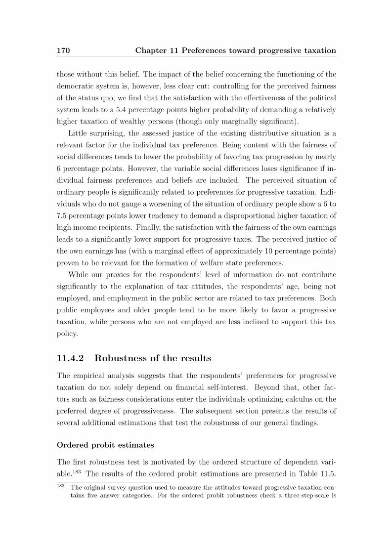
170 Chapter 11 Preferences toward progressive taxation
those without this belief. The impact of the belief concerning the functioning of the
democratic system is, however, less clear cut: controlling for the perceived fairness
of the status quo, we find that the satisfaction with the effectiveness of the political
system leads to a 5.4 percentage points higher probability of demanding a relatively
higher taxation of wealthy persons (though only marginally significant).
Little surprising, the assessed justice of the existing distributive situation is a
relevant factor for the individual tax preference. Being content with the fairness of
social differences tends to lower the probability of favoring tax progression by nearly
6 percentage points. However, the variable social differences loses significance if in-
dividual fairness preferences and beliefs are included. The perceived situation of
ordinary people is significantly related to preferences for progressive taxation. Indi-
viduals who do not gauge a worsening of the situation of ordinary people show a 6 to
7.5 percentage points lower tendency to demand a disproportional higher taxation of
high income recipients. Finally, the satisfaction with the fairness of the own earnings
leads to a significantly lower support for progressive taxes. The perceived justice of
the own earnings has (with a marginal effect of approximately 10 percentage points)
proven to be relevant for the formation of welfare state preferences.
While our proxies for the respondents’ level of information do not contribute
significantly to the explanation of tax attitudes, the respondents’ age, being not
employed, and employment in the public sector are related to tax preferences. Both
public employees and older people tend to be more likely to favor a progressive
taxation, while persons who are not employed are less inclined to support this tax
policy.
11.4.2 Robustness of the results
The empirical analysis suggests that the respondents’ preferences for progressive
taxation do not solely depend on financial self-interest. Beyond that, other fac-
tors such as fairness considerations enter the individuals optimizing calculus on the
preferred degree of progressiveness. The subsequent section presents the results of
several additional estimations that test the robustness of our general findings.
Ordered probit estimates
The first robustness test is motivated by the ordered structure of dependent vari-
able.183 The results of the ordered probit estimations are presented in Table 11.5.
183 The original survey question used to measure the attitudes toward progressive taxation con-tains five answer categories. For the ordered probit robustness check a three-step-scale is
11.4 Econometric analysis 171
The marginal effects are calculated for each of the three categories of the dependent
variable and, thus, represent the impact of the explanatory variable on the proba-
bility that an individual chooses either of these categories (i.e. prefers a tax policy
with rich people paying a higher, the same or a smaller share of their incomes in
taxes). In general, the findings are widely unaffected by the choice of the ordered
probit approach. An exception is the impact of information since both the perceived
importance of politics and the education variables are now partly significant.
Additional controls and specification of individual incomes
Table 11.6 contains the results of additional estimates including further controls184
and provides further information on the impact of the individuals’ pecuniary inter-
est. Instead of the respondents position within the income distribution, we capture
the static financial self-interest by including binary variables referring to different
net income categories. The estimates confirm that individuals with the lowest in-
come tend to be most supportive to progressive taxation. As a further robustness
check, we include additional individual control variables capturing the respondents’
job status as blue versus white collar worker and his religiosity (i.e. membership in
an institutionalized religious community). Our main results are unaffected by the
inclusion of these variables. While religiosity has no significant effect on individ-
ual attitudes toward progressive taxation, being a blue collar worker increases the
probability of preferring progressive tax rates by 11 percentage points.
exploited since we pooled the observations in the categories indicating that the rich shouldpay a smaller or much smaller share of their income in taxes as well as those related to alarger or much larger share. This is necessary because only 21 respondents state that theyprefer a regressive taxation (i.e. that the rich should compared to the poor pay a (much)smaller share of their income in taxes). An analysis including all five categories is, thus, notreasonable.
184 Descriptive statistics for all variables that are introduced in this section are presented in TableB.5 in the appendix.
172 Chapter 11 Preferences toward progressive taxationT
able
11.5
:R
obust
nes
ste
st:
order
edP
robit
esti
mat
es
hig
her
share
sam
esh
are
smaller
share
(1)
(2)
(3)
(4)
(1)
(2)
(3)
(4)
(1)
(2)
(3)
(4)
Inte
rmed
.In
com
e-0
.100
8***
-0.1
314*
**-0
.087
4**
-0.1
223*
**0.
0872
***
0.11
47**
*0.
0777
**0.
1093
***
0.01
36**
*0.
0167
***
0.00
96**
0.01
30**
*(0
.032
4)(0
.033
8)(0
.036
0)(0
.036
9)(0
.028
0)(0
.029
5)(0
.032
0)(0
.032
9)(0
.005
4)(0
.006
0)(0
.004
8)(0
.005
5)H
igh
Inco
me
-0.1
727*
**-0
.189
5***
-0.1
587*
**-0
.186
6***
0.14
95**
*0.
1654
***
0.14
12**
*0.
1667
***
0.02
32**
*0.
0241
***
0.01
75**
*0.
0199
***
(0.0
483)
(0.0
487)
(0.0
531)
(0.0
522)
(0.0
418)
(0.0
425)
(0.0
472)
(0.0
467)
(0.0
084)
(0.0
086)
(0.0
076)
(0.0
080)
Soci
alM
obil
ity
-0.0
059
-0.0
016
-0.0
002
0.00
530.
0051
0.00
140.
0002
-0.0
047
0.00
080.
0002
0-0
.000
6(0
.007
8)(0
.007
9)(0
.008
6)(0
.008
5)(0
.006
7)(0
.006
9)(0
.007
7)(0
.007
6)(0
.001
1)(0
.001
0)(0
.000
9)(0
.000
9)N
eed
0.04
93**
0.05
48**
-0.0
431*
*-0
.048
9**
-0.0
063*
*-0
.005
8**
(0.0
248)
(0.0
263)
(0.0
217)
(0.0
235)
(0.0
035)
(0.0
033)
Eff
ort
-0.1
266*
**-0
.109
0***
0.11
05**
*0.
0974
***
0.01
61**
*0.
0116
***
(0.0
253)
(0.0
293)
(0.0
221)
(0.0
262)
(0.0
051)
(0.0
046)
Dem
ocr
acy
0.03
110.
0526
*-0
.027
2-0
.047
0*-0
.004
-0.0
056*
(0.0
255)
(0.0
276)
(0.0
223)
(0.0
247)
(0.0
034)
(0.0
034)
Soci
alD
iffer
ence
s-0
.051
4*-0
.009
50.
0458
*0.
0085
0.00
57*
0.00
1(0
.028
3)(0
.030
5)(0
.025
2)(0
.027
3)(0
.003
5)(0
.003
3)O
rdin
ary
Peo
ple
-0.0
541*
-0.0
675*
*0.
0482
*0.
0603
**0.
0060
*0.
0072
**(0
.029
0)(0
.028
2)(0
.025
8)(0
.025
2)(0
.003
6)(0
.003
7)A
deq
uat
eW
age
-0.0
926*
**-0
.097
8***
0.08
24**
*0.
0874
***
0.01
02**
*0.
0104
***
(0.0
272)
(0.0
273)
(0.0
242)
(0.0
244)
(0.0
041)
(0.0
042)
Imp
orta
nce
Pol
itic
s-0
.038
8-0
.045
9*-0
.038
6-0
.048
9*0.
0336
0.04
01*
0.03
440.
0437
*0.
0052
0.00
59*
0.00
430.
0052
*(0
.026
4)(0
.027
3)(0
.028
8)(0
.029
1)(0
.022
9)(0
.023
8)(0
.025
7)(0
.026
0)(0
.003
8)(0
.003
8)(0
.003
4)(0
.003
4)S
econ
dar
yE
du
cati
on0.
0418
0.04
620.
0537
0.06
84**
-0.0
362
-0.0
403
-0.0
478
-0.0
612*
*-0
.005
6-0
.005
9-0
.005
9-0
.007
3**
(0.0
316)
(0.0
320)
(0.0
341)
(0.0
337)
(0.0
274)
(0.0
280)
(0.0
304)
(0.0
302)
(0.0
044)
(0.0
043)
(0.0
040)
(0.0
041)
Up
per
Sec
ond
ary
Ed
uca
tion
0.01
530.
0085
0.02
040.
0191
-0.0
132
-0.0
074
-0.0
182
-0.0
171
-0.0
021
-0.0
011
-0.0
022
-0.0
02(0
.040
9)(0
.040
8)(0
.044
4)(0
.043
4)(0
.035
4)(0
.035
7)(0
.039
5)(0
.038
8)(0
.005
5)(0
.005
2)(0
.004
9)(0
.004
6)U
niv
ersi
ty0.
0221
-0.0
023
0.01
73-0
.004
4-0
.019
10.
002
-0.0
154
0.00
39-0
.003
0.00
03-0
.001
90.
0005
(0.0
444)
(0.0
437)
(0.0
471)
(0.0
456)
(0.0
384)
(0.0
381)
(0.0
419)
(0.0
407)
(0.0
060)
(0.0
056)
(0.0
052)
(0.0
048)
Age
0.00
28**
*0.
0040
***
0.00
45**
*0.
0055
***
-0.0
024*
**-0
.003
5***
-0.0
040*
**-0
.004
9***
-0.0
004*
**-0
.000
5***
-0.0
005*
**-0
.000
6***
(0.0
010)
(0.0
010)
(0.0
012)
(0.0
012)
(0.0
009)
(0.0
009)
(0.0
010)
(0.0
011)
(0.0
002)
(0.0
002)
(0.0
002)
(0.0
002)
Fem
ale
-0.0
046
0.00
11-0
.000
70.
0066
0.00
4-0
.001
0.00
06-0
.005
90.
0006
-0.0
001
0.00
01-0
.000
7(0
.025
3)(0
.025
7)(0
.027
4)(0
.027
4)(0
.021
9)(0
.022
4)(0
.024
4)(0
.024
5)(0
.003
4)(0
.003
3)(0
.003
0)(0
.002
9)E
ast
0.02
510.
0143
-0.0
105
-0.0
039
-0.0
217
-0.0
124
0.00
930.
0035
-0.0
034
-0.0
018
0.00
120.
0004
(0.0
250)
(0.0
260)
(0.0
277)
(0.0
281)
(0.0
216)
(0.0
227)
(0.0
247)
(0.0
251)
(0.0
035)
(0.0
033)
(0.0
031)
(0.0
030)
Un
emp
loye
d-0
.013
1-0
.029
20.
0052
-0.0
170.
0113
0.02
54-0
.004
60.
0152
0.00
180.
0037
-0.0
006
0.00
18(0
.055
0)(0
.056
0)(0
.063
0)(0
.061
4)(0
.047
6)(0
.048
9)(0
.056
0)(0
.054
9)(0
.007
4)(0
.007
2)(0
.006
9)(0
.006
5)N
otE
mp
loye
d-0
.054
6-0
.061
5-0
.083
2*-0
.084
5*0.
0473
0.05
370.
0741
*0.
0755
*0.
0073
0.00
780.
0092
*0.
0090
*(0
.037
5)(0
.038
0)(0
.043
1)(0
.043
2)(0
.032
4)(0
.033
2)(0
.038
3)(0
.038
6)(0
.005
3)(0
.005
2)(0
.005
4)(0
.005
3)S
elf-
Em
plo
yed
0.02
420.
0274
0.02
310.
0205
-0.0
209
-0.0
239
-0.0
206
-0.0
183
-0.0
033
-0.0
035
-0.0
025
-0.0
022
(0.0
524)
(0.0
516)
(0.0
538)
(0.0
520)
(0.0
453)
(0.0
450)
(0.0
479)
(0.0
465)
(0.0
071)
(0.0
066)
(0.0
060)
(0.0
056)
Pu
bli
cE
mp
loye
e0.
0720
*0.
0725
*0.
0716
*0.
0688
*-0
.062
3*-0
.063
2*-0
.063
7*-0
.061
5*-0
.009
7*-0
.009
2*-0
.007
9*-0
.007
3*(0
.038
5)(0
.037
9)(0
.041
0)(0
.039
7)(0
.033
3)(0
.033
0)(0
.036
5)(0
.035
5)(0
.005
6)(0
.005
3)(0
.005
0)(0
.004
7)P
seu
do
R2
0.02
70.
0656
0.06
020.
1039
0.02
70.
0656
0.06
020.
1039
0.02
70.
0656
0.06
020.
1039
Ob
serv
atio
ns
1034
963
871
827
1034
963
871
827
1034
963
871
827
Note
s:O
rdere
dpro
bit
est
imate
s(r
ep
ort
ed
are
avera
ge
marg
inal
eff
ects
for
each
cate
gory
of
the
dep
endent
vari
able
).*/**/***
denote
ssi
gnifi
cance
at
10%
/5%
/1%
level.
11.4 Econometric analysis 173
Differential impact of fairness consideration for different income groups
A key result of our empirical analysis is the relevance of fairness considerations (i.e.
fairness preferences and assessments as well as beliefs) in explaining German voters’
attitudes toward progressive taxation. A possible interpretation of this finding may
be that tax rate preferences do not only reflect a person’s position in the income dis-
tribution but are also driven by fairness preferences, beliefs and the assessment of the
current distribution. It is, however, possible that fairness considerations do not have
an independent impact on tax policy preferences but are themselves a consequence
of individual financial self-interests. This is indeed suggested by the psychologi-
cal literature, which refers to a “self-serving bias” (e.g. Babcock and Loewenstein,
1997). This bias affects the perception and judgements since individuals tend to
regard an advantageous (disadvantageous) outcome as fair (unfair). Hence, the ef-
fect of fairness preferences and assessments might be driven predominantly by low
income respondents who benefit from a progressive taxation and, therefore, regard
it as fair. Likewise, mostly high income recipients might believe that effort matters
for success.
As a first descriptive test of this argument’s validity, we compare the mean
values of the fairness variables for different income groups. The first three columns
of Table 11.7 compare two subsamples with differ with regard to the respondents’
net incomes. The results suggest that the 50 percent of the individuals with the
lowest net incomes indeed significantly differ in their fairness preferences, beliefs
and assessments from the 50 percent with the highest incomes. Individuals in the
upper half of the income distribution are less likely to prefer the need principle but
are more inclined to stress the role of effort for success and to assess the social
and their own situation as fair. To check whether this result is driven by low or
high income respondents, Table 11.7 compares the respondents with the lowest as
well as highest individual net income (10th and 90th percentile) with the remaining
sample. On average, low income persons do not entertain significantly different
fairness preferences, beliefs or assessments than the other respondents. In contrast to
that, high income persons (the ten percent of the sample with the highest incomes)
are, on average, significantly more inclined to believe that effort matters and to
regard the social or their own situation as fair. In line with this, rich individuals
do less often prefer the need principle. Thus, the observable differences between
individuals in the lower and upper half of the income distribution predominantly
reflect different assessments by high income respondents.
174 Chapter 11 Preferences toward progressive taxation
Table 11.6: Robustness test: different income groups and additional control variables
(1) (2) (3)
Income 300-500 -0.0230(0.1125)
Income 500-750 -0.0646(0.1067)
Income 750-1000 -0.1791*(0.1039)
Income 1000-1250 -0.1424(0.1039)
Income 1250-1500 -0.2175**(0.1047)
Income 1500-2000 -0.1258(0.1061)
Income 2000-2500 -0.1457(0.1151)
Income 2500-3000 -0.2451**(0.1208)
Income > 3000 -0.3302***(0.1182)
Intermed. Income -0.1322*** -0.1220***(0.0375) (0.0374)
High Income -0.1722*** -0.1857***(0.0532) (0.0531)
Social Mobility 0.0061 0.0040 0.0049(0.0086) (0.0087) (0.0087)
Need 0.0585** 0.0671** 0.0608**(0.0267) (0.0269) (0.0269)
Effort -0.1008*** -0.0981*** -0.1002***(0.0297) (0.0296) (0.0298)
Democracy 0.0475* 0.0585** 0.0558*(0.0284) (0.0282) (0.0283)
Social Differences -0.0172 -0.0242 -0.0184(0.0310) (0.0310) (0.0311)
Ordinary People -0.0823*** -0.0739** -0.0751***(0.0286) (0.0286) (0.0287)
Adequate Wage -0.0980*** -0.0960*** -0.0984***(0.0276) (0.0276) (0.0277)
Importance Politics -0.0464 -0.0345 -0.0363(0.0297) (0.0295) (0.0297)
Secondary Education 0.0476 0.0612* 0.0439(0.0342) (0.0347) (0.0345)
Upper Sec. Education 0.0041 0.0218 -0.0045(0.0448) (0.0450) (0.0445)
University 0.0022 0.0129 0.0028(0.0471) (0.0462) (0.0467)
Age 0.0052*** 0.0052*** 0.0051***(0.0012) (0.0012) (0.0012)
Female -0.0082 0.0243 0.0021(0.0282) (0.0289) (0.0279)
East 0.0089 -0.0004 -0.0017(0.0285) (0.0286) (0.0308)
Unemployed 0.0011 0.0002 -0.0062(0.0639) (0.0628) (0.0636)
Not Employed -0.0859* -0.0385 -0.0825*(0.0440) (0.0465) (0.0440)
Self-Employed 0.0256 0.0544 0.0145(0.0537) (0.0541) (0.0528)
Public Employee 0.0654 0.0832** 0.0675*(0.0404) (0.0402) (0.0404)
Blue collar 0.1141***(0.0415)
Religion -0.0202(0.0314)
Pseudo R2 0.1231 0.1190 0.1103Observations 827 827 827
Notes: Probit estimates (reported are average marginal effects). */**/*** denotes significance at 10%/ 5%/1% level.
11.4 Econometric analysis 175
Tab
le11
.7:
Fai
rnes
sco
nsi
der
atio
ns
oflo
wan
dhig
hin
com
ein
div
idual
s(c
ompar
ison
ofm
ean
valu
es)
Low
inco
mes
Hig
hin
com
es
≤50
thp
erc.>
50th
per
c.<
10th
per
c.≥
10th
per
c.≥
90th
per
c.<
90th
per
c.(1
)(2
)(2
)-
(1)
(3)
(4)
(4)
-(3
)(5
)(6
)(6
)-
(5)
Nee
dM
ean
0.55
800.
4008
-0.1
572*
**0.
5256
0.48
63-0
.039
30.
3229
0.50
660.
1836
***
(Std
.Err
.)(0
.012
4)(0
.014
0)(0
.031
5)(0
.009
8)(0
.029
2)(0
.009
8)O
bs.
1593
1220
253
2560
257
2556
Eff
ort
Mea
n0.
5263
0.56
170.
0354
*0.
5766
0.53
84-0
.038
10.
621
0.53
38-0
.087
2***
(Std
.Err
.)(0
.012
6)(0
.014
2)(0
.031
4)(0
.009
9)(0
.030
3)(0
.009
9)O
bs.
1556
1214
248
2522
256
2514
Soc
ial
diff
eren
ces
Mea
n0.
3053
0.43
190.
1266
***
0.36
220.
3597
-0.0
024
0.54
290.
3417
-0.2
012*
**(S
td.E
rr.)
(0.0
114)
(0.0
141)
(0.0
302)
(0.0
094)
(0.0
311)
(0.0
093)
Obs.
1608
1220
254
2574
256
2572
Ord
inar
ype
ople
Mea
n0.
2261
0.30
220.
0761
***
0.22
350.
2625
0.03
890.
3886
0.24
63-0
.142
3***
(Std
.Err
.)(0
.010
5)(0
.013
3)(0
.026
6)(0
.008
7)(0
.031
0)(0
.008
6)O
bs.
1561
1191
246
2506
247
2505
Ade
quat
ew
age
Mea
n0.
4246
0.53
840.
1138
***
0.41
330.
4849
0.07
160.
6451
0.46
18-0
.183
2***
(Std
.Err
.)(0
.022
0)(0
.023
0)(0
.057
2)(0
.016
6)(0
.049
8)(0
.016
8)O
bs.
504
468
7589
793
879
Note
s:C
omp
aris
onof
mea
nva
lues
ofth
eva
riab
les
Need
,E
ffort
,Socia
ldif
ferences,
Ordin
ary
people
an
dA
dequate
wag
efo
rd
iffer
ent
inco
me
grou
ps.
Th
eas
sign
men
tof
ind
ivid
ual
sto
diff
eren
tin
com
egro
up
sis
base
don
thei
rin
div
idu
al
net
inco
me.
*/**/***
den
ote
ssi
gnifi
can
ceat
10%
/5%
/1%
leve
l.
176 Chapter 11 Preferences toward progressive taxation
Although this exercise suggests that financial self-interest are reflected in fairness
considerations, the question whether fairness motives have a uniform impact on in-
dividual preferences for tax progression over all income groups can only be answered
based on multivariate regressions. Thus, we interact the respondents’ income with
their fairness preferences, assessments and beliefs to check whether fairness consider-
ations affect tax policy preferences differently for high and low income individuals.185
The results presented in Table 11.8 do not support this view since none of the inter-
action terms is significant. In specification (1) to (5), a categorial variable indicating
the individual monthly net income186 is interacted with the fairness variables. The
results suggest an overall strong income effect but only individual beliefs and the
perception of an adequate payment remain significant after the inclusion of the in-
teraction terms. Since the self-serving bias might be more evident among individuals
with a very low or high income (as suggested by Table 11.7), we further interact
our fairness indicators with two binary variables equal to one for respondents be-
longing either to the ten percent of the population with the lowest (specifications
(6) to (10)) or those with the highest (specifications (11) to (15)) incomes. For
these groups fairness considerations have a stronger impact on preferences for tax
progression though without a significant difference between income groups (i.e. the
interaction effect is not significantly different from zero). Thus, fairness consider-
ations have an independent impact on individual tax rate preferences and are not
just an additional channel through which narrow redistributive self-interest drives
attitudes toward progressive taxation.
Different income types and incentives of the German tax system
In the preceding analysis individual net income has been our proxy for the immedi-
ate financial self-interest. This variable may, however, not be able to fully capture
the impact of taxation on one’s own available net income. The use of individual
incomes, for instance, ignores that the respondent might live in a household and
shares resources with other income recipients. Thus, a person who works only part-
time but lives in a high income family may be treated as a low income individual
though he actually belongs to the upper part of the income distribution. Based
185 The calculation of interaction effects in non-linear models requires some additional proceduresbecause the marginal effect of an interaction term do not provide reliable information on itssize or significance. Moreover, the interaction effect depends on the independent variables andis, hence, observation-specific (Ai and Norton, 2003). We calculate the interactions effectsby applying the procedure proposed by Ai and Norton and report average values for theinteraction effects and the standard errors.
186 This variable consists of ten income categories.
11.4 Econometric analysis 177
on this reasoning, we re-estimate our baseline regressions using the respondent’s
equivalent net income instead of his individual net income.187 Table 11.9 reports
the results. Equivalent incomes have a weaker impact on the respondents’ tax rate
preferences than individual incomes. The variable is only marginally significant (and
is insignificant if the respondent’s fairness assessment is not included) and the size
of the marginal effect is rather negligible. Part of the financial self-interest effect
now seems to be captured by the respondents’ social mobility since individuals who
experienced upward mobility tend to be significantly less supportive toward pro-
gressive tax systems. The results remain widely robust with respect to the fairness
proxies, only some individual characteristics (such as age, being not employed and
employment in the public sector) lose significance. Moreover, one proxy for the re-
spondents’ level of information, the perceived importance of politics for their life,
becomes at least partly significant.
As an additional robustness test, we include dummy variables indicating whether
the respondent is married or has own children (see specification 5). However, neither
the marital status nor the presence of children seems to be significantly related to
individual attitudes toward progressive tax systems. This result is rather surprising
since the German tax system allows a joint tax assessment for married individuals
and, thus, treats tax payers differently depending on their marital status.
From the perspective of a person who is legally married,188 the individual income
may not capture his self-interest regarding tax progression because the tax payments
are determined by the income of both spouses. A person earning a low income, for
instance, might not benefit from a progressive taxation if his or her spouse has a well
paid job. What is essential, however, is that the inclusion of these dummy variables
does not change the key results for fairness-related indicators.
187 We calculate the equivalent income to adjust the household income by the household sizeand to take economies of scale in household consumption into account. An intermediateequivalence scale is used and the equivalent income is equal to the monthly net income of thehousehold divided by the square root of the number of household members. The householdincome variable includes several unrealistically high income observations (outliers). Thus,we have applied a top-coding procedure and replaced all incomes higher than ten times themedian income by this value.
188 For tax purposes the legal marital status of an individual matters. Thus, we distinguishbetween married (including separated couples) and non-married (i.e. single, divorced andwidowed individuals).
178 Chapter 11 Preferences toward progressive taxationT
able
11.8
:R
obust
nes
ste
st:
inte
ract
ion
bet
wee
nfa
irnes
sco
nsi
der
atio
ns
and
inco
me
Fair
ness
vari
able
sin
tera
cted
wit
h...
net
inco
me
low
net
inco
me
hig
hnet
inco
me
(1)
(2)
(3)
(4)
(5)
(6)
(7)
(8)
(9)
(10)
(11)
(12)
(13)
(14)
(15)
Inco
me
-0.0
233*
**-0
.031
7***
-0.0
192*
*-0
.027
5***
-0.0
283*
**0.
087
1.12
290.
0776
0.09
790.
0694
-0.1
049*
*-0
.110
3-0
.114
7*-0
.138
8**
-0.1
860*
**(0
.008
9)(0
.011
6)(0
.009
6)(0
.008
6)(0
.010
6)(0
.082
2)(3
9.62
45)
(0.0
735)
(0.0
714)
(0.0
801)
(0.0
517)
(0.0
695)
(0.0
658)
(0.0
533)
(0.0
690)
Nee
d0.
0741
0.05
97**
0.05
37*
(0.0
736)
(0.0
277)
(0.0
287)
Nee
d×
-0.0
006
0.02
750.
0882
Inco
me
(0.0
127)
(0.0
852)
(0.0
978)
Eff
ort
-0.1
537*
*-0
.089
7***
-0.1
018*
**(0
.076
5)(0
.030
6)(0
.031
9)E
ffor
t×
0.00
17-0
.095
70.
019
Inco
me
(0.0
128)
(0.0
850)
(0.0
978)
Soci
alD
iffer
ence
s0.
0461
-0.0
319
-0.0
309
(0.0
766)
(0.0
320)
(0.0
331)
Soci
alD
iffer
ence
s×
-0.0
124
0.10
310.
0526
Inco
me
(0.0
127)
(0.0
847)
(0.0
997)
Ord
inar
yP
eop
le-0
.126
7-0
.081
6***
-0.0
980*
**(0
.077
3)(0
.029
7)(0
.030
8)O
rdin
ary
Peo
ple×
0.00
320.
1005
0.15
88In
com
e(0
.014
6)(0
.097
5)(0
.106
)A
deq
uat
eW
age
-0.1
303*
-0.1
062*
**-0
.117
3***
(0.0
734)
(0.0
285)
(0.0
295)
Ad
equ
ate
Wag
e×
-0.0
018
0.12
270.
1631
Inco
me
(0.0
129)
(0.0
851)
(0.1
103)
Pse
ud
oR
20.
1059
0.10
660.
1068
0.10
630.
1061
0.09
840.
1036
0.09
940.
0985
0.09
910.
0979
0.09
750.
0977
0.10
090.
1014
Note
s:P
robit
est
imate
s(r
ep
ort
ed
are
avera
ge
marg
inal
eff
ects
).T
he
calc
ula
tion
of
rep
ort
ed
avera
ge
inte
racti
on
eff
ects
and
the
corr
esp
ondin
gavera
ge
standard
err
ors
isbase
don
Ai
and
Nort
on
(2003).
*/**/***
denote
ssi
gnifi
cance
at
10%
/5%
/1%
level.
The
incom
euse
dfo
rth
ecalc
ula
tion
of
the
inte
racti
on
eff
ects
consi
stof
ten
cate
gori
es
indic
ati
ng
the
resp
ondents
indiv
idual
net
incom
e(n
et
incom
e,
colu
mns
(1)
to(5
))and
dum
my
vari
able
sequal
toone
ifth
ere
spondent
belo
ngs
toth
ete
np
erc
ent
wit
hth
elo
west
(low
net
incom
e,
colu
mns
(6)
to(1
0))
or
hig
hest
(hig
hnet
incom
e,
colu
mns
(11)
to(1
5))
indiv
idual
net
incom
e.
Addit
ional
vari
able
s(n
ot
show
n)
are
those
inclu
ded
inth
eb
enchm
ark
specifi
cati
on
(see
Table
11.4
,colu
mn
4).
The
regre
ssio
ns
are
base
don
827
obse
rvati
ons.
11.4 Econometric analysis 179
The analysis presented in Table 11.10 addresses this issue by dividing the sample
based on the respondents’ marital status and analyzing the determinants of tax
progression preferences separately for legally married and non-married individuals.
The results indicate that for married persons the individual income is significantly
related to their attitudes toward progressive taxation. Furthermore, the magnitude
and significance of the income effect is not affected by the inclusion of variables,
which proxy the income potential of the respondents’ partner. Attitudes toward a
progressive tax system do not differ between individuals whose partner is employed
(either full- or part-time) and those without a working spouse (irrespectively of a
person’s individual income).
The comparison of the empirical results for the two samples reveals further in-
sights on differences in attitudes toward taxation between married and non-married
individuals. The results have to be regarded with caution due to a considerable
reduction of the number of observations as a consequence of the sample split. While
preferences for the need principle and the perceived situation of ordinary people con-
tribute significantly to the explanation of tax progression preferences among non-
married individuals, they do not explain these attitudes among married persons.
Beyond that also the effects of effort and the perceived fairness of social differences
and of own wages differ between both samples. Though fairness considerations seem
to matter for both groups of respondents, the concrete effects of fairness aspects (as
well as self-interest) on individual attitudes toward progressive taxation might de-
pend strongly on the group of individuals considered and their life situation. Our
main results presented in Table 11.4 should, hence, be interpreted as an average
effect for a sample of German voters but must not apply to each single individual
or group of individuals.
Although we cannot rule out that omitted variables may drive individual financial
self-interest, fairness considerations, level of information and individual character-
istics as well as attitudes toward progressive taxation, this analysis points at the
relevance of both fairness aspects and narrow redistributive self-interest in deter-
mining preferences for different tax schemes.

180 Chapter 11 Preferences toward progressive taxation
Table 11.9: Robustness test: equivalent household incomes
(1) (2) (3) (4) (5)
Equiv. income/100 -0.0006 -0.0006 -0.0009* -0.0008* -0.0009**(0.0004) (0.0004) (0.0004) (0.0005) (0.0005)
Equiv. income2/10,000 0.0000 0.0000 0.0000* 0.0000* 0.0000*(0.0000) (0.0000) (0.0000) (0.0000) (0.0000)
Social Mobility -0.0167** -0.0130* -0.0103 -0.0070 -0.0065(0.0072) (0.0073) (0.0080) (0.0080) (0.0080)
Importance Politics -0.0404* -0.0418* -0.0416 -0.0478* -0.0492*(0.0240) (0.0251) (0.0269) (0.0276) (0.0276)
Secondary Education 0.0174 0.0196 0.0173 0.0251 0.0246(0.0283) (0.0293) (0.0311) (0.0314) (0.0314)
Upper Secondary Education -0.0055 -0.0068 -0.0345 -0.0307 -0.0293(0.0372) (0.0381) (0.0408) (0.0413) (0.0411)
University 0.0259 0.0078 0.0597 0.0420 0.0381(0.0402) (0.0405) (0.0435) (0.0434) (0.0433)
Age 0.0008 0.0014 0.0020** 0.0029*** 0.0028**(0.0008) (0.0009) (0.0010) (0.0010) (0.0011)
Female 0.0243 0.0317 0.0230 0.0316 0.0316(0.0224) (0.0229) (0.0245) (0.0248) (0.0249)
East 0.0154 0.0112 -0.0195 -0.0108 -0.0106(0.0225) (0.0235) (0.0253) (0.0261) (0.0261)
Unemployed -0.0253 -0.0192 -0.0028 -0.0050 0.0062(0.0477) (0.0492) (0.0568) (0.0562) (0.0571)
Not Employed 0.0245 0.0194 -0.0061 -0.0174 -0.0134(0.0304) (0.0312) (0.0357) (0.0362) (0.0363)
Self-Employed 0.0099 -0.0004 -0.0095 -0.0235 -0.0193(0.0444) (0.0443) (0.0460) (0.0453) (0.0455)
Public Employee 0.0603* 0.0583 0.0504 0.0490 0.0496(0.0362) (0.0363) (0.0386) (0.0383) (0.0382)
Need 0.0586** 0.0547** 0.0529**(0.0229) (0.0247) (0.0247)
Effort -0.0993*** -0.0622** -0.0593**(0.0232) (0.0271) (0.0271)
Democracy 0.0273 0.0458* 0.0436*(0.0233) (0.0257) (0.0257)
Social Differences -0.0718*** -0.0505* -0.0527*(0.0253) (0.0276) (0.0276)
Ordinary People -0.0863*** -0.1004*** -0.1020***(0.0267) (0.0265) (0.0264)
Adequate Wage -0.0858*** -0.0866*** -0.0884***(0.0250) (0.0255) (0.0255)
Married 0.0343(0.0303)
Children -0.0195(0.0346)
Pseudo R2 0.0181 0.0429 0.0634 0.0892 0.0910Observations 1310 1212 1061 1007 1006
Notes: Probit estimates (reported are average marginal effects). */**/*** denotes significance at10%/ 5%/ 1% level.
11.4 Econometric analysis 181
Table 11.10: Robustness test: sample split according to marital status
Married Single, divorced or widowed(1) (2) (3) (1) (2) (3)
Intermed. Income -0.1362*** -0.1367*** -0.1022* 0.0547(0.0513) (0.0513) (0.0592) (0.1220)
High Income -0.2002*** -0.2030*** -0.1836* -0.1072(0.0667) (0.0668) (0.1038) (0.1764)
Income -0.0262** -0.0037(0.0120) (0.0326)
Social Mobility 0.0145 0.014 0.0146 -0.004 -0.0516* -0.0555*(0.0109) (0.0109) (0.0109) (0.0144) (0.0259) (0.0272)
Need 0.0252 0.025 0.0108 0.1035** 0.1656** 0.1615**(0.0328) (0.0328) (0.0329) (0.0453) (0.0761) (0.0761)
Effort -0.1149*** -0.1140*** -0.1154*** -0.0818 -0.1191 -0.1157(0.0361) (0.0362) (0.0364) (0.0517) (0.0880) (0.0862)
Democracy 0.0504 0.0503 0.0577* 0.0603 0.0183 0.0393(0.0346) (0.0345) (0.0345) (0.0484) (0.0872) (0.0859)
Social Differences -0.0849** -0.0873** -0.0800** 0.0911 0.1274 0.1147(0.0362) (0.0362) (0.0362) (0.0562) (0.0951) (0.0957)
Ordinary People -0.0282 -0.0296 -0.0332 -0.1637*** -0.1512* -0.1457*(0.0353) (0.0353) (0.0354) (0.0480) (0.0804) (0.0821)
Adequate Wage -0.1150*** -0.1126*** -0.1069*** -0.0708 0.0476 0.0464(0.0344) (0.0345) (0.0346) (0.0479) (0.0856) (0.0859)
Importance Politics -0.0286 -0.0284 -0.0272 -0.0697 -0.1252 -0.1228(0.0361) (0.0361) (0.0362) (0.0498) (0.0912) (0.0904)
Secondary Education 0.0181 0.0195 0.0201 0.081 0.016 0.039(0.0426) (0.0428) (0.0426) (0.0576) (0.1051) (0.1056)
Upper Secondary Education -0.0536 -0.0518 -0.0335 0.0702 0.1281 0.152(0.0591) (0.0593) (0.0603) (0.0689) (0.1260) (0.1306)
University -0.006 -0.009 -0.0212 0.0753 -0.0172 -0.0326(0.0573) (0.0578) (0.0581) (0.0868) (0.1356) (0.1368)
Age 0.0049*** 0.0052*** 0.0052*** 0.0041** -0.0028 -0.0016(0.0017) (0.0018) (0.0018) (0.0020) (0.0045) (0.0044)
Female 0.007 0.0062 0.0049 -0.0126 0.0007 0.0006(0.0380) (0.0399) (0.0395) (0.0475) (0.0882) (0.0911)
East -0.0046 -0.0049 -0.004 0.007 0.0386 0.0217(0.0361) (0.0361) (0.0357) (0.0489) (0.0939) (0.0933)
Unemployed -0.0284 -0.0314 -0.0096 -0.0248 -0.1449 -0.1211(0.0790) (0.0794) (0.0781) (0.1141) (0.2486) (0.2399)
Not Employed -0.0919* -0.085 -0.0987* -0.0183 0.1225 0.0743(0.0518) (0.0524) (0.0526) (0.0894) (0.2101) (0.2005)
Self-Employed 0.0968 0.0945 0.1136 -0.1008 -0.0011 -0.0013(0.0702) (0.0701) (0.0707) (0.0835) (0.1178) (0.1220)
Public Employee 0.0974** 0.0993** 0.1094** -0.0041 0.0765 0.064(0.0489) (0.0490) (0.0498) (0.0702) (0.1153) (0.1140)
Partner: part-time worker 0.0515 0.1992(0.0528) (0.1981)
Partner: full-time worker 0.0247 0.0541 0.0417 -0.1102(0.0407) (0.0975) (0.1096) (0.2413)
Partner: full-time worker × -0.0089 0.024Income (0.0151) (0.0437)Pseudo R2 0.1526 0.1546 0.1546 0.1199 0.1941 0.1853Observations 525 525 525 301 113 113
Notes: Probit estimates (reported are average marginal effects). */**/*** denotes significance at10%/ 5%/ 1% level. Income refers to individual net incomes.
182 Chapter 11 Preferences toward progressive taxation
11.5 Conclusion
Political-economic approaches explaining the size of the welfare state are usually
based on the assumption that individuals solely apply the criterion of their own
redistributive gain or loss when they reflect on the preferred system. Thus, an
individual’s demand for redistribution should largely result from his position in the
income distribution. Our findings, however, indicate that an analysis of individual
tax preferences that focuses solely on this narrow financial calculus leaves out an
important part of the story. Individuals do not only choose the tax system that
is most beneficial to their own material advantage but fairness considerations also
play an important role. Consequently, even high income individuals may support a
tax system where they have to pay a larger share of their income in taxes than low
income earners. Especially the fairness preferences, the beliefs on the reasons for
inequality and the perceived justice of the status quo distribution contribute to the
explanation of individual heterogeneity in attitudes toward progressive taxation.
Our findings are highly relevant when it comes to the actual implementation of
tax reforms. To foster voter support for potentially growth-enhancing tax policies
(via a lower degree of tax progression), it is important to also address the fairness-
related concerns about such a reform. Focusing on fairness aspects seems to be
an essential issue for a successful selling of reforms. Especially the perception of
decreasing social justice determines the voters’ preference for a progressive taxa-
tion. Voters might support a greater degree of tax progression because they want
to reduce potentially unfair income differences which do not reflect differences in
effort. High marginal tax rates may, however, lower individual work incentives. If
individuals adjust their behavior the relevance of effort as a determinant of financial
success decreases. Hence, the perceived justice of income differences further falls and
demand for progressive taxation increases. To overcome this potential vicious circle,
politicians could, for instance, stress the relevance of industriousness for economic
success as well as the impact of incentives for individual effort. Given our results,
the belief that everybody is responsible for his own economic situation would also
increase the voters’ support for tax reforms which aim at reducing disincentives that
result from marginal tax rates increasing in income.

Chapter 12
Labor market policy preferences∗
12.1 Introduction
Highly regulated labor markets remain a challenge for many industrialized countries.
While demographic change makes a better use of the labor force highly desirable,
existing labor market institutions still entail obstacles and disincentives for employ-
ment. At the same time, attempts to enact market oriented labor market reforms are
regularly confronted with significant political resistance. The German experience in
recent years gives an example for the political problems of increasing labor market
flexibility: although many of the underlying problems of German labor market had
been well known by experts for years, the “Hartz reforms” have only been possi-
ble after a dramatic increase of unemployment. And even though these reforms
are regarded to contribute to a falling unemployment (Franz, 2006), they remain
politically contentious.
In recent years, the contrast between reform needs and observable reform ac-
tivities - which is not confined to labor market policy - has attracted increasing
academic attention. A first strand of the relevant literature explores survey data
for typical differences between expert and lay perceptions of economic phenomena
and also takes account of psychological insights (Baron and Kemp, 2004; Blendon
et al., 1997; Caplan, 2002). A second literature is based on cross-country compar-
isons and scrutinizes the country or timing specific factors which foster or block
reforms (for a survey see chapter 4 in Heinemann et al., 2008). From the latter liter-
ature a specific insight emerges with respect to labor market reforms: unlike reforms
of financial markets, product markets or foreign trade, no overall trend of market
∗ This chapter is based on a joint work with Friedrich Heinemann and Ivo Bischoff (see Heine-mann et al., 2009).
183
184 Chapter 12 Labor market policy preferences
friendly reforms has been detected for labor markets in industrialized countries over
recent decades. On this field, regulation indicators often stay constant or even in-
crease (Helbling et al., 2004). This persistence of regulation makes it desirable to
widen our understanding for the individual factors which shape the support for in-
terventionist labor market institutions and policies. Here our contribution comes in:
based on survey data we explore the drivers of labor market reform acceptance at
the individual level.
Comparable studies have been undertaken for pension reforms (Boeri et al., 2002;
Boeri and Tabellini, 2012) indicating that, besides self-interest, information and
problem awareness are major drivers of reform acceptance. An important point of
reference is the literature on the political economy of labor market regulation start-
ing with the insider-outsider-theory (Lindbeck and Snower, 1988) and advanced in
recent years by contributions such as Saint-Paul (2000), Boeri et al. (2004) and
Neugart (2008). These authors are particularly interested in understanding the
relative political attractiveness of unemployment benefits versus employment pro-
tection, given that cross-country evidence indicates that generous unemployment
benefits and rigid employment protection rules may be substitutes. Both Saint-Paul
and Boeri et al. stress the importance of individual skill levels whereas Neugart
draws the attention to the role of voters without labor market activity who depend
on within household transfers. While these labor economics approaches focus on
self-interest (i.e. a person prefers that labor market policy which guarantees him
the highest net gain) as an explanation for sticky labor market institutions. Beyond
that, our approach focuses on further explanations for labor market policy prefer-
ences such as fairness preferences or the role of beliefs about the role of effort for
economic success.
This chapter is organized as follows: in section 12.2 we present the database and
our indicators of labor market reform preferences. Section 12.3 is devoted to the
theoretical identification of factors that may explain why individuals differ in their
views on labor market reforms. We present our econometric results as well as some
robustness checks (section 12.4) and offer policy conclusions in section 12.5.
12.2 Labor market preferences of German voters
In this study, we focus on ALLBUS data, which has been collected in the years 2000
and 2006. The year-2006 wave is a particularly valuable source for the assessment of
labor market policies as it contains questions defined in the context of the Interna-
12.2 Labor market preferences of German voters 185
tional Social Survey Programme (ISSP). The questions related to the ISSP modules
“Work Orientation II” and “Role of Government IV” include items highly relevant
for the acceptance of labor market reforms.189 The content of the year-2000 wave
is less specific on labor markets but offers questions on acceptance of social benefit
cuts in general and on redistributive preferences.
This combined data set contains the following items which function as our in-
dicators for the individual preferences on labor market reforms and as dependent
variables in the subsequent regressions.190 Two questions ask for the acceptance of
benefit cuts: the one from the year-2000 wave refers to social benefits in gen-
eral, whereas the 2006-wave focuses more specifically on the acceptance of cutting
unemployment benefits. Two further questions from the year-2006 data set are
linked to the assessment of interventionist labor market policy, i.e. the support for
subsidies to declining industries and public employment programs.191
Finally, one question refers to employment protection and asks for the willingness to
accept temporary contracts in order to avoid unemployment. It has to be stressed
that this latter question is distinct from the others insofar as it does not ask for the
assessment of a political approach but for individual behavior. Lacking an alterna-
tive measure for the vividly debated point of employment protection, we include it in
our analysis. However, analytical results based on this question must be interpreted
with caution.
From the point of view of economic experts, the mentioned questions obviously
lack precision. Survey respondents can have very different ideas on the particular
design of employment programs or subsidies to declining industries. The
questions on cutting (unemployment) benefits are also far from precise with respect
to the specificities of a reform, which includes benefit cuts. In spite of these limita-
tions, the answers nevertheless reveal the individual’s tendency to support or reject
market-oriented reforms which are based on a less generous welfare state and less
government interventions.
To facilitate the interpretation, all policy preference indicators have been re-
coded into binary variables that are equal to one if the respondent is in favor of
189 ALLBUS respondents participate either in the module “Work Orientation III” or “Role ofGovernment IV”, thus, data from both modules can only be used separately. This limitationprecludes the construction of aggregate indicators of reform acceptance summarizing individ-ual positions over all policy issues.
190 A detailed description of our variables is offered in Table B.2 in the appendix.191 An earlier version of this study (see Heinemann et al., 2009) also covered the support of an
increase in the pension age. The acceptance of different pension reform options is, however,analyzed extensively in chapter 13 of this book and is, thus, not further discussed in thecontext of labor market reforms.
186 Chapter 12 Labor market policy preferences
Figure 12.1: Preferences for market oriented labor market policies
0%
10%
20%
30%
40%
50%
60%
70%
80%
Cutting social benefits Cutting unemploymentbenefits
Cutting subsidies todecling industries
Phasing outemployment programs
Liberalizing employmentprotection
liberal reform approaches (i.e. preferring a cut of benefits, supporting a cut of sub-
sidies as well as employment programs and accepting lower standards of employment
protection) and zero otherwise.
Figure 12.1 reveals that the vast majority supports interventionist labor mar-
ket policies and is skeptical on cutting benefits. Thus, the opinions of (economic)
experts are far from popular among the German population. The average accep-
tance of liberalizing reforms ranges only between 16 (phasing out of employment
programs) and 22 percent (cutting subsidies to declining industries). The only ex-
ception is the acceptance of terminable contracts which is supported by 72 percent.
However, the mentioned character of the underlying survey question indicates that
this supportive view reflects individual flexibility rather than policy preferences.
Note that the rejection rates for cutting social benefits in the year-2000 wave and
for cutting unemployment benefits in the year-2006 wave are almost the same. This
is remarkable given that in between both years substantial labor market reforms
have reduced the generosity of the system.
12.3 Potential determinants of individual labor
market policy preferences
Very different factors may explain why individuals diverge in their views on labor
market reforms. First, narrow self-interest related to individual gains and losses
from a given policy is likely to play a central role, since individuals are affected
12.3 Determinants of labor market policy preferences 187
differently by reforms depending on their economic situation. Second, individuals
have different levels of economically relevant information and entertain diverging
economic beliefs on the role of incentives, for example. Both could lead them to
different conclusions concerning the effectiveness of labor market reforms. Third,
reforms may be judged from a fairness perspective with different ideas of fairness
leading to different views on reforms.192 In this section, we discuss how different
proxies for these three (and some other) factors should influence labor market reform
acceptance. We pay particular attention to the five reform issues, which are covered
by the ALLBUS survey.
Self-interest
The idea that self-interest drives both the support for and resistance against labor
market reforms is the central creed of the political-economic view at labor market
institutions. According to a highly influential work (Lindbeck and Snower, 1988),
insiders (the employed) have an interest in labor market regulations shielding them
against wage competition by outsiders (the unemployed). This theory can explain
why democracies opt for employment protection even at the costs of raising struc-
tural unemployment as long as the median voter is employed. Saint-Paul (2000)
advances this basic idea further to explain the stability of rigid labor market insti-
tutions. He shows that unskilled workers may demand employment protection at
the costs of skilled labor and the unemployed. Boeri et al. (2004) suggests that low
skilled workers tend to favor employment protection relative to unemployment bene-
fits and that this holds in particular for countries with a compressed wage structure.
Neugart (2008) proposes that voters who are not part of the labor force and depend
on transfers from a wage earner within their household are particularly supportive
for employment protection (relative to unemployment benefits). These insights are
helpful to identify individual characteristics which approximate self-interest in the
formation of labor market policy preferences.193
192 The focus on fairness aspects considered in this study is motivated both by data availabilityand the public debate in Germany after the reforms of the ‘Agenda 2010’. Naturally, otherfactors such as altruism, solidarity or negative external effects from poverty should also con-tribute to the willingness to support redistribution for individuals who are net payers to thewelfare state. Nonetheless, the assessment of the ‘Hartz-reforms’ in Germany seems to bewidely based on the perceived justice of the income distribution.
193 Due to conceptual and data reasons our analytical approach is different to that of Boeri et al.(2004) and Neugart (2008), who study the relative support of employment protection versusunemployment benefits. Conceptually, we are keen to understand the heterogeneity of viewsat a much wider range of labor market policy issues including active labor market policies.Apart from that, data limitations preclude a direct comparison of employment protection and
188 Chapter 12 Labor market policy preferences
The appropriate identification of self-interest will differ depending on which spe-
cific aspect of labor market institutions is at stake. With respect to the level of
unemployment benefits we would clearly expect that unemployed or those with a
particular exposure to job risk oppose benefit cuts. Employment risk is related
to both job characteristics, e.g. private as opposed to public sector employment,
and individual risk factors such as low qualification. Hence, all these factors should
be negatively correlated with the support for reforms implying a cut in benefits.
Whereas the unemployed and the employed with a significant unemployment
risk should entertain similar preferences for high benefits, the insider-outsider the-
ory predicts that both groups differ in their self-interest vis-a-vis measures to protect
existing jobs.194 These measures are not confined to installing employment protec-
tion rules but also include market interventions, for instance, through subsidies for
declining industries. Because the unemployed do not benefit from this kind of initia-
tives, we expect support to be confined to workers and in particular to those whose
current job is at risk. Public employment programs are less exclusively targeted at
job insiders. Therefore, they should be welcome by unemployed and employees alike
as long as the latter’s job is endangered.
For a number of reasons, the individual income shapes the self-interest in labor
market reforms. First, income is a proxy for qualification, which in turn signals job
security since unemployment disproportionately threatens workers with low quali-
fication. Second, with increasing income interventionist labor market policies lose
their attraction because they become increasingly expensive from the individual per-
spective due to increasing contributions and taxes. Though unemployment benefits
increase with former income in the German benefit system (at least up to the contri-
bution ceiling), this effect does not outweigh the two factors named above. Hence,
the higher the income, the more likely it is that the individual is a net payer to the
welfare state. Both effects imply the same sign prediction: high income individuals
should support liberalization and benefit cuts while opposing expensive subsidies or
public employment programs.
Like income, age co-determines the self-interest in labor market reforms since
older members of the workforce tend to face a lower chance of re-employment if
they become unemployed. Thus, they should be more supportive of employment
unemployment benefit preferences for individuals since our preference proxies for these tworeform dimensions originate from non-overlapping subsamples of the 2006 ALLBUS data.
194 The overall impact of employment protection on unemployment is ambiguous since its effectis different for employed and unemployed individuals. The protection of existing jobs reducesthe flows into unemployment and, hence, protects workers. Employers anticipate this and willhire fewer workers, which lowers the re-employment opportunities of the unemployed.
12.3 Determinants of labor market policy preferences 189
protection, high unemployment benefit, subsidies for declining industries and public
employment programs. As people beyond pension age do not have a strong self-
interest in these issues, this impact of age can only be expected for respondents in
working age.
ALLBUS allows us to control for the respondents’ age, their employment sta-
tus, their subjective judgement on their unemployment risk and employment in the
public sector (see Table B.2 for precise data definitions). Beside income we also
make use of a self-employment dummy since entrepreneurs are supposed to be net-
contributors to the welfare state.
Information
Information has an impact in the context of economic policy and reform debates. In
their analysis of Italian survey data, Boeri and Tabellini (2012) find that respondents
who are more informed about the costs and functioning of the pension system are
more willing to accept reforms. We expect a similar impact of information also
in the context of market-oriented labor market reforms as well-informed and well-
educated people should have at least a rough understanding of the functioning of
labor markets.
We make use of two variables as proxies of the respondents’ degree of informa-
tion about the consequences of labor market policy reforms: first, we control for
education achievements through a dummy for a university degree. This variable
is a combined factor, which approximates not only information but also income
prospects and job market risks. Second, the participants’ assessment concerning
their degree of political information (ALLBUS 2006) or the perceived importance of
politics for their everyday life (ALLBUS 2000) is used.
Beliefs
Given that information is generally far from complete, we expect individuals to differ
in their economic beliefs. With respect to labor market policies, the belief concerning
the impact of incentives on economic effort and the impact of effort on economic
success are relevant (e.g. Alesina and Angeletos, 2005; Faravelli, 2007). The belief
that individuals are responsible for their own economic situation should lead to a
more favorable assessment of reforms targeted at fostering job search incentives such
as cuts in unemployment benefits. Similarly, interventionist policies like subsidies for
declining industries or employment programs should be less popular among people
190 Chapter 12 Labor market policy preferences
who share these beliefs.
Moreover, beliefs on the procedural fairness of the political system may influ-
ence policy (reform) preferences. Following the concept of procedural fairness, the
question of whether a certain outcome is considered fair, crucially depends on the
procedure through which it has been generated (e.g. Anand, 2001; Dolan et al.,
2007). We do not have a clear sign prediction for the impact of the procedural
beliefs on labor market reform acceptance because the perception of a fair political
procedures could legitimize both the existing institutions (e.g. the current level of
benefits) and its reforms (e.g. cutting these benefits).
The respondents’ beliefs concerning the impact of effort on economic success are
captured using dummy-variables indicating whether the respondents believe that
income differences increase the incentive for individual effort (ALLBUS 2000) and
that “the future of the people in the East depends on their will to work” (ALLBUS
2006), respectively. The assessment whether “politicians are interested in the prob-
lems of the ordinary people” is used as an indicator for the respondents’ beliefs about
procedural fairness (ALLBUS 2006). For ALLBUS 2000 we exploit information on
the participants’ beliefs concerning “the functioning of the democratic system in
Germany”.195
Fairness aspects
Labor market policies are an integrative part of welfare state policies and have a
substantial impact on the income distribution (compare the first part of this book).
Hence, fairness preferences are likely to affect the assessment of labor market re-
forms. An individual whose concept of fairness is dominated by the need principle
(i.e. an income distribution according to individual needs) will have different reform
preferences than people whose concept of fairness is dominated by the equity prin-
ciple (i.e. income distribution should reflect individual effort see e.g. Fong, 2001;
Konow, 2003), for example. This individual should be more supportive of high
unemployment benefits and interventionist labor market approaches.
Besides fairness preferences, the perceived justice of the status quo distribution
may explain different preferences for labor market policies. Individuals who are
not content with the fairness of the existing distributive outcomes should be more
inclined to support redistributive labor market policies.
195 The latter is also used in the empirical analysis of voters’ attitudes toward tax progression(chapter 11). Since ALLBUS 2006 does not include the corresponding survey question, I usea different indicator for the respondents’ belief about procedural fairness.
12.3 Determinants of labor market policy preferences 191
The preferences for the need principle are measured based on an ALLBUS 2000
question whether the respondent prefers a distributive outcome that guarantees
a “decent income even without achievement”. No comparable question has been
included in the year-2006 survey and, thus, distributive preferences can only be
employed to explain the individual assessment of social benefit cuts. The assessed
fairness of the social situation is measured using a dummy variable, which equals one
if the respondent does not perceive a worsening of the situation of ordinary people
(and is zero otherwise).
Personal characteristics
A number of personal characteristics are likely to go along with specific preferences
for labor market reforms. Some of these personal characteristics capture specific
aspects of financial self-interest, information, beliefs or fairness assessments that
cannot be observed directly, while others account for new aspects.
It is by now an established empirical fact that the history of communism has
left its marks in behavior and social preferences of Germans who were socialized
under that regime. Alesina and Fuchs-Schundeln (2007) show that, compared to
their Western German countrymen, East Germans have a stronger preference for
redistribution that cannot fully be explained by a narrow redistributive self-interest
and the simple fact that East Germans are relatively poor. Bischoff et al. (2008)
show that Eastern Germans judge the existing social differences in their country
to be less fair than their Western fellow citizens. Following these insights a specific
“GDR effect” may also have an impact on reform preferences even if our study design
allows to the control for income or job risk. We, thus, expect that socialization under
Communism implies a stronger preference for interventionist labor market policies
and welfare state generosity.
Religiosity is another personal characteristic of potential importance. Religious
people are more likely to believe that it is one’s duty to be industrious in the here
and now (e.g. Benabou and Tirole, 2006b; Tan, 2006). This may lead them to be
skeptical on generous support for the unemployed or activist employment policies.
On the other hand, they are likely to exhibit a stronger sensitivity for inequality
and other social problems (e.g. Tan, 2006) and perhaps also a moral commitment
to help the poor.196 The net effect of religiosity on the assessment of labor market
reforms is, thus, undetermined.
196 A detailed discussion of the attitude of the church regarding economic freedom is provided inVaubel (2010).
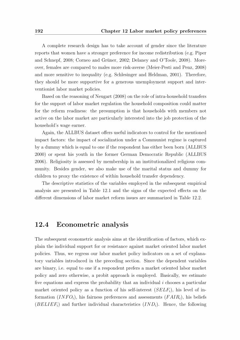
192 Chapter 12 Labor market policy preferences
A complete research design has to take account of gender since the literature
reports that women have a stronger preference for income redistribution (e.g. Piper
and Schnepf, 2008; Corneo and Gruner, 2002; Delaney and O’Toole, 2008). More-
over, females are compared to males more risk-averse (Meier-Pesti and Penz, 2008)
and more sensitive to inequality (e.g. Schlesinger and Heldman, 2001). Therefore,
they should be more supportive for a generous unemployment support and inter-
ventionist labor market policies.
Based on the reasoning of Neugart (2008) on the role of intra-household transfers
for the support of labor market regulation the household composition could matter
for the reform readiness: the presumption is that households with members not
active on the labor market are particularly interested into the job protection of the
household’s wage earner.
Again, the ALLBUS dataset offers useful indicators to control for the mentioned
impact factors: the impact of socialization under a Communist regime is captured
by a dummy which is equal to one if the respondent has either been born (ALLBUS
2000) or spent his youth in the former German Democratic Republic (ALLBUS
2006). Religiosity is assessed by membership in an institutionalized religious com-
munity. Besides gender, we also make use of the marital status and dummy for
children to proxy the existence of within household transfer dependency.
The descriptive statistics of the variables employed in the subsequent empirical
analysis are presented in Table 12.1 and the signs of the expected effects on the
different dimensions of labor market reform issues are summarized in Table 12.2.
12.4 Econometric analysis
The subsequent econometric analysis aims at the identification of factors, which ex-
plain the individual support for or resistance against market oriented labor market
policies. Thus, we regress our labor market policy indicators on a set of explana-
tory variables introduced in the preceding section. Since the dependent variables
are binary, i.e. equal to one if a respondent prefers a market oriented labor market
policy and zero otherwise, a probit approach is employed. Basically, we estimate
five equations and express the probability that an individual i chooses a particular
market oriented policy as a function of his self-interest (SELFi), his level of in-
formation (INFOi), his fairness preferences and assessments (FAIRi), his beliefs
(BELIEFi) and further individual characteristics (INDi). Hence, the following
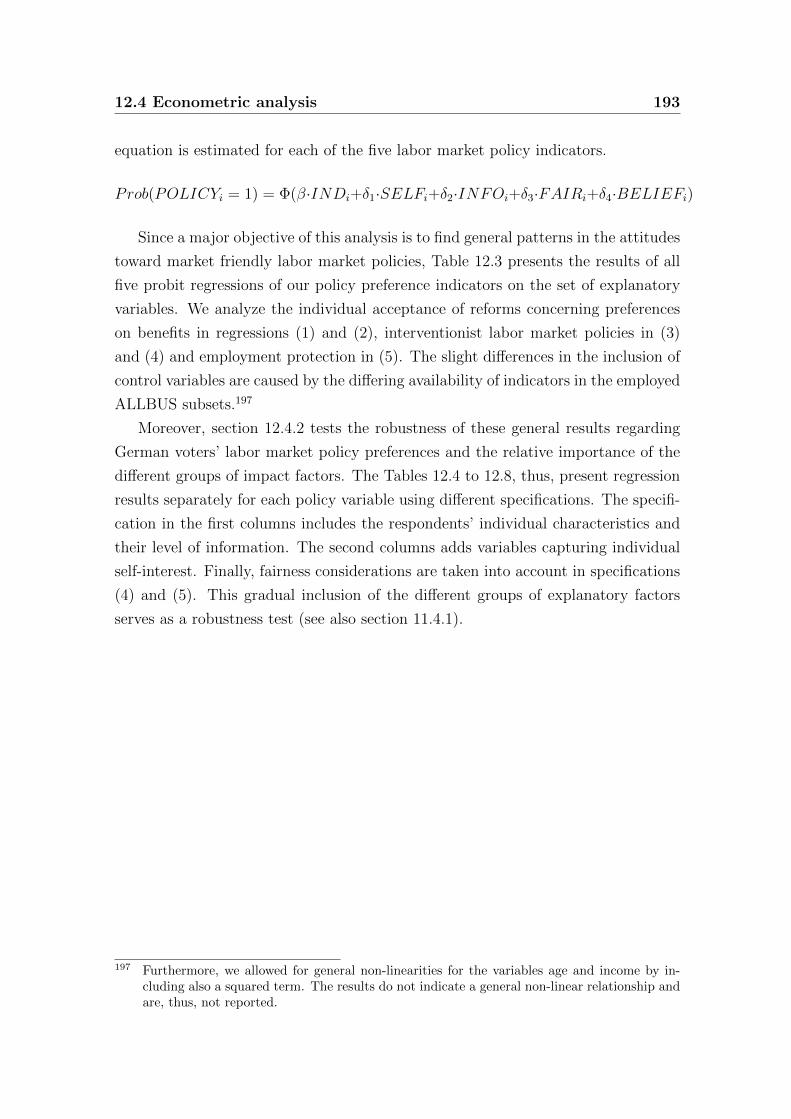
12.4 Econometric analysis 193
equation is estimated for each of the five labor market policy indicators.
Prob(POLICYi = 1) = Φ(β·INDi+δ1·SELFi+δ2·INFOi+δ3·FAIRi+δ4·BELIEFi)
Since a major objective of this analysis is to find general patterns in the attitudes
toward market friendly labor market policies, Table 12.3 presents the results of all
five probit regressions of our policy preference indicators on the set of explanatory
variables. We analyze the individual acceptance of reforms concerning preferences
on benefits in regressions (1) and (2), interventionist labor market policies in (3)
and (4) and employment protection in (5). The slight differences in the inclusion of
control variables are caused by the differing availability of indicators in the employed
ALLBUS subsets.197
Moreover, section 12.4.2 tests the robustness of these general results regarding
German voters’ labor market policy preferences and the relative importance of the
different groups of impact factors. The Tables 12.4 to 12.8, thus, present regression
results separately for each policy variable using different specifications. The specifi-
cation in the first columns includes the respondents’ individual characteristics and
their level of information. The second columns adds variables capturing individual
self-interest. Finally, fairness considerations are taken into account in specifications
(4) and (5). This gradual inclusion of the different groups of explanatory factors
serves as a robustness test (see also section 11.4.1).
197 Furthermore, we allowed for general non-linearities for the variables age and income by in-cluding also a squared term. The results do not indicate a general non-linear relationship andare, thus, not reported.
194 Chapter 12 Labor market policy preferences
Table 12.1: Descriptive statistics
Variable Mean Std.Dev. Obs.
ALLBUS 2000Cutting social benefits 0.176 0.381 2874Age 47.639 17.283 3804Income 4.923 2.229 2911Insecure 0.079 0.27 3797Unemployed 0.067 0.249 3797Civil servant 0.037 0.189 3797Self-employed 0.062 0.241 3797University 0.14 0.347 3757Politically informed 0.658 0.474 3804Need 0.496 0.5 3665Ordinary People 0.75 0.433 3563Effort 0.604 0.489 3576Democracy 0.443 0.497 3713East 0.501 0.5 3804Religion 0.669 0.471 3778Female 0.52 0.5 3804Married 0.607 0.489 3796Children 0.71 0.454 3804
ALLBUS 2006Cutting unemployment benefits 0.181 0.385 1571Cutting subsidies to declining industries 0.222 0.416 1547Phasing out employment programs 0.159 0.366 1549Liberalizing employment protection 0.722 0.448 879Age 49.332 17.233 3413Income 1249.878 872.286 2644Insecure 0.075 0.263 3418Unemployed 0.079 0.27 3418Civil servant 0.031 0.173 3418Self-employed 0.058 0.234 3418University 0.154 0.361 3381Politically informed 0.435 0.496 1566Ordinary people 0.864 0.343 3319Effort 0.687 0.464 3199Procedural fairness 0.176 0.381 3275East 0.378 0.485 3022Female 0.516 0.5 3421Religion 0.665 0.472 3404Married 0.596 0.491 3417Children 0.723 0.448 3403
12.4 Econometric analysis 195
Table 12.2: Sign expectations
Support for (+) / resistance against (-)...Cutting Cutting Phasing out Liberalisingbenefits1 subsidies to employment employment
declining programs protectionindustries
Umemployed - + - +Job risk - - - -Income + + + +Age∗ - - -Information + + + +Preference:
-need principlePrinciple of distributionBelief: self-responsibility + + +Belief: functioning ? ? ? ?democracyPerception:situation ordinary people - - - -East Germany - - - -Religious ? ? ? ?Female - - - -Children/ Married ? - - -
1 Applies to unemployment and social benefits.∗ Sign of expected age effect is limited to individuals in employment age.
12.4.1 Main results
Our findings regarding the impact factors of general labor market policy preferences
are presented in Table 12.3. A first overall insight from the regressions is that indi-
vidual labor market reform preferences are clearly shaped by self-interest. A larger
income is associated with a stronger support for market oriented reforms; only in
the case of employment protection preferences the coefficient misses significance.198
Unemployment increases the resistance against cuts in payments strongly. Similarly,
we find that the perception of a high unemployment risk significantly fosters the re-
sistance against unemployment benefit cuts. These results indicate that pecuniary
interests are a major impact factor for individual labor market reform preferences.
We also find some support for the insider-outsider-theory. As explained in section
198 To consider a possible impact of personal wealth we also included a dummy-variable equal toone for individuals living in a self-owned house or flat. Since this variable has found to be notsignificant, the results are not reported.
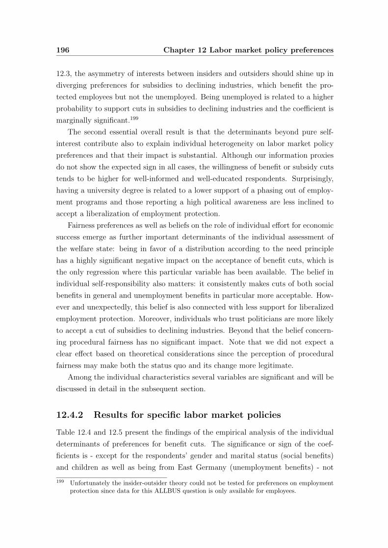
196 Chapter 12 Labor market policy preferences
12.3, the asymmetry of interests between insiders and outsiders should shine up in
diverging preferences for subsidies to declining industries, which benefit the pro-
tected employees but not the unemployed. Being unemployed is related to a higher
probability to support cuts in subsidies to declining industries and the coefficient is
marginally significant.199
The second essential overall result is that the determinants beyond pure self-
interest contribute also to explain individual heterogeneity on labor market policy
preferences and that their impact is substantial. Although our information proxies
do not show the expected sign in all cases, the willingness of benefit or subsidy cuts
tends to be higher for well-informed and well-educated respondents. Surprisingly,
having a university degree is related to a lower support of a phasing out of employ-
ment programs and those reporting a high political awareness are less inclined to
accept a liberalization of employment protection.
Fairness preferences as well as beliefs on the role of individual effort for economic
success emerge as further important determinants of the individual assessment of
the welfare state: being in favor of a distribution according to the need principle
has a highly significant negative impact on the acceptance of benefit cuts, which is
the only regression where this particular variable has been available. The belief in
individual self-responsibility also matters: it consistently makes cuts of both social
benefits in general and unemployment benefits in particular more acceptable. How-
ever and unexpectedly, this belief is also connected with less support for liberalized
employment protection. Moreover, individuals who trust politicians are more likely
to accept a cut of subsidies to declining industries. Beyond that the belief concern-
ing procedural fairness has no significant impact. Note that we did not expect a
clear effect based on theoretical considerations since the perception of procedural
fairness may make both the status quo and its change more legitimate.
Among the individual characteristics several variables are significant and will be
discussed in detail in the subsequent section.
12.4.2 Results for specific labor market policies
Table 12.4 and 12.5 present the findings of the empirical analysis of the individual
determinants of preferences for benefit cuts. The significance or sign of the coef-
ficients is - except for the respondents’ gender and marital status (social benefits)
and children as well as being from East Germany (unemployment benefits) - not
199 Unfortunately the insider-outsider theory could not be tested for preferences on employmentprotection since data for this ALLBUS question is only available for employees.

12.4 Econometric analysis 197
sensitive to choice of the specification.
The empirical analysis points at a strong effect of pecuniary interest for a person’s
attitudes toward benefit cuts: individuals who are or expect to be net recipients of
these benefits oppose their reduction, while net payers (high income recipients) sup-
port benefit cuts. Being unemployed reduces the probability of supporting a cut of
social (unemployment) benefits by 16 to 18 (12) percentage points. The assessment
of a reduction of unemployment benefits is also significantly opposed by persons who
fear a job loss and, thus, the reliance on unemployment benefits in the near future.
The impact of having an insecure job is with a marginal effect of approximately
15 percentage points also sizable. In addition, self-employed respondents entertain
a significantly stronger preference for social but not unemployment benefit cuts,
while older respondents are less inclined to support a reduction of benefits for the
unemployed.
198 Chapter 12 Labor market policy preferencesT
able
12.3
:D
eter
min
ants
ofla
bor
mar
ket
pol
icy
pre
fere
nce
s
Cu
ttin
gC
utt
ing
Cutt
ing
sub
sid
ies
Ph
asi
ng
ou
tL
iber
ali
zin
gso
cial
ben
efits
un
emp
loym
ent
ben
efits
tod
ecli
nin
gin
du
stri
esem
plo
ym
ent
pro
gra
ms
emp
loym
ent
pro
tect
ion
(1)
(2)
(3)
(4)
(5)
Sel
f-in
tere
stA
ge-0
.000
7-0
.003
4***
0.0
013
0.0
003
-0.0
040**
(0.0
006)
(0.0
008)
(0.0
009)
(0.0
008)
(0.0
018)
Inco
me
0.01
39**
*0.
0001
***
0.0
001***
0.0
001***
0(0
.004
1)(0
.0000)
(0.0
000)
(0.0
000)
(0.0
000)
Inse
cure
-0.0
355
-0.1
571***
-0.0
069
-0.0
602
0.0
645
(0.0
315)
(0.0
499)
(0.0
470)
(0.0
470)
(0.0
557)
Un
emp
loye
d-0
.164
9***
-0.1
259**
0.0
799*
0.0
113
(0.0
565)
(0.0
559)
(0.0
479)
(0.0
458)
Civ
ilse
rvan
t-0
.054
4-0
.0766
-0.1
242**
-0.0
305
-0.0
732
(0.0
363)
(0.0
591)
(0.0
629)
(0.0
604)
(0.0
743)
Sel
f-em
plo
yed
0.09
79**
*-0
.03
0.0
34
-0.0
059
-0.0
401
(0.0
282)
(0.0
475)
(0.0
518)
(0.0
500)
(0.0
611)
Info
rmati
on
Un
iver
sity
0.05
44**
-0.0
022
0.1
109***
-0.0
744**
0.0
688
(0.0
223)
(0.0
340)
(0.0
344)
(0.0
364)
(0.0
554)
Pol
itic
ally
info
rmed
-0.0
052
-0.0
091
0.1
019***
0.0
357
-0.0
638*
(0.0
183)
(0.0
242)
(0.0
248)
(0.0
238)
(0.0
373)
Fair
nes
spre
fere
nce
san
dass
essm
ent
Nee
d-0
.093
8***
(0.0
165)
Ord
inar
yp
eop
le-0
.010
2-0
.120
8***
-0.0
155
-0.0
475
-0.0
355
(0.0
176)
(0.0
321)
(0.0
371)
(0.0
346)
(0.0
555)
Con
tin
ued
on
nex
tpa
ge
12.4 Econometric analysis 199T
able
12.3
–co
nti
nu
edfr
om
pre
vio
us
page
Cu
ttin
gC
utt
ing
Cutt
ing
sub
sid
ies
Ph
asi
ng
ou
tL
iber
ali
zin
gso
cial
ben
efits
un
emp
loym
ent
ben
efits
tod
ecli
nin
gin
du
stri
esem
plo
ym
ent
pro
gra
ms
emp
loym
ent
pro
tect
ion
(1)
(2)
(3)
(4)
(5)
Bel
iefs
Eff
ort
0.06
81**
*0.
0753
***
0.0
178
0.0
274
-0.0
734*
(0.0
172)
(0.0
258)
(0.0
265)
(0.0
250)
(0.0
385)
Pro
ced
ura
lfa
irn
ess
0.01
16-0
.0153
0.1
025***
0.0
20.0
803
(0.0
166)
(0.0
309)
(0.0
319)
(0.0
310)
(0.0
506)
Indiv
idu
al
chara
cter
isti
csE
ast
-0.0
728*
**-0
.0368
-0.0
602*
0.0
027
-0.0
141
(0.0
186)
(0.0
304)
(0.0
329)
(0.0
302)
(0.0
462)
Rel
igio
n0.
0626
***
0.03
06
-0.1
216***
-0.0
073
-0.0
355
(0.0
200)
(0.0
293)
(0.0
304)
(0.0
287)
(0.0
437)
Fem
ale
-0.0
070.
0035
-0.0
331
-0.0
249
0.0
931**
(0.0
177)
(0.0
253)
(0.0
268)
(0.0
252)
(0.0
398)
Mar
ried
0.01
530.
0002
0.0
047
0.0
208
-0.0
108
(0.0
192)
(0.0
274)
(0.0
297)
(0.0
278)
(0.0
424)
Ch
ild
ren
-0.0
109
-0.0
159
-0.0
123
-0.0
444
0.0
096
(0.0
222)
(0.0
306)
(0.0
336)
(0.0
305)
(0.0
474)
Reg
ress
ion
dia
gnost
ics
Pse
ud
oR
20.
1198
0.10
47
0.1
281
0.0
403
0.0
525
Ob
serv
atio
ns
2019
1003
999
997
614
Note
s:P
rob
ites
tim
ates
(rep
orte
dar
eav
erag
em
argi
nal
effec
ts).
*/**/***
den
ote
ssi
gn
ifica
nce
at
10%
/5%
/1%
level
.
200 Chapter 12 Labor market policy preferences
Besides self-interest, the respondents’ level of education is significantly related
to their attitudes toward social but not unemployment benefits. Respondents with
a university degree show a 5 to 8 percentage points higher inclination to support a
reduction of social benefit payments.
Fairness aspects further contribute to the explanation of the individual hetero-
geneity in benefit preferences. On the one hand, the belief that income differences
increase work incentives is related to an about 7 percentage points higher likelihood
to support lower social or unemployment benefits. On the other hand, persons who
prefer a distribution according to the need principle show a 9.4 percentage points
lower inclination to agree with social benefit cuts. While the assessment of the
situation of ordinary people does not significantly explain support for social ben-
efit cuts, individuals who perceive a worsening of the situation of ordinary people
show a 12 percentage points lower probability of supporting a reduction of unem-
ployment transfers.200 The impact of individual characteristics differs somewhat for
the assessment of social and unemployment benefits. The membership in an in-
stitutionalized religious community is related to a 6 to 7 percentage points higher
probability to support a reduction of social benefits but has no impact on the assess-
ment of unemployment benefits. Persons from the former GDR show a significant
lower inclination to support a cut in social benefits, while the stronger resistance
of East Germans against lower benefits for the unemployed diminish if fairness con-
siderations are taken into account. This may indicate that different welfare state
preferences of East and West Germans reflect at least partly differential fairness
motives (a possible explanation for this is offered in chapter 14).
In contrast to the assessment of benefit cuts, pecuniary self-interests are less
relevant for individual preferences for policy interventions into labor market. The
support for a cut of subsidies to declining industries and a phasing out of employment
programs increases in the individual’s income and, hence, tax payments. The interest
of civil servants in maintaining subsidies might reflect a bureaucratic interest. A
further self-interest related factor is the respondents’ age as the individual willingness
to accept a terminable contract decreases for older persons.
200 The differences in the impact of the assessed fairness of the situation of ordinary people onpreferences for social and unemployment benefits may partly be driven by the inclusion offairness preferences. The highly significant effect of fairness assessment for unemploymentbenefits might to some extent also reflect different fairness preferences.
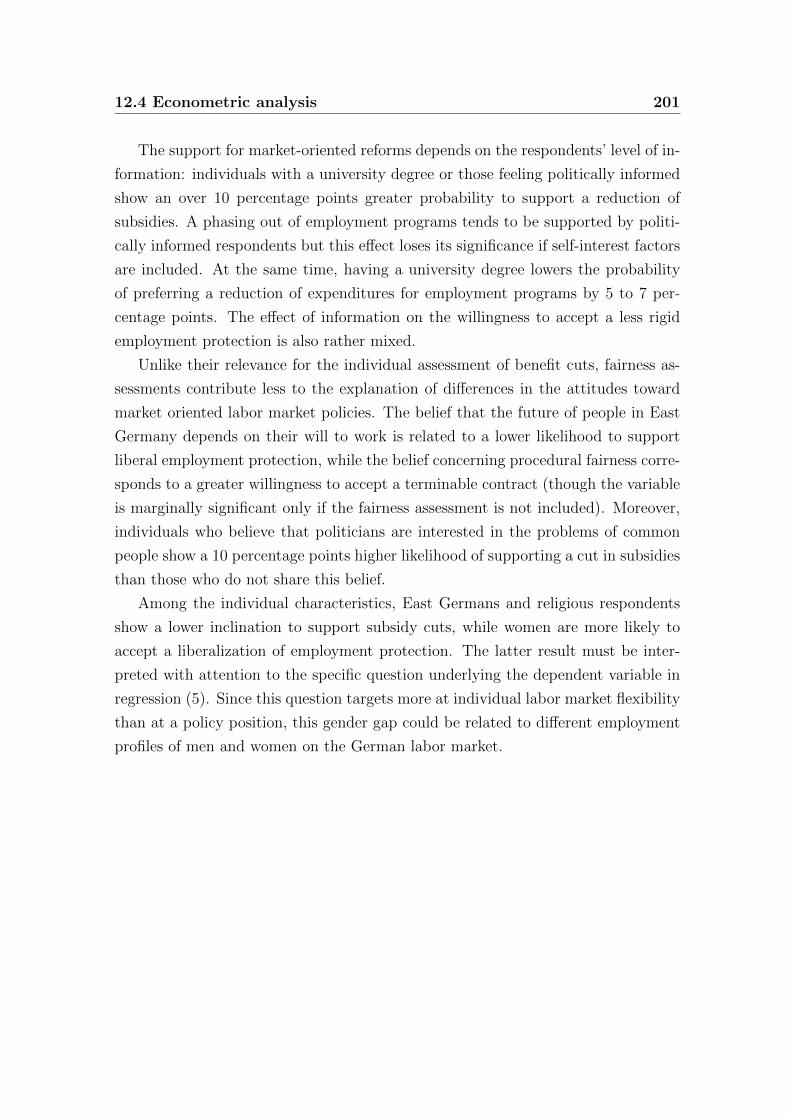
12.4 Econometric analysis 201
The support for market-oriented reforms depends on the respondents’ level of in-
formation: individuals with a university degree or those feeling politically informed
show an over 10 percentage points greater probability to support a reduction of
subsidies. A phasing out of employment programs tends to be supported by politi-
cally informed respondents but this effect loses its significance if self-interest factors
are included. At the same time, having a university degree lowers the probability
of preferring a reduction of expenditures for employment programs by 5 to 7 per-
centage points. The effect of information on the willingness to accept a less rigid
employment protection is also rather mixed.
Unlike their relevance for the individual assessment of benefit cuts, fairness as-
sessments contribute less to the explanation of differences in the attitudes toward
market oriented labor market policies. The belief that the future of people in East
Germany depends on their will to work is related to a lower likelihood to support
liberal employment protection, while the belief concerning procedural fairness corre-
sponds to a greater willingness to accept a terminable contract (though the variable
is marginally significant only if the fairness assessment is not included). Moreover,
individuals who believe that politicians are interested in the problems of common
people show a 10 percentage points higher likelihood of supporting a cut in subsidies
than those who do not share this belief.
Among the individual characteristics, East Germans and religious respondents
show a lower inclination to support subsidy cuts, while women are more likely to
accept a liberalization of employment protection. The latter result must be inter-
preted with attention to the specific question underlying the dependent variable in
regression (5). Since this question targets more at individual labor market flexibility
than at a policy position, this gender gap could be related to different employment
profiles of men and women on the German labor market.
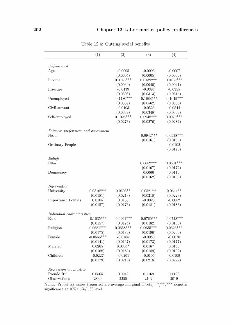
202 Chapter 12 Labor market policy preferences
Table 12.4: Cutting social benefits
(1) (2) (3) (4)
Self-interestAge -0.0005 -0.0006 -0.0007
(0.0005) (0.0005) (0.0006)Income 0.0143*** 0.0139*** 0.0139***
(0.0039) (0.0040) (0.0041)Insecure -0.0439 -0.0394 -0.0355
(0.0303) (0.0313) (0.0315)Unemployed -0.1780*** -0.1688*** -0.1649***
(0.0539) (0.0562) (0.0565)Civil servant -0.0403 -0.0523 -0.0544
(0.0339) (0.0348) (0.0363)Self-employed 0.1026*** 0.0948*** 0.0979***
(0.0273) (0.0276) (0.0282)
Fairness preferences and assessmentNeed -0.0942*** -0.0938***
(0.0161) (0.0165)Ordinary People -0.0102
(0.0176)
BeliefsEffort 0.0652*** 0.0681***
(0.0167) (0.0172)Democracy 0.0066 0.0116
(0.0162) (0.0166)
InformationUniversity 0.0810*** 0.0503** 0.0521** 0.0544**
(0.0181) (0.0213) (0.0218) (0.0223)Importance Politics 0.0105 0.0133 -0.0023 -0.0052
(0.0157) (0.0173) (0.0181) (0.0183)
Individual characteristicsEast -0.1035*** -0.0961*** -0.0760*** -0.0728***
(0.0157) (0.0174) (0.0182) (0.0186)Religion 0.0681*** 0.0658*** 0.0635*** 0.0626***
(0.0175) (0.0189) (0.0196) (0.0200)Female -0.0565*** -0.0165 -0.0080 -0.0070
(0.0141) (0.0167) (0.0173) (0.0177)Married 0.0265 0.0304* 0.0167 0.0153
(0.0168) (0.0183) (0.0189) (0.0192)Children -0.0227 -0.0201 -0.0106 -0.0109
(0.0179) (0.0210) (0.0218) (0.0222)
Regression diagnosticsPseudo R2 0.0565 0.0949 0.1169 0.1198Observations 2839 2255 2102 2019
Notes: Probit estimates (reported are average marginal effects). */**/*** denotessignificance at 10%/ 5%/ 1% level.
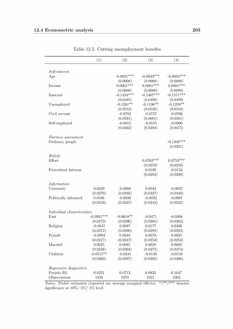
12.4 Econometric analysis 203
Table 12.5: Cutting unemployment benefits
(1) (2) (3) (4)
Self-interestAge -0.0031*** -0.0033*** -0.0034***
(0.0008) (0.0008) (0.0008)Income 0.0001*** 0.0001*** 0.0001***
(0.0000) (0.0000) (0.0000)Insecure -0.1434*** -0.1467*** -0.1571***
(0.0485) (0.0490) (0.0499)Unemployed -0.1201** -0.1196** -0.1259**
(0.0552) (0.0556) (0.0559)Civil servant -0.0782 -0.0757 -0.0766
(0.0591) (0.0601) (0.0591)Self-employed -0.0015 -0.0185 -0.0300
(0.0462) (0.0483) (0.0475)
Fairness assessmentOrdinary people -0.1208***
(0.0321)
BeliefsEffort 0.0763*** 0.0753***
(0.0259) (0.0258)Procedural fairness 0.0199 -0.0153
(0.0293) (0.0309)
InformationUniversity 0.0429 -0.0008 0.0034 -0.0022
(0.0279) (0.0330) (0.0337) (0.0340)Politically informed 0.0106 -0.0039 -0.0032 -0.0091
(0.0216) (0.0237) (0.0243) (0.0242)
Individual characteristicsEast -0.0931*** -0.0618** -0.0471 -0.0368
(0.0272) (0.0296) (0.0305) (0.0304)Religion -0.0047 0.0097 0.0177 0.0306
(0.0272) (0.0286) (0.0292) (0.0293)Female -0.0094 0.0045 0.0078 0.0035
(0.0217) (0.0247) (0.0253) (0.0253)Married 0.0045 0.0085 0.0028 0.0002
(0.0248) (0.0268) (0.0275) (0.0274)Children -0.0515** -0.0245 -0.0150 -0.0159
(0.0260) (0.0297) (0.0305) (0.0306)
Regression diagnosticsPseudo R2 0.0221 0.0713 0.0833 0.1047Observations 1328 1070 1021 1003
Notes: Probit estimates (reported are average marginal effects). */**/*** denotessignificance at 10%/ 5%/ 1% level.
204 Chapter 12 Labor market policy preferences
Table 12.6: Cutting subsidies to declining industries
(1) (2) (3) (4)
Self-interestAge 0.0010 0.0013 0.0013
(0.0008) (0.0009) (0.0009)Income 0.0001*** 0.0001*** 0.0001***
(0.0000) (0.0000) (0.0000)Insecure -0.0261 -0.0103 -0.0069
(0.0462) (0.0468) (0.0470)Unemployed 0.0655 0.0769 0.0799*
(0.0476) (0.0479) (0.0479)Civil servant -0.1018* -0.1226* -0.1242**
(0.0609) (0.0627) (0.0629)Self-employed 0.0245 0.0361 0.0340
(0.0504) (0.0517) (0.0518)
Fairness assessmentOrdinary people -0.0155
(0.0371)
BeliefsEffort 0.0225 0.0178
(0.0263) (0.0265)Procedural fairness 0.1044*** 0.1025***
(0.0304) (0.0319)
InformationUniversity 0.1737*** 0.1279*** 0.1153*** 0.1109***
(0.0261) (0.0325) (0.0335) (0.0344)Politically informed 0.1146*** 0.1126*** 0.1024*** 0.1019***
(0.0215) (0.0239) (0.0246) (0.0248)
Individual characteristicsEast -0.1041*** -0.0721** -0.0583* -0.0602*
(0.0281) (0.0315) (0.0325) (0.0329)Female -0.0904*** -0.0328 -0.0364 -0.0331
(0.0219) (0.0258) (0.0264) (0.0268)Married -0.0173 -0.0020 0.0001 0.0047
(0.0260) (0.0285) (0.0293) (0.0297)Religion -0.1214*** -0.1218*** -0.1261*** -0.1216***
(0.0274) (0.0295) (0.0299) (0.0304)Children 0.0229 -0.0073 -0.0059 -0.0123
(0.0277) (0.0321) (0.0331) (0.0336)
Regression diagnosticsPseudo R2 0.0992 0.1219 0.1286 0.1281Observations 1325 1066 1017 999
Notes: Probit estimates (reported are average marginal effects). */**/*** denotessignificance at 10%/ 5%/ 1% level.
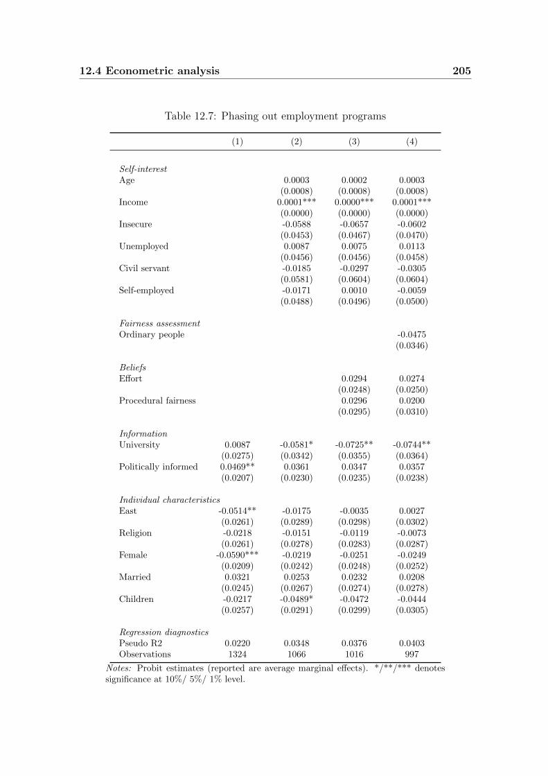
12.4 Econometric analysis 205
Table 12.7: Phasing out employment programs
(1) (2) (3) (4)
Self-interestAge 0.0003 0.0002 0.0003
(0.0008) (0.0008) (0.0008)Income 0.0001*** 0.0000*** 0.0001***
(0.0000) (0.0000) (0.0000)Insecure -0.0588 -0.0657 -0.0602
(0.0453) (0.0467) (0.0470)Unemployed 0.0087 0.0075 0.0113
(0.0456) (0.0456) (0.0458)Civil servant -0.0185 -0.0297 -0.0305
(0.0581) (0.0604) (0.0604)Self-employed -0.0171 0.0010 -0.0059
(0.0488) (0.0496) (0.0500)
Fairness assessmentOrdinary people -0.0475
(0.0346)
BeliefsEffort 0.0294 0.0274
(0.0248) (0.0250)Procedural fairness 0.0296 0.0200
(0.0295) (0.0310)
InformationUniversity 0.0087 -0.0581* -0.0725** -0.0744**
(0.0275) (0.0342) (0.0355) (0.0364)Politically informed 0.0469** 0.0361 0.0347 0.0357
(0.0207) (0.0230) (0.0235) (0.0238)
Individual characteristicsEast -0.0514** -0.0175 -0.0035 0.0027
(0.0261) (0.0289) (0.0298) (0.0302)Religion -0.0218 -0.0151 -0.0119 -0.0073
(0.0261) (0.0278) (0.0283) (0.0287)Female -0.0590*** -0.0219 -0.0251 -0.0249
(0.0209) (0.0242) (0.0248) (0.0252)Married 0.0321 0.0253 0.0232 0.0208
(0.0245) (0.0267) (0.0274) (0.0278)Children -0.0217 -0.0489* -0.0472 -0.0444
(0.0257) (0.0291) (0.0299) (0.0305)
Regression diagnosticsPseudo R2 0.0220 0.0348 0.0376 0.0403Observations 1324 1066 1016 997
Notes: Probit estimates (reported are average marginal effects). */**/*** denotessignificance at 10%/ 5%/ 1% level.
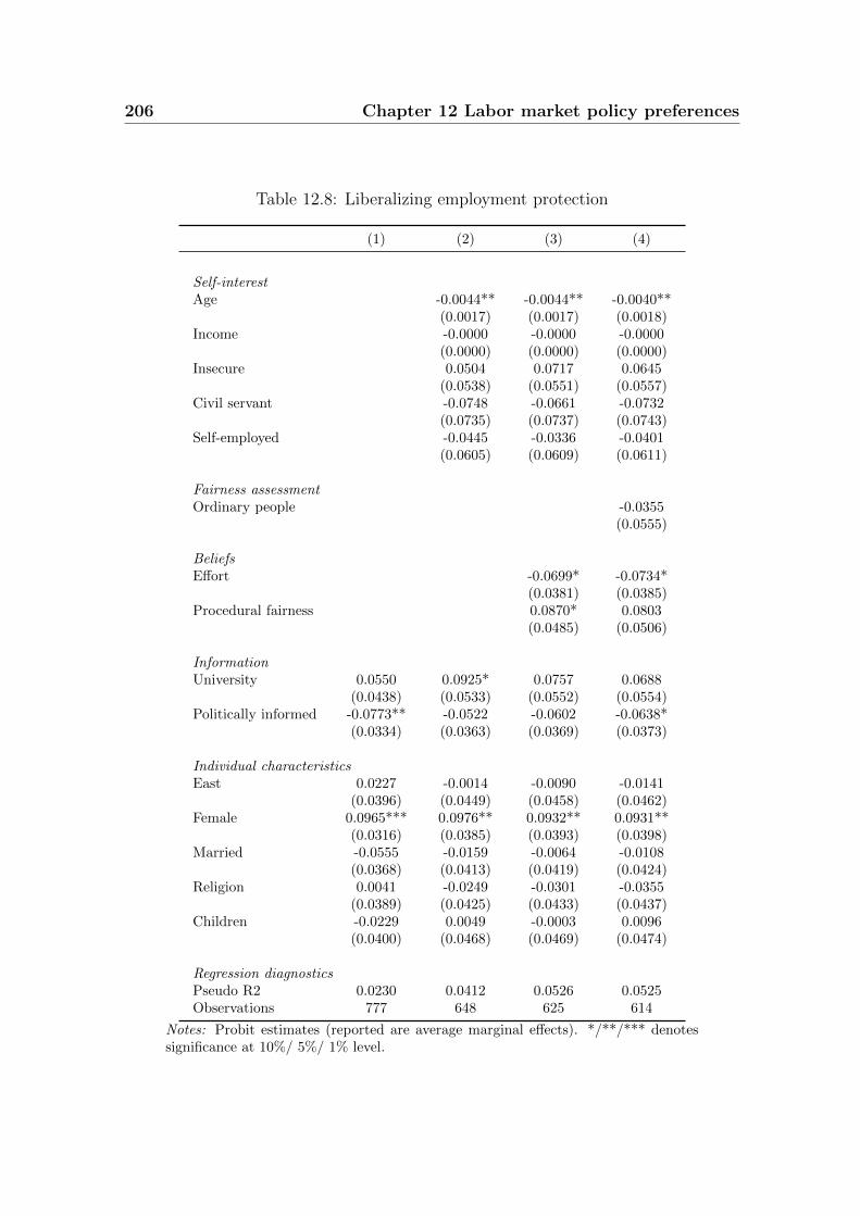
206 Chapter 12 Labor market policy preferences
Table 12.8: Liberalizing employment protection
(1) (2) (3) (4)
Self-interestAge -0.0044** -0.0044** -0.0040**
(0.0017) (0.0017) (0.0018)Income -0.0000 -0.0000 -0.0000
(0.0000) (0.0000) (0.0000)Insecure 0.0504 0.0717 0.0645
(0.0538) (0.0551) (0.0557)Civil servant -0.0748 -0.0661 -0.0732
(0.0735) (0.0737) (0.0743)Self-employed -0.0445 -0.0336 -0.0401
(0.0605) (0.0609) (0.0611)
Fairness assessmentOrdinary people -0.0355
(0.0555)
BeliefsEffort -0.0699* -0.0734*
(0.0381) (0.0385)Procedural fairness 0.0870* 0.0803
(0.0485) (0.0506)
InformationUniversity 0.0550 0.0925* 0.0757 0.0688
(0.0438) (0.0533) (0.0552) (0.0554)Politically informed -0.0773** -0.0522 -0.0602 -0.0638*
(0.0334) (0.0363) (0.0369) (0.0373)
Individual characteristicsEast 0.0227 -0.0014 -0.0090 -0.0141
(0.0396) (0.0449) (0.0458) (0.0462)Female 0.0965*** 0.0976** 0.0932** 0.0931**
(0.0316) (0.0385) (0.0393) (0.0398)Married -0.0555 -0.0159 -0.0064 -0.0108
(0.0368) (0.0413) (0.0419) (0.0424)Religion 0.0041 -0.0249 -0.0301 -0.0355
(0.0389) (0.0425) (0.0433) (0.0437)Children -0.0229 0.0049 -0.0003 0.0096
(0.0400) (0.0468) (0.0469) (0.0474)
Regression diagnosticsPseudo R2 0.0230 0.0412 0.0526 0.0525Observations 777 648 625 614
Notes: Probit estimates (reported are average marginal effects). */**/*** denotessignificance at 10%/ 5%/ 1% level.
12.5 Conclusion 207
12.5 Conclusion
Economists tend to explain labor market reform resistance by referring to approaches
that focus predominantly on an individual’s financial gain or loss from a particular
policy. While our results indicate that this approach has empirical substance and
helps to understand individual assessments of different reform dimensions, it leaves
out an important part of the story. It is indeed the case that individuals who have
high incomes, are young and possess a safe job are more inclined to favor benefit
cuts than those in less favorable circumstances. Nevertheless, the resistance against
labor market reforms can only partly be explained by a narrow financial self-interest.
The findings suggest that voters’ positions are also influenced by their informative
situation, by their beliefs on the sources of economic success or the functioning of
democracy. In Germany, heterogeneity of views is also increased by the split history
of the country with East Germans being more supportive toward redistribution
than their West German fellow citizens even if individuals from both parts share
a similar socioeconomic profile. Our results point to one possible explanation why
expert views on labor markets differ so often from lay perceptions: resistance must
not necessarily be expected from the reform losers only and it cannot be taken for
granted that reform winners will be on the side of liberalizing labor market reforms.
Furthermore, our analysis may allow drawing lessons for a successful selling of market
oriented labor market reforms: it may not be sufficient to stress the individual
advantages of a reform. In addition, policies could also address other sources of
reform resistance. For example, the perception that individual labor market is a
function of individual effort should be helpful to foster reform acceptance and needs
to be communicated.
Finally, our results are important for the possible impact of a macroeconomic
shock on the acceptance of market oriented labor market reforms. While the general
reform literature is optimistic that crisis fosters the acceptance for reforms (Pitlik
and Wirth, 2003), for labor market reforms less optimism is warranted. With a
cyclical increase of unemployment an increasing number of voters is faced with the
risk of dismissal and will, therefore, have an increasing interest in a comfortable level
of unemployment benefits and protection or subsidies from a pure self-interest per-
spective. Beyond self-interest, a cyclical downturn caused by an external shock such
as the global financial crisis has an additional reform impeding effect: the additional
unemployment is the clear consequence of an external event not in the responsibility
of employees. This may in turn reduce the support for reforms which target at in-
creasing individual effort, for instance, through stronger job search incentives. From

208 Chapter 12 Labor market policy preferences
these considerations we would forecast that the financial and economic crisis may
complicate market oriented labor market reforms.
Chapter 13
Pension reform preferences∗
13.1 Introduction
Adjusting the structures of developed welfare states to population ageing remains
one of the key challenges of economic policy in many industrial countries. Notwith-
standing these necessities, reform options such as a higher pension age are unpop-
ular among the majority of voters albeit with substantial individual heterogeneity.
Preceding studies have explored numerous important drivers of pension reform pref-
erences. According to these insights, an individual’s socio-economic characteristics
like gender, income or age matter as does the degree of information on the extent of
the system imbalances. So far, however, the literature has not looked into another
potential source of reform resistance, which is related to an individual’s (dis-)utility
from work. Hence, this contribution argues that intrinsic motivation, which has
received increasing attention on other fields of economic analysis, must not be over-
looked in a comprehensive analysis of pension reform preferences. Pension reforms
impose or reduce restrictions on ageing citizens to offer their work at the labor mar-
ket. Therefore, an individual’s work motivation should have an impact on reform
preferences. People with intrinsic work motivation will be less opposed to longer
working years compared to people for whom work is a burden.
To specify the theoretical link between work motivation and pension reform
preferences, we regard the optimization on pension age within the framework of
an optimal job separation decision. In this context, retirement offers an outside
option to the continuation of work and co-determines a reservation wage. If the
older worker’s job does not pay the reservation wage, the retirement option is more
∗ This chapter is based on a joint work with Friedrich Heinemann and Marc-Daniel Moessinger(see Heinemann et al., 2013).
209

210 Chapter 13 Pension reform preferences
attractive. Intrinsically motivated workers will, ceteris paribus, demand a lower
reservation wage whereas someone with a large disutility from work will demand a
higher compensation for staying in employment. Therefore, a higher pension age
should be a relatively attractive reform option for intrinsically motivated workers
compared to the reform alternatives of cutting pensions or increasing contributions.
In the empirical part, this prediction is tested for data from the representa-
tive ALLBUS survey (“Allgemeine Bevolkerungsumfrage der Sozialwissenschaften”:
German General Social Survey) of the German population. This test adds to the
scarce literature on the drivers of pension reform preferences (surveyed below) in
at least two respects. First, it is innovative as it focuses on intrinsic motivation
as a potential determinant of reform acceptance. As such, it also advances the in-
trinsic motivation literature, which, so far, is unrelated to the formation of policy
preferences. Second, it does not look at pension reform in general but differentiates
between three distinct reform options and their relative popularity: cutting pensions,
increasing contributions and lifting the pension age. The results strongly confirm
that (lacking) intrinsic work motivation is a robust determinant for individual (re-
sistance to and) support for a higher pension age. A reversed effect is observable
with respect to the support for higher pension contributions: intrinsically motivated
individuals are less willing than others to pay the price for early retirement through
higher contributions.
The chapter is structured as follows: section 13.2 briefly surveys the literature on
both the drivers of pension reform preferences and the role of intrinsic motivation in
economic contexts. Section 13.3 derives the theoretical expectations to which extent
intrinsic work motivation should affect different pension reform options. The data
and empirical results are presented in Sections 13.4 and 13.5 followed by robustness
checks and conclusions on the feasibility of pension reforms.
13.2 Literature survey
13.2.1 Pension reform preferences
The existing scarce literature on the drivers of pension reform preferences has suc-
cessfully shed light on some important aspects. Individuals’ socio-economic char-
acteristics help to explain variation: the young are more reform oriented than the
old; males more than females; the rich more than the poor (Boeri et al., 2002,
2001). The divide between the old and the young generation is a consequence of
13.2 Literature survey 211
the different costs of reforms depending on age. Much of this variation is obviously
consistent with a self-interest view on the welfare state along the lines of Meltzer
and Richard (1981) where voters judge welfare arrangements on the basis of their
individual monetary net balance. Women (due to longer life expectation compared
to men), the old (due to their more limited time horizon compared to the young),
and the poor (due to the redistributive elements in pay-as-you-go (PAYG) systems
and due to a higher unemployment risk compared to the rich) are relative winners
of unadjusted PAYG systems. Consistently, all these groups show a relative low
inclination to accept reforms which cut back pensions or lift pension age. Scheubel
et al. (2009) expand the standard set of self-interest related determinants to the
individually expected work ability at pension age and show that this expectation
significantly drives the rejection of a higher retirement age.
A further insight from this empirical literature is that, beyond self-interest, in-
formation matters. Boeri et al. (2002, 2001) show for a survey of European citizens
that the respondents underestimate the costs of the system and have an unrealis-
tic expectation of benefits. The better voters are informed, the more they support
reforms which would allow for a partial opting out of mandatory PAYG systems
toward private funded schemes. For Italian survey data, Boeri and Tabellini (2012)
find that voters are vastly uninformed about the cost and functioning of the pension
system and that the degree of information helps to predict an individual’s readiness
to accept reforms. However, even better information does not guarantee support
for sustainability improving reforms. Generally, reforms which cut back the size of
PAYG systems lack support, even among those who are informed about an imminent
pension crisis (Boeri et al., 2002).
In addition to self-interest and information related factors, the non-economic ap-
proaches stress that individual ideological views contribute to shape pension reform
preferences. For example, Lynch and Myrskyla (2009) exploit Eurobarometer data
to demonstrate that ideological proxies, such as general views on the welfare state or
union membership, significantly influence individual positions on pension reforms.
In a macro cross-national study, Schneider (2009) confirms that trade union power
reduces the likelihood of pension reforms. At the same time, the objective reform
need, measured on the basis of projected pension spending increases, speeds up
reform activity.
The existing literature is focused on the acceptance of pension reforms in general
without paying particular attention to the drivers of relative popularity of different
pension reform options. Yet, Boeri et al. (2002) present descriptive evidence for
212 Chapter 13 Pension reform preferences
this relative attractiveness in their two country study. According to these results,
a higher pension age is more attractive in Italy than in Germany with the reversed
pattern for cutting pensions. None of the existing approaches have, however, in-
cluded an individual’s utility or disutility from work. Thus, the picture remains
incomplete.
13.2.2 Intrinsic motivation
The key contribution of the intrinsic motivation literature to economics is its widen-
ing of the perspective on incentives. Deci’s definition is as follows: “One is said
to be intrinsically motivated to perform an activity when one receives no apparent
reward except the activity itself” (Deci, 1971, p. 105). Whereas, in particular in the
context of principal-agent relationships, neoclassical economics has stressed the role
of monetary or other extrinsic incentives, the intrinsic motivation literature extends
this view.
One insight of the literature is that monetary incentives or punishments might
even be counterproductive as these externally set constraints may crowd out in-
trinsic motivation (Benabou and Tirole, 2003, 2006b). The empirical evidence is
manifold and ranges from experiments, where incentives crowd out reciprocity, over
tax honesty, where fines may lead to lower tax morale, up to labor supply decisions,
where the introduction of small monetary incentives for voluntary works may reduce
supply or labor efficiency (Frey and Jegen, 2001; Frey, 2008). The existence of in-
trinsic motivation has become important for modern economics’ advice on optimum
institutions. For instance, the conclusions relate to optimal organizational forms of
modern companies with respect to an optimal balance of extrinsic and intrinsic mo-
tivation to solve social dilemmas (Osterloh et al., 2002) or to the design of optimal
knowledge transfer (Osterloh and Frey, 2000).
Although the relevance of intrinsic motivation has been established in numerous
contexts, there is one striking gap: so far, this concept has not been related to the
formation of policy preferences. We aim at filling this gap in the context of pen-
sion reform preferences - a field particularly promising since it is about government
interference with individual freedom of choice to end working life.201
201 For Germany, to which our empirical study applies, working beyond the pension age is legallypossible without substantial economic disincentives (there are no cuts in pensions with addi-tional active labor income). However, individual and collective work contracts regularly referto the official pension age as to the age related contract end. Hence, the pension system’sretirement age often imposes a de facto binding constraint on the retirement decision. An eco-nomic rationale for employers supporting this mandatory retirement age is given by Lazear’s
13.3 Theoretical expectations 213
13.3 Theoretical expectations
Intuitively, there should be a link between pension reform preferences and intrinsic
motivation. Somebody who obtains large intrinsic rewards from work should feel less
threatened by the prospect of a later pension age compared to somebody working
‘just for the money’.
To analyze the impact of intrinsic work motivation on pension reform prefer-
ences in a more precise way, it is useful to look at the preferred retirement age in
the context of an optimizing job separation decision.202 The job separation liter-
ature assumes that it is optimal for both employers and employees that a worker
leaves a firm whenever outside opportunities offer a more productive employment
(Mortensen, 1978). Certainly, when reflecting retirement, the outside option is of
a different nature and does not relate to the productivity (and wage) which can
be achieved with another employer. This reflection, nevertheless, relates to another
type of outside option which offers a pension in combination with increased leisure
consumption. The combined features of this outside option (including factors such as
company pension plans203, wealth or non-labor income) determine an older worker’s
reservation wage. Only if labor income for a given age still exceeds the reservation
wage associated with the pension outside option, an individual will prefer work over
retirement.
Ceteris paribus, workers with a large disutility from work might require a higher
reservation wage and have a preference to retire earlier than those with moderate
disutility or even positive utility from work. There is considerable evidence that
individual retirement decisions are indeed heavily influenced by job satisfaction and
working conditions (Blekesaune and Solem, 2005, and the survey therein) so that
it appears promising to assume a similar link for the formation of preferences on
pension reforms.204
However, preference formation on pension reform options is more complex than
famous life cycle- and efficiency wage model (Lazear, 1979).202 Filer and Honig (2005) suggest this analogy for their analysis of endogenous retirement and
(private) pension decisions.203 Retirement incentive effects of pension plans crucially depend on their construction: defined
benefit plans often penalize workers who work beyond the plan’s retirement age (Johnson andSteuerle, 2004).
204 The literature, according to which monetary early retirement incentives (e.g. through pensioncuts for early retirement, which are too small compared to an actuarially fair cut) are highlyeffective (see Gruber and Wise, 2004, 2007; Borsch-Supan et al., 2004, 2007), does not falsifythe possible impact of intrinsic work motivation on retirement preferences. None of thesestudies has analyzed to which extent intrinsic work motivation proxies have had a significantimpact.
214 Chapter 13 Pension reform preferences
the individual retirement decision. For the latter, it is merely the adjustment to
the incentives of an exogenously given pension system. For the former, it is the
reasoning on parameter changes which would serve the individual utility best over
the (rest of one’s) life cycle.
The challenge for a static PAYG pension system which is not adjusted to an
increase in longevity is that, in the beginning of a representative insured’s life cycle,
his present value of received pensions, PV P , exceeds his present value of contri-
butions, PV C, with the implicit individual pension debt, ID = PV P − PV C.205
Thereby, the implicit individual pension debt of a representative individual in age
group A depends on the following policy parameters: the retirement age R, the
pension contributions C, and the annual pension payments P . Abstracting from
growth, income heterogeneity and uncertainty, the individual pension debt is thus
denoted by
IDA = PV PA − PV CA =∞∑i=R
PaAiδi−A −
R−1∑i=A
CaAiδi− A,
where aAi denotes the survival probability of age group A up to age i and δ is
the economy’s discount factor (see Borsch-Supan, 1992).
Increasing longevity pushes up the survival probabilities aAi and increases IDA.
This especially holds true for the post-retirement age.206 A reform which wants
to restore sustainability would then have to cut back the sum of all age groups’
ID to zero. Basically, this adjustment can occur through any of the three policy
parameters (or some of them in combination): increasing pension contributions C,
cutting pensions P , or lifting retirement age R.207
It is immediately obvious that an individual’s age will affect his preference for
one of the preferred reform options. A higher C imposes a cost early in the life cycle
but not after retirement. Hence, the relative preference for higher contributions
205 In addition, there is a problem from decreased fertility, which aggravates the mismatch betweenactive workers’ contributions and pensioners’ benefits. This does, however, not change thesubsequent reasoning qualitatively.
206 The aAi for younger (pre-retirement) age already are close to one so that the increasing effectof longevity is rather important for PV P than for PV C.
207 The precise trade-offs between these types of adjustment depend on the parameters of the pen-sion system and demographics. For example, Devesa-Carpio and Devesa-Carpio (2010) showfor Spain that, alternatively, a contribution increase by 22%, a decrease of the replacementrate by 14% or a delay of the retirement age by 5% would bring the PAYG pension systemback into equilibrium. Furthermore, it should be stressed that an actuarial adjustment ofpension benefit to longer working years would not be able to foster the system’s sustainability(Breyer and Kifmann, 2002). Later retirement only alleviates the sustainability of PAYGpension schemes if it is not fully compensated through a higher level of pensions.
13.3 Theoretical expectations 215
should increase with age approaching retirement age.208 A preference for lower
pensions should, on the contrary, decline with age approaching retirement. While
lower pensions (instead of higher contributions) are relatively attractive for the
young with retirement far ahead, they are much less attractive for people close to
or in retirement who do not benefit (substantially) from savings in contributions. A
higher pension age which effectively cuts back PV P through a later start of pension
payments is particularly unattractive for older workers facing retirement.209 It is
relatively attractive for younger workers and even more for pensioners, who are past
the critical age to be affected. These age effects have been identified before (see
above 13.2.1) and we now concentrate on preference heterogeneity within one age
group. For that purpose we regard the relative attraction of cutting P , raising C,
or raising R for members of the identical age group A where any of these reforms
would cut back IDA by the same amount ∆IDA.210
Our key interest is now how individuals of the same age group and with identical
discount factors might differ in their reform options because of differences in intrinsic
work motivation. Here it is essential that an identical income effect within one age
group (defined by ∆IDA) would translate differently into individual utility. For
workers with a high disutility from labor, the higher retirement age will be particular
unattractive since it confronts them with a substantial loss in leisure. The assessment
is different for those with only low disutility or even utility from work in the sense
that they even would prefer unpaid work over sitting at home. For the latter, the
longer working lifetime is no loss but utility-enhancing. A higher pension age in
these cases may also alleviate a binding constraint, which, so far, has prevented
them from working beyond the pension age before the reform. This reform would
then simply expand the leeway for self-determination, which again reinforces the
importance of intrinsic motivation. Since the latter is particularly powerful in the
absence of external restrictions (Frey, 1997b), the reform’s impact thus intensifies.
Taken together, there is the clear theoretical prediction that - holding all other
208 Sinn and Ubelmesser (2002) define the age dependent population split of supporters andopponents to a cutback of the PAYG system on that basis.
209 This only holds if older workers are not protected by generous transitory arrangements, as itis the case for the very slow German phasing in of a higher pension age (from 65 to 67), whichonly becomes fully effective from the year 2029 onwards.
210 For members of the same age group, heterogeneous individual time preferences can make adifference. Individuals who discount the future more heavily compared to other individualsof the same age group will generally be more inclined to accept costs which materialize in themore distant future, i.e. pension cuts or a higher pension age. In the following, we will abstractfrom this complication and assume the individual discount rates to be either homogeneous orat least uncorrelated to our key variables of interest.
216 Chapter 13 Pension reform preferences
factors like age or discount rate constant - the reform option of a higher pension age
should be relative attractive for those with low work disutility compared to those
for whom longer working years is a nuisance.211
We would not expect that intrinsic motivation impacts equally positively on the
acceptance of lower pension payments or higher pension contributions. Both re-
form proposals are not associated with any increase in self-determination. Even
if intrinsically motivated workers do not work just for the money, they would not
welcome new external interventions which cause resistance. It is a central insight of
the intrinsic motivation literature that extrinsic incentives can crowd out intrinsic
motivation. Extrinsic (typically monetary) incentives which are regarded as inade-
quate have a destructive effect on work motivation (Frey, 1997a). For example, a
cut of net income from active work due to higher pension contributions is likely to
be regarded as a move towards an inadequate compensation for work efforts. Given
the insights from the mentioned literature, one cannot expect that this move will be
more acceptable for workers who enjoy their work compared to those with a larger
disutility from working. A similar reasoning applies for cutting pensions. Intrinsi-
cally motivated workers could perceive this move as disrespect for their high efforts
and react not in a less critical way than other workers.
Thus, the specific difference between workers with a high and low intrinsic work
motivation concentrates on the assessment of a higher pension age. While all three
reform options (higher contributions, lower benefits, longer working years) confront
workers (of the same age group and with equal individual discount rates) with the
same income effect, only the longer working years option increases the scope for self-
determination and should be the favorite of people who enjoy their work. Hence, our
subsequent empirical testing is based on the prediction that intrinsically motivated
respondents should have one clear favorite among the reform options, which is a
higher pension age.
One qualification, however, could blur the clear prediction on the impact of
intrinsic motivation on the reservation wage and reform preferences. It relates to
the fact that a wage has to compensate for the disutility of work at the margin
(Lazear and Oyer, 2007): it might well be the case that an older worker still receives
satisfaction from his work in general but would be glad to have a lower work load
or fewer working hours. As a consequence, the wage has to compensate him for
211 Welfare analyses of pension reform usually assume that the increase of leisure following re-tirement is as such always utility enhancing (e.g. Lachance, 2008). The existence of intrinsicwork motivation points to the possibility that this may not necessarily be the case or, at least,that the utility of pension related leisure may be highly heterogeneous across individuals.
13.4 Data 217
his effort at the margin. If they were free to choose, intrinsically motivated older
workers would then stay in employment but possibly reduce their effort or working
hours. Regularly, this freedom of choice does not exist so that an employee might
not face a decision at the margin but has to reflect whether to stay in employment
at all. Only an empirical test can show to which extent this problem invalidates the
expectation that intrinsically motivated workers have lower reservation wages and,
hence, are more open for late retirement.
Our conceptual framework also allows identifying further essential determinants
which should affect pension reform preferences. In principle, all factors which influ-
ence an older worker’s reservation wage, such as wealth, health or non-labor income,
should matter and should, as far as available, be covered as control variables in an
empirical approach.
13.4 Data
For our empirical test we use data from the representative ALLBUS survey, which
has been conducted from March to August 2006 (Terwey et al., 2007).212 In Ger-
many, this period was characterized by a large public and parliamentary debate on
the future of the pension system, which resulted in the decision to gradually increase
the pension age with the relevant law taking effect in 2007.
The ALLBUS data offers all necessary preconditions for testing the impact of
intrinsic motivation on pension reform preferences. Besides a rich coverage of socio-
economic characteristics, it includes questions on the acceptance of the three basic
pension reform options: a higher pension age, higher contributions to the PAYG
system and lower pension payments.213 This specific type of question is particu-
larly useful as it confronts respondents with different reform alternatives, which are
equally able to improve the sustainability of the PAYG system. Surveys, which only
ask for the acceptance or rejection of one reform option, such as a higher pension
age, are confronted with the problem that results could rather reflect general reform
willingness than the assessment of the specific reform option (Scheubel et al., 2009).
212 Most of the data used in this chapter has been collected in the context of the survey module“Work orientation” of the International Social Programme (ISSP).
213 The precise question is as follows: “Currently there is a large discussion in Germany aboutpensions, the financing of pensions and pension age. Below you find three possible measuresto solve the problems of the statutory pension system. If you had to decide for one of these,which one would you choose?” with the three answer options ‘‘To solve the problems of thestatutory pension system, the pension age should be increased/ pension contributions shouldbe increased/ the statutory pensions should be cut”. An overview on all variable definitions isgiven in the appendix (see Table B.3).

218 Chapter 13 Pension reform preferences
With that ALLBUS question, this is less of a concern and we are able to measure
the relative popularity of different reform options independent from the popularity
of pension reforms in general.
The survey equally covers a set of questions which can be employed as indica-
tors for the complex of intrinsic work motivation. The survey participants answer
the question whether they would like to stay employed even without needing the
money earned or whether they are willing to work harder to support the organiza-
tion. The precise questions run as follows: our like work dummy represents the
support for the statement “I would like to work even without need for the money”
and the work for firm dummy marks individuals who declare “I am ready to
work harder than I have to in order to contribute to my firm’s/organization’s suc-
cess”. Both variables are empirically and conceptually distinct. Empirically, the low
correlation coefficient (0.13) indicates that respondents perceive the both questions
targeting at quite independent issues. Conceptually, the first proxy is clearly much
closer to Deci’s definition (section 13.2.2) of intrinsic motivation than the second
because it is so explicit about working without monetary incentives. The second
question is rather related to concepts of organizational commitment. This has dif-
ferent dimensions (Meyer and Allen, 1991) ranging from an affective attachment to
an organization over perceived costs of leaving an organization up to normative obli-
gations to remain with the organization. Our question is closest to the measurement
of affective attachment, which typically includes items like ours on the willingness
to exert effort. In the empirical test we include this measure for a cross-check: from
a theoretical point of view, we would expect the measure of intrinsic motivation to
have a clearer impact on the pension age preference compared to the organizational
commitment proxy. Hence, contrasting both measures’ results helps us to assess
whether it is really the intrinsic work motivation and not some type of company
related affection which drives the results for pension age preferences.
The descriptive statistics (Table 13.1) confirm the finding from other studies that
a higher pension age is not a popular solution. If they had to accept one reform,
the survey respondents would rather opt for higher contributions. The least popular
reform is, however, cutting pensions. According to our intrinsic motivation proxies,
around two thirds classify as intrinsically motivated in the sense that they do not
work primarily for the money. About one third is ready to work hard for their firm
to improve the company’s success.
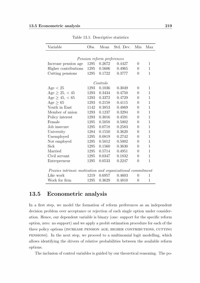
13.5 Econometric analysis 219
Table 13.1: Descriptive statistics
Variable Obs. Mean Std. Dev. Min Max
Pension reform preferencesIncrease pension age 1295 0.2672 0.4427 0 1Higher contributions 1295 0.5606 0.4965 0 1Cutting pensions 1295 0.1722 0.3777 0 1
ControlsAge < 25 1293 0.1036 0.3049 0 1Age ≥ 25, < 45 1293 0.3434 0.4750 0 1Age ≥ 45, < 65 1293 0.3372 0.4729 0 1Age ≥ 65 1293 0.2158 0.4115 0 1Youth in East 1142 0.3853 0.4869 0 1Member of union 1293 0.1237 0.3294 0 1Policy interest 1293 0.3016 0.4591 0 1Female 1295 0.5058 0.5002 0 1Job insecure 1295 0.0718 0.2583 0 1University 1284 0.1550 0.3620 0 1Unemployed 1295 0.0819 0.2742 0 1Not employed 1295 0.5012 0.5002 0 1Sick 1295 0.1560 0.3630 0 1Married 1295 0.5714 0.4951 0 1Civil servant 1295 0.0347 0.1832 0 1Entrepreneur 1295 0.0533 0.2247 0 1
Proxies intrinsic motivation and organizational commitmentLike work 1219 0.6957 0.4603 0 1Work for firm 1295 0.3629 0.4810 0 1
13.5 Econometric analysis
In a first step, we model the formation of reform preferences as an independent
decision problem over acceptance or rejection of each single option under consider-
ation. Hence, our dependent variable is binary (one: support for the specific reform
option, zero: no support) and we apply a probit estimation procedure for each of the
three policy options (increase pension age, higher contributions, cutting
pensions). In the next step, we proceed to a multinomial logit modelling, which
allows identifying the drivers of relative probabilities between the available reform
options.
The inclusion of control variables is guided by our theoretical reasoning. The po-
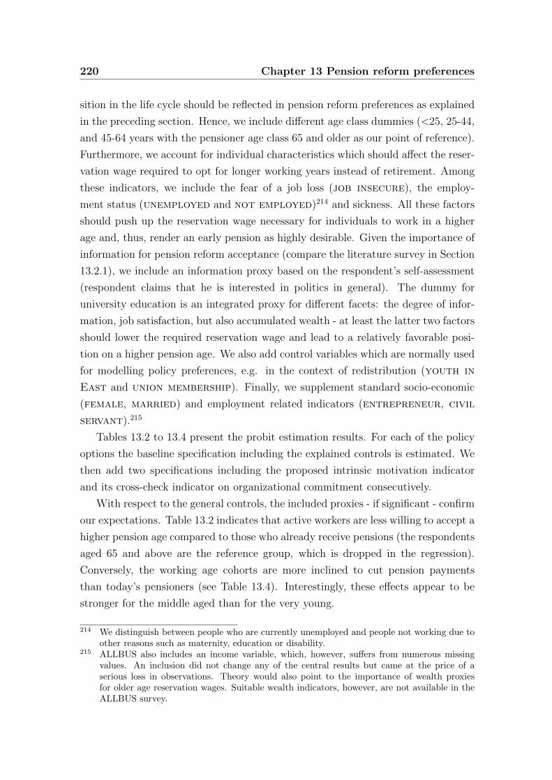
220 Chapter 13 Pension reform preferences
sition in the life cycle should be reflected in pension reform preferences as explained
in the preceding section. Hence, we include different age class dummies (<25, 25-44,
and 45-64 years with the pensioner age class 65 and older as our point of reference).
Furthermore, we account for individual characteristics which should affect the reser-
vation wage required to opt for longer working years instead of retirement. Among
these indicators, we include the fear of a job loss (job insecure), the employ-
ment status (unemployed and not employed)214 and sickness. All these factors
should push up the reservation wage necessary for individuals to work in a higher
age and, thus, render an early pension as highly desirable. Given the importance of
information for pension reform acceptance (compare the literature survey in Section
13.2.1), we include an information proxy based on the respondent’s self-assessment
(respondent claims that he is interested in politics in general). The dummy for
university education is an integrated proxy for different facets: the degree of infor-
mation, job satisfaction, but also accumulated wealth - at least the latter two factors
should lower the required reservation wage and lead to a relatively favorable posi-
tion on a higher pension age. We also add control variables which are normally used
for modelling policy preferences, e.g. in the context of redistribution (youth in
East and union membership). Finally, we supplement standard socio-economic
(female, married) and employment related indicators (entrepreneur, civil
servant).215
Tables 13.2 to 13.4 present the probit estimation results. For each of the policy
options the baseline specification including the explained controls is estimated. We
then add two specifications including the proposed intrinsic motivation indicator
and its cross-check indicator on organizational commitment consecutively.
With respect to the general controls, the included proxies - if significant - confirm
our expectations. Table 13.2 indicates that active workers are less willing to accept a
higher pension age compared to those who already receive pensions (the respondents
aged 65 and above are the reference group, which is dropped in the regression).
Conversely, the working age cohorts are more inclined to cut pension payments
than today’s pensioners (see Table 13.4). Interestingly, these effects appear to be
stronger for the middle aged than for the very young.
214 We distinguish between people who are currently unemployed and people not working due toother reasons such as maternity, education or disability.
215 ALLBUS also includes an income variable, which, however, suffers from numerous missingvalues. An inclusion did not change any of the central results but came at the price of aserious loss in observations. Theory would also point to the importance of wealth proxiesfor older age reservation wages. Suitable wealth indicators, however, are not available in theALLBUS survey.
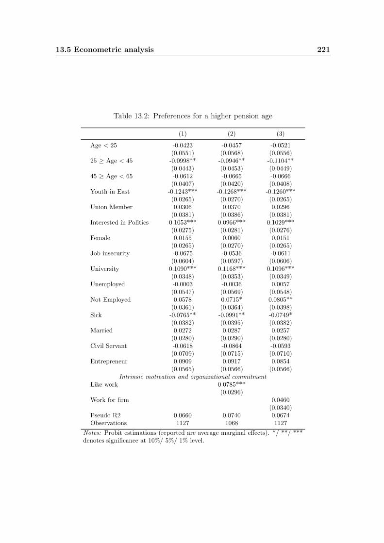
13.5 Econometric analysis 221
Table 13.2: Preferences for a higher pension age
(1) (2) (3)
Age < 25 -0.0423 -0.0457 -0.0521(0.0551) (0.0568) (0.0556)
25 ≥ Age < 45 -0.0998** -0.0946** -0.1104**(0.0443) (0.0453) (0.0449)
45 ≥ Age < 65 -0.0612 -0.0665 -0.0666(0.0407) (0.0420) (0.0408)
Youth in East -0.1243*** -0.1268*** -0.1260***(0.0265) (0.0270) (0.0265)
Union Member 0.0306 0.0370 0.0296(0.0381) (0.0386) (0.0381)
Interested in Politics 0.1053*** 0.0966*** 0.1029***(0.0275) (0.0281) (0.0276)
Female 0.0155 0.0060 0.0151(0.0265) (0.0270) (0.0265)
Job insecurity -0.0675 -0.0536 -0.0611(0.0604) (0.0597) (0.0606)
University 0.1090*** 0.1168*** 0.1096***(0.0348) (0.0353) (0.0349)
Unemployed -0.0003 -0.0036 0.0057(0.0547) (0.0569) (0.0548)
Not Employed 0.0578 0.0715* 0.0805**(0.0361) (0.0364) (0.0398)
Sick -0.0765** -0.0991** -0.0749*(0.0382) (0.0395) (0.0382)
Married 0.0272 0.0287 0.0257(0.0280) (0.0290) (0.0280)
Civil Servant -0.0618 -0.0864 -0.0593(0.0709) (0.0715) (0.0710)
Entrepreneur 0.0909 0.0917 0.0854(0.0565) (0.0566) (0.0566)
Intrinsic motivation and organizational commitmentLike work 0.0785***
(0.0296)Work for firm 0.0460
(0.0340)Pseudo R2 0.0660 0.0740 0.0674Observations 1127 1068 1127
Notes: Probit estimations (reported are average marginal effects). */ **/ ***denotes significance at 10%/ 5%/ 1% level.
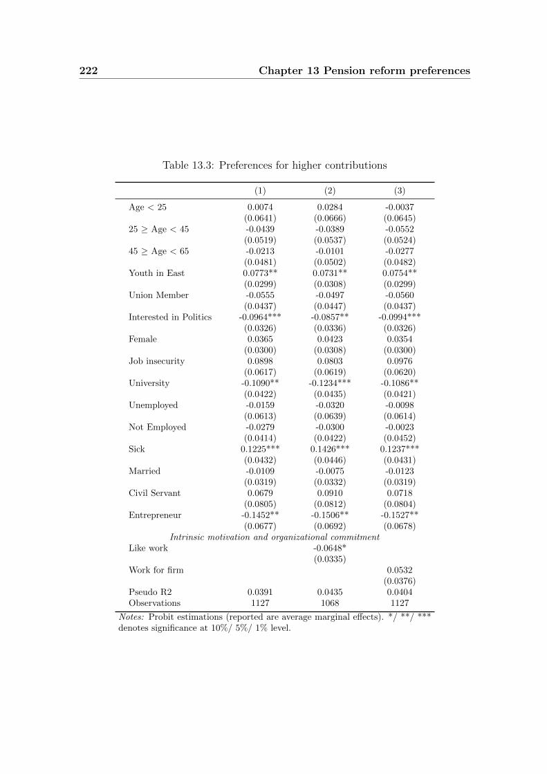
222 Chapter 13 Pension reform preferences
Table 13.3: Preferences for higher contributions
(1) (2) (3)
Age < 25 0.0074 0.0284 -0.0037(0.0641) (0.0666) (0.0645)
25 ≥ Age < 45 -0.0439 -0.0389 -0.0552(0.0519) (0.0537) (0.0524)
45 ≥ Age < 65 -0.0213 -0.0101 -0.0277(0.0481) (0.0502) (0.0482)
Youth in East 0.0773** 0.0731** 0.0754**(0.0299) (0.0308) (0.0299)
Union Member -0.0555 -0.0497 -0.0560(0.0437) (0.0447) (0.0437)
Interested in Politics -0.0964*** -0.0857** -0.0994***(0.0326) (0.0336) (0.0326)
Female 0.0365 0.0423 0.0354(0.0300) (0.0308) (0.0300)
Job insecurity 0.0898 0.0803 0.0976(0.0617) (0.0619) (0.0620)
University -0.1090** -0.1234*** -0.1086**(0.0422) (0.0435) (0.0421)
Unemployed -0.0159 -0.0320 -0.0098(0.0613) (0.0639) (0.0614)
Not Employed -0.0279 -0.0300 -0.0023(0.0414) (0.0422) (0.0452)
Sick 0.1225*** 0.1426*** 0.1237***(0.0432) (0.0446) (0.0431)
Married -0.0109 -0.0075 -0.0123(0.0319) (0.0332) (0.0319)
Civil Servant 0.0679 0.0910 0.0718(0.0805) (0.0812) (0.0804)
Entrepreneur -0.1452** -0.1506** -0.1527**(0.0677) (0.0692) (0.0678)
Intrinsic motivation and organizational commitmentLike work -0.0648*
(0.0335)Work for firm 0.0532
(0.0376)Pseudo R2 0.0391 0.0435 0.0404Observations 1127 1068 1127
Notes: Probit estimations (reported are average marginal effects). */ **/ ***denotes significance at 10%/ 5%/ 1% level.
13.5 Econometric analysis 223
Table 13.4: Preferences for pension cuts
(1) (2) (3)
Age < 25 0.0699 0.0442 0.0858(0.0541) (0.0574) (0.0539)
25 ≥ Age < 45 0.1676*** 0.1551*** 0.1834***(0.0437) (0.0460) (0.0437)
45 ≥ Age < 65 0.1176*** 0.1084** 0.1268***(0.0418) (0.0443) (0.0415)
Youth in East 0.0440* 0.0505** 0.0474**(0.0228) (0.0236) (0.0227)
Union Member 0.0283 0.0161 0.0284(0.0321) (0.0337) (0.0320)
Interested in Politics -0.0119 -0.0116 -0.0060(0.0253) (0.0264) (0.0253)
Female -0.0462** -0.0416* -0.0438*(0.0229) (0.0239) (0.0228)
Job insecurity -0.0402 -0.0416 -0.0523(0.0447) (0.0458) (0.0451)
University -0.0031 -0.0021 -0.0029(0.0327) (0.0340) (0.0324)
Unemployed 0.0171 0.0371 0.0081(0.0463) (0.0486) (0.0459)
Not Employed -0.0335 -0.0477 -0.0694**(0.0314) (0.0329) (0.0334)
Sick -0.0480 -0.0446 -0.0498(0.0363) (0.0377) (0.0360)
Married -0.0158 -0.0224 -0.0139(0.0243) (0.0255) (0.0241)
Civil Servant -0.0096 -0.0077 -0.0157(0.0573) (0.0587) (0.0572)
Entrepreneur 0.0363 0.0408 0.0513(0.0469) (0.0485) (0.0467)
Intrinsic motivation and organizational commitmentLike work -0.0081
(0.0261)Work for firm -0.0801***
(0.0268)Pseudo R2 0.0515 0.0513 0.0601Observations 1127 1068 1127
Notes: Probit estimations (reported are average marginal effects). */ **/ ***denotes significance at 10%/ 5%/ 1% level.
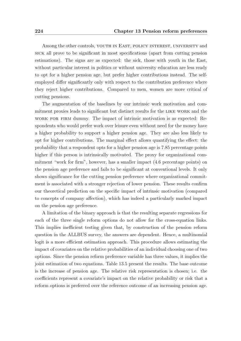
224 Chapter 13 Pension reform preferences
Among the other controls, youth in East, policy interest, university and
sick all prove to be significant in most specifications (apart from cutting pension
estimations). The signs are as expected: the sick, those with youth in the East,
without particular interest in politics or without university education are less ready
to opt for a higher pension age, but prefer higher contributions instead. The self-
employed differ significantly only with respect to the contribution preference where
they reject higher contributions. Compared to men, women are more critical of
cutting pensions.
The augmentation of the baselines by our intrinsic work motivation and com-
mitment proxies leads to significant but distinct results for the like work and the
work for firm dummy. The impact of intrinsic motivation is as expected: Re-
spondents who would prefer work over leisure even without need for the money have
a higher probability to support a higher pension age. They are also less likely to
opt for higher contributions. The marginal effect allows quantifying the effect: the
probability that a respondent opts for a higher pension age is 7.85 percentage points
higher if this person is intrinsically motivated. The proxy for organizational com-
mitment “work for firm”, however, has a smaller impact (4.6 percentage points) on
the pension age preference and fails to be significant at conventional levels. It only
shows significance for the cutting pension preference where organizational commit-
ment is associated with a stronger rejection of lower pension. These results confirm
our theoretical prediction on the specific impact of intrinsic motivation (compared
to concepts of company affection), which has indeed a particularly marked impact
on the pension age preference.
A limitation of the binary approach is that the resulting separate regressions for
each of the three single reform options do not allow for the cross-equation links.
This implies inefficient testing given that, by construction of the pension reform
question in the ALLBUS survey, the answers are dependent. Hence, a multinomial
logit is a more efficient estimation approach. This procedure allows estimating the
impact of covariates on the relative probabilities of an individual choosing one of two
options. Since the pension reform preference variable has three values, it implies the
joint estimation of two equations. Table 13.5 present the results. The base outcome
is the increase of pension age. The relative risk representation is chosen; i.e. the
coefficients represent a covariate’s impact on the relative probability or risk that a
reform options is preferred over the reference outcome of an increasing pension age.
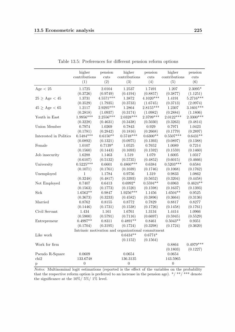
13.5 Econometric analysis 225
Table 13.5: Preferences for different pension reform options
higher pension higher pension higher pensioncontributions cuts contributions cuts contributions cuts
(1) (2) (3) (4) (5) (6)
Age < 25 1.1725 2.0104 1.2537 1.7491 1.207 2.3095*(0.3726) (0.9749) (0.4194) (0.8857) (0.3877) (1.1251)
25 ≥ Age < 45 1.3731 4.5571*** 1.3872 4.1020*** 1.4191 5.2716***(0.3529) (1.7935) (0.3733) (1.6745) (0.3713) (2.0974)
45 ≥ Age < 65 1.2117 2.9295*** 1.2864 2.8155*** 1.2307 3.1601***(0.2818) (1.0937) (0.3174) (1.0982) (0.2884) (1.1806)
Youth in East 1.9956*** 2.2556*** 2.0328*** 2.3799*** 2.0122*** 2.3300***(0.3228) (0.4631) (0.3438) (0.5030) (0.3263) (0.4814)
Union Member 0.7974 1.0269 0.7843 0.929 0.7971 1.0423(0.1781) (0.2842) (0.1816) (0.2668) (0.1779) (0.2897)
Interested in Politics 0.5484*** 0.6150** 0.5748*** 0.6300** 0.5507*** 0.6431**(0.0892) (0.1321) (0.0975) (0.1393) (0.0897) (0.1388)
Female 1.0107 0.7139* 1.0525 0.7652 1.0089 0.7214(0.1560) (0.1443) (0.1693) (0.1592) (0.1559) (0.1460)
Job insecurity 1.6288 1.1463 1.519 1.079 1.6005 1.0317(0.6107) (0.5132) (0.5735) (0.4852) (0.6015) (0.4666)
University 0.5225*** 0.6601 0.4860*** 0.6384 0.5203*** 0.6584(0.1071) (0.1761) (0.1039) (0.1746) (0.1068) (0.1762)
Unemployed 1 1.1784 0.9756 1.319 0.9833 1.0862(0.3248) (0.4817) (0.3393) (0.5652) (0.3204) (0.4458)
Not Employed 0.7407 0.6413 0.6992* 0.5594** 0.6963 0.4624**(0.1563) (0.1773) (0.1520) (0.1598) (0.1637) (0.1393)
Sick 1.6562** 0.9847 1.9256*** 1.1456 1.6504** 0.9525(0.3673) (0.3233) (0.4582) (0.3896) (0.3664) (0.3136)
Married 0.8762 0.8155 0.8772 0.7829 0.8817 0.8277(0.1446) (0.1731) (0.1538) (0.1726) (0.1458) (0.1761)
Civil Servant 1.434 1.161 1.6761 1.3134 1.4414 1.0966(0.5900) (0.5791) (0.7116) (0.6697) (0.5945) (0.5529)
Entrepreneur 0.4997** 0.8311 0.4891** 0.8461 0.5043** 0.9351(0.1704) (0.3195) (0.1724) (0.3298) (0.1724) (0.3620)
Intrinsic motivation and organizational commitmentLike work 0.6434** 0.6774*
(0.1152) (0.1564)Work for firm 0.8864 0.4979***
(0.1803) (0.1227)Pseudo R-Square 0.0609 0.0654 0.0654chi2 133.6748 136.3135 143.5965p 0 0 0
Notes: Multinominal logit estimations (reported is the effect of the variables on the probabilitythat the respective reform option is preferred to an increase in the pension age). */ **/ *** denotethe significance at the 10%/ 5%/ 1% level.
226 Chapter 13 Pension reform preferences
Hence, the relative risk ratios reported in Tables 13.5 and 13.7 differs from that
of regression coefficients. If the relative risk ratio of a variable is smaller (greater)
than one, then this variable raises (lowers) the probability that a person prefers
an increase in the pension age over higher contributions or pension cuts.216 The
baseline is followed by specifications augmented by each of the motivation proxies
consecutively.
The results for the multinomial logit estimations show some differences to the
probit results. Generally, a more critical screening is required since less control vari-
ables keep their significance. For instance, the gender variable loses its significance if
the motivation dummies are included. The age effects are confirmed: active workers
are much more likely to opt for lower pensions than for a higher pension age (factor
4.6 for the 25-44 age group). An absent university education, a youth in the East
and no particular interest in politics are robustly significant and foster a rejection
of higher pension ages relative to the other solutions.
Both our indicator for intrinsic motivation and the indicator for organizational
commitment survive the multinomial testing. As for the probit analysis, the like
work and the work for firm proxies turn out to have a significant but distinct
effect. The predicted probabilities in Table 13.6 report the size of the effect.
Table 13.6: Predicted probabilities for intrinsic motivation and organizational com-mitment
Reform preferenceIncrease pension age Higher contributions Cutting pensions
Like work 0 0.1885 0.6389 0.17271 0.2630 0.5737 0.1633
Work for firm 0 0.2303 0.5780 0.19171 0.2748 0.6113 0.1139
These predictions are calculated for average values of all other covariates and
show the difference between probabilities for respondents who are and those who
are not intrinsically motivated. For those who would work even without the need for
the money earned, the crucial difference is related to a higher probability of opting
for higher pension age and a lower probability of opting for higher contributions. No
216 The reported ratios are obtained by exponentiating the coefficients of the multinominal logitmodel. The relative risk ratios indicate how a change in the variable in question affects theprobability (or risk) that the outcome falls into the comparison group (i.e. preferring highercontributions or pension cuts) compared to the probability that the outcome falls into thereference group (i.e. preferring an increase in pension age).
13.6 Robustness 227
marked difference exists for the cutting pension preference. For the organizational
commitment motivation proxy work for firm, a particular marked difference
exists for the cutting pension preference. Those who feel a large loyalty to their
firm or organization are less likely to opt for lower pensions whereas variation in
organizational commitment is not associated with a large variation in the pension
age preferences.
13.6 Robustness of the results
Our findings support the empirical relevance of the preceding theoretical reasoning:
Respondents with a high degree of intrinsic work motivation are more likely to
opt for a postponement of the statutory retirement age. However, this result may
equally reflect other links in the data structure. Although we already control for
numerous important individual characteristics, missing variables could distort the
regression. Thus, it cannot be ruled out that intrinsic motivation is linked to a
general individual inclination for reform. Furthermore, there is a straightforward
alternative story which could explain our key result: it could simply be the case
that workers with a physically demanding job are both less intrinsically motivated
and, naturally, less optimistic that they would be capable of continuing to work
at a higher age (Scheubel et al., 2009). In this case, our result would reflect the
impact of job characteristics related to physical stress. In the following, we check
for the reliability of our results with respect to these possible objections and also
provide several regression variants to check for the general robustness of our findings.
In these robustness checks, we now concentrate on our intrinsic motivation proxy
like work (robustness checks for the organizational commitment proxy work for
firm did not leave to any substantial modifications of the above insights and are,
thus, not reported).
13.6.1 Physical job stress
With respect to physical job stress, some of our standard control variables already
have a proxy characteristic in this regard, such as gender, the education variable
(university) or the profession dummies (civil servant, entrepreneur). In
addition, we experiment with the following more direct control variables: (1) a
dummy hard work which indicates that the respondent has to perform a physical
straining job and (2) a dummy variable equal one if the respondent is a blue
collar worker. These additional controls should filter out intrinsic motivation
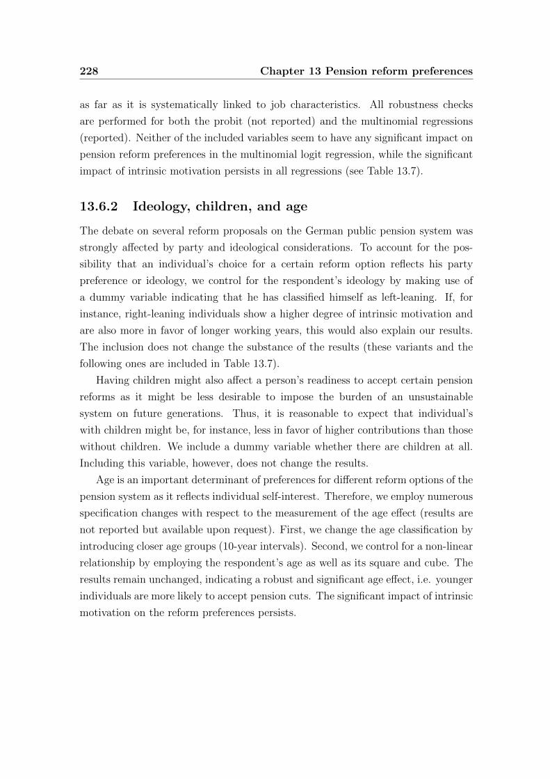
228 Chapter 13 Pension reform preferences
as far as it is systematically linked to job characteristics. All robustness checks
are performed for both the probit (not reported) and the multinomial regressions
(reported). Neither of the included variables seem to have any significant impact on
pension reform preferences in the multinomial logit regression, while the significant
impact of intrinsic motivation persists in all regressions (see Table 13.7).
13.6.2 Ideology, children, and age
The debate on several reform proposals on the German public pension system was
strongly affected by party and ideological considerations. To account for the pos-
sibility that an individual’s choice for a certain reform option reflects his party
preference or ideology, we control for the respondent’s ideology by making use of
a dummy variable indicating that he has classified himself as left-leaning. If, for
instance, right-leaning individuals show a higher degree of intrinsic motivation and
are also more in favor of longer working years, this would also explain our results.
The inclusion does not change the substance of the results (these variants and the
following ones are included in Table 13.7).
Having children might also affect a person’s readiness to accept certain pension
reforms as it might be less desirable to impose the burden of an unsustainable
system on future generations. Thus, it is reasonable to expect that individual’s
with children might be, for instance, less in favor of higher contributions than those
without children. We include a dummy variable whether there are children at all.
Including this variable, however, does not change the results.
Age is an important determinant of preferences for different reform options of the
pension system as it reflects individual self-interest. Therefore, we employ numerous
specification changes with respect to the measurement of the age effect (results are
not reported but available upon request). First, we change the age classification by
introducing closer age groups (10-year intervals). Second, we control for a non-linear
relationship by employing the respondent’s age as well as its square and cube. The
results remain unchanged, indicating a robust and significant age effect, i.e. younger
individuals are more likely to accept pension cuts. The significant impact of intrinsic
motivation on the reform preferences persists.
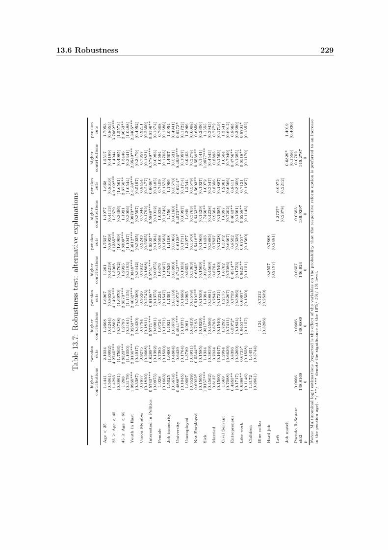
13.6 Robustness 229
Tab
le13
.7:
Rob
ust
nes
ste
st:
alte
rnat
ive
expla
nat
ions
hig
her
pensi
on
hig
her
pensi
on
hig
her
pensi
on
hig
her
pensi
on
hig
her
pensi
on
contr
ibuti
ons
cuts
contr
ibuti
ons
cuts
contr
ibuti
ons
cuts
contr
ibuti
ons
cuts
contr
ibuti
ons
cuts
Age<
25
1.4
441
2.1
034
1.2
668
1.6
967
1.2
61
1.7
627
1.1
977
1.6
68
1.2
517
1.7
053
(0.5
061)
(1.0
992)
(0.4
244)
(0.8
626)
(0.4
219)
(0.8
929)
(0.4
113)
(0.8
610)
(0.4
189)
(0.8
655)
25≥
Age<
45
1.4
293
4.2
745***
1.3
802
4.1
491***
1.3
968
4.1
385***
1.2
679
4.0
102***
1.4
944
3.7
662***
(0.3
861)
(1.7
503)
(0.3
718)
(1.6
970)
(0.3
762)
(1.6
909)
(0.3
496)
(1.6
561)
(0.4
085)
(1.5
573)
45≥
Age<
65
1.2
88
2.8
323***
1.2
793
2.8
573***
1.2
925
2.8
309***
1.1
921
2.6
760**
1.3
446
2.6
653**
(0.3
179)
(1.1
050)
(0.3
161)
(1.1
155)
(0.3
193)
(1.1
047)
(0.3
006)
(1.0
544)
(0.3
341)
(1.0
488)
Youth
inE
ast
1.9
965***
2.3
135***
2.0
253***
2.4
032***
2.0
348***
2.3
812***
2.0
873***
2.4
180***
2.0
549***
2.3
405***
(0.3
387)
(0.4
917)
(0.3
430)
(0.5
089)
(0.3
442)
(0.5
035)
(0.3
597)
(0.5
197)
(0.3
479)
(0.4
952)
Unio
nM
em
ber
0.7
857
0.9
275
0.7
794
0.9
526
0.7
812
0.9
243
0.7
644
0.8
454
0.7
857
0.9
211
(0.1
820)
(0.2
668)
(0.1
811)
(0.2
743)
(0.1
808)
(0.2
655)
(0.1
792)
(0.2
477)
(0.1
821)
(0.2
650)
Inte
rest
ed
inP
oliti
cs
0.5
743***
0.6
289**
0.5
771***
0.6
198**
0.5
751***
0.6
303**
0.5
888***
0.6
660*
0.5
789***
0.6
196**
(0.0
975)
(0.1
392)
(0.0
981)
(0.1
375)
(0.0
975)
(0.1
394)
(0.1
012)
(0.1
485)
(0.0
983)
(0.1
374)
Fem
ale
1.0
28
0.7
385
1.0
724
0.7
224
1.0
476
0.7
598
1.0
638
0.7
409
1.0
584
0.7
608
(0.1
663)
(0.1
550)
(0.1
771)
(0.1
547)
(0.1
687)
(0.1
583)
(0.1
745)
(0.1
573)
(0.1
705)
(0.1
586)
Job
inse
curi
ty1.5
025
1.0
683
1.4
921
1.1
391
1.5
526
1.1
198
1.5
56
1.1
996
1.4
607
1.0
954
(0.5
674)
(0.4
804)
(0.5
673)
(0.5
159)
(0.5
890)
(0.5
066)
(0.6
180)
(0.5
570)
(0.5
531)
(0.4
941)
Univ
ers
ity
0.4
888***
0.6
439
0.4
941***
0.6
073*
0.4
742***
0.6
128*
0.4
573***
0.6
214*
0.4
936***
0.6
273*
(0.1
045)
(0.1
764)
(0.1
071)
(0.1
686)
(0.1
033)
(0.1
711)
(0.0
997)
(0.1
714)
(0.1
057)
(0.1
722)
Unem
plo
yed
1.0
097
1.3
789
0.9
81
1.2
995
0.9
655
1.2
977
1.0
49
1.2
544
0.9
403
1.3
966
(0.3
528)
(0.5
931)
(0.3
413)
(0.5
578)
(0.3
363)
(0.5
570)
(0.3
763)
(0.5
579)
(0.3
278)
(0.6
008)
Not
Em
plo
yed
0.6
922*
0.5
544**
0.7
193
0.5
192**
0.6
845*
0.5
418**
0.6
433**
0.5
603**
0.5
539**
0.6
856
(0.1
505)
(0.1
585)
(0.1
629)
(0.1
530)
(0.1
509)
(0.1
566)
(0.1
429)
(0.1
627)
(0.1
441)
(0.2
306)
Sic
k1.9
157***
1.1
334
1.9
317***
1.1
394
1.9
197***
1.1
423
1.7
466**
1.0
072
1.9
077***
1.1
555
(0.4
562)
(0.3
859)
(0.4
596)
(0.3
881)
(0.4
569)
(0.3
885)
(0.4
238)
(0.3
547)
(0.4
543)
(0.3
943)
Marr
ied
0.8
137
0.7
034
0.8
783
0.7
843
0.8
784
0.7
837
0.9
384
0.8
356
0.8
895
0.7
772
(0.1
500)
(0.1
647)
(0.1
540)
(0.1
731)
(0.1
540)
(0.1
728)
(0.1
685)
(0.1
887)
(0.1
563)
(0.1
719)
Civ
ilServ
ant
1.6
69
1.2
994
1.7
292
1.2
175
1.6
702
1.3
072
1.6
897
1.2
861
1.6
504
1.3
541
(0.7
088)
(0.6
639)
(0.7
411)
(0.6
267)
(0.7
086)
(0.6
667)
(0.7
202)
(0.6
566)
(0.7
040)
(0.6
912)
Entr
epre
neur
0.4
855**
0.8
356
0.5
072*
0.7
759
0.4
914**
0.8
552
0.4
643**
0.8
411
0.4
756**
0.8
665
(0.1
717)
(0.3
269)
(0.1
824)
(0.3
096)
(0.1
733)
(0.3
336)
(0.1
661)
(0.3
300)
(0.1
685)
(0.3
380)
Lik
ew
ork
0.6
388**
0.6
735*
0.6
453**
0.6
697*
0.6
425**
0.6
757*
0.6
258**
0.7
121
0.6
518**
0.6
701*
(0.1
146)
(0.1
558)
(0.1
157)
(0.1
550)
(0.1
151)
(0.1
560)
(0.1
145)
(0.1
687)
(0.1
170)
(0.1
552)
Childre
n1.3
172
1.4
451
(0.2
661)
(0.3
744)
Blu
ecollar
1.1
24
0.7
212
(0.3
286)
(0.2
539)
Hard
job
0.8
557
0.7
868
(0.2
197)
(0.2
481)
Left
1.3
727*
0.9
972
(0.2
378)
(0.2
212)
Job
matc
h0.6
829*
1.4
019
(0.1
556)
(0.4
030)
Pse
udo
R-S
quare
0.0
666
0.0
666
0.0
657
0.0
683
0.0
702
chi2
138.8
169
138.8
889
136.9
24
136.9
297
146.2
787
p0
00
00
Note
s:M
ult
inom
inal
logit
est
imati
ons
(rep
ort
ed
isth
eeff
ect
of
the
vari
able
son
the
pro
babilit
yth
at
the
resp
ecti
ve
refo
rmopti
on
ispre
ferr
ed
toan
incre
ase
inth
ep
ensi
on
age).
*/
**/
***
denote
the
signifi
cance
at
the
10%
/5%
/1%
level.
230 Chapter 13 Pension reform preferences
13.6.3 Job match
Finally, one might argue that our measures of intrinsic motivation may also capture
other factors such as the job match quality. It is possible that individuals with a
better match are more willing to continue to work simply because they are gaining
rents from their present employment. Then, the significant relationship between
intrinsic motivation and pension reform preferences would not indicate a causal
effect but rather result from a better job match that increases both the general
willingness to work and the preferences of a postponement of the statutory pension
age. To address this concern, we proxy the quality of the respondent’s job match
by including a dummy variable equal to one if the respondent states that he can
make use of his past work experience and/or job skills for his present job. The
results presented in Table 13.7 indicate that individuals with a better job match
are more likely to prefer an increase in the pension age than higher contributions.
Including this variable, however, does not weaken the impact of intrinsic motivation
on pension reform acceptance.
13.6.4 General reform inclination
Our theoretical reasoning for the impact of intrinsic motivation is specific to reforms
related to working time. If this reasoning is indeed responsible for our empirical
findings, we would not expect a significant impact on reform issues unrelated to
working times. Significant results for non-work related reform issues would be a hint
that intrinsic motivation is just a proxy for some other type of important individual
characteristic which is not covered by our controls. To check for this possibility, we
apply a placebo regression. We estimate a similar specification as in Table 13.2,
but now for reform issues without any obvious theoretical link to intrinsic work
motivation. Two different reform options are chosen which are completely unrelated
to working conditions or working time: first, the approval to municipal suffrage
for foreigners and, second, the approval of the need for Islam-teaching at German
schools. The results of the regressions are presented in Table 13.8. In none of the
cases our intrinsic motivation indicators are among the significant determinants.
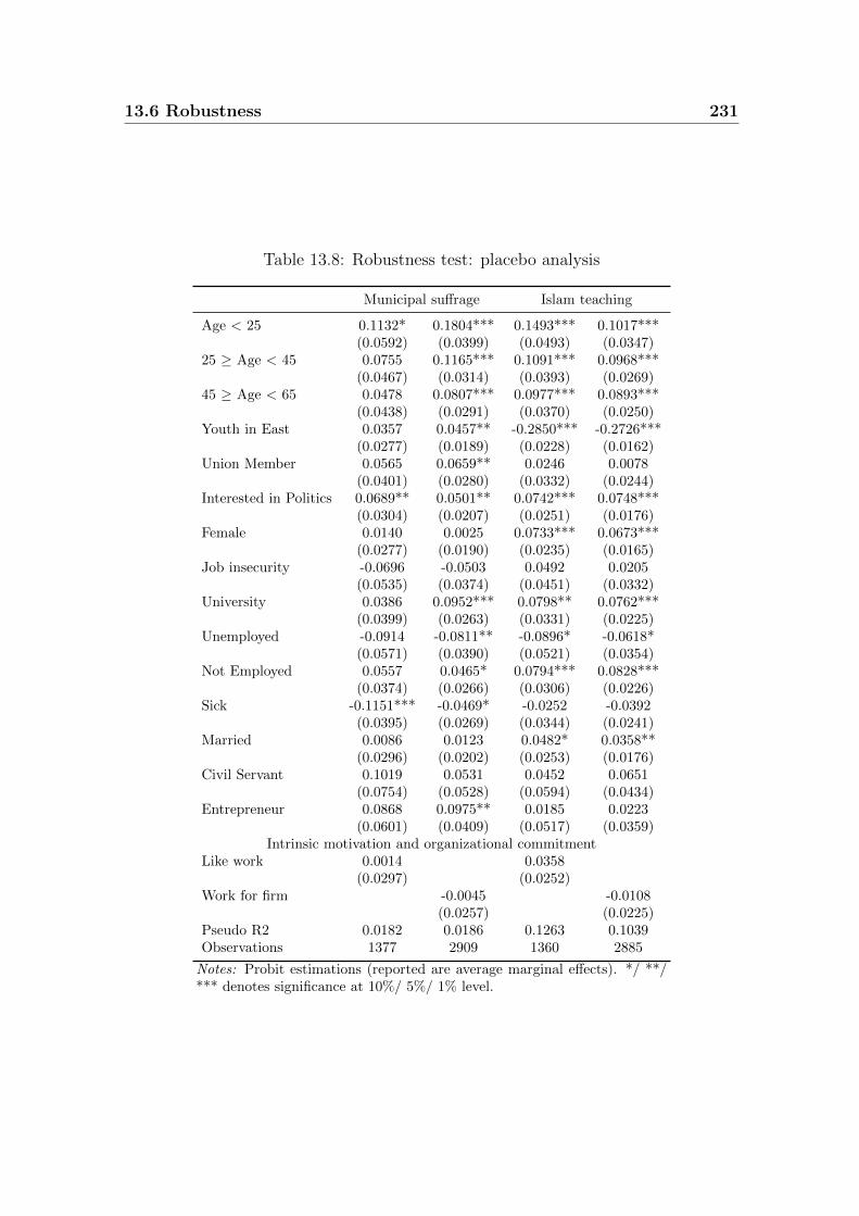
13.6 Robustness 231
Table 13.8: Robustness test: placebo analysis
Municipal suffrage Islam teaching
Age < 25 0.1132* 0.1804*** 0.1493*** 0.1017***(0.0592) (0.0399) (0.0493) (0.0347)
25 ≥ Age < 45 0.0755 0.1165*** 0.1091*** 0.0968***(0.0467) (0.0314) (0.0393) (0.0269)
45 ≥ Age < 65 0.0478 0.0807*** 0.0977*** 0.0893***(0.0438) (0.0291) (0.0370) (0.0250)
Youth in East 0.0357 0.0457** -0.2850*** -0.2726***(0.0277) (0.0189) (0.0228) (0.0162)
Union Member 0.0565 0.0659** 0.0246 0.0078(0.0401) (0.0280) (0.0332) (0.0244)
Interested in Politics 0.0689** 0.0501** 0.0742*** 0.0748***(0.0304) (0.0207) (0.0251) (0.0176)
Female 0.0140 0.0025 0.0733*** 0.0673***(0.0277) (0.0190) (0.0235) (0.0165)
Job insecurity -0.0696 -0.0503 0.0492 0.0205(0.0535) (0.0374) (0.0451) (0.0332)
University 0.0386 0.0952*** 0.0798** 0.0762***(0.0399) (0.0263) (0.0331) (0.0225)
Unemployed -0.0914 -0.0811** -0.0896* -0.0618*(0.0571) (0.0390) (0.0521) (0.0354)
Not Employed 0.0557 0.0465* 0.0794*** 0.0828***(0.0374) (0.0266) (0.0306) (0.0226)
Sick -0.1151*** -0.0469* -0.0252 -0.0392(0.0395) (0.0269) (0.0344) (0.0241)
Married 0.0086 0.0123 0.0482* 0.0358**(0.0296) (0.0202) (0.0253) (0.0176)
Civil Servant 0.1019 0.0531 0.0452 0.0651(0.0754) (0.0528) (0.0594) (0.0434)
Entrepreneur 0.0868 0.0975** 0.0185 0.0223(0.0601) (0.0409) (0.0517) (0.0359)
Intrinsic motivation and organizational commitmentLike work 0.0014 0.0358
(0.0297) (0.0252)Work for firm -0.0045 -0.0108
(0.0257) (0.0225)Pseudo R2 0.0182 0.0186 0.1263 0.1039Observations 1377 2909 1360 2885
Notes: Probit estimations (reported are average marginal effects). */ **/*** denotes significance at 10%/ 5%/ 1% level.

232 Chapter 13 Pension reform preferences
Hence, the placebo test shows that between intrinsic motivation matters for
pension reforms but not for the other reforms. This points to a specific link only for
pension reform preferences. This backs our confidence that our results on pension
reform preferences are driven by the proposed causal chain and not just a general
individual inclination to accept change.217
13.7 Conclusion
Our findings suggest that intrinsic work motivation is indeed related to work-related
reform processes - at least with respect to the formation of pension reform prefer-
ences. The empirical results confirm the predictions of our theoretical reasoning,
which makes a clear case for the existence of such a link. Our intrinsic motivation
proxy proves to be robustly significant in a series of econometric tests, in which
we pay careful attention to an individual’s physical job stress and apply numerous
modifications to the included control variables. For a multitude of specifications,
respondents who experience utility from their work beyond the money they earn are
more willing to embark on reforms leading to a higher pension age. This key result
has implications both for the intrinsic motivation literature and our understanding
of reform processes. So far, intrinsic motivation has been recognized to be important
for the efficiency of firms and organizations. Our findings point beyond that insight
toward the formation of policy preferences and, thus, probably the adaptability of
modern welfare states and societies. A lack of non-monetary work incentives can
be a reform constraint and therefore highly relevant for a country’s institutional
adaptability.
While these insights can be helpful for a broader understanding of reform re-
sistance in certain contexts, it is more difficult to derive conclusions of immediate
policy relevance. A first difficulty is that a population’s degree of intrinsic motiva-
tion is hardly verifiable. So it will not be possible to prescribe reform strategies for a
country dependent on its population’s level of intrinsic motivation. Furthermore, it
is unclear to which extent policy really is able to influence this human trait, whether
it is an exogenous feature or reactive to policy measures. There are some hints in the
intrinsic motivation literature that this type of motivation is not purely exogenous.
217 This placebo test also makes us confident that the notorious “single source bias” (Champbelland Fiske, 1959) does not poison our results in a serious way. This bias can occur if someunobservable circumstances of one single source (e.g. one survey) influence different answersso that emerging correlations are spurious. If, for example, a respondent had a good workingday he might, consequentially, rate both his work motivation high and be particularly openfor reforms.

13.7 Conclusion 233
For example, it is known that extrinsic incentives can crowd out intrinsic motives so
that a lot may depend on adequate payment systems (Ockenfels et al., 2010). But
these approaches are hardly under the government’s direct control. Nevertheless,
a modest conclusion from our results would be that reform strategists should be
sensible for the possibility that a lack of intrinsic work motivation can be a relevant
reform constraint.

Chapter 14
Television and individual belief
formation∗
14.1 Introduction
The analysis in the preceding chapters of this book support the view that individual
preferences for redistribution or labor market policies cannot fully be explained by
pure self-interest but also reflect fairness considerations, for example. An explana-
tion for this general finding is that voters usually want to reduce inequality as far
as it is driven by factors that are beyond individual control (such as luck or social
conditions) but reward individual effort. Individuals, however, do not exactly know
to what extent a certain level of inequality reflects differences in individual effort
or is a consequence of other factors. Therefore, people have to form and rely on
beliefs about the relative importance of effort as a determinant of success in life, for
instance, when voting on redistributive policies.
The relevance of beliefs on the drivers of success as an explanation for policy
preferences and also actual policies has been established both through studies using
individual-level survey data (e.g. Alesina and Giuliano, 2009; Corneo and Gruner,
2002; Fong, 2001) and cross-national comparisons (Alesina et al., 2001; Alesina and
Glaeser, 2004). Alesina et al. (2001), for instance, conclude that the observable
differences in the size and structure if the U.S. and European welfare state are driven
by considerable differences in beliefs. Despite their policy relevance, our knowledge
about the process of individual belief formation remains still incomplete.
The literature on belief formation suggests that individuals use available infor-
mation from various sources to learn about the rewards to effort and form their
∗ Other versions of this study are Hennighausen (2012, 2013).
235
236 Chapter 14 Television and belief formation
corresponding beliefs about the drivers of success. They use, for instance, their per-
sonal experience or family history to learn about the relative importance of effort
(Piketty, 1995; Di Tella et al., 2007; Giuliano and Spilimbergo, 2009).
Moreover, Alesina and Glaeser (2004) argue that observable differences in beliefs
of Americans and Europeans do not just reflect differences in personal experience
but are rather a result of political indoctrination. Convincing empirical evidence
isolating the impact of indoctrination (such as exposure to Marxist ideas) on beliefs
about the drivers of success is still missing. This contribution wants to close this
gap by analyzing whether political indoctrination via mass media has a persistent
impact on beliefs.
To answer this question empirically, I test whether the exposure to West Ger-
man television and thereby to Western world views and ideologies has affected East
Germans’ beliefs. The focus on the case of the former German Democratic Republic
(GDR) has at least two advantages: first, state-controlled mass media was used to
promote the ideologies and world views of both German states. The predominant
ideology not only differed considerably between Communist and Western states but
also comprised assumptions about the determinants of success in life and social
mobility.
Second, by focusing on the GDR, I can exploit a natural experiment on the recep-
tion of Western television broadcasts. Approximately 15 percent of the population
living in the Southeast and the Northeast of the GDR could not receive Western
television broadcasts. In these regions, the strength of the over-the-air television
signal was too low to receive these broadcasts either because the nearest West Ger-
man transmitter station was too far away or because the area was surrounded by
mountains. Therefore, the population in these regions constitutes a natural coun-
terfactual to the majority of GDR citizens who were already exposed to Western
television before reunification. Moreover, since the decision to watch West German
broadcasts was partly exogenous for each GDR citizen (given his or her place of
residence), it is possible to overcome the self-selection problem common in empirical
works on media effects.218
The empirical analysis draws on two different data sets. First, I use survey data
collected in the GDR during the late 1980s to test whether the differential access
to Western television is reflected in East Germans’ beliefs before reunification. The
218 Empirical approaches which do not use any exogenous source of variation in media access tomeasure media effects usually face a self-selection problem: it is not clear whether a personhas a certain attitude because of a particular media source or whether the decision to utilizea media source is actually driven by prior attitudes.
14.1 Introduction 237
second part of the analysis is devoted to the persistence of the Western television ef-
fect during the 1990s. For that purpose I exploit longitudinal data from the German
Socio-Economic Panel (SOEP).
This study adds to the literature both on belief formation and on media. It
is closely related to empirical studies on the role of television which indicate that
values, attitudes or behavior are affected by information on different ways of life and
world views as presented in entertainment programs (e.g. soap operas or movies).
Recent examples are cable television in rural India which has improved women’s
status by offering information about urban life (Jensen and Oster, 2009) or access to
national telenovelas in Brazil presenting mostly small and wealthy families which has
increased divorce rates (Chong and La Ferrara, 2009) and reduced fertility (Chong
et al., 2008). So far, literature has mostly focused on the immediate impact of media
on attitudes and behavior. I provide further evidence indicating that television has
also the power to persistently affect certain attitudes.
A further contributes of this study is the analysis of a permanent exposure to
considerably different and biased media sources to beliefs about drivers of success.
By this, it offers insights into the role of political indoctrination for the formation
of individual beliefs (as suggested by Alesina and Glaeser, 2004).
Recently, the impact of Communism on individuals’ attitudes or preferences has
received much attention among economists. By focusing on the case of Germany,
this literature usually interprets differences between East and West Germans as a
result of different socialization during the 40 years of separation (e.g. Alesina and
Fuchs-Schundeln, 2007; Heineck and Sussmuth, 2010). Socialization, however, is a
broad and rather imprecise concept that encompasses all differences in general life
experience. Attempts to identify the impact of specific aspects of socialization on
individual beliefs (or other attitudes) have, to my knowledge, not been undertaken
before. This study isolates the effect of indoctrination by state-controlled televi-
sion on beliefs about the drivers of success from the broader aspect of different
socialization and life experience in both parts of Germany. Bringing forward the
argument that life experience of the population should not differ systematically be-
tween regions with and without Western television reception, differences between
the two groups can be attributed to the impact of Western television and the set of
information provided therein.
The remainder of this chapter is organized as follows: section 14.2 provides in-
stitutional facts about television in the GDR. The subsequent section offers some
insights into the role of television for belief formation. Section 14.4 is devoted to
238 Chapter 14 Television and belief formation
the discussion of the identification strategy, the empirical approach and the data.
The results are presented in section 14.5, followed by a discussion of potential con-
founding factors and further tests in section 14.6. Finally, section 14.7 offers some
concluding remarks.
14.2 Institutional background: television in the
GDR
Following World War II, Germany was separated by the allied forces and in 1949
two independent German states were founded. While these states did not differ
substantially before their separation (Alesina and Fuchs-Schundeln, 2007), 40 years
of political and economic division led to a strong divergence in living standards.
GDR citizens suffered from economic scarcity and political repression by the state
authorities. In November 1989 the unexpected opening of the inner-German border
by the GDR regime resulted in the merging of the two German states, with the
monetary union in July 1990 and the political reunification in October 1990.
In both German states, the first television broadcasting corporations were founded
in 1952 (e.g. Meyen, 2003). In West Germany, two public corporations were estab-
lished, the First German Television (ARD) with its constituent regional broadcasting
institutions and in 1963 the Second German Television (ZDF). The state-controlled
television of the GDR consisted of two channels, DFF 1 and DFF 2, which started
their regular broadcasting in 1956 and 1969. In February 1990 the GDR parliament
declared East German television to be politically independent. Finally, in the course
of political reunification, GDR television was integrated into the system of the Fed-
eral Republic of Germany (FRG) though Eastern and Western states are served by
regional channels of their own.
In 1955 only 1.2 percent of the GDR households had a television set. The
availability of television, however, strongly increased in the 1960s and 1970s.219
In 1988 about 96 of 100 GDR households had at least one television set (GDR
Statistical Office, various years).
The majority of GDR citizens was able to receive West German television (i.e.
usually the main public stations ARD, ZDF, and a regional broadcast station) al-
ready before reunification and had, by this, access to different information about
219 Already in 1965 48.5 percent of all households had a television set. The share of householdswith television further increased to 81.6 percent in 1975 and 93.4 percent in 1985 (GDRStatistical Office, various years).

14.2 Institutional background: television in the GDR 239
the West and the way of life there but also on the situation in the GDR.
However, approximately 15 percent of the GDR population living in the North-
east around Greifswald and in the Southeast around Dresden (called “Valley of
the Clueless”) could not receive Western television (see also Etzkorn and Stiehler,
1998). In these regions the strength of the over-the-air-signal of West German tele-
vision transmitter stations was below a certain threshold required for West German
television reception either due to geographical or topological reasons (i.e. these re-
gions were either too far away from the next transmitter station or surrounded by
mountains).
Figure 14.1 illustrates the reception of the FRG television channel ARD within
the GDR as well as the 15 administrative districts of the GDR. The dark areas
mark the two regions without ARD reception that coincide almost perfectly with
the district of Dresden and parts of the districts Neubrandenburg and Rostock.
Figure 14.1: West German television reception in the GDR
The figure shows the GDR administrative districts (left) and the access to the West German
television channel ARD in the GDR (right). The quadratic dots indicate West German
transmitters, and the dark areas are the regions without access to West German television.
The subsequent empirical analysis relies on the assumption that East Germans
who had the opportunity to watch West German television actually did watch it,
while those without access to Western television did not. Table 14.1 presents survey
data on the frequency of watching West German television collected in 1988/89 in

240 Chapter 14 Television and belief formation
Table 14.1: Self-reported frequency of watching West German television
How often do you watch FRG television?District Mean Std.Dev. Median Never (in %) Obs. missings
Berlin 1.5 0.78 1 0.24 416 3Cottbus 1.28 0.72 1 1.67 60 0Dresden 4.30 1.23 5 63.52 734 50Erfurt 1.40 0.76 1 1.23 641 8Karl-Marx-Stadt 1.51 0.82 1 2.05 622 11Leipzig 1.85 1.18 1 5.42 274 3Magdeburg 1.35 0.72 1 1.09 542 7Schwerin 1.47 0.91 1 1.04 191 1
How often do you watch West German television? (1) every day, (2) more than once a week, (3)
once a week, (4) less than once a week, (5) never. Source: GDR survey data collected between
November 1988 and February 1989 (provided by the Zentralinstitut fur Jugendforschung).
eight of the fifteen GDR-districts. The self-reported intensities of FRG television
reception indicate its popularity.220 The average respondent watched FRG broad-
casts almost every day. Those from the Dresden-district, however, watched Western
television significantly less often than those living in other parts of the GDR. Over-
all, 63.5 percent of the respondents living in the district of Dresden declared that
they never watch Western television.
14.3 The role of Western television in belief for-
mation
In general, individuals have only an imperfect knowledge about the true relation-
ship between effort and success in life. Consequently, they have to rely on beliefs
regarding this relationship, for instance, when voting on redistributive policies or
deciding on how much effort to put into work. To form these beliefs, individuals use
(noisy) signals they receive from different sources (ranging from own experience and
learning from earlier generations to information provided by others).
So far, both theoretical and empirical studies show that personal experience
matters for belief formation (e.g. Piketty, 1995; Giuliano and Spilimbergo, 2009;
220 West German television programs were very popular among GDR citizens both as a source ofpolitical information and entertainment. The regime had been well aware of this popularity.In the 1960s, the authorities took several measures to prevent the reception of West Germantelevision (e.g. removing antennas directed to the West). In the 1970s, however, Erich Ho-necker stated that everyone could use Western media sources as he or she wanted to. At thelatest in the 1980s, most East Germans watched FRG television (Stiehler, 2001).
14.3 The role of Western television in belief formation 241
Di Tella et al., 2007). Alesina and Glaeser (2004) provide an alternative explanation
for the observed heterogeneity in beliefs between the United States and Europe. The
authors point out that this heterogeneity does not necessarily reflect differences in
experience or incentives221 but are rather a result of political indoctrination. While
Europeans have long been exposed to Marxist ideas about the class system, right-
wing politicians in the United States had more power to push their own way of
understanding economic opportunity.
Several empirical studies comparing popular beliefs and attitudes toward the
welfare state in former socialist countries and Western democracies indeed find sys-
tematic and persistent differences (Corneo and Gruner, 2002; Suhrcke, 2001). In the
case of Germany, these differences are particularly obvious: even several decades
after reunification, East and West Germans entertain different beliefs and prefer-
ences for state intervention (e.g. Alesina and Fuchs-Schundeln, 2007; Heineck and
Sussmuth, 2010, ; see also the empirical analysis in chapter 12 and 13). In line with
Marxist ideas about limited opportunities of upward social mobility in the working
class, East Germans are more inclined to believe that external forces (such as so-
cial conditions and connections) determine individual fortunes than West Germans.
These persistent differences are widely interpreted as an overall consequence of so-
cialization such as experience of life in a communist regime and a planned economy
as well as exposure to the Marxist-Leninist ideology in schools, at the work-place
and in mass media. Due to a considerable degree of centralization in virtually all
policy fields, there should be no systematic differences in general life experience or
indoctrination in schools or at work among GDR citizens. In one respect, however,
the experience of East Germans differed: while people living in the Northeast and
Southeast of the country could only watch state-controlled GDR television, most
people had also access to West German television broadcasts and the set of infor-
mation provided therein.
Television, which is a powerful tool for politicians to disseminate their ideolog-
ical ideas, was used for political indoctrination in the GDR. Consequently, the set
of information provided by both Western and Eastern television broadcasts had
been biased in favor of the respective world views and ideologies and, thus, differed
221 Alesina and Angeletos (2005) argue that any preexisting differences in beliefs between coun-tries can be manifested since they result in different welfare policies with different implicationson incentives to exert effort. This can explain why systematical deviations in beliefs aboutthe role of effort in income generation can persist between the United States and Europeancountries. Benabou and Tirole (2006a) further argue that individuals need to believe in a “justworld” to motivate themselves or their children toward effort. Therefore, they systematicallydistort their beliefs by (subconsciously) ignoring information indicating the opposite.
242 Chapter 14 Television and belief formation
considerably during the cold war.
Empirical evidence indicates that biased reporting by television affects atti-
tudes and voting behavior. The choice of television news by individuals in the
Islamic world correlates with their attitudes toward the United States (Gentzkow
and Shapiro, 2004): persons watching Al Jazeera are more skeptical toward the
United States than those watching CNN International.222 Moreover, politically
biased television broadcasts affect voting behavior (e.g. DellaVigna and Kaplan
(2007) for the U.S. and Enikolopov et al. (2011) for Russia). Existing evidence for
the GDR, however, does not indicate a successful indoctrination of GDR citizens
by biased television reports. Kern and Hainmueller (2009) find that access to West-
ern television actually increased the satisfaction with life in the GDR in the late
1980s. Despite a more critical view on the situation in the GDR, the availability of
Western television seemingly stabilized the regime. The authors argue that Western
television entertained GDR citizens and, by this, made their life more bearable. The
relevance of West German entertainment programs as free time activity has been
emphasized by several media studies focusing on East Germany (e.g. Meyen, 2002).
As indicated by recent empirical studies, entertainment programs have the power
to change individual attitudes or behavior (an extensive survey is provided by Prat
and Stromberg, 2011). Movies or soap operas expose individuals to information on
different ways of life and the characters presented in these programs serve as role
models. Jensen and Oster (2009) show that access to cable television and, thus, the
opportunity to learn about the life and status of urban women as presented in soap
operas has lowered the acceptability of domestic violence against women and son
preferences in rural India. Additional evidence is based on the reception of famous
Brazilian telenovelas which present families that are usually smaller and wealthier
than the average family in Brazil. Individuals who are exposed to this information
seem to adapt the favorable assessment of smaller family sizes since the fertility is
lower (Chong and La Ferrara, 2009) and divorce rates are higher (Chong et al., 2008)
in areas where these telenovelas are available.
Given the popularity of West German entertainment programs among the popu-
lation of the GDR and motivated by recent findings regarding the role of television,
I expect that West German television broadcasts affected East Germans’ beliefs
about the drivers of success in a comparable way. By watching Western entertain-
ment programs, GDR citizens were exposed to world views, values and ideologies
222 This finding, however, does not allow any conclusions about the causal impact of exposure tobiased mass media on attitudes since the decision to watch Al Jazeera or CNN Internationalis likely to be driven by a person’s prior attitudes toward the United States.
14.4 Empirical strategy and data 243
common in the West.223 The everyday confrontation with a different world view and
ideology is assumed to make people absorb at least part of it. This should also be
true for beliefs about the relative merits of effort as a determinant of success since
the Marxist and Capitalist ideology differ considerably in this issue. Though access
to West German television broadcasts does not imply a uniform effect of exposure to
Western ideas and ideology, on average East Germans who received this information
might be expected to entertain beliefs that are different from those citizens who had
only access to the views provided by GDR television.
Moreover, beliefs that have been built up over decades are likely to remain rela-
tively stable over time (Giuliano and Spilimbergo, 2009). Thus, differences between
East Germans with and without access to West German television should not di-
minish very quickly once everyone has had access to these broadcasts.
14.4 Empirical strategy and data
A naıve econometric approach to analyze how television affects individual beliefs
would be to regress these beliefs on (self-reported) television watching. However,
the choice of a certain television broadcast may not be exogenous: if a person
agrees widely with the socialist ideology and is, thus, more inclined to share the
predominant beliefs he might avoid Western television broadcasts. In this case, any
correlation between Western television and beliefs cannot be interpreted as a causal
effect. To overcome this self-selection problem, I exploit the exogenous variation in
regional availability of West German television broadcasts in the GDR. Basically,
my empirical strategy is to compare the beliefs of GDR citizens who had access to
Western television already before reunification with those who had not. A similar
approach has recently been applied by Bursztyn and Cantoni (2012) and Kern and
Hainmueller (2009).224
223 While objective information about the possibilities of upward mobility can be also presented inthe news, East Germans might even learn more about - and probably adopt - Western ideasabout social mobility and income generation by watching movies or soap operas in whichcharacters get promoted due to their effort or experienced upward mobility e.g. during theeconomic miracle in the 1950s and 1960s (“Wirtschaftswunder”). In addition to West Germanproductions also U.S. soap operas (e.g. Denver Clan and Dallas) had been very popular amongGDR citizens (Hesse, 1988).
224 Kern and Hainmueller limit their analysis on the late 1980s and offer, thus, no informationon the persistence of the Western television effect on particular attitudes. Bursztyn andCantoni relate advertisement in West German television during the 1980s to East Germans’consumption choices after reunification. While Western television does not affect overallconsumption levels, the intensity of advertisement during the 1980s is reflected in consumptionof certain categories of goods in 1993 for East Germans who had access to FRG broadcasts.
244 Chapter 14 Television and belief formation
In a first step, I use survey data collected by the central institute for youth re-
search (“Zentralinstitut fur Jugendforschung”) between November 1988 and Febru-
ary 1989 in eight of the fifteen GDR districts.225 This survey covers mostly teenagers
and young adults employed in preselected production units.226 The data contains
information on a range of attitudes and beliefs as well as on socioeconomic character-
istics which allow to measure the impact of several decades of exposure to Western
television on East Germans beliefs. Based on this data, I estimate the following
reduced form equation:
Yid = β0 + βDd + γXid + δGd + εid, (14.1)
where the outcome variable Yid denotes the belief of an individual i living in district
d.227 This dummy variable equals one for respondents who believe that a high level
of effort pays off for the society and also for themselves, and is zero otherwise.228
The key variable of interest, Dd, indicates whether the respondent lives in a district
with West German television reception. Since the area of the GDR without access
to Western television has coincided almost perfectly with the district of Dresden, Dd
is equal to a Dresden-dummy.229 Furthermore, Xid includes a set of individual-level
controls and Gd captures several district characteristics.
After focusing on the impact of differential access to Western television on East
Germans’ beliefs in the late 1980s, the second part of the empirical analysis is
225 These districts are Berlin, Cottbus, Dresden, Erfurt, Karl-Marx-Stadt, Leipzig, Magdeburg,and Schwerin.
226 Several GDR survey data sets have been collected by the GESIS-ZA and made available forsocial research. In general, one might be skeptical about the reliability of data collected byGDR institutions as the respondents may not have revealed their true opinions due to fear ofpolitical prosecution or disadvantages for their future life or career. However, the researchershad guaranteed anonymity by distributing the questionnaires to a group of participants, gavethem the opportunity to answer them on their own and collected them altogether afterwards(e.g. Stiehler, 1998; Meyen, 2003). This process seemed to work as many respondents gavecritical answers e.g. to questions concerning the regime and authorities.
227 More detailed information on the variables and the corresponding survey questions is availablein Table B.4 in the appendix.
228 The exact wording of the question is as follows: “I have made the experience that a highlevel effort (hohe Leistungen) pays off for the society and also for myself”. The German wordLeistung might not only be translated by effort but also by achievement or performance. Frommy point of view, effort better fits the meaning of this sentence. The key statement and alsothe interpretation of the empirical analysis does not change if one assumes that the surveyquestion refers to achievements or performance. Still, this question addresses the relevance ofdiscretionary factors, which can be directly controlled by an individual.
229 Besides the district of Dresden also parts of the districts Rostock and Neubrandenburg hadno access to Western television (see Figure 14.1). For the latter, however, no survey data isavailable.
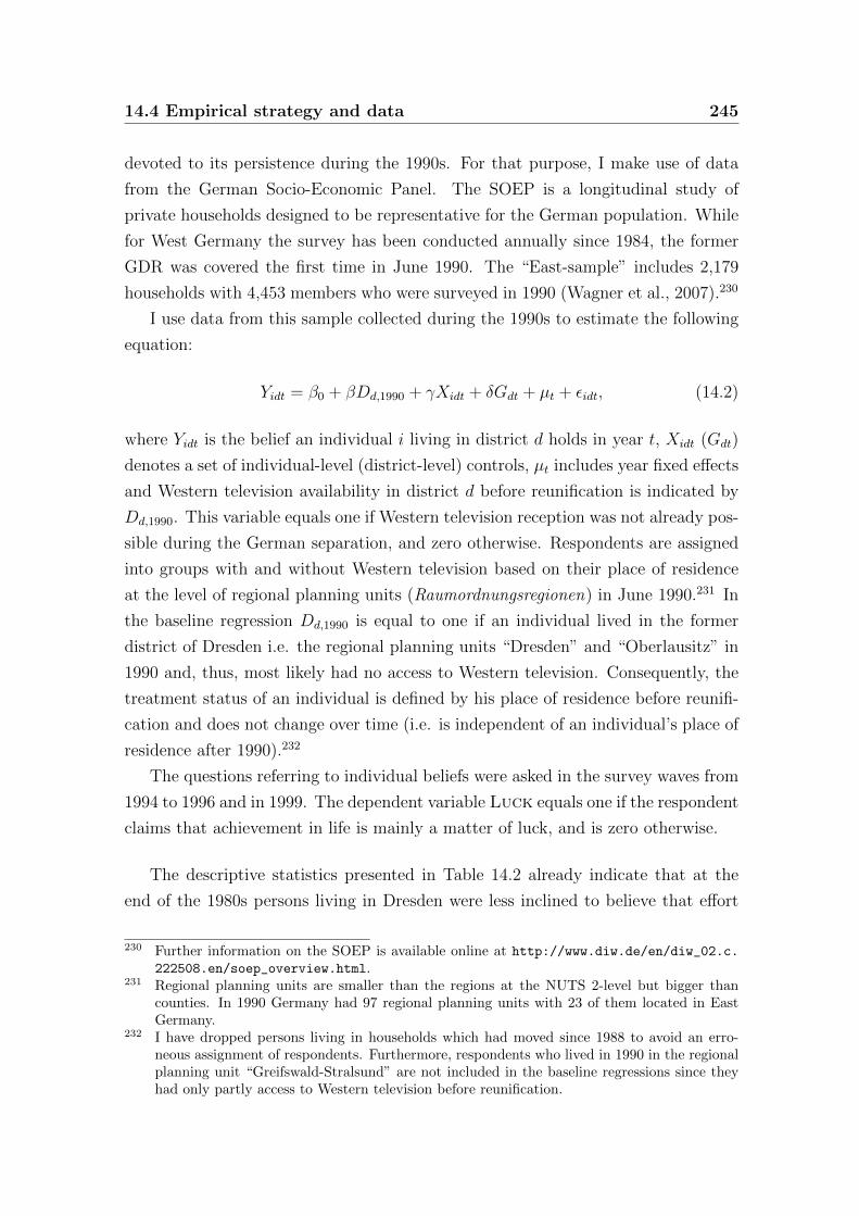
14.4 Empirical strategy and data 245
devoted to its persistence during the 1990s. For that purpose, I make use of data
from the German Socio-Economic Panel. The SOEP is a longitudinal study of
private households designed to be representative for the German population. While
for West Germany the survey has been conducted annually since 1984, the former
GDR was covered the first time in June 1990. The “East-sample” includes 2,179
households with 4,453 members who were surveyed in 1990 (Wagner et al., 2007).230
I use data from this sample collected during the 1990s to estimate the following
equation:
Yidt = β0 + βDd,1990 + γXidt + δGdt + µt + εidt, (14.2)
where Yidt is the belief an individual i living in district d holds in year t, Xidt (Gdt)
denotes a set of individual-level (district-level) controls, µt includes year fixed effects
and Western television availability in district d before reunification is indicated by
Dd,1990. This variable equals one if Western television reception was not already pos-
sible during the German separation, and zero otherwise. Respondents are assigned
into groups with and without Western television based on their place of residence
at the level of regional planning units (Raumordnungsregionen) in June 1990.231 In
the baseline regression Dd,1990 is equal to one if an individual lived in the former
district of Dresden i.e. the regional planning units “Dresden” and “Oberlausitz” in
1990 and, thus, most likely had no access to Western television. Consequently, the
treatment status of an individual is defined by his place of residence before reunifi-
cation and does not change over time (i.e. is independent of an individual’s place of
residence after 1990).232
The questions referring to individual beliefs were asked in the survey waves from
1994 to 1996 and in 1999. The dependent variable Luck equals one if the respondent
claims that achievement in life is mainly a matter of luck, and is zero otherwise.
The descriptive statistics presented in Table 14.2 already indicate that at the
end of the 1980s persons living in Dresden were less inclined to believe that effort
230 Further information on the SOEP is available online at http://www.diw.de/en/diw_02.c.
222508.en/soep_overview.html.231 Regional planning units are smaller than the regions at the NUTS 2-level but bigger than
counties. In 1990 Germany had 97 regional planning units with 23 of them located in EastGermany.
232 I have dropped persons living in households which had moved since 1988 to avoid an erro-neous assignment of respondents. Furthermore, respondents who lived in 1990 in the regionalplanning unit “Greifswald-Stralsund” are not included in the baseline regressions since theyhad only partly access to Western television before reunification.
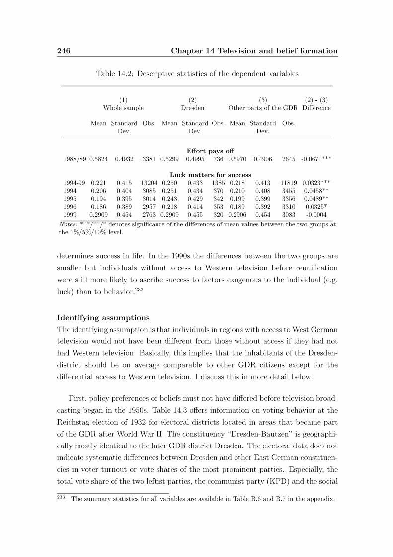
246 Chapter 14 Television and belief formation
Table 14.2: Descriptive statistics of the dependent variables
(1) (2) (3) (2) - (3)Whole sample Dresden Other parts of the GDR Difference
Mean Standard Obs. Mean Standard Obs. Mean Standard Obs.Dev. Dev. Dev.
Effort pays off1988/89 0.5824 0.4932 3381 0.5299 0.4995 736 0.5970 0.4906 2645 -0.0671***
Luck matters for success1994-99 0.221 0.415 13204 0.250 0.433 1385 0.218 0.413 11819 0.0323***1994 0.206 0.404 3085 0.251 0.434 370 0.210 0.408 3455 0.0458**1995 0.194 0.395 3014 0.243 0.429 342 0.199 0.399 3356 0.0489**1996 0.186 0.389 2957 0.218 0.414 353 0.189 0.392 3310 0.0325*1999 0.2909 0.454 2763 0.2909 0.455 320 0.2906 0.454 3083 -0.0004
Notes: ***/**/* denotes significance of the differences of mean values between the two groups atthe 1%/5%/10% level.
determines success in life. In the 1990s the differences between the two groups are
smaller but individuals without access to Western television before reunification
were still more likely to ascribe success to factors exogenous to the individual (e.g.
luck) than to behavior.233
Identifying assumptions
The identifying assumption is that individuals in regions with access to West German
television would not have been different from those without access if they had not
had Western television. Basically, this implies that the inhabitants of the Dresden-
district should be on average comparable to other GDR citizens except for the
differential access to Western television. I discuss this in more detail below.
First, policy preferences or beliefs must not have differed before television broad-
casting began in the 1950s. Table 14.3 offers information on voting behavior at the
Reichstag election of 1932 for electoral districts located in areas that became part
of the GDR after World War II. The constituency “Dresden-Bautzen” is geographi-
cally mostly identical to the later GDR district Dresden. The electoral data does not
indicate systematic differences between Dresden and other East German constituen-
cies in voter turnout or vote shares of the most prominent parties. Especially, the
total vote share of the two leftist parties, the communist party (KPD) and the social
233 The summary statistics for all variables are available in Table B.6 and B.7 in the appendix.
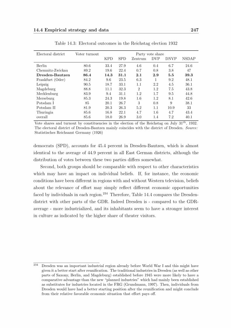
14.4 Empirical strategy and data 247
Table 14.3: Electoral outcomes in the Reichstag election 1932
Electoral district Voter turnout Party vote shareKPD SPD Zentrum DVP DNVP NSDAP
Berlin 80.6 33.4 27.9 4.6 0.4 6.7 24.6Chemnitz-Zwickau 89.2 19.6 22.4 0.7 0.8 3.8 47Dresden-Bautzen 86.4 14.3 31.1 2.1 2.9 5.5 39.3Frankfurt (Oder) 84.2 9.6 23.5 6.3 1 9.2 48.1Leipzig 90.5 18.7 33.1 1.1 2.2 4.5 36.1Magdeburg 88.8 11.1 32.3 2 1.2 7.5 43.8Mecklenburg 83.9 9.4 31.1 1.2 1.7 9.5 44.8Merseburg 85.3 24.3 19.8 1.6 1.2 8.1 42.6Potsdam I 85 20.1 26.7 3 0.8 9 38.1Potsdam II 81.9 20.3 26.3 5.2 1.1 10.9 33Thuringia 85.6 16.8 22.1 4.7 1.6 4.7 43.4overall 85.6 18.0 26.9 3.0 1.4 7.2 40.1
Vote shares and turnout by constituencies in the election of the Reichstag on July 31th, 1932.The electoral district of Dresden-Bautzen mainly coincides with the district of Dresden. Source:Statistisches Reichsamt Germany (1926)
democrats (SPD), accounts for 45.4 percent in Dresden-Bautzen, which is almost
identical to the average of 44.9 percent in all East German districts, although the
distribution of votes between these two parties differs somewhat.
Second, both groups should be comparable with respect to other characteristics
which may have an impact on individual beliefs. If, for instance, the economic
conditions have been different in regions with and without Western television, beliefs
about the relevance of effort may simply reflect different economic opportunities
faced by individuals in each region.234 Therefore, Table 14.4 compares the Dresden-
district with other parts of the GDR. Indeed Dresden is - compared to the GDR-
average - more industrialized, and its inhabitants seem to have a stronger interest
in culture as indicated by the higher share of theater visitors.
234 Dresden was an important industrial region already before World War I and this might havegiven it a better start after reunification. The traditional industries in Dresden (as well as otherparts of Saxony, Berlin, and Magdeburg) established before 1945 were more likely to have acomparative advantage than the new “planned industries” which had mainly been establishedas substitutes for industries located in the FRG (Grundmann, 1997). Then, individuals fromDresden would have had a better starting position after the reunification and might concludefrom their relative favorable economic situation that effort pays off.
248 Chapter 14 Television and belief formation
Tab
le14
.4:
Com
par
ison
ofG
DR
-dis
tric
ts
(1)
(2)
(1)-
(2)
(3)
(1)-
(3)
(4)
(1)-
(4)
(5)
(1)-
(5)
(6)
(7)
(6)-
(7)
Dre
sden
GD
Rw
ith
(p-v
alu
e)ex
cl.
Ber
lin
(p-v
alu
e)S
axony
(p-v
alu
e)E
ast
ern
GD
R(p
-valu
e)V
alley
GD
R(p
-valu
e)W
este
rnte
levis
ion
Pop
ula
tion
den
sity
254
408.2
5-1
54.2
5156.8
2-9
7.1
8285
-31
168.6
7-8
5.3
3146.3
3408.2
5-2
61.9
2(0
.5534)
(0.0
017)
(0.3
193)
(0.3
292)
(0.6
226)
Fem
ale
pop
ula
tion
52.6
52.0
10.5
951.9
7-0
.63
52.8
5-0
.25
51.8
4-0
.7573
51.6
52.0
1-0
.41
(%d
istr
ict
pop
.)(0
.0030)
(0.0
037)
(0.4
120)
(0.3
354)
(0.3
193)
Work
ing
age
pop
ula
tion
62.9
65.0
3-2
.13
64.8
11.9
163.7
5-0
.85
64.8
71.9
164.6
365.0
3-0
.4(%
dis
tric
tp
op
.)(0
.0000)
(0.0
000)
(0.3
656)
(0.1
508)
(0.6
049)
Hig
hed
uca
ted
work
ers
20.6
20.1
0.5
18.9
31.6
718.8
51.7
518.8
5-1
.67
20.1
720.1
0.0
7(%
work
ing
pop
.)(0
.6894)
(0.0
009)
(0.5
177)
(0.1
568)
(0.9
796)
Rel
ati
ve
Lab
or
Inco
me
99
101.0
8-2
.08
100.9
11.9
198.5
0.5
103
498.6
7101.0
8-2
.41
(GD
Raver
age
100)
(0.0
739)
(0.1
249)
(0.7
952)
(0.4
015)
(0.2
928)
Ind
ust
rial
emp
loym
ent
42.8
37.3
95.4
138.4
9-4
.31
44
-1.2
40.0
7-2
.73
29.2
737.3
9-8
.12
(%to
tal
emp
l.)
(0.0
501)
(0.1
039)
(0.8
187)
(0.6
672)
(0.1
908)
Agri
cult
ura
lem
plo
ym
ent
8.1
11.1
9-3
.09
12.1
24.0
27.1
50.9
510.0
92.8
16.5
311.1
95.3
4(%
tota
lem
pl.)
(0.0
806)
(0.0
190)
(0.5
604)
(0.4
306)
(0.0
000)
Ind
ust
rial
pro
du
ctio
n10.7
7.0
13.6
97.1
5-3
.56
10.1
50.5
58.5
-2.2
5.2
77.0
1-1
.74
(%G
DR
ind
.p
rod
.)(0
.0062)
(0.0
135)
(0.8
536)
(0.3
886)
(0.5
066)
Hosp
ital
bed
s95.7
99.2
2-3
.52
97.7
12.0
1105.8
-10.1
83.6
7-1
2.0
395.9
799.2
2-3
.25
(per
10,0
00
inh
ab
it.)
(0.3
879)
(0.6
224)
(0.5
842)
(0.1
403)
(0.6
979)
Th
eate
rvis
itors
0.0
019
0.0
015
0.0
004
0.0
014
-0.0
007
0.0
014
0.0
005
0.0
012
-0.0
007
0.0
018
0.0
015
0.0
003
(%d
istr
ict
pop
.)(0
.0189)
(0.0
015)
(0.0
340)
(0.0
820)
(0.3
634)
Com
pari
son
of
mea
nvalu
esfo
rtr
eatm
ent
an
dco
ntr
ol
gro
up
s.T
he
trea
tmen
tgro
up
incl
ud
esei
ther
(1)
Dre
sden
or
(6)
all
dis
tric
tsw
ith
ou
tfu
llacc
ess
toW
est
Ger
man
tele
vis
ion
(Dre
sden
,N
eub
ran
den
bu
rg,
an
dR
ost
ock
).Sources:
GD
RS
tati
stic
al
Offi
ce,
info
rmati
on
on
lab
or
inco
me
an
dsh
are
of
work
ing
pop
ula
tion
wit
hu
niv
ersi
tyd
egre
efr
om
(Kin
d,
1997).
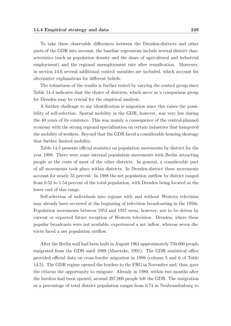
14.4 Empirical strategy and data 249
To take these observable differences between the Dresden-districts and other
parts of the GDR into account, the baseline regressions include several district char-
acteristics (such as population density and the share of agricultural and industrial
employment) and the regional unemployment rate after reunification. Moreover,
in section 14.6 several additional control variables are included, which account for
alternative explanations for different beliefs.
The robustness of the results is further tested by varying the control group since
Table 14.4 indicates that the choice of districts, which serve as a comparison group
for Dresden may be crucial for the empirical analysis.
A further challenge to my identification is migration since this raises the possi-
bility of self-selection. Spatial mobility in the GDR, however, was very low during
the 40 years of its existence. This was mainly a consequence of the central-planned
economy with the strong regional specialization on certain industries that hampered
the mobility of workers. Beyond that the GDR faced a considerable housing shortage
that further limited mobility.
Table 14.5 presents official statistics on population movements by district for the
year 1988. There were some internal population movements with Berlin attracting
people at the costs of most of the other districts. In general, a considerable part
of all movements took place within districts. In Dresden-district these movements
account for nearly 55 percent. In 1988 the net population outflow by district ranged
from 0.52 to 1.54 percent of the total population, with Dresden being located at the
lower end of this range.
Self-selection of individuals into regions with and without Western television
may already have occurred at the beginning of television broadcasting in the 1950s.
Population movements between 1953 and 1957 seem, however, not to be driven by
current or expected future reception of Western television. Dresden, where these
popular broadcasts were not available, experienced a net inflow, whereas seven dis-
tricts faced a net population outflow.
After the Berlin wall had been built in August 1961 approximately 750,000 people
emigrated from the GDR until 1989 (Maretzke, 1991). The GDR statistical office
provided official data on cross-border migration in 1989 (column 5 and 6 of Table
14.5). The GDR regime opened the borders to the FRG in November and, thus, gave
the citizens the opportunity to emigrate. Already in 1989, within two months after
the borders had been opened, around 297,000 people left the GDR. The emigration
as a percentage of total district population ranges from 0.74 in Neubrandenburg to
250 Chapter 14 Television and belief formation
Table 14.5: Internal and external migration in the GDR 1988/89
Internal migration Cross-border migration (1989)
net outflow % within net outflow gross emigration emigrantsDistrict 1953-1957 (%)∗ districts 1988 (%)∗ (%)∗
Berlin 33683 2.62Cottbus -1.48 49.22 0.99 13516 1.53Dresden -0.15 54.54 0.70 46017 2.62Erfurt 0.73 50.85 0.66 20445 1.65Frankfurt -3.61 36.56 1.54 10788 1.51Gera -0.34 51.99 0.83 15632 2.11Halle 1.19 52.14 -0.93 27319 1.54Karl-Marx-Stadt 3.07 61.47 0.52 40347 2.17Leipzig -0.31 44.82 0.97 30654 2.25Magdeburg 0.84 52.50 0.74 14761 1.18Neubrandenburg 2.70 41.34 1.33 4590 0.74Potsdam -3.19 42.45 1.10 17026 1.52Rostock -0.55 46.29 1.09 11279 1.23Schwerin 1.45 46.02 1.02 6029 1.01Suhl 0.91 43.42 0.74 4872 0.89GDR 296958 1.64Average 0.09 48.12 0.81∗ As a share of total district population in the previous year. Source: Information on internal migration based onGDR Statistical Office (various years).
2.62 in Berlin and Dresden. Compared to individuals in other districts, those from
Dresden were more likely to leave the GDR. However, this difference is not large.
Although I cannot completely rule out the possibility of self-selection, I address
this issue by using longitudinal data. Doing so, I can control for spatial mobility
once the treatment status of an individual has been identified based on his place
of residence in June 1990. In principle, my findings could also be driven by some
Dresden-specific factor. In section 14.6, I discuss and test the relevance of several
alternative explanations of the findings. Since the results remain robust, I am confi-
dent that my findings can be explained by differential access to Western television.
14.5 Econometric analysis
Table 14.6 presents the empirical findings concerning the determinants of the belief
that effort pays off during the late 1980s. I employ a probit approach since the
dependent variable is binary. As a first test of the robustness of the results to the
inclusion of control variables, I gradually add a set of variables capturing individual-
and district-level characteristics. I start with a regression of the respondents’ belief
on the Dresden-dummy (i.e. the treatment indicator), the second specification adds
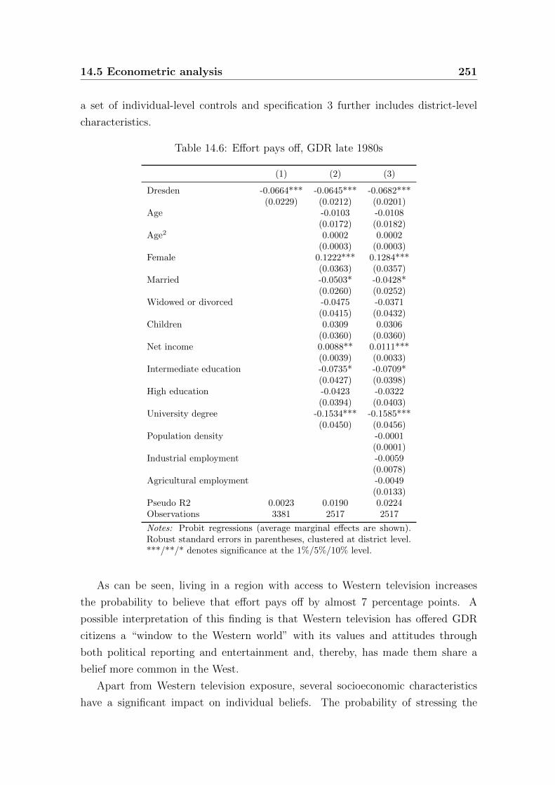
14.5 Econometric analysis 251
a set of individual-level controls and specification 3 further includes district-level
characteristics.
Table 14.6: Effort pays off, GDR late 1980s
(1) (2) (3)
Dresden -0.0664*** -0.0645*** -0.0682***(0.0229) (0.0212) (0.0201)
Age -0.0103 -0.0108(0.0172) (0.0182)
Age2 0.0002 0.0002(0.0003) (0.0003)
Female 0.1222*** 0.1284***(0.0363) (0.0357)
Married -0.0503* -0.0428*(0.0260) (0.0252)
Widowed or divorced -0.0475 -0.0371(0.0415) (0.0432)
Children 0.0309 0.0306(0.0360) (0.0360)
Net income 0.0088** 0.0111***(0.0039) (0.0033)
Intermediate education -0.0735* -0.0709*(0.0427) (0.0398)
High education -0.0423 -0.0322(0.0394) (0.0403)
University degree -0.1534*** -0.1585***(0.0450) (0.0456)
Population density -0.0001(0.0001)
Industrial employment -0.0059(0.0078)
Agricultural employment -0.0049(0.0133)
Pseudo R2 0.0023 0.0190 0.0224Observations 3381 2517 2517
Notes: Probit regressions (average marginal effects are shown).Robust standard errors in parentheses, clustered at district level.***/**/* denotes significance at the 1%/5%/10% level.
As can be seen, living in a region with access to Western television increases
the probability to believe that effort pays off by almost 7 percentage points. A
possible interpretation of this finding is that Western television has offered GDR
citizens a “window to the Western world” with its values and attitudes through
both political reporting and entertainment and, thereby, has made them share a
belief more common in the West.
Apart from Western television exposure, several socioeconomic characteristics
have a significant impact on individual beliefs. The probability of stressing the
252 Chapter 14 Television and belief formation
importance of effort for success is, other things equal, lower for male, married,
better educated,235 and poorer individuals.
Does the effect of differential access to Western television on East Germans’ be-
liefs persist after FRG broadcasts had been available in all parts of the GDR and
individuals could also learn about life in West Germany by their own experience?
Table 14.7 displays the results of the probit estimates on the determinants of beliefs
between 1994 and 1999. In the first column, the belief that success in life is mainly
a matter of luck is regressed on the Dresden-dummy and year fixed effects. The fol-
lowing specifications successively add a set of individual-level controls (specification
2), the regional unemployment rate (specification 3) and current state of residence
fixed effect (specification 4).
The findings suggest that the exposure to FRG television had a persistent effect
on East Germans’ beliefs: persons who had access to Western television were less
likely to believe that luck determines opportunities in life than individuals from
parts of the GDR without Western television. This is the case, although I control for
current economic factors (e.g. net household income, occupation, and employment
status) and regional unemployment. The effect of television on individual beliefs
is also sizable as the marginal effect of the Dresden-dummy ranges from 3.2 to 4.8
percentage points. Thus, the impact of FRG television is 1.5 to 2 times the effect
of being currently unemployed.
Several further explanatory variables affect individual beliefs. The respondent’s
age has a significant but non-linear impact. The probability of believing that luck
is a major determinant of success is higher for women, unemployed respondents,
blue collar workers, and civil servants. Furthermore, the perceived relevance of
luck decreases in both the respondent’s own and his father’s level of education,236
the household income, the number of children living in the same household and
increases in household size as well as former unemployment experience. Finally,
living in states with higher unemployment as well as in West Germany increases the
perceived importance of luck (at least if other state characteristics are captured by
current state of residence fixed effects).
The regression results presented in Table 14.8 provide further insights into how
235 The fact that highly-educated individuals are less inclined to believe that effort pays off forthemselves might be a consequence of the communist system itself: income inequality was lowin the GDR, implying that a person with an university degree had no substantially higherincome than a low educated worker. Hence, the beliefs of highly-educated individuals maysimply reflect their personal experience. Another explanation might be that only citizens whoagree with socialism were allowed to attend a university.
236 The results do not change if instead of the father’s the mother’s level of education is included.
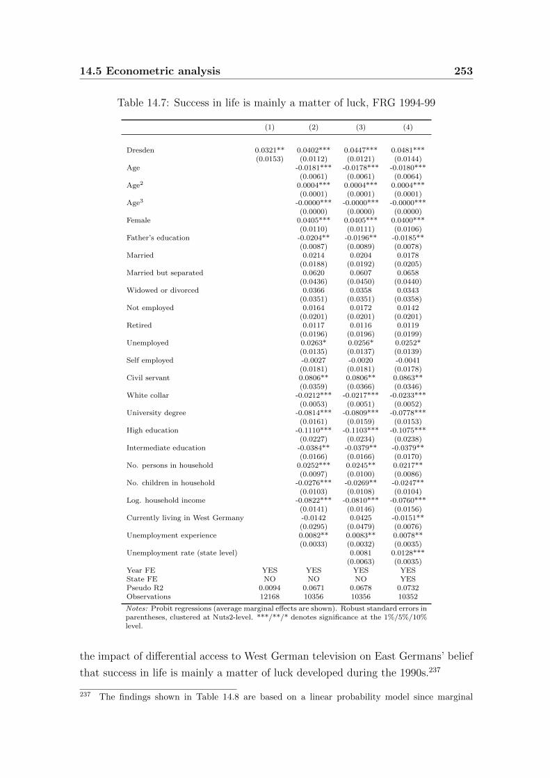
14.5 Econometric analysis 253
Table 14.7: Success in life is mainly a matter of luck, FRG 1994-99
(1) (2) (3) (4)
Dresden 0.0321** 0.0402*** 0.0447*** 0.0481***(0.0153) (0.0112) (0.0121) (0.0144)
Age -0.0181*** -0.0178*** -0.0180***(0.0061) (0.0061) (0.0064)
Age2 0.0004*** 0.0004*** 0.0004***(0.0001) (0.0001) (0.0001)
Age3 -0.0000*** -0.0000*** -0.0000***(0.0000) (0.0000) (0.0000)
Female 0.0405*** 0.0405*** 0.0400***(0.0110) (0.0111) (0.0106)
Father’s education -0.0204** -0.0196** -0.0185**(0.0087) (0.0089) (0.0078)
Married 0.0214 0.0204 0.0178(0.0188) (0.0192) (0.0205)
Married but separated 0.0620 0.0607 0.0658(0.0436) (0.0450) (0.0440)
Widowed or divorced 0.0366 0.0358 0.0343(0.0351) (0.0351) (0.0358)
Not employed 0.0164 0.0172 0.0142(0.0201) (0.0201) (0.0201)
Retired 0.0117 0.0116 0.0119(0.0196) (0.0196) (0.0199)
Unemployed 0.0263* 0.0256* 0.0252*(0.0135) (0.0137) (0.0139)
Self employed -0.0027 -0.0020 -0.0041(0.0181) (0.0181) (0.0178)
Civil servant 0.0806** 0.0806** 0.0863**(0.0359) (0.0366) (0.0346)
White collar -0.0212*** -0.0217*** -0.0233***(0.0053) (0.0051) (0.0052)
University degree -0.0814*** -0.0809*** -0.0778***(0.0161) (0.0159) (0.0153)
High education -0.1110*** -0.1103*** -0.1075***(0.0227) (0.0234) (0.0238)
Intermediate education -0.0384** -0.0379** -0.0379**(0.0166) (0.0166) (0.0170)
No. persons in household 0.0252*** 0.0245** 0.0217**(0.0097) (0.0100) (0.0086)
No. children in household -0.0276*** -0.0269** -0.0247**(0.0103) (0.0108) (0.0104)
Log. household income -0.0822*** -0.0810*** -0.0760***(0.0141) (0.0146) (0.0156)
Currently living in West Germany -0.0142 0.0425 -0.0151**(0.0295) (0.0479) (0.0076)
Unemployment experience 0.0082** 0.0083** 0.0078**(0.0033) (0.0032) (0.0035)
Unemployment rate (state level) 0.0081 0.0128***(0.0063) (0.0035)
Year FE YES YES YES YESState FE NO NO NO YESPseudo R2 0.0094 0.0671 0.0678 0.0732Observations 12168 10356 10356 10352
Notes: Probit regressions (average marginal effects are shown). Robust standard errors inparentheses, clustered at Nuts2-level. ***/**/* denotes significance at the 1%/5%/10%level.
the impact of differential access to West German television on East Germans’ belief
that success in life is mainly a matter of luck developed during the 1990s.237
237 The findings shown in Table 14.8 are based on a linear probability model since marginal
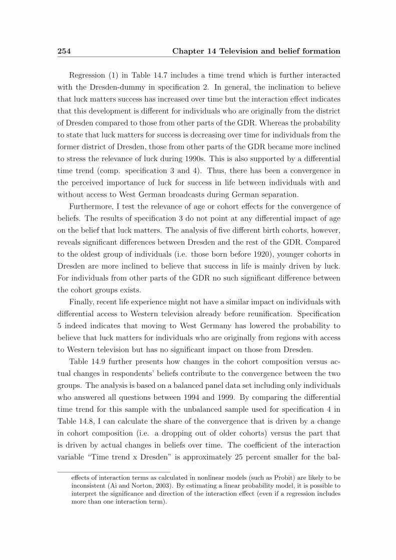
254 Chapter 14 Television and belief formation
Regression (1) in Table 14.7 includes a time trend which is further interacted
with the Dresden-dummy in specification 2. In general, the inclination to believe
that luck matters success has increased over time but the interaction effect indicates
that this development is different for individuals who are originally from the district
of Dresden compared to those from other parts of the GDR. Whereas the probability
to state that luck matters for success is decreasing over time for individuals from the
former district of Dresden, those from other parts of the GDR became more inclined
to stress the relevance of luck during 1990s. This is also supported by a differential
time trend (comp. specification 3 and 4). Thus, there has been a convergence in
the perceived importance of luck for success in life between individuals with and
without access to West German broadcasts during German separation.
Furthermore, I test the relevance of age or cohort effects for the convergence of
beliefs. The results of specification 3 do not point at any differential impact of age
on the belief that luck matters. The analysis of five different birth cohorts, however,
reveals significant differences between Dresden and the rest of the GDR. Compared
to the oldest group of individuals (i.e. those born before 1920), younger cohorts in
Dresden are more inclined to believe that success in life is mainly driven by luck.
For individuals from other parts of the GDR no such significant difference between
the cohort groups exists.
Finally, recent life experience might not have a similar impact on individuals with
differential access to Western television already before reunification. Specification
5 indeed indicates that moving to West Germany has lowered the probability to
believe that luck matters for individuals who are originally from regions with access
to Western television but has no significant impact on those from Dresden.
Table 14.9 further presents how changes in the cohort composition versus ac-
tual changes in respondents’ beliefs contribute to the convergence between the two
groups. The analysis is based on a balanced panel data set including only individuals
who answered all questions between 1994 and 1999. By comparing the differential
time trend for this sample with the unbalanced sample used for specification 4 in
Table 14.8, I can calculate the share of the convergence that is driven by a change
in cohort composition (i.e. a dropping out of older cohorts) versus the part that
is driven by actual changes in beliefs over time. The coefficient of the interaction
variable “Time trend x Dresden” is approximately 25 percent smaller for the bal-
effects of interaction terms as calculated in nonlinear models (such as Probit) are likely to beinconsistent (Ai and Norton, 2003). By estimating a linear probability model, it is possible tointerpret the significance and direction of the interaction effect (even if a regression includesmore than one interaction term).
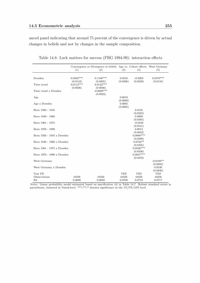
14.5 Econometric analysis 255
anced panel indicating that around 75 percent of the convergence is driven by actual
changes in beliefs and not by changes in the sample composition.
Table 14.8: Luck matters for success (FRG 1994-99): interaction effects
Convergence or Divergence in beliefs Age vs. Cohort effects West Germany(1) (2) (3) (4) (5)
Dresden 0.0502*** 0.1108*** 0.0316 -0.0203 0.0470***(0.0143) (0.0205) (0.0266) (0.0230) (0.0134)
Time trend 0.0112*** 0.0122***(0.0026) (0.0026)
Time trend x Dresden -0.0088***(0.0022)
Age 0.0010(0.0009)
Age x Dresden 0.0005(0.0005)
Born 1920 - 1945 0.0185(0.0325)
Born 1946 - 1960 0.0008(0.0385)
Born 1961 - 1975 -0.0160(0.0541)
Born 1976 - 1990 0.0012(0.0642)
Born 1920 - 1945 x Dresden 0.0888***(0.0386)
Born 1946 - 1960 x Dresden 0.0722**(0.0325)
Born 1961 - 1975 x Dresden 0.0536***(0.0336)
Born 1976 - 1990 x Dresden 0.0847***(0.0433)
West Germany -0.0188**(0.0092)
West Germany x Dresden 0.0536(0.0946)
Year FE YES YES YESObservations 10356 10356 10356 10356 10356R2 0.0690 0.0692 0.0708 0.0716 0.0717
Notes: Linear probability model estimated based on specification (4) in Table 14.7. Robust standard errors inparentheses, clustered at Nuts2-level. ***/**/* denotes significance at the 1%/5%/10% level.
256 Chapter 14 Television and belief formation
Table 14.9: Luck matters for success (FRG 1994-99): differential time trends (bal-anced panel)
(1) (2) (3)
Dresden 0.0824*** 0.0862*** 0.0899***(0.0262) (0.0204) (0.0224)
Time trend 0.0207*** 0.0144*** 0.0145***(0.0033) (0.0032) (0.0029)
Time trend x Dresden -0.0059* -0.0059** -0.0066***(0.0031) (0.0023) (0.0023)
State FE NO NO YESObservations 9119 9119 9119R2 0.0628 0.0638 0.0685
Notes: Linear probability model. Estimates include all explanatory variables introducedin specifications 2 to 4 in Table 14.7 but are restricted to individuals who answered thequestion on the relevance of luck for success in all years (balanced panel). Robust stan-dard errors in parentheses, clustered at Nuts2-level. ***/**/* denotes significance at the1%/5%/10% level.
14.6 Robustness and some further results
The empirical findings suggest that East Germans with access to Western television
were more inclined to share beliefs more common in the West both before reunifi-
cation and several years afterwards. Dresden seems to be on average comparable to
other GDR-districts (see Table 14.3 and 14.4). Still, a major concern might be that
factors others than television reception cause the differences in beliefs. In the fol-
lowing, I test the robustness of the results by varying the group of districts Dresden
is compared to (control group) and include variables which account for alternative
explanations.
14.6.1 Varying the control group
In Table 14.10 the robustness of the results is tested using different groups of districts
as a comparison group for Dresden. First, I exclude observations from East Berlin
from the sample. The district of Berlin is not fully comparable to other districts
due to its position as the capital of the GDR and the fact that the former city of
Berlin had been separated by the allied forces. Second, the analysis will be restricted
to Saxon districts (Dresden, Leipzig and Karl-Marx-Stadt). These districts share a
common history as parts of the Kingdom of Saxony and, therefore, most likely also a
14.6 Robustness and some further results 257
common culture and values. Moreover, they are also highly comparable with respect
to other characteristics (see Table 14.4). Furthermore, the observable differences
could also be explained by the geographical location of the Dresden-district in the
Eastern part of the GDR. It could also be the case that after the fall of the Berlin
wall higher costs of travelling to West Germany due to the larger distance deters
the population in the Eastern part from learning about the West by own experience.
If that explains the different beliefs, then the same should apply to other regions
located in the Eastern part of the GDR. Thus, I restrict the analysis to these regions.
For the analysis based on the SOEP also data for the outermost Northeast of the
GDR, which had only partial access to these broadcasts is available. Hence, the
treatment group is extended to both regions without Western television reception
(i.e., Dresden and the regional planning unit Greifswald-Stralsund).
The results indicate that the treatment effect remains widely unchanged if East
Berlin is excluded or only Saxon districts are analyzed. If the control group is
restricted to regions in the East of the GDR, the treatment effect becomes smaller.
Furthermore, the treatment effect loses its significance if Greifswald is included as the
second part of the GDR with only partial access to Western television. Although
this may be an indication that the results are driven by (unobserved) Dresden-
specific characteristics, the partial insignificance does not necessarily imply that
Western television has no effect. The area in the Northeast without West German
television reception did not coincide perfectly with “Greifswald-Stralsund” (as it
was the case with the district of Dresden in the Southeast).238 Consequently, the
smaller and less significant treatment effect may reflect downward biased estimates
as individuals might be assigned to the treatment group who actually had access
to Western television. Furthermore, Dresden and Greifswald-Stralsund differ with
respect to other characteristics (e.g. Greifswald-Stralsund is more rural). This
heterogeneity might have contributed to the loss of significance since the treatment
effect gets highly significant if state fixed effects controlling for such heterogeneity
are included.
238 This is also indicated by a survey conducted by the central institute for youth research in 1981.While 68.8 percent of the respondents living in the district of Dresden stated that they didnot watch Western television at all, the share in the districts Rostock and Neubrandenburgwas only 27 percent.
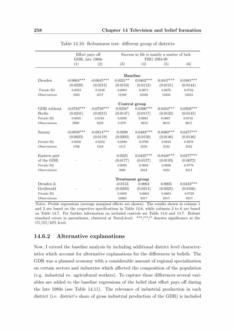
258 Chapter 14 Television and belief formation
Table 14.10: Robustness test: different group of districts
Effort pays off Success in life is mainly a matter of luckGDR, late 1980s FRG 1994-99(1) (2) (3) (4) (5) (6)
BaselineDresden -0.0664*** -0.0645*** 0.0321** 0.0402*** 0.0447*** 0.0481***
(0.0229) (0.0212) (0.0153) (0.0112) (0.0121) (0.0144)Pseudo R2 0.0023 0.0190 0.0094 0.0671 0.0678 0.0732
Observations 3382 2517 12168 10356 10356 10352
Control groupGDR without -0.0783*** -0.0759*** 0.0256* 0.0390*** 0.0434*** 0.0503***Berlin (0.0241) (0.0215) (0.0147) (0.0117) (0.0132) (0.0145)Pseudo R2 0.0035 0.0185 0.0095 0.0684 0.0687 0.0742
Observations 2990 2258 11279 9619 9619 9615
Saxony -0.0859*** -0.0814*** 0.0298 0.0483*** 0.0480*** 0.0477***(0.0023) (0.0119) (0.0203) (0.0150) (0.0146) (0.0146)
Pseudo R2 0.0056 0.0232 0.0088 0.0796 0.0845 0.0878
Observations 1596 1218 4115 3532 3532 3522
Eastern part 0.0225 0.0435*** 0.0448*** 0.0277***of the GDR – – (0.0177) (0.0127) (0.0133) (0.0072)Pseudo R2 0.0095 0.0694 0.0696 0.0778
Observations 4068 3424 3424 3414
Treatment groupDresden & -0.0153 0.0004 0.0005 0.0423***Greifswald – – (0.0293) (0.0314) (0.0325) (0.0160)Pseudo R2 0.0095 0.0663 0.0663 0.0729
Observations 10963 9317 9317 9317
Notes: Probit regressions (average marginal effects are shown). The results shown in column 1and 2 are based on the respective specifications in Table 14.6, while columns 3 to 6 are basedon Table 14.7. For further information on included controls see Table 14.6 and 14.7. Robuststandard errors in parentheses, clustered at Nuts2-level. ***/**/* denotes significance at the1%/5%/10% level.
14.6.2 Alternative explanations
Now, I extend the baseline analysis by including additional district level character-
istics which account for alternative explanations for the differences in beliefs. The
GDR was a planned economy with a considerable amount of regional specialization
on certain sectors and industries which affected the composition of the population
(e.g. industrial vs. agricultural workers). To capture these differences several vari-
ables are added to the baseline regressions of the belief that effort pays off during
the late 1980s (see Table 14.11). The relevance of industrial production in each
district (i.e. district’s share of gross industrial production of the GDR) is included
14.6 Robustness and some further results 259
in column (1). Further controls are the share of working age population (as a per-
centage of total district population) in column (2) and the level of education of the
district’s working population (share of workers with an university degree) in column
(3). While the share of industrial production has no significant effect on the respon-
dents’ beliefs, a higher share of population in their working age and better educated
workers increase the probability to believe that effort pays off.
Furthermore, the geographical location of a district may be related to its in-
habitants’ attitudes. Hence, I include both a variable indicating whether a district
has a common border with the FRG and the distance between the district capi-
tal and Berlin (in kilometers). The results, however, do not indicate a significant
relationship.
Finally, Dresden was famous for its arts and culture. Thus, the population
had perhaps been more interested in culture, arts, and literature. More generally,
if (traditionally educated) middle-class intellectuals entertain different beliefs than
the rest of the population this could also explain the main findings of this paper.
Therefore, I include both dummy-variables indicating whether the respondent had
lately been to a theater, cinema, or museum (specifications 6 to 8) and the number
of theater visitors in each district (weighted by the total district population). The
individual interest in arts and culture affects beliefs at least partly: individuals who
visited cinema and museums are more likely to believe that effort pays off. Moreover,
individuals in districts where a higher share of the population visits theaters are less
inclined to believe that effort pays off.
An overall important finding is that the inclusion of these further control vari-
ables does not change the results in substance with the treatment indicator remain-
ing robust and significant.
The identification of the Western television effect during the 1990s does not
only depend on the absence of structural differences before reunification but also on
the assumption that both regions were not hit by (systematically) different shocks
afterwards. Otherwise, the observable differences between individuals from Dresden
and those from other parts of the GDR could also be a consequence of differences
in the economic or social conditions.
To address these concerns, I add several regional characteristics to my baseline
specification using data from the SOEP (see specification 4 in Table 14.7). Table
14.12 displays the results. Due to data constraints, the specifications 2 to 6 are only
based on observations for the years 1996 and 1999. To enhance the comparability
of the results and to distinguish between the impact of different samples and of
260 Chapter 14 Television and belief formation
additional controls, column 1 shows the results of the baseline regression based on
observations from 1996 and 1999.
After reunification, wide parts of East Germany faced considerable problems as
most parts of the GDR economy were not capable of competing with the West.
Since unemployment increased during the 1990s, some East German regions experi-
enced a considerable population loss and demographic problems. To capture related
economic and demographic differences, I add each regional planning unit’s popula-
tion density (specification 2), share of inhabitants older than 65 (specification 3),
unemployment rate (specification 4), average monthly labor income of industrial
workers (specification 5), and GDP per capita (specification 6). The results indicate
that only the regional unemployment rate has a significant effect on the respondents
likelihood to believe that success is mainly a consequence of luck. More important,
the coefficients of the Dresden-dummy remain highly significant and robust.
Another concern is related to cultural or religious differences between the two
groups. Thus, I include the respondent’s own religious denomination in 1990 and
his mother’s religion to proxy cultural effects.239 The findings suggest a significant
impact of religion on the belief regarding the role of luck for success: individuals
with a religious mother (independent of her denomination) are more inclined to
believe that luck matters. The results on the respondent’s own religion in 1990
show that protestants (and those belonging to other religious communities) tend to
be more (less) likely to stress the relevance of luck than those without on religious
denomination. The Dresden-dummy again remains robust.
239 Using the father’s instead of the mother’s religion does not change the results.
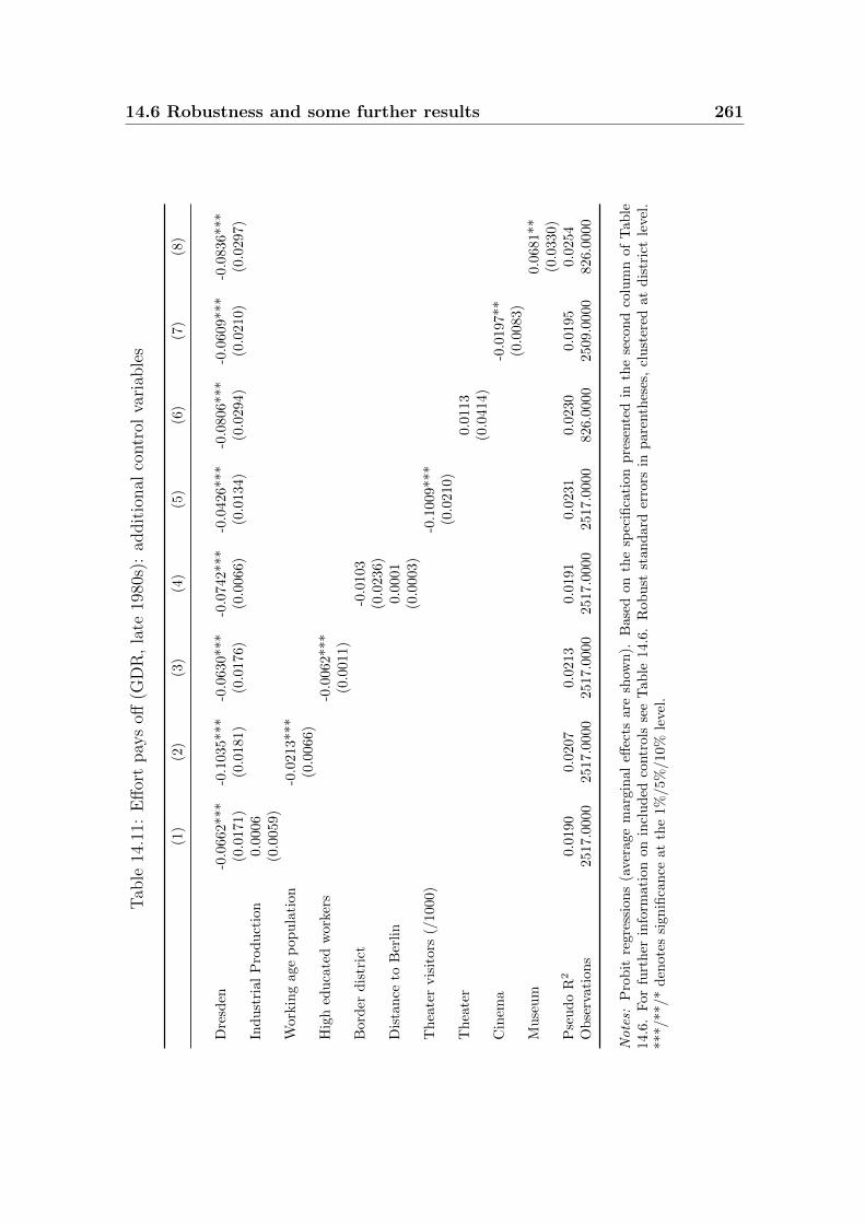
14.6 Robustness and some further results 261
Tab
le14
.11:
Eff
ort
pay
soff
(GD
R,
late
1980
s):
addit
ional
contr
olva
riab
les
(1)
(2)
(3)
(4)
(5)
(6)
(7)
(8)
Dre
sden
-0.0
662*
**-0
.103
5***
-0.0
630***
-0.0
742***
-0.0
426***
-0.0
806***
-0.0
609***
-0.0
836***
(0.0
171)
(0.0
181)
(0.0
176)
(0.0
066)
(0.0
134)
(0.0
294)
(0.0
210)
(0.0
297)
Ind
ust
rial
Pro
du
ctio
n0.
0006
(0.0
059)
Wor
kin
gag
ep
opu
lati
on-0
.021
3***
(0.0
066)
Hig
hed
uca
ted
wor
kers
-0.0
062***
(0.0
011)
Bor
der
dis
tric
t-0
.0103
(0.0
236)
Dis
tan
ceto
Ber
lin
0.0
001
(0.0
003)
Th
eate
rvis
itor
s(/
1000
)-0
.1009***
(0.0
210)
Th
eate
r0.0
113
(0.0
414)
Cin
ema
-0.0
197**
(0.0
083)
Mu
seu
m0.0
681**
(0.0
330)
Pse
ud
oR
20.
0190
0.02
07
0.0
213
0.0
191
0.0
231
0.0
230
0.0
195
0.0
254
Ob
serv
atio
ns
2517
.000
025
17.0
000
2517.0
000
2517.0
000
2517.0
000
826.0
000
2509.0
000
826.0
000
Note
s:P
rob
itre
gres
sion
s(a
vera
gem
argi
nal
effec
tsare
show
n).
Base
don
the
spec
ifica
tion
pre
sente
din
the
seco
nd
colu
mn
of
Tab
le14
.6.
For
furt
her
info
rmat
ion
onin
clu
ded
contr
ols
see
Tab
le14.6
.R
ob
ust
stan
dard
erro
rsin
pare
nth
eses
,cl
ust
ered
at
dis
tric
tle
vel.
***/
**/*
den
otes
sign
ifica
nce
atth
e1%
/5%
/10%
leve
l.

262 Chapter 14 Television and belief formation
Tab
le14
.12:
Luck
mat
ters
for
succ
ess
(FR
G19
94-9
9):
addit
ional
contr
olva
riab
les
(1)
(2)
(3)
(4)
(5)
(6)
(7)
(8)
Dre
sden
0.03
58***
0.0
393***
0.0
367***
0.0
312***
0.0
357***
0.0
348***
0.0
678***
0.0
490***
(0.0
118)
(0.0
137)
(0.0
109)
(0.0
110)
(0.0
115)
(0.0
108)
(0.0
161)
(0.0
119)
Pop
ula
tion
den
sity
0.0
001
(0.0
001)
Inh
abit
ants
old
erth
an65
0.0
010
(0.0
063)
Un
emp
loym
ent
rate
(reg
ion
alp
lan
nin
gu
nit
)0.0
111***
(0.0
031)
Ave
rage
ind
ust
rial
wag
e0.0
000
(0.0
000)
GD
Pp
erca
pit
a-0
.002
7(0
.0027)
Mot
her
:C
ath
olic
0.0
710**
(0.0
303)
Mot
her
:P
rote
stan
t0.0
510***
(0.0
198)
Mot
her
:O
ther
0.0
870**
(0.0
402)
Res
pon
den
t(1
990)
:C
ath
olic
-0.0
065
(0.0
274)
Res
pon
den
t(1
990)
:P
rote
stan
t0.0
324*
(0.0
178)
Res
pon
den
t(1
990)
:O
ther
-0.0
702*
(0.0
360)
Pse
ud
oR
20.
0787
0.0
788
0.0
787
0.0
796
0.0
787
0.0
787
0.0
631
0.0
806
Ob
serv
atio
ns
5394
5394
5394
5394
5394
5394
2274
9212
Note
s:P
rob
itre
gres
sion
s(a
vera
gem
argi
nal
effec
tsar
esh
own
).B
ase
don
the
spec
ifica
tion
pre
sente
din
the
seco
nd
colu
mn
of
Tab
le14.7
.F
or
furt
her
info
rmat
ion
onin
clu
ded
contr
ols
see
Tab
le14
.7.
Om
itte
dca
tegory
inth
esp
ecifi
cati
on
s(8
)an
d(9
)is
no
reli
gio
n.
Rob
ust
stan
dard
erro
rsin
par
enth
eses
,cl
ust
ered
atd
istr
ict
leve
l.**
*/**
/*d
enot
essi
gn
ifica
nce
at
the
1%
/5%
/10%
leve
l.

14.6 Robustness and some further results 263
14.6.3 Additional insights into the role of Western television
The main objective of East German television was the indoctrination of the audi-
ence to alter their attitudes toward the GDR and socialism. Kern and Hainmueller
(2009) analyze - based on GDR survey data - how access to West German television
has affected attitudes toward the GDR in the late 1980s. They find that Western
television contributed to a more positive assessment of different aspects of life in the
GDR. Their basic explanation for this is that Western television made life in the
GDR more bearable, which increased general satisfaction and made East Germans
less critical toward the GDR regime and realities of socialism. This is in line with
my argument that West German television affected East Germans’ beliefs mainly by
presenting different world views and values in its entertainment programs. Insofar,
Kern and Hainmuller’s and my work shed a light on different aspects of entertain-
ment provided by television.
Though the effect of Western television on economic beliefs persisted during
the 1990s, this must not be the case for the attitudes toward the GDR. If the main
contribution of Western television was the entertainment of East Germans, the effect
of different access to these broadcasts should not persist once everyone obtains the
opportunity to watch and the situation in the GDR actually changes. Thus, I
complement the analysis of Kern and Hainmueller (2009) by testing empirically
whether the attitudes toward the GDR are still different between individuals from
Dresden and other parts of the GDR after the reunification process started.
The empirical results presented in Table 14.13 confirm the earlier finding that
before reunification, individuals without access to Western television were more skep-
tical toward several aspects of life in the GDR. Those living in the district of Dresden
are significantly less content with the quality of reporting by state-controlled GDR
media, less satisfied with life in the GDR in general, and significantly less optimistic
about the future development of the economy and democracy in socialist states. Fur-
thermore, the findings indicate a significantly positive relationship between access
to Western television and the agreement with the Marxist-Leninist ideology.
Table 14.14 presents the findings of the analysis using data from the SOEP
for the 1990s to test the persistence of differential attitudes after the reunification.
In summer 1990, soon after the inner-German border was opened, no significant
differences in the assessment of the social security and the democracy in the GDR
are observable.
However, individuals from the Dresden-district are relatively more satisfied with
the standard of living in East Germany after reunification. While individuals who
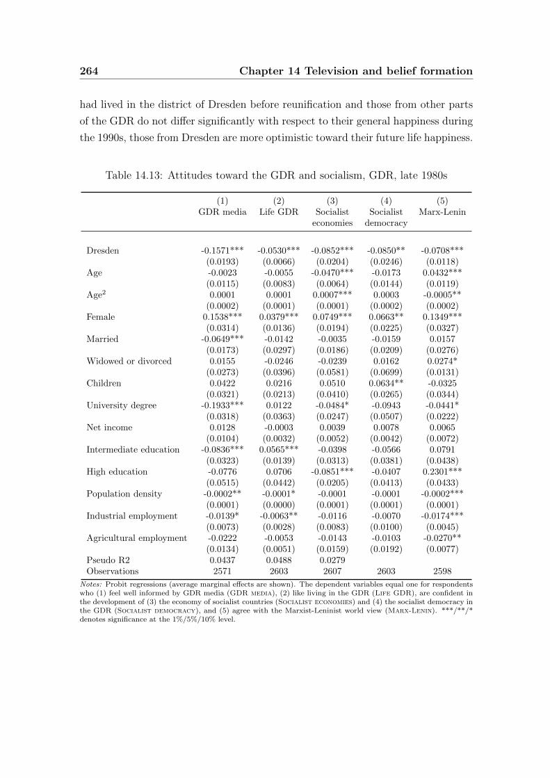
264 Chapter 14 Television and belief formation
had lived in the district of Dresden before reunification and those from other parts
of the GDR do not differ significantly with respect to their general happiness during
the 1990s, those from Dresden are more optimistic toward their future life happiness.
Table 14.13: Attitudes toward the GDR and socialism, GDR, late 1980s
(1) (2) (3) (4) (5)GDR media Life GDR Socialist Socialist Marx-Lenin
economies democracy
Dresden -0.1571*** -0.0530*** -0.0852*** -0.0850** -0.0708***(0.0193) (0.0066) (0.0204) (0.0246) (0.0118)
Age -0.0023 -0.0055 -0.0470*** -0.0173 0.0432***(0.0115) (0.0083) (0.0064) (0.0144) (0.0119)
Age2 0.0001 0.0001 0.0007*** 0.0003 -0.0005**(0.0002) (0.0001) (0.0001) (0.0002) (0.0002)
Female 0.1538*** 0.0379*** 0.0749*** 0.0663** 0.1349***(0.0314) (0.0136) (0.0194) (0.0225) (0.0327)
Married -0.0649*** -0.0142 -0.0035 -0.0159 0.0157(0.0173) (0.0297) (0.0186) (0.0209) (0.0276)
Widowed or divorced 0.0155 -0.0246 -0.0239 0.0162 0.0274*(0.0273) (0.0396) (0.0581) (0.0699) (0.0131)
Children 0.0422 0.0216 0.0510 0.0634** -0.0325(0.0321) (0.0213) (0.0410) (0.0265) (0.0344)
University degree -0.1933*** 0.0122 -0.0484* -0.0943 -0.0441*(0.0318) (0.0363) (0.0247) (0.0507) (0.0222)
Net income 0.0128 -0.0003 0.0039 0.0078 0.0065(0.0104) (0.0032) (0.0052) (0.0042) (0.0072)
Intermediate education -0.0836*** 0.0565*** -0.0398 -0.0566 0.0791(0.0323) (0.0139) (0.0313) (0.0381) (0.0438)
High education -0.0776 0.0706 -0.0851*** -0.0407 0.2301***(0.0515) (0.0442) (0.0205) (0.0413) (0.0433)
Population density -0.0002** -0.0001* -0.0001 -0.0001 -0.0002***(0.0001) (0.0000) (0.0001) (0.0001) (0.0001)
Industrial employment -0.0139* -0.0063** -0.0116 -0.0070 -0.0174***(0.0073) (0.0028) (0.0083) (0.0100) (0.0045)
Agricultural employment -0.0222 -0.0053 -0.0143 -0.0103 -0.0270**(0.0134) (0.0051) (0.0159) (0.0192) (0.0077)
Pseudo R2 0.0437 0.0488 0.0279Observations 2571 2603 2607 2603 2598
Notes: Probit regressions (average marginal effects are shown). The dependent variables equal one for respondentswho (1) feel well informed by GDR media (GDR media), (2) like living in the GDR (Life GDR), are confident inthe development of (3) the economy of socialist countries (Socialist economies) and (4) the socialist democracy inthe GDR (Socialist democracy), and (5) agree with the Marxist-Leninist world view (Marx-Lenin). ***/**/*denotes significance at the 1%/5%/10% level.
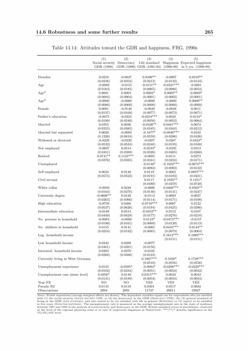
14.6 Robustness and some further results 265
Table 14.14: Attitudes toward the GDR and happiness, FRG, 1990s
(1) (2) (3) (4) (5)Social security Democracy Life standard Happiness Expected happinessGDR (1990) GDR (1990) GDR (1991-94) (1990-99) in 5 yrs. (1990-99)
Dresden 0.0218 -0.0047 0.0496** -0.0007 0.0319**(0.0248) (0.0353) (0.0213) (0.0132) (0.0144)
Age -0.0089 -0.0155 -0.0151** -0.0321*** -0.0001(0.0163) (0.0185) (0.0065) (0.0080) (0.0054)
Age2 0.0001 0.0003 0.0002* 0.0005** -0.0003*(0.0004) (0.0004) (0.0001) (0.0002) (0.0001)
Age3 -0.0000 -0.0000 -0.0000 -0.0000 0.0000**(0.0000) (0.0000) (0.0000) (0.0000) (0.0000)
Female 0.0081 -0.0140 -0.0049 -0.0048 0.0011(0.0137) (0.0109) (0.0077) (0.0073) (0.0071)
Father’s education -0.0075 -0.0224 -0.0218*** 0.0022 0.0124*(0.0189) (0.0240) (0.0059) (0.0052) (0.0064)
Married 0.0355 0.0036 -0.0326** 0.0481*** 0.0074(0.0355) (0.0385) (0.0165) (0.0164) (0.0212)
Married but separated 0.0626 -0.0093 -0.1077* -0.0946*** 0.0102(0.1226) (0.0818) (0.0559) (0.0286) (0.0426)
Widowed or divorced -0.0228 -0.0220 -0.0287 0.0267 0.0323*(0.0532) (0.0534) (0.0240) (0.0193) (0.0168)
Not employed -0.0697 0.0514 -0.0533* -0.0335 0.0313(0.0451) (0.0389) (0.0326) (0.0405) (0.0268)
Retired 0.0741** 0.1123*** -0.0085 0.0111 0.0273(0.0376) (0.0385) (0.0161) (0.0224) (0.0171)
Unemployed -0.0146* -0.1622*** -0.0674***(0.0082) (0.0092) (0.0132)
Self employed 0.0624 0.0149 0.0119 0.0062 0.0897***(0.0574) (0.0523) (0.0191) (0.0183) (0.0221)
Civil servant 0.0117 0.1035** 0.1451*(0.0480) (0.0478) (0.0740)
White collar -0.0050 0.0248 -0.0006 0.0460*** 0.0505**(0.0163) (0.0270) (0.0130) (0.0141) (0.0247)
University degree -0.0606** 0.0120 -0.0113 0.0093 0.0027(0.0263) (0.0366) (0.0114) (0.0171) (0.0108)
High education -0.0759 0.0466 -0.0716*** 0.0087 0.0122(0.0537) (0.0626) (0.0194) (0.0425) (0.0286)
Intermediate education -0.0188 0.0514 -0.0352** 0.0153 0.0107(0.0449) (0.0429) (0.0177) (0.0276) (0.0218)
No. persons in household -0.0083 -0.0099 0.0123* -0.0475*** -0.0157(0.0190) (0.0161) (0.0069) (0.0120) (0.0113)
No. children in household 0.0155 0.0141 -0.0065 0.0416*** 0.0144**(0.0254) (0.0182) (0.0085) (0.0073) (0.0064)
Log. household income 0.1613*** 0.1060***(0.0151) (0.0151)
Low household income 0.0342 0.0289 -0.0077(0.0461) (0.0391) (0.0150)
Intermed. household income 0.0203 0.0270 -0.0105(0.0268) (0.0386) (0.0123)
Currently living in West Germany 0.1867*** 0.1028* 0.1728***(0.0510) (0.0556) (0.0556)
Unemployment experience 0.0125 -0.0395* -0.0084* -0.0296*** -0.0229***(0.0102) (0.0234) (0.0051) (0.0054) (0.0042)
Unemployment rate (state level) 0.0256* 0.0149 0.0215*** 0.0023 0.0043(0.0141) (0.0189) (0.0054) (0.0054) (0.0054)
Year FE NO NO YES YES YESPseudo R2 0.0145 0.0118 0.0404 0.0517 0.0682Observations 2994 2991 11747 20011 19927
Notes: Probit regressions (average marginal effects are shown). The dependent variables equals one for respondents who are satisfiedwith (1) the social security (Social security GDR, or (2) the democracy in the GDR (Democracy GDR), the (3) general standard ofliving in the GDR (Life standard), and who stated to be (4) satisfied with life in general (Happiness) or (5) expect to be satisfiedin five years (Expected happiness). The unemployment rate is measured as the average unemployment rate in the state of residencebetween 1991 and 1995 in the analysis of social security and democracy in the GDR. Robust standard errors in parentheses, clusteredat the level of the regional planning units or in case of (expected) happiness at Nuts2-level. ***/**/* denotes significance at the1%/5%/10% level.
266 Chapter 14 Television and belief formation
14.7 Conclusion
This study exploits a natural experiment on West German television reception in
the former GDR to analyze its impact on East Germans’ beliefs before and up to
one decade after reunification. I show that the availability of Western television has
made East Germans more inclined to believe that effort rather than luck determines
success in life. Moreover, Western television also affected attitudes toward the GDR
and socialism. While the exposure to West German media is reflected in personal
beliefs up to ten years after reunification, differences in attitudes diminished soon
after the fall of the Berlin wall.
I argue that the regime-stabilizing effect of Western television and its impact
on East Germans’ beliefs reflect two different aspects of entertainment programs
(e.g. movies or soap operas). In the short run, these programs made life in real-
existing socialism more bearable. Beyond entertainment, Western soap operas and
movies also provided additional signals about the relationship between effort (as
opposed to predetermined factors such as luck) and success and by this affected
the corresponding beliefs of East Germans. Those elementary beliefs remain rather
stable once they are formed in a critical age (e.g. during early adulthood; see
Giuliano and Spilimbergo, 2009), which can explain the persistence of the effect of
differential access to Western television during the 1990s.
It might be true that the main findings of this paper are driven by some Dresden-
specific factor. Given the robustness of the result to various additional tests, I am,
however, confident that West German television has indeed affected the beliefs and
attitudes of East Germans. Hence, state-controlled media seem to have been a part
of socialization that has left its marks on East Germans minds.
This analysis is based on exposure to Western television in the GDR and, thus,
on a specific situation. Still, it indicates that the role of information provided by
mass media should not be overlooked for belief formation. Since beliefs on the drivers
of success are also correlated with voters’ preferences for redistribution, television
may affect policy outcomes even if that may not be intended but may just be a
byproduct of providing entertainment.
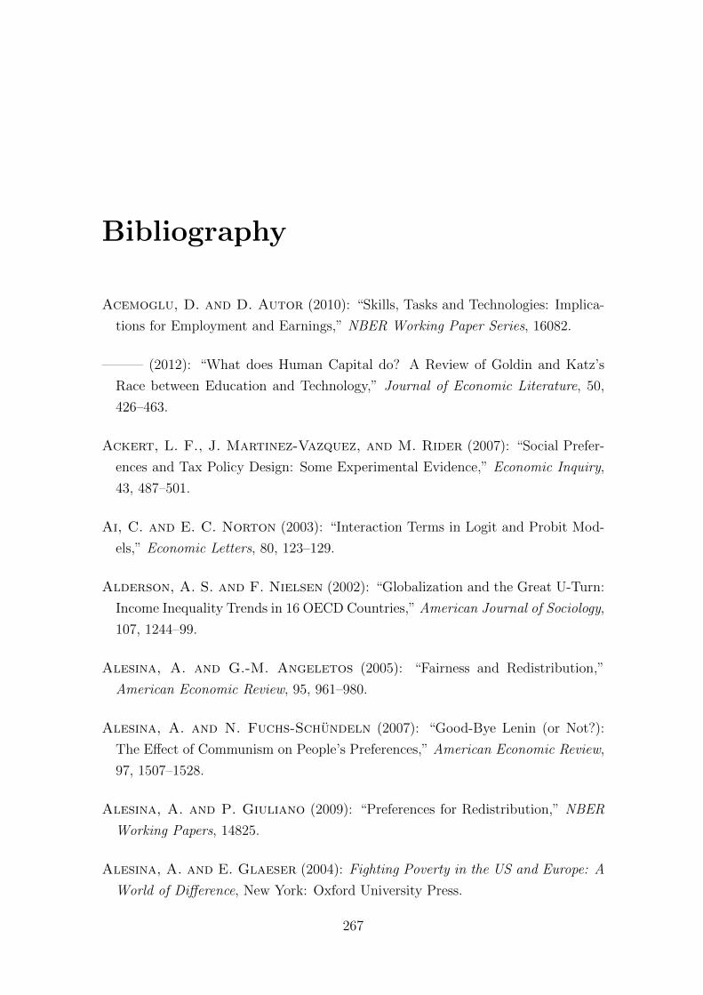
Bibliography
Acemoglu, D. and D. Autor (2010): “Skills, Tasks and Technologies: Implica-
tions for Employment and Earnings,” NBER Working Paper Series, 16082.
——— (2012): “What does Human Capital do? A Review of Goldin and Katz’s
Race between Education and Technology,” Journal of Economic Literature, 50,
426–463.
Ackert, L. F., J. Martinez-Vazquez, and M. Rider (2007): “Social Prefer-
ences and Tax Policy Design: Some Experimental Evidence,” Economic Inquiry,
43, 487–501.
Ai, C. and E. C. Norton (2003): “Interaction Terms in Logit and Probit Mod-
els,” Economic Letters, 80, 123–129.
Alderson, A. S. and F. Nielsen (2002): “Globalization and the Great U-Turn:
Income Inequality Trends in 16 OECD Countries,” American Journal of Sociology,
107, 1244–99.
Alesina, A. and G.-M. Angeletos (2005): “Fairness and Redistribution,”
American Economic Review, 95, 961–980.
Alesina, A. and N. Fuchs-Schundeln (2007): “Good-Bye Lenin (or Not?):
The Effect of Communism on People’s Preferences,” American Economic Review,
97, 1507–1528.
Alesina, A. and P. Giuliano (2009): “Preferences for Redistribution,” NBER
Working Papers, 14825.
Alesina, A. and E. Glaeser (2004): Fighting Poverty in the US and Europe: A
World of Difference, New York: Oxford University Press.
267
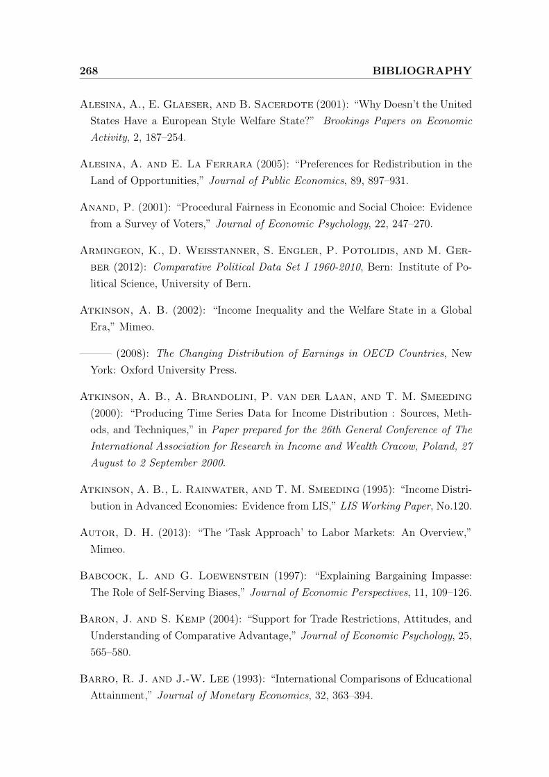
268 BIBLIOGRAPHY
Alesina, A., E. Glaeser, and B. Sacerdote (2001): “Why Doesn’t the United
States Have a European Style Welfare State?” Brookings Papers on Economic
Activity, 2, 187–254.
Alesina, A. and E. La Ferrara (2005): “Preferences for Redistribution in the
Land of Opportunities,” Journal of Public Economics, 89, 897–931.
Anand, P. (2001): “Procedural Fairness in Economic and Social Choice: Evidence
from a Survey of Voters,” Journal of Economic Psychology, 22, 247–270.
Armingeon, K., D. Weisstanner, S. Engler, P. Potolidis, and M. Ger-
ber (2012): Comparative Political Data Set I 1960-2010, Bern: Institute of Po-
litical Science, University of Bern.
Atkinson, A. B. (2002): “Income Inequality and the Welfare State in a Global
Era,” Mimeo.
——— (2008): The Changing Distribution of Earnings in OECD Countries, New
York: Oxford University Press.
Atkinson, A. B., A. Brandolini, P. van der Laan, and T. M. Smeeding
(2000): “Producing Time Series Data for Income Distribution : Sources, Meth-
ods, and Techniques,” in Paper prepared for the 26th General Conference of The
International Association for Research in Income and Wealth Cracow, Poland, 27
August to 2 September 2000.
Atkinson, A. B., L. Rainwater, and T. M. Smeeding (1995): “Income Distri-
bution in Advanced Economies: Evidence from LIS,” LIS Working Paper, No.120.
Autor, D. H. (2013): “The ‘Task Approach’ to Labor Markets: An Overview,”
Mimeo.
Babcock, L. and G. Loewenstein (1997): “Explaining Bargaining Impasse:
The Role of Self-Serving Biases,” Journal of Economic Perspectives, 11, 109–126.
Baron, J. and S. Kemp (2004): “Support for Trade Restrictions, Attitudes, and
Understanding of Comparative Advantage,” Journal of Economic Psychology, 25,
565–580.
Barro, R. J. and J.-W. Lee (1993): “International Comparisons of Educational
Attainment,” Journal of Monetary Economics, 32, 363–394.
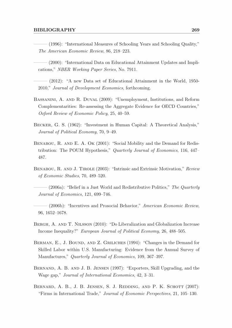
BIBLIOGRAPHY 269
——— (1996): “International Measures of Schooling Years and Schooling Quality,”
The American Economic Review, 86, 218–223.
——— (2000): “International Data on Educational Attainment Updates and Impli-
cations,” NBER Working Paper Series, No. 7911.
——— (2012): “A new Data set of Educational Attainment in the World, 1950-
2010,” Journal of Development Economics, forthcoming.
Bassanini, A. and R. Duval (2009): “Unemployment, Institutions, and Reform
Complementarities: Re-assessing the Aggregate Evidence for OECD Countries,”
Oxford Review of Economic Policy, 25, 40–59.
Becker, G. S. (1962): “Investment in Human Capital: A Theoretical Analysis,”
Journal of Political Economy, 70, 9–49.
Benabou, R. and E. A. Ok (2001): “Social Mobility and the Demand for Redis-
tribution: The POUM Hypothesis,” Quarterly Journal of Economics, 116, 447–
487.
Benabou, R. and J. Tirole (2003): “Intrinsic and Extrinsic Motivation,” Review
of Economic Studies, 70, 489–520.
——— (2006a): “Belief in a Just World and Redistributive Politics,” The Quarterly
Journal of Economics, 121, 699–746.
——— (2006b): “Incentives and Prosocial Behavior,” American Economic Review,
96, 1652–1678.
Bergh, A. and T. Nilsson (2010): “Do Liberalization and Globalization Increase
Income Inequality?” European Journal of Political Economy, 26, 488–505.
Berman, E., J. Bound, and Z. Griliches (1994): “Changes in the Demand for
Skilled Labor within U.S. Manufacturing: Evidence from the Annual Survey of
Manufactures,” Quarterly Journal of Economics, 109, 367–397.
Bernand, A. B. and J. B. Jensen (1997): “Exporters, Skill Upgrading, and the
Wage gap,” Journal of International Economics, 42, 3–31.
Bernard, A. B., J. B. Jensen, S. J. Redding, and P. K. Schott (2007):
“Firms in International Trade,” Journal of Economic Perspectives, 21, 105–130.
270 BIBLIOGRAPHY
Bischoff, I., F. Heinemann, and T. Hennighausen (2008): “Individual Deter-
minants of Social Fairness Assessments - The Case of Germany,” ZEW Discussion
Paper, 063.
Blanchard, O. and T. Philippon (2003): “The Decline of Rents, and the rise
and fall of European Unemployment,” Mimeo.
Blankart, C. B. (2008): Offentliche Finanzen in der Demokratie, Munchen:
Vahlen Verlag.
Blekesaune, M. and P. E. Solem (2005): “Working Conditions and Early
Retirement,” Research on Aging, 27, 3–30.
Blendon, R., J. Benson, M. Brodie, R. Morin, D. Altman, D. Gitter-
man, M. Brossard, and M. James (1997): “Bridging the gap Between the
Public’s and the Economists’ Views of the Economy,” Journal of Economic Per-
spectives, 11, 105–118.
Blinder, A. S. and A. B. Krueger (2004): “What Does the Public Know about
Economic Policy, and How Does It Know It?” Brookings Papers on Economic
Activity, 35, 327–397.
Boeri, T., A. Borsch-Supan, and G. Tabellini (2001): “Would you like to
Shrink the European Welfare State? A Survey of European Citizens,” Economic
Policy, 16, 9–50.
——— (2002): “Pension Reforms and the Opinions of European Citizens,” Ameri-
can Economic Review, 92, 396–401.
Boeri, T., J. Conde-Ruiz, and V. Galasso (2004): “Cross-Skill Redistribution
and the Tradeoff between Unemployment Benefits and Employment Protection,”
IZA Discussion Paper No. 1371.
Boeri, T. and G. Tabellini (2012): “Does Information Increase Political Sup-
port for Pension Reform?” Public Choice, 150, 327–362.
Boockmann, B. and R. Vaubel (2009): “The Theory of Raising Rivals’ Costs
and Evidence from the International Labour Organisation,” The World Economy,
32, 862–887.
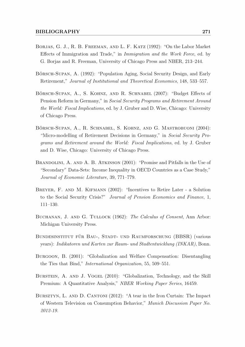
BIBLIOGRAPHY 271
Borjas, G. J., R. B. Freeman, and L. F. Katz (1992): “On the Labor Market
Effects of Immigration and Trade,” in Immigration and the Work Force, ed. by
G. Borjas and R. Freeman, University of Chicago Press and NBER, 213–244.
Borsch-Supan, A. (1992): “Population Aging, Social Security Design, and Early
Retirement,” Journal of Institutional and Theoretical Economics, 148, 533–557.
Borsch-Supan, A., S. Kohnz, and R. Schnabel (2007): “Budget Effects of
Pension Reform in Germany,” in Social Security Programs and Retirement Around
the World: Fiscal Implications, ed. by J. Gruber and D. Wise, Chicago: University
of Chicago Press.
Borsch-Supan, A., R. Schnabel, S. Kohnz, and G. Mastrobuoni (2004):
“Micro-modelling of Retirement Decisions in Germany,” in Social Security Pro-
grams and Retirement around the World: Fiscal Implications, ed. by J. Gruber
and D. Wise, Chicago: University of Chicago Press.
Brandolini, A. and A. B. Atkinson (2001): “Promise and Pitfalls in the Use of
“Secondary” Data-Sets: Income Inequality in OECD Countries as a Case Study,”
Journal of Economic Literature, 39, 771–779.
Breyer, F. and M. Kifmann (2002): “Incentives to Retire Later - a Solution
to the Social Security Crisis?” Journal of Pension Economics and Finance, 1,
111–130.
Buchanan, J. and G. Tullock (1962): The Calculus of Consent, Ann Arbor:
Michigan University Press.
Bundesinstitut fur Bau-, Stadt- und Raumforschung (BBSR) (various
years): Indikatoren und Karten zur Raum- und Stadtentwicklung (INKAR), Bonn.
Burgoon, B. (2001): “Globalization and Welfare Compensation: Disentangling
the Ties that Bind,” International Organization, 55, 509–551.
Burstein, A. and J. Vogel (2010): “Globalization, Technology, and the Skill
Premium: A Quantitative Analysis,” NBER Working Paper Series, 16459.
Bursztyn, L. and D. Cantoni (2012): “A tear in the Iron Curtain: The Impact
of Western Television on Consumption Behavior,” Munich Discussion Paper No.
2012-19.
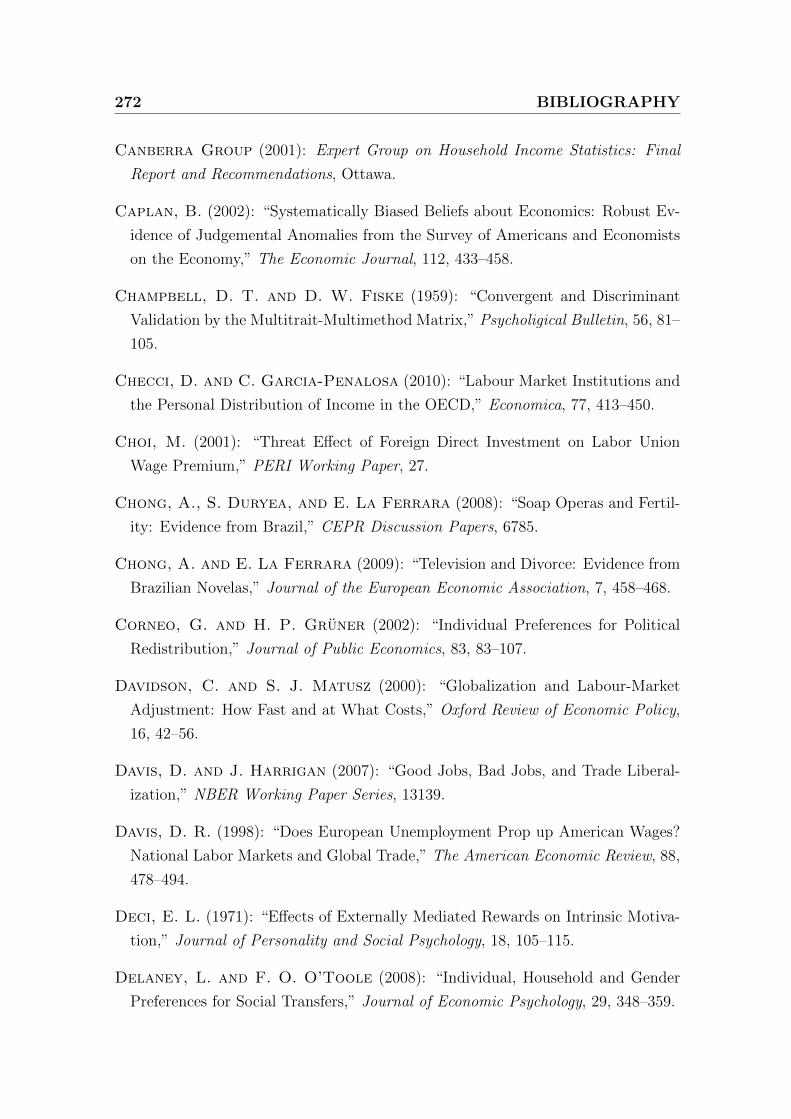
272 BIBLIOGRAPHY
Canberra Group (2001): Expert Group on Household Income Statistics: Final
Report and Recommendations, Ottawa.
Caplan, B. (2002): “Systematically Biased Beliefs about Economics: Robust Ev-
idence of Judgemental Anomalies from the Survey of Americans and Economists
on the Economy,” The Economic Journal, 112, 433–458.
Champbell, D. T. and D. W. Fiske (1959): “Convergent and Discriminant
Validation by the Multitrait-Multimethod Matrix,” Psycholigical Bulletin, 56, 81–
105.
Checci, D. and C. Garcia-Penalosa (2010): “Labour Market Institutions and
the Personal Distribution of Income in the OECD,” Economica, 77, 413–450.
Choi, M. (2001): “Threat Effect of Foreign Direct Investment on Labor Union
Wage Premium,” PERI Working Paper, 27.
Chong, A., S. Duryea, and E. La Ferrara (2008): “Soap Operas and Fertil-
ity: Evidence from Brazil,” CEPR Discussion Papers, 6785.
Chong, A. and E. La Ferrara (2009): “Television and Divorce: Evidence from
Brazilian Novelas,” Journal of the European Economic Association, 7, 458–468.
Corneo, G. and H. P. Gruner (2002): “Individual Preferences for Political
Redistribution,” Journal of Public Economics, 83, 83–107.
Davidson, C. and S. J. Matusz (2000): “Globalization and Labour-Market
Adjustment: How Fast and at What Costs,” Oxford Review of Economic Policy,
16, 42–56.
Davis, D. and J. Harrigan (2007): “Good Jobs, Bad Jobs, and Trade Liberal-
ization,” NBER Working Paper Series, 13139.
Davis, D. R. (1998): “Does European Unemployment Prop up American Wages?
National Labor Markets and Global Trade,” The American Economic Review, 88,
478–494.
Deci, E. L. (1971): “Effects of Externally Mediated Rewards on Intrinsic Motiva-
tion,” Journal of Personality and Social Psychology, 18, 105–115.
Delaney, L. and F. O. O’Toole (2008): “Individual, Household and Gender
Preferences for Social Transfers,” Journal of Economic Psychology, 29, 348–359.
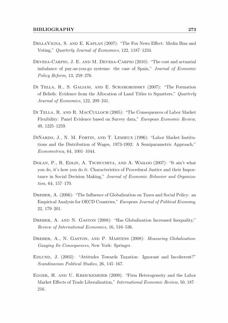
BIBLIOGRAPHY 273
DellaVigna, S. and E. Kaplan (2007): “The Fox News Effect: Media Bias and
Voting,” Quarterly Journal of Economics, 122, 1187–1234.
Devesa-Carpio, J. E. and M. Devesa-Carpio (2010): “The cost and actuarial
imbalance of pay-as-you-go systems: the case of Spain,” Journal of Economic
Policy Reform, 13, 259–276.
Di Tella, R., S. Galiani, and E. Schargrodsky (2007): “The Formation
of Beliefs: Evidence from the Allocation of Land Titles to Squatters,” Quarterly
Journal of Economics, 122, 209–241.
Di Tella, R. and R. MacCulloch (2005): “The Consequences of Labor Market
Flexibility: Panel Evidence based on Survey data,” European Economic Review,
49, 1225–1259.
DiNardo, J., N. M. Fortin, and T. Lemieux (1996): “Labor Market Institu-
tions and the Distribution of Wages, 1973-1992: A Semiparametric Approach,”
Econometrica, 64, 1001–1044.
Dolan, P., R. Edlin, A. Tschuchiya, and A. Wailoo (2007): “It ain’t what
you do, it’s how you do it: Characteristics of Procedural Justice and their Impor-
tance in Social Decision Making,” Journal of Economic Behavior and Organiza-
tion, 64, 157–170.
Dreher, A. (2006): “The Influence of Globalization on Taxes and Social Policy: an
Empirical Analysis for OECD Countries,” European Journal of Political Economy,
22, 179–201.
Dreher, A. and N. Gaston (2008): “Has Globalization Increased Inequality,”
Review of International Economics, 16, 516–536.
Dreher, A., N. Gaston, and P. Martens (2008): Measuring Globalisation:
Gauging Its Consequences, New York: Springer.
Edlund, J. (2003): “Attitudes Towards Taxation: Ignorant and Incoherent?”
Scandinavian Political Studies, 26, 145–167.
Egger, H. and U. Kreickemeier (2009): “Firm Heterogeneity and the Labor
Market Effects of Trade Liberalization,” International Economic Review, 50, 187–
216.
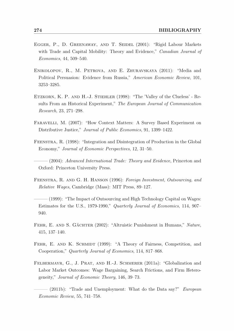
274 BIBLIOGRAPHY
Egger, P., D. Greenaway, and T. Seidel (2001): “Rigid Labour Markets
with Trade and Capital Mobility: Theory and Evidence,” Canadian Journal of
Economics, 44, 509–540.
Enikolopov, R., M. Petrova, and E. Zhuravskaya (2011): “Media and
Political Persuasion: Evidence from Russia,” American Economic Review, 101,
3253–3285.
Etzkorn, K. P. and H.-J. Stiehler (1998): “The ’Valley of the Clueless’ - Re-
sults From an Historical Experiment,” The European Journal of Communication
Research, 23, 271–298.
Faravelli, M. (2007): “How Context Matters: A Survey Based Experiment on
Distributive Justice,” Journal of Public Economics, 91, 1399–1422.
Feenstra, R. (1998): “Integration and Disintegration of Production in the Global
Economy,” Journal of Economic Perspectives, 12, 31–50.
——— (2004): Advanced International Trade: Theory and Evidence, Princeton and
Oxford: Princeton University Press.
Feenstra, R. and G. H. Hanson (1996): Foreign Investment, Outsourcing, and
Relative Wages, Cambridge (Mass): MIT Press, 89–127.
——— (1999): “The Impact of Outsourcing and High Technology Capital on Wages:
Estimates for the U.S., 1979-1990,” Quarterly Journal of Economics, 114, 907–
940.
Fehr, E. and S. Gachter (2002): “Altruistic Punishment in Humans,” Nature,
415, 137–140.
Fehr, E. and K. Schmidt (1999): “A Theory of Fairness, Competition, and
Cooperation,” Quarterly Journal of Economics, 114, 817–868.
Felbermayr, G., J. Prat, and H.-J. Schmerer (2011a): “Globalization and
Labor Market Outcomes: Wage Bargaining, Search Frictions, and Firm Hetero-
geneity,” Journal of Economic Theory, 146, 39–73.
——— (2011b): “Trade and Unemployment: What do the Data say?” European
Economic Review, 55, 741–758.
BIBLIOGRAPHY 275
Filer, R. and M. Honig (2005): “Endogenous Pensions and Retirement Behav-
ior,” CESifo Working Paper No. 1547.
Fong, C. (2001): “Social Preferences, Self Interest, and the Demand for Redistri-
bution,” Journal of Public Economics, 80, 225–246.
Franz, W. (2006): “Bewertung Hartz IV und Ein-Euro-Jobs durch den
Sachverstandigenrat,” Zeitschrift fur Wirtschaftspolitik, 55, 177–181.
Freeman, R. B. (1995): “Are Your Wages Set in Beijing?” Journal of Economic
Perspectives, 9, 15–32.
Frey, B. (1997a): Markt und Motivation: Wie okonomische Arbeitsanreize die
(Arbeits-)Moral verdrangen, Munchen: Vahlen.
——— (1997b): “On the Relationship Between Intrinsic and Extrinsic work Moti-
vation,” International Journal of Industrial Organization, 15, 427–439.
——— (2008): Motivation Crowding Theory - a new Approach to Behaviour, Can-
berra: Roundtable Proceedings, Productivity Commission, 37–54.
Frey, B. and R. Jegen (2001): “Motivation Crowding Theory: A Survey of
Empirical Evidence,” Journal of Economic Surveys, 15, 589–611.
Fuest, C. and B. Huber (2001): “Tax Progression and Human Capital in Im-
perfect Labour Markets,” German Economic Review, 2, 1–18.
Fuest, C., B. Huber, and J. Mintz (2005): “Capital Mobility and Tax Com-
petition,” Foundations and Trends in Microeconomics, 1, 1–62.
Gaston, N. and D. Trefler (1995): “Union Wage Sensitivity to Trade and
Protection: Theory and Evidence,” Journal of International Economics, 39, 1–
25.
GDR Statistical Office (various years): Statistical Yearbook of the German
Democratic Republic, Berlin: Staatsverlag der Deutschen Demokratischen Re-
publik.
Geishecker, I. and H. Gorg (2007): “Winners and Losers: A Micro-Level
Analysis of International and Wages,” CEPR Discussion Paper Series, No.6484.
276 BIBLIOGRAPHY
Gentzkow, M. A. and J. M. Shapiro (2004): “Media, Education and Anti-
Americanism in the Muslim World,” Journal of Economic Perspectives, 18, 117–
133.
Giuliano, P. and A. Spilimbergo (2009): “Growing Up in a Recession: Beliefs
and the Macroeconomy,” NBER Working Paper, 15321.
Goldberg, P. K. and N. Pavnic (2007): “Distributional Effects of Globalization
in Developing Countries,” Journal of Economic Literature, XLV, 39–82.
Goldin, C. and L. F. Katz (2007a): “Long-Run Changes in the Wage Struc-
ture: Narrowing, Widening, Polarizing,” Brookings Papers on Economic Activity,
2:2007, 135–165.
——— (2007b): “The Race between Education and Technology: The Evolution of
U.S. Educational Wage Differentials, 1890 to 2005,” NBER Working Paper Series,
12984.
Gornick, J. C., B. H. Ragnarsdottir, and S. Kostecki (2013): “LIS, Cross-
National Data Center - An Overview,” LIS Technical Working Paper Series, No.
5.
Gottschalk, P. and T. M. Smeeding (2000): “Empirical Evidence on Income
Inequality in Industrialized Countries,” in Handbook of Income Distribution, ed.
by A. Atkinson and F. Bourguignon, Amsterdam: Elsevier, vol. 1, chap. 5, 261–
307.
Greenaway, D. and D. Nelson (2001): “Globalisation and Labour Markets:
Literature Review and Synthesis,” University of Nottingham, GEP Discussion
Paper, 29.
Griliches, Z. (1969): “Capital-Skill Complementarity,” Review of Economics and
Statistics, 51, 465–468.
Grossman, G. M. and E. Rossi-Hansberg (2008): “Trading Tasks: A Simple
Theory of Offshoring,” American Economic Review, 98, 1978–1997.
Gruber, J. and D. A. Wise (2004): Social Security Programs and Retirement
Around the World: Micro-estimation, Chicago: University of Chicago Press.
——— (2007): Social Security Programs and Retirement Around the World: Fiscal
Implications, Chicago: University of Chicago Press.
BIBLIOGRAPHY 277
Grundmann, S. (1997): “Territorialplanung in der DDR: Indikatoren zur Anal-
yse regionaler Disparitaten - Die sozial-raumliche Struktur der DDR in den 80er
Jahren,” in Regionale Strukturen im Wandel, ed. by A. Becker, Opladen, 7–44.
Gwartney, J., R. Lawson, and J. Hall (2012): “Economic Freedom Dataset,”
published in Economic Freedom of the World: 2012 Annual Report.
Harrigan, J. and A. Reshef (2011): “Skill Biased Heterogeous Firms, Trade
Liberalization, and the Skill Premium,” NBER Working Paper Series, 17604.
Harrison, A., J. McLaren, and M. S. McMillan (2010): “Recent Findings
on Trade and Inequality,” .
Heineck, G. and B. Sussmuth (2010): “A Different Look at Lenin’s Legacy:
Trust, Risk, Fairness and Cooperativeness in the Two Germanies,” IZA Discus-
sion Paper No. 5219.
Heinemann, F. (2008): “Is the Welfare State Self-Destructive? A Study of Gov-
ernment Benefit Morale,” Kyklos, 61, 237–257.
Heinemann, F., I. Bischoff, and T. Hennighausen (2009): “Choosing from
the Reform Menu Card - Individual Determinants of Labour Market Policy Pref-
erences,” Jahrbucher fur Nationalokonomie und Statistik, 229, 180–197.
Heinemann, F., M. Forg, D. Frey, E. Jonas, W. Rotfuss, E. Traut-
Mattausch, and P. Westerheide (2008): Psychologie, Wachstum und Re-
formfahigkeit, vol. 88 of Schriftenreihe des ZEW, Baden-Baden: Nomos.
Heinemann, F., T. Hennighausen, and M.-D. Moessinger (2013): “Intrin-
sic Work Motivation and Pension Reform Preferences,” Journal of Pension Eco-
nomics and Finance, 12, 190–217.
Heinemann, F., T. Hennighausen, E. Traut-Mattausch, M. Kocher,
E. Jonas, and D. Frey (2011): Gerechtigkeitswahrnehmung von Steuer-
und Sozialsystemreformen, vol. 100 of ZEW Wirtschaftsanalysen, Baden-Baden:
Nomos.
Heinemann, F. and E. Janeba (2011): “Viewing Tax Policy through Party-
Colored Glasses: What German Politicians Believe,” German Economic Review,
12, 286–311.
278 BIBLIOGRAPHY
Helbling, T., D. Hakura, and X. Debrun (2004): Forstering Structural Re-
forms in Industrial Countries, Washington D.C., 103–146.
Helpman, E., M. Melitz, and S. Yeaple (2004): “Export versus FDI with
Heterogenous Firms,” American Economic Review, 94, 900–316.
Hennighausen, T. (2012): “Exposure to Television and Individual Beliefs: Evi-
dence from a Natural Experiment,” ZEW Discussion Paper, 12-078.
——— (2013): “Exposure to Television and Individual Beliefs: Evidence from a
Natural Experiment,” SOEP Papers on Multidisciplinary Panel Data Research,
535.
Hennighausen, T. and F. Heinemann (forthcoming): “Don’t Tax Me? Deter-
minants of Individual Attitudes Toward Progressive Taxation,” German Economic
Review.
Hesse, K. R. (1988): Westmedien in der DDR. Nutzung, Image und Auswirkungen
bundesrepublikanischen Horfunks und Fernsehens, Koln.
Hettich, W. and S. Winer (1997): “The Political Economy of Taxation,” in
Perspectives on Public Choice, ed. by D. Mueller, Cambridge, 481–505.
Hickman, D. C. and W. W. Olney (2011): “Globalization and Investment in
Human Capital,” Industrial and Labor Relations Review, 64, 654–672.
Hite, P. and M. Roberts (1991): “An Experimental Investigation of Taxpayer
Judgements in Rate Structure in the Individual Income Tax System,” Journal of
American Taxation Association, 13, 47–63.
Howell, D. R. and M. Rehm (2009): “Unemployment Compensation and High
European Unemployment: A Reassessment with new Benefit Indicators,” Oxford
Review of Economic Policy, 25, 60–93.
IMF (2012): “International Financial Statistics,” DSI International Statistical Year-
book.
Janeba, E. (1998): “Tax Competition in Imperfectly Competitive Markets,” Jour-
nal of International Economics, 44, 135–153.
——— (2007): “Exports, Unemployment and the Welfare State,” CESifo Working
Paper Series, 1977.
BIBLIOGRAPHY 279
Jensen, R. and E. Oster (2009): “The Power of TV: Cable Television and
Women’s Status in India,” The Quarterly Journal of Economics, 124, 1057–1094.
Johnson, G. E. (1997): “Changes in Earnings Inequality: The Role of Demand
Shifts,” The Journal of Economic Perspectives, 11, 41–54.
Johnson, G. E. and F. Stafford (1999): “The Labor Market Implications of
International Trade,” in Handbook of Labor Economics, ed. by O. Ashenfelder and
D. Card, Elsevier Science Publisher B.V., vol. 3, chap. 34, 2215–2288.
Johnson, R. W. and E. Steuerle (2004): “Promoting work at Older ages:
the role of Hybrid Pension Plans in an Aging Population,” Journal of Pension
Economics and Finance, 3, 157–177.
Kenworthy, L. (2008): Jobs with Equality, New York: Oxford University Press.
Kenworthy, L. and J. Pontusson (2005): “Rising Inequality and the Politics
of Redistribution in Affluent Countries,” Perspectives on Politics, 3, 449–471.
Kern, H. L. and J. Hainmueller (2009): “Opium for the Masses: How Foreign
Media Can Stabilze Authorien Regimes,” Political Analysis, 17, 377–399.
Kind, G. (1997): “Territorialentwicklung und Territorialplanung in der DDR:
Ergebnisse und Auswirkungen auf die Raumstruktur Deutschlands,” in Regionale
Strukturen im Wandel, ed. by A. Becker, Opladen, 17–103.
Koeninger, W., M. Leonardi, and L. Nunziata (2007): “Labor Market Insti-
tutions and Wage Inequality,” Industrial and Labor Relations Review, 60, 340–356.
Konow, J. (2003): “Which is the Fairest One of All? A Positive Analysis of Justice
Theories,” Journal of Economic Literature, 41, 1188–1239.
Krugman, P. (1980): “Scale Economics, Product Differentation and the Patterns
of Trade,” American Economic Review, 9, 469–479.
——— (1995): “Growing World Trade: Causes and Consequences,” Brookings Pa-
pers on Economic Activity, 1995, 327–377.
Krusell, P., L. E. Ohanian, J.-V. Rıos-Rull, and G. L. Violante (2000):
“Capital-Skill Complementarity and Inequality: A Macroeconomic Analysis,”
Econometrica, 68, 1029–1053.
280 BIBLIOGRAPHY
Kurokawa, Y. (2010): “A Survey of Trade and Wage Inequality: Anomalies,
Resolutions, and New Trends,” Tsukuba Economics Working Papers, No. 2010-
007.
Lachance, M.-E. (2008): “Pension Reductions: Can Welfare be Preserved by
Delaying Retirement?” Journal of Pension Economics and Finance, 7, 157–177.
Lawrence, R. Z. and M. J. Slaughter (1993): “International Trade and Amer-
ican Wages in the 1980s: Giant Sucking Sound or Small Hiccup?” Brookings
Papers on Economic Activity. Microeconomics, 1993, 161–226.
Lazear, E. P. (1979): “Why is there mandatory retirement?” Journal of Political
Economy, 87, 1261–1284.
Lazear, E. P. and P. Oyer (2007): “Personnel Economics,” NBER Working
Paper No. 13480.
Lindbeck, A. (1995): “Welfare State Disincentives with Endogenous Habits and
Norms,” Scandinavian Journal of Economics, 97, 447–494.
Lindbeck, A. and D. J. Snower (1988): The Insider-Outsider Theory of Em-
ployment and Unemployment, Cambridge (Mass.): MIT Press.
Lindquist, M. J. (2005): “Capital–Skill Complementarity and Inequality in Swe-
den,” Scandinavian Journal of Economics, 107, 711–735.
LIS (various years): “Luxembourg Income Study Database (multiple countries),”
Http://www.lisdatacenter.org (Accessed May to July 2013).
Lynch, J. and M. Myrskyla (2009): “Always the Third Rail? Pension Income
and Policy Preferences in European Democracies,” Comparative Political Studies,
42, 1068 – 1097.
Machin, S. and J. Van Reenen (1998): “Technology and Changes in the Skill
Structure: Evidence from Seven OECD Countries,” Quarterly Journal of Eco-
nomics, 113, 1215–1244.
Mahler, V. A. (2004): “Economic Globalization, Domestic Politics, and Income
Inequality in the Developed Countries. A Cross-National Study,” Comparative
Political Studies, 37, 1025–1053.
BIBLIOGRAPHY 281
Maretzke, S. (1991): “Tendenzen der Wanderungsentwicklung zwischen den alten
und neuen Bundeslandern im Zeitraum 1989 und 1990,” in Raumentwicklung in
den alten und neuen Bundeslandern. Arbeitsbeitrage zum Raumordnungsbericht
der Bundesregierung 1991, ed. by Bundesforschungsanstalt fur Landeskunde und
Raumordnung, Bonn, 10–21.
Meier-Pesti, K. and E. Penz (2008): “Sex or Gender? Expanding the Sex-
Based View by Introducing Masculinity and Feminity as Predictors of Financial
Risk Taking,” Journal of Economic Psychology, 29, 180–196.
Melitz, M. J. (2003): “The Impact of Trade on Intra-Industry Reallocations and
Aggregate Industry Productivity,” Econometrica, 71, 1695–1725.
Meltzer, A. and S. Richard (1981): “A Rational Theory of Size of Govern-
ment,” Journal of Political Economy, 89, 914–927.
Meyen, M. (2002): “Kollektive Ausreise? Zur Reichweite ost- und westdeutscher
Fernsehprogramme in der DDR,” Publizistik, 47, 200–220.
——— (2003): Einschalten, Umschalten, Ausschalten? Das Fernsehen im DDR-
Alltag, Leipzig.
Meyer, J. P. and N. J. Allen (1991): “A Three-Component Conceptualization
of Organizational Commitment,” Human Resource Managment Review, 1, 61–89.
Milanovic, B. (2000): “The Median Voter Hypothesis, Income Inequality and
Income Redistribution: An Empirical Test with the Required Data,” Luxembourg
Income Study Working Paper, No. 256.
Moene, K. and M. Wallerstein (2001): “Inequality, Social Insurance, and
Redistribution,” American Political Science Review, 95, 859–874.
——— (2003): “Earnings Inequality and Welfare Spending. A Disaggregated Anal-
ysis,” World Politics, 55, 485–516.
Mohl, P. and O. Pamp (2008): “Income Inequality and Redistributive Spending:
An Empirical Investigation of Competing Theories,” Luxembourg Income Study
Working Paper, No. 491.
Mortensen, D. T. (1978): “Specific Capital and Labor Turnover,” The Bell Jour-
nal of Economics, 9, 572–586.
282 BIBLIOGRAPHY
Neugart, M. (2008): “The Choice of Insurance in the Labor Market,” Public
Choice, 134, 445–462.
Nickell, S. (1997): “Unemployment and Labor Market Rigidities: Europe versus
North America,” Journal of Economic Perspectives, 11, 55–74.
Nickell, S., L. Nunziata, and W. Ochel (2005): “Unemployment in the
OECD since the 1960s. What do we Know?” Economic Journal, 115, 1–27.
Nickell, W. (2006): “The CEP-OECD Institutions Data Set (1960-2004),” CEP
Discussion Paper, No 759.
Niskanen, W. (1971): Bureaucracy and Representative Government, Chicago: Al-
dine Atherton.
Ockenfels, A., D. Sliwka, and P. Werner (2010): “Bonus Payments and
Reference Point Violations,” IZA Discussion Paper No. 4795, 31.
OECD (2007): Benefits and Wages 2007. OECD Indicators, Paris: OECD Publ.
——— (2008): Growing Unequal? Income Distribution and Poverty in OECD Coun-
tries, Paris: OECD Publ.
——— (2010a): “Annual Labour Force Statistics: Summary Tables,” OECD Em-
ployment and Labour Market Statistics (database), OECD.Stat (Accessed on
13/04/29).
——— (2010b): “Earnings: Gross Earnings Decile Ratios,” OECD Employment and
Labour Market Statistics (database), OECD Stat. (Accessed on 20 June 2013).
——— (2010c): “Macro trade indicators,” OECD Statistics on Measuring Globali-
sation (database), OECD.Stat (Accessed on 12 June 2013).
——— (2010d): “Multi-factor Productivity,” OECD Productivity Statistics
(database), OECD.Stat (Accessed on 30 April 2013).
——— (2011): Divided We Stand: Why Inequality Keeps Rising, Paris: OECD
Publ.
——— (2012a): “Main Science and Technology Indicators,” OECD Science, Tech-
nology and R&D Statistics (database), OECD.Stat (Accessed on 30 April 2013).
BIBLIOGRAPHY 283
——— (2012b): “Quarterly National Accounts,” OECD National Accounts Statis-
tics (database), OECD.Stat (Accessed on 11 June 2013).
——— (2013a): “OECD Annual Projections,” Economic Outlook No. 93,
OECD.Stat (Accessed on 22 July 2013).
——— (2013b): “Trade in Value by Partner Countries,” Monthly Statistics of In-
ternational Trade (database)., OECD.Stat (Accessed on 11 June 2013).
——— (2013c): “Unit Labour Costs - Annual Indicators,” Main Econmic Indicators
(database), OECD.Stat (Accessed on 29 April 2013).
Osterloh, M. and B. Frey (2000): “Motivation, Knowledge Transfer, and Or-
ganizational Forms,” Organization Science, 11, 538–550.
Osterloh, M., J. Frost, and B. Frey (2002): “The Dynamics of Motivation in
New Organizational Forms,” International Journal of the Economics of Business,
9, 61–77.
Piketty, T. (1995): “Social Mobility and Redistributive Politics,” Quarterly Jour-
nal of Economics, 3, 551–583.
Piper, G. and S. Schnepf (2008): “Gender Differences in Charitable Giving in
Great Britain,” Voluntas, 19, 103–124.
Pitlik, H. and S. Wirth (2003): “Do Crises Promote the Extent of Economic
Liberalization?: An Empirical Test,” European Journal of Political Economy, 19,
565–581.
Potrafke, N. (2013): “Globalization and Labor Market Institutions: Interna-
tional Empirical Evidence,” Journal of Comparative Economics, forthcoming.
Prat, A. and D. Stromberg (2011): “The Political Economy of Mass Media,”
CEPR Discussion Paper No. 8246.
Ramsey, F. (1928): “A Mathematical Theory of Saving,” Economic Journal, 38,
543–599.
Ranjan, P. (2012): “Trade Liberalization, Unemployment, and Inequality with
Endogenous Job Destruction,” International Review of Economics and Finance,
23, 16–29.
284 BIBLIOGRAPHY
Rawls, J. (1971): A Theory of Justice, Cambridge: Belknap Press.
Razin, A. (2003): “FDI Flows and Domestic Investment: Overview,” CESifo Eco-
nomic Studies, 49, 415–428.
Reed-Arthurs, R. and S. Sheffrin (2010): “Understanding the Public’s Atti-
tudes towards Redistribution through Taxation,” Working Paper Tulane Univer-
sity, Department of Economics, 1005.
Richardson, J. D. (1995): “Income Inequality and Trade: How to Think, What
to Conclude,” Journal of Economic Perspectives, 9, 33–55.
Roberts, M., P. Hite, and C. Bradley (1994): “Understanding Attitudes
Toward Progressive Taxation,” Public Opinion Quarterly, 58, 165–190.
Rodrik, D. (1997): Has Globalization Gone Too Far?, Washington D.C.: Peterson
Institute for International Economics.
——— (1998): “Why Do More Open Economies Have Bigger Governments?” Jour-
nal of Political Economy, 106, 997–1032.
Ruffin, R. J. (1984): “International Factor Movements,” in Handbooks of Inter-
national Economics, ed. by R. W. Jones and P. B. Kenen, Amsterdam New York
Oxford: Elsevier Science Publisher B.V., vol. I, 237–288.
Sachs, J. D. and H. J. Shatz (1994): “Trade and Jobs in U.S. Manufacturing,”
Brookings Papers on Economic Activity, 1, 1–84.
Sachverstadigenrat zur Begutachtung der gesamtwirtschaftlichen
Entwicklung (2013): Gegen eine ruckwartsgewandte Wirtschaftspolitik.
Jahresgutachten 2013/14, Wiesbaden: Statistisches Bundesamt.
Saint-Paul, G. (2000): The Political Economy of Labour Market Institutions,
Oxford: Oxford University Press.
Scheubel, B., D. Schunk, and J. Winter (2009): “Don’t Raise the Retire-
ment Age! An Experiment on Opposition to Pension Reforms and East-West
Differences in Germany,” CESifo Working Paper No. 2752.
Schlesinger, M. and C. Heldman (2001): “Gender Gap or Gender Gaps? New
Perspectives on Support for Government Action and Policies,” Journal of Politics,
63, 59–92.
BIBLIOGRAPHY 285
Schneider, O. (2009): “Reforming Pensions in Europe: Economic Fundamentals
and Political Factors,” CESifo Working Paper No. 2572.
Schulze, G. G. and H. W. Ursprung (1999): “Globalisation of the Economy
and the Nation State,” World Economy, 22, 295–352.
Sheffrin, S. (1993): “What Does the Public Believe about Tax Fairness?” Na-
tional Tax Journal, 46, 301–308.
——— (1994): “Perception of Fairness in the Crucible of Tax Policy,” in Tax Pro-
gressivity and Income Inequality, ed. by J. Slemrod, Cambridge, 309–334.
Sinn, H.-W. (2003): The New Systems Competition, Malden (Mass.): Wiley-
Blackwell.
Sinn, H.-W. and S. Ubelmesser (2002): “Pensions and the path to Gerontocracy
in Germany,” European Journal of Political Economy, 19, 153–158.
Slaughter, M. (2001): “International Trade and Labor-Demand Elasticities,”
Journal of International Economics, 54, 27–56.
Slemrod, J. (2006): “The Role of Misperceptions in Support for Regressive Tax
Reform,” National Tax Journal, 59, 57–75.
Sondak, H. and T. Tyler (2007): “How Does Procedural Justice Shape the
Desirability of Markets?” Journal of Economic Psychology, 28, 79–92.
Statistisches Reichsamt Germany (1926): Statistical Yearbook of the German
Reich 1924, Berlin: Schmidt Berlin.
Stiehler, H.-J. (1998): “Das Tal der Ahnungslosen. Erforschung der TV-
Rezeption zur Zeit der DDR.” in Medienrezeption seit 1945. Forschungsbefunde
und Forschungsperspektiven., ed. by W. Klingler, G. Roters, and M. Gerhards,
Baden-Baden, 187–202.
——— (2001): Leben ohne Westfernsehen: Studien zur Medienwirkung und Medi-
ennutzung in der Region Dresden in den 80er Jahren, Leipzig.
Stolper, W. F. and P. A. Samuelson (1941): “Protection and Real Wages,”
The Review of Economic Studies, 9, 58–73.
Suhrcke, M. (2001): “Preferences for Inequality: East vs. West,” Innocenti Work-
ing Paper, No. 89.
286 BIBLIOGRAPHY
Tan, J. H. W. (2006): “Religion and Social Preferences: An Experimental Study,”
Economic Letters, 90, 60–67.
Terwey, M., A. Bens, H. Baumann, and S. Baltzer (2007): Datenhandbuch
ALLBUS 2006. ZA - Nr. 4500, Koln und Mannheim: GESIS.
Tinbergen, J. (1974): “Substition of Graduate by Other Labor,” Kyklos, 27, 217–
226.
Trefler, D. (2004): “The Long and Short of the Canada-U.S. Free Trade Agree-
ment,” American Economic Review, 94, 870–895.
Tullock, G. (1965): The Politics of Bureaucracy, Washington D.C.
Van Reenen, J. (2011): “Wage Inequality, Technology and Trade: 21st Century
Evidence,” CEP Occasional paper, 28.
Vannoorenberghe, G. (2011): “Trade between Symmetric Countries, Hetero-
geneous Firms, and the Skill Premium,” Canadian Journal of Economics, 44,
148–170.
Vannoorenberghe, G. and E. Janeba (2013): “Trade and the Political Econ-
omy of Redistribution,” CES ifo Working Papers, 4062.
Varian, H. R. (1980): “Redistributive Taxation as Social Insurance,” Journal of
Public Economics, 14, 49–68.
Vaubel, R. (2000): “Internationaler Politischer Wettbewerb: Eine europaische
Wettbewerbsaufsicht fur Regierungen und die empirische Evidenz,” in Jahrbuch
fur Neue Politische Okonomie, Mohr Siebeck, vol. 19, 280–309.
——— (2005): “Sozialpolitische Konsequenzen der Globalisierung: Theorie und
Empirie,” in Weltwirtschaftlicher Strukturwandel, nationale Wirtschaftspolitik
und politische Rationalitat: Festschrift fur Juergen B. Donges zum 65. Geburtstag,
ed. by A. Freytag, Koln: Kolner Univ.-Verlag, 143–158.
——— (2010): “Freiheit in Deutschland: Wettbewerb der Staaten, Einfluss der
Kirche, amerikanisches Erbe - Versuch einer historischen Erklarung,” Jahrbuch
fur die Ordnung von Wirtschaft und Gesellschaft (ORDO), 61, 53–74.
——— (2012): “Redistribution as Income Insurance,” Public Choice, 152, 389–392.
BIBLIOGRAPHY 287
Wagner, G. G., J. R. Frick, and J. Schupp (2007): “The German Socio-
Economic Panel Study (SOEP) - Scope, Evolution and Enhancements,” SOEP
Papers, No. 1.
Wildasin, D. E. (1995): “Factor Mobility, Risk and Redistribution in the Welfare
State,” Scandinavian Journal of Economics, 97, 527–546.
Wilensky, H. (1976): The ’New Corporatism’. Centralization and the Welfare
State, London.
Wilson, J. D. and D. E. Wildasin (2004): “Capital Tax Competition: bane or
boon,” Journal of Public Economics, 88, 1065–1091.
Wood, A. (1995): “How Trade Hurt Unskilled Workers,” Journal of Economic
Perspectives, 9, 57–80.
——— (1998): “Globalisation and the Rise in Labour Market Inequalities,” Eco-
nomic Journal, 108, 1463–1482.
World Bank (2012): “World Development Indicators,” (electronic database), (Ac-
cessed on 23 April 2013).
Yeaple, S. (2005): “A Simple Model of Firm Heterogeneity, International Trade,
and Wages,” Journal of International Economics, 65, 1–20.
Zellner, A. (1962): “An Efficient Method of Estimating Seemingly Unrelated
Regressions and Tests for Aggregation bias,” Journal of the American Statistical
Association, 57, 348–368.
Zentralinstitut fur Jugendforschung (1989): “Politisches Klima und
gesellschaftliche Bedingungen in der DDR 1989 (ZA 6008),” Zentralarchiv fur
Empirische Sozialforschung (GESIS-ZA).
Zodrow, G. R. and P. Mieszkowski (1986): “Pigou, Tiebout, Property Tax-
ation, and the Underprovision of Local Public Goods,” Journal of Urban Eco-
nomics, 19, 356–370.


Appendices
289


Appendix A
Globalization and income
inequality
A.1 Data description and issues
291

292 Appendix AT
able
A.1
:V
aria
ble
des
crip
tion
Vari
ab
leD
efi
nit
ion
Sou
rce
Incom
ed
istr
ibu
tion
vari
ab
les
Mar
ket
inco
mes
Gin
ico
effici
ent
of
the
dis
trib
uti
on
of
mark
etin
com
es.
Ow
nca
lcu
lati
on
sb
ase
don
LIS
data
.D
isp
osab
lein
com
esG
ini
coeffi
cien
tof
the
dis
trib
uti
on
of
dis
posa
ble
inco
mes
.R
edis
trib
uti
onP
erce
nta
ged
iffer
ence
bet
wee
nth
eG
ini
coeffi
cien
tof
the
mark
etan
dd
isp
osab
lein
com
ed
istr
ibu
tion
.
Tra
nsm
issi
on
vari
ab
les
Lab
orin
com
esh
are
Annu
alla
bor
inco
me
share
defi
ned
as
tota
lla
bor
cost
s(i
.e.
com
-p
ensa
tion
ofem
plo
yees
ad
just
edfo
rth
ese
lf-e
mp
loye
d)
div
ided
by
nom
inal
outp
ut.
OE
CD
Main
Eco
nom
icIn
dic
ato
rs
Wag
ed
isp
ersi
onD
ecil
era
tio
(i.e
.th
era
tio
bet
wee
nth
e9th
an
dth
e1st
dec
ile)
of
gros
sw
ages
offu
ll-t
ime
emp
loye
es.
OE
CD
(2010b
)E
arn
ings
data
base
Un
emp
loym
ent
rate
Un
emp
loym
ent
as
ap
erce
nta
ge
of
the
civil
ian
lab
or
forc
e.O
EC
DL
ab
ou
rF
orc
eS
tati
stic
sR
elat
ive
sup
ply
ofhu
man
cap
ital
Nu
mb
erof
ind
ivid
uals
wit
hte
rtia
ryed
uca
tion
div
ided
by
those
for
wh
omp
rim
ary
edu
cati
on
isth
eh
igh
est
edu
cati
on
al
deg
ree
(both
exp
ress
edas
ap
erce
nta
ge
of
the
pop
ula
tion
old
erth
an
25
years
).
Barr
oan
dL
ee(2
012)
Rel
ativ
ein
com
eof
the
un
em-
plo
yed
Ave
rage
net
inco
me
of
un
emp
loye
din
div
idu
als
rela
tive
toth
eav
-er
age
net
inco
me
of
full-t
ime
emp
loye
es.
Th
ean
aly
sis
isli
mit
edto
ind
ivid
ual
sag
ed25
to64
years
.
Ow
nca
lcu
lati
on
sb
ase
don
LIS
data
.
Glo
bali
zati
on
ind
icato
rsT
rad
eop
enn
ess
(log
)T
rad
ein
good
san
dse
rvic
es(i
.e.
sum
of
ex-
an
dim
port
s)as
ap
erce
nta
geof
GD
P.
OE
CD
(2010c)
:M
acr
oT
rade
Indi-
cato
rsN
on-O
EC
Dim
por
ts(l
og)
Imp
orts
from
non
-OE
CD
(excl
ud
ing
OP
EC
)co
untr
ies
as
ash
are
ofto
tal
imp
orts
.O
EC
D(2
013b
):M
onth
lyS
tati
stic
sof
Inte
rnat
ion
al
Tra
de
Net
cap
ital
exp
orts
Net
exp
orts
offo
reig
nd
irec
t,p
ort
foli
oan
doth
erin
vest
men
tsas
ap
erce
nta
geof
GD
P.
Cap
ital
flow
s(I
MF
,2012),
GD
P(W
orl
dB
an
k,
2012)
Con
tin
ued
on
nex
tpa
ge

Appendix A 293T
ab
leA
.1–
conti
nu
edfr
om
pre
vio
us
page
Vari
ab
leD
efi
nit
ion
Sou
rce
Contr
ol
vari
ab
les
Cap
ital
per
wor
ker
(log
)G
ross
fixed
cap
ital
form
ati
on
div
ided
by
tota
lem
plo
ym
ent.
Gro
ssfixed
cap
ital
form
ati
on
(OE
CD
,2012b
),to
tal
emp
loym
ent
(OE
CD
,2010a)
Lab
orp
rod
uct
ivit
yL
abor
pro
du
ctiv
ity
per
un
itla
bor
inp
ut
(i.e
.re
al
ou
tpu
td
ivid
edby
tota
lla
bor
inp
ut.
OE
CD
(2013c)
:U
nit
Lab
ou
rC
ost
s
Mu
ltif
acto
rp
rod
uct
ivit
yG
row
thof
mult
ifact
or
pro
du
ctiv
ity
for
the
tota
lec
on
om
y(i
.e.
dif
-fe
ren
ceb
etw
een
the
rate
of
chan
ge
of
ou
tpu
tan
dra
teof
chan
ge
ofto
tal
inp
ut.
OE
CD
(2010d
):P
rod
uct
ivit
yD
ata
base
Ou
tpu
tga
pD
evia
tion
ofac
tual
GD
Pfr
om
pote
nti
al
GD
Pas
a%
of
the
po-
tenti
alG
DP
.O
EC
D(2
013a):
Eco
nom
icO
utl
ook
Lab
orm
arke
tfr
eed
omL
abor
mar
ket
regu
lati
on
ind
ex(s
ub
com
pon
ent
5B
of
the
Eco
-n
omic
Fre
edom
of
the
Worl
din
dex
).G
wart
ney
etal.
(2012)
Lef
tgo
vern
men
tC
abin
etco
mp
osit
ion
:so
cial
dem
ocr
ati
can
doth
erle
ftp
art
ies
inp
erce
nta
geof
tota
lca
bin
etp
ost
s(w
eighte
dby
day
sin
offi
ce).
Arm
ingeo
net
al.
(2012)
Vot
ertu
rnou
tV
oter
turn
out
inp
arl
iam
enta
ryel
ecti
on
s.G
DP
per
cap
ita
Rea
lG
DP
div
ided
by
tota
lp
op
ula
tion
.O
EC
D(2
012b
)D
evia
tion
real
GD
Pgr
owth
Dev
iati
onof
the
real
GD
Pgro
wth
rate
from
its
five-
year
aver
age.
OE
CD
(2012b
)
Vari
ab
les
rob
ust
ness
test
Gro
ssca
pit
alm
ovem
ents
(log
)S
um
ofin
-an
dou
tflow
sof
fore
ign
dir
ect,
port
folio
an
doth
erin
-ve
stm
ents
asa
per
centa
ge
of
GD
P.
Cap
ital
flow
s(I
MF
,2012),
GD
P(W
orl
dB
an
k,
2012)
Net
FD
Iex
por
tsN
etex
por
tsof
fore
ign
dir
ect
inves
tmen
tsas
ap
erce
nta
ge
of
GD
P.
Cap
ital
flow
s(I
MF
,2012),
GD
P(W
orl
dB
an
k,
2012)
ICT
inve
stm
ent
(log
)C
ontr
ibu
tion
ofIC
Teq
uip
men
tto
gro
wth
of
tota
lca
pit
al
serv
ices
(in
per
cent)
.O
EC
D(2
010d
):P
rod
uct
ivit
yD
ata
base
R&
Dex
pen
dit
ure
s(l
og)
Gro
ssd
omes
tic
exp
end
itu
rein
rese
arc
han
dex
per
imen
tal
dev
el-
opm
ent
asa
per
centa
ge
of
GD
P.
OE
CD
(2012a):
Main
Sci
ence
an
d
R&
Dp
erso
nn
el(l
og)
Tot
alR
&D
per
son
nel
per
1,0
00
emp
loye
es.
Tec
hn
olo
gy
Ind
icato
rs
Con
tin
ued
on
nex
tpa
ge

294 Appendix AT
ab
leA
.1–
conti
nu
edfr
om
pre
vio
us
page
Vari
ab
leD
efi
nit
ion
Sou
rce
Em
plo
ym
ent
pro
tect
ion
Ind
icat
orof
the
emp
loym
ent
pro
tect
ion
legis
lati
on
(in
crea
sin
gin
stri
ctn
ess
ofem
plo
ym
ent
pro
tect
ion
).
Nic
kell
(2006)
Un
ion
den
sity
Un
ion
den
sity
iseq
ualto
the
rati
ob
etw
een
un
ion
mem
ber
ship
an
dem
plo
ym
ent
(in
per
cent)
.U
nio
nco
vera
geN
um
ber
ofw
orke
rsco
vere
dby
coll
ecti
veagre
emen
tsas
ap
erce
nt-
age
ofto
tal
emp
loym
ent.
Bar
gain
ing
coor
din
atio
nIn
dex
ind
icat
ing
the
deg
ree
of
barg
ain
ing
coord
inati
on
(in
crea
sin
gin
the
deg
ree
ofco
ord
inati
on
both
on
emp
loye
rs’
an
dem
plo
yees
’si
de
(inte
rpol
ated
).G
ross
rep
lace
men
tra
tes
OE
CD
ben
efit
rep
lace
men
tra
tes
base
don
gro
ssin
com
esan
din
-te
rpol
ated
.B
enefi
td
ura
tion
Ind
exca
ptu
rin
gth
ele
vel
of
ben
efits
inth
ela
ter
years
of
asp
ell
rela
tive
toth
ose
avail
ab
lefo
rth
efi
rst
year.
Min
imu
mw
age
Min
imu
mw
age
as
ap
erce
nta
ge
of
the
med
ian
wage.
Tax
wed
geS
um
ofem
plo
ym
ent
tax
rate
(i.e
.em
plo
yers
’so
cial
secu
rity
con
-tr
ibu
tion
s),
dir
ect
tax
rate
(in
com
eta
xan
dem
plo
yees
’so
cial
se-
curi
tyco
ntr
ibu
tion
s)an
din
dir
ect
tax
rate
s.
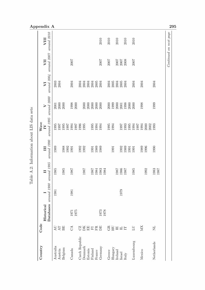
Appendix A 295T
able
A.2
:In
form
atio
nab
out
LIS
dat
ase
ts
Cou
ntr
yC
od
eW
ave
His
tori
cal
III
III
IVV
VI
VII
VII
ID
ata
base
saro
un
d1980
aro
un
d1985
aro
un
d1990
aro
un
d1995
aro
un
d2000
aro
un
d2004
aro
un
d2007
aro
un
d2010
Au
stra
lia
AU
1981
1985
1989
1995
2001
200
3A
ust
ria
AT
1997
2000
200
4B
elgi
um
BE
1985
1988
1995
2000
1992
1997
Can
ada
CA
1971
1981
1987
1991
1994
1998
2004
2007
1975
1997
2000
Cze
chR
epu
bli
cC
Z1992
1996
200
4D
enm
ark
DK
1987
1992
1995
2000
2004
Est
onia
EE
2000
200
4F
inla
nd
FI
1987
1991
1995
2000
200
4F
ran
ceF
R1984
1989
1994
2000
200
5G
erm
any
DE
1973
1983
1989
1994
2000
2004
2007
2010
1978
1984
Gre
ece
GR
1995
2000
2004
2007
2010
Hu
nga
ryH
U1991
1994
1999
2005
Irel
and
IE1987
2000
2004
2007
2010
Isra
elIL
1979
1986
1992
1997
2001
200
52007
Ital
yIT
1987
1989
1993
1998
2004
2008
2010
1991
1995
2000
Lu
xem
bou
rgL
U1985
1991
1994
2000
200
42007
2010
1997
Mex
ico
MX
1989
1994
1998
2004
1992
1996
2000
2002
Net
her
lan
ds
NL
1983
1990
1993
1999
2004
1987
Con
tin
ued
on
nex
tpa
ge
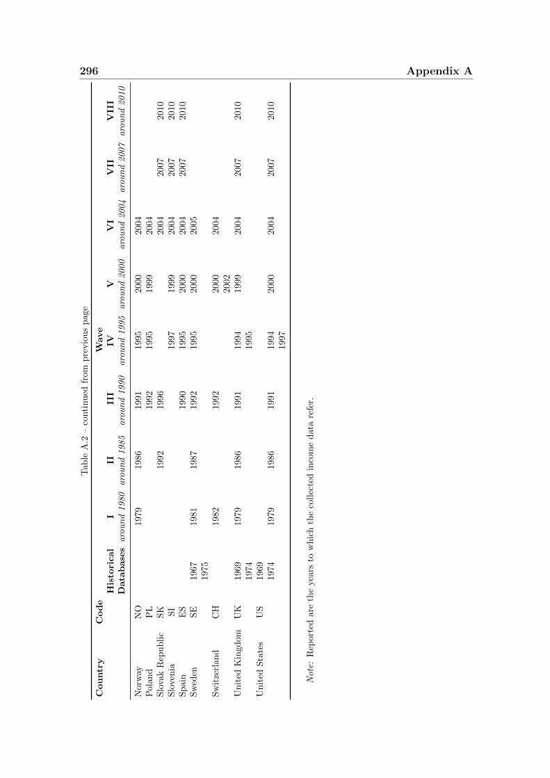
296 Appendix AT
ab
leA
.2–
conti
nu
edfr
om
pre
vio
us
page
Cou
ntr
yC
od
eW
ave
His
tori
cal
III
III
IVV
VI
VII
VII
ID
ata
base
saro
un
d1980
aro
un
d1985
aro
un
d1990
aro
un
d1995
aro
un
d2000
aro
un
d2004
aro
un
d2007
aro
un
d2010
Nor
way
NO
1979
1986
1991
1995
2000
200
4P
olan
dP
L1992
1995
1999
2004
Slo
vak
Rep
ub
lic
SK
1992
1996
2004
2007
2010
Slo
ven
iaS
I1997
1999
2004
2007
2010
Sp
ain
ES
1990
1995
2000
2004
2007
2010
Sw
eden
SE
1967
1981
1987
1992
1995
2000
200
519
75S
wit
zerl
and
CH
1982
1992
2000
2004
2002
Un
ited
Kin
gdom
UK
1969
1979
1986
1991
1994
1999
200
42007
2010
1974
1995
Un
ited
Sta
tes
US
1969
1974
1979
1986
1991
1994
2000
2004
2007
2010
1997
Note
:R
epor
ted
are
the
year
sto
wh
ich
the
coll
ecte
din
com
ed
ata
refe
r.
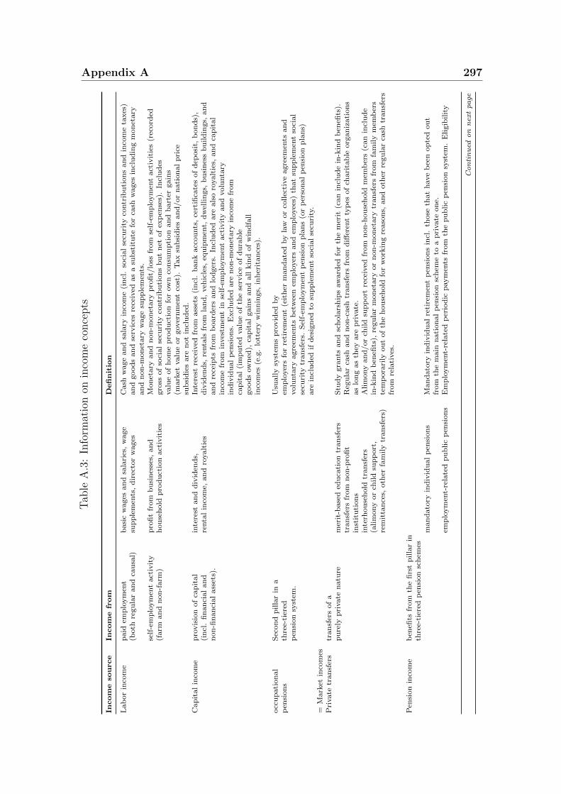
Appendix A 297T
able
A.3
:In
form
atio
non
inco
me
conce
pts
Incom
eso
urce
Incom
efr
om
Defi
nit
ion
Lab
or
inco
me
paid
emp
loym
ent
basi
cw
ages
an
dsa
lari
es,
wage
Cash
wage
an
dsa
lary
inco
me
(in
cl.
soci
al
secu
rity
contr
ibu
tion
san
din
com
eta
xes
)(b
oth
regu
lar
an
dca
usa
l)su
pp
lem
ents
,d
irec
tor
wages
an
dgood
san
dse
rvic
esre
ceiv
edas
asu
bst
itu
tefo
rca
shw
ages
incl
ud
ing
mon
etary
an
dn
on
-mon
etary
wage
sup
ple
men
ts.
self
-em
plo
ym
ent
act
ivit
yp
rofi
tfr
om
bu
sin
esse
s,an
dM
on
etary
an
dn
on
-mon
etary
pro
fit/
loss
from
self
-em
plo
ym
ent
act
ivit
ies
(rec
ord
ed(f
arm
an
dn
on
-farm
)h
ou
seh
old
pro
du
ctio
nact
ivit
ies
gro
ssof
soci
al
secu
rity
contr
ibu
tion
sb
ut
net
of
exp
ense
s).
Incl
ud
esvalu
eof
hom
ep
rod
uct
ion
for
ow
nco
nsu
mp
tion
an
db
art
ergain
s(m
ark
etvalu
eor
gover
nm
ent
cost
).T
ax
sub
sid
ies
an
d/or
nati
on
al
pri
cesu
bsi
die
sare
not
incl
ud
ed.
Cap
ital
inco
me
pro
vis
ion
of
cap
ital
inte
rest
an
dd
ivid
end
s,In
tere
stre
ceiv
edfr
om
ass
ets
(in
cl.
ban
kacc
ou
nts
,ce
rtifi
cate
sof
dep
osi
t,b
on
ds)
,(i
ncl
.fi
nan
cial
an
dre
nta
lin
com
e,an
dro
yalt
ies
div
iden
ds,
renta
lsfr
om
lan
d,
veh
icle
s,eq
uip
men
t,d
wel
lin
gs,
bu
sin
ess
bu
ild
ings,
and
non
-fin
an
cial
ass
ets)
.an
dre
ceip
tsfr
om
board
ers
an
dlo
dger
s.In
clu
ded
are
als
oro
yalt
ies,
an
dca
pit
al
inco
me
from
inves
tmen
tin
self
-em
plo
ym
ent
act
ivit
yan
dvolu
nta
ryin
div
idu
al
pen
sion
s.E
xcl
ud
edare
non
-mon
etary
inco
me
from
cap
ital
(im
pu
ted
valu
eof
the
serv
ice
of
du
rab
legood
sow
ned
),ca
pit
al
gain
san
dall
kin
dof
win
dfa
llin
com
es(e
.g.
lott
ery
win
nin
gs,
inh
erit
an
ces)
.
occ
up
ati
onal
Sec
on
dp
illa
rin
aU
sually
syst
ems
pro
vid
edby
pen
sion
sth
ree-
tier
edem
plo
yer
sfo
rre
tire
men
t(e
ith
erm
an
date
dby
law
or
collec
tive
agre
emen
tsan
dp
ensi
on
syst
em.
volu
nta
ryagre
emen
tsb
etw
een
emp
loyer
san
dem
plo
yee
s)th
at
sup
ple
men
tso
cial
secu
rity
tran
sfer
s.S
elf-
emp
loym
ent
pen
sion
pla
ns
(or
per
son
al
pen
sion
pla
ns)
are
incl
ud
edif
des
ign
edto
sup
ple
men
tso
cial
secu
rity
.=
Mark
etin
com
esP
rivate
tran
sfer
str
an
sfer
sof
ap
ure
lyp
rivate
natu
rem
erit
-base
ded
uca
tion
tran
sfer
sS
tud
ygra
nts
an
dsc
hola
rsh
ips
aw
ard
edfo
rth
em
erit
(can
incl
ud
ein
-kin
db
enefi
ts).
tran
sfer
sfr
om
non
-pro
fit
Reg
ula
rca
shan
dn
on
-cash
tran
sfer
sfr
om
diff
eren
tty
pes
of
chari
tab
leorg
an
izati
on
sin
stit
uti
on
sas
lon
gas
they
are
pri
vate
.in
terh
ou
seh
old
tran
sfer
sA
lim
ony
an
d/or
child
sup
port
rece
ived
from
non
-hou
seh
old
mem
ber
s(c
an
incl
ud
e(a
lim
ony
or
child
sup
port
,in
-kin
db
enefi
ts),
regu
lar
mon
etary
or
non
-mon
etary
tran
sfer
sfr
om
fam
ily
mem
ber
sre
mit
tan
ces,
oth
erfa
mily
tran
sfer
s)te
mp
ora
rily
ou
tof
the
hou
seh
old
for
work
ing
reaso
ns,
an
doth
erre
gu
lar
cash
tran
sfer
sfr
om
rela
tives
.
Pen
sion
inco
me
ben
efits
from
the
firs
tp
illa
rin
thre
e-ti
ered
pen
sion
sch
emes
man
dato
ryin
div
idu
al
pen
sion
sM
an
dato
ryin
div
idu
al
reti
rem
ent
pen
sion
sin
cl.
those
that
have
bee
nop
ted
ou
tfr
om
the
main
nati
on
al
pen
sion
sch
eme
toa
pri
vate
on
e.em
plo
ym
ent-
rela
ted
pu
blic
pen
sion
sE
mp
loym
ent-
rela
ted
per
iod
icp
aym
ents
from
the
pu
blic
pen
sion
syst
em.
Eligib
ilit
y
Continued
onnextpa
ge
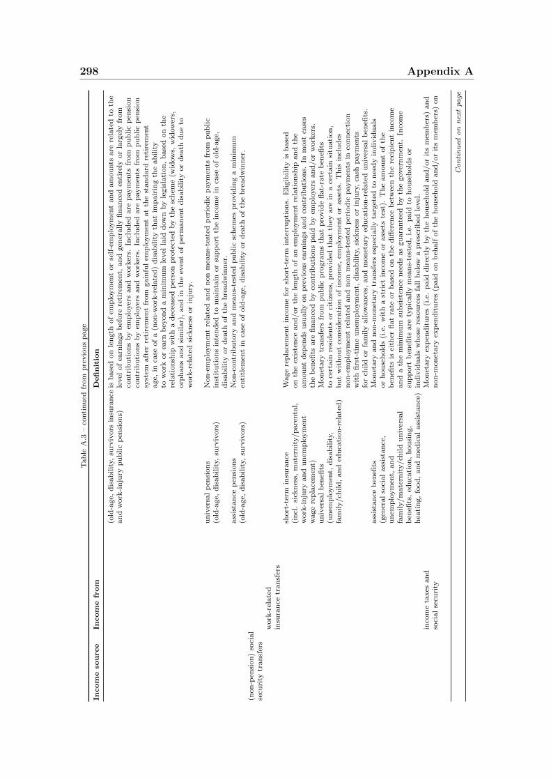
298 Appendix AT
ab
leA
.3–
conti
nu
edfr
om
pre
vio
us
page
Incom
eso
urce
Incom
efr
om
Defi
nit
ion
(old
-age,
dis
ab
ilit
y,su
rviv
ors
insu
ran
ceis
base
don
len
gth
of
emp
loym
ent
or
self
-em
plo
ym
ent
an
dam
ou
nts
are
rela
ted
toth
ean
dw
ork
-in
jury
pu
bli
cp
ensi
on
s)le
vel
of
earn
ings
bef
ore
reti
rem
ent,
an
dgen
erally
fin
an
ced
enti
rely
or
larg
ely
from
contr
ibu
tion
sby
emp
loyer
san
dw
ork
ers.
Incl
ud
edare
paym
ents
from
pu
blic
pen
sion
contr
ibu
tion
sby
emp
loyer
san
dw
ork
ers.
Incl
ud
edare
paym
ents
from
pu
blic
pen
sion
syst
emaft
erre
tire
men
tfr
om
gain
ful
emp
loym
ent
at
the
stan
dard
reti
rem
ent
age,
inca
seof
a(n
on
-work
-rel
ate
d)
dis
ab
ilit
yth
at
imp
air
ing
the
ab
ilit
yto
work
or
earn
bey
on
da
min
imu
mle
vel
laid
dow
nby
legis
lati
on
,b
ase
don
the
rela
tion
ship
wit
ha
dec
ease
dp
erso
np
rote
cted
by
the
sch
eme
(wid
ow
s,w
idow
ers,
orp
han
san
dsi
milar)
,an
din
the
even
tof
per
man
ent
dis
ab
ilit
yor
dea
thd
ue
tow
ork
-rel
ate
dsi
ckn
ess
or
inju
ry.
un
iver
sal
pen
sion
sN
on
-em
plo
ym
ent
rela
ted
an
dn
on
mea
ns-
test
edp
erio
dic
paym
ents
from
pu
blic
(old
-age,
dis
ab
ilit
y,su
rviv
ors
)in
stit
uti
on
sin
ten
ded
tom
ain
tain
or
sup
port
the
inco
me
inca
seof
old
-age,
dis
ab
ilit
yor
dea
thof
the
bre
ad
win
ner
.ass
ista
nce
pen
sion
sN
on
-contr
ibu
tory
an
dm
ean
s-te
sted
pu
blic
sch
emes
pro
vid
ing
am
inim
um
(old
-age,
dis
ab
ilit
y,su
rviv
ors
)en
titl
emen
tin
case
of
old
-age,
dis
ab
ilit
yor
dea
thof
the
bre
ad
win
ner
.(n
on
-pen
sion
)so
cial
secu
rity
tran
sfer
sw
ork
-rel
ate
din
sura
nce
tran
sfer
ssh
ort
-ter
min
sura
nce
Wage
rep
lace
men
tin
com
efo
rsh
ort
-ter
min
terr
up
tion
s.E
ligib
ilit
yis
base
d(i
ncl
.si
ckn
ess,
mate
rnit
y/p
are
nta
l,on
the
exis
ten
cean
d/or
the
len
gth
of
an
emp
loym
ent
rela
tionsh
ipan
dth
ew
ork
-in
jury
an
dun
emp
loym
ent
am
ou
nt
dep
end
su
sually
on
pre
vio
us
earn
ings
an
dco
ntr
ibuti
on
s.In
most
case
sw
age
rep
lace
men
t)th
eb
enefi
tsare
fin
an
ced
by
contr
ibu
tion
sp
aid
by
emp
loyer
san
d/or
work
ers.
un
iver
sal
ben
efits
Mon
etary
tran
sfer
sfr
om
pu
blic
pro
gra
ms
that
pro
vid
efl
at-
rate
ben
efits
(un
emp
loym
ent,
dis
ab
ilit
y,to
cert
ain
resi
den
tsor
citi
zen
s,p
rovid
edth
at
they
are
ina
cert
ain
situ
ati
on
,fa
mily/ch
ild
,an
ded
uca
tion
-rel
ate
d)
bu
tw
ith
ou
tco
nsi
der
ati
on
of
inco
me,
emp
loym
ent
or
ass
ets.
Th
isin
clu
des
non
-em
plo
ym
ent
rela
ted
an
dn
on
mea
ns-
test
edp
erio
dic
paym
ents
inco
nn
ecti
on
wit
hfi
rst-
tim
eu
nem
plo
ym
ent,
dis
ab
ilit
y,si
ckn
ess
or
inju
ry,
cash
paym
ents
for
child
or
fam
ily
allow
an
ces,
an
dm
on
etary
edu
cati
on
-rel
ate
dun
iver
sal
ben
efits
.ass
ista
nce
ben
efits
Mon
etary
an
dn
on
-mon
etary
tran
sfer
ses
pec
ially
targ
eted
ton
eed
yin
div
idu
als
(gen
eral
soci
al
ass
ista
nce
,or
hou
seh
old
s(i
.e.
wit
ha
stri
ctin
com
eor
ass
ets
test
).T
he
am
ou
nt
of
the
un
emp
loym
ent,
an
db
enefi
tsis
eith
erfl
at
rate
or
base
don
the
diff
eren
ceb
etw
een
the
reci
pie
nt
inco
me
fam
ily/m
ate
rnit
y/ch
ild
un
iver
sal
an
da
the
min
imu
msu
bsi
sten
cen
eed
sas
gu
ara
nte
edby
the
gover
nm
ent.
Inco
me
ben
efits
,ed
uca
tion
,h
ou
sin
g,
sup
port
ben
efits
are
typ
ically
mea
ns-
test
ed,
i.e.
paid
toh
ou
seh
old
sor
hea
tin
g,
food
,an
dm
edic
al
ass
ista
nce
)in
div
idu
als
wh
ose
reso
urc
esfa
llb
elow
ap
resc
rib
edle
vel
.in
com
eta
xes
an
dM
on
etary
exp
end
itu
res
(i.e
.p
aid
dir
ectl
yby
the
hou
seh
old
an
d/or
its
mem
ber
s)an
dso
cial
secu
rity
non
-mon
etary
exp
end
itu
res
(paid
on
beh
alf
of
the
hou
seh
old
an
d/or
its
mem
ber
s)on
Continued
onnextpa
ge
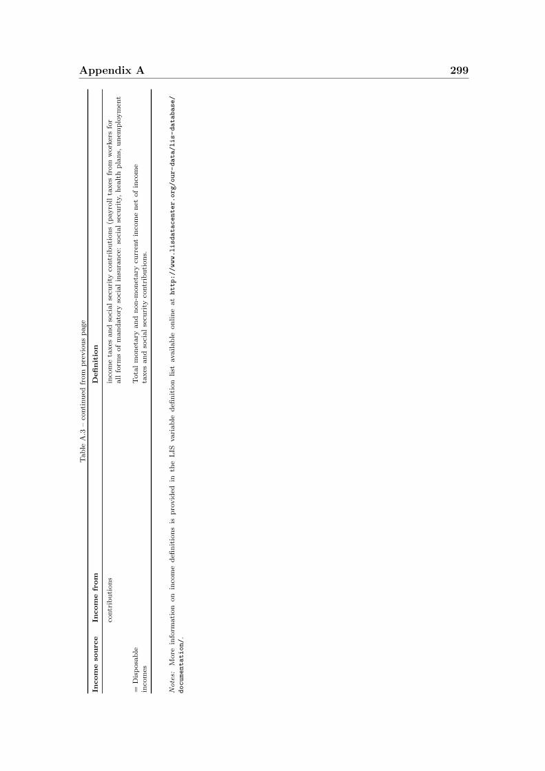
Appendix A 299T
ab
leA
.3–
conti
nu
edfr
om
pre
vio
us
page
Incom
eso
urce
Incom
efr
om
Defi
nit
ion
contr
ibuti
on
sin
com
eta
xes
an
dso
cial
secu
rity
contr
ibu
tion
s(p
ayro
llta
xes
from
work
ers
for
all
form
sof
man
dato
ryso
cial
insu
ran
ce:
soci
al
secu
rity
,h
ealt
hp
lan
s,u
nem
plo
ym
ent
=D
isp
osa
ble
Tota
lm
on
etary
an
dn
on
-mon
etary
curr
ent
inco
me
net
of
inco
me
inco
mes
taxes
an
dso
cial
secu
rity
contr
ibu
tion
s.
Notes:
More
info
rmati
on
on
inco
me
defi
nit
ion
sis
pro
vid
edin
the
LIS
vari
ab
ledefi
nit
ion
list
availab
leon
lin
eathttp://www.lisdatacenter.org/our-data/lis-database/
documentation/.
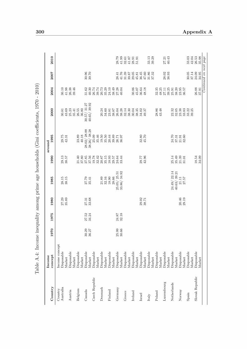
300 Appendix AT
able
A.4
:In
com
ein
equal
ity
amon
gpri
me
age
hou
sehol
ds
(Gin
ico
effici
ents
,19
70-
2010
)
Incom
earou
nd
Cou
ntr
ycon
cep
t1970
1975
1980
1985
1990
1995
2000
2004
2007
2010
Cou
ntr
yIn
com
eco
nce
pt
Au
stra
lia
Dis
posa
ble
27.2
928.1
529.1
329.7
530.8
130.1
0M
ark
et35.8
938.1
538.5
742.3
143.6
941.9
8A
ust
ria
Dis
posa
ble
25.2
326.3
8M
ark
et35.4
139.4
6B
elgiu
mD
isp
osa
ble
21.4
023.8
926.5
5M
ark
et37.8
040.1
836.8
0C
an
ad
aD
isp
osa
ble
30.2
927.5
227.3
127.7
927.8
528.0
2/
28.8
830.5
7/
31.2
731.6
230.9
6M
ark
et36.2
734.2
433.6
835.4
137.5
638.2
6/
38.2
840.6
5/
39.9
240.3
039.7
0C
zech
Rep
ub
lic
Dis
posa
ble
19.7
825.0
926.7
4M
ark
et32.4
235.4
639.7
4D
enm
ark
Dis
posa
ble
21.8
920.8
719.5
020.2
420.7
3M
ark
et32.1
635.1
535.5
034.6
035.2
9F
inla
nd
Dis
posa
ble
18.9
018.9
320.4
423.8
124.1
0M
ark
et28.6
629.5
739.8
938.8
738.4
9G
erm
any
Dis
posa
ble
25.9
924.8
725.0
5/
25.5
124.6
426.7
126.0
427.2
828.4
128.7
9M
ark
et30.6
632.1
833.8
6/
34.9
233.4
436.9
738.2
840.0
441.7
641.9
9G
reec
eD
isp
osa
ble
32.1
431.3
932.6
1M
ark
et38.3
039.8
741.8
7Ir
elan
dD
isp
osa
ble
30.0
430.8
629.0
528.9
1M
ark
et38.3
545.0
745.8
151.9
1Is
rael
Dis
posa
ble
29.0
229.7
732.8
034.0
236.6
436.4
5M
ark
et38.7
142.9
645.7
049.3
748.1
847.6
0It
aly
Dis
posa
ble
31.8
633.1
3M
ark
et37.3
239.2
9P
ola
nd
Dis
posa
ble
28.8
632.3
5M
ark
et43.4
848.2
5L
uxem
bou
rgD
isp
osa
ble
27.1
128.0
227.2
1M
ark
et39.2
538.9
340.4
3N
eth
erla
nd
sD
isp
osa
ble
24.4
9/
22.1
425.1
424.7
022.3
225.9
1M
ark
et40.6
3/
39.2
135.4
937.3
132.0
538.2
0N
orw
ay
Dis
posa
ble
20.4
621.1
121.3
921.9
123.3
823.9
5M
ark
et29.1
927.5
731.0
132.6
033.8
336.5
7S
pain
Dis
posa
ble
33.2
230.0
533.0
3M
ark
et39.2
537.1
442.0
4S
lovak
Rep
ubli
cD
isp
osa
ble
18.5
426.8
824.0
926.5
3M
ark
et34.0
937.9
134.9
535.9
8Continued
onnextpa
ge
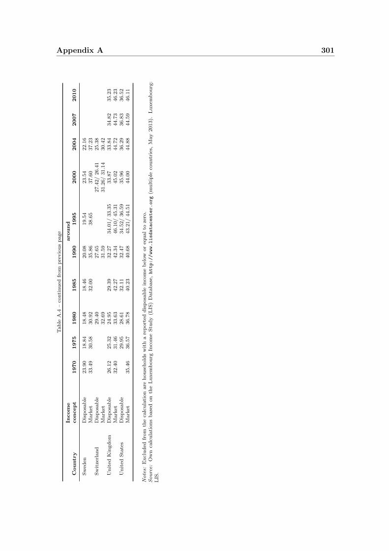
Appendix A 301T
ab
leA
.4–
conti
nu
edfr
om
pre
vio
us
page
Incom
earou
nd
Cou
ntr
ycon
cep
t1970
1975
1980
1985
1990
1995
2000
2004
2007
2010
Sw
eden
Dis
posa
ble
23.9
018.8
418.4
818.4
620.0
819.5
423.5
422.1
6M
ark
et33.4
930.5
830.9
232.0
035.8
638.6
537.6
037.2
3S
wit
zerl
an
dD
isp
osa
ble
29.4
027.6
527.4
2/
26.4
125.3
8M
ark
et32.6
931.5
931.2
6/
31.1
430.4
2U
nit
edK
ingd
om
Dis
posa
ble
26.1
225.3
224.9
529.3
932.2
734.0
1/
33.3
533.8
733.8
434.8
235.2
3M
ark
et32.4
031.4
633.6
342.2
742.3
446.1
0/
45.3
145.0
244.7
244.7
346.2
3U
nit
edS
tate
sD
isp
osa
ble
29.9
528.6
132.1
132.4
734.5
2/
36.5
935.9
636.2
936.8
336.5
2M
ark
et35.4
636.5
736.7
840.2
340.6
843.2
1/
44.5
144.0
044.8
844.5
946.1
1
Notes:
Excl
ud
edfr
om
the
calc
ula
tion
are
hou
seh
old
sw
ith
are
port
edd
isp
osa
ble
inco
me
bel
ow
or
equ
al
toze
ro.
Source:
Ow
nca
lcu
lati
on
sb
ase
don
the
Lu
xem
bou
rgIn
com
eS
tud
y(L
IS)
Data
base
,http://www.lisdatacenter.org
(mu
ltip
leco
untr
ies,
May
2013).
Lu
xem
bou
rg:
LIS
.
302 Appendix A
A.1.1 Measurement error
Researchers who conduct empirical studies of the income distribution and the com-
parison of distributions or trends in inequality across countries usually have to ad-
dress several data quality issues. Since the available data on income distributions
deviates from the ideal measure of economic well-being, it is important to identify
the relevant sources of measurement error.
To illustrate what kind of measurement error will bias across country comparisons
of inequality levels and trends, I make use of an simple error component model
proposed by Atkinson et al. (2000); Gottschalk and Smeeding (2000).
Cross-country comparison of inequality levels
The measure of the jth percentile in country c is equal to:
lnP jc = lnπj
c +mjc
mjc = dc + vj + ejc,
where P jc is the measured percentile j in country c, πj
c stands for the true percentile
using the ideal concept of economic well-being and mjc is the measurement error
component. The measurement error can be decomposed into three different sources
of error: dc is a country specific component that affects all deciles in a country
similarly, vj is a decile-specific component which is common to all countries, and ejc
is both decile- and country-specific.
Calculation the ratio of the 90th and 10th percentile in a single country c, the
measured inequality level can be expressed as follows:
ln(P 90c /P 10
c ) = ln(π90c /π
10c ) + (v90 − v10) + (e90
c − e10c ).
The measurement error does only consist of decile-specific components, while d90c /d
10c
cancels out. Consequently, measurement error that affects all deciles in a country
equally (e.g. consumption of public goods unrelated to the decile rank) will not bias
the 90/10 ratio.
Now, I focus on cross-national studies by comparing the 90/10 ratio in country
L and K:
ln(P 90L /P 10
L )− ln(P 90K /P 10
K ) = ln(π90L /π
10L )− ln(π90
K /π10K ) + (e90
L − e10L )− (e90
K − e10K ).
For cross-national comparisons of inequality at a point in time only errors that differ
Appendix A 303
both across deciles and across countries matter and should be addressed appropri-
ately.240
Cross-country comparison of trends in inequality
To start with within-country trends, suppose that the measured percentile j in year
t is equal to:
lnP jt = lnπj
t +mjt
mjt = nt + vj + rjt ,
where nt is a time-specific component that affects all deciles and rjt is both decile-
and time-specific.
The measured 90/10 ratio is then as follows:
ln(P 90t /P 10
t ) = ln(π90t /π
10t ) + (v90 − v10) + (r90
t − r10t ).
Over time, the 90/10 ratio in a given country is only affect by measurement error
that is both decile- and time-specific.
ln(P 90t /P 10
t )− ln(P 90t+1/P
10t+1) = ln(π90
t /π10t )− ln(π90
t+1/π10t+1)
+ (r90t − r10
t )− (r90t+1 − r10
t+1)
After focusing on the relevant sources of measurement error for cross-country
comparisons in level of inequality and within-country trends in inequality, the fol-
lowing combines both in the comparison of inequality trends across countries.
lnP jct = lnπj
ct +mjct
mjct = dc + vj + ejc + hjct
hjct = gct + rjt + f jct,
where gct is a time-specific component that affects all deciles equally in country c
and f jct is a time-, country- and decile-specific component.
The comparison of trends in the 90/10 ratio between two countries L and K
240 The irrelevance of certain error components does not imply that measurement error is notan important issue in cross-country analysis of inequality. Although the measurement error(noise) gets smaller, the same applies for the ideal measure (signal). By comparing theinequality across countries (and/or time) the signal-to-noise ratio might even decrease (e.g.Gottschalk and Smeeding, 2000).
304 Appendix A
looks as follows:
(ln(P 90Lt − P 10
Lt )− ln(P 90L,t+1 − P 10
L,t+1))− (ln(P 90Kt − P 10
Kt)− ln(P 90K,t+1 − P 10
K,t+1)) =
(ln(π90Lt − π10
Lt)− ln(π90L,t+1 − π10
L,t+1))− (ln(π90Kt − π10
Kt)− ln(π90K,t+1 − π10
K,t+1))
+((h90Lt − h10
Lt)− (h90L,t+1 − h10
L,t+1))− ((h90Kt − h10
Kt)− (h90K,t+1 − h10
K,t+1))
The remaining measurement error hjct in cross-country comparison of trends can be
further decomposed. Since the error component gct is common to all deciles in a
country in a given year, it will not bias an analysis of the 90/10 ratio. Furthermore,
the component rjt that is time- and decile-specific but common across countries drops
out. The relevant error that will blur a comparison of trends in inequality across
countries is therefore time-, country- and decile-specific (f jct).
I have, thus, for the cross-country comparison of trends put a special emphasize
on changes in the LIS data over time within countries affecting different parts of the
income distribution differently.

Appendix A 305
A.2 Robustness checks
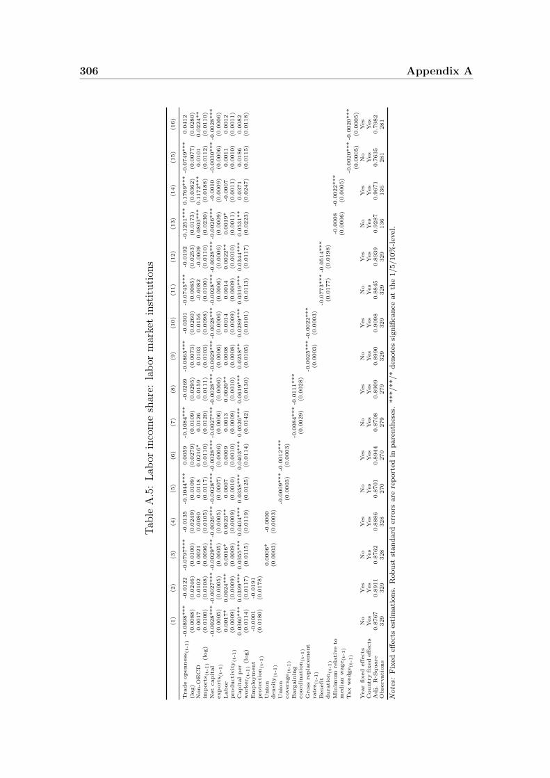
306 Appendix A
Tab
leA
.5:
Lab
orin
com
esh
are:
lab
orm
arke
tin
stit
uti
ons
(1)
(2)
(3)
(4)
(5)
(6)
(7)
(8)
(9)
(10)
(11)
(12)
(13)
(14)
(15)
(16)
Tra
de
op
enness
(t-1
)-0
.0898***
-0.0
122
-0.0
797***
-0.0
135
-0.1
044***
0.0
059
-0.1
084***
-0.0
269
-0.0
865***
-0.0
301
-0.0
745***
-0.0
192
-0.1
251***
0.1
769***
-0.0
749***
0.0
412
(log)
(0.0
088)
(0.0
246)
(0.0
100)
(0.0
249)
(0.0
109)
(0.0
279)
(0.0
109)
(0.0
295)
(0.0
073)
(0.0
260)
(0.0
085)
(0.0
253)
(0.0
173)
(0.0
362)
(0.0
077)
(0.0
280)
Non-O
EC
D0.0
017
0.0
102
0.0
021
0.0
080
0.0
118
0.0
216*
0.0
126
0.0
159
0.0
103
0.0
156
-0.0
082
-0.0
009
0.0
803***
0.1
172***
0.0
101
0.0
224**
imp
ort
s (t-1
)(l
og)
(0.0
100)
(0.0
108)
(0.0
096)
(0.0
105)
(0.0
117)
(0.0
110)
(0.0
120)
(0.0
111)
(0.0
103)
(0.0
098)
(0.0
100)
(0.0
110)
(0.0
230)
(0.0
188)
(0.0
112)
(0.0
110)
Net
capit
al
-0.0
028***
-0.0
027***
-0.0
029***
-0.0
026***
-0.0
028***
-0.0
028***
-0.0
027***
-0.0
028***
-0.0
029***
-0.0
028***
-0.0
028***
-0.0
028***
-0.0
026***
-0.0
010
-0.0
030***
-0.0
028***
exp
ort
s (t-1
)(0
.0005)
(0.0
005)
(0.0
005)
(0.0
005)
(0.0
007)
(0.0
006)
(0.0
006)
(0.0
006)
(0.0
006)
(0.0
006)
(0.0
006)
(0.0
006)
(0.0
009)
(0.0
009)
(0.0
006)
(0.0
006)
Lab
or
0.0
017*
0.0
024***
0.0
016*
0.0
023**
0.0
007
0.0
009
0.0
013
0.0
020**
0.0
008
0.0
014
0.0
014
0.0
022**
0.0
019*
-0.0
007
0.0
011
0.0
012
pro
ducti
vit
y(t-1
)(0
.0009)
(0.0
009)
(0.0
009)
(0.0
009)
(0.0
010)
(0.0
010)
(0.0
009)
(0.0
010)
(0.0
008)
(0.0
009)
(0.0
009)
(0.0
010)
(0.0
011)
(0.0
011)
(0.0
010)
(0.0
011)
Capit
al
per
0.0
360***
0.0
399***
0.0
355***
0.0
404***
0.0
358***
0.0
403***
0.0
526***
0.0
619***
0.0
258**
0.0
289***
0.0
319***
0.0
344***
0.0
531**
0.0
371
0.0
186
0.0
082
work
er (
t-1
)(l
og)
(0.0
114)
(0.0
117)
(0.0
115)
(0.0
119)
(0.0
125)
(0.0
114)
(0.0
142)
(0.0
130)
(0.0
105)
(0.0
101)
(0.0
113)
(0.0
117)
(0.0
223)
(0.0
247)
(0.0
115)
(0.0
118)
Em
plo
ym
ent
-0.0
001
-0.0
191
pro
tecti
on(t-1
)(0
.0180)
(0.0
178)
Unio
n0.0
006*
-0.0
000
densi
ty(t-1
)(0
.0003)
(0.0
003)
Unio
n-0
.0009***
-0.0
012***
covera
ge(t-1
)(0
.0003)
(0.0
003)
Barg
ain
ing
-0.0
084***
-0.0
111***
coord
inati
on(t-1
)(0
.0029)
(0.0
028)
Gro
ssre
pla
cem
ent
-0.0
025***
-0.0
022***
rate
s (t-1
)(0
.0003)
(0.0
003)
Benefi
t-0
.0773***
-0.0
514***
dura
tion(t-1
)(0
.0177)
(0.0
198)
Min
imum
rela
tive
to-0
.0008
-0.0
022***
media
nw
age(t-1
)(0
.0006)
(0.0
005)
Tax
wedge(t-1
)-0
.0020***
-0.0
020***
(0.0
005)
(0.0
005)
Year
fixed
eff
ects
No
Yes
No
Yes
No
Yes
No
Yes
No
Yes
No
Yes
No
Yes
No
Yes
Countr
yfi
xed
eff
ects
Yes
Yes
Yes
Yes
Yes
Yes
Yes
Yes
Yes
Yes
Yes
Yes
Yes
Yes
Yes
Yes
Adj.
R-S
quare
0.8
767
0.8
911
0.8
762
0.8
886
0.8
701
0.8
944
0.8
708
0.8
909
0.8
990
0.9
098
0.8
845
0.8
939
0.9
287
0.9
671
0.7
635
0.7
982
Obse
rvati
ons
329
329
328
328
270
270
279
279
329
329
329
329
136
136
281
281
Notes:
Fix
edeff
ects
esti
mati
on
s.R
ob
ust
stan
dard
erro
rsare
rep
ort
edin
pare
nth
eses
.***/**/*
den
ote
ssi
gn
ifica
nce
at
the
1/5/10%
-lev
el.
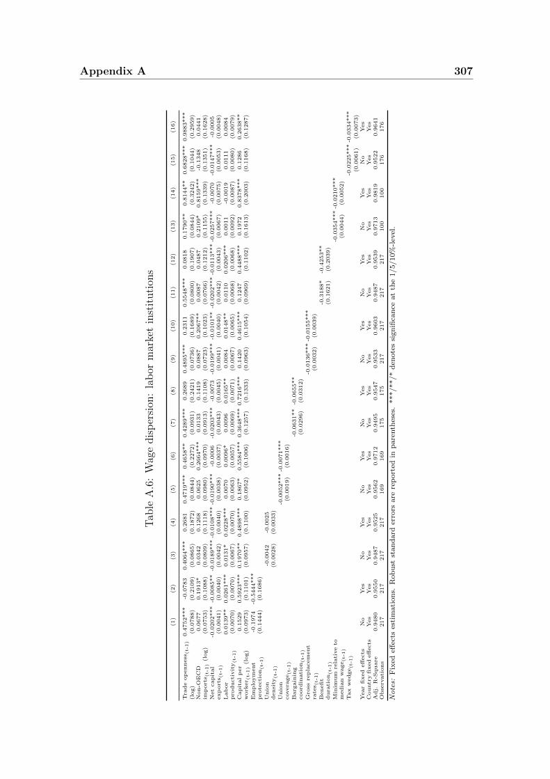
Appendix A 307
Tab
leA
.6:
Wag
edis
per
sion
:la
bor
mar
ket
inst
ituti
ons
(1)
(2)
(3)
(4)
(5)
(6)
(7)
(8)
(9)
(10)
(11)
(12)
(13)
(14)
(15)
(16)
Tra
de
op
enness
(t-1
)0.4
752***
-0.0
783
0.4
064***
0.2
681
0.4
719***
0.4
658**
0.4
289***
0.2
689
0.4
895***
0.2
311
0.5
548***
0.0
818
0.1
790**
0.8
144**
0.6
828***
0.9
883***
(log)
(0.0
788)
(0.2
109)
(0.0
865)
(0.1
872)
(0.0
844)
(0.2
272)
(0.0
931)
(0.2
421)
(0.0
736)
(0.1
689)
(0.0
800)
(0.1
907)
(0.0
844)
(0.3
242)
(0.1
044)
(0.2
959)
Non-O
EC
D0.0
677
0.1
913*
0.0
342
0.1
268
0.0
625
0.2
664***
0.0
133
0.1
419
0.0
887
0.2
067**
0.0
087
0.0
487
0.2
109*
0.8
159***
-0.1
348
0.0
441
imp
ort
s (t-1
)(l
og)
(0.0
753)
(0.1
088)
(0.0
809)
(0.1
118)
(0.0
980)
(0.0
970)
(0.0
913)
(0.1
108)
(0.0
723)
(0.1
023)
(0.0
766)
(0.1
212)
(0.1
155)
(0.1
339)
(0.1
351)
(0.1
628)
Net
capit
al
-0.0
202***
-0.0
085**
-0.0
189***
-0.0
108***
-0.0
190***
-0.0
006
-0.0
203***
-0.0
073
-0.0
199***
-0.0
101**
-0.0
202***
-0.0
113***
-0.0
257***
-0.0
070
-0.0
147***
-0.0
005
exp
ort
s (t-1
)(0
.0041)
(0.0
040)
(0.0
042)
(0.0
040)
(0.0
038)
(0.0
037)
(0.0
043)
(0.0
045)
(0.0
041)
(0.0
040)
(0.0
042)
(0.0
043)
(0.0
067)
(0.0
075)
(0.0
053)
(0.0
048)
Lab
or
0.0
139**
0.0
261***
0.0
131*
0.0
228***
0.0
070
0.0
096*
0.0
096
0.0
165**
0.0
084
0.0
148**
0.0
110
0.0
206***
0.0
011
-0.0
019
0.0
111
0.0
084
pro
ducti
vit
y(t-1
)(0
.0070)
(0.0
070)
(0.0
067)
(0.0
070)
(0.0
063)
(0.0
057)
(0.0
069)
(0.0
071)
(0.0
067)
(0.0
065)
(0.0
068)
(0.0
068)
(0.0
092)
(0.0
087)
(0.0
080)
(0.0
079)
Capit
al
per
0.1
529
0.5
923***
0.1
970**
0.4
898***
0.1
867*
0.5
584***
0.3
648***
0.7
216***
0.1
420
0.4
615***
0.1
247
0.4
488***
0.1
972
0.8
378***
0.1
286
0.2
638**
work
er (
t-1
)(l
og)
(0.0
973)
(0.1
101)
(0.0
957)
(0.1
100)
(0.0
952)
(0.1
006)
(0.1
257)
(0.1
333)
(0.0
963)
(0.1
054)
(0.0
969)
(0.1
102)
(0.1
613)
(0.2
003)
(0.1
168)
(0.1
287)
Em
plo
ym
ent
-0.1
974
-0.5
444***
pro
tecti
on(t-1
)(0
.1444)
(0.1
686)
Unio
n-0
.0042
-0.0
025
densi
ty(t-1
)(0
.0028)
(0.0
033)
Unio
n-0
.0052***
-0.0
071***
covera
ge(t-1
)(0
.0019)
(0.0
016)
Barg
ain
ing
-0.0
631**
-0.0
655**
coord
inati
on(t-1
)(0
.0296)
(0.0
312)
Gro
ssre
pla
cem
ent
-0.0
136***
-0.0
155***
rate
s (t-1
)(0
.0032)
(0.0
039)
Benefi
t-0
.3188*
-0.4
253**
dura
tion(t-1
)(0
.1621)
(0.2
039)
Min
imum
rela
tive
to-0
.0354***
-0.0
210***
media
nw
age(t-1
)(0
.0044)
(0.0
052)
Tax
wedge(t-1
)-0
.0225***
-0.0
334***
(0.0
061)
(0.0
073)
Year
fixed
eff
ects
No
Yes
No
Yes
No
Yes
No
Yes
No
Yes
No
Yes
No
Yes
No
Yes
Countr
yfi
xed
eff
ects
Yes
Yes
Yes
Yes
Yes
Yes
Yes
Yes
Yes
Yes
Yes
Yes
Yes
Yes
Yes
Yes
Adj.
R-S
quare
0.9
480
0.9
550
0.9
487
0.9
525
0.9
562
0.9
712
0.9
495
0.9
547
0.9
533
0.9
603
0.9
487
0.9
539
0.9
713
0.9
819
0.9
522
0.9
641
Obse
rvati
ons
217
217
217
217
169
169
175
175
217
217
217
217
100
100
176
176
Notes:
Fix
edeff
ects
esti
mati
on
s.R
ob
ust
stan
dard
erro
rsare
rep
ort
edin
pare
nth
eses
.***/**/*
den
ote
ssi
gn
ifica
nce
at
the
1/5/10%
-lev
el.
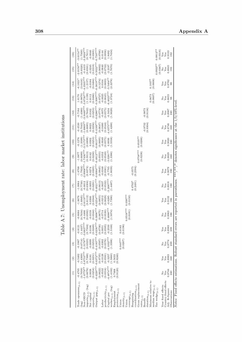
308 Appendix A
Tab
leA
.7:
Unem
plo
ym
ent
rate
:la
bor
mar
ket
inst
ituti
ons
(1)
(2)
(3)
(4)
(5)
(6)
(7)
(8)
(9)
(10)
(11)
(12)
(13)
(14)
(15)
(16)
Tra
de
op
enness
(t-1
)-0
.4705
-0.5
482
-0.1
987
-0.8
121
-0.6
684
-1.8
676
-1.0
064
-1.6
768
-1.0
877
-0.1
276
-0.4
530
-0.7
184
1.0
170
-6.1
021*
-2.0
150**
-3.6
154**
(log)
(0.7
059)
(1.4
369)
(0.6
714)
(1.4
437)
(0.7
634)
(1.6
845)
(0.7
730)
(1.7
924)
(0.6
689)
(1.3
599)
(0.7
043)
(1.4
380)
(0.9
870)
(3.6
416)
(0.8
320)
(1.7
569)
Non-O
EC
D-1
.6779**
-3.8
753***
-1.3
178**
-3.6
837***
-0.4
466
-2.8
119***
-0.6
612
-2.8
908***
-1.7
436***
-3.5
173***
-1.6
869**
-3.9
449***
-3.8
730***
-4.3
505***
-0.4
419
-3.2
824***
imp
ort
s (t-1
)(l
og)
(0.6
676)
(0.7
388)
(0.6
323)
(0.7
504)
(0.6
592)
(0.8
112)
(0.6
304)
(0.8
374)
(0.5
913)
(0.6
898)
(0.6
685)
(0.7
642)
(1.1
139)
(1.2
157)
(0.6
501)
(0.7
611)
Net
capit
al
0.0
038
0.0
181
-0.0
099
0.0
106
-0.0
159
0.0
300
-0.0
055
0.0
274
0.0
142
0.0
302
0.0
023
0.0
162
0.0
112
-0.0
184
-0.0
245
-0.0
040
exp
ort
s (t-1
)(0
.0254)
(0.0
251)
(0.0
253)
(0.0
249)
(0.0
344)
(0.0
344)
(0.0
291)
(0.0
305)
(0.0
230)
(0.0
253)
(0.0
256)
(0.0
253)
(0.0
486)
(0.0
484)
(0.0
318)
(0.0
305)
Outp
ut
gap(t-1
)-0
.4220***
-0.6
372***
-0.4
183***
-0.6
230***
-0.3
896***
-0.6
254***
-0.4
021***
-0.6
084***
-0.4
812***
-0.6
615***
-0.4
169***
-0.6
280***
-0.3
087***
-0.3
819***
-0.5
022***
-0.7
507***
(0.0
622)
(0.0
735)
(0.0
597)
(0.0
736)
(0.0
675)
(0.0
855)
(0.0
613)
(0.0
845)
(0.0
555)
(0.0
695)
(0.0
647)
(0.0
774)
(0.0
727)
(0.1
274)
(0.0
692)
(0.0
766)
Lab
or
-0.0
532
-0.0
128
-0.0
362
0.0
051
-0.0
714
-0.0
212
-0.0
637
-0.0
348
-0.0
352
-0.0
049
-0.0
480
-0.0
075
-0.0
025
0.0
164
-0.0
640
0.0
144
pro
ducti
vit
y(t-1
)(0
.0554)
(0.0
591)
(0.0
576)
(0.0
595)
(0.0
530)
(0.0
629)
(0.0
532)
(0.0
581)
(0.0
549)
(0.0
575)
(0.0
544)
(0.0
575)
(0.0
645)
(0.0
693)
(0.0
732)
(0.0
956)
Capit
al
per
-4.4
874***
-0.3
257
-4.1
032***
-0.2
550
-5.4
688***
-0.6
285
-5.2
687***
-0.7
705
-3.0
281**
0.8
936
-4.4
375***
-0.3
434
-6.4
623***
-5.5
404**
-2.2
197
1.8
492
work
er (
t-1
)(l
og)
(1.4
192)
(1.5
860)
(1.3
398)
(1.5
168)
(1.5
074)
(1.7
390)
(1.4
487)
(1.8
039)
(1.3
386)
(1.5
558)
(1.4
288)
(1.5
629)
(1.3
724)
(2.2
278)
(1.7
670)
(1.7
434)
Em
plo
ym
ent
0.7
468
0.5
633
pro
tecti
on(t-1
)(0
.9120)
(0.9
240)
Unio
n0.0
447**
0.0
183
densi
ty(t-1
)(0
.0207)
(0.0
196)
Unio
n0.0
518***
0.0
387**
covera
ge(t-1
)(0
.0181)
(0.0
150)
Barg
ain
ing
0.4
702*
-0.0
575
coord
inati
on(t-1
)(0
.2491)
(0.2
594)
Gro
ssre
pla
cem
ent
0.0
758***
0.0
535**
rate
s (t-1
)(0
.0238)
(0.0
206)
Benefi
t-0
.9732
-0.9
873
dura
tion(t-1
)(0
.9304)
(0.9
134)
Min
imum
rela
tive
to0.0
673
0.1
037*
media
nw
age(t-1
)(0
.0607)
(0.0
608)
Tax
wedge(t-1
)0.0
922**
0.0
812**
(0.0
367)
(0.0
318)
Year
fixed
eff
ects
No
Yes
No
Yes
No
Yes
No
Yes
No
Yes
No
Yes
No
Yes
No
Yes
Countr
yfi
xed
eff
ects
Yes
Yes
Yes
Yes
Yes
Yes
Yes
Yes
Yes
Yes
Yes
Yes
Yes
Yes
Yes
Yes
Adj.
R-S
quare
0.8
744
0.8
983
0.8
774
0.8
983
0.8
963
0.9
132
0.8
918
0.9
079
0.8
829
0.9
020
0.8
746
0.8
987
0.8
655
0.8
782
0.8
845
0.9
103
Obse
rvati
ons
240
240
239
239
186
186
190
190
240
240
240
240
98
98
192
192
Notes:
Fix
edeff
ects
esti
mati
on
s.R
ob
ust
stan
dard
erro
rsare
rep
ort
edin
pare
nth
eses
.***/**/*
den
ote
ssi
gn
ifica
nce
at
the
1/5/10%
-lev
el.
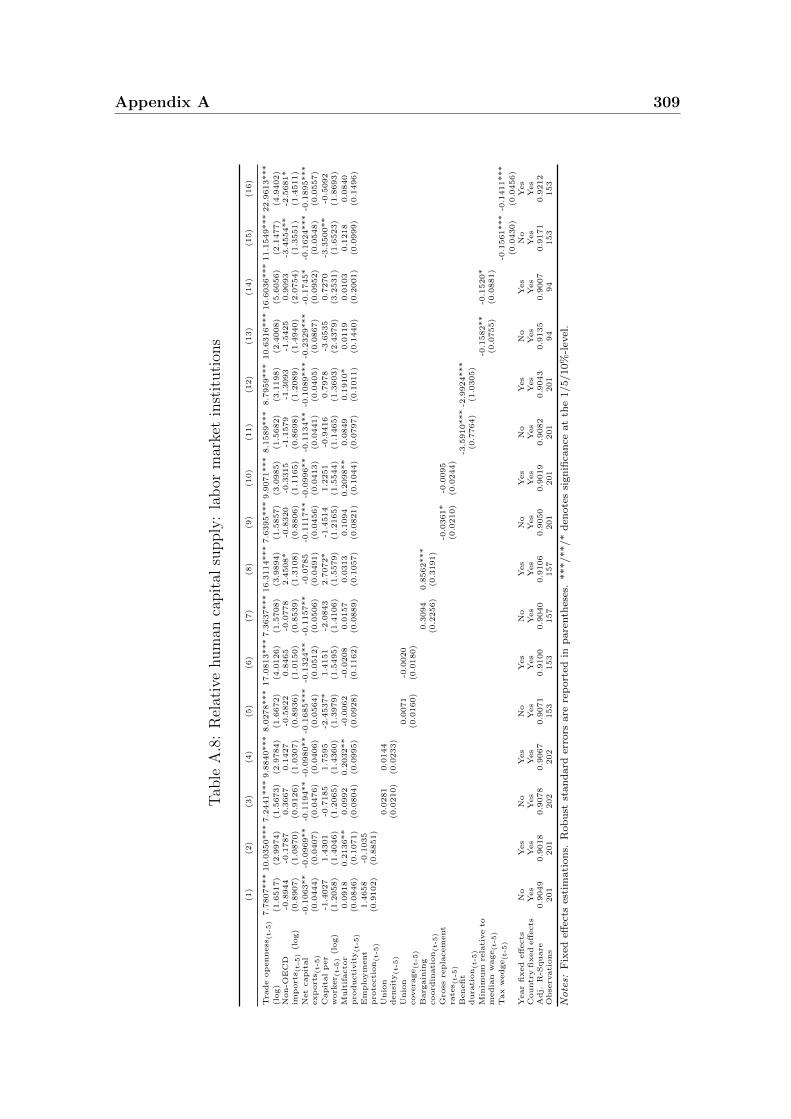
Appendix A 309
Tab
leA
.8:
Rel
ativ
ehum
anca
pit
alsu
pply
:la
bor
mar
ket
inst
ituti
ons
(1)
(2)
(3)
(4)
(5)
(6)
(7)
(8)
(9)
(10)
(11)
(12)
(13)
(14)
(15)
(16)
Tra
de
op
enness
(t-5
)7.7
807***
10.0
350***
7.2
441***
9.8
840***
8.0
278***
17.0
813***
7.3
637***
16.3
114***
7.6
395***
9.9
071***
8.1
589***
8.7
959***
10.6
316***
16.6
036***
11.1
549***
22.9
613***
(log)
(1.6
517)
(2.9
974)
(1.5
673)
(2.9
784)
(1.6
672)
(4.0
126)
(1.5
708)
(3.9
894)
(1.5
857)
(3.0
985)
(1.5
682)
(3.1
198)
(2.4
008)
(5.6
056)
(2.1
477)
(4.9
402)
Non-O
EC
D-0
.8944
-0.1
787
0.3
667
0.1
427
-0.5
822
0.8
465
-0.0
778
2.4
508*
-0.8
320
-0.3
315
-1.1
579
-1.3
093
-1.5
425
0.9
093
-3.4
554**
-2.5
681*
imp
ort
s (t-5
)(l
og)
(0.8
907)
(1.0
870)
(0.9
126)
(1.0
307)
(0.8
936)
(1.0
150)
(0.8
539)
(1.3
108)
(0.8
806)
(1.1
165)
(0.8
698)
(1.2
089)
(1.4
940)
(2.0
754)
(1.3
551)
(1.4
511)
Net
capit
al
-0.1
063**
-0.0
969**
-0.1
194**
-0.0
980**
-0.1
685***
-0.1
324**
-0.1
157**
-0.0
785
-0.1
117**
-0.0
996**
-0.1
134**
-0.1
089***
-0.2
329***
-0.1
745*
-0.1
624***
-0.1
895***
exp
ort
s (t-5
)(0
.0444)
(0.0
407)
(0.0
476)
(0.0
406)
(0.0
564)
(0.0
512)
(0.0
506)
(0.0
491)
(0.0
456)
(0.0
413)
(0.0
441)
(0.0
405)
(0.0
867)
(0.0
952)
(0.0
548)
(0.0
557)
Capit
al
per
-1.4
027
1.4
301
-0.7
185
1.7
595
-2.4
537*
1.4
151
-2.0
843
2.7
072*
-1.4
514
1.2
251
-0.9
416
0.7
978
-3.6
535
0.7
270
-3.3
500**
-0.5
092
work
er (
t-5
)(l
og)
(1.2
058)
(1.4
046)
(1.2
065)
(1.4
360)
(1.3
979)
(1.5
495)
(1.4
106)
(1.5
579)
(1.2
165)
(1.5
544)
(1.1
465)
(1.3
603)
(2.4
379)
(3.2
531)
(1.6
523)
(1.8
693)
Mult
ifacto
r0.0
918
0.2
136**
0.0
992
0.2
032**
-0.0
062
-0.0
208
0.0
157
0.0
313
0.1
094
0.2
098**
0.0
849
0.1
910*
0.0
119
0.0
103
0.1
218
0.0
840
pro
ducti
vit
y(t-5
)(0
.0846)
(0.1
071)
(0.0
804)
(0.0
995)
(0.0
928)
(0.1
162)
(0.0
889)
(0.1
057)
(0.0
821)
(0.1
044)
(0.0
797)
(0.1
011)
(0.1
440)
(0.2
001)
(0.0
999)
(0.1
496)
Em
plo
ym
ent
1.4
658
-0.1
035
pro
tecti
on(t-5
)(0
.9102)
(0.8
851)
Unio
n0.0
281
0.0
144
densi
ty(t-5
)(0
.0210)
(0.0
233)
Unio
n0.0
071
-0.0
020
covera
ge(t-5
)(0
.0160)
(0.0
180)
Barg
ain
ing
0.3
094
0.8
562***
coord
inati
on(t-5
)(0
.2256)
(0.3
191)
Gro
ssre
pla
cem
ent
-0.0
361*
-0.0
095
rate
s (t-5
)(0
.0210)
(0.0
244)
Benefi
t-3
.5910***
-2.9
924***
dura
tion(t-5
)(0
.7764)
(1.0
305)
Min
imum
rela
tive
to-0
.1582**
-0.1
520*
media
nw
age(t-5
)(0
.0755)
(0.0
881)
Tax
wedge(t-5
)-0
.1561***
-0.1
411***
(0.0
430)
(0.0
456)
Year
fixed
eff
ects
No
Yes
No
Yes
No
Yes
No
Yes
No
Yes
No
Yes
No
Yes
No
Yes
Countr
yfi
xed
eff
ects
Yes
Yes
Yes
Yes
Yes
Yes
Yes
Yes
Yes
Yes
Yes
Yes
Yes
Yes
Yes
Yes
Adj.
R-S
quare
0.9
049
0.9
018
0.9
078
0.9
067
0.9
071
0.9
100
0.9
040
0.9
106
0.9
050
0.9
019
0.9
082
0.9
043
0.9
135
0.9
007
0.9
171
0.9
212
Obse
rvati
ons
201
201
202
202
153
153
157
157
201
201
201
201
94
94
153
153
Notes:
Fix
edeff
ects
esti
mati
on
s.R
ob
ust
stan
dard
erro
rsare
rep
ort
edin
pare
nth
eses
.***/**/*
den
ote
ssi
gn
ifica
nce
at
the
1/5/10%
-lev
el.
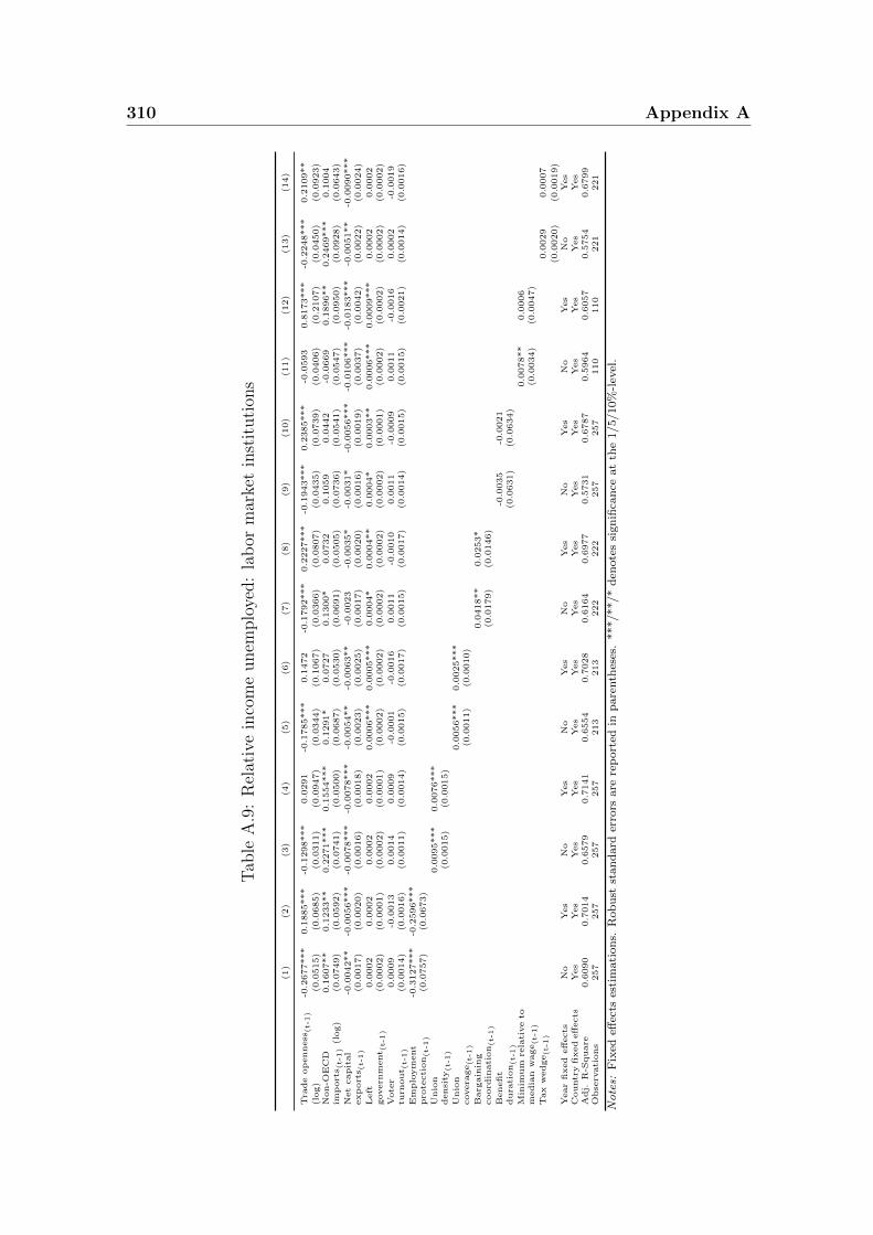
310 Appendix A
Tab
leA
.9:
Rel
ativ
ein
com
eunem
plo
yed:
lab
orm
arke
tin
stit
uti
ons
(1)
(2)
(3)
(4)
(5)
(6)
(7)
(8)
(9)
(10)
(11)
(12)
(13)
(14)
Tra
de
op
enness
(t-1
)-0
.2677***
0.1
885***
-0.1
298***
0.0
291
-0.1
785***
0.1
472
-0.1
792***
0.2
227***
-0.1
943***
0.2
385***
-0.0
593
0.8
173***
-0.2
248***
0.2
109**
(log)
(0.0
515)
(0.0
685)
(0.0
311)
(0.0
947)
(0.0
344)
(0.1
067)
(0.0
366)
(0.0
807)
(0.0
435)
(0.0
739)
(0.0
406)
(0.2
107)
(0.0
450)
(0.0
923)
Non-O
EC
D0.1
607**
0.1
233**
0.2
271***
0.1
554***
0.1
291*
0.0
727
0.1
300*
0.0
732
0.1
059
0.0
442
-0.0
669
0.1
896**
0.2
469***
0.1
004
imp
ort
s (t-1
)(l
og)
(0.0
749)
(0.0
592)
(0.0
741)
(0.0
500)
(0.0
687)
(0.0
530)
(0.0
691)
(0.0
505)
(0.0
736)
(0.0
541)
(0.0
547)
(0.0
950)
(0.0
928)
(0.0
643)
Net
capit
al
-0.0
042**
-0.0
056***
-0.0
078***
-0.0
078***
-0.0
054**
-0.0
063**
-0.0
023
-0.0
035*
-0.0
031*
-0.0
056***
-0.0
106***
-0.0
183***
-0.0
051**
-0.0
090***
exp
ort
s (t-1
)(0
.0017)
(0.0
020)
(0.0
016)
(0.0
018)
(0.0
023)
(0.0
025)
(0.0
017)
(0.0
020)
(0.0
016)
(0.0
019)
(0.0
037)
(0.0
042)
(0.0
022)
(0.0
024)
Left
0.0
002
0.0
002
0.0
002
0.0
002
0.0
006***
0.0
005***
0.0
004*
0.0
004**
0.0
004*
0.0
003**
0.0
006***
0.0
009***
0.0
002
0.0
002
govern
ment (
t-1
)(0
.0002)
(0.0
001)
(0.0
002)
(0.0
001)
(0.0
002)
(0.0
002)
(0.0
002)
(0.0
002)
(0.0
002)
(0.0
001)
(0.0
002)
(0.0
002)
(0.0
002)
(0.0
002)
Vote
r0.0
009
-0.0
013
0.0
014
0.0
009
-0.0
001
-0.0
016
0.0
011
-0.0
010
0.0
011
-0.0
009
0.0
011
-0.0
016
0.0
002
-0.0
019
turn
out (
t-1
)(0
.0014)
(0.0
016)
(0.0
011)
(0.0
014)
(0.0
015)
(0.0
017)
(0.0
015)
(0.0
017)
(0.0
014)
(0.0
015)
(0.0
015)
(0.0
021)
(0.0
014)
(0.0
016)
Em
plo
ym
ent
-0.3
127***
-0.2
596***
pro
tecti
on(t-1
)(0
.0757)
(0.0
673)
Unio
n0.0
095***
0.0
076***
densi
ty(t-1
)(0
.0015)
(0.0
015)
Unio
n0.0
056***
0.0
025***
covera
ge(t-1
)(0
.0011)
(0.0
010)
Barg
ain
ing
0.0
418**
0.0
253*
coord
inati
on(t-1
)(0
.0179)
(0.0
146)
Benefi
t-0
.0035
-0.0
021
dura
tion(t-1
)(0
.0631)
(0.0
634)
Min
imum
rela
tive
to0.0
078**
0.0
006
media
nw
age(t-1
)(0
.0034)
(0.0
047)
Tax
wedge(t-1
)0.0
029
0.0
007
(0.0
020)
(0.0
019)
Year
fixed
eff
ects
No
Yes
No
Yes
No
Yes
No
Yes
No
Yes
No
Yes
No
Yes
Countr
yfi
xed
eff
ects
Yes
Yes
Yes
Yes
Yes
Yes
Yes
Yes
Yes
Yes
Yes
Yes
Yes
Yes
Adj.
R-S
quare
0.6
090
0.7
014
0.6
579
0.7
141
0.6
554
0.7
028
0.6
164
0.6
977
0.5
731
0.6
787
0.5
964
0.6
057
0.5
754
0.6
799
Obse
rvati
ons
257
257
257
257
213
213
222
222
257
257
110
110
221
221
Notes:
Fix
edeff
ects
esti
mati
on
s.R
ob
ust
stan
dard
erro
rsare
rep
ort
edin
pare
nth
eses
.***/**/*
den
ote
ssi
gn
ifica
nce
at
the
1/5/10%
-lev
el.
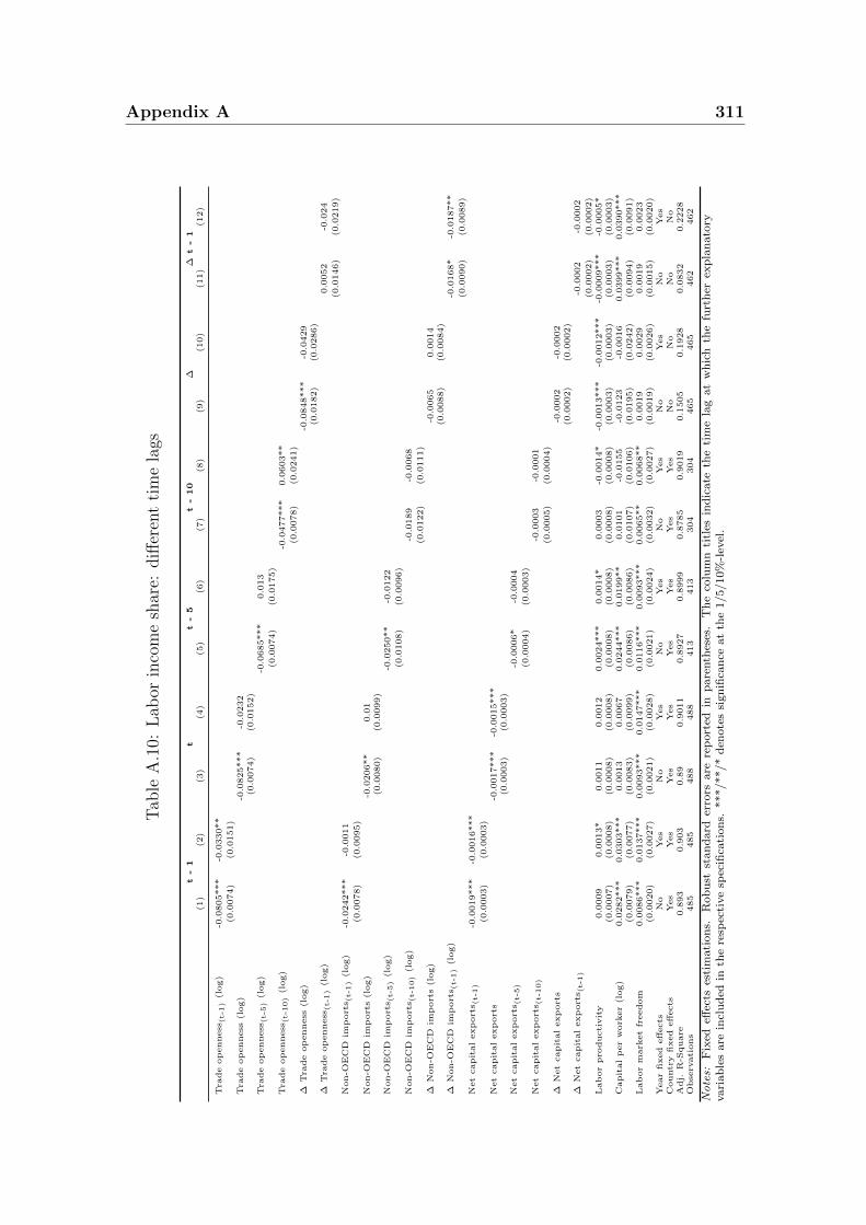
Appendix A 311
Tab
leA
.10:
Lab
orin
com
esh
are:
diff
eren
tti
me
lags
t-1
tt
-5
t-10
∆∆
t-1
(1)
(2)
(3)
(4)
(5)
(6)
(7)
(8)
(9)
(10)
(11)
(12)
Tra
de
op
enness
(t-1
)(l
og)
-0.0
805***
-0.0
330**
(0.0
074)
(0.0
151)
Tra
de
op
enness
(log)
-0.0
825***
-0.0
232
(0.0
074)
(0.0
152)
Tra
de
op
enness
(t-5
)(l
og)
-0.0
685***
0.0
13
(0.0
074)
(0.0
175)
Tra
de
op
enness
(t-1
0)
(log)
-0.0
477***
0.0
603**
(0.0
078)
(0.0
241)
∆T
rade
op
enness
(log)
-0.0
848***
-0.0
429
(0.0
182)
(0.0
286)
∆T
rade
op
enness
(t-1
)(l
og)
0.0
052
-0.0
24
(0.0
146)
(0.0
219)
Non-O
EC
Dim
port
s (t-1
)(l
og)
-0.0
242***
-0.0
011
(0.0
078)
(0.0
095)
Non-O
EC
Dim
port
s(l
og)
-0.0
206**
0.0
1(0
.0080)
(0.0
099)
Non-O
EC
Dim
port
s (t-5
)(l
og)
-0.0
250**
-0.0
122
(0.0
108)
(0.0
096)
Non-O
EC
Dim
port
s (t-1
0)
(log)
-0.0
189
-0.0
068
(0.0
122)
(0.0
111)
∆N
on-O
EC
Dim
port
s(l
og)
-0.0
065
0.0
014
(0.0
088)
(0.0
084)
∆N
on-O
EC
Dim
port
s (t-1
)(l
og)
-0.0
168*
-0.0
187**
(0.0
090)
(0.0
089)
Net
capit
al
exp
ort
s (t-1
)-0
.0019***
-0.0
016***
(0.0
003)
(0.0
003)
Net
capit
al
exp
ort
s-0
.0017***
-0.0
015***
(0.0
003)
(0.0
003)
Net
capit
al
exp
ort
s (t-5
)-0
.0006*
-0.0
004
(0.0
004)
(0.0
003)
Net
capit
al
exp
ort
s (t-1
0)
-0.0
003
-0.0
001
(0.0
005)
(0.0
004)
∆N
et
capit
al
exp
ort
s-0
.0002
-0.0
002
(0.0
002)
(0.0
002)
∆N
et
capit
al
exp
ort
s (t-1
)-0
.0002
-0.0
002
(0.0
002)
(0.0
002)
Lab
or
pro
ducti
vit
y0.0
009
0.0
013*
0.0
011
0.0
012
0.0
024***
0.0
014*
0.0
003
-0.0
014*
-0.0
013***
-0.0
012***
-0.0
009***
-0.0
005*
(0.0
007)
(0.0
008)
(0.0
008)
(0.0
008)
(0.0
008)
(0.0
008)
(0.0
008)
(0.0
008)
(0.0
003)
(0.0
003)
(0.0
003)
(0.0
003)
Capit
al
per
work
er
(log)
0.0
282***
0.0
303***
0.0
013
0.0
067
0.0
244***
0.0
199**
0.0
101
-0.0
155
-0.0
123
-0.0
016
0.0
399***
0.0
390***
(0.0
079)
(0.0
077)
(0.0
083)
(0.0
099)
(0.0
086)
(0.0
086)
(0.0
107)
(0.0
106)
(0.0
195)
(0.0
242)
(0.0
094)
(0.0
091)
Lab
or
mark
et
freedom
0.0
086***
0.0
137***
0.0
093***
0.0
147***
0.0
116***
0.0
093***
0.0
065**
0.0
068**
0.0
019
0.0
029
0.0
019
0.0
023
(0.0
020)
(0.0
027)
(0.0
021)
(0.0
028)
(0.0
021)
(0.0
024)
(0.0
032)
(0.0
027)
(0.0
019)
(0.0
026)
(0.0
015)
(0.0
020)
Year
fixed
eff
ects
No
Yes
No
Yes
No
Yes
No
Yes
No
Yes
No
Yes
Countr
yfi
xed
eff
ects
Yes
Yes
Yes
Yes
Yes
Yes
Yes
Yes
No
No
No
No
Adj.
R-S
quare
0.8
93
0.9
03
0.8
90.9
011
0.8
927
0.8
999
0.8
785
0.9
019
0.1
505
0.1
928
0.0
832
0.2
228
Obse
rvati
ons
485
485
488
488
413
413
304
304
465
465
462
462
Notes:
Fix
edeff
ects
esti
mati
on
s.R
ob
ust
stan
dard
erro
rsare
rep
ort
edin
pare
nth
eses
.T
he
colu
mn
titl
esin
dic
ate
the
tim
ela
gat
wh
ich
the
furt
her
exp
lan
ato
ryvari
ab
les
are
incl
ud
edin
the
resp
ecti
ve
spec
ifica
tion
s.***/**/*
den
ote
ssi
gn
ifica
nce
at
the
1/5/10%
-lev
el.
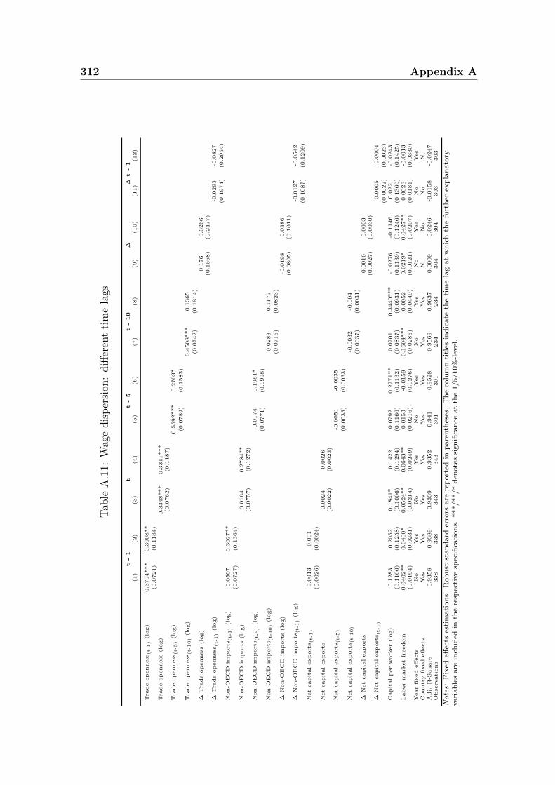
312 Appendix A
Tab
leA
.11:
Wag
edis
per
sion
:diff
eren
tti
me
lags
t-1
tt
-5
t-10
∆∆
t-1
(1)
(2)
(3)
(4)
(5)
(6)
(7)
(8)
(9)
(10)
(11)
(12)
Tra
de
op
enness
(t-1
)(l
og)
0.3
794***
0.3
008**
(0.0
721)
(0.1
184)
Tra
de
op
enness
(log)
0.3
348***
0.3
311***
(0.0
762)
(0.1
187)
Tra
de
op
enness
(t-5
)(l
og)
0.5
592***
0.2
703*
(0.0
789)
(0.1
583)
Tra
de
op
enness
(t-1
0)
(log)
0.4
508***
0.1
365
(0.0
742)
(0.1
814)
∆T
rade
op
enness
(log)
0.1
76
0.3
266
(0.1
568)
(0.2
477)
∆T
rade
op
enness
(t-1
)(l
og)
-0.0
293
-0.0
827
(0.1
974)
(0.2
954)
Non-O
EC
Dim
port
s (t-1
)(l
og)
0.0
507
0.3
027**
(0.0
727)
(0.1
364)
Non-O
EC
Dim
port
s(l
og)
0.0
164
0.2
784**
(0.0
757)
(0.1
272)
Non-O
EC
Dim
port
s (t-5
)(l
og)
-0.0
174
0.1
951*
(0.0
771)
(0.0
998)
Non-O
EC
Dim
port
s (t-1
0)
(log)
0.0
283
0.1
177
(0.0
715)
(0.0
823)
∆N
on-O
EC
Dim
port
s(l
og)
-0.0
198
0.0
386
(0.0
805)
(0.1
011)
∆N
on-O
EC
Dim
port
s (t-1
)(l
og)
-0.0
127
-0.0
542
(0.1
087)
(0.1
209)
Net
capit
al
exp
ort
s (t-1
)0.0
013
0.0
01
(0.0
026)
(0.0
024)
Net
capit
al
exp
ort
s0.0
024
0.0
026
(0.0
022)
(0.0
023)
Net
capit
al
exp
ort
s (t-5
)-0
.0051
-0.0
035
(0.0
033)
(0.0
033)
Net
capit
al
exp
ort
s (t-1
0)
-0.0
032
-0.0
04
(0.0
037)
(0.0
031)
∆N
et
capit
al
exp
ort
s0.0
016
0.0
003
(0.0
027)
(0.0
030)
∆N
et
capit
al
exp
ort
s (t-1
)-0
.0005
-0.0
004
(0.0
022)
(0.0
023)
Capit
al
per
work
er
(log)
0.1
283
0.2
052
0.1
841*
0.1
422
0.0
792
0.2
771**
0.0
701
0.3
440***
-0.0
276
-0.1
146
0.0
22
-0.0
243
(0.1
106)
(0.1
258)
(0.1
006)
(0.1
294)
(0.1
166)
(0.1
132)
(0.0
837)
(0.0
931)
(0.1
139)
(0.1
246)
(0.1
360)
(0.1
425)
Lab
or
mark
et
freedom
0.0
402**
0.0
400*
0.0
524**
0.0
643**
0.0
153
-0.0
159
0.1
604***
0.0
052
0.0
219*
0.0
427**
0.0
028
-0.0
013
(0.0
194)
(0.0
231)
(0.0
214)
(0.0
249)
(0.0
216)
(0.0
276)
(0.0
285)
(0.0
449)
(0.0
121)
(0.0
207)
(0.0
181)
(0.0
330)
Year
fixed
eff
ects
No
Yes
No
Yes
No
Yes
No
Yes
No
Yes
No
Yes
Countr
yfi
xed
eff
ects
Yes
Yes
Yes
Yes
Yes
Yes
Yes
Yes
No
No
No
No
Adj.
R-S
quare
0.9
358
0.9
389
0.9
339
0.9
352
0.9
41
0.9
528
0.9
569
0.9
637
0.0
009
0.0
246
-0.0
158
-0.0
247
Obse
rvati
ons
338
338
343
343
301
301
234
234
304
304
303
303
Notes:
Fix
edeff
ects
esti
mati
on
s.R
ob
ust
stan
dard
erro
rsare
rep
ort
edin
pare
nth
eses
.T
he
colu
mn
titl
esin
dic
ate
the
tim
ela
gat
wh
ich
the
furt
her
exp
lan
ato
ryvari
ab
les
are
incl
ud
edin
the
resp
ecti
ve
spec
ifica
tion
s.***/**/*
den
ote
ssi
gn
ifica
nce
at
the
1/5/10%
-lev
el.
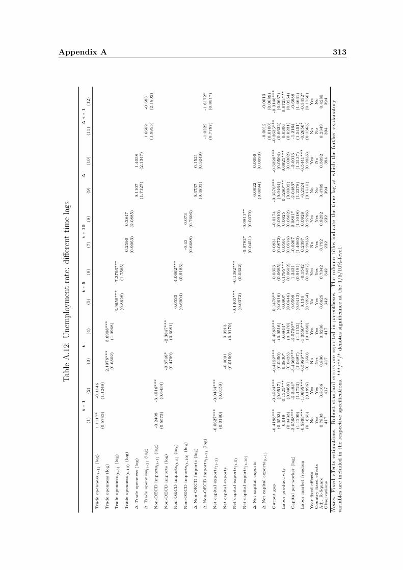
Appendix A 313
Tab
leA
.12:
Unem
plo
ym
ent
rate
:diff
eren
tti
me
lags
t-1
tt
-5
t-10
∆∆
t-1
(1)
(2)
(3)
(4)
(5)
(6)
(7)
(8)
(9)
(10)
(11)
(12)
Tra
de
op
enness
(t-1
)(l
og)
1.1
117*
-0.1
146
(0.5
743)
(1.1
248)
Tra
de
op
enness
(log)
2.1
978***
3.6
908***
(0.6
802)
(1.0
968)
Tra
de
op
enness
(t-5
)(l
og)
-3.9
650***
-7.3
793***
(0.8
628)
(1.7
585)
Tra
de
op
enness
(t-1
0)
(log)
0.2
596
0.3
847
(0.9
063)
(2.0
885)
∆T
rade
op
enness
(log)
0.1
107
1.4
058
(1.7
127)
(2.1
347)
∆T
rade
op
enness
(t-1
)(l
og)
1.6
602
-0.5
831
(1.9
855)
(2.1
802)
Non-O
EC
Dim
port
s (t-1
)(l
og)
-0.2
408
-3.4
516***
(0.5
573)
(0.6
434)
Non-O
EC
Dim
port
s(l
og)
-0.8
746*
-2.3
847***
(0.4
799)
(0.6
081)
Non-O
EC
Dim
port
s (t-5
)(l
og)
0.0
533
-4.0
662***
(0.6
904)
(0.9
183)
Non-O
EC
Dim
port
s (t-1
0)
(log)
-0.4
30.0
73
(0.6
688)
(0.7
606)
∆N
on-O
EC
Dim
port
s(l
og)
0.3
737
0.1
521
(0.4
833)
(0.5
249)
∆N
on-O
EC
Dim
port
s (t-1
)(l
og)
-1.0
222
-1.6
172*
(0.7
787)
(0.8
517)
Net
capit
al
exp
ort
s (t-1
)-0
.0627***
-0.0
434***
(0.0
180)
(0.0
150)
Net
capit
al
exp
ort
s-0
.0001
0.0
213
(0.0
190)
(0.0
170)
Net
capit
al
exp
ort
s (t-5
)-0
.1403***
-0.1
382***
(0.0
372)
(0.0
322)
Net
capit
al
exp
ort
s (t-1
0)
-0.0
782*
-0.0
811**
(0.0
451)
(0.0
379)
∆N
et
capit
al
exp
ort
s-0
.0022
0.0
096
(0.0
094)
(0.0
093)
∆N
et
capit
al
exp
ort
s (t-1
)-0
.0012
-0.0
013
(0.0
100)
(0.0
089)
Outp
ut
gap
-0.4
188***
-0.4
524***
-0.4
122***
-0.4
583***
0.1
478**
0.0
353
0.0
831
-0.0
174
-0.3
576***
-0.3
220***
-0.2
635***
-0.3
148***
(0.0
503)
(0.0
517)
(0.0
450)
(0.0
516)
(0.0
616)
(0.0
695)
(0.0
872)
(0.0
910)
(0.0
464)
(0.0
504)
(0.0
632)
(0.0
637)
Lab
or
pro
ducti
vit
y0.0
19
0.1
325***
0.0
830*
0.0
844*
0.0
907
0.1
795***
0.0
501
0.0
025
0.1
280***
0.0
925***
0.0
306
0.0
723***
(0.0
433)
(0.0
468)
(0.0
425)
(0.0
470)
(0.0
646)
(0.0
652)
(0.0
576)
(0.0
562)
(0.0
302)
(0.0
302)
(0.0
231)
(0.0
254)
Capit
al
per
work
er
(log)
-3.0
568***
-2.2
484*
-3.4
360***
-2.5
729**
0.9
599
1.2
431
-0.0
207
2.0
801*
-2.0
483*
-2.0
013
-1.2
164
-0.6
988
(1.1
209)
(1.1
723)
(1.0
687)
(1.1
152)
(0.9
413)
(0.9
191)
(1.4
060)
(1.1
018)
(1.2
278)
(1.2
137)
(1.5
451)
(1.4
661)
Lab
or
mark
et
freedom
-0.5
863***
-1.0
695***
-0.5
989***
-1.0
550***
0.1
34
-0.1
542
0.2
397
0.0
928
-0.2
124
-0.5
441***
-0.2
656*
-0.3
432*
(0.1
665)
(0.1
896)
(0.1
550)
(0.1
880)
(0.2
254)
(0.2
427)
(0.2
935)
(0.2
796)
(0.1
515)
(0.2
035)
(0.1
365)
(0.1
760)
Year
fixed
eff
ects
No
Yes
No
Yes
No
Yes
No
Yes
No
Yes
No
Yes
Countr
yfi
xed
eff
ects
Yes
Yes
Yes
Yes
Yes
Yes
Yes
Yes
No
No
No
No
Adj.
R-S
quare
0.7
803
0.8
166
0.8
06
0.8
236
0.6
625
0.7
342
0.7
52
0.8
252
0.4
789
0.5
092
0.2
349
0.4
285
Obse
rvati
ons
417
417
417
417
342
342
232
232
394
394
394
394
Notes:
Fix
edeff
ects
esti
mati
on
s.R
ob
ust
stan
dard
erro
rsare
rep
ort
edin
pare
nth
eses
.T
he
colu
mn
titl
esin
dic
ate
the
tim
ela
gat
wh
ich
the
furt
her
exp
lan
ato
ryvari
ab
les
are
incl
ud
edin
the
resp
ecti
ve
spec
ifica
tion
s.***/**/*
den
ote
ssi
gn
ifica
nce
at
the
1/5/10%
-lev
el.
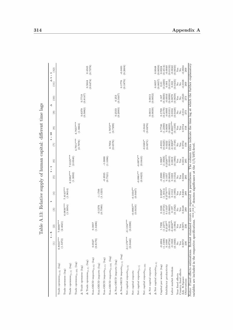
314 Appendix A
Tab
leA
.13:
Rel
ativ
esu
pply
ofhum
anca
pit
al:
diff
eren
tti
me
lags
t-5
tt
-1
t-10
∆∆
t-1
(1)
(2)
(3)
(4)
(5)
(6)
(7)
(8)
(9)
(10)
(11)
(12)
Tra
de
op
enness
(t-5
)(l
og)
6.8
433***
7.6
690***
(1.5
372)
(2.4
621)
Tra
de
op
enness
(log)
6.0
836***
7.4
143***
(1.3
054)
(1.9
614)
Tra
de
op
enness
(t-1
)(l
og)
6.2
382***
7.0
125***
(1.3
692)
(2.0
346)
Tra
de
op
enness
(t-1
0)
(log)
4.7
911***
6.7
657***
(0.7
978)
(1.9
864)
∆T
rade
op
enness
(log)
0.6
379
0.7
719
(0.5
882)
(0.8
147)
∆T
rade
op
enness
(t-1
)(l
og)
0.5
644
0.4
343
(0.6
474)
(0.7
378)
Non-O
EC
Dim
port
s (t-5
)(l
og)
0.0
527
0.3
957
(0.8
178)
(1.0
496)
Non-O
EC
Dim
port
s(l
og)
-0.5
376
-1.1
709
(0.7
580)
(1.1
223)
Non-O
EC
Dim
port
s (t-1
)(l
og)
-0.2
935
-1.0
888
(0.7
521)
(1.1
096)
Non-O
EC
Dim
port
s (t-1
0)
(log)
0.7
954
1.7
873**
(0.6
576)
(0.7
298)
∆N
on-O
EC
Dim
port
s(l
og)
0.2
533
0.2
53
(0.2
093)
(0.3
447)
∆N
on-O
EC
Dim
port
s (t-1
)(l
og)
0.1
776
-0.0
491
(0.1
870)
(0.2
604)
Net
capit
al
exp
ort
s (t-5
)-0
.1179***
-0.1
184***
(0.0
446)
(0.0
398)
Net
capit
al
exp
ort
s-0
.0983**
-0.1
034**
(0.0
416)
(0.0
447)
Net
capit
al
exp
ort
s (t-1
)-0
.0961**
-0.0
974**
(0.0
423)
(0.0
443)
Net
capit
al
exp
ort
s (t-1
0)
-0.0
461*
-0.0
444
(0.0
271)
(0.0
276)
∆N
et
capit
al
exp
ort
s0.0
013
0.0
013
(0.0
039)
(0.0
052)
∆N
et
capit
al
exp
ort
s (t-1
)0.0
057
0.0
048
(0.0
057)
(0.0
059)
Capit
al
per
work
er
(log)
-0.4
884
1.7
296
0.1
826
2.3
028*
-0.2
989
1.9
967
-0.8
531
0.7
746
0.1
709
0.1
67
0.0
10.0
024
(1.1
509)
(1.2
477)
(1.0
716)
(1.3
014)
(1.1
000)
(1.3
568)
(0.8
425)
(1.2
380)
(0.2
178)
(0.3
600)
(0.2
460)
(0.4
514)
Mult
ifacto
rpro
ducti
vit
y0.1
099
0.2
129**
0.1
103*
0.2
776***
0.1
057
0.2
520***
0.0
222
0.0
699
-0.0
095
-0.0
016
0.0
01
-0.0
049
(0.0
758)
(0.0
913)
(0.0
663)
(0.0
911)
(0.0
649)
(0.0
910)
(0.0
621)
(0.0
695)
(0.0
101)
(0.0
099)
(0.0
116)
(0.0
133)
Lab
or
mark
et
freedom
-0.1
923
-0.4
630**
0.1
97
0.1
512
0.1
693
0.0
819
-0.3
065*
-0.4
665***
0.0
334
0.0
078
0.0
21
-0.0
042
(0.1
668)
(0.1
884)
(0.1
582)
(0.1
893)
(0.1
552)
(0.1
960)
(0.1
749)
(0.1
339)
(0.0
448)
(0.0
659)
(0.0
435)
(0.0
650)
Year
fixed
eff
ects
No
Yes
No
Yes
No
Yes
No
Yes
No
Yes
No
Yes
Countr
yfi
xed
eff
ects
Yes
Yes
Yes
Yes
Yes
Yes
Yes
Yes
No
No
No
No
Adj.
R-S
quare
0.9
072
0.9
071
0.8
448
0.8
404
0.8
556
0.8
513
0.9
752
0.9
754
-0.0
14
-0.0
523
-0.0
168
-0.0
604
Obse
rvati
ons
236
236
289
289
285
285
158
158
273
273
269
269
Notes:
Fix
edeff
ects
esti
mati
on
s.R
ob
ust
stan
dard
erro
rsare
rep
ort
edin
pare
nth
eses
.T
he
colu
mn
titl
esin
dic
ate
the
tim
ela
gat
wh
ich
the
furt
her
exp
lan
ato
ryvari
ab
les
are
incl
ud
edin
the
resp
ecti
ve
spec
ifica
tion
s.***/**/*
den
ote
ssi
gn
ifica
nce
at
the
1/5/10%
-lev
el.
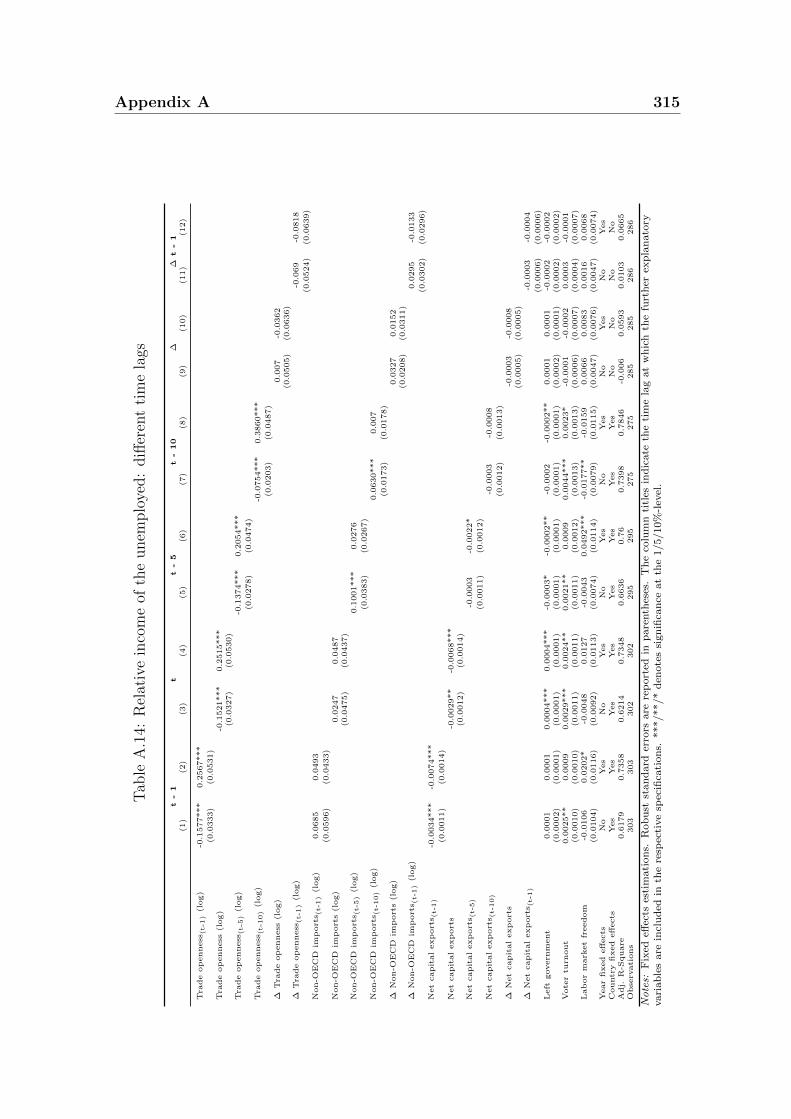
Appendix A 315
Tab
leA
.14:
Rel
ativ
ein
com
eof
the
unem
plo
yed:
diff
eren
tti
me
lags
t-1
tt
-5
t-10
∆∆
t-1
(1)
(2)
(3)
(4)
(5)
(6)
(7)
(8)
(9)
(10)
(11)
(12)
Tra
de
op
enness
(t-1
)(l
og)
-0.1
577***
0.2
567***
(0.0
333)
(0.0
531)
Tra
de
op
enness
(log)
-0.1
521***
0.2
515***
(0.0
327)
(0.0
530)
Tra
de
op
enness
(t-5
)(l
og)
-0.1
374***
0.2
054***
(0.0
278)
(0.0
474)
Tra
de
op
enness
(t-1
0)
(log)
-0.0
754***
0.3
860***
(0.0
203)
(0.0
487)
∆T
rade
op
enness
(log)
0.0
07
-0.0
362
(0.0
505)
(0.0
636)
∆T
rade
op
enness
(t-1
)(l
og)
-0.0
69
-0.0
818
(0.0
524)
(0.0
639)
Non-O
EC
Dim
port
s (t-1
)(l
og)
0.0
685
0.0
493
(0.0
596)
(0.0
433)
Non-O
EC
Dim
port
s(l
og)
0.0
247
0.0
487
(0.0
475)
(0.0
437)
Non-O
EC
Dim
port
s (t-5
)(l
og)
0.1
001***
0.0
276
(0.0
383)
(0.0
267)
Non-O
EC
Dim
port
s (t-1
0)
(log)
0.0
630***
0.0
07
(0.0
173)
(0.0
178)
∆N
on-O
EC
Dim
port
s(l
og)
0.0
327
0.0
152
(0.0
208)
(0.0
311)
∆N
on-O
EC
Dim
port
s (t-1
)(l
og)
0.0
295
-0.0
133
(0.0
302)
(0.0
296)
Net
capit
al
exp
ort
s (t-1
)-0
.0034***
-0.0
074***
(0.0
011)
(0.0
014)
Net
capit
al
exp
ort
s-0
.0029**
-0.0
068***
(0.0
012)
(0.0
014)
Net
capit
al
exp
ort
s (t-5
)-0
.0003
-0.0
022*
(0.0
011)
(0.0
012)
Net
capit
al
exp
ort
s (t-1
0)
-0.0
003
-0.0
008
(0.0
012)
(0.0
013)
∆N
et
capit
al
exp
ort
s-0
.0003
-0.0
008
(0.0
005)
(0.0
005)
∆N
et
capit
al
exp
ort
s (t-1
)-0
.0003
-0.0
004
(0.0
006)
(0.0
006)
Left
govern
ment
0.0
001
0.0
001
0.0
004***
0.0
004***
-0.0
003*
-0.0
002**
-0.0
002
-0.0
002**
0.0
001
0.0
001
-0.0
002
-0.0
002
(0.0
002)
(0.0
001)
(0.0
001)
(0.0
001)
(0.0
001)
(0.0
001)
(0.0
001)
(0.0
001)
(0.0
002)
(0.0
001)
(0.0
002)
(0.0
002)
Vote
rtu
rnout
0.0
025**
0.0
009
0.0
029***
0.0
024**
0.0
021**
0.0
009
0.0
044***
0.0
023*
-0.0
001
-0.0
002
0.0
003
-0.0
001
(0.0
010)
(0.0
010)
(0.0
011)
(0.0
011)
(0.0
011)
(0.0
012)
(0.0
013)
(0.0
013)
(0.0
006)
(0.0
007)
(0.0
004)
(0.0
007)
Lab
or
mark
et
freedom
-0.0
106
0.0
202*
-0.0
048
0.0
127
-0.0
043
0.0
492***
-0.0
177**
-0.0
159
0.0
066
0.0
083
0.0
016
0.0
068
(0.0
104)
(0.0
116)
(0.0
092)
(0.0
113)
(0.0
074)
(0.0
114)
(0.0
079)
(0.0
115)
(0.0
047)
(0.0
076)
(0.0
047)
(0.0
074)
Year
fixed
eff
ects
No
Yes
No
Yes
No
Yes
No
Yes
No
Yes
No
Yes
Countr
yfi
xed
eff
ects
Yes
Yes
Yes
Yes
Yes
Yes
Yes
Yes
No
No
No
No
Adj.
R-S
quare
0.6
179
0.7
358
0.6
214
0.7
348
0.6
636
0.7
60.7
398
0.7
846
-0.0
06
0.0
593
0.0
103
0.0
665
Obse
rvati
ons
303
303
302
302
295
295
275
275
285
285
286
286
Notes:
Fix
edeff
ects
esti
mati
on
s.R
ob
ust
stan
dard
erro
rsare
rep
ort
edin
pare
nth
eses
.T
he
colu
mn
titl
esin
dic
ate
the
tim
ela
gat
wh
ich
the
furt
her
exp
lan
ato
ryvari
ab
les
are
incl
ud
edin
the
resp
ecti
ve
spec
ifica
tion
s.***/**/*
den
ote
ssi
gn
ifica
nce
at
the
1/5/10%
-lev
el.
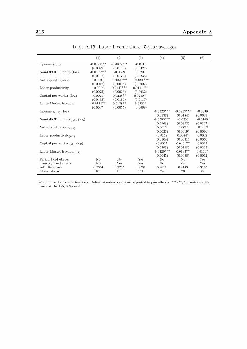
316 Appendix A
Table A.15: Labor income share: 5-year averages
(1) (2) (3) (4) (5) (6)
Openness (log) -0.0397*** -0.0928*** -0.0313(0.0099) (0.0183) (0.0321)
Non-OECD imports (log) -0.0682*** -0.0059 0.0201(0.0197) (0.0172) (0.0235)
Net capital exports -0.0001 -0.0028*** -0.0021***(0.0017) (0.0006) (0.0007)
Labor productivity -0.0074 0.0147*** 0.0141***(0.0075) (0.0026) (0.0032)
Capital per worker (log) 0.0071 0.0238** 0.0280**(0.0482) (0.0115) (0.0117)
Labor Market freedom -0.0118** 0.0138** 0.0121*(0.0047) (0.0055) (0.0068)
Openness(t-1) (log) -0.0423*** -0.0813*** -0.0039(0.0137) (0.0184) (0.0603)
Non-OECD imports(t-1) (log) -0.0503*** -0.0308 -0.0108(0.0163) (0.0303) (0.0327)
Net capital exports(t-1) 0.0016 -0.0016 -0.0013(0.0026) (0.0019) (0.0016)
Labor productivity(t-1) -0.0158 0.0074* 0.0042(0.0109) (0.0041) (0.0050)
Capital per worker(t-1) (log) -0.0317 0.0401** 0.0312(0.0496) (0.0188) (0.0225)
Labor Market freedom(t-1) -0.0129*** 0.0133** 0.0116*(0.0045) (0.0058) (0.0062)
Period fixed effects No No Yes No No YesCountry fixed effects No Yes Yes No Yes YesAdj. R-Square 0.2664 0.9265 0.9291 0.2811 0.9149 0.9115Observations 101 101 101 79 79 79
Notes: Fixed effects estimations. Robust standard errors are reported in parentheses. ***/**/* denotes signifi-cance at the 1/5/10%-level.
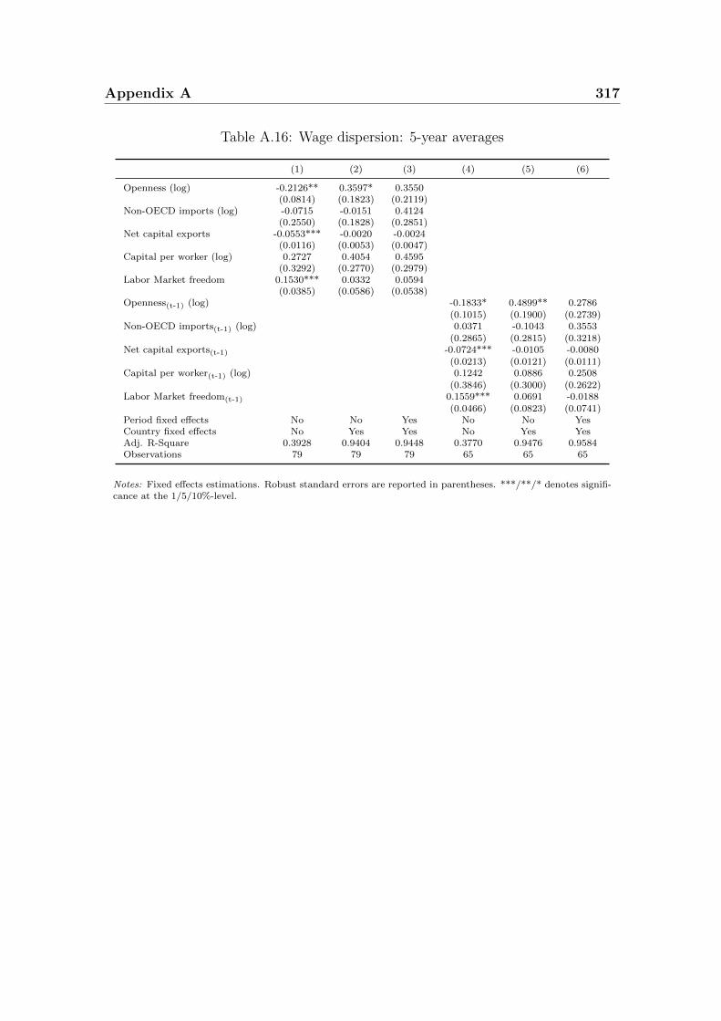
Appendix A 317
Table A.16: Wage dispersion: 5-year averages
(1) (2) (3) (4) (5) (6)
Openness (log) -0.2126** 0.3597* 0.3550(0.0814) (0.1823) (0.2119)
Non-OECD imports (log) -0.0715 -0.0151 0.4124(0.2550) (0.1828) (0.2851)
Net capital exports -0.0553*** -0.0020 -0.0024(0.0116) (0.0053) (0.0047)
Capital per worker (log) 0.2727 0.4054 0.4595(0.3292) (0.2770) (0.2979)
Labor Market freedom 0.1530*** 0.0332 0.0594(0.0385) (0.0586) (0.0538)
Openness(t-1) (log) -0.1833* 0.4899** 0.2786(0.1015) (0.1900) (0.2739)
Non-OECD imports(t-1) (log) 0.0371 -0.1043 0.3553(0.2865) (0.2815) (0.3218)
Net capital exports(t-1) -0.0724*** -0.0105 -0.0080(0.0213) (0.0121) (0.0111)
Capital per worker(t-1) (log) 0.1242 0.0886 0.2508(0.3846) (0.3000) (0.2622)
Labor Market freedom(t-1) 0.1559*** 0.0691 -0.0188(0.0466) (0.0823) (0.0741)
Period fixed effects No No Yes No No YesCountry fixed effects No Yes Yes No Yes YesAdj. R-Square 0.3928 0.9404 0.9448 0.3770 0.9476 0.9584Observations 79 79 79 65 65 65
Notes: Fixed effects estimations. Robust standard errors are reported in parentheses. ***/**/* denotes signifi-cance at the 1/5/10%-level.
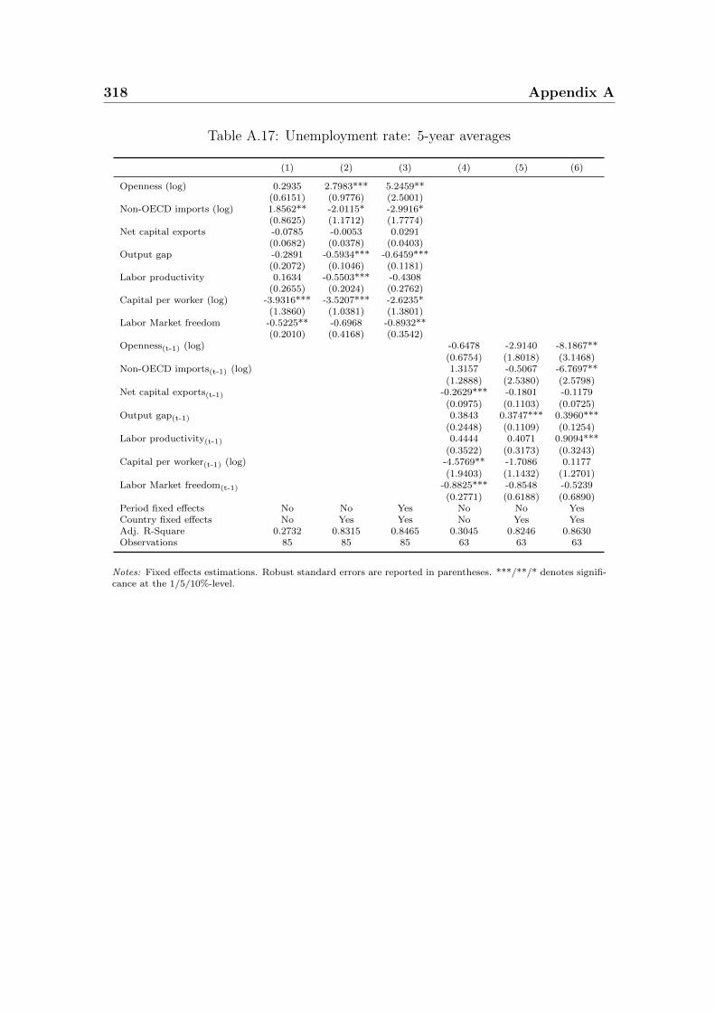
318 Appendix A
Table A.17: Unemployment rate: 5-year averages
(1) (2) (3) (4) (5) (6)
Openness (log) 0.2935 2.7983*** 5.2459**(0.6151) (0.9776) (2.5001)
Non-OECD imports (log) 1.8562** -2.0115* -2.9916*(0.8625) (1.1712) (1.7774)
Net capital exports -0.0785 -0.0053 0.0291(0.0682) (0.0378) (0.0403)
Output gap -0.2891 -0.5934*** -0.6459***(0.2072) (0.1046) (0.1181)
Labor productivity 0.1634 -0.5503*** -0.4308(0.2655) (0.2024) (0.2762)
Capital per worker (log) -3.9316*** -3.5207*** -2.6235*(1.3860) (1.0381) (1.3801)
Labor Market freedom -0.5225** -0.6968 -0.8932**(0.2010) (0.4168) (0.3542)
Openness(t-1) (log) -0.6478 -2.9140 -8.1867**(0.6754) (1.8018) (3.1468)
Non-OECD imports(t-1) (log) 1.3157 -0.5067 -6.7697**(1.2888) (2.5380) (2.5798)
Net capital exports(t-1) -0.2629*** -0.1801 -0.1179(0.0975) (0.1103) (0.0725)
Output gap(t-1) 0.3843 0.3747*** 0.3960***(0.2448) (0.1109) (0.1254)
Labor productivity(t-1) 0.4444 0.4071 0.9094***(0.3522) (0.3173) (0.3243)
Capital per worker(t-1) (log) -4.5769** -1.7086 0.1177(1.9403) (1.1432) (1.2701)
Labor Market freedom(t-1) -0.8825*** -0.8548 -0.5239(0.2771) (0.6188) (0.6890)
Period fixed effects No No Yes No No YesCountry fixed effects No Yes Yes No Yes YesAdj. R-Square 0.2732 0.8315 0.8465 0.3045 0.8246 0.8630Observations 85 85 85 63 63 63
Notes: Fixed effects estimations. Robust standard errors are reported in parentheses. ***/**/* denotes signifi-cance at the 1/5/10%-level.
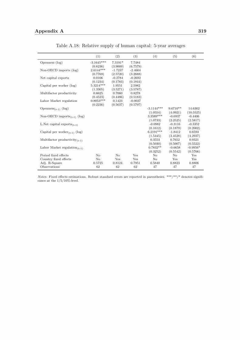
Appendix A 319
Table A.18: Relative supply of human capital: 5-year averages
(1) (2) (3) (4) (5) (6)
Openness (log) -3.1645*** 7.3191* 7.7484(0.8236) (3.9009) (6.7579)
Non-OECD imports (log) 2.6144*** -1.7237 -2.4604(0.7769) (2.5720) (3.2688)
Net capital exports 0.0106 -0.2784 -0.2692(0.1234) (0.1783) (0.1844)
Capital per worker (log) 5.3214*** 1.9551 2.5982(1.3305) (3.5271) (3.5787)
Multifactor productivity 0.6625 0.7060 0.8278(0.4523) (0.4486) (0.5183)
Labor Market regulation 0.8053*** 0.1423 -0.0037(0.2236) (0.5637) (0.5797)
Openness(t-1) (log) -3.1144*** 9.6710** 14.6302(1.0554) (4.0921) (10.5525)
Non-OECD imports(t-1) (log) 3.3589*** -0.6937 -0.4406(1.0733) (2.2525) (2.5817)
L.Net capital exports(t-1) -0.0982 -0.3116 -0.3352(0.1612) (0.1879) (0.2002)
Capital per worker(t-1) (log) 6.2191*** -1.8412 0.6593(1.5445) (3.4528) (4.2937)
Multifactor productivity(t-1) 0.3553 0.7652 0.9321(0.5030) (0.5007) (0.5522)
Labor Market regulation(t-1) 0.7832** -0.6658 -0.9956*(0.3252) (0.5542) (0.5706)
Period fixed effects No No Yes No No YesCountry fixed effects No Yes Yes No Yes YesAdj. R-Square 0.5725 0.8124 0.7951 0.5840 0.8823 0.8806Observations 62 62 62 47 47 47
Notes: Fixed effects estimations. Robust standard errors are reported in parentheses. ***/**/* denotes signifi-cance at the 1/5/10%-level.
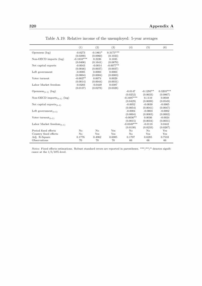
320 Appendix A
Table A.19: Relative income of the unemployed: 5-year averages
(1) (2) (3) (4) (5) (6)
Openness (log) -0.0273 -0.1861* 0.3175***(0.0290) (0.0960) (0.1033)
Non-OECD imports (log) -0.1833*** 0.2226 0.1035(0.0406) (0.1641) (0.0870)
Net capital exports -0.0043 -0.0014 -0.0077**(0.0046) (0.0037) (0.0037)
Left government -0.0005 0.0003 0.0003(0.0004) (0.0004) (0.0003)
Voter turnout -0.0027* 0.0074 0.0029(0.0014) (0.0044) (0.0031)
Labor Market freedom -0.0203 -0.0449 0.0387(0.0137) (0.0278) (0.0328)
Openness(t-1) (log) -0.0147 -0.1293** 0.3203***(0.0252) (0.0633) (0.0867)
Non-OECD imports(t-1) (log) -0.1697*** 0.1110 0.0048(0.0429) (0.0699) (0.0549)
Net capital exports(t-1) -0.0052 -0.0030 -0.0065(0.0054) (0.0041) (0.0047)
Left government(t-1) -0.0004 -0.0003 -0.0002(0.0004) (0.0003) (0.0002)
Voter turnout(t-1) -0.0036** 0.0036 -0.0024(0.0015) (0.0034) (0.0031)
Labor Market freedom(t-1) -0.0349*** -0.0118 0.0442(0.0130) (0.0233) (0.0267)
Period fixed effects No No Yes No No YesCountry fixed effects No Yes Yes No Yes YesAdj. R-Square 0.1776 0.4962 0.6905 0.1797 0.6285 0.7533Observations 70 70 70 66 66 66
Notes: Fixed effects estimations. Robust standard errors are reported in parentheses. ***/**/* denotes signifi-cance at the 1/5/10%-level.
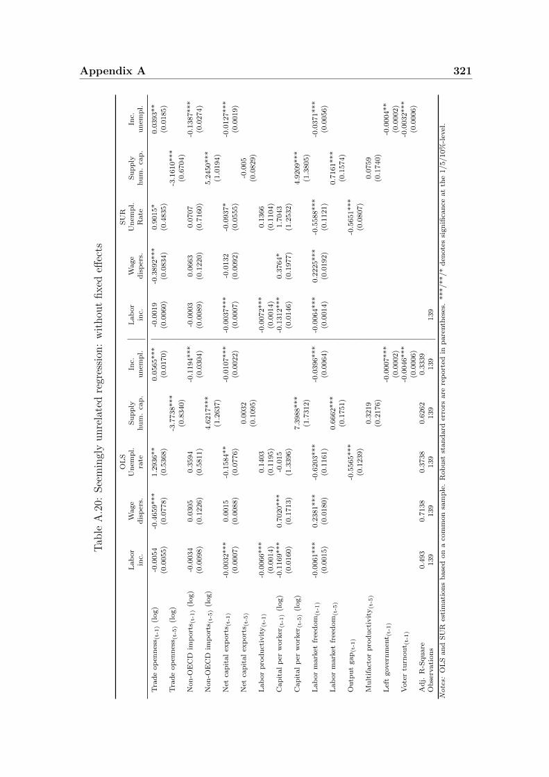
Appendix A 321
Tab
leA
.20:
See
min
gly
unre
late
dre
gres
sion
:w
ithou
tfixed
effec
ts
OL
SS
UR
Lab
or
Wage
Un
emp
l.S
up
ply
Inc.
Lab
or
Wage
Un
emp
l.S
up
ply
Inc.
inc.
dis
per
s.ra
tehu
m.
cap
.u
nem
pl.
inc.
dis
per
s.R
ate
hu
m.
cap
.u
nem
pl.
Tra
de
op
enn
ess (
t-1)
(log)
-0.0
054
-0.4
659***
1.2
936**
0.0
565***
-0.0
019
-0.3
892***
0.9
015*
0.0
393**
(0.0
055)
(0.0
778)
(0.5
368)
(0.0
170)
(0.0
060)
(0.0
834)
(0.4
835)
(0.0
185)
Tra
de
op
enn
ess (
t-5)
(log)
-3.7
738***
-3.1
610***
(0.8
340)
(0.6
704)
Non
-OE
CD
imp
ort
s (t-
1)
(log)
-0.0
034
0.0
305
0.3
594
-0.1
194***
-0.0
003
0.0
663
0.0
707
-0.1
387***
(0.0
098)
(0.1
226)
(0.5
811)
(0.0
304)
(0.0
089)
(0.1
220)
(0.7
160)
(0.0
274)
Non
-OE
CD
imp
ort
s (t-
5)
(log)
4.6
217***
5.2
450***
(1.2
637)
(1.0
194)
Net
cap
ital
exp
ort
s (t-
1)
-0.0
032***
0.0
015
-0.1
584**
-0.0
107***
-0.0
037***
-0.0
132
-0.0
937*
-0.0
127***
(0.0
007)
(0.0
088)
(0.0
776)
(0.0
022)
(0.0
007)
(0.0
092)
(0.0
555)
(0.0
019)
Net
cap
ital
exp
ort
s (t-
5)
0.0
032
-0.0
05
(0.1
095)
(0.0
829)
Lab
or
pro
du
ctiv
ity
(t-1
)-0
.0066***
0.1
403
-0.0
072***
0.1
366
(0.0
014)
(0.1
195)
(0.0
014)
(0.1
104)
Cap
ital
per
work
er(t
-1)
(log)
-0.1
169***
0.7
020***
-0.0
15
-0.1
312***
0.3
764*
1.7
043
(0.0
160)
(0.1
713)
(1.3
396)
(0.0
146)
(0.1
977)
(1.2
532)
Cap
ital
per
work
er(t
-5)
(log)
7.3
988***
4.9
209***
(1.7
312)
(1.3
805)
Lab
or
mark
etfr
eed
om
(t-1
)-0
.0061***
0.2
381***
-0.6
203***
-0.0
396***
-0.0
064***
0.2
225***
-0.5
588***
-0.0
371***
(0.0
015)
(0.0
180)
(0.1
161)
(0.0
064)
(0.0
014)
(0.0
192)
(0.1
121)
(0.0
056)
Lab
or
mark
etfr
eed
om
(t-5
)0.6
662***
0.7
161***
(0.1
751)
(0.1
574)
Ou
tpu
tgap
(t-1
)-0
.5565***
-0.5
651***
(0.1
239)
(0.0
807)
Mu
ltif
act
or
pro
du
ctiv
ity
(t-5
)0.3
219
0.0
759
(0.2
176)
(0.1
740)
Lef
tgover
nm
ent (
t-1)
-0.0
007***
-0.0
004**
(0.0
002)
(0.0
002)
Vote
rtu
rnou
t (t-
1)
-0.0
046***
-0.0
032***
(0.0
006)
(0.0
006)
Ad
j.R
-Squ
are
0.4
93
0.7
138
0.3
738
0.6
262
0.3
339
Ob
serv
ati
on
s139
139
139
139
139
139
Notes:
OL
San
dS
UR
esti
mati
on
sb
ase
don
aco
mm
on
sam
ple
.R
ob
ust
stan
dard
erro
rsare
rep
ort
edin
pare
nth
eses
.***/**/*
den
ote
ssi
gn
ifica
nce
at
the
1/5/10%
-lev
el.
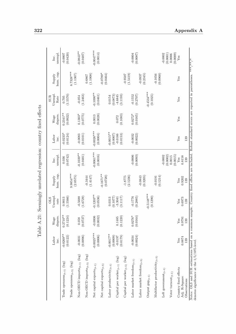
322 Appendix A
Tab
leA
.21:
See
min
gly
unre
late
dre
gres
sion
:co
untr
yfixed
effec
ts
OL
SS
UR
Lab
or
Wage
Un
emp
l.S
up
ply
Inc.
Lab
or
Wage
Un
emp
l.S
up
ply
Inc.
inc.
dis
per
s.ra
tehu
m.
cap
.u
nem
pl.
inc.
dis
per
s.R
ate
hu
m.
cap
.u
nem
pl.
Tra
de
op
enn
ess (
t-1)
(log)
-0.0
269**
0.2
710**
0.9
013
0.0
36
-0.0
233*
0.2
341**
0.7
05
-0.0
007
(0.0
122)
(0.1
224)
(1.5
566)
(0.0
742)
(0.0
124)
(0.0
922)
(1.5
570)
(0.0
420)
Tra
de
op
enn
ess (
t-5)
(log)
9.9
854***
8.7
328***
(2.0
575)
(1.1
367)
Non
-OE
CD
imp
ort
s (t-
1)
(log)
-0.0
031
0.0
58
-0.5
688
-0.1
039**
-0.0
083
0.1
303*
-0.0
54
-0.0
843**
(0.0
096)
(0.0
727)
(1.6
729)
(0.0
401)
(0.0
101)
(0.0
775)
(1.2
463)
(0.0
407)
Non
-OE
CD
imp
ort
s (t-
5)
(log)
-0.3
444
0.6
867
(1.4
147)
(1.1
908)
Net
cap
ital
exp
ort
s (t-
1)
-0.0
025***
-0.0
006
-0.1
203**
-0.0
061***
-0.0
026***
0.0
013
-0.1
090**
-0.0
047***
(0.0
006)
(0.0
032)
(0.0
536)
(0.0
016)
(0.0
004)
(0.0
028)
(0.0
461)
(0.0
014)
Net
cap
ital
exp
ort
s (t-
5)
-0.1
671**
-0.0
789*
(0.0
720)
(0.0
464)
Lab
or
pro
du
ctiv
ity
(t-1
)-0
.0017**
0.0
313
-0.0
015**
0.0
154
(0.0
009)
(0.1
077)
(0.0
007)
(0.0
873)
Cap
ital
per
work
er(t
-1)
(log)
-0.0
197
0.1
485
-3.3
041
-0.0
166
0.0
72
-4.6
845
(0.0
179)
(0.1
220)
(3.1
117)
(0.0
153)
(0.1
083)
(3.1
193)
Cap
ital
per
work
er(t
-5)
(log)
-1.8
775
-0.9
507
(2.1
236)
(1.5
419)
Lab
or
mark
etfr
eed
om
(t-1
)-0
.0034
0.0
276*
-0.1
776
-0.0
006
-0.0
032
0.0
272*
-0.1
552
-0.0
004
(0.0
024)
(0.0
164)
(0.2
885)
(0.0
093)
(0.0
022)
(0.0
165)
(0.2
707)
(0.0
087)
Lab
or
mark
etfr
eed
om
(t-5
)-0
.0843
-0.0
937
(0.3
205)
(0.2
345)
Ou
tpu
tgap
(t-1
)-0
.5148***
-0.4
534***
(0.1
290)
(0.1
025)
Mu
ltif
act
or
pro
du
ctiv
ity
(t-5
)-0
.0191
-0.1
056
(0.1
214)
(0.0
960)
Lef
tgover
nm
ent (
t-1)
-0.0
002
-0.0
002
(0.0
002)
(0.0
001)
Vote
rtu
rnou
t (t-
1)
0.0
015
0.0
006
(0.0
015)
(0.0
009)
Cou
ntr
yfi
xed
effec
tsY
esY
esY
esY
esY
esY
esY
esY
esY
esY
esA
dj.
R-S
qu
are
0.8
874
0.9
791
0.6
973
0.9
202
0.8
158
Ob
serv
ati
on
s139
139
139
139
139
139
Notes:
OL
San
dS
UR
esti
mati
on
sb
ase
don
aco
mm
on
sam
ple
.C
ou
ntr
yfi
xed
effec
tsare
incl
ud
ed.
Rob
ust
stan
dard
erro
rsare
rep
ort
edin
pare
nth
eses
.***/**/*
den
ote
ssi
gn
ifica
nce
at
the
1/5/10%
-lev
el.

Appendix B
Policy preferences of German
voters
B.1 Data sources and definitions
323

324 Appendix BT
able
B.1
:D
escr
ipti
onof
vari
able
suse
din
the
anal
ysi
sof
atti
tudes
tow
ard
pro
gres
sive
taxat
ion
(chap
ter
11)
Varia
ble
Un
itE
xp
lan
ati
on
Cate
gorie
s
Tax
Pro
gre
ssio
nD
um
my
Res
pon
den
t’s
pre
fere
nce
for
pro
gre
ssiv
e1,
ifth
ere
spon
den
tfa
vors
a(s
teep
)p
rogre
ssio
n.
tax
rate
s.
Tax
Pre
fere
nce
Ord
inal
Res
pon
den
t’s
tax
rate
pre
fere
nce
1,
ifth
ere
spon
den
tfa
vors
regre
ssiv
eta
xati
on
.
2,
ifth
ere
spon
den
tfa
vors
ap
rop
ort
ion
al
taxati
on
.
scale
3,
ifth
ere
spon
den
tfa
vors
apro
gre
ssiv
eta
xati
on
.
Low
Inco
me
Du
mm
y1,
ifth
ere
spon
den
tb
elon
gs
toth
e25th
inco
me
per
centi
le(i
.e.
has
less
than
750
Eu
ron
et
inco
me
per
month
).
Inte
rmed
.In
com
eD
um
my
Res
pon
den
t’s
pla
cem
ent
inth
e1,
ifth
ere
spon
den
th
as
am
onth
lyn
etin
com
e
inco
me
dis
trib
uti
on
.b
etw
een
750
an
d1500
Eu
ro.
Hig
hIn
com
eD
um
my
1,
ifth
ere
spon
den
tb
elon
gs
toth
e75th
inco
me
per
centi
le(i
.e.
has
at
least
1500
Eu
ron
et
inco
me
per
month
).
Equ
ivale
nt
inco
me
Conti
nu
ou
sR
esp
on
den
t’s
hou
seh
old
inco
me
equ
ivale
nt
inco
me
=
vari
ab
lead
just
edfo
rh
ou
seh
old
size
.house
hold
net
incom
e/√
no.
pers
ons
inhouse
hold
Soci
al
Mob
ilit
yO
rdin
al
Ch
an
ge
inth
ere
spon
den
t’s
posi
tion
inth
eN
egati
ve
(posi
tive)
valu
e:ex
per
ien
ceof
scale
soci
al
stra
tum
du
rin
gth
ela
stte
nyea
rs.
dow
nw
ard
(upw
ard
)so
cial
mob
ilit
y
Low
Ed
uca
tion
Du
mm
y
1,
ifth
ere
spon
den
th
as
no
or
alo
wer
seco
nd
ary
sch
ool
leavin
gce
rtifi
cate
(usu
ally
nin
eyea
rsof
sch
oolin
gor
less
).
Sec
on
dary
Ed
uca
tion
Du
mm
y1,
ifth
ere
spon
den
th
as
an
inte
rmed
iate
Res
pon
den
t’s
level
of
edu
cati
on
.se
cond
ary
sch
ool
leavin
gce
rtifi
cate
.
Up
per
Sec
.E
du
cati
on
Du
mm
y1,
ifth
ere
spon
den
th
as
an
up
per
seco
nd
ary
sch
ool
leavin
gce
rtifi
cate
.
Un
iver
sity
Du
mm
y1,
ifth
ere
spon
den
th
as
an
un
iver
sity
(for
ap
plied
scie
nce
)d
egre
e. Continued
onnextpa
ge

Appendix B 325T
ab
leB
.1–
conti
nu
edfr
om
pre
vio
us
page
Varia
ble
Un
itE
xp
lan
ati
on
Cate
gorie
s
Imp
ort
an
ceP
oliti
csD
um
my
Politi
csst
ron
gly
infl
uen
ceou
rli
ves
.1,
ifth
ere
spon
den
tap
pro
ves
.
Nee
dD
um
my
Dec
ent
inco
me
even
wit
hou
tach
ievem
ent.
1,
ifth
ere
spon
den
tap
pro
ves
.
Eff
ort
Du
mm
yD
iffer
ence
sin
soci
al
stan
din
gas
1,
ifth
ere
spon
den
tap
pro
ves
.in
centi
ve
for
ind
ivid
ual
ach
ievem
ent.
Dem
ocr
acy
Du
mm
yS
ati
sfact
ion
wit
hth
eG
erm
an
dem
ocr
acy
.1,
ifth
ere
spon
den
tis
(fu
lly)
sati
sfied
.
Soci
al
Diff
eren
ces
Du
mm
yT
he
soci
al
diff
eren
ces
are
just
.1,
ifth
ere
spon
den
tap
pro
ves
.
Ord
inary
Peo
ple
Du
mm
yL
ife
for
ord
inary
peo
ple
isn
ot
1,
ifth
ere
spon
den
tap
pro
ves
.get
tin
gw
ors
e.
Ad
equ
ate
Wage
Du
mm
yJu
stp
ay
giv
ensk
ills
an
deff
ort
.1,
ifth
ere
spon
den
tap
pro
ves
.
Age
Dis
cret
eA
ge
of
the
resp
on
den
t.18
–95
yea
rsvari
ab
le
Fem
ale
Du
mm
yS
exof
the
resp
on
den
t.1,
ifth
ere
spon
den
tis
fem
ale
.
East
Du
mm
yO
rigin
of
the
resp
on
den
t.1,
ifth
ere
spon
den
th
as
bee
nb
orn
inth
e
form
erG
DR
.
Un
emp
loyed
Du
mm
y1,
ifth
ere
spon
den
tis
un
emp
loyed
.
Not
Em
plo
yed
Du
mm
yE
mp
loym
ent
statu
sof
the
resp
on
den
t.1,
ifth
ere
spon
den
tis
not
emp
loyed
.
Sel
f-E
mp
loyed
Du
mm
y1,
ifth
ere
spon
den
tis
self
-em
plo
yed
.
Pu
blic
Em
plo
yee
Du
mm
yE
mp
loym
ent
of
the
resp
on
den
t1,
ifth
ere
spon
den
tis
ap
ub
lic
emp
loyee
.
inth
ep
ub
lic
sect
or.
Wh
ite
Collar
Du
mm
yT
yp
eof
resp
on
den
t’s
job
.1,
ifth
ere
spon
den
tis
aw
hit
eco
llar
work
er.
Blu
eC
ollar
Du
mm
y1,
ifth
ere
spon
den
tis
ab
lue
collar
work
er.
Leg
ally
marr
ied
Du
mm
y
Mari
tal
Sta
tus
of
the
resp
on
den
t.
1,
ifth
ere
spon
den
tis
legally
marr
ied
(i.e
.ei
ther
livin
gto
get
her
or
sep
ara
ted
spou
ses)
.
Not
marr
ied
Du
mm
y1,
ifth
ere
spon
den
tis
not
marr
ied
(i.e
.si
ngle
,d
ivorc
edor
wid
ow
ed).
No.
Ch
ild
ren
(hh
)D
iscr
ete
Nu
mb
erof
min
or
child
ren
livin
g0
–6
child
ren
vari
ab
lein
the
resp
on
den
t’s
hou
seh
old
.
No.
Per
son
s(h
h)
Dis
cret
eN
um
ber
of
per
son
slivin
g1
–11
per
son
svari
ab
lein
the
resp
on
den
t’s
hou
seh
old
.
Continued
onnextpa
ge

326 Appendix BT
ab
leB
.1–
conti
nu
edfr
om
pre
vio
us
page
Varia
ble
Un
itE
xp
lan
ati
on
Cate
gorie
s
Rel
igio
sity
Du
mm
yR
elig
iou
sd
enom
inati
on
of
the
1,
ifth
ere
spon
den
tb
elon
gs
toan
resp
on
den
t.in
stit
uti
on
alize
dre
ligio
us
com
mu
nit
y.
Part
ner
:n
ot
emp
loyed
Du
mm
y
Em
plo
ym
ent
statu
sof
the
resp
on
den
t’s
part
ner
.
1,
ifth
ere
spon
den
t’s
part
ner
isn
ot
emp
loyed
.
Part
ner
:p
art
-tim
ew
ork
erD
um
my
1,
ifth
ere
spon
den
t’s
part
ner
work
sp
art
-tim
e.
Part
ner
:fu
ll-t
ime
work
erD
um
my
1,
ifth
ere
spon
den
t’s
part
ner
work
sfu
ll-t
ime.
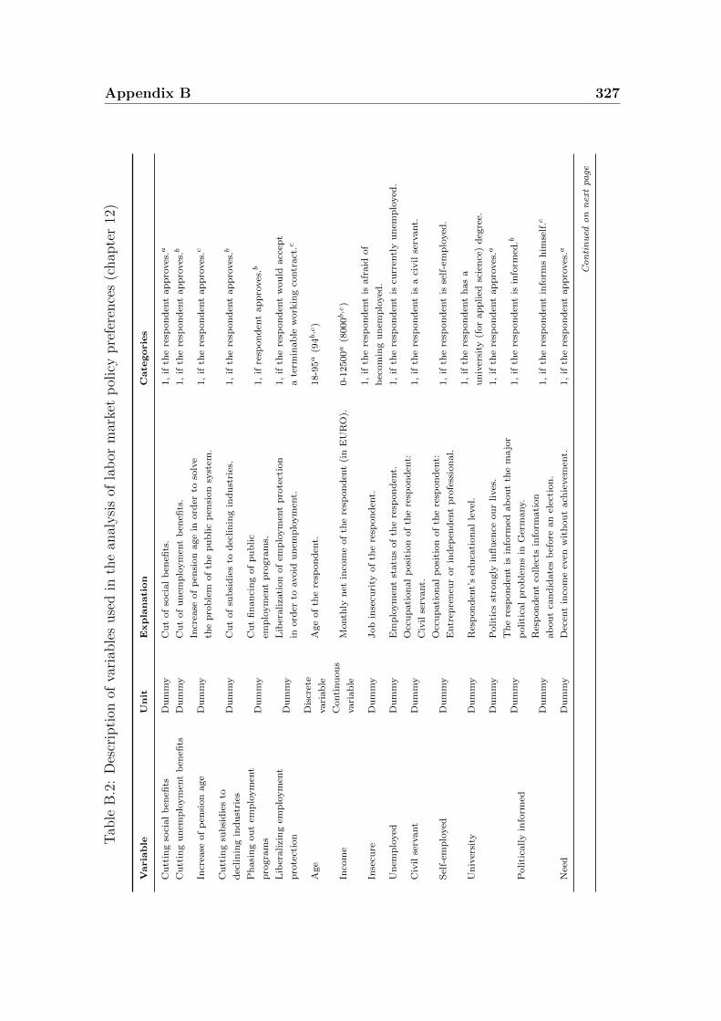
Appendix B 327T
able
B.2
:D
escr
ipti
onof
vari
able
suse
din
the
anal
ysi
sof
lab
orm
arke
tp
olic
ypre
fere
nce
s(c
hap
ter
12)
Varia
ble
Un
itE
xp
lan
ati
on
Cate
gorie
s
Cu
ttin
gso
cial
ben
efits
Dum
my
Cu
tof
soci
al
ben
efits
.1,
ifth
ere
spon
den
tap
pro
ves
.a
Cu
ttin
gu
nem
plo
ym
ent
ben
efits
Du
mm
yC
ut
of
un
emp
loym
ent
ben
efits
.1,
ifth
ere
spon
den
tap
pro
ves
.b
Incr
ease
of
pen
sion
age
Du
mm
yIn
crea
seof
pen
sion
age
inord
erto
solv
e1,
ifth
ere
spon
den
tap
pro
ves
.cth
ep
rob
lem
of
the
pu
blic
pen
sion
syst
em.
Cu
ttin
gsu
bsi
die
sto
Du
mm
yC
ut
of
sub
sid
ies
tod
eclin
ing
ind
ust
ries
.1,
ifth
ere
spon
den
tap
pro
ves
.bd
eclin
ing
ind
ust
ries
Ph
asi
ng
ou
tem
plo
ym
ent
Du
mm
yC
ut
fin
an
cin
gof
pu
blic
1,
ifre
spon
den
tap
pro
ves
.bp
rogra
ms
emp
loym
ent
pro
gra
ms.
Lib
eralizi
ng
emp
loym
ent
Du
mm
yL
iber
aliza
tion
of
emp
loym
ent
pro
tect
ion
1,
ifth
ere
spon
den
tw
ou
ldacc
ept
pro
tect
ion
inord
erto
avoid
un
emp
loym
ent.
ate
rmin
ab
lew
ork
ing
contr
act
.c
Age
Dis
cret
eA
ge
of
the
resp
on
den
t.18-9
5a
(94b,c
)vari
ab
le
Inco
me
Conti
nu
ou
sM
onth
lyn
etin
com
eof
the
resp
on
den
t(i
nE
UR
O).
0-1
2500a
(8000b,c
)vari
ab
le
Inse
cure
Du
mm
yJob
inse
curi
tyof
the
resp
on
den
t.1,
ifth
ere
spon
den
tis
afr
aid
of
bec
om
ing
un
emp
loyed
.
Un
emp
loyed
Du
mm
yE
mp
loym
ent
statu
sof
the
resp
on
den
t.1,
ifth
ere
spon
den
tis
curr
entl
yu
nem
plo
yed
.
Civ
ilse
rvant
Du
mm
yO
ccu
pati
on
al
posi
tion
of
the
resp
on
den
t:1,
ifth
ere
spon
den
tis
aci
vil
serv
ant.
Civ
ilse
rvant.
Sel
f-em
plo
yed
Du
mm
yO
ccu
pati
on
al
posi
tion
of
the
resp
on
den
t:1,
ifth
ere
spon
den
tis
self
-em
plo
yed
.E
ntr
epre
neu
ror
ind
epen
den
tp
rofe
ssio
nal.
Un
iver
sity
Du
mm
yR
esp
on
den
t’s
edu
cati
on
al
level
.1,
ifth
ere
spon
den
th
as
a
un
iver
sity
(for
ap
plied
scie
nce
)d
egre
e.
Politi
cally
info
rmed
Du
mm
yP
oliti
csst
ron
gly
infl
uen
ceou
rlives
.1,
ifth
ere
spon
den
tap
pro
ves
.a
Du
mm
yT
he
resp
on
den
tis
info
rmed
ab
ou
tth
em
ajo
r1,
ifth
ere
spon
den
tis
info
rmed
.bp
oliti
cal
pro
ble
ms
inG
erm
any.
Du
mm
yR
esp
on
den
tco
llec
tsin
form
ati
on
1,
ifth
ere
spon
den
tin
form
sh
imse
lf.c
ab
ou
tca
nd
idate
sb
efore
an
elec
tion
.
Nee
dD
um
my
Dec
ent
inco
me
even
wit
hou
tach
ievem
ent.
1,
ifth
ere
spon
den
tap
pro
ves
.a
Continued
onnextpa
ge

328 Appendix B
Tab
leB
.2–
conti
nu
edfr
om
pre
vio
us
page
Varia
ble
Un
itE
xp
lan
ati
on
Cate
gorie
s
Ord
inary
Peo
ple
Du
mm
yL
ife
for
ord
inary
peo
ple
is1,
ifth
ere
spon
den
tap
pro
ves
.get
tin
gw
ors
e.
Eff
ort
Du
mm
yIn
com
ed
iffer
ence
sin
crea
seth
ein
centi
ve
1,
ifre
spon
den
tap
pro
ves
.afo
rin
div
idu
al
effort
.
Du
mm
yF
utu
reof
the
peo
ple
inth
eE
ast
1,
ifth
ere
spon
den
tap
pro
ves
.b,c
dep
end
son
the
will
tow
ork
.
Pro
ced
ura
lfa
irn
ess
Du
mm
yS
ati
sfact
ion
wit
hd
emocr
acy
inG
erm
any.
1,
ifth
ere
spon
den
tis
sati
sfied
.a
Du
mm
yP
oli
tici
an
sare
inte
rest
edin
1,
ifth
ere
spon
den
tap
pro
ves
.b,c
pro
ble
ms
of
com
mon
peo
ple
.
East
Du
mm
yO
rigin
of
the
resp
on
den
t.1,
ifth
ere
spon
den
tis
born
inth
efo
rmer
GD
R.a
Du
mm
yS
tate
inw
hic
hth
ere
spon
den
tsp
ent
his
you
th.
1,
ifth
ere
spon
den
tsp
ent
his
you
th
inth
efo
rmer
GD
R.b,c
Rel
igio
nD
um
my
Rel
igio
us
den
om
inati
on
of
the
resp
on
den
t.1,
ifth
ere
spon
den
tb
elon
gs
toan
inst
itu
tion
alize
dre
ligio
us
com
mu
nit
y.
Fem
ale
Du
mm
yS
exof
the
resp
on
den
t.1,
ifth
ere
spon
den
tis
fem
ale
.
Marr
ied
Du
mm
yM
ari
tal
statu
sof
the
resp
on
den
t.1,
ifth
ere
spon
den
tis
marr
ied
.
Ch
ild
ren
Du
mm
yC
hild
ren
of
the
resp
on
den
t.1,
ifth
ere
spon
den
th
as
ow
nch
ild
ren
.
a:
AL
LB
US
2000,b:
ISS
PR
ole
of
Gover
nm
ent
(AL
LB
US
2006),
c:
ISS
PW
ork
Ori
enta
tion
(AL
LB
US
2006)
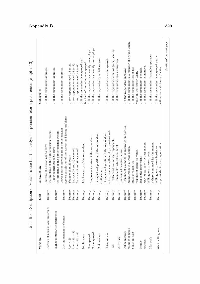
Appendix B 329T
able
B.3
:D
escr
ipti
onof
vari
able
suse
din
the
anal
ysi
sof
pen
sion
refo
rmpre
fere
nce
s(c
hap
ter
13)
Varia
ble
Un
itE
xp
lan
ati
on
Cate
gorie
s
Incr
ease
of
pen
sion
age
pre
fere
nce
Du
mm
yIn
crea
seof
pen
sion
age
toso
lve
1,
ifth
ere
spon
den
tap
pro
ves
.
the
pro
ble
ms
of
the
pu
blic
pen
sion
syst
em.
Hig
her
contr
ibu
tion
pre
fere
nce
Du
mm
yH
igh
erco
ntr
ibu
tion
sto
solv
e1,
ifth
ere
spon
den
tap
pro
ves
.
the
pro
ble
ms
of
the
pu
blic
pen
sion
syst
em.
Cu
ttin
gp
ensi
on
pre
fere
nce
Du
mm
yL
ow
erp
ensi
on
paym
ent
from
pu
blic
pen
sion
1,
ifth
ere
spon
den
tap
pro
ves
.
syst
emas
solu
tion
of
the
curr
ent
an
dfa
cin
gp
rob
lem
s.
Age<
25
Du
mm
yY
ou
nger
than
25
yea
rs.
1,
for
resp
on
den
tsaged
18
to24.
Age≥
25,<
45
Du
mm
yB
etw
een
25
an
d45
yea
rsold
.1,
for
resp
on
den
tsaged
25
to45.
Age≥
45,<
65
Du
mm
yB
etw
een
45
an
d65
yea
rsold
.1,
for
resp
on
den
tsaged
45
to65.
Job
inse
cure
Du
mm
yJob
inse
curi
tyof
the
resp
on
den
t.1,
ifth
ere
spon
den
tis
emp
loyed
an
d
isafr
aid
of
bec
om
ing
un
emp
loyed
.
Un
emp
loyed
Du
mm
yE
mp
loym
ent
statu
sof
the
resp
on
den
t.1,
ifth
ere
spon
den
tis
curr
entl
yu
nem
plo
yed
.
Not
emp
loyed
Du
mm
y1,
ifth
ere
spon
den
tis
curr
entl
yn
ot
emp
loyed
.
Civ
ilse
rvant
Du
mm
yO
ccu
pati
on
al
posi
tion
of
the
resp
on
den
t:1,
ifth
ere
spon
den
tis
aci
vil
serv
ant.
civil
serv
ant.
Entr
epre
neu
rD
um
my
Occ
up
ati
on
al
posi
tion
of
the
resp
on
den
t:1,
ifth
ere
spon
den
tis
self
-em
plo
yed
.en
trep
ren
eur
or
self
-em
plo
yed
pro
fess
ion
al.
Sic
kD
um
my
Hea
lth
con
dit
ion
of
the
resp
on
den
t.1,
ifth
ere
spon
den
tfe
els
not
(ver
y)
hea
lthy.
Un
iver
sity
Du
mm
yR
esp
on
den
t’s
edu
cati
on
al
level
.1,
ifth
ere
spon
den
th
as
au
niv
ersi
ty
(for
ap
plied
scie
nce
)d
egre
e.
Poli
cyin
tere
stD
um
my
Res
pon
den
tcl
aim
sto
be
inte
rest
edin
politi
cs.
1if
the
resp
on
den
tap
pro
ves
.
Mem
ber
of
un
ion
Du
mm
yM
emb
ersh
ipin
atr
ad
eu
nio
n.
1,
ifth
ere
spon
den
tis
am
emb
erof
atr
ad
eu
nio
n.
You
thin
East
Du
mm
yS
tate
inw
hic
hth
e1,
ifth
ere
spon
den
tsp
ent
his
resp
on
den
tsp
ent
his
you
th.
you
thin
the
form
erG
DR
.
Fem
ale
Du
mm
yS
exof
the
resp
on
den
t.1,
ifth
ere
spon
den
tis
fem
ale
.
Marr
ied
Du
mm
yM
ari
tal
statu
sof
the
resp
on
den
t.1,
ifth
ere
spon
den
tis
marr
ied
.
Lik
ew
ork
Du
mm
yW
illin
gn
ess
tow
ork
,ev
en1,
ifth
ere
spon
den
t(s
tron
gly
)ap
pro
ves
.if
ther
eis
no
nee
dfo
rth
em
on
ey.
Work
willin
gn
ess
Du
mm
yW
illin
gn
ess
tow
ork
hard
erto
1,
ifth
ere
spon
den
tis
emp
loyed
an
dis
sup
port
the
firm
or
org
an
izati
on
.w
illin
gto
work
hard
erfo
rfi
rm.
Continued
onnextpa
ge

330 Appendix B
Tab
leB
.3–
conti
nu
edfr
om
pre
vio
us
page
Varia
ble
Un
itE
xp
lan
ati
on
Cate
gorie
s
Mu
nic
ipal
suff
rage
Du
mm
yR
eform
pro
posa
l:M
un
icip
al
suff
rage
for
fore
ign
ers.
1,
ifth
ere
spon
den
tapp
roves
.
Isla
mte
ach
ing
Du
mm
yR
eform
pro
posa
l:Is
lam
teach
ing
at
Ger
man
state
sch
ools
.1,
ifth
ere
spon
den
tap
pro
ves
.
Ch
ild
ren
Du
mm
yC
hild
ren
livin
gin
the
resp
on
den
t’s
hou
seh
old
.1,
ifth
ere
spon
den
tlives
at
least
wit
hon
ech
ild
.
Blu
eco
llar
Du
mm
yR
esp
on
den
t’s
job
posi
tion
.1,
ifth
ere
spon
den
tis
emp
loyed
an
dis
ab
lue
collar
work
er.
Hard
Job
Du
mm
yR
esp
on
den
th
as
ap
hysi
cally
dem
an
din
gjo
b.
1,
ifth
ere
spon
den
tis
emp
loyed
an
dh
as
top
erfo
rma
physi
cally
dem
an
din
gjo
b.
Lef
tD
um
my
Sel
f-ass
essm
ent
of
resp
on
den
t’s
ideo
logy.
1,
ifth
ere
spon
den
tcl
ass
ifies
him
self
as
left
.
Job
matc
hD
um
my
Use
fuln
ess
of
resp
on
den
t’s
past
work
1if
resp
on
den
tca
nw
idel
yu
sep
ast
exp
erie
nce
an
d/or
job
skills
for
pre
sent
job
.w
ork
exp
erie
nce
/jo
bsk
ills
,0
oth
erw
ise.
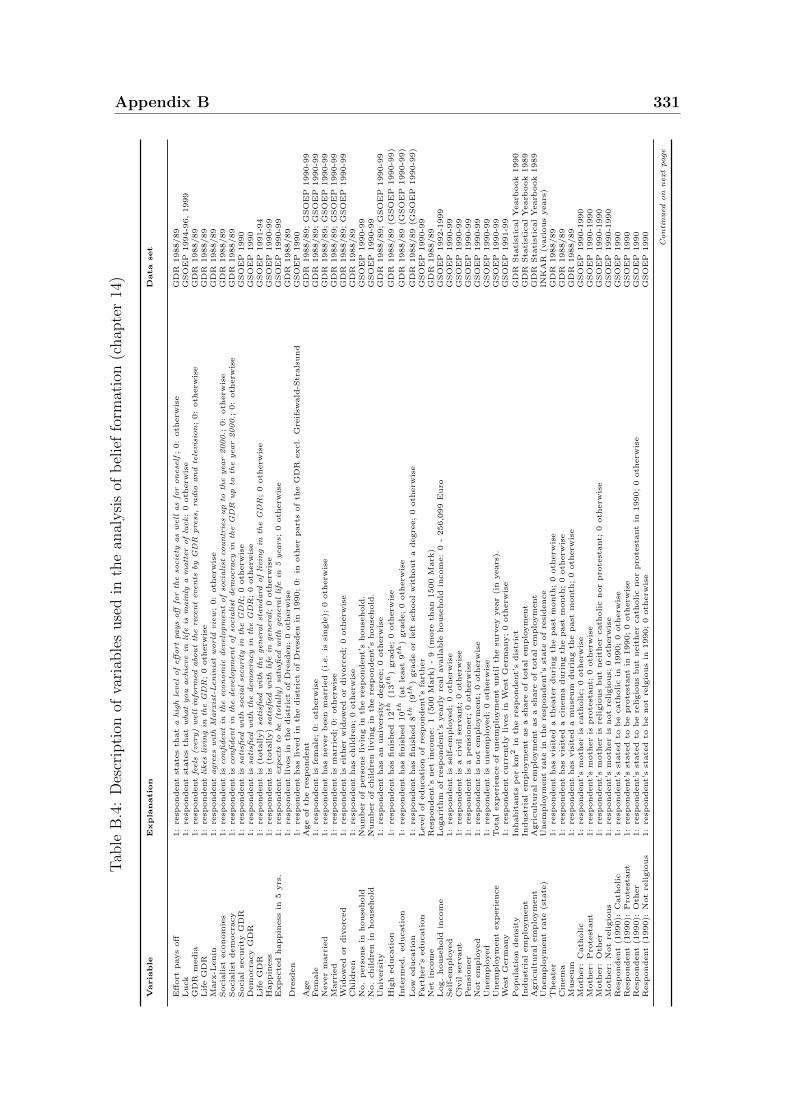
Appendix B 331T
able
B.4
:D
escr
ipti
onof
vari
able
suse
din
the
anal
ysi
sof
bel
ief
form
atio
n(c
hap
ter
14)
Varia
ble
Expla
natio
nD
ata
set
Eff
ort
pays
off
1:
resp
ondent
state
sth
at
ahig
hle
vel
of
eff
ort
pays
off
for
the
socie
tyas
well
as
for
on
ese
lf;
0:
oth
erw
ise
GD
R1988/89
Luck
1:
resp
ondent
state
sth
at
what
you
achie
ve
inli
feis
main
lya
matt
er
of
luck;
0oth
erw
ise
GSO
EP
1994-9
6,
1999
GD
Rm
edia
1:
resp
ondent
feels
(very)
well
info
rm
edabo
ut
the
rece
nt
even
tsby
GD
Rpre
ss,
radio
an
dte
levis
ion
;0:
oth
erw
ise
GD
R1988/89
Lif
eG
DR
1:
resp
ondent
likes
livin
gin
the
GD
R;
0oth
erw
ise
GD
R1988/89
Marx
-Lenin
1:
resp
ondent
agre
es
wit
hM
arxis
t-L
en
inis
tw
orld
vie
w;
0:
oth
erw
ise
GD
R1988/89
Socia
list
econom
ies
1:
resp
ondent
isco
nfi
den
tin
the
econ
om
icdevelo
pm
en
tof
socia
list
cou
ntr
ies
up
toth
eyea
r2000.;
0:
oth
erw
ise
GD
R1988/89
Socia
list
dem
ocra
cy
1:
resp
ondent
isco
nfi
den
tin
the
develo
pm
en
tof
socia
list
dem
ocra
cy
inth
eG
DR
up
toth
eyea
r2000.;
0:
oth
erw
ise
GD
R1988/89
Socia
lse
curi
tyG
DR
1:
resp
ondent
issa
tisfi
edw
ith
socia
lse
cu
rit
yin
the
GD
R;
0oth
erw
ise
GSO
EP
1990
Dem
ocra
cy
GD
R1:
resp
ondent
issa
tisfi
edw
ith
the
dem
ocra
cy
inth
eG
DR
;0
oth
erw
ise
GSO
EP
1990
Lif
eG
DR
1:
resp
ondent
is(t
ota
lly)
sati
sfied
wit
hth
egen
era
lst
an
dard
of
livin
gin
the
GD
R;
0oth
erw
ise
GSO
EP
1991-9
4H
appin
ess
1:
resp
ondent
is(t
ota
lly)
sati
sfied
wit
hli
fein
gen
era
l;0
oth
erw
ise
GSO
EP
1990-9
9E
xp
ecte
dhappin
ess
in5
yrs
.1:
resp
ondent
expec
tsto
be(t
ota
lly)
sati
sfied
wit
hgen
era
lli
fein
5yea
rs;
0oth
erw
ise
GSO
EP
1990-9
9
Dre
sden
1:
resp
ondent
lives
inth
edis
tric
tof
Dre
sden;
0oth
erw
ise
GD
R1988/89
1:
resp
ondent
has
lived
inth
edis
tric
tof
Dre
sden
in1990;
0:
inoth
er
part
sof
the
GD
Rexcl.
Gre
ifsw
ald
-Str
als
und
GSO
EP
1990
Age
Age
of
the
resp
ondent
GD
R1988/89;
GSO
EP
1990-9
9Fem
ale
1:
resp
ondent
isfe
male
;0:
oth
erw
ise
GD
R1988/89;
GSO
EP
1990-9
9N
ever
marr
ied
1:
resp
ondent
has
never
been
marr
ied
(i.e
.is
single
);0
oth
erw
ise
GD
R1988/89;
GSO
EP
1990-9
9M
arr
ied
1:
resp
ondent
ism
arr
ied;
0:
oth
erw
ise
GD
R1988/89;
GSO
EP
1990-9
9W
idow
ed
or
div
orc
ed
1:
resp
ondent
iseit
her
wid
ow
ed
or
div
orc
ed;
0oth
erw
ise
GD
R1988/89;
GSO
EP
1990-9
9C
hildre
n1:
resp
ondent
has
childre
n;
0oth
erw
ise
GD
R1988/89
No.
pers
ons
inhouse
hold
Num
ber
of
pers
ons
livin
gin
the
resp
ondent’
shouse
hold
.G
SO
EP
1990-9
9N
o.
childre
nin
house
hold
Num
ber
of
childre
nlivin
gin
the
resp
ondent’
shouse
hold
.G
SO
EP
1990-9
9U
niv
ers
ity
1:
resp
ondent
has
an
univ
ers
ity
degre
e;
0oth
erw
ise
GD
R1988/89;
GSO
EP
1990-9
9
Hig
heducati
on
1:
resp
ondent
has
finis
hed
12th
(13th
)gra
de;
0oth
erw
ise
GD
R1988/89
(GSO
EP
1990-9
9)
Inte
rmed.
educati
on
1:
resp
ondent
has
finis
hed
10th
(at
least
9th
)gra
de;
0oth
erw
ise
GD
R1988/89
(GSO
EP
1990-9
9)
Low
educati
on
1:
resp
ondent
has
finis
hed
8th
(9th
)gra
de
or
left
school
wit
hout
adegre
e;
0oth
erw
ise
GD
R1988/89
(GSO
EP
1990-9
9)
Fart
her’
seducati
on
Level
of
educati
on
of
resp
ondent’
sfa
rther
GSO
EP
1990-9
9N
et
incom
eR
esp
ondent’
snet
incom
e:
1(5
00
Mark
)-
9(m
ore
than
1500
Mark
)G
DR
1988/89
Log.
house
hold
incom
eL
ogari
thm
of
resp
ondent’
syearl
yre
al
available
house
hold
incom
e:
0-
256,0
99
Euro
GSO
EP
1992-1
999
Self
-em
plo
yed
1:
resp
ondent
isse
lf-e
mplo
yed;
0oth
erw
ise
GSO
EP
1990-9
9C
ivil
serv
ant
1:
resp
ondent
isa
civ
ilse
rvant;
0oth
erw
ise
GSO
EP
1990-9
9P
ensi
oner
1:
resp
ondent
isa
pensi
oner;
0oth
erw
ise
GSO
EP
1990-9
9N
ot
em
plo
yed
1:
resp
ondent
isnot
em
plo
ym
ent;
0oth
erw
ise
GSO
EP
1990-9
9U
nem
plo
yed
1:
resp
ondent
isunem
plo
yed;
0oth
erw
ise
GSO
EP
1990-9
9U
nem
plo
ym
ent
exp
eri
ence
Tota
lexp
eri
ence
of
unem
plo
ym
ent
unti
lth
esu
rvey
year
(in
years
).G
SO
EP
1990-9
9W
est
Germ
any
1:
resp
ondent
curr
entl
yli
ves
inW
est
Germ
any;
0oth
erw
ise
GSO
EP
1991-9
9
Popula
tion
densi
tyIn
habit
ants
per
km
2in
the
resp
ondent’
sdis
tric
tG
DR
Sta
tist
ical
Yearb
ook
1990
Indust
rial
em
plo
ym
ent
Indust
rial
em
plo
ym
ent
as
ash
are
of
tota
lem
plo
ym
ent
GD
RSta
tist
ical
Yearb
ook
1989
Agri
cult
ura
lem
plo
ym
ent
Agri
cult
ura
lem
plo
ym
ent
as
ash
are
of
tota
lem
plo
ym
ent
GD
RSta
tist
ical
Yearb
ook
1989
Unem
plo
ym
ent
rate
(sta
te)
Unem
plo
ym
ent
rate
inth
ere
spondent’
sst
ate
of
resi
dence
INK
AR
(vari
ous
years
)T
heate
r1:
resp
ondent
has
vis
ited
ath
eate
rduri
ng
the
past
month
;0
oth
erw
ise
GD
R1988/89
Cin
em
a1:
resp
ondent
has
vis
ited
acin
em
aduri
ng
the
past
month
;0
oth
erw
ise
GD
R1988/89
Muse
um
1:
resp
ondent
has
vis
ited
am
use
um
duri
ng
the
past
month
;0
oth
erw
ise
GD
R1988/89
Moth
er:
Cath
olic
1:
resp
ondent’
sm
oth
er
iscath
olic;
0oth
erw
ise
GSO
EP
1990-1
990
Moth
er:
Pro
test
ant
1:
resp
ondent’
sm
oth
er
ispro
test
ant;
0oth
erw
ise
GSO
EP
1990-1
990
Moth
er:
Oth
er
1:
resp
ondent’
sm
oth
er
isre
ligio
us
but
neit
her
cath
olic
nor
pro
test
ant;
0oth
erw
ise
GSO
EP
1990-1
990
Moth
er:
Not
religio
us
1:
resp
ondent’
sm
oth
er
isnot
religio
us;
0oth
erw
ise
GSO
EP
1990-1
990
Resp
ondent
(1990):
Cath
olic
1:
resp
ondent’
sst
ate
dto
be
cath
oli
cin
1990;
0oth
erw
ise
GSO
EP
1990
Resp
ondent
(1990):
Pro
test
ant
1:
resp
ondent’
sst
ate
dto
be
pro
test
ant
in1990;
0oth
erw
ise
GSO
EP
1990
Resp
ondent
(1990):
Oth
er
1:
resp
ondent’
sst
ate
dto
be
religio
us
but
neit
her
cath
olic
nor
pro
test
ant
in1990;
0oth
erw
ise
GSO
EP
1990
Resp
ondent
(1990):
Not
religio
us
1:
resp
ondent’
sst
ate
dto
be
not
relg
ious
in1990;
0oth
erw
ise
GSO
EP
1990
Con
tin
ued
on
next
page
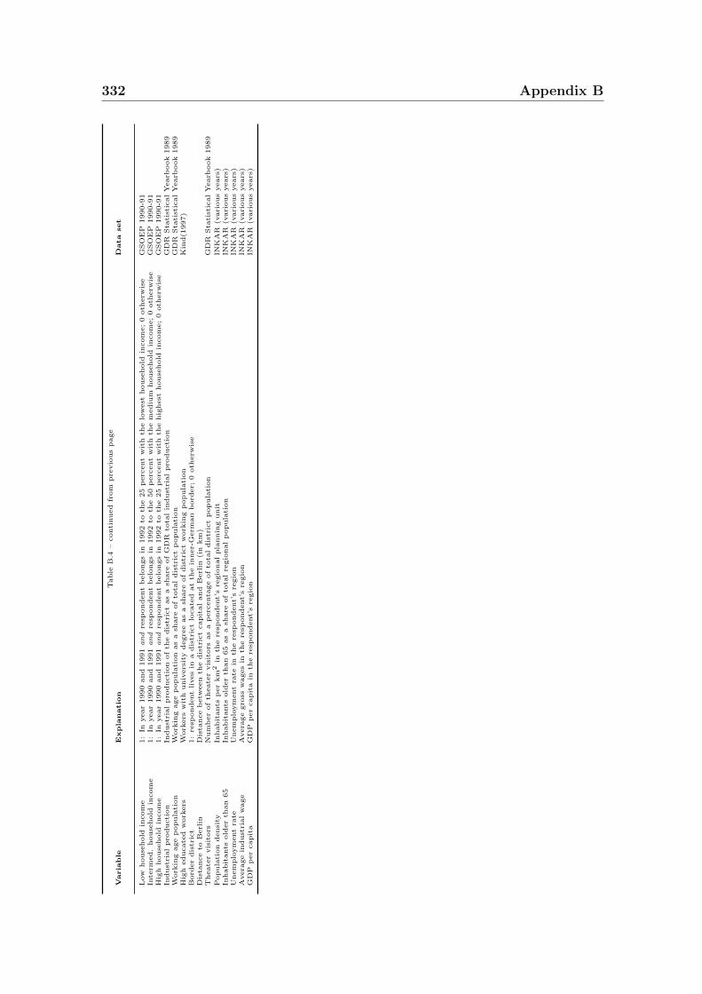
332 Appendix BT
able
B.4
–conti
nued
from
pre
vio
us
page
Varia
ble
Expla
natio
nD
ata
set
Low
house
hold
incom
e1:
Inyear
1990
and
1991
an
dre
spondent
belo
ngs
in1992
toth
e25
perc
ent
wit
hth
elo
west
house
hold
incom
e;
0oth
erw
ise
GSO
EP
1990-9
1In
term
ed.
house
hold
incom
e1:
Inyear
1990
and
1991
an
dre
spondent
belo
ngs
in1992
toth
e50
perc
ent
wit
hth
em
ediu
mhouse
hold
incom
e;
0oth
erw
ise
GSO
EP
1990-9
1H
igh
house
hold
incom
e1:
Inyear
1990
and
1991
an
dre
spondent
belo
ngs
in1992
toth
e25
perc
ent
wit
hth
ehig
hest
house
hold
incom
e;
0oth
erw
ise
GSO
EP
1990-9
1In
dust
rial
pro
ducti
on
Indust
rial
pro
ducti
on
of
the
dis
tric
tas
ash
are
of
GD
Rto
tal
indust
rial
pro
ducti
on
GD
RSta
tist
ical
Yearb
ook
1989
Work
ing
age
popula
tion
Work
ing
age
popula
tion
as
ash
are
of
tota
ldis
tric
tp
opula
tion
GD
RSta
tist
ical
Yearb
ook
1989
Hig
heducate
dw
ork
ers
Work
ers
wit
huniv
ers
ity
degre
eas
ash
are
of
dis
tric
tw
ork
ing
popula
tion
Kin
d(1
997)
Bord
er
dis
tric
t1:
resp
ondent
lives
ina
dis
tric
tlo
cate
dat
the
inner-
Germ
an
bord
er;
0oth
erw
ise
Dis
tance
toB
erl
inD
ista
nce
betw
een
the
dis
tric
tcapit
al
and
Berl
in(i
nkm
)T
heate
rvis
itors
Num
ber
of
theate
rvis
itors
as
ap
erc
enta
ge
of
tota
ldis
tric
tp
opula
tion
GD
RSta
tist
ical
Yearb
ook
1989
Popula
tion
densi
tyIn
habit
ants
per
km
2in
the
resp
ondent’
sre
gio
nal
pla
nnin
gunit
INK
AR
(vari
ous
years
)In
habit
ants
old
er
than
65
Inhabit
ants
old
er
than
65
as
ash
are
of
tota
lre
gio
nal
popula
tion
INK
AR
(vari
ous
years
)U
nem
plo
ym
ent
rate
Unem
plo
ym
ent
rate
inth
ere
spondent’
sre
gio
nIN
KA
R(v
ari
ous
years
)A
vera
ge
indust
rial
wage
Avera
ge
gro
ssw
ages
inth
ere
spondent’
sre
gio
nIN
KA
R(v
ari
ous
years
)G
DP
per
capit
aG
DP
per
capit
ain
the
resp
ondent’
sre
gio
nIN
KA
R(v
ari
ous
years
)
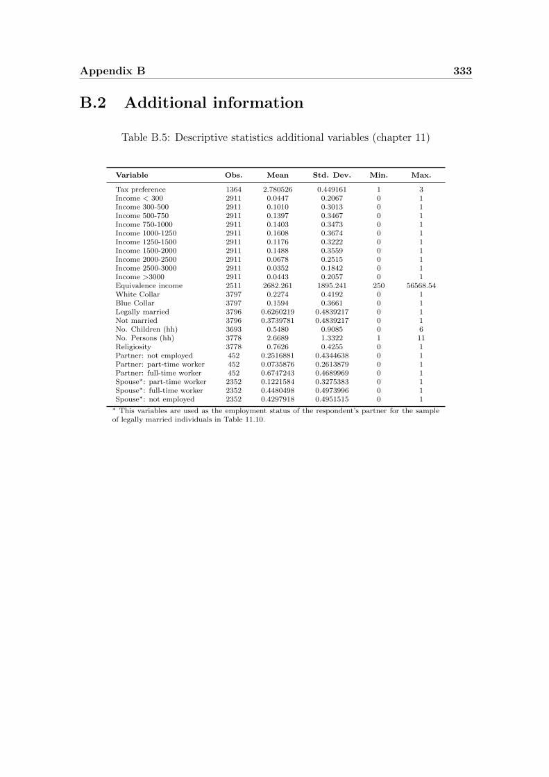
Appendix B 333
B.2 Additional information
Table B.5: Descriptive statistics additional variables (chapter 11)
Variable Obs. Mean Std. Dev. Min. Max.
Tax preference 1364 2.780526 0.449161 1 3Income < 300 2911 0.0447 0.2067 0 1Income 300-500 2911 0.1010 0.3013 0 1Income 500-750 2911 0.1397 0.3467 0 1Income 750-1000 2911 0.1403 0.3473 0 1Income 1000-1250 2911 0.1608 0.3674 0 1Income 1250-1500 2911 0.1176 0.3222 0 1Income 1500-2000 2911 0.1488 0.3559 0 1Income 2000-2500 2911 0.0678 0.2515 0 1Income 2500-3000 2911 0.0352 0.1842 0 1Income >3000 2911 0.0443 0.2057 0 1Equivalence income 2511 2682.261 1895.241 250 56568.54White Collar 3797 0.2274 0.4192 0 1Blue Collar 3797 0.1594 0.3661 0 1Legally married 3796 0.6260219 0.4839217 0 1Not married 3796 0.3739781 0.4839217 0 1No. Children (hh) 3693 0.5480 0.9085 0 6No. Persons (hh) 3778 2.6689 1.3322 1 11Religiosity 3778 0.7626 0.4255 0 1Partner: not employed 452 0.2516881 0.4344638 0 1Partner: part-time worker 452 0.0735876 0.2613879 0 1Partner: full-time worker 452 0.6747243 0.4689969 0 1Spouse∗: part-time worker 2352 0.1221584 0.3275383 0 1Spouse∗: full-time worker 2352 0.4480498 0.4973996 0 1Spouse∗: not employed 2352 0.4297918 0.4951515 0 1∗ This variables are used as the employment status of the respondent’s partner for the sampleof legally married individuals in Table 11.10.
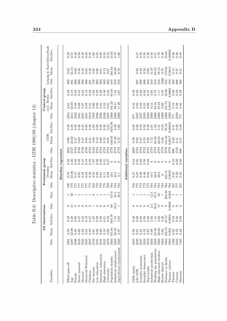
334 Appendix BT
able
B.6
:D
escr
ipti
vest
atis
tics
-G
DR
1988
/89
(chap
ter
14)
All
ob
servati
on
sT
reatm
ent
grou
pC
ontr
ol
grou
pD
resd
enG
DR
excl
.B
erlin
Lei
pzi
g&
Karl
-Marx
-Sta
dt
Vari
ab
les
Ob
s.M
ean
Std
.Dev
.M
in.
Max.
Ob
s.M
ean
Std
.Dev
.O
bs.
Mea
nS
td.D
ev.
Ob
s.M
ean
Std
.Dev
.O
bs.
Mea
nS
td.D
ev.
Base
lin
eregress
ion
Eff
ort
pays
off
3381
0.5
80.4
90
1736
0.5
30.5
02645
0.6
00.4
92254
0.6
10.4
9860
0.6
20.4
9A
ge
3497
23.0
96.3
815
50
770
23.3
66.3
62727
23.0
26.3
82314
22.9
76.1
9891
24.1
36.7
4F
emale
3526
0.4
80.5
00
1777
0.5
10.5
02749
0.4
70.5
02332
0.4
80.5
0900
0.6
00.4
9N
ever
marr
ied
3525
0.6
80.4
70
1777
0.6
50.4
82748
0.6
90.4
62331
0.6
90.4
5900
0.5
60.5
0M
arr
ied
3525
0.2
80.4
50
1777
0.3
20.4
72748
0.2
70.4
52331
0.2
70.4
5900
0.4
00.4
9D
ivorc
ed/W
idow
ed3525
0.0
40.1
90
1777
0.0
40.1
82748
0.0
40.2
02331
0.0
40.1
9900
0.0
40.2
0C
hild
ren
3507
0.3
30.4
70
1773
0.3
80.4
92734
0.3
10.4
62318
0.3
10.4
6891
0.4
00.4
9N
etin
com
e2742
3.9
11.8
71
9594
4.0
21.8
72148
3.8
81.8
61859
3.8
01.8
3730
3.8
61.8
6L
ow
edu
cati
on
3531
0.0
90.2
90
1778
0.0
90.2
82753
0.1
00.2
92336
0.0
90.2
9903
0.0
60.2
5In
term
ed.
edu
cati
on
3531
0.8
00.4
00
1778
0.8
10.4
02753
0.8
00.4
02336
0.8
10.3
9903
0.8
10.4
0H
igh
edu
cati
on
3531
0.1
00.3
10
1778
0.1
10.3
12753
0.1
00.3
02336
0.1
00.3
0903
0.1
30.3
4U
niv
ersi
ty3479
0.0
60.2
30
1769
0.0
80.2
72710
0.0
50.2
22297
0.0
50.2
2893
0.0
70.2
5P
op
ula
tion
den
sity
3563
555.8
1958.7
868
3174
784
254
02779
640.9
51070.3
92360
191.2
385.0
4910
291.6
515.6
5In
du
stri
al
emp
loym
ent
3563
38.5
07.7
324.3
48.1
784
42.8
02779
37.2
88.3
62360
39.4
17.2
4910
45.6
03.7
8A
gri
cult
ura
lem
plo
ym
ent
3563
9.3
75.0
51
22.2
784
8.1
02779
9.7
35.6
62360
11.2
84.6
7910
6.7
01.0
6
Ad
dti
on
al
varia
ble
s
GD
Rm
edia
3455
0.3
60.4
80
1758
0.2
70.4
42697
0.3
90.4
9877
0.4
20.4
9L
ife
GD
R3520
0.9
10.2
80
1775
0.8
50.3
52745
0.9
30.2
62327
0.9
30.2
6897
0.9
20.2
7S
oci
alist
econ
om
ies
3527
0.4
50.5
00
1773
0.3
80.4
92754
0.4
70.5
02337
0.5
00.5
0899
0.4
90.5
0S
oci
alist
dem
ocr
acy
3524
0.5
20.5
00
1772
0.4
60.5
02752
0.5
30.5
02333
0.5
50.5
0898
0.5
80.5
0M
arx
-Len
in3516
0.6
50.4
80
1775
0.6
00.4
92741
0.6
60.4
82323
0.6
60.4
7894
0.6
90.4
6In
du
stri
al
pro
du
ctio
n3563
8.3
82.8
22.5
12.5
784
10.7
02779
7.7
22.8
72360
8.1
22.9
5910
11.0
72.1
6W
ork
ing
age
pop
ula
tion
3563
64.3
91.4
162.9
67.5
784
62.9
02779
64.8
21.3
22360
64.3
40.7
3910
63.5
30.5
1H
igh
edu
cate
dw
ork
ers
3563
20.6
24.6
917
33
784
20.6
02779
20.6
35.3
12360
18.4
31.1
1910
18.1
31.7
0B
ord
erd
istr
ict
3563
0.6
90.4
60
1784
00
2779
0.8
80.3
32360
0.8
60.3
52360
0.7
00.4
6D
ista
nce
toB
erlin
3563
156.7
867.3
70
283.4
5784
165.4
10
2779
154.3
476.1
02360
181.7
442.8
8910
178.6
219.0
3T
hea
ter
vis
itors
3563
0.0
02
0.0
004
0.0
008
0.0
03
784
0.0
019
02779
0.0
017
0.0
0045
2360
0.0
015
0.0
002
910
0.0
014
0.0
0002
Th
eate
r1166
0.2
20.4
20
1257
0.2
50.4
3909
0.2
20.4
1771
0.1
80.3
9302
0.1
50.3
6C
inem
a3522
0.4
30.5
00
1777
0.5
00.5
02745
0.4
10.4
92329
0.3
80.4
9898
0.3
70.4
8M
use
um
1165
0.4
20.4
90
1257
0.4
50.5
0908
0.4
10.4
9771
0.4
00.4
9304
0.4
10.4
9
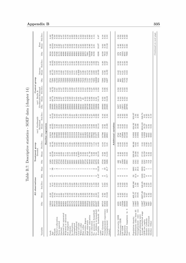
Appendix B 335T
able
B.7
:D
escr
ipti
vest
atis
tics
-SO
EP
dat
a(c
hap
ter
14)
All
observatio
ns
Treatm
ent
group
Controlgroup
Dre
sden
excl.
Gre
ifsw
ald
-excl.
Berl
in&
Str
als
und
Gre
ifsw
ald
-Str
als
und
Saxony
East
Vari
able
Obs
Mean
Std
.Dev.
Min
Max
Obs
Mean
Std
.Dev.
Obs
Mean
Std
.Dev.
Obs
Mean
Std
.Dev.
Obs
Mean
Std
.Dev.
Obs
Mean
Std
.Dev.
Baseline
regressio
n
Luck
13910
0.2
20.4
10
11385
0.2
50.4
311819
0.2
20.4
110928
0.2
20.4
22731
0.2
20.4
23018
0.2
20.4
2A
ge
36715
43.5
416.4
17
98
3734
42.3
916.1
631786
43.6
516.4
229383
43.7
416.5
27284
45.1
316.6
28159
44.6
416.8
0Fem
ale
36715
0.5
20.5
00
13734
0.5
30.5
031786
0.5
20.5
029383
0.5
20.5
07284
0.5
30.5
08159
0.5
20.5
0Fath
er’
seducati
on
31059
2.3
10.6
40
43252
2.3
50.6
526892
2.3
00.6
324857
2.2
80.6
16150
2.3
00.6
36726
2.2
50.5
9N
ever
marr
ied
36460
0.2
10.4
10
13718
0.2
00.4
031560
0.2
10.4
129204
0.2
00.4
07252
0.1
80.3
98115
0.2
00.4
0M
arr
ied
36301
0.6
60.4
70
13704
0.6
90.4
631422
0.6
60.4
729082
0.6
70.4
77222
0.6
80.4
78090
0.6
70.4
7M
arr
ied
but
separa
ted
36301
0.0
10.1
00
13704
0.0
10.0
931422
0.0
10.1
029082
0.0
10.1
07222
0.0
10.1
08090
0.0
10.1
0W
idow
ed
or
div
orc
ed
36301
0.1
20.3
20
13704
0.1
10.3
131422
0.1
20.3
229082
0.1
20.3
27222
0.1
20.3
38090
0.1
30.3
3N
ot
em
plo
yed
36173
0.0
30.1
70
13691
0.0
30.1
731318
0.0
30.1
728964
0.0
30.1
77200
0.0
30.1
78064
0.0
30.1
8P
ensi
oner
36173
0.1
90.4
00
13691
0.1
70.3
831318
0.2
00.4
028964
0.2
00.4
07200
0.2
10.4
18064
0.2
20.4
1In
educati
on
36173
0.0
50.2
10
13691
0.0
50.2
131318
0.0
50.2
128964
0.0
40.2
07200
0.0
40.2
08064
0.0
40.2
0U
nem
plo
yed
36173
0.1
00.3
00
13691
0.0
90.2
931318
0.1
00.3
128964
0.1
10.3
17200
0.1
10.3
18064
0.1
20.3
2Self
-em
plo
yed
36173
0.0
40.2
00
13691
0.0
50.2
231318
0.0
40.2
028964
0.0
40.1
97200
0.0
40.1
88064
0.0
40.2
0C
ivil
serv
ant
36173
0.0
10.1
10
13691
0.0
07
0.0
831318
0.0
10.1
128964
0.0
10.1
07200
0.0
09
0.0
98064
0.0
10.1
1W
hit
ecollar
36269
0.2
80.4
50
13697
0.2
90.4
531401
0.2
70.4
529041
0.2
70.4
47219
0.2
70.4
48083
0.2
50.4
3B
lue
collar
36269
0.2
40.4
30
13697
0.2
40.4
331401
0.2
40.4
329041
.25
0.4
37219
0.2
60.4
48083
0.2
30.4
2U
niv
ers
ity
degre
e36290
0.2
30.4
20
13710
0.2
50.4
331402
0.2
30.4
229032
0.2
20.4
17196
0.2
10.4
18073
0.2
20.4
1H
igh
educati
on
35912
0.1
30.3
40
13674
0.1
50.3
531070
0.1
30.3
428759
0.1
20.3
27157
0.1
30.3
47981
0.1
20.3
3In
term
ed.
educati
on
35597
0.7
90.4
10
13640
0.7
80.4
230795
0.7
90.4
128498
0.8
00.4
07121
0.7
80.4
124836
0.8
00.4
0L
ow
educati
on
35642
0.0
80.2
70
13644
0.0
80.2
730834
0.0
80.2
728535
0.0
80.2
77124
0.0
90.2
87938
0.1
00.3
1N
o.
pers
ons
inhouse
hold
36715
3.0
11.1
91
83734
3.2
21.1
431786
2.9
91.2
029383
3.0
11.2
07284
2.8
01.0
68159
2.9
11.1
4N
o.
childre
nin
house
hold
66357
0.8
30.9
90
66970
1.0
61.0
157477
0.8
20.9
952866
0.8
11.0
012898
0.6
90.9
2A
vailable
house
hold
in-
com
e28283
10.1
40.5
03.4
712.2
32859
10.1
90.4
924504
10.1
40.5
022638
10.1
30.5
05624
10.0
90.4
76248
10.0
70.4
7
West
Germ
any
36715
0.0
30.1
70
13734
0.0
40.1
931786
0.0
30.1
629383
0.0
30.1
67284
0.0
40.2
08159
0.0
30.1
8U
nem
plo
ym
ent
exp
eri
ence
35404
0.3
60.9
30
19
3626
0.2
80.7
330665
0.3
60.9
528346
0.3
60.9
67049
0.3
60.9
27812
0.3
90.9
4U
nem
plo
ym
ent
rate
(sta
te)
32332
15.8
23.2
53.7
21.7
3286
14.9
13.2
128001
15.8
93.2
425885
16.0
23.2
56407
14.9
93.2
77169
15.3
23.1
0
Additio
nalvaria
ble
s
Socia
lse
curi
tyG
DR
4335
0.4
30.5
00
1446
0.4
20.4
93740
0.4
30.5
03457
0.4
40.5
0862
0.4
30.5
0978
0.4
50.5
0D
em
ocra
cy
GD
R4334
0.4
20.4
90
1447
0.4
00.4
93738
0.4
30.5
03455
0.4
40.5
0862
0.4
70.5
0978
0.4
60.5
0L
ife
GD
R15028
0.2
30.4
20
11569
0.2
50.4
412984
0.2
30.4
212011
0.2
30.4
32934
0.2
10.4
13353
0.2
30.4
2H
appin
ess
36095
0.5
30.5
00
13690
0.5
30.5
031246
0.5
30.5
028894
0.5
30.5
07170
0.5
30.5
08031
0.5
10.5
0E
xp
ecte
dhappin
ess
in5
yrs
.35945
0.6
10.4
90
13681
0.6
50.4
831123
0.6
10.4
928785
0.6
10.4
97132
0.6
30.4
87990
0.6
00.4
9
Popula
tion
densi
ty13467
405.3
7895.8
852
3891
1341
229.9
586.6
611692
434.9
2953.0
7In
habit
ants
old
er
than
65
13467
15.7
41.5
912.4
19.1
1341
16.6
80.6
211692
15.6
91.6
3U
nem
plo
ym
ent
rate
(re-
gio
nal
pla
nnin
gunit
)13467
18.0
52.8
86
23.4
1341
17.3
13.1
611692
18.0
82.8
3
Avera
ge
indust
rial
wage
13467
2007.2
9340.2
51035
3835
1341
17.3
13.1
611692
2016.2
3348.7
4G
DR
per
capit
a13467
16.6
43.0
813.2
41.9
1341
16.5
93.6
211692
16.7
03.0
1M
oth
er:
Cath
olic
7067
0.0
70.2
50
1719
0.1
00.3
06043
0.0
70.2
5M
oth
er:
Pro
test
ant
7067
0.3
20.4
70
1719
0.3
20.4
76043
0.3
40.4
7M
oth
er:
Oth
er
7067
0.0
40.1
90
1719
0.0
40.1
86043
0.0
40.1
9
Con
tin
ued
on
next
page
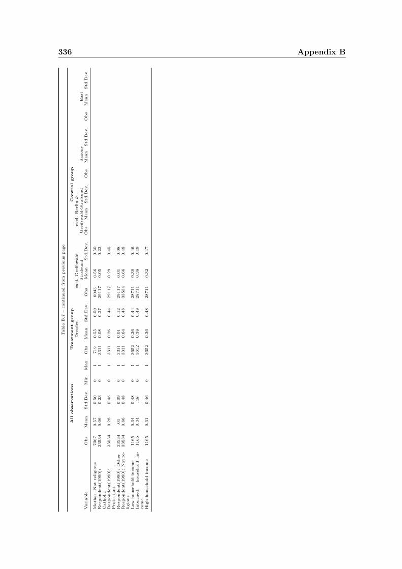
336 Appendix BT
able
B.7
–conti
nued
from
pre
vio
us
page
All
observatio
ns
Treatm
ent
group
Controlgroup
Dre
sden
excl.
Gre
ifsw
ald
-excl.
Berl
in&
Str
als
und
Gre
ifsw
ald
-Str
als
und
Saxony
East
Vari
able
Obs
Mean
Std
.Dev.
Min
Max
Obs
Mean
Std
.Dev.
Obs
Mean
Std
.Dev.
Obs
Mean
Std
.Dev.
Obs
Mean
Std
.Dev.
Obs
Mean
Std
.Dev.
Moth
er:
Not
religio
us
7067
0.5
70.5
00
1719
0.5
50.5
06043
0.5
60.5
0R
esp
ondent(
1990):
Cath
olic
33534
0.0
60.2
30
13311
0.0
80.2
729117
0.0
50.2
3
Resp
ondent(
1990):
Pro
test
ant
33534
0.2
80.4
50
13311
0.2
60.4
429117
0.2
90.4
5
Resp
ondent(
1990):
Oth
er
33534
.01
0.0
90
13311
0.0
10.1
229117
0.0
10.0
8R
esp
ondent(
1990):
Not
re-
ligio
us
33534
0.6
60.4
80
13311
0.6
40.4
833534
0.6
60.4
8
Low
house
hold
incom
e1165
0.3
40.4
80
13652
0.2
60.4
428711
0.3
00.4
6In
term
ed.
house
hold
in-
com
e1165
0.3
4.4
80
13652
0.3
80.4
928711
0.3
80.4
9
Hig
hhouse
hold
incom
e1165
0.3
10.4
60
13652
0.3
60.4
828711
0.3
20.4
7

LEBENSLAUF
Tanja Hennighausen
03/2014 Promotion in Volkswirtschaftslehre an der Universitat
Mannheim
seit 06/2009 Wissenschaftliche Mitarbeiterin an der Universitat
Mannheim, Lehrstuhl fur Volkswirtschaftslehre,
Politische Okonomie
05/2008 - 07/2012 Wissenschaftliche Mitarbeiterin am Zentrum fur
Europaische Wirtschaftsforschung (ZEW), Mannheim
12/2007 Abschluss als Diplom-Volkswirtin an der Universitat
Mannheim
10/2002 - 12/2007 Studium der Volkswirtschaftslehre an der Universitat
Mannheim
06/2002 Abitur an der Modellschule Obersberg in Bad Hersfeld

Eidesstattliche Erklarung
Hiermit erklare ich, die vorliegende Dissertation selbstandig angefertigt und mich keiner
anderen als der in ihr angegebenen Hilfsmittel bedient zu haben. Insbesondere sind
samtliche Zitate aus anderen Quellen als solche gekennzeichnet und mit Quellenangaben
versehen.
Mannheim, 11.12.2013
Tanja Hennighausen