econstor www.econstor.eu

Der Open-Access-Publikationsserver der ZBW – Leibniz-Informationszentrum WirtschaftThe Open Access Publication Server of the ZBW – Leibniz Information Centre for Economics

Standard-Nutzungsbedingungen:

Die Dokumente auf EconStor dürfen zu eigenen wissenschaftlichenZwecken und zum Privatgebrauch gespeichert und kopiert werden.

Sie dürfen die Dokumente nicht für öffentliche oder kommerzielleZwecke vervielfältigen, öffentlich ausstellen, öffentlich zugänglichmachen, vertreiben oder anderweitig nutzen.

Sofern die Verfasser die Dokumente unter Open-Content-Lizenzen(insbesondere CC-Lizenzen) zur Verfügung gestellt haben sollten,gelten abweichend von diesen Nutzungsbedingungen die in der dortgenannten Lizenz gewährten Nutzungsrechte.

Terms of use:

Documents in EconStor may be saved and copied for yourpersonal and scholarly purposes.

You are not to copy documents for public or commercialpurposes, to exhibit the documents publicly, to make thempublicly available on the internet, or to distribute or otherwiseuse the documents in public.

If the documents have been made available under an OpenContent Licence (especially Creative Commons Licences), youmay exercise further usage rights as specified in the indicatedlicence.

zbw Leibniz-Informationszentrum WirtschaftLeibniz Information Centre for Economics

de Hoop, Jacobus; Rosati, Furio C.

Working Paper

Does promoting school attendance reduce childlabour? Evidence from Burkina Faso's BRIGHTproject

Discussion Paper series, Forschungsinstitut zur Zukunft der Arbeit, No. 6601

Provided in Cooperation with:Institute for the Study of Labor (IZA)

Suggested Citation: de Hoop, Jacobus; Rosati, Furio C. (2012) : Does promoting schoolattendance reduce child labour? Evidence from Burkina Faso's BRIGHT project, DiscussionPaper series, Forschungsinstitut zur Zukunft der Arbeit, No. 6601

This Version is available at:http://hdl.handle.net/10419/62422

DI

SC

US

SI

ON

P

AP

ER

S

ER

IE

S

Forschungsinstitut zur Zukunft der ArbeitInstitute for the Study of Labor

Does Promoting School Attendance Reduce Child Labour? Evidence from Burkina Faso’s BRIGHT Project

IZA DP No. 6601

May 2012

Jacobus de HoopFurio C. Rosati

Does Promoting School Attendance

Reduce Child Labour? Evidence from Burkina Faso’s BRIGHT Project

Jacobus de Hoop Understanding Children’s Work

Furio C. Rosati

Understanding Children’s Work and IZA

Discussion Paper No. 6601 May 2012

IZA

P.O. Box 7240 53072 Bonn

Germany

Phone: +49-228-3894-0 Fax: +49-228-3894-180

E-mail: iza@iza.org

Any opinions expressed here are those of the author(s) and not those of IZA. Research published in this series may include views on policy, but the institute itself takes no institutional policy positions. The Institute for the Study of Labor (IZA) in Bonn is a local and virtual international research center and a place of communication between science, politics and business. IZA is an independent nonprofit organization supported by Deutsche Post Foundation. The center is associated with the University of Bonn and offers a stimulating research environment through its international network, workshops and conferences, data service, project support, research visits and doctoral program. IZA engages in (i) original and internationally competitive research in all fields of labor economics, (ii) development of policy concepts, and (iii) dissemination of research results and concepts to the interested public. IZA Discussion Papers often represent preliminary work and are circulated to encourage discussion. Citation of such a paper should account for its provisional character. A revised version may be available directly from the author.

IZA Discussion Paper No. 6601 May 2012

ABSTRACT

Does Promoting School Attendance Reduce Child Labour? Evidence from Burkina Faso’s BRIGHT Project

Using data from BRIGHT, an integrated program that aims to improve school participation in rural communities in Burkina Faso, we investigate the impact of school subsidies and increased access to education on child work. Regression discontinuity estimates demonstrate that, while BRIGHT substantially improved school participation, it increased children’s participation in economic activities and chores. This combination of increased school participation and work can be explained by the introduction of a simple non convexity in the standard model of altruistic utility maximizing households. If education programs are implemented to achieve a combination of increased school participation and a reduction in child work, they may either have to be combined with different interventions that effectively reduce child work or they may have to be tuned more carefully to the incentives and constraints the child laborer faces. JEL Classification: I25, J22, J24, O12, O55 Keywords: Burkina Faso, child labour, regression discontinuity, school participation Corresponding author: Furio C. Rosati Understanding Children’s Work (UCW) c/o CEIS, University of Rome “Tor Vergata” Via Columbia 2 00133 Rome Italy E-mail: frosati@ucw-project.org

2

1 Introduction1

High costs of education and limited access to schools are often seen as

important determinants of child labour. Reductions in the cost of education

and increased access to schools are therefore advocated as an instrument to

reduce the incidence of child labour. However, the impact of such

interventions on child labour is not unambiguous from a theoretical point of

view (Cigno and Rosati, 2005; Edmonds, 2007).2 In fact, policies aimed at

promoting school participation risk increasing child labour if they are not

carefully tailored to the incentives and constraints faced by children in

developing countries. Empirical evidence on this matter therefore has

important policy implications.

In this paper we look at the impact of Burkina Faso’s BRIGHT

program on several dimensions of child work. BRIGHT implemented a

package of education interventions in 132 rural villages consisting of two

main components: the construction of a primary school and the provision of

direct incentives for school participation in the form of school meals for all

pupils and take-home rations for female pupils.3 Evidence on the impact of

interventions that, like the BRIGHT program, provide in-kind subsidies for

school participation and reduce the cost of traveling to school on child work is

scarce and does not always exploit unambiguously exogenous variation in

treatment status.

Two previous papers evaluate the impact of the provision of food for

education programs on child labour. Ravaillon and Wodon (2000) use (non-

1 We thank Marco Manacorda for valuable comments. The findings, interpretations, and conclusions expressed in this paper are entirely those of the authors. They do not necessarily represent the views of UCW or its partner organizations: the International Labour Organization, UNICEF, and the World Bank. Funding for this project was provided by the United States Department of Labor. This document does not necessarily reflect the views or policies of the United States Department of Labor, nor does mention of trade names, commercial products, or organizations imply endorsement by the United States Government. 2 The ambiguity stems mainly from the fact that school attendance and work are not mutually exclusive activities, as children can adjust leisure following a change in the relative price of education or changes in the income available to the household. 3 In addition, the program implemented a range of advocacy measures.

3

random) program placement as an instrument to identify the effect of the

provision of monthly food rations in Bangladesh. They find that the provision

of school meals substantially increases school attendance, but results in a

markedly smaller decrease in child work: children appear to be substituting

leisure with schooling, only marginally reducing the time devoted to work.

Kazianga et al. (2008) use a randomized controlled trial to evaluate the impact

of school meals and take-home rations in Burkina Faso. They find mixed

effects of these interventions on school participation and child work, primarily

among girls. Girls’ school enrollment increases as a result of the interventions,

but their average attendance deteriorates. Moreover girls alter the allocation of

labour away from productive activities toward domestic activities which, the

authors argue, children can combine more easily with school activities.

To our knowledge, Kondylis and Manacorda (2012) is the most recent

paper to examine the role of school proximity. The authors use micro data

from Tanzania to investigate the relationship between distance to school and

work and school participation. The estimates do not exploit an exogenous

instrument to identify the causal effect of distance to school on work and

school participation. Instead, the estimations control for observed

socioeconomic characteristics of households and distance to other facilities

which, the authors argue, helps correct for non-random spatial distribution of

households within the village. Their results suggest that school proximity

leads to a rise in school attendance, but not to a noticeable reduction in child

labour.

The BRIGHT project offers a particularly interesting opportunity to

provide additional evidence on the impact of this type of education

interventions on child labour. First, BRIGHT is well situated to bring about

changes in school participation and child labour, as school participation rates

in Burkina Faso rank among the lowest in the world and children are widely

engaged in economic activities and household chores (henceforth we use the

term work to refer to the combination of children’s economic activities and

4

chores). Second, extensive household, child, and school surveys administered

as part of the program allow us to provide detailed evidence on the interaction

between child labour and school participation. Third, the setup of the BRIGHT

program provides a strong quasi-experimental identification mechanism.

This identification mechanism exploits the fact that BRIGHT was

allocated on the basis of an index that ranked villages in order of their

potential to improve school attendance and education outcomes. A total of 293

rural villages from 49 departments subscribed for participation in the BRIGHT

program. Within each department, the subscribing villages were ranked based

on this index and those in the top half of the ranking were selected into the

program. Following Levy et al. (2009), we exploit this assignment procedure

in a regression discontinuity framework to estimate the causal effect of the

BRIGHT program. A limitation that should be noted at the outset is that this

estimation procedure does not allow us to distinguish the marginal impact of

the separate components of the BRIGHT program (i.e. the construction of

schools and the provision of in-kind incentives).

In accordance with Levy et al. (2009), we find that BRIGHT had a

strong impact on school participation. Regression discontinuity estimates

suggest that school enrollment exhibits a discontinuity of roughly 13

percentage points in marginal BRIGHT villages. More surprisingly, despite

this marked increase in school participation, we observe no decrease in the

prevalence of child work in the marginal BRIGHT villages. If anything, our

estimates indicate that children’s participation in work increased as a result of

the BRIGHT education interventions.

We show that this pattern of changes in schooling and child labour

status is consistent with the predictions of a simple altruistic household utility

maximization model. Broadly speaking, the model indicates that some of the

children who were not in school before the intervention will enroll and that the

children who were already in school will remain enrolled. There is no such

clear theoretical prediction for the change in child work. Among children who

5

were already in school, the change in the prevalence of child work is

ambiguous. The same holds among children who begin to attend school as a

consequence of the program. Finally, if there is some degree of income

pooling, we can expect spillover income effects from the take-home rations

provided to enrolled girls on male siblings.

A more articulate picture emerges when we decompose the overall

impact of BRIGHT to account for these potential spillover effects. There is

evidence of substantially increased school participation for girls, boys without

female siblings, and boys with female siblings (who potentially benefit from

spillover effects). However, changes in work participation are not the same

within these subgroups. Girls appear to have increased their school

participation without altering their involvement in work. Boys, particularly

those without female siblings, do appear to have increased their participation

in work.

When we take a closer look at children’s involvement in work, we find

that the increase in work participation among boys primarily takes place

within the household. We find no discontinuities in the types of activities

conducted by children nor do we find discontinuities in remunerated activities.

Moreover, although here the information is more limited, we find no evidence

that the intensive margin of child work changed in marginal BRIGHT villages.

Importantly, we also find little evidence that working while attending

school has a detrimental effect on school participation. Children attend school

regularly when they are enrolled, as suggested by self-reported attendance,

teacher reported attendance, and information obtained during surprise school

visits. Moreover, we find that children in marginal BRIGHT villages exhibit

improvements in performance on a mathematics and French language test of

roughly .2 to .4 standard deviations. Improvements in learning outcomes are

comparable among children who are in school only and those who combine

school attendance with work.

6

Together, the presented results suggest that in a low income country

like Burkina Faso promoting school enrollment does not necessarily reduce

children’s involvement in work. On the contrary, it might raise participation in

work for some groups of children. However, there is no evidence that the

increase in child work hampers school attendance or reduces learning in

school.

The remainder of this paper is structured as follows. Section 2

develops the model that guides the interpretation of the results in the paper.

Section 3 discusses the setting, the design of the BRIGHT project, and the data

we use in this paper. Section 4 provides a description of the estimation

procedures and presents the results and section 5 concludes.

2 Theoretical Outline

In this section we develop a simple model that provides basic insights

into the relationship between households’ schooling and work decisions on the

one hand and the monetary and time costs of education on the other. We

consider a unitary household decision model with parents maximizing a utility

function defined over household consumption, children’s leisure, and

children’s education. This very simple model captures the characteristics of an

altruistic overlapping generation model that are essential for the development

of our analysis.

We assume that the number of children is predetermined and equal to

one (i.e. we treat fertility as exogenous) and that adult labour supply is fixed.

Relaxing these assumptions will not change our main results.4 More critically,

we assume that households do not have access to capital markets: if they did,

investment in human capital would be separable from consumption decisions.

As this paper concerns households living in rural Burkina Faso, the hypothesis

of an imperfect credit market looks reasonable. Finally, we assume that school

attendance requires a fixed amount of time, i.e. if the parents decide to send

4 For a more detailed discussion of child labour supply see Cigno and Rosati (2005)

7

their child to school then they need to commit a predetermined amount of the

child’s time to commuting to and from school and attending classes.5

More formally, households maximize the following utility function:

max𝐶,𝐿,𝑆 𝑈(𝐶, 𝐿, 𝑆)

s.t. 𝑆 = 𝑆𝑝 + 𝑆𝑐, 𝑆𝑐 = 0,1, 𝐶 = 𝑌0 + 𝑤𝐻 − 𝑒𝑆𝑐

𝐻 + 𝐿 + 𝑆𝑐𝜑 = 1, 0 ≤ 𝐻, 𝐿 ≤ 1, 0 < 𝜑 < 1

where C is household consumption, L is child leisure , and S is the child’s

level of education. The child’s level of education (S) is given by the sum of the

number of years previously spent in school (𝑆𝑝) and current school attendance

(𝑆𝑐). 𝑆𝑐 takes the value 1 if the household sends the child to school and 0

otherwise. Consumption (C) is equal to the sum of the parent’s exogenous

income (𝑌0) and the revenues from child labour (which equal the child labour

wage rate (w) multiplied by the time the child spends working (H)) minus the

monetary cost of an additional period of education (e) consisting of formal and

informal school fees, books, uniforms etc. If the child attends school it spends

a fixed amount of time (𝜑) commuting to school and attending classes.6 Total

time available to the child for work (H), leisure (L), and schooling (𝑆𝑐𝜑) is

normalized to 1. In our model the cost of attending school thus includes both

monetary costs (e) and time costs (𝜑).

Because of the non convexity in the child’s time constraint (resulting

from the fixed amount of time required by school attendance) households

maximize an indirect utility function whose arguments are the maximum

utility achievable when households respectively decide to enroll or not to

enroll their child in school:

5 As we show later in the paper, if pupils in our sample are enrolled in school they attend regularly: attendance rates for those enrolled are over 95% according to multiple sources including unannounced spot checks. Hence, the assumption of spending a fixed amount of time in school seems reasonable. 6 We do not consider study time and other inputs to education, as we are only concerned with school attendance.

8

max𝑆

𝑈( 𝑈1∗,𝑈2 ∗ )

= max�𝑈1∗ = max

𝐿𝑈(𝑌0 + 𝑤(1 − 𝐿), 𝐿, 𝑆𝑝) 𝑆𝑐 = 0

𝑈2∗ = max

𝐿𝑈(𝑌0 + 𝑤(1 − 𝐿 − 𝜑) − 𝑒, 𝐿, 𝑆𝑝 + 1) 𝑆𝑐 = 1

For either enrollment state (𝑆𝑐 = 0,1), child work (𝐻) is implicitly determined

by equalizing the marginal rate of substitution between consumption and

leisure (𝑈𝐿, 𝑈𝐶

,⁄ ) to the wage rate (w). If 𝑈𝐿, 𝑈𝐶

,⁄ > 𝑤 at 𝐻 = 0 we have a

corner solution and the child does not work (∀𝑆 = 0,1). The model thus

allows for four possible combinations of work and education: work only,

school attendance only, school attendance and work, or neither.

What happens to school participation and child work when a program

such as BRIGHT is implemented? To answer this question, recall that

BRIGHT consists of two main components (described in more detail below).

First, BRIGHT builds new schools, which reduces the time pupils spend

commuting to and from school and thus the fixed time devoted to education

(𝜑). Second, BRIGHT provides direct incentives in the form of school meals

(to both boys and girls) and take-home rations (to girls only), which implicitly

reduces the monetary cost of education (𝑒).

The impact of BRIGHT on school participation is uniform. Both

components of the program (a reduction in the cost of education (𝑒) and in the

fixed time devoted to education (𝜑)) unambiguously raise 𝑈2∗ with respect

to 𝑈1∗ for any value of H. Hence, children who were in school will continue to

be in school. Children who were not in school will begin to attend school if

the interventions result in a sufficient increase in the (indirect) utility of school

participation. Otherwise, they remain out of school. The overall effect of a

program such as BRIGHT on school participation is thus unambiguously non-

negative.

9

Next, we look at the more complex effect of BRIGHT on child work.

A summary of this discussion can be found in Table 1. First, the work status of

children who were and remain out of school is not changed. If they were not

working before the reduction in the cost of education, they will not start

working. If they were working, they will continue working with the same

intensity. This claim can readily be verified, as the monetary cost of education

(𝑒) and fixed time spent in school (𝜑) do not enter the utility function in this

case.

The theoretical prediction of changes in work status for children who

were in school and remain in school is more complex. On the one hand, these

pupils experience a reduction in the fixed time they spend in school (𝜑), which

lowers their marginal utility of leisure. On the other hand, they experience a

reduction in the costs of education (𝑒), which reduces the marginal utility of

household consumption. The former effect may be expected to increase

children’s propensity to work while the latter effect (which is stronger for girls

as they also receive take-home rations) may be expected to reduce their

propensity to work. The aggregate change in work participation depends on

the relative importance of these two effects.

Working children who begin to attend school following the

intervention also experience two opposing effects on their participation in

work (𝐻). On the one hand, the marginal utility of leisure increases as the

child has to spend part of its time (𝜑) at school. On the other hand, the

marginal utility of consumption (and thus of child work) increases as

households now face the cost of education (𝑒). Children will stop working

only if the increase in the marginal utility of leisure is large with respect to the

increase in the marginal utility of consumption. By the same token, children

who were neither working nor attending school might start working when they

begin to attend school following a reduction in the cost of education (𝑒) or in

the fixed time devoted to education (𝜑), if the increase in the marginal utility

10

of income with respect to that of leisure is large. Again, the income effect will

be greater for girls, as they also receive a take-home ration.

We have in the model assumed that households have only one child. If

this were not the case, then spillover effects might occur. Consider a

household which has both a male and a female child. The girl will receive a

take-home ration if she attends school in addition to the benefits that are also

received by boys. This take-home ration will further reduce her cost of

education and at the same time increase the overall resources potentially

available to the household. If there is at least some degree of income pooling

within the household, it is possible to observe spillover effects of the take-

home rations provided to girls on boys belonging to the same household. Such

spillover income effects, if present, will increase the probability that a male

child attends school and decrease the probability that he works.

In summary, following a reduction in the cost of education, school

attendance will increase (or in the limit remain the same): some of the children

who were previously not in school will enroll and the children who were

already in school will remain enrolled. There is no such clear theoretical

prediction for the change in child work. Among children who remain out of

school the prevalence of child labour should remain constant. Among children

who remain in school or switch into school the change in the prevalence of

child work is ambiguous. Finally, if there is some degree of income pooling,

we can expect spillover income effects on male siblings of eligible girls.

Although we cannot unambiguously predict the overall change in child work

following a reduction in the cost of education, we can predict that the number

of children working only will decrease, because some of these children will

begin to attend school and possibly stop working. We should also observe a

decrease in the share of children involved in neither activity as some of these

children might enroll in school and possibly start working.

11

3 Setting, Study Design, and Data7

3.1 Education and Child Labour in Burkina Faso

Burkina Faso is a poor landlocked country in western Africa. In 2008 it

had roughly 16 million inhabitants, over 45% of which were children under

the age of 15 and 80% of which lived in rural areas. Average life expectancy

was 54 years and, with a per capita PPP GNI8 of US$1130, Burkina Faso was

one of the poorest countries in the world.9

Primary education in Burkina Faso is officially free of charge. In

practice, however, schools typically do ask pupils for a contribution. School

participation is nominally compulsory until the age of 16 and children are

supposed to attend primary school for 6 years, between the ages of 6 and 12.10

However, access to (particularly secondary) education is often limited,

especially in rural areas. The government of Burkina Faso supports several

initiatives to improve access to schooling and promote girls’ education in

particular. One of these initiatives is a 10-year plan (2002–2011) for the

development of basic education. Activities implemented as part of this 10-year

plan included the construction and restoration of primary schools.

Burkina Faso’s education statistics are bleak but improving. In 2006,

37% of 5 to 14 year old children were attending school. School attendance of

boys (40%) exceeded that of girls (33%) and attendance was substantially

higher in urban areas (67%) than in rural areas (32%).11 Although attendance

rates were comparatively low, the country has made substantial progress in

education outcomes over the past decades. In 2006, the primary school

completion rate (% of relevant age group) was 31%, up from 10% in 1981.

7 This section heavily draws on and quotes from the original impact evaluation by Levy et al. (2009). 8 Atlas method, current international US$ 9 World Development Indicators Database, The World Bank. Accessed November 2011. 10 At the end of the 6th grade in primary school a national exam determines whether pupils can proceed to secondary school. 11 UCW database ( www.ucw-project.org )

12

The 2006 literacy rate was 39% among 15 to 24 year old youths, up from 20%

in 1991.12

Children in Burkina Faso are widely engaged in economic activities: in

2006 approximately 38% of all 5 to 14 year old children was economically

active. This number can be broken down as follows: 27% of 5 to 14 year old

children was involved only in economic activities, 11% combined school with

economic activities.13 On average, economically active children spent 21

hours a week on economic activities. The number of working hours was

higher for economically active children who were not in school (24 hours)

than for those who were in school (13 hours). Participation in economic

activities was neither balanced across boys (44%) and girls (31%) nor across

rural (41%) and urban areas (20%). Children’s economic activities were

primarily in agriculture (69%) and domestic work in third party households

(22%) and most of the work performed by children was not remunerated.

It is also common for children to be involved in household chores: in

2006 roughly 60% of 5 to 14 year old children participated in chores. Children

who performed chores spent on average 15 hours a week on these activities.

Engagement in chores differed across gender groups: prevalence was 76%

among girls and 45% among boys and (for those engaged in chores) hours

spent per week on chores was 17 for girls and 12 for boys.

3.2 The BRIGHT Program

The BRIGHT program aimed to improve education outcomes of

children in rural villages in Burkina Faso. The program was financed by the

Millennium Challenge Corporation (MCC) and implemented by a consortium

of NGOs under the supervision of USAID.14 In 2005, the program started to

12 World Development Indicators Database, The World Bank. Accessed November 2011. 13 UCW database ( www.ucw-project.org ) 14 The following NGOs implemented the program: Plan International, Catholic Relief Services, Tin Tua, and the Forum for African Women Educationalists

13

implement an integrated package of education interventions in 132 rural

villages.

The package of interventions included two main components. First, a

school was built in each of the intervention villages. The construction work

started around October 2006 and finished around April 2007. Second, direct

incentives in the form of school kits, textbooks, and school meals for all

pupils, and take-home rations of dry rice for girls with a monthly attendance

rate of 90% or higher, were provided to encourage children’s school

participation. Additionally, in all the villages a range of advocacy measures

took place. More details on the interventions can be found in Appendix A.

3.3 Assignment of Villages to the BRIGHT program

The BRIGHT program was implemented in 49 departments of the 10

provinces that have the lowest girls’ primary completion rates in Burkina

Faso.15 Each of these 49 departments was allowed to nominate villages to be

considered for participation in the BRIGHT program. In total, the departments

nominated 293 villages. Out of these villages 132 were selected to participate

in the BRIGHT program. Villages were selected according to the following

selection procedure.

First, each of the nominated villages was visited by a staff member of

the Ministry of Education who assisted representatives of the village in

completing an application form consisting of 16 questions. The responses to

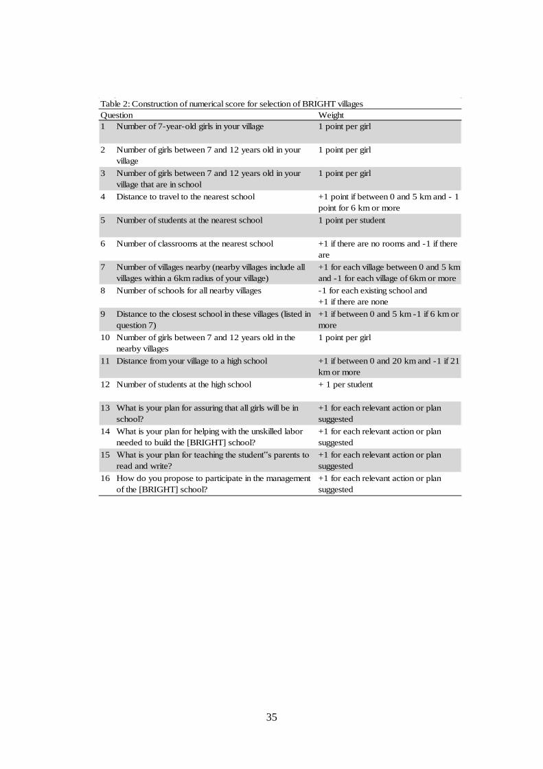
these questions were then used to assign each village a numerical score. Table

2 presents the 16 questions and the weights assigned to these questions to

construct the numerical score.

Within each department, the villages were then ranked based on this

numerical score and those in the top half were selected to receive a BRIGHT

school. In the event of an odd number of villages, the median village did not

15 These provinces are: Banwa, Gnagana, Komandjari, Namentenga, Oudalan, Sanmentenga, Seno, Soum, Tapoa, and Yagha

14

receive a school. Two departments nominated only one village. These villages

were both selected to receive a BRIGHT school. This process generated a set

of 138 villages that should have participated in the BRIGHT program.

However, in the end only 132 of these 138 villages were selected because of

limited funding.

3.4 Data

Mathematica Policy Research, Inc. (MPR) was hired to evaluate the

BRIGHT program. As part of the evaluation, MPR in turn hired a team of

researchers from the University of Ouagadougou to survey households and

schools within the 293 villages that applied to the program. Data were only

collected at the end of the program, there is no baseline available. The dataset

contains data for 287 of the 293 villages. This subsection provides a brief

overview of the data collection efforts.16 The final dataset is publicly available

on the MCC website.17

3.4.1 The Household Survey

The household survey was administered in the spring of 2008. In each

village, 30 households with school-age children (5 to 12 years old) were

randomly selected to be surveyed.18 To develop the village-level household

sampling frame, data collectors first conducted a complete census of

households in each village. In that census, they identified households with

school-age children and collected information about the household’s access to

16 Data for 6 villages are missing for the following reasons: 2 villages could not be located by data collectors (this is likely due to villages whose names differed either because of the dialect or an incorrect spelling recorded on the application form), 2 villages were from the departments that nominated only one village (and are thus are not suitable for regression discontinuity analysis, more details provided below), and finally 2 villages were excluded because no data was available for them (without further explanation). 17 http://www.mcc.gov/pages/countries/impact/impact-evaluation-for-burkina-fasos-threshold-program/burkina-faso-threshold-program 18 Households were defined as a group of persons, living together (in a common physical space), working together under the authority of a person called “head of household” and taking their meals together, or from the same supply of food. The members of household must have lived together in this fashion during at least 9 of the previous 12 months.

15

beasts of burden. Once the sampling frame at the village level was complete, it

was stratified by access to beasts of burden, which served as a proxy for

wealth. Three strata were identified: households who owned at least one beast

of burden, households who did not own but had access to one, and households

who neither owned nor had access to one. This method of stratification was

suggested by researchers at the University of Ouagadougou in order to ensure

a representative household sample, under hypothesis that the means of

production is positively correlated with income. From each of these strata, 10

households were randomly chosen to be surveyed.19 The household survey

was conducted with the head of household or another knowledgeable member

of the household.20 The questionnaire contained one section collecting general

information on the household (religion, ethnicity etc.) and the house in which

it resides (construction materials, water source etc.).

The survey also collected specific information on all 5 to 12 years old

children in the household, including sections on their participation in

education and work. In particular, we use the information on school

enrollment in the 2007-2008 school year, school attendance in the week prior

to the interview, economic activities for someone who is not a member of the

household (either remunerated or not) in the week and year prior to the

interview, economic activities conducted for the household21 in the week prior

to the interview and household chores22. Appendix B reports the questions on

which the variables are based.

19 For each stratum, the selection was done by writing the names of each head of an eligible household on a piece of paper, placing those pieces of paper in a hat, and then drawing 10 names. The selection process was carried out in a public manner in each village. 20 The questionnaire was based on several existing questionnaires widely used in developing countries including the Demographic and Health Survey (USAID), the Multiple Indicator Cluster Survey (UNICEF), and the Living Standards Measurement Study (World Bank). 21 Economic activities for the household include : tending for animals, helping with farming, helping with shopping, or doing other family work (for example in a business or selling goods in the street). 22 Household chores include the following activities: collecting firewood, cleaning, fetching water, and taking care of younger siblings.

16

We also use the results of a mathematics and French test administered

to each of the 5 to 12 year old children in the household as part of the

household survey. The mathematics test contains 11 questions to see whether

children are able to (i) identify written numbers, (ii) count, (iii) say whether

one number is higher or lower than another, (iv) add numbers, and (v) subtract

numbers. The French test contains 8 questions to see whether children can (i)

identify written letters, (ii) read simple words, (iii) read more complicated

words, and (iv) identify a missing word in a sentence.

3.4.2 The School Survey

A school questionnaire was administered in addition to the household

survey in the spring of 2008.23 24 Data collectors first determined the total

number schools, if any, that children from each village attended regularly on

the basis of information provided by the village elders. The three schools

closest to the village center (at a maximum distance of 10 kilometers) were

then selected to be surveyed. A total of 360 schools was identified through this

procedure.

When possible, the school survey was conducted with the school

director. It collected information on the school, its personnel, and (in the

spring 2008 follow-up school survey) on the school attendance of children

identified in the household survey.25 For the latter module, the interviewer

23 A first wave of school surveys was conducted in the fall of 2007, but this paper does not use data from that first wave. 24 Both the household and school questionnaire were first written in English and then translated into French. Since French is rarely spoken in rural villages, the French version of the household questionnaire then had to be translated into many different languages (sixty-eight languages are currently spoken in Burkina Faso). Faced with the prospect of surveying people in so many different languages, MPR determined that the best approach was to hire interviewers fluent in both French and local languages and train them to translate the instrument as they conducted the interview. The questionnaires were piloted in 5 intervention and 5 control villages and adjusted (shortened) according to the findings of the pilot before being implemented. 25 Matching of children identified in the household survey with children in the schools was done while interviewers were in each village. Interviewers first completed the household surveys. They then compiled and populated the school attendance roster with the names of all children identified in the household surveys as being enrolled in a local school. They included

17

conducted a roll-call and noted any absences. In addition, the teachers in the

school were asked “Of the last three days the school was open, how many did

the student attend?” In this paper we use both the roll-call data and the

attendance information obtained from the teachers.

4 Estimation Strategy and Results

4.1 Regression Discontinuity Estimation Strategy

As explained above, villages were assigned to the BRIGHT program

on the basis of a numerical score (henceforth the forcing variable). Within

each department, only the villages ranking in the top half of the distribution

were selected into the BRIGHT program. This assignment procedure

implicitly identifies a threshold in the forcing variable within each department.

We exploit these thresholds in a regression discontinuity framework to

identify the causal effect of the BRIGHT program on child work.26 The

intuition behind the regression discontinuity design is that villages with a

forcing variable just below the threshold score are similar to villages with a

forcing variable just above the threshold. These villages therefore serve as a

valid control group to measure the impact of the BRIGHT program.

Formally, we identify the impact of the BRIGHT program by

estimating the following sharp regression discontinuity equation:

𝑌𝑣𝑖 = 𝛼 + 𝛽𝐷𝑣 + ∑ 𝛾𝑘𝑘≥1 (𝑋𝑣 − 𝑐)𝑘 + ∑ 𝛿𝑘𝑘≥1 𝐷𝑣(𝑋𝑣 − 𝑐)𝑘 + 𝛝𝐙𝐢 + φv + 𝜀𝑖

(1)

the child’s household ID and household listing number on the roster. These identifiers were used later to link the school data to the household data. Once in the school, interviewers used the roster to collect attendance and enrollment information only for those children on that roster. 26 The regression discontinuity approach was first introduced by Thistlethwaite and Campbell (1960) and later formalized by Hahn et al. (2001). Recent advances in the use of regression discontinuity methods are documented by Imbens and Lemieux (2008) and Lee and Lemieux (2010).

18

where 𝑌𝑣𝑖 is the outcome of interest for individual i in village v, 𝛼 is the

intercept, 𝐷𝑣 is a dummy taking the value 1 if a village was selected into the

BRIGHT program (i.e. had a forcing variable score above the implicit

threshold), the term ∑ 𝛾𝑘𝑘≥1 (𝑋𝑣 − 𝑐)𝑘 is a polynomial of order k that

approximates the relationship between the outcome of interest and the distance

of a the village’s forcing variable 𝑋𝑣 from the threshold value c. The

term ∑ 𝛿𝑘𝑘≥1 𝐷𝑣(𝑋𝑣 − 𝑐)𝑘 includes the dummy for selection into the BRIGHT

program 𝐷𝑣 and thus allows for a different functional form of the polynomial

above and below the threshold score. Zi is a vector of individual and

household level control variables and φv represents department fixed effects.

The error term 𝜀𝑖 captures all other determinants of the outcome of interest.

The estimated coefficient 𝛽 gives the average local effect of a village being

selected into the BRIGHT program.

Because the villages are selected into the BRIGHT program at the

department level, the threshold score for participation in the BRIGHT program

differs across departments. Following Levy et al (2009), we normalize forcing

variables across districts by centering the threshold values of each department

at 0.27 We estimate polynomials of orders 1, 2, and 3 and, following Lee and

Lemieux (2010), we use the Akaike information criterion (AIC) to obtain an

indication of the optimal order of the polynomial. We cluster standard errors at

the village level.

The regression discontinuity approach will yield consistent parametric

estimates of BRIGHT’s average treatment effect if the specified polynomial

correctly approximates the relationship between the distance of the village’s

forcing variable from the cutoff scores (𝑋𝑣 − 𝑐) and outcome 𝑌𝑣𝑖.

Misspecification becomes more likely when observations further from the

cutoff score are used. We therefore check for the robustness of the estimated

results within multiple bandwidths around the cutoff scores. We show which

27 This normalization procedure maintains the relative distance of each village score from the threshold.

19

of the presented bandwidths (h) are preferred using the following cross-

validation criterion proposed by Imbens and Lemieux (2008):

𝐶𝑉𝑦(ℎ) = 1𝑛∑ (𝑌𝑣𝑖 − 𝑌�(Xv))2𝑛1

where the preferred bandwidth is given by:

ℎ𝐶𝑉𝑜𝑝𝑡 = 𝑎𝑟𝑔𝑚𝑖𝑛𝐶𝑉𝑦(ℎ).

This cross-validation criterion minimizes the mean squared differences

between actual and estimated outcomes. In doing so, the cross-validation

criterion balances the precision of the estimates (which increases with the

bandwidth) against the bias that may result from using too large a bandwidth.

4.2 Validity of the Regression Discontinuity Approach

The assignment procedure on the basis of the forcing variable, outlined

above, appears to have been executed carefully. Nearly all of the 287 villages

in the data were correctly assigned to the intervention and the control group on

the basis of their forcing variables. Of the 136 villages in the data that should

have received the BRIGHT program only 11 did not receive the intervention.28

Of these 11 villages, 6 were not selected because the program funds were

insufficient and 5 were later discarded because their location proved

inappropriate (for instance because there was no suitable water source).29 Four

villages that should not have been selected were selected. Levy et al (2009)

indicate that the villages that were selected, but should not have been selected,

were the next highest in the ranking within their department. This suggests

28 9 of the latter villages had effective normalized forcing values of 0, i.e. they were at the cutoff point. 29 No information is available to distinguish between the villages discarded for lack of funds and the villages discarded for inappropriate locations.

20

that within these departments the BRIGHT intervention was assigned to the

next highest ranked on the basis of the forcing variable.

Given that the number of incorrectly selected villages is small, we

decided to remove them from the data instead of pursuing a fuzzy regression

discontinuity estimation procedure. (Fuzzy regression discontinuity estimates,

not displayed in this paper but available on request, are very similar to the

results presented below.) We also removed any departments that, as a result of

removing incorrectly selected villages or narrowing the bandwidth, have only

villages above or below the threshold remaining and are therefore not suitable

for regression discontinuity analysis.

The validity of the regression discontinuity approach rests on the

assumption that, except for participation in the BRIGHT program, the

marginal villages (i.e. the villages just above and below the threshold in each

department), were similar at baseline. As the BRIGHT program did not collect

baseline data (other than the information, not available to us, collected through

the application form) a direct test for the similarity of the marginal villages is

not possible. However, we can use the household and school survey data

collected at the end of the program to see if variables that are not likely to be

affected by the program are indeed similar in the marginal villages.30

Table 3 provides the descriptive statistics for a series of observed

household and child characteristics and tests for differences across villages

above and below the threshold. The characteristics considered include the

education, religion and ethnic group of the household head, the age of the

children and their relationship to the household head, the characteristics of the

dwelling and the possession of durable goods. The test is carried out

30 McCrary (2008) proposed to look at the density of the forcing variable around the threshold score to gauge the validity of the regression discontinuity approach. Irregularities in the density could signal that the forcing variable has been manipulated by (potential) beneficiaries, which would invalidate the regression discontinuity design. The McCrary (2008) approach, however, cannot be used for the Burkina Faso BRIGHT data. The reason for this is that threshold scores are only implicitly determined: within each district the forcing variable of the marginal selected village represents the threshold score. As a result, villages are by definition bunched just above the cutoff score.

21

estimating equation (1) for each of the observed characteristics. Estimates are

based on a second order polynomial and are given for 3 different bandwidths

around the threshold score. The estimates do not include any controls other

than the polynomial terms and the department fixed effects.

Overall the estimates suggest that differences between households and

children living in villages just below or just above the threshold score are

limited. Children in the marginal intervention villages are somewhat less

likely to be male and are slightly younger (columns (1), (2), and (3)).

Households in the intervention villages are somewhat less likely to own a

bicycle or an animal cart and somewhat more likely to own a motor cycle

(columns (5), (6), and (7)). The magnitude of these differences is fairly small

and we feel confident that the households in the villages just below the

threshold score serve as a valid control group in the regression discontinuity

analysis presented in this paper.

4.3 Results

4.3.1 Overall Impact on School Participation and Child work

While BRIGHT substantially increased school participation it also

resulted in a modest increase in children’s participation in work. Figures 1 and

2 respectively examine the overall impact of BRIGHT on school participation

and child labour. The horizontal axes of the graphs display the distance of the

village forcing variable to the threshold score for selection into the BRIGHT

program. Negative scores indicate the extent to which the forcing variable falls

short of this cutoff point and vice versa for positive scores. The vertical axes

respectively depict the fraction of children attending school (self-reported) and

the fraction participating in work and chores. Dots depict local averages and

the lines are fitted quadratic regressions.

Figure 1 shows that self-reported school enrollment in the 2007-2008

school year increased substantially as a result of the BRIGHT program. At the

threshold, the proportion of children enrolled in school is approximately 15

22

percentage points higher in BRIGHT villages than in control villages.31 Below

-section 4.3.4 and Table 7- we show that school enrollment and school

attendance figures are virtually identical. Figure 2 shows that the pronounced

increase in school enrollment, is not accompanied by a decrease in children’s

participation in work in the 7 days prior to the interview (where work is

defined as the combination of all economic activities and household chores

identified in the household survey, see Appendix B). Instead, participation in

work appears to increase modestly at the threshold.

Table 4 quantifies these graphical results. For the two outcomes

presented in figures 1 and 2 the table shows estimates of the discontinuity at

the threshold score for polynomials of order 1-3 and for 3 different

bandwidths.32 These estimates by and large confirm the graphical findings.

The probability of being enrolled in school (39% in the overall sample,

column (10)) has increased substantially. Estimates hover between 11 and 17

percentage points. The probability of participating in work (75% in the overall

sample) did not decrease in any of the estimates. If anything, in accordance

with the graphical evidence, the results suggest that there is a modest

(borderline significant) increase in the probability of participating in work.

The program thus generated a substantial increase in school participation

without reducing -in fact even increasing- children’s participation in work.

The following subsections further disentangle and explain this finding.

4.3.2 Disaggregated Impact on School Participation and Child work

Because the content of BRIGHT differed for boys and girls (girls

receive take-home rations conditional on sufficient school attendance, while

boys do not), we assess whether the effects of BRIGHT were different for the

following three groups of children: girls, boys without female siblings, and

31 A similar figure can be found in the original impact evaluation report of the BRIGHT program (see Levy et al, 2009). 32 The regressions in Table 4 (and all following tables) include the household and child characteristics discussed above (in Table 2) as controls.

23

boys with female siblings (who may experience a spillover effect from their

siblings take-home rations).33 Figure 3 shows the impact of BRIGHT on

school participation and work for each of these three subgroups. Panel A of

Table 5 again quantifies these graphical results.34

We observe substantial increases in school participation in all three

subgroups. The increase appears to be somewhat stronger for girls and boys

with female siblings (both around 15 percentage points) than for boys without

female siblings (around 10 percentage points). This finding is consistent with

the fact that girls receive additional benefits and with the hypothesis that these

additional benefits are shared within the household. Child work is not reduced

as a consequence of the increase in school participation. On the contrary, child

work increased substantially for boys without female siblings (7 to 15

percentage points). Girls and boys with female siblings experience no change

or perhaps a modest increase in work (0 to 7 percentage points and not highly

significant).

Panel B shows that the observed changes in school participation are

accompanied by a similar increase in the fraction of children who are both in

school and in work within all three subgroups (roughly 10 to 16 percentage

points). There are three potential explanations for this increase in participation

in both activities: (i) children who were previously working only entered

school without stopping to work, (ii) children who were previously in school

only entered work without quitting school, or (iii) idle children entered both

activities. We now explore these potential explanations in more detail for each

of the three subgroups.35

Among girls, we observe a strong shift from participation in work only

to participation in both activities (11 to 15 percentage points). This figure

33 For brevity, we do not show a table with discontinuities in covariates (similar to table 3) for these 3 subgroups. Those tables, however, are available from the authors on request. 34 We show results for three different bandwidths of second order polynomial regressions, results for different polynomial orders are available on request 35 For brevity we do not show further graphs, but the graphical evidence (available on request) is in accordance with the results in the table.

24

suggests that a substantial number of girls entered school without stopping to

work. Within this subgroup there also appears to have been a modest shift

from participating in none of the activities to participating in both activities (0

to 5 percentage points). Among boys without female siblings we observe the

opposite pattern. They experience a strong decrease in the probability of being

idle (7 to 10 percentage points) and no significant decrease in the probability

of working only. Hence, it appears that many of these boys begin working and

attending school at the same time. Boys with female siblings appear to be

between these two extremes, as they experience both a decrease in the

probability of working only (6 to 11 percentage points) and a decrease in the

probability of being idle (5 to 11 percentage points). There is no compelling

evidence of a change in the proportion of children who only attend school for

any of the three subgroups. The point estimates are sometimes positive,

sometimes negative, and with one exception at the 10% level none of them are

statistically significant.36

Without baseline information it is not possible to conclusively explain

what shifts in activity status explain these findings. However, these results are

in accordance with the theoretical model presented earlier. The model showed

that children who were initially working but not in school may well continue

working when they switch into school as a result of the program. Children

who were previously idle may start working if they switch into school,

depending on the relative changes in the marginal utility of consumption and

leisure.

4.3.3 A Closer Look at the Impact on Child Work

We have just seen that the BRIGHT program increased the school

attendance of working children and the prevalence of work. Now we

investigate whether these changes are accompanied by changes in the kind of

work children are carrying out and in the intensity of child work.

36 Graphical evidence, not displayed here, supports this finding.

25

First, as shown in Table 6, only a comparatively small fraction of the

surveyed children was involved in economic activities for someone who is not

a member of the household in the 7 days prior to the interview. This fraction

was somewhat higher among boys without female siblings (8%) than among

other children (5%). The BRIGHT program did not significantly affect these

proportions, nor did it affect the intensity with which children are engaged in

these activities. Children who were involved in economic activities for

someone who is not a member of the household spent on average 7 to 8 hours

per weeks on this activity and this figure is not discontinuous at the threshold.

The coefficients are sometimes negative and sometimes positive and never

statistically significant. Apparently, children did not alter their participation in

economic activities outside the household in response to BRIGHT and the

changes in child work observed above must take place within the household.

Indeed we find evidence of a discontinuity in participation in work for

the household at the threshold score. A substantial number of children

participated in work for the household in the 7 days prior to the interview

(70% of boys without female siblings, 73% of boys with female siblings, and

78% of girls). In marginal BRIGHT villages boys increased their participation

in these activities. Point estimates range from 7 to 15 percentage points for

boys without female siblings and from 3 to 7 percentage points for boys with

female siblings. Information on working hours is not available for these

activities (section 3 of this paper indicates that these hours are typically

substantial (double digits)). We do have evidence on the number of different

economic activities and chores children conducted for the household in the

week prior to the interview. On average, children who indicated that they

participate in work for the household conducted 2.1 to 2.8 such activities. The

number of activities is again not affected by the BRIGHT program.

Finally, we look at two other indicators of economic activities

conducted for someone not a member of the household: remunerated

economic activities conducted in the 7 days prior to the interview, and

26

economic activities conducted in the year prior to the interview. We find that

virtually none of the children conduct remunerated economic activities in both

control and BRIGHT villages. Approximately 9 to 10% of the children

conducted economic activities for someone who is not a member of the

household in the year prior to the interview. Two of the estimates suggest a

significant negative effect of the BRIGHT program on this outcome. However,

as these estimates exceed the average proportion of children who conducted

economic activities outside the household in the past year, they appear to be

imprecise. The remaining estimates suggest that BRIGHT had no effect on

economic activities outside the household in the year prior to the interview.

Graphic results (not presented here) support the latter finding.

Overall, we conclude that BRIGHT affected primarily the extensive

margin of work conducted for the household. There is no evidence that

BRIGHT increased children’s participation in work outside the household or

that BRIGHT affected the intensive margin of child work.

4.3.4 A Closer Look at the Impact on School Participation

As shown above, the children who enrolled in school as a result of

BRIGHT typically also (started to) work. If the participation in work keeps

these pupils from attending school regularly, we would expect average school

attendance rates to drop in marginal BRIGHT villages. To investigate this

issue, we look at 3 measures of school attendance: self-reported attendance on

the most recent day the school was open, teacher reported attendance in the 3

days prior to the school survey, and presence in school during the roll-call

(each of these measures is, of course, conditional on being enrolled in school).

Table 7 shows that school enrollment is a remarkably good measure of

school attendance. On average, among pupils who indicate that they are

enrolled in school, self-reported attendance on the most recent day school was

open is nearly 100%, teacher reported attendance in the 3 days prior to the

school survey is roughly 3 days, and presence in school during the roll-call is

27

also nearly 100%. This finding holds for all three subgroups of children

considered. Accordingly, we observe virtually no discontinuity in the three

measures of school attendance at the threshold. Given that we have no reason

to doubt the accuracy of the data, we conclude that children who are enrolled

in school (be it in a BRIGHT village or not) attend school regularly.

This result implies that children who enrolled as a response to the

BRIGHT program (of whom the vast majority either continued to work or

started to work) now see their daily activities increase substantially. School

days in Burkina Faso typically last 5 hours (from 7AM until noon). Moreover,

children in the BRIGHT data spend an average of 41 minutes commuting to

and from school. Together these figures imply that, during a typical school

week, children who start attending school as a result of the BRIGHT program

spend over 28 hours on school participation and commuting to and from

school that were previously available for other activities. Children who started

attending school in response to BRIGHT and continued to work or (more

importantly) started to work are, therefore, likely to have substantially reduced

their leisure time.

4.3.5 The Impact of BRIGHT on Pupil Learning

Finally, we investigate the impact of the BRIGHT program on

mathematics and French test Z-scores. To calculate the Z-scores scores we

separately sum the number of correct answers on the mathematics test

(ranging from 0 to 11) and on the French test (ranging from 0 to 8) and then

standardize by subtracting the mean test score and dividing by the standard

deviation. If participation in work keeps pupils from learning in school, we

would expect an impact of BRIGHT on pupil learning primarily among pupils

who are not involved in these activities. To investigate this issue in more

detail, we separate separately test the impact of the BRIGHT program among

pupils who are in school only and among all other pupils.

28

This analysis relies on the assumption that we can compare children

who are in school only for marginal BRIGHT and non-BRIGHT villages. This

assumption seems reasonable, given that we observe no clear discontinuity in

the proportion of children involved only in school at the BRIGHT threshold

(section 4.3.2 and Table 5 Panel B).37 For pupils who are in school only, the

analysis then identifies the pure effect of better learning in school as a result of

the BRIGHT program. For the other children (who are working when in

school), the estimate represents the combined effect of a higher probability of

being in school and of better learning when in school.

Table 8 shows that the BRIGHT program resulted in substantial

improvements in French and mathematics test scores (roughly 0.2 to 0.4

standard deviations) for both subgroups. With one exception at the 10% level,

Chow tests indicate that the improvements of mathematics and French test

scores were similar among children who were in school only and all other

children. We cannot know whether improvements in learning would have been

more pronounced in the latter subgroup if BRIGHT had resulted in larger

decreases in child labour. That being said, the results indicate that integrated

education interventions such as BRIGHT can have a substantial impact on

pupil learning even in settings where a large number of children combine

school participation with work.

5 Conclusion

This paper uses data from Burkina Faso’s BRIGHT program to show

that improving access to education and providing school subsidies does not

always reduce children’s involvement in work, even if it does promote school

attendance. BRIGHT aimed to increase school participation through the

construction of primary schools and the provision of school meals and take-

home rations to female pupils. This paper exploits an index-based assignment

mechanism to identify the impact of the project on school participation and

37 We acknowledge that without baseline data we cannot further substantiate this claim.

29

child work. Our regression discontinuity estimates show that BRIGHT had a

pronounced impact on school participation. However, the program was not

accompanied by a reduction in child work. In fact, consistent with a theoretical

model of children’s time use, instead of preventing children from participating

in work and chores, the interventions slightly increased children’s

participation in productive activities, possibly to finance their participation in

education. The increased school attendance then mainly comes from reduced

leisure.

We decompose this result for three subgroups (girls, boys without

female siblings, and boys with female siblings) and take a closer look at the

interaction between education and work to better understand the limited

impact of the program on school participation. We find that working girls who

enter school as a result of the program do not stop working. We also observe

that some of the boys who were neither working nor attending school begin to

work when the program induces them to enroll in school. Does the increase

and the continued involvement of children in economic activities and

household chores reduce the impact of the program on learning outcomes?

While we cannot answer this answer conclusively, we show that even in the

absence of a reduction in child work, the BRIGHT program substantially

increased the learning outcomes of both working and not working children

attending school.

We conclude that programs that reduce both the time and the monetary

costs of education are not necessarily sufficient to reduce child labour even if

they effectively increase school attendance. If education programs are

implemented to achieve a combination of increased school participation and a

reduction in child work they may either have to be combined with different

interventions that effectively reduce child work or they may have to be tuned

more carefully to the incentives and constraints the child laborer faces.

30

Appendix A: The BRIGHT Program

In 2005, the BRIGHT program started to implement an integrated

package of interventions in each of the 132 villages. This appendix provides a

detailed description of the implemented interventions:

1. A primary school was constructed in each of the 132 BRIGHT

villages. These schools were built according to a prototype with three

classrooms, two multipurpose halls, one office, and one storage room.

Construction also included teachers’ lodgings situated close to the

school, with two bedrooms, one living room, one kitchen, and one

bathroom (latrine). BRIGHT provided each school with a borehole,

equipped with a manual pump easy to use by children. Separate latrine

blocks were built for girls and boys to ensure privacy and security.

Schools also received equipment, including student desks, teacher

desks, chairs, metal bookshelves, and playground equipment. Child

care centers were constructed in 10 of the 132 school complexes. The

construction work started around October 2006. By April 2007 most of

the schools had been constructed.

2. In all BRIGHT schools, daily meals were offered to pupils (boys and

girls) via a canteen. For both the schools and the child care centers, the

monthly ration consisted of 5 kilograms of rice and 0.5 liter of oil per

child.

3. Girls who achieved a 90-percent rate of school attendance received a

monthly ration of 8 kilograms of dry rice to take home.

4. For the 2006–2007 school year, the project purchased and distributed

school kits for first and second grade classes. That year, however,

textbooks were not widely available. As a result, only 2,500 second

grade textbooks were distributed. In 2007–2008, the government

provided all schools, including BRIGHT schools, with kits and

textbooks.

31

5. A wide range of activities that sought to change socio-cultural

behaviors presenting obstacles to girls’ school enrollment, retention,

and achievement was implemented over the course of the program. The

purpose of these activities was to bring together communities and those

with a stake in the education system to discuss the issues involved in,

and barriers to, girls’ education. The activities included informational

meetings; door-to-door canvassing; gender-sensitivity training for

ministry officials, pedagogical inspectors, teachers, and community

members; a girls’ education day; radio broadcasts; posters; and awards

for female teachers. In the first year (school year 2006–2007), 33

selected communities benefited from the campaign. During the second

project year (school year 2007–2008), the same activities were carried

out in the remaining 99 communities and new activities were initiated

for all 132 communities.

6. The program provided literacy training to adult females and mentoring

to girl students. The rationale behind the literacy training was to

provide uneducated mothers with non-formal education (literacy and

micro-project management training) to help them prioritize their girls’

education. Mentoring was meant to help girls and their families

envision a productive future by providing them with female role

models who could set examples of the benefits of education and

encourage and support them during their school careers. In the first

project year, 254 literacy centers were opened and recruited trainees.

Ten centers did not open, or were closed shortly after opening, due to

lack of interest.

7. Finally, the program included capacity building in the form of training

provided to local officials in the Ministry of Education, child care

center monitors, and teachers. The capacity building included training

on completion of school registers.

32

Appendix B: Questions from Household Survey

This appendix reproduces the questions from the household and school

survey used to define the outcome variables of this study. Two questions were

used from the household survey education section:

• During the 2007-2008 school year has (name) attended school or

preschool at any time?

• Did (name) attend school on the most recent day school was open?

Eleven questions were used from the household survey child labour section:

• During the past week, did (name) do any kind of work for someone

who is not a member of this household? (if yes: for pay in cash or

kind?)

• Since last (day of the week), about how many hours did he/she do

this work for someone who is not a member of this household? (if

more than one job, include all hours at all jobs.)

• At any time during the past year, did (name) do any kind of work for

someone who is not a member of this household?

• During the past week, did (name) help with collecting firewood?

• During the past week, did (name) help with cleaning?

• During the past week, did (name) help with fetching water?

• During the past week, did (name) help with taking care of younger

siblings?

• During the past week, did (name) help tend animals?

• During the past week, did (name) help with farming?

• During the past week, did (name) help with shopping?

• During the past week, did (name) do any other family work (in a

business or selling goods in the street?)

Finally, one question was used from the school survey:

• “Of the last three days the school was open, how many did the

student attend?”

33

References

Cigno, A. and F. C. Rosati (2005). The Economics of Child Labour,

Oxford University Press

Edmonds, E. (2007). “Child Labor” ,in T. P. Schultz and J. Strauss,

eds., Handbook of Development Economics, Volume 4 (ElsevierScience,

Amsterdam, North-Holland)

Hahn, J., P. Todd, and W. Van der Klaauw (2001). “Identifcation and

Estimation of Treatment Effects with a Regression Discontinuity Design.”

Econometrica, 69 (1), 201-209.

Imbens, G. W. and T. Lemieux (2008). “Regression Discontinuity

Designs: A Guide to Practice.” Journal of Econometrics, 142 (2), 615-635.

Kazianga, H., D. de Walque,, and H. Alderman (2008). “Educational

and Health Impact of Two School Feeding Schemes: Evidence from a

Randomized Trial in Burkina Faso.” Working Paper.

Kondylis, F. and M. Manacorda (2012). “School Proximity and Child

Labor: Evidence from Rural Tanzania.” Journal of Human Resources, 47 (1),

32-63.

Lee, D. S. and T. Lemieux (2010). “Regression Discontinuity Designs

in Economics.” Journal of Economic Literature, 48, 281-355.

Levy, D., M. Sloan, L. Linden, and H. Kazianga (2009). Impact

Evaluation of Burkina Faso’s Bright Program: Final Report, Mathematica

Policy Research, Inc., Washington D.C., USA.”

McCrary, J. (2008). “Manipulation of the Running Variable in the

Regression Discontinuity Design. ” Journal of Econometrics, 142 (2), 698-

714.

Ravallion, M. and Q. Wodon (2000). “Does Child Labour Displace

Schooling? Evidence on Behavioural Responses to an Enrollment Subsidy.”

Economic Journal, 110 (462), C158-C175.

34

Thistlethwaite, D. L. and D. T. Campbell (1960). “Regression-

Discontinuity Analysis: An Alternative to the Ex-Post Facto Experiment.”

Journal of Educational Psychology, 51, 309-317.

Tables

Table 1: Predicted changes in work statusΔ school participation Initial work status Δ work status

(1) (2) (3)Stay out of school Not working 0

Working 0Stay in school Not working +

Working -Switch into school Not working +

Working -Column (1) gives the change in school participation as a result of the reduction in costs of education. Column (2) represents the work status of the child in absence of the reduction in the cost of education. Finally, column (3) shows the change in work status with a reduction in the cost of education: - = non-positive change, 0 = no change, + = non-negative change.

35

Table 2: Construction of numerical score for selection of BRIGHT villagesQuestion Weight1 Number of 7-year-old girls in your village 1 point per girl

2 Number of girls between 7 and 12 years old in your village

1 point per girl

3 Number of girls between 7 and 12 years old in your village that are in school

1 point per girl

4 Distance to travel to the nearest school +1 point if between 0 and 5 km and - 1 point for 6 km or more

5 Number of students at the nearest school 1 point per student

6 Number of classrooms at the nearest school +1 if there are no rooms and -1 if there are

7 Number of villages nearby (nearby villages include all villages within a 6km radius of your village)

+1 for each village between 0 and 5 km and -1 for each village of 6km or more

8 Number of schools for all nearby villages -1 for each existing school and+1 if there are none

9 Distance to the closest school in these villages (listed in question 7)

+1 if between 0 and 5 km -1 if 6 km or more

10 Number of girls between 7 and 12 years old in the nearby villages

1 point per girl

11 Distance from your village to a high school +1 if between 0 and 20 km and -1 if 21 km or more

12 Number of students at the high school + 1 per student

13 What is your plan for assuring that all girls will be in school?

+1 for each relevant action or plan suggested

14 What is your plan for helping with the unskilled labor needed to build the [BRIGHT] school?

+1 for each relevant action or plan suggested

15 What is your plan for teaching the student‟s parents to read and write?

+1 for each relevant action or plan suggested

16 How do you propose to participate in the management of the [BRIGHT] school?

+1 for each relevant action or plan suggested

36

Table 3: Discontinuities in covariatesBandwidth 100 250 500 Mean Bandwidth 100 250 500 Mean

(1) (2) (3) (4) (5) (6) (7) (8)Characteristics of the household head Characteristics of the houseMale 0.006 0.018 -0.011 0.978 Floor natural 0.028 -0.027 -0.010 0.943

(0.010) (0.011) (0.009) (0.029) (0.024) (0.019)Not educated -0.042 0.003 -0.001 0.891 Floor rudimentary 0.009 0.012* 0.003 0.007

(0.044) (0.029) (0.024) (0.007) (0.007) (0.006)Muslim -0.182* -0.045 -0.030 0.593 Floor finished -0.034 0.020 0.011 0.047

(0.100) (0.062) (0.056) (0.028) (0.024) (0.018)Christian -0.016 -0.006 -0.011 0.133 Roof natural 0.126 -0.051 0.029 0.579

(0.080) (0.040) (0.034) (0.140) (0.084) (0.063)Animist 0.186** 0.050 0.044 0.264 Roof rudimentary -0.127 0.038 -0.020 0.305

(0.077) (0.051) (0.046) (0.150) (0.090) (0.067)Moore (mother tongue) -0.119 -0.028 -0.027 0.365 Roof finished 0.001 0.016 -0.008 0.112

(0.159) (0.082) (0.061) (0.060) (0.036) (0.029)Fulfude (mother tongue) 0.002 0.049 0.063 0.203

(0.153) (0.075) (0.055) Durable goods and cattle owned by the householdGulmachema (mother tongue) -0.044 -0.051 -0.057 0.287 Radio -0.098 -0.001 0.012 0.563

(0.082) (0.060) (0.050) (0.061) (0.047) (0.039)Mossi (ethnicity) -0.127 -0.035 -0.036 0.372 Mobile phone -0.055 0.024 0.013 0.138

(0.159) (0.082) (0.062) (0.039) (0.031) (0.023)Peul (ethnicity) -0.006 0.037 0.051 0.189 Watch -0.123 0.031 -0.012 0.587

(0.152) (0.073) (0.053) (0.090) (0.056) (0.045)Gourmanche (ethnicity) -0.027 -0.021 -0.028 0.296 Bicycle -0.131** -0.078* -0.081** 0.859

(0.083) (0.059) (0.049) (0.066) (0.044) (0.035)Motor cycle -0.060 0.053* 0.035 0.210

Characteristics of the child (0.042) (0.028) (0.023)Male -0.030 -0.041** -0.036** 0.531 Animal cart -0.202** -0.026 -0.050 0.444

(0.034) (0.018) (0.014) (0.095) (0.056) (0.042)Age (years) 0.210 0.146* 0.151** 8.118 Cattle -0.163* -0.002 -0.030 0.652

(0.129) (0.079) (0.071) (0.083) (0.054) (0.044)Son or daughter of head -0.019 -0.034 -0.030 0.889

(0.028) (0.022) (0.019)Observations: villages (clusters) 130 212 248 271 Observations: villages (clusters) 130 212 248 271Observations: households 3,830 6,263 7,219 7900 Observations: households 3,830 6,263 7,219 7900Observations: children 9,605 15,917 18,370 20289Notes: *** p<0.01, ** p<0.05, * p<0.1. Estimated discontinuities in covariates that we expect to be unaffected by the BRIGHT program. All estimates are based on a second order polynomial and include department fixed effects. Standard errors (in parentheses) are clustered at the village level. Means are calculated for the unrestricted sample of 271 villages.

37

Table 4: Overall impact: discontinuities in the proportion of children enrolled in school and participating in economic activities and / or choresBandwidth 100 100 100 250 250 250 500 500 500Polynomial 1 2 3 1 2 3 1 2 3 Mean

(1) (2) (3) (4) (5) (6) (7) (8) (9) (10)0.133*** 0.125* 0.114 0.136*** 0.159*** 0.119** 0.169*** 0.125*** 0.141*** 0.388(0.042) (0.065) (0.092) (0.031) (0.042) (0.058) (0.028) (0.035) (0.047)

AIC 10,555 10,545 10,549 17,761 17,755 17,744 20,591 20,565 20,563CVC 0.1726 0.1725 0.1725 0.1783 0.1780 0.1780 0.1789 0.1788 0.1786

0.053 0.023 0.025 0.069*** 0.033 0.073 0.010 0.072** 0.036 0.748(0.033) (0.053) (0.074) (0.026) (0.035) (0.045) (0.023) (0.029) (0.035)

AIC 9,351 9,346 9,337 15,203 15,190 15,186 17,651 17,574 17,556CVC 0.1589 0.1589 0.1585 0.1595 0.1593 0.1592 0.1599 0.1594 0.1592Observations: children 9,605 9,605 9,605 15,917 15,917 15,917 18,370 18,370 18,370 20289

Enrolled in school (2007-2008 school year).

Participating in work in 7 days prior to interview.

Notes: *** p<0.01, ** p<0.05, * p<0.1. Estimated discontinuities in the proportion of children enrolled in school and participating in economic activities and / or in chores at the threshold scores. All estimates include department fixed effects and include the variables displayed in table 2 as controls. Standard errors (in parentheses) are clustered at the village level. Means are calculated for the unrestricted sample of 271 villages.

38

Table 5: Disaggregated impact: discontinuities in the proportion of children enrolled in school and participating in economic activities and / or choresSubgroupBandwidth 100 250 500 Mean 100 250 500 Mean 100 250 500 Mean

(1) (2) (3) (4) (5) (6) (7) (8) (9) (10) (11) (12)Panel A: Shifts in school enrollment and work

0.123* 0.180*** 0.154*** 0.397 0.071 0.126** 0.109** 0.376 0.170*** 0.157*** 0.107*** 0.382(0.070) (0.047) (0.040) (0.073) (0.051) (0.044) (0.066) (0.046) (0.039)

CVC 0.1716 0.1752 0.1757 0.1577 0.1632 0.1654 0.1725 0.1780 0.1788-0.013 0.017 0.050* 0.778 0.073 0.097** 0.154*** 0.705 0.039 0.032 0.074* 0.729(0.056) (0.037) (0.030) (0.061) (0.047) (0.038) (0.062) (0.039) (0.038)

CVC 0.1391 0.1361 0.1352 0.1523 0.1529 0.1581 0.1591 0.1593 0.1594Panel B: Explanation of overall shift:In both activities 0.111* 0.162*** 0.158*** 0.311 0.059 0.150*** 0.161*** 0.248 0.100* 0.137*** 0.126*** 0.263

(0.065) (0.042) (0.037) (0.064) (0.044) (0.038) (0.059) (0.041) (0.035)CVC 0.1613 0.1642 0.1633 0.1411 0.1399 0.1382 0.1485 0.1529 0.1538

-0.125 -0.145*** -0.107** 0.468 0.014 -0.053 -0.008 0.457 -0.061 -0.105** -0.052 0.465(0.083) (0.053) (0.043) (0.084) (0.060) (0.050) (0.071) (0.051) (0.045)

CVC 0.2122 0.2134 0.2133 0.2024 0.2027 0.2049 0.2115 0.2158 0.2168Enrolled in school only 0.012 0.018 -0.003 0.086 0.013 -0.024 -0.052* 0.129 0.070 0.020 -0.018 0.119

(0.028) (0.023) (0.018) (0.036) (0.033) (0.027) (0.052) (0.031) (0.027)CVC 0.0657 0.0680 0.0689 0.0786 0.0855 0.0910 0.0929 0.0941 0.0940In neither activity 0.002 -0.035 -0.047** 0.136 -0.086 -0.073** -0.101*** 0.167 -0.109* -0.052* -0.055** 0.152

(0.043) (0.025) (0.020) (0.053) (0.033) (0.028) (0.056) (0.030) (0.024)CVC 0.0904 0.0864 0.0843 0.0979 0.0998 0.0993 0.0948 0.0946 0.0934Observations: children 4,453 7,491 8,611 9517 1,784 2,826 3,306 3584 3,368 5,600 6,453 7188Notes: *** p<0.01, ** p<0.05, * p<0.1. Estimated discontinuities in the proportion of children enrolled in school and participating in economic activities and / or in chores at the threshold scores. All estimates are based on a second order polynomial and include department fixed effects and the variables displayed in table 2 as controls. Standard errors (in parentheses) are clustered at the village level. Means are calculated for the unrestricted sample of 271 villages.

Girls Boys without female siblings Boys with female siblings

Enrolled in school (2007-2008 school year).

Participating in work only

Participating in work in 7 days prior to interview.

39

Table 6: Economic activities and or choresSubgroupBandwidth 100 250 500 Mean 100 250 500 Mean 100 250 500 Mean

(1) (2) (3) (4) (5) (6) (7) (8) (9) (10) (11) (12)-0.024 0.023 0.012 0.052 0.020 0.026 0.001 0.075 -0.031 0.020 0.012 0.051(0.031) (0.026) (0.020) (0.043) (0.038) (0.033) (0.030) (0.025) (0.019)

CVC 0.0335 0.0445 0.0413 0.0545 0.0641 0.0599 0.0381 0.0425 0.0404-3.056 -0.397 0.204 5.234 3.948 -0.316 0.591 6.461 2.349 -0.112 0.018 6.564(2.422) (0.968) (1.001) (3.108) (1.340) (1.195) (1.478) (1.142) (0.964)

CVC 5.9773 7.9055 8.0269 6.7110 10.4493 10.3251 9.4535 10.8877 10.4986-0.002 0.017 0.049 0.775 0.070 0.084* 0.146*** 0.695 0.057 0.030 0.071* 0.725(0.062) (0.039) (0.031) (0.064) (0.048) (0.039) (0.067) (0.040) (0.038)

CVC 0.1406 0.1378 0.1365 0.1539 0.1552 0.1601 0.1601 0.1605 0.1606-0.231 -0.124 -0.022 2.820 0.165 0.193 0.233 2.100 0.027 -0.255 -0.067 2.268(0.288) (0.196) (0.166) (0.403) (0.231) (0.202) (0.343) (0.236) (0.206)

CVC 3.1104 3.2746 3.2969 2.8283 2.9535 2.9649 3.1894 3.3151 3.35990.005* 0.007* 0.003 0.006 -0.001 0.005 -0.000 0.010 -0.016 -0.001 -0.001 0.006(0.003) (0.004) (0.003) (0.008) (0.009) (0.008) (0.014) (0.006) (0.005)

CVC 0.0022 0.0057 0.0053 0.0059 0.0106 0.0091 0.0054 0.0064 0.0058-0.112** 0.026 -0.014 0.087 0.007 0.057 0.019 0.100 -0.149*** 0.009 -0.014 0.091(0.050) (0.035) (0.025) (0.073) (0.048) (0.038) (0.057) (0.041) (0.029)

CVC 0.0686 0.0766 0.0718 0.0755 0.0850 0.0796 0.0751 0.0787 0.0745Observations: children 4,453 7,491 8,611 9517 1,784 2,826 3,306 3584 3,368 5,600 6,453 7188Observations: children (hours in economic activities) 181 434 453 488 125 240 258 268 155 311 334 366

Number of economic activities and choresconducted for the household (7 days prior to the interview).

Remunerated economic activities for someone who is not a member of the household (7 days prior to the interview).

Economic activities for someone who is not a member of the household (year prior to the interview).

Notes: *** p<0.01, ** p<0.05, * p<0.1. Estimated discontinuities at the threshold scores. All estimates are based on a second order polynomial and include department fixed effects and the variables displayed in table 2 as controls. Standard errors (in parentheses) are clustered at the village level. Means are calculated for the unrestricted sample of 271 villages.

Girls Boys without female siblings Boys with female siblings

Economic activities for someone who is not a member of the household (7 days prior to the interview).

Participation in economic activities or chores for the household (7 days prior to the interview).

Hours in economic activities for someone who is not a member of the household (7 days prior to the interview).

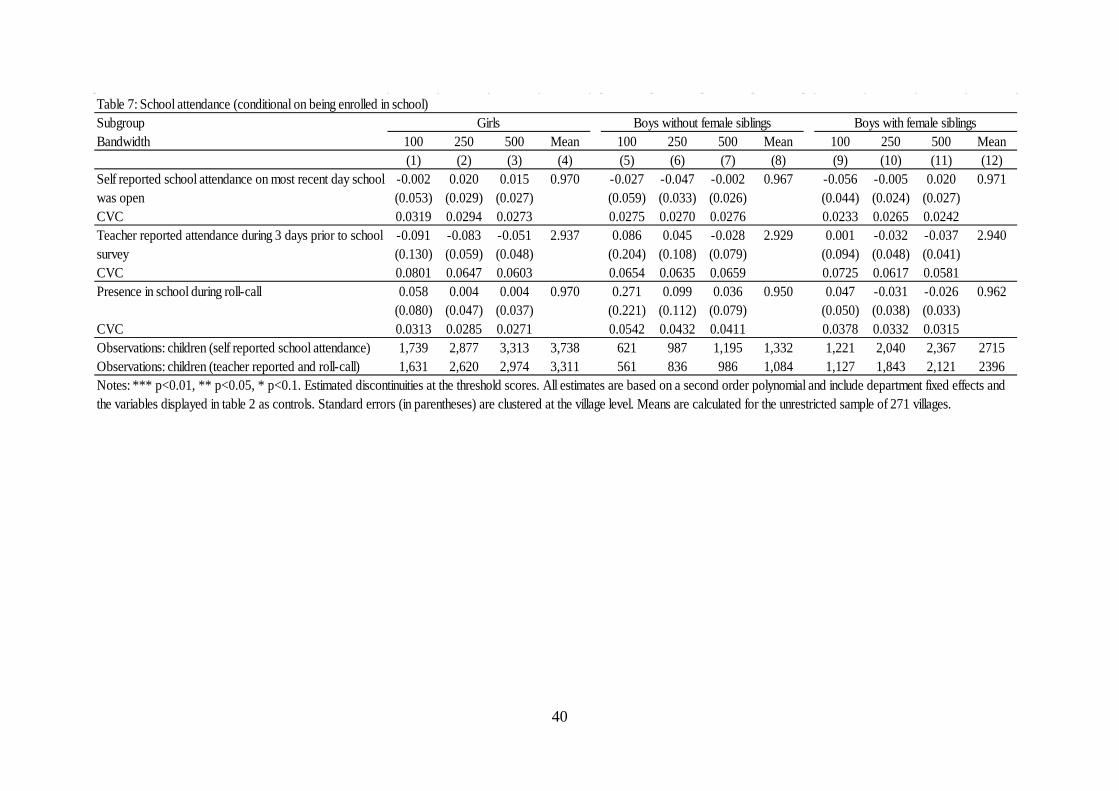
40

Table 7: School attendance (conditional on being enrolled in school)SubgroupBandwidth 100 250 500 Mean 100 250 500 Mean 100 250 500 Mean

(1) (2) (3) (4) (5) (6) (7) (8) (9) (10) (11) (12)-0.002 0.020 0.015 0.970 -0.027 -0.047 -0.002 0.967 -0.056 -0.005 0.020 0.971(0.053) (0.029) (0.027) (0.059) (0.033) (0.026) (0.044) (0.024) (0.027)

CVC 0.0319 0.0294 0.0273 0.0275 0.0270 0.0276 0.0233 0.0265 0.0242-0.091 -0.083 -0.051 2.937 0.086 0.045 -0.028 2.929 0.001 -0.032 -0.037 2.940(0.130) (0.059) (0.048) (0.204) (0.108) (0.079) (0.094) (0.048) (0.041)

CVC 0.0801 0.0647 0.0603 0.0654 0.0635 0.0659 0.0725 0.0617 0.05810.058 0.004 0.004 0.970 0.271 0.099 0.036 0.950 0.047 -0.031 -0.026 0.962

(0.080) (0.047) (0.037) (0.221) (0.112) (0.079) (0.050) (0.038) (0.033)CVC 0.0313 0.0285 0.0271 0.0542 0.0432 0.0411 0.0378 0.0332 0.0315Observations: children (self reported school attendance) 1,739 2,877 3,313 3,738 621 987 1,195 1,332 1,221 2,040 2,367 2715Observations: children (teacher reported and roll-call) 1,631 2,620 2,974 3,311 561 836 986 1,084 1,127 1,843 2,121 2396Notes: *** p<0.01, ** p<0.05, * p<0.1. Estimated discontinuities at the threshold scores. All estimates are based on a second order polynomial and include department fixed effects and the variables displayed in table 2 as controls. Standard errors (in parentheses) are clustered at the village level. Means are calculated for the unrestricted sample of 271 villages.

Girls Boys without female siblings Boys with female siblings

Self reported school attendance on most recent day school was open

Teacher reported attendance during 3 days prior to school survey

Presence in school during roll-call

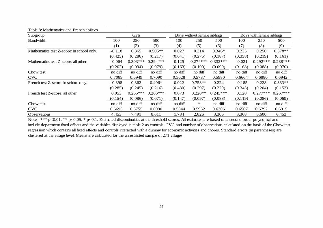
41

Table 8: Mathematics and French abilitiesSubgroupBandwidth 100 250 500 100 250 500 100 250 500

(1) (2) (3) (4) (5) (6) (7) (8) (9)-0.118 0.365 0.505** 0.027 0.314 0.346* 0.235 0.250 0.378**(0.425) (0.286) (0.217) (0.641) (0.275) (0.187) (0.358) (0.219) (0.161)-0.064 0.303*** 0.294*** 0.125 0.274*** 0.332*** -0.021 0.292*** 0.288***(0.202) (0.094) (0.079) (0.163) (0.100) (0.090) (0.168) (0.088) (0.070)

Chow test: no diff no diff no diff no diff no diff no diff no diff no diff no diffCVC 0.7089 0.6949 0.7090 0.5628 0.5737 0.5980 0.6664 0.6880 0.6942

-0.398 0.362 0.406* 0.022 0.758** 0.224 -0.185 0.228 0.333**(0.285) (0.245) (0.216) (0.480) (0.297) (0.229) (0.345) (0.204) (0.153)0.053 0.265*** 0.266*** 0.073 0.220** 0.245*** 0.128 0.277*** 0.267***

(0.154) (0.086) (0.071) (0.147) (0.097) (0.088) (0.119) (0.086) (0.069)Chow test: no diff no diff no diff no diff * no diff no diff no diff no diffCVC 0.6695 0.6755 0.6990 0.5344 0.5932 0.6306 0.6507 0.6792 0.6915Observations 4,453 7,491 8,611 1,784 2,826 3,306 3,368 5,600 6,453

French test Z-score: all other

Notes: *** p<0.01, ** p<0.05, * p<0.1. Estimated discontinuities at the threshold scores. All estimates are based on a second order polynomial and include department fixed effects and the variables displayed in table 2 as controls. CVC and number of observations calculated on the basis of the Chow test regression which contains all fixed effects and controls interacted with a dummy for economic activities and chores. Standard errors (in parentheses) are clustered at the village level. Means are calculated for the unrestricted sample of 271 villages.

Girls Boys without female siblings Boys with female siblings

Mathematics test Z-score: in school only.

Mathematics test Z-score: all other

French test Z-score: in school only.

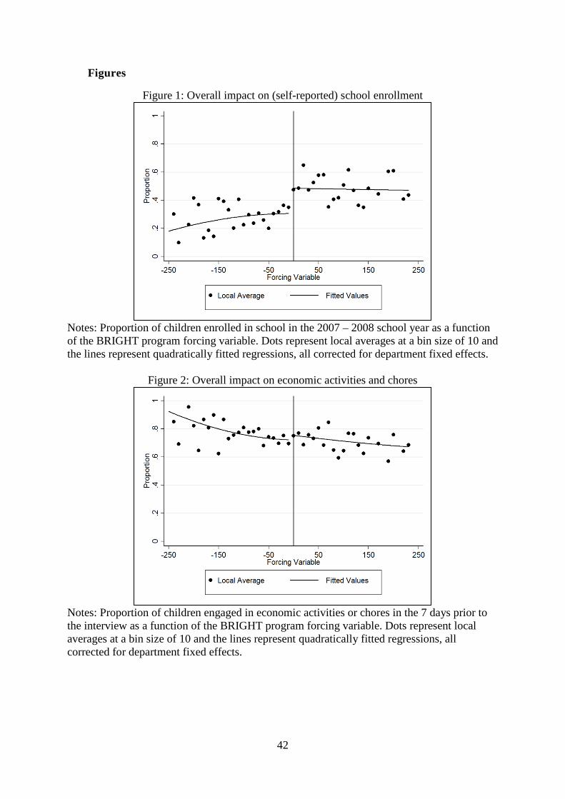
42

Figures

Figure 1: Overall impact on (self-reported) school enrollment

Notes: Proportion of children enrolled in school in the 2007 – 2008 school year as a function of the BRIGHT program forcing variable. Dots represent local averages at a bin size of 10 and the lines represent quadratically fitted regressions, all corrected for department fixed effects.

Figure 2: Overall impact on economic activities and chores

Notes: Proportion of children engaged in economic activities or chores in the 7 days prior to the interview as a function of the BRIGHT program forcing variable. Dots represent local averages at a bin size of 10 and the lines represent quadratically fitted regressions, all corrected for department fixed effects.

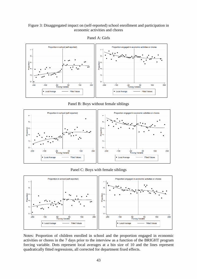
43

Figure 3: Disaggregated impact on (self-reported) school enrollment and participation in economic activities and chores

Panel A: Girls

Panel B: Boys without female siblings

Panel C: Boys with female siblings

Notes: Proportion of children enrolled in school and the proportion engaged in economic activities or chores in the 7 days prior to the interview as a function of the BRIGHT program forcing variable. Dots represent local averages at a bin size of 10 and the lines represent quadratically fitted regressions, all corrected for department fixed effects.