Embed Size (px)
Citation preview
INDUSTRIAL PRODUCTION MODELS
A THEORETICAL STUDY
BY
SVEN DAN" PROFESSOR OF MANAGERIAL ECONOMICS
UNIVERSITY OF COPENHAGEN
WITH 71 FIGURES
1966
SPRINGER·VERLAG
WIEN . NEW YORK
ISBN-13: 978-3-7091-8142-3 e-ISBN-13: 978-3-7091-8140-9 DOl: 10.1007/978-3-7091-8140-9
AIle Rechte, insbesondere das der tJbersetzung in fremde Sprachen, vorbehalten. Ohne schriftliche Genehmigung des Verlages ist es auch nicht gestattet,
diesea Buch oder Teile daraus auf photomechanischem Wege (Photokopie, Mikrokopie) oder sonstwie zu vervieHiltigen.
Library of Congress Catalog Card Number: 66-15847
© 1966 by Springer-VerlagjWien
Softcover reprint of the hardcover 1st edition 1966
Titel-Nr.9172
In grateful memory of
FREDERIK ZEUTHEN
Preface
This book is a result of many years' interest in the economic theory of production, first aroused by the reading of Professor ERICH SCHNEIDER'S classic Theorie der Produktion. A grant from the Danish-Norwegian Foundation made it possible for me to spend six months at the Institute of Economics, University of Oslo, where I became acquainted with Professor RAGNAR FRISCH'S penetrating pioneer works in this field and where the plan of writing the present book was conceived. Further studies as a Rockefeller fellow at several American universities, especially an eight months' stay at the Harvard Economic Research Project, and a visit to the Unione Industriale di Torino have given valuable impulses. For these generous grants, and for the help and advice given by the various institutions I have visited, I am profoundly grateful.
My sincere thanks are also due to the University of Copenhagen for the exceptionally favourable working conditions which I have enjoyed there, and to the Institute of Economics-especially its director, Professor P. N0RREGAARD RASMUSsEN-for patient and encouraging interest in my work. I also wish to thank the Institute's office staff, Miss G. SUENSON and Mrs. G. STEN0R, for their constant helpfulness, and Mrs. E. HAUGEBO for her efficient work in preparing the manuscript, which was completed in the spring of 1965.
Finally, I am indebted to The University of Chicago Press (as publisher of the Journal of Political Economy) and the Harvard University Press for permission to quote from various books and articles, and to Professor HOLLIS B. CHENERY, who has kindly allowed me to quote material from his unpublished doctor's thesis.
Copenhagen, April, 1966 SVEN DAN0
Contents
Preface
Chapter I. Introduction 1. Entrepreneurial Behaviour and Optimization Models 2. Input-Output Relationships . . . . . . . .
Chapter II. Some Fundamental Concepts 1. Production and the Concept of a Process 2. The Variables: Inputs and Outputs 3. The Technological Relations: The Production Function 4. Efficient Production and Economic Optimization . . .
Chapter III. Linear Production Models and Discontinuous Factor SuJastitution
A. Limitational Inputs and Fixed Coefficients of Production
B. Discontinuous Substitution: The Linear Production Model 1. The Production Relations. 2. Optimization Problems
C. Discontinuities in General . .
Chapter IV. Production Functions with Continuous Factor Suhstitution
A. Factor Substitution and the Isoquant Map. . . . 1. The Region of Substitution . . . • . . . . . 2. Returns to Scale and Elasticities of Production 3. The Convexity .Assumption . . . . . . 4. The Elasticity of Substitution. . . • .
B. Production Curves and Diminishing Returns
C. An Alternative Model . . . . . . .
D. Cost Minimization . . . . . . . . 1. Marginal Equilibrium Conditions 2. Boundary Minima ...... .
E. The Expansion Path and the Cost Function
F. The Optimum Level of Output . . . . . .
Chapter V. More Complex Models
A. Substitution with Shadow Factors 1. "Product Shadows" . 2. "Factor Shadows" . .
B. Constrained Substitution
C. Complementary Groups of Substitutional Inputs
Palle
V
1 1 2
5 5 6
10 12
16
16
23 23 31
43
46
46 46 50 52 57
59
63
66 66 74
82
89
97
97 97
100
103
103
VIII
Chapter VI.
Contents
The General Single-Product Model . Page
106
Chapter VII. Divisibility, Returns to Scale, and the Shape or the Cost Function 109
A. Fixed Factors and the Production Function
B. The Dimensions of Capacity Utilization 1. Spatial Divisibility. . . . . . 2. The Time Dimension ..... 3. Divisibility in Space and Time
C. Cyclic Processes . . . . . . . .
D. The Relevance of the U-Shaped Marginal Cost Curve
Chapter VIII. Product Quality and the Production Function
A. Product Quality in the Theory of Production. .
B. Quality Parameters in the Production Function
C. Quality Constraints . . . . . . . . . . . . . 1. Quality Functions and the Production Function 2. Quality Con~traints in Blending Processes
Chapter IX. Plant and Process Production Models
A. Process Interdependencies and Optimization •
B. Vertical Integration of Processes . . . . . . 1. A Sequence of Processes with Continuous Substitution 2. Problems of Suboptimization . . . . . . 3. Other Examples of Vertical Integration
C. Integration of Parallel Sequences of Processes
Chapter X. Multi-Product Models . . . . . .
A. Alternative Processes and Joint Production
B. Alternative Processes . 1. Process Additivity. . . 2. Linear Models ..... 3. Continuous Substitution
C. Multi-Product Processes . . 1. Joint Production and Cost Allocation 2. Fixed Output Proportions . . . . . 3. Linear Models. . . . . . . • . . . 4. Continuous Product and Factor Substitution 5. Shadow Products . . . . . . . . 6. The General Joint-Production Model
Appendix 1. Constrained Maximization ..
A. Lagrange's Method of Undetermined Multipliers
B. Linear Programming and the Simplex Criterion •
C. Non-Linear Programming and the Kuhn-Tucker Conditions
109
111 111 115 122
123
129
132
132
134
137 137 143
148
148
149 149 151 156
162
166
166
168 168 168 176
181 181 181 182 183 188 189
190
190
193
200
Appendix 2_ Homogeneous Production Functions and the Law or Variable Proportions 205
References . 215
Index eo :- 218
Chapter I
Introduction
1. Entrepreneurial Behaviour and Optimization Models
The central subject of economic science is the allocation of scarce resources. From this point of view the main body of economic theory falls into two parts: the theory of production, which deals with problems of allocation in production, and the theory of consumption or demand.
The economic theory of production, therefore, is as old as economics itself. The modern approach to problems of allocation in production dates back to the Ricardian analysis of income distribution. The subsequent introduction of marginal analysis, a mode of thinking which was embryonically present in RIOARDO'S distribution model although he did not explicitly apply differential calculus, prepared the way for the neoclassical theory of the firm with its later developments and also made possible the application of such concepts as aggregated production functions, marginal productivities, etc. in theories of income distribution, economic growth, and other fields of macroeconomic analysis.
In microeconomics, the theory of production is often defined in a broad sense as identical with the theory of the firm. Its purpose is to describe and explain entrepreneurial behaviour, usually in terms of an optimization model where some objective function (e.g. the profit function), which by hypothesis is the criterion of preference underlying the decisions of the firm, is maximized subject to the technological and market restrictions on the firm's behaviour.
For example, the familiar short-run cost function for a single-product firm in a competitive market is derived from the hypothesis that the firm minimizes total cost-i.e., maximizes profit-for each particular level of output with the production function as a side condition; the optimal level of output is then determined by maximizing revenue minus cost. (Alternatively, the solution may be determined in one step without using explicitly the concept of the cost function, maximizing profit subject to the production function). This procedure solves the allocation problem-how much to produce, and by what combination of inputs-for a given set of prices; moreover, by examining the response of the equilibrium position to changes in product price and factor prices respectively, we can trace the firm's supply curve for the product and the demand function for each input.
DaDlJ. Produotlon Models 1
2 Introduotion
More generally, the behaviour of a multi-product firm selling its productfj and buying factors in imperfect markets can be analysed within a model where the side conditions are the production function (or functions), the demand functions for the products, and the factor supply functions (as seen by the producer). The solutions to the system of side conditions-more strictly, the non-negative solutions-represent the range of feasible alternatives open to the firm, i.e., the range of economic choice, and the firm's behaviour is deduced from the hypothesis that, in any situation, the entrepreneur prefers that solution which maximizes the particular objective function (for example, short-run profit), and acts accordingly. The implications of this hypothesis with respect to price and production policy can be tested empirically.
An alternative interpretation of models of this type, more relevant in managerial economics where the emphasis is on optimization in production planning rather than on entrepreneurial behaviour, is that the model is a normative one in the sense that it aims at determining the optimum allocation for a given criterion of optimality (objective function), the latter having been selected beforehand on its own merits rather than as a working hypothesis which mayor may not turn out to be in accordance with actual behaviour.
2. Input-Output Relationships
In a narrower sense, the theory of production is a theory of production functions, concentrating on the technological relations between inputs and outputs in production with special reference to the possibilities of substitution.
While production technology as such does not, strictly speaking, fall within the province of economics, it has an economic aspect in so far as the production function permits of economic choice; to the extent that this is the case, the study of technical input-output relationships becomes a basic concern of the economist's and a prerequisite of dealing with problems of allocation in production, whether for the purpose of analysing entrepreneurial behaviour or with a view to normative optimization models and their practical applications to production planning. In either case the production relations are a fundamental part of the model-from a formal point of view they enter among the side conditions of the optimization problemso that the shape and structure of the production function has immediate bearing on the allocation problem; in particular, the number of technological equations relative to the number of inputs and outputs is crucial to the range of choice and to the type of substitution that is feasible. The detailed study of production relations, therefore, cannot be dismissed as a matter belonging entirely under the province of engineering, though the economist will naturally have to rely heavily on engineering data for empirical information.
It is the theory of production in this restricted sense that is the main theme of the present study. The purpose of the book is to throw some light on the quantitative relations between the various inputs and outputs of
Input.Output Relationships 3
industrial production processes taking place within given plants, where variable factors cooperate with fixed capital equipment.
Problems of optimal allocation will be dealt with, primarily in order to illustrate the range of economic choice permitted by the models; for this reason the examples of optimization will be based upon the simplest possible assumptions, namely, short-run profit maximization under fixed prices of inputs and outputs. This is not to be taken as flat acceptance of a particular hypothesis on entrepreneurial behaviour, nor is it postulated that the assumption of fixed prices is a realistic one. The various optimization models in the book are not at all intended to give realistic descriptions of behaviour but are meant to demonstrate the possibilities of economic choice under certain technological restrictions which the firm will have to respect whatever the type of market and no matter what pattern of behaviour the firm chooses to follow. It is beyond the scope of the present study to indicate what the decisions of the entrepreneur will be on different hypotheses on the firm's objective and under more complicated market conditions. It may be argued in any case that the maximum profit solution to a problem of allocation in production, and particularly the least-cost solution to a factor substitution problem, is always of interest in the more practically oriented field of managerial economics, not only because of its "normative" characteras witness the many practical applications of linear programming, where profit maximization as the criterion of optimality is usually taken for granted-but also as a standard of comparison with solutions derived from alternative objectives.
The analysis being confined to productive processes that take place within given plants, i. e., to short run economic choice in production, new investment in productive equipment will be neglected. It may be objected that, even in the comparatively short run, actual changes in the factor combination are often accompanied by greater or smaller changes in the fixed equipment, that is, by the introduction of new fixed factorsl, and that substitution in this sense is of greater economic consequence than minor adjustments of variable inputs within an unchanged plant. Certainly the concept of a static short-run production function representing a given method of production with given equipment is inadequate as a description of a firm constantly undergoing technological change. However, this is no reason why economic choice in short-run situations with given equipment should be ignored. After all, even a rapidly expanding firm has to make plans for the operation of the plant such as it is at its present stage of development, taking account of the possibilities of input substitution and economic choice in general; moreover, such plans of operation for hypothetical alternatives with respect to productive equipment are essential to rational investment decisions.
Inventory accumulation will also be disregarded: no distinction is made between production and sales, or between quantities of materials purchased and quantities used as input.
1 This problem of short-run alterations in existing plants and their eHect on the firm's cost curve is treated by STIGLBB (1939). pp. 317 H.
4 Introduction
A microeconomic theory of production models may aim at describing input-output relationships for the production unit as a whole-Le., the plant-or the primary object of analysis may be the individual technical process. Just as the financial control unit-the firm-may be composed of several plants, the overall operation of the plant can usually be divided up into a number of distinct, well-defined technical processes-associated, for example, with particular units of equipment or with particular outputseach of which can be described in terms of a particular production model. Much of the literature neglects this complication, more or less tacitly assuming that the product or products are made in one process or, at least, that the integration of the several processes presents no problems as far as the production function and optimal allocation are concerned.
The present study will deal mostly with production models referring to individual technical processes within the plant, although the theoretical analysis will be rounded off with a brief treatment of the integration problem. To keep the analysis at the lowest possible level of aggregation seems likely to be the more fruitful approach. The concept of technological substitution refers logically to the more fundamental unit of the individual process, and so do most of the engineering data from which empirical evidence may be drawn.
Chapter II
Some Fundamental Concepts
t. Production and the Concept of a Process
We shall now proceed to the theoretical analysis of industrial production processes.
Industrial production can be defined as the transformation of materials into products by a series of energy applications, each of which effects welldefined changes in the physical or chemical characteristics of the materials. The production of commodities is organized in technical units called plants, a plant being a technically coordinated aggregate of fixed equipment under common management.
The total productive activity that takes place within a plant can be broken down into separate processes. This can be done more or less arbitrarily in many different ways, depending on the purpose of the analysis and the degree of simplification required, and no clear-cut and universally accepted definition of a productive process exists; it is to a large extent a matter of convenience1• If the distinction between plant and process is based on a division of the fixed equipment, as is frequently the case in economic analysis, the concept of a process may refer to the aggregate of all units of a single durable factor used by the plant2, e. g. machines of a specified type, or to major divisions of the plant such as departments3, groupings of technologically complementary equipment4, etc. Further subdivision by products may be called for in cases of joint production where the several products are interrelated only in that they have to share the capacity of the fixed equipment; in such cases the production of each commodity is better regarded as a separate process (or chain of processes). For the purposes of the present study it has been found convenient to use the term "process", as distinct from the total productive activity of the plant, somewhat loosely to mean any specified treatment to which materials are subjected and which brings them further towards the final product or products. A productive
1 For a thorough discussion of the process concept see CHENERY (1953), pp. 299 H. 8 This is the concept of the "stage", the basic unit in JANTZEN'S theory of cost; of. BREMS
(1952 a, b). 3 CARLSON (1939), pp. 10 f., illustrates this by the example of a sawmill which, for the
purpose of production and cost analysis, is conveniently divided into three technical units corresponding to the processes of power production, sawing, and planing.
, Of. CHENERY (1953), p. 299.
6 Some Fundamental Concepts
process in this sense will generally be associated with particular items, or aggregates of complementary items, of fixed equipment whose services represent the fixed or scarce inputs of the process1•
2. The Variables: Inputs and Outputs
(a) In order for a productive process to be fully defined it is necessary to specify very carefully the inputs going into the process and the outputs, or products, resulting from it, as well as to specify the technology of the process itself.
The outputs, to be denoted in the following by Xj (j = 1, 2, .•• , n), are the economic goods produced in the process. Waste products, as long as they are disposed of as worthless, do not count as outputs in an economic sense, although they may come to do so should they become valuable such as to be associated with a positive (market or accounting) price. It should be borne in mind that outputs, as defined here, refer to particular processes rather than to the plant or firm as a whole so that an output is not necessarily a finished marketable product; the output of an intermediate process is an input of the next stage of processing, just as some of the inputs of material may represent intermediate products made in a preceding process rather than primary raw materials.
The inputs of a productive process, to be indicated by the symbols v, (i = 1, 2, ... , m), are the measurable quantities of economic goods and services consumed in the process: materials, labour, energy and other current inputs purchased and used by the firm, as well as the services of the fixed equipment, e.g. machine time. Only such factors as are subject to the firin's control are to be included among the inputs; although, for example, climatic conditions may affect the level of output in certain processes so that the climate may be termed a factor of production in a very broad sense, it is not an input either in a technical or in an economic sense.
Each input must be technologically fully specified and quantitatively measurable in well-defined, homogeneous physical units. The familiar broad categories of land, labour, and capital may be useful in a highly idealized model of production in the abstract, if used and interpreted with the utmost care, but they are grossly inadequate for a detailed, empirically meaningful analysis of concrete productive processes on the microeconomic level. Different kinds of labour should be regarded as distinct inputs when they perform different tasks in the process (and, perhaps, are paid differently). Different grades of a raw material should be treated as so many qualitatively distinct inputs (possibly substitutable for one another). For similar reasons, the services of different items of fixed capital equipment must be kept apart in the analysis, except that an aggregate of technologically complementary
1 This concept of a process should not be confused with a method of production charac· terized by fixed coefficients, known in the linear programming literature as a "(linear) process" or an "activity"; the latter term will be used in Ch. TIL A productive process as defined above may be described in terms of an activity if, and only if, all inputs are limitational with constant technical coefficients.
The Variables: Inputs and Outputs 7
equipment may for convenience be treated as a single factor whose services represent a single input, a procedure applicable to any complex of inputs which for technical reasons will have to vary proportionately. In any case the units in which an input is measured will be required to be physically homogeneous such as to exclude qualitative changes from the analysis; only quantitative variations in the number of identical units of each single input will be consideredl .
Current inputs will be measured in the units in which they are purchased by the firm, i.e., in such units as are usually associated with market prices. For example, fuel should be measured in tons of coal, gallons of oil, etc., not in terms of heating value (calories). In the case of labour, man-hours will be used as unit of measurement whether the workers are paid by the hour or per unit of output produced (piece-work rates)2; in the latter case a given piece-work rate merely implies that the hourly wage is no longer constant but varies with the level of output and the factor combination (unless the labour coefficient is a technologically given constant)3.
As to capital inputs, the various items of capital equipment as Buch do not appear as input variables in models of production processes taking place
1 As an example of a production model which does not fulfil this requirement we may quote from STIGLER (1939), p. 307: "The law of diminishing returns requires full adaptability of the form, but not the quantity, of the "fixed" productive services to the varying quantity of the other productive service. To use a well-known example, when the ditch-digging crew is increased from ten to eleven, the ten previous shovels must be metamorphosed into eleven smaller or less durable shovels equal in value to the former ten, if the true marginal product of eleven laborers is to be discovered." The fixed factor, thus defined, iB not a well-defined input in a technical sense at all; any variation in the level of output iB accompanied by qualitative changes in one of the inputs, disguised as quantitative changeB by the use of capital value as the unit of measurement. Clearly this procedure iB quite unsuitable for analysing production procesBeB within a given plant where variable inputB cooperate with a given Btock of Bpecified fixed equipment.
2 To measure the input of labour in terms of output produced becauBe this iB the basiB of piece-work rates would be to dodge the problem of defining and determining the quantitative relationshipB between inputs and outputs. Carried to its logical conclusion the procedure leads to a production relation of the form
x=v, which is formally a case of limitationality (the coefficient of production being = 1) but which iB totally devoid of empirical content. The quantity of an input Bhould always be meaBured independently without reference to the resulting output and the quantities of other inputB employed-a rule not alwaYB observed in, for example, the theory of distribution where working eHort, ultimately defined and meaBured in termB of productivity, is sometimes counted aB a separate dimension of the Bupply of labour.
a Let x be output, v input of labour in man-hourB, and w the (given) piece-work rate. Then the hourly wage will be
w·x q=-
v
where w is constant whereaB x iB a function of v and-in the case of factor subBtitutabilityof other inpUtB aB well.
Moreover, the piece-work rate will appear as a parameter in the production function (the higher the rate, the higher output per hour). We shall not, however, consider such variations in the remuneration of labour.

8 Some Fundamental Concepts
within a given plant; being given in number, they are fixed factors. In so far as they are productive only in an indirect manner, i.e., by their mere presence, they are represented by parameters in the production model or by the shape of the production function. Buildings are a case in point. On the other hand, the 8ervice8 of such capital equipment as is directly productive in the sense that the rate of output varies with the utilization rate should be explicitly represented in the model by a specific input variable--a point not always observed in the literature. For example, even if the stock of machines of a certain kind is fixed, the flow of services which the machines yield during the period considered-aR measured in machine hours-must be specified in the production function as a input variable along with the current inputs because it affects output per period (i. e., per unit of calendar time) in a similar way. More specifically, the input variable should represent the number of machine hours actually u8ed during the period since idle time does not contribute to output. Even when the fixed factor itself is physically indivisible (e.g. one machine) its services are usually divisible in the time dimension so that it is necessary to distinguish between the amount of services available--i.e., the capacity of the factor-and the amount which is used during the period; the latter is the input to be specified as a variable whereas the former represents an upper limit to it. Thus the services of the fixed factor represent an input which it not fixed in the sense of being constant but which may, more appropriately, be termed a scarce input because of the capacity limitation. It is only in the highly special case of the services being completely indivisible that they need not be specified explicitly as an input variable but may be taken as implicit in the shape of the production relations.
Since the"costs of the fixed factors as such are independent of the degree of utilization, being in the nature of "historical" costs derived from the prices at which the equipment was bought, no market prices are associated with their services, which can therefore, in a short-run model, be regarded as free inputs up to capacity. It is possible to determine imputed prices in the sense of marginal opportunity costs associated with the services of fixed factors ("shadow prices"), but they are not market prices and should not appear in the cost function; nor are they in any way related to the fixed costs.
(b) Production being a time-consuming process, a complete technical description of a productive process would have to include an account of the configuration of inputs and outputs in time. However, the time lags between these variables-i.e., the length of the production period-can usually be neglected in an economic study of short-run production functions, especially when the productive processes analysed are continuous and repetitive with a constant instantaneous time rate of output. The present analysis will be confined to timeless production in the sense that inputs and outputs are referred to the same period. In a short-run analysis we also ignore the links between consecutive production periods due to the fact that some factors of production (the fixed plant) are durable. Nor will we deal with the coordination of operations in time, i.e., the proper timing of arrivals of units
The Variables: Inputs and Outputs 9
requiring processing and the order in which the various jobs of processing are to be performed!; for one thing these problems do not arise when only a single process or operation is considered.
There is one aspect of the time factor, however, which will have to be taken into account even in short-run static analysis. Inputs and outputs, and thus also cost and profit, are time rates, having the dimension of physical units per period of time. As BREMS has put it, "That cost is a time rate is ultimately apparent from what economists have to say about cost. If cost were measured in dollars, and if quantity were measured in pounds, yards, or another physical unit, one could always increase quantity with a proportional increase in cost-simply by letting a longer time elapse! Obviously this is not what economists mean when they talk about the cost-quantity relationship. What they mean is this: How does an increase in quantity produced (or sold) within a unit period of time affect costs within that period 1"2
The quantities of inputs and outputs can be varied in time as well as in space--for example, total labour input in man-hours is number of workers times number of hours worked-and in order to specify the set of feasible combinations, i.e., the production function, we must first specify the kind of variation that we wish to consider. This we do by measuring inputs and outputs in physical units per period of given (though arbitrary) length-for example, per week, month, or other unit of calendar time--thus confining the analysis to "spatial" variations and such variations in the time dimension as are feasible within the given period. The latter kind of variation consists in varying the utilization rate, the proportion of "active" hours to total available hours per period of calendar time. In choosing the length of period we also fix the capacity of the plant or fixed equipment, capacity being dependent on the number of plant or machine hours available per period. Had the variables of the production model been measured in absolute physical units, there would be no capacity limitation since output could always be expanded indefinitely in the time dimension (presumably at constant returns to scale), which is clearly not the kind of variation we are interested in analysing, although we must allow for the possibility of less than full-time utilization of capacity.
In economic literature--particularly in examples of the law of variable proportions in agriculture--inputs and output are sometimes defined in terms of absolute physical units (e.g. corn yield in bushels, fertilizer in pounds); in such cases, however, it is implicitly understood that the quantities refer to a given period (a year). The fact that an identical repetition of the process-applying twice the amounts of labour, fertilizer, etc. to two years' services of the same acreage of land-will double the yield of corn is hardly an interesting one; what matters is the relationship of inputs and output within a period of given length.
1 Cf. FRISCH (1956), p. 25. For treatment of these problems of "scheduling" or "sequencing" the reader is referred to the literature on operations research; cf., for example, CHURCH
MAN, AexOFF and ARNOFF (1957), Ch. 16. 2 Cf. BREMS (1951), p. 55.
10 Some Fundamental Concepts
3. The Technological Relations: The Production Function
For economic analysis, a well-defined productive process with specified inputs can be described in more or less idealized form in terms of a production function or, more generally, a production model, i.e., a system of quantitative relationships expressing the restrictions which the technology of the process imposes on the simultaneous variations in the quantities of inputs and outputs. To ensure uniqueness it is assumed that, for each particular factor combination, the inputs.- are organized in a given specified manner as prescribed by the technology; indeed, this-together with the requirement that the list of specified inputs (and outputs) shall remain the same over the range of variation considered-may be taken as a definition of a given constant technologyl.
A priori there is no reason why the production model should always consist of one equation only. Single-equation models are an important class of special cases; for example, the case of a single product with all inputs continuously substitutable is represented by a single production function expressing x as depending upon the v's. But this will not do in cases where some of the v's are related by technological side conditions so that there are fewer than m independent input variables, or where the quantities consumed of certain inputs are uniquely related to the amount of output produced. It is sufficient here to mention fixed coefficients of production (limitational inputs) as an example. In the more general case, then, the production model for a single-output process can be written
x = ",(VI, VII, ••• , vm) (k = 1, 2, ... , M) (1)
where 1 <M <m. More generally still, allowing for joint production, the model has the form
(k =1,2, ... , M) (2)
where the number of equations cannot exceed m + n - 1 because the system must obviously have at least one degree of freedom such as not to be completely determined from the outset. The production model is often referred to as the production function even when it consists of more than one inputoutput relation. From an economic point of view the number of equations as compared with the number of variables-i.e., the number of degrees of freedom which the technology permits-is one of the most important characteristics of the technology of a particular process because it represents the dimension of the range of economic choicell •
This is not brought out explicitly if the input variables of the model are defined as available amounts of the respective inputs, WI, WII, ••• , Wm, rather
1 Of. FRISCH (1956), pp. 20 ff. Conversely, FRISCH defines technological change as irreversible change in the organization of a given set of factors (and thus in the shape of the production function) or qualitative change in one or more faotors (new inputs replacing others in the list of specified inputs).
The existence of particular factor combinations where one or more inputs is zero (i. e., not used) is not ruled out by the definition as long as the oriterion of reversibility is observed.
2 This also holds for linear produotion models with disoontinuous substitution, where the aotivity levels appear as variables in addition to the v's and z's.
The Technological Relations: The Production :Function 11
than the amounts actually consumed in the process, Vb V2, ••• , Vm • Since, by definition, there are no technological restrictions on the variation of the quantities that are available, the w's can be treated as independent variables. It follows that a single-product model can always be written in the form
(3)
where, for uniqueness, x is to be interpreted as the maximum amount of output that can be produced with any given set of input amounts availablel •
In this manner, the number of equations in the model can be reduced to one regardless of the particular technology that characterizes the process.
However, quite apart from the fact that the procedure is not immediately applicable to cases of joint production2, the simplification thus obtained is more apparent than real. The analytical advantage of writing the model in the form (3) is somewhat limited since the function does not possess continuous derivatives except when all inputs are continuously substitutable for one another, in which case the model consists of a single equation anyhow. Moreover, the formulation (3) tends to blur the fundamental issue of substitutability. In the case of fixed coefficients of production, for example, the inputs may be available in any amounts but they will be used in fixed proportions; the maximum level of output is determined by the scarcest input, relative scarcity being defined with reference to the production coefficients. The basic characteristic of the production technology is the absence of factor substitution, and this is directly brought out only by a model of type (1) expressing proportionality between output and the amount of each particular input consumed. The production function (3) must be thought of as derived from these more fundamental technological relationships. Besides, for cost accounting as well as for the analysis of the firm's demand for factors of production, the relevant variables are the input amounts actually used rather than the quantities that happen to be available3•
For these reasons the analysis of production processes is in general best carried out in terms of models of type (1) or (2), using Vb V2, ••• , Vm for input variables rather than WI, W2, ••• , Wm. The latter are relevant only in the case of the fixed factors, whose service~ are not bought in the market but available to the firm in given amounts per period. These limiting amounts should appear in the model only as upper bounds to the amounts of services actually used. This means that, in addition to the technological relations, we have explicit capacity restrictions in the form of inequalities
(4)
1 Of. FRISCH (1953), pp. 1 ff. The production function is defined in this way by SAMUELSON
(1947), Ch. IV, and by many other authors. 2 For one thing, xt, X3, ••• , x,. cannot always be given arbitrary values (with a view
to maximizing Xl) when the values of the independent input variables Wh W2, ••• , Wm have been picked. In the case of joint production with fixed output proportions and fixed input coefficients there will be an upper limit to the amount of each particular product that can be produced with given input amounts available.
3 Of. the concept of real cost, from which the cost function is derived by multiplying by the factor prices and adding.
12 Some Fundamental Concepts
where Va is an input variable in the production function-representing, for example, the number of machine hours utilized per period of calendar time-whereas VB represents available machine hours per period (=ws)1. The two coincide only when the services are completely indivisible so that we have Vs = Ws = V8, in which case the fixed factor is represented in the production function not by a variable V8 but by the parameter Vs 2.
The production model is defined over the non-negative region since negative values of Xi or Vi are devoid of economic meaning. This means that the variations of the input and output variables are also constrained by the non-negativity requirement8
Vi >0, Xi >0 (5)
although these restrictions are not always written out explicitly.
4. Efficient Production and Economic Optimization
With maximum short-run profit as the criterion of optimal allocation, the optimization problem with which the firm is confronted is that of maximizing the profit function
m
Z =px - L qiVt
i=1
--or, in the multi-product casc, n m
Z = L PiXi - L qtVt
j=1 i=1
-subject to the technological restrictions (1) or (2) (the production model), to capacity limitations (4), and to the non-negativity requirements (5)8. It is assumed that the product prices Pi and factor prices q, are constant (in the case of fixed factors, usually equal to zero) so that the profit function is linear'. The side conditions constitute a system of equations and in-
1 Oapacity re8tricti0n8 on input8 representing the services of the fixed factors, V.::S; fI" lead to an upper limit to the amount of output that can be produced per period, x ::S;x, where x is called the (maximum) capacity of the plant (or process).
2 Buildings may also set capacity limits although their services are not specified as input variables (cf. above); there is an upper bound to the number of machines and other equipment that can be housed in a factory building and thus to the amount of output that can be produced. However, in a model which assumes that the number of machines and other items of capital equipment is fixed, limitations of this kind never become effective and should be left out as redundant.
3 The profit function as defined here refers to a single process rather than to the plant as a whole. If the operation of the plant is described in terms of several interrelated processes, a separate optimization model may be formulated for each process, using accounting rather than market prices for intermediate goods. The question whether suboptimization of this kind leads to maximum aggregate profit is discussed in Ch. IX.
4 For greater generality the constant prices would have to be replaced by demand functions relating the PJ to the XJ and by factor supply functions q, = q,(Vj). Selling effort as a parameter of action may be introduced by letting the cost of advertising appear as a parameter in each demand function and also as an additional term in the cost function. These complications will be neglected because we are primarily interested in the technical production relations as such. The problem of product quality, which raises further complications, is dealt with in Ch.VIII.
Efficient Production and Economic Optimization 13
equalities defining the set of feasible points; all points-i. e., quantitative combinations of inputs and outputs-which satisfy the system represent alternative feasible solutions to the optimization problem and that point among them which yields the greatest profit is the optimal solution l .
The solution to this problem represents both the optimal (least-cost) allocation of inputs and the optimal level of output (in the multi-product case, the optimal product mix). Instead of solving these two allocation problems simultaneously, they may be treated separately in two steps. The first is to determine the cost function by minimizing total (variable) cost of production
subject to (1) or (2), (4), and (5) for given parametric x or Xi; the solution gives the locus of least-cost points in input space, i. e., the optimal values of the Vc in terms of the Xi. Inserting these values in the linear cost expression we get c as a function of the output parameters,
c =c(x) or c =C(Xl, X2, ... , xn),
which is the familiar cost function of economic theory. The second step is to maximize the profit expression
n
Z =px-c(x) or z = L PiXJ-C(Xl, X2, .•• , xn) i=1
such as to determine the level of output (in the case of joint production, the optimal product mix).
It may be argued that this kind of two-step analysis, frequently used in textbooks as a mere expository device, can be dismissed as representing a roundabout way of getting to the optimum solution of the overall optimization problem; from an analytical point of view the cost function as an intermediate stage can be dispensed with altogether when the purpose of the analysis is to find the point of maximum profit. The tendency in recent management science and operations research is towards taking this view, the more so because the cost curves to be derived from linear programming and related models of production are analytically awkward because of discontinuities. On the other hand, the separation of the problem into two steps may be defended on the ground that it reflects a similar separation of management functions, since in practice the decisions with respect to the level of output and the adjustment of the factor combination are often made separately by different administrative units within the firm2 3, although the
1 The mathematical methods of maximizing some function subject to side conditions vary with the formal nature of the problem (the types of functions and constraints involved). A brief account of the various methods of constrained optimization-the Lagrange-multiplier device, linear programming, etc.-is given in Appendix 1.
S Of. SHEPHARD (1953), p. 9. 3 It may also be argued that the degree of realism in the underlying assumptions (profit
maximization and constant prices) is different between the two kinds of decisions: even when
14 Some Fundamental Concepts
two sets of production decisions must of course be coordinated in some way to ensure the best results.
Obviously, as mentioned above, the range of choice open to the firm in optimizing production depends on the number of degrees of freedom in the production model (1) or (2) 1. In the case of only one degree of freedom everything is determined up to a scale factor representing the level of operations. The optimization problem is economically interesting only when the production function has enough degrees of freedom to allow substitution, i.e., when the same level of output or the same batch of outputs can be produced by alternative combinations of inputs2 (factor substitution) or when a given input combination can produce alternative combinations of outputs (product substitution).
According to the conventional division of labour between the technician and the economist, it is the former's job to provide the production relationships, whereas the latter is responsible for indicating the optimal allocation of resources, in the present case that combination of inputs and outputs which will maximize profit subject to (1) or (2), (4), and (5). The position of the economic optimum will depend on the product and factor prices.
It may happen, however, that the region of feasible solutions contains points which can be dismissed beforehand regardless of economic considerations-i.e., no matter what the prices are-because they are technologically inefficient in the sense that it is possible to produce more of one output without having to produce less of any other output and without using more of any input, or that it is possible to produce the same amounts of all outputs with less of one input and not more of any other input. More precisely, a point (xjO, vIa) satisfying (2), (4), and (5) is inefficient if there exists at least one other feasible point (XiI, V,l) such that
(1 =1,2, ... , n; i =1,2, ... , m) (6)
(not all equalities or the two points would coincide). Clearly an inefficient point cannot represent maximum profit (or minimum cost) since it follows from (6) that
A m A m
L: Pi Xl0- L: q,v,O < L: PiXl 1 - L: q,V,1 (7) i=1 '-1 j-l '-1
for any set of non-negative prices (not all equal to zero). Conversely, if there exists some point (XiI, V,l) for which (7) holds for any set of prices, the given point (xiO, vIa) will be technically inefficient as we have
the firm does not aim at maximum profit, there is no particular reason why it should not try to manufacture its products in the cheapest possible way, and the factor prices are less likely to vary with the firm's production decisions than the prices of the products.
1 The inequalities (4) and (5), being in the nature of mere boundary conditions, impose bounds on the values of the variables but do not affect the number of degrees of freedom, i.e., the dimension of the set of feasible solutions to the optimization problem.
a That is, by alternative combinations of the &arne inputs-including, of course, combinations in which some of the input variables are zero.
Efficient Production and Economic Optimization 15
II m
Ipj(XjO_Xjl) + I q~(V,l_V'O) <0 i-I i=1
which, for P120 and q, >0, is readily seen to imply (6). Thus the economically relevant range of economic choice is restricted to the set of technologically efficient points, i.e., feasible points which are not inefficient as defined above. For any two efficient points (Xjl, V,I) and (XI2, V,2) we have
II m II m
2: P1 XJl-I q,v,1 ~ I pj Xl2- I q,v,2, J=1 1=1 1=1 1=1
their relative profitability-and thus the choice between them-depending on what the prices are. This is where the economist comes in1•
Inefficiency in production means that resources are employed in a wasteful manner. Some cases of obvious waste have been ruled out beforehand by our definition of the input variables in the production function as the quantities of inputs actually used in the process: for example, in the case of fixed coefficients of production, combinations where the inputs are in "wrong" proportions so that some of them are not used up do not belong to the production function at all. There are other examples of waste, however, which are compatible with the production function as defined here and which are to be described as inefficient production. One example is a factor combination in which the marginal productivity of some input is negative; such a point is inefficient in that it is possible to produce more by using less of the input in question without using more of other inputs2.
1 In terms of vector analysis, the efficiency problem is that of ordering all vectors (Xl, Xs, .. _, Xn, -VI, -'Os, .. _, -'Om)
representing points satisfying (2), (4), and (5) (except that inputs have been given a negative sign). One such vector is greater than another if the inequaJity ;;::: holds for each pair of corresponding elements, i.e., if relations such as (6) can be established between them. If this can be done between any two of the vectors, a complete ordering can be established and the optimization problem solves itseH without resort to economics as there is only one efficient point. This is unlikely ever to be the case in reality. The vectors must be expected to be only partially orderable, i.e., there is a choice between several eHicient points (in some cases, an infinity of such points) and the choice will have to be made on the basis of economic considerations; see ClwmES and COOPER (1961), Vol. I, pp. 294-296. Of. the analogous concept of PARETO
optimality in the theory of economic weHare. 2 This was of course recognized long before the efficiency concept had been developed
by KOOPMANS (1951) in connexion with the linear activity analysis model. See, for example, GLOERFELT-TARP (1937).
Chapter III
Linear Production Models and Discontinuous Factor Substitution
A. Limitational Inputs and Fixed Coefficients of Production
(a) We shall now deal with the more important types of production functions for processes which produce one single commodity, with particular emphasis on the formal aspects that are connected with factor substitutability.
The simplest kind of production model is that in which all inputs are limitational in the sense that no factor substitution is possible; a given quantity of output can be produced by one and only one combination of inputs. This means that the amount of each input used in the process depends on the level of output only!,
Vi =vdx) (i =1,2, ... , m) (1)
or, written in terms of the inverse functions,
x =/1 (VI) = ... =tm(vm).
This case is also known as perfect complementarity: not only does it take some of each input to get a positive product, but the quantities required are uniquely related to output.
An important special case is that of proportionality between x and the Vi,
Vi = ai . x ( 1 a)
where the at are constant coefficients of production2 so that the model is characterized by constant returns to scale.
1 The term "limitational" in this sense was first coined by FRISCH (1932). A wider concept of limitationality was later introduced by FRISCH (1953) pp. 3 ff., to include other cases of mUlti-equation models; cf. Ch. V.
2 The case of fixed coefficients of production is usually associated with the name of W ALRAS. In the first editions of the Elements, the coefficients of production in his model of general equilibrium were technologically given constants, an assumption made primarily for the sake of simplicity. In the definitive edition, however, the assumption of fixed coefficients in Lesson 20 was a purely provisional one, to be dropped later in Lesson 36 where the marginal productivity theory was introduced explicitly. Cf. WALRAS (English ed., 1954), pp. 239 f., 382 ff., and 549 ff. Constant technical coefficients-though at the industry level rather than that of the individual firm or process-are also characteristic of LEONTIEF'S input-output models, cf. LEONTJEF (1941, 1953).
Limitational Inputs and Fixed Coefficients of Production 17
From an economic point of view this type of production model is not particularly interesting because the corresponding optimization problems are trivial. There is no economic problem of cost minimization for given level of output since the factor combination is technically determined. The production relations (1) define a one-dimensional curve in m-dimensional input space-in the special case (1 a), a straight line-each point of the curve being the isoquant for a particular value of x; and the expansion path, i.e., the locus of optimal (least-cost) factor combinations, will coincide with this curve no matter what the factor prices are.
The only optimization problem which involves economic considerations is that of determining the optimum level of output. In the linear limitational case (1 a) the total variable cost of production
c =i~ qt V, =(~ qtat) ·x,
The standard textbook example of production processes with limitational inputs is chemical reactions. It is widely held by economists that the technology of a chemical reaction can always be described by a set of constant input coefficients determined by stoichiometric proportions, an idea which appears to date back to PARETO, whose somewhat irrelevant concrete example-water made from hydrogen and oxygen-has shown a curious persistence in economic literature. (Of. PARETO (1897), p. 102, and (1927), pp. 326 f.) This would indeed be true if chemical reactions were always characterized by instantaneous 100% conversion of materials fed into the process in stoichiometric proportions. Actually, however, it may not be economical to allow the process to go to completion because the rate of conversion is a decreasing function of reaction time (although in some cases the use of catalysts will speed up the process); moreover, the rate will depend on process conditions such as temperature, pressure, initial concentrations, etc. even if the process equipment is fixed. In the second place, even if sufficient time is allowed for the process, the chemical equilibrium which is eventually attained is seldom characterized by 100% conversion of the materials; in a reversible process the degree of conversion-i.e., the yield of the process-is subject to variation by manipulating the process conditions. Thirdly, the process may be disturbed by side reactions between the components. Some of the process conditions through which the yield can be controlled are directly related to the inputs of materials (viz. the initial concentrations), others (e.g. temperature) are connected with the input of energy. All this means that optimum operation is not uniquely determined but will depend on the prices.
Still, concrete examples of chemical processes exist in which the input coefficients are stoichiometrically determined or at least approximately fixed for a given plant. Numerical data for a plant producing a variety of chemicals (ammonia, nitric acid, ammonium carbonate, polyvinyl chloride, etc.) are reported by BARGONI, GIARDINA. and RwossA. (1954). These compounds are made from wholly or in part the same chemicals (acetylene, carbon dioxide, hydrogen, chlorine, etc.) which combine in fixed proportions for each product.
Mechanical processes where the product is manufactured on constant-speed machines attended by a constant number of operators and where machine time and raw-material input are constant per unit of output can be described by a model of the type (1&). (H alternative machinery is available the case will be characterized by discontinuous substitution (Ch. III, B) whereas variable machine speed leads to continuous factor substitution, cf. Ch. VII, B.) For an empirical example see FRENCKNER (1957), pp. 81 ff.: a machine-tool factory turns out three different products (machines) each of which requires constant amounts of inputs per unit of output, including constant machine times on the fixed equipment (lathes, milling and grinding machines, etc.). Similarly, the extensive study of the cotton textile industry due to ANNE P. GROSSE (1953) points to the conclusion-supported by a wealth of engineering information-that cotton textile manufacturing is characterized by the absence of factor substitution at all stages (op. cit., pp. 369 f.).
DaDil. ProdUotlOD Models
18 Linear Production Models and Discontinuous Factor Substitution
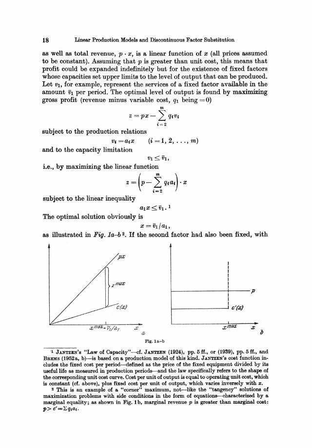
as well as total revenue, p . x, is a linear function of x (all prices assumed to be constant). Assuming that p is greater than unit cost, this means that profit could be expanded indefinitely but for the existence of fixed factors whose capacities set upper limits to the level of output that can be produced. Let VI, for example, represent the services of a fixed factor available in the amount 'ih per period. The optimal level of output is found by maximizing gross profit (revenue minus variable cost, qi being = 0)
m
Z =px- 2: qcVt
i=2
subject to the production relations V, =atX
and to the capacity limitation (i =1,2, ... , m)
VI < 'ih, i.e., by maximizing the linear function
subject to the linear inequality alx<'ih. 1
The optimal solution obviously is
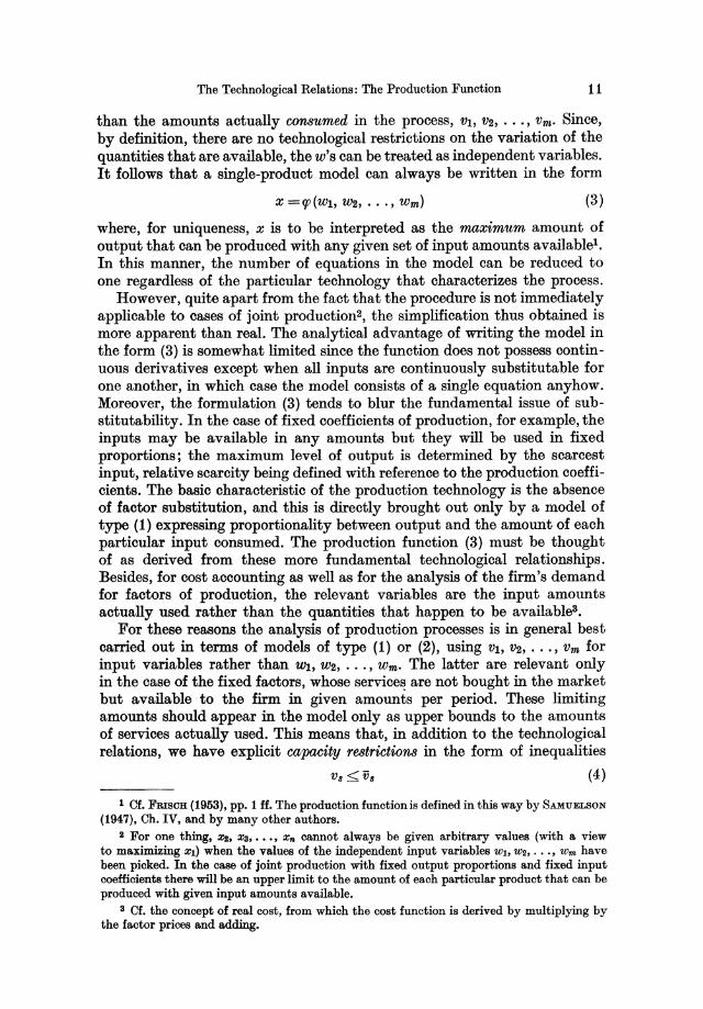
x = 'ih/al, as illustrated in Fig. la-b 2. If the second factor had also been fixed, with
c(.r}
Flg. l a-b
~------------~----p I I I
f--------------..... c'(.zj
'1 JANTZEN'S "Law of Capacity"-cf. JANTZEN (1924), pp. 5 ff., or (1939), pp. 5 ff., and BREMS (1952a, b)-is based on a production model of this kind. JANTZEN'S cost function includes the fixed cost per period-defined as the price of the fixed equipment divided by its useful life as measured in production periods-and the law specifically refers to the shape of the corresponding unit cost curve. Cost per unit of output is equal to operating unit cost, which is constant (of. above), plus fixed cost per unit of output, which varies inversely with x.
2 This is an example of a "corner" maximum, not--like the "tangency" solutions of maximization problems with side conditions in the form of equations-characterized by a marginal equality; as shown in Fig. 1 b, marginal revenue p is greater than marginal cost: p> c'=L:qjaj.
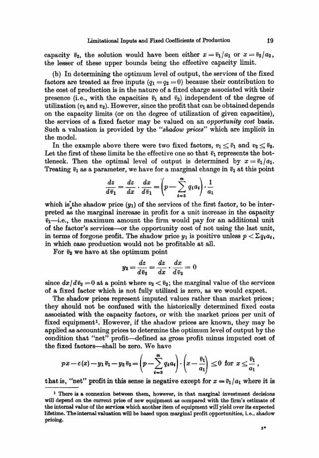
Limitational Inputs and Fixed Coefficients of Production 19
capacity Va, the solution would have been either x = VI / al or x = Va / ~, the lesser of these upper bounds being the effective capacity limit.
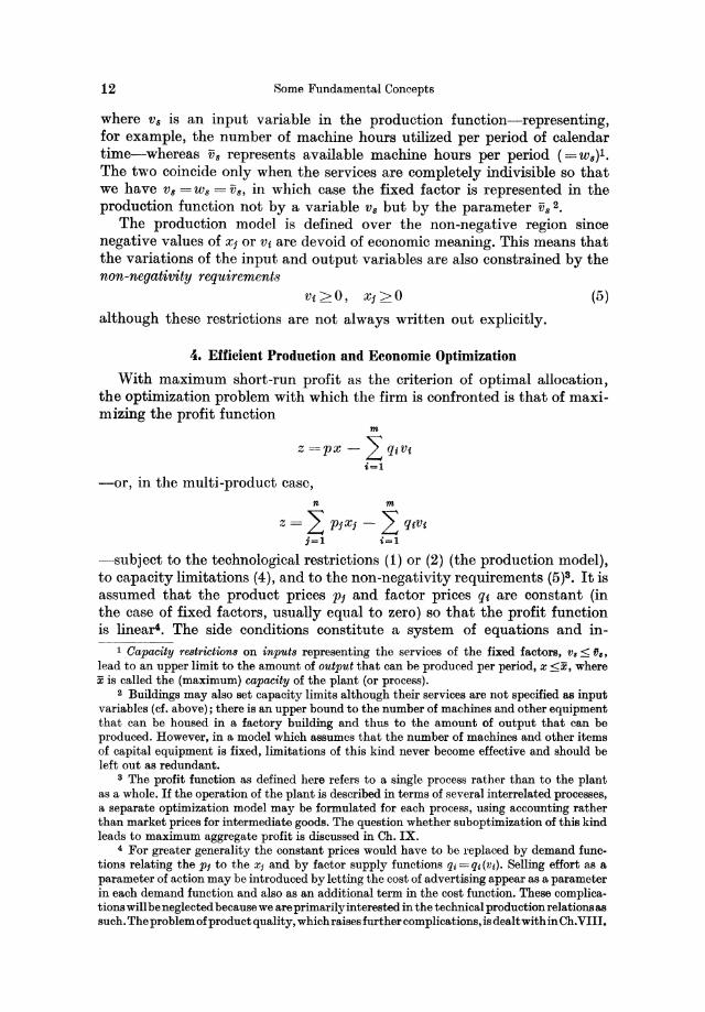
(b) In determining the optimum level of output, the services of the fixed factors are treated as free inputs (ql =qa =0) because their contribution to the cost of production is in the nature of a fixed charge associated with their presence (i. e., with the capacities VI and V2) independent of the degree of utilization (VI and va). However, since the profit that can be obtained depends on the capacity limits (or on the degree of utilization of given capacities), the services of a fixed factor may be valued on an opportunity C08t basis. Such a valuation is provided by the "8hadow price8" which are implicit in the model.
In the example above there were two fixed factors, VI:::;:: VI and Va :::;:: ~. Let the first of these limits be the effective one so that VI represents the bottleneck. Then the optimal level of output is determined by x = VI/al. Treating VI as a parameter, we have for a marginal change in VI at thispoint
d: =~. d~ =I(p_ ~ qfa,).!.. dVI dx dVI f-t al .-3
which is:the shadow price (YI) of the services of the first factor, to be interpreted as the marginal increase in profit for a unit increase in the capacity tit-i.e., the maximum amount the firm would pay for an additional unit of the factor's services-or the opportunity cost of not using the last unit, in terms of forgone profit. The shadow price YI is positive unless p <~qfaf' in which case production would not be profitable at all.
For ~ we have at the optimum point
dz dz dx Ya=-=-'-=O
dva dx dvs
since dx / d~ = 0 at a point where Va < Va; the marginal value of the services of a fixed factor which is not fully utilized is zero, as we would expect.
The shadow prices represent imputed values rather than market prices; they should not be confused with the historically determined fixed costs associated with the capacity factors, or with the market prices per unit of fixed equipment!. However, if the shadow prices are known, they may be applied as accounting prices to determine the optimum level of output by the condition that "net" profit-defined as gross profit minus imputed cost of the fixed faotors-shall be zero. We have
_ _ ( m ) (VI) VI pX-C(X)-YIfJ].-YaVa= P-6Qfaf • x- al :::;::0 for x:::;::al'
that is, "net" profit in this sense is negative except for x = VI / al where it is
1 There is a connexion between them, however, in tha.t marginal investment decisions will depend on the current price of new equipment as compared with the firm's estimate of the internal value of the services which another item of equipment will yield over its expected lifetime. The internal valuation will be based upon marginal profit opportunities, i.e., shadow pricing.
20 Linear Production Models and Discontinuous Factor Substitution
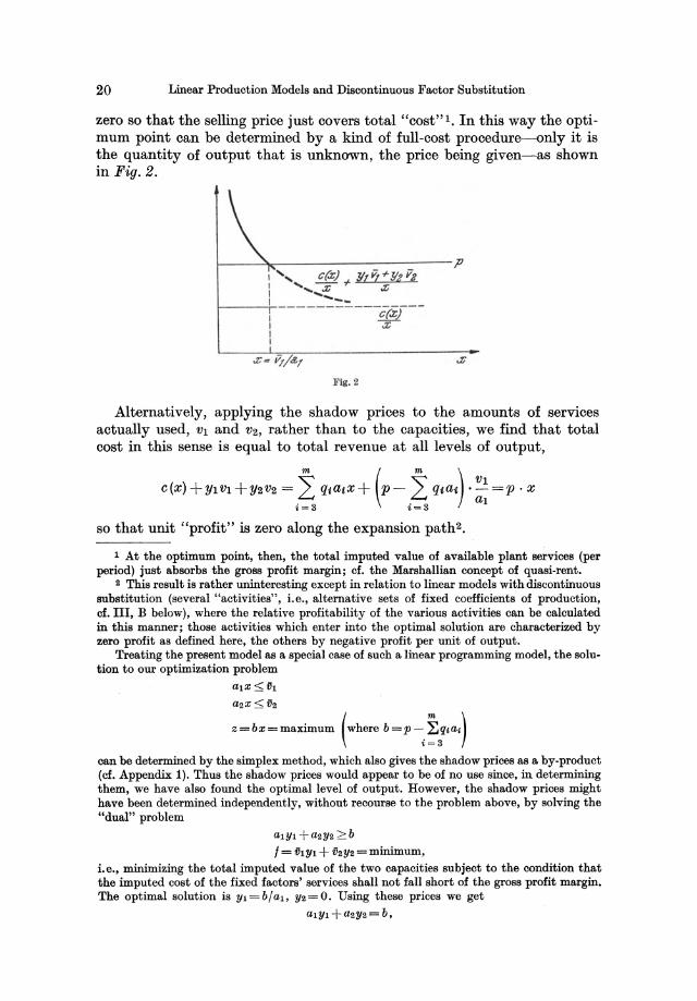
zero so that the selling price just covers total "cost"l. In this way the optimum point can be determined by a kind of full-cost procedure-only it is the quantity of output that is unknown, the price being given-as shown in Fig . 2.
~--~r------------------P I " C(z)!lf ~ + !It 173
.... --:;:- + ,z ........... .... _------------c~)---
,z
Fig. 2
Alternatively, applying the shadow prices to the amounts of services actually used, VI and Vz, rather than to the capacities, we find that total cost in this sense is equal to total revenue at all levels of output,
c(x) +YIVI +Y2VZ = i~ qta,x+ (p- i~ qtat). :~ =p . x
so that unit "profit" is zero along the expansion path2•
1 At the optimum point, then, the total imputed value of available plant services (per period) just absorbs the gross profit margin; cf. the Marshallian concept of quasi.rent.
2 This result is rather uninteresting except in relation to linear models with discontinuous substitution (several "activities", i.e., alternative sets of fixed coefficients of production, cf. III, B below), where the relative profitability of the various activities can be calculated in this manner; those activities which enter into the optimal solution are characterized by zero profit as defined here, the others by negative profit per unit of output.
Treating the present model as a special case of such a linear programming model, the solu-tion to our optimization problem
alx:::; f11
a2x:::; f12
z=bx=maximum (where b=P-.i:qtai) t = 3
can be determined by the simplex method, which also gives the shadow prices as a by-product (cf. Appendix 1). Thus the shadow prices would appear to be of no use since, in determining them, we have also found the optimal level of output. However, the shadow prices might have been determined independently, without recourse to the problem above, by solving the "dual" problem
alYl + a2Y2 ;::: b f = f11Yl + f12Y2 = minimum,
i.e., minimizing the total imputed value of the two capacities subject to the condition that the imputed cost of the fixed factors' services shall not fall short of the gross profit margin. The optimal solution is Yl = b / aI, Y2 = O. Using these prices we get
alYl+a2Y2=b,
Limitational Inputs and Fixed Coefficients of Production 21
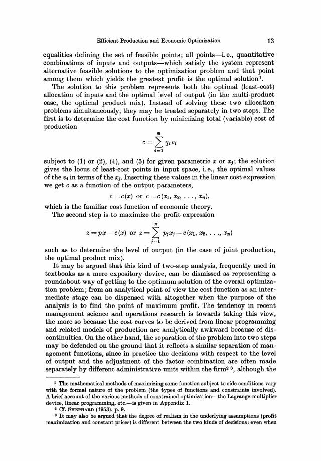
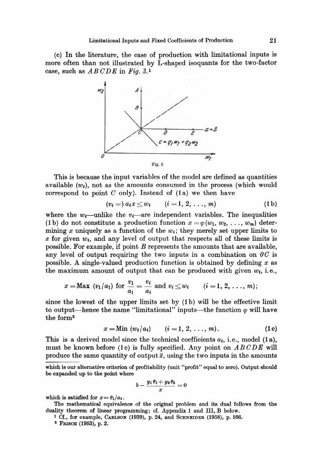
(c) In the literature, the case of production with limitational inputs is more often than not illustrated by L-shaped isoquants for the two-factor case, such as AB ODE in Fig. 3. 1
A
~---D"?:----E~-.z ~.£
o Fig. S
This is because the input variables of the model are defined as quantities available (Wi), not as the amounts consumed in the process (which would correspond to point 0 only). Instead of (1 a) we then have
(i =1,2, ... , m) (1 b)
where the wt-unlike the Vi-are independent variables. The inequalities (1 b) do not constitute a production function x =q;(Wl, W2, ... , wm) determining x uniquely as a function of the Wi; they merely set upper limits to x for given Wi, and any level of output that respects all of these limits is possible. For example, if point B represents the amounts that are available, any level of output requiring the two inputs in a combination on 00 is possible. A single-valued production function is obtained by defining x as the maximum amount of output that can be produced with given Wi, i. e.,
VI Vt x =Max (Vl/al) for - = - and Vt <Wi (i =1,2, ... , m);
al at
since the lowest of the upper limits set by (1 b) will be the effective limit to output-hence the name "limitational" inputs-the function q; will have the form2
(i =1,2, ... , m). (1 c)
This is a derived model since the technical coefficients at, i.e., model (la), must be known before (lc) is fully specified. Any point on ABODE will produce the same quantity of output ii, using the two inputs in the amounts
which is our alternative criterion of profitability (unit "profit" equal to zero). Output should be expanded up to the point where
which is satisfied for x= ill/al.
b- Ylfh+Y2 i12 =0 X
The mathematical equivalence of the original problem and its dual follows from the duality theorem of linear programming; cf. Appendix 1 and III, B below.
I Cf., for example, CARLSON (1939), p. 24, and SCHNEIDER (1958), p. 166. 2 FRIsCH (1953), p. 2.
22 Linear Production Models and Discontinuous Factor Substitution
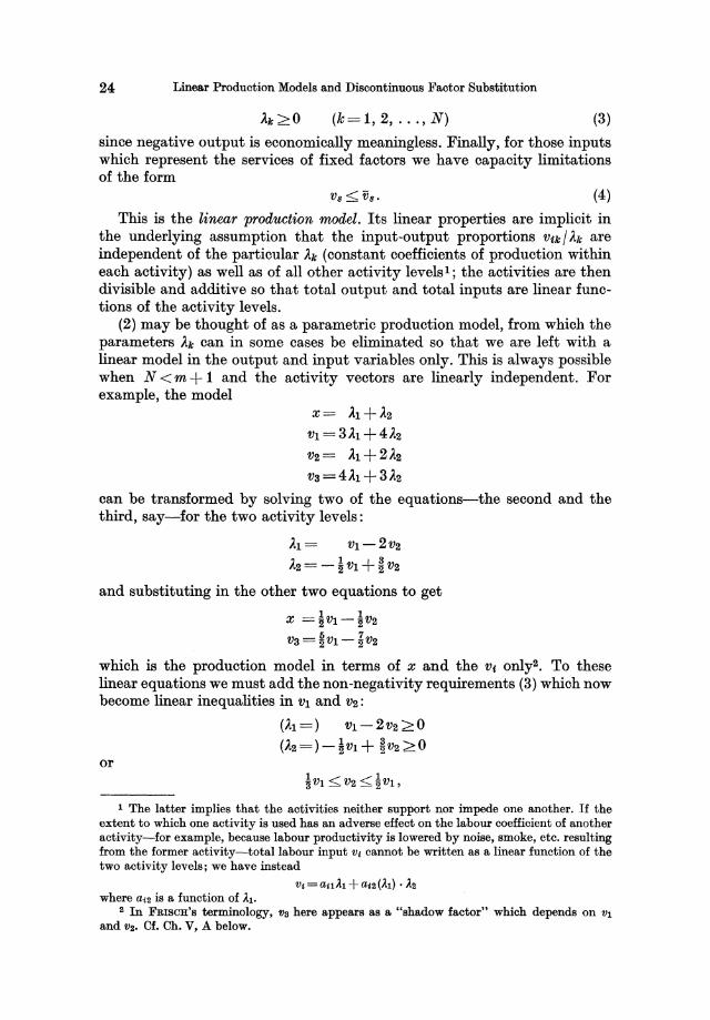
VI =alx and V2 =~x. At point 0 the inputs are available in precisely those amounts; at B there is "too much" of W2 available (WI being the minimum factor) so that the excess amount BO will go to waste, whereas point D implies waste of the first input. Thus, 0 is the only efficient point on the isoquant ABODE: it represents not only maximum output for given inputs-this is true of every point on ABO D E when the production function is defined by (1 c)-but also the minimum of inputs which will produce the given Xl.
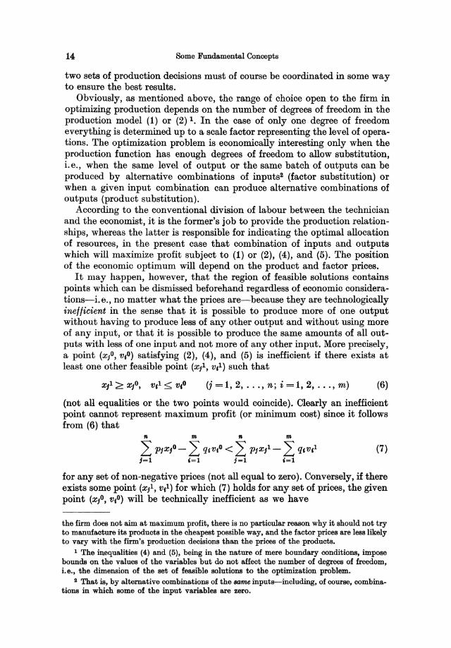
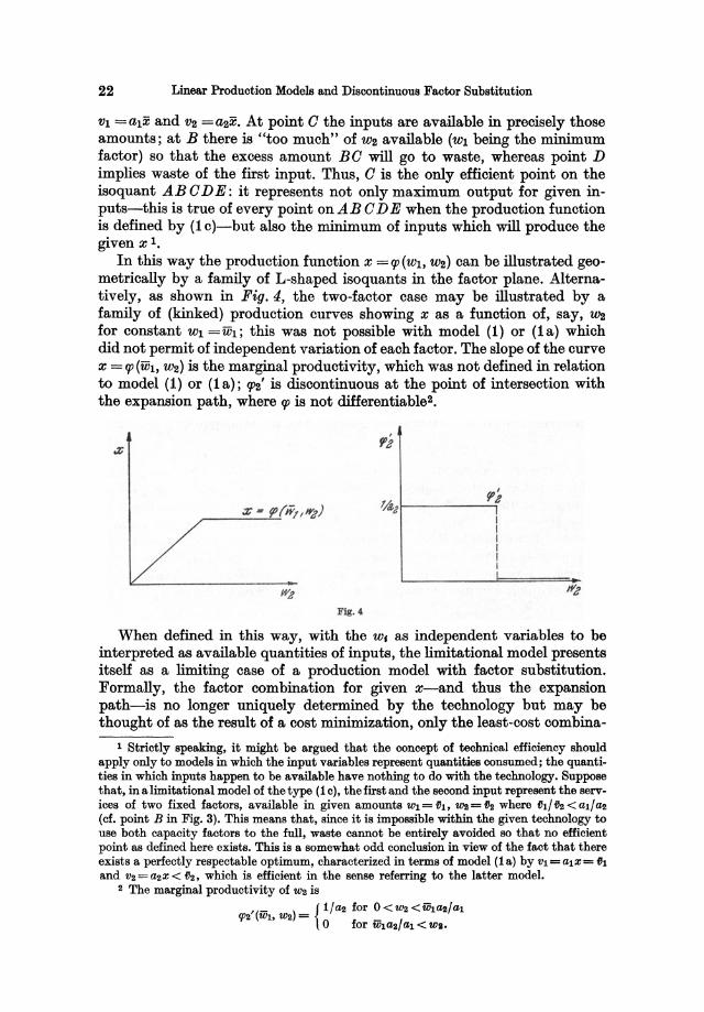
In this way the production function x =1P(Wl, W2) can be illustrated geometrically by a family of L-shaped isoquants in the factor plane. Alternatively, as shown in Fig. 4, the two-factor case may be illustrated by a family of (kinked) production curves showing x as a function of, say, W2 for constant WI =ui}; this was not possible with model (1) or (1a) which did not permit of independent variation of each factor. The slope of the curve x =1P(uh, W2) is the marginal productivity, which was not defined in relation to model (1) or (1 a); 1J12' is discontinuous at the point of intersection with the expansion path, where IP is not differentiable2•
Fig .•
?'z -'l{e2!------'1
When defined in this way, with the WI as independent variables to be interpreted as available quantities of inputs, the limitational model presents itself as a limiting case of a production model with factor substitution. Formally, the factor combination for given x-and thus the expansion path-is no longer uniquely determined by the technology but may be thought of as the result of a cost minimization, only the least-cost combina-
1 Strictly speaking, it might be argued that the concept of technical efficiency should apply only to models in which the input variables represent quantities consumed; the quantities in which inputs happen to be available have nothing to do with the technology. Suppose that, inalimitational model of the type (lc), the first and the second input represent the services of two fixed factors, available in given amounts Wl = Db WI! = D2 where fh/ D2 < al/0-2 (cf. point B in Fig. 3). This means that, since it is impossible within the given technology to use both capacity factors to the full, waste cannot be entirely avoided so that no efficient point as defined here exists. This is a somewhat odd conclusion in view of the fact that there exists a perfectly respectable optimum, characterized in terms of model (la) by Vl =alX= 01
and V2 = a2X < 02, which is efficient in the sense referring to the latter model. 2 The marginal productivity of WI! is
'(_ ) {1/0-2 for O<w2<fih0-2/al fP2 Wl, W2 = o for fih0-2/al < WI.
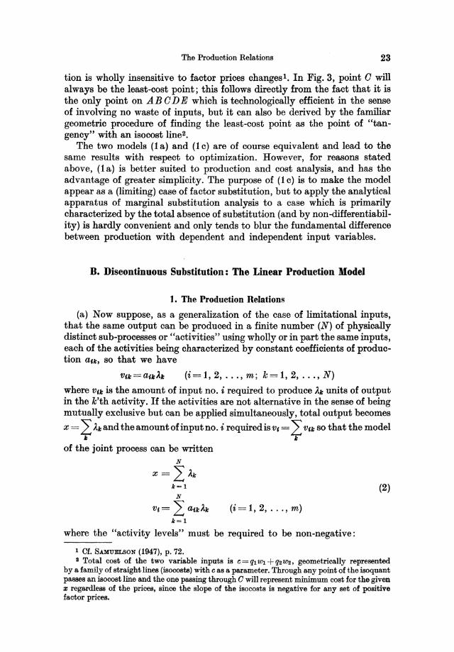
The Production Relations 23
tion is wholly insensitive to factor prices changes!. In Fig. 3, point 0 will always be the least-cost point; this follows directly from the fact that it is the only point on ABO D E which is technologically efficient in the sense of involving no waste of inputs, but it can also be derived by the familiar geometric procedure of finding the least-cost point as the point of "tangency" with an isocost line2•
The two models (1a) and (1c) are of course equivalent and lead to the same results with respect to optimization. However, for reasons stated above, (1 a) is better suited to production and cost analysis, and has the advantage of greater simplicity. The purpose of (1 c) is to make the model appear as a (limiting) case of factor substitution, but to apply the analytical apparatus of marginal substitution analysis to a case which is primarily characterized by the total absence of substitution (and by non-differentiability) is hardly convenient and only tends to blur the fundamental difference between production with dependent and independent input variables.
B. Discontinuous Substitution: The Linear Production Model
1. The Production Relations
(a) Now suppose, as a generalization of the case of limitational inputs, that the same output can be produced in a finite number (N) of physically distinct sub-processes or "activities" using wholly or in part the same inputs, each of the activities being characterized by constant coefficients of production a'k, so that we have
V(k = a(kAk (i=1, 2, ... , m; k=1, 2, ... , N)
where V(k is the amount of input no. i required to produce Ak units of output in the k'th activity. If the activities are not alternative in the sense of being mutually exclusive but can be applied simultaneously, total output becomes
x = 2: Ak and the amount of input no. i required is v, = L V,k so that the model k k
of the joint process can be written N
X= LAk k=1
N
vC=La'kAk (i=1,2, ... ,m) k=1
where the "activity levels" must be required to be non-negative:
1 Cf. SAlIIUELSON (1947). p. 72.
(2)
a Total cost of the two variable inputs is c = ql Wl + qa wa. geometrically represented by a. family of straight lines (isocosts) with c as a parameter. Through any point of the isoquant passes an isooost line and the one passing through a will represent minimum cost for the given :z; regardless of the prices. since the slope of the isocosts is negative for any set of positive factor prices.
24 Linear Production Models and Discontinuous Factor Substitution
(k=1, 2, ... , N) (3)
since negative output is economically meaningless. Finally, for those inputs which represent the services of fixed factors we have capacity limitations of the form
(4) This is the linear production model. Its linear properties are implicit in
the underlying assumption that the input-output proportions VUe I Ak are independent of the particular Ak (constant coefficients of production within each activity) as well as of all other activity levels 1 ; the activities are then divisible and additive so that total output and total inputs are linear functions of the activity levels.
(2) may be thought of as a parametric production model, from which the parameters Ak can in some cases be eliminated so that we are left with a linear model in the output and input variables only. This is always possible when N < m + 1 and the activity vectors are linearly independent. For example, the model
x= A1 +A2 V1 = 3A1 +4A2 V2 = A1 + 2A2 Va = 4A1 + 3A2
can be transformed by solving two of the equations-the second and the third, say-for the two activity levels:
A1 = V1-2v2
A2=-lvl+l v2
and substituting in the other two equations to get
x =lVl-iv2 V3= ~Vl- iV2
which is the production model in terms of x and the V, only2. To these linear equations we must add the non-negativity requirements (3) which now become linear inequalities in Vl and V2:
or
(A1 = ) V1 - 2 V2 > 0 (A2=)-ivl+ IV2>O
1 The latter implies that the activities neither support nor impede one another. If the extent to which one activity is used has an adverse effect on the labour coefficient of another activity-for example, because labour productivity is lowered by noise, smoke, etc. resulting from the former activity-total labour input Vi cannot be written as a linear function of the two activity levels; we have instead
Vi = anAl + ai2 (AI) • A2 where al2 is a function of AI.
a In FRISCH's terminology, Va here appears as a "shadow factor" which depends on VI
and VI. Cf. Ch. V, A below.
The Production Relations 25
i.e., the ratio of V2 to V1 is bounded by the relative technical coefficients in the two activities.
In the general case, however, no such elimination is possible and the model has to be considered in the general form (2).
Within each separate activity no factor substitution is possible since the inputs are limitational with respect to output ilk. The model (2)-(4) as a whole, however, permits of substitution in that the same total output can be produced by an infinite number of linear combinations of the activities (except in the special case N = 1, which is the limitational production model with constant coefficients); for given x =x, the isoquant is defined in parametric form by
N
Vj= 2: ajkilk k=l
(i=1, 2, ... , m)
where the parameters-the activity levels-must be non-negative and satisfy
N
2: ilk=X. k=l
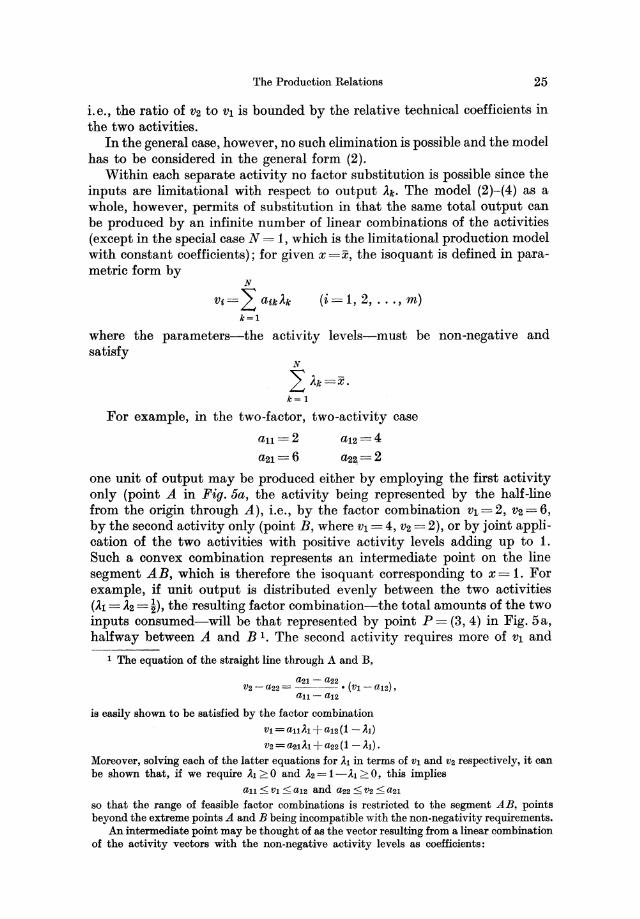
For example, in the two-factor, two-activity case
au=2 ~1=6
one unit of output may be produced either by employing the first activity only (point A in Fig.5a, the activity being represented by the half-line from the origin through A), i.e., by the factor combination V1.= 2, V2 = 6, by the second activity only (point B, where Vl = 4, V2 = 2), or by joint application of the two activities with positive activity levels adding up to 1. Such a convex combination represents an intermediate point on the line segment AB, which is therefore the isoquant corresponding to x = 1. For example, if unit output is distributed evenly between the two activities (ili = il2 = i), the resulting factor combination-the total amounts of the two inputs consumed-will be that represented by point P= (3, 4) in Fig. 5a, halfway between A and B 1. The second activity requires more of V1 and
1 The equation of the straight line through A and B,
a21-~2 V2 - U22 = ---- • (VI - a12) ,
an- al2
is easily shown to be satisfied by the factor combination Vl = anAl + al2 (1 - AI)
V2=U2lAI+a22(1- Al). Moreover, solving each of the latter equations for Al in terms of Vl and V2 respectively, it can be shown that, if we require Al 2: 0 and A2 = i-AI 2: 0, this implies
an ::; VI ::; a12 and a22::; V2 ::; a21 so that the range of feasible factor combinations is restricted to the segment AB, points beyond the extreme points A and B being incompatible with the non-negativity requirements.
An intermediate point may be thought of as the vector resulting from a linear combination of the activity vectors with the non-negative activity levels as coefficients:
26 Linea.r Production Models and Di!continuous Factor Substitution
less of V2 per unit output than does the first; hence, increasing A,2 at the expense of A,I (= 1 - A,2) implies a substitution of VI for V2 along the isoquant AB.
FIg.5a- b
The half-line extending from the origin through any intermediate point on AB may be thought of as an activity possessing the same linear properties (fixed technical coefficients, constant returns to scale) as the two "elementary" activities from which it has been derived: proportionate variation in A,I and A,2 implies that x, VI, and V2 vary in the same proportion, cf. (2). Hence all isoquants may be constructed as radial projections of AB.
When AB is downward sloping as in Fig. 5a, no point on the isoquant is technically inefficient: the same amount of output can be produced with less of one input only by using more of the other. In the case of AB being positively inclined (or parallel to one of the axes), however, only one of the activities is efficient; thus in Fig. 5b, whereas all points on the isoquant AB are feasible, a complete ordering of the points can be established I to show that point B is clearly inefficient, and so are all intermediate points. Only the activity containing A will represent efficient production.
In the case of more than two activities, the isoquants will be convex polygons-radial projections of one another-such as ABODE in Fig. 6. The boundary segments AB, BO, etc. represent linear combinations of two activities yielding a total output of one unit. An interior point of the polygon employs three or more activities; all such points are obviously inefficient, as well as points on the segments AE and ED. For example, E cannot be
[:1] =).1' [!11] +).2· [!12] , tis a21 a22
cf. the parallelogram of forces. Point P of Fig. 580 is illustrated in this way in the factor dia- . gram, the coefficients being ).1 = ).2 = !-.
1 Cf. Ch. II a.bove.
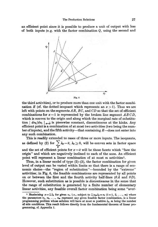
The Production Relations 27
an efficient point since it is possible to produce a unit of output with less of both inputs (e.g. with the factor combination Q, using the second and
Fill. 6
the third activities), or to produce more than one unit with the factor combina.tion E (cf. the dotted isoquant which represents an x> 1). Thus we are left with points on the segments A B, B 0, and 0 D so that the set of efficient combinations for x=1 is represented by the broken line segment ABOD, which is convex to the origin and along which the marginal rate of substitution I dV2/dvl I ,,-i is piecewise constant, discontinuous at the kinks. Any efficient point is a combination of at most two activities (two being the number of inputs), and the fifth activity-that containing E-does not enter into any such combination.
This is readily extended to cases of three or more inputs. The isoquants,
as defined by (2) for L Ak =x, Ak > 0, will be convex sets in factor space k
and the set of efficient points for x =X will be those facets which "face the origin" and which are negatively inclined to each of the axes. An efficient point will represent a linear combination of at most m activities l .
Thus, in a linear model of type (2)-(3), the factor combination for given level of output can be varied within limits so that there is a range of economic choice-the "region of substitution"-bounded by the "extreme" activities ; in Fig. 6, the feasible combinations are represented by all points on or between the first and the fourth activity half-lines (OA and OD) . However, such substitution as is possible is discontinuous in the sense that the range of substitution is generated by a finite number of elementary linear activities, any feasible overall factor combination being some "aver-
1 Maximizing X=LAk for given VI , i.e., subject to Lal.l;Ak=V, (i= 1, 2, .. . , m) where the parameters VI, V2, • •. , V", represent any given feasible factor combination, is a linear programming problem whose solution will have at most m positive Ak, m being the number of side conditions. This result follows directly from the fundamental theorem of linear programming, cf. Appendix 1.
28 Linear Production Models and Discontinuous Factor Substitution
age" of the combinations required for the same level of output by each of the activities that are employed12.
The model is characterized by constant returns to scale. A given but arbitrary set of activity levels Ak = AkO (> 0) corresponds to a point P in factor space with coordinates
and belonging to the isoquant
N
Via = L aikAkO k=l
N
xO= LAkO. k=l
Multiplying the activity levels by the same number p, leads to a new point
1 It might be argued that "discontinuous substitution" is hardly an appropriate term for a case where the relative factor combination can in fact be varied continuously within limits. However, the classical case of contin'U0'U8 substitutability, as defined with reference to a continuous and differentiable production function X=X(Vl, V2, ••• , vm), is characterized by infinitesimal variation of the marginal rate of substitution being possible (again within limits), i.e., by smoothly curved isoquants, whereas in the linear case the (efficient) isoquants are piecewise linear-a property which reflects discontinuities in the marginal productivitiesso that the least-cost combination will respond in a discontinuous manner to changes in the factor prices (cf. below).
2 The linear model of production was developed after World War II in connexion with the technique of linear programming, due to DANTZIG and KOOPMANS-cf. KOOPMANS (1951), esp. Cha. II-III-and applied to the theory of the firm by DORFMAN (1951). However, the idea of factor substitution under a linear technology characterized by a finite number of linear activities was anticipated by ZEUTHEN (1942), p. 66 (English ed. (1955), pp. 64 ff.), who had previously pointed out that several "methods of production"-i.e., sets of technical coefficients-may be used simultaneously to produce the same commodity, cf. ZEUTHEN (1928), pp. 34 and 38, and (1933), pp. 18 ff.
In a somewhat different context--namely, in showing that concave pieces of an isoquant belonging to a homogeneous production function with continuous substitutability cannot be efficient--the idea of combining activities linearly was used, and illustrated by the parallelogram of forces, by GLOERFELT-TARP (1937), pp. 257 f., and generalized to the multi-product case by SCHMIDT (1939), pp. 293 ff. Discontinuities in the marginal rate of substitution were treated in a general way-not restricted to the linear case--by SAMUELSON (1947), Ch.4 (cf. below).
For an empirical example of discontinuous substitution see CHARNES, COOPER and FARR (1953). The machine shop considered in this example manufactures several products (which are interdependent in that they share the services of the plant's fixed equipment), but each product can be produced in a finite number of linear activities because alternative kinds of fixed equipment can be used. For example, the first of the products listed can be manufactured on anyone of four different types of screw machines. For the fifth product there are two types of screw machines which can do each other's jobs and two types of grinders, and each of the four combinations defines an activity.
It must be pointed out that the linear programming model characterized by a finite number of activities also applies to allocation problems which can scarcely be described as cases of discontinuous substitution as defined here. For example, the problem may be to find the least-cost combination of given materials (blending ingredients) which gives a product (blend) of specified composition; each input (ingredient) defines an activity whose coefficients represent the composition of the ingredient in terms of the constituents required in the blend. Models of this kind are dealt with in Ch. VIII, C below.
on the isoquant
The Production Relations
N
V, = L afk",Ako ='" . V,O k=l
N
X = L ",AkO ='" . XO k=1
29
so that the isoquants are radial projections of one another. Accordingly, the elasticity of production, i.e., the elasticity of x with respect to a proportionate variation in all inputs (or, which comes to the same thing, with respect to the scale factor "'), is unity everywhere; for dVf/Vt=v,od",/",VfO=d",/", (i= 1,2, ... , m) we have
e= dx . Vt = dx . !!..=xO. -"'-=1 dv, x d", x",· XO
identically in ",. Setting xo= 1 so that x = "', the parameter", can be thought of as representing the level of a derived activity whose technical coefficients are the v,o and which is geometrically illustrated by the half-line from the origin through P.
There may, of course, be zeroes among the coefficients atk, i. e., the various activities produce the same output using wholly or in part different inputs. This is likely to be the rule rather than the exception: while it is perhaps difficult to see why it should be possible to produce the same output only by a finite number of sets of technical coefficients (though these activities can be used jointly), it is easy to imagine cases in which each activity is characterized by using an input which is specific to it (e.g. a fixed factor whose services require the variable inputs in technologically fixed proportions). In such cases each new activity adds a new dimension to the factor space.
(b) We have defined the Vf as quantities consumed of the various inputs. Alternatively, we may ask the question: How much is it possible to produce with given available quantities of the inputs, WI, W2, ... , Wm 1 The answer is given by
N N
X = Max L: Ak subject to (Vf =) L: a'kAk < Wt and Ak > 0 k=1 k=1
(i=1, 2, ... , m; k=1, 2, ... , N).
The maximization procedure will ensure uniqueness so that we can write the resulting x as a single-valued production function with the Wt as independent variables:
(5)
(In the special case of N = 1, i.e., limitationality, the function will have the form
(i = 1, 2, ... , m), cf. above.)
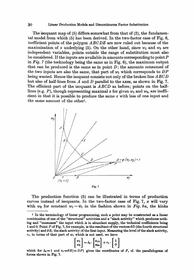
30 Linear Production Models and Discontinuous Factor Substitution
The isoquant map of (5) differs somewhat from that of (2), the fundamental model from which (5) has been derived. In the two-factor case of Fig. 6, inefficient points of the polygon ABO DE are now ruled out because of the maximization of x underlying (5). On the other hand, since WI and W2 are independent variables, points outside the range of substitution must also be considered. If the inputs are available in amounts corresponding to point P in Fig. 7 (the technology being the same as in Fig. 6), the maximum output that can be produced is the same as in point D; the amounts consumed of the two inputs are also the same, that part of WI which corresponds to DP being wasted. Hence the isoquant consists not only of the broken line ABO D but also of half-lines from A and D parallel to the axes, as shown in Fig. 7. The efficient part of the isoquant is ABOD as before; points on the hal£lines (e.g. P), though representing maximal x for given WI and W2, are inefficient in that it is possible to produce the same x with less of one input and the same amount of the otherl.
/
/ /
/ Ii
Fig.?
The production function (5) can be illustrated in terms of production curves instead of isoquants. In the two-factor case of Fig. 7, x will vary with W2 for constant WI = uh in the fashion shown in Fig. 8a, the kinks
1 In the terminology of linear programming, such a point may be constructed as a linear combination of one of the "structural" activities and a "slack activity" which produces nothing and "consumes" the input which is in abundant supply, the technical coefficients being 1 and O. Point P of Fig. 7, for example, is the resultant of the vectors OD (the fourth structural activity) and OR, the slack activity of the first input. Measuring the level of the slack activity, r1, in terms of that part of W1 which is not used, we have
[ :] = A. . [::] + r1 • [ ~ ] which for A4 = 1 and r1 =0 R ( = D P) gives the coordinates of P, cf. the parallelogram of forces shown in Fig. 7.
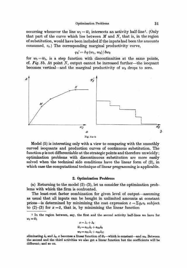
Optimization Problems 31
occurring whenever the line WI = uh intersects an activity half-line l • (Only that part of the curve which lies between M and N, that is, in the region of substitution, would have been included if the inputs had been the amounts consumed, Vi.) The corresponding marginal productivity curve,
CP2'=bcp(wl, w2)/bw2
for WI =wl, is a step function with discontinuities at the same points, cf. Fig. 8b. At point N, output cannot be increased further-the isoquant becomes vertical-and the marginal productivity of W2 drops to zero.
tfi,
Flg. 8a-b
I '------,
I
i I L-.-,
I I
Model (5) is interesting only with a view to comparing with the smoothly curved isoquants and production curves of continuous substitution. The function cp is not differentiable at the strategic points and therefore unwieldy ; optimization problems with discontinuous substitution are more easily solved when the technical side conditions have the linear form of (2), in which case the computational technique of linear programming is applicable.
2. Optimization Problems
(a) Returning to the model (2)-(3), let us consider the optimization problems with which the firm is confronted.
The least-cost factor combination for given level of output-assuming as usual that all inputs can be bought in unlimited amounts at constant prices-is determined by minimizing the cost expression c =l:q,Vt subject to (2)-(3) for x =x, that is, by minimizing the linear function
1 In the region between, say, the first and the second activity half-lines we have for
X=Al+A2 ii!t =allAl + auAz Wz =a21Al + a22AZ;
eliminating A1 and A2, x becomes a linear function of w1-which is constant-and W2. Between the second and the third activities we also get a linear function but the coefficients will be different; and 80 on.
32 Linear Production Models and Discontinuous Factor Substitution
c ~ i~ q, ,~: .. 1. ~ .~, (~/, ... ) 1, ~ .~, c... (6)
(where Ck is cost per unit produced in the k'th activity) subject to the linear side condition
(7)
for Ak >0 (k =1,2, ... , N). A problem of this type cannot be solved by traditional methods of con
strained maximization (elimination of dependent variables or, more generally, Lagrange's method of undetermined multipliers)1 but will have to be solved as a problem of linear programming, though in this case a trivial one: the optimal solution is obviously to produce the required x units of output in that activity which has the lowest unit cost Ck. 2
Thus the least-cost point will be one of the "corners" of the efficient boundary of the isoquant3 • In the two-factor case shown in Fig. 9 there are
1 Cf. Appendix 1. a Consider the minimization of (6) subject to (7) and (3) as a formal problem of linear
programming, to be solved by the simplex method (see Appendix 1). Then we know from the fundamental theorem of linear programming that a single activity will suffice to give an optimal solution since there is only one linear side condition, (7). Now suppose that, for example, the first activity has the lowest unit cost:
Cl<C", (k=2,3, ... , N). Choosing the first activity as a basis, we solve (7) for Al and substitute in (6) to get total cost as a function of the non-basic variables A2, As, ... , AN:
(i) Al=X-A2- ..• -AN
(ii) C=ClX+(C2-cl)Aa+ ••. +(CN-Cl)AN. The coefficients in (ii) are, by assumption, all positive; it follows that, since A2, Aa, ..• , AN cannot be negative, C is a minimum for all these variables equal to zero so that the basic solution
represents minimum cost. Any other feasible solution (non-negative set of values of activity levels A",) will represent
higher cost so that the solution is also unique. Had we assumed instead that Cl = Ca, all other C"'> Cl, the coefficient of A2 would have
been zero and the value of C would not have been affected by As becoming positive (but :::;;x or Al would become negative). In this case any non-negative combination of the first and the second activities for which Al + Aa =X would represent minimum cost; but it would still be possible to attain minimum cost by using one activity only (the first or the second).
Thus it is a BUfficie:nt condition for minimum that the coefficients of the non-basic variables in (ii)-the "simplex coefficients"-are all non-negative. This condition, known as the "simplex criterion", is also a neces8ary condition (except for the special case of "degeneracy," which cannot occur here) since the solution could be improved if one of the coefficients had been negative.
8 Only efficient points need be considered since cost can never be a minimum when it is possible to produce the same amount of output with less of one input and not more of any other (cf. Ch. II above). On the other hand, the inclusion of inefficient points-which are often difficult to detect and sort out beforehand in more complicated problems-will do no harm since they will automatically be thrown out during the simplex calculations, just as they are ruled out by geometric considerations in the simple two-factor example.
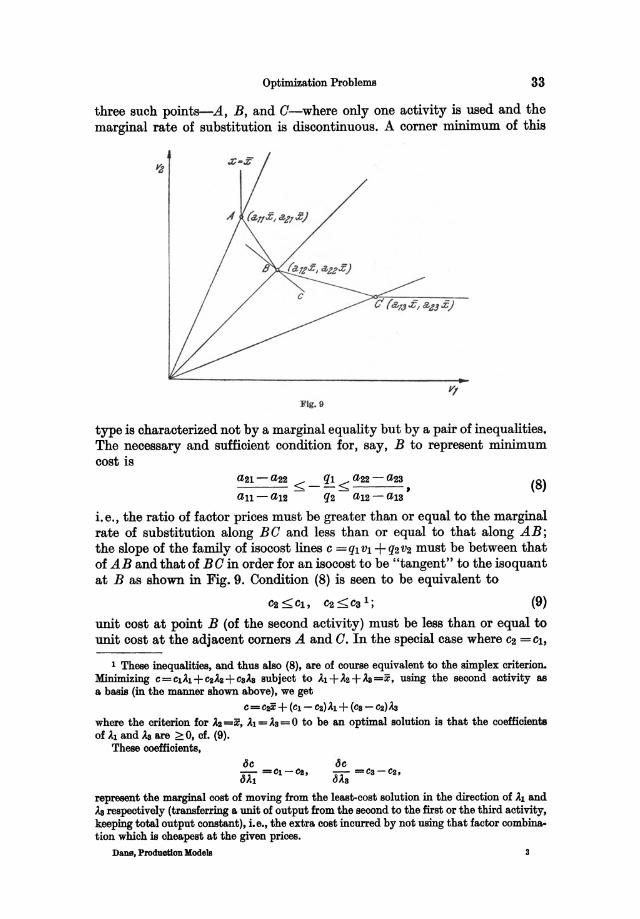
Optimization Problems 33
three such points-A, B, and a-where only one activity is used and the marginal rate of substitution is discontinuous. A corner minimum of this
Fig. 9
type is characterized not by a marginal equality but by a pair of inequalities. The necessary and sufficient condition for, say, B to represent minimum cost is
(8)
i. e., the ratio of factor prices must be greater than or equal to the marginal rate of substitution along BO and less than or equal to that along AB; the slope of the family of isocost lines c = qi VI + q2 V2 must be between that of AB and that of B a in order for an isocost to be "tangent" to the isoquant at B as shown in Fig. 9. Condition (8) is seen to be equivalent to
(9)
unit cost at point B (of the second activity) must be less than or equal to unit cost at the adjacent corners A and O. In the special case where C2 =CI,
1 These inequalities, and thus also (8), are of course equivalent to the simplex criterion. Minimizing C = C1A1 + C2AII + csAs subject to Al + A2 + As =x, using the second activity as a basis (in the manner shown above), we get
C=C2x + (C1- C2)A1 + (ca- cz)As where the criterion for As =x, Al = As = 0 to be an optimal solution is that the coefficients of Al and As are ~ 0, of. (9).
These coeffioients, bc bc
- =C1-C2, - =Ca-C2, bAl bAa
represent the marginal cost of moving from the least-cost solution in the direction of Al and As respectively (transferring a unit of output from the second to the first or the third activity, keeping total output constant), i.e., the extra cost incurred by not using that factor oombination whioh is cheapest at the given prioes.
Dans, Produotion Models
34 Linear Production Models and Discontinuous Factor Substitution
C2 < CS, so that the isocosts are parallel to AB, any point of the segment AB represents minimum cost so that the solution is not unique, but it is still possible to find a least-cost point which uses one activity only (A or B).
As long as the price ratio keeps within the limits (8), the optimal factor combination is completely insensitive to factor price changes: it is only when the isocost lines become steeper than A B or less steep than B 0 that the optimum point responds, jumping to A or 0 respectively. Thus the response of the least-cost point to factor price changes is discontinuous. Specifically, the sensitivity of the optimum position with respect to one of the prices, say, ql, may be traced by treating ql as a parameter; for q2 constant, (8) defines a pair of limits to ql within which B is the least-cost point!.
(b) With x as a parameter, the locus of least-cost points defines the expansion path as a straight line in the non-negative factor space (except in the special case where the optimal combination is not unique), the same activity being optimal at all levels of output when the factor prices are constant. Hence total cost will be proportional to output,
C = (%1 qtatt). A.t =Ct· x,
activity no. t being the cheapest. Since total revenue is also proportional to x when the price of the product is constant,
r =p. x,
no finite maximum of profit exists and an optimal level of output cannot be determined on the basis of revenue and cost when all inputs are available in unlimited amounts.
However, the latter assumption is not a realistic one: in short-run optimization problems there will always be one or more scarce inputs representing the services of fixed factors of production, i.e., there will be additional restrictions of the type (4) which impose upper bounds on certain inputs and thus also on the level of output. (The coefficients of such inputs in the cost function will usually be zero since total cost is not affected by the degree of capacity utilization as such.) Hence the factor combination determined by minimizing (6) subject to (7) and (3) represents a feasible least-cost solution only in so far as it respects the capacity restrictions (4); if it does not, the problem has to be reformulated with (4) as additional side conditions. Let the M first inputs (M <m) be the services of fixed factors with capacities tit, V2, ... , VM (and prices q1 =q2 = ... =qM =0). Then the problem of cost minimization for given x =x is that of minimizing total variable cost of the current inputs VM+1, VM+2, ••• , Vm:
(10)
1 We might go further and study the succession of optimal solutions obtained as ql varies from zero upwards. This would be an example of "parametric programming" where some of
and N
Optimization Problems
N
(x=) L A~= x t~= I
(v, =) L a,~A~ < v, 1 (i=1,2, .•. ,M).
35
(7)
(U)
For parametric x, the solution to this linear programming problem determines the factor combination as depending on the level of output, i.e., the expansion path and the corresponding cost function. The optimal level of output can then be determined by maximizing total revenue minus total cost.
The optimal value of x could have been determined directly, without using the expansion path and the cost function as an intermediate stage, by maximizing total (gross) profit
N N
z=px-C= L: (p-C~)A~= L: Z~A~ (12) ~=I Ie-I
(where Zk =P-Ck is unit gross profit in the k'th activity) subject to (3) and (U) 2. This procedure is all the more expedient in cases of this type as the marginal cost function derived from the linear model turns out to be discontinuous.
(c) Linear programming problems cannot be solved analytically in the sense that it is possible to express the optimal values of the variables (here, the Ak and thus also x and the 'Of) in terms of the unspecified parameters a,~, Ck or Z~ (i.e., P and the q,), and v,. The simplex method is essentially a method of numerical solution: the simplex criterion gives a necessary and sufficient criterion for optimality, but whether it is satisfied by a particular basic solution or not depends upon the numerical values of the parameters.
The optimization procedures may be illustrated by a numerical example with two factors. Let the production technology be represented by four activities with input coefficients as follows:
the strategic coefficients are treated as unspecified parameters (in the present case, the Ck, which are all affected by a change in ql).
1 By the fundamental theorem of linear programming, at most M + 1 positive variablesstructural and/or slack variables-are required for an optimal solution, M + 1 being the num· ber of linear side conditions (7)-(11). There are N structural variables A,. (k = 1, 2, ••• , N) and M slack variables r, (i = 1, 2, ••. , M), the latter defined by rewriting the capacity restriotions (11) in the form
(i=1, 2, ••• , M) 1e=1
where r, (2'=0) is to be interpreted as idle capacity of the i'th fixed factor (r,=D,-tlh i.e., factor services ava.ila.ble minus servioes used). The occurrence of a particular positive slack variable r, in the optimal solution indicates that the i'th fixed faotor is not an effective limit to output (at the given price constellation) so that the corresponding side condition might as well have been left out.
I The optimal solution, as determined by linear programming methods, will involve not more than M (in the absence of degeneracy, just M) positive variables.
8· .
36 Linear Production Models and Discontinuous Factor Substitution
~= 1 2
k=
123 4
1 6
The first input represents the services of a fixed factor, free (ql =0) but available up to the capacity limit iiI = 24 only; the second is a variable factor whose price is q2 = 2. Then the least-cost combination is determined by minimizing e = q2 V2, = 2 V2 for x =X and VI < iiI (or VI + r = ih where the slack variable r represents unused capacity), i.e., by minimizing
subject to )1.1 +A2+A3+A4=X
4Al +3A2+2As +M+r= 24(= ih)
(13)
(14)
(15)
where all variables-including the slack variable r, whose coefficient in the cost function is zero-are required to be > O.
This is a (parametric) linear programming problem, readily solved by the simplex method l .
The first step is to select a basis of two variables, corresponding to the number of linear side conditions. The first activity is the cheapest and will obviously be preferred for x < ih / all = 6, the maximum quantity that can be produced in activity no. 1 alone. This suggests the choice of (Al' r) as an initial basis. Solving (14)-(15) for these variables and substituting in (13) we have
Al= X-A2-A3-~
r= (24-4x)+A2+2As+3M
e=4x+2A2+4A3+8A4o
(16)
The third of these equations shows that cost will be a minimum for A2 = As = A4 = 0 because e is an increasing function of the three variables so that the simplex criterion is satisfied2• Hence the least-cost solution is
Al=X, r=24-4x, e=4x (17)
as expected, only the solution is restricted to the interval 0 <x < 6, as r becomes negative (i.e., the solution is no longer feasible) for x >6. Only the first activity is used; the solution is the same as the one we should have found by minimizing (13) subject to (14) only. Marginal cost (= variable unit cost) is de I dx = 4, the coefficient of x in the third equation of (16).
1 The numerical procedure in the following corresponds to that outlined in Appendix 1 except for the slight complication due to the presence of the unspecified parameter iii, which makes the problem a case of parametric programming.
2 The simplex criterion for a basic feasible solution to be a minimum requires that the "simplex coefficients"-the coefficients of the non-basic variables in the equation giving c as a function of these variables---shall be non-negative (cf. Appendix 1). Had one of the coefficients, say that of A2 in the third equation of (16), been zero, this would have indicated that the solution was optimal but not unique since a marginal increase in ita (at the expense of A1) would not affect c.
Optimiza.tion Problems 37
For x > 6 the capacity limit becomes effective and we must look for another solution in which r is = o. A natural choice of a new basis is (Al' As), i.e., some combination of the cheapest and the second-cheapest activity, As having now replaced r as a non-zero variable. Solving for Al, A2, and c in terms of the other three variables-this can be done either from (13)-(15) as before or, more easily, from (16)-we get
Al= (24-3x)+ As+2~- r
As= (4x-24)-2A3-3~+ r c = (12x - 48) + OAs + 2~ + 2r
where again the simplex criterion is satisfied so that
Al=24-3x, A2=4x-24, c= 12x-48 (18)
-a combination of the two activities-is a least-cost solution within the interval where it is feasible, i. e., for Al = 24 - 3x > 0 and A2 = 4x - 24 > 0, or 6 <x < 8. Within this interval marginal cost is again constant, now equal to dc / dx = 12. At x = 6, where the two intervals overlap, the two solutions (17) and (18) coincide and only one activity is used. .
Proceeding in this fashion, the following least-cost solutions for higher levels of output emerge:
A2=24-2x, As=3x-24, c=12x-48 for 8~x<12 (19) As=24-x, ~=2x-24, c= 16x-96 for 12 <x<24 (20)
where marginal cost is 12 and 16 respectively. For x >24 no non-negative solution exists; x = 24 is the maximum output that can be produced, as was evident from the outset since fh/a14=24, the fourth activity having the lowest coefficient of Vl per unit of output.
These results are illustrated in Fig. lOa-c. Fig. lOa shows that the expansion path in the factor diagram is OABOD, where OA corresponds to solution (17), AB to (18), etc. The same result could also have been arrived at by geometrical considerations, recalling that for ql = 0 the isocosts are parallel to the Vl axis. The cost function (total variable cost) is piecewise linear, cf. Fig. lOb (where A', B', etc. correspond to A, B, etc. in Fig. 10a) and marginal cost is a step function as shown in Fig.lOc.
The optimal point on the expansion path OABOD can then be determined by comparing marginal revenue (=the product price, p) with the marginal cost function as shown in Fig. 10c. For p = 15, for example, profit is a maximum at 0 where x = As = 12, marginal cost being
dc {16(>15) for x >12 dx = 12« 15) for x <12.
This result could have been arrived at directly by maximizing the profit function
(21)
subject to the capacity restriction (15) for Ak > 0 and r:;;::: o. Solving (15) for As and substituting in (21) we have
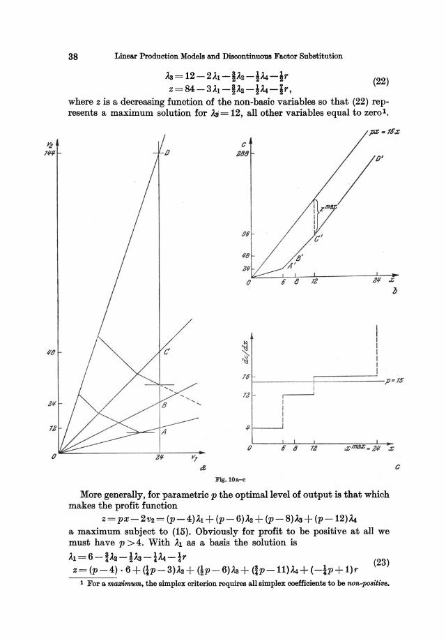
38 Linear Production Models and Discontinuous Factor Substitution
Aa= 12-2ih ~IA2-IM-lr Z= 84-3AI-~A2-IM-ir,
(22)
where Z is a decreasing function of the non-basic variables so that (22) represents a maximum solution for A.sI= 12, all other variables equal to zero!.
U~ _______ -+=========-f- Jl-IS
lZ
111------'
(J o 8 111
Flg.lOa-c
More generally, for parametric p the optimal level of output is that which makes the profit function
Z= PX-2V2= (p-4)AI + (p-6)A2+ (p- 8)Aa+ (p-12)M a maximum subject to (15). Obviously for profit to be positive at all we must have p > 4. With Al as a basis the solution is
AI=6- !A2-IAa- iM-ir Z= (p-4). 6+ (lp-3)A2+ {~p-6)A3+ {ip-11)M+ {-ip+ 1)r (23)
1 For a maximum, the simplex criterion requires all simplex coefficients to be non.positive.
c
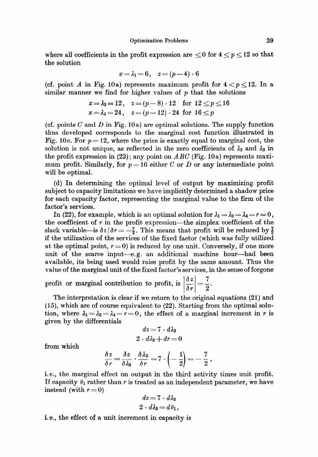
Optimization Problems 39
where all coefficients in the profit expression are < 0 for 4 <p < 12 so that the solution
X=Al=6, z=(p-4)·6
(cf. point A in Fig. lOa) represents maximum profit for 4 <p:::;;12. In a similar manner we find for higher values of p that the solutions
x=A3=12, z=(p-8) ·12 for 12 <p:::;;16
x=~=24, Z= (p-12) ·24 for 16 <p
(cf. points 0 and D in Fig. lOa) are optimal solutions. The supply function thus developed corresponds to the marginal cost function illustrated in Fig. 10c. For p = 12, where the price is exactly equal to marginal cost, the solution is not unique, as reflected in the zero coefficients of A2 and A3 in the profit expression in (23); any point on ABO (Fig. lOa) represents maximum profit. Similarly, for p = 16 either 0 or D or any intermediate point will be optimal.
(d) In determining the optimal level of output by maximizing profit subject to capacity limitations we have implicitly determined a shadow price for each capacity factor, representing the marginal value to the firm of the factor's services.
In (22), for example, which is an optimal solution for Al = A2 = ~ = r = 0, the coefficient of r in the profit expression-the simplex coefficient of the slack variable-is ~z/~r= -~. This means that profit will be reduced by i if the utilization of the services of the fixed factor (which was fully utilized at the optimal point, r = 0) is reduced by one unit. Conversely, if one more unit of the scarce inpu~. g. an additional machine hour-had been available, its being used would raise profit by the same amount. Thus the value of the marginal unit of the fixed factor's services, in the sense of forgone
profit or marginal contribution to profit, is I ~ z I = 2. ~r 2
The interpretation is clear if we return to the original equations (21) and (15), which are of course equivalent to (22). Starting from the optimal solution, where Al = A2 = ~ = r = 0, the effect of a marginal increment in r is given by the differentials
dz=7 . dAa
2 . dA3 + dr = 0 from which
:: = :~ . ~A: =7. (_~) = _ ~, i. e., the marginal effect on output in the third activity times unit profit. If capacity ih rather than r is treated as an independent parameter, we have instead (with r = 0)
dz=7 . dA3
2· dAa=d;;h,
i.e., the effect of a unit increment in capacity is
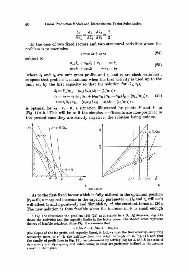
40 Linear Production Models and Discontinuous Factor Substitution
~Z ~Z ~A3 7 ~?h = ~A3· ~?h ="2.
In the case of two fixed factors and two structural activities where the problem is to maximize
subject to au Al + a12 A2 + fl
~lAl+~2A2
(24)
(25)
(where Zl and Z2 are unit gross profits and fl and f2 are slack variables), suppose that profit is a maximum when the first activity is used up to the limit set by the first capacity so that the solution for (At, f2),
Al = VI I au - (a12 I aU)A2 - (1 I aU)fl
f2 = V2 - vla21 I au + (~laI21 au- ~2)A2 + (a21/au)fl (26) Z = ZI VII an - (Zlal2I au - Z2)A2 - (z11 an)fl,
is optimal for 1..2 = fl = 0, a situation illustrated by points P and P' in Fig. lla-b. 1 This will be so if the simplex coefficients are non-positive; in the present case they are strictly negative, the solution being unique.
a b Flg.lh.-b
As to the first fixed factor which is fully utilized in the optimum position (fl = 0), a marginal increase in the capacity parameter iit (1..2 and fl still = 0) will affect Al and Z positively and diminish f2, cf. the constant terms in (26). The new solution is thus feasible when the increase in tit is small enough
1 Fig.lla illustrates the problem (24)-(25) as it stands in a (A,l,A,2) diagram; Fig.llb shows the activities and the capacity limits in the factor plane. The shaded areas represent the set of feasible solutions. Since Fig. 11 a assumes that
-Zl/Z2< -all/aI2 < -~I/a22 (the slopes of the iso-profit and capacity lines), it follows that the first activity-requiring relatively more of VI-is the half-line from the origin through P' in Fig. 11 b and that the family of profit lines in Fig. 11 b (as determined by solving (25) for A,1 and A,2 in terms of fh - rl = Vl and 02 - r2 = V2 and substituting in (24» are positively inclined in the manner shown in the figure.
Optimization Problems 41
not to make f2 negative 1 ; it is also optimal since the simplex coefficients are not affected. Thus, by the third equation of (26), the marginal value of the services of the first fixed factor is
(= ~;1' ~;> cf. (24)-(25»),
which is numerically equal to the simplex coefficient of f1,
= -' -, cf. (24)-(25) , ( ~z ~ A1 ) ~A1 ~f1
the interpretation being that a marginal increase in f1 (unutilized capacity) for given 1h is equivalent to a reduction of capacity for constant f1 = O. The effects of a positive and a negative shift in 1h on the optimal position are represented in Fig. 11 by a move from P to Q or R (or from P' to Q' or R').
Fig. 11 also suggests that a (small) marginal change in the second capacity V2 will not change the equilibrium position. At the given prices V2 is not a bottleneck factor (f2 > 0), so an increase in V2 will add nothing to profit but will merely result in a corresponding increase in unutilized capacity f2;
the factor is not effectively scarce but is a free good. This is confirmed by (26): the new solution where r2 and V2 have been increased by the same amount leaves everything else as it was, so it is feasible and optimal for A2 = f1 = 0 and we have
~=o. t5 V2
Correspondingly, the simplex coefficient of f2 may be said to be zero since r2,
being a basic variable, does not enter into the third equation of (26). Thus the shadow prices associated with the fixed factors are both non
negative, being numerically equal to the simplex coefficients of the corresponding slack variables in the optimal basic solution 2 ; the shadow price is zero if the factor is not fully utilized (f( > 0), positive if the factor is effectively scarce (or zero in the special case where the simplex coefficient of ft happens to be zero so that the solution is not unique). This result can easily be shown to hold for any number of fixed factors (M) and structural activities (N) 3 where total gross profit
(12)
1 In the special ("degenerate") case of fa being = 0 in the initial optimum position-i. e., when the two capacity lines intersect at P (or P')-fh cannot be increased without f2 becoming negative, unless fl is increased similarly. This means that a marginal increase in the capacity ih will add nothing to profit; the same applies to an increase in ila.
2 In numerically specified models, where ili does not occur explicitly as a parameter in the solution but is concealed in the constant terms in (26), we cannot calculate (Jz/ (J ili directly from the solution, but we can always find the simplex coefficient (JZ/(Jf;.
3 For a proof see Appendix 1.
42 Linear Production Models and Discontinuous Factor Substitution
is maximized subject to non-negativity requirements Ak >0 (k= 1,2, ... , N) and to the capacity limitations
N N
LaikAk<vi or LaikAk+ri=Vi (i=1,2, ... ,M) (11) k=l k=l
where the slack varia blesri must also be >0 ortheinequalities would be reversed. By the duality theorem of Hnear programming, the shadow prices deter
mined by solving this problem correspond to the optimal solution of the "dual" problem of minimizing the linear function
M
g = L ViYi (27) i=l
subject to M M
L aikYi > Zk or L aikYi - 8k = Zk (k= 1,2, ... , N) (28) i=l i=l
where the Yt as well as the slack variables 8k must be non-negative1. The optimal value of y." is numerically equal to the simplex coefficient of rt in the optimal solution to the maximization problem, and 8k is numerically equal to the simplex coefficient of Ak; conversely, Ak and ri are equal to the simplex coefficients of 8k and Yt respectively. The maximum value of Z is equal to the minimum of g.
Consequently the Yi, as determined by solving the dual problem, can be identified with the shadow prices associated with the respective factor services Vt. The slack variables 8k also have an economic interpretation: by (28) we have
i=l
which is "net" profit per unit of output in the k'th activity, defined as gross profit (Zk = P - Ck where Ck is variable cost per unit) minus the opportunity cost of utilizing the fixed factors, using the shadow prices as accounting prices per unit of factor service used. Unit net profit in this sense is nonpositive since 8k > 0 in the optimal solution.
This result provides an alternative method of optimal planning: in solving the dual problem we have implicitly solved the problem of maximizing gross profit subject to (11), i.e., determined the optimal activity levels Ak. The interpretation of the dual is that only those activities should be used whose unit net profit is zero: 8k=0 means that 8k, being a non-basic variable in the optimum solution, has a positive simplex coefficient which is equal to Ak 2. All other activities have negative net profit and this indicates that it
1 The duality theorem, which was first applied to shadow pricing in the firm by DORFMAN
(1951), pp. 45 ff., is stated in Appendix 1. For a simple proof of the theorem see, e.g., DAN0
(1960), pp. 109-113. 8 Assuming uniqueness, the simplex coefficients of the non-basic variables will be strictly
negative in the maximum problem, strictly positive in the dual (minimum) problem. If zeroes occur in one of the problems, the other will be "degenerate."
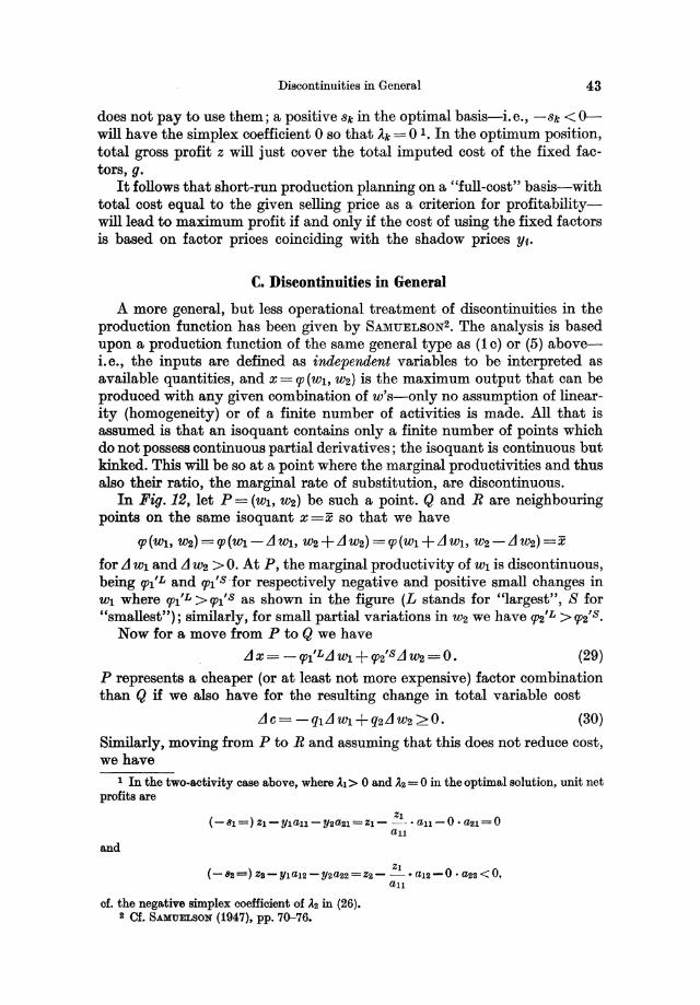
Discontinuities in General 43
does not pay to use them; a positive 8k in the optimal basis-Le., -8k <0-will have the simplex coefficient 0 so that Ak = 0 1. In the optimum position, total gross profit z will just cover the total imputed cost of the fixed factors, g.
It follows that short-run production planning on a "full-cost" basis-with total cost equal to the given selling price as a criterion for profitabilitywill lead to maximum profit if and only if the cost of using the fixed factors is based on factor prices coinciding with the shadow prices Yf.
c. Discontinuities in General
A more general, but less operational treatment of discontinuities in the production function has been given by SAMUELSONz. The analysis is based upon a production function of the same general type as (1c) or (5) aboveLe., the inputs are defined as independent variables to be interpreted as available quantities, and X=CP(W1, wz) is the maximum output that can be produced with any given combination of w's-only no assumption of linearity (homogeneity) or of a finite number of activities is made. All that is assumed is that an isoquant contains only a finite number of points which do not possess continuous partial derivatives; the isoquant is continuous but kinked. This will be so at a point where the marginal productivities and thus also their ratio, the marginal rate of substitution, are discontinuous.
In Fig. 12, let P = (WI, Wz) be such a point. Q and R are neighbouring points on the same isoquant X=X so that we have
cp(WI, Wz)=CP(WI-L1WI, wz+L1Wz)=CP(W1+ L1W1, wz-L1Wz)=x
for L1 WI and L1 Wz > O. At P, the marginal productivity of W1 is discontinuous, being CP1'L and cp1's-for respectively negative and positive small changes in WI where CP1'L >CP1'S as shown in the figure (L stands for "largest", S for "smallest"); similarly, for small partial variations in Wz we have cpz'L >cpz's.
Now for a move from P to Q we have
(29)
P represents a cheaper (or at least not more expensive) factor combination than Q if we also have for the resulting change in total variable cost
L1c= -q1L1W1 +qzL1Wz >0. (30)
Similarly, moving from P to R and assuming that this does not reduce cost, we have
1 In the two-activity case above, where ).1> 0 and ).2 = 0 in the optimal solution, unit net profits are
and
(-81=) Z1-Y1all-YSaS1=Z1- 211_. all-O. as1=O all
cf. the negative simplex coefficient of ).2 in (26). S Of. SAMUELSON (1947), pp. 70-76.
44 Linear Produotion Models and Disoontinuous Faotor Substitution
.1 X = 9'1'8.1 WI - 9'2'LL1 W2 = 0 (31)
.1 c = qd ¥'1- q2L1 W2 >0. (32)
Ai! w.? ____ -+ P
I I ~ ----++-I I I I I I I I I I I I I I I I I I I I I I I I I I I I I I I I I I I
I
W, W, w,? Wz w, Fig. 12
Eliminating .1 W2 from (29)-(30) and from (31 )-(32) respectively we find that the necessary and sufficient condition for P to be a local least-cost point (not necessarily unique) is
9'1' 8 ql 9'1' L -<-<-. (33) 9'2'L - q2 - 9"28
Thus the factor combination P is insensitive to factor price changes as long as the price ratio keeps within the bounds set by the left-hand and righthand marginal rates of substitution at PI. At the upper and lower critical values of, say, ql for constant q2 the response of WI and W2 to marginal changes in ql will be discontinuous.
If the isoquant is assumed to be convex to the origin so that the isocost line c = ql WI + q2 W2 which is "tangent" to x = x at P does not intersect the isoquant, P represents not only a local minimum of c but also a minimum "in the large"-a global optimum-for values of ql and q2 satisfying (33).
Condition (33) is seen to include continuity as a special case: for
9'1'8=9'I'L=9'I' and 9'2'8=9'2'L=9'2'
(33) becomes the familiar marginal equality2
ql 9'1' -=-,. q2 9'2
The extreme case of discontinuity is that of limitational inputs. Let the production function be
X=9'(Wl, W2) = Min (wI/aI, W2/a2),
cf. (1 c). At a point where x = Wl/al = W2/~ the left- and right-hand partial derivatives are
I In the case of m inputs, (33) generalizes to (m - 1) pairs of inequalities qll'S ql qll' L -<-< - (i=2,3, ... ,m), qI{L - q,- qII's
each pair derived in a similar manner for compensating variations in WI and W2, WI and Wa, etc. S Cf. Ch. IV, D.
W,
Discontinuities in General
rpl'L= l/al, rpl'S= 0, l{J2'L= 11 as, l{J2's= 0;
45
then (33) says that suoh a point is optimal for any factor price ratio from zero to infinity, i.e., for any set of non-negative prioes.
SAMUELSON mentions no other partioular examples of discontinuities. However, (33) also covers the more general oase of a linear model with discontinuous substitution. In the three-activity oase of Fig. 9 above, B is a least-cost point for faotor prices satisfying (8) (whioh in turn is equivalent to the simplex oriterion), as is obvious from geometrical oonsiderations. Precisely the same oondition for minimum cost emerges if the marginal produotivities are oaloulated and applied to (33)1.
1 For small variations in the activity levels we have
Llx=LlAl +LlAs+LlA3 LI WI = allLl Al + aIsLl As + a18L1 As LI Ws = aSILI Al + asaLl As + as8L1 As.
Now, the left-hand derivative of the production function X=tp(WI, Ws) with respect to WI at point B is found by setting LlWs=O and LlAs=O in the equations (the third activity is not used for efficient production to the left of B), eliminating LI Al and LI As:
Llx au-asl
For LI WI = 0 and LI As = 0 we find for a positive partial variation in Ws:
LIz alB -all _____ =tpB's. LlWs - aisasi-assall
The ratio of the marginal productivities-i.e., the marginal rate of substitution along BA-is
tpI'L _ ass - asl
Similarly, along BO we have
tps's - all - al~'
Qh'S as8 - ass tpS'L = alB - a13'
Substituting in (33), we get the conditions (8).
Chapter IV
Produetion Funetions with Continuous Faetor Substitution
A. Factor Substitution and the Isoquant Map
1. The Region of Substitution
(a) The "olassioal" type of faotor substitution, long predominant in eoonomio theory by virtue of its plausibility and analytioal oonvenienoe, finds expression in a produotion funotion
X=X(Vl, V2, ••• , vm), (1)
assumed to possess oontinuous first- and seoond-order partial derivatives in the region of definition v, > 0, x >0. The underlying prooess must be teohnologioally defined in suoh a way as to make the produotion funotion single-valued; when the existing teohnioal knowledge leads to a multiplevalued funotion beoause a given set of input amounts V, may be organized in different ways, this means that the prooess is inoompletely speoified. To obtain uniqueness in suoh oases it is usually assumed 1 that the faotors are always organized in a teohnioally optimal fashion so that the produotion funotion is defined as giving the maximum amount of output for any faotor oombination.
When the V, are defined as inputs oonsumed in the prooess, points at whioh one or more marginal produotivities xc' = ~ x I ~ V, is negative are not excluded from the produotion funotion (1), only suoh a point is obviously ineffioient in that a greater amount of output oan be produoed with less of the faotor or faotors in question, other inputs oonstant2• Henoe, with a view to optimal allooation in produotion, we are partioularly interested in points at whioh
xl ~o (i= 1,2, ... , m) (2)
so that x is an inoreasing or at least non-deoreasing funotion of all V,. (1)-(2)
1 Cf., e.g., CARLSON (1939), pp. 14 f. 2 A negative marginal productivity implies that the input in question is actually harmful;
leaving some of it idle would lead to greater output, thus apparently contradicting the definition of (1) as giving maximum output for any combination of inputs. The contradiction is resolved, however, if it is recalled that the VI are, by definition, the amounts actually used, whether harmful or not. The alternative definition of the production function as giving maximum output for any combination of input amounts available, x=Ij?(wl> Wa, ••• , Wm), is dealt with below.
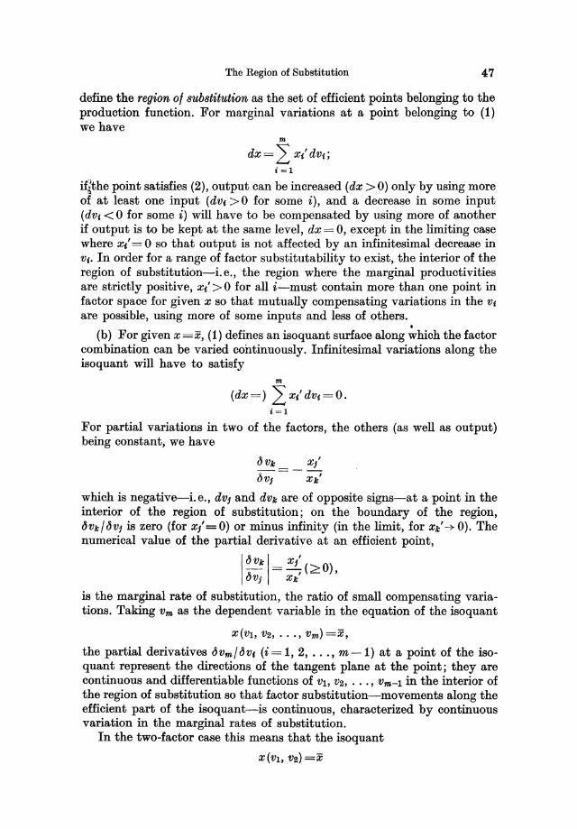
The Region of Substitution 47
define the region 01 substitution as the set of efficient points belonging to the production function. For marginal variations at a point belonging to (1) we have
m
dx = 2: x/ dVi ; i=1
if~the point satisfies (2), output can be increased (dx >0) only by using more of at least one input (dVi >0 for some i), and a decrease in some input (dVi < 0 for some i) will have to be compensated by using more of another if output is to be kept at the same level, dx = 0, except in the limiting case where xi' = 0 so that output is not affected by an infinitesimal decrease in Vi. In order for a range of factor substitutability to exist, the interior of the region of substitution-i.e., the region where the marginal productivities are strictly positive, x/ > 0 for all i-must contain more than one point in factor space for given x so that mutually compensating variations in the Vi are possible, using more of some inputs and less of others . .
(b) For given x =x, (1) defines an isoquant surface along which the factor combination can be varied continuously. Infinitesimal variations along the isoquant will have to satisfy
m
(dx =) 2: xl' dVi = 0 . i=1
For partial variations in two of the factors, the others (as well as output) being constant, we have
/5Vk= _ x/ /5Vj Xk'
which is negative-i. e., dVj and dVk are of opposite signs-at a point in the interior of the region of substitution; on the boundary of the region, /5Vk/15Vj is zero (for x/=O) or minus infinity (in the limit, for Xk'-+O). The numerical value of the partial derivative at an efficient point,
j 15Vkj= x<C2::0), 15Vj Xk
is the marginal rate of substitution, the ratio of small compensating variations. Taking Vm as the dependent variable in the equation of the isoquant
X(VI' V2, ... , vm)=x,
the partial derivatives 15vm/15v, (i=l, 2, ... , m-1) at a point of the isoquant represent the directions of the tangent plane at the point; they are continuous and differentiable functions of VI, V2, ... , Vm-l in the interior of the region of substitution so that factor substitution-movements along the efficient part of the isoquant-is continuous, characterized by continuous variation in the marginal rates of substitution.
In the two-factor case this means that the isoquant
X(VI' V2) =X
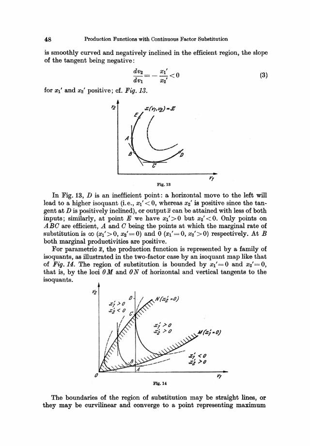
48 Production Functions with Continuous Factor Substitution
is smoothly curved and negatively inclined in the efficient region, the slope of the tangent being negative:
dV2= _ Xl' <0 dVI X2'
(3)
for Xl' and X2' positive; cf. Fig. 13.
Fig. 18
In Fig. 13, D is an inefficient point : a horizontal move to the left will lead to a higher isoquant (i.e., Xl' < 0, whereas X2' is positive since the tangent at D is positively inclined), or output x can be attained with less of both inputs; similarly, at point E we have XI'>O but X2' <0. Only points on ABO are efficient, A and 0 being the points at which the marginal rate of substitution is 00 (XI'>O, X2'=0) and 0 (XI'=O, X2'>0) respectively. At B both marginal productivities are positive.
For parametric x, the production function is represented by a family of isoquants, as illustrated in the two-factor case by an isoquant map like that of Fig. 14. The region of substitution is bounded by Xl' = 0 and X2' = 0, that is, by the loci 0 M and ON of horizontal and vertical tangents to the isoquants.
[)
FIg. 14,
.&; < ()
.&; >()
The boundaries of the region of substitution may be straight lines, or they may be curvilinear and converge to a point representing maximum
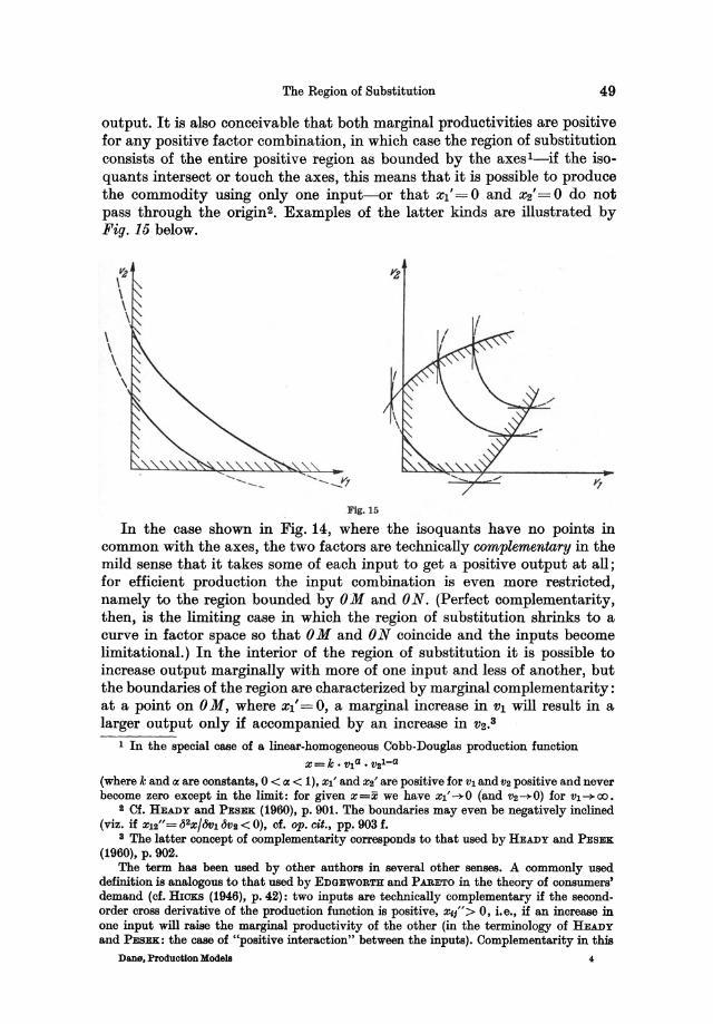
The Region of Substitution 49
output. It is also conceivable that both marginal productivities are positive for any positive factor combination, in which case the region of substitution consists of the entire positive region as bounded by the axes I-if the isoquants intersect or touch the axes, this means that it is possible to produce the commodity using only one input-or that Xl' = 0 and X2' = 0 do not pass through the origin2. Examples of the latter kinds are illustrated by Fig. 15 below.
\ \ \ \ \
I
Fig. 16
In the case shown in Fig. 14, where the isoquants have no points in common with the axes, the two factors are technically complementary in the mild sense that it takes some of each input to get a positive output at all ; for efficient production the input combination is even more restricted, namely to the region bounded by OM and ON. (Perfect complementarity, then, is the limiting case in which the region of substitution shrinks to a curve in factor space so that 0 M and ON coincide and the inputs become limitational.) In the interior of the region of substitution it is possible to increase output marginally with more of one input and less of another, but the boundaries of the region are characterized by marginal complementarity: at a point on 0 M, where Xl' = 0, a marginal increase in VI will result in a larger output only if accompanied by an increase in V2 .3
I In the special case of a linear-homogeneous Cobb· Douglas production function x=k. vIa. V21- a
(where k and ex are constants, 0 < ex < 1), Xl' and X2' are positive for VI and V2 positive and never become zero except in the limit: for given x=x we have XI'-+O (and V2-+0) for VI-+OO .
2 Cf. HEADY and PESEK (1960), p. 901. The boundaries may even be negatively inclined (viz. if XI2"= 02X/ OO1 OVa < 0), cf. op. cit. , pp. 903 f.
3 The latter concept of complementarity corresponds to that used by HEADY and PESEK
(1960), p. 902. The term has been used by other authors in several other senses. A commonly used
definition is analogous to that used by EDGEWORTH and PARETO in the theory of consumers' demand (cf. HICKS (1946), p. 42) : two inputs are technically complementary if the secondorder cross derivative of the production function is positive, Xl/'> 0, i.e., if an increase in one input will raise the marginal productivity of the other (in the terminology of HEADY
and PESEK: the case of "positive interaction" between the inputs). Complementarity in this DallB. Production Models 4
50 Produotion Funotions with Continuous Faotor Substitution
2. Returns to Seale and Elasticities of Production
When the production function is homogeneous of degree one, that is, when
X(,uVl, ,uV2, ••. , ,uvm)=,u' x(Vl, Vz, ••• , 'lim)
for any point on the production surface and for any (positive) value of ,u, the isoquants are radial projections of one another. This case may be looked upon as a limiting case of the linear model with discontinuous substitution. The half-line in factor space from the origin through any point (v10, vzo, .•• , vmO) on the isoquant x = 1 is a linear activity determined by Vi = ,u . Vio (i = 1,2, ... , m) where the Vio are the technical coefficients and the scale factor ,u = x represents the level of the activityl. The isoquant surfaces are generated by an infinite number of such elementary activities so that there are no discontinuities, but they can be approximated to any desired degree by a finite number of activities-the more activities, the smoother the isoquants will be.
A production function of this type is characterized by constant returns to scale: proportional variation in all inputs will change output in the same proportion so that average returns x l,u (or the ratio of x to each input) are constant, independent of the scale factorz. This property follows directly from the definition of homogeneity; it is also reflected in the elasticity of production being equal to one at all points. In general, for any given production function (1), let (vIO, V2o, ... , vmO) be an arbitrary point on the isoqua.nt x = 1 so that variations in the scale of output with the same relative
sense is not opposed to substitutability as defined above, of. HICKS, Zoc. cit.; when x =X(Vl, Va) is homogeneous of degree one, Xli" is positive everywhere in the region of substitution if the isoquants are convex, of. Appendix 2.
Still another concept of oomplementarity is defined as the cross derivative of the fum's factor demand funotion being negative: 6vI/6ql<0. On rather restriotive assumptions only can it be proved that the inputs are oomplementary in demand if they are teohnically complementary in the sense that Xli"> 0 at the point of equilibrium, of. FRISCH (1956), pp. 187 fi.
1 The boundary of the region of substitution is generated by half-lines representing those aotivities in which x{ =0 for some i. For p.= 1/V1 (say), the definition of homogeneity leads to
X=X(Vl, Va, ••• , Vm)=Vl· x(1, Va/VI, •• " Vm/VI)
=vt· I(va/vl, ... , Vm/V1)
whioh is an equivalent way of writing the production function. The partial derivatives of the function in this form turn out to depend on the relative faotor proportions Vl/Vl only. It follows that x,' is constant (e.g. =0) for proportional faotor variation. In Fig. 14, for example, OM and ON will be straight lines if the production function is homogeneous of the first degree.
2 It must be emphasized again that the production function treated here refers to a process taking place within a given plant. The inputs associated with the fixed oapital equipment represent the services of the respeotive items of equipment (e.g. machine hours per period), not these items themselves, which are assumed to be available in given numbers. The occurrence of constant returns to scale within the plant depends on the possibility of varying these inputs along with the other variable inputs (labour, etc.), i.e., of varying the utilization of the plant for constant relative factor proportions. Whenever the doubling of all inputs represents a mere repetition (in time or space), output will also be doubled. This problem, which must not be confused with the question of large-scale economies where plants of different sizes are compared, is treated in some detail below (Ch. VII).
Returns to Scale and Elasticities of Production 51
factor proportions can be expressed by Vi = I-' • v,o (i = 1,2, ... , m). Then the elasticity of production I at the point (VI, Vz, .•• , Vm) may be defined as
dx I-' 8=-'-
dl-' x'
that is, the elasticity of the production function
x=x(1-' . v1o, I-' • V2o, ••• , I-' • vmO)
with respect to the parameter 1-" In general, the value of 8 will depend on the Vi, i. e., on the scale factor I-' and the relative factor proportions as given by the v,o; for small variations from a particular point, average returns to scale (x / 1-') will be increasing, constant, or decreasing according as e ~ 1 at the point so that d (x / 1-') / dl-' = (I-' • dx / dl-' - x) / 1-'2 ~ O. If the production function is homogeneous of the first degree we have X(VI, V2, .•. , vm) = I-' • x(vIO, V20, ... , vmO) or x = I-' identically and therefore e = 1 at any point.
Alternatively, proportional factor variation may be expressed by dVf/V,=k (constant) for all i and the elasticity of production may be defined accordingly as the elasticity of the production function with respect to any input, say, VI:
dx VI 8=-'-
dVI x (for dVt/v,=k, i=l, 2, ... , m).
The two definitions of e are of course equivalent as dVt / Vi = v,o dl-' / I-' • v,o = dl-'/I-"
The latter definition leads to an important theorem. The differential of x being dx = ~ x,' dv, = k • ~ v,xc' for dv, / Vi = k, we have , ,
or m
e· X= L Vtxc' i=1
at any point on the production surface2•
(4)
(4) holds for any production function (1); if the function is homogeneous of degree one, Euler's theorem says that X=~VfXt' identically so that
1 Also known as the "passus coefficient" (FRIscn), the "function coefficient" (CARLSON),
or-in German-"der Ergiebigkeitsgrad" or "die Niveauelastizitii-t" (SCHNEIDER); cf. SCHNEI
DER (1934), pp. 9 ff., and (1958), p. 178. 2 Theorem (4) also holds for proportional variation of a subset of inputs VA:, ••• , Vm, the
others being constant (Vi = fit for i = 1, 2, ... , k -1) if E is redefined accordingly as the elasticity of the function
4}(VA:, ... , Vm)=X(tllo"" tlA:-l, VA:, ..• , vm)
with respect to VA: for dVI/VI=constant (i=k, ... , m). The proof is the same. With this interpretation, (4) has been named the Wicksell.John8on theorem, cf. SCHNEIDER (1934), pp.19ff.
52 Produotion Funotions with Continuous Faotor Substitution
B = 1 1. More generally, for a production function which is homogeneous of order r so that multiplication of any factor combination by I-' will multiply output by 1-", the elasticity of production will be identically equal to r 2.
Another theorem follows directly from (4):
~ , v, ~ B = ~ Xc • X = ~ B, (5)
i =1 i=1
where Be is the elasticity of the production function with respect to VI, the partial elasticity of production. In the case of first-degree homogeneity the partial elasticities add up to one.
3. The Convexity Assumption
(a) In order for any point in the region of substitution to represent minimum cost for some non-negative set of factor prices (cf. below), the isoquants must be assumed to be convex to the origin in the region. In the two-factor case this is simple enough: at any point (Vl, V2) where Xl' >0 and X2' >0, the curvature of the isoquant x(vl, V2) =x through the point must be positive:
d2v2 = (X2')2 xu" - 2Xl' X2' Xl2" + (Xl') 2X22" > 0 dV12 - (X2')3 '
(6)
that is, the slope dV2/dvl«0) must be an increasing function of Vl. (6) is the condition for the isoquant to be convex from below, as seen from the axis of the independent variable Vl. Since the isoquant is negatively inclined in the region considered, it will also be convex from the other axis,
d2vl/ dV22 = (X2' / Xl')3 • d2v2/ dV12> 0,
and thus convex to the origin when (6) is satisfied. The interpretation of (6) is that the amount of V2 saved by applying another unit of VI for X constant becomes smaller as the substitution proceeds: the marginal rate of substitution I dV2/ dVll = - dV2/ dVl (> 0) is a decreasing function of Vl 3. In
1 For proof of Euler's theorem see, for example, OSGOOD (1925), pp. 121 f. (Conversely, sinoe we know already that 8= 1 identioally, (4) may be taken as proof of the theorem.)
II For a point (V10, Vllo, ••• , vmO) on x=1 we have by the definition of r'th-order homogeneity
80 that
8= dx . !:!:..=r. ",r-1. !!:...=r identioally. d", x ",r
The whole isoquant map can be construoted from a single isoquant (for example, X= 1) also for r * 1-forgiven",. x(f') =",r = oonstantindependent of the v,o, of. above----only x does not vary in the same proportion as ",. Returns to scale are inoreasing or deoreasing everywhere according as r > 1 or r < 1.
S Convexity is sometimes desoribed as "inerea&ing marginal rate of substitution", referring to I dVsI dVll as a funotion of Vll (or I dV11 dVlll as a function of Vl), of. ALLEN (1938). p.286.
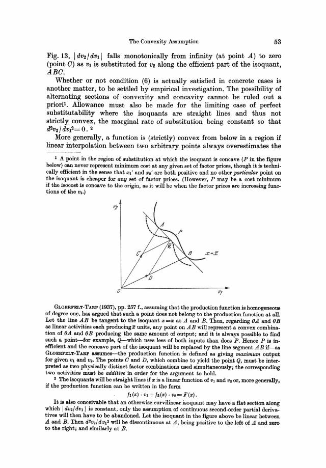
The Convexity Assumption 53
Fig. 13, I dV2/ dV11 falls monotonically from infinity (at point A) to zero (point 0) as VI is substituted for V2 along the efficient part of the isoquant, ABO.
Whether or not condition (6) is actually satisfied in concrete cases is another matter, to be settled by empirical investigation. The possibility of alternating sections of convexity and concavity cannot be ruled out a prioril . Allowance must also be made for the limiting case of perfect substitutability where the isoquants are straight lines and thus not strictly convex, the marginal rate of substitution being constant so that d2v2/ dV12= O. 2
More generally, a function is (strictly) convex from below in a region if linear interpolation between two arbitrary points always overestimates the
1 A point in the region of substitution at which the isoquant is concave (P in the figure below) can never represent minimum cost at any given set of factor prices, though it is technically efficient in the sense that Xl' and X2' are both positive and no other particular point on the isoquant is cheaper for any set of factor prices. (However, P may be a cost mininmID if the isocost is concave to the origin, as it will be when the factor prices are increasing functions of the Vj.)
o
GLOERFELT-TARP (1937), pp. 257 f., assuming that the production function is homogeneous of degree onll, has argued that such a point does not belong to the production function at all. Let the line AB be tangent to the isoquant x=x at A and B. Then, regarding OA and OB as linear activities each producing x units, any point on AB will represent a convex combination of OA and OB producing the same amount of output; and it is always possible to find such a point-for example, Q-which uses less of both inputs than does P. Hence P is inefficient and the concave part of the isoquant will be replaced by the line segment AB if-as GLoERFELT-TARP assumes-the production function is defined as giving maximum output for given Vl and V2. The points C and D, which combine to yield the point Q, must be interpreted as two physically distinct factor combinations used simultaneously; the corresponding two activities must be additive in order for the argument to hold.
2 The isoquants will be straight lines if X is a linear function of VI and V2 or, more generally, if the production function can be written in the form
II (x) . VI + /2 (X) • V2 = F (x).
It is also conceivable that an otherwise curvilinear isoquant may have a flat section along which I dV2! dVI I is constant, only the assumption of continuous second-order partial derivatives will then have to be abandoned. Let the isoquant in the figure above be linear between A and B. Then d2v2!dvI2 will be discontinuous at A, being positive to the left of A and zero to the right; and similarly at B.
54 Production Functions with Continuous Factor Substitution
actual value of the function1• With, say, Vm as the dependent variable, the equation of the isoquant
can be written Vm= 1 (VI, V2, •.. , Vm-l).
The function 1 is convex from below in the region of substitution if the following inequality holds for any two distinct points (VI0, •.. , VmO) and (VI, ••• , Vm):
(1-19-) • /(Vlo, ... , V!_I) + 19- • /(V1, ••• , Vm-1)
>1 {[(1-0)V10+0V1], ••. , [(1-19-)V!_I+19-vm-l]}
for any positive fraction 19-, 0 < 19- < 1. 2 Rearranging we have
I(Vl,"" vm-1)-/(V10, ... , V!_l)
> f{[V10 +19-(V1- VI0)] , ... , [V!_1+:(Vm-1- V!_1)]} - /(Vt°, •.. , V!_l)
where I(V1, ••• , Vm-1)=Vm and /(V10, ... , V!_l)=Vmo• In the limit (for 19- 4 0) 8 convexity is seen to imply
v. > ".'+ :~U"l" (v,-v,,) (~ •• '+ :~[ .:T (.<-".o») (7)
for any two distinct efficient points satisfying
X(V10, •.. , VmO) = X (V1, .. • ,vm)=x.
Since the""equation of the plane tangent to the isoquant at (VI0, ••. ,VmO) is the corresponding equality, the geometric interpretation of (7) is that any other efficient point on the isoquant lies above the tangent plane-that is, in the direction of the dependent variable, vm-except in the limiting case where (Xm')o= 0 so that (//)0= - 00. As long as only efficient points are considered, (7) can be rearranged to give a similar inequality with any other input as dependent variable. In other words, if the isoquant function is convex in the region of substitution for some set of m-1 independent input variables-cf. (7)-the isoquant is convex in all factor directions, and therefore convex to the origin, in the efficient region. Rearranging (7) into the''"more symmetrical form
1 This is the definition used by KUHN and TuCKER (1951)-0£. Appendix 1 below--except that the limiting case of linearity, where linear interpolation neither underestimates nor overestimates the function, is excluded. If it is to be allowed for, the inequality signs > must be replaced by 2 in the following.
II In the two-factor case the geometric interpretation is obvious: Between any two points, e.g. Band G in Fig. 13, the isoquant lies below the chord connecting the points (the line segment BG).
8 For (}=O, the right-hand side of the inequality is an indeterminate form, 0/0; for (}-+O it approaches a limit which is the ratio of the derivatives of numerator and denominator with respect to (}. (Of. OSGOOD (1925), pp. 208 f., and KUHN and TuCKER (1951), pp. 485 f.)
The Convexity Assumption
m 2: (xt')O . (v,- v~O) > 0 i=1
(x,'>O, i=1,2, ... ,m),
55
(8)
which in equality form would represent the equation of the tangent plane at (VI0, ••• , vmO), convexity to the origin is seen to imply in geometric terms that all efficient points distinct from the point of tangency are "outside" the tangent plane. More precisely, the tangent plane-negatively inclined in all directions-at an arbitrary efficient point (v10, ••• , VmO) on the isoquant will be intersected by the line segment in factor space connecting the origin and any other efficient point (VI> ••• , vm) on the isoquant. For m = 2, (7) or (8) is equivalent to convexity in the sense of (6).1
Inequality (8), with the same geometric interpretation, also holds when (VI, .•• , vm ) is an arbitrary inefficient point on the isoquant (still assuming that the arbitrary fixed point (v10, ... , vmO) is efficient). In order for a point (v!, ... , vm) to represent the global minimum of z =:E (x/)Ov, subject to x=x(VI, V2, ... , vm), in which case it would be "inside" the tangent plane, it would have to satisfy the necessary conditions
(i = 1, 2, ... , m)
where u is a Lagrange multiplier. Since (x/)o>O for all i, we have either x/ > 0 or x/ < 0 for all i at the point. Suppose the latter to be the case"'at a point Q = (v1Q, ... , vmQ) belonging to the isoquant x =X and satisfying the necessary conditions for minimum z. Then select some other point R=(V1R, ... , vmR) in factor space such that V,R<V,Q for i=l, 2, ... , m. For variations along the straight line through Q and R, the production function can be written in terms of a parameter t,
where
For t = 1 we have point Q where V,= v,Q, x = f (1) = x, whereas t = 0 corresponds to point R. The derivative of the function is
which for t = 1 becomes
1 Expanding the isoquant function V2 = I (Vl) by Taylor's series (cf. ALLEN (1938), pp. 451£.) we have
I (Vl) = I (vlO) + f' (vlO) • (Vl - VlO) + t . f" . (Vl - Vl O)2
where f" (= d2v2/ dVl2) is taken at the point vlo + D(Vl - VlO) for some positive fraction D. It follows that, when (7) is satisfied, f" will be positive at this intermediate point and therefore also at vlo since the interval Vl - Vlo can be made arbitrarily small and I" is a continuous function. Hence, VlO being an arbitrary point, (6) is satisfied everywhere in the interior of the region of substitution. Conversely, if (6) is satisfied everywhere, so are (7) and (8).
56 Produotion FunotiollB with Continuous Factor Substitution
m
1'(1) = L (V,Q-V,R) • (x/)Q<O. i=1
Assuming that t (t) = 0 for some t = T < 1-if this were not the case, a positive output would result from negative amounts of all inputs-it is obvious from a graph of the continuous function x = t (t) that there exists an intermediate point in the region T < t < 1 where t (t) =x, that is, another point S = (VIS, ..• , VmS) on the isoquant x =x such that v,s < v,Q for all i. Hence we have
m m L (x/)OVtS < L (X/)OViQ ; i=1 i=1
in other words, a point Q characterized by (xc')Q < 0 (i = 1, 2, ... , m) cannot represent the global minimum of z on the isoquant. The "best" point, therefore, is the best efficient point, (v10, ... , vmO). The tangent plane at this point has no other points--efficient or otherwise-in common with the isoquant, as expressed by (8).12
(b) The isoquant X(Vl, ••. , vm ) =X cannot be illustrated geometrically by an isoquant map when m > 2, unless the substitution which is considered is restricted in such a way that only one input variable is capable of independent variation. The question is to what extent the characteristic features of the two-dimensional isoquant persist for variations of this kind.
For example, in the three-factor case we may wish to study compensating variations in VI and V2 for constant V3 = V3. The equation of the isoquant in terms of VI and V2 is
X(V1, V2, V3)=4'>(V1, V2)=X
where 4'>1'=Xl' and 4'>2'=X2'. In the interior of the region of substitution belonging to the function 4'>-the region where 4'>1' and 4'>2' are both positivethe isoquant will be downward sloping,
dV2 / dV1 = -4'>1' / 4'>2' < o. Assuming that the three-dimensional isoquant is convex to the origin in the region where xc'>O (i= 1,2,3), (8) for V3=V30= v3leads to
[ 4'> ,]0
V2 >V20+ - 4'>~, . (V1- VI0)
for any two points on 4'> (VI, V2) =X satisfying 4'>1'>0, 4'>2'>0, and X3'>0.
1 If Q is a feasible point (vjQ ~ 0 for all i), the origin may be used for R so that we have VI = t . vjQ; f(t) will be zero for t = 0 (or for some t in the region 0 < t < 1), and f(t) =X at some intermediate point. However, in order to prove analytically that (8) holds for any point (Vl' ... , vm) on the isoquant and therefore also for any feasible point, the possibility that there may exist infeasible points Q where x;' :s; 0 for all i must be taken into aooount, though suoh points are devoid of eoonomio meaning. In suoh oases the point R has to be seleoted differently in order to ellBure v,Q> ViR for all i.
2 Sinoe (vl O, ••• , vmO) may be any efficient point, (8) implies in the two-faotor oase that the isoquant is oonfined to the region bounded by the vertioal and horizontal tangents and the efficient points (in Fig. 13, the tangents at A and 0 and the ourve AB 0).
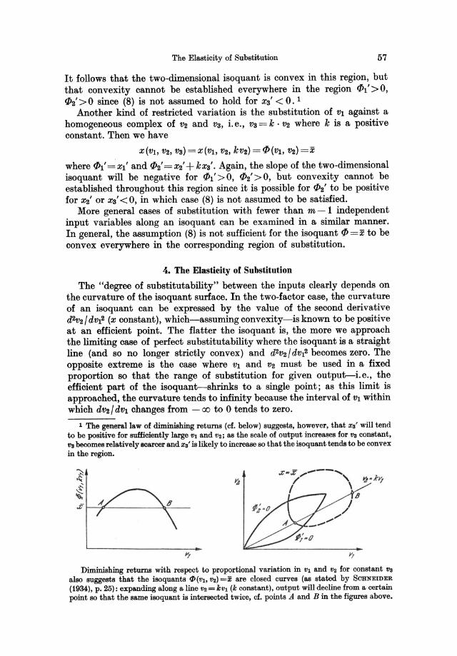
The Elasticity of Substitution 57
It follows that the two-dimensional isoquant is convex in this region, but that convexity cannot be established everywhere in the region fPl' > 0, fP2' > ° since (8) is not assumed to hold for xa' < 0. 1
Another kind of restricted variation is the substitution of VI against a homogeneous complex of V2 and Va, i. e., Va = k . V2 where k is a positive constant. Then we have
X(Vl, V2, va) = X (VI, V2, kV2) = fP(VI, V2) =X
where fPl' = Xl' and fP2' = X2' + kXa'. Again, the slope of the two-dimensional isoquant will be negative for (/)1' > 0, fP2' > 0, but convexity cannot be established throughout this region since it is possible for fP2' to be positive for X2' or xa' < 0, in which case (8) is not assumed to be satisfied.
More general cases of substitution with fewer than m - 1 independent input variables along an isoquant can be examined in a similar manner. In general, the assumption (8) is not sufficient for the isoquant fP =X to be convex everywhere in the corresponding region of substitution.
4. The Elasticity of Substitution
The "degree of sUbstitutability" between the inputs clearly depends on the curvature of the isoquant surface. In the two-factor case, the curvature of an isoquant can be expressed by the value of the second derivative d 2v2/ dVl2 (x constant), which-assuming convexity-is known to be positive at an efficient point. The flatter the isoquant is, the more we approach the limiting case of perfect substitutability where the isoquant is a straight line (and so no longer strictly convex) and d2V2/dv12 becomes zero. The opposite extreme is the case where VI and V2 must be used in a fixed proportion so that the range of substitution for given output-i. e., the efficient part of the isoquant-shrinks to a single point; as this limit is approached, the curvature tends to infinity because the interval of VI within which dV2/ dVI changes from - 00 to ° tends to zero.
1 The general law of diminishing returns (cf. below) suggests, however, that X3' will tend to be positive for sufficiently large Vl and V2; as the scale of output increases for Vs constant, Vs becomes relatively scarcer and xs' is likely to increase so that the isoquant tends to be convex in the region.
~ ~ f ~ .f t--jS------~--
Diminishing returns with respect to proportional variation in Vl and V2 for constant Vs
also suggests that the isoquants I/> (VI, V2)=X are closed curves (as stated by SCHNEIDER (1934), p. 25): expanding along a line V2 = kVl (k constant), output will decline from a certain point so that the same isoquant is intersected twice, cf. points A and B in the figures above.
58 Production Functions with Continuous Factor Substitution
The second-order derivative d2v2/ dV12, however, has the disadvantage of being dependent on the units in which the inputs are measured. A more convenient measure of the degree of substitutability is provided by the elasticity of substitution, defined as the elasticity of the relative factor proportion along the isoquant with respect to a change in the marginal rate of substitution 1 :
S12= _d_(V_2_/V_1_) _ . (-dv2/dvd = -:' ::-:d--=-(v_2-',-/--::V1_)-,-. dV2/ dv1 d(-dv2/dv1) V2/V1 d(dv2/dv1) V2/ V1
(V2-V1· dV2/dv1)· (-dV2/dv1) (9)
V1 V2 . d2v2/ dV12
for x constant. S12, which is a pure number-positive in the interior of the region of substitution provided that the isoquant is convex, cf. (3) and (6)is a function of Vl and V2, subject to X(V1, V2) =X and thus to Xl' dV1 + X2' dV2 = 0. 2 The elasticity of substitution it not an appropriate tool for describing the shape of the whole isoquant-much less for characterizing a particular production function in its entirety-unless the shape of the isoquant happens to be such that S12 is constant along the curves; the elasticity
1 Cf. ALLEN (1938), pp. 341 ff. 2 Evaluating 812 further, expressing dV2/ dVl and d2V2! dV12 in terms of the derivatives
of the production function (cf. (3) and (6) above), the elasticity becomes
-Xl' Xs' (VI Xl' + V2XS') 812 = -Vl-V-2::C[(-XS-c')--::-s-x-n-:-:" -_ 2Xl' Xs' XlS"-+-'--'('--X-:l':-::)S-X-ss-:"'j ,
cf. ALLEN, op. cit., p. 342. If the production function is homogeneous of degree one, this reduces to
Xl' . X2' 812= ----,
X • X12"
using Euler's theorem; cf. ALLEN, op. cit., p. 343. In this case the elasticity of substitution is a function of the relative factor combination vs/ VI only, independent of the scale of output X, since Xl' and X2' are homogeneous of degree zero and XIS" is homogeneous of degree -1, cf. ALLEN, op. cit., p. 319.
3 Setting 81S, as evaluated in (9), equal to a (positive) constant 8 gives a second-order non-linear differential equation whose general solution for Vs in terms of VI represents the general shape of an isoquant with constant elasticity of substitution. The solution is more easily obtained directly from the definition of 81S, setting VS! VI = u and - dvs! dVl = V and recalling that du/u=dlog.u, dv/v=dlog. V so that we have
which, by integration, gives
d logeu -- = 8 (constant) d log. v
log.u=8 .10g.v+K or u=k· VB
where k (= eK > 0) is an arbitrary constant. Thus we have the first-order d~erential equation (i) v2/ VI = k • (-dV2/ dVl)8
or, separating the variables, vs-1lB dvs = k1 • VC11B dvl (where kl = _k-lls < 0)
whose integral for 8 '*' 1 is (ii) VS(B-1I IB= kl . VI (8-11 IB+ ks
where kr « 0) and k2 are arbitrary constants. (For 8 ~ 00, the isoquant (ii) approaches a linear shape; for 8~0 the differential equation (i) tends towards VS!V1 = k). For 8 = 1 the solution is
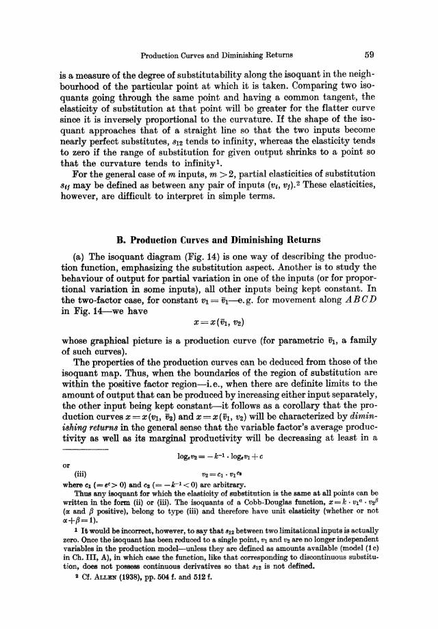
Production Curves and Diminishing Returns 59
is a measure of the degree of substitutability along the isoquant in the neighbourhood of the particular point at which it is taken. Comparing two isoquants going through the same point and having a common tangent, the elasticity of substitution at that point will be greater for the flatter curve since it is inversely proportional to the curvature. If the shape of the isoquant approaches that of a straight line so that the two inputs become nearly perfect substitutes, S12 tends to infinity, whereas the elasticity tends to zero if the range of substitution for given output shrinks to a point so that the curvature tends to infinity 1.
For the general case of m inputs, m > 2, partial elasticities of substitution Sf1 may be defined as between any pair of inputs (v(, VJ).2 These elasticities, however, are difficult to interpret in simple terms.
B. Production Curves and Diminishing Returns
(a) The isoquant diagram (Fig. 14) is one way of describing the production function, emphasizing the substitution aspect. Another is to study the behaviour of output for partial variation in one of the inputs (or for proportional variation in some inputs), all other inputs being kept constant. In the two-factor case, for constant Vl= Vl-e.g. for movement along ABeD in Fig. 14-we have
X=X(Vl, V2)
whose graphical picture is a production curve (for parametric VI, a family of such curves).
The properties of the production curves can be deduced from those of the isoquant map. Thus, when the boundaries of the region of substitution are within the positive factor region-i.e., when there are definite limits to the amount of output that can be produced by increasing either input separately, the other input being kept constant-it follows as a corollary that the production curves X=X(Vl, V2) and X= x(ih, V2) will be characterized by diminishing returns in the general sense that the variable factor's average productivity as well as its marginal productivity will be decreasing at least in a
or (iii)
where 1:1 (=ec> 0) and C2 (= -k-1 <0) are arbitrary. Thus any isoquant for which the elasticity of substitution is the same at all points can be
written in the form (ii) or (iii). The isoquants of a Cobb-Douglas function, X= k . V1 a • V2 fJ (oc and f1 positive), belong to type (iii) and therefore have unit elasticity (whether or not oc+f1=1).
1 It would be incorrect, however, to say that 812 between two limitational inputs is actually zero. Once the isoquant has been reduced to a single point, V1 and V2 are no longer independent variables in the production model-unless they are defined as amounts available (model (1c) in Ch. III, A), in which case the function, like that corresponding to discontinuous substitution, does not possess continuous derivatives so that 812 is not defined.
2 Cf. ALLEN (1938), pp. 504 f. and 512 f.
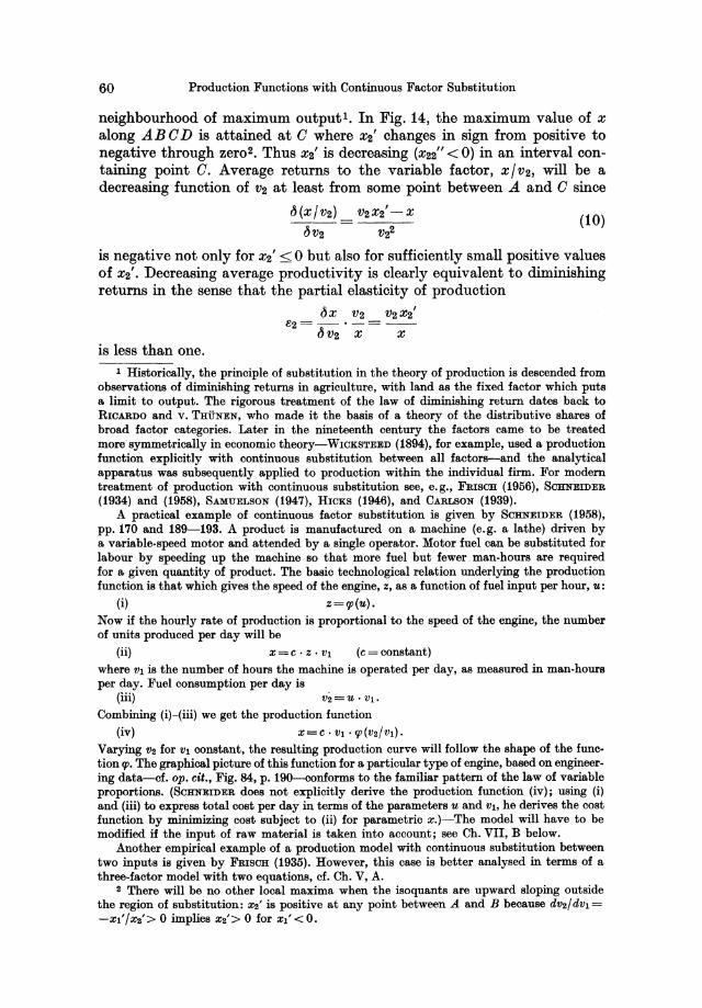
60 Production Functions with Continuous Factor Substitution
neighbourhood of maximum output!. In Fig. 14, the maximum value of x along AB CD is attained at C where xz' changes in sign from positive to negative through zeroz. Thus xz' is decreasing (xzz" < 0) in an interval containing point C. Average returns to the variable factor, xjvz, will be a decreasing function of vz at least from some point between A and C since
b(xjvz) V2X2'-X ----
bV2 vz2 (10)
is negative not only for X2' ~ 0 but also for sufficiently small positive values of xz'. Decreasing average productivity is clearly equivalent to diminishing returns in the sense that the partial elasticity of production
bx V2 V2XZ' 82=-'-=--
bV2 X X is less than one.
1 Historically, the principle of substitution in the theory of production is descended from observations of diminishing returns in agriculture, with land as the fixed factor which puts a limit to output. The rigorous treatment of the law of diminishing return dates back to RICARDO and v. TWNEN, who made it the basis of a theory of the distributive shares of broad factor categories. Later in the nineteenth century the factors came to be treated more symmetrically in economic theory-WICKsTEED (1894), for example, used a production function explicitly with continuous substitution between all factors-and the analytical apparatus was subsequently applied to production within the individual firm. For modern treatment of production with continuous substitution see, e.g., FRISCH (1956), SCHNEIDER (1934) and (1958), SAMUELSON (1947), HICKS (1946), and CARLSON (1939).
A practical example of continuous factor substitution is given by SCHNEIDER (1958), pp. 170 and 189-193. A product is manufactured on a machine (e.g. a lathe) driven by a variable-speed motor and attended by a single operator. Motor fuel can be substituted for labour by speeding up the machine so that more fuel but fewer. man-hours are required for a given quantity of product. The basic technological relation underlying the production function is that which gives the speed of the engine, z, as a function of fuel input per hour, u:
(i) z=tp(u).
Now if the hourly rate of production is proportional to the speed of the engine, the number of units produced per day will be
(ii) x = c . z . VI (c = constant) where VI is the number of hours the machine is operated per day, as measured in man-hours per day. Fuel consumption per day is
(iii) V2 = u • VI.
Combining (i)-(iii) we get the production function
(iv) X=C· VI' tp(V2/Vl).
Varying V2 for VI constant, the resulting production curve will follow the shape of the function tp. The graphical picture of this function for a particular type of engine, based on engineering data-cf. op. cit., Fig. 84, p. 190-conforms to the familiar pattern of the law of variable proportions. (SCHNEIDER does not explicitly derive the production function (iv); using (i) and (iii) to express total cost per day in terms of the parameters u and VI, he derives the cost function by minimizing cost subject to (ii) for parametric x.)-The model will have to be modified if the input of raw material is taken into account; see Ch. VII, B below.
Another empirical example of a production model with continuous substitution between two inputs is given by FRISCH (1935). However, this case is better analysed in terms of a three-factor model with two equations, cf. Ch. V, A.
2 There will be no other local maxima when the isoquants are upward sloping outside the region of substitution: X2' is positive at any point between .A and B because dV2/ dVl = -Xl' fX2'> 0 implies X2'> 0 for Xl' < O.
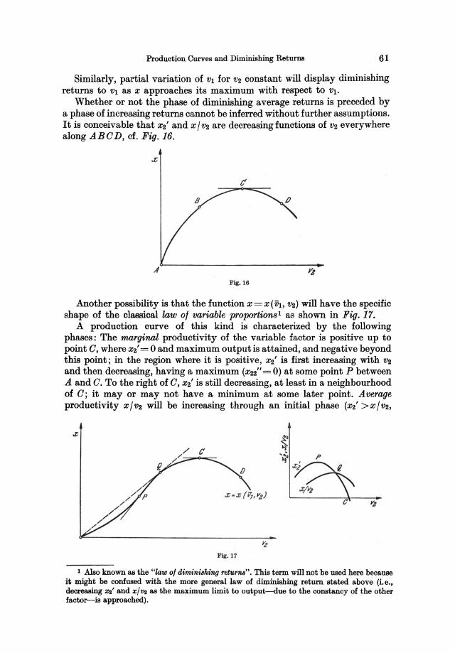
Production Curves and Diminishing Returns 61
Similarly, partial variation of VI for V2 constant will display diminishing returns to VI as x approaches its maximum with respect to VI.
Whether or not the phase of diminishing average returns is preceded by a phase of increasing returns cannot be inferred without further assumptions. It is conceivable that X2' and x / V2 are decreasing functions of V2 everywhere along ABeD, cf. Fig. 16.
Fla. 16
Another possibility is that the function x=x(iit, V2) will have the specific shape of the classical law of variable proportions l as shown in Fig. 17.
A production curve of this kind is characterized by the following phases: The marginal productivity of the variable factor is positive up to point e, where X2' = 0 and maximum output is attained, and negative beyond this point; in the region where it is positive, X2' is first increasing with V2
and then decreasing, having a maximum (X22"=O) at some point P between A and e. To the right of e, X2' is still decreasing, at least in a neighbourhood of e; it mayor may not have a minimum at some later point. Average productivity x / V2 will be increasing through an initial phase (X2' > x / V2,
Fig. 17
1 Also known as the "law 01 dimini8hing returns". This term will not be used here because it might be confused with the more general law of diminishing return stated above (i.e., decreasing xs' and x/vs as the maximum limit to output-due to the constancy of the other factor-is approached).
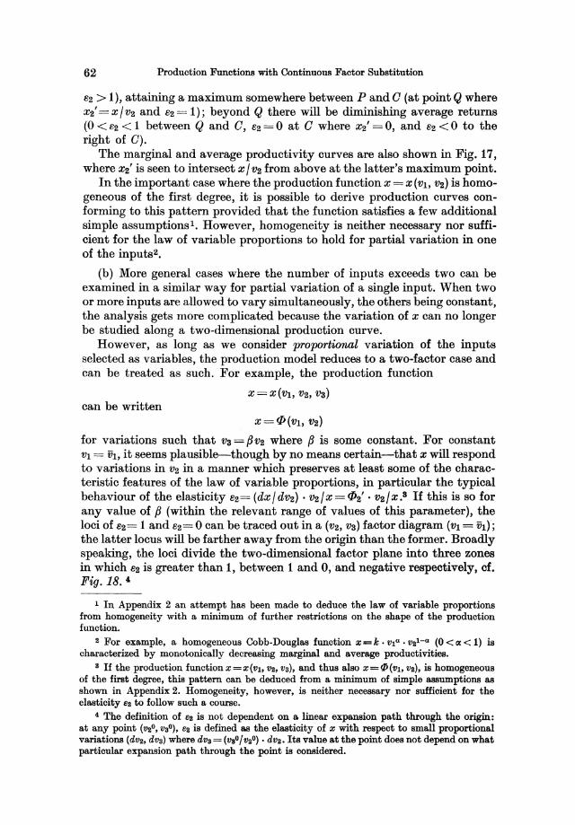
62 Production Functions with Continuous Factor Substitution
82> 1), attaining a maximum somewhere between P and 0 (at point Q where X2' = x / V2 and 82 = 1); beyond Q there will be diminishing average returns (0 < 82 < 1 between Q and 0, 82 = 0 at 0 where X2' = 0, and 82 < 0 to the right of 0).
The marginal and average productivity curves are also shown in Fig. 17, where X2' is seen to intersect x / V2 from above at the latter's maximum point.
In the important case where the production function x = x (Vl' VI) is homogeneous of the first degree, it is possible to derive production curves conforming to this pattern provided that the function satisfies a few additional simple assumptions I. However, homogeneity is neither necessary nor sufficient for the law of variable proportions to hold for partial variation in one of the inputsl.
(b) More general cases where the number of inputs exceeds two can be examined in a similar way for partial variation of a single input. When two or more inputs are allowed to vary simultaneously, the others being constant, the analysis gets more complicated because the variation of x can no longer be studied along a two-dimensional production curve.
However, as long as we consider proportional variation of the inputs selected as variables, the production model reduces to a two-factor case and can be treated as such. For example, the production function
X=X(Vl, VI, V3)
can be written x = 4) (Vl, V2)
for variations such that V3 = {J VI where {J is some constant. For constant VI = th, it seems plausible-though by no means certain-that x will respond to variations in V2 in a manner which preserves at least some of the characteristic features of the law of variable proportions, in particular the typical behaviour of the elasticity 82 = (dx / dV2) • VI / x = 4)2' • V2 / X. 8 If this is so for any value of {J (within the relevant range of values of this parameter), the loci of 81= 1 and 81= 0 can be traced out in a (V2, V3) factor diagram (Vl = Vl); the latter locus will be farther away from the origin than the former. Broadly speaking, the loci divide the two-dimensional factor plane into three zones in which 82 is greater than 1, between 1 and 0, and negative respectively, of. Fig. 18. "
I In Appendix 2 an attempt has been made to deduce the law of variable proportions from homogeneity with a minimum of further restrictions on the shape of the production function.
2 For example, a homogeneous Cobb-Douglas function X= Ie. VIa. Val - a (0 < IX < 1) is characterized by monotonically decreasing marginal and average productivities.
8 If the production function X=X(Vb Va, va), and thus also X=4'>(Vl, va), is homogeneous of the first degree, this pattern can be deduced from a minimum of simple assumptions as shown in Appendix 2. Homogeneity, however, is neither necessary nor sufficient for the elasticity Ell to follow such a course.
4 The definition of Ell is not dependent on a linear expansion path through the origin: at any point (v&0, vaO), 8a is defined as the elasticity of x with respect to small proportional variations (dva, dva) where dVa= (Va0/v&0) • dva. Its value at the point does not depend on what particular expansion path through the point is considered.
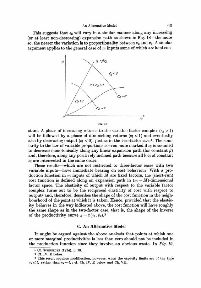
An Alternative Model 63
This suggests that 62 will vary in a similar manner along any increasing (or at least non-decreasing) expansion path as shown in Fig. 1S-the more so, the nearer the variation is to proportionality between V2 and V3. A similar argument applies to the general case of m inputs some of which are kept con-
Fig. IS
stant. A phase of increasing returns to the variable factor complex (62 ) 1) will be followed by a phase of diminishing returns (62 < 1) and eventually also by decreasing output (62 < 0), just as in the two-factor case l • The similarity to the law of variable proportions is even more marked if 62 is assumed to decrease monotonically along any linear expansion path (for constant (J) and, therefore, along any positively inclined path because all loci of constant 62 are intersected in the same order.
These results-which are not restricted to three-factor cases with two variable inputs-have immediate bearing on cost behaviour. With a production function in m inputs of which M are fixed factors, the (short-run) cost function is defined along an expansion path in (m - M)-dimensional factor space. The elasticity of output with respect to the variable factor complex turns out to be the reciprocal elasticity of cost with respect to output2 and, therefore, describes the shape of the cost function in the neighbourhood of the point at which it is taken. Hence, provided that the elasticity behaves in the way indicated above, the cost function will have roughly the same shape as in the two-factor case, that is, the shape of the inverse of the productivity curve x = x (VI, V2). 3
c. An Alternative Model
It might be argued against the above analysis that points at which one or more marginal productivities is less than zero should not be included in the production function since they involve an obvious waste. In Fig. 19,
1 Cf. SOHNEIDER (1934), p. 18. 2 Cf. IV, E below. 3 This result requires modification, however, when the capacity limits are of the type
v.:S; fI, rather than v, = fI, ; cf. Ch. IV, E below and Ch. VII.
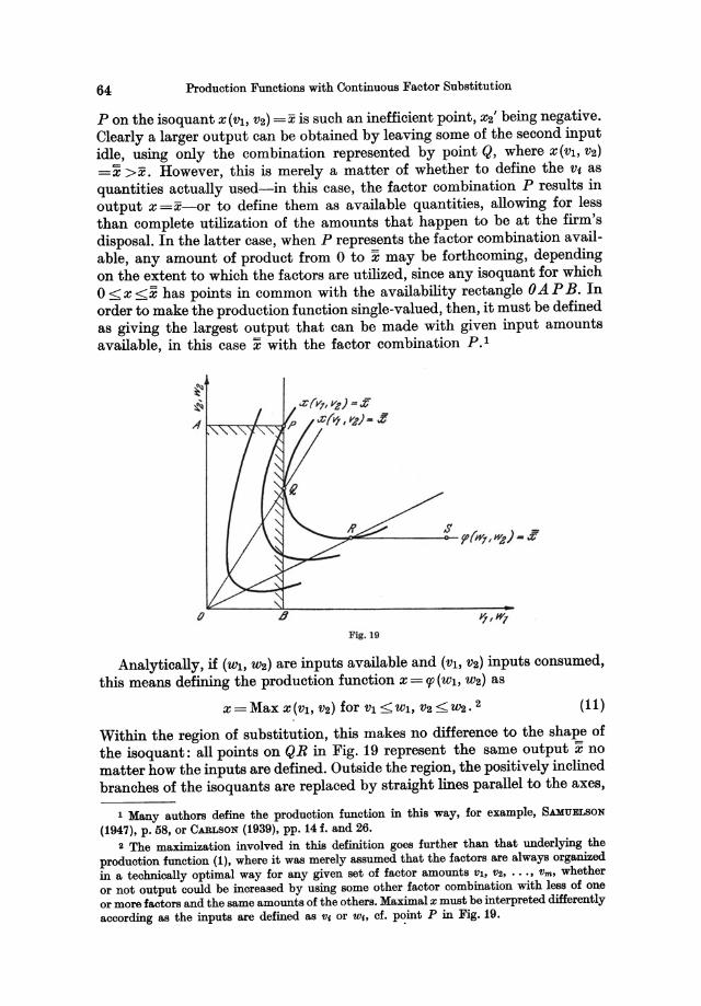
64 Production Functions with Continuous Factor Substitution
P on the isoquant x (v!, V2) =X is such an inefficient point, X2' being negative. Clearly a larger output can be obtained by leaving some of the second input idle, using only the combination represented by point Q, where X(VI' vz) =x >x. However, this is merely a matter of whether to define the Vt as quantities actually used-in this case, the factor combination P results in output x =x-or to define them as available quantities, allowing for less than complete utilization of the amounts that happen to be at the firm's disposal. In the latter case, when P represents the factor combination available, any amount of product from 0 to x may be forthcoming, depending on the extent to which the factors are utilized, since any isoquant for which o <x <x has points in common with the availability rectangle OA P B. In order to make the production function single-valued, then, it must be defined as giving the largest output that can be made with given input amounts available, in this case x with the factor combination P.I
Fig. 19
Analytically, if (Wl' Wz) are inputs available and (VI, Vz) inputs consumed, this means defining the production function x = q; (WI, Wz) as
(11)
Within the region of substitution, this makes no difference to the shape of the isoquant: all points on QR in Fig. 19 represent the same output x no matter how the inputs are defined. Outside the region, the positively inclined branches of the isoquants are replaced by straight lines parallel to the axes,
I Many authors define the production function in this way, for example, SAMUELSON (1947), p. 58, or CARLSON (1939), pp. 14 f. and 26.
2 The maximization involved in this definition goes further than that underlying the production function (1), where it was merely assumed that the factors are always organized in a technically optimal way for any given set of factor amounts VI, V2, ••• , Vm, whether or not output could be increased by using some other factor combination with less of one or more factors and the same amounts of the others. Maximal x must be interpreted differently according as the inputs are defined as Vj or WI. cf. p~int P in Fig. 19.
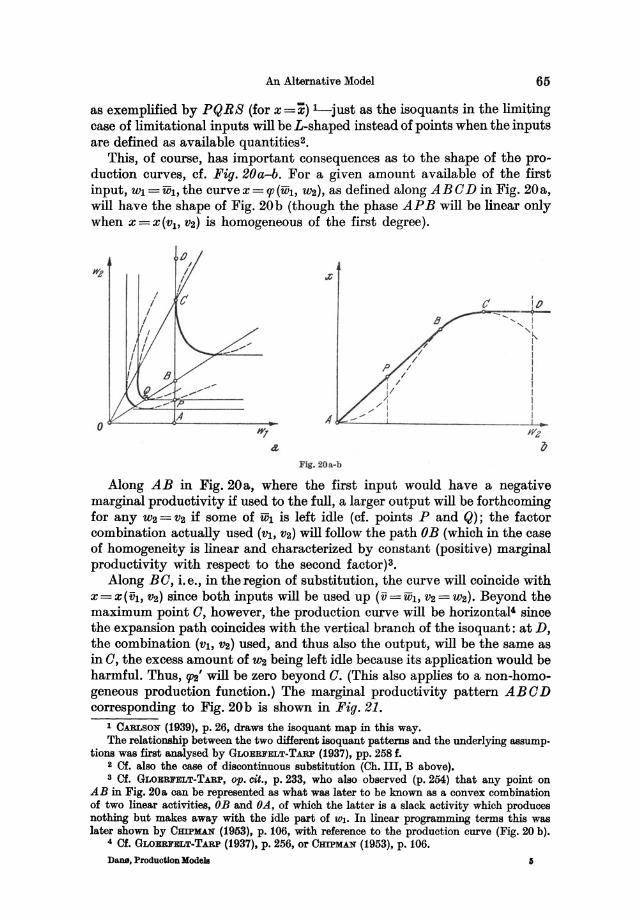
An Alternative Model 65
as exemplified by PQRS (for x=x) I_just as the isoquants in the limiting case of limitational inputs will be L-shaped instead of points when the inputs are defined as available quantities2•
This, of course, has important consequences as to the shape of the production curves, cf. Fig. 20a-b. For a given amount available of the first input, wI=uh, the curve x = 9'(uh, W2), as defined along ABCD in Fig. 20a, will have the shape of Fig. 20b (though the phase AP B will be linear only when x=x(v1, V2) is homogeneous of the first degree).
r: 1.0 " I , ,
',,I I I I I I I I I I
o ~---o.:-------A~~_~ ________ ~I~
Hi .t
Flg.201L·b
Wz Q
Along AB in Fig.20a, where the first input would have a negative marginal productivity if used to the full, a larger output will be forthcoming for any W2 = V2 if some of WI is left idle (cf. points P and Q); the factor combination actually used (VI, V2) will follow the path OB (which in the case of homogeneity is linear and characterized by constant (positive) marginal productivity with respect to the second factor)3.
Along BC, i.e., in the region of substitution, the curve will coincide with x = X(VI, V2) since both inputs will be used up (v = WI, V2 = W2). Beyond the maximum point C, however, the production curve will be horizontal' since the expansion path coincides with the vertical branch of the isoquant: at D, the combination (VI, V2) used, and thus also the output, will be the same as in C, the excess amount of W2 being left idle because its application would be harmful. Thus, 9'2' will be zero beyond C. (This also applies to a non-homogeneous production function.) The marginal productivity pattern ABC D corresponding to Fig. 20b is shown in Fig. 21.
1 CARLSON (1939), p. 26, draws the isoquant map in this way. The relationship between the two different isoquant patterns and the underlying assump·
tions was first analysed by GLOEBFELT-TARP (1937), pp. 258 f. 2 Of. also the case of discontinuous substitution (Ch. III, B above). 3 Of. GLOEBFELT-TARP, op. cit., p.233, who also observed (p.254) that any point on
AB in Fig. 20a can be represented as what was later to be known as a convex combination of two linear activities, OB and OA, of which the latter is a slack activity which produces nothing but makes away with the idle part of WI. In linear programming terms this was later shown by CHIPMAN (1953), p. 106, with reference to the production curve (Fig. 20 b).
4 Of. GLOEBFELT-TARP (1937), p. 256, or CHIPMAN (1953), p. 106. DaDS. Production Models
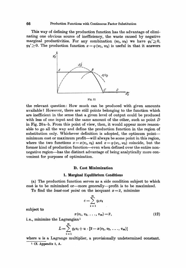
66 Production Functions with Continuous Factor Substitution
This way of defining the production function has the advantage of eliminating one obvious source of inefficiency, the waste caused by negative marginal productivities. For any combination (WI, W2) we have 11'1'>0, !p2' > O. The production function x = 11' (WI, W2) is useful in that it answers
I /
/ I
/ /
I
",-
/ /
Fig. 21
c o
the relevant question: How much can be produced with given amounts available ~ However, there are still points belonging to the function which are inefficient in the sense that a given level of output could be produced with less of one input and the same amount of the other, such as point D in Fig. 20a-b. From this point of view, then, it would appear more reasonable to go all the way and define the production function in the region of substitution only. Whichever definition is adopted, the optimum pointminimum cost or maximum profit-will always be some point in this region, where the two functions X=X(Vl, V2) and X=IP(WI, W2) coincide, but the former kind of production function-even when defined over the entire nonnegative region-has the distinct advantage of being analytically more convenient for purposes of optimization.
D. Cost Minimization
1. Marginal Equilibrium Conditions
(a) The production function serves as a side condition subject to which cost is to be minimized or-more generally-profit is to be maximized.
To find the least-cost point on the isoquant x = x, minimize
subject to
m
c= L qtV,
i=1
X(Vl, V2, ... , vm)=x, i. e., minimize the Lagrangian 1
m
L= L q,v,+u· [X-X(Vl, V2, ••. , vm)] i-1
(12)
where u is a Lagrange multiplier, a provisionally undetermined constant. 1 Of. Appendix I, A.
or
Marginal Equilibrium Conditions
The necessary first-order conditions for a minimum are
m llL dL= '-dv(=O L... llv(
i=1
llL = q(-u, x/=O II V(
(i=1,2, ... , m),
67
(13)
which, with (12), determine u and the VI. 1 Geometrically, this means that the isocost plane through the point is tangent to the isoquant surface: at the common point, the q, will be proportional to the xl so that the gradient of the isocost plane in any direction, (3vm/(3Vt= -qt/qm (i= 1,2, ... , m-1), is equal to that of the tangent plane, (3vm/(3Vj= -x//xm'.
Assuming that there exists one or more non-negative (and thus feasible) solutions to (12)-(13)2, solutions involving negative marginal productivities can be discarded at once since an inefficient point can never be optimal3 ;
in other words, only points in the region of substitution need be considered. To ensure that a feasible, efficient point satisfying (12)-(13) represents
a minimum rather than a maximum, additional information is required. If the nature of the solution is not obvious-e. g. from geometrical considerations in the two-factor case--the second-order condition for a constrained minimum provides a criterion. It is sufficient for the solution of (12)-(13) to represent a (local) minimum that
m m (32L d2L= L L (3v,(3Vj dvtdvj >0
i = Ij = 1
at the point for all variations satisfying (12), i. e., subject to m
2: xt'dv,=O. i=1
Since, for constant prices, (32L = -u . Xt!,' where u = qt / xl' > 0 at an (3v,(3Vj
efficient point, this boils down to m m m
2: 2: x,," dv, dVj < 0 for 2: xl dV1= o. (14) i=lj=1 i=1
1 W ALRAS, of all people, was the first to give (in the later editions of his Element8) a rigorous treatment of the conditions for minimum cost under continuous substitution; of. W ALRAS (English ed., 1954), pp. 384 f., 549 f., and 604 f.
2 If the isoquant is linear, the least-cost point is generally not characterized by (13); cf. below.
8 Of. Ch. II above. If x" < 0 for some i, a marginal decrease in the corresponding v, will raise output; if accompanied by appropriate marginal decreases in those inputs for which x{ > 0, we can get back to some point on the isoquant x =x, i. e., there exist factor combinations which produce this amount using less of all factors (except those for which x,'=O, which are left as they were) and thus at less cost.
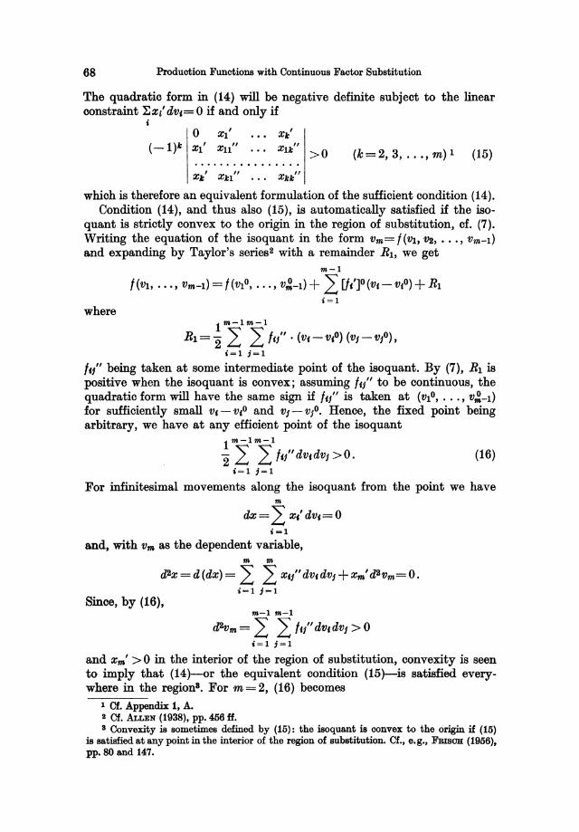
68 Production Functions with Continuous Factor Substitution
The quadratic form in (14) will be negative definite subject to the linear constraint ~:I:" dv,= 0 if and only if
i o :1:1' • •• :1:,/
( - l)k :l:1' xu" ... xu" >0 (k=2, 3, ... , m) 1 (15)
which is therefore an equivalent formulation of the sufficient condition (14). Condition (14), and thus also (15), is automatically satisfied if the iso
quant is strictly convex to the origin in the region of substitution, cf. (7). Writing the equation of the isoquant in the form Vm= I ('IJJ., Vs, ••• , Vm-l) and expanding by Taylor's series2 with a remainder R1, we get
m-l
l(v1, ... , Vm-l) = I (VI0, ... , V~-l) + L U/]O(v,- v,O) + R1 i=1
where 1 m-lm-l
R1="2 L L I,l'· (v,-v,O) (Vl- Vl0) , i=1 ;=1
lel' being taken at some intermediate point of the isoquant. By (7), R1 is positive when the isoquant is convex; assuming 1,/' to be continuous, the quadratic form will have the same sign if I'l' is taken at (Vlo, ... , V~-I) for sufficiently small v, - v,o and Vl- vio. Hence, the fixed point being arbitrary, we have at any efficient point of the isoquant
1 m-1m-l
"2L LI,l'dv,dvl>O. (16) i=1 ;=1
For infinitesimal movements along the isoquant from the point we have m
dx= L :I:/dv,=O i-1
and, with Vm as the dependent variable, m m
d2:1: = d(dx) = L L x,/'dv,dv,+:l:m'd2vm=O. i=1 ;=1
Since, by (16), m-l m-l
d2vm= L L l,l'dv,dVj >0 i=1 ;=1
a.nd xm' > 0 in the interior of the region of substitution, convexity is seen to imply that (14)--or the equivalent condition (15)-is satisfied everywhere in the regions. For m=2, (16) becomes
1 Of. Appendix 1, A-Il Of • .ALLEN (1938), pp. 456 H. 8 Convexity is sometimes defined by (15): the isoquant is convex to the origin if (15)
is satisfied at any point in the interior of the region of substitution. Of., e.g., F1wKm (1956), pp. 80 and 147.
Marginal Equilibrium Conditions 69
cf. (6). Moreover, convexity throughout the region of substitution guarantees
that the solution determined by (12)-(13) is unique. At a feasible, efficient point (v10, •• • , vmO) satisfying (13) we have
which with (8) gives (xc')O = q, I u
1 m
u' L q,' (v,-v,O) >0 i=l
for all points (VI, .•. , vm) on the isoquant (not all V, = V,O).I Since u is positive for some or all qf positive and xi' > 0, this implies
m m
L qfV,O < L q,Vf, i=l !i=l
that is, an efficient point which satisfies the necessary conditions is cheaper than any other factor combination. Thus, for a convex isoquant, (13) is necessary as well as sufficient for minimum cost and the solution represents a global minimum. (In the two-factor case this is geometrically obvious.)
Had the isoquant been alternately convex and concave in the region of substitution, there would have been several points satisfying (13), some of which represent local minima-such as P and R in Fig. 22, of which R is the global minimum at the particular set of prices-whereas others such as Q and S, where the isoquant is concave, are local maxima2•
Flg.22
1 This holds whether (Vl' • •• , vm ) is efficient or not, cf. above. 2 Fig. 22 shows that, whereas point 8 can be discarded straight away as being inefficient
(Xl' < 0, X2' < 0), it is poBBible for a point such as Q to be efficient although it can never represent a least-cost solution for any set of prices; Q cannot be ruled out by the technological efficiency criterion when Xl' and X2' are positive at the point-unless the "bulge" can be replaced by a straight line representing combinations of points on the convex parts of the isoquant (cf. Ch. IV, A above).
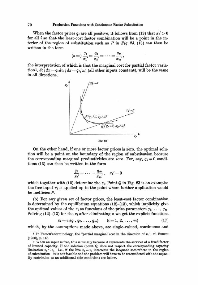
70 Production Functions with Continuous Factor Substitution
When the factor prices q, are all positive, it follows from (13) that x,' > 0 for all i so that the least-cost factor combination will be a point in the interior of the region of substitution such as P in Fig. 23. (13) can then be written in the form
ql q2 qm (u=)-,=-,= ... =-"
Xl X2 Xm
the interpretation of which is that the marginal cost for partial factor variation l , de! dx =q,dv,! dx=q,!x/ (all other inputs constant), will be the same in all directions.
Fig. 23
On the other hand, if one or more factor prices is zero, the optimal solution will be a point on the boundary of the region of substitution because the corresponding marginal productivities are zero. For, say, ql = 0 conditions (13) can then be written in the form
which together with (12) determine the v,. Point Q in Fig. 23 is an example: the free input Vl is applied up to the point where further application would be inefficient2•
(b) For any given set of factor prices, the least-cost factor combination is determined by the equilibrium equations (12)-(13), which implicitly give the optimal values of the v, as functions of the price parameters ql, •.. , qm. Solving (12)-(13) for the v, after eliminating u we get the explicit functions
v,=V,(ql,q2, ... ,qm) (i=1,2, ... ,m) (17)
which, by the assumptions made above, are single-valued, continuous and
I In FRISCH'S terminology, the "partial marginal cost in the direction of VI'" cf. FRISCH (1956), p. 146.
2 When an input is free, this is usually because it represents the services of a fixed factor of limited capacity. If the solution (point Q) does not respect the corresponding capacity limitation VI::; 01-i. e., if the line VI = 01 intersects the isoquant somewhere in the region of substitution-it is not feasible and the problem will have to be reconsidered with the capacity restriction as an additional side condition; see below.
Marginal Equilibrium Conditions 71
differentiable so that the least-cost combination will respond in a continuous manner to factor price changes. Furthermore, the functions are homogeneous of degree zero: proportional variation in all q, leaves the solution for the v, unaltered.
The displacement of the equilibrium position brought about by given finite changes in one or more factor prices is best studied by comparing alternative solutions to (12)-(13). The effect of a marginal change in a single q(, on the other hand, can be traced by differentiating the system (12)-(13) with respect to the price in question. In the two-factor case write the system in the form
=x ql . X2' (Vb V2) - q2 • Xl' (Vb V2) = 0 ;
differentiating with respect to, say, q2 (ql constant) we get
, ~V2 0 +X2 .-=
~q2
( " ") t5 VI (" ") ~ V2 , qlX12 - q2 Xn • - + qlX22 - q2X12 • - = Xl t5 q2 t5 q2
(12a)
(13a)
which is a linear equation system in the partial derivatives with respect to q2 of the functions VI = VI (ql, q2), V2 = V2 (q1, q2). (The coefficients are constant because the derivatives of the production function are taken at the particular point of equilibrium.)
Solving the equations, and making use of (13a) to eliminate ql in the determinant of the system, we have
~ VI -Xl' (X2')2
~q2 - q2 D (18)
where D = (X2')2Xn" - 2Xl' X2' X12" + (Xl')2 x22".
In elasticity form we have
~ VI q2 -Xl' (X2')2 ---=----~q2 VI vlD
~ V2 • q2 = (Xl') 2X2'
f'lQ2 V2 V2D (19)
These partial elasticities, which are independent of the units of measurement, are functions of VI and V2; their values depend on the properties of the production function-the first and second derivatives-at the particular equilibrium point at which they are taken. Their respective signs, however, will be the same at any point. By the assumption of convexity (6) we have D < 0 1 at a least-cost point in the interior of the region of substitution where Xl' and X2' are both positive. It follows that
f'lVl 0 ~V2 < 0 ~q2 > , ~q2
1 This result also follows from the second-order minimum conditions (15): for k = 2, the determinant which is to be positive is equal to -D.
72 Produotion Funotions with Continuous Faotor Substitution
and the elasticities will also be positive and negative respectively-that is, a fall in q2 will lead to a substitution of V2 for Vi, as is also geometrically obvious.
In the general m-factor case it can similarly be shown that more will be used of an input which has become cheaper (~V(/~q, <0).1 The cross derivatives ~Vi / ~q, (i =1= j) may vary in sign. Differentiating the general equilibrium equations
X(Vl, V2, ••• , vm) =X
u.xc'-q, =0 (i=1,2, ... ,m)
with respect to, for example, qm, we have
~ ~vi ~xl· ~qm =0 ;=1
, ~u Im" ~Vi Xc ·-+u· Xu ·-=0
~qm . ~qm 3=1
, ~u ~ ~vi Xm • ~ + u • ~ Xm/' • ~ = 1.
uqm. uqm 3=1
(i=1, 2, ... , m-1)
(12)
(13)
Mter dividing through by u in all but the first equation the system can be solved for ~Vm/~qm to give
~Vm (1/ u2) • L1mm
~qm - (1/u). L1
where L1 is the bordered determinant
0 Xl'
Xl' Xu " L1=
Xm ,
Xml " X " mm
and L1mm is the determinant obtained from L1 by deleting the last row and the last column. The second-order minimum conditions as written in the form (15) imply that L1 and L1mm are of opposite signs, and u is positive; hence
~Vm O· ~ V, 0 f 11· --< , I.e., -< or a t. ~qm ~q,
as the numbering is immaterial. The cross derivatives ~vJ / ~q, cannot be shown to be all positive as in
the two-factor case, though the positive signs can be expected to be dominant since more of V, must be offset by less of some or all other inputs if X is to remain constant. Nor can a definite conclusion with respect to the sign of ~U/~qm be reached by solving the system for this variable.
1 Of. SAMUELSON (1947), pp. 63 fi.
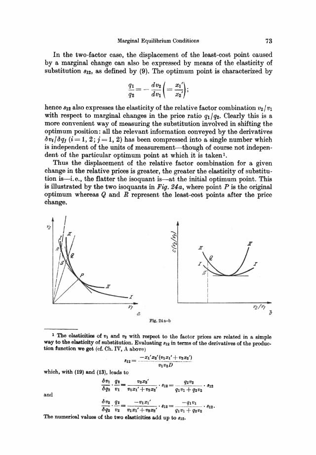
Marginal Equilibrium Conditions 73
In the two-factor case, the displacement of the least-cost point caused by a marginal change can also be expressed by means of the elasticity of substitution 812, as defined by (9). The optimum point is characterized by
q1 = _ ddv2 (= Xl:); q2 V1 X2
hence 812 also expresses the elasticity of the relative factor combination V2/V! with respect to marginal changes in the price ratio q1 / q2. Clearly this is a more convenient way of measuring the substitution involved in shifting the optimum position: all the relevant information conveyed by the derivatives t5v,/t5qj (i= 1,2; i= 1,2) has been compressed into a single number which is independent of the units of measurement-though of course not independent of the particular optimum point at which it is taken!.
Thus the displacement of the relative factor combination for a given change in the relative prices is greater, the greater the elasticity of substitution is-i.e., the flatter the isoquant is-at the initial optimum point. This is illustrated by the two isoquants in Fig. 24a, where point P is the original optimum whereas Q and R represent the least-cost points after the price change.
FIg. 24a-b
1 The elasticities of V1 and V2 with respect to the factor prices are related in a simple way to the elasticity of substitution. Evaluating 812 in terms of the derivatives of the production function we get (cf. Ch. IV, A above)
-X1'X2'(V1X1' + V2X2') 812 = -.-------. --- .- - - -
V1V2D
which, with (19) and (13), leads to
<5V1 q2 V2X2' q2V2 - ._= ·812= ·812 <5q2 V1 V1X1'+V2X2' q1V1+q2V2
and <5V2 q2 -V1X1' -q1V1 - ._= ---·812= ------·812. <5q2 V2 VIX1' + V2X2' q1 V1 + q2V2
The numerical values of the two elasticities add up to 812.
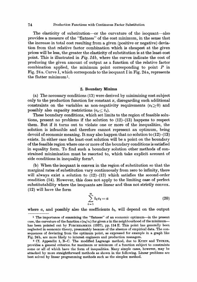
74 Production Functions with Continuous Factor Substitution
The elasticity of substitution-or the curvature of the isoquant--also provides a measure of the "flatness" of the cost minimum, in the sense that the increase in total cost resulting from a given (positive or negative) deviation from that relative factor combination which is cheapest at the given prices will be less, the greater the elasticity of substitution is at the least-cost point. This is illustrated in Fig. 24b, where the curves indicate the cost of producing the given amount of output as a function of the relative factor combination applied, the minimum point corresponding to point P in Fig. 24a. Curve I, which corresponds to the isoquant I in Fig. 24a, represents the flatter minimum l .
2. Boundary Minima
(a) The necessary conditions (13) were derived by minimizing cost subject only to the production function for constant x, disregarding such additional constraints on the variables as non-negativity requirements (Vt:::::::O) and possibly also capacity restrictions (V8< V8)'
These boundary conditions, which set limits to the region of feasible solutions, present no problems if the solution to (12)-(13) happens to respect them. But if it turns out to violate one or more of the inequalities, the solution is infeasible and therefore cannot represent an optimum, being devoid of economic meaning. It may also happen that no solution to (12)-(13) exists. In either case the least-cost solution will be a point on the boundary of the feasible region where one or more of the boundary conditions is satisfied in equality form. To find such a boundary solution other methods of constrained minimization must be resorted to, which take explicit account of side conditions in inequality form2•
(b) When the isoquant is convex in the region of substitution so that the marginal rates of substitution vary continuously from zero to infinity, there will always exist a solution to (12)-(13) which satisfies the second-order condition (14). However, this does not apply to the limiting case of perfect substitutability where the isoquants are linear and thus not strictly convex. (12) will have the form
m
L b,ve=a i=1
(20)
where a, and possibly also the coefficients be, will depend on the output
1 The importance of examining the "flatness" of an economic optimum-in the present case, the curvature of the function c (VI! VI) for given x in the neighbourhood of the minimumhas been pointed out by FORCBHAMMER (1937), pp. 114 ff. This point has generally been neglected in economic theory, presumably because of the absence of empirical data. The consequences of deviating from the optimum point, as expressed for example in a graph like Fig. 24 b, are more likely to interest engineers and production managers.
I Cf. Appendix 1, B-C. The modified Lagrange method, due to KUHN and TUCKER, provides a general criterion for maximum or minimum of a function subject to constraints some or all of which have the form of inequalities. Many simple cases, however, may be attacked by more straightforward methods as shown in the following. Linear problems are best solved by linear programming methods such as the simplex method.
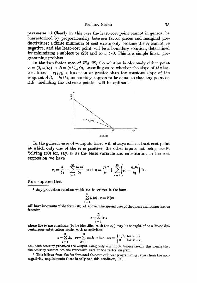
Boundary Minima 75
parameter x.1 Clearly in this case the least-cost point cannot in general be characterized by proportionality between factor prices and marginal productivities; a finite minimum of cost exists only because the v, cannot be negative, and the least-cost point will be a boundary solution, determined by minimizing c subject to (20) and to Vf > O. This is a simple linear programming problem.
In the two-factor case of Fig. 26, the solution is obviously either point A = (0, alb2 ) or B= (albl , 0), according as to whether the slope of the isocost lines, -qil q2, is less than or greater than the constant slope of the isoquant AB, -bI /b2, unless they happen to be equal so that any point on A B-including the extreme points-will be optimal.
B
Fig. 25
In the general case of m inputs there will always exist a least-cost point at which only one of the v, is positive, the other inputs not being used2•
Solving (20) for, say, VI as the basic variable and substituting in the cost expression we have
VI = ~ _ ~ b,v, and c = qi a + ~ (qf _ qi bf ) v,. bi Lt bl b1 Lt b1
i=2 i = 2
Now suppose that
1 Any production function which can be written in the form m ~ f,(x). Vj=l'(x)
i = 1
will have isoquants of the form (20), cf. above. The special case of the linear and homogeneous function
m
x=~ b,v, i = l
where the b, are constants (to be identified with the xt') may be thought of as a linear discontinuous-substitution model with m activities:
~ , ~'h { lib, for k = i X=~"I;, v,=~ /lil;"" were a,,,= 0 f k .
k = 1 k = 1 or * $ ,
i. e., each activity produces the output using only one input. Geometrically this means that the activity vectors are the respective axes of the factor diagram.
2 This follows from the fundamental theorem of linear programming; apart from the nonnegativity requirements there is only one side condition, (20).
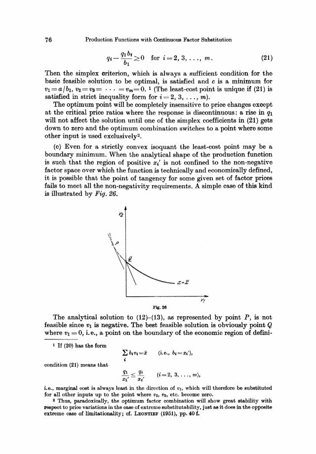
76 Production Functions with Continuous Factor Substitution
(21)
Then the simplex criterion, which is always a sufficient condition for the basic feasible solution to be optimal, is satisfied and c is a minimum for vI=ajbl, V2=VS= ... =Vm=O. I (The least-cost point is unique if (21) is satisfied in strict inequality form for i = 2, 3, . . . , m).
The optimum point will be completely insensitive to price changes except at the critical price ratios where the response is discontinuous : a rise in ql will not affect the solution until one of the simplex coefficients in (21) gets down to zero and the optimum combination switches to a point where some other input is used exclusively2.
(c) Even for a strictly convex isoquant the least-cost point may be a boundary minimum. When the analytical shape of the production function is such that the region of positive x/ is not confined to the non-negative factor space over which the function is technically and economically defined, it is possible that the point of tangency for some given set of factor prices fails to meet all the non-negativity requirements. A simple case of this kind is illustrated by Fig. 26.
FIg. 28
The analytical solution to (12)-(13), as represented by point P, is not feasible since VI is negative. The best feasible solution is obviously point Q where VI =0, i.e., a point on the boundary of the economic region of defini-
1 If (20) has the form (i.e., b,=x{),
condition (21) means that
(i=2, 3, . .. , m),
i.e., marginal cost is always least in the direction of Vl, which will therefore be substituted for all other inputs up to the point where V2, Va, etc. become zero.
2 Thus, paradoxically, the optimum factor combination will show great stability with respect to price variations in the case of extreme substitutability, just as it does in the opposite extreme case of limitationality; cf. LEONTIEF (1951), pp. 40 f.
Boundary;'Minima 77
tion; this will be so for any pair of prices satisfying the inequality
qi (XI')Q qi q2 (- ex) <) - q2 < - (X2')Q or (XI')Q ~ (X2')Q
which replaces the corresponding equality derived from conditions (13). c is greater at Q than at P.
In the general case of m inputs, a similar expedient suggests itself when Lagrange's method fails to produce a feasible solution. Let P = (VIP, V2P, ••. , VmP) represent the minimum of c subject to (12), characterized by
q,=u' (x/)P (i= 1,2, ... , m), (22)
of. (13). Now suppose that VIP < 0 but all other VIP > O. Discarding the solution P as infeasible, let us try-as we did in the two-factor example-to set VI = 0 beforehand and see whether this leads to a feasible least-cost solution. Minimizing the cost expression subject to (12) with VI = O-the equality form of the boundary condition VI :2: 0 which was violated by the solution P-we get a new solution Q = (vIQ, V2Q, ••. , vmQ), determined by the side conditions x(vIQ, V2Q, •.• , vmQ)=x, ViQ=O, and the necessary minimum conditions
(i=2,3, ... ,m) (23)
where A. is a Lagrange multiplier I. It can be shown that this solution, if feasible and efficient (v,Q >0, (xl)Q >0), is cheaper than any other feasible point on the isoquant.
For all q, :2: 0 we have (x/)P:2: 0 for all i. Assuming that Q is also a point in the regionofsubstitution, i.e., (x/)Q >0 (i = 1,2, ... , m), it follows from the convexity assumption (8) that
m 2: (xc')P. (v,Q-v,P) >0
'-1 and
m L: (xc')Q. (v,P-v,Q) >0.
'-1 Multiplying by u and A. respectively (both positive) and adding, we get (cf. (22)-(23))
[ql-A.· (Xl')Q]· (V1Q-vIP) >0
or, since VIQ=O, VIP <0, qi > A. • (XI')Q.
Now, by (8) we have with Q as the fixed point (v,o=v,Q) m
(XI')Q· (VI-VIQ) + L (xl)Q· (Vf-V1Q) >0 i=2
(24)
(25)
1 In the two·f&otor oaae (Fig. 26) the solution Q follows directly from the two side conditions; there is no range of choice and hence no need for minimization.
78 Production Functions with Continuous Factor Substitution
for any point (VI, V2, •.. , Vm), distinct from Q. (25) combines with (23)-(24) to give
m L q,. (v,-v,Q) >0 i=1
provided that VI-VIQ;;;:::O, i.e., for any non-negative VI. In other words, whereas c is less at P than at any other point of the isoquant, including Q, point Q is a global minimum in the region VI ;;;::: 0 and therefore represents the optimal factor combination provided that it turns out to be feasible (v,Q >0 also for i = 2,3, ... , m) and efficient. This boundary solution is characterized by
(i=2, 3, ... , m);
the interpretation is that the first factor will not be used because the partial marginal cost with respect to VI at the point is greater than partial marginal cost in any other factor direction so that substitution of VI for other inputs along the isoquant would only raise the cost of producing the given output.
Suppose, however, that V2Q < 0 so that Q is not feasible. Now set VI = V2 = 0 and minimize c over again to get a new solution R, determined by X(VIR, V2R, ... , vmR)=x, vIR=V2R=0, and the conditions
(i=3, 4, ... , m), (26)
I-' being a Lagrange multiplier. Then-assuming that (xl)R;;;:::O for all iconvexity implies
m L (Xl)R . (v,P - V,R) > 0 '=1
m L (xl)P. (V,R_V,P) >0, i=1
which with (22) and (26) leads to
Similarly,
and
[ql -I-' • (XI')R] . (-VIP) > [q2 -I-' . (X2')R] • V2P•
m L (xl)Q • (V,R - V,Q) > 0 \=1
m L (Xc')R • (V,Q - V,R) > 0
.-1 combine with (23) and (26) to give
q2 > I-' . (X2')R
since v2Q<0. For v1P<0 and V2P >0 as assumed, (27)-(28) lead to
(27)
(28)
Boundary Minima
By (8) we also have m L (Xc')R. (VI-V,R) >0
i=1
from which, using (26), (28), and (29), m
L q,' (VI-VIR) > 0 i= 1
79
(29)
for any point (Vl, V2, ••• , Vm) with non-negative Vl and V2. Hence R represents the least-cost factor combination in the region Vl20, V2 >0 if it is feasible (VfR 2 0 for i = 3, 4, ... , m) and efficient. If VaR turns out to be negative, however, we proceed to a new solution S, setting VlS = V2S = VaS = 0, and so on.
Thus the least-cost point is a boundary solution characterized by
ql>v,xl, qf=V'X,' (j=1,2, ... ,k; i=k+1, ... ,m) (30)
where Vl, V2, ••• , Vt = 0, and these conditions l are satisfied by the first of the efficient points Q, R, S, ... which turns out to be feasible-provided that the original solution as determined by (12)-(13) has only one negative input (vlP < 0). If also V2P < 0, (30) together with the convexity assumption (8) is still sufficient for a feasible point to represent the least-cost combination, but (30) is no longer automatically satisfied by the point because (29) does not necessarily follow from (27)-(28) for vzP < O.
The general problem of minimizing c subject to x = x and V, 20 can also be dealt with by Kuhn and Tucker's modified Lagrange method for solving problems of non-linear programming. The side condition x = x can be broken up into the equivalent pair of inequalities x 2 x, x <x. Then the problem can be formulated as the maximization of -c subject to x- X20, x- x 20, and v, 20. This is equivalent to finding a saddle point-i.e., a maximum with respect to the V, and a minimum with respect to the Lagrange multipliers Ul and U2, also required to be non-negative-of the Lagrangian
m
L= - L q,V,+UI • [X{VI, V2, ••. , vm) - x] +U2' [X-X{VI, V2, .•• , Vm)].
'-1 . N ece88ary conditions for a constrained maximum of -c are that there exist multipliers UI and U2 such that the following necessary conditions for a saddle value of L are satisfied Z:
1 SAMUELSON (1947). pp. 69 f., states the condition in the form gi/x,'"C. v
for inputs not actually used. This diHers from (30) only in that it includes the special case of equality where some of the inputs which were not set = 0 beforehand turn out also to be zero. (For example, if Q is the least-cost point, VaQ may turn out to be = 0 so that the solutions Q and R coincide and we have not only ga!(xa')Q=;' but also ga/(xa')R=[J.)
2 Of. Appendix 1, C, conditions (15)-(16).
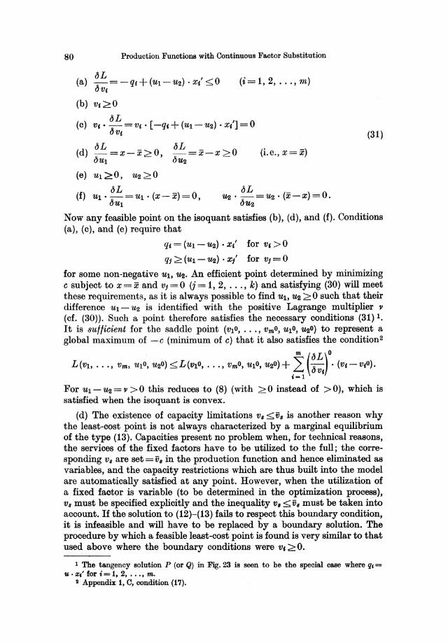
80 Production Functions with Continuous Factor Substitution
(i= 1,2, ... , m)
(b) Vt ~O
(c) V,· bL = Vi . [-q, + (Ul - U2) . xl] = 0 bVi (31)
bL bL (d) -=x-x~O, -=x-x>O (Le.,x=x)
bUl bU2-
(e) Ul ~O, U2 >0
bL (f) Ul· - = Ul • (x - x) = 0,
bUl
bL _ U2' -=U2' (x-x)=O.
bU2
Now any feasible point on the isoquant satisfies (b), (d), and (f). Conditions (a), (c), and (e) require that
qt = (Ul-U2) • x/ for Vi >0
qj>(Ul-U2) ,xl for Vj=O
for some non-negative Ul, U2. An efficient point determined by minimizing c subject to x = x and Vj = 0 (j = 1, 2, ... , k) and satisfying (30) will meet these requirements, as it is always possible to find Ul, U2 > 0 such that their difference Ul - U2 is identified with the positive Lagrange multiplier 'P
(cf. (30)). Such a point therefore satisfies the necessary conditions (31) 1.
It is sufficient for the saddle point (VI0 , ••• , vmo, ulo, U20) to represent a global maximum of -c (minimum of c) that it also satisfies the condition2
m (bL)O L(Vl' ... , Vm, u10, U20) < L ('I1}0, •• " vmo, u10, U20) +.L ~ Vi • (V, - v(O).
,=1
For Ul - U2 = 'JI > 0 this reduces to (8) (with > 0 instead of > 0), which is satisfied when the isoquant is convex.
(d) The existence of capacity limitations Va ~V8 is another reason why the least-cost point is not always characterized by a marginal equilibrium of the type (13). Capacities present no problem when, for technical reasons, the services of the fixed factors have to be utilized to the full; the corresponding VB are set =v, in the production function and hence eliminated as variables, and the capacity restrictions which are thus built into the model are automatically satisfied at any point. However, when the utilization of a fixed factor is variable (to be determined in the optimization process), VB must be specified explicitly and the inequality VB <V8 must be taken into account. If the solution to (12)-(13) fails to respect this boundary condition, it is infeasible and will have to be replaced by a boundary solution. The procedure by which a feasible least-cost point is found is very similar to that used above where the boundary conditions were Vi ~ O.
1 The tangency solution P (or Q) in Fig. 23 is seen to be the special case where q, = u . xl' for i = 1, 2, ... , m.
2 Appendix 1, C, condition (17).
Boundary Minima 81
Fig. 27 illustrates a case of this type, VI representing the services of a fixed factor of capacity iiI. The point of tangency I, where q1/XI' =q2!X2', is the least-cost point only if it respects the capacity limitation VI::;: ih; if it does not-cf. point P where VIP> VI so that the solution is not feasiblethe boundary condition becomes effective and we must look for another solution which minimizes cost for VI = VI, i.e., a solution on the boundary of the feasible region. In Fig. 27 this is obviously point Q (where c is greater than at P).
I ( I \ \
\
11', Flg.27
More generally, let the point P represent the minimum of c on the isoquant so that
qc=u' (x/)P (i= 1,2, ... , m)
(cf. (13». Suppose that VIP> VI. To get a feasible solution set VI = VI and minimize cost over again; the new solution-assumed to be non-negativeis determined by (12) and
q,=)'.(x/)Q (i=2,3, .•. ,m) (32) for VI Q = iit. Then, assuming that P and Q are both efficient points, the convexity assumption (8) again leads to
[ql-), . (Xl')Q] • (vlQ - VIP) > 0
which in turn, since VIQ=Vl <VIP, leads to
ql <), • (XI')Q, from which we have
ql ' (VI-VlQ) >),. (Xl')Q· (Vl-V1Q)
(33)
(34)
for all VI <vlQ=iit. With Q as the fixed point (v,o=v,Q), (8) combines with (32) and (34) to give
m 2: q, . (Vf-V,Q) >0 for VI ~VI ,=1
so that Q represents minimum cost in the region VI < VI, i. e., Q is the best feasible solution.
1 Normally we have ql = 0 for a capacity factor so that the isocost lines are horizontal. Da.ns. Production Models 6
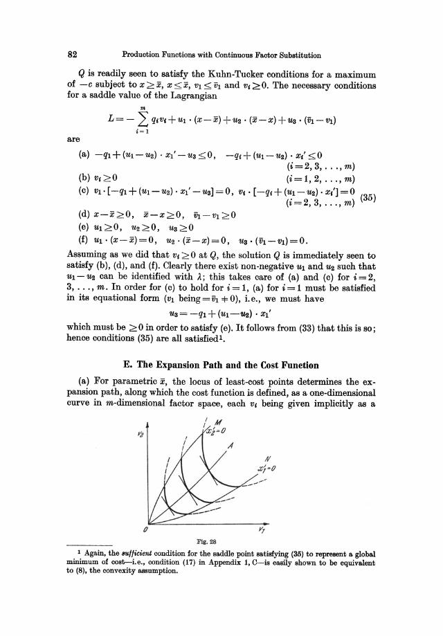
82 Produotion FunotioIUl with Continuous Faotor Substitution
Q is readily seen to satisfy the Kuhn-Tucker conditions for a maximum of -c subject to x >x, X::;: X, VI < iiI and v,;;::: o. The necessary conditions for a saddle value of the Lagrangian
are
m
L=- L q,V,+UI· (x-x)+U2. (x-x)+us· (iiI-VI) i= 1
(a) -ql + (UI - U2) . Xl' - US::;: 0, -qt + (UI - U2) . xl::;: 0 (i=2, 3, ... , m)
(b) Vt>O (i=1, 2, ... , m)
(c) VI· [-ql + (UI-U2)· Xl' -Us] =0, V,· [-qt+ (~I-U2)· xc'] =0 (35) (~=2,3, ... ,m)
(d) x-x>O, x-x;;:::O, ih-VI;;:::O
(e) UI >0, U2 >0, us;;:::O
(f) UI· (x-x) =0, U2· (x-x)=O, Us· (ih-VI)=O.
Assuming as we did that V, >0 at Q, the solution Q is immediately seen to satisfy (b), (d), and (f). Clearly there exist non-negative UI and U2 such that UI-U2 can be identified with A; this takes care of (a) and (c) for i=2, 3, ... , m. In order for (c) to hold for i = 1, (a) for i = 1 must be satisfied in its equational form (VI being = ih =l= 0), i. e., we must have
Us = -ql + (Ul-U2) . Xl'
which must be > 0 in order to satisfy (e). It follows from (33) that this is so; hence conditions (35) are all satisfied l .
E. The Expansion Path and the Cost Function
(a) For parametric X, the locus of least-cost points determines the expansion path, along which the cost function is defined, as a one-dimensional curve in m-dimensional factor space, each VI being given implicitly as a
Fig. 28
1 Again, the sufficient condition for the saddle point satisfying (35) to represent a. global minimum of cost-i.e., oondition (17) in Appendix 1, G--is easily shown to be equiva.lent to (8), the convexity assumption.
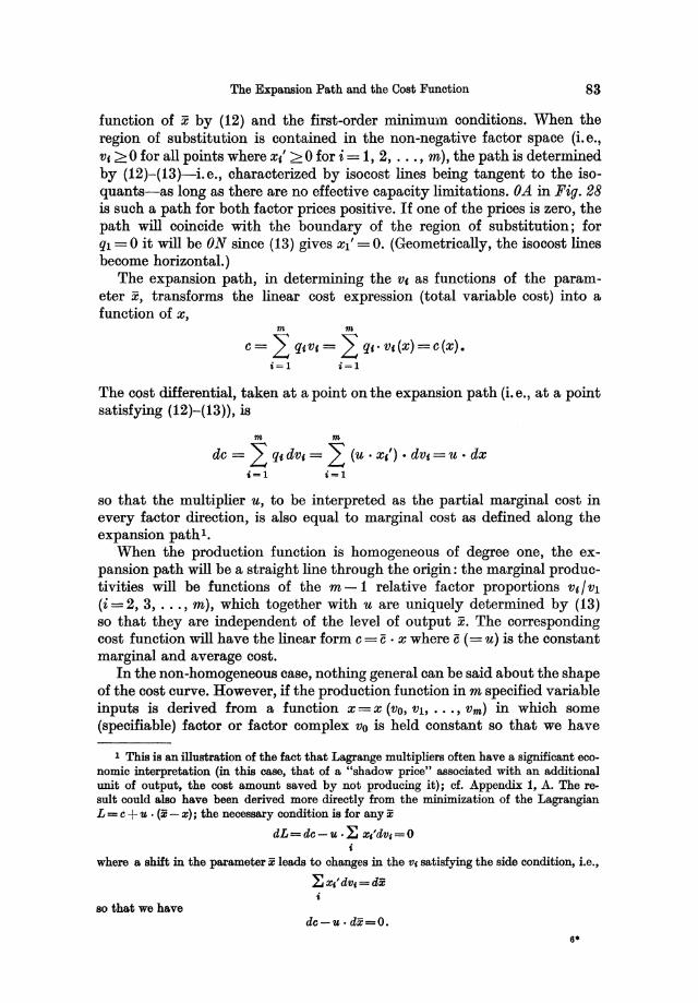
The Expansion Path and the Cost Funotion 83
function of x by (12) and the first-order minimum conditions. When the region of substitution is contained in the non-negative factor space (Le., v, > 0 for all points where x,' ::2: 0 for i = 1, 2, ... , m), the path is determined by (12)-(13)-i.e., characterized by isocost lines being tangent to the isoquants-as long as there are no effective capacity limitations. OA in Fig. 28 is such a path for both factor prices positive. If one of the prices is zero, the path will coincide with the boundary of the region of substitution; for ql = 0 it will be ON since (13) gives Xl' = O. (Geometrically, the isocost lines become horizontal.)
The expansion path, in determining the v, as functions of the parameter x, transforms the linear cost expression (total variable cost) into a function of x,
m m
e = 2: q,v, = 2: qf' v,(x) =e(x). i=1 i=1
The cost differential, taken at a point on the expansion path (i.e., at a point satisfying (12)-(13», is
m m
de = 2: q,dv, = 2: (u. x,'). dv,=u· dx i-I i=1
so that the multiplier u, to be interpreted as the partial marginal cost in every factor direction, is also equal to marginal cost as defined along the expansion pathl.
When the production function is homogeneous of degree one, the expansion path will be a straight line through the origin: the marginal productivities will be functions of the m - 1 relative factor proportions v, / Vl (i = 2, 3, ... , m), which together with u are uniquely determined by (13) so that they are independent of the level of output x. The corresponding cost function will have the linear form e = C • x where c (= u) is the constant marginal and average cost.
In the non-homogeneous case, nothing general can be said about the shape of the cost curve. However, if the production function in m specified variable inputs is derived from a function X=X (vo, Vl, ... , Vm) in which some (specifiable) factor or factor complex Vo is held constant so that we have
1 This is an illustration of the fact that Lagra.nge multipliers often ha.ve a significant eoonomio interpretation (in this case, that of a "shadow prioe" assooiated with an additional unit of output, the cost amount saved by not produoing it); of. Appendix 1, A. The reo sult oould also have been derived more directly from the minimization of the Lagrangian L = c + 'U . (z - z); the neoessary oondition is for any z
dL=dc-'U.~ z,'dv,=O i
where a shift in the parameter z leads to ohanges in the v, satisfying the side oondition, i.e.,
~z,'dv,=dz
so that we have dc-'U· dz=O.
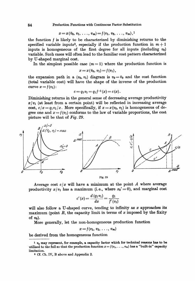
YJ
84 Production Functions with Continuous Factor Substitution
x=x(iio, VI, ••• , Vm)=/(VI, VZ, • • • , vm),1
the function / is likely to be characterized by diminishing returns to the specified variable inputs2, especially if the production function in m + 1 inputs is homogeneous of the first degree for all inputs (including vo) variable. Such cases will often lead to the familiar cost pattern characterized by U-shaped marginal cost.
In the simplest possible case (m= 1) where the production function is
x=x(iio, VI) = f(Vl) ,
the expansion path in a (vo, VI) diagram is Vo = vo and the cost function (total variable cost) will have the shape of the inverse of the production curve x = f(Vl):
c = qIVl =ql/-l (x) = c(x).
Diminishing returns in the general sense of decreasing average productivity x I VI (at least from a certain point) will be reflected in increasing average cost, CIX=qlVI/x. More specifically, if x=x(vo, VI) is homogeneous of degree one and x = / (VI) conforms to the law of variable proportions, the cost picture will be that of Fig. 29.
.z I
~ .:r;!7l<1L / 8 --- -z; ..... ,- , ...
A , , <.:.
~
FIg. 29
Average cost clx will have a minimum at the point A where average productivity x I VI has a maximum (i. e., where xo' = 0), and marginal cost
c'(x)= d(qIVI)= ~ dx f' (VI)
will also follow a U-shaped curve, tending to infinity as x approaches its maximum (point B, the capacity limit in terms of x imposed by the fixity of vo).
More generally, let the non-homogeneous production function
X=/(VI, V2, ••• , vm)
be derived from the homogeneous function
1 Vo may represent, for example, a capacity factor which for technical reasons has to be utilized to the full so that the production function x = I (VI. ••• , vm) has a "built-in" capacity limitation.
S Of. Ch. IV, B above and Appendix 2.
The Expansion Path and the Cost Function 85
x=x(Vo, Vb ... , vm)
for Vo = vo. Then the expansion path no longer represents partial variation of a single input and the cost curve cannot be based on the inverse of a production curve. Instead, the expansion path is determined implicitly by
qt- U ' !"(Vl, V2, ... , vm)=O
!(Vb V2, ... , vm) = x (i= 1,2, ... , m)
(36)
for parametric x. Although the relative factor proportions V2/ Vb ... , vm / Vl will not be
constant along this path (in which case the problem would reduce to a twofactor analysis where Vl would now represent a homogeneous factor complex), the cost picture will resemble that of Fig. 29. Any set of constant relative factor proportions Vt/vo (i = 1,2, ... , m) is represented by a half-line through the origin in (m+ i)-dimensional factor space; each half-line is characterized by constant average cost. Assuming that the region of substitution as defined by xo' > 0, xi' > 0 (i = 1, 2, ... , m) is contained in the positive (m + i)-dimensional factor space, the efficient half-lines will be positively inclined and one of them, as determined by minimizing cost subject to x=x(vo, Vl, ... , vm) and thus characterized by
xo' (vo, Vb .•. , Vm ) = 0
qt-A' x,'(Vo, Vl, ... , vm)=O (i=1, 2, .. . ,m) (37)
where A is a Lagrange multiplier, represents the locus of least-cost (and least average cost) points. For x such that (37) is satisfied for vo=vo, i.e., at the point where the half-line intersects the plane Vo = vo, A can be identified with the multiplier U of (36). This means that the point lies on the expansion path (36) and is characterized by marginal cost being equal to average cost. At any other point on the plane, and thus at any other point of the expansion path (36), average cost is higher, assuming convexity as usual. If it is also assumed that 0(0) = 0, it follows that the total cost function-and hence also average and marginal cost-will have the same general shape as in Fig. 29.
A similar cost picture can be derived from the assumption that the elasticity of output with respect to scale, e-that is, the elasticity of x with respect to a proportional variation of the variable inputs Vl, ... , vm-decreases from values greater than 1 through 0 to negative values as output increases along the expansion path (which, as we have seen, does not have to be linear for e to be defined at any point of the path)l. This pattern, which may be said to summarize the generalized law of variable proportions, is deducible from a few simple assumptions if the production function is derived from a homogeneous function x = x (Vo, Vb ... , vm ) for Vo = va, but it may also occur in cases where the non-homogeneity of the production function x =! (VI, V2, ... , Vm) cannot meaningfully be ascribed to the constancy of an unspecified input.
1 Cf. Ch. IV, B above.
86 Production Functions with Continuous Factor Substitution
At any point on the expansion path we have, by (13), m m
e = 2: q,v, =u· 2: vel,' i=1 '=1
where u=e' and, by (4), L veil =e· x. Thus we get! i
e = e / (x . e') = dx • ~, de x
(38)
that is, e is not only the elasticity of production but also the flexibility of cost (the reciprocal elasticity of the cost function, or the elasticity of output with respect to cost along the expansion path). When e is a known function of x along the expansion path, (38) is a differential equation which can be solved to give the cost function e=e(x). In the present case, e(x) is incompletely specified, but the assumed properties of the function are sufficient to determine the main characteristics of the cost function. It follows from (38) that for e ~ 1 we have
,:s;;.e d d(e/x) x.e'-e:s;;.O e::>- an x2 ::>.
X dx
Thus average cost will be decreasing in the initial phase of increasing returns to scale (e > 1), increasing in the subsequent phase of decreasing returns (0 <e < 1), and be a (global) minimum at the point of constant returns to scale (e= 1), where it is intersected from below by the marginal cost curve. As to marginal cost, we have for 0 < e < 1, if e is assumed to decrease monotonically in this interval,
de x· (c')2-e. (x. e" + e') -= <0 dx (x. e')2
and hence
" e' (, c) I e e > _. e - - , where e - - >0 for e < 1 e x x
so that marginal cost is increasing in this phase; by (38), e' -+ ex> as output expands towards the point where e becomes zero. Finally, the additional assumption e (0) = 0 guarantees that there will be an initial phase of decreasing marginal cost. It is geometrically obvious that a total cost curve starting at the origin must have this property if c / x is to have a minimum for some positive x; more rigorously, expansion of the cost function by Taylor's series,
e(O)=e(x)-x. e'(x)+ x2 . e"({)ox) 2
for some positive fraction fJ, shows that e" ({)ox), and hence also e" (x) for small x, will be negative, recalling that e (0) = 0 and that e - x . e' > 0 for e > 1. It follows that the marginal cost curve is likely to be U-shaped,
1 Of. SCHNEIDER (1934), pp. 42 f., and FRIsCH (1956), pp. 163 f.
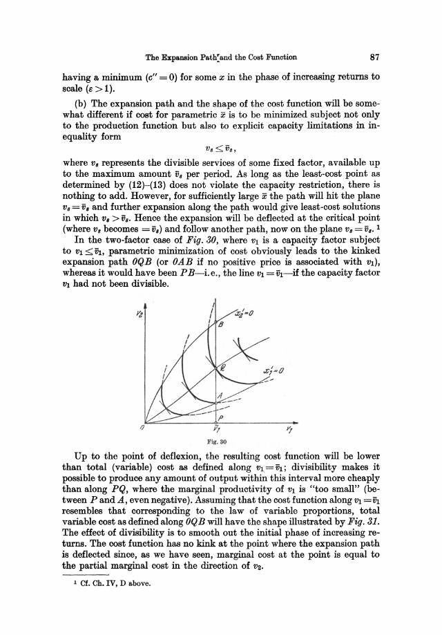
The Expansion Path: and the Cost Function 87
having a minimum (e" = 0) for some x in the phase of increasing returns to scale (e > 1).
(b) The expansion path and the shape of the cost function will be somewhat different if cost for parametric x is to be minimized subject not only to the production function but also to explicit capacity limitations in inequality form
Vs < vs, where Va represents the divisible services of some fixed factor, available up to the maximum amount Vs per period. As long as the least-cost point as determined by (12)-(13) does not violate the capacity restriction, there is nothing to add. However, for sufficiently large x the path will hit the plane VB = Va and further expansion along the path would give least-cost solutions in which Va > VB. Hence the expansion will be deflected at the critical point (where VB becomes = va) and follow another path, now on the plane VB = V,. I
In the two-factor case of Fig. 30, where VI is a capacity factor subject to VI < VI, parametric minimization of cost obviously leads to the kinked expansion path OQB (or OAB if no positive price is associated with VI),
whereas it would have been P B-i. e., the line VI = VI-if the capacity factor VI had not been divisible.
Fig. SO
Up to the point of deflexion, the resulting cost function will be lower than total (variable) cost as defined along VI = VI; divisibility makes it possible to produce any amount of output within this interval more cheaply than along PQ, where the marginal productivity of VI is "too small" (between P and A, even negative). Assuming that the cost function along VI =VI
resembles that corresponding to the law of variable proportions, total variable cost as defined along OQB will have the shape illustrated by Fig. 31. The effect of divisibility is to smooth out the initial phase of increasing returns. The cost function has no kink at the point where the expansion path is deflected since, as we have seen, marginal cost at the point is equal to the partial marginal cost in the direction of V2 .
1 Cf. Ch. IV, D above.
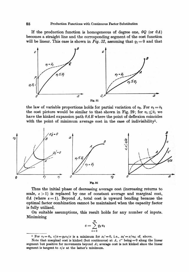
o
88 Production Functions with Continuous Factor Substitution
If the production function is homogeneous of degree one, OQ (or OA) becomes a straight line and the corresponding segment of the cost function will be linear. This case is shown in Fig. 32, assuming that ql = 0 and that
B c c
6
FI/r.81
the law of variable proportions holds for partial variation of V2. For VI = 1it the cost picture would be similar to that shown in Fig. 29; for VI ::;; iit we have the kinked expansion path OAB where the point of deflexion coincides with the point of minimum average cost in the case of indivisibilityl.
i x, -IJ
Fla. 82
B
Thus the initial phase of decreasing average cost (increasing returns to scale, e > 1) is replaced by one of constant average and marginal cost, OA (where e = 1). Beyond A, total cost is upward bending because the optimal factor combination cannot be maintained when the capacity factor is fully utilized.
On suitable assumptions, this result holds for any number of inputs. Minimizing
1 For V1=t)1, C/X=Q2 V2/X is a minimum for X1'=0, i.e., X2'=X/ V2 ; of. above. Note that marginal cost is kinked (but continuous) at A, c" being=O along the linear
segment but positive for movements beyond A; average cost is not kinked since the linear segment is tangent to c/x at the latter's minimum.
8
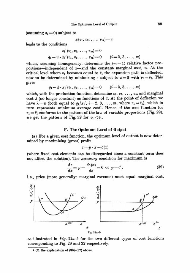
The Optimum Level of Output 89
(assuming ql = 0) subject to
X(VI' V2, ••• , Vm) = x leads to the conditions
Xl' (VI, V2, ••• , Vm) = 0
q, - u . xl (VI, V2, ••• , Vm ) = 0 (i = 2, 3, ... , m)
which, assuming homogeneity, determine the (m-l) relative factor proportions-independent of x-and the constant marginal cost, u. At the critical level where VI becomes equal to iiI the expansion path is deflected, now to be determined by minimizing c subject to X = x with VI = ih. This gives
q, - '). . x,' (ih, V2, ••• , vm) = 0 (i = 2, 3, ... , m)
which, with the production function, determine V2, Va, .•• , Vm and marginal cost'). (no longer constant) as functions of x. At the point of deflexion we have ').=u (both equal to q,jxl, i=2, 3, ... , m, where VI = iiI) , which in turn represents minimum average costl . Hence, if the cost function for VI = ih conforms to the pattern of the law of variable proportions (Fig. 29), we get the pattern of Fig. 32 for VI < iiI.
F. The Optimum Level of Output
(a) For a given cost function, the optimum level of output is now determined by maximizing (gross) profit
z=p· x-c(x)
(where fixed cost elements can be disregarded since a constant term does not affect the solution). The necessary condition for maximum is
dz dc(x) , -= p - --=0 or p=c , (39) dx dx
i.e., price (more generally: marginal revenue) must equal marginal cost,
pt---q:--..... --~!------ pr-----------~~_,~
A
.zop tfl,
Fig. 33o.- b
as illustrated in Fig. 33a-b for the two different types of cost functions corresponding to Fig. 29 and 32 respectively.
1 Cf. the explanation of (36)-(37) above.
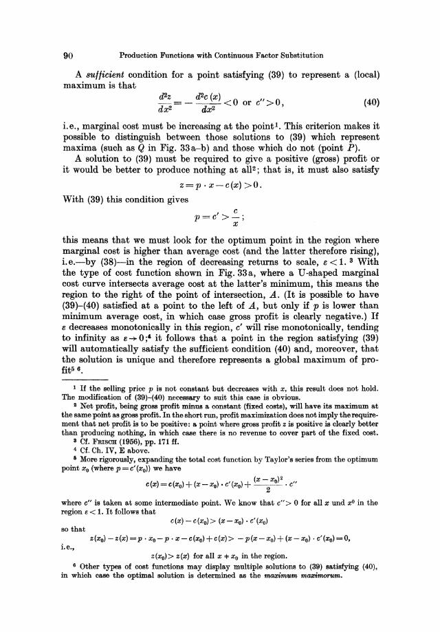
90 Production Functions with Continuous Factor Substitution
A 8Ulficient condition for a point satisfying (39) to represent a (local) maximum is that
d2z d2c (x) 0 "0 -=---< or c > , dx2 dX2
(40)
i.e., marginal cost must be increasing at the point!. This criterion makes it possible to distinguish between those solutions to (39) which represent maxima (such as Q in Fig. 33 a-b) and those which do not (point P).
A solution to (39) must be required to give a positive (gross) profit or it would be better to produce nothing at all2 ; that is, it must also satisfy
z=p· x-c(x) >0. With (39) this condition gives
c p=c' >-;
x
this means that we must look for the optimum point in the region where marginal cost is higher than average cost (and the latter therefore rising), i.e.-by (38)-in the region of decreasing returns to scale, e < 1. 3 With the type of cost function shown in Fig. 33a, where a U-shaped marginal cost curve intersects average cost at the latter's minimum, this means the region to the right of the point of intersection, A. (It is possible to have (39)-(40) satisfied at a point to the left of A, but only if p is lower than minimum average cost, in which case gross profit is clearly negative.) If e decreases monotonically in this region, c' will rise monotonically, tending to infinity as e ~ 0;' it follows that a point in the region satisfying (39) will automatically satisfy the sufficient condition (40) and, moreover, that the solution is unique and therefore represents a global maximum of profit56•
1 If the selling price p is not constant but decreases with x, this result does not hold. The modification of (39)-(40) necessary to suit this case is obvious.
S Net profit, being gross profit minus a constant (fixed costs), will have its maximum at the same point as gross profit. In the short run, profit maximization does not imply the requirement that net profit is to be positive: a point where gross profit z is positive is clearly better than producing nothing, in which case there is no revenue to cover part of the fixed cost.
a Cf. FRIsCH (1956), pp. 171 ff. 4 Cf. Ch. IV, E above. I More rigorously, expanding the total cost function by Taylor's series from the optimum
point Xo (where p = e' (xo» we have
e(x)=e(xo)+(x-xo) • e'(xo) + (X_XO)2. e" 2
where e" is taken at some intermediate point. We know that e"> 0 for all x und XO in the region e < 1. It follows that
e(x) -e(xo» (x-xo)· e'(xo) so that
z(xo) - z(x) =p . xo-p . x- e(xo)+e(x» - p(x-xo) + (x - xo) . e'(xo) =0, i.e.,
z(xo» z(x) for all x*, Xo in the region. 6 Other types of cost functions may display multiple solutions to (39) satisfying (40),
in which case the optimal solution is determined as the maxiwum maximorum.
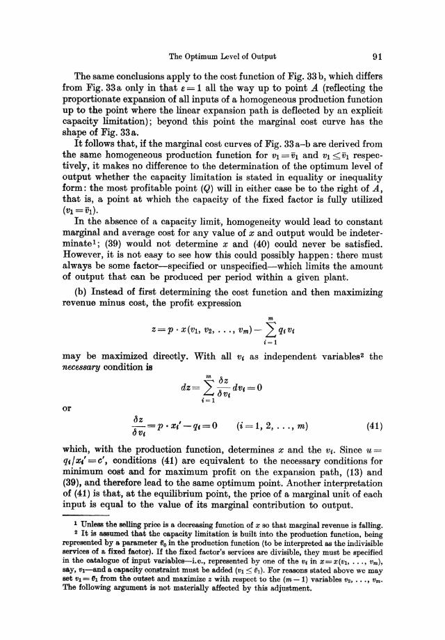
The Optimum Level of Output 91
The same conclusions apply to the cost function of Fig. 33 b, which differs from Fig. 33 a only in that B = 1 all the way up to point A (reflecting the proportionate expansion of all inputs of a homogeneous production function up to the point where the linear expansion path is deflected by an explicit capacity limitation); beyond this point the marginal cost curve has the shape of Fig. 33 a.
It follows that, if the marginal cost curves of Fig. 33a-b are derived from the same homogeneous production function for VI = ih and VI < ih respectively, it makes no difference to the determination of the optimum level of output whether the capacity limitation is stated in equality or inequality form: the most profitable point (Q) will in either case be to the right of A, that is, a point at which the capacity of the fixed factor is fully utilized (VI=ih).
In the absence of a capacity limit, homogeneity would lead to constant marginal and average cost for any value of x and output would be indeterminate I ; (39) would not determine x and (40) could never be satisfied. However, it is not easy to see how this could possibly happen: there must always be some factor-specified or unspecified-which limits the amount of output that can be produced per period within a given plant.
(b) Instead of first determining the cost function and then maximizing revenue minus cost, the profit expression
m
Z = P . x (VI, V2, ••• , Vm) - 2: qi Vi
i=l
may be maximized directly. With all V, as independent variables2 the necessary condition is
or !5z , 0 -=p·x, -qf= !5 Vi
(i = 1, 2, ... , m) (41)
which, with the production function, determines x and the Vi. Since u =
q,/x/ =c', conditions (41) are equivalent to the necessary conditions for minimum cost and for maximum profit on the expansion path, (13) and (39), and therefore lead to the same optimum point. Another interpretation of (41) is that, at the equilibrium point, the price of a marginal unit of each input is equal to the value of its marginal contribution to output.
1 Unless the selling price is a decreasing function of x so that marginal revenue is falling. 2 It is assumed that the capacity limitation is built into the production function, being
represented by a parameter 110 in the production function (to be interpreted as the indivisible services of a fixed factor). If the fixed factor's services are divisible, they must be specified in the catalogue of input variables--i.e., represented by one of the v, in X=X(Vl, ••• , vm), say, VI-and a capacity constraint must be added (VI::; VI). For reasons stated above we may set VI = 111 from the outset and maximize z with respect to the (m - 1) variables V2, ••• , vm •
The following argument is not materially affected by this adjustment.
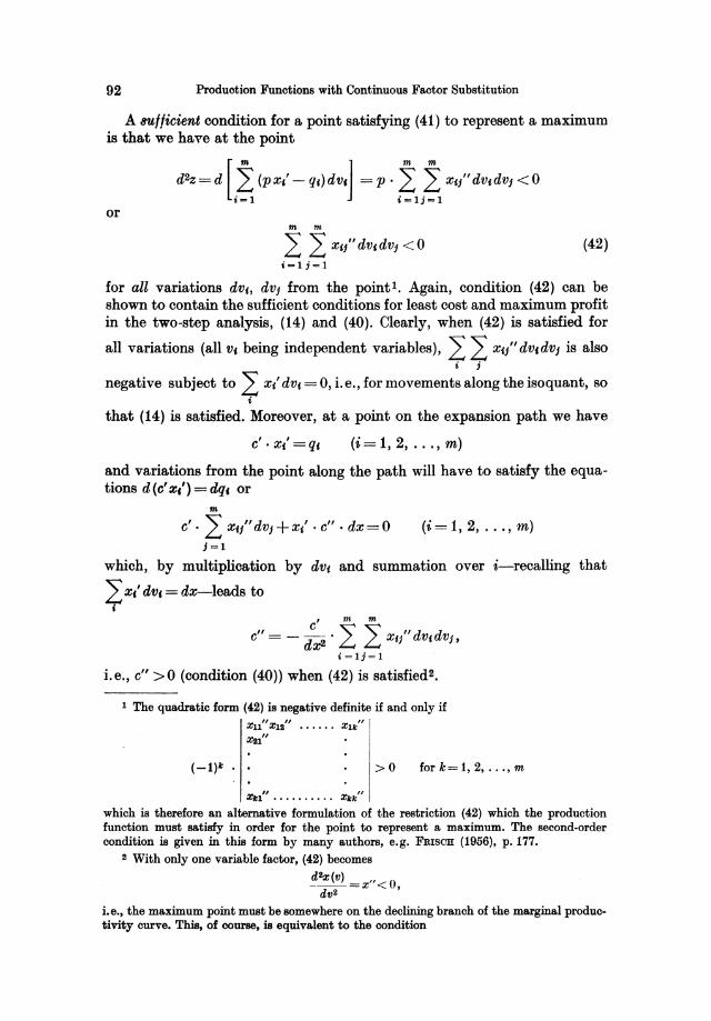
92 Production Funotions with Continuous Factor Substitution
A 8'Uflieient condition for a point satisfying (41) to represent a maximum is that we have at the point
or lit lit
2: 2: xc/' dvc dVj < 0 i-l;=1
(42)
for aU variations dv(, dVj from the point 1. Again, condition (42) can be shown to contain the sufficient conditions for least cost and maximum profit in the two-step analysis, (14) and (40). Clearly, when (42) is satisfied for
all variations (all Vc being independent variables), 2: 2: xci" dv,dvj is also i ;
negative subject to L xl dv, = 0, i. e., for movements along the isoquant, so i
that (14) is satisfied. Moreover, at a point on the expansion path we have
e'· x,' =q, (i= 1,2, ... , m)
and variations from the point along the path will have to satisfy the equations d(c'zc')=dq, or
lit
e'. 2: Z,/' dVl+ X/' e"· dx=O (i= 1,2, ... , m) ;=1
which; by multiplication by dv, and summation over i-recalling that
L xc' dv, = dx-Ieads to i
, lit lit
" e '" '" ltd d e = - dxS . ~ ~ x" v, v}, i=1;=1
i.e., e" >0 (condition (40» when (42) is satisfied2•
1 The quadratio form (42) is negative definite if and only if xu" XlI" •••••• X1II:"
X81"
(-1)1: • >0 fork=1.2 •...• m
x"l" ••• • • . • . .. XI:I:"
whioh is therefore an alternative formulation of the restriotion (42) whioh the produotion funotion must satisfy in order for the point to represent a maximum. The seoond-order condition is given in this form by many authors. e.g. FRISCH (1956). p.177.
a With only one variable factor, (42) becomes
~ax(v) =x"<O. dv2
i.e •• the maximum point must be somewhere on the declining branoh of the marginal produotivity ourve. This, of course, is equivalent to the condition
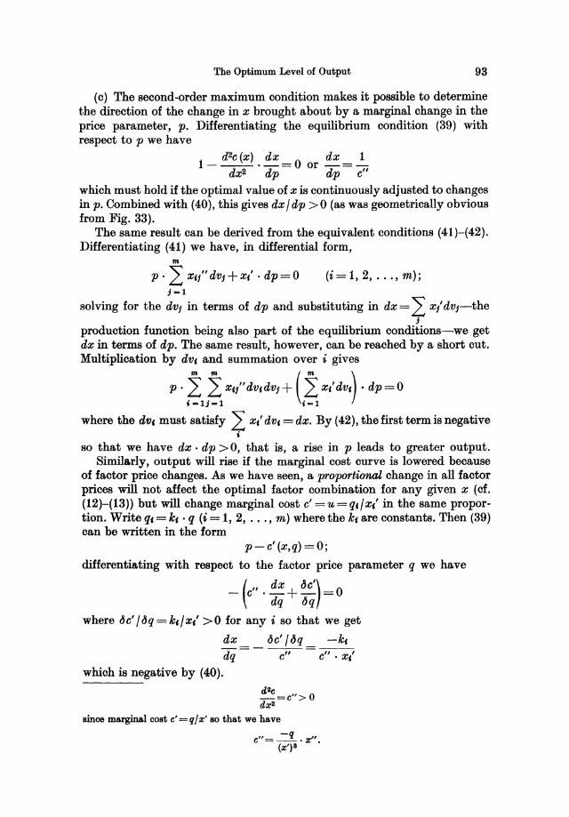
The Optimum Level of Output 93
(c) The second-order maximum condition makes it possible to determine the direction of the change in x brought about by a marginal change in the price parameter, p. Differentiating the equilibrium condition (39) with respect to p we have
1 _ d2e (x) . dx = 0 or dx = ~ dx2 dp dp e"
which must hold if the optimal value of x is continuously adjusted to changes in p. Combined with (40), this gives dx / dp > 0 (as was geometrically obvious from Fig. 33).
The same result can be derived from the equivalent conditions (41)-(42). Differentiating (41) we have, in differential form,
m
p. L: X,l' dvl+ X,'. dp=O (i= 1,2, ... , m); ;-1
solving for the dVI in terms of dp and substituting in dx = 2: xl dVl-the ;
production function being also part of the equilibrium conditions-we get dx in terms of dp. The same result, however, can be reached by a short cut. Multiplication by dv, and summation over i gives
p. ~ ~ x,l'dv,dvl+ (~xldV,) • dp=O i-l/=1 i=1
where the dv, must satisfy 2: xl dv, = dx. By (42), the first term is negative i
so that we have dx· dp >0, that is, a rise in p leads to greater output. Similarly, output will rise if the marginal cost curve is lowered because
of factor price changes. As we have seen, a proportional change in all factor prices will not affect the optimal factor combination for any given x (of. (12)-(13» but will change marginal cost e' =u=q,/x,' in the same proportion. Write q, = k, . q (i = 1, 2, ... , m) where the k, are constants. Then (39) can be written in the form·
p-e'(x,q)=O;
differentiating with respect to the factor price parameter q we have
- (e'" ~; + ~~)=O where dc' /dq=k,/x,' >0 for any i so that we get
dx dc' / dq -k, dq = --r= e"· xl
which is negative by (40).
die =c"> 0 axS
Bince marginal OOBt c'='1/x' BO that we have
c"= -'1 . x". (x') 8
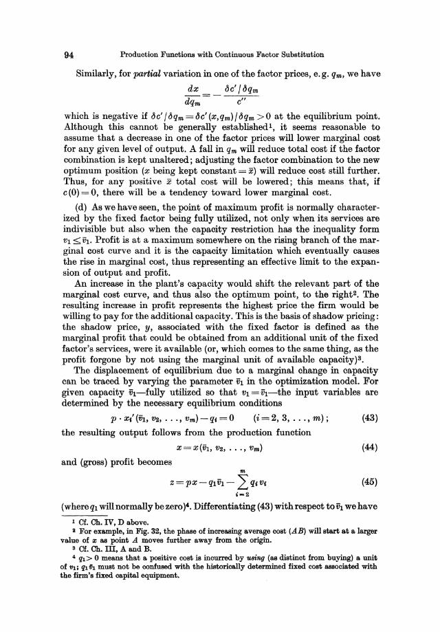
94 Production Functions with Continuous Factor Substitution
Similarly. for partial variation in one of the factor prices. e.g. qm. we have
dx tJe' / tJqm - = - ----'--=--dqm e"
which is negative if tJe' /tJqm=tJe'(x.qm)/tJqm >0 at the equilibrium point. Although this cannot be generally established 1, it seems reasonable to assume that a decrease in one of the factor prices will lower marginal cost for any given level of output. A fall in qm will reduce total cost if the factor combination is kept unaltered; adjusting the factor combination to the new optimum position (x being kept constant = x) will reduce cost still further. Thus. for any positive x total cost will be lowered; this means that. if e (0) = O. there will be a tendency toward lower marginal cost.
(d) As we have seen. the point of maximum profit is normally characterized by the fixed factor being fully utilized. not only when its services are indivisible but also when the capacity restriction has the inequality form VI <ih. Profit is at a maximum somewhere on the rising branch of the marginal cost curve and it is the capacity limitation which eventually causes the rise in marginal cost. thus representing an effective limit to the expansion of output and profit.
An increase in the plant's capacity would shift the relevant part of the marginal cost curve. and thus also the optimum point. to the right2. The resulting increase in profit represents the highest price the firm would be willing to pay for the additional capacity. This is the basis of shadow pricing: the shadow price, y. associated with the fixed factor is defined as the marginal profit that could be obtained from an additional unit of the fixed factor's services. were it available (or, which comes to the same thing, as the profit forgone by not using the marginal unit of available capacity) 3.
The displacement of equilibrium due to a marginal change in capacity can be traced by varying the parameter iii in the optimization model. For given capacity vI-fully utilized so that VI = vI-the input variables are determined by the necessary equilibrium conditions
p.x,'(ih,V2 •... ,vm)-q,=O (i=2,3 •...• m); (43)
the resulting output follows from the production function
X=X(VI. V2 • ...• vm) (44)
and (gross) profit becomes m
Z=PX-qlvl- L q,v, i-2
(45)
(where ql will normally be zero)'. Differentiating (43) with respect to VI we have
1 Cf. Ch. IV, D above. B For example, in Fig. 32, the phase of increasing average cost (AB) will start at a larger
value of z as point A moves further away from the origin. S Cf. Ch. III, A and B. 4 ql> 0 means that a positive cost is incurred by UBing (as distinct from buying) a unit
of !It; ql"l must not be confused with the historically determined fixed cost associated with the firm's fixed capital equipment.
The Optimum Level of Output 95
" + L:m "
dV1 0 P . Xu P . X'1' --=- = dVl
(i=2, 3, "" m) (46) j =2
which may be solved for the dVj / dih to give the displacement of the equilibrium values of V2, ••• , Vm due to a marginal change in ~h, assuming that the inputs are adjusted optimally to the changing capacity. The displacement of X and z follows by substitution in
and dz dx ~ dVj dih = P . dih - ql - L. qj . d~h
;=2
(47)
(48)
which result from differentiation of (44) and (45). However, if we are interested only in dz /dvl, there is no need to solve (46): equations (47)-(48) give
dz , ~, dVj , dVI =PXI -ql+ L. (pXj -qj)' dVI =PXI -ql
;=2
where, by (43), the coefficients of the dVj / dVI vanish so that the shadow price becomes
dz , Y= dVI =PXl -ql'
In other words, an extra unit of VI raises output by Xl' units, from the value of which we must subtract the cost of using it (if any)!; or, alternatively,
dz <5 X ( /')' Y = - . ----=- = P - ql Xl • Xl dx <5 VI
where P - ql/ Xl' is selling price minus partial marginal cost in the direction of VI. 2
1 This result needs oareful interpretation. It does not follow from what has been said that the ourrent inputs V2, ••• , Vm are kept oonstant when the optimum position is shiftedon the contrary, they are ohanged aocording to (46). What follows is that the ohanges in V2,
••• , Vm and the ohange in x resulting from them oanoel out as far as profit is oonoerned so that the marginal net effeot on z is the same as if only fit had inoreased. This is not surprising when it is recalled that marginal oost at an optimal point is the same in every faotor direotion.
2 The shadow prioe oan be identified with a Lagrange multiplier (of. Appendix 1, A). Maximizing z subjeot to the side oondition Vi = 1h, using the Lagrangian
m L=p . X (Vi, V2, ••• , Vm) - qiVi- ~ qiVi+U' (t1i- Vi)
i=2 where U is a Lagrange multiplier, neoessary maximum oonditions are
t5L, t5L, -=PXi -qi-U=O, -=PXI -qt=O (i=2, 3, .. ", m) a~ a~
(or, alternatively, dL=.~ (pXj' - qt) dVj -UdVi= dz - UdVi=O) .=1
96 Production Functions with Continuous Factor Substitution
When the capacity is fully utilized at the optimum point, the shadow price is positive since otherwise profit could be increased by leaving part of iiI idle (equivalent to a decrease in capacity), contradicting the assumption that profit is at a maximum for V1 = ih 1. On the other hand, had V1 been less than iiI at the optimum point, y would be zero since a marginal change in capacity would leave the equilibrium position and thus also profit unaltered j this reflects the intuitively obvious fact that the utilization of a fixed factor is a free good up to capacity.
When the production function is homogeneouS of degree one, we have by Euler's theorem .
m
X= V1XI' + L v,xc' '=2
identically. Combining this with (43) and with VI = VI, we have at the point of maximum profit
or, if ql >0 so that the term q1v1 must be included in total variable cost, m
VI· (PXI' -ql) = pX- qIVI- L q,v, = z. i-2
It follows not only that the shadow price-the marginal opportunity value per unit of vI-is positive (because z > 0) but also that the total imputed value of the fixed factor's services, as evaluated on the basis of the shadow price, equals the total gross profit earned at the point of maximum profit2. Consequently, if the firm determines the scale of output on a "full-cost" basis in the sense that the selling price is required to cover average variable cost plus the unit cost associated with the fixed factorS, this costing procedure leads to maximum profit only if the latter cost element is estimated on the basis of the shadow price. Any other cost price per unit of VI will lead to a less profitable scale of output'.
from which we get dz -=u=px{-Ql=lI· dV1
1 This argument does not hold in the case of indivisibility where V1 is always = f1 because less than full utilization of capacity is impossible by assumption.
S Of. the ooncept of quasi-rent. S "Full-cost" pricing in the usual sense consists in fixing the selling price on the basis
of total unit cost (including some profit margin) at a predetermined level of output, whereas the problem here is to find that x for which total unit cost is exactly equal to the given price of the produot.
4 This result does not hold when the produotion function is not homogeneous of degree one in all m input variables.
Chapter V
More Complex Models
A. Substitution with Shadow Factors
1. "Product Shadows"
(a) The models of the previous chapters represent special cases in the sense that all inputs are in the same position: they are all substitutable for one another-continuously or otherwise--or perfectly complementary (limitational).
An obvious generalization is a "mixed" type of production model where some but not all of the inputs are mutual substitutes. To take a simple example, the technology of a process may be represented by the model
or
x=f(vI, V2)
V3=a3' x
1 x = f (VI, V2) = - . V3
a3
(1)
where VI and V2 are continuously substitutable whereas V3 is a limitational input with the constant coefficient of production a3. I (More generally, V3
may be some increasing function of x.) It is an example of what has been termed a "shadow factor"-more specifically, a "product shadow"2: V3
follows x like its shadow, depending only on the level of output regardless of what combination of VI and V2 is used.
Since models of this type are characterized by the number of independent variables (degrees of freedom) being less than the number of inputs, partial variation of one input for all others constant is not possible so that marginal productivities cannot be defined in the usual way. For example, for V2 and V3 constant in (1), x and hence also VI is determined; for given values of VI and V2, on the other hand, V3 cannot vary because x is determined by the
1 This case was first noticed by PARETO (1897), § 714, p. 83, and § 717, p. 85. SCHNEIDER (1934), p. 3, has suggested that models of this type have a wide range of application, actual production processes being characterized by separate groups of substitutional and limitational inputs. See also SCHULTZ (1929), p.517, GEORGEScu·RoEGEN (1935), STIGLER (1946), pp. 364 ff., and FRISCH (1953), Ch. 12-13.
2 FRIsCH (1953), pp. 22 ff. See also SCHNEIDER (1934), p. 6. Daoo, Production Models 7
98 More Complex Models
first equation and Vs by the second. However, it is possible to analyse the model in terms of the marginal productivities of the substitutional factors alone if they are defined as the partial derivatives of the first equation of the model:
it being understood that all other substitutional factors-in this case, V2 and VI respectively-are kept constant whereas the limitational input Va is adjusted in accordance with the second equation I.
Like other multi-equation models, (1) can be rewritten as a single production function in terms of input amounts available:
x=Min [1p(WI' W2), Walas] =tp(WI, W2, Wa) (la) where
1p(WI' W2) = Max t(VI, V2) for VI :::;;WI, V2 <W2.
In this formulation, where the Wt are independent variables so that partial variation is possible, the marginal productivities can be defined in the usual manner-Le., tp,' =lJtpllJwf, i= 1,2, 3--only they are discontinuous at points where there is "just enough" of Ws (Ws = aa ·1p(WI, W2)), i.e., at points which also belong to (1):
tpl'=O, tp2'=O, tps'=l/as for Wslas<1p(WI,W2)
tpl'=/I'. tps'=t2', tps'=O for Ws/aa>1p(WI.W2).2
The optimal factor combination for given level of output is determined by minimizing variable cost subject to (1) for given x= x. Since the shadow factor depends only on x, the cost of Va is represented by a constant term in the cost expression and the problem reduces to that of minimizing the cost of VI and V2,
subject to
1 Cf. SOHNEIDER (1934), p.5, and Fmscn (1953), p.23. Taking the differentials of (1) we have
dx= /t'dV1 + la' dva , dva=asdx where the marginal productivity of V1 is now defined as dx/dv1 for diJ2=O and dvs=aadx, i.e., as/t'; similarly for dVl=O we have dx/dva=/a'. The isoquantfor given x is defined by lk=dva=O, i.e., by
/1' dVl + /S'dV2 = 0 along which the ma.rgina.I rate of substitution is
-dva/dvl=/!'I/s'> 0 (in the region where II' and Is' are positive).
I GEORGESCU-RoEGEN (1935), pp.41-43, appears to have a model of the type (ta) in mind when he defines alimitational factor by the existence of points at which all other factors have marginal productivities equal to zero (i.e., output cannot be increased without increasing the factor in question). From this he deduces a model of the type (1). However, as pointed out by KALnoR (1937), such points may also exist in the case where all inputs are substitutable (in the two·factor case, all points on the boundary of the region of substitution when this region does not cover the whole of the positive factor plane). For an input to be limitational at a point we must further require that output cannot be raised by increasing the input alone, of. Fmscn (1953), p.3-a condition satisfied by model (1) or (ta).
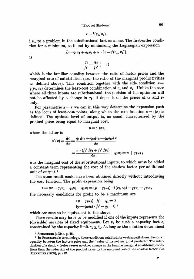
"Product Shadows" 99
x = t(Vi, vz),
i.e., to a problem in the substitutional factors alone. The first-order condition for a minimum, as found by minimizing the Lagrangian expression
is L=qIVl +q2V2+U, [x- f(VI, V2)],
qi qs /l'=/z' (=u)
which is the familiar equality between the ratio of factor prices and the marginal rate of substitution (i. e., the ratio of the marginal productivities as defined above). This condition together with the side condition x = f(VI, vs) determines the least-cost combination of VI and V2. Unlike the case where all three inputs are substitutional, the position of the optimum will not be affected by a change in qa; it depends on the prices of VI and Vz only.
For parametric x = x we can in this way determine the expansion path as the locus of least-cost points, along which the cost function e=c(x) is defined. The optimal level of output is, as usual, characterized by the product price being equal to marginal cost,
p=c'(x), where the latter is
e' (x) = de = qIdvl +qsdvz +qaaa dx dx dx
U . (h' dVI + /2' dvs) + + = ~~=U ~~;
dx
U is the marginal cost of the substitutional inputs, to which must be added a constant term representing the cost of the shadow factor per additional unit of output. I
The same result could have been obtained directly without introducing the cost function. The profit expression being
z = px-qIVI-qzV2 -qaVa= (p-qaaa) • t(VI, V2) -qIVI-q2V2,
the necessary conditions for profit to be a maximum are
(p-qa~) • /1' -qi =0 (p-qaaa)· /2' -q2=0 2
which are seen to be equivalent to the above. These results may have to be modified if one of the inputs represents the
(divisible) services of fixed equipment. Let VI be such a capacity factor, constrained by the capacity limit VI ::;;VI. As long as the solution determined
1 SOBNEIDER (1934), p. 48. 2 In SCHNEIDER'S terminology, these conditions establish for each substitutional factor an
equality between the factor's price and the "value of its net marginal product." The introduction of a shadow factor causes no other change in the familiar marginal equilibrium conditions than the reduction of the product price by the marginal cost of the shadow factor. See SOBNEIDER (1958). p. 212.
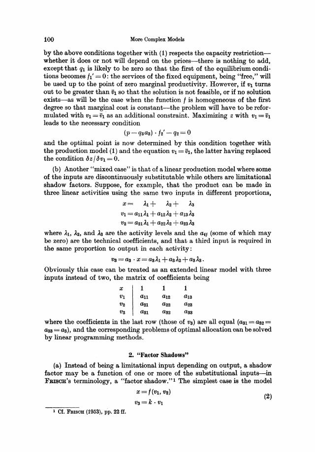
100 More Complex Models
by the above conditions together with (1) respects the capacity restrictionwhether it does or not will depend on the prices-there is nothing to add, except that ql is likely to be zero so that the first of the equilibrium conditions becomes /1'= 0: the services of the fixed equipment, being "free," will be used up to the point of zero marginal productivity. However, if VI turns out to be greater than ih so that the solution is not feasible, or if no solution exists-as will be the case when the function f is homogeneous of the first degree so that marginal cost is constant-the problem will have to be reformulated with Vl =ih·as an additional constraint. Maximizing z with VI = ih leads to the necessary condition
(p-qsas) . /2' -Q2=0 and the optimal point is now determined by this condition together with the production model (1) and the equation VI = th, the latter having replaced the condition d z / d VI = O.
(b) Another "mixed case" is that of a linear production model where some of the inputs are discontinuously substitutable while others are limitational shadow factors. Suppose, for example, that the product can be made in three linear activities using the same two inputs in different proportions,
x = Al + A2 + As VI = an Al + al2 A2 + alS As v2=a21AI +a22A2+~sAs
where Al, A2, and As are the activity levels and the a't (some of which may be zero) are the technical coefficients, and that a third input is required in the same proportion to output in each activity:
va=as' x=asAl +asA2+asAs. Obviously this case can be treated as an extended linear model with three inputs instead of two, the matrix of coefficients being
x 1 1 1 VI all au alS V2 ~l ~2 a23
Vs asl aS2 a33
where the coefficients in the last row (those of va) are all equal (aSI = as2 = ass = as), and the corresponding problems of optimal allocation can be solved by linear programming methods.
2. "Factor Shadows"
(a) Instead of being a limitational input depending on output, a shadow factor may be a function of one or more of the substitutional inputs-in FRISou's terminology, a "factor shadow." I The simplest case is the model
X= f(VI, V2) (2)
1 Of. FrosCH (1953). pp. 22 H.
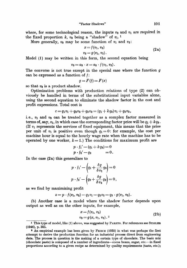
"Factor Shadows" 101
where, for some technological reason, the inputs V3 and Vl are required in the fixed proportion le, V3 being a "shadow" of Vl. 1
More generally, Va may be some function of Vl and V2: x=l(vl, V2)
V3 = g(Vl, V2). Model (1) may be written in this form, the second equation being
V3=a3· x=as· I(vl, V2).
(2a)
The converse is not true except in the special case where the function g can be expressed as a function of I:
g=F(/)=F(x) so that Va is a product shadow.
Optimization problems with production relations of type (2) can obviously be handled in terms of the substitutional input variables alone, using the second equation to eliminate the shadow factor in the cost and profit expressions. Total cost is
C =qlVl +q2V2 +q3V3 = (ql + kqS)Vl +q2V2,
i. e., Vl and Vs can be treated together as a complex factor measured in terms of, say, Vl, in which case the corresponding factor price will be ql + leqs. (If Vl represents the services of fixed equipment, this means that the price per unit of Vl is positive even though ql = 0: for example, the cost per machine hour is equal to the hourly wage rate when the machine has to be operated by one worker, le= 1.) The conditions for maximum profit are
p . /1' - (ql + leq3) = 0 p. 12' -q2 =0.
In the case (2 a) this generalizes to
p. /l'- (ql +!JL qs) =0 r)Vl
p. 12' - (q2+ ::2 qs) =0,
as we find by maximizing profit
Z = P • I(vl, V2) - ql Vl- q2V2 - qs . g(Vl' V2).
(b) Another case is a model where the shadow factor depends output as well as on the other inputs, for example,
x=/(vl, V2)
upon
(2b)
1 This type of model, like (1) above, was suggested by PARETO. For references see STIGLER (1946), p. 365.
I .An empirical example has been given by FRISCH (1935) in what was perhaps the first attempt to derive the production function for an industrial process direct from engineering data. The process in question is the making of a certain type of chocolate. The basic mix (chocolate paste) is composed of a number of ingredients-cocoa beans, sugar, etc.-in fixed proportions according to a given recipe as determined by quality requirements (taste, etc.);
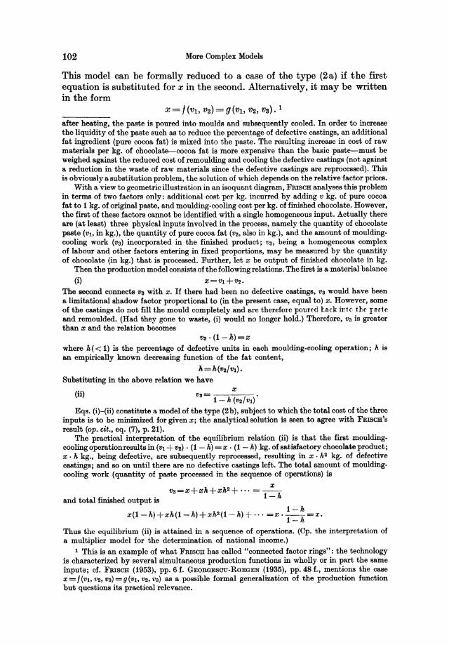
102 More Complex Models
This model can be formally reduced to a case of the type (2a) if the first equation is substituted for x in the second. Alternatively, it may be written in the form
x=t(Vl, V2) = g(Vl, V2, va).1
after heating, the paste is poured into moulds and subsequently cooled. In order to increase the liquidity of the paste such as to reduce the percentage of defective castings, an additional fat ingredient (pure cocoa fat) is mixed into the paste. The resulting increase in cost of raw materials per kg. of chocolate--cocoa fat is more expensive than the basic paste-must be weighed against the reduced cost of remoulding and cooling the defective castings (not against a reduction in the waste of raw materials since the defective castings are reprocessed). This is obviously a substitution problem, the solution of which depends on the relative factor prices.
With a view to geometric illustration in an isoquant diagram, FRISCH analyses this problem in terms of two factors only: additional cost per kg. incurred by adding v kg. of pure cocoa fat to 1 kg. of original paste, and moulding-cooling cost per kg. of finished chocolate. However, the first of these factors cannot be identified with a single homogeneous input. Actually there are (at least) three physical inputs involved in the process, namely the quantity of chocolate paste (Vh in kg.), the quantity of pure cocoa fat (V2, also in kg.), and the amount of mouldingcooling work (Va) incorporated in the finished product; Va, being a homogeneous complex of labour and other factors entering in fixed proportions, may be measured by the quantity of chocolate (in kg.) that is processed. Further, let x be output of finished chocolate in kg.
Then the production model consists of the following relations. The first is a material balance
(i) X=Vi+V2. The second connects Va with x. If there had been no defective castings, Va would have been a limitational shadow factor proportional to (in the present case, equal to) x. However, some of the castings do not fill the mould completely and are therefore pound lack iI1te thE' pEte and remoulded. (Had they gone to waste, (i) would no longer hold.) Therefore, Va is greater than x and the relation becomes
va·(l-h)=x where h( < 1) is the percentage of defective units in each moulding-cooling operation; his an empirically known decreasing function of the fat content,
h=h(V2!Vi). Substituting in the above relation we have
X Va= .
1- h (V2/Vi) (ii)
Eqs. (i)-(ii) constitute a model of the type (2 b), subject to which the total cost of the three inputs is to be minimized for given x; the analytical solution is seen to agree with FRISCH's result (op. cit., eq. (7), p. 21).
The practical interpretation of the equilibrium relation (ii) is that the first mouldingcooling operation results in (Vi + V2) . (1 - h) = x . (1 - h) kg. of satisfactory chocolate product; x . h kg., being defective, are subsequently reprocessed, resulting in x . h2 kg. of defective castings; and so on until there are no defective castings left. The total amount of mouldingcooling work (quantity of paste processed in the sequence of operations) is
va=x+xh+xh2 + •.. = _x_ 1-h and total finished output is
1-h x(l-h) +xh(1-h)+xh2(1-h)+··· =x· ---=X.
1-h
Thus the equilibrium (ii) is attained in a sequence of operations. (Cp. the interpretation of a multiplier model for the determination of national income.)
1 This is an example of what FRISCH has called "connected factor rings": the technology is characterized by several simultaneous production functions in wholly or in part the same inputs; cf. FRISCH (1953), pp. 6 f. GEORGESCu-RoEGEN (1935), pp. 48 f., mentions the case x = /(Vh V2, Va) = g(Vi, V2, Va) as a possible formal generalization of the production function but questions its practical relevance.
Constrained Substitution - Complementary Groups of Substitutional Inputs 103
B. Constrained Substitution
Suppose that the inputs of a production process are all substitutable for one another but that the variation is constrained by one or more side relations in some or all of the input variables 1. A simple example is the model
X=f(V1, V2, vs) g(V1,V2,VS)=O.
(3)
Whereas the previous models (1), (2), (2a), and (2b) were characterized by the number of degrees of freedom being equal to the number of substitutional inputs-for each shadow factor an additional equation was introducedfactor constraints like the second equation of (3) reduce the number of independent input variables in the production function proper, f. (In the extreme case of m inputs and m - 1 constraints the inputs will be limitational, but the general case of constrained substitution allows for some degree of variability in the factor proportions.)
Models of the type (2b) can be expressed in this form, but (3) may also be an "original" model with an interpretation of its own. For example, although any point (x, V1, V2, vs) satisfying the first equation may be feasible in the sense that the factor combination yields a positive amount of output, some factor combinations must be ruled out because the resulting product does not conform to the quality standard that is required; in this case the side condition g = 0 represents a quality constraint defining a region of factor combinations which give a satisfactory product.
Quality constraints may also have the weaker form of inequalities in some or all of the v"~ in which case they merely narrow down the region of substitution without affecting the dimensionality of the production model; the side conditions come in as boundary conditions in the optimization problem 2•
Capacity limitations of the type Vs < Vs are another special example of factor constraints in inequality form.
Necessary conditions for maximum profit subject to (3) are found by maximizing the Lagrangian
L= z+ u . g= p . l(vI, V2, vs) -qItJl-q2V2 -qsvs + u . g(VI, V2, Va)
where u is a Lagrange multiplier. The conditions are
( -u =) p . /I' - ql = P . 12' - q2 = P . Is' - qs gl' . g2' gS'
which together with the two equations of (3) determine the optimum values of the four variables.
C. Complementary Groups of Substitutional Inputs
Another possible generalization is a production model of the form
x=l(vI,v2)=g(vs,v4) (4)
1 Cf. BORDIN (1944). p. 77. 2 The problem of quality specifications in the production model is dealt with in some detail
in Ch. VITI.
104 More Complex Models
which is characterized by separate factor groupSl. One interpretation is that the production process is composed of several distinct sub-processes whose production functions-in the present case, I and g-have no inputs in common.
The inputs belonging to each group-for example, VI and Va-are substitutable for one another while the groups as such are complementary in the sense that a higher rate of output requires an increase in both l(v1, va) and g(vs, V4); output cannot be kept constant with more of VI and Va and less of Va and V4. The factor groups are in much the same position with respect to each other and to output as are the several "production functions" in cases of limitationality (perfect complementarity) such as
x = ft (VI) = la (Va)
of which (4) is a generalization2• This becomes obvious if model (4) is rewritten in terms of input amounts available:
x=Min [cp(W1' wa),tp(wa, W4)] where
and tp (wa, W4) = Max g( Va, V4) for Vs S WS, V4 < W4.
The least-cost point for given x = X, as determined by minimizing the cost expression subject to I - x = 0, g - x = 0, is characterized by
q1/ ft' = qa/ la'
which together with the first side condition determines VI and Va, and
qs/ gs' = q4/ g4'
which must be combined with g(vs, V4) = x to give the inputs of the second factor group. In other words, the familiar conditions for minimum cost under continuous substitution apply to each factor group separately; the leastcost combination of VI and Va is independent of the prices of Vs and V4, and vice versa.
For variable output, maximization of the Lagrangian expression
L=PX-qlVl- ••• -q4V4+Ul· [/('111, Va)-X]+ua· [g(vs, V4)-X]
1 The case was mentioned by PARETO, although in the form
h(a"av, •• • )=0, /2(aU,a"" ••• )=0 where at is the production coefficient of factor no. t:
at = Vt/x and so on. (Still other inputs are assumed by PARETO to be constant in the general case.) Cf. PARETO (1897), § 714, p. 83n.; see also SCHULTZ (1929), pp. 549-551. In the form used here-cf. (4)-the model has been treated by GEORGESCU-RoEGEN (1935), p.48, and also by FRISCH (1953), pp. 6 f. (under the name "disconnected factor rings"); cf. also FRISCH (1932), p. 64.
2 FRISOH (1953), p. 6, cites the example of a compound product whose parts are manufactured separately. When the parts are not made in equal numbers (f '*' g), the production function for the composite product is x=Min ri, g), the level of output being determined by the bottleneck just as in the case of limitationality. Cf. Ch. IX, C below.
Complementary Groups of Substitutional Inputs 105
with respect to x and VI, ••• , V4 leads to the following conditions for maximum profit:
P = UI + U2, ttl = qll h' = q21 12' , U2 = qal (fa' = q41 (f4'
where Ul and U2 are Lagrange multipliers; UI + U2 is to be interpreted as marginal cost at the optimal point since
de = qi dVl + ... + q4 dv4 = Ul • h' dVl + /2' dV2 + U2' (fa'dva + (f4' dV4 = Ul + U2, dx dx dx dx
and Ul and U2 are the specific marginal costs associated with the respective factor groups (sub-processes).
Chapter VI
The General Single-Product Model
(a) In the previous chapters (III-V) a number of different production functions have been discussed. The cases presented do not, however, form an exhaustive catalogue of single-output production models: other cases are possible and the characteristic features of the respective models discussed may be combined in various ways. Only empirical research can bring to light which of the models are of practical relevance and which are not.
From a formal-perhaps somewhat formalistic-point of view, the various cases may be thought of as special cases of a more general model of production. One way of writing all the cases in a common form is to express output as a function of inputs available,
X=!p(Wl' W2, •.. , wm ) (1)
where the w, are all independent variables. The various cases can then be classified according to the form of the function !po In order to do this, however, it is necessary to know the more fundamental technological relationships-fnr example, technically given coefficients of production, factor constraints, etc.-which characterize the process in question. Engineering information of this kind will usually be given in terms of input amounts consumed, v,. For this reason-and for other reasons already stated-the formulation (1), though quite legitimate, is scarcely adequate to our purpose.
(b) In terms of the variables v" not all independent in the general case, most of the models presented l can be written in the multi-equation form
X=f,.:(Vl; V2, ••. , vm ) (k= 1,2, ... , M <m) (2)
where the number of degrees of freedom (independent variables), N = m + 1 - M, ranges from 1 to m.
The number of equations, M, relative to the number of inputs, m, is in a sense the most important characteristic of any particular case since the dimensionality of a production model reflects the possibilities of factor substitution: a model in which all inputs are independent and continuously substitutable is the special case M = 1 (i. e., N = m) and the opposite extreme is that of M = m (i. e., N = 1) where all inputs are limitational and no substitution is possible. The various models of Ch. V represent intermediate cases in the sense that 1 <M <m.
1 With the sole exception of the linear discontinuous-substitution model «,f. Ch. III, B).
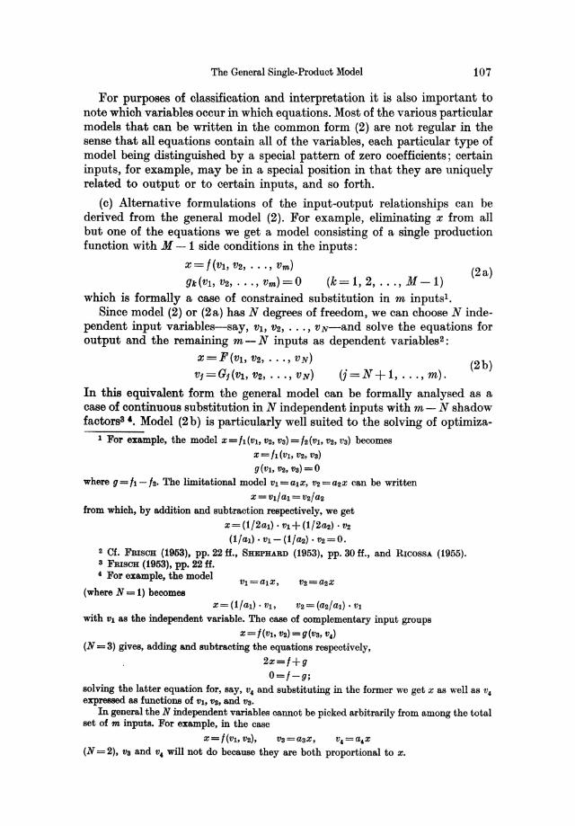
The General Single.Product Model 107
For purposes of classification and interpretation it is also important to note which variables occur in which equations. Most of the various particular models that can be written in the common form (2) are not regular in the sense that all equations contain all of the variables, each particular type of model being distinguished by a special pattern of zero coefficients; certain inputs, for example, may be in a special position in that they are uniquely related to output or to certain inputs, and so forth.
(c) Alternative formulations of the input-output relationships can be derived from the general model (2). For example, eliminating x from all but one of the equations we get a model consisting of a single production function with M - 1 side conditions in the inputs:
x=t(Vl, V2, ... , vm)
gk(Vl, V2, ••• , vm)=O (k= 1,2, ... , M -1) (2a)
which is formally a case of constrained substitution in m inputsi. Since model (2) or (2a) has N degrees of freedom, we can choose N inde
pendent input variables-say, VI, V2, ... , vN-and solve the equations for output and the remaining m - N inputs as dependent variables2 :
X=F(VI, V2, ... , VN)
Vj=Gi (Vl,V2, ... ,VN) (j=N+1, ... ,m). (2b)
In this equivalent form the general model can be formally analysed as a case of continuous substitution in N independent inputs with m - N shadow factors3 t. Model (2b) is particularly well suited to the solving of optimiza-
I For example, the model X= h(VI, V2, V3) = !2(VI, V2, V3) becomes X=/l(VI, V2, va) g(VI, V2, Va) =0
where g=/l-!2' The limitational model VI=aIX, V2=a2X can be written
x=vI!al = v2fa2
from which, by addition and subtraction respectively, we get x=(1f2at}. vI+(lj2a2)' V2
(lfal) . VI- (1ja2) . V2 =0.
2 Cf. FRISCH (1953), pp. 22 ff., SHEPHARD (1953). pp. 30 ff., and RWOSSA (1955). a FRISCH (1953), pp. 22 ff. 4 For example, the model
(where N = 1) becomes X=(ljal)' Vlo V2=(a2!aI)' VI
with VI as the independent variable. The case of complementary input groups X= !(VI, V2) =g(Va, v,)
(N = 3) gives, adding and subtracting the equations respectively,
2x=!+g
O=!-g;
solving the latter equation for, say, v, and substituting in the former we get x as well as v4
expressed as functions of VI, Va, and Va. In general the N independent variables cannot be picked arbitrarily from among the total
set of m inputs. For example, in the case
X=!(VloVa), V3=a3X, v,=a,x
(N = 2), Va and v, will not do because they are both proportional to x.
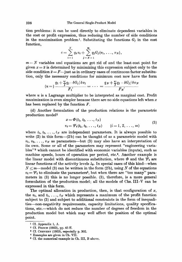
108 The General Single-Produot Model
tion problems: it can be used directly to eliminate dependent variables in the cost or profit expression, thus reducing the number of side conditions in the maximization problem l . Substituting the functions GI in the cost function,
N m
c= L q,Vt+ L qIGJ(Vl, ••. , VN), i=1 j=N+I
m - N variables and equations are got rid of and the least-cost point for given x = x is determined by minimizing this expression subject only to the side condition x = F-just as in ordinary cases of continuous factor substitution, only the necessary conditions for minimum cost now have the form
ql+~qj· tJGj/tJVI qN+~qJ . tJGi/tJVN (u=) ; F I ' = ... = 'FN '
where u is a Lagrange multiplier to be interpreted as marginal cost. Profit maximization is even simpler because there are no side equations left when x has been replaced by the function F.
(d) Another formulation of the production relations is the parametric production model2
x=f/J(tl, t2, ... , tN)
Vt = IJ', (tl' t2, •.• , tN) (i= 1,2, ... , l1t) (3)
where lI, t2, ••• , tN are independent parameters. It is always possible to write (2) in this form-(2b) can be thought of as a parametric model with VI, V2, •.• , VN as parameters-but (3) may also have an interpretation of its own. Some or all of the parameters may represent "engineering variables"3 which cannot be identified with economic variables (inputs), such as machine speeds, hours of operation per period, etc.'. Another example is the linear model with discontinuous substitution, where f/J and the IJ', are linear functions of the activity levels Ak. In special cases of this kind-when N <m-model (3) can be written in the form (2b), using N of the equations Vt = IJ', to eliminate the parameters5, but when there are "too many" parameters in (3) this is no longer possible. (3), therefore, is a more general formulation of the production model; aU the models of Chs.III-V can be expressed in this form.
The optimal allocation in production, then, is that configuration of x, the V"~ and tt, ... , t N which represents a maximum of the profit function subject to (3) and subject to additional constraints in the form of inequalities-non-negativity requirements, capacity limitations, quality specifications, "etc.-which do not reduce the number of degrees of freedom in the production model but which may well affect the position of the optimal point.
1 Of. Appendix 1, A. 2 Of. FRISCH (1953), pp. 45 ff. a Cf. CHENERY (1953), espeoially p. 302. 4 Examples are given in Ch. VII. 6 Of. the numerical example in Ch. III, B above.

Chapter VII
Divisibility, Returns to Seale, and the Shape of the Cost Function
A. Fixed Factors and the Production Function
The neoclassical theory of production traditionally assumes, in shortrun analysis of the individual firm (or process), that not all of the factors of production involved are variable. Those which represent the plant are assumed to be fixed in an absolute sense, the plant being composed of given indivisible units of capital equipment.
In a two-factor analysis of an agricultural production process let VI denote the factor "land" while Va is the variable factor (e.g. labour, or a homogeneous complex of variable inputs), and let the production function be
X=X(Vl, va). (1)
(Alternatively, (1) may be interpreted as an industrial production function where VI represents the fixed equipment and Va represents a complex of variable inputs.) The short-run situation is characterized by VI being fixed, ill=ih. Then output may as well be written as a function of Va only,
x=x(ih, va)=/(va), (2)
where the value of VI is no longer specified in the production function but is implicit in the specification of the function 11. For variations in Va, output is assumed to follow the law of variable proportions as shown in Fig.34a (OABO) a. The corresponding total cost function (including fixed costs) will have the shape DEFG indicated in Fig. 34b, the cost of the variable factor being its price times the inverse of the production function:
c = qava = qa/-l (x).
The marginal cost curve, c'=qa/l', will have the familiar U-shape which is so characteristic of neoclassical theory. The curvilinear shape of the pro-
I In the words of v. STACKELBERG (1938), p.78: "Bekanntlioh wird bei kurzfristiger Andenmg der Ausbringung ein Teil der Produktionsmittel in unverii.nderten Mengen aufgewendet. Die Aufwandsmengen diaser Produktionsmittel treten ... in der Produktionsfunktion nicht ala Variable in Ersoheinung, sondern sind mitbestimmend fUr die Form diaser Funktion. Man kann sie .•• einfa.ch fortla.ssen."
a The produotion curve is especially likely to have this particular shape if the production function is homogeneous of degree one in VI and Va (of. Ch. IV, B and Appendix 2), an assumption often made in neoolassical theory.
110 Divisibility, Returns to Scale, and the Shape of the Cost Function
duction and cost curves is due to the fact that variations in the level of output must necessarily be accompanied by changes in the proportion of "2 to VI when the latter cannot be adjusted to fluctuations in x .
/ I
I --------....,/--I
/.
c c
IJ
F ig. 34a-b
Now if we allow for divisibility, the model becomes less rigid in that both inputs will be capable of continuous variation, although in the short-run situation VI is available only up to a limit, ih. The cost function is now defined along an expansion path determined by minimizing c = q2 V2 I subject to (1) for parametric x = x and to the capacity restriction VI < ~h, which has replaced the "built-in" capacity parameter VI in (2). As we have seen2,
the variation of x with V2 in Fig. 34a now follows the path OA' B 0 3, whichassuming homogeneity-is linear up to B, the point where the expansion path is deflected because VI becomes = VI.' The divisibility of VI makes it possible to rule out points on OAB ; point A is inefficient since Xl' <0, and output can be increased by reducing the utilization of VI (V2 being the same) until Xl' becomes = 0 at point A'. Along OA' B the relative factor proportion is constant and the elasticity of production, e, is equal to one.
Correspondingly, for efficient production the total cost curve DE F G in Fig. 34b is replaced by DE'FG where marginal cost is constant along the linear segment DE' F . 6
1 Assuming ql = O. 2 Cf. Ch. IV, E (esp. Fig. 32). 3 This observation-without reference to the corresponding cost function-was apparently
first made by GLOERFELT-TARP (1937), pp. 225--233, and later by CmPMAN (1953), p. 106. The inefficiency of points on OAB had previously been pointed out by KNIGHT (1921), pp. 100 f.
4 It does Mt follow that the marginal productivity of the variable input Va will be constant up to point B; X2' is defined as 6x/6va for VI constant, i.e., as the slope of the tangent at a point on the production curve OABC. All that the argument states is that the expansion path in Fig. 34& will not coincide with OABC.
6 Cost functions of this kind have been treated in the literature but usually without precise indication of how they may come about. SCHNEIDER (1934), pp. 13 and 49, first justified them on purely empirical grounds, but in his later works--cf. SCHNEIDER (1958), pp. 170 and 189 ff.-he has derived a cost function of this shape from a parametric production model (cf. below).
Spatial Divisibility 111
The crucial question, then, is whether or not it is realistic to assume that the fixed factor is divisible-a question which is closely bound up with that of homogeneity, the usual common-sense argument for homogeneity in production functions being that twice the amount of all inputs will double output because it is a mere repetition (in time or space)!.
This is ultimately a matter of empirical research, not a question to which the pure theory of production and cost can readily provide a general answer. Still, it would seem as though the problem of divisibility has traditionally been given rather less than due attention in the literature. In the following we shall deal with plant divisibility in some detail to see in what way the fixed factor can be divisible and how divisibility affects the cost functions belonging to a variety of hypothetical production models.
B. The Dimensions of Capacity Utilization
1. Spatial Divisibility
(a) Let us first assume that the fixed factor is physically divisible in space but indivisible in the time dimension2•
An obvious example is an agricultural production process where several variable inputs (labour, fertilizer, etc.) cooperate with the services of a plot of land during a period of a year. The factor "land" is physically divisible in that it is not necessary to cultivate the entire available acreage; actually factor combinations involving negative marginal productivity of land will be ruled out as inefficient. Land, however, is not divisible in the time dimension in the sense that it is possible to use it for part of the production period only. This is due to the fact that grain-growing is an example of intermittent production: the product emerges not continuously during the production period but at discrete points of time-once a year-whereas the fixed factor must be employed continuously throughout the period. (For this reason it does not matter whether the input of land is defined as the acreage as such or as its services, e. g. in terms of acre-years, as long as we consider a given period of a year.)
Another exampleS is an industrial plant composed of a number of identical units (machines, reactors, etc.), some of which may not be utilized, but which are indivisible in the time dimension in that those units which are actually used have to be effectively operated during the entire period considered"; only in this case the fixed factor is not continuously variable since an integral number of units of equipment will have to be operated.
1 In Fig. 34a, for example, if..4.' is hallway between 0 and B, the expansion from 0 to..4.' is identioally repeated in moving on from..4.' to B.
2 In the following, only such fixed factors are considered as are directly productive (of. Ch. II above). There is no need to include buildings in the list of specified inputs since their productiveness consists in mere presence.
8 DEAN (1941), pp. 4 ff. 4 Blast furnaces, for example, must be operated continuously without breaks, cf. DEAN
(1951), p. 275.
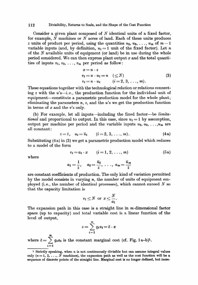
112 Divisibility, Returns to Scale, and the Shape of the Cost Function
Consider a given plant composed of N identical units of a fixed factor, for example, N machines or N acres of land. Each of these units produces z units of product per period, using the quantities U2, Us, ... , Um of m - 1 variable inputs (and, by definition, Ul = 1 unit of the fixed factor). Let n of the N available units of equipment (or land) be in use during the whole period considered. We can then express plant output x and the total quantities of inputs Vt, V2, ••. , Vm per period as follow:
x=n·z (3)
(i=2, 3, ... , m).
These equations together with the technological relation or relations connecting z with the u's-i.e., the production function for the individual unit of equipment-constitute a parametric production model for the whole plant; eliminating the parameters n, z, and the u's we get the production function in terms of x and the v's only. .
(b) For example, let all inputs-including the fixed factor-be limitational and proportional to output. In this case, since Ul = 1 by assumption, output per machine per period and the variable inputs U2, U3, ••• ,Um are all constant:
z=z, u,=u, (i=2,3, ... ,m). (4a)
SUbstituting (4a) in (3) we get a parametric production model which reduces to a model of the form
where v,=a,· x
1 al =-=,
z
(i=l, 2, ... , m) (5a)
. .. ,
are constant coefficients of production. The only kind of variation permitted by the model consists in varying n, the number of units of equipment employed (i.e., the number of identical processes), which cannot exceed N so that the capacity limitation is
N vl<N or x~-.
al
The expansion path in this case is a straight line in m-dimensional factor space (up to capacity) and total variable cost is a linear function of the level of output,
m
m
C = L q,v, = e . x ;=2
where e= L q,a, is the constant marginal cost (cf. Fig.la-b)l.
'-2 1 Strictly speaking, when n is not continuously divisible but can assume integral values
only (n=l, 2, •.• , N machines), the expansion path as well as the cost function will be a sequence of discrete points of the straight line. Marginal cost is no longer defined. but inere-
Spatial Divisibility 113
(c) On the other hand, if U2, Us, •.• , um are continuously substitutable inputs (Ul still being = 1 by definition), we have
Z=q>(U2, us, ... , um). (4b)
Eliminating the m + 1 parameters n, Z, and Uz, us, ... , Um from the parametric model (3)-(4b) we get the production function for the whole plant:
X=Vl' q> -, -, ••• , - =X(Vl, V2, ••. , vm) (vz Vs vm) Vt Vt VI
(5b)
where we now have m substitutable inputs of which VI represents the degree of utilization of the fixed equipment-i. e., the "extensive" dimension of capacity utilization-whereas an increase in output brought about by increasing vs, ... , Vm for VI constant is to be interpreted as more intensive utilization of the plant (intensive farming, etc.).
The function (5 b) is seen to be homogeneous of the first degree, hence the expansion path is a straight line in m-dimensional factor space as long as n < N and the corresponding phase of the cost function will be linear. When the capacity is fully utilized in the extensive dimension (n = N), the expansion path is deflected and further expansion requires more intensive operation, increasing vz, ... , Vm and thus changing the factor proportions. Because VI is now fixed, output cannot be expanded indefinitely; the second phase of the expansion will be characterized by decreasing returns to scale and marginal cost will be rising up to the point of maximum capacity I. Thus the cost function will have the same general shape as that shown in Fig. 322.
mental costA cIA x (forA x = Z = 11 al) is the same at all points and equal to average variable cost. The stepwise expansion path derived by BREMS (1952a, b) for this case is based on the assumption that the isoquants are L-shaped, including points characterized by less than full utilization of the available factor quantities. Even if this definition of the production function is adopted, such points cannot belong to the expansion path because they are clearly inefficient, cf. Ch. III, A.
1 Of. Ch.lV, E. I When n is a discrete variable assuming integral values only, the expansion path will be
somewhat different; in the two-factor case the graphical picture will be as follows:
where the expansion path is composed of the disconnected line segments AA', BB', etc.; points on A' A", B' B", etc. are not eHicient since the points B, 0, etc. represent larger output
Dane. Produotlou Models 8
114 Divisibility, Returns to Scale, and the Shape of the Cost Function
(d) The linear shape of the cost curve within the limit v! <N is derived from the assumption of homogeneity, which in turn is related to that of plant divisibility. When the fixed factor is divisible, it is tempting to make the further assumption that the production process is also divisible in the sense that, as output is expanded by more units of the fixed factor coming into use, each consecutive unit cooperates with the same quantities of the other inputs to yield the same amount of output. This assumption is implicit in the model, where (3) states that total output and total inputs are the same multiple of output and inputs associated with a unit of the fixed factor, the latter variables being related by (4a) or (4b), so that output can be expanded by identical repetition in the space dimension (more extensive cultivation of the soil, utilizing more machines, etc.).
It is precisely this element of repetitiveness, based on factor divisibility, that underlies the usual common-sense justification of constant returns to scale. The argument is plausible enough in many cases; a more general theoretical model, however, must allow for the possibility of economies (or diseconomies) of scale within the plant. Analytically this means that n may appear as an additional variable in (4 b) :
Z = <p(U2' Us, ... , Urn, n); (5b) then becomes
(6)
which is no longer homogeneous and which therefore leads to a non-linear expansion path and a non-linear cost function!.
at less cost so that it will pay to produce these larger outputs and dispose of the amount of output not required. The corresponding cost function will also be discontinuous:
However, these discontinuities are of little cousequence if N is a large number; the shape of the curves will then approach that of Fig. 32.
lOne interpretation is that an additional factor is involved in the production process but not specified explicitly as an input variable because it is an indivisible fixed factor (representing, for example, "entrepreneurship", "organization", etc.), vo=Do. The absence of linearity can then be "explained" by the fixity of V O if it is argued that the production function ought to be homogeneous if all m + 1 factors were va.riable. This postulate, however, is empirically meaningful only if vO can be defined in such a way as to be physically specifiable in quantitative terms, i.e., measura.ble (of. Appendix 2).
The Time Dimension 115
2. The Time Dimension
(a) Next let us consider the case where the fixed factor is physically indivisible but divi8ible in the time dimen8ion in that it is possible to vary the number of hours of operation per period of calendar time. For example, the utilization of a machine in terms of machine hours per month may be variable within the limit set by the total number of hours the machine is available in a month. In such cases it is the 8ervice8 of the fixed factor which are represented by the input variable VI, not the factor itself (e.g. machine hours rather than machines).
Clearly, full divisibility of this kind is possible only when the production process considered is a continuou8 one in the sense that output and inputs are continuous flows in time. In the case of intermittent production, as we have seen above, the process and thus also the use of the fixed factor in a period is an indivisible whole.
In much of the literature on the theory of production the time dimension is eliminated by the assumption that the plant is operated at full capacity in time, for example, that the number of effective working hours per day is fixed l , so that output per period (day) can be varied only by more or less intensive operation. While this may in fact be correct in some cases of continuous productionz, as a general assumption it is unnecessarily restrictive and leads to factor combinations which are uneconomical or even clearly inefficient.
To clarify the argument, let us consider a hypothetical productive process. A plant produces z units of a single product with labour, energy, raw material, and other variable inputs in quantities Uz, U3, ••• , Um in physical units per hour of effective operation3• The plant as such is fixed and physically indivisible (e.g. one machine) but its services, as measured in plant hours of effective operation (machine hours), are continuously divisible; the input of plant services per hour of operation, UI, is of course = 1 by definition.
The rate of output per period of calendar time (e.g. per day) and inputs per period, when the plant is operated t hours out of the T hours available per period, will be
x=t· Z
VI = t . UI = t ( < T)' (7)
Vt= t· Ut (i=2, 3, ... , m).
When the production function for an hour's operation is known, we can eliminate t, z, and the u's and the production function for output per period emerges.
The introduction of the time factor adds a new dimension to the production model; as the equation
x=t· z
1 Of., for example, CARLSON (1939), p. 15 n. 2 Such as processes which are continuous also in the sense that, for technical reasons,
the plant must be operated continuously without breaks (e.g. blast furnaces, cf. above). 3 Not per calendar hour.
116 Divisibility, Returns to Scale, and the Shape of the Cost Function
shows, the quantity of product per period can be expanded not only by applying larger amounts of variable inputs per hour (provided that substitution is possible), thus increasing the hourly rate of output by more intensive utilization of the fixed factor, but also by increasing the number of hours of operation per period, that is, by more extensive operation in the time dimension. (The capacity of the plant, similarly, has two dimensions, capacity per period being maximum output per hour times the number of hours (T) the plant is available per period.) And a given level of output can be attained by different combinations of t and z, producing more per hour in fewer hours per period; in so far as they represent different factor combinations, a new dimension has been added to the substitution possibilities.
(b) Assume first that all inputs are limitational with constant input-output coefficients. Then, by analogy with (4a) and (5a) above, output and variable inputs per hour of effective operation will be constant since the input of machine services per hour is constant by definition (UI = 1):
z=z, u,=Ut (i=2,3, ... ,m). (Sa)
The parametric production model (7)-(8a) reduces to
(i=1,2, ... ,m) (9a) where
(i=2,3, ... ,m)
are constant coefficients of production. No factor substitution for x constant is possible. The only kind of variation permitted by this model is a proportional expansion of output and inputs in the time dimension up to the limit t = T; in terms of output per period the capacity limitation is
T x:s;;-. al
The expansion path is linear and so is the cost function.
(c) Suppose instead that the u's are continuously substitutable factors. Then we have
z=rp(uz, Ua, •.• , um)
and this combines with (7) to give
(VZ Va vm) X=Vlorp -,-•...• -VI VI VI
(8b)
(9b)
which is perfectly analogous to (5b) as derived from (3)-(4b). The time dimension, as represented by t = VI. adds a new variable and substitutable factor to the (m-1) already present in (8b); the latter equation, in which the input of plant services per hour is fixed (UI = 1), represents a more restricted field of variation. presumably obeying the law of variable proportions. When all m factors are free to vary, i. e .• for VI = t < T, the expansion path in m-dimensional factor space will be a straight line whose direction depends on the factor prices qz, qa, ... , qm (Xl' being = 0 for
The Time Dimension 117
q1 = 0) and along which marginal cost is constant. When the capacity is fully utilized in the time dimension (111 = T), further expansion requires more "intensive" operation; this means changing the factor proportions as z increases-of. (8 b )-80 that we get diminishing returns and rising marginal cost at this stage. In other words, the cost function will have the shape of Fig. 32.
If the inputs are substitutable but in a discontinuous fashion because the production function consists of a finite number of linear activities, the curvilinear phase of the cost curve will be replaced by a broken line pieced together from linear segments; marginal cost, accordingly, will be a step function (cf. Fig. 10).
(d) Another class of models, presumably relevant to many industrial production processes, is represented by the "mixed" cases where not all of the inputs are independent variables; some of them are mutual substitutes whereas others are shadow factors, either limitational factors or tied up with the substitutional inputs by additional relations. Let U1, ••• , U4 be inputs of machine hours, man-hours, energy (or fuel), and raw material, all per hour of effective operation, and let us assume throughout that raw material is a limitational input, a units of material being required per unit of output produced. A couple of special cases of the mixed type may then be distinguished.
Let us first assume that the ratio of man-hours to machine hours is fixed, the technical characteristics of the machine being such that it requires a constant number of operators, k, but that the hourly rate of output can be expanded within limits by speeding up the machine, which in turn requires more energy or fuel input per hour. Then, in addition to
x=t ·z (10)
(i=2,3,4) we have
(11 a)
In this case, the only substitution that is possible within the model is that of energy or fuel for the machine-labour factor complex. Eliminating t, z, and the u's from the parametric production model (10)-(11 a) we are left with three equations,
which may also be written
X=Vl· ~ (::)
Va=k.Vl
V4=a· x
118 Divisibility, Returns to Scale, and the Shape of the Cost Function
(12a)
V4=a·· x,
so that we have a production function in two substitutable inputs, V2 and Vs, whereas Vl and V4 are shadow factors (Vl being a "factor shadow" and V4 a "product shadow")l. Output per day can be expanded either in the time dimension as represented by V2 (or Vl), i.e., by working more hours per day, or by applying more fuel or energy per hour during a working day of given length, i.e., by speeding up the machine2•
Since the production function (12a) is homogeneous of degree one, the expansion path is a straight line in the (V2, vs) plane for t < T, i.e., for V2 < k . T, and marginal cost
, q2 + qs + s c = 12' q4a = Is' q4a
is constant in the region, cf. 00 in Fig. 35. Expansion along this path represents more extensive utilization of machine capacity in the time dimension: hourly output z and the rates of inputs per hour (the Ut) are constant for proportionate variation in V2 and Vs. At the point 0 where t becomes = T, capacity is exhausted in the time dimension and further expansion of output will have to follow the path
V2=T.U2=k.T
1 Cf. Ch. V, A. l! Using a model based on technological assumptions similar to those underlying model
(12a)-which he considers typical of industrial production processes-GuTENBERG (1963), pp. 210 ff., has argued that processes of this kind are characterized by the absence of factor substitution. Speeding up the machine requires not only more fuel and energy as well as more raw material; the operators will have to work harder and the heavier demands made on the machine will cause greater wear and tear and higher costs of repair. Hence all inputs are limitational: z cannot be increased for constant inputs of labour and machine service, each of the four inputs being uniquely determined by output.
The answer to this is that the constancy of 'U1 and 'Ua in (11a) is a consequence of the units of measurement chosen. When labour is measured in man-hours, 'U2 remains constant for variations in z and the fact that the operators have to work harder when the machine runs at greater speed is represented by an increase in the (average) productivity of labour,
x/va = z/'U2 =cp('Us)! k. To interpret this as an increase in the input of labour is to measure labour in terms of the output it produces (i.e., in terms of man-hours times output per man-hour, Va' (X/V2)=X), which is unreasonable not only because the production function is bypassed but also because a man-hour is the unit with which the factor price qa is associated (assuming that the workers are paid by the hour).
As to machine services, increased wear and tear and cost of repair per hour can be taken into account by treating them as separate inputs (shadow factors) depending on z along with fuel and raw material, thus purging the factor "machine service" of all other dimensions than the utilization rate in the time dimension.
For a more detailed discussion of Gutenberg'S argument see DAN0 (1965). S Cf. Ch. V, A.
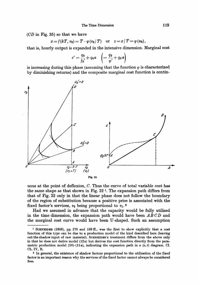
The Time Dimension 119
(CD in Fig. 35) so that we have
x=/(kT, vs)=T . q;(vs/T) or z=x/T=q;(ua),
that is, hourly output is expanded in the intensive dimension. Marginal cost
c' = ;:' +q4a (= :' + q4a)
is increasing during this phase (assuming that the function q; is characterized by diminishing returns) and the composite marginal cost function is contin-
Y,?-k'T ~ (v,-T) (Y,)
Jl'Ia;.36
uous at the point of deflexion, C. Thus the curve of total variable cost has the same shape as that shown in Fig. 321. The expansion path differs from that of Fig. 32 only in that the linear phase does not follow the boundary of the region of substitution because a positive price is associated with the fixed factor's services, V2 being proportional to Vl . 2
Had we assumed in advance that the capacity would be fully utilized in the time dimension, the expansion path would have been AB CD and the marginal cost curve would have been U-shaped. Such an assumption
1 SCHNEIDER (1958), pp. 170 and 189 ff., was the first to show explicitly that a cost function of this type can be due to a production model of the kind described here (leaving out the shadow input of raw material). SCHNEIDER'S treatment differs from the above only in that he does not derive model (12a) but derives the cost function directly from the parametric production model (10)-(11a), indicating the expansion path in a (z, t) diagram. Cf. Ch. IV, B.
2 In general, the existence of shadow factors proportional to the utilization of the fixed factor is an important reason why the services of the fixed factor cannot always be considered free.
120 Divisibility, Returns to Scale, and the Shape of the Cost Function
is unnecessarily restrictive in the case of continuous production with a fixed factor that is divisible in time, ignoring as it does an important aspect of substitution, and leads to a cost curve which cannot claim to represent minimum cost for any given level of output per period. Points on the line segment AB represent inefficient factor combinations (X2' < 0) and points on BO, though not technically inefficient, do not correspond to least-cost combinations for q2 > o.
(e) A formally similar model can be set up to represent the case where 'U2, the number of machine operators, is variable whereas the speed of the machine, and thus the energy or fuel input, is constant, output per hour of operation depending on the number of operators only. We then have
Z='I/'(U2)
Ua = K (constant) (11 b)
U4=a· z. These equations, together with (10), lead to a production function of the form
X =- . Va • 'I/' K·-1 (V2) K Va
1 Vl=-' Va
K (12b)
V4=a ·x. As in model (12a), labour and energy (or fuel) are substitutes; the interpretation, however, is quite different. Labour now represents the intensive dimension (number of workers simultaneously employed) whereas the rate of capacity utilization in time is changed by varying Vl along with Va, the amount of fuel or energy consumed being constant per hour of operation; output per hour can be increased by more labour-intensive operation, not by increasing the speed of the machine. The model is still homogeneous of degree one and the expansion path as well as the cost function will have the same general shape as in the previous example1.
(f) Still another variant is a model allowing for variable number of operators as well as for variable machine speed. This implies that 'U2 and Us are mutually substitutable factors in the production function for hourly output2, whereas the time dimension is now represented by Vl only. Combining the assumptions
Z =,u ('U2, Us) (110)
with (10) we have
1 Except that 'U2 assumes integral values only so that Vg = t . 'U~continuoUBly divisible in the time dimension for t < T-becomes a discrete variable for given t= T.
2 The interpretation is that output per hour depends on machine speed (in r.p.m.) and on the number of operators, machine speed in turn being a function of energy or fuel input per hour.
The Time Dimension 121
(12c)
V4=a· x,
a model similar to those above except that there are now three substitutable factors. The expansion path is a straight line in the three-dimensional factor space l up to the point t = VI = T, beyond which further expansion will be accompanied by changing factor proportions and, hence, by rising marginal cost up to the point of maximum capacity (where the partial derivatives of the function p are zero).
(g) The linear segment of the expansion path and the corresponding linear segment of the cost curve in the examples above are due to the assumed homogeneity of the production function, which in turn reflects the assumption that an hour's operation is a mere duplication of the preceding hour. This is implicit in the assumption that output per hour, Z = x / t, is independent of t. Suppose, however, that average output per hour depends not only on the factor combination employed but also on the length of the working day (labour productivity declines when the workers get tired, etc.). In model (11 a), for example, this would imply replacing the first equation by
Z=tp(U3, t},
t being here the number of hours of operation per day2 8. The first equation of (12a) would then have the form
X=V10tp(V3,Vl) or X=~'V2.tp(k.V3,~oV2) ~ k ~ k
which is not homogeneous of degree one (cf. (6». The expansion path for minimum cost will no longer be a straight line for t < T, nor will the corresponding segment of the cost curve be linear.
Another assumption implicit in the models above, and in the usual derivation of the cost function, is the constancy of factor prices, especially the wage rate. If the capacity limitation in the time dimension allows for overtime or multiple-shift operation, labour cost per man-hour will rise with t in a discontinuous manner and marginal cost will be constant only as long as t is kept within normal hours.
1 Since partial variation of V1 no longer affects cost-as it did above where Va or Vs was a shadow factor-the expansion path will be on the boundary of the region of substitution (X1'=O).
2 If the period considered had been a week, a month, etc. rather than a day, z would not be affected by all kinds of variation in t; for example, it would be possible within limits to vary the number of days of operation per month for constant number of hours worked per day.
s One interpretation of the equation is that, although working speed is constant for Us constant, being determined by the speed of the machine, the percentage of defective units of product is larger when the operators are tired. (It is also likely to increase with the speed of the machine, i. e., with Us for constant t, but this effect is implicit in the shape of the function f when z is interpreted as number of non-defective units made per hour.)
122 Divisibility, Returns to Scale, and the Shape of the Cost Function
3. Divisibility in Space and Time
In some cases the fixed factor is divisible in space as well as in time. By way of example, consider a continuous process which differs from that underlying model (12a) only in that the plant is composed of N identical machines some of which may not be used during the period considered. Let s denote output per machine per hour of effective operation, and let s be a function of fuel input per machine per hour, ys; each machine is worked by a fixed number of operators, Y2 = k. Then total output and total inputs per hour when n machines are operated (n <N) are
z=n· s=n· q;(ys)
UI=n
U2=n· k
Us=n· ya
U4=n·a·s=a·z.
(machine hours per hour = number of machines used)
(man-hours per hour = number of operators)
The parametric production model for total output and total inputs per period when the plant is operated t hours (t < T) becomes
x = t . z = t . n . s = t . n . q; (Ys)
VI = t . UI = t . n
V2=t'U2=t.n.k
Va=t·Us=t·n·ys
V4 = t . U4 = t . n . a . 8 = a . x
which reduces to the three-equation model
x = VI • q; (::) or alternatively x = ~ . V2 . q; (k . vs) k V2
v2=k,VI
V4=a· x.
(13)
This model is formally analogous to (12a); the only difference in interpretation is that the input of plant services (machine hours)-with its shadow, labour input-is variable in two extensive dimensions, VI being number of machines operated times number of operating hours per period. The variation is subject to the restrictions t < T, n <N, i.e., VI < T . N; within these limits it makes no difference to cost or profit whether output is expanded in the t or in the n direction-for example, whether all machines are operated half time or half of the machines are utilized all available hours-as was obvious from the outset since the parametric production model gives x and the v's as functions not of t and n separately but of their product t . n.1 The shape of the cost curve will be the same as above.
1 Still more generally, the time dimension may be split up into several components---for example, t = number of days per month times number of hours per day-with a similar effect.
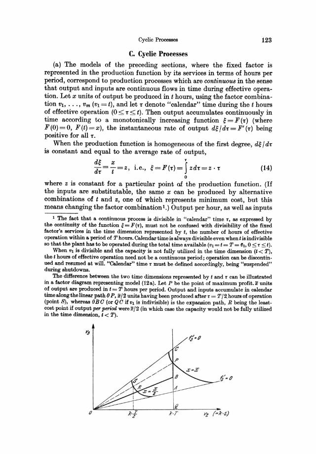
Cyclic Processes 123
C. Cyclic Processes
(a) The models of the preceding sections, where the fixed factor is represented in the production function by its services in terms of hours per period, correspond to production processes which are continuous in the sense that output and inputs are continuous flows in time during effective operation. Let x units of output be produced in t hours, using the factor combination VI, ••• , Vm (VI = t), and let -r denote "calendar" time during the t hours of effective operation (0 < -r < t). Then output accumulates continuously in time according to a monotonically increasing function ~ = F (-r) (where F (0) = 0, F (t) = x), the instantaneous rate of output d~ I d-r = F' (-r) being positive for all -r.
When the production function is homogeneous of the first degree, d~ I d-r is constant and equal to the average rate of output,
d~ X. T
d-r = T=z, l.e., ~=F(-r:)= J zd-r:=z· -r (14) o
where z is constant for a particular point of the production function. (If the inputs are substitutable, the same x can be produced by alternative combinations of t and z, one of which represents minimum cost, but this means changing the factor combination I.) Output per hour, as well as inputs
1 The fact that a continuous process is divisible in "calendar" time T, as expressed by the continuity of the function; = F (T), must not be confused with divisibility of the fixed factor's services in the time dimension represented by t, the number of hours of effective operation within a period of T hours. Calendar time is always divisible even when t is indivisible so that the plant has to be operated during the total time available (Vl = t = T = 1h, 0 ::; T ::; t).
When Vl is divisible and the capacity is not fully utilized in the time dimension (t < T), the t hours of effective operation need not be a continuous period; operation can be discontin· ued and resumed at will. "Calendar" time T must be defined accordingly, being "suspended" during shutdowns.
The difference between the two time dimensions represented by t and T can be illustrated in a factor diagram representing model (120.). Let P be the point of maximum profit. x units of output are produced in t = T hours per period. Output and inputs accumulate in calendar time along the linear path 0 P, x j 2 units having been produced aften = T / 2. hours of operation (point 8), whereas OBC (or QC ifvl is indivisible) is the expansion path, R being the least· cost point if output per period werexj2 (in which case the capacity would not be fully utilized in the time dimension, t < T).
fJ'· /J
Ye (-!r·t)
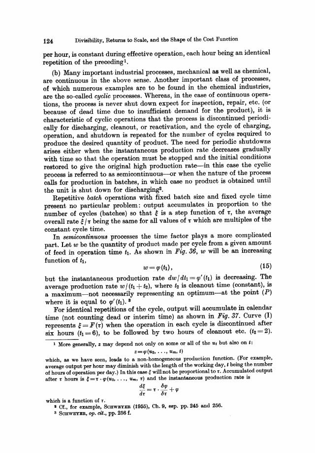
124 Divisibility, Returns to Scale, and the Shape of the Cost Function
per hour, is constant during effective operation, each hour being an identical repetition of the preceding l .
(b) Many important industrial processes, mechanical as well as chemical, are continuous in the above sense. Another important class of processes, of which numerous examples are to be found in the chemical industries, are the so-called cyclic processes. Whereas, in the case of continuous operations, the process is never shut down expect for inspection, repair, etc. (or because of dead time due to insufficient demand for the product), it is characteristic of cyclic operations that the process is discontinued periodically for discharging, cleanout, or reactivation, and the cycle of charging, operation, and shutdown is repeated for the number of cycles required to produce the desired quantity of product. The need for periodic shutdowns arises either when the instantaneous production rate decreases gradually with time so that the operation must be stopped and the initial conditions restored to give the original high production rate-in this case the cyclic process is referred to as semicontinuous-or when the nature of the process calls for production in batches, in which case no product is obtained until the unit is shut down for discharging2.
Repetitive batch operations with fixed batch size and fixed cycle time present no particular problem: output accumulates in proportion to the number of cycles (batches) so that ~ is a step function of T, the average overall rate ~ / T being the same for all values of T which are multiples of the constant cycle time.
In semicontinUOUB processes the time factor plays a more complicated part. Let w be the quantity of product made per cycle from a given amount of feed in operation time tl. As shown in Fig. 36, w will be an increasing function of tl,
(15)
but the instantaneous production rate dw / dtl = q/ (h) is decreasing. The average production rate wI (h + "t2), where t2 is cleanout time (constant), is a maximum-not necessarily representing an optimum-at the point (P) where it is equal to q/ (tl). 8
For identical repetitions of the cycle, output will accumulate in calendar time (not counting dead or interim time) as shown in Fig. 37. Curve (I) represents ~ = F (T) when the operation in each cycle is discontinued after six hours (tl = 6), to be followed by two hours of cleanout etc. ("t2 = 2).
1 More generally, z may depend not only on some or all of the 'UI but also on t: z=qJ('Ua, ••• , 'Um, t)
which, as we have seen, leads to a non-homogeneous production function. (For example, average output per hour may diminish with the length of the working day, t being the number of hours of operation per day.) In this case; will not be proportional to T. Accumulated output after T hours is ;=T . 11' ('U2' ••• , 'Um, T) and the instantaneous production rate is
dE = T • dqJ + 11' dT dT
which is a function of T.
• Cf., for example, SCHWEYEB (1955), Ch. 9, asp. pp. 245 and 256. 3 SCHWEYER, op. cit., pp. 256 f.
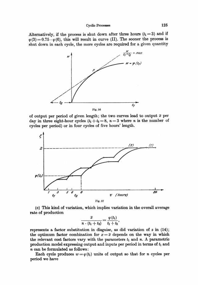
Cyolio Processes 125
Alternatively, if the process is shut down after three hours (h = 3) and if qJ(3) =0.75 'qJ(6), this will result in curve (II). The sooner the process is shut down in each cycle, the more cycles are required for a given quantity
w
w z;/~t2 - max
Fig. 36
of output per period of given length; the two curves lead to output x per day in three eight-hour cycles (h + i2 = 8, n = 3 where n is the number of cycles per period) or in four cycles of five hours' length.
(II) (IJ .z; ------------------------~-~----.,.-;.-
~ (nourSj
FIg. 37
(c) This kind of variation, which implies variation in the overall average rate of production
x _ qJ(h) n· (h + t2) - h + t2'
represents a factor substitution in disguise, as did variation of z in (14); the optimum factor combination for x = x depends on the way in which the relevant cost factors vary with the parameters hand n. A parametric production model expressing output and inputs per period in terms of hand n can be formulated as follows:
Each cycle produces w = qJ (tl) units of output so that for n cycles per period we have
126 Divisibility, Returns to Scale, and the Shape of the Cost Function
(16)
Let VI represent the complex of variable inputs (except raw material) involved in active operation, measured in hours per period. Then we have
VI =n • tl, (17)
whereas total cleanout work, measured in hours per period, will depend on the number of cycles only:
(18)
where t2 is constant. The services of the plant or fixed equipment, in terms of total hours of operation and cleanout per period of T hours, will be
Va=n· (t1+t2) «T). (19)
Finally, for a constant amount k of feed (raw material) required per cycle, total input of feed per period is
V4=n. k. I (20) Eliminating the parameters nand tl in order to translate (16)-(20) into
a model involving economic variables only, we are left with a production function in (v!, V2) and two "shadow functions" expressing Va and V4 in terms of VI and V2:
x = ~ . V2 • <p (t2 • VI) = t (VI, V2) t2 V2
Va = VI + V2 ( < T)
k V4= _. V2
t2
(21)
where k and t2 are given constants and the shape of the function cp (tl) = cp(t2VI/V2) is known from the theory of the particular process in question or from experimental data2•
Like the above models of continuous processes, (21) is homogeneous of degree one; this is due to the fact that the process is a continual repetitive operation, a repetition of identical cycles. V2, together with its shadow V4, is substitutable for VI; the two curves in Fig. 37 represent two specific factor combinations for the same amount of product, namely (I)
x = n . cp(tl) = 3 . cp(6); VI = n . tt = 3 ·6= 18; V2 = n • l2 = 3 ·2 = 6
and (II) x=4·cp(3); vl=4·3=12; v2=4.2=8.
It is true that n can assume integral values only, but the resulting discontinuities in the variables are of little consequence when a sufficiently long period (T hours) is considered. The cyclic nature of the process then becomes
1 Other inputs which are constant per cycle may be included in V4 (or in V2) which then becomes a complex factor.
2 The parametric model (16)-(20) corresponds to the engineering model given by SORWEYER, loco cit., who does not, however, derive the economic production function (21). SCHWEYER also ignores (20) and the cost of material (feed).
Cyclic Processes 127
a matter of secondary importance; VI and Va can be treated as continuously substitutable inputs and the curves ~ = F (.,;) of Fig. 37 approach the linear shape (14) which characterizes continuous processes with a homogeneous production function.
This is brought out clearly if the process, like a continuous one, is analysed not on the basis of the cycle but in terms of output and inputs per hour of effective operation (or, to reduce the discontinuities, per day) and number of hours (days) per period. The parametric model then becomes
x=t· z
Va = t . Us where
Vs=t·Us
Z= tp(h) tl +ta
tl Ul=--
tl+~
~ Us= tl+~
us=1
and where t = n(tl +~) < T.
(d) The least-cost factor combination for given x = if is determined by minimizing
C=QlVl+qaVa+Q,V,=qlVl+ (qa+ q,~)va subject to x = / (VI, Va), treating Va and v, as a composite factor measured in units of Va (i. e., on an hourly basis). Because of the homogeneity of the model, the relative factor combination is independent of if, the necessary condition for minimum cost being
(c'=) ql = qa+q,k/~ (22) h' la'
where h' =tp' and la' = (1/~) . tp- (VI/va) . q/ are functions of VI/va, cf. (21). Hence, as long as VI and Va are independent variables-i. e., within the capacity limit VI +va ~ T-the expansion path is a straight line, OA in Fig. 38, and marginal cost c' is constant!. Expansion along OA represents a variation of capacity utilization in the time dimension: tl = ~ . VI/va is constant and so are z and the u, so that output is expanded by varying the
1 SOHWlllYEB (1956), p. 259, defines optimum operation as minimum 'Unit cost, using It as independent variable to find the minimum of
e qlh+q2t2 :c II' (h)
(ignoring the cost of raw material). This is of course equivalent to minimizing total cost for given level of output, of. (22), when marginal cost is constant for any given value of h.
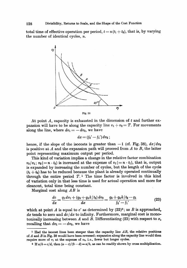
128 Divisibility, Returns to Scale, and the Shape of the Cost Function
total time of effective operation per period, t = n(tl + t2), that is, by varying the number of identical cycles, n.
Fig. 38
At point A, capacity is exhausted in the dimension of t and further expansion will have to be along the capacity line VI + V2 = T. For movements along the line, where dVI = - dV2, we have
dx = (/2' - /1') dV2 ;
hence, if the slope of the isocosts is greater than -1 (cf. Fig. 38), dxjdv2 is positive at A and the expansion path will proceed from A to B, the latter point representing maximum output per period.
This kind of variation implies a change in the relative factor combination V2 j VI; V2 (= n . ~) is increased at the expense of vI( = n • tl), that is, output is expanded by increasing the number of cycles, but the length of the cycle (tl +~) has to be reduced because the plant is already operated continually through the entire period T.l The time factor is involved in this kind of variation only in that less time is used for actual operation and more for cleanout, total time being constant.
Marginal cost along A B is
de qldvl+(q2+q4kjt2)dv2 q2+q4kjt2-ql dx = dx = /2' - /1' (23)
which at point A is equal to e' as determined by (22)2; as B is approached, dx tends to zero and de j dx to infinity. Furthermore, marginal cost is monotonically increasing between A and B. Differentiating (23) with respect to x, recalling that dVl = - dV2, we have
I Had the isocost lines been steeper than the capacity line AB, the relative positions of A and B in Fig. 38 would have been reversed: expansion along the capacity line would then require more of VI at the expense of V2, i.e., fewer but longer cycles.
2 H ajb =cjd, then (a - c)j(b - d) =ajb, as can be readily shown by cross multiplication.
where
i.e.,
The Relevance of the U-Shaped Marginal Cost Curve
I " "t2 I" ,,-t2Vl I" "t:! (Vl)2 11 =rp . -, 12 =rp • --, 22 =rp • --, V2 (V2)2 (V2)3
I " 21 "+1 "- " (t2 + 2t2Vl+t:!(Vl)2) <0 11 - 12 22 -rp • - -- --V2 (V2)2 (V2)3
129
so that d2c/dx2 >0. Hence-neglecting the discontinuities in the variables due to n being an integer-the cost curve as defined along OAB has the same shape as that belonging to a homogeneous model of continuous production with a fixed factor which is divisible in the time dimension 1.
D. The Relevance of the U.Shaped Marginal Cost Curve
(a) The first conclusion to be drawn from all these examples is that, in a wide variety of apparently typical cases of production processes, the kind of cost function known from neoclassical theory is inapplicable because it does not represent the locus of least-cost combinations even when the production function has the shape typically assumed by the traditional theory of production. Neoclassical analysis, when based on the assumption that the fixed factor is indivisible in time and space, leaves out the important part which the extensive dimensions of capacity utilization play in the substitution process by opening up the possibility of proportionate variation of all inputs. The neoclassical cost function with the U-shaped marginal cost curve is relevant only in the special case where the plant is indivisible in space and its services are also indivisible in the time dimension.
It has long been recognized that the rate of capacity utilization may have several dimensions, that in such cases the kind of variation considered must be specified in order for the cost function to be defined-this aspect is particularly important in the interpretation of empirical cost curves-and that the optimum path of expansion and the resulting cost function will involve variation in all dimensions2• None the less, the U-shaped marginal
1 Again, output and inputs accumulate in calendar time along the line 0 P in Fig. 38 where P represents the factor combination actuaJIy chosen (the point of maximum profit); of. above.
\! WINDING PlmBBSBN (1933), in an attempt to reconcile the neoclassical cost curve with the linear cost function assumed by the "engineering" school of thought (notably JANTZBN
(1924)), was apparently the first to draw attention to the significance of divisibility in the time dimension, interpreting the two types of cost functions as resulting from variations in the intensive and the time dimension of capacity utilization respectively. This idea. was further elaborated by SmnOID)]llB (1937, 1940), which led v. STAOKELBEBG (1941), esp. p. 36, to the conclusion that the cost curve, as defined by cost mjnjmj?Ation for parametric level of output, will have the general shape of Fig. 32 above. The same discovery was made independently by DUN (1941), pp. 5 H., who also pointed out that physical divisibility of the plant will have a sim.i1a.r eHect on the shape of the cost curve. (DUN (1951), p. 275, has suggested a third source of cost linearity, namely variability of machine speed; however, as model (10)-
DaDIIJ, Production lIodels II
130 Divisibility, Returns to Scale, and the Shape of the Cost Function
cost curve has shown great persistence in economic literature. Several explanations of this fact may be offered.
For one thing, neoclassical theory has been traditionally preoccupied with production processes which are not continuous in the above sense. In the absence of empirical material on industrial production processes, factor substitution has been illustrated largely by examples drawn from agriculture, the classic example being grain cultivation with land as the fixed factor. In processes of this type the product is obtained intermittently, the instantaneous rate of output being zero until the crop is ripe and ready to be harvested; the production period, therefore, is indivisible and the utilization of the fixed factor has a time dimension only in the trivial sense that the process is capable of repetition during the next period. (It is precisely for this reason that, in such cases, the dimension of output and inputs is often indicated in terms of absolute physical units, neglecting "per period.") During the production period the capacity of the "plant" is always fully utilized in the time dimension. If the spatial divisibility of the fixed factor is also disposed of by defining the production function as referring to a given plot of land all of which is in cultivation, the shape of the production function and that of the cost curve are likely to follow the law of variable proportions.
Secondly, it has not always been realized that, even when a factor of production is an indivisible unit, its services may be perfectly divisible. A machine as such is an indivisible fixed factor, but when the rate of capacity utilization can be varied in the time dimension, the relevant input in the production function is not the number of machines but their services in terms of number of machine hours used per period. The input of machine services is continuously variable up to capacity so that it is a scarce input rather than a fixed factor. The distinction between the factor and its services is less important when the use of the factor is indivisible in the time dimension; number of acres or acre services per year will do equally well. But in any case of divisibility-spatial or temporal, or both-the capacity restriction must have the form VI <iiI and the amount actually used, VI, must be specified in the production function.
One reason why this point has often been missed is, perhaps, that VI
usually does not appear in the cost function because no positive price is associated with this input. Another is that inequalities tend to be mathematically awkward in marginal analysis. It is true that the introduction of a single capacity restriction in inequality form-such as the capacity limit in model (12 a)-does not unduly complicate the argument, but the resulting
(110.) above shows, higher machine speed requires more energy or fuel per machine hour so that this is really a case of more intensive operation with changing factor proportions, cf. WINDING PEDERSEN (1949), p. 51.)
The optimal expansion path was indicated in a very general way by SCHNEIDER (1937) as the locus of tangency between "isocosts" and "isoquants" in a (z, t) diagram. The specific shape of the path-i.e., constant z up to the point where t= T-and the corresponding cost curve (Fig. 32) were subsequently developed by SCHNEIDER (1942), pp. 148 ff., and illustrated by an example-based on engineering data-of the type (10)-(11 a), cf. SCHNEIDER (1958), pp. 170 and 189 ff. (see Ch. VII, B above).
The Relevance of the U-Shaped Marginal Cost Curve 131
cost function (Fig. 32) is not an analytic function; it is pieced together from two such functions, in contrast to the cost function derived from the law of variable proportions. It was only the discovery of the linear models of production which paved the way for inequality constraints in the theory of production: in order to get meaningful solutions to linear optimization problems, methods had to be devised for maximization of linear functions subject to linear inequalities l •
(b) Needless to say, the question of the practical relevance of the Ushaped marginal cost curve cannot be settled by theoretical argument alone: it is ultimately a matter of empirical research. It must be emphasized, however, that the underlying question of factor divisibility is not a purely technological one. While some cases of indivisibility in the time dimension are due to technical necessity (processes which cannot be discontinued during the period), there are other cases where shutdowns are technically possible but undesirable for different reasons, for example, as a matter of policy2. As regards spatial divisibility, agricultural cost functions will have a linear segment if the acreage in cultivation is adjusted optimally to the level of output, but the marginal cost curve is likely to be U-shaped, despite the physical divisibility of the factor "land," if it refers to a given plot in cultivation3• In short, the result will depend on the underlying assumptions with respect to the fixed factor, and the same technology may lead to either type of cost function.
1 Cf. Appendix 1. 2 Of. Ooat Behavior and Price Policy (1943), p. 111 n. 3 This is the situation that underlies empirical production and cost functions derived from
experiments in agriculture.
Chapter VIII
Product Quality and the Production Function
A. Product Quality in the Theory of Production
We have so far disregarded the complications that my arise if variations in product quality are taken into consideration.
The concept of a production function has operational meaning only with referenoe to a particular product or class of products; in order for the model to be defined at all the produot must be specified in terms of its relevant properties. When nothing explicit is said about product quality and the quantity produced is considered the sole dimension of the product, the speoification must be understood to be implicit in the model, it being tacitly assumed that the general nature of the product as well as its specific quality is given by the selection of inputs and the shape of the production function. To the extent that the qualitative properties of the product reflect the properties of the inputs, a sufficiently uniform product quality oan be ensured by exclu~g suoh inputs from consideration as would lead to an unacceptable product (e.g. inferior raw materials)l; and the production function may be defined as the set of points which represent a satisfactory quality as specified by the producer. Different grades of the "same" product may of course exist but are treated as so many distinct products, each of which has a separate produotion and cost function (unless they are produoed jointly, a case to be desoribed in terms of a multi-product model).
The development of the theory of the firm that took place in the thirties led to the recognition that product quality-as well as selling effort-is an important parameter of action to the firm along with price (or quantity produced)!!. The emphasis, however, was on the demand side: it was of oourse realized that differences in product quality are reflected in the costs of production, but little attention was paid to the underlying production function and to the way in which the cost function is derived from it when
1 It will be reca.lled that our definition of the production function (Ch. II) requires each particular input to be qualitatively well-defined; qualitative change in one or more of the specified factors represents technological change, i.e., a diHerent production function. This does not rule out the poBSibility of two or more inputs in the production model representing diHerent grades of the "same" input (e.g. high-quality and low-quality materials which may be substituted for one another without seriously affecting product quality), only each of them must be represented by a separate variable til.
a The pioneer work was CluMBERLIN (1933).
Produot Quality in the Theory of Produotion 133
product quality occurs as a parameter. This was natural enough as long as product quality was regarded as non-quantitative1 : in that case the proper way of introducing the quality aspect is to consider a multitude of different production and cost functions, each of which corresponds to a particular product quality-in effect, to a different product.
The subsequent recognition that product quality is a multi-dimensional concept defined by a number-possibly a large number-of quality criteria, some of which can and should be regarded as quantitative, measurable magnitudes2, made no appreciable change in the picture so far as nonquantitative criteria were concerned: each particular combination of such criteria should obviously be considered as a separate product with a production and cost function (as well as a demand function) of its owns. It is only when the product cannot be exhaustively described in terms of these criteria that a problem arises. Clearly the quantitative criteria must somehow appear as parameters in the cost function-higher quality is likely to be associated with higher cost-but the relationship of the quality parameters to the underlying production function is by no means unambiguous.
We shall now subject the quality problem to a more rigorous treatment, in order to examine the various ways in which quality parameters may come into the production model and the effects of quality specifications on the problem of input substitution and cost minimization. Since the analysis is largely concentrated on the production and cost relationships, no attempt will be made to explain how the optimum level of product quality is actually determined; this is a problem to be solved within a wider frame of reference, that of the theory of the firm in its most general sense, which provides a model for the simultaneous determination of output, price, product quality, selling effort, and inputs'. In the present context, product quality will be treated as a parameter, or a set of parameters, to be specified somehow by the firm.
By product quality, then, we will understand the total of such physical and other characteristics of the product as affect the cost of producing it; in other words, quality is the set of properties needed for a complete specification of the product and for the cost function to be determined6• Only quantitative, measurable quality criteria will be considered; properties which are non-quantitative in the sense that they cannot be represented by a continuously variable parameter will be disregarded (i.e., assumed to be
1 CJLumEB.LIN, op. cit., pp. 78 f., then held the view that "'product' variations are in their essence qualitative rather than quantitative" and therefore non-measurable.
2 BBmlS (1951) is the chief exponent of this school of thought. 3 Of. BBlIlM:S, op. cit., p. 57. 4 The reader is referred to the special literature, in partioular to BREMS (1951). Some useful
references are given in BREMS (1957), p. 105. & From the point of view of demand, on the other hand, the product and its qualities are
defined by speoHying the properties whioh are represented by parameters in the demand funotion. The two sets of quality parameters do not neoessarily coincide and a complete model of the firm should take all quality dimensions into acoount, whether they appear in the demand or cost function or in both.
134 Product Quality and the Production Function
implicit in the shape of the production function) since, as we have seen, products which differ in respect to such qualities may in the present context be treated as distinct commodities.
B. Quality Parameters in the Production Function
(a) In order for the input-output relationships to be fully specified, the product must be completely defined in terms of quality: all relevant quality dimensions must be specified, whether they are measurable or not.
Some kinds of quality change-particularly those concerning non-quantitative quality criteria-can be effected only by discontinuous change in the technology, that is, by switching to a different production function. On the other hand, as to such dimensions as are quantifiable, it seems plausible to assume that a continuous range of quality levels-as represented by the values of the continuous quality parameters-can be produced within the same basic technologyl; the same inputs are used but higher product quality, like a higher rate of output, requires more of some or all inputs.
This means that the quality parameters appear as parameters in the production model; or, to put if differently, the technology of the process can be described by a family of production functions. In practical terms, the interpretation is that the shape of the production function represents an incomplete description of the technical procedure by which a given selection of well-defined inputs are transformed into the product; the "details" of the technology are assumed to depend uniquely on the particular product quality desired. Once the values of the quality parameters have been fixed by the firm, the production relationships are fully specified; conversely, product quality is continuously manageable-at least within limits-through modifications in the technical procedure adopted by the firm.
By way of illustration, let output x depend on a single input v and a quality parameter y, assumed to be continuously variable:
x=x(v, y).
The amount of input required depends not only on the quantity to be produced but also on the quality dimension of the product as represented by y. Within the relevant region, x is an increasing function of v, i.e.,
f5x>O (y constant), ~v
and so is y,
(x constant),
assuming that it takes more of the input to produce a better quality (as represented by a higher value of y)2. For given v, output can be increased
1 ZEUTHEN (1928), p. 30. S ZEUTHEN, loco cit., used the term "marginal quality improvement" for dllldv, though
he had. & somewhat different production model in mind (of. below).
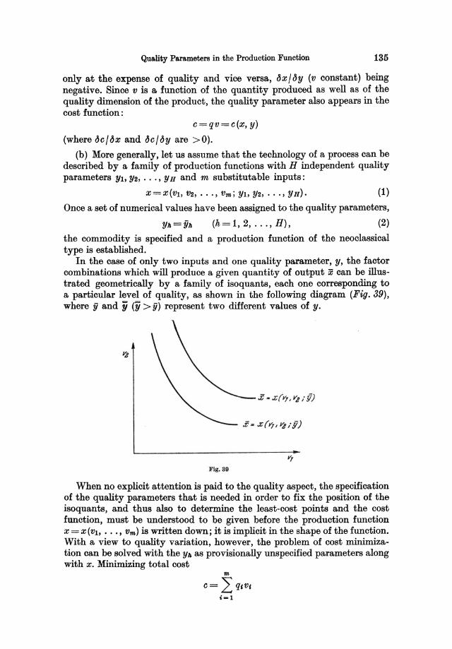
Quality Parameters in the Production Function 135
only at the expense of quality and vice versa, lJx/by (v constant) being negative. Since v is a function of the quantity produced as well as of the quality dimension of the product, the quality parameter also appears in the cost function:
c=qv=c(x, y)
(where bc/bx and bc/lJy are >0).
(b) More generally, let us assume that the technology of a process can be described by a family of production functions with H independent quality parameters YI, Yz, . .. , Y Hand m substitutable inputs:
X=X(VI, Vz, ••• , Vm; YI, Yz, ... , YH). (1)
Once a set of numerical values have been assigned to the quality parameters,
(h= 1,2, ... , H), (2)
the commodity is specified and a production function of the neoclassical type is established.
In the case of only two inputs and one quality parameter, y, the factor combinations which will produce a given quantity of output x can be illustrated geometrically by a family of isoquants, each one corresponding to a particular level of quality, as shown in the following diagram (Fig. 39), where fi and y (y > fi) represent two different values of y.
Fig. SO
When no explicit attention is paid to the quality aspect, the specification of the quality parameters that is needed in order to fix the position of the isoquants, and thus also to determine the least-cost points and the cost function, must be understood to be given before the production function X= X (VI, ••• , Vm ) is written down; it is implicit in the shape of the function. With a view to quality variation, however, the problem of cost minimization can be solved with the Yh as provisionally unspecified parameters along with x. Minimizing total cost
136 Product Quality and the Production Function
subject to (1) for given x and given Yh (and for given factor prices), the necessary conditions are
(u=)~= •.. = qm, Xl' xm'
which together with (1) determine the Vi in terms of the given X and Yh, that is, for all conceivable values of X and the Yh. Substituting the solution to this parametric minimization problem in the cost expression we have
m
c= L q(v,=c(x; YI, Yz, ••. , YH). (3) i=l
This is the parametric cost function-or family of cost functions-usually considered in price-quality equilibrium models of the firml. For fixed values of the Yh, (3) becomes a cost func.tion of the familiar type.
(c) Quality criteria may of course appear as parameters in other types of production models, for example, in a model characterized by fixed coefficients of production z :
(i= 1,2, ... , m).
For given product quality the coefficients a, are constants, but different quality specifications will correspond to different values of the at, which are therefore functions of the Yh 3 :
a,=a'(YI, Yz, .•. , YH);
hence the production model can be written as
(i=1,2, ... ,m),
and the corresponding cost function becomes
(4)
I BREMS (1951), p.56, explains the occurrence of quality (and selling-effort) parameters in the cost function in this manner, and proceeds to show (pp. 62 ff.) how the optimal values of x, the YII, and p are determined by maximizing profit
z=px-c(x; Yl, ..• , YH) subject to the demand function
x=/(p; Yl, ••. , YH) (where the product price p is a parameter of action along with the Yh).
2 This has been suggested by BREMS (1957). Ch. 17 of BREMS (1959) contains a revised version of this article.
ZEUTHEN (1928), p. 30, pointed out that, in some cases of fixed coefficients of production, partial variation in one input may affect product quality though the level of output remains the same. This will be so in a model of the type
vl=al(Y)'x, V2=a2'X where, for V2 and thus also x constant, changes in VI will affect y. (Had both coefficients of production been functions of y, as in model (4) below, V2 and x could not both have been constant for variations in VI.)
3 For example, the amount of labour required per unit of product may depend on the desired degree of workmanship, cf. BREMS (1957), p. 106. This quality criterion may of course also appear in production functions of the type (1), where labour is substitutable for other inputs.
Quality Functions and the Production Function 137
m
c= L q,a,X=C(YI, YZ, ... , YH)' X.l (5) i=1
Since the a, are uniquely determined when product quality has been specified by assigning a set of particular values to the Ylh the coefficients of production may themselves be taken as representing product quality, at least in the sense that a change in a, reflects a change in the quality of the product; quality is then defined as the complete specification of the production processz. This approach has the advantage of evading the somewhat tricky problem of quality measurability in a simple and elegant manner; the a, are always measurable.
(d) In deriving the cost functions (3) and (5) we have treated the quality dimensions Yh as provisionally unspecified parameters, to be determined in a comprehensive model (not dealt with here) which takes into account the effect of quality variation on the demand for the product3• If the firm considers this effect to be negligible-this may be the case if demand is largely dependent on the non-quantitative quality criteria which are implicitly specified in the shape of the production function-the firm will profit by fixing the Yh at their lowest possible values'. Or the market may be such that the product is judged to be acceptable only if its quality is kept within certain limits,
~<~<~~ ~ in which case the cost of production is at a minimum for any given x if each of the quality parameters is fixed at its lowest permissible limit, fih.
C. QuaHty Constraints
1. Quality Functious and the Production Function
(a) The purpose of the models above has been to show that the appearance of quality parameters in the production function may be due to a technology with "built-in" possibilities of quality variation. The quality dimensions of
1 It might be argued that (4) is not a case of fixed coefficients (limitational inputs) since the at can in fact be varied. The point is, however, that such variations cannot be interpreted as input substitution (accompanied by quality change) since they are brought about not by a change in factor prices but by variations in product quality.
a Of. BBEMS (1957), p. 106; this observation is the main point in the article.-Strictly speaking, it will have to be assumed that each at depends on one quality parameter only, since otherwise there may be diHerent combinations of the 11" which correspond to the same value of a, (i.e., the quality parameters may be "substitutes" with respect to the coefficient of production) 80 that product quality may change without a, being affected. However, it is scarcely to be expected that such a change in the 11" will leave aU of the a, unaffected.
8 Of. above . .. Assuming that the V, for given z.--as given by the technology or determined by cost
minimization-and thus also the cost function are monotonically increasing (or at least nondecreasing) functions of the 11'"
II This way of taking the demand function into account amounts to assuming that demand will respond in a discontinuous manner to quality changes that go beyond certain limits.Alternatively, (6) may have a purely technical interpretation: the same basic process permits of quality variation only within limits.
138 Product Quality and the Production Function
the product enter as parameters in the production function (more generally: in each of the relations that constitute the production model) so that the product has to be completely specified before the technological model can be established.
However, this is not the only possible explanation of a cost function depending on quality dimensions as well as on output. It is conceivable that, for a continuous range of product variants, the production function as such is independent of the quality dimensions-in order to specify the technology it is sufficient to indicate roughly the general nature of the product-but that the quality of the product varies with the factor combination 1.
In other words, in addition to the production function proper, e.g.
(7)
the complete production model includes a number of additional equations expressing the quality dimensions in terms of the inputs:
Yh=Yh('1h, V2, ••• , vm)
for given specification of the product,
(h= 1,2, ., ., H);2 (8)
Yh=Yh, (9)
equations (8) impose constraints on the variations of the v,. 3 From a formal point of view (7)-(8) may be regarded along with the previous models as a multi-equation production model containing quality parameters. It is a special case, however, in that the technology of the process, as represented by (7), is separated from the quality aspect; product quality is controlled only through the choice of factor combination.
Two particular cases of this model can be distinguished according as to whether or not (8) contain inputs which do not occur in (7)'.
(b) Let us first assume that there are no other variables (inputs) in (8) than those already present in (7)5. In that case (8) can be described as pure quality constraints: for specified values of the Yh they are side relations which rule out certain areas of the production functionS (7). For a sufficiently
1 Cf. BARBOD (1936). This important article, which was the first serious attempt to treat the problem of quality variation within the context of the theory of production, appears to have-passed almost unnoticed.
The same general idea has later been suggested by ClmNERY (1953), p. 310, possibly inspired by linear-programming models of industrial blending processes where quality specifications lead to side conditions on the inputs (cf. below).
B There is no need to include x among the variables of (8) since it can always be eliminated, using (7).
3 In BARBOD'S terminology, (7) is called "the quantity function" and (8) "the technical quality function", op. cit., pp. 27-29.
, These cases-dealt with under (b) and (c) below-correspond to BARBOD'S cases I and III, of. op. cit., p.42. BARFOD'S model II is a special case of III, cf. below.
5 This assumption does not imply that all of the v, in (7) also occur in (8). It is perfectly possible for product quality to depend on some of the inputs only (e.g. those representing materials).
8 ClmNERY, loco cit.
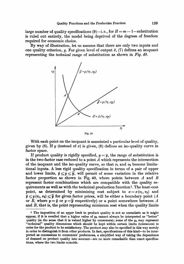
Quality Functions and the Production Function 139
large number of quality specifications (9)-Le., for H =m-l-substitution is ruled out entirely, the model being deprived of the degrees of freedom required for economic choice.
By way of illustration, let us assume that there are only two inputs and one quality criterion, y. For given level of output x, (7) defines an isoquant representing the technical range of substitution as shown in Fig. 40.
Fig. 40
With each point on the isoquant is associated a particular level of quality, given by (8). If y (instead of x) is given, (8) defines an iso-quality curve in factor space.
If product quality is rigidly specified, y = ii, the range of substitution is in the two-factor case reduced to a point A ' which represents the intersection of the isoquant and the iso-quality curve, so that VI and V2 become limitational inputs. A less rigid quality specification in terms of a pair of upper and lower limits, ii s,y s, '0, will permit of some variation in the relative factor proportion as shown in Fig. 40, where points between A and B represent factor combinations which are compatible with the quality requirements as well as with the technical production function I. The least-cost point, as determined by minimizing cost subject to X=X(VI, V2) and ii < y (VI, V2) s, Y for given factor prices, will be either a boundary point (A or B, where y = ii or y = y respectively) or a point somewhere between A and B, that is, the point representing minimum cost when the quality limits
1 The imposition of an upper limit to product quality is not as unrealistic as it might appear, if it is recalled that a higher value of y" cannot always be interpreted as "better" quality (in the sense that it is valued higher by consumers); some of the y" may represent "technical" quality dimensions which should be kept within certain limits (tolerances) in order for the product to be satisfactory. The product may also be specified in this way merely in order to distinguish it from other products. In fact, specifications of this kind-to be interpreted as concessions to consumers' preferences, a simplified way of taking the dependence of demand on product quality into account-are no more remarkable than exact specifications, where the two limits coincide.
140 Product Quality and the Production Function
are disregarded. Such a tangency minimum is the more likely, the wider the quality tolerance is and the less product quality depends on the relative factor combination.
In the general m-factor case, the introduction of H quality specifications will reduce the number of independent input variables from m to m - H and the complete production model (7)-(9) can be described as a case of constrained substitution 1. For given x the range of substitution in m-dimensional factor space is reduced to the configuration of points which represents the intersection of the isoquant-as defined by (7) for x = x-and the isoquality surfaces (8)-(9) 2. If product quality is specified only in terms of pairs of inequalities, the permissible region of substitution is represented by a bounded area on the isoquant surface.
If the quality dimensions are not specified beforehand but are regarded as unknown parameters of action whose optimal values are to be determined in a wider model which takes the demand function into account, the leastcost point for given x and the cost function can be determined with the Yh as parameters. Minimizing total cost subject to (7)-(8) for given x = x and Yh = Yh, differentiation of the Lagrangian expression
m H
L= 2: qtV,+u. (x-x)+ 2: Uh' (Yh-Yh) 1=1 11.=1
with respect to the v, leads to m necessary conditions which with (7) and (8) determine the v, (and the Lagrangian multipliers U and Uk) in terms of x and ii, ... , ii H. Substituting in c = };q,Vt we get a parametric cost function
(to)
I Of. Ch. V. B. 2 BARFOD. op. cit., pp. 49-51, cites an empirical example from the technical literature
(of. FOG (1934), pp. 33 ff.). The process in question is the decolorization of vegetable oils by means of bleaching coal or bleaching earth. or by a mixture of both. These bleaching agents remove the colour constituents from the oil by adsorption. Let VI and VI denote the quanties (in kg.) of the two bleaching agents applied to Va kg. of unbleached oil. and let x be the output (in kg.) of bleached oil. The production function for the bleaching process consists of two equations. The first is a material balance
X=Va - TIVI- TSV2
where TI and Ts are constants-determined by experiment----expressing the amounts of raw material (unbleached oil) lost in the adsorption process per kg. of bleaching agent applied. (BA.RFOD erroneously writes the material balance as x = Va. but does take the losses into account when solving the optimization problem.) Second. the degree of bleaching obtainedas expressed by the extinction coefficient, 1/. which can be measured by means of a photometer-is a function of the three inputs,
1/ = 1/(VI, Vs. va),
which puts an additional constraint on the variables when the quality of the product-the desired degree of bleaching-is specified, 1/ = y. For a given amount of Va to be bleached. a given value of 1/ can be obtained by alternative combinations of VI and VI. which are therefore substitutes in producing this quality effect. The shape of the function 1/ for given Va under given process conditions has been determined experimentally for cocoanut oil and soybean oil respectively and illustrated by "isocolors". which permit the graphical detemrlnation of the optimal combination of the bleaching agents for given prices.
Quality Functions and the Production Function 141
just as we did in the case of production functions with "built-in" quality parameters (cf. (3) above).
On the other hand, the firm may choose to disregard the effect of quality variations on the demand for the product and allow quality to be determined solely by cost considerations. In that case the production model consists of (7) only and the cost function is determined by minimizing cost subject to (7) for given parametric x, taking full advantage of the unconstrained range of substitution along the isoquants. The values of the Yk, as determined by inserting the least-cost factor combinations in (8), represent the cheapest quality level for given x.
A similar procedure may be resorted to if demand conditions are taken into account only by specifying a set of upper and lower limits to product quality, cf. (6) above. If the values of the Yk determined by minimizing cost for given x (or, more generally, by maximizing profit) subject to (7) turn out to respect inequalities (6), there is nothing to add; on the other hand, if one or more of the inequalities is violated, the problem has to be reformulated as a case of constrained maximization with (6) and (8) as boundary conditions and the optimal solution will be a point on the boundary of the permissible region.
Quality constraints of the type (8) may be combined with other types of technological models than (7), in which all inputs were assumed to be continuously substitutable. Substitution may be discontinuous, or some of the inputs may be limitational. However, some degree of substitution must be present in the purely technical production relations if quality variation is to be possible 1.
(c) The second class of cases is characterized by quality functions (8) containing inputs which do not appear in the production function (7) or, more generally, in the technological relations which constitute the production model proper. In cases of this type equations (8)-(9) can no longer be described as pure quality constraints; they also serve to introduce additional inputs2 and to link them up with those of (7), i.e., they contain technical information and in this sense are part of the technological production model. Thus a complete separation of technology and quality considerations is no longer possible as it was in the previous class of models; in fact, (7)-(8) may be thought of as a multi-equation production model with built-in quality parameters similar to the cases dealt with above. The model represents a special case only in that quality parameters do not occur in all the relations of the model.
By way of example, consider the model
X=X(Vl, V2, V3)
Y = Y (VI, V2, V3, V4, VI;).
(11)
(12)
1 In a model where all inputs are limitational, quality variation is possible only if the coefficients depend on quality parameters, but this means that we have a model where the Yh are built into the production relationships, cf. (4) above.
2 In BARl!'on's terminology such inputs are called "technical quality factors"; cf. BARFOD, 0]1. cit., p. 42.
142 Product Quality and the Produotion Funotion
Since the production function (11) does not contain the quality parameter y, it is possible to produce the commodity using only VI, '112, and Va if product quality is disregarded; the cost function is then determined by minimizing total cost of the three inputs subject to (11) for parametric x=x, and the quality level of the resulting crude product is given by (12) for '114 = '115 = o. If a better product is desired, quality can be improved by use of '114 and '115
(assuming Y4' and Y5' >0); for given specified y = y, equation (12) becomes part of the production model, a kind of generalized "shadow function" with '114 and '115 as factor shadows 1. Unlike the quality constraints dealt with above, (12) does not reduce the range of substitution defined by (11) for given x, but the position of the least-cost point will depend on the specified value of y. Minimizing the cost of all five inputs subject to (11)-(12) for parametric x and y we get the necessary conditions
q,-Ul'X/-U2'Yc'=0 (i=1,2,3)
q, -U2'Yc'=0 (i=4,5) . (Ul and U!! being Lagrange multipliers) which with (11)-(12) determine each of the V" and thus also cost, as functions of x and y.
Had product quality been a function of '114 and '115 only,
(12a)
the optimal combination of VI, '112, and 'Va would have been independent of y, their values being determined by (11) for given X=X and the conditions
q,-Ul'Xc'=O (i=1,2,3),
whereas '114 and '115 would depend solely on the specified quality level, being determined by
qc-U!!' y{=O (i=4,5)
together with (12a) for y=y. This special case, however, is not likely to occur since, if the quality
constraints have no variables in common with the technological production function, there is no connexion in the model between the quality factors and the quantity of output produced. In general, a higher level of output must be expected to require greater amounts of these inputs2. In model (11)-(12) this link is provided by the occurrence of '111, '112, and 'Va in both functions. A more direct connexion is established if output x takes their place in the quality function,
y=y(x, '114, '115) (12b)
(which can be written in the form (12), substituting (11) for X)8. In cases of this type, like (12a), the optimal combination of '111, '112, and 'Va for given x is independent of the specified value of y, but the optimal values of the quality factors are functions of x as well as of y.
1 Of. Ch. V, A. I BABlI'OD, op. cit., who treats models of this type as a separate case (II). appears to have
overlooked this point. S For given y, model (U)-(12b) becomes an example of what FmSCH has oalled "dis·
oonneoted factor rings," of. Ch. V, C above.
Quality Constraints in Blending Processes 143
Quality constraints of the type (12), with the special cases (12a) and (12 b), are characterized by containing several quality factors-in the present models, V4 and v5-which are substitutable for each other with respect to product quality. There may well be cases, however, in which each particular property of the product is provided by one particular quality factor only so that in addition to (11) we have quality constraints of the form
Yl = Yl (x, V4)
Y2 = Y2 (x, V5)
(12c)
where V4 and V5 become limitational shadow factors (product shadows)! when the quality of the product has been specified23• In cases of this type the position of the least-cost point is independent of the quality specifications, depending solely on the prices of the inputs in (11).
2. Quality Constraints in Blending Processes
(a) Quality functions of the type (8) are of particular importance in blending processes, where the product is made by mixing a number of materials4• The general nature of the product is determined by the choice of materials, but the particular quality of the blend will usually vary in a continuous manner with its composition; indeed, the very purpose of blending ingredients is to get a product which in a sense represents a combination of their respective properties.
The basic relation of a production model representing a physical blending process is a simple material balance,
m
X= LV" i=l
(13)
where the v, are the quantities of the respective ingredients (materials)5. This equation, which is a special form of the production function (7), hardly conveys any technical information except the trivial fact that the materials are equivalent (perfect substitutes) as far as the quantity of output is con-
1 Cf. Ch. V, A above. 2 One interpretation of (11)-(12c) is that (11) represents a preliminary operation producing
a crude product which subsequently undergoes further treatment (finishing operations) requiring specific inputs to provide the qualities desired in the finished product.
3 In the case of fixed coefficients of production, (12c) can be written in the form
v4=a4(Y1)' x, v5=a5(Y2)' x. The coefficients a4 and aG, which are uniquely determined by the quality parameters, may take the place of Y1 and Y2 as representing product quality, cf. above.
4 The mixing of ingredients with the purpose of bringing about a chemical reaction is not treated here; we are concerned only with physical blending operations where the compo· nents preserve their chemical identity.
6 (13) always holds if x and the v, are measured in units of weight, whereas volumes are not necessarily additive; for example, a change of volume occurs if water is mixed with alcohol.
144 Product Quality and the Production Function
cerned. Clearly this is not a very interesting case-the least-cost factor combination consists in using the cheapest ingredient only-unless further restrictions are imposed by quality specifications.
Let Yl, Y2, ... , Y H denote measurable quality criteria, and assume that each quality dimension of the product depends on the blending proportions, i.e., on the Vi/X:
(VI V2 vm) YII =YII -, -, ... ,-X X X
(h= 1,2, ... , H), (14)
which may be written in the form (8) if the material balance (13) is substituted for x. When the desired quality of the product is specified either by assigning particular values to the functions or by specifying upper and lower limits to the YII, (14) impose constraints-equations or inequalitieson the choice of factor combination.
The most restricted case is that of H = m - 1 quality specifications in equality form, where the Vi are uniquely determined by (13)-(14) for given x. This may happen, for example, if each ingredient is the sole provider of a particular quality dimension so that the constraints have the form
Yh=Yh(:II) (h=1,2, ... ,H) (14a)
which for YII = fill (h = 1, 2, ... , m - 1) determine the blending proportions I so that the production function can be written
where
and, by (13),
(h=1, 2, ... , m)
m-l
am=1- 2: all· 11=1
(h=1, 2, ... , m-1)
In all other cases-for fewer than m - 1 exact quality specifications or for any number of quality requirements in inequality form-a range of substitution exists and the optimal composition of the blend is determined by minimizing cost subject to (13) for given output and to (14) for specified values or permissible intervals of the YII.
The quality functions will frequently be of linear form, m
"" Vi YII= L YM' X (14b) i=l
where the YM are constants2 to be interpreted as quality indicators for the respective inputs8 so that, for each of the specified quality dimensions,
1 Had all m quality dimensions been specified, the model would have been overdetermined, cf. (13).
2 Sometimes called "blending numbers," of. SYMONDS (1955), p.4. 8 For example, if the product is made of the first material only so that Vl=X, (14b)
identifies Yhl with y,..
Quality Constraints in Blending Processes 145
product quality Yl& is a weighted average of the qualities of the ingredients with the blending proportions as weights1. This will always be so when Y'" represents the content of some constituent in a unit of v,: the total content of the constituent per unit of x, i. e., in a unit of the blended product, is indicated by the right-hand side of (14 b)2 8.
When the quality functions are all linear , the optimal mix is determined by linear programming methods: the total cost of materials c=~q,v, is to be roiniroized subject to the linear equation (13) for X= x and to (14b), which are linear equations in the v, for Yl& = Yl& or linear inequalities if upper and lower limits, or both, are specified for the Yl&.4 A model of this kind has a certain resemblance to discontinuous substitution with a finite number of linear activities if (13) is written in the form
( 1fori=k where au;= 0 f . k or ~ =1= ,
but it is trivial in that the activities are defined by the inputs, the v, being activity levels, and differs from other linear production models also in that factor substitution is constrained by linear quality requirements.
When some of the quality dimensions which define the quality of the blend depend on its composition but are incapable of objective measurement, such as taste, it is not possible to formulate the corresponding quality requirements in mathematical terms; all we know is that the range of substitution as defined by (13) and by those quality specifications which can be expressed explicitly may not be acceptable in its entirety. However, it is sometimes possible to demarcate the region of acceptable factor combinations by applying some objective criterion which is more or less vaguely correlated with the quality in question (e.g. the contents of certain ingredients as representing taste), or to use a numerical grading scale as an indicator of quality. 1£ these roads are barred, some sort of trial-and-error procedure must be resorted to.
1 This is known in ohemical technology as the so-called "Mixture Law" when applicable to physical properties of liquid and solid solutions; cf. PERRY (1941), p.616.
2 At least when z and the v, are measured in units of weight, cf. above. 8 The ingredients may be thought of as given blends of wholly or partly the same con
stituents, and the product as a blend of blends whose composition in terms of constituents is a weighted average of the compositions of the respective ingredients. The optimization problem becomes trivial when constituents are themselves used as ingredients (e. g. the manufacturing of vitamin pills from synthetic vitamin preparations rather than from natural foods each containing more than one vitamin).
, One of the classio problems of linear programming is the so-called "diet problem," where a given selection of foods is "mixed" such as to make a "diet" which satisfies given nutritional requirements at minimum cost, the '!III' and '!III being the contents of nutrients (vitamins, calories) per unit of ingredient (food no. i) and per unit of blend (diet) respectively. (Eq. (13) may be disregarded if the total quantity of food per day is not specified.)
Linear blending problems of this kind appear to be of considerable practical importance, especially in the food industry. Some of the first successful practical applications of linear programming were problems of optimal blending with specifications of contents or other qualities which "blend linearly" at least approximately. Examples and references are given in DAN'" (1960), Cha. m and V.
D&WII. ProductJonKodela 10
146 Product Quality and the Production Function
(b) In the blending problems above, all other inputs than materials-such as labour and energy required for the mechanical mixing of the ingredientshave been disregarded.
This is permissible when the other inputs do not appear in the quality functions (14) any more than in the material balance (13). For example, they may be uniquely determined by output regardless of product qualityi.e., they are limitational shadow factors which are constant for given xor they may form a separate group of mutually substitutable inputs which is complementary to the group of substitutable material inputs in (13). As an example of the latter case, let Vb V2, and Va be materials whose relative proportions determine product quality, y, and let V4 and Vs denote two other inputs which can be substituted for each other. Then the model is
X=VI+V2+ Va=g(V4, vs)
(VI V2 va) y=y -, -,-x x x
(15)
and the least-cost factor combination for given x and specified y can be determined for each factor group separately I ; the optimal blending proportions are the same regardless of the combination of V4 and Vs that is applied. (Had V4 and Vs been limitational inputs, the equation X=g(V4, vs)
would have been replaced by V4 = a4X, Vs = asx but the conclusion would be the same.)
However, the assumption that product quality depends on the blending proportions only is not always justified. There are cases where the effect of a change in the blending proportions on product quality can be offset by appropriate adjustments of labour and other factors. Instead of (15), for example, the model may be of the form
(VI V2 Va ) y=y -, -, -, x, V4, Vs X X x
(16)
where V4 and Vs no longer form a separate factor group but come into the model through the quality function so that we have a model of the type (11)-(12). The optimal combination of materials for given level of output and specified product quality no longer depends on the prices of materials only; the costs of V4 and Vs will have to be considered in the cost function which is to be minimized2•
1 Of. Ch. V, C. a An empirical example of this type is implicit in the production function for chocolate
(FRISOH (1935» which is cited in Ch. V, A above. The product is made by heating, moulding, and cooling a mixture of two ingredients,
W x=~+_
where the amount of processing work, Va-measured in terms of the quantity of chocolate mix to be processed-is a shadow factor complex depending on the percentage of defective castings. in a single moulding operation, It, which in turn depends on the blending proportion va! VI. Let y denote the percentage of perfect castings required in the finished product. Then the second equation of the model is
Quality Constraints in Blending Processes 147
(ii) v8·(1-h)=x.y whereh=h(va/vl) which states that the non-defective units produced per period are (1- h) times the quantity of mix that is processed per period and y times total output per period. The quality parameter y may be specified at any value within the interval 1 - II, ::;; y ::;; 1. When, as in FRISCH'S example, no defective units are tolerated-i. e., y = 1-the defective castings resulting from each operation are reprocessed in subsequent operations so that we have
v8·(1-h)=x. On the other hand, if all defective units are accepted such as they are (i.e., neither scrapped nor reprocessed) so that y = 1 - 11" a single operation will do so that we have
V3=X.
For y specified at some value between 1 - II, and 1, some but not all of the defective units made in the first moulding operation will have to be reprocessed. For example, let II, be = 0.20 and y = 0.95; then for 100 kg. of paste processed there will be 20 kg. of defective castings, of which 18.75 kg. are reprocessed, leaving only (20 - 18.75) + 0.20 X 18.75 = 5 kg. of defective units.
Eq. (ii) may be written as a quality function
[l-h(va/Vl))' Va y= ,
x of. (16), or as a shadow function with a quality parameter,
V3= x·y 1-k(va/vl)
For given output and given blending ratio, Va increases with product quality y.
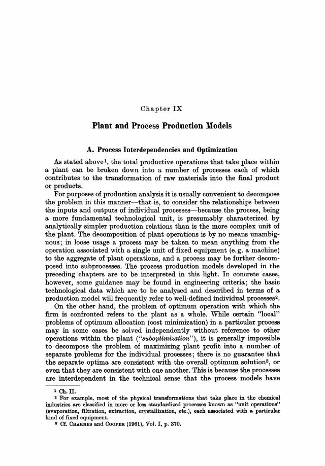
Chapter IX
Plant and Proeess Produetion Models
A. Process Interdependencies and Optimization
As stated above!, the total productive operations that take place within a plant can be broken down into a number of processes each of which contributes to the transformation of raw materials into the final product or products.
For purposes of production analysis it is usually convenient to decompose the problem in this manner-that is, to consider the relationships between the inputs and outputs of individual processes-because the process, being a more fundamental technological unit, is presumably characterized by analytically simpler production relations than is the more complex unit of the plant. The decomposition of plant operations is by no means unambiguous; in loose usage a process may be taken to mean anything from the operation associated with a single unit of fixed equipment (e.g. a- machine) to the aggregate of plant operations, and a process may be further decomposed into subprocesses. The process production models developed in the preceding chapters are to be interpreted in this light. In concrete cases, however, some guidance may be found in engineering criteria; the basic technological data which are to be analysed and described in terms of a production model will frequently refer to well-defined individual processes2•
On the other hand, the problem of optimum operation with which the firm is confronted refers to the plant as a whole. While certain "local" problems of optimum allocation (cost minimization) in a particular process may in some cases be solved independently without reference to other operations within the plant ("suboptimization"), it is generally impossible to decompose the problem of maximizing plant profit into a number of separate problems for the individual processes; there is no guarantee that the separate optima are consistent with the overall optimum solutionS, or even that they are consistent with one another. This is because the processes are interdependent in the technical sense that the process models have
1 Ch.II. B For example, most of the physical transformations that take plaoe in the ohemioal
industries are olassified in more or less standardized prooeBBeB known as "unit operations" (evaporation, filtration, extraction, orysta.llization, eto.), each 8.BBOoiated with a particular kind of fixed equipment.
8 Of. CHARNEs and COOPER (1961), Vol. I, p. 370.
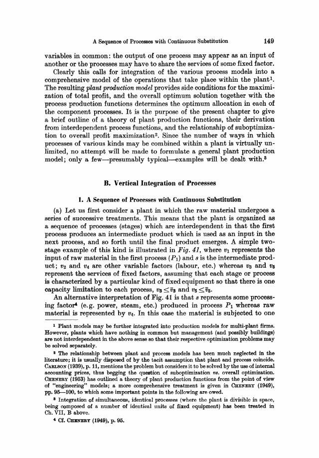
A Sequence of Processes with Continuous Substitution 149
variables in common: the output of one process may appear as an input of another or the processes may have to share the services of some fixed factor.
Clearly this calls for integration of the various process models into a comprehensive model of the operations that take place within the plant!. The resulting plant production model provides side conditions for the maximization of total profit, and the overall optimum solution together with the process production functions determines the optimum allocation in each of the component processes. It is the purpose of the present chapter to give a brief outline of a theory of plant production functions, their derivation from interdependent process functions, and the relationship of suboptimization to overall profit maximization2• Since the number of ways in which processes of various kinds may be combined within a plant is virtually unlimited, no attempt will be made to formulate a general plant production model; only a few-presumably typical-examples will be dealt with.s
B. Vertical Integration of Processes
1. A Sequence of Processes with Continuous Substitution
(a) Let us first consider a plant in which the raw material undergoes a series of successive treatments. This means that the plant is organized as a sequence of processes (stages) which are interdependent in that the first process produces an intermediate product which is used as an input in the next process, and so forth until the final product emerges. A simple twostage example of this kind is illustrated in Fig. 41, where VI represents the input of raw material in the first process (PI) and 8 is the intermediate product; V2 and V4 are other variable factors (labour, etc.) whereas Vs and Vs
represent the services of fixed factors, assuming that each stage or process is characterized by a particular kind of fixed equipment so that there is one capacity limitation to each process, Vs <vs and Vs ~vs.
An alternative interpretation of Fig. 41 is that 8 represents some processing factor' (e.g. power, steam, etc.) produced in process PI whereas raw material is represented by V4. In this case the material is subjected to one
1 Plant models may be further integrated into production models for multi-plant firms. However, plants which have nothing in common but management (and possibly buildings) are not interdependent in the above sense so that their respective optimization problems may be solved separately.
S The relationship between plant and process models has been much neglected in the literature; it is usually disposed of by the tacit assumption that plant and process coincide. CARLSON (1939), p. 11, mentions the problem but considers it to be solved by the use of internal accounting prices, thus begging the question of suboptimization V8. overall optimization. CHENERY (1953) has outlined a theory of plant production functions from the point of view of "engineering" models; a more comprehensive treatment is given in CHENERY (1949), pp. 95-100, to which some important points in the following are owed.
8 Integration of simultaneous, identical processes (where the plant is divisible in space, being composed of a number of identical units of fixed equipment) has been treated in Ch. VII, B above.
4. Cf. CHENERY (1949), p. 95.
150 Plant and Process Production Models
treatment only (P2 ), but the problem of integration is formally similar to the case where PI represents an initial stage of processing.
s
Flg.41
(b) Assume first that the inputs of each process are continuously substitutable. Then, ignoring for the moment the capacity factors (assuming that they are always fully utilized), the production functions for the two processes have the form
s = f(VI, V2)
x=g(s, V4).
(1)
(2) The plant production function expressing x in terms of VI. V2, and V4 is
readily obtained by eliminating s: I
x=g[/(VI. V2), v4]=F(VI, V2, V4) (3)
so that the integration results in a production function of the same general type as the process functions. The three inputs are continuously substitutable for one another; in the region where the marginal productivities in (1)-(2) are all positive we have
FI'=g,'· /1' >0, F2'=g,'· /2' >0, F4'=g4' >0
so that, for x constant, ~ V, 1 ~ Vj = - F II F t' < 0 for any pair of inputs (i, j = 1, 2, 4).
The point of maximum plant profit is determined by maximizing z = px - qi VI - q2V2 - q4 V4 subject to the plant production function (3); the first-order maximum conditions
(i = 1,2,4)
together with (3) determine VI, V2, V4, and x. (4) can be written in the form
, () qt p=c x =F,' (i= 1,2,4)
(4)
where c=c(x) is the plant cost function, the expansion path along which it is defined being determined by the production function (3) and
ql _ q2 _ q4 F I '- F 2'- F4"
the conditions for minimum cost for parametric x . Because of the constant inputs V3 and Vs the marginal cost curve may be excepted to be U -shaped.
1 Cf. CHENERY (1949), p. 97, or (1953), p. 311.
Problems of Suboptimization 151
2. Problems of Suboptimization
(a) In solving the plant optimization problem we have also determined the optimum allocation in the component processes: for the values of VI and Vz given by (3)-(4), 8 is determined by the process function (1), or by (2) for the optimal values of x and V4.
This immediately raises the question whether the two process optima could have been found separately by independent suboptimization of each process.
By the first two equations of (4) we have
, ql qz (p. gs =)7[= 71
so that the overall optimum satisfies the familiar condition for minimum cost in the first process. In other words, the optimum factor combination in PI is a point on the expansion path corresponding to this process, a locus which can be determined without regard to the second process since it depends only on ql, qz, and the shape of (1). However, complete suboptimization is not possible without additional information; there is nothing to indioate what particular point on the expansion path represents the optimum level of output in PI, nor can we determine even the locus of least-cost points belonging to Pz. In order to get any further some sort of price must be attached to the intermediate product 8. This is precisely what is done in practical cost accountingl.
Let the intermediate product be "sold" by the first process to the second at some arbitrarily fixed accounting price, 1t. Then, maximizing profit in PI
Zl =1t8-ql VI - qzvz
subject to (1), we get the necessary conditions
1t. h' -ql=O} or 1t= ql = qz 1t. Iz' -qz=O /I' Iz' (5)
which, with (1), determine VI. Vz, and 8. Similarly, the conditions for maximum profit in Pz as determined by maximizing
subject to (2) become
p. g,' -1t =O} 1t q4 , or p=-=-p. g4 -q4=O ga' g4'
(6)
and (2)-(6) determine 8, V4, and xZ•
However, there is nothing to guarantee that the two suboptima will be consistent; indeed, the respective solutions for 8 will generally differ. The higher the accounting price 1t is, the more of 8 will be produced in PI-Cf.
1 Of. CARLSON (1939), p. 11 n. 2 (5) and (6) are maximum conditions only if Zl and Za are ;::: 0 at the respective points.
If an overall solution exists at which Z> 0, i.e., pX-q4V4> qlVl+q2V2, there will exist an intervalof'lt", defined bypx-q4v4> 'It"8> qlVl +q2V2, within which Zl andzs are both positive.
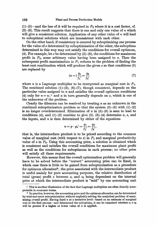
152 Plant and Prooees Production Models
(1)-(5)-and the less of it will be required in P2 where it is a cost factor, cf. (2)-(6). This result suggests that there is one and only one value of 7t which will give a consistent solution. Application of any other value of 7t will lead to suboptimal solutions which are inconsistent with each other.
On the other hand, if consistency is ensured by sub optimizing one process for the value of 8 determined by suboptimization of the other, the sub optima determined in this way may not satisfy the conditions for overall optimum, (4). For example, let 8 be determined by (2)-(6), the conditions for maximum profit in P2 , some arbitrary value having been assigned to 7t. Then the subsequent profit maximization in PI reduces to the problem of finding the least-cost combination which will produce the given 8 so that conditions (5) are replaced by
ql q2 (u=) h'= /2' (7)
where u is a Lagrange multiplier to be interpreted as marginal cost in Pl. The combined solution (1)-(2), (6)-(7), though consistent, depends on the particular value assigned to 7t and satisfies the overall optimum conditions (4) only for 7t = u; I and u in turn generally depends on 8, which is one of the unknowns of the problem.
Clearly the dilemma can be resolved by treating 7t as an unknown in the combined suboptimization problem so that the system (5)-(6) with (1)-(2) is no longer overdetermined. Elimination of 7t in (5)-(6) is seen to lead to conditions (4), and (1)-(2) combine to give (3). (3)-(4) determine x, 8, and the inputs, and 7t is then determined by either of the equations
, ql q2 7t = P . (j, = h' = /2"
that is, the intermediate product is to be priced according to the common value of marginal cost (with respect to 8) in PI and marginal productivity value of 8 in P2. Using this accounting price, a solution is obtained which is consistent and satisfies the overall conditions for maximum plant profit as well as the conditions for suboptimum in each process; no other price will satisfy all these requirements.
However, this means that the overall optimization problem will generally have to be solved before the "correct" accounting price can be fixed, in which case there is little to be gained from suboptimization as a procedure for optimum allocation2 ; the price associated with the intermediate product is useful mainly for pure accounting purposes, the relative distribution of total (gross) profit z between Zl and Z2 being dependent on the internal price at which the intermediate product is "sold" by one accounting unit
1 This is another illustration of the fact that Lagrange multipliers are often directly interpretable in economic terms.
2 In practice, however, the accounting price and the optimum allocation can be determined by trial-and-error suboptimization without explicitly solving the analytical problem of maximizing overall profit. Having fixed 7t at a tentative level-based on an estimate of marginal cost in the first process-and determined the suboptima, it can be examined whether Zl + Z2
will be greater if a. higher or lower value of 7t is applied.
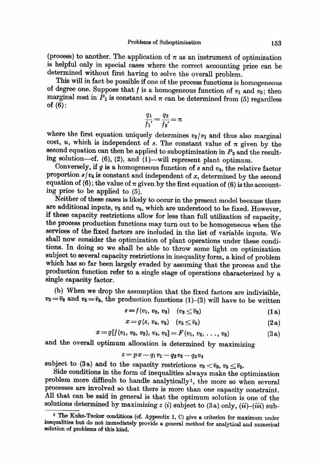
Problems of Suboptimization 153
(process) to another. The application of 7t as an instrument of optimization is helpful only in special cases where the correct accounting price can be determined without first having to solve the overall problem.
This will in fact be possible if one of the process functions is homogeneous of degree one. Suppose that t is a homogeneous function of VI and V2; then marginal cost in PI is constant and 7t can be determined from (5) regardless of (6):
ql q2 -=-=7t /1' /2'
where the first equation uniquely determines V2 / VI and thus also marginal cost, u, which is independent of 8. The constant value of 7t given by the second equation can then be applied to suboptimization in P2 and the resulting solution-cf. (6), (2), and (1)-will represent plant optimum.
Conversely, if y is a homogeneous function of 8 and V4, the relative factor proportion 8/ V4 is constant and independent of x, determined by the second equation of (6); the value of 7t given by the first equation of (6) is the accounting price to be applied to (5).
Neither of these cases is likely to occur in the present model because there are additional inputs, Va and vs, which are understood to be fixed. However, if these capacity restrictions allow for less than full utilization of capacity, the process production functions may turn out to be homogeneous when the services of the fixed factors are included in the list of variable inputs. We shall now consider the optimization of plant operations under these conditions. In doing so we shall be able to throw some light on optimization subject to several capacity restrictions in inequality form, a kind of problem which has so far been largely evaded by assuming that the process and the production function refer to a single stage of operations characterized by a single capacity factor.
(b) When we drop the assumption that the fixed factors are indivisible, Va = Va and Vs = vs, the production functions (1 )-(3) will have to be written
8=t(VI, V2, va) (Va <va) (1a)
X=y(8,V4,VS) (vs<vs) (2a)
x = yU (VI, V2, Va), V4, Vs] = F (VI, V2, ... , vs)
and the overall optimum allocation is determined by maximizing
Z=PX-qIVI-q2V2-q4V4
subject to (3a) and to the capacity restrictions Va <Va, Vs <VS.
(3a)
Side conditions in the form of inequalities always make the optimization problem more difficult to handle analyticallyl, the more so when several processes are involved so that there is more than one capacity constraint. All that can be said in general is that the optimum solution is one of the solutions determined by maxhnizing z (i) subject to (3a) only, (ii)-(iii) sub-
1 The Kuhn-Tucker conditions (cf. Appendix 1, 0) give a criterion for maximum under inequalities but do not immediately provide a general method for analytical and numerical solution of problems of this kind.
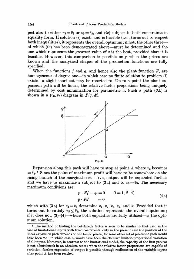
154 Plant and Process Production Models
ject also to either Va = Va or V5 = V5, and (iv) subject to both constraints in equality form. If solution (i) exists and is feasible (i. e., turns out to respect both inequalities), it represents the overall optimum; if not, the other threeof which (iv) has been demonstrated above-must be determined and the one which represents the greatest value of z is the best, provided that it is feasible. However, this comparison is possible only when the prices are known and the analytical shapes of the production functions are fully specified.
When the functions f and g, and hence also the plant function F, are homogeneous of degree one-in which case no finite solution to problem (i) exists-a slight short cut may be resorted to. Up to a point the plant expansion path will be linear, the relative factor proportions being uniquely determined by cost minimization for parametric x. Such a path (OA) is shown in a (va, V5) diagram in Fig. 42.
/
Fig. 42
Expansion along this path will have to stop at point A where Va becomes = Va. 1 Since the point of maximum profit will have to be somewhere on the rising branch of the marginal cost curve, output will be expanded further and we have to maximize z subject to (3a) and to Va = Va. The necessary maximum conditions are
p.Ft'-qt=O
p. F5' =0
(i = 1,2,4) (4a)
which with (3 a) for Va = Va determine VI, V2, V4, V5, and x. Provided that it turns out to satisfy V5 < V5, the solution represents the overall optimum; if it does not, (3)-(4)-where both capacities are fully utilized-is the optimum solution.
1 The method of finding the bottleneck factor is seen to be similar to that used in the case of limitational inputs with fixed coefficients, only in the present case the position of the linear expansion path depends on the factor prices; for some other set of prices the path would have been OA', in which case 115 would have been the effective limit to proportional variation of all inputs. Moreover, in contrast to the limitational model, the capacity of the first process is not a bottleneck in an absolute sense: when the relative factor proportions are capable of variation, further expansion of output is possible through reallocation of the variable inputs after point A has been reached.
Problems of Suboptimization 155
The plant cost function is illustrated by the marginal cost curve of Fig. 43. The initial phase of constant c' (x)-cf. the linear expansion path OA in Fig. 42, as given by
(c'=)~=~=~, Fs'=Fs'=O F 1' F 2' F4'
which determine the four relative factor proportions-is followed by a phase of increasing marginal cost (AB) where Vs is fully utilized, the expansion path being determined by (3a) and the conditions
(c'=)~= ~=~ vs=vs, Fs'=O. F 1' F 2 ' F4"
Solution (3a)-(4a) represents an optimum on this branch of the marginal cost curve: for p = Ii (point P in Fig. 43), the optimum condition p = c' is seen to be equivalent to (4a).
c'($)
\ 2 ---------- ,-- ------\ \ r:
\ \
" ------------~-\, A
....... _--
Fig. 43
For increasing values of the parameter p, the higher level of output determined by p = c' (x) will require more of each input, including Vs, up to the point (B) where Vs becomes equal to vs. Further expansion will have to follow the path given by (3a) and
, ql q2 q4 (c =) F 1'= F 2'=-F4" vs=vs, vs=vs,
where c' -+ 00 as output approaches the maximum capacity of the plant, x=xmax (as determined by F/'=-O (i=1, 2, 4), vs=vs, vs=vs). Optimum solutions in this third phase of the cost function-cf. point Q where p = c'are seen to be represented by (3)-(4).
In other words, the marginal cost function is pieced together from three different sections. The composite function is continuous (but not differentiable) atA and B, c' being=ql/F1' everywhere. (Hadvs andvs been indivisible, as assumed in (1)-(3), the first two phases would have been replaced by the dotted curve G B, the marginal cost curve G B Q being U -shaped; cf. above.)
156 Pla.nt and Process Production Models
Optimum solutions on the curve section A B, where Vs = Vs but V5 < V5, can be determined by SUboptimization because the process function g is homogeneous in the variable inputs 8, V4 and V5. The conditions for maximum profit in the respective processes are
(where Va = iis) and
TC' h' -ql=O TC ·/2' -q2=0
p.g,'-TC=O
P ·gl-Q4=0
P ·g5' =0
(5a)
(6a)
which are consistent if TC is treated as an unknown. Since the partial derivatives of g are functions of the relative factor proportions 8/ V4 and 8/ V5, the latter are determined uniquely by the second and third equation of (6a) and the first equation gives TC as equal to the constant marginal productivity value. Applying this value of TC to suboptimization in the first process, VI, V2, and 8 are given by (5a) and (fa) (for Vs =iis). This also determines V4 and V5 and, by (2a), output x. The combined solution is seen to be equivalent to the overall optimum (3a)-(4a), but it has been found without solving these equations; this was possible because, g being homogeneous, the suboptimum conditions for P2 permitted the determination of TC independently of the allocation problem in Pl.
If V5 rather than Vs had been the bottleneck factor-cf. the expansion path OA' in Fig. 42-the conditions for maximum profit in Ph
TC • It' - Ql = 0 TC·/2'-Q2=0 TC • Is' =0
(5b)
would determine the factor proportions VI! Vs and V2! Vs as well as TC, the latter being equal to the constant marginal cost along the linear expansion path. Using this accounting price in the conditions for SUboptimum in P2,
p. g,'-TC =0
P ·g4'-Q4=0 (6b)
(where V5 =V5), we get a solution (1a)-(2a), (5b)-(6b), which coincides with the overall optimum solution determined by (3a) and the conditions for maximum plant profit,
p.F/-Qc=O
p.Fs' =0.
(i= 1,2,4) (4b)
3. Other Examples of Vertical Integration
(a) Now let us assume that the intermediate product produced by the first process is a limitational shadow factor in the second, all other inputs being substitutable in the respective processes as before. Then the process models can be written
Other Examples of Vertical Integration 157
8=/(Vl, V2, Va) (vs ::;;;vs) (8) and
X=g(V4, vs) (vs <vs) (9)
8=a·x
where a is the constant coefficient of production. The assumption that 8
is proportional to x is probably realistic in many cases where 8 is a material (produced in PI) to be further processed in P2.
In cases of this type elimination of 8 leads to an integrated plant model consisting of two equationsl,
1 x=-·/(th,V2,VS)=g(V4,VS) (vs::;;;tis,vs<vs), (10)
a
one for each process2•
The plant optimum is determined by maximizing total profit subject to the two production functions (10) and to the corresponding capacity constraints. Again, if the functions 1 and g are assumed to be homogeneous of the first degree, the bottleneck factor can be detected by confronting the linear phase of the expansion path in a (Va, vs) diagram with the limitations Va ::;;; Vs and Vs < vs. Let Va be the effective limit i then, maximizing the Lagrangian
L = P .. ! . 1 (VI, V2, tis) - ql VI - q2 V2 - q4 V4 + u . (g (V4' vs) - ! . 1 (Vl' V2, tis))
and eliminating the multiplier u, we get the conditions
~ . (p _ q4) = ql = q2 a gl h' 12' gs'=O.
(11)
The solution determined by (10)-(11) with Va = tis represents plant optimums. The first two equations of (11) are to be interpreted as an equality between the marginal cost of producing 8 in P l and the marginal profit derived from processing another unit of 8 in P2, ~Z2/~8.
Suboptimization in PI, i.e., maximization of
Zl = 1t • 1 (VI, V2, tis) - ql VI- q2V2,
leads to the conditions
1t. /1' -ql=O
1t. /2' -q2=0 i
the conditions for maximum of
Zs = px -1t8 - q4V4 = (p -1ta) . g(V4, vs) -q4V4
1 Of. ClmN1cBy (1949), p. 97.
(12)
S This is an example of oomplementary groups of substitutional inputs or, in FRIsCH'S
terminology, "disconnected factor rings," of. Ch. V, C. 8 Unless "6 turns out to be greater than "6, in which case z must be maximized over again
for "1="1 as well as "8="8; the former condition then replaces ga'=O in (11).
158 Plant and Process Produotion Models
are (p-7ta). gl-q4=0
(p-7ta)·gs' =0. (13)
Assuming that g is a homogeneous function, (13) determine the relative factor combination V4/V5 and 7t, the latter being equal to
7t =! . (p _ q4) a gl
which is constant, independent of output. Substitution of this value in (12) is seen to lead to the plant optimum conditions (11). In other words, provided that the function g is homogeneous, the complete problem can be solved by suboptimization, starting with the second process.
Had V5 turned out to be the bottleneck capacity, the conditions for maximum profit in the respective processes would have been
7t . /1' - ql = 0
7t·/2'-q2=0 (12a)
7t . Is' =0
which for I homogeneous of degree one leads to a uniquely determined accounting price equal to the constant marginal cost (= average variable cost) in PI, and
(13a)
(where V5=VS). For the value of 7t given by (12a) the combined solution (8)-(9), (12a)-(13a) (for V5 =vs) is equivalent to the overall maximum of z as determined by (10) and the conditions
! . (p _ q4) = ql = q2 a g4' It' 12' (11 a)
Is' =0. 1
(b) Suppose instead that the inputs of each process are alllimitational,
v,=a,·8 (i = 1,2,3), Va <vs (14)
1 It must be emphasized that suboptimization is impoBBible when the produotion functions for the successive processes have other variables than the intermediateproduotin common.
FBISOH'S ohocolate production funotion-of. Ch. V, A above-is a oase in point. The produotion function may be deoomposed into prooess functions for mixing and moulding-cooling respeotively:
and
(Ps) 8=:1:
where 8 is the quantity of ohocolate mix to be moulded and oooled. Though in some respeots similar to (8)-(9), the model diHers in that VI and Vs appear in both prooesa funotions: the amount of moulding-cooling work to be done depends on the liquidity of the mix, whioh in turn depends on the mixing proportion. The least-oost mix, therefore, cannot be determined independently of the optimization problem in the seoond prooess and vioe versa; a mix oonsisting only of the oheaper input (vd is not consistent with the overall cost minimum.
and
Other Examples of Vertical Integration
8=a,· x
v,=a,· x (i=4,5),
159
(15)
where the a, are constant coefficients of productionl. (14)-(15) immediately reduce to an integrated plant production model of the same type,
Vi = (a,a,) . x (i = 1, 2, 3)
(i=4, 5). (16)
Total variable plant cost is proportional to output, and plant optimumprovided that unit gross profit is ~ O-is determined by the bottleneck capacity,
-M· (VS V5) 2 x- ill --, -. asa8 as
(17)
Linear constant-coefficient models with several capacity limitations are usually to be interpreted in this way, being derived from-or decomposable into-models of successive processes (stages) each of which is associated with a particular fixed factorS".
1 If 8 is measured in units of x, as will be = 1. 2 The shadow price associated with the effective bottleneck factor-cf. Ch. III, A
expresses the increase in profit made possible by a unit increase in the factor's capacity, i.e., the marginal profitability of investment with a view to harmonizing the capacities of the processes.
3 FRENCKNER (1957), pp. 81 ff., has given an empirical example of a model of this kind. A machine shop turns out three different products (two kinds of lathes and a mixing machine) using the same fixed factors, and each product is made in a single activity with constant coefficients at the respective stages. There are five successive stages, each defined by an operation performed on a particular kind of fixed equipment-two kinds of lathe operations, milling, drilling, and assembly-and therefore five capacity limits.
The sales potential is virtually unlimited so that the firm can sell as much as it can turn out if anyone of the products is produced exclusively; however, since this would result in idle capacity at those stages which are not effective bottlenecks, it is more profitable to make several products jointly.
4 JANTZEN'S "Law of Harmony"-cf. JANTZEN (1924), pp. 39f£., or (1939), pp. 33 ff.; see also BREMS (1952 a, b)-is based on a production model of this type, only the capacity factors are treated as variable since JANTZEN was concerned with the behaviour of total unit cost when the capacities of the processes (stages) are adjusted along with the expansion of output in such a way as to minimize total cost for any level of output. (JANTZEN'S total plant cost per period is the sum of variable (operating) cost, which is proportional to output, and "fixed" (or "equipment") cost per period, the latter being defined for each kind of durable factor as the value of the capital stock divided by its useful life in terms of periods.)
While the services of fixed equipment are perfectly divisible in the time dimension, the units in whi .. h these durable factors as such are purchased are large and indivisible so that the capacities of the successive processes-cf. (17)--are usually not geared to each other; in JANTZEN'S terminology, the composition of the plant is disharmonious. In the example above, let fls be the effective limit; then output can be expanded further only by installing another unit of the third factor, thus doubling the capacity of the first stage; and so forth. Whenever a new unit of durable equipment is purchased and installed, total plant cost per unit of output jumps in a discontinuous manner; unit cost will be a minimum only for those levels of output which are common multiples of the capacities (in terms of x) of the respective units of the fixed factors. At such a point the plant is harmoniously composed and idle capacity does not occur at any stage.
160 Plant and Process Production Models
(c) Finally, let each of the process models be linear and characterized by discontinuous substitution:
and
M
8= 2: I-'J j=1
M
Vt = 2: atJ I-'J
j=1
N
x= 2: Ak
k=1
N
8 = 2: aSkAk
k =1
N
Vt = 2: atkAk
k =1
(18)
(i=1,2,3), V3<V3
(19)
(i ,4,5), vs<vs.
I-'J and Ak are the activity levels (required to be > 0) of the sub-activities in PI and P2 respectively. Eliminating 8, we get a linear plant model where x and some of the Vt are linear functions of the Ak and the other inputs depend on the I-'}, the two groups of activity levels being connected by the linear equation
M N
(8 =) 2: I-'J = 2: aSkAk. (20) j=1 k=l
The optimum allocation of the plant is determined by maximizing total profit, which can be expressed as a linear function of the M + N activity levels, subject to (20) and to the capacity limitations Va <Va, Vs <vs which are linear inequalities in the 1-'1 and the Ak respectively I. At most three activity levels will be positive in the optimum solution.
Model (18)-(19) assumes that the intermediate product turned out by PI is the same no matter how it is made and can be used as an input for any method of production applied in P 2.2 Now assume instead that PI and P2 are technically interdependent in the stronger sense that a unit of final output produced by activity no. k in P 2 requires a constant amount a,k
of the intermediate product 8k turned out by the k'th activity of the first stage; any other activity in PI produces a technically different intermediate product which does not fit in. This means that the second equation of (19) will have to be replaced by
1 Linear programming problems of this type are particularly easy to solve numerically because of the many zeroes in the coefficient matrix.
2 This assumption is implicit in the first equation of (18) and the second equation of (19): the Pi as well as the a,kAk are additive.
Other Exa.mples of Vertical Integration 161
(where ad: may often for convenience be set = 1) and the model for the first process becomes
The integrated plant model becomes N
X= L At k=l N
V, = L a'ta,kAt t=l
N
V,= L a,tAt k-l
(i=1,2,3).
(i= 1,2,3), (21)
(i=4,5),
which is a linear discontinuous-substitution model with N activities, each of which corresponds to a particular technical quality of the intermediate product. Only two activities (at most) will be used in the optimum allocation l , corresponding to the number of capacity constraints2•
1 In solving the plant optimization problem by linear programming, shadow prices of the fixed factors are implicitly determined, of. Ch. III, B. These imputed prices represent the marginal values to the firm of additional capacity in the respective processes and can therefore be used as a guide to investment decisions with a view to increasing the capacities.
I CHABNEs, COOPER and FARR (1953) have given an empirical example of a linear plant model which may be interpreted as a kind of intermediate case between (18)-(19) and (21). The plant turns out a multitude of products which are scheduled through the same sequence of mechanical processes, the more important capacity factors of which are screw machines and grinders respectively. Each product can be produced in a number of linear activities.
Consider one such product (no. 5) in isolation. There are four activities, all of which have the same input coeHicient for each variable factor so that unit profit is the same in all four activities; they differ only in respect to the input coefficients of the capacity factors. The matrix of these coefficients (machine times per unit) has the form (op. cit., pp. 120 f.):
I IAI As As A41
PI I :~: I ala ala alb al~ I ~ ~:: Ps I :: I as. asb as. ~ I ~ :::
The interpretation of the nnderlying model appears to be as follows: The first processing stage (PI) can be performed by either of two types of screw machines,
with capacities '1. and 'l~ respectively; similarly there are two types of grinders capable of doing each other's jobs. Each of the four machine types defines a sub-activity, characterized by a machine-time coefficient (al., etc.). The intermediate products produced by the two sub-activities at the first stage (PI) are apparently not technically identical-if they were they would be additive as in (18)-(19)-but either one can be used as an input for either sub-activity at the subsequent stage (PI) so that there will be four plant activities as shown in the table. (In general, there will be M . N plant activities as against M + N in the plant model corresponding to (18)-(19), where each sub-activity in PI could be combined with any combination of sub-activities in PI producing the requisite amonnt of intermediate product.)
DaDIII, Produotion lIodela 11
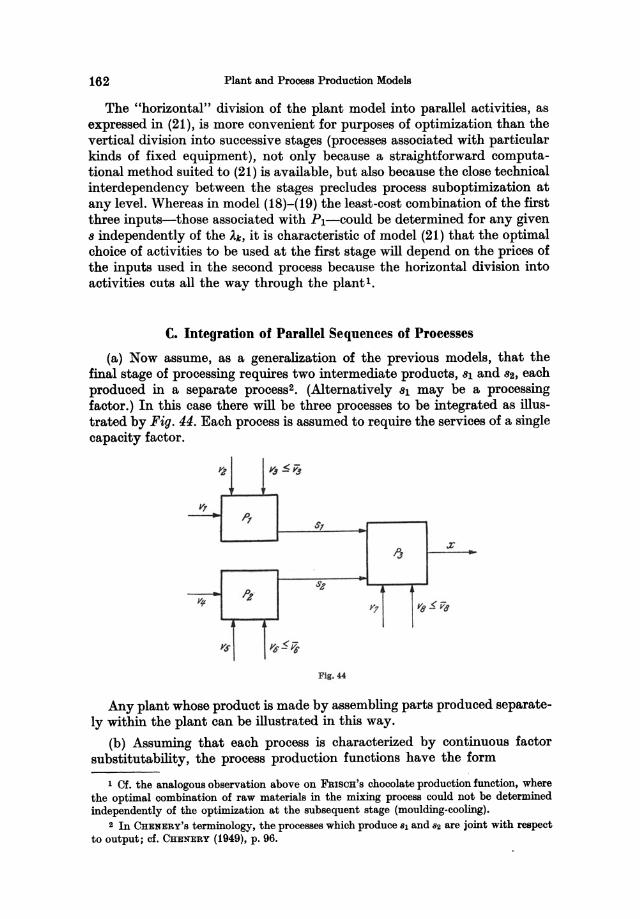
162 Plant and Process Production Models
The "horizontal" division of the plant model into parallel activities, as expressed in (21), is more convenient for purposes of optimization than the vertical division into successive stages (processes associated with particular kinds of fixed equipment), not only because a straightforward computational method suited to (21) is available, but also because the close technical interdependency between the stages precludes process suboptimization at any level. Whereas in model (18)-(19) the least-cost combination of the first three inputs-those associated with PI-could be determined for any given 8 independently of the Ak, it is characteristic of model (21) that the optimal choice of activities to be used at the first stage will depend on the prices of the inputs used in the second process because the horizontal division into activities cuts all the way through the plantl.
c. Integration of Parallel Sequences of Processes
(a) Now assume, as a generalization of the previous models, that the final stage of processing requires two intermediate products, 81 and 82, each produced in a separate process2• (Alternatively 81 may be a processing factor.) In this case there will be three processes to be integrated as illustrated by Fig. 44. Each process is assumed to require the services of a single capacity factor.
~ 1~~~
~ f} $,
-1 J:
-;;- ~ oft'
Y7 Ya ~ Va
Ys Y6'5~
FIg.«
Any plant whose product is made by assembling parts produced separately within the plant can be illustrated in this way.
(b) Assuming that each process is characterized by continuous factor substitutability, the process production functions have the form
1 Cf. the analogous observation above on FRISCH's chocolate production function, where the optimal combination of raw materials in the mixing process could not be determined independently of the optimization at the subsequent stage (moulding-cooling).
2 In CHENERY'S terminology, the processes which produce 81 and 82 are joint with respect to output; cf. CHENERY (1949), p. 96.
Integration of Parallel Sequences of Processes
8l=f(Vl,v2,vs) (Vs<vs)
82=g(V4, Vs, V6) (V6<V6)
X=h(81, 82, V7, VS) (vs<vs).
The integrated production function for the plant becomes
163
(22)
(23)
(24)
x=h(f,g,v7,VS)=F(Vl, ... ,vs) (va<Va,V6<V6,VS<VS) (25)
where all inputs are substitutable. The plant expansion path, as determined by minimizing total cost for
parametric x, and the corresponding cost function will pass through four phases. For sufficiently small x there will be idle capacity in all processes. At a certain level of output one of the three capacity factors becomes fully utilized; from some later point, two capacities will be exhausted; and so on. Each time a capacity limit is reached, the equation F/ = 0 for the factor in question is replaced by Vt = Vt in the equilibrium conditions; the marginal cost function will be continuous but kinked at these pointsl.
Again, the allocation which leads to maximum plant profit can be determined by suboptimization only in special cases where marginal cost is constant in one of the processes. Assume that the three process production functions and thus also (25) are homogeneous of degree one so that the first phase is characterized by constant marginal cost along a linear expansion path. Let Va < Va be the effective capacity limit which puts a stop to expansion along this path 2; then we know that Va = Va at the point of overall optimum.
As long as the capacity factor of the second process is less than fully utilized, marginal cost in P2, dC2/ d82, will be constant, the locus of least-cost points being determined by (23) and
(26)
Applying the constant marginal cost as the accounting price 1t2 of 82,
(27)
the conditions for suboptimal allocation in the second process are seen to be satisfied. The conditions for maximum profit in the third process-assuming that there is sufficient capacity-are
p. h/- 1tl=O
p. hg' -1t2=0
p. h7' -q7 =0
p. hs' =0.
(28)
1 Cf. the three-phase oost funotion (oorresponding to a model with two capacity faotors) shown in Fig. 43.
2 For given prices the bottleneok is determined in a similar way to that applied in Fig. 42, only there are now three oapaoity restriotions.
11*
164 Plant and Process Production Models
For the given value of 1I:a, the three relative factor proportions in Ps are determined by the last three equations of (28); if 11:1 is set=p· hi-i.e., if the first intermediate product is priced according to its constant marginal productivity value in Ps-the complete conditions for maximum profit in Ps are satisfied. Finally, applying this value of 11:1 to the conditions for maximum profit in Pl,
11:1' /1' -ql=O
11:1 • fa' - qa = 0 (29)
(where Vs = vs), the three suboptima given by (26)-(29) with (22)-(24) are seen to form a consistent solution which is equivalent to the overall optimum solution as determined by (25) and the conditions
p. F/ -q,=O (i= 1,2,4,5,7)
p. F/ =0 (;=6,8) (30)
for Vs = Va. If it is feasible-i.e., if it respects the capacity limitations for P a and Ps-the solution represents the overall optimum; if it is not, a new solution will have to be found, setting ve=iie or vs=iis from the outset.
(c) When 81 and 8a are interpreted as parts to be assembled in the third process, it is perhaps more realistic to assume that they are limitational inputs in PS.1 Then (24) has to be replaced by
X=h(V7, va)
(24 a)
8a=fl2 • x and (25) becomes
which is characterized by complementary groups of substitutional inputs, each group corresponding to a processa•
Still assuming that the functions are homogeneous of the first degree and that Vs is the bottleneck factor, maximize the Lagrangian
L=p. h- L: q,V,+U1' (f- a1' h)+'Uz' (g-fl2' h) , for Va = Va. This leads to the conditions
1 FRIsCH (1953), p. 6, exemplifies this by a cutlery works: one blade and one handle are required to produce a knife.
S Cf. Ch. V, C a.bove. FRISCH (1953), pp. 6 f., derives the plant production function for a general case of this type in a slightly different way, treating the limitational factors 810
82, ••• as independent variables so that the plant function becomes x=Min (8JlaJ)
(cf. Ch. III, A, model (lc». This of course makes no difference to the optimum solution.
Integration of Parallel Sequences of Processes 165
Va=Va
(30a)
p=UIal+U2 a 2+ i7" hs'=O. 7
The solution determined by (30a) and (25a) represents the plant optimum provided that it respects the other two capacity constraints. Suboptimization clearly leads to the same result for 'ltl = UI and 'lt2 = U2, where UI and U2 can be interpreted as marginal cost in PI and P 2 ; U2 is a constant determined independently by the second group of equations (i.e., the conditions for maximum profit in P2 ) and 'ltl = UI then follows from the last equations, h7' and hs' being functions of V7 / Vs.
(d) The models above are examples of "parallel" processes which are interdependent through the joint application of their products at a subsequent stage of processing. Another kind of interdependency results from the joint use of some fixed factor such as a machine or a processing factor subject to a capacity limitation l . The fact that labour and other current inputs are used in both processes does not in itself establish any relationship between them2-the amounts of labour required by the respective processes can be varied independently-but if the processes have to share the services of the plant's fixed equipment the processes cannot be considered separately.
This kind of interdependency is particularly important in multi-product plants where the several products are processed by wholly or in part the same machines, a case which will be dealt with in the following chapter.
1 In CHENBBY'S terminology, the processes are joint with respect to inputs, cf. CHENERY
(1949), p. 96. 2 CHENERY, op. cit., pp. 97 f. The joint use of buildings can generally be disregarded since
the available floor space does not represent an eHective bottleneck in the short run, cf. op. cit., p.99.
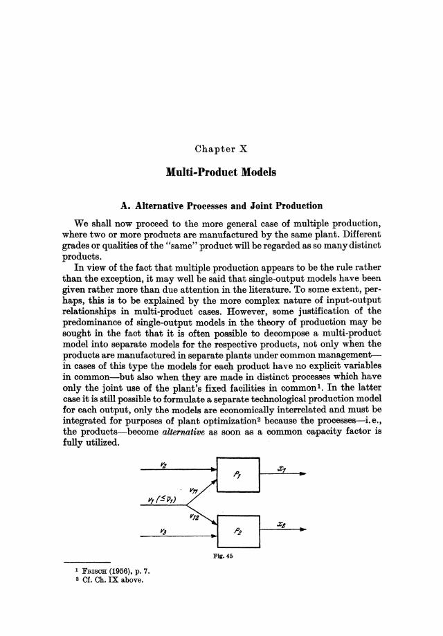
Chapter X
Multi-Product Models
A. Alternative Processes and Joint Production
We shall now proceed to the more general case of multiple production, where two or more products are manufactured by the same plant. Different grades or qualities of the "same" product will be regarded as so many distinct products.
In view of the fact that multiple production appears to be the rule rather than the exception, it may well be said that single-output models have been given rather more than due attention in the literature. To some extent, perhaps, this is to be explained by the more complex nature of input-output relationships in multi-product cases. However, some justification of the predominance of single-output models in the theory of production may be sought in the fact that it is often possible to decompose a multi-product model into separate models for the respective products, not only when the products are manufactured in separate plants under common managementin cases of this type the models for each product have no explicit variables in common-but also when they are made in distinct processes which have only the joint use of the plant's fixed facilities in common 1. In the latter case it is still possible to formulate a separate technological production model for each output, only the models are economically interrelated and must be integrated for purposes of plant optimization2 because the processes-i.e., the products-become alternative as soon as a common capacity factor is fully utilized.
1 FRISCH (1956), p. 7. 2 Of. Ch. IX above.
Fig. 45
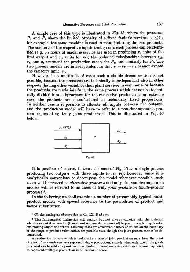
Alternative Processes and Joint Production 167
A simple case of this type is illustrated in Fig. 45, where the processes PI and P2 share the limited capacity of a fixed factor's services, VI:::;:; ih ; for example, the same machine is used in manufacturing the two products. The amounts of the respective inputs that go into each process can be identified (e.g. Vll hours of machine service are used in producing Xl units of the first output and VI2 units for X2); the technical relationships between Vll, V2, and Xl represent the production model for PI, and similarly for P2. The two process models are interdependent in that VI = Vll + Vl2 cannot exceed the capacity limit, VI.
However, in a multitude of cases such a simple decomposition is not possible, because the processes are technically interdependent also in other respects (having other variables than plant services in common)l or because the products are made jointly in the same process which cannot be technically divided into subprocesses for the respective products; as an extreme case, the products are manufactured in technically fixed proportions. In neither case is it possible to allocate all inputs between the outputs, and the production model will have to refer to a non-decomposable process representing truly joint production. This is illustrated in Fig. 46 below.
y,(5v,) .];,
Y,t P .];3
v"
Fig. 46
It is possible, of course, to treat the case of Fig. 45 as a single process producing two outputs with three inputs (VI, V2, Va); however, since it is analytically convenient to decompose the model whenever possible, such cases will be treated as alternative prOCes8es and only the non-decomposable models will be referred to as cases of truly joint production (multi-product processes )2 .
In the following we shall examine a number of presumably typical multiproduct models with special reference to the possibilities of product and factor substitution.
1 Of. the analogous observation in Ch. IX, B above. I This fundamental distinction will usually but not always coincide with the criterion
whether or not it is possible (though not necessarily economical) to produce each output with. out making any of the others. Limiting cases are conceivable where solutions on the boundary of the range of product substitution are possible even though the joint process cannot be de· composed.
A production process which is technically a case of joint production may from the point of view of economic analysis represent single production, namely when only one of the goods produced can be sold at a positive price. Under different market conditions the case may come to represent multiple production in an economic sense.
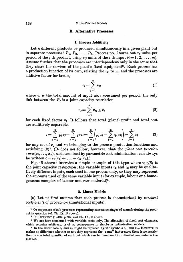
168 Multi-Product Models
B. Alternative Processes
1. Process Additivity
Let n different products be produced simultaneously in a given plant but in separate processes l Pl , P2, ... , Pn. Process no. j turns out Xi units per period of the j'th product, using V'i units of the i'th input (i= 1,2, ... , m). Assume further that the processes are interdependent only in the sense that they share the services of the plant's fixed equipment2. Each process has a production function of its own, relating the VCj to Xi> and the processes are additive factor for factor,
" V,= 2: v" (1)
j=1
where v, is the total amount of input no. i consumed per period; the only link between the Pi is a joint capacity restriction
" V,= 2: V'i <v, (2)
j=1
for each fixed factor VB' It follows that total (plant) profit and total cost are additively separable,
• ~ ,~1'1"'-~ q ••• ~ ,~( 1'1'" -~ q •• + ,~ " (3)
for any set of Xi and Vii belonging to the process production functions and satisfying (2)3. (It does not follow, however, that the plant C08t f'!l-nction C = C (Xl, ••• , Xn), as determined by parametric cost minimization, can always be written C=Cl(Xl}+ ••• + cn(xn}.}
Fig. 45 above illustrates a simple example of this type where Vl <Vl is the joint capacity restriction; the variable inputs V2 and Va may be qualitatively different inputs, each used in one process only, or they may represent the amounts used of the same variable input (for example, labour or a homogeneous complex of labour andraw material)'.
2. Linear Models
(a) Let us first assume that each process is characterized by constant coefficients of production (limitational inputs),
I Or sequences of sub-processes representing succeBBive stages of manufacturing the prod. uct in question (cf. Ch. IX, B above).
I Of. CHENERY (1949), p. 96, and Ch. IX, C above. 8 We are here concerned with variable costs only. The allocation of fixed cost elements,
which remains arbitrary, is of no consequence in short-run optimization models. 4 In the latter case Va and Va might be replaced by the symbols val and vaa. However, it
makes no difference whether or not they represent the "same" factor since there is no restriction on the total quantity of an input which can be purchased in unlimited amounts on the market.
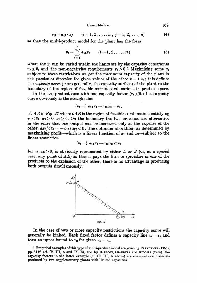
Linear Models 169
v'i=al1' Xi (i= 1,2, ... , m; j= 1,2, ... , n) (4)
so that the multi-product model for the plant has the form n
Vf= L aiJXj (i=1,2, ... ,m) (5) i~l
where the Xj can be varied within the limits set by the capacity constraints Va <VB and the non-negativity requirements Xj >0. 1 Maximizing some Xj
subject to these restrictions we get the maximum capacity of the plant in this particular direction for given values of the other n - 1 Xj; this defines the capacity curve (more generally, the capacity surface) of the plant as the boundary of the region of feasible output combinations in product space.
In the two-product case with one capacity factor (VI <VI) the capacity curve obviously is the straight line
(VI =) all XI + a12X2 = VI,
cf. AB in Fig. 47 where OAB is the region of feasible combinations satisfying VI <iit, X120, X220. On the boundary the two processes are alternative in the sense that one output can be increased only at the expense of the other, dX2/dxl= -all/aI2 <0. The optimum allocation, as determined by maximizing profit-which is a linear function of Xl and x:a-subject to the linear restriction
(VI =) all Xl + al2X2 < VI
for Xl, X2 >0, is obviously represented by either A or B (or, as a special case, any point of AB) so that it pays the firm to specialize in one of the products to the exclusion of the other; there is no advantage in producing both outputs simultaneously.
Fig. 47
In the case of two or more capacity restrictions the capacity curve will generally be kinked. Each fixed factor defines a capacity line VB = VB and thus an upper bound to X2 for given Xl = Xl,
1 Empirical examples of this type of multi-product model are given by FRENCKNER (1957), pp. 81 ff. (of. Ch. III, A and IX, B), and by BARGONI, GIARDINA and RICOSSA (1954); the capacity factors in the latter example (cf. Ch. III, A above) are chemical raw materials produced by two supplementary plants with limited capacities.
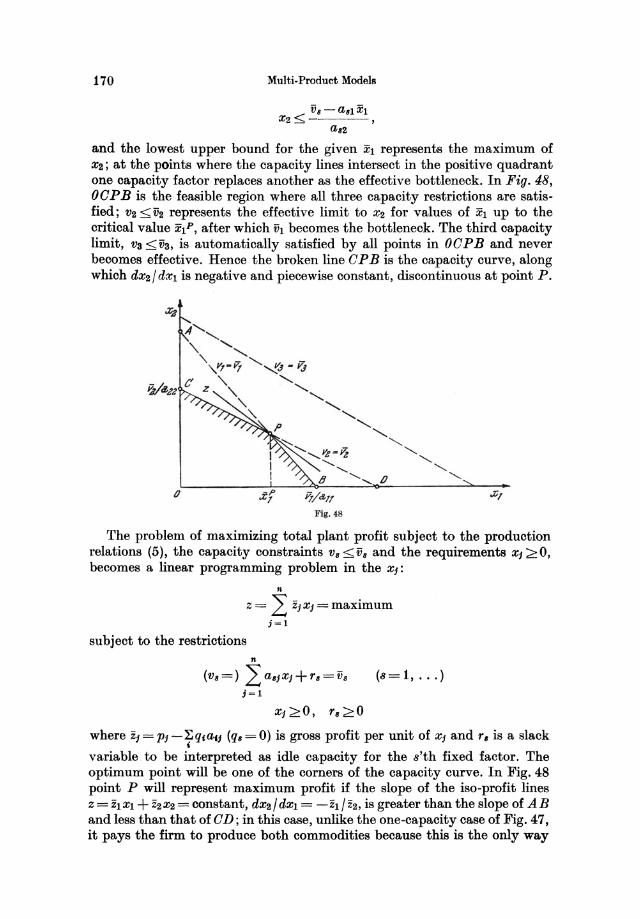
170 Multi-Product Models
VB - a31Xl X2< ,
a,2
and the lowest upper bound for the given Xl represents the maximum of X2; at the points where the capacity lines intersect in the positive quadrant one capacity factor replaces another as the effective bottleneck. In Fig. 48, OOPB is the feasible region where all three capacity restrictions are satisfied; V2 < V2 represents the effective limit to X2 for . values of Xl up to the critical value xlP, after which VI becomes the bottleneck. The third capacity limit, Va < Va, is automatically satisfied by all points in 00 P B and never becomes effective. Hence the broken line OP B is the capacity curve, along which dX2/ dXl is negative and piecewise constant, discontinuous at point P.
tJ D i}/&/I .);,
Fig. 48
The problem of maximizing total plant profit subject to the production relations (5), the capacity constraints V8 < V8 and the requirements Xj > 0, becomes a linear programming problem in the Xj:
11
Z= 2: zjxj=maximum j=l
subject to the restrictions 11
(v,=) 2:a,jxj+rS=v8 j=l
Xj>o, r, >0
(8= 1, ... )
where Zj = Pi -~qtatj (q, = 0) is gross profit per unit of Xj and r, is a slack , variable to be interpreted as idle capacity for the 8'th fixed factor. The optimum point will be one of the corners of the capacity curve. In Fig. 48 point P will represent maximum profit if the slope of the iso-profit lines Z= ZlXl + Z2X2 = constant, dX2/dxl = -Zl/Z2, is greater than the slope of AB and less than that of OD; in this case, unlike the one-capacity case of Fig. 47, it pays the firm to produce both commodities because this is the only way
Linear Models 171
in which the two capacities VI and V2 can be fully utilized. It is only when Zl is large compared to ~ or vice versa that it pays to specialize (point B or G), thus leaving some of V2 or VI idle I.
The numerical values of the simplex coefficients of the slack variables r8 in the optimum solution can be interpreted as shadow prices associated with the fixed factors VB' If P in Fig. 48 represents maximum profit, VI and V2
will have positive shadow prices because the services of the first two capacity factors are scarce; V3, on the other hand, is available in abundant supply so that a marginal increase in V3 would add nothing to profit, i. e., its shadow price is zero.
The shadow prices y, can be used as an alternative instrument of optimal planning. It follows from the duality theorem of linear programming2 that "net" lmit profit-defined as gross unit profit, zi, minus the inputed cost of the amounts used of the fixed factors' services, ~YBa'i-will be zero in , those activities (processes) which are actually used in the optimum solution (Xi> 0), negative in those activities for which Xi = O. Using this criterion for each process (product) separately, the plant optimum can be found by suboptimization; the shadow prices which are applied as accounting prices associated with the fixed factors can be determined independently-i.e., without solving the plant optimum problem above-since they are identical with the optimum solution of the dual problem of minimizing total imputed cost of the fixed factors
subject to
for y, >0.
g= L:v,y, ,
(i=1,2, ... ,n)
(b) Now assume that discontinuous factor substitution is possible in each of the processes so that each product can be made in a finite number of linear activities. In the two-product case the model for the first process becomes
M M
Xl = L: Ai, Vu = L: afiAi i-I ;=1
and for the second process N
X2= L Pit, k-l
(i=1, 2, ... , m) (6)
(i=1,2, ... ,m) (7)
where the Ai and Pk are activity levels and the ali and b'k are technical coefficients characterizing the respective activities. The process models (6) and (7) are interrelated through capacity constraints of the form
1 .An instructive hypothetical model of this type-an automobile firm producing trucks and automobiles under four capacity restrictions-is given by DORFMAN (1953), pp. 798 ff.
2 Of. Appendix 1, Band Ch. III, B above.
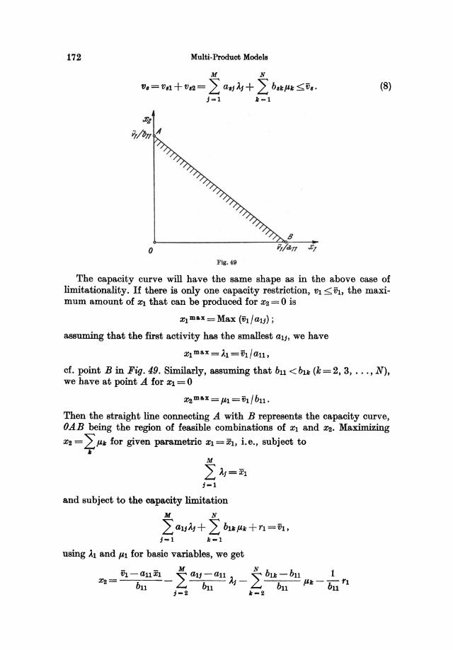
172 Multi-Product Models
M N
11, =VI1 + V62 = 2: a,jAj+ 2: b,,,I-''' <V,. (8) j=1 k-l
Fig. 49
The capacity curve will have the same shape as in the above case of limitationality. If there is only one capacity restriction, VI <VI, the maximum amount of Xl that can be produced for X2 = 0 is
Xl max = Max (ih!alJ);
assuming that the first activity has the smallest alj, we have
Xl max = Al =Vl!an,
cf. point B in Fig. 49. Similarly, assuming that bn <bu (k=2, 3, . . . , N), we have at point A for Xl = 0
X2 max = 1-'1 =Vl! bn.
Then the straight line connecting A with B represents the capacity curve, OAB being the region of feasible combinations of Xl and X2. Maximizing
X2= L>" for given parametric Xl=Xl, i.e., subject to lr
and subject to the capacity limitation M N
2: al}A} + 2: bUl-'k + rl =Vl, }=1 k-l
using Al and 1-'1 for basic variables, we get
- - M Nb b 1 VI - an Xl 2: al} - an 1 L lk - n
X2 = - "'j - I-'k - - rl bn bll bll bll
;-2 k-2
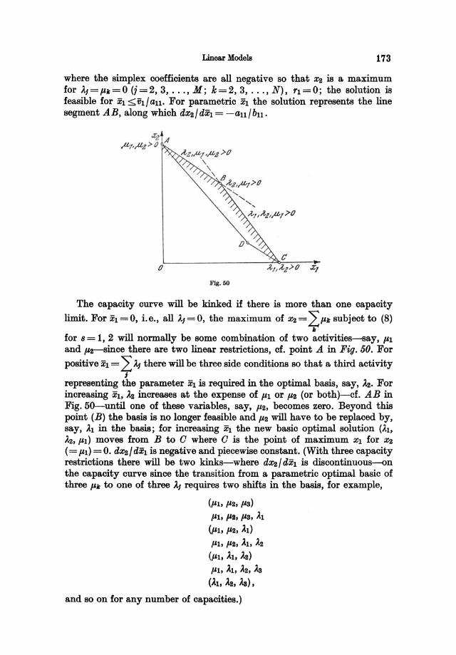
Linear Models 173
where the simplex coefficients are all negative so that X2 is a maximum for ).1=1',,=0 (i=2, 3, . .. , M; k=2, 3, .. . , N), rl=O; the solution is feasible for Xl ~.fh/all . For parametric Xl the solution represents the line segment A B, along which dX2 / dXl = -au / bu.
Fig. 60
The capacity curve will be kinked if there is more than one capacity
limit. For Xl = 0, i. e., all ).j = 0, the maximum of X2 = LP" subject to (8)
" for 8= 1,2 will normally be some combination of two activities-say, PI and P2-Bince there are two linear restrictions, cf. point A in Fig. 50. For
positive Xl = L: A.j there will be three side conditions so that a third activity J
representing the parameter Xl is required in the optimal basis, say, ).2. For increasing Xl, ).2 increases at the expense of PI or 1'2 (or both)-cf. AB in Fig. 50-until one of these variables, say, 1'2, becomes zero. Beyond this point (B) the basis is no longer feasible and 1'2 will have to be replaced by, say, ).1 in the basis; for increasing Xl the new basic optimal solution ().l, ).2, pI) moves from B to 0 where 0 is the point of maximum Xl for X2 (= pI) = o. dX2 / dXl is negative and piecewise constant. (With three capacity restrictions there will be two kinks-where dX2 / dXl is discontinuous-on the capacity curve since the transition from a parametric optimal basic of three 1''' to one of three ).1 requires two shifts in the basis, for example,
(pl,p2,pa) PI, ps, pa, ).1
(PI, 1'2, ).1)
PI, ps, ).1, ).2
(PI, ).1, ).2)
PI, ).1, ).2, As ().l, ).2, As),
and so on for any number of capacities.)
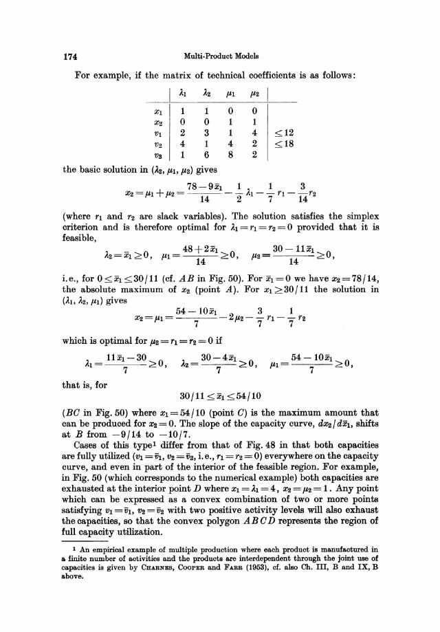
174 Multi-Product Models
For example, if the matrix of technical coefficients is as follows:
A1 A2 1-'1 1-'2
Xl 1 1 0 0 X2 0 0 1 1 VI 2 3 1 4 <12 V2 4 1 4 2 <18 Vs 1 6 8 2
the basic solution in (A2' 1-'1, 1-'2) gives
7S-9x1 1 1 3 X2 = 1-'1 + 1-'2 = - A1 - - r1 - ~r2
14 2 7 14
(where r1 and r2 are slack variables). The solution satisfies the simplex criterion and is therefore optimal for A1 = r1 = r2 = 0 provided that it is feasible,
30-11x1 0 1-'2= 14 >,
i.e., for 0<X1 <30/11 (cf. AB in Fig. 50). For X1=0 we have x2=78/14, the absolute maximum of X2 (point A). For Xl;;::: 30 /11 the solution in (A1' A2, 1-'1) gives
which is optimal for 1-'2 = rl = '2 = 0 if
l1Xl-30 A2= 30- 4x1 ........ 0 , AI= 7 ;;:::0, 7 c::::.:
that is, for 30/11 <Xl <54/10
(BO in Fig. 50) where xl=54/10 (point 0) is the maximum amount that can be produced for xs=O. The slope of the capacity curve, dxs/dxl, shifts at B from -9/14 to -10/7.
Cases of this type l differ from that of Fig. 48 in that both capacities are fully utilized (Vl =ih, Vs =V2, i.e., r1 = r2 =0) everywhere on the capacity curve, and even in part of the interior of the feasible region. For example, in Fig. 50 (which corresponds to the numerical example) both capacities are exhausted at the interior point D where Xl = Al = 4, Xs = 1-'2 = 1. Any point which can be expressed as a convex combination of two or more points satisfying Vl = Vl, Vs = V2 with two positive activity levels will also exhaust the capacities, so that the convex polygon AB 0 D represents the region of full capacity utilization.
1 An empirical example of multiple production where each product is manufactured in a finite number of activities and the products are interdependent through the joint use of capacities is given by CliARNES, COOPER and FARR (1953), cf. also Ch. m, B and IX, B above.
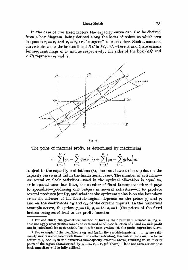
Linear Models 175
In the case of two fixed factors the capacity curve can also be derived from a box diagram, being defined along the locus of points at which two isoquants Xl = Xl and X2 = X2 are "tangent" to each other. Such a contract curve is shown as the broken line AB 0 in Fig. 51, where A and 0 are origins for isoquant maps of Xl and X2 respectively; the sides of the box (A Q and A P) represent VI and V2.
FIg. 61
The point of maximal profit, as determined by maximizing
z~ ,~(P1-,~ ql.,,) A, + .~,(P2 -,~ q1b .. ),,,
subject to the capacity restrictions (8), does not have to be a point on the capacity curve as it did in the limitational case l . The number of activitiesstructural or slack activities-used in the optimal allocation is equal to, or in special cases less than, the number of fixed factors; whether it pays to specialize-producing one output in several activities-or to produce several products jointly, and whether the optimum point is on the boundary or in the interior of the feasible region, depends on the prices Pi and q, and on the coefficients a'i and bu of the current inputs2. In the numerical example above, the prices PI = 12, P2 = 15, q3 = 1 (the prices of the fixed factors being zero) lead to the profit function
1 For one thing, the geometrical method of finding the optimum illustrated in Fig. 48 does not apply since profit z cannot be expressed as a linear function of Xl and X2; unit profit can be calculated for each activity but not for each product, cf. the profit expression above.
2 For example, if the coefficients an and bl2 for the variable inputs va, ... , Vm are suffi· ciently small (as compared with those in the other activities), the best solution may be to use activities Al and #2 in the numerical two-capacity example above, resulting in an interior point of the region characterized by VI = fiI, V2 = f2 (cf. above).-It is not even certain that both capacities will be fully utilized.
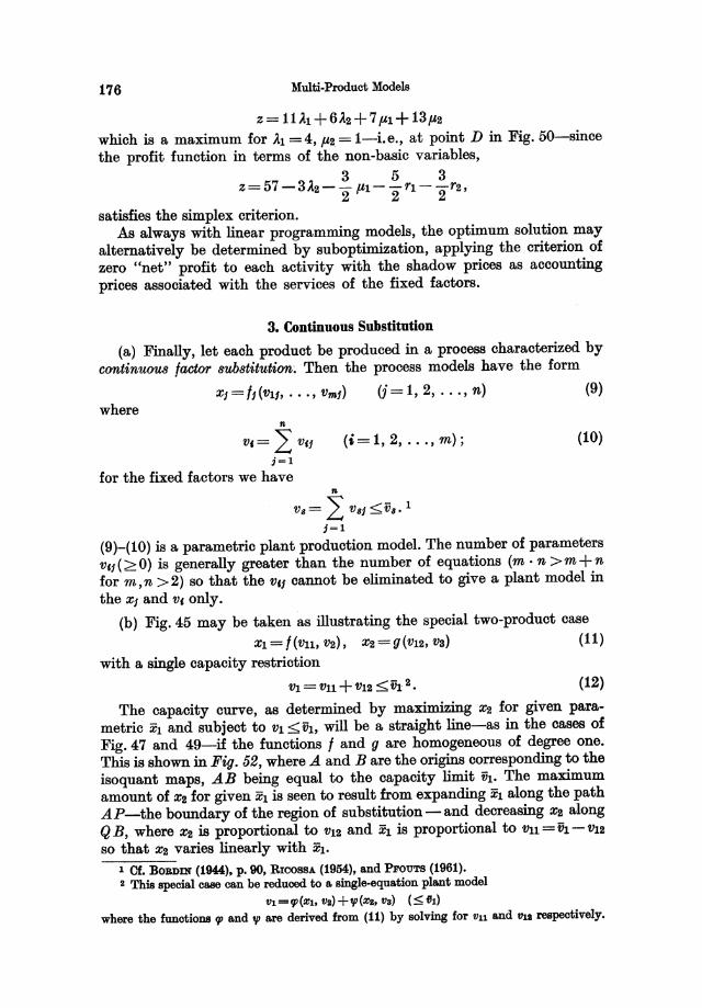
176 Multi-Product Models
Z= 11Al+6la+7 Pl+13ps which is a maximum for Al =4, ps = 1-i.e., at point D in Fig.50-since the profit function in terms of the non-basic variables,
3 5 3 Z = 57 - 3As - 2 Pl- 2 rl - 2 rs ,
satisfies the simplex criterion. As always with linear programming models, the optimum solution may
alternatively be determined by suboptimization, applying the criterion of zero "net" profit to each activity with the shadow prices as accounting prices associated with the services of the fixed factors.
3. Continuous Substitution
(a) Finally, let each product be produced in a process characterized by continuous factor substitution; Then the process models have the form
XI=ft('fJJ.I"",Vml) (i=1,2, ..• ,n) (9) where
n
'11,= 2: Vf, i-1
for the fixed factors we have
(i=1,2, ••• ,m);
n
'11,= 2: VB,~VB.l j=1
(10)
(9)-(10) is a parametric plant production model. The number of parameters Vf'(~O) is generally greater than the number of equations (m. n >m+n for m,n >2) so that the '11'1 cannot be eliminated to give a plant model in the XI and v, only.
(b) Fig. 45 may be taken as illustrating the special two-product case XJ.=f(V11,VS), XS=g(VlS,Va) (11)
with a single capacity restriction
'111= '1111 + VIS <V1 S ' (12)
The capacity curve, as determined by maximizing Xs for given para.metric Xl and subject to VI ::;;: Vl, will be a straight line-as in the cases of Fig. 47 and 49-if the functions f and g are homogeneous of degree one. This is shown in Fig. 62, where A and B are the origins corresponding to the isoquant maps, AB being equal to the capacity limit iiJ.. The maximum amount of Xs for given Xl is seen to result from expanding Xl along the path AP-the boundary of the region of substitution - and decreasing Xs along Q B, where Xs is proportional to 'fJJ.s and XI is proportional to 'fJJ.l = iiJ. - 'fJJ.2 so that Xs varies linearly with Xl.
1 Of. BOBDIN (1944). p. 90. RIooSBA. (1954). a.nd ProUTS (1961). I This special case can be reduced to a single-equation plant model
fJJ.=9'(:IlJ.. fJlI) +tp(zs. tIa) (~t11l where the functions 9' and tp are derived from (11) by solving for till and till respectively.
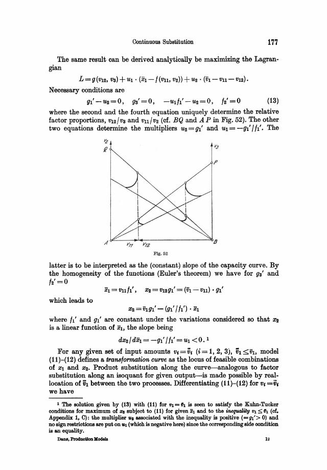
Continuous Substitution 177
The same result can be derived analytically be maximizing the Lagrangian
L = g (V1Z, Va) + U1 . (Xl - / (Vll, va)) + Uz • (ih - Vll- V1Z).
Necessary conditions are
gl'-Uz=O, ga'=O, -u1h'-ua=0, /a'=O (13)
where the second and the fourth equation uniquely determine the relative factor proportions, v1a/va and vulva (cf. BQ and AP in Fig. 52). The other two equations determine the multipliers Uz =gl' and U1 = -g1' I h'. The
Fig. 62
latter is to be interpreted as the (constant) slope of the capacity curve. By the homogeneity of the functions (Euler's theorem) we have for ga' and /a'=O
which leads to Xa = thg1' - (gl' / h') • Xl
where h' and gl' are constant under the variations considered so that Xl! is a linear function of Xl, the slope being
dxz/dx1= -gl'/h'=U1 <0. 1
For any given set of input amounts v, =v, (i = 1,2,3), V1 ~ih, model (11)-(12) defines a trans/ormation curve as the locus of feasible combinations of Xl and X2. Product substitution along the curve-analogous to factor substitution along an isoquant for given output-is made possible by reallocation of iit between the two processes. Differentiating (11}-(12) for v, =v, we have
1 The solution given by (13) with (11) for tl1=fJt is seen to sa.tisfy the Kuhn-Tucker oonditions for maximum of Zt subject to (11) for given Xl and to the inequality til:$; fJt (of. Appendix 1, 0): the multiplier Us &S8Ociated with the inequa.Iity is positive (=gt'> 0) a.nd no sign restrictions a.re put on "1 (which is negative here) since the corresponding side oondition is an equa.Iity.
D&IIlJ. ProduoUon )locIeIs
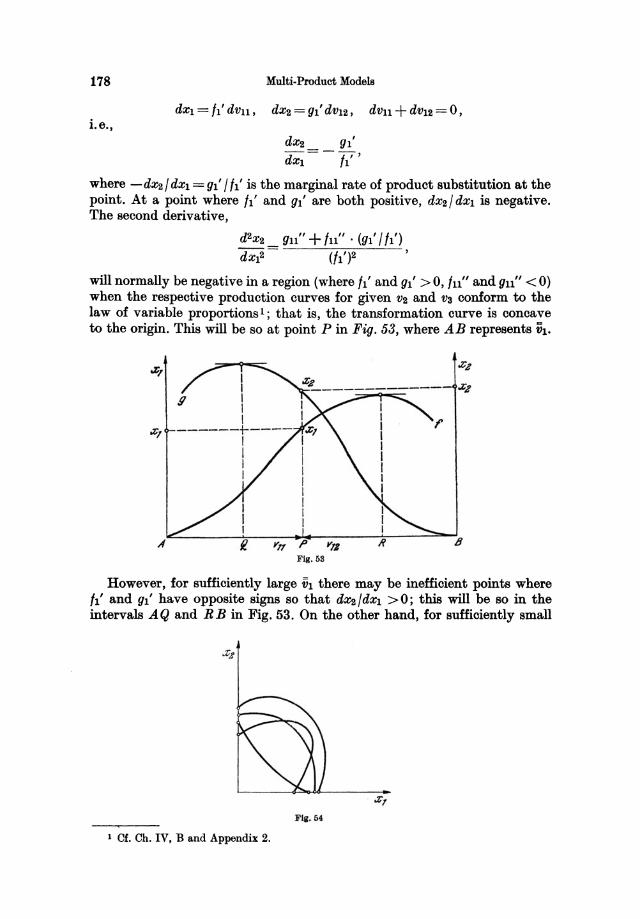
178 Multi-Product Models
i.e., dX2 gl' dXl - -7['
where -dX2/ dXl = gl' / /I' is the marginal rate of product substitution at the point. At a point where h' and gl' are both positive, dX2/ dXl is negative. The second derivative,
d2x2 gn" + In" . (gl' / /I') dX12 - (/1')2
will normally be negative in a region (where /I' and gl' > 0, /n" and gn" < 0) when the respective production curves for given V2 and Va conform to the law of variable proportions 1 ; that is, the transformation curve is concave to the origin. This will be so at point P in Fig. 53, where AB represents VI.
A·~------~--~~~--~----~----~~B
Fig. 68
However, for sufficiently large VI there may be inefficient points where /I' and gl' have opposite signs so that dX2/dxl >0; this will be so in the intervals AQ and RB in Fig. 53. On the other hand, for sufficiently small
F ig. 64
1 Cf. Ch. IV, B and Appendix 2.
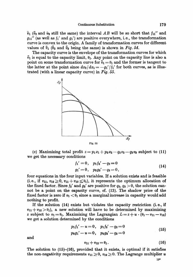
Continuous Substitution 179
VI (va and Vs still the same) the interval AB will be so short that lu" and gu" (as well as /I' and gl') are positive everywhere, i.e., the transformation curve is convex to the origin. A family of transformation curves for different values of VI (V2 and vs being the same) is shown in Fig. 54.
The capacity curve is the envelope of the transformation curves for which VI is equal to the capacity limit, th. Any point on the capacity line is also a point on some transformation curve for VI = ih and the former is tangent to the latter at the point since dxa / dXI = -gl' / /I' for both curves, as is illustrated (with a linear capacity curve) in Fig. 55.
FIg. 66
(c) Maximizing total profit Z=PIXI +Paxa-qav2-qsvs subject to (11) we get the necessary conditions
/I' =0, Pl/a'-qa=O (14)
gl' =0, Pags' -qs=O,
four equations in the four input variables. If a solution exists and is feasible (i. e., if Vu, V12 > 0, Vu + VIa ~ iit), it represents the optimum allocation of the fixed factor. Since /2' and gs' are positive for qa, qs > 0, the solution cannot be a point on the capacity curve, cf. (13). The shadow price of the fixed factor is zero if VI < ih since a marginal increase in capacity would add nothing to profit.
If the solution (14) exists but violates the capacity restriction (i. e., if Vu + VIa >ih), a new solution will have to be determined by maximizing Z subject to VI = th. Maximizing the Lagrangian L = Z + u . (th - Vu - V12)
we get a solution determined by the conditions
and
PIlI' -u=O, PI/2' -qa=O
Pagl' -u=O, Pags' -qs=O
vu+ vI2=ii}.
(15)
(16)
The solution to (15)-(16), provided that it exists, is optimal if it satisfies the non-negativity requirements Vu ~O, VIa >0. The Lagrange multiplier u
12-
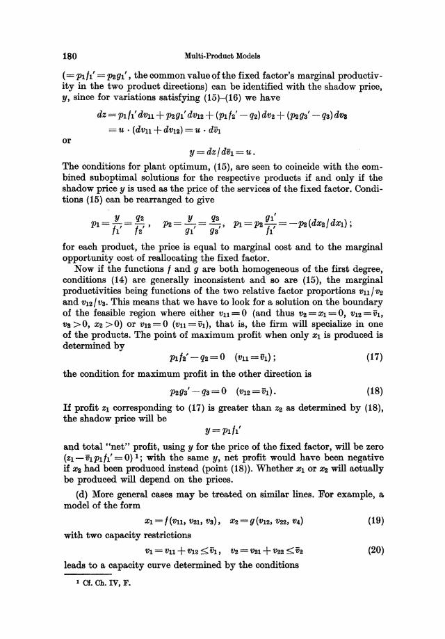
180 Multi-Product Models
(= Pl/1' = pag1' , the common value of the fixed factor's marginal productivity in the two product directions) can be identified with the shadow price, y, since for variations satisfying (15)-(16) we have
or
dz = P1/1' dV11 + pag1' dV12 + (P1/2' - q2) dV2 + (pagS' - qs) dva
= u - (dvll + dV12) = u - d;h
y = dz / d;h = u_
The conditions for plant optimum, (15), are seen to coincide with the combined suboptimal solutions for the respective products if and only if the shadow price y is used as the price of the services of the fixed factor. Conditions (15) can be rearranged to give
y q2 Y qs gl' / P1 = h' = 12" pa = gl' = gS" P1 = P2 /1' = -pa (dX2 dX1);
for each product, the price is equal to marginal cost and to the marginal opportunity cost of reallocating the fixed factor.
Now if the functions I and g are both homogeneous of the first degree, conditions (14) are generally inconsistent and so are (15), the marginal productivities being functions of the two relative factor proportions Vll / V2 and V12 / Vs. This means that we have to look for a solution on the boundary of the feasible region where either V11=O (and thus V2=X1=0, V12=V1, va >0, X2>0) or V12=0 (V11=V1), that is, the firm will specialize in one of the products. The point of maximum profit when only Xl is produced is determined by
Pl/2' -q2=0 (v11=ih); (17)
the condition for maximum profit in the other direction is
pags' -qs=O (V12=V1). (i8)
If profit Zl corresponding to (17) is greater than Z2 as determined by (18), the shadow price will be
y = P1/1'
aI),d total "net" profit, using y for the price of the fixed factor, will be zero (zl-ihp1/1' =0) 1; with the same y, net profit would have been negative if X2 had been produced instead (point (18». Whether Xl or X2 will actually be produced will depend on the prices.
(d) More general cases may be treated on similar lines. For example, a model of the form
x1=/(Vll, V21, vs), X2=g(V12, V22, V4)
with two capacity restrictions
V1 = V11 + V12 < V1 , V2 = V21 + VS2 < vs leads to a capacity curve determined by the conditions
1 Cf. Ch. IV, F.
(19)
(20)
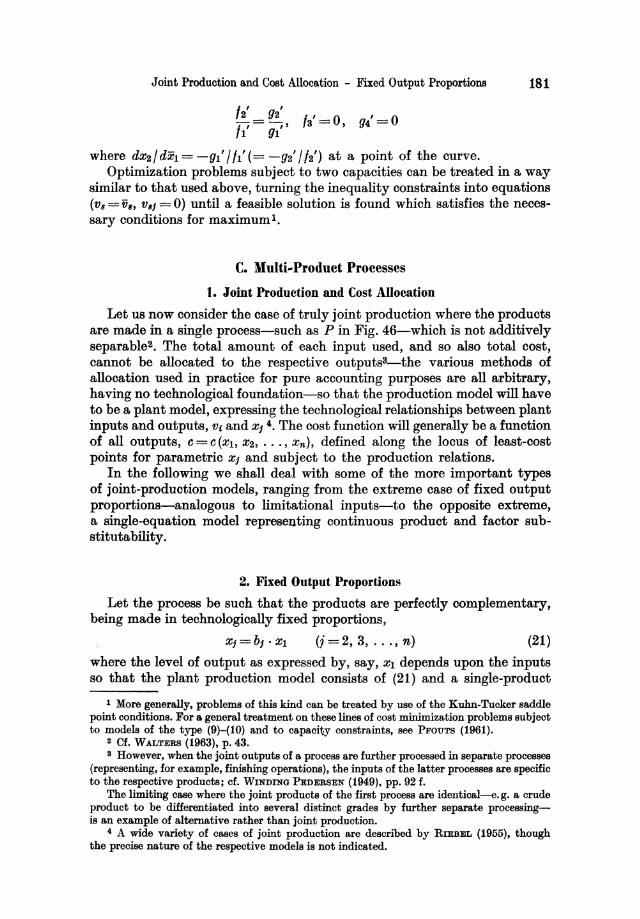
Joint Production and Cost Allocation - Fixed Output Proportions 181
f ' , ~ = gs. fa' = o. gl = 0 /I' gl'
where dxs / dXl = -gl' / ft' (= -gS' / Is') at a point of the curve. Optimization problems subject to two capacities can be treated in a way
similar to that used above. turning the inequality constraints into equations (V8 = V,. V'I = 0) until a feasible solution is found which satisfies the necessary conditions for maximum l .
c. Multi-Product Processes
1. Joint Production and Cost Allocation
Let us now consider the case of truly joint production where the products are made in a single process-such as P in Fig. 46-which is not additively separables. The total amount of each input used. and so also total cost. cannot be allocated to the respective outputsa-the various methods of allocation used in practice for pure accounting purposes are all arbitrary. having no technological foundation-so that the production model will have to be a plant model. expressing the technological relationships between plant inputs and outputs. Vi and Xi '. The cost function will generally be a function of all outputs. c = C (Xl, xs • ... , xn). defined along the locus of least-cost points for parametric Xi and subject to the production relations.
In the following we shall deal with some of the more important types of joint-production models. ranging from the extreme case of fixed output proportions-analogous to limitational inputs-to the opposite extreme. a single-equation model representing continuous product and factor substitutability.
2. Fixed Output Proportions
Let the process be such that the products are perfectly complementary. being made in technologically fixed proportions.
xi=bi·Xl (i=2.3, ...• n) (21)
where the level of output as expressed by, say. Xl depends upon the inputs so that the plant production model consists of (21) and a single-product
1 More generally, problems of this kind can be treated by use of the Kuhn-Tucker saddle point conditions. For a general treatment on these lines of cost minimization problems subject to models of the type (9)-(10) and to capacity constraints, see PFOUTS (1961).
2 Cf. WALTERS (1963), p. 43. 3 However, when the joint outputs of a process are further processed in separate processes
(representing, for example, finishing operations), the inputs of the latter processes are specific to the respective products; cf. WINDING PEDERSEN (1949). pp. 92 f.
The limiting case where the joint products of the first process are identical-e. g. a crude product to be diHerentiated into several distinct grades by further separate processingis an example of alternative rather than joint production.
4 A wide variety of cases of joint production are described by RIEBEL (1955), though the precise nature of the respective models is not indicated.
182 Multi-Product Models
model in Xl and the v,. The latter model may be characterized by continuous substitution, or the v, may be proportional to Xl so that the model consists of a single activity; other models are also possible I. In any case, the transformation curve for any given (feasible) factor combination will be a point in product space, cf. point P in Fig. /56. It is possible to get any combination on AP or P B (or in the interior of the rectangle OAP B) by producing the combination P and allowing some of Xl or Xz to go to waste (or destroying it)2. However, since the output variables Xl and X2 are defined as quantities actually produced, AP B is not the transformation curve belonging to (21); only point P belongs to the production model3 •
(J B
Fig. 56
Whatever kind of model connects Xl with the Vt, the multi-product model of the plant can be treated as a single-output case in these m + 1 variables, only the price associated with Xl (revenue per unit of Xl) becomes
3. Linear Models
Now if there is more than one linear activity which produces the n products jointly, the model will be of the form
N
Xj= L bjkAk
k=1
N
v,= L atkAk
k~l
(j=1, 2, ... , n)
(22)
(i=1, 2, ... , m)
where the relative output proportions Xj I Xl (j = 2, 3, .•. , n), as well as the relative factor combination, can be varied within limits by varying the ratios
1 Of. Chs. III-VI. 2 Of. SCHMIDT (1939), pp. 288 f. 3 Cf. the analogous problem whether the isoquants are L-shaped or single points in cases
of limitational inputs (Ch. III, A).
Continuous Product a.nd Factor Substitution 183
of the (non-negative) activity levels A.t (k= 1,2, ... , N) as illustrated by the two-product, four-activity case of Fig. 57. The feasible product region is bounded by the two extreme activity half-lines and by the capacity curve, which will be a broken line. In Fig. 57, VI =ih at A, B, G, and D and on the segments connecting them, whereas the second capacity factor is fully utilized at E, F, G, and H; the capacity curve-the locus of maximum X2 for given parametric Xl and for VI <th, V2 ~ii2-will be AP FQH . I
FIB. 57
The point where total profit z-a linear function of the activity levels A.t-is a maximum subject to two capacity restrictions will generally be characterized by two positive activity levels (not necessarily both structural)2. It does not have to be a point on the capacity curve; for example, the activity through G may be used in the optimal solution if it has sufficiently small input coefficients for the variable inputs.
4. Continuous Product and Factor Substitution
(a) The "classical" model of joint production is the production function
(23)
an obvious generalization of the single-product model x = x (VI, V2, ••• , Vm)3.
1 Point G is not on the capacity curve since both Xl and Xz are greater at Q, which represents a convex combination of F and H.-Note, however, that G cannot be dismissed as inefficient: Q is "better" than G with respect to the factor vz, but it is quite possible that it uses more of other (variable) inputs not specified in the figure. The concept of inefficiency applies to transformation curves, not to capacity curves.
2 Even if only one structural activity level is positive in the optimum solution, both products will be made (except in the special case where one of the output coefficients in the activity is zero so that the activity half-line coincides with one of the axes). The activities may be said to be alternative in the above sense but the product8 are not.
S For modem treatments see, for example, CARLSON (1939), Ch. 5; HICKS (1946), Ch.6 with Appendix; DORFMAN (1951), Ch. 1; and ALLEN (1956), Ch. 18, 2.
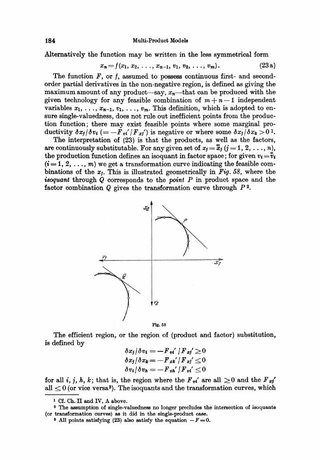
184 Multi-Produot Model!
Alternatively the function may be written in the less symmetrical form
Xn = t (Xl. X2, ... , Xn-I, VI, V2, ••• , vm). (23 a)
The function F, or t, assumed to possess continuous first- and secondorder partial derivatives in the non-negative region, is defined as giving the maximum amount of any product-say, xn-that can be produced with the given technology for any feasible combination of m + n - 1 independent variables Xl, ••• , Xn-l, VI, ••• , Vm • This definition, which is adopted to ensure single-valuedness, does not rule out inefficient points from the production function; there may exist feasible points where some marginal productivity lJ XI /lJ v, (= - F vt' / F xl) is negative or where some lJ XI /lJ Xk > 0 1.
The interpretation of (23) is that the products, as well as the factors, are continuously substitutable. For any given set of XI = XI (j = 1, 2, ... , n), the production function defines an isoquant in factor space; for given v, = ti, (i = 1,2, ... , m) we get a transformation curve indicating the feasible combinations of the XI. This is illustrated geometrically in Fig. 58, where the isoquant through Q corresponds to the point P in product space and the factor combination Q gives the transformation curve through P 2.
FIg. 58
The efficient region, or the region of (product and factor) substitution, is defined by
lJXI/lJv, = -F vt' / F x/ ~O lJxI /lJXk= -F xk' / F xl <0 lJ v, /lJ Vh = - F vh' / F vc' < 0
for all i, j, h, k; that is, the region where the F v" are all ~O and the Fxl all ~ 0 (or vice versa3). The isoquants and the transformation curves, which
1 Cf. Ch. IT and IV, A above. 2 The assumption of single-valuedness no longer precludes the interseotion of isoquants
(or transformation ourves) as it did in the single-produot case. 8 All points satisfying (23) also satisfy the equation - F = o.
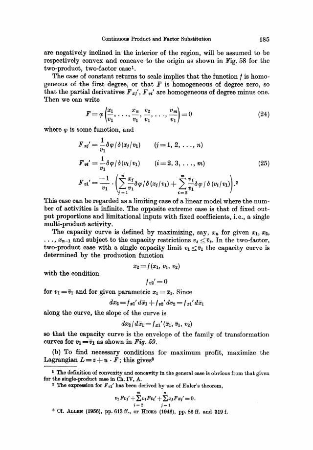
ContinuouB Product and Factor Substitution 185
are negatively inclined in the interior of the region, will be assumed to be respectively convex and concave to the origin as shown in Fig. 58 for the two-product, two-factor case l .
The case of constant returns to scale implies that the function I is homogeneous of the first degree, or that F is homogeneous of degree zero, so that the partial derivatives F x/, F vi' are homogeneous of degree minus one. Then we can write
(Xl Xn V2 vm)
F = qJ VI"'" VI ' VI' •.. , v;:- = 0 (24)
where qJ is some function, and
(j = 1,2, ... , n)
FtIi'=~dqJ/d(V(/Vl) (i=2,3, ... ,m) (25) VI
, -1 (In Xi Im Vt ) FVl =-. -dqJ/d(Xi/VI)+ -dqJ/t5(V'/Vl).2 VI VI VI
;=1 i=2
This case can be regarded as a limiting case of a linear model where the number of activities is infinite. The opposite extreme case is that of fixed output proportions and limitational inputs with fixed coefficients, i.e., a single multi-product activity.
The capacity curve is defined by maximizing, say, Xn for given Xl, X2, ••• , Xn-l and subject to the capacity restrictions VS <V8' In the two-factor, two-product case with a single capacity limit VI <VI the capacity curve is determined by the production function
X2 = I (Xl, VI, V2) with the condition
Ivz' =0
for VI = VI and for given parametric Xl = Xl. Since
dX2 = I zl' dXl + IV2' dvz = I xl' dXl
along the curve, the slope of the curve is
dX2/ dXl = I xl' (Xl, VI, vz)
so that the capacity curve is the envelope of the family of transformation curves for VI =ii} as shown in Fig. 59.
(b) To find necessary conditions for maximum profit, maximize the Lagrangian L = z + u . F; this gives3
1 The definition of convexity and concavity in the general case is obvious from that given for the single-product case in Ch. IV, A.
2 The expression for Fvl' has been derived by use of Euler's theorem, m n
v1Fv!' + ~v,Fvi' + ~xJFx/ = O. i=2 j=l
3 Cf. ALLEN (1956), pp. 613 ff., or HICKS (1946), pp. 86 ff. and 319 f.
186 Multi-Product Models
pj+U .Fz/=O
-qf +U. Fflt' =0
Fig, 59
(j=1,2"",n)
(i= 1,2"", m)
(26)
(27)
(where the prices of the capacity factors are zero), If a solution to (23) and (26)-(27) exists and is feasible-i. e" if it is non-negative and respects the capacity constraints Vs ~v8-it represents the point of optimum allocation!, (26)-(27) can be rearranged to give
pj= F 'IF' (i=1, 2"", m; j=1, 2"", n), (28) flf zl
that is, for each particular product the price is equal to the partial marginal cost in every factor direction; it is also equal to marginal opportunity cost in every product direction,
(j, k=1, 2, ... , n). (29)
At the optimum point the slope of the tangent to the transformation curve (the marginal rate of product substitution) is equal to the price ratio,
PIIPk= -dxkldxl (j, k= 1,2, . , "n),
and similarly for the marginal rate of substitution on the isoquant we have
(i, h= 1,2, ... , m).
The same results could have been obtained by first minimizing cost for given parametric Xj, thus determining the joint cost function c = C (Xl, ... , xn ), and next maximizing total revenue minus cost. Minimizing the Lagran-
gian L= 2>fVf-U' F for given xl=Xj we get (27) above: , ql-U' F fl / =0;
since at a point on the expansion path satisfying these conditions and the production function we have
1 Sufficient second-order conditions are given by ALLEN and HICKS, loco cit, These stability conditions are automatically satisfied and ensure a unique maximum if the isoquants are convex and the transformation curves are concave,
Continuous Product and Factor Substitution 187
de = L q, dv, = u . L F vi' dv, = - u . L F:e/ dXj i i ;
it follows that -uF:e/ is the partial marginal cost of product no. i along the expansion path,
e/ =~e/~xl= -uF:e/.
At the point of maximum profit we must have
pj-e/=O (i=1, 2, ... , n)
which leads to conditions (26)1. Now if the production function F is homogeneous of degree zero, there
exists no solution to conditions (26)-(27) and the production function (23) since there are m + n + 1 equations in m + n variables, u / VI and the m + n -1 relative proportions Xj/Vb V,/Vl (i =2,3, ... , m)2. In order to get a solution the capacity restrictions will have to be taken explicitly into account. With a single capacity limit, maximize the Lagrangian L = z + u . F for Vl = th. This leads to conditions similar to (26)-(27), except that we have got rid of the first equation of (27) so that the system is no longer overdetermined. With this modification the interpretation of the optimum solution is similar to that given above3•
The solution implicitly determines the shadow price of the fixed factor, y. For arbitrary variations in the Xj and V, we have
n m
dz= L PI dXj - 2: q,dv,; ;=1 i=2
if the variations are to satisfy the production function (23) in differential form for VI = ih,
n m
2: F:e/ dXj+FvI' dih + 2: F"t'dv(=O ;=1 i=2
(where dih is a marginal increase in the fixed factor's capacity) as well as the optimum conditions (26)-(27) for i = 2, 3, ... , m, this reduces to
dz=u· F"l' . dih so that
y=u· F"l'.
1 STACKELBERG (1932), p.63, who does not specify the underlying production function, defines an expansion path in product space as the locus of tangency between cost and revenue indifference curves.
I The situation is quite analogous to that of profit maximization under a linear·homogeneous single-output production function, cf. Ch. IV, E-F.
3 For positive factor prices the optimum solution is not a point on the capacity curve; by (28) the marginal productivities of the variable inputs are positive (6xm/6Vj=qjfpm> 0) whereas 6Xmf6Vj=0 on the capacity curve (taking Xm as the dependent variable). The opti. mum solution is a point on a transformation curve where VI = VI, but it is not the point where the curve touches the envelope. This is analogous to profit maximization subject to a singleoutput production function and to a capacity restriction VI S VI, cf. Ch. IV, F above. A point where the capacity of the fixed factor is fully utilized (VI = VI) does not necessarily represent maximum output, x=xmax.
188 Multi-Product Models
Since, by (26), u= -pjIFz/ (1=1,2, ... , n), it follows that
Y=pj' (~Xj/~'fh),
that is, the shadow price-the marginal contribution to profit of an increase in ih-is equal to the value of the marginal productivity of '171 in every product direction. Alternatively, by (27) we get
y=-q"(~V,/~ih) (i=2,3, ... ,m) so that the tangency conditions for the isoquant are satisfied for all pairs of inputs if the shadow price is applied to the services of the fixed factor. Using this price, the marginal conditions (27) and (28) are satisfied also for i = 1; any other price will lead to an inoptimal allocation.
By the homogeneity of the function F (Euler's theorem) we have n m L xjFzl + fhFtll ' + L v,Ff),' =0,
;=1 i=2
which with conditions (26)-(27) (i=2, 3, ... , m; 1=1, 2, ... , n) leads to n m L pjXj-u· V· Ff)l' - L q,v,=O
;=1 i=2 where
uVlF til' = yVl
is the total imputed value of the fixed factor's services; using the shadow price, total "net" profit is zerol.
5. Shadow Products
Finally, let us assume that there is a separate production function for each output in terms of the same inputs,
Xj=!j(Vl,V2, ... ,Vm) (j=1,2, ... ,n).2 .(30) A model of this kind 3 implies that the output proportions xiI Xl (1 = 2, 3, ... , n) can be varied only through variations in the factor combination: the transformation curve for given v, = V, is a single point in product space but the position of the point depends on the parameters v,. Conversely, for given values of the Xj there are n equations in the v, so that the model is characterized by constrained factor substitution (for n < m)4. Considering Xl as the primary product, the other products X2, ••• , Xn may be regarded as "shadow products", by analogy with the case of shadow factors5•
1 Cpo the analogous result in the single-product case (Ch. IV, F above). 2 Cpo the above case of alternative production with continuous substitution, where the
total amount of each input v, can be allocated to the separate inputs (Vj=LVil)' ;
3 Models of this type have been treated by ALLEN (1938), p.350 (Example 39), and FRISCH (1953), pp. 39 fi.
e Of. Ch. V, B above. II Cf. Ch. V, A above. In the general case (30) the position of the XI in the model is analo
gous to that of product shadows; the case of fixed output proportions-(21) above-represents the special case fl=bl/1 (j=2, 3, ... , n) where the b1 are constants, resembling models with factor shadows.
The General Joint-Production Model 189
The optimum allocation is determined by the production functions (30) and the conditions for maximum profit,
n lJ 11 2: PI lJv( -q, = 0 (i = 1,2, - .. , m), (31) j=1
or by maximizing z = 2>j xI - C (Xl, ..• , xn) where the partial marginal j
costs c/ can be identified with Lagrange multipliers Uj used in minimizing total cost for given parametric Xj, the least-cost conditions being
n lJ 11 q,- "" Uj-=O ~ lJVt
j=1
(i = 1, 2, ... , m)
so that m m n lJl n
dc= 2: q,dv, = 2: 2: UllJ~, dv, = 2: Uj dXI· ;=1 i=lj=1 j=1
6. The General Joint-Production Model
From a formal point of view, most of the above models of joint production can be thought of as special cases of a general model 1
(k=l, 2, ... , M <m+n) (32)
where the number of degrees of freedom, N = m + n - M, is crucial to the possibilities of product and factor substitution. The extreme cases are M = 1, i.e., a model with continuous product and factor substitution (m+n-1 independent variables), and M =m+n-1 (N = 1), the case of joint production with fixed output proportions and limitational inputs.
Intermediate models where 1 < M < m + n - 1 can be rewritten to give M dependent variables in terms of the m + n - M independent variables (inputs and outputs). For example, a model with factor substitution and fixed output proportions-cf. (21) above-represents a case where M =n and the equations have a special form which makes it possible to eliminate the input variables from all but one equation. A model with shadow products such as (30). also characterized by M = n, permits each output to be expressed in terms of the m inputs2.
More generally, the model can be written in parametric form, each input and output variable being a function of m + n - M independent parameters. The cases which have just been discussed can all be written in this form, using a set of input variables for parameters, but the parametric type of model is the more general in that it also includes the linear discontinuoussubstitution models where the activity levels serve as parameters.
1 Of. HENDERSON (1950), pp. 299 f., and (1953), p. 157; RICossA (1955); STACKELBERG (1938), pp. 81 f.; Roy (1950), pp. 50 f.; and FRISCH (1953), pp. 38 ff.
2 FRISCH (1953), pp. 38 ff., has given an instructive classification of the various possible cases, based on the relative magnitudes of m, n, and M and the specific structure of the equations.
Appendix 1
Constrained Maximization
A. Lagrange's Method of Undetermined Multipliers
(a) The typical problem of economic optimization is that of maximizing (or minimizing) some objective function-for example, total cost or total profit-subject to one or more side conditions in the same variables.
Let g (Xl, X2, ... , xn) be the function to be maximized subject to m constraints
Ih(XI, X2, •.. , xn)=O (h=1, 2, ... , m) (1)
where m < n and where g and the 116 are assumed to be differentiable functions. In principle, we can always reduce a problem of this type to the maximization of a function of n - m independent variables, eliminating m dependent variables from the function g by means of equations (1), and set the partial derivatives equal to zero. This method presents no difficulties in the special case where each of the equations (1) gives a particular variable as an explicit function of n-m independent Xc (the same in all equations)!. In the more general case, the process of elimination is less easy to handle and some other method must be resorted to.
(b) A simple procedure, which has the added advantage of treating all variables in a symmetrical manner, is provided by the classical method of undetermined multipliers2, due to LAGRANGE. This method may be assumed to be well-known and a brief summary of the basic principle will suffice.
Form the Lagrangian expression m
L = g (Xl, X2, ••• , Xn) + L: uhlh (Xl, X2, .•• , Xn) II =1
where UI, U2, ••• , Um are provisionally undetermined constants. Then the problem of maximizing the function g subject to (1) is equivalent to that of finding an unconstrained maximum of L, treating Xl, X2, ••• , Xn as independent variables. The necessary condition for a maximum is that the firstorder differential vanishes:
I For example, if profit z = px - ql VI - qavs - ••• is to be maximized subjeot to a produotion funotion X=X(VI, Vs, ••• ), the obvious prooedure is to take the inputs VI, Va, ••• as
independent variables, substituting the production funotion in the profit expression, whioh is then maximized with respect to the input variables.
2 See e.g. OSGOOD (1925), pp. 180 ff.; ALLEN (1938), pp.364-367 and 498-500; and SAMUELSON (1947), pp. 362-379.
Lagrange's Method of Undetermined Multipliers
11 l'JL dL= "Y __ dx,=O,
~ l'Jx, i=l
i. e., that the partial derivatives of the Lagrangian L vanish:
~L = ~g + ~ Uh~/h=O (i=1, 2, ••. , n). uXt uX, ~ uX,
h=l
191
(2)
Under "normal" conditions the n equations (2) together with the m equations (1) determine Xl, Xa, ••• , Xn and Ul, Ua, ••• , Um uniquely. If we are not interested in the values of the multipliers Uh, we can eliminate them so that we are left with n equations which determine the X,. The latter system of equations is easily shown to be identical with the set of necessary maximum conditions obtained if g is reduced to a function of n - m independent variables; hence the two methods of constrained maximization are equivalent!. These methods are particularly well suited for the optimization problems of neoclassical economic theory, where the equilibrium positions are typically characterized by marginal equalities-geometrically interpretable as "tangency" conditions-derived from solutions of the form (2).
(c) The same necessary conditions apply if we are looking for a constrained minimum. In concrete problems, available additional information will frequently be sufficient to determine whether a point satisfying (1)-(2) is a maximum or a minimum. In the absence of such information, sufficient conditions in terms of second-order derivatives will have to be formulated.
For an unconstrained maximum "in the small" of the Lagrangian expression, the sufficient condition is
n n l'J2L d2L= 2: .2 l'Jx,l'Jxl dx,dx! <0
i=l;=l
for all variations in the neighbourhood which satisfy
n l'J /h d/h= .2 l'J x, dx, =0 (h=1, 2, ... , m).
1=1
(3)
For a local minimum, the inequality must be reversed. Thus a quadratic form in dXl, dXa, ••• , dXn is to be negative (positive) definite subject to a
1 In the simple case of m = 1, for a maximum of g subject to f = 0 we must have
dg=gl'dxl +g2'dx2+ ••. +gn'dxn =0 for all variations satisfying
df=/t'dxl+f2'dx2+ •.. +fn'dX,.=O. Eliminating e.g. dXl, we have with X2, ... , x" as independent variables
dg= (g2' - g{f2'//l')dx2 + ... + (gn' - gl'fn'//l')dxn =0. Alternatively, using a Lagrangian multiplier we get
dL= (gl' + u/l') dXl + (g2' +u/2')dX2 + ... + (gn' + uf,.')dXn =0. In either case we are led to the necessary condition
g{!f{=gl'//l' (i=2, 3, ... , n).
192 Constrained Maximization
number of linear restrictions, a criterion which can be shown to involve certain restrictions upon the signs of the principal minors of the determinant
tJ2L whose elements are --- "bordered" with the coefficients of the linear
tJXt tJXI
t . t· . tJ In res rIC IOns, I.e., .-. tJXt
For example, in the case of a single side condition I (Xl, X2, ••• , Xn) = 0 we have, treating u as a constant and all variables as independent,
from which n n
d2L= L L (gel' + ul,/')dx, dxl·
i=1j=1
This quadratic form is negative definite subject to the linear restriction
i=1
if and only if
o /1' /1' gu" + u lu" (_1)k
Ik' glk" + U Ilk" > 0
/k' gkl" + u /k1" . .. gu" + u /kk"
(k=2, 3, ... , n). (4)
For a minimum, where the quadratic form is to be positive definite, the determinants in (4) must all be negative l .
The sufficient condition (3), like the first-order conditions (2), can be shown to be equivalent to that derived from the maximization of g as a function of n - m independent variables,
d2g<O where
(h=l, 2, ... , m)2.
I Cf. ALLEN (1938), pp. 491 f. For a complete proof of the second-order conditions see BURGER (1955).
S In the case of only one side condition 1=0, let Xl be the dependent va.riable. Differentiating
where dxs, ••• , dx .. (but not dXI) are to be treated as constant, we have d2g = gil d 2xI + dXI (gu" dXI + ... + gl .. " dx .. ) + ...
. . . + dx" (g"l" dXl + . . . + g .... " dx,,)
where dl=O and thus also dSI = It' d2xl + dXl (f11" dXl + ... + /1,," dx .. ) + ...
. . . + dx.. (/ .. 1" dXl + ... + I .... " dx,,) = O.
Linear Programming and the Simplex Criterion 193
(d) The Lagrangian multipliers have an interesting interpretation relevant to many eoonomio optimization models 1• Let the side conditions be of the form
(h=1,2, ... ,m)
where the b/a are constants, i.e.,
!/a = b/a-F/a (Xl, Xs, .•. , Xn)=O.
The point at whioh the funotion g has a maximum or a minimum subject to the side oonditions is determined by (1)-(2). Now, what will be the effect on g of an infinitesimal change in one of the oonstant terms, say, b1 1
By (2) we have n n m lJF
dg= L g, dx, = L L 'U/a lJx: dx, i-I i=111=1
where the variations are to satisfy (1), i.e.,
n fJF1 " lJF/a ,- dx,=db1 and ,- dx,=O L., fJ x, L., fJ X, i=1 i=1
(h=2, 3, ..• , m).
Substituting, we get dg='Uldbl
whioh means that the marginal ohange in g with respeot to a partial ohange in one of the constant terms is equal to the Lagrangian multiplier assooiated with the oorresponding side oonditions. This result holds for any variation from a point satisfying (1)-(2), not only for a movement towards a new maximum (or minimum) position.
B. Linear Programming and the Simplex Criterion
(a) The applicability of Lagrange's method (or the equivalent method of elimination) is subject to three limitations, eaoh of whioh is serious in some eoonomio optimization models where the optimum point is not a "tangency"
Eliminating d2xl we get (of. ALLEN (1938), pp. 498 f. and 466)
" n dIg = ~ ~ (g,l' - /Il' gl' / h') dx, dXJ
;=lj=1
which is equal to dB L since, by the necessa.ry conditions,
u= -g1'/h'. Substituting this in (4), we get the necessary and sufficient conditions for dIg to be negative definite subject to df = 0, i. e., the sufficient conditions for a (local) maximum of g subject to the side condition 1=0.
1 Cf. SAMUELSON (1947), p. 132, and JOHANSEN (1962). 2 An important example with a single side condition is cost minimization for constant
value of a production function, where the Lagrangian multiplier can be interpreted as marginal cost for small arbitrary variations from the least-cost point. Another example is profit maximization subject to a capacity limitation (in the form of an equality); in this case, u represents the fixed factor's marginal contribution to profit, i.e., its shadow price.
Dans, Production Modell IS
194 Constrained Maximization
solution characterized by marginal equalities of the type (2) but a "boundary" or "comer" solution.
(i) In the first place, the method does not take account of the fact that economic variables are generally defined over the non-negative region. In other words, in addition to the side conditions 111 = 0 we also have nonnegativity requirements x, 2 O. There is nothing in the method to guarantee that these requirements are automatically satisfied. If a particular point as determined by (1)-(2) happens to respect them, all is well; if it does not, the maximum solution is not feasible, being devoid of economic meaning, and some other method has to be resorted to.
(ii) Second, if the functions g and 111 are all linear, the partial derivatives d g / d x, and dill / d x, are constant and the necessary conditions cannot be satisfied. This reflects the fact that a linear function (in this case, g as reduced to a function of n - m independent variables) has no finite maximum or minimum i-unless the variables are further constrained, for example, by non-negativity requirements, in which case we also run into the difficulty mentioned above.
(iii) In the third place, some or all of the side conditions in an economic optimization model may have the form of structural inequalitiess rather than equations, so that we have
!1I(Xl, Xs, ••• , xn) 20.
As with non-negativity requirements, we can always try the Lagrangian method, provisionally disregarding the structural inequalities, and hope for the best. But if it turns out that the solution does not respect them, the solution is not feasible and the method breaks down. Alternatively, we may resort to the device of transforming an inequality into an equation by introducing a "slack" variable XII' = til so that the inequality can be written
CPII (Xl, Xs, ••• , Xn, XII') = 111 (Xl, XS, ••• , Xn) - XII' = O.
However, the side condition in this form imposes no restriction on the variables Xl, Xs, ••• , Xn, being a mere definition of the additional variable, unless combined with the non-negativity requirement
XII' >0
1 As an example, take g=C1Xl+C2X2 subject to alxl+lI2x2=b. Condition (2) becomes Cl- al u=O, C2 -II2U=O
which cannot be satisfied simultaneously unless Cl/ al happens to be = C2/112, in which case we have
g=u(alXl +a2x2) =U· b=constant so that there is no question of maximization.
The meaning of this is seen more clearly if we try to solve the problem by elimination of the dependent variable, say, Xl. Solving the side condition for Xl and substituting in 9 we have .
g=clb/al + (C2 - Clll2/al)X2
which is a linear (i.e., steadily increasing or decreasing) function of the one independent variable Xa unless the coefficient of X2 happens to be zero to that 9 is constant.
a Capacity restrictions, for example, will generally be of this form.
Linear Programming and the Simplex Criterion 195
to ensure that the inequality I,,";?O is not reversed l • Again, we do not get very far without a method which can take non-negativity requirements into account.
(b) Such a procedure, applicable to the linear case, has been devised by DANTZIG2 under the name of the "simplex method".
Suppose we have the problem of maximizing a linear function
g = CIXI + C2XS + ... + C"x"
subject to m linear restrictions
1,,=a"lxI+a"2Xs+ .•• +a""xn-b,,=O (k=1, 2""J m) (5)
where the variables are required to be non-negative
x,>O (i=1,2, ... ,n). (6)
There is no loss of generality in assuming that the side conditions have the form of equations since linear inequalities can always be turned into linear equations by introducing slack variables as indicated above; in this case some of the x, must be interpreted as slack variables, x,,' having the coefficient 0 in the function g, 1 (or -1) in the k'th side condition, and 0 in all other side conditions, and the slack variables-like the "structural" variables-are required to be >0. Likewise, a minimum problem can be written in the same form since min g = max (-g). Thus, any problem of linear programming-i.e., the maximization or minimization of a linear function subject to linear constraints (equations and/or inequalities) and to non-negativity requirements-can be reduced to a problem of the type above.
Because of the linearity of the model, elimination of variables is a easy matter. Therefore, a procedure that suggests itseH is that of expressing g in terms of n - m independent variables, taking due account of (6). Taking Xl, X2, ... , Xm as dependent ("basic") variables, we solve the system of m side conditions (5)8 to get
" x,=if,- 2: XC/Xi
j-m+l
(i= 1,2, •.. J m) (7)
where if, and the coefficients X'I are constants depending on the a", and the b". Substituting in g we have
1 For example, the linear inequality
can be written as the equation alxl+asxS+x'=b
where x' = b - atXl - asXa ;:::: O. Had. the inequality been alxl+aszs;::::b,
the sla.ck variable would have had. the coefficient -1 in the equation. s Cf. DANTZIG (1951). 8 Assuming that the familiar conditions for a. unique solution to exist are satisfied.
IS·
196
where
and
Constrained Maximization
n
g=g- L XOjXJ, j=m+l
m
g = L CtXt i=l
m
XOj = L CtXij - Cj i=l
(8)
are constants depending upon the aM, bh, and Ct. Having thus expressed g as a linear function of the independent ("non-basic") variables, how are the XJ to be determined for maximum g?
The clue to this is provided by the fundamental theorem of linear programming, which says that, if the maximum problem can be solved, there exists a maximum solution in which at most m of the n variables are positive, i. e., at least n - m variables are zerol. One such "basic" solution is found by putting the n - m independent variables Xj equal to zero in (7)-(8):
Xt=Xi, Xj=O, g=g (i=1, 2, ... , m; i=m+1, ... , n). (9)
Let us assume that all Xi > O. (If this were not so, we would have to pick another basis of m dependent variables which satisfies this condition, and renumber the variables accordingly.) Then our basic solution is feasible: it satisfies the side conditions (of which (7) is merely an alternative form) and all of the n variables are non-negative. Whether or not it is also a maximum solution, depends on the signs of the coefficients -XOj in (8), the "simplex coefficients". If the XOj are all positive, i.e.,
~g -=-XOj<O ~Xj
(i=m+1, ... , n),
g is a decreasing function of the Xj. This means that, negative values of the Xj not being admissible, (7)-(8) gives a maximum solution for all Xj = 0: any positive Xj will give a smaller value of g. If one of the XOj is = 0, the corresponding Xj may be given a positive value (so long as this does not violate the requirement Xi >0, cfr. (7)) without the value of g being affected-i.e., the solution is not unique-but (9) is still an optimal solution. In other words,
~g -=-XOj<O (j=m+1, ... , n) (10) ~Xj
-a condition known as the "simplex criterion"-is a sufficient condition for the basic feasible solution (9) to represent a maximum2. (For a minimum,
1 For a simple proof (due to DAVlD GALE) see, for example, DAN0 (1960), pp. 104 f. For a geometric interpretation see op. cit., pp. 5-9.
2 Cf. the non-linear case without non-negativity requirements, where the maximum position is characterized by (Jg/(JXj being equal to zero when g has been expressed in terms of the independent variables Xj, see A above.
Linear Programming and the Simplex Criterion 197
the inequality must be reversed.) It is also a necessary condition provided that the basic variables are all strictly positive, Xf >0. Suppose that (9) is an optimal solution, positive in all X(, and that the criterion (10) is not satisfied, one of the XOi being negative. Then the solution can be improved by giving the corresponding Xi a small positive value, which is a contradiction. However, if there are zeroes among the Xf ("degeneracy"), this reasoning breaks down because it may not be possible to increase Xi except at the expense of an x, which is zero in the basic solution l .
If the solution (9) does not satisfy the simplex criterion, it does not represent a maximum (assuming all Xf >0) and another solution must be looked for. It is possible that a maximum solution in more than m positive variables exists, but the fundamental theorem tells us that it cannot yield a larger value of g than the best basic solution. Hence, in principle, the
problem can always be solved by testing each of the (:) basic solutions,
first for feasibility and next for optimality, using the simplex criterion.
However, (:) is a large number when m and n are not very small and the
procedure soon becomes impracticable. A short cut by which the computationallabour can be reduced very considerably is the iterative procedure known as Dantzig's simplex algorithm. Using an arbitrary basic feasible solution as a starting point, the procedure is to improve the solution by moving to a neighbouring basis-i.e., replacing one of the basic variables by an XJ whose XOi is negative--and so forth, until a solution is attained which satisfies the simplex criterion. If degeneracy does not occur, the procedure will always converge and a maximum solution is usually found in a few steps2. With a slight modification (due to CHARNES), the simplex method can also be used to deal with cases of degeneracy3.
In contrast to the Lagrange method (or the equivalent method of eliminating dependent variables), the simplex method is essentially a numerical procedure: while it provides a criterion by which a feasible solution can be tested for optimality when the values of the constants are known, as well as an iterative numerical procedure for determining an optimal solution, it cannot yield an analytical solution for the variables and for g in terms of the constants aM, b", and c,.
The optimum solution to a linear programming problem is a "corner" solution, geometrically represented by a corner point (in the case of multiple optima, several such points as well as all intermediate points) on the boundary of the feasible region as defined by (5)-(6) and characterized by equilibrium conditions in the form of marginal inequalities (the simplex criterion).
(c) In a linear economic model, it will often be of interest to examine in what way the optimum position is affected by changes in the parameters
1 By (7), if x( = 0 and ~xi/~Xi = -Xlj < 0 for some i, then the Xj in question cannot be increased from zero to a positive value (all other XJ still = 0) without making Xi negative, thus violating (6).
a For a simple exposition see DAN0 (1960), pp. 11-14, 65-74, and 107-109. 8 See, for example, op. cit., pp. 80-84.
198 Constrained Maximization
a"" b", or c, ("parametric linear programming"). Suppose, for example, that one of the right-hand terms in the side conditions (5)-say, bl-undergoes an infinitesimal change. What will be the effect on g1
Let us assume that the side conditions subject to which we are to maxi-n
mize g = L c,x, have the form of inequalities
'~l n
L a",x, <b" i=l
(h= 1,2, ... , m)
which can be transformed into equations by introducing non-negative slack variables x,,' (= xn+") to get
n
L a",x, + x,,' = b", i=l
which have the form (5) except that there are now n+m variables. Now, starting from an optimal basic solution, let bl and the corresponding
slack variable Xl' be increased by the same infinitesimal amount, db l = dXI'. Then the side conditions will be satisfied by a new solution which differs from the original one only in that Xl' is greater than before; the value of g is not affected since the coefficient of Xl' in g is zero. The new solution is feasible, but not necessarily basic and optimal.
Suppose, first, that Xl' is a basic variable, being positive in the original solution. Then, solving for the basic variables, we get for Xl':
Xl' = bl- (linear terms in the non-basic variables)
and this is the only place where bl occurs in the equations corresponding to (7)-(8). It follows that the new solution obtained by adding the same amount to bl and Xl' is basic, feasible, and-since the XOJ are the same as before---optimal, and the maximum value of g remains the same. Hence the marginal effect on g of a small change in bl is zero,
dg=O. dbl=O.
If, on the other hand, Xl' is a non-basic variable (i. e., = 0) in the original maximum position, the new solution is still feasible but no longer basic since, with Xl' > 0, there are now m + 1 positive variables (barring degeneracy). Now, by assumption, ~g/~Xl' <0. If it is strictly negative, this means that a higher value of g can be attained by reducing Xl' to zero. The position thus reached is a basic, feasible, and optimal solution; the basis and the XOj
are the same as in the original position, only the values of the basic variables are different and g has risen by the amount dg= -(~g/~XI')dbl' This also holds for ~g/~Xl'=O, in which case we have dg=O.
In other words, the effect on g of a marginal change in the constant term b" is numerically equal to the (negative) simplex coefficient -XOj associated with the corresponding slack variable x,,'. This result is seen to hold whether x,,' is a basic variable or not, if we write (8) (with n non-basic variables) in the form
Linear Programming and the Simplex Criterion
n+m
g=g- L XO,Xt i=l
199
where the basic variables enter with zero coefficients. Then we have for a marginal change in b,,:
where, by the simplex criterion,
.1\ /.1\ , { = 0 for x,,' basic -ug uX" =XO,n+" . > 0 for x,,' non-basIc.
For purposes of interpretation, it is interesting to note that these coefficients can be identified with the optimal values of the "dual" problem of minimizing the function
subject to y,,>O (h=1, 2, .. 0, m) and to
(i = 1, 2, ... , n)
or, with non-negative slack variables y/, m
I aIltYt-Y/ =Ci·
11=1
By the duality theorem of linear programming I, in the optimal basic solutions of the two problems we have
to m
I c'x, = I b"y" i=l II =1
and y" = Xo, n+",
i. e., for a change in b" we have
dg = y"db". 2
Thus the variables y" have an interpretation analogous to that of the Lagrange multipliers u" above.
1 For a proof see DANO (1960), pp. 109-113. For economic interpretation see op. cit., pp.92-95.
2 This result has an important economic interpretation. If the side conditions subject to which profit is to be maximized represent capacity limitations, y" can be interpreted as the "shadow price" of capacity factor no. h since it represents the increase in profit associated with a unit increase in the capacity b".
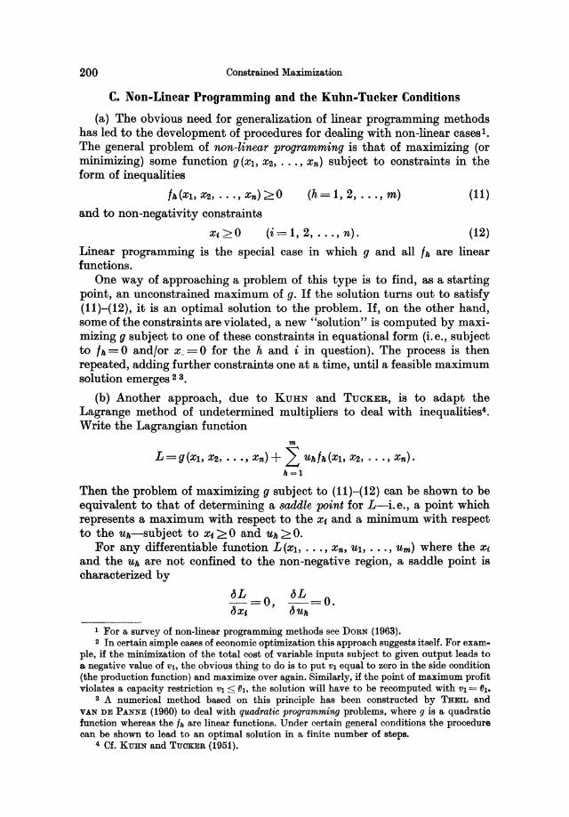
200 Constrained Maximization
C. Non-Linear Programming and the Kuhn-Tucker Conditions
(a) The obvious need for generalization of linear programming methods has led to the development of procedures for dealing with non-linear cases1•
The general problem of non-linear programming is that of maximizing (or minimizing) some function g (Xl, X2, ... , x,,) subject to constraints in the form of inequalities
(h=1,2, ... ,m) (11)
and to non-negativity constraints
X~>O (i=l, 2, ... , n). (12)
Linear programming is the special case in which g and all Ik are linear functions.
One way of approaching a problem of this type is to find, as a starting point, an unconstrained maximum of g. If the solution turns out to satisfy (11)-(12), it is an optimal solution to the problem. If, on the other hand, some of the constraints are violated, a new "solution" is computed by maximizing g subject to one of these constraints in equational form (i.e., subject to Ik=O and/or x;=O for the hand i in question). The process is then repeated, adding further constraints one at a time, until a feasible maximum solution emerges 2 3.
(b) Another approach, due to KUHN and TUCKER, is to adapt the Lagrange method of undetermined multipliers to deal with inequalities'. Write the Lagrangian function
m
L=g(X1, X2, ••• , X,,) + L uklk(x1, X2, •.• , x,,). 11=1
Then the problem of maximizing g subject to (11)-(12) can be shown to be equivalent to that of determining a saddle point for L-i.e., a point which represents a maximum with respect to the x, and a minimum with respect to the uk-8ubject to x, > 0 and Uk 2 O.
For any differentiable function L(X1' .•• , X", U1, .•. , um) where the Xi and the Uk are not confined to the non-negative region, a saddle point is characterized by
1 For a survey of non-linear programming methods see DORN (1963). 2 In certain simple cases of economic optimization this approach suggests itself. For exam
ple, if the minimization of the total cost of variable inputs subject to given output leads to a negative value of Vl, the obvious thing to do is to put Vl equal to zero in the side condition (the production function) and maximize over again. Similarly, if the point of maximum profit violates a capacity restriction Vl ~ Dh the solution will have to be recomputed with Vl = Dl.
S A numerical method based on this principle has been constructed by THEIL and VAN DE PANNE (1960) to deal with quadratic programming problems, where g is a quadratic function whereas the /11 are linear functions. Under certain general conditions the procedure can be shown to lead to an optimal solution in a finite number of steps.
4 Cf. KUHN and TUCKER (1951).
Non-Linear Programming and the Kuhn-Tucker Conditions 201
When it is required that x, > 0, Uh > 0, these necessary conditions must be modified. If some x, happens to be zero at the saddle point, bL/bxt may be
L L
Flg.l
negative instead of zero, as illustrated in Fig. 1. Similarly, bL/buh must be non-negative. Hence the necessary conditions are
bL { =0 for Xt >0 (13) b x, < 0 for x, = 0
b L { = 0 for Uh > 0 (14) bUh >0 for Uh=O,
which may be written in the form
~L bL -<0 Xt>O, x,-=O bx, - , bx,
bL Uh>O, Uh--=O
bUh
(i= 1,2, ... , n) (15)
(h= 1,2, ... , m). (16)
Sufficient conditions for a point (XIO, X20 , ••• , xno, u1o, U20 , ••• , umO)
satisfying (15)-(16) to be a saddle point are
for all x, >0, Uh >0. 1
Now consider the problem of maxtmtztng g 8ubject to the constraints /h > 0 and x, > 0, where g and the /h are assumed to be differentiable. It can be shown that, subject to certain mild qualifications as to the functions /h,
1 Proof: Applying (17), (15), (18), and (16) in this order (with Xt=x,o and Uh=UhO in (15)-(16)), we are led to
L(Xh ••• , Xn, u1o, ... , UmO) ::; L(x10, ... , xno, u1o, •• . , UmO) ::; L(XIO, ••. , Xno, Ul, ••• , Um)
for all x, ~ 0 and Uh ~ 0, which is the definition of a saddle point. Cf. op. cit., p. 483.
202 Constrained Maximization
it is necessary in order for a point (XIO, X20, ••• , XnO) to be a solution of this constrained maximum problem that there exist a set of non-negative Lagrange multipliers UIIO which, with the XtO, satisfy the necessary conditions (15)-(16) for a saddle value of the Lagrangian function
m
L = g (Xl, X2, ••• , xn) + 2: Uklh (Xl, X2, ••• , Xn).
11=1
It is always a sul/icient condition for a (global) maximum that they satisfy (15), (16), and (17)1.
Moreover, if the functions g and 111 are concave2 for Xi > 0, conditions
(17 )-( 18) are automatically satisfied for the Lagrangian L = g + 2: Uh Ih, so 11
that in this case (15)-(16) are both necessary and sul/icient for a constrained maximum of g as well as for a saddle value of L.3 These conditions-known as the Kuhn-Tucker conditions-can be written
(cf. (12)) (19)
(i = 1, 2, ... , n)
and
(~=) Ih>O bUh
(cf. (11))
Uk>O (20)
uhlh=O (h= 1,2, ... , m).
1 For proofs, see op. cit., pp. 483- 485.
2 A function F(x) is said to be concave if linear interpolation between any two points never overestimates the actual value of the function at the point of interpolation; cf. the onevariable case illustrated below, where for all x and XO in the region of definition we have
(1 - {})F(xo)+ {} F(x) :s; F {(1 - {})XO + {}x} (O:S; &:s; 1).
F
or
Convexity is defined as the reverse (linear interpolation never underestimates the value of the function). Cf. op. cit., p. 485.
3 See op. cit., pp. 485 f. The proof follows directly from the definition of concavity.
Non-Linear Programming and the Kuhn-Tucker Conditions 203
For a constrained minimum of g subject to (11)-(12), the Kuhn-Tucker m
conditions must be applied to the Lagrangian £ = -g + L uhlh since a 11-1
minimum of g is equivalent to a maximum of (-g). Hence, in (19)-(20) ,}g I ,}x, must be replaced by -,}g I ,}Xt. The necessary conditions are also sufficient for a global minimum if the function g is convex (but the 111 concave) because this implies that (-g) is concave.
Conditions (19}-(20) give a criterion which must be satisfied by an optimal solution but do not immediately provide an algorithm to obtain numerical solutions of concrete problems. For certain classes of non-linear programming problems-for example, quadratic programming, where g is a quadratic function and the 111 are linear-computational techniques have been developed to find solutions which satisfy the Kuhn-Tucker conditions!.
(c) In the case of some or all of the side conditions being equations rather than inequalities, the maximum problem can be written in the above form. For example, if the side conditions are
/1~0, la=O the side equation is equivalent to the pair of inequalities
la~O, la<O and the Lagrangian, with multipliers u, v, W, becomes
£ = g + U /1 + via + W (- fa) .
Applying (19}-(20), it is seen that, whereas v and W (as well as u) must be non-negative at the optimal point, no such constraint is placed on their difference v - w, the coefficient of la in £. Hence, writing the Lagrangian in the form
L = Ul/1 + ua/a
where u! = u, Ua = v - w, the Kuhn-Tucker conditions apply with the modification that 6£ / 6ua = la = 0 instead of > 0 (the second side condition now being an equation) and that the corresponding multiplier Ua is no longer required to be non-negative. This result holds for any case of "mixed" side conditions, including the case of all side conditions being equalities.
If 111=0 for all h and if the requirement x,>O is dropped, (19)-(20) become the "classical" Lagrange conditions (2) and (1)2.
Linear programming, where g and the Ih are linear functions, is another special case. The simplex criterion can be shown to be equivalent to the
1 See, e.g., DORN (1963), pp. 180 ff. 2 Note that in this case the side conditions (1) emerge by differentiating L with respect
to the multipliers: 6L -=/,,=0 6u"
whereas we have in the Kuhn-Tucker case 6L -=/" ??o. 6u"
204 Constrained Maximization
Kuhn-Tucker conditions; the sufficiency of (19)-(20) follows from the fact that a linear function is a limiting case of concavity. In the linear case the Lagrange multipliers Uk can be identified with the variables Yk of the dual problem l , to be interpreted in a similar way as the Uk in the "classical" case. This follows from the symmetry of the Lagrangian with respect to X( and Uk 2:
= h~l bkuk + i~ Xt (cc - h~l aM Uk).
Maximizing 2: c«x« subject to L a",x, < b k , Xc > 0 with multipliers Uk (using i i
the Lagrangian L to find a saddle point (19)-(20)) leads to identically
the same conditions as those obtained by minimizing L bkuk subject to k 2: aM Uk > c" Uk > 0 (using the Lagrangian -L with the x( as multipliers);
k
hence the Uk are the dual variables. Duality theorems, with dual variables identical with Lagrange multi
pliers, have also been established for certain classes of non-linear programming problems3•
1 Cf. above. S Cf. KUHN and TUCKER, op. cit., p. 487. 3 Cf. DORN (1963), pp. 175 ff.
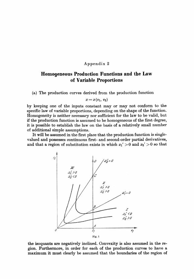
Appendix 2
Homogeneous Production Functions and the Law of Variable Proportions
(a) The production curves derived from the production function
x=x(vl, V2)
by keeping one of the inputs constant mayor may not conform to the specific law of variable proportions, depending on the shape of the function. Homogeneity is neither necessary nor sufficient for the law to be valid, but if the production function is assumed to be homogeneous of the first degree, it is possible to establish the law on the basis of a relatively small number of additional simple assumptions.
It will be assumed in the first place that the production function is singlevalued and possesses continuous first- and second-order partial derivatives, and that a region of substitution exists in which Xl' > 0 and X2' > 0 so that
.JJr
.x; >0 .z; <0
o
A
y, Flg.l
1I .x; .> (J
.xi NJ x;. {}
the isoquants are negatively inclined. Convexity is also assumed in the region. Furthermore, in order for each of the production curves to have a maximum it must clearly be assumed that the boundaries of the region of
206 Homogeneous Production Functions and the Law of Variable Proportions
substitution in the factor diagram are positively inclined, dividing the positive factor region into three zones as shown in Fig. 1, where Zone II is the region of substitution. Outside this region the isoquants are positively inclined so that Zone I, where Xl' < 0, is also characterized by X2' > ° whereas in Zone III we have Xl' > 0, X2' < 0.
Assuming homogeneity of degree one, the marginal productivities are functions of the ratio V2jVI only; hence the boundaries of the region of substitution, Xl' = ° and X2' = 0, will be straight lines passing through the origin. Homogeneity also implies
(1)
identically (Euler's theorem); it follows that Zone I is characterized by
Xl' <X/VI, X2' >xjV2' Zone II by
and Zone III by Xl' >xjVI, X2' <XjV2.
On the boundaries of Zone II we have Xl' = 0, X2' = X / V2 and X2' = 0, Xl' = X j VI respectively.
Now consider partial variation of, say, V2 for the other input constant (vl=ih), as illustrated in Fig. 1 by the path ABOD which passes through Zones I, II, and III 1. The corresponding production curve (total product) x=x(iit, V2) will have its maximum point at 0, where its slope X2' changes in sign from positive (along AO) to negative (beyond 0) through zero. Average productivity xjV2 will have a maximum at B, where it is intersected from above by the marginal productivity curve, since
~(XjV2) V2X2'-X ----
~V2 V22
is zero at B, positive in Zone I (AB), and negative in Zones II and III (i. e., beyond B). Correspondingly, the partial elasticity of production E2 =X2'· V2/X is unity at B, > 1 along AB, and < 1 beyond B (and also < ° beyond 0)2.
Furthermore, x2'is decreasing along BO, i.e., ~2xj~V22=X22" <0, so that the production curve X (iit, V2) is concave from below between Band 0. This follows from the assumption that the isoquants are convex in Zone II, using also the assumption of homogeneity. At any point on BO, the curvature of the isoquant passing through the point is positive:
1 In examining x as a function of V2 for Vi = fh we are not necessarily assuming that Vi
is a capacity factor representing fixed capital equipment. Even if it does, the capacity restriction may have the form Vi :::; fh rather than a strict equality because the services of the capital equipment are continuously divisible; in this case there is complete symmetry between the two inputs, at least within the capacity limit, so that we might as well have considered-with a similar result--a partial variation in the utilization of the capital equipment, Vi, for given amount of the current input, V2 = 02.
2 Assuming that x >0 everywhere on the path (cf. below).
Homogeneous Production Functions and the Law of Variable Proportions 207
d2v2 = (X2')2 xu" - 2XI' X2' X12" + (XI')2 X22" >0 (x constant). dVl2 -(X2')3
In general nothing is known about the second-order derivatives, but when the production function satisfies Euler's theorem identically we can differentiate (1) partially with respect to VI and V2 to get!
(2)
identically. Using this result to eliminate xu" and X12" (= X21") we have
(3)
in Zone II, where X2' > 0 so that we must have X22" < 0 at any point between Band C. X22" is also negative at Band C. Since B represents a maximum for X/V2, we have
(j2(X / V2) = V23 • X22" - (V2 X2' - x) . 2V2 < 0 (jV22 V24
which, since V2X2' = x at the point, implies X22" < 0 at B. The negativity of X22" at C, on the other hand, follows directly from the fact that x has a maximum at this point.
On the basis of the assumptions thus far made it is not possible to specify further the shape of the production curve outside the region of substitution. However, if we assume specifically that output is zero at point A, i.e., x(ih, 0) = 0 (and thus, by the homogeneity of the function, at all points on the axis: x(vl, 0)=0 for all VI), we can deduce that x is positive at any point between A and B, and that the production curve will have a point of inflexion somewhere in this region.
Expanding by Taylor's series with a remainder, starting from an arbitrary point (ih, h) on AB, we have
x(ih,0)=x(ih,h)-h.X2'(ih,-&h) for some -&,0<-&<1
which, since x (ih, 0)=0, h >0, and X2' >0, gives x (ih, h) >0 for all h in Zone I. Expanding with an additional term we get
x(ih, 0) = x (ih, h) - h . X2' (ih, h) + h2 . X22" (ih, -&h) ; 2
(4)
in Zone I we have X2' > x / h, hence X22" (ih, -& h) > 0 for some positive fraction -&. For sufficiently small h, X22" (VI, h) will have the same sign, X22" being continuous by assumption. In other words, X22" is positive in the neighbourhood of A. Since it is known to be negative in B, there must be at least one point on AB where X22" = O. Assuming as the simpler case-not unduly restrictive-that there is only one such point of inflexion, P, it represents a maximum of the marginal productivity. The production curve, then, is convex from below along A P, concave from P to B.
1 Of. ALLEN (1938). pp. 317 f.
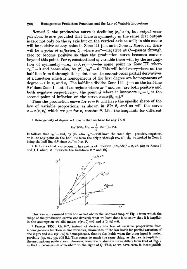
208 Homogeneous Production Functions and the Law of Variable Proportions
Beyond G, the production curve is declining (X2' < 0), but output never gets doum to zero provided that there is symmetry in the sense that output is zero not only on the VI axis but on the vertical axis as well; in this case x will be positive at any point in Zone III just as in Zone I. Moreover, there will be a point of inflexion, Q, where x22"-negative at G-passes through zero to become positive so that the production curve becomes convex beyond this point. For V2 constant and VI variable there will, by the assumption of symmetry-i. e., x (0, V2) = O-be some point in Zone III where xu" = 0 and hence also, by (2), X22" = O. This will hold everywhere on the half-line from 0 through this point since the second-order partial derivatives of a function which is homogeneous of the first degree are homogeneous of degree -1 in VI and V2. The half-line divides Zone III-just as the half-line o P does Zone I-into two regiollB where xu" and X22" are both positive and both negative respectively I ; the point Q where it intersects VI = ih is the second point of inflexion on the curve x=x(ih, V2).2
Thus the production curve for VI = ih will have the specific shape of the law of variable proportions, as shown in Fig. 2, and so will the curve x=x(v, V2) which we get for V2 constant3, Like the isoquants for different
I Homogeneity of degree -1 means that we have for any k> 0
X22" (kVI' kV2) = ..!.. . X22" (VI, V2). k
It follows that x22"-and, by (2), also xn"-will have the same sign-positive, negative, or O-at any point on the half-line from the origin through (VI, V2), the watershed in Zone I being the half-line OP since X22" = 0 at P.
2 It follows that any isoquant has points of inflexion (d 2v2/ dVI2 = 0, of. (3)) in Zones I and III where it intersects the half-lines OP and OQ :
o
.r!!-.o
---~.,-"'-I'
A
This was not assumed from the outset about the isoquant map of Fig. 1 from which the shape of the production curves was derived; what we have done is to show that it is implicit in the assumption we did make : X(OI, 0)=0 and X(0,02)=0.
3 FRISCH (1956), Ch.6-7, instead of deriving the law of variable proportions from a homogeneous function in two variables, shows that, if the law holds for partial variation of one input and X=X(Vl, V2) is homogeneous, then it also holds when the other input is varied partially (op. cit., pp. 108 ff.). This comes to much the same thing, as the law is implicit in the assumptions made above. However, FRISCH's production curve differs from that of Fig. 2 in that x becomes = 0 somewhere to the right of Q. This, as we have seen, is incompatible
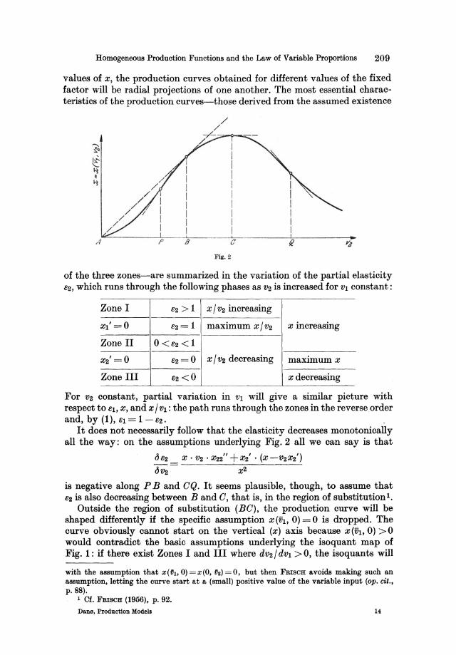
Homogeneous Production Functions and the Law of Variable Proportions 209
values of x, the production curves obtained for different values of the fixed factor will be radial projections of one another. The most essential characteristics of the production curves-those derived from the assumed existence
/ /
/ /
/
/ /
/
A /
B c FIg. 2
of the three zones-are summarized in the variation of the partial elasticity E2, which runs through the following phases as V2 is increased for VI constant:
Zone I e2 >1 x j V2 increasing
XI'=O e2= 1 maximum Xjv2 x increasing
Zone II o <E2 < 1
X2'=0 E2=0 X j V2 decreasing maximum x
Zone III E2 <0 x decreasing
For V2 constant, partial variation in VI will give a similar picture with respect to El, x, and x j VI: the path runs through the zones in the reverse order and, by (1), EI = 1- E2.
It does not necessarily follow that the elasticity decreases monotonically all the way: on the assumptions underlying Fig. 2 all we can say is that
.Il 11 + ' ( ') uE2 x· V2 • X22 , X2· X-V2X2
~V2 - x2
is negative along P Band CQ. It seems plausible, though, to assume that E2 is also decreasing between Band C, that is, in the region of substitution I.
Outside the region of substitution (BC), the production curve will be shaped differently if the specific assumption x(ih, 0) = 0 is dropped. The curve obviously cannot start on the vertical (x) axis because x(ih, 0) >0 would contradict the basic assumptions underlying the isoquant map of Fig. 1: if there exist Zones I and III where dV2j dVI > 0, the isoquants will
with the assumption that x(ih, 0) = x(O, V2) = 0, but then FRISCH avoids making such an assumption, letting the curve start at a (small) positive value of the variable input (QP. cit., p.88).
1 Cf. FRISCH (1956), p. 92.
Dane, Production Modeu 14
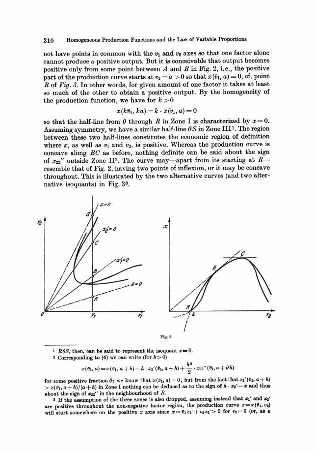
210 Homogeneous Production Functions and the Law of Variable Proportions
not have points in common with the VI and V2 axes so that one factor alone cannot produce a positive output. But it is conceivable that output becomes positive only from some point between A and B in Fig. 2, i. e., the positive part of the production curve starts at V2 = a > 0 so that x (iiI, a) = 0, cf. point R of Fig. 3. In other words, for given amount of one factor it takes at least so much of the other to obtain a positive output. By the homogeneity of the production function, we have for k > 0
x(kiiI, ka) = k . x (iiI, a) = 0
so that the half-line from 0 through R in Zone I is characterized by x = o. Assuming symmetry, we have a similar half -line 0 S in Zone III 1. The region between these two half-lines constitutes the economic region of definition where x, as well as VI and V2, is positive. Whereas the production curve is concave along Be as before, nothing definite can be said about the sign of X22" outside Zone II2. The curve may-apart from its starting at Rresemble that of Fig. 2, having two points of inflexion, or it may be concave throughout. This is illustrated by the two alternative curves (and two alternative isoquants) in Fig. 33 •
----If
Z-Q --FIg. 3
1 ROB, then, can be said to represent the isoquant x=O. 2 Corresponding to (4) we can write (for h> 0)
X(OI, a) =x(D1, a+h) - h. x2'(1h, a+h) + ~2 • X22"(Dl,a +Dh)
for some positive fraction D; we know that X(Dl' a) =0, but from the fact thatx2'(01, a+h) > x(Dlt a+h)/(a+h) in Zone I nothing can be deduced as to the sign of h· X2'-X and thus about the sign of X22" in the neighbourhood of R.
3 If the assumption of the three zones is also dropped, assuming instead that Xl' and X2' are positive throughout the non-negative factor region, the production curve X=X(f11, tla) will start somewhere on the positive X axis since X=f11Xl'+V2X2'> 0 for V2=0 (or, as a
Homogeneous Produotion Funotions and the Law of Variable Proportions 211
(b) The more general case of a homogeneous production function with any number of inputs can be examined on similar lines for proportional variation in some of the inputs, the others being held fast, since this case reduces to a two-factor model. Let the inputs be divided into two groups, the members of which are varied in fixed proportions to VI and to Vz respectively:
For variations thus restricted, the production function can be written as a homogeneous function of VI and vz,
where x = X (VI, Vz, ••• , Vm} = ~(VI' V2) = VI ~l' + V2~Z'
~l' = Xl' + L (X,x,' , , ~2' =X2' + Lf3tXt'. , Assuming that the straight lines representing ~l' = 0 and ~2' = 0 in a (VI, V2)
map are positively inclined and divide the positive quadrant into three zones (as in Fig. 1 above), the production curves
X=~(VI' vz} and x=~(vl, vz}
-where VI and Vz now represent homogeneous complexes of inputs measured in units of input no. 1 and 2 respectively-will show diminishing average returns to the variable factor complex from a certain point: for VI=VI (and thus VB = (XBVI = constant), average productivity X / V2 will have a maximum at the point where VI = VI intersects ~l' = 0, and output X will have a maximum for ~z' =0. Correspondingly, the elasticity of production with respect to the variable factor complex, EZ = (dx / dvz) . Vz / x = ~z' . Vz / x-not to be confused with the partial elasticity X2'· vz/x-will decrease from values greater than 1 through 1 (at the point of maximum x/vz) and 0 to negative values. For further specification of the shape of the production curve additional assumptions~.g. ~(VI' O}=O-will have to be introduced I.
limiting case, start at the origin if Xl' = 0 coinoides with the VI axis); the produotion ourve will have no maximum point (X2' never becomes zero) and there will be diminishing returns everywhere sinoe
~(XIV2) = V2X2' - X = _ !llXl' < o. ~V2 V22 va2
1 Note, however, that oonoavity of the produotion ourve in the region of substitution oannot be established unless it is speoifically assumed that the isoquants 0(Vl' V2) =X are convex in the region. Suob convexity does not follow from the assumption that the isoquants belonging to the produotion funotion X(Vl' V2, ••• , vm) are convex to the origin for xi'> 0 (i = 1, 2, •.. , m). Convexity in m-dimensional faotor spaoe means that we have for any two distinot points of the isoquant in the region
m
(i) ~ (~')O • (VI - v,O) > 0 i=l
whioh for variations restrioted as above becomes (ii) (01')0 . (VI - VI0) + (02')0 . (Va - V20) > o.
These inequalities hold for points at whioh all of the xl' are positive. Sinoe it is possible for 01' or O2' to be positive even when some of the xl' are negative, it follows that (ii) does not neoeBBarily hold for all effioient points of the two-dimensional isoquant.
14·
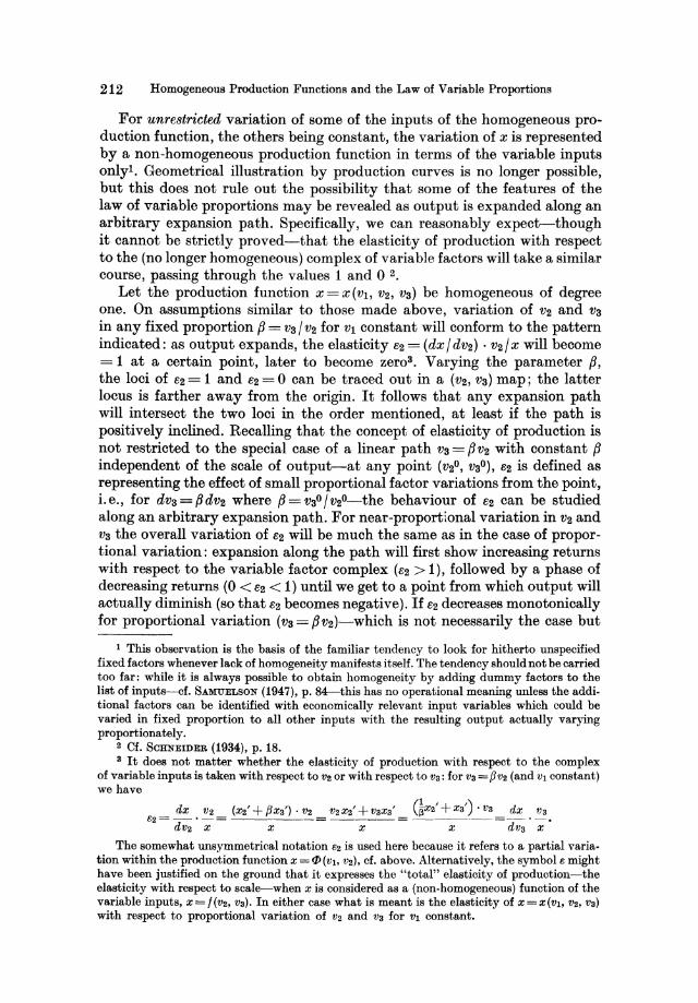
212 Homogeneous Production Functions and the Law of Variable Proportions
For unrestricted variation of some of the inputs of the homogeneous production function, the others being constant, the variation of x is represented by a non-homogeneous production function in terms of the variable inputs onlyi. Geometrical illustration by production curves is no longer possible, but this does not rule out the possibility that some of the features of the law of variable proportions may be revealed as output is expanded along an arbitrary expansion path. Specifically, we can reasonably expect-though it cannot be strictly proved-that the elasticity of production with respect to the (no longer homogeneous) complex of variable factors will take a similar course, passing through the values 1 and 0 2.
Let the production function X=X(VI, V2, va} be homogeneous of degree one. On assumptions similar to those made above, variation of V2 and Va in any fixed proportion {3 = va! V2 for VI constant will conform to the pattern indicated: as output expands, the elasticity 82 = (dx! dV2) . V2! x will become = 1 at a certain point, later to become zeros. Varying the parameter {3, the loci of 82 = 1 and 82 = 0 can be traced out in a (V2' vs) map; the latter locus is farther away from the origin. It follows that any expansion path will intersect the two loci in the order mentioned, at least if the path is positively inclined. Recalling that the concept of elasticity of production is not restricted to the special case of a linear path Vs = {3 V2 with constant {3 independent of the scale of output-at any point (V20 , VSO), 82 is defined as representing the effect of small proportional factor variations from the point, i.e., for dvs={3dv2 where {3=vsOjv20-the behaviour of 82 can be studied along an arbitrary expansion path. For near-proportional variation in V2 and Vs the overall variation of 82 will be much the same as in the case of proportional variation: expansion along the path will first show increasing returns with respect to the variable factor complex (82) 1), followed by a phase of decreasing returns (0 < 82 < 1) until we get to a point from which output will actually diminish (so that 82 becomes negative). If 82 decreases monotonically for proportional variation (vs = {3v2}-which is not necessarily the case but
1 This observation is the basis of the familiar tendency to look for hitherto unspecified fixed factors whenever lack of homogeneity manifests itself. The tendency should not be carried too far: while it is always possible to obtain homogeneity by adding dummy factors to the list of inputs-cf. SAMUELSON (1947), p. 84-this has no operational meaning unless the additional factors can be identified with economically relevant input variables which could be varied in fixed proportion to all other inputs with the resulting output actually varying proportionately.
2 Cf. SCHNEIDER (1934), p. 18. 3 It does not matter whether the elasticity of production with respect to the complex
of variable inputs is taken with respect to Vs or with respect to V3: for Va = {3 V2 (and Vl constant) we have
(~X2' +X3') . Va dx V3 --x---=dV3'X'
The somewhat unsymmetrical notation E2 is used here because it refers to a partial variation within the production function x=l1i(vt, V2). cf. above. Alternatively. the symbol e might have been justified on the ground that it expresses the "total" elasticity of production-the elasticity with respect to scale-when x is considered as a (non-homogeneous) function of the variable inputs, X=t(V2. V3). In either case what is meant is the elasticity of X=X(Vl. V2. V3) with respect to proportional variation of V2 and Va for Vl constant.
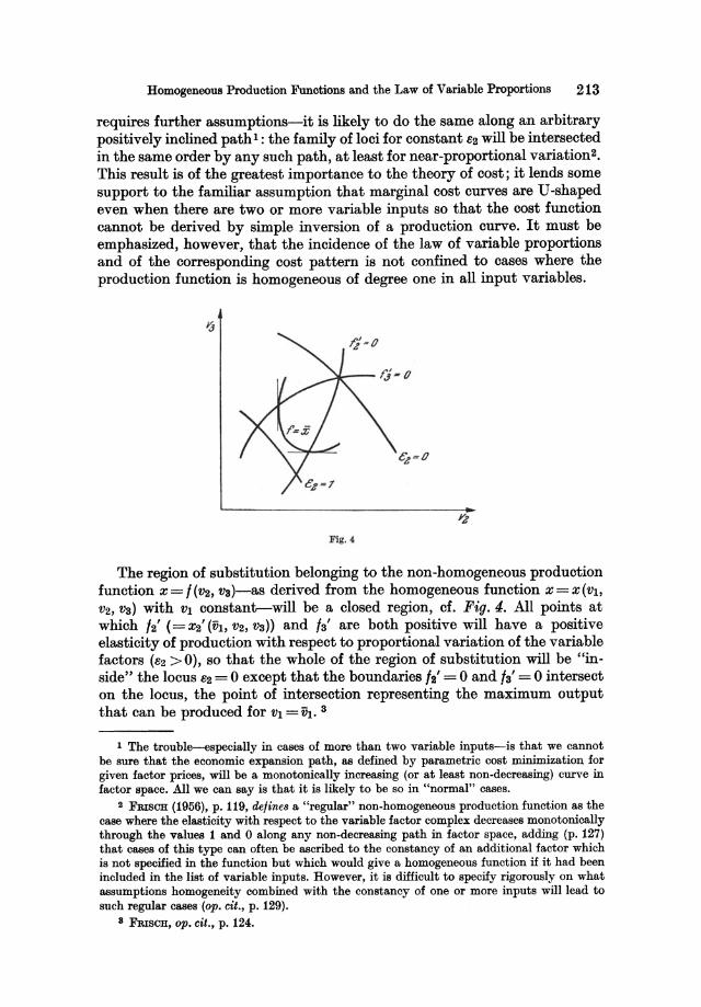
Homogeneous Production Functions and the Law of Variable Proportions 213
requires further assumptions-it is likely to do the same along an arbitrary positively inclined path I : the family of loci for constant £2 will be intersected in the same order by any such path, at least for near-proportional variation2•
This result is of the greatest importance to the theory of cost; it lends some support to the familiar assumption that marginal cost curves are V-shaped even when there are two or more variable inputs so that the cost function cannot be derived by simple inversion of a production curve. It must be emphasized, however, that the incidence of the law of variable proportions and of the corresponding cost pattern is not confined to cases where the production function is homogeneous of degree one in all input variables.
FIg. 4
The region of substitution belonging to the non-homogeneous production function x=/(v2,v3)-as derived from the homogeneous function X=X(VI, V2, V3) with VI constant-will be a closed region, cf. Fig. 4. All points at which 12' (= X2' (fh, V2, V3)) and 13' are both positive will have a positive elasticity of production with respect to proportional variation of the variable factors (£2 >0), so that the whole of the region of substitution will be "inside" the locus £2 = 0 except that the boundaries 12' = 0 and 13' = 0 intersect on the locus, the point of intersection representing the maximum output that can be produced for VI =ih. 3
1 The trouble---especially in cases of more than two variable inputs-is that we cannot be sure that the economic expansion path, as defined by parametric cost minimization for given factor prices, will be a monotonically increasing (or at least non-decreasing) curve in factor space. All we can Bay is that it is likely to be so in "normal" cases.
2 FRISCH (1956), p. 119, defines a "regular" non-homogeneous production function as the case where the elasticity with respect to the variable factor complex decreases monotonically through the values 1 and 0 along any non-decreasing path in factor space, adding (p. 127) that cases of this type can often be ascribed to the constancy of an additional factor which is not specified in the function but which would give a homogeneous function if it had been included in the list of variable inputs. However, it is difficult to specify rigorously on what assumptions homogeneity combined with the constancy of one or more inputs will lead to such regular cases (op. cit., p. 129).
8 FRISCH, op. cit., p. 124.
References
ALLEN, R. G. D. (1938), Mathematical Analysis for Economists, London: Macmillan. - (1956), Mathematical Economics, London: Macmillan. BARFOD, BeRGE (1936), Forenet Produktion og Kvalitetsrendring, Nord. Tidsskr. Tek. 0kon.,
lb. nr. 5. BARGONI, A., B. GIARDINA, and S. RrcossA (1954), Un esempio di programmazione lineare
nell'industria, Ch. 3 in A. BORDIN, ed., La programmazione lineare nell'industria, Torino: Unione Industriale.
BORDIN, ARRIGO (1944), Statica economica, Milano and Messina: Principato. BREMS, HANS (1952a), A Discontinuous Cost Function, Amer. Econ. Rev., Vol. 42. - (1957), Input-Output Coefficients as Measures of Product Quality, Amer. Econ. Rev.,
Vol. 47. - (1959), Output, Employment, Capital, and Growth, New York: Harper. - (1951), Product Equilibrium under Monopolistic Competition, Cambridge: Harvard Uni-
versity Press. - (1952b), En sammenligning mellem den grengse og den Jantzen'ske omkostningsteori,
National0kon. Tidsskr., 90. bd. BURGER, E. (1955), On Extrema with Side Conditions, Econometrica, Vol. 23. CARLSON, SUNE (1939), A Study on the Pure Theory of Production, London: King. CHAMBERLIN, EDWARD H. (1933), The Theory of Monopolistic Competition, Cambridge:
Harvard University Press. CHARNES, A., and W. W. COOPER (1961), Management Models and Industrial Applications
of Linear Programming, Vol. I-II, New York: Wiley. CHARNES, A., W. W. COOPER, and DONALD FARR AND STAFF (1953), Linear Programming
and Profit Preference Scheduling for a Manufacturing Firm, J. Operations Res. Soc. of America, Vol. 1.
CHENERY, HOLLIS B. (1949), Engineering Bases of Economic Analysis, Cambridge: Harvard University. (UnpUblished thesis.)
- (1953), Process and Production Functions from Engineering Data, Ch. 8 in Leontief (1953). CHIPMAN, JOHN (1953), Linear Programming, Rev. Econ. Statist., Vol. 35. CHuRCHMAN, C. W., R. L. ACKOFF, and E. L. ARNOFF (1957), Introduction to Operations
Research, New York: Wiley. Cost Behavior and Price Policy (1943), New York: National Bureau of Economic Research. DAN0, SVEN (1960), Linear Programming in Indnstry: Theory and Applications, Wien:
Springer. - (1965), A Note on Factor Substitution in Industrial Production Processes, Unternehmens
forschung, Bd. 9. DANTZIG, GEORGE B. (1951), Maximization of a Linear Function of Variables Subject to Linear
Inequalities, Ch. 21 in KOOPMANS (1951). DEAN, JOEL (1951), Managerial Economics, New York: Prentice-Hall. - (1941), The Relation of Cost to Output for a Leather Belt Shop, New York: National
Bureau of Economic Research. DORFMAN, ROBERT (1951), Application of Linear Programming to the Theory of the Firm,
Berkeley and Los Angeles: University of California Press. - (1953), Mathematical, or "Linear", Programming: A Nonmathematical Exposition, Amer.
Econ. Rev., Vol. 43. DORN, W. S. (1963), Non-Linear Programming-A Survey, Management Science, Vol. 9.
216 References
FOG, E. S. B. (1934), Blegning af Olier, Kem. Maanedsbl., 15. Aarg. FORCH1IA.lIIMER, N. (1937), Elektriske Gledelampers Levetid og 0konomi, Nord. Tidsskr. Tek.
0kon., lb. nr. 8. FRENCKNER, T. PAULSSON (1957), Betriebswirtschaftslehre und Verfahrensforschung, Z. han
delswiss. Forsch., 9. Jahrgang. FroSCH, RAGNAR (1932), Einige Punkte einer Preistheorie mit Boden und Arbeit als Produk
tionsfaktoren, Z. Nat.Okon., Bd. 3. - (1956), Innledning til produksjonsteorien, 1. hefte, 8. utg., Oslo: Universitetets Social
ekonomiske Institutt. [English translation: FroSCH (1965), Ch. 1-11.] - (1953), Innledning til produksjonsteorien, 2. hefte, Oslo: Universitetets Socialekonomiske
Institutt. [English translation: FRIsCH (1965), Ch. 12-19.] - (1935), The Principle of Substitution. An Example of Its Application in the Chocolate
Industry, Nord. Tidsskr. Tek. 0kon., lb. nr. 1. - (1965), Theory of Production, Dordrecht: Reidel. GEORGESCu-RoEGEN, N. (1935), Fixed Coefficients of Production and the Marginal Produc
tivity Theory, Rev. Econ. Stud., Vol. 3. GLOERl!'ELT-TARP, B. (1937), Den ekonomisk definerede Produktionsfunktion og den hetero
gene Fremstillingsproces, Nord. Tidsskr. Tek. 0kon., lb. nr. 10. GROSSE, ANNE P. (1953), The Technological Stmcture of the Cotton Textile Industry, Ch. 10
in LEONTIEI!' (1953). GUTENBERG, ERICH (1963), Grundlagen der Betriebswirtschaftslehre, Erster Band: Die Pro
duktion, 8./9. Aufl., Berlin: Springer. HEADY, EARL 0., and JOHN PESEK (1960), Expansion Paths for Some Production Functions,
Econometrica, Vol. 28. HENDERSON, JOHN S. (1953), Marginal Productivity Analysis-A Defect and a Remedy,
Econometrica, Vol. 21. - (1950), Production with Limitational Goods, Econometrica, Vol. 18. HICKS, J. R. (1946), Value and Capital, 2nd ed., Oxford: Clarendon. JANTZEN, IVAR (1939), Basic Principles of Business Economics and National Calculation,
Copenhagen: Gad. - (1924), Voxende Udbytte i Industrien, Nationalekon. Tidsskr., 62. Bd. JOHANSEN, LED!' (1962), Notat om tolkingen av Lagrange-multiplikatorer, Memorandum fra
Socialekonomisk Institutt, Oslo. KALnOR, NICHOLAS (1937), Limitational Factors and the Elasticity of Substitution, Rev.
Econ. Stud., Vol.4. KNIGHT, FRANK H. (1921), Risk, Uncertainty and Profit, Boston: Houghton Mifflin. KOOPIIlANS, TJALLING C. (1951), ed., Activity Analysis of Production and Allocation, Cowles
Commission Monograph No. 13, New York: Wiley. KUHN, H. W., and A. W. TuCKER (1951), Nonlinear Programming, pp. 481-492 in J. NEY-
1IlAN, ed., Proceedings of the Second Berkeley Symposium on Mathematical Statistics and Probability, Berkeley and Los Angeles: University of California Press.
LEONTIEI!', WASSILY (1941), The Stmcture of American Economy, 1919-1929, Cambridge: Harvard University Press.
LEONTIEI!', WASSILY, and others (1953), Studies in the Stmcture of the American Economy, New York: Oxford University Press.
OSGOOD, WILLLUI F. (1925), Advanced Calculus, New York: Macmillan. PARETO, VILFREDO (1897), Cours d'economie politique, Vol. II, Lausanne: Rouge. - (1927), Manuel d'economie politique, 2e ad., Paris: Giard. PEDERSEN, H. WINDING (1949), Omkostninger og prispolitik, 2. udg., Kebenhavn: Hest. - (1933), Omkring Kapacitetsudnyttelsesteorien, National0kon. Tidsskr., 71. Bd. PERRY, JOHN H. (1941), ed., Chemical Engineers' Handbook, 2nd ed., New York: McGraw
Hill. Pll'OUTS, RALPH W. (1961), The Theory of Cost and Production in the Multi-Product Firm,
Econometrica, Vol. 29. RICOSSA, SERGIO (1955), Nuove applicazioni della teoria economica della produzione, G.
Econo., Vol. 14. - (1954), Nuovi e vecchi problemi della produzione, Note Econometriche, N. 11.
References 217
RIEBEL, PAUL (1955), Die Kuppelproduktion: Betriebs- und Marktprobleme, Ki:iln: West· deutsoher Verlag.
Roy, RENE (1950), Remarques sur les phenomenes de produotion, Metroeoonomioa, Vol. 2. SAMUELSON, PAUL A. (1947), Foundations of Eoonomio Analysis, Cambridge: Harvard Uni
versity Press. SCHMIDT, ERIK (1939), 0konomisk definerede produktionsfunktioner, Nord. Tidsskr. Tek.
0kon., lb. Dr. 17-18. SCHNEIDER, ERICH (1958), Einfiihrung in die Wirtsohaftstheorie, II. Teil, 5. verb. u. erw.
Aufl., Tiibingen: Mohr. - (1937), Kapaoitetsudnyttelsesproblemets to Dimensioner, Nord. Tidsskr. Tek. 0kon.,
lb. Dr. 7. - (1942), Teoria della produzione, Milano: Casa Editrioe Ambrosiana. - (1934), Theorie der Produktion, Wien: Springer. - (1940), Vber den EinfluI3 von Leistung und Besohaftigung auf Kosten und Erfolg einer
Untemehmung mit homogener Massenfabrikation, Aroh. math. Wirtsoh., Bd.6. SCHULTZ, HENRY (1929), Marginal Produotivity and the General Prioing Prooess, J. Polito
Econ., Vol. 37. SCHWEYER, HERBERT E. (1955), Prooess Engineering Eoonomios, New York: MoGraw-Hill. SHEPHARD, RONALD W. (1953), Cost and Produotion Funotions, Prinoeton: University Press. STACKELBERG, HEINRICH v. (1938), Angebot und Naohfrage in der Produktionswirtsohaft,
Aroh. math. Wirtsoh., Bd. 4. - (1932), Grundlagen einer reinen Kostentheorie, Wien: Springer. - (1941), Stundenleistung und Tagesleistung, Aroh. math. Wirtsoh., Bd.7. STIGLER, GEORGE J. (1939), Produotion and Distribution Theories in the Short Run, J. Polito
Eoon., Vol. 47. - (1946), Produotion and Distribution Theories: The Formative Period, New York: Mao
millan. SYMONDS, GIFFORD H. (1955), Linear Programming: The Solution of Refinery Problems,
New York: EsBO Standard Oil Co. THEIL, H., and C. VAN DE PANNE (1960), Quadratio Programming as an Extension of Classioal
Quadratio Maximization, Management Soienoe, Vol. 7. W ALRAS, LEON (1954), Elements of Pure Eoonomios, Translated by WILLIAM JAFFE,
London: Allen & Unwin. WALTERS, A. A. (1963), Produotion and Cost Funotions: An Eoonometrio Survey, Econo
metrioa, Vol. 31. WWKSTEED, PBnJ:p H. (1894), An Essay on the Co-ordination of the Laws of Distribution,
London: Maomillan. ZEUTHEN, F. (1955), Eoonomio Theory and Method, London: Longmans. - (1933), Das Prinzip der Knappheit, teohnisohe Kombination und i:ikonomisohe Qualitat.
Z. Nat.Okon., Bd. 4. - (1928), Den 0konomiske Fordeling, K0benhavn: Busok. - (1942), 0konoInisk Teori og Metode, K0benhavn: Busok.
Index
Accounting prices 12 n., 19, 149 n., 151 ff., 163, 171, 176
Activity 6 n., 20 n., 23 ff., 50 Activity level 23 ALLEN, R. G. D. 55 n., 58 n., 59 n., 68 n.,
183 n., 185 n., 186 n., 188 n., 190 n., 192 n., 193 n., 207 n.
Alternative processes 167 ff., 188 n.
BARFOD, B. 138 n., 140 n., 141 n., 142 n. BARGONI, A. 17 n., 169 n. Basic solution 173, 195 ff. Batch operations 124 Blending numbers 144 n. Blending processes 143 ff. BORDIN, A. 103 n., 176 n. Bottleneck factor 154 ff., 159, 163 n. Boundary conditions 14 n., 74 ff., 141 Boundary maximum or minimum 17 ff.,
32 ff., 43 ff., 74 ff., 139, 141, 170, 180, 194 ff.
Box diagram 175 BREMS, H. 5 n., 9, 113 n., 133 n., 136 n.,
137 n., 159 n. Buildings (as factors of production) 8, 12 n.,
111 n. BURGER, E. 192 n.
Capacity, maximum 12 n., 113, 116 Capacity curve 169 ff., 172 ff., 176 ff., 179,
183, 185, 187 n. Capacity restrictions 9, 11 f., 18 ff., 24,
34 ff., 63 n., 74, 80 ff., 84 n., 91, 99 ff., 110 ff., 129 ff., 153 ff., 169 f., 171 ff., 179 ff., 185 ff.
Capacity utilization 9, 19, 50 n., 87 ff., 109 ff., 129 f.
Capital equipment 5 ff. CARLSON, S. 5 n., 21 n., 51 n., 60 n., 64 n.,
65 n., 115 n., 149 n., 151 n., 183 n. CHAMBERLIN, E. H. 132 n., 133 n. CHARNES, A. 15 n., 28 n., 148 n., 161 n.,
174n., 197 Chemical reactions 17 n. CHENERY, H. B. 5 n., 108 n., 138 n., 149 n.,
157 n., 162 n., 165 n., 168 n.
CHIPMAN, J. 65 n., 110 n. CHURCHMAN, C. W. 9 n. Cobb-Douglas functions 49 n., 59 n., 62 n. Coefficients of production 16 ff., 23 ff.,
136 f., 143 n. Complementarity 16, 49, 157 n., 164, 181 f. Complementary groups of inputs 103 ff., 146,
157 n., 164 Complementary products 181 f. Concavity 53,69, 178, 185,202 f., 206 Constrained maximization or minimization
190 ff. Constrained substitution 103, 107, 140, 188 Continuous processes 8, 115, 123, 130 Continuous substitution 28 n., 46 ff., 113,
116 f., 135 f., 149 ff., 162 ff., 176 ff., 183 ff.
Convex combination 25, 174 Convexity 27, 52 ff., 68 f., 179, 185, 202 f.,
205 ff. COOPER, W. W. 15 n., 28 n., 148 n., 161 n.,
174n. Corner maximum, Bee boundary maximum Cost function 13 f., 37 ff., 83 ff., 109 if.,
129 ff., 155 f. Cost minimization 17, 22 f., 31 ff., 43 ff.,
66 ff., 98 ff., 109 ff., 135 f. Current inputs 7, 175 Cyclic processes 124 ff.
DAN0, S. 42 n., 118 n., 145 n., 196 n., 197 n., 199n.
DANTZIG, G. B. 28 n., 195 ff. DEAN, J. 111 n., 129 n. Decreasing return, Bee dimiuishing return Deflexion, point of 87 ff., 110 ff. Degeneracy 32 n., 41 n., 42 n., 197 Diet problem' 145 n. Dimiuishing return 7 n., 57 n., 59 ff., 84 ff.,
205 ff. Discontinuous substitution 23 ff., 28 n., 50,
100, 117, 145, 160.ff., 171 ff. Displacement of equilibrium 34, 70 ff., 76,
94 ff. Divisibility of fixed factors 7 f., 84 n., 91 n.,
99 f., 109 ff., 130
Index 219
DORFMAN, R. 42 n., 171 n., 183 n. DORN, W. S. 200 n., 203 n., 204 n. Duality in linear and non· linear program
ming 20 n., 42, 171, 199 ff., 204 Dummy factors 114 n., 212 n.
EDGEWORTH, F. Y. 49 n. Efficient points 12 ff., 20 f., 26 f., 46 ff.,
52 ff., 67 ff., 184 Elasticity of production 29, 50 ff., 85 ff., 110,
206,212 Elasticity of substitution 57 ff., 73 f. Engineering production model 126 n. Engineering variables 108 Euler's theorem 51 f., 96, 185 n., 188, 206 ff. Expansion path 37 f., 82 ff., 99 ff., 110 ff.,
130 n., 150, 154 ff., 163 ff., 186 Extensive dimension of capacity utilization
113 ff.
Factor of production 6 ff., 10 f. Factor shadow 100 ff., 107, 117 f. Feasible points 27,34,67,76 ff., 194 ff. Final product 148 Fixed costs 19, 90 n. Fixed factors 5 ff., 11 f., 18 ff., 34 ff., 50 n.,
109 ff., 129 ff., 148 ff., 153 ff., 157 ff., 166 ff., 175
FOG, E. S. B. 140 n. FOROHHAMMER, N. 74 n. FRENCKNER, T. PAULSSON 17 n., 159 n.,
169n. FRISCH, R. 9 n., 10 n., 11 n., 16 n., 21 n.,
24 n., 50 n., 51 n., 60 n., 68 n., 70 n., 86 n., 90 n., 92 n., 97 n., 98 n., 100 n., 101 n., 102 n., 104 n., 107 n., 108 n., 142 n., 146 n., 157 n., 162 n., 164 n., 166 n., 188 n., 189 n., 208 n., 209 n., 213n.
Full-cost pricing 20, 43, 96
GALE, D. 196 n. GEORGESCu-RoEGEN, N. 99 n., 100 n., 102 n.,
104n. GIARDINA, B. 17 n., 169 n. Global maximum or minimum 69, 86, 202 GLOERFELT-TABP, B. 15 n., 28 n., 53 n., 65 n. GROSSE, A. P. 17 n. GUTENBERG, E. 118 n.
HEADY, E. O. 49 n. HENDERSON, J. S. 189 n. HICKS, J. R. 50 n., 60 n., 183 n., 185 n.,
186n. Homogeneous functions 50 H., 58 n., 62,
83 H., 91, 96, 110 H., 153 H., 158, 163, 176 H., 180, 185, 187 f., 205 H.
Increasing return 59 ff., 206 ff. Inefficient points 14 f., 26 f., 46 ff., 55 f.,
67,178,183 n., 184 Inflexion, points of 207 ff. Input 6 ff., 10 f. Instantaneous rate of output 123 f. Integration of process models 149 H. Intensive dimension of capacity utilization
113 H. Intermediate product 6, 149 ff. Intermittent production 111, 115, 130 Investment decisions 3, 19 n. Isocost 23, 33, 67, 76, 81, 83 Iso-quality curve 139 Isoquant 17, 21 H., 25 H., 30 H., 43 ff.,
47 H., 63 H., 74 ff., 135, 184, 205 H.
JANTZEN, I. 5 n., 129 n., 159 n. JOHANSEN, L. 193 n. Joint processes 162 n., 165 n. Joint production 10 f., 167, 181 ff.
KALnOR, N. 98 n. KNIGHT, F. H. 110 n. KOOPMANS, T. C. 15 n., 28 n. KUHN, H. W. 54 n., 200 ff. Kuhn-Tucker saddle point conditions 74 n.,
79 f., 82, 153, 177 n., 181 n., 200 ff.
Lagrange multipliers 32, 66 f., 74 n., 77 H., 83 ff., 95 n., 99, 103, 104 f., 140, 142, 152, 157,164,177,179, 185 H., 190ff., 202H.
Law of capacity 18 n. Law of diminishing returns 7 n., 61 n. Law of harmony 159 n. Law of variable proportions 60 ff., 85, 109 ff.,
130,205 ff. Least-cost point, Bee cost minimization LEONTIEF, W. 16 n., 76 n. Limitational inputs 16 H., 25, 97 H., 112,
116 ff., 136 f., 143, 146, 156, 158, 164, 168 ff.
Linear production model 24, 100, 145, 182 f. Linear programming 20 n., 27 n., 28 n.,
32 ff., 74 n., 75 f., 160 n., 170 f., 195 ff.
Marginal cost 18, 36 H., 84 H., 109 H., 129 H. Marginal productivity 21, 43 H., 46 ff., 65 f. Marginal rate of (factor) substitution 33,
43 H., 47, 52 f. Marginal rate of (product) substitution 178,
186 MARsHALL, A. 20 n. Mixing processes, Bee blending proceBSeB Mixture Law 145 n. Multiple production 166 H. Multiple-shift operation 121
220 Index
Non-linear programming 200 ff. Non-negativity requirements 12, 24 ff., 74 ff.,
179, 194 ff.
Opportunity cost 19, 186 Optimization 12 ff., 17,31 ff., 66 ff. OSGOOD, W. F. 52 n., 54 n., 190 n. Output 6
Panne, C. van de 200 n. Parallel processes 162 ff. Parametric linear programming 34 ff., 197 f. Parametric production model 108, 112 ff. PARETO, V. 16 n., 17 n., 49 n., 97 n., 101 n.,
104n. Partial elasticity of production 50 ff., 60 ff.,
206 Partial marginal cost 70 n., 187 PEDERSEN, H. WINDING 129 n., 181 n. Perfect complementarity 16, 49, 181 f. Perfect substitutability 53, 74 ff., 143 f. PERRY, J. H. 145 n. PESEK, J. 49 n. PFOUTS, R. W. 176 n. Plant 5 Plant production and cost model 4, 148 ff.,
168,181 Process 5 f., 148 ff. Processing factor 149 f. Product quality 132 ff. Product shadow 97 ff., 117 f. Production 5 Production curve 30 f., 59 ff., 65 f., 109 f.,
178,205 ff. Production function, production model 10 ff.,
106 ff., 132 ff., 137 ff., 189 Profit function 12 Profit maximization 3, 13 n., 18, 37 f., 89 ff.,
99 ff.
Quadratic programming 200 n. Quality constraints 137 ff. Quality parameters 134 ff. Quality specifications 135 ff. Quasi-rent 20 n., 96 n.
Region of substitution 27, 46 ff., 52 ff., 64 ff., 67 fl., 184, 205 ff.
Returns to scale, constant 28 f., 50 ff., 109 ff., 185
- - -, decreasing 52 n., 90 - - -, increasing 52 n. RICARDO, D. 1, 60 n. RICOSSA, S. 17 n., 107 n., 169 n., 176 n.,
189 n. RIEBEL, P. 181 n. Roy, R. 189 n.
Saddle point 80, 82, 200 ff. SAMUELSON, P. A. 11 n., 23 n., 28 n., 43 ff.,
60 n., 64 n., 72 n., 79 n., 190 n., 212 n. SCHMIDT, E. 28 n., 182 n., 189 n. SCHNEIDER, E. 21 n., 51 n., 57 n., 60 n.,
63 n., 86 n., 97 n., 98 n., 99 n., 110 n., 119 n., 129 n., 212 n.
SCHULTZ, H. 97 n., 104 n. SCHWEYER, H. E. 124 n., 126 n., 127 n. Selling effort 12 n., 132 f., 136 n. Semicontinuous processes 124 ff. Services of fixed factors 8, 115 ff., 130 Shadow factor 24 n., 97 ff., 107, 117 ff.,
142, 146, 156 ff. Shadow function 126, 142 Shadow price 8, 19 f., 39 ff., 83 n., 94 ff.,
159 n., 161 n., 171, 176, 179 ff., 187 f., 193 n., 199 n.
Shadow product 188 f. SHEPHARD, R. W. 107 n. Simplex coefficients 32 n., 36 n., 173,
196 ff. Simplex criterion 32 n., 33 n., 76, 196 ff. Simplex method 32 n., 35 ff., 195 ff. Slack activity 30 n. Slack variable 42, 174, 194 ff. Spatial divisibility of fixed factors 111 ff.,
122 Stability conditions 67 ff., 92 ff., 186 n. STACKELBERG, H. v. 109 n., 129 n., 187 n. STIGLER, G. J. 3 n., 7 n., 97 n., 101 n. Structural activity 30 n. Suboptimization 148, 151 ff., 162 ff., 171,
176, 180 Substitution 2 f., 14, 46 ff., 60 n. SYMONDS, G. H. 144 n.
Technical quality factors 141 n. Technological change 10 n., 132 n., 134 Technology 2, 10, 12 ff., 134 ff. THEIL, H. 200 n. THUNEN, J. H. v. 60 n. Time dimension of capacity utilization
115 ff., 122 Transformation curve 177 f., 182, 183 n.,
184 ff., 187 n., 188 TUCKER, A. W. 54 n., 200 ff.
Unit operations 148 n.
Vertical integration of processes 149 ff.
W ALRAS, L. 16 n., 67 n. WALTERS, A. A. 181 n. WICKSTEED, P. H. 60 n.
ZEUTHEN, F. 28 n., 134 n., 136 n.