Embed Size (px)
Citation preview
Locally Boolean Domains andUniversal Models for
Infinitary Sequential Languages
Vom Fachbereich Mathematikder Technischen Universitat Darmstadt
zur Erlangung des akademischen Grades einesDoktors der Naturwissenschaften (Dr. rer. nat.)
genehmigte
Dissertation
von
Dipl.-Math. Tobias Low
aus Offenbach am Main
Referent: Prof. Dr. Thomas StreicherKorreferent: Dr. James David LairdTag der Einreichung: 23. Oktober 2006Tag der mundlichen Prufung: 1. Dezember 2006
Darmstadt 2007D 17

AbstractIn the first part of this Thesis we develop the theory of locally boolean domains andbistable maps (as introduced in [Lai05b]) and show that the category of locally booleandomains and bistable maps is equivalent to the category of Curien-Lamarche games andobservably sequential functions (cf. [CCF94]). Further we show that the category oflocally boolean domains has inverse limits of ω-chains of embedding/projection pairs.
In the second part we consider the category of locally boolean domains and bistablemaps as model for functional programming languages: in [Lai05a] J. Laird has shownthat an infinitary sequential extension of the functional core language PCF has a fullyabstract model in the category of locally boolean domains. We introduce an extensionSPCF∞ of his language by recursive types and show that it is universal for its model inlocally boolean domains. Finally we consider an infinitary target language CPS∞ for theCPS translation of [RS98] and show that it is universal for a model in locally booleandomains which is constructed like Dana Scott’s D∞ where D = O = {⊥,>}.
3
ZusammenfassungIm ersten Teil dieser Arbeit wird die Theorie lokal boolescher Bereiche und bistabilerAbbildungen (siehe [Lai05b]) entwickelt. Es wird gezeigt, dass die Kategorie lokal boole-scher Bereiche und bistabiler Abbildungen zur Kategorie von Curien-Lamarche Spielenund beobachtbar sequenzieller Funktionen aquivalent ist. Weiterhin zeigen wir, dassdie Kategorie lokal boolescher Bereiche und bistabiler Abbildungen inverse Limiten vonω-Ketten von Einbettungs-/Projektionspaaren besitzt.
Im zweiten Teil der Arbeit betrachten wir die Kategorie lokal boolescher Bereiche undbistabiler Abbildungen als Modell fur funktionale Programmiersprachen: in [Lai05a] hatJ. Laird gezeigt, dass es in der Kategorie lokal boolescher Bereiche ein voll abstraktesModell fur eine infinitare, sequentielle Erweiterung der funktionalen Kernsprache PCFgibt. Wir definieren SPCF∞, eine Erweiterung von Lairds Sprache um rekursive Typen,und zeigen, dass diese Sprache universell bezuglich ihres Modells in der Kategorie lokalboolescher Bereiche ist. Schließlich betrachten wir fur die CPS Ubersetzung aus [RS98]eine infinitare Zielsprache CPS∞ und zeigen, dass sie universell bezuglich ihres Modellsin der Kategorie lokal boolescher Bereiche ist, welches wie Dana Scotts D∞ mit D =O = {⊥,>} konstruiert ist.
ErklarungHiermit versichere ich, dass ich diese Dissertation selbstandig verfasst und nur dieangegebenen Hilfsmittel verwendet habe.
Tobias Low
4
Contents
1 Introduction 71.1 Sequentiality and Full Abstraction . . . . . . . . . . . . . . . . . . . . . . 71.2 Locally boolean domains . . . . . . . . . . . . . . . . . . . . . . . . . . . 91.3 Overview of this thesis . . . . . . . . . . . . . . . . . . . . . . . . . . . . 9
2 Locally Boolean Domains 132.1 Locally Boolean Orders . . . . . . . . . . . . . . . . . . . . . . . . . . . . 132.2 Locally Boolean Domains . . . . . . . . . . . . . . . . . . . . . . . . . . 152.3 Bistable maps . . . . . . . . . . . . . . . . . . . . . . . . . . . . . . . . . 31
3 Locally boolean domains and Curien-Lamarche games 353.1 Curien-Lamarche games as locally boolean domains . . . . . . . . . . . . 353.2 Locally boolean domains as Curien-Lamarche games . . . . . . . . . . . . 403.3 Observable sequentiality vs. bistability . . . . . . . . . . . . . . . . . . . 463.4 Equivalence of the categories LBD and OSA . . . . . . . . . . . . . . . 503.5 Exponentials in the categories LBD and OSA . . . . . . . . . . . . . . . 523.6 Exponentials as function spaces . . . . . . . . . . . . . . . . . . . . . . . 58
4 Properties of the category LBD 634.1 Products, biliftings and sums . . . . . . . . . . . . . . . . . . . . . . . . 634.2 Embedding/Projection Pairs in LBD . . . . . . . . . . . . . . . . . . . . 654.3 Inverse Limits of Projections in LBD . . . . . . . . . . . . . . . . . . . . 684.4 Countably based Locally Boolean Domains . . . . . . . . . . . . . . . . . 80
5 A universal model for the language SPCF∞ in LBD 855.1 Definition of SPCF∞ . . . . . . . . . . . . . . . . . . . . . . . . . . . . . 855.2 Operational semantics . . . . . . . . . . . . . . . . . . . . . . . . . . . . 885.3 Interpretation of types . . . . . . . . . . . . . . . . . . . . . . . . . . . . 905.4 Denotational semantics of SPCF∞ . . . . . . . . . . . . . . . . . . . . . . 925.5 Universality of SPCF∞ . . . . . . . . . . . . . . . . . . . . . . . . . . . . 93
6 CPS∞: An infinitary CPS target language 996.1 The untyped language CPS∞ . . . . . . . . . . . . . . . . . . . . . . . . . 996.2 Universality of CPS∞ . . . . . . . . . . . . . . . . . . . . . . . . . . . . . 1006.3 Lack of faithfulness of the interpretation . . . . . . . . . . . . . . . . . . 103
7 Conclusion and possible extensions 105
5
Contents
Bibliography 107
AcknowledgementsThe first person to thank here is my scientific advisor, Thomas Streicher, for his supportand for many helpful explanations, comments and discussions. Further, I am gratefulto Jim Laird on the one hand for refereeing this thesis and on the other hand for hisfoundations of the theory of locally boolean domains and bistable maps.
This thesis was typeset using LATEX and a lot of macro packages. I would like to thankall people involved in developing and providing all this free software.
Finally, very special thanks go to Daniela. Without her love and encouragement thisthesis would not have been possible.
6
1 Introduction
The aim of this thesis is to show that the category LBD of locally boolean domainsand bistable maps (as introduced by J. Laird in [Lai05b]) is equivalent to the categoryOSA of Curien-Lamarche games and observably sequential maps (as introduced byR. Cartwright, P.L. Curien and M. Felleisen in [CCF94]). Further we introduce thelanguage SPCF∞, a sequential extension of PCF by recursive types, error elements and acatch-construct, and show that it is universal for its model in LBD. Finally we consideran infinitary target language CPS∞ for the CPS translation (of [RS98]) and show thatCPS∞ is universal for a model in LBD which is constructed like Dana Scott’s D∞ whereD = O = {⊥,>}.
1.1 Sequentiality and Full Abstraction
The investigation of sequential functional programming languages started end of the1960ies when D. Scott introduced the language LCF (Logic of Computable Functions) forreasoning about computable functionals of higher type. This paper was finally publishedas [Sco93] but circulated for a long time as an unpublished but most influencing technicalreport. In [Plo77] G. Plotkin first gave a detailed meta-mathematical analysis of PCF(Programming Computable Functions), the functional kernel language underlying thelogical calculus LCF.
The language PCF is simply typed λ-calculus extended by a base type of naturalnumbers, some basic arithmetic operations, a conditional and fixpoint combinators forexpressing general recursion. In [Plo77] Plotkin formulated an operational semantics forPCF as a term rewriting systems constrained by a leftmost-outermost reduction-strategywhich is sequential in the sense that each PCF term t contains a unique subterm t′ thathas to be reduced in the next step of evaluation.
Having an operational and denotational semantics for PCF there arises the questionhow these two semantics should be related. Obviously, reduction preserves the denota-tion of terms. In [Plo77] he proved computational adequacy, i.e. that a closed term t ofbase type reduces to a numeral n whenever JtK = n. Thus for closed terms of base typetheir denotational semantics coincides with their operational semantics. Two (closed)terms t1 and t2 can be used interchangeably iff for all contexts C[−] of base type C[t1]and C[t2] have the same meaning. Such terms are called observationally equivalent.Obviously, if two terms have the same denotational semantics then they are also obser-vationally equivalent. A model is called fully abstract iff denotational equality coincideswith observational equivalence. Already in [Sco93] D. Scott observed that his domainmodel lacks full abstraction because of the parallel-or function which is continuous but
7
1 Introduction
not sequentially computable. In [Plo77] Plotkin showed that Scott’s domain model isfully abstract for the extension of PCF with parallel-or. (If one further adds a contin-uous existential quantifier then the denotable elements of the Scott model are preciselythe computable ones as also shown in [Plo77].)
In [Mil77] R. Milner constructed a fully abstract model as the ideal completion ofa quotient by observational equivalence of those PCF-terms which denote finite ele-ments. Moreover, he showed that all order extensional fully abstract domain (i.e. cpo-enriched)models of PCF are isomorphic. However, since Milner’s model is a (kind of)term model it does not give rise to a syntax-free characterisation of sequentiality. Sincethat a lot of people have tried to overcome this unsatisfying situation by suggestingdifferent approaches to a syntax-free semantical characterisation of PCF sequentiality.
First in [Ber78, Ber79] G. Berry introduced his stable domains as a model for PCFwhich excludes the incriminated parallel-or but nevertheless contains functions whichare not sequential in the sense of Milner-Vuillemin [Mil77, Vui74] providing a satisfy-ing characterisation of sequentiality for first order functions. In [KP93] G. Kahn andG. Plotkin introduced so-called “concrete domains” allowing them to define a notion ofsequentiality a la Milner-Vuillemin for functions between them. A disadvantage of theirapproach was that the underlying model is not cartesian closed anymore. This defectwas remedied in [BC82] by G. Berry and P.-L. Curien albeit where they introduced acategory SA of sequential data structures and sequential algorithms. But this model isnot well-pointed since sequential algorithms may be different although they are exten-sionally equal, i.e. behave the same way for all arguments (e.g. “left” and “right” versionof addition etc.).
In a long range attack Bucciarelli and Ehrhard finally managed to characterise theextensional collapse of SA in [BE91, Ehr96] as the category SS of strongly stable func-tions between strongly stable domains. The category SS is still not order extensionalsince it validates e.g. O× O ∼= 2⊥ and thus not fully abstract for PCF. Nevertheless, itcaptures a more liberal notion of sequentiality which was studied thoroughly in [Lon02]and also lies at the heart of our investigations in this Thesis.
In the early 1990ies F. Lamarche and P.-L. Curien came up with a reformulation of therelevant part of SA in terms of games and strategies [Lam92, Cur94]. They restrictedconcrete data structures to so-called filiform ones (every datum can be constructedin only one way) which can be described as very simple games (with 2 player and nowinning) and reformulated sequential algorithms as strategies for these games. (We writeSA also for this slightly more restrictive category.) In [CCF94] (see also [CF92, AC98])R. Cartwright, P.-L. Curien and M. Felleisen showed that an extension of SA withnon-recuperable error elements gives rise to a fully abstract model OSA (observablysequential algorithms) for SPCF an extension of PCF with error elements and controloperators catch.
This was the starting point for the flourishing field of Game Semantics. Abramsky,Malacaria and Jagadeesan in [AJM00] and Hyland and Ong [HO00] (see also Nickau[Nic94]) came up with sophisticated games models capturing PCF definability withoutbeing (order) extensional. It was shown by R. Loader in [Loa01] that already for finitaryPCF (booleans instead of natural numbers as basic data type) observational equivalence
8
1.2 Locally boolean domains
is not decidable. Hence PCF sequentiality cannot be characterised effectively and thusthere cannot exist a simple characterisation of the fully abstract model for finitary PCF.
Later on game semantics was extended to more complicated non-functional languageswhere quotients can be obtained more easily. For languages with store observationalequality coincides with equality of strategies [AM97, AHM98]. In Laird’s Thesis [Lai98]it was shown that PCFµ, i.e. PCF extended with continuations, has a fully abstract modelin SA (and that SA is the quotient of the model for PCFµ given by innocent, but notnecessarily well-bracketed strategies a la [HO00].
1.2 Locally boolean domains
Thus (observably) sequential algorithms have turned out as an important semantic modelcapturing a notion of sequentiality more liberal than PCF definability. Moreover, thismodel is wellpointed, i.e. extensional, in presence of error elements as shown in [CCF94].Thus, there should be a presentation of OSA where functions are not given by algo-rithms but rather as continuous functions preserving some structure. This structure wasidentified by J. Laird around 2002 culminating in his notion of locally boolean domain[Lai05b]. He started from G. Berry’s notion of bidomain [Ber78, Ber79] (domains withan extensional and a stable order) for which he could show in [Lai03b] that they give riseto a fully abstract model for unary PCF, i.e. PCF over base type O with basic operation∧ : O× O→ O.
He further observed that ∧ can be eliminated by requiring that functions are also“costable”, i.e. preserve binary suprema of elements which are bounded from beloww.r.t. a costable order. Instead of dealing with three different orders Laird showed thatit suffices to consider the extensional and the bistable order which is the intersection ofthe stable and costable order. In [Lai03a] he then proved that one obtains a universalmodel for the language SPCF+, i.e. SPCF extended by countable sums and products, inthe category BB of bistable biorders and monotone and bistable (i.e. preserving binaryinfima and suprema of bistably bounded elements) functions.
As bistable biorders are far more general than observably sequential algorithms in[Lai05b] (see also [Str04, Cur05] J. Laird identified a full subcategory LBD of BBwhich is equivalent to OSA, namely so-called locally boolean domains where the bistablestructure is derived from an involution operation (w.r.t. the extensional order).
1.3 Overview of this thesis
In Chapter 2 we give a detailed exposition of the theory of locally boolean domains.Based on the work of J. Laird in [Lai05b] and an unpublished note [Str04] of T. Streicherwe define a locally boolean order as a partial ordered set (D,v) equipped with aninvolution ¬ : D → D where infima and suprema of certain bounded pairs have to exist.After introducing a stable order ≤s and a costable order ≤c on D we define a locallyboolean domain as a complete locally boolean order where finite elements w.r.t. ≤s are
9
1 Introduction
also compact w.r.t. v and each element is the supremum of the finite primes stably belowit. We prove a lot of (sometimes fairly technical) lemmas that are useful later on. Thekey observations are that a locally boolean domain is a dI-domain w.r.t. ≤s, and thatthe prime elements of a locally boolean domain form a tree w.r.t. ≤s. We introduce thenotion of bistable map between locally boolean domains, i.e. Scott-continuous functionsthat preserve infima of stably upper bounded and suprema of costably lower boundedpairs.
In Chapter 3 we give a quick recap of Curien-Lamarche games with error elements.We show how to construct a locally boolean domain from a Curien-Lamarche game andvice versa. After characterising the bistable maps between locally boolean domains asthose functions that are sequential in the sense of Milner-Vuillemin [Mil77, Vui74, KP93]and error propagating we establish an equivalence between the category LBD and thecategory OSA of Curien-Lamarche games and observably sequential maps/algorithms.Finally we analyse the structure of exponentials in the category LBD and show thatLBD is cpo-enriched w.r.t. to the extensional order and w.r.t. to the stable order.
In Chapter 4 we show that LBD is closed under basic categorical constructions likeproducts, biliftings and sums. Next we show that inverse limits of ω-chains of embed-ding/projection pairs (w.r.t. ≤s) exist in LBD and are constructed as usual. Finally,adapting a result of J. Longley in [Lon02] we show that every countably based locallyboolean domain appears as retract of U = [N→N] where N are the bilifted naturalnumbers, i.e. that U is a universal object for countably based locally boolean domains.
In Chapter 5 we introduce the language SPCF∞, an infinitary version of SPCF asconsidered in [CCF94]. More explicitly, it is obtained from simply typed λ-calculusby adding (countably) infinite sums and products, error elements, a control operatorcatch and recursive types.1 Using evaluation contexts (in order to formalise the be-haviour of the control operator catch) we present a call-by-name operational semanticsfor SPCF∞. In the second part of this chapter we show that the category LBD givesrise to a computationally adequate model for SPCF∞ and that SPCF∞ is universal forthis model. Recursive types in SPCF∞ are interpreted as bifree solutions of recursivedomain equations which can be constructed as bilimits of appropriate ω-chains of em-bedding/projection pairs. Adopting techniques from [Pit96] one can show that the LBDmodel of SPCF∞ is computational adequate. Next we exhibit each SPCF∞ type as anSPCF∞ definable retract of the first order type N→N (where N is the type of biliftednatural numbers) from which universality of SPCF∞ follows immediately since everyelement of JN→NK is obviously SPCF∞ definable.
In the last chapter we construct a LBD model for a (kind of) infinitary untypedλ-calculus CPS∞ where every element of the model can be denoted by a closed CPS∞term. In [RS98] it has been observed that O∞, i.e. Scott’s D∞ with D = O = {⊥,>},can be obtained as bifree solution (cf. [Pit96]) of the type equation D = [Dω→O]. Sincesolutions of recursive type equations are available in LBD we may consider also the
1Notice that due to the presence of infinite sum and product types it will be sufficient to have a singlecontrol operator catch whereas in SPCF there is associated a control operator catch with everytype σ1→ . . .→σn→N.
10
1.3 Overview of this thesis
bifree solution of the equation for D in LBD. Canonically associated with this typeequation is the language CPS∞ whose terms are given by the grammar
M ::= x | λ~x.M〈 ~M〉 | λ~x.>
where ~x ranges over infinite lists of pairwise distinct variables and ~M over infinite listsof terms. Notice that CPS∞ is more expressive than untyped λ-calculus with an errorelement > since one may apply a term to an infinite list of arguments. Consider e.g. theterm λ~x.x0〈~⊥〉 whose interpretation retracts D to O by sending > to > and everythingelse to ⊥ which is not expressible in λ-calculus with a constant >. We show that CPS∞is universal for its model in D. For this purpose we proceed as follows.
We first observe that the finite elements of D all arise from simply typed λ-calculusover O. Since the latter is universal for its LBD model (as shown in [Lai05a]) and allretractions of D to finite types are CPS∞ definable it follows that all finite elements of Dare definable in CPS∞. Then borrowing an idea from [Lai98] we show that the supremumof any sequence of elements in D increasing w.r.t. ≤s is CPS∞ definable provided theelements of the sequence are CPS∞ definable. Thus, universality of CPS∞ for its LBDmodel D follows from the fact that every element of D appears as supremum of anω-chain of finite elements increasing w.r.t. ≤s.
Although the interpretation of CPS∞ in D is surjective it turns out that it may identifyterms with different infinite normal form, i.e. that the interpretation is not faithful.Finally, we discuss a way how this shortcoming can be avoided, namely by extendingCPS∞ with a parallel construct ‖ and refining the observation type O to O′ ∼= List(O′).2
2This can be considered as a “qualitative” reformulation of a “quantitative” model considered byF. Maurel in his Thesis [Mau04].
11

1 Introduction
12
2 Locally Boolean Domains
The notion of locally boolean orders and locally boolean domains was first introducedby Jim Laird in [Lai05b]. The following foundation of locally boolean orders and locallyboolean domains is based on an unpublished note [Str04] of Thomas Streicher. We startfrom scratch: first we give the definition of locally boolean orders and locally booleandomains and deduce a set of basic lemmas that will be useful later on. Moreover weintroduce the notion of bistable maps between locally boolean domains.
We assume that the reader is familiar with basic categorical and domain-theoreticnotions.
2.1 Locally Boolean Orders
We define locally boolean orders as partially ordered sets with an involution satisfyingcertain constraints:
Definition 2.1.1. An involution on a partial order (P,v) is a function ¬ : P → P with¬¬x = x and ¬y v ¬x whenever x v y.
A locally boolean order (lbo) is a triple A = (|A|,v,¬) where (A,v) is a partial orderand ¬ : |A| → |A| is an involution such that
(1) for every x ∈ |A| the set {x,¬x} has a least upper bound x> = x t ¬x (and,therefore, also a greatest lower bound x⊥ = ¬(x>) = x u ¬x)
(2) whenever x v y> and y v x> (notation x ↑ y) then {x, y} has a supremum x t yand an infimum x u y.
A is complete if (|A|,v) is a cpo, i.e. every directed subset X has a supremum⊔
X.A is pointed if it has a least element ⊥ (and thus also a greatest element > = ¬⊥).
As usual, we write x ∈ A (resp. X ⊆ A) for x ∈ |A| (resp. X ⊆ |A|). �
We write x ↓ y as an abbreviation for ¬x ↑ ¬y, and x l y for x ↑ y and x ↓ y. A setX ⊆ A is called stably coherent (notation ↑X) iff x ↑ y for all x, y ∈ X. Analogously, Xis called costably coherent (notation ↓X) iff x ↓ y for all x, y ∈ X. We call a set X ⊆ Abistably coherent (notation lX) iff ↑X and ↓X.
If x ↓ y then x t y = ¬(¬x u ¬y) and x u y = ¬(¬x t ¬y). Accordingly, the dual of alocally boolean order is a locally boolean order again.
Notice that for elements x and y we have x l y iff x⊥ = y⊥ iff x> = y> .
Proposition 2.1.2. If a lbo A is complete, then it is also cocomplete, i.e. every v-codirected subset X has an infimum
dX.
13
2 Locally Boolean Domains
Proof. If X is a codirected subset of A then the set {¬x | x ∈ X} is directed and has⊔{¬x | x ∈ X} as supremum. By duality we get ¬
⊔{¬x | x ∈ X} as the infimum of
X.
Furthermore, on a lbo A using ¬ one may define a stable and a costable order asfollows.
Definition 2.1.3. For a lbo A we define the following partial orders on |A|. For x, y ∈ A
stable order: x ≤s y iff x v y and x ↑ y
costable order: x ≤c y iff x v y and x ↓ y (iff ¬y ≤s ¬x)
bistable order: x ≤b y iff x ≤s y and x ≤c y (iff x v y and x l y) �
The following characterisation of ≤s (and ≤c) turns out as useful.
Lemma 2.1.4. Let A be a lbo and x, y ∈ A. Then the following are equivalent
(1) x ≤s y
(2) x v y v x>
(3) x v y and x⊥ v y⊥.
Proof. ad (1) ⇒ (2) : Suppose x ≤s y. Then x v y and y v x> (because x ↑ y).
ad (2)⇒ (3) : Suppose x v y v x>. Then x⊥ v y and x⊥ v ¬y, i.e. x⊥ v yu¬y = y⊥.
ad (3) ⇒ (1): Suppose x v y and x⊥ v y⊥. Then x v y v y> and y v y> v x>, i.e.x ↑ y.
Notice that by duality we have x ≤c y iff y⊥ v x v y iff x v y and x> v y>. Furtherwe have x ≤b y iff x v y and y⊥ = x⊥ iff x v y and y> = x>.
Using Lemma 2.1.4 it is easy to check that ≤s, ≤c and ≤b are actually partial orders.
Lemma 2.1.5. Let A be a lbo and x, y ∈ A. Then x ↑ y iff x and y are bounded above(by x t y) in the stable order.
Proof. Suppose x ↑ y. Then we have x, y v xty and xty v x>, y>. Thus x, y ≤s xty.Suppose x, y ≤s z. Then x v z v y> and y v z v x> and thus x ↑ y.
Accordingly we have x ↓ y iff x and y are bounded below (by x u y) in the costableorder.
14
2.2 Locally Boolean Domains
2.2 Locally Boolean Domains
For the definition of locally boolean domains we introduce the notions of finite and primeelements of a locally boolean order.
Definition 2.2.1. Let A be a lbo.An element p ∈ A is called prime iff whenever x ↑ y or x ↓ y and p v x t y then
p v x or p v y. We write P(A) for the set {p ∈ A | p is prime} and P(x) for the set{p ∈ P(A) | p ≤s x}.
An element e ∈ A is called finite iff the set {x ∈ A | x ≤s e} is finite. We write F(A)for the set {e ∈ A | e is finite} and F(x) for the set {e ∈ F(A) | e ≤s x}.
Finally, an element p ∈ A is called finite prime iff p is finite and prime. We writeFP(A) for the set P(A) ∩ F(A) and FP(x) for the set P(x) ∩ F(A). �
Lemma 2.2.2. Let A be a lbo, p ∈ P(A) and x, y ∈ A with x ↑ y or x ↓ y. If x 6v ¬pand y 6v ¬p then x u y 6v ¬p.
Proof. Suppose p ∈ P(A) and x, y ∈ A with x ↑ y or x ↓ y. Thus ¬x ↓ ¬y or ¬x ↑ ¬y.If xu y v ¬p then p v ¬(xu y) = ¬xt¬y from which it follows that p v ¬x or p v ¬y,i.e. x v ¬p or y v ¬p.
Definition 2.2.3. (locally boolean (pre-)domain)A locally boolean predomain (lbpd) is a complete locally boolean order A such that forall x ∈ A
(1) x =⊔
FP(x) and
(2) all finite primes in A are compact w.r.t. v, i.e. for all p ∈ FP(A) and directed setsX with p v
⊔X there exists an x ∈ X with p v x.
A locally boolean domain (lbd) is a pointed locally boolean predomain. �
Lemma 2.2.4. Let x and y be elements of a lbpd A with x ↑ y. Then x t y and x u yare the stable supremum and infimum of x and y, respectively.
Proof. Suppose x ↑ y.From Lemma 2.1.5 we know that x, y ≤s x t y. Suppose x, y ≤s z. Then x t y v z.
Suppose p ∈ FP(z). Then p v x> and p v y>. Thus, as p is prime, we have (1) p v xor (2) p v y or (3) p v ¬x,¬y. In cases (1) and (2) we have p v x t y and in case (3)we have p v ¬xu¬y = ¬(xt y). Thus, in any case we have p v (xt y)>. By condition(1) of Def. 2.2.3 it follows that z v (x t y)>. Thus x t y ≤s z as desired.
We have x u y v x, y. Suppose p ∈ FP(x). Then p v x v y> and thus (1) p v y or(2) p v ¬y. In case (1) we have p v x u y and in case (2) we have p v ¬y v ¬x t ¬y =¬(x u y). So in any case we have p v (x u y)>. Thus, by condition (1) of Def. 2.2.3we have x v (x u y)> and therefore x u y ≤s x as desired. Similarly, one shows thatx u y ≤s y. Suppose z ≤s x, y. Then z v x u y and x u y v x, y v z>. Thus z ≤s x u yas desired.
15
2 Locally Boolean Domains
Lemma 2.2.5. Let x and y be elements of a lbpd A. Then it follows that:
(1) The following statements are equivalent:
(i) x ↑ y
(ii) x t y and x⊥ t y⊥ exist and (x t y)⊥ = x⊥ t y⊥
(iii) x t y and x> u y> exist and (x t y)> = x> u y>
(2) The following statements are equivalent:
(i) x ↓ y
(ii) x u y and x> u y> exist and (x u y)> = x> u y>
(iii) x u y and x⊥ t y⊥ exist and (x u y)⊥ = x⊥ t y⊥
Proof. ad (1) (i) ⇒ (ii) : Suppose x ↑ y.Then x⊥ v x v y> = (y⊥)> and y⊥ v y v x> = (x⊥)>, hence x⊥ ↑ y⊥ and it follows
that the suprema x t y and x⊥ t y⊥ exist.For showing that x⊥ t y⊥ v (x t y)⊥, suppose p ∈ FP(x⊥ t y⊥). Then, as p is
prime we have (1) p v x⊥ or (2) p v y⊥. In case (1) we get p v x⊥ v x t y,¬x,¬y(where x⊥ v ¬y follows from y v x>). Thus, we get p v x t y,¬x u ¬y, and finally,p v (x t y) u ¬(x t y) = (x t y)⊥. In case (2) we proceed analogously.
For showing that (xty)⊥ v x⊥ty⊥, suppose p ∈ FP((xty)⊥). Then, p v xty,¬(xty),thus, p v xty,¬xu¬y, thus, p v xty,¬x,¬y. As p is prime we have (1) p v x,¬x,¬yor (2) p v y,¬x,¬y. In case (1) we get p v x⊥ v x⊥ t y⊥. In case (2) we proceedanalogously.
Thus, it follows that x⊥ t y⊥ = (x t y)⊥ as desired.
ad (1) (ii) ⇒ (iii) : Suppose xt y and x⊥ t y⊥ exist and (xt y)⊥ = x⊥ t y⊥. Then itfollows that
(x t y)> = ¬((x t y)⊥)
= ¬(x⊥ t y⊥)
= ¬x⊥ u ¬y⊥
= x> u y>
as desired.
ad (1) (iii) ⇒ (i) : Suppose (x t y)> = x> u y>, then it follows that
x, y v x t y
v (x t y)>
= x> u y>
v x>, y>
thus, we have x ↑ y.
ad (2) : This follows from (1) by duality.
16
2.2 Locally Boolean Domains
Given a set X we write Pf.n.e.(X) for the set of finite, nonempty subsets of X.
Lemma 2.2.6. Let A be a lbpd and X ∈ Pf.n.e.(A) with ↑X. Then it follows that:
(1) The set X has an infimumd
X w.r.t. v which is an infimum also w.r.t. ≤s anda supremum
⊔X w.r.t. v which is a supremum also w.r.t. ≤s.
(2) If y ∈ A with ↑(X ∪ {y}) then y ↑d
X and y ↑⊔
X.
(3) (⊔
X)⊥ =⊔{x⊥ | x ∈ X} and (
⊔X)> =
d{x> | x ∈ X}
Proof. We proceed by induction on the size of X. The claims are obvious if X containsprecisely one element. Suppose the claims hold for X and ↑X ∪ {y}.
ad (1) and (2) : By Lemma 2.2.4 it suffices to show that y ↑d
X and y ↑⊔
X. Asx v y> for all x ∈ X we have
dX v y> and
⊔X v y>. Suppose p ∈ FP(y). Then for all
x ∈ X we have p v y v x> and thus, as p is prime, that p v x or p v ¬x. Thus either (i)p v x for all x ∈ X or (ii) p v ¬x for some x ∈ X. In case (i) we have p v
dX and thus
also p v (d
X)>. In case (ii) we have p v⊔
x∈X ¬x = ¬d
X v (d
X)>. Thus, in anycase we have p v (
dX)>. As p v y v x> for all x ∈ X we get p v
d{x> | x ∈ X} and,
using (3) for X, that p v (⊔
X)>. Accordingly, we have y v (⊔
X)> and y v (d
X)>
as desired.
ad (3) : We have
(⊔
(X ∪ {y}))⊥ = (⊔
X t y)⊥
= (⊔
X)⊥ t y⊥ (†)
=⊔{x⊥ | x ∈ X} t y⊥ (ih)
=⊔
({x⊥ | x ∈ X} ∪ {y⊥})
and
(⊔
(X ∪ {y}))> = (⊔
X t y)>
= (⊔
X)> u y> (†)
=l{x> | x ∈ X} u y> (ih)
=l
({x> | x ∈ X} ∪ {y>})
where (†) follows from Lemma 2.2.5(1).
Lemma 2.2.7. An element x of a lbpd is finite iff FP(x) is finite.
Proof. Obviously, if x is finite then FP(x) is finite.Suppose FP(x) is finite. If y ≤s x then FP(y) ⊆ FP(x) and y =
⊔FP(y). Thus there
are at most as many y ≤s x as there are subsets of FP(x). As a finite set has only finitelymany subsets it follows that {y ∈ A | y ≤s x} is finite, i.e. that x is finite.
17
2 Locally Boolean Domains
Notice that for a lbd A we always have ⊥ ∈ FP(A).
Lemma 2.2.8. If A is a lbpd and x ∈ A then FP(x) 6= ∅.
Proof. Suppose FP(x) = ∅. By the definition of lbpds x =⊔∅ = ⊥. Hence, ⊥ is the
least element of A, and we get ∅ = FP(⊥) = {⊥}.
Lemma 2.2.9. An element of a lbpd A is compact w.r.t. v iff it is finite.
Proof. Suppose c is a compact element of A. By Lemma 2.2.8 it follows that FP(c) isnonempty. Let X := {
⊔Y | Y ∈ Pf.n.e.(FP(c))}. Obviously, the set X is directed and
has supremum c. As c is compact there exists a finite nonempty subset X0 of FP(c)with c =
⊔X0. If p ∈ FP(c) then p ≤s c =
⊔X0 and thus there exists a q ∈ X0 with
p v q. As p and q are stably bounded (by c) it follows that p ≤s q. Accordingly, we haveFP(c) ⊆
⋃q∈X0
FP(q) which is finite since X0 is finite and the FP(q) are finite. ThusFP(c) is finite from which it follows by Lemma 2.2.7 that c is finite in A as desired.
For showing the reverse implication suppose e is a finite element of A. Then FP(e) isfinite. As by Def. 2.2.3(2) all elements of FP(e) are compact and e =
⊔FP(e) the element
e is a supremum of finitely many compact elements and thus compact as well.
Lemma 2.2.10. Let A be a lbpd and c, d ∈ F(A) with c ↑ d then c t d ∈ F(A).
Proof. It follows from Lemma 2.2.9 that c and d are compact w.r.t. v. Thus, it followsthat c t d is compact and thus also finite by Lemma 2.2.9.
Lemma 2.2.11. Let x and y be elements of a lbpd A then t.f.a.e.
(1) x v y
(2) ∀p∈FP(x).∃q∈FP(y). p v q
(3) ∀c∈F(x).∃d∈F(y). c v d
Proof. Suppose x, y ∈ A.
ad (1) ⇒ (2) : Suppose x v y and p ∈ FP(x). Then p v y =⊔
F(y). As bycondition (2) of Def. 2.2.3 the element p is compact w.r.t. v there is a finite nonempty setY0 ⊆ FP(y) with p v
⊔Y0. As p is prime and ↑Y0 there exists an element q ∈ Y0 ⊆ FP(y)
with p v q.
ad (2) ⇒ (3) : Suppose ∀p∈FP(x).∃q∈FP(y). p v q holds and c ∈ F(x). As bycondition (2) of Def. 2.2.3 the element c is compact w.r.t. v there is a finite nonemptyset X0 ⊆ FP(x) with c v
⊔X0. For all p ∈ X0 there exists a p ∈ FP(y) with p v p.
Now, let d :=⊔{p | p ∈ X0} then c v d and it follows from Lemma 2.2.10 that d is
finite.
ad (3) ⇒ (1) : This is obvious.
Lemma 2.2.12. Every lbpd is algebraic w.r.t. the extensional order.
18
2.2 Locally Boolean Domains
Proof. By Lemma 2.2.9 every finite element is compact w.r.t. v. Every x ∈ A is thesupremum of the compact elements c v x because x =
⊔FP(x) and all elements of
FP(x) are finite and thus compact.It remains to show that the set {c | c compact and c v x} is directed w.r.t. v. Let
X := {⊔
Y | Y ∈ Pf.n.e.(FP(x))}. Since by Lemma 2.2.8 the set FP(x) is nonempty itfollows that X is nonempty. Let c and c′ be compact elements with c, c′ v x. As Xis directed and x =
⊔X there exist finite nonempty subsets X0 and X1 of FP(x) with
c v⊔
X0 and c′ v⊔
X1. Thus c, c′ v⊔
(X0 ∪ X1) v x and⊔
(X0 ∪ X1) is compactsince it is a finite supremum of compact elements.
The next two lemmas will show that suprema w.r.t. v of stably coherent directedsets are also suprema w.r.t. ≤s and that suprema of arbitrary nonempty stably coherentsubsets exist. These facts will be crucial for showing that (|A|,≤s) is a dI-predomain(cf. Thm. 2.2.18).
Lemma 2.2.13. Let A be a lbpd and X be a stably (i.e. w.r.t. ≤s) directed subset of Athen
⊔X is the supremum of X w.r.t. ≤s.
Proof. As A is complete there exists the supremum⊔
X of X w.r.t. v. As X is stablydirected we have x v y> for all x, y ∈ X. Thus
⊔X v y> for all y ∈ X from which it
follows that⊔
X is a stable upper bound of X. Suppose X ≤s z. Then⊔
X v z. Itremains to show that z v (
⊔X)>. For this purpose suppose p ∈ FP(z). As x ≤s z for all
x ∈ X we have p v z v x> for all x ∈ X. As p is prime we have p v x or p v ¬x for allx ∈ X. Thus, either (1) p v x for some x ∈ X or (2) p v ¬x for all x ∈ X. In case (1) wehave p v
⊔X v (
⊔X)>. In case (2) we have p v
dx∈X ¬x = ¬(
⊔X) v (
⊔X)>. Thus
p v (⊔
X)> for all p ∈ FP(z) from which it follows that z v (⊔
X)> as desired.
Lemma 2.2.14. Let A be a lbpd and X be a nonempty stably coherent subset of A thenthe supremum
⊔X exists and is also the supremum of X w.r.t. ≤s.
Proof. Let X be a nonempty stably coherent subset of A, and let Z := {⊔
Y | Y ∈Pf.n.e.(X)}. Obviously, by Lemma 2.2.6 the set Z is directed w.r.t. v and also ≤s. Thusit follows from Lemma 2.2.13 that
⊔Z is also a supremum w.r.t. ≤s. Thus
⊔Z is a
stable upper bound of X (because every element of X is stably below some element ofZ). For showing that
⊔Z is the least upper bound of X w.r.t. ≤s suppose X ≤s z.
Then z is also a stable upper bound of Z from which it follows by Lemma 2.2.13 that⊔Z ≤s z.
Lemma 2.2.15. For a lbpd A all elements of F(A) are compact w.r.t. ≤s.
Proof. Suppose c ∈ F(A) with c ≤s
⊔X. Then c v
⊔X v c>. From Lemma 2.2.9 it
follows that c is compact. Thus, there exists an x ∈ X with c v x v⊔
X v c>. Thus,c ≤s x.
Lemma 2.2.16. Let A be a lbpd and x ∈ A. If x is compact w.r.t. v then x is compactw.r.t. ≤s.
19
2 Locally Boolean Domains
Proof. Suppose x is a compact w.r.t. v. Let X ⊆ A be directed w.r.t. ≤s and x ≤s
⊔X.
Then it follows that X is directed w.r.t. v and x v⊔
X. As x is compact w.r.t. v thereexists a e ∈ X with x v e. As x, e ≤s
⊔X it follows that x ↑ e. Thus we have x ≤s e
and it follows that x is a compact w.r.t. ≤s.
Next we give the definition of dI-(pre)-domains.
Definition 2.2.17. Let D be an algebraic dcpo. The properties d and I are defined asfollows:
(I) Each compact element dominates at most finitely many elements.
(d) If {x, y, z} are bounded then x ∧ (y ∨ z) = (x ∧ y) ∨ (x ∧ z).
A bounded complete algebraic dcpo satisfying properties d and I is called a dI-predomain.A dI-predomain with least element ⊥ is called a dI-domain. �
Next we show that a lbpd A is a dI-predomain w.r.t. ≤s which has suprema of allnonempty bounded subsets. (Notice that the definition of dI-predomains only postulatesthe existence of suprema of bounded nonempty finite subsets.)
Theorem 2.2.18. If A is a lbpd then (|A|,≤s) is a dI-predomain with stable supremaof all nonempty stably coherent subsets.
Proof. From Lemma 2.2.13 and Lemma 2.2.14 it follows that (|A|,≤s) is a dcpo, andthat it has stable suprema of nonempty stably coherent sets from which it follows that(|A|,≤s) has suprema of nonempty bounded subsets as required for dI-predomains.
Next we show that (|A|,≤s) is algebraic. As we already know that (|A|,≤s) hassuprema of nonempty bounded sets it suffices to show that every element of A is thestable supremum of some set of compact elements. Let x ∈ A and Z := {
⊔Y | Y ∈
Pf.n.e.(FP(x))}. Then all elements of Z are compact w.r.t. v and using Lemma 2.2.16 itfollows that all elements of Z are compact w.r.t. ≤s. Further, we get that Z is stablydirected (as FP(x) is nonempty and by Lemma 2.2.6) and it follows that x =
⊔FP(x) =⊔
Z.For verifying the I-property we have to show that every stably compact element c is
finite. W.l.o.g. assume that c is different from ⊥. Let Z := {⊔
Y | Y ∈ Pf.n.e.(FP(c))}.Obviously Z is stably directed and c =
⊔Z. As c is assumed as stably compact there
exists a finite nonempty subset X0 of FP(c) with c =⊔
X0. As the elements of X0 arecompact w.r.t. v their supremum
⊔X0 is also compact w.r.t. v. Thus, by Lemma 2.2.9
it follows that c =⊔
X0 is finite as desired.For verifying the d-property suppose ↑{x, y, z}. We have to show that x u (y t z) =
(x u y) t (x u z). For showing the nontrivial inequality suppose p ∈ FP(x u (y t z)).Then p v x and p v y t z. As p is prime we have (1) p v y or (2) p v z. In case(1) we have p v x u y and in case (2) we have p v x u z. Thus in any case we havep v (x u y) t (x u z). Thus, we have x u (y t z) v (x u y) t (x u z) as desired.
20
2.2 Locally Boolean Domains
Lemma 2.2.19. Let A be a lbpd and X be a nonempty subset of A with ↑X. If p ∈ FP(A)and p v
⊔X then there exists an element x ∈ X with p v x and (p ≤s x whenever
p ≤s
⊔X).
Proof. For all F ∈ Pf.n.e.X it holds that ↑F and thus⊔
F exists. Accordingly, theset X := {
⊔F | F ∈ Pf.n.e.(X)} is stably coherent and directed. As p is compact
w.r.t. v there exists a finite subset F of X with p v⊔
F , and as p is prime, thereexists an element x ∈ F with p v x. Furthermore, if p ≤s
⊔X then it follows that
p v x v⊔
X v p>, thus, p ≤s x as desired.
In the next two lemmas we show that the infimum (resp. the supremum) of stablycoherent nonempty set is given by the supremum of the intersection (resp. union) of thesets of finite prime elements.
Lemma 2.2.20. Let A be a lbpd and X be a nonempty subset of A with ↑X. Thend
Xexists, is also the infimum w.r.t. ≤s and
lX =
⊔(⋂x∈X
FP(x)) .
Proof. Suppose X is a nonempty subset of A with ↑X. Then the set Z := {d
Y | Y ∈Pf.n.e.(X)} is codirected. Hence its infimum
dZ exists and
dZ =
dX. Let x ∈ X and
p ∈ FP(x). Then for all u ∈ X we have u ↑ x, thus it follows that p v x v u> = u t ¬uand as p is prime we get p v u or p v ¬u. Thus we have either p v u for all u ∈ Xor there exists a u ∈ X with p v ¬u. In the first case we get p v
dX v (
dX)>, and
in the second case we get p v ¬u v⊔{¬y | y ∈ X} = ¬
dX v (
dX)> and it follows
thatd
X ≤s x. Thusd
X is also the infimum of X w.r.t. ≤s.For all y ∈ X we have
⋂x∈X FP(x) ⊆ FP(y). Hence,
⋂x∈X FP(x) is stably coherent
and⊔
(⋂
x∈X FP(x)) ≤s y for all y ∈ X. Thus,⊔
(⋂
x∈X FP(x)) ≤s
dX. For showing
the reverse inequality suppose p ∈ FP(d
X). Asd
X ≤s x for all x ∈ X it follows thatp ∈ FP(x) for all x ∈ X. Thus p ∈
⋂x∈X FP(x) and we get p ≤s
⊔(⋂
x∈X FP(x)) asdesired.
Lemma 2.2.21. Let A be a lbpd and X be a nonempty subset of A with ↑X. Then itfollows that
FP(⊔
X) =⋃x∈X
FP(x) and FP(l
X) =⋂x∈X
FP(x) .
Proof. For showing FP(⊔
X) =⋃
x∈X FP(x) suppose p ∈ FP(⊔
X). Then from it followsLemma 2.2.19 that there exists a x ∈ X with p ≤s x. Hence FP(
⊔X) ⊆
⋃x∈X FP(x).
For the reverse inclusion suppose p ∈⋃
x∈X FP(x) then there exists a x ∈ X withp ∈ FP(x). As ↑X it follows that p ≤s x ≤s
⊔X. Thus p ∈ FP(
⊔X).
21
2 Locally Boolean Domains
For showing the second equation consider
FP(l
X) = FP(⊔
(⋂x∈X
FP(x))) (†)
=⋃{FP(y) | y ∈
⋂x∈X
FP(x)} (‡)
=⋂x∈X
FP(x) (§)
where (†) follows from Lemma 2.2.20, (‡) follows from the first equation of this lemma.Finally we show that (§) holds. Since for all p ∈ FP(A) we have that p ∈ FP(p)holds it follows immediately that
⋂x∈X FP(x) ⊆
⋃{FP(y) | y ∈
⋂x∈X FP(x)} holds.
For the reverse inclusion suppose p ∈⋃{FP(y) | y ∈
⋂x∈X FP(x)} then there exists
a y ∈⋂
x∈X FP(x) with p ∈ FP(y), thus p ≤s y. Thus it follows that y ∈ FP(x) forall x ∈ X, thus as p ≤s y it follows that p ∈ FP(x) for all x ∈ X. Thus we havep ∈
⋂x∈X FP(x) as desired.
Notice that a lbpd A gives rise to a bistable biorder (A,v, l) as introduced by J. Lairdin [Lai05a]. By Lemma 2.2.6 and its dual statement it follows that the relation l is anequivalence relation. Further from Lemma 2.2.5 it follows that equivalence classes w.r.t.l are closed under binary suprema and infima w.r.t. v and satisfy the distributivity law(by Thm. 2.2.18).
Definition 2.2.22. If A is a lbpd and x ∈ A then we write [x]l for the set {y ∈ A | x ly}. We call [x]l the bistably connected component of x.
If X is a nonempty subset of A with lX then we write [X]l for the connected com-ponent {y ∈ A | l(X ∪ {y})} and X⊥ (resp. X>) for the bottom (resp. top) element of[X]l. �
Lemma 2.2.23. If A is a lbpd and x ∈ A then [x]l is a boolean algebra w.r.t. ≤b.
Proof. Suppose x ∈ A. Then using Lemma 2.2.6 it follows that stable suprema andcostable infima coincide with those w.r.t. v and that l{x, y, xuy, xty} holds wheneverx l y. Using that and Thm. 2.2.18 it follows [x]l satisfies the distributivity law. Negationon [x]l is given by the restriction of ¬ to [x]l. The bottom element is given by x⊥ andthe top element by x>.
Lemma 2.2.24. In a lbpd from x v y = y⊥ it follows that x = x⊥ and x ≤s y.
Proof. We have x v y = y⊥ v ¬y v ¬x. Thus x⊥ = x u ¬x = x, and as x⊥ = x v y⊥ itfollows x ≤s y as desired.
Lemma 2.2.25. In a lbpd from x ≤s y ≤s z and x l z it follows that l{x, y, z}.
Proof. We have x⊥ v y⊥ v z⊥ and x⊥ = z⊥. Thus x⊥ = y⊥ = z⊥ as desired.
Lemma 2.2.26. In a lbpd from x ≤s y it follows that x⊥ ≤s y⊥.
22
2.2 Locally Boolean Domains
Proof. From x ≤s y it follows that x⊥ v y⊥. Moreover, we have (x⊥)⊥ = x⊥ v y⊥ =(y⊥)⊥. Thus x⊥ ≤s y⊥.
Lemma 2.2.27. Let A be a lbpd. If X ⊆ A is directed w.r.t. ≤s then (⊔
X)⊥ =⊔{x⊥ |
x ∈ X}.
Proof. Suppose X ⊆ A is directed w.r.t. ≤s. If x ≤s y then from Lemma 2.2.26 itfollows that x⊥ ≤s y⊥. Thus the set {x⊥ | x ∈ X} is directed and
⊔{x⊥ | x ∈ X}
exists. For all x ∈ X we have x ≤s
⊔X and further that x⊥ v (
⊔X)⊥. Thus it
follows that⊔{x⊥ | x ∈ X} v (
⊔X)⊥. Now, suppose p ∈ FP((
⊔X)⊥) then p = p⊥
by Lemma 2.2.24. As p is compact and p ≤s
⊔X there exists an element x ∈ X with
p ≤s x and by Lemma 2.2.26 it follows that p ≤s x⊥. Thus p ≤s
⊔{x⊥ | x ∈ X} and we
have (⊔
X)⊥ v⊔{x⊥ | x ∈ X} as desired.
Lemma 2.2.28. Let A be a lbpd. If X, Y ⊆ A are directed w.r.t. ≤s and {[x]l | x ∈X} = {[y]l | y ∈ Y } (i.e. X and Y touch the same bistably connected components of A),then
⊔X l
⊔Y .
Proof. As {[x]l | x ∈ X} = {[y]l | y ∈ Y } it follows that {x⊥ | x ∈ X} = {y⊥ | y ∈ Y }.Using Lemma 2.2.27 we get (
⊔X)⊥ =
⊔{x⊥ | x ∈ X} =
⊔{y⊥ | y ∈ Y } = (
⊔Y )⊥ as
desired.
Lemma 2.2.29. Let x and y be elements of a lbpd A.
(1) If x ↑ y then the following statements hold:
(i) (x u y)⊥ = x⊥ u y⊥
(ii) (x u y)> = x> t y>
(2) If x ↓ y then the following statements hold:
(i) (x t y)> = x> t y>
(ii) (x t y)⊥ = x⊥ u y⊥
Proof. ad (1)(i) : From x ↑ y it follows that x⊥ v x v y> = (y⊥)> and y⊥ v y v x> =(x⊥)>. Thus, ↑{x, x⊥, y, y⊥} holds. From Lemma 2.2.6 it follows that x⊥ u y⊥ ≤s xu y.Using Lemma 2.2.26 we get (x⊥ u y⊥)⊥ ≤s (x u y)⊥. Further, from Lemma 2.2.24 itfollows that (x⊥ u y⊥)⊥ = x⊥ u y⊥. Thus, we have x⊥ u y⊥ ≤s (x u y)⊥. For showing(x u y)⊥ ≤s x⊥ u y⊥, notice that x u y ≤s x, y holds. From Lemma 2.2.26 we get(x u y)⊥ ≤s x⊥, y⊥. Thus, (x u y)⊥ ≤s x⊥ u y⊥ as desired.
ad (1)(ii) : Using (1)(i) we get (x u y)> = ¬((x u y)⊥) = ¬(x⊥ u y⊥) = ¬x⊥ t ¬y⊥ =x> t y>.
ad (2) : These statements follow from (1) by duality.
Lemma 2.2.30. Let A be a lbpd and x, y ∈ A and x v y then x ↑ ¬y.
Proof. Suppose x v y. Then x v y v y> = (¬y)> and ¬y v ¬x v x> as desired.
23
2 Locally Boolean Domains
Lemma 2.2.31. Let A be a lbpd and x, y ∈ A. Then x v y iff x ≤s z ≤c y for somez ∈ A.
Proof. The reverse implication is obvious as ≤s and ≤c are included in v.For the forward implication assume that x v y. Then x ↑ ¬y by Lemma 2.2.30. Thus
also x ↑ y⊥ and x⊥ ↑ y⊥. Putting z := x t y⊥ we have x ≤s z because x v z andusing Lemma 2.2.5 it follows that x⊥ v x⊥ t y⊥ = (x t y⊥)⊥ = z⊥, and z ≤c y becausex, y⊥ v y and y⊥ v x⊥ t y⊥ = z⊥, thus z v y and z> v y>.
Lemma 2.2.32. Let A be a lbpd and x, y ∈ A. If there exists a z ∈ A with z v x, y orx, y v z then FP(x) ∩ FP(y) 6= ∅.
Proof. Suppose (1) x, y v z or (2) z v x, y. If (1) then it follows from Lemma 2.2.30 thatx ↑ ¬z and y ↑ ¬z, thus x⊥ ↑ z⊥ and y⊥ ↑ z⊥. If (2) then it follows from Lemma 2.2.30that z ↑ ¬x and z ↑ ¬y, thus z⊥ ↑ x⊥ and z⊥ ↑ y⊥. Thus in either case we get x⊥ ↑ z⊥and y⊥ ↑ z⊥. Thus x⊥ u z⊥ ≤s z⊥ and y⊥ u z⊥ ≤s z⊥. Hence x⊥ u z⊥ ↑ y⊥ u z⊥ andit follows that u := (x⊥ u z⊥) u (y⊥ u z⊥) ≤s x⊥, y⊥. From Lemma 2.2.8 it follows thatFP(u) 6= ∅, and as FP(u) ⊆ FP(x⊥) ⊆ FP(x) and FP(u) ⊆ FP(y⊥) ⊆ FP(y) we getFP(x) ∩ FP(y) 6= ∅.
Next we introduce the notion of atom and investigate the structure of the bistablyconnected components [x]l.
Definition 2.2.33. Let A be a lbpd and x ∈ A. We write At(x) for the set of atoms ofthe boolean algebra ([x]l,≤b). �
Lemma 2.2.34. Let A be a lbpd and X be a nonempty subset of A with lX. Then itfollows that
⊔X,
dX ∈ [X]l.
Proof. Suppose X is a nonempty subset of A with lX. Then due to Lemma 2.2.23 thesubset [X]l forms a boolean algebra w.r.t. ≤b. For all finite nonempty subsets F of X we
have that⊔
F ∈ [X]l. Thus, the set X := {⊔
F | F ∈ Pf.n.e.(X)} is bistably coherent
and directed. As⊔
X is the least upper bound of X, it follows that⊔
X exists andusing Lemma 2.2.13 we get that x ≤s
⊔X holds for all x ∈ X. For all x ∈ X we have
that x ≤s x> = X>. Thus as⊔
X is supremum w.r.t. ≤s it follows from Lemma 2.2.13that
⊔X ≤s X>. From Lemma 2.2.25 it follows that x l
⊔X for all x ∈ X, thus we
get⊔
X ∈ [X]l.As
dX = ¬
⊔{¬x | x ∈ X} l
⊔{¬x | x ∈ X} and {¬x | x ∈ X} ⊆ [X]l it follows
thatd
X ∈ [X]l.
Theorem 2.2.35. Let A be a lbpd and x ∈ A then [x]l is a complete atomic booleanalgebra w.r.t. ≤b.
Proof. Suppose x ∈ A. Then from Lemma 2.2.23 and Lemma 2.2.34 it follows that [x]lis a complete boolean algebra.
Suppose y ∈ [x]l and p ∈ FP(y) with p 6= p⊥. Then we get that p⊥ v y⊥ = x⊥ holds.As p, x⊥ ≤s y it follows that p t x⊥ exists. Further, as x⊥ ≤s p t x⊥ ≤s y it follows
24
2.2 Locally Boolean Domains
from Lemma 2.2.25 that p t x⊥ ∈ [x]l. For showing that p t x⊥ is an atom supposep t x⊥ = u t v for u, v ∈ [x]l. As p v u t v we have p v u or p v v. If p v u thenp ≤s u (as p⊥ v x⊥ = u⊥) and thus p t x⊥ ≤s u ≤s p t x⊥, i.e. p t x⊥ = u. Similarly,one shows that p t x⊥ = v if p v v. Thus u = p t x⊥ or v = p t x⊥ as desired.
If y ∈ [x]l and y 6= x⊥ then for every p ∈ FP(y) we have p⊥ v y⊥ = x⊥. Thus everyy ∈ [x]l is the supremum of all p t x⊥ with p ∈ FP(y) and p⊥ 6= p, i.e. a supremum ofatoms in [x]l.
Notice that in a complete atomic boolean algebra B we have B ∼= (P(A),⊆) where Ais the set atoms of B and
⊔x∈X(xu y) = (
⊔x∈X x)u y and
dx∈X(xt y) = (
dx∈X x)t y
holds for all X ⊆ B and y ∈ B.
Lemma 2.2.36. If A is a lbpd and p ∈ FP(A) then either p = p⊥ or p ∈ At(p).
Proof. If neither p = p⊥ nor p ∈ At(p) then p = u t v for some u, v ∈ [p]l with u, v 6= pin contradiction to p being prime.
Lemma 2.2.37. Let A be a lbpd and p ∈ FP(A) with p 6= p⊥. Then p = q wheneverp ≤s q ∈ FP(A).
Proof. Suppose p ∈ FP(A) with p 6= p⊥. Then by Lemma 2.2.36 we have p ∈ At(p).Suppose p ≤s q ∈ FP(A). Then q v p> = p t ¬p, and as q is prime it follows that (1)q v p or (2) q v ¬p holds. In case (1) we immediately get p = q. In case (2) we havep v ¬q. Thus as p v q from Lemma 2.2.30 it follows that p ↑ ¬q. Thus p ≤s 6= q. Thusp ≤s q u¬q = q⊥ which entails p = p⊥ (by Lemma 2.2.24) contradicting the assumptionp 6= p⊥.
Lemma 2.2.38. Let A be a lbpd and p ∈ FP(A) such that p is not ≤s-maximal in FP(A).Then p = p⊥ holds.
Proof. This is an immediate consequence of Lemma 2.2.37.
Lemma 2.2.39. Let A be a lbpd and x ∈ A. Then x = x⊥ iff p = p⊥ for all p ∈ FP(x).
Proof. For the forward implication suppose p ∈ FP(x). Then p ≤s x = x⊥, thus p = p⊥by Lemma 2.2.24.
For the reverse implication suppose p = p⊥ for all p ∈ FP(x). Then p = p⊥ v x⊥ forall p ∈ FP(x). Thus we have x =
⊔FP(x) v x⊥ and it follows that x = x⊥.
Lemma 2.2.40. Let A be a lbpd, x ∈ A and a ∈ At(x). Then there exists a uniquep ∈ FP(a) with a = p t a⊥. Further, for this unique p it holds that p 6= p⊥.
Proof. Suppose a ∈ At(x). Then a 6= a⊥. If p ∈ FP(a) with p = p⊥ then p = p⊥ ≤s a⊥and p t a⊥ = a⊥ 6= a. Hence, we need a p ∈ FP(A) with p 6= p⊥. As a 6= a⊥ it followsfrom Lemma 2.2.39 that there exists a p ∈ FP(a) with p 6= p⊥. Suppose there existsa q ∈ FP(a) with q 6= q⊥ and p 6= q. Let Z := FP(a) \ {q}. From Lemma 2.2.39 itfollows that p, q /∈ FP(a⊥) ⊆ FP(a) thus FP(a⊥) $ Z $ FP(a). As Z is stably coherentlet z :=
⊔Z then a⊥ =
⊔FP(a⊥) <s z <s
⊔FP(a) = a (because p 6≤s q and q 6≤s p by
25
2 Locally Boolean Domains
Lemma 2.2.37). Thus l{a⊥, z, a} by Lemma 2.2.25, and a⊥ <b z <b a contradicting theassumption that a ∈ At(x).
Now, given an atom a ∈ At(x) let p be the unique element in FP(a) with p 6= p⊥. Wehave shown FP(a) = {r ∈ FP(a) | r = r⊥} ∪ {p}. As {r ∈ FP(a) | r = r⊥} = FP(a⊥) weget a =
⊔FP(a) = p t
⊔FP(a⊥) = p t a⊥ as desired.
Given an x ∈ A with x = x⊥ there arises the question how to characterise those finiteprime elements p for which the stable supremum of x and p exists and is an atom in[x]l.
Lemma 2.2.41. Let A be a lbpd, x ∈ A with x = x⊥ and p ∈ FP(A) with p 6= p⊥ ∈FP(x). Then the stable supremum of x and p exists iff x v ¬p. Further, if x ↑ p thenx t p ∈ At(x).
Proof. Suppose p 6= p⊥ ≤s x. Then x v p>. The stable supremum of x and p exists iffx ↑ p, i.e. iff x v p> and p v x>. Thus x ↑ p iff p v x> iff x⊥ v ¬p iff x v ¬p. Now, ifx ↑ p then (x t p)⊥ = x⊥ t p⊥ = x⊥, and it follows that x <b x t p. Thus, there existsan atom a ∈ At(x) with a ≤b x t p. From Lemma 2.2.40 it follows that there exists aunique q ∈ FP(a) with q 6= q⊥ and a = xt q. Thus, q ≤s xt p. As q is prime and q 6v xwe get that q v p holds. As p ↑ x it follows that p ≤s xt p. Thus we have q, p ≤s xt p.Thus q ↑ p and as q v p it follows that q ≤s p. As q 6= q⊥ it follows from Lemma 2.2.37that q = p. Thus we get a = x t p as desired.
Lemma 2.2.42. Let A be a lbpd, x ∈ A with At(x) 6= ∅ and p ∈ FP(A) with p v x>.Then there exists an a ∈ At(x) with p v a. Further, if p 6= p⊥ then there exists a uniquea ∈ At(x) with p v a.
Proof. Suppose x ∈ A with At(x) 6= ∅ and p ∈ FP(A) with p v x>. As At(x) is nonemptyand ↑At(x) and x> =
⊔At(x) hold it follows from Lemma 2.2.19 that there exists an
a ∈ At(x) with p v a.Further, suppose p 6= p⊥. If p v a1, a2 for different a1, a2 ∈ At(x) then p v a1ua2 = x⊥.
Thus it follows that p = p⊥ in contradiction with p 6= p⊥.
Theorem 2.2.43. Let A be a lbpd. Then FP(A) is a tree and downward closed w.r.t.≤s, i.e. for all p ∈ FP(A) the set FP(p) is linearly ordered by ≤s and p′ ≤s p impliesp′ ∈ FP(A).
Proof. Suppose there exists a prime p such that FP(p) is not linearly ordered by ≤s.As (A,≤s) is a dI-domain there exists a ≤s-minimal prime p such that FP(p) is notlinearly ordered by ≤s. We show that this is impossible from which it follows that forall p ∈ FP(A) the set FP(p) is linearly ordered by ≤s as desired.
Let p1, p2 ∈ FP(p) such that neither p1 ≤s p2 nor p2 ≤s p1. Obviously, then bothp1 and p2 are strictly below p w.r.t. ≤s. Thus, by minimality of p both FP(p1) andFP(p2) are linearly ordered by ≤s. As p1 ↑ p2 there exists p0 = p1 u p2 which is aninfimum w.r.t. ≤s and v. Obviously, both p1 and p2 are different from p0. Thus we havep0 <s pi <s p for i ∈ {1, 2}. From Lemma 2.2.38 it follows that pi = pi⊥ for i ∈ {0, 1, 2}.
26
2.2 Locally Boolean Domains
As p0 <s p we get p0 < p v p>0 and it follows that p0 6= p>0 . Thus we get that At(p0) 6= ∅and as p v p>0 and p is prime it follows from Lemma 2.2.42 that there exists a uniquea ∈ At(p0) with p v a. By Lemma 2.2.40 there exists a unique q ∈ FP(a) with q 6= q⊥and a = p0 t q. As p1 v p v a = q t p0 and p1 is prime it follows that p1 v q or p1 v p0.The latter cannot happen as otherwise p0 = p1 and, accordingly, we have p1 v q. Thus,we have a = q t p0 v q t p1 = q ∈ FP(A), i.e. that a = q and a is prime. As p0⊥ = p0
we have a v p>0 = ¬p0 = ¬(p1 u p2) = ¬p1 t ¬p2. As a is prime it follows that a v ¬p1
or a v ¬p2 (because ¬p1 ↓ ¬p2). Thus p1 v ¬a or p2 v ¬a. As p1, p2 v p v a we have
p0⊥ = p0 v p1 v a u ¬a = a⊥ = p0⊥ or
p0⊥ = p0 v p2 v a u ¬a = a⊥ = p0⊥ ,
i.e. p1 = p0⊥ = p0 or p2 = p0⊥ = p0 which is impossible since p1, p2 6= p0.
Finally, suppose p ∈ FP(A) and p′ ≤s p. As FP(p) is finite and linearly ordered w.r.t.≤s, so is FP(p′). Thus, we have p′ =
⊔FP(p′) = max≤s FP(p′) and it follows that p′ is
prime.
From Lemma 2.2.24 and Thm. 2.2.43 it follows that for a finite prime element p withp = p⊥ and x ∈ A we have x v p iff x ≤s p and x is finite prime with x = x⊥. InLemma 2.2.47 we will characterise those cases when a prime is extensionally below acell, i.e. a finite prime q with q ∈ At(q) (cf. Section 3.1). For this purpose we will needthe following auxiliary lemmas.
Lemma 2.2.44. Let A be a lbpd and x, y ∈ A with x v y. Then x ↑ y⊥.
Proof. We have x v y v y> = (y⊥)> and y⊥ v ¬y v ¬x v x>.
Lemma 2.2.45. Let A be a lbpd and x ∈ A with FP(x) = {x}. Then x is minimal w.r.t.v.
Proof. Suppose FP(x) = {x} and y < x, then by Lemma 2.2.44 it follows that y ↑ x⊥.Thus we get yux⊥ <s x and FP(yux⊥) $ FP(x). Hence we have FP(yux⊥) = ∅ whichis impossible by Lemma 2.2.8.
Lemma 2.2.46. Let A be a lbpd and p, q ∈ FP(A). If p is minimal w.r.t. ≤s and p v qthen already p ≤s q.
Proof. Suppose p ∈ FP(A) is ≤s-minimal and q ∈ FP(A) with p v q. Then FP(p) = {p}and p = p⊥. Due to Lemma 2.2.44 we have p ↑ q⊥, and thus p u q⊥ ≤s p. As p is≤s-minimal we have p u q⊥ = p. Thus we get p⊥ = p v q⊥ and hence p ≤s q asdesired.
Lemma 2.2.47. Let A be a lbpd and q ∈ FP(A) with q 6= q⊥. For p ∈ FP(A) we havep v q iff p ≤s q or p ≤c q.
27
2 Locally Boolean Domains
Proof. The implication from right to left is obvious. The reverse implication we proveby induction on |FP(p)|.
If |FP(p)| = 1 and p v q then p is ≤s-minimal and, therefore, by Lemma 2.2.46 wehave p ≤s q.
Suppose |FP(p)| > 1 and p v q. As FP(p) is finite and linearly ordered w.r.t. ≤s, letp0 be the greatest (w.r.t. ≤s) element in FP(p) with p0 6= p. Obviously, we have p0 = p0⊥and |FP(p0)| < |FP(p)|. Thus, by induction hypothesis we have p0 ≤s q or p0 ≤c q. Weshow that in either case p ≤s q or p ≤c q.
Suppose p0 ≤c q. Then q⊥ v p0⊥ v p⊥. As p v q by assumption we have p ≤c q asdesired.
Suppose p0 ≤s q. As p0 = q implies p0 ≤c q we can assume that p0 <s q holds. Wehave that p0 = p0⊥ v q⊥ holds. Suppose neither p ≤s q nor p ≤c q, i.e. p⊥ 6v q⊥ andq⊥ 6v p⊥. Then p⊥ 6= p0 as otherwise p⊥ = p0 = p0⊥ v q⊥ (because p0 ≤s q). Thusas p0 6= p⊥, p⊥ ≤s p and p0 is the greatest (w.r.t. ≤s) element in FP(p) with p0 6= p itfollows that p = p⊥. As p0 <s q we have q v p0
>. Thus p0 < p>0 and it follows thatAt(p0) 6= ∅ and as q is prime and q v p0
> it follows from Lemma 2.2.42 that there existsan atom a ∈ At(p0) with q v a. As p v q it follows by Lemma 2.2.44 that p ↑ q⊥. Thusp u q⊥ is an infimum w.r.t. ≤s and v. As p = p⊥ and q⊥ are incomparable w.r.t. v itfollows that p u q⊥ 6= p and p u q⊥ 6= p. Thus, as p0 ≤s p u q⊥ we have p0 = p u q⊥and, accordingly, also p0
> = ¬p t q>. By Lemma 2.2.40 there exists a prime c withc ↑ a⊥ = p0 and a = c t p0. Thus, we have c v a v p0
> = ¬p t q>. As p ↑ q⊥ it followsthat ¬p ↓ q>. Thus as c is prime it follows that c v ¬p or c v q>. As p0 v p andp0 v q v q> hold anyway it follows that a v ¬p or a v q>. This, however, is impossibleas shown by the following reasoning. If a v ¬p then p v ¬a and as p v q v a it followsthat p v a u ¬a = p0 in contradiction to p0 v p and p0 6= p. If a v q> then q⊥ v ¬aand as q⊥ v q v a it follows that q⊥ v a u ¬a = p0. As p0 v q⊥ we get p0 = q⊥. Thuswe have q⊥ = p0 v p = p⊥ in contradiction to the fact that p⊥ and q⊥ are incomparablew.r.t. v.
Thus we have shown that it cannot hold that neither p ≤s q nor p ≤c q, hence itfollows that p ≤s q or p ≤c q as desired.
Theorem 2.2.48. Let A be a lbpd and p, q ∈ FP(A). Then p v q iff p ≤s q or p ≤c q.
Proof. The implication from right to left is immediate.We prove the reverse implication by case analysis on q. If q = q⊥ and p v q then from
Lemma 2.2.24 it follows that p ≤s q. If q 6= q⊥ then it follows from Lemma 2.2.36 thatq ∈ At(q). As p v q we get from Lemma 2.2.47 that p ≤s q or p ≤c q as desired.
Thm. 2.2.48 allows us to give the following slightly improved characterisation of theextensional order.
Theorem 2.2.49. Let A be a lbpd and x, y ∈ A. Then x v y iff for all p ∈ FP(x) thereexists a q ∈ FP(y) with p ≤c q.
Proof. The implication from right to left is obvious (using Lemma 2.2.11).
28
2.2 Locally Boolean Domains
For the reverse implication suppose x v y and p ∈ FP(x). By Lemma 2.2.11 thereexists a q′ ∈ FP(y) with p v q′. By Thm. 2.2.48 we have p ≤s q′ or p ≤c q′. In thefirst case putting q := p we have q = p ∈ FP(y) and p ≤c q. In the second case puttingq := q′ we have q ∈ FP(y) and p ≤c q.
Theorem 2.2.50. Let A be a lbpd and x, y ∈ A. Then x v y iff for all c ∈ F(x) thereexists a d ∈ F(y) with c ≤c d.
Proof. The implication from right to left is obvious (using Lemma 2.2.11).For the reverse implication suppose x v y and c ∈ F(x). Then there exists p1, . . . , pn ∈
FP(x) with⊔{p1, . . . , pn} = c. Using Thm. 2.2.49 we get q1, . . . , qn ∈ FP(y) with
q⊥ v pi v qi for i ∈ {1, . . . , n}. Now, we have⊔{p1, . . . , pn} v
⊔{q1, . . . , qn} and,
using Lemma 2.2.5(1),⊔{q1, . . . , qn}⊥ =
⊔{q1⊥, . . . , qn⊥} v
⊔{p1, . . . , pn}. Thus, c =⊔
{p1, . . . , pn} ≤c
⊔{q1, . . . , qn} ∈ F(y) as desired.
Based on Thm. 2.2.49 we will obtain a characterisation of the costable ordering. Forthis purpose, however, we need the following lemma.
Lemma 2.2.51. Let A be a lbpd and p ∈ FP(A). Then p is minimal w.r.t. ≤c iffp = p⊥.
Proof. Let p ∈ FP(A). Suppose p = p⊥. If q is an element with q ≤c p then q v p =p⊥ v q⊥ v q and thus p = q. Thus p is minimal w.r.t. ≤c. If p ∈ FP(A) is minimal w.r.t.≤c then p = p⊥ since p⊥ ≤c p.
Theorem 2.2.52. Let A be a lbpd and x, y ∈ A. Then x ≤c y iff the following twoconditions hold
(1) for every p ∈ FP(x) there exists a q ∈ FP(y) with p ≤c q
(2) for every q ∈ FP(y⊥) there exists a p ∈ FP(x) with q ≤c p.
Proof. Let x, y ∈ A. We have x ≤c y iff y⊥ v x v y. By Thm. 2.2.49 the secondinequality is equivalent to (1) and the first inequality is equivalent to (2).
Lemma 2.2.53. Let A be a lbpd x ∈ A and p ∈ FP(x). Then the following statementsare equivalent:
(1) p ≤s ¬x
(2) p v ¬x
(3) p = p⊥
Proof. Suppose x ∈ A and p ∈ FP(x).
ad (1) ⇒ (2) : This is obvious.
ad (2) ⇒ (3) : Suppose p v ¬x. As p ∈ FP(x) it follows that p ≤s x. Thusp v x u ¬x = x⊥. Using Lemma 2.2.24 we get p = p⊥.
ad (3)⇒ (1) : Suppose p = p⊥. As p ∈ FP(x) we have p ≤s x. Thus by Lemma 2.2.26it follows that p = pbot ≤s x⊥. As x⊥ ≤s ¬x it follows p ≤s ¬x as desired.
29
2 Locally Boolean Domains
Lemma 2.2.54. Let A be a lbpd and x, y ∈ A with x l y. Then it holds that
(1) ∀p∈FP(x).∃q∈FP(y). p l q
(2) ∀c∈F(x).∃d∈F(y). c l d
Proof. Suppose x, y ∈ A with x l y.
ad (1) : Suppose p ∈ FP(x). From Thm. 2.2.43 it follows that p⊥ ∈ FP(x). As p⊥ ≤s xit follows that p⊥ ≤s x⊥ by Lemma 2.2.26. Thus, p⊥ ≤s x⊥ = y⊥ ≤s y and we havep⊥ ∈ FP(y) and p l p⊥.
ad (2) : Suppose c ∈ F(x) then c is finite and c ≤s x. It follows that c⊥ is finiteand c⊥ ≤s x. From Lemma 2.2.26 it follows that c⊥ ≤s x⊥. As x⊥ = y⊥ we havec⊥ ≤s x⊥ ≤s y⊥ ≤s y, thus c⊥ ∈ F(y) and c l c⊥.
Lemma 2.2.55. Let A be a lbpd and x, y ∈ A.
(1) If x ↓ y then there exist elements x′, y′ ∈ [x t y]l with x′ ≤s x, y′ ≤s y andx′ t y′ = x t y.
(2) If x ↑ y then there exist elements x′, y′ ∈ [x u y]l with x ≤c x′, y ≤c y′ andx′ u y′ = x u y.
Proof. Suppose x, y ∈ A.
ad (1) : Putting x′ :=⊔
FP(xty)∩FP(x) and y′ :=⊔
FP(xty)∩FP(y) it follows thatx′ ≤s x, x t y and y′ ≤s y, x t y. From Lemma 2.2.29(2)(ii) we get (x t y)⊥ = x⊥ u y⊥.Thus, (x t y)⊥ ≤s x⊥. If p ∈ FP((x t y)⊥) then p ∈ FP(x t y) and p ∈ FP(x⊥) ⊆ FP(x).Thus (x t y)⊥ ≤s x′. Now, as (x t y)⊥ ≤s x′ ≤s x t y using Lemma 2.2.25 we getx t y l x′. Analogously, it follows that x t y l y′. Thus, x′, y′ ∈ [x t y]l. For showingx′ t y′ = x t y, consider
x′ t y′ = (⊔
FP(x t y) ∩ FP(x)) t (⊔
FP(x t y) ∩ FP(y))
=⊔
(FP(x t y) ∩ FP(x)) ∪ (FP(x t y) ∩ FP(y))
=⊔
FP(x t y) ∩ (FP(x) ∪ FP(y)) (†)
=⊔
FP(x t y) (†)
= x t y
where (†) follows from Lemma 2.2.21 and (‡) holds as p ∈ FP(x t y) implies p ∈ FP(x)or p ∈ FP(y) (since p is prime).
ad (2) : This follows from (1) by duality.
As final result of this section we show that one can reconstruct a lbpd from theunderlying bistable biorder (cf. [Lai05a]). Thus being a lbpd is property of a bistablebiorder rather than an additional structure.
30
2.3 Bistable maps
Theorem 2.2.56. Let A be a lbpd. Then the involution ¬ : |A| → |A| is uniquelydetermined by the extensional order v and the stable order ≤s.
Proof. Suppose A is a lbpd. Given the stable order ≤s we can reconstruct the stablecoherence relation ↑ by
x ↑ y iff ∃z∈A. x, y ≤s z
for all x, y ∈ A.Since ∀x, y∈A.(x↑y → yvx>) it follows that x> = maxv{y ∈ A | x ↑ y}. Thus as
x l y iff x> = y> we obtain the bistable coherence relation of A. Finally since for allx ∈ A the set [x]l is a boolean algebra with ¬|[x]l as boolean negation we get ¬x as the
least element of all y ∈ [x]l with x t y = x>.Thus we have determined the involution ¬ in terms of v and ≤s.
2.3 Bistable maps
In this section we introduce bistable maps. The notion of bistable map is an extensionof Berry’s notion of stable maps. A stable map preserves infima of stably coherent pairswhile in Lemma 2.3.3 we show that bistable maps can be characterised as those stablemaps that are also costable i.e. preserve suprema of costably coherent pairs.
As usual we call a function f : A → B between lbpds (Scott) continuous iff f ismonotone, i.e. for all x, y ∈ A, x v y implies f(x) v f(y) and preserves directed leastupper bounds w.r.t. v, i.e.
f(⊔
D) =⊔
f(D)
for all v-directed subsets D ⊆ A.
Definition 2.3.1. Let A and B be lbpds. A function f : A→ B
• preserves stable (resp. costable, resp. bistable) coherence iff for all x, y ∈ A, x ↑ y(resp. x ↓ y, resp. x l y) implies
f(x) ↑ f(y) (resp. f(x) ↓ f(y), resp. f(x) l f(y))
• preserves stably coherent infima (resp. costably coherent suprema, resp. bistablycoherent infima and suprema) iff for all x, y ∈ A, x ↑ y (resp. x ↓ y, resp. x l y)implies
f(x u y) = f(x) u f(y)
(resp. f(x t y) = f(x) t f(y),
resp. f(x u y) = f(x) u f(y) and f(x t y) = f(x) t f(y))
A function f : A→ B is called stable (resp. costable, resp. bistable) iff
31
2 Locally Boolean Domains
(1) f is (Scott) continuous,
(2) f preserves stable (resp. costable, resp. bistable) coherence
(3) f preserves stably coherent infima (resp. costably coherent suprema, resp. bistablycoherent infima and suprema)
If A and B are pointed then a bistable map f is called strict if f(⊥A) = ⊥B, and f iscalled bistrict if f(⊥A) = ⊥B and f(>A) = >B �
Obviously the identity map on a lbpd is bistable and it is an easy exercise to verifythat the composition of bistable maps is also bistable. The ensuing category of locallyboolean (pre)domains and sequential maps will be denoted by LBD (resp. LBPD).
Lemma 2.3.2. Let A and B be lbpds and f : A→ B a monotone function then t.f.a.e.
(1) f preserves the bistable order
(2) f preserves bistable coherence
(3) f(x)⊥ = f(x⊥)⊥ for all x ∈ A
(4) f(x)> = f(x>)> for all x ∈ A
(5) f preserves stable and costable coherence
(6) f preserves the stable and the costable order
Proof. Suppose f : A→ B is a monotone function.
ad (1) ⇒ (2) : Obvious.
ad (2) ⇒ (3) : Suppose f preserves bistable coherence. As x l x⊥ it follows thatf(x) l f(x⊥). Thus, f(x)⊥ = f(x⊥)⊥.
ad (3) ⇒ (4) : Suppose f(x)⊥ = f(x⊥)⊥ for all x ∈ A. Using negation we getf(x)> = f(x⊥)> for all x ∈ A. In particular, we have f(x>)> = f((x>)⊥)> = f(x⊥)>
for all x ∈ A. Thus f(x)> = f(x>)> for all x ∈ A.
ad (4) ⇒ (5) : Suppose that f(x)> = f(x>)> holds for all x ∈ A. Suppose x ↑ y,i.e. x v y> and y v x>. Then f(x) v f(y>) v f(y>)> = f(y)>. Analogously, we getf(y) v f(x)>, thus f(x) ↑ f(y).
For the preservation of the costable coherence notice that from ∀x∈A. f(x)> = f(x>)>
it follows that ∀x∈A. f(x)⊥ = f(x>)⊥. Thus for all x ∈ A it follows that f(x⊥)⊥ =f((x⊥)>)⊥ = f(x>)⊥ = f(x)⊥. Suppose x ↓ y, i.e. x⊥ v y and y⊥ v x. Then f(x)⊥ =f(x⊥)⊥ v f(x⊥) v f(y), and analogously, f(y)⊥ v f(x), thus, f(x) ↓ f(y).
ad (5) ⇒ (6) : Suppose f preserves stable and costable coherence. Suppose x ≤s y,then f(x) v f(y) as f is monotone, and f(x) ↑ f(y) as f preserves stable coherence.Analogously, it follows that f preserves the costable order.
ad (6) ⇒ (1) : Suppose preserves the stable and the costable order and x l y. Thenx ↑ y and x ↓ y, thus, f(x) ↑ f(y) and f(x) ↓ f(y), thus, f(x) l f(y).
32
2.3 Bistable maps
Lemma 2.3.3. Let A and B be lbpds and f : A → B be monotone. Then f preservesbistable coherence and bistably coherent infima and suprema iff f preserves stable andcostable coherence, stably coherent infima and costably coherent suprema.
Proof. The reverse implication is obvious.For the forward implication suppose that f preserves bistable coherence and bistably
coherent infima and suprema and let x, y ∈ A.Suppose x ↑ y. As f preserves bistable coherence it follows from Lemma 2.3.2 that f
preserves stable coherence. Thus we get f(x) ↑ f(y). As f is monotone it follows thatf(xu y) v f(x)u f(y). Because of Lemma 2.2.55(2) there exist elements x′, y′ ∈ A withx′ l y′, x ≤c x′, y ≤c y′ and xu y = x′ u y′. Thus we have f(x)u f(y) v f(x′)u f(y′) =f(x′ u y′) = f(x u y). Thus we get f(x) u f(y) = f(x u y) as desired. The preservationof costably coherent suprema follows by duality and using Lemma 2.2.55(1).
As an immediate consequence of Lemma 2.3.3 we get the following characterisationof bistable maps which will be used implicitly from now on.
Corollary 2.3.4. Let A and B be lbpds and f : A → B a function. Then f is bistableiff f is stable and costable.
33

2 Locally Boolean Domains
34
3 Locally boolean domains andCurien-Lamarche games
3.1 Curien-Lamarche games as locally boolean domains
One of the simplest notion of games is the notion of Curien-Lamarche games or Sequen-tial Data Structures as given in [CCF94, AC98]. The morphism between those gamesare given by observably sequential functions. In [CCF94] R. Cartwright, P.L. Curienand M. Felleisen have shown that Curien-Lamarche games and observably sequentialfunctions provide a fully abstract model for the language SPCF i.e. an extension of PCFby error elements and control operators catch. Since we want to interpret an infini-tary extension of SPCF in locally boolean domains we first show that the categories ofCurien-Lamarche games and observably sequential algorithms and locally boolean do-mains and bistable maps (cf. Section 2.3) are equivalent. We will establish a translationfrom locally boolean domains to Curien-Lamarche games and vice versa.
We will only give the basic definition of Curien-Lamarche games. For a detailedintroduction we refer to [Lam92, CCF94, AC98].
Definition 3.1.1. A Curien-Lamarche game (or simply a CL-game from now on) is atriple A = (C, V, P ) where C is a set of cells, V is a set of values and P is a prefix-closedset of (finite) sequences whose entries at odd positions are cells and whose entries at evenpositions are values. We write (C, V )∗ for the set of all such alternating sequences, QueA
for the set of all s in P whose length is odd and RspA for the set of all s in P whoselength is even. We write Rsp>A for the set RspA ∪ (QueA×{>}).
A strategy of A is a subset x of Rsp>A such that
(1) x is closed under even length prefixes and
(2) q·v1, q·v2 ∈ x implies v1 = v2 for all q ∈ QueA and v1, v2 ∈ V ∪ {>}.
Notice, that we assume w.l.o.g. that > /∈ V . We write Strat(A) for the set of all strategiesof A. �
Thus a strategy x may be understood as (the graph of) a partial function σ : QueA ⇀V ∪{>} whose domain of definition is closed under odd length prefixes and satisfies thecondition q·σ(q) ∈ Rsp>A for all q ∈ dom(σ).
Given a CL-game A the set Strat(A) ordered by set inclusion is denoted by D(A). Apartial order that is isomorphic to D(A) is called the observably sequential domain gen-erated by A. We write OSA for the category of Curien-Lamarche games and observablysequential algorithms (cf. [CCF94, AC98] and Section 3.3).
35
3 Locally boolean domains and Curien-Lamarche games
Next we present the object part of an equivalence between the category LBD of locallyboolean domains and bistable maps and the category OSA. For this purpose we firstdefine an extensional order on the strategies of a CL-game.
Definition 3.1.2. Let A = (C, V, P ) be a CL-game and x a strategy of A and q ∈ QueA
• If q·v ∈ x for some v ∈ V ∪ {>} we write q ∈ Fill(x) (q is filled in x).
• If r ∈ x and q = r·c for some c ∈ C, we say that q is enabled in x.
• If q is enabled in x but q /∈ Fill(x), we write q ∈ Acc(x) (q is accessible from x).
�
Definition 3.1.3. Let A be a CL-game. For elements r, s ∈ Rsp>A we write
r v s iff r is a prefix of s or (s = q·> and q is a prefix of r).
For strategies x, y ∈ Strat(A) we write
x v y iff ∀r∈x.∃s∈y. r v s . �
Lemma 3.1.4. Let A be a CL-game. Then v is a partial order on Rsp>A.
Proof. Obviously, v is reflexive.Suppose there are r, s ∈ Rsp>A with r v s and s v r. Then (r is a prefix of s or
(s = q·> and q is a prefix of r)) and (s is a prefix of r or (r = q′·> and q is a prefix ofs)). Assuming that r is a proper prefix of s it follows that r = q′·> and q is a prefix of swhich is impossible. Assuming that r 6= s, s = q·> and q is a prefix of r it follows thats is a proper prefix of r which is also impossible. Thus it follows that r = s and we haveshown that v is antisymmetric.
Suppose there are r, s, t ∈ Rsp>A with r v s and s v t. Then (r is a prefix of s or(s = q·> and q is a prefix of r)) and (s is a prefix of t or (t = q′·> and q is a prefix ofs)).
Suppose that r is a prefix of s. If s is a prefix of t then obviously r is a prefix of t. Ift = q′·> and q is a prefix of s then r is a prefix of q′ or q′ is a prefix of r. Thus in bothcases we get r v t.
Suppose that s = q·> and q is a prefix of r. If s is a prefix of t then it follows thats = t. If t = q′·> and q is a prefix of s then q′ is a prefix of r. Thus in both cases weget r v t.
Thus we have shown that v is transitive.
Lemma 3.1.5. Let A be a CL-game. Then v is a partial order on Strat(A).
Proof. Reflexivity and transitivity of v follow immediately from the definition of v andLemma 3.1.4.
For showing that v is antisymmetric suppose there are x, y ∈ Strat(A) with x v yand y v x. Let r ∈ x. Then there exists a s ∈ y with r v s. If r is a prefix of s then as
36
3.1 Curien-Lamarche games as locally boolean domains
y is closed under even length prefixes (by Def. 3.1.1(1)) it follows that r ∈ y. Otherwisewe have that s = q·> and q is a prefix of r. If s = r then r ∈ y. So, we can assume thats = q·>, q is a prefix of r and s 6= r.
As y v x there exists r′ ∈ x with s v r′. If s is a prefix of r′ then as s = q·> it followsthat r′ = s. Otherwise we have that r′ = q′·> and q′ is a prefix of s. Thus in both casesit follows that r′ = q′·> for some q′ and that q′ is a prefix of s. Thus it follows that q′
is a prefix of r. As r 6= s it follows that there exists a v′ 6= > with q′ · v′ is a prefix ofr. Hence it follows from Def. 3.1.1(1) that q′ · v′ ∈ x. Thus we have q′ · v′, q′ · > ∈ x incontradiction with Def. 3.1.1(2)
Thus it follows that r ∈ y. Hence we get x ⊆ y. Analogously, it follows that y ⊆ x.Thus we get x = y and it follows that v is antisymmetric.
Definition 3.1.6. Given a CL-game A = (C, V, P ) we define D(A) := (Strat(A),v,¬)where negation ¬ : Strat(A)→ Strat(A) is defined by
¬x := (x ∩ RspA) ∪ {q·> | q ∈ Acc(x)}
for all x ∈ Strat(A). �
Lemma 3.1.7. Let A be a CL-game and x ∈ D(A). Then
(1) x t ¬x = x ∪ ¬x = x ∪ {q·> | q ∈ Acc(x)} and
(2) x u ¬x = x ∩ ¬x = x ∩ RspA
hold.
Proof. Suppose x ∈ D(A). The second equality of (1) (resp. (2)) is an immediateconsequence of the definition of the negation.
ad (1) : Let y ∈ D(A) with x,¬x v y and r ∈ x ∪ ¬x. Thus r ∈ x or r ∈ ¬x and itfollows that there exists a s ∈ y with r v s as desired.
ad (2) : Obviously, we have x ∩ ¬x v x,¬x. We show that y v x ∩ ¬x whenevery v x,¬x.
Let y ∈ D(A) with y v x,¬x and r ∈ y. Thus there exist s ∈ x and s′ ∈ ¬x withr v s, s′. If s ∈ RspA then we get s ∈ x ∩ RspA. Analogously, if s′ ∈ RspA we gets′ ∈ x∩RspA. In case that s, s′ /∈ RspA we get s = t·c·> and s′ = t′·c′·>. We proceed bycase analysis on r. If r is a prefix of t or t′ we are finished. Otherwise t·c and t′·c′ areboth prefixes of r (because r v s, s′). Thus t·c is a prefix of t′·c′ or vice versa. W.l.o.g.suppose that t·c is a prefix of t′·c′. As t·c·> = s ∈ x and t′·c′·> = s′ ∈ ¬x it follows from(1) that t·c·>, t′·c′·> ∈ xt¬x. As t·c is a prefix of t′·c′ it follows from Def. 3.1.1(2) thatt·c = t′·c′. Thus we have t·c·> ∈ x,¬x which contradicts Def. 3.1.6.
Thus for each r ∈ y there exists an s ∈ x ∩ ¬x with r v s and it follows thatx ∩ ¬x = x u ¬x.
Notice that the previous lemma allows for the definition of stable coherence in D(A).Next we show that infima (resp. suprema) of stably coherent pairs exists and is givenby their intersection (resp. union).
37
3 Locally boolean domains and Curien-Lamarche games
Lemma 3.1.8. Let A be a CL-game and x, y ∈ D(A) with x ↑ y. If q·> ∈ x and r ∈ yand q is a prefix of r then q·> = r.
Proof. Suppose x, y ∈ D(A) with x ↑ y and q·> ∈ x. It suffices to show that q·v ∈ yimplies v = >. Thus suppose q·v ∈ y. As x v y> there exists a s ∈ y> with q·> v s.Thus we have either case q·> = s and get v = > by Def. 3.1.1(2), or s = q′·> and q′ isa proper prefix of q but this contradicts the assumption that q·> ∈ y.
Lemma 3.1.9. Let A be a CL-game and x, y ∈ D(A) with x ↑ y. Then
(1) x t y = x ∪ y and
(2) x u y = x ∩ y
hold.
Proof. Suppose x, y ∈ D(A). Then obviously x ∩ y ∈ D(A). For showing that x ∪ y ∈D(A) suppose q·v1 ∈ x and q·v2 ∈ y. As x v y> we get v2 = v1 or v2 = >. In casev2 = > it follows from y v x> that v1 = v2 or v1 = >, hence v1 = > = v2.
ad (1) : Let z ∈ D(A) with x, y v z and r ∈ x∪ y. Thus r ∈ x or r ∈ y and it followsthat there exists a s ∈ z with r v s as desired.
ad (2) : Let z ∈ D(A) with z v x, y and r ∈ z. Thus there exist s ∈ x and s′ ∈ y withr v s, s′. We proceed by case analysis on r. If r is a prefix of s and s′ then r ∈ x ∩ y.In case that r is not a prefix of s we have s = q·> and q is a prefix of r. If r is a prefixof s′ then q is a prefix of s′ and it follows from Lemma 3.1.8 that s = s′. If r is not aprefix of s′ then s′ = q′·> and q is a prefix of q′ or vice versa. W.l.o.g. suppose that qis a prefix of q′. As q·> = s ∈ x, q′·> = s′ ∈ y and q is a prefix of q′ it follows fromLemma 3.1.8 that s = s′ holds.
Thus for each r ∈ z there exists an s ∈ x ∩ y with r v s and it follows that x ∩ y =x u y.
Thus we have shown that (D(A),v,¬) is a locally boolean order. Next we show that(D(A),v,¬) is directed complete.
First we have the following characterisation of the stable order of D(A).
Lemma 3.1.10. Let A be a CL-game and x, y ∈ D(A). Then x ≤s y iff x ⊆ y.
Proof. The forward implication is an immediate consequence of Lemma 3.1.9. For thereverse implication suppose x ⊆ y. Thus, we have x v y.
For showing that y v x> suppose r ∈ y. Then r ∈ x or r /∈ x. Notice that byLemma 3.1.7 we have x> = x ∪ {q·> | q ∈ Acc(x)}. Hence, if r ∈ x then r ∈ x>. Hencewe assume that r /∈ x.
Suppose there exists a s ∈ x with r v s. If r is a prefix of s then it follows fromDef. 3.1.1(1) that r ∈ x in contradiction with r /∈ x. If s = q·> and q is a prefix of rthen as x ⊆ y we get s ∈ y, thus it follows from Def. 3.1.1(2) that s = r and hence r ∈ xin contradiction with r /∈ x.
38
3.1 Curien-Lamarche games as locally boolean domains
Thus we have shown that ¬∃s∈x. r v s holds. Hence there exists a maximal prefix tof r with t ∈ x (t might be ε). As t ∈ RspA and t is a proper prefix of r there exists acell c such that t·c is a prefix of r and t·c ∈ Acc(x). Thus, t·c·> ∈ x>. As r v t·c·> weget y v x> as desired.
Next we show that (D(A),v,¬) is directed complete.
Lemma 3.1.11. Let A be a CL-game and X ⊆ D(A) a directed subset then⊔
X existsand is given by
SX := {r ∈⋃
X | ¬(∃y∈X, q∈QueA. q·>∈y ∧ r < q·> ∧ q prefix of r)}
Proof. Suppose X ⊆ D(A) is directed. First we show that SX is an element of D(A).Suppose r ∈ SX and r′ is an even length prefix of r. If there was a q·> ∈ y ∈ X with
r′ < q·> and q′ a prefix of r′ then we get r < q·> and q a prefix of r in contradictionwith r ∈ SX .
Suppose q·v1, q·v2 ∈ SX and v1 6= v2. As X is directed there exists a q′·> ∈ y ∈ Xwith q·v1, q·v2 v q′·> and q′ is a prefix of q. Thus as v1 6= > or v2 6= > it follows thatq·v1 /∈ SX or q·v2 /∈ SX .
Next we show that SX is the supremum of X.First notice the following fact. Let x ∈ X and r ∈ x. Then r ∈ SX or there exists a
y ∈ X with q·> ∈ y and q is a prefix of r. Iterating this argument it follows that r ∈ SX
or there exists a y ∈ X and q·> ∈ y with q·> ∈ SX and q is a prefix of r. (Since r hasonly finitely many prefixes we eventually get such a y ∈ X and a q·> ∈ y.)
Hence it follows that for all x ∈ X and r ∈ x there exists a s ∈ SX with r v s. ThusSX is an upper bound of X.
Finally let y ∈ D(A) with x v y for all x ∈ X. If r ∈ SX then r ∈ x for some x ∈ X,thus there exists a s ∈ y with r v s. Hence it follows that SX v y.
Given an element r ∈ Rsp>A then we write r for the set of even length prefixes of r.Obviously, it follows that r ∈ Strat(A).
Lemma 3.1.12. Let A be a CL-game. Then p ∈ FP(D(A)) iff p = r for a uniquelydetermined element r ∈ Rsp>A.
Proof. Suppose x ∈ D(A). If |x| is not finite then as r ⊆ x for all r ∈ x it follows fromLemma 3.1.10 that x /∈ F(D(A)). On the other hand, if |x| is finite then x has at mostfinitely many subsets hence it follows from Lemma 3.1.10 that x ∈ F(D(A)).
So, suppose |x| is finite and suppose that there does not exist an element r ∈ Rsp>Awith r = x. As x is finite there exists a maximal sequence s in x. Thus it follows thatx \ {s} and s are stably coherent elements of D(A) with (x \ {s}) t s = x.
Assuming that x v x \ {s} holds. Then as x \ {s} ⊆ x it follows that x \ {s} ≤s x,hence x \ {s} v x, thus we get x = x \ {s} as contradiction.
39
3 Locally boolean domains and Curien-Lamarche games
Assuming that x v s holds. Let r ∈ x and suppose q·> ∈ s such that q is a prefix ofr. Then it follows that q·> = s and from Lemma 3.1.8 it follows that r = s. Thus isx v s then for all r ∈ x it follows that r = s or r is a prefix of s. Hence it follows thatx = s′ for some prefix s′ of s in contradiction with the assumption that x is not of theform r for some r ∈ Rsp>A.
Thus it follows that x is not prime.
Now, suppose p = r for some r ∈ Rsp>A. Let x, y ∈ D(A) with x ↑ y or x ↓ y andp v x t y.
In case of x ↑ y there exists an s ∈ x t y = x ∪ y with r v s. Hence, p v x or p v y.In case of x ↓ y then x t y = ¬(¬x u ¬y) = ¬(¬x ∩ ¬y). Thus there exists an
s ∈ ¬(¬x ∩ ¬y) with r v s. If s = q·v with v 6= > then s ∈ ¬x ∩ ¬y, thus s ∈ ¬x,¬y,thus s ∈ x, y and it follows that p v x or p v y.
If s = r·c·> then r ∈ ¬x ∩ ¬y and r·c·> /∈ ¬x ∩ ¬y, thus w.l.o.g. r·c·> /∈ ¬x andr ∈ ¬x, thus r·c·> ∈ ¬¬x = x and it follows that p v x.
Hence we can identify the finite prime elements of D(A) with the set Rsp>A.
Lemma 3.1.13. Let A be a CL-game and x ∈ FP(D(A)). Then x =⊔
FP(x).
Proof. Let x ∈ D(A). It is easy to check that FP(x) = {r | r ∈ x}. Thus⊔
FP(x) =x.
Lemma 3.1.14. Let A be a CL-game and p ∈ FP(D(A)). Then p is compact (w.r.t.v).
Proof. Suppose p ∈ FP(D(A)). Then by Lemma 3.1.12 there exists a r ∈ Rsp>A withr = p. Let X ⊆ D(A) be directed with p v
⊔X. Thus there exists a s ∈
⊔X with
r v s. Using Lemma 3.1.11 it follows that there exists a x ∈ X with s ∈ x and hencep v x.
Theorem 3.1.15. Let A be a CL-game. Then D(A) is a locally boolean domain.
Proof. From Lemma 3.1.7, Lemma 3.1.9 and Lemma 3.1.11 it follows that D(A) isa complete lbo. From Lemma 3.1.13 and Lemma 3.1.14 ensure that D(A) fulfils therequirements (1) and (2) of Def. 2.2.3.
3.2 Locally boolean domains as Curien-Lamarche games
In this section we show how to construct a CL-game from a locally boolean domain. Forthis purpose we divide the set of finite prime elements of a lbd into a set of cells and aset of values. The set of positions of the CL-game will be derived from the tree structureof the finite prime elements.
Notice that we will write ≺s to denote the neighbourhood relation induced by thestable order ≤s, i.e. x ≺s y iff x ≤s y, x 6= y and there does not exist an element z withx ≤s z ≤s y and x 6= z 6= y.
40
3.2 Locally boolean domains as Curien-Lamarche games
Definition 3.2.1. Let A be a lbpd. A cell in A is an element c ∈ FP(A) with c 6= c⊥.We write Cell(A) for the set of cells in A. �
Lemma 3.2.2. Let A be a lbpd, p ∈ FP(A) and a ∈ A with a ∈ At(a). If a⊥ ≺s p v athen a ∈ Cell(A).
Proof. Let p ∈ FP(A), a ∈ A with a ∈ At(a) and a⊥ ≺s p v a. From Lemma 2.2.40 itfollows that there exists a unique q ∈ FP(a) with qt a⊥ = a. As p v a = qt a⊥ and p isprime we get p v q since p 6v a⊥. Thus a⊥ < q and as qta⊥ = a we get q = a 6= a⊥.
Lemma 3.2.3. Let A be a lbpd and p ∈ FP(A). If p is not ≤s-minimal then there existsa unique cell c ∈ Cell(A) with c⊥ ≺s p v c. We also write C(p) for this unique cell c.
Proof. Let p ∈ FP(A) such that p is not ≤s-minimal. Thus, it follows from Thm. 2.2.43that there exists a unique d ∈ FP(A) with d ≺s p. Further, by Lemma 2.2.38 it followsthat d = d⊥. As d⊥ = d ≺s p it follows that d⊥ < p v d>. Thus d⊥ < d>. ThusAt(d) 6= ∅. Hence it follows from Lemma 2.2.42 that there exist an atom a ∈ At(d) withp v a and using Lemma 3.2.2 it follows that a ∈ Cell(A).
For showing uniqueness of a suppose there exists a cell a′ ∈ Cell(A) with a 6= a′ anda′⊥ ≺s p v a′. Then it follows from Thm. 2.2.43 that a′⊥ = a⊥. Thus we have a′⊥ l a⊥and as p v a, a′, a 6= a′ and a, a′ ∈ At(a′) it follows that p v au a′ = a′⊥ in contradictionwith a′⊥ ≺s p.
Definition 3.2.4. Let A be a lbpd, c ∈ Cell(A) and x ∈ A. We say that x fills c withvalue v iff v ∈ FP(x) and c⊥ ≺s v v c. We say that x fills c iff there exists a v ∈ FP(x)with c⊥ ≺s v v c. We define
Fill(x) := {c ∈ Cell(A) | x fills c} .
We call a cell c accessible from x iff c⊥ ≤s x and x does not fill c. We define
Acc(x) := {c ∈ Cell(A) | c is accessible from x} . �
Next we collect a few properties of the notion of filling.
Lemma 3.2.5. Let A be a lbpd, c ∈ Cell(A) and x ∈ A with c⊥ ∈ FP(x). Then x doesnot fill c iff x v ¬c.
Proof. Due to the assumption c⊥ ∈ FP(x) we have x v c>. Thus, for every p ∈ FP(x)we have p v c> = c t ¬c and as p is prime that p v c or p v ¬c.
The statement x v ¬c is equivalent to ∀p∈FP(x).∃q∈FP(¬c). p ≤c q which in turn isequivalent to the negation of ∃p∈FP(x).∀q∈FP(¬c). p 6≤c q. We are finished if we canshow that for all p ∈ FP(x) it holds that
p fills c iff ∀q∈FP(¬c). p 6≤c q
as then x v ¬c iff ¬∃p ∈ FP(x). (p fills c), i.e. iff x does not fill c.
41
3 Locally boolean domains and Curien-Lamarche games
Suppose x fills c, i.e. there exists a p ∈ FP(x) with c⊥ ≺s p v c. Suppose q ∈ FP(¬c)with p ≤c q. Then p v c and p v q v ¬c and thus c⊥ v p v c u ¬c = c⊥, i.e. p = c⊥contradicting the assumption c⊥ ≺s p.
Suppose that
∀q ∈ FP(¬c). p 6≤c q (†)
holds. Then it cannot hold that p ≤s c⊥ as then p ∈ FP(¬c) which implies p 6≤c p by(†). As p v x v c> it follows that p v c or p v ¬c.
Next we show that p v ¬c cannot hold. Suppose p v ¬c. Then as p is finite primethere is a q ∈ FP(¬c) with p v q. By Thm. 2.2.48 we have p ≤s q or p ≤c q. Thus wehave to consider the cases p ≤c q and p <s q (since p = q implies p ≤c q).
If p ≤c q holds then using (†) we get a contradiction since q ∈ FP(¬c).If p <s q holds then p = p⊥ v q⊥ v c⊥ and, therefore, by Lemma 2.2.24 it follows
that p ≤s c⊥ in contradiction with c⊥ ≺s p.Thus we have shown p 6v ¬c and since p v c or p v ¬c it follows that p v c, i.e. p <s c
or p ≤c c. If p <s c then p⊥ = p v c⊥ and thus p ≤s c⊥ which we have already seento be impossible. Thus we have p ≤c c, i.e. p v c and c⊥ v p⊥. Thus c⊥ ≤s p⊥ ≤s p.It follows that c⊥ 6= p as otherwise p ≤s c⊥ which we have already refuted. Thus wehave shown that c⊥ <s p v c holds and using Thm. 2.2.43 it follows that there exists av ∈ FP(p) (namely p itself) with c⊥ ≺s v v c, i.e. p fills c as desired.
Lemma 3.2.6. Let A be a lbpd, p ∈ FP(A) and c ∈ Cell(A). Then p fills c iff c⊥ <s p vc.
Proof. For the forward implication suppose p fills c, i.e. there exists an element v ∈ FP(p)with c⊥ ≺s v v c. Thus we get that c⊥ ∈ FP(p) and it follows from Lemma 3.2.5 thatp 6v ¬c. As c⊥ <s p it follows that p v c> = c t ¬c and as p is prime we get p v c orp v ¬c. Thus p v c since p v ¬c is impossible.
For the reverse implication suppose c⊥ <s p v c. As FP(p) is finite, c⊥ ∈ FP(p) andc⊥ <s p there exists an element v ∈ FP(p) with c⊥ ≺s v ≤s p v c. Thus p fills c.
Lemma 3.2.7. Let A be a lbpd and p, q ∈ FP(A). If p fills cell c with value v and p ≤s qthen q also fills c with v.
Proof. Suppose p fills cell c with value v. Then v ∈ FP(p). If p ≤s q then v ∈ FP(p) ⊆FP(q), thus q fills c with v.
Lemma 3.2.8. Let A be a lbpd and c a cell in A. If p1, p2 ∈ FP(A) with p1 ↑ p2 thatboth fill c then p1 u p2 also fills c.
Proof. As p1 ↑ p2 their infimum p1 u p2 exists and is an infimum also w.r.t. ≤s. As p1
and p2 both fill the cell c we have c⊥ ≤s p1up2 v c. It remains to show that c⊥ 6= p1up2.Suppose c⊥ = p1 u p2. Then c v c> = ¬p1 t ¬p2. As c is prime we have c v ¬p1 orc v ¬p2, i.e. p1 v ¬c or p2 v ¬c. As p1, p2 v c it follows that p1 v c⊥ or p1 v c⊥. Asc⊥ v p1, p2 we have p1 = c⊥ or p2 = c⊥ in contradiction with the assumption that bothp1 and p2 fill c.
42
3.2 Locally boolean domains as Curien-Lamarche games
Lemma 3.2.9. Let A be a lbpd and c a cell in A. Let p1, p2 ∈ FP(A) that both fill c andare ≤s-minimal with this this property. Then p1 ↑ p2 implies p1 = p2.
Proof. Suppose p1 and p2 are finite primes that both fill c and are ≤s-minimal with thisproperty. Assume p1 ↑ p2. Then by Lemma 3.2.8 the element p1up2 fills c as well. Thus,as p1 and p2 are ≤s-minimal primes filling c it follows that p1 = p1 u p2 = p2.
As an immediate consequence of the above lemmas we get:
Corollary 3.2.10. Let A be a lbpd, c ∈ Cell(A) and x ∈ A. Then x fills c with at mostone value.
Corollary 3.2.11. Let A be a lbpd, c ∈ Cell(A) and x, y ∈ A with x ↑ y. If x fills c withvalue v and y fills c with value v′ then v = v′.
Further for elements x and y that belong to the same connected component w.r.t. ≤s,i.e. FP(x) ∩ FP(y) 6= ∅, we get the following characterisation of stable coherence.
Lemma 3.2.12. Let A be a lbpd and x, y ∈ A with FP(x) ∩ FP(y) 6= ∅. Then x ↑ y iffeach cell c filled by x and y is filled by both with the same value.
Proof. Suppose x, y ∈ A with FP(x) ∩ FP(y) 6= ∅.The forward implication is given in Cor. 3.2.11.For the reverse implication suppose that each cell c filled by x and y is filled by both
with the same value. Let p ∈ FP(x). We show that p v q>.If p is ≤s-minimal then as FP(x) ∩ FP(y) 6= ∅ it follows that p ∈ FP(y) and thus
p ∈ FP(y>). Hence we can assume that p is not ≤s-minimal. Thus by Lemma 3.2.2there exists a unique cell c with c⊥ ≺s p v c, thus x fills c with p. We proceed by caseanalysis:
Suppose y fills c. Then y fills c with p and it follows that p ∈ FP(y), thus p ∈ FP(y>).Suppose y does not fill c. As p is finite it follows using Thm. 2.2.43 that there exists a
q ∈ FP(y) that is ≤s-maximal with q ≤s p. As q <s p there is a v ∈ FP(x) with q ≺s v,i.e. there is a cell c′ filled by x with v and c′⊥ = q. As v /∈ FP(y) it follows that c′ isnot filled in y. Using Lemma 3.2.5 we get y v ¬c′. Thus, c′ v ¬y v y>. As p fills c′ itfollows that p v c′, thus p v y>.
Thus we have shown that ∀p∈FP(x). p v y>. Hence we get x v y>.Analogously, one can show that y v x> holds, thus we get x ↑ y as desired.
Lemma 3.2.13. Let A be a lbpd, x ∈ A, c ∈ Cell(A) and x fills c with value v. Theneither v = v⊥ or v = c.
Proof. Suppose x fills c with v. Then c⊥ ≺s v v c. Assuming v 6= c it follows thatv /∈ [c]l since c is an atom. Thus c⊥ 6= v⊥ and as c⊥ <s v it follows that c⊥ <s v⊥ ≤s vand hence v⊥ = v since c⊥ ≺s v.
Lemma 3.2.14. Let A be a lbpd, c ∈ Cell(A) and x, y ∈ A with x v y and c⊥ ∈FP(x) ∩ FP(y). If x fills c with value v then y fills c with v or c.
43
3 Locally boolean domains and Curien-Lamarche games
Proof. Suppose c ∈ Cell(A), x, y ∈ A with x v y, c⊥ ∈ FP(x) ∩ FP(y) and x fills c withvalue v. Then by Lemma 3.2.5 it follows that x 6v ¬c, thus y 6v ¬c and using Lemma 3.2.5again we get that y fills c. Thus, there exists a v′ ∈ FP(y) with c⊥ ≺s v′ v c. If v′ = c weare done. Hence we assume that v′ 6= c. Thus, we have v′ = v′⊥ by Lemma 3.2.13 and itfollows that v′ ∈ FP(y⊥) ⊆ FP(¬y). As x ↑ ¬y it follows that v ↑ v′ and by Lemma 3.2.9we get v = v′ as desired.
Using the above lemma we get the following characterisation of the extensional orderof lbds:
Lemma 3.2.15. Let A be a lbd and x, y ∈ A. Then x v y iff
∀c∈Cell(A).∀v∈FP(A). (x fills c with v →(y fills c with v ∨ ∃c′∈Cell(A). (v fills c′ ∧ y fills c′ with c′))) .
Proof. Suppose x, y ∈ A.For the forward implication suppose that x v y, c is a cell and x fills c with v. Thus
v ∈ FP(x) and it follows from Thm. 2.2.49 that there exists a q ∈ FP(y) with v ≤c q.If v ≤s q then v ∈ FP(y) and it follows that y fills c with v. Hence we can assumethat v 6≤s q. Thus v <c q. Thus q⊥ v v⊥ and v < q. As q⊥ v v⊥ it follows thatq⊥ ≤s v⊥ ≺s v. Thus we get q⊥ <s v v q, i.e. q is a cell filled by v and y fills q with q.
For the reverse implication we show that ∀p∈FP(x).∃q∈FP(y). pvq holds.Suppose p ∈ FP(x) and w.l.o.g. p 6= ⊥. Then there exists a cell c filled by x with value
p and we have to consider two cases:
(1) y fills c with p : Then p ∈ FP(y) and we are finished.
(2) ∃c′∈Cell(A). (p fills c′∧y fills c′ with c′) : Then by Lemma 3.2.6 we get that p v c′.As y fills c′ with c′ we have c′ ∈ FP(y). Thus p v y as desired.
Next we show how to construct a CL-game from a lbd. We will interpret the elements ofa lbd as strategies of the associated CL-game. Notice that for cells c we have c⊥ ≺s c v cand we interpret c ∈ FP(x) as the strategy x fills the cell c with >. The following notionwill be useful:
Definition 3.2.16. Let A be a lbd and p ∈ FP(A) with p 6= ⊥. We write ←−p for thesequence
• c1v1 . . . cnvn iff p = p⊥ and vn = p
• c1v1 . . . cn−1vn−1cn iff p 6= p⊥ and cn = p
with c1⊥ = ⊥, ci⊥ ≺s vi v ci for all i ∈ {1, . . . , n} and vi = ci+1⊥ for all i ∈{1, . . . , n−1}. We call ←−p the position generated by p.Notice that Lemma 3.2.3 and Thm. 2.2.43 ensure that ←−p is well defined. �
44
3.2 Locally boolean domains as Curien-Lamarche games
Theorem 3.2.17. Let A be a lbd. Then G(A) := (CA, VA, PA) with
• CA := Cell(A)
• VA := FP(A) \ ({⊥} ∪ Cell(A))
• PA := {←−p | p ∈ FP(A) \ {⊥}}
is a CL-game.
Proof. The set of positions PA is obviously closed under non-empty prefixes. Thus(CA, VA, PA) is a CL-game.
Lemma 3.2.18. Let A be a lbd and p, q ∈ FP(A). If ←−p ∧←−q ∈ RspG(A) then p ↑ q.
Proof. Suppose p, q ∈ FP(A) with ←−p ∧ ←−q ∈ RspG(A). W.l.o.g. we assume that p 6= q.Thus there exists a response r ∈ RspG(A) and c, d ∈ Cell(A) with c 6= d such that r·cis a prefix of ←−p and r·d is a prefix of ←−q . It follows from Def. 3.2.16 that c⊥ = d⊥.Now using Lemma 3.2.3 and Thm. 2.2.43 it follows that p does not fill the cell d, andas d⊥ = c⊥ ∈ FP(p) it follows from Lemma 3.2.5 that p v ¬d. Thus d v ¬p v p>, andsince q fills d using Lemma 3.2.6 we get q v d v ¬p v p>. Analogously, we can showthat p v q> holds. Thus p ↑ q as desired.
Lemma 3.2.19. Let A be a lbd and x ∈ A. Then
Sx :={←−p | p ∈ FP(x) ∩ VA
}∪{←−c ·> | c ∈ FP(x) ∩ CA
}is an element of G(A). Further, |G(A)| = {Sx | x ∈ A}.
Proof. Suppose x ∈ A. Then it follows from Thm. 2.2.43 that Sx is closed under responseprefixes. Let r1, r2 ∈ Sx with r1 ∧ r2 6= ε. Suppose r1 ∧ r2 is not a response, i.e. r1 ∧ r2
is a query q = r′·c. Thus there exist v1, v2 ∈ V such that q·v1 is a prefix of r1, q·v2 is aprefix of r2 and v1 6= v2. As v1, v2 ∈ FP(x) it follows that v1 ↑ v2, and since v1 and v2
both fill c and are minimal with this property it follows from Lemma 3.2.9 that v1 = v2
in contradiction with v1 6= v2.For showing that each strategy of G(A) is of the form Sx for some x ∈ X suppose
s ∈ G(A). LetFPs := {v ∈ VA | ←−v ∈ s} ∪ {c ∈ CA | ←−c ·> ∈ s} .
we will prove that ↑FPs and SFFPs = s. Suppose p, q ∈ FPs and w.l.o.g. we assume
p 6= p′. As s is a strategy it follows that ←−p ∧ ←−q ∈ RspG(A). Hence, it follows fromLemma 3.2.18 that p ↑ q. For showing that SF
FPs = s suppose r ∈ s. Thus there existsa p ∈ FP(A) with r = ←−p or r = ←−p ·>. In either case it follows that p ∈ FPs. Thusp ∈ FP(
⊔FPs), thus r ∈ SF
FPs . For the reverse inclusion suppose r ∈ SFFPs . Hence,
there exists a p ∈ FP(⊔
FPs) with r = ←−p or r = ←−p ·>. Thus, there exists a p′ ∈ FPs
with p ≤s p′ and as s is closed under response prefixes it follows that p ∈ FPs. Hence,we have r ∈ s as desired.
45
3 Locally boolean domains and Curien-Lamarche games
3.3 Observable sequentiality vs. bistability
In this section we show that the notion of bistable maps between lbpds coincides withthe notion of observably sequential maps between CL-games as introduced in [CCF94,Cur05]. For this purpose we show that bistable maps are exactly those maps thatare sequential in the sense of Milner-Vuillemin (cf. [Mil77, Vui74, KP93]) and errorpropagating.
Definition 3.3.1. Let A and B be lbpds and f : A → B a function that is continuousw.r.t. ≤s. If c′ is a cell accessible from f(x) and there exists a y ∈ A with x ≤s y andf(y) fills c′ then a sequentiality index for f at (x, c′) is a cell c accessible from x suchthat for every y with x ≤s y if f(y) fills c′ then y fills c. �
Definition 3.3.2. Let A and B be lbpds. A function f : A → B is called sequentialin the sense of Milner-Vuillemin (or simply MV-sequential), iff f is continuous w.r.t.≤s and whenever x ≤s y, c′ ∈ Acc(f(x)) and f(y) fills c′ then there exists a uniquesequentiality index for f at (x, c′).
We say that a MV-sequential function f is error propagating iff for any sequentialityindex q at (x, q′), if q′ is filled by f(y) for some y with x <s y then f(x t q) fills q′ withq′.
We further say that f is observably sequential if f is MV-sequential and error prop-agating. �
In the following sequence of lemmas we show that a bistable map between locallyboolean predomains is also observably sequential.
Lemma 3.3.3. Let A and B be lbpds and f : A→ B a bistable map. Suppose x, y ∈ Awith x ≤s y and c′ ∈ Acc(f(x)) such that f(y) fills c′. Then there exists a uniquea ∈ At(x) with f(a) 6v ¬c′ and for this unique a it holds that f(¬a) v ¬c′.
Proof. Suppose x, y ∈ A with x ≤s y and c′ ∈ Acc(f(x)) such that f(y) fills c. Asc′⊥ ≤s f(x) ≤s f(y) and f(y) fills c′ it follows from Lemma 3.2.5 that f(y) 6v ¬c′. Asx ≤s y we get y v x>, thus f(x>) 6v ¬c′ (as otherwise f(y) v ¬c′). As f(x>) =f(⊔
At(x)) =⊔
a∈At(x) f(a) (because lAt(x) and f is bistable) there exists an atom
a ∈ At(x) with f(a) 6v ¬c′.Suppose there exists an atom a′ ∈ At(x) with a′ 6= a and f(a′) 6v ¬c′. As c′ is prime,
f(a) l f(a) and f(a), f(a′) 6v ¬c′ it follows from Lemma 2.2.2 that f(a) u f(a′) 6v ¬c′.Thus f(x⊥) = f(a u a′) = f(a) u f(a′) 6v ¬c′ and it follows that f(x) 6v ¬c′. ByLemma 3.2.5 it follows that f(x) fills c′ in contradiction with c′ ∈ Acc(f(x)).
Since c′ ∈ Acc(f(x)) it follows from Lemma 3.2.5 that f(x) v ¬c′. Thus we havef(a) u f(¬a) = f(a u ¬a) = f(x⊥) v f(x) v ¬c′ and as c′ is prime it follows thatf(a) v ¬c′ or f(¬a) v ¬c′. As f(a) v ¬c′ is impossible it follows that f(¬a) v ¬c′ asdesired.
Lemma 3.3.4. Let A and B be lbpds. If f : A → B is bistable then f is observablysequential.
46
3.3 Observable sequentiality vs. bistability
Proof. Suppose f : A→ B is bistable.First we show that f is continuous w.r.t. ≤s. Let X ⊆ A be directed w.r.t. ≤s. Then
X ⊆ A be directed w.r.t. v and as f is continuous it follows that f(⊔
X) =⊔
f [X]. Asf is monotone w.r.t. ≤s it follows that f [X] is directed w.r.t. ≤s. Thus it follows fromLemma 2.2.13 that
⊔f [X] is also the supremum of f [X] w.r.t. ≤s.
Next we show that f is MV-sequential. Suppose x, y ∈ A with x ≤s y and c′ ∈Acc(f(x)) such that f(y) fills c′. Then by Lemma 3.3.3 there exists a unique atoma ∈ At(x) with
f(a) 6v ¬c′ (†)
and for this unique a it holds that
f(¬a) v ¬c′ (‡)
From Lemma 2.2.40 it follows that there exists a unique c ∈ FP(a) with a = x⊥ t c andfor this c it holds that c 6= c⊥. Thus c is a cell. We show that c is a sequentiality indexfor f at (x, c′).
First notice that for all z ∈ A with x⊥ ≤s z it holds that z v x>, thus
z v ¬a ⇔ z v ¬(x⊥ t c)
⇔ z v x> u ¬c
⇔ z v x> and z v ¬c⇔ z v ¬c
(§)
Suppose x 6v ¬c. Then by (§) we get x 6v ¬a. Thus as a ∈ At(x) it follows thata ≤b x. As f(a) 6v ¬c′ it follows that f(x) 6v ¬c′. Thus by Lemma 3.2.5 it follows thatf(x) fills c′ in contradiction with c′ ∈ Acc(f(x)). Hence we have x v ¬c, and as c ≤s awe have c⊥ ≤s a⊥ = x⊥ ≤s x. Thus from Lemma 3.2.5 it follows that x does not fill c.Hence as c⊥ ≤s x we get c ∈ Acc(x).
Let z ∈ A with x ≤s z and suppose f(z) fills c′. Then from Lemma 3.2.5 we getf(z) 6v ¬c′. As f(¬a) v ¬c′ it follows that z 6v ¬a. Thus by (§) it follows that z 6v ¬c,and as c⊥ ≤s x ≤s y it follows from Lemma 3.2.5 that z fills c. Thus we have shownthat c is a sequentiality index for f at (x, c′).
For showing uniqueness of this sequentiality index suppose there exists a sequentialityindex d for f at (x, c′) with d 6= c. As c′⊥ ≤s f(x) it follows that c′⊥ ≤s f(x)⊥ = f(a)⊥ ≤s
f(a) and as f(a) 6v ¬c′ it follows from Lemma 3.2.5 that f(a) fills c′. Thus a fills d withsome value v.
Suppose v = v⊥. Then as v ≤s a (since a fills d with v) it follows that v⊥ ≤s a⊥. Thusv = v⊥ ≤s a⊥ = x⊥ ≤s x. Thus x fills d in contradiction to d ∈ Acc(x). Thus we havev 6= v⊥ and it follows from Lemma 3.2.13 that v = d. Thus d ∈ FP(a). As x⊥ ↑ d itfollows from Lemma 2.2.41 that x⊥ t d ∈ At(x). Thus as x⊥, d ≤s a we get x⊥ t d = a.From Lemma 2.2.40 it follows that d is the unique element in FP(a) with d 6= d⊥ anda = d t x⊥ in contradiction to c ∈ FP(a), c 6= c⊥, a = c t x⊥ and c 6= d.
47
3 Locally boolean domains and Curien-Lamarche games
Finally, for showing that f is error propagating notice that we have already shownthat f(a) fills c′. Thus there exists a v′ ∈ FP(f(a)) with c′⊥ ≺s v′ v c′. As a l xand f is bistable it follows that f(a) l f(x) thus f(a)⊥ = f(x)⊥. Suppose v′ = v′⊥then v′ = v′⊥ ≤s f(a)⊥ = f(x)⊥ ≤s f(x), thus v′ ∈ FP(f(x)) in contradiction toc′ ∈ Acc(f(x)). Thus v′ 6= v′⊥ and it follows that v′ = c′. As c′ ∈ FP(f(a)) anda = x⊥ t c ≤s x t c it follows that c′ ∈ FP(f(x t c)). Thus f(x t c) fills c′ with c′.
In the next lemma we show that an observably sequential map between locally booleanpredomains is also bistable.
Lemma 3.3.5. Let A and B be lbpds and f : A→ B. If f is observably sequential thenf is bistable.
Proof. Suppose f is observably sequential.
f is monotonic w.r.t. v : Suppose x v y and p ∈ FP(f(x)). We show that p v f(y)holds.
As f is continuous w.r.t. ≤s there exists an e ∈ F(x) with p ≤s f(e). Since x v y byThm. 2.2.50 it follows that there exists a d ∈ F(y) with e ≤c d. Let s :=
⊔(FP(e)∩FP(d)).
(Since e v d it follows from Lemma 2.2.32 that FP(e) ∩ FP(d) 6= ∅, thus s exists.)
If p v f(s) then p v f(s) ≤s f(d) ≤s f(y).
Hence we can assume that p 6v f(s). Then p /∈ FP(f(s)). Let q be the greatestelement w.r.t. ≤s of {q ∈ FP(p) | q ≤s f(s)} (q exists because FP(p) is finite and byThm. 2.2.43 linearly ordered w.r.t. ≤s.) As q <s p we have q⊥ = q. Then there exists aunique cell c′ ∈ Cell(B) such that c′⊥ = q and c′ is filled by p and f(e) with some value w.As c′⊥ = q ≤s f(s) ≤s f(e) it follows from Cor. 3.2.11 that if f(s) fills c′ then f(s) fillsc′ with w which is impossible since otherwise q = c′⊥ <s w ≤s p, f(s) in contradiction tomaximality of q. Thus c′ ∈ Acc(f(s)). Since f is MV-sequential there exists a uniquesequentiality index c for f at (s, c′). As f(e) fills c′ and s ≤s e it follows that e fills cwith some value v. As c⊥ ≤s s ≤s d it follows from Lemma 3.2.14 that d fills c with vor c. If d fills c with v then since both e and d fill c with v and s =
⊔(FP(e) ∩ FP(d))
it follows that s fills c with v in contradiction to c ∈ Acc(s). Thus d fills c with c fromwhich it follows that c′ ≤s f(c) ≤s f(d) as f is error propagating. As p fills c′ it followsfrom Lemma 3.2.6 that p v c′. Thus p v c′ ≤s f(c) ≤s f(d) ≤s f(y).
f is continuous w.r.t.v : Let X ⊆ A be directed w.r.t.v. As we already know that f ismonotone w.r.t. v it follows that f(X) is directed,
⊔f(X) exists and
⊔f(X) v f(
⊔X).
For showing the reverse inequality let p ∈ FP(f(⊔
X)). As f is continuous w.r.t. ≤s
there exists an element e ∈ F(⊔
X) with p ≤s f(e). As e is compact there exists a x ∈ Xwith e v x, and as f is monotone w.r.t. v we get f(e) v f(x). Thus, we have thatp ≤s f(e) v f(x) v
⊔f(X).
f preserves bistable coherence: By Lemma 2.3.2 it suffices to show that f(x⊥)⊥ =f(x)⊥ for all x ∈ A. Suppose x ∈ A. As f is monotone w.r.t. ≤s it follows thatf(x⊥) ≤s f(x), thus f(x⊥)⊥ ≤s f(x)⊥. For showing the reverse inequality supposep ∈ FP(f(x)⊥). Then we have p = p⊥. If p is ≤s-minimal we get p ≤s f(x⊥)⊥ since
48
3.3 Observable sequentiality vs. bistability
p ↑ f(x⊥)⊥. Hence we can assume that p is not ≤s-minimal. Thus, there exists a uniquecell c with c⊥ ≺s p v c, i.e. p fills c with value p.
We show that f(x⊥)⊥ fills c′. Suppose f(x⊥)⊥ does not fill c. Hence p /∈ FP(f(x⊥)⊥).Let q be the greatest element w.r.t. ≤s of {q ∈ FP(p) | q ≤s f(x⊥)⊥} (q exists becausep ↑ f(x⊥)⊥ and FP(p) is finite and by Thm. 2.2.43 linearly ordered w.r.t. ≤s.) Asq ≤s f(x⊥)⊥ we get q⊥ <s q and as q <s p it follows that there exists a cell c′ withc′⊥ = q that is filled by p value v′. By maximality of q it follows that v′ /∈ FP(f(x⊥)⊥).Thus as p ↑ f(x⊥)⊥ it follows from Cor. 3.2.11 that f(x⊥)⊥ does not fill c′. As c′⊥ = q ∈FP(f(x⊥)⊥) we get c′ ∈ Acc(f(x⊥)⊥).
Suppose that f(x⊥) fills c′ with value w′. If w′ = w′⊥ then from w′ = w′
⊥ ≤s f(x⊥) weget w′ ≤s f(x⊥)⊥ which is impossible since f(x⊥)⊥ does not fill c′. Assuming w′ 6= w′
⊥then w′ = c′ and as w′ = c′ ≤s f(x⊥) and f is monotone w.r.t. ≤s it follows thatc′ ∈ FP(f(x)). As p⊥ = p ∈ FP(f(x)) fills c′ with value v′ = v′⊥ it follows that f(x) fillsc′ with v′ 6= c′ and we have a contradiction.
Thus as c′⊥ ≤s f(x⊥)⊥ ≤s f(x⊥) and f(x⊥) does not fill c′ we have c′ ∈ Acc(f(x⊥)).As f is observably sequential and p fills c′ and p ≤s f(x)⊥ it follows that there exists aunique sequentiality index r for f at (x⊥, c′).
As f(x)⊥ and therefore also f(x) fills c′ it follows that x fills r with some value u.Assuming u = u⊥ it follows from u = u⊥ ≤s x that u ≤s x⊥. Hence x⊥ fills r incontradiction with r ∈ Acc(x⊥). Thus u⊥ 6= u = r and it follows that r ∈ FP(x). As fis error propagating and x⊥ ≤s x and f(x) fills c′ it follows that f(x⊥t r) fills c′ with c′.Thus c′ ∈ FP(f(x⊥ t r)) and as x⊥, r ≤s x, thus x⊥ t r ≤s x, and f is monotone w.r.t.≤s it follows that c′ ∈ FP(f(x)). As p = p⊥ ∈ FP(f(x)) fills c′ with some value v′ = v′⊥we get a contradiction and it follows that f(x⊥)⊥ fills c′.
Thus f(x⊥)⊥ fills c with some value v. As f(x⊥)⊥ ↑ f(x)⊥ by Cor. 3.2.11 we get v = p.Thus we have p ∈ FP(f(x⊥)⊥).
f preserves bistably coherent infima and suprema: Suppose x, y ∈ A with x l y.As we already know that f preserves bistable coherence it follows that f(x) l f(y).Hence f(x) u f(y) and f(x) t f(y) exist, and as f is monotonic w.r.t. ≤s we havef(x u y) ≤s f(x) u f(y) and f(x) t f(y) ≤s f(x t y).
Suppose f(x u y) <s f(x) u f(y) then there exists a cell c′ that is accessible fromf(x u y) and filled by f(x) u f(y). Let c be the sequentiality index at (x u y, c′). Thenc ∈ Acc(x u y) and there exist v and w such that c is filled by x with v and by y withw. As x ↑ y it follows from Cor. 3.2.11 that v = w. Thus using Lemma 2.2.21 we getv ∈ FP(x u y) in contradiction with c ∈ Acc(x u y).
For showing that f(x t y) v f(x) t f(y) suppose p ∈ FP(f(x t y)). We have either(1) p = p⊥ or (2) p 6= p⊥. In case (1) we get p = p⊥ ≤s f(x t y)⊥ = f(x)⊥ ≤s f(x) ≤s
f(x) t f(y) since f is monotone w.r.t. ≤s and preserves bistable coherence.
In case (2) first notice that:
(‡)If c is a cell filled by x but not filled by x⊥ then x fills c with value c (since forall finite prime elements p with p = p⊥ we have p ∈ FP(x) iff p ∈ FP(x⊥)) andc ∈ Acc(x⊥) (since c⊥ ≤s x and hence c⊥ ≤s x⊥).
49
3 Locally boolean domains and Curien-Lamarche games
We have p 6= p⊥, hence p is a cell.
Let us assume that f(xty)⊥ fills p. Then as f(xty)⊥ ↑ f(xty) and as f(xty) fills pwith p it follows from Cor. 3.2.11 that f(xt y)⊥ fills p with p. Hence p ∈ FP(f(xt y)⊥)in contradiction with p 6= p⊥. Thus f(x t y)⊥ does not fill p.
If f(x) fills p then as f(x)⊥ = f(x t y)⊥ (since f preserves bistable coherence) itfollows from (‡) that f(x) fills p with p, and hence p ≤s f(x) v f(x) t f(y).
Thus, suppose f(x) does not fill p. Thus f(x⊥) does not fill p (since f(x⊥) ≤s f(x)). Asp⊥ ≤s f(x t y)⊥ = f((x t y)⊥)⊥ = f(x⊥)⊥ = f(x)⊥ ≤s f(x⊥) we have p ∈ Acc(f(x⊥)).As x⊥ ≤s x t y and p ∈ FP(f(x t y)), i.e. f(x t y) fills p (with p), there exists asequentiality index c for f at (x⊥, p). As (x t y)⊥ = x⊥ and x⊥ does not fill p it followsby (‡) that x t y fills c with c, i.e. c ≤s x t y. As c is prime it follows that c v x orc v y. As c ∈ Acc(x⊥) we have c⊥ v x⊥ = y⊥ and thus c ≤s x or c ≤s y.
As f is error propagating f(x⊥ t c) fills p with p. If c ≤s x then x⊥ t c ≤s x andthus f(x⊥ t c) ≤s f(x) from which it follows that f(x) fills p with p contradicting theassumption that f(x) does not fill p. Thus we have c ≤s y. As x⊥ t c ≤s y and thusf(x⊥ t c) ≤s f(y) it follows that f(y) fills p with p. Thus p ≤s f(y) ≤s f(x)t f(y).
Using Lemma 3.3.4 and Lemma 3.3.5 we get the following characterisation of bistablemaps between locally boolean domains.
Theorem 3.3.6. Let A and B be lbpds and f : A → B. Then f is bistable iff f isobservably sequential.
3.4 Equivalence of the categories LBD and OSA
Using the results of the previous sections of this chapter we show that the categoriesLBD and OSA are equivalent.
Theorem 3.4.1. Let A be a lbd. Then A ∼= D(G(A)).
Proof. We have D(G(A)) = (|G(A)|,¬,v) = ({Sx | x ∈ A},¬,v) by Lemma 3.2.19.Obviously, the mapping x 7→ Sx is a bijection from |A| to {Sx | x ∈ A}.
Suppose x, y ∈ A with x v y, i.e. ∀p∈FP(x).∃q∈FP(y). p v q, or equivalently (†)∀p∈FP(x).∃q∈FP(y). p ≤s q ∨ p ≤c q (by Thm. 2.2.48). Since (†) is equivalent to thefact that ∀r∈Sx.∃s∈Sy. r v s we get x v y iff Sx v Sy.
Suppose x ∈ A. Then
S¬x ={←−p | p ∈ FP(¬x) ∩ VA
}∪{←−c ·> | c ∈ FP(¬x) ∩ CA
}and
¬Sx = (Sx ∩ RspG(A)) ∪ {q·> | q ∈ Acc(Sx)} .
50
3.4 Equivalence of the categories LBD and OSA
Suppose r ∈ RspG(A). Then
r ∈ ¬Sx ⇔ r ∈ Sx
⇔ ∃p∈FP(x)∩VA. r =←−p⇔ ∃p∈FP(x). p = p⊥ ∧ r =←−p⇔ ∃p∈FP(¬x). p = p⊥ ∧ r =←−p⇔ ∃p∈FP(¬x)∩VA. r =←−p⇔ r ∈ S¬x .
Suppose r ∈ RspG(A), c ∈ CA and q = r·c ∈ QueG(A). First notice that:
(†)
If q is enabled in Sx then either q = c or there exist q′ ∈ QueG(A) and v ∈ VA suchthat q = q′·v·c. In the first case we have c⊥ = ⊥ and in the second case we havec⊥ = v, thus in both cases we have c⊥ ∈ FP(x). On the other hand, if c⊥ ∈ FP(x)then obviously ←−c is enabled in Sx.
Thus, we get
q·> ∈ ¬Sx ⇔ q ∈ Acc(Sx)
⇔ q is enabled but not filled in Sx
⇔ q is enabled in Sx and x v ¬c (‡)⇔ q is enabled in Sx and c v ¬x⇔ c ∈ FP(¬x) (§)⇔ q·> ∈ S¬x
where (‡) follows by (†) and Lemma 3.2.5, and (§) holds as ←−c = q is enabled in Sx iffc⊥ ∈ FP(x) iff c⊥ ∈ FP(¬x), and c⊥ ≤s x⊥ and c v ¬x iff c ≤s ¬x.
Thus, we have shown that S¬x = ¬Sx and it follows that A ∼= D(G(A)).
Notice that in the category of CL-games and observably sequential maps two objectsA and B are isomorphic iff (Strat(A),⊆) ∼= (Strat(B),⊆).
Theorem 3.4.2. Let A = (C, V, P ) be a CL-game. Then A ∼= G(D(A)).
Proof. Suppose s ∈ A. Then s ∈ D(A) and it follows from Lemma 3.1.12 that FP(s) =s ∩ Rsp>A. Hence, we get by Lemma 3.2.19 that
Ss ={←−p | p ∈ s ∩ RspA
}∪{←−c ·> | c ∈ s ∩ (QueA×{>})
}is a strategy of G(D(A)). The map s 7→ Ss is obviously injective and preserves andreflects the subset relation. As the strategies of A are the elements of D(A) it followsfrom Lemma 3.2.19 that s 7→ Ss is surjective.
Theorem 3.4.3. The category LBD of locally boolean domains and bistable maps isequivalent to the category OSA of Curien-Lamarche games and observably sequentialalgorithms.
51
3 Locally boolean domains and Curien-Lamarche games
Proof. We define the functors D : OSA → LBD and G : LBD → OSA on objectsas given above. If f ∈ OSA(A, B) then we put D(f)(x) = f(x) for all x ∈ D(A). Iff ∈ LBD(A, B) then we put G(f)(x) = Sf(
FFPx) for all x ∈ G(A).
In Thm. 3.4.1 and Thm. 3.4.2 we have show that the object parts of the functors D andG are essentially surjective. Further it follows from Thm. 3.3.6 that for all observablysequential domains A and B the induced map OSA(A, B) → LBD(D(A),D(B)) is abijection.
In [McC96] G. McCusker constructed a category of games with sums. In an analogousway we can construct a category POSA which is a free coproduct completion of thecategory OSA. Further, J. Laird has shown in [Lai05b] that every lbd is the limit ofan ω-chain of prenex normal forms constructed using only products and sums. Hence itfollows that the category POSA is equivalent to the category LBPD.
In [CCF94] it is shown that OSA is cartesian closed. Thus we get cartesian closednessof POSA, and hence also of LBD and LBPD, for free.
Theorem 3.4.4. The categories LBD and LBPD are cartesian closed.
3.5 Exponentials in the categories LBD and OSA
In the final section of this chapter we give a characterisation of the extensional order andthe involution of exponentials in the category LBD. The extensional order will happento coincide with the pointwise extensional order for morphisms in LBD. Finally weshow that the category LBD is cpo-enriched w.r.t. the extensional order v and w.r.t.the stable order ≤s.
Next we present the definition of the exponential of CL-games as introduced in [CCF94](see also for further details). Notice that given a sequence s = p0 · . . . · pn then we writes@i for pi.
Definition 3.5.1. Let A = (C, V, P ) be a CL-game. A path sequence s over A is asequence over the alphabet (QueA ∪ RspA) such that:
1. s ∈ (QueA, RspA)∗, and s is non-repetitive in QueA (which implies that s is alsonon-repetitive in RspA);
2. for all i ≥ 1 such that 2i + 1 ≤ |s| there exists a v ∈ V such that s@(2i + 1) =s@(2i) · d;
3. s@0 ∈ C; and
4. for all i ≥ 1 such that 2i ≤ |s| there exists a j such that 2j + 1 < 2i and s@(2i) =s@(2j + 1) · c for some c ∈ C.
�
52
3.5 Exponentials in the categories LBD and OSA
A path sequence is constructed from tokens that are paths. Thus we can consider apath sequences as a linearisation of a state. In [CCF94] it is shown that the exponentialof CL-games is given by the following construction.
Given a path sequence s over A we write ‖s‖ for the set {s@(2i + 1) | 2i + 1 ≤ |s|}.In [CCF94, Lemma 6.8] it is shown that for any path sequence s over A the set ‖s‖ is astate of A.
Theorem 3.5.2. Let G1 = (C1, V1, P1) and G2 = (C2, V2, P2) be CL-games. Let Rsp1 =RspG1
, Que1 = QueG1and S1 be the set of path sequences over G1. Then the exponential
[G1→G2] is given by G = (C, V, P ) where
C = RspG1+ C2
V = QueG1+ V2
P = {p ∈ (C, V )∗ | π⇒1 (p) ∈ S1, π⇒2 (p) ∈ P2
p@0 ∈ C2,
if p@(i+1) ∈ C2 then p@i ∈ V2,
if p@(i+1) ∈ Rsp1 then p@i ∈ Que1}
The corresponding functions π⇒1 , π⇒2 : P → P are defined as follows:
π⇒i (ε) = ε
π⇒i (p · >) = π⇒i (p) · >π⇒i (p · 〈x, i〉) = π⇒i (p) · xπ⇒i (p · 〈x, j〉) = π⇒i (p) if i 6= j
π⇒i (ε) = ε, π⇒i (p·〈x, i〉) = π⇒i (p)·x, π⇒i (p·〈x, j〉) = π⇒i (p) if i 6= j, π⇒i (p·>) = π⇒i (p)·>for x ∈ C2 ∪ V2 ∪ Rsp1 ∪ Que1 and i, j ∈ {1, 2}.
The application of some f ∈ D([G1→G2]) to some x ∈ D(G1) is given by
f(x) ={π⇒2 (p)∈RspG2| ‖π⇒1 (p)‖ ⊆ x, p∈f} ∪
{π⇒2 (p)·>∈Rsp>G2|
∃q∈QueG1.(‖π⇒1 (p)‖∪{q·>}⊆x ∧ p·〈q, 1〉∈f)} .
Lemma 3.5.3. Let f ∈ D([G1→G2]) and x ∈ D(G1) then f(x) =⋃{p(x) | p ∈ f}.
Proof. This follows immediately from the definition of f(x) in Thm. 3.5.2
Definition 3.5.4. Let A, B be lbds and f, g : A → B be bistable maps. Then we writef vpw g iff ∀x ∈ A. f(x) v g(x). If f vpw g then we say that f is pointwise extensionallybelow g. �
Lemma 3.5.5. Let A = (CA, VA, PA) and B = (CB, VB, PB) be CL-games and p, q ∈FP([D(A)→D(B)]). Then p vpw q implies p v q.
53
3 Locally boolean domains and Curien-Lamarche games
Proof. Suppose p, q ∈ FP([D(A)→D(B)]). As [D(A)→D(B)] is isomorphic to D(A→B)it follows from Thm. 3.2.17 that ←−p and ←−q are positions of the CL-game G(D(A→B))which is isomorphic to the CL-game A→B. Thus we have ←−p = c1v1 · · · cnvn and ←−q =c′1v
′1 · · · c′mv′m.Consider the following proposition
P (i) := ∀j ≤ i.(cj = c′j ∧ vj = v′j) ∨ ∃j ≤ i.(←−q = c1v1 · · · cj>) .
With induction we show that ∀i≤n. P (i) holds.Suppose i < n and P (i) holds. We show that P (i + 1) holds.Since P (i) holds we have that ∀j ≤ i.(cj = c′j ∧ vj = v′j) or ∃j ≤ i.(q = c1v1 · · · cj>)
holds. If the second proposition holds then we immediately get P (i + 1).So, suppose that ∀j ≤ i.(cj = c′j ∧ vj = v′j) holds. We have that ci+1 ∈ CB or
ci+1 ∈ RspA. If ci+1 ∈ CB (resp. ci+1 ∈ RspA) then it follows that vi ∈ VB (resp.vi ∈ QueA). As vi = v′i we get c′i+1 ∈ CB (resp. c′i+1 ∈ RspA) or c′i+1 does not exist, i.e.m < i + 1.
Suppose ci+1 6= c′i+1 or c′i+1 does not exist. Let
x :=
{‖π⇒1 (c1v1 · · · ci+1vi+1)‖ if vi+1 ∈ VB ∪ {>},‖π⇒1 (c1v1 · · · ci+1vi+1) · >‖ if vi+1 ∈ QueA.
and let k be the maximal index k ≤ i + 1 with ck ∈ CB. Then it follows that p(x) fillsck with vi+1 (resp. with >). If c′i+1 does not exist then q(x) obviously does not fill ck. Ifc′i+1 ∈ CB \ {ci+1} then k = i+1 and q(x) does not fill ck. Finally if c′i+1 ∈ RspA \ {ci+1}then there exist w,w′ ∈ VA with ci+1 = vi · w and c′i+1 = vi · w′, hence as vi · w′ /∈ x itfollows that q(x) does not fill ck. So, q(x) does not fill ck and it follows that p(x) 6v q(x)in contradiction with p vpw q. Thus we have that
c1v1 · · · civici+1 = c′1v′1 · · · c′iv′ic′i+1 . (†)
Suppose vi+1 ∈ VB ∪ {>}. Then p(x) fills ck with value vi+1. If v′i+1 ∈ (VB \ {vi+1})∪QueA then it follows from (†) that q(x) enables ck but does not fill it. Thus from (†)and p(x) v q(x) it follows that v′i+1 = vi+1 or v′i+1 = > as desired.
Finally suppose vi+1 ∈ QueA. Then p(x) fills ck with >. If v′i+1 ∈ QueA \ {vi+1} thenit follows from (†) that q(x) enables ck but does not fill it. If v′i+1 ∈ VB then q(x) fillsck with value v′i+1. As in both cases it follows that p(x) 6v q(x) we get v′i+1 = vi+1 orv′i+1 = > as desired.
Now using induction it follows that P (n) holds. Thus we have
q = c1v1 · · · cnvnc′n+1v
′n+1 · · · c′mv′m with m ≥ n or
q = c1v1 · · · cj> with j ≤ n.
and it follows that p v q.
Lemma 3.5.6. Let A = (CA, VA, PA) and B = (CB, VB, PB) be CL-games and p ∈FP([D(A)→D(B)]) and g ∈ [D(A)→D(B)]. If p vpw g then there exists a q ∈ FP(g)with p vpw q.
54
3.5 Exponentials in the categories LBD and OSA
Proof. Suppose p ∈ FP([D(A)→D(B)]) and g ∈ [D(A)→D(B)] with p vpw g. As[D(A)→D(B)] is isomorphic toD(A→B) it follows from Thm. 3.2.17 that←−p is a positionof the CL-game G(D(A→B)) which is isomorphic to the CL-game A→B. Thus we have
←−p = c1v1 · · · cnvn .
Let
x :=
{‖π⇒1 (c1v1 · · · ci+1vi+1)‖ if vi+1 ∈ VB ∪ {>},‖π⇒1 (c1v1 · · · ci+1vi+1) · >‖ if vi+1 ∈ QueA.
Then as p(x) is prime it follows from Lemma 3.5.3 that there exists a q ∈ FP(g) withp(x) v q(x). We show that p vpw q holds.
Suppose there exists a y ∈ A such that p(y) 6v q(y). Let
y′ := (x ∩ y ∩ RspA) ∪ {q · > ∈ y | ∃v. q · v ∈ x} .
Then it follows that p(y) = p(y′) (since y′ contains all the responses (possibly endingwith >) of y that may be inspected by p) and hence p(y′) 6v q(y′). As p(y′) v g(y′) thereexists a q′ ∈ FP(g) with p(y′) v q′(y′).
As q, q′ ∈ FP(g) it follows that both are stably coherent. Thus as q 6= q′ we get that
ci+1ri+1 · · · cnrn = q
c1r1 · · · ciri
c′i+1r′i+1 · · · c′mr′m = q′
where ci+1 6= c′i+1. From the definition of the positions given in Thm. 3.5.2 it followsthat either ci+1, c
′i+1 ∈ CB or ci+1, c
′i+1 ∈ RspA.
Suppose that ci+1, c′i+1 ∈ CB. If q′(y′) does not fill c′i+1 then it follows that q′(y′) v
q(y′) and thus p(y′) v q(y′) in contradiction with p(y′) 6v q(y′). Otherwise suppose q′(y′)fills c′i+1. Then c′i+1 is also filled by p(y′) (as otherwise it follows that p(y′) v q(y′)) butthen in order to get extensionally above p(x), q(x) fills some cell cj with j ≤ i (andcj ∈ CB) with >. Since q′(y′) fills c′i+1 it follows that q′(y′) fills cj and thus q(y′) fills cj.From the definition of y′ it follows that q(y′) fills cj with >. Thus q′(y′) fills cj with >in contradiction with the fact that q′(y′) fills c′i+1.
Now suppose ci+1, c′i+1 ∈ RspA. Thus as ci+1 6= c′i+1 there exists values v, v′ ∈ VA
with v 6= v′ and a q ∈ QueA such that ci+1 = q · v and c′i+1 = q · v′. If q′(y′) does notfill c′i+1 then it follows that q′(y′) v q(y′) and thus p(y′) v q(y′) in contradiction withp(y′) 6v q(y′). Otherwise suppose q′(y′) fills c′i+1. Then q · v′ ∈ y′ and by definition of y′
it follows that q · v′ ∈ x. Thus q · v /∈ x. Hence in order to get extensionally above p(x),q(x) fills some cell cj with j ≤ i (and cj ∈ CB) with >. Since q′(y′) fills c′i+1 it followsthat q′(y′) fills cj and thus q(y′) fills cj. From the definition of y′ it follows that q(y′)fills cj with >. Thus q′(y′) fills cj with > in contradiction with the fact that q′(y′) fillsc′i+1.
55
3 Locally boolean domains and Curien-Lamarche games
Theorem 3.5.7. Let A, B be lbds and f, g : A → B be bistable maps. Then f v g ifff vpw g holds.
Proof. Suppose f, g : A → B are bistable. For the forward implication suppose f v g.Let x ∈ A. Since the category LBD is cartesian closed it follows that
f(x) = evalA,B(f, x) v evalA,B(g, x) = g(x)
as desired.For the reverse implication suppose f vpw g. Let p ∈ FP(f). Then p v f holds and
using the already shown forward implication of this lemma we get p vpw f . Thus it fol-lows that p vpw g holds. As [A→B] ∼= [D(G(A))→D(G(B))] it follows from Lemma 3.5.6that there exists a q ∈ FP(g) with p vpw q. Finally it follows from Lemma 3.5.5 thatp v q as desired.
Notice, that a bistable map f between lbpds A and B is continuous w.r.t. the ex-tensional order and continuous w.r.t. the stable order. However, a bistable map will ingeneral not be cocontinuous w.r.t. the costable order as shown by the following example.
Example 3.5.8. Let O be the lbd ({⊥,>},vO,¬O) with ⊥ vO > and ¬O(⊥) = >, andN be the lbd (N ∪ {⊥,>},vN,¬N) with ⊥ vN n vN > and ¬O(⊥) = > and ¬O(n) = nfor all n ∈ N.
Let F : [N→OO] → O be defined recursively as F (f) = f(0)(F (λn.f(n+1))). Letf = λn.idO and fn(k) = idO for k < n and fn(k) = λn.> for k ≥ n. Obviously, the setX := {fn | n ∈ N} is costably coherent, codirected w.r.t. ≤c and f =
dX. As F is least
with the properties of its defining equation we have F (f) = ⊥ and F (fn) = > for all n.Thus, we have F (
dX) = ⊥ whereas
dF [X] = >, i.e. F fails to be cocontinuous w.r.t.
≤c.
Whereas in the finite case there is a perfect symmetry between ⊥ and > this symmetryis broken in the infinitary case where ⊥ can manifest itself as nontermination whichcannot be detected in finite time.
In the following two lemmas we analyse for bistable maps f : A → B the strategycorresponding to the map ¬f . These observations lead to the characterisation of theinvolution ¬ for exponentials in the category LBD given in Thm. 3.5.11.
Lemma 3.5.9. Let A = (CA, VA, PA) and B = (CB, VB, PB) be CL-games, x ∈ D(A),f ∈ LBD(D(A),D(B)) and c ∈ Cell(D(B)). If f(x) fills c with > then there exists aunique minimal (w.r.t. the prefix order) path s := c1v1 · · · civi ∈ f such that s(x) fills cwith >.
Proof. Suppose f ∈ LBD(D(A),D(B)), x ∈ D(A) and c ∈ Cell(D(B)) such thatf(x) fills c with >. Then from Lemma 3.5.3 it follows that there exists a path s :=c1v1 · · · civi ∈ f such that s(x) fills c with >. W.l.o.g. we can assume that s is minimal.
Suppose there exists another minimal path s′ := c′1v′1 · · · c′jv′j ∈ f such that s 6= s′
and s′(x) fills c with >. As s ↑ s′ and s u s′ = s ∩ s′ it follows that s u s′ $ s. As
(su s′)(x) = s(x)u s′(x) fills c with > we get a contradiction to the minimality of s.
56
3.5 Exponentials in the categories LBD and OSA
Lemma 3.5.10. Let A = (CA, VA, PA) and B = (CB, VB, PB) be CL-games, f ∈LBD(D(A),D(B)) and e ∈ F(D(A)). Then (¬f)(e) = ¬f(¬e) holds.
Proof. Suppose f ∈ LBD(D(A),D(B)) and e ∈ F(D(A)). Let c ∈ Cell(D(B)).Suppose that (¬f)(e) fills c with value v and v 6= >. Thus there exists a path p ∈ ¬f
with p = c1v1 · · · civi and vi = v and cj = c for some j ≤ i and ∀k > j. ck /∈ CB. Asv 6= > it follows from Def. 3.1.6 that p ∈ f . Thus we get that f(e) fills c with v. Ass := ‖π⇒1 (c1v1 · · · civi)‖ ⊆ e and s does not fill any cell with > it follows that s ∈ ¬e.Thus f(¬e) fill c with v. And as v 6= > it follows that ¬f(¬e) fills c with v.
Suppose that (¬f)(e) fills c with >. Then by Lemma 3.5.9 there exists a uniqueminimal path s := c1v1 · · · civi ∈ ¬f such that s(e) fills c with >. We consider the casevi = > and vi 6= >.
Suppose vi = >. Then it follows that s is a maximal path in ¬f . Thus s is the onlypath in ¬f such that s(e) fills c with >. Further from minimality of s and since vi = >it follows that s(e⊥) fills c with >. Thus s(¬e) fills c with >. Thus (¬f)(¬e) fills c with>. As s /∈ f but all s′ ∈ f for all prefixes of s it follows that c is accessible from f(¬e).Thus ¬f(¬e) fills c with >.
Suppose vi 6= >. Then s ∈ f and it follows that f(e) fills c with >. As s is the leastpath w.r.t. the prefix order such that s(e) fills c with > it follows that ‖π⇒1 (c1v1 · · · civi) ·>‖ ⊆ e. As ‖π⇒1 (c1v1 · · · civi) · >‖ 6⊆ ¬e but ‖π⇒1 (c1v1 · · · ci)‖ ⊆ ¬e it follows that c isaccessible from f(¬e). Thus ¬f(¬e) fills c with >.
If cell c is enabled but not filled by (¬f)(e) then as e is finite this cannot result froman infinite sequence of queries and responses in A. Thus with a similar argument asabove one can show that c ∈ Acc((¬f)(e)) implies c ∈ Acc(¬f(¬e)). Finally if c is notenabled in (¬f)(e) then it follows from Def. 3.1.6 that c is not enabled in ¬f(¬e).
Thus we have shown that (¬f)(e) and ¬f(¬e) fill the cells of B identically and itfollows that (¬f)(e) = ¬f(¬e).
Theorem 3.5.11. Let A and B be lbds, f : A→ B be bistable and x ∈ A. Then
(¬f)(x) =⊔{¬f(¬e) | e ∈ F(x)}
holds.
Proof. Suppose f : A→ B is bistable. Then we get
(¬f)(x) = (¬f)(⊔
F(x))
=⊔{(¬f)(e) | e ∈ F(x)} (†)
=⊔{¬f(¬e) | e ∈ F(x)} (‡)
where (†) follows as F(x) is directed and ¬f is continuous and (‡) from Lemma 3.5.10and as D(G(A)) ∼= A and D(G(B)) ∼= B.
Corollary 3.5.12. Let A and B be lbds and f : A→ B be bistable. Then
57
3 Locally boolean domains and Curien-Lamarche games
(1) (¬f)(e) = ¬f(¬e) for all e ∈ F(A) and
(2) (¬f)(x) ≤b ¬f(¬x) for all x ∈ A
holds.
Proof. Suppose A and B are lbds and f : A→ B is a bistable map.
ad (1) : This follows immediately from Thm. 3.5.11.
ad (2) : Suppose x ∈ A. As f l ¬f it follows from Lemma 3.6.2 that f(x) l (¬f)(x).Thus we get l{(¬f)(x), f(x),¬f(x),¬f(¬x)}. As ¬f(¬c) ≤s ¬f(¬x) for all c ∈ F(x),we get that (¬f)(x) ≤s ¬f(¬x) holds. Thus, it follows that (¬f)(x) ≤b ¬f(¬x) asdesired.
3.6 Exponentials as function spaces
In this section we show that the exponential [A→B] of lbds A and B can also beconsidered as function space of bistable maps. The main results of this section are thefact that infima and suprema of stably or costably coherent bistable maps are computedpointwise and that the category LBD is cpo-enriched w.r.t. the extensional order v andw.r.t. the stable order ≤s.
Notice, that throughout this section we use the fact that the binary products of lbdsA and B is given by (|A| × |B|,v,¬) where v and ¬, and thus also the (co-/bi-)stablerelations and orders are defined componentwise (cf. Section 4.1).
Lemma 3.6.1. Let A and B be lbpds, f : A→ B a bistable map and x ∈ A. Then
(1) f⊥(x) = f(x) u (¬f)(x) and
(2) f>(x) = f(x) t (¬f)(x)
holds.
Proof. Suppose f : A → B is bistable and let x ∈ A. Then f l ¬f and hence (f, x) l(¬f, x). As evalA,B is a bistable map it follows that
f⊥(x) = (f u ¬f)(x)
= evalA,B(f u ¬f, x)
= evalA,B((f, x) u (¬f, x))
= evalA,B(f, x) u evalA,B(¬f, x)
= f(x) u (¬f)(x)
holds. Analogously, one can show that f>(x) = f(x) t (¬f)(x) holds.
Lemma 3.6.2. Let A and B be lbpds and f, g : A→ B bistable maps. Then
(1) f ↑ g implies ∀x∈A. f(x) ↑ g(x) and
58
3.6 Exponentials as function spaces
(2) f ↓ g implies ∀x∈A. f(x) ↓ g(x) .
Proof. ad (1) : Suppose f, g : A → B be bistable maps and let x ∈ A. If f ↑ g then(f, x) ↑ (g, x) and as evalA,B preserves stable coherence it follows that f(x) ↑ g(x).
ad (2) : This follows analogously.
Lemma 3.6.3. Let A and B be lbpds and f, g : A→ B bistable maps with f ↑ g. Then
(1) (f u g)(x) = f(x) u g(x) and
(2) (f t g)(x) = f(x) t g(x)
holds.
Proof. Suppose f, g : A → B are bistable maps with f ↑ g and let x ∈ A. Then(f, x) ↑ (g, x) holds and as evalA,B is a bistable map it follows that
(f u g)(x) = (f u g)(x)
= evalA,B(f u g, x)
= evalA,B((f, x) u (g, x))
= evalA,B(f, x) u evalA,B(g, x)
= f(x) u g(x)
holds.For showing that (f t g)(x) = f(x) t g(x) notice that from Lemma 3.1.9 it follows
that the supremum of the strategies Sf and Sg is given by their union. Thus it followsfrom the definition of the application in Thm. 3.5.2 that (Sf tSg)(x) = Sf (x)∪Sg(x) =Sf (x) t Sg(x) (where the last equation follows as Sf (x) ↑ Sg(x) and by Lemma 3.6.2).As [A→B] ∼= D(G([A→B])) ∼= D(G(A)→G(B)) we get (f t g)(x) = f(x) t g(x).
Lemma 3.6.4. Let A and B be lbpds and f, g : A→ B bistable maps with f ↓ g. Then
(1) (f u g)(x) = f(x) u g(x) and
(2) (f t g)(x) = f(x) t g(x)
holds.
Proof. Suppose f, g : A → B are bistable maps with f ↑ g and let x ∈ A. Then(f, x) ↓ (g, x) holds and as evalA,B is a bistable map it follows that
(f t g)(x) = (f t g)(x)
= evalA,B(f t g, x)
= evalA,B((f, x) t (g, x))
= evalA,B(f, x) t evalA,B(g, x)
= f(x) t g(x)
59
3 Locally boolean domains and Curien-Lamarche games
holds.Next we show that (f u g)(x) = f(x) u g(x) holds. As f ↓ g it follows that ¬f ↑ ¬g.
Thus we get
(f u g)(x) = (¬(¬f t ¬g))(x)
=⊔{¬(¬f t ¬g)(¬e) | e ∈ F(x)}
=⊔{¬((¬f)(¬e) t (¬g)(¬e)) | e ∈ F(x)} (†)
=⊔{¬(¬f)(¬e) u ¬(¬g)(¬e) | e ∈ F(x)}
=⊔{(¬¬f)(e) u (¬¬g)(e) | e ∈ F(x)} (‡)
=⊔{f(e) u g(e) | e ∈ F(x)}
= f(x) u g(x) (§)
where (†) follows as ¬f ↑ ¬g and from Lemma 3.6.3 and (‡) follows from Cor. 3.5.12(1).Finally, (§) holds for the following reason: obviously we have
⊔{f(e) u g(e) | e ∈
F(x)} v f(x) u g(x). For showing the reverse inequality suppose p ∈ FP(f(x) u g(x))holds. Thus, as p v f(x), g(x) and p is compact there exist e1, e2 ∈ F(x) with p v f(e1)and p v g(e2). As F(x) is directed there exists a e3 ∈ F(x) with e1, e2 v e3. Hence, wehave p v f(e3), g(e3) and it follows that p v f(e3) u g(e3) v
⊔{f(e) u g(e) | e ∈ F(x)}
as desired.
Thus, we have shown that infima and suprema of stably or costably coherent bistablemaps are computed pointwise. Next we show that the category LBD is cpo-enrichedw.r.t. v and w.r.t. ≤s.
Lemma 3.6.5. Let A and B be lbpds. If F is a directed subset of [A→B] then
(⊔
F )(x) =⊔{f(x) | f ∈ F}
for all x ∈ A.
Proof. Suppose F is a directed subset of [A→B] and x ∈ A. Then F ×{x} is a directedsubset of [A→B] × A with
⊔(F × {x}) = (
⊔F, x). As evalA,B is continuous it follows
that
(⊔
F )(x) = evalA,B(⊔
F, x)
= evalA,B(⊔
(F × {x}))
=⊔{evalA,B(f, x) | f ∈ F}
=⊔{f(x) | f ∈ F}
as desired.
60
3.6 Exponentials as function spaces
Theorem 3.6.6. The categories LBD and LBPD are cpo-enriched w.r.t. v and w.r.t.≤s.
Proof. Suppose A, B and C are lbpds and f ∈ [A→B] and g ∈ [B→C]. Let F be adirected (resp. stably directed) subset of [A→B] with
⊔F = f and x ∈ A. Then it
follows that
g((⊔
F )(x)) = g(⊔{f ′(x) | f ′ ∈ F}) (†)
=⊔{g(f ′(x)) | f ′ ∈ F} (‡)
=⊔{(g ◦ f ′)(x) | f ′ ∈ F}
= (⊔{g ◦ f ′ | f ′ ∈ F})(x) (†)
holds, where (†) follows from Lemma 3.6.5 and (‡) holds as⊔{f ′(x) | f ′ ∈ F} is directed.
Thus it follows that g ◦ (⊔
F ) =⊔
f ′∈F{g ◦ f ′} holds.Analogously one can show that (
⊔G)◦f =
⊔g′∈G{g′◦f} holds for all directed subsets
G of [B→C]. Thus it follows that composition of morphisms is continuous w.r.t. v andw.r.t. ≤s.
61

3 Locally boolean domains and Curien-Lamarche games
62
4 Properties of the category LBD
In this chapter we show that LBD and LBPD are closed under basic categorical con-structions. In the first section we show how to construct products, coproducts, biliftingsand sums in LBPD (resp. LBD). In the next sections we introduce the notion of embed-ding/projection pair and show that inverse limits of ω-chains of embedding/projectionpairs (w.r.t. ≤s) exist in LBD and are constructed as usual. Finally, adapting a resultof J. Longley in [Lon02] we show that every countably based locally boolean domainappears as retract of U = [N→N] where N are the bilifted natural numbers, i.e. that Uis a universal object for countably based locally boolean domains.
4.1 Products, biliftings and sums
In this section we show how to construct products, coproducts, biliftings and sums inLBPD (resp. LBD). We only present the results and leave the proofs as an easy exerciseto the reader. Further notice that for notational convenience we assume set unions tobe disjoint when building coproducts, biliftings and sums.
Definition 4.1.1. Let (Ai)i∈I be a family of lbpds. If j ∈ I then we define εj : |Aj| →∏i∈I |Ai| by
(εj(x))i :=
{x if i = j and
⊥ otherwise
for all x ∈ |Aj| and i ∈ I. �
Theorem 4.1.2. Let (Ai)i∈I be a family of lbpds. Further let∏i∈I
Ai := (∏i∈I
|Ai|,v,¬)
with x v y iff xi v yi for all i ∈ I and ¬x = (¬xi)i∈I for all x, y ∈∏
i∈I |Ai|. Then∏i∈I
Ai with πi :∏i∈I
Ai → Ai : (xi)i∈I 7→ xi for all i ∈ I
is a product of the Ai in LBPD (resp. LBD).An element x ∈
∏i∈I Ai is finite prime (resp. a cell) iff x = εi(p) for some i ∈ I and
p ∈ FP(Ai) (resp. p ∈ Cell(Ai)).Further,
∏i∈I Ai is pointed iff all the Ai are.
As an immediate consequence we get:
63
4 Properties of the category LBD
Corollary 4.1.3. The object 1 := ({∗},v,¬) with ∗ v ∗ and ¬(∗) = ∗ is terminal inLBPD (resp. LBD).
Next, we consider coproducts.
Theorem 4.1.4. Let (Ai)i∈I be a family of lbpds. Further let∐i∈I
Ai := (∐i∈I
|Ai|,v,¬)
where (i, x) v (j, y) iff i = j and x v y and ¬(i, x) = (i,¬(x)) for all (i, x), (j, y) ∈∐i∈I |Ai| Then ∐
i∈I
Ai with ιi : Ai →∐i∈I
Ai : x 7→ (i, x) for all i ∈ I
is a coproduct of the Ai in LBPD.An element (i, x) ∈
∐i∈I Ai is finite prime (resp. a cell) iff x ∈ FP(Ai) (resp. x ∈
Cell(Ai)).
In contrast to the category LBPD, the category LBD does not have coproducts,since coproducts in general do not have a least element. Nevertheless we can constructseparated sum of lbds by bilifting the coproduct given in LBPD.
Theorem 4.1.5. Let A be a lbpd then its bilifting A↑ is a lbd with
|A↑| := |A| ∪ {⊥′,>′} (we assume ⊥′,>′ /∈ |A|),
the extensional order is the extensional order on A extended by ⊥′ v x v >′ forall x ∈ |A↑|,
negation is given by the negation on A extended by ¬⊥′ = >′, ¬>′ = ⊥′.Further we have FP(A↑) = FP(A) ∪ {⊥′,>′} and Cell(A↑) = Cell(A) ∪ {>′}.Theorem 4.1.6. Let A and B be lbpds and f : A → B a sequential map. Thenf↑ : A↑ → B↑, defined by
f↑(x) =
⊥′ if x = ⊥′
>′ if x = >′
f(x) otherwise
is sequential.Further ( )↑ : LBPD→ LBD is a locally continuous functor, and for all lbds A we havesequential functions upA : A→ A↑ and downA : A↑ → A with
upA(x) = x
and
downA(x) =
⊥ if x = ⊥′
> if x = >′
x otherwise
64
4.2 Embedding/Projection Pairs in LBD
Theorem 4.1.7. Let (Ai)i∈I be a family of lbpds. Then∑i∈I
Ai := (∐i∈I
Ai)↑ .
is the separated sum of the Ai, i.e. given a lbd B and bistable maps fi : Ai → B for all i ∈I, there exists a unique bistrict bistable map f :
∑i∈I Ai → B with fi = f ◦up‘
i∈I Ai◦ιi.
Finally we get the following result which is crucial for the interpretation of productand sum types in LBD.
Theorem 4.1.8. For all sets I we have the following local continuous functors:
(1)∏
i∈I : LBDI → LBD with∏
i∈I fi = (fi ◦ πi)i∈I
(2)∐
i∈I : LBPDI → LBPD with∐
i∈I fi = [ιi ◦ fi]i∈I
(3)∑
i∈I : LBDI → LBD with∑
i∈I fi = (∐
i∈I fi)↑
4.2 Embedding/Projection Pairs in LBD
For constructing recursive types in LBD we have to introduce an appropriate notion ofembedding/projection pairs in LBD and, further, a notion of inverse limit for ω-chainsof embedding/projection pairs.
Definition 4.2.1. An embedding/projection pair (ep-pair) from A to B in LBD (no-tation (ι, π) : A → B) is a pair of LBD morphisms ι : A → B and π : B → A withπι = idA and ιπ ≤s idB.
If (ι, π) : A → B and (ι′, π′) : B → C then their composition is defined as (ι′, π′) ◦(ι, π) = (ι′ ◦ ι, π ◦π′). We write LBDep for the ensuing category of embedding/projectionpairs in LBD. �
Notice that this is the usual definition of ep-pair when viewing LBD as order enrichedby the stable and not by the extensional order.
Lemma 4.2.2. Suppose (ι, π) : A → B then ι is left adjoint to π w.r.t. ≤s, i.e. for allx ∈ A and y ∈ B we have ι(x) ≤s y iff x ≤s π(y).
Proof. Suppose ι(x) ≤s y then x = π(ι(x)) ≤s π(y). If x ≤s π(y) then ι(x) ≤s
ι(π(y)) ≤s y where the last inequality holds since ιπ ≤s idB and ιπ(y) = evalB,B(ιπ, y) ≤s
evalB,B(id, y) = y.
Lemma 4.2.3. Suppose (ι, π) : A→ B. Then
(1) ι(x⊥) = ι(x)⊥
(2) π(y⊥) = π(y)⊥
65
4 Properties of the category LBD
holds for all x ∈ A and y ∈ B.
Proof. Suppose (ι, π) : A→ B.
ad (1) : Obviously, we have ι(x)⊥ ≤b ι(x⊥). Further, we get π(ι(x)⊥) ≤b π(ι(x⊥)) =x⊥, thus, x⊥ = π(ι(x)⊥). It follows that ι(x⊥) = ι(π(ι(x)⊥)) ≤s ι(x)⊥ as desired.
ad (2) : As ι(π(y⊥)) ≤s y⊥ we have ι(π(y⊥)) = ι(π(y⊥))⊥ = ι(π(y))⊥ by Lemma 2.2.24.Using ι(π(y))⊥ = ι(π(y)⊥) which holds by (1) we get
π(y⊥) = π(ι(π(y⊥))) = π(ι(π(y))⊥) = π(ι(π(y)⊥)) = π(y)⊥
as desired.
Corollary 4.2.4. Suppose (ι, π) : A→ B. Then
(1) ι(¬x) ≤b ¬ι(x)
(2) ι(¬x) = ¬ι(x) u ι(x>)
(3) π(¬y) ≤b ¬π(y)
(4) π(¬y) = ¬π(y) u π(y>)
holds for all x ∈ A and y ∈ B.
Proof. Suppose (ι, π) : A→ B.
ad (1) : Suppose x ∈ A. As [x]l is a boolean algebra and ι(x) u ι(¬x) = ι(x u ¬x) =ι(x⊥) = ι(x)⊥ it follows that ι(¬x) ≤b ¬ι(x).
ad (2) : Suppose x ∈ A. Then it follows that
¬ι(x) u ι(x>) = ¬ι(x) u ι(x t ¬x)
= ¬ι(x) u (ι(x) t ι(¬x))
= (¬ι(x) u ι(x)) t (¬ι(x) u ι(¬x))
= ι(x)⊥ t (¬ι(x) u ι(¬x))
= ¬ι(x) u ι(¬x)
= ι(¬x) by (1)
ad (3) : Suppose y ∈ B. Then as [y]l is a boolean algebra and π(y) u π(¬y) =π(y u ¬y) = π(y⊥) = π(y)⊥ we get π(¬y) ≤b ¬π(y).
ad (4) : Suppose y ∈ B. Then it follows that
¬π(y) u π(y>) = ¬π(y) u π(y t ¬y)
= ¬π(y) u (π(y) t π(¬y))
= (¬π(y) u π(y)) t (¬π(y) u π(¬y))
= π(y)⊥ t (¬π(y) u π(¬y))
= ¬π(y) u π(¬y)
= π(¬y) by (3)
66
4.2 Embedding/Projection Pairs in LBD
Lemma 4.2.5. Let f, g ∈ LBD(A, B) then
f ≤s g ⇔ ∀x, y∈A. x ≤s y → (f(y)↑g(x) ∧ f(x)=f(y)ug(x)) .
Proof. This is proven in [AC98, Lemma 12.2.7.].
Lemma 4.2.6. Suppose (ι, π) : A → B and x, y ∈ B. Then x ≤s y = ιπ(y) impliesx = ιπ(x).
Proof. Suppose ιπ ≤s idB holds. It follows from Lemma 4.2.5 that ιπ(x) = ιπ(y) u x =y u x = x.
As an immediate consequence of Lemma 4.2.6 we get
Corollary 4.2.7. Suppose (ι, π) : A→ B. Then ιπ(A) is downward closed w.r.t. ≤s.
Lemma 4.2.8. Suppose (ι, π) : A → B and x ∈ B. Then ∃y∈[x]l. y = ιπ(y) holds iffx⊥ = ιπ(x⊥).
Proof. Suppose y ∈ [x]l with y = ιπ(y). Hence, x⊥ ≤s y and using Lemma 4.2.6 we getx⊥ = ιπ(x⊥). The reverse implication is trivial as x⊥ ∈ [x]l.
Lemma 4.2.9. Suppose (ι, π) : A → B. Let X ⊆ A be v-codirected then π(d
X) =dπ(X).
Proof. As π is monotone the set π(X) is codirected and π(d
X) vd
π(X). If x ∈ Xthen ι(π(x)) ≤s x, thus
dι(π(X)) v
dX. As ι is monotone we get ι(
dπ(X)) vd
ι(π(X)) vd
X. Thus,d
π(X) = π(ι(d
π(X))) v π(d
X) as desired.
Lemma 4.2.10. Suppose (ι, π) : A→ B. Then
(1) ι(x t y) = ι(x) t ι(y) if x, y ∈ A with x ↑ y
(2) π(x t y) = π(x) t π(y) if x, y ∈ B with x ↑ y
hold.
Proof. Suppose (ι, π) : A→ B.
ad (1) : As ι is a left adjoint w.r.t. ≤s it preserves stable suprema.
ad (2) : Let % : B → B denote the retraction ι ◦ π, then from % ≤s idB it followsthat %(x) = %(x t y) u x and %(y) = %(x t y) u y. Hence, %(x) t %(y) = (%(x t y) u x) t(%(x t y) u y) = %(x t y) u (x t y) = %(x t y). As ι preserves stable suprema we getι(π(x) t π(y)) = ι(π(x)) t ι(π(y)) = ι(π(x t y)). Finally, as ι is an injection it followsthat π(x t y) = π(x) t π(y).
Notice that embeddings and projections preserve stable infima and suprema but theydo not preserve negation.
67
4 Properties of the category LBD
Example 4.2.11. Consider the embedding ι : 1 → O then we have ι(∗) = ⊥ = ι(¬∗)whereas ¬⊥ = >. Further, consider the projection π : OO → O : f 7→ f(⊥) (whosecorresponding embedding sends u to λx.u). We have π(idO) = ⊥ = π(¬idO) whereas¬⊥ = >.
Moreover, projections π need not to be constant on bistably connected componentsnot containing any fixpoint of ιπ. Consider the first projection O × OO → O whoseassociated embedding sends u to (u,⊥). Notice that π is not constant on the equivalenceclass {(⊥, idO), (>, idO)} as its image under π is {⊥,>}.
However, we can show that embeddings send atoms to atoms and projections sendatoms to atoms or ⊥-elements.
Lemma 4.2.12. Let (ι, π) : A → B be an ep-pair in LBD. Then for all x ∈ A anda ∈ At(x) it follows that ι(a) ∈ At(ι(a)).
Proof. Suppose x ∈ A and a ∈ At(x). As π(ι(a)⊥) = π(ι(a))⊥ = a⊥ 6= a it follows thatι(a) 6= ι(a)⊥. As [ι(a)]l is a complete atomic boolean algebra it suffices to show thatι(a) bistably dominates at most one atom. Hence, suppose b, b′ ∈ At(ι(a)) with b 6= b′
and b, b′ ≤b ι(a). Thus, b, b′ <b ι(a). Then as b l b′ and b t b′ ≤b ι(a) and we getπ(b) t π(b′) = π(b t b′) ≤b π(ι(a)) = a. Thus π(b) = a or π(b′) = a since a is an atomand l{a, π(b), π(b′)}. Assuming w.l.o.g. that π(b) = a it follows that ι(π(b)) = ι(a) >b bin contradiction with ι(π(b)) ≤s b.
Lemma 4.2.13. Let (ι, π) : A → B be an ep-pair in LBD. Then for all y ∈ B andb ∈ At(y) either π(b) ∈ At(π(b)) or π(b)⊥ = π(b).
Proof. W.l.o.g. we assume that ι is an inclusion. Suppose b ∈ At(y). As [π(b)]l is acomplete atomic boolean algebra it suffices to show that from a1, a2 ∈ At(π(b)) anda1, a2 ≤b π(b) it follows that a1 = a2. Hence, suppose a1, a2 ∈ At(π(b)) with a1 6= a2
and a1, a2 ≤b π(b). First we show that (†) ai t b⊥ = b holds for i = 1, 2. Obviously b isan upper bound for ai and b⊥ w.r.t. ≤s since b⊥ ≤b b and ai ≤b π(b) ≤s b. Thus ai t b⊥exists. Suppose ai, b⊥ ≤s y ≤s b. Then we have b⊥ v y⊥ v b⊥, i.e. b⊥ = y⊥, from whichit follows that b⊥ ≤b y ≤b b. Accordingly, as b is an atom, we have b⊥ = y or y = b.If b⊥ = y then ai ≤s y = b⊥ from which it follows by Lemma 2.2.24 that ai⊥ = ai incontradiction with ai ∈ At(π(b)). Thus y = b, which finishes the proof of (†).
As ↑{a1, a2, b⊥} we have
b = b u b = (a1 t b⊥) u (a2 t b⊥) = (a1 u a2) t b⊥ = π(b⊥)⊥ t b⊥ = b⊥
contradicting the assumption that b is an atom.
4.3 Inverse Limits of Projections in LBD
This section is dedicated to the proof, that inverse limits exist in LBDep and arecomputed in the usual way. So, let A : ω → LBDep be a functor. Then, we write
68
4.3 Inverse Limits of Projections in LBD
(ιn+1,n, πn,n+1) for the ep-pair A(n, n+1) : An → An+1. The inverse limit of A (notationA∞), provided it exists, has the set of all sequences x ∈
∏n∈ω An with xn = πn,n+1(xn+1)
for all n ∈ ω as underlying set. The extensional order on A∞ is defined pointwise, i.e.x v y iff xn v yn for all n ∈ ω.
Unfortunately, we can not simply define negation on A∞ in a pointwise way. Thereason is that projections in general do not commute with negation (cf. Example 4.2.11).
Definition 4.3.1. Let A : ω → LBDep be a functor. Then we write (ιn+1,n, πn,n+1) forthe ep-pair A(n, n+1) for all n ∈ ω and set
A∞ := {x ∈∏n∈ω
An | xn = πn,n+1(xn+1) for all n ∈ ω} .
For elements x, y ∈ A∞ we write x v y iff xn v yn for all n ∈ ω. �
Further, we will use the following notation: given a functor A : ω → LBDep andn < k then we write πn,k for πn,n+1 ◦ · · · ◦ πk−1,k and ιk,n for ιk,k+1 ◦ · · · ◦ ιn−1,n. Forn = k, we put πn,n = ιn,n = idAn .
Lemma 4.3.2. Let A and B be lbpds, f : A→ B a bistable map and x ∈ A. Then
f(¬x) = (¬f(x) u f(x>)) t f(x⊥) = (¬f(x) t f(x⊥)) u f(x>)
resp.¬f(¬x) = (f(x) t ¬f(x>)) u ¬f(x⊥) = (f(x) u ¬f(x⊥)) t ¬f(x>)
holds.
Proof. As f is bistable and x l ¬x it follows that l{f(x), f(¬x),¬f(x)}, thus
(¬f(x) u f(x>)) t f(x⊥) = (¬f(x) u f(x t ¬x)) t f(x u ¬x)
= (¬f(x) u (f(x) t f(¬x))) t (f(x) u f(¬x))
= ((¬f(x) u f(x)) t (¬f(x) u f(¬x))) t (f(x) u f(¬x))
= f(x)⊥ t (¬f(x) u f(¬x)) t (f(x) u f(¬x))
= (¬f(x) u f(¬x)) t (f(x) u f(¬x))
= (¬f(x) t f(x)) u f(¬x)
= f(x)> u f(¬x)
= f(¬x)
further, we have
(¬f(x) u f(x>)) t f(x⊥) = (¬f(x) t f(x⊥)) u (f(x>) t f(x⊥))
= (¬f(x) t f(x⊥)) u f(x>)
as desired.
69
4 Properties of the category LBD
In the next lemma we show that bistable maps restricted to a bistably connectedcomponent preserve arbitrary infima and suprema.
Lemma 4.3.3. Let A and B be lbpds, f : A→ B a bistable map and X be a nonemptysubset of A with lX then
(1) f(⊔
X) =⊔{f(x) | x ∈ X} and
(2) f(d
X) =d{f(x) | x ∈ X} .
Proof. Suppose f : A→ B is bistable and X is a nonempty subset of A with lX.
ad (1) : As the set {⊔
F | F ∈ Pf.n.e.(X)} is directed, it follows that
f(⊔
X) = f(⊔{⊔
F | F ∈ Pf.n.e.(X)})
=⊔{f(⊔
F ) | F ∈ Pf.n.e.(X)}
=⊔{⊔{f(x) | x ∈ F} | F ∈ Pf.n.e.(X)}
=⊔{f(x) | x ∈ X}
as desired.
ad (2) : As f preserves bistable coherence it follows that for all x ∈ X the terms f(x),f(¬x), f(X>), f(X⊥) and their respective negation happen to be bistably coherent,thus we get
f(l
X)
= f(¬⊔{¬x | x ∈ X})
= (¬f(⊔{¬x | x ∈ X}) u f(X>)) t f(X⊥) (†)
= (¬⊔{f(¬x) | x ∈ X} u f(X>)) t f(X⊥) (‡)
= (¬⊔{(¬f(x) t f(X⊥)) u f(X>) | x ∈ X} u f(X>)) t f(X⊥) (†)
= (¬⊔{¬((f(x) u ¬f(X⊥)) t ¬f(X>)) | x ∈ X} u f(X>)) t f(X⊥)
= (l{(f(x) u ¬f(X⊥)) t ¬f(X>) | x ∈ X} u f(X>)) t f(X⊥)
= (((l{f(x) | x ∈ X} u ¬f(X⊥)) t ¬f(X>)) u f(X>)) t f(X⊥) (§)
= (((l{f(x) | x ∈ X} u ¬f(X⊥)) u f(X>)) t (¬f(X>) u f(X>))) t f(X⊥)
= (l{f(x) | x ∈ X} u ¬f(X⊥)) t f(X>)⊥ t f(X⊥) (¶)
= (l{f(x) | x ∈ X} u ¬f(X⊥)) t f(X⊥)
= (l{f(x) | x ∈ X} t f(X⊥)) u (¬f(X⊥) t f(X⊥))
=l{f(x) | x ∈ X} u f(X⊥)> (||)
=l{f(x) | x ∈ X} (††)
70
4.3 Inverse Limits of Projections in LBD
where (†) follows from Lemma 4.3.2, (‡) follows from (1), (§) follows from Thm. 2.2.35,(¶) follows as
d{f(x) | x ∈ X} u ¬f(X⊥) ≤b f(X>) (since f(x) ≤b f(X>) for all
x ∈ X), (||) follows as f(X⊥) ≤b f(x) for all x ∈ X and (††) follows as f(x) ≤b f(X⊥)>
for all x ∈ X.
Lemma 4.3.4. Let A : ω → LBDep be a functor and x ∈ A∞. Then for all n, k ∈ ωwith n ≤ k we have
(1) πn,k(¬xk) ≤b πn,k′(¬xk′) for all k′ ∈ ω with n ≤ k′ ≤ k
(2)d
k≥n πn,k(¬xk) ∈ An
(3)d
k>n πn,k(¬xk) = πn,n+1(d
k≥n+1 πn+1,k(¬xk))
Proof. Suppose A : ω → LBDep is a functor and x ∈ A∞.
ad (1) : Suppose k′ ∈ ω with n ≤ k′ ≤ k. Then we have πn,k(¬xk) = πn,k′(πk′,k(¬xk)).As πk,k′(¬xk′) ≤b ¬πk,k′(xk′) by Cor. 4.2.4(3), it follows that
πn,k(¬xk) ≤b πn,k′(¬πk,k′(xk)) = πn,k(¬xk′)
as desired.
ad (2) : From (1) it follows that l{πn,k(¬xk) | k ≥ n}. As bistably connectedcomponents are complete boolean algebras it follows that
dk≥n πn,k(¬xk) exists and is
in An.
ad (3) : From Lemma 4.3.3(2) it follows that
πn,n+1(l
k≥n+1
πn+1,k(¬xk)) =l
k≥n+1
πn,n+1(πn+1,k(¬xk))
=l
k≥n+1
πn,k(¬xk)
=l
k≥n
πn,k(¬xk)
where the last equation follows from (1).
Using Lemma 4.3.4 we can define negation A∞. Notice that the sequence in thedefinition of (¬x)n is decreasing w.r.t. the bistable order. Taking the infimum of thissequence eliminates all those occurrences of > in ¬xn whose corresponding occurrencesof ⊥ in xn “develop” to something different from ⊥ in subsequent xk.
Definition 4.3.5. Let A : ω → LBDep be a functor and x ∈ A∞. Then we define¬x : A∞ → A∞ by
(¬x)n :=l
k≥n
πn,k(¬xk) .
�
71
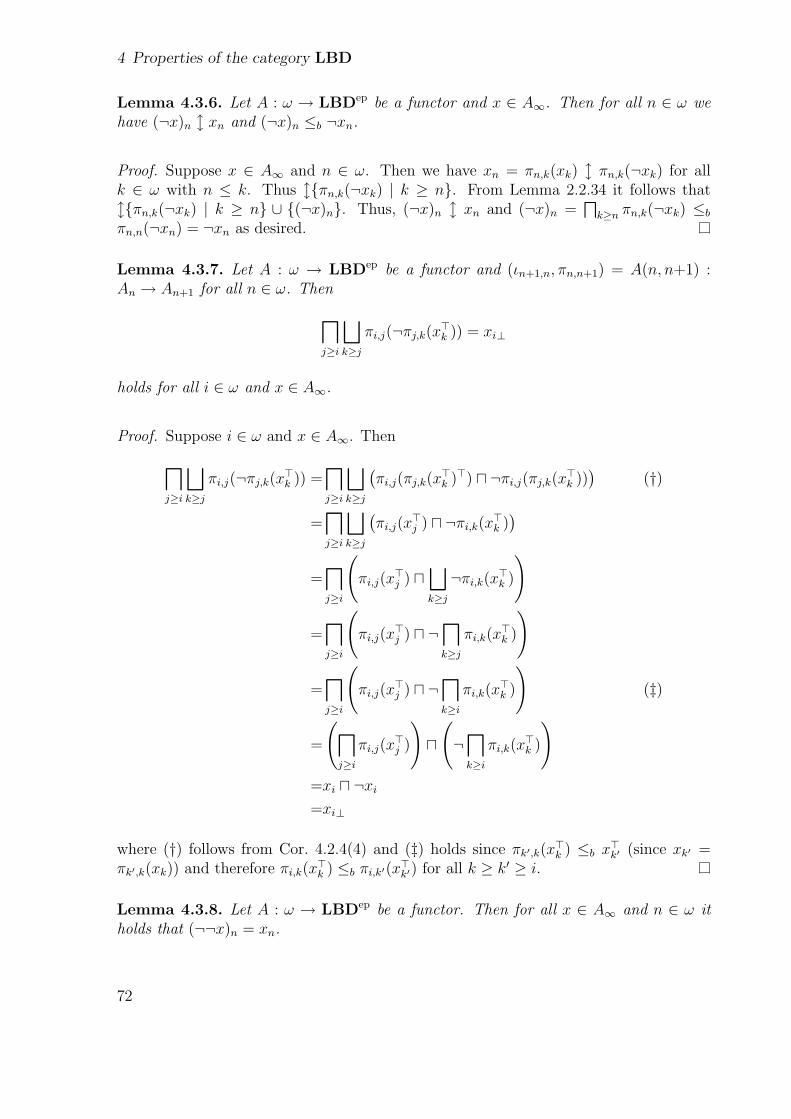
4 Properties of the category LBD
Lemma 4.3.6. Let A : ω → LBDep be a functor and x ∈ A∞. Then for all n ∈ ω wehave (¬x)n l xn and (¬x)n ≤b ¬xn.
Proof. Suppose x ∈ A∞ and n ∈ ω. Then we have xn = πn,k(xk) l πn,k(¬xk) for allk ∈ ω with n ≤ k. Thus l{πn,k(¬xk) | k ≥ n}. From Lemma 2.2.34 it follows thatl{πn,k(¬xk) | k ≥ n} ∪ {(¬x)n}. Thus, (¬x)n l xn and (¬x)n =
dk≥n πn,k(¬xk) ≤b
πn,n(¬xn) = ¬xn as desired.
Lemma 4.3.7. Let A : ω → LBDep be a functor and (ιn+1,n, πn,n+1) = A(n, n+1) :An → An+1 for all n ∈ ω. Then
l
j≥i
⊔k≥j
πi,j(¬πj,k(x>k )) = xi⊥
holds for all i ∈ ω and x ∈ A∞.
Proof. Suppose i ∈ ω and x ∈ A∞. Then
l
j≥i
⊔k≥j
πi,j(¬πj,k(x>k )) =
l
j≥i
⊔k≥j
(πi,j(πj,k(x
>k )>) u ¬πi,j(πj,k(x
>k )))
(†)
=l
j≥i
⊔k≥j
(πi,j(x
>j ) u ¬πi,k(x
>k ))
=l
j≥i
(πi,j(x
>j ) u
⊔k≥j
¬πi,k(x>k )
)
=l
j≥i
(πi,j(x
>j ) u ¬
l
k≥j
πi,k(x>k )
)
=l
j≥i
(πi,j(x
>j ) u ¬
l
k≥i
πi,k(x>k )
)(‡)
=
(l
j≥i
πi,j(x>j )
)u
(¬
l
k≥i
πi,k(x>k )
)=xi u ¬xi
=xi⊥
where (†) follows from Cor. 4.2.4(4) and (‡) holds since πk′,k(x>k ) ≤b x>k′ (since xk′ =
πk′,k(xk)) and therefore πi,k(x>k ) ≤b πi,k′(x
>k′) for all k ≥ k′ ≥ i.
Lemma 4.3.8. Let A : ω → LBDep be a functor. Then for all x ∈ A∞ and n ∈ ω itholds that (¬¬x)n = xn.
72
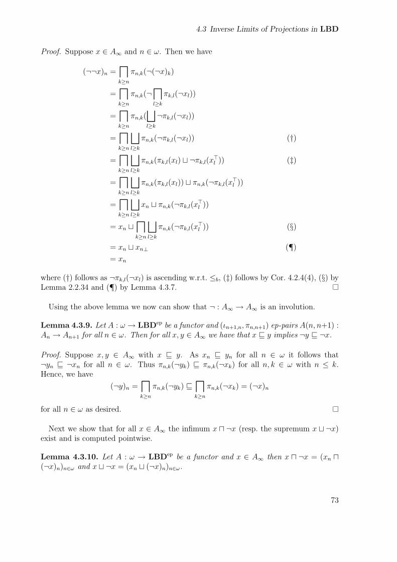
4.3 Inverse Limits of Projections in LBD
Proof. Suppose x ∈ A∞ and n ∈ ω. Then we have
(¬¬x)n =l
k≥n
πn,k(¬(¬x)k)
=l
k≥n
πn,k(¬l
l≥k
πk,l(¬xl))
=l
k≥n
πn,k(⊔l≥k
¬πk,l(¬xl))
=l
k≥n
⊔l≥k
πn,k(¬πk,l(¬xl)) (†)
=l
k≥n
⊔l≥k
πn,k(πk,l(xl) t ¬πk,l(x>l )) (‡)
=l
k≥n
⊔l≥k
πn,k(πk,l(xl)) t πn,k(¬πk,l(x>l ))
=l
k≥n
⊔l≥k
xn t πn,k(¬πk,l(x>l ))
= xn tl
k≥n
⊔l≥k
πn,k(¬πk,l(x>l )) (§)
= xn t xn⊥ (¶)= xn
where (†) follows as ¬πk,l(¬xl) is ascending w.r.t. ≤b, (‡) follows by Cor. 4.2.4(4), (§) byLemma 2.2.34 and (¶) by Lemma 4.3.7.
Using the above lemma we now can show that ¬ : A∞ → A∞ is an involution.
Lemma 4.3.9. Let A : ω → LBDep be a functor and (ιn+1,n, πn,n+1) ep-pairs A(n, n+1) :An → An+1 for all n ∈ ω. Then for all x, y ∈ A∞ we have that x v y implies ¬y v ¬x.
Proof. Suppose x, y ∈ A∞ with x v y. As xn v yn for all n ∈ ω it follows that¬yn v ¬xn for all n ∈ ω. Thus πn,k(¬yk) v πn,k(¬xk) for all n, k ∈ ω with n ≤ k.Hence, we have
(¬y)n =l
k≥n
πn,k(¬yk) vl
k≥n
πn,k(¬xk) = (¬x)n
for all n ∈ ω as desired.
Next we show that for all x ∈ A∞ the infimum x u ¬x (resp. the supremum x t ¬x)exist and is computed pointwise.
Lemma 4.3.10. Let A : ω → LBDep be a functor and x ∈ A∞ then x u ¬x = (xn u(¬x)n)n∈ω and x t ¬x = (xn t (¬x)n)n∈ω.
73
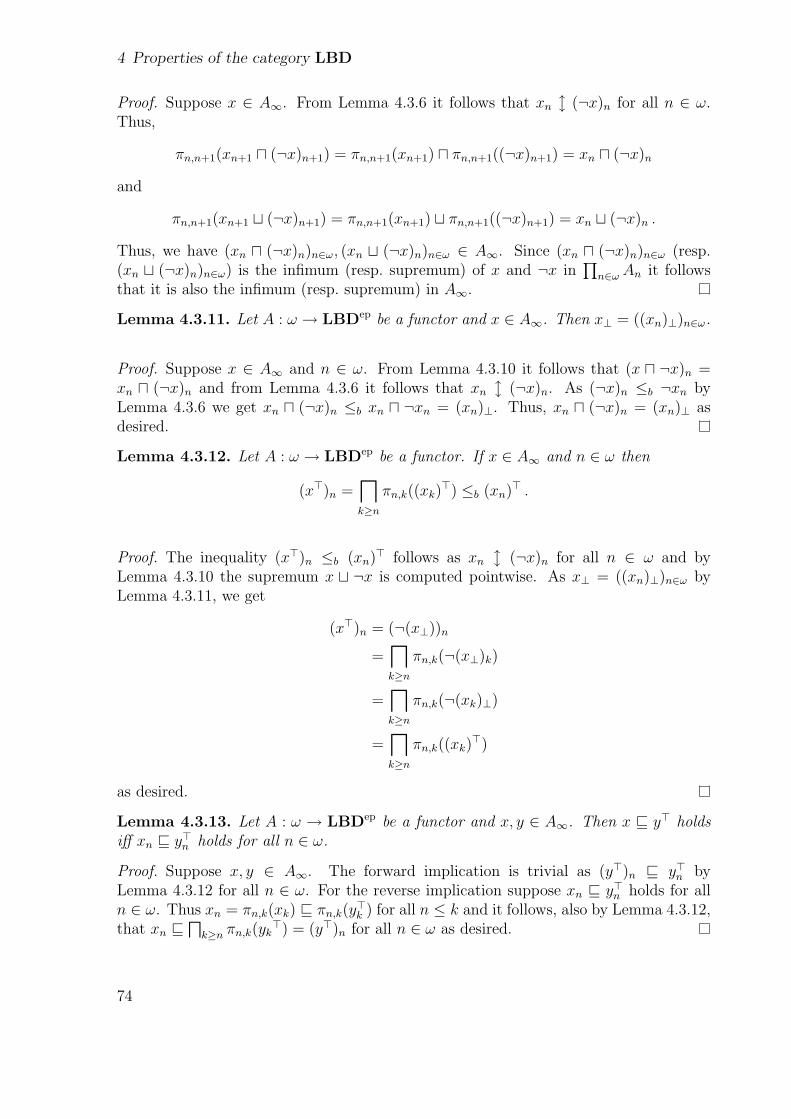
4 Properties of the category LBD
Proof. Suppose x ∈ A∞. From Lemma 4.3.6 it follows that xn l (¬x)n for all n ∈ ω.Thus,
πn,n+1(xn+1 u (¬x)n+1) = πn,n+1(xn+1) u πn,n+1((¬x)n+1) = xn u (¬x)n
and
πn,n+1(xn+1 t (¬x)n+1) = πn,n+1(xn+1) t πn,n+1((¬x)n+1) = xn t (¬x)n .
Thus, we have (xn u (¬x)n)n∈ω, (xn t (¬x)n)n∈ω ∈ A∞. Since (xn u (¬x)n)n∈ω (resp.(xn t (¬x)n)n∈ω) is the infimum (resp. supremum) of x and ¬x in
∏n∈ω An it follows
that it is also the infimum (resp. supremum) in A∞.
Lemma 4.3.11. Let A : ω → LBDep be a functor and x ∈ A∞. Then x⊥ = ((xn)⊥)n∈ω.
Proof. Suppose x ∈ A∞ and n ∈ ω. From Lemma 4.3.10 it follows that (x u ¬x)n =xn u (¬x)n and from Lemma 4.3.6 it follows that xn l (¬x)n. As (¬x)n ≤b ¬xn byLemma 4.3.6 we get xn u (¬x)n ≤b xn u ¬xn = (xn)⊥. Thus, xn u (¬x)n = (xn)⊥ asdesired.
Lemma 4.3.12. Let A : ω → LBDep be a functor. If x ∈ A∞ and n ∈ ω then
(x>)n =l
k≥n
πn,k((xk)>) ≤b (xn)> .
Proof. The inequality (x>)n ≤b (xn)> follows as xn l (¬x)n for all n ∈ ω and byLemma 4.3.10 the supremum x t ¬x is computed pointwise. As x⊥ = ((xn)⊥)n∈ω byLemma 4.3.11, we get
(x>)n = (¬(x⊥))n
=l
k≥n
πn,k(¬(x⊥)k)
=l
k≥n
πn,k(¬(xk)⊥)
=l
k≥n
πn,k((xk)>)
as desired.
Lemma 4.3.13. Let A : ω → LBDep be a functor and x, y ∈ A∞. Then x v y> holdsiff xn v y>n holds for all n ∈ ω.
Proof. Suppose x, y ∈ A∞. The forward implication is trivial as (y>)n v y>n byLemma 4.3.12 for all n ∈ ω. For the reverse implication suppose xn v y>n holds for alln ∈ ω. Thus xn = πn,k(xk) v πn,k(y
>k ) for all n ≤ k and it follows, also by Lemma 4.3.12,
that xn vd
k≥n πn,k(yk>) = (y>)n for all n ∈ ω as desired.
74
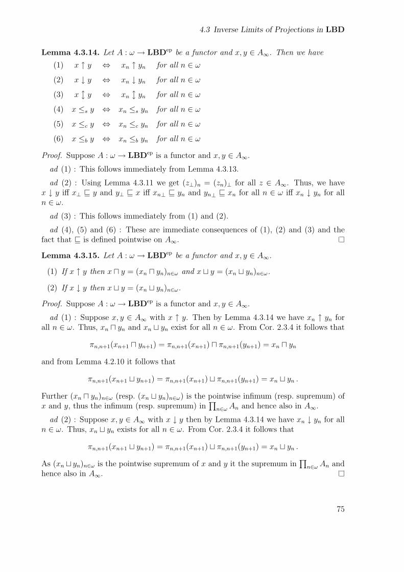
4.3 Inverse Limits of Projections in LBD
Lemma 4.3.14. Let A : ω → LBDep be a functor and x, y ∈ A∞. Then we have
(1) x ↑ y ⇔ xn ↑ yn for all n ∈ ω
(2) x ↓ y ⇔ xn ↓ yn for all n ∈ ω
(3) x l y ⇔ xn l yn for all n ∈ ω
(4) x ≤s y ⇔ xn ≤s yn for all n ∈ ω
(5) x ≤c y ⇔ xn ≤c yn for all n ∈ ω
(6) x ≤b y ⇔ xn ≤b yn for all n ∈ ω
Proof. Suppose A : ω → LBDep is a functor and x, y ∈ A∞.
ad (1) : This follows immediately from Lemma 4.3.13.
ad (2) : Using Lemma 4.3.11 we get (z⊥)n = (zn)⊥ for all z ∈ A∞. Thus, we havex ↓ y iff x⊥ v y and y⊥ v x iff xn⊥ v yn and yn⊥ v xn for all n ∈ ω iff xn ↓ yn for alln ∈ ω.
ad (3) : This follows immediately from (1) and (2).
ad (4), (5) and (6) : These are immediate consequences of (1), (2) and (3) and thefact that v is defined pointwise on A∞.
Lemma 4.3.15. Let A : ω → LBDep be a functor and x, y ∈ A∞.
(1) If x ↑ y then x u y = (xn u yn)n∈ω and x t y = (xn t yn)n∈ω.
(2) If x ↓ y then x t y = (xn t yn)n∈ω.
Proof. Suppose A : ω → LBDep is a functor and x, y ∈ A∞.
ad (1) : Suppose x, y ∈ A∞ with x ↑ y. Then by Lemma 4.3.14 we have xn ↑ yn forall n ∈ ω. Thus, xn u yn and xn t yn exist for all n ∈ ω. From Cor. 2.3.4 it follows that
πn,n+1(xn+1 u yn+1) = πn,n+1(xn+1) u πn,n+1(yn+1) = xn u yn
and from Lemma 4.2.10 it follows that
πn,n+1(xn+1 t yn+1) = πn,n+1(xn+1) t πn,n+1(yn+1) = xn t yn .
Further (xn u yn)n∈ω (resp. (xn t yn)n∈ω) is the pointwise infimum (resp. supremum) ofx and y, thus the infimum (resp. supremum) in
∏n∈ω An and hence also in A∞.
ad (2) : Suppose x, y ∈ A∞ with x ↓ y then by Lemma 4.3.14 we have xn ↓ yn for alln ∈ ω. Thus, xn t yn exists for all n ∈ ω. From Cor. 2.3.4 it follows that
πn,n+1(xn+1 t yn+1) = πn,n+1(xn+1) t πn,n+1(yn+1) = xn t yn .
As (xn t yn)n∈ω is the pointwise supremum of x and y it the supremum in∏
n∈ω An andhence also in A∞.
75
4 Properties of the category LBD
Lemma 4.3.16. Let A : ω → LBDep be a functor. Then A∞ is a lbo.
Proof. From Lemma 4.3.9 and Lemma 4.3.8 it follows that ¬ : |A∞| → |A∞| is aninvolution. Lemma 4.3.10 ensures the existence of x> and x⊥ for all x ∈ |A∞|, andLemma 4.3.15 provides binary infima and suprema of stably coherent elements.
Lemma 4.3.17. Let A : ω → LBDep be a functor then (A∞,v) is a cpo. If X is adirected subset of A∞ then
⊔X = (
⊔{xn | x ∈ X})n∈ω.
Proof. Suppose X ⊆ A∞ is v-directed. As the extensional order v is given pointwiseon A∞ it follows that for all n ∈ ω the set {xn | x ∈ X} is directed w.r.t. v. Asπn,n+1(
⊔{xn+1 | x ∈ X}) =
⊔{πn,n+1(xn+1) | x ∈ X} =
⊔{xn | x ∈ X} and (
⊔{xn |
x ∈ X})n∈ω is the supremum of X in∏
n∈ω An it follows that it is also the supremum inA∞.
Next we study finite prime elements of A∞.
Definition 4.3.18. If A : ω → LBDep is a functor. Then we define πn : A∞ → An by
πn(x) := xn
and ιn : An → A∞ by
(ιn(x))k :=
{πk,n(x) if k ≤ n,
ιk,n(x) otherwise,
for all k ∈ ω. Further, we put rn := ιn ◦ πn for all n ∈ ω. �
Lemma 4.3.19. For all n ∈ ω the functions πn : A∞ → An, ιn : An → A∞ andrn : A∞ → A∞ from Def. 4.3.18 are bistable.
Proof. This follows as πk,n and ιk,n are bistable for all k ≤ n and using Lemma 4.3.14.
Lemma 4.3.20. Let A : ω → LBDep be a functor, x ∈ A∞ and y ∈ An for some n ∈ ω.Then
(1) y v xn implies ιn(y) v x and
(2) y ≤s xn implies ιn(y) ≤s x.
Proof. Suppose x ∈ A∞ and y ∈ An.
ad (1) : If y v xn then (ιn(y))n = y v xn. Let k ∈ ω, if k ≤ n then (ιn(x))k =πk,n(y) v πk,n(xn) = xk. If k > n then (ιn(x))k = ιk,n(y) v ιk,n(xn) v xk. Thus,ιn(y) v x as desired.
ad (2) : If y ≤s xn then (ιn(y))n = y ≤s xn. Let k ∈ ω, if k ≤ n then (ιn(x))k =πk,n(y) ≤s πk,n(xn) = xk. If k > n then (ιn(x))k = ιk,n(y) ≤s ιk,n(xn) = ιk,n(πn,k(xk)) ≤s
xk. Thus, ιn(y) ≤s x as desired.
76
4.3 Inverse Limits of Projections in LBD
Lemma 4.3.21. Let A : ω → LBDep be a functor then
FP(A∞) = {ιn(p) | n ∈ ω and p ∈ FP(An)} .
Proof. Suppose p ∈ FP(A∞) then the set {q ∈ A∞ | q ≤s p} is finite. Let n := |{q ∈A∞ | q ≤s p}|. By Lemma 4.3.20 n is an upper bound for |{q ∈ Ai | q ≤s pi}| for alli ∈ ω. Further, there exists a k ∈ ω such that |{q ∈ Ak | q ≤s pk}| = n. As pi+1 stablydominates at least as many elements as pi it follows that |{q ∈ Al | q ≤s pl}| = n forall l ≥ k. As all the maps ιl,k are injective and preserve the stable order it follows that|{r ∈ Al | r ≤s ιl,k(pk)}| ≥ n. Thus, as ιl,k(pk) ≤s pl we get ιl,k(pk) = pl for all l ≥ k.Hence, p = ιk(pk) and pk is finite.
For showing that pk is prime suppose x, y ∈ Ak with x ↑ y or x ↓ y. If pk v x t ythen from Lemma 4.3.20 it follows that p v ιk(x t y). Using Cor. 2.3.4 (in case x ↓ y)and Lemma 4.2.10 (in case x ↑ y) we get πl,k(x t y) = πl,k(x) t πl,k(y) for all l ≤ k andιl,k(x t y) = ιl,k(x) t ιl,k(y) for all l > k. Thus, it follows that ιk(x t y) = ιk(x) t ιk(y).As ιk(x) ↑ ιk(y) or ιk(x) ↓ ιk(y) (since ιk is bistable) and p v ιk(x t y) = ιk(x) t ιk(y)we get p v ιk(x) or p v ιk(y). Thus, pk v x or pk v y as desired.
For the reverse inclusion suppose p ∈ FP(Ak) for some k ∈ ω and y, z ∈ A∞ with y ↑ zor y ↓ z. If ιk(p) v y t z then it follows from Lemma 4.3.15 that (y t z)k = yk t zk,and from Lemma 4.3.14 that yk ↑ zk or yk ↓ zk. As (ιk(p))k v yk t zk and (ιk(p))k =p ∈ FP(Ak) we get p v yk or p v zk. W.l.o.g. assume p v yk. Then by Lemma 4.3.20it follows that ιk(p) v y. Thus, ιk(p) ∈ P(A∞). Suppose l > k. From Lemma 4.2.6 itfollows that ιl,k(πk,l(r)) = r for all r ≤s ιl,k(p). Thus, if x ∈ A∞ with x ≤s ιk(p) thenxl ≤s ιk(p)l = ιl,k(p) and it follows that x = ιk(xk) = ιk(q) for some q ≤s p. As p isfinite there exist only finitely many q with q ≤s p. Thus, ιk(p) is also finite.
Lemma 4.3.22. Let A : ω → LBDep be a functor and x ∈ A∞ then
FP(x) = {ιn(p) | n ∈ ω and p ∈ FP(xn)} .
Proof. Suppose x ∈ A∞. Then we have FP(x) = {y ∈ FP(A∞) | y ≤s x}. Thus, fromLemma 4.3.21 it follows that
FP(x) = {ιn(q) | n ∈ ω, q ∈ FP(An) and ιn(q) ≤s x} .
Using Lemma 4.3.14 we get
FP(x) = {ιn(q) | n ∈ ω, q ∈ FP(An) and q ≤s xn}= {ιn(p) | n ∈ ω and p ∈ FP(xn)}
as desired.
Theorem 4.3.23. Let A : ω → LBDep be a functor. Then A∞ is a lbd.
77
4 Properties of the category LBD
Proof. We already know from Lemma 4.3.16 and Lemma 4.3.17 that A∞ is a completelbo. Further, as every An has a least element ⊥ it follows that A∞ has also a leastelement ⊥. Thus, A∞ is pointed. It remains to show that A∞ fulfils the requirements(1) and (2) of Def. 2.2.3:
ad (1) : Suppose x ∈ A∞. Then it follows from Lemma 4.3.22 that FP(x) = {ιn(p) |n ∈ ω and p ∈ FP(xn)}. For all n ∈ ω and p ∈ FP(xn) we have (ιn(p))n = p and itfollows that xn ≤s (
⊔{ιn(p) | p ∈ FP(xn)})n. As ιn(p) ≤s x for all n ∈ ω and p ∈ FP(xn)
by Lemma 4.3.20, it follows that xn = (⊔{ιn(p) | p ∈ FP(xn)})n Thus, x =
⊔FP(x) as
desired.
ad (2) : Suppose p ∈ FP(A∞), X a directed subset of A∞ and p v⊔
X. FromLemma 4.3.21 it follows that there exists an i ∈ ω and a q ∈ Ai with p = ιi(q). Further,⊔
X = (⊔{xn | x ∈ X})n∈ω by Lemma 4.3.17. Thus, there exists an x ∈ X with q v xi.
From Lemma 4.3.20 it follows that ιi(q) v x. Thus, p v x as desired.
Theorem 4.3.24. Let A : ω → LBDep be a functor then the following holds:
(1) The locally boolean domain A∞ together with the morphisms πn : A∞ → An for alln ∈ ω is a limit over the diagram D←− := ((An)n∈ω, (πn,n+1)n∈ω) in LBD.
(2) The locally boolean domain A∞ together with the morphisms ιn : An → A∞ for alln ∈ ω is a colimit over the diagram D−→ := ((An)n∈ω, (ιn+1,n)n∈ω) in LBD.
(3) (ιn, πn) is an ep-pair for every n ∈ ω.
(4)⊔
n∈ω ιn ◦ πn = idA∞
Proof. ad (1) : The construction of the limiting object A∞ and the projections πn is theusual one for categories of domains. Thus, having another cone (B, (fn)n∈ω) over thediagram D←− it follows that the function f : B → A∞ with f(x) := (fn(x))n∈ω is Scott
continuous. Thus, it remains to show that f is bistable. Suppose x, y ∈ B with x l y.Then it follows that fn(xuy) = fn(x)ufn(y) and fn(xty) = fn(x)tfn(y) for all n ∈ ωand we get
f(x u y) = (fn(x u y))n∈ω
= (fn(x) u fn(y))n∈ω
= (fn(x))n∈ω u (fn(y))n∈ω (†)= f(x) u f(y)
and
f(x t y) = (fn(x t y))n∈ω
= (fn(x) t fn(y))n∈ω
= (fn(x))n∈ω t (fn(y))n∈ω (†)= f(x) t f(y)
78
4.3 Inverse Limits of Projections in LBD
where (†) holds as fn(x) l fn(y) for all n ∈ ω and the infimum (resp. supremum) iscomputed pointwise (by Lemma 4.3.15).
ad (2) : Like in the proof of (1) it remains to show that if (B, (fn)n∈ω) is a co-cone over the diagram D−→ then the function f : A∞ → B with f(x) :=
⊔n∈ω fn(xn)
is bistable. First, notice that for x ∈ A∞ we have fn(xn) = fn+1(ιn+1,n(xn)) =fn+1(ιn+1,n(πn,n+1(xn+1))) ≤s fn+1(xn+1), thus we have
fn(xn) ≤s fn+1(xn+1) (†)
for all n ∈ ω. Suppose x, y ∈ A∞. If x l y then it follows that xn l yn and fn(xn) l fn(yn)for all n ∈ ω. Thus, using Lemma 2.2.28 it follows that f(x) l f(y). Further, we havefn(xn t yn) = fn(xn) t fn(yn) for all n ∈ ω and it follows that
f(x t y) =⊔n∈ω
fn((x t y)n)
=⊔n∈ω
fn(xn t yn)
=⊔n∈ω
fn(xn) t fn(yn)
=⊔n∈ω
fn(xn) t⊔n∈ω
fn(yn)
= f(x) t f(y)
From monotonicity of f we get f(x u y) v f(x) u f(y). Suppose p ∈ FP(⊔
n∈ω fn(xn) u⊔n∈ω fn(yn)) then p ∈ FP(
⊔n∈ω fn(xn)) and p ∈ FP(
⊔n∈ω fn(yn)). Thus, there exists an
i ∈ ω such that p v fi(xi) u fi(yi) v f(x) u f(y) as desired.
ad (3) : Suppose n ∈ ω. Then we have πn ◦ ιn(x) = πn(ιn(x)) = ιn(x)n = x, thusπn ◦ ιn = idAn . If x, y ∈ A∞ and x ≤s y then for all n, k ∈ ω it follows that
((ιn ◦ πn)(x))k = (ιn(xn))k =
{πk,n(xn) if k ≤ n,
ιk,n(xn) if k > n,
((ιn ◦ πn)(y) u x)k = ιn(yn)k u xk =
{πk,n(xn) if k ≤ n,
ιk,n(yn) u xk if k > n.
As ιk,n ◦ πn,k ≤s idAkfor all k > n and xk ≤s yk it follows that ιk,n ◦ πn,k(xk) =
ιk,n ◦ πn,k(yk) u xk. Thus, we have ιk,n(xn) = ιk,n(yn) u xk as desired.
ad (4) : We have ιn ◦ πn ≤s idA∞ for all n ∈ ω thus⊔
n∈ω ιn ◦ πn ≤s idA∞ . Onthe other hand, we have (idA∞(x))m = (ιm ◦ πm(x))m ≤s
(⊔n∈ω ιn ◦ πn(x)
)m
. Thus,⊔n∈ω ιn ◦ πn = idA∞ .
79
4 Properties of the category LBD
4.4 Countably based Locally Boolean Domains
We will now restrict to those locally boolean (pre)domains where the set of finite primeelements is countable. Notice that countably based lbds will be sufficient for the inter-pretation of the language SPCF∞ (cf. Chapter 5).
Further, adapting a result of J. Longley in [Lon02] we show that every countablybased locally boolean domain appears as retract of U = [N→N] where N are the biliftednatural numbers, i.e. that U is a universal object for countably based locally booleandomains.
Definition 4.4.1. A lbpd (resp. lbd) A is countably based (a cblbpd (resp. cblbd)) iffthe set FP(A) is countable.We write ωLBPD (resp. ωLBD) for the category of countably based locally boolean(pre)domains and sequential maps. �
Obviously, for a lbpd A the set FP(A) is countable iff F(A) is countable.
Lemma 4.4.2. The category ωLBD has countable bilifted sums and products, is carte-sian closed, and is closed under inverse limits of ω-chains of embedding projectionpairs.
Proof. It is well known that the category OSA restricted to Curien-Lamarche gameswith countable sets of cells and values forms a cartesian closed category and this categoryis obviously equivalent to ωLBD.
The other statements are left as an exercise to the reader.
We now define abbreviations for some frequently used cblbds.
Definition 4.4.3. We define the following cblbds:
1 :=∏i∈∅
(The empty product.)
O :=∑i∈∅
(The empty sum.)
N :=∑i∈ω
1 (The bilifted natural numbers.)
U := [N→N] (The bistable endomaps on N.)
Further, given a lbpd A we introduce the abbreviation Aω for∏
i∈ω A. �
We call the type O the type of observations. More explicitly O can be described asthe lbd ({⊥,>},v,¬) with ⊥ v > and ¬⊥ = >. Notice that [A→O] separates pointsin A for any lbd A.
The data type N will serve as the type of bilifted natural numbers. More explicitly Ncan be described as the lbd (N ∪ {⊥,>},v,¬) with x v y iff x = ⊥ or y = > or x = y,
80
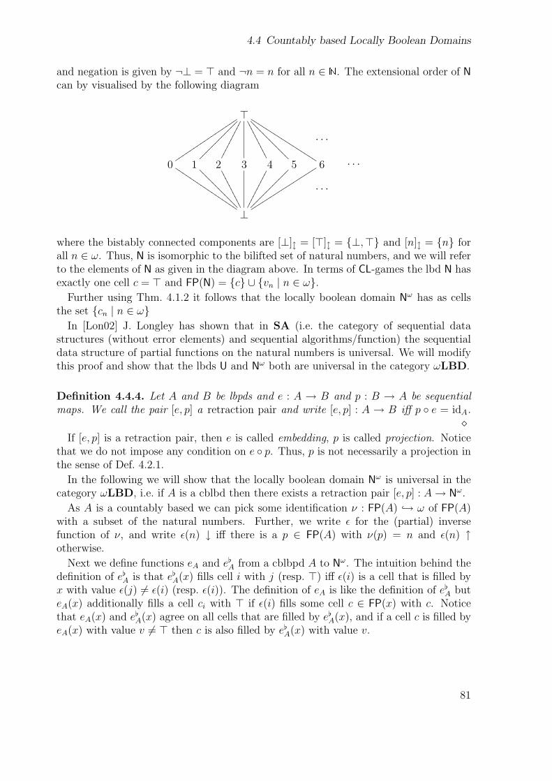
4.4 Countably based Locally Boolean Domains
and negation is given by ¬⊥ = > and ¬n = n for all n ∈ N. The extensional order of Ncan by visualised by the following diagram
>
· · ·
0
uuuuuuuuuuuuuuuuu
IIIIIIIIIIIIIIIII 1
������������
????
????
????
2
����������
0000
0000
003 4
0000000000
����������
5
????????????
����
����
����
6
KKKKKKKKKKKKKKKKK
sssssssssssssssss · · ·
· · ·
⊥
where the bistably connected components are [⊥]l = [>]l = {⊥,>} and [n]l = {n} forall n ∈ ω. Thus, N is isomorphic to the bilifted set of natural numbers, and we will referto the elements of N as given in the diagram above. In terms of CL-games the lbd N hasexactly one cell c = > and FP(N) = {c} ∪ {vn | n ∈ ω}.
Further using Thm. 4.1.2 it follows that the locally boolean domain Nω has as cellsthe set {cn | n ∈ ω}
In [Lon02] J. Longley has shown that in SA (i.e. the category of sequential datastructures (without error elements) and sequential algorithms/function) the sequentialdata structure of partial functions on the natural numbers is universal. We will modifythis proof and show that the lbds U and Nω both are universal in the category ωLBD.
Definition 4.4.4. Let A and B be lbpds and e : A → B and p : B → A be sequentialmaps. We call the pair [e, p] a retraction pair and write [e, p] : A → B iff p ◦ e = idA.
�If [e, p] is a retraction pair, then e is called embedding, p is called projection. Notice
that we do not impose any condition on e ◦ p. Thus, p is not necessarily a projection inthe sense of Def. 4.2.1.
In the following we will show that the locally boolean domain Nω is universal in thecategory ωLBD, i.e. if A is a cblbd then there exists a retraction pair [e, p] : A→ Nω.
As A is a countably based we can pick some identification ν : FP(A) ↪→ ω of FP(A)with a subset of the natural numbers. Further, we write ε for the (partial) inversefunction of ν, and write ε(n) ↓ iff there is a p ∈ FP(A) with ν(p) = n and ε(n) ↑otherwise.
Next we define functions eA and e[A from a cblbpd A to Nω. The intuition behind the
definition of e[A is that e[
A(x) fills cell i with j (resp. >) iff ε(i) is a cell that is filled byx with value ε(j) 6= ε(i) (resp. ε(i)). The definition of eA is like the definition of e[
A buteA(x) additionally fills a cell ci with > if ε(i) fills some cell c ∈ FP(x) with c. Noticethat eA(x) and e[
A(x) agree on all cells that are filled by e[A(x), and if a cell c is filled by
eA(x) with value v 6= > then c is also filled by e[A(x) with value v.
81
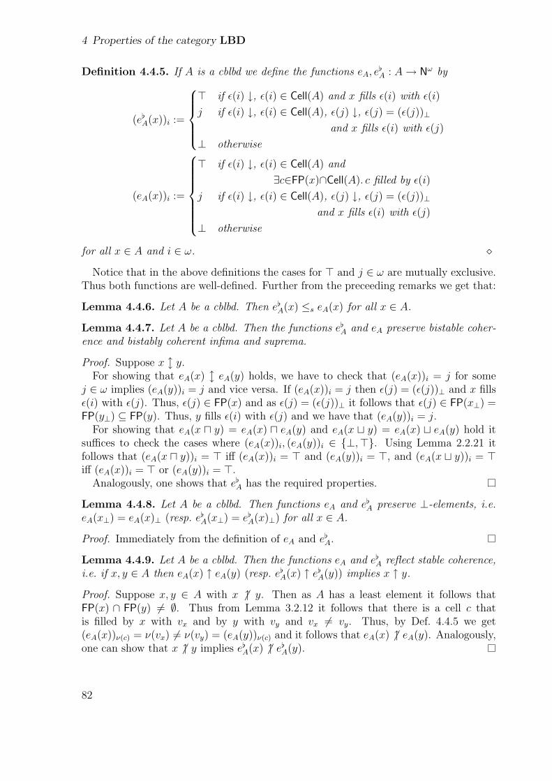
4 Properties of the category LBD
Definition 4.4.5. If A is a cblbd we define the functions eA, e[A : A→ Nω by
(e[A(x))i :=
> if ε(i) ↓, ε(i) ∈ Cell(A) and x fills ε(i) with ε(i)
j if ε(i) ↓, ε(i) ∈ Cell(A), ε(j) ↓, ε(j) = (ε(j))⊥
and x fills ε(i) with ε(j)
⊥ otherwise
(eA(x))i :=
> if ε(i) ↓, ε(i) ∈ Cell(A) and
∃c∈FP(x)∩Cell(A). c filled by ε(i)
j if ε(i) ↓, ε(i) ∈ Cell(A), ε(j) ↓, ε(j) = (ε(j))⊥
and x fills ε(i) with ε(j)
⊥ otherwise
for all x ∈ A and i ∈ ω. �
Notice that in the above definitions the cases for > and j ∈ ω are mutually exclusive.Thus both functions are well-defined. Further from the preceeding remarks we get that:
Lemma 4.4.6. Let A be a cblbd. Then e[A(x) ≤s eA(x) for all x ∈ A.
Lemma 4.4.7. Let A be a cblbd. Then the functions e[A and eA preserve bistable coher-
ence and bistably coherent infima and suprema.
Proof. Suppose x l y.For showing that eA(x) l eA(y) holds, we have to check that (eA(x))i = j for some
j ∈ ω implies (eA(y))i = j and vice versa. If (eA(x))i = j then ε(j) = (ε(j))⊥ and x fillsε(i) with ε(j). Thus, ε(j) ∈ FP(x) and as ε(j) = (ε(j))⊥ it follows that ε(j) ∈ FP(x⊥) =FP(y⊥) ⊆ FP(y). Thus, y fills ε(i) with ε(j) and we have that (eA(y))i = j.
For showing that eA(x u y) = eA(x) u eA(y) and eA(x t y) = eA(x) t eA(y) hold itsuffices to check the cases where (eA(x))i, (eA(y))i ∈ {⊥,>}. Using Lemma 2.2.21 itfollows that (eA(x u y))i = > iff (eA(x))i = > and (eA(y))i = >, and (eA(x t y))i = >iff (eA(x))i = > or (eA(y))i = >.
Analogously, one shows that e[A has the required properties.
Lemma 4.4.8. Let A be a cblbd. Then functions eA and e[A preserve ⊥-elements, i.e.
eA(x⊥) = eA(x)⊥ (resp. e[A(x⊥) = e[
A(x)⊥) for all x ∈ A.
Proof. Immediately from the definition of eA and e[A.
Lemma 4.4.9. Let A be a cblbd. Then the functions eA and e[A reflect stable coherence,
i.e. if x, y ∈ A then eA(x) ↑ eA(y) (resp. e[A(x) ↑ e[
A(y)) implies x ↑ y.
Proof. Suppose x, y ∈ A with x 6 ↑ y. Then as A has a least element it follows thatFP(x) ∩ FP(y) 6= ∅. Thus from Lemma 3.2.12 it follows that there is a cell c thatis filled by x with vx and by y with vy and vx 6= vy. Thus, by Def. 4.4.5 we get(eA(x))ν(c) = ν(vx) 6= ν(vy) = (eA(y))ν(c) and it follows that eA(x) 6 ↑ eA(y). Analogously,one can show that x 6 ↑ y implies e[
A(x) 6 ↑ e[A(y).
82
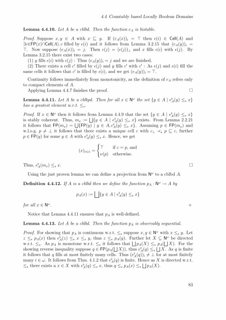
4.4 Countably based Locally Boolean Domains
Lemma 4.4.10. Let A be a cblbd. Then the function eA is bistable.
Proof. Suppose x, y ∈ A with x v y. If (eA(x))i = > then ε(i) ∈ Cell(A) and∃c∈FP(x)∩Cell(A). c filled by ε(i) and it follows from Lemma 3.2.15 that (eA(y))i =>. Now suppose (eA(x))i = j. Then ε(j) = (ε(j))⊥ and x fills ε(i) with ε(j). ByLemma 3.2.15 there exist two cases:
(1) y fills ε(i) with ε(j) : Thus (eA(y))i = j and we are finished.(2) There exists a cell c′ filled by ε(j) and y fills c′ with c′ : As ε(j) and ε(i) fill the
same cells it follows that c′ is filled by ε(i), and we get (eA(y))i = >.
Continuity follows immediately from monotonicity, as the definition of eA refers onlyto compact elements of A.
Applying Lemma 4.4.7 finishes the proof.
Lemma 4.4.11. Let A be a cblbpd. Then for all x ∈ Nω the set {y ∈ A | e[A(y) ≤s x}
has a greatest element w.r.t. ≤s.
Proof. If x ∈ Nω then it follows from Lemma 4.4.9 that the set {y ∈ A | e[A(y) ≤s x}
is stably coherent. Thus, mx :=⊔{y ∈ A | e[
A(y) ≤s x} exists. From Lemma 2.2.21it follows that FP(mx) =
⋃{FP(y) | y ∈ A, e[
A(y) ≤s x}. Assuming p ∈ FP(mx) andw.l.o.g. p 6= ⊥ it follows that there exists a unique cell c with c⊥ ≺s p v c, furtherp ∈ FP(y) for some y ∈ A with e[
A(y) ≤s x. Hence, we get
(x)ν(c) =
{> if c = p, and
ν(p) otherwise.
Thus, e[A(mx) ≤s x.
Using the just proven lemma we can define a projection from Nω to a cblbd A.
Definition 4.4.12. If A is a cblbd then we define the function pA : Nω → A by
pA(x) :=⊔{y ∈ A | e[
A(y) ≤s x}
for all x ∈ Nω. �
Notice that Lemma 4.4.11 ensures that pA is well-defined.
Lemma 4.4.13. Let A be a cblbd. Then the function pA is observably sequential.
Proof. For showing that pA is continuous w.r.t. ≤s suppose x, y ∈ Nω with x ≤s y. Letz ≤s pA(x) then e[
A(z) ≤s x ≤s y, thus z ≤s pA(y). Further let X ⊆ Nω be directedw.r.t. ≤s. As pA is monotone w.r.t. ≤s it follows that
⊔pA(X) ≤s pA(
⊔X). For the
showing reverse inequality suppose q ∈ FP(pA(⊔
X)), thus e[A(q) ≤s
⊔X. As q is finite
it follows that q fills at most finitely many cells. Thus (e[A(q))i 6= ⊥ for at most finitely
many i ∈ ω. It follows from Thm. 4.1.2 that e[A(q) is finite. Hence as X is directed w.r.t.
≤s there exists a x ∈ X with e[A(q) ≤s x, thus q ≤s pA(x) ≤s
⊔pA(X).
83
4 Properties of the category LBD
For showing that pA is observably sequential suppose x, y ∈ Nω with x ≤s y, c′ ∈Acc(pA(x) and pA(y) fills c′. Then e[
A(c′⊥) <s y and it follows that y fills the cell cν(c′),thus cν(c′) is the unique sequentiality index for pA at (x, c′). Uniqueness follows aspA(x t cν(c′)) fills c′. Further by definition of e[
A it follows that pA(x t cν(c′)) fills c′ withvalue c′, thus pA is error propagating.
Thus we can show that each cblbd is a retract of the lbd Nω.
Theorem 4.4.14. The cblbd Nω is universal in the category ωLBD, i.e. if A is a cblbdthen there exists a retraction pair [e, p] : A→ Nω.
Proof. We show that [eA, pA] : A→ Nω is a retraction pair. By Thm. 3.3.6, Lemma 4.4.10and Lemma 4.4.13 and it follows that eA and pA are bistable maps.
For showing that pA ◦ eA = idA suppose x ∈ A. As e[A(x) ≤s eA(x) by Lemma 4.4.6 it
follows that x ≤s pA(eA(x)).For showing the reverse inequality suppose p ∈ FP(pA(eA(x))) and w.l.o.g. p 6= ⊥.
Then e[A(p) ≤s eA(x) and p fills a unique cell c ∈ Cell(A) with value p. We proceed by
case analysis on p. In case that p = p⊥ then (e[A(p))ν(c) = ν(p). As e[
A(p) ≤s eA(x) itfollows that (eA(x))ν(c) = ν(p), thus p ∈ FP(x). In case that p 6= p⊥ then p = c and(e[
A(p))ν(c) = >. Thus (eA(x))ν(c) = > and it follows that there exists a cell c′ that isfilled by c and x fills c′ with value c′. As p, x ≤s pA(eA(x)) we have p ↑ x and it followsfrom Cor. 3.2.11 that the filling of p and x agrees on those cells filled by both. Thus, asall cells except c that are filled by p are filled with values v = v⊥ it follows that c = c′.Hence we get p = c ∈ FP(x) as desired.
As an easy consequence it follows that type of bistable endomaps on the biliftednatural numbers is also universal.
Corollary 4.4.15. The cblbd U is universal in the category ωLBD.
Proof. It is an easy exercise to verify that the maps e : Nω → U and p : U → Nω givenby
e(x) :=
> 7→ >i 7→ xi for all i ∈ ω
⊥ 7→ ⊥
and
p(f)i := f(i) for all i ∈ ω
are both bistable and form a retraction pair [e, p] : Nω → U. Using Thm. 4.4.14 it followsthat U is universal.
84
5 A universal model for the language SPCF∞in LBD
In the first part of this chapter we introduce the language SPCF∞ and its operational se-mantics. The language SPCF∞ is an infinitary version of SPCF as introduced in [CCF94].More explicitly, it is obtained from simply typed λ-calculus by adding (countably) infinitesums and products, error elements, a control operator catch and recursive types. Wegive a call-by-name operational semantics for SPCF∞ where we use evaluation contextsin order to formalise the behaviour of the control operator catch.
In the second part of this chapter we present a computationally adequate model forSPCF∞ in the category LBD. Further we exhibit each SPCF∞ type as an SPCF∞definable retract of the type N→N from which we deduce universality of SPCF∞ for itsLBD model.
5.1 Definition of SPCF∞
First we define the types of the language SPCF∞. Since SPCF∞ has recursive types wealso have to consider types with free type variables.
We assume a given set of type variables (denoted by α, α′ and so on) and generatethe types of SPCF∞ as follows:
σ ::= α | σ→σ | µα.σ | Σi∈nσ | Πi∈nσ
where n ∈ ω + 1.
A type σ is called closed iff it does not contain a free type variable α, i.e. eachoccurrence of a type variable α is bound under by some µα. We introduce the followingabbreviations for types:
0 := Σi∈∅ (type of observations)
1 := Πi∈∅ (empty product)
N := Σi∈ω1 (natural numbers)
n := Σi∈n1 (for all n ∈ ω+1)
σ↑ := Σi∈1σ (bilifting)
σ0+ · · ·+σn−1 := Σi∈nσi (n-ary sum)
σ0× · · ·×σn−1 := Πi∈nσi (n-ary product)
85
5 A universal model for the language SPCF∞ in LBD
Additionally, for a given SPCF∞ type σ and n ∈ ω + 1 we define the abbreviation
σn := Πi∈nσ
The terms of SPCF∞ are derived using the following grammar:
t ::= x | (λx : σ.t) | (tt) |〈ti〉i∈n | prΠi∈nσi
i (t)
inΣi∈nσi
i (t) | caseΣi∈nσi,τ tof (ini x⇒ ti)i∈n
foldµα.σ(t) | unfoldµα.σ(t) |>Σi∈nσi | catch(t)
for any variable x, n ∈ ω + 1 and all types σ, σi, τ and type variables α.By 〈ti〉i∈n we denote
〈t0, . . . , tn−1〉 if n ∈ ω
and〈t0, t1, t2, . . .〉 if n ∈ ω .
Accordingly, by caseΣi∈nσi,τ tof (ini x⇒ t)i∈n we denote
caseΣi∈nσi,τ tof (in0 ⇒ t0, . . . , inn−1 ⇒ tn−1) if n ∈ ω
andcaseΣi∈nσi,τ tof (in0 ⇒ t0, in1 ⇒ t1, in2 ⇒ t2, . . .) if n ∈ ω .
Further we define the values of SPCF∞ by the grammar
v ::= (λx : σ.t) |〈ti〉i∈n
inΣi∈nσi
i (t)
foldµα.σ(t)
>Σi∈nσi
for all terms t. The values >Σi∈nσi are called error values the other values are calledproper values.
Type annotations are merely used for type inference, we will omit them when they areclear from the context. Terms not containing any free variables are called closed termsor programs the other terms are called open terms.
For the typing rules (as given in table Table 5.1), we look at terms-in-context of theform Γ ` M : τ , where M is a term, τ a closed type and Γ ≡ x1 : σ1, . . . , xn : σn is acontext assigning closed types σ1, . . . , σn to a finite set of variables x1, . . . , xn. If Γ is theempty context, then we also write M : τ for Γ `M : τ .
Notice that even in the presence of infinite constructions (countable product and sum)we do not consider contexts with infinitely many free variables as we are interested onlyin those terms-in-context that can be transformed into closed terms.
86
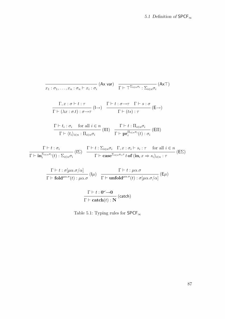
5.1 Definition of SPCF∞
(Ax var)x1 : σ1, . . . , xn : σn ` xi : σi
(Ax>)Γ ` >Σi∈nσi : Σi∈nσi
Γ, x : σ ` t : τ(I→)
Γ ` (λx : σ.t) : σ→τ
Γ ` t : σ→τ Γ ` s : σ(E→)
Γ ` (ts) : τ
Γ ` ti : σi for all i ∈ n(IΠ)
Γ ` 〈ti〉i∈n : Πi∈nσi
Γ ` t : Πi∈nσi(EΠ)
Γ ` prΠi∈nσi
i (t) : σi
Γ ` t : σi(IΣ)
Γ ` inΣi∈nσi
i (t) : Σi∈nσi
Γ ` t : Σi∈nσi Γ, x : σi ` si : τ for all i ∈ n(EΣ)
Γ ` caseΣi∈nσi,τ tof (ini x⇒ si)i∈n : τ
Γ ` t : σ[µα.σ/α](Iµ)
Γ ` foldµα.σ(t) : µα.σ
Γ ` t : µα.σ(Eµ)
Γ ` unfoldµα.σ(t) : σ[µα.σ/α]
Γ ` t : 0ω→0(catch)
Γ ` catch(t) : N
Table 5.1: Typing rules for SPCF∞
87
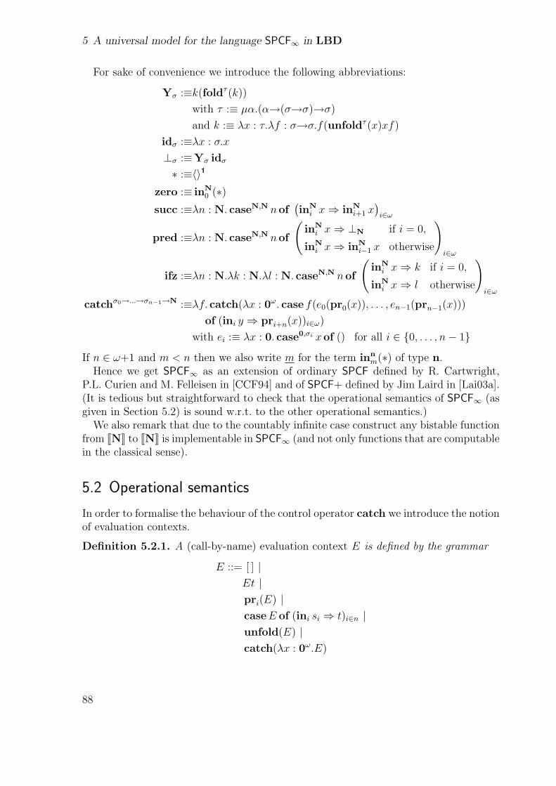
5 A universal model for the language SPCF∞ in LBD
For sake of convenience we introduce the following abbreviations:
Yσ :≡k(foldτ (k))
with τ :≡ µα.(α→(σ→σ)→σ)
and k :≡ λx : τ.λf : σ→σ.f(unfoldτ (x)xf)
idσ :≡λx : σ.x
⊥σ :≡Yσ idσ
∗ :≡〈〉1
zero :≡ inN0 (∗)
succ :≡λn : N. caseN,N nof(inN
i x⇒ inNi+1 x
)i∈ω
pred :≡λn : N. caseN,N nof
(inN
i x⇒ ⊥N if i = 0,
inNi x⇒ inN
i−1 x otherwise
)i∈ω
ifz :≡λn : N.λk : N.λl : N. caseN,N nof
(inN
i x⇒ k if i = 0,
inNi x⇒ l otherwise
)i∈ω
catchσ0→...→σn−1→N :≡λf. catch(λx : 0ω. case f(e0(pr0(x)), . . . , en−1(prn−1(x)))
of (ini y ⇒ pri+n(x))i∈ω)
with ei :≡ λx : 0. case0,σi xof () for all i ∈ {0, . . . , n− 1}
If n ∈ ω+1 and m < n then we also write m for the term innm(∗) of type n.
Hence we get SPCF∞ as an extension of ordinary SPCF defined by R. Cartwright,P.L. Curien and M. Felleisen in [CCF94] and of SPCF+ defined by Jim Laird in [Lai03a].(It is tedious but straightforward to check that the operational semantics of SPCF∞ (asgiven in Section 5.2) is sound w.r.t. to the other operational semantics.)
We also remark that due to the countably infinite case construct any bistable functionfrom JNK to JNK is implementable in SPCF∞ (and not only functions that are computablein the classical sense).
5.2 Operational semantics
In order to formalise the behaviour of the control operator catch we introduce the notionof evaluation contexts.
Definition 5.2.1. A (call-by-name) evaluation context E is defined by the grammar
E ::= [ ] |Et |pri(E) |caseE of (ini si ⇒ t)i∈n |unfold(E) |catch(λx : 0ω.E)
88
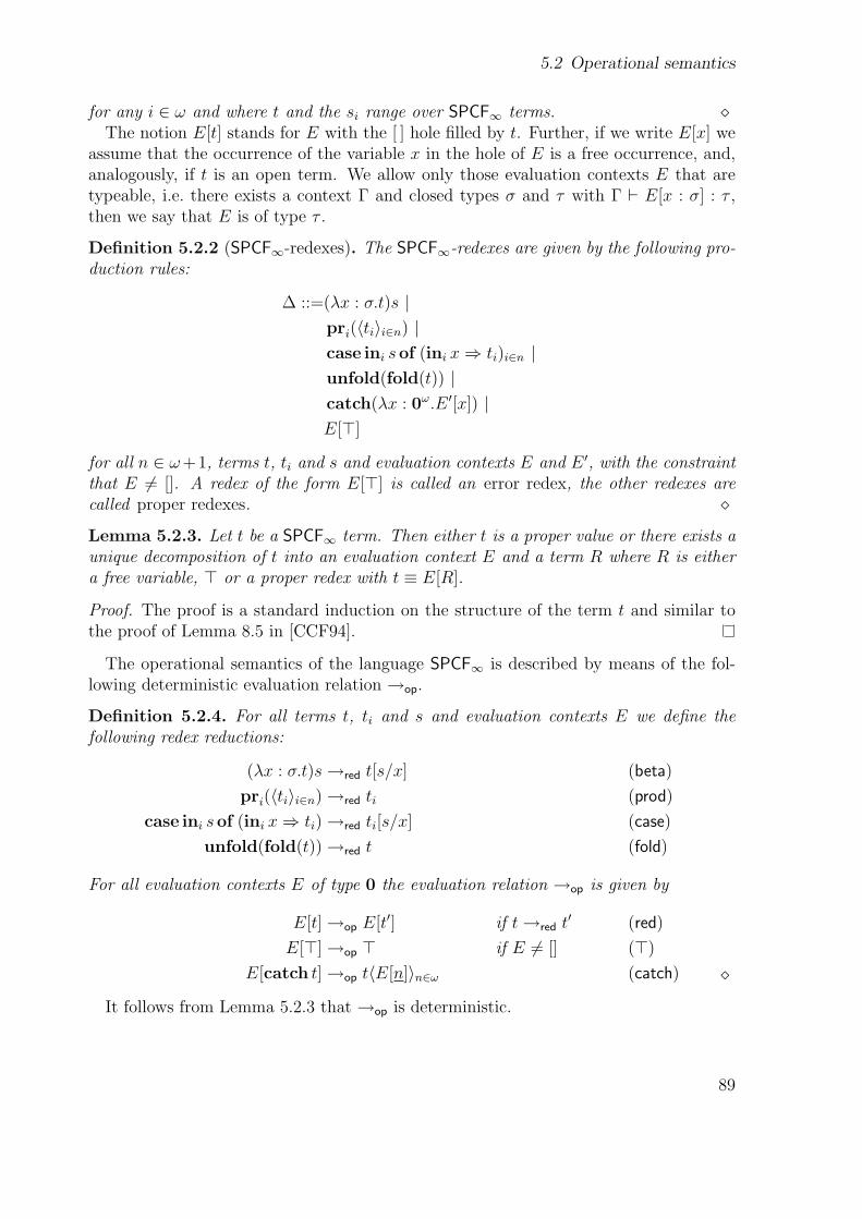
5.2 Operational semantics
for any i ∈ ω and where t and the si range over SPCF∞ terms. �The notion E[t] stands for E with the [ ] hole filled by t. Further, if we write E[x] we
assume that the occurrence of the variable x in the hole of E is a free occurrence, and,analogously, if t is an open term. We allow only those evaluation contexts E that aretypeable, i.e. there exists a context Γ and closed types σ and τ with Γ ` E[x : σ] : τ ,then we say that E is of type τ .
Definition 5.2.2 (SPCF∞-redexes). The SPCF∞-redexes are given by the following pro-duction rules:
∆ ::=(λx : σ.t)s |pri(〈ti〉i∈n) |case ini sof (ini x⇒ ti)i∈n |unfold(fold(t)) |catch(λx : 0ω.E ′[x]) |E[>]
for all n ∈ ω+1, terms t, ti and s and evaluation contexts E and E ′, with the constraintthat E 6= []. A redex of the form E[>] is called an error redex, the other redexes arecalled proper redexes. �
Lemma 5.2.3. Let t be a SPCF∞ term. Then either t is a proper value or there exists aunique decomposition of t into an evaluation context E and a term R where R is eithera free variable, > or a proper redex with t ≡ E[R].
Proof. The proof is a standard induction on the structure of the term t and similar tothe proof of Lemma 8.5 in [CCF94].
The operational semantics of the language SPCF∞ is described by means of the fol-lowing deterministic evaluation relation →op.
Definition 5.2.4. For all terms t, ti and s and evaluation contexts E we define thefollowing redex reductions:
(λx : σ.t)s→red t[s/x] (beta)
pri(〈ti〉i∈n)→red ti (prod)
case ini sof (ini x⇒ ti)→red ti[s/x] (case)
unfold(fold(t))→red t (fold)
For all evaluation contexts E of type 0 the evaluation relation →op is given by
E[t]→op E[t′] if t→red t′ (red)
E[>]→op > if E 6= [] (>)
E[catch t]→op t〈E[n]〉n∈ω (catch) �
It follows from Lemma 5.2.3 that →op is deterministic.
89
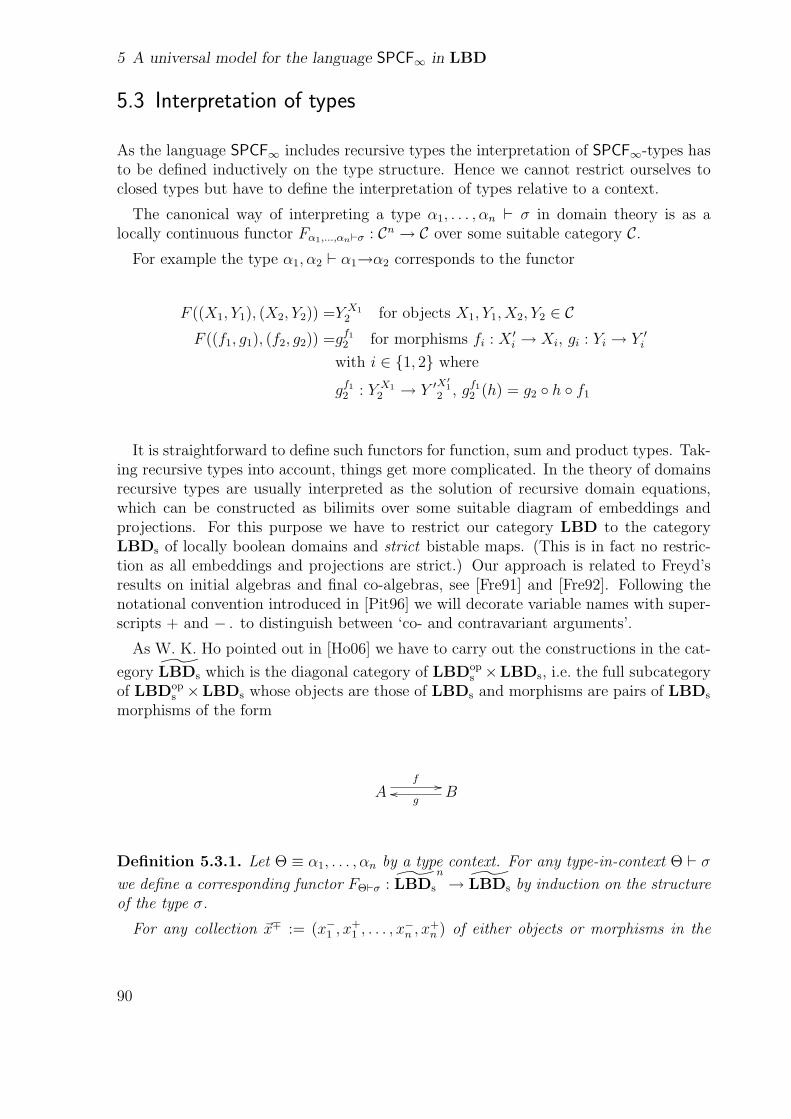
5 A universal model for the language SPCF∞ in LBD
5.3 Interpretation of types
As the language SPCF∞ includes recursive types the interpretation of SPCF∞-types hasto be defined inductively on the type structure. Hence we cannot restrict ourselves toclosed types but have to define the interpretation of types relative to a context.
The canonical way of interpreting a type α1, . . . , αn ` σ in domain theory is as alocally continuous functor Fα1,...,αn`σ : Cn → C over some suitable category C.
For example the type α1, α2 ` α1→α2 corresponds to the functor
F ((X1, Y1), (X2, Y2)) =Y X12 for objects X1, Y1, X2, Y2 ∈ C
F ((f1, g1), (f2, g2)) =gf1
2 for morphisms fi : X ′i → Xi, gi : Yi → Y ′
i
with i ∈ {1, 2} where
gf1
2 : Y X12 → Y ′X′
12 , gf1
2 (h) = g2 ◦ h ◦ f1
It is straightforward to define such functors for function, sum and product types. Tak-ing recursive types into account, things get more complicated. In the theory of domainsrecursive types are usually interpreted as the solution of recursive domain equations,which can be constructed as bilimits over some suitable diagram of embeddings andprojections. For this purpose we have to restrict our category LBD to the categoryLBDs of locally boolean domains and strict bistable maps. (This is in fact no restric-tion as all embeddings and projections are strict.) Our approach is related to Freyd’sresults on initial algebras and final co-algebras, see [Fre91] and [Fre92]. Following thenotational convention introduced in [Pit96] we will decorate variable names with super-scripts + and − . to distinguish between ‘co- and contravariant arguments’.
As W. K. Ho pointed out in [Ho06] we have to carry out the constructions in the cat-
egory LBDs which is the diagonal category of LBDops ×LBDs, i.e. the full subcategory
of LBDops ×LBDs whose objects are those of LBDs and morphisms are pairs of LBDs
morphisms of the form
Af //
Bg
oo
Definition 5.3.1. Let Θ ≡ α1, . . . , αn by a type context. For any type-in-context Θ ` σ
we define a corresponding functor FΘ`σ : LBDs
n
→ LBDs by induction on the structureof the type σ.
For any collection ~x∓ := (x−1 , x+1 , . . . , x−n , x+
n ) of either objects or morphisms in the
90
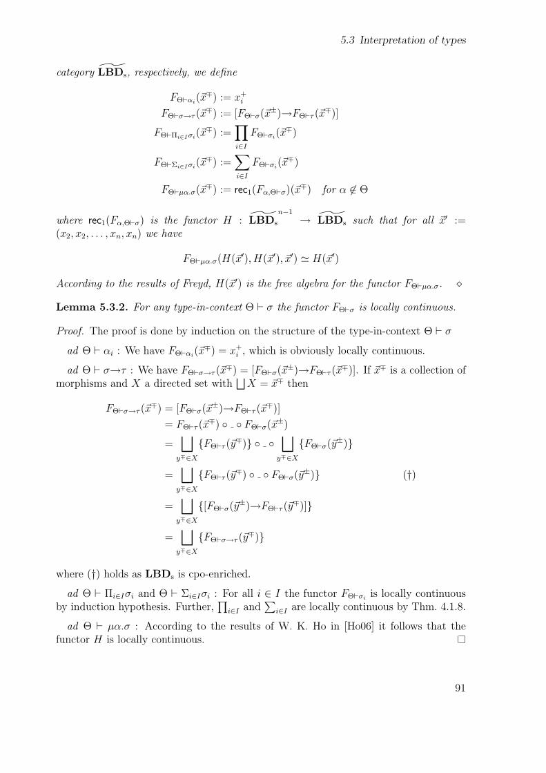
5.3 Interpretation of types
category LBDs, respectively, we define
FΘ`αi(~x∓) := x+
i
FΘ`σ→τ (~x∓) := [FΘ`σ(~x±)→FΘ`τ (~x
∓)]
FΘ`Πi∈Iσi(~x∓) :=
∏i∈I
FΘ`σi(~x∓)
FΘ`Σi∈Iσi(~x∓) :=
∑i∈I
FΘ`σi(~x∓)
FΘ`µα.σ(~x∓) := rec1(Fα,Θ`σ)(~x∓) for α 6∈ Θ
where rec1(Fα,Θ`σ) is the functor H : LBDs
n−1
→ LBDs such that for all ~x′ :=(x2, x2, . . . , xn, xn) we have
FΘ`µα.σ(H(~x′), H(~x′), ~x′) ' H(~x′)
According to the results of Freyd, H(~x′) is the free algebra for the functor FΘ`µα.σ. �
Lemma 5.3.2. For any type-in-context Θ ` σ the functor FΘ`σ is locally continuous.
Proof. The proof is done by induction on the structure of the type-in-context Θ ` σ
ad Θ ` αi : We have FΘ`αi(~x∓) = x+
i , which is obviously locally continuous.
ad Θ ` σ→τ : We have FΘ`σ→τ (~x∓) = [FΘ`σ(~x±)→FΘ`τ (~x
∓)]. If ~x∓ is a collection ofmorphisms and X a directed set with
⊔X = ~x∓ then
FΘ`σ→τ (~x∓) = [FΘ`σ(~x±)→FΘ`τ (~x
∓)]
= FΘ`τ (~x∓) ◦ ◦ FΘ`σ(~x±)
=⊔
y∓∈X
{FΘ`τ (~y∓)} ◦ ◦
⊔y∓∈X
{FΘ`σ(~y±)}
=⊔
y∓∈X
{FΘ`τ (~y∓) ◦ ◦ FΘ`σ(~y±)} (†)
=⊔
y∓∈X
{[FΘ`σ(~y±)→FΘ`τ (~y∓)]}
=⊔
y∓∈X
{FΘ`σ→τ (~y∓)}
where (†) holds as LBDs is cpo-enriched.
ad Θ ` Πi∈Iσi and Θ ` Σi∈Iσi : For all i ∈ I the functor FΘ`σiis locally continuous
by induction hypothesis. Further,∏
i∈I and∑
i∈I are locally continuous by Thm. 4.1.8.
ad Θ ` µα.σ : According to the results of W. K. Ho in [Ho06] it follows that thefunctor H is locally continuous.
91
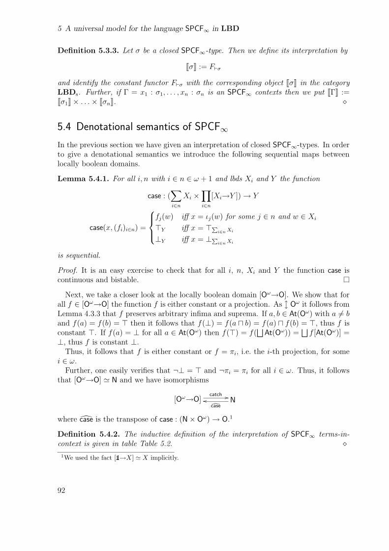
5 A universal model for the language SPCF∞ in LBD
Definition 5.3.3. Let σ be a closed SPCF∞-type. Then we define its interpretation by
JσK := F`σ
and identify the constant functor F`σ with the corresponding object JσK in the categoryLBDs. Further, if Γ = x1 : σ1, . . . , xn : σn is an SPCF∞ contexts then we put JΓK :=Jσ1K× . . .× JσnK. �
5.4 Denotational semantics of SPCF∞
In the previous section we have given an interpretation of closed SPCF∞-types. In orderto give a denotational semantics we introduce the following sequential maps betweenlocally boolean domains.
Lemma 5.4.1. For all i, n with i ∈ n ∈ ω + 1 and lbds Xi and Y the function
case : (∑i∈n
Xi ×∏i∈n
[Xi→Y ])→ Y
case(x, (fi)i∈n) =
fj(w) iff x = ιj(w) for some j ∈ n and w ∈ Xi
>Y iff x = >Pi∈n Xi
⊥Y iff x = ⊥Pi∈n Xi
is sequential.
Proof. It is an easy exercise to check that for all i, n, Xi and Y the function case iscontinuous and bistable.
Next, we take a closer look at the locally boolean domain [Oω→O]. We show that forall f ∈ [Oω→O] the function f is either constant or a projection. As l Oω it follows fromLemma 4.3.3 that f preserves arbitrary infima and suprema. If a, b ∈ At(Oω) with a 6= band f(a) = f(b) = > then it follows that f(⊥) = f(a u b) = f(a) u f(b) = >, thus f isconstant >. If f(a) = ⊥ for all a ∈ At(Oω) then f(>) = f(
⊔At(Oω)) =
⊔f [At(Oω)] =
⊥, thus f is constant ⊥.Thus, it follows that f is either constant or f = πi, i.e. the i-th projection, for some
i ∈ ω.Further, one easily verifies that ¬⊥ = > and ¬πi = πi for all i ∈ ω. Thus, it follows
that [Oω→O] ' N and we have isomorphisms
[Oω→O]catch //
Ndcaseoo
where case is the transpose of case : (N× Oω)→ O.1
Definition 5.4.2. The inductive definition of the interpretation of SPCF∞ terms-in-context is given in table Table 5.2. �
1We used the fact [1→X] ' X implicitly.
92
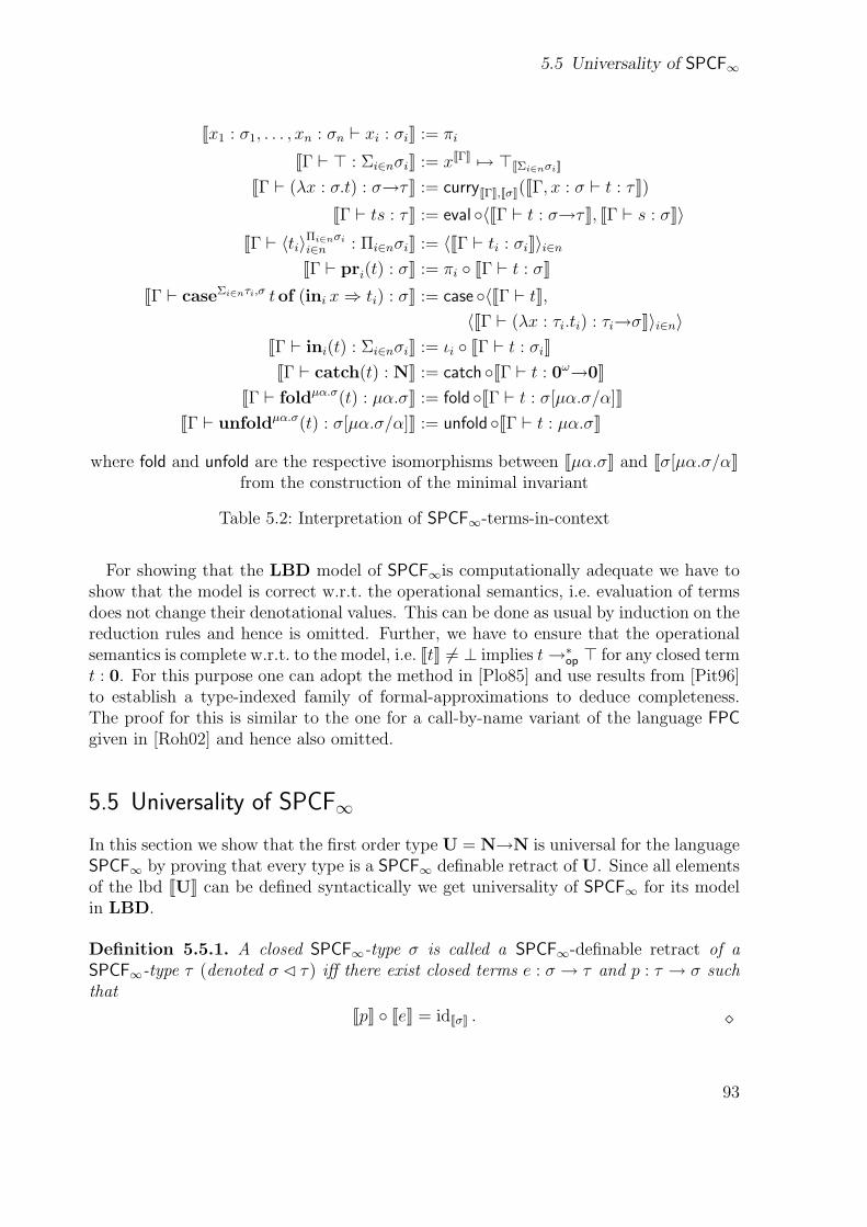
5.5 Universality of SPCF∞
Jx1 : σ1, . . . , xn : σn ` xi : σiK := πi
JΓ ` > : Σi∈nσiK := xJΓK 7→ >JΣi∈nσiK
JΓ ` (λx : σ.t) : σ→τK := curryJΓK,JσK(JΓ, x : σ ` t : τK)
JΓ ` ts : τK := eval ◦〈JΓ ` t : σ→τK, JΓ ` s : σK〉JΓ ` 〈ti〉Πi∈nσi
i∈n : Πi∈nσiK := 〈JΓ ` ti : σiK〉i∈n
JΓ ` pri(t) : σK := πi ◦ JΓ ` t : σKJΓ ` caseΣi∈nτi,σ tof (ini x⇒ ti) : σK := case ◦〈JΓ ` tK,
〈JΓ ` (λx : τi.ti) : τi→σK〉i∈n〉JΓ ` ini(t) : Σi∈nσiK := ιi ◦ JΓ ` t : σiKJΓ ` catch(t) : NK := catch ◦JΓ ` t : 0ω→0K
JΓ ` foldµα.σ(t) : µα.σK := fold ◦JΓ ` t : σ[µα.σ/α]KJΓ ` unfoldµα.σ(t) : σ[µα.σ/α]K := unfold ◦JΓ ` t : µα.σK
where fold and unfold are the respective isomorphisms between Jµα.σK and Jσ[µα.σ/αKfrom the construction of the minimal invariant
Table 5.2: Interpretation of SPCF∞-terms-in-context
For showing that the LBD model of SPCF∞is computationally adequate we have toshow that the model is correct w.r.t. the operational semantics, i.e. evaluation of termsdoes not change their denotational values. This can be done as usual by induction on thereduction rules and hence is omitted. Further, we have to ensure that the operationalsemantics is complete w.r.t. to the model, i.e. JtK 6= ⊥ implies t→∗
op > for any closed termt : 0. For this purpose one can adopt the method in [Plo85] and use results from [Pit96]to establish a type-indexed family of formal-approximations to deduce completeness.The proof for this is similar to the one for a call-by-name variant of the language FPCgiven in [Roh02] and hence also omitted.
5.5 Universality of SPCF∞
In this section we show that the first order type U = N→N is universal for the languageSPCF∞ by proving that every type is a SPCF∞ definable retract of U. Since all elementsof the lbd JUK can be defined syntactically we get universality of SPCF∞ for its modelin LBD.
Definition 5.5.1. A closed SPCF∞-type σ is called a SPCF∞-definable retract of aSPCF∞-type τ (denoted σ � τ) iff there exist closed terms e : σ → τ and p : τ → σ suchthat
JpK ◦ JeK = idJσK . �
93
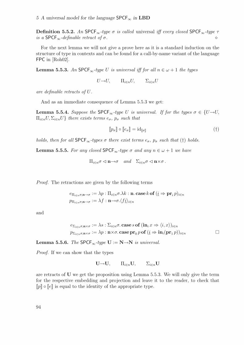
5 A universal model for the language SPCF∞ in LBD
Definition 5.5.2. An SPCF∞-type σ is called universal iff every closed SPCF∞-type τis a SPCF∞-definable retract of σ. �
For the next lemma we will not give a prove here as it is a standard induction on thestructure of type in contexts and can be found for a call-by-name variant of the languageFPC in [Roh02].
Lemma 5.5.3. An SPCF∞-type U is universal iff for all n ∈ ω + 1 the types
U→U, Πi∈nU, Σi∈nU
are definable retracts of U .
And as an immediate consequence of Lemma 5.5.3 we get:
Lemma 5.5.4. Suppose the SPCF∞-type U is universal. If for the types σ ∈ {U→U,Πi∈nU, Σi∈nU} there exists terms eσ, pσ such that
JpσK ◦ JeσK = idJσK (†)
holds, then for all SPCF∞-types σ there exist terms eσ, pσ such that (†) holds.
Lemma 5.5.5. For any closed SPCF∞-type σ and any n ∈ ω + 1 we have
Πi∈nσ � n→σ and Σi∈nσ � n×σ .
Proof. The retractions are given by the following terms
eΠi∈nσ,n→σ := λp : Πi∈nσ.λk : n. case k of (i⇒ pri p)i∈n
pΠi∈nσ,n→σ := λf : n→σ.〈fi〉i∈n
and
eΣi∈nσ,n×σ := λs : Σi∈nσ. case sof (ini x⇒ 〈i, x〉)i∈n
pΣi∈nσ,n×σ := λp : n×σ. casepr0 pof (i⇒ ini(pr1 p))i∈n
Lemma 5.5.6. The SPCF∞-type U := N→N is universal.
Proof. If we can show that the types
U→U, Πi∈nU, Σi∈nU
are retracts of U we get the proposition using Lemma 5.5.3. We will only give the termfor the respective embedding and projection and leave it to the reader, to check thatJpK ◦ JeK is equal to the identity of the appropriate type.
94
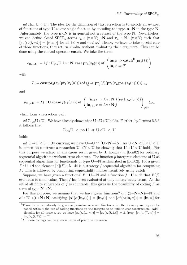
5.5 Universality of SPCF∞
ad Πi∈nU � U : The idea for the definition of this retraction is to encode an n-tupelof functions of type U as one single function by encoding the type n×N in the type N.Unfortunately, the type n×N is in general not a retract of the type N. Nevertheless,we can define closed SPCF∞-terms ιn : (n×N)→N and πn : N→(n×N) such thatJπn(ιn〈i, m〉)K = J〈i, m〉K for all i ∈ n and m ∈ ω.2 Hence, we have to take special careof those functions, that return a value without evaluating their argument. This can bedone using the control operator catch. We take the terms
eΠi∈nU := λf : Πi∈nU.λn : N. casepr0(π2(n))of
(in0 x⇒ catchU(pri(f))
in1 x⇒ T
)
with
T := casepr0(πn(pr1(π2(n))))of (j ⇒ prj(f)(pr1(πn(pr1(π2(n))))))j∈n
and
pΠi∈nU := λf : U.〈case f(ι2〈0, i〉)of
(in0 x⇒ λn : N.f(ι2〈1, ιn〈i, n〉〉)
inj+1 x⇒ λn : N.j
)j∈ω
〉i∈n
which form a retraction pair.
ad Σi∈nU�U : We have already shown that U×U�U holds. Further, by Lemma 5.5.5it follows that
Σi∈nU � n×U � U×U � U
holds.
ad U→U � U : By currying we have U→U ∼= (U×N)→N. As U×N � U×U � Uit suffices to construct a retraction U→N � U for showing that U→U � U holds. Forthis purpose we adapt an analogous result given by J. Longley in [Lon02] for ordinarysequential algorithms without error elements. The function p interprets elements of U assequential algorithms for functionals of type U→N as described in [Lon02]. For a givenF : U→N the element JeK(F ) : N→N is a strategy / sequential algorithm for computingF . This is achieved by computing sequentiality indices iteratively using catch.
Suppose, we have given a functional F : U→N and a function f : U such that F (f)evaluates to some value. Then f has been evaluated at only finitely many terms. As theset of all finite subgraphs of f is countable, this gives us the possibility of coding F asterm of type N→N.
For this purpose, we assume that we have given functions3 α : (1+N+N)→N andα∗ : N→(1+N+N) satisfying Jα∗(α(in0〈〉))K = Jin0〈〉K and Jα∗(α(ini n))K = Jini nK for
2Those terms can already be given as primitive recursive functions, i.e. the terms ιn and πn can becoded without the use of coding functions on the integers as an infinite case-construction. Addi-tionally, for all those ιn, πn we have Jπn(ιn〈⊥,m〉)K = Jπn(ιn〈i,⊥〉)K = ⊥ (resp. Jπn(ιn〈>,m〉)K =Jπn(ιn〈i,>〉)K = >).
3All those codings can be given in terms of primitive recursion.
95
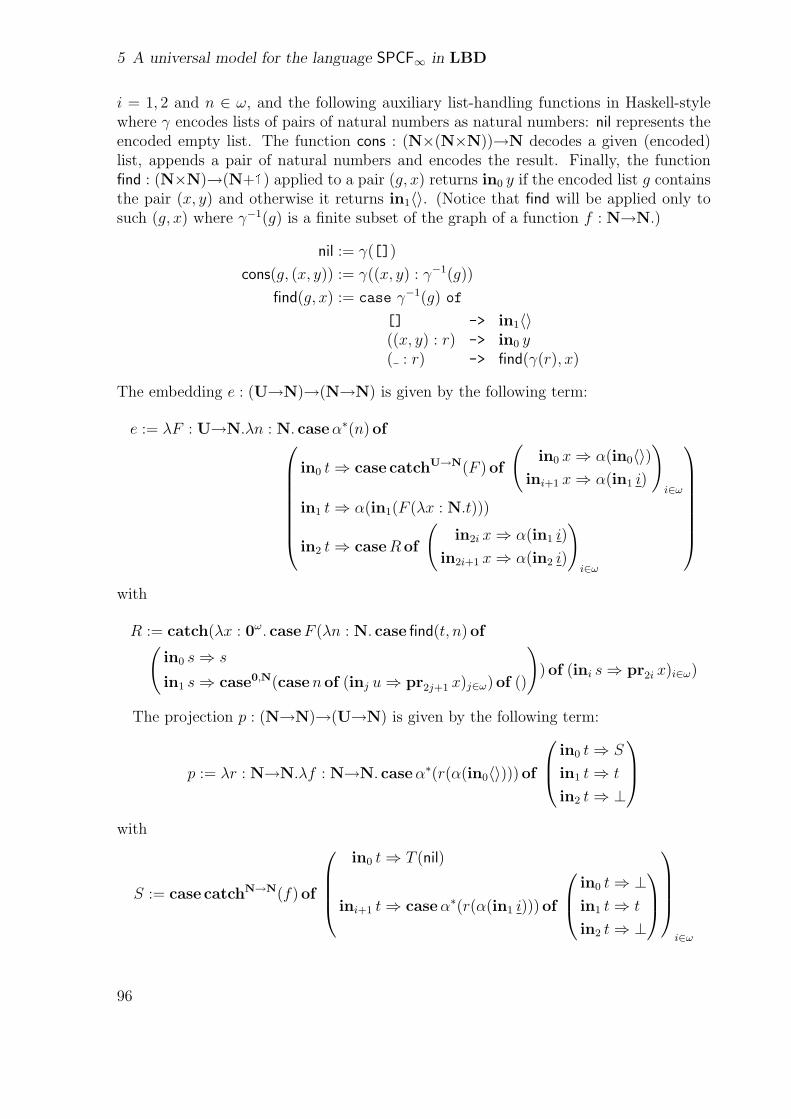
5 A universal model for the language SPCF∞ in LBD
i = 1, 2 and n ∈ ω, and the following auxiliary list-handling functions in Haskell-stylewhere γ encodes lists of pairs of natural numbers as natural numbers: nil represents theencoded empty list. The function cons : (N×(N×N))→N decodes a given (encoded)list, appends a pair of natural numbers and encodes the result. Finally, the functionfind : (N×N)→(N+1) applied to a pair (g, x) returns in0 y if the encoded list g containsthe pair (x, y) and otherwise it returns in1〈〉. (Notice that find will be applied only tosuch (g, x) where γ−1(g) is a finite subset of the graph of a function f : N→N.)
nil := γ([])
cons(g, (x, y)) := γ((x, y) : γ−1(g))
find(g, x) := case γ−1(g) of
[] -> in1〈〉((x, y) : r) -> in0 y( : r) -> find(γ(r), x)
The embedding e : (U→N)→(N→N) is given by the following term:
e := λF : U→N.λn : N. caseα∗(n)ofin0 t⇒ case catchU→N(F )of
(in0 x⇒ α(in0〈〉)
ini+1 x⇒ α(in1 i)
)i∈ω
in1 t⇒ α(in1(F (λx : N.t)))
in2 t⇒ caseR of
(in2i x⇒ α(in1 i)
in2i+1 x⇒ α(in2 i)
)i∈ω
with
R := catch(λx : 0ω. caseF (λn : N. case find(t, n)of(in0 s⇒ s
in1 s⇒ case0,N(casenof (inj u⇒ pr2j+1 x)j∈ω)of ()
))of (ini s⇒ pr2i x)i∈ω)
The projection p : (N→N)→(U→N) is given by the following term:
p := λr : N→N.λf : N→N. caseα∗(r(α(in0〈〉)))of
in0 t⇒ S
in1 t⇒ t
in2 t⇒ ⊥
with
S := case catchN→N(f)of
in0 t⇒ T (nil)
ini+1 t⇒ caseα∗(r(α(in1 i)))of
in0 t⇒ ⊥in1 t⇒ t
in2 t⇒ ⊥
i∈ω
96
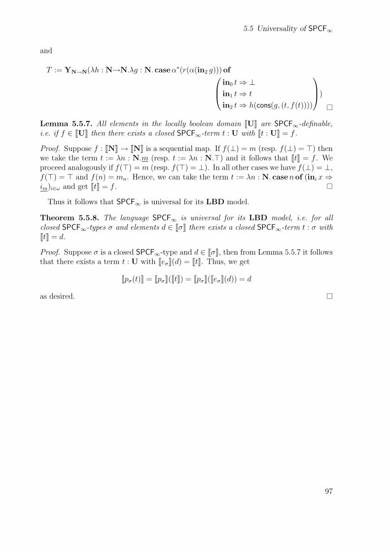
5.5 Universality of SPCF∞
and
T := YN→N(λh : N→N.λg : N. caseα∗(r(α(in2 g)))of in0 t⇒ ⊥in1 t⇒ t
in2 t⇒ h(cons(g, (t, f(t))))
)
Lemma 5.5.7. All elements in the locally boolean domain JUK are SPCF∞-definable,i.e. if f ∈ JUK then there exists a closed SPCF∞-term t : U with Jt : UK = f .
Proof. Suppose f : JNK→ JNK is a sequential map. If f(⊥) = m (resp. f(⊥) = >) thenwe take the term t := λn : N.m (resp. t := λn : N.>) and it follows that JtK = f . Weproceed analogously if f(>) = m (resp. f(>) = ⊥). In all other cases we have f(⊥) = ⊥,f(>) = > and f(n) = mn. Hence, we can take the term t := λn : N. casenof (ini x⇒im)i∈ω and get JtK = f .
Thus it follows that SPCF∞ is universal for its LBD model.
Theorem 5.5.8. The language SPCF∞ is universal for its LBD model, i.e. for allclosed SPCF∞-types σ and elements d ∈ JσK there exists a closed SPCF∞-term t : σ withJtK = d.
Proof. Suppose σ is a closed SPCF∞-type and d ∈ JσK, then from Lemma 5.5.7 it followsthat there exists a term t : U with JeσK(d) = JtK. Thus, we get
Jpσ(t)K = JpσK(JtK) = JpσK(JeσK(d)) = d
as desired.
97

5 A universal model for the language SPCF∞ in LBD
98
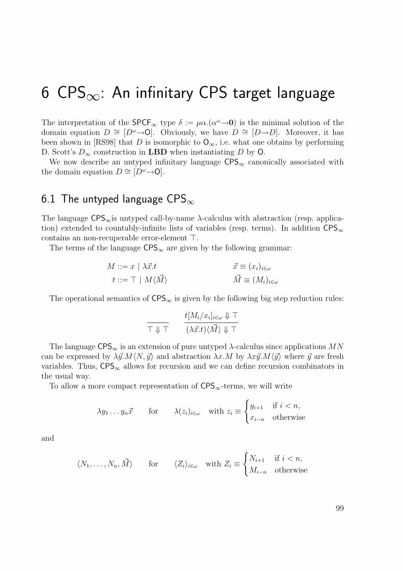
6 CPS∞: An infinitary CPS target language
The interpretation of the SPCF∞ type δ := µα.(αω→0) is the minimal solution of thedomain equation D ∼= [Dω→O]. Obviously, we have D ∼= [D→D]. Moreover, it hasbeen shown in [RS98] that D is isomorphic to O∞, i.e. what one obtains by performingD. Scott’s D∞ construction in LBD when instantiating D by O.
We now describe an untyped infinitary language CPS∞ canonically associated withthe domain equation D ∼= [Dω→O].
6.1 The untyped language CPS∞
The language CPS∞is untyped call-by-name λ-calculus with abstraction (resp. applica-tion) extended to countably-infinite lists of variables (resp. terms). In addition CPS∞contains an non-recuperable error-element >.
The terms of the language CPS∞ are given by the following grammar:
M ::= x | λ~x.t ~x ≡ (xi)i∈ω
t ::= > | M〈 ~M〉 ~M ≡ (Mi)i∈ω
The operational semantics of CPS∞ is given by the following big step reduction rules:
> ⇓ >
t[Mi/xi]i∈ω ⇓ >
(λ~x.t)〈 ~M〉 ⇓ >
The language CPS∞ is an extension of pure untyped λ-calculus since applications MNcan be expressed by λ~y.M〈N, ~y〉 and abstraction λx.M by λx~y.M〈~y〉 where ~y are freshvariables. Thus, CPS∞ allows for recursion and we can define recursion combinators inthe usual way.
To allow a more compact representation of CPS∞-terms, we will write
λy1 . . . yn~x for λ(zi)i∈ω with zi ≡
{yi+1 if i < n,
xi−n otherwise
and
〈N1, . . . , Nn, ~M〉 for 〈Zi〉i∈ω with Zi ≡
{Ni+1 if i < n,
Mi−n otherwise
99
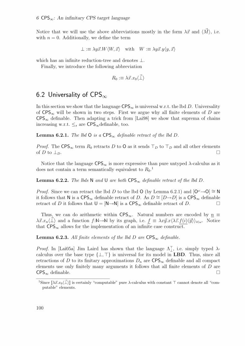
6 CPS∞: An infinitary CPS target language
Notice that we will use the above abbreviations mostly in the form λ~x and 〈 ~M〉, i.e.with n = 0. Additionally, we define the term
⊥ :≡ λy~x.W 〈W,~x〉 with W :≡ λy~x.y〈y, ~x〉
which has an infinite reduction-tree and denotes ⊥.Finally, we introduce the following abbreviation
R0 :≡ λ~x.x0〈~⊥〉
6.2 Universality of CPS∞
In this section we show that the language CPS∞ is universal w.r.t. the lbd D. Universalityof CPS∞ will be shown in two steps. First we argue why all finite elements of D areCPS∞ definable. Then adapting a trick from [Lai98] we show that suprema of chainsincreasing w.r.t. ≤s are CPS∞definable, too.
Lemma 6.2.1. The lbd O is a CPS∞ definable retract of the lbd D.
Proof. The CPS∞ term R0 retracts D to O as it sends >D to >D and all other elementsof D to ⊥D.
Notice that the language CPS∞ is more expressive than pure untyped λ-calculus as itdoes not contain a term semantically equivalent to R0.
1
Lemma 6.2.2. The lbds N and U are both CPS∞ definable retract of the lbd D.
Proof. Since we can retract the lbd D to the lbd O (by Lemma 6.2.1) and [Oω→O] ∼= Nit follows that N is a CPS∞ definable retract of D. As D ∼= [D→D] is a CPS∞ definableretract of D it follows that U = [N→N] is a CPS∞ definable retract of D.
Thus, we can do arithmetic within CPS∞. Natural numbers are encoded by n ≡λ~x.xn〈~⊥〉 and a function f :N→N by its graph, i.e. f ≡ λx~y.x〈λ~z.f(i)〈~y〉〉i∈ω. Noticethat CPS∞ allows for the implementation of an infinite case construct.
Lemma 6.2.3. All finite elements of the lbd D are CPS∞ definable.
Proof. In [Lai05a] Jim Laird has shown that the language Λ>⊥, i.e. simply typed λ-calculus over the base type {⊥,>} is universal for its model in LBD. Thus, since allretractions of D to its finitary approximations Dn are CPS∞ definable and all compactelements use only finitely many arguments it follows that all finite elements of D areCPS∞ definable.
1Since Jλ~x.x0〈~⊥〉K is certainly “computable” pure λ-calculus with constant > cannot denote all “com-putable” elements.
100
6.2 Universality of CPS∞
Definition 6.2.4. Let f : A→ O be a LBD morphism then we define the map f : A→[O→O] with
f(a)(u) :=
{u if f(a>) = ⊥O and
f(a) otherwise. �
Informally, the map f can be described as the function where
“in the strategy of f all occurrences of ⊥ are replaced by u”.
Next we show that for all f : A → O in LBD the map f : A → [O→O] is an LBDmorphism as well.
Lemma 6.2.5. If f : A→ O is a sequential map between lbds then the function f : A→[O→O] given by Def. 6.2.4 is sequential.
Proof. For showing monotonicity suppose a1, a2 ∈ A with a1 v a2 and u ∈ O. Weproceed by case analysis on f(a>1 ).
Suppose f(a>1 ) = ⊥O. Thus, f(a1)(u) = u. If f(a>2 ) = ⊥O then f(a2)(u) = u,
and we get f(a1)(u) = u = f(a2)(u). If f(a>2 ) = >O then f(a2)(u) = f(a2). Asf(a>1 ) = ⊥O it follows that f(¬a1) = ⊥O and f(¬a2) = ⊥O (because ¬a2 v ¬a1). As>O = f(a>2 ) = f(a2) t f(¬a2) it follows that f(a2) = >O as desired.
If f(a>1 ) = >O then f(a1)(u) = f(a1). W.l.o.g. assume f(a1) = >O. Then >O =
f(a1) v f(a2) v f(a>2 ). Hence, f(a2) = >O = f(a>2 ) and we get f(a2)(u) = f(a2) = >O.
Next we show that f is bistable. Let a1 l a2, thus (†) a>1 = a>2 = (a1 u a2)>.
If f(a>1 ) = f(a>2 ) = ⊥O then f(a1) = idO = f(a2). If f(a>1 ) = f(a>2 ) = >O then
f(ai) = λx:O. f(ai) for i ∈ {1, 2}. Since λx:O.⊥O l λx:O.>O it follows that f preservesbistable coherence.
Finally we show that f preserves bistably coherent suprema and infima. If f((a1 ua2)
>) = ⊥O then f(a1ua2)(u) = u = f(a1)(u)u f(a2)(u) (since f(a>1 ) = f(a>2 ) = ⊥O by
(†)). Otherwise, if f((a1ua2)>) = >O then f(a1ua2)(u) = f(a1ua2) = f(a1)uf(a2) =
f(a1)(u) u f(a2)(u) (since f is bistable and f(a>1 ) = f(a>2 ) = >O by (†)).Analogously, one shows that f preserves bistably coherent suprema.
The following observation is useful when computing with functions of the form f .
Lemma 6.2.6. If f : A→ O is a LBD morphism then f(a)(⊥O) = f(a).
Proof. If f(a) = ⊥O then f(a)(⊥O) = ⊥O = f(a) since ⊥ and f(a) are the only possible
values of f(a)(⊥O). If f(a) = >O then f(a>) = >O and thus f(a)(⊥O) = f(a) asdesired.
Lemma 6.2.7. For f, g : A → O with f ≤s g it holds that g(x) = f(x) ◦ g(x) for allx ∈ A.
101
6 CPS∞: An infinitary CPS target language
Proof. Suppose f ≤s g. Let x ∈ A and u ∈ O. We have to show that g(x)(u) =
f(x)(g(x)(u)).
If g(x>) = ⊥O then f(x>) = ⊥O (since f ≤s g) and thus g(x)(u) = u = f(x)(g(x)(u)).Thus, w.l.o.g. suppose g(x>) = >O. Then g(x)(u) = g(x).
If f(x) = >O then f(x>) = >O = g(x) and, therefore, we have f(x)(g(x)(u)) =f(x) = >O = g(x) = g(x)(u).
Suppose f(x) = ⊥O.
If g(x) = ⊥O then we have f(x)(g(x)(u)) = f(x)(g(x)) = f(x)(⊥O) = ⊥O where thelast equality holds by Lemma 6.2.6.
Now suppose g(x) = >O. We proceed by case analysis on the value of f(x>).
If f(x>) = ⊥O then f(x)(g(x)(u)) = g(x)(u) and we are finished.We show that the case f(x>) = >O cannot happen. Suppose f(x>) = >O. Then by
bistability we have >O = f(x>) = f(x) t f(¬x) = ⊥O t f(¬x) = f(¬x) and thus also¬f(¬x) = ⊥O. Since f ≤s g we have g v f>. Moreover, by Cor. 3.5.12(2) we have(¬f)(x) v ¬f(¬x). Thus, we have >O = g(x) v f>(x) = f(x) t (¬f)(x) = (¬f)(x) v¬f(¬x) = ⊥O which clearly is impossible.
In the following we denote by i : O → D and p : D → O the embedding of O into D(resp. projection from D to O) given by
i(x) :=
{>D if x = >O,
⊥D otherwisep(x) :=
{>O if x = >D,
⊥O otherwise.
Definition 6.2.8. Let f ∈ D ∼= [Dω→O]. Then we write f for that element of D with
f(d0, ~d) := fn(~d)(p(d0)) �
Lemma 6.2.9. For every finite f in D the element f is also finite and thus CPS∞definable.
Proof. If A is a finite lbd then for every f : A → O the LBD map f : A → [O→O] isalso finite. This holds in particular for f in the finite type hierarchy over O.
Since embeddings of lbds preserves finiteness of elements we conclude that for everyfinite f in D the element f is finite as well. Thus, by Lemma 6.2.3 the element f isCPS∞ definable.
Now we are ready to prove our universality result for CPS∞.
Theorem 6.2.10. All elements of the lbd D are CPS∞ definable.
Proof. Suppose f ∈ D. Then f =⊔
fn for some increasing (w.r.t. ≤s) chain (fn)n∈ω of
finite elements. Since by Lemma 6.2.9 all fn are CPS∞ definable there exists a CPS∞term F with JFnK = fn for all n ∈ ω.
102
6.3 Lack of faithfulness of the interpretation
Since recursion is available in CPS∞ one can exhibit a CPS∞ term Ψ such that
Ψg = λx. g(0)(Ψ(λn. g(n+1))x) =⊔n∈ω
(g(0) ◦ · · · ◦ g(n))(⊥)
holds. (Using computational adequacy of the model one can show that Ψg denotes theleast fixpoint of the sequence ((g(0) ◦ · · · ◦ g(n))(⊥))n∈ω.)
Thus, the term Mf ≡ λ~x. Ψ(λy.λz.F 〈y, i(z), ~x〉) denotes f since
Mf (~d) = Ψ(λy.λz.F (y, i(z), ~d))
=⊔n∈ω
(λz.F0(i(z), ~d)) ◦ · · · ◦ (λz.Fn(i(z), ~d))(⊥)
=⊔n∈ω
(λz.f0(i(z), ~d)) ◦ · · · ◦ (λz.fn(i(z), ~d))(⊥)
=⊔n∈ω
((λz.f0(~d)(p(i(z)))) ◦ · · · ◦ (λz.fn(~d)(p(i(z)))))(⊥)
=⊔n∈ω
((λz.f0(~d)(z)) ◦ · · · ◦ (λz.fn(~d)(z)))(⊥)
=⊔n∈ω
(f0(~d) ◦ · · · ◦ fn(~d))(⊥)
=⊔n∈ω
(fn(~d))(⊥) (by Lemma 6.2.7)
=⊔n∈ω
fn(~d) (by Lemma 6.2.6)
= f(~d)
for all ~d ∈ Dω.
6.3 Lack of faithfulness of the interpretation
In the previous section we have shown that the interpretation of closed CPS∞ terms inthe lbd D is surjective. Recall that infinite normal forms for CPS∞ are given by thegrammar
N ::= x | λ~x.> | λ~x.x〈 ~N〉understood in a coinductive sense.
Definition 6.3.1. We call a model faithful iff for all normal forms N1, N2 if JN1K =JN2K then N1 = N2. �
We will show that the LBD model of CPS∞ is not faithful.2 For a closed CPS∞ termM consider
M∗ ≡ λ~x.x0〈 λ~y.x0〈⊥, M, ~⊥〉, ~⊥ 〉2For an affine version of CPS∞ on can show that the LBD model is faithful.
103
6 CPS∞: An infinitary CPS target language
Lemma 6.3.2. For closed CPS∞ terms M1, M2 it holds that JM∗1 K = JM∗
2 K.
Proof. We will show that for all terms M the term M∗ is semantically equivalent to theterm R0, i.e. for all ~d ∈ Dω we have JM∗K(~d) = > iff d0 = >.
If d0 = ⊥ or d0 = > then we are finished.Otherwise there is an n such that d0 evaluates the n-th argument first. If n = 0 then
d0〈⊥, M, ~⊥〉 = ⊥, thus
d0〈λ~y.d0〈⊥, M, ~⊥〉, ~⊥〉 = d0〈~⊥〉 = ⊥ .
which is also the case if n 6= 0.
Suppose N1 and N2 are different infinite normal forms. Then N∗1 and N∗
2 have differentinfinite normal forms and we get JN∗
1 K = JN∗2 K by Lemma 6.3.2. Thus, the LBD model
of CPS∞ is not faithful.
Lemma 6.3.3. There exist infinite normal forms N1, N2 in CPS∞ that can not be sep-arated by CPS∞ terms.
Proof. We have different normal forms N1, N2 with JN1K = JN2K. Since all CPS∞ termspreserve model equality the terms N1 and N2 cannot be separated by CPS∞ terms.
Notice that in pure untyped λ-calculus different normal forms can always be separated(cf. [Bar84]).
104
7 Conclusion and possible extensions
We think that the defect that interpretation of CPS∞ in the locally boolean domain Dis not faithful (cf. Section 6.3) can be overcome by extending the language by a parallel
construct and refining the observation type O to O′ ∼= List(O′). The language CPS‖∞
associated with the domain equation D ' Dω → O′ is given by
M ::= x | λ~x.t
t ::= > |M〈 ~M〉 | L t ‖ . . . ‖ t M
The syntactic values are given by the grammar V ::= > | L V ‖ . . . ‖V M. The operational
semantics of CPS‖∞ is the operational semantics of CPS∞ extended by the rule
(λ~x.ti)〈 ~M〉 ⇓ Vi for all i ∈ {1, . . . , n}
(λ~x.L t1‖ . . . ‖tn M)〈 ~M〉 ⇓ L V1‖ . . . ‖Vn M
and the normal forms of CPS‖∞ are given by the grammar
N ::= x | λ~x.t
t ::= > | x〈 ~N〉 | L t‖ . . . ‖t M
understood in a coinductive sense.Separability of normal forms can be shown for an affine version of CPS∞ by substitut-
ing the respective projections for head variables. Using the parallel construct L . . . ‖ . . . Mof CPS
‖∞ we can substitute for a head variable quasi simultaneously both the respective
projection and the head variable itself. Since the interpretation of CPS‖∞ is faithful
w.r.t. the parallel construct L . . . ‖ . . . M we get separation for CPS‖∞ normal forms as in
the affine case. This kind of argument can be seen as a “qualitative” reformulation of arelated “quantitative” method introduced by F. Maurel in his Thesis [Mau04] albeit inthe somewhat more complex context of J.-Y. Girard’s Ludics [Gir01].
In a sense this is not surprising since our parallel construct introduced above allowsone to make the same observations as with parallel-or. The only difference is that ourparallel construct keeps track of all possibilities simultaneously whereas the traditionalsemantics of parallel-or takes their supremum thus leading out of the realm of sequen-tiality. This is avoided by our parallel construct at the price of a more complicateddomain of observations. For an approach in a similar spirit see [HM99].
Another prospect is the development of a theory of computability for locally booleandomains. In [Asp90] A. Asperti has successfully developed a notion of computability
105
7 Conclusion and possible extensions
for the stable model of PCF. We are convinced that this approach can be extended tolocally boolean domains. Curien-Lamarche games A arising as interpretation of a typeexpressions are effective (i.e. PA ⊆ Rsp>(A) is decidable). An element s ∈ Strat(A) iscomputable iff s is an r.e. subset of Rsp>(A). Obviously, an element f ∈ U = [N→N] iscomputable in this sense iff it can be denoted by an r.e. term. Since all eσ : σ � U : pσ
can be denoted by r.e. terms it follows that all computable elements of type JσK can bedenoted by r.e. terms. Obviously, denotations of r.e. terms of type σ denote computableelements of JσK. Thus elements of JσK are computable iff they can be denoted by r.e.terms.
106
Bibliography
[AC98] Roberto M. Amadio and Pierre-Louis Curien. Domains and lambda-calculi.Cambridge University Press, New York, NY, USA, 1998.
[AHM98] Samson Abramsky, Kohei Honda and Guy McCusker. A fully abstract gamesemantics for general references. In Vaughan Pratt, editor, Proceedings of theThirteenth Annual IEEE Symp. on Logic in Computer Science, LICS 1998,pages 334–344. IEEE Computer Society Press, June 1998.
[AJM00] Samson Abramsky, Radha Jagadeesan and Pasquale Malacaria. Full abstrac-tion for PCF. Inf. Comput., 163(2):409–470, 2000.
[AM97] S. Abramsky and G. McCusker. Linearity, sharing and state: a fully abstractgame semantics for idealized algol with active expressions, 1997.
[Asp90] Andrea Asperti. Stability and computability in coherent domains. Inf. Com-put., 86(2):115–139, 1990.
[Bar84] H. P. Barendregt. The Lambda Calculus - its syntax and semantics. NorthHolland, 1981, 1984.
[BC82] G. Berry and P. L. Curien. Sequential algorithms on concrete data structures.Theoretical Computer Science, 20(3):265–321, July 1982.
[BE91] A. Bucciarelli and T. Ehrhard. Sequentiality and strong stability. In Proc.of the Sixth Annual IEEE Symposium on Logic in Computer Science, pages138–145, Amsterdam, The Netherlands, 1991.
[Ber78] G. Berry. Stable models of typed λ-calculi. In Proceedings of the 5th Interna-tional Colloquium on Automata, Languages and Programming, volume 62 ofLecture Notes in Computer Science, pages 72–89. Springer Verlag, 1978.
[Ber79] G. Berry. Modeles Completement Adequats et Stables des lambda–calcul types.PhD thesis, Universite Paris VII, 1979.
[CCF94] R. Cartwright, P.-L. Curien and M. Felleisen. Fully abstract models of ob-servably sequential languages. Information and Computation, 111(2):297–401,1994.
107
Bibliography
[CF92] Robert Cartwright and Matthias Felleisen. Observable sequentiality and fullabstraction. In Conference Record of the Nineteenth Annual ACM SIGPLAN-SIGACT Symposium on Principles of Programming Languages, pages 328–342, Albuquerque, New Mexico, January 1992.
[Cur94] P.-L. Curien. On the symmetry of sequentiality. Lecture Notes in ComputerScience, 802:29–71, 1994.
[Cur05] Pierre-Louis Curien. Sequential algorithms as bistable maps. Un-published notes, available from http://www.pps.jussieu.fr/~curien/
laird-sa.ps.gz, 2005.
[Ehr96] Thomas Ehrhard. Projecting sequential algorithms on strongly stable func-tions. Annals of Pure and Applied Logic, 77(3):201–244, 1996.
[Fre91] P.J. Freyd. Algebraically complete categories. In Category Theory, Como1990, volume 1488 of Lecture Notes in Mathematics, pages 95–104. Springer-Verlag, 1991.
[Fre92] P.J. Freyd. Remarks on algebraically compact categories. In Applications ofcategories in Computer Science, volume 77 of London Math. Society LectureNotes Series, pages 95–106. Cambridge University Press, 1992.
[Gir01] Jean-Yves Girard. Locus solum: From the rules of logic to thelogic of rules. Math. Struct. in Comp. Science, 11(3):301–506, 2001.http://iml.univ-mrs.fr/~girard/Articles.html.
[HM99] Russell Harmer and Guy McCusker. A fully abstract game semantics for finitenondeterminism. In LICS, pages 422–430, 1999.
[HO00] J. M. E. Hyland and C.-H. L. Ong. On full abstraction for PCF: I. models,observables and the full abstraction problem, ii. dialogue games and innocentstrategies, iii. a fully abstract and universal game model. Information andComputation, 163:285–408, 2000.
[Ho06] Weng Kin Ho. An operational domain-theoretic treatment of recursive types.Electr. Notes Theor. Comput. Sci., 158:237–259, 2006.
[KP93] G. Kahn and Gordon D. Plotkin. Concrete domains. Theoretical ComputerScience, 121:187–277, 1993.
[Lai98] J. Laird. A semantic analysis of control. PhD thesis, University of Edin-burgh, 1998. Available from http://www.cogs.susx.ac.uk/users/jiml/
thesis.ps.gz.
[Lai03a] J. Laird. Bistability: an extensional characterization of sequentiality. InProceedings of CSL ’03, number 2803 in LNCS. Springer, 2003.
108
Bibliography
[Lai03b] J. Laird. A fully abstract bidomain model of unary FPC. In 5th InternationalConference on Typed Lambda-Calculi and Applications. Springer LNCS, 2003.
[Lai05a] J. Laird. Bistable biorders: a sequential domain theory. Submitted, 2005,Available from http://www.cogs.susx.ac.uk/users/jiml/bb.pdf, 2005.
[Lai05b] J. Laird. Locally boolean domains. Theoretical Computer Science, 342:132 –148, 2005.
[Lam92] F. Lamarche. Sequentiality, games and linear logic. In Workshop on Cat-egorical Logic in Computer Science. Publications of the Computer ScienceDepartment of Aarhus University, DAIMI PB-397-II, 1992.
[Loa01] Ralph Loader. Finitary PCF is not decidable. Theor. Comput. Sci., 266(1-2):341–364, 2001.
[Lon02] John Longley. The sequentially realizable functionals. Ann. Pure Appl. Logic,117(1-3):1–93, 2002.
[Mau04] F. Maurel. Un cadre quantitatif pour la Ludique. PhD thesis, Universite Paris7, Paris, 2004.
[McC96] Guy McCusker. Games and full abstraction for FPC. In Logic in ComputerScience, pages 174–183, 1996.
[Mil77] Robin Milner. Fully abstract models of typed λ-calculi. Theoretical ComputerScience, 4:1–22, 1977.
[Nic94] H. Nickau. Hereditarily sequential functionals. In Proceedings of the Sympo-sium on Logical Foundations of Computer Science: Logic at St. Petersburg.Springer, 1994.
[Pit96] Andrew M. Pitts. Relational properties of domains. Information and Com-putation, 127(2):66–90, 1996.
[Plo77] G.D. Plotkin. LCF considered as a programming language. Theoretical Com-puter Science, 5:223–255, 1977.
[Plo85] G. D. Plotkin. Lectures on predomains and partial functions. Course notes,Center for the Study of Language and Information, Stanford, 1985.
[Roh02] Alexander Rohr. A Universal Realizability Model for Sequential FunctionalComputation. PhD thesis, TU Darmstadt, Fachbereich Mathematik, 2002.
[RS98] B. Reus and T. Streicher. Classical logic, continuation semantics and abstractmachines. J. Funct. Prog., 8(6):543–572, 1998.
[Sco93] D.S. Scott. A type theoretical alternative to iswim, cuch, owhy. TheoreticalComputer Science, 121:411–440, 1993.
109
Bibliography
[Str04] Th. Streicher. Locally boolean domains (working notes). Unpublished notes,available from http://www.mathematik.tu-darmstadt.de/~streicher/
LAIRD/lbdWN.ps.gz, 2004.
[Vui74] J. Vuillemin. Syntaxe, Semantique et Axiomatique d’un Langage de Program-mation Simple. PhD thesis, Universite Paris VII, 1974.
110
Curriculum Vitae
Tobias Low
geboren am 5. Dezember 1973 in Offenbach am Main
1993 Allgemeine Hochschulreife,Oberstufengymnasium Claus-von-Stauffenberg Schule, Rodgau
1994 - 2000 Studium der Mathematik mit Wahlpflichtfach Informatik,Technische Universitat Darmstadt
2000 Hochschulabschluss als Diplom-Mathematiker,Diplomarbeit “Element-Realizability-Topos”
2001 - 2006 Doktorand am Fachbereich Mathematik der TU Darmstadt,Forschungsbereich Logik


![Javakurs für Anfänger - LMU München€¦ · // boolean gefunden bleibt true, sobald (temperaturen[i] < 1.0) einmal true wurde. Aufgabe 1: Nutzereingaben speichern Erstellen Sie](https://img.pdfslide.org/doc/110x75/605ffc54501782115d556175/javakurs-fr-anfnger-lmu-m-boolean-gefunden-bleibt-true-sobald-temperatureni.jpg)


![· Web viewArray dapat bertipe sederhana byte, word, integer, real, boolean, char, string dan tipe scalar atau subrange. Contoh: Var X : array [ 1..100 ] of integer ; Larik X dideklarasikan](https://img.pdfslide.org/doc/110x75/6088377e590337594f0a0d59/web-view-array-dapat-bertipe-sederhana-byte-word-integer-real-boolean-char.jpg)


![RO 2018-1.ppt [Kompatibilitätsmodus] - tu-ilmenau.de · Bit Wahrheitswert 0/1 oder true/false 1 true (Boolean) Byte Zahl, Befehl… 00000000 -11111111 11001001 C9 (hexadez.) Wort](https://img.pdfslide.org/doc/110x75/5e0fb2160b27c433f67ceef5/ro-2018-1ppt-kompatibilittsmodus-tu-bit-wahrheitswert-01-oder-truefalse.jpg)