Embed Size (px)
Citation preview
Long‐Term Open‐Pit Planning by Ant Colony Optimization
2. Revised Edition
The Faculty of Georesources and Materials Engineering of the
RWTH Aachen University
submitted by
Javad, Sattarvand, M.Sc.
from (Marand‐Iran)
in respect of the academic degree of
Doctor of Engineering
approved thesis
Advisors: Univ.‐Prof. Dr.‐Ing. Christian Niemann‐Delius
Univ.‐Prof. Dr.‐Ing. F. Ludwig Wilke
Date of the oral examination: 06.02.2009
Zusammenfassung
i
ZUSAMMENFASSUNG
Die Aufgabenstellung einer langfristigen Planung von Festgesteinstagebauen mit
diskontinuierlicher Gewinnung ist eine große kombinatorische Herausforderung, die nicht
durch mathematische Programmierung in angemessener Zeit gelöst werden kann. Diese
Dissertation stellt einen neuentwickelten metaheuristischen Algorithmus vor, der auf den
Theorien des Ameisenalgorithmus (Ant Colony Optimization, ACO) basiert. Darüber hinaus
wird die Anwendung des entwickelten Modells anhand einer langfristigen Planung eines
zwei-dimensionalen hypothetischen Block-Modells untersucht verifiziert.
ACO beschreibt das natürliche Verhalten von Ameisen bei der Futtersuche, das die kürzeste
Strecke zwischen Kolonie und Nahrungsquelle zum Ziel und bereits mehrfach erfolgreich zur
Lösung anderer kombinatorischer Probleme beigetragen hat. In der Natur wird das Problem
der optimalen Routenfindung mittels Pheromonen, die eine Nachricht von einer Ameise an
die nächste übertragen, gelöst. Die Pheromone steuern die Wegfindung der Ameisen, so
dass sie nicht nach dem Zufallsprinzip wandern, sondern den Pheromonspuren folgen. Mit
der Zeit verdunsten die Pheromone von der Spur, die selten oder gar nicht mehr genutzt
wird, währenddessen die Route mit der kürzesten Strecke erhalten bleibt.
Um mit der ACO-Theorie eine langfristige Planung eines Festgesteins-tagebaus zu simulieren,
wird die Anzahl der Pheromonspuren jedes Blocks mit der Anzahl der Planungsperioden
gleichgesetzt. Die Pheromonspuren, die einem Block zugeordnet werden können, stellen die
maximale Abbauteufe einer jeden Blockspalte pro Abbauperiode dar.
Die Form eines bestimmten Tagebaus kann, unter Beachtung der Böschungswinkel, durch
ein einfaches Datenfeld von ganzen Zahlen dargestellt werden. Dabei stellt jedes Element
dieses Datenfeldes die Tiefe des Tagebaus in einer einzelnen Spalte des Block-Modells dar.
Wenn dieses Konzept zu einer langfristigen Produktionsplanung erweitert wird, wird jeder
Produktionsplan durch ein Datenfeld dargestellt, dass mehrere Abbauteufen für jede Spalte
des Blockmodells in Relation zu den verschiedenen Produktionsperioden aufweist.
Am Anfang wird eine initiale Tagebauplanung anhand des Lerchs-Grossmann Algorithmuses
und den von Wang & Sevim entwickelten Algorithmus „Alternative zur Parametrisierung
Algorithmus“ erstellt und die Werte der Pheromon Werte entsprechend initialisiert.
Basierend auf der Tagebauplanung werden den Blöcken, die in direkter Nähe zu den Blöcken
des tiefsten Punkts liegen, während der Initialisierung höhere Pheromonwerte zugeordnet.
Long-Term Open-Pit Planning by Ant Colony Optimization
ii
Diese Vorgehensweise erzeugt eine Reihe von zufälligen Zeitplänen, die nicht weit von der
ursprünglichen Lösung sind.
In jeder ACO-Iteration werden basierend auf den aktuellen Pheromonmengen zuerst
mehrere Tagebaupläne erstellt. Dieser Prozess wird als “Bestimmung der Teufe“
gekennzeichnet und implementiert. Während des Prozesses wird die Teufe in jeder Periode
für jede Spalte des Blockmodells bestimmt. Je höher der Wert der Pheromonspur eines
Blocks ausfällt, desto größer ist die Möglichkeit, dass der Block als maximale Abbauteufe für
die jeweilige Periode gewählt wird. Anschließend werden die Pheromonwerte aller Blöcke
um einen gewissen Betrag durch Evaporation verringert. Im nächsten Schritt werden die
Pheromonwerte der Blöcke, die den Abbaustand zur jeweiligen Periode begrenzen, je nach
Qualität der Lösung des folgenden Abbaustands erhöht. Durch wiederholte Iterationen
werden die Pheromonwerte der Blöcke, die die Form der optimalen Lösung definieren
erhöht, während die Werte der anderen Blöcke signifikant verkleinert werden.
Die ACO Optimierung Iterationen können auf verschiedene Arten implementiert werden. In
der ersten und einfachsten Methode, Ant System (AS), dürfen alle konstruierten
Tagebaustände zur Pheromonablagerung beitragen. Die zweite Methode, elitäres Ant-
System (EAS) zeichnet sich dadurch aus, dass der optimale Plan zusätzlich Pheromone in
jeder Iteration ablegt. ASrank ist die dritte Methode in der nur eine geringe Anzahl von guten
Tagebauplänen Pheromon hinzufügen kann. Die weiteren Varianten, Max-Min Ant System
(MMAS) und Ant Colony System (ACS), erlauben nur den bis zu diesem Zeitpunkt besten
Abbauplanungen Pheromone abzulegen und nutzen zusätzlich spezielle
Pheromoneinschränkungen, die eine Stagnation im lokalen Optimum verhindern.
Um die Effizienz des Algorithmus zu überprüfen wurde ein Computerprogramm entwickelt,
dass auf Visual Basic 2005 als Programmiersprache aufbaut. In einer Fallstudie wurde ein
Blockmodell einer hypothetischen Eisenerzlagerstätte mit 1000 Blöcken erstellt. Anhand des
Blockmodells wurden die verschiedenen Varianten der ACO analysiert, um die beste
Kombination der ACO-Parameter zu identifizieren. Die Analyse zeigte, dass die ACO den
Wert der ersten Tagebauplanungen bis zu 34 % in einer akzeptablen Rechenzeit verbessern
kann. Diese Verbesserung ist vor allem der Berücksichtigung von evtl. Einbußen
zuzuschreiben, die aus einer Überschreitung von Kapazitätsgrenzen oder Produktqualitäten
resultiert. Es konnte bewiesen werden, dass die MMAS Variante, die Variante mit der
größten Exploartion von Lösungen ist, währenddessen die AVS Variante die schnellste
Methode ist. Diese beiden Varianten sind die Einzigen, die sich aufgrund des Speicherbedarfs
von Rechnern auf große Blockmodelle anwenden lassen.
Abstract
iii
ABSTRACT
The problem of long-term planning of a hard rock open pit mine (discontinuous exploitation
operation) is a large combinatorial problem which cannot be solved in a reasonable amount
of time through mathematical programming models because of its large size. In this thesis, a
new metaheuristic algorithm has been developed based on the Ant Colony Optimization
(ACO) and its application in long-term scheduling of a two dimensional hypothetical block
model has been analysed.
ACO is inspired by the foraging behaviour of ants (i.e. finding the shortest way from the
colony to the food source), and has been successfully implemented in several combinatorial
optimization problems. In nature, ants transmit a message to other members by laying down
a chemical trail called pheromones. Instead of travelling in a random manner, the
pheromone trail allows the ants to trace the path. Over time, the pheromones layed over
longer paths evaporate, whereas those over shorter routes continue to be marched over.
In order to simulate the ACO process for long-term planning of a hard rock open-pit mine,
various programming variables have been considered for each block as the pheromone
trails. The number of these variables is equal to the number of planning periods. In fact
these pheromone trails represent the desirability of the block for being the deepest point of
the mine in that column for the given mining period.
The shape of any given pit (in respect to the slope angles) can be represented by means of a
simple array of integer numbers. Each element in this array shows the depth of the pit in an
individual column of block model. Extending this concept to a long-term production
planning, a mine schedule would be represented by an array that has several mine depths at
each column of block model related to different production periods.
At the beginning, the values of the pheromone trails are initialized according to a mine
schedule generated by Lerchs-Grossmann’s algorithm and the alternative to
parameterization algorithm of Wang & Sevim. During initialization, relatively higher values
of pheromones are assigned to those blocks that are close to the deepest points of the push
backs in the initial mine schedule. This leads the procedure to construct a series of random
schedules which are not far from the initial solution.
In each ACO iteration, several mine schedules are constructed based on current pheromone
trails. This is implemented through a process called “depth determination”. In this process
the depth of a mine in each period is determined for each column of the block model. The
Long-Term Open-Pit Planning by Ant Colony Optimization
iv
higher the value of the pheromone trail of a particular block, the higher the possibility of
selecting that block as the pit depth in that period. Subsequently the pheromone values of
all blocks are reduced to a certain percentage (evaporation) and additionally the pheromone
value of the participating blocks used in defining the constructed schedules are increased
according to the quality of the generated solutions. Through repeated iterations, the
pheromone values of the blocks which define the shape of the optimum solution are
increased whereas those of the others have been significantly evaporated.
The ACO optimization iterations could be implemented in a variety of ways. The Ant System
(AS) is the first and simplest method, whereby all of the constructed schedules are allowed
to contribute in the pheromone deposition. In each iteration of the second method, the
Elitist Ant System (EAS), the best schedule found up to that iteration (the best-so-far
schedule) is also allowed to deposit pheromones. ASrank is the third method in which only a
few good schedules are able to add pheromones. The other variants are the Max-Min Ant
System (MMAS) and the Ant Colony System (ACS), which allow only the best-so-far schedule
to deposit pheromones and utilise special pheromone limitations in order to prevent the
stagnation in local optimums.
To test the efficiency of the algorithm, a computer program has been developed in Visual
Basic 2005 programming language. As a case study, the block model of a hypothetical iron
ore deposit with 1000 blocks was considered and different variants of ACO had been
analysed in order to find the best combination of ACO parameters. The analysis revealed
that the ACO is able to improve the value of the initial mining schedule by up to 34% in a
reasonable computational time. This is mainly contributed to the consideration of the
penalties to the deviations of the capacities and the production qualities from their
permitted limits. It had also been proved that the MMAS is the most explorative variant,
while ACS is the fastest method. These two variants also count as the only variants which
could be applied to a large block model in respect to the amount of memory needed.
Table of Contents
v
TABLE OF CONTENTS
LIST OF FIGURES ............................................................................................................................................. IX
LIST OF TABLES .............................................................................................................................................. XI
LIST OF ABBREVIATIONS ........................................................................................................................... XII
1 INTRODUCTION ......................................................................................................................... 1
1.1 Complexity of pit optimization .......................................................................................................... 2
1.2 Numerical example ........................................................................................................................... 4
1.3 A brief review of the literature .......................................................................................................... 6
1.4 Structure of the research ................................................................................................................... 9
2 THE PROBLEM OF LONG-TERM OPEN PIT PRODUCTION PLANNING .................. 11
2.1 Mathematical programming models ................................................................................................ 11
2.1.1 Integer linear programming (IP) .......................................................................................................... 11
Objective function ........................................................................................................................................ 11
Mining capacity constraints ......................................................................................................................... 12
Processing capacity constraints.................................................................................................................... 12
Constraints for the average grade of products ............................................................................................ 12
Reserve constraints ...................................................................................................................................... 13
Sequencing constraints ................................................................................................................................ 13
Binary variables ............................................................................................................................................ 14
2.1.2 The linear programming (LP) formulization of the model ................................................................... 14
2.2 Mathematical approaches for solution of the model ........................................................................ 15
2.2.1 Lagrangian Parameterization ............................................................................................................... 15
Ultimate Pit Limit (UPL) Problem ................................................................................................................. 15
Understanding Lagrangian parameterization .............................................................................................. 16
2.2.2 Clustering approach ............................................................................................................................. 16
2.2.3 Branch and cut technique .................................................................................................................... 19
2.2.4 Dynamic programming (DP) formulation ............................................................................................ 19
2.3 Heuristic algorithms ........................................................................................................................ 21
2.3.1 Whittle’s optimization process ............................................................................................................ 21
Definition of UPL problem ............................................................................................................................ 22
Lerchs-Grossmann algorithm ....................................................................................................................... 23
Steps of the algorithm .................................................................................................................................. 24
Long-Term Open-Pit Planning by Ant Colony Optimization
vi
Step 2 in a closer look: ................................................................................................................................. 25
Numerical example ...................................................................................................................................... 27
Construction of nested pits .......................................................................................................................... 31
The best and worst case mining scenarios ................................................................................................... 32
UPL selection based on the NPV-Tonnage graph ......................................................................................... 32
Mine scheduling ........................................................................................................................................... 33
2.3.2 Sevim’s suggested approach ............................................................................................................... 36
Nested-pits creation algorithm .................................................................................................................... 37
Dynamic programming based search algorithm .......................................................................................... 41
Considering working-slope angles ................................................................................................................ 43
2.4 Metaheuristic methods ................................................................................................................... 46
2.4.1 Introduction ......................................................................................................................................... 46
Combinatorial optimization ......................................................................................................................... 46
Metaheuristics .............................................................................................................................................. 46
2.4.2 Genetic algorithm (GA) ........................................................................................................................ 47
Chromosome representation of the pits ...................................................................................................... 48
Initial population .......................................................................................................................................... 48
Assessment of pit fitness .............................................................................................................................. 49
Reproduction of pit population .................................................................................................................... 49
Termination condition of the algorithm ....................................................................................................... 50
2.4.3 Simulated annealing (SA) ..................................................................................................................... 51
Objective function ........................................................................................................................................ 51
Constraints ................................................................................................................................................... 54
Initial solution ............................................................................................................................................... 54
Perturbation mechanism .............................................................................................................................. 55
Acceptance criterion .................................................................................................................................... 56
Cooling schedule .......................................................................................................................................... 57
Initial temperature ....................................................................................................................................... 57
3 ANT COLONY OPTIMIZATION (ACO) ............................................................................... 59
3.1 TSP Definition ................................................................................................................................. 60
3.2 Basic elements in solution of TSP by ACO ........................................................................................ 60
3.2.1 Construction graph .............................................................................................................................. 60
3.2.2 Constraints ........................................................................................................................................... 61
3.2.3 Pheromone trails and heuristic information ....................................................................................... 61
3.3 Variants of ACO algorithm for TSP ................................................................................................... 61
3.3.1 Ant System (AS) ................................................................................................................................... 61
Pheromone Initialization .............................................................................................................................. 61
Solution construction ................................................................................................................................... 62
Table of Contents
vii
Update of Pheromone Trails ........................................................................................................................ 63
3.3.2 Elitist Ant System (EAS) ........................................................................................................................ 64
3.3.3 Rank-Based Ant System (ASrank) ........................................................................................................... 64
3.3.4 MAX–MIN Ant System (MMAS) ........................................................................................................... 65
Pheromone Trail Limits ................................................................................................................................ 66
Pheromone Trail Initialization and Re-initialization ..................................................................................... 66
3.3.5 Ant Colony System (ACS) ..................................................................................................................... 66
Tour Construction ........................................................................................................................................ 67
Global Pheromone Trail Update ................................................................................................................... 67
Local Pheromone Trail Update ..................................................................................................................... 67
Additional Remarks ...................................................................................................................................... 68
3.3.6 Approximate Nondeterministic Tree Search (ANTS) ........................................................................... 69
Use of Lower Bounds .................................................................................................................................... 70
Solution Construction ................................................................................................................................... 70
Pheromone Trail Update .............................................................................................................................. 71
3.3.7 Hyper-Cube Framework ACO ............................................................................................................... 71
Pheromone Trail Update Rules .................................................................................................................... 72
3.4 Adding local search to ACO .............................................................................................................. 73
3.5 Implementing ACO algorithms for TSP ............................................................................................. 73
3.5.1 Data Structures .................................................................................................................................... 73
Intercity distances ........................................................................................................................................ 73
Nearest-Neighbour Lists ............................................................................................................................... 73
Pheromone Trails ......................................................................................................................................... 74
Combining Pheromone and Heuristic Information ...................................................................................... 74
Pheromone Update ...................................................................................................................................... 74
Representing Ants ........................................................................................................................................ 74
Overall Memory Requirement ..................................................................................................................... 75
3.5.2 Algorithm steps ................................................................................................................................... 75
Data Initialization ......................................................................................................................................... 75
Termination Condition ................................................................................................................................. 76
Solution Construction ................................................................................................................................... 76
Local Search .................................................................................................................................................. 76
Pheromone Update ...................................................................................................................................... 76
3.5.3 Changes for implementing other variants of ACO ............................................................................... 77
4 ACO APPROACH FOR THE LONG-TERM SCHEDULING OF OPEN PIT MINES ....... 79
4.1 Pheromone Initialization ................................................................................................................. 79
4.2 Construction of schedules ............................................................................................................... 80
4.2.1 The process of depth determination ................................................................................................... 80
Long-Term Open-Pit Planning by Ant Colony Optimization
viii
4.2.2 Pit generation according to the selected depths (normalization) ....................................................... 82
4.2.3 Mine schedule construction from generated pits ............................................................................... 83
4.3 Pheromone update ......................................................................................................................... 83
4.3.1 Pheromone Evaporation ...................................................................................................................... 84
4.3.2 Pheromone Deposition ........................................................................................................................ 85
4.4 Implementation tool ....................................................................................................................... 85
4.4.1 Input block model tab.......................................................................................................................... 85
4.4.2 Input parameters tab ........................................................................................................................... 86
4.4.3 Initial solution tab ................................................................................................................................ 87
4.4.4 ACO optimizer tab ............................................................................................................................... 88
4.5 Case study ....................................................................................................................................... 90
4.6 ACO variants and setting of parameters .......................................................................................... 91
4.6.1 Ant system (AS).................................................................................................................................... 91
Number of ants in each iteration ................................................................................................................. 94
Initial pheromone value ............................................................................................................................... 95
Priority factors of pheromone and heuristic information ............................................................................ 95
4.6.2 Elitist Ant System (EAS) ........................................................................................................................ 96
4.6.3 Rank Based Ant Szstem (ASrank) ........................................................................................................... 99
4.6.4 Max-Min Ant System (MMAS) ............................................................................................................. 99
4.6.5 Ant Colony System (ACS) ................................................................................................................... 101
5 CONCLUSION .......................................................................................................................... 103
5.1 Discussion ..................................................................................................................................... 104
5.2 Perspective research ..................................................................................................................... 106
REFERENCES .................................................................................................................................. 107
List of figures
ix
LIST OF FIGURES
Figure 1-1 Block model ............................................................................................................... 2
Figure 1-2 Circular fashion of open pit optimization ................................................................. 3
Figure 1-3 Numerical example ................................................................................................... 4
Figure 1-4 Improved schedule of the numerical example ......................................................... 5
Figure 2-1 Steps of the mine planning method based on the fundamental tree algorithm ... 17
Figure 2-2 Network representation of a 2-D block model, ...................................................... 18
Figure 2-3 Second step of lerchs and Grossmann algorithm ................................................... 25
Figure 2-4 Critical path ............................................................................................................. 26
Figure 2-5 Small numerical example block model to illustrate LG .......................................... 27
Figure 2-6 Adding dummy root and initial strong and weak nodes and edges ....................... 28
Figure 2-7 First iteration ........................................................................................................... 28
Figure 2-8 Second iteration ...................................................................................................... 29
Figure 2-9 Third iteration ......................................................................................................... 29
Figure 2-10 Fourth iteration ..................................................................................................... 30
Figure 2-11 Normalization ........................................................................................................ 30
Figure 2-12 Fifth connection and cut ....................................................................................... 30
Figure 2-13 The last connection and cut .................................................................................. 31
Figure 2-14 Typical NPV-Tonnage graph in Whittle’s method ................................................. 32
Figure 2-15 Yearly production of mine for the best and worst case mining scenarios ........... 33
Figure 2-16 Milawa algorithm, NPV mode (a), Balance mode (b) ........................................... 34
Figure 2-17 Ore-waste graph of the periods ............................................................................ 35
Figure 2-18 Final schedule ........................................................................................................ 35
Figure 2-19 Main stages of Sevim’s suggested process ........................................................... 36
Figure 2-20 Cone template ....................................................................................................... 37
Figure 2-21 Construction and sorting of the cones ................................................................. 40
Figure 2-22 Illustration of the dynamic programming approach for the best push backs
selection ................................................................................................................................... 42
Figure 2-23 Generated nested pits for different cut-off grades .............................................. 44
Figure 2-24 Working-slope pit series ....................................................................................... 45
Figure 2-25 Genetic algorithm versus conventional mine planning ........................................ 47
Figure 2-26 The main steps of open pit production planning by genetic algorithm ............... 48
Figure 2-27 Steps of open pit schedule optimization by simulated annealing ........................ 52
Long-Term Open-Pit Planning by Ant Colony Optimization
x
Figure 2-28 The mechanism of block perturbation .................................................................. 55
Figure 2-29 Upward-downward cones to determine transferability of blocks ....................... 56
Figure 4-1 Main steps of ACO for long-term production planning of open pit mines ............. 79
Figure 4-2 Pheromone initialization of the blocks. .................................................................. 80
Figure 4-3 Maximum and minimum depth definition in depth determination process ......... 81
Figure 4-4 Generation of a new pit based on the selected depths and previous pit .............. 83
Figure 4-5 Combination of generated pits to produce a mine schedule ................................ 84
Figure 4-6 The input block model tab ...................................................................................... 86
Figure 4-7 Input parameters tab .............................................................................................. 87
Figure 4-8 Initial solution tab ................................................................................................... 88
Figure 4-9 ACO optimizer tab ................................................................................................... 89
Figure 4-10 Improvement of scheduling value by basic AS ..................................................... 93
Figure 4-11 Variation of revenues and penalty costs during basic AS ..................................... 93
Figure 4-12 Decreasing effect of the variance in basic AS optimization .................................. 94
Figure 4-13 Efficiency of EAS with ............................................................................... 96
Figure 4-14 Efficiency of ASrank with ........................................................................... 98
Figure 4-15 Efficiency of MMAS with and ................................... 100
Figure 4-16 Possibility of using higher perturbation distance ............................................... 100
Figure 4-17 Efficiency of ACS with and ...................................... 102
List of Tables
xi
LIST OF TABLES
Table 1-1 Characteristics of the pushbacks of the numerical example designed by LG and
parameterization ........................................................................................................................ 5
Table 1-2 Characteristics of the numerical example’s pushbacks improved by ACO ............... 6
Table 2-1 Steps of Wang&Sevim’s suggested method for nested pits generation ................ 39
Table 3-1 Parameter Settings for ACO Algorithms without Local Search ............................... 63
Table 4-1 The process of depth determination ....................................................................... 82
Table 4-2 Characteristics of the initial push backs .................................................................. 91
Table 4-3 Effect of ant number on the solution quality and calculation time ........................ 94
Table 4-4 Effect of the initial pheromone on the solution quality and calculation time ........ 95
Table 4-5 Effect of priority factors of pheromone and heuristic information ........................ 96
Table 4-6 Effect of the reinforcement to the best so far ant .................................................. 97
Table 4-7 Effect of reinforcement to the best so far ant ........................................................ 99
Long-Term Open-Pit Planning by Ant Colony Optimization
xii
LIST OF ABBREVIATIONS
ACO Ant Colony Optimization
ACS Ant Colony System
ANTS Approximate nondeterministic Tree Search
AS Ant System
DP Dynamic Programming
EAS Elitist Ant System
GA Genetic Algorithm
IP Integer Programming
LG Lerchs & Grossmann’s algorithm
LP Linear Programming
MIP Mixed Integer Programming
MMAS Max-Min Ant System
NCF Net Cash Flow
NPV Net Present Value
PSO Particle Swarm Optimization
SA Simulated Annealing
SP Stochastic Programming
TS Tabu Search
Introduction
1
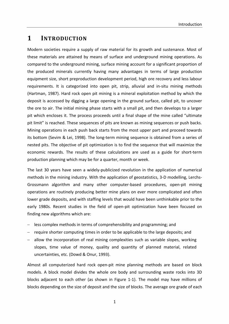
1 INTRODUCTION
Modern societies require a supply of raw material for its growth and sustenance. Most of
these materials are attained by means of surface and underground mining operations. As
compared to the underground mining, surface mining account for a significant proportion of
the produced minerals currently having many advantages in terms of large production
equipment size, short preproduction development period, high ore recovery and less labour
requirements. It is categorized into open pit, strip, alluvial and in-situ mining methods
(Hartman, 1987). Hard rock open pit mining is a mineral exploitation method by which the
deposit is accessed by digging a large opening in the ground surface, called pit, to uncover
the ore to air. The initial mining phase starts with a small pit, and then develops to a larger
pit which encloses it. The process proceeds until a final shape of the mine called “ultimate
pit limit” is reached. These sequences of pits are known as mining sequences or push backs.
Mining operations in each push back starts from the most upper part and proceed towards
its bottom (Sevim & Lei, 1998). The long-term mining sequence is obtained from a series of
nested pits. The objective of pit optimization is to find the sequence that will maximize the
economic rewards. The results of these calculations are used as a guide for short-term
production planning which may be for a quarter, month or week.
The last 30 years have seen a widely-publicized revolution in the application of numerical
methods in the mining industry. With the application of geostatistics, 3-D modelling, Lerchs-
Grossmann algorithm and many other computer-based procedures, open-pit mining
operations are routinely producing better mine plans on ever more complicated and often
lower grade deposits, and with staffing levels that would have been unthinkable prior to the
early 1980s. Recent studies in the field of open-pit optimization have been focused on
finding new algorithms which are:
less complex methods in terms of comprehensibility and programming; and
require shorter computing times in order to be applicable to the large deposits; and
allow the incorporation of real mining complexities such as variable slopes, working
slopes, time value of money, quality and quantity of planned material, related
uncertainties, etc. (Dowd & Onur, 1993).
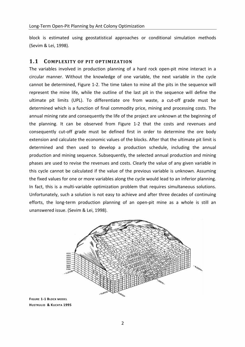
Almost all computerized hard rock open-pit mine planning methods are based on block
models. A block model divides the whole ore body and surrounding waste rocks into 3D
blocks adjacent to each other (as shown in Figure 1-1). The model may have millions of
blocks depending on the size of deposit and the size of blocks. The average ore grade of each
Long-Term Open-Pit Planning by Ant Colony Optimization
2
block is estimated using geostatistical approaches or conditional simulation methods
(Sevim & Lei, 1998).
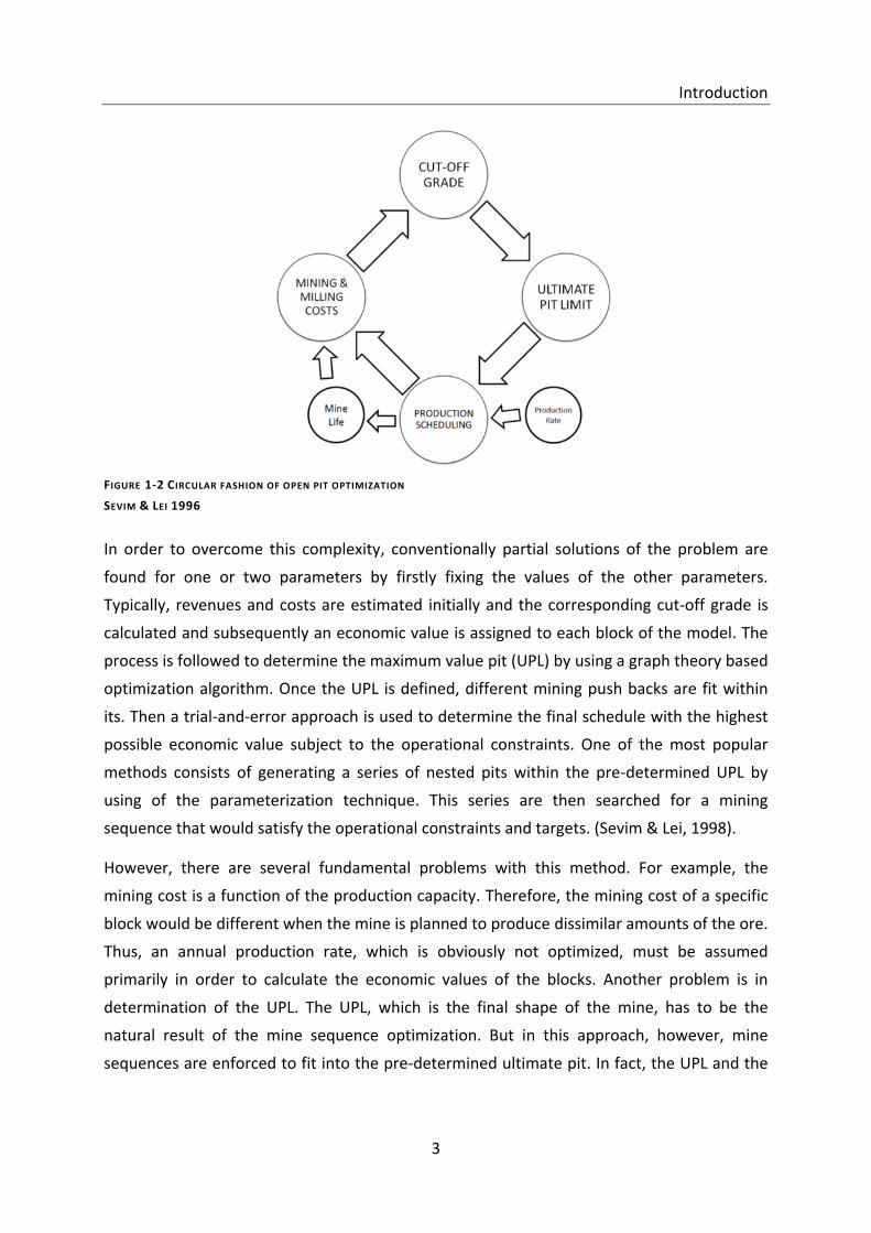
1.1 COMPLEXITY OF PIT OPT IMIZATION
The variables involved in production planning of a hard rock open-pit mine interact in a
circular manner. Without the knowledge of one variable, the next variable in the cycle
cannot be determined, Figure 1-2. The time taken to mine all the pits in the sequence will
represent the mine life, while the outline of the last pit in the sequence will define the
ultimate pit limits (UPL). To differentiate ore from waste, a cut-off grade must be
determined which is a function of final commodity price, mining and processing costs. The
annual mining rate and consequently the life of the project are unknown at the beginning of
the planning. It can be observed from Figure 1-2 that the costs and revenues and
consequently cut-off grade must be defined first in order to determine the ore body
extension and calculate the economic values of the blocks. After that the ultimate pit limit is
determined and then used to develop a production schedule, including the annual
production and mining sequence. Subsequently, the selected annual production and mining
phases are used to revise the revenues and costs. Clearly the value of any given variable in
this cycle cannot be calculated if the value of the previous variable is unknown. Assuming
the fixed values for one or more variables along the cycle would lead to an inferior planning.
In fact, this is a multi-variable optimization problem that requires simultaneous solutions.
Unfortunately, such a solution is not easy to achieve and after three decades of continuing
efforts, the long-term production planning of an open-pit mine as a whole is still an
unanswered issue. (Sevim & Lei, 1998).
FIGURE 1-1 BLOCK MODEL
HUSTRULID & KUCHTA 1995
Introduction
3
In order to overcome this complexity, conventionally partial solutions of the problem are
found for one or two parameters by firstly fixing the values of the other parameters.
Typically, revenues and costs are estimated initially and the corresponding cut-off grade is
calculated and subsequently an economic value is assigned to each block of the model. The
process is followed to determine the maximum value pit (UPL) by using a graph theory based
optimization algorithm. Once the UPL is defined, different mining push backs are fit within
its. Then a trial-and-error approach is used to determine the final schedule with the highest
possible economic value subject to the operational constraints. One of the most popular
methods consists of generating a series of nested pits within the pre-determined UPL by
using of the parameterization technique. This series are then searched for a mining
sequence that would satisfy the operational constraints and targets. (Sevim & Lei, 1998).
However, there are several fundamental problems with this method. For example, the
mining cost is a function of the production capacity. Therefore, the mining cost of a specific
block would be different when the mine is planned to produce dissimilar amounts of the ore.
Thus, an annual production rate, which is obviously not optimized, must be assumed
primarily in order to calculate the economic values of the blocks. Another problem is in
determination of the UPL. The UPL, which is the final shape of the mine, has to be the
natural result of the mine sequence optimization. But in this approach, however, mine
sequences are enforced to fit into the pre-determined ultimate pit. In fact, the UPL and the
FIGURE 1-2 CIRCULAR FASHION OF OPEN PIT OPTIMIZATION
SEVIM & LEI 1996
Long-Term Open-Pit Planning by Ant Colony Optimization
4
mining schedule should not be calculated individually if correct optimization is desired.
(Sevim & Lei, 1998).
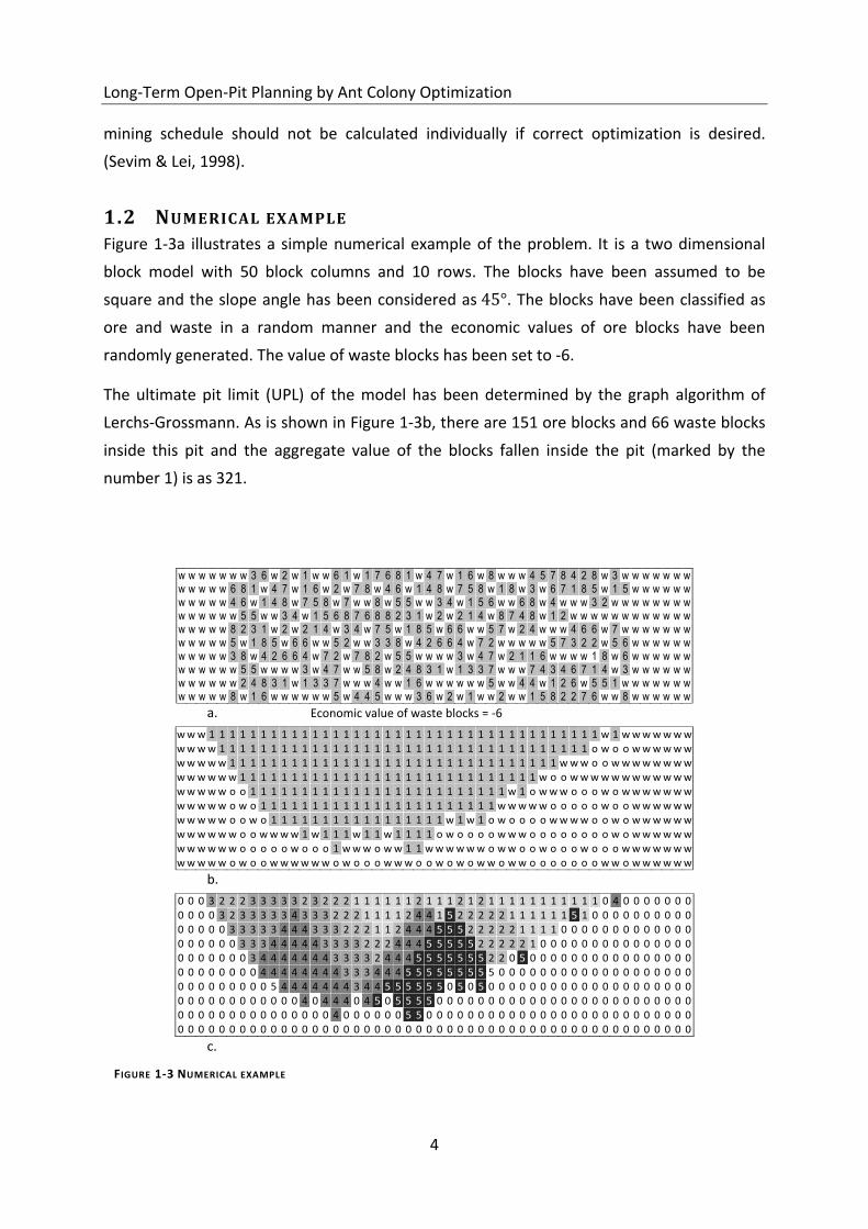
1.2 NUMERICAL EXAMPLE
Figure 1-3a illustrates a simple numerical example of the problem. It is a two dimensional
block model with 50 block columns and 10 rows. The blocks have been assumed to be
square and the slope angle has been considered as . The blocks have been classified as
ore and waste in a random manner and the economic values of ore blocks have been
randomly generated. The value of waste blocks has been set to -6.
The ultimate pit limit (UPL) of the model has been determined by the graph algorithm of
Lerchs-Grossmann. As is shown in Figure 1-3b, there are 151 ore blocks and 66 waste blocks
inside this pit and the aggregate value of the blocks fallen inside the pit (marked by the
number 1) is as 321.
w w w w w w w 3 6 w 2 w 1 w w 6 1 w 1 7 6 8 1 w 4 7 w 1 6 w 8 w w w 4 5 7 8 4 2 8 w 3 w w w w w w w w w w w w 6 8 1 w 4 7 w 1 6 w 2 w 7 8 w 4 6 w 1 4 8 w 7 5 8 w 1 8 w 3 w 6 7 1 8 5 w 1 5 w w w w w w w w w w w 4 6 w 1 4 8 w 7 5 8 w 7 w w 8 w 5 5 w w 3 4 w 1 5 6 w w 6 8 w 4 w w w 3 2 w w w w w w w w w w w w w w 5 5 w w 3 4 w 1 5 6 8 7 6 8 8 2 3 1 w 2 w 2 1 4 w 8 7 4 8 w 1 2 w w w w w w w w w w w w w w w w w 8 2 3 1 w 2 w 2 1 4 w 3 4 w 7 5 w 1 8 5 w 6 6 w w 5 7 w 2 4 w w w 4 6 6 w 7 w w w w w w w w w w w w 5 w 1 8 5 w 6 6 w w 5 2 w w 3 3 8 w 4 2 6 6 4 w 7 2 w w w w w 5 7 3 2 2 w 5 6 w w w w w w w w w w w 3 8 w 4 2 6 6 4 w 7 2 w 7 8 2 w 5 5 w w w w 3 w 4 7 w 2 1 1 6 w w w w 1 8 w 6 w w w w w w w w w w w w 5 5 w w w w 3 w 4 7 w w 5 8 w 2 4 8 3 1 w 1 3 3 7 w w w 7 4 3 4 6 7 1 4 w 3 w w w w w w w w w w w w 2 4 8 3 1 w 1 3 3 7 w w w 4 w w 1 6 w w w w w w 5 w w 4 4 w 1 2 6 w 5 5 1 w w w w w w w w w w w w 8 w 1 6 w w w w w w 5 w 4 4 5 w w w 3 6 w 2 w 1 w w 2 w w 1 5 8 2 2 7 6 w w 8 w w w w w w
a. Economic value of waste blocks = -6
w w w 1 1 1 1 1 1 1 1 1 1 1 1 1 1 1 1 1 1 1 1 1 1 1 1 1 1 1 1 1 1 1 1 1 1 1 1 1 1 w 1 w w w w w w w w w w w 1 1 1 1 1 1 1 1 1 1 1 1 1 1 1 1 1 1 1 1 1 1 1 1 1 1 1 1 1 1 1 1 1 1 1 1 o w o o w w w w w w w w w w w 1 1 1 1 1 1 1 1 1 1 1 1 1 1 1 1 1 1 1 1 1 1 1 1 1 1 1 1 1 1 1 1 w w w o o w w w w w w w w w w w w w w 1 1 1 1 1 1 1 1 1 1 1 1 1 1 1 1 1 1 1 1 1 1 1 1 1 1 1 1 1 w o o w w w w w w w w w w w w w w w w w o o 1 1 1 1 1 1 1 1 1 1 1 1 1 1 1 1 1 1 1 1 1 1 1 1 1 w 1 o w w w o o o w o w w w w w w w w w w w w o w o 1 1 1 1 1 1 1 1 1 1 1 1 1 1 1 1 1 1 1 1 1 1 1 w w w w w o o o o o w o o w w w w w w w w w w w o o w o 1 1 1 1 1 1 1 1 1 1 1 1 1 1 1 1 1 w 1 w 1 o w o o o o w w w w o o w o w w w w w w w w w w w w o o w w w w 1 w 1 1 1 w 1 1 w 1 1 1 1 o w o o o o w w w o o o o o o o o w o w w w w w w w w w w w w o o o o o w o o o 1 w w w o w w 1 1 w w w w w w o w w o o w o o o w o o o w w w w w w w w w w w w o w o o w w w w w w o w o o o w w w o o w o w o w w o w w o o o o o o o w w o w w w w w w
b.
0 0 0 3 2 2 2 3 3 3 3 3 2 3 2 2 2 1 1 1 1 1 1 2 1 1 1 2 1 2 1 1 1 1 1 1 1 1 1 1 1 0 4 0 0 0 0 0 0 0 0 0 0 0 3 2 3 3 3 3 3 4 3 3 3 2 2 2 1 1 1 1 2 4 4 1 5 2 2 2 2 2 1 1 1 1 1 1 5 1 0 0 0 0 0 0 0 0 0 0 0 0 0 0 0 3 3 3 3 3 4 4 4 3 3 3 2 2 2 1 1 2 4 4 4 5 5 5 2 2 2 2 2 1 1 1 1 0 0 0 0 0 0 0 0 0 0 0 0 0 0 0 0 0 0 0 3 3 3 4 4 4 4 4 3 3 3 3 2 2 2 4 4 4 5 5 5 5 5 2 2 2 2 2 1 0 0 0 0 0 0 0 0 0 0 0 0 0 0 0 0 0 0 0 0 0 0 3 4 4 4 4 4 4 4 3 3 3 3 2 4 4 4 5 5 5 5 5 5 5 2 2 0 5 0 0 0 0 0 0 0 0 0 0 0 0 0 0 0 0 0 0 0 0 0 0 0 0 4 4 4 4 4 4 4 4 3 3 3 4 4 4 5 5 5 5 5 5 5 5 5 0 0 0 0 0 0 0 0 0 0 0 0 0 0 0 0 0 0 0 0 0 0 0 0 0 0 0 0 5 4 4 4 4 4 4 4 3 4 4 5 5 5 5 5 5 0 5 0 5 0 0 0 0 0 0 0 0 0 0 0 0 0 0 0 0 0 0 0 0 0 0 0 0 0 0 0 0 0 0 0 0 4 0 4 4 4 0 4 5 0 5 5 5 5 0 0 0 0 0 0 0 0 0 0 0 0 0 0 0 0 0 0 0 0 0 0 0 0 0 0 0 0 0 0 0 0 0 0 0 0 0 0 0 0 4 0 0 0 0 0 0 5 5 0 0 0 0 0 0 0 0 0 0 0 0 0 0 0 0 0 0 0 0 0 0 0 0 0 0 0 0 0 0 0 0 0 0 0 0 0 0 0 0 0 0 0 0 0 0 0 0 0 0 0 0 0 0 0 0 0 0 0 0 0 0 0 0 0 0 0 0 0 0 0 0 0 0 0 0
c.
FIGURE 1-3 NUMERICAL EXAMPLE
Introduction
5
Pus
hbac
k N
o.
Ore
num
ber
Was
te n
umbe
r
Tot
al n
umbe
r
Ave
rage
of o
re
valu
e
Pus
hbac
k V
alue
(Und
isco
unte
d)
Com
plet
ion
of
push
bac
k*
Pus
hbac
k V
alue
(Dis
coun
ted*
*)
1 30 10 40 5.93 118 3.97 80.80 2 26 14 40 5.12 49 7.41 24.16 3 26 14 40 4.65 37 10.86 13.14 4 39 15 54 4.18 73 16.02 15.84 5 30 13 43 4.07 44 20 6.54
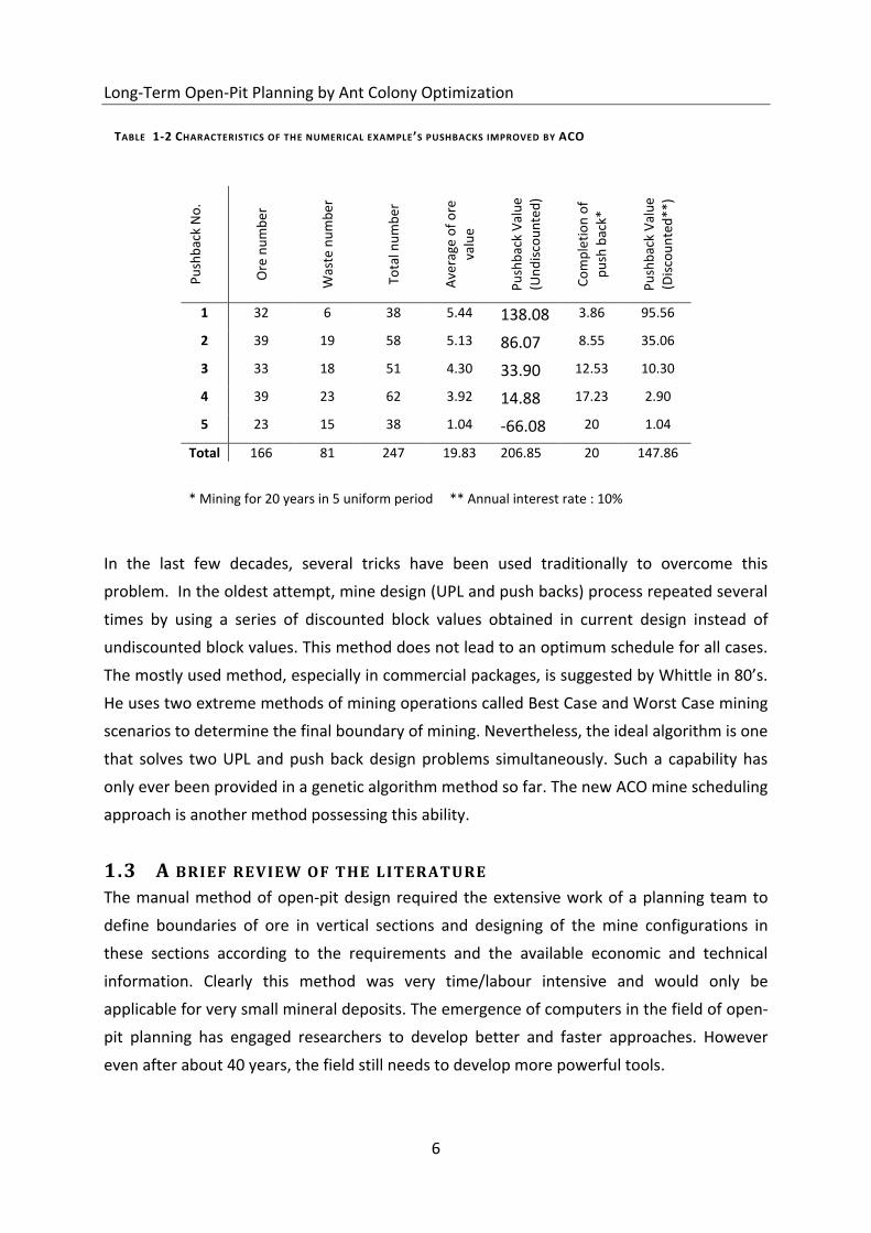
Total 151 66 217 4.75 321 20 140.49 * Mining for 20 years in 5 uniform period ** Annual interest rate : 10%
0 0 4 3 3 2 2 2 2 3 2 3 2 2 2 1 1 1 1 1 1 1 1 2 1 1 1 1 1 1 1 1 1 1 1 1 1 1 1 1 1 3 1 0 0 0 0 0 0 0 0 0 0 4 3 3 2 2 3 3 3 3 3 2 2 2 2 1 1 2 2 1 2 2 2 1 3 1 2 1 2 1 1 2 1 2 1 1 3 1 3 3 0 0 0 0 0 0 0 0 0 0 0 0 4 3 3 3 3 3 3 4 3 3 2 2 2 2 2 2 2 2 2 3 4 3 3 4 2 2 2 2 2 2 2 2 2 0 0 0 3 0 0 0 0 0 0 0 0 0 0 0 0 0 0 4 3 3 4 4 4 4 4 3 3 2 2 2 2 2 2 2 3 4 4 4 5 4 4 2 3 2 2 2 2 5 0 0 0 0 0 0 0 0 0 0 0 0 0 0 0 0 0 0 0 0 4 4 4 4 4 4 4 4 3 3 3 2 3 2 2 3 4 4 4 5 5 5 4 4 3 3 5 2 5 0 0 0 0 0 0 0 0 0 0 0 0 0 0 0 0 0 0 0 0 0 0 4 4 4 4 4 4 4 4 3 3 3 3 3 3 4 4 4 5 5 5 5 5 4 4 5 0 0 0 0 0 0 0 0 0 0 0 0 0 0 0 0 0 0 0 0 0 0 0 0 0 0 4 4 4 4 4 4 4 4 4 3 3 3 5 4 4 5 5 5 5 5 5 5 5 0 0 0 0 0 0 0 0 0 0 0 0 0 0 0 0 0 0 0 0 0 0 0 0 0 0 0 0 0 0 0 4 4 4 4 4 5 3 5 5 5 5 5 5 5 0 5 5 5 0 0 0 0 0 0 0 0 0 0 0 0 0 0 0 0 0 0 0 0 0 0 0 0 0 0 0 0 0 0 0 0 0 4 4 4 5 0 0 5 0 0 5 5 0 0 0 0 0 0 0 0 0 0 0 0 0 0 0 0 0 0 0 0 0 0 0 0 0 0 0 0 0 0 0 0 0 0 0 0 0 0 0 0 0 5 0 0 0 0 0 0 0 0 0 0 0 0 0 0 0 0 0 0 0 0 0 0 0 0 0 0 0 0 0 0 0 0 0 0
An initial long-term plan had been created for the model using the heuristic method of Wang
& Sevim (1995), Figure 1-3c. The desired size of push backs in this case was set to 40 blocks.
It could be observed that the designed push backs are almost uniform in size, with a
descending average from 5.93 to 4.07. Assuming an interest rate of ten percent and the
mine life of 20 years, the value of the generated schedule decreases from the attractive 321
units (in the undiscounted case) to 140.49 units considering the time value of money
(discounted value), Table 1-1.
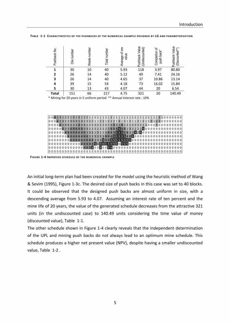
The other schedule shown in Figure 1-4 clearly reveals that the independent determination
of the UPL and mining push backs do not always lead to an optimum mine schedule. This
schedule produces a higher net present value (NPV), despite having a smaller undiscounted
value, Table 1-2 .
FIGURE 1-4 IMPROVED SCHEDULE OF THE NUMERICAL EXAMPLE
TABLE 1-1 CHARACTERISTICS OF THE PUSHBACKS OF THE NUMERICAL EXAMPLE DESIGNED BY LG AND PARAMETERIZATION
Long-Term Open-Pit Planning by Ant Colony Optimization
6
Pu
shb
ack
No
.
Ore
nu
mb
er
Was
te n
um
ber
Tota
l nu
mb
er
Ave
rage
of
ore
valu
e
Pu
shb
ack
Val
ue
(Un
dis
cou
nte
d)
Co
mp
leti
on
of
pu
sh b
ack*
Pu
shb
ack
Val
ue
(Dis
cou
nte
d**
)
1 32 6 38 5.44 138.08 3.86 95.56
2 39 19 58 5.13 86.07 8.55 35.06
3 33 18 51 4.30 33.90 12.53 10.30
4 39 23 62 3.92 14.88 17.23 2.90
5 23 15 38 1.04 -66.08 20 1.04
Total 166 81 247 19.83 206.85 20 147.86
* Mining for 20 years in 5 uniform period ** Annual interest rate : 10%
In the last few decades, several tricks have been used traditionally to overcome this
problem. In the oldest attempt, mine design (UPL and push backs) process repeated several
times by using a series of discounted block values obtained in current design instead of
undiscounted block values. This method does not lead to an optimum schedule for all cases.
The mostly used method, especially in commercial packages, is suggested by Whittle in 80’s.
He uses two extreme methods of mining operations called Best Case and Worst Case mining
scenarios to determine the final boundary of mining. Nevertheless, the ideal algorithm is one
that solves two UPL and push back design problems simultaneously. Such a capability has
only ever been provided in a genetic algorithm method so far. The new ACO mine scheduling
approach is another method possessing this ability.
1.3 A BRIEF REVIEW OF THE LITERATURE
The manual method of open-pit design required the extensive work of a planning team to
define boundaries of ore in vertical sections and designing of the mine configurations in
these sections according to the requirements and the available economic and technical
information. Clearly this method was very time/labour intensive and would only be
applicable for very small mineral deposits. The emergence of computers in the field of open-
pit planning has engaged researchers to develop better and faster approaches. However
even after about 40 years, the field still needs to develop more powerful tools.
TABLE 1-2 CHARACTERISTICS OF THE NUMERICAL EXAMPLE’S PUSHBACKS IMPROVED BY ACO
Introduction
7
In early studies (Pana, 1965; Williams, 1974; Lemieux, 1979) the moving cone algorithm was
used to design the outline of the final pit shape. The algorithm starts from the surface and
searches for ore blocks with positive economic value. Thereafter, it constructs a minimum
removal cone on such a block. All blocks inside this cone are considered as removed if the
sum of the economic values of these blocks is positive. The algorithm continues the search
until all the ore blocks in the model have been examined. Despite the 3D nature of the
method and the ability to consider variable slopes, it was proved very soon that the moving
cone algorithm was not able to find the best solution in all cases.
After development of various 2D mathematical methods that were able to find the optimum
UPL on vertical sections, several studies were carried out to combine 2D sections and
provide 3D pits (Johnson & Sharp; 1971, Wright;1987). Later Koenigsberg (1982) and Wilke &
Wright (1984) succeeded in directly applying dynamic programming to solve the 3D pit
design problem. The Lerchs and Grossmann’s algorithm might be one of the most utilized
algorithms in open-pit optimization field. Authors used the graph theory to formulate the
model optimum pit limit, see chapter 2.3.1. Afterwards several researchers attempted to
develop more efficient algorithms for the UPL problem (Huttagosol and Cameron, 1992;
Yegulalp and Arias, 1992; Zhao and Kim, 1992; Hochbaum, 2001).
Subsequent studies focused on a more general problem rather than the UPL. It was the
production planning problem. This challenging problem tried to answer the following
questions (Dagdelen & Johnson, 1986):
Should a given block be mined by the end of mine life or not? (UPL problem)
If yes:
When should it be mined? (Mine sequencing problem), and
Where should it be send? E.g. processing plant, leach pad or waste dump? (Cut-off
grade problem)
As Chapter 2 explains, this is a huge mathematical programming model that could not be
solved by available computer software and hardware.
An early optimization attempt in production scheduling reverts back to the studies done by
Wilke and Reimer (1977). Authors proposed a linear programming model for the short-term
production scheduling of an open-pit iron ore mining operation. Later, Jordi and Currin
(1979) proposed a goal programming model to optimize net present value, the total net
profit and the total gold output. Zhang et al. (1986) described a new Interactive Dynamic
Optimization Method (IDOM) that combined inventory theory, dynamic programming,
Long-Term Open-Pit Planning by Ant Colony Optimization
8
computer simulation and interactive technique to formulate a production scheduling
problem of open-pit mines.
One of the major developed concepts was the application of lagrangian parameterization for
optimization of production planning problem by Dagdelen and Johnson (1986). This concept
uses the UPL algorithm applied to block models with varied block values to produce
production schedules. The concept of lagrangian parameterization utilized later by Whittle
to develop the most known commercial package in the field of open-pit optimization.
Whittle’s method is a heuristic approach that uses the different block values to produce a
series of nested pits and selects the UPL and mining push backs corresponding to the
maximum NPV. Sevim and Lei (1996) described methodology comprising a group of heuristic
algorithms and unconventional dynamic programming. This method had the capability to
determine the cut-off grade, mining and milling production rates, mining sequence, mine life
and UPL. In the recent studies conducted by Ramazan & Dagdelen (1998), a new algorithm
which could develop push backs of minimum stripping ratio was presented. Ramazan &
Dagdelen and Jonson (2005) proposed a new production scheduling optimization technique
based on the fundamental tree algorithm to decrease the number of integer variables and to
solve the problem as a mathematical programming model.
Debny & Schofield (1996) attempted to use metaheuristic algorithms for first time in pit
optimization; however, their developed genetic algorithm model was not able to be applied
in real mining cases because of long computational times. In another study, Kumral and
Dowd (2005) proposed another metaheuristic algorithm based on simulated annealing to
improve the value of a given sub-optimal mine schedule.
The non-deterministic view to the open-pit optimization is another research field which has
received a lot of attraction in recent years. Osanloo & Gholamnejad (2008) modelled the
long-term production scheduling problem by chance-constrained binary integer
programming in a stochastic environment. Dimitrakopoulos (1998) outlined a general
framework for modelling uncertainty and assessing geological risk. Conditional simulation is
a class of Monte Carlo techniques that can be used to equally generated representatives of
the in-situ ore body variability. Achireko & Frimpong (1996) proposed a new algorithm called
MCS/MFNN which had the capability to address the random field properties associated with
the ore grades, reserve and commodity prices. After modelling the block characteristics by
conditional simulation, they used artificial neural networks to classify the blocks into classes
based on their conditioned values. The error back propagation algorithm is then used to
optimize the UPL by minimizing the desired and actual output errors in a multilayer
Introduction
9
perception under pit wall slope constraints. Frimpong et al. (1998) developed an intelligent
pit optimizer (IPOP) to deal with the random properties of optimized pit layouts. It combines
stochastic models of ore reserves and commodity prices to generate economic block and
target values.
Recently, designing integrated intelligent systems for decision making on mineral resource
exploitation is becoming of increasing interest. They provide analysis with intelligent design
options to deal with structural, hydrological and tectonics problems of mine design.
Frimpong and Szymanski (2002) have discussed current state-of-art technology and research
in intelligent modelling, and have also addressed the current and future research frontiers in
intelligent modelling.
1.4 STRUCTURE OF THE RESEARCH
The main objective of the current study was to develop a mathematical and computer
modelling background of a new metaheuristic algorithm based on Ant Colony Optimization
(ACO) for optimization of long-term open-pit designs.
To achieve this, a computer program has been provided to test the proposed algorithm. As a
case study, the block model of a hypothetical iron ore deposit is generated and the values of
grades have been randomly assigned. The application of the newly developed algorithm is
tested several times to achieve the best range of the parameters and proper variants of the
ACO method.
Chapter 2 elucidates the background, concepts and problems associated with the existing
open-pit optimization techniques, such as mathematical modelling, heuristic and
metaheuristic algorithms. This chapter contains the analytical survey of the literature on
open-pit optimization algorithms and discusses their limitations. Chapter 3 deals with the
basic fundamentals of the ant colony optimization. The principals of ACO have been
explained by using the well-known travelling salesman problem in Chapter 3. In Chapter 4
the major solution steps for a long-term open-pit planning problem by means of ACO is
presented. The user interface of the programmed software and the results of its application
on the case study have been included in this chapter. Chapter 5 contains all conclusions and
recommendations for further research works arising from this research study.

The problem of long-term open-pit production planning
11
2 THE PROBLEM OF LONG-TERM OPEN-PIT PRODUCTION
PLANNING
The open-pit mine production scheduling problem can be defined as discovering the
sequence in which rock blocks should be removed from the deposit as a certain material
type in order to maximise the total discounted profit from the mine subject to a variety of
physical and economic constraints. The size and the complexity of the problem cause that
the currently available tools and methods are either yield suboptimal answers or not
suitable for application to reasonable-sized deposits. This part discusses the long-term open-
pit production planning problem from a mathematical programming point of view.
2.1 MATHEMATICAL PROGRAMMING MODELS
2.1.1 INTEGER LINEAR PROGRAMMING (IP)
Integer linear programming (IP) can be effectively used to model the production scheduling
problem of an open-pit mine (Caccetta et al., 1998). It can be defined as following:
Objective function
The objective function could be expressed as the maximization of net present return by
mining and processing of blocks.
∑ ∑∑
Where
: The binary decision variables of the model (
if block is mined as type in
time period and if otherwise).
: The objective function coefficients, representing the return from (or the cost of)
mining of block as type in time period .
: The index of the blocks in the ore body, .
: The index of different possible types that a block may be mined as (for instance if
the block is mined as waste, if the block is mined as processing ore and if the
block is mined as leaching ore and etc.), .
and : The index of periods over which the mine is being scheduled, .
The model consists of binary variables.
Long-Term Open-Pit Planning by Ant Colony Optimization
12
The target will be subject to the following constraints:
Mining capacity constraints
Total tonnage of extracted material should be between a pre-determined upper and lower
limit.
∑∑
∑∑
Where
: Total tonnage of block .
: The maximum and minimum allowed capacity of mining operation for the
period of .
The model has number of mining capacity constraints.
Processing capacity constraints
Quantity of each material type should also be between the defined boundaries:
∑
∑
Where
: The maximum and minimum allowed capacity of processing of material
type for the period of .
The number of processing capacity constraints will be .
Constraints for the average grade of products
Average grade of each production element should be between pre-determined limits:
The problem of long-term open-pit production planning
13
∑(
)
∑(
)
Where
: The index of valuable elements in blocks (such as copper, silver and gold),
: The grade of element in block
: The maximum and minimum limits of the average grade defined for the
element of the material type in the period .
Based on this formula there will be number of average grade constraints
required in the model. Normally no constraint required at least for the waste, therefore, the
maximum number of constraints could be considered as ( ) .
Reserve constraints
The reserve constraints are mathematically necessary to ensure that a block is mined only
once.
∑∑
The number of constraints required in this case equals to the number of blocks, .
The main point in this formula is that when ∑ ∑
, it means that the block
will not be mined at all. In other words the problem of ultimate pit limit (UPL) has also been
enclosed in this formulation.
Sequencing constraints
The sequencing constraints ensure that a block can only be removed if all overlaying blocks
have been removed in the previous or current periods.
(∑
) (∑∑
)
Where
Long-Term Open-Pit Planning by Ant Colony Optimization
14
: The index for the set of overlying restricting blocks that should be removed earlier for
mining of block , ,
The model should have number of this constraint type. This constraint could be
written in a compressed version with less number of constraints:
(∑
) ∑(∑∑
)
Ramazan et al. (2004) showed that first case is faster at the run time.
Binary variables
Finally the variables of the model should be binary.
Through simply stated, an integer linear programming formulation of the open pit
scheduling problem usually involves a large number of variables and constraints. For
example, a small copper-molybdenum deposit containing 10,000 blocks and 10 planning
periods would require the solution of an integer programming problem with 300,000
variables, 200 mining and milling constraints, 900,000 sequencing constraints and 10,000
reserve constraints. Clearly this is beyond the capacity of current integer programming
packages.
2.1.2 THE LINEAR PROGRAMMING (LP) FORMULIZATION OF THE MODEL
Johnson (1969) has discussed the LP modelling of the long-term open-pit production
planning problem. The major benefit in this model is that the fractional block extraction
becomes possible.
The LP model could be easily achieved by new definitions for the decision variables,
coefficients of the objective function and discarding the binary nature of the variables in MIP
formulation as following:
: The proportion of block to be mined in period as a processing type .
: The NPV resulting from mining a unit weight of material in block during period if it
is considered as processing type .
Johnson (1969) proposed to solve this problem by decomposing of the large multi-period
production planning model into a master problem and a set of sub-problems that are exactly
similar to UPL problem. After solving all sub-problems by well-known UPL algorithms such as
Lerchs-Grossmann’s algorithm, solving the master problem would be relatively simple.
The problem of long-term open-pit production planning
15
Although this method produces optimum solutions for each period individually, however, it
does not optimize the problem totally. It also encounters situations in which some portion of
a block could be extracted while all the overlying blocks have not been fully mined. In other
words some percentages of overlying blocks are suspended in air. These downsides and high
number of constraints cause the approach not to be practical. (Osanloo et al., 2008)
2.2 MATHEMATICAL APPROACH ES FOR SOLUTION OF THE MODEL
Several approaches have been proposed in literature to solve this model. Dagdelen and
Johnson (1986) and Caccetta et al. (1998) used lagrangian parameterization in order to relax
mining and milling constraints into objective function. Consequently the problem could be
handled by repetition of any UPL algorithm such as Lerchs-Grossmann (1965) graph theory
based algorithm. Caccetta et al. (1998) utilized lagrange multipliers to omit the mining and
milling constraints and solved the model using subgradient optimization method. Dowd &
Onur (1992) and Onur & Dowd (1993) formulated the problem as a dynamic programming
model. Later Ramazan et al. (2005) described the application of fundamental tree algorithm
to reconstruct the mining blocks and decrease the number of variables in scheduling
problem without reducing the resolution of the model or optimality of the results. A
fundamental tree is defined as any combination of blocks such that the blocks can be
profitably mined respecting slope constraints. Following comprehensively reviews the most
important literatures.
2.2.1 LAGRANGIAN PARAMETERIZATION
The idea of lagrangian parameterization originates from the fact that the mining and
processing constraints are relatively few in number but complicate the underlying structure
of the whole problem. Using Lagrangian multipliers, the complex multi-period problem of
open-pit production planning could be decomposed into smaller single-period problems that
could be solved using optimum pit limit (UPL) design algorithms. Considering very efficient
UPL algorithms such as Learchs-Grossman (1965) and Zhao-Kim (1992) and etc., this makes
possible to solve a relatively large long-term open-pit scheduling problem.
Before going into the formulization of this powerful concept, it is needed to define the UPL
problem.
Ultimate Pit Limit (UPL) Problem
When formulated as a mathematical program, the objective in solving UPL problem is to find
all the available ore material in the deposit which will maximize the profits and when mined,
will satisfy the pit slope requirements. This problem can be formulated as:
Long-Term Open-Pit Planning by Ant Colony Optimization
16
∑
Where is the economic value of the block, is the set of the blocks which must be
removed earlier in order to reach the block and is one if the block is mined and is
zero otherwise. (Dagdelen & Johnson, 1986). Details of the well-known Lerchs-Grossmann
algorithm of UPL calculation has been explained in chapter 2.3.1.
Understanding Lagrangian parameterization
The mining and milling constraints could be simply relaxed by multiplication of constraints in
Lagrange multipliers and subtracting of resulted phrase from the objective function.
Therefore the model can be re- written as:
∑ ∑∑
Where are the new coefficients that have been obtained by subtracting Lagrange
multipliers from the original coefficients.
Now the Lagrange multipliers should be adjusted using the sub-gradient method until the
optimum schedule is obtained. At each step, only a problem similar to an ultimate pit limit
problem needs to be solved. In cases that there are no multipliers that can result in a
feasible solution for the constraints, this method may not converge to an optimum solution.
This leads to a problem known as the gap problem.
Caccetta et al. (1998) applied the method on a real ore body with 20,979 blocks and six time
periods and the schedule obtained was within 5% of the theoretical optimum. One year later
Akaike & Dagdelen (1999) proposed a 4D-network relaxation method which was capable to
consider dynamic cut-off grade concept during the scheduling process and handle the
stockpile option.
2.2.2 CLUSTERING APPROACH
One of the recent mathematical approaches to solve an IP model of production planning of
an open-pit mine is the clustering method proposed by Ramazan et al. (2005). Clustering is
defined as the classification of a large amount of data into a relatively few number of similar
classes. The reason is to reduce complexity in the considered application in order to obtain
The problem of long-term open-pit production planning
17
improved decisions based on the available information. Authors combined ore and waste
blocks together to decrease the number of binary variables in the linear programming
model. They defined the fundamental tree as any combination of blocks within the push
backs, such that can be profitability mined and satisfy the slope constraints and no chosen
sub-set of a fundamental tree meeting these requirements could be found. The clustering
process is done using an LP formulation in a way that no available information of any
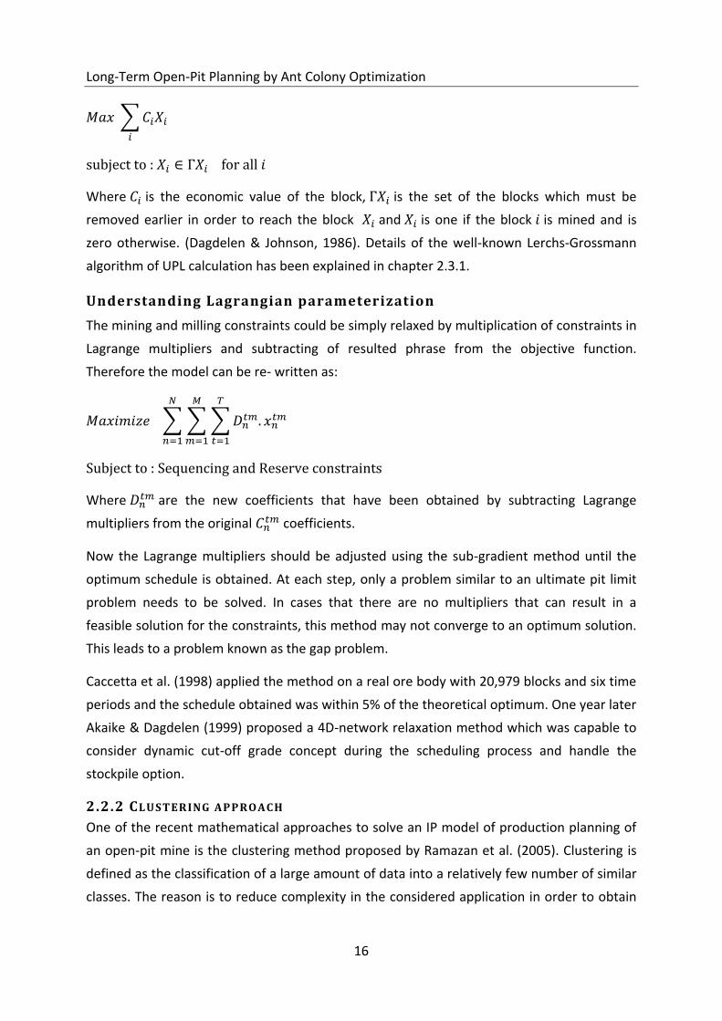
individual block to be lost. Steps of algorithm have been shown in Figure 2-1.
Figure 2-2 illustrates a 2D block model on which three fundamental trees are created by a
linear programming formulation. Tree I can be mined first after which trees II and III become
accessible for mining. After determination of the fundamental trees, their precedency is
calculated by means of a cone template. In this stage, each fundamental tree is treated as an
individual mining block containing a certain ore quantity, metal content and quality
characteristics. Now an IP model could be generated by assigning a binary variable to each
fundamental tree and each production period. This model is then solved by CPLEX software
and contents of the UPL are allocated to 3 to 5 smaller volumes (push backs). Finally,
fundamental trees are scheduled by an IP formulation including all mining and milling
operational constraints and tree sequence requirements. (Osanloo et al. 2008, Ramazan et
al. 2005)
The main advantages of this method are:
The number of model’s binary variables is directly proportional to the number of trees
and periods. Therefore, it can result in reducing the size of the model and, hence,
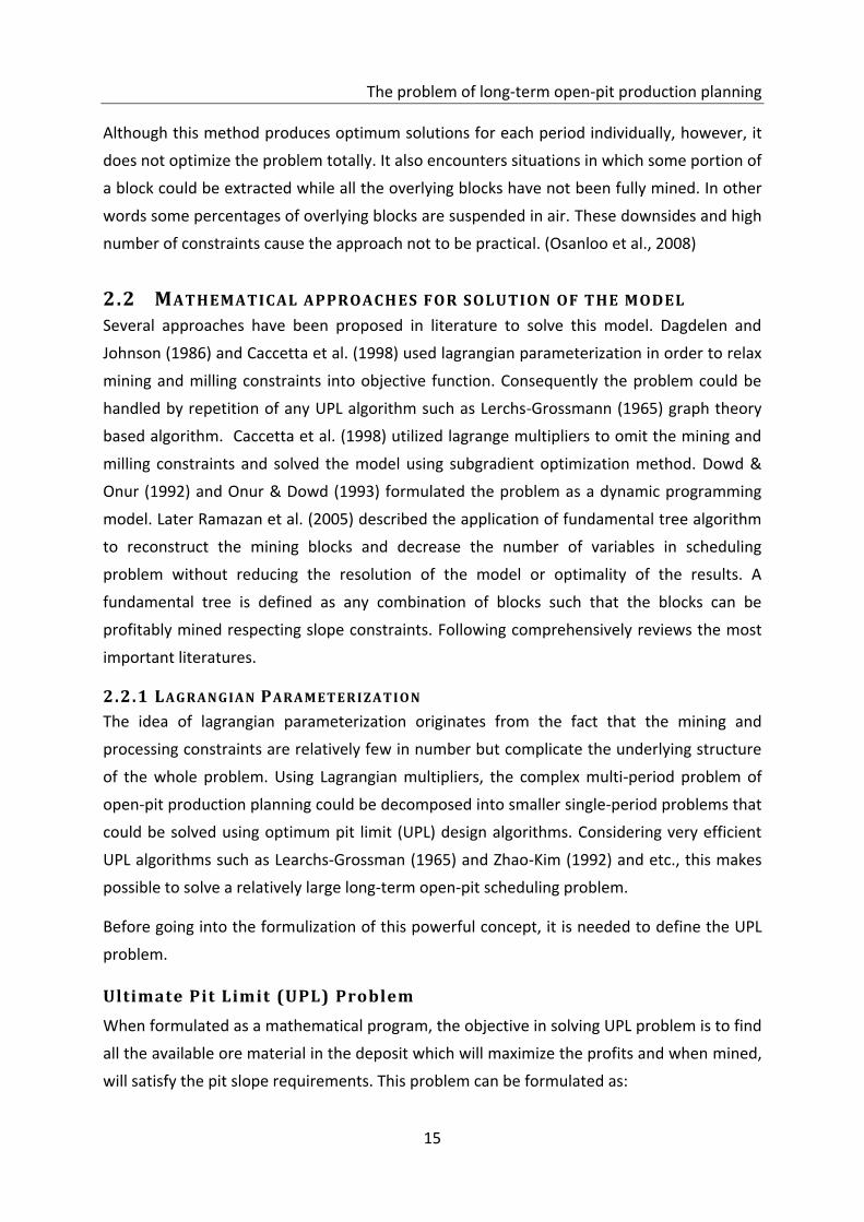
Generate a cone template
Find the fundamental trees for each pushback
Sequence the fundamental trees
Schedule the fundamental trees
Design the haul roads and smooth the pits
FIGURE 2-1 STEPS OF THE MINE PLANNING METHOD BASED ON THE FUNDAMENTAL TREE ALGORITHM
Long-Term Open-Pit Planning by Ant Colony Optimization
18
bigger block models can be solved by this technique. Authors indicated that by using
this method the number of binary variable can be decreased from 38,457 to 5,512 in a
case. (Ramazan et al. 2005).
The gap problem could be eliminated.
Further studies on this algorithm revealed that it gives a schedule with a 6% higher
NPV than those predicted by the use of other software such as Mintec Scheduler, NPV
Scheduler and Millawa algorithm of Whittle. (Bernabe and Dagdelen, 2002).
The drawbacks of the method are as follows.
In very large deposits, the number of trees to be scheduled and corresponding binary
variables in the model would be still high enough to make the model impractical.
Since the fundamental trees are defined inside push backs, the optimality of this
method will be up to the optimality of the push back determination routine.
Probably more than one iteration of the LP formulation is necessary for identifying
optimal fundamental.
The complexity of the implementation of the steps of this method highly affects its
public acceptance. (Osanloo et al. 2008, Ramazan et al. 2005)
A B
FIGURE 2-2 NETWORK REPRESENTATION OF A 2-D BLOCK MODEL,
(A) THE NETWORK REPRESENTATION OF THE SOLUTION OF THE LP FORMULATION AS THREE FUNDAMENTAL TREES SURROUNDED BY
DASHED LINES (B) (RAMAZAN ET. AL. 2005)

The problem of long-term open-pit production planning
19
2.2.3 BRANCH AND CUT TECHNI QUE
Branch-and-cut technique is an efficient method for solution of combinatorial optimization
problems that are formulated as mixed integer linear programming problems. It is an exact
algorithm which combines a cutting plane and the branch-and-bound algorithm. It works by
solving a sequence of linear programming relaxations of the IP problem. The cutting plane
improves the relaxation of the problem to more closely approximation. Branch-and-bound
algorithm carries out by a sophisticated divide and conquer tactic to solve problems.
Efficiently solution of a general IP problem is usually not possible by means of a cutting plane
approach; and normally branching is also necessary, which consequences in a branch-and-
cut approach (Mitchell 1999). Perhaps the best known branch-and-cut algorithms are those
that have been used to solve the travelling salesman problem (TSP). (Appelegate et al. 1995).
Application of Branch-and-cut procedure for solution of IP model of the long-term open-pit
scheduling problem is effectively outlined by Caccetta and Hill (2003). Explicitly
incorporation of most operational constraints such as maximum vertical depth, minimum pit
bottom width and stockpile option in the optimization procedure could be accounted as the
major advantages of their method. The process is able to provide acceptable solutions for
production planning problems of medium sized mines. Nevertheless, for large problems it is
relatively difficult to obtain an optimal solution. Authors illustrated that on a case study with
about 209,600 blocks and ten planning periods, a solution with precision of 2.5% could be
found within four hours. The other disadvantage of their process is that it does not consider
cutoff grade optimization. The authors recommended that by conjunction of their branch-
and-cut methods with heuristics or meta-heuristics a good (possibly optimal) solution can be
obtained. This would be also suitable to show how far from optimal this solution may be
obtained. (Caccetta and Hill 2003).
Defining all variables of the periods as binary values would prevent this algorithm to
generate even a feasible solution for the long-term open-pit scheduling model;
consequently, the number of binary variables should be reduced by setting of some variables
as real numbers. For instance, setting of the variables corresponding to the positive blocks as
binary and the rest of variables as real could significantly decrease the solution time. By this
action the IP model transforms to an MIP model. This strategy is usually applied to all of the
above-mentioned IP models. (Osanloo et al. 2008).
2.2.4 DYNAMIC PROGRAMMING (DP) FORMULATION
This method consists of dividing of the prime problem into smaller problems for which an
optimal solution could be easily found. To do this, it searches all possibilities and chooses the
Long-Term Open-Pit Planning by Ant Colony Optimization
20
optimum one. Unlike other operations research methods, there is not standard
mathematical approach for dynamic programming models solution. (Osanloo et al. 2008).
In this regard, the long-term production planning problem is modelled as a graph whose
nodes represent the state of the system and arcs are related to the action that takes the
system from one state to another. Solution of the production planning problem could be
considered as finding the path with the highest value. (Osanloo et al. 2008).
In the first attempts, dynamic programming was applied on the open-pit production
planning problem by Roman (1974). His formulation simultaneously calculates the pit limit
and block sequencing problems. In this formulation, the location of the block that must be
mined in the last period is determined at starting stage of the sequencing process.
Accordingly, all possible ways to schedule blocks above the particular block respecting to the
slope constraints are checked and then the optimum sequence is determined by a NPV
calculation routine. The sequence related to the highest NPV is chosen and its value is
assigned to the initial pit outline. The blocks near the pit boundary have to be examined to
define if they contribute to a positive NPV or not. Thus the blocks that do not correspond to
a positive NPV are detached from the pit and a new pit sequence and NPV are attained. This
procedure continues until no block is required to be detached from the pit. The advantage of
this method is that it is based on the time value of the money and considers scheduling in
determination of the ultimate pit limit. The drawbacks of this technique are as follows:
It cannot be applied on large block models.
There is no guarantee that mining and milling constraints will be met in each period.
The effect of the mine size on the unit cost is not considered. (Osanloo et al. 2008).
Another DP formulation for the long-term planning problem expressed by Dowd and Onur
(1992 & 1993). They indicated that in the previously proposed DP model, the number of
alternatives which have to be considered is very high and beyond the memory of current
PCs. They showed that this number could be reduced by means of elimination of the
unattractive alternatives. Authors proposed algorithm could take all kinds of constraints,
mobility and equipment access constraints into consideration and eliminate unattractive
sequences as soon as they appear. The long calculation time was the major drawback of this
method.
The other attempt was a method proposed by Tolwinski and Underwood (1992) by
combining DP, stochastic optimization, artificial intelligence and heuristic rules to solve the
long-term production planning problem. In their DP model the problem was equivalent to
The problem of long-term open-pit production planning
21
finding a path with the largest value in a graph ( ), where denotes the set of
nodes related to the states of the model as the sequence of the pits, is the set of block
removal edges and is the weights (rewards) associated with elements. Supposing to
be the node related to the initial state of the mine, the problem of optimal production
scheduling would be equivalent to finding a path through the graph that
minimizes the total reward. For a practical case with numerous nodes, solution of DP model
all of the nodes requires to be taken into account (blind search) and this leads to NP hard
condition. To avoid it, Tolwinski and Underwood suggested an informed search method,
based on AI and heuristic rules. Despite practicality of this technique for big models, it still
suffers from the lack of guarantee to provide mathematically proven optimal solution or
even sometimes a feasible solution. (Osanloo et al. 2008).
Later Tolwinski (1998) and Tolwinski and Golosinski (1995) developed a routine based on the
depth first search method for the DP formulation. Again in spite of the capability of
application on large block models, however, the gaining the highest NPV was still infeasible.
In another study Erarslan and Celebi (2001) utilized a simulative optimization model to find
the optimum pit limit and production plan. In their DP formulation each extracted block was
defined as a state of a DP stage. Despite very big advantages of this method such as
simultaneous calculation of UPL and scheduling, ability to estimate unit costs for each new
pit scenario and considering all types of constraints; again like the other DP approaches,
finding the optimal solution was not practical for large deposits. (Osanloo et al. 2008).
2.3 HEURISTIC ALGORITHMS
In the last three decades lots of heuristic algorithms have been suggested in the field of
open-pit production planning, but mostly cover only an individual part of the global
optimization and needs be integrated with others to provide a general solution for the
problem. Among them Whittle’s method and Sevim’s techniques are relatively integrated
approaches that could cover all parts of the open-pit scheduling problem.
2.3.1 WHITTLE ’S OPTIMIZATION PROCE SS
Whittle’s process is based on the fast implementation of a series of Lerchs-Grossmann (LG)
algorithm. This algorithm produces the mathematically optimum final pit shell, but only if
maximum undiscounted cash flow is the criterion for optimization. The process tries to
assist selection of the optimum final pit by providing a best and worst case mining schedules
and associated NPV curves. This normally produces a very wide range of possible pits among
Long-Term Open-Pit Planning by Ant Colony Optimization
22
which the engineer must pick a single optimal pit up, usually by guesswork, experience or
rules-of-thumb.
It should be noted that the only used optimization criterion in Whittle’s method is to
maximize the Net Present Value (NPV) of the cash flows gaining from the sales of metal or
concentrate obtained from the pit. Therefore if the company derives revenues from
downstream activities or if it looks for the maximum utilization of the mineral resource, or
uses some measure other than NPV, the engineer must adjust the criteria accordingly.
In this part, firstly the steps of well-known Lerchs-Grossmann (LG) algorithm have been
explained. Then the concepts of the best and worst mining cases on the nested pits created
by LG algorithm have been described. Finally the suggested method of whittle and milawa
algorithm for providing of mine schedules have been stated.
Definition of UPL problem
During an open-pit mining operation blocks of the rock are extracted from the earth and
surface of the land is being continuously excavated towards forming a deeper and deeper pit
until its ultimate shape and termination of the operation. In order to design the optimal
outline of a pit, one that maximizes the profit, the entire area is divided into a 3-dimensional
grid of blocks and the metal content of each block is estimated based on the available
geological information gotten from drill cores. Then each block gets an economic weight,
representing the value of the ore in it, minus the costs involved in removing and processing
of that block. While trying to maximize the total economic weight of the blocks to be
extracted, there are also contouring constraints that have to be respected. These constraints
correspond to the slope stability requirements of the open pit mining and the precedence
constraints that prevent blocks from being mined before the others in higher layers of them.
Subject to these constraints, the objective of the optimization problem is to find the most
profitable set of the blocks.
The UPL problem can be modelled as a directed graph ( ). Each block corresponds
to a node with a weight representing the net economic value of the individual block.
There is a directed arc from node to node if block can not be extracted before block ,
which is normally in a layer right above block . Now the objective is to find the set of blocks
to be extracted while maximizes the profit. This is equivalent to finding a maximum-weight
closed set of nodes, where a set of nodes is closed if it contains all successors of the nodes in
the set. Such a set is called a maximum closure of .
The problem of long-term open-pit production planning
23
Lerchs-Grossmann algorithm
The algorithm works by flagging certain blocks as "strong", meaning that they are planned to
be mined. Blocks that are not strong are labelled as "weak", represents that there is no
current plan to mine them. A block is considered to be strong if it belongs to a group of
linked blocks, known as a branch, with a total positive value. Initially, each block is a
separate branch and thus only the blocks with a positive economic value are strong.
The algorithm checks for the arcs that run from a strong block to a weak block. Such pairs of
blocks indicate a precedence conflict, and the algorithm tries to resolve this conflict by
changing the links between blocks. As these changes are established, a tree structure is built
up in which the blocks are linked together in branches. Lerchs and Grossmann indicated that
when a check through all the arcs does not detect any possible strong to weak connection,
then those blocks which are labelled as strong, constitute the optimal pit. They also
demonstrated that this situation would be reached after a finite, but unknown, number of
iterations. In practice the number of required checks would be anything from ten to a few
hundred times of the arcs number to achieve optimality.
Before the algorithm is explained, the following terms should be defined (Stuart, 2008):
Slope Graph: A directed graph whose vertices represent the blocks of rock in the model.
Directed edges of this graph point upwards to other vertices which must be mined earlier so
that acceptable pit slopes to be left. This graph does not change during the algorithm
process. The object of the LG algorithm is to find the maximum closure on this graph.
Tree Graph: A rooted tree whose edges always coincide with the edges of the slope graph
(regardless of direction). This graph changes in the course of the algorithm.
Dummy root: An extra non-existent vertex assumed to lie below the rest of the blocks, and is
considered to be the root of the tree graph at all times.
Edge support: All edges and vertices in the tree graph support a mass. The mass is supported
by an edge which is the sum of economic value of the vertices on the leafward side branch.
In other words, by removing an edge, the tree graph is divided into two separate branches
and the support of this edge refers to the sum of economic values of the branch which does
not include the dummy root.
Vertex support: Is equivalent to the sum of economic value of the vertex itself and all
vertices on its leafward side branch.
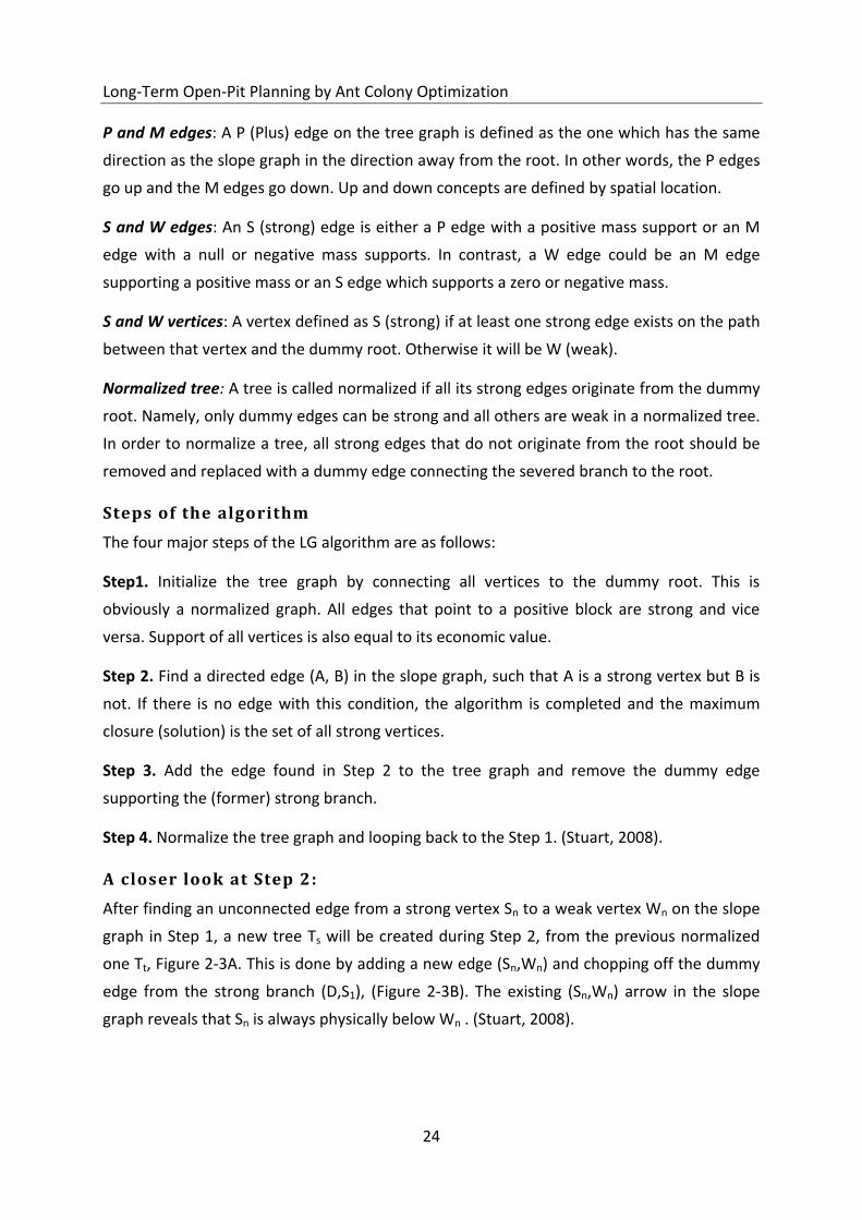
Long-Term Open-Pit Planning by Ant Colony Optimization
24
P and M edges: A P (Plus) edge on the tree graph is defined as the one which has the same
direction as the slope graph in the direction away from the root. In other words, the P edges
go up and the M edges go down. Up and down concepts are defined by spatial location.
S and W edges: An S (strong) edge is either a P edge with a positive mass support or an M
edge with a null or negative mass supports. In contrast, a W edge could be an M edge
supporting a positive mass or an S edge which supports a zero or negative mass.
S and W vertices: A vertex defined as S (strong) if at least one strong edge exists on the path
between that vertex and the dummy root. Otherwise it will be W (weak).
Normalized tree: A tree is called normalized if all its strong edges originate from the dummy
root. Namely, only dummy edges can be strong and all others are weak in a normalized tree.
In order to normalize a tree, all strong edges that do not originate from the root should be
removed and replaced with a dummy edge connecting the severed branch to the root.
Steps of the algorithm
The four major steps of the LG algorithm are as follows:
Step1. Initialize the tree graph by connecting all vertices to the dummy root. This is
obviously a normalized graph. All edges that point to a positive block are strong and vice
versa. Support of all vertices is also equal to its economic value.
Step 2. Find a directed edge (A, B) in the slope graph, such that A is a strong vertex but B is
not. If there is no edge with this condition, the algorithm is completed and the maximum
closure (solution) is the set of all strong vertices.
Step 3. Add the edge found in Step 2 to the tree graph and remove the dummy edge
supporting the (former) strong branch.
Step 4. Normalize the tree graph and looping back to the Step 1. (Stuart, 2008).
A closer look at Step 2:
After finding an unconnected edge from a strong vertex Sn to a weak vertex Wn on the slope
graph in Step 1, a new tree Ts will be created during Step 2, from the previous normalized
one Tt, Figure 2-3A. This is done by adding a new edge (Sn,Wn) and chopping off the dummy
edge from the strong branch (D,S1), (Figure 2-3B). The existing (Sn,Wn) arrow in the slope
graph reveals that Sn is always physically below Wn . (Stuart, 2008).
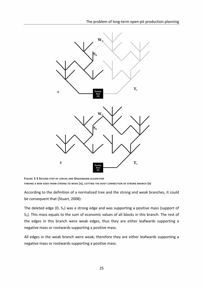
The problem of long-term open-pit production planning
25
According to the definition of a normalized tree and the strong and weak branches, it could
be consequent that (Stuart, 2008):
The deleted edge (D, S1) was a strong edge and was supporting a positive mass (support of
S1). This mass equals to the sum of economic values of all blocks in this branch. The rest of
the edges in this branch were weak edges, thus they are either leafwards supporting a
negative mass or rootwards supporting a positive mass.
All edges in the weak branch were weak; therefore they are either leafwards supporting a
negative mass or rootwards supporting a positive mass.
FIGURE 2-3 SECOND STEP OF LERCHS AND GROSSMANN ALGORITHM
FINDING A NEW EDGE FROM STRONG TO WEAK (A), CUTTING THE ROOT CONNECTION OF STRONG BRANCH (B)
A
B
Long-Term Open-Pit Planning by Ant Colony Optimization
26
After Step 2, the only parts of the tree graph that will be altered is the vertices and edges on
a path from S1 to the root which could be shown as S1,S2...Sn, Wn, Wn-1….W2,W1,D and
termed the critical path (black path on Figure 2-4).
Support of vertices on critical path could be updated as following:
By definition the supported mass is the sum of all individual masses on the branch side of a
vertex. After step 2, S1 loses the contribution of everything that S2 supports. If the new and
old masses supported by S1 are shown in MnewS1 and MoldS1 then it could be written:
MnewS1= MoldS1 - MoldS2
Notice that MoldS1 is the mass of the whole strong branch prior to Step 2.
Following the path from S1 to Sn after Step 2, the mass supported by any vertex Sx on this
path equals to the mass of the old strong branch MoldS1 minus the mass that was supported
by the next vertex on the path MoldSx+1. Therefore generally, one could write:
MnewSx = MoldS1- MoldSx+1
The mass supported by Sn, MnewSn, is equal to the mass of the entire strong branch before
Step 2, which was equal to MoldS1.
The masses supported by the all vertices on the critical path from Wn to D will be increased
by the weight of the entire strong branch. So that
MnewWx = MoldWx + MoldS1
FIGURE 2-4 CRITICAL PATH
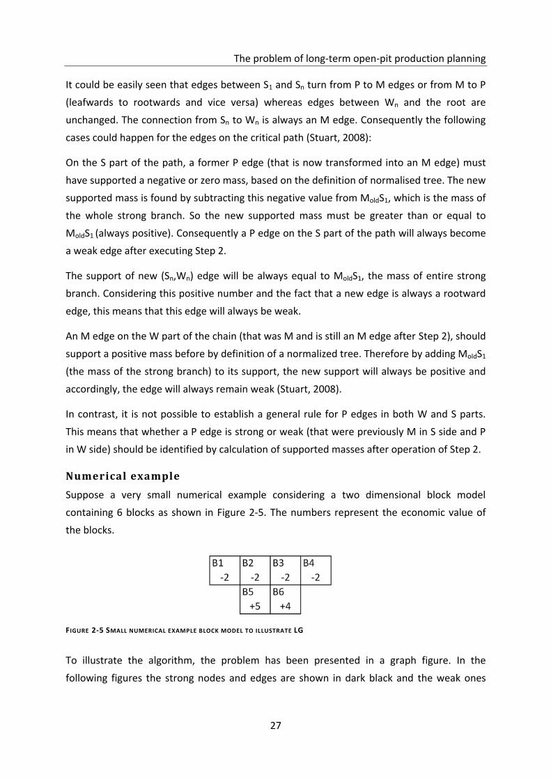
The problem of long-term open-pit production planning
27
It could be easily seen that edges between S1 and Sn turn from P to M edges or from M to P
(leafwards to rootwards and vice versa) whereas edges between Wn and the root are
unchanged. The connection from Sn to Wn is always an M edge. Consequently the following
cases could happen for the edges on the critical path (Stuart, 2008):
On the S part of the path, a former P edge (that is now transformed into an M edge) must
have supported a negative or zero mass, based on the definition of normalised tree. The new
supported mass is found by subtracting this negative value from MoldS1, which is the mass of
the whole strong branch. So the new supported mass must be greater than or equal to
MoldS1 (always positive). Consequently a P edge on the S part of the path will always become
a weak edge after executing Step 2.
The support of new (Sn,Wn) edge will be always equal to MoldS1, the mass of entire strong
branch. Considering this positive number and the fact that a new edge is always a rootward
edge, this means that this edge will always be weak.
An M edge on the W part of the chain (that was M and is still an M edge after Step 2), should
support a positive mass before by definition of a normalized tree. Therefore by adding MoldS1
(the mass of the strong branch) to its support, the new support will always be positive and
accordingly, the edge will always remain weak (Stuart, 2008).
In contrast, it is not possible to establish a general rule for P edges in both W and S parts.
This means that whether a P edge is strong or weak (that were previously M in S side and P
in W side) should be identified by calculation of supported masses after operation of Step 2.
Numerical example
Suppose a very small numerical example considering a two dimensional block model
containing 6 blocks as shown in Figure 2-5. The numbers represent the economic value of
the blocks.
To illustrate the algorithm, the problem has been presented in a graph figure. In the
following figures the strong nodes and edges are shown in dark black and the weak ones
FIGURE 2-5 SMALL NUMERICAL EXAMPLE BLOCK MODEL TO ILLUSTRATE LG
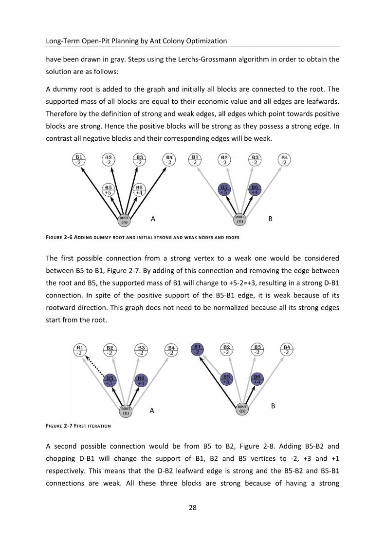
Long-Term Open-Pit Planning by Ant Colony Optimization
28
have been drawn in gray. Steps using the Lerchs-Grossmann algorithm in order to obtain the
solution are as follows:
A dummy root is added to the graph and initially all blocks are connected to the root. The
supported mass of all blocks are equal to their economic value and all edges are leafwards.
Therefore by the definition of strong and weak edges, all edges which point towards positive
blocks are strong. Hence the positive blocks will be strong as they possess a strong edge. In
contrast all negative blocks and their corresponding edges will be weak.
The first possible connection from a strong vertex to a weak one would be considered
between B5 to B1, Figure 2-7. By adding of this connection and removing the edge between
the root and B5, the supported mass of B1 will change to +5-2=+3, resulting in a strong D-B1
connection. In spite of the positive support of the B5-B1 edge, it is weak because of its
rootward direction. This graph does not need to be normalized because all its strong edges
start from the root.
A second possible connection would be from B5 to B2, Figure 2-8. Adding B5-B2 and
chopping D-B1 will change the support of B1, B2 and B5 vertices to -2, +3 and +1
respectively. This means that the D-B2 leafward edge is strong and the B5-B2 and B5-B1
connections are weak. All these three blocks are strong because of having a strong
FIGURE 2-7 FIRST ITERATION
A B
A B
FIGURE 2-6 ADDING DUMMY ROOT AND INITIAL STRONG AND WEAK NODES AND EDGES
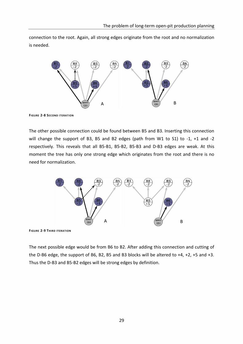
The problem of long-term open-pit production planning
29
connection to the root. Again, all strong edges originate from the root and no normalization
is needed.
The other possible connection could be found between B5 and B3. Inserting this connection
will change the support of B3, B5 and B2 edges (path from W1 to S1) to -1, +1 and -2
respectively. This reveals that all B5-B1, B5-B2, B5-B3 and D-B3 edges are weak. At this
moment the tree has only one strong edge which originates from the root and there is no
need for normalization.
The next possible edge would be from B6 to B2. After adding this connection and cutting of
the D-B6 edge, the support of B6, B2, B5 and B3 blocks will be altered to +4, +2, +5 and +3.
Thus the D-B3 and B5-B2 edges will be strong edges by definition.
FIGURE 2-9 THIRD ITERATION
A B
FIGURE 2-8 SECOND ITERATION
A B
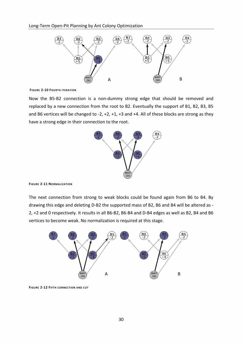
Long-Term Open-Pit Planning by Ant Colony Optimization
30
Now the B5-B2 connection is a non-dummy strong edge that should be removed and
replaced by a new connection from the root to B2. Eventually the support of B1, B2, B3, B5
and B6 vertices will be changed to -2, +2, +1, +3 and +4. All of these blocks are strong as they
have a strong edge in their connection to the root.
The next connection from strong to weak blocks could be found again from B6 to B4. By
drawing this edge and deleting D-B2 the supported mass of B2, B6 and B4 will be altered as -
2, +2 and 0 respectively. It results in all B6-B2, B6-B4 and D-B4 edges as well as B2, B4 and B6
vertices to become weak. No normalization is required at this stage.
FIGURE 2-12 FIFTH CONNECTION AND CUT
A B
FIGURE 2-11 NORMALIZATION
FIGURE 2-10 FOURTH ITERATION
A B
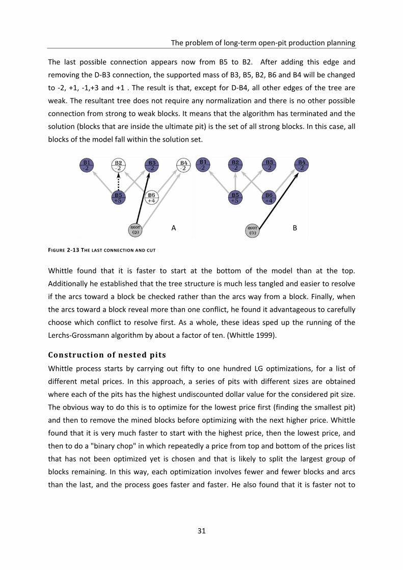
The problem of long-term open-pit production planning
31
The last possible connection appears now from B5 to B2. After adding this edge and
removing the D-B3 connection, the supported mass of B3, B5, B2, B6 and B4 will be changed
to -2, +1, -1,+3 and +1 . The result is that, except for D-B4, all other edges of the tree are
weak. The resultant tree does not require any normalization and there is no other possible
connection from strong to weak blocks. It means that the algorithm has terminated and the
solution (blocks that are inside the ultimate pit) is the set of all strong blocks. In this case, all
blocks of the model fall within the solution set.
Whittle found that it is faster to start at the bottom of the model than at the top.
Additionally he established that the tree structure is much less tangled and easier to resolve
if the arcs toward a block be checked rather than the arcs way from a block. Finally, when
the arcs toward a block reveal more than one conflict, he found it advantageous to carefully
choose which conflict to resolve first. As a whole, these ideas sped up the running of the
Lerchs-Grossmann algorithm by about a factor of ten. (Whittle 1999).
Construction of nested pits
Whittle process starts by carrying out fifty to one hundred LG optimizations, for a list of
different metal prices. In this approach, a series of pits with different sizes are obtained
where each of the pits has the highest undiscounted dollar value for the considered pit size.
The obvious way to do this is to optimize for the lowest price first (finding the smallest pit)
and then to remove the mined blocks before optimizing with the next higher price. Whittle
found that it is very much faster to start with the highest price, then the lowest price, and
then to do a "binary chop" in which repeatedly a price from top and bottom of the prices list
that has not been optimized yet is chosen and that is likely to split the largest group of
blocks remaining. In this way, each optimization involves fewer and fewer blocks and arcs
than the last, and the process goes faster and faster. He also found that it is faster not to
FIGURE 2-13 THE LAST CONNECTION AND CUT
A B
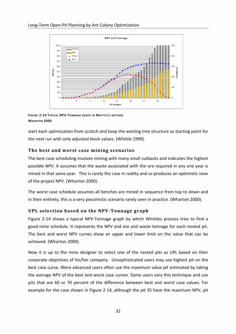
Long-Term Open-Pit Planning by Ant Colony Optimization
32
start each optimization from scratch and keep the existing tree structure as starting point for
the next run with only adjusted block values. (Whittle 1999).
The best and worst case mining scenarios
The best case scheduling involves mining with many small cutbacks and indicates the highest
possible NPV. It assumes that the waste associated with the ore required in any one year is
mined in that same year. This is rarely the case in reality and so produces an optimistic view
of the project NPV. (Wharton 2000).
The worst case schedule assumes all benches are mined in sequence from top to down and
in their entirety, this is a very pessimistic scenario rarely seen in practice. (Wharton 2000).
UPL selection based on the NPV -Tonnage graph
Figure 2-14 shows a typical NPV-Tonnage graph by which Whittles process tries to find a
good mine schedule. It represents the NPV and ore and waste tonnage for each nested pit.
The best and worst NPV curves show an upper and lower limit on the value that can be
achieved. (Wharton 2000).
Now it is up to the mine designer to select one of the nested pits as UPL based on their
corporate objectives of his/her company. Unsophisticated users may use highest pit on the
best case curve. More advanced users often use the maximum value pit estimated by taking
the average NPV of the best and worst case curves. Some users vary this technique and use
pits that are 60 or 70 percent of the difference between best and worst case values. For
example for the case shown in Figure 2-14, although the pit 35 have the maximum NPV, pit
FIGURE 2-14 TYPICAL NPV-TONNAGE GRAPH IN WHITTLE’S METHOD
WHARTON 2000
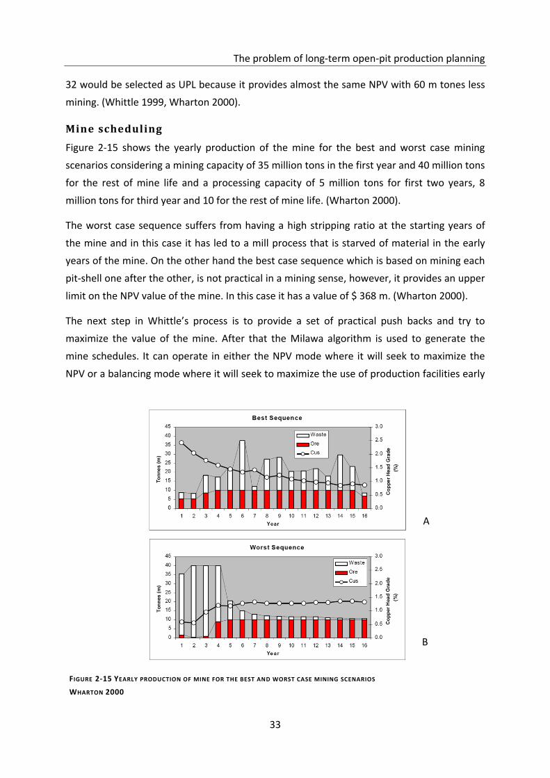
The problem of long-term open-pit production planning
33
32 would be selected as UPL because it provides almost the same NPV with 60 m tones less
mining. (Whittle 1999, Wharton 2000).
Mine scheduling
Figure 2-15 shows the yearly production of the mine for the best and worst case mining
scenarios considering a mining capacity of 35 million tons in the first year and 40 million tons
for the rest of mine life and a processing capacity of 5 million tons for first two years, 8
million tons for third year and 10 for the rest of mine life. (Wharton 2000).
The worst case sequence suffers from having a high stripping ratio at the starting years of
the mine and in this case it has led to a mill process that is starved of material in the early
years of the mine. On the other hand the best case sequence which is based on mining each
pit-shell one after the other, is not practical in a mining sense, however, it provides an upper
limit on the NPV value of the mine. In this case it has a value of $ 368 m. (Wharton 2000).
The next step in Whittle’s process is to provide a set of practical push backs and try to
maximize the value of the mine. After that the Milawa algorithm is used to generate the
mine schedules. It can operate in either the NPV mode where it will seek to maximize the
NPV or a balancing mode where it will seek to maximize the use of production facilities early
FIGURE 2-15 YEARLY PRODUCTION OF MINE FOR THE BEST AND WORST CASE MINING SCENARIOS
WHARTON 2000
A
B
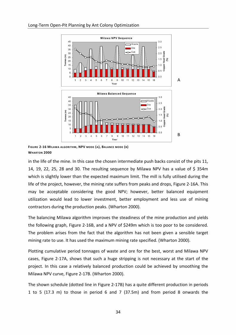
Long-Term Open-Pit Planning by Ant Colony Optimization
34
in the life of the mine. In this case the chosen intermediate push backs consist of the pits 11,
14, 19, 22, 25, 28 and 30. The resulting sequence by Milawa NPV has a value of $ 354m
which is slightly lower than the expected maximum limit. The mill is fully utilised during the
life of the project, however, the mining rate suffers from peaks and drops, Figure 2-16A. This
may be acceptable considering the good NPV; however, better balanced equipment
utilization would lead to lower investment, better employment and less use of mining
contractors during the production peaks. (Wharton 2000).
The balancing Milawa algorithm improves the steadiness of the mine production and yields
the following graph, Figure 2-16B, and a NPV of $249m which is too poor to be considered.
The problem arises from the fact that the algorithm has not been given a sensible target
mining rate to use. It has used the maximum mining rate specified. (Wharton 2000).
Plotting cumulative period tonnages of waste and ore for the best, worst and Milawa NPV
cases, Figure 2-17A, shows that such a huge stripping is not necessary at the start of the
project. In this case a relatively balanced production could be achieved by smoothing the
Milawa NPV curve, Figure 2-17B. (Wharton 2000).
The shown schedule (dotted line in Figure 2-17B) has a quite different production in periods
1 to 5 (17.3 m) to those in period 6 and 7 (37.5m) and from period 8 onwards the
FIGURE 2-16 MILAWA ALGORITHM, NPV MODE (A), BALANCE MODE (B)
WHARTON 2000
A
B
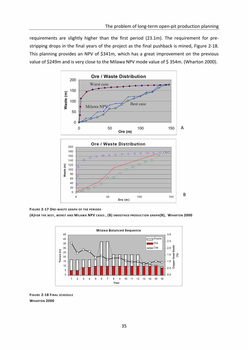
The problem of long-term open-pit production planning
35
requirements are slightly higher than the first period (23.1m). The requirement for pre-
stripping drops in the final years of the project as the final pushback is mined, Figure 2-18.
This planning provides an NPV of $341m, which has a great improvement on the previous
value of $249m and is very close to the Milawa NPV mode value of $ 354m. (Wharton 2000).
FIGURE 2-18 FINAL SCHEDULE
WHARTON 2000
FIGURE 2-17 ORE-WASTE GRAPH OF THE PERIODS
(A)FOR THE BEST, WORST AND MILAWA NPV CASES , (B) SMOOTHED PRODUCTION GRAPH(B), WHARTON 2000
A
B
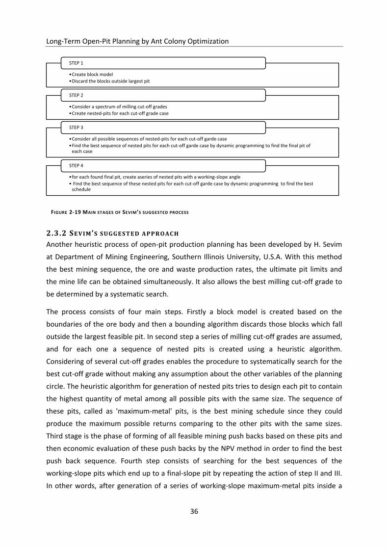
Long-Term Open-Pit Planning by Ant Colony Optimization
36
2.3.2 SEVIM ’S SUGGESTED APPROACH
Another heuristic process of open-pit production planning has been developed by H. Sevim
at Department of Mining Engineering, Southern Illinois University, U.S.A. With this method
the best mining sequence, the ore and waste production rates, the ultimate pit limits and
the mine life can be obtained simultaneously. It also allows the best milling cut-off grade to
be determined by a systematic search.
The process consists of four main steps. Firstly a block model is created based on the
boundaries of the ore body and then a bounding algorithm discards those blocks which fall
outside the largest feasible pit. In second step a series of milling cut-off grades are assumed,
and for each one a sequence of nested pits is created using a heuristic algorithm.
Considering of several cut-off grades enables the procedure to systematically search for the
best cut-off grade without making any assumption about the other variables of the planning
circle. The heuristic algorithm for generation of nested pits tries to design each pit to contain
the highest quantity of metal among all possible pits with the same size. The sequence of
these pits, called as 'maximum-metal' pits, is the best mining schedule since they could
produce the maximum possible returns comparing to the other pits with the same sizes.
Third stage is the phase of forming of all feasible mining push backs based on these pits and
then economic evaluation of these push backs by the NPV method in order to find the best
push back sequence. Fourth step consists of searching for the best sequences of the
working-slope pits which end up to a final-slope pit by repeating the action of step II and III.
In other words, after generation of a series of working-slope maximum-metal pits inside a
•Create block model
•Discard the blocks outside largest pit
STEP 1
•Consider a spectrum of milling cut-off grades
•Create nested-pits for each cut-off grade case
STEP 2
•Consider all possible sequences of nested-pits for each cut-off garde case
•Find the best sequence of nested pits for each cut-off garde case by dynamic programming to find the final pit of each case
STEP 3
•for each found final pit, create aseries of nested pits with a working-slope angle
• Find the best sequence of these nested pits for each cut-off garde case by dynamic programming to find the best schedule
STEP 4
FIGURE 2-19 MAIN STAGES OF SEVIM’S SUGGESTED PROCESS
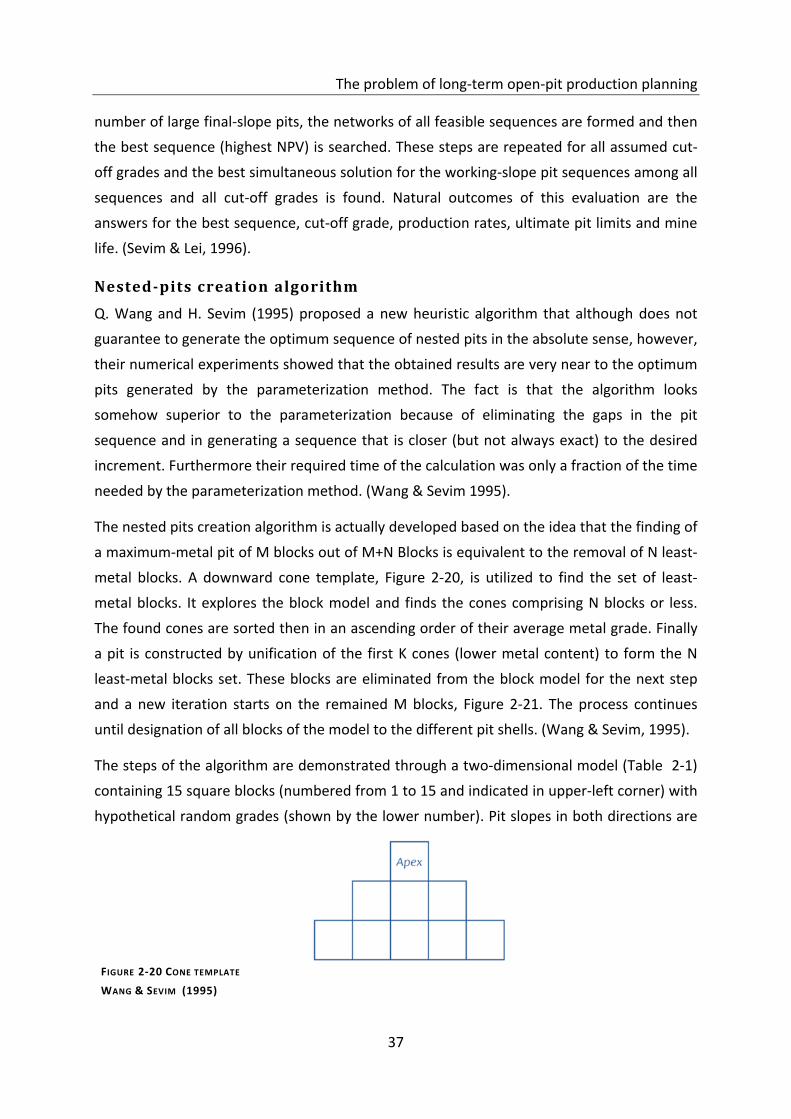
The problem of long-term open-pit production planning
37
number of large final-slope pits, the networks of all feasible sequences are formed and then
the best sequence (highest NPV) is searched. These steps are repeated for all assumed cut-
off grades and the best simultaneous solution for the working-slope pit sequences among all
sequences and all cut-off grades is found. Natural outcomes of this evaluation are the
answers for the best sequence, cut-off grade, production rates, ultimate pit limits and mine
life. (Sevim & Lei, 1996).
Nested-pits creation algorithm
Q. Wang and H. Sevim (1995) proposed a new heuristic algorithm that although does not
guarantee to generate the optimum sequence of nested pits in the absolute sense, however,
their numerical experiments showed that the obtained results are very near to the optimum
pits generated by the parameterization method. The fact is that the algorithm looks
somehow superior to the parameterization because of eliminating the gaps in the pit
sequence and in generating a sequence that is closer (but not always exact) to the desired
increment. Furthermore their required time of the calculation was only a fraction of the time
needed by the parameterization method. (Wang & Sevim 1995).
The nested pits creation algorithm is actually developed based on the idea that the finding of
a maximum-metal pit of M blocks out of M+N Blocks is equivalent to the removal of N least-
metal blocks. A downward cone template, Figure 2-20, is utilized to find the set of least-
metal blocks. It explores the block model and finds the cones comprising N blocks or less.
The found cones are sorted then in an ascending order of their average metal grade. Finally
a pit is constructed by unification of the first K cones (lower metal content) to form the N
least-metal blocks set. These blocks are eliminated from the block model for the next step
and a new iteration starts on the remained M blocks, Figure 2-21. The process continues
until designation of all blocks of the model to the different pit shells. (Wang & Sevim, 1995).
The steps of the algorithm are demonstrated through a two-dimensional model (Table 2-1)
containing 15 square blocks (numbered from 1 to 15 and indicated in upper-left corner) with
hypothetical random grades (shown by the lower number). Pit slopes in both directions are
FIGURE 2-20 CONE TEMPLATE
WANG & SEVIM (1995)

Long-Term Open-Pit Planning by Ant Colony Optimization
38
assumed to be simply 45°. Now, the goal is to find a sequence of max-metal pits with a size
increment of 3 blocks and at most 4 blocks for the smallest pit. Evaluations start from the
lower-left block and sequentially move to the upper and right blocks. (Wang & Sevim, 1995)
a. STEPS OF THE ALGORIT HM
The steps of the algorithm are as following: (Wang & Sevim, 1995)
By putting the apex of the cone template on the most lower-left block (Block no. 1), three
blocks (Blocks 1, 8 and 13 with the average grade of 0.567 g/t) fall inside the cone. The cone
is acceptable (because the number of blocks is not greater than the increment size, 3);
therefore, it can be stored in sorting array as the first cone.
First column has no more blocks and algorithm considers the bottom block of the next
column (Block 8). Placing the apex of cone shell on Block 8, Blocks 8 and 13 with the average
grade of 0.65 g/t will fall inside. This cone is also acceptable and is inserted in the sorting
array as the second place because of its average grade which is greater than that of the
previous cone.
When the next upper block in column II (Block 2) comes to be the apex of the cone shell, it
will contain five blocks (2, 8, 9, 13 and 14), which is more than 3. Consequently, the cone is
ignored and the algorithm continues by the bottom block of the third column.
Setting the cone apex on the Block number 13 shows that it is the only block of the cone.
The average grade of 0.7 g/t, which is greater than the average grade of previous cones,
locates it in the third place of the array.
Block 9 is the next one that should gain the apex of the cone template. This time the cone
consists of three blocks (9, 13 and 14) with an average grade of 0.633 g/t. this makes it
acceptable and inserts it in between Cone 1 and Cone 2 in the array. In other words, the new
cone becomes Cone 2 and the former Cones 2 and 3 turn into Cones 3 and 4 respectively.
The procedure continues until all seven columns are considered and an array of cones with
ascending average grade order is obtained. The first cone of the array (lowest average grade)
contains three blocks (7, 12 and 15) which is equal to the desired nested pit size. Hence
these three blocks are disregarded from the block model, the block model is updated and
algorithm moves to the next iteration. During the second iteration remaining 12 blocks of
maximum-metal pit (shown below the original in table), will be altered in the same way.
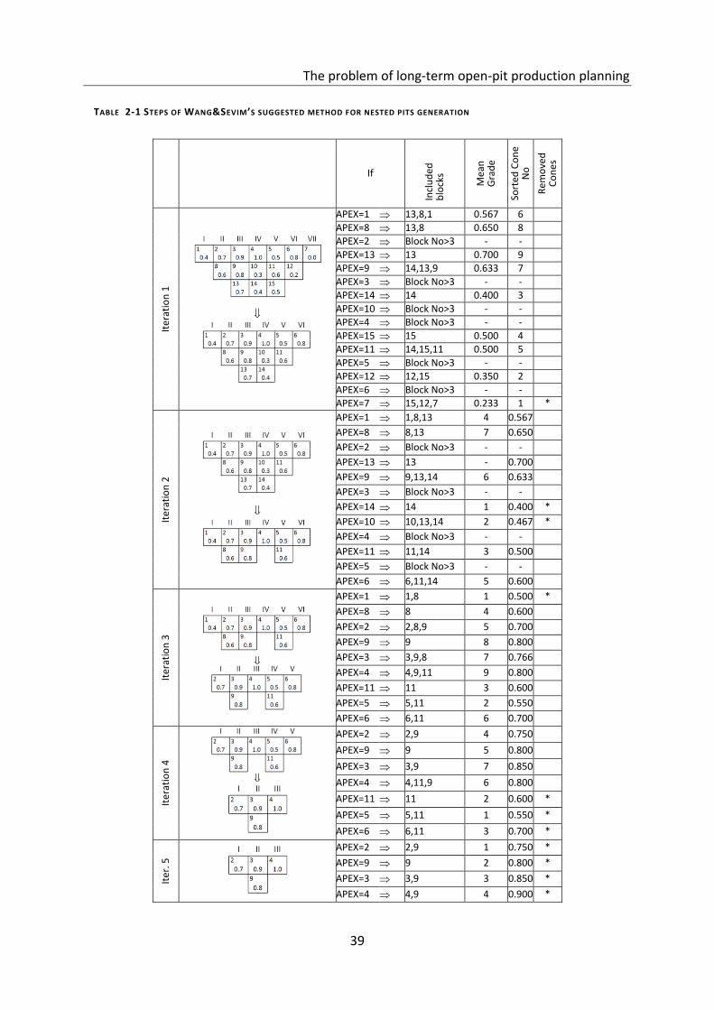
The problem of long-term open-pit production planning
39
Rem
ove
d
Co
ne
s
Sort
ed C
on
e
No
Mea
n
Gra
de
Incl
ud
ed
blo
cks If
6 0.567 13,8,1 APEX=1
Iter
atio
n 1
8 0.650 13,8 APEX=8
- - Block No>3 APEX=2
9 0.700 13 APEX=13
7 0.633 14,13,9 APEX=9
- - Block No>3 APEX=3 3 0.400 14 APEX=14
- - Block No>3 APEX=10 - - Block No>3 APEX=4
4 0.500 15 APEX=15 5 0.500 14,15,11 APEX=11
- - Block No>3 APEX=5 2 0.350 12,15 APEX=12
- - Block No>3 APEX=6 * 1 0.233 15,12,7 APEX=7
0.567 4 1,8,13 APEX=1
Iter
atio
n 2
0.650 7 8,13 APEX=8
- - Block No>3 APEX=2
0.700 - 13 APEX=13
0.633 6 9,13,14 APEX=9
- - Block No>3 APEX=3
* 0.400 1 14 APEX=14
* 0.467 2 10,13,14 APEX=10
- - Block No>3 APEX=4
0.500 3 11,14 APEX=11
- - Block No>3 APEX=5
0.600 5 6,11,14 APEX=6
* 0.500 1 1,8 APEX=1
Iter
atio
n 3
0.600 4 8 APEX=8
0.700 5 2,8,9 APEX=2
0.800 8 9 APEX=9
0.766 7 3,9,8 APEX=3
0.800 9 4,9,11 APEX=4
0.600 3 11 APEX=11
0.550 2 5,11 APEX=5
0.700 6 6,11 APEX=6
0.750 4 2,9 APEX=2
Iter
atio
n 4
0.800 5 9 APEX=9
0.850 7 3,9 APEX=3
0.800 6 4,11,9 APEX=4
* 0.600 2 11 APEX=11
* 0.550 1 5,11 APEX=5
* 0.700 3 6,11 APEX=6
* 0.750 1 2,9 APEX=2
Iter
. 5
* 0.800 2 9 APEX=9
* 0.850 3 3,9 APEX=3
* 0.900 4 4,9 APEX=4
TABLE 2-1 STEPS OF WANG&SEVIM’S SUGGESTED METHOD FOR NESTED PITS GENERATION
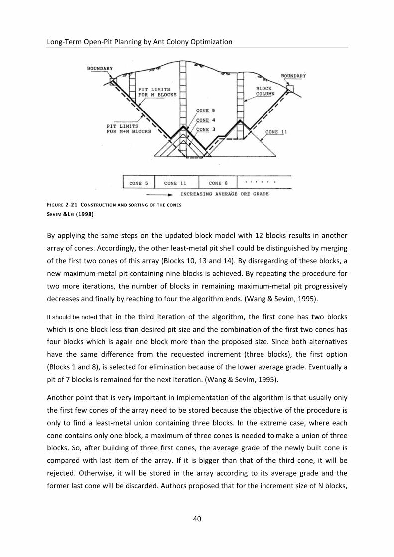
Long-Term Open-Pit Planning by Ant Colony Optimization
40
By applying the same steps on the updated block model with 12 blocks results in another
array of cones. Accordingly, the other least-metal pit shell could be distinguished by merging
of the first two cones of this array (Blocks 10, 13 and 14). By disregarding of these blocks, a
new maximum-metal pit containing nine blocks is achieved. By repeating the procedure for
two more iterations, the number of blocks in remaining maximum-metal pit progressively
decreases and finally by reaching to four the algorithm ends. (Wang & Sevim, 1995).
It should be noted that in the third iteration of the algorithm, the first cone has two blocks
which is one block less than desired pit size and the combination of the first two cones has
four blocks which is again one block more than the proposed size. Since both alternatives
have the same difference from the requested increment (three blocks), the first option
(Blocks 1 and 8), is selected for elimination because of the lower average grade. Eventually a
pit of 7 blocks is remained for the next iteration. (Wang & Sevim, 1995).
Another point that is very important in implementation of the algorithm is that usually only
the first few cones of the array need to be stored because the objective of the procedure is
only to find a least-metal union containing three blocks. In the extreme case, where each
cone contains only one block, a maximum of three cones is needed to make a union of three
blocks. So, after building of three first cones, the average grade of the newly built cone is
compared with last item of the array. If it is bigger than that of the third cone, it will be
rejected. Otherwise, it will be stored in the array according to its average grade and the
former last cone will be discarded. Authors proposed that for the increment size of N blocks,
FIGURE 2-21 CONSTRUCTION AND SORTING OF THE CONES
SEVIM &LEI (1998)
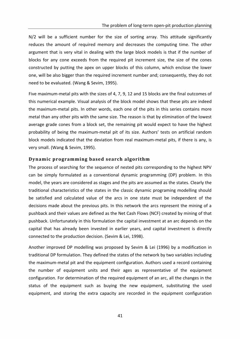
The problem of long-term open-pit production planning
41
N/2 will be a sufficient number for the size of sorting array. This attitude significantly
reduces the amount of required memory and decreases the computing time. The other
argument that is very vital in dealing with the large block models is that if the number of
blocks for any cone exceeds from the required pit increment size, the size of the cones
constructed by putting the apex on upper blocks of this column, which enclose the lower
one, will be also bigger than the required increment number and; consequently, they do not
need to be evaluated. (Wang & Sevim, 1995).
Five maximum-metal pits with the sizes of 4, 7, 9, 12 and 15 blocks are the final outcomes of
this numerical example. Visual analysis of the block model shows that these pits are indeed
the maximum-metal pits. In other words, each one of the pits in this series contains more
metal than any other pits with the same size. The reason is that by elimination of the lowest
average grade cones from a block set, the remaining pit would expect to have the highest
probability of being the maximum-metal pit of its size. Authors’ tests on artificial random
block models indicated that the deviation from real maximum-metal pits, if there is any, is
very small. (Wang & Sevim, 1995).
Dynamic programming based search algorithm
The process of searching for the sequence of nested pits corresponding to the highest NPV
can be simply formulated as a conventional dynamic programming (DP) problem. In this
model, the years are considered as stages and the pits are assumed as the states. Clearly the
traditional characteristics of the states in the classic dynamic programing modelling should
be satisfied and calculated value of the arcs in one state must be independent of the
decisions made about the previous pits. In this network the arcs represent the mining of a
pushback and their values are defined as the Net Cash Flows (NCF) created by mining of that
pushback. Unfortunately in this formulation the capital investment at an arc depends on the
capital that has already been invested in earlier years, and capital investment is directly
connected to the production decision. (Sevim & Lei, 1998).
Another improved DP modelling was proposed by Sevim & Lei (1996) by a modification in
traditional DP formulation. They defined the states of the network by two variables including
the maximum-metal pit and the equipment configuration. Authors used a record containing
the number of equipment units and their ages as representative of the equipment
configuration. For determination of the required equipment of an arc, all the changes in the
status of the equipment such as buying the new equipment, substituting the used
equipment, and storing the extra capacity are recorded in the equipment configuration
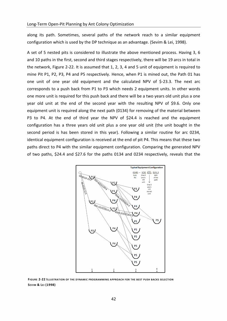
Long-Term Open-Pit Planning by Ant Colony Optimization
42
along its path. Sometimes, several paths of the network reach to a similar equipment
configuration which is used by the DP technique as an advantage. (Sevim & Lei, 1998).
A set of 5 nested pits is considered to illustrate the above mentioned process. Having 3, 6
and 10 paths in the first, second and third stages respectively, there will be 19 arcs in total in
the network, Figure 2-22. It is assumed that 1, 2, 3, 4 and 5 unit of equipment is required to
mine Pit P1, P2, P3, P4 and P5 respectively. Hence, when P1 is mined out, the Path 01 has
one unit of one year old equipment and the calculated NPV of $-23.3. The next arc
corresponds to a push back from P1 to P3 which needs 2 equipment units. In other words
one more unit is required for this push back and there will be a two years old unit plus a one
year old unit at the end of the second year with the resulting NPV of $9.6. Only one
equipment unit is required along the next path (0134) for removing of the material between
P3 to P4. At the end of third year the NPV of $24.4 is reached and the equipment
configuration has a three years old unit plus a one year old unit (the unit bought in the
second period is has been stored in this year). Following a similar routine for arc 0234,
identical equipment configuration is received at the end of pit P4. This means that these two
paths direct to P4 with the similar equipment configuration. Comparing the generated NPV
of two paths, $24.4 and $27.6 for the paths 0134 and 0234 respectively, reveals that the
FIGURE 2-22 ILLUSTRATION OF THE DYNAMIC PROGRAMMING APPROACH FOR THE BEST PUSH BACKS SELECTION
SEVIM & LEI (1998)
The problem of long-term open-pit production planning
43
next extensions of the path towards P5 should be made from 0234 instead of 0134. Hence,
the decision made about the extension of P4 is independent from the route which has been
passed up to this point. The proposed DP algorithm eliminates all the economically inferior
Paths (such as 0134) and carries forward the information on superior Paths (like 0234).
There are two other similar states in Stage 3 that decreases the number of distinct states at
Stage 3 from 10 to 7. This considerably reduces the size of the network. (Sevim & Lei, 1998).
After evaluation of all paths, their NPV is compared by the algorithm to find the highest NPV.
The state corresponding to the highest NPV defines the UPL. Then, tracing back from the
UPL, the algorithm generates the optimal mine sequence. It should be noted that each state
of the network has a related NPV which may decline from that state to the next one if the
mining activity along the arc connecting those states does not provide a positive cash flow.
(Sevim & Lei 1998).
Considering working-slope angles
A simple hypothetical network has been utilized to demonstrate the process of considering
working-slope angles. For this example spectrum of three cut-off grades is considered and
for each cut-off grade a series of final-slope maximum-metal pits is determined. Figure 2-23
shows the network of all possible mining sequences that could be formed from these pits.
For instance, for the third cut-off grade (X3, drawn in the foreground) five maximum-metal
pits are generated from P1 (the innermost and the smallest pit) to P5 (the outermost and
the largest pit). It is also assumed that the incremental block numbers between two
successive pits to be uniform and equal to the lowest possible production rate throughout
the series. (Sevim & Lei 1996).
The network shown in Figure 2-23 demonstrates that if P5 is mined in the first year, the
mine will be ended in one year. Instead, by mining pit P1 in the first year, one of the pits P2,
P3, P4 or P5 would be considered for the next year. The other connections of the network
have the same explanation. Paths of the network could be defined as the sequences of pits
which begin at time zero and ends in any of the pits and corresponds to a feasible
production schedule. A net present cash flow (NPV) could be calculated for each path by
summing up the discounted net cash flows of the push backs along the path to time zero.
The best path of each network can be chosen then, as the path corresponding to the highest
NPV. Consequently the final best path could be found among the best paths of all networks
by comparison of their NPV. (Sevim & Lei 1996).
Long-Term Open-Pit Planning by Ant Colony Optimization
44
Suppose that the best path of the foreground network in Figure 2-23 to be as the marked
thick line (0-P1-P3-P4). It reveals that the mining ends at P4 and the mining of the pushback
from P4 to P5 has a negative cash flow. Therefore P5 is not included in the sequence.
However, the best mining sequence needs to be made by a series of working-slope pits
nested inside a large final-slope pit which is normally found in previous phase. As shown in
Figure 2-24, two series of six working-slope maximum-metal pits are created ending at the
pits P3 and P4. Then two new networks have been generated based on these series, and
their best sequences have been found. There are two key points which have to be explained
here. Firstly, the series of working-slope pits are constructed not only within the best final
pit of the phase III but also within some smaller pits, like P3 in this case. The reason is that by
applying the working-slope pits, the economics of the project changes too and the found
final pit in phase III may no longer be the real UPL. Secondly, dissimilar to phase III, the best
paths on the network of the working-slope pits have to be always end up at the last pit (the
final-slope pit within which the series of working-slope pits have been generated). (Sevim &
Lei 1996).
FIGURE 2-23 GENERATED NESTED PITS FOR DIFFERENT CUT-OFF GRADES
SEVIM & LEI (1996)
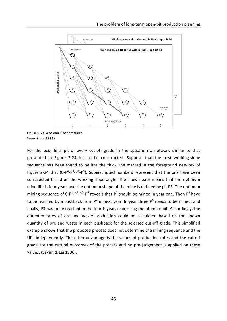
The problem of long-term open-pit production planning
45
For the best final pit of every cut-off grade in the spectrum a network similar to that
presented in Figure 2-24 has to be constructed. Suppose that the best working-slope
sequence has been found to be like the thick line marked in the foreground network of
Figure 2-24 that (0-P2-P4-P5-P6). Superscripted numbers represent that the pits have been
constructed based on the working-slope angle. The shown path means that the optimum
mine-life is four years and the optimum shape of the mine is defined by pit P3. The optimum
mining sequence of 0-P2-P4-P5-P6 reveals that P2 should be mined in year one. Then P4 have
to be reached by a pushback from P2 in next year. In year three P5 needs to be mined; and
finally, P3 has to be reached in the fourth year, expressing the ultimate pit. Accordingly, the
optimum rates of ore and waste production could be calculated based on the known
quantity of ore and waste in each pushback for the selected cut-off grade. This simplified
example shows that the proposed process does not determine the mining sequence and the
UPL independently. The other advantage is the values of production rates and the cut-off
grade are the natural outcomes of the process and no pre-judgement is applied on these
values. (Sevim & Lei 1996).
FIGURE 2-24 WORKING-SLOPE PIT SERIES
SEVIM & LEI (1996)
Long-Term Open-Pit Planning by Ant Colony Optimization
46
2.4 METAHEURISTIC METHODS
2.4.1 INTRODUCTION
Metaheuristic optimization methods are a higher class of heuristic searching algorithms that
are widely used for solving many of NP-hard combinatorial optimization problems.
Combinatorial optimization
A combinatorial optimization problem could be defined as any maximization or minimization
problem that is normally easy to state but very difficult to solve. Fundamentally a
combinatorial optimization problem involves in finding the values of discrete variables in a
way that the optimal value of a certain objective function to be reached subject to some
problem constraints. The large Travelling Salesman Problems (TSP), Shortest-Path Problem,
Assignment Problem, Sequential Ordering Problem and Knapsack Problem are typical
examples of the combinatorial optimization problems. (Dorigo & Stützle, 2004).
Combinatorial optimization problems are basically associated with a set of problem
instances. The term problem denotes the overall query which has to be answered, generally
having several parameters (variables) with undetermined values. A problem with particular
values for its parameters called as instance. In other words an instance of a combinatorial
problem П could be defined as a triple (Ѕ,f,Ω), where S refers to the set of candidate
solutions, f denotes the objective function having a value f(s) for each candidate solution
Ss , and Ω represents the set of problem constraints. Solutions that satisfy the problem
constraints Ω define the set of feasible solutions SS ~ . Finding the globally optimal feasible
solution *s is the aim of any optimization problem. For instance in a minimization problems
the target is to find a solution Ss~* in a way that )()( * sfsf for all Ss
~ . (Dorigo & Stützle,
2004)
Metaheuristics
In engineering applications, most of the combinatorial problems are NP-hard. Normally the
optimal solution of such a problem cannot be obtained within an acceptable computation
time. Therefore approximation methods have to be utilized in order to practically answering
of the large instances of the problem. An approximation method returns a near-optimal
solution in a comparatively shorter time. Sometimes the approximation methods are
colloquially called heuristics. They normally act by building new solutions or improving the
available solutions by using a set of problem-specific knowledge. (Dorigo & Stützle, 2004).
During last decades the new class of heuristic procedures, known as metaheuristics, has got
a strong research attraction. A metaheuristics could be defined as a series of algorithmic
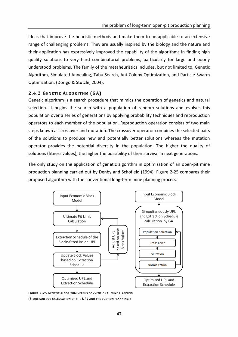
The problem of long-term open-pit production planning
47
ideas that improve the heuristic methods and make them to be applicable to an extensive
range of challenging problems. They are usually inspired by the biology and the nature and
their application has expressively improved the capability of the algorithms in finding high
quality solutions to very hard combinatorial problems, particularly for large and poorly
understood problems. The family of the metaheuristics includes, but not limited to, Genetic
Algorithm, Simulated Annealing, Tabu Search, Ant Colony Optimization, and Particle Swarm
Optimization. (Dorigo & Stützle, 2004).
2.4.2 GENETIC ALGORITHM (GA)
Genetic algorithm is a search procedure that mimics the operation of genetics and natural
selection. It begins the search with a population of random solutions and evolves this
population over a series of generations by applying probability techniques and reproduction
operators to each member of the population. Reproduction operation consists of two main
steps known as crossover and mutation. The crossover operator combines the selected pairs
of the solutions to produce new and potentially better solutions whereas the mutation
operator provides the potential diversity in the population. The higher the quality of
solutions (fitness values), the higher the possibility of their survival in next generations.
The only study on the application of genetic algorithm in optimization of an open-pit mine
production planning carried out by Denby and Schofield (1994). Figure 2-25 compares their
proposed algorithm with the conventional long-term mine planning process.
FIGURE 2-25 GENETIC ALGORITHM VERSUS CONVENTIONAL MINE PLANNING
(SIMULTANEOUS CALCULATION OF THE UPL AND PRODUCTION PLANNING )
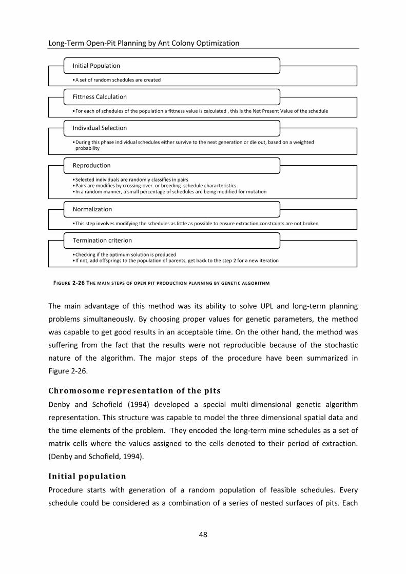
Long-Term Open-Pit Planning by Ant Colony Optimization
48
The main advantage of this method was its ability to solve UPL and long-term planning
problems simultaneously. By choosing proper values for genetic parameters, the method
was capable to get good results in an acceptable time. On the other hand, the method was
suffering from the fact that the results were not reproducible because of the stochastic
nature of the algorithm. The major steps of the procedure have been summarized in
Figure 2-26.
Chromosome representation of the pits
Denby and Schofield (1994) developed a special multi-dimensional genetic algorithm
representation. This structure was capable to model the three dimensional spatial data and
the time elements of the problem. They encoded the long-term mine schedules as a set of
matrix cells where the values assigned to the cells denoted to their period of extraction.
(Denby and Schofield, 1994).
Initial population
Procedure starts with generation of a random population of feasible schedules. Every
schedule could be considered as a combination of a series of nested surfaces of pits. Each
•A set of random schedules are created
Initial Population
•For each of schedules of the population a fittness value is calculated , this is the Net Present Value of the schedule
Fittness Calculation
•During this phase individual schedules either survive to the next generation or die out, based on a weighted probability
Individual Selection
•Selected individuals are randomly classifies in pairs •Pairs are modifies by crossing-over or breeding schedule characteristics •In a random manner, a small percentage of schedules are being modified for mutation
Reproduction
•This step involves modifying the schedules as little as possible to ensure extraction constraints are not broken
Normalization
•Checking if the optimum solution is produced •If not, add offsprings to the population of parents, get back to the step 2 for a new iteration
Termination criterion
FIGURE 2-26 THE MAIN STEPS OF OPEN PIT PRODUCTION PLANNING BY GENETIC ALGORITHM
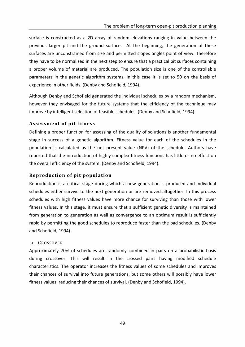
The problem of long-term open-pit production planning
49
surface is constructed as a 2D array of random elevations ranging in value between the
previous larger pit and the ground surface. At the beginning, the generation of these
surfaces are unconstrained from size and permitted slopes angles point of view. Therefore
they have to be normalized in the next step to ensure that a practical pit surfaces containing
a proper volume of material are produced. The population size is one of the controllable
parameters in the genetic algorithm systems. In this case it is set to 50 on the basis of
experience in other fields. (Denby and Schofield, 1994).
Although Denby and Schofield generated the individual schedules by a random mechanism,
however they envisaged for the future systems that the efficiency of the technique may
improve by intelligent selection of feasible schedules. (Denby and Schofield, 1994).
Assessment of pit fitness
Defining a proper function for assessing of the quality of solutions is another fundamental
stage in success of a genetic algorithm. Fitness value for each of the schedules in the
population is calculated as the net present value (NPV) of the schedule. Authors have
reported that the introduction of highly complex fitness functions has little or no effect on
the overall efficiency of the system. (Denby and Schofield, 1994).
Reproduction of pit population
Reproduction is a critical stage during which a new generation is produced and individual
schedules either survive to the next generation or are removed altogether. In this process
schedules with high fitness values have more chance for surviving than those with lower
fitness values. In this stage, it must ensure that a sufficient genetic diversity is maintained
from generation to generation as well as convergence to an optimum result is sufficiently
rapid by permitting the good schedules to reproduce faster than the bad schedules. (Denby
and Schofield, 1994).
a. CROSSOVER
Approximately 70% of schedules are randomly combined in pairs on a probabilistic basis
during crossover. This will result in the crossed pairs having modified schedule
characteristics. The operator increases the fitness values of some schedules and improves
their chances of survival into future generations, but some others will possibly have lower
fitness values, reducing their chances of survival. (Denby and Schofield, 1994).
Long-Term Open-Pit Planning by Ant Colony Optimization
50
b. MUTATION
Mutation is the other important operator in reproduction. It randomly acts on a probabilistic
basis on approximately 0.1% of the cells in the schedule to maintain genetic diversity and
prevents the system from stagnation in an incorrect optimum. It is done by randomly
modification of the elevations of the selected cells. (Denby and Schofield, 1994).
c. NORMALIZING OF THE PI TS
The action of crossover and mutation operators normally does not care to the shape of the
pits in generated mine schedules. This leads the resulting pits to violate constraints and a
normalization process to be needed after each action. Normalization procedure involves in
modification of the schedule, as little as possible, to ensure that the extraction constraints,
such as the number of cells in each scheduling period or the geomechanical sequencing
constraints (slope angles) are not exceeded. The normalization process consists of two
stages. In first pass surface points are gradually brought closer together till the slope angle
and geotechnical constraints to be satisfied. Then, during the size constraint pass, surface
points are either raised or lowered within geotechnically accepted limits until the size of pit
becomes acceptable. These can sometimes result in significant alterations to the schedules.
(Denby and Schofield, 1994).
d. LOCAL OPTIMIZATION
Authors discovered that the addition of a local optimizer greatly improves the optimization
performance. They employed a programmed logic rule to swap blocks of high value that are
scheduled for the late extraction periods with blocks of low value that are scheduled for
early extractions. The approach utilizes pure logic and is not influenced by probability. Once
the surface has been checked by local optimizer, it is necessary to normalize the surface
again. Authors reported a 35% improvement in the speed of algorithm by use of the local
optimizer. (Denby and Schofield, 1994).
Termination condition of the algorithm
The number of generations required to reach the optimum schedule varies depending on
the complexity and the scale of the problem. Authors informed that for a problem consisting
200 blocks, approximately 95% of final optimum could be reached after 50 to 120
generations, whereas to reach 98% of the optimum requires as many as 380 generations.
However, the way in which the genetic algorithm is formulated has a significant effect on the
efficiency of the system. (Denby and Schofield, 1994).
The problem of long-term open-pit production planning
51
2.4.3 S IMULATED ANNEALING (SA)
Annealing is the process in which a metallic or glass solid is heated up sufficiently to allow its
atoms and molecules to reach in a stress-free state (but not so much that cause melting) and
then cooled gradually down to rearrange in a new configuration. In simulated annealing
method, the value of the function under optimization is equivalent to the energy of the solid
in reality. It begins with a random solution and then perturbs that solution slightly to create
another potentially better solution. If the new solution satisfies the constraints and
corresponds to a better objective function value than the existing solution, it is accepted
without question. However, if the fitness value of new solution is less than that of previous,
then a decision on its acceptance has to be made based on the current temperature of the
system. This lets the procedure to jump out of potentially sub-optimal solutions. During the
iterations of the algorithm, the temperature of the system is gradually lowered until the
approximately optimum solution has been found. (Thomas 1996).
Initial temperature and the cooling rate are the critical factors in the success of simulated
annealing process. Excessively low starting temperature makes the process to converge too
quickly and a sub-optimal solution might be produced. In contrast, extremely high initial
temperature would cause spending a long time on poor initial solutions. Similarly, rapidly
cooling of the system potentially gets locked around a local-optimum solution and produces
a sub-optimal consequence. On the other hand, disproportionately slow cooling rate
unnecessarily rises the computation time. (Thomas 1996).
Kumral and Dowd (2005) investigated the solution of the open-pit mine production
scheduling problem by using of SA metaheuristic. Figure 2-27 shows the major steps of this
process. The idea behind this research was that any sub-optimal schedule can be improved
by using SA. Therefore, they constructed a sub-optimal schedule by a conventional
production planning algorithm and submitted it to the SA to improve its fitness value. The
main supersede of this routine is that it employs a multi-objective function (comprised three
minimization components in this study). On the other hand, independent determination of
UPL and production schedule would be counted as a disadvantageous for this method.
(Kumral & Dowd 2005).
Objective function
The objective function of the problem is expressed as minimization of a multi-objective
function comprised three cost components including:
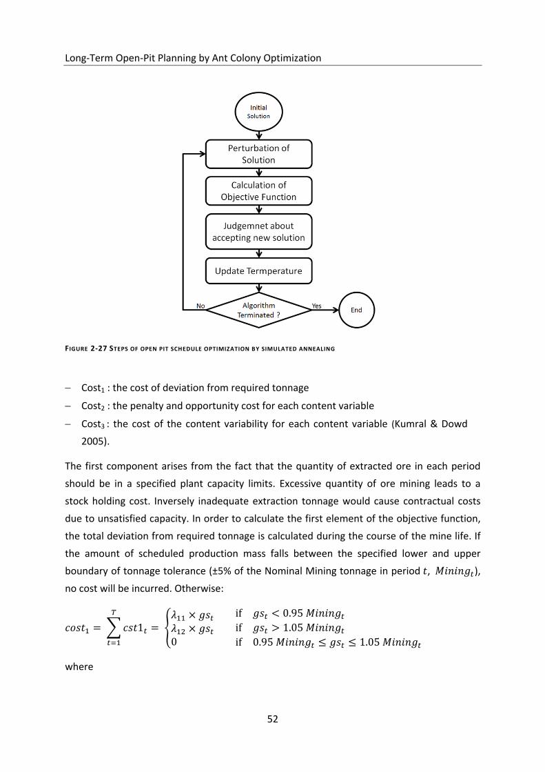
Long-Term Open-Pit Planning by Ant Colony Optimization
52
Cost1 : the cost of deviation from required tonnage
Cost2 : the penalty and opportunity cost for each content variable
Cost3 : the cost of the content variability for each content variable (Kumral & Dowd
2005).
The first component arises from the fact that the quantity of extracted ore in each period
should be in a specified plant capacity limits. Excessive quantity of ore mining leads to a
stock holding cost. Inversely inadequate extraction tonnage would cause contractual costs
due to unsatisfied capacity. In order to calculate the first element of the objective function,
the total deviation from required tonnage is calculated during the course of the mine life. If
the amount of scheduled production mass falls between the specified lower and upper
boundary of tonnage tolerance (±5% of the Nominal Mining tonnage in period , ),
no cost will be incurred. Otherwise:
∑
where
FIGURE 2-27 STEPS OF OPEN PIT SCHEDULE OPTIMIZATION BY SIMULATED ANNEALING
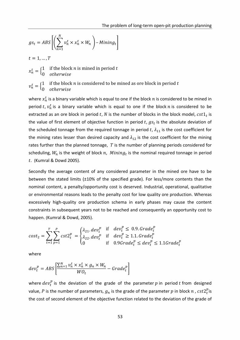
The problem of long-term open-pit production planning
53
[(∑
) ]
where is a binary variable which is equal to one if the block is considered to be mined in
period , is a binary variable which is equal to one if the block is considered to be
extracted as an ore block in period , is the number of blocks in the block model, is
the value of first element of objective function in period , is the absolute deviation of
the scheduled tonnage from the required tonnage in period , is the cost coefficient for
the mining rates lesser than desired capacity and is the cost coefficient for the mining
rates further than the planned tonnage, is the number of planning periods considered for
scheduling, is the weight of block , is the nominal required tonnage in period
. (Kumral & Dowd 2005).
Secondly the average content of any considered parameter in the mined ore have to be
between the stated limits (±10% of the specified grade). For less/more contents than the
nominal content, a penalty/opportunity cost is deserved. Industrial, operational, qualitative
or environmental reasons leads to the penalty cost for low quality ore production. Whereas
excessively high-quality ore production schema in early phases may cause the content
constraints in subsequent years not to be reached and consequently an opportunity cost to
happen. (Kumral & Dowd, 2005).
∑∑
where
[
∑
]
where
is the deviation of the grade of the parameter in period from designed
value, is the number of parameters, is the grade of the parameter in block ,
is
the cost of second element of the objective function related to the deviation of the grade of
Long-Term Open-Pit Planning by Ant Colony Optimization
54
the parameter in the period ,
is the designed grade of the parameter in period
and is tonnage of the ore in period in the current schedule, and are the cost
coefficients for the low and high grade mining respectively. (Kumral & Dowd, 2005).
Kumral & Dowd (2005) considered the last element of the objective function to minimize the
content variance of the variable under consideration. They expressed that by sending the
extracted ore to stockpiling or processing operation, the variance could has a direct
influence on the mill efficiency or parameters of the stacking and reclaiming. Moreover, the
fluctuations of the content may result in disturbing the quality of the process or the finished
product. (Kumral & Dowd 2005).
∑ ∑
where
∑
( )
-
where
is the content variance of the parameter in period and is the cost
coefficient .
Using a weighting summation, three mentioned components are converted into a single
objective function. Magnitude of the weights (priorities of the objective function
components) seems to depend on the ore body, sales contract, structure of the ore market
and the plant characteristics. (Kumral & Dowd 2005).
∑ (Kumral & Dowd, 2005)
where is the priority coefficient of the objective component and is the
number of objectives components (three in this case). Considering an unbiased combination
of the components, the sum of weights needs to be equal to one. (Kumral & Dowd 2005).
∑ (Kumral & Dowd, 2005)
Initial solution
It has been experienced that the computational time to converge towards a good solution
could be very long utilizing a random initial solution. Kumral and Dowd (2005) used
lagrangian parameterization method proposed by Dagdelen and Johnson (1986) to obtain a
favourable initial solution.
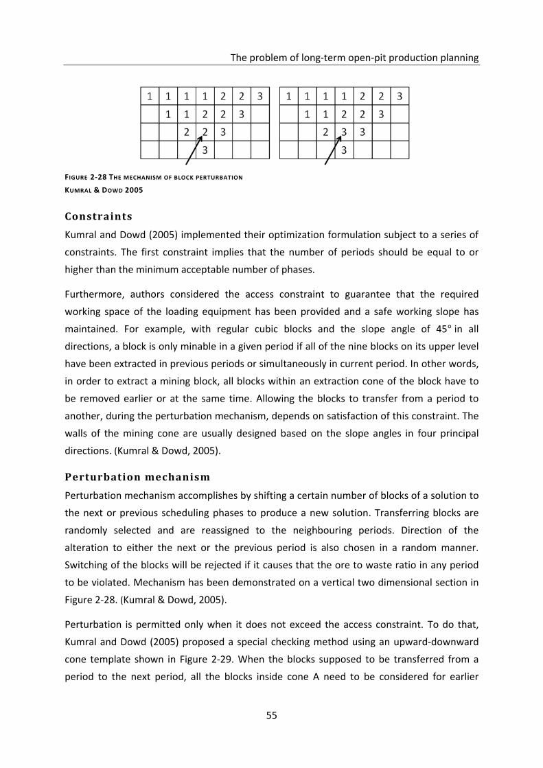
The problem of long-term open-pit production planning
55
Constraints
Kumral and Dowd (2005) implemented their optimization formulation subject to a series of
constraints. The first constraint implies that the number of periods should be equal to or
higher than the minimum acceptable number of phases.
Furthermore, authors considered the access constraint to guarantee that the required
working space of the loading equipment has been provided and a safe working slope has
maintained. For example, with regular cubic blocks and the slope angle of 45 in all
directions, a block is only minable in a given period if all of the nine blocks on its upper level
have been extracted in previous periods or simultaneously in current period. In other words,
in order to extract a mining block, all blocks within an extraction cone of the block have to
be removed earlier or at the same time. Allowing the blocks to transfer from a period to
another, during the perturbation mechanism, depends on satisfaction of this constraint. The
walls of the mining cone are usually designed based on the slope angles in four principal
directions. (Kumral & Dowd, 2005).
Perturbation mechanism
Perturbation mechanism accomplishes by shifting a certain number of blocks of a solution to
the next or previous scheduling phases to produce a new solution. Transferring blocks are
randomly selected and are reassigned to the neighbouring periods. Direction of the
alteration to either the next or the previous period is also chosen in a random manner.
Switching of the blocks will be rejected if it causes that the ore to waste ratio in any period
to be violated. Mechanism has been demonstrated on a vertical two dimensional section in
Figure 2-28. (Kumral & Dowd, 2005).
Perturbation is permitted only when it does not exceed the access constraint. To do that,
Kumral and Dowd (2005) proposed a special checking method using an upward-downward
cone template shown in Figure 2-29. When the blocks supposed to be transferred from a
period to the next period, all the blocks inside cone A need to be considered for earlier
FIGURE 2-28 THE MECHANISM OF BLOCK PERTURBATION
KUMRAL & DOWD 2005
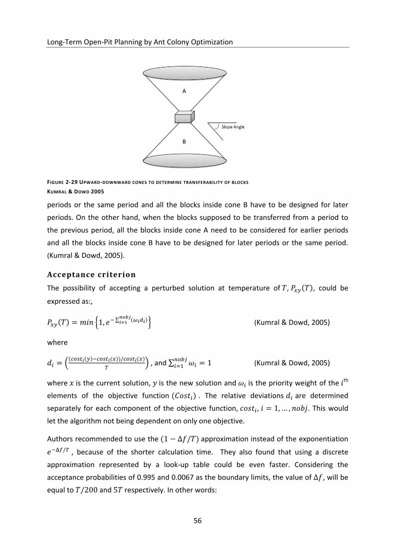
Long-Term Open-Pit Planning by Ant Colony Optimization
56
periods or the same period and all the blocks inside cone B have to be designed for later
periods. On the other hand, when the blocks supposed to be transferred from a period to
the previous period, all the blocks inside cone A need to be considered for earlier periods
and all the blocks inside cone B have to be designed for later periods or the same period.
(Kumral & Dowd, 2005).
Acceptance criterion
The possibility of accepting a perturbed solution at temperature of , ( ), could be
expressed as:,
( ) ∑ ( ) (Kumral & Dowd, 2005)
where
(( ( ) ( )) ( )
) , and ∑
(Kumral & Dowd, 2005)
where is the current solution, is the new solution and is the priority weight of the th
elements of the objective function ( ) . The relative deviations are determined
separately for each component of the objective function, , . This would
let the algorithm not being dependent on only one objective.
Authors recommended to use the ( ) approximation instead of the exponentiation
, because of the shorter calculation time. They also found that using a discrete
approximation represented by a look-up table could be even faster. Considering the
acceptance probabilities of 0.995 and 0.0067 as the boundary limits, the value of , will be
equal to and respectively. In other words:
FIGURE 2-29 UPWARD-DOWNWARD CONES TO DETERMINE TRANSFERABILITY OF BLOCKS
KUMRAL & DOWD 2005
The problem of long-term open-pit production planning
57
or (Kumral & Dowd, 2005)
Therefore the value of ( ) for different values of an integer Index Number (from 1 to
1000) could be previously computed and saved in a table. Then by rounding the value of
to the nearest integer and using the pre-computed table, the acceptance
possibility could be easily obtained. (Kumral & Dowd, 2005).
Cooling schedule and termination rule
Kumral and Dowd (2005) used a fluctuating cooling process. They proposed to cool the
system after any accepted solution and heat it up after any rejected solution. They used
( ) and ( ) functions for cooling and heating the system
respectively. Temperature of the system will be balanced by having heating
iteration against each cooling one. In other words, system heats up when the proportion of
the rejected to the accepted moves is higher than , which will subsequently decrease the
number of rejects against acceptances. In contrast, when the proportion of the rejected to
the accepted moves is less than , system will be cooled and this will increase the number of
rejects against acceptances. Hence, the schedule tends to converge theoretically to a point
that the ratio of rejected to accepted solutions to be around . Authors used this fact as the
termination criterion too. They found that using and the value of
objective function decreases slowly at the beginning of the procedure and reaches a stable
state at the end. (Kumral & Dowd, 2005).
Initial temperature
Another substantial parameter in the performance of the SA is the initial temperature. Too
high initial temperature makes the procedure to scatter for a long time on poor solutions.
Excessively low initial temperatures could also lead the algorithm to be trapped in a local
optima. The conducted experiments by the authors revealed that by taking the ratio of the
number of the rejected moves to the accepted moves as 150 yields good solutions in shorter
running time in comparison with the other initial temperatures. Initial temperature was
selected as 1.67 to produce this ratio. (Kumral & Dowd, 2005).

Ant colony optimization (ACO)
59
3 ANT COLONY OPTIMIZATION (ACO)
Ants first evolved around 120 million years ago, take form in over 11,400 different species
and are considered one of the most successful insects due to their highly organised colonies,
sometimes consisting of millions of ants. The field of “ant algorithms” derived from the
observation of the behaviour of real ants, in order to inspire the basic idea of designing of
the innovative algorithms for answering the optimization problems. One of the most
effective models of ant algorithms known as Ant Colony Optimization (ACO) has been
magnificently applied on several combinatorial optimization problems such as travelling
salesman, sequential ordering, general assignment, multiple knapsack and network routing
problems to produce high quality approximate solutions. It has been inspired by the foraging
behaviour of the ants. (Dorigo & Stützle, 2004).
In the real world, ants (initially) wander randomly, and return to their colony after finding
food while laying down pheromone trails. A pheromone is any chemical or set of chemicals
produced by living organisms to transmit a message to other members of the species. Ants
tend likely not to travel at random, but to instead follow the pheromone trails and
reinforcing it. Over time, however, the pheromone trails evaporate and lose their attraction
strength. The more time that takes for an ant to travel along a path (longer paths), the
higher evaporation of the pheromones. In contrast, shorter paths get more attracted and
their pheromone density increases up to be balanced with the evaporation rate. In fact, the
pheromone evaporation avoids the system to convergence to a local optimal solution. In
other words, the first paths chosen by the ants would be followed by the other ones, if there
were no evaporation. By finding a new path with shorter distance from colony to food
source, other ants are also promoted to follow that path, and eventually all the ants follow a
single path. (Wikipedia).
Probably, the best way of illustrating how the ACO metaheuristic functions is by explaining
how it has been utilized to solve the Travelling Salesman Problems (TSP). TSP is a
comprehensively investigated problem in the literature and for a long time has appealed a
significant amount of study efforts. The main reasons for the selection of TSP as the base
problem to describe the operational procedure of ACO are: (Dorigo & Stützle, 2004)
TSP is a NP-hard optimization model that frequently arises in engineering applications;
TSP is a typical problem to which ACO algorithm has been originally applied;
TSP is an comprehensible problem, therefore, the behaviour of the algorithm is not
complicated by unnecessary details;
Long-Term Open-Pit Planning by Ant Colony Optimization
60
TSP has been known as a typical examination bed for new solution approaches and a
good performance on the TSP is normally considered as evidence of their practicality;
The history of ACO indicates that the most efficient ACO algorithms for TSP were also
effective for a wide range of other problems. (Dorigo & Stützle, 2004).
3.1 TSP DEFINITION
TSP is the problem of a salesman who wants to start from his hometown and travel to a
certain number of customer cities (visiting each city exactly once) and finally get back home
through the shortest path. Mathematically it could be denoted as a complete weighted
graph ( ) where is the set of nodes (cities), and is the set of arcs (roads). Each
arc ( ) has a value (length) , which reveals the distance from city to city , and
. The goal of the problem is to discover the shortest Hamiltonian circuit of the graph.
Hamiltonian circuit is defined as a closed tour that visits each of the nodes exactly once.
for every pair of the nodes in symmetric TSPs while in asymmetric TSPs at least for
one pair of the cities . (Dorigo & Stützle, 2004).
The problem has shown an NP-hard behaviour even by removing the condition of one time
visiting of each city. Traditionally the following approaches have been applied to solve TSP:
Analytical algorithms: They find the exact solutions and work fast only for relatively
small problem sizes. Examples are linear programming, brute force search, dynamic
programming and branch-and-bound.
Heuristic algorithms: They deliver either seemingly or probably good solutions, but
they could not be proved to be optimal. Numerous approximation algorithms like
nearest neighbour and greedy algorithm are included in this class.
Metaheuristic algorithms: They could yield better solutions and high approximation in
reasonable time for large problems. Examples are genetic algorithm and ant colony
optimization. (Wikipedia).
3.2 BASIC ELEMENTS IN SOLUTION OF TSP BY ACO
3.2.1 CONSTRUCTION GRAPH
The problem is represented as a mathematical graph structure called construction graph. It
is identical to the problem arrangement, i.e. a set of nodes correspond to the cities and the
set of arcs correspond to the roads. A weight is assigned to each arc which represents the
distance between cities and . The set of all possible Hamiltonian walks are the states
of the problem. (Dorigo & Stützle, 2004).
Ant colony optimization (ACO)
61
Generally it favours to work on complete graphs in which there is at least one route between
any two nodes. For incomplete graphs, it is possible to add new arcs to convert it to
complete graph. Assigning large weights to the additional arcs guarantees that they will not
be used in the optimal solution and final answer will not be affected.
3.2.2 CONSTRAINTS
All cities must be visited in the TSP and the visit has to be at most once. This is the single
constraint of TSP. In order to satisfy this constraint, at each step of the algorithm, ants are
only allowed to choose their next destination (the feasible neighbourhood set of an ant
located in city ) among those cities that have not been visited yet. (Dorigo & Stützle, 2004).
3.2.3 PHEROMONE TRAILS AND HEURISTIC INFORMATIO N
Each arc of the graph has been assigned a pheromone value representing the
desirability of the city to be visited after city . A heuristic information value is also
allocated to each arc which is usually defined as the inverse of the distance from city to ,
i.e. . (Dorigo & Stützle, 2004).
3.3 VARIANTS OF ACO ALGORITHM FOR TSP
The early types of ACO consisted of updating the pheromone trails immediately after moving
from a city to another; but later studies showed that it would be more effective if the
pheromone values to be updated after construction of all tours. Generally the quantity of
deposited pheromone by each ant is a function of its tour length. Nowadays the preliminary
variants have been abandoned due to their lower performance. (Dorigo & Stützle, 2004).
3.3.1 ANT SYSTEM (AS)
Ant system (AS) is the simplest version of ACO. It was initially proposed by Dorigo et al.
(1991); and developed later by Dorigo, Maniezzo & Colorni (1991); Dorigo (1992). The
algorithm starts by using initial pheromone values on graph edges which is usually
determined heuristically. It is followed then by two main steps of the ACO algorithm known
as the solution constructions and the pheromone update. (Dorigo & Stützle, 2004).
Pheromone Initialization
The value of initial pheromone is one of the key controllable parameters in AS. By too low
initial pheromone values the exploration is biased by the first tours and generally results in
trapping inside inferior zones of the search domain. Oppositely, the extremely high
pheromone values can lose many of the primary iterations until the evaporation reduces the
trails adequately so that the deposited pheromone of the ants to be able to affect the
Long-Term Open-Pit Planning by Ant Colony Optimization
62
search. Dorigo & Stützle (2004) suggested setting the initial pheromone trails to a value
slightly higher than the expected pheromone deposition by the ants in one iteration. They
proposed to use a rough estimate of this value as , where represents the number
of ants, and denotes the length of any initial tour generated by any tour construction
procedure such as nearest-neighbourhood. (Dorigo & Stützle, 2004).
Solution construction
In the course of each ACO iteration, a series of solutions (tours) are constructed by
artificial ants. They concurrently build a series of tours by starting from a randomly chosen
city and step by step travelling through all other cities. At each step, ant utilizes a
probabilistic choice rule, named random proportional rule, to decide about the next
travelling city. The probability of choosing as the next city by ant , when it is presently
located at city , is equal to:
[ ] [ ]
∑ [ ] [ ]
(Dorigo & Stützle, 2004)
Where are the heuristic information of the system, and are the relative
prominence of the pheromone values and the heuristic information, and is the set of
feasible neighbourhood cities of ant when being at city (the set of not visited cities).
The random proportional rule implies that the higher the value of the pheromone trail and
heuristic information of a certain arc, the higher the chance of choosing that arc. The relative
values of the parameters and defines the performance of the algorithm from pure
greedy search ( ) to completely pheromone based action ( ) either which lead to
rather poor results or rapid stagnation. Relevant values of involved parameters for different
variants of ACO algorithm have been indicated in Table 3-1. (Dorigo & Stützle, 2004).
In practise, each ant has to preserve a memory to save the list of cities that already visited,
in the order that they were visited. It is quite convenient in defining the list of feasible
neighbourhoods during tour construction as well as in calculation of the tour length and
retracing of the path while pheromone deposition. (Dorigo & Stützle, 2004).
Solution construction could be implemented in parallel or sequentially. The parallel method
consists of letting all ants to make a move to next city at each construction step, while the
sequential approach allows an ant to build a complete tour before starting the next ant.
However, both alternatives are equivalent in AS. (Dorigo & Stützle, 2004)
Ant colony optimization (ACO)
63
ACO algorithm
α β ρ m τo
AS 1 2 to 5 0.5 n m/Cnn
EAS 1 2 to 5 0.5 n (e+m)/ ρCnn
ASrank 1 2 to 5 0.1 n 0.5w(w-1)/ρCnn
MMAS 1 2 to 5 0.02 n 1/ ρCnn
ACS 1 2 to 5 0.1 10 1/nCnn
: the number of cities in a TSP instance. EAS: parameter should set to . ASrank: number ofranked ants is . MMAS: maximum pheromone trail limit is
and
( √
) (( ) √
) , where is the average number of different choices available to an ant at each step while constructing a solution TSP instances with up to 200 cities, should use always the iteration best pheromone update rule, In larger instances both the iteration-best and the best-so-far pheromone update rules should be used alternately. ACS: In local pheromone trail update rule: . In pseudorandom proportional action choice rule: .
Update of Pheromone Trails
The pheromone trails need to be updated after construction of all tours. In general the
update process has two major stages called evaporation and deposition. Evaporation lowers
the pheromone value of all arcs by a constant factor. Then deposition adds extra pheromone
on the arcs that the ants have crossed in their tours. Pheromone evaporation and deposition
could be mathematically expressed as:
( ) ( ) (Dorigo & Stützle, 2004)
∑
( ) (Dorigo & Stützle, 2004)
( )
(Dorigo & Stützle, 2004)
Where is the evaporation rate ( ), is the amount of pheromone that ant
deposits on the arcs that it has visited and is the length of the tour built by -th ant
and is computed as the sum of the lengths of the arcs belong to . (Dorigo & Stützle, 2004).
TABLE 3-1 PARAMETER SETTINGS FOR ACO ALGORITHMS WITHOUT LOCAL SEARCH
DORIGO &STÜTZLE 2004
Long-Term Open-Pit Planning by Ant Colony Optimization
64
In fact the evaporation avoids the algorithm to accumulate unlimited magnitude of the
pheromone on arcs. I other words, it enables ACO to disremember the poor solutions that
formerly found. Indeed, the pheromone value of an arc will be decreases exponentially in a
few number of iterations if it is not passed by the ants often. (Dorigo & Stützle, 2004).
It should be noted that during pheromone deposition, the amount of deposited pheromone
by any ant is directly proportional to the quality of its tour. Consequently, arcs that are
passed by numerous high quality (short tour) ants will collect further pheromone. This
increases their attraction to be taken by the next ants in upcoming iterations of the
algorithm. (Dorigo & Stützle, 2004).
3.3.2 ELITIST ANT SYSTEM (EAS)
The elitist strategy of Ant System was one of the primary improvements on the initial AS
presented by Dorigo (1992) and Dorigo et al., (1991) and (1996). The main enhancement of
EAS comes from a special attention which has been given to the best tour that found since
the start of the algorithm (it will be indicated as , the best-so-far tour, in the following).
In other words, EAS utilizes a supplementary ant to deposit further pheromone to the arcs of
the best-so-far tour. This is a typical example of a daemon action in ACO. Pheromone
evaporation in EAS is applied similar to that was in AS. (Dorigo & Stützle, 2004).
To implement the extra strengthening of tour , an amount of is deposited to its
arcs in each iteration. Where is the length of the tour and is a coefficient that
expresses the relative significance given to the best-so-far tour . Accordingly, the
pheromone deposit equation can be rewritten as:
∑
(Dorigo & Stützle, 2004)
( )
(Dorigo & Stützle, 2004)
Experiments of Dorigo (1992) revealed that the better tours in a lower number of iterations
could be found using the elitist strategy with an appropriate value of . (Dorigo & Stützle,
2004).
3.3.3 RANK-BASED ANT SYSTEM (ASRANK)
Rank Based Ant System (ASrank) was the other significant enhancement over the AS,
proposed by Bullnheimer et al. (1999). In ASrank the ants are sorted based on their tour
length and a rank is assigned to each ant accordingly. Then, only the ( ) best ranked
ants and the best-so-far ant are allowed to deposit pheromone. Deposited pheromone of
Ant colony optimization (ACO)
65
each ant is also proportional to its rank. Hence, the best-so-far ant always deposits the
largest amount of pheromone and gives the strongest feedback, with a weight of . Thus,
the pheromone update rule of ASrank could be written as:
∑ ( )
(Dorigo & Stützle, 2004)
Where and
.
Bullnheimer et al. (1999) disclosed that ASrank performs slightly better than EAS and
considerably better than AS. (Dorigo & Stützle, 2004).
3.3.4 MAX–MIN ANT SYSTEM (MMAS)
MAX–MIN Ant System (MMAS) is one of the most efficient and detailed studied ACO
algorithms, Stützle & Hoos (1997) and (2000); Stützle (1999). MMAS presents four main
modifications to AS. Firstly, it only allows the iteration-best ant or the best-so-far ant to
deposit pheromone. This would usually lead to a rapid stagnation situation due to the
extreme growth in pheromone amount of initially constructed good but suboptimal tour.
MMAS applies three other adaptations to prevent stagnation. Second modification of MMAS
involves in limiting the pheromone values to the range of [ ]. Thirdly, it initializes
the pheromone trails to the upper limit and uses a quite low evaporation rate. As a final
adjustment, algorithm reinitializes the pheromone trails each time that the system seems to
approach stagnation. The process of evaporation is as same as in AS. The deposition of new
pheromone can be written as below:
(Dorigo & Stützle, 2004)
, or
(Dorigo & Stützle, 2004)
where is the length of the iteration-best tour.
MMAS alternatively utilizes the iteration-best and the best-so-far tours to update
pheromone trails. In fact, using the best-so-far ant for pheromone update makes the search
to concentrate quickly around , while application of the iteration-best ant is less focused.
Stützle (1999) showed that the frequency of using best-so-far instead of iteration-best could
be determined according to the size of the TSP instance. He proposed to use only iteration-
best pheromone updates for small TSP instances. But instead, for large TSPs with hundreds
of cities, the best performance obtains by progressively increasing of the frequency of using
the best-so-far tour. (Dorigo & Stützle, 2004).
Long-Term Open-Pit Planning by Ant Colony Optimization
66
The Limits of Pheromone Trails
MMAS is known as one of the most explorative ACO algorithms. This power comes from the
effect of imposed lower and upper boundaries on pheromone values ( and ). The
upper limit prevents the primarily found arcs to become predominant and lead to
stagnation. The lower limit also protects the poorly visited arcs to get out of calculation. In
fact, the imposed pheromone boundaries limit the probability of selecting a path to
the interval of [ ], with . (Dorigo & Stützle, 2004).
Assuming the upper pheromone limit in long run equal to ( is the length of the
optimal tour) the maximum permitted value of pheromone could be set to its
preliminary estimation as . Obviously, the value of should be updated after
finding each new best-so-far tour. Evaluations of Stützle (1999) revealed that the lower
pheromone limit plays even more important role in preventing stagnation. He suggested
that the lower pheromone limit to be set as a fraction of upper limit ( ).
(Dorigo & Stützle, 2004).
Pheromone Trail Initialization and Re -initialization
In MMAS the pheromone trails are initially set to and the pheromone evaporation rate
is set to a quite low level. This action generates a gradual growth in the relative difference of
the pheromone trails of the arcs which makes the primary phases of the MMAS to be very
explorative. (Dorigo & Stützle, 2004).
As another development, MMAS occasionally re-initializes the pheromone trails to raise the
exploration of the less attractive arcs. This is usually triggered when the algorithm
approaches stagnation. The stagnation would be distinguished when no improved tour is
found after a given number of iterations. (Dorigo & Stützle, 2004).
3.3.5 ANT COLONY SYSTEM (ACS)
Ant Colony System (ACS) is another innovative ACO algorithm proposed by Dorigo &
Gambardella (1997a,b) by application of three major alterations in AS. Firstly, it uses an
aggressive action choice rule called pseudorandom proportional rule to more strongly use of
the system experience. Furthermore, the pheromone update occurs only on the arcs of the
best-so-far tour. Finally, besides the general pheromone update, ACS removes some
pheromone from the arcs which have been passed through during tour constructions. This is
applied immediately after a move and improves the exploration of the other paths. (Dorigo
& Stützle, 2004).
Ant colony optimization (ACO)
67
Tour Construction
The routine that ACS follows to move from a city to another city entirely differs from that
of previous variants of ACO. It is based on a so called pseudorandom proportional rule. The
rule could be expressed as following:
[ ]
(Dorigo & Stützle, 2004)
where is a random variable with normal distribution, is a parameter valued between
zero and one and is a random variable selected similar to the main AS equation ( ). In
plain words, with probability of the ant will choose the city which has the highest learned
knowledge i.e. [ ] ; whereas with probability of ( ) it will utilize a probabilistic
approach similar to AS. The explorative behaviour of the algorithm could be controlled by
tuning of the parameter . (Dorigo & Stützle, 2004).
Global Pheromone Trail Update
Similar to MMAS, the only ant that is permitted to deposit pheromone here is the best-so-far
ant. But the major difference in ACS compared to the previous versions is that the
evaporation of pheromone is also applied to the arcs of only. Thus, the update in ACS is
implemented as the following equation:
( ) ( ) and
(Dorigo & Stützle, 2004)
Limiting the process of evaporation to only the arcs of the best-so-far ant reduces the
computational complexity of the problem. In other words, the deposition and evaporation
could be combined in a single step by using a discounted pheromone magnitude which runs
into a weighted averaging between the old and deposited pheromone values.
Experiments indicated that in small TSP instances the iteration-best tour could also be
considered for the pheromone update. But the best-so-far ant generates better solutions for
large instances with more than 100 cities. (Dorigo & Stützle, 2004).
Local Pheromone Trail Update
Another big difference of ACS with the former ACO algorithms is the considering of a local
pheromone update rule, additional to the global pheromone trail updating. The ants apply
this local pheromone update rule during their tour construction and immediately after
having crossed an arc ( ):
( ) (Dorigo & Stützle, 2004)
Long-Term Open-Pit Planning by Ant Colony Optimization
68
Where ( ) and are the parameters of the local pheromone update.
Investigates showed that the value of 0.1 would be a proper estimate for the value of . It is
also found that the value of can be set as equal to the initial pheromone trail values.
Consequently, a good initial estimate for could be , where is the number of
cities and is the length of a possible tour constructed by any heuristic such as nearest-
neighbour method. (Dorigo & Stützle, 2004).
In the earlier discussed AS variants it did not matter if the tour construction to be done in
parallel or sequential way. But it is important to note that, because of the local pheromone
update rule in ACS, this makes a big difference. The idea behind the local pheromone update
is to makes the arcs which have been passed by any ant, less desirable for the next ants. This
could prevent the ants not to converge to the generation of a common path; i.e., not to
show a stagnation behaviour. In order to generate such an improved exploration power, the
pheromone trail of arc ( ) is reduced to some percentage, immediately after passing
over of an ant. In fact the local pheromone update provides an escalation in the exploration
of arcs that have not been visited yet. Consequently, to benefit from the information of each
ant by the others, during each iteration, all the ants have to move in parallel. (Dorigo &
Stützle, 2004).
Additional Remarks
Ant Colony System is based on a former algorithm proposed by Dorigo & Gambardella (1996)
known as Ant-Q. The main practical difference between ACS and Ant-Q is in the formula of
the calculation of the parameter , which in ACS is set to but in Ant-Q is equal to
, where is a parameter and
is the maximum of
pheromone trails among all the cities that the ant has not visited yet when ant is
positioned at the city (the neighbourhood cities ). (Dorigo & Stützle, 2004).
The individual idea of calculating τ0 was originally inspired by an equivalent well-known
reinforcement learning algorithm (Sutton & Barto, 1998) and a related method used in Q-
learning (Watkins & Dayan, 1992). Later experiments showed that the setting of τ0 to a small
fixed value leads to approximately the same performance while causing major simplification
in the algorithm; subsequently, the Ant-Q was substituted by ACS. (Dorigo & Stützle, 2004).
A remarkable similarity exists between MMAS and ACS algorithms. MMAS explicitly confines
the pheromone trails to the defined maximum and minimum limits. A quite similar action
can be distinguished in ACS which performs implicitly. The fact is that the pheromone trails
can never fall under τ0 in ACS executions due to the initial values of the pheromone trails and
Ant colony optimization (ACO)
69
their both global and local update rules; because, as it could be read from their formulas, the
initial values of the pheromone trails are set to the value of τ0 and the amount of deposited
pheromone are always more than or equal to τ0. On the other hand, the pheromone trails
can never exceed the value of the 1/Cbs which can easily be substantiated from the global
pheromone update formula. In other words, it is implicitly assured in ACS formulation that
the pheromone trails to be limited to the boundary of ( ) . (Dorigo &
Stützle, 2004).
As the last point, it should be point out that ACS is the only ACO algorithm that limits the
number of choices that need to be considered during each tour construction stage by using a
candidate lists. Generally, the list includes a series of the best-ranked alternatives, defined
based on the heuristic norms. For example in the TSP case, the candidate list of each city i
would comprise the cities j, which are in a short distance. The list of candidates could be
defined in several ways. Ordinarily, ACS sorts the neighbours of the city in an ascending
order of distances firstly and then selects a few number of the closest cities to be inserted in
the ’s candidate list. Therefore, the candidate lists could be constructed before beginning of
the solution and remain stable during the entire calculation procedure. The ant when
situated at city , decides on the subsequent city only among those cities in the candidate
list that are not passed yet. In case all the cities in the list of candidates are already visited,
then one of the remaining cities is considered to be evaluated. Experimental evaluations
have revealed that the quality of solution obtained by the algorithm can be improved by use
of candidate lists. However, the significantly increase in the speed of the solution procedure
is more important benefit of using the candidate lists. (Dorigo & Stützle, 2004).
3.3.6 APPROXIMATE NONDETERMINISTIC TREE SEARCH (ANTS)
The Approximate nondeterministic tree search (ANTS) proposed by Maniezzo (1999) is
another ACO algorithm that gets some concepts from mathematical programming. In fact it
can be frankly extended to the branch & bound procedure. Hence, the name ANTS originates
from the fact that this algorithm could be interpreted as an approximate nondeterministic
tree search. Precisely, ANTS calculates the lower bounds by a partial solution in order to find
the heuristic information to be used by each ant during the construction of solutions.
Actually, the algorithm can be extended to an exact mathematical programming algorithm;
however, ACO part of the algorithm is presented here. (Dorigo & Stützle, 2004).
Besides the presentation of the lower bounds estimation technique by mathematical
programming in ANTS, it offers also two further adjustments to AS. The first is the use of a
Long-Term Open-Pit Planning by Ant Colony Optimization
70
novel action choice rule and the second is the modified pheromone trail update rule,
described in following. (Dorigo & Stützle, 2004).
Use of Lower Bounds
In order to calculate the heuristic information related to desirability of adding an arc ( ),
the ANTS algorithm uses lower bounds by discovering of a partial solution. Algorithm adds
the arc to current partial solution in a trial manner and estimates the cost of a complete tour
including this arc through a lower bound. The value of heuristic information is then
calculated based on the estimated cost value, to enter in the probabilistic procedure of
decision making by the ants in the tour construction stages. As a result, desirability of adding
a particular arc increases by decreasing the estimated cost. (Dorigo & Stützle, 2004).
The advantage of using lower bounds in calculation of the heuristic information is that it
prevents discarding of the feasible moves which lead to partial solutions and their estimated
costs are larger than that of the best-so-far solution. However, it has a drawback that at each
single construction step of an ant a lower bound needs to be calculated and therefore
computational time would be significantly increased. Hence the lower bound has to be
calculated efficiently to compensate the disadvantage as much as possible. (Dorigo &
Stützle, 2004).
Solution Construction
Unlike the most other ACO algorithms, during the solution construction by the ants, ANTS
uses a quite different rule for calculation of the probabilities of the ant situated at city to
choose the next city . The utilized rule could be expressed as following:
( )
∑ ( )
(Dorigo & Stützle, 2004)
where is a parameter, , and is the feasible neighbourhood set as before.
Similarly the probability of moving to a city which does not belong to this set is zero.
This formula, compared to that of AS, has the advantage of using only one parameter
rather than two ( and ). Furthermore, it has a simpler mathematical structure to combine
pheromone trails and heuristic information (only summation instead of multiplications and
powering) and consequently it is faster to compute. (Dorigo & Stützle, 2004).
Ant colony optimization (ACO)
71
Pheromone Trail Update
One of the other particular characteristics of the ANTS is that it does not evaporate the
pheromone trails explicitly. The procedure of pheromone updates in ANTS could be
expressed as following:
∑
(Dorigo & Stützle, 2004)
Where is defined by:
(
)
( )
(Dorigo & Stützle, 2004)
where is a constant, is the value of a lower bound on the optimal solution value
computed at the beginning of the algorithm ( where is the length of the optimal
tour), and is the moving average of the last tours constructed by the ants, i.e., the
mean length of the most recent solutions that produced during the process ( is the
constant coefficient of the algorithm). (Dorigo & Stützle, 2004).
In other words, if the length of any constructed tour is longer than the current moving
average, the pheromone trail of the belonging arcs will be decreased; whereas, the
pheromone trail of the arcs of a better ant’s solution (with shorter length) will be increased.
The dynamic scaling of the objective function differences is the other outcome of this
formulation. It is particularly beneficial during the last iterations of the algorithm when the
absolute difference between the solution qualities gets smaller and, accordingly,
becomes equal to . The algorithm could be stopped once a solution with an objective
function value equal to is obtained, since has been considered as an estimate of the
optimal solution. (Dorigo & Stützle, 2004).
It should be noted that up to now ANTS has not been applied to the TSP. However, very
good results have been reported for the application of ANTS on a quadratic assignment
problem. (Dorigo & Stützle, 2004).
3.3.7 HYPER-CUBE FRAMEWORK ACO
Blum, Roli, & Dorigo (2001) introduced the hyper-cube framework of ACO. The main
characteristic of the hyper-cube framework is that it automatically converts the pheromone
values to fall them always in the interval [0, 1]. The idea was inspired by the mathematical
programming formulation of many combinatorial optimization problems, in which the
problem solutions could be effectively encoded by the binary vectors. The decision variables
Long-Term Open-Pit Planning by Ant Colony Optimization
72
of a binary optimization model can only accept the values 0, 1 which are classically related
to the solution elements such as those are used during solution construction by the ants. In
other words, each solution of the problem corresponds to a corner of an n-dimensional
hyper-cube (n is the number of decision variables in the problem). Problem relaxation is one
the leading techniques for generation of the lower bounds for the model. This lets the
decision variables to take values from the distance of [0, 1]. Therefore, the set of possible
solutions could be considered as the set of all vectors that are convex
combinations of binary vectors :
∑ [ ] ∑ (Dorigo & Stützle, 2004)
Accordingly, the pheromone trail values of an ACO problem are normalized to fall in the
interval [0, 1] and the vector of pheromones ( ) will be corresponded to a point
in problem domain, . Clearly, any solution of the problem could be represented by a binary
vector. (Dorigo & Stützle, 2004).
Similarly, a series of decision variable could be considered for each arc ( ) of a TSP
problem. The value of decision variable will be set to when the arc ( ) has been
contributed in construction of the tour, and to otherwise. In this regard, each
decision variable will be associated with a pheromone value. In fact, this is the standard
approach in solution of TSPs by means of ACO algorithms, which previously described.
(Dorigo & Stützle, 2004).
Pheromone Trail Update Rules
As mentioned, the pheromone trails need to be in the interval [ ] in the hyper-cube
framework. This could be simply realised by slightly adjusting of the standard pheromone
update rules as following:
( ) ∑
(Dorigo & Stützle, 2004)
Where is defined as:
∑ ( )
( )
(Dorigo & Stützle, 2004)
This formulation assures that the pheromone trails remain less than one after update. In
other words, the new pheromone is a move of the old pheromone vector towards the vector
of the weighted average of the solutions. (Dorigo & Stützle, 2004).
Ant colony optimization (ACO)
73
3.4 ADDING LOCAL SEARCH T O ACO
It is nearly an accepted rule in all metaheuristics that by combining a local search algorithm
and using a better initial solution the quality of obtaining solutions as well as the calculation
speed could be significantly improved. Similarly there is a considerable potential of
improvement in ACO to use local search. Experiments revealed that the iterated local search
algorithm is one of the best-performing algorithms for TSP. (Dorigo & Stützle, 2004).
To apply the local search on ACO, the solutions should be converted to their local optimum
after that the ants have completed their solution construction. It should be noted that the
pheromone trails are updated on the arcs of locally optimized solutions and clearly after
application of the local search routine. The combination of ACO tour construction with local
search could lead to better solution in most of the cases; because the neighbourhood set
that they uses is quite different and there is a quite high potential of improving a solution
constructed by ACO by means of local search. Obviously, the local search is not able to
obtain high quality solutions as standalone and usually requires a good starting solution to
only improve it. Such a solution could be delivered by ACO. (Dorigo & Stützle, 2004).
3.5 IMPLEMENTING ACO ALGORITHMS FOR TSP
3.5.1 DATA STRUCTURES
The series of mandatory data structures is required to store: TSP instances, pheromone trails
and artificial ants. Following describes an overall summary of the key data structures that
are necessary for execution of an ACO algorithm.
Intercity distances
For a TSP with number of cities the easiest way to save all pre-computed intercity
distances is to use a two dimensional matrix. However, it is usually impossible (or too
expensive) to store the full distance matrix in the main memory for very large instances of
ACO. Alternatively, the distances between a city and the cities of its nearest-neighbour list
could be calculated and stored in the memory. This can significantly reduce the necessary
volume of required memory and computation. Another tip which could be used to speed up
the algorithm is to store distances as integers, since the operations on integers are generally
done considerably faster than the operations on real numbers. (Dorigo & Stützle, 2004).
Nearest-Neighbour Lists
As mentioned, using a list of nearest neighbours for each city could be suitable to speed up
the algorithm. To do so, a sorting routine is applied for each city of problem instance. The
Long-Term Open-Pit Planning by Ant Colony Optimization
74
major speedup arises by cutting of the list after a certain number of cities in the list. (Dorigo
& Stützle, 2004).
Pheromone Trails
There is a value corresponding to each arc of the construction graph that needs to be saved,
related to the amount of its pheromone trail. For an asymmetric TSP instance, a number of
distinct pheromone values needs to be stored. It can be accomplished by utilizing a
simple matrix. Despite the fact that the required number of variables for a symmetric
ACO instance equals to ( ) , similar to the distance matrix, using a symmetric
matrix to store the pheromones would be appropriate in this case too. (Dorigo & Stützle,
2004).
Combining Pheromone and Heuristic Information
A vast number of probability calculations are required to combine the values of pheromone
trails and heuristic information based on the formula [ ]
[ ]
∑ [ ]
[ ]
during each stage of the tour constructing, when an ant located on a city chooses the
next city . These are very close values that have to be calculated in each iteration by all of
the ants on each locating city. Experiments showed that the calculation times may be
considerably decreased by means of a supplementary matrix to store the values of the
[ ] [ ]
. Once again, like the pheromone values and the distance matrices, it is
convenient to store the values of [ ] [ ]
in a matrix for a symmetric TSP instance.
Furthermore, considering the fact that the [ ]
values are constant during entire process,
its values could be stored in another supplementary matrix to avoid re-computing of these
values in each iteration. (Dorigo & Stützle, 2004).
Pheromone Update
Limiting the calculation of the values in the matrix of nearest-neighbour list of a city would
be another optimization technique in speeding up the algorithm. In case of large TSP
instances with thousands of cities, this could reduce the computation time significantly.
(Dorigo & Stützle, 2004).
Representing the Ants
During each tour construction, the ant needs to store its partial solution which has built up
to that point. It is also required to define the feasible neighbourhoods of each city as well as
calculating and saving the objective function value of the generated solution.
Ant colony optimization (ACO)
75
Storing of the so far generated solution can be easily implemented by saving the partial tour
in an adequately big array. This could be also used to check whether a city has not been
visited yet and belongs to the feasible neighbourhood. Inappropriately, the computation
time dramatically intensifies by application of this simple feasible neighbourhood
determination method. The best trick to round this problem could be by simply designation
of an extra binary array to each ant and setting the values to 1 if the city has already been
visited and 0 if not. After each move, the binary array has to be updated. Finally, the length
of the tours can simply computed by summing the arc lengths in the tour. In conclusion,
representation of any ant requires a data structure that consists of one variable for storing
of the tour length, one dimensional array for storing the tour and a dimensional
binary array for saving the past nodes. (Dorigo & Stützle, 2004).
Overall Memory Requirement
In summary, a TSP problem with number of cities requires four dimensional
matrices for saving of distance matrix, pheromone matrix, heuristic information matrix and
pre-computed probabilities matrix. Additionally it needs another dimensional matrix
for the lists of the nearest-neighbours, where is the maximum number of the nearest-
neighbours for a city. Furthermore, two one dimensional arrays with the size of and
are needed for every ant to save the tour and the visited cities respectively. A single integer
variable will also store the length of the constructed tour. Information of the all individual
ants has to be memorized by the end of iteration too (except in MMAS and ACS in which
saving of the iteration-best ant is enough). Moreover the intermediate results, such as the
best-so-far solution, and some statistical information about the performance of the
algorithm have to be also saved; however, the later data structures occupies a very little
memory compared to earlier arrays. To conclude, approximately bytes of memory will
be needed for a TSP instance with cities (except for MMAS and ACS which is much less).
(Dorigo & Stützle, 2004).
3.5.2 ALGORITHM STEPS
Data Initialization
The following steps have to be executed respectively during data initialization of the
program:
Reading the instance,
Computing the distance matrix,
Determining the nearest-neighbour lists for all cities and
Long-Term Open-Pit Planning by Ant Colony Optimization
76
Initializing the pheromone matrix and the pre-computed probabilities matrix.
It is also necessary to update the parameters of the algorithm and the information of the
ants after each iteration. Variables such as CPU usage, number of iterations, the best-so-far
solution that keep the track of the statistical information need to be revised after each
iteration too. (Dorigo & Stützle, 2004).
Termination Condition
Calculation can be ended when at least one of the following termination conditions is
reached:
Finding a solution within a certain distance from estimated optimal solution;
Exceeding the maximum number of tour constructions or algorithm iterations;
After a definite time of CPU execution;
Stagnation of the algorithm. (Dorigo & Stützle, 2004).
Solution Construction
The process of each solution construction consists of the following steps:
All cities should be marked as unvisited to clear the memory of previous ants;
A random initial city needs to be designated to each ant;
Letting the ants to move from city to city (based on the AS choice rule) and generate
their tours;
Computing the length of the constructed tour.
All of ants need to follow steps above in a parallel or sequential order (for ACS only in
parallel). The number of construction steps is the same for all of the ants because they all
have to visit exactly cities. (Dorigo & Stützle, 2004).
Local Search
Small adjustments could be applied on the constructed tours using a local search procedure
to improve their qualities. (Dorigo & Stützle, 2004).
Pheromone Update
The pheromone update procedure applies at the end of each iteration, and involves in two
major stages: pheromone evaporation and pheromone deposition. Evaporation diminishes
the pheromone value of all arcs by a constant evaporation factor while deposition adds
some extra values to the pheromone of the arcs belonging to the constructed tours. Only
one or very few number of ants are permitted to deposit pheromone (except in the
Ant colony optimization (ACO)
77
conventional AS and EAS). Hence, the procedure of pheromone trail deposition is not very
long and complex excepting in AS and EAS. Thus, the speeding up tricks are usually
unnecessary for the pheromone trail update procedures, particularly for ACS where both the
pheromone evaporation and deposition actions are applied only on the arcs that are crossed
by the best-so-far ant. (Dorigo & Stützle, 2004).
3.5.3 CHANGES FOR IMPLEMENT ING OTHER VARIANTS O F ACO
Most of the above-mentioned points are common for all of ACO variants; however, there are
individual essential adjustments corresponding to each ACO algorithm. Some of these
variations are as following:
Deposited pheromone in EAS and ASrank is applied proportional to the quality of
solutions. It could be implemented by adding some weight factors to the standard
pheromone deposition.
To control the pheromone limits in MMAS it would rather to integrate it into the
procedure of pheromone update. (Dorigo & Stützle, 2004).
ACS is the particular variant of ACO whose execution involves in more individual cares, some
of which are summarized below:
The pseudorandom proportional action choice rule is used during tour construction in
ACS. Accordingly, a random number should be generated for the each move of the
ants, to decide between the next best and the AS decision rule.
A special procedure should be programmed to be applied immediately after moving
an ant to a new city in order to consider the local pheromone update.
The global pheromone trail update is applied at the end of each iteration only on arcs
belonging to the best-so-far tour. Its implementation is similar to that of local update.
In ACS, the pre-computed probabilities matrix does not need to be updated in the
course of the algorithm (except during initialization) due to the special formulation of
the local and global pheromone trail update rules. (Dorigo & Stützle, 2004).

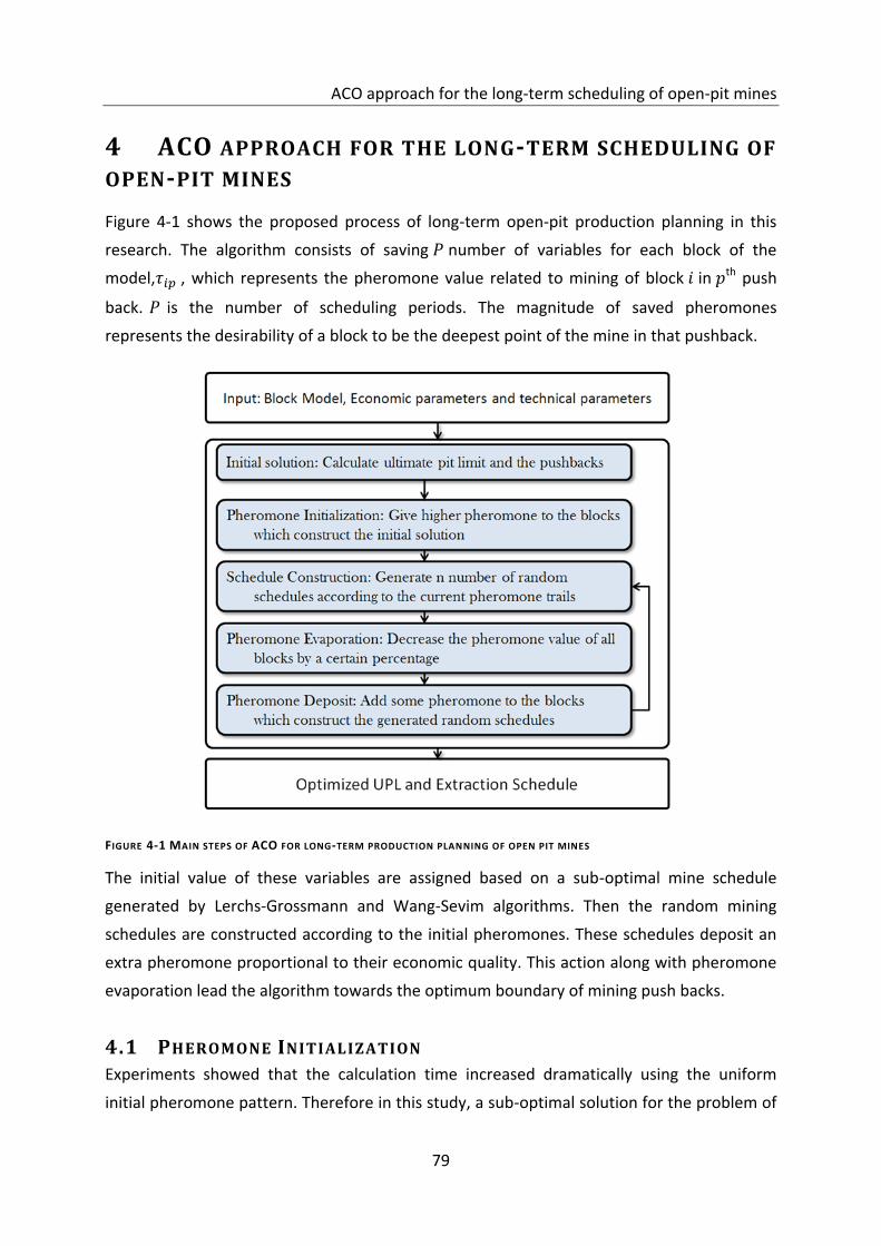
ACO approach for the long-term scheduling of open-pit mines
79
4 ACO APPROACH FOR THE LONG-TERM SCHEDULING OF
OPEN-PIT MINES
Figure 4-1 shows the proposed process of long-term open-pit production planning in this
research. The algorithm consists of saving number of variables for each block of the
model, , which represents the pheromone value related to mining of block in th push
back. is the number of scheduling periods. The magnitude of saved pheromones
represents the desirability of a block to be the deepest point of the mine in that pushback.
The initial value of these variables are assigned based on a sub-optimal mine schedule
generated by Lerchs-Grossmann and Wang-Sevim algorithms. Then the random mining
schedules are constructed according to the initial pheromones. These schedules deposit an
extra pheromone proportional to their economic quality. This action along with pheromone
evaporation lead the algorithm towards the optimum boundary of mining push backs.
4.1 PHEROMONE INITIALIZATION
Experiments showed that the calculation time increased dramatically using the uniform
initial pheromone pattern. Therefore in this study, a sub-optimal solution for the problem of
FIGURE 4-1 MAIN STEPS OF ACO FOR LONG-TERM PRODUCTION PLANNING OF OPEN PIT MINES
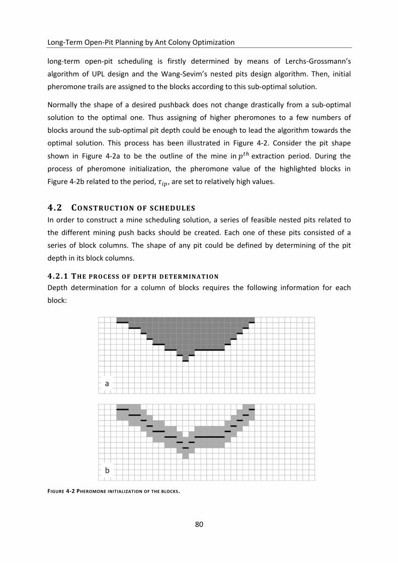
Long-Term Open-Pit Planning by Ant Colony Optimization
80
long-term open-pit scheduling is firstly determined by means of Lerchs-Grossmann’s
algorithm of UPL design and the Wang-Sevim’s nested pits design algorithm. Then, initial
pheromone trails are assigned to the blocks according to this sub-optimal solution.
Normally the shape of a desired pushback does not change drastically from a sub-optimal
solution to the optimal one. Thus assigning of higher pheromones to a few numbers of
blocks around the sub-optimal pit depth could be enough to lead the algorithm towards the
optimal solution. This process has been illustrated in Figure 4-2. Consider the pit shape
shown in Figure 4-2a to be the outline of the mine in extraction period. During the
process of pheromone initialization, the pheromone value of the highlighted blocks in
Figure 4-2b related to the period, , are set to relatively high values.
4.2 CONSTRUCTION OF SCHEDULES
In order to construct a mine scheduling solution, a series of feasible nested pits related to
the different mining push backs should be created. Each one of these pits consisted of a
series of block columns. The shape of any pit could be defined by determining of the pit
depth in its block columns.
4.2.1 THE PROCESS OF DEPTH DETERMINATION
Depth determination for a column of blocks requires the following information for each
block:
FIGURE 4-2 PHEROMONE INITIALIZATION OF THE BLOCKS.
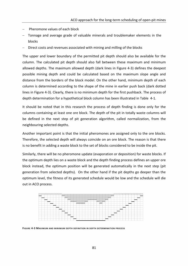
ACO approach for the long-term scheduling of open-pit mines
81
Pheromone values of each block
Tonnage and average grade of valuable minerals and troublemaker elements in the
blocks
Direct costs and revenues associated with mining and milling of the blocks
The upper and lower boundary of the permitted pit depth should also be available for the
column. The calculated pit depth should also fall between these maximum and minimum
allowed depths. The maximum allowed depth (dark lines in Figure 4-3) defines the deepest
possible mining depth and could be calculated based on the maximum slope angle and
distance from the borders of the block model. On the other hand, minimum depth of each
column is determined according to the shape of the mine in earlier push back (dark dotted
lines in Figure 4-3). Clearly, there is no minimum depth for the first pushback. The process of
depth determination for a hypothetical block column has been illustrated in Table 4-1.
It should be noted that in this research the process of depth finding is done only for the
columns containing at least one ore block. The depth of the pit in totally waste columns will
be defined in the next step of pit generation algorithm, called normalization, from the
neighbouring selected depths.
Another important point is that the initial pheromones are assigned only to the ore blocks.
Therefore, the selected depth will always coincide on an ore block. The reason is that there
is no benefit in adding a waste block to the set of blocks considered to be inside the pit.
Similarly, there will be no pheromone update (evaporation or deposition) for waste blocks. If
the optimum depth lies on a waste block and the depth finding process defines an upper ore
block instead, the optimum position will be generated automatically in the next step (pit
generation from selected depths). On the other hand if the pit depths go deeper than the
optimum level, the fitness of its generated schedule would be low and the schedule will die
out in ACO process.
FIGURE 4-3 MAXIMUM AND MINIMUM DEPTH DEFINITION IN DEPTH DETERMINATION PROCESS
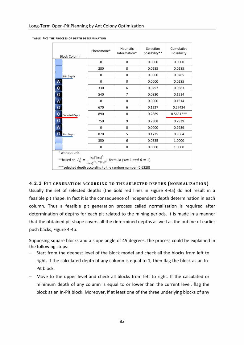
Long-Term Open-Pit Planning by Ant Colony Optimization
82
4.2.2 P IT GENERATION ACCORDING TO THE SELECTED DEPTHS (NORMALIZATION)
Usually the set of selected depths (the bold red lines in Figure 4-4a) do not result in a
feasible pit shape. In fact it is the consequence of independent depth determination in each
column. Thus a feasible pit generation process called normalization is required after
determination of depths for each pit related to the mining periods. It is made in a manner
that the obtained pit shape covers all the determined depths as well as the outline of earlier
push backs, Figure 4-4b.
Supposing square blocks and a slope angle of 45 degrees, the process could be explained in the following steps:
Start from the deepest level of the block model and check all the blocks from left to
right. If the calculated depth of any column is equal to 1, then flag the block as an In-
Pit block.
Move to the upper level and check all blocks from left to right. If the calculated or
minimum depth of any column is equal to or lower than the current level, flag the
block as an In-Pit block. Moreover, if at least one of the three underlying blocks of any
Block Column
Pheromone* Heuristic Information*
Selection possibility**
Cumulative Possibility
0 0 0.0000 0.0000
280 8 0.0285 0.0285
0 0 0.0000 0.0285
0 0 0.0000 0.0285
330 6 0.0297 0.0583
540 7 0.0930 0.1514
0 0 0.0000 0.1514
670 6 0.1227 0.27424
890 8 0.2889 0.5631***
750 9 0.2308 0.7939
0 0 0.0000 0.7939
870 5 0.1725 0.9664
350 6 0.0335 1.0000
0 0 0.0000 1.0000
* without unit
**based on
[ ] [ ]
∑ [ ] [ ]
formula ( )
***selected depth according to the random number (0.6328)
Selected Depth
W
O
O
W
O
O
O
W
O
Min Depth
Max Depth
TABLE 4-1 THE PROCESS OF DEPTH DETERMINATION
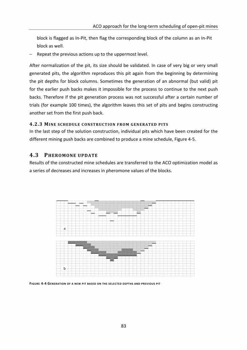
ACO approach for the long-term scheduling of open-pit mines
83
block is flagged as In-Pit, then flag the corresponding block of the column as an In-Pit
block as well.
Repeat the previous actions up to the uppermost level.
After normalization of the pit, its size should be validated. In case of very big or very small
generated pits, the algorithm reproduces this pit again from the beginning by determining
the pit depths for block columns. Sometimes the generation of an abnormal (but valid) pit
for the earlier push backs makes it impossible for the process to continue to the next push
backs. Therefore if the pit generation process was not successful after a certain number of
trials (for example 100 times), the algorithm leaves this set of pits and begins constructing
another set from the first push back.
4.2.3 M INE SCHEDULE C ONSTRUCTION FROM GEN ERATED PITS
In the last step of the solution construction, individual pits which have been created for the
different mining push backs are combined to produce a mine schedule, Figure 4-5.
4.3 PHEROMONE UPDATE
Results of the constructed mine schedules are transferred to the ACO optimization model as
a series of decreases and increases in pheromone values of the blocks.
FIGURE 4-4 GENERATION OF A NEW PIT BASED ON THE SELECTED DEPTHS AND PREVIOUS PIT
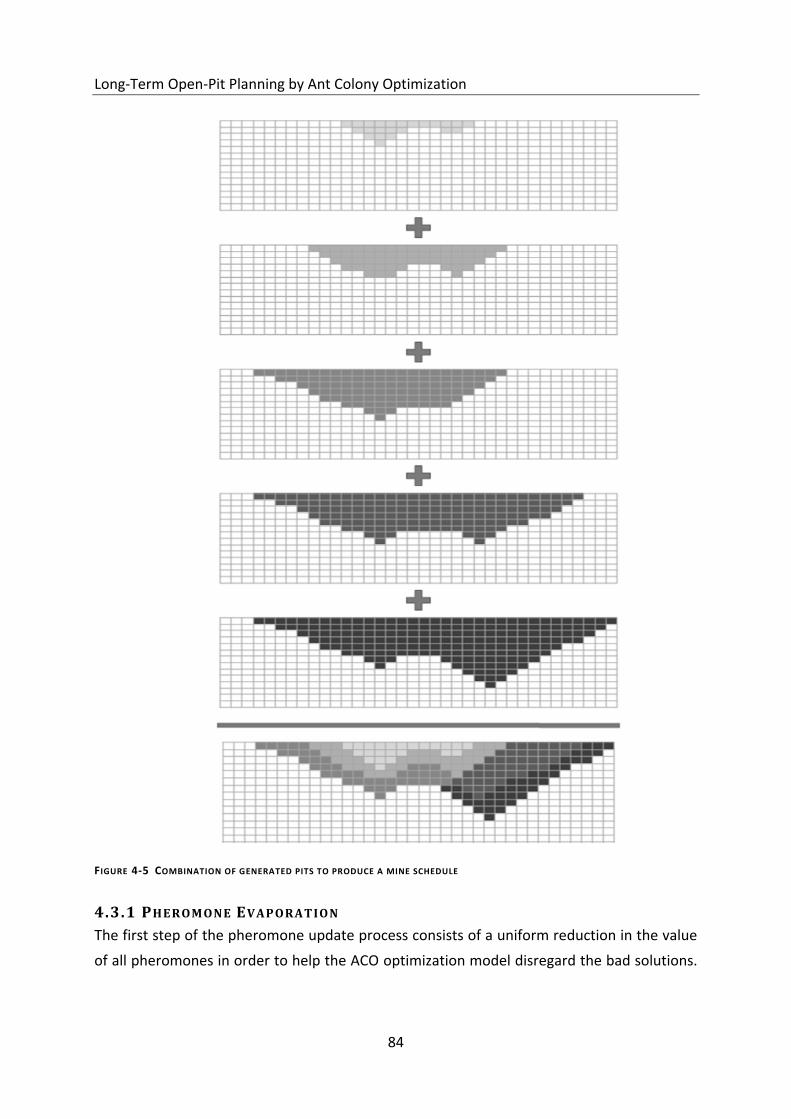
Long-Term Open-Pit Planning by Ant Colony Optimization
84
4.3.1 PHEROMONE EVAPORATION
The first step of the pheromone update process consists of a uniform reduction in the value
of all pheromones in order to help the ACO optimization model disregard the bad solutions.
FIGURE 4-5 COMBINATION OF GENERATED PITS TO PRODUCE A MINE SCHEDULE
ACO approach for the long-term scheduling of open-pit mines
85
In this stage, the pheromone value of all blocks corresponding to all production schedules
should be decreased by a certain percentage.
4.3.2 PHEROMONE DEPOSITION
Consider to be the deepest block of push back of constructed mine schedule in
the column of the block model. The pheromone value of this block grows during the
deposition phase by adding an additional pheromone value. The magnitude of the added
pheromones differs for different variants of ACO algorithm.
It should be noted that the deposition action is applied only to the ore blocks. In cases where
the pit depth lies on a waste block, the additional pheromone is assigned to an imaginary
block on the ground surface. This causes that the desirability of other ore blocks of the
column not to increase because of the lack of pheromone deposition in the optimal depth.
4.4 IMPLEMENTATION TOOL
To evaluate the applicability of the proposed ACO algorithm for long-term planning of open-
pit mines, a computer program has been developed in Visual Studio 2005 programming
environment for the implementation of calculations. The program interface consists of four
different graphical user interface windows, including the input block model, input
parameters, initial solution and ACO optimizer tabs, Figure 4-6.
4.4.1 INPUT BLOCK MODEL TAB
Implementation of the algorithm starts with importing a uniform block model to the
program. The block model should be prepared as a text (ASCII) file in which the information
of each block should be written in a separate line called records. These information fields
could include coordinates, metal grades and troublous elements.
In order to import the block model file into the program, the user can type the exact address
into (1) or could browse through folders by clicking button (2). Clicking the preview button
(3) will show the first 100 lines of the inputed file in the preview text box (12). This helps the
user recognize the structure of the input file and assists in filling in the following parameters.
Then, the number of blocks in X, Y and Z directions must be entered in (4).
The program has the ability to use both index coordinates, (i,j,k), and real world coordinates,
(x,y,z), which is selectable in (5). In fact the program does not need the real coordinates for
optimization and the i, j and k indexes are used in all calculations. Therefore if the real world
coordinates are imported into the program, the origin of the block model and size of blocks
will be calculated using the given information.
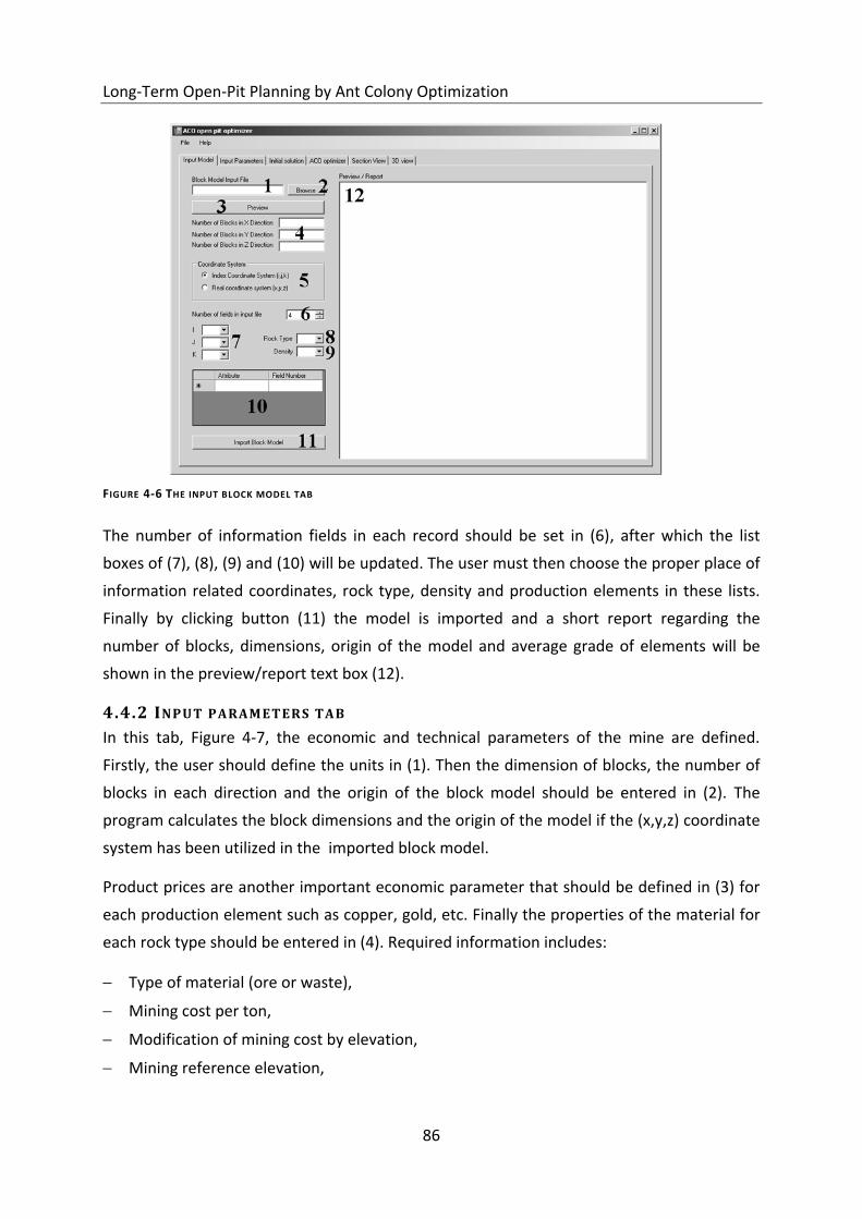
Long-Term Open-Pit Planning by Ant Colony Optimization
86
The number of information fields in each record should be set in (6), after which the list
boxes of (7), (8), (9) and (10) will be updated. The user must then choose the proper place of
information related coordinates, rock type, density and production elements in these lists.
Finally by clicking button (11) the model is imported and a short report regarding the
number of blocks, dimensions, origin of the model and average grade of elements will be
shown in the preview/report text box (12).
4.4.2 INPUT PARAMETERS TAB
In this tab, Figure 4-7, the economic and technical parameters of the mine are defined.
Firstly, the user should define the units in (1). Then the dimension of blocks, the number of
blocks in each direction and the origin of the block model should be entered in (2). The
program calculates the block dimensions and the origin of the model if the (x,y,z) coordinate
system has been utilized in the imported block model.
Product prices are another important economic parameter that should be defined in (3) for
each production element such as copper, gold, etc. Finally the properties of the material for
each rock type should be entered in (4). Required information includes:
Type of material (ore or waste),
Mining cost per ton,
Modification of mining cost by elevation,
Mining reference elevation,
FIGURE 4-6 THE INPUT BLOCK MODEL TAB
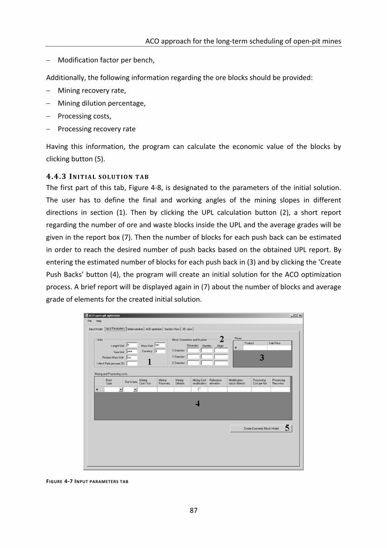
ACO approach for the long-term scheduling of open-pit mines
87
Modification factor per bench,
Additionally, the following information regarding the ore blocks should be provided:
Mining recovery rate,
Mining dilution percentage,
Processing costs,
Processing recovery rate
Having this information, the program can calculate the economic value of the blocks by
clicking button (5).
4.4.3 INITIAL SOLUTION TAB
The first part of this tab, Figure 4-8, is designated to the parameters of the initial solution.
The user has to define the final and working angles of the mining slopes in different
directions in section (1). Then by clicking the UPL calculation button (2), a short report
regarding the number of ore and waste blocks inside the UPL and the average grades will be
given in the report box (7). Then the number of blocks for each push back can be estimated
in order to reach the desired number of push backs based on the obtained UPL report. By
entering the estimated number of blocks for each push back in (3) and by clicking the ‘Create
Push Backs’ button (4), the program will create an initial solution for the ACO optimization
process. A brief report will be displayed again in (7) about the number of blocks and average
grade of elements for the created initial solution.
FIGURE 4-7 INPUT PARAMETERS TAB
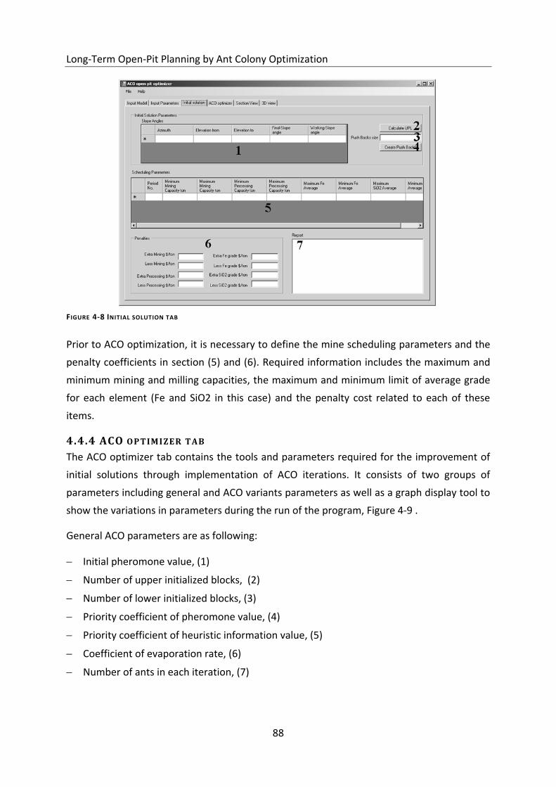
Long-Term Open-Pit Planning by Ant Colony Optimization
88
Prior to ACO optimization, it is necessary to define the mine scheduling parameters and the
penalty coefficients in section (5) and (6). Required information includes the maximum and
minimum mining and milling capacities, the maximum and minimum limit of average grade
for each element (Fe and SiO2 in this case) and the penalty cost related to each of these
items.
4.4.4 ACO OPTIMIZER TAB
The ACO optimizer tab contains the tools and parameters required for the improvement of
initial solutions through implementation of ACO iterations. It consists of two groups of
parameters including general and ACO variants parameters as well as a graph display tool to
show the variations in parameters during the run of the program, Figure 4-9 .
General ACO parameters are as following:
Initial pheromone value, (1)
Number of upper initialized blocks, (2)
Number of lower initialized blocks, (3)
Priority coefficient of pheromone value, (4)
Priority coefficient of heuristic information value, (5)
Coefficient of evaporation rate, (6)
Number of ants in each iteration, (7)
FIGURE 4-8 INITIAL SOLUTION TAB
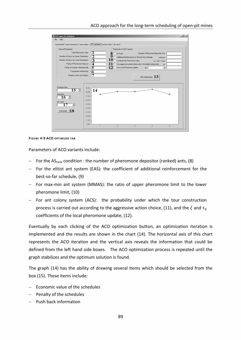
ACO approach for the long-term scheduling of open-pit mines
89
Parameters of ACO variants include:
For the ASrank condition : the number of pheromone depositor (ranked) ants, (8)
For the elitist ant system (EAS): the coefficient of additional reinforcement for the
best-so-far schedule, (9)
For max-min ant system (MMAS): the ratio of upper pheromone limit to the lower
pheromone limit, (10)
For ant colony system (ACS): the probability under which the tour construction
process is carried out according to the aggressive action choice, (11), and the and
coefficients of the local pheromone update, (12).
Eventually by each clicking of the ACO optimization button, an optimization iteration is
implemented and the results are shown in the chart (14). The horizontal axis of this chart
represents the ACO iteration and the vertical axis reveals the information that could be
defined from the left hand side boxes. The ACO optimization process is repeated until the
graph stabilizes and the optimum solution is found.
The graph (14) has the ability of drawing several items which should be selected from the
box (15). These items include:
Economic value of the schedules
Penalty of the schedules
Push back information
FIGURE 4-9 ACO OPTIMIZER TAB
Long-Term Open-Pit Planning by Ant Colony Optimization
90
For the last case, the number of push backs and required information must be chosen from
(16) and (17) respectively. Selected information types could be one of the Fe or SiO2
average, the number of blocks (ore, waste or total) or the life of the periods. Then the
defined chart would be added to the graph by clicking the button (18). The chart is able to
display up to 10 different information graphs simultaneously.
4.5 CASE STUDY
A hypothetical block model of an iron ore deposit containing 1000 blocks was created and
the grades of Fe and SiO2 were randomly assigned to all ore blocks. The grades of Fe and
SiO2 varied from 45 to 65 and from 5 to 15 percent respectively. According to these grades
the net economic values of the blocks were calculated in the distance of 1 to 9. A constant
value of -6 was assigned to the waste blocks.
At the beginning the outline of the ultimate pit is determined by the Lerchs-Grossmann’s
graph algorithm. The calculated UPL contains 455 ore and 161 waste blocks which led to 681
units of undiscounted economic value. Then mining push backs were generated by the
alternative to parameterization algorithm of Wang-Sevim. Through this, 9 uniform push
backs with the size of 70 blocks were constructed. Considering an annual interest rate of
10% and the mine life of 20 years, the discounted economic value of the constructed initial
schedule was calculated as 323 units. Table 4-2 shows the block numbers and the average
grades of the push backs in the initial solution.
As a simple scheduling condition, the following restrictions were considered for each period
of this case study:
Mining rate: from 59 to 64 blocks per period
Processing rate: from 47 to 53 blocks per period
Average allowed grade of Fe: from 54 to 56 percent
Average allowed grade of SiO2: from 9 to 11
Anything exceeding these limits has been considered to have 1 currency unit of penalty cost
for each of the extra or fewer blocks. Consequently the value of the constructed initial
scheduling solution received 79 currency units of penalty costs and its economic value
dropped to 244 units.
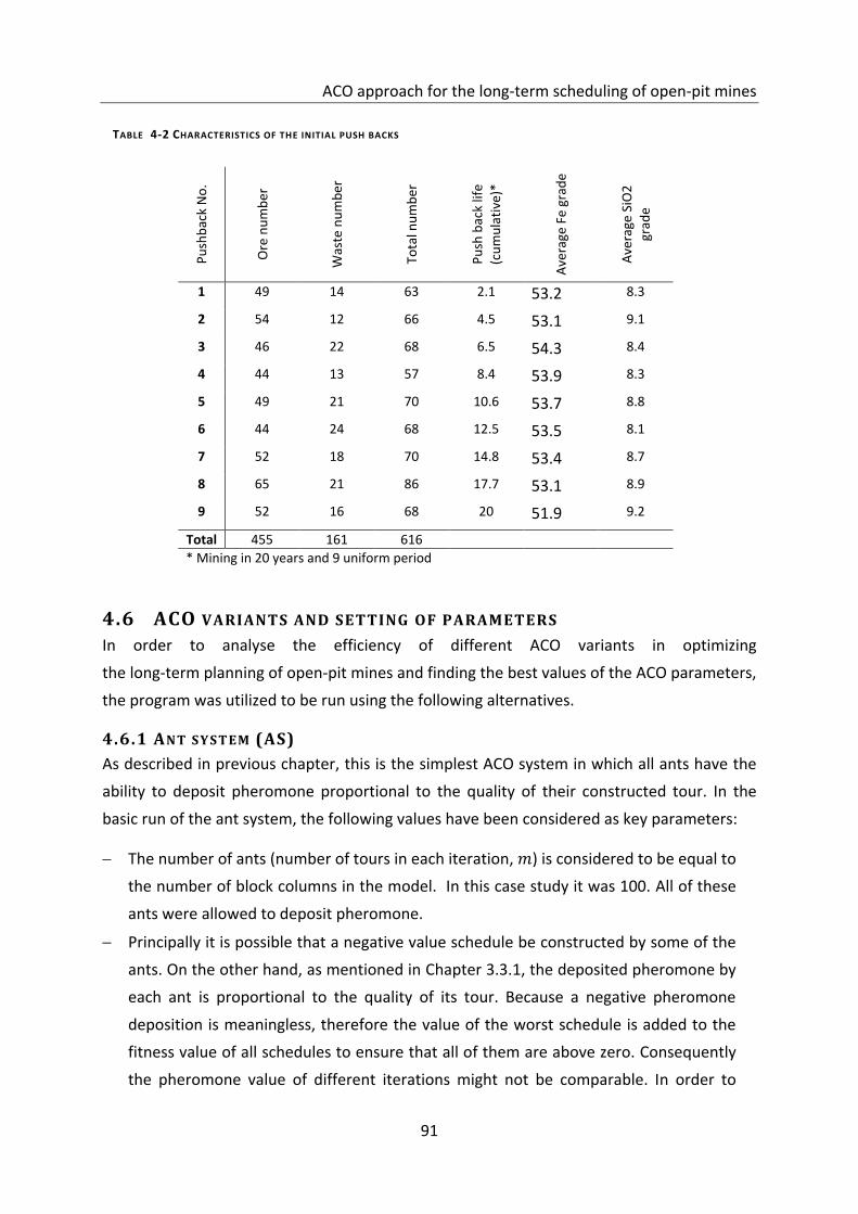
ACO approach for the long-term scheduling of open-pit mines
91
Pu
shb
ack
No
.
Ore
nu
mb
er
Was
te n
um
ber
Tota
l nu
mb
er
Pu
sh b
ack
life
(cu
mu
lati
ve)*
Ave
rage
Fe
grad
e
Ave
rage
SiO
2
grad
e
1 49 14 63 2.1 53.2 8.3
2 54 12 66 4.5 53.1 9.1
3 46 22 68 6.5 54.3 8.4
4 44 13 57 8.4 53.9 8.3
5 49 21 70 10.6 53.7 8.8
6 44 24 68 12.5 53.5 8.1
7 52 18 70 14.8 53.4 8.7
8 65 21 86 17.7 53.1 8.9
9 52 16 68 20 51.9 9.2
Total 455 161 616
* Mining in 20 years and 9 uniform period
4.6 ACO VARIANTS AND SETTING OF PARAMETERS
In order to analyse the efficiency of different ACO variants in optimizing
the long-term planning of open-pit mines and finding the best values of the ACO parameters,
the program was utilized to be run using the following alternatives.
4.6.1 ANT SYSTEM (AS)
As described in previous chapter, this is the simplest ACO system in which all ants have the
ability to deposit pheromone proportional to the quality of their constructed tour. In the
basic run of the ant system, the following values have been considered as key parameters:
The number of ants (number of tours in each iteration, ) is considered to be equal to
the number of block columns in the model. In this case study it was 100. All of these
ants were allowed to deposit pheromone.
Principally it is possible that a negative value schedule be constructed by some of the
ants. On the other hand, as mentioned in Chapter 3.3.1, the deposited pheromone by
each ant is proportional to the quality of its tour. Because a negative pheromone
deposition is meaningless, therefore the value of the worst schedule is added to the
fitness value of all schedules to ensure that all of them are above zero. Consequently
the pheromone value of different iterations might not be comparable. In order to
TABLE 4-2 CHARACTERISTICS OF THE INITIAL PUSH BACKS
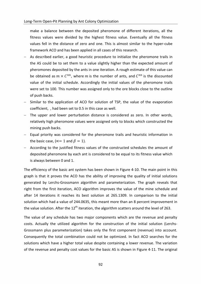
Long-Term Open-Pit Planning by Ant Colony Optimization
92
make a balance between the deposited pheromone of different iterations, all the
fitness values were divided by the highest fitness value. Eventually all the fitness
values fell in the distance of zero and one. This is almost similar to the hyper-cube
framework ACO and has been applied in all cases of this research.
As described earlier, a good heuristic procedure to initialize the pheromone trails in
the AS could be to set them to a value slightly higher than the expected amount of
pheromones deposited by the ants in one iteration. A rough estimate of this value can
be obtained as , where is the number of ants, and is the discounted
value of the initial schedule. Accordingly the initial values of the pheromone trails
were set to 100. This number was assigned only to the ore blocks close to the outline
of push backs.
Similar to the application of ACO for solution of TSP, the value of the evaporation
coefficient, , had been set to 0.5 in this case as well.
The upper and lower perturbation distance is considered as zero. In other words,
relatively high pheromone values were assigned only to blocks which constructed the
mining push backs.
Equal priority was considered for the pheromone trails and heuristic information in
the basic case, ( and ).
According to the justified fitness values of the constructed schedules the amount of
deposited pheromone by each ant is considered to be equal to its fitness value which
is always between 0 and 1.
The efficiency of the basic ant system has been shown in Figure 4-10. The main point in this
graph is that it proves the ACO has the ability of improving the quality of initial solutions
generated by Lerchs-Grossmann algorithm and parameterization. The graph reveals that
right from the first iteration, ACO algorithm improves the value of the mine schedule and
after 14 iterations it reaches its best solution at 265.1309. In comparison to the initial
solution which had a value of 244.0635, this meant more than an 8 percent improvement in
the value solution. After the 12th iteration, the algorithm scatters around the level of 263.
The value of any schedule has two major components which are the revenue and penalty
costs. Actually the utilized algorithm for the construction of the initial solution (Lerchs-
Grossmann plus parameterization) takes only the first component (revenue) into account.
Consequently the total combination could not be optimized. In fact ACO searches for the
solutions which have a higher total value despite containing a lower revenue. The variation
of the revenue and penalty cost values for the basic AS is shown in Figure 4-11. The original
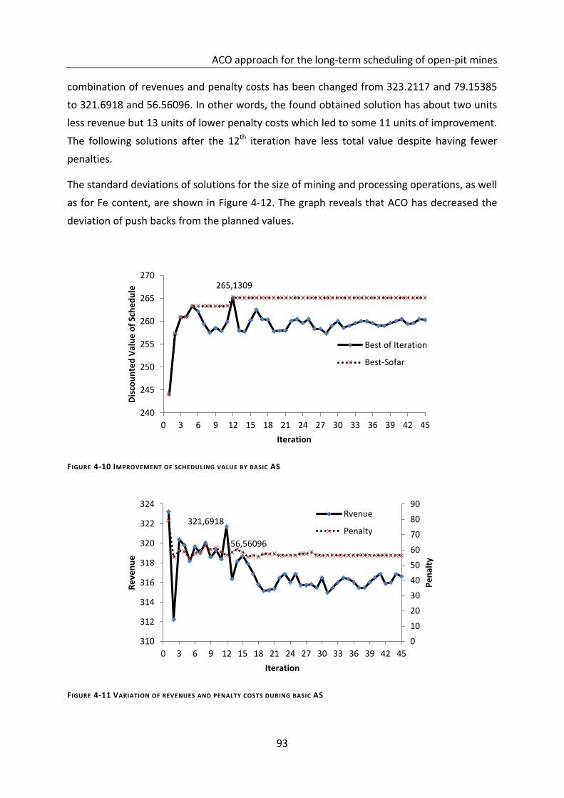
ACO approach for the long-term scheduling of open-pit mines
93
combination of revenues and penalty costs has been changed from 323.2117 and 79.15385
to 321.6918 and 56.56096. In other words, the found obtained solution has about two units
less revenue but 13 units of lower penalty costs which led to some 11 units of improvement.
The following solutions after the 12th iteration have less total value despite having fewer
penalties.
The standard deviations of solutions for the size of mining and processing operations, as well
as for Fe content, are shown in Figure 4-12. The graph reveals that ACO has decreased the
deviation of push backs from the planned values.
265,1309
240
245
250
255
260
265
270
0 3 6 9 12 15 18 21 24 27 30 33 36 39 42 45
Dis
cou
nte
d V
alu
e o
f Sc
he
du
le
Iteration
Best of Iteration
Best-Sofar
321,6918
56,56096
0
10
20
30
40
50
60
70
80
90
310
312
314
316
318
320
322
324
0 3 6 9 12 15 18 21 24 27 30 33 36 39 42 45
Pe
nal
ty
Re
ven
ue
Iteration
Rvenue
Penalty
FIGURE 4-11 VARIATION OF REVENUES AND PENALTY COSTS DURING BASIC AS
FIGURE 4-10 IMPROVEMENT OF SCHEDULING VALUE BY BASIC AS
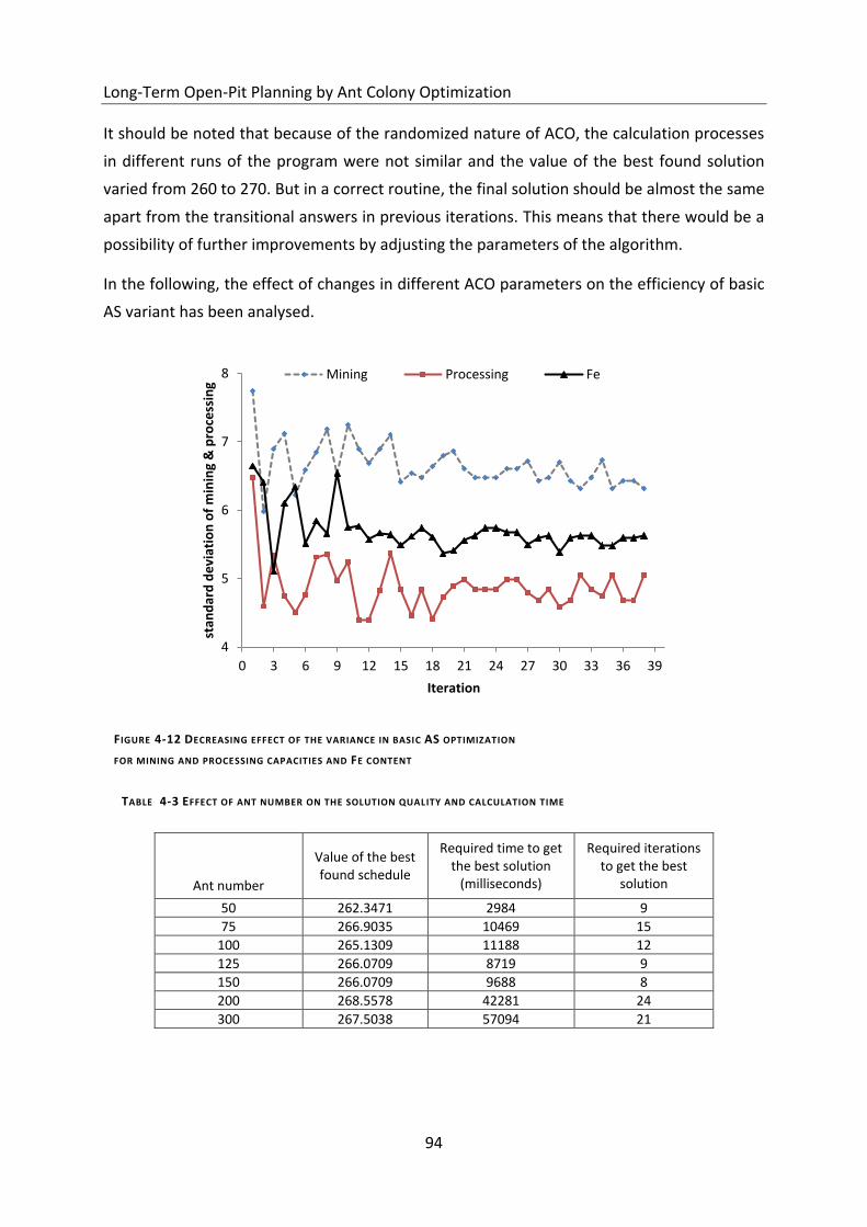
Long-Term Open-Pit Planning by Ant Colony Optimization
94
It should be noted that because of the randomized nature of ACO, the calculation processes
in different runs of the program were not similar and the value of the best found solution
varied from 260 to 270. But in a correct routine, the final solution should be almost the same
apart from the transitional answers in previous iterations. This means that there would be a
possibility of further improvements by adjusting the parameters of the algorithm.
In the following, the effect of changes in different ACO parameters on the efficiency of basic
AS variant has been analysed.
Ant number
Value of the best found schedule
Required time to get the best solution
(milliseconds)
Required iterations to get the best
solution
50 262.3471 2984 9
75 266.9035 10469 15
100 265.1309 11188 12
125 266.0709 8719 9
150 266.0709 9688 8
200 268.5578 42281 24
300 267.5038 57094 21
4
5
6
7
8
0 3 6 9 12 15 18 21 24 27 30 33 36 39
stan
dar
d d
evi
atio
n o
f m
inin
g &
pro
cess
ing
Iteration
Mining Processing Fe
TABLE 4-3 EFFECT OF ANT NUMBER ON THE SOLUTION QUALITY AND CALCULATION TIME
FIGURE 4-12 DECREASING EFFECT OF THE VARIANCE IN BASIC AS OPTIMIZATION
FOR MINING AND PROCESSING CAPACITIES AND FE CONTENT
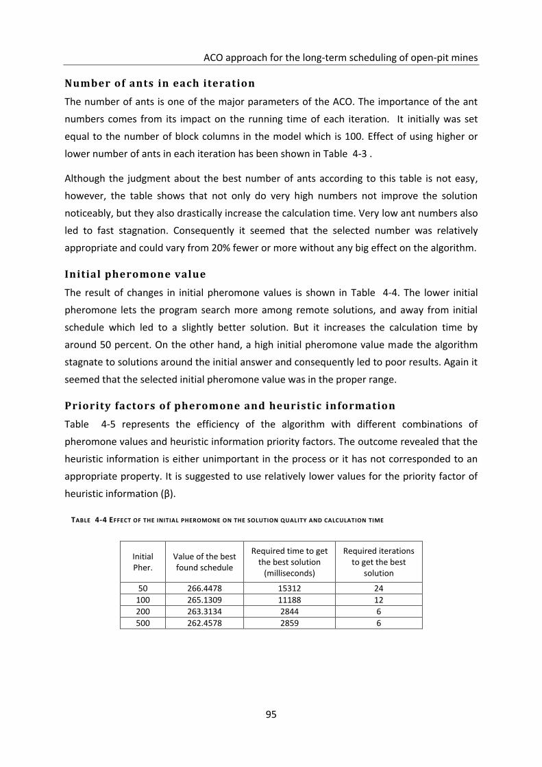
ACO approach for the long-term scheduling of open-pit mines
95
Number of ants in each iteration
The number of ants is one of the major parameters of the ACO. The importance of the ant
numbers comes from its impact on the running time of each iteration. It initially was set
equal to the number of block columns in the model which is 100. Effect of using higher or
lower number of ants in each iteration has been shown in Table 4-3 .
Although the judgment about the best number of ants according to this table is not easy,
however, the table shows that not only do very high numbers not improve the solution
noticeably, but they also drastically increase the calculation time. Very low ant numbers also
led to fast stagnation. Consequently it seemed that the selected number was relatively
appropriate and could vary from 20% fewer or more without any big effect on the algorithm.
Initial pheromone value
The result of changes in initial pheromone values is shown in Table 4-4. The lower initial
pheromone lets the program search more among remote solutions, and away from initial
schedule which led to a slightly better solution. But it increases the calculation time by
around 50 percent. On the other hand, a high initial pheromone value made the algorithm
stagnate to solutions around the initial answer and consequently led to poor results. Again it
seemed that the selected initial pheromone value was in the proper range.
Priority factors of pheromone and heuristic information
Table 4-5 represents the efficiency of the algorithm with different combinations of
pheromone values and heuristic information priority factors. The outcome revealed that the
heuristic information is either unimportant in the process or it has not corresponded to an
appropriate property. It is suggested to use relatively lower values for the priority factor of
heuristic information (β).
Initial Pher.
Value of the best found schedule
Required time to get the best solution
(milliseconds)
Required iterations to get the best
solution
50 266.4478 15312 24
100 265.1309 11188 12
200 263.3134 2844 6
500 262.4578 2859 6
TABLE 4-4 EFFECT OF THE INITIAL PHEROMONE ON THE SOLUTION QUALITY AND CALCULATION TIME
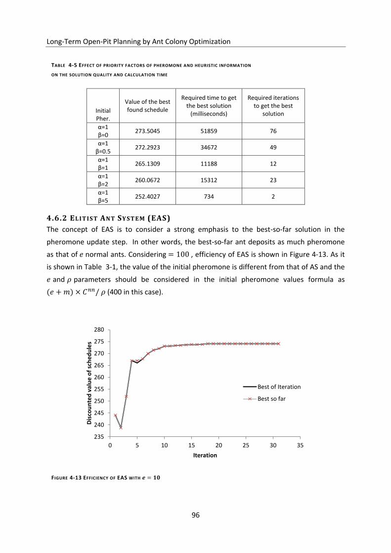
Long-Term Open-Pit Planning by Ant Colony Optimization
96
Initial Pher.
Value of the best found schedule
Required time to get the best solution
(milliseconds)
Required iterations to get the best
solution
α=1 β=0
273.5045 51859 76
α=1 β=0.5
272.2923 34672 49
α=1 β=1
265.1309 11188 12
α=1 β=2
260.0672 15312 23
α=1 β=5
252.4027 734 2
4.6.2 ELITIST ANT SYSTEM (EAS)
The concept of EAS is to consider a strong emphasis to the best-so-far solution in the
pheromone update step. In other words, the best-so-far ant deposits as much pheromone
as that of normal ants. Considering , efficiency of EAS is shown in Figure 4-13. As it
is shown in Table 3-1, the value of the initial pheromone is different from that of AS and the
and parameters should be considered in the initial pheromone values formula as
( ) (400 in this case).
235
240
245
250
255
260
265
270
275
280
0 5 10 15 20 25 30 35
Dis
cou
nte
d v
alu
e o
f sc
he
du
les
Iteration
Best of Iteration
Best so far
FIGURE 4-13 EFFICIENCY OF EAS WITH
TABLE 4-5 EFFECT OF PRIORITY FACTORS OF PHEROMONE AND HEURISTIC INFORMATION
ON THE SOLUTION QUALITY AND CALCULATION TIME
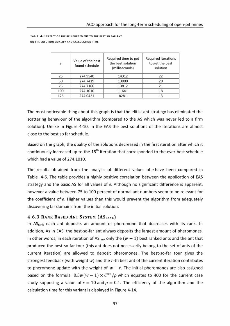
ACO approach for the long-term scheduling of open-pit mines
97
e Value of the best found schedule
Required time to get the best solution
(milliseconds)
Required iterations to get the best
solution
25 274.9540 14312 22
50 274.7419 13000 20
75 274.7166 13812 21
100 274.1010 11641 18
125 274.0421 8281 13
The most noticeable thing about this graph is that the elitist ant strategy has eliminated the
scattering behaviour of the algorithm (compared to the AS which was never led to a firm
solution). Unlike in Figure 4-10, in the EAS the best solutions of the iterations are almost
close to the best so far schedule.
Based on the graph, the quality of the solutions decreased in the first iteration after which it
continuously increased up to the 18th iteration that corresponded to the ever-best schedule
which had a value of 274.1010.
The results obtained from the analysis of different values of have been compared in
Table 4-6. The table provides a highly positive correlation between the application of EAS
strategy and the basic AS for all values of . Although no significant difference is apparent,
however a value between 75 to 100 percent of normal ant numbers seem to be relevant for
the coefficient of . Higher values than this would prevent the algorithm from adequately
discovering far domains from the initial solution.
4.6.3 RANK BASED ANT SYSTEM (AS R A N K )
In ASrank each ant deposits an amount of pheromone that decreases with its rank. In
addition, As in EAS, the best-so-far ant always deposits the largest amount of pheromones.
In other words, in each iteration of ASrank only the ( ) best ranked ants and the ant that
produced the best-so-far tour (this ant does not necessarily belong to the set of ants of the
current iteration) are allowed to deposit pheromones. The best-so-far tour gives the
strongest feedback (with weight ) and the -th best ant of the current iteration contributes
to pheromone update with the weight of . The initial pheromones are also assigned
based on the formula ( ) which equates to 400 for the current case
study supposing a value of and . The efficiency of the algorithm and the
calculation time for this variant is displayed in Figure 4-14.
TABLE 4-6 EFFECT OF THE REINFORCEMENT TO THE BEST SO FAR ANT
ON THE SOLUTION QUALITY AND CALCULATION TIME
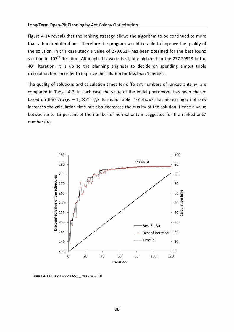
Long-Term Open-Pit Planning by Ant Colony Optimization
98
Figure 4-14 reveals that the ranking strategy allows the algorithm to be continued to more
than a hundred iterations. Therefore the program would be able to improve the quality of
the solution. In this case study a value of 279.0614 has been obtained for the best found
solution in 107th iteration. Although this value is slightly higher than the 277.20928 in the
40th iteration, it is up to the planning engineer to decide on spending almost triple
calculation time in order to improve the solution for less than 1 percent.
The quality of solutions and calculation times for different numbers of ranked ants, , are
compared in Table 4-7. In each case the value of the initial pheromone has been chosen
based on the ( ) formula. Table 4-7 shows that increasing not only
increases the calculation time but also decreases the quality of the solution. Hence a value
between 5 to 15 percent of the number of normal ants is suggested for the ranked ants’
number ( ).
279.0614
0
10
20
30
40
50
60
70
80
90
100
235
240
245
250
255
260
265
270
275
280
285
0 20 40 60 80 100 120
Iteration
Cal
cula
tio
n t
ime
Dis
cou
nte
d v
alu
e o
f th
e s
che
du
les
Best So Far
Best of Iteration
Time (s)
FIGURE 4-14 EFFICIENCY OF ASRANK WITH
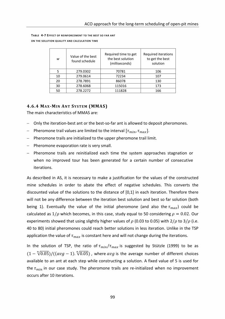
ACO approach for the long-term scheduling of open-pit mines
99
w Value of the best found schedule
Required time to get the best solution
(milliseconds)
Required iterations to get the best
solution
5 279.0302 70781 106
10 279.0614 72234 107
20 278.7891 86078 130
30 278.6068 115016 173
50 278.2272 111828 166
4.6.4 MAX-M IN ANT SYSTEM (MMAS)
The main characteristics of MMAS are:
Only the iteration-best ant or the best-so-far ant is allowed to deposit pheromones.
Pheromone trail values are limited to the interval [ ].
Pheromone trails are initialized to the upper pheromone trail limit.
Pheromone evaporation rate is very small.
Pheromone trails are reinitialized each time the system approaches stagnation or
when no improved tour has been generated for a certain number of consecutive
iterations.
As described in AS, it is necessary to make a justification for the values of the constructed
mine schedules in order to abate the effect of negative schedules. This converts the
discounted value of the solutions to the distance of [0,1] in each iteration. Therefore there
will not be any difference between the iteration best solution and best so far solution (both
being 1). Eventually the value of the initial pheromone (and also the ) could be
calculated as which becomes, in this case, study equal to 50 considering . Our
experiments showed that using slightly higher values of (0.03 to 0.05) with 2 to 3 (i.e.
40 to 80) initial pheromones could reach better solutions in less iteration. Unlike in the TSP
application the value of is constant here and will not change during the iterations.
In the solution of TSP, the ratio of is suggested by Stützle (1999) to be as
( √
) (( ) √
) , where is the average number of different choices
available to an ant at each step while constructing a solution. A fixed value of 5 is used for
the in our case study. The pheromone trails are re-initialized when no improvement
occurs after 10 iterations.
TABLE 4-7 EFFECT OF REINFORCEMENT TO THE BEST SO FAR ANT
ON THE SOLUTION QUALITY AND CALCULATION TIME
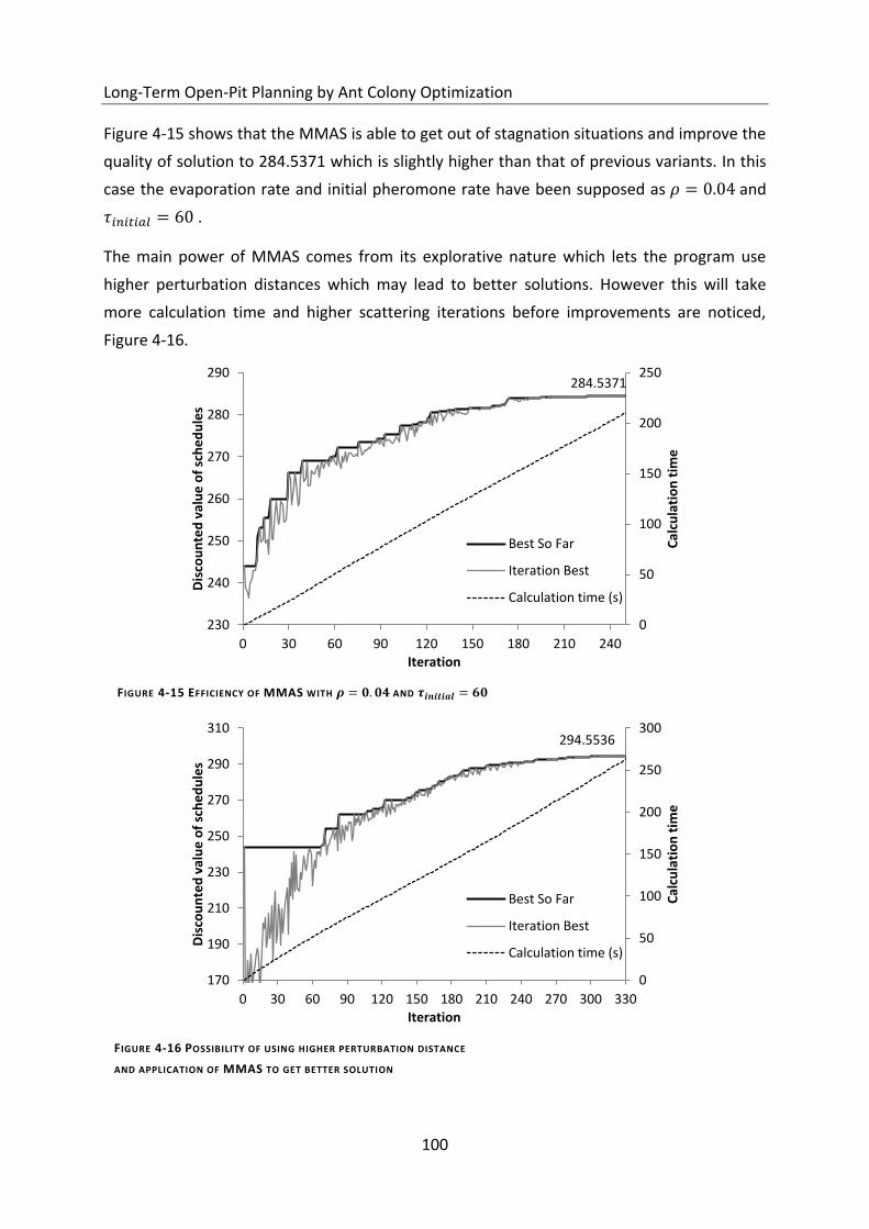
Long-Term Open-Pit Planning by Ant Colony Optimization
100
Figure 4-15 shows that the MMAS is able to get out of stagnation situations and improve the
quality of solution to 284.5371 which is slightly higher than that of previous variants. In this
case the evaporation rate and initial pheromone rate have been supposed as and
.
The main power of MMAS comes from its explorative nature which lets the program use
higher perturbation distances which may lead to better solutions. However this will take
more calculation time and higher scattering iterations before improvements are noticed,
Figure 4-16.
284.5371
0
50
100
150
200
250
230
240
250
260
270
280
290
0 30 60 90 120 150 180 210 240Iteration
Cal
cula
tio
n t
ime
Dis
cou
nte
d v
alu
e o
f sc
he
du
les
Best So Far
Iteration Best
Calculation time (s)
294.5536
0
50
100
150
200
250
300
170
190
210
230
250
270
290
310
0 30 60 90 120 150 180 210 240 270 300 330Iteration
Cal
cula
tio
n t
ime
Dis
cou
nte
d v
alu
e o
f sc
he
du
les
Best So Far
Iteration Best
Calculation time (s)
FIGURE 4-16 POSSIBILITY OF USING HIGHER PERTURBATION DISTANCE
AND APPLICATION OF MMAS TO GET BETTER SOLUTION
FIGURE 4-15 EFFICIENCY OF MMAS WITH AND
ACO approach for the long-term scheduling of open-pit mines
101
4.6.5 ANT COLONY SYSTEM (ACS)
The ant colony system differs from the previous variants from the following points of view:
Pseudorandom proportional action choice rule: with the probability of the ants
makes its destination to the node which has the highest [ ] [ ]
. Whereas it has
the probability of using the same routine as AS for the selection. A value of
is suggested for the TSP solution.
Global pheromone update: in ACS only one ant (the best-so-far ant) is allowed to add
pheromones after each iteration. Additionally, unlike AS, the evaporation process only
applies to the arcs of the best-so-far tour, not to all the arcs.
Local pheromone update: the ants use a local pheromone update rule that they apply
immediately after having crossed an arc during the tour construction of ACS.
In order to evaluate the efficiency of ACS on our case study, the best values of the
parameters were found as below:
Number of ants: 10
Evaporation rate: 0.1
Initial pheromone value: 0.01
Local pheromone update factor: 0.1
Pseudorandom choice probability: 0.9
Obtained results of using ACS have been shown in Figure 4-17. The main noticeable point in
ACS is that the number of ants has been drastically reduced which has direct effect on the
calculation time of each iteration. For instance, the run time of iterations have been reduced
from 700 to 1000 milliseconds in previous variants of ACO, to less than 100 ms in ACS.
Another factor that helps the speed of the ACS algorithm is the fact that pheromone
evaporation and deposition happen only on the arcs of the best so far solution.
Consequently, when compared to the other variants of ACO, ACS could reach much better
solutions in a given time of calculation. This might be very beneficial for the big block
models.
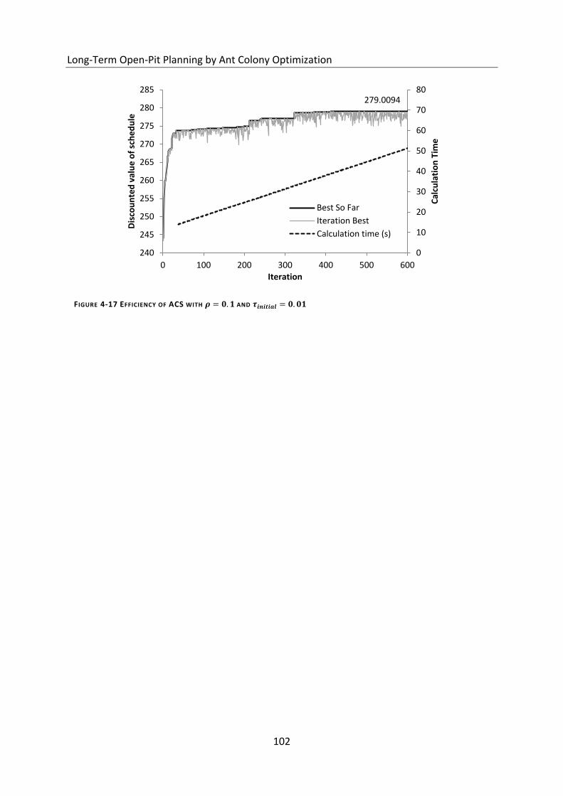
Long-Term Open-Pit Planning by Ant Colony Optimization
102
279.0094
0
10
20
30
40
50
60
70
80
240
245
250
255
260
265
270
275
280
285
0 100 200 300 400 500 600Iteration
Cal
cula
tio
n T
ime
Dis
cou
nte
d v
alu
e o
f sc
he
du
le
Best So Far
Iteration Best
Calculation time (s)
FIGURE 4-17 EFFICIENCY OF ACS WITH AND
Conclusion
103
5 CONCLUSION
A new algorithm for open-pit optimization using ant colony optimization has been developed
and used to optimize the long-term scheduling of open-pit for a two dimensional randomly
simulated block model. The algorithm is inspired by foraging behaviour of ants.
The shapes of the pits (respective of the slope angles) are represented by means of a simple
array of integer numbers. Each element of this array shows the depth of a pit in an individual
column of block model. Extending this concept to the long-term production planning, any
mine schedule is represented by an array that has several mine depths at each column of
block model related to different production periods.
In order to simulate the process, some programming variables are considered for each block
as the pheromone trails. The numbers of these variables are equal to the number of
planning periods. In fact these pheromone trails represent the desirability of the block for
being the deepest point of the mine in that column for the given mining period.
At the beginning, the values of the pheromone trails are initialized according to a mine
schedule generated by Lerchs-Grossmann’s algorithm and the alternative to
parameterization algorithm of Wang & Sevim. During initialization, relatively higher values
of pheromone are assigned to those blocks that are close to the deepest points of the push
backs in the initial mine schedule. This leads the procedure to construct a series of random
schedules which are not far from the initial solution.
In each ACO iteration, several mine schedules are generated based on the current
pheromone trails. This is implemented by a process called “depth determination”. In this
process the depth of a mine in each period is determined for each column of the block
model. The higher the value of the pheromone trail of a certain block, the higher the
possibility of selecting that block as the pit depth in that period. Then the pheromone values
of all blocks are reduced to a certain percentage (evaporation) and additionally the
pheromone value of those blocks that participated in defining the constructed schedules are
increased according to the quality of the generated solutions. Via repeated iterations, the
pheromone values of the blocks which define the shape of the optimum solution are
increased whereas those of the others have been significantly evaporated.
The analysis carried out on the case study revealed that the ACO can improve the value of
the mining schedule by up to 34%. This is mainly contributed to the fact that penalties can
be considered in relation to their deviation from the permitted limits.
Long-Term Open-Pit Planning by Ant Colony Optimization
104
5.1 DISCUSSION
The major benefits of using of the proposed algorithm compared to the former methods are:
Most of the available methods and algorithms follow a certain target (such as highest
NPV, lowest stripping ratio etc.) in their solution strategy; therefore, later changes in
the desired target would be very difficult or impossible with them. The ACO approach
is able to consider any kind of objective functions in the optimization process. Even
very complex objective functions do not have a significant influence on the efficiency
of the method. This is because of the fact that all schedules are generated based on
the pheromone values in the ACO, regardless of the objective function. Then the
values of the generated schedules are calculated in the next step according to the
defined target.
Variable slope angles can be modelled with ease in the generated schedules. The
method even has the ability of applying very complex slope differentiations. The only
change in the program would only be required in the normalization routine. It is also
possible to consider working slope angles by supposing different values for the slopes
of the inner periods and the most outer phase.
During the ACO optimization iterations thousands of mine schedules are randomly
created according to the pheromone values. In order to model uncertainty related to
the characteristics of the blocks, these schedules can be constructed based on a series
of the random variables instead of deterministic values.
In each iteration of the ACO, number of mine schedules are being constructed. The
calculation time of the algorithm is highly dependent on the value of which is
usually (except for ACS) considered equal to the number of block columns in the
model. In other words the calculation time of a double sized block model in each
direction (8 times more blocks) is expected to be only 4 times more. Therefore the
required calculation time of a block model with one million blocks is expected to be
around 100 times that of the case study used in this research.
In the Ant System (AS) and Elitist Ant System (EAS) variants of the ACO algorithm, a
large number of mining schedules (all constructed schedules) have to be saved in the
memory during each iteration to be used in the pheromone update stage. This makes
the application of these variants very difficult, or even impossible, for large block
models (because of being heavily memory intensive). Memory usage relatively
decreases in the ASrank and reaches an acceptable range in the Max-Min Ant System
(MMAS) and Ant Colony System (ACS) where only the best schedule needs to be saved
Conclusion
105
during the iteration. For a block model with one million blocks, the capacity of 4MB
will be sufficient for the MMAS and ACS variants, for example.
On the other hand disadvantages of the method which have to be considered are:
The process is not mathematically proven to always reach the best schedule.
The ACO algorithm needs to save numbers of variables in the memory for each block
representing the desirability of the block for being the pit depth in different mining
periods. In fact, the number of these variables is equal to the number of planning
phases. In addition, it might be essential for large block models to provide another
module to exclude unnecessary blocks and to manage the required memory.
The efficiency of ACO algorithm is highly dependent on the parameters like number of
ants, evaporation rates, deposited pheromones in each iteration, etc. The found
combinations of these parameters for this case study are not essentially the best
combination for all deposits and block models. Hence a trial and error process might
be necessary at the beginning to set the relevant combination of parameters for each
individual case.
In addition to the initial solution’s primary function of leading the algorithm towards a
relatively good solution, it is also necessary to control the size of generated pits.
Without an initial solution, the program might scatter among unacceptable sized
solutions. As described in Chapter 4.1, relatively higher values are assigned to the
blocks close to the initial solution depths in order to initialize the pheromone values.
However, adding high pheromone values only to the small number of blocks does not
let the algorithm to deviate from the primary schedule. The distance that the
schedules are allowed to be constructed is set by the perturbation number during the
initialization. The bigger this value, the higher the possibility of finding better
solutions. For the studied case, only the max-min ant system (MMAS) was able to
accept a higher perturbation distance. Hence obtaining the optimum solution is not
always reachable by the other variants of ACO if it is far from the initial solution.
The required memory for a large block model is high for the AS, EAS and ASrank
variants which make them impractical for a real deposit in practice.
Calculation time is around two hours for a block model with one million blocks except
the ACS variant which is fast enough even for large models. The only problem which
we faced with the ACS in the studied case was that it was not explorative enough to
approach the optimum solution.
Long-Term Open-Pit Planning by Ant Colony Optimization
106
5.2 PERSPECTIVE RESEARCH
The current research comprised a background study for the application of the new
metaheuristic methods in the optimization of the long-term open-pit planning. Further
investigations are suggested in the following fields.
The elaborated program has allowed for the implementation of two dimensional
cases and a 1:1 slopes. However, its application in a real mining case has not been
tested yet. Supplementary programming is suggested to be done in a 3D extension of
the algorithm, and should consider different angles and working slopes. Additionally it
is also suggested that a faster programming environment such as c++ to be used
instead of the currently used VB language.
The studied case shows that the ACS is comparatively fast and MMAS provides a
relatively explorative approach. Application of a combination of these two
alternatives is suggested to be studied.
The family of metaheuristics is not limited to the studied algorithms explained in this
thesis. Application of other methods such as particle swarm optimization (PSO) and
Tabu search (TS) are certainly additional future research subjects.
References
107
REFERENCES
Achireko P.K. & Frimpong S. (1996) “Open Pit Optimization using Artificial Neural Networks on Conditionally Simulated Blocks” Proceedings of 26th APCOM symp., PennState University, University Park, PA
Akaike A. & Dagdelen K. (1999) “A strategic production scheduling method for an open pit mine” Proceedings of 28th APCOM symp., Colorado School of Mine, pp. 729 – 738
Appelegate R., Bixby R., Chvatal V. & Cook W. (1995) “Finding Cuts in the TSP (A Preliminary Report). DIMACS Technical Report, pp. 95 – 105
Bernabe, D., Dagdelen, K. (2002) “Comparative analysis of open pit mine scheduling techniques for strategic mine planning of TINTAYA copper mine in Peru” SME Annual Meeting
Blum C., Roli A. & Dorigo M. (2001) “HC–ACO: The hyper-cube framework for Ant Colony Optimization” Proceedings of Metaheuristics International Conference, Porto, Portugal, vol. 2, pp. 399–403
Bullnheimer B., Hartl R. F., & Strauss C. (1999) “A new rank-based version of the Ant System: A computational study” Central European Journal for Operations Research and Economics, 7(1), pp. 25–38
Caccetta L. & S. P. Hill (2003) “An Application of Branch and Cut to Open Pit Mine Scheduling” Journal of Global Optimization, (27), pp. 349–365
Caccetta L., Kelsey P. & Giannini L. (1998) “Open pit mine production scheduling” Proceedings of third regional APCOM symp., Kalgoorlie, The Australasian Institute of Mining and Metallurgy Publication Series No. 5/98, pp. 65–72.
Dagdelen K. & Francois-Bongarcon D. (1982) “Towards the complete double parameterization of recovered reserves in open pit mining”, Proceedings of 17th APCOM symp., Colorado School of Mines, pp. 288 – 296
Dagdelen K. & Johnson T.B. (1986) “Optimum open pit mine production scheduling by Lagrangian parameterization”, Proceedings of 19th APCOM symp., Littleton, Colorado, pp. 127 – 142
Dagdelen K. (2001) “Open pit optimization—strategies for improving economics of mining projects through mine planning”, 17th International Mining Congress and Exhibition of Turkey- IMCET, Ankara, pp. 117-121
Denby B. & Schofield D. (1994) “Open pit design and scheduling by use of genetic algorithms” Trans. Inst. Min. Metall. (Sec. A: Min. Industry), 103, pp. A21 – A26.
Denby B. & Schofield D. (1995a) “The use of genetic algorithms in underground mine scheduling” Proceedings of 25th APCOM symp., Brisbane, Australia, pp. 389 – 394.
Denby B. & Schofield D. (1995b) “Inclusion of risk assessment in open pit design and scheduling” Trans. Inst. Min. Metall. (Sec. A: Min. Industry), 104, pp. A67 – A71
Denby B. & Schofield D. (1996) “Genetic algorithms for open pit scheduling-extension into 3-dimentions”, Proceedings of MPES conference, Sao Paulo, Brazil, pp. 177-185
Denby B., Schofield D. & Surme T. (1998) “Genetic algorithms for flexible scheduling of open pit operations” Proceedings of 27th APCOM symp., London, pp. 473 – 483
Long-Term Open-Pit Planning by Ant Colony Optimization
108
Dimitrakopoulos R. (1998) “conditional simulation algorithms for modelling orebody uncertainty in open pit optimization” International journal of surface mining, reclamation and environment, 12, pp. 173-179
Dorigo M. & Gambardella L. M. (1996) “A study of some properties of Ant-Q” Proceedings of Fourth International Conference on Parallel Problem Solving from Nature, vol. 1141 of Lecture Notes in Computer Science, Berlin, pp. 656–665
Dorigo M. & Gambardella L. M. (1997a) “Ant colonies for the travelling salesman problem” BioSystems, 43(2), pp. 73–81
Dorigo M. & Gambardella L. M. (1997b) “Ant Colony System: A cooperative learning approach to the traveling salesman problem” IEEE Transactions on Evolutionary Computation, 1(1), pp. 53–66
Dorigo M. & Stützle T. (2004) “Ant Colony Optimization” A Bradford Book, ISBN 0-262-04219-3, pp. 67-113
Dorigo M. (1992) “Optimization, Learning and Natural Algorithms” PhD thesis *in Italian+, Dipartimento di Elettronica, Politecnico di Milano, Milan.
Dorigo M., Maniezzo V. & Colorni A. (1991) “Positive feedback as a search strategy” Technical report 91-016, Dipartimento di Elettronica, Politecnico di Milano, Milan
Dowd P.A. & Onur A.H. (1992) “Optimizing open pit design and sequencing” Proceedings of 23rd APCOM symp., Tucson, Arizona, pp. 411 – 422
Dowd P.A. & Onur A.H. (1993) “Optimization of Open-pit Mine Design-Part 1: Optimal Open-pit Design” Trans. Inst. Min. Metall. (Sec. A: Min. Industry), 102, pp. A95-A104
Elevi B. & Salamon M. D. G. (1990) “Traditional VS. mathematical optimization model of open pit mine planning”, Proceedings of 22nd APCOM symp., Berlin, pp. 69-80
Elevli B. (1995) “Open pit mine design and extraction sequencing by use of OR and AI concept” International Journal of Surface Mining, Reclamation and Environment, vol. 9, pp. 149 – 153
Erarslan K. & Celebi N. (2001) “A simulative model for optimum open pit design” CIM Bulletin, vol. 94, pp. 59 – 68
Frimpong S. & Achireko P.K. (1997) ”The MCS/MFNN Algorithm for Open Pit Optimization” International Journal of Surface Mining, Reclamation and Environment, vol. 11, pp. 45-52
Frimpong S., Achireko, P.K. & Whiting, J.M. (1998) “An Intelligent Pit Optimizer using Artificial Neural Networks” Summer Computer Simulation Conference, Arlington, VA, pp. 743-748
Frimpong S., Szymanski J. (2002) “Intelligent modelling: advances in open pit mine design and optimization research” International Journal of Surface Mining, Reclamation and Environment, vol. 16, pp. 134-143
Frimpong S., Whiting J. M. & Szymanski J. (1998) “Stochastic optimization annealing of an intelligent open pit mine design” Mineral resource engineering, vol. 7, pp. 15-27
Hanson N., Hodson D. & Mullins M. (2001) “Skin Analysis in the Selection of the Final Pit Limits”, Strategic Mine Planning Conference Proceeding, Whittle Programming Pty. Ltd, Perth Australia
Hartman H. L. (1987) “Introductory mining engineering” John Wiley & Sons, Inc. , pp. 149-150
Hochbaum D. S. (2001) “A New-Old Algorithm for Minimum-cut and Maximum-flow in Closure Graphs” Networks, Vol. 37(4), pp. 171-193
References
109
Huang S. (1993) “Computer based optimization of open pit mining sequences”, Trans. Inst. Min. Metall. (Sec. A: Min. Industry), 102, pp. A125 – A133
Hustrulid W. & Kuchta M. (1995) “Open pit mine planning and design”, Balkema, Rottherdam, pp. 427-442
Huttagosol P. & Cameron R. (1992) “A computer design of ultimate pit limit by using transportation algorithm” Proceedings of 23rd APCOM symp., Tucson, Arizona, pp. 443–460
Johnson T. B. & Sharp R.W. (1971) “Three Dimensional Dynamic Programming Method for Optimal Ultimate Pit Design” US Bureau of Mines, Report of Investigation
Johnson T.B. (1969) “Optimum production scheduling” Proceedings of 8th APCOM symp., Salt Lake City, Utah, pp. 539 – 562
Jordi K. C. & Currin D.C. (1979) “Goal programming for strategic planning”, Proceedings of 16th APCOM symp., Tucson Arizona , pp. 296-303
Kim Y. C. & Cai W. L., (1990) “Long range mine sequencing with 0-1 programming”, Proceedings of 22nd APCOM symp., Berlin, pp. 131-144
Kim Young C. (1978) “Ultimate pit limit design , methodologies using computer models, the state of the art”, Mining engineering, pp. 1454-1458
Koenigsberg, E. (1982) “The Optimum Contours of an Open Pit Mine: An Application of Dynamic Programming” Proceedings of 17th APCOM symp., Colorado School of Mines, pp. 274-287.
Kumral M. & Dowd P.A. (2002) “Short-Term Mine Production Scheduling for Industrial Minerals using Multi-Objective Simulated Annealing”, Proceedings of 30th APCOM symp., Fairbanks, Alaska, pp. 731-742
Kumral M. & Dowd P.A. (2005) “A simulated annealing approach to mine production scheduling” Journal of the Operational Research Society, 56, pp. 922–930
Lemieux M. (1979) “Moving Cone Optimizing Algorithm” Computer methods for the 80’s in the mineral industry, New York. AIME, pp. 329–345
Lerchs H. & Grossmann I. F. (1965) “Optimum design of open pit mines” Canadian Institute of Mining Trans., 68, pp. 17-24
Maniezzo, V. (1999) “Exact and approximate nondeterministic tree-search procedures for the quadratic assignment problem” INFORMS Journal on Computing, 11(4), pp. 358–369.
Mitchell G.E, (1999) “Branch-and-Cut Algorithms for Combinatorial Optimization Problems” Rensselaer Polytechnic Institute, Troy, NY, Technical report
Onur, A.H. and Dowd, P.A., (1993) “Open pit optimization-part 2: production scheduling and inclusion of roadways” Trans. Inst. Min. Metall. (Sec. A: Min. Industry), 102, pp. A105 – A113.
Osanloo M., Gholamnejad J. & Karimi B. (2008) “Long-term open pit mine production planning: a review of models and algorithms”, International Journal of Mining, Reclamation and Environment, Vol. 22(1), pp. 3 – 35
Pana M. T. (1965) “The simulation approach to open pit design” Proceedings of the 5th APCOM symp., Johannesburg, pp. 139 - 144.
Ramazan S. & Dagdelen K. & Johnson T. B., (2005) “Fundamental tree algorithm in optimizing production scheduling for open pit mine design”, Trans. Inst. Min. Metall. (Sec. A: Mining Technol.), 114, pp. A45 – A114.
Long-Term Open-Pit Planning by Ant Colony Optimization
110
Ramazan S. & Dagdelen K., (1998) “A new push back design algorithm in open pit mining”, Proceedings of 17th MPES conference, Calgary, Canada, pp. 119 – 124.
Ramazan S. & Dimitrakopoulos R. (2004) “Stochastic Optimisation of Long-Term Production Scheduling for Open Pit Mines With a New Integer Programming Formulation” Orebody Modelling and Strategic Mine Planning Spectrum Series, Vol. 14, pp. 359-365
Roman, R.J. (1974) “The role of time value of money in determining an open pit mining sequence and pit limits” Proceedings of 12th APCOM symp., Colorado school of mine, pp. 72 – 85
Sevim H. & Lei Da. D. (1996) “Production planning with working-slope maximum-metal pit sequences”, Trans. Inst. Min. Metall. (Sect. A: Min. technol.), Vol. 105, pp. A93-A98
Sevim H. & Lei Da. D. (1998) “The problem of production planning in open pit mines”, INFOR (Information systems and operational research) vol. 36, no. 1/2, pp. 1-12
Stuart N., “An Introduction to the Theory of Pit Optimisation”, Accessed November 2008, http://www.agt.net/public/nstuart/pan/PanTMain.htm
Stützle T. & Hoos H. (1997) “The MAX-MIN Ant System and local search for the travelling salesman problem” Proceedings of the IEEE International Conference on Evolutionary Computation, pp. 309–314
Stützle T. & Hoos H. (2000) ”MAX-MIN Ant System” Future Generation Computer Systems, 16(8), pp. 889–914
Stützle T. (1999) ”Local Search Algorithms for Combinatorial Problems: Analysis, Improvements, and New Applications” vol. 220 of DISKI. Sankt Augustin, Germany, Infix.
Sutton R.S. & Barto A.G. (1998) “Reinforcement Learning: An Introduction” Cambridge, MA, MIT Press
Thomas G. S., (1996) “Optimisation and Scheduling of Open Pits via Genetic Algorithms and Simulated Annealing” First International Symposium on Mine Simulation via the Internet
Tolwinski B. & Golosinski T.S. (1995) “Long term open pit scheduler” Proceedings of 4th MPES conference, Calgary, Canada, pp. 256 – 270
Tolwinski B. & Underwood R. (1992) “An algorithm to estimate the optimal evolution of an open pit mine” Proceedings of 23rd APCOM symp., Tucson, Arizona, pp. 399 – 409
Tolwinski B. (1998) “Scheduling production for open pit mines” Proceedings of 27th APCOM symp., Royal School of Mines, London, pp. 19 – 23
Wang Q. & Sevim H. (1995) “Alternative to parameterization in finding a series of maximum-metal pits for production planning” Mining engineering, pp. 178-182
Watkins C. J. & Dayan P. (1992) “Q-Learning” Machine Learning, vol. 8, pp. 279–292
Wharton C. (2000) “Add value to your mine through improved long term scheduling”, Whittle north American strategic mine planning conference, Colorado, pp. 1-13
Whittle J. (1989) “The Facts and Fallacies of Open Pit Optimization” Whittle Programming Pty Ltd
Whittle J. (1999) “A decade of open pit mine planning and optimization - The craft of turning algorithms into packages”, Proceedings of 28th APCOM symp., Golden, Colorado School of Mines, pp. 15-24
Whittle J., (1988) ”Beyond optimization in open pit design”, First Canadian Conference on Computer Applications in the Mineral Industry, Rotterdam: Balkema, pp. 331 – 337
References
111
Wikipedia, The Free Encyclopaedia, Ant Colony Optimization, Available from http://en.wikipedia.org/wiki/Ant_colony_optimization
Wilke F. L. & Reimer T. H. (1977) “Optimizing the short term production schedule for an open pit iron ore mining operation”, Proceedings of 15th APCOM symp., Brisbane, Australia, pp. 425 - 433
Wilke F. L. & Wright E.A. (1984) “Determining the Optimal Ultimate Pit Design for Hard Rock Open Pit Mines Using Dynamic Programming” Erzmetall (37), pp. 139-144
Wilke F.L., Mueller K. & Wright E.A. (1984) “Ultimate pit and production scheduling optimization” Proceedings of 18th APCOM symp., London
Williams C. E. (1974) “Computerized Year by Year Open Pit Mine Scheduling” Society of Mining Engineers of AIME Transactions, pp. 309-317
Wright E. A. (1987) “The Use of Dynamic Programming for Open Pit Mine Design: Some Practical Implications” Mining Science and Technology, vol. 6, pp. 97-104
Wright E. A. (1990) “Open Pit Mine Design Models: An Introduction with FORTRAN/77 Programs” Trans Tech Publications, Clausthal, Germany
Yegulalp T. M. & Arias J.A. (1992) “A fast algorithm to solve ultimate pit limit problem, Proceedings of 23rd APCOM symp., Tucson, Arizona, pp. 391 – 398
Zhang M. (2006) “Combining genetic algorithms and topological sort to optimize open-pit mine plans”, Proceedings of 15th MPES conference, Torino, Italy
Zhang Y. G., Yum Q. X., Gui E.Y. & Xu L.J. (1986) “A new approach for production scheduling in open pit mines” Proceedings of 19th APCOM symp., Littleton, Colorado, pp. 70-78
Zhao H. & Kim Y. C. (1992) “A new optimum pit limit design algorithm” Proceedings of 23rd APCOM symp., pp. 423 – 434