Masterarbeit - TU Wien€¦ · Masterarbeit Photorealistic Rendering Of Measured BRDF Data Ausgefuhrt am Institut f¨ ur¨ Computergraﬁk und Algorithmen der Technischen Universit¨at

Masterarbeit

Photorealistic Rendering Of Measured BRDF Data

Ausgefuhrt am Institut furComputergrafik und Algorithmender Technischen Universitat Wien

unter der Anleitung vonUniv.Prof. Dipl.-Ing. Dr.techn. Werner Purgathofer

und Mitwirkung vonDipl.-Ing. Andrea Weidlich

durch

Murat Sari bakk. techn.

Salzlande 15/10/47A-8700 Leoben

Wien, am 1. Mai 2008

Contents

1 Introduction 11.1 Light Basics . . . . . . . . . . . . . . . . . . . . . . . . . . . . . 1

1.1.1 Historic Background . . . . . . . . . . . . . . . . . . . . 11.1.2 Nature Of Light . . . . . . . . . . . . . . . . . . . . . . . 21.1.3 Light And Color . . . . . . . . . . . . . . . . . . . . . . 2

1.2 Radiometry . . . . . . . . . . . . . . . . . . . . . . . . . . . . . 41.2.1 Radiance . . . . . . . . . . . . . . . . . . . . . . . . . . 51.2.2 Irradiance . . . . . . . . . . . . . . . . . . . . . . . . . . 5

1.3 Rendering Equation . . . . . . . . . . . . . . . . . . . . . . . . . 51.4 BRDF . . . . . . . . . . . . . . . . . . . . . . . . . . . . . . . . 7

1.4.1 Properties . . . . . . . . . . . . . . . . . . . . . . . . . . 81.4.2 Isotropic And Anisotropic Materials . . . . . . . . . . . . 81.4.3 Beyond BRDF’s . . . . . . . . . . . . . . . . . . . . . . 9

1.5 Purpose and Outline . . . . . . . . . . . . . . . . . . . . . . . . . 10

2 Representing BRDFs 112.1 Material Classification . . . . . . . . . . . . . . . . . . . . . . . 112.2 Empirical Reflectance Models . . . . . . . . . . . . . . . . . . . 12

2.2.1 Lambert Reflectance Model . . . . . . . . . . . . . . . . 132.2.2 Phong Reflectance Model . . . . . . . . . . . . . . . . . 132.2.3 Lafortune Reflectance Model . . . . . . . . . . . . . . . . 142.2.4 Ward Reflectance Model . . . . . . . . . . . . . . . . . . 16

2.3 Physical Plausible Reflectance Models . . . . . . . . . . . . . . . 182.3.1 Cook-Torrance Reflectance Model . . . . . . . . . . . . . 192.3.2 He-Torrance-Sparrow-Green Reflectance Model . . . . . 20

3 BRDF Acquisition 223.1 Gonioreflectometer . . . . . . . . . . . . . . . . . . . . . . . . . 223.2 BRDF Measurement Databases . . . . . . . . . . . . . . . . . . . 24

3.2.1 CUReT Database . . . . . . . . . . . . . . . . . . . . . . 243.2.2 Cornell Database . . . . . . . . . . . . . . . . . . . . . . 24

i

CONTENTS ii

3.2.3 MERL Database . . . . . . . . . . . . . . . . . . . . . . 25

4 Monte Carlo Rendering 274.1 Basic Elements Of The Probability Theory . . . . . . . . . . . . . 28

4.1.1 Random Variable . . . . . . . . . . . . . . . . . . . . . . 284.1.2 Probability Density Function . . . . . . . . . . . . . . . . 284.1.3 Cumulative Distribution Function . . . . . . . . . . . . . 284.1.4 Expected Value . . . . . . . . . . . . . . . . . . . . . . . 294.1.5 Variance And Standard Deviation . . . . . . . . . . . . . 29

4.2 Monte Carlo Integration . . . . . . . . . . . . . . . . . . . . . . 294.2.1 Importance Sampling . . . . . . . . . . . . . . . . . . . . 304.2.2 Inversion Sampling . . . . . . . . . . . . . . . . . . . . . 314.2.3 Rejection Sampling . . . . . . . . . . . . . . . . . . . . . 32

5 Implementation 345.1 Rendering in ART . . . . . . . . . . . . . . . . . . . . . . . . . . 345.2 Data Representation . . . . . . . . . . . . . . . . . . . . . . . . . 35

5.2.1 Merl . . . . . . . . . . . . . . . . . . . . . . . . . . . . . 355.2.2 Cornell . . . . . . . . . . . . . . . . . . . . . . . . . . . 35

5.3 Rejection Sampling . . . . . . . . . . . . . . . . . . . . . . . . . 38

6 Results 406.1 MERL Renderings . . . . . . . . . . . . . . . . . . . . . . . . . 40

6.1.1 Gold Metallic . . . . . . . . . . . . . . . . . . . . . . . . 406.1.2 Aluminum Oxide . . . . . . . . . . . . . . . . . . . . . . 416.1.3 Blue Fabric . . . . . . . . . . . . . . . . . . . . . . . . . 426.1.4 Blue Rubber . . . . . . . . . . . . . . . . . . . . . . . . 436.1.5 Pink Plastic . . . . . . . . . . . . . . . . . . . . . . . . . 446.1.6 Purple Paint . . . . . . . . . . . . . . . . . . . . . . . . . 446.1.7 Brass . . . . . . . . . . . . . . . . . . . . . . . . . . . . 45

6.2 Cornell Renderings . . . . . . . . . . . . . . . . . . . . . . . . . 466.2.1 Garnet Red . . . . . . . . . . . . . . . . . . . . . . . . . 466.2.2 Krylon Blue . . . . . . . . . . . . . . . . . . . . . . . . . 47

7 Conclusion 49

A Spherical Coordinates 50

B Rusinkiewicz Coordinate Frame 52

CONTENTS iii

C BRDF Polar Plots 54C.1 Gold Metallic . . . . . . . . . . . . . . . . . . . . . . . . . . . . 54C.2 Aluminum Oxide . . . . . . . . . . . . . . . . . . . . . . . . . . 55C.3 Blue Fabric . . . . . . . . . . . . . . . . . . . . . . . . . . . . . 56C.4 Blue Rubber . . . . . . . . . . . . . . . . . . . . . . . . . . . . . 57C.5 Pink Plastic . . . . . . . . . . . . . . . . . . . . . . . . . . . . . 58C.6 Purple Paint . . . . . . . . . . . . . . . . . . . . . . . . . . . . . 59C.7 Brass . . . . . . . . . . . . . . . . . . . . . . . . . . . . . . . . 60C.8 Garnet Red . . . . . . . . . . . . . . . . . . . . . . . . . . . . . 61C.9 Krylon Blue . . . . . . . . . . . . . . . . . . . . . . . . . . . . . 62

CONTENTS iv

KurzfassungFotorealistisches Rendering von gemessenen Oberflachendaten hat ein grossesAnwendungsfeld, in erster Linie werden die Daten verwendet um Referenz-bilder fur Analytische Oberflachen-Modelle zu erzeugen. Bevor die Datenfur die Erzeugung von Referenzbilderen verwendet werden konnen mussendiese zuerst gemessen, gefittet und interpoliert werden. In dieser Diplomar-beit werden zwei BRDF (Bidirectional Reflectance Distribution Function) Daten-banken fur gemessene Oberflachendaten, die von zwei verschiedenen Univer-sitaten gemessen wurden, fur die Simulation verwendet. Eine Datenbank enthaltdie Oberflachendaten in Form von Spektral Messungen und die andere Daten-bank enthalt die Messungen im RGB Format. Weiteres werden verschiedeneOberflachen-Modelle und grundlegende Monte Carlo Sampling Methoden betra-chtet.Die grundlegende Aufgabe der Diplomarbeit war es die gemessenenOberflachendaten in das Advanced Rendering Toolkit (ART) einzubauen um diesefur das Rendering zu verwenden. Das Advanced Rendering Toolkit wird seit 1996auf der TU-Wien vom Institut fur Computergraphik und Algorithmen entwickelt.Zusatzlich werden zu den gerenderten Bildern auch Polar Diagramme erzeugt,welche die Reflektionseigenschaften der Materialien zeigen.

CONTENTS v

AbstractPhoto realistic rendering of measured data is a widely used method to generatereference images for analytical models. But before we can render measured datait has to be acquired and then fitted and interpolated. In this thesis we review twoBRDF (Bidirectional Reflectance Distribution Function) databases from differentUniversities. One database consists of Spectral data where the other only mea-sured the materials in RGB color space. Furthermore we introduce the reader inthe basic BRDF models and in the basics of Monte Carlo sampling methods.We integrate the rendering of measured BRDF data in the Advanced RenderingToolkit (ART), which is developed since 1996 from the Institute of ComputerGraphics and Algorithms of the Vienna University of Technology. Also we evalu-ate the generated images, with polar plots, to show their reflectance property. Alsowe show our trilinear interpolation approach, which was used for the data fromthe Cornell University. To present our work we also rendered several images withthe ART pathtracer.

Chapter 1

Introduction

1.1 Light Basics

1.1.1 Historic BackgroundFirst some facts about the historical development of light theory. Christiaan Huy-gens [Huy78] proposed a wave theory of light, he demonstrated how waves in-terfere to form a wavefront and propagate in a straight line. With his theory hewas able to derive the laws of reflection and refraction, but with his wave theory hehad difficulties to describe the behavior of other materials. Isaac Newton [New04]published his light theory in 1704, according his theory light is composed of tinyparticles, with his theory he was able to describe reflection and also refractionthrough a lens.The particle theory of Newton [New04] dominated until Thomas Young [You02]showed, in his experiments, that light behaves like an electromagnetic wave. In1803 Thomas Young [You02] studied interference and diffraction of light. Hisexperiment consist of a light source and a plane, with two narrow slits inserted,which is between the light source and the detector plane. Waves from one slitare superimposed with waves from the other slit, so they produced a interferencepattern on the detector plane with alternate bright and dark lines. In 1905 AlbertEinstein [Ein5a] created the quantum theory of light, a quantum is a tiny packetof energy with no mass. Einstein demonstrated with the photoelectric effect ex-periment that the wave theory alone was not enough. In the end of 1905 Einstein[Ein5a] also showed that light can behave as a continues wave. So this behavioris called the duality of light, waves and particles co-exist at the quanta level.

1

CHAPTER 1. INTRODUCTION 2

1.1.2 Nature Of LightLight in the particle model consists of tiny packets of energy. These particle canbe reflected or refracted by matter. Every time a particle is reflected or refracted,an amount of the energy is transferred into heat. The particle packets travel untilall the energy is transferred in another form of energy, the energy conservationimplies that no energy disappear but the energy will be transformed in a otherform.Light has all the basic properties of an electromagnetic wave like an amplitude,wavelength, phase, frequency and speed. Because the speed of light is constantit is possible to match a single frequency to exact one wavelength. The phase invacuum, can be different between two waves. If two waves overlap, they interferewith each other, as shown in Figure 1.1 The interference can be constructive ordestructive. Constructive interference occurs when two interfering waves have adisplacement (amplitude) in the same direction, then the amplitude of the resultingwave is the sum of the amplitudes of the two waves at a discrete point. Destructiveinterference occurs when two waves have a displacement in the opposite direction,so that the resulting amplitude is the difference between the amplitudes of the twowaves.

Figure 1.1: Interference between waves: A shows the constructive interference; Bshows the destructive interference (image taken from [Wil])

1.1.3 Light And ColorElectromagnetic spectrum that is visible for the human eye, has a range from 380to 750 nm. These wavelength λ are perceived as colors. Due the fact that thespectrum is continues there are no real boundaries between colors, but here is anapproximation table:


Color Wavelength [nm]violet 380–450blue 450–495green 495-570yellow 570–590orange 590-620red 620-750

Table 1.1: Visible Spectrum

For color perception three components needed: a light source, an object and adetector (in our case the eye) [JN86]. The light source emits light energy whichhits, for example, a blue ball. This ball absorbs all frequencies of visible light,which comes from the light source, except the frequencies that are perceived fromthe eye (the detector) as blue color.The human eye has three types of color receptors, which are known as cone cells,and each of them has a different spectra response curve. The three groups of conetypes are defined as:

• L: they responds most to light of long wavelengths, where λ is between500-700 nm

• M: they responds most to light of medium wavelengths, where λ is between450-630 nm

• S: they responds most to light of short wavelengths, where λ is between400-500 nm

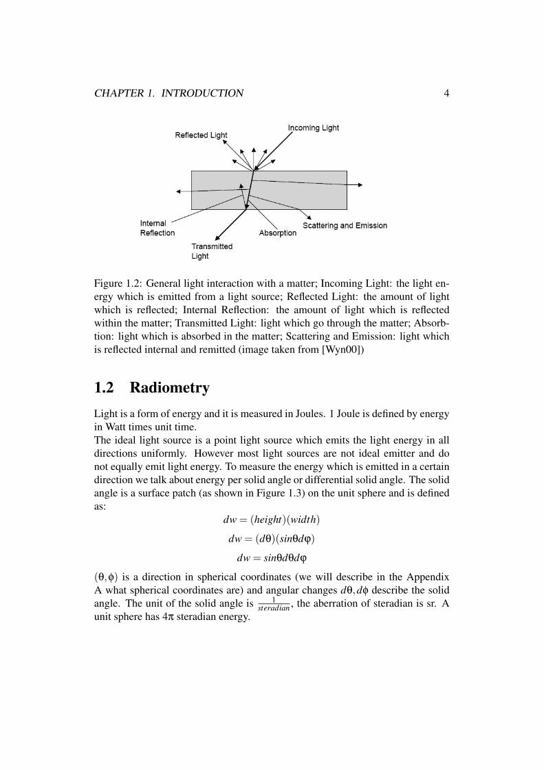
Cones are less sensitive to light, but the human eye has rod cells which are morelight sensitive (rods are responsible for night vision). Rods and cones are mutuallyinterconnected and perform pre-processing tasks like edge enhancement.The LMS cones are color sensitive, also known as RGB sensors, and the rods areluminance sensitive, also known as H (hue). The RGBH signal is converted intothe L*a*b color space.We do not go any deeper in color science in the scope of this thesis, of coursethere is much more to learn about it. There are three main interactions whenlight hits matter, in Figure 1.2 we illustrate it, they are reflection, absorption andtransmittance. The interactions with light depends on the physical compositionand characteristics of the material and the physical composition of light. Figure1.2 shows following items:


Figure 1.2: General light interaction with a matter; Incoming Light: the light en-ergy which is emitted from a light source; Reflected Light: the amount of lightwhich is reflected; Internal Reflection: the amount of light which is reflectedwithin the matter; Transmitted Light: light which go through the matter; Absorb-tion: light which is absorbed in the matter; Scattering and Emission: light whichis reflected internal and remitted (image taken from [Wyn00])

1.2 RadiometryLight is a form of energy and it is measured in Joules. 1 Joule is defined by energyin Watt times unit time.The ideal light source is a point light source which emits the light energy in alldirections uniformly. However most light sources are not ideal emitter and donot equally emit light energy. To measure the energy which is emitted in a certaindirection we talk about energy per solid angle or differential solid angle. The solidangle is a surface patch (as shown in Figure 1.3) on the unit sphere and is definedas:

dw = (height)(width)

dw = (dθ)(sinθdϕ)

dw = sinθdθdϕ

(θ,φ) is a direction in spherical coordinates (we will describe in the AppendixA what spherical coordinates are) and angular changes dθ,dφ describe the solidangle. The unit of the solid angle is 1

steradian , the aberration of steradian is sr. Aunit sphere has 4π steradian energy.


Figure 1.3: Solid angle dw on the unit sphere (image taken from [Geb03])

1.2.1 RadianceRadiance is the measure of light energy which is emitted in a certain direction.When we talk about radiance in connection with the wavelength, we mean thewhole electromagnetic spectrum and not only the range of the visible light. Whenwe talk about luminance we mean only the visible spectrum, exactly speaking,luminance is defined as photometrically weighted light energy that leaves the sur-face.

1.2.2 IrradianceIrradiance is the amount of energy which is received at a surface point. As in thecase of radiance we talk also about the whole spectrum; if we only talk about thevisible spectrum, we talk about illuminance. The irradiance is defined as energyper area. If we move the light source away from the surface, the energy whicharrives at the surface is reduced proportional to the inverse square distance.

1.3 Rendering EquationA surface is visible to human perception when a light source exists, so what weneed is a way to describe the light transport in a scene.Kajiya [Kaj86] introduced 1986 the rendering equation, which describes the light


transport in a scene with one equation. The definition of the rendering equation is

I(x,x′) = g(x,x′)∗ [e(x,x′)+∫

Sp(x,x′,x′′)∗ I(x′,x′′)∗dx′′] (1)

where:

• I(x,x′) is the light energy which pass from a point x′ to point x.

• g(x,x′) is the geometry term which is usually 1r2 where r is the distance

between the points and it is zero if one of them is occluded.

• e(x,x′) the emission term defines how much light energy is emitted from x′

to x.

• p(x,x′,x′′) how much light energy is scattered from x′′ to x through a patchof surface x′; it encodes how light from a given direction is modified uponreflection from a surface.

•∫

S is the integral over S =⋃

Si, the union of all surfaces.

Equation (1) is a Fredholm Integro-differential of second grade which is impossi-ble to solve analytically, due its recursive nature. The rendering equation can bedescribed as a pair of two points (as above) or for a point and a direction.

I(x,ω) = Ie(x,ω)+∫

Ω

fr(x,ω′,ω)∗ I(x,ω′)(ω′.n)∗dω′ (2)

where:

• I(x,ω) is the light energy from point x in direction ω

• Ie(x,ω) emitted from point x in direction ω

• fr(x,ω′,ω) is the BRDF, which defines the proportion of light energy thatis reflected at the position x

• I(x,ω′) is the incoming light energy from the position x and direction ω′

• (ω′.n′) is the attenuation of the incoming light energy due to incident angle

•∫

Ωis the integral over the complete hemisphere


1.4 BRDFThe Bidirectional Reflectance Distribution Function (BRDF) definition dependson the radiance / irradiance ratio. As we already mentioned, radiance tells us howmuch light energy a point distritbute and irradiance,the counterpart to radiance,tells us how much light energy arrives on a surface patch.The BRDF is given by:

fr(ωi→ ωr) =Ir(ω)

Ii(ωr)cos(θi)dωr(3)

• fr(ωi→ ωr) is the BRDF with the unit 1sr

• Ir(ω) is the radiance

• Ii(ωr)cos(θi)dωr is the irradiance, the cosine is the projection from the solidangle to the surface patch

Equation 3 shows that the BRDF is not in the range [0,1] because of the cosineterm. The vectors ωr and ωo are normally parameterized through spherical co-ordinates. In spherical coordinates a vector is described through two angles, theazimuth angle φ and the decline angle θ, both illustrated in Figure 1.4. How tocalculate a vector to spherical coordinate and back to cartesian coordinates is de-scribed in the appendix A.

Figure 1.4: Spherical coordinates: θ the azimuthal angle in the x, y plane; φ is thepolar angle from the z-axis; r is the distance from the origin. (image taken from[Wei])

In the next chapter we present several BRDF models which different materialtypes.


1.4.1 PropertiesEach BRDF has two fundamental properties. The first is that they reciprocity hasto be valid. That means if we swap the incoming ray and the outgoing ray theresulting reflectance value must be the same.

fr(ωi→ ωr) = fr(ωr→ ωi) (4)

The second property is that the energy conservation law holds.∫Ω

fr(ωi→ ωr) <= 1 (5)

The first property is important for raytracing application. Due the symmetry itdoes not matter if we shoot rays from the eye or if we shoot rays from the lightsource, the result must be same. But we also can save storage memory of mea-sured BRDF’s, with the first property, because we only need to store the halfhemisphere.The second property guarantees that a surface is not emitting more energy thanthe incoming light energy. Violating this property would result in a BRDF whichwould glow. Not every BRDF full fill the last property. Also note that theseproperties are unique to reflection.

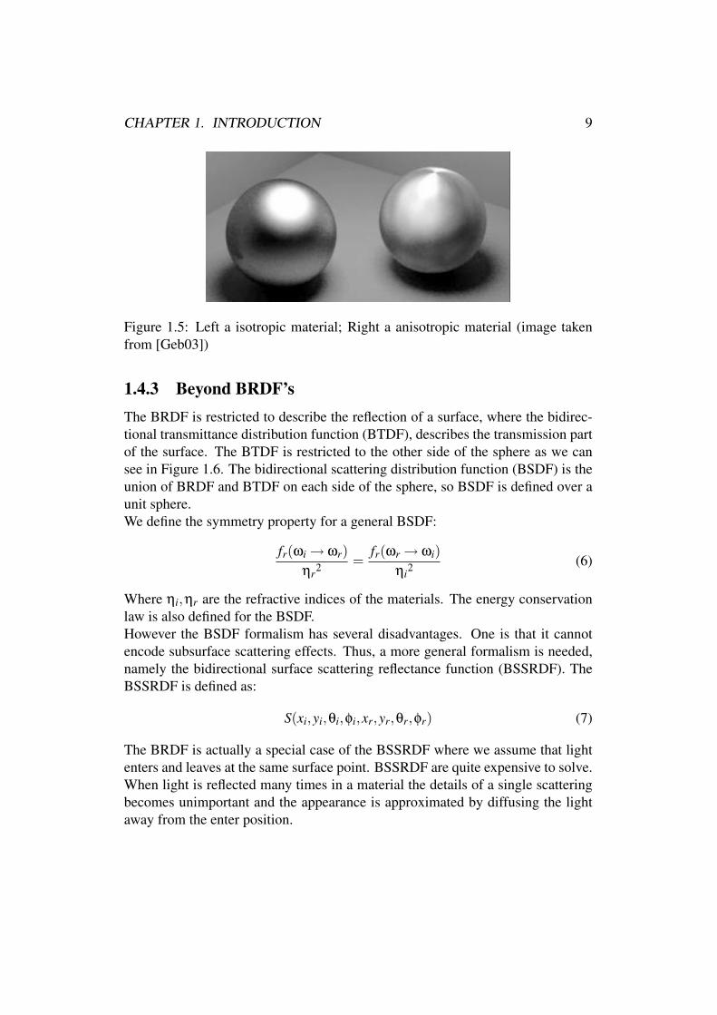
1.4.2 Isotropic And Anisotropic MaterialsThese two classes of BRDF surfaces define a certain behavior dependant on theviewers position and orientation. So anisotropic material change their reflectionbehavior when the viewing angle is changed, brushed metal is e.g. an example foran anisotropic material. The exact definition is that reflectance properties changewith respect to rotation of the surface around the normal vector.Anisotropic materials can also change the reflection in a dynamic manner, thehuman skin is an example for this behavior. But most of the materials are almostrotation invariant, so we can ignore the anisotropic effect for them.Isotropic materials do not depend on the viewer angle, smooth plastic or paints aree.g. examples for isotropic materials. That means that the BRDF for a isotropicmaterial only needs 3 parameters to describe the reflectance. These parametersare Θi,Θr,Φdi f f . The parameter Φdi f f do not need any alignment in world spaceits defined as the difference between Φi and Φr, the angles are shown in Figure1.3.


Figure 1.5: Left a isotropic material; Right a anisotropic material (image takenfrom [Geb03])

1.4.3 Beyond BRDF’sThe BRDF is restricted to describe the reflection of a surface, where the bidirec-tional transmittance distribution function (BTDF), describes the transmission partof the surface. The BTDF is restricted to the other side of the sphere as we cansee in Figure 1.6. The bidirectional scattering distribution function (BSDF) is theunion of BRDF and BTDF on each side of the sphere, so BSDF is defined over aunit sphere.We define the symmetry property for a general BSDF:

fr(ωi→ ωr)ηr2 =

fr(ωr→ ωi)ηi2

(6)

Where ηi,ηr are the refractive indices of the materials. The energy conservationlaw is also defined for the BSDF.However the BSDF formalism has several disadvantages. One is that it cannotencode subsurface scattering effects. Thus, a more general formalism is needed,namely the bidirectional surface scattering reflectance function (BSSRDF). TheBSSRDF is defined as:

S(xi,yi,θi,φi,xr,yr,θr,φr) (7)

The BRDF is actually a special case of the BSSRDF where we assume that lightenters and leaves at the same surface point. BSSRDF are quite expensive to solve.When light is reflected many times in a material the details of a single scatteringbecomes unimportant and the appearance is approximated by diffusing the lightaway from the enter position.


Figure 1.6: Left: BRDF describes the reflection off the surface; Right: BRDF +BTDF describes light rays which are reflected through the microfacet structure ofthe surface. (image taken from [Wik])

1.5 Purpose and OutlineThe main purpose of thesis is to integrate measured BRDF data from the Mit-subishi Electric Research Laboratories (merl) [MPBM03] and data from the Cor-nell University in ART (Advanced Rendering Toolkit). ART is a photorealisticrendering toolkit which is developed by the Institute of Computer Graphics andAlgorithms of the Vienna University of Technology.The merl database has over 100 isotropic materials which are very dense mea-sured, the color space of the data is RGB. To calculate the solid angle for eachray pair we had to resample the data once for each material. The Cornell databasehas 11 different isotropic materials, the measurement are present as spectral datain different sampling rates and are also present as RGB data without any gamutmapping, the data contains negative red values. The main purpose of this is togenerate reference images to test the analytical surfaces in other words to createground truth images.In the next chapter we present different reflectance models then we talk aboutBRDF acquisition and describe the acquisition process. The chapter about MonteCarlo renderings introduces the reader in the basics of the Monte Carlo methodswhich are essential for image synthesis. Finally we show our implementation andthe rendering results.

Chapter 2

Representing BRDFs

There are different ways to describe materials through a BRDF representation.The first way is the measure and fit approach-we could measure a material witha Gonioreflectometer and use the measured data for the rendering. Measuring asurface is time consuming and could take several hours ([Mat03]). The fact thatthe BRDF is a four dimensional function makes the measuring process technicalchallenging, but the measuring approach is necessary for verification purposes,although thats not the only area where measured data are needed.For example, the NASA has a Reflectometer(SOC-200) which they use to de-sign paints for Stealth aircrafts. These paints absorb and reflect electromagneticwaves in the wrong direction and making the painted object invisible for the radar.Measured BRDF’s are also used in the movie ”The Matrix 2” for realistic clothrendering ([Bor03]).Another representation of BRDF is the approximation through analytical re-flectance models. The two types of analytical reflectance models are the physicalplausible models and empirical reflectance models (also known as phenomeno-logical reflectance model). Physical plausible reflectance models try to take careof the physical properties of the material, so that each parameter has a physicalmeaning, and could be theoretically measured. Empirical (or phenomenological)reflectance models describing reflectance with parameters that do not have anyphysical mean such as the Phong [Pho75] reflectance model. But before we de-scribe some BRDF models, we present some material classification in the nextsection.

2.1 Material ClassificationWe already introduced isotropic and anisotropic materials. Now we introduceoptical material properties for material classification: ideal diffuse, ideal specular,

11

CHAPTER 2. REPRESENTING BRDFS 12

directional diffuse and rough specular.

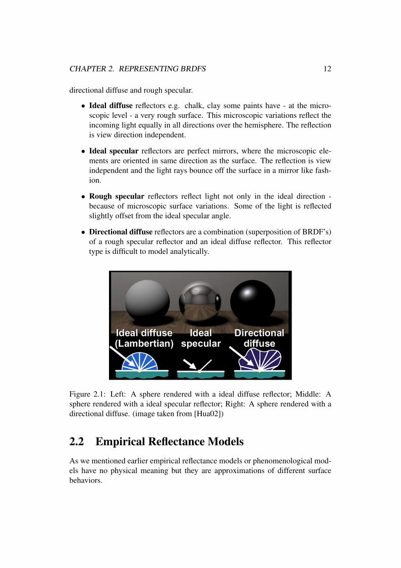
• Ideal diffuse reflectors e.g. chalk, clay some paints have - at the micro-scopic level - a very rough surface. This microscopic variations reflect theincoming light equally in all directions over the hemisphere. The reflectionis view direction independent.

• Ideal specular reflectors are perfect mirrors, where the microscopic ele-ments are oriented in same direction as the surface. The reflection is viewindependent and the light rays bounce off the surface in a mirror like fash-ion.

• Rough specular reflectors reflect light not only in the ideal direction -because of microscopic surface variations. Some of the light is reflectedslightly offset from the ideal specular angle.

• Directional diffuse reflectors are a combination (superposition of BRDF’s)of a rough specular reflector and an ideal diffuse reflector. This reflectortype is difficult to model analytically.

Figure 2.1: Left: A sphere rendered with a ideal diffuse reflector; Middle: Asphere rendered with a ideal specular reflector; Right: A sphere rendered with adirectional diffuse. (image taken from [Hua02])

2.2 Empirical Reflectance ModelsAs we mentioned earlier empirical reflectance models or phenomenological mod-els have no physical meaning but they are approximations of different surfacebehaviors.


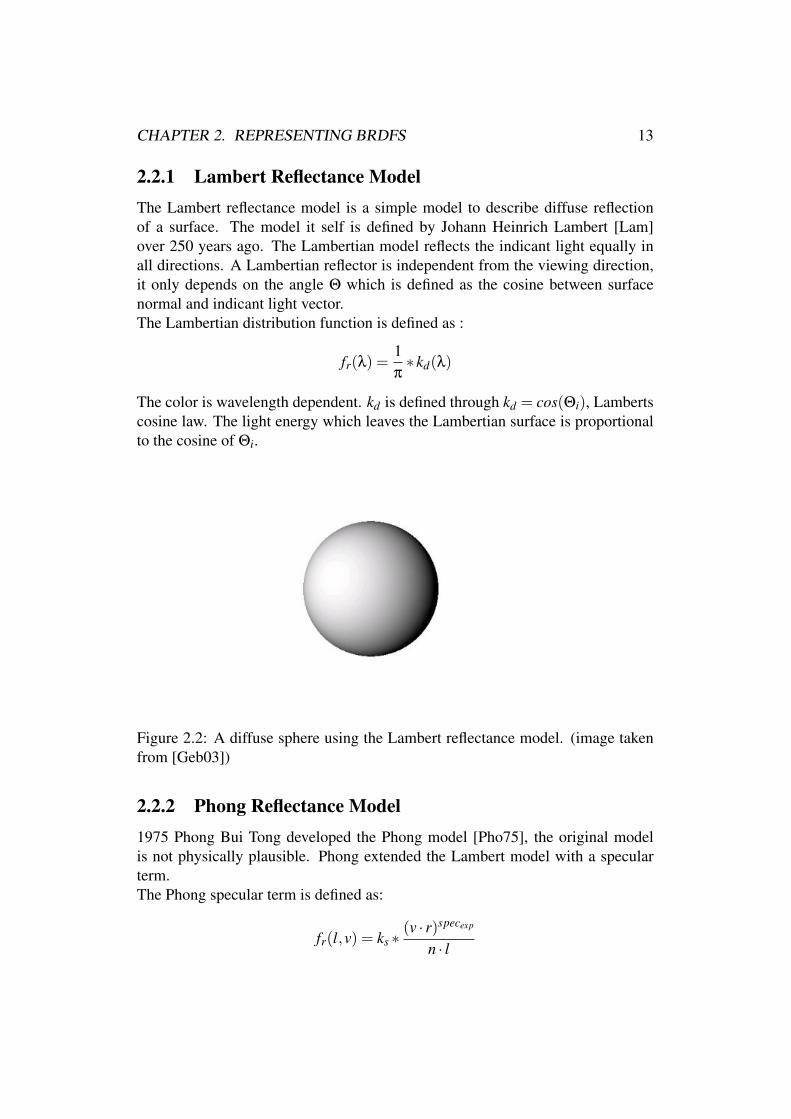
2.2.1 Lambert Reflectance ModelThe Lambert reflectance model is a simple model to describe diffuse reflectionof a surface. The model it self is defined by Johann Heinrich Lambert [Lam]over 250 years ago. The Lambertian model reflects the indicant light equally inall directions. A Lambertian reflector is independent from the viewing direction,it only depends on the angle Θ which is defined as the cosine between surfacenormal and indicant light vector.The Lambertian distribution function is defined as :

fr(λ) =1π∗ kd(λ)

The color is wavelength dependent. kd is defined through kd = cos(Θi), Lambertscosine law. The light energy which leaves the Lambertian surface is proportionalto the cosine of Θi.

Figure 2.2: A diffuse sphere using the Lambert reflectance model. (image takenfrom [Geb03])

2.2.2 Phong Reflectance Model1975 Phong Bui Tong developed the Phong model [Pho75], the original modelis not physically plausible. Phong extended the Lambert model with a specularterm.The Phong specular term is defined as:

fr(l,v) = ks ∗(v · r)specexp

n · l


Where l is the light vector (vector from the surface point to the light source), v isthe view vector (from viewer to the surface point), r reflection vector (in whichdirection the light is reflected), ks is the specular coefficient and specexp is thespecular exponent. For this model, Phong made two assumptions, namely all lightsources are moved to infinite and that the viewer is also moved to infinite.Since this equation only describes the specular term, the full equation is the sum(superposition) of the diffuse (Lambert) term and the specular term:

fr(l,v) =1π∗ kd + ks ∗

(v · r)specexp

n · l

There is also a modification of the Phong model by Lewis [Lew93] which make itphysical plausible.

2.2.3 Lafortune Reflectance ModelThe Lafortune et al. [LFTG97] model is a generalization of the cosine lobe modelfrom Lewis which is based on the Phong model. Lafortune et al. [LFTG97] de-veloped a model which can describe various BRDFs like non-Lambertian diffusereflection, specularity at grazing angles, off-specular reflection, retro reflectionand anisotropic reflection. The main drawback of the original cosine lobe modelis that there are several problems with directional-diffuse reflectance.The definition of the generalization of the classical cosine lobe model is:

fr(L,V ) =kd

π+ ks(LT MV )n

where:

• L is the unit vector to the light source

• V is the unit view vector

• kd is the diffuse coefficient

• ks is the specular coefficient

• M is 3 x 3 matrix which must be symmetric; otherwise the Helmholtz reci-procity would not hold

• n is the specular exponent


After singular value decomposition of the matrix M we get M = QT DQ.Where Q is the transformation of the local coordinate system and D is a diag-onal matrix.Now we can rewrite model as:

fr(L,V ) =kd

π+ ks(CxLxVx +CyLyVy +CzLzVz)n

With the parameters Cx,Cy and Cz we can form several BRDF models. For aisotropic reflection the parameter Cx and Cy have to be equal.To get the original cosine lobe the parameters have to following appearance−Cx =−Cy =−Cz = n

√Cs. To gain an anisotropic reflection the parameters Cx,Cy and Cz

must assigned with different values. These parameters are described in detail in[LFTG97].

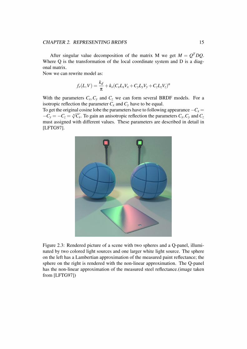
Figure 2.3: Rendered picture of a scene with two spheres and a Q-panel, illumi-nated by two colored light sources and one larger white light source. The sphereon the left has a Lambertian approximation of the measured paint reflectance; thesphere on the right is rendered with the non-linear approximation. The Q-panelhas the non-linear approximation of the measured steel reflectance.(image takenfrom [LFTG97])


2.2.4 Ward Reflectance ModelIn the year 1992 Ward [War92] build an image based gonioreflectometer to mea-sure and acquire data from isotropic and anisotropic surfaces. Ward measuredrolled brass, rolled aluminum, lightly brushed aluminum, varnished plywood,enamel finished metal and a painted cardboard box also isotropic surfaces mea-sured like glossy grey paper. The measurements of the Ward imaging gonioreflec-tometer prototype has two limitations. First the prototype is not able to measurenear grazing angles. The second limitation is that the prototype is not able to mea-sure polished surfaces with sharp specular peaks.To use the raw measurement data for the rendering is impractical due the natureof the data. The data is incomplete to represent to whole hemisphere and to noisy.Therefore Ward tried to develop a model which fits the data for the isotropic andanisotropic measurments with as few parameters as possible.The aim of the Ward model is first to fulfill physical properties (energy conserva-tion, Helmholtz reciprocity) and second to be mathematical simple like the widelyused Phong model. The Gaussian distribution, which is often used in formulationsof reflectance ([War92], [CT82], [Coo86]), is used to describe the statistical differ-ence of the surface height. The Gaussian model is used instead of the commonlyused geometric attenuation factors and the Fresnel coefficient, the geometric fac-tors usually tend to counteract to the Fresnel coefficient Ward [War92].The isotropic Gaussian Model:

fds,iso(θi,φi,θr,φr) =fd

π+ fs ∗

1√cos(θi)cos(θr)

∗ exp[−tan2δ/α2]4πα2

where:

• fd is the diffuse reflectance

• fs is the specular reflectance

• δ is the angle between the surface normal vector and the half vector

• α is the standard deviation of the surface slope, α should not greater than0.2 to no violate the normalization

• 14πα2 is the normalization factor


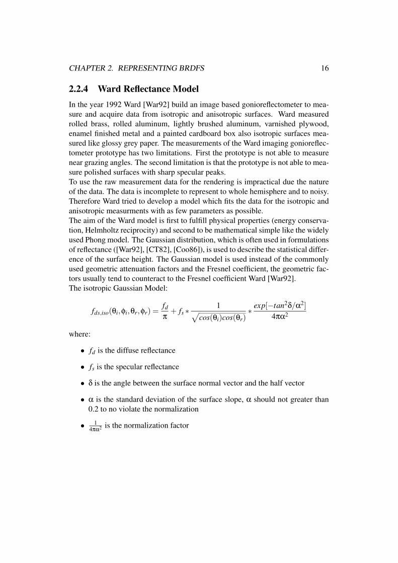
Figure 2.4: Material independent variables and angles which are used in the Wardreflectance model where x and y are the tangents of the surface point, n is thenormal vector, h is the half vector between dr and di; ”the indicant light arrivesalong di and is simulated or measured in direction dr” Ward [War92]. (imagetaken from [Geb03] and slightly modified)

The Gaussian reflectance model is extended to support surfaces with two perpen-dicular slope distributions, αx and αy. The anisotropic Gaussian Model is definedas follows:

fds(θi,φi,θr,φr)=fd

π+ fs∗


∗exp[−tan2δ(cos2φ/αx

2 + sin2φ/αy2)]

4παx2αy2

where:

• fd is the diffuse reflectance

• fs is the specular reflectance

• δ is the angle between the surface normal vector and the half vector

• αx is the standard deviation of the surface slope in x direction

• αy is the standard deviation of the surface slope in y direction

• φ is the azimuth angle of the half vector projected into the surface plane


A computationally approximation of the above equation is:

fds(θi,φi,θr,φr)=fd

π+ fs∗


∗ 14παxαy

∗exp(−2(h·−→x

αx)2 +(h·−→y

αy)2

1+h ·n)

where:

• h ·−→x = sinθrcosθr+sinθicosθi

||−→h ||

• h ·−→y = sinθrsinθr+sinθisinθi

||−→h ||

• h ·−→n = cosθr+cosθi

||−→h ||

• ||−→h ||=

√2+2sinθrsinθi(cosθrcosθi + sinθrsinθi)+2cosθrcosθi

The missing variables are described in Figure 2.4. So the total reflectance is thesum of the fd term (diffuse term) and the fs term (rough specular term). ”αx andαy represent the standard deviation of the surface slope in each of the perpendic-ular directions” Ward [War92]. All four variables have a physical meaning andcould optionally measured.

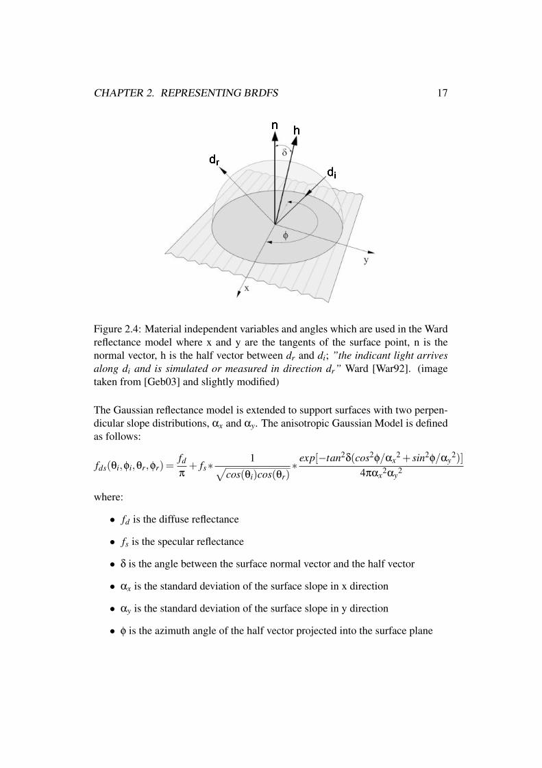
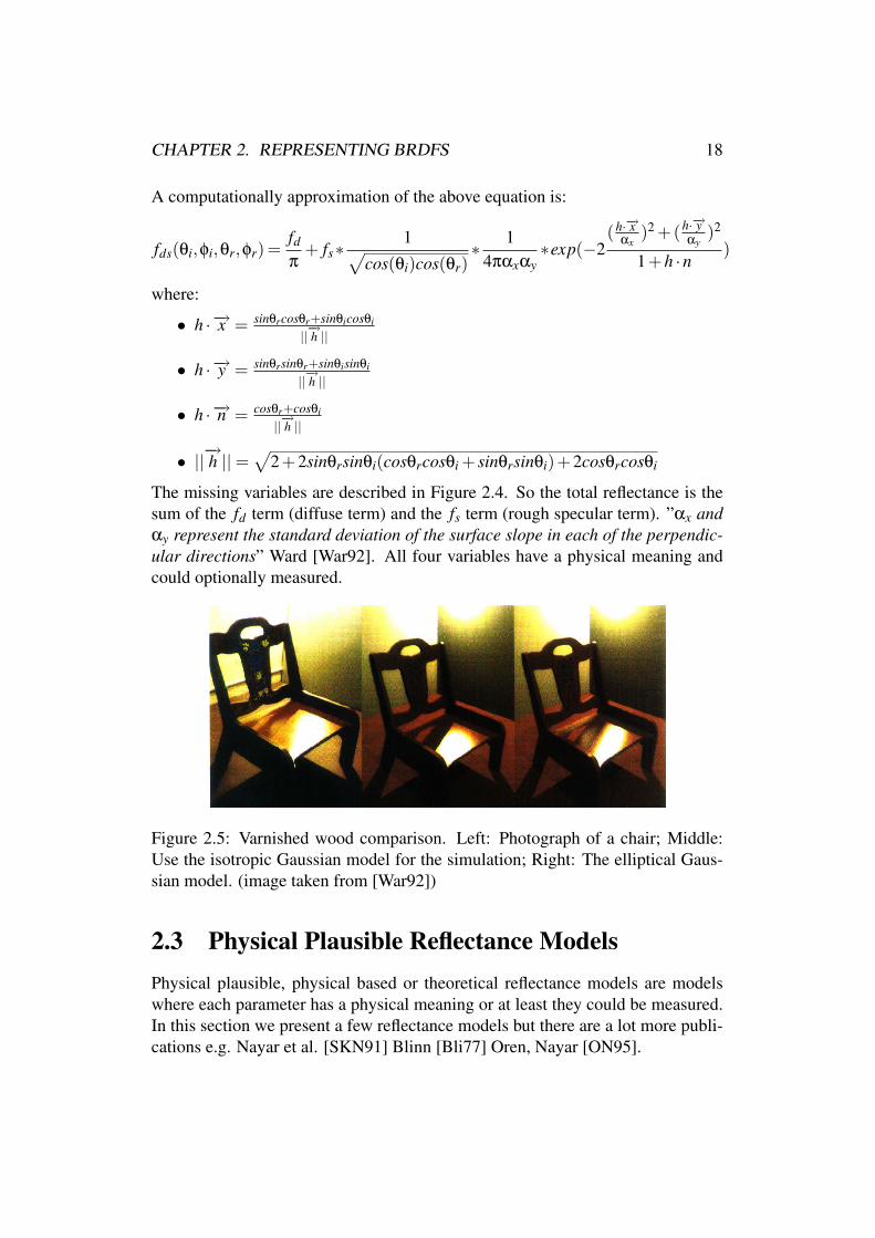
Figure 2.5: Varnished wood comparison. Left: Photograph of a chair; Middle:Use the isotropic Gaussian model for the simulation; Right: The elliptical Gaus-sian model. (image taken from [War92])

2.3 Physical Plausible Reflectance ModelsPhysical plausible, physical based or theoretical reflectance models are modelswhere each parameter has a physical meaning or at least they could be measured.In this section we present a few reflectance models but there are a lot more publi-cations e.g. Nayar et al. [SKN91] Blinn [Bli77] Oren, Nayar [ON95].


2.3.1 Cook-Torrance Reflectance ModelThe model from Cook and Torrance [CT82], which was published in 1982, isbased on the model from Torrance and Sparrow [KET67] and the Blinn [Bli77]reflectance model. The Cook-Torrance model is able to represent different metalslike gold but it is also capable to represent plastic with various roughens.The Torrance-Sparrow model was the first published physically based BRDFmodel. The calculations of reflectance from roughed surfaces are on the basisof geometrical optics, also the calculations are only valid if the wavelength λ oflight is smaller than the least squared mean σm of the surface roughness. Also theroughness of the surface is assumed to be isotropic. Furthermore Torrance andSparrow showed that the assumption that the reflectance of roughed surfaces onlyoccur in form of diffuse reflection only hold if the indicant angle is near to thesurface normal vector. But the also showed that the maximum energy occur on aangle which is greater than the specular peak this phenomena is called off specularpeak [KET67].The Cook-Torrance reflectance model is composed from three different compo-nents the microfacet distribution, the Fresnel coefficients and the geometric atten-uation.The facets are assumed as mirror-like (perfectly reflective) and isotropic dis-tributed. It is also assumed that the facets are V-shaped, this means that eachneighbor has the same slope angle but in the inverse direction. In the Cook-Torrance model it is possible to use different distributions for the microfacet orien-tations, the Torrance-Sparrow model is restricted to a Gauss distribution, but theymake use of the Beckmann distribution function. The geometric term accountseffects of masking and shadowing between microfacets (shown in Figure 2.6), theterm determine the amount of the specular reflection.

Figure 2.6: Left: shows the masking and self shadowing effects due the microfacetsurface structure;Right: show the v-shaped facets. (image taken from [Wyn00])

The geometric term does not depend on any physical property of the surface.The Fresnel term determine the reflection of each microfacet.


The Cook-Torrance model is defined as:

fr(θi,φi,θr,φr) =kd

π+

ks

π∗ FDG

cos(θi)cos(θr)

where:

• kd is the diffuse reflectance coefficient

• ks is the specular reflectance coefficient

• F is the Fresnel coefficient

• D is the geometric attenuation

• G is the microfacet distribution

With the Cook-Torrance model it was first possible to render rough conductorsthat have the unique property that their highlights are colored. With simple BRDFmodels like the Phong model every material looks like plastic because of the whitehighlight.

Figure 2.7: Several materials simulated with the Cook-Torrance reflectance model(image taken from [CT82])

2.3.2 He-Torrance-Sparrow-Green Reflectance ModelHe et. al. [HTSG91] developed as a model which takes the wave nature of lightinto account to model phenomena like interference and diffraction.


The model consists of three main reflectance components: specular, directionaldiffuse and uniform diffuse. The model itself is an analytic model which hassmooth transitions from the specular to the diffuse reflectance behavior. The spec-ular component accounts mirror like facets, like the Cook-Torrance model, alsoroughness, shadowing/masking and the Fresnel term is taken into account.The specular component is the result of the first surface reflection. The direc-tional diffuse is responsible for diffraction and interference effects. The uniformdiffuse component estimates that the microfacets are V-shaped, based on geo-metrical optics. Multiple surface and subsurface reflections result as the uniformdiffuse term. The HTSG has several parameters. These are: surface roughness,index of refraction, autocorrelation length and uniform diffuse term. The defini-tion of the reflectance model is the sum of the three components. Due the complexnature of the terms we redirect to the original paper, which is a good starting pointfor the reader.

Chapter 3

BRDF Acquisition

The BRDF can be directly measured from real surfaces. There are several BRDFdata sets available which already measurement. This chapter gives an overviewabout a device for measuring the BRDF from a surface. Furthermore we reviewseveral BRDF measurement databases which are available, free of any charge, foracademic purpose.

3.1 GonioreflectometerA gonioreflectometer is a device for BRDF acquisition, but there exist severaldifferent gonioreflectometer types e.g. Murray etal. [MC75], Foo [Foo97] orWard [War92].Murray etal. [MC75] designed a basic gonioreflectometer, which is shown inFigure 3.1. The measuring system consists of a light source, material source anda reflectance detector.

• The light source is an MR16 incandescent lamp.

• The photodetector is of the silicon photodiode type.

• The material sample diameter is only 6.5mm

These three components are positioned with stepper motors, so the system pro-vides the needed four degree of freedom which is required by the - anisotropic -BRDF definition. The stepper motors are controlled by a computer, with ASCIIcommands, through the RS232 serial port. The system measure the voltage differ-ential to the illuminance on the face of the photocell Murray etal. [MC75] for thedata acquisition.

22

CHAPTER 3. BRDF ACQUISITION 23

Figure 3.1: Basic gonioreflectometer designed by Murray etal. [MC75] (imagetaken from [MC75])

In contrast to that Ward [War92] build an imaging gonioreflectometer, namelya silver hemisphere reflectometer. The system consists of a half-silvered hemi-sphere, a CCD camera with a fish-eye lens, a light source (a three watt quartz-halogen lamp) and a sample holder. The light is reflected from the material tothe silver hemisphere which reflect the light onto the CCD array. A computercontrolled motor moves the light source during data acquisition and the sample ismoved manually.

Figure 3.2: Side view of the imaging gonioreflectometer designed by Ward[War92]. (image taken from [War92])


The use of the gonioreflectometer in his ordinary form is slow and time con-suming. Ward’s imaging gonioreflectometer can obtain BRDF results faster, thehemisphere of reflection is captured in one image, and at lower cost as the tradi-tional approach. The Cornell University [Foo97] extended the imaging approachand built their own device. Matusik [Mat03] also built an imaging gonioreflec-tometer which is described in the next section.

3.2 BRDF Measurement DatabasesIn this thesis two BRDF databases are used for the image synthesis, the first oneis the database which the Cornell University offers and the second one is offeredby the Mitsubishi Electric Research Laboratories (Merl). In the next two sectionswe take a deeper look how this two databases acquired their BRDF data from thematerials. For the sake of completeness the CURet database is also mentionedhere, but this one is not used for image synthesis.

3.2.1 CUReT DatabaseThe CUReT database consists of 60 measured materials, the samples are not densemeasured approximately 200 reflectance measurements over varying incident andreflected angles (Dana etal. [DvGNK99]). They also offer a BRDF parameterdatabase which fits the parameters for the Oren-Nayar [ON95] and the Koenderinkreflectance model ([DvGNK99]).The samples are not dense enough to use it directly as BRDF lookup table and togenerate a reference image (in fact it could be used with interpolation, but thenwe do not get a meaningful reference image).

3.2.2 Cornell DatabaseThe Cornell University offers also a small BRDF database [LFTG97] which con-sists of eleven material samples which are all isotropic. The samples are availableas spectral, XYZ or as RGB data. Each material sample has over 1000 measure-ments of varying incident and reflected angles and can be used as BRDF lookuptable for direct rendering.They originally measured 1024 wavelength samples, per sample point, which aredown sampled to 65 or 31 wavelengths with a regular sample distance from 5 or10 nm. They sampled between 400 and 700nm due to the fact that the samplingsbelow 400 and over 700nm are noisy. The raw data, which is available on theCornell website, has several errors and are not interpolated except the house paintdata which is interpolated and cleaned. Unfortunately the measuring process of


the materials are not documented except the house paint [LFTG97] and the acqui-sition of the skin measuring [MWLT00].

3.2.3 MERL DatabaseThe Mitsubishi Electric Research Laboratories [MPBM03] have the largestisotropic BRDF database and consists of over 100 materials. They build a cus-tom imaging gonioreflectometer for the BRDF acquisition. The device was buildwith the idea in mind to make dense BRDF measurements which could directlyused as a table-based model.Matusik [Mat03] put the measurement system in an isolated room, the walls in theroom were painted with a matte black paint. The gonioreflectometer itself consistof three main components: ”QImaging Retiga 1300 (a 10-bit, and a 1300 x 1030resolution Firewire camera), a Kaidan MDT-19 (a precise computer-comtrolledturntable), and a Hamamatsu SQ Xenon lamp (a lamp with stable light emissionoutput and a continuous and relatively constant radiation spectrum over the visi-ble light range”[Mat03]. The light source can move in 0.5 increments. However,to cover the whole hemisphere, the imaging gonioreflectometer needs 330 HighDynamic Range (HDR) images; to capture these images the system needs 4 hours.To get the relative position between light source, camera and material source, ageometric calibration has to be done which is described in detail in [Mat03]. Dueto the fact that the camera can only make 10-bit images, they make use of themulti-exposure technique to capture the dynamic range of the scene. So eachHDR image is composed from eighteen 10-bit pictures with increasing exposuretime.To compute the BRDF for a pixel one need - beside the radiance of the pixel whichis already given by the HDR images - the irradiance for the pixel. To calculate theirradiance, the image pixel is intersected with the sphere to determine the point pon the material source. Then the normal vector of p is calculated. But one alsoneeds the distance to the light source from p and the camera vector. With thesevariables Matusik was able to calculate the irradiance. Since the BRDF is the ratiobetween radiance and irradiance, Matusik was able to calculate the BRDF valuefor a point p on the material source.The data representation could not done with a regular sampled grid over the hemi-sphere, even with high tesselated one, because the specular peaks become ovallobes. Rusinkiewicz [Rus04] proposed a new coordinate frame (illustrated in Fig-ure 3.3) which require less storage space for isotropic BRDF’s and represent thespecular peak efficiently (the new coordinate frame is described in detail in ap-pendix B). With the new coordinate frame [Mat03] was able to use smaller binsnear the specular angle, so in fact, the grid is irregular. Matusik subdivide the θhand θd in 90 bins and φd in 360 bins, but through the reciprocity property of the


BRDF he cut it to 180 bins down. The resulting data set has 1,458,000 bins percolor channel.The samples are very dense measured and can directly used as tabulated BRDFtable or it can be used to create new BRDF’s through linear combination of theexistent measurements. MERL has also a small BRDF database for anisotropicmaterials which is - since we concentrated on isotropic BRDF’s in the scope ofthis thesis - not relevant for us. Ngan et. al. [NDM05] have also analyzed thecomplete isotropic BRDF database and fitted several analytical models to theirmeasurements.

Figure 3.3: Left: ordinary coordinate frame, Right: Rusinkiewicz coordinateframe. (image taken from [Rus04])

In this thesis the Cornell and the isotropic Merl database are used for the imagesynthesis in ART (Advanced Rendering Toolkit). In the next chapter we take anoverview about Monte-Carlo sampling, which we need to sample the BRDF data.

Chapter 4

Monte Carlo Rendering

Scientists introduced the term Monte Carlo in the year 1940 while working on nu-clear weapon projects in the Los Alamos National Laboratory. It refers to mathe-matical techniques that use statistical sampling to solve a problem1. Monte Carlomethods have a wide spread application field from the Physical chemistry, Relia-bility engineering to Computer Graphics.Monte Carlo raytracing (Jensen [Jen01]) is important for realistic image synthesisfrom complex scenes. As mentioned in chapter one we have to solve the render-ing equation [Kaj86], which describe the light transport in the scene. One way tosolve this equation is to use Monte Carlo methods.In former times finite element methods were the first choice to solve the equationnumerically. Finite element methods have several drawbacks, which Monte Carlomethods do not have. With finite element methods the scene geometry must betessellated, which result in high memory consumption, also not every BRDF canhandled with these methods. Also the runtime of Monte Carlo based algorithm arein O(logN), where the fastest finite element method is in O(NlogN). The biggestdrawback of Monte Carlo raytracing is the variance seen as noise in the renderedimages. There are several methods to decrease the noise which we catch later inthis chapter.This chapter has following structure: first we take an short overview about thebasic elements of the probability theory then we discuss Monte Carlo integrationand introduce several sampling methods.

1There are also Las Vegas methods which use also randomness in their algorithms. The dif-ference between them is that Las Vegas methods use randomness but the give always the correctresult in contrast Monte Carlo methods return frequently the wrong result but return the correctresult in average.

27

CHAPTER 4. MONTE CARLO RENDERING 28

4.1 Basic Elements Of The Probability TheoryIn this section discusses the basic elements of the probability theory. Note thatwe only discuss a tiny subset of the probability theory. Also note that this is onlya review of the basic elements and not a in depth explanation, for an in depthexplanation read Kalos and Whitlock [KW86].

4.1.1 Random VariableA random variable X is defined as an scalar or vector quantity whose values aretaken from some domain Ω. The domain Ω can be discrete or continues. Adiscrete domain is for example all values that can appear when a dice is tossedthen X is a random variable defined as X ∈ 1,2,3,4,5,6. Continues randomvariable X is defined as X ∈ −∞,∞. A distribution of values describes thebehavior of the random variable X . Furthermore, the distribution of values can bedescribed by the probability density function (from now on we use the acronymPDF) which we describe in the next section.

4.1.2 Probability Density FunctionUsually when a random variable X has a certain PDF p this association is denotedas X ∼ p. The density function p defines the relative likelihood of a randomvariable X which takes a certain value.The PDF must fulfil two properties:

• p(X)≥ 0 the probability is always positive (including zero)

•∫

Ωp(X)dx must integrate to over the domain Ω

4.1.3 Cumulative Distribution FunctionThe cumulative distribution function (CDF) describes the probability distributionof random variable X. The CDF of X is defined as: F(X) =

∫ xΩ

p(X)dxThe CDF must fulfil two properties:

• limx→−∞

F(X) = 0

• limx→+∞

F(X) = 1


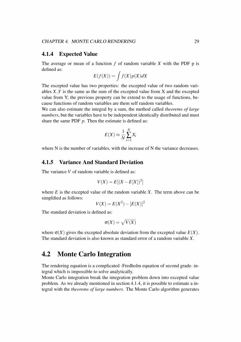
4.1.4 Expected ValueThe average or mean of a function f of random variable X with the PDF p isdefined as:

E( f (X)) =∫

f (X)p(X)dX

The excepted value has two properties: the excepted value of two random vari-ables X ,Y is the same as the sum of the excepted value from X and the exceptedvalue from Y; the previous property can be extend to the usage of functions, be-cause functions of random variables are them self random variables.We can also estimate the integral by a sum, the method called theorems of largenumbers, but the variables have to be independent identically distributed and mustshare the same PDF p. Then the estimate is defined as:

E(X)≈ 1N

N

∑i=1

Xi

where N is the number of variables, with the increase of N the variance decreases.

4.1.5 Variance And Standard DeviationThe variance V of random variable is defined as:

V (X) = E[(X−E[X ])2]

where E is the excepted value of the random variable X . The term above can besimplified as follows:

V (X) = E(X2)− [E(X)]2

The standard deviation is defined as:

σ(X) =√

V (X)

where σ(X) gives the excepted absolute deviation from the excepted value E(X).The standard deviation is also known as standard error of a random variable X .

4.2 Monte Carlo IntegrationThe rendering equation is a complicated -Fredholm equation of second grade- in-tegral which is impossible to solve analytically.Monte Carlo integration break the integration problem down into excepted valueproblem. As we already mentioned in section 4.1.4, it is possible to estimate a in-tegral with the theorems of large numbers. The Monte Carlo algorithm generates


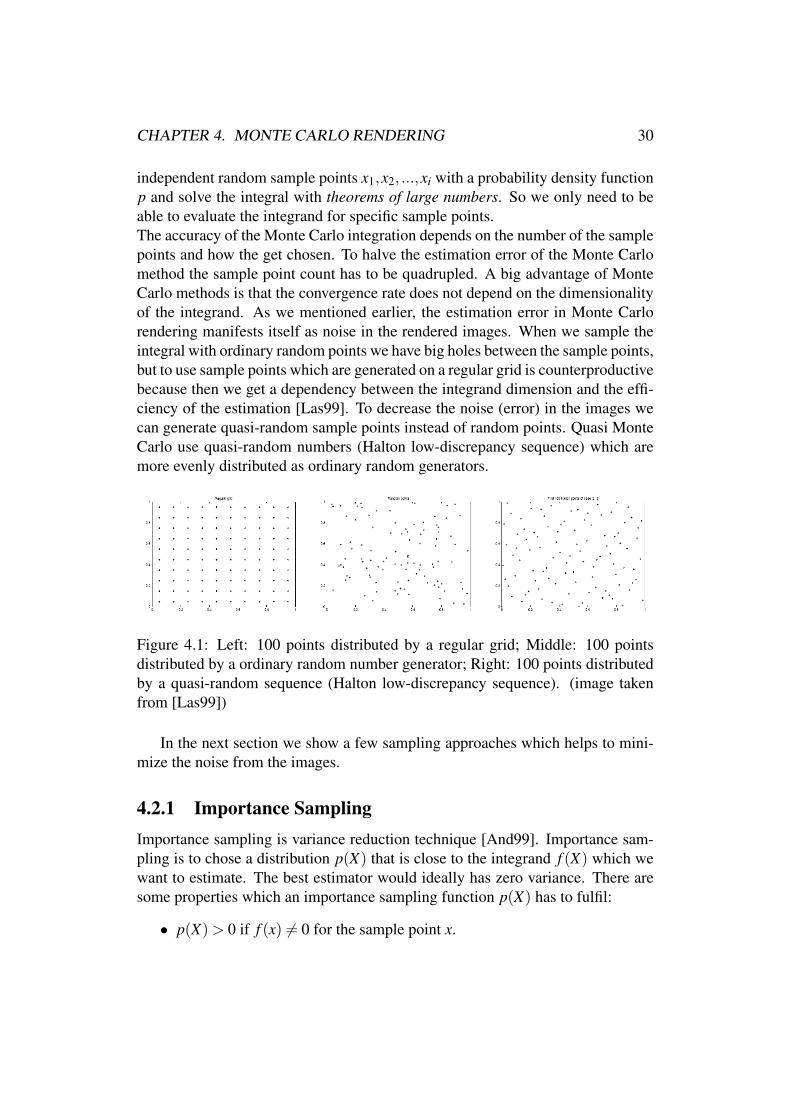
independent random sample points x1,x2, ...,xi with a probability density functionp and solve the integral with theorems of large numbers. So we only need to beable to evaluate the integrand for specific sample points.The accuracy of the Monte Carlo integration depends on the number of the samplepoints and how the get chosen. To halve the estimation error of the Monte Carlomethod the sample point count has to be quadrupled. A big advantage of MonteCarlo methods is that the convergence rate does not depend on the dimensionalityof the integrand. As we mentioned earlier, the estimation error in Monte Carlorendering manifests itself as noise in the rendered images. When we sample theintegral with ordinary random points we have big holes between the sample points,but to use sample points which are generated on a regular grid is counterproductivebecause then we get a dependency between the integrand dimension and the effi-ciency of the estimation [Las99]. To decrease the noise (error) in the images wecan generate quasi-random sample points instead of random points. Quasi MonteCarlo use quasi-random numbers (Halton low-discrepancy sequence) which aremore evenly distributed as ordinary random generators.

Figure 4.1: Left: 100 points distributed by a regular grid; Middle: 100 pointsdistributed by a ordinary random number generator; Right: 100 points distributedby a quasi-random sequence (Halton low-discrepancy sequence). (image takenfrom [Las99])

In the next section we show a few sampling approaches which helps to mini-mize the noise from the images.

4.2.1 Importance SamplingImportance sampling is variance reduction technique [And99]. Importance sam-pling is to chose a distribution p(X) that is close to the integrand f (X) which wewant to estimate. The best estimator would ideally has zero variance. There aresome properties which an importance sampling function p(X) has to fulfil:

• p(X) > 0 if f (x) 6= 0 for the sample point x.


• it should be fast to sample from p(X).

• p(X) should be proportional to f (X), like p(X)∗α≥ f (X).

• it should be possible to compute the density p(X) for any value of X .

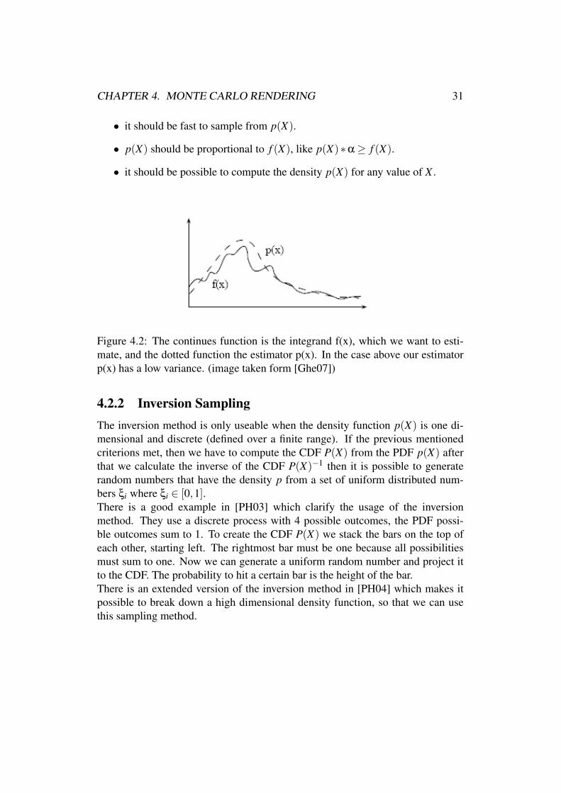
Figure 4.2: The continues function is the integrand f(x), which we want to esti-mate, and the dotted function the estimator p(x). In the case above our estimatorp(x) has a low variance. (image taken form [Ghe07])

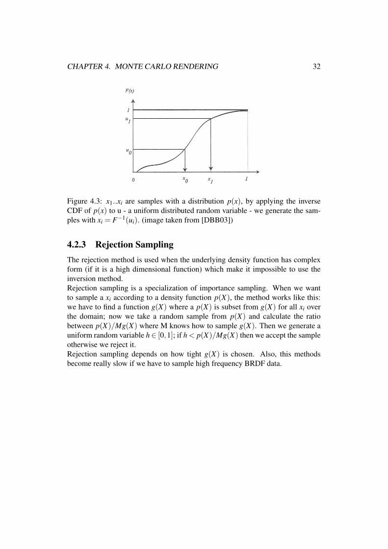
4.2.2 Inversion SamplingThe inversion method is only useable when the density function p(X) is one di-mensional and discrete (defined over a finite range). If the previous mentionedcriterions met, then we have to compute the CDF P(X) from the PDF p(X) afterthat we calculate the inverse of the CDF P(X)−1 then it is possible to generaterandom numbers that have the density p from a set of uniform distributed num-bers ξi where ξi ∈ [0,1].There is a good example in [PH03] which clarify the usage of the inversionmethod. They use a discrete process with 4 possible outcomes, the PDF possi-ble outcomes sum to 1. To create the CDF P(X) we stack the bars on the top ofeach other, starting left. The rightmost bar must be one because all possibilitiesmust sum to one. Now we can generate a uniform random number and project itto the CDF. The probability to hit a certain bar is the height of the bar.There is an extended version of the inversion method in [PH04] which makes itpossible to break down a high dimensional density function, so that we can usethis sampling method.


Figure 4.3: x1..xi are samples with a distribution p(x), by applying the inverseCDF of p(x) to u - a uniform distributed random variable - we generate the sam-ples with xi = F−1(ui). (image taken from [DBB03])

4.2.3 Rejection SamplingThe rejection method is used when the underlying density function has complexform (if it is a high dimensional function) which make it impossible to use theinversion method.Rejection sampling is a specialization of importance sampling. When we wantto sample a xi according to a density function p(X), the method works like this:we have to find a function g(X) where a p(X) is subset from g(X) for all xi overthe domain; now we take a random sample from p(X) and calculate the ratiobetween p(X)/Mg(X) where M knows how to sample g(X). Then we generate auniform random variable h∈ [0,1]; if h < p(X)/Mg(X) then we accept the sampleotherwise we reject it.Rejection sampling depends on how tight g(X) is chosen. Also, this methodsbecome really slow if we have to sample high frequency BRDF data.


Figure 4.4: Rejection sampling: blue samples are accepted (∈ p(X)), red samplesare rejected (3 p(X)). (image taken form [Ghe07])

Chapter 5

Implementation

In this chapter we present the implementation of this diploma thesis but also givea short introduction about the rendering toolkit which was used for the implemen-tation.

5.1 Rendering in ARTSince 1996 the Institute of Computer Graphics and Algorithms of the Vienna Uni-versity of Technology is developing a photorealistic rendering toolkit called ART(Advanced Rendering Toolkit). ART is a collection of several libraries which areseparated according of their functionality. The libraries are written in a mix ofANSI C99 and Objective C, ANSI C99 is used for performance-critical modulesand Objective-C for the high level modules. Modeling in ART is done throughCSG, NURBS and subdivision surfaces, there is also a Turing-complete shadinglanguage available.ART is a physical-based renderer, so there is a distinction between color, light andreflectance values to handle features like fluorescence or polarization are avail-able, and several internal color types (at this time it is a compile option), ARTis capable of using spectra instead of ordinary color values. The supported colortypes are Spectra with 8, 16 or 45 samples and also RGB and CIE XYZ colorspace, the latter two are mostly for reference purpose. The colorimetric accuracyis direct proportional to the number of samples, but with an increase of the sam-ple number also the computation increase. There are also several publications outthere which already used ART for their research e.g. Weidlich et al. [WW07],Wilkie et al. [WWLP06].During the implementation we used ART as an ordinary RGB color space ren-derer with the MERL data and the Cornell RGB data but we also used ART as aSpectra renderer with Cornell Spectra data.

34

CHAPTER 5. IMPLEMENTATION 35

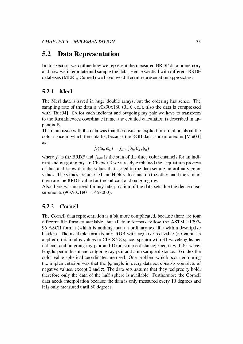
5.2 Data RepresentationIn this section we outline how we represent the measured BRDF data in memoryand how we interpolate and sample the data. Hence we deal with different BRDFdatabases (MERL, Cornell) we have two different representation approaches.

5.2.1 MerlThe Merl data is saved in huge double arrays, but the ordering has sense. Thesampling rate of the data is 90x90x180 (θh,θd,φd), also the data is compressedwith [Rus04]. So for each indicant and outgoing ray pair we have to transformto the Rusinkiewicz coordinate frame, the detailed calculation is described in ap-pendix B.The main issue with the data was that there was no explicit information about thecolor space in which the data lie, because the RGB data is mentioned in [Mat03]as:

fr(ωi,ωo) = fsum(θh,θd,φd)

where fr is the BRDF and fsum is the sum of the three color channels for an indi-cant and outgoing ray. In Chapter 3 we already explained the acquisition processof data and know that the values that stored in the data set are no ordinary colorvalues. The values are on one hand HDR values and on the other hand the sum ofthem are the BRDF value for the indicant and outgoing ray.Also there was no need for any interpolation of the data sets due the dense mea-surements (90x90x180 = 1458000).

5.2.2 CornellThe Cornell data representation is a bit more complicated, because there are fourdifferent file formats available, but all four formats follow the ASTM E1392-96 ASCII format (which is nothing than an ordinary text file with a descriptiveheader). The available formats are: RGB with negative red value (no gamut isapplied); tristimulus values in CIE XYZ space; spectra with 31 wavelengths perindicant and outgoing ray-pair and 10nm sample distance; spectra with 65 wave-lengths per indicant and outgoing ray-pair and 5nm sample distance. To index thecolor value spherical coordinates are used. One problem which occurred duringthe implementation was that the φo angle in every data set consists complete ofnegative values, except 0 and π. The data sets assume that they reciprocity hold,therefore only the data of the half sphere is available. Furthermore the Cornelldata needs interpolation because the data is only measured every 10 degrees andit is only measured until 80 degrees.


The first approach for a memory presentation of the Cornell data was a KD-Tree,the nearest neighbor search is done in O(logN) [HMS06]. For the KD-Tree con-struction the variables θi,θo and φo are used to create the decisions nodes. TheKD-Tree was a good data structure to index the BRDF data, but is a bad datastructure for a trilinear interpolation because with the KD-Tree it is only possibleto make linear interpolation.The second approach for the data structure are something like a B*-Tree. The treegeneration is constructed as following:

• Find all unique θi angles in the ASTM file (in a normal Cornell data set itsabout 10-11 data record) this angles build the first layer of root nodes.

• For each θi search all possible θo angles in the ASTM file and add this listof all possible θo as a seconde layer to the current node.

• Now we hold θi and θo and search for all possible φo and add them to thecurrent θo node.

• Finally we sort the arrays ascending.

Figure 5.1 illustrate the Cornell data structure. The arrays are sorted with Quick-sort and so we achieve the nearest neighbor search in each array in O(logN).

Figure 5.1: Cornell data representation

We introduced this structure for a fast trilinear interpolation approach. Topresent the approach we assume that we have the incoming and outgoing ray andalready have transformed them to spherical coordinates. φdi f f is the differenceangle between φi and φo, the difference angle is sufficient for the isotropic case.An important side note for the correct calculation of the φdi f f angle is that we firsthave to branch which φ (φi or φo) angle is greater then we subtract the smaller


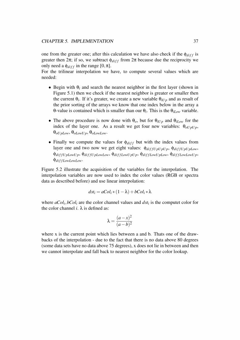
one from the greater one; after this calculation we have also check if the φdi f f isgreater then 2π; if so, we subtract φdi f f from 2π because due the reciprocity weonly need a φdi f f in the range [0,π].For the trilinear interpolation we have, to compute several values which areneeded:

• Begin with θi and search the nearest neighbor in the first layer (shown inFigure 5.1) then we check if the nearest neighbor is greater or smaller thenthe current θi. If it’s greater, we create a new variable θiU p and as result ofthe prior sorting of the arrays we know that one index below in the array aθ-value is contained which is smaller than our θi. This is the θiLow variable.

• The above procedure is now done with θo, but for θiU p and θiLow for theindex of the layer one. As a result we get four new variables: θoU pU p,θoU pLow, θoLowU p, θoLowLow.

• Finally we compute the values for φdi f f but with the index values fromlayer one and two now we get eight values: φdi f fU pU pU p, φdi f fU pU pLow,φdi f fU pLowU p, φdi f fU pLowLow, φdi f f LowU pU p, φdi f f LowU pLow, φdi f f LowLowU p,φdi f f LowLowLow.

Figure 5.2 illustrate the acquisition of the variables for the interpolation. Theinterpolation variables are now used to index the color values (RGB or spectradata as described before) and use linear interpolation:

dsti = aColi ∗ (1−λ)+bColi ∗λ

where aColi,bColi are the color channel values and dsti is the computet color forthe color channel i. λ is defined as:

λ =(a− x)2

(a−b)2

where x is the current point which lies between a and b. Thats one of the draw-backs of the interpolation - due to the fact that there is no data above 80 degrees(some data sets have no data above 75 degrees), x does not lie in between and thenwe cannot interpolate and fall back to nearest neighbor for the color lookup.


Figure 5.2: Trilinear interpolation

5.3 Rejection SamplingIn chapter 4 we already described what rejection sampling is in a general manner,in this section we present the way it is implemented for this thesis.First the BRDF volume is separated into slices. Each slice has a fix θi and a θoand φdi f f is varying, θi is used to index the volume. Then we calculate the areaof the cell and the maximum for each slice and save the resulting array to the harddisk to speed up the start up time for the next rendering process.The maximum is defined as the sum of each channel. Note that the sum of thechannels in the MERL data set is the BRDF value at this point. At the end wehave to resample the complete BRDF with a regular grid. The grid cells haveto be really small-so that we do not miss any BRDF value. The resampling ofthe Cornell data take about 15 minutes where the MERL data take more than 30minutes.Wtether to accept a ray or not is figured out through the decision equation:

ratio =fsum(θh,θd,φd)

Mslice

if the ratio is greater or equal than h (where h is a random variable between 0 and1) then the ray is accepted otherwise it is rejected. To get the correct Mslice weuse θi to index the correct volume, and here is the drawback of the approach. Ifthe grid cells are not small enough it could happen that we miss a maximum value


and the rejection sample would not converge right.The PDF is computed as:

pd f =fsum(θh,θd,φd)

pd fslicePatch∗ 1

pd fcurCel

where pd fslicePatch is precomputed during the resampling as:

pd fslicePatch =2∗π∗ cos(θo− samplingWidth)− cos(θo)

sampleCount

and pd fcurCel is the cell area on the sphere surface. The pdf calculation workedwith the Cornell data but gives some false results with the MERL data. After manytrials to find a correct pdf we found that we got no errors if we use fsum(θh,θd,φd)as pdf.

Chapter 6

Results

In this chapter we present our results in form of rendered images. Also polar plotswere made for several angles. The polar plots were generated with a self madetool. The polar plots for each materials are illustrated in the appendix C.

6.1 MERL RenderingsThe images were rendered with the ART pathtracer with lightsource sampling and512 samples per pixel, an image resolution of 640x480 and with a recursion depthof five, all renderings made in RGB color space. We used a simple scene to test therenderings. As sampling technique rejection sampling is used, where the materialswhich are ideal diffuse or directional diffuse reflectors have a faster convergencethan materials which are ideal specular or rough specular reflectors. Materialswhich are more diffuse were rendered approximately between 3 - 4 hours wherethe specular materials took between 12 - 15 hours. The most problematic materialwas Brass because the material has a tiny specular lobe, the rejection samplingwith this material consumed the most time, because most of the sample points arerejected during the sample process.For the polar plots three different angle combinations are used: θi = 45 and θo =45; θi = 75 and θo = 75; θi = 85 and θo = 85.

6.1.1 Gold MetallicGold metallic paint has a metallic shine, with fine aluminum powder and pigmentsto get the metallic shine. This material has tiny bright spots caused by mirror likeflakes. These spots are visible on grazing angles. The reflectance property isrough specular (glossy), as the polar plots show. Ngan et al. [NDM05] show thatthere is no analytical reflectance model that can reproduce the material with an

40

CHAPTER 6. RESULTS 41

error under ∼ 0.02, which they demonstrated in there experimental results whichis in fact rather good, but not very surprising since the Cook-Torrance model wasdeveloped to simulate this material type.

Figure 6.1: Gold Metallic

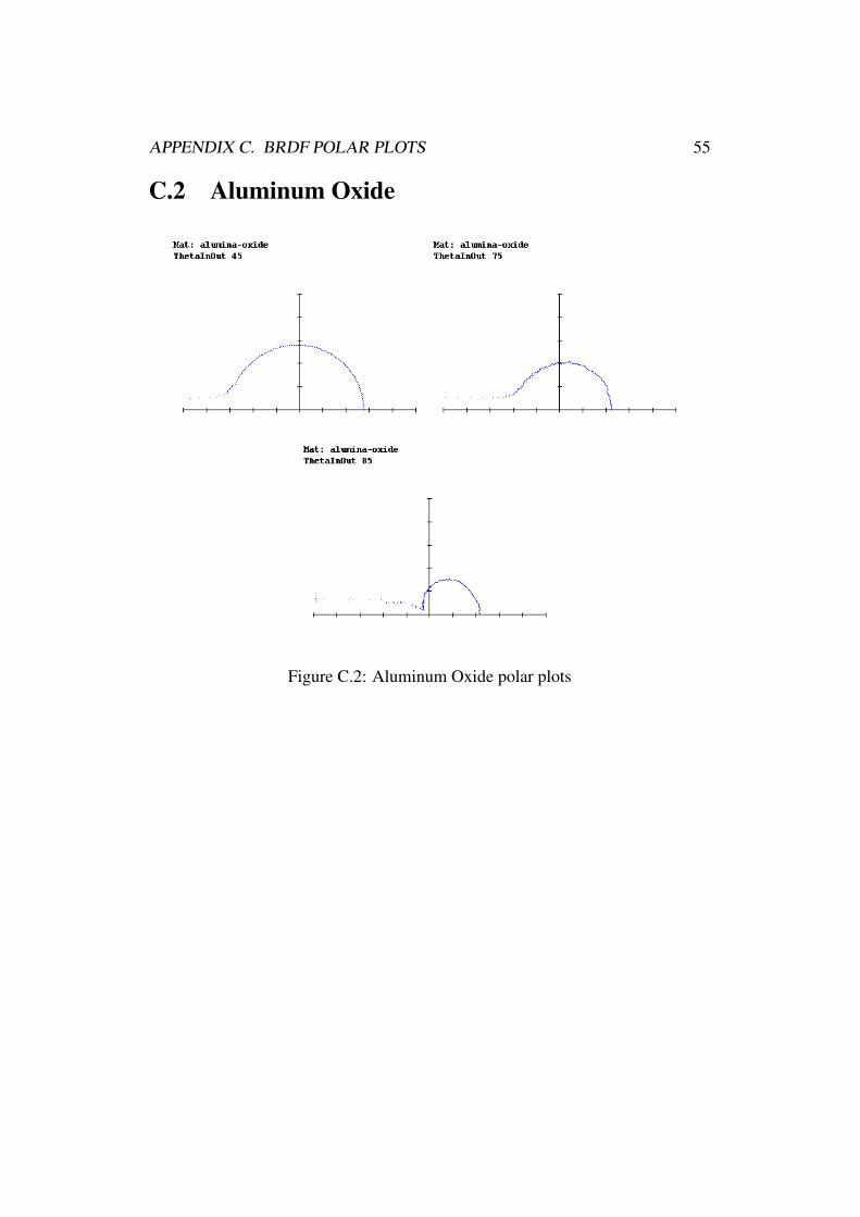
6.1.2 Aluminum OxideAluminum oxide is also a paint with pigments,which has a better hiding (opac-ity) performance. The opacity is improved by optimal sizing the oxide particles.Aluminum oxide has sharp specular reflections. The reflectance property is di-rectional diffuse, as the polar plots show. The experimental results of Ngan et al.[NDM05] show that the tested analytical reflectance models have almost the samereproduction performance with an error rate of ∼ 0.08. The analytical modelsperform not as good as in the case of gold metallic paint since the normal Fresnelequations do not hold in the case of aluminum oxide.


Figure 6.2: Aluminum Oxide

6.1.3 Blue FabricBlue fabric is a textile material, so they have a complex microfacet structure. It isnearly perfect diffuse except for grazing angles it produces rough specular reflec-tion. This material has the fastest convergence of all rendered MERL materialsin this thesis. As the polar plots show the material is ideal diffuse at the specularangle. The Lafortune et al. [LFTG97] reflectance model is able to reproduce thematerial with a small error of 0.000831 [NDM05].


Figure 6.3: Blue Fabric

6.1.4 Blue RubberBlue rubber is a rough surface which has specular highlights at grazing angles,where the highlights at the specular angle are soft which is difficult to see, thepolar plots show sharp lobes at grazing angles but with a big diffuse component.The He et al. [HTSG91] model has the smallest reproduction error of 0.00134[NDM05].

Figure 6.4: Blue Rubber


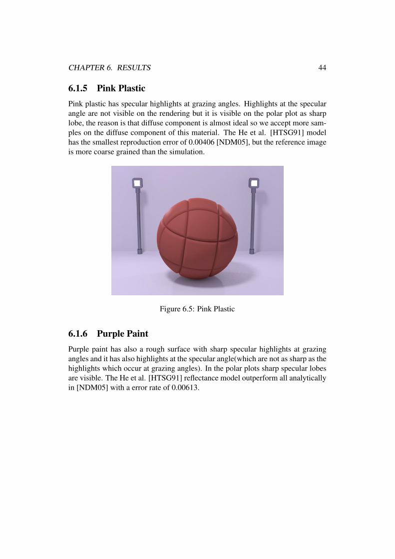
6.1.5 Pink PlasticPink plastic has specular highlights at grazing angles. Highlights at the specularangle are not visible on the rendering but it is visible on the polar plot as sharplobe, the reason is that diffuse component is almost ideal so we accept more sam-ples on the diffuse component of this material. The He et al. [HTSG91] modelhas the smallest reproduction error of 0.00406 [NDM05], but the reference imageis more coarse grained than the simulation.

Figure 6.5: Pink Plastic

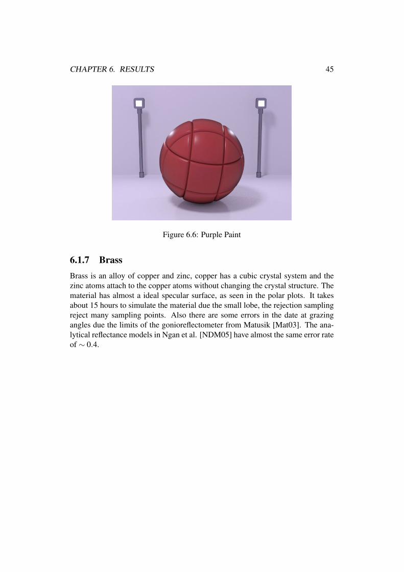
6.1.6 Purple PaintPurple paint has also a rough surface with sharp specular highlights at grazingangles and it has also highlights at the specular angle(which are not as sharp as thehighlights which occur at grazing angles). In the polar plots sharp specular lobesare visible. The He et al. [HTSG91] reflectance model outperform all analyticallyin [NDM05] with a error rate of 0.00613.


Figure 6.6: Purple Paint

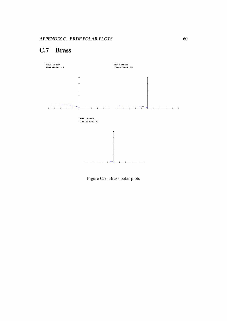
6.1.7 BrassBrass is an alloy of copper and zinc, copper has a cubic crystal system and thezinc atoms attach to the copper atoms without changing the crystal structure. Thematerial has almost a ideal specular surface, as seen in the polar plots. It takesabout 15 hours to simulate the material due the small lobe, the rejection samplingreject many sampling points. Also there are some errors in the date at grazingangles due the limits of the gonioreflectometer from Matusik [Mat03]. The ana-lytical reflectance models in Ngan et al. [NDM05] have almost the same error rateof ∼ 0.4.


Figure 6.7: Brass

6.2 Cornell RenderingsThe Cornell data is rendered with 1024 samples and a recursion depth of five, allrenderings made with the ART Spectra 8 renderer.For the polar plots four different angle combinations are used: θi = 0 and θo = 0;θi = 15 and θo = 15; θi = 45 and θo = 45; θi = 75 and θo = 75. Only two samplesare included in the thesis because the other material samples provided form theCornell University are uncomplete, not interpolated and contain errors.

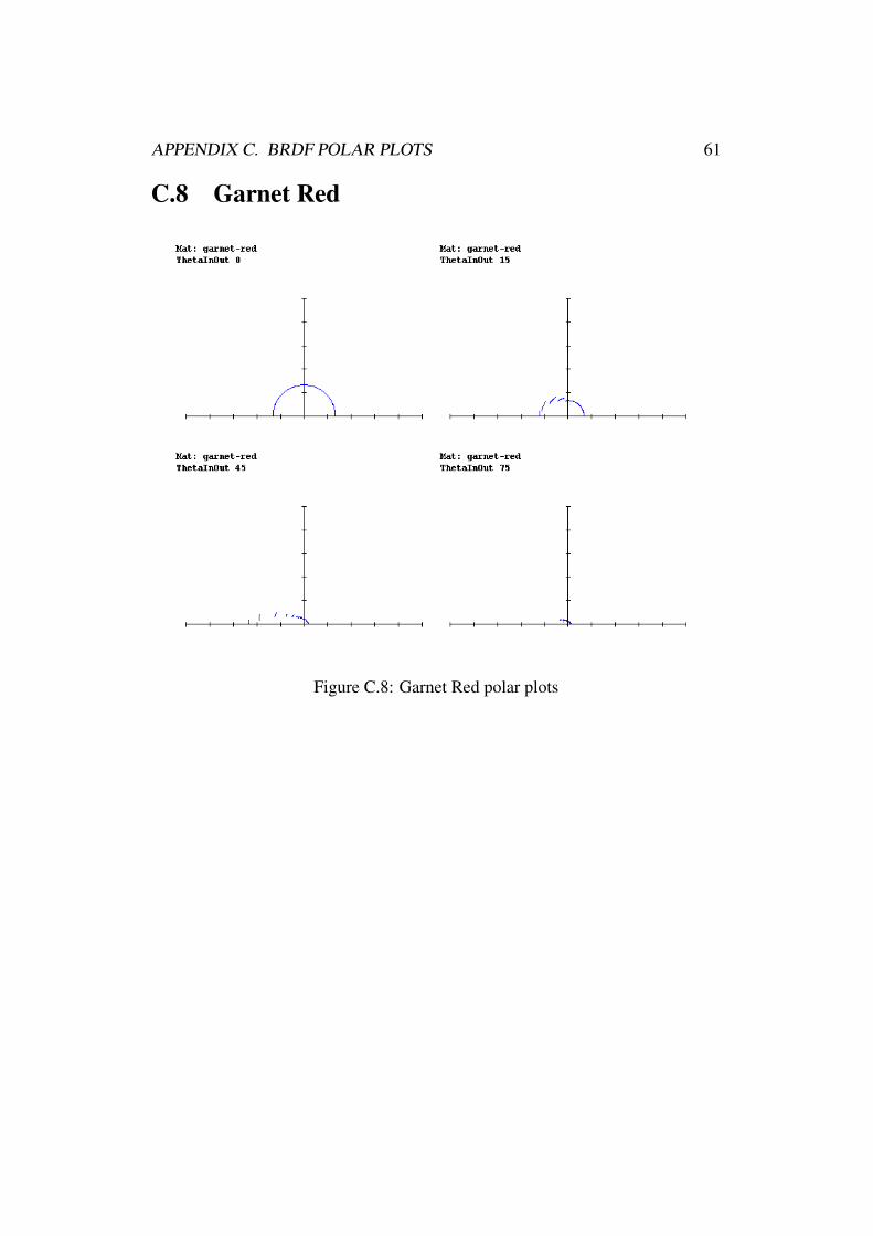
6.2.1 Garnet RedGarnet Red is a spray paint with a low gloss component. The material is ren-dered twice; once it is rendered without interpolation and the second time withinterpolation to show the interpolation effect. The materials have bright specularhighlights at grazing angles and at the specular angle (see the polar plots). Forcertain angle the materials are almost ideal diffuse.


Figure 6.8: Garnet Red without interpolation and 256 samples. The renderingtook thirty minutes.

Figure 6.9: Garnet Red with interpolation and 1024 samples. The rendering tookthree hours.

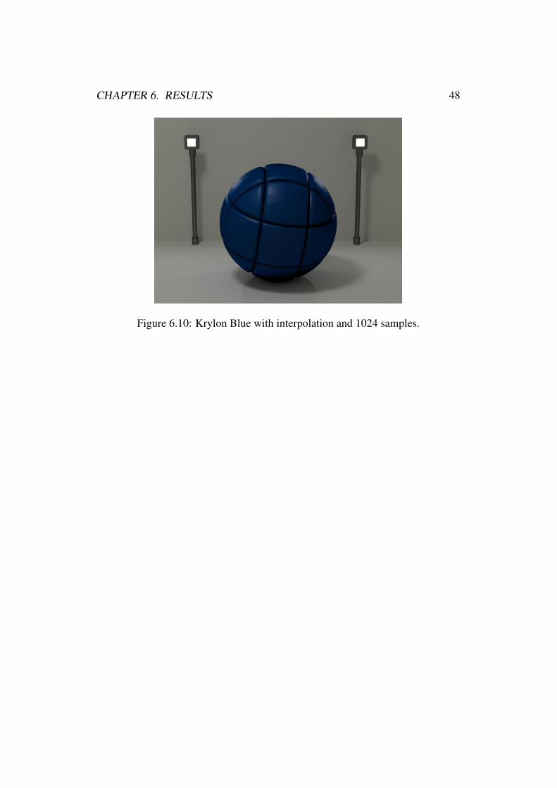
6.2.2 Krylon BlueKrylon Blue is also a spray paint with a low gloss component. It has the samereflectance characteristics as Garnet Red.


Figure 6.10: Krylon Blue with interpolation and 1024 samples.

Chapter 7

Conclusion

In this thesis we used two BRDF measurement databases for image synthesis witha photorealistic rendering toolkit, namely the Advanced Rendering Toolkit (ART),developed at the University of Technology Vienna. One of the challenges duringthe implementation was that there is almost no information on how to calculate aPDF for measured data. In this paper we tried to give the reader an overview aboutthe important things which are needed to reproduce the images we generated us-ing ART, but we tried also to go in depth were other paper and thesis do not. Wepresented a PDF formula for the Cornell database and also a data structure fortrilinear interpolation. We also showed important details of the data set, whichare not mentioned anywhere else. We rendered only a representative subset of theMERL data, because the fact that a rendering took between 3 - 15 hours. Due thedesign of ART it is also possible to use a measured BRDF surface n times withjust one memory presentation of the data.Also only isotropic measurements were used for the image synthesis but the datastructure is already ready for anisotropic data. As we already mentioned in Chap-ter 3, MERL extended their library with some anisotropic materials.The work is limited to make use of the measured data for direct rendering butwith the MERL database it is possible to generate new BRDF’s through linearcombination. There are several new approaches to generate new BRDF’s likeBRDFShop ([MC06]).

49

Appendix A

Spherical Coordinates

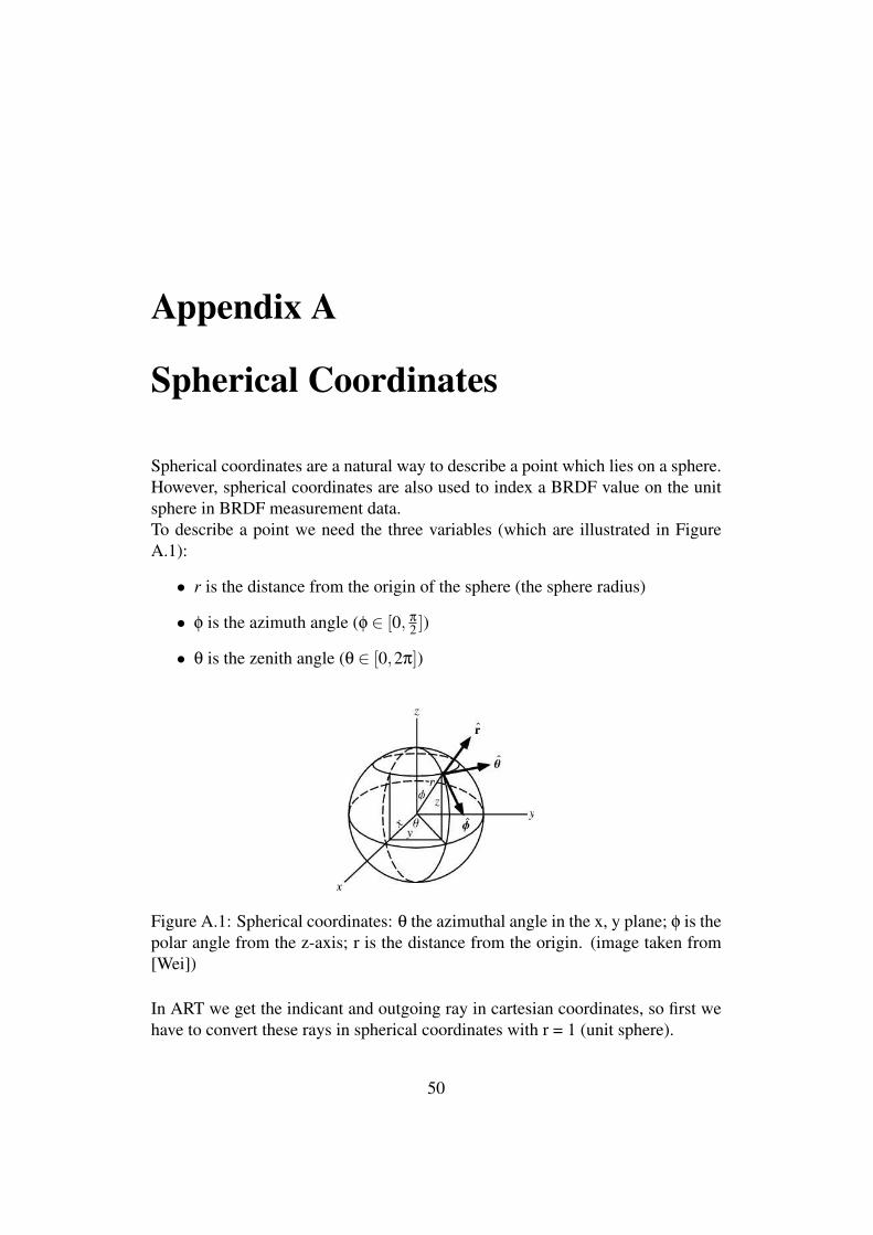
Spherical coordinates are a natural way to describe a point which lies on a sphere.However, spherical coordinates are also used to index a BRDF value on the unitsphere in BRDF measurement data.To describe a point we need the three variables (which are illustrated in FigureA.1):

• r is the distance from the origin of the sphere (the sphere radius)

• φ is the azimuth angle (φ ∈ [0, π

2 ])

• θ is the zenith angle (θ ∈ [0,2π])

Figure A.1: Spherical coordinates: θ the azimuthal angle in the x, y plane; φ is thepolar angle from the z-axis; r is the distance from the origin. (image taken from[Wei])

In ART we get the indicant and outgoing ray in cartesian coordinates, so first wehave to convert these rays in spherical coordinates with r = 1 (unit sphere).

50

APPENDIX A. SPHERICAL COORDINATES 51

To convert a vector with x, y, z from cartesian coordinates to spherical coordinates:

r =√

x2 + y2 + z2 (1)

θ = tan−1 yx

(2)

φ = cos−1 zr

(3)

And to convert back to cartesian coordinates:

x = rcosθsinφ (4)

y = rsinθsinφ (5)

z = rcosφ (6)

Appendix B

Rusinkiewicz Coordinate Frame

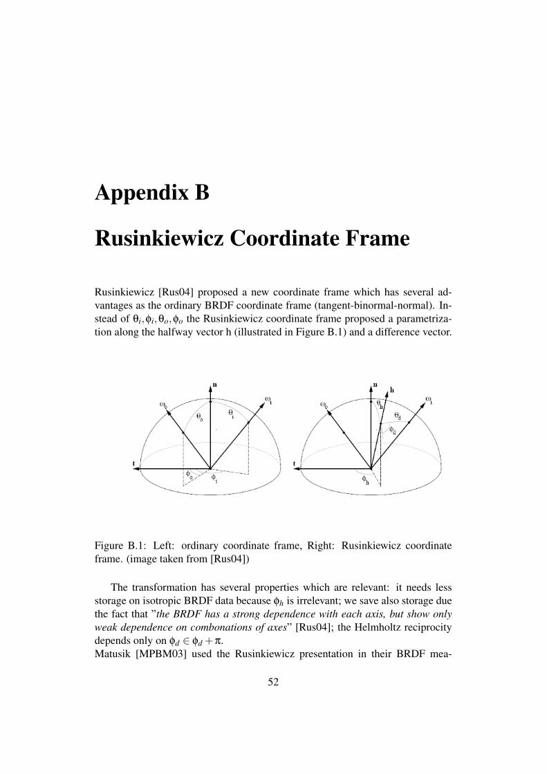
Rusinkiewicz [Rus04] proposed a new coordinate frame which has several ad-vantages as the ordinary BRDF coordinate frame (tangent-binormal-normal). In-stead of θi,φi,θo,φo the Rusinkiewicz coordinate frame proposed a parametriza-tion along the halfway vector h (illustrated in Figure B.1) and a difference vector.

Figure B.1: Left: ordinary coordinate frame, Right: Rusinkiewicz coordinateframe. (image taken from [Rus04])

The transformation has several properties which are relevant: it needs lessstorage on isotropic BRDF data because φh is irrelevant; we save also storage duethe fact that ”the BRDF has a strong dependence with each axis, but show onlyweak dependence on combonations of axes” [Rus04]; the Helmholtz reciprocitydepends only on φd ∈ φd +π.Matusik [MPBM03] used the Rusinkiewicz presentation in their BRDF mea-

52

APPENDIX B. RUSINKIEWICZ COORDINATE FRAME 53

surements so that we needed to transform from the vector representation in theRusinkiewiz coordinate frame. To do this we calculate the halfway vector h as:

h =ωi +ωo

2(1)

where ωi and ωo are the incoming and outgoing ray (these two vectors are alreadyin local space). Then we have to transform the halfway vector into sphericalcoordinates (with r = 1) and get θh and φh. To get θd and φd we need a differencevector which is calculated in two steps: first we rotate ωi around the local normalvector with −φh as angle; after the first step we get a new vector which we rotatearound the local binormal with −θh as angle; now we have the difference vectorafter the conversion in spherical coordinates we have the two angles θd and φd .To index the BRDF data from [MPBM03] we use θd , θh and φd .

Appendix C

BRDF Polar Plots

C.1 Gold Metallic

Figure C.1: Gold Metallic polar plots

54

APPENDIX C. BRDF POLAR PLOTS 55

C.2 Aluminum Oxide

Figure C.2: Aluminum Oxide polar plots


C.3 Blue Fabric

Figure C.3: Blue Fabric polar plots


C.4 Blue Rubber

Figure C.4: Blue Rubber polar plots


C.5 Pink Plastic

Figure C.5: Pink Plastic polar plots


C.6 Purple Paint

Figure C.6: Purple Paint polar plots


C.7 Brass

Figure C.7: Brass polar plots


C.8 Garnet Red

Figure C.8: Garnet Red polar plots


C.9 Krylon Blue

Figure C.9: Krylon Blue polar plots

List of Figures

1.1 Interference between waves: A shows the constructive interfer-ence; B shows the destructive interference (image taken from [Wil]) 2

1.2 General light interaction with a matter; Incoming Light: the lightenergy which is emitted from a light source; Reflected Light: theamount of light which is reflected; Internal Reflection: the amountof light which is reflected within the matter; Transmitted Light:light which go through the matter; Absorbtion: light which isabsorbed in the matter; Scattering and Emission: light which isreflected internal and remitted (image taken from [Wyn00]) . . . . 4

1.3 Solid angle dw on the unit sphere (image taken from [Geb03]) . . 51.4 Spherical coordinates: θ the azimuthal angle in the x, y plane; φ

is the polar angle from the z-axis; r is the distance from the origin.(image taken from [Wei]) . . . . . . . . . . . . . . . . . . . . . . 7

1.5 Left a isotropic material; Right a anisotropic material (imagetaken from [Geb03]) . . . . . . . . . . . . . . . . . . . . . . . . 9

1.6 Left: BRDF describes the reflection off the surface; Right: BRDF+ BTDF describes light rays which are reflected through the mi-crofacet structure of the surface. (image taken from [Wik]) . . . . 10

2.1 Left: A sphere rendered with a ideal diffuse reflector; Middle: Asphere rendered with a ideal specular reflector; Right: A sphererendered with a directional diffuse. (image taken from [Hua02]) . 12

2.2 A diffuse sphere using the Lambert reflectance model. (imagetaken from [Geb03]) . . . . . . . . . . . . . . . . . . . . . . . . 13

2.3 Rendered picture of a scene with two spheres and a Q-panel, il-luminated by two colored light sources and one larger white lightsource. The sphere on the left has a Lambertian approximation ofthe measured paint reflectance; the sphere on the right is renderedwith the non-linear approximation. The Q-panel has the non-linear approximation of the measured steel reflectance.(imagetaken from [LFTG97]) . . . . . . . . . . . . . . . . . . . . . . . 15

63

LIST OF FIGURES 64

2.4 Material independent variables and angles which are used in theWard reflectance model where x and y are the tangents of the sur-face point, n is the normal vector, h is the half vector betweendr and di; ”the indicant light arrives along di and is simulatedor measured in direction dr” Ward [War92]. (image taken from[Geb03] and slightly modified) . . . . . . . . . . . . . . . . . . . 17

2.5 Varnished wood comparison. Left: Photograph of a chair; Middle:Use the isotropic Gaussian model for the simulation; Right: Theelliptical Gaussian model. (image taken from [War92]) . . . . . . 18

2.6 Left: shows the masking and self shadowing effects due the mi-crofacet surface structure;Right: show the v-shaped facets. (im-age taken from [Wyn00]) . . . . . . . . . . . . . . . . . . . . . . 19

2.7 Several materials simulated with the Cook-Torrance reflectancemodel (image taken from [CT82]) . . . . . . . . . . . . . . . . . 20

3.1 Basic gonioreflectometer designed by Murray etal. [MC75] (im-age taken from [MC75]) . . . . . . . . . . . . . . . . . . . . . . 23

3.2 Side view of the imaging gonioreflectometer designed by Ward[War92]. (image taken from [War92]) . . . . . . . . . . . . . . . 23

3.3 Left: ordinary coordinate frame, Right: Rusinkiewicz coordinateframe. (image taken from [Rus04]) . . . . . . . . . . . . . . . . . 26

4.1 Left: 100 points distributed by a regular grid; Middle: 100points distributed by a ordinary random number generator; Right:100 points distributed by a quasi-random sequence (Halton low-discrepancy sequence). (image taken from [Las99]) . . . . . . . . 30

4.2 The continues function is the integrand f(x), which we want toestimate, and the dotted function the estimator p(x). In the caseabove our estimator p(x) has a low variance. (image taken form[Ghe07]) . . . . . . . . . . . . . . . . . . . . . . . . . . . . . . . 31

4.3 x1..xi are samples with a distribution p(x), by applying the in-verse CDF of p(x) to u - a uniform distributed random variable- we generate the samples with xi = F−1(ui). (image taken from[DBB03]) . . . . . . . . . . . . . . . . . . . . . . . . . . . . . . 32

4.4 Rejection sampling: blue samples are accepted (∈ p(X)), red sam-ples are rejected (3 p(X)). (image taken form [Ghe07]) . . . . . . 33

5.1 Cornell data representation . . . . . . . . . . . . . . . . . . . . . 365.2 Trilinear interpolation . . . . . . . . . . . . . . . . . . . . . . . . 38

6.1 Gold Metallic . . . . . . . . . . . . . . . . . . . . . . . . . . . . 416.2 Aluminum Oxide . . . . . . . . . . . . . . . . . . . . . . . . . . 42

LIST OF FIGURES 65

6.3 Blue Fabric . . . . . . . . . . . . . . . . . . . . . . . . . . . . . 436.4 Blue Rubber . . . . . . . . . . . . . . . . . . . . . . . . . . . . . 436.5 Pink Plastic . . . . . . . . . . . . . . . . . . . . . . . . . . . . . 446.6 Purple Paint . . . . . . . . . . . . . . . . . . . . . . . . . . . . . 456.7 Brass . . . . . . . . . . . . . . . . . . . . . . . . . . . . . . . . 466.8 Garnet Red without interpolation and 256 samples. The rendering

took thirty minutes. . . . . . . . . . . . . . . . . . . . . . . . . . 476.9 Garnet Red with interpolation and 1024 samples. The rendering

took three hours. . . . . . . . . . . . . . . . . . . . . . . . . . . 476.10 Krylon Blue with interpolation and 1024 samples. . . . . . . . . . 48

A.1 Spherical coordinates: θ the azimuthal angle in the x, y plane; φ

is the polar angle from the z-axis; r is the distance from the origin.(image taken from [Wei]) . . . . . . . . . . . . . . . . . . . . . . 50

B.1 Left: ordinary coordinate frame, Right: Rusinkiewicz coordinateframe. (image taken from [Rus04]) . . . . . . . . . . . . . . . . . 52

C.1 Gold Metallic polar plots . . . . . . . . . . . . . . . . . . . . . . 54C.2 Aluminum Oxide polar plots . . . . . . . . . . . . . . . . . . . . 55C.3 Blue Fabric polar plots . . . . . . . . . . . . . . . . . . . . . . . 56C.4 Blue Rubber polar plots . . . . . . . . . . . . . . . . . . . . . . . 57C.5 Pink Plastic polar plots . . . . . . . . . . . . . . . . . . . . . . . 58C.6 Purple Paint polar plots . . . . . . . . . . . . . . . . . . . . . . . 59C.7 Brass polar plots . . . . . . . . . . . . . . . . . . . . . . . . . . 60C.8 Garnet Red polar plots . . . . . . . . . . . . . . . . . . . . . . . 61C.9 Krylon Blue polar plots . . . . . . . . . . . . . . . . . . . . . . . 62

Bibliography

[And99] Eric C. Anderson. Monte carlo methods and importance sampling.oct 1999.

[Bli77] James F. Blinn. Models of light reflection for computer synthesizedpictures. ACM, pages 192–198, 1977.

[Bor03] George Borshukov. Measured brdf in film production - realisticcloth appearance for ”the matrix reloaded”. ESC Entertainment,2003.

[Coo86] Robert L. Cook. Stochastic sampling in computer graphics. ACMTrans. Graph., 5(1):51–72, 1986.

[CT82] R. L. Cook and K. E. Torrance. A reflectance model for computergraphics. ACM Trans. Graph., 1(1):7–24, 1982.

[DBB03] Philip Dutre, Philippe Bekaert, and Kavita Bala. Advanced globalillumination. 2003.

[DvGNK99] Kristin J. Dana, Bram van Ginneken, Shree K. Nayar, and Jan J.Koenderink. Reflectance and texture of real-world surfaces. ACMTransactions on Graphics, 18(1):1–34, 1999.

[Ein5a] Albert Einstein. On a heuristic viewpoint concerning the productionand transformation of light. Annalen der Physik 17, pages 132–148,1905a.

[Foo97] Sing Choong Foo. A gonioreflectometer for measuring the bidirec-tional reflectance of material for use in illumination computation.aug 1997.

[Geb03] Nikolaus Gebhardt. Einige brdf modelle. 2003.

[Ghe07] Mihai Calin Ghete. Mathematical basics of monte carlo renderingalgorithms. 2007.

66

BIBLIOGRAPHY 67

[HMS06] Warren Hunt, William R. Mark, and Gordon Stoll. Fast kd-treeconstruction with an adaptive error-bounded heuristic. 2006 IEEESymposium on Interactive Ray Tracing, Sept. 2006.

[HTSG91] Xiao D. He, Kenneth E. Torrance, Francois X. Sillion, and Donald P.Greenberg. A comprehensive physical model for light reflection.ACM, pages 175–186, 1991.

[Hua02] Jian Huang. Global illumination. SIGGRAPH, 2002.

[Huy78] Christiaan Huygens. Traite de la lumiere. 1678.

[Jen01] Henrik Wann Jensen. Monte carlo ray tracing for realistic imagesynthesis. State of the Art 39, Stanford University, aug 2001.

[JN86] Gerald H. Jacobs Jay Neitz. Polymorphism of the long-wavelengthcone in normal human colour vision. Nature 323, pages 623 – 625,1986.

[Kaj86] James T. Kajiya. The rendering equation. nov 1986.

[KET67] E. M. Sparrow K. E. Torrance. Theory for off-specular reflectionfrom roughened surfaces. Optical Society of America, 57(9):1105–1114, sep 1967.

[KW86] M. Kalos and P. Whitlock. Monte carlo methods. New York: Wileyand Sons, 1986.

[Lam] Johann Heinrich Lambert. Lamberts cosine law. Retrieved April 20,2008, http://de.wikipedia.org/wiki/Lambertsches Gesetz.

[Las99] Szirmay-Kalos Laszlo. Monte-carlo methods in global illumination.1999.

[Lew93] Robert R. Lewis. Making shaders more physically plausible. FourthEurographics Workshop on Rendering, (Series EG 93 RW):47–62,1993.

[LFTG97] Eric P. F. Lafortune, Sing-Choong Foo, Kenneth E. Torrance, andDonald P. Greenberg. Non-linear approximation of reflectance func-tions. ACM Press/Addison-Wesley Publishing Co, pages 117–126,1997.

[Mat03] Wojciech Matusik. A Data-Driven Reflectance Model. PhD thesis,Massachusetts Institute Of Technology, 2003.

BIBLIOGRAPHY 68

[MC75] A.M. Smith Murray-Coleman, J.F. The automshd measurement ofbrdfs and their application to luminaire modeling. Journal of theIlluminating Engineering Sociery, 18(6):311–317, 1975.

[MC06] Jaroslav Krivanek Mark Colbert, Sumanta Pattanaik. Brdf-shop:Creating physically correct bidirectional reflectance distributionfunction. IEEE Computer Society, pages 30–36, jan 2006.

[MPBM03] Wojciech Matusik, Hanspeter Pfister, Matthew Brand, and LeonardMcMillan. A data-driven reflectance model. ACM Trans. Graph.,22(3):759–769, 2003.

[MWLT00] S. Marschner, S. Westin, E. Lafortune, and K. Torrance. Image-based brdf measurement. S.R. Marschner, S.H. Westin, E.P.F. Lafor-tune, and K.E. Torrance. Image-Based BRDF measurement. AppliedOptics, 39(16):2592–2600, 2000.

[NDM05] Addy Ngan, Frdo Durand, and Wojciech Matusik. Experimentalanalysis of brdf models. Eurographics Association, pages 117–126,2005.

[New04] Isaac Newton. Opticks or a treatise of the reflections, refractions,inflections and colours of light. 1704.

[ON95] M. Oren and S.K. Nayar. Generalization of the lambertian modeland implications for machine vision. IJCV, 14(3):227–251, apr1995.

[PH03] Matt Pharr and Greg Humphreys. Physically-Based Image SynthesisFrom Theory To Implementation. 4. nov 2003.

[PH04] Matt Pharr and Greg Humphreys. Infinite area light source withimportance sampling. 2004.

[Pho75] Bui Tuong Phong. Illumination for computer generated pictures.Commun. ACM, 18(6):311–317, 1975.

[Rus04] Szymon M. Rusinkiewicz. A new change of variables for efficientbrdf representation. Proceedings of the 2004 SIGGRAPH Confer-ence, 23(3):496–505, aug 2004.

[SKN91] Takeo Kanade Shree K. Nayarm, Katsushi Ilkeuchi. Surface reflec-tion: Physical and geometrical perspectives. ACM, 13:611–634, jul1991.

BIBLIOGRAPHY 69

[War92] Gregory J. Ward. Measuring and modeling anisotropic reflection.ACM, pages 265–272, jul 1992.

[Wei] Eric Weisstein. Spherical coordinates.From MathWorld–A Wolfram Web Resource,http://mathworld.wolfram.com/SphericalCoordinates.html.

[Wik] Wikipedia. Bidirectional scattering distribu-tion function. Retrieved April 20, 2008,http://en.wikipedia.org/wiki/Bidirectional scattering distribution function.

[Wil] Alexander Wilkie. Vorlesung einfuhrung in die farbwissenschaft.Lecture delivered 2005 at Technical University Vienna.

[WW07] Andrea Weidlich and Alexander Wilkie. Arbitrarily layered micro-facet surfaces. GRAPHITE ’07: Proceedings of the 5th interna-tional conference on Computer graphics and interactive techniquesin Australia and Southeast Asia, pages 171–178, 2007.

[WWLP06] Alexander Wilkie, Andrea Weidlich, Caroline Larboulette, andWerner Purgathofer. A reflectance model for diffuse fluorescent sur-faces. Proceedings of Graphite 2006, pages 321–328, 2006.

[Wyn00] Chris Wynn. An introduction to brdf based lighting. Technical re-port, NVIDIA Corporation, 2000.

[You02] Thomas Young. The wave theory of light (pmm 259). 1802.

Documents

Masterarbeit - TU Wien€¦ · Masterarbeit Photorealistic Rendering Of Measured BRDF Data Ausgefuhrt am Institut f¨ ur¨ Computergraﬁk und Algorithmen der Technischen Universit¨at