Embed Size (px)
Citation preview
Universität LeipzigFakultät für Mathematik und Informatik
Institut für Informatik
Master's Thesis Computer Science
Design and Investigation of a Multi Agent Based
XCS Learning Classi�er System with Distributed
Rules
Mirko Pinseler
Student of Computer Science
Leipzig, 31.03.2016
Supervisor
Prof. Dr. Martin Middendorf
Universität LeipzigFakultät für Mathematik und Informatik
Institut für Informatik
Mirko Pinseler:
Design and Investigation of a Multi Agent Based XCS Learn-ing Classi�er System with Distributed Rules
Master's Thesis Computer ScienceLeipzig University
Contents
Introduction 1
1 Prerequisites and Background 5
1.1 General Framework . . . . . . . . . . . . . . . . . . . . . . . . . 5
1.2 The Classi�er . . . . . . . . . . . . . . . . . . . . . . . . . . . . 6
1.3 Basic Work�ow . . . . . . . . . . . . . . . . . . . . . . . . . . . 6
1.4 Components . . . . . . . . . . . . . . . . . . . . . . . . . . . . 7
1.5 Problem Types . . . . . . . . . . . . . . . . . . . . . . . . . . . 9
1.6 Historic Remarks . . . . . . . . . . . . . . . . . . . . . . . . . . 11
1.7 Related Work . . . . . . . . . . . . . . . . . . . . . . . . . . . . 13
2 XCS 16
2.1 Which XCS to Build On . . . . . . . . . . . . . . . . . . . . . . 16
2.2 Strength vs. Accuracy . . . . . . . . . . . . . . . . . . . . . . . 17
2.3 Components of XCS . . . . . . . . . . . . . . . . . . . . . . . . 17
2.3.1 The Classi�er . . . . . . . . . . . . . . . . . . . . . . . . 18
2.3.2 Performance Component . . . . . . . . . . . . . . . . . . 19
2.3.3 Reinforcement Component . . . . . . . . . . . . . . . . . 20
2.3.4 Discovery Component . . . . . . . . . . . . . . . . . . . 22
2.4 Action Set Subsumption . . . . . . . . . . . . . . . . . . . . . . 24
2.5 XCSJava 1.0 . . . . . . . . . . . . . . . . . . . . . . . . . . . . . 24
2.5.1 Problem Types . . . . . . . . . . . . . . . . . . . . . . . 24
2.6 Program Execution . . . . . . . . . . . . . . . . . . . . . . . . . 25
3 XCS-DR 28
3.1 Structure of XCS-DR . . . . . . . . . . . . . . . . . . . . . . . . 29
3.2 Components of XCS-DR . . . . . . . . . . . . . . . . . . . . . . 30
iii
CONTENTS
3.2.1 The Classi�er . . . . . . . . . . . . . . . . . . . . . . . . 30
3.2.2 Performance Component . . . . . . . . . . . . . . . . . . 30
3.2.3 Reinforcement Component . . . . . . . . . . . . . . . . . 33
3.2.4 Discovery Unit . . . . . . . . . . . . . . . . . . . . . . . 35
3.3 The Main Loop . . . . . . . . . . . . . . . . . . . . . . . . . . . 37
3.4 Exploit Mode . . . . . . . . . . . . . . . . . . . . . . . . . . . . 38
3.4.1 Action Selection . . . . . . . . . . . . . . . . . . . . . . . 38
3.4.2 The Prediction Array Problem . . . . . . . . . . . . . . . 40
3.4.3 Formation of the Action Set . . . . . . . . . . . . . . . . 41
3.4.4 Updating Classi�ers . . . . . . . . . . . . . . . . . . . . 42
3.5 Explore in XCS-DR . . . . . . . . . . . . . . . . . . . . . . . . . 43
3.5.1 Traditional Explore and Delegations . . . . . . . . . . . 43
3.5.2 Exploring Classi�cations . . . . . . . . . . . . . . . . . . 45
3.5.3 Evolution of Delegation Classi�ers . . . . . . . . . . . . . 45
3.5.4 Local Best Action, Random Target Agent . . . . . . . . 47
3.5.5 Global Best Action, All Delegations . . . . . . . . . . . . 47
3.5.6 Global Best Action, Random Target Agent . . . . . . . . 47
3.5.7 Global Best Action, Random Home Agent . . . . . . . . 48
3.5.8 Classi�er Updates in Delegation Explore . . . . . . . . . 48
3.6 Limitations and Conclusions . . . . . . . . . . . . . . . . . . . . 49
4 XCS-DR Java Implementation 52
4.1 Problem Types . . . . . . . . . . . . . . . . . . . . . . . . . . . 52
4.1.1 The Multiplexer Payo� Landscape . . . . . . . . . . . . 53
4.2 Criticism of the XCSJava 1.0 Implementation . . . . . . . . . . 53
4.3 Program Structure of XCS-DR . . . . . . . . . . . . . . . . . . . 55
4.3.1 Package controller . . . . . . . . . . . . . . . . . . . . . . 55
4.3.2 Package environment . . . . . . . . . . . . . . . . . . . . 57
4.3.3 Package performanceComponent . . . . . . . . . . . . . . 58
4.3.4 Package reinforcementComponent . . . . . . . . . . . . . 61
4.3.5 Package discoveryComponent . . . . . . . . . . . . . . . 63
4.3.6 Package utils . . . . . . . . . . . . . . . . . . . . . . . . 63
4.4 Running the Program . . . . . . . . . . . . . . . . . . . . . . . . 63
4.5 Editing and Compiling the Sources . . . . . . . . . . . . . . . . 67
4.6 Output . . . . . . . . . . . . . . . . . . . . . . . . . . . . . . . . 67
iv
CONTENTS
5 Performance Analysis 69
5.1 Measured Variables . . . . . . . . . . . . . . . . . . . . . . . . . 70
5.2 Comparison of XCSJava 1.0 with XCS-DR . . . . . . . . . . . . 72
5.3 Comparison of the Delegation Explore Modes . . . . . . . . . . 74
5.3.1 More Complex Problems and Agent Structures . . . . . . 77
5.4 The 11-Multiplexer Problem . . . . . . . . . . . . . . . . . . . . 77
5.5 The 8-Incremental Parity Problem . . . . . . . . . . . . . . . . . 79
5.6 Woods2 . . . . . . . . . . . . . . . . . . . . . . . . . . . . . . . 80
5.7 Maze4 . . . . . . . . . . . . . . . . . . . . . . . . . . . . . . . . 82
5.8 Random Entry-Agent . . . . . . . . . . . . . . . . . . . . . . . . 83
5.9 Classi�cation and Delegation Patterns . . . . . . . . . . . . . . 83
5.9.1 Fixed Entry-Agent . . . . . . . . . . . . . . . . . . . . . 86
5.9.2 Random Entry-Agent . . . . . . . . . . . . . . . . . . . 88
5.10 Conclusion . . . . . . . . . . . . . . . . . . . . . . . . . . . . . . 88
Summary and Conclusion 90
Bibliography A
List of Figures F
Erklärung I
v
Introduction
The concept of Learning Classi�er Systems (LCS) has been introduced in 1976
by John H. Holland. LCS are adaptable machine-learning algorithms that are
applied in �elds such as data-mining, robot control and modeling and optimiza-
tion. Since its emergence the concept of LCS underwent multiple changes and
enhancements and a wide range of di�erent systems has been developed. One
remarkable system that constitutes the basis of this thesis is the eXtended Clas-
si�er System (XCS), introduced by Stewart W. Wilson in 1995.
It is the goal of a LCS to reach a certain environmental state by executing
certain actions. To determine the action to execute, a LCS contains a collection
of rules that represents the knowledge the system has acquired. A single rule
is also called a classi�er. When being confronted with a problem, the LCS
makes decisions based on its population of classi�ers. It perpetually updates and
improves that population to make better decisions in the future. Such a classi�er
population usually contains thousands of classi�ers in a single set. The problem
to be dealt with in this thesis is the development of a LCS that can potentially be
applied in distributed memory-constrained environments such as Wireless Sensor
Networks (WSN). A single node in a WSN or any other distributed architecture
might not have enough memory to keep track of thousands of classi�ers. This
thesis introduces a LCS that is able to handle such constraints imposed by
certain distributed architectures.
With technology moving more and more towards parallelism and distribu-
tion, observable in the emergence of multi-core processors, cluster computing,
network applications and more, a reliable LCS resembling and adapting to dis-
tributed architectures could provide a huge bene�t. The work presented here
constitutes an attempt of developing a coherent, powerful Learning Classi�er
System, applicable to real world problems, that handles its knowledge in a dis-
tributed way.
1
INTRODUCTION
The introduced LCS has been realized by adapting an implementation of
Wilson's eXtended Classi�er System (XCS). The introduced architecture splits
the population of classi�ers into subsets, so called agents. To make sure such
a system works appropriately, minor and major changes have necessarily been
applied to almost every part of the original XCS. The biggest challenge was
not to adapt XCS basic architecture but to ensure the proper interaction of all
adapted components.
The basic unit of every LCS is the single classi�er. A classi�er consists of
a condition and action part. For any given problem instance that is posed to
the system, a classi�er proposes its action if the input matches the condition.
Usually, there are several classi�ers with matching conditions that are proposing
di�erent actions. The classi�ers compete against each other for activation and
the system executes the action that is expected to reap the highest reward. The
received reward is distributed between all classi�ers that have contributed to
the outcome. The population of classi�ers is constantly updated and improved
towards more accurate solutions. This is achieved by a credit assignment mech-
anism and a Genetic Algorithm (GA). The GA selects classi�ers from the pop-
ulation, replicates them and performs genetic operators such as crossover and
mutation to create new classi�ers. Such newly created classi�ers are inserted
into the population and older, badly performing classi�ers are deleted. Hence,
a LCS evolves a more and more accurate solution as it classi�es more problem
instances.
The main problem to be solved by this work is to alter the architecture of
XCS in a way that its knowledge is distributed among several agents. These
agents have to be interacting e�ciently to classify a given problem instance. An
agent is supposed to be able to decide whether to classify that problem instance
himself or to delegate it to another agent that seems better suited to that speci�c
problem instance. It is desired that a problem instance passes as few agents as
possible and is still being classi�ed correctly. Further more, such an altered
structure of the population has to be incorporated into the credit assignment
mechanism, the GA and all other components. This is necessary for the system
to be able to evolve accurate solutions and communication structures between
the agents. The resulting system is supposed to preserve most of XCS simplicity
while reaching similar classi�cation performance.
As mentioned earlier, such a system could potentially be implemented in
2
INTRODUCTION
distributed environments. Consider a Wireless Sensor Network (WSN) where
the architecture of several memory-constrained nodes resembles the architecture
of the classi�er system that will be introduced in this thesis. In a WSN that
applies such an adapted XCS, classi�ers would be distributed among all nodes
and only a few relevant nodes would have to contribute to the classi�cation of
a given problem instance. Such a solution does not only extend the concept of
Learning Classi�er Systems, making it better suited to distributed environments,
it also shows the general capability of LCS to evolve complex structures that go
beyond the straight problem solution.
To facilitate such interacting agents, the concept of the single classi�er had to
be enhanced. The action part of the single classi�er has been extended, enabling
delegations to other agents. Hence, classi�ers are no longer only proposing
actions on the environment, but also delegations to other agents. A problem
instance is posed to one agent at a time. Within such an agent, the expected
reward is determining whether to classify the problem instance or to delegate it
to another agent that seems more suitable. Hence, a problem instance is being
passed from agent to agent until a classi�cation that expects high reward can be
executed. All original components had to be adapted to facilitate this kind of
behavior. Classi�ers that are delegating problem instances to well suiting agents
are rewarded by the system. The GA replicates and evolves delegating classi�ers
similarly to traditional classi�ers and performs the same genetic operators on
them. Also, the system takes care that no agent contains too many classi�ers
as space is limited. The introduction of all these changes led to the adapted
XCS that is established and analyzed in this thesis, eXtended Classi�er System
- Distributed Rules (XCS-DR).
Chapter 1 provides all the necessary background information to understand
the concept of Learning Classi�er Systems. It introduces the common compo-
nents, gives a short overview of the historic development of the �eld and discusses
work that is related to that thesis. Chapter 2 explains Wilson's XCS in greater
detail. It provides an extensive descriptions of XCS' components and how these
are interacting to solve a given problem. A thorough understanding of XCS
and its vital mechanisms is necessary to grasp the changes introduced in the
subsequent chapter. Chapter 3 introduces XCS-DR, the agent-based extension
of XCS. It provides insights about how exactly the distributed architecture has
been realized and what problems had to be dealt with. The subsequent chapter
3
INTRODUCTION
discusses and explains the Java implementation of XCS-DR. The overall struc-
ture of the program is provided as well as explanations about how to modify the
source code and run the program. The last chapter, chapter 5, evaluates XCS-
DR's performance. It illustrates how accurately XCS-DR performs compared to
the original and how di�erent con�gurations and problems posed to the system
a�ect performance.
4
Chapter 1
Prerequisites and Background
This chapter provides the necessary background information to grasp the concept
of Learning Classi�er Systems. First, it is the general framework introduced that
includes the de�nition of a single classi�er, the basic work�ow of a LCS and the
interacting components. Next, some historic background of the �eld of LCS is
provided and at last it is discussed related work.
1.1 General Framework
There is not a totally clear-cut de�nition of what a Learning Classi�er System
(LCS) is since manifold di�erent kinds of LCS exist, with di�erent underlying
models, suited to various problem types. Learning classi�ers are machine learn-
ing algorithms able to solve complex and perpetually changing problems. They
are rule-based systems interacting with an environment and adapting to it in
order to maximize a certain kind of reward. The basic LCS framework combines
ideas from di�erent �elds of research such as arti�cial intelligence, evolutionary
theory and machine learning [44].
In general, all Learning Classi�er Systems apply two learning and optimiza-
tion techniques, gradient-based approximation and evolutionary optimization.
Both interact to locally approximate a function and improve that approximation
over time [4]. Gradient-based approximation addresses the local approximation
of a target function. It is optimizing the prediction value of a single classi�er and
therefore providing a local �tness quality estimate for it. However, evolution-
ary optimization is aimed towards improving the structure and accuracy of the
overall classi�er population using the �tness estimate provided by the gradient-
5
1.2. THE CLASSIFIER
based approximation. Through the evolutionary optimization all classi�ers in
a population compete against each other for survival and replication. The new
classi�ers generated by the evolutionary optimization technique are also to be
evaluated by the gradient-based approach.
Learning Classi�er Systems are applicable to a wide range of problems such
as robot control, function approximation, data mining and more [4].
1.2 The Classi�er
The basic building block that every LCS applies in one way or another is the
concept of a classi�er. This is also referred to as a rule. A single classi�er rep-
resents a piece of knowledge about the problem to be solved by the system. A
classi�er typically consists of a condition C, action A, prediction p and might
have additional parameters such as �tness, prediction error, etc. associated
with it. The environmental input state, that all classi�ers are being compared
to, is typically represented as a bit vector. The general interpretation of these
structures is that if condition C is satis�ed by a certain input and its proposed
action A is executed, a reward of the prediction value p can be expected. Usu-
ally C ∈ {0, 1,#}L where # is de�ned as the �don't care� symbol and L is the
length of environmental input. If there is a # symbol at a certain position in
the condition, it matches with both 0 and 1. Therefore, it does not matter
whether the input vector is 0 or 1 at that particular position. The action part
A ∈ {a1, a2, . . . , an} de�nes the action that a classi�er proposes if matched.
Example:
• Input: 0110
• Classi�er: 01#0 : a1 p = 100
The classi�er's condition matches the input and proposes action a1. A reward
of 100 is expected if action a1 is executed
1.3 Basic Work�ow
In a standard LCS detectors translate the environmental state into input mes-
sages. Any classi�er of the population that matches the input message proposes
6
1.4. COMPONENTS
its action. The LCS puts all matching classi�ers into a match set and further
creates a situation where all classi�ers in that set bid to be activated. Gener-
ally, the more credit a rule has accumulated the more likely it is for it to be
activated. The term strength is used to refer to the amount of payo� a classi�er
has accumulated. For any given input message the system selects the action
that is expected to reap the highest reward. After selecting an action the LCS
creates an action set from the match set that contains all classi�ers proposing
the selected action. The chosen ation is then translated into actions on the en-
vironment by e�ectors. In certain situations the environment provides a reward
for good decisions. The reward is being distributed between all classi�ers in the
action set. Every certain steps a Genetic Algorithm becomes active, searching
for new, more e�ective rules and deleting ine�ective rules.
Example:
• A resource collecting robot is in front of some kind of resource. The sensors
of the robot translate that environmental state into an input message.
The input message is compared to all classi�ers. Some matching classi�ers
propose turning around. Some classi�ers propose collecting the resource
and others propose other actions. The combined payo� prediction for the
classi�ers that propose collecting the resource is the highest. Therefore
the system selects that action. The reward is received immediately in the
form of resources and distributed among all classi�ers in the action set.
1.4 Components
There are four basic components that are common for almost all LCS [44]:
Performance Component The performance component is responsible for
interacting with the environment. It receives environmental input, sends back
the chosen action and receives reward for good choices.
Knowledge Representation Every LCS manages one or more sets of rules
that are making up the entire classi�er population of the system. This is the
core of every LCS since the classi�er population represents a model of the en-
vironment and thus embodies the current knowledge of the system. There are
7
1.4. COMPONENTS
two di�erent types of LCS regarding the classi�er population. A Michigan LCS
is characterized by a single population of rules whereas the Pittsburgh approach
evolves multiple competing rule sets. The LCS that are subject of this thesis
are of Michigan type. A single classi�er in the population is simple, containing
only a very limited amount of knowledge. It is their combined activation that
makes it possible for them to handle complex and novel environmental states.
As Holland stated �there wont be a enough single monolithic rules to handle
situations like 'a red Saab by the side of the road with a �at tire' but it is han-
dled by simultaneously activating rules for the building blocks of the situation:
'car', 'roadside', and the like.� [29, p. 4]. Knowledge representation is often
considered to be part of the performance component.
Credit Assignment The environment provides reward in certain situations if
competent decisions have been made by the LCS. For instance if after multiple
steps a robot is able to collect resources from a source, it is rewarded for the
success. It is the credit assignment component's task to determine the payo�
amount and distribute it between classi�ers. For this purpose the LCS keeps
track of the performance of every single classi�er and is able to assess its future
success through a prediction parameter. The goal is to reward classi�ers that
have contributed to the current reward. However, many classi�ers might be
active at the same time. A major problem is to distinguish between classi�ers
that actually contributed to the positive outcome and others that have been
ine�ective or even obstructive. Another challenge for the credit assignment
mechanism is to provide a fair payo� also for classi�ers that did not seem like
good decisions at the time they were being active but set the stage for later
success. A rewarded classi�er shares its payo� with preceding classi�ers that
made its activation possible. However, di�erent LCS apply various di�erent
variants of distributing credit between the classi�ers. Possible approaches are
the traditional bucket brigade algorithm, supervised learning, Q-Learning and
more. The credit assignment unit is also referred to as reinforcement component.
Discovery Component A LCS needs a mechanism of evolving its classi�ers
towards better solutions for the environmental input. Classi�ers that are working
incorrectly should be replaced and valuable classi�ers should be replicated. Also
new classi�ers should be created to explore the problem space. Generating
8
1.5. PROBLEM TYPES
classi�ers randomly is not e�ective for problems of a certain size. Therefore
a more sophisticated approach is necessary to address this issue. The goal of
e�ective rule discovery in LCS is usually addressed through a Genetic Algorithm
(GA). GAs [16, 19] apply concepts from biological �elds such as evolutionary
theory and are based on ideas such as natural selection. The GA uses the �tness
parameter of each classi�er to determine its replication value. Classi�ers with a
higher �tness are less likely to be replaced and more likely to be reproduced. For
the generation of classi�ers, the GA makes use of genetic operators such as Cross-
Over, Mutation and Selection. A particular GA is described in further detail in
the next chapter. There have been introduced manifold di�erent kinds of GAs.
Today, the concept of niche-based GAs in contrast to panmictically acting GAs
is widely adopted, making the search for new classi�ers more precise. A niche
GA is not active on the whole population of classi�ers but only on a subset of it
(e.g. match set, action set). It avoids creating competition between otherwise
unrelated classi�ers [44]. While it is common for most LCS to rely on a GA,
there have been proposed alternative, "non-evolutionary" implementations of a
discovery component based on di�erent search heuristics (i.e. [38, 43]).
1.5 Problem Types
Butz stated that "despite their somewhat misleading name, LCSs are not only
systems suitable for classi�cation problems, but may be rather viewed as a very
general, distributed optimization technique" [4, p. 961]. LCS in general are able
to solve classi�cation problems, problems originating the �eld of reinforcement
learning (RL), function approximation and general prediction problems.
Every speci�c problem can be characterized as either a single-step problem
or a multi-step problem. In a single-step problem reward is received immediately
after an action was executed (i.e. Boolean Multiplexer Problem). In those kinds
of problems successive situations are not related to each other and therefore the
environment is providing reward independently for every situation. In a multi-
step problem several successive situations are related to each other and feedback
is provided delayed only after a certain satisfactory environmental state has been
reached (i.e. Maze Problems).
9
1.5. PROBLEM TYPES
Classi�cation Problems In a classi�cation problem there is a set of problem
instances with each instance belonging to a certain class. It is the LCS' task
to classify all instances of a given problem type with maximum accuracy. The
solution found by the LCS is supposed to be a general problem solution, meaning
that other unseen instances are classi�ed correctly also. Classi�cation problems
are single-step problems. Typical classi�cation problems are boolean functions
(e.g. Boolean Multiplexer), image classi�cation or medical diagnosis.
Reinforcement Learning Problems originating RL are usually multi-step
problems. LCS have been applied to two types of Sequential Decision Problems
called Markov decision problems (MDP) and partially observable Markov de-
cision problems (POMDP) [3]. The POMDP are not discussed further in this
thesis. For a detailed introduction regarding POMDP and LCS see [3]. A MDP
is �the problem of calculating an optimal policy in an accessible, stochastic envi-
ronment with a known transition model� [39, p. 518]. An accessible, stochastic
environment is an environment where the transition between states is dependent
only on the choice of a certain action and a certain state-dependent transition
probability and not on previous actions. The environment is accessible if at each
step the agent is able to perceive the current state it is in (e.g. robot receiving
sensory input). The term policy de�nes a complete mapping from any state to
a certain action. The LCS' ability to �nd the optimal action (the action that is
expected to reap the maximum reward) in any given state is equal to calculating
an optimal policy and therefore solving the MDP.
There is also a class of problems called non-Markov decision problems (non-
MDP) that are harder to solve than MDPs. The di�erence is that for an agent in
a non-MDP the transition between states is not only dependent on the chosen
action and the state-dependent transition probability but also on past states
the agent was in. Non-MDPs are not solvable by traditional LCS since they
do not have the ability to store information about past states. But there have
also been LCSs investigated dealing with non-MDPs such as ZCSM and XCSM
[6, 34]. Their ability to handle non-MDPs stems from the addition of memory
that stores limited information regarding previous states. Typical RL problems
are maze problems or block world problems. A maze task is characterized by
some agent that has to �nd resources in a maze. In block world problems,
moving blocks to a certain constellation in a block world leads to success.
10
1.6. HISTORIC REMARKS
Function Approximation Problems Approximate the value of a function
by a set of partially overlapping approximation rules. E.g. Arctangent, polyno-
mials, etc.
General Prediction Problems Any problem where a certain reward value
has to be predicted.
Generally, there are two ways a LCS can be applied to a problem. It can
be used either in online or o�ine mode. Online mode presents the training
instances to the system one at a time. The system's classi�er population is
subject to constant evolution, changing continuously at all times. Michigan
LCSs typically apply this approach. In contrast to that, o�ine learning systems
have a distinguished training phase where all the training instances are presented
to the system and the classi�er population evolves. After training the rule set is
�xed and applied to the problem. O�ine learning is often used for data mining
problems. Pittsburgh LCSs evolve multiple rule sets during training phase which
enables them to �nd a better solution with less training instances in some cases
compared to a Michigan LCS. But the fact that they are evolving multiple
competing rule sets with only one being applied to the problem after training
restricts them to o�ine learning only. Therefore the Michigan approach can be
applied to a broader range of problem domains being able to solve problems
online and o�ine. Also due to the smaller population of rules at all times in
a Michigan LCS (only one rule set exists) it can be applied to bigger, more
complex tasks.
1.6 Historic Remarks
The original Learning Classi�er System concept was introduced in 1976 by John
H. Holland in [20]. In the beginning it was simply called classi�er system. Hol-
land's more well-known invention, the Genetic Algorithm [19], was developed
one year earlier. In the 80s the now common name Learning Classi�er System
prevailed [37]. Holland's �rst implementation of a classi�er system, Cognitive
System One (CS-1) [30], was the �rst one to merge a Genetic Algorithm with
a credit assignment scheme to evolve a set of rules as a problem solution. It
was developed at the University of Michigan and would establish the founda-
11

1.6. HISTORIC REMARKS
tion for a whole branch of LCS called "Michigan-style" LCS. In comparison the
dissertation of Smith in 1980 at the University of Pittsburgh [41], introducing
LS-1, inspired what would be called "Pittsburgh-style" LCS. The basic distinc-
tion between both systems can be found in their population of rules. Where the
"Pitt-approach" is characterized by multiple variable length rule-sets, each rep-
resenting a solution to the problem, the "Michigan-style" LCS is characterized
by a single rule-set. In the 1980s Holland further investigated and improved the
concept of learning classi�ers [21, 22, 23, 24, 25, 26, 27, 28]. He was �rst to
apply the later widely adopted bucket brigade algorithm (BBA) [26] for credit
assignment. Meanwhile speci�c GAs were scrutinized in detail as well. Booker
proposed the use of a niche-based GA on a system based on CS-1 [1]. In a niche
GA the GA only acts on small sets of rules, e.g. the match set, instead of the
whole rule population. In 1986 Holland introduced his hallmark LCS, Standard
CS [22], that would become the benchmark to compare against for many fu-
ture LCS. Between the late 80s and the mid 90s research activity slowed down
on the �eld of classi�er systems. This was mainly due to the systems inherent
complexity that made them hard to understand and their still narrow range of
applications [44].
The introduction of Q-Learning in 1989 [45] and the publication of ZCS by
Wilson in 1994 [47] constituted a revolution for the �eld of leaning classi�ers that
brought it back to life. Q-learning, perhaps the most widely used reinforcement
learning algorithm to day, could be applied as a much better way of payo�
distribution between classi�ers. Wilson's ZCS, Zeroth Level Classi�er System,
was a system with a much simpler architecture than its predecessors and the �rst
one to apply a credit assignment scheme resembling Q-learning. It dismissed the
more complicated but also more common Bucket Brigade algorithm. One year
later, with the introduction of an eXtended Classi�er System (XCS) [48], Wilson
introduced what would become the most thoroughly studied and best understood
LCS to date. XCS was the �rst LCS to apply accuracy based �tness combined
with a niche GA compared to the more commonly used strength-based �tness
at that time. It was a simple LCS with superior performance to earlier more
complex implementations. The XCS evolves maximally general and accurate
rules.
In the following years new kinds of LCS have emerged. In 1998 Stolzman
laid the foundation for a new family of LCS called Anticipatory Classi�ers by
12
1.7. RELATED WORK
introducing ACS [42]. ACS extended the classic framework by also anticipating
changes to the environment after a certain action has been undertaken. It is able
to predict the consequences to the environment of a certain action in a certain
situation. Therefore rules are represented in the form of condition-action-e�ect.
The ACS architecture proved useful for speeding up learning, planning and more.
Further research of Wilson led to the introduction of XCSF [50], a classi�er
system for function approximation.
More recently, distributed LCS and LCS dealing with non-Markov problems
have been investigated in more detail. DXCS developed by Dam et al [7, 8, 9]
for example deals with multiple XCS instances to solve data mining problems.
Since this thesis point of emphasis is mainly built on Wilson's original XCS,
further, recent accomplishments in other areas of the �eld of LCS are not intro-
duced here.
1.7 Related Work
There has been put a lot of work in exploring Classi�er Systems working with
multiple instances or agents. Three distinct areas of research have become appar-
ent. There has been put e�ort into developing Multi-Classi�er Systems (MCS)
that are characterized by the combination of multiple distinct LCSs to yield
better classi�cation results [36]. Ranawana and Palade found out that for large
datasets with a certain level of noise involved, researchers have been unsatis-
�ed with the classi�cation accuracy by a single LCS. This circumstance led to
the idea of combining several distinct LCS. Due to noise being involved it is
hardly possible to engineer one perfect LCS suitable for all problem instances of
a given domain. But combining di�erent machine learning paradigms to solve
the same problem can lead to better results due to the di�erent processing of
the data. For that approach to be successful it is important that the classi�ers
are su�ciently diverse, not always providing similar results. This is rather in-
tuitive since, with all classi�ers being equal, no improvements can be made by
combining them. Another need for a MCS to work is that each classi�er has to
have an accuracy of at least 50%. Important for the success of a MCS is the
selection criterion. There are various possible combiner functions to determine
the output such as SUM, majority voting or Bayesian combination. To organize
the classi�ers, di�erent topologies have been applied, such as parallel or cascad-
13
1.7. RELATED WORK
ing topology. The combinations of di�erent LCS have been scrutinized, among
others, by [11, 12, 15, 32].
An area that among other approaches deals with multiple LCS instances is
ensemble learning. Dam et. al have developed a system called DXCS [7] which
consists of multiple instances of XCS to solve distributed data mining problems
(DDM). They are addressing the problem of classifying big aggregates of data
located in di�erent places. To avoid heavy network tra�c and security issues
involved in sending big amounts of data over a network DXCS uses several client
XCS instances that are interacting with a central server XCS. The clients classify
their raw data and send their derived model to the server XCS. The server applies
an approach called knowledge probing [18] to assemble a consistent model of the
clients classi�cations. This concept has also been extended for other LCSs,
called DLCS [10]. In the �eld of ensemble learning and DDM there have been
investigated various other approaches as well [13, 17, 31, 33].
Gersho� and Schulenburg examined the performance of multiple hierarchi-
cally interacting XCS agents (CB-HXCS) [14]. CB-HXCS makes use of a hier-
archy of XCS instances so that every instance only acts on a subdomain of the
given problem. For CB-HXCS to work it is necessary for the environment to
be partitioned into subspaces. At the bottom of the hierarchy are multiple base
level agents that consist of several XCS instances, so called micro-agents. To
each base level agent is assigned an environmental partition. For a given prob-
lem instance the base level agent decides the output signal by collecting votes
from its micro-agents. A simple majority vote is taking place. The base level
agents also emit information on the con�dence of their decisions based on the
voting. After voting the majority signal is exposed to one or more appropriate
meta agents. This process repeats until the top of the hierarchy is reached. The
top level meta agent emits the �nal classi�cation. Experiments have shown that
in some situations CB-HXCS solved classi�cation problems more e�ciently than
a standard XCS.
The work that constitutes the original inspiration for the topic of this thesis,
although not closely related to XCS, is [40] by Scheidler and Middendorf. In
their paper, a multi agent Pittsburgh LCS is introduced and examined. The
main characteristic of this system is that it extends the action part of the single
classi�er. In contrast to conventional classi�ers, the possible action values do not
only include all possible actions on the environment but also delegation actions
14
1.7. RELATED WORK
that forward the input to other agents. Also every agent has restricted classi�er
storage capacity and therefore can only keep a certain maximum number of
classi�ers. Both these changes to the classic LCS framework are adopted in this
thesis and applied to XCS. In training phase every agent keeps multiple rule-sets
choosing the best one for deployment after training phase �nished. The system
had to solve several problems, such as the Incremental Multiplexer Problem and
the Incremental Parity Problem. Scheidler and Middendorf not only examined
its accuracy, but also the evolving delegation patterns in a ring topology, grid
topology and fully connected agents with di�erent communication penalties.
It was observed that with communication costs being zero, a clear distinction
between delegating and classifying agents could be made. In contrast to high
communication costs, where much less delegation took place and classi�cation
was distributed evenly between agents.
15

Chapter 2
XCS
This chapter provides a brief description of XCS, the speci�c classi�er system
to build on in this thesis. Since its publication, XCS has been subject to mani-
fold investigations, advancements and re�nements due to its simple architecture
and superior performance compared to previous LCS. This chapter provides an
overview of XCS' components and core concepts as well as of its inner workings.
Also, the Java implementation XCSJava 1.0 developed by Martin V. Butz is
introduced in short, since this code constitutes the foundation for the extension
introduced in the following chapter.
2.1 Which XCS to Build On
There have been various kinds of XCS developed since its �rst publication. The
main work of this thesis builds on and extends the XCSJava 1.0 source code and
therefore the speci�c XCS implemented by XCSJava 1.0 is explained here. XC-
SJava 1.0 is close to the original system explained in [48] with a couple of mod-
i�cations. The modi�cations implemented by XCSJava 1.0 are mainly the ones
introduced in [5]. According to the documentation of XCSJava 1.0 [2] it is imple-
mented as close to [5] as possible. This chapter not only describes the XCS out-
lined in [5] but also points out the few di�erences between this system and XC-
SJava 1.0. At the beginning of the work, the original source code of XCSJava 1.0
could be downloaded from ftp://ftp-illigal.ge.uiuc.edu/pub/src/XCSJava/XCSJava1.0.tar.Z.
Unfortunately, at the time of writing the server is not online anymore and there
is no other place to download XCSJava 1.0 from.
16
2.2. STRENGTH VS. ACCURACY
2.2 Strength vs. Accuracy
In most LCS developed prior to XCS, the strength of each classi�er was the
central parameter to maintain. Strength constitutes a payo� prediction of the
classi�er, if its condition is matched and its proposed action executed. It is
often referred to as prediction. Strength is an important quantity for a LCS to
�nd the most pro�table action since it provides a prediction of the payo� that a
classi�er is receiving. Moreover, in previous systems strength has been the basis
to determine a classi�er's �tness in the GA. Classi�ers with higher strength had
a higher probability to replicate and a lower probability to be deleted. However,
Wilson identi�ed several problems associated with using the strength value as a
�tness estimate. First, there might be di�erent payo� levels in di�erent niches
of the problem space which can lead to the takeover of classi�ers in high-pro�t
niches. Second, the GA is unable to make a di�erence between highly accurate
classi�ers in low-payo� niches and overgeneral classi�er generating the same
average payo�. Further more in strength-based GAs there has no tendency been
observed towards accurate generalizations. For a more detailed discussion of the
problems associated with strength as a �tness quality estimate see [48]. The
observed problems lead Wilson to rede�ne a classi�er's �tness in XCS by taking
accuracy into account. He replaced the strength parameter with three new ones:
a prediction parameter p to measure the average payo� received, prediction error
ε that measures the error of the prediction parameter and �tness F , an inverse
function of the prediction error. The �tness parameter is the one used by the
GA to determine a classi�er's replication and survival value for the system. This
approach avoids encouraging overgeneral classi�ers with low accuracy. Further
more it tends to form a complete mapping X × A ⇒ P from the product set
of the problem space and possible actions to payo�. Therefore, the system
does not only converge on what seems to be the best solution but explores the
consequences of every action. This is due to the property that highly accurate
classi�ers survive and replicate even if their expected payo� is very low.
2.3 Components of XCS
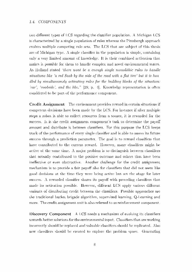
Figure 2.1 shows an overview of XCS' parts and components and how they
are interacting to form the working system. Central aspects are the additional
17
2.3. COMPONENTS OF XCS
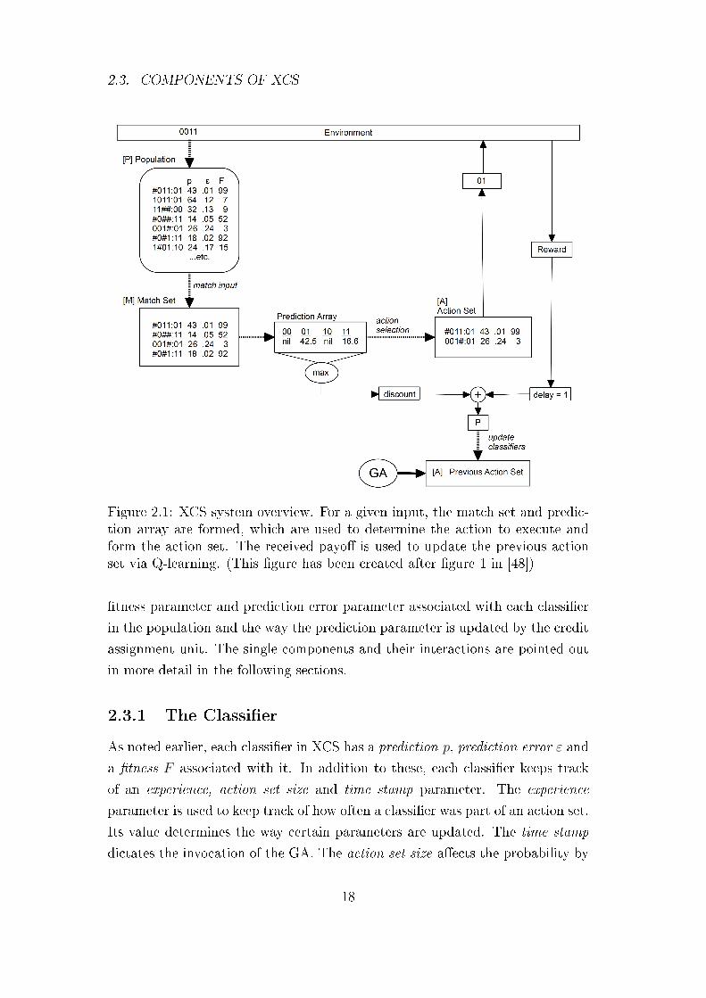
Figure 2.1: XCS system overview. For a given input, the match set and predic-tion array are formed, which are used to determine the action to execute andform the action set. The received payo� is used to update the previous actionset via Q-learning. (This �gure has been created after �gure 1 in [48])
�tness parameter and prediction error parameter associated with each classi�er
in the population and the way the prediction parameter is updated by the credit
assignment unit. The single components and their interactions are pointed out
in more detail in the following sections.
2.3.1 The Classi�er
As noted earlier, each classi�er in XCS has a prediction p, prediction error ε and
a �tness F associated with it. In addition to these, each classi�er keeps track
of an experience, action set size and time stamp parameter. The experience
parameter is used to keep track of how often a classi�er was part of an action set.
Its value determines the way certain parameters are updated. The time stamp
dictates the invocation of the GA. The action set size a�ects the probability by
18
2.3. COMPONENTS OF XCS
which a classi�er is deleted from the population.
Other than that is every classi�er implemented in XCS as what is termed
a macro-classi�er. This means that even if a classi�er occurs twice or more in
the population there is only one macro-classi�er that keeps track of its quantity
by a numerosity parameter. Whenever an already existing classi�er is gener-
ated and inserted in the population only the existent classi�er's numerosity is
incremented. So instead of N identical classi�ers, there is one classi�er with
numerosity N kept in the population. The concept of macro-classi�ers is just a
programming technique used to speed up matching. All procedures treat macro-
classi�ers as if they were multiple traditional classi�ers.
2.3.2 Performance Component
The Di�erent Sets
• The population [P ] represents the actual knowledge of the system. It
contains all existing classi�ers. Its size is �xed.
• The match set [M ] is formed each cycle by comparing the input state with
every classi�er in [P ] and adding all matching classi�ers to [M ].
• The action set [A] is formed by adding to it all classi�ers from [M ] that
propose the action selected for execution.
• The previous action set [A]−1 is maintained in the system every cycle to
update its classi�er's parameters.
The Prediction Array As noted above, [M ] is formed by matching the input
with the population. To �nd the best action to execute, XCS generates a pre-
diction array that has an entry for every possible action. The prediction array
associates an expected payo� with every possible action. Therefor it calculates
the �tness-weighted average of the predictions of classi�ers in [M ] proposing the
same action. Actions that are not present in [M ] get the value nil associated
with them in the prediction array.
Assume there are n classi�ers proposing action ak in [M ]. The associated
predictions and �tnesses are p1, p2, . . . , pn and f1, f2, . . . , fn. In that case the
19
2.3. COMPONENTS OF XCS
entry P (ak) for action ak in the prediction array is calculated as follows:
P (ak) =
∑ni=1 pi ∗ fi∑ni=1 fi
(3.1)
This value is computed for every action that occurs in a classi�er of the
match set.
Action Selection After forming the prediction Array XCS decides which ac-
tion to execute. There are di�erent possible ways to determine such an action.
In this system two approaches are applied. One is choosing the action with the
highest prediction in the prediction array and the other one is choosing an action
randomly. There are two di�erent modes of execution, explore and exploit, and
each of them is associated with one of the action selection schemes. See section
2.6 for further explanation.
2.3.3 Reinforcement Component
The reinforcement component is assigned with distributing payo� and updating
all classi�ers of the previous action set [A]−1. Every time a classi�er belongs to
[A]−1 its parameters are updated. The update mechanism is activated right after
an action has been executed and payo� received. The order in which the updates
occur is experience, prediction error, prediction, action set size, and �tness which
di�ers from the original system. Note that in single-step problems, such as the
multiplexer problem, the update procedure is executed on the current action set
[A] since consecutive steps are not related.
Updating Prediction To update a classi�er's prediction, the Reinforcement
Learning technique Q-learning is applied. Wilson �rst implemented Q-learning
in a LCS in ZCS [47]. After the execution of a selected action, payo� is received.
The current payo� and the maximum prediction value of the prediction array
Pmax are used to calculate the quantity P : P = reward+ γPmax. The discount
factor γ is set to 0.95 in XCSJava 1.0 which is di�erent from the 0.71 suggested
in [5]. For single-step problems it is P = reward.
After calculating P , that value is used in combination with the Widrow-Ho�
delta rule [47] to update the prediction pj of each classi�er in [A−1] ([A] in
20
2.3. COMPONENTS OF XCS
single-step problems):
pj ← pj + β (P − pj)
. The learning rate parameter β is set to 0.2 in XCSJava 1.0. It establishes
the impact a single update has on the classi�er's prediction. Note that the
Widrow-Ho� rule is used only when a classi�er has an experience of at least
1/β. Otherwise �the new values in each case are simple averages of the previous
values and the current one� [48, p. 153]. The applied formula, with experience
expj of clj is:
pj ←pj (expj − 1) + P
expj(3.2)
This two-phase technique is called moyenne adaptive modifée (MAM). Ac-
cording to [48, p. 153] this �makes the system less sensitive to initial, possibly
arbitrary, settings of the parameters�. MAM is applied to the update of the
prediction, prediction error and action set size parameters. When XCS was �rst
introduced in [48], MAM has also been applied to the �tness update.
Fitness Calculation A classi�er's �tness is updated on the basis of its relative
accuracy. First, for a classi�er cj in [A]−1 ([A] for single-step problems) its
accuracy kj is computed. XCSJava 1.0 applies Wilson's power function published
in [49]:
kj = α
(εjε0
)−ν
for εj > ε0 and kj = 1 otherwise. Thus, if a classi�er's prediction error is
smaller or equal to ε0, its accuracy is set to 1. ν is set to 5 in XCSJava 1.0.
In the ensuing step, the relative accuracy k′j is computed by dividing kj by the
total of the accuracies of the classi�ers in [A]−1 ([A] for single-step problems).
For s macro-classi�ers in [A]−1 (resp. [A]) and n being the numerosity of a
macro-classi�er:
k′
j =nj ∗ kj∑si=1 ni ∗ ki
. At last, the Widrow-Ho� formula is applied to update the �tness Fj of clj with
its relative accuracy:
Fj ← Fj + β(k
′
j − Fj)
(3.3)
In contrast to [48] is the MAM technique not used for the �tness update in
XCSJava 1.0.
21
2.3. COMPONENTS OF XCS
Remaining Parameters The prediction error of a classi�er cj, εj is ad-
justed using the MAM technique with the according Widrow-Ho� rule: εj ←εj + β (|P − pj| − εj). Section 2.3.3 clari�ed how P is computed. The same
procedure is applied to the update of the action set size asj of classi�er cj, with
the according Widrow-Ho� formula: asj ← asj + β (cs− asj). The quantity csmarks the current action set size. All these parameter updates apply the MAM
technique. Consequently, in case of expj <1β, formula 3.2 is applied, with the
according parameter to be averaged.
The experience of each classi�er is incremented as soon as the update pro-
cedure begins.
2.3.4 Discovery Component
Genetic Algorithm The Genetic Algorithm occurs after the reinforcement
component �nished updating parameters. It is a niche GA acting only on the
action set. The time stamp parameter of each classi�er marks the last time it was
part of an action set where the GA was active on. The GA acts only occasionally
on the action set, when the di�erence between the average of all classi�er's
time stamps in the action set and the current counter exceeds a threshold θ:
actual time − time stamp avg > θ. θ is set to 25 in XCSJava 1.0. When
the GA becomes active it selects two classi�ers from the action set via roulette
wheel selection. The relation of a classi�er's �tness to the total of the �tnesses of
all classi�ers of the action set constitutes its selection probability. Thus, in this
selection method is the probability for a classi�er to be selected proportionate to
its �tness value. See [5] for a detailed description in pseudo-code. Both selected
classi�ers are copied and with a certain probability there is a two-point crossover
performed on them. The two-point crossover procedure randomly chooses a
number between 0 and the length of the classi�er's condition for each classi�er.
The parts of each classi�er's condition that are located between these two points
are switched. Crossover does not a�ect the action of a classi�er. Thereafter,
the GA performs mutation with a certain probability on each classi�er. For
each symbol of the classi�er's condition, mutation switches it with a certain
probability to a random value. But it never a�ects the condition in a way that
the classi�er would not match the current input anymore. Mutations also occur
on the action part of a classi�er. For a detailed description of the mutation
22
2.3. COMPONENTS OF XCS
operation see [5].
Before the o�spring classi�ers can be inserted into the population the GA
performs a GA subsumption procedure. If one of the parents is more general
than the o�spring classi�er, the o�spring is deleted and instead the parent's
numerosity is incremented. The term more general means that the parent has
to have the same action as the child and at every position in the condition
has the same symbol as the child or a #. For this kind of subsumption to be
possible, the subsuming parent has to be su�ciently experienced and accurate.
It has to have an experience higher than θsub and a prediction error smaller ε0.
In XCSJava 1.0 θsub is set to 20. The reasoning behind GA subsumption is that
the subsumed o�spring could not add any value to the system since everything
it accomplishes is already accomplished by its highly accurate parent.
If no subsumption has been taken place, the GA inserts the o�spring classi-
�ers into the population. There is a possibility that the population is full. In
this case classi�ers have to be deleted to free up space for the o�spring. The clas-
si�ers to be deleted are selected via �tness-dependent roulette-wheel selection.
The exact procedure is described in [5].
Covering The discovery unit is not only responsible for GA execution but
also provides a covering mechanism. Covering takes place if some of the possible
actions are not covered by the classi�ers of the match set. Then, for each missing
action, a correspondent classi�er containing that action and containing a random
matching condition is created and added to the population and match set. If the
population is full, the same deletion method is applied as mentioned previously
in the GA description. The original XCS also applies a covering mechanism to
deal with the case that the system gets stuck in a loop. A loop could occur for
example in a maze environment if the agent is moving back and forth between
two cells all the time. XCSJava 1.0 implements a simpler mechanism to deal
with loops. It is incrementing a counter every step and the speci�c problem
instance is terminated if that counter exceeds a certain threshold. The counter
threshold is set to 50 in XCSJava 1.0.
23
2.4. ACTION SET SUBSUMPTION
2.4 Action Set Subsumption
Besides the GA subsumption described in 2.3.4 there is another kind of sub-
sumption, called action set subsumption, taking place in XCS. The underlying
principle is the same as for GA subsumption but it occurs every time an action
set has been updated. Action set subsumption �rst identi�es the most general
classi�er in the action set with su�cient experience and accuracy. The term
'most general' refers to the classi�er with the most # symbols in its condition.
Afterward, all classi�ers that are subsumed by this most general classi�er are
removed from the action set and population and instead the most general clas-
si�er's numerosity is raised accordingly.
2.5 XCSJava 1.0
XCSJava 1.0 is a Java implementation of the XCS system by Martin V. Butz
published in the year 2000. This section describes certain aspects speci�c to
XCSJava 1.0. It explains the problem types this implementation is able to solve
and brie�y introduces the main �ow of the program.
2.5.1 Problem Types
XCSJava 1.0 is able to solve two kinds of problems, the multiplexer problem
and �ve distinct maze tasks. Whereas the multiplexer is a single-step problem,
maze problems in general are multi-step problems.
Multiplexer Problem The multiplexer problem is de�ned for binary strings
that are assigned either to class 0 or 1. The string of bits consists of an address
part and remaining bits. The address points to a single bit in the remaining part
and if that bit is 0 (resp. 1) the problem instance belongs to class 0 (resp. 1).
The multiplexer can be of di�erent sizes following the pattern: address length+
2address length. Consider the 3-multiplexer. The binary string is of size three with
the �rst bit constituting the address. For the 3-multiplexer 000 is classi�ed as
0 since the zeroth bit after the address is 0. In contrast 010 belongs to class 1.
Correct classi�cations for all instances of the 3-multiplexer are:
• '010', '011', '101', '111' belong to class 1
24
2.6. PROGRAM EXECUTION
• '000', '001', '100', '110' belong to class 0
Common problem sizes are the 6-mulitplexer, 11-multiplexer and 20-multiplexer.
XCSJava 1.0 supports multiplexer problems of any size. It just uses the largest
multiplexer �tting the speci�ed string length and �lls the irrelevant extra bits
with random values.
Maze Problems A maze problem consists of a grid of cells. A cell can be
empty or contain food or an obstacle. A moving agent (also called animat [46])
that was placed on a random cell in the beginning, is moving around in the
maze trying to �nd food. The animat is able to move to all eight adjacent cells
of its current position. If it is moving towards an obstacle it does not leave its
actual position but still one time step elapses. If it steps on a cell containing
food, the food is automatically eaten and reward is received. When food was
found, the speci�c problem instance has been completed. Afterward the food
regrows instantly and the animat is placed in another random position, trying
to �nd food again. There are �ve prede�ned maze environments that XCSJava
supports. Their de�nitions can be found in the 'Environments' folder of the
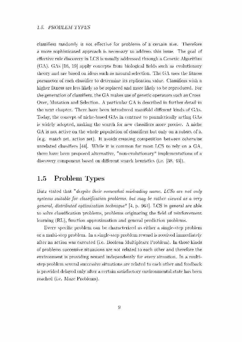
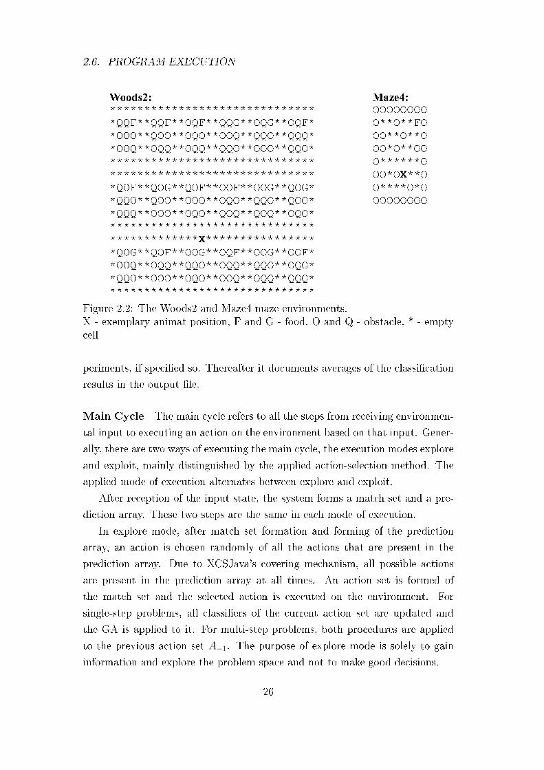
project. The mazes Woods2 and Maze4 are shown in �gure 2.2. If in a maze
without borders the animat is moving beyond an edge of the environment, it
reappears at the opposite side. In some environments such as Woods2 there are
two di�erent kinds of obstacles and food. The animat treats them all the same
but this increases the complexity of the problem.
2.6 Program Execution
XCSJava takes four to six parameters as input to control the main program ex-
ecution. These parameters specify the kind of problem to be solved, the output
�le to document the performance and so on. For a detailed description, see the
documentation [2]. When XCSJava starts, it �rst decodes the input parameters
and instantiates the correct environment that speci�es the problem to be solved.
Afterward it executes the main cycle for a certain number of times that can be
de�ned by an input parameter. Typical is a number of �ve to twenty thou-
sand. When the main cycle has been executed the speci�ed number of times,
one experiment �nished. XCS then might conduct an additional number of ex-
25
2.6. PROGRAM EXECUTION
Figure 2.2: The Woods2 and Maze4 maze environments.X - exemplary animat position, F and G - food, O and Q - obstacle, * - emptycell
periments, if speci�ed so. Thereafter it documents averages of the classi�cation
results in the output �le.
Main Cycle The main cycle refers to all the steps from receiving environmen-
tal input to executing an action on the environment based on that input. Gener-
ally, there are two ways of executing the main cycle, the execution modes explore
and exploit, mainly distinguished by the applied action-selection method. The
applied mode of execution alternates between explore and exploit.
After reception of the input state, the system forms a match set and a pre-
diction array. These two steps are the same in each mode of execution.
In explore mode, after match set formation and forming of the prediction
array, an action is chosen randomly of all the actions that are present in the
prediction array. Due to XCSJava's covering mechanism, all possible actions
are present in the prediction array at all times. An action set is formed of
the match set and the selected action is executed on the environment. For
single-step problems, all classi�ers of the current action set are updated and
the GA is applied to it. For multi-step problems, both procedures are applied
to the previous action set A−1. The purpose of explore mode is solely to gain
information and explore the problem space and not to make good decisions.
26
2.6. PROGRAM EXECUTION
In exploit mode the action with the highest expected payo� is chosen. That
is the action in the prediction array with the highest value associated to it.
The GA is never active in exploit mode and the credit assignment unit is only
activated in multi-step problems. The concern of exploit mode is to maximize
the system's reward. In this mode the system keeps track of its performance to
determine how accurately it is classifying.
Whereas in the original XCS and in [5], the mode of execution is chosen
randomly (with probability 0.5 each), XCSJava 1.0 simply alternates between
explore and exploit.
27
Chapter 3
XCS-DR
This chapter introduces the agent-based extension of XCS, XCS-DR. XCS-DR
stands for 'XCS with Distributed Rules'. First, the main enhancements and
all of its consequences to the overall system are explained. XCS-DR is mostly
distinguished from traditional LCS by the structure of its classi�er population.
In XCS-DR the population is not just a mere pool of classi�ers but is subdi-
vided into several agents of a certain size, all of them containing classi�ers. The
agents are able to exchange or delegate the input state to be classi�ed. This
increase in the population's complexity implies consequences to all other com-
ponents as well. This chapter provides a coherent picture of all the adapted
components and procedures taking place inside XCS-DR. First, it is explained
XCS-DR's architecture and all of its adapted components. The subsequent sec-
tion describes the main execution cycle. Thereafter, it is shown how XCS-DR
behaves in exploit mode. In the ensuing section, explore mode is introduced
and the challenges the agent-based architecture posed to it. Finally, there is a
section discussing the limitations of XCS-DR since many original ideas and pos-
sible enhancements could not be incorporated into its current design. In many
cases are pseudo-code algorithms displayed to facilitate a better understanding
of XCS-DR's inner workings.
Note that the term agent might be a bit confusing in this context as the no-
tion of an agent in this thesis di�ers from the de�nition of a traditional software-
agent. The term has been adopted from [40].
From now on, when it is referred to the 'original XCS' or 'original system',
the XCS implemented by XCSJava 1.0 is meant.
28
3.1. STRUCTURE OF XCS-DR
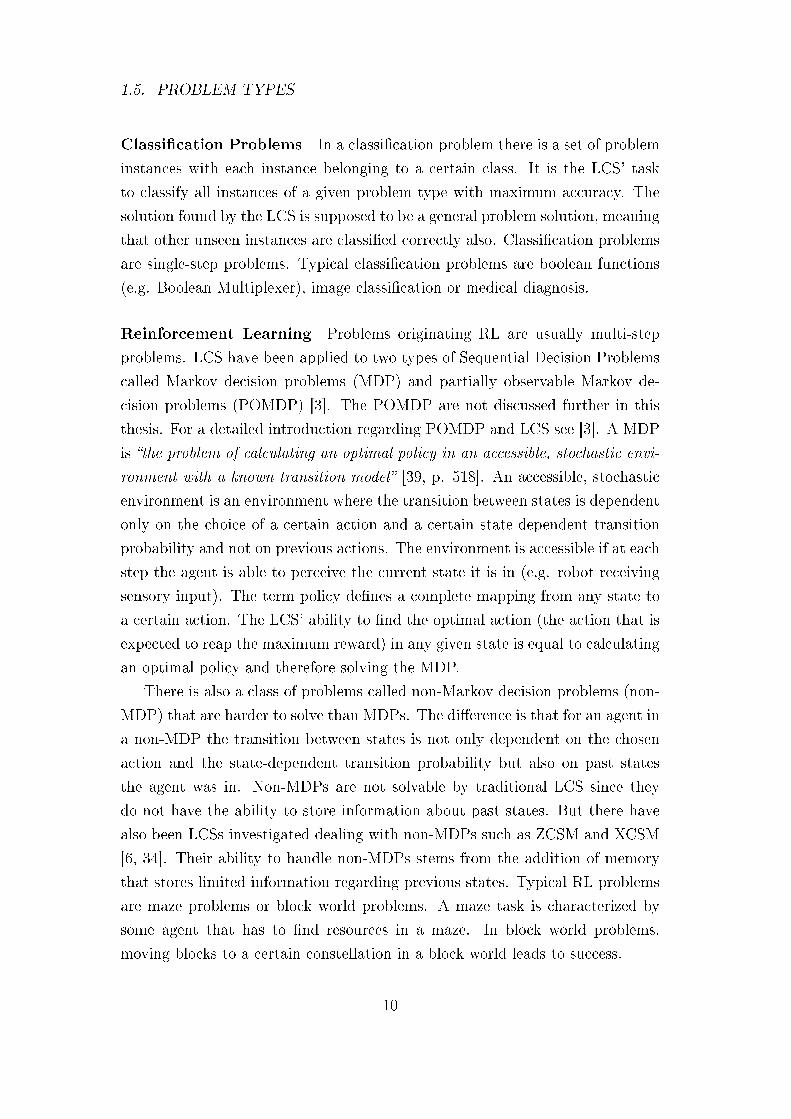
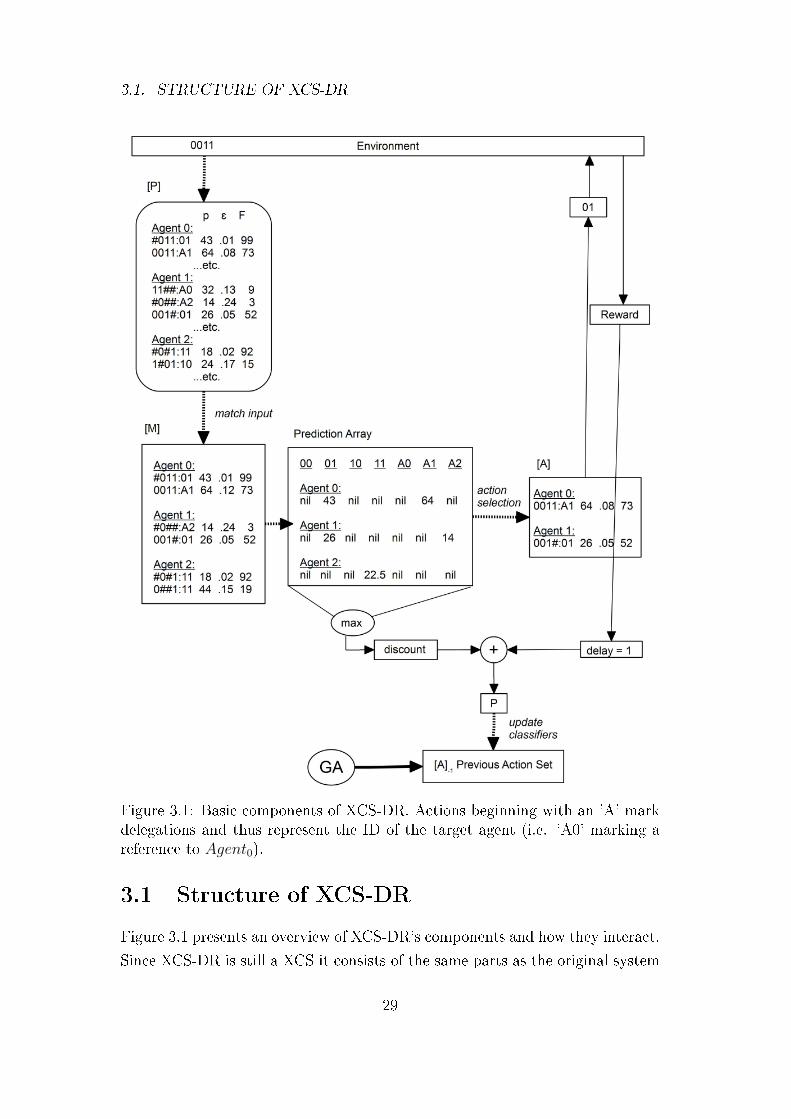
Figure 3.1: Basic components of XCS-DR. Actions beginning with an 'A' markdelegations and thus represent the ID of the target agent (i.e. 'A0' marking areference to Agent0).
3.1 Structure of XCS-DR
Figure 3.1 presents an overview of XCS-DR's components and how they interact.
Since XCS-DR is still a XCS it consists of the same parts as the original system
29
3.2. COMPONENTS OF XCS-DR
but partially, their inner workings di�er vastly from the archetype. As can
be seen in �gure 3.1 all the classi�er sets as well as the prediction array are
subdivided into agents. Also the possible actions a classi�er can propose are
not just actions on the environment but also delegations to other agents. In
the latter, case the input state is handed to the referenced agent. The focal
points, that separate XCS-DR's architecture from the original, are the set of
possible actions, the structure of the classi�er sets and prediction array and
the way they are formed in certain situations. Also the functionality of the
reinforcement component is adapted extensively.
3.2 Components of XCS-DR
As noted earlier XCS-DR includes the same components as the original XCS.
This section provides an overview of the design of every particular component
and points out the di�erences to the original.
3.2.1 The Classi�er
The classi�er in XCS-DR is basically composed of the same elements as in
the original system. Only the action part is enhanced. Every classi�er ei-
ther contains a traditional action that is being executed on the environment
or the action part can be the ID of an agent. The latter denotes that the
classi�er's action proposes a delegation of the input state to the referenced
agent. Therefore, for k agents and n environmental actions we have A ∈{a1, a2, . . . , an, Agent0, Agent1, . . . , Agentk−1}. From now on, actions that
contain a delegation are referred to as delegation actions whereas traditional ac-
tions are referred to as classi�cation actions. Classi�ers containing a delegation
action are simply referred to as delegations and classi�ers containing a classi�ca-
tion action are referred to as classi�cations. The agent that a delegation points
to is called target agent.
3.2.2 Performance Component
The Population As mentioned earlier the main enhancement of XCS-DR lies
in the partitioning of the population. XCS-DR's population is subdivided into
agents with each agent having a unique ID assigned to it. For k agents the ID
30
3.2. COMPONENTS OF XCS-DR
Algorithm 3.1 Form Match Set
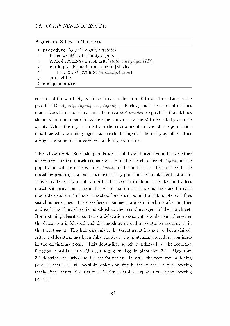
1: procedure FormMatchSet(state)2: Initialize [M ] with empty agents3: AddMatchingClassifiers(state, entryAgentID)4: while possible action missing in [M] do5: PerformCovering(missingAction)6: end while
7: end procedure
consists of the word 'Agent' linked to a number from 0 to k− 1 resulting in the
possible IDs Agent0, Agent1, . . . , Agentk−1. Each agent holds a set of distinct
macro-classi�ers. For the agents there is a slot number s speci�ed, that de�nes
the maximum number of classi�ers (not macro-classi�ers) to be held by a single
agent. When the input state from the environment arrives at the population
it is handed to an entry-agent to match the input. The entry-agent is either
always the same or it is selected randomly each time.
The Match Set Since the population is subdivided into agents this structure
is required for the match set as well. A matching classi�er of Agenti of the
population will be inserted into Agenti of the match set. To begin with the
matching process, there needs to be an entry point in the population to start at.
This so-called entry-agent can either be �xed or random. This does not a�ect
match set formation. The match set formation procedure is the same for each
mode of execution. To match the classi�ers of the population a kind of depth-�rst
search is performed. The classi�ers in an agent are examined one after another
and each matching classi�er is added to the according agent of the match set.
If a matching classi�er contains a delegation action, it is added and thereafter
the delegation is followed and the matching procedure continues recursively in
the target agent. This happens only if the target agent has not yet been visited.
After a delegation has been fully explored, the matching procedure continues
in the originating agent. This depth-�rst search is achieved by the recursive
function AddMatchingClassifiers described in algorithm 3.2. Algorithm
3.1 describes the whole match set formation. If, after the recursive matching
process, there are still possible actions missing in the match set, the covering
mechanism occurs. See section 3.2.4 for a detailed explanation of the covering
process.
31
3.2. COMPONENTS OF XCS-DR
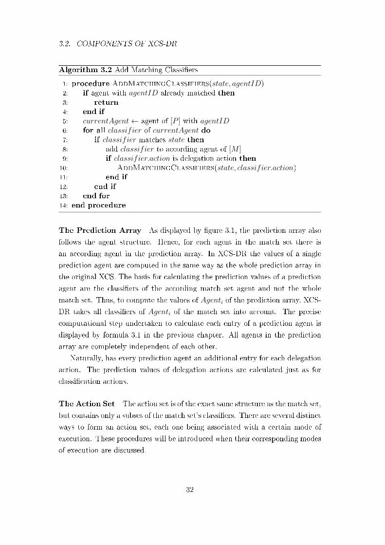
Algorithm 3.2 Add Matching Classi�ers
1: procedure AddMatchingClassifiers(state, agentID)2: if agent with agentID already matched then3: return
4: end if
5: currentAgent← agent of [P ] with agentID6: for all classifier of currentAgent do7: if classifier matches state then8: add classifier to according agent of [M ]9: if classifier.action is delegation action then
10: AddMatchingClassifiers(state, classifier.action)11: end if
12: end if
13: end for
14: end procedure
The Prediction Array As displayed by �gure 3.1, the prediction array also
follows the agent structure. Hence, for each agent in the match set there is
an according agent in the prediction array. In XCS-DR the values of a single
prediction agent are computed in the same way as the whole prediction array in
the original XCS. The basis for calculating the prediction values of a prediction
agent are the classi�ers of the according match set agent and not the whole
match set. Thus, to compute the values of Agenti of the prediction array, XCS-
DR takes all classi�ers of Agenti of the match set into account. The precise
computational step undertaken to calculate each entry of a prediction agent is
displayed by formula 3.1 in the previous chapter. All agents in the prediction
array are completely independent of each other.
Naturally, has every prediction agent an additional entry for each delegation
action. The prediction values of delegation actions are calculated just as for
classi�cation actions.
The Action Set The action set is of the exact same structure as the match set,
but contains only a subset of the match set's classi�ers. There are several distinct
ways to form an action set, each one being associated with a certain mode of
execution. These procedures will be introduced when their corresponding modes
of execution are discussed.
32
3.2. COMPONENTS OF XCS-DR
3.2.3 Reinforcement Component
Updating classi�ers and distributing payo� di�ers from the original system.
There are commonalities, such as the update order of the parameters experi-
ence, prediction, prediction error, action set size and �tness. Also the updates
occur as well on the previous action set [A]−1 in multi-step problems respectively
on the current action set [A] in single-step problems. As in the original system,
in single-step problems the updates only occur during explore and in multi-step
problems the updates occur during both explore and exploit. Generally, action
sets are updated in XCS-DR by iterating over all of their agents and updat-
ing all the classi�ers of an agent one after another. The update procedure of
the parameters experience and action set size did not change compared to the
original. The updates of prediction, prediction error and �tness are dependent
on whether the current classi�er is a delegation or classi�cation and the cur-
rent mode of execution. These procedures will be examined later on when the
corresponding execution modes are introduced.
Fitness Decline The agent-based architecture of XCS-DR is posing some
problems to the �tness calculation. Simply applying the original �tness update
procedure lead to unsatisfying results. XCS-DR still applies the original Widrow-
Ho� formula for the �tness update. But the relative accuracy is calculated
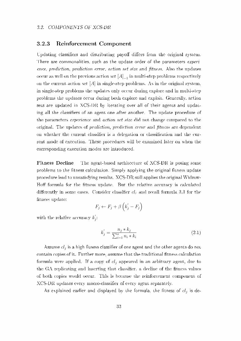
di�erently in some cases. Consider classi�er clj and recall formula 3.3 for the
�tness update:
Fj ← Fj + β(k
′
j − Fj)
with the relative accuracy k′j:
k′
j =nj ∗ kj∑si=1 ni ∗ ki
(2.1)
Assume clj is a high �tness classi�er of one agent and the other agents do not
contain copies of it. Further more, assume that the traditional �tness calculation
formula were applied. If a copy of clj appeared in an arbitrary agent, due to
the GA replicating and inserting that classi�er, a decline of the �tness values
of both copies would occur. This is because the reinforcement component of
XCS-DR updates every macro-classi�er of every agent separately.
As explained earlier and displayed by the formula, the �tness of clj is de-
33
3.2. COMPONENTS OF XCS-DR
termined by computing its relative accuracy in the action set. This results in
much lower �tness values if several instances of clj are scattered across multiple
agents. This is because all the scattered copies of clj are updated independently,
but add collectively to the accuracy sum. Since every instance of clj has a lower
numerosity than they have altogether, for each scattered instance of clj, the
numerator of equation 2.1 is much smaller than it would be if all classi�ers were
stored in the same agent. This leads to a much lower relative accuracy. Hence,
the scattered clj share their total �tness, proportionate to their respective nu-
merosity. If a classi�er appears multiple times with almost equal numerosities
in every location, the resulting �tness value declines signi�cantly. The more
scattered a classi�er is and the higher its accuracy, the stronger is the resulting
total �tness decline.
Two strategies have been applied to avoid this e�ect, one for classi�cations
and another one for delegations. The former is explained in section 3.2.4 and
the latter in 3.5.8.
Overgenerals The reinforcement component of XCS-DR has been slightly
modi�ed to contribute to the evolution of more accurate classi�cations. During
early experiments, the system exposed a tendency towards evolving overgeneral
classi�ers. Overgenerals are classi�ers whose condition is too general and thus
matches too many environmental states. This leads to the misclassi�cation of
some problem instances. The design of the original XCS prevents overgenerals
from emerging but for some reason such classi�ers appear in XCS-DR. This in-
dicates that the system's components are not yet working perfectly to evolve
maximally accurate and general solutions, as XCS does. The most devastat-
ing e�ect in XCS-DR was exhibited by classi�cations containing only dont-care
symbols in their condition part. Such a classi�cation must be an overgeneral,
since none of the problems implemented by XCS-DR can be solved by one single,
maximally general classi�er. A problem that could be solved by a single classi�er
with a maximally general condition would not be of any practical value.
Hence, a very simple step has been implemented to prevent such overgeneral
classi�ers from causing any damage. During the �tness update of classi�cations
it is checked whether or not their condition contains dont-care symbols only. If
so, the following Widrow-Ho� formula is applied for the �tness update:
34
3.2. COMPONENTS OF XCS-DR
Algorithm 3.3 Covering
1: procedure PerformCovering(missingAction)2: clcover ← generate covering classi�er with missingAction3: insert clcover into random agent of [M]4: insert clcover into same agent of [P]5: if missingAction is delegation action then6: AddMatchingClassifiers(state,missingAction)7: end if
8: end procedure
Fj ← Fj + β
(k
′j
100− Fj
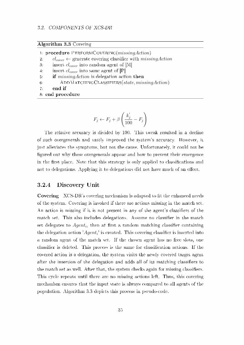
)The relative accuracy is divided by 100. This tweak resulted in a decline
of such overgenerals and vastly improved the system's accuracy. However, it
just alleviates the symptoms, but not the cause. Unfortunately, it could not be
�gured out why these overgenerals appear and how to prevent their emergence
in the �rst place. Note that this strategy is only applied to classi�cations and
not to delegations. Applying it to delegations did not have much of an e�ect.
3.2.4 Discovery Unit
Covering XCS-DR's covering mechanism is adapted to �t the enhanced needs
of the system. Covering is invoked if there are actions missing in the match set.
An action is missing if it is not present in any of the agent's classi�ers of the
match set. This also includes delegations. Assume no classi�er in the match
set delegates to Agenti, then at �rst a random matching classi�er containing
the delegation action 'Agenti' is created. This covering classi�er is inserted into
a random agent of the match set. If the chosen agent has no free slots, one
classi�er is deleted. This process is the same for classi�cation actions. If the
covered action is a delegation, the system visits the newly covered target agent
after the insertion of the delegation and adds all of its matching classi�ers to
the match set as well. After that, the system checks again for missing classi�ers.
This cycle repeats until there are no missing actions left. Thus, this covering
mechanism ensures that the input state is always compared to all agents of the
population. Algorithm 3.3 depicts this process in pseudo-code.
35
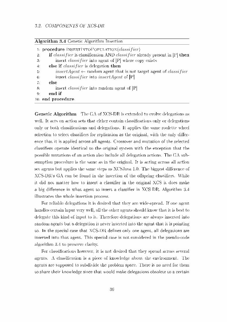
3.2. COMPONENTS OF XCS-DR
Algorithm 3.4 Genetic Algorithm Insertion
1: procedure InsertIntoPopulation(classifier)2: if classifier is classi�cation AND classifier already present in [P] then3: insert classifier into agent of [P] where copy exists4: else if classifier is delegation then5: insertAgent← random agent that is not target agent of classifier6: insert classifier into insertAgent of [P]7: else
8: insert classifier into random agent of [P]9: end if
10: end procedure
Genetic Algorithm The GA of XCS-DR is extended to evolve delegations as
well. It acts on action sets that either contain classi�cations only or delegations
only or both classi�cations and delegations. It applies the same roulette wheel
selection to select classi�ers for replication as the original, with the only di�er-
ence that it is applied across all agents. Crossover and mutation of the selected
classi�ers operate identical to the original system with the exception that the
possible mutations of an action also include all delegation actions. The GA sub-
sumption procedure is the same as in the original. It is acting across all action
set agents but applies the same steps as XCSJava 1.0. The biggest di�erence of
XCS-DR's GA can be found in the insertion of the o�spring classi�ers. While
it did not matter how to insert a classi�er in the original XCS it does make
a big di�erence in what agent to insert a classi�er in XCS-DR. Algorithm 3.4
illustrates the whole insertion process.
For reliable delegations it is desired that they are wide-spread. If one agent
handles certain input very well, all the other agents should know that it is best to
delegate this kind of input to it. Therefore delegations are always inserted into
random agents but a delegation is never inserted into the agent that it is pointing
to. In the special case that XCS-DR de�nes only one agent, all delegations are
inserted into that agent. This special case is not considered in the pseudo-code
algorithm 3.4 to preserve clarity.
For classi�cations however, it is not desired that they spread across several
agents. A classi�cation is a piece of knowledge about the environment. The
agents are supposed to subdivide the problem space. There is no need for them
to share their knowledge since that would make delegations obsolete to a certain
36
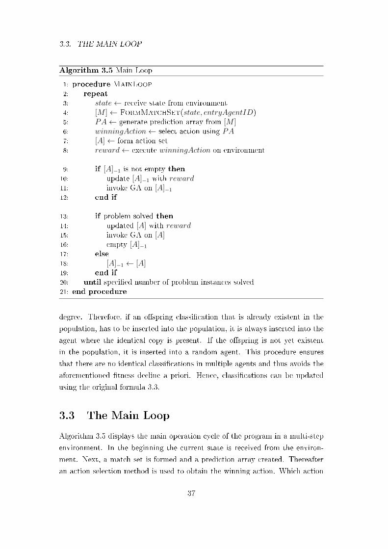
3.3. THE MAIN LOOP
Algorithm 3.5 Main Loop
1: procedure MainLoop2: repeat
3: state← receive state from environment4: [M ]← FormMatchSet(state, entryAgentID)5: PA← generate prediction array from [M ]6: winningAction← select action using PA7: [A]← form action set8: reward← execute winningAction on environment
9: if [A]−1 is not empty then10: update [A]−1 with reward11: invoke GA on [A]−1
12: end if
13: if problem solved then14: updated [A] with reward15: invoke GA on [A]16: empty [A]−1
17: else
18: [A]−1 ← [A]19: end if
20: until speci�ed number of problem instances solved21: end procedure
degree. Therefore, if an o�spring classi�cation that is already existent in the
population, has to be inserted into the population, it is always inserted into the
agent where the identical copy is present. If the o�spring is not yet existent
in the population, it is inserted into a random agent. This procedure ensures
that there are no identical classi�cations in multiple agents and thus avoids the
aforementioned �tness decline a priori. Hence, classi�cations can be updated
using the original formula 3.3.
3.3 The Main Loop
Algorithm 3.5 displays the main operation cycle of the program in a multi-step
environment. In the beginning the current state is received from the environ-
ment. Next, a match set is formed and a prediction array created. Thereafter
an action selection method is used to obtain the winning action. Which action
37
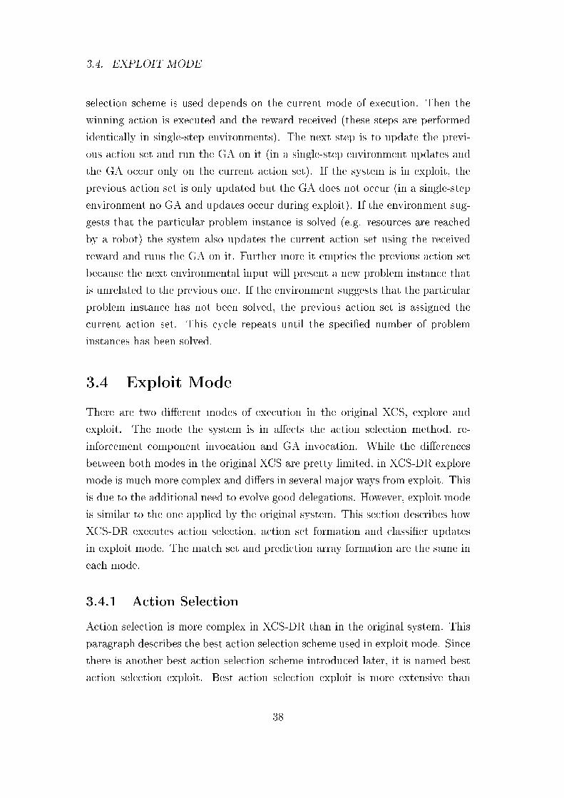
3.4. EXPLOIT MODE
selection scheme is used depends on the current mode of execution. Then the
winning action is executed and the reward received (these steps are performed
identically in single-step environments). The next step is to update the previ-
ous action set and run the GA on it (in a single-step environment updates and
the GA occur only on the current action set). If the system is in exploit, the
previous action set is only updated but the GA does not occur (in a single-step
environment no GA and updates occur during exploit). If the environment sug-
gests that the particular problem instance is solved (e.g. resources are reached
by a robot) the system also updates the current action set using the received
reward and runs the GA on it. Further more it empties the previous action set
because the next environmental input will present a new problem instance that
is unrelated to the previous one. If the environment suggests that the particular
problem instance has not been solved, the previous action set is assigned the
current action set. This cycle repeats until the speci�ed number of problem
instances has been solved.
3.4 Exploit Mode
There are two di�erent modes of execution in the original XCS, explore and
exploit. The mode the system is in a�ects the action selection method, re-
inforcement component invocation and GA invocation. While the di�erences
between both modes in the original XCS are pretty limited, in XCS-DR explore
mode is much more complex and di�ers in several major ways from exploit. This
is due to the additional need to evolve good delegations. However, exploit mode
is similar to the one applied by the original system. This section describes how
XCS-DR executes action selection, action set formation and classi�er updates
in exploit mode. The match set and prediction array formation are the same in
each mode.
3.4.1 Action Selection
Action selection is more complex in XCS-DR than in the original system. This
paragraph describes the best action selection scheme used in exploit mode. Since
there is another best action selection scheme introduced later, it is named best
action selection exploit. Best action selection exploit is more extensive than
38
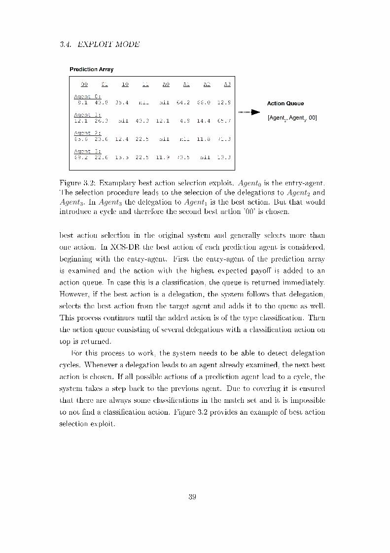
3.4. EXPLOIT MODE
Figure 3.2: Examplary best action selection exploit. Agent0 is the entry-agent.The selection procedure leads to the selection of the delegations to Agent2 andAgent3. In Agent3 the delegation to Agent1 is the best action. But that wouldintroduce a cycle and therefore the second best action '00' is chosen.
best action selection in the original system and generally selects more than
one action. In XCS-DR the best action of each prediction agent is considered,
beginning with the entry-agent. First the entry-agent of the prediction array
is examined and the action with the highest expected payo� is added to an
action queue. In case this is a classi�cation, the queue is returned immediately.
However, if the best action is a delegation, the system follows that delegation,
selects the best action from the target agent and adds it to the queue as well.
This process continues until the added action is of the type classi�cation. Then
the action queue consisting of several delegations with a classi�cation action on
top is returned.
For this process to work, the system needs to be able to detect delegation
cycles. Whenever a delegation leads to an agent already examined, the next best
action is chosen. If all possible actions of a prediction agent lead to a cycle, the
system takes a step back to the previous agent. Due to covering it is ensured
that there are always some classi�cations in the match set and it is impossible
to not �nd a classi�cation action. Figure 3.2 provides an example of best action
selection exploit.
39
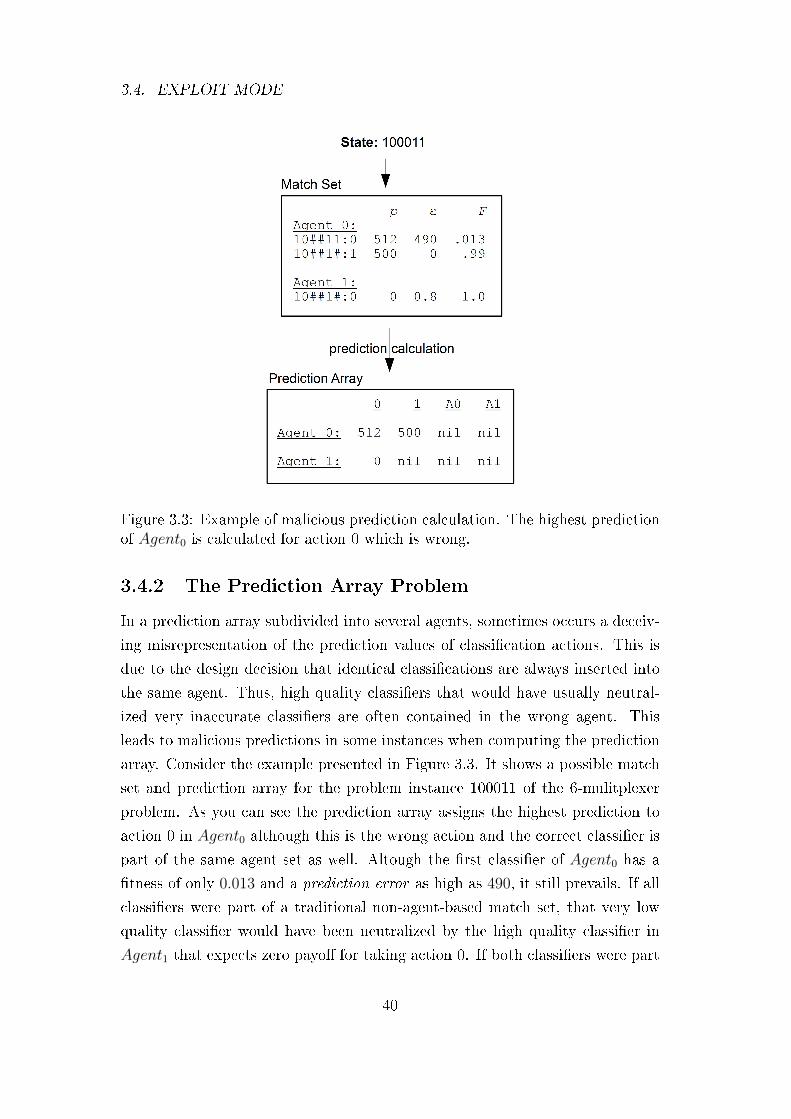
3.4. EXPLOIT MODE
Figure 3.3: Example of malicious prediction calculation. The highest predictionof Agent0 is calculated for action 0 which is wrong.
3.4.2 The Prediction Array Problem
In a prediction array subdivided into several agents, sometimes occurs a deceiv-
ing misrepresentation of the prediction values of classi�cation actions. This is
due to the design decision that identical classi�cations are always inserted into
the same agent. Thus, high quality classi�ers that would have usually neutral-
ized very inaccurate classi�ers are often contained in the wrong agent. This
leads to malicious predictions in some instances when computing the prediction
array. Consider the example presented in Figure 3.3. It shows a possible match
set and prediction array for the problem instance 100011 of the 6-mulitplexer
problem. As you can see the prediction array assigns the highest prediction to
action 0 in Agent0 although this is the wrong action and the correct classi�er is
part of the same agent set as well. Altough the �rst classi�er of Agent0 has a
�tness of only 0.013 and a prediction error as high as 490, it still prevails. If all
classi�ers were part of a traditional non-agent-based match set, that very low
quality classi�er would have been neutralized by the high quality classi�er in
Agent1 that expects zero payo� for taking action 0. If both classi�ers were part
40
3.4. EXPLOIT MODE
of the same agent or part of a traditional match set, their combined prediction
for action 0 would have been 512∗0.013+0∗1.01.0+0.013
= 6.571 which is far below the actual
512 for the same action in Agent0. Due to the fact that the neutralizing clas-
si�cation is part of Agent1 and all identical classi�cations will be inserted into
Agent1 as well, this one has no chance to in�uence the prediction calculation
of Agent0. This structural di�erence to the original system enables low �tness
classi�ers, that would have been irrelevant in a non-agent-based approach, to
gain control in some cases and lead to wrong classi�cations.
The straightforward solution applied by XCS-DR to restrict the in�uence of
such malicious classi�ers is to ignore classi�ers with too low of a �tness value.
During calculation of the prediction array there has to be found a sensible �tness
threshold that excludes very weak classi�ers. The �tness of each newly created
classi�er is initialized with 0.01 and experiments have shown that setting this
value as a threshold for the prediction calculation leads to good results. This
means the prediction array ignores every classi�er with a �tness below 0.01 in
its prediction calculation procedure. The threshold should not be too high since
that causes good classi�ers to be ignored too often as well. The exclusion of low
�tness classi�ers takes place during prediction calculation only. These classi�ers
are still part of the action set and get updated as every other classi�er.
3.4.3 Formation of the Action Set
After applying best action selection exploit, an action set is formed. Action
selection exploit does not necessarily return only a single classi�cation action
but might instead result in a queue of several delegations and a classi�cation
action on top. Due to the particular process of choosing the best action of every
prediction agent beginning with the entry-agent, each action in the queue can
be associated with a certain match set agent. The action that �rst entered
the queue is the one selected from the entry-agent. Therefore all classi�ers in
the entry-agent of the match set containing that �rst action are added to the
according agent of the action set. If the added action is a classi�cation action,
the queue does not contain any additional actions and the action set is complete.
If it is a delegation, its target agent of the match set is investigated for classi�ers
containing the next action in the queue. This process is repeated until every
action in the queue was considered. Algorithm 3.6 depicts this process.
41
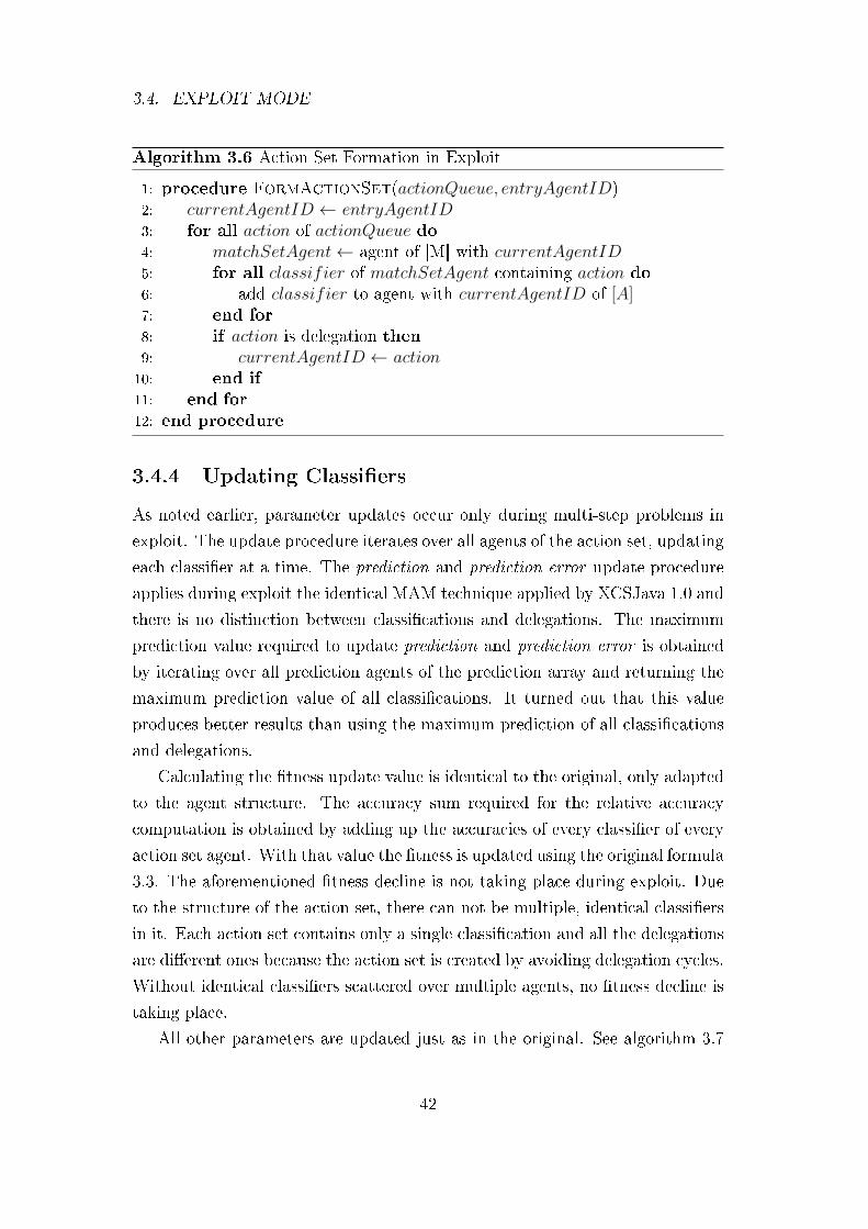
3.4. EXPLOIT MODE
Algorithm 3.6 Action Set Formation in Exploit
1: procedure FormActionSet(actionQueue, entryAgentID)2: currentAgentID ← entryAgentID3: for all action of actionQueue do4: matchSetAgent← agent of [M] with currentAgentID5: for all classifier of matchSetAgent containing action do6: add classifier to agent with currentAgentID of [A]7: end for
8: if action is delegation then9: currentAgentID ← action
10: end if
11: end for
12: end procedure
3.4.4 Updating Classi�ers
As noted earlier, parameter updates occur only during multi-step problems in
exploit. The update procedure iterates over all agents of the action set, updating
each classi�er at a time. The prediction and prediction error update procedure
applies during exploit the identical MAM technique applied by XCSJava 1.0 and
there is no distinction between classi�cations and delegations. The maximum
prediction value required to update prediction and prediction error is obtained
by iterating over all prediction agents of the prediction array and returning the
maximum prediction value of all classi�cations. It turned out that this value
produces better results than using the maximum prediction of all classi�cations
and delegations.
Calculating the �tness update value is identical to the original, only adapted
to the agent structure. The accuracy sum required for the relative accuracy
computation is obtained by adding up the accuracies of every classi�er of every
action set agent. With that value the �tness is updated using the original formula
3.3. The aforementioned �tness decline is not taking place during exploit. Due
to the structure of the action set, there can not be multiple, identical classi�ers
in it. Each action set contains only a single classi�cation and all the delegations
are di�erent ones because the action set is created by avoiding delegation cycles.
Without identical classi�ers scattered over multiple agents, no �tness decline is
taking place.
All other parameters are updated just as in the original. See algorithm 3.7
42
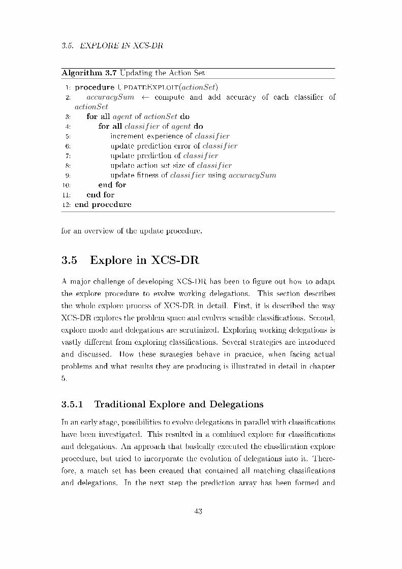
3.5. EXPLORE IN XCS-DR
Algorithm 3.7 Updating the Action Set
1: procedure UpdateExploit(actionSet)2: accuracySum ← compute and add accuracy of each classi�er ofactionSet
3: for all agent of actionSet do4: for all classifier of agent do5: increment experience of classifier6: update prediction error of classifier7: update prediction of classifier8: update action set size of classifier9: update �tness of classifier using accuracySum
10: end for
11: end for
12: end procedure
for an overview of the update procedure.
3.5 Explore in XCS-DR
A major challenge of developing XCS-DR has been to �gure out how to adapt
the explore procedure to evolve working delegations. This section describes
the whole explore process of XCS-DR in detail. First, it is described the way
XCS-DR explores the problem space and evolves sensible classi�cations. Second,
explore mode and delegations are scrutinized. Exploring working delegations is
vastly di�erent from exploring classi�cations. Several strategies are introduced
and discussed. How these strategies behave in practice, when facing actual
problems and what results they are producing is illustrated in detail in chapter
5.
3.5.1 Traditional Explore and Delegations
In an early stage, possibilities to evolve delegations in parallel with classi�cations
have been investigated. This resulted in a combined explore for classi�cations
and delegations. An approach that basically executed the classi�cation explore
procedure, but tried to incorporate the evolution of delegations into it. There-
fore, a match set has been created that contained all matching classi�cations
and delegations. In the next step the prediction array has been formed and
43
3.5. EXPLORE IN XCS-DR
a random classi�cation action selected for execution. This step is crucial for
exploring classi�cations and therefore the action selection method could not be
changed. Afterward, the action set was created by adding all classi�cations with
the according action and all delegations that reach a classi�cation that is already
part of the action set. The term 'reaches' means that either the target agent of
the delegation contains such a classi�cation or that, by following further delega-
tions, at least one visited agent contains such a classi�cation. After creating the
action set the selected action was executed and payo� received and distributed.
While this works perfectly �ne to update classi�cations with the received
payo�, the same procedure does not apply well to delegations. The main problem
is that random action selection is not suitable to evolve delegations. That fact
stems from the inherent di�erence between what is a valuable classi�cation and
a valuable delegation. A valuable classi�cation correctly predicts the payo� that
is received when executing its proposed action. A valuable delegation predicts
the payo� that is received when the delegation's target agent executes the action
with the highest prediction. These characteristics of valuable classi�cations and
delegations directly result from the way the exploit procedure has been designed.
Since a delegation predicts payo� in a more indirect way, one can not evolve
it e�ciently by using random action selection. Assume, in the just mentioned
explore scheme, action a1 had been chosen by random action selection. Further
more, assume there is a best action a2 in that situation. For a delegation it does
not matter what amount of payo� a1 receives. It matters whether its target agent
would have executed a2 in exploit. And if so, the amount of payo� received by
a2 is of importance to that delegation. Hence, updating delegations with the
irrelevant payo� information gained by executing a1 is completely misleading.
In practice, updating delegations with such bad information led to the evolution
of delegations with extremely high prediction errors and very low �tnesses. To
avoid this issue a separate delegation explore mode has been added to the system.
Note that I do not consider it impossible to evolve useful classi�cations and
delegations in parallel. But all the investigated approaches led to very inaccurate
delegations and evolving delegations separately seemed to be the more promising
approach.
44
3.5. EXPLORE IN XCS-DR
3.5.2 Exploring Classi�cations
Since no reasonable way to evolve delegations and classi�cations in parallel could
be found, both tasks have to be achieved independently from each other. Hence
the traditional explore mode had to be split in two explores. The system no
longer alternates between exploit and explore but between exploit, classi�cation
explore and delegation explore. Pursuing this approach takes more time to
evolve good classi�ers since in total twice as many explore steps are performed
compared to the original XCS. To evolve good classi�cations during explore,
XCS-DR mainly proceeds as the original. This is the mode called classi�cation
explore. For a given state, a match set is created, covering might occur, a
random action is chosen, an action set is built and the reward is collected. With
the received reward all classi�ers of the previous action set are updated and the
GA might occur. The match set is formed as described earlier. An action is
chosen randomly from the set of possible classi�cation actions. The action set
is created by adding all classi�ers of the match set to it that hold the winning
classi�cation action. The delegations of the match set are ignored. The update
procedure is the same that is applied during exploit. The �tness decline can
not occur because only classi�cations are part of the action set and identical
classi�cations are always added to the same agent. Thus, no classi�ers are
scattered across the action set.
Due to the discovery unit inserting identical classi�cations always in the same
agent, every agent is able to solve only parts of the problem. The general process
of evolving classi�cations is so close to the original that for a given environment
the same classi�ers prevail in XCS-DR as in the original system. That is desired
behavior since the original system explores an accurate and maximally general
solution for a given problem. See chapter 5 for an experimental comparison of
a single-agent XCS-DR and XCSJava 1.0.
3.5.3 Evolution of Delegation Classi�ers
As noted earlier it is the goal of a single delegation to point to an agent more
suitable for matching input states. This means, if the matching input state were
classi�ed by the home agent of the delegation, less payo� would be received
than if the input were classi�ed by the delegation's target agent. Thus the main
goal of a delegation explore mode must be to distribute payo� in a way that
45
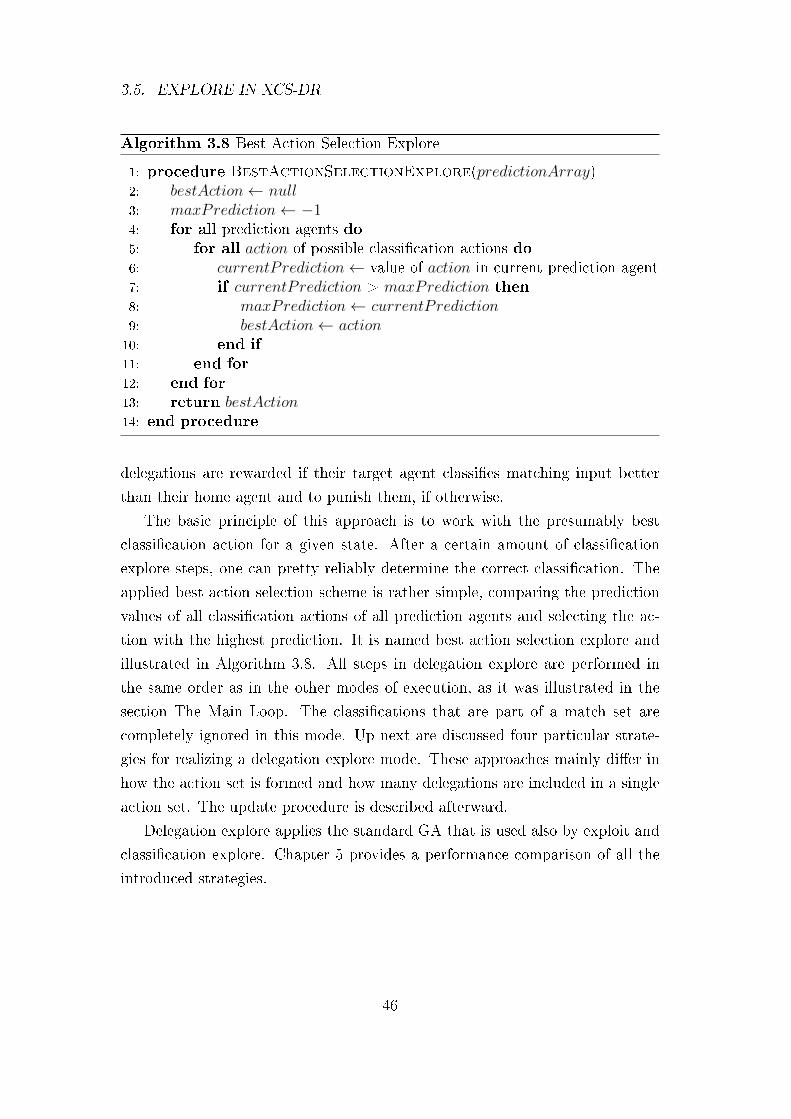
3.5. EXPLORE IN XCS-DR
Algorithm 3.8 Best Action Selection Explore
1: procedure BestActionSelectionExplore(predictionArray)2: bestAction← null3: maxPrediction← −14: for all prediction agents do5: for all action of possible classi�cation actions do6: currentPrediction← value of action in current prediction agent7: if currentPrediction > maxPrediction then8: maxPrediction← currentPrediction9: bestAction← action
10: end if
11: end for
12: end for
13: return bestAction14: end procedure
delegations are rewarded if their target agent classi�es matching input better
than their home agent and to punish them, if otherwise.
The basic principle of this approach is to work with the presumably best
classi�cation action for a given state. After a certain amount of classi�cation
explore steps, one can pretty reliably determine the correct classi�cation. The
applied best action selection scheme is rather simple, comparing the prediction
values of all classi�cation actions of all prediction agents and selecting the ac-
tion with the highest prediction. It is named best action selection explore and
illustrated in Algorithm 3.8. All steps in delegation explore are performed in
the same order as in the other modes of execution, as it was illustrated in the
section The Main Loop. The classi�cations that are part of a match set are
completely ignored in this mode. Up next are discussed four particular strate-
gies for realizing a delegation explore mode. These approaches mainly di�er in
how the action set is formed and how many delegations are included in a single
action set. The update procedure is described afterward.
Delegation explore applies the standard GA that is used also by exploit and
classi�cation explore. Chapter 5 provides a performance comparison of all the
introduced strategies.
46
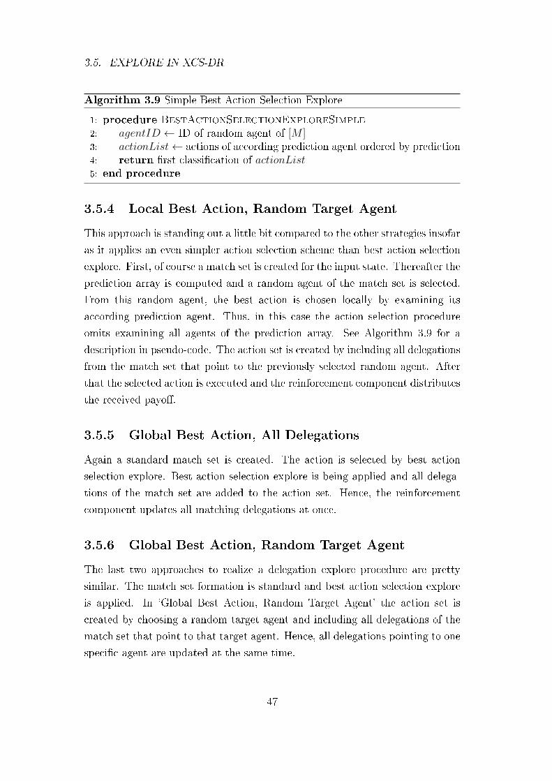
3.5. EXPLORE IN XCS-DR
Algorithm 3.9 Simple Best Action Selection Explore
1: procedure BestActionSelectionExploreSimple2: agentID ← ID of random agent of [M ]3: actionList← actions of according prediction agent ordered by prediction4: return �rst classi�cation of actionList5: end procedure
3.5.4 Local Best Action, Random Target Agent
This approach is standing out a little bit compared to the other strategies insofar
as it applies an even simpler action selection scheme than best action selection
explore. First, of course a match set is created for the input state. Thereafter the
prediction array is computed and a random agent of the match set is selected.
From this random agent, the best action is chosen locally by examining its
according prediction agent. Thus, in this case the action selection procedure
omits examining all agents of the prediction array. See Algorithm 3.9 for a
description in pseudo-code. The action set is created by including all delegations
from the match set that point to the previously selected random agent. After
that the selected action is executed and the reinforcement component distributes
the received payo�.
3.5.5 Global Best Action, All Delegations
Again a standard match set is created. The action is selected by best action
selection explore. Best action selection explore is being applied and all delega-
tions of the match set are added to the action set. Hence, the reinforcement
component updates all matching delegations at once.
3.5.6 Global Best Action, Random Target Agent
The last two approaches to realize a delegation explore procedure are pretty
similar. The match set formation is standard and best action selection explore
is applied. In 'Global Best Action, Random Target Agent' the action set is
created by choosing a random target agent and including all delegations of the
match set that point to that target agent. Hence, all delegations pointing to one
speci�c agent are updated at the same time.
47
3.5. EXPLORE IN XCS-DR
3.5.7 Global Best Action, Random Home Agent
In this approach the randomly chosen agent is not marking the target agent, but
the home agent. The di�erence to the previous approach is that the action set is
created by adding to it all delegations of that random match set home agent. It
does not matter where the delegations are pointing to. Therefore, in this case all
delegations contained in a single random match set agent are updated at once.
3.5.8 Classi�er Updates in Delegation Explore
As noted earlier, there is a di�erence between useful classi�cations and useful
delegations that requires an adapted update procedure for delegations. In all
previously introduced delegation explore procedures, there has been employed
some kind of best action selection. Therefore, the received reward is expected
to be higher than by executing random actions and it can not be used directly
to update delegations. In XCS-DR a delegation receives payo�, if the prediction
of the delegation's target agent is higher than the prediction of the delegation's
home agent for the selected action. Otherwise, the reward for that delegation
is set to zero. The idea behind this approach is that a higher prediction for the
presumably best action in a speci�c agent indicates that this agent would rather
likely select that action during exploit. Hence, if that agent is the delegation's
target agent, the delegation itself is useful. Whereas the computation of P is
di�erent, the actual update formulas applied to the prediction and prediction
error parameters are the ones used in the original. See Algorithm 3.10 for an
illustration of this process in pseudo-code.
The �tness calculation of delegations also di�ers from the original. Due to the
previously mentioned possible �tness decline caused by scattered delegations, a
di�erent calculation of the relative accuracy has to be applied. For a delegation
dj in the action set, there is a total numerosity njtotal computed by adding up
the numerosities of all delegations identical to dj in the action set. Thereafter,
the relative accuracy of dj is calculated using its corresponding njtotal instead
of the actual numerosity nj. If there are no identical delegations scattered over
multiple agents, the total numerosity of a delegation and its actual numerosity
are the same. For a delegation dj with accuracy kj and corresponding total
numerosity njtotal is the relative accuracy computed with the following formula:
48
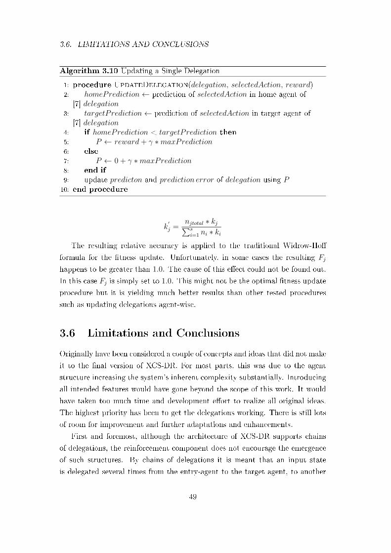
3.6. LIMITATIONS AND CONCLUSIONS
Algorithm 3.10 Updating a Single Delegation
1: procedure UpdateDelegation(delegation, selectedAction, reward)2: homePrediction← prediction of selectedAction in home agent of
[7] delegation3: targetPrediction← prediction of selectedAction in target agent of
[7] delegation4: if homePrediction < targetPrediction then5: P ← reward+ γ ∗maxPrediction6: else
7: P ← 0 + γ ∗maxPrediction8: end if
9: update predicton and prediction error of delegation using P10: end procedure
k′
j =njtotal ∗ kj∑si=1 ni ∗ ki
The resulting relative accuracy is applied to the traditional Widrow-Ho�
formula for the �tness update. Unfortunately, in some cases the resulting Fj
happens to be greater than 1.0. The cause of this e�ect could not be found out.
In this case Fj is simply set to 1.0. This might not be the optimal �tness update
procedure but it is yielding much better results than other tested procedures
such as updating delegations agent-wise.
3.6 Limitations and Conclusions
Originally have been considered a couple of concepts and ideas that did not make
it to the �nal version of XCS-DR. For most parts, this was due to the agent
structure increasing the system's inherent complexity substantially. Introducing
all intended features would have gone beyond the scope of this work. It would
have taken too much time and development e�ort to realize all original ideas.
The highest priority has been to get the delegations working. There is still lots
of room for improvement and further adaptations and enhancements.
First and foremost, although the architecture of XCS-DR supports chains
of delegations, the reinforcement component does not encourage the emergence
of such structures. By chains of delegations it is meant that an input state
is delegated several times from the entry-agent to the target agent, to another
49
3.6. LIMITATIONS AND CONCLUSIONS
target agent, and so on until it is �nally classi�ed. The reinforcement component
only rewards delegations when their target agent immediately provides a high
prediction value and does not provide any payo� if further delegations would
have lead to successful classi�cation instead. This simpli�cation was necessary to
evolve sensible delegations in the �rst place but an extension of the reinforcement
component is thinkable.
Also, at �rst it was considered to introduce a way of penalizing delegations
as it is applied in [40] to exert a certain kind of control over emerging delegation
structures. For instance one could think of generally penalizing delegations by
distributing less payo� to them in order to encourage early classi�cation. Or if
chains of delegations were emerging in the system one could restrict the maxi-
mum number of hops through penalties. Due to the complications of evolving
valuable delegations in general, this ideas had been discarded and there is no
penalty whatsoever implemented.
Another idea has been to implement graph structures for the agents. For
instance, enabling a grid topology where only delegations to adjacent agents
would have been allowed. It would not be di�cult to implement such a pre-
determined graph structure but this could not go hand in hand with the way
classi�cations are distributed among agents right now. Certain agents would
not be able to delegate to the agent containing the correct classi�er for a certain
state because of the according agent not being adjacent in the graph. Therefore,
the distribution of classi�cations would have to be changed, which would entail
further adaptations.
Finally, the agents of XCS-DR might not be independent enough of each
other to be applied successfully in a distributed scenario. The explore process
requires a certain amount of communication between the agents, e.g. for calcu-
lating the accuracy sum or sharing reward which might be too much to handle
e�ciently in a distributed environment. However, it would certainly be possible
to optimize these processes for distributed environments. As of right now, the
system could easily be adapted to o�ine application in distributed scenarios. In
o�ine learning a LCS is previously trained to evolve the classi�er population be-
fore being applied to the actual problem. After the training phase the classi�er
set is �xed. O�ine learning works for environments that are not changing but
is inapplicable to �uctuating environments. Since the exploit mode of XCS-DR
does not require lots of communication between the agents except for delegating
50

3.6. LIMITATIONS AND CONCLUSIONS
input, an adapted XCS-DR would be suitable for o�ine applications such as
wireless sensor networks.
51
Chapter 4
XCS-DR Java Implementation
The architecture of the XCS-DR implementation is vastly di�erent from XCS-
Java 1.0. While XCSJava 1.0 was the starting point, its whole design had to
be revised and enhanced to adapt the system to its additional requirements.
Also XCS-DR implements a new kind of problem it is able to solve, the incre-
mental parity problem. First, in this chapter, the incremental parity problem is
examined and compared to the multiplexer problem. Next, the structure of XC-
SJava 1.0 is discussed and criticized in brief and some of its unfavorable design
decisions and implementation details are traced down. Thereafter, the overall
architecture of XCS-DR's Java implementation is introduced and explained. An
overview of the package and class structure is presented as well as a brief descrip-
tion of most classes. Further more, this chapter shows how to run and con�gure
the XCS-DR implementation and how to read the output. Additionally, it is
explained how to edit the project's source code. This is crucial to be able to
fully explore XCS-DR's functionality since some parameter changes can only be
undertaken in the source code.
4.1 Problem Types
XCS-DR is able to solve the multiplexer and maze problems that the original
system implemented. Further more it is extended to also solve the incremental
parity problem (IPP). The incremental parity problem of size m (m−IPP) isde�ned for binary strings of length m. Strings have to be classi�ed by their
parity. The parity of such a string is 0 if the number of 1s in the string is even
and 1 otherwise. E.g. the instance 00101 of the 5-IPP is of class 0, whereas 01101
52
4.2. CRITICISM OF THE XCSJAVA 1.0 IMPLEMENTATION
is of class 1. This characterization makes it a single-step problem that is di�erent
from the multiplexer problem insofar, as it lacks the potential for generalization.
Whereas an accurate solution to the multiplexer requires relatively few rules
due to most positions being irrelevant, the m-IPP requires at least 2(m−1) [40]
rules to correctly classify every problem instance. This is because every single
bit of every IPP instance is relevant and it is impossible to generalize without
sacri�cing accuracy. The IPP was implemented mainly to compare how XCS-DR
performs when facing problems that have very low generalization potential.
4.1.1 The Multiplexer Payo� Landscape
The XCSJava 1.0 implementation provides a payo� landscape for the multiplexer
problem that has originally been taken from [48]. It is adopted by XCS-DR
and can be applied by setting the con�guration parameter payo�-type to 1. The
payo� landscape associates di�erent payo� values to di�erent problem instances.
It subdivides the problem space and a correct classi�cation always receives 300
payo� more than an incorrect classi�cation. For instance the correct, matching
classi�er 000### : 0 would receive 300 payo� when executed, whereas the
incorrect classi�er 000### : 1 would receive 0 payo�. 01#0## : 0 would
receive 400 payo� and 01#0## : 1 would receive 100 payo�. Every possible
address has di�erent payo� values associated with it that are received after
correct or incorrect classi�cation. The payo�s rise in 100 point increments from
the lowest address to the highest address.
4.2 Criticism of the XCSJava 1.0 Implementation
XCSJava 1.0 violates many principles of object oriented design in general and
several Java best practices in particular. This resulted in source code that is
hard to understand and to adapt. As stated by McConnell in [35, pp. 78] �Man-
aging complexity is the most important technical topic in software development�.
It is important for a program to be readable and to provide several levels of
abstraction from the underlying technical implementation details by providing
well structured classes and reasonable interfaces.
Unfortunately, XCSJava 1.0 is not making use of Java's ability to organize
classes in a package structure. Each of the implemented classes is de�ned in the
53
4.2. CRITICISM OF THE XCSJAVA 1.0 IMPLEMENTATION
default package, which is strongly discouraged by Java design guidelines. The
classes of XCSJava 1.0 do not present a coherent encapsulation of functionality
but rather mix all kinds of di�erent procedures in a single class. For instance, the
class XClassi�erSet of XCSJava contains constructors for creating a population,
a match set and an action set. All of these sets share some commonalities but
also have distinct properties. Consequentially, it would have been much more
bene�cial to implement a common superclass and move the unique functionality
of each of these classi�er sets into a single subclass inheriting from the common
superclass. XClassi�erSet implements the data structure for all kinds of clas-
si�er sets but further more, it contains the code for running the GA and for
creating output. This is too much unrelated functionality contained in a single
class. Another obvious violation of best practices can be found in the XCSCon-
stants class which implements all constants as non-static variables and hence the
program has to instantiate XCSConstants to access its constants. There could
be pointed out several other instances of poor class design that are omitted here.
As a result of all these design decisions, the class design does not at all provide
a clear mapping from the structure of the code to the actual problem domain.
Also, the design of the single methods in XCSJava 1.0 is lacking clarity. In
many cases the layout is inconsistent, with parts of the code being indented
correctly and others not. Some methods such as the match set constructor
of XClassi�erSet are very long and therefore hard to understand. Just as the
class implementations, many methods do not provide functional cohesion and
should have been split into shorter, more concise methods. Variables and indexes
introduced often have confusing or meaningless names that are not speaking for
themselves. A single loop index sometimes is used repeatedly in multiple loops,
resulting in very confusing code (e.g. the method con�rmClassi�ersInSet() of
XClassi�erSet). More over, some methods provide a return value that is never
used (e.g. removeClassi�er(XClassi�er classi�er) from XClassi�erSet).
All these disadvantageous implementation characteristics make the source
code of XCSJava 1.0 complex, hard to understand and hard to change. To
implement a version with extended functionality, the design had to be completely
revised and the code refactored. This resulted in the package and class structure
that is presented next.
54
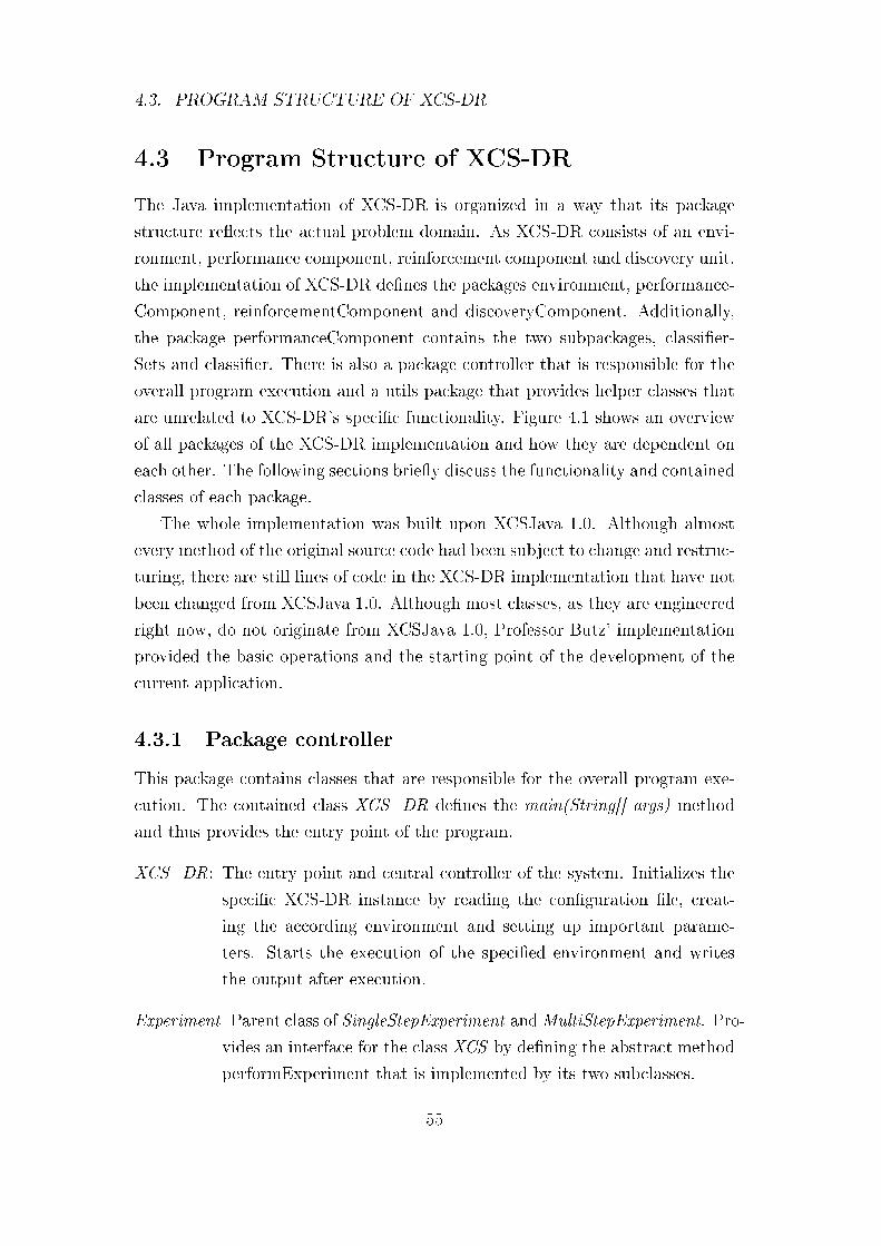
4.3. PROGRAM STRUCTURE OF XCS-DR
4.3 Program Structure of XCS-DR
The Java implementation of XCS-DR is organized in a way that its package
structure re�ects the actual problem domain. As XCS-DR consists of an envi-
ronment, performance component, reinforcement component and discovery unit,
the implementation of XCS-DR de�nes the packages environment, performance-
Component, reinforcementComponent and discoveryComponent. Additionally,
the package performanceComponent contains the two subpackages, classi�er-
Sets and classi�er. There is also a package controller that is responsible for the
overall program execution and a utils package that provides helper classes that
are unrelated to XCS-DR's speci�c functionality. Figure 4.1 shows an overview
of all packages of the XCS-DR implementation and how they are dependent on
each other. The following sections brie�y discuss the functionality and contained
classes of each package.
The whole implementation was built upon XCSJava 1.0. Although almost
every method of the original source code had been subject to change and restruc-
turing, there are still lines of code in the XCS-DR implementation that have not
been changed from XCSJava 1.0. Although most classes, as they are engineered
right now, do not originate from XCSJava 1.0, Professor Butz' implementation
provided the basic operations and the starting point of the development of the
current application.
4.3.1 Package controller
This package contains classes that are responsible for the overall program exe-
cution. The contained class XCS_DR de�nes the main(String[] args) method
and thus provides the entry point of the program.
XCS_DR: The entry point and central controller of the system. Initializes the
speci�c XCS-DR instance by reading the con�guration �le, creat-
ing the according environment and setting up important parame-
ters. Starts the execution of the speci�ed environment and writes
the output after execution.
Experiment Parent class of SingleStepExperiment andMultiStepExperiment. Pro-
vides an interface for the class XCS by de�ning the abstract method
performExperiment that is implemented by its two subclasses.
55
4.3. PROGRAM STRUCTURE OF XCS-DR
Figure 4.1: Package diagram of the XCS-DR Java implementation. All depen-dencies to and from subpackages of performanceComponent are illustrated asdependencies to and from their parent package.
56
4.3. PROGRAM STRUCTURE OF XCS-DR
SingleStepExperiment Controls and operates the alternation between explore
classi�cation, explore delegation and exploit in single-step environ-
ments. Interacts with the environment and invokes the reinforcement
component and genetic algorithm. Collects data while solving the
problem instances.
MultiStepExperiment Controls and operates the alternation between explore
classi�cation, explore delegation and exploit in multi-step environ-
ments. Interacts with the environment and invokes the reinforcement
component and genetic algorithm. Collects data while solving the
problem instances.
4.3.2 Package environment
This package de�nes all the problem types (environments) of XCS-DR. It pro-
vides an implementation of each available problem type. Further problem types
could easily be added by providing additional implementations of the interface
Environment. This package also provides a factory class for the convenient in-
stantiating of the di�erent environments.
Environment: Interface that de�nes all the methods a certain environment has
to provide to XCS-DR. Important methods include resetState() that
returns a random problem instance or executeAction() that executes
a certain action and returns payo�.
MPEnvironment: Implementation of the interface Environment that represents
the multiplexer problem.
MazeEnvironment: Implementation of Environment that represents all kinds of
maze problems. Has to be supplied with a particular maze type
during instantiation.
IPPEnvironment: Implementation of Environment that represents the incre-
mental parity problem.
EnvironmentFactory: This factory class instantiates the correct environment
during initialization. Has to be supplied with the parameters speci-
�ed in the con�g �le.
57
4.3. PROGRAM STRUCTURE OF XCS-DR
ProblemTypes: Enum that de�nes all problem types. Used by EnvironmentFac-
tory.
4.3.3 Package performanceComponent
The package performanceComponent mainly consists of an implementation of
the prediction array and contains a constants class. It includes two subpackages,
classi�er and classi�erSets. PerformanceComponent and its subpackages contain
the core part of the program by implementing the actual classi�er, prediction
array and all classi�er sets. Figure 4.2 displays the according class diagram of
this package.
AgentPredictionArray : This class represents the agent-based prediction array.
It contains several instances of PredictionAgent, provides methods
for action selection and accessing prediction values.
PredictionAgent : The class PredictionAgent computes the prediction values of
an according match set agent. Provides methods to access the pre-
diction values of actions. Mainly accessed by AgentPredictionArray
during action selection.
XCSConstants : Constants class that contains all parameters that are introduced
in the original system such as the learning rate β or the discount rate
γ. Additionally, contains agent related constants such as the total
number of agents and the number of slots per agent.
Subpackage classi�er The package classi�er contains classes that make up
the structure of a single macro-classi�er. It provides an implementation of the
macro-classi�er concept with all of its parameters as well as implementations of
the di�erent types of actions. Figure 4.3 displays the according class diagram of
this package.
MacroClassi�er : Implementation of the macro-classi�er concept. This class
speci�es member variables for the action, condition, numerosity,
prediction and all other parameters necessary to model a macro-
classi�er. It also provides functionality to access and set these pa-
rameters.
58
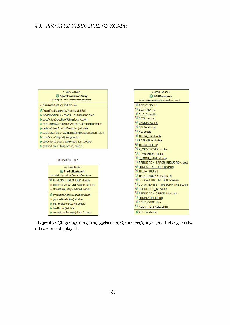
4.3. PROGRAM STRUCTURE OF XCS-DR
Figure 4.2: Class diagram of the package performanceComponent. Private meth-ods are not displayed.
59
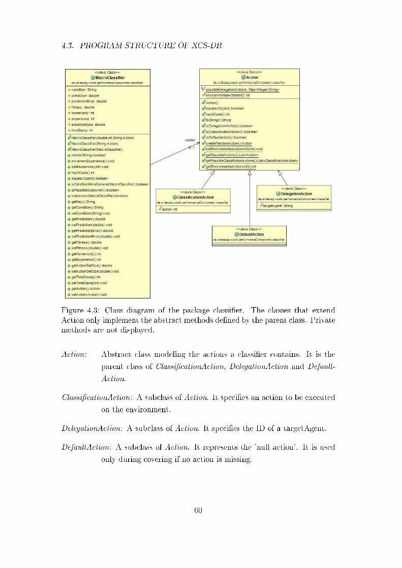
4.3. PROGRAM STRUCTURE OF XCS-DR
Figure 4.3: Class diagram of the package classi�er. The classes that extendAction only implement the abstract methods de�ned by the parent class. Privatemethods are not displayed.
Action: Abstract class modeling the actions a classi�er contains. It is the
parent class of Classi�cationAction, DelegationAction and Default-
Action.
Classi�cationAction: A subclass of Action. It speci�es an action to be executed
on the environment.
DelegationAction: A subclass of Action. It speci�es the ID of a targetAgent.
DefaultAction: A subclass of Action. It represents the 'null action'. It is used
only during covering if no action is missing.
60
4.3. PROGRAM STRUCTURE OF XCS-DR
Subpackage classi�erSets The package classi�erSets contains the implemen-
tations of all kinds of classi�er sets such as the population and match set. The
general class AgentClassi�erSet provides functionality that all speci�c classi-
�er sets have in common, such as accessing contained classi�ers. An instance
of AgentClassi�erSet contains several instances of Classi�erAgent, that in turn
contains a collection of macro-classi�ers. See �gure 4.4 for the according class
diagram of this package.
AgentClassi�erSet : Parent class of all speci�c classi�er sets. It contains a limited
amount of instances of Classi�erAgent. This class provides methods
for adding and deleting classi�ers to and from the contained instances
of Classi�erAgent as well as auxiliary functionality.
Classi�erAgent : An instance of this class contains a limited amount of instances
of MacroClassi�er. Instances of Classi�erAgent are identi�ed within
their according AgentClassi�erSet by an ID. The maximum number
of contained macro-classi�ers is speci�ed in the con�g �le.
AgentPopulation: A subclass of AgentClassi�erSet. It represents the actual pop-
ulation of classi�ers. Provides methods for insertion and deletion of
classi�ers.
AgentMatchSet : A subclass of AgentClassi�erSet. This class implements the
match set construction and covering mechanism.
AgentActionSet : A subclass of AgentClassi�erSet. It represents the action set
and provides functionality for action set formation and action set
subsumption.
4.3.4 Package reinforcementComponent
ReinforcementComponent consists of classes providing the functionality for dis-
tributing payo� and updating classi�er parameters.
ActionSetUpdater : This class provides the di�erent action set update proce-
dures. ActionSetUpdater determines the amount of payo� that each
classi�er receives and controls the parameter updates of all classi�ers
of an action set. Which update procedure is executed depends on
the mode of execution.
61
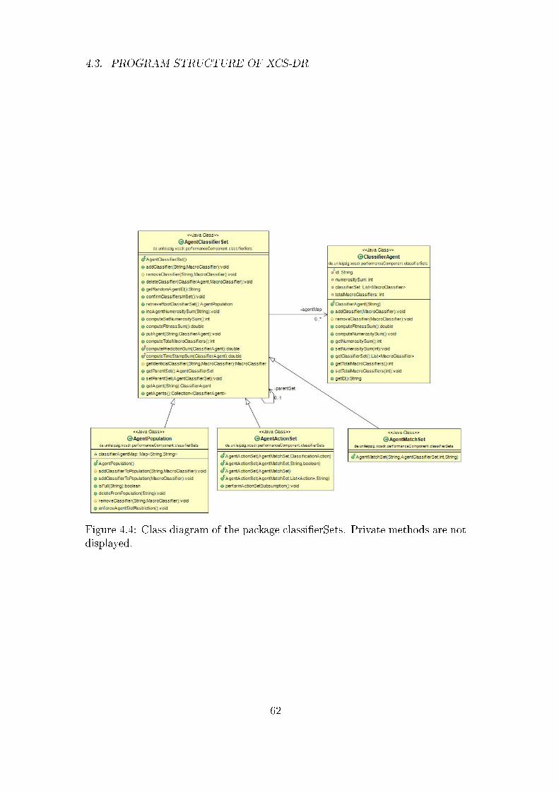
4.3. PROGRAM STRUCTURE OF XCS-DR
Figure 4.4: Class diagram of the package classi�erSets. Private methods are notdisplayed.
62
4.4. RUNNING THE PROGRAM
Classi�erUpdater : This class computes and sets the actual update values of all
parameters of a single classi�er. It provides the according Widrow-
Ho� formulas and implements the MAM technique.
4.3.5 Package discoveryComponent
Contains the genetic algorithm of the XCS-DR implementation. The covering
mechanism is not part of this package but rather placed directly inside the class
AgentMatchSet of the package classi�erSets. This is because the covering pro-
cedure is a very simple one and at the time of development it seemed reasonable
to implement it where it is executed.
AgentGeneticAlgorithm: This class provides the method runGA() that executes
the entire genetic algorithm, from selecting two parent classi�ers for
replication to inserting the newly created o�spring classi�ers into the
population.
4.3.6 Package utils
The utils package mainly implements auxiliary functionality. It provides classes
that are unrelated to the speci�cation of XCS-DR but necessary for correct pro-
gram execution. It is responsible for reading the con�g parameters and record-
ing the system performance during exploit. The classes in this package are very
loosely related. An introduction of every single class of this package is omitted
here since they do not provide functionality speci�c to XCS-DR.
4.4 Running the Program
The project directory contains an executable Java Archive �le, xcs-dr.jar. To
run the program, navigate to the �le and execute 'java -jar xcs-dr.jar' in the
command prompt. This executes XCS-DR by applying the parameters speci�ed
in a con�g.properties �le. XCS-DR either uses the con�g �le that is stored in
the same directory as the jar �le or if there is no such �le, it applies a default
one that is included within the jar �le. In contrast to XCSJava 1.0, the program
does not accept any command line arguments. All important program settings
63
4.4. RUNNING THE PROGRAM
are speci�ed within the con�g �le. Figure 4.5 shows the default con�g �le that
is included in the �le xcs-dr.jar.
Some con�guration parameters are speci�c to certain types of problems. For
instance, is the parameter payo�-type speci�c to the multiplexer problem. The
values of such speci�c parameters are relevant only if the problem-type param-
eter is set to a certain value and ignored otherwise. I.e. if the user enters IPP
or MAZE as problemtype, the value of payo�type will be ignored during exe-
cution. The following listing provides a short description of each con�guration
parameter.
dont-care-prob: Speci�es the probability of inserting dont-care symbols into a
classi�er's condition during covering. Every position of the condition
is turned into a dont-care symbol with that probability.
mutation-prob: Speci�es the probability of mutating a classi�er's condition and
action during GA execution. Every position of the condition and the
action are mutated with that probability.
random-entry : Speci�es whether the entry-agent is random or the same for every
problem instance.
�tness-threshold : Classi�ers with a �tness below or equal to that threshold are
being ignored during prediction calculation.
agents : Speci�es the number of agents in the population.
slot-no: Speci�es the number of classi�er slots per agent. This parameter
constitutes the limit for the sum of the numerosities of all macro-
classi�ers contained in one agent.
problem-type: Speci�es the particular problem to solve. Can be set to MP for
the multiplexer problem, IPP for the incremental parity problem
and MAZE for various prede�ned maze problems.
output-dir : Speci�es the directory where all output �les are saved to. The out-
put is written after all experiments �nished.
trials : Speci�es the number of exploit cycles of one experiment. Before
each exploit, a classi�cation explore and a delegation explore cycle
64
4.4. RUNNING THE PROGRAM
is executed. Hence, the system executes three times as many problem
instances as de�ned by this parameter.
experiments : De�nes the number of experiments executed consecutively. The
length of an experiment is de�ned by the trials parameter. After
execution of a given number of exploit cycles (speci�ed by the trials
parameter), one experiment is �nished.
prob-length: Speci�c to the IPP and MP problem types. It de�nes the number
of bits that each problem instance consists of. While for the IPP
arbitrary problem lengths are possible, the MP has to be of length
k + 2k. The system still accepts arbitrary problem lengths for the
MP. In case prob-length is not of length k+2k, the largest multiplexer
that �ts the speci�ed length is created and the supernumerous bits
are assigned random values by the environment for each problem
instance.
payo�-type: Speci�c to the MP problem type. If it is 0 the systems receives a
reward of 1000 from the environment for every correct classi�cation.
If the value is set to 1 the system receives reward according to the
payo� map described previously in section 4.1.1.
maze: Speci�c to the MAZE problem type. Speci�es the particular maze
to apply. Possible values are Woods1, Woods2, Maze4, Maze5 and
Maze6. The according maze de�nitions are included as text �les in
the resources folder of the project's sources.
encoding : Speci�c to the MAZE problem type. Possible values are 2 and 3.
Speci�es the number of bits that each position in a maze is encoded
with. Woods2 is usually encoded with 3 bits and Maze4 typically
with 2 bits. This parameter has simply been adopted from XCSJava
1.0. The documentation of XCSJava 1.0 does not provide much
information about speci�c encodings.
65
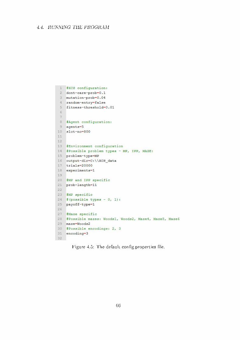
4.4. RUNNING THE PROGRAM
Figure 4.5: The default con�g.properties �le.
66
4.5. EDITING AND COMPILING THE SOURCES
4.5 Editing and Compiling the Sources
XCS-DR has been implemented with the project management tool Apache
Maven. Maven is a tool that provides support during all stages of the soft-
ware development process, such as automating the build process, managing de-
pendencies, reporting and documentation and more. Every Maven project is
speci�ed by a XML �le, the pom.xml, which de�nes the project con�guration.
Maven enforces a package structure that contains the domain name of the com-
pany that is hosting the software project. The source code of XCS-DR has been
created by a student of Universität Leipzig and the according domain name is
uni-leipzig.de. Since Java does not allow packages to contain hyphens, all pack-
ages are pre�xed with de.unileipzig.xcsdr, according to the Maven guidelines.
This pre�x constitutes the Maven groupId that uniquely identi�es the project.
The sources of XCS-DR can be edited with any text editor or IDE that
supports Java code. To access any Maven-speci�c functionality and create an
executable Java Archive �le (jar), Apache Maven has to be installed on the host
computer. Some IDEs, such as Eclipse, provide build-in support for Apache
Maven. To build the project and create an executable jar �le from the sources,
navigate to the project directory within the command prompt and execute 'mvn
clean compile assembly:single'. This builds the project and saves an executable
jar in the 'target' folder of the project.
4.6 Output
XCS-DR provides two kinds of ouput. On the one hand in the console where the
program is running and on the other hand writing output �les in the speci�ed
output directory.
In the console, XCS-DR writes:
• The number of the current experiment
• The number of so far examined problems in exploit
• The average accuracy of the last 50 exploit cycles (single-step problems)
resp. the average distance to food of the last 50 exploit cycles (maze
problems)
67
4.6. OUTPUT
• The total number of macro-classi�ers in the population
Additionally, XCS-DR produces several output �les that are created at the end
of program execution, after all classi�cations �nished. All �les are saved to
the output directory speci�ed in the con�g �le. The �le accuracy.txt keeps
track of the system's performance by either containing the average accuracy
(single-step problems) or average distance to food (maze problems). The �le
pred_error.txt records the average prediction error, graph.txt keeps track of the
delegations in the system and how many problem instances each agent classi�es
and number_of_classi�cations.txt and number_of_delegations.txt record the
average totals of classi�cations resp. delegations in the population. The next
chapter provides in detail explanations about how these quantities are measured.
The output directory can also contain a �le population.txt that contains a
snapshot of the classi�er population. When the method logPopulation of the
class PopulationLogger is called, the program writes every macro-classi�er of
the current population to that �le. This class has mainly been in use during de-
bugging and troubleshooting. The �nal program does not write any populations
but by editing the source code it could easily be added.
68
Chapter 5
Performance Analysis
This chapter presents an analysis of XCS-DR's performance. The main points
of interest are how accurately it classi�es problem instances compared to the
original and how di�erent numbers of agents a�ect the performance. During
every conducted experiment, the system has been provided with a high enough
slot number such that the �nal performance of XCS-DR, after convergence of
the classi�er population, has not been a�ected negatively. This work mainly
focused on the development of an accurately working agent-based XCS and this
chapter investigates to what extent this goal has been reached. An extended in-
vestigation of di�erent slot numbers and their e�ects on the performance could
be part of future investigations. The term performance is used from now on
interchangeably for accuracy if the system acts in a single-step environment
respectively for distance to food if the system acts in maze environments. Ex-
periments have been conducted for the 6-MP, 11-MP, 8-IPP, Woods2 and Maze4
problems. Although Maze6 is the most complex environment implemented by
XCS-DR, Maze4 has been chosen as the most complex problem to pose to the
system. This was due to the computational e�ort necessary to solve complex
multi-step problems while maintaining several agents. Since most experiments
have been repeated hundreds of times with di�erent con�gurations, choosing an
even more complex environment than Maze4 would have taken too much time
of computation.
At �rst in this chapter are introduced all measured variables. Thereafter, it
is investigated how the single-agent XCS-DR performs compared to XCSJava
1.0. The underlying principles of XCS have not been changed in XCS-DR and
therefore a single-agent XCS-DR should be exhibiting the same performance as
69

5.1. MEASURED VARIABLES
XCSJava 1.0. The third section compares the di�erent kinds of explore dele-
gation procedures that have been introduced in the previous chapter and de-
termines which one is working best. Thereafter, it is analyzed the performance
of several multi-agent XCS-DR con�gurations in the 11-MP environment. The
subsequent sections present a similar analysis of XCS-DR's performance in the
8-IPP, Woods2 and Maze4 environment. During the experiments conducted for
the previously mentioned sections, the entry-agent of XCS-DR has been the same
each cycle. Section 5.8 investigates how XCS-DR behaves when the entry-agent
is determined randomly each time. The last section of this chapter provides
an analysis of the emerging classi�cation and delegation patterns of the agents.
It is broken down how the classi�cation and delegation of the input state is
distributed between the agents.
As long as not mentioned otherwise, are all parameter settings in the ex-
periments the ones applied by XCSJava 1.0. Note that during all multiplexer
experiments, the in section 4.1.1 introduced payo� map has been applied by
setting the parameter payo�-type to 1.
5.1 Measured Variables
XCS-DR measures several quantities during the exploit phase that describe the
behavior of the system and how it performs. The most important measurement
is accuracy in single-step environments respectively distance to food in maze
environments as both are ultimately recording the system's performance.
Average Accuracy Measured only for single-step problems. XCSJava 1.0
measures how many of the last 50 problem instances have been classi�ed cor-
rectly during exploit and calculates the average. Therefore, the system provides
an accuracy value every 50 exploit steps. This procedure has been adopted by
XCS-DR. The resulting accuracy averages are averaged again over several ex-
periments. Since accuracy values are provided only every 50 steps, the resulting
accuracy curve looks choppy. By conducting many experiments, deviations have
been smoothed out. This data is provided by the output �le accuracy.txt.
Average Distance to Food This is the equivalence of the accuracy in the
implemented multi-step problems. Instead of measuring whether a problem
70
5.1. MEASURED VARIABLES
instance has been classi�ed correctly, the system records the number of steps
necessary to reach food. The overall procedure is the same as for the accuracy,
averaging every 50 steps and over several experiments. The data is contained in
the ouput �le accuracy.txt.
Proportionate Classi�cations Records for each agent how many problem
instances have been classi�ed during exploit. A problem instance is classi�ed by
an agent, if this agent determines the action that is executed on the environment.
This measure is calculated relative to the total number of classi�cations and
averaged over several experiments. Proportionate classi�cations are recorded in
the output �le graph.txt.
Proportionate Delegations: Records for each pair of agents how many
problem instances have been delegated between them during exploit. This
measure is calculated relative to the total number of delegations and averaged
over several experiments. The directions of delegations are considered. There
is a separate value for the delegation Agenti → Agentk and another one for
Agentk → Agenti. This quantity and the previous one are useful for analyzing
the emerging classi�cation and delegation patterns. Proportionate delegations
are also recorded in the output �le graph.txt.
Number of Classi�cations Records during each exploit cycle the total num-
ber of classi�cation classi�ers in the system. It is calculated by adding up the
numerosities of all classi�cations of all agents and averaged over several experi-
ments. This data is contained in the output �le number_of_classi�cations.txt.
Number of Delegations Records during each exploit cycle the total num-
ber of delegation classi�ers in the system. It is calculated by adding up the
numerosities of all delegations of all agents and averaged over several experi-
ments. This quantity and the previous one determine how many slots of the
system are occupied by each kind of classi�er. This data is contained in the
output �le number_of_delegations.txt.
Average Prediction Error The average prediction error is recorded just as
the average accuracy. It is averaged over 50 steps and multiple experiments.
71
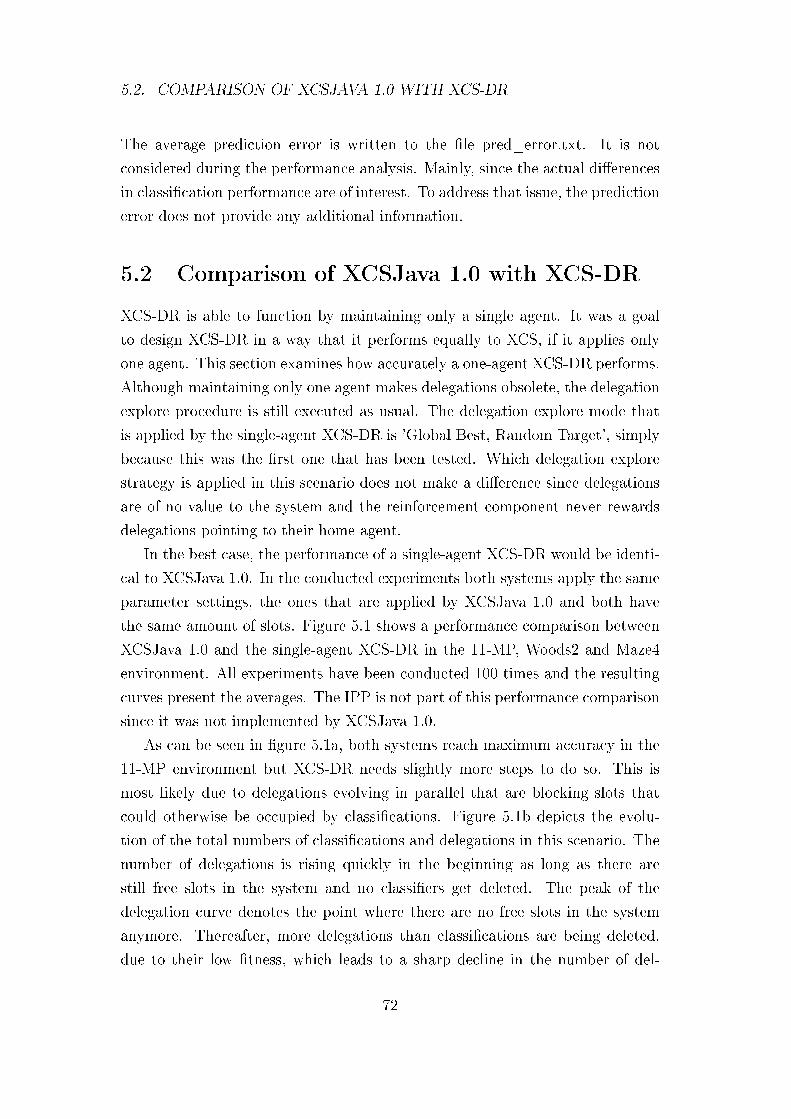
5.2. COMPARISON OF XCSJAVA 1.0 WITH XCS-DR
The average prediction error is written to the �le pred_error.txt. It is not
considered during the performance analysis. Mainly, since the actual di�erences
in classi�cation performance are of interest. To address that issue, the prediction
error does not provide any additional information.
5.2 Comparison of XCSJava 1.0 with XCS-DR
XCS-DR is able to function by maintaining only a single agent. It was a goal
to design XCS-DR in a way that it performs equally to XCS, if it applies only
one agent. This section examines how accurately a one-agent XCS-DR performs.
Although maintaining only one agent makes delegations obsolete, the delegation
explore procedure is still executed as usual. The delegation explore mode that
is applied by the single-agent XCS-DR is 'Global Best, Random Target', simply
because this was the �rst one that has been tested. Which delegation explore
strategy is applied in this scenario does not make a di�erence since delegations
are of no value to the system and the reinforcement component never rewards
delegations pointing to their home agent.
In the best case, the performance of a single-agent XCS-DR would be identi-
cal to XCSJava 1.0. In the conducted experiments both systems apply the same
parameter settings, the ones that are applied by XCSJava 1.0 and both have
the same amount of slots. Figure 5.1 shows a performance comparison between
XCSJava 1.0 and the single-agent XCS-DR in the 11-MP, Woods2 and Maze4
environment. All experiments have been conducted 100 times and the resulting
curves present the averages. The IPP is not part of this performance comparison
since it was not implemented by XCSJava 1.0.
As can be seen in �gure 5.1a, both systems reach maximum accuracy in the
11-MP environment but XCS-DR needs slightly more steps to do so. This is
most likely due to delegations evolving in parallel that are blocking slots that
could otherwise be occupied by classi�cations. Figure 5.1b depicts the evolu-
tion of the total numbers of classi�cations and delegations in this scenario. The
number of delegations is rising quickly in the beginning as long as there are
still free slots in the system and no classi�ers get deleted. The peak of the
delegation curve denotes the point where there are no free slots in the system
anymore. Thereafter, more delegations than classi�cations are being deleted,
due to their low �tness, which leads to a sharp decline in the number of del-
72
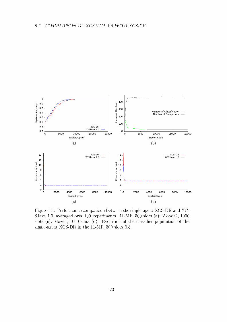
5.2. COMPARISON OF XCSJAVA 1.0 WITH XCS-DR
(a) (b)
(c) (d)
Figure 5.1: Performance comparison between the single-agent XCS-DR and XC-SJava 1.0, averaged over 100 experiments. 11-MP, 500 slots (a); Woods2, 1000slots (c); Maze4, 1000 slots (d). Evolution of the classi�er population of thesingle-agent XCS-DR in the 11-MP, 500 slots (b).
73
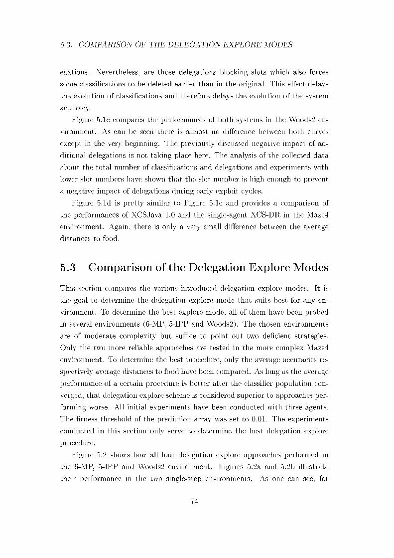
5.3. COMPARISON OF THE DELEGATION EXPLORE MODES
egations. Nevertheless, are those delegations blocking slots which also forces
some classi�cations to be deleted earlier than in the original. This e�ect delays
the evolution of classi�cations and therefore delays the evolution of the system
accuracy.
Figure 5.1c compares the performances of both systems in the Woods2 en-
vironment. As can be seen there is almost no di�erence between both curves
except in the very beginning. The previously discussed negative impact of ad-
ditional delegations is not taking place here. The analysis of the collected data
about the total number of classi�cations and delegations and experiments with
lower slot numbers have shown that the slot number is high enough to prevent
a negative impact of delegations during early exploit cycles.
Figure 5.1d is pretty similar to Figure 5.1c and provides a comparison of
the performances of XCSJava 1.0 and the single-agent XCS-DR in the Maze4
environment. Again, there is only a very small di�erence between the average
distances to food.
5.3 Comparison of the Delegation Explore Modes
This section compares the various introduced delegation explore modes. It is
the goal to determine the delegation explore mode that suits best for any en-
vironment. To determine the best explore mode, all of them have been probed
in several environments (6-MP, 5-IPP and Woods2). The chosen environments
are of moderate complexity but su�ce to point out two de�cient strategies.
Only the two more reliable approaches are tested in the more complex Maze4
environment. To determine the best procedure, only the average accuracies re-
spectively average distances to food have been compared. As long as the average
performance of a certain procedure is better after the classi�er population con-
verged, that delegation explore scheme is considered superior to approaches per-
forming worse. All initial experiments have been conducted with three agents.
The �tness threshold of the prediction array was set to 0.01. The experiments
conducted in this section only serve to determine the best delegation explore
procedure.
Figure 5.2 shows how all four delegation explore approaches performed in
the 6-MP, 5-IPP and Woods2 environment. Figures 5.2a and 5.2b illustrate
their performance in the two single-step environments. As one can see, for
74
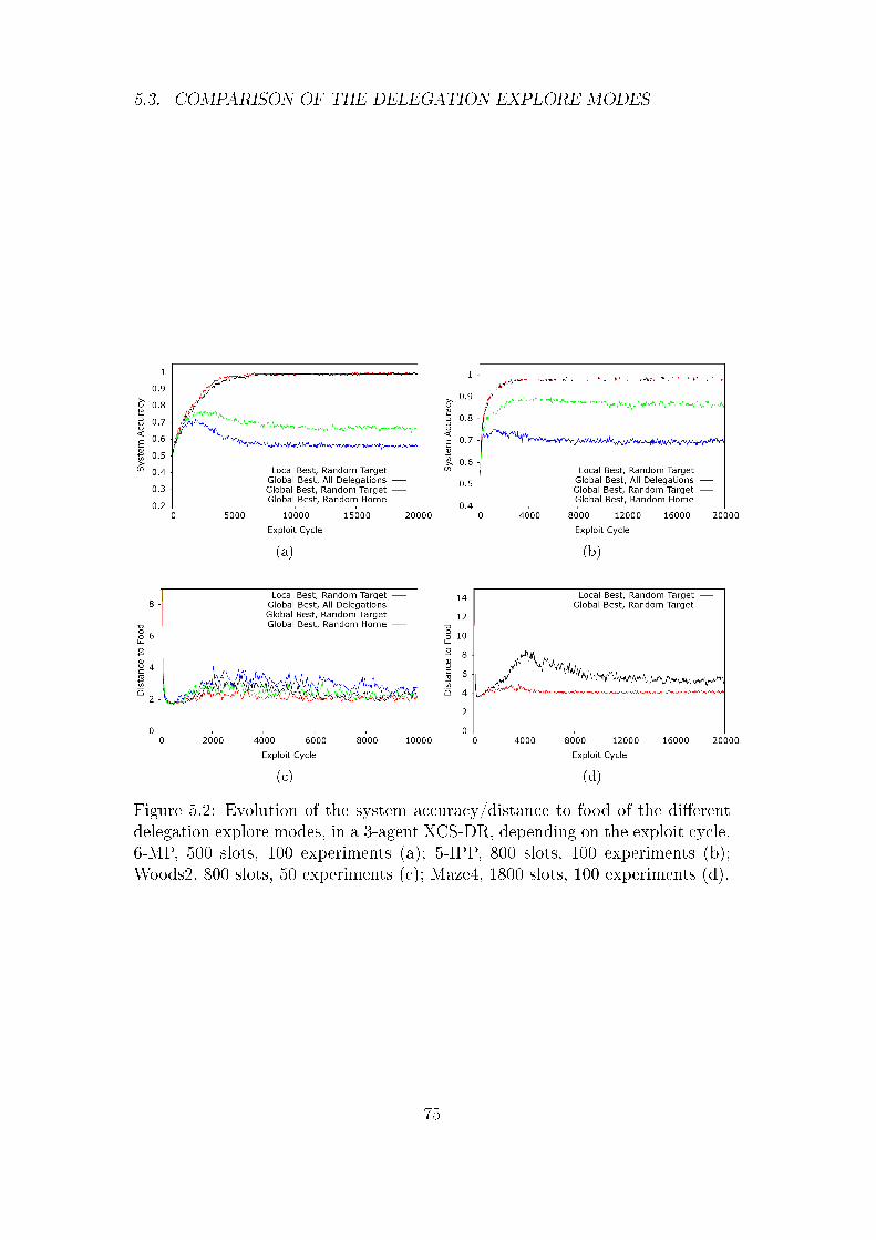
5.3. COMPARISON OF THE DELEGATION EXPLORE MODES
(a) (b)
(c) (d)
Figure 5.2: Evolution of the system accuracy/distance to food of the di�erentdelegation explore modes, in a 3-agent XCS-DR, depending on the exploit cycle.6-MP, 500 slots, 100 experiments (a); 5-IPP, 800 slots, 100 experiments (b);Woods2, 800 slots, 50 experiments (c); Maze4, 1800 slots, 100 experiments (d).
75
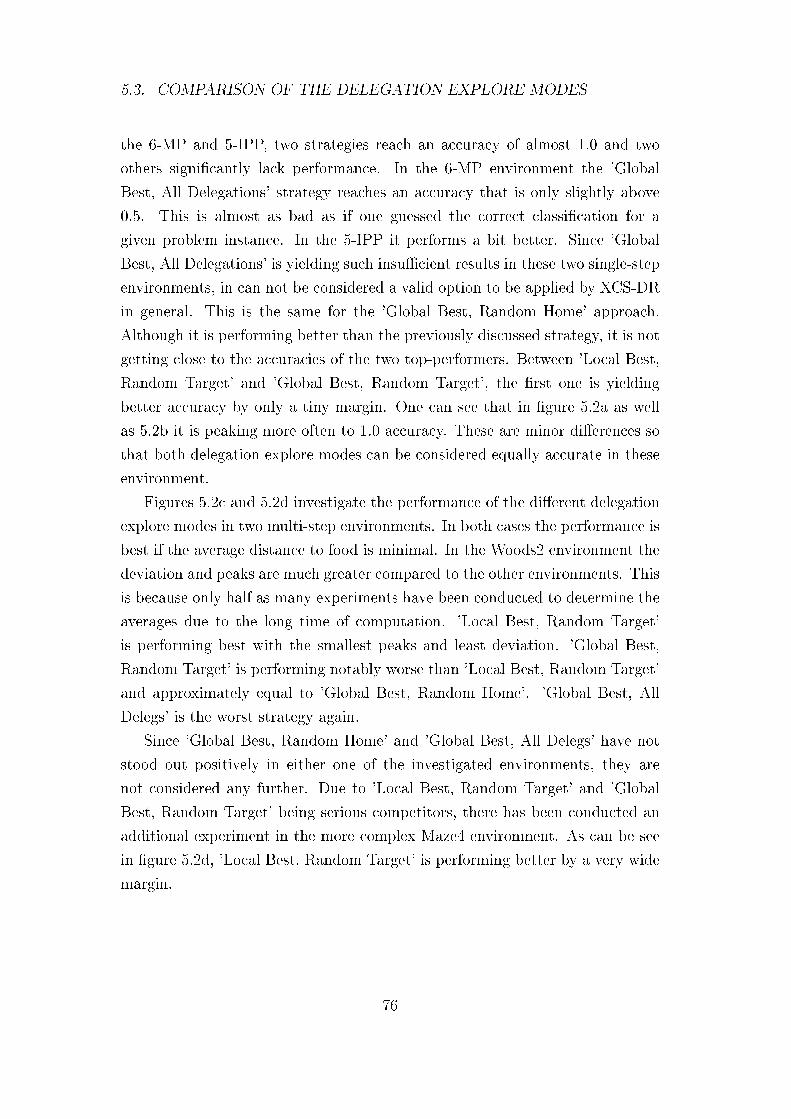
5.3. COMPARISON OF THE DELEGATION EXPLORE MODES
the 6-MP and 5-IPP, two strategies reach an accuracy of almost 1.0 and two
others signi�cantly lack performance. In the 6-MP environment the 'Global
Best, All Delegations' strategy reaches an accuracy that is only slightly above
0.5. This is almost as bad as if one guessed the correct classi�cation for a
given problem instance. In the 5-IPP it performs a bit better. Since 'Global
Best, All Delegations' is yielding such insu�cient results in these two single-step
environments, in can not be considered a valid option to be applied by XCS-DR
in general. This is the same for the 'Global Best, Random Home' approach.
Although it is performing better than the previously discussed strategy, it is not
getting close to the accuracies of the two top-performers. Between 'Local Best,
Random Target' and 'Global Best, Random Target', the �rst one is yielding
better accuracy by only a tiny margin. One can see that in �gure 5.2a as well
as 5.2b it is peaking more often to 1.0 accuracy. These are minor di�erences so
that both delegation explore modes can be considered equally accurate in these
environment.
Figures 5.2c and 5.2d investigate the performance of the di�erent delegation
explore modes in two multi-step environments. In both cases the performance is
best if the average distance to food is minimal. In the Woods2 environment the
deviation and peaks are much greater compared to the other environments. This
is because only half as many experiments have been conducted to determine the
averages due to the long time of computation. 'Local Best, Random Target'
is performing best with the smallest peaks and least deviation. 'Global Best,
Random Target' is performing notably worse than 'Local Best, Random Target'
and approximately equal to 'Global Best, Random Home'. 'Global Best, All
Delegs' is the worst strategy again.
Since 'Global Best, Random Home' and 'Global Best, All Delegs' have not
stood out positively in either one of the investigated environments, they are
not considered any further. Due to 'Local Best, Random Target' and 'Global
Best, Random Target' being serious competitors, there has been conducted an
additional experiment in the more complex Maze4 environment. As can be see
in �gure 5.2d, 'Local Best, Random Target' is performing better by a very wide
margin.
76
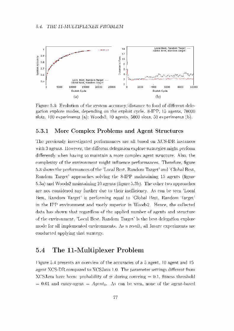
5.4. THE 11-MULTIPLEXER PROBLEM
(a) (b)
Figure 5.3: Evolution of the system accuracy/distance to food of di�erent dele-gation explore modes, depending on the exploit cycle. 8-IPP, 15 agents, 70000slots, 100 experiments (a); Woods2, 10 agents, 5000 slots, 50 experiments (b).
5.3.1 More Complex Problems and Agent Structures
The previously investigated performances are all based on XCS-DR instances
with 3 agents. However, the di�erent delegation explore strategies might perform
di�erently when having to maintain a more complex agent structure. Also, the
complexity of the environment might in�uence performances. Therefore, �gure
5.3 shows the performances of the 'Local Best, Random Target' and 'Global Best,
Random Target' approaches solving the 8-IPP maintaining 15 agents (�gure
5.3a) and Woods2 maintaining 10 agents (�gure 5.3b). The other two approaches
are not considered any further due to their ine�ciency. As can be seen 'Local
Best, Random Target' is performing equal to 'Global Best, Random Target'
in the IPP environment and vastly superior in Woods2. Hence, the collected
data has shown that regardless of the applied number of agents and structure
of the environment, 'Local Best, Random Target' is the best delegation explore
mode for all implemented environments. As a result, all future experiments are
conducted applying that strategy.
5.4 The 11-Multiplexer Problem
Figure 5.4 presents an overview of the accuracies of a 5-agent, 10-agent and 15-
agent XCS-DR compared to XCSJava 1.0. The parameter settings di�erent from
XCSJava have been: probability of # during covering = 0.1, �tness threshold
= 0.01 and entry-agent = Agent0. As can be seen, none of the agent-based
77
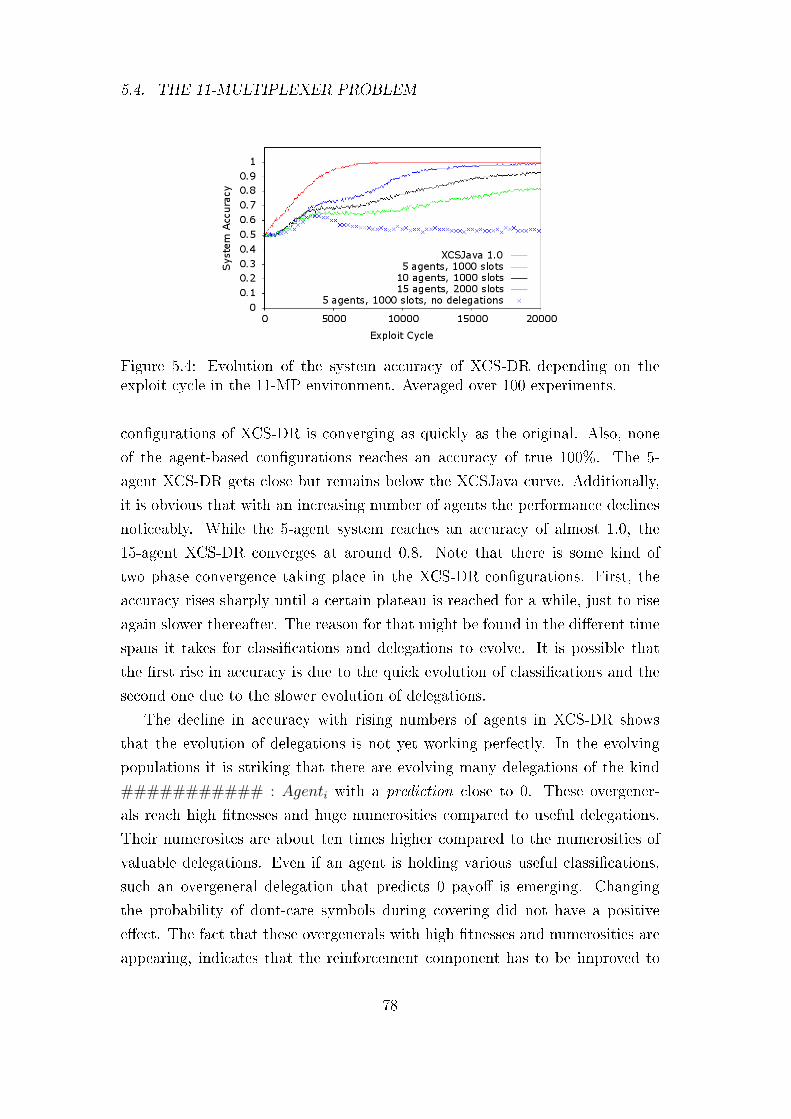
5.4. THE 11-MULTIPLEXER PROBLEM
Figure 5.4: Evolution of the system accuracy of XCS-DR depending on theexploit cycle in the 11-MP environment. Averaged over 100 experiments.
con�gurations of XCS-DR is converging as quickly as the original. Also, none
of the agent-based con�gurations reaches an accuracy of true 100%. The 5-
agent XCS-DR gets close but remains below the XCSJava curve. Additionally,
it is obvious that with an increasing number of agents the performance declines
noticeably. While the 5-agent system reaches an accuracy of almost 1.0, the
15-agent XCS-DR converges at around 0.8. Note that there is some kind of
two phase convergence taking place in the XCS-DR con�gurations. First, the
accuracy rises sharply until a certain plateau is reached for a while, just to rise
again slower thereafter. The reason for that might be found in the di�erent time
spans it takes for classi�cations and delegations to evolve. It is possible that
the �rst rise in accuracy is due to the quick evolution of classi�cations and the
second one due to the slower evolution of delegations.
The decline in accuracy with rising numbers of agents in XCS-DR shows
that the evolution of delegations is not yet working perfectly. In the evolving
populations it is striking that there are evolving many delegations of the kind
########### : Agenti with a prediction close to 0. These overgener-
als reach high �tnesses and huge numerosities compared to useful delegations.
Their numerosites are about ten times higher compared to the numerosities of
valuable delegations. Even if an agent is holding various useful classi�cations,
such an overgeneral delegation that predicts 0 payo� is emerging. Changing
the probability of dont-care symbols during covering did not have a positive
e�ect. The fact that these overgenerals with high �tnesses and numerosities are
appearing, indicates that the reinforcement component has to be improved to
78
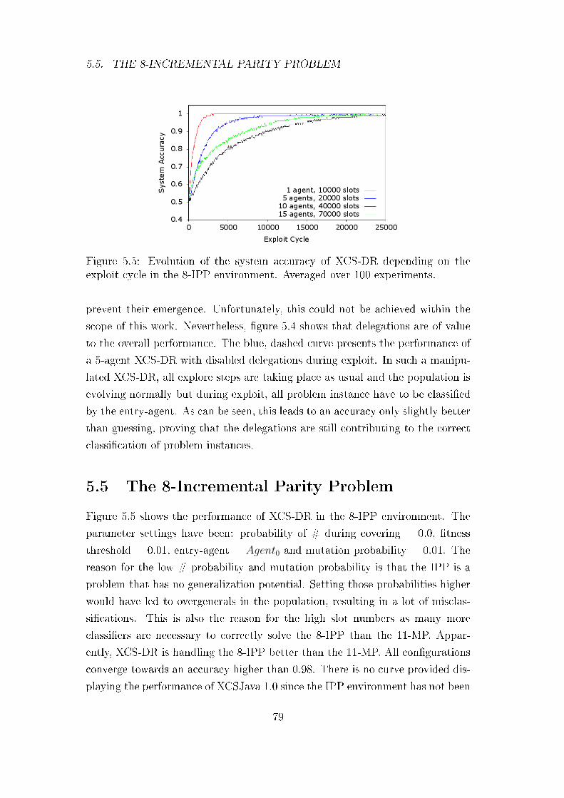
5.5. THE 8-INCREMENTAL PARITY PROBLEM
Figure 5.5: Evolution of the system accuracy of XCS-DR depending on theexploit cycle in the 8-IPP environment. Averaged over 100 experiments.
prevent their emergence. Unfortunately, this could not be achieved within the
scope of this work. Nevertheless, �gure 5.4 shows that delegations are of value
to the overall performance. The blue, dashed curve presents the performance of
a 5-agent XCS-DR with disabled delegations during exploit. In such a manipu-
lated XCS-DR, all explore steps are taking place as usual and the population is
evolving normally but during exploit, all problem instance have to be classi�ed
by the entry-agent. As can be seen, this leads to an accuracy only slightly better
than guessing, proving that the delegations are still contributing to the correct
classi�cation of problem instances.
5.5 The 8-Incremental Parity Problem
Figure 5.5 shows the performance of XCS-DR in the 8-IPP environment. The
parameter settings have been: probability of # during covering = 0.0, �tness
threshold = 0.01, entry-agent = Agent0 and mutation probability = 0.01. The
reason for the low # probability and mutation probability is that the IPP is a
problem that has no generalization potential. Setting those probabilities higher
would have led to overgenerals in the population, resulting in a lot of misclas-
si�cations. This is also the reason for the high slot numbers as many more
classi�ers are necessary to correctly solve the 8-IPP than the 11-MP. Appar-
ently, XCS-DR is handling the 8-IPP better than the 11-MP. All con�gurations
converge towards an accuracy higher than 0.98. There is no curve provided dis-
playing the performance of XCSJava 1.0 since the IPP environment has not been
79
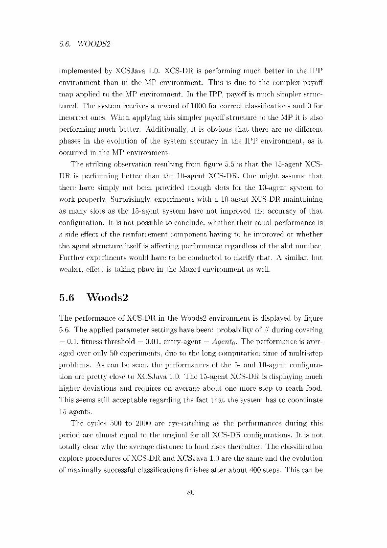
5.6. WOODS2
implemented by XCSJava 1.0. XCS-DR is performing much better in the IPP
environment than in the MP environment. This is due to the complex payo�
map applied to the MP environment. In the IPP, payo� is much simpler struc-
tured. The system receives a reward of 1000 for correct classi�cations and 0 for
incorrect ones. When applying this simpler payo� structure to the MP it is also
performing much better. Additionally, it is obvious that there are no di�erent
phases in the evolution of the system accuracy in the IPP environment, as it
occurred in the MP environment.
The striking observation resulting from �gure 5.5 is that the 15-agent XCS-
DR is performing better than the 10-agent XCS-DR. One might assume that
there have simply not been provided enough slots for the 10-agent system to
work properly. Surprisingly, experiments with a 10-agent XCS-DR maintaining
as many slots as the 15-agent system have not improved the accuracy of that
con�guration. It is not possible to conclude, whether their equal performance is
a side e�ect of the reinforcement component having to be improved or whether
the agent structure itself is a�ecting performance regardless of the slot number.
Further experiments would have to be conducted to clarify that. A similar, but
weaker, e�ect is taking place in the Maze4 environment as well.
5.6 Woods2
The performance of XCS-DR in the Woods2 environment is displayed by �gure
5.6. The applied parameter settings have been: probability of # during covering
= 0.1, �tness threshold = 0.01, entry-agent = Agent0. The performance is aver-
aged over only 50 experiments, due to the long computation time of multi-step
problems. As can be seen, the performances of the 5- and 10-agent con�gura-
tion are pretty close to XCSJava 1.0. The 15-agent XCS-DR is displaying much
higher deviations and requires on average about one more step to reach food.
This seems still acceptable regarding the fact that the system has to coordinate
15 agents.
The cycles 500 to 2000 are eye-catching as the performances during this
period are almost equal to the original for all XCS-DR con�gurations. It is not
totally clear why the average distance to food rises thereafter. The classi�cation
explore procedures of XCS-DR and XCSJava 1.0 are the same and the evolution
of maximally successful classi�cations �nishes after about 400 steps. This can be
80
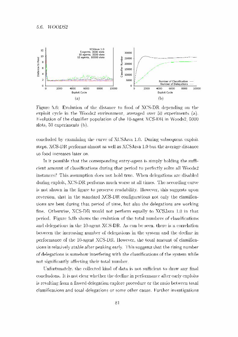
5.6. WOODS2
(a) (b)
Figure 5.6: Evolution of the distance to food of XCS-DR depending on theexploit cycle in the Woods2 environment, averaged over 50 experiments (a).Evolution of the classi�er population of the 10-agent XCS-DR in Woods2, 5000slots, 50 experiments (b).
concluded by examining the curve of XCSJava 1.0. During subsequent exploit
steps, XCS-DR performs almost as well as XCSJava 1.0 but the average distance
to food increases later on.
Is it possible that the corresponding entry-agent is simply holding the su�-
cient amount of classi�cations during that period to perfectly solve all Woods2
instances? This assumption does not hold true. When delegations are disabled
during exploit, XCS-DR performs much worse at all times. The according curve
is not shown in the �gure to preserve readability. However, this suggests upon
reversion, that in the standard XCS-DR con�gurations not only the classi�ca-
tions are best during that period of time, but also the delegations are working
�ne. Otherwise, XCS-DR would not perform equally to XCSJava 1.0 in that
period. Figure 5.6b shows the evolution of the total numbers of classi�cations
and delegations in the 10-agent XCS-DR. As can be seen, there is a correlation
between the increasing number of delegations in the system and the decline in
performance of the 10-agent XCS-DR. However, the total amount of classi�ca-
tions is relatively stable after peaking early. This suggests that the rising number
of delegations is somehow interfering with the classi�cations of the system while
not signi�cantly a�ecting their total number.
Unfortunately, the collected kind of data is not su�cient to draw any �nal
conclusions. It is not clear whether the decline in performance after early exploits
is resulting from a �awed delegation explore procedure or the ratio between total
classi�cations and total delegations or some other cause. Further investigations
81
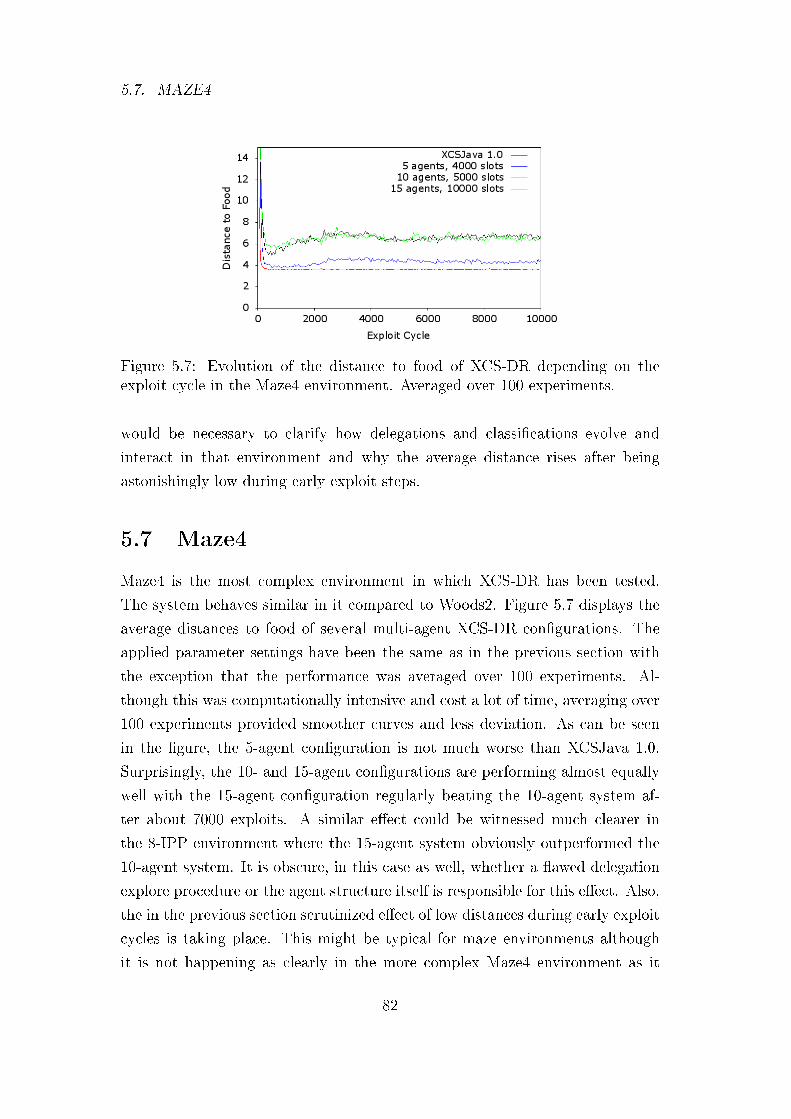
5.7. MAZE4
Figure 5.7: Evolution of the distance to food of XCS-DR depending on theexploit cycle in the Maze4 environment. Averaged over 100 experiments.
would be necessary to clarify how delegations and classi�cations evolve and
interact in that environment and why the average distance rises after being
astonishingly low during early exploit steps.
5.7 Maze4
Maze4 is the most complex environment in which XCS-DR has been tested.
The system behaves similar in it compared to Woods2. Figure 5.7 displays the
average distances to food of several multi-agent XCS-DR con�gurations. The
applied parameter settings have been the same as in the previous section with
the exception that the performance was averaged over 100 experiments. Al-
though this was computationally intensive and cost a lot of time, averaging over
100 experiments provided smoother curves and less deviation. As can be seen
in the �gure, the 5-agent con�guration is not much worse than XCSJava 1.0.
Surprisingly, the 10- and 15-agent con�gurations are performing almost equally
well with the 15-agent con�guration regularly beating the 10-agent system af-
ter about 7000 exploits. A similar e�ect could be witnessed much clearer in
the 8-IPP environment where the 15-agent system obviously outperformed the
10-agent system. It is obscure, in this case as well, whether a �awed delegation
explore procedure or the agent structure itself is responsible for this e�ect. Also,
the in the previous section scrutinized e�ect of low distances during early exploit
cycles is taking place. This might be typical for maze environments although
it is not happening as clearly in the more complex Maze4 environment as it
82
5.8. RANDOM ENTRY-AGENT
is in Woods2. Generally, the 15-agent system is performing about 50% worse
than the original which is a similar result compared to Woods2. The 10-agent
con�guration performs much worse in Maze4 relative to Woods2. The average
distances achieved seem still acceptable regarding the fact that the delegation
explore procedure is not yet reinforcing optimal delegations. The food is discov-
ered with delay by XCS-DR compared to XCSJava 1.0, but it is still performing
much better than a randomly moving animat would.
5.8 Random Entry-Agent
Figures 5.8 and 5.9 show the performances of several XCS-DR con�gurations
when the entry agent is chosen randomly each cycle. The con�guration pa-
rameters during each experiment have been the same as in the according �xed
entry-agent experiment.
As can be seen, in certain situations such a con�guration performs slightly
worse compared to its �xed entry-agent counterpart (such as the 10-agent 8-IPP
con�guration) and in others it performs better (such as 10-agent Woods2). In
most cases the performances of the random-entry con�gurations almost perfectly
match the according performances in a �xed-entry system except for slight sta-
tistical deviations. The system displays the desired behavior of all agents being
of equal importance and capable of handling the input state. The emerging
structures are not asymmetric ones whose performance is dependent on a dis-
tinguished superior entry-agent. To create a system of equal, interacting agents
was one of the design goals of XCS-DR and the performance curves presented
in this section show that this goal has been achieved.
5.9 Classi�cation and Delegation Patterns
This section provides an analysis of the emerging delegation structures in XCS-
DR as the classi�er population evolves. It is scrutinized how many problem
instances each agent classi�es and what kinds of delegation patterns evolve.
The delegation and classi�cation patterns are visualized as graphs. Each node
in such a graph represents an agent of XCS-DR and the size of each node cor-
responds to the relative number of problem instances the according agent has
classi�ed. Each directed edge between two agents indicates that delegations
83
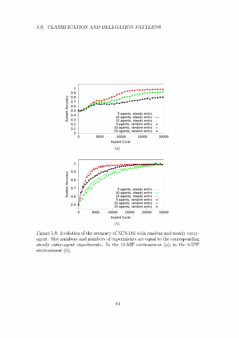
5.9. CLASSIFICATION AND DELEGATION PATTERNS
(a)
(b)
Figure 5.8: Evolution of the accuracy of XCS-DR with random and steady entry-agent. Slot numbers and numbers of experiments are equal to the correspondingsteady entry-agent experiments. In the 11-MP environment (a); in the 8-IPPenvironment (b).
84
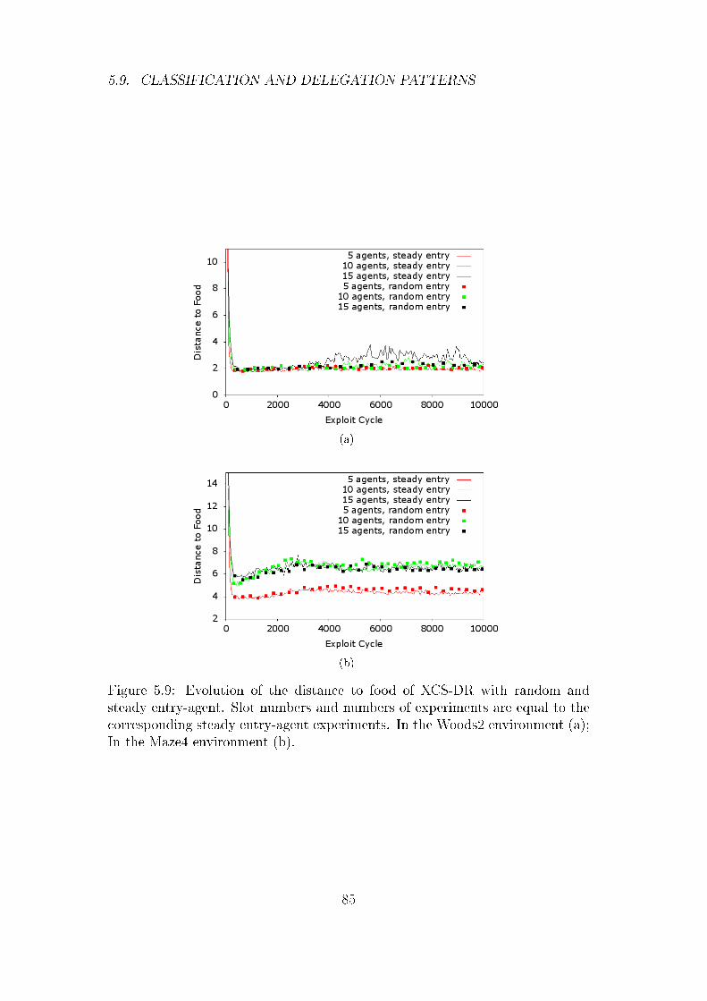
5.9. CLASSIFICATION AND DELEGATION PATTERNS
(a)
(b)
Figure 5.9: Evolution of the distance to food of XCS-DR with random andsteady entry-agent. Slot numbers and numbers of experiments are equal to thecorresponding steady entry-agent experiments. In the Woods2 environment (a);In the Maze4 environment (b).
85
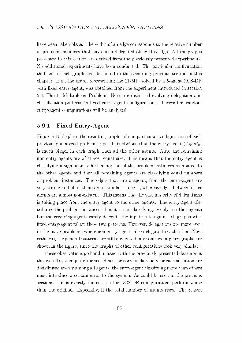
5.9. CLASSIFICATION AND DELEGATION PATTERNS
have been taken place. The width of an edge corresponds to the relative number
of problem instances that have been delegated along this edge. All the graphs
presented in this section are derived from the previously presented experiments.
No additional experiments have been conducted. The particular con�guration
that led to each graph, can be found in the according previous section in this
chapter. E.g., the graph representing the 11-MP, solved by a 5-agent XCS-DR
with �xed entry-agent, was obtained from the experiment introduced in section
5.4, The 11-Multiplexer Problem. Next are discussed evolving delegation and
classi�cation patterns in �xed entry-agent con�gurations. Thereafter, random
entry-agent con�gurations will be analyzed.
5.9.1 Fixed Entry-Agent
Figure 5.10 displays the resulting graphs of one particular con�guration of each
previously analyzed problem type. It is obvious that the entry-agent (Agent0)
is much bigger in each graph than all the other agents. Also, the remaining
non-entry-agents are of almost equal size. This means that the entry-agent is
classifying a signi�cantly higher portion of the problem instances compared to
the other agents and that all remaining agents are classifying equal numbers
of problem instances. The edges that are outgoing from the entry-agent are
very strong and all of them are of similar strength, whereas edges between other
agents are almost non-existent. This means that the vast majority of delegations
is taking place from the entry-agent to the other agents. The entry-agent dis-
tributes the problem instances, that it is not classifying, evenly to other agents
but the receiving agents rarely delegate the input state again. All graphs with
�xed entry-agent follow these two patterns. However, delegations are more even
in the maze problems, where non-entry-agents also delegate to each other. Nev-
ertheless, the general patterns are still obvious. Only some exemplary graphs are
shown in the �gure, since the graphs of other con�gurations look very similar.
These observations go hand in hand with the previously presented data about
the overall system performance. Since the correct classi�ers for each situation are
distributed evenly among all agents, the entry-agent classifying more than others
must introduce a certain error to the system. As could be seen in the previous
sections, this is exactly the case as the XCS-DR con�gurations perform worse
than the original. Especially, if the total number of agents rises. The reason
86
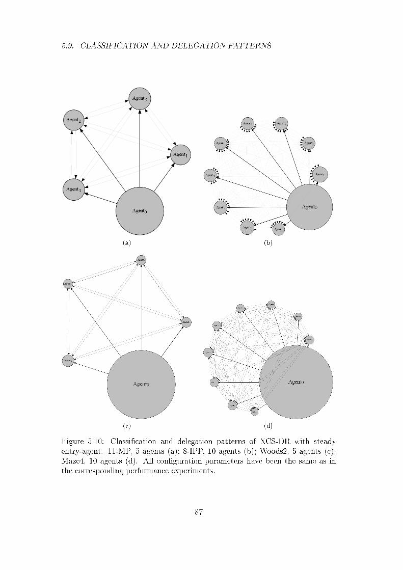
5.9. CLASSIFICATION AND DELEGATION PATTERNS
(a) (b)
(c) (d)
Figure 5.10: Classi�cation and delegation patterns of XCS-DR with steadyentry-agent. 11-MP, 5 agents (a); 8-IPP, 10 agents (b); Woods2, 5 agents (c);Maze4, 10 agents (d). All con�guration parameters have been the same as inthe corresponding performance experiments.
87
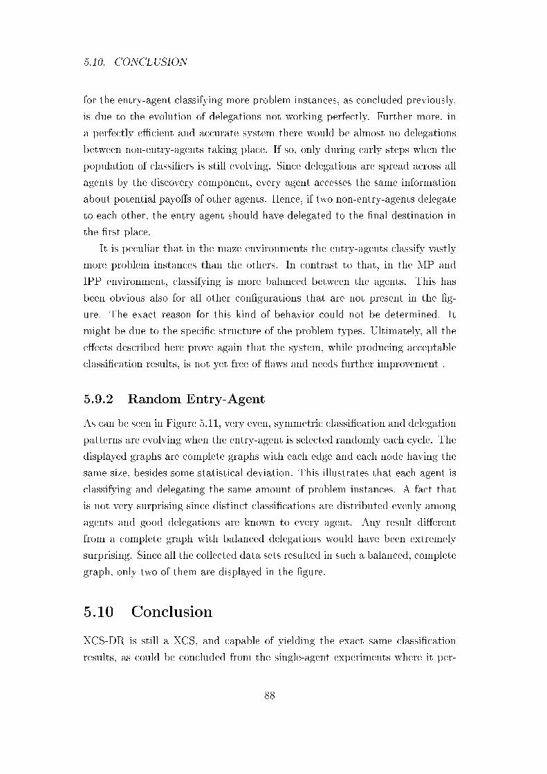
5.10. CONCLUSION
for the entry-agent classifying more problem instances, as concluded previously,
is due to the evolution of delegations not working perfectly. Further more, in
a perfectly e�cient and accurate system there would be almost no delegations
between non-entry-agents taking place. If so, only during early steps when the
population of classi�ers is still evolving. Since delegations are spread across all
agents by the discovery component, every agent accesses the same information
about potential payo�s of other agents. Hence, if two non-entry-agents delegate
to each other, the entry-agent should have delegated to the �nal destination in
the �rst place.
It is peculiar that in the maze environments the entry-agents classify vastly
more problem instances than the others. In contrast to that, in the MP and
IPP environment, classifying is more balanced between the agents. This has
been obvious also for all other con�gurations that are not present in the �g-
ure. The exact reason for this kind of behavior could not be determined. It
might be due to the speci�c structure of the problem types. Ultimately, all the
e�ects described here prove again that the system, while producing acceptable
classi�cation results, is not yet free of �aws and needs further improvement .
5.9.2 Random Entry-Agent
As can be seen in Figure 5.11, very even, symmetric classi�cation and delegation
patterns are evolving when the entry-agent is selected randomly each cycle. The
displayed graphs are complete graphs with each edge and each node having the
same size, besides some statistical deviation. This illustrates that each agent is
classifying and delegating the same amount of problem instances. A fact that
is not very surprising since distinct classi�cations are distributed evenly among
agents and good delegations are known to every agent. Any result di�erent
from a complete graph with balanced delegations would have been extremely
surprising. Since all the collected data sets resulted in such a balanced, complete
graph, only two of them are displayed in the �gure.
5.10 Conclusion
XCS-DR is still a XCS, and capable of yielding the exact same classi�cation
results, as could be concluded from the single-agent experiments where it per-
88
5.10. CONCLUSION
(a) (b)
Figure 5.11: Classi�cation and delegation patterns of XCS-DR with randomentry-agent. 8-IPP, 5 agents (a); Woods2, 10 agents (b). All con�guration pa-rameters have been the same as in the corresponding performance experiments.
formed equal to XCSJava 1.0. As the number of agents rises, the performance
of XCS-DR declines. In some environments more than in others. The classi�ca-
tions that XCS-DR evolves are equal to the ones that are evolving in XCSJava
1.0. This stems from the fact that both perform equal when only a single agent
is applied to XCS-DR. As XCS-DR's agents have been provided with a high
enough slot number during every experiment, the reason for the decline of per-
formances must lie somewhere in the concept of a subdivided population with
classi�ers supporting delegations and how their introduction a�ects the overall
system. This is backed up by the observation that XCS-DR tends to reinforce
overgeneral, useless delegations and classi�cations. The emergence of the latter
could partially be prevented by the tweak introduced in 3.2.3. However, the ex-
act cause for the partial dysfunction of the evolution of classi�ers could not be
identi�ed. It could be the �tness update mechanism or the action set formation
or some other source. Ultimately, constitutes the introduction of delegations
in a subdivided classi�er population a signi�cant increase in complexity of the
overall system. Regarding that fact, is XCS-DR still performing satisfactory by
classifying problem instances correctly with a high percentage and �nding food
in a maze reliably, even with high agent numbers.
89
Summary and Conclusion
This thesis has introduced and investigated a new kind of rule-based evolutionary
online learning system. It addressed the problem of distributing the knowledge
of a Learning Classi�er System, that is represented by a population of classi�ers.
The result is a XCS-derived Learning Classi�er System 'XCS with Distributed
Rules' (XCS-DR) that introduces independent, interacting agents to distribute
the system's acquired knowledge evenly. The agents act collaboratively to solve
problem instances at hand. XCS-DR's design and architecture have been intro-
duced and its classi�cation performance has been evaluated and scrutinized in
detail in this thesis. While not reaching optimal performance, compared to the
original XCS, it could be shown that XCS-DR still yields satisfactory classi�-
cation results. It could be shown that in the simple case of applying only one
agent, the introduced system performs as accurately as XCS.
Chapter 1 supplied the reader with general background information about
the �eld of LCS. The concept of LCS, its components and underlying principles
have been discussed. Also, this chapter provided brief remarks about the historic
development of the �eld and reviewed related work.
Chapter 2 introduced XCS, the system that has been extended. It was
explained how XCS distinguishes between strength and accuracy of its classi�ers
and how all the components of the system interact to form a simple yet e�ective
Learning Classi�er System.
The following chapter discussed XCS-DR, the adapted XCS system that has
been designed to �t the speci�c needs of a distributed population. A second
kind of classi�er, the delgation, has been introduced. Delegations di�er from
traditional classi�ers by their action part as they propose the forwarding of a
problem instance to another agent of the population. All the components of
the original system such as the population, match set and prediction array have
been adapted to facilitate interacting agents and enable accurate classi�cations.
90
Chapter 4 discussed the Java implementation of XCS-DR that has been
derived from XCSJava 1.0, a Java implementation of XCS. The con�guration of
the program, its design and package structure and other relevant implementation
details have been included in this part of the thesis.
The last chapter scrutinized the performance of the Java implementation of
XCS-DR. It turned out that the system reaches the same performance results as
XCSJava 1.0 if it applies only a single agent. But as soon as the agent number
rises, XCS-DR performs inferior to the original. It could be concluded that the
delegation procedure is still �awed and needs improvement for XCS-DR to reach
optimal performance. Nevertheless, if one takes XCS-DR's higher complexity
and prototype character into account, it still displayed satisfying performance
results.
Future research on XCS-DR should �rst and foremost be directed towards
improving the system's classi�cation performance. Since its inferior performance
is caused by the malfunctioning evolution of delegations, e�orts should be under-
taken to further understand and improve the whole delegation explore procedure.
Outstanding issues that should be clari�ed are why overgeneral delegations are
evolving, how the �tness update of the system could be improved, if there is a
more accurate way to update the prediction value of a delegation, whether the
action set formation could be altered and why the total numerosities of classi-
�cations are usually higher than the ones of delegations. Due to the increased
inherent complexity of the system it is much harder to understand entirely than
the original XCS. Hence, understanding the exact working of XCS-DR and all of
its internal mechanisms would be essential to future research. Once the system
performs as accurately as XCS, one could direct research towards making the
agents more independent of each other respectively of the overall system.
91
Bibliography
[1] Booker, L. B. (1982). Intelligent Behavior as an Adaptation to the Task
Environment. PhD thesis, University of Michigan, Ann Arbor, MI.
[2] Butz, M. V. (2000). XCSJava 1.0: An implementation of the XCS classi�er
system in Java. Technical report, Illinois Genetic Algorithms Lab, University
of Illinois, Urbana, IL.
[3] Butz, M. V. (2004). Rule-based Evolutionary Online Learning Systems:
Learning Bound, Classi�cation, and Prediction. PhD thesis, University of
Illinois, Urbana, IL.
[4] Butz, M. V. (2015). Learning Classi�er Systems. In Kacprzyk, J. and
Pedrycz, W., editors, Springer Handbook of Computational Intelligence, pages
961�981. Springer.
[5] Butz, M. V. and Wilson, S. W. (2000). An Algorithmic Description of XCS.
In Advances in Learning Classi�er Systems: Proceedings of the 3rd Interna-
tional Workshop, pages 253�272. Springer.
[6] Cli�, D. and Ross, S. (1994). Adding temporary memory to ZCS. Adaptive
Behavior, 3(2):101�150.
[7] Dam, H. H., Abbass, H. A., and Lokan, C. (2005a). DXCS: An XCS System
For Distributed Data Mining. In Proceedings of the 7th annual conference on
Genetic and evolutionary computation, pages 1883�1890. ACM.
[8] Dam, H. H., Abbass, H. A., and Lokan, C. (2005b). Investigation on DXCS:
An XCS system for distribution data mining, with continuous-valued inputs
in static and dynamic environments. In Proceedings of the IEEE Congress on
Evolutionary Computation, pages 618�625. IEEE.
A
[9] Dam, H. H., Abbass, H. A., Lokan, C., et al. (2005c). The Performance of
the DXCS System on Continuous-Valued Inputs in Stationary and Dynamic
Environments. In The 2005 IEEE Congress on Evolutionary Computation,
volume 1, pages 618�625. IEEE.
[10] Dam, H. H., Rojanavasu, P., Abbass, H. A., and Lokan, C. (2008). Dis-
tributed Learning Classi�er Systems. In Learning Classi�er Systems in Data
Mining, pages 69�91. Springer.
[11] Dietterich, T. G. (2000). An Experimental Comparison of Three Meth-
ods for Constructing Ensembles of Decision Trees: Bagging, Boosting, and
Randomization. Machine Learning, 40(2):139�157.
[12] Gader, P. D., Mohamed, M. A., and Keller, J. M. (1996). Fusion of hand-
written word classi�ers. Pattern Recognition Letters, 17(6):577�584.
[13] Gao, Y., Huang, J. Z., Rong, H., and Gu, D. (2005). Learning Classi�er
System Ensemble for Data Mining. In Proceedings of the 7th Annual Workshop
on Genetic and Evolutionary Computation, pages 63�66. ACM.
[14] Gersho�, M. and Schulenburg, S. (2007). Collective Behavior based Hi-
erarchical XCS. In Proceedings of the 9th annual conference companion on
Genetic and evolutionary computation, pages 2695�2700. ACM.
[15] Ghahramani, Z. and Kim, H. (2003). Bayesian Classi�er Combination.
Technical report, University College London, UK.
[16] Goldberg, D. E. (1989). Genetic Algorithms in Search, Optimization and
Machine Learning. Addion Wesley.
[17] Guerra-Salcedo, C. and Whitley, D. (1999). Genetic Approach to Feature
Selection for Ensemble Creation. In GECCO-99: Proceedings of Genetic and
Evolutionary Computation Conference, pages 236�243. ACM.
[18] Guo, Y., Rueger, S., Sutiwaraphun, J., and Forbes-Millott, J. (1997). Meta-
Learning for Parallel Data Mining. In Proceedings of the Seventh Parallel
Computing Workshop, pages 1�11.
B
[19] Holland, J. H. (1975). Adaptation in Natural and Arti�cial Systems: An
Introductory Analysis with Applications to Biology, Control and Arti�cial In-
telligence. The University of Michigan Press.
[20] Holland, J. H. (1976). Adaptation. Progress in Theoretical Biology, 4:263�
293.
[21] Holland, J. H. (1980). Adaptive algorithms for discovering and using general
patterns in growing knowledge bases. International Journal of Policy Analysis
and Information Systems, 4(3):245�268.
[22] Holland, J. H. (1983a). Escaping brittleness: the possibilities of general-
purpose learning algorithms applied to parallel rule-based systems. In Pro-
ceedings Second International Workshop on Machine Learning, pages 593�623.
[23] Holland, J. H. (1983b). Induction in arti�cial intelligence. Technical report,
University of Michigan, Ann Arbor, MI.
[24] Holland, J. H. (1983c). A more detailed discussion of classi�er systems.
Technical report, University of Michigan, Ann Arbor, MI.
[25] Holland, J. H. (1984). Genetic algorithms and adaptation. In Proceedings of
the NATO Advanced Research Institute on Adaptive Control, pages 317�333.
[26] Holland, J. H. (1985). Properties of the Bucket Brigade. In Proceedings of
the 1st International Conference on Genetic Algorithms, pages 1�7. L. Erl-
baum Associates Inc.
[27] Holland, J. H. (1986). A mathematical framework for studying learning in
classi�er systems. Physica D: Nonlinear Phenomena, 22(1):307�317.
[28] Holland, J. H. (1987). Genetic algorithms and classi�er systems: founda-
tions and future directions. Technical report, University of Michigan, Ann
Arbor, MI.
[29] Holland, J. H., Booker, L. B., Colombetti, M., Dorigo, M., Goldberg, D. E.,
Forrest, S., Riolo, R. L., Smith, R. E., Lanzi, P. L., Stolzmann, W., and
Wilson, W. (2000). What Is a Learning Classi�er System? In Lanzi, P. L.,
Stolzmann, W., and Wilson, W., editors, Learning Classi�er Systems, pages
3�32. Springer.
C
[30] Holland, J. H. and Reitman, J. (1978). Cognitive systems based on adaptive
agents. Pattern-Directed Inference Systems.
[31] Jong, K., Mary, J., Cornuéjols, A., Marchiori, E., and Sebag, M. (2004).
Ensemble Feature Ranking. In Knowledge Discovery in Databases: PKDD
2004, pages 267�278. Springer.
[32] Kittler, J., Hatef, M., Duin, R. P. W., and Matas, J. (1998). On Combining
Classi�ers. IEEE Transactions on Pattern Analysis and Machine Intelligence,
20(3):226�239.
[33] Kuncheva, L. I. (2004). Combining Pattern Classi�ers: Methods and Algo-
rithms. John Wiley & Sons.
[34] Lanzi, P. L. (1998). Adding Memory to XCS. In Evolutionary Computa-
tion Proceedings, 1998. IEEE World Congress on Computational Intelligence.,
pages 609�614. IEEE.
[35] McConnell, S. (2004). Code Complete. Pearson Education.
[36] Ranawana, R. and Palade, V. (2006). Multi-Classi�er Systems: Review
and a Roadmap for Developers. International Journal of Hybrid Intelligent
Systems, 3(1):35�61.
[37] Riolo, R. L. (1988). Empirical studies of default hierarchies and sequences
of rules in learning classi�er systems. PhD thesis, University of Michigan,
Ann Arbor, MI.
[38] Riolo, R. L. (1991). Lookahead planning and latent learning in a classi�er
system. In From Animals to Animats: Proceedings of the First International
Conference on Simulation of Adaptive Behavior, pages 316�326. MIT Press.
[39] Russel, S., Norvig, P., Canny, J., Malik, J., and Edwards, D. (1995). Arti-
�cial Intelligence: A Modern Approach. Prentice-Hall.
[40] Scheidler, A. and Middendorf, M. (2011). Learning Classi�er Systems to
Evolve Classi�cation Rules for Systems of Memory Constrained Components.
Evolutionary Intelligence, 4(3):127�143.
[41] Smith, S. F. (1980). A learning system based on genetic adaptive algorithms.
PhD thesis, University of Pittsburgh, Pittsburgh, PA.
D
[42] Stolzmann, W. (1998). Anticipatory Classi�er Systems. Genetic Program-
ming, 98:658�664.
[43] Stolzmann, W. (2000). An Introduction to Anticipatory Classi�er Systems.
In Learning Classi�er Systems, pages 175�194. Springer.
[44] Urbanowicz, R. J. and Moore, J. H. (2009). Learning Classi�er Systems: a
Complete Introduction, Review, and Roadmap. Journal of Arti�cial Evolution
and Applications, pages 1�25.
[45] Watkins, C. J. C. H. (1989). Learning from Delayed Rewards. PhD thesis,
University of Cambridge England.
[46] Wilson, S. W. (1986). Knowledge Growth in an Arti�cial Animal. In
Adaptive and Learning Systems, pages 255�264. Springer.
[47] Wilson, S. W. (1994). ZCS: A Zeroth Level Classi�er System. Evolutionary
Computation, 2(1):1�18.
[48] Wilson, S. W. (1995). Classi�er Fitness Based on Accuracy. Evolutionary
Computation, 3(2):149�175.
[49] Wilson, S. W. (2000). Get Real! XCS with Continuous-Valued Inputs. In
Learning Classi�er Systems, pages 209�219. Springer.
[50] Wilson, S. W. (2002). Classi�ers that Approximate Functions. Natural
Computing, 1(2-3):211�234.
E

List of Figures
2.1 XCS system overview. For a given input, the match set and pre-
diction array are formed, which are used to determine the action
to execute and form the action set. The received payo� is used
to update the previous action set via Q-learning. (This �gure has
been created after �gure 1 in [48]) . . . . . . . . . . . . . . . . . 18
2.2 The Woods2 and Maze4 maze environments.
X - exemplary animat position, F and G - food, O and Q - ob-
stacle, * - empty cell . . . . . . . . . . . . . . . . . . . . . . . . 26
3.1 Basic components of XCS-DR. Actions beginning with an 'A'
mark delegations and thus represent the ID of the target agent
(i.e. 'A0' marking a reference to Agent0). . . . . . . . . . . . . 29
3.2 Examplary best action selection exploit. Agent0 is the entry-
agent. The selection procedure leads to the selection of the delega-
tions to Agent2 and Agent3. In Agent3 the delegation to Agent1
is the best action. But that would introduce a cycle and therefore
the second best action '00' is chosen. . . . . . . . . . . . . . . . 39
3.3 Example of malicious prediction calculation. The highest predic-
tion of Agent0 is calculated for action 0 which is wrong. . . . . . 40
4.1 Package diagram of the XCS-DR Java implementation. All de-
pendencies to and from subpackages of performanceComponent
are illustrated as dependencies to and from their parent package. 56
4.2 Class diagram of the package performanceComponent. Private
methods are not displayed. . . . . . . . . . . . . . . . . . . . . . 59
4.3 Class diagram of the package classi�er. The classes that extend
Action only implement the abstract methods de�ned by the par-
ent class. Private methods are not displayed. . . . . . . . . . . . 60
F
4.4 Class diagram of the package classi�erSets. Private methods are
not displayed. . . . . . . . . . . . . . . . . . . . . . . . . . . . . 62
4.5 The default con�g.properties �le. . . . . . . . . . . . . . . . . . 66
5.1 Performance comparison between the single-agent XCS-DR and
XCSJava 1.0, averaged over 100 experiments. 11-MP, 500 slots
(a); Woods2, 1000 slots (c); Maze4, 1000 slots (d). Evolution of
the classi�er population of the single-agent XCS-DR in the 11-
MP, 500 slots (b). . . . . . . . . . . . . . . . . . . . . . . . . . . 73
5.2 Evolution of the system accuracy/distance to food of the di�erent
delegation explore modes, in a 3-agent XCS-DR, depending on the
exploit cycle. 6-MP, 500 slots, 100 experiments (a); 5-IPP, 800
slots, 100 experiments (b); Woods2, 800 slots, 50 experiments (c);
Maze4, 1800 slots, 100 experiments (d). . . . . . . . . . . . . . . 75
5.3 Evolution of the system accuracy/distance to food of di�erent
delegation explore modes, depending on the exploit cycle. 8-IPP,
15 agents, 70000 slots, 100 experiments (a); Woods2, 10 agents,
5000 slots, 50 experiments (b). . . . . . . . . . . . . . . . . . . . 77
5.4 Evolution of the system accuracy of XCS-DR depending on the
exploit cycle in the 11-MP environment. Averaged over 100 ex-
periments. . . . . . . . . . . . . . . . . . . . . . . . . . . . . . . 78
5.5 Evolution of the system accuracy of XCS-DR depending on the
exploit cycle in the 8-IPP environment. Averaged over 100 exper-
iments. . . . . . . . . . . . . . . . . . . . . . . . . . . . . . . . . 79
5.6 Evolution of the distance to food of XCS-DR depending on the
exploit cycle in the Woods2 environment, averaged over 50 exper-
iments (a). Evolution of the classi�er population of the 10-agent
XCS-DR in Woods2, 5000 slots, 50 experiments (b). . . . . . . . 81
5.7 Evolution of the distance to food of XCS-DR depending on the
exploit cycle in the Maze4 environment. Averaged over 100 ex-
periments. . . . . . . . . . . . . . . . . . . . . . . . . . . . . . . 82
5.8 Evolution of the accuracy of XCS-DR with random and steady
entry-agent. Slot numbers and numbers of experiments are equal
to the corresponding steady entry-agent experiments. In the 11-
MP environment (a); in the 8-IPP environment (b). . . . . . . . 84
G
5.9 Evolution of the distance to food of XCS-DR with random and
steady entry-agent. Slot numbers and numbers of experiments
are equal to the corresponding steady entry-agent experiments.
In the Woods2 environment (a); In the Maze4 environment (b). 85
5.10 Classi�cation and delegation patterns of XCS-DR with steady
entry-agent. 11-MP, 5 agents (a); 8-IPP, 10 agents (b); Woods2,
5 agents (c); Maze4, 10 agents (d). All con�guration parameters
have been the same as in the corresponding performance experi-
ments. . . . . . . . . . . . . . . . . . . . . . . . . . . . . . . . 87
5.11 Classi�cation and delegation patterns of XCS-DR with random
entry-agent. 8-IPP, 5 agents (a); Woods2, 10 agents (b). All con-
�guration parameters have been the same as in the corresponding
performance experiments. . . . . . . . . . . . . . . . . . . . . . 89
H

Erklärung
"Ich versichere, dass ich die vorliegende Arbeit selbständig und nur unter
Verwendung der angegebenen Quellen und Hilfsmittel angefertigt habe,
insbesondere sind wörtliche oder sinngemäÿe Zitate als solche gekennzeichnet.
Mir ist bekannt, dass Zuwiderhandlung auch nachträglich zur Aberkennung des
Abschlusses führen kann".
Leipzig, 31.03.2016
I