Measurement of the Conditioned Turbulence and Temperature Field of a Ring Stabilized Bunsen Type Premixed Burner Using Planar Laser Rayleigh Scattering and

Stereo Particle Image Velocimetry

Sebastian Pfadler, Micha Löffler, Friedrich Dinkelacker, Alfred Leipertz

Lehrstuhl für Technische Thermodynamik

Friedrich-Alexander Universität Erlangen-Nürnberg Am Weichselgarten 8

D-91058 Erlangen, Germany E-Mail: sp@ltt.uni-erlangen.de

1 ABSTRACT

The turbulence and temperature field of Bunsen type turbulent lean methane/air flames has been investigated using Planar Laser Rayleigh Scattering (PLRS) and Stereo Particle Image Velocimetry (Stereo PIV). Temporal averaged reaction progress variable plots have been computed from PLRS measurements in order to provide a basis with regard to the verification of CFD models. Turbulence was characterised by Stereo PIV in one plane for all directions in space. Averaged velocity fields have been calculated as well as Reynolds decomposed fluctuation vector fields. Conditioned RMS-values of the turbulent fluctuations in terms of unburnt and burnt gas could be determined making use of the information gained from a threshold setting procedure in the PIV raw images. Furthermore several length scales were measured indirectly from PIV vector plots. In this context all integral length scales being accessible with Stereo PIV were computed separately for burnt and unburnt region and compared to each others. It could be observed that all integral length scales become longer in the burnt zone. Additionally, the conditioned Taylor and the Kolmogorov length have been extracted from PIV fields using correlation equations suggested by Bradley and Tennekes.

2 INTRODUCTION

To improve the models which are the base of nowadays used Computational Fluid Dynamcis (CFD) codes being applied on the field of turbulent combustion research, a close collaboration between numerical investigations and experimental studies is of importance. This means that experimental work has to provide the necessary data in order to verify numerical results and thus to establish a basis for an improvement of current numerical models. Of special interest is the knowledge of the flow and turbulence field, thus averaged velocities, their fluctuations, the turbulence intensity and relevant length scales need to be known. Since the flame influences the flow and turbulence field significantly, for instance, flame generated turbulence is a well known phenomena, a distinction of the turbulence characterisation has to be done between burnt and unburnt part of the flame. This article describes which turbulence parameters are accessible from PIV data and highlights conditioned results achieved in a turbulent premixed combustion system. For a useful comparison with numeric investigations additionally temperature fields were measured with PLRS. From this temperature fields averaged reaction progress variables have been determined.

3 EXPERIMENTAL SETUP

3.1 Burner

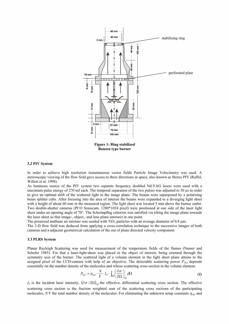
In the following investigation a ring stabilized turbulent Bunsen type burner was applied. The operating range was changed in terms of fuel-air ratio and total mass flow rate resulting in 8 stable working points representing the complete stable range. Lean methane/air mixtures have been investigated as they are of most essential technical interest. (an overview of the operating points is given in Figure 10) In order to reach nearly homogenous isotropic turbulence conditions a perforated plate with holes of 4 mm diameter was used. After passing the turbulence plate the flow is forced through a conical part and thus gets accelerated. Without the flame stabilising ring at the burner outlet very lean flames at high outlet velocities would lift off and extinguish. The advantage of this way of flame stabilisation is the benefit of having the stabilizer conform to the burner port. This leads to an almost complete combustion without any leakage of fuel combined with non-changed emissions compared to the unstabilized construction (Johnson, Kostiuk et al. 1998).

g

3.2 PIV System

In order to achieve high resolution instantaneous vector fields Particle Image stereoscopic viewing of the flow field gave access to three directions in space, also knWillert et al. 1998). As luminous source of the PIV system two separate frequency doubled Nd:YAGmaximum pulse energy of 270 mJ each. The temporal separation of the two pulses wato give an optimal shift of the scattered light in the image plane. The beams were beam splitter cube. After focusing into the area of interest the beams were expandewith a height of about 60 mm in the measured region. The light sheet was located 5 mTwo double-shutter cameras (PCO Sensicam, 1280*1024 pixel) were positioned atsheet under an opening angle of 70°. The Scheimpflug criterion was satisfied via tiltithe laser sheet so that image-, object,- and lens plane intersect in one point. The premixed methane air mixture was seeded with TiO2 particles with an average diaThe 3-D flow field was deduced from applying a cross-correlation technique to thecameras and a adjacent geometrical calculation of the out of plane directed velocity co

3.3 PLRS System

Planar Rayleigh Scattering was used for measurement of the temperature fields Schefer 1985). For that a laser-light-sheet was placed in the object of interest, bsymmetry axis of the burner. The scattered light of a volume element in the lightassigned pixel of the CCD-camera with help of an objective. The detectable scatessentially on the number density of the molecules and whose scattering cross section

Ω

Ω∂∂

⋅⋅⋅= ∫∆ΩdI

VNP

effoptDet

ση 0

I0 is the incident laser intensity, ( )effΩ∂∂ /σ the effective, differential scattering cscattering cross section is the fraction weighted sum of the scattering cross semolecules, N/V the total number density of the molecules. For eliminating the unkno

stabilising rin

perforated plate

Figure 1: Ring stabilizedBunsen type burner

Velocimetry was used. A own as Stereo PIV (Raffel,

lasers were used with a s adjusted to 30 µs in order superposed by a polarising d to a diverging light sheet m above the burner outlet.

one side of the laser light ng the image plane towards

meter of 0.8 µm. successive images of both mponent.

of the flames (Namer and eing oriented through the sheet plane attains to the tering power PDet depends in the volume element.

(1)

ross section. The effective ctions of the participating wn setup constants ηopt and

the scattering collection angle Ω usually for temperature determination the pixelwise quotient is formed with a reference picture at known temperature Tref and pressure pref (from dry air at room temperature).

( )σ

σ refrefref

Det

refDetRay I

ITp

TpP

PQ ⋅⋅==

0

,0,

//

(2)

The temperature of each pixel is accessible with an accuracy, which is in particular depending on the change of the medium scattering cross section. Dealing with methan/air flames this deviation is smaller than 2-4% (Dinkelacker 1993) (Kampmann, Leipertz et al. 1993).

pp

PP

TT ref

refDet

refDetref ⋅⋅⋅=

σσ, (3)

The first of the two PIV-laserpulses (pulsed Nd:YAG laser) was applied for Rayleigh-thermometry. A double-intensified CCD-camera (LaVision StreakStar) was employed as detector. To minimize light reflexes in the background, the burner was built in a housing equipped with a for 30° inclined backplane and two sidewalls with thin oblong apertures for the optical access. With this setup it was possible to make measurements with a minimum distance to the burner top edge of less then 10 mm, the whole picture area is about 50 x 50 mm². For the temperature field measurements were taken series of 50 pictures each.

4 THEORY OF INTEGRAL LENGTH SCALES

Adapting Reynolds decomposition of the instantaneous velocity at a specified location in space yields a time averaged velocity for the considered location and a instantaneous fluctuation.

),tx(iu)x(iU,t)x(iu vvv ′+= (4)Using PIV, time averages are normally replaced by ensemble averages from several consecutive measurements. Besides this Reynolds decomposition, spatial correlation lengths are of significant interest to characterise turbulent flows. Spatial correlations may be described by the correlation tensor between the velocity fluctuations of two vector components of two adjacent vectors at two different locations (Rotta 1972),

),(),(),( trxutxutrR jiijvvvv +′⋅′= (5)

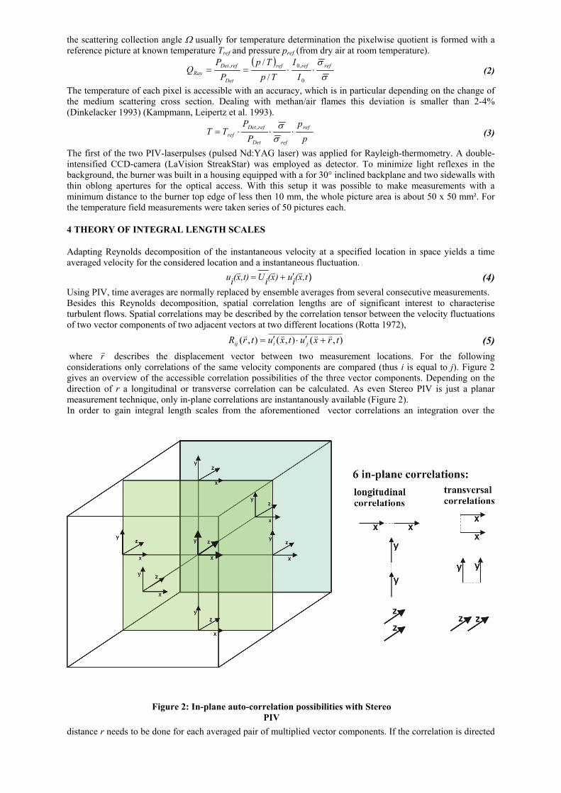
where rv describes the displacement vector between two measurement locations. For the following considerations only correlations of the same velocity components are compared (thus i is equal to j). Figure 2 gives an overview of the accessible correlation possibilities of the three vector components. Depending on the direction of r a longitudinal or transverse correlation can be calculated. As even Stereo PIV is just a planar measurement technique, only in-plane correlations are instantanously available (Figure 2). In order to gain integral length scales from the aforementioned vector correlations an integration over the

distance r needs to b

Figure 2: In-plane auto-correlation possibilities with StereoPIV

e done for each averaged pair of multiplied vector components. If the correlation is directed

perpendicular to the considered vector component the correlation function is denominated as transverse correlation function q(r). In case that the direction of rv points towards the respective vector component a longitudinal correlation function l(r) is formed (Rotta 1972). The mathematical description (with suitable normalisation) follows as:

2

)()()(i

BiAi

u

uurl′

′′=

2

)()()(

j

BjAj

u

uurq

′

′′=

(6)

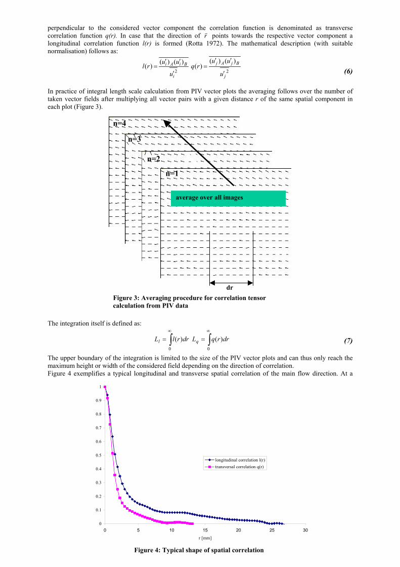
In practice of integral length scale calculation from PIV vector plots the averaging follows over the number of taken vector fields after multiplying all vector pairs with a given distance r of the same spatial component in each plot (Figure 3).

average over all images

dr

n=4

n=3

n=2

n=1

The integration itself is

The upper boundary omaximum height or wiFigure 4 exemplifies a

0

0.1

0.2

0.3

0.4

0.5

0.6

0.7

0.8

0.9

1

0

Figure 3: Averaging procedure for correlation tensorcalculation from PIV data

defined as:

∫∞

=0

)( drrlLl ∫∞

=0

)( drrqLq (7)

f the integration is limited to the size of the PIV vector plots and can thus only reach the dth of the considered field depending on the direction of correlation. typical longitudinal and transverse spatial correlation of the main flow direction. At a

5 10 15 20 25 30

r [mm]

longitudinal correlation l(r)transversal correlation q(r)

Figure 4: Typical shape of spatial correlation

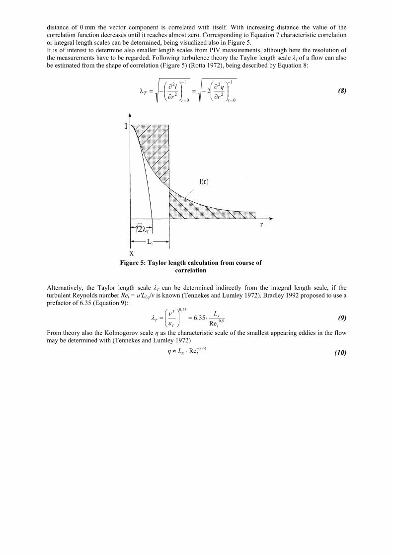
distance of 0 mm the vector component is correlated with itself. With increasing distance the value of the correlation function decreases until it reaches almost zero. Corresponding to Equation 7 characteristic correlation or integral length scales can be determined, being visualized also in Figure 5. It is of interest to determine also smaller length scales from PIV measurements, although here the resolution of the measurements have to be regarded. Following turbulence theory the Taylor length scale λT of a flow can also be estimated from the shape of correlation (Figure 5) (Rotta 1972), being described by Equation 8:

1

02

21

02

22

−

=

−

=

∂∂

−=

∂∂

−=λrr

T rq

rl (8)

Alternatively, the Taylor turbulent Reynolds numbeprefactor of 6.35 (Equatio

From theory also the Kolmmay be determined with (T

Figure 5: Taylor length calculation from course ofcorrelation

length scale λT can be determined indirectly from the integral length scale, if the r Ret = u'Ll,q/ν is known (Tennekes and Lumley 1972). Bradley 1992 proposed to use a n 9):

50

25,03

Re35.6 ,

t

x

TT

L⋅=

=

ενλ (9)

ogorov scale η as the characteristic scale of the smallest appearing eddies in the flow ennekes and Lumley 1972)

43Re /txLη −⋅≈ (10)

5 THRESHOLD SETTING PROCEDURE IN PIV RAW IMAGES

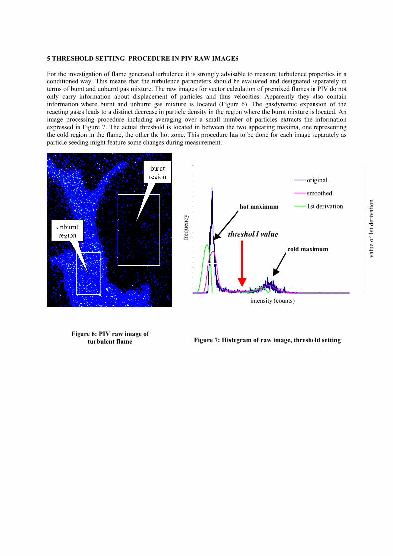
For the investigation of flame generated turbulence it is strongly advisable to measure turbulence properties in a conditioned way. This means that the turbulence parameters should be evaluated and designated separately in terms of burnt and unburnt gas mixture. The raw images for vector calculation of premixed flames in PIV do not only carry information about displacement of particles and thus velocities. Apparently they also contain information where burnt and unburnt gas mixture is located (Figure 6). The gasdynamic expansion of the reacting gases leads to a distinct decrease in particle density in the region where the burnt mixture is located. An image processing procedure including averaging over a small number of particles extracts the information expressed in Figure 7. The actual threshold is located in between the two appearing maxima, one representing the cold region in the flame, the other the hot zone. This procedure has to be done for each image separately as particle seeding might feature some changes during measurement.

0

50

100

150

200

250

0 100 200 300 400 500 600 700

intensity (counts)

freq

uenc

y

0

0.5

1

1.5

2

2.5

3

3.5

4

4.5

5

valu

e of

1st

der

ivat

ion

original

smoothed

1st derivationhot maximum

cold maximum

threshold value

Figure 7: Histogram of raw image, threshold setting

Figure 6: PIV raw image ofturbulent flame

6 EXPERIMENTAL RESULTS

6.1 PLRS Measurements

2500 K

position 250 K

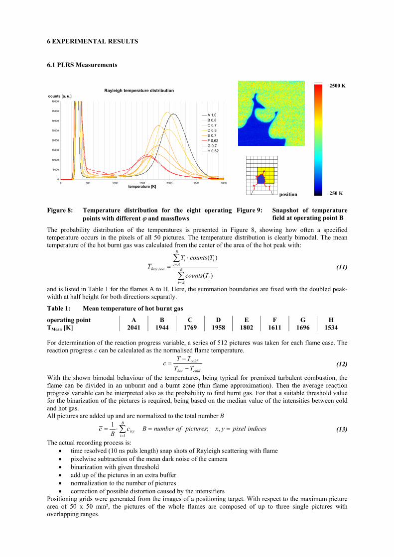
Figure 8: Temperature distribution for the eight operating points with different ϕ and massflows

Figure 9: Snapshot of temperature field at operating point B

Rayleigh temperature distribution

0

5000

10000

15000

20000

25000

30000

35000

40000

0 500 1000 1500 2000 2500 3000temperature [K]

counts [a. u.]

A 1,0B 0,8C 0,7D 0,8E 0,7F 0,62G 0,7H 0,62

The probability distribution of the temperatures is presented in Figure 8, showing how often a specified temperature occurs in the pixels of all 50 pictures. The temperature distribution is clearly bimodal. The mean temperature of the hot burnt gas was calculated from the center of the area of the hot peak with:

∑

∑

=

=

⋅= B

Aii

B

Aiii

coaRay

Tcounts

TcountsTT

)(

)(, (11)

and is listed in Table 1 for the flames A to H. Here, the summation boundaries are fixed with the doubled peak-width at half height for both directions separatly.

Table 1: Mean temperature of hot burnt gas

operating point A B C D E F G H TMean [K] 2041 1944 1769 1958 1802 1611 1696 1534 For determination of the reaction progress variable, a series of 512 pictures was taken for each flame case. The reaction progress c can be calculated as the normalised flame temperature.

coldhot

cold

TTTT

c−

−= (12)

With the shown bimodal behaviour of the temperatures, being typical for premixed turbulent combustion, the flame can be divided in an unburnt and a burnt zone (thin flame approximation). Then the average reaction progress variable can be interpreted also as the probability to find burnt gas. For that a suitable threshold value for the binarization of the pictures is required, being based on the median value of the intensities between cold and hot gas. All pictures are added up and are normalized to the total number B

indicespixelyxpicturesofnumberBcB

cB

iixy ==⋅= ∑

=

,;11

(13)

The actual recording process is: • time resolved (10 ns puls length) snap shots of Rayleigh scattering with flame • pixelwise subtraction of the mean dark noise of the camera • binarization with given threshold • add up of the pictures in an extra buffer • normalization to the number of pictures • correction of possible distortion caused by the intensifiers

Positioning grids were generated from the images of a positioning target. With respect to the maximum picture area of 50 x 50 mm², the pictures of the whole flames are composed of up to three single pictures with overlapping ranges.

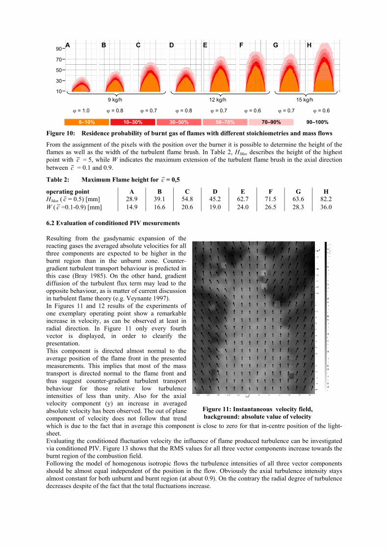
Figure 10: Residence probability of burnt gas of flames with different stoichiometries and mass flows

From the assignment of the pixels with the position over the burner it is possible to determine the height of the flames as well as the width of the turbulent flame brush. In Table 2, HMax describes the height of the highest point with c = 5, while W indicates the maximum extension of the turbulent flame brush in the axial direction between c = 0.1 and 0.9.

Table 2: Maximum Flame height for c = 0,5

operating point A B C D E F G H HMax ( c = 0.5) [mm] 28.9 39.1 54.8 45.2 62.7 71.5 63.6 82.2 W ( c =0.1-0.9) [mm] 14.9 16.6 20.6 19.0 24.0 26.5 28.3 36.0

6.2 Evaluation of conditioned PIV mesurements

Resulting from the gasdynamic expansion of the reacting gases the averaged absolute velocities for all three components are expected to be higher in the burnt region than in the unburnt zone. Counter-gradient turbulent transport behaviour is predicted in this case (Bray 1985). On the other hand, gradient diffusion of the turbulent flux term may lead to the opposite behaviour, as is matter of current discussion in turbulent flame theory (e.g. Veynante 1997). In Figures 11 and 12 results of the experiments of one exemplary operating point show a remarkable increase in velocity, as can be observed at least in radial direction. In Figure 11 only every fourth vector is displayed, in order to clearify the presentation.

This component is directed almost normal to the average position of the flame front in the presented measurements. This implies that most of the mass transport is directed normal to the flame front and thus suggest counter-gradient turbulent transport behaviour for those relative low turbulence intensities of less than unity. Also for the axial velocity component (y) an increase in averaged absolute velocity has been observed. The out of plane component of velocity does not follow that trend which is due to the fact that in average this component isheet.

A 90 B C D E F H

9 kg/h 12 kg/h 15 kg/h

ϕ = 1.0 ϕ = 0.8 ϕ = 0.7 ϕ = 0.8 ϕ = 0.7 ϕ = 0.6 ϕ = 0.7 ϕ = 0.6

10

90–100% 70–90% 50–70% 30–50% 10–30% 0–10%

30

50

70

G

Evaluating the conditioned fluctuation velocity the influevia conditioned PIV. Figure 13 shows that the RMS valueburnt region of the combustion field. Following the model of homogenous isotropic flows theshould be almost equal independent of the position in thalmost constant for both unburnt and burnt region (at aboudecreases despite of the fact that the total fluctuations incre

Figure 11: Instantaneous velocity field,background: absolute value of velocity

s close to zero for that in-centre position of the light-

nce of flame produced turbulence can be investigated s for all three vector components increase towards the

turbulence intensities of all three vector components e flow. Obviously the axial turbulence intensity stays t 0.9). On the contrary the radial degree of turbulence ase.

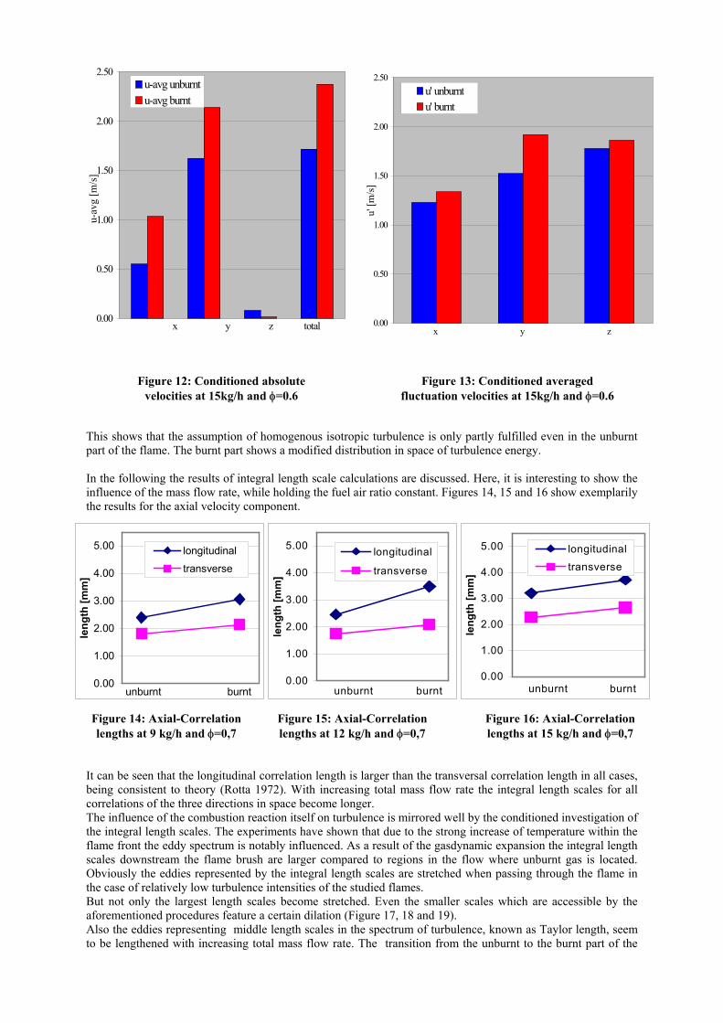
Figure 16: Axial-Correlation lengths at 15 kg/h and φ=0,7

0.00

0.50

1.00

1.50

2.00

2.50

u' [m

/s]

u' unburntu' burnt

x y z

0.00

0.50

1.00

1.50

2.00

2.50

u-av

g [m

/s]

u-avg unburntu-avg burnt

x y z total

Figure 12: Conditioned absolute velocities at 15kg/h and φ=0.6

Figure 13: Conditioned averaged fluctuation velocities at 15kg/h and φ=0.6

This shows that the assumption of homogenous isotropic turbulence is only partly fulfilled even in the unburnt part of the flame. The burnt part shows a modified distribution in space of turbulence energy. In the following the results of integral length scale calculations are discussed. Here, it is interesting to show the influence of the mass flow rate, while holding the fuel air ratio constant. Figures 14, 15 and 16 show exemplarily the results for the axial velocity component.

0.00

1.00

2.00

3.00

4.00

5.00

leng

th [m

m]

longitudinal

transverse

burntunburnt0.00

1.00

2.00

3.00

4.00

5.00

leng

th [m

m]

longitudinal

transverse

unburnt burnt0.00

1.00

2.00

3.00

4.00

5.00

leng

th [m

m]

longitudinal

transverse

unburnt burnt

Figure 14: Axial-Correlation lengths at 9 kg/h and φ=0,7

Figure 15: Axial-Correlation lengths at 12 kg/h and φ=0,7

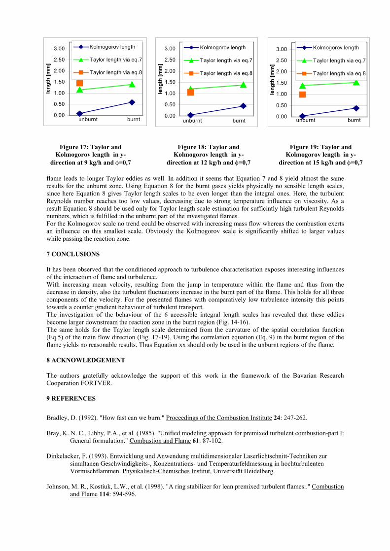
It can be seen that the longitudinal correlation length is larger than the transversal correlation length in all cases, being consistent to theory (Rotta 1972). With increasing total mass flow rate the integral length scales for all correlations of the three directions in space become longer. The influence of the combustion reaction itself on turbulence is mirrored well by the conditioned investigation of the integral length scales. The experiments have shown that due to the strong increase of temperature within the flame front the eddy spectrum is notably influenced. As a result of the gasdynamic expansion the integral length scales downstream the flame brush are larger compared to regions in the flow where unburnt gas is located. Obviously the eddies represented by the integral length scales are stretched when passing through the flame in the case of relatively low turbulence intensities of the studied flames. But not only the largest length scales become stretched. Even the smaller scales which are accessible by the aforementioned procedures feature a certain dilation (Figure 17, 18 and 19). Also the eddies representing middle length scales in the spectrum of turbulence, known as Taylor length, seem to be lengthened with increasing total mass flow rate. The transition from the unburnt to the burnt part of the

0.00

0.50

1.00

1.50

2.00

2.50

3.00le

ngth

[mm

]Kolmogorov length

Taylor length via eq.7

Taylor length via eq.8

burntunburnt 0.00

0.50

1.00

1.50

2.00

2.50

3.00

leng

th [m

m]

Kolmogorov length

Taylor length via eq.7

Taylor length via eq.8

unburnt burnt0.00

0.50

1.00

1.50

2.00

2.50

3.00

leng

th [m

m]

Kolmogorov length

Taylor length via eq.7

Taylor length via eq.8

unburnt burnt

di 7

Figure 19: Taylor and Kolmogorov length in y-

direction at 15 kg/h and φ=0,7

Figure 18: Taylor and Kolmogorov length in y-

direction at 12 kg/h and φ=0,7

flamresusincReyresunumForan whi

7 C

It hof tWitdeccomtowThebecThe(Eqflam

8 A

TheCoo

9 R

Bra

Bra

Din

Joh

Figure 17: Taylor and Kolmogorov length in y-rection at 9 kg/h and φ=0,

e leads to longer Taylor eddies as well. In addition it seems that Equation 7 and 8 yield almost the same lts for the unburnt zone. Using Equation 8 for the burnt gases yields physically no sensible length scales, e here Equation 8 gives Taylor length scales to be even longer than the integral ones. Here, the turbulent nolds number reaches too low values, decreasing due to strong temperature influence on viscosity. As a lt Equation 8 should be used only for Taylor length scale estimation for sufficintly high turbulent Reynolds bers, which is fulfilled in the unburnt part of the investigated flames.

the Kolmogorov scale no trend could be observed with increasing mass flow whereas the combustion exerts influence on this smallest scale. Obviously the Kolmogorov scale is significantly shifted to larger values le passing the reaction zone.

ONCLUSIONS

as been observed that the conditioned approach to turbulence characterisation exposes interesting influences he interaction of flame and turbulence. h increasing mean velocity, resulting from the jump in temperature within the flame and thus from the rease in density, also the turbulent fluctuations increase in the burnt part of the flame. This holds for all three ponents of the velocity. For the presented flames with comparatively low turbulence intensity this points ards a counter gradient behaviour of turbulent transport. investigation of the behaviour of the 6 accessible integral length scales has revealed that these eddies ome larger downstream the reaction zone in the burnt region (Fig. 14-16). same holds for the Taylor length scale determined from the curvature of the spatial correlation function .5) of the main flow direction (Fig. 17-19). Using the correlation equation (Eq. 9) in the burnt region of the e yields no reasonable results. Thus Equation xx should only be used in the unburnt regions of the flame.

CKNOWLEDGEMENT

authors gratefully acknowledge the support of this work in the framework of the Bavarian Research peration FORTVER.

EFERENCES

dley, D. (1992). "How fast can we burn." Proceedings of the Combustion Institute 24: 247-262.

y, K. N. C., Libby, P.A., et al. (1985). "Unified modeling approach for premixed turbulent combustion-part I: General formulation." Combustion and Flame 61: 87-102.

kelacker, F. (1993). Entwicklung und Anwendung multidimensionaler Laserlichtschnitt-Techniken zur simultanen Geschwindigkeits-, Konzentrations- und Temperaturfeldmessung in hochturbulenten Vormischflammen. Physikalisch-Chemisches Institut, Universität Heidelberg.

nson, M. R., Kostiuk, L.W., et al. (1998). "A ring stabilizer for lean premixed turbulent flames:." Combustion and Flame 114: 594-596.

Kampmann, S., Leipertz, A., et al. (1993). "Two-dimensional temperature measurements in a technical combustor with laser Rayleigh scattering." Applied Optics 32(30): 6167-6172.

Namer, J., Schefer, R.W. (1985). "Error estimates for Rayleigh scattering density and temperature measurements in premixed flames." Experiments in Fluids 3: 1-9.

Raffel, M., Willert, C., et al. (1998). Particle Image Velocimetry. Berlin, Springer.

Rotta, J. C. (1972). Turbulente Strömungen, Eine Einführung in die Theorie und ihre Anwendungen. Stuttgart, B. G. Teubner.

Tennekes, H., Lumley, L.J. (1972). A first course in turbulence. Cambridge, Mass., MIT Press.

Veynante, D., Trouvé, A., et al. (1997). "Gradient and counter-gradient scalar transport in turbulent premixed flames." Journal Fluid Mechanics 332: 263-293.