MICRO UAV BASED GEOREFERENCED ORTHOPHOTO GENERATION IN VIS+NIR … · 2013-10-29 · MICRO UAV BASED GEOREFERENCED ORTHOPHOTO GENERATION IN VIS+NIR ... a Humboldt-Universit ¨at zu

MICRO UAV BASED GEOREFERENCED ORTHOPHOTO GENERATION IN VIS+NIRFOR PRECISION AGRICULTURE

Ferry Bachmanna, Ruprecht Herbstb, Robin Gebbersc, Verena V. Hafnera

a Humboldt-Universitat zu Berlin, Department of Computer Science, Berlin, Germany –(bachmann, hafner)@informatik.hu-berlin.de

b Humboldt-Universitat zu Berlin, Landwirtschaftlich-Gartnerische Fakultat, Berlin, Germany – [email protected] Leibniz Institut fur Agrartechnik Potsdam-Bornim e.V., Potsdam, Germany – [email protected]

KEY WORDS: UAV, Orthophoto, VIS, NIR, Precision Agriculture, Exposure Time, Vignetting

ABSTRACT:

This paper presents technical details about georeferenced orthophoto generation for precision agriculture with a dedicated self-constructed camera system and a commercial micro UAV as carrier platform. The paper describes the camera system (VIS+NIR)in detail and focusses on three issues concerning the generation and processing of the aerial images related to: (i) camera exposuretime; (ii) vignetting correction; (iii) orthophoto generation.

1 INTRODUCTION

In the domain of precision agriculture, the contemporary gener-ation of aerial images with high spatial resolution is of great in-terest. Useful in particular are aerial images in the visible (VIS)and near-infrared (NIR) spectrum. From that data, a number ofso-called vegetation indices can be computed which enable todraw conclusions on biophysical parameters of the plants (Jensen,2007, pp. 382–393). In recent years, due to their ease-of-useand flexibility, micro unmanned aerial vehicles (micro UAVs) areincreasingly gaining interest for the generation of such aerial im-ages (Nebiker et al., 2008).

This paper focusses on the generation of georeferenced orthopho-tos in VIS+NIR using such a micro UAV. The research was car-ried out within a three-year project called agricopter. The overallgoal of this project was to develop a flexible, reasonably pricedand easy to use system for generating georeferenced orthophotosin VIS+NIR as an integral part of a decision support system forfertilization.

We will first describe a self-constructed camera system dedicatedfor this task. Technical details will be presented that may be help-ful in building up a similar system or to draw comparisons tocommercial solutions. Then we will describe issues concerningthe generation and processing of the aerial images which mightbe of general interest: (i) practical and theoretical considerationsconcerning the proper configuration of camera exposure time;(ii) a practicable vignetting correction procedure that can be con-ducted without any special technical equipment; (iii) details aboutthe orthophoto generation including an accuracy measurement.

As prices could be of interest in application-oriented research, wewill state them without tax for some of the components (at their2011 level).

2 SYSTEM COMPONENTS

The system used to generate the aerial images and the corre-sponding georeference information consists of two components:a customized camera system constructed during the project and acommercial micro UAV used as carrier platform.

2.1 Camera System

There were three main goals for the camera system.

Multispectral information The main objective was to gatherinformation in the near-infrared and visible spectrum. The detailsof the spectral bands should be adjustable with filters.

Suitability for micro UAV As the camera system should beused as payload on the micro UAV, the system had to be light-weight and should be able to cope with high angular velocities toavoid motion blur or other distortions of the images.

Georeferencing information The aerial images should be aug-mented with GNSS information to facilitate georeferenced ortho-photo generation.

As these goals were not concurrently realizable with a singlecommercial solution, we decided to built up our own system fromcommercial partial solutions. The system was inspired by a sys-tem described in (Nebiker et al., 2008). However, it differs in itsindividual components and is designed for georeferenced ortho-photo generation. The main components are the cameras, a GNSSreceiver and a single-board-computer interfacing the previous ones.

2.1.1 Cameras and Lenses We used two compact board-levelcameras (UI-1241LE-C and UI-1241LE-M from IDS Imaging,costs approx. 310e and 190e), each weighing about 16 g with-out lenses. The first one is an RGB camera and the second onea monochrome camera with high sensitivity in the NIR range.The infrared cut filter glass in the monochrome camera was ex-changed with a daylight cut filter resulting in a sensitive range ofapprox. 700 nm to 950 nm. An additional monochrome camerawith a band-pass filter glass could be easily added to the systemto augment it with a desired spectral band (see figure 4).

Both cameras have a pixel count of 1280x1024, resulting in aground sampling distance of approx. 13 cm with our flight alti-tude of 100 m. This is more than sufficient for the applicationcase of fertilization support. The advantage of the small pixelcount is a huge pixel size of 5.3 µm resulting in short exposuretimes to avoid motion blur. This is especially important on a plat-form with high angular velocities like a micro UAV (see also sec-tion 3.1). For the same reason it is important to use cameras witha global shutter. Flight experiments with a rolling shutter cameraresulted in strongly distorted images exposed during a rotation ofthe UAV.

We used a compact S-mount lens (weight 19 g) suitable for in-frared photography for both cameras (BL-04018MP118 from VD-

International Archives of the Photogrammetry, Remote Sensing and Spatial Information Sciences, Volume XL-1/W2, 2013UAV-g2013, 4 – 6 September 2013, Rostock, Germany

This contribution has been peer-reviewed. 11

Optics, costs approx. 105e each). The focal length is approx.4 mm resulting in an angle of view of approx. 81◦ horizontal and68◦ vertical. With our flight altitude of 100 m this corresponds toa field of view of 170 m× 136 m. The wide angle has the advan-tage of highly overlapping image blocks to facilitate the imageregistration process.

The cameras are mounted on a pan-tilt unit designed by the localcompany berlinVR (Germany) to ensure the cameras are pointingroughly in nadir direction throughout the flight.

Figure 1 shows raw sample images made with the describedcamera-lens combination. Note the variations in the test field andthe barrel lens distortion.

Figure 1: Raw RGB (left) and NIR (right) sample images of a fertiliza-tion test field (altitude approx. 50 m).

2.1.2 GNSS Receiver The system was augmented with aGNSS receiver (Navilock NL-651EUSB u-blox 6, weight 14 g,costs approx. 40e) to directly associate the images with theGNSS data. We did not use the receiver of the UAV to have aflexible stand-alone solution which potentially could be used onanother UAV.

2.1.3 Single-Board-Computer and Software We used asingle-board-computer (BeagleBoard xM, weight 37 g, costs ap-prox. 160e) on board the UAV to be the common interfacefor the cameras, the GNSS receiver and the user of the system.The board is running the Angstrom embedded Linux distributionwhich is open source and has a broad community support.

The GNSS receiver was interfaced via USB and the UBX proto-col. The cameras were connected via USB and a software inter-face from IDS Imaging was used which is available for the Bea-gleBoard upon request. An additional trigger line (GPIO) wasconnected to the cameras to simultaneously trigger both cameras.The user connects to the board via WLAN in ad hoc mode and aSecure Shell (SSH).

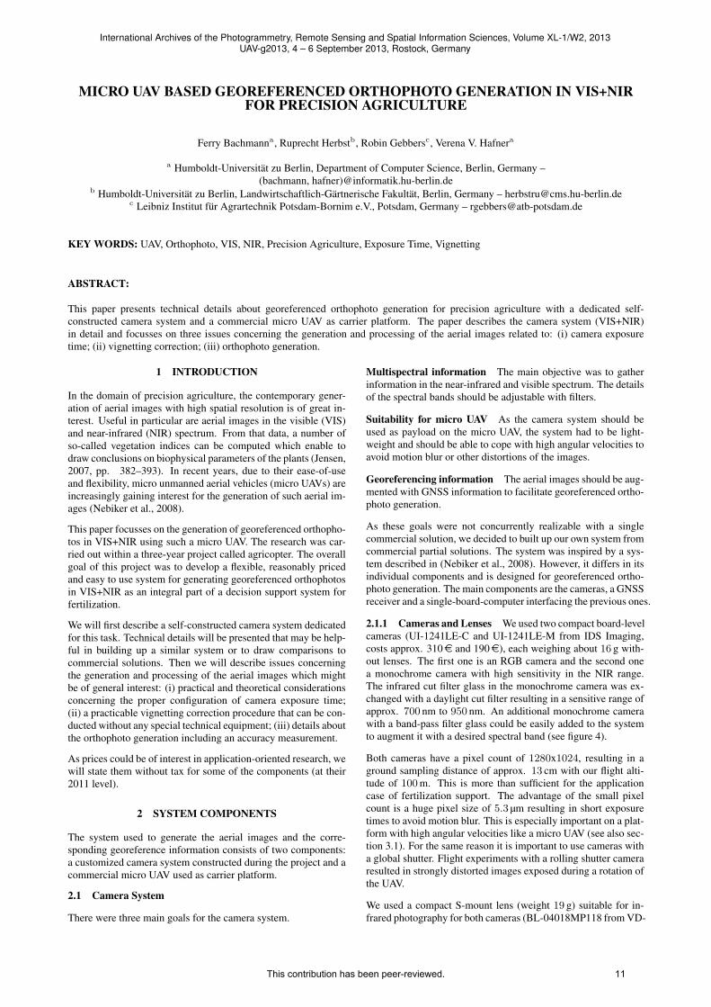
Figure 2: Close-up of constructed camera system with: (bottom) twoboard-level cameras in pan-tilt unit; (right) GNSS receiver mounted ontop of the UAV during flight; (top) single-board-computer interfacing thecameras and the GNSS receiver.

We implemented a simple software running on the single-board-computer, which is started and initialized by the user via SSH.After reaching a user-defined altitude near the final flight alti-tude, the software starts a brightness calibration for both cameras.

When finished, the exposure time is kept constant during flight.When reaching a user-defined photo altitude, the software startsimage capturing which is done as fast as possible. Each photo issaved together with the GNSS data. Image capturing is stopped,when the photo altitude is left. After landing, the flight data canbe transfered with WLAN or directly loaded from an SD-Card toa computer running the orthophoto generation software.

2.2 Micro UAV

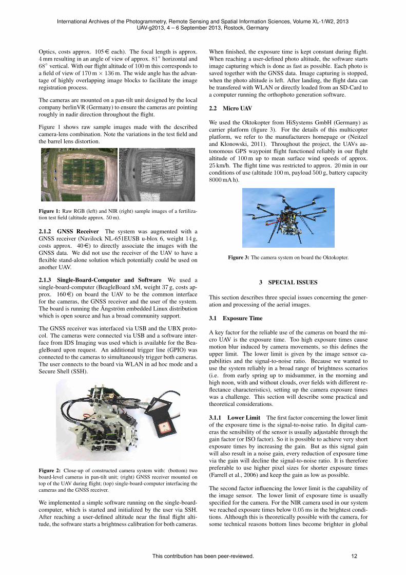
We used the Oktokopter from HiSystems GmbH (Germany) ascarrier platform (figure 3). For the details of this multicopterplatform, we refer to the manufacturers homepage or (Neitzeland Klonowski, 2011). Throughout the project, the UAVs au-tonomous GPS waypoint flight functioned reliably in our flightaltitude of 100 m up to mean surface wind speeds of approx.25 km/h. The flight time was restricted to approx. 20 min in ourconditions of use (altitude 100 m, payload 500 g, battery capacity8000 mA h).

Figure 3: The camera system on board the Oktokopter.

3 SPECIAL ISSUES

This section describes three special issues concerning the gener-ation and processing of the aerial images.

3.1 Exposure Time

A key factor for the reliable use of the cameras on board the mi-cro UAV is the exposure time. Too high exposure times causemotion blur induced by camera movements, so this defines theupper limit. The lower limit is given by the image sensor ca-pabilities and the signal-to-noise ratio. Because we wanted touse the system reliably in a broad range of brightness scenarios(i.e. from early spring up to midsummer, in the morning andhigh noon, with and without clouds, over fields with different re-flectance characteristics), setting up the camera exposure timeswas a challenge. This section will describe some practical andtheoretical considerations.

3.1.1 Lower Limit The first factor concerning the lower limitof the exposure time is the signal-to-noise ratio. In digital cam-eras the sensibility of the sensor is usually adjustable through thegain factor (or ISO factor). So it is possible to achieve very shortexposure times by increasing the gain. But as this signal gainwill also result in a noise gain, every reduction of exposure timevia the gain will decline the signal-to-noise ratio. It is thereforepreferable to use higher pixel sizes for shorter exposure times(Farrell et al., 2006) and keep the gain as low as possible.

The second factor influencing the lower limit is the capability ofthe image sensor. The lower limit of exposure time is usuallyspecified for the camera. For the NIR camera used in our systemwe reached exposure times below 0.05 ms in the brightest condi-tions. Although this is theoretically possible with the camera, forsome technical reasons bottom lines become brighter in global



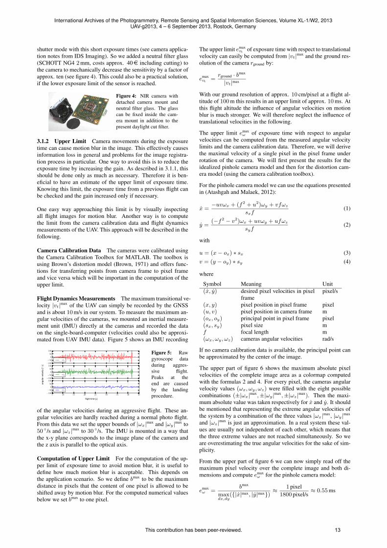
shutter mode with this short exposure times (see camera applica-tion notes from IDS Imaging). So we added a neutral filter glass(SCHOTT NG4 2 mm, costs approx. 40e including cutting) tothe camera to mechanically decrease the sensitivity by a factor ofapprox. ten (see figure 4). This could also be a practical solution,if the lower exposure limit of the sensor is reached.

Figure 4: NIR camera withdetached camera mount andneutral filter glass. The glasscan be fixed inside the cam-era mount in addition to thepresent daylight cut filter.

3.1.2 Upper Limit Camera movements during the exposuretime can cause motion blur in the image. This effectively causesinformation loss in general and problems for the image registra-tion process in particular. One way to avoid this is to reduce theexposure time by increasing the gain. As described in 3.1.1, thisshould be done only as much as necessary. Therefore it is ben-eficial to have an estimate of the upper limit of exposure time.Knowing this limit, the exposure time from a previous flight canbe checked and the gain increased only if necessary.

One easy way approaching this limit is by visually inspectingall flight images for motion blur. Another way is to computethe limit from the camera calibration data and flight dynamicsmeasurements of the UAV. This approach will be described in thefollowing.

Camera Calibration Data The cameras were calibrated usingthe Camera Calibration Toolbox for MATLAB. The toolbox isusing Brown’s distortion model (Brown, 1971) and offers func-tions for transferring points from camera frame to pixel frameand vice versa which will be important in the computation of theupper limit.

Flight Dynamics Measurements The maximum transitional ve-locity |vt|max of the UAV can simply be recorded by the GNSSand is about 10 m/s in our system. To measure the maximum an-gular velocities of the cameras, we mounted an inertial measure-ment unit (IMU) directly at the cameras and recorded the dataon the single-board-computer (velocities could also be approxi-mated from UAV IMU data). Figure 5 shows an IMU recording

−100

−50

0

50

100

ωx

−100

−50

0

50

100

ωy

5 10 15 20 25 30 35 40 45−100

−50

0

50

100

ωz

angu

larv

eloc

ity[°/s

]

flight time [s]

Figure 5: Rawgyroscope dataduring aggres-sive flight.Peaks at theend are causedby the landingprocedure.

of the angular velocities during an aggressive flight. These an-gular velocities are hardly reached during a normal photo flight.From this data we set the upper bounds of |ωx|max and |ωy|max to50 ◦/s and |ωz|max to 30 ◦/s. The IMU is mounted in a way thatthe x-y plane corresponds to the image plane of the camera andthe z axis is parallel to the optical axis.

Computation of Upper Limit For the computation of the up-per limit of exposure time to avoid motion blur, it is useful todefine how much motion blur is acceptable. This depends onthe application scenario. So we define bmax to be the maximumdistance in pixels that the content of one pixel is allowed to beshifted away by motion blur. For the computed numerical valuesbelow we set bmax to one pixel.

The upper limit emaxvt of exposure time with respect to translational

velocity can easily be computed from |vt|max and the ground res-olution of the camera rground by:

emaxvt =

rground · bmax

|vt|max

With our ground resolution of approx. 10 cm/pixel at a flight al-titude of 100 m this results in an upper limit of approx. 10 ms. Atthis flight altitude the influence of angular velocities on motionblur is much stronger. We will therefore neglect the influence oftranslational velocities in the following.

The upper limit emaxω of exposure time with respect to angular

velocities can be computed from the measured angular velocitylimits and the camera calibration data. Therefore, we will derivethe maximal velocity of a single pixel in the pixel frame underrotation of the camera. We will first present the results for theidealized pinhole camera model and then for the distortion cam-era model (using the camera calibration toolbox).

For the pinhole camera model we can use the equations presentedin (Atashgah and Malaek, 2012):

x =−uvωx + (f2 + u2)ωy + vfωz

sxf(1)

y =(−f2 − v2)ωx + uvωy + ufωz

syf(2)

with

u = (x− ox) ∗ sx (3)v = (y − oy) ∗ sy (4)

where

Symbol Meaning Unit(x, y) desired pixel velocities in pixel

framepixel/s

(x, y) pixel position in pixel frame pixel(u, v) pixel position in camera frame m(ox, oy) principal point in pixel frame pixel(sx, sy) pixel size mf focal length m(ωx, ωy, ωz) cameras angular velocities rad/s

If no camera calibration data is available, the principal point canbe approximated by the center of the image.

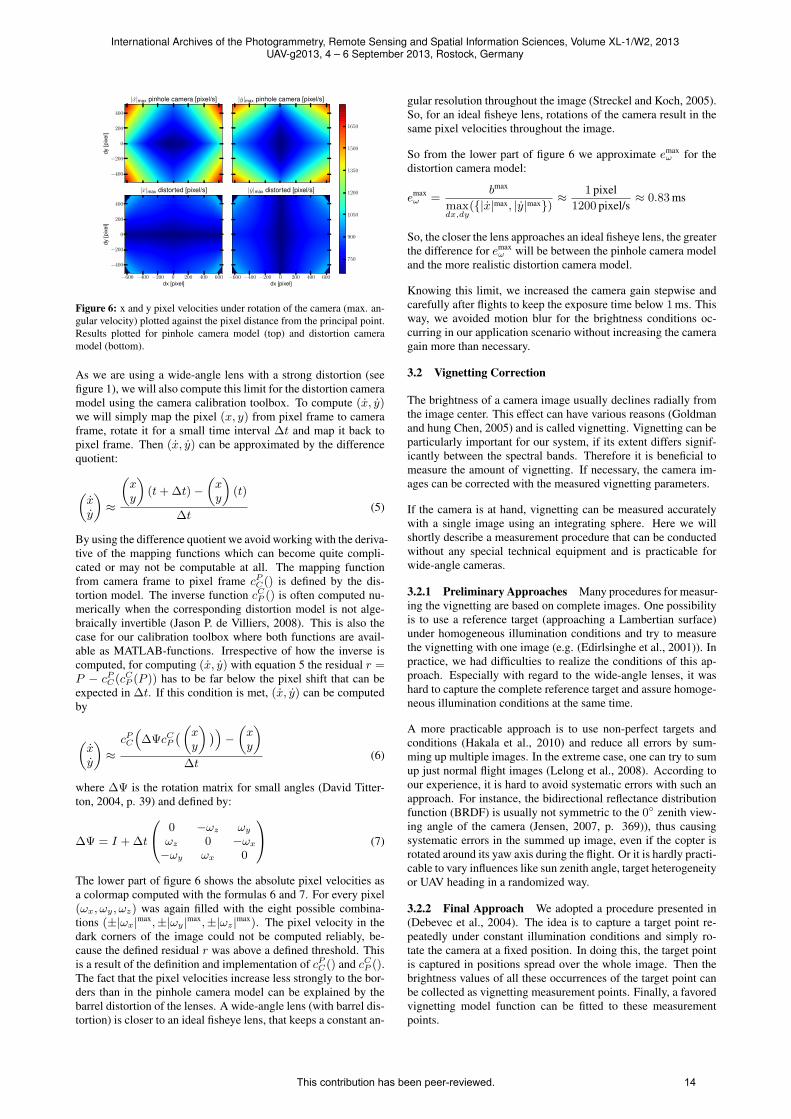
The upper part of figure 6 shows the maximum absolute pixelvelocities of the complete image area as a colormap computedwith the formulas 2 and 4. For every pixel, the cameras angularvelocity values (ωx, ωy, ωz) were filled with the eight possiblecombinations (±|ωx|max,±|ωy|max,±|ωz|max). Then the maxi-mum absolute value was taken respectively for x and y. It shouldbe mentioned that representing the extreme angular velocities ofthe system by a combination of the three values |ωx|max, |ωy|max

and |ωz|max is just an approximation. In a real system these val-ues are usually not independent of each other, which means thatthe three extreme values are not reached simultaneously. So weare overestimating the true angular velocities for the sake of sim-plicity.

From the upper part of figure 6 we can now simply read off themaximum pixel velocity over the complete image and both di-mensions and compute emax

ω for the pinhole camera model:

emaxω =

bmax

maxdx,dy

({|x|max, |y|max}) ≈1 pixel

1800 pixel/s≈ 0.55 ms



−400

−200

0

200

400

dy[p

ixel

]|x|max pinhole camera [pixel/s] |y|max pinhole camera [pixel/s]

−600 −400 −200 0 200 400 600dx [pixel]

−400

−200

0

200

400

dy[p

ixel

]

|x|max distorted [pixel/s]

−600 −400 −200 0 200 400 600dx [pixel]

|y|max distorted [pixel/s]

750

900

1050

1200

1350

1500

1650

Figure 6: x and y pixel velocities under rotation of the camera (max. an-gular velocity) plotted against the pixel distance from the principal point.Results plotted for pinhole camera model (top) and distortion cameramodel (bottom).

As we are using a wide-angle lens with a strong distortion (seefigure 1), we will also compute this limit for the distortion cameramodel using the camera calibration toolbox. To compute (x, y)we will simply map the pixel (x, y) from pixel frame to cameraframe, rotate it for a small time interval ∆t and map it back topixel frame. Then (x, y) can be approximated by the differencequotient:

(xy

)≈

(xy

)(t + ∆t)−

(xy

)(t)

∆t(5)

By using the difference quotient we avoid working with the deriva-tive of the mapping functions which can become quite compli-cated or may not be computable at all. The mapping functionfrom camera frame to pixel frame cP

C() is defined by the dis-tortion model. The inverse function cC

P () is often computed nu-merically when the corresponding distortion model is not alge-braically invertible (Jason P. de Villiers, 2008). This is also thecase for our calibration toolbox where both functions are avail-able as MATLAB-functions. Irrespective of how the inverse iscomputed, for computing (x, y) with equation 5 the residual r =P − cP

C(cCP (P )) has to be far below the pixel shift that can be

expected in ∆t. If this condition is met, (x, y) can be computedby

(xy

)≈

cPC

(∆ΨcC

P

((xy

)))− (xy

)∆t

(6)

where ∆Ψ is the rotation matrix for small angles (David Titter-ton, 2004, p. 39) and defined by:

∆Ψ = I + ∆t

0 −ωz ωy

ωz 0 −ωx

−ωy ωx 0

(7)

The lower part of figure 6 shows the absolute pixel velocities asa colormap computed with the formulas 6 and 7. For every pixel(ωx, ωy, ωz) was again filled with the eight possible combina-tions (±|ωx|max,±|ωy|max,±|ωz|max). The pixel velocity in thedark corners of the image could not be computed reliably, be-cause the defined residual r was above a defined threshold. Thisis a result of the definition and implementation of cP

C() and cCP ().

The fact that the pixel velocities increase less strongly to the bor-ders than in the pinhole camera model can be explained by thebarrel distortion of the lenses. A wide-angle lens (with barrel dis-tortion) is closer to an ideal fisheye lens, that keeps a constant an-

gular resolution throughout the image (Streckel and Koch, 2005).So, for an ideal fisheye lens, rotations of the camera result in thesame pixel velocities throughout the image.

So from the lower part of figure 6 we approximate emaxω for the

distortion camera model:

emaxω =

bmax

maxdx,dy

({|x|max, |y|max}) ≈1 pixel

1200 pixel/s≈ 0.83 ms

So, the closer the lens approaches an ideal fisheye lens, the greaterthe difference for emax

ω will be between the pinhole camera modeland the more realistic distortion camera model.

Knowing this limit, we increased the camera gain stepwise andcarefully after flights to keep the exposure time below 1 ms. Thisway, we avoided motion blur for the brightness conditions oc-curring in our application scenario without increasing the cameragain more than necessary.

3.2 Vignetting Correction

The brightness of a camera image usually declines radially fromthe image center. This effect can have various reasons (Goldmanand hung Chen, 2005) and is called vignetting. Vignetting can beparticularly important for our system, if its extent differs signif-icantly between the spectral bands. Therefore it is beneficial tomeasure the amount of vignetting. If necessary, the camera im-ages can be corrected with the measured vignetting parameters.

If the camera is at hand, vignetting can be measured accuratelywith a single image using an integrating sphere. Here we willshortly describe a measurement procedure that can be conductedwithout any special technical equipment and is practicable forwide-angle cameras.

3.2.1 Preliminary Approaches Many procedures for measur-ing the vignetting are based on complete images. One possibilityis to use a reference target (approaching a Lambertian surface)under homogeneous illumination conditions and try to measurethe vignetting with one image (e.g. (Edirlsinghe et al., 2001)). Inpractice, we had difficulties to realize the conditions of this ap-proach. Especially with regard to the wide-angle lenses, it washard to capture the complete reference target and assure homoge-neous illumination conditions at the same time.

A more practicable approach is to use non-perfect targets andconditions (Hakala et al., 2010) and reduce all errors by sum-ming up multiple images. In the extreme case, one can try to sumup just normal flight images (Lelong et al., 2008). According toour experience, it is hard to avoid systematic errors with such anapproach. For instance, the bidirectional reflectance distributionfunction (BRDF) is usually not symmetric to the 0◦ zenith view-ing angle of the camera (Jensen, 2007, p. 369)), thus causingsystematic errors in the summed up image, even if the copter isrotated around its yaw axis during the flight. Or it is hardly practi-cable to vary influences like sun zenith angle, target heterogeneityor UAV heading in a randomized way.

3.2.2 Final Approach We adopted a procedure presented in(Debevec et al., 2004). The idea is to capture a target point re-peatedly under constant illumination conditions and simply ro-tate the camera at a fixed position. In doing this, the target pointis captured in positions spread over the whole image. Then thebrightness values of all these occurrences of the target point canbe collected as vignetting measurement points. Finally, a favoredvignetting model function can be fitted to these measurementpoints.



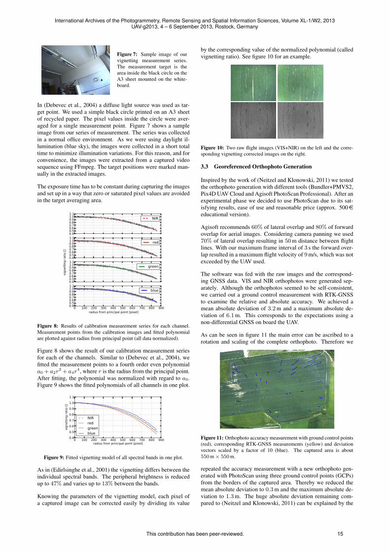
Figure 7: Sample image of ourvignetting measurement series.The measurement target is thearea inside the black circle on theA3 sheet mounted on the white-board.

In (Debevec et al., 2004) a diffuse light source was used as tar-get point. We used a simple black circle printed on an A3 sheetof recycled paper. The pixel values inside the circle were aver-aged for a single measurement point. Figure 7 shows a sampleimage from our series of measurement. The series was collectedin a normal office environment. As we were using daylight il-lumination (blue sky), the images were collected in a short totaltime to minimize illumination variations. For this reason, and forconvenience, the images were extracted from a captured videosequence using FFmpeg. The target positions were marked man-ually in the extracted images.

The exposure time has to be constant during capturing the imagesand set up in a way that zero or saturated pixel values are avoidedin the target averaging area.

0.40.50.60.70.80.91.01.1

NIR

0.40.50.60.70.80.91.01.1

red

0.40.50.60.70.80.91.01.1

green

0 100 200 300 400 500 600 700 800 9000.40.50.60.70.80.91.01.1

blue

vig

nett

ing r

ati

o [

]

radius from principal point [pixel]

Figure 8: Results of calibration measurement series for each channel.Measurement points from the calibration images and fitted polynomialare plotted against radius from principal point (all data normalized).

Figure 8 shows the result of our calibration measurement seriesfor each of the channels. Similar to (Debevec et al., 2004), wefitted the measurement points to a fourth order even polynomiala0 + a2r

2 + a4r4, where r is the radius from the principal point.

After fitting, the polynomial was normalized with regard to a0.Figure 9 shows the fitted polynomials of all channels in one plot.

0 100 200 300 400 500 600 700 800 900radius from principal point [pixel]

0.4

0.5

0.6

0.7

0.8

0.9

1.0

1.1

vig

nett

ing r

ati

o [

]

NIRredgreenblue

Figure 9: Fitted vignetting model of all spectral bands in one plot.

As in (Edirlsinghe et al., 2001) the vignetting differs between theindividual spectral bands. The peripheral brightness is reducedup to 47% and varies up to 13% between the bands.

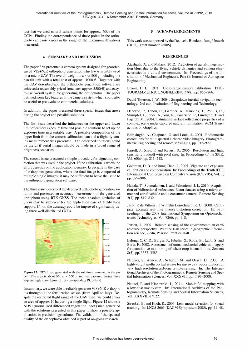
Knowing the parameters of the vignetting model, each pixel ofa captured image can be corrected easily by dividing its value

by the corresponding value of the normalized polynomial (calledvignetting ratio). See figure 10 for an example.

Figure 10: Two raw flight images (VIS+NIR) on the left and the corre-sponding vignetting corrected images on the right.

3.3 Georeferenced Orthophoto Generation

Inspired by the work of (Neitzel and Klonowski, 2011) we testedthe orthophoto generation with different tools (Bundler+PMVS2,Pix4D UAV Cloud and Agisoft PhotoScan Professional). After anexperimental phase we decided to use PhotoScan due to its sat-isfying results, ease of use and reasonable price (approx. 500eeducational version).

Agisoft recommends 60% of lateral overlap and 80% of forwardoverlap for aerial images. Considering camera panning we used70% of lateral overlap resulting in 50 m distance between flightlines. With our maximum frame interval of 3 s the forward over-lap resulted in a maximum flight velocity of 9 m/s, which was notexceeded by the UAV used.

The software was fed with the raw images and the correspond-ing GNSS data. VIS and NIR orthophotos were generated sep-arately. Although the orthophotos seemed to be self-consistent,we carried out a ground control measurement with RTK-GNSSto examine the relative and absolute accuracy. We achieved amean absolute deviation of 3.2 m and a maximum absolute de-viation of 6.1 m. This corresponds to the expectations using anon-differential GNSS on board the UAV.

As can be seen in figure 11 the main error can be ascribed to arotation and scaling of the complete orthophoto. Therefore we

Figure 11: Orthophoto accuracy measurement with ground control points(red), corresponding RTK-GNSS measurements (yellow) and deviationvectors scaled by a factor of 10 (blue). The captured area is about550 m× 550 m.

repeated the accuracy measurement with a new orthophoto gen-erated with PhotoScan using three ground control points (GCPs)from the borders of the captured area. Thereby we reduced themean absolute deviation to 0.3 m and the maximum absolute de-viation to 1.3 m. The huge absolute deviation remaining com-pared to (Neitzel and Klonowski, 2011) can be explained by the



fact that we used natural salient points for approx. 50% of theGCPs. Finding the correspondence of those points in the ortho-photo can cause errors in the range of the maximum deviationsmeasured.

4 SUMMARY AND DISCUSSION

The paper first presented a camera system designed for georefer-enced VIS+NIR orthophoto generation which was reliably usedon a micro UAV. The overall weight is about 500 g including thepan-tilt unit with a total cost of approx. 1000e. Together withthe UAV described and the orthophoto generation software weachieved a reasonably priced (total cost approx 3500e) and easy-to-use overall system for generating the orthophotos. The paperoutlined some key features of the camera system which could alsobe useful to pre-evaluate commercial solutions.

In addition, the paper presented three special issues that aroseduring the project and possible solutions.

The first issue described the influences on the upper and lowerlimit of camera exposure time and possible solutions to set up theexposure time in a suitable way. A possible computation of theupper limit from the camera calibration data and a flight dynam-ics measurement was presented. The described solutions couldbe useful if aerial images should be made in a broad range ofbrightness scenarios.

The second issue presented a simple procedure for vignetting cor-rection that was used in the project. If the calibration is worth theeffort depends on the application scenario. Especially in the caseof orthophoto generation, where the final image is composed ofmultiple single images, it may be sufficient to leave the issue tothe orthophoto generation software.

The third issue described the deployed orthophoto generation so-lution and presented an accuracy measurement of the generatedorthophoto using RTK-GNSS. The mean absolute deviation of3.2 m may be sufficient for the application case of fertilizationsupport. If not, the accuracy could be improved significantly us-ing three well-distributed GCPs.

0.60

0.45

0.30

0.15

0.00

0.15

0.30

0.45

Figure 12: NDVI map generated with the solutions presented in the pa-per. The area is about 550 m× 550 m and was captured during threesequent flights (see figure 11 for corresponding RGB data).

In summary, we were able to reliably generate VIS+NIR orthopho-tos throughout the fertilization season (from April to July). De-spite the restricted flight range of the UAV used, we could coveran area of approx 10 ha during a single flight. Figure 12 shows aNDVI (normalized differenced vegetation index) map generatedwith the solutions presented in this paper to show a possible ap-plication in precision agriculture. The validation of the spectralquality of the orthophotos obtained is part of on-going research.

5 ACKNOWLEDGEMENTS

This work was supported by the Deutsche Bundesstiftung Umwelt(DBU) [grant number 26805].

REFERENCES

Atashgah, A. and Malaek, 2012. Prediction of aerial-image mo-tion blurs due to the flying vehicle dynamics and camera char-acteristics in a virtual environment. In: Proceedings of the In-stitution of Mechanical Engineers, Part G: Journal of AerospaceEngineering.

Brown, D. C., 1971. Close-range camera calibration. PHO-TOGRAMMETRIC ENGINEERING 37(8), pp. 855–866.

David Titterton, J. W., 2004. Strapdown inertial navigation tech-nology. 2nd edn, Institution of Engineering and Technology.

Debevec, P., Tchou, C., Gardner, A., Hawkins, T., Poullis, C.,Stumpfel, J., Jones, A., Yun, N., Einarsson, P., Lundgren, T. andFajardo, M., 2004. Estimating surface reflectance properties of acomplex scene under captured natural illumination. ACM Trans-actions on Graphics.

Edirlsinghe, A., Chapman, G. and Louis, J., 2001. Radiometriccorrections for multispectral airborne video imagery. Photogram-metric Engineering and remote sensing 67, pp. 915–922.

Farrell, J., Xiao, F. and Kavusi, S., 2006. Resolution and lightsensitivity tradeoff with pixel size. In: Proceedings of the SPIE,Vol. 6069, pp. 211–218.

Goldman, D. B. and hung Chen, J., 2005. Vignette and exposurecalibration and compensation. In: Proceedings of the Tenth IEEEInternational Conference on Computer Vision (ICCV05), Vol. 1,pp. 899–906.

Hakala, T., Suomalainen, J. and Peltoniemi, J. I., 2010. Acquisi-tion of bidirectional reflectance factor dataset using a micro un-manned aerial vehicle and a consumer camera. Remote Sensing2(3), pp. 819–832.

Jason P. de Villiers, F. Wilhelm Leuschnerb, R. G., 2008. Centi-pixel accurate real-time inverse distortion correction. In: Pro-ceedings of the 2008 International Symposium on Optomecha-tronic Technologies, Vol. 7266, pp. 1–8.

Jensen, J., 2007. Remote sensing of the environment: an earthresource perspective. Prentice Hall series in geographic informa-tion science, 2 edn, Pearson Prentice Hall.

Lelong, C. C. D., Burger, P., Jubelin, G., Roux, B., Labb, S. andBaret, F., 2008. Assessment of unmanned aerial vehicles imageryfor quantitative monitoring of wheat crop in small plots. Sensors8(5), pp. 3557–3585.

Nebiker, S., Annen, A., Scherrer, M. and Oesch, D., 2008. Alight-weight multispectral sensor for micro uav opportunities forvery high resolution airborne remote sensing. In: The Interna-tional Archives of the Photogrammetry, Remote Sensing and Spa-tial Information Sciences, Vol. XXXVII, pp. 1193–2000.

Neitzel, F. and Klonowski, J., 2011. Mobile 3d-mapping witha low-cost uav system. In: International Archives of the Pho-togrammetry, Remote Sensing and Spatial Information Sciences,Vol. XXXVIII-1/C22.

Streckel, B. and Koch, R., 2005. Lens model selection for visualtracking. In: LNCS 3663 (DAGM Symposium 2005), pp. 41–48.



Documents

MICRO UAV BASED GEOREFERENCED ORTHOPHOTO GENERATION IN VIS+NIR … · 2013-10-29 · MICRO UAV BASED GEOREFERENCED ORTHOPHOTO GENERATION IN VIS+NIR ... a Humboldt-Universit ¨at zu