FORSCHUNGSZENTRUM ROSSENDORF ~Mitglied der Wissenschaftsgemeinschaft Gottfried Wilhelm Leibniz

WISSENSCHAFTLICH-TECHNISCHE BERICHTE

FZR-325- _J'lii!iiiillliji!i-iW'W

Juli 2001ISSN 1437-322X

Mirela Gavrilas und Thomas Höhne

OECD/CSNI ISP NR. 43 Rapid Boron Dilution

Transient Tests for Code Verification

Post Test Calculation with CFX-4

Herausgeber:Forschungszentrum Rossendorf e.v.

Postfach 51 01 190-01314 Dresden

Telefon +49 351 2600Telefax +49 351 2 69 0461

http://www.fz-rossendorf.de/

Als Manuskript gedrucktAlle Rechte beim Herausgeber

FORSCHUNGSZENTRUM ROSSENDORF C?Z:mWISSENSCHAFTLICH-TECHNISCHE BERICHTE

FZR-325Juli 2001

Mirela Gavrilas und Thomas Höhne

OECD/CSNI ISP NR. 43 Rapid Boron Dilution

Transient Tests tor Code Veritication

Post Test Calculation with CFX-4

OECD/CSNI ISP NR. 43RAPID BORON DILUTION TRANSIENT TESTS FOR CODE

VERIFICATIONPOST TEST CALCULATION WITH CFX-4

Mirela Gavrilas

University of MarylandDepartment of Materials and Nuclear EngineeringCollege Park, MD 20742-2115/ USA

Table of Contents

Thomas Höhne

Research Center Rossendorf (FZR)Institute for Safety ResearchD - 01314 Dresden / Gel1llany

1. The ISP-43 Tests 2

1.1 Test A-single inlet, single outlet, external tank injection 3

1.2 Test B-single inlet, single outlet, steam generator injection 4

2. Temperature Measurement 5

3. Computational Modeling 10

3.1 Choice ofmodels and nodalization 10

3.2 Model assumptions, geometry preparation and grid generation 11

4. Results 13

4.1 Test A 13

4.2 Test B 18

5. Conclusion 25

Literature 25

1. The ISP-43 Tests

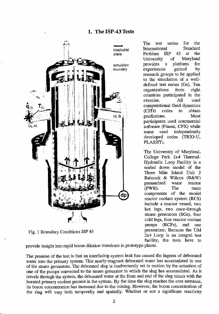
The test series for theInternational StandardProblem ISP 43 at theUniversity of Marylandprovides a platfonn forexperiences gained byresearch groups to be appliedto the simulation of a well­defined test series [Ga]. Tenorganizations from eightcountries partidpated in theexercise. All usedcomputational fluid dynamics(CFD) codes to obtainpredictions. Mostparticipants used commercialsoftware (Fluent, CFX) whilesome used independentlydeve10ped codes (TRIO-U,PLASHY).

inlet/outletplane

simulationboundary

-

The University of Maryland,College Park 2x4 Thennal­Hydraulic Loop Facility is ascaled down model of theThree Mile Island Unit 2Babcock & Wilcox (B&W)pressurized water reactor(PWR). The maincomponents of the modelreactor coolant system (RCS)inc1ude a reactor vessel, twohot legs, two once-throughsteam generators (SGs), fourcold legs, four reactor coolantpumps (RCPs), and one

Fig. 1 Boundary Conditions ISP 43 pressurizer. Because the UM2x4 Loop is an integral testfacility, the tests have to

provide insight into rapid boron-dilution transients in prototype plants.

The premise of the test is that an interfacing-system leak has caused the ingress of deboratedwater into the primary system. This nearly-stagnant deborated water has accumulated in oneof the steam generators. The deborated slug is inadvertently set in motion by the actuation ofone of the pumps connected to the steam generator in which the slug has accumulated. As ittravels through the system, the deborated water at the front and end of the slug mixes with theborated primary coolant present in the system. By the time the slug reaches the core entrance,its boron concentration has increased due to the mixing. However, the boron concentration ofthe slug will vary both temporally and spatially. Whether or not a significant reactivity

2

excursion will result following the penetration of the slug into the core depends on the boronconcentration of the fluid in both time and space. The initiallboundary conditions andgeometry dependence of core-inlet boron-concentration has been recognized early in rapidboron-dilution investigations, and confirmed during the UM 2x4 Loop experimental program.To predict the potential consequences of different initiating scenarios in different reactors,simulations are desirable. The UM tests focus on the downcomer region which is where mostof the re-boration of the slug occurs (Fig. 1). The preponderance of mixing is induced byturbulent eddies caused by either geometric discontinuities (including the pump impellers) orlarge velocity gradients among adjacent streams of fluid. The tests are designed to make atransition from a configuration that is nearly special effect to full integral test.

1.1 Test A-single inlet, single outlet, external tank injection

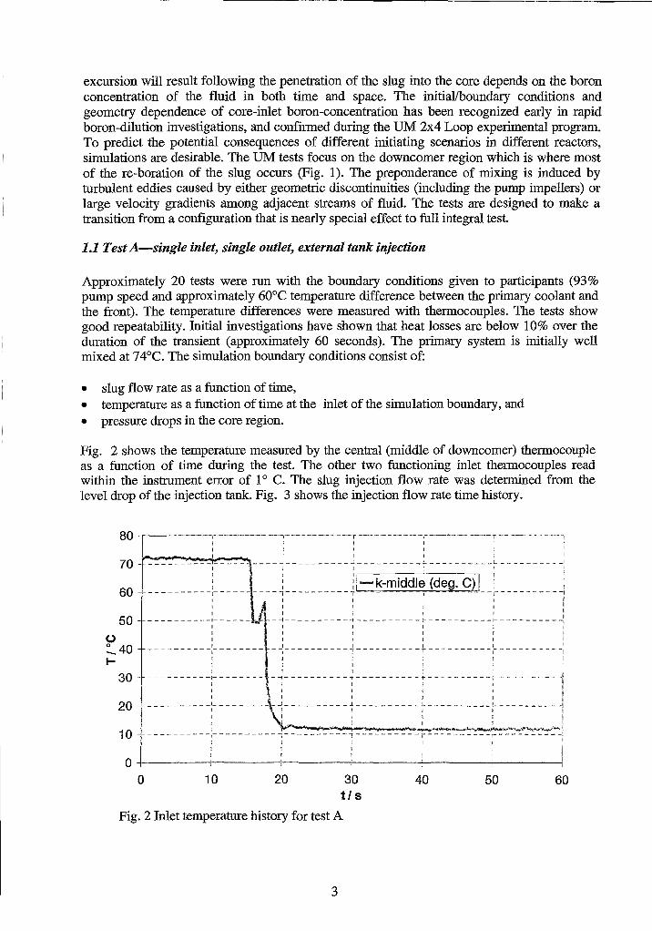
Approximately 20 tests were ron with the boundary conditions given to participants (93%pump speed and approximately 60°C temperature difference between the primary coolant andthe front). The temperature differences were measured with thermocouples. The tests showgood repeatability. Initial investigations have shown that heat losses are below 10% over theduration of the transient (approximately 60 seconds). The primary system is initially wellmixed at 74°C. The simulation boundary conditions consist of:

• slug flow rate as a function of time,• temperature as a function of time at the inlet of the simulation boundary, and• pressure drops in the core region.

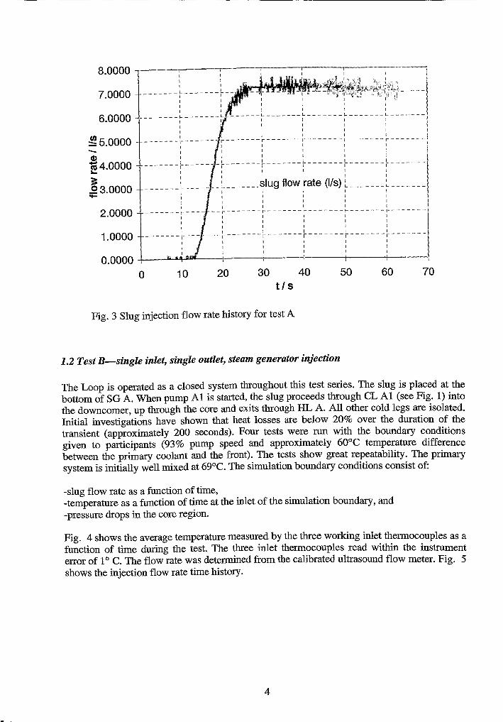
Fig. 2 shows the temperature measured by the central (middle of downcomer) thermocoupleas a function of time during the test. The other two functioning inlet thermocouples readwithin the instrument error of 1° C. The slug injection flow rate was determined from thelevel drop of the injection tank. Fig. 3 shows the injection flow rate time history.

- -rI

4----------~----------~----------;----i II :I I________ ~ L_________ _ ~ _1 I

,I

IIII

- - - - - - - - - -J- - - - -

I1I

- - - - - - - - - -1- - - --IIII- - - - - - - - - -~- - - --

I- - - - - - - - - -1- - - --

III

---- 1 --

III

II I

1""_...._..._..._...._.._...._""'_-_..:__'_"'_-_"'_""' J 1 ~ ~ . _I.----------------,

20

70

10 ----------r---------,----------7---

60

50o:'40....

30

605040O+------j------j---------+-----t-----'----.........,

o 10 20 301/5

Fig. 2 Inlet temperature history for test A

3

70605040302010

~ '__--'I'--- r----~-~'~"~_m__r_=""~"==li.""'m"=__,

I I 1 ~ ~l' ~

I ! i-------:-------:-- -----1

1 I I aI I 1 i ! [ •

_______ ~-------~. I L ~ L ~ . II I I I I j II I I )I 1 I [ 1 ~

-------~------ ~-------~-------~-------~-------~-------II I 1 I I 1 II I I I I ! 1I i I I I I !

-------:-----~-:-------:-------:-------:-------:-------I_______ ~ ~ .slug flow rate (lIs) ~-------~-------l

I I • , I I I~ I I I i I

I I I I tI I I I I !

_______ j " --r-------r-------r-------r-------r------~

I I I J i 1I ~ I I I II I I 1 J It I I I r I-------r--- ---r-------r-------r-------r-------r---·----I I I I ~ iI I I I ) tI I 1 i I I

8.0000

7.0000

6.0000

~5.0000-Q)

«S 4.000010-

~.E3.0000-

2.0000

1.0000

0.00000

t/s

Fig. 3 Slug injection flow rate history for test A

1.2 Test B-single inlet, single outlet, steam generator injection

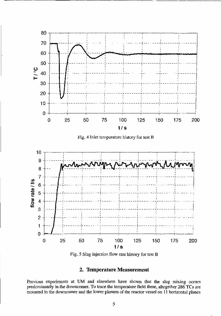
The Loop is operated as a closed system throughout this test series. The slug is placed at thebottom of SG A. When pump Al is started, the slug proceeds through CL Al (see Fig. 1) intothe downcomer, up through the core and exits through HL A. All other cold legs are isolated.Initial investigations have shown that heat losses are below 20% over the duration of thetransient (approximately 200 seconds). Four tests were ron with the boundary conditionsgiven to participants (93% pump speed and approximately 60°C temperature differencebetween the primary coolant and the front). The tests show great repeatability. The primarysystem is initially well mixed at 69°C. The simulation boundary conditions consist of:

-slug flow rate as a function of time,-temperature as a function of time at the inlet of the simulation boundary, and-pressure drops in the core region.

Fig. 4 shows the average temperature measured by the three working inlet thermocouples as afunction of time during the test. The three inlet thermocouples read within the instrumenterror of 1° C. The flow rate was determined from the calibrated ultrasound flow meter. Fig. 5shows the injection flow rate time history.

4

200175150125100

tl s755025

!!

I I J I t J ]____ ~ J l L ~ J L _

I I i I I ri I t I ]1 I I I !I I I I I

- - - T ~!""""'--oiii-..-~r-;';-"-"-"'-"--~__IiiIiö_~ ~-"-"-ioi-"-_-jji--1

!I__________ J L L ~ ~ _

1 I I :-------1J [ J I 1 : I1~~~~~~~J~~~~~~~~~~~~~~~~[~~~~~~~~~~~~~~~J~~~~~~~~[~~~~~~~II rr ~ J ! J 1 i[ t ~ rr ; [ ~ IJ ! i [ ij I I

1 1 r I 1 J I-~-------~--------I--------~-------~-------~--------~-------

I , I I I I I ,r r j I ~ 1 J

r r I 1 t ~ ~

i J I 1 J 1 I-------1-------~--------~-------f-------~-------~--------~-------

rr 1 J t r r[ 1 I 1 I I tI [ ! ~ J J '

oo

80

70

60

50

30

10

20

(,)

~ 40I-

Fig. 4 Inlet temperature history for test B

2001751501257550 100tl S

Fig. 5 Slug injection flow rate history for test B

25

,I I j

-------~--------~-------f-------~--------~-------J---I " __'L_••

I I________ L ~

! ! I, I

J J I t I- -i - - - - - '- - -!- - - - - - - - + - - - - - - - -1- - - - - - - - +- - - - - - - - -:i - - .- - - -- - - I-- - - _.~ - ~ - -

I ! I ! j

~ ! [ I !r I r I 1

-,--------r-------T--------I--------r-------~--------r-------

1 ~ I I i~ rl I j ~ f--1------- -------r--------j--------r-------l---·---- -----~-

[ i l II j j ! ~ I__ J L ~ J ~_______ _ L _

r· I j

I I I ~ ~

! J I I i ~

--~--------~-------+ l--------~-------~--------~ ~

, I I lf I I J 11 ~ J ~ j J

- - - , - - - - - - - - r - - - - - - - T - - - - - - - -J- - - - - - - - r '- - - - ~ - - "1 - - - - <- - - - ;- - ~ -

I J I I J1 j I II I i i

---~--------~-------7------- -------r------- ---.-------I ~ t I

I I

10

9

8

7U)

:::::: 6-(1)- 5co:r..

~ 40;:

3

2

1

00

2. Temperature Measurement

Previous experiments at UM and elsewhere have shown that the slug mlxmg occurspredominantly in the downcomer. To trace the temperature field there. altogether 286 Tes aremounted in the downcomer and the lower plenum of the reactor vessel on 11 horizontal planes

5

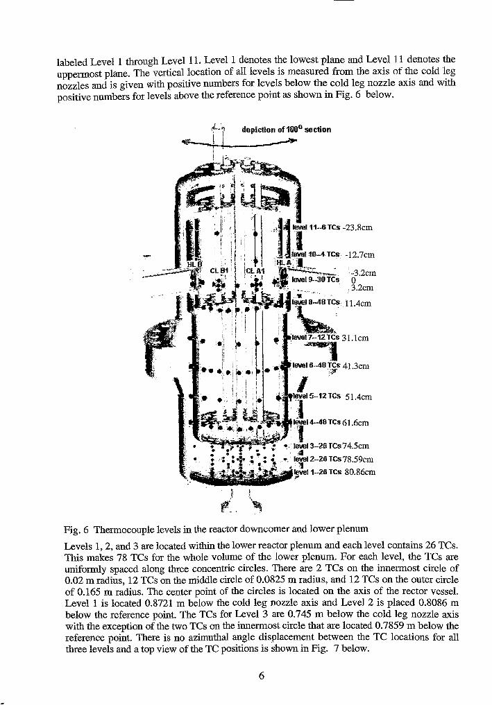
labeled Level 1 through Level 11. Level 1 denotes the lowest plane and Level 11 denotes theupperrnost plane. The verticallocation of all levels is measured from the axis of the cold legnozzles and is given with positive numbers for levels below the cold leg nozzle axis and withpositive numbers for levels above the reference point as shown in Fig. 6 below.

depiction of 180° secti,on

Fig. 6 Thermocouple levels in the reactor downcomer and lower plenum

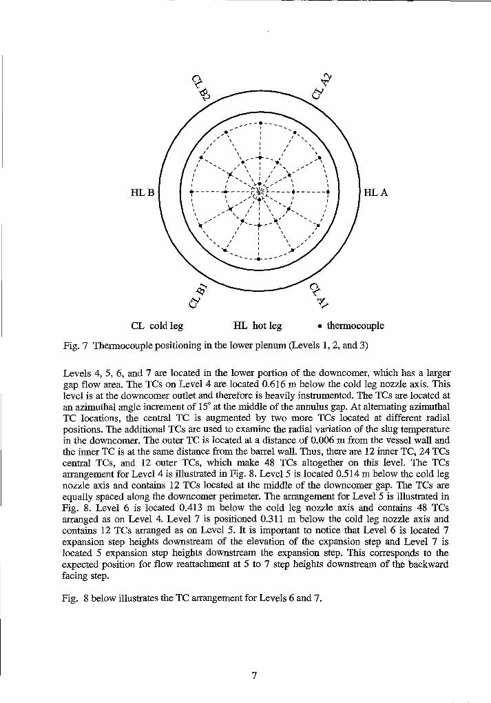
Levels 1, 2, and 3 are located within the lower reactor plenum and each level contains 26 TCs.This makes 78 TCs for the whole volume of the lower plenum. For each level, the TCs areuniformly spaced along three concentric circ1es. There are 2 TCs on the innermost circ1e of0.02 m radius, 12 TCs on the middle circle of 0.0825 m radius, and 12 TCs on the outer circ1eof 0.165 m radius. The center point of the circ1es is located on the axis of the rector vessel.Level 1 is located 0.8721 m below the cold leg nozzle axis and Level 2 is placed 0.8086 mbelow the reference point. The TCs for Level 3 are 0.745 m below the cold leg nozzle axiswith the exception of the two TCs on the innerrnost circ1e that are located 0.7859 m below thereference point. There is no azimuthaI angle displacement between the TC locations for allthree levels and a top view ofthe TC positions is shown in Fig. 7 below.

6

HLB HLA

CL cold leg HL hot leg • thermocouple

Fig. 7 Thermocouple positioning in the lower plenum (Levels 1, 2, and 3)

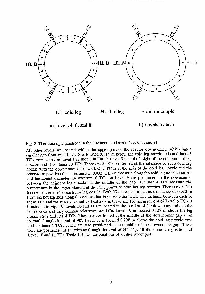
Levels 4, 5, 6, and 7 are located in the lower portion of the downcorner, which has a largergap flow area. The TCs on Level 4 are located 0.616 m below the cold leg nozzle axis. Thislevel is at the downcorner outlet and therefore is heavily instrurnented. The TCs are located atan azimuthal angle increment of 150 at the middle of the annulus gap. At altemating azimuthaiTC locations, the central TC is augmented by two more TCs located at different radialpositions. The additional TCs are used to examine the radial variation of the slug temperaturein the downcorner. The outer TC is located at a distance of 0.006 m from the vessel wall andthe inner TC is at the same distance from the barrel wall. Thus, there are 12 inner TC, 24 TCscentral TCs, and 12 outer TCs, which make 48 TCs altogether on this level. The TCsarrangement for Level 4 is illustrated in Fig. 8. Level 5 is located 0.514 m be10w the cold legnozz1e axis and contains 12 TCs located at the middle of the downcorner gap. The TCs areequally spaced along the downcorner perimeter. The arrangement for Level 5 is illustrated inFig. 8. Level 6 is 10cated 0.413 m below the cold leg nozzle axis and contains 48 TCsarranged as on Level 4. Level 7 is positioned 0.311 m below the cold leg nozzle axis andcontains 12 TCs arranged as on Level 5. It is important to notice that Level 6 is located 7expansion step heights downstream of the elevation of the expansion step and Level 7 islocated 5 expansion step heights downstream the expansion step. This corresponds to theexpected position for flow reattachment at 5 to 7 step heights downstream of the backwardfacing step.

Fig. 8 below illustrates the TC arrangement for Levels 6 and 7.

7

HLB

••

•••

•

•

• HLB

CL cold leg

a) Levels 4,6, and 8

HL hot leg • thermocouple

b) Levels 5 and 7

Fig.8 Thermocouple positions in the downcomer (Levels 4, 5, 6, 7, and 8)

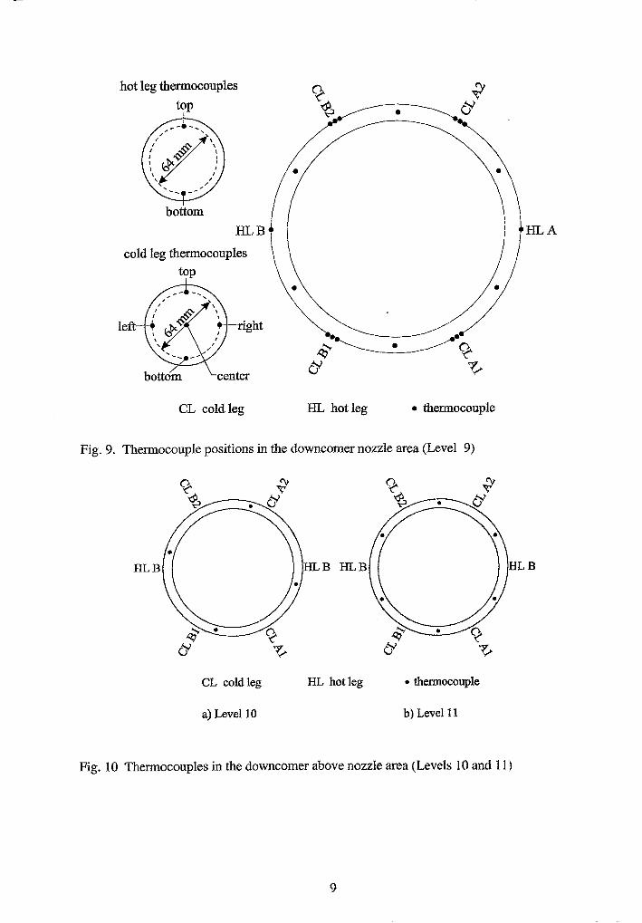
All other levels are located within the upper part of the reactor downcomer, which has asmaller gap flow area. Level 8 is located 0.114 m below the cold leg nozzle axis and has 48TCs arranged as on Level 4 as shown in Fig. 9. Level 9 is at the height of the cold and hot legnozzles and it contains 30 TCs. There are 5 TCs positioned at the interface of each cold legnozzle with the downcomer outer wall. One TC is at the axis of the cold leg nozzle and theother 4 are positioned at a distance of 0.032 m from that axis along the cold leg nozzle verticaland horizontal diameter. In addition, 6 TCs on Level 9 are positioned in the downcomerbetween the adjacent leg nozzles at the middle of the gap. The last 4 TCs measure thetemperature in the upper plenum at the inlet points to both hot leg nozzles. There are 2 TCslocated at the inlet to each hot leg nozzle. Both TCs are positioned at a distance of 0.032 mfrom the hot leg axis along the vertical hot leg nozzle diameter. The distance between each ofthese TCs and the reactor vessel vertical axis is 0.241 m. The arrangement of Level 9 TCs isillustrated in Fig. 9. Levels 10 and 11 are located in the portion of the downcomer above theleg nozzles and they contain relatively few TCs. Level 10 is located 0.127 m above the legnozzle axes and has 4 TCs. They are positioned at the middle of the downcomer gap at anazimuthal angle interval of 90°. Level 11 is located 0.238 m above the cold leg nozzle axesand contains 6 TCs, which are also positioned at the middle of the downcomer gap. TheseTCs are positioned at an azimuthai angle interval of 60°. Fig. 10 illustrates the positions ofLevel 10 and 11 TCs. Table 1 shows the positions of all thermocouples.

8

bottom

HLA

•

•right

HLB

cold leg thermocouplestop

hot leg thermocouples

top

left

CL cold leg HL hotleg • thermocouple

Fig. 9. Thermocouple positions in the downcorner nozzle area (Level 9)

HLB HLB

CL cold leg HL hotleg • thermocouple

a) Level 10 b) Levelll

Fig.1O Thermocouples in the downcorner above nozzle area (Levels 10 and 11)

9

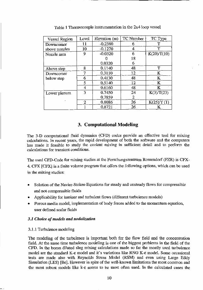
Table 1 Thermocouple instrumentation in the 2x4100p vesse~

Vessel Region Level Elevation (m) TC Number TC TypeDowncorner 11 -0.2380 6 Tabove nozzles 10 -0.1270 4 TNozzle area 9 -0.0320 6 K(20)/T(10)

0 180.0320 6

Above step 8 0.1140 48 TDowncomer 7 0.3110 12 Kbelow step 6 0.4130 48 K

5 0.5140 12 K4 0.6160 48 K

Lower plenum 3 0.7450 24 K(3)/T(23)0.7859 2

2 0.8086 26 K(25)/T (1)1 0.8721 26 K

3. Computational Modeling

The 3-D computational fluid dynamics (CFD) codes provide an effective tool for mixingcalculations. In recent years, the rapid development of both the software and the computershas made it feasible to study the coo1ant mixing in sufficient detail and to perform thecalculations for transient conditions.

The used CFD-Code for mixing studies at the Forschungszentrum Rossendorf (FZR) is CFX­

4. CFX [CFX] is a finite volume program that offers the following options, which can be used

in the mixing studies:

• Solution of the Navier-Stokes-Equations for steady and unsteady flows for compressible

and not compressib1e fluids

• Applicability for laminar and turbulent flows (different turbulence models)

• Porous media model, implementation of body forces added to the momentum equation,

user defined scalar fields

3.1 Choice 0/models and nodalization

3.1.1 Turbulence modeling

The modeling of the turbulence is important both for the flow field and the concentrationfield. At the same time turbulence modeling is one of the biggest problems in the field of theCFD. In the boron diluted slug mixing calculations made so far the mostly used turbulencemodel are the standard K-e model and it's variations like RNG K-e model. Some occasionaltests are made also with Reynolds Stress Model (RSM) and even using Large EddySimulation (LES) [Be]. However in spite of the well-known limitations the most common andthe most robust models like k-e seems to be most often used. In the calculated cases the

10

standard K-e model was used. Calculation were also performed without any turbulence model(laminar).

3.1.2 Numerical diffusion, nodalization and time step size

Numerical error is a combination of many aspects; the grid density, discretization method,time step size and convergence error have a11 their own effect. When a validation of thecomputational model is made using a certain experiment, the separation of different numericaleffects is difficult; for example, the numerical diffusion, i.e. a numerical error which acts likean artificial extra diffusion, can affect to the result in the same direction like too largeturbulent viscosity used in some turbu1ence models.

The numerical diffusion can be minimized using denser grids, higher order discretizationmethods and suitable time step size. Often the computation time puts some limits for these,but anyhow in a11 CFD computations results should be ensured to be grid and time-stepindependent, and if not possible, the uncertainties should be quantified. If the time steps aretoo large the influence of numerieal diffusion on the results is very high, if the time steps aretoo small the computational time exceeds.

Generally, it is important to find an optimum between acceptable resu1ts and computationaltime. In the calculated cases the optimum is a time step of 0.1 s.

3.2 Model assumptions, geometry preparation and grid generation

An incompressible fluid was assumed for the coo1ant flow in pressurized water reactors.

The inlet boundary conditions (velocity, temperature, etc.) were set at the inlet nozzles. Theoutlet boundary conditions were pressure controlled. Passive scalar fields as weIl astemperature differences according to the given boundary conditions were used to describe theboron dilution processes.

The calcu1ations were done on a SGI Origin 200 (1 GB RAM, 4x R 10000 180 MHz, 64 BitCPU) workstation platform. The generated grid contained ca. 450000 nodes. The transientcalcu1ations last a few weeks.

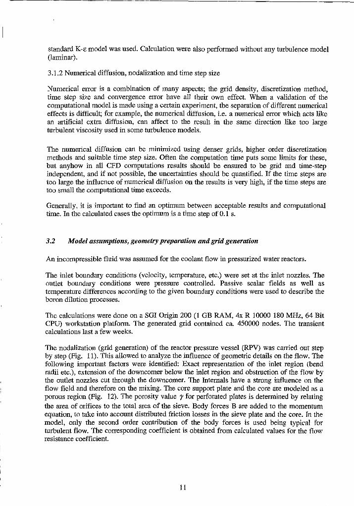
The nodalization (grid generation) of the reactor pressure vesse1 (RPV) was carried out stepby step (Fig. 11). This allowed to analyze the influence of geometrie details on the flow. Thefollowing important factors were identified: Exact representation of the inlet region (bendradii etc.), extension of the downcomer below the inlet region and obstruction of the flow bythe outlet nozzles cut through the downcomer. The Internals have a strong influence on theflow field and therefore on the mixing. The core support plate and the core are modeled as aporous region (Fig. 12). The porosity value '}' for perforated plates is determined by relatingthe area of orifices to the total area of the sieve. Body forces Bare added to the momentumequation, to take into account distributed friction losses in the sieve plate and the core. In themodel, only the second order contribution of the body forces is used heing typical forturbulent flow. The corresponding coefficient is obtained from calculated values for thc tlowresistance coefficient.

11

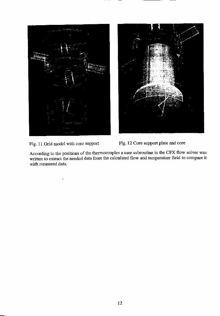
Fig. 11 Grid model with core support Fig. 12 Core support plate and core

According to the positions of the thermocouples a user subroutine in the CFX flow solver waswritten to extract the needed data from the calculated flow and temperature field to compare itwith measured data.

12

4. Results

4.1 TestA

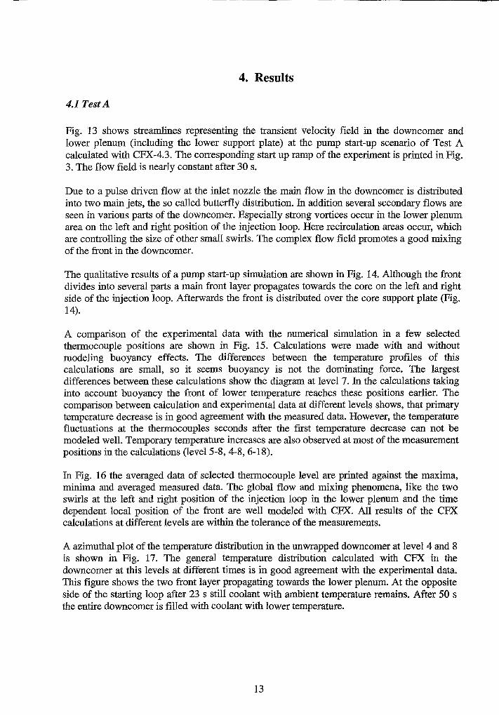
Fig. 13 shows streamlines representing the transient velocity field in the downcorner andlower plenum (including the lower support plate) at the pump start-up scenario of Test Acalculated with CFX-4.3. The corresponding start up ramp of the experiment is printed in Fig.3. The flow field is nearly constant after 30 s.

Due to a pulse driven flow at the inlet nozzle the main flow in the downcorner is distributedinto two main jets, the so called butterfly distribution. In addition several secondary flows areseen in various parts of the downcorner. Especially strong vortices occur in the lower plenumarea on the left and right position of the injection loop. Here recirculation areas occur, whichare controlling the size of other small swirls. The complex flow field prornotes a good mixingof the front in the downcorner.

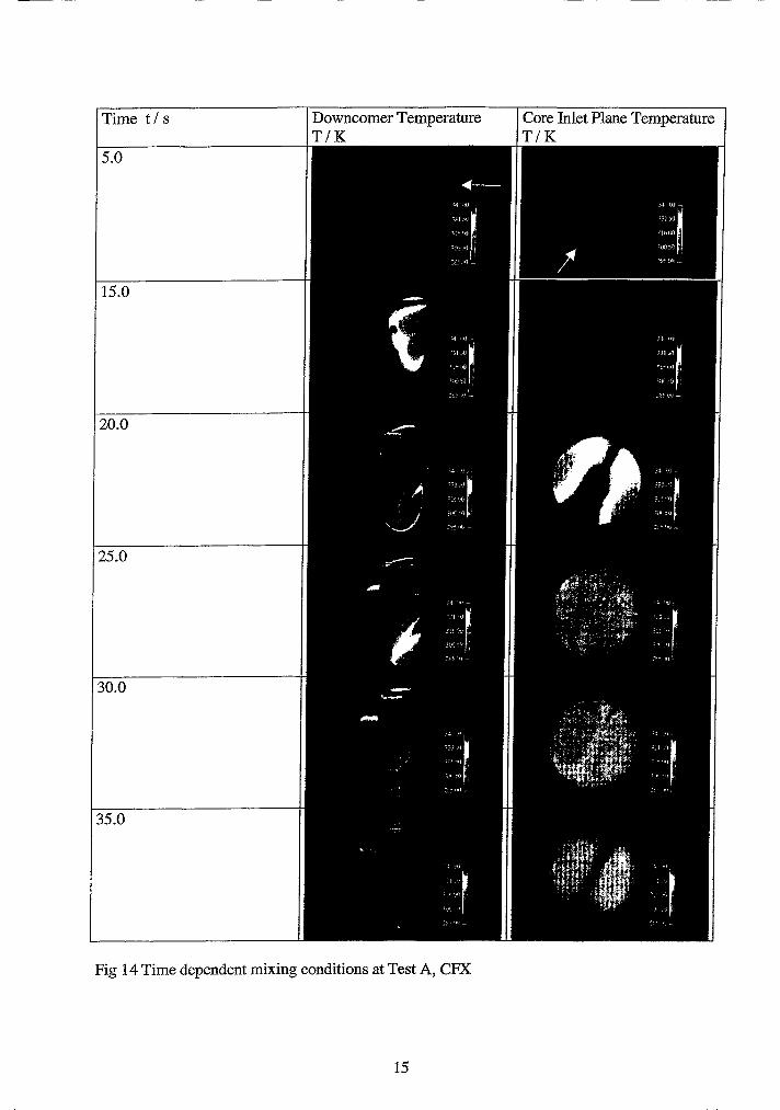
The qualitative results of a pump start-up simulation are shown in Fig. 14. Although the frontdivides into several parts a main front layer propagates towards the core on the left and rightside of the injection loop. Afterwards the front is distributed over the core support plate (Fig.14).

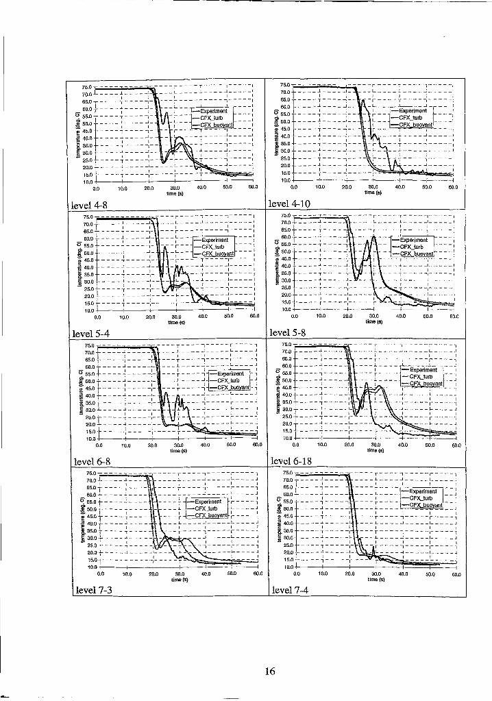
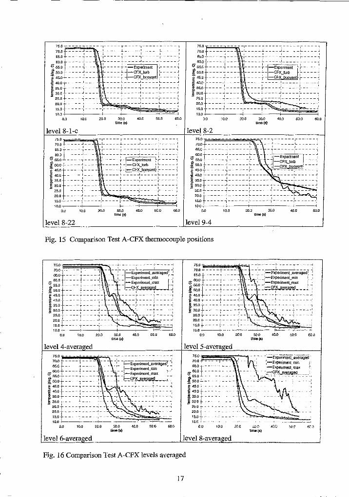
A comparison of the experimental data with the numerical simulation in a few selectedthermocouple positions are shown in Fig. 15. Calculations were made with and withoutmodeling buoyancy effects. The differences between the temperature profiles of thiscalculations are small, so it seems buoyancy is not the dominating force. The largestdifferences between these calculations show the diagram at level 7. In the calculations takinginto account buoyancy the front of lower temperature reaches these positions earlier. Thecomparison between calculation and experimental data at different levels shows, that primarytemperature decrease is in good agreement with the measured data. However, the temperaturefluctuations at the thermocouples seconds after the first temperature decrease can not bemodeled well. Temporary temperature increases are also observed at most of the measurementpositions in the calculations (level 5-8, 4-8, 6-18).

In Fig. 16 the averaged data of selected thermocouple level are printed against the maxima,minima and averaged measured data. The global flow and mixing phenomena, like the twoswirls at the left and right position of the injection loop in the lower plenum and the timedependent local position of the front are weIl modeled with CFX. All results of the CFXcalculations at different levels are within the tolerance of the measurements.

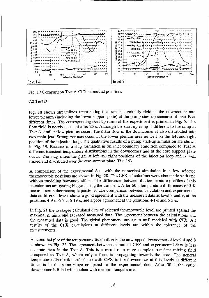
A azimuthaI plot of the temperature distribution in the unwrapped downcorner at level 4 and 8is shown in Fig. 17. The general temperature distribution calculated with CFX in thedowncorner at this levels at different times is in good agreement with the experimental data.This figure shows the two front layer propagating towards the lower plenum. At the oppositeside of the starting loop after 23 s still coolant with ambient temperature remains. After 50 sthe entire downcomer is filled with coolant with lower temperature.

13

20 s after start-up

60 s after start-u

Fig. 13 Transient flow conditions at Test A (ve1ocity)

14

5.0

25.0

20.0

Core !nIet Plane TemperatureT/K

Time t/ s

15.0

30.0

35.0

Downcomer TemperatureT/K

1------------+

Fig 14 Time dependent mixing conditions at Test A, CFX

15

60.050.040.0

---'-l---~-~

~ ..J ·I

, 1-~--I--~~-l

~-'- --L I

1- - --I

level 4-8 level 4-10

.+ .. -..,•..+----140.0 50.0 60.0

,4

30.0time ($)

~=~~-';~=~~~I

-, ~"= = 6 ~_ ~ = _ JI I---r -----r----'

-~ -=t-=- =t~:fxe;~~ft·.J·,,=: ~" .. T--" '~_QFX-buoyanl" - .1- - <0 '" -~ '~l ~ ,", - ,- ~ r~ ~ ..c,' =, ~ "J

l, _~, _ d, Ir-- -,

~,~i > __ b~~."=~J

I , 1"I------r- --1

_ c., ~,~., ,_,., .J

r I

75.0 ~=="'=-;;,rr70.0 ...i _ •. , C~ _

I65.0 --,.--,----

60.0 ----------~ 55.0 - - - - ~ _. <- - -,.850.0 - - - - ~ - - - - '~':e45.0 - - .. - -, - - " ,- -,.a 40.0 t' __.__ -1_,__ ... _1e ; I8. 35.0 . ----.,.•.• --",

i 30.0 ~' - - - - ..1 - - - - .,j. .-- 1 I~o ----~-----I---~·

20.0 - - - - ~ - - - - -:- -' .. -15.0 - - - - "I - - - - -1- -~ - - ~

10.0 I I0.0 10.0 20.0

level 5-8ßO ----~----------T----~-----r----'

70.0 - - - _..1 - - - __I1 I

65.0 - - - - -, - - - - -,

_ 60.0 t - - - - ~ - - - - -:-o 55.0 +- - - - - _- - - - -.-CI; . "Cl) 50.0 t----...l. - - - - _l_:S, I I

~ :~:~ -l- ====~ =====:=i 35.0 +- - - - - ~ - - - - -:-

! :~~ ~ ====~ =====i= =20.01 - - ---1- - - - -- -'l>o_""'.....~15.0± : ~ : c:10.0 ----+=

0.0 10.0 20.0 40.0 50.0 60.0

level 5-4

level 6-8 level 6-1875.0 - - - - - - - - - -~- - - - - T - - - -..,- - - - -\- - - --1

70.0 ,: - - - - -: - - - - - - - - - ~ - - - - ~ - - - - -;- - - - - ~65.0 t ----~ ---- I - - - - T - - - -1- - - - -j- - - --1

f~[~m~~::-:::~1~~mwe I i !! I I8. 35.0 T - - .. - ,,- .. _.... - .. - T - • - - '"1 - - -" -, - - - .. 1

!30.0t----~-----, - ---~-----~----i25.0 -.- - - - -" - - - --I - - -, - - - - -,- - - --120.0 +- .. - .. _-I .. _ ,, __ - -i __ - - _i- - - .. - ,

15.0 +- - - .... .': - - - - _:_ - - - - r - 1

10.0-!-" l; I I

0.0 10.0 20.0 30.0 40.0 50.0 60.0time (s)

75.0.,.- - - - - - - - - - - - - - - T' - - -. ~,'.., -"- - - -~- - - --170.0 ..1 _,65.0 -----,-----60.0 ..1 _

~ 55.0 - - - - ~ - - - - -1

f 50.0 - - - - ~ - - - - -:! 45.0 - - - - .,. - - - - -I

! 40.0 - - - - ~ - - '- - -:8. 35.0 - - - - -, - .. - - -,

§ 30.0 - - - - ~ - - - - -:-25.0 - - - - -, - - - .. -,­20.0 - - - - -I - - - - -1-

15.0 - - - - i - - - - -:- - - - T

10.00.0 10.0 20.0 30.0 40.0 50.0 60.0

tlme(s)

level 7-3 level 7-4

16

50.0 50.0 10.0 20.0I

40.0 50.0 50.0

leveI8-1-c level 8-275.0 - - - - - - - - - - -1- - - - - T - - - - '-,- - - - - I - - - - -:;.

10.0 20.0 30.0time(s)

40.0 50.0 50.0

~o---------- ------,------r-----l7QO ~ L J L_~ j

~ J I I~o -----,------r- -7------~-----160.0 ....: L __ J . , .J

~ 55.0r-----~------~- -~ =~~:r;;~nt 1- --1

' 50.0 ------;------~-- ~-CFX-buoyant. ----

i:~~=====J======~===-=======~===-~]e 1 i J . !

i~~~::~:j:~::::~:::~:j::::;;~::::~:10.0 : I I

0.0 10.0 20.0 30.0 40.0 50.0time(s)

level 8-22 level 9-4

Fig. 15 Comparison Test A-CFX therrnocouple positions

6iLQ50.040.0

=:=-Expe'rimenLaveragedI ~~'-ExperjmenLmin 11,

_ J-ExperimenLmax ~-J_ .'-CFX .aveE\tl!l2_~_.i

i I)-~1".,..

30.0time (I)

10.0

75.0-t---·-~~·"'~~-

70.0t- --- -t ~ ---65.0t----+---- -

~ :~:~ r= ===1 = - ==-;~50.0+----+----~ 45.0+----~'"..• ­! 40.0+----~o---­

~ 35.0 T - - - - c - -- - ., •.B 30.0+---. ~ -7- - - - .~ -2&0~----T----'·- -~

20.015.010.0.,----+--·····.....

0.0I

50.050.040.0

75.0 ~==~~;;=;;~"i---:- ---- ~ ---- -; - --- -;70.0 - - - - r - - - -, - _- =:= _ -ExperimenLaveraged~ J65.0 - - - - + - - - - -J ,-ExperimenLmin' I

~:~:~+====i====j - -1-- -ExperimenLmax ~'" . -CFX avera ed~5450 ..00t----==±------=~= I I I~ f ' , ----r----~----,:::I: 00 I j L l. .1

1;5:0 ====~====~= - --~----~----~~ 30.0 - ---7----~-- L ~----~

~.O ----T----'-- -- ----T----'20.0 _ - - - .L -l _ _ _ _1_ _ _ L_

15.0 1. - - - - -;- - - - - ~ - - - - -,10.0 1 I I I

0.0 10.0 20.0 30.0time(s)

I-j

600SM

.i:"';Exper,mell(llveiageaI,:-ExperimenLminn

. '-ExperimenCmax. ;:9!><_\lVerageq ~ _-::-~.

:30.0time (I)

75.0 ~~:;;~;:;==,S:7:":170.065.0t----'--

~::~I=_-=, -=-.~! 50.0.1. - -­l!! 45.0i 400!35.0! 300

25020.015.010.0

00 wo <00

level5-avera ed

60.0

- - "

50.0

I •

_1_ J-Experiment_averaged~~-!-Experimencmin ,. ..!

_ _ "__1-ExperimenLmax L. -,'

___ . i-CFX.averased ---lI

75.0 /i'__~iiii-=~""",

70.0 ,es,or' ----+----

0' 50.0 I - - - - +--- -­.55.00-----.,.----.;

! 50.0 +- - - - -""i - - - - ~e45.0 +- - - - - T - - - - ~~ 40.0+----t - - - - -= - - --I8.. 35.0 +- - -- - T - - - - - - ~ -,

j30.ot----f------ '25.0t-- - - -T-- - --,--

~~:~ t = = ==: = === ~ = = - = -..=~=:-~-:-±~~~~===:310.0 : .•------ .

0.0 10.0 20.0 30.0 40.0time(s)

level 6-avera ed level 8-averaged

Fig. 16 Comparison Test A-CFX levels averaged

17

~~f~,~: j~-;~,~i~~~~: !.~;~.;;: -:1:~ ~::E.500t__ .:... -+_~._ : -Exp.O.Os ~_''' L -----,

l2 . T ',I ." 1 -exp.22.8s ~_:!'__ ~' _, ,=45.oT----i~--1 -exp.so.2S. ":.,::· 1 '~ 40.0 T - - - -.., - - - - •• 'CFX 0.0 s • -.., I ,0. 350 t· -' I. ~--'-----I-----IE . ---- ,---. '''CFX23.0s· 1 I I.'!! 30.0 ----I--- J "·CFXSO.Os . -,-----'-----,

~~.~±====1====_:_ = ~ =1=====:= - -==:1S:0+ '0 _; -~ ._ •••-.~._••• o' -.-:10.0 , I I I ! I I

o W w ~ - ~ -azimuthaI position J0

level 4 level 8

Fig. 17 Comparison Test A-CFX azimuthai positions

4.2 TestB

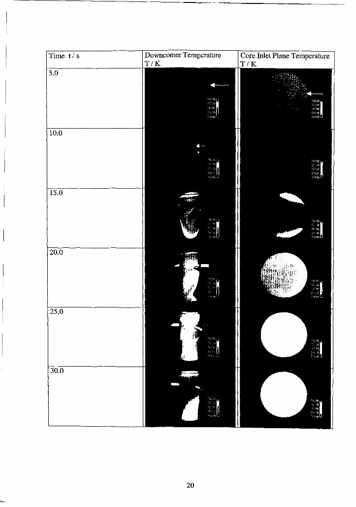
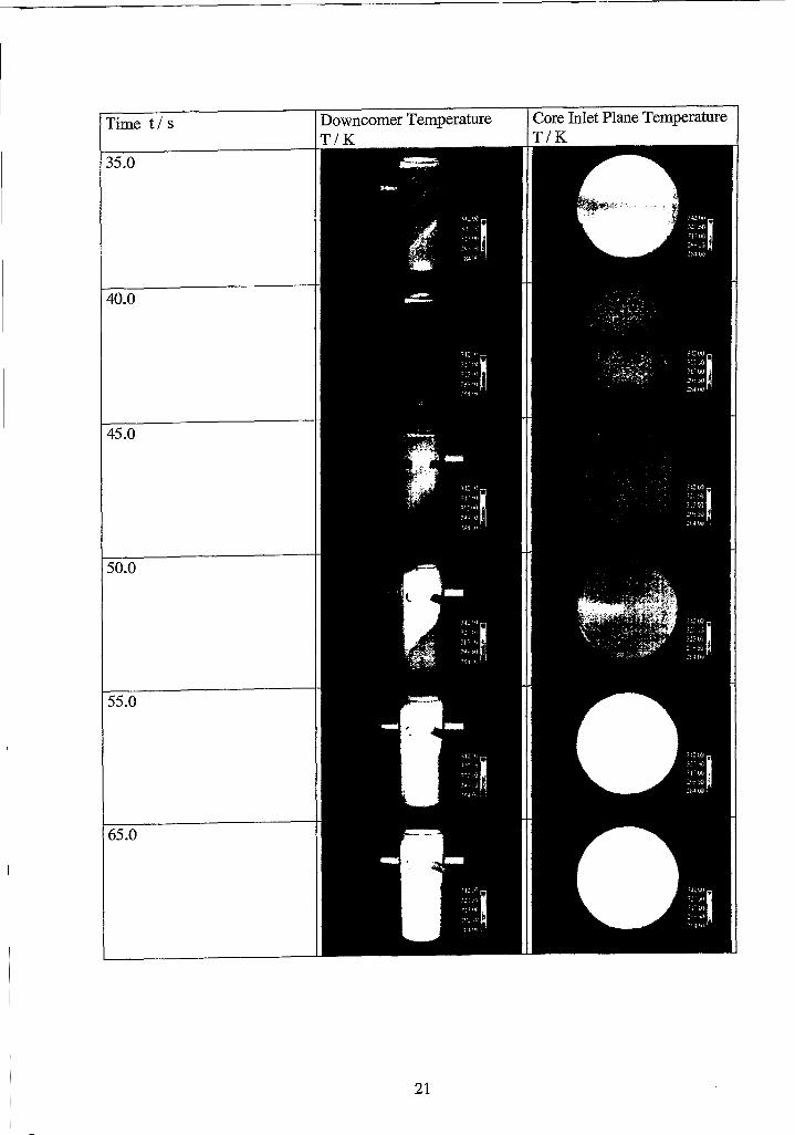
Fig. 18 shows streamlines representing the transient velocity field in the downcorner andlower plenum (including the lower support plate) at the pump start-up scenario of Test B atdifferent times. The corresponding start-up ramp of the experiment is printed in Fig. 5. Theflow field is nearly constant after 25 s. Although the start-up ramp is different to the ramp atTest A similar flow pictures occur. The main flow in the downcorner is also distributed intotwo main jets. Strang vortices occur in the lower plenum area as weIl on the left and rightposition of the injection loop. The qualitative results of a pump start-up simulation are shownin Fig. 19. Because of a slug formation as an inlet boundary condition compared to Test Adifferent transient temperature distributions in the downcorner and at the core support plateoccur. The slug enters the plate at left and right positions of the injection loop and is weIlmixed and distributed over the core support plate (Fig. 19).

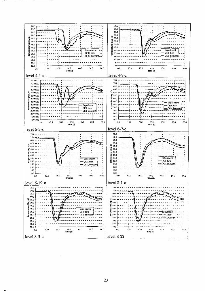
A comparison of the experimental data with the numerical simulation in a few selectedthermocouple positions are shown in Fig. 20. The CFX calculations were also made with andwithout modeling buoyancy effects. The differences between the temperature profiles of thiscalculations are getting bigger during the transient. After 60 s temperature differences of 5 Koccur at some thermocouple positions. The comparison between calculation and experimentaldata at different levels shows a good agreement with the measured data at level 8 and 9, at thepositions 4-9-c, 6-7-c, 6-19-c, and a poor agreement at the positions 4-1-c and 6-3-c.

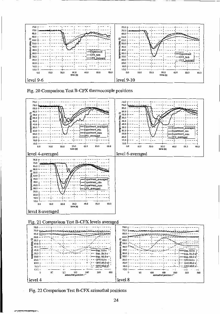
In Fig. 21 the averaged calculated data of selected thermocouple level are printed against themaxima, minima and averaged measured data. The agreement between the calculations andthe measured data is good. The global phenomena are again well modeled with CFX. Allresults of the CFX calculations at different levels are within the tolerance of themeasurements.

A azimuthai plot of the temperature distribution in the unwrapped downcorner of level 4 and 8is shown in Fig. 22. The agreement between azimuthai CFX and experimental data is lessaccurate than in the Test A. This is a result of a more complex transient mixing fieldcompared to Test A, where only a front is propagating towards the core. The generaltemperature distribution calculated with CFX in the downcorner at this levels at differenttimes is in the same range compared to the experimental data. After 50 s the entiredowncorner is filled with coolant with medium temperature.

18

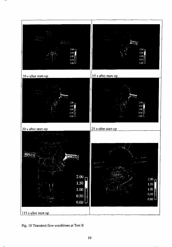
115 s after start-li

Fig. 18 Transient flow conditions at Test B

19

Time tl s

5.0

10.0

15.0

20.0

25.0

30.0

20

Core !nIet Plane TemperatureT/K

35.0

40.0

45.0

Core Inlet Plane TemperatureT/K

65.0

55.0

50.0

Time t/ s Downcorner TemperatureI-- --+T / K

21

70.0

75.0

Time tl s Core Inlet Plane TemperatureT/K

Downcomer Temperature~ -hT 1K

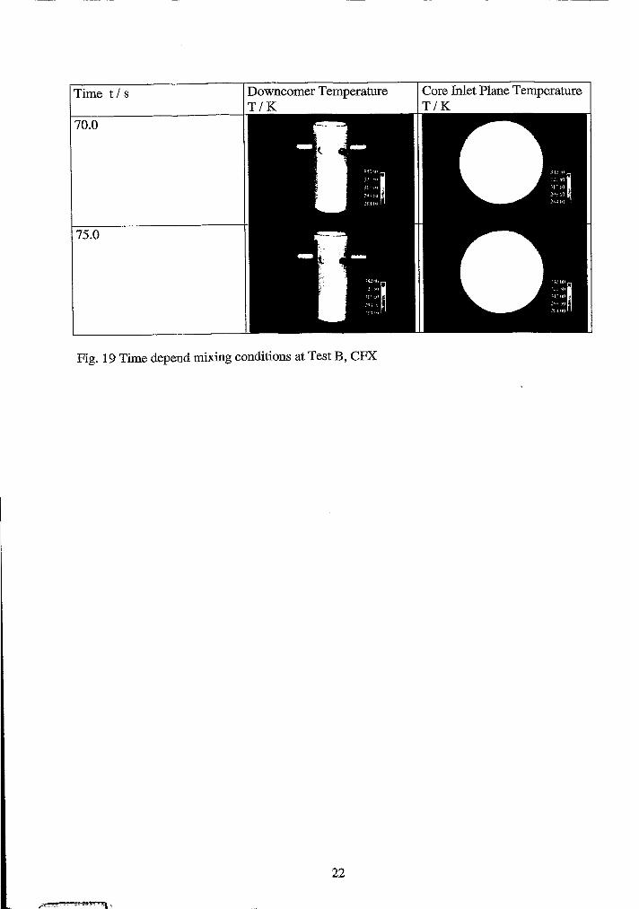
Fig. 19 Time depend mixing conditions at Test B, CFX

22

50.0

leveI4-1-c

30.0time(s)

leveI4-9-c----,-----j-----T----'-----r----l____ ~ ~ L ~ L J

I

leveI6-3-c

~~.~ I ====J=====:= ====I ====~=====~ ====J. I 1 I ! I

~:HE===E== =i=== ==F =- =;== -- --1

~ 50.0 Li' ~ - - _. ~ - - - -:- - - - t l I J

Q) 45.0 ----..,.--- -J~- - T----i-----r----l

.a 400t-----l.---- 1- ~_l... --l.. -----~----"~ . l I I I : !~ 35.0 - - - - 'I - - - - I - - - T - - - - j Experiment [ - 1E 30.0 - - - - ..l - - - - I - - - .!- - - - - -CFX t rb ,- "S, I !' _U'I!

25.0t-----,----!' ---r---- '!-CFX buoyantr-"1

:H[===~ ==== =j== ===f= ===~==== -~= ===i0.0 10.0 20.0 30.0 40.0 50.0 60.0

Iime(s)

leveI6-7-c

:~I---='=====:=====I====J=====~====~l ~ J I:65.0 - - - - I' - - - -t- - - - - T -

roo ----~- __ L _

~ 55.0 ----~- --~-- -T~--- --~~f"~ 50.0 - - - - .J. _ _ _f_ _ _ J,. ~ _ ~ _ -1 __ ~ ~ _ 1.- ~ _ ~ _ .!& ~ I f :1

i :~:~tl ====~== ==:= -= =t==~~~~p~r~m~~[I~::=j~ 30.0 - - - - J - - -! - - - .!- - - .,-CFX_turb ~ - - _ J

- 25.0, - _ - - ~ - _ _I - , __ ~--CFX buoyantL _

20.0 +- - - - - -+ - -. - - - - - - - - - - - -i_ - - - -1- - -"

:~:~t----i-----i- --- -:----: .~. -.' .-.~ ~~:-'-I0.0 10.0 20.0 30.0 40.0 50.0 60.0

time(s)

level 6-19-c leveI8-1-c

3Mtime(s)

200010.0

75.0

70'0r=="""'~oii\65.0

60.0~ 5500.g 50.0e45.0~ 40.08. 35.0~ 30.0- 25.0

20.015.010.0 +--~--l---~-~-'--_ ..-

0.0

~~I---='=====:=====I====J=====~====J• i I l : ~

65.0 - - -J- - - - - r - - -., - - - r ~ - - -"l

~ :~~~ J- ====~ = ==:= =~m - - - ~ J

g 50 0t---_.1._ - -1- -:s. . [

~ :~:~-====~==i 35.0 1 ~ - - .:. ~ - -E 30.0t----.l--.e i l

25.0f-----,--20.0 J _

15.0 - - - - ~ - - - -

10.0 . i0.0 10.0 20.0 40.0 50.0 60.0

leveI8-3-c level 8-22

23

level 9-6 level 9-10

Fig. 20 Comparison Test B-CFX therrnocouple positions

i~ImmW~:: ~: :::--:: ~-~~-~;--; j

~ 45.0t---- T ----

! 40.0 ~---f---- ~ . 11l. 35.0 : - - - - T - - - - - - - -;- - -Expenmen\....averaged~ 30.01. .:. __ - _.J _ _ _ _;_ _ -Experimen\....min- 25.0 t ~ ~ ;_ - -Experiment_max I

20.0 .(- .L ..J 1_ _ -CFX avera ed

15.0+----+---- ~ ~ ----:- ----~ ----+~ ---~10.0 I I i I I I I

0.0 10.0 20.0 30.0 40.0 50.0 60.0time(s)

level 4-avera ed

~~:~ t ---- ~ ----~ -===-1- ====t====+====~~O~----+- --~- ---1- ----~

~:~:~t====i=- Ji50.0+--~~-f--~ 45.0 f' - - - - .,. - - .., - -1- - -Experiment averaged~ 40.0 I - - ~ - f - - - - -~- - -Experiment-min ~1l. 35.0 • ~ ~ - - T - - - - - - -,- - -,-ExperimenLmax 'urE 30.0 T - - - -- ~ - - - - - - _L - -!'-CFX averaaedoS; ~ [ 2 ~ J

~~:~ I : : ==I ===_-, _====:= =__ =~ _-__ I JI1 t 1 ! I ~ I

15.0 t ---- T - - - - !: ~ ~ --:- ----~ ----T - - - - -;10.0.· -+ 1-· , " I .

0.0 10.0 20.0 30.0 40.0 50.0 60.0time(s)

level 8-avera ed

~:~t====1====j=====~=====~====~====~65.0 f -----; -- i - - - -:- - - - ~ - - - - -i

0 60.0 +----'-- ., ----,- -, --, .t ~~:~ ====f= =- - 1- --=-: -=~-~=== =; == =- ~! 45.0 - - - - T - - - - -" -~- - - - I - - - - 1" - - - - -I! 40.0 ----t--- ! ] __ L l. ~

1l. 35.0 - - - - T - - - -..., - - - -,- - ,-Experimen\""averaged ...,~ 30.0 ----f---- 1-- --:-- -Experiment_mi" ~

25.0 - - - - T - - - - - - - -,- -!-Experimen\....max ...,20.0 - - - _.L - - - _..J - - - -,- - -CFX avera ed .J

15.0 - - - - +---- ~ -----:- ---- I - - - - T - - - - ~10.0 +----+----1----+----1-----+----;

0.0 10.0 20.0 30.0 40.0 50.0 60.0time(s)

level 6-avera ed

FiO". 21 Com arison Test B-CFX levels avera ed75.0 7 ~ ~ '1' -~, ~ - -:~ ~,~" - ~~ Ir - - - - T ~ ~ - - -rr- ~ - - - ~70.04 ~- -I __ .~._ .. J. ._~ .... _.

~ :~:~t ~o~~i,~,~~=~:~::-_:~':~?='=='~la>, ~ ~_'':::._,~11~~_~_~ J."" "

i~f~i?~~:~=~~~t~Wf:i~~~t25,0 +- - -" - - - - - - -; c•• 'CFX 0.0 s ~ c

2Q 0"- - - ". 4 - - - '- - -- - 4 - ii.. 'CFX 25.0 sf-15:0~---- -:~X50.0SL.,I

I;level 4

~:w 180 240szimulhal position ff 0

300 360

E:~f====r~:.=j~ ~:.~ ~ r.~-~~~ ~~~-=~= ====:60.0~ I .... " .....-.r ... ...,._..... _: __........ c.

iE~§l~~~j~ 30.0.,- - - -.- - - - - .1-- -- -~ -- - - J. - '-EXP.50.2st,- 25.0 t ----2 -- - - - - - - ~ - - - - -I- -'CFX 0.0 s H

211.0 t - - -- 4 - - - - _1_ - - - - :- - - - - J. - ,- - 'CFX 25.0 Si

15.0 -!"_-_-_-_-~-__-----__!.--_-----__ci-~._-_-_-_-i---L.;=.=.=.~C~FX~5~0~.0'::S~L10.0 i

o 60 120 160 240 300 36CazimuthaI position J 0

level 8

Fig. 22 Comparison Test B-CFX azimuthal positions

24

5. Conclusion

The need of the experimental support for validation of the computational tools to be appliedto analyze the mixing of diluted slugs has been recognized in various countries. The test seriesfor the International Standard Problem ISP-43 provides a platform for experiences to beapplied to the simulation of a well-defined test series. Test A and B of the UM2x4loop testfacility were calculated with the CFD Code CFX-4.3. The results show qualitatively goodagreement with the experimental data for both tests. The structure of the flow field and theform of the propagating temperature perturbation front are well modeled by the CFD code.However, deviations occur at local positions. Comparative calculations with and withouttaking into account buoyancy have shown, that buoyancy effects are noticeable, but themixing is mainly momentum controlled.

Literature

[Be] Bernard, I.P., Haapalehto, T., Review of Turbulence Modeling for NumericalSimulation of Nuc1ear Reactor Thermal-Hydraulics, Research Report, LapeenrantaUniversity ofTechnology, 1996

[CFX] CFX-4.4 User Manual (2001), AEA Technology

[Ga] Gavrilas, M., Boron Mixing Code Assessment Test at the UMCP 2x4 Loop, 25th WaterReactor Safety Meeting, Oct. 22, 1997

25